a comparison of economic development between texas

A COMPARISON OF ECONOMIC DEVELOPMENT BETWEEN TEXAS

CITIES USING THE ECONOMIC DEVELOPMENT TAX 4A/4B

AND TEXAS CITIES NOT USING THE TAX

by

RAVINDRA KUMAR JAIN

Presented to the Faculty of the Graduate School of

The University of Texas at Arlington in Partial Fulfillment

of the Requirements

for the Degree of

DOCTOR OF PHILOSOPHY

THE UNIVERSITY OF TEXAS AT ARLINGTON

May 2012

ii

Copyright © by R. K. JAIN 2012

All Rights Reserved

iii

ACKNOWLEDGEMENTS

My sincere gratitude goes to my supervising professor, Dr. Rodney Hissong, who

provided valuable guidance, support, encouragement and compassion to keep my

morale high. Although I was away from the Metroplex, Dr. Hissong had the

patience to work with me though e-mails and audio-conferences. I am equally

thankful to my other committee members Dr. Sherman Wyman and Dr. Ardeshir

Anjomani for their input.

I wish to thank Mohammed Abdul Mujeeb of Fort Worth, TX for his I.T. help.

Sincere thanks go to my family for their continued support and to my sister Sneh

Lata Jain of Bluefield, VA who incessantly asked me the expected completion

date. My late father Shri Roshan Lal Jain who showed us the light for higher

education would have been very proud of me for achieving this degree.

April 19, 2012

iv

ABSTRACT

A COMPARISON OF ECONOMIC DEVELOPMENT BETWEEN TEXAS CITIES

USING THE ECONOMIC DEVELOPMENT TAX 4A/4B

AND TEXAS CITIES NOT USING THE TAX

Ravindra Kumar Jain, Ph. D

The University of Texas at Arlington, 2012

Supervising Professor: Rodney V. Hissong

Objective. Over the last three decades, economic development has been a major

policy issue in the State of Texas. But after the amendment of the Development

Corporation Act of 1979 and subsequent amendments, municipalities are using

the provisions of Section 4A and 4B to enhance economic development. The

purpose of this research is to determine if the Section 4A/4B adopting cities are

doing better in employment and income growth than the non-adopting cities.

Methods. Using the employment, income, population, and quality of life variables

data for years 1990, 2000, and 2007, this study evaluates the impact of ED

policies of Sections 4A/4B on employment and income growth. Multiple regression

models are used including Wooldridge’s Fixed Effects model. Results. The

inference from all the models can be summarized that: (1) Sales tax revenues

collecting cities under the provisions of Sections 4A/4B are not doing better than

the non adopting cities both in employment and income growth; (2) Other ED

v

policies such as TIFs, Freeport Zones, Property Tax abatements, etc; have

statistically significant contribution at 90 percent confidence level. Conclusions.

The research cast doubt on the efficacy of Sections 4A/4B economic development

policies.

vi

TABLE OF CONTENTS

ACKNOWLEDGEMENTS ...................................................................................... iii

ABSTRACT ........................................................................................................... iv

LIST OF FIGURES ............................................................................................. viii

LIST OF TABLES .................................................................................................. ix

Chapter Page

1. INTRODUCTION .............................................................................................. 1

1.1. The Necessity of Economic Development ................................................. 2

1.2. Business Location and Tax Incentives ...................................................... 3

1.3. The Competition in Incentives and Rebates ............................................. 5

1.4. Economic Development in Texas – A Novel Approach ............................. 8

1.5. Organization of Research ......................................................................... 9

2. LOCAL ECONOMIC DEVELOPMENT AND LITERATURE REVIEW ........... 11

2.1. Economic Development .......................................................................... 11

2.2. Local Economy and Economic Growth ................................................... 13

2.3. Economic Development Literature Review ............................................. 18

2.4. The Incentive Debate .............................................................................. 20

3. ECONOMIC DEVELOPMENT IN TEXAS ..................................................... 29

3.1. Economic Development in Texas ............................................................ 29

3.2. History of Sections 4A/4B Sales Tax Legislation ..................................... 32

3.3. Goals of Economic Development Corporations ...................................... 35

3.4. Differences in the Authorized Uses of the Tax Proceeds ........................ 37

4. HYPOTHESIS, METHODOLOGY, AND DATA ............................................. 40

4.1. Purpose and Methodology of Research .................................................. 40

4.2. Hypothesis .............................................................................................. 43

vii

4.3. Data and Methodology .............................................................................. 43

4.4. Sources of Data ........................................................................................ 46

4.5. Employment Change Model ...................................................................... 48

4.6. Variables and Their Significance ............................................................... 50

4.7. Descriptive Statistics ................................................................................. 56

5. ANALYSIS OF REGRESSION MODELS AND RESULTS .............................. 58

5.1. Basic Form of Models ............................................................................... 58

5.2. Employment Change Models .................................................................... 59

5.3. Wooldridge Fixed Effects Model ................................................................ 64

5.4. ED Variables as Dummy Variables ........................................................... 68

5.5. Model for DELCITEMP with Normalized ED Variables ............................. 70

5.6. DELCITEMP Model w/Dummy ED Variables with Normalized DELCITPOP .......................................................................... 72

5.7. Income Change Models ............................................................................ 74

5.8. Employment Change Models Beyond 2000 ............................................... 77

5.9. Employment Change Model for 1990-2007 ................................................ 78

5.10. Employment Change Model for Small Cities (Population ≤30,000) ............................................................................... 80

6. CONCLUSIONS AND RECOMMENDATIONS ................................................ 83

APPENDIX

1. ECONOMIC DEVELOPMENT PROGRAMS IN TEXAS ..................................... 86

2. CITIES IN THE STUDY ........................................................................................... 90

3. ECONOMIC REGIONS OF THE STATE OF TEXAS ........................................ 100

BIBLIOGRAPHY ................................................................................................. 102

BIOGRAPHICAL INFORMATION ....................................................................... 109

viii

LIST OF FIGURES

Figure Page

5.1 Mean Growth 1990-2000…………………………………………..…..62

5.2 Adoption Rate…………………………………………………….……..63

ix

LIST OF TABLES

Table Page

2.1 Economic Development Incentives Offered within the United States ....... 20

2.2 States Use of 15 Most Common Tax Incentives, 1996 ............................ 22

3.1 Mean of Population of ED Adopting vs. non-Adopting Cities .................. 31

3.2 Mean of Employment of ED Adopting vs. non-Adopting Cities ................ 31

3.3 Mean of Median Income of ED Adopting vs. non-Adopting Cities ........... 32

3.4 Objectives of Cities’ Economic Development Corporations ..................... 37

4.1 Descriptive Statistics ............................................................................... 57

5.1 Dependent Variable DELCITEMP1, Change in City Employment between 1990-2000 ................................................................................. 60

5.2 Comparison of Means for Change in City Population, Employment & Income between Adopting and non-Adopting Cities During 1990 and 2000 ......................................................................................................... 62

5.3 Dependent Variable DELCITEMP1, Change in City Population between 1990 and 2000 Using Wooldridge Fixed Effects Model ............ 67

5.4 DELCITEMP1, Change in City Employment between 1990-2000 w/ED Variables as Dummy Variables ...................................................... 69

5.5 DELCITEMP1, Change in City Employment between 1990-2000 w/Normalized ED Variables ..................................................................... 71

5.6 DELCITEMP1, Change in City Employment between 1990-2000, w/Dummy ED Variables and Normalized DELCITPOP1 ........................... 73

5.7 Dependent Variable DELCITINC1, Change in Median Household Income between 1990-2000 ..................................................................... 76



x

5.10 Employment Change Model for Small Cities (Population ≤ 30,000) ......... 81

1

CHAPTER 1

INTRODUCTION

The key function of the local governments is to provide services

such as public safety, healthcare, transportation, fire protection, education, and

social services for its residents (Holtz-Eakin, 1996) and create an environment

conducive to create jobs by retaining or attracting investors. Providing adequate

services requires resources. Municipal governments have very limited choices

to raise funds necessary to provide adequate and quality services. Therefore,

the cities make a concerted effort that businesses locate in their city. If there is a

healthy and growing business base in a city, it provides a reliable tax base that

in turn raises revenues for the treasury. Generally, a healthy business base also

provides jobs that are essential to fuel the engine of our consumer based

economy. Creating jobs is also very popular slogan among the elected officials.

When those who are eligible to work are employed, it is expected that people

will have sufficient income to spend. The higher the average wage, the residents

can buy instead of renting homes. This scenario helps both the businesses and

the local government. The employed residents contribute to the local economy

which translates into increased incomes for the businesses and increased sales

tax and property tax revenues for the city. This situation offers a great story for

the elected officials during their election campaigns.

2

1.1 The Necessity of Economic Development

It is almost a necessity for most of the city governments to have

economic development departments to attract new businesses or retain the

existing ones. Economic development can bring in new business, expand

existing businesses, create jobs, increase average income, make available

more discretionary funds, and for the city government, more revenues through

growth and taxes. When a primary business decides to open a new plant in a

city, several supporting services and ancillary product plants are also attracted.

With the growth in business, job market increases in the city. With more people

employed, local retailers’ sales and revenues also go up. With more jobs

created, housing market improves. Collectively, all these contribute to the city

revenues as a result of property, sales tax and user fee growth. With enough

revenues at their disposal, the cities can not only perform their basic key

functions but also provide good roads, better schools, park and recreation

facilities, libraries, transportation, necessary health services, thereby increasing

the quality of life. Such an idealistic environment in a city will attract more

business, music and opera, malls with nationwide chain stores, institutions of

higher learning, etc. Building such an environment has almost become

necessary to attract businesses because there is increased competition in this

era of global economy. It is no different than attracting a big event like Super

Bowl game of the National Football League, or the Olympics or major political

party’s convention for Presidential race. Cities add amenities, infra-structure,

3

shopping malls, hotels, and nightclubs to win the event because there is tough

competition and such events brings job and are a boost to the economy. To win

the Super Bowl XLVI, Indianapolis, Indiana did exactly like that and in this

“landlocked railroad stop with no beaches, no mountains, no casinos, no desert

spas”, they added what it took to compete despite the exogenous factor of

February cold (American Way, January 2012). Like the above mentioned

events, the competition to attract a business to start a plant or expand an

existing plant has become very intense at the state and the city level

governments.

1.2 Business Location and Tax Incentives

In today’s interdependent world economy and access to cheap labor

and instantaneous exchange of information, it has made it more complex for the

state and local governments to compete not only with each other but with

international players. “Low-cost land with transportation and communications

infrastructure in place is no longer scarce. Technology quickly jumps national

borders. Costs for reliable labor are lower in many places across the globe”

(Nolan, et al 2011, 26). This illustrates that the low-cost competitive

environment, has made it much more competitive to attract new businesses.

Therefore, the governments are spending more money in subsidies and benefits

to attract or retain businesses. This practice of tax incentives and benefits has

become so pervasive that the states are literally at war with one another

4

(Bowman, 1988; Burner, 1992; Guskind, 1989; Haider, 1992; Hanson, 1993;

Kenyon, 1991).

Of course, there is nothing new to the phenomenon of states

subsidizing private industry with public money. The incentives offered can be in

various forms, but tax-related incentives are very common. Incentives may be

one of the tools to attract new business but the business climate and other

factors such as good school districts, qualified workers meeting industry’s

technical needs, transit system, recreation amenities, etc. in a state or region,

can be a strong magnet to attract new or retain an existing business.

In a recent article in The Examiner published from Washington, DC, it

was reported that “Virginia Governor Bob McDonnell has been poaching jobs

from Maryland”, thereby intensifying the longtime rivalry between the

neighboring states (November 10, 2011). However, a closer review of the

reasons for businesses to opt for Virginia over Maryland shows that despite the

location of both in proximity to Washington D.C., it is the tax structure of Virginia

that has a significant impact. Corporate income tax in Virginia is six (6) percent

versus 8.25 in Maryland and there is no local income tax in Virginia. Personal

income tax is also higher in Maryland. According to this article, “Economists

point to Maryland’s high corporate and personal income taxes as the top

reasons why corporations favor Virginia”. This assumes greater significance in

the light of that Maryland had offered Bechtel $9.5 million in taxpayer’s money to

stay in MD, but Bechtel opted for VA. After Northrop Grumman chose Fairfax

5

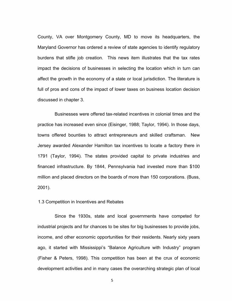
County, VA over Montgomery County, MD to move its headquarters, the

Maryland Governor has ordered a review of state agencies to identify regulatory

burdens that stifle job creation. This news item illustrates that the tax rates

impact the decisions of businesses in selecting the location which in turn can

affect the growth in the economy of a state or local jurisdiction. The literature is

full of pros and cons of the impact of lower taxes on business location decision

discussed in chapter 3.

Businesses were offered tax-related incentives in colonial times and the

practice has increased even since (Eisinger, 1988; Taylor, 1994). In those days,

towns offered bounties to attract entrepreneurs and skilled craftsman. New

Jersey awarded Alexander Hamilton tax incentives to locate a factory there in

1791 (Taylor, 1994). The states provided capital to private industries and

financed infrastructure. By 1844, Pennsylvania had invested more than $100

million and placed directors on the boards of more than 150 corporations. (Buss,

2001).

1.3 Competition in Incentives and Rebates

Since the 1930s, state and local governments have competed for

industrial projects and for chances to be sites for big businesses to provide jobs,

income, and other economic opportunities for their residents. Nearly sixty years

ago, it started with Mississippi’s “Balance Agriculture with Industry” program

(Fisher & Peters, 1998). This competition has been at the crux of economic

development activities and in many cases the overarching strategic plan of local

6

and state governments (Watson and Morris, 2008). Almost every state and

metropolitan area has expanded the size and scope of economic development

programs. More money is being spent on subsidies to new branch plants at

increasing rate, and even conservative states have intervened in the private

market by subsidizing business research and industrial modernization (Bartik,

1991).

Policymakers have responded with a host of incentives designed to

alter location decisions. According to Anderson and Wassmer (2000, page7), “in

1991, every state had the option of providing relief from at least one of its major

taxes. For example, 34 states provide that the inventory held by a business can

be at least partially exempt from property taxation. Minnesota, North Dakota,

and New Jersey offer some form of exemption or credit toward the state

corporate income tax. Efforts to conserve energy are granted special treatment

in 27 states, while 38 states offer preferable tax treatment for pollution control

equipment. A state-based investment tax credit exists in at least 25 states. The

same number of states offer a business tax credit or exemption for new job

creation. Local governments abate or exempt business property from taxation in

33 states by 1991”. Tennessee state and local governments provide subsidy

with a net present value of $144 million, mostly in the form of property tax

abatements to General Motors Saturn plant (Fisher and Peters, 1998).

The state of Kentucky gave a much larger subsidy to Toyota. State

and/or local governments can also exempt a business from sales and use taxes

7

in Illinois, Minnesota, and New Jersey. Tax forgiveness, tax increment finance

authorities (TIFAs), industrial development bonds (IDBs), municipal land

acquisitions, establishment of development authorities and zones, and other

related activities are some examples of incentives accorded to bring in new, to

expand the existing, or to retain the existing businesses (The National

Association of State Development Agencies (NASDA) 1983). In addition to the

usual incentives to enhance economic development, some states use

employment tax credits as one of the primary tools of state economic

development Faulk (2002). Last two decades have seen serious competition

among jurisdictions to attract businesses to enhance economic development in

their areas. Armed with the wide variety of incentive packages public officials

attempt to retain existing plants, facilitate plant expansions and attract new

plants. Thus limited local resources must be distributed between incentives for

job growth and basic services like protection, safety, healthcare, and other

social services. Local governments like any other level of government are

affected by the economic cycles. In addition to funds from property tax, sales

and use tax, they are to a large extent dependent on the higher level

governments for carrying out their business. At the national level the issue of

economic development has taken increased significance because of the long

run fiscal pressures, constrained by budget deficits, a conservative political

philosophy and Iraq and Afghanistan wars. This has thrust industrial recruitment

to the top of the state and local policy agenda. With many federal development

programs eliminated or reduced sharply, the amount of state and local money to

8

“buy payroll” during the 1980s spiraled upward. This resulted in local

governments assuming increased responsibility and flexibility to explore ways to

raise revenues. One of the ways to achieve this goal of enhancing economic

development is to attract businesses to create jobs.

1.4 Economic Development in Texas - A Novel Approach

Texas Legislature passed Section 4A in 1989 to improve economic

development (Handbook of Economic Development Laws for Texas Cities,

2008). But instead of giving tax incentives or rebates, it authorized the local

governments to impose sales tax subject to certain constraints and to use the

revenue raised through this sales tax for creating Economic Development

Corporations which this study will explore if the Texas cities that adopted the

Economic Development provisions had any impact on increasing jobs and

income versus the cities which did not utilize these economic development

avenues. Data for population, income, civilian employment, and variables that

operationalize quality of life attributes will be collected for 1990, 2000 and 2007.

Although it is relatively easier to get decade-ending data, year 2007 is selected

instead of 2010 to avoid effect of recession that began in 2007 as determined by

the National Bureau of Economic Research. Multiple linear regression models

will be developed to estimate the impact of Section 4A/4B economic

development policies.

9

1.5 Organization of Research

The starting point of the research is the economic development activity

in the state of Texas that began with the passage of the Development

Corporation Act of 1979 (Texas Civil Statues Article 5109.6) that allowed

municipalities to create nonprofit corporations (called development corporations)

by adding half percent sales tax subject to definite criteria that promoted the

creation of new and expanded industry and manufacturing activity within the

municipality and its vicinity.

Chapter 2 includes local economic development, the effect of national

and state economy on cities, agglomeration economies and their impact on

different economic regions, followed by literature review including pros and cons

of various rebates and incentives offered to the businesses to expand or start

manufacturing plants in their jurisdiction, with the objective of bringing jobs to

the state.

Various studies have been done to determine impact of the incentives

on the outcome of economic development. However, these studies experience

problems in comparing cities. For example, since so many differences exist

between localities, the inter-regional studies find the results not conclusive. In

addition, the provisions of Sections 4A and 4B are unique to the State of Texas

and therefore, the results are not comparable to other non-Texas cities. Other

states such as Georgia, South Carolina, Wisconsin, and Iowa have used some

variant of sales tax for property tax relief. The State of Florida passed local

10

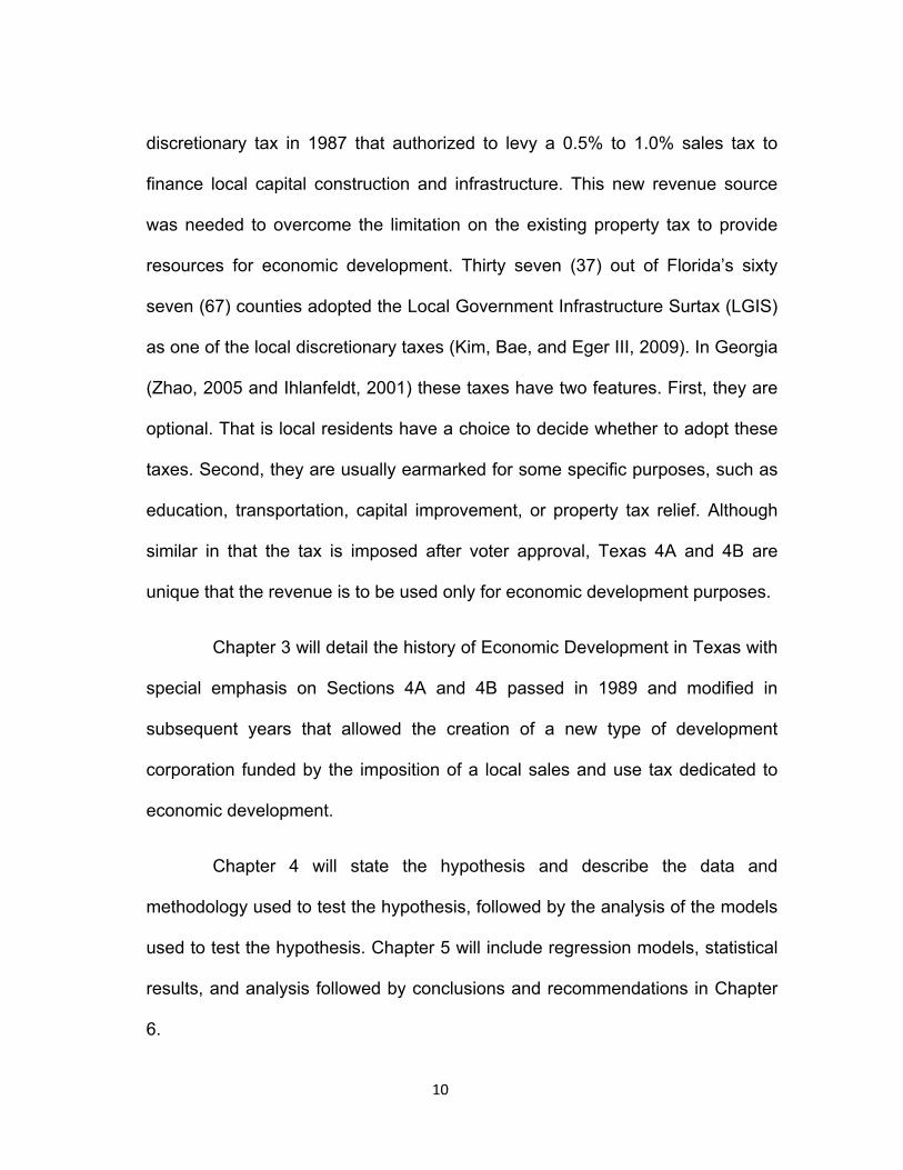
discretionary tax in 1987 that authorized to levy a 0.5% to 1.0% sales tax to

finance local capital construction and infrastructure. This new revenue source

was needed to overcome the limitation on the existing property tax to provide

resources for economic development. Thirty seven (37) out of Florida’s sixty

seven (67) counties adopted the Local Government Infrastructure Surtax (LGIS)

as one of the local discretionary taxes (Kim, Bae, and Eger III, 2009). In Georgia

(Zhao, 2005 and Ihlanfeldt, 2001) these taxes have two features. First, they are

optional. That is local residents have a choice to decide whether to adopt these

taxes. Second, they are usually earmarked for some specific purposes, such as

education, transportation, capital improvement, or property tax relief. Although

similar in that the tax is imposed after voter approval, Texas 4A and 4B are

unique that the revenue is to be used only for economic development purposes.

Chapter 3 will detail the history of Economic Development in Texas with

special emphasis on Sections 4A and 4B passed in 1989 and modified in

subsequent years that allowed the creation of a new type of development

corporation funded by the imposition of a local sales and use tax dedicated to

economic development.

Chapter 4 will state the hypothesis and describe the data and

methodology used to test the hypothesis, followed by the analysis of the models

used to test the hypothesis. Chapter 5 will include regression models, statistical

results, and analysis followed by conclusions and recommendations in Chapter

6.

11

CHAPTER 2

LOCAL ECONOMIC DEVELOPMENT

AND LITERATURE REVIEW

2.1 Economic Development

Economic Development implies that the welfare of the residents is

expected to improve as a result of private entrepreneur, state or local

government’s efforts to create jobs. What does this mean? It means that overall

the standard of living will improve, median household income level will rise,

services provided by the city will improve in quality and in response for all

citizens, unemployment will decrease, etc. This includes increase in median

household income and decrease in unemployment, as measures of economic

development, along with several other parameters. Some researchers describe

“economic development as the practice by which wealth generation is attained

through the goals of job creation and increasing the local tax base” (Blakely and

Bradshaw, 2002; Blakely and Green Leigh, 2009). But other economists call

increase in per capita income as economic growth (O’Sullivan 2007). Others

explain economic growth as an increase in total output or income (Greenwood

and Holt, 2010). Currid-Halkett and Stolarick (2011) describe economic

development as “an essential component of local policy and governing and a

perceived driver of success and vitality of localities, cities and regions alike”.

12

For the purpose of this research, these two terms economic

development and economic growth will be used interchangeably. “Conventional

economics has equated economic growth with economic development, implicitly

assuming that growth will bring improvement in quality of life and in the standard

of living. However, standard of living refers to overall wellbeing that goes beyond

income”, (Greenwood and Holt, 2010, p3). This means that if overall income

increases on one hand but crime and pollution increase simultaneously, then the

standard of living has fallen. In a broader sense, the objective should be to

improve the standard of living and the quality of life, for individuals within a

community. To achieve this goal, state and local policy makers have been

increasingly seeking policies, which are most cost effective in stimulating their

jurisdictions’ economies.

Economic development has been a major policy issue for most of the

metropolitan areas in the United States for at least three decades. Economic

development can bring new business or expand an existing business, with the

express objective of increasing or creating employment opportunities for local

residents. The cities achieve this objective by offering the businesses some

incentive that results in reducing their cost of operation. It is comparable to

micro-level fiscal policy. The city assists in increasing expected profit of the firms

by reducing the tax burden or the cost of operation and in return the city hopes

to foster company’s growth or attract new business to the area.

13

These policies help in two ways. The assisted firms expand operations

and hire more people. The arrival of the new business or the expansion of the

existing one can potentially bring in some ancillary business in support of the

initial firm. This means more jobs opportunities and hence improvement in

income and economic wellbeing. On the government side, it means greater tax

revenue and more funds for providing improved city services.

2.2 Local Economy and Economic Growth

Numerous forces affect local economies. An expanding or contracting

national economy can affect favorably or adversely local economy as can

change in the regional or state economies. The events of September 11, 2001

and the on-going wars in Iraq and Afghanistan, coupled with the downturn of

global markets, have created recessionary conditions in the country. The

unemployment rate is stubbornly above 8.4%, federal budget is in red by more

than $14.3 trillion, and the credit rating of USA has been downgraded from AAA.

According to the Wall Street Journal (July 22, 2011), more than one in

three of the unemployed workers in several of the largest U. S. states have been

out of job for more than a full year. Across the country, long periods of

unemployment have been more prevalent recently than previous recoveries

going back to the 1940s. Nationally, 30% of the unemployed, 4.4 million job

seekers, were out of for more than a year in June 2011, up from 29% of the

unemployed in June 2010. A headline in USA Today on June 24, 2011

summarized this economic condition: Jobless claims up, home sales down.

14

These recessionary conditions are affecting most of the states adversely and

because of lack of funds, teachers, police officers, fire fighters, etc. are being

laid off. Library and recreational services like parks and swimming are curtailed.

And it is not just the United States which is affected by these recessionary

conditions. Worries about the global economy are rippling through financial

markets in Europe and Asia as well. Since the states are required to have a

balanced budget, these conditions have further put budgetary burdens on the

states.

Notwithstanding the budgetary constraints, the local governments must

provide basic services and balance their budgets. The local governments have

to work with assumption, namely, that the public resources are finite and public

needs infinite. To provide these services, the local governments use their power

to tax to raise revenues.

But if the taxes are too high, residents of the city might think to move to

some other city. In addition, in adverse economic conditions, it can be a political

and economic suicide to raise taxes. The idea is that citizen mobility is greater at

the local level than at the national level; thus the Tiebout (1956) mechanism

allows them to “vote with their feet” by choosing a residential jurisdiction that

closely matches their preferences for local public goods and services (Stansel,

2006). From this perspective, residents and businesses seek the best tax-to-

services ratio and will move from one locality to another to attain it. The Tiebout

mechanism is very simple. If the residents of a city feel that the municipality they

15

live in, has high taxes compared to other regional cities, then they will move to

cities of their liking. “Voting with their feet” represents moving to more desirable

municipality. This means the local governments do have real constraints on

raising the taxes. California’s Proposition 13 has shown that increasing taxes

without serious resistance can no longer be taken as granted. Following

Proposition 13, which abruptly reduced local property tax revenues in the state

by half, in 1980, Massachusetts voters approved Proposition 2 ½, which set an

absolute limit on the property tax rate and the annual increase of tax levy

(Zhao, 2005). This opened the floodgate and many other states followed suit.

Therefore, one of the most important policy issues facing major metropolitan

areas in the United States now and for at least the past three decades, is

economic development in their jurisdictions, not only for jobs, but also to

discourage mobility, specifically of middle- to upper-income residents, by

adopting policies that strengthen the local economy and for revenues that can

be generated as a result of business growth (Hunter, 2001).

The situation gets further complicated because of the pressing urban

problems, such as crime, poverty, unemployment, blight, deteriorating

infrastructure, and fiscal stress and from the continued redistribution of

employment and residence from central cities and inner suburbs to outer

suburbs and rural areas (Anderson and Wassmer, 2000; Mark, Mcguire and

Papke,2000). Redistribution of economic activity within most metropolitan areas

has also created labor market issue of a spatial mismatch between low-skilled

16

employees residing in central cities and inner suburbs and potential employers

located increasingly farther out in urban areas. Paul Peterson (1981) in his City

Limits book argues that individuals weigh the costs and benefits of local

government services in their residential location decisions. He asserted that city

officials recognize the import of these individual decisions. Furthermore, officials

are primarily interested in the strength of their city’s economy and therefore want

to retain and attract middle- and upper-income households and businesses.

These two conditions, the mobility of residents, individuals and businesses and

the concomitant intercity competition, result in policy making that prefers

developmental policies to build the local economy over redistributive policies.

However, in many areas, local governments are increasingly working together to

address inter jurisdictional problems and issues by forming regional partnerships

to foster the economic development of a multi jurisdictional or regional area

(Olberding, 2002), with the objective of enhancing economic growth in their

region.

Among the various sources of economic growth, agglomeration

economics has a significant impact on creating jobs. The economic forces that

cause firms to locate close to one another in clusters are called agglomeration

economies. The forces acting on firms in a single industry are called localization

economies, indicating that they are “local” to a particular industry. When

agglomeration economies cross industry boundaries, they are called

urbanization economies. Urbanization economies depend on the aggregate

17

level of economic activity in a given area, and therefore, benefit all, regardless of

their industry. Urban economy theory suggests that agglomeration economies

contribute to growth by physical proximity that increases productivity through

input sharing, labor pooling, labor matching, and knowledge spillovers. This

results in lowering of costs of specific skill types. Search costs for a computer

software designer are expected to be lower in a metropolitan area where large

number of software firms are located.

Information networks efficiently match perspective employees with

employers who have demand for such skills. The experience of the designer is

easily determined by virtue of his or her work performed in the area. The

reputation of the company is equally determined by local information. This type

of information reduces the time and resources necessary to hire a new person.

It also attracts more designers and designing companies to the area. Other

localization economies occur in the intermediate goods market and the

consumer final goods market. Metropolitan areas characteristically exhibit

localization economies and urbanization economies to perspective firms.

Theater and fine arts communities also benefit from large population

bases. The presence of arts community creates an amenity that attracts

industries and population further increasing the size of the metropolitan areas.

Agglomeration economies play an integral role in urban growth by attracting

population that demands a variety of goods and services. To satisfy such needs

of goods and services attracts more firms supplying such products. In turn, this

18

attracts labor with specialized skills that earn higher labor income (Fujita and

Thisse, 2002).

2.3 Economic Development Literature Review

Economic development has assumed great significance over the last

three decades and as a result there is a vast literature on the subject of

economic development. The literature review will focus on various economic

development incentives that the cities and the states have used including the

degree of impact of these incentives.

Cities use various policies to economic development in their

jurisdictions. Various incentives are used to affect the business location

decisions. Obviously funding for other services is impacted when the resources

are used to promote economic development with the hope of improving the

revenues, the services and quality of life. Do these incentives work? Do the tax

policies of the states and the cities affect business location decisions? Critics

argue that the state and local economic development policies cannot achieve

these benefits. The reason given for such criticism is that the policies have little

effect on growth of a small region such as state or metropolitan area. Also the

state and local taxes are too small a percentage of business costs to affect

growth decisions.

Numerous studies have shown that taxes, in general, have a small or

no effect on employment (Faulk, 2002). Surveys of business firms often show a

19

low ranking of state and local taxes as a location determinant. However, other

researchers such as Bartik (1991) have argued that economic development

policies can significantly affect the growth of a state or metropolitan area, help

the unemployed and improve the overall economy. Recent econometric

evidence indicates that variations in state and local taxes do have effects on

state or metropolitan growth that are likely to be considered significant by most

policy makers (Luce, 1994; Mark, McGuire, and Papke, 2000).

Abatement of taxes is one type of policy to attract new business or

retain or help in expansion of an existing business. The business entity has to

evaluate the total package offered by the city or state to determine its value to

the firm (Grubert and Mutti, 2000). It may include tax incentives like corporate

income tax, sales tax, property tax; non-tax incentives like general-purpose

financing, customized job training, infrastructure subsidies. In addition the firm

may consider the quality of services such as transportation and police; rating of

school district; etc. The firm has to evaluate the value of such incentives in the

context of its bottom line. Fifty million dollars of BMW’s $130 million package

included expansion of the Greenville-Spartanburg airport. However, It is

reasonable to assume that all the benefits of expansion will not be captured by

BMW. The value to BMW will be much smaller than $130 million. The firm in

making their location decision considers all these factors affecting the firm in the

short run and long run.

20

Table 2.1 lists the options available to states for the inducement of

economic development. In addition, the State of Texas offers Tax Increment

financing, Freeport and Super Freeport exemptions, Property tax abatements,

Issuing Debt to finance economic development, etc. Appendix 1 lists economic

development programs and tools available in the State of Texas.

Table 2.1 Economic Development Incentives Offered within the United States

Economic Development Initiatives (EDIs) Manufacturing Revenue Bonds (Tax Exempt) Manufacturing Revenue Bonds (Taxable) General Obligation Bonds Umbrella Bonds Manufacturing Revenue Bond Guarantees Direct State Loans Loan Guarantees State-funded Interest Subsidies State-funded Equity/Venture Capital Corporations Privately Sponsored Development Credit Corporations Customized Manufacturing Training Tax Incentives Enterprise Zones SOURCE: NASDA (1983 and 1991)

2.4 The Incentive Debate

The literature is full of research as to whether or not the incentives

offered by the cities or states have any effect on business location and

employment opportunities. The critics of using incentives to promote economic

development believe that the reduction in local unemployment and upward swings

in real wages are short term because of labor mobility. If that is true, then the

21

macroeconomic policies that affect the short run performance of an economy may

also affect its long-run performance. According to Bartik (1993), short-term

economic development policies do affect long run prospects. Short term economic

development policies provide the benefit of higher land and property values

because some folks did get jobs, acquired skills and increased their employability

and real wages in the long run.

Bartik research has another argument in terms of efficiency. Bartik

argues that cities that have high unemployment may enjoy greater social

benefits from an additional local job than the cities with low unemployment. High

unemployment cities are also more likely to have underused public infrastructure

and services. An additional job poses little additional public cost to the city.

Local incentives that redirect a job from a low unemployment city to a high

unemployment city are efficient in the sense of correcting the misruled market

signal that exists without it. However, a business location decision does not

depend just on the incentives, specifically tax incentives. Unionization, corporate

taxes, infrastructure, educational institutes, medical facilities, closeness to the

airport, and a whole of other factors impact the location decision (Bartik, 1985).

Incentives can be in different forms. But the tax incentives are more

prevalent. Offering tax incentives to firms is part of the state and local policy

maker’s tool kit used to attract or maintain economic activity in a jurisdiction

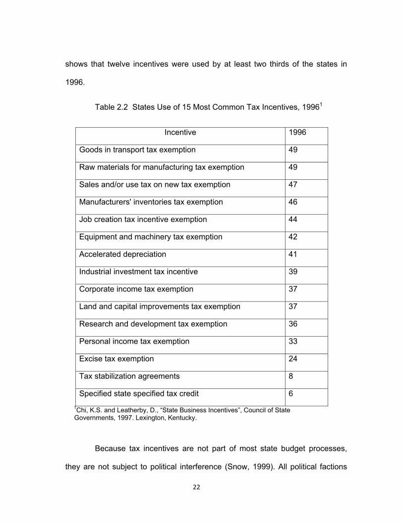
(Hanson and Rohlin, 2011). Chi and Leatherby (1997) has provided the list of

15 most common business tax incentives. Table 2.2 lists these incentives and it

22

shows that twelve incentives were used by at least two thirds of the states in

1996.

Table 2.2 States Use of 15 Most Common Tax Incentives, 19961

Incentive 1996

Goods in transport tax exemption 49

Raw materials for manufacturing tax exemption 49

Sales and/or use tax on new tax exemption 47

Manufacturers' inventories tax exemption 46

Job creation tax incentive exemption 44

Equipment and machinery tax exemption 42

Accelerated depreciation 41

Industrial investment tax incentive 39

Corporate income tax exemption 37

Land and capital improvements tax exemption 37

Research and development tax exemption 36

Personal income tax exemption 33

Excise tax exemption 24

Tax stabilization agreements 8

Specified state specified tax credit 6 1Chi, K.S. and Leatherby, D., “State Business Incentives”, Council of State Governments, 1997. Lexington, Kentucky.

Because tax incentives are not part of most state budget processes,

they are not subject to political interference (Snow, 1999). All political factions

23

use tax codes. Businesses receiving them are most supportive, whereas

taxpayers funding them are largely unaware or indifferent. Those who support

tax incentives rationalize using the arguments such as protecting the state or

city from losing business to other state or city or rescuing failing business which

could have drastic consequences for the state or city employment and revenues

(Buss 2001). However, the literature is replete with the articles by those who

oppose the tax incentives and provide stories in which incentives did not work or

did not produce revenue or job growth (Glickman and Woodward 1989, Guskind

1990, Hovey 1986).

Researchers on both sides of the issue have justified their findings and

criticized the other side. However, the arguments do not lead to a definite result

and it appears that the real winners are the businesses that get the benefits.

There is ongoing debate centered on the effectiveness of local economic

development practices and their efficacy. The literature is full of research with

arguments going in both directions. Part of the problem is the lack of consensus

on a generally accepted definition of economic development or ways to measure

it. (Hissong, 2001). Most of the local incentives are site specific. As Courant

(1994) stated that this geographical heterogeneity is extremely difficult to correct

for statistically.

Bartik (1991) research and recent econometric evidence indicates,

though not very rigorously, that state and local business taxes do have effects

on state or metropolitan area growth that are considered to be significant. He

24

concludes that state and local taxes do exert a statistically significant negative

influence on the location choice of firms. Bartik’s argument is that incentive-

induced employment growth has advantageous long-term effects on a locality’s

labor force participation and unemployment rates. This effect increases in

magnitude as the size of the area under consideration diminishes. This impact is

long-term, progressive and salutary.

Ebert and Stone (1992) also find increased labor force participation of

local residents to be the primary labor supply response to increased job growth.

These results are in line with Bartik’s (1991, 1993, 2001) findings that strong

employment growth benefits workers with the least skills and education because

a tight labor market forces employers to hire them. This outcome lowers the

area unemployment rate and increases area labor force participation. Partridge,

Rickman & Li (2009) research on county level employment growth yielded

similar results. That is successful local economic development initiatives can

provide benefits to original residents across a wide range of nonmetropolitan

areas, particularly to those that have had persistently high poverty. Anderson

and Wassmer (2000) explain this positive impact of incentive induced economic

development policy by describing economic theory related to the intra-

metropolitan location of business enterprises. The firms have a demand for sites

that are supplied by municipalities. The influence of local fiscal variables tax and

spending levels exert more influence at an intra-area level compared to an inter-

25

area level on business location choice, because more of the variables that

influence location are held constant.

Fisher (1997), Wasylenko (1997) and Mark, McGuire and Papke (1997)

discuss both inter-regional and intra-regional studies to determine whether taxes

and other policy variables impact location of firm decision. Taxes vary from one

locale to another within a region while many labor market and cost factors are

constant. Therefore, the effect of taxes is expected to be more important in intra-

regional decisions. They concluded that taxes are a statistically significant

factor.

The importance of state fiscal policies on economic growth is very

succinctly described in a recently published article in Public Finance Review.

The authors (Alm and Rogers, 2010) discuss this issue by addressing the

average annual growth rates of individual per capita income for the forty-eight

contiguous states from 1947 to 1997. It varied from 1.73 to 3.15. What factors

affect the rate of economic growth? Some factors like climate and proximity to

national markets cannot be changed by state or national government. Other

factors like labor force skills can be changed in the long run. Thus we are left

with fiscal policies –tax and expenditures- as the primary means available to

state governments for accelerating economic growth in the short run. The

research indicates that state economic policies matter. The correlation between

state and local taxation policies is often statistically significant. There is

moderately strong evidence that a state’s political orientation (the political party

26

of governor and presence of tax and expenditure limitations) has consistent and

measureable effects on per capita income growth rates. However, Hines (1996)

and Tannenwald (1997) in their studies came to opposite conclusions about the

effect of taxes on location of a firm decision.

But tax incentives are just one way to attract businesses to start or

expand in a city or state. Other examples are manufacturing revenue bonds,

general obligation bonds, loan guarantees, enterprise zones; etc. Enterprise

zones (EZ) programs are very high on the list of economic development policy

makers. EZ programs provide tax incentives for investment and job creation in

economically depressed areas.

The notion of EZ began in Britain, when Geoffrey Howe of the British

Conservative Party called for tax exemptions for firms that located in a specific

area. The idea spread to the United States, and in June 1980, Congressmen

Jack Kemp and Robert Garcia introduced EZ legislation. By the time federal

legislation was passed in 1987, more than 30 states had EZ programs up and

running. The research has shown that EZ programs created jobs at low cost and

average economic activity increased after the area achieved EZ status. (Billings

2009, Boarnet 2001, Couch & Barnett 2004, Elvery 2009, Lambert & Coomes

2001, O’Keefe 2004). However, the research points out that determining factors

to be classified EZ are politically motivated rather objectively. Some of the other

financial methods include abating property tax liability within an enterprise zone

(EZ) or a Freeport Zone and redirecting property tax revenue by virtue of tax

27

increment finance agreements. The location-based tax incentives do impact the

establishment location and employment but in varying degrees across industry

sectors. The empirical analysis shows that location-based tax incentives have a

positive effect on firm location in some of the industries and a negative effect in

industries that could be crowded out (Hanson and Rohlin, 2011).

Since 1989, the type of projects which were allowed under the

economic development legislation has undergone many changes as a result of

several amendments to the original Act. While in the beginning, the emphasis

was on manufacturing and industrial type of projects with the intent of expanding

or retaining the businesses, to create jobs, it is no longer a requirement to

create jobs in certain situations and the ED sales tax revenue can be used for

projects that enhance the quality of life. There is hardly any distinction between

Type A (Section 4A) and Type B (Section 4B) corporations. Cities are using

these funds on enhancing property values. However, there is no visibility on

property enhancements in the annual report that the cities are required to submit

to the Attorney General’s office. The report includes primary economic

development objectives and the choices are job retention or creation, tourism,

sports and recreation facilities, infrastructure projects and others. How the

enhancement of properties affects the creation of jobs or increases the revenue

because of high property value, is beyond the scope of this research.

Based on the literature review, I believe that the incentives do help in

attracting the businesses and creating jobs but the quality and the quantity of

28

these jobs varies from one location to another. This research will address the

effect on employment change and the average household income change as a

result of a specific economic development policy in the State of Texas.

29

CHAPTER 3

ECONOMIC DEVELOPMENT IN TEXAS

3.1 Economic Development in Texas

In the previous chapter, various incentives to attract or retain a business

in a city or state were discussed. These involved in one form or another

concession in taxes or providing infrastructure (airport expansion, roads, training

and facilities). The end result in each of these offerings was to lower the cost to

the business and thereby making it attractive or more profitable to the firm in

locating the business in the offering city. Texas like any other state promotes

economic development in various ways. Appendix 1 lists various programs

through which the State of Texas promotes economic development. The list is

the Table of Contents from Economic Development Handbook published by

Attorney General’s office. The first section is titled Sales Tax for Economic

Development. Unlike other rebates on certain types of taxes to promote

economic development, the State of Texas is imposing sales tax with the voters’

approval, to promote economic development. In Texas, the new revenue

measure passed under the Development Corporation Act that allows the cities

to impose sales tax subject to ceiling constraints provides a new source of

revenues to promote economic development.

30

Although the sales tax exemption has been used as an incentive for

economic development (Mikesell, 2001), the Development Corporation Act is

different in the sense that it uses the sales tax to raise revenue to promote

economic development. Some cities have taken advantage of this new source

and some have not. Since 1989, 558 cities have levied an economic

development sales tax under Sections 4A or 4B or both (Economic

Development Handbook 2008 published by the Office of the Attorney General of

Texas, p3).

During the 1990s, 164 cities with population greater than 10,000 were

eligible to adopt the economic development (ED) tax in the form of Section 4A or

Section 4B, or both. The number has grown to 180 by 2007. Out of 180 cities

eligible for adoption of these Sections, 114 have adopted the ED tax. For the

purpose of this study, if the eligible city had a population of 10,000 or more in

2000, it was included in the data, notwithstanding if the population threshold of

10,000 in 1990 was met or not. Actually, there were 21 cities in 1990 data which

had a population of less than 10,000. Table 3.1 shows that the mean of the

population of the cities adopting ED is less consistently from 1990 to 2007. This

is in line with the intention of the original legislation of providing a tool for smaller

cities competing for economic development. On the average, the population

means differ by about 8,000 between ED adopting and non-adopting cities.

31

Table 3.1 Mean of Population of ED Adopting vs. non-Adopting Cities

1990 – 2000

2000 - 2007

1990 -2007

Description Count1 Mean Count1 Mean Count1 Mean Cities not adopting ED 66 38,367 51 49,739 51 55,753

Cities which adopted ED 114 32,137 129 39,369 129 46,580

Mean of all 180 cities 34,421 42,308 49,179

count1 is the count at the end of the period

Table 3.2 provides the information of employment means between

adopting and non-adopting cities. The cities adopting Sections 4A/4B have

lower employment in 1990 as is expected. That is one reason these cities

adopted economic development policies to enhance employment. This policy

decision is in conformity with the intent of the legislation. However, the

percentage increase in employment of the adopting cities is far less than the

non-adopting cities (28.20% vs. 22.52% between 1990 and 2000).

Table 3.2 Mean of Employment of ED Adopting vs. non-Adopting Cities

1990 -2000

2000 - 2007

1990 -2007

Description Count1 Mean Count1 Mean Count1 Mean Cities not adopting ED 66 17,956 51 23,019 51 26,945



Count1 is the count at the end of the period

32

Table 3.3 shows the median household income means at three points

(1990, 2000 and 2007) between the cities that adopted these Sections and

those which did not adopt. All dollars are shown in year 2000 $.

Table 3.3 Mean of Median Income of ED Adopting vs. non-Adopting Cities

1990 -2000

2000 -2007

1990 -2007

Description Count1 Mean Count1 Mean Count1 Mean Cities not adopting ED 66 $40,410 51 $44,785 51 $44,639 Cities which adopted ED 114 $37,897 129 $43,065 129 $41,511 Mean of all 180 cities $38,819 $43,552 $42,397

Count1 is the count at the end of period

Cities adopting ED policies under Sections 4A/4B have lower mean,

although the range of the difference between the means has narrowed, though

not substantially.

3.2 History of Sections 4A/4B Sales Tax Legislation

Prior to 1979, there were few statutory vehicles in Texas that facilitated

economic development efforts. Business leaders asked the Texas Legislature

for authorization to create an entity that could encourage the development of

new local commerce.

The Texas Legislature passed the Development Corporation Act of

1979 (Texas Revised Civil Statues Article 5190.6). The Development

Corporation Act of 1979 (the “Act”) allows municipalities to create nonprofit

33

development corporations to promote the creation of new and expanded

industry and manufacturing activity within the municipality and its vicinity. The

development corporation was unfunded by the city, as restricted by the state

legislation (Joslove, 2000). The development corporations operated separately

from the municipalities in conjunction with industrial foundations and were

dependent for funding from private sources. Thus these corporations were only

as effective as these were persuasive in soliciting funds which was always

difficult.

Back in 1936, Mississippi was the first state to actively encourage

private industrial development through publicly sanctioned activity which was

achieved by issuing industrial development bond backed by the revenue stream

of private projects. But Texas Constitution did not permit public expenditures or

private economic development. In November 1987, the voters approved an

amendment to the Texas Constitution that allowed expenditures for economic

development because they serve a public purpose and were therefore,

permitted under Texas law. This amendment states in pertinent part:

Notwithstanding any other provision of this constitution, the legislature

may provide for the creation of programs and the making of loans and grants of public money for the public purposes of development and diversification

of the economy of the state. (Tex. Const. art. III, § 52-a.)

34

Subsequently, many new laws were passed granting economic

development authority to municipalities. In 1989, the Texas Legislature

amended the Act and added Section 4A. Section 4A allowed the creation of a

new type of development corporation which could be funded by the imposition of

a local sales and use tax. The revenues collected from this sales tax were to be

dedicated to economic development and the voters had to approve this new tax

to be used for economic development, at an election. By statute, the proceeds

of Section 4A sales tax are dedicated to economic development primarily to

promote new and expanded industrial and manufacturing activities. Section 4A

is available to cities that were located within a county of fewer than 500,000; “or

the city has a population of fewer than 50,000 and is located within two or more

counties, one of which is Bexar, Dallas, El Paso, Harris, Hidalgo, Tarrant, or

Travis; or the city has a population of less than 50,000 and is within the San

Antonio or Dallas Rapid Transit Authority territorial limits but has not elected to

become part of the transit authority”, (2008 Economic Development Laws for

Texas Cities, Handbook of Economic Development, Office of the Attorney

General of Texas, Austin, Texas) and had room within the local sales tax cap to

adopt an additional one-half cent sales tax. Since then 115 cities have taken

advantage of the provisions of Section 4A.

The legislature authorized a new type of sales tax in 1991, a Section 4B

sales tax. This legislation authorized a one-half cent sales tax to be used to

promote a wide range of civic and commercial projects. Section 4B sales tax

35

was so popular because it provided lots of flexibility in the usage of funds, that

the Texas Legislature in 1993 broadened its availability to any city that was

eligible to adopt a Section 4A sales tax, if after the adoption of Section 4A sales

tax, the sales tax would be less than or equal to two (2) percent. This meant

that cities could adopt either the Section 4A or the Section 4B tax in a county of

less than 500,000 if they had room in their local sales tax.

Per the Economic Development Handbook, 2008 published by Attorney

General’s office, over 558 cities have levied an economic development sales

tax. Out of 558 cities, 104 cities have passed both Section 4A and 4B, 339 cities

have approved Section 4B and the remaining have passed just Section 4A.

Additional sales tax revenue in excess of $376 million dollars annually,

dedicated to the promotion of local economic development has been raised by

these cities. In 2007, the Legislature authorized the re-codification of several

civil statue provisions including Sections 4A and 4B. Effective April 1, 2009, the

economic development corporations adopting Sections 4A and 4B will be known

as Type A or Type B corporations.

3.3 Goals of Economic Development Corporations

Cities that collect the ED tax must establish an economic development

corporation that is responsible for managing the funds and projects undertaken.

When the city receives sales tax revenue from the state comptroller’s office, it

transfers the ED tax revenue to the corporation. The board of the directors of the

corporation, appointed by the city council, decides for which purposes to use the

36

funds. According to Economic Development Handbook published by the

Attorney General’s Office (2008), “the ordinance or resolution must state what

purposes the corporation can further on the city’s behalf. The purposes shall be

limited to the promotion and development of industrial and manufacturing

enterprises to encourage employment and the public welfare”. In addition to the

city maintaining oversight authority, the Texas Office of the State Comptroller

requires the economic development corporation to submit an annual report of its

activities. The city must approve the corporation’s articles of incorporation by

ordinance or resolution. During the 1997 Legislative Session, the Texas

Legislature added Section 4C of the Development Corporation Act. This

requires both Section 4A and Section 4B economic development corporations to

submit an annual, one-page report to the State Comptroller’s Office (Economic

Development Handbook 2008, Attorney General of Texas, Austin, Texas, p. 35

The following items must be included in the report:

Primary Economic Development Objectives Total Revenues for the Preceding Fiscal Year Statement Total Expenditures of the Preceding Fiscal Year Statement and by following categories Administration Personnel Marketing or Promotion Direct Business Incentives Job Training Debt Service Capital Costs Affordable Housing Payments to Taxing Units, including School Districts List of the corporation’s capital assets, including land and buildings

37

Respondents can include from one to five objectives; Job Creation or

Retention, Infrastructure Improvement, Sports and Recreation Facilities,

Tourism, and Other. The latest report available from Comptroller’s office

provides the frequency of objectives. These are summarized in Table 3.4. As

expected, the objective of job creation or job retention is the most cited objective

followed by infrastructure projects. Some cities adopted both Section 4A and

Section 4B. More cities adopt Section 4B than 4A because of the flexibility this

section allows in the usage of funds.

Table 3.4 Objectives of Cities' Economic Development Corporations

Job Retention or

Creation Tourism

Sports & Recreation Facilities

Infrastructure Projects Others

97 25 51 75 29 Source: Texas Comptroller of Public Accounts Economic Development Corporation Report: Fiscal Years 2008 and 2009

3.4 Differences in the Authorized Uses of the Tax Proceeds

Type A tax is generally considered more restrictive of the two taxes in

terms of authorized types of expenditures. The types of projects permitted under

Section 4A include the more traditional types of economic development initiatives

that facilitate manufacturing and industrial activity. The Section 4A sales tax may

also fund business-related airports, ports and industrial facilities, research-related

facilities, and certain airport-related facilities 25 miles from an international

border, as well as eligible job training classes, certain career centers and certain

38

infrastructure improvements which promote or develop new or expanded

business enterprises. The statue also allows a 4A corporation to undertake most

4B-type projects without having to change from a 4A corporation to a 4B

corporation.

A 4B sales tax allows greater flexibility in expending revenues. Generally,

allowable 4B expenditures include not only those available under 4A, but also

projects that contribute to the quality of life in the improvements of facilities

community, such as park-related facilities, professional and amateur sports and

athletic facilities, tourism and entertainment facilities, affordable housing or other

improvements or facilities that promote new or expanded business enterprises

that create or retain primary jobs.

Over the years, the line between the Sections 4A and 4B has become blurred.

While it all started to promote new and expanded industrial and manufacturing

activities to create jobs, now it appears almost any activity is covered under

these two Sections. Texas Rangers, a Major Baseball Team, from Arlington,

Texas and Dallas Cowboys, a National Football League team from Dallas, TX

recently built baseball ballpark and football stadium in Arlington, TX using

provisions of Sections 4B.

Examples of the projects that create jobs include manufacturing and industrial

facilities, research and development facilities, military facilities, primary job

training facilities for use by institutions of higher education, etc.

39

This long list of projects has resulted in oversight problems. Dallas Business

Journal (October 2002) has cited several instances where it appears that funds

from these Sections were used although the projects were not covered by either

of the two Sections. Examples published include ambulances, fire trucks and

government buildings in West Texas, private home for a company executive in

Longview, etc. Consequently, certain lawmakers including former-State

Representative Bill Ratliff with the support of Lt. Governor, have considered in

the past to scrap these Sections. But their efforts to scrap or revamp the

economic-development portions of the state sales tax, have not been successful.

On the contrary, in 2005, Texas lawmakers passed legislation (HB 2928)

reinserting the language that was eliminated in 2003. At that time, HB2912

eliminated loopholes in the Development Corporation Act of 1979 that enabled

Texas communities to use 4A and 4B tax revenues in ways never envisioned,

such as building fire stations and city halls. HB 2928 grants small, rural

communities additional flexibility to attract retail development.

Section 4A and 4B can be adopted if the citizens vote for the increase in

sales tax for economic development projects. In order to encourage the citizens

to vote for this sales tax increase, municipalities propose a reduction in property

tax which makes the sales tax increase more palatable.

40

CHAPTER 4

HYPOTHESIS, DATA AND METHODOLOGY

4.1 Purpose and Methodology of Research

The purpose of this study is to determine if the cities using Sections 4A

and/or 4B of Texas Development Corporation Act did better than those not

using these provisions. This is done by collecting data of Texas cities whose

population was at least 10,000 in year 2000 per US Census Bureau. The data

is collected for 1990, 2000 and 2007. Year 2007 is selected instead of 2010

to avoid the impact of recession that began right at the end of 2007. Some

cities in the study have population of less than 10,000 in 1990 but are

included in the study if the population in 2000 was at least 10,000. Six cities,

namely Austin, Dallas, El Paso, Fort Worth, Houston and San Antonio are

excluded as these cities are not eligible to collect ED tax because of size

limitations in the legislation. The total sample size of the study has 180 cities

of varying size, geographic location and age. Appendix 2 lists the cities along

with their population in 2000. The purpose of the study is to determine if cities

using 4A/4B did better than the cities not using these provisions. Doing better

means that the cities are not only growing both in population and employment

41

but are also adding to the quality of life for its citizens. One of the measures

used in the literature to measure the improvement in the quality of life is

median household income. A new business in a city may have plenty of jobs

providing low level wages that may result in employment growth but not

median income growth. This scenario does not add to the quality of life.

According to Weissbourd, Ventures and Berry (2004), “the common

measure of an urban area’s success has been its population growth.

Population growth was a good measure of success and economic prosperity”.

In a study done by Glaeser, Scheinkman and Shleifer (1995), it was found

that income and population growth were both good indicators of the economic

growth. What was true in the study done by Glaeser et al, for the period 1960

-1990 is no longer true.

The recent data shows that the positive correlation between population

growth and income broke down in late 1980s and 1990s. This supports my

reasoning that considered alone, the population growth or employment

growth do not indicate that the quality of life is getting better. Change in

median household income provides the information if the city is doing better

as a result of economic development policies. This argument is also

supported by the latest census numbers that show the changing

demographics in the lone star state. Although one cannot generalize, it is

reasonable to assume that the new arrivals (legally or illegally) from Latin

American countries lack language skills, education, communication skills, and

42

are ill-equipped to contribute in any meaningful way to the city’s economy.

They may get employment but the income they earn is not going to improve

the quality of life of the city population taken as a whole.

Commonly used variables in the literature to measure the effectiveness

of economic development actions are change in income, change in

employment, and change in population. This study uses these variables to

determine the impact of 4A/4B. Change in employment has been used among

others by Agostini (2007), Alm & Rogers (2010), Bartik (1994), Billings

(2009), Boarnet (2001), Buss (2001); Carroll & Wasylenko (1994), Elvery

(2009), Faulk (2002), Hanson & Rohlin (2011), Leichenko (2001), Limi

(2005), Mark et al.(2000), O’Keefe (2004), Owyang et al. (2008), Partridge et

al. (2009), Shaffer & Collender (2009), Wasylenko & McGuire (1985), and

Weissbourd & Ventures (2004). Change in income has been used among

others by Alm & Rogers (2010), Agostini (2007), Shaffer and Collender (2009)

and Weissbourd & Ventures (2004). Both of these variables are good and

practical measures of economic development. Many economic development

programs are initiated to bring jobs to the location. But imposition of tax to

promote employment growth, though popular among elected officials, does

not necessarily improve quality of life if the jobs are minimum wage paying

jobs.

Economists recognize that economic growth differs from economic

development. High skilled jobs that generate greater local household income

43

are much more desirable than low skilled jobs. Job growth that results in jobs

requiring a mix level of skills and pay accordingly is preferable than a job

growth just for the sake of job growth, without regard to the quality of the

occupations. Therefore, to foster long term economic development, it is

imperative that the employment growth provides a mixture of jobs. As stated

in chapter 1, if people have jobs, they will have income to spend. If it is a

good mix of jobs, that is; not just minimum wage jobs, people will be able to

afford necessities of comfortable life. This will result in more income for local

businesses and for the city from increased tax to the treasury. So

employment and income are very crucial to measure the success of economic

development initiatives

4.2 Hypothesis

The overarching research hypothesis is that adoption of economic

development Sections 4A/4B has no impact on economic growth as

measured by change in employment and change in average household

income controlling for other factors that affect economic growth.

4.3 Data and Methodology

The most frequent reason for economic development used by the elected

officials is expected growth in jobs. Therefore, one of the statistical models

used to test the hypothesis will use change in employment as the dependent

variable (DV) to determine the impact of Sections 4A/4B on economic

44

development. This model in this research is named Employment Change

Model. However, increase in jobs does not necessarily mean the standard of

living is increasing because jobs levels vary from those that pay minimum

wage and do not require any special skill set to those that are technical in

nature and pay reasonably high salaries. Hence, the effect of 4A/4B is also

tested on household income change. This model in this research is named

Household Income Change Model.

Before describing the models, let us first address briefly the type and

period of the data. This study uses the panel data method. A panel data set is

a data set over some factors such as population, income, employment,

economic development tax, etc. collected at a point in time and then

repeating the collection of data on the same subjects (in this case cities) for

the same factors at a different point or points in time. This data collected for

this study is from years 1990, 2000, and 2007. The year 2007 was selected

instead of 2010 to avoid the impact of recession that began around that

period. The nation and the State of Texas experienced historical growth

during the 1990s that continued in the next decade with very slight

interruptions. According to National Bureau of Economic Research (NBER)’s

Business Cycle Dating Committee a peak in business activity occurred in the

U.S. economy in March 2001. A peak marks the end of an expansion and the

beginning of a recession. The expansion lasted exactly 10 years, the longest

in the NBER's chronology. There was a brief period of recession and NBER’s

45

committee determined in December 2007 that the expansion that began in

November 2001 lasted 73 months.

Three sets of time periods will be used to run Employment Change

Models but the Income Change Model will be over the decade of 1990-2000

because the independent variables like families below the level of poverty,

number of high school or college graduates, and the number of people

owning homes, data is available only every ten years. The three sets of

periods are 1990 to 2000, 2000 to 2007 and 1990 to 2007. These periods will

be identified by subscript j on the variables. For example change in the city

population during 1990 and 2000, will be denoted by DELCITPOP1 change in

county employment during 1990 - 2007 will be denoted by DELCNTYEMP3.

The first time period had relatively good economic growth, followed by a

period that had a brief recession. But period of 2000 to 2007 started showing

a downward trend towards the end and that is why this research did not go

beyond 2007. The model will be run for the entire period of 1990 to 2007 to

determine if the longevity of economic development revenues had any impact

on jobs and income. It is assumed that the employment change as well as

income change will show better results, if the city used the funds from

Sections 4A/4B for a longer period. Predictor variable MONTHS which is the

number of months, the revenue is collected, will be used to capture the length

of the period.

46

4.4 Sources of Data

The data was primarily collected from Texas State Data Center (TSDC),

Window on State Government, Texas Comptroller of Public Accounts Office,

Attorney General’s Office of the State of Texas and from US Census Bureau.

US Census Bureau that conducts census every decade is the prime source of

data for population. The Texas State Data Center (TSDC) and Office of the

State Demographer which functions as a focal point for the distribution of

Census, is another important source for demographic, economic, and social

statistics for the Texas cities, from where the data for the study has been

extracted. The link for this source is (http://txsdc.utsa.edu/About/Index.aspx).

TSDC was initiated in 1980 to establish a state level liaison to the U. S.

Bureau of the Census for better dissemination of Texas census and related

data. TSDC is used for cities and counties population, employment, median

household income, families below poverty levels, number and percent of

persons 25 years of age or older who are high school or college graduates

and number of households who own homes.

Only civilian employment is considered from TSDC’s Table 16:

Employment Status of the Population 16 years of Age and Older for the State

of Texas a Numeric and Percent Change, that provides total labor force

divided into civilian labor force and armed forces. Civilian labor force is further

divided into employed and unemployed. Detailed data by city and county for

years 1990 and 2000 was available from US Census Bureau and TSDC.

47

However, for the year 2007, the data for smaller cities was not easily

available.

Factsheets from American Community Survey and Texas Workforce

Commission online data, were used to fill in most of the blanks and the

remaining are based on the estimates for years 2005 to 2007 published by

TSDC. These estimates were compared by taking the rate of change between

2000 and 2010 and in most cases were determined to be reasonable

estimates. Economic Development (ED) Sales Tax 4A/4B and other ED Tax

data was collected from Texas Comptroller of Public Accounts website

(http://www.window.state.tx.us/) which provides sales and use tax along with

its components, date the tax started or changed. Sections 4A/4B ED rates

and Other ED rates are listed by city. This website

(https://ourcpa.cpa.state.tx.us/taxrates/RateHistResults.jsp) provides by city

Sales Tax Rate History along with effective dates and rates by each category.

. Texas Comptroller’s office also provided the same information but their

records did not go to 1990.

Attorney General’s Office publishes information on Economic

Development in Texas. This describes the details regarding how to start, what

uses, and lists the cities that have adopted the Sections 4A and 4B sales tax

for economic development.

48

4.5 Employment Change Model (1990-2000)

The dependent variable in this model is the change in city employment,

DELCITEMPj where j varies from 1 to 3 for each of the three periods stated

earlier. This captures a decade long (1990-2000) and 2000-2007, change in

employment in Texas cities. It is possible for a city to have gained and lost

employment during the decade or the period between 1990 and 2007. This

study will not capture those intra-decade trends. The statistical model

regresses DELCITEMPj on the independent variables that measure the

amount of Section 4A/4B tax revenue collected by the city and other control

variables. The city employment growth can be operationalized by change in

the employment. The change in employment can be computed in two ways.

One is the absolute population difference (P1 – P2) between two data points,

say 1990 and 2000. The other is percentage change [((P1 –P2 ) *100)/P1] in

population.

A comparison of means shown previously in Table 3.2 revealed a

significant difference in the city employment levels between the cities that

adopted the Section 4A/4B tax and those that did not. Cities that adopted the

tax had significantly fewer jobs than their non-adopting counterparts. Adopting

cities’ 1990 mean employment was 14,418 and the mean for non-adopting

cities was 17,956. This pattern holds out for 1990, 2000 and 2007.

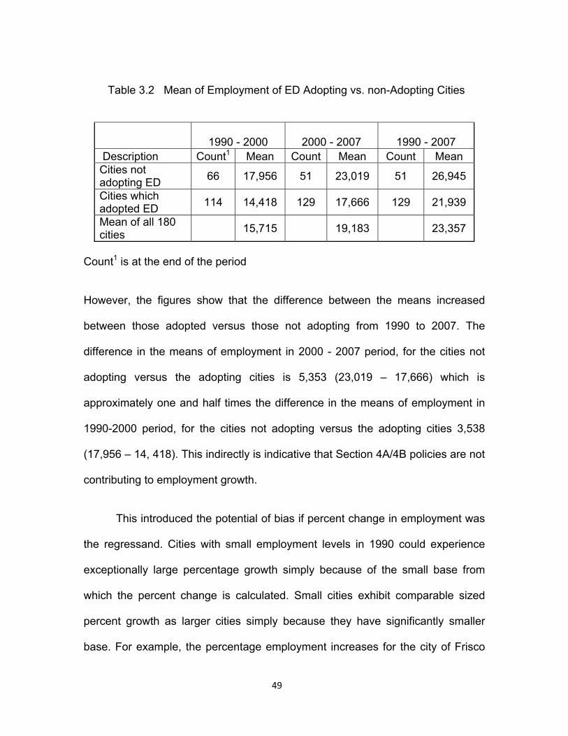
49

Table 3.2 Mean of Employment of ED Adopting vs. non-Adopting Cities

1990 - 2000

2000 - 2007

1990 - 2007

Description Count1 Mean Count Mean Count Mean Cities not adopting ED 66 17,956 51 23,019 51 26,945



Count1 is at the end of the period

However, the figures show that the difference between the means increased

between those adopted versus those not adopting from 1990 to 2007. The

difference in the means of employment in 2000 - 2007 period, for the cities not

adopting versus the adopting cities is 5,353 (23,019 – 17,666) which is

approximately one and half times the difference in the means of employment in

1990-2000 period, for the cities not adopting versus the adopting cities 3,538

(17,956 – 14, 418). This indirectly is indicative that Section 4A/4B policies are not

contributing to employment growth.

This introduced the potential of bias if percent change in employment was

the regressand. Cities with small employment levels in 1990 could experience

exceptionally large percentage growth simply because of the small base from

which the percent change is calculated. Small cities exhibit comparable sized

percent growth as larger cities simply because they have significantly smaller

base. For example, the percentage employment increases for the city of Frisco

50

and Flower Mound during the decade 1990-2000 are 465.8 and 218.16

respectively. During the same period, the City of Arlington had a growth of 20%

in employment (from 146,327 to 175,452). The population of Frisco increased

from 6,138 in 1990 to 94,595 in 2007.

One-way ANOVA (Hawkins & Weber, 1980) indicated no relationship

between the percent growth of employment and the adoption of economic

development sales tax (F=0.104, p=0.747). Alternatively, one-way ANOVA

rejected the null hypothesis of no relationship between absolute employment

growth and the adoption of economic development tax (F= 1.422, p =0.235).

Based on these empirical results and the inclusion of city population and city

employment as control variables, the absolute growth of city employment was

chosen to operationalize employment growth.

4.6 Variables and Their Significance

The amount of tax revenue collected by the city (EDTAXREVj) is measured

by the average amount collected based on the number of months the city

collected the tax. Only the number of months cities collect the tax is used

because not all cities collected the tax the same number of months.

An aggregate measure may reflect two cities collecting the same amount

and hide the fact that one city has collected revenue over a number of years at a

low rate and the other city has collected the revenue over a shorter period but at

a relatively higher rate. A monthly average, based on the number of months the

51

city collected the tax, differentiates those cities. Because the effects of the city

spending tax revenue on economic development may be lagged, the length of

time the city collects the tax is important. A city that collects the tax for six years

will more likely see results than the city that collects the tax for one year. Many

projects may not be complete within a year and may not produce benefits until

the third or fourth years.

We control for the length of time the city collects the 4A/4B tax by including

the number of months (MONTHSj) a city has collected as a control variable. It is

expected that the cities with more months of collection, ceteris paribus, will

experience greater economic growth than those cities that do not collect the tax

or collect it for a shorter time. All financial values were converted to 2000 dollars

before the monthly averages were calculated. Producer Price Index from Global

Insights was used to determine the factors. Similarly, all household incomes were

converted to 2000 dollars. The year 2000 was chosen as a base because the

data in the study spans over 1990 to 2007 and it seemed more appropriate to

use 2000.

The amount of Section 4A/4B tax revenue is collected from information

from the Office of the Texas State Comptroller. The Office of the Comptroller

publishes total sales and use tax revenue by month for each city. The office also

provides historical data for sales and use tax for each city and the various

components of the total sales tax rate. For example, one can determine, of a 2

percent total local sales and use tax rate, that 1 percentage point is the base

52

rate, ½ of a percentage point is Section 4A/4B and that ½ of a percentage point

is for property tax relief. In addition, the start date and the end date of each

component are reported. Given an amount of sales tax revenue, the amount of

the economic development sales tax is calculated as the percent of the total

revenue equal to the percent of the total local rate comprised of the ED sales tax.

In the hypothetical city above, the Section 4A/4B tax rate is approximately 25

percent of the total rate and the Section 4A/4B tax generated about 25 percent of

the total local sales and use tax revenue.

Cities pursue local economic development in a number of ways. Some of

the other financial methods besides Section 4A/4B taxes, include abating

property tax liability within an enterprise zone or a Freeport zone and redirecting

property tax revenue by virtue of tax increment finance agreements, Cities can

implement these agreements while contemporaneously collecting the economic

development sales tax. It is necessary to separate, as much as possible, the

effect of these economic development policies from the effect of the Section

4A/4B sales tax. Texas cities are required to report annually to the State

Comptroller the amount of tax revenue they forego or redirect attributable to

these types of financial agreements. We computed the constant dollar average of

this foregone revenue, by policy type and aggregate and included it in the model

as a measure of other economic efforts by the cities. These measures admittedly

do not capture non-financial efforts or non reported efforts of cities. They do,

53

however, provide a reasonable approximation of overall effort of other economic

development programs.

The 1990 population of the city (CITPOP90), the change in city population

during the decade (DELCITPOPj), the size of the county employment in 1990

(CNTYEMP90) and the change in county employment between 1990 and 2000

(DELCNTYEMPNETj) all contribute to capture the urbanization and localization

economies affecting the city economy. The change in the county employment is

net of the change in city employment to avoid the influence of the growth of city

employment on county employment growth. This is expected to be the case

where the city in the study is the overwhelming largest city in the county. The

growth of the city employment more likely affects the entire county employment

rather than vice versa. An example of this situation is Lubbock. Lubbock city

employment is 95,035 in 2000; 83 percent of Lubbock County employment of

114,711. County employment operationalizes urbanization economies and city

population operationalizes localization economies.

The example of Lubbock demonstrates how a single central city can

dominate the economy of an entire county, or even adjacent counties. Not all

central cities may be so dominate.

A phenomenon in urban economies is the decentralization of people and

jobs. Central cities have consistently lost population and employment relative to

the metropolitan area as a whole since the middle of twentieth century. Robin M.

54

Leichenko (2000) investigates the broad-based trends of urban change in the

United States between 1970 and 1997. However, this trend of decentralization

continued through the beginning of the 21st century and continues today. One

consequence is that central cities either loose employment relative to other cities,

or worse, experience an absolute decline in population and employment as

people and businesses move to suburbia and exurbia.

The results of his study suggest that suburban and city growth are

interrelated but the nature of interrelationship varies over time. Interestingly, his

results indicate that population and employment growth in cities tend to be jointly

determined. His model takes into account this potential source of simultaneity by

using simultaneous equation model where in change in population is an

independent variable in one equation and dependent variable in another

equation. In this study, the change in population, change in employment and

change in median household income are used but without simultaneity. In this

study, we capture the trend of jobs and people leaving the central city during the

1990s and beyond by using a dummy variable CENTRAL. It is expected that job

growth in central cities will be less than the job growth in other cities. Average

Job Growth in 24 Central Cities is 12.7 and 15.7 for 1990-2000 and 2000-2007

respectively, compared to other cities job growth of 26.3% and 24.2% for the

same two time periods.

As mentioned above, metropolitan areas are defined as Metropolitan

Statistical Areas (MSA) and are not equal. In addition, cities in rural counties are

55

not part of an MSA. Large MSAs contain a wider variety of goods and services

than smaller MSAs and rural counties. Direct international flights are not

available in every MSA. Smaller MSAs may be regional hubs of economic activity

but may specialize in agriculture or timber industries. Large MSAs are statewide

or international hubs and hence are affected by different factors than smaller

MSAs. At the same time, because of their heterogeneous economies, large

MSAs can weather economic changes better than the small MSAs or rural

counties.

Two dummy variables, SMMETRO and RURAL, are equal to one for a city

in a small MSA or rural county and zero otherwise. Cities in counties of small

metropolitan areas or rural counties are expected to grow slower than cities in

counties of large metropolitan areas. The large metropolitan areas were defined

to be Austin MSA, Dallas-Fort Worth MSA, El Paso MSA, Houston MSA and San

Antonio MSA.

Finally, different regions of the state may experience different economic fortunes.

The more urbanized regions of the state are more populated, more diversified

and more capable to adjust to changes in the state and national economies. The

model includes a dummy variable (SMLREG) that equals one if the city is in a

small economic region or the state and 0 otherwise. It is to capture the

differences in growth between the large regions of the state and the smaller

regions. Less than half of the cities, 47 percent, are located in large economic

regions. The State of Texas is divided into twelve economic regions. These are

56

listed in Appendix 3. The large regions are determined to be the Alamo region

(San Antonio), the Capital region (Austin), the Gulf Coast region (Houston), and

the Metroplex region (Dallas/Fort Worth). Of the counties in the study, total 2000

county population is 11.0 million for large region counties. Aggregate county

population for small region counties is 5.7 million. Over two-thirds of the

population resides in the four large regions. It is expected, given the greater

variety of activities, markets, and inputs, that the cities in the larger regions will

experience more growth and development than comparable cities in

correspondingly smaller regions of the state.

4.7 Descriptive Statistics

Table 4.1 contains the descriptive statistics of the dependent variable, the

independent variables and control variables for cities. Overall city employment

increases, on average, by nearly 4900 jobs during 1990s and 8478 jobs during

1990-2007, with some cities losing jobs. The 1990 mean city population is slightly

more than 34,000 and 49,000 in 2007.

57

Table 4.1 Descriptive Statistics

Variable Descriptions Count Minimum Maximum Mean Std. Dev.

City Population 1990 180 3,944 261,721 34,422 41,342

City Population 2000 180 10,302 332,969 42,308 49,556

City Population 2007 180 9,942 359,365 49,179 55211

City Employment 1990 180 2,195 146,327 15,715 20,438

City Employment 2000 180 2,740 175452 19183 23997

City Employment 2007 180 4,503 188480 23357 26907

City Household Income 1990 180 12,908 77,530 29,408 11,841



ED Tax Normalized 90-00 180 - $2,655,257 $230,814 $317,708

OED Tax Norm’lizd 90-00 180 - $1,467,626 $214,638 $290,022

The next chapter 5 discusses the OLS estimates of regressing the statistical

models and their results.

58

CHAPTER 5

ANALYSIS OF REGRESSION MODELS AND RESULTS

5.1 Basic Form of Models

In this chapter, all the models for Employment Change and Income Change

will be run using SPSS. As explained in the chapter, these models we will also

run these models using Wooldridge Fixed Effects Model. Based on previous

chapter’s discussion, the Change in city Employment model will have the

following variables as shown in the following DV = f (IV) equation.

DELCITEMPj = β0 + β1 * EDTAXREVj + β2 *MONTHSj + β3 * OTHEREVj + β4 *

CITPOP90+ β5 * DELCITPOPj + β6 * CNTYEMP90 + β7 * DELCNTYEMPNETj

+ β8 * SMMETRO + β9 * RURAL + β10 * SMLREG + β11 * CENTRAL

The variables have been explained in the previous chapter and βj are the

coefficients which will be determined by the OLS regression tool. The first model

is for the dependent variable change in city employment between 1990 and 2000

(DELCITEMP1). The independent variables are economic development policies

variables EDTAXREV1 per month, the number of months (MONTHS1) the

59

revenue is collected and the other ED revenues (OEDREV1). The literature

review indicated that the change in employment and change in population move

together. Therefore, DELCITPOP1 has been included as the independent

variable along with the initial city population. Since the city employment is

affected by agglomeration economics of the county as a whole, county

employment and net change in county employment have been included as

independent variables. The economic nature of the city, as to whether it is a

central city or in a rural county along with the economic region (small or large),

have been included as control variables. The purpose is to determine the effect

on change in employment as a result of economic development policies by

including the variables that could have impact on the outcome.

The first employment change model is for the period 1990 to 2000.

5.2 Employment Change Models

Regression Results and Analysis

The results of regression of the first model are shown in Table 5.1.

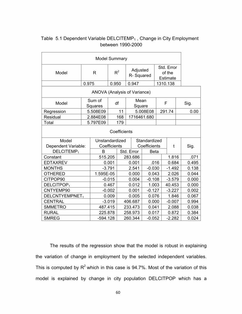
60

Table 5.1 Dependent Variable DELCITEMP1 , Change in City Employment between 1990-2000

Model Summary

Model R R2 Adjusted R- Squared

Std. Error of the

Estimate 0.975 0.950 0.947 1310.138

ANOVA (Analysis of Variance)

Model Sum of Squares df Mean

Square F Sig.

Regression 5.508E09 11 5.008E08 291.74 0.00Residual 2.884E08 168 1716461.680 Total 5.797E09 179

Coefficients

Model Dependent Variable:

DELCITEMP1

Unstandardized Coefficients

Standardized Coefficients t Sig.

Β Std. Error Beta Constant 515.205 283.686 1.816 .071EDTAXREV 0.001 0.001 .016 0.684 0.495MONTHS -3.791 2.541 -0.030 -1.492 0.138OTHERED 1.595E-05 0.000 0.043 2.026 0.044CITPOP90 -0.015 0.004 -0.108 -3.579 0.000DELCITPOP1 0.467 0.012 1.003 40.453 0.000CNTYEMP90 -0.002 0.001 -0.127 -3.227 0.002DELCNTYEMPNET1 0.009 0.005 0.076 1.846 0.067CENTRAL -3.019 406.687 0.000 -0.007 0.994SMMETRO 487.415 233.473 0.041 2.088 0.038RURAL 225.878 258.973 0.017 0.872 0.384SMREG -594.128 260.344 -0.052 -2.282 0.024

The results of the regression show that the model is robust in explaining

the variation of change in employment by the selected independent variables.

This is computed by R2 which in this case is 94.7%. Most of the variation of this

model is explained by change in city population DELCITPOP which has a

61

coefficient of .467 and t value of 40. 453. This means that a change of 1000 in

population adds 467 jobs. However, the analysis of the results of the rest of the

model independent variables, reveal unexpected results. The coefficients of

beginning city population (CITPOP90) is negative which theoretically will mean,

ceteris paribus, if original population is 1000 more, it will result in employment to

go down by 15 people. It does not make sense. Same is the case for initial

county employment. ED sales tax revenue has a coefficient not significantly

different from zero as indicated by computed t-value of 0.684. It means ED tax

revenue had no impact on the growth of employment. Therefore, one can

conclude that at an α value of 5%, ED and Other ED have no contribution in

explaining variation in change in employment over the decade of 1990 to 2000.

Earlier we showed in Tables 3.1 and 3.2 that those cities that adopted Sections

4A/4B had less population and less employment than the cities that did not

implement the ED sales tax. But that was expected because the intent of the

legislation was to give a means or opportunity for small cities for economic

development. However, the data over the decade (1990-2000) shows that

economic development policy did not produce the desired result. Table 5.2

shows the difference means in population, employment and income growth

between adopting and non-adopting cities. Non-adopting cities grew in all three

areas far better than the adopting cities.

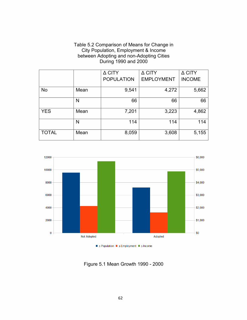
62

Table 5.2 Comparison of Means for Change in

City Population, Employment & Income between Adopting and non-Adopting Cities

During 1990 and 2000

∆ CITY POPULATION

∆ CITY EMPLOYMENT

∆ CITY INCOME

No Mean 9,541 4,272 5,662

N 66 66 66

YES Mean 7,201 3,223 4,862

N 114 114 114

TOTAL Mean 8,059 3,608 5,155

Figure 5.1 Mean Growth 1990 - 2000

63

It is also interesting to note that the mean of employment and population

ratio of adopting and non adopting cities over the decade did not change. It

stayed 44% for adopting and not adopting cities. These initial observations

support the hypothesis of this research that economic development policies as

envisioned in the legislation of Sections 4A and 4B have no significant impact on

employment growth. The rate at which the cities have been adopting the sales

tax economic development policies has been dropping since 1998 when 11 cities

adopted either of the two Sections. Since then it has trickled down to 2 cities in

years 2003 to 2007, the last year of this study (Figure 5.2). May be these ED

policies are not yielding the intended results of economic growth and city officials

have lost interest in going to the voters.

Figure 5.2 Adoption Rate

0

5

10

15

20

Number of Cities adopting 4A/4BBy Year

Adopted

64

Although the model overall has good predictability with F=291.74

and R2 of 0.95, the negative coefficients of some independent variables do not

make sense.

5.3 Wooldridge Fixed Effects Model

Wooldridge (2006) describes a similar situation. He had two years of

data for cities across USA and using one year data got a model that showed that

crime rate goes down when unemployment increased. Obviously, it is not

expected. Therefore, the model needed some changes. His theory was that the

model needs more variables like efforts of police force to combat crime,

demographics of the population such as age distribution, gender distribution,

education levels, etc. But many of the above factors may be hard to control but

relatively stay fixed in a city over a short duration of 5 to 10 years. He came up

with an approach where by the factors affecting the dependent variable are

divided into two groups, unobserved or fixed effects and observed effects. The

factors such as age distribution, gender distribution, law enforcement efforts,

which are difficult to control but are more or less fixed between two time periods

of short duration, he called unobserved or fixed effects. These fixed effects are

assumed to be constant overtime. Then the regression model can be written as

Yit = β0 + δ0 d2t + β1 xit + ai + uit , t = 1, 2

where in the notation Yit , i denotes the city and t denotes the time period. The

variable d2t is a dummy variable that equals zero when t =1 and one when t =2.

65

Intercept for t = 1 is β0 and the intercept for t = 2 is β0 + δ0 . The variable ai

captures all unobserved, time-constant factors that affect Yit .That is why it does

not have subscript of time (t). Wooldridge suggests combing the data for two time

periods in one model and creating first-differenced equation. Let us write the

equations for t = 1 and t = 2.

Yi1 = β0 + β1 xi1 + ai + ui1 , t = 1 (1)

Yi2 = β0 + δ0 + β1 xi2 + ai + ui2 , t = 2 (2)

Subtracting the first equation from the second results in the following

Yi2 - Yi1 = δ0 + β1 (xi2 - xi1) + (ui2 - ui1)

The above equation is the change in the dependent variable and the

independent variables or predictors are also shown as deltas. The intercept δ0 is

the change in the intercept between two time periods. I will use Wooldridge first-

differenced equation to determine the change in employment over two periods of

1990 and 2000, (DELCITEMP1) by subtracting out the fixed effect variables such

as RURAL, CENTRAL, SMLREGN, and SMLMETRO. The character of the cities

relative to these variables remained same over the decade.

DELCITEMP1 = δ0 + β1 * DELEDREV1 + β2 * DELOEDREV1 + β3 * DELCITPOP1

+ β4 * DELCNTYEMPNET1

66

SPSS produced the following Table 5.3 for this model. The results of this model

confirm what was expected that the ED policies did not contribute in any

significant way towards job growth and the change in city population explains

most of the variation in the employment change. All other variables remaining

same, an increase of 1000 population adds 456 jobs, supporting the economic

theory that people go where jobs are.

67

Table 5.3 Dependent Variable DELCITEMP1,Change in City Population between 1990 and 2000 Using Wooldridge Fixed Effects Model

Model Summary


Std. Error of the

Estimate 0.968 0.936 0.935 1459.280


Model Sum of Squares df Mean Square F Sig.


Coefficients


DELCITEMP1



Β Std. Error Beta Constant -81.219 168.154 -0.483 .0630DELCITPOP1 0.457 0.010 0.983 46.457 0.000DELCNTYEMPNET1 -4.934E-5 0.002 0.000 -0.022 0.982DELEDTAX1 0.000 0.000 -0.048 -2.196 0.029DELOEDTAX1 0.000 0.000 0.040 1.967 0.051

From the above two Employment Change Models, the inference is

that the city employment growth is not dependent in any significant way on

Sections 4A or 4B economic development policies. Most of the change in jobs

can be explained by the growth in the population. Thus one can preliminary

accept the null hypothesis that ED has no impact on economic development.

However, the reason for the ED policy variables coming at a negative or

statistically insignificant levels could be that out of 180 observations, 66 are zero

68

because the cities chose not to adopt Section 4A or 4B. Such a large number of

zeros in the observations, skews the distribution of the data.

5.4 ED Variables as Dummy Variables

To overcome the above potential problem of skewed distribution,

both the ED policy variables are classified as dummy variables. If the city

adopted ED policy, 1 was assigned to Section 4A/4B ED variable, otherwise 0.

The new variable is denoted by ED1 for 1990-2000 time period. Similarly, if the

city was foregoing revenue due to other ED policies such as Freeport

Exemptions, Tax Incremental Finance Agreements, property tax abatements;

etc.; a dummy variable OTHERED1 with a value of 1, otherwise 0 was used.

Results of this regression model are shown in Table 5.4.

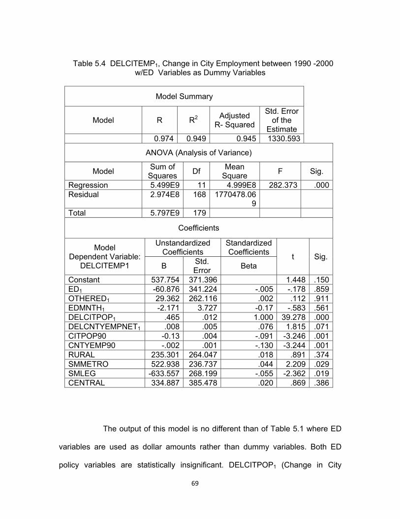
69

Table 5.4 DELCITEMP1, Change in City Employment between 1990 -2000 w/ED Variables as Dummy Variables

Model Summary


Std. Error of the

Estimate 0.974 0.949 0.945 1330.593


Model Sum of Squares Df Mean

Square F Sig.

Regression 5.499E9 11 4.999E8 282.373 .000Residual 2.974E8 168 1770478.06

9

Total 5.797E9 179

Coefficients


DELCITEMP1



Β Std. Error Beta

Constant 537.754 371.396 1.448 .150ED1 -60.876 341.224 -.005 -.178 .859OTHERED1 29.362 262.116 .002 .112 .911EDMNTH1 -2.171 3.727 -0.17 -.583 .561DELCITPOP1 .465 .012 1.000 39.278 .000DELCNTYEMPNET1 .008 .005 .076 1.815 .071CITPOP90 -0.13 .004 -.091 -3.246 .001CNTYEMP90 -.002 .001 -.130 -3.244 .001RURAL 235.301 264.047 .018 .891 .374SMMETRO 522.938 236.737 .044 2.209 .029SMLEG -633.557 268.199 -.055 -2.362 .019CENTRAL 334.887 385.478 .020 .869 .386

The output of this model is no different than of Table 5.1 where ED

variables are used as dollar amounts rather than dummy variables. Both ED

policy variables are statistically insignificant. DELCITPOP1 (Change in City

70

Population between 1990 and 2000) is the predominant predictor with a t- value

of 39.278 and ceteris paribus, a change of 1000 in population adds 465 jobs.

Other significant variables are CNTYEMP90 and CITPOP90. But both of these

variables have negative coefficients which does not make sense. SMLREG is

significant and has a coefficient of -633.557, meaning that if the city is in small

economic region, it will result in the loss of 633 jobs. Overall, changing the ED

policy variables did not change the outcome of this regression model. The

inference with respect to the ED policy variables remains that these are not

statistically significant.

5.5 Model for DELCITEMP with Normalized ED Variables

Since the predictor DELCITPOPj has been the driving factor in

explaining the model, I normalized the ED policy variables by dividing the ED

dollar values by CITPOP90 expressed in (‘000). DELCITPOPj was also divided

by CITPOP90 to get per capita transformation per 1000. The results of this model

are shown in Table 5.5

71

Table 5.5 DELCITEMP1, Change in City Employment between 1990 -2000 w/Normalized ED Variables

Model Summary


Std. Error of the

Estimate 0.530 0.28

10.239 4965.063



Square F Sig.

Regression 1.631E9 10 1.631E8 6.614 .000Residual 4.166E9 169 24651850.12 Total 5.797E9 179

Coefficients


DELCITEMP1



Β Std. Error Beta

Constant 2716.34 1151.853

2.358 .020

EDMNTH1 -4.209 13.485 -.033 -.312 .755EDTAXNRMALIZD1 -7.374E-5 .002 -.004 -.035 .972OEDNORMALIZED1 .000 .001 .009 .120 .905DELCITPOPRATIO1 3758.39 931.492 .385 4.035 .000DELCNTYEMPNET1 .019 .018 .169 1.037 .301CNTYEMP90 -.003 .002 -.178 -1.161 .247RURAL -1082.10 981.751 -.081 -1.102 .272SMMETRO 1363.02 887.607 .114 1.536 .127SMLREG -2091.01 981.794 -.183 -2.13 .035CENTRAL 2830.68 1253.56

5.170 2.258 .025

Both the ED policy variables even after normalization remain

statistically insignificant. The new transformed variable DELCITPOPRATIO1

72

which is the original DELCITPOP divided by CITPOP90 is significant. If the ratio

of change in population to initial population is 1, then the change in employment

is expected to be about 3,760 jobs, ceteris paribus. If the city is located in a small

economic region, it is expected that the jobs will decrease on the average by

about 2,100 compared to cities in the large economic regions.

5.6 DELCITEMP Model w/ Dummy ED Variables and Normalized DELCITPOP

Next, a combination of the above two models was considered

because in the model described in Table 5.5, the issue of 66 cities with zero

values may have skewed the results. The next model is using ED policy variables

as dummy variables as described earlier and the change in population variable

DELCITPOPj will be transformed to per capita by dividing by CITPOP90. These

results are in Table 5.6.

73

Table 5.6 DELCITEMP1, Change in City Employment between 1990 -2000, w/Dummy ED Variables and Normalized DELCITPOP

Model Summary

Model R R2 Adjusted

R- Squared

Std. Error of the

Estimate 0.558 0.312 0.271 4859.298



Square F Sig.

Regression 1.806E9 10 1.806E8 7.649 .000Residual 3.991E9 169 23612776.9

7

Total 5.797E9 179

Coefficients


DELCITEMP1



Β Std. Error Beta Constant 2019.384 1348.715 1.497 .136EDMNTH1 17.965 13.562 .141 1.325 .187ED1 -2583.006 1233.578 -.219 -2.094 .038OTHERED1 1723.003 949.535 .123 1.815 .071DELCITPOPRATIO1 3604.993 752.462 .369 4.791 .000DELCNTYEMPNET1 .016 .018 .146 .915 .361CNTYEMP90 -.002 .002 -.144 -.959 .339RURAL -844.680 961.102 -.063 -.879 .381SMMETRO 1470.113 870.664 .123 1.688 .093SMLREG -2268.134 970.861 -.198 -2.336 .021CENTRAL 2690.685 1221.901 .161 2.202 .029

The output of this model is no different from the previous ones in the

sense that the ED policy variable representing Section 4A/4B, although

statistically significant has a negative coefficient, meaning that if the city has

adopted the ED policy under these sections, it is expected to lose jobs, which

74

does not seem realistic. The OTHERED variable is statistically significant at α

equal to 10% but not at α equal to 5%. Change in population divided by initial

population, i.e., per capita change in population is statistically significant as was

the case in previous models. This drives home the fact that population is the

engine for the jobs which has been stated in the literature as well. It is expected

that the cities in the small economic regions on the average will lose jobs

compared to the cities in the large economic region which because of

agglomeration economies generally do better than the cities in small regions.

Now, models for Income change model will be discussed. These

models are specified to measure the impact of ED policies on quality of life. It is

suspected from the Employment Change Model results that the adoption of these

sections will have more likely than not, have no impact on income growth.

5.7 Income Change Models

In this model change in income will be regressed by using the

independent variables of population growth divided by initial population

(DELCITPOPRATIO1), initial household median income (1990) escalated to 2000

(CITINC90ESC00), net county employment change (DELCNTYEMPNET1), four

fixed effects variables of rural, central, small or large economic region and small

metro plus the quality of life variables of home ownership, college graduates, and

level of poverty, all normalized to represent per capita change. The ED policy

variables will be used as dummy variables as described earlier.

75

The results of this model are shown in Table 5.7. Both ED policy variables are

statistically insignificant. As in the previous models, change in net county

employment and per capita change in city population are significant statistically.

Initial median household income is significant and the model predicts that for

each $1,000 of initial income, one job will be added to the economy. Contribution

of the quality variables change in the ratio of the number college graduates to the

city population and change in the per capita poverty level are significant. The

results of the model indicate that for each one point increase in

COLGRADRATIOPOPCHNG, income is expected to increases by $126 and one

point decrease in poverty levels adds $166 to income. The third quality of life

predictor, the home ownership is significant but with a negative coefficient, which

cannot be explained logically. The F value of the model is 27.014 which is

significant and the model explains 67.8% of the variation

From the above results for the data for period 1990 to 2000, one can infer

that the ED policies of Sections 4A/4B are not generating jobs or improving the

quality of life. Other ED policy variable yielded inconsistent results.

76

Table 5.7 Dependent Variable DELCITINC1 , Change in Median Household Income between 1990-2000

Model Summary

Model R R2 Adjusted

R- Squared

Std. Error of the

Estimate 0.824 0.679 0.654 4201.32877


Model Sum of Squares df Mean

Square F Sig.


Coefficients


DELCITINC1



Β Std. Error Beta Constant -1314.425 1682.519 -.781 0.436ED1 -989.388 1075.959 -0.067 -.920 0.359EDMNTH1 4.633 11.789 0.029 .393 .695OTHERED1 -1277.023 825.643 -0.072 -1.547 0.124DELCITPOPRATIO1 2120.844 872.910 0.173 2.430 0.016CITINC90ESC00 0.100 0.031 0.220 3.230 0.001DELCNTYEMPNET1 0.015 0.008 0.104 1.734 0.085CENTRAL 238.996 1056.151 0.011 0.226 0.821SMMETRO -261.431 761.666 -0.017 -.343 0.732RURAL 187.308 834.632 .011 .224 0.823SMREG -162.361 873.303 -.011 -0.186 0.853COLGRADRATIOPOPCHNG1

126.483 17.631 0.562 7.174 0.000

POVRTYRATIOPOPCHNG1

-166.116 50.329 -.174 -3.301 0.001

HOMEOWNRATIOPOPCHNG1

-68.086 20.556 -.168 -3.312 0.001

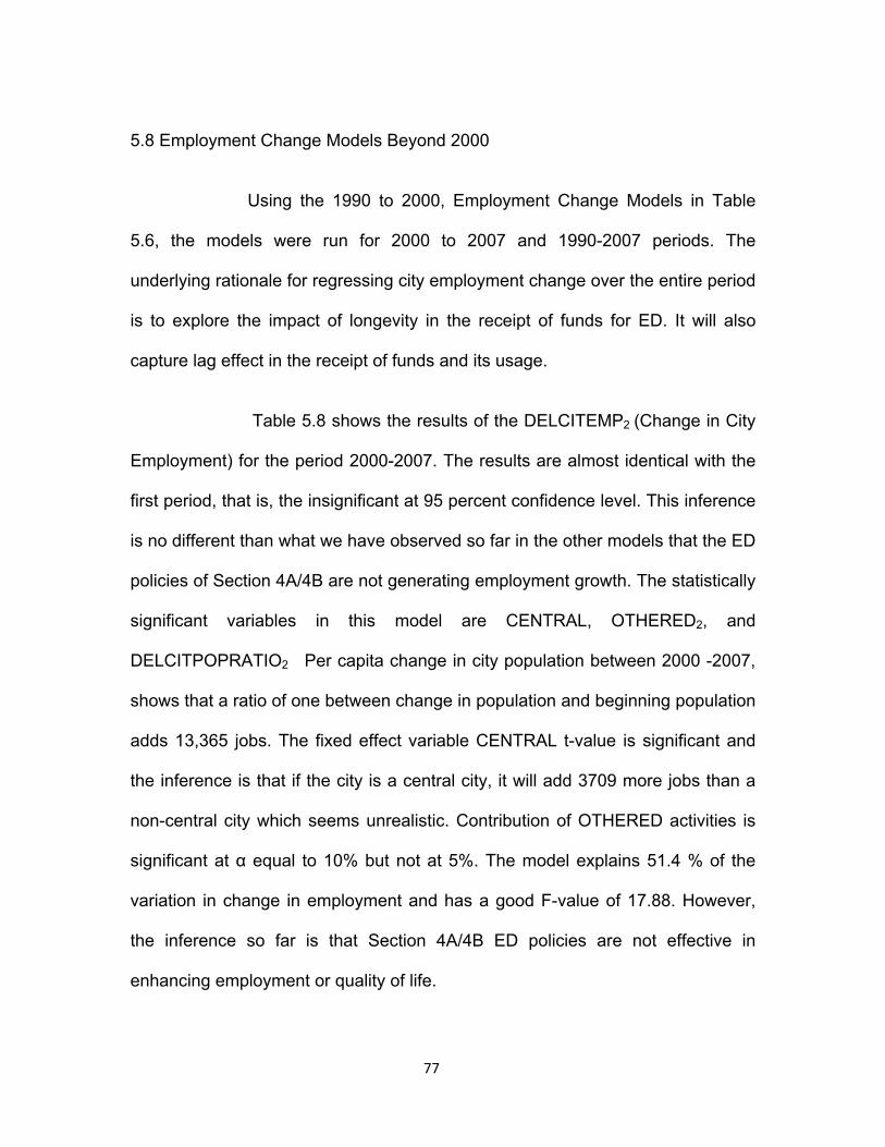
77

5.8 Employment Change Models Beyond 2000

Using the 1990 to 2000, Employment Change Models in Table

5.6, the models were run for 2000 to 2007 and 1990-2007 periods. The

underlying rationale for regressing city employment change over the entire period

is to explore the impact of longevity in the receipt of funds for ED. It will also

capture lag effect in the receipt of funds and its usage.

Table 5.8 shows the results of the DELCITEMP2 (Change in City

Employment) for the period 2000-2007. The results are almost identical with the

first period, that is, the insignificant at 95 percent confidence level. This inference

is no different than what we have observed so far in the other models that the ED

policies of Section 4A/4B are not generating employment growth. The statistically

significant variables in this model are CENTRAL, OTHERED2, and

DELCITPOPRATIO2 Per capita change in city population between 2000 -2007,

shows that a ratio of one between change in population and beginning population

adds 13,365 jobs. The fixed effect variable CENTRAL t-value is significant and

the inference is that if the city is a central city, it will add 3709 more jobs than a

non-central city which seems unrealistic. Contribution of OTHERED activities is

significant at α equal to 10% but not at 5%. The model explains 51.4 % of the

variation in change in employment and has a good F-value of 17.88. However,

the inference so far is that Section 4A/4B ED policies are not effective in

enhancing employment or quality of life.

78

Table 5.8 DELCITEMP2, Change in City Employment between 2000-2007 w/Dummy ED Variables and Normalized DELCITPOP2

Model Summary

Model R R2 Adjusted

R- Squared

Std. Error of the

Estimate 0.717 0.514 0.485 4036.5643


Model Sum of Squares Df Mean Square F Sig.

Regression 2.913E9 10 2.913E8 17.876 .000 Residual 2.754E9 169 16293851.85 Total 5.666E9 179

Coefficients


DELCITEMP2



Β Std. Error Beta Constant 693.547 1139.373 .609 .544EDMNTH2 -13.324 22.103 -.102 -.603 .547ED2 451.842 2096.269 .036 .216 .830OTHERED2 1323.994 725.036 .106 1.826 .070DELCITPOPRATIO2 13634.332 1183.445 .696 11.521 .000DELCNTYEMPNET2 -.001 .007 -.013 -.115 .909CNTYEMP00 .001 .001 .054 .456 .649RURAL -536.169 811.208 -.040 -.661 .510SMMETRO -71.319 717.902 -.006 -.099 .921SMLREG 281.076 808.204 .025 .348 .728CENTRAL 3709.493 1008.741 .225 3.677 .000

5.9 Employment Model for 1990-2007

Table 5.9 is the model for the entire period of 1990-2007. The

expectation in running this model was to see if the longer duration will have any

different impact of ED policy variables on employment growth. This regression

79

model does not yield any different results that have been seen before. The longer

period does not impact Section 4A/4B ED policy variables and these remain

statistically insignificant in explaining variation in the employment growth. Other

ED variable is statistically significant at α equal to 10% but not at 5%. Out of the

four fixed effect variables CENTRAL is significant meaning that if the city is a

central city in the county, ceteris paribus, it will add 5843 jobs, compared to non

central cities.

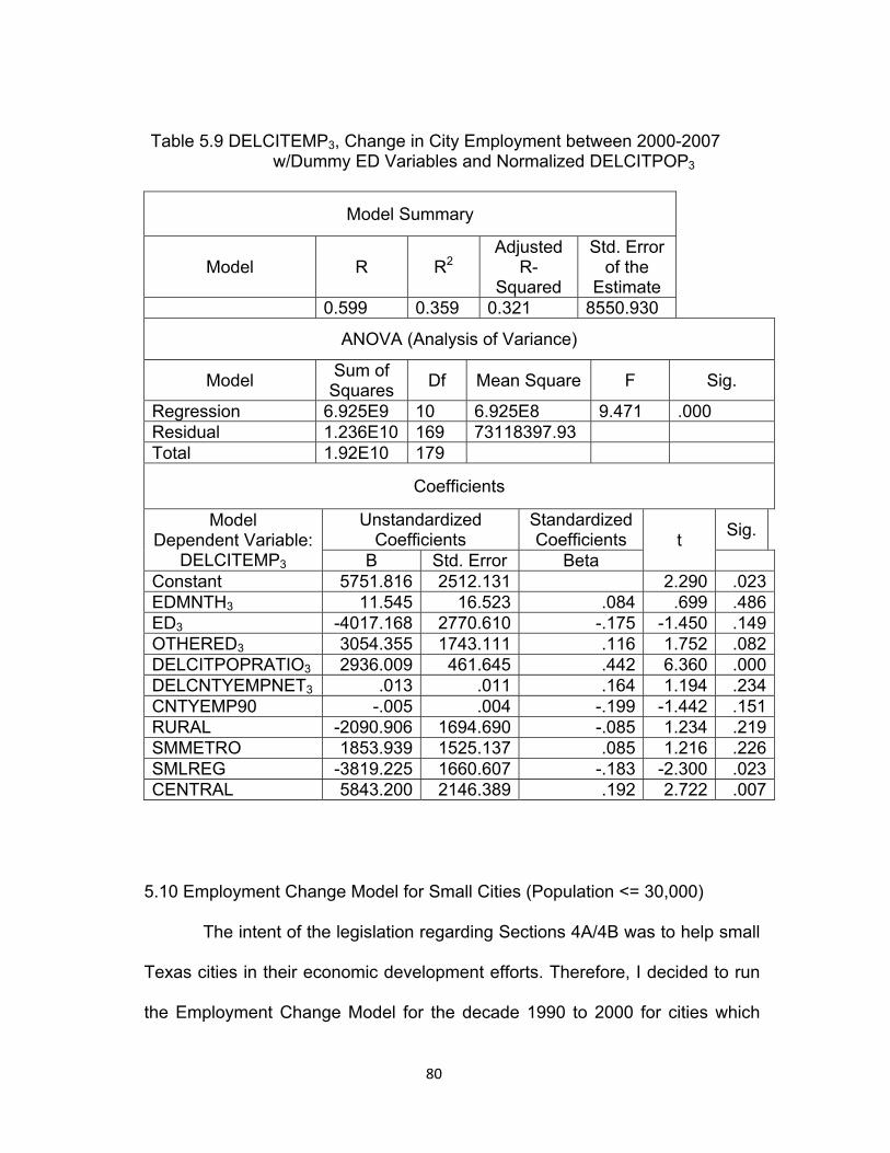
80

Table 5.9 DELCITEMP3, Change in City Employment between 2000-2007 w/Dummy ED Variables and Normalized DELCITPOP3

Model Summary

Model R R2 Adjusted

R- Squared

Std. Error of the

Estimate 0.599 0.359 0.321 8550.930



Regression 6.925E9 10 6.925E8 9.471 .000 Residual 1.236E10 169 73118397.93 Total 1.92E10 179

Coefficients


DELCITEMP3



Β Std. Error Beta Constant 5751.816 2512.131 2.290 .023EDMNTH3 11.545 16.523 .084 .699 .486ED3 -4017.168 2770.610 -.175 -1.450 .149OTHERED3 3054.355 1743.111 .116 1.752 .082DELCITPOPRATIO3 2936.009 461.645 .442 6.360 .000DELCNTYEMPNET3 .013 .011 .164 1.194 .234CNTYEMP90 -.005 .004 -.199 -1.442 .151RURAL -2090.906 1694.690 -.085 1.234 .219SMMETRO 1853.939 1525.137 .085 1.216 .226SMLREG -3819.225 1660.607 -.183 -2.300 .023CENTRAL 5843.200 2146.389 .192 2.722 .007

5.10 Employment Change Model for Small Cities (Population <= 30,000)

The intent of the legislation regarding Sections 4A/4B was to help small

Texas cities in their economic development efforts. Therefore, I decided to run

the Employment Change Model for the decade 1990 to 2000 for cities which

81

had a population of less than or equal to 30,000 in 1990. The results are in

Table 5.10

Table 5.10 Employment Change Model for CITPOP90 ≤ 30,000


Std. Error of the Estimate

0.813 .661 0.631 2057.875



Regression 9.478E8 10 94780818.91 22.381 .000 Residual 4.870E8 115 4234850.397 Total 1.435E9 125

Coefficients


DELCITEMP30000



β Std. Error Beta Constant 690.551 618.051 1.117 .266EDMNTH 9.633 7.132 .126 1.351 .179ED30000 -667.190 648.949 -.094 -1.028 .306OTHERED30000 569.915 443.564 .073 1.285 .201DELCITPOPRATIO30000 3619.850 339.265 .723 10.670 .000DELCNTYEMPNET30000 .006 .009 .089 .643 .521CNTYEMP90 -.001 .001 -.092 -.696 .488RURAL 115.165 441.420 .016 .261 .795SMMETRO 36.919 479.236 .005 .077 .939SMLREG -996.573 464.757 -.144 -2.144 .034CENTRAL -267.311 2127.396 -.007 -.126 .900

The results of the Table 5.10 for CITPOP90 less than or equal to

30,000 are no different than the rest of the models. Both Section 4A/4B and

Other ED policy variables are statistically insignificant. Other than the

82

DELCITPOPRATIO, which is a ratio of change in population divided by the

original population, the only other predictor which is significant is SMLREG

(small economic region). Its β-coefficient is negative (-996.573) meaning that if

the city is in the small economic region, ceteris paribus, it will lose 996 jobs

compared to the cities which are in large economic regions, which makes

sense because the small economic regions do not enjoy the benefits of

agglomeration economies.

83

CHAPTER 6

CONCLUSIONS AND RECOMMENDATIONS

The above analysis leads the author to conclude that at the α value

of 0.10 the hypothesis, that the cities in Texas that adopted Section 4A/4B did

not do better in employment growth and income growth than the cities which

chose not to adopt these economic development provisions, can be accepted.

Various regression models run with data over a period of 1990 thru 2007 show

that the economic development sales tax collected by the cities did not in any

significant way impacted either the job growth or the income growth. Per capita

change in population is found to be the largest explanatory variable for

employment growth. The variable OTHER ED which encompasses economic

development efforts through Tax Increment Finance Agreements, Freeport

Zones, property tax relief, has been consistently significant at confidence level

(1 –α) of 90% but not at 95%. The quality of life variables, change in the number

of families below the poverty level and the change in the number of college

graduates explained the change in income during 1990 and 2000. I chose 2007

as the ending point of this research to avoid the impact of recession that began

around that time period.

84

The economic indicators data were hard to obtain. Yearly estimates

of population, employment and income are published based on well established

and acceptable methodologies. However, variables like high school graduates,

college graduates, families below poverty level, housing units, etc. are generally

not available for intermediate years. This is the limitation of this study that

income model could not be run for 2001-2007 time period.

Collecting sales tax for economic development is unique because

the literature addresses a litany of articles on the subject of economic

development where the state or city governments give rebates in taxes, assist

with their own funds the cost of infra-structure or training to attract businesses

with the hope of bringing in jobs to their location. This study is also unique in that

it addresses the small Texas cities (with a population of at least 10,000 in year

2000) while most studies on employment, population, or income growth address

large metropolitan cities.

It was not in the scope of this study to contact the cities that adopted

Sections 4A/4B to get more in-depth information on the corporations which they

created and the projects they undertook with the help of the funds collected

through sales tax. It would be very useful to conduct a survey using an

appropriate questionnaire technique followed by a sample of interviews to

decipher the use of funds by type of projects undertaken. This research has

concluded that within the limits of statistics, these ED provisions did not affect job

or income growth. It will be very prudent as part of future research to investigate

85

and determine the exact use of funds, actual number of jobs created,

improvement in quality of life factors, etc. As we know criticism has been raised

in the past as reported in the Dallas Journal by some state legislatures that the

funds raised for economic development have been used for ambulances, fire

trucks and government buildings in West Texas, private home for a company

executive in Longview, etc. Therefore, it will be interesting to understand the

utilization of funds towards job growth which is a major objective for any

economic development.

86

APPENDIX 1

ECONOMIC DEVELOPMENT PROGRAMS IN TEXAS

87

ECONOMIC DEVELOPMENT PROGRAMS IN TEXAS

Table of Contents I. The Sales Tax for Economic Development

Using Sales Tax to Promote Economic Development Differences Between the Section 4A and the Section 4B Sales Tax Section 4A Economic Development Sales Tax Section 4B Economic Development Sales Tax

II. Alternative Tax Initiatives for Local Development City/County Venue Project Tax Additional Taxes and Fees that Voters Can Approve Chapter 335 Sports and Community Venue Districts

III. Local Property Tax Incentives Property Tax Abatement Tax Increment Financing Texas Economic Development Act Adopting the Freeport and Super Freeport Exemptions IV. Economic Development Through Tourism

The Local Hotel Occupancy Tax County Development District Tax V. City, County, Cooperative, and Regional Efforts A City's Authority to Make Grants and Loans Providing Land to Promote Economic Development Municipal Agreements Not to Annex Use of Interlocal Agreements Economic Development Activities by Councils of Government County Economic Development Powers Municipal and County Ability to Provide Loans or Grants VI. Issuing Debt to Finance Economic Development Legal Authority to Issue Bonds Procedures for Issuing Bonds for Economic Development Other Instruments to Finance Infrastructure Improvements

88

VII. Other Economic Development Initiatives Public Improvement Districts Municipal Management Districts Municipal Development Districts Neighborhood Empowerment Zones North American Free Trade Agreement Impact Zones Economic Development Projects in Certain Counties County Assistance Districts VIII. Public Disclosure of Economic Development Negotiations Open Meetings and Public Information Acts IX. Synopses of Attorney General Opinions on Economic Development Section 4A Sales Tax Section 4B Sales Tax City/County Venue Project Tax Property Tax Abatement Tax Increment Financing Adopting the Freeport Exemption Local Hotel Occupancy Tax County Development District Tax Loans Under Local Government Code Chapter 380 Public Improvement Districts Municipal Management Districts County Economic Development Powers Public Disclosure of Economic Development Negotiations Miscellaneous Opinions Concerning Economic Development X. Different Economic Development Programs, Loans & Grants Offered by State Agencies Defense Economic Adjustment Assistance Grant Program (DEAAG) Defense Economic Readjustment Zone Program Federal Tax Credits Office of the Governor Product Development Fund Revolving Loan Fund Update Texas Department of Agriculture Texas Department of Housing and Community Affairs Texas Emerging Technology Fund Overview Texas Enterprise Fund Program Texas Enterprise Zone Program Texas Heritage Trails Program

89

Texas Historical Commission Grant Writing Workshops Texas Industrial Revenue Bond Program: Issuance of Bonds by Development Corporations Texas Industry Development Loan Program Texas Leverage Fund The Texas Main Street Program Texas Preservation Trust Fund Grant Program Texas Water Development Board The Certified Local Government (CLG) Program Visionaries in Preservation Program

90

APPENDIX 2

CITIES IN THE STUDY

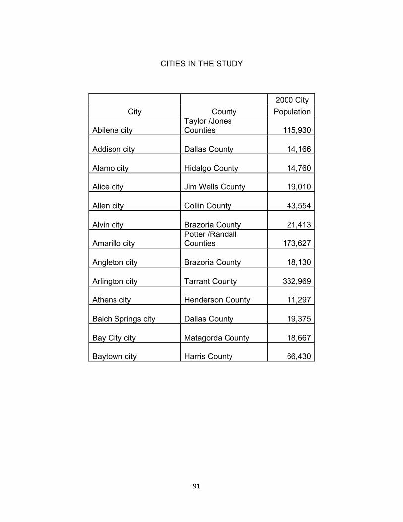
91

CITIES IN THE STUDY

City County 2000 City Population

Abilene city Taylor /Jones Counties

115,930

Addison city Dallas County

14,166

Alamo city Hidalgo County

14,760

Alice city Jim Wells County

19,010

Allen city Collin County

43,554

Alvin city Brazoria County

21,413

Amarillo city Potter /Randall Counties

173,627

Angleton city Brazoria County

18,130

Arlington city Tarrant County

332,969

Athens city Henderson County

11,297

Balch Springs city Dallas County

19,375

Bay City city Matagorda County

18,667

Baytown city Harris County

66,430

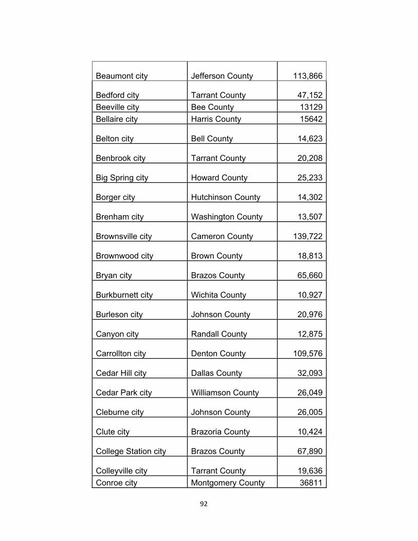
92

Beaumont city Jefferson County

113,866

Bedford city Tarrant County

47,152 Beeville city Bee County 13129 Bellaire city Harris County 15642

Belton city Bell County

14,623

Benbrook city Tarrant County

20,208

Big Spring city Howard County

25,233

Borger city Hutchinson County

14,302

Brenham city Washington County

13,507

Brownsville city Cameron County

139,722

Brownwood city Brown County

18,813

Bryan city Brazos County

65,660

Burkburnett city Wichita County

10,927

Burleson city Johnson County

20,976

Canyon city Randall County

12,875

Carrollton city Denton County

109,576

Cedar Hill city Dallas County

32,093

Cedar Park city Williamson County

26,049

Cleburne city Johnson County

26,005

Clute city Brazoria County

10,424

College Station city Brazos County

67,890

Colleyville city Tarrant County

19,636 Conroe city Montgomery County 36811

93

Converse city Bexar County 11508

Coppell city Dallas County

35,958

Copperas Cove city Coryell County

29,592

Corinth city Denton County

11,325

Corpus Christi city Nueces County

277,454

Corsicana city Navarro County

24,485

Deer Park city Harris County

28,520

Del Rio city Val Verde County

33,867

Denison city Grayson County

22,773

Denton city Denton County

80,537

DeSoto city Dallas County

37,646

Dickinson city Galveston County

17,093

Donna city Hidalgo County

14,768

Dumas city Moore County

13,747

Duncanville city Dallas County

36,081

Eagle Pass city Maverick County

22,413

Edinburg city Hidalgo County

48,465

El Campo city Wharton County

10,945

Ennis city Ellis County

16,045

Euless city Tarrant County

46,005

Farmers Branch city Dallas County

27,508

Flower Mound city Denton County

50,702

94

Forest Hill city Tarrant County

12,949 Freeport city Brazoria County 12,708

Friendswood city Galveston County

29,037

Frisco city Collin County

33,714

Gainesville city Cooke County

15,538

Galena Park city Harris County

10,592

Galveston city Galveston County

57,247

Garland city Dallas County

215,768

Gatesville city Coryell County

15,591

Georgetown city Williamson County

28,339

Grand Prairie city Dallas County

127,427

Grapevine city Tarrant County

42,059

Greenville city Hunt County

23,960

Groves city Jefferson County

15,733

Haltom City city Tarrant County

39,018

Harker Heights city Bell County

17,308

Harlingen city Cameron County

57,564

Henderson city Rusk County

11,273

Hereford city Deaf Smith County

14,597

Hewitt city McLennan County

11,085

Highland Village city Denton County

12,173

Humble city Harris County

14,579

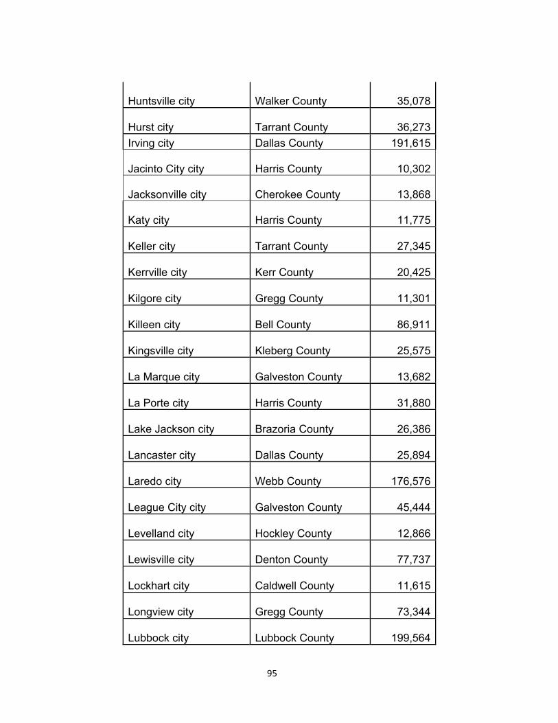
95

Huntsville city Walker County

35,078

Hurst city Tarrant County

36,273 Irving city Dallas County 191,615

Jacinto City city Harris County

10,302

Jacksonville city Cherokee County

13,868

Katy city Harris County

11,775

Keller city Tarrant County

27,345

Kerrville city Kerr County

20,425

Kilgore city Gregg County

11,301

Killeen city Bell County

86,911

Kingsville city Kleberg County

25,575

La Marque city Galveston County

13,682

La Porte city Harris County

31,880

Lake Jackson city Brazoria County

26,386

Lancaster city Dallas County

25,894

Laredo city Webb County

176,576

League City city Galveston County

45,444

Levelland city Hockley County

12,866

Lewisville city Denton County

77,737

Lockhart city Caldwell County

11,615

Longview city Gregg County

73,344

Lubbock city Lubbock County

199,564

96

Lufkin city Angelina County

32,709

Mansfield city Tarrant County

28,031

Marshall city Harrison County

23,935 McAllen city Hidalgo County 106,414

McKinney city Collin County

54,369

Mercedes city Hidalgo County

13,649

Mesquite city Dallas County

124,523

Midland city Midland County

94,996

Mineral Wells city Palo Pinto County

16,946

Mission city Hidalgo County

45,408

Missouri City city Fort Bend County

52,913

Mount Pleasant city Titus County

13,935

Nacogdoches city Nacogdoches County

29,914

Nederland city Jefferson County

17,422

New Braunfels city Comal County

36,494

North Richland Hills city Tarrant County

55,635

Odessa city Ector County

90,943

Orange city Orange County

18,643

Palestine city Anderson County

17,598

Pampa city Gray County

17,887

Paris city Lamar County

25,898

Pasadena city Harris County

141,674

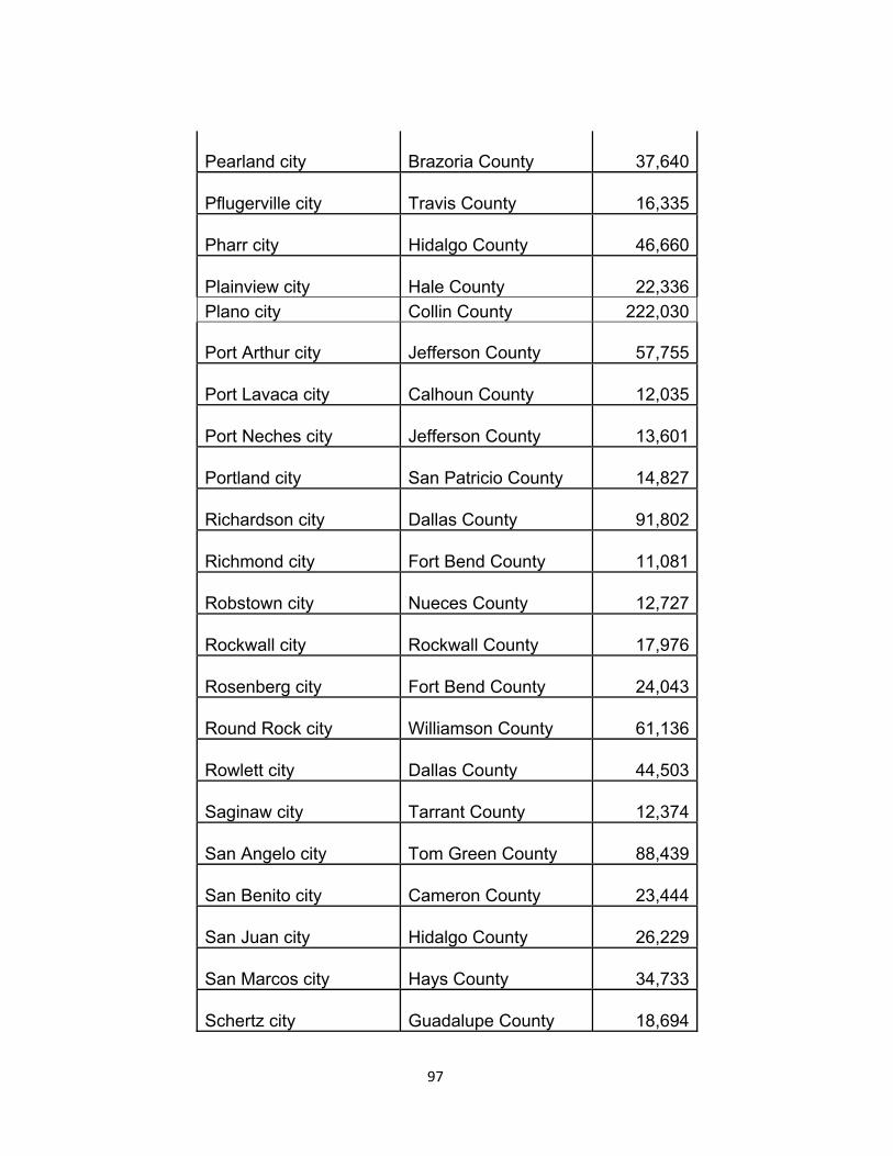
97

Pearland city Brazoria County

37,640

Pflugerville city Travis County

16,335

Pharr city Hidalgo County

46,660

Plainview city Hale County

22,336 Plano city Collin County 222,030

Port Arthur city Jefferson County

57,755

Port Lavaca city Calhoun County

12,035

Port Neches city Jefferson County

13,601

Portland city San Patricio County

14,827

Richardson city Dallas County

91,802

Richmond city Fort Bend County

11,081

Robstown city Nueces County

12,727

Rockwall city Rockwall County

17,976

Rosenberg city Fort Bend County

24,043

Round Rock city Williamson County

61,136

Rowlett city Dallas County

44,503

Saginaw city Tarrant County

12,374

San Angelo city Tom Green County

88,439

San Benito city Cameron County

23,444

San Juan city Hidalgo County

26,229

San Marcos city Hays County

34,733

Schertz city Guadalupe County

18,694

98

Seagoville city Dallas County

10,823

Seguin city Guadalupe County

22,011

Sherman city Grayson County

35,082

Snyder city Scurry County

10,783

Socorro city El Paso County

27,152 South Houston city Harris County 15,833

Southlake city Tarrant County

21,519

Stafford city Fort Bend County

15,681

Stephenville city Erath County

14,921

Sugar Land city Fort Bend County

63,328

Sulphur Springs city Hopkins County

14,551

Sweetwater city Nolan County

11,415

Taylor city Williamson County

13,575

Temple city Bell County

54,514

Terrell city Kaufman County

13,606

Texarkana city Bowie County

34,782

Texas City city Galveston County

41,521

The Colony city Denton County

26,531

Tyler city Smith County

83,650

Universal City city Bexar County

14,849

University Park city Dallas County

23,324

Uvalde city Uvalde County

14,929

99

Vernon city Wilbarger County

11,660

Victoria city Victoria County

60,603

Vidor city Orange County

11,440

Waco city McLennan County

113,726

Watauga city Tarrant County

21,908

Waxahachie city Ellis County

21,426 Weatherford city Parker County 19,000

Weslaco city Hidalgo County

26,935 West University Place city Harris County

14,211

White Settlement city Tarrant County

14,831

Wichita Falls city Wichita County

104,197

Wylie city Collin County

15,132

100

APPENDIX 3

ECONOMIC REGIONS OF THE STATE OF TEXAS

101

ECONOMIC REGIONS OF THE STATE OF TEXAS

Map of Economic Regions

102

BIBLIOGRAPHY

Agostini, Claudio A., “The Impact of State Corporate Taxes on FDI Location”, Public Finance Review, 35, p335, 2007

Alm, James & Rogers, Janet., “Do State Fiscal Policies Affect State Economic Growth?”, Public Finance Review, 39, p483, 2010

American Way, American Airlines Publishing, January 2012

Anderson, John E. & Wassmer, Robert W., Bidding for Business. Kalamazoo: W.E. Upjohn Institute for Employment Research, 2000.

Bartik, Timothy J., Who Benefits from State and Local Economic Development Policies? Kalamazoo: W.E. Upjohn Institute for Employment Research, 1991

Bartik, Timothy J.,Business Location Decisions in the United States: Estimates of Unionization, Taxes, and other characteristics of States”. Journal of Business and Economic Statistics, vol.3, no. 1 (1985), p14-22

Bartik, Timothy J., “ Who Benefits from local job growth: Migrants or the original residents?”. Regional Studies 27, no.4 (1993): 297-311

Bartik, Timothy J., “ Jobs, Productivity, and Local Economic Development: What Implications Does Economic Research Have for the Role of Government? National Tax Journal, vol 47 , December 1994, p.847-61

Bartik, Timothy J.,Jobs for the poor: Can labor demand policies help? New York: Russell Sage, 2001.

Billings, Stephens., “ Do Enterprise Zones Work?: An Analysis at the Borders., Public Finance Review, 2009, 37, 68

Blakely, E. and Bradshaw, T., Planning Local Economic Development, Thousand Oaks, CA: Sage, 2002

103

Blakely, E. and Green Leigh, N., Planning Local Economic Development: Theory and Practice (4th ed.), Thousand Oaks, CA: Sage, 2009

Boarnet, Marlon G., “ Enterprise Zones and Job Creation: Linking Evaluation and Practice”., Economic Development Quarterly, 15, 242 (2001)

Bowman, A. ,”Competition for Economic Development among Southeastern States’, Urban Affairs Quarterly, 23, 511-527 (1988)

Burnier, D. , “Becoming Competitive: How Policymakers view Incentive Based Development Policy”, Economic Development Quarterly, 6, 14-24 (1992)

Buss, Terry F., The Effect of State Incentives on Economic Growth and Firm Location Decisions: An Overview of the Literature. Economic Development Quarterly, 15 (2001). 90.

Carroll, Robert and Wasylenko, Michael, “ Do State Business Climates Still matter? Evidence of a Structural Change.” National Tax Journal 47 No. 1, March 1994, p. 19, -37

Chi, K. S. and Leatherby, D., “State Business Incentives”. Council of State Governments, 1997,Lexington, Kentucky.

Couch, Jim F and Barrett, J. Douglas. , “ Alabama’s Enterprise Zones: Designed to Aid the Needy?”, Public Finance Review, 32, 65 (2004)

Courant, Paul N., “ How would you know a Good Economic Policy If You Tipped Over One”?, National Tax Journal 47, no. 4, (1994), p 863

Currid-Hacket, Elizabeth and Stolarick, Kevin., “The Great Divide: Economic Development Theory Versus Practice-A-Survey of the Current Landscape”, Economic Development Quarterly, 25, 143 (2011)

Dallas Business Journal, October 2002)

Eberts, R. W. & Stone, J., Wage and employment adjustment in local labor markets. Kalamazoo, MI: W. E. Upjohn Institute for Labor Research, 1992

Eisinger, P. ,The Rise of the Entrepreneurial State. Milwaukee: University of Wisconsin Press.

Elvery, Joel A., “ The Impact of Enterprise Zones on Resident Employment: An Evaluation of the Enterprise Zone Programs of California and Florida”, Economic Development Quarterly., 2009, 23, 44

104

Faulk, Dagney, “ Do State Economic development Incentives Create Jobs? An Analysis of State Employment Tax Credits”. National Tax Journal, Vol. LV, No. 2, June 2002, p. 263

Fisher, Peter S. & Peters, Alan H. Industrial Incentives, Competition Among American States and Cities. Kalamazoo, MI: W.E. Upjohn Institute for Labor Research, 1998

Fisher, Ronald C., “ The Effects of State and Local Public Services on Economic Development”, New England Economic Review, Federal Reserve Bank of Boston, Proceedings of a Symposium, March-April 1997, p53

Fujita, Masahisa & Thisse, Jaques-Francois, Economics of Agglomerationn: Cities Industrial Location, and Regional Growth.Cambridge: Cambridge University Press, 2002

Glaeser, E, Scheinkman, J. and Shleifer, Andrei , “Economic Growth in a Cross-Section of Cities” , Journal of Monetary Economics, Vol. 36 (1995), 117-143 Glickman, Norman, and Woodward, Douglas., The New Competitors: How Foreign Investors are Changing the U.S. Economy. New York: Basic Books, 1989

Greenwood, Daphne T. and Holt, Richard P.F., Local Economic Development in the 21st Century. Armonk, New York : M. E. Sharpe, 2007

Grubert, Harry & Mutti, John, “ Do Taxes Influence Where U.S. corporations Invest”? National Tax Journal, Vol. 53 No. 4 Part 1 , December 2000, p.825

Guskind, Robert., “Games Cities Play”, National Journal, 21, 634-640, 1989

Guskind, Robert., “The Giveaway Game Continues”. Planning 56(2), 1990.

Haider, D., “Place wars: New Realities of the 1990s”, Economic Development Quareterly, 6, 127-134, 1992

Handbook of Economic Development Laws for Texas Cities, 2008, Office of the Attorney General, Texas. Austin, Texas..

Hanson, Andrew and Shawn Rohlin. 2011. The Effect of Location-Based Tax Incentives on Establishment Location and Employment across Industry Sectors. Public Finance Review 39 (March) : 195-225.

105

Hanson, R. L., “Bidding for Business: A second war between the states?”, Economic Development Quarterly, 7, 183-198, 1993

Hawkins, Clark A. and Weber, Jean E. Statistical Analysis Applications to Business and Economics. New York: Harper and Row Publishers, 1980.

Hines, James R., Jr.,” Altered States: Taxes and the Location of Foreign Direct Investment in America.” American Economic Review 86 No.5 (December 1996):1076-94.

Hissong, Rod, “ The Efficacy of Local Economic Development Incentives”. Financing Economic Development in the 21st Century. New York: M.E. Sharpe, 2001

Holtz- Eakin, Douglas, “ Fundamental Tax Reform and State and Local Governments”, National Tax Journal, 49, September 1996, p 475-86

Hovey, Harold A., “ Interstate Tax Competition and Economic Development’. In Reforming State Tax Systems, Steven Gold, ed. Washington, D.C.: National Conference of State Legislature, 1986

Hunter, Kenneth G., “An Analysis of the Effect of Lobbying Efforts and Demand-Side Economic Development Policies on State Economic Health”, Public Administration Quarterly, vol.25, no. 1, Spring 2001.

Ihlanfeldt, Keith R. and Sjoquist, David L., “ Conducting an Analysis of Georgia’s Economic Development Tax Incentive Program., Economic Development Quarterly, 15, 217 (2001)

Joslove, Scott, “ Handbook on Economic development Laws for Texas Volume 1. Office of the Attorney General, Texas. Austin, Texas.

Kenyon, D. A. Competition among states and local governments . Washington, DC: Urban Institute, 1991

Kim, DaeJin, Bae, Sang Seok, and Eger III, Robert J., “Is Local Discretionary Sales Tax Adopted to Counteract Fiscal Stress? : The Case of Florida Counties”, Economic Development Quarterly, 2009, 23, 150

Lambert, Thomas E. and Coomes, Paul A., “An Evaluation of the Effectiveness of Louisville’s Enterprise Zone”, Economic Development Quarterly, 2001, 15, 168

Leichenko, Robin M., “Growth and Change in U.S. Cities and Suburbs”, Growth and Change, 2001, 32, p326

106

Limi, Atsushi, “Decentralization and Economic Growth Revisited: An Empirical Note”, Journal of Urban Economics, 2005, vol 57, 449-461

Luce, T.F, “ Local Taxes, Public Services and the Intrametropolitan Location of Firms and Households”. Public Finance Quarterly, 1994, vol 22 no.2 p139

Mark, Stephen T, McGuire, Therese J. & Papke, Leslie E., “ The Influence of Taxes on Employment and Population Growth: Evidence from the Washington, DC Metropolitan Area”, National Tax Journal, 53, March 2000, p105

Mikesell, John L., “ Sales Tax Incentives for Economic Development: Why shouldn’t Production Exemptions be General?’, National Tax Journal, vol. LIV, no.3, September 2001, p557

Nolan, C., Morrison, E., Kumar, I., Galloway, H., and Cordes, S., “Linking Industry and Occupation Clusters in Regional Economic Development”, Economic Development Quarterly, 25, 2011, p26

O’Keefe, Suzanne, “ Job Creation in California’s Enterprise Zones: a Comparison using a Propensity Score Matching Model”, Journal of Urban Economics, 2004, 131

O’Sullivan, Arthur, Urban Economics (6th ed. : McGraw-Hill Irwin, Boston, MA, 2007

Olberding, Julie C.,”Does Regionalism Beget regionalism? The Relationship between Norms and Regional Partnerships for Economic development”, Public Adminstration Review, vol.62, No. 4, July-August 2002.

Owyang, M.T, Piger, J. M., Wall, H. J. & Wheeler, C. H., “The economic performance of cities: A Markov-switching approach”, Journal of Urban Economics, 64, p538, 2008

Partridge, Mark D., Rickman, Dan S. and Li Hui., Who Wins From Local Economic Development?: A Supply Decomposition of U.S. County Employment Growth., Economic Development Quarterly, 23, 13 (2009)

Peterson, P.E. , City Limits. Chicago: University of Chicago Press, 1981.

Shaffer, Sherrill & Collender, Robert N.,”Federal Credit Programs and Local Economic Performance”, Economic Development Quarterly, 23, p28, 2009

Snow, D. R., “Do Legistalive Procedures Affect Tax Expenditures”, Journal of Public Budgeting, Accounting and Financial Management, 11, 400-426 (1999)

107

Stansel, Dean. ,”Interjurisdictional Competition and Local Government Spending in U.S. Metropolitian Areas”, Public Finance Review, 34, #2, March 2006.

Taylor, M. ,”A Proposal To Prohibit Industrial Relocation Subsidies”, Texas Law Review, 72, p 669-713, 1994

Tannenwald, Robert, Bradbury, Katharine L. and Kodrzycki, Yolanda K, “The Effects of State and Local Policies on Economic Development: An Overview”, New England Economic Review, Federal Reserve Bank of Boston, March-April 1997.

Taylor, M, “A Proposal to Prohibit Industrial Relocation Subsidies”, Texas Law Review, 72, p 669

Texas Comptroller of Public Accounts website (http://www.window.state.tx.us/)

Texas State Data Center (TSDC) and Office of the State Demographer, University of Texas at San Antonio, Texas

The Examiner, Washington DC: November 10, 2011

Tiebout, Charles M. , “ A Pure Theory of Local Expenditures”, Journal of Political Economy, 64 (5), p.416-24, 1956.

UMRA, P.L. 104-4, 1995, “The National Association of State Development Agencies (NASDA), 1995

USA Today, June 24, 2011

Wall Street Journal, July 22, 2011

Wasylenko, Michael, “Texation and Economic Development: The State of the Economic Literature”, New England Economic Review, March-April 1997, p37. In Henry Herzog and Alan Schlottmann, eds Industry Location and Public Policy. Knoxville, TN: University of Tennessee Press

Wasylanko, Michael and McGuire, Therese, “ Jobs and Taxes: The Effect of business Climate on States’ Employment Growth Rates”. National Tax Journal, vol.38, no. 4 (December 1985), p 497

Watson, D. J., & Morris, J. C. Building the Local Economy: Cases in Economic Development. Athens: Carl Vinson Institute of Government, Georgia, 2008

108

Weissbourd, Robert, Ventures, R.W. and Berry Christopher The Changing

Dynamics of Urban America: R.W.Ventures (March 2004)

Wooldridge, Jeffrey M., Introductory Econometrics, A Modern Approach. United

States of America: Thomson South-Western, 2006

Zhao, Zhirong., Motivations, Obstacles, and Resources: The Adoption of the

General –Purpose Local Option Sales Tax in Georgia Counties. Public Finance

Review, 33, 721 (2005)

109

BIOGRAPHICAL INFORMATION

The author has more than 35 years of experience in the defense industry and

has worked for Bell Helicopter Textron and The Boeing Company. He has

graduate degrees in engineering, business, personnel and human resource

management. He taught as a part time instructor at Texas Christian University,

Ft. Worth, Texas; University of Texas at Arlington; Virginia Tech, Blacksburg, VA;

and full time at Ohio University, Athens, Ohio and West Virginia University,

Morgantown, WV.

a comparison of economic development between texas

Documents

Transcript of a comparison of economic development between texas