A Comparative Study of Protocols for EfficientData Propagation in Smart Dust Networks�

I. Chatzigiannakis1,2, T. Dimitriou3, M. Mavronicolas4, S. Nikoletseas1,2, andP. Spirakis1,2

1 Computer Technology Institute, P.O. Box 1122, 26110 Patras, Greece{ichatz,nikole,spirakis}@cti.gr

2 Department of Computer Engineering and Informatics,University of Patras, 26500 Patras, Greece3 Athens Information Technology (AIT)

tdimitriou@ait.gr4 Department of Computer Science,

University of Cyprus, CY-1678 Nicosia, Greecemavronic@cs.ucy.ac.cy

Abstract. Smart Dust is comprised of a vast number of ultra-small fullyautonomous computing and communication devices, with very restrictedenergy and computing capabilities, that co-operate to accomplish a largesensing task. Smart Dust can be very useful in practice i.e. in the localdetection of a remote crucial event and the propagation of data reportingits realization to a control center.In this work, we have implemented and experimentally evaluated fourprotocols (PFR, LTP and two variations of LTP which we here intro-duce) for local detection and propagation in smart dust networks, undernew, more general and realistic modelling assumptions. We compara-tively study, by using extensive experiments, their behavior highlightingtheir relative advantages and disadvantages. All protocols are very suc-cessful. In the setting we considered here, PFR seems to be faster whilethe LTP based protocols are more energy efficient.

1 Introduction, Our Results, and Related Work

Recent dramatic developments in micro-electro-mechanical (MEMS) systems,wireless communications and digital electronics have already led to the develop-ment of small in size, low-power, low-cost sensor devices. Such extremely smalldevices integrate sensing, data processing and communication capabilities. Ex-amining each such device individually might appear to have small utility, howeverthe effective distributed co-ordination of large numbers of such devices may leadto the efficient accomplishment of large sensing tasks.� This work has been partially supported by the IST Programme of the European

Union under contract numbers IST-1999-14186 (ALCOM-FT) and IST-2001-33116(FLAGS).

H. Kosch, L. Boszormenyi, H. Hellwagner (Eds.): Euro-Par 2003, LNCS 2790, pp. 1003–1016, 2003.c© Springer-Verlag Berlin Heidelberg 2003

1004 I. Chatzigiannakis et al.

Large numbers of sensor nodes can be deployed in areas of interest (such asinaccessible terrains or disaster places) and use self-organization and collabora-tive methods to form a sensor network. Their wide range of applications is basedon the possible use of various sensor types (i.e. thermal, visual, seismic, acoustic,radar, magnetic, etc.) in order to monitor a wide variety of conditions (e.g. tem-perature, object presence and movement, humidity, pressure, noise levels etc.).Thus, sensor networks can be used for continuous sensing, event detection, lo-cation sensing as well as micro-sensing. Hence, sensor networks have importantapplications, including (a) military (like forces and equipment monitoring, bat-tlefield surveillance, targeting, nuclear, biological and chemical attack detection),(b) environmental applications (such as fire detection, flood detection, precisionagriculture), (c) health applications (like telemonitoring of human physiologicaldata) and (d) home applications (e.g. smart environments and home automa-tion). For an excellent survey of wireless sensor networks see [1] and also [6,12].

Note however that the efficient and robust realization of such large, highly-dynamic, complex, non-conventional networking environments is a challengingalgorithmic and technological task. Features including the huge number of sen-sor devices involved, the severe power, computational and memory limitations,their dense deployment and frequent failures, pose new design and implementa-tion aspects which are essentially different not only with respect to distributedcomputing and systems approaches but also to ad-hoc networking techniques.

Contribution: We focus on an important problem under a particular model ofsensor networks that we present. More specifically, continuing the research of ourteam (see [2], [4]), we study the problem of local detection and propagation, i.e.the local sensing of a crucial event and the energy and time efficient propagationof data reporting its realization to a (fixed or mobile) control center. This centermay be some human authorities responsible of taking action upon the realizationof the crucial event. We use the term “sink” for this control center. We note thatthe protocols we present here can also be used for the more general problem ofdata propagation in sensor networks (see [10]).

As opposed to [5] (where a 2-dimensional lattice deployment of particles isused) we extend the network model to the general case of particle deploymentaccording to a random, uniform distribution. We study here the more realisticcase when the control center is not a line in the plane (i.e. as in [2]) but a singlepoint.

Under these more general and realistic (in terms of motivation by appli-cations) modelling assumptions, we implemented and experimentally evaluatedfour information propagation protocols: (a) The Probabilistic Forwarding Pro-tocol (PFR) that avoids flooding by favoring in a probabilistic way certain “closeto optimal” transmissions, (b) the Local Target Protocol (LTP), where data ispropagated by each time selecting the best (with respect to progress towardsthe sink) particle for passing information and (c) we propose two variations ofLTP according to different next particle selection criteria. We note that we hadto carefully design the protocols to work under the new network models.

A Comparative Study of Protocols for Efficient Data Propagation 1005

The extensive simulations we have performed show that all protocols are verysuccessful. In the setting we considered here, PFR seems to achieve high successrates in terms of time and hops efficiency, while the LTP based protocols manageto reduce the energy spent in the process by activating less particles.

Discussion of Selected Related Work:A family of negotiation-based information dissemination protocols suitable

for wireless sensor networks is presented in [9]. In contrast to classic flooding,in SPIN sensors negotiate with each other about the data they possess usingmeta-data names. These negotiations ensure that nodes only transmit data whennecessary, reducing the energy consumption for useless transmissions.

A data dissemination paradigm called directed diffusion for sensor networksis presented in [10]. An observer requests data by sending interests for nameddata; data matching the interest is then “drawn” down towards that node byselecting a single path or through multiple paths by using a low-latency tree.[11] presents an alternative approach that constructs a greedy incremental treethat is more energy-efficient and improves path sharing.

In [8] a clustering-based protocol is given that utilizes randomized rotation oflocal cluster heads to evenly distribute the energy load among the sensors in thenetwork. In [15] a new energy efficient routing protocol is introduced that doesnot provide periodic data monitoring (as in [8]), but instead nodes transmit dataonly when sudden and drastic changes are sensed by the nodes. As such, thisprotocol is well suited for time critical applications and compared to [8] achievesless energy consumption and response time.

We note that, as opposed to the work presented in this paper, the aboveresearch focuses on energy consumption without examining the time efficiencyof their protocols. Furthermore, note that our protocols are quite general in thesense that (a) they do not assume global network topology information, (b) donot assume geolocation information (such as GPS information) and (c) use verylimited control message exchanges, thus having low communication overhead.

2 The Model

Sensor networks are comprised of a vast number of ultra-small homogenous sen-sors, which we call “grain” particles. Each grain particle is a fully-autonomouscomputing and communication device, characterized mainly by its availablepower supply (battery) and the energy cost of computation and transmissionof data. Such particles (in our model here) cannot move.

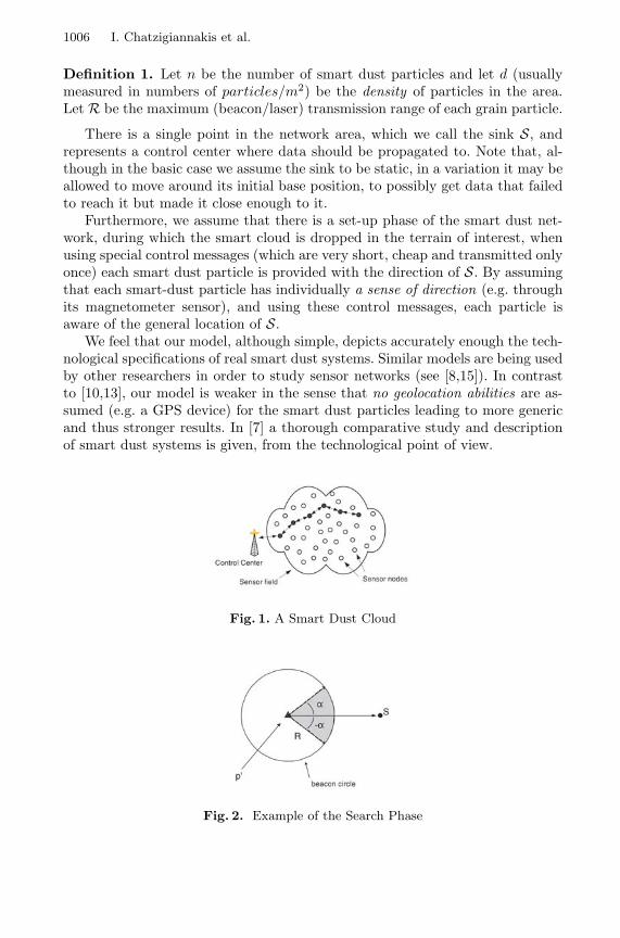
Each particle is equipped with a set of monitors (sensors) for light, pressure,humidity, temperature etc. Each particle has a broadcast (digital radio) beaconmode which can be also a directed transmission of angle α around a certain line(possibly using some special kind of antenna, see Fig. 2).

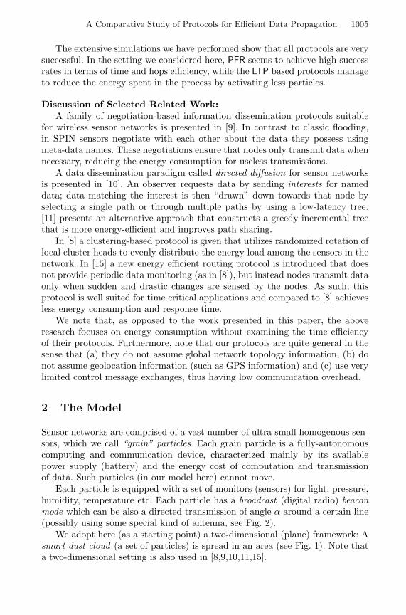
We adopt here (as a starting point) a two-dimensional (plane) framework: Asmart dust cloud (a set of particles) is spread in an area (see Fig. 1). Note thata two-dimensional setting is also used in [8,9,10,11,15].

1006 I. Chatzigiannakis et al.

Definition 1. Let n be the number of smart dust particles and let d (usuallymeasured in numbers of particles/m2) be the density of particles in the area.Let R be the maximum (beacon/laser) transmission range of each grain particle.

There is a single point in the network area, which we call the sink S, andrepresents a control center where data should be propagated to. Note that, al-though in the basic case we assume the sink to be static, in a variation it may beallowed to move around its initial base position, to possibly get data that failedto reach it but made it close enough to it.

Furthermore, we assume that there is a set-up phase of the smart dust net-work, during which the smart cloud is dropped in the terrain of interest, whenusing special control messages (which are very short, cheap and transmitted onlyonce) each smart dust particle is provided with the direction of S. By assumingthat each smart-dust particle has individually a sense of direction (e.g. throughits magnetometer sensor), and using these control messages, each particle isaware of the general location of S.

We feel that our model, although simple, depicts accurately enough the tech-nological specifications of real smart dust systems. Similar models are being usedby other researchers in order to study sensor networks (see [8,15]). In contrastto [10,13], our model is weaker in the sense that no geolocation abilities are as-sumed (e.g. a GPS device) for the smart dust particles leading to more genericand thus stronger results. In [7] a thorough comparative study and descriptionof smart dust systems is given, from the technological point of view.

Fig. 1. A Smart Dust Cloud

Fig. 2. Example of the Search Phase

A Comparative Study of Protocols for Efficient Data Propagation 1007

3 The Problem

Assume that a single particle, p, senses the realization of a local crucial event E .Then the propagation problem P is the following:

“How can particle p, via cooperation with the rest of the grain particles,efficiently propagate information info(E) reporting realization of eventE to the sink S?”

Because of the dense deployment of particles close to each other, multi-hopcommunication consumes less power than a traditional single hop propagation.Also, multi-hop communication can effectively overcome some of the signal prop-agation effects in long-distance wireless transmissions. Furthermore, short-rangehop-by-hop transmissions may help to smoothly adjust propagation around ob-stacles. Finally, the low energy transmission in hop-by-hop may enhance security,protecting from undesired discovery of the data propagation operation.

Because of the above reasons, data propagation should be done in a multi-hop way. To minimize the energy consumption in the sensor network we wishto minimize the number of hops (directed transmissions) performed in the datapropagation process. Note that the number of hops also characterizes propaga-tion time, assuming an appropriate MAC protocol [18].

Furthermore, an interesting aspect is how close to the sink data is propagated(in the case where data does not exactly reach the sink). Note that proximityto the sink might be useful in the case where the sink is mobile or it performs a“limited flooding” to get the information from the final position it arrived.

4 The Probabilistic Forwarding Protocol (PFR)

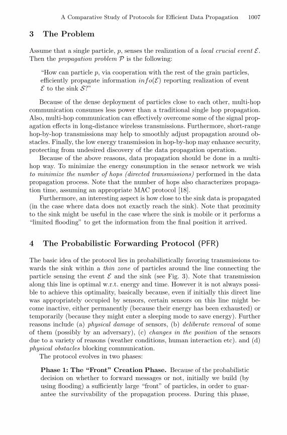
The basic idea of the protocol lies in probabilistically favoring transmissions to-wards the sink within a thin zone of particles around the line connecting theparticle sensing the event E and the sink (see Fig. 3). Note that transmissionalong this line is optimal w.r.t. energy and time. However it is not always possi-ble to achieve this optimality, basically because, even if initially this direct linewas appropriately occupied by sensors, certain sensors on this line might be-come inactive, either permanently (because their energy has been exhausted) ortemporarily (because they might enter a sleeping mode to save energy). Furtherreasons include (a) physical damage of sensors, (b) deliberate removal of someof them (possibly by an adversary), (c) changes in the position of the sensorsdue to a variety of reasons (weather conditions, human interaction etc). and (d)physical obstacles blocking communication.

The protocol evolves in two phases:

Phase 1: The “Front” Creation Phase. Because of the probabilisticdecision on whether to forward messages or not, initially we build (byusing flooding) a sufficiently large “front” of particles, in order to guar-antee the survivability of the propagation process. During this phase,

1008 I. Chatzigiannakis et al.

Fig. 3. Thin zone of particles around the line connecting the particle sensing the eventE and the sink S.

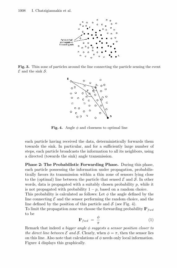
Fig. 4. Angle φ and closeness to optimal line

each particle having received the data, deterministically forwards themtowards the sink. In particular, and for a sufficiently large number ofsteps, each particle broadcasts the information to all its neighbors, usinga directed (towards the sink) angle transmission.

Phase 2: The Probabilistic Forwarding Phase. During this phase,each particle possessing the information under propagation, probabilis-tically favors its transmission within a thin zone of sensors lying closeto the (optimal) line between the particle that sensed E and S. In otherwords, data is propagated with a suitably chosen probability p, while itis not propagated with probability 1 − p, based on a random choice.This probability is calculated as follows: Let φ the angle defined by theline connecting E and the sensor performing the random choice, and theline defined by the position of this particle and S (see Fig. 4).To limit the propagation zone we choose the forwarding probability IPfwd

to beIPfwd =

φ

π(1)

Remark that indeed a bigger angle φ suggests a sensor position closer tothe direct line between E and S. Clearly, when φ = π, then the sensor lieson this line. Also note that calculations of φ needs only local information.Figure 4 displays this graphically.

A Comparative Study of Protocols for Efficient Data Propagation 1009

Thus, we get that φ1 > φ2 implies that for the corresponding particlesp1, p2, p1 is closer to the E-S line than p2, thus

IPfwd(p1) =φ1

π>

φ2

π= IPfwd(p2) (2)

Remark: Certainly, there might exist other probability choices for favor-ing certain transmissions. We are currently working on such alternativechoices.

5 The Local Target Protocol (LTP) and Its Variations

We now present a protocol for smart dust networks which we call the “LocalTarget” protocol and two variations that use different next particle selectioncriteria. In this protocol, each particle p′ that has received info(E) from p (via,possibly, other particles) does the following:

Phase 1: The Search Phase. It uses a periodic low energy broadcastof a beacon in order to discover a particle nearer to S than itself. Amongthe particles returned, p′ selects a unique particle p′′ that is “best” withrespect to progress towards the sink. We here consider two criteria formeasuring the quality of this progress and also a randomized version toget a good average mix:(a) Euclidean Distance. In this case, the particle p′′

E that among all par-ticles found achieves the bigger progress on the p′S line, should beselected. We call this variation of the our protocol LTPE. This isconsidered as the “basis” LTP.

(b) Angle Optimality. In this case, the particle p′′A such that the angle

p′′Ap′S is minimum, should be selected. We call this variation of the

our protocol LTPA.(c) Randomization. Towards a good average case performance of the pro-

tocol, we use randomization to avoid bad behavior due to the worstcase input distributions for each selection (i.e. particles forming bigangles with the optimal line in LTPE and particles resulting to smallEuclidean progress in LTPA). Thus, we find p′′

E , p′′A and randomly

select one of them, with probability 12 . We call this protocol LTPR.

Phase 2: The Direct Transmission Phase. Then, p′ sends info(E) top′′ and sends a success message to p (i.e. to the particle that it originallyreceived the information from).

Phase 3: The Backtrack Phase. If the search phase fails to discovera particle nearer to S, then p′ sends a fail message to p.

In the above procedure, propagation of info(E) is done in two steps; (i)particle p′ locates the next particle (p′′) and transmits the information and (ii)particle p′ waits until the next particle (p′′) succeeds in propagating the messagefurther towards S. This is done to speed up the backtrack phase in case p′′ doesnot succeed in discovering a particle nearer to S.

1010 I. Chatzigiannakis et al.

6 Efficiency Measures

Definition 2. Let hA (for “active”) be the number of “active” sensor particlesparticipating in the data propagation and let ETR be the total number of datatransmissions during propagation. Let T be the total time for the propagationprocess to reach its final position and H the total number of “hops” required.

Clearly, by minimizing hA we succeed in avoiding flooding and thus we mini-mize energy consumption. Remark that in LTP we count as active those particlesthat transmit info(E) at least once.

Note that hA, ETR, T and H are random variables. Furthermore, we definethe success probability of our algorithm where we call success the eventual datapropagation to the sink.

Definition 3. Let IPs be the success probability of our protocol.

We also focus on the study of the following parameter. Suppose that thedata propagation fails to reach the sink. In this case, it is very important toknow “how close” to the sink it managed to get. Propagation reaching closeto the sink might be very useful, since the sink (which can be assumed to bemobile) could itself move (possibly by performing a random walk) to the finalpoint of propagation and get the desired data from there. Even assuming a fixedsink, closeness to it is important, since the sink might in this case begin some“limited” flooding to get to where data propagation stopped. Clearly, the closerto the sink we get, the cheaper this flooding becomes.

Definition 4. Let F be the final position of the data propagation process. LetD be F ’s (Euclidean) distance from the sink S.

Clearly in the case of total success F coincides with the sink and D = 0.

7 Experimental Evaluation

We evaluate the performance of the four protocols by a comparative experimentalstudy. The protocols have been implemented as C++ classes using the datatypes for two-dimensional geometry of LEDA [16] based on the environmentdeveloped in [2], [4]. Each class is installed in an environment that generatessensor fields given some parameters (such as the area of the field, the distributionfunction used to drop the particles), and performs a network simulation for agiven number of repetitions, a fixed number of particles and certain protocolparameters. After the execution, the environment stores the results in files sothat the measurements can be represented in a graphical way.

In the full paper ([3]), we provide for all protocols a more detailed descrip-tion of the implementation, including message structures, data structures at aparticle, initialization issues and pseudo-code for the protocol.

In our experiments, we generate a variety of sensor fields in a 100m by 100msquare. In these fields, we drop n ∈ [100, 3000] particles randomly uniformly

A Comparative Study of Protocols for Efficient Data Propagation 1011

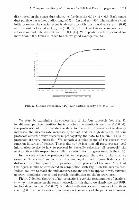
distributed on the smart-dust plane, i.e. for densities 0.01 ≤ d ≤ 0.3. Each smartdust particle has a fixed radio range of R = 5m and α = 90o. The particle p thatinitially senses the crucial event is always explicitly positioned at (x, y) = (0, 0)and the sink is located at (x, y) = (100, 100). Note that this experimental setupis based on and extends that used in [8,11,15]. We repeated each experiment formore than 5,000 times in order to achieve good average results.

0

0.1

0.2

0.3

0.4

0.5

0.6

0.7

0.8

0.9

1

0.01 0.03 0.05 0.07 0.09 0.11 0.13 0.15 0.17 0.19 0.21 0.23 0.25 0.27 0.29

Particle Density (d)

Su

cces

s R

ate

(Psu

cces

s)

PFR LTPe LTPa LTPr

Fig. 5. Success Probability (IPs) over particle density d = [0.01, 0.3].

We start by examining the success rate of the four protocols (see Fig. 5),for different particle densities. Initially, when the density is low (i.e. d ≤ 0.06),the protocols fail to propagate the data to the sink. However as the densityincreases, the success rate increases quite fast and for high densities, all fourprotocols almost always succeed in propagating the data to the sink. Thus, allprotocols are very successful. We remark a similar shape of the success ratefunction in terms of density. This is due to the fact that all protocols use localinformation to decide how to proceed by basically selecting (all protocols) thenext particle with respect to a similar criterion (best progress towards the sink).

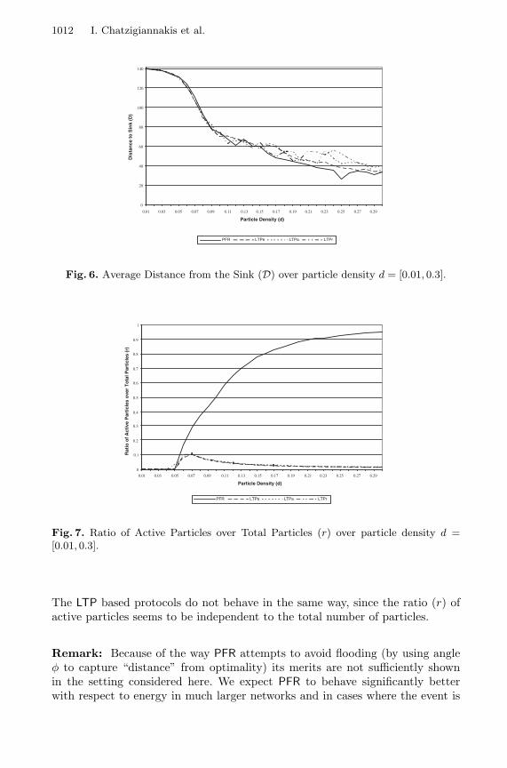
In the case when the protocols fail to propagate the data to the sink, weexamine “how close” to the sink they managed to get. Figure 6 depicts thedistance of the final point of propagation to the position of the sink. Note thatthis figure should be considered in conjunction with Fig. 5 on the success rate.Indeed, failures to reach the sink are very rare and seem to appear in very extremenetwork topologies due to bad particle distribution on the network area.

Figure 7 depicts the ratio of active particles over the total number of particles(r = hA

n ) that make up the sensor network. In this figure we clearly see that PFR,for low densities (i.e. d ≤ 0.07), it indeed activates a small number of particles(i.e. r ≤ 0.3) while the ratio (r) increases as the density of the particles increases.

1012 I. Chatzigiannakis et al.

0

20

40

60

80

100

120

140

0.01 0.03 0.05 0.07 0.09 0.11 0.13 0.15 0.17 0.19 0.21 0.23 0.25 0.27 0.29

Particle Density (d)

Dis

tan

ce t

o S

ink

(D)

PFR LTPe LTPa LTPr

Fig. 6. Average Distance from the Sink (D) over particle density d = [0.01, 0.3].

0

0.1

0.2

0.3

0.4

0.5

0.6

0.7

0.8

0.9

1

0.01 0.03 0.05 0.07 0.09 0.11 0.13 0.15 0.17 0.19 0.21 0.23 0.25 0.27 0.29

Particle Density (d)

Rat

io o

f A

ctiv

e P

arti

cles

ove

r T

ota

l Par

ticl

es (

r)

PFR LTPe LTPa LTPr

Fig. 7. Ratio of Active Particles over Total Particles (r) over particle density d =[0.01, 0.3].

The LTP based protocols do not behave in the same way, since the ratio (r) ofactive particles seems to be independent to the total number of particles.

Remark: Because of the way PFR attempts to avoid flooding (by using angleφ to capture “distance” from optimality) its merits are not sufficiently shownin the setting considered here. We expect PFR to behave significantly betterwith respect to energy in much larger networks and in cases where the event is

A Comparative Study of Protocols for Efficient Data Propagation 1013

sensed in an average place of the network. Also, stronger probabilistic choices(i.e. IPfwd =

(φπ

)α

, where a > 1 a constant) may further limit propagation time.

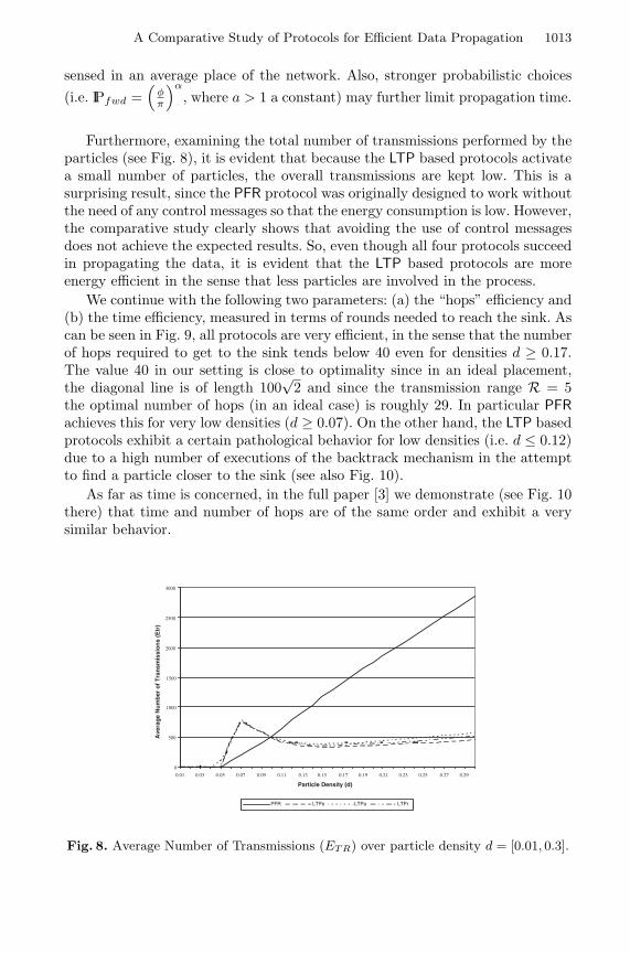
Furthermore, examining the total number of transmissions performed by theparticles (see Fig. 8), it is evident that because the LTP based protocols activatea small number of particles, the overall transmissions are kept low. This is asurprising result, since the PFR protocol was originally designed to work withoutthe need of any control messages so that the energy consumption is low. However,the comparative study clearly shows that avoiding the use of control messagesdoes not achieve the expected results. So, even though all four protocols succeedin propagating the data, it is evident that the LTP based protocols are moreenergy efficient in the sense that less particles are involved in the process.

We continue with the following two parameters: (a) the “hops” efficiency and(b) the time efficiency, measured in terms of rounds needed to reach the sink. Ascan be seen in Fig. 9, all protocols are very efficient, in the sense that the numberof hops required to get to the sink tends below 40 even for densities d ≥ 0.17.The value 40 in our setting is close to optimality since in an ideal placement,the diagonal line is of length 100

√2 and since the transmission range R = 5

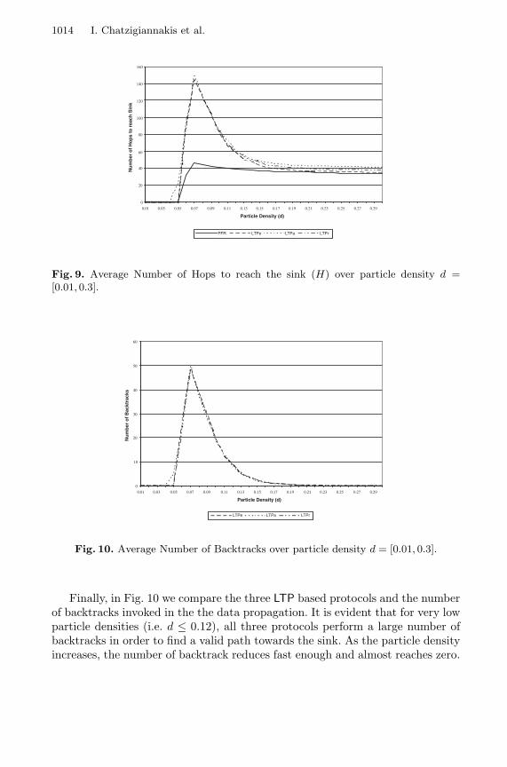
the optimal number of hops (in an ideal case) is roughly 29. In particular PFRachieves this for very low densities (d ≥ 0.07). On the other hand, the LTP basedprotocols exhibit a certain pathological behavior for low densities (i.e. d ≤ 0.12)due to a high number of executions of the backtrack mechanism in the attemptto find a particle closer to the sink (see also Fig. 10).

As far as time is concerned, in the full paper [3] we demonstrate (see Fig. 10there) that time and number of hops are of the same order and exhibit a verysimilar behavior.

0

500

1000

1500

2000

2500

3000

0.01 0.03 0.05 0.07 0.09 0.11 0.13 0.15 0.17 0.19 0.21 0.23 0.25 0.27 0.29

Particle Density (d)

Ave

rag

e N

um

ber

of

Tra

nsm

issi

on

s (E

tr)

PFR LTPe LTPa LTPr

Fig. 8. Average Number of Transmissions (ETR) over particle density d = [0.01, 0.3].

1014 I. Chatzigiannakis et al.

0

20

40

60

80

100

120

140

160

0.01 0.03 0.05 0.07 0.09 0.11 0.13 0.15 0.17 0.19 0.21 0.23 0.25 0.27 0.29

Particle Density (d)

Nu

mb

er o

f H

op

s to

rea

ch S

ink

PFR LTPe LTPa LTPr

Fig. 9. Average Number of Hops to reach the sink (H) over particle density d =[0.01, 0.3].

0

10

20

30

40

50

60

0.01 0.03 0.05 0.07 0.09 0.11 0.13 0.15 0.17 0.19 0.21 0.23 0.25 0.27 0.29

Particle Density (d)

Nu

mb

er o

f B

ackt

rack

s

LTPe LTPa LTPr

Fig. 10. Average Number of Backtracks over particle density d = [0.01, 0.3].

Finally, in Fig. 10 we compare the three LTP based protocols and the numberof backtracks invoked in the the data propagation. It is evident that for very lowparticle densities (i.e. d ≤ 0.12), all three protocols perform a large number ofbacktracks in order to find a valid path towards the sink. As the particle densityincreases, the number of backtrack reduces fast enough and almost reaches zero.

A Comparative Study of Protocols for Efficient Data Propagation 1015

8 Future Work

We plan to also investigate alternative probabilistic choices for favoring certaindata transmissions for the PFR protocol and consider alternative backtrack mech-anisms for the LTP protocol. Also, we wish to study different network shapes,various distributions used to drop the sensors in the area of interest and thefault-tolerance of the protocols. Finally, we plan to provide performance com-parisons with other protocols mentioned in the related work section, as wellas implement and evaluate hybrid approaches that combine the PFR and LTPprotocols in a parameterized way.

References

1. I.F. Akyildiz, W. Su, Y. Sankarasubramaniam and E. Cayirci: Wireless sensornetworks: a survey. In the Journal of Computer Networks, Volume 38, pp. 393–422, 2002.

2. I. Chatzigiannakis, S. Nikoletseas and P. Spirakis: Smart Dust Protocols for LocalDetection and Propagation. In Proc. 2nd ACM Workshop on Principles of MobileComputing – POMC’2002.

3. I. Chatzigiannakis, T. Dimitriou, M. Mavronicolas S. Nikoletseas and P. Spirakis:A Comparative Study of Protocols for Efficient Data Propagation in Smart DustNetworks. FLAGS, TR, http://ru1.cti.gr/FLAGS.

4. I. Chatzigiannakis and S. Nikoletseas: A Sleep-Awake Protocol for InformationPropagation in Smart Dust Networks. In Proc. 3rd Workshop on Mobile and Ad-Hoc Networks (WMAN)–IPDPS Workshops, IEEE Press, p. 225, 2003.

5. I. Chatzigiannakis, T. Dimitriou, S. Nikoletseas and P. Spirakis: A ProbabilisticForwarding Protocol for Efficient Data Propagation in Sensor Networks. FLAGSTechnical Report, FLAGS-TR-14, 2003.

6. D. Estrin, R. Govindan, J. Heidemann and S. Kumar: Next Century Challenges:Scalable Coordination in Sensor Networks. In Proc. 5th ACM/IEEE InternationalConference on Mobile Computing – MOBICOM’1999.

7. S.E.A. Hollar: COTS Dust. Msc. Thesis in Engineering-Mechanical Engineering,University of California, Berkeley, USA, 2000.

8. W. R. Heinzelman, A. Chandrakasan and H. Balakrishnan: Energy-Efficient Com-munication Protocol for Wireless Microsensor Networks. In Proc. 33rd HawaiiInternational Conference on System Sciences – HICSS’2000.

9. W. R. Heinzelman, J. Kulik and H. Balakrishnan: Adaptive Protocols for In-formation Dissemination in Wireless Sensor Networks. In Proc. 5th ACM/IEEEInternational Conference on Mobile Computing – MOBICOM’1999.

10. C. Intanagonwiwat, R. Govindan and D. Estrin: Directed Diffusion: A Scalable andRobust Communication Paradigm for Sensor Networks. In Proc. 6th ACM/IEEEInternational Conference on Mobile Computing – MOBICOM’2000.

11. C. Intanagonwiwat, D. Estrin, R. Govindan and J. Heidemann: Impact of NetworkDensity on Data Aggregation in Wireless Sensor Networks. Technical Report 01-750, University of Southern California Computer Science Department, November,2001.

12. J.M. Kahn, R.H. Katz and K.S.J. Pister: Next Century Challenges: Mobile Net-working for Smart Dust. In Proc. 5th ACM/IEEE International Conference onMobile Computing, pp. 271–278, September 1999.

1016 I. Chatzigiannakis et al.

13. B. Karp: Geographic Routing for Wireless Networks. Ph.D. Dissertation, HarvardUniversity, Cambridge, USA, 2000.

14. µ-Adaptive Multi-domain Power aware Sensors:http://www-mtl.mit.edu/research/icsystems/uamps, April, 2001.

15. A. Manjeshwar and D.P. Agrawal: TEEN: A Routing Protocol for Enhanced Effi-ciency in Wireless Sensor Networks. In Proc. 2nd International Workshop on Paral-lel and Distributed Computing Issues in Wireless Networks and Mobile Computing,satellite workshop of 16th Annual International Parallel & Distributed ProcessingSymposium – IPDPS’02.

16. K. Mehlhorn and S. Naher: LEDA: A Platform for Combinatorial and GeometricComputing. Cambridge University Press, 1999.

17. TinyOS: A Component-based OS for the Network Sensor Regime.http://webs.cs.berkeley.edu/tos/, October, 2002.

18. W. Ye, J. Heidemann and D. Estrin: An Energy-Efficient MAC Protocol for Wire-less Sensor Networks. In Proc. 12th IEEE International Conference on ComputerNetworks – INFOCOM’2002.

19. Wireless Integrated Sensor Networks: http:/www.janet.ucla.edu/WINS/, April,2001.