1454  |  wileyonlinelibrary.com/journal/mee3 Methods Ecol Evol. 2019;10:1454–1468.© 2019 The Authors. Methods in Ecology and Evolution © 2019 British Ecological Society

Received: 1 October 2018  |  Accepted: 4 March 2019

DOI: 10.1111/2041-210X.13209

R E S E A R C H A R T I C L E

A comparative analysis of common methods to identify waterbird hotspots

Allison L. Sussman1,2  | Beth Gardner3  | Evan M. Adams3,4  | Leo Salas5 | Kevin P. Kenow6  | David R. Luukkonen7 | Michael J. Monfils8 | William P. Mueller9 | Kathryn A. Williams4 | Michele Leduc‐Lapierre10 | Elise F. Zipkin1,2

1Department of Integrative Biology, Michigan State University, College of Natural Science, East Lansing, Michigan; 2Ecology, Evolutionary Biology, and Behavior Program, Michigan State University, East Lansing, Michigan; 3School of Environmental and Forest Science, University of Washington, Seattle, Washington; 4Biodiversity Research Institute, Portland, Maine; 5Point Blue Conservation Science, Petaluma, California; 6U.S. Geological Survey, Upper Midwest Environmental Sciences Center, La Crosse, Wisconsin; 7Department of Fisheries and Wildlife, Michigan State University, East Lansing, Michigan; 8Michigan Natural Features Inventory, Michigan State University Extension, Lansing, Michigan; 9Western Great Lakes Bird and Bat Observatory, Port Washington, Wisconsin and 10Great Lakes Commission, Ann Arbor, Michigan

This article has been contributed to by US Government employees and their work is in the public domain in the USA.

CorrespondenceAllison L. SussmanEmail: sussman7@msu.edu

Funding informationU.S. Fish and Wildlife Service Great Lakes Fish and Wildlife Restoration Act grants program

Handling Editor: Jana McPherson

Abstract1. Hotspot analysis is a commonly used method in ecology and conservation to iden-

tify areas of high biodiversity or conservation concern. However, delineating and mapping hotspots is subjective and various approaches can lead to different con-clusions with regard to the classification of particular areas as hotspots, compli-cating long‐term conservation planning.

2. We present a comparative analysis of recent approaches for identifying water-bird hotspots, with the goal of developing insights about the appropriate use of these methods. We selected four commonly used measures to identify persistent areas of high use: kernel density estimation, Getis‐Ord Gi*, hotspot persistence and hotspots conditional on presence, which represent the range of quantitative hotspot estimation approaches used in waterbird analyses. We applied each of the methods to aerial survey waterbird count data collected in the Great Lakes from 2012–2014. For each approach, we identified areas of high use for seven species/species groups and then compared the results across all methods and to mean ef-fort‐corrected counts.

3. Our results indicate that formal hotspot analysis frameworks do not always lead to the same conclusions. The kernel density and Getis‐Ord Gi* methods yielded the most similar results across all species analysed and were generally correlated with mean effort‐corrected count data. We found that these two models can differ substantially from the hotspot persistence and hotspots conditional on presence estimation approaches, which were not consistently similar to one another. The hotspot persistence approach differed most significantly from the other methods but is the only method to explicitly account for temporal variation.

     |  1455Methods in Ecology and Evolu onSUSSMAN et Al.

1  | INTRODUC TION

Hotspots are defined as small geographic areas (within a predefined larger region) that exhibit persistent high concentrations of indi-viduals or species (Harcourt, 2017; Possingham & Wilson, 1993). In the three decades since Myers (2008) first introduced the term, the definition of hotspots has expanded and adapted to reflect changes in conservation goals (Briscoe, Maxwell, Kudela, Crowder, & Croll, 2009). Animal hotspots are generally defined as areas with high levels of at least one of the following biological measures: species abundance, richness or endemism; rare, threatened or endangered species; and/or taxonomic distinctiveness (Briscoe et al., 2009; Prendergast, Quinn, et al., 1993). Hotspots are typically designated on a case‐by‐case basis because patterns vary by species and loca-tion; thus, the threshold to differentiate between hotspots and other locations naturally varies (Nelson & Boots, 2011). For example, com-mon definitions of hotspots focus on determining areas with con-sistent high species abundance (Davoren, 1983; Piatt et al., 2005), richness or biological activity (Sydeman, Brodeur, Grimes, Bychkov, & McKinnell, 2006) or some combination of these (Nur et al., 2012). Hotspots have also been defined as locations where some metric ex-ceeds a predefined threshold, such as the top five percent of the data (Harvey et al., 2013) or locations outside one (Santora & Veit, 2012; Suryan, Santora, & Veit, 2012) or three (Zipkin et al., 2015) standard deviations above the mean of a particular region or area sampled. Such definitions attempt to quantify hotspots (allowing for direct location comparison) as opposed to identifying hotspots using only qualitative criteria, which was common until recently (Mittermeier, Turner, Larsen, Brooks, & Gascon, 1988). The different approaches to identify hotspots have become increasingly complex and may lead to dissimilar or inconsistent results (Araujo, 2014; Daru, Bank, & Davies, 2015; Harvey et al., 2013; Hobday & Pecl, 2000; Orme et al., 2007; Prendergast, Quinn, et al., 1993; Prendergast, Quinn, Lawton, Eversham, & Gibbons, 1993). The consequence of applying different metrics to define hotspots is a lack of congruence across measures and, thus, hotspot locations, culminating in controversy and conflict over long‐term conservation efforts (Marchese, 2011; Orme et al., 2007; Prendergast, Quinn, et al., 1993). Such controversies could

potentially be avoided through a transparent statement of objec-tives at the start of analysis accompanied by a thorough explanation for selecting a specific method or metric.

Waterbird species display extreme variability in habitat use over both space and time (Certain, Bellier, Planque, & Bretagnolle, 2007; Piatt, Sydeman, & Wiese, 2006; Votier et al., 2008). They often exhibit large, patchy aggregations offshore, making it difficult to measure their spatial distributions. As such, the foremost method to determine patterns of waterbird species is to identify locations of persistent aggregation or high use, such as hotspots. Hotspot identification is useful in studies of highly mobile organisms, such as waterbirds, because the likelihood that a survey event of any given location is representative of true abundance at that location is low due to the extreme variability of their distributions (Santora & Veit, 2012). There are many methods to examine the diversity and abun-dance patterns of open water populations, but locating persistent high‐use areas is a frequent first step towards understanding the processes that generate spatial patterns of species distributions and informing effective conservation action (Nelson & Boots, 2011).

For waterbird abundance data, hotspot analyses are typically conducted using one of the following approaches: (1) qualitative analyses (e.g. through mapping abundance); (2) spatial statistics; or (3) classic statistical modelling (parametric or nonparametric) tech-niques (Tremblay et al., 2009). Historically, areas of high density or concentration were displayed and compared visually, and mapping relative species abundances remains a prevalent conservation tool (Harvey et al., 2013; Tremblay et al., 2009). Yet, qualitative ap-proaches are limited because they often do not reflect temporal changes (i.e. they are simply a snapshot in time), cannot adequately account for aggregations and can be misleading based on how data are collected, classified and presented (Marchese, 2011). As a result, more rigorous quantitative approaches, typically in the form of spa-tial statistics or generalized linear models (GLMs), were developed. Spatial statistics use data collected in both focal and surrounding locations to identify areas of high use. As their name suggests, these techniques account for spatial patterns in the data (Harvey et al., 2013). In contrast, classic statistical modelling techniques, which use GLM‐based frameworks, do not typically consider explicit spatial

4. We recommend considering the ecological question and scale of conservation or management activities prior to designing survey methodologies. Deciding the ap-propriate definition and scale for analysis is critical for interpretation of hotspot analysis results as is inclusion of important covariates. Combining hotspot analysis methods using an integrative approach, either within a single analysis or post hoc, could lead to greater consistency in the identification of waterbird hotspots.

K E Y W O R D S

gamma distribution, Getis‐Ord Gi*, Great Lakes, kernel density estimation, log‐normal distribution, parametric and nonparametric models, persistence, spatial models, spatial statistics

1456  |    Methods in Ecology and Evolu on SUSSMAN et Al.

correlation in hotspot identification and instead require the use of statistical distributions and a metric or threshold to account for variations in abundance patterns (Oppel et al., 2005; Santora & Veit, 2012; Zipkin et al., 2015). Waterbirds are highly mobile and tend to aggregate in large groups, resulting in highly skewed data with many absences in space and over time. As such, selecting an appropriately skewed statistical distribution to model waterbird data is funda-mental to accurately identifying hotspots using statistical modelling approaches (Zipkin, Leirness, Kinlan, O'Connell, & Silverman, 2014).

In this study, we evaluate four quantitative methods to iden-tify waterbird hotspots using data collected in the Great Lakes: kernel density estimation, Getis‐Ord Gi*, hotspot persistence and hotspots conditional on presence. We selected these four tech-niques because they are commonly used and represent the range of quantitative hotspot estimation approaches that have been em-ployed in waterbird analyses, incorporating spatially explicit pro-cesses to varying degrees. Kernel density estimation is perhaps the most well‐known and widely used spatial method for identifying hotspots. Kernel density estimation is an interpolation technique that is used to estimate the probability density function of a vari-able of interest (e.g. abundance) to identify areas of high density (O'Brien, Webb, Brewer, & Reid, 2012; Suryan et al., 2012; Wilson et al., 2009; Wong, Gjerdrum, Morgan, & Mallory, 2014). A less common spatial statistic for detecting hotspots is the Getis‐Ord Gi* statistic (Gi*), which allows for cluster evaluation within a specified distance of a single point but does not smooth over grid cells (Getis & Ord, 2019; Kuletz, 2018; Santora, Reiss, Loeb, & Veit, 2013). Gi* analysis is a spatial tool that identifies spatially explicit areas with values higher in magnitude than would be expected due to random chance, independent of the magnitude of abundance (Kuletz et al., 2018; Santora et al., 2013). For the other two models, we adapted GLM‐based techniques which have been used to identify water-bird hotspot locations. Hotspot persistence defines hotspots for every unique sampling event and calculates persistence over time (Johnson, Zipkin, O’Connell, & Caldow, 2012; Santora & Veit, 2012; Suryan et al., 2012). Hotspots conditional on presence combines survey data from all sampling events and defines hotspots as loca-tions with a long‐term average abundance greater than three times the regional mean, conditional on species presence (Kinlan et al., 2015; Zipkin et al., 2015).

Our objective was to compare consistency across methodologi-cally different, yet commonly used, hotspot analysis techniques for several waterbird species and species groups. Other methods for identifying hotspots exist and may be useful, but we restricted our analysis to techniques that have been used for waterbird analyses. We applied the four hotspot methods to the species data and then performed pairwise correlations with each method and to the mean effort‐corrected count data to measure the strength and association between the different approaches. This allowed us to quantify the degree to which the various estimators aligned in their assessments of waterbird hotspots. The results of our analyses can provide in-sights for more objective and goal‐driven hotspot delineation to in-form species conservation and research priorities.

2  | MATERIAL S AND METHODS

2.1 | Study area & data description

We conducted systematic aerial transect surveys of waterbirds in portions of Lakes Erie, Huron and Michigan, as well as Lake St. Clair during fall, winter and spring seasons from late September 2012 through early June 2014 (Figure 1a, Appendix S1). The data used in our analysis were collected as part of ongoing long‐term survey efforts to monitor waterbirds in the Great Lakes. Although not collected for the explicit purpose of comparing hotspot identification techniques, these data provide an excellent case study because of the geographic scope and number of species observed. Transects ranged in length from 3 to 177 km cover-ing approximately 8,000 km within the entire study area. Most of the transects (97%) were surveyed repeatedly with an aver-age number of 10.68 (SD: 3.85) sampling events per transect with approximately 83,000 km flown over the duration of the survey period. We defined a sampling event as a unique year‐month‐day (survey date) combination within each region of the Great Lakes. Transects were spaced 3.2–5 km apart and flight altitude ranged from 61 to 100 m above the lake's surface. Two observers, one on either side of the plane, recorded every waterbird flock that was detected in the observable portion of the transect (the area not obscured by the plane); observers were not permitted to use binoculars, and thus all detections were made using the naked eye. For each sighting, we recorded the species, flock size (i.e. number of individuals seen), and latitude and longitude (using onboard GPS) on the transect line. For large flocks that covered many square kilometres (i.e. up to 30 km), the location recorded was an approximate to the centre of the flock. Birds were identi-fied to the lowest taxonomic group possible when observers were unable to determine species.

We integrated the data into the open access Midwest Avian Data Center (MWADC), a regional node of the Avian Knowledge Network (AKN), hosted by Point Blue Conservation Science (http://data.point blue.org/partn ers/mwadc/ ). In some cases, observational data (e.g. location, species and flock size) were collected separately from effort data (e.g. survey date, location, transect flown, etc.) such that waterbird observations did not in-clude the corresponding transect attribution (23.4% of records). For these records, we used a 1‐m buffer to identify the closest transect, matched by survey date, to each observation record. We used data collected on the location of the transect line when available (42.26% of transect lines) and GIS to reconstruct the transect lines from observations in instances when that infor-mation was not recorded. Inclement weather and extensive ice coverage necessitated some surveys to be halted prematurely or conducted over a short period of time. We, thus, assumed that instances in which an area was surveyed over multiple consecu-tive days were a single sampling event. During the survey period, 253 transects were surveyed resulting in 136 unique sampling events.

     |  1457Methods in Ecology and Evolu onSUSSMAN et Al.

F I G U R E 1   (a) Map of the study area showing the number of sampling events per 5 × 5 km grid cell during the entire survey period. (b) Mean effort‐corrected count data for the all‐species‐combined species group (species list found in Table 1). Potential hotspots (values above the 75% percentile) across all sampled locations for the all‐species‐combined group as estimated with each of the four hotspot analysis approaches: (c) kernel density estimation, (d) Getis‐Ord Gi*, (e) hotspot persistence, and (f) hotspots conditional on presence. The “Hotspots” legend on panel (c) is used for all four hotspot analysis approach maps (c–f). Grid cells sampled less than four times were excluded from the analysis and are shaded in grey. Note the survey regions are delineated for the hotspot persistence approach (e) because hotspots in this method are calculated relative to other grid cells within these specific regions

1458  |    Methods in Ecology and Evolu on SUSSMAN et Al.

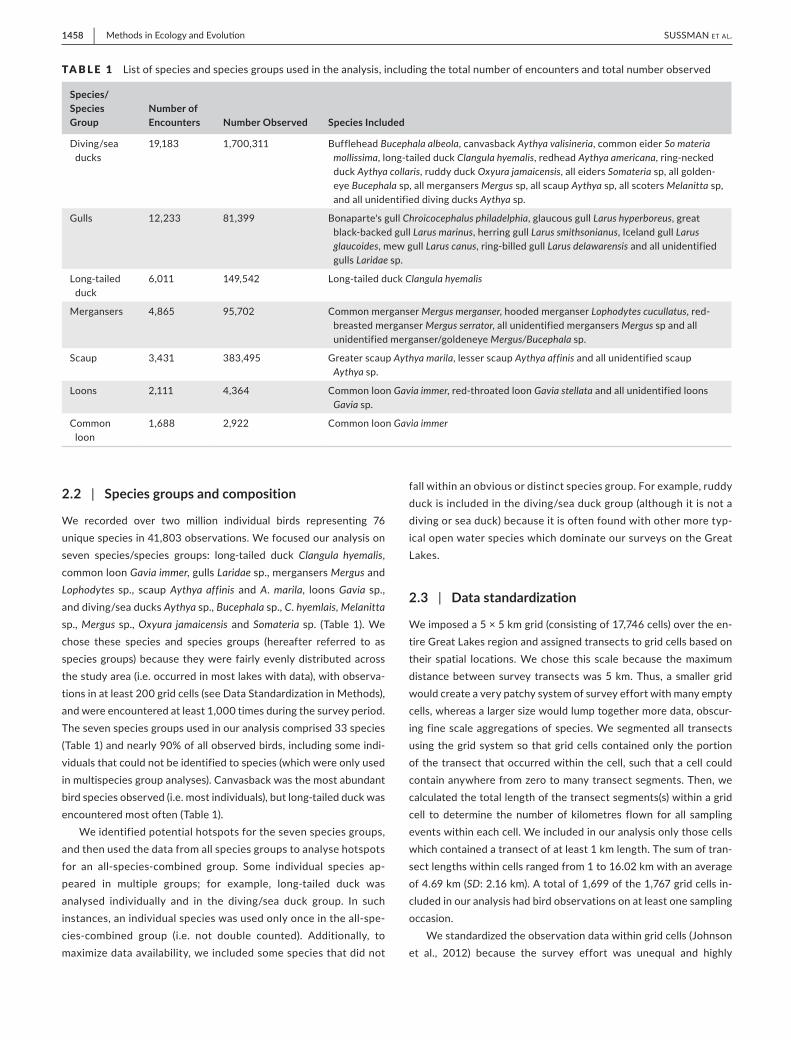
2.2 | Species groups and composition

We recorded over two million individual birds representing 76 unique species in 41,803 observations. We focused our analysis on seven species/species groups: long‐tailed duck Clangula hyemalis, common loon Gavia immer, gulls Laridae sp., mergansers Mergus and Lophodytes sp., scaup Aythya affinis and A. marila, loons Gavia sp., and diving/sea ducks Aythya sp., Bucephala sp., C. hyemlais, Melanitta sp., Mergus sp., Oxyura jamaicensis and Somateria sp. (Table 1). We chose these species and species groups (hereafter referred to as species groups) because they were fairly evenly distributed across the study area (i.e. occurred in most lakes with data), with observa-tions in at least 200 grid cells (see Data Standardization in Methods), and were encountered at least 1,000 times during the survey period. The seven species groups used in our analysis comprised 33 species (Table 1) and nearly 90% of all observed birds, including some indi-viduals that could not be identified to species (which were only used in multispecies group analyses). Canvasback was the most abundant bird species observed (i.e. most individuals), but long‐tailed duck was encountered most often (Table 1).

We identified potential hotspots for the seven species groups, and then used the data from all species groups to analyse hotspots for an all‐species‐combined group. Some individual species ap-peared in multiple groups; for example, long‐tailed duck was analysed individually and in the diving/sea duck group. In such instances, an individual species was used only once in the all‐spe-cies‐combined group (i.e. not double counted). Additionally, to maximize data availability, we included some species that did not

fall within an obvious or distinct species group. For example, ruddy duck is included in the diving/sea duck group (although it is not a diving or sea duck) because it is often found with other more typ-ical open water species which dominate our surveys on the Great Lakes.

2.3 | Data standardization

We imposed a 5 × 5 km grid (consisting of 17,746 cells) over the en-tire Great Lakes region and assigned transects to grid cells based on their spatial locations. We chose this scale because the maximum distance between survey transects was 5 km. Thus, a smaller grid would create a very patchy system of survey effort with many empty cells, whereas a larger size would lump together more data, obscur-ing fine scale aggregations of species. We segmented all transects using the grid system so that grid cells contained only the portion of the transect that occurred within the cell, such that a cell could contain anywhere from zero to many transect segments. Then, we calculated the total length of the transect segments(s) within a grid cell to determine the number of kilometres flown for all sampling events within each cell. We included in our analysis only those cells which contained a transect of at least 1 km length. The sum of tran-sect lengths within cells ranged from 1 to 16.02 km with an average of 4.69 km (SD: 2.16 km). A total of 1,699 of the 1,767 grid cells in-cluded in our analysis had bird observations on at least one sampling occasion.

We standardized the observation data within grid cells (Johnson et al., 2012) because the survey effort was unequal and highly

TA B L E 1   List of species and species groups used in the analysis, including the total number of encounters and total number observed

Species/Species Group

Number of Encounters Number Observed Species Included

Diving/sea ducks

19,183 1,700,311 Bufflehead Bucephala albeola, canvasback Aythya valisineria, common eider So materia mollissima, long‐tailed duck Clangula hyemalis, redhead Aythya americana, ring‐necked duck Aythya collaris, ruddy duck Oxyura jamaicensis, all eiders Somateria sp, all golden-eye Bucephala sp, all mergansers Mergus sp, all scaup Aythya sp, all scoters Melanitta sp, and all unidentified diving ducks Aythya sp.

Gulls 12,233 81,399 Bonaparte's gull Chroicocephalus philadelphia, glaucous gull Larus hyperboreus, great black‐backed gull Larus marinus, herring gull Larus smithsonianus, Iceland gull Larus glaucoides, mew gull Larus canus, ring‐billed gull Larus delawarensis and all unidentified gulls Laridae sp.

Long‐tailed duck

6,011 149,542 Long‐tailed duck Clangula hyemalis

Mergansers 4,865 95,702 Common merganser Mergus merganser, hooded merganser Lophodytes cucullatus, red‐breasted merganser Mergus serrator, all unidentified mergansers Mergus sp and all unidentified merganser/goldeneye Mergus/Bucephala sp.

Scaup 3,431 383,495 Greater scaup Aythya marila, lesser scaup Aythya affinis and all unidentified scaup Aythya sp.

Loons 2,111 4,364 Common loon Gavia immer, red‐throated loon Gavia stellata and all unidentified loons Gavia sp.

Common loon

1,688 2,922 Common loon Gavia immer

     |  1459Methods in Ecology and Evolu onSUSSMAN et Al.

variable across cells within the study area (Figure 1a). We divided the number of observations of a species for the sampling event‐grid cell combination by the summed transect length, resulting in a con-tinuous effort‐corrected count (Figure 1b). We used data from all sampling events in our hotspot analysis; however, we limited the method comparisons, correlations and hotspot maps to grid cells that contained at least four sampling events, for a total of 1,473 grid cells (83.4% of surveyed cells). Using grid cells with at least four sam-pling events allowed for analysis across the study region, while mini-mizing the chances of false hotspot identification due to insufficient data (Figure 1a; Kuletz et al., 2018; Zipkin et al., 2015). To calculate a mean effort‐corrected count for each species group in surveyed grid cells, we divided the summed effort‐corrected counts in a grid cell (across all sampling events) by the total number of sampling events for that grid cell.

2.4 | Hotspot analysis

2.4.1 | Kernel density estimation

Kernel density estimation is a common method for estimating rela-tive density in animal populations that aggregate and has been used repeatedly to identify waterbird hotspot locations and marine areas in need of protection (Wilson et al., 2009, O'Brien et al., 2012, Suryan et al., 2012, and Wong et al., 2014). This modelling approach converts point data (i.e. effort‐corrected counts) into a continuous surface grid reflecting relative densities across all grid cells, where the resulting density of each grid cell is weighted according to the distance from the focal location/grid cell (Wong et al., 2014).

To implement the kernel density method, we calculated the mid-point of each grid cell and assigned all effort‐corrected counts of the species group (across all sampling events) to the midpoint of the grid cell in which they occurred. We accounted for uneven sampling effort (grid cells were surveyed 1–30 times, Figure 1a) by dividing the summed counts in a grid cell by the total number of sampling events for that grid cell. We used the kernel density tool in the Spatial Analyst extension of ArcGIS 10.3.1 (ESRI, 1992) to estimate bird density, inputting values for both bandwidth and cell size. The bandwidth, or size of the neighbourhood over which the density is averaged, is the amount of smoothing applied to each kernel (Nelson & Boots, 2011). Smoothing allows for abundance prediction in non‐ (or low‐) sampled areas by assuming that neighbours behave more similarly to one another than at locations that are further away. Small bandwidth values may result in fragmented small‐scale kernels, lead-ing to underestimation of hotspots, whereas large values result in oversmoothed general kernels, overestimating hotspots (Wong et al., 2014). We selected a 5‐km bandwidth for kernel smoothing based on both the geographic extent of the data and the distance between survey transects (Suryan et al., 2012). Kernel density es-timation results in a raster, which is a matrix of pixels where each pixel contains a value representing information (e.g. estimated bird abundance; ESRI, 1992). The cell size for the output raster can also affect the interpretation of the kernel estimate: large cell sizes may

result in a blocky raster that is a poor approximation of a continuous surface, and small cell sizes may result in a raster of many cells that is over‐fit or takes an inordinate amount of time to calculate (Beyer, 2015). We selected a cell size of 1 × 1 km for the output raster. For each species group, we extracted the mean expected count from the resulting kernel density raster back to the 5‐km2 grid for comparison with the other methods. Each raster cell was assigned to a corre-sponding 5 km2 grid cell based on its midpoint; we then averaged the density values from all raster cells for each grid cell, where the higher the value, the more likely it is to be a hotspot.

2.4.2 | Getis‐Ord Gi*

The Getis‐Ord Gi* (Gi*) statistic detects hotspots while also indicat-ing the statistical significance of those hotspots (Kuletz et al., 2018; Santora et al., 2013). The Gi* technique identifies grid cells whose data points cluster spatially by examining each grid cell within the context of the neighbouring cells (Getis & Ord, 2019). Gi* differs from kernel density estimation because it incorporates the value of each feature in the context of its neighbours, whereas kernel density estimates the neighbours based on the focal feature and then ap-plies a smoothing over those neighbours.

To implement the Gi* statistic, we again calculated the midpoint of each grid cell and assigned all effort‐corrected counts of the spe-cies group across all sampling events to the midpoint of the cell into which they occurred. We accounted for uneven sampling effort by dividing the summed effort‐corrected grid cell counts by the total number of sampling events for that cell. We built a neighbours list for all grid cells using Rook's case contiguity (i.e. grid cells that share a border), and then used the neighbours list to calculate a row‐stan-dardized spatial weights matrix (spdep package in r; Bivand, Hauke, & Kossowski, 2018, Bivand & Piras, 2008, R Core Team, 2010). The matrix informs every grid cell's relationship to all other cells in the neighbourhood (Kuletz et al., 2018). We used the effort‐corrected counts and the spatial weights matrix to calculate the Gi* for each grid cell (spdep package in r; Bivand et al., 2018, Bivand & Piras, 2008, R Core Team, 2010). Gi* produces a z‐score for each grid cell, where high positive values are statistically significant and indicate the possibility of a local cluster of high species abundance (i.e. a hotspot) that is unlikely due to random chance.

2.4.3 | Hotspot persistence

The hotspot persistence method quantifies the persistence of species counts within individual grid cells (Johnson et al., 2012; Santora & Veit, 2012; Suryan et al., 2012). To implement this method, we first fit a gamma distribution to the effort‐corrected continuous species group count data, summed within grid cells, for each unique sampling event (fitdistrplus package in r; Delignette‐Muller & Dutang, 2015, R Core Team, 2010). We selected the two‐parameter gamma distribution (shape and scale) because it can fit a variety of continuous right‐skewed data (Bolker, 2014; Dennis & Patil, 2010) and because it has been used before with

1460  |    Methods in Ecology and Evolu on SUSSMAN et Al.

this hotspot analysis technique (Johnson et al., 2012). We then assigned a probability to each grid cell based on the fit of the data within the cumulative distribution curve for that sampling event. This allowed us to identify grid cells (for each unique sampling event) with high abundance of the target species group relative to other cells. Within a unique sampling event, we identified grid cells as hotspots if the value of the cumulative distribution for the cell, based on the fit of the gamma distribution, was above the 75th percentile for that sampling event. After identifying which grid cells were categorized as hotspots for every unique sampling event, we calculated the proportion of sampling events in which a grid cell was identified as a hotspot to examine persistence. The final output was the proportion of sampling events, ranging from zero to one, in which a grid cell was considered a hotspot for the target species group. Values of zero indicate the grid cell was never a hotspot. The higher the proportion, the more frequently the grid cell was considered a hotspot, with a value of one indicat-ing the grid cell was a hotspot for all sampling events.

2.4.4 | Hotspots conditional on species presence

The hotspots conditional on presence method calculates the long‐term probability that a grid cell is a hotspot for a particular species given observed abundances over time (Kinlan et al., 2015; Zipkin et al., 2015). To implement this method, we fit the effort‐corrected count data using a log‐normal distribution (fitdistrplus package in r; Delignette‐Muller & Dutang, 2015, R Core Team, 2010). Because the log‐normal distribution does not contain zero in its support, we used only the positive effort‐corrected counts. The log‐normal is a two parameter (mean and standard deviation), positive, contin-uous probability distribution characterized by a heavy tail and has been shown to fit waterbird data well because of its flexible shape and ability to fit heavily skewed data (Limpert, Stahel, & Abbt, 2015; Zipkin et al., 2014). We then estimated prevalence in the reference region as the proportion of cells with occurrences for the target species group (at least one individual observed within the cell over all sampling events) relative to the total number of cells surveyed (Kinlan et al., 2015). We defined the reference re-gion as the entire area sampled across the Great Lakes. We then simulated data with a two‐part Monte Carlo approach to calculate hotspot locations using the estimated mean and standard devia-tion from the log‐normal distribution (the count component) and the prevalence estimate (the Bernoulli component; Kinlan et al., 2015, Zipkin et al., 2015). We defined a hotspot as a grid cell in which the long‐term average effort‐corrected count conditional on presence (with α = 0.05 threshold) was at least three times the mean of the reference region, also conditional on presence (Kinlan et al., 2015). The resulting values, ranging from zero to one, rep-resent the proportion of simulated sample means that are greater than three times the average count. Values close to zero indicate the grid cell is not a hotspot. Values close to one indicate a high probability that the long‐term average abundance in the grid cell is greater than three times the mean of the reference region.

2.5 | Comparative analysis of the methods

Our objective was to determine the degree of congruence among the four methods across species groups and for all‐species‐com-bined. We compared methods using only grid cells that were sur-veyed four or more times. To quantify the consistency among the four approaches in their ability to detect hotspots, we performed a Pearson's product–moment correlation to evaluate the pairwise as-sociations of the four approaches with a Bonferroni adjustment and an alpha level of 0.05 (Hmisc package in r; R Core Team, 2010, Harrel, 2012). In addition to comparing the four hotspot analysis methods, we also compared the methods with the mean effort‐corrected count using the same correlation test. We analysed the correlation coefficients (ranging from zero to one) to determine associations among the different approaches: the higher the value, the higher the correlation between two methods.

We produced maps for all species groups to visually compare the results of the four hotspot analysis approaches and mean effort‐cor-rected counts (Appendices S2–S9). For the first set of maps, we plot-ted the values produced for each grid cell using each hotspot analysis technique. Direct visual comparison among the hotspot methods can be difficult because the scale of the results for each method varies (i.e. kernel density produces unbounded positive values, Gi* produces both positive and negative values, and hotspot persistence and hotspots conditional on presence range between zero to one). To resolve this issue, we created a second set of maps for each spe-cies group in which we considered a hotspot as any grid cell with a value above the 75th percentile (of all values for that method) and plotted those according to their percentiles.

3  | RESULTS

The highest correlation between methods for all species groups oc-curred between kernel density and Gi* estimation approaches with a correlation ≥ 0.80 for all species groups except mergansers (Table 2). For mergansers, the correlation between the two explicitly spatial methods was 0.67 and nearly identical to the correlation between Gi* and the hotspots conditional on presence method. For the other species groups, including all‐species‐combined, there was much higher congruency between kernel density and Gi* than any other combination of pairwise comparisons (excluding mean effort‐cor-rected data, discussed below; Table 2; Appendices S2–S9). For exam-ple, for all‐species‐combined there was 94% overlap in identification of hot and non‐hot grid cells between kernel density estimation and Gi* (Figure 1c–d). In general, the two other methods were no more similar to one another than to either kernel density and Gi* with cor-relations between the models that varied by species (Table 2). Kernel density estimation and hotspot persistence showed the lowest cor-relations (0.03–0.56) for the species groups that we examined. For the all‐species‐combined group, we found that the four methods identified the same 63% of grid cells as non‐hot locations (below the 75th percentile), while approximately 8% of grid cells were identified

     |  1461Methods in Ecology and Evolu onSUSSMAN et Al.

TA B L E 2   Pearson correlation matrix of pairwise comparisons between the four hotspot analysis methods (kernel density estimation, Getis‐Ord Gi*, hotspot persistence, and hotspots conditional on presence) and mean effort‐corrected counts, with a Bonferroni adjustment

Kernel density estimation Getis‐Ord Gi*

Hotspot persistence

Hotspots condi‐tional on presence

Mean effort‐cor‐rected count

All species/groups

Kernel density estimation 1.000 0.870 0.121 0.441 0.928

Getis‐Ord Gi* 0.870 1.000 0.125 0.435 0.650

Hotspot persistence 0.121 0.125 1.000 0.332 0.093

Hotspots conditional on presence 0.441 0.435 0.332 1.000 0.375

Mean effort‐corrected Count 0.928 0.650 0.093 0.375 1.000

Diving/sea ducks

Kernel density estimation 1.000 0.874 0.160 0.467 0.929

Getis‐Ord Gi* 0.874 1.000 0.167 0.458 0.655

Hotspot persistence 0.160 0.167 1.000 0.364 0.123

Hotspots conditional on presence 0.467 0.458 0.364 1.000 0.395

Mean effort‐corrected Count 0.929 0.655 0.123 0.395 1.000

Gulls

Kernel density estimation 1.000 0.808 0.318 0.457 0.865

Getis‐Ord Gi* 0.808 1.000 0.325 0.459 0.715

Hotspot persistence 0.318 0.325 1.000 0.446 0.274

Hotspots conditional on presence 0.457 0.459 0.446 1.000 0.443

Mean effort‐corrected Count 0.865 0.715 0.274 0.443 1.000

Long‐tailed duck (LTDU)

Kernel density estimation 1.000 0.804 0.407 0.475 0.725

Getis‐Ord Gi* 0.804 1.000 0.451 0.432 0.469

Hotspot persistence 0.407 0.451 1.000 0.583 0.350

Hotspots conditional on presence 0.475 0.432 0.583 1.000 0.495

Mean effort‐corrected Count 0.725 0.469 0.350 0.495 1.000

Mergansers

Kernel density estimation 1.000 0.672 0.433 0.600 0.739

Getis‐Ord Gi* 0.672 1.000 0.547 0.669 0.812

Hotspot persistence 0.433 0.547 1.000 0.575 0.539

Hotspots conditional on presence 0.600 0.669 0.575 1.000 0.778

Mean effort‐corrected Count 0.739 0.812 0.539 0.778 1.000

Scaup

Kernel density estimation 1.000 0.878 0.562 0.661 0.950

Getis‐Ord Gi* 0.878 1.000 0.586 0.623 0.707

Hotspot persistence 0.562 0.586 1.000 0.686 0.469

Hotspots conditional on presence 0.661 0.623 0.686 1.000 0.611

Mean effort‐corrected Count 0.950 0.707 0.469 0.611 1.000

Loons

Kernel density estimation 1.000 0.808 0.047** 0.210 0.910

Getis‐Ord Gi* 0.808 1.000 0.063 0.258 0.517

Hotspot persistence 0.047** 0.063 1.000 0.454 0.026**

Hotspots conditional on presence 0.210 0.258 0.454 1.000 0.136

Mean effort‐corrected count 0.910 0.517 0.026** 0.136 1.000

(Continues)

1462  |    Methods in Ecology and Evolu on SUSSMAN et Al.

as hotspot locations under all four methods (above the 75th percen-tile). The remaining 29% of the cells were identified as hotspots by one, two or three of the methods. Loons and common loon were the only two species groups to have insignificant correlations (α = 0.05, Table 2). The patterns observed with these two species groups may be due in part to insufficient data availability.

The hotspot persistence approach differed most significantly from the other three methods and had the lowest correlations over-all with other methods (Table 2; Figures 1 and 2). Unlike the other methods, the hotspot persistence approach calculates hotspots relative to the survey region, rather than the entire study area (i.e. Figure 1a and e), and also explicitly incorporates temporal variability. For example, in the analysis of the scaup species group, we found that many grid cells in Lake St. Clair were identified as hotspots by all methods except for hotspot persistence (Figure 2; Appendix S7). The counts for scaup were generally quite high in Lake St. Clair relative to other surveyed locations. However, the hotspot persistence method revealed that individual grid cells within Lake St. Clair did not often have high counts on repeated occasions (as evidenced with zeros and other low values in grid cells; Figure 2e). The all‐species‐com-bined analysis produced similar results, with 9% of grid cells iden-tified as hotspots by the persistence approach but not by the other three methods (Figure 1b–f; Appendix S2).

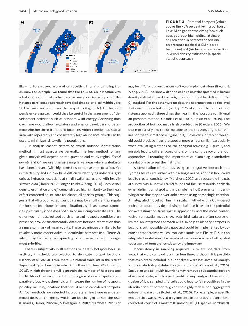
Kernel density and Gi*, which consider space in an explicit man-ner, are inherently different from hotspot persistence and hotspots conditional on presence, which rely on parametric distributions, as is evident in both the correlations and maps (Table 2; Appendices S2–S9). Hotspot persistence and hotspots conditional on presence tended to select single grid cells as hotspots, whereas kernel density and Gi* selected small clusters of grid cells as hotspots (Figure 3). In many cases, grid cells that were highly ranked with the hotspots con-ditional on presence approach, were also highly ranked with kernel density and Gi*. However, the surrounding grid cells tended to also be highly ranked with kernel density and Gi* (Figure 3).

Species‐specific hotspots for common loon and long‐tailed duck occurred in areas identified as hotspots for the corresponding species group (loons and diving/sea ducks, respectively). Common loon observations comprised 67% of the loon group observations (Table 1). A reanalysis of the loon group without common loons did not substantially alter correlations between the different methods

(Appendix S10). Yet, when long‐tailed duck data were removed from the diving/sea duck group (9% of the data), Gi* showed a higher cor-relation than kernel density estimation with hotspots conditional on presence (although kernel density and Gi* were still highly correlated with one another; Appendix S10), suggesting that long‐tailed ducks may be disproportionately influencing the results of the hotspot analysis for the diving/sea duck group.

Correlations between the mean effort‐corrected counts and each of the four methods were highly consistent among the species groups (Table 2). For most species groups, kernel density estimation had the highest correlation with mean effort‐corrected counts, fol-lowed by Gi* and hotspots conditional on presence, with hotspot persistence being least similar. Correlations between mean effort‐corrected counts and kernel density estimation tended to be fairly high; though this was not true for the mergansers group, which had the highest correlation between mean effort‐corrected counts and Gi*. The only species group to demonstrate its highest correlation between mean effort‐corrected count and a GLM‐based technique (hotspots conditional on presence) was the common loon. For seven of the eight species groups, mean effort‐corrected count had the lowest correlation with the hotspot persistence approach (Table 2).

4  | DISCUSSION

Despite the frequent use of hotspot analyses in management and conservation, we found that the various hotspot analysis approaches resulted in inconsistent identification of hotspots within the Great Lakes waterbird dataset, and that the degree of this inconsistency varied by species group. If conservation and management decisions are based on hotspot analyses, it is important to understand the ad-vantages, limitations, and potential biases in the various approaches to facilitate selection of the most appropriate method to answer the question(s) of interest. Our analysis revealed that methods to esti-mate hotspots using explicitly spatial approaches, specifically kernel density and Gi*, produce highly correlated results and can likely be used as surrogates for one another. Not surprisingly, these spatial smoothing methods were often also highly correlated with mean ef-fort‐corrected counts. These approaches are likely to be most ap-propriate when the objective is to identify hotspot locations within

Kernel density estimation Getis‐Ord Gi*

Hotspot persistence

Hotspots condi‐tional on presence

Mean effort‐cor‐rected count

Common loon (COLO)

Kernel density estimation 1.000 0.800 0.027** 0.049** 0.060

Getis‐Ord Gi* 0.800 1.000 0.032** 0.075 0.087

Hotspot persistence 0.027** 0.032** 1.000 0.606 0.536

Hotspots conditional on presence 0.049** 0.075 0.606 1.000 0.718

Mean effort‐corrected count 0.060 0.087 0.536 0.718 1.000

Note: Correlations are significant unless otherwise denoted (**) at an alpha level of 0.05. Values above and below of the diagonals are mirror images (gray values are duplicates).

TA B L E 2   (Continued)

     |  1463Methods in Ecology and Evolu onSUSSMAN et Al.

specific temporal constraints (e.g. within a single season). Spatial hot-spot techniques might also be useful in the creation and delineation of open water sanctuaries or marine preserves, as these areas often encompass large geographic ranges such that the information of spa-tial neighbours can be helpful. The other two modelling techniques that we examined produce less consistent results with each other, the spatial methods and mean effort‐corrected counts, the degree to which varied by species. The hotspot persistence approach differed the most from the other methods. Hotspot persistence estimates

hotspots based on unique sampling events within survey regions and then identifies whether those areas persist as hotspots over time, while the other three approaches (and mean effort‐corrected count data) focus on average abundance over the entire survey period. The hotspot persistence approach (perhaps more so than the other ap-proaches) may thus perform best with a high number of sampling events rather than our minimum of four surveys (Kinlan et al., 2015). Studies constrained to a small geographic range would benefit from the hotspot persistence approach because smaller areas are more

F I G U R E 2   Hotspot maps for the scaup species group (greater scaup Aythya marila pictured in top left, panel a) in western Lake Erie, including (b) mean effort‐corrected counts. The hotspot values are shown on the raw scales for each of the four methods: (c) kernel density estimation, (d) Getis‐Ord Gi*, (e) hotspot persistence, and (f) hotspots conditional on presence

1464  |    Methods in Ecology and Evolu on SUSSMAN et Al.

likely to be surveyed more often resulting in a high sampling fre-quency. For example, we found that the Lake St. Clair location was a hotspot under most techniques for many species groups, but the hotspot persistence approach revealed that no grid cell within Lake St. Clair was more important than any other (Figure 1e). The hotspot persistence approach could thus be useful in the assessment of de-velopment activities such as offshore wind energy. Analysing data over time would allow regulators and energy developers to deter-mine whether there are specific locations within a predefined spatial area with repeatedly and consistently high abundance, which can be used to minimize risk to wildlife populations.

Our analysis cannot determine which hotspot identification method is most appropriate generally. The best method for any given analysis will depend on the question and study region. Kernel density and Gi* are useful in assessing large areas where waterbirds have been present (with high densities) on at least one occasion. Yet kernel density and Gi* can have difficulty identifying individual grid cells as hotspots, especially at small spatial scales and with heavily skewed data (Harris, 2017; Songchitruska & Zeng, 2010). Both kernel density estimation and Gi* demonstrated high similarity to the mean effort‐corrected count data for almost all species groups. This sug-gests that effort‐corrected count data may be a sufficient surrogate for hotspot techniques in some situations, such as coarse summa-ries, particularly if one does not plan on including covariate data. The other two methods, hotspot persistence and hotspots conditional on presence, provide fundamentally different hotspot information than a simple summary of mean counts. These techniques are likely to be relatively more conservative in identifying hotspots (e.g. Figure 3), which may be desirable depending on conservation and manage-ment priorities.

There is subjectivity in all methods to identify hotspots because arbitrary thresholds are selected to delineate hotspot locations (Harvey et al., 2013). Thus, there is a natural trade‐off in the rate of Type I and Type II errors in selecting a threshold level (Kinlan et al., 2015). A high threshold will constrain the number of hotspots and the likelihood that an area is falsely categorized as a hotspot is com-paratively low. A low threshold will increase the number of hotspots, possibly including locations that should not be considered hotspots. All four methods we selected incorporate at least one user‐deter-mined decision or metric, which can be changed to suit the user (Canadas, Bellier, Planque, & Bretagnolle, 2007; Marchese, 2011) or

may be different across various software implementations (Bivand & Wong, 2016). The bandwidth and cell size must be specified in kernel density estimation and the neighbourhood must be defined in the Gi* method. For the other two models, the user must decide the level that constitutes a hotspot (i.e. top 25% of cells in the hotspot per-sistence approach; three times the mean in the hotspots conditional on presence method; Canadas et al., 2007, Zipkin et al., 2015). The production of hotspot maps is also subjective (Carolan, 2015). We chose to classify and colour hotspots as the top 25% of grid cell val-ues for the four methods (Figure 1c–f). However, a different thresh-old could produce maps that appear more or less similar (particularly when evaluating methods on their original scales; e.g. Figure 2) and possibly lead to different conclusions on the congruency of the four approaches, illustrating the importance of examining quantitative correlations between the methods.

A combination of methods using an integrative approach that synthesizes results, either within a single analysis or post hoc, could lead to greater consistency (Marchese, 2011) and reduce the impacts of survey bias. Nur et al. (2012) found that the use of multiple criteria (when defining a hotspot within a single method) prevents misidenti-fying areas that may be overlooked when using only a single criterion. An integrated model combining a spatial method with a GLM‐based technique could provide a desirable balance between the potential for overestimation from spatial approaches and the more conser-vative non‐spatial models. As waterbird data are often sparse or limited, an integrated approach will also help to identify hotspots in locations with possible data gaps and could be implemented by av-eraging standardized values from each model (e.g. Figure 4). Such an integrated model would be beneficial in scenarios where both spatial coverage and temporal consistency are important.

Inconsistency in sampling required us to exclude data from areas that were sampled less than four times, although it is possible that even areas included in our analysis were not sampled enough for accurate hotspot detection (Hazen, 2009; Zipkin et al., 2015). Excluding grid cells with few visits may remove a substantial portion of available data, which is undesirable in any analysis. However, in-clusion of low sampled grid cells could lead to false positives in the identification of hotspots, given the highly mobile and aggregated nature of waterbirds (Kuletz et al., 2018). For example, a specific grid cell that was surveyed only one time in our study had an effort‐corrected count of almost 900 individuals (all‐species‐combined).

F I G U R E 3   Potential hotspots (values above the 75% percentile) in a portion of Lake Michigan for the diving/sea duck species group, highlighting (a) single‐cell selection in hotspots conditional on presence method (a GLM‐based technique) and (b) clustered cell selection in kernel density estimation (a spatial statistic approach)

     |  1465Methods in Ecology and Evolu onSUSSMAN et Al.

Had we included cells that were surveyed less than four times, this cell would have been designated as a hotspot by all four methods. Yet, it is difficult to assess the validity of this designation without repeated sampling. For some rare species, though, it may be neces-sary to reduce the threshold of required survey events to maximize data use.

Variation in hotspot identification across the methods may be due in part to scale. Scale is important to several aspects of hotspot identification: (1) the scale at which the data are collected, (2) the spatial scale at which the data are analysed, and (3) the scale at which management decisions will be made. It is important to ac-count for potential discrepancies in the geographic scale of popu-lation‐level processes and the resolution of different datasets when deciding the spatial scale for analysis. The 5‐km2 grid we used is a fine‐scale resolution to identify and map hotspots and may result in less consistency across methods than a larger, coarser grid (Daru et al., 2015). The distance between and design of transect surveys can directly affect the outcome of hotspot analyses, and we, therefore, recommend simultaneous and thorough consideration of survey de-sign and analysis prior to data collection. Survey bias, the presence of spatial patterns in survey effort, is a ubiquitous concern when de-lineating hotspots (Prendergast, Wood, Lawton, & Eversham, 2015), and its effects may lead to different results depending on the ana-lytical methods used.

The four approaches used in this study were selected because they have been previously used to identify areas of high‐use for waterbird species in other studies. However, variations of these models (e.g. selecting a different threshold cut‐off or using a met-ric other than the mean, such as standard deviation) as well as other potential hotspot methods could be used to model abun-dance data. For example, cluster analysis models that have been developed for monitoring crime rates or traffic accidents and pat-terns, which have not yet been applied to wildlife data, may pro-vide more nuanced approaches to hotspot analyses (Hengl, 2014; Tango, 1995). We used r and ArcGIS to run our analysis; however, other software packages may also be useful for hotspot model-ling. For instance, SATScAn is free software developed to detect disease clusters by analysing spatial, temporal and/or space‐time data (Kulldorf, 2006). The platform can run different types of models (such as normal, ordinal and exponential models, as well as those we implement in this paper) and adjust for underlying spatial inhomogeneity as part of the default software features. We expect that continued software and model development will allow for advances in hotspot analysis methods.

Hotspot analysis is a first step in understanding species distribu-tion patterns, but it is often equally or more important to determine why certain areas contain persistent aggregations of waterbirds. The use of mechanistic or associative models with covariates that help explain and elucidate hotspots should be considered in those cases where knowledge of the system and adequate covariate data exist (e.g. Nur et al., 2012). We did not include environmental variables (e.g. bathymetry, surface temperature, ice coverage, etc.) or sea-sonality in our hotspot analysis, although they most certainly play an important role in explaining the distribution and abundance pat-terns of waterbirds (Nur et al., 2012; Suryan et al., 2012). Although excluding covariates does not affect our model comparison results, it precludes understanding why certain locations are identified as hotspots. Some environmental variables, such as habitat suitability and food availability, are critical to discerning species behaviours and patterns and are occasionally used as proxies for hotspots when data are limited (Shirkey, 2002; Briscoe et al., 2009; Folmer, Olff, & Piersma, 1999; Hyrenbach et al., 2015). However, challenges arise with incorporating environmental variables that are dynamic (e.g. ice cover or temperature), making identification of static hotspot locations relative to environmental variables difficult (Briscoe et al., 2009; Marchese, 2011) and perhaps less useful for certain man-agement‐related questions. Waterbird hotspots may not be fixed locations, and may vary by season, annually, or on even longer time frames. Seasonal variability in waterbird species is an important fac-tor that we did not consider in our analysis; abundances can fluc-tuate during migration or at overwintering locations and shifts in distributions may occur even within seasons (Suryan et al., 2016).

Survey methods and modelling techniques have improved over time, but waterbird species are highly mobile, making the identifi-cation of priority areas difficult (Arcos, Hauke, & Kossowski, 2013; Harvey et al., 2013; Marchese, 2011). Through our study, we demon-strate that delineating hotspots is often subjective, as different

F I G U R E 4   Potential hotspots from an integrated hotspot modelling approach across all sampled locations for the all‐species‐combined species group (species list found in Table 1). We combined two hotspot analysis techniques, one spatial statistic approach (Getis‐Ord Gi*) and one GLM‐based technique (hotspots conditional on presence). The results shown in this map were produced by calculating the average percentile of the two selected methods for all grid cells, resulting in a value from zero to one where high values closer to one are more likely to be hotspots than low values closer to zero. Grid cells sampled less than four times were excluded from the analysis and are shaded in grey. We binned the percentiles for mapping purposes and consider a species hotspot as any grid cell with an average value above the 75th percentile

1466  |    Methods in Ecology and Evolu on SUSSMAN et Al.

analysis techniques and thresholds can produce varying results. Regardless of their drawbacks, hotspot analyses are likely to remain an important tool for conservation because of their relative ease to implement. Thus, the inconsistencies we found in our comparisons necessitates attention by conservation practitioners. Researchers should clearly identify conservation and management goals to select the most appropriate analysis method(s). This, along with incorpora-tion of covariates, will allow hotspot analyses to be both useful and meaningful. Conservation and management decisions on hotspots are often long‐lasting and should be done carefully and with full un-derstanding of model limitations.

DATA AVAIL ABILIT Y S TATEMENT

Data are available in the Dryad Digital Repository (https ://doi.org/10.5061/dryad.rs776p3) and the Midwest Avian Data Center, a regional node of the Avian Knowledge Network, hosted by Point Blue Conservation Science (http://data.point blue.org/partn ers/mwadc/ ). The data and code to run analyses are also available on GitHub (https ://zipki nlab.github.io/).

ACKNOWLEDG EMENTS

We would like to thank the pilots (Mike Callahan, Derek DeRuiter, Brian Lubinski, Keith Teague, Luke Wuest and Sarah Folsom Yates) and observers (Jeff Bahls, Seth Cutright, Tim Demers, Joelle Gehring, Luke Fara, Kristen Finch, Steven Houdek, Robby Lambert, Tom Schultz, Brendan Shirkey, Howie Singer and Joel Trick) for col-lecting the data for this study. We are grateful to Matt Farr, Sam Rossman, and Sarah Saunders for feedback on the selected hotspot approaches; Victoria Pebbles, Becky Pearson and Katie Koch for project management and support; Michael Fitzgibbon and Jeffrey Tash for GIS and data support; Kathy Kuletz and Patrick O'Hara for input on the spatial models and standardization process; and Catherine Lindell for guidance and feedback on previous versions of this manuscript. We are also grateful for insightful written com-ments provided by J. McPherson, J. Stanton, R.R. Veit, R.P. White, and one anonymous reviewer. The greater scaup (Aythya marila) image in Figure 2 was found on Wikimedia Commons: Calibas/CC‐BY‐SA‐4.0. This project was funded by the U.S. Fish and Wildlife Service Great Lakes Fish and Wildlife Restoration Act grants pro-gram (GLFWRA 2006). Any use of trade, product or firm names is for descriptive purposes only and does not imply endorsement by the U.S. Government.

AUTHORS’ CONTRIBUTIONS

A.L.S. and E.F.Z. conceived the ideas, analysed the data and led the writing of the manuscript; B.G. and E.M.A. contributed to the de-velopment of the methodology; K.P.K., D.R.L., M.J.M., W.P.M., and K.A.W. designed the surveys and collected the data; L.S. combined datasets and provided data management & G.I.S. support; M.L.L.

provided project oversight and management. All authors contributed to the drafts and gave final approval for publication.

ORCID

Allison L. Sussman https://orcid.org/0000‐0002‐6996‐9982

Beth Gardner https://orcid.org/0000‐0002‐9624‐2981

Evan M. Adams https://orcid.org/0000‐0002‐4327‐6926

Kevin P. Kenow https://orcid.org/0000‐0002‐3062‐5197

R E FE R E N C E S

Araujo, M. B. (2002). Biodiversity hotspots and zones of ecological transition. Conservation Biology, 16(6), 1662–1663. https ://doi.org/10.1046/j.1523‐1739.2002.02068.x

Arcos, J. M., Becares, J., Villero, D., Brotons, L., Rodriguez, B., & Ruiz, A. (2012). Assessing the location and stability of foraging hotspots for pelagic seabirds: An approach to identify marine Important Bird Areas (IBAs) in Spain. Biological Conservation, 156, 30–42. https ://doi.org/10.1016/j.biocon.2011.12.011

Beyer, H. (2014). Kernel density estimation in introducing the geospa-tial modelling environment. Spatial Ecology LLC. Version, 0.7.2, RC2. www.spatialecology.com/gme.

Bivand, R. S., Hauke, J., & Kossowski, T. (2013). Computing the Jacobian in Gaussian spatial autoregressive models: An illustrated comparison of available methods. Geographical Analysis, 45(2), 150–179. https ://doi.org/10.1111/gean.12008

Bivand, R., & Piras, G. (2015). Comparing implementations of estima-tion methods for spatial econometrics. Journal of Statistical Software, 63(18), 1–36. https ://doi.org/10.18637/ jss.v063.i18

Bivand, R. S., & Wong, D. W. S. (2018). Comparing implementations of global and local indicators of spatial association. TEST, 27, 716–748. https ://doi.org/10.1007/s11749‐018‐0599‐x

Bolker, B. (2008). Chapter 4: Probability distributions in ecological models and data in R (p. 508). Princeton, NJ: Princeton University Press.

Briscoe, D. K., Maxwell, S. M., Kudela, R., Crowder, L. B., & Croll, D. (2016). Are we missing important areas in pelagic conservation? Redefining conservation hotspots in the ocean. Endangered Species Research, 29, 229–237.

Canadas, E. M., Fenu, G., Penas, J., Lorite, J., Mattana, E., & Bacchetta, G. (2014). Hotspots within hotspots: Endemic plant rich-ness, environmental drivers, and implications for conservation. Biological Conservation, 170, 282–291. https ://doi.org/10.1016/j.biocon.2013.12.007

Carolan, M. S. (2009). This is not a biodiversity hotspot: The power of maps and other images in the environmental sciences. Society and Natural Resources, 22(3), 278–286. https ://doi.org/10.1080/08941 92080 1961040

Certain, G., Bellier, E., Planque, B., & Bretagnolle, V. (2007). Characterising the temporal variability of the spatial distribution of animals: An application to seabirds at sea. Ecography, 30, 695–708. https ://doi.org/10.1111/j.2007.0906‐7590.05197.x

Daru, B. H., van der Bank, M., & Davies, T. J. (2015). Spatial incongru-ence among hotspots and complementary areas of tree diversity in southern Africa. Biodiversity Research, 21, 769–780. https ://doi.org/10.1111/ddi.12290

Davoren, G. K. (2007). Effects of gill‐net fishing on marine birds in a biological hotspot in the northwest Atlantic. Conservation Biology, 21(4), 1032–1045. https ://doi.org/10.1111/j.1523‐1739.2007. 00694.x

     |  1467Methods in Ecology and Evolu onSUSSMAN et Al.

Delignette‐Muller, M. L., & Dutang, C. (2015). fitdistrplus: An R package for fitting distributions. Journal of Statistical Software, 64(4), 1–34. http://www.jstat soft.org/v64/i04/.

Dennis, B., & Patil, G. P. (1983). The gamma distribution and weighted multimodal gamma distributions as models of population abun-dance. Mathematical Biosciences, 68(2), 187–212. https ://doi.org/10.1016/0025‐5564(84)90031‐2

ESRI (2015). ArcGIS desktop: Release 10.3.1. Redlands, CA: Environmental Systems Research Institute.

Folmer, E. O., Olff, H., & Piersma, T. (2010). How well do food distri-butions predict spatial distributions of shorebirds with different degrees of self‐organization? Journal of Animal Ecology, 79, 747–756. https ://doi.org/10.1111/j.1365‐2656.2010.01680.x

Getis, A., & Ord, J. K. (1992). The analysis of spatial association by use of distance statistics. Geographical Analysis, 24(3), 189–206. https ://doi.org/10.1111/j.1538‐4632.1992.tb002 61.x

Harcourt, A. H. (1999). Coincidence and mismatch of biodiver-sity hotspots: A global survey for the order, primates. Biological Conservation, 93, 163–175.

Harrell Jr., F. E. with contributions from Charles Dupont and many oth-ers. (2019). Hmisc: Harrell Miscellaneous. R package version 4.2‐0. https ://CRAN.R‐proje ct.org/packa ge=Hmisc .

Harris, N. L. (2017). Using spatial statistics to identify emerging hot spots of forest loss. Environmental Research Letters, 12, 1–13.

Harvey, G. K. A., Nelson, T. A., Fox, C. H., & Paquet, P. C. (2017). Quantifying marine mammal hotspots in British Columbia. Canada. Ecosphere, 8(7), 1–22. https ://doi.org/10.1002/ecs2.1884

Hazen, E. L., Suryan, R. M., Santora, J. A., Bograd, S. J., Watanuki, Y., & Wilson, R. P. (2013). Scales and mechanisms of marine hotspot formation. Marine Ecology Progress Series, 487, 177–183. https ://doi.org/10.3354/meps1 0477

Hengl, T. (2009). A practical guide to geostatistical mapping.Hobday, A. J., & Pecl, G. T. (2014). Identification of global marine

hotspots: Sentinels for change and vanguards for adaptation ac-tion. Reviews in Fish Biology and Fisheries, 24, 415–425. https ://doi.org/10.1007/s11160‐013‐9326‐6

Hyrenbach, K. D., Forney, K. A., & Dayton, P. K. (2000). Marine protected areas and ocean basin management. Aquatic Conservation: Marine and Freshwater Ecosystems, 10, 437–458. https ://doi.org/10.1002/1099‐0755(20001 1/12)10:6<437:AID‐AQC42 5>3.0.CO;2‐Q

Johnson, S. M., Connelly, E. E., Williams, K. A., Adams, E. M., Stenhouse, I. J., & Gilbert, A. T. (2015). Integrating data across survey methods to identify spatial and temporal patterns in wildlife distributions. In: K. A. Williams, E. E. Connelly, S. M. Johnson, & I. J. Stenhouse (Eds.), Wildlife densities and habitat use across temporal and spatial scales on the Mid‐ Atlantic Outer Continental Shelf: Final report to the Department of Energy Efficiency and Renewable Energy Wind & Water Power Technologies Office (p. 56). Award Number: DE‐EE0005362. Report BRI 2015–11, Portland, Maine: Biodiversity Research Institute.

Kinlan, B. P., Zipkin, E. F., O’Connell, A. F., & Caldow, C. (2012). Statistical analyses to support guidelines for marine avian sampling: final re‐port. U.S. Department of the Interior, Bureau of Ocean Energy Management, Office of Renewable Energy Programs, Herndon, VA. OCS Study BOEM 2012–101. NOAA Technical Memorandum NOS NCCOS 158. xiv+77 pp.

Kuletz, K. J., Ferguson, M. C., Hurley, B., Gall, A. E., Labunski, E. A., & Morgan, T. C. (2015). Seasonal spatial patterns in seabird and ma-rine mammal distribution in the eastern Chukchi and western Beaufort seas: Identifying biologically important areas. Progress in Oceanography, 136, 175–200.

Kulldorf, M. (2018). SATScAn User Guide for version 9.6.Lakes, G. (2006). Fish and Wildlife Restoration Act. (GLFWRA) of, pp.

2430–109th Congress. https ://www.govtr ack.us/congr ess/bills/ 109/s2430

Limpert, E., Stahel, W. A., & Abbt, M. (2001). Log‐normal distributions across the sciences: Keys and clues. BioScience, 51(5), 341–352. https ://doi.org/10.1641/0006‐3568(2001)051[0341:LNDAT S]2.0.CO;2

Marchese, C. (2015). Biodiversity hotspots: A shortcut for a more com-plicated concept. Global Ecology and Conservation, 3, 297–309. https ://doi.org/10.1016/j.gecco.2014.12.008

Mittermeier, R. A., Turner, W. R., Larsen, F. W., Brooks, T. M., & Gascon, C. (2011). Global biodiversity conservation: The critical role of hotspots in Biodiversity Hotspots. pp 3–22.

Myers, N. (1988). Threatened biotas: “Hot spots” in tropical forests. The Environmentalist, 8(3), 187–208. https ://doi.org/10.1007/BF022 40252

Nelson, T. A., & Boots, B. (2008). Detecting spatial hot spots in landscape ecology. Ecography, 31, 556–566. https ://doi.org/10.1111/j.0906‐7590.2008.05548.x

Nur, N., Jahncke, J., Herzog, M. P., Howar, J., Hyrenbach, K. D., Zamon, J. E., … Stralberg, D. (2011). Where the wild things are: Predicting hotspots of seabird aggregations in the California Current System. Ecological Applications, 21, 2241–2257. https ://doi.org/10.1890/10‐1460.1

O’Brien, S. H., Webb, A., Brewer, M. J., & Reid, J. B. (2012). Use of ker-nel density estimation and curvature to set Marine Protected Area boundaries: Identifying a Special Protection Area for wintering red‐throated divers in the UK. Biological Conservation, 156, 15–21.

Oppel, S., Meirinho, A., Ramírez, I., Gardner, B., O’Connell, A. F., Miller, P. I., & Louzao, M. (2012). Comparison of five modeling techniques to predict the spatial distribution of seabirds. Biological Conservation, 156, 94–104.

Orme, C. D. L., Davies, R. G., Burgess, M., Eigenbrod, F., Pickup, N., Olson, V. A., … Owens, I. P. F. (2005). Global hotspots of species richness are not congruent with endemism or threat. Nature, 436(18), 1016–1019. https ://doi.org/10.1038/natur e03850

Piatt, J. F., Sydeman, W. J., & Wiese, F. (2007). Introduction: A modern role for seabirds as indicators. Marine Ecology Progress Series, 352, 199–204.

Piatt, J. F., Wetzel, J., Bell, K., DeGange, A. R., Balogh, G. R., Drew, G. S., … Byrd, G. V. (2006). Predictable hotspots and foraging habitat of the endangered short‐tailed albatross (Phoebastria albatrus) in the North Pacific: Implications for conservation. Deep‐Sea Research II, 53, 387–398. https ://doi.org/10.1016/j.dsr2.2006.01.008

Possingham, H. P., & Wilson, K. A. (2005). Turning up the heat on hotspots. Nature, 436(18), 919–920. https ://doi.org/10.1038/436919a

Prendergast, J. R., Quinn, R. M., Lawton, J. H., Eversham, B. C., & Gibbons, D. W. (1993). Rare species, the coincidence of diversity hotspots and conservation strategies. Nature, 365, 335–337.

Prendergast, J. R., Wood, S. N., Lawton, J. H., & Eversham, B. C. (1993). Correcting for variation in recording effort in analyses of diversity hotspots. Biodiversity Letters, 1(2), 39–53. https ://doi.org/10.2307/2999649

R Core Team. (2015). R: A language and environment for statistical comput‐ing. Vienna, Austria: R Foundation for Statistical Computing. http://www.R‐proje ct.org/

Santora, J. A., Reiss, C. S., Loeb, V. J., & Veit, R. R. (2010). Spatial associ-ation between hotspots of baleen whales and demographic patterns of Antarctic krill Euphasia superba suggests size‐dependent preda-tion. Marine Ecology Progress Series, 405, 255–269.

Santora, J. A., & Veit, R. R. (2013). Spatio‐temporal persistence of top predator hotspots near the Antarctic Peninsula. Marine Ecology Progress Series, 487, 287–304. https ://doi.org/10.3354/meps1 0350

Shirkey, B. T. (2012).Diving duck abundance and distribution on Lake St. Clair and western Lake Erie. M.S.Thesis, Michigan State University, East Lansing.

Songchitruska, P., & Zeng, X. (2010). Getis‐Ord spatial statistics to identify hot spots by using incident management data. Journal

1468  |    Methods in Ecology and Evolu on SUSSMAN et Al.

of the Transportation Research Board, 2165, 42–51. https ://doi.org/10.3141/2165‐05

Suryan, R. M., Kuletz, K. J., Parker‐Stetter, S. L., Ressler, P. H., Renner, M., Horne, J. K., … Labunski, E. A. (2016). Temporal shifts in seabird populations and spatial coherence with prey in the southeastern Bering Sea. Marine Ecology Progress Series, 549, 199–215. https ://doi.org/10.3354/meps1 1653

Suryan, R. M., Santora, J. A., & Veit, R. R. (2012). New approach for using remotely sensed chlorophyll a to identify seabird hotspots. Marine Ecology Progress Series, 451, 213–225. https ://doi.org/10.3354/meps0 9597

Sydeman, W. J., Brodeur, R. D., Grimes, C. B., Bychkov, A. S., & McKinnell, S. (2006). Marine habitat ‘hotspots’ and their use by migratory species and top predators in the North Pacific Ocean: introduc-tion. Deep Sea Research II, 53, 247–249. https ://doi.org/10.1016/j.dsr2.2006.03.001

Tango, T. (1995). A class of tests for detecting ‘general’ and ‘focused’ clus-tering of rare diseases. Statistics in Medicine, 14(21–22), 2323–2334. https ://doi.org/10.1002/sim.47801 42105

Tremblay, Y., Bertrand, S., Henry, R. W., Kappes, M. A., Costa, D. P., & Shaffer, S. A. (2009). Analytical approaches to investigating seabird‐environment interactions: A review. Marine Ecology Progress Series, 391, 153–164. https ://doi.org/10.3354/meps0 8146

Votier, S. C., Birkhead, T. R., Oro, D., Trinder, M., Granthan, M. J., Clark, J. A., … Hatchwell, B. J. (2008). Recruitment and sur-vival of immature seabirds in relation to oil spills and climate variability. Journal of Animal Ecology, 77, 974–983. https ://doi.org/10.1111/j.1365‐2656.2008.01421.x

Wilson, L. J., McSorley, C. A., Gray, C. M., Dean, B. J., Dunn, T. E., Webb, A., & Reid, J. B. (2009). Radio‐telemetry as a tool to de-fine protected areas for seabirds in the marine environment. Biological Conservation, 142, 1808–1817. https ://doi.org/10.1016/j.biocon.2009.03.019

Wong, S. N. P., Gjerdrum, C., Morgan, K. H., & Mallory, M. L. (2014). Hotspots in cold seas: The composition, distribution, and abundance of marine birds in the North American Arctic. Journal of Geophysical Research: Oceans, 119, 1691–1705. https ://doi.org/10.1002/2013J C009198

Zipkin, E. F., Kinlan, B. P., Sussman, A., Rypkema, D., Wimer, M., & O’Connell, A. F. (2015). Statistical guidelines for assessing marine avian hotspots and coldspots: A case study on wind energy devel-opment in the U.S. Atlantic Ocean. Biological Conservation, 191, 216–223. https ://doi.org/10.1016/j.biocon.2015.06.035

Zipkin, E. F., Leirness, J. B., Kinlan, B. P., O’Connell, A. F., & Silverman, E. D. (2014). Fitting statistical distributions to sea duck count data: Implications for survey design and abundance estimation. Statistical Methodology, 17, 67–81. https ://doi.org/10.1016/j.stamet.2012.10.002

SUPPORTING INFORMATION

Additional supporting information may be found online in the Supporting Information section at the end of the article.

How to cite this article: Sussman AL, Gardner B, Adams EM, et al. A comparative analysis of common methods to identify waterbird hotspots. Methods Ecol Evol. 2019;10:1454–1468. https ://doi.org/10.1111/2041‐210X.13209