A Burning Issue: - White Rose eTheses Online

A Burning Issue:

Assessing the impact of

alternative grouse moor

managements on

vegetation dynamics and

carbon cycling on UK

blanket bogs

Phoebe Alice Morton

PhD

University of York

Environment

September 2016

3

Abstract

Blanket bogs are a globally rare habitat and store vast quantities of carbon in the form of peat.

In the UK, blanket bogs are subject to a variety of anthropogenic activities which threaten their

ability to maintain this carbon store long term. Release of this carbon is likely to exacerbate

climate change. Burning peatlands to encourage Calluna vulgaris on grouse moors is thought

to be detrimental to peat-forming vegetation, water quality and the peatland carbon balance

but lacks robust evidence. This study aimed to assess the effects of different methods of

Calluna management on the carbon balance, vegetation dynamics and water quality of blanket

bogs.

A paired catchment manipulation was combined with plot-scale manipulations and replicated

across three English blanket bogs managed as grouse moors to examine the effects of burning,

mowing, no management and variations thereof on the carbon balance and vegetation

changes.

Carbon balances indicated that unmanaged areas were a carbon sink whereas both burning

and mowing caused carbon release. Taking the quantities of burnt plant biomass and tractor

fuel into account, burnt areas were a stronger carbon source than mown areas. Mowing

increased both height and cover of Calluna compared to burning, promoted growth of

Eriophorum vaginatum, a peat-forming species, and had less bare ground. The nutritional

content of Calluna increased under management, being slightly higher following burning than

mowing.

A pot experiment was combined with radiocarbon analysis to explore whether Calluna-

associated ericoid fungi break down recalcitrant matter in the peat. The radiocarbon dates

strongly indicated that ericoid fungi decomposed recalcitrant ancient compounds within the

peat, releasing these as gaseous and aquatic carbon.

Altering Calluna management practices by replacing burning with mowing, where feasible,

could potentially bring benefits for the peatland carbon balance and water quality by

increasing abundance of peat-forming species without negatively impacting upon grouse.

5

Table of Contents

Abstract ..........................................................................................................................................3

Table of Contents ...........................................................................................................................5

List of Tables ............................................................................................................................... 10

List of Figures .............................................................................................................................. 12

Dedication ................................................................................................................................... 15

Acknowledgements .................................................................................................................... 16

Author's declaration ................................................................................................................... 18

1 General Introduction .......................................................................................................... 19

1.1 Sphagnum moss: The foundation ‘stone’ of peat ...................................................... 19

1.2 Digging deeper into British bogs ................................................................................. 21

1.3 A potted and rather dry recent history of bogs .......................................................... 23

1.4 Peatlands under fire! .................................................................................................. 26

1.5 Muddying the waters .................................................................................................. 29

1.6 Thesis overview .......................................................................................................... 31

2 To burn or not to burn? Comparing the carbon balance of three UK peatlands managed as

grouse moors and three grouse moor management techniques............................................... 34

2.1 Introduction ................................................................................................................ 34

2.2 Methods ...................................................................................................................... 37

2.2.1 Site descriptions .................................................................................................. 37

2.2.2 Site set up ........................................................................................................... 39

2.2.2.1 WTD meters .................................................................................................... 40

2.2.2.2 Preparing the NEE, CH4 and SR patches .......................................................... 42

2.2.3 Management implementation ............................................................................ 42

2.2.3.1 Burning ............................................................................................................ 42

2.2.3.2 Mowing ........................................................................................................... 43

2.2.3.3 Sphagnum addition ......................................................................................... 45

2.2.4 Gas flux measurements ...................................................................................... 45

2.2.4.1 NEE flux measurements .................................................................................. 45

6

2.2.4.1.1 NEE flux measurements chamber volume correction ............................... 47

2.2.4.1.2 NEE flux measurements chamber volume correction - methods ............. 47

2.2.4.1.3 NEE flux measurements chamber volume correction - results and

discussion ................................................................................................................... 48

2.2.4.2 CH4 flux measurements ................................................................................... 49

2.2.4.3 SR flux measurements ..................................................................................... 51

2.2.5 DOC and POC measurements .............................................................................. 51

2.2.6 Data analysis ........................................................................................................ 52

2.2.6.1 Stream flow rate calculations .......................................................................... 52

2.2.6.2 Statistical analyses ........................................................................................... 52

2.2.6.3 Upscaling NEE flux measurements .................................................................. 53

2.2.6.4 Upscaling CH4 flux measurements ................................................................... 54

2.2.6.5 Upscaling DOC and POC measurements ......................................................... 54

2.2.6.6 NECB calculation .............................................................................................. 55

2.3 Results ......................................................................................................................... 55

2.3.1 NEE flux measurements ....................................................................................... 56

2.3.2 SR flux measurements ......................................................................................... 57

2.3.3 CH4 flux measurements ....................................................................................... 63

2.3.4 DOC and POC measurements .............................................................................. 63

2.3.5 NECBs ................................................................................................................... 65

2.4 Discussion .................................................................................................................... 68

2.4.1 CO2 fluxes ............................................................................................................. 70

2.4.2 CH4 fluxes ............................................................................................................. 72

2.4.3 DOC and POC concentrations and exports .......................................................... 76

2.4.4 NECBs ................................................................................................................... 78

2.4.5 Uncertainties and limitations .............................................................................. 82

2.4.6 Conclusions .......................................................................................................... 83

3 Vegetation Matters: Comparing the vegetation dynamics on three UK peatlands under

alternative grouse moor managements ...................................................................................... 85

7

3.1 Introduction ................................................................................................................ 85

3.2 Methods ...................................................................................................................... 88

3.2.1 Study sites and site set-up .................................................................................. 88

3.2.2 Vegetation surveys ............................................................................................. 88

3.2.2.1 1 m x 1 m and 5 m x 5 m field surveys ............................................................ 88

3.2.2.2 Photo resurveys .............................................................................................. 92

3.2.3 Measuring Calluna standing biomass, height and LAI ........................................ 93

3.2.3.1 Collecting Calluna ........................................................................................... 93

3.2.3.2 Percentage cover and height of Calluna ......................................................... 93

3.2.3.3 Fresh, air-dry and oven-dry weights ............................................................... 94

3.2.3.4 Leaf area index (LAI) ....................................................................................... 94

3.2.3.5 Correcting LAI for water loss........................................................................... 94

3.2.4 Plant nutrient content ........................................................................................ 95

3.2.4.1 Acid digests ..................................................................................................... 95

3.2.4.2 ICP elemental analysis .................................................................................... 95

3.2.4.3 C:N analysis ..................................................................................................... 96

3.2.5 Data analysis ....................................................................................................... 96

3.2.5.1 Vegetation surveys - species richness and diversity ....................................... 97

3.2.5.2 Vegetation surveys - percentage cover .......................................................... 97

3.2.5.3 Photo resurveys .............................................................................................. 99

3.2.5.4 Calluna standing biomass, height and LAI ...................................................... 99

3.2.5.5 Plant nutrient content .................................................................................. 100

3.3 Results ....................................................................................................................... 101

3.3.1 Vegetation field surveys ................................................................................... 101

3.3.2 Photo resurveys ................................................................................................ 108

3.3.3 Calluna standing biomass, height and LAI ........................................................ 110

3.3.4 Plant nutrient content ...................................................................................... 113

3.4 Discussion ................................................................................................................. 113

3.4.1 Species richness and diversity .......................................................................... 118

8

3.4.2 Vegetation composition .................................................................................... 120

3.4.3 Photo resurveys ................................................................................................. 125

3.4.4 Calluna standing biomass, height and LAI ......................................................... 126

3.4.5 Plant nutrient content ....................................................................................... 129

3.4.6 Conclusions ........................................................................................................ 132

4 Getting to the root of the matter: can ericoid fungi break down recalcitrant organic

carbon compounds? .................................................................................................................. 134

4.1 Introduction ............................................................................................................... 134

4.2 Methods .................................................................................................................... 137

4.2.1 Peat preparation ................................................................................................ 137

4.2.2 Pot preparation ................................................................................................. 138

4.2.3 Pre-treatment measurements ........................................................................... 139

4.2.4 Making charcoal ................................................................................................ 142

4.2.5 Culturing ericoid mycorrhizas ............................................................................ 142

4.2.6 Growing Calluna plants...................................................................................... 142

4.2.7 Treatment set-up ............................................................................................... 143

4.2.8 Pot measurements ............................................................................................ 145

4.2.9 14C sampling ....................................................................................................... 146

4.2.10 Data analysis ...................................................................................................... 148

4.2.10.1 Pot measurements (pre- and post-treatment) .......................................... 148

4.2.10.2 14C processing ............................................................................................ 149

4.2.10.3 Statistical analysis ...................................................................................... 150

4.3 Results ....................................................................................................................... 151

4.3.1 Water measurements ........................................................................................ 151

4.3.2 Gas flux measurements ..................................................................................... 153

4.3.3 14C measurements ............................................................................................. 153

4.4 Discussion .................................................................................................................. 159

4.4.1 Treatment effects on water quality ................................................................... 159

4.4.2 Treatment effects on gas fluxes ........................................................................ 163

9

4.4.3 Treatment effects on radiocarbon age ............................................................. 165

4.4.4 General caveats and limitations ....................................................................... 169

4.4.5 Conclusions ....................................................................................................... 170

5 General Discussion ............................................................................................................ 172

5.1 Summary of findings ................................................................................................. 172

5.2 Impacts of different methods of Calluna management on peatlands and C cycling ......

.................................................................................................................................. 174

5.3 Implications of different methods of Calluna management for landowners and their

grouse .................................................................................................................................. 177

5.4 Further considerations.............................................................................................. 179

5.5 Concluding remarks .................................................................................................. 181

Appendix A - Upscaling NEE flux measurements to annual budgets ....................................... 183

Appendix B - Redundancy analyses using year, site or block as constraining variables ........... 188

Appendix C - Plant nutrient content minimum and maximum values ..................................... 192

Appendix D - Raw 14C values and publication codes ............................................................... 195

References ................................................................................................................................ 197

10

List of Tables

Table 2.1 Dates of each management or site set-up activity at each site. ................................. 44

Table 2.2 Dates of net ecosystem exchange, CH4 and soil respiration flux measurements for

each site, which were always measured at a single site on the same day as each other. .......... 46

Table 2.3 Means (± 95% confidence intervals) of measured gas fluxes and water

concentrations for each site across years. .................................................................................. 60

Table 2.4 Results from linear mixed effects models between each C measurement and its

explanatory variables. ................................................................................................................. 64

Table 2.5 The net ecosystem C balance (NECB) at Nidderdale, Mossdale and Whitendale for

2012-2015. ................................................................................................................................... 67

Table 2.6 The net ecosystem C balance (NECB) for burnt, mown and unmanaged areas for

2012-2015. ................................................................................................................................... 69

Table 3.1 Dates of vegetation surveys and Calluna plant collection at each site, see text for

details of activities. ...................................................................................................................... 91

Table 3.2 Results from linear mixed effects models of the effect of interaction between

management and time period (pre- and post-management) for each vegetation species. ..... 107

Table 3.3 Mean percentage cover of Calluna, Eriophorum, Sphagnum, non-Sphagnum mosses,

bare ground, brash/dead/ burnt material and other species determined from the field and

photo surveys split by plot size. ................................................................................................ 109

Table 3.4 Results from linear mixed effects models investigating differences in Calluna nutrient

content between the four managements in the pre- and post-management periods

(numerator degrees of freedom = 3) and between the four managements in each of the three

sites in each period (numerator degrees of freedom = 6). ....................................................... 114

Table 3.5 Results of post-hoc tests for pairwise comparisons of elemental concentrations

between the managements are given, where DN is unmanaged, BR is brash removed, LB is left

brash and FI is burnt. ................................................................................................................. 115

Table 4.1 Dates (all in 2015) when plant pots were measured for CO2 and CH4 and when water

samples were collected from the pots. ..................................................................................... 141

Table 4.2 Codes used for the 12 pot treatments and the components of each pot treatment.

................................................................................................................................................... 144

Table 4.3 Pot treatment averages in the pre- and post-treatment periods of the DOC

concentrations, SUVA254 values, Hazen units, E4/E6 ratios and CH4 fluxes. ............................. 152

Table 4.4 Radiocarbon (14C) ages in years BP and the associated CO2 and DOC contributions for

each treatment component calculated using the mass balance approach. ............................. 158

file://///storage.its.york.ac.uk/sei/Private/pam503/PhD/Writings/Formatted%20docs/Submitted%20thesis%20-%20accepted%20track%20changes%20for%20corrections.docx%23_Toc478407972


11

Table C.1 The minimum (min), maximum (max) and average (av) concentrations of each of the

11 elements measured in Calluna leaves for each site pre- and post-management. .............. 193


11 elements measured in Calluna leaves for each managment pre- and post-management. .......

.................................................................................................................................................. 194

Table D.1 Scottish Universities Environmental Research Centre (SUERC) publication codes and

sample types. ............................................................................................................................ 196

12

List of Figures

Figure 1.1 Schematic diagram showing the relationships of concepts and processes within

peatlands. .................................................................................................................................... 33

Figure 2.1 Location of the three study sites in north-west England (top maps, red stars). The

catchment boundaries (thick red lines) and weather station (blue star) are detailed in the

lower maps (from left star to right star) at Whitendale, Mossdale and Nidderdale. ................. 38

Figure 2.2 Schematic diagram of a typical site layout of the two sub-catchments (blue outline)

and four blocks (yellow outline) within each. ............................................................................. 41

Figure 2.3 Means (± 95% confidence intervals) of Full Light net ecosystem exchange fluxes of

all sites combined for the pre- and post-management periods. ................................................. 58

Figure 2.4 Means (± 95% confidence intervals) of the Reco component of the net ecosystem

exchange fluxes of all sites combined for the pre- and post-management periods. .................. 59


each site for the pre- and post-management periods. ............................................................... 61

Figure 2.6 Means (± 95% confidence intervals) of the Reco component of net ecosystem

exchange fluxes of each site for the pre- and post-management periods. ................................ 62

Figure 2.7 Means (± 95% confidence intervals) of dissolved organic carbon concentrations for

the burnt and mown catchments of all sites combined for the pre- and post-management

periods. Different letters indicate significant differences between management and time

period interaction. ....................................................................................................................... 66

Figure 2.8 Means (± 95% confidence intervals) of particulate organic carbon concentrations for



period interaction. ....................................................................................................................... 66



lower maps (from left star to right star) at Whitendale, Mossdale and Nidderdale. ................. 89


and four blocks (yellow outline) within each. ............................................................................. 90

Figure 3.3 Mean (± 95% confidence intervals of the mean) of the species richness (i.e. number

of species) for each management group in each year split by plot size. .................................. 102

Figure 3.4 Mean (± 95% confidence intervals of the mean) of the effective number of species,

derived by taking the exponential of the Shannon H index, for each management group in each

year split by plot size. ................................................................................................................ 103





13

Figure 3.5 Redundancy analysis (RDA) of vegetation composition in 2013, 2014 and 2015 (i.e.

post-management) with management as the constraining variable. ...................................... 104

Figure 3.6 Mean (± 95% confidence intervals of the mean) percentage cover of A) Calluna

vulgaris, B) Eriophorum vaginatum, C) brash/dead/burnt material and D) bare ground for each

management group in the pre- (2012) and post-management (2013-5) periods for the 5 m x 5

m plots. ..................................................................................................................................... 106

Figure 3.7 Mean (± 95% confidence intervals of the mean) of the biomass (split into ‘leafy’ and

‘woody’ biomass, represented by pale and dark grey bars respectively) and leaf area index

(black diamonds) of the Calluna cut from the net ecosystem exchange circles (covering an area

of 660 cm2) for each management group in the pre- (2012) and post-management (2015)

periods. ..................................................................................................................................... 111

Figure 3.8 Mean (± 95% confidence intervals of the mean) of Calluna height for each

management group by year. .................................................................................................... 112

Figure 3.9 Mean (± 95% confidence intervals of the mean) of percentage of Calluna plants

germinated from seed (i.e. were < 3 cm tall) for each management group by year. .............. 112

Figure 3.10 Mean (± 95% confidence intervals of the mean) of A) N content, B) P content, C) K

content, D) Na content, E) Mg content, F) Ca content, G) Fe content, H) Al content, I) Mn

content, J) Zn content and K) Cu content of Calluna for each management group in the pre-

(2012) and post-management (2015) periods.......................................................................... 117

Figure 4.1 Schematic of a full pot set-up. ................................................................................. 140

Figure 4.2 Pot treatment averages in the pre- and post-treatment periods of the CO2 fluxes. .....

.................................................................................................................................................. 154

Figure 4.3 Pot treatment averages of the CO2 fluxes (grey bars), taken the day before

radiocarbon sampling, and the 14C content of the CO2 (white diamonds). .............................. 155

Figure 4.4 Pot treatment averages of the DOC concentrations (grey bars), measured in the

water samples taken for radiocarbon sampling, and the 14C content of the DOC (white

diamonds). ................................................................................................................................ 156

Figure A.1 Comparison of the measured CO2 fluxes at different PAR levels to the modelled

values which were used to construct the light response curve for Nidderdale DN plots in

October 2012, and from which the parameters Pmax, Km and Reco are derived in Eq. A.1. ....... 184

Figure A.2 Regression between chamber air temperature and A) the calculated Pmax values

(linear) and B) the calculated Reco values (exponential) for Nidderdale DN plots in 2012. ...... 184

Figure A.3 Linear regression between the calculated Km values for Nidderdale DN plots in 2012

and the corresponding average monthly PAR measurements. ................................................ 186

Figure A.4 Monthly modelled NEE fluxes for each of the three upscaled managements (FI, LB

and DN) at each of the three sites. ........................................................................................... 187




14

Figure B.1 Redundancy analysis (RDA) of vegetation composition in 2013, 2014 and 2015 (i.e.

post-management) with year as the constraining variable. ..................................................... 189


post-management) with site as the constraining variable. ....................................................... 190


post-management) with block as the constraining variable. .................................................... 191

15

Dedication

To Sarah (Shayesy),

who should have

shared this journey

with me, and to Nan

and Grandad, whom

I know had hoped

they would get to

hold this thesis.

16

Acknowledgements

Funding for my research, studentship and fees was generously provided by Defra, Natural

England and The Moorland Association. I am thankful to these organisations for giving me the

opportunity to complete my studies. The radiocarbon analysis work was supported by the

NERC Radiocarbon Facility NRCF010001 (allocation number 1841.1014).

I would like to thank my supervisor, Dr. Andreas Heinemeyer, for his advice, support and

encouragement over the past four years. I would also like to thank all the members of my

thesis advisory committee, Prof. Phil Ineson, Dr. Colin McClean, Dr. Astrid Hanlon and Dr. Tim

Thom.

I am very grateful to all the enthusiastic people who have helped with fieldwork and labwork

throughout this project. I am eternally indebted to Tom Sloan, who was always willing to drop

everything at a moment’s notice to, amongst other things, fix machines, assist with sample

preparation or aid me in relocating 48 incredibly heavy plant pots from office to lab to

greenhouse to courtyard and back to greenhouse! Mel Meredith-Williams, Harry Vallack, Scott

Lambert, Anda Baumerte, Jose Vega Barbera, Lewis Paxton, Becky Berry, George Rowley,

Stephen Harrison, Natalie Weldon and Rachel Pateman have all been on great assistance on

the numerous field trips. The Environment Department technicians have always been

incredibly helpful and I would particularly like to thank Rebecca Sutton and Debs Sharpe for

allowing me to spread soil, water and heather across the lab many times over without ever

appearing annoyed. A special thank you to Dr. Clare Rickerby for her moss identification skills.

I would like to thank all the gamekeepers and land owners of the three estates where the

majority of this study was conducted, along with United Utilities and the Yorkshire Peat

Partnership for allowing and securing land access. Without your support and goodwill, none of

this would have been possible.

I am grateful to Jonathan Leake for supplying the ericoid fungus culture for use in the pot

experiment, and to Irene Johnson, Thorunn Helgason and David Sherlock for their helpful

advice on culturing fungi.

A big thank you to Dr. Mark Garnett of the NERC Radiocarbon Facility, without whom it is

unlikely the radiocarbon analysis would have happened. I thank you for your advice in

preparing the funding applications, for the loan of the molecular sieve sampling system, for

prioritising the samples processing and for all your help with mass balance equations.

17

Within the university, there are many staff I am grateful to, even if they will insist they were

just doing their job. To Colin Abbott, Alison Fenwick, Chris Lancaster, Paul Scott and the rest of

the horticultural team, thank you for patiently explaining how best to culture plants, as well as

the holiday watering. Mark Benton from Biology Mechanical Workshops has always been a

huge help, carrying out all the requests I asked, however bizarre. He has also generously (and

possibly, unadvisedly) lent me tools whenever he was unable to lend a hand at that moment.

I would also like to thank Olivier Missa for his stats lectures and James Hodgson for his

statistical advice.

I am incredibly grateful to the whole of SEI-York for their support throughout the whole

process and for adopting me as one of them from the beginning.

Thank you to YUSAC for helping to keep me sane and active by dragging me on trips and

throwing me into the sea every so often. In particular, a massive thank you to Sarah Leith, Alex

Harvey and Izzy Neligan for feeding me at regular intervals and making sure I was still

functioning.

I would like to thank both of my parents for both the financial and mental support they have

provided throughout my PhD, even if they didn’t necessarily understand what I was doing to

start with. And thanks Mum for the proofreading and constant reminders that most sentences

really do require verbs. Thanks also to my brother, Edmund, for those long Monday morning

chats from China about everything and anything non-PhD related.

Finally, I would like to thank Luke for his unending support, advice, proofreading and hugs,

both real and virtual. I am sure it has been as tiring for you some days as it has been for me. I

hope I have used enough full stops to satisfy even you.

18

Author's declaration

I declare that the work presented in this thesis is my own, and is written by me, except where

outlined below:

Access to the sites used in Chapters 2 and 3, and the site set up was secured and arranged by

Dr. Andreas Heinemeyer, amongst others, as part of the Defra project BD5104. I was present

for and undertook field measurements of all the gaseous fluxes detailed in Chapter 2 with the

help of Dr. Andreas Heinemeyer, Dr. Harry Vallack, Tom Sloan, Dr. Mel Meredith-Williams,

Scott Lambert, Anda Baumerte and numerous student volunteers. I collected and analysed

only a few of the water samples detailed in Chapter 2, with the majority collected and

analysed by Tom Sloan, Mel Meredith-Williams, Scott Lambert and Anda Baumerte. Dr.

Andreas Heinemeyer upscaled some of the NEE flux measurements detailed in Chapter 2 and I

upscaled the rest under his guidance. He also provided the stream flow rate data for all

catchments. I carried out all the statistical analysis and upscaling of other carbon measures.

I designed and conducted the vegetation surveys detailed in Chapter 3 with the help of Dr.

Andreas Heinemeyer and Dr. Clare Rickerby. I took the photographs of the vegetation with the

help of Dr. Andreas Heinemeyer and reassessed for percentage cover myself. I cut the majority

of the Calluna samples, with the remainder cut by Tom Sloan. I analysed the Calluna samples,

both physically and statistically, and all the vegetation data.

I prepared all the components of the pot experiment detailed in Chapter 4 and assembled the

experiment. I measured all the CO2 fluxes from the pots and collected and analysed all the

DOC samples. I collected the samples for radiocarbon dating and these samples were analysed

by the NERC Radiocarbon Facility. This work was supported by the NERC Radiocarbon Facility

NRCF010001 (allocation number 1841.1014). I performed the mass balance with the

radiocarbon data. Mass balance interpretation was aided by Dr. Mark Garnett.

The maps in Chapters 2 and 3 were created by Steve Cinderby under my guidance. Erik Willis

made the species labels on the redundancy analysis graph in Chapter 3 readable.

I declare that this work has not previously been presented for an award at this, or any other,

University. All sources are acknowledged as References.

19

1 General Introduction

1.1 Sphagnum moss: The foundation ‘stone’ of peat

Peatlands occur on all continents across the world (Joosten & Clarke, 2002), globally covering

about 4 million km2 in total, which equates to approximately 3% of global land area (Rydin &

Jeglum, 2006). Peatlands are commonly considered to be areas consisting of peat deposits

more than 30 cm deep, where peat is defined as a soil containing over 30% organic matter

(Joosten & Clarke, 2002). The vast majority of peatlands (80%) are found in the northern

hemisphere, with substantial peat deposits also found in the tropics (Joosten & Clarke, 2002;

Limpens et al., 2008). Boreal and sub-arctic peatlands are estimated to store 270-547 Pg (1 Pg

= 1015 g) of carbon (C), which represents over one third of the world’s total soil C store

(Gorham, 1991; Turunen et al., 2002; Yu et al., 2010). By comparison, tropical peatlands

contain 82-92 Pg C (Page et al., 2011), the global vegetation C stock is 550 Pg C and the

atmosphere contains about 780 Pg C (Houghton, 2007), thus making northern peatlands one

of the most important global stores of terrestrial C.

Peat is formed from dead vegetation which has not fully decomposed due to a constantly high

(i.e. near surface) water table depth (WTD) creating anoxic conditions (Joosten & Clarke,

2002). Not all vegetation is ‘peat forming’ and not all peat is formed of the same vegetation. In

the tropics, peat largely consists of tree remains (Page et al., 2011) whereas New Zealand peat

is predominantly formed from plants in the Restionaceae family (Rydin & Jeglum, 2006).

Northern hemisphere peats are usually composed of Sphagnum mosses (Gorham, 1991),

although Saxifraga species , reeds and sedges tend to be the main peat formers around

springs (Gorham, 1991; Lindsay, 2010).

Peatlands are a specific type of wetland, with mires being peatlands which actively form peat

(Joosten & Clarke, 2002). Mires are classified into two broad groups based on hydrology:

ombrotrophic mires, or bogs, which are solely fed by precipitation and thus hydrologically

detached from any groundwater sources; and minerotrophic mires, or fens, which are also fed

by water which has been in contact with the mineral bedrock and can thus bring in nutrients

from external sources (Lindsay, 2010). Bogs are further split into raised bogs, constituting

domed mounds of peat which are raised above the general land surface and tend to be found

in lowland areas (Brooks & Stoneman, 1997), and blanket bogs, comprising extensive areas of

peat which cover the underlying bedrock, often following the contours of the mineral ground

(Lindsay, 2010).

20

Blanket bogs are found across the world (Gallego-Sala & Prentice, 2013), predominantly in

upland areas as cool temperatures and high precipitation are required for their formation

(Lindsay, 2010). This cool damp climate creates low evaporation rates (Lindsay et al., 1988),

typically giving rise to the formation of an ironpan by podzolisation of the original soils, leading

to waterlogging (Brooks & Stoneman, 1997). Most Sphagnum species prefer wet conditions

therefore, when present in the area, they are likely to colonise. All bryophytes, including

Sphagnum mosses, grow from the tip as the base dies (Glime, 2007), which allows layers of

dead vegetation to build up (Clymo, 1992). Due to the low hydraulic conductivity of semi-

decomposed Sphagnum (Ingram, 1982), the water level remains at or close to the surface,

reducing the rate of oxygen infiltration to the point where it is used more rapidly than it is

replaced, thereby creating anaerobic conditions and greatly slowing the rate of decomposition

(Clymo & Hayward, 1982).

Additionally, the large empty hyaline cells in Sphagnum leaves store water even after they

have died (Lindsay, 2010), further aiding maintenance of a high WTD. In living plants, the

hyaline cells enable the Sphagnum to cope with the wet conditions by providing a large

surface area for cation exchange, the process through which Sphagnum exchanges hydrogen

ions for nutrients (e.g. Ca, K) dissolved in the water (Clymo, 1963; Daniels & Eddy, 1990). This

release of hydrogen ions acidifies the water surrounding the plants (Clymo, 1963) which,

combined with the antibacterial properties of sphagnan (Børsheim et al., 2001), a chemical

which Sphagnum produces, further retards decomposition.

Despite the anoxic conditions, decomposition still occurs, albeit at a much reduced rate to that

above the water table. This effectively creates two distinct layers within the peat, the acrotelm

and the catotelm (Ivanov, 1981), with the boundary between the two usually defined as the

lowest depth to which the water table falls except during drought conditions (e.g. Clymo,

1992; Evans et al., 1999). The acrotelm, the layer above the WTD boundary, tends to be at

least 10-20 cm deep and consists mainly of dead moss, intermingled with the roots of vascular

plants, topped by the living Sphagnum layer (Ivanov, 1981). Beneath, the catotelm constitutes

the bulk of the peat, made mainly of partially decomposed plant fragments (Ivanov, 1981),

with a less ordered structure which is compressed slightly by the weight of the upper layers

(Clymo, 1992). In the acrotelm, aerobic microbes are present and thus decomposition in this

layer is much more rapid than that beneath (Ingram, 1982). However, a small amount of the

acrotelm matter is passed to the catotelm, as the collapse and settling of the vegetation

structure slows water movement, causing the water table boundary between the layers to rise

at approximately the same rate as the surface extends upwards (Clymo, 1992). Once within

the catotelm, decomposition slows and the process is predominantly driven by Archaea which

21

can cope with the anoxic conditions (Lindsay, 2010). The growth rate of a bog is therefore

equal to the quantity of material reaching the catotelm (minus the small amount of

decomposition products produced below the water table) which tends to be between 0.1 and

1 mm y-1 (Tallis, 1995; Yu et al., 2001; Heinemeyer et al., 2010). Estimates of the apparent

long-term peat accumulation derived from peat depth and age measurements, indicate that

this equates to 14-26 g C m-2 y-1 (Gorham, 1991; Turunen et al., 1999, 2002; Roulet et al.,

2007).

The anaerobic conditions in the catotelm result in methane (CH4) being the main product of

decomposition. Much of the CH4 produced within the peat does not reach the surface but is

stored in micro-bubbles in the catotelm and consumed by methanotrophs for energy (Brown,

1995). Additionally, much of the CH4 travelling to the surface is consumed and oxidised to CO2

as it passes through the oxygenated layers of the acrotelm (Calhoun & King, 1997). Some CH4

does reach the surface, mainly by ebullition (bubbles of gas expelled to the atmosphere) or by

transport through aerenchyma, which are hollow tubes found within the sedge stems, thus

meaning the CH4 bypasses the aerobic zone (Ström et al., 2003).

Globally, wetlands are estimated to release between 38 and 157 Tg CH4 y-1, making them the

largest natural source of CH4 (Petrescu et al., 2010). As CH4 is a greenhouse gas 28 times as

potent as CO2 over a 100-year timespan (Myhre et al., 2013), peatlands appear a substantial

contributor to global climate change. However, because peatlands accumulate C over time due

to the waterlogged conditions preventing decomposition, they are a net sink of C (Bain et al.,

2011) and have exerted a net cooling effect on global temperatures (Frolking et al., 2011).

1.2 Digging deeper into British bogs

In the UK, peatland formation is thought to have begun approximately 8,000-10,000 years ago

at the end of the last ice age, due to changing climatic conditions (Charman, 2002) and forest

loss (Moore, 1973) leading to wetter soil conditions. About 7% of the UK’s land surface is

covered by peatlands (Rydin & Jeglum, 2006). The majority of these peatlands are blanket

bogs (Bain et al., 2011), meaning that approximately 13% of the world’s blanket bog area is

found within the UK (Ratcliffe & Thompson, 1988).

Peat depth of British bogs can range from 0.3 m (the minimum depth required for the area to

be classed as a peatland) to over 10 m in some raised bogs, although depths rarely exceed 6 m

in blanket mires (Lindsay, 1995) and depth measurements are sometimes truncated at 1 m

(e.g. Garnett et al., 2001). The bulk density (the weight per unit volume of dry material) of UK

peat is often accepted to be 0.03 g cm-3 for the acrotelm peat and 0.12 g cm-3 for the catotelm

22

peat (Clymo, 1992), although there are relatively few bulk density measurements (Lindsay,

2010). Nonetheless, current best estimates indicate that UK peatlands store at least 3.2 Pg C,

which is equivalent to 20 times the C stored in UK forests (Bain et al., 2011).

As well as playing a role in regulating global climate by storing C, British peatlands also provide

a range of ecosystem services, including flood regulation, water filtration, biodiversity and

cultural benefits (Millennium Ecosystem Assessment, 2005). There is a temporal mismatch

between the precipitation input and the water release because the Sphagnum creates a rough

surface, slowing overland water flow and allowing infiltration (Holden et al., 2008). Due to the

low hydraulic conductivity within the peat (Ingram, 1982), movement of water is slow meaning

that water release occurs gradually, helping to prevent flooding after heavy rain events

(Holden et al., 2007a). Released water has a low pH because of the Sphagnum exchanging

hydrogen ions for nutrients (Clymo, 1963; Daniels & Eddy, 1990), thus reducing bacteria

(Børsheim et al., 2001). This slow water movement also filters out particles making water

cheap to purify (Bain et al., 2011).

Blanket bogs support unique assemblages of plants (Thompson et al., 1995) and, in turn, these

provide nesting habitats for many rare bird species, such as golden plovers, dunlin and

peregrine falcons (Holden et al., 2007a; Carroll et al., 2011). As the surface of most bogs is

undulating and many of the plant species require different sets of hydrological conditions,

each area of a bog will have a different assemblage of species, although Sphagnum species

occur throughout all but the very driest parts (Lindsay et al., 1988). In very wet areas and

shallow pools, S. cuspidatum usually dominates (Hill et al., 2007), often dotted with common

cotton-grass (Eriophorum angustifolium), other sedges, bogbean (Menyanthes trifoliata) and

sundews (Lindsay, 2010). Where the water table dips just beneath the surface, other

Sphagnum species appear, such as S. fallax, S. palustre and S. papillosum (Hill et al., 2007;

O’Reilly, 2008), along with a few vascular plants, such as Erica tetralix (Lindsay, 2010). Areas

with deeper WTDs support hummock-forming Sphagnum species, such as S. fuscum and S.

capillifolium (Hill et al., 2007), along with other mosses, such as Racomitrium languinosum,

and more vascular plants including heather (Calluna vulgaris), hares-tail cotton-grass (E.

vaginatum) and berry species, such as cranberry (Vaccinium oxycoccus), bilberry (V. myrtillus)

and crowberry (Empetrum nigrum) (Lindsay, 2010).

Hummock-forming Sphagnum species tend to grow more slowly than those in pools but they

are also the main peat forming species as they tend to decompose more slowly (Belyea &

Malmer, 2004). This is because the hummock species have a more stable cell water content,

are less prone to drying out and therefore the hummock can maintain a moist sub-surface in

23

all but the driest conditions, enabling continuation of growth and limiting amounts of aerobic

decomposition (Lindsay, 2010). It is this feature which enabled bogs to continue growing at a

relatively constant rate through the various changes in climate which have occurred over the

last 10,000 years, whereby the assemblage of Sphagnum species changed with the climate

(Belyea & Malmer, 2004).

However, despite the resilience of Sphagnum to previous changes in climate, there are

concerns that anthropogenic climate change may negatively affect peatlands (e.g. Gorham,

1991). Clymo et al. (1998) demonstrated that a mean annual temperature of 5-10°C, combined

with wet conditions is most conducive to peat accumulation. This is because, although colder

and wetter conditions retard photosynthesis, they also suppress decomposition of organic

material. Warmer and drier conditions result in greater plant production but also cause a drop

in water table depth, hence increasing aerobic decay of organic matter (Clymo, 1987; Clymo &

Pearce, 1995). The UK is on the southern edge of the climatic envelope for northern

hemisphere peat formation (Wieder & Vitt, 2006), having a milder and wetter climate than

much of continental Europe. Therefore, there is concern that UK peatlands will be more

vulnerable to climate change than other northern hemisphere peatlands, which could result in

a reduction or possibly even reversal of peat accumulation (Gorham, 1991). This is particularly

pertinent given that the climate change predications for the UK indicate a decrease in summer

precipitation and an increase in summer temperatures (Murphy et al., 2009), which is likely to

increase evaporation rates, leading to a drop in WTDs.

In theory, given the mechanisms Sphagnum mosses employ to maintain constantly damp

conditions, climate change could merely result in a shift in the dominant Sphagnum species,

thus enabling mires to continue accumulating peat. However, the assumption would be that all

British blanket bogs are hydrologically stable, peat-forming mires: this is not the case. The

IUCN Peatland Programme estimate that over 80% of all UK bogs are in a damaged state (Bain

et al., 2011). This figure is even lower for England, with Natural England (2010) estimating that

only 1% of English deep peats are undamaged.

1.3 A potted and rather dry recent history of bogs

There are a variety of reasons for this degradation, many with a long history, and include

drainage, fertilisation, afforestation, peat excavation for fuel and horticulture, atmospheric

pollution, overgrazing and rotational burning (Holden et al., 2007a; Natural England, 2010;

Evans et al., 2014). Although this list covers a broad range of activities, all items hold at least

two things in common. Firstly, all are, at least in part, carried out by humans (Evans et al.,

2014). Secondly, all result in a lower WTD, leading to an increase in decomposition of organic

24

matter from higher rates of oxygenation, detrimentally affecting and sometimes even

reversing peat accumulation (e.g. Frolking et al., 2011). Additionally, a combination of the

activity itself and a lower WTD has resulted in the loss of much of the surface layer of

Sphagnum mosses and other peat forming species (Natural England, 2010). In some cases, this

has resulted in the loss of the entire acrotelm, exposing catotelm peat to aerobic

decomposition and creating a ‘haplotelmic’ peatland (Ingram & Bragg, 1984).

Although many peatlands may have their origins in woodland clearance and deliberate burning

to create pastures and enable crop cultivation (Simmons, 2003), peatlands tend to have a low

nutrient content due to the high WTD preventing decomposition and nutrient cycling (Clymo,

1992). Therefore, to counter this, many bogs have had shallow drainage ditches or ‘grips’ dug

across them to speed up water movement, preventing waterlogging (Holden et al., 2004).

Gripping occurred on the largest scale in the mid-20th century due to agricultural

intensification, and was often combined with liming and fertiliser application to improve

grassland for livestock (Natural England, 2010). Digging of drainage ditches for commercial

forestry planting also increased at a similar time (Condliffe, 2009). Many lowland peatlands,

especially fens, also had water pumped out to improve drainage. One such fen, Holme Fen,

has a fixed iron post inserted through the bedrock - since its insertion in 1848 when the peat

was 6.7 m deep, it had lost over 3.5 m by 1978 (Hutchinson, 1980), thus illustrating the impact

of drainage upon peat. Approximately 21% of blanket bogs in England are gripped, with 24% of

deep peat under cultivation, although these areas overlap (Natural England, 2010). There is

extensive evidence that drainage by humans can substantially lower the water table depth

(see Holden et al. (2004) for a review), increasing oxygen ingress and hence decomposition.

Peat cutting for use as a fuel has been prevalent across much of the UK for centuries (Smart et

al., 1986), with Somerset peat being cut since Roman times (Somerset County Council, 2009).

Before commercialisation, the peat was cut by hand into blocks and stacked to dry before

being burnt in homes, as fuel for both cooking and heating (Smart et al., 1986). It is estimated

that 11% of all UK blanket bogs have been affected by past peat cutting (Bain et al., 2011) and

commercial peat extraction still continues in some areas (Smart et al., 1986), especially in

Ireland, with large quantities milled, dried and removed each year – just one of the Irish-based

companies, Bord na Móna, produces 4 Tg milled peat per year for fuel use alone (Bord na

Móna). Peat is also extracted for horticultural purposes (Evans et al., 2014) due to its high

water holding capacity. Removal of both the surface layer, which is necessary to extract the

peat, and the peat itself can have profound effects on the peatland hydrology (Smart et al.,

1986). Additionally, combustion of the peat releases much of the stored C to the atmosphere

25

as CO2 and peat used in horticulture dries out and eventually decomposes to CO2 as well

(Lindsay, 2010).

Many atmospheric pollutants have been generated since the Industrial Revolution, largely

through combustion of fossil fuels, including sulphur dioxide (SO2), nitrous oxides, ammonia

and ozone (Holden et al., 2007a). Despite Sphagnum species not only tolerating acid environs

but also acidifying the water surrounding them (Clymo, 1963), surface acidification through

the deposition of SO2 can damage Sphagnum, to the point where it has been virtually

eliminated in the southern Pennines (Ferguson & Lee, 1983). This leads to areas of bare peat

which are then subject to drying and erosion (Evans et al., 2006), with haggs and gullies

forming, further drying peat. Natural England (2010) estimates that at least 14% of blanket

bogs are hagged and gullied. Overgrazing can compound the problems caused by SO2 pollution

by animals trampling vegetation, which can kill Sphagnum and cause compaction of the peat

surface, altering water flow and leading water runoff and further erosion (Holden et al.,

2007a).

Erosion not only presents the immediate problem of C loss from the catchment but also

provides an unstable surface for revegetation, especially on slopes (Holden et al., 2007b).

Additionally, erosion can greatly increase levels of particulate organic C (POC) in stream water

(Evans et al., 2006), which can decompose to dissolved organic C (DOC) downstream (Worrall

& Moody, 2014). Higher concentrations of DOC make the water harder to treat and can react

with compounds used in the chlorination process used to disinfect drinking water, resulting in

the formation of carcinogenic disinfection by-products, such as trihalomethanes and

haloacetic acids (Singer, 1999; Clay et al., 2012).

Whilst many of the aforementioned issues have greatly affected peatlands and peat formation

in the UK, there is growing recognition that peatlands are of great value, both economically

and culturally (Millennium Ecosystem Assessment, 2005; Evans et al., 2014). Grips have been

blocked across many peatlands, with over €250 million spent on peatland drain blocking since

the late 1980s (Armstrong et al., 2009). There has been a great reduction in SO2 deposition,

with deposition more than halving in the last 15 years of the previous century, largely caused

by a reduction in emissions (Fowler et al., 2005). Whilst peat cutting is still prevalent for fuel

purposes in some areas (Smart et al., 1986), there have been calls from the government to

phase out the use of peat for horticultural purposes (HM Government, 2011). Combined with

these measures, there is also a concerted effort being made by organisations such as The

Moorland Association and Moors for the Future to revegetate large areas of peatland which

26

are actively eroding. There is however one other major activity affecting blanket bogs which

has received less remedial attention than many of the others: rotational burning.

1.4 Peatlands under fire!

It is estimated that 30% of English blanket bogs are subject to rotational burning (Natural

England, 2010). Burning has been used periodically by humans on upland vegetation to clear

areas or stimulate new growth to improve sheep grazing since Neolithic times (Fyfe et al.,

2003; Simmons, 2003) and has been common practice in some areas since at least Mediaeval

times (Rackham, 1986; Worrall et al., 2011). There has been an intensification in burning over

the past 100-200 years, but more recently, analysis of aerial imagery has revealed that the

area of new burns in the uplands almost doubled between the 1970s and 2000 (Yallop et al.,

2006). Although wildfires are a natural phenomenon on peatlands, the prescribed burning

currently used on many blanket bogs occurs much more frequently (Allen et al., 2013), usually

on an 8-25 year rotation (Clay et al., 2015). Thus, although Sphagnum mosses are capable of

recovery following infrequent burning (i.e. wildfires), regular exposure to fire causes damage

and drying (Holden et al., 2007a), which can increase fire intensity (Turetsky et al., 2011).

Burning is predominantly used to manage grouse moors, although this usually coincides with

improved sheep grazing and there are areas burnt solely for sheep (Holden et al., 2007a).

Depending on the intention, the length of the burn rotation can be used to encourage

different species. In areas which already have high cover of Molinia caerulea, a moorland

grass, burning can increase this cover, providing grazing for sheep (Grant et al., 1963). On

Calluna-Eriophorum bog, both Hobbs (1984) and Lee et al. (2013) found that a short (10 year)

burning rotation favoured Eriophorum vaginatum whilst longer rotations of 20 years or more

led to Calluna dominance.

Burning is usually carried out over many small areas at a time, which helps to keep fires under

control. The aim is produce a quick-moving cool burn (Defra, 2007), which should usually be

aided by a steady breeze (of about 8-12 mph or Force 3) blowing downhill and be burnt uphill

into the wind on slopes (Defra, 2007; The Scottish Government, 2011), to remove old woody

growth and litter, leaving the root stock and ground cover of bryophytes largely untouched.

However, these ideal conditions rarely occur, necessitating burning on stiller days, which can

produce slower-moving hotter burns killing most or all of the plants (including bryophytes)

present, or windier days, which can cause fires to burn out of control. In exceptional

circumstances, fires can burn for weeks, consuming large quantities of peat, with vegetation

taking years to recover (Radley, 1965; Davies et al., 2013).

27

As well as the weather conditions, the standing biomass of the vegetation and the soil

conditions can influence the speed and temperature with which a fire burns (Allen et al.,

2013). In areas with a high proportion of old Calluna, fires tend to burn more intensely as

there is a high wood content meaning damage to the underlying peat is therefore more likely

(Albertson et al., 2010). The opposite can happen if the peat is very wet or frozen – the fire will

be unable to burn for very long and the water or ice are likely to protect the bryophyte layer,

and hence the peat, from the heat (Rowell, 1988).

The idea of regularly burning small areas rotationally for the management of red grouse

(Lagopus lagopus scoticus (Latham)) appears to have primarily been endorsed and encouraged

by Lovat (1911). Before, old Calluna seems to have been burnt on a less structured basis, with

burning for grouse occurring since the 1840s in Scotland and the early 1800s in England

(Holden et al., 2007a). The main aim of burning is to provide new shoots of Calluna because

this constitutes much of the diet of the adult red grouse (Grant et al., 2012). After the age of

about 20-30 years, Calluna stems lignify, turn woody and their growth slows (Gimingham,

1975). Burning removes much of this old growth and leaf litter as well as encouraging heather

seed germination and regeneration from mature heather root stock (Liepert et al., 1993).

However, whilst burning to encourage regeneration may be necessary on dry ground, Calluna

growing on deep wet peat can regenerate naturally by layering (i.e. adventitious rooting) of

stems (MacDonald et al., 1995), which brings the necessity of burning for regeneration on

blanket bogs into question. In fact, government guidelines (the Heather and Grass Burning

Code in England and Wales and The Muirburn Code in Scotland) recommend against burning

on areas where peat is deeper than 50 cm (Defra, 2007; The Scottish Government, 2011).

However, there are also exceptions - Defra (2007) allow burning on deep peat in England and

Wales under special pre-agreed circumstances, whilst The Scottish Government (2011) allow

burning on blanket bogs in Scotland where Calluna makes up more than 75% of the

vegetation. Given that many of these blanket bogs have been burnt for well over 100 years,

Calluna often dominates, therefore giving the appearance on the surface of not being blanket

bog. Additionally, these guidelines are not legally binding. The only parts of either code which

have legal implications are the dates of burning which encompass the period between 1st

October to 15th April in upland areas (Defra, 2007; The Scottish Government, 2011).

These burn dates are usually adhered to as they coincide with the breeding and shooting

seasons. Birds begin nesting from mid-April and so burning after this would risk scorching eggs

or killing chicks who cannot fly for at least the first few weeks after hatching (Savory, 1977).

The shooting season begins on 12th August and so burning during this period could disperse

28

the grouse and jeopardise shoots (Lovat, 1911). As the grouse shooting is worth approximately

£10 million per year to the British economy and employs about 2500 people (Thirgood et al.,

2000), yet many moors in England run at the margins of their financial limits (Dougill et al.,

2006), great efforts are made to protect grouse through breeding and shooting.

Whilst Calluna is found in many parts of oceanic Europe, about 75% of the world’s Calluna-

dominated moorland occurs in Britain (Tallis et al., 1998) and this habitat is thus considered of

international importance (Thompson et al., 1995; Thirgood et al., 2000). As well as the

financial returns of shooting to the economy, many people value Calluna moorland for its

aesthetics, particularly when it is in bloom in August, and thus tourism further benefits the

rural economy (Fischer & Marshall, 2010).

However, there is evidence that burning can also disrupt the C accumulation of blanket bogs.

The loss of the ‘active’ peat-forming Sphagnum layer, which can occur if bogs are burnt under

non-ideal conditions (Holden et al., 2007a), causes a drop in WTD and aeration of the peat.

Additionally, Calluna itself further dries the peat due to its high transpiration rate, thus

lowering the WTD and aiding the decline in peat-forming Sphagnum (Worrall et al., 2007). This

decline towards a haplotelmic state (Ingram & Bragg, 1984) enables aerobic microbes to break

down the peat faster. Combined with a decline in sphagnan and hydrogen ions in the peat

from the loss of Sphagnum, this can cause blanket bogs to change from a net C sink to a net C

source, having implications for climate change (Davidson & Janssens, 2006).

The net ecosystem C balance (NECB) is the net rate of C accumulation or loss from an

ecosystem, with negative values indicating C gain and positive values C loss (Chapin et al.,

2006). Measurements of the NECB are relatively rare but appear similar on unburnt peatlands

in Canada (-22 g C m-2 y-1; Roulet et al., 2007) and Sweden (-24 g C m-2 y-1; Nilsson et al., 2008).

In the UK, the NECB can be more variable, with measurements showing both higher (-56 g C m-

2 y-1 and -72.4 g C m-2 y-1; Worrall et al., 2009 and Dinsmore et al., 2010, respectively) and

lower (+8.3 g C m-2 y-1; Billett et al., 2004) NECBs than the long-term estimates, although a

longer term study (>10 years) gave similar values to the Canadian and Swedish NECBs (-28 g C

m-2 y-1; Helfter et al., 2015).

In comparison, studies which have specifically investigated the NECB on rotationally burnt

blanket bogs in the UK have all demonstrated a net loss of C. Ward et al. (2007) showed burnt

areas lost an average of 25.5 g C m-2 y-1 at Moor House National Nature Reserve, whilst Clay et

al. (2010) showed losses of 117.8 g C m-2 y-1 at the same site. Clay et al. (2015) demonstrated a

range of losses of between 4 g C m-2 y-1 and 269 g C m-2 y-1 for areas of different burn ages in

northern England. Even when the longer term NECB was considered using depth of a layer of

29

spheroidal carbonaceous particles as a marker in the peat and quantifying the C store above

this, areas on a 10 year burn cycle had an average reduced sequestration rate of 73 g C m-2 y-1

after three burn cycles compared to the unburnt areas on the same site (Garnett et al., 2000).

1.5 Muddying the waters

This represents a substantial loss of C when considered across the whole of the UK. As

Sphagnum is still being lost in many areas, whether through burn damage, drainage or from

some other causes, the rate of C loss may increase. One component of the C budget for which

there is evidence of a long term increase is DOC. Since at least 1962, the colour of water from

peat covered catchments has been increasing due to higher DOC concentrations in the stream

water (Worrall et al., 2003a). This has not been a trend restricted to the UK however: water

colour and DOC concentrations have increased across the northern hemisphere since at least

1990 (Stoddard et al., 2003; Skjelkvåle et al., 2005; Monteith et al., 2007).

About 70% of the UK’s drinking water comes from surface waters, much of which originate

from peat-covered upland areas (Bain et al., 2011). The higher levels of DOC and browner

water therefore pose a problem for the water companies, who must abide by regulations to

provide water without colour that is safe for human consumption (Defra, 2016). The problem

is further complicated by the fact that DOC is a complex mixture of both coloured and non-

coloured substances. The coloured substances are humic, hydrophilic, amorphous and acidic

compounds of high molecular weight (Thurman, 1985; Wallage et al., 2006a) and are divided

into humic acids and fulvic acids. The humic acids are darker coloured (dark brown to black)

than the fulvic acids (pale brown to yellow) and have a higher molecular weight (Thurman,

1985). The non-coloured substances consist mainly of simple compounds such as

carbohydrates, fats, proteins and waxes, which are easily broken down by microorganisms so

have a shorter residency time than the humic substances (Schnitzer & Khan, 1972; Thurman,

1985).

DOC is removed from water in treatment plants by adding an amount of coagulant which

varies with the quantity and colour of the DOC in the water (Clay et al., 2012). However, whilst

this removes the darker and heavier humic acids fairly easily, it is harder to remove the fulvic

acids and non-coloured substances (Worrall & Burt, 2009). If these substances remain in the

water when chlorine is added to disinfect it, they can form trihalomethanes and haloacetic

acids (Singer, 1999; Clay et al., 2012), many of which are considered to be carcinogenic.

Therefore, there is great need to reduce DOC production at its source in order to improve

water quality, thus reducing treatment costs and the risk of creating unsafe drinking water.

30

However, reduction of DOC concentrations in peatland stream waters presents a great

challenge, not least because the reasons for its increase are still unclear. Explanations for this

long term DOC increase include more severe and prolonged droughts (Worrall & Burt, 2004),

increasing temperatures due to climate change (Freeman et al., 2001a; Worrall et al., 2004),

land management such as drainage (Worrall et al., 2003a) and recovery from acidification

(Evans et al., 2005) as a result of a reduction in nitrate and sulphate deposition (Stoddard et

al., 2003; Monteith et al., 2007; Dawson et al., 2009). Whilst many of these factors are

widespread and have been shown to correlate significantly with the DOC trend in the

catchments or streams studied, there is still much uncertainty associated with the causes of

DOC increase, because not all catchments show increased DOC, with some even exhibiting a

decrease in DOC concentrations (Skjelkvåle et al., 2001; Worrall et al., 2003a). Monteith et al.

(2007) demonstrated that DOC concentrations in rivers and lakes across Europe and North

America increased proportionally to the rates at which sulphate deposition declined, indicating

that DOC concentrations are returning to pre-industrial, pre-acidification levels. Experimental

evidence from field manipulations in the UK supported this relationship (Evans et al., 2012),

suggesting that this is the main reason for DOC concentration increases.

As burning peatlands is not widespread across the whole northern hemisphere, with the

majority of intense rotational burning occurring in Britain, it is therefore unlikely to be a major

cause of increasing DOC concentrations. There are suggestions, however, that burning can

lead to browner water, although there is debate as to whether it directly increases DOC and

POC production (Holden et al., 2012). Yallop & Clutterbuck (2009) observed a correlation

between bare peat caused by burning and higher DOC concentrations, whilst Clutterbuck &

Yallop (2010) linked changes measured in humic coloured DOC over four decades to the

increase in moorland burning within the catchments of the water bodies studied, after

accounting for changes in sulphate deposition. Conversely, Clay et al. (2012) found that,

although burning caused elevated water colour in the first few years after burning, this did not

affect DOC concentrations, whilst Clay et al. (2009) found no difference in water colour or DOC

concentrations between burnt and unburnt areas.

A possible mechanism as to why burning does not produce consistent effects in DOC

production could be due to different burn rotation lengths producing different species

compositions (Hobbs, 1984; Lee et al., 2013). It has also been shown that different plant

functional types can influence DOC production in both soil and drain waters, with areas

dominated by Calluna having higher DOC concentrations than areas of predominantly sedge or

Sphagnum cover (Armstrong et al., 2012). There are also suggestions that this is linked to the

release of labile C compounds from vascular plants into the soil (Bragazza et al., 2013),

31

‘priming’ microbial decomposition of soil C (Fontaine et al., 2007; Hartley et al., 2012; Lindén

et al., 2013; Wild et al., 2016). Specifically, burning results in an increase in C uptake in the

plants by photosynthesis which leads to greater transfer of this recently fixed C below ground

(Ward et al., 2012). Warming increases respiration of old soil C from areas dominated by

Calluna, indicating that the Calluna does prime microbial decomposition (Walker et al., 2016).

It has been suggested that ericoid fungi, which form mycorrhizal associations with Calluna

roots, could be responsible for much of this decomposition (Walker et al., 2016), due to them

possessing saprotrophic abilities (Haselwandter et al., 1990; Varma & Bonfante, 1994; Burke &

Cairney, 1998). Therefore, these ericoid fungi may also be partially responsible for the

observed increase in DOC concentrations and thus indirectly encouraged by burning.

1.6 Thesis overview

Blanket bogs are a globally rare habitat, with the UK supporting 13% of the world’s blanket

bogs by area (Ratcliffe & Thompson, 1988). However, only 1% of England’s deep peats are in a

favourable state and over half of the blanket bogs have lost much or all of their peat forming

vegetation (Natural England, 2010). Inappropriate land management appears to be one of the

major threats to blanket bogs and has the potential to interact with and exacerbate climate

change through release of the vast quantities of C stored within the peat (Holden et al.,

2007a).

The release of C as greenhouse gases is not the only issue associated with peatland

degradation and loss. Peatlands provide an array of ecosystem services including water

storage and filtration, and are the source of much of the UK’s drinking water (Holden et al.,

2007a; Bain et al., 2011). Recent increases in stream water colour and DOC release into

peatland waters (Worrall et al., 2003a) are creating a greater and more expensive challenge

for water companies to provide clear and safe water to the population (Worrall & Burt, 2009;

Clay et al., 2012).

Burning to encourage Calluna regeneration for red grouse is thought to be detrimental to peat

forming vegetation, to water quality and to the peatland C balance (Holden et al., 2007a; Ward

et al., 2007; Clutterbuck & Yallop, 2010), although conclusive evidence is lacking. Furthermore,

the increase in Calluna cover caused by burning and the effect of this on soil microorganisms

(Ward et al., 2012) has yet to be fully assessed. Given the importance of grouse shooting to

the UK upland rural economy (Thirgood et al., 2000) and the vital need to conserve blanket

bogs for their ability to store and sequester C as well as provide multiple additional ecosystem

services (Evans et al., 2014), there is an urgent need to assess different forms of upland

management in order to satisfy all of these requirements.

32

This aim of this thesis is to investigate the effects of different methods of grouse moor

management on the C balance, water quality and vegetation dynamics of blanket bogs in order

to determine which management is the most sympathetic towards active peat formation

whilst still allowing sufficient Calluna regrowth of a high enough quality to enable continuation

of a grouse moor. This thesis first presents field research using a paired catchment approach

on the C balance of three English blanket bogs and the C balance of various grouse moor

management methods. This field experiment is then considered in terms of management

effects on vegetation composition, as well as specific effects on Calluna metrics. Finally, the

specific effects of Calluna and its belowground constituents on C release are examined in an

experimental pot scale manipulation. Figure 1.1 gives an overview of how the ideas and

concepts around peatlands and management are related to one another and form the basis

for the different chapters.

Specifically, the remaining chapters in this thesis cover the following:

Chapter 2 describes a multiple site catchment scale field experiment which examines the

effects of different types of grouse moor management on the C balance of blanket bogs. Each

component of the C balance is considered individually for each of six management options.

The components are then drawn together to determine the C balance for each of the three

field sites studied and for the three main management options.

Chapter 3 investigates the vegetation responses to the different managements described in

Chapter 2 on the same three field sites. Species richness and diversity are assessed, along with

the species composition to determine which managements could promote the recovery and

longevity of peat forming species. The effects of the different managements on Calluna growth

and biomass production are explored, and the nutrient content of the Calluna is quantified

and compared to the nutritional requirements of red grouse.

Chapter 4 utilises a fully crossed replicated pot experiment containing ericoid fungi, Calluna

plants and charcoal to assess the potential of ericoid fungi, both when in mycorrhizal

association with Calluna and when free living, to decompose recalcitrant organic matter. Flux

measurements are used to determine plant and fungal contributions to C release and

combined with radiocarbon dating to investigate the origins of the liberated C.

Chapter 5 discusses the findings of the preceding chapters and places them in the wider

context of upland management. The impacts of different Calluna management techniques on

both peatlands and grouse moors are considered, along with directions for future work and

longer term implications.

33

Figure 1.1 Schematic diagram showing the relationships of concepts and processes within

peatlands.

The central concepts are shown within puzzle pieces. Factors with an overarching impact on

the peatland system are shown in the circle. Individual concepts and processes surround the

central concepts and dashed boxes indicate which chapter these are covered in.

34

2 To burn or not to burn? Comparing the carbon balance of

three UK peatlands managed as grouse moors and three

grouse moor management techniques

2.1 Introduction

Globally peatlands cover less than 3% of the world’s land surface (Rydin & Jeglum, 2006), yet

represent a vast carbon (C) store. Northern hemisphere peatlands alone are estimated to store

270-547 Pg C (1 Pg = 1015 g), which equates to over one third of the world’s total soil C pool

(Gorham, 1991; Turunen et al., 2002; Yu et al., 2010). In the UK, peatland formation is thought

to have begun approximately 8,000-10,000 years ago at the end of the last ice age, due to

changing climatic conditions (Charman, 2002) leading to wetter soil conditions. This led to

large swathes of upland areas becoming blanketed in a layer of peat, resulting in the UK today

supporting up to 13% of the world’s blanket bog by area (Ratcliffe & Thompson, 1988).

The net ecosystem C balance (NECB) is the net rate of C accumulation or loss from an

ecosystem, with negative values indicating C gain and positive values C loss (Chapin et al.,

2006). Net ecosystem exchange (NEE), which is the balance between CO2 uptake by

photosynthesis and CO2 loss by respiration from plants and soil, is often the largest component

of the NECB in peatlands (Billett et al., 2010) and is thus often considered the most important

component. Measurements of NEE encompass values of -40 g C m-2 y-1 (range: -2 to -112 g C m-

2 y-1) for a bog in Canada (Roulet et al., 2007), -52 g C m-2 y-1 (range: -48 to -55 g C m-2 y-1) for a

Swedish mire (Nilsson et al., 2008), -56 g C m-2 y-1 (range: -32 to -80 g C m-2 y-1) for a bog in

Ireland (McVeigh et al., 2014) and -64 g C m-2 y-1 (range: -5 to -136 g C m-2 y-1) for a Scottish

peatland (Helfter et al., 2015). Although the variability of NEE fluxes between - and especially

within - these peatlands is large, all values represent a substantial drawdown of C from the

atmosphere and demonstrates the importance of peatlands in helping regulate global CO2

concentration, and hence climate (Billett et al., 2010). The only other C input is the deposition

of organic C via precipitation, although this is generally considered to be small, in the region of

1-3 g C m-2 y-1 (Billett et al., 2004; Neal et al., 2005; Nilsson et al., 2008), and is rarely

measured (e.g. Worrall et al., 2009; Dinsmore et al., 2010).

Respiration, which is included in the NEE flux, is the main form of terrestrial C loss (Nilsson et

al., 2008; Dinsmore et al., 2010), with CH4 release representing a much smaller but still

considerable form of C loss. Globally peatlands represent a substantial source of CH4 (Bartlett

& Harriss, 1993; Huttunen et al., 2003), due to microbes decomposing organic matter under

the anaerobic conditions produced by the waterlogged soils (Lai, 2009). The rest of the C loss

35

from peatlands occurs via the aquatic pathway, in the form of dissolved organic C (DOC),

particulate organic C (POC), dissolved inorganic C (DIC), dissolved CO2 and dissolved CH4 (Billett

et al., 2010). The aquatic C flux is usually dominated by DOC, with POC, DIC and dissolved CH4

making relatively minor contributions (Billett et al., 2004; Nilsson et al., 2008; Dinsmore et al.,

2010), although POC exports can be higher than DOC (Worrall et al., 2003b), particularly in

areas subject to erosion (Evans et al., 2006). Inclusion of dissolved CO2 in NECB calculations

has been both advocated (Dinsmore et al., 2010), due to its contribution to the aquatic C flux

often being of the same order of magnitude as that of DOC (Nilsson et al., 2008; Worrall et al.,

2009), and questioned, due to its age suggesting that its origins may sometimes be geogenic

(Billett et al., 2015). DOC and POC are included in the NECB as they are a C form which is

transported from peatlands. Whilst much of this C will decompose and be released to the

atmosphere as CO2 or CH4 (Billett et al., 2004; Worrall & Moody, 2014), a small fraction may be

incorporated into marine dissolved organic matter instead (Meyers-Schulte & Hedges, 1986),

thereby not necessarily representing a complete C loss.

Rates of peat accumulation vary over time, largely due to variations in climate (Clymo et al.,

1998). Colder and wetter conditions not only suppress decomposition of organic material but

also retard photosynthesis, whereas warmer and drier conditions result in greater plant

production but also cause a drop in water table depths (WTDs) and hence an increase in

aerobic decay of organic matter (Clymo, 1987; Clymo & Pearce, 1995). The UK is on the

southern edge of the climatic envelope for northern hemisphere peat formation (Wieder &

Vitt, 2006), having a milder and wetter climate than much of continental Europe. Therefore,

there is concern that UK peatlands will be more vulnerable to climate change than other

northern hemisphere peatlands, possibly reducing or even reversing peat accumulation

(Gorham, 1991), particularly given mounting evidence of long-term increases in DOC

concentrations (Worrall et al., 2003a; Worrall & Burt, 2007) and the relationship of DOC

release to rising temperatures (Freeman et al., 2001a). This is of particular important since

much of the UK’s drinking water supply comes from peatlands (Holden et al., 2007a).

As well as being under threat from a changing climate, many UK peatlands are also subject to

human pressures, including periodic burning. Although wildfires are a natural phenomenon on

peatlands, prescribed burning is much more frequent (Allen et al., 2013), usually on a rotation

of 8-25 years (Clay et al., 2015). Despite areas of the English uplands having been managed by

burning for centuries to improve sheep grazing (Simmons, 2003), there has been a substantial

increase in burning, with the area of new burns almost doubling between the 1970s and 2000

(Yallop et al., 2006). The vast majority of recent burning is undertaken to encourage the

development of new shoots of Calluna vulgaris for red grouse (Lagopus lagopus scoticus

36

(Latham)) to eat, in order to increase grouse densities and provide a shootable surplus for the

game industry. Although government guidelines recommend against burning on areas of peat

deeper than 50 cm (Defra, 2007), it is estimated that 16% of all deep peat in England is

rotationally burnt, including 30% of blanket bog (Natural England, 2010).

Ideally when burning, gamekeepers aim to produce ‘cool’ burns which rapidly move through

small patches of mature Calluna, burning the majority of the living leaves and stems and

scorching the dead litter on the ground, whilst leaving the root stock, and hence peat, largely

intact (Albertson et al., 2010). However, it is not always possible to burn under ideal conditions

and fires can be unpredictable, leading to both hotter burns and burns covering greater areas

than intended. In exceptional circumstances, fires can burn for weeks, consuming large

quantities of peat (Radley, 1965). Even when controlled, burning can damage or remove other

vegetation, including the moss layer, leading to bare ground, which causes drying and erosion

(Holden et al., 2007a). Over 70% of peatlands in England are classed as degraded, with over

30% of deep peats currently lacking typical peatland vegetation (Natural England, 2010),

including peat forming Sphagnum species.

Eroding peat has been shown to release high quantities of POC, sometimes leading to a neutral

or positive NECB (Evans et al., 2006), but there have been very few studies of the effects of

rotation moorland burning on the NECB of deep peat in the UK. Unmanaged peatlands appear

to take up C relatively consistently across the northern hemisphere, based on NECB

measurements from Canada (-22 g C m-2 y-1; Roulet et al., 2007), Sweden (-24 g C m-2 y-1;

Nilsson et al., 2008) and Scotland (-28 g C m-2 y-1; Helfter et al., 2015). However, the few

studies which have specifically investigated the NECB on rotationally burnt blanket bogs in the

UK have all demonstrated a net loss of C. Burnt areas at Moor House National Nature Reserve

lost 25.5 g C m-2 y-1 nine years into a 10 year burn cycle (Ward et al., 2007) , whilst Clay et al.

(2010) estimated losses of 117.8 g C m-2 y-1 at the same site shortly after burning occurred. A

study of two other peatlands in northern England demonstrated a range of losses of between

4 g C m-2 y-1 and 269 g C m-2 y-1 for areas of different burn ages (Clay et al., 2015). The amount

of C lost from vegetation during the burning process was not included in the latter estimates.

Despite these studies all pointing to burning negatively impacting the peatland C balance,

burning is still a widespread management practice across the UK (Natural England, 2010).

There are other methods which can be used to manage Calluna moorland, namely mowing,

but this can necessitate buying expensive machinery or employing a subcontractor. There are

also concerns that the weight of a tractor on such a wet surface could damage or compact the

peat. However, mowing could be less damaging to vegetation, especially Sphagnum mosses,

37

than burning because the brash left by mowing may hold moisture and prevent the peat

surface drying out. Additionally, mowing would return the cut biomass to the system,

potentially increasing C sequestration. Although large quantities of brash may increase the risk

of wildfire, brash is used in peatland restoration and therefore could be removed and used for

restoration work elsewhere.

This study aimed to examine the effects of different types of Calluna management on the

NECB on three English blanket bogs. The impact of traditional rotational burning was

compared to that of mowing on a catchment scale, with the effects of leaving or removing the

brash generated from mowing, and the effect of adding Sphagnum fragments after mowing,

also assessed at a plot scale. Specifically, the magnitude of C losses and gains for each

component of the NECB were compared for the six different plot level managements and

measurements were upscaled to provide an estimate for the NECB of each peatland site. The

NECB was also calculated for burnt, mown and unmanaged areas of the peatlands to test the

hypothesis that mowing would be less detrimental than burning to the peatland C balance.

2.2 Methods

2.2.1 Site descriptions

The three study sites were all located in north-west England (Figure 2.1). The names used to

identify the sites throughout this thesis are Nidderdale, Mossdale and Whitendale. The sites

were chosen because all were classed as blanket bogs with peat over 1 m deep and were

managed as grouse moors. Typically, the sites were managed with a 10-15 year burn rotation

and all had a long history of burning (more than 100 years based on local knowledge). All sites

had more than 50% Calluna cover, with at least some existing bog vegetation in the form of

Eriophorum and Sphagnum species, and had a stocking density of <0.5 ewes ha-1. The sites had

similar altitudes and weather conditions and allowed for a pair of similar sized sub-

catchments, each with a main stream.

Nidderdale is located on the Middlesmoor estate in the Nidderdale valley, which lies within the

Yorkshire Dales National Park, UK, at 54°10’07”N; 1°55’02”W (UK Grid Reference SE055747)

about 450 m above sea level. The site had an average annual air temperature of 7.1°C and

annual precipitation of 1651 mm during the four year study period. It is situated on mudstone

from the Millstone Grit group with intermingled sandstone (Kidd et al., 2007). The soil is a

poorly draining organic peat in the Winter Hill series with an average depth of 1.5 m at the

experimental plots; peat depth ranges from 0.2 m to 2.9 m (according to measurements made

on the study area in 2012 using manual peat depth rods). Most of the grips within the study

38



lower maps (from left star to right star) at Whitendale, Mossdale and Nidderdale.

Rights statement: MiniScale® [TIFF geospatial data], Scale 1:1000000, Tiles: GB, Updated: 3

December 2015, Ordnance Survey (GB), Using: EDINA Digimap Ordnance Survey Service,

http://digimap.edina.ac.uk, Downloaded: 2016-09-09 14:35:01.73

39

area were blocked within the last 10 years but none were blocked during the study period. The

two sub-catchments were ~11 ha and ~14 ha.

Mossdale is located in Upper Wensleydale within the Yorkshire Dales National Park at

54°19’01”N; 2°17’18”W (UK Grid Reference SD813913) about 390 m above sea level. During

the four year study period, the average annual air temperature was 7.2°C and annual

precipitation was 2115 mm. The site lies on limestone which is overlain by thin sandstone and

covered with mudstone (Hall, 1979). The soil is a poorly draining organic peat in the Winter Hill

series with an average depth of 1.0 m at the experimental plots; peat depth ranges from 0.3 m

to 2.1 m (according to measurements made on the study area in 2012 using manual peat

depth rods). Most of the grips that were within the study area have been blocked within the

last 10 years. Three were unintentionally blocked during the study period on the control

catchment on 20th November 2013. The two sub-catchments were ~8 ha and ~10 ha.

Whitendale is located within the Forest of Bowland AONB, Lancashire, at 53°59’04”N;

2°30’03”W (UK Grid Reference SD672543) about 410 m above sea level. The average annual

air temperature was 7.6°C and the site had 1863 mm of precipitation per year during the four

year study period. The site is situated on interbedded sandstone and mudstone with areas

solely of mudstone (Ewen et al., 2015). The soil is a poorly draining organic peat in the Winter

Hill series (Ewen et al., 2015) with an average depth of 1.5 m at the experimental plots; peat

depth ranges from 0.2 m to 4.5 m (according to measurements made on the study area in

2012 using manual peat depth rods). This study area had no grips, although gullies similar to

grips were present in some areas. The two sub-catchments were ~8 ha and ~11 ha.

2.2.2 Site set up

In March 2012, automated weather stations (AWS; MiniMet AWS, Skye Instruments Ltd,

Llandrindod Wells, UK) were erected between the sub-catchments at each site. The AWS

recorded hourly values for wind speed and direction, soil temperature, air temperature, air

pressure, relative humidity, precipitation, total radiation and photosynthetically active

radiation (PAR). Sub-catchment boundaries were defined based on the watershed. The rough

outline of a catchment was identified using contour lines on a map. The top of the ridge

around the edge of each sub-catchment was walked around with a GPS to accurately record

the outline. A V-notch flow weir (with a notch angle of 90°) was constructed at the outflow of

each sub-catchment. A water table depth (WTD) meter (WT-HR 1000, TruTrack, New Zealand)

was positioned inside plastic tubing within the upstream weir pool to monitor the stream flow.

40

One sub-catchment of each site was assigned to a business-as-usual burning management

with the other being assigned to management by mowing. Within each sub-catchment four

blocks were defined (Figure 2.2). In the burning sub-catchment, each block contained one plot;

FI plots were solely burnt. In the mown catchment, each block contained five plots; LB plots

were mown with the brash left, BR plots were mown with the brash removed, LB+Sph plots

(see “Sphagnum addition” below) were mown with the brash left and Sphagnum propagules

added, BR+Sph plots were mown with brash removed and Sphagnum propagules added and

DN plots were left uncut as the no management control (Figure 2.2).

All plots were 5 m x 5 m and were marked out with wooden corner posts protruding

approximately 50 cm from the peat surface. In one corner of each plot (see Figure 2.2 for

diagram of a typical plot), a temperature logger (Tinytag Plus 2 – TGP -4017 data logger,

Gemini Data Loggers Ltd, Chichester, UK) was placed on the surface and covered by a

reflective lid secured by plastic mesh and pegs. Adjacent to the lid, a WTD meter was inserted

(see below). The instruments were covered by a metal mesh cage which was pegged at the

bottom and folded at the top to prevent sheep damage and allow easy access. Circular areas

for repeated methane (CH4), net ecosystem exchange (NEE) and soil respiration (SR)

measurements were chosen in each plot (Figure 2.2) and marked with metal pegs. A 1 m x 1 m

sub-plot was marked in each plot in a different corner to that of the WTD meter (Figure 2.2).

2.2.2.1 WTD meters

Within the metal mesh cage on each plot (see Figure 2.2), a peat core of 1 m depth (or less if

the bedrock was reached) was removed using a stainless steel 5 cm x 5 cm box corer and a 3

cm wide plastic tube was inserted to prevent infilling. A WTD meter (WT-HR 1000, TruTrack,

New Zealand) was placed inside this tube so that the zero-line on the meter was flush with the

peat surface.

During mowing (see below), the weight of the tractors compacted the peat by about 7-8 cm

which also pushed the plastic tubing in the WTD meter holes down. The surrounding peat then

sprung back, leaving the tubes buried. Additionally, the drainage holes near the bottom of

some WTD meters had become blocked with peat, causing erroneous readings. Therefore, it

was deemed necessary to re-core all WTD meter holes to both remove peat build up at the

bottom and to retrieve the plastic tubing.

The box corer was used to remove a core which included the original plastic tube. The peat

was separated from the tube and the tube was reinserted into the hole so that its top was

flush with the peat surface. Before being replaced, additional holes were drilled into the outer

41


and four blocks (yellow outline) within each.

Each plot (red outline) is 5 m x 5 m. C plots are in the burning sub-catchment and represent

burnt plots (FI). T1-T5 are plots in the mowing sub-catchment and represent mown plots with

brash left (LB), mown plots with brash removed (BR), mown plots with the brash left and

Sphagnum propagules added (LB+Sph), mown plots with the brash removed and Sphagnum

propagules added (BR+Sph) and plots left uncut as a no management (“do nothing”) control

(DN). Within each plot is a corner 1 m x 1 m sub-plot (green square), a circle for repeated CH4

measurements (purple circle), a circle for repeated soil respiration measurements (orange

circle), a circle for repeated NEE measurements (green circle) and a mesh cage containing a

WTD meter and temperature logger (blue circle).

42

tube of the WTD meters so drainage was possible even if the bottom holes became reblocked

with peat.

2.2.2.2 Preparing the NEE, CH4 and SR patches

Directly behind each CH4 peg on a plot, the moss surface was removed from a 20 cm diameter

circle which contained no vascular plants. This created an indentation which enabled exact re-

location as well as removing the surface autotrophic C fluxes. Dense overhanging vascular

plants were clipped back to allow access. During field visits, any plants growing within the

circles were removed prior to measurements.

A 30 cm circle was selected for the NEE measurements on each plot. These areas included

sufficient Calluna stems to be deemed representative of the whole plot and were demarcated

only by the pegs (i.e. no indent was made).

Areas for SR measurements were similar to those for CH4 measurements in that areas without

vascular plant shoots were chosen. A 15 cm circle of the moss surface was removed, providing

an indent and removing autotrophic fluxes, and any overhanging vegetation was clipped back.

Similarly, plant regrowth was removed as necessary.

2.2.3 Management implementation

Site manipulation by management was designed to mimic a 10 year burn rotation. On maps,

the sub-catchments were split into patches of approximately 0.3 ha. All plots within a block

were included within the same 0.3 ha patch. In the business-as-usual burning sub-catchments,

20% of these patches were designated as areas for burning in spring 2013 and in the mowing

sub-catchments, 20% of the patches were designated for mowing in spring 2013. All patches

containing plots were included in these burnt and mown areas. A further 20% of each sub-

catchment was designated for either burning or mowing (according to sub-catchment) in

spring 2015.

The areas identified for burning and mowing were identified on the sites using handheld GPS

units (eTrex 8, Garmin, Olathe, KS, USA) and were marked out on the sites with bamboo canes.

All WTD meters and temperature loggers were temporarily removed prior to burning and

mowing in 2013 to prevent heat or tractor damage.

2.2.3.1 Burning

Burning was undertaken by the local gamekeeper at each site (see Table 2.1 for dates) who

was instructed to burn as he usually would. This resulted in some slight differences in burning

43

processes between the sites. However, where possible, fires at all sites were lit at the downhill

edge of the marked areas on dry days with a gentle breeze to fan the flames uphill (to slow the

spread) and were beaten out with paddles at the uphill edge.

At Nidderdale, each patch was mown around before the fires were set to act as a fire break.

There were four people present to set and control the fires in 2013 and two in 2015. At

Mossdale in 2013, only the gamekeeper and one other were present to set and control the

fires whereas three people were present to tend the fires in 2015. At Whitendale, six people

were present to set and control the fires in 2013 and three people in 2015.

2.2.3.2 Mowing

All mesh cages and corner posts were removed and laid outside the marked mowing areas in

line with the holes to enable easier relocation of the plots. Coloured duct tape was placed in

the post and WTD meter holes to further facilitate this. Pegs on the CH4, SR and NEE patches

were pushed into the peat until almost level with the surface. Despite being within mown

blocks (see Figure 2.2), DN plots were not mown, with an unmown buffer zone of

approximately 1 m left around the edges.

Mowing was undertaken by the gamekeeper at Nidderdale, by Dalefoot Compost (contractor)

at Mossdale and by Dinsdales Moorland Services (contractor) at Whitendale (see Table 2.1 for

dates). The tractors used were all fitted with double tyres to reduce compaction of the peat

and used only a single pass to cut and chop the vegetation. At Nidderdale, a circular rotating

flail, set to a height of 15 cm, was used to cut the Calluna. At Mossdale, a rotating cylindrical

cutter with a cutting height of 14 cm was used and at Whitendale, a similar cylindrical cutter

also with a cutting height of 14 cm was used.

Once mown, the plot corner posts were reinserted. Where the thickness of brash made it

impossible to relocate the holes, and/or the coloured tape had been pulled out and deposited

elsewhere by the mowers, posts were placed in approximately the correct location, defined by

the other plot markers. On all plots, at least one corner post hole was found. All WTD meter

holes and Rhizon samplers were relocated. The CH4, NEE and SR pegs were relocated using a

metal detector.

Brash was removed from the BR and BR+Sph plots by raking and from the CH4, NEE and SR

patches on these plots by hand (see Table 2.1 for dates). On LB and LB+Sph plots, care was

taken that brash was distributed on the CH4, NEE and SR patches and inside the metal mesh

cage in a manner representing brash distribution across the plot. All brash was left on the

mown areas outside the plots.

44

Table 2.1 Dates of each management or site set-up activity at each site.

See text for details of what each activity involved.

Management/set

up activity

Nidderdale Mossdale Whitendale

CH4, NEE and SR

patch set up

24th July 2012 26th July 2012 25th July 2012

Burning 5th March 2013

10th & 14th April 2015

1st March 2013

19th March 2015

21st February 2013

18th March 2015

Mowing 11th April 2013

13th January 2015

10th April 2013

31st March 2015

7th March 2013

13th & 14th March 2015

Brash removal

from plots

11th April 2013 10th April 2013 18th April 2013

Sphagnum pellet

addition

25th March 2014 25th March 2014 26th March 2014

45

2.2.3.3 Sphagnum addition

Sphagnum was added by means of pellets (BeadaMoss, Micropropagation Services,

Loughborough, UK; see Table 2.1 for dates). The BeadaMoss pellets consisted of fragments or

“propagules” of a single Sphagnum species encased in a water gel coating, which protected

the Sphagnum fragments from desiccation until the moss has established. Pellets containing

Sphagnum capillifolium, S. papillosum and S. palustre were used in equal amounts.

For each BR+Sph and LB+Sph plot, a quadrat was placed over the 1 m x 1 m corner sub-plot

which subdivided it into 25 equal squares. Thirty-three BeadaMoss pellets of each species

were added to the sub-plot, with each quadrat square receiving at least one pellet of each

species. The remainder of each 5 m x 5 m plot was divided into 1 m strips and the Sphagnum

pellets were applied to each strip separately, at a rate of approximately 100 pellets per 1 m2,

by shaking a pot from side to side to prevent pellets from clumping and sticking together.

2.2.4 Gas flux measurements

The NEE, CH4 and SR fluxes at a single site were always measured on the same day as each

other (see Table 2.2 for dates) in order to reduce climate variations between sites in a single

measurement set.

2.2.4.1 NEE flux measurements

A custom built clear Perspex chamber (Biology Mechanical Workshop, University of York, UK)

with an internal diameter of 29.5 cm and a height of 20 cm, connected to an infrared gas

analyser (IRGA; Model 8100, Li-Cor, Lincoln, NE, USA), was used for NEE measurements. All

plants which were rooted within the NEE circle were bundled together, a PAR sensor (QS5 –

PAR Quantum Sensor, Delta-T Devices, Cambridge, UK) was positioned within the NEE circle so

that it would not be covered by vegetation or shadows and the chamber was carefully placed

over the stems and sensor. On plots where the vegetation was taller than 20 cm (all plots in

the pre-management period and DN plots throughout), an extra collar of the same clear

Perspex and either 20 or 40 cm tall (depending on the vegetation height) was placed over the

vegetation with the chamber placed on top and taped around to seal the join. A temperature

sensor (Therm 30K OHM@25C, part number: 434-08943, Li-Cor, Lincoln, NE, USA) connected

to the IRGA was inserted to 5 cm depth next to the chamber and the chamber was sealed to

the atmosphere by means of wet Sphagnum moss being tucked around the base.

The CO2 concentration within the chamber was measured every second (s) for 90 s. These

measurements were made in more than 90% of the total PAR (“Full Light” measurement; trials

46

Table 2.2 Dates of net ecosystem exchange, CH4 and soil respiration flux measurements for

each site, which were always measured at a single site on the same day as each other.

Nidderdale Mossdale Whitendale

24th July 2012

9th October 2012

4th December 2012

25th June 2013

17th July 2013

2nd September 2013

26th November 2013

8th April 2014

23rd June 2014

8th September 2014

10th November 2014

10th March 2015

30th June 2015

18th August 2015

25th November 2015

26th July 2012

10th October 2012

5th December 2012

26th June 2013

18th July 2013

3rd September 2013

27th November 2013

9th April 2014

24th June 2014

9th September 2014

11th November 2014

11th March 2015

1st July 2015

19th August 2015

8th December 2015

25th July 2012

12th October 2012

11th December 2012

27th June 2013

19th July 2013

4th September 2013

28th November 2013

10th April 2014

25th June 2014

10th September 2014

12th November 2014

12th March 2015

2nd July 2015

20th August 2015

4th December 2015

47

prior to this study determined that the amount of light reflected by the Perspex of the

chamber was less than 10%; A. Heinemeyer, unpublished data). Without removing the

chamber, a shading mesh was placed over the chamber (“30% Light” measurement; on

average 30% of total light penetrated the chamber) and CO2 concentrations recorded for

another 90 s. Depending on the light conditions and amount of vegetation in the chamber, a

second shading mesh was placed over the first (“10% Light” measurement; on average 10% of

total light penetrated the chamber) and another 90 s flux was recorded. For the final 90 s flux,

a custom made cover (Environment Department, University of York, UK) was placed over the

chamber, blocking out all light (ecosystem respiration or “Reco” measurement). The Sphagnum

moss seal was removed from plots after measurements to prevent establishment on the NEE

circles and to avoid excess relocation around the site.

2.2.4.1.1 NEE flux measurements chamber volume correction

NEE measurements necessitated including plants within the chamber. As the volume of the

chamber used is important in calculating the CO2 flux (Holland et al., 1999), plants with large

volumes would reduce the chamber volume and may result in incorrect fluxes. Therefore,

plant volumes were estimated in the field and these estimates were validated in the

laboratory. The aims were to verify whether including plant volumes in NEE flux calculations

was necessary and, if so, whether volume estimates made in the field could be used as proxy

for volume measurements, without the need for destructive sampling.

2.2.4.1.2 NEE flux measurements chamber volume correction - methods

During NEE measurements in October 2012, the largest NEE chamber extension (see chamber

description in Section 2.2.4.1) was used on all plots, meaning that the chamber had a total

height of 60 cm and a volume of 39.6 L. The volume of Calluna was estimated as a percentage

of the chamber volume to the nearest 5%. Shortly before burning and mowing in spring 2013,

all plants within the NEE measurement circles were cut at the stem bases, bagged and sealed.

Stems were cut so that the Calluna from each NEE circle fitted as compactly as possible into its

bag. Using tongs, a bag was slowly submerged in a 20 L bucket, which was filled to the brim

with water and inside a larger container. The bags were mainly sealed but one corner was left

open to allow air to escape as it was forced up by the water pressure. The water displaced by

the sample was measured and the bucket refilled. An empty bag was also measured five times

in the same manner but using a 1 L beaker. The average of this was subtracted from each

sample to give the Calluna volume.

48

The LiCor Viewer software was used to derive the CO2 fluxes from the most linear 60 s portion

(Li-Cor Biosciences, 2007) of each NEE measurement under each light condition. For all 2012

NEE measurements and all NEE measurements on DN plots, the measured Calluna volume was

subtracted from the chamber volume. All CO2 fluxes were adjusted for (corrected) chamber

volume and collar surface area and all fluxes were expressed in µmol CO2 m-2 s-1. To determine

whether plant volume correction for chamber volume was necessary, all 2012 NEE fluxes were

also calculated using the original (i.e. ignoring the plants) chamber volume.

A paired Student’s t-test (using the function “t.test” in the R “stats” package; R Core Team,

2016) comparing the corrected and uncorrected 2012 NEE fluxes was used to determine

whether subtracting the plant volume from the chamber volume significantly affected the NEE

fluxes. A linear regression model test (employing the function “lm” in the R “stats” package; (R

Core Team, 2016) was used to determine the relationship between the estimated percentage

volume of Calluna within the chamber and the measured volume. Separate linear regressions

were also used on the same data which had been split by site.

2.2.4.1.3 NEE flux measurements chamber volume correction - results and discussion

The difference between NEE fluxes corrected for Calluna volume and uncorrected fluxes

ranged from -0.59 µmol CO2 m-2 s-1 to 0.76 µmol CO2 m

-2 s-1 with a mean of 0.04 µmol CO2 m-2

s-1. There was a significant difference between the corrected and uncorrected fluxes (t791 =

10.00, p < 0.0001). The estimated percentage of chamber volume occupied by Calluna ranged

from 10% to 65% with a mean of 33%. The percentage of the chamber volume which was

actually occupied by Calluna ranged from 0.93% to 6.54% with a mean of 2.73%, which was

approximately 12 times less than the estimated percentage volume. Mossdale had the

greatest plant volume on average (1329 cm3) and Nidderdale had the smallest (942 cm3).

There was a significant linear relationship between the estimated and measured volumes

across the sites (R2 = 0.60, p < 0.0001). There was also a significant linear relationship between

estimated and measured volumes at all three sites but the strength of the relationship was

weakest at Nidderdale (R2 = 0.33, p < 0.0001), stronger at Mossdale (R2 = 0.63, p < 0.0001) and

strongest at Whitendale (R2 = 0.73, p < 0.0001).

The results indicate that plant volumes should be incorporated into NEE flux calculations as

they can make a small but significant difference to the fluxes. The larger the NEE fluxes and the

larger the Calluna plants are in relation to the chamber, the greater the absolute change in

NEE fluxes. This inclusion would be particularly important if NEE fluxes are being upscaled as

any errors in flux calculations would be multiplied. Although there was a 12-fold difference

between the estimated and measured Calluna volumes, the difference was relatively

49

consistent. The different strengths of the relationship between measured and estimated

volumes between sites is likely to be due to observers becoming more consistent at estimating

volumes with practice; volumes at Nidderdale were estimated on the first day of a three day

field campaign, those at Mossdale on the second day and those at Whitendale on the third.

Therefore, with a little practice, non-destructive field estimations of Calluna plant volumes,

using a correction factor, are likely to be sufficiently accurate to improve NEE flux calculations.

Here the NEE fluxes were corrected for only the 2012 and DN fluxes due to mowing and

burning removing the majority of the Calluna biomass from the plots meaning that most plants

were estimated to take up less than 5% of the chamber volume during post-management NEE

measurements. Assuming that the magnitude of difference between percentage estimation in

the field and true Calluna volume was similar in other years and for smaller plants, this would

mean that the Calluna would have filled a maximum of 1.25% of the chamber (the 20 cm tall

chamber was mostly used post-management) during post-management measurements on any

managed plot, mostly substantially less. This method only took Calluna plant volume into

account. Given that using these Calluna volumes resulted in significantly different NEE fluxes,

in future, investigation into whether volumes of other plants, including moss, affect flux

calculations is warranted.

2.2.4.2 CH4 flux measurements

CH4 fluxes were measured using two different methods. All CH4 measurements in 2012 and

2013 were made using cover-boxes (a modification on the static chamber method described in

Livingston & Hutchinson, 1995) from which gas samples were withdrawn at set time points.

These samples were then analysed for CH4 concentrations. CH4 measurements from and

including June 2014 were measured in real time using an Ultraportable Greenhouse Gas

Analyser (UGGA; Model 915-0011, Los Gatos Research, Inc., San Jose, CA, USA).

The cover-boxes comprised a 10 cm tall collar and 15 cm tall chamber, both of which were 20

cm in diameter and made of uPVC pipe (Plumb Center, Wolseley UK Ltd, Leamington Spa, UK).

The chambers were topped with circular pieces of uPVC which were glued in place. The

chambers were insulated with reflective wadding to minimise any internal temperature

change (internal chamber temperatures were monitored periodically and, even on hot days,

changed by less than 3°C during the whole closure period). The end of a 2 m length of vacuum

tubing (Tygon Formulation R-3603 Tubing, Part number AAC00002, Saint-Gobain Performance

Plastics, Akron, OH, USA) was pushed through a rubber bung (SubaSeal No. 25, Sigma-Aldrich,

St Louis, MO, USA) which was secured in a small hole drilled through the top of each chamber.

50

The non-chamber end of the tubing was knotted to create a closed system when the chamber

and collar were sealed together.

All plots in a pair of blocks were measured simultaneously. Collars were inserted into the

indents created in the CH4 patches by moss removal. Chambers were placed on top and sealed

by means of a 10 cm wide rubber band rolled over the join. Wet Sphagnum moss was packed

around the base of the collars to create an airtight seal. Gas samples were extracted 5, 15, 25

and 50 minutes after the chambers were sealed by inserting the hypodermic needle

(Microlance 0.5 mm x 25 mm, Becton Dickinson & Company Limited, Drogheda, Ireland) of a

20 ml syringe into the tubing above the knot, flushing the syringe three times to equilibrate

the gas in the tubing with that in the chamber and injecting the sample into a pre-evacuated

12 ml vial (Exetainer 839W, Labco Ltd, High Wycombe, UK).

The gas samples were stored at ambient temperature and analysed within one month. Gas

chromatography flame ionisation detection (GC-FID; AutoSystem XL Gas Chromatograph,

Perkin Elmer Arnel, Waltham, MA, USA) was used to quantify CO2, CH4 and N2O concentrations

in each vial, aided by a 60-space custom built carousel (Biology Mechanical Workshop,

University of York, UK). Blanks (pure nitrogen), standards (a reference gas containing 10 ppm

N2O, 100 ppm CH4, 500 ppm CO2, BOC Gases, Guildford, UK) and air (ambient air) samples

were used to calibrate results.

The UGGA was connected to a modified (a pressure vent was added in the chamber top) cover

box chamber with two sections of tubing (Bev-a-line IV, Thermoplastic Processes, Inc.,

Georgetown, DE, USA) creating to create a closed system. The chamber was placed gently onto

the CH4 circle of a plot and sealed around with wet Sphagnum to obtain an airtight seal. A

tablet (Google Nexus, Google Inc., Mountain View, CA, USA) was used to view the flux in real

time. On plots where fluxes spiked and then dropped suddenly, the chamber was removed,

vented and replaced as these measurements indicated release of a CH4 bubble, probably

caused by chamber placement disturbance, not a true flux. Fluxes were measured over a

maximum of 5 minutes.

For the CH4 measurements taken using cover boxes, fluxes were derived by regressing the five

CH4 concentrations against the time points the samples were withdrawn from the chambers

and the change in CH4 was calculated. Similarly, for measurements using the UGGA, fluxes

were derived by regressing the most linear 90 s section of the measurements over time and

calculating the increase in CH4. With both sets of measurements, the flux was discarded and

recorded as zero if the R2 value of the linear slope was less than 0.5. Whilst this R2 value is low,

this was due to some very low CH4 fluxes meaning that measurement variability was very

51

large. All fluxes were also assessed by eye to verify the linear trend. The chamber volume and

collar surface area were used to adjust all CH4 fluxes (Holland et al., 1999) and they were

expressed in nmol CH4 m-2 s-1.

2.2.4.3 SR flux measurements

For SR flux measurements, the IRGA was connected to a 10 cm automated survey chamber

(Model 8100-102, Li-Cor, Lincoln, NE, USA). A 10 cm diameter, 5 cm tall uPVC collar (Plumb

Center, Wolseley UK Ltd, Leamington Spa, UK) with a bevelled bottom edge was placed firmly

(i.e. in full contact with the soil but without cutting sub-surface roots) in the centre of the SR

circle with the survey chamber on top. The CO2 concentration in the chamber was measured

every second for 45 seconds.

The LiCor Viewer software was used to derive the CO2 fluxes from the most linear 30 s portion,

based on the R2 value, of each measurement (Li-Cor Biosciences, 2007). The chamber volume

and collar surface area were used to express all CO2 fluxes in µmol CO2 m-2 s-1.

2.2.5 DOC and POC measurements

Stream water samples were collected monthly between July 2012 and December 2015 from

the v-notch weirs on all six sub-catchments. Water samples were collected in pre-rinsed

polypropylene bottles (Nalgene, Thermo Scientific, Rochester, NY, USA) directly from the

outflow of the weirs. All samples were stored in the dark at 4°C within 24 hours of collection

and processed within one month.

Particulate organic matter was separated from a 500 ml subsample of stream water by filtering

under vacuum through a pre-ashed (combusted in a muffle furnace for 2 hours at 550°C) and

weighed 0.7 µm glass-fiber filter (Whatman glass microfiber filters, Grade GF/F, 47 mm

diameter, Sigma-Aldrich, Dorset, UK). Filters were dried overnight in an oven at 105°C, and re-

weighed to determine the amount of particulate matter. Filter papers were combusted in a

muffle furnace at 375°C for 16 hours following Ball (1964). Samples were cooled and

reweighed to determine loss on ignition (LOI) which was used to calculate POC (see Ball (1964)

for details).

The filtered stream water samples were refiltered through Rhizon samplers to ensure

consistent C fractions were sampled. The DOC concentrations were determined using a total

carbon analyser (either LiquiTOC or vario TOC cube, Elementar Analysensysteme GmbH,

Hanau, Germany; due to technical reasons, it was not possible to use the same analyser for all

samples). Prior to analysis, samples were acidified and sparged with oxygen to remove any

52

inorganic carbon. A five-point calibration was determined with a sodium carbonate and

potassium hydrogen phthalate (SC/KHP) solution and standards of 50 ppm SC/KHP were

regularly analysed during a machine run to reduce machine drift and errors. All samples were

analysed in at least duplicate. Both DOC and POC concentrations were expressed as mg C L-1.

2.2.6 Data analysis

2.2.6.1 Stream flow rate calculations

The height of the water over flowing over each v-notch weir was measured during each site

visit. The WTDs recorded by the logger in the pool upstream of each flow weir were corrected

(due to some gradually sinking into the pool base over time) using these heights. The

instantaneous stream flow rate, Q, was calculated using the form:

𝑄 = 4.28 × 𝐶𝑒 × tan𝜃

2× (𝐻 + 𝑘)

5

2 Eq.2.1

where Ce is the effective discharge coefficient, θ is the angle of the v-notch in radians, H is the

measured head over the weir (i.e. the corrected WTD) in feet and k is the head correction

factor (Bengtson, 2010).

The effective discharge coefficient, Ce, was calculated using Eq.2.2 and the head correction

factor, k, was calculated using Eq.2.3:

Ce=0.61-(8.7x10-4×θ)+ (6.1×10-6×θ2) Eq.2.2

k=0.014-(3.4x10-4×θ)+ (3.3×10-6×θ2) - (1.1×10-8×θ3) Eq.2.3

where θ is the angle of the v-notch in degrees (Bengtson, 2010). The stream flow rates were

expressed in L h-1.

2.2.6.2 Statistical analyses

All statistical analyses were carried out in R version 3.3.1 (R Core Team, 2016) unless otherwise

stated. Following Zuur et al. (2009), residuals were plotted against fitted values and visually

assessed for normality and homogeneity of variance. Where values are quoted, these

represent the mean (± 95% confidence intervals). The critical p value chosen for significance

was 0.05.

Linear mixed effects models employing the “lmer” function from the “lmerTest” package

(Kuznetsova et al., 2016) were used to test for management and site effects on the Full Light

53

and Reco fluxes, CH4 and SR fluxes and DOC and POC concentrations. Due to producing many

small fluxes (i.e. close to 0) and very few large fluxes, Full Light NEE, Reco, CH4 and SR data were

square-root transformed for analysis. The managements, sites and time period (either pre-

management, i.e. before management implementation, or post-management, i.e. after

management implementation) were used as fixed effects, as were the interactions between

them. The month in which measurements were made was also included as a fixed effect as

were appropriate environmental variables; PAR and soil temperature (Tsoil) were included in

the Full Light NEE model, Tsoil in the Reco and SR models, Tsoil and WTD in the CH4 model and

the daily stream water export in the DOC and POC models. A random intercept was included

for each model, with a nested structure of blocks in sites (to account for spatial heterogeneity)

in years (to account for repeated measurements).

Following the 10-step protocol in section 5.10 of Zuur et al. (2009), variables were dropped

stepwise from each linear mixed effects model and the log-likelihood ratio and AIC value were

used to assess whether a variable should be dropped or kept in the model. For the final

models, the “satterthwaite” option was used to calculate the denominator degrees of freedom

as the time periods resulted in an unbalanced design (Spilke et al., 2005). Where significant

interactions were found, the “glht” function with the “Tukey” option from the “multcomp”

package (Hothorn et al., 2008) was used to compare groups within the interaction terms.

2.2.6.3 Upscaling NEE flux measurements

The NEE fluxes were upscaled for FI, LB and DN managements for each site, due to these being

the three main managements across the catchments. A more detailed explanation is given in

Appendix A, along with example figures and calculations, but is briefly explained here. Light

response curves were constructed separately for each management at each site for each set of

NEE measurements (i.e. a curve was modelled for FI measurements at Nidderdale in July 2012,

a separate curve for FI measurements at Nidderdale for October 2012, etc.) , using the form:

CO2 flux=Pmax×PAR

PAR+Km+Reco Eq.2.4

where CO2 flux is the modelled CO2 flux at a particular light level, Pmax is the maximum CO2

uptake of the curve, PAR is the amount of light in µmol m-2 s-1, Km is a calculated constant and

Reco is the modelled maximum CO2 release (equivalent to the Reco measurement with the dark

chamber cover). Following Brown (2001), Pmax, Km and Reco were calculated using the Solver

function in Excel (Microsoft, 2010), which was set to maximise the R2 of the modelled curve

through the measured data points (see Figure A.1 in Appendix A).

54

The calculated Pmax and Reco values for each site and management combination were

separately regressed against the average chamber temperatures recorded during NEE

measurements, giving a linear equation for the Pmax relationship with temperature and an

exponential equation for the Reco temperature relationship (see Figure A.2). Monthly averages

of PAR were calculated from the hourly measured AWS recordings and these were regressed

by site for each year against the Km values. This produced linear equations, for which the

intercept was set to zero, for each year-site-management regression (see Figure A.3).

The hourly air temperatures recorded by the AWS were used in the regression-derived

equations to calculate Pmax and Reco on an hourly basis to derive the hourly maximum C uptake

and C release, respectively, for the DN, FI and LB managements. Likewise, the equation

derived from the regression of Km and PAR was used with the average monthly PAR

measurements from the AWS to calculate a value of Km for each month of each year for each

site and management combination. These values were used in Eq.2.4 to derive the net hourly

C flux (NEE) for each of the three managements at each of the three sites for each of the four

years and were summed to derive monthly (see Figure A.4) and yearly fluxes. The measured

NEE fluxes were compared to the modelled NEE fluxes to check that the model was adequate

to be used to upscale the fluxes (Appendix A). Fluxes were converted from µmol CO2 m-2 s-1 to

g C m-2 y-1.

2.2.6.4 Upscaling CH4 flux measurements

The CH4 fluxes were upscaled for FI, LB and DN managements, due to these being the three

main managements across the catchments. CH4 fluxes were upscaled using time only as they

showed no relationship with any environmental variable. Each CH4 flux was converted from

nmol CH4 m-2 y-1 to g C m-2 y-1 using the molecular weight of CH4. Fluxes were then averaged

across managements and sites within years.

2.2.6.5 Upscaling DOC and POC measurements

DOC and POC exports were upscaled for each sub-catchment at each site. DOC and POC

concentrations were converted from mg C L-1 to g C m-3. As only one DOC and one POC

concentration measurement was available for each month, it was assumed that these

concentrations represented the average concentrations for that month. Therefore, monthly

DOC and POC concentrations were multiplied by the total monthly water loss of the sub-

catchment and summed to express DOC and POC export in g C m-2 y-1.

55

2.2.6.6 NECB calculation

For the site NECBs in 2012, all the measurements for NEE, CH4, DOC and POC were averaged

across the three managements which were upscaled as this period was before management

implementation. In 2013, 20% of each sub-catchment was mown and burnt respectively,

leaving 80% of the entire catchment unmanaged. Therefore, NEE and CH4 were averaged

across managements proportionally for each site, i.e.:

Average site NEE=(0.8×DN NEE)+(0.1×FI NEE)+(0.1×LB NEE) Eq.2.5

where DN NEE is the upscaled NEE flux for the DN management at a site, FI NEE is the upscaled

NEE flux for the FI management and LB NEE is the upscaled NEE flux for the LB management.

DOC and POC exports were averaged across the two sub-catchments of a site to derive the site

DOC and POC exports. This meant that the three main management types were all

incorporated in the same proportions as used for NEE and CH4 due to each stream receiving

runoff from the whole sub-catchment, which contained unmanaged areas. For 2015, the same

principle was applied to calculating the site NECBs but an additional 20% of each sub-

catchment was managed meaning 60% of the whole of each catchment was unmanaged with

20% burnt and 20% mown.

For the management NECBs, the NEE and CH4 fluxes were averaged for each management

across the three sites. Similarly, the DOC and POC exports for the FI and LB managements

were averaged across the three sites. As there was no DN sub-catchment, the average of the FI

and LB DOC and POC exports were used for the DN management DOC and POC exports, as

much of each sub-catchment was unmanaged.

2.3 Results

The different site approaches to burning and mowing described in Methods resulted in slightly

different outcomes at each site. At Nidderdale, burnt areas received even and consistent burns

which were all contained within the designated areas but were surrounded by a narrow (2-3

m) mown strip. On mown areas, the cutter left large piles of brash in some places with other

areas barely covered. As the brash dried, it was distributed more evenly by the wind (although

this was the case on all sites).

At Mossdale, one fire in 2013 (which contained a plot) moved faster than expected, spreading

out of the designated area and burning into the moss layer in places. All burnt areas at

Mossdale visually appeared more thoroughly burnt (shorter stick was left and more of the

56

moss was blackened) than at the other sites. The mowing at Mossdale produced the finest

brash.

At Whitendale, some fires did not burn well in 2013 due to partial snow cover which left large

amounts of stick and much of the leaf litter on the ground. In a few cases, Calluna plants were

effectively singed rather than burnt, some even retaining a few leaves. Fires burnt more

thoroughly in 2015. The brash left on the mown areas at Whitendale was much coarser (2-5

cm long) than that at the other two sites. Additionally, two areas due to be burnt at

Whitendale in 2015 were accidentally mown before burning. Therefore, the areas designated

for burning were moved so the mown areas were not included. This resulted in the full 20% of

the burnt catchment being put to flames but there was also an additional 0.6 ha of mown

Calluna within the catchment. However, these mown areas were on the periphery of the burnt

catchment and did not include any plots, making it unlikely that any C results were greatly

affected.

2.3.1 NEE flux measurements

The Full Light NEE flux measurements ranged from -19.91 to 5.96 µmol CO2 m-2 s-1 with an

average of 0.74 µmol CO2 m-2 s-1 (negative values represent CO2 uptake) and the Reco fluxes

were between 0.03 and 15.64 µmol CO2 m-2 s-1 with a mean of 2.72 µmol CO2 m

-2 s-1. During

Full Light measurements, the PAR ranged from 15 to 1951 µmol m-2 s-1 with an average of 531

µmol m-2 s-1. Soil temperatures were very similar between the pairs of Full Light and Reco

measurements (less than 0.5°C).

There was a significant interaction between managements and time period for both Full Light

and Reco NEE fluxes (F5, 988 = 12.34, p < 0.0001 and F5, 991 = 12.52, p < 0.0001, respectively).

There were no significant differences in 2012 under either light condition (Figures 2.3 and 2.4).

Post-management, DN plots took up significantly more CO2 than any other management under

Full Light conditions (Figure 2.3; p < 0.001 for all) and emitted significantly more CO2 during

Reco fluxes (Figure 2.4; p < 0.001 for all). On average across the post-management period, FI

and BR plots lost CO2 in Full Light, resulting in BR+Sph plots showing significantly lower fluxes

than both of these managements (Figure 2.3; p < 0.01 for both) and LB+Sph plots having

significantly lower fluxes than FI plots (Figure 2.3; p < 0.01). Conversely, BR+Sph plots had

higher Reco CO2 fluxes than FI and BR plots (Figure 2.4; p < 0.01 for both) and LB+Sph plots had

higher fluxes than FI plots (Figure 2.4; p < 0.01). LB plots also emitted significantly more CO2

than FI plots during Reco measurements (Figure 2.4; p < 0.001).

57

Both Full Light and Reco NEE fluxes differed significantly between sites (F2, 5 = 11.38, p = 0.0131

and F2, 47 = 7.57, p = 0.0014, respectively), with Mossdale having the highest CO2 uptake in Full

Light conditions and greatest CO2 loss during Reco measurements (Table 2.3). Nidderdale

showed the smallest uptake of CO2 under Full Light conditions and the lowest CO2 loss during

Reco measurements.

There was also a significant three-way interaction between management, time period and site

under both NEE conditions (F10, 988 = 1.90, p = 0.0411 and F10, 991 = 2.29, p = 0.0117 for Full Light

and Reco NEE measurements, respectively). There were no significant differences pre-

management. At Nidderdale, DN plots had significantly lower CO2 fluxes than any other

management in Full Light and higher during Reco measurements (Figures 2.5 and 2.6; p < 0.001

for all). The same was true at Mossdale, apart from FI plots also showing lower Reco fluxes than

LB and BR+Sph plots (Figure 2.6; p < 0.001 for both). At Whitendale, plots under DN

management only showed greater CO2 uptake under Full Light conditions, and greater CO2

release during Reco measurements, than plots under FI, LB and BR managements (Figures 2.5

and 2.6; p < 0.001 for all). Similarly, FI plots took up less CO2 during Full Light measurements

but lost less CO2 during Reco measurements than LB+Sph and BR+Sph plots (Figures 2.5 and 2.6;

p < 0.001 for all). BR plots also emitted significantly less CO2 during Reco measurements than

LB+Sph and BR+Sph plots (Figure 2.6; p < 0.01) and LB plots also lost significantly less than

LB+Sph plots (Figure 2.6; p < 0.04).

PAR had a non-linear effect on the Full Light fluxes (Table 2.4). The negative PAR coefficient

and the smaller positive PAR2 coefficient together demonstrate that an increase in PAR

increased CO2 uptake but by a smaller amount than the previous increment. Likewise, soil

temperature had a similar non-linear effect on Reco fluxes (Table 2.4). Here the linear Tsoil

coefficient was positive and the Tsoil2 coefficient was negative, demonstrating that with every

unit increase in temperature, the increase in CO2 flux declined. Soil temperature also

significantly affected Full Light NEE fluxes (Table 2.4) although the overall direction of the

effect was unclear due to increasing temperature causing both greater uptake and release of

CO2. Despite the inclusion of both PAR and soil temperature in the analysis, the month in

which measurements were taken also significantly affected both the Full Light NEE and Reco

fluxes (Table 2.4), suggesting that instantaneous light levels and soil temperatures were not

the only factors influencing the CO2 fluxes.

2.3.2 SR flux measurements

SR fluxes ranged from 0.05 to 10.22 µmol CO2 m-2 s-1 with a mean of 1.56 µmol CO2 m

-2 s-1.

There was no significant interaction between management and time period (F5, 992 = 1.84, p =

58


all sites combined for the pre- and post-management periods.

Management codes are used where DN represents unmanaged, FI represents burnt, BR

represents mown plots with the brash removed, LB represents mown plots with the brash left,

BR+Sph represents mown plots with the brash removed and Sphagnum propagules added and

LB+Sph represents mown plots with the brash left and Sphagnum propagules added. Different

letters within each time period indicate significant differences between managements.

59

Figure 2.4 Means (± 95% confidence intervals) of the Reco component of the net ecosystem

exchange fluxes of all sites combined for the pre- and post-management periods.


represents mown plots with the brash removed, LB represents mown plots with the brash left,

BR+Sph represents mown plots with the brash removed and Sphagnum propagules added and

LB+Sph represents mown plots with the brash left and Sphagnum propagules added. Different

letters within each time period indicate significant differences between managements.

60

Table 2.3 Means (± 95% confidence intervals) of measured gas fluxes and water concentrations

for each site across years.

Values in bold indicate significant differences between sites.

Type of measurement Nidderdale Mossdale Whitendale

Full Light NEE (µmol CO2 m-2 s-1) -0.31 ± 0.24 -1.16 ± 0.33 -0.75 ± 0.26

Reco (µmol CO2 m-2 s-1) 2.51 ± 0.25 2.96 ± 0.31 2.70 ± 0.27

SR (µmol CO2 m-2 s-1) 1.53 ± 0.14 1.80 ± 0.18 1.35 ± 0.13

CH4 (nmol CH4 m-2 s-1) 21.59 ± 10.54 112.17 ± 42.47 25.95 ± 8.32

DOC concentration (mg C L-1) 26.59 ± 3.57 26.00 ± 3.40 18.36 ± 2.44

POC concentration (mg C L-1) 2.84 ± 0.51 1.56 ± 0.36 2.13 ± 0.74

61

Figu

re 2

.5 M

ean

s (±

95

% c

on

fid

ence

inte

rval

s) o

f Fu

ll Li

ght

net

eco

syst

em e

xch

ange

flu

xes

of

eac

h s

ite

for

the

pre

- an

d p

ost

-man

agem

ent

per

iod

s.

Man

agem

ent

cod

es a

re u

sed

wh

ere

DN

rep

rese

nts

un

man

aged

, FI r

epre

sen

ts b

urn

t, B

R r

ep

rese

nts

mo

wn

plo

ts w

ith

th

e b

rash

rem

ove

d, L

B r

epre

sen

ts

mo

wn

plo

ts w

ith

th

e b

rash

left

, BR

+Sp

h r

epre

sen

ts m

ow

n p

lots

wit

h t

he

bra

sh r

emo

ved

an

d S

ph

ag

nu

m p

rop

agu

les

add

ed a

nd

LB

+Sp

h r

ep

rese

nts

mo

wn

plo

ts w

ith

th

e b

rash

left

an

d S

ph

ag

nu

m p

rop

agu

les

add

ed. D

iffe

ren

t le

tter

s w

ith

in e

ach

tim

e p

erio

d in

dic

ate

sign

ific

ant

dif

fere

nce

s b

etw

een

man

agem

ents

.

62

Figu

re 2

.6 M

ean

s (±

95

% c

on

fid

ence

inte

rval

s) o

f th

e R

eco c

om

po

nen

t o

f n

et e

cosy

stem

exc

han

ge f

luxe

s o

f e

ach

sit

e fo

r th

e p

re-

and

po

st-m

anag

emen

t p

erio

ds.

Man

agem

ent

cod

es a

re u

sed

wh

ere

DN

rep

rese

nts

un

man

aged

, FI r

epre

sen

ts b

urn

t, B

R r

ep

rese

nts

mo

wn

plo

ts w

ith

th

e b

rash

rem

ove

d, L

B r

epre

sen

ts m

ow

n

plo

ts w

ith

th

e b

rash

left

, BR

+Sp

h r

epre

sen

ts m

ow

n p

lots

wit

h t

he

bra

sh r

emo

ved

an

d S

ph

ag

nu

m p

rop

agu

les

add

ed a

nd

LB

+Sp

h r

ep

rese

nts

mo

wn

plo

ts w

ith

the

bra

sh le

ft a

nd

Sp

ha

gn

um

pro

pag

ule

s ad

ded

. Dif

fere

nt

lett

ers

wit

hin

eac

h t

ime

per

iod

ind

icat

e si

gnif

ican

t d

iffe

ren

ces

bet

wee

n m

anag

emen

ts.

63

0.10). On average, Mossdale had the highest SR and Whitendale the lowest (Table 2.3) but

these differences were not significant (F2, 4 = 3.28, p = 0.14), nor was there a significant

interaction between management, time period and site (F10, 992 = 0.74, p = 0.68).

Tsoil ranged from -1.4°C to 35.8°C. SR fluxes showed a significant positive non-linear

relationship with Tsoil (Table 2.4). As with the NEE fluxes, the month during which

measurements were taken also significantly affected the SR flux (Table 2.4), with greater fluxes

occurring in summer months, particularly July.

2.3.3 CH4 flux measurements

The CH4 fluxes were very variable, ranging from -137.6 to 4203 nmol CH4 m-2 s-1. The mean flux

was 53.2 nmol CH4 m-2 s-1, although over 28% of the fluxes were 0 nmol CH4 m

-2 s-1 meaning

that the median flux was only 2.0 nmol CH4 m-2 s-1. There was no significant interaction

between management and time period (F5, 1036 = 0.58, p = 0.72). On average, Mossdale

released substantially more CH4 than either Nidderdale or Whitendale (Table 2.3) but this

difference was not significant (F2, 6 = 2.93, p = 0.14), nor was there a significant interaction

between management, time period and site (F10, 1036 = 0.76, p = 0.66).

The CH4 fluxes were negatively, but not significantly, affected by WTD (i.e. as the water table

dropped further below the peat surface, CH4 fluxes decreased; Table 2.4). However, as with

NEE and SR fluxes, the month of measurement significantly affected the CH4 fluxes (Table 2.4),

with greatest fluxes in August.

2.3.4 DOC and POC measurements

It was not possible to determine either DOC or POC concentrations at Nidderdale or Mossdale

in July 2013 as the streams were too dry. There were an additional seven samples from which

it was not possible to determine POC as the water volumes collected were not sufficient, due

to dry or partially frozen streams. The DOC concentrations in the stream water ranged from

3.9 to 87.5 mg C L-1 across sites and averaged 23.6 mg C L-1. The POC concentrations were

much lower, ranging from 0.2 to 28.0 mg C L-1 with an average of 2.2 mg C L-1. The daily

average stream flow on days which water samples were taken ranged from 0.2 to 132000 L h-1

with a mean of 14468 L h-1.

There was a significant interaction between management and time period for both DOC and

POC concentration (F1, 120 = 7.74, p = 0.0063 and F1, 146 = 13.18, p = 0.0047, respectively). There

was only a significant difference in DOC concentration before management implementation

(Figure 2.7; p < 0.001) with the DOC concentration in the burnt catchment remaining relatively

64

Table 2.4 Results from linear mixed effects models between each C measurement and its

explanatory variables.

Only explanatory variables which assessment of the log-likelihood ratio (used after dropping

variables stepwise; see Section 2.2.6.2) determined as explaining sufficient variation are

shown. Measurement types followed by (sqrt) were square-root transformed before being

used in the models. Variables followed by 2 were squared before being used in the models.

Type of

measurement

Explanatory

variable Coefficient

df (numerator,

denominator) F-value p-value

Full Light NEE

(sqrt) PAR -0.0026 1, 859 81.46 <0.0001

PAR2 1.3 x 10-6 1, 942 54.99 <0.0001

Tsoil 0.0484 1, 893 35.47 <0.0001

Month - 8, 788 37.24 <0.0001

Reco (sqrt) Tsoil 0.0600 1, 1032 32.96 <0.0001

Tsoil2 -0.0008 1, 1029 11.00 0.0009

Month - 8, 1011 25.76 <0.0001

Soil respiration

(sqrt) Tsoil2 0.0008 1, 842 186.98 <0.0001

Month - 8, 920 69.94 <0.0001

CH4 (sqrt) WTD2 -0.0002 1, 980 2.27 0.13

Month - 8, 1037 28.31 <0.0001

DOC

concentration Daily stream flow -0.0673 1, 125 1.70 0.19

Month - 11, 27 1.85 0.09

POC

concentration Daily stream flow 0.0019 1, 26 0.06 0.82

Month - 11, 9 5.66 0.0082

65

stable over time and that in the mown catchment increasing from pre- to post- management.

The opposite was true for POC concentrations where concentrations from the mown

catchment remained relatively similar but those from the burnt catchment were significantly

lower after management implementation than those from the mown catchment (Figure 2.8; p

< 0.001) but were slightly higher before.

Both DOC and POC concentrations were significantly different between sites (F2, 80 = 21.56, p <

0.0001 and F2, 151 = 7.56, p = 0.0007, respectively). Nidderdale had the highest DOC and POC

concentrations, whilst Whitendale showed the lowest DOC concentrations and Mossdale the

lowest POC concentrations (Table 2.3). There was no significant interaction between

management, time period and site for either DOC or POC concentrations (F2, 118 = 1.31, p = 0.27

and F2, 140 = 0.24, p = 0.79, respectively).

Despite DOC and POC being carried in the stream water, the average daily stream flow did not

significantly affect DOC or POC concentrations (Table 2.4). Both DOC and POC concentrations

were highest in July. POC concentrations were significantly affected by month whereas DOC

concentrations were not (Table 2.4).

2.3.5 NECBs

From the component C fluxes and exports, it was possible to determine the NECB for each site

and for three management regimes (FI, LB and DN). The site NECBs indicate that on average

over the four years of measurements, Nidderdale was a net source of C, whilst Mossdale acted

as a net sink of C and Whitendale was virtually in equilibrium (Table 2.5). This was not the case

for all three sites in every year. Nidderdale consistently acted as a net source of C, although

the amount lost varied year on year, with more than five times as much C emitted in 2015 as in

2013 (Table 2.5). Mossdale acted as a very strong C sink in 2013, and to a lesser extent in 2014,

compared to either of the other sites in any year (Table 2.5). However, this site became a

strong C source in 2015, losing more C than gained the previous year. Whitendale lost C in two

years and gained C in two years, including gaining in 2015 when both Nidderdale and Mossdale

showed a net loss of C (Table 2.5).

The NEE fluxes at Mossdale were consistently negative, meaning that CO2 uptake via

photosynthesis outweighed CO2 loss by respiration, whereas respiration was greater than

photosynthesis at Nidderdale in 2013 and 2015, with an average overall NEE C loss across

years, and at Whitendale in 2012 and 2014 (Table 2.5). On average, the largest C loss at

Nidderdale and Whitendale was via DOC export in stream water, whereas at Mossdale C loss

from CH4 emissions was greater that from DOC export (Table 2.5). However, the largest C

66

Figure 2.7 Means (± 95% confidence intervals) of dissolved organic carbon concentrations for



period interaction.

Figure 2.8 Means (± 95% confidence intervals) of particulate organic carbon concentrations for



period interaction.

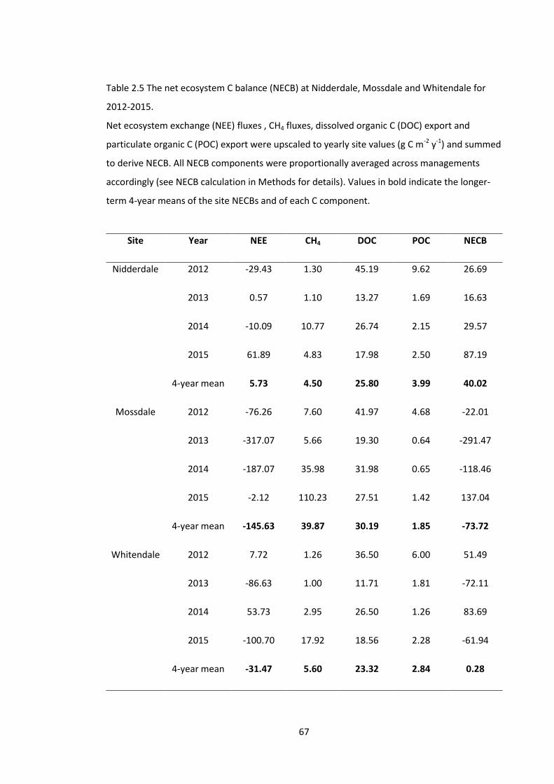
67

Table 2.5 The net ecosystem C balance (NECB) at Nidderdale, Mossdale and Whitendale for

2012-2015.

Net ecosystem exchange (NEE) fluxes , CH4 fluxes, dissolved organic C (DOC) export and

particulate organic C (POC) export were upscaled to yearly site values (g C m-2 y-1) and summed

to derive NECB. All NECB components were proportionally averaged across managements

accordingly (see NECB calculation in Methods for details). Values in bold indicate the longer-

term 4-year means of the site NECBs and of each C component.

Site Year NEE CH4 DOC POC NECB

Nidderdale 2012 -29.43 1.30 45.19 9.62 26.69

2013 0.57 1.10 13.27 1.69 16.63

2014 -10.09 10.77 26.74 2.15 29.57

2015 61.89 4.83 17.98 2.50 87.19

4-year mean 5.73 4.50 25.80 3.99 40.02

Mossdale 2012 -76.26 7.60 41.97 4.68 -22.01

2013 -317.07 5.66 19.30 0.64 -291.47

2014 -187.07 35.98 31.98 0.65 -118.46

2015 -2.12 110.23 27.51 1.42 137.04

4-year mean -145.63 39.87 30.19 1.85 -73.72

Whitendale 2012 7.72 1.26 36.50 6.00 51.49

2013 -86.63 1.00 11.71 1.81 -72.11

2014 53.73 2.95 26.50 1.26 83.69

2015 -100.70 17.92 18.56 2.28 -61.94

4-year mean -31.47 5.60 23.32 2.84 0.28

68

source at each site was not the same every year. In 2012 and 2013, DOC export represented

the largest C loss at all sites but CH4 effluxes released more C at Mossdale in 2014 and 2015,

and the NEE flux released most C at Nidderdale in 2015 and Whitendale in 2014 (Table 2.5). On

average, POC represented the smallest return of C to the atmosphere at all sites but C loss

from POC export was greater than that from CH4 release at Nidderdale and Whitendale in

2012 and 2013 (Table 2.5).

The management NECBs demonstrate that over the three years after management

implementation, both the burnt and mown areas acted as C sources whereas the unmanaged

areas acted as C sinks (Table 2.6). Interestingly, all three of the management groups which

were upscaled also acted as small C sources in 2012 (Table 2.6), which was before

management was carried out. Whilst both burnt and mown areas consistently lost C across

years, unmanaged areas strongly took up C in 2013, gained a moderate amount of C in 2014

and showed only a very small net gain of C in 2015 (Table 2.6).

In the pre-management year, the annual NEE flux of all three management groups was

negative (Table 2.6), indicating that the vegetation was taking up more C than the systems

were losing. This was consistently the case in all years for the unmanaged areas, whereas the

NEE measurements on burnt and mown areas showed a net C loss in the post-management

years (Table 2.6). Interestingly, the burnt NEE fluxes were highest in 2013, the year in which

burning took place, and decreased in the subsequent two years whereas mown NEE fluxes

were a lot lower in 2013 than either 2014 or 2015 (Table 2.6). The largest return of C to the

atmosphere from unmanaged areas was via CH4 effluxes but was via DOC export for burnt and

mown areas (Table 2.6). However, this was not consistent, with mown and unmanaged areas

losing more C as CH4 than DOC in 2015 (Table 2.6). On average, POC export represented the

smallest C loss for all managements, although C loss via POC export was greater than C loss

through CH4 effluxes for all three managements in 2012 and for mown areas in 2013 (Table

2.6).

2.4 Discussion

There was no attempt made to reconcile the differences in burning and mowing methods and

outcomes between the sites as it was deemed that the variation probably encompassed the

range of burning and mowing techniques across Northern England. Therefore, any results

emerging consistently from the burnt and mown areas across all sites were likely to be directly

attributable to the management itself and results where all site values were grouped together

are likely to be applicable to other sites.

69

Table 2.6 The net ecosystem C balance (NECB) for burnt, mown and unmanaged areas for

2012-2015.

Net ecosystem exchange (NEE), CH4, dissolved organic C (DOC) and particulate organic C (POC)

were upscaled to yearly management values (g C m-2 y-1) and summed to derive NECB. All

NECB components were averaged across sites. The DOC and POC components for unmanaged

areas are the averages of values for burnt and mown areas. Values in bold indicate the 3-year

post-management (2013-2015) means of the management NECBs and of each C component.

Management Year NEE CH4 DOC POC NECB

Burnt (FI) 2012 -31.72 2.93 39.23 7.03 17.47

2013 143.47 1.80 15.24 1.13 161.19

2014 126.07 20.25 26.69 1.53 174.54

2015 74.74 13.56 21.29 1.83 111.42

3-year mean 114.76 11.72 21.07 1.50 149.05

Mown (LB) 2012 -18.44 0.74 43.21 6.51 32.02

2013 79.76 0.99 14.28 1.63 96.66

2014 138.96 28.04 30.12 1.18 198.30

2015 129.36 21.73 21.41 2.30 174.79

3-year mean 116.03 16.92 21.94 1.70 156.59

Unmanaged

(DN) 2012 -47.80 6.49 41.22 6.77 6.68

2013 -195.88 2.94 14.76 1.38 -176.79

2014 -92.89 14.36 28.41 1.35 -48.77

2015 -90.77 62.11 21.35 2.07 -5.24

3-year mean -126.51 26.47 21.50 1.60 -76.94

70

2.4.1 CO2 fluxes

The management types which showed high CO2 uptake during Full Light flux measurements

also showed high CO2 release during Reco flux measurements (Figures 2.3 and 2.4). This effect is

likely due to the size of the plants, particularly as the DN plots showed both the greatest

drawdown and release of CO2 in Full Light and dark (Reco) conditions respectively. Larger plants

usually host more leaves, and hence should have a greater photosynthetic capacity, which

would explain the greater CO2 uptake during Full Light conditions. Larger plants also are likely

to produce more respiration, not only from their leaves and roots, but also from

decomposition of leaf and root litter, which is likely to be greater beneath larger plants (Brown

& MacFadyen, 1969).

Interestingly, there was no significant difference in SR fluxes between managements. Although

the lack of a management effect is likely to be because of the removal of the aboveground

vegetation, the SR fluxes still contained litter decomposition (except on the BR and BR+Sph

plots) and belowground autotrophic respiration from plant roots spreading below the cleared

SR circle. Given the lack of difference in SR fluxes between managements and that SR fluxes

were substantially lower than Reco fluxes (Table 2.3), this suggests that it is the aboveground

part of the plants which have the greatest influence on the CO2 fluxes. Dixon et al. (2015)

demonstrated that NEE fluxes were best explained by the height of the Calluna plants on

blanket bogs dominated by Calluna in the South Pennines and Peak District, which would

support this suggestion. However, Dixon et al. (2015) concluded that, where Calluna was

dominant, the NEE flux would almost always result in a net loss of CO2 and that this loss would

increase with Calluna height. In the present study, the difference between the average post-

management DN Full Light and Reco fluxes was 1.79 µmol CO2 m-2 s-1, which was smaller than

the difference between the equivalent averages for any other management (compare Figures

2.3 and 2.4). This suggests that the net CO2 loss does not necessarily increase when taller

Calluna plants are present. Additionally, the NEE component of the NECB should all be positive

if the results of Dixon et al. (2015) were applicable in this study. This was not the case with

only the burnt and mown areas showing positive fluxes, even in 2013, despite any Calluna

regrowth being extremely short (see Chapter 3). The difference between the present study

and that of Dixon et al. (2015) could lie in the area studied: their study was conducted in the

South Pennines and Peak District which have become virtually devoid of Sphagnum mosses

due to historic air pollution, whereas all sites in this study possessed some Sphagnum, as well

as Eriophorum, which would have contributed to C drawdown by photosynthesis.

Alternatively, or additionally, Dixon et al. (2015) inserted their collars into the peat by up to 5

71

cm, probably severing some surface roots and enhancing decomposition, whereas collars in

the present study were only placed on the surface.

It is possible that a difference in temperature caused the differences in NEE fluxes between

sites (Table 2.3), as temperature had a significant effect on both NEE fluxes (Table 2.4),

although, as the difference in annual average temperature between the three sites is only

0.6°C, it is unlikely that it was temperature alone. As PAR also had a significant effect on NEE

fluxes, site differences could have been caused by different light levels occurring during

measurements. However, Nidderdale received most light on average (data not shown) and

took up least CO2 during Full Light measurements (Table 2.4), making this an unlikely cause.

Plant size may also be a contributing factor to the site differences as Mossdale had both the

largest plants (greatest volume) and the highest CO2 uptake and loss for Full Light and Reco

fluxes, respectively (Table 2.3). The substantially higher cover of Sphagnum mosses at

Mossdale compared to the other two sites (see Chapter 3) may have also contributed to

Mossdale having the highest Full Light NEE fluxes, as Sphagnum-dominated peat has been

shown to release less CO2 than peat dominated by other species (Dunn et al., 2015). Whilst

high Sphagnum cover does not explain why Mossdale released most CO2 in the dark, the

greater size of the Calluna plants may have offset the presence of Sphagnum. However, as the

site NEE fluxes were compared across managements, it is likely that the differences in

management techniques between the sites also accounted for some of the measured

difference in the fluxes.

This is emphasised by the three-way interactions between site, management and time period.

The absence of significant differences in NEE fluxes before management implementation gives

credence to the post-management differences occurring as a direct consequence of the

managements. Nidderdale had the most uniform management and indeed there were only

differences between DN NEE fluxes (under both light conditions) and NEE fluxes of all other

managements; there were no differences between any mown or burnt NEE fluxes. Mossdale

and Whitendale had less uniform burns and, accordingly, some FI NEE fluxes differed from NEE

fluxes of some of the mowing managements. Interestingly, both managements which included

Sphagnum addition at Whitendale took up nearly as much CO2 as DN plots during Full Light

measurements and lost nearly as much through Reco. Whilst this may have been due to these

plots regenerating more rapidly than other plots by chance, particularly since this was not

observed at Mossdale or Nidderdale, it hints at some Sphagnum establishment and growth.

There was, however, no noticeable increase in Sphagnum cover on the LB+Sph or BR+Sph plots

on any site.

72

Perhaps of greatest note, is that plots under FI management were the only areas to

consistently lose CO2 during Full Light NEE measurements across the post-management period

(Figure 2.5). As Mossdale appeared to have the most thorough burns and Whitendale the

least, it might be expected that Mossdale FI plots would lose more C than Whitendale FI plots.

This was not the case, with the opposite being true. Ward et al. (2012) found no differences in

NEE fluxes between burnt and unburnt areas of Calluna-dominated blanket bog at Moor

House National Nature Reserve but showed that burning increased the transfer rate of newly

fixed C below ground. As Mossdale was more thoroughly burnt, there were fewer plants

present which were capable of assimilating C compared to Whitendale FI plots, meaning that

belowground respiration was likely to be lower.

Despite not showing significantly different Full Light NEE fluxes from all other managements

when viewed across all sites (Figure 2.3), the consistent C loss from FI plots shows that the

vegetation was slower to recover and regenerate following burning than mowing (FI plots had

more unvegetated ground than any other management; see Chapter 3). However, the NECB

showed that the burnt areas actually lost slightly less C on average over the three years than

the mown areas, largely due to the C lost from the NEE component of the NECB decreasing

every year following burning whereas the C lost via NEE in the mown areas increased.

Although it is not possible to compare the mown NEE fluxes with other studies as, to the

author’s knowledge, there are none on peatlands, the trajectory of the C loss from NEE on the

burnt and mown areas suggests that over a longer time period, the C losses from mown areas

could be substantially greater than from the burnt areas. This could be because, although

Calluna regeneration is slower after fire than after cutting (see Chapter 3), new growth is more

vigorous and will overtake Calluna regrowth of mown areas. Alternatively, vegetation other

than Calluna may also have contributed to the differences in NEE fluxes as burning has been

shown to significantly affect other peatland species (Harris et al., 2011), particularly

bryophytes (Burch, 2008).

2.4.2 CH4 fluxes

Vegetation has also been shown to have a strong association with CH4 fluxes (Couwenberg et

al., 2011; Gray et al., 2013; Lai et al., 2014). Although the areas on which the CH4 fluxes were

measured had had the surface vegetation removed, the belowground plant system was not

directly disturbed and vegetation removal was only from a small (20 cm diameter) circle,

meaning that the vegetation - and management - was still expected to have influenced these

measurement areas. All measurement areas in burnt and mown plots received burnt material

and brash, respectively, in a manner similar to that of the rest of the plot. Additionally,

73

management of moorland vegetation can alter the structure of the soil microbial community

(Ward et al., 2012), which could plausibly affect the CH4 dynamics. Therefore, as both burning

and mowing greatly altered the surface vegetation around the measurement areas, it was

expected that this would also alter CH4 fluxes but there was no significant differences between

managements. This is in contrast to the findings of Ward et al. (2007) who measured lower

CH4 fluxes on burnt compared to unburnt plots. To the author’s knowledge, there are no

studies comparing CH4 emissions on blanket bogs which have been managed by mowing.

However, CH4 emissions from the different mowing managements at all sites spanned such a

wide range of values, including the lowest CH4 flux being measured from a BR+Sph plot and

the highest from a BR plot (both at Mossdale), which therefore encompassed all DN and FI

values, it appears that mowing did not affect CH4 fluxes, at least, not consistently.

A possible reason for this could be not the vegetation removal itself, but that the removal of

vegetation lowered the surface of some of the measurement circles, causing waterlogging.

Higher WTDs and standing water create conditions conducive to CH4 formation (Lai et al.,

2014), yet it was observed that waterlogged areas did not always produce the highest CH4

fluxes and some of the highest fluxes came from measurement areas which were not

waterlogged at all. This suggests that the waterlogging caused by vegetation removal is

unlikely to have greatly elevated the CH4 fluxes.

Further to this, Mossdale showed substantially higher CH4 fluxes than Nidderdale and

Whitendale, was generally established to be the wettest site (i.e. higher precipitation and

WTDs, often with areas of standing water) and therefore WTD was deemed to be the most

likely factor influencing CH4 fluxes. However, although WTD2 was included in the linear mixed

model, it did not have a significant effect on CH4 fluxes again suggesting that waterlogging is

unlikely to have had a great effect on the CH4 fluxes. Soil temperature was also initially

included in the linear mixed model but did not explain sufficient variation in the CH4 fluxes to

be included in the final model. It is surprising that neither temperature nor WTD showed a

significant effect on CH4 fluxes, since the link between these in wetlands is well established

(Liblik et al., 1997; Hargreaves & Fowler, 1998; MacDonald et al., 1998; Lai et al., 2014).

Interestingly, Ward et al. (2007) also did not find a significant effect of WTD on CH4 fluxes in

their study, which was also conducted on a northern England blanket bog which was

dominated by Calluna. Therefore, a long term effect of high Calluna cover, regardless of

whether Calluna shoots are present during measurements, may be to alter the relationship

between WTD and CH4 fluxes. This is particularly pertinent since peatlands typically are a net

source of CH4 (Clymo & Pearce, 1995; Hargreaves & Fowler, 1998; Ward et al., 2007; Gray et

74

al., 2013) whereas some net CH4 oxidation was observed in this study (negative CH4 fluxes),

suggesting alterations in the peatland system. As the month of measurement was the only

variable tested to exhibit a significant effect on CH4 fluxes and fluxes were highest by far in

August, when plant growth rates are typically all high, an increase in root exudates of labile C

for methanogenesis, combined with interaction between plants, temperature and WTD may

help to explain the CH4 fluxes observed.

Part of the reason that the CH4 fluxes between managements and sites did not show

significant differences could be due to the large number of fluxes which were recorded as

zero, although these null fluxes were well distributed between the managements and sites. It

is important to note however, that a flux recorded as zero did not necessarily mean that there

was no CH4 production or oxidation; in most cases, it was the result of a very small flux from

which the variation was too high to produce the required R2 value, but in a few cases, it was

due to a non-linear flux. Additionally, measurements made with the UGGA resulted in higher

average CH4 fluxes overall than those made with cover boxes, which would appear to suggest a

mismatch between the two approaches. However, the discrepancy was not due to the

difference in measurement methods (the two methods were comparable to one another when

deployed one after another on the same areas; A. Heinemeyer, pers. comm.), it was due to the

difference in measurement method resolution: the UGGA recorded CH4 concentrations

approximately every 2 seconds whereas the cover boxes produced five time points over 50

minutes. This resulted in far fewer fluxes being discarded and recorded as zero from the UGGA

than cover box method (52 over 7 full sets of measurements compared to 271 over 8 full sets

of measurements). Therefore, it is likely that there is some error associated with the average

CH4 fluxes and, more importantly, with the upscaled CH4 fluxes. Although it is difficult to

quantify the magnitude and direction of this error, it is likely to be small.

In contrast to the large proportion of CH4 fluxes recorded as zero, there were some

exceptionally high fluxes, including two over 4000 nmol CH4 m-2 s-1. In the dataset

incorporating nearly 5000 chamber measurements of CH4 fluxes complied by Levy et al. (2012)

from 21 sites across the UK, the highest flux is over an order of magnitude smaller. However,

Levy et al. (2012) set 200 nmol CH4 m-2 s-1 as an arbitrary threshold and assumed

measurements over this were due to measurement error or ebullition.

High CH4 measurements were not excluded from the dataset in the present study for a

number of reasons. Whilst it is possible that the extreme values recorded were as a result of

ebullition, the majority of CH4 fluxes which were greater than 200 nmol CH4 m-2 s-1 - of which

there were only 58 out of the 1116 recorded CH4 fluxes across the four years - were measured

75

with the UGGA. When using the UGGA, episodic ebullition events (bubbles) were detected on

site where a rapid increase in CH4 emission was followed by a rapid decrease and these

measurements were repeated, thereby greatly reducing the probability that ebullition events

were recorded. However, steady ebullition could have produced a linear flux during the five

minute chamber closure period which would not have been detected as such. The use of

boardwalks (e.g. as in Cooper et al., 2014) may have reduced the likelihood that walking close

to the plots facilitated the ebullition of CH4 but boardwalks were not used, partly due to

logistics and partly due to the potential of boardwalks to alter or affect surrounding vegetation

(e.g. Lindsay & Ross, 1993). Additionally, steady ebullition may not have been as a result of

movement around the plots forcing CH4 out; changes in air pressure or WTD can also release

CH4 stored within the peat matrix (Glaser et al., 2004; Tokida et al., 2007). By including these

potential ebullition events, the average CH4 fluxes may be higher than most previously

published but may actually be closer to the real fluxes, as small chambers deployed

periodically usually miss recording ebullition (see Baird et al. (2009) for a discussion of

measuring episodic ebullition with static chambers), which can represent a substantial

contribution to the total CH4 flux (Tokida et al., 2007).

Although the highest values are substantially higher than previously published values, they are

of the same order of magnitude as the maximum ‘hotspot’ values as those in Fenner et al.

(2011), who recorded values up to ~1000 nmol CH4 m-2 s-1 on a rewetted peatland. Cooper et

al. (2014) also observed that rewetted peatland sites had ‘hotspot’ areas, where CH4 emissions

greatly increased in some areas but not others. Whilst the peatlands in this study were not

undergoing rewetting, they have a history of management meaning they are not pristine

peatlands and therefore may function in different ways, potentially similar to rewetted

peatlands. In a study investigating effects of management, Ward et al. (2007) noted that CH4

emissions were higher on grazed areas compared to ungrazed, but could not find a reason to

explain why. Similarly, Dinsmore et al. (2009) found 0.5% of their study catchment was

responsible for 12% of its emissions but this did not always relate to rush or sedge dominated

areas. These studies all point to large variability in CH4 fluxes over small scales with the

dominant factors controlling the fluxes being unclear. Excluding high CH4 measurements from

the NECB almost certainly underestimates the true amount of C lost or gained from a

peatland. The plots in this study were not measured for CH4 before being selected. If plots on

superficially similar ground can produce such a wide range of CH4 fluxes, then it is highly likely

that there are other areas across the catchments also producing a similar, perhaps even wider,

range of values. For these reasons, the very high CH4 fluxes measured in this study were not

only included in the analysis of instantaneous site and management fluxes, but were also

76

included in the yearly NECB calculations. Additionally, as the only factor which showed a

significant influence on the CH4 fluxes was the month of measurement, the fluxes were

upscaled using time only as it was not clear whether any other variable would be appropriate

to use on these sites. Therefore, this incorporated the assumption that the whole of each site

was similar to the Calluna dominated areas measured, but all sub-catchments contained areas

dominated by rushes or sedges, usually by streams and ditches, which often produce higher

CH4 emissions than the rest of a site (Evans et al., 2015). Although there appeared to be no

relationship between sedge cover and CH4 fluxes (data not shown), it is possible that sedges

contributed to some of the highest CH4 fluxes.

2.4.3 DOC and POC concentrations and exports

The significant difference in DOC concentrations between the burning- and mowing-

designated catchments pre-management combined with the absence of a difference post-

management (Figure 2.7) suggests that, if there was any true management effect on the DOC

concentrations, this was smaller than the natural difference between the sub-catchments.

However, as the POC concentrations followed the same pattern (Figure 2.8), and the post-

management difference was significant between burnt and mown areas, management may

have impacted upon the DOC concentrations, albeit only weakly. If this were the case, given

that the burnt sub-catchments produced higher DOC and POC concentrations pre-

management and lower concentrations post-management than the mown sub-catchments,

this suggests that burning caused lower DOC and POC concentrations than mowing.

Although there are very few, if any, studies which specifically assess the effect of mowing

peatland vegetation on DOC and POC concentrations, there have been a number investigating

the effects of burning, many of which focus on sites in northern England. In a review of the

impacts of burning on DOC, Holden et al. (2012) noted that, across catchment-scale studies,

burning appeared to cause an increase in water colour, and hence probably DOC

concentrations, although it was not always possible to disentangle the effect of burning from

the high Calluna cover on the areas which were burnt. Nevertheless, Yallop & Clutterbuck

(2009) observed higher DOC concentrations in areas where burning caused bare peat and

Clutterbuck & Yallop (2010) related an increase in humic coloured DOC to the level of

moorland burning in six catchments. The results in the present study contradict these

correlative analyses, with both DOC and POC concentrations in the stream water from burnt

sub-catchments being lower post-management than pre-management. As DOC concentrations

from mown sub-catchments were slightly higher post-management and POC concentrations

only slightly lower than pre-management, this suggests that mowing may be detrimental to

77

water quality. This is of particular importance to water companies, for whom higher DOC

concentrations can pose treatment problems (Singer, 1999; Clay et al., 2012).

A possible reason for the difference between the DOC concentrations from mown and burnt

catchments could be related to nutrient release. Monitoring of water chemistry at Blue Lough

in Northern Ireland, both before and after a large wildfire, revealed a sharp increase in nitrate

concentration post-fire which caused a drop in pH and DOC concentration (Evans et al., 2016).

The prescribed burning in the present study probably produced a similar response to the

wildfire at Blue Lough whereas mowing probably resulted in more nutrients being retained in

the brash and preventing a large change in pH - over time, more nutrients may be released

from the brash which could alter pH and hence DOC concentrations.

In terms of the peatland NECB however, the concentrations of DOC and POC in the stream

water are not necessarily important; instead, it is the total export of DOC and POC which

matters. When considered in the context of global C cycling, it is the ultimate fate of the

exported C which is most important. There is evidence to show that much of the DOC and POC

exported from peatlands in stream water is decomposed to CO2 and CH4 downstream and

released to the atmosphere (Billett et al., 2004; Worrall & Moody, 2014), meaning that DOC

and POC export from peatland should be considered as C loss in the same way as the

terrestrial gas fluxes. The DOC and POC exports from the burnt and mown sub-catchments are

remarkably similar (Table 2.6), despite the differences in concentrations. It is not possible to

conclusively state that whether management in general affects DOC and POC exports, due to

the paired sub-catchment approach meaning that there were no unmanaged sub-catchments

available from which to sample. However, although it should be noted that less than half of

each sub-catchment had actually been subject to management by the end of 2015, the

similarity between the sub-catchment DOC and POC exports suggests that neither

management had a more detrimental or beneficial effect than the other on aquatic C losses.

In contrast, there was a much greater difference in both DOC and POC concentrations (Table

2.3) and exports (Table 2.5) between the sites. Specifically, Whitendale showed much lower

DOC concentrations and exports than the other two sites and the same was true with POC at

Mossdale. As the daily stream flow had little effect on either DOC or POC concentration, it is

unlikely that differences in rainfall and runoff between the sites caused these differences.

However, the lower DOC concentrations and exports could be related to the lower cover of

Calluna (see Chapter 3) as high Calluna cover is associated with higher DOC concentrations

(Vestgarden et al., 2010; Armstrong et al., 2012; Dunn et al., 2015). This might also partially

explain why DOC exports were so much lower at all three sites post-management (Table 2.5)

78

because substantial amounts of Calluna had been removed from all sub-catchments. Similarly,

as Sphagnum cover was substantially higher at Mossdale than at the other two sites (see

Chapter 3), the water flow across the peat may have been slower, reducing erosion and hence

POC concentrations and exports (Evans et al., 2014). However, this does not explain the

substantially lower POC concentrations and exports from all sites and management post-

management as there were no changes in Sphagnum cover (see Chapter 3). Interestingly, DOC

concentration was the only C measurement on which the month of measurement did not have

a significant effect. However, as both DOC and POC concentrations were highest in July, it is

likely that DOC and POC release were affected either by greater activity of plants and soil

organisms (Briones et al., 2010; Wild et al., 2016) or by the warmer and drier conditions

(Freeman et al., 2001a). As the sites are in the same region of northern England and therefore

receive similar weather, the most likely explanation for the observed differences in DOC and

POC concentrations and exports between the sites is a difference in plant composition and

growth, and the associated belowground assemblage.

2.4.4 NECBs

The site NECBs indicate that, over the four years of the study, one site was a C sink, one was a

C source and the third was practically C neutral. It is interesting that the three sites, which

were all superficially similar at the start of the study and were all managed in the same ways

throughout the study, should produce three very different outcomes. Just as pertinent, none

of the site NECBs are consistent between years, and year is not necessarily a predictor of the

magnitude nor direction of the overall C flux. For example, the only year in which Mossdale

lost C - and this loss was substantial (Table 2.5) - was 2015, with Nidderdale also showing its

greatest C loss in the same year, whereas Whitendale took up more C in 2015 than it had lost

in 2012. Given that all three sites are located in north-west England and are therefore subject

to similar climatic conditions, and that all three sites are Calluna dominated, the opposite

direction of the NECBs for different sites in the same years suggests that there are likely to be

unmeasured or even unknown factors influencing the C dynamics on these peatlands.

Annual variability in the NECB has been recorded elsewhere. Dinsmore et al. (2010) calculated

that a lowland peatland in Scotland took up an average of 69.5 g C m-2 y-1. Whilst the site was a

sink for both years used in their study and averaged -28 g C m-2 y-1 over a 10 year period

(Helfter et al., 2015), an earlier study (Billett et al., 2004) found that the same site lost 8.3 g C

m-2 y-1. Whilst there were some methodological differences between the two shorter term

studies, the primary difference was the size of the NEE fluxes. This is also the case in this study

with the NEE fluxes showing the greatest variability of any component of the NECB for all three

79

sites. Other studies have demonstrated a large variability in NEE between years (Lafleur et al.,

2003; Roulet et al., 2007; Ward et al., 2007; Worrall et al., 2009) but none of these measured

the NECB at more than one site, meaning that much of the inter-annual variability was

attributed to changes in the climate whereas, in this study, climate appears less likely to be the

sole cause of the variation. One potential reason for the NEE balance for Mossdale in 2015

being close to neutral could be due to damage of the Calluna plants by either heather beetle

(Lochmaea suturalis (Thomson)) or Phytophthora species. It was noted that substantial areas

of Calluna were browned or reddened and there is evidence showing Calluna dieback

following infestation by either heather beetle (Scandrett & Gimingham, 1991) or Phytophthora

species (Orlikowski et al., 2004), thus decreasing photosynthesis and CO2 uptake. However, it

was not determined whether heather beetles or Phytophthora species were responsible for

this discolouration of Calluna, nor whether this was the specific cause of the reduction in C

uptake during NEE. Given the C uptake via NEE was over 100 times lower at Mossdale in 2015

compared to 2013, more research into the causes of NEE variability and the impacts of heather

beetle and Phytophthora damage is needed.

Conversely to most other studies, DOC export did not always represent the largest C loss at all

sites in all years. This is because some of the CH4 fluxes recorded in this study were an order of

magnitude higher than those recorded or calculated in C budgets in other studies. Dinsmore et

al. (2010) calculated C losses via CH4 to be less than 0.5 g C m-2 y-1, although they did

acknowledge that these values were low for a UK peatland. However, higher values of 2.7 mg

CH4 m-2 h-1 measured in Caithness using an eddy co-variance system (Hargreaves & Fowler,

1998), and of 3.5 mg CH4 m-2 h-1 measured at Moor House (Ward et al., 2007), are still at the

lower end of those recorded in this study. Even average ‘hotspot’ CH4 fluxes of 2.2 mg CH4 m-2

h-1 from gullies at Moor House (McNamara et al., 2008) and of 8.2 mg CH4 m-2 h-1 from ditches

in Wales (Cooper et al., 2014) are substantially lower than the 2015 average (12.6 mg CH4 m-2

h-1) at Mossdale.

These higher CH4 values were prevalent across all sites and managements in 2014 and 2015

when the UGGA was used for measurements. However, as previously mentioned, the

measurement methods used were comparable to each other so it is unlikely that method

alone caused the high variability and high CH4 emissions. Additionally, Mossdale lost over 7 g C

m-2 y-1 via CH4 in 2012 when only cover boxes were used, which is substantially higher than the

2015 CH4 efflux from Nidderdale or the 2014 loss from Whitendale (Table 2.5). Therefore, as

with NEE, factors such as climate and change in vegetation and microbial assemblages may

have played a role in causing the high inter-annual and inter-site variability of the CH4 fluxes.

80

Alternatively, all CH4 fluxes were measured using small static chambers, regardless of the

measurement method. Static chambers are a sensitive method of measurement but are prone

to a host of problems, including pressure effects, flux inhibition through high concentration

build-ups, leaks and spatial variability of gas fluxes (Denmead, 2008). Therefore, the chambers

used in this study, not just for CH4 fluxes but also for NEE fluxes, may have caused errors in the

measurements. Measurement errors or bias related to spatial variability of fluxes are most

likely in this study, especially given the wide range of fluxes on superficially similar plots. If the

measurement circles had higher or lower fluxes compared to the rest of the plot, these

differences would have been multiplied when the annual fluxes were calculated. Techniques

such as eddy covariance solve many of the problems associated with static chambers

(Denmead, 2008), although these are usually costly methods and present the problem of

obtaining reliable results from smaller areas of interest (Baird et al., 2009), such as the

different management areas. Whilst the measurement methods may have introduced errors,

all plots were measured in the same way which reduces the chance that a particular site or

management accumulated more errors than any other.

The NECB for the three different managements also showed considerable inter-annual

variability, partially as they were calculated using measurements from all sites. However, it is

clear that management also affected the NECB. All three managements were small C sources

in the pre-management year (Table 2.6). Although the unmanaged areas lost least C in 2012,

the consistency with which these areas took up CO2 via NEE post-management, compared to

the consistency and magnitude with which the burnt and mown areas lost C through NEE

fluxes, strongly suggests that the DN management was most beneficial in terms of the

peatland NECB.

This is in direct contrast to the findings of Ward et al. (2007) who found that areas at Moor

House which were burnt had a more negative NEE flux (i.e. took up more C) than unburnt

areas. However, although the burnt areas were on a 10 year burn rotation, which is

comparable to this study, the plots were measured nine years into the cycle, whereas this

study currently only extends three years into the burn cycle. Therefore it is likely that the

vegetation was much more established on the burnt Moor House plots and possibly the

Calluna was starting to degenerate on the unburnt plots, whereas the Calluna on the burnt

plots in this study was still very short and at fairly low cover (see Chapter 3). A study by Clay et

al. (2015) investigated more recent burns but also showed burning appeared to increase C

uptake, with young burn scars (1-6 years since burning) tending to have a negative NEE flux.

Nonetheless, when other C losses were included, Clay et al. (2015) demonstrated that all ages

of burn caused C release, which agrees with this study. Additionally, Garnett et al. (2000) used

81

spheroidal carbonaceous particles as a marker in the peat to calculate that areas on a 10 year

burn cycle had an average reduced sequestration rate of 73 g C m-2 y-1 after three burn cycles

compared to unburnt areas. If reduced C sequestration is taken to mean C loss, this value is

much closer to the annual C loss calculated for burnt areas in the present study.

It is not possible to compare the mown NECB to literature values as, to the author’s

knowledge, this is the first C budget calculated for UK peatlands under a rotation mowing

regime. It is, however, possible to compare to the NECB for burnt areas. The most striking

feature is the similarity between the annual burnt and mown NECBs (Table 2.6). The CH4, DOC

and POC values all follow a similar yearly pattern. The main difference is that, after

management implementation, C loss via NEE from the mown areas was lowest directly

following mowing and increased thereafter, whereas that from burnt areas was highest after

burning and C loss declined over the following two years. It is not possible to tell from only

three years of post-management data what the likely trajectory of the NEE fluxes will be,

although C loss from NEE on both burnt and mown areas was lower in 2015 than 2014, hinting

that vegetation was beginning to recover and take up C.

Based on these values, it appears that burning is slightly more beneficial for the peatlands in

terms of C sequestration than mowing. However, no measurements were taken during

management implementation. For mowing, there should not have been any additional C loss

to the usual fluxes as the brash was left (only BR and BR+Sph plots had brash removed and

these mowing management variants were not upscaled). For burning, the majority of the

standing plant biomass was pyrolysed, although a small amount of this remained as charcoal,

and there may also have been some peat lost in the fires. The latter was not possible to

quantify but, from measuring standing biomass on plots before burning (see Chapter 3), 587 (±

155) g C m-2 of Calluna was burnt, with only about 7 g C of that biomass turned into charcoal

(see Chapter 4). Therefore, for a 10 year burn cycle, an additional 58 g C m-2 y-1 should be

added to the NECB for burnt areas. Although biomass was not lost via mowing, tractors were

used to carry out the mowing and therefore the amount of C released from the fuel used

should also be accounted for. Based on fuel usage figures provided by the gamekeepers and

contractors, average emissions for a 10 year management cycle from fuel usage were 14.1 g C

m-2 y-1 for mowing and 1.9 g C m-2 y-1 for burning (butane was used to start the fires and a fire

break was cut using a tractor at Nidderdale in 2013; A. Heinemeyer, pers. comm.). This meant

that for the first three years following management implementation, burnt areas lost more C

than mown areas (209 g C m-2 y-1 and 171 g C m-2 y-1, respectively).

82

2.4.5 Uncertainties and limitations

There is great uncertainty associated with upscaling gas fluxes from small static chambers to

the landscape scale (Fox et al., 2008). This is particularly pertinent in this study due to the large

variations in flux measurements even when sampled on the same day and under similar

conditions. As already discussed, this variation could mean that measurement circles had

higher or lower fluxes than other areas of the plots, potentially giving rise to errors. Static

chambers are also host to a range of other problems which may have also introduced

measurement errors. Additionally, the landscape was heterogeneous but all plots were

focussed on areas which had a high cover of Calluna in 2012, meaning that when fluxes were

upscaled, it was assumed that the fluxes from the plots were representative of the whole site

or management, which is not necessarily the case. Nevertheless, the NECBs were calculated

similarly across all sites and managements and therefore it is likely that any error created in

assuming homogeneity between plot and landscape when upscaling chamber measurements

was similar across catchments, thus justifying comparison between the sites and

managements.

One factor which was not always consistent between managements was the amount of

Calluna in the chamber during measurements. Whilst fluxes were corrected for the differences

in volumes (see Section 2.2.4.1), it was sometimes difficult to place the PAR sensor inside the

chamber without it being shaded by branches in areas where Calluna was very tall and dense.

This was very similar between the plots on a site pre-management but this problem was

removed from all but DN plots post-management, as mowing and burning greatly reduced

Calluna height and density. Therefore, for DN plots, PAR measurements may have been slightly

lower than actual PAR levels meaning that upscaled NEE fluxes may have overestimated the

CO2 uptake. However, given the huge difference in post-management NEE fluxes between the

managed and unmanaged plots, it is highly unlikely that any shading of the PAR sensor would

alter the conclusion that managed areas lose far more C than unmanaged areas.

Despite the streams collecting water from the whole of each sub-catchment and therefore

stream DOC and POC not being subject to the same uncertainties with upscaling as chamber

measurements, the management DOC and POC exports included water from areas under

different managements. Both burnt and mown sub-catchments had areas (over half the sub-

catchment in total) which had not been burnt or mown, meaning that monitoring would need

to continue for longer than the full 10 year rotation in order to measure the effects of only

burning or mowing. Additionally, the unmanaged DOC and POC exports were estimated from

83

the burnt and mown sub-catchments, although this is actually likely to be more accurate due

to this being the dominant management type across the catchments throughout the study.

This study did not quantify all the C inputs and losses of the peatland system. DOC inputs from

precipitation were not measured or estimated, nor were dissolved inorganic carbon (DIC),

dissolved CO2 or dissolved CH4, which are all C species exported in stream water. However, DIC

and dissolved CH4 exports tend to be very small, usually smaller than POC exports (Worrall et

al., 2003b; Billett et al., 2004; Dinsmore et al., 2010), thus only adding a few grams extra to the

annual NECB. Similarly, the DOC inputs from precipitation tend to be very small (Worrall et al.,

2003b; Neal et al., 2005) and therefore may cancel out, or even exceed, the DIC and dissolved

CH4 losses. Although DOC usually represents the largest aquatic C export, there is increasing

evidence that dissolved CO2 in stream water can be an important peatland C loss (Hope et al.,

2001; Dinsmore et al., 2010). As there was little variation in DOC exports and one of the main

aims of this study was to compare the effects of different managements on C fluxes, it is likely

that the dissolved CO2 export also was similar between managements. This is because DOC and

POC in the stream contribute to the dissolved CO2 (Worrall & Moody, 2014) and therefore it is

reasonable to expect their concentrations to be related, although there is some debate as to

the sources contributing to dissolved CO2 and therefore whether it should be included at all in

the NECB (Billett et al., 2015). Nonetheless, it is acknowledged that C loss in the NECBs

presented here may be underestimated by between 2 g C m-2 y-1 (Worrall et al., 2003b) and 23

g C m-2 y-1 (Billett et al., 2015), although these values would not change any site or

management NECB shown here to be a C sink to a C source.

2.4.6 Conclusions

The site NECBs presented here demonstrate that peatlands managed as grouse moors can

represent either a C source or a C sink. Moreover, a single site may not consistently sequester

or release C every year, mainly due to variability in NEE, and similar sites may not necessarily

follow the same yearly pattern as one another. This is an important consideration given that

most studies on peatlands usually consider a single site and often measurements are only

made over the course of a couple of years at most. Additionally, CH4 fluxes made a greater

contribution to the NECB in some years and at some sites than DOC exports did, highlighting

both the huge variability in these fluxes and the lack of knowledge of peatland C fluxes and the

factors influencing them. Gaining long-term datasets of peatland NECB across a number of

sites is thus a necessity in order to fully understand the C dynamics of peatlands, particularly

those which are likely to be subject to disturbances such as management, and to decipher the

controls on the annual variation.

84

Both the plot level C fluxes and the upscaled management NECBs show that DN management

was the most beneficial for the peatlands in terms of C sequestration and, out of the three

managements which were upscaled, was the only one to show a net gain of C. There was very

little difference in the NECBs of burnt and mown areas, although there appeared to be

differences in the time taken for the system to respond, suggesting that management by

either method had a similar effect on the peatland C dynamics. When the loss of the plant

biomass was taken into account, mowing appeared to be a slightly more favourable option to

burning even when tractor fuel consumption was considered. In order to fully assess whether

this is the case long-term and whether C uptake declines as vegetation ages on DN areas, the

effects of management on the peatland NECB need determining over at least one full 10 year

management rotation.

Grouse moors use management to encourage new shoots for grouse to eat. Although new

shoots can grow from adventitious rooting of prostrate stems (MacDonald et al., 1995),

younger Calluna is thought to be more nutritious (Moss, 1967; Savory, 1978). Therefore, if the

aim was to increase C sequestration - or at least minimise C loss - whilst still maintain a healthy

grouse population, ceasing all forms of management may place these two objectives at odds

with one another. There is also the possibility that stopping all management could cause an

increased fuel load, which risks increasing wildfire frequency and intensity (Allen et al., 2013),

although this may depend upon the moisture content of the peat and on the vegetation

present. Sphagnum mosses can aid water storage in the peat (Bain et al., 2011; Evans et al.,

2014) and therefore management which encourages Sphagnum could help to solve both the

problem of an increased fuel load and a lack of new shoots by increasing peat moisture

content and encouraging regeneration by adventitious rooting. Furthermore, photosynthesis

is the only means by which a peatland can take up C, and Calluna quantity and quality is of

utmost importance to the grouse for which the moors are currently managed, meaning that

vegetation dynamics should also be taken into account when considering the benefits and

drawbacks of the different management options.

85

3 Vegetation Matters: Comparing the vegetation dynamics on

three UK peatlands under alternative grouse moor

managements

3.1 Introduction

Boreal and subarctic peatlands contain over one third of the world’s total soil C store(Gorham,

1991; Turunen et al., 2002) and are mainly composed of the dead remains of Sphagnum

mosses (Bain et al., 2011). Bryophytes, including Sphagnum, grow from the tip as the base dies

(Glime, 2007), allowing layers of dead vegetation to build up (Clymo, 1992). A combination of

the large empty hyaline cells in Sphagnum (Lindsay, 2010) and the low hydraulic conductivity

of the amorphous dead matter (Ingram, 1982) creates and maintains high water table depths

(WTDs) and anaerobic conditions. This lack of oxygen retards decomposition, thus creating

layers of semi-decomposed vegetation which constitute peat.

In the UK, much of the peat is found in the uplands in the form of blanket bog, which began

forming after the end of the last ice age between 8,000 and 10,000 years ago as a result of a

wetter climate (Charman, 2002). Changes in the climate alter the water balance of peatlands

(Mauquoy et al., 2002), causing a shift in the assemblage of Sphagnum species, all of which

have different growth and decomposition rates, hence altering peat accumulation rates

(Belyea & Malmer, 2004).

The wide array of hydrological conditions under which Sphagnum species thrive means that

peatlands are relatively resilient to changes in the climate. However, Sphagnum mosses are

wetland species meaning that there are concerns that anthropogenic climate change may

negatively affect peatlands (e.g. Gorham, 1991). There is extensive evidence that drainage by

humans can substantially lower the water table (see Holden et al. (2004) for a review),

increasing oxygen ingress and hence decomposition (Freeman et al., 2001b). The predicted

decrease in summer precipitation, combined with rising temperatures (Murphy et al., 2009), is

expected to have similar effects.

Blanket bogs support unique assemblages of plants (Thompson et al., 1995) and the

vegetation composition can give an indication of the condition of a bog (Natural England,

2010), as each species requires a different set of hydrological conditions. Eriophorum species,

which also contribute to peat formation (Bain et al., 2011), and Sphagnum species can occupy

a wide range of WTDs (depending on the specific species) whilst rushes, sundews (Drosera

species) and bogbean (Menyanthes trifoliata) tend to be found only in wetter areas and dwarf

86

shrubs including bilberry (Vaccinium myrtillus),crowberry (Empetrum nigrum), ling heather

(Calluna vulgaris) and cross-leaved heather (Erica tetralix) tend to dominate drier areas

(Lindsay, 2010). According to a report in 2010 (Natural England, 2010) on the state of English

peatlands, over 50% of blanket bogs did not support peat forming vegetation and the majority

displayed signs of damage. Given the size of the C store and the rarity of this habitat, as well as

its importance in regulating both water quality and quantity (Freeman et al., 2001a; Holden et

al., 2007a; Armstrong et al., 2012; Evans et al., 2014), conservation of and restoration to

actively growing peatlands which can regulate their own water tables is crucial, in order to

avoid exacerbating climate change by C release (Dorrepaal et al., 2009) and to preserve the

breeding habitats of rare birds (Carroll et al., 2011).

As well as drainage and climate change threatening the stability of the long-term storage and

accumulation of C in blanket bogs, burning also alters the WTD and species composition of

peatlands. Although areas of the English uplands have been subject to periodic burning for

centuries to improve sheep grazing (Simmons, 2003), a rise in the popularity of grouse

shooting 100-200 years ago saw an intensification in burning which still continues, with the

area of new burns in the uplands almost doubling between the 1970s and 2000 (Yallop et al.,

2006). Wildfires are a natural phenomenon on peatlands but the prescribed burning

associated with grouse management occurs much more frequently (Allen et al., 2013), usually

on an 8-25 year rotation (Clay et al., 2015). Therefore, although Sphagnum mosses are capable

of recovery following infrequent burning, regular exposure to fire causes damage and drying

(Holden et al., 2007a), which can increase fire intensity (Turetsky et al., 2011). This can

damage and remove other vegetation (Holden et al., 2007a), leading to bare ground, erosion

and C loss (Evans et al., 2006, 2014).

Burning tends to lead to Calluna dominance (although if an incorrect rotation is chosen for the

prevailing conditions, Eriophorum vaginatum or Molinia caerulea can dominate; Grant et al.,

1963; Hobbs, 1984; Lee et al., 2013), which is ultimately the aim, as Calluna is the main food

source for red grouse (Lagopus lagopus scoticus (Latham)). However, Calluna has a high rate of

evapotranspiration (Worrall et al., 2007) which also dries the peat, reducing Sphagnum growth

and recovery (Campeau & Rochefort, 1996). Additionally, although burning can initially

increase the cover of species other than Calluna (Harris et al., 2011), when Calluna plants

mature, the canopy closes over and this can severely reduce the amount of light reaching the

ground (Gimingham, 1960), ultimately reducing species diversity (Harris et al., 2011).

Burning is not only undertaken to increase the cover of Calluna but also to remove old growth

and encourage new shoots. Whilst this is believed to be necessary on drier areas, Calluna

87

growing on deep wet peat can regenerate naturally by layering (i.e. adventitious rooting) of

stems (MacDonald et al., 1995), bringing the necessity of burning for regeneration into

question. Indeed, government guidelines recommend against burning on areas where peat is

deeper than 50 cm (Defra, 2007), although this advice is not always heeded, with an estimated

30% of blanket bogs being burnt (Natural England, 2010). However, burning removes dead

litter and unproductive woody growth, which reduces the risk of wildfire occurrence and

intensity (Albertson et al., 2010; Allen et al., 2013). Additionally, it has long been advocated

that burning produces more nutritious Calluna shoots by releasing the nutrients from the old

growth and making them available for the new plants (Lovat, 1911; Picozzi, 1968).

Both nitrogen (N) and phosphorus (P) are important nutrients for red grouse (Moss, 1969,

1972), particularly for chicks (Savory, 1977) and breeding hens (Moss et al., 1975). There is, in

fact, evidence that grouse selectively feed on Calluna with a high N and P content (Moss, 1972,

1977) and this selection is even more pronounced in chicks than adults (Savory, 1977). As

grouse also prefer to consume Calluna shoots from plants between two and eight years old

(Savory, 1978), this suggests management is necessary to encourage a constant supply of

relatively young Calluna if the aim is to encourage grouse.

However, there are methods of management other than burning, such as mowing, although

relatively little is known about the effects of mowing on vegetation. For Calluna, there is

evidence showing that regeneration after cutting is very similar to that after burning in terms

of height and cover, with the main differences lying in the season of management (Miller &

Miles, 1970) and in the proportions of vegetative regeneration and seed germination (Liepert

et al., 1993). Mowing may also be less damaging to other vegetation, especially Sphagnum

mosses, than burning as the brash left behind may hold moisture and prevent the peat surface

drying out, as well as potentially being incorporated into the peat. Although large quantities of

brash may increase the risk of wildfire, this could be removed and sold for restoration work

elsewhere. However, mowing can necessitate buying expensive machinery or paying

subcontractors and there are concerns that the weight of a tractor on deep bogs could

compact or damage the peat.

This study aimed to assess the effects of different types of Calluna management on the

vegetation dynamics on the blanket bogs in northern England. Changes in vegetation

composition, Calluna height, standing biomass, leaf area index (LAI) and nutrient contents

were investigated over four years on areas which had been burnt or mown. The effects of

leaving or removing brash which had been generated by mowing, as well as the effects of

adding Sphagnum fragments after burning or mowing were also assessed. Additionally, the

88

validity of assessing vegetation composition from photographs was determined. It was

hypothesised that mowing would result in greater Sphagnum cover and less bare ground than

burning, but that there would not be any difference in Calluna cover, height, biomass and LAI

between mown and burnt areas. Burnt areas were expected to have Calluna with a higher

nutrient than mown or unmanaged areas.

3.2 Methods

3.2.1 Study sites and site set-up

Three sites, all located in north-west England, were surveyed (Figure 3.1). The sites were

Nidderdale, Mossdale and Whitendale, which are all described in full in Section 2.2.1. The set-

up of the site was identical to that described in Section 2.2.2 (Figure 3.2), with the exception

that there was an additional plot with added Sphagnum propagules (see Section 2.2.3.3 for

details of Sphagnum addition) in every block within the burnt sub-catchment. Therefore, in the

burning (FI) sub-catchment, each block contained two plots; FI plots were solely burnt and

FI+Sph plots were burnt with Sphagnum propagules added. In the mown catchment, each

block contained five plots; LB plots were mown with the brash left, BR plots were mown with

the brash removed, LB+Sph plots were mown with the brash left and Sphagnum propagules

added, BR+Sph plots were mown with brash removed and Sphagnum propagules added and

DN plots were left uncut as the no management control. Details of burning, mowing and

Sphagnum addition are given in Section 2.2.3. All plots were 5 m x 5 m and were marked out

with wooden corner posts. A 1 m x 1 m sub-plot was marked out in the corner of each plot

(Figure 3.2) with bamboo canes.

3.2.2 Vegetation surveys

3.2.2.1 1 m x 1 m and 5 m x 5 m field surveys

Vegetation surveys were conducted annually at all three sites on consecutive days between

2012 and 2015 in either September or October (see Table 3.1 for dates) due to logistical

reasons. The 1 m x 1 m sub-plots and 5 m x 5 m plots were assessed on each occasion. A 1 m2

quadrat split into 25 equal squares was placed over 1 m x 1 m sub-plot during the surveys to

aid estimation of percentage cover. The 1 m² quadrat was left in place during the survey of the

5 m x 5 m plot to give guidance for percentage estimation.

All plants were identified to the species level and their percentage cover and that of bare

ground and brash were visually estimated. As there was a substantial moss layer beneath the

89



lower maps (from left star to right star) at Whitendale, Mossdale and Nidderdale.

Rights statement: MiniScale® [TIFF geospatial data], Scale 1:1000000, Tiles: GB, Updated: 3

December 2015, Ordnance Survey (GB), Using: EDINA Digimap Ordnance Survey Service,

http://digimap.edina.ac.uk, Downloaded: 2016-09-09 14:35:01.73

90


and four blocks (yellow outline) within each.

Each plot (red outline) is 5 m x 5 m. C plots are in the burning sub-catchment and represent

burnt plots (FI) and the additional C1 plots are burnt plots with added Sphagnum propagules

(FI+Sph). T1-T5 are plots in the mowing sub-catchment and represent mown plots with brash

left (LB), mown plots with brash removed (BR), mown plots with the brash left and Sphagnum

propagules added (LB+Sph), mown plots with the brash removed and Sphagnum propagules

added (BR+Sph) and plots left uncut as a no management (“do nothing”) control (DN). Within

each plot is a corner 1 m x 1 m sub-plot (green square), a circle for repeated CH4

measurements (purple circle), a circle for repeated soil respiration measurements (orange

circle), a circle for repeated NEE measurements (green circle) and a mesh cage containing a

WTD meter and temperature logger (blue circle).

C1

91

Table 3.1 Dates of vegetation surveys and Calluna plant collection at each site, see text for

details of activities.

Pre-management Calluna plants were collected on different dates in the burnt (FI) and mown

(LB) sub-catchments.

Activity Nidderdale Mossdale Whitendale

Vegetation surveys 29th October 2012

30th September 2013

15th September 2014

14th September 2015

30th October 2012

1st October 2013

16th September 2014

15th September 2015

31st October 2012

2nd October 2013

17th September 2014

16th September 2015

Pre-management

Calluna plant

collection

5th March 2013 (FI)

11th April 2013 (LB)

1st March 2013 (FI)

9th April 2013 (LB)

21st February 2013 (FI)

7th March 2013 (LB)

Post-management

Calluna plant

collection

18th August 2015 19th August 2015 20th August 2015

Additional Calluna

plant collection

17th July 2013 18th July 2013 19th July 2013

92

vascular plants particularly pre-management, the overstorey and understorey were recorded

separately. Here the overstorey is taken to mean that which can be seen when viewed from

above. Overstorey cover of all species totalled 100%, understorey cover was less than or equal

to 100% and total cover therefore was between 100 and 200% as no plot had more than two

layers of vegetation. Brash and bare ground cover was included in the overstorey cover where

living vegetation was absent. However, in the understorey layer, brash was only recorded if it

represented whole dead plants (i.e. litter was not included) and bare ground was not recorded

due to some vascular plants being so dense they formed both over- and understorey. All

surveys were conducted by the same three observers.

National vegetation classification (NVC) categories were determined for each management

type at each site in 2012 and 2015 (pre- and post-management) using MAVIS software (DART

Computing & Smart, 2014).

3.2.2.2 Photo resurveys

A photo of each plot was taken during each survey to enable comparison of percentage cover

between on the ground estimates and aerial images. On the 1 m x 1 m plots, a digital camera

with a rotatable screen (Canon E600 with a 18-55 mm lens, Canon, Tokyo, Japan) was held

directly above the plot to take the photograph. On the 5 m x 5 m plots, a GoPro camera

(Hero3, GoPro Inc., San Mateo, CA, USA) was attached to a custom-adapted (Biology

Workshops, University of York) window cleaning pole, which was extendable to 5 m, and

raised over the plots. A smartphone app (GoPro Camera Suite, CameraSuite.org,

Guntramsdorf, Germany) was used to remotely trigger the sensor and to ensure the

photograph encompassed all four corner posts.

For the 1 m x 1 m plot photos, reassessment of percentage cover was aided by the quadrat

dividers. Percentage cover guides (Terry & Chilingar, 1955; Owens & Sergy, 1994) were used to

reassess the 5 m x 5 m plot photos. Only the overstorey vegetation was reassessed, as

photographs could not capture vegetation or ground beneath this layer. The vegetation was

grouped into plant functional types (PFTs) as individual species identification was not reliable,

especially on the 5 m x 5 m plots. The groups were Calluna, Eriophorum, Sphagnum species,

non-Sphagnum mosses, bare ground, brash/dead/burnt material and other species. Where it

was not possible to distinguish between Sphagnum and other mosses, it was recorded as non-

Sphagnum moss.

93

3.2.3 Measuring Calluna standing biomass, height and LAI

3.2.3.1 Collecting Calluna

Pre-management Calluna plants were cut from the 29 cm diameter circles used for net

ecosystem exchange (NEE) measurements (see Section 2.2.4.1.2) before mowing and burning

were carried out (see Table 3.1 for dates). Post-management, the Calluna plants were cut from

a patch the same size as the NEE circle where the Calluna cover was representative of that

across the plot (Table 3.1). The slight difference in location was because pre-management the

plants could be cut directly from the NEE patches as these were scheduled to be burnt or

mown, whereas NEE flux monitoring was ongoing when post-management plants were cut. All

plants were cut with secateurs as close to the stem bases at the peat surface as possible to

gather all the aboveground Calluna biomass (resulting in some stems being cut below the

moss layer). Plants from each plot were bagged separately and the bags sealed to prevent

water loss.

3.2.3.2 Percentage cover and height of Calluna

The percentage cover of Calluna was assessed on each 1 m x 1 m and 5 m x 5 m plot during the

vegetation field surveys in each year meaning that the cover values for the 2012 and 2015

surveys were approximately the cover on the plots when the pre- and post-management

samples were cut, respectively. Calluna height was measured in five places on each plot during

the vegetation surveys and was averaged for each plot in each year.

For the Calluna cut post management, stems were photographed from above when arranged

on a 30 cm diameter flower board and percentage cover was estimated using the same guides

as for the photo resurveys (Terry & Chilingar, 1955; Owens & Sergy, 1994). The height of the

Calluna cut post-management was measured in five places whilst on the flower board and

averaged.

Calluna heights less than or equal to 3 cm were classed as having germinated from seed within

the past year due to the observation that most of the regenerating shoots grew from woody

stems at least 3-4 cm tall. Heights of 4 cm or more were assumed to be either regrowth from

stems existing before management implementation or Calluna plants germinated from seed in

a previous year. Percentage germination was determined for each plot in each year according

to these height classes.

94

3.2.3.3 Fresh, air-dry and oven-dry weights

Samples were split into ‘leafy’ and ‘woody’ portions and weighed. Leaves which were not grey-

brown and desiccated (i.e. were likely to have been alive within the past year) were included in

the ‘leafy’ portion: this was effectively the photosynthetic portion of the plants which had

been active during the majority of the NEE measurement campaigns (see Chapter 2 for NEE

measurement details, dates and results).

The ‘leafy’ and ‘woody’ portions of each sample were left to air-dry fully (for at least 5 days)

after which each portion was re-weighed. Subsamples of approximately 1 g air-dried ‘leafy’

material and 3-4 g air-dried ‘woody’ material were weighed out from each sample. These were

stored in paper bags to prevent moisture absorption. The subsamples were dried in an oven at

65°C until constant weight was achieved. On removal from the oven, the subsamples were

cooled in a desiccator and re-weighed.

3.2.3.4 Leaf area index (LAI)

Before oven-drying, each ‘leafy’ subsample was spread out in a single layer in a clear Perspex

tray and scanned on an Epson Perfection 4870 scanner (Epson America, Inc., Long Beach, CA,

USA). Images were analysed using WinRhizo 1995 software (Régent Instruments Inc., Sainte-

Foy, Québec, Canada) set to TWAIN interface and calibrated for use with leaf area. Some

subsamples were split into two and the areas summed to avoid leaves overlapping in the scan

area (10 cm x 15 cm). Images generated during the scans were checked manually to ensure

detection of all leaves.

3.2.3.5 Correcting LAI for water loss

As most samples were collected within a short period of time, it was not possible to process all

Calluna immediately following cutting. Whilst samples were processed as soon as possible, it

took a month to fully separate and weigh them all. Additionally, as soon as a bag was opened

to separate the sample into ‘leafy’ and ‘woody’, the Calluna began drying out, lost weight and

the leaves shrank. Therefore, additional samples were taken from all three sites (see Table 3.1

for dates) to obtain correction factors for fresh leaf area to calculate LAI.

Samples were double bagged and sealed immediately following cutting to ensure minimal

moisture loss. All samples were weighed on 23rd July 2013 before bags were unsealed. To

obtain full fresh sample weights, bag weights were subtracted once plants had been air-dried.

Each sample was unsealed briefly to remove three ~1 g subsamples of ‘leafy’ material which

were immediately weighed on a fine balance and scanned to obtain fresh leaf area as before

95

(see Section 3.2.3.4). All subsamples were left 4-6 days to air-dry before being re-weighed and

re-scanned. Subsamples were oven-dried at 65°C until a constant weight was achieved as

before for direct comparison between these correction samples and the actual plot samples.

3.2.4 Plant nutrient content

3.2.4.1 Acid digests

The oven dried ‘leafy’ Calluna subsamples from the NEE plots were ground in a ball mill.

Approximately 0.5 g of each ground subsample was weighed on a four point balance and

placed in a Kjedahl tube with 10 ml of 70% nitric acid (AnalaR NORMAPUR® grade, VWR

International LLC, Radnor, PA, USA). A glass marble was placed on top of each tube and tubes

were left overnight. For each block (18 tubes), there was a ‘blank’ consisting of only nitric acid

(i.e. without the Calluna material). The following morning, the tubes were heated by

increasing the temperature by 10°C every 15 minutes in a heating block until 60°C was

reached. Tubes were left at 60°C for 3 hours then heated to 110°C using the same incremental

method. After a further 6 hours, the tubes were removed from the heating blocks and left to

cool overnight.

A small quantity (5-10 ml) of ultra-pure deionised water was added to each tube and swirled

to mix. Each sample was separately filtered through a hardened ashless filter paper (125 mm

diameter, No. 540, Whatman, GE Healthcare Life Sciences, Little Chalfont, UK) into a centrifuge

tube. The marble and Kjedahl tube were also rinsed into the filter paper and the filter paper

was rinsed around with ultra-pure water. The samples were then re-filtered through clean

filter papers into volumetric flasks and each sample made up to 100 ml with ultra-pure water.

Samples were stored in clean centrifuge tubes at room temperature. Acid digests of the pre-

management Calluna were carried out between 13th and 28th May 2015 in three separate

batches and post-management Calluna samples were digested between 14th and 30th October

2015, also in three batches.

3.2.4.2 ICP elemental analysis

All samples were diluted by half to run in an inductively coupled plasma mass spectrometer

(ICP; iCAP 7000 Series ICP spectrometer, Thermo Scientific, Waltham, MA, USA), with 10 ml of

sample mixed with 10 ml of ultra-pure water in clean centrifuge tubes. Blanks and washes

were both nitric acid, which was diluted to the same concentration as that in the samples, and

two washes were run after every 12 samples. A certified reference material (Birch leaf

Standard, CatNo. B2166, Elemental Microanalysis Ltd, Okehampton, UK) was also run between

96

the two washes. Element concentrations were calibrated using 0.5, 1, 2, 5, 10 and 20 ppm

concentrations of a multi-element standard (CertipurR, Merck KGaA, Darmstadt, Germany),

containing K, Na, Ca, Mg, Fe, Al, Mn, Zn, Cu and Pb, which was made up in a nitric acid matrix.

Phosphorus was similarly calibrated using 0.5, 1, 2, 5 and 10 ppm concentrations of a

phosphorus standard containing H3PO4 (CertipurR, Merck KGaA, Darmstadt, Germany). Argon

was used as the carrier gas. Pre-management samples were run in the ICP on 3rd June 2015

and post-management samples on 4th November 2015. Many of the Pb concentrations were

below the machine limit of detection, resulting in negative concentrations being recorded.

Therefore, Pb was excluded from further analyses.

3.2.4.3 C:N analysis

Approximately 50 mg of each ground oven dried ‘leafy’ Calluna subsample taken from the NEE

plots was accurately weighed on a 4 point balance and folded into a tin foil cup (Art-No. 05 000

429, Elementar Analysensysteme GmbH, Hanau, Germany) to form a tight ball. The samples

were analysed using the “Plant500” method in a C:N analyser (vario Macro, Elementar

Analysensysteme GmbH, Hanau, Germany). Standards were glutamic acid and the results were

factored according to the standards. For the pre-management Calluna, C:N analysis was

carried out between 7th May and 18th June 2015. For the post-management Calluna, the C:N

analysis was carried out between 9th November and 2nd December 2015.

3.2.5 Data analysis

There was no visual evidence of successful establishment of Sphagnum from the Beadmoss

pellets (see Sections 3.2.1 and 2.2.3.3 for details of Sphagnum pellet addition). Additionally,

Sphagnum propagules were only added to relevant plots in 2014 whereas burning and mowing

were carried out in 2013.Therefore, for the purposes of analysis, any plots to which Sphagnum

was added were combined with the other plots of the same management (i.e. FI+Sph and FI

plots were grouped, LB+Sph and LB plots were grouped, and BR+Sph and BR plots were

grouped). This resulted in four management groups - burning (FI), mowing with the brash left

(LB), mowing with brash removed (BR) and the unmanaged control (DN) - meaning that, across

sites, there were 12 DN replicates and 24 FI, LB and BR replicates.

All statistical analyses were carried out in R version 3.3.1 (R Core Team, 2016). Following Zuur

et al. (2009), residuals were plotted against fitted values and visually assessed for normality

and homogeneity of variance. Where a transformation was used on the data, residuals of the

transformed data were assessed. Where values are quoted, these represent the mean (± 95%

confidence intervals). The critical p value chosen for significance was 0.05.

97

3.2.5.1 Vegetation surveys - species richness and diversity

Species richness and diversity were calculated for each plot in each year at both plot sizes.

Shannon’s H index was used for diversity and was calculated using the “diversity” function

(“vegan” package”; Oksanen et al., 2016). The exponential was taken of each number returned

by the diversity function to convert these values to the effective number of species, i.e. the

number of equally common species, which can be compared more clearly. Species richness

was calculated as the average number of species per management per year at both plot sizes

using “specnumber” (“vegan” package; Oksanen et al., 2016).

Linear mixed models employing the “lmer” function from the “lmerTest” package (Kuznetsova

et al., 2016) were used separately on the diversity and species richness values. The fixed

effects in the model were management, time period (‘pre-management’ = 2012 and ‘post-

management’ = 2013-5), site, survey scale (i.e. plot size) and the interactions between these. A

random intercept was included for each model, with a nested structure of blocks in sites (to

account for spatial heterogeneity) in years (to account for repeated measurements).

Following the 10-step protocol in section 5.10 of Zuur et al. (2009), variables were dropped

stepwise from each linear mixed effects model and the log-likelihood ratio and AIC value were

used to assess whether a variable should be dropped or kept in the model. For the final

models, the “satterthwaite” option was used to calculate the denominator degrees of freedom

of the F statistics because the different lengths of the time periods caused an unbalanced

design (Spilke et al., 2005). Where differences were significant, the “glht” function with the

“Tukey” option from the “multcomp” package (Hothorn et al., 2008) was used to determine

between which groups the differences occurred.

3.2.5.2 Vegetation surveys - percentage cover

Burnt material was combined with brash/dead Calluna to create a single group to prevent

burnt matter becoming the dominant “species” which separated burnt plots from the other

plots. To simplify the analysis, only total percentage cover data from the 5 m x 5 m plots were

used. The percentage cover data of all species (including bare ground and brash/dead/burnt

material) were transformed using the Hellinger’s distance option of the “decostand” function

in the “vegan” package (Oksanen et al., 2016). The Hellinger transformation was used as it

removed problems arising from plots having more than 100% cover recorded in total, without

altering the weighting given to rare or abundant species (Legendre & Gallagher, 2001).

Redundancy analysis (RDA) is an ordination technique in which the ordination is constrained

by the variables (Kindt & Coe, 2005). RDA was run on the Hellinger transformed vegetation

98

matrix using the “rda” function of the “vegan” package (Oksanen et al., 2016) to assess the

effect of management on the vegetation composition. As the site and block in which the plots

were located and the year of the survey were likely to influence the vegetation cover, these

variables were also applied to the RDA to assess their effect on the vegetation matrix.

However, although forward selection (using the “forward.sel” function in the “packfor”

package; Dray, 2013) showed all these variables to be significant in the same model, the RDA

was run separately for each variable (four models in total) in order to assess the effects of

each variable more clearly. Almost all 2012 (pre-management) observations had high Calluna

cover, resulting in them having nearly identical RDA scores to DN plots from post-management

years, which considerably lowered the amount of variation the model explained. Pre-

management data were therefore excluded from the final analysis to demonstrate the impacts

of each management more clearly.

To facilitate interpretation, the function “cascadeKM” using the Calinski-Harabasz criterion

was used to determine an appropriate number of groups formed by k-means clustering. This

was visually checked using the “kmeans” function. The function “ordihull” was used to add

polygons according to the k-groups onto the RDA. These functions were all from the “vegan”

package (Oksanen et al., 2016).

RDA identifies the main drivers separating plots from each other and k-means partitioning

enables the identification of groups amongst the observations. However, neither allows for

direct testing of specific variables between groups. Therefore, the results of the RDA were

useful in aiding selection of species to investigate further. Eight main species were identified

by the RDA and used for further testing. Additionally, all Sphagnum species, other than S.

fallax which was one of the eight chosen, were summed and tested as an extra ‘species’ (there

were too many zeros to test each species separately).

Linear mixed models were implemented as described for species richness and diversity

(Section 3.2.5.1) with the following exceptions. The Hellinger transformed species percentage

cover data were used to test the effect of management for each of the identified species in

turn. The fixed effects were management and time period, and the interaction between them.

As Calluna and E. vaginatum were the dominant plants and Sphagnum species are arguably

the most important on a peatland, site was also used as a fixed effect for these three models

to determine whether the site-wise differences in management implementation and climatic

conditions affected the changes in plant cover over time more than the managements

themselves. This would then indicate whether these management responses could be

expected in general across other sites or were site specific.

99

3.2.5.3 Photo resurveys

As the photo resurvey data was neither normally distributed nor were the variances equal,

either as a whole or when split by plot size or PFT, and as the field and photo surveys were

paired by plot in each year, a Wilcoxon signed rank test was used, which employed the

“wilcox.test” function with the “paired” option in the “stats” package (R Core Team, 2016).

The test was used on the full dataset to determine whether the percentage cover values

differed between the two methods and also when the data was split by plot size and by PFT to

see whether these influenced the method of surveying.

3.2.5.4 Calluna standing biomass, height and LAI

The oven-dried subsample weights were divided by the air-dried subsample weights and

multiplied by the full air-dried weights to obtain full sample oven-dried biomass for each NEE

flux chamber area. ‘Leafy’ and ‘woody’ portions were calculated separately. As the Calluna cut

from the chamber areas was only from a very small area of the plot, upscaling merely by

multiplying the biomass over the full plot area was not appropriate, particularly post-

management when Calluna cover and height was more variable. Therefore the biomass on

the 5 m x 5 m plots was calculated for the post-management period by the following equation:

𝑃𝑙𝑜𝑡 𝑏𝑖𝑜𝑚𝑎𝑠𝑠 = 𝐵𝑖𝑜𝐶ℎ

𝐴𝑟𝑒𝑎𝐶ℎ×

%𝐶𝑜𝑣𝑒𝑟𝐶ℎ

%𝐶𝑜𝑣𝑒𝑟𝑃𝑙×

𝐻𝑡𝐶ℎ

𝐻𝑡𝑃𝑙× 𝐴𝑟𝑒𝑎𝑃𝑙 Eq.3.1

where Plot biomass is the calculated Calluna biomass on the plot in g, BioCh is the biomass of

the Calluna cut from the chamber area in g, AreaCh is the area the chamber covers in cm2,

%CoverCh is the Calluna percentage cover in the chamber area, %CoverPl is the Calluna

percentage cover in the plot, HtCh is the average height of the Calluna from the chamber area

in cm, HtPl is the average height of the Calluna from the plot in cm and AreaPl is the area of

the plot in cm2.

Plot biomass could not be calculated in the same way for the pre-management period because

no measurements were made in the pre-management period of percentage cover of Calluna in

the chamber, height of Calluna in the chamber or height of Calluna on the 5 m x 5 m plots.

However, as Calluna cover was more uniform in the pre-management period and the cut

Calluna mostly filled the chamber, the amount of C lost during burning on the 1 m x 1 m FI sub-

plots was calculated as:

𝐶𝑎𝑙𝑙𝑢𝑛𝑎 𝐶 =𝐵𝑖𝑜𝐶ℎ

𝐴𝑟𝑒𝑎𝐶ℎ× %𝐶𝑜𝑣𝑒𝑟𝑃𝑙 × 𝐴𝑟𝑒𝑎𝑃𝑙 × %𝐶 Eq.3.2

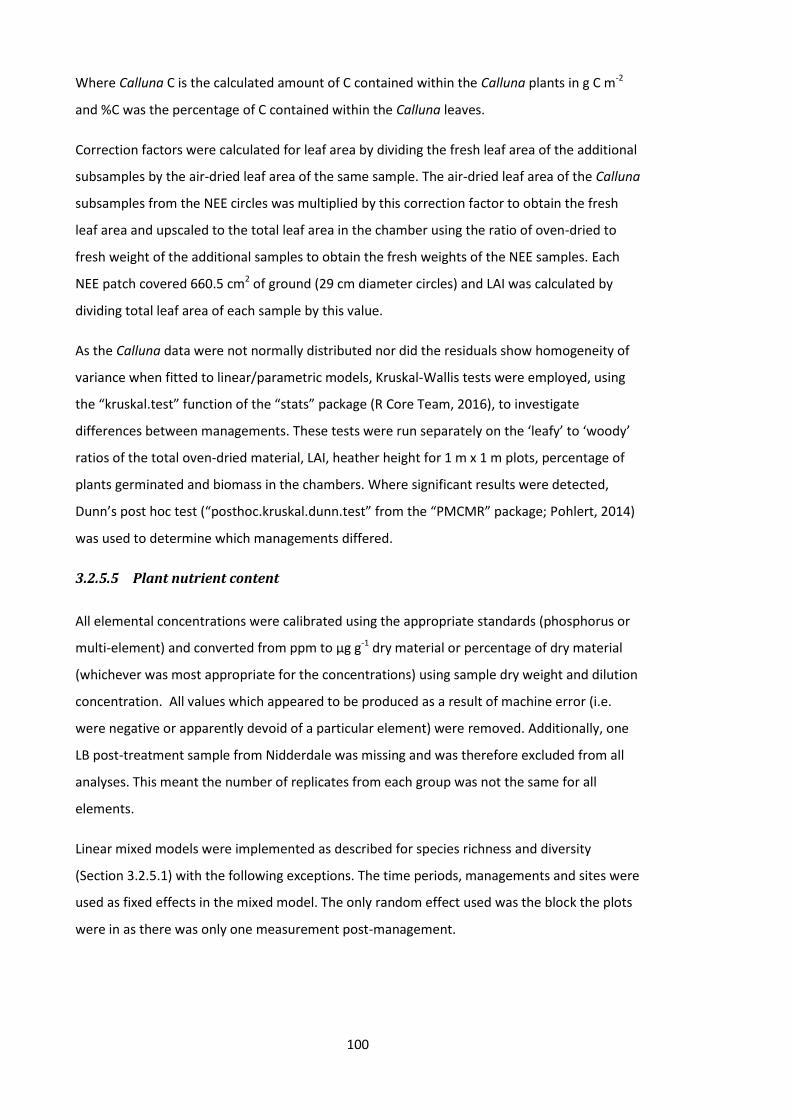
100

Where Calluna C is the calculated amount of C contained within the Calluna plants in g C m-2

and %C was the percentage of C contained within the Calluna leaves.

Correction factors were calculated for leaf area by dividing the fresh leaf area of the additional

subsamples by the air-dried leaf area of the same sample. The air-dried leaf area of the Calluna

subsamples from the NEE circles was multiplied by this correction factor to obtain the fresh

leaf area and upscaled to the total leaf area in the chamber using the ratio of oven-dried to

fresh weight of the additional samples to obtain the fresh weights of the NEE samples. Each

NEE patch covered 660.5 cm2 of ground (29 cm diameter circles) and LAI was calculated by

dividing total leaf area of each sample by this value.

As the Calluna data were not normally distributed nor did the residuals show homogeneity of

variance when fitted to linear/parametric models, Kruskal-Wallis tests were employed, using

the “kruskal.test” function of the “stats” package (R Core Team, 2016), to investigate

differences between managements. These tests were run separately on the ‘leafy’ to ‘woody’

ratios of the total oven-dried material, LAI, heather height for 1 m x 1 m plots, percentage of

plants germinated and biomass in the chambers. Where significant results were detected,

Dunn’s post hoc test (“posthoc.kruskal.dunn.test” from the “PMCMR” package; Pohlert, 2014)

was used to determine which managements differed.

3.2.5.5 Plant nutrient content

All elemental concentrations were calibrated using the appropriate standards (phosphorus or

multi-element) and converted from ppm to µg g-1 dry material or percentage of dry material

(whichever was most appropriate for the concentrations) using sample dry weight and dilution

concentration. All values which appeared to be produced as a result of machine error (i.e.

were negative or apparently devoid of a particular element) were removed. Additionally, one

LB post-treatment sample from Nidderdale was missing and was therefore excluded from all

analyses. This meant the number of replicates from each group was not the same for all

elements.

Linear mixed models were implemented as described for species richness and diversity

(Section 3.2.5.1) with the following exceptions. The time periods, managements and sites were

used as fixed effects in the mixed model. The only random effect used was the block the plots

were in as there was only one measurement post-management.

101

3.3 Results

3.3.1 Vegetation field surveys

Overall, the MAVIS software classified all plots at all sites in 2012 and 2015 as the NVC

category M19a, which is the Erica tetralix subcommunity of the Calluna vulgaris – Eriophorum

vaginatum blanket mire community.

In total, 77 species, including 13 different species of Sphagnum, were found across the three

sites during the four survey years. Some species were found only at one site during one year

whereas others were present at all sites throughout. The species richness differed significantly

between survey scales (F1, 612 = 552.99, p < 0.001), with the 5 m x 5 m plots hosting 14.1

species on average compared to 9.0 species on 1 m x 1 m plots (Figure 3.3). There was also a

significant interaction between site and scale (F2, 612 = 7.10, p = <0.001), with Nidderdale having

fewest species on both 1 m x 1 m sub-plots and 5 m x 5 m plots (7.0 and 11.0, respectively),

Whitendale more (9.4 and 15.1, respectively) and Mossdale the most (10.6 and 16.0,

respectively). There was no significant interaction between management and time period (F3,

612 = 1.95, p = 0.12) although the species richness increased slightly on all managements over

time.

The Shannon’s H diversity index was not significantly different between the survey scales (F1,

611 = 3.70, p = 0.06), but was between the sites (F2, 611 = 71.92, p < 0.001), with Nidderdale

having the lowest diversity. There was a significant interaction between management and time

period (F3, 611 = 4.98, p = 0.002). The diversity increased significantly from the pre-management

to the post-management period on both the FI (p < 0.001) and LB (p = 0.008) plots, with FI

plots having significantly lower diversity than BR and LB plots (p < 0.03 for both) in the pre- but

not post-management period (Figure 3.4). There was no significant interaction between

management, site and period (F6, 586 = 1.04, p = 0.40).

When management was used as the constraining variable in the RDA, 18.9% of the overall

variability of the Hellinger-transformed vegetation matrix (excluding 2012 data) was explained

(adjusted R2 = 0.19, F3, 248 = 20.54, p < 0.001). The first axis separated plots which were

dominated by brash/dead/burnt material from those dominated by Calluna (RDA1 of Figure

3.5). The second gradient separated observations with a high cover of Hypnum jutlandicum

from those with a high cover of Eriophorum vaginatum and, to a lesser extent, Sphagnum

fallax (RDA2 of Figure 3.5). The k-means partitioning satisfactorily divided the 252

observations into three groups (F2, 249 = 70.00, p < 0.001). These groups, when plotted over the

102

Figure 3.3 Mean (± 95% confidence intervals of the mean) of the species richness (i.e. number

of species) for each management group in each year split by plot size.


represents mown plots with the brash removed and LB represents mown plots with the brash

left. Different letters within each time period indicate significant differences between

managements.

103

Figure 3.4 Mean (± 95% confidence intervals of the mean) of the effective number of species,

derived by taking the exponential of the Shannon H index, for each management group in each

year split by plot size.



left. Different letters within each time period indicate significant differences between

managements.

104

Figure 3.5 Redundancy analysis (RDA) of vegetation composition in 2013, 2014 and 2015 (i.e.

post-management) with management as the constraining variable.

Black crosses represent the centroids of the management groups where DN represents

unmanaged, FI represents burnt, BR represents mown plots with the brash removed and LB

represents mown plots with the brash left. Red crosses represent the positions of individual

species. The eight most influential are labelled with the first three letters of the genus name

and species name (for plant species; Bsh_dd is brash/dead/burnt material and Bare is bare

ground). Coloured dots represent the position of each individual plot in a given year where

dark green is for DN, orange is for FI, blue is for BR and pink is for LB. The groups assigned by k-

means partitioning are shown by the polygons.

105

RDA graph, coincided closely with the centroids of the management groups (see Figure 3.5),

effectively creating a burnt, a mown and an unmanaged polygon. These polygons show that

Calluna was the most closely associated species with the ‘unmanaged polygon’, E. vaginatum

was with the ‘mown polygon’ and brash/dead/burnt material was with the ‘burnt polygon’.

Moreover, when the observations were coloured by their actual management, 83% of the DN

observations fitted into the ‘unmanaged polygon’, 82% of the FI plots fitted into the ‘burnt

polygon’ (or were in the small overlap) and 58% of each of the BR and LB observations fitted

into the ‘mown polygon’ (or were in the small overlap).

When year was used as the constraining variable for the RDA, it explained 8.9% of the variance

of the vegetation matrix (Appendix B; adjusted R2 = 0.09, F2, 249 = 13.33, p < 0.001). The first axis

explained most of the variability (92.5%) and plots generally moved from brash/dead/burnt

material in 2013 which were both on the far left to Calluna and E. vaginatum on the right in

2015. Most DN plots remained on the right-hand side for all years. This RDA indicated that the

main change between years was that plots which had been burnt or mown regained

vegetation.

The RDA incorporating site as the constraining variable explained 12.4% of the variability of

the transformed vegetation matrix (Appendix B; adjusted R2 = 0.12, F2, 249 = 18.74, p < 0.001).

The first axis separated Mossdale, which was most closely associated with S. fallax and S.

capillifolium, from the other two which were associated with H. jutlandicum. The second axis

separated Nidderdale, which had more Calluna, from Whitendale, which had more E.

vaginatum and Vaccinium myrtillus.

The blocks to which the plots were allocated also explained a small (3.7%) but significant

(Appendix B; adjusted R2 = 0.04, F3, 248 = 4.20, p < 0.001) amount of the variability of the matrix

when used as the constraining variable of the RDA. However, the species were very clustered

at the centre and it was not clear which species were associated with which blocks.

The eight most influential species/groups identified by the RDA and chosen for further analysis

were Calluna, brash/dead/burnt material, H. jutlandicum, E. vaginatum, E. angustifolium, S.

fallax, bare ground and Campylopus introflexus. Additionally, all Sphagnum species (excluding

S. fallax) were summed and analysed as a single group. Of these nine species/groups, Calluna,

E. vaginatum, bare ground and brash/dead/burnt material showed significant interactions

between management and time period (see Table 3.2 for linear mixed model results). Only E.

vaginatum showed any significant differences in the pre-management period with LB plots

having significantly higher cover than FI plots (Figure 3.6B; p = 0.025). Percentage cover of E.

vaginatum increased significantly from the pre-management to post-management period on

106

Figure 3.6 Mean (± 95% confidence intervals of the mean) percentage cover of A) Calluna

vulgaris, B) Eriophorum vaginatum, C) brash/dead/burnt material and D) bare ground for each

management group in the pre- (2012) and post-management (2013-5) periods for the 5 m x 5

m plots.



left. Different lower case letters within each time period indicate significant differences

between managements.

A

C D

B

107

Table 3.2 Results from linear mixed effects models of the effect of interaction between

management and time period (pre- and post-management) for each vegetation species.

For each model, the F value, the p value and the Satterthwaite approximation of the

denominator degrees of freedom (df), are given. The numerator degrees of freedom = 3 for all

models. Results of post-hoc tests for pairwise comparisons of the managements are also given,

where DN is unmanaged, BR is brash removed, LB is left brash and FI is burnt. Only post-hoc

results from the post-management period are shown (there were no significant differences

pre-management). Significant values are shown in bold.

Species F

value

p

value df

DN to

BR

DN to

LB

DN to

FI

BR to

LB

BR to

FI

LB to

FI

Calluna

vulgaris 42.62 <0.001 271 <0.001 <0.001 <0.001 1.00 0.013 0.10

Brash/dead/

burnt

material

14.97 <0.001 272 <0.001 <0.001 <0.001 0.80 <0.001 0.001

Hypnum

jutlandicum 2.70 0.05 270 - - - - - -

Eriophorum

vaginatum 5.32 <0.001 295 <0.001 <0.001 0.73 0.98 <0.001 <0.001

Eriophorum

angustifolium 1.45 0.23 272 - - - - - -

Sphagnum

fallax 0.30 0.83 270 - - - - - -

Bare ground 8.67 <0.001 271 <0.001 <0.001 0.002 0.013 <0.001 0.11

Campylopus

introflexus 1.83 0.14 272 - - - - - -

All Sphagnum

spp. 0.54 0.66 297 - - - - - -

108

BR and LB plots (p < 0.011) but not on FI or DN plots (Figure 3.6B; p > 0.05). This resulted in BR

and LB plots having significantly higher E. vaginatum cover than DN and FI plots post-

management (Table 3.2; Figure 3.6B). DN plots had significantly higher Calluna cover and

significantly lower cover of brash/dead/burnt material and bare ground than the other

managements (Table 3.2; Figures 3.6A, 3.6B and 3.6C). BR plots also had marginally but

significantly more Calluna than FI plots (Table 3.2; Figure 3.6A). There was also significantly

higher cover of brash/dead/burnt material on FI plots compared to BR and LB plots (Table 3.2;

Figure 3.6A) whereas BR plots had significantly more bare ground than LB and FI plots (Table

3.2; Figure 3.6A).

Nidderdale had higher Calluna cover across all plots post-management than the other two

sites (significant interaction between site and period; F2, 295 = 4.98, p = 0.007) but there was no

significant interaction between management, period and site (F6, 295 = 1.60, p = 0.15), despite

Calluna cover at Whitendale almost halving on DN plots due to frost damage over the winter

of 2012/13. There was a significant different in E. vaginatum cover between sites (F2, 295 =

14.26, p < 0.001), with Whitendale having the highest cover, but no significant interaction

between management, period and site (F6, 295 = 0.67, p = 0.68). Likewise, Sphagnum cover was

significantly different between sites (F2, 297 = 275.67, p < 0.001), with Mossdale having the most

Sphagnum, but no significant interaction between management, period and site (F6, 297 = 0.94,

p = 0.47). Interestingly, Nidderdale had the most Sphagnum species recorded (11 species)

despite having lowest cover (1.5%), whilst Mossdale had the fewest (8 species) but by far the

highest cover (26.8%). Whitendale had low Sphagnum cover (1.7%) with 10 species recorded.

3.3.2 Photo resurveys

There were 84 photos for which Sphagnum and non-Sphagnum moss could not be

distinguished out of a total of 570 photos which contained some form of moss, meaning less

than 15% of moss was unclassified. Although field and photo survey percentage cover

estimates appeared similar (Table 3.3), there was a significant difference between them (V2393

= 1509200, p = 0.022). When the data was split by the plot size, the percentage cover

estimates between field and photo surveys were significantly different for the 5 m x 5 m plots

(V1138 = 354210, p = 0.006) but not for the 1 m x 1 m plots (V1255 = 404060, p = 0.44). There was

a significant difference between field and photo estimates for all species groups (p < 0.02 for

all) but neither estimate was consistently higher for all categories (Table 3.3). Overall, there

was a tendency for groups with low percentage covers to be underestimated in the photos, as

plants were too small to see, and groups with higher percentage cover to be underestimated

in the field, due to the viewing angle of the observer.

109

Table 3.3 Mean percentage cover of Calluna, Eriophorum, Sphagnum, non-Sphagnum mosses,

bare ground, brash/dead/ burnt material and other species determined from the field and

photo surveys split by plot size.

Species group 1 m x 1 m field

survey

1 m x 1 m

photo survey

5 m x 5 m field

survey

5 m x 5 m

photo survey

Calluna vulgaris 26.7 27.2 15.7 15.1

Eriophorum spp. 22.4 23.5 29.6 30.8

Sphagnum spp. 6.0 5.2 5.1 4.0

Non-Sphagnum moss 20.1 16.2 19.9 16.9

Brash/dead/burnt 2.9 2.6 2.6 2.9

Bare ground 21.1 24.5 26.1 29.9

Other spp. 1.0 0.7 1.2 0.3

110

3.3.3 Calluna standing biomass, height and LAI

The average ‘leafy’ to ‘woody’ ratio (i.e. grams of ‘leafy’ material per gram ‘woody’ material)

was over five times higher post-management than pre-management period. The ‘leafy’ to

‘woody’ ratio was only significantly different between managements after management

implementation (Figure 3.7; χ23 = 30.10, p < 0.001), with DN plots having substantially lower

ratios than any other management (p < 0.001 for all). LAI was higher overall in the pre-

management period and showed no differences between managements in this period (Figure

3.7; χ23 = 0.76, p = 0.86). Similarly to the ‘leafy’ to ‘woody’ ratio, LAI was significantly different

post-management (χ23 = 28.74, p < 0.001) with DN plots having higher LAIs than the other

managements (Figure 3.7; p < 0.001 for all).

Calluna was shortest in 2013 directly after mowing and burning and height increased slightly

thereafter. Calluna height was only different between managements in the post-management

period on both the 1 m x 1 m sub-plots (Figure 3.8; χ23 = 30.52, p < 0.001) and 5 m x 5 m plots

(Figure 3.8; χ23 = 124.37, p < 0.001). On both plot sizes, DN plots consistently had significantly

taller Calluna than other plots (Figure 3.8; p < 0.001 for all). On 5 m x 5 m plots, Calluna was

also significantly shorter on FI plots than on LB and BR plots (Figure 3.8; p < 0.001 for all).

No Calluna was classed as germinating from seed in 2012 nor did any germinate on DN plots in

any year (all plants were >4 cm). The percentage of Calluna plants which were classed as

germinated was highest in 2013 and decreased thereafter (Figure 3.9). There were significant

differences in percentage of germinated Calluna plants measured on different managements

on both the 1 m x 1 m sub-plots (Figure 3.9; χ23 = 46.89, p < 0.001) and 5 m x 5 m plots (Figure

3.9; χ23 = 50.39, p < 0.001). On both plot sizes, DN plots had significantly lower germination

than the other managements and FI plots had significantly higher germination than LB plots

(Figure 3.9; p < 0.04 for all). On 5 m x 5 m plots, FI plots also had a significantly higher

proportion of Calluna germinated from seed than BR plots (Figure 3.9; p < 0.001).

On average, the biomass of the Calluna cut from the chambers pre-management was 88.8 (±

11.0) g and did not differ significantly between managements (Figure 3.7; χ23 = 0.89, p = 0.83).

Post-management, the average Calluna biomass cut from the chamber-sized circles on DN

plots was 97.0 (± 24.9) g which was significantly higher than the 6.0 (± 1.4) g cut from burnt

and mown plots (Figure 3.7; χ23 = 29.65, p < 0.001). When post-management Calluna biomass

was scaled up to the full plot sizes, there was 9737 (± 2890) g on the 5 m x 5 m DN plots and an

average of 639 (± 130) g on the BR, LB and FI plots (these managements were combined as

values were very similar). On average, the pre-management FI plots contained 1129 (± 297) g

Calluna biomass m-2. The C content of the corresponding ‘leafy’ material was 52.3 (± 0.1) %

111

Figure 3.7 Mean (± 95% confidence intervals of the mean) of the biomass (split into ‘leafy’ and

‘woody’ biomass, represented by pale and dark grey bars respectively) and leaf area index

(black diamonds) of the Calluna cut from the net ecosystem exchange circles (covering an area

of 660 cm2) for each management group in the pre- (2012) and post-management (2015)

periods.

112

Figure 3.8 Mean (± 95% confidence intervals of the mean) of Calluna height for each

management group by year.



left. Different lower case letters within each year of each survey size indicate significant

differences between managements.

Figure 3.9 Mean (± 95% confidence intervals of the mean) of percentage of Calluna plants

germinated from seed (i.e. were < 3 cm tall) for each management group by year.



left. Different lower case letters within each year of each survey size indicate significant

differences between managements.

113

and was assumed to be similar or greater in ‘woody’ material. This meant that 587 (± 155) g C

m-2 was lost on average during burning.


Nutrient concentrations were mainly higher at all sites after management implementation

than before (see Table C.1 in Appendix C for minimum maximum and average values).

Concentrations of N, K, Na, Ca, Fe, Al, Mn, Zn and Cu in Calluna were significantly different

between sites (see Table 3.4 for p values), with Mossdale having the lowest and Whitendale

the highest concentrations of N, Fe, Al and Cu. Mossdale also had the lowest overall

concentration of Zn in its Calluna but Nidderdale had the highest. Whitendale had the lowest

amount of Ca and Mn in its Calluna with Mossdale and Nidderdale having similar amounts.

Mossdale had highest amounts of K and Na, particularly pre-management, and Nidderdale had

the least. Despite these differences between sites, only Zn showed a difference between sites

in the pre- and post-management periods (F6, 116 = 1.81, p = 0.004; Mossdale had significantly

lower content than the other two sites in the post-management period) and there were no

elements for which the concentrations in Calluna differed significantly between managements

within a site in the different time periods (see Table 3.4).

Nutrient concentrations were more similar between managements before management

implementation than after (see Table C.2 in Appendix C for minimum maximum and average

values). Concentrations of N, P, K, Na, Mg, Al, Mn and Cu were significantly different in Calluna

plants between managements but only in the post-management period (see Table 3.4 for p

values). There were no significant differences between managements for Na and Cu in the

post-management period (p > 0.05 for all). DN plots had significantly lower concentrations of

N, P, K, Mg and Mn than all other managements (Figure 3.10; see Table 3.5 for p values) and

significantly higher concentrations of Al than LB and FI plots. There was no significant

difference in N, P, Mg, Al and Mn concentrations between BR, LB and FI plots but FI plots had

significantly higher Calluna K concentrations than BR or LB plots (Figure 3.10C; see Table 3.5

for p values). The only element which showed a significant interaction between management,

time period and site was Na (Figure 3.10D; see Table 3.5 for p values) but the post-hoc test

revealed that only FI and DN plots differed pre-management (p < 0.001).

3.4 Discussion

Due to logistical reasons, it was not possible to conduct the 2012 vegetation survey until

October. This was not ideal as plants usually begin to senesce and die back by early

September, meaning that it is possible that the cover of some species, particularly grasses and

114

Table 3.4 Results from linear mixed effects models investigating differences in Calluna nutrient

content between the four managements in the pre- and post-management periods

(numerator degrees of freedom = 3) and between the four managements in each of the three

sites in each period (numerator degrees of freedom = 6).

For each model, the F value, the p value and the Satterthwaite approximation of the

denominator degrees of freedom (df) are given. Significant values are shown in bold.

Element

Management: Period

interaction

Management: Period:

Site interaction Site Model

df

F value P value F value P value F value P value

N 12.28 <0.001 0.46 0.83 12.43 <0.001 119

P 5.09 0.002 0.94 0.47 2.70 0.07 115

K 8.06 <0.001 1.47 0.19 3.91 0.023 116

Na 3.76 0.013 2.51 0.026 12.25 <0.001 119

Ca 2.18 0.10 0.66 0.68 8.31 <0.001 116

Mg 3.00 0.034 1.06 0.39 1.89 0.16 115

Fe 1.44 0.23 1.63 0.15 9.85 <0.001 115

Al 3.69 0.014 2.05 0.06 8.88 <0.001 119

Mn 21.22 <0.001 0.78 0.59 3.60 0.030 119

Zn 2.68 0.05 2.06 0.06 18.59 <0.001 116

Cu 3.70 0.012 1.24 0.29 9.05 <0.001 299

115

Table 3.5 Results of post-hoc tests for pairwise comparisons of elemental concentrations

between the managements are given, where DN is unmanaged, BR is brash removed, LB is left

brash and FI is burnt.

Only post-hoc results from the post-management period are shown. Significant values are

shown in bold.

Element DN to BR DN to LB DN to FI BR to LB BR to FI LB to FI

N <0.001 <0.001 <0.001 1.00 0.40 0.12

P <0.001 <0.001 <0.001 0.84 0.26 0.93

K 0.036 0.009 <0.001 1.00 <0.001 <0.001

Mg 0.005 <0.001 <0.001 0.90 0.09 0.65

Al 0.06 0.009 0.031 1.00 1.00 1.00

Mn <0.001 <0.001 <0.001 1.00 0.55 0.46

116

A

F E

C

B

D

117

Figure 3.10 Mean (± 95% confidence intervals of the mean) of A) N content, B) P content, C) K

content, D) Na content, E) Mg content, F) Ca content, G) Fe content, H) Al content, I) Mn

content, J) Zn content and K) Cu content of Calluna for each management group in the pre-

(2012) and post-management (2015) periods.



left. Different lower case letters within each time period indicate significant differences

between managements.

I J

K

H G

118

sedges, may have been underestimated, or that a few species may not have been recorded.

The subsequent vegetation surveys were conducted during late September to maintain

consistency between the years and all plots were surveyed each year within a three day

period. Therefore, any plant cover or species richness errors made due to plant dieback are

likely to be consistent across sites, managements and years, warranting direct comparison.

Additionally, incidental observations made of the vegetation at sites during other

measurement occasions (see Chapter 2) suggest that cover values are unlikely to be

substantially different if the surveys were conducted during the summer months.

3.4.1 Species richness and diversity

All management groups at all three sites both before and after management implementation

were classified as the Erica tetralix subcommunity of the Calluna vulgaris – Eriophorum

vaginatum blanket mire community (NVC sub-group M19a). This both confirmed that the sites

still supported a blanket bog vegetation community and that the sites were very similar to one

another. The result also suggested that the species composition in all managements was

similar.

The species richness confirms that management had little impact on the number of species

(Figure 3.3). The Shannon’s diversity index indicated that there was a small management effect

on the effective number of species (Figure 3.4), i.e. a change in the number and evenness of

species in the plant community. However, most of the significant differences in species

diversity occurred between the management groups before burning and mowing. Despite this,

FI plots had significantly higher diversity post-management than pre-management and no

longer had lower diversity than LB or BR plots, suggesting that burning did increase species

diversity more than any other management (Figure 3.3). This finding is supported by Harris et

al. (2011) who concluded that prescribed (i.e. regular and controlled) burning was needed to

maintain diversity. They also showed that there was an immediate (1-10 years) increase in

species numbers following burning. There was a slight increase in species richness from pre- to

post-management for all managements apart from the 5 m x 5 m DN plots (Figure 3.3). Given

that species diversity also increased from pre- to post-management, this suggests that the

removal of the dominant Calluna resulted in more light and space for understorey plants to

grow (Grace & Woolhouse, 1973), leading to a more even species composition. The slight

increase in number of species on 1 m x 1 m DN sub-plots may have been due to observers

becoming more experienced at searching for species over time and therefore may not have

been a true increase. Alternatively, the substantial decrease in Calluna cover on Whitendale

DN plots due to frost damage during the winter of 2012/13 may have contributed to the

119

increase in species diversity on DN plots (Figure 3.4) and enabled additional species to

colonise.

Regardless of the decline in living Calluna at Whitendale, Calluna at all sites was over 30 cm

tall at the start of the study and DN plots maintained this height throughout (Figure 3.8).

However, Harris et al. (2011) concluded that Calluna should be burnt before reaching 25 cm in

height as other species in areas where Calluna was over 40 cm tall had restricted growth.

Therefore, there should have been very few species on any plot in 2012 and on DN plots

throughout the study, with far higher species richness on post-management burnt and mown

plots. This was not the case (Figure 3.3). It could be that the Calluna on all sites had a

sufficiently open structure (see MacDonald et al. (1995) for a description of different Calluna

growth forms) before management implementation to allow sufficient light to penetrate for

photosynthesis in the understorey (Grace & Woolhouse, 1973) leading to greater productivity

and species richness (Hector et al., 1999). A longer study would be needed to elucidate

whether species richness and diversity declined on the DN plots as Calluna height increased

and whether species richness increased on the burnt and mown plots.

Both species richness and diversity were significantly different between sites. This could be

seen to contradict the finding that all three sites were classified as the same NVC. However,

the NVC only uses a “constancy value” between 1 and 5 for each species (see MAVIS user

guide; DART Computing & Smart, 2014) meaning that each class is relatively broad.

Nevertheless, the differences in species richness and diversity between sites indicate that the

sites were not as similar as they first appeared. Mossdale had the highest diversity and

richness and visually appeared the least heavily managed (there were large areas without

Calluna, although no plots were located in these areas, as well as areas with a Sphagnum

carpet and with no obvious haggs or areas without peat), whilst Nidderdale had the lowest

richness and diversity and appeared the most intensively managed (there was an obvious burn

pattern across the wider site, not just the study catchment, and rocks showed through the

peat in places at the downslope end of the catchment). This suggests that management by

burning may result in a decrease in species richness but only over a longer period of time than

this study covers. However, Mossdale was also the wettest site (mean annual precipitation

(MAP) of 2115 mm) and Nidderdale the driest site (MAP of 1651 mm), meaning that climate

may play a role in regulating species richness and diversity on blanket bogs. Without further

research, it is not possible to conclusively state whether climate or management intensity is

the greater driver of species richness and diversity.

120

3.4.2 Vegetation composition

In contrast to the similarities in species diversity and richness, the species composition

changed over time in some managements. The RDA, combined with the k-means polygons,

showed that the burnt, mown and uncut groups each had a major and minor factor separating

them with another two factors in the overlap between the burnt and mown groups (Figure

3.5). Given that RDAs usually use many variables to attempt to explain changes or differences

in vegetation cover (e.g. Field et al., 2014; González & Rochefort, 2014), it is remarkable that

managements alone, especially when combined across sites and years, explained nearly 20%

of the variability of the vegetation composition. Additionally, this was greater than the

variability explained by site (12.4%), year (8.9%) and block (3.7%). Contrary to the NVC results,

this strongly suggests that management was instrumental in driving changes in species

composition. Considering that a burnt and a mown polygon were clearly identified, these

changes were not solely due to a reduction in Calluna. Other factors such as climate and

landscape features (e.g. slope, aspect, etc.) may also have influenced the vegetation cover but

are far more likely to have acted across all plots on a site, regardless of management.

It is however not necessarily the number nor evenness of species, nor what drives species

composition which ultimately matters for a bog: it is which species are affected that matters

most. As peat represents a vast and stable C store (Gorham, 1991) and is largely composed of

and maintained by Sphagnum moss (Bain et al., 2011), Sphagnum species are arguably the

most important group of plants on blanket bogs. It is generally thought that burning retards

Sphagnum growth, as burning can dry the peat (Holden et al., 2014), and there is evidence

that frequent burning can reduce Sphagnum cover and C uptake (Kuhry, 1994). Additionally,

the high Calluna cover encouraged by burning can increase evapotranspiration, also drying the

peat (Worrall et al., 2007), which can reduce Sphagnum growth and recovery (Campeau &

Rochefort, 1996).

Surprisingly, the results of this study did not show a negative impact of burning on total

Sphagnum cover. Admittedly, S. fallax, which was the only Sphagnum species showing

influence in the RDA (Figure 3.5) and had lower cover on FI plots than any other plots post-

management, but FI plots also had lowest cover of this species pre-management and there

was a small increase in S. fallax cover after burning. Additionally, when the cover of all

Sphagnum species (excluding S. fallax) was combined, Sphagnum cover was relatively constant

across periods in all managements. By chance, FI plots had less Sphagnum cover than DN, BR

or LB plots before management implementation and this cover was maintained even three

years after burning took place. However, longer term monitoring is required to fully assess the

121

effects of burning on Sphagnum cover and to determine whether the brash on LB plots

enhanced Sphagnum growth by protecting Sphagnum fragments and plants from desiccation.

It is interesting to note that there was an inverse relationship between the number of

Sphagnum species and the total cover of Sphagnum. Mossdale had much higher Sphagnum

percentage cover than the other two sites but only 8 species and Nidderdale had the lowest

cover but 11 species. The difference in the cover of Sphagnum species is likely to be related to

moisture since Mossdale was the wettest site (MAP of 2115 mm) and Nidderdale the driest

(MAP of 1651 mm). This theory is supported by Campeau & Rochefort (1996) who found that

all except one (which was not found on any site in the present study) of the Sphagnum species

they investigated had greatly increased cover in wetter conditions. The difference in number

of species may be related to the type of habitat each species prefers since not all species were

found at all sites. For example, S. tenellum is usually found on bare peaty ground or well

drained wet heaths (Amphlett & Payne, 2010a) and this species only occurred at Nidderdale,

probably because the other sites were too wet or because Nidderdale was more disturbed.

Additionally, Breeuwer et al. (2009) found that S. cuspidatum and S. magellanicum responded

conversely to different water table regimes, perhaps explaining why both these species were

only found in localised areas in the present study. However, S. fallax was found at all sites. This

species inhabits a wide range of habitats (Amphlett & Payne, 2010b) which may explain its

distribution and why it appeared unaffected by management (Table 3.2). Due to the low cover

of the other Sphagnum species, which necessitated grouping them for analysis, it is possible

that individual Sphagnum species did respond differently to the various managements, but

that these differences were not detectable at such low cover.

Regardless, retaining Sphagnum is important for blanket bogs. Dunn et al. (2015) showed that

areas of bog dominated by Sphagnum mosses (unspecified mixture) were more beneficial for C

storage than either Juncus effusus or Calluna, as the peat directly beneath released less CO2,

CH4 and DOC. Although in the present study these C fluxes were not specifically measured on

Sphagnum-dominated ground, Mossdale took up more C than the other two sites (see Chapter

2) and had greater Sphagnum cover. High Sphagnum cover is also very beneficial in terms of

water storage and can help to regulate flood waters (Bain et al., 2011; Evans et al., 2014), as

well as being associated with lower DOC concentrations in stream water (Vestgarden et al.,

2010; Armstrong et al., 2012). Ultimately, choosing a management which promotes and

maintains Sphagnum cover and growth will be beneficial for the hydrology and C balance of a

blanket bog (Gorham, 1991; Orwin & Ostle, 2012; Dunn et al., 2015), but further study is

needed in order to determine whether any management assessed here will satisfy these

requirements.

122

E. vaginatum and E. angustifolium are also typical bog species although their importance on

and benefits for a bog are not as clear as those of Sphagnum mosses. On the one hand,

Eriophorum species can take up substantial amounts of C (Bortoluzzi et al., 2006), can

contribute to peat formation (Crowe et al., 2008; Bain et al., 2011) and rapidly colonise bare

peat after disturbance (Crowe et al., 2008), thereby reducing runoff and increasing water

retention time in the peat (Grayson et al., 2010) which could therefore benefit Sphagnum

recolonisation. On the other hand, E. vaginatum can form dense tussocks, which may block

out light beneath, and has aerenchyma which facilitate CH4 release (e.g. Greenup et al., 2000;

Fenner et al., 2011; Cooper et al., 2014) as well as aerating the peat, which may accelerate

decomposition (Freeman et al., 2001b). It is therefore unclear as to whether Eriophorum

species are beneficial for the C balance of a peatland or not, since these species may both

contribute to C accumulation and stimulate C release. As Eriophorum species are typically

found on peatlands which have a net uptake of C (e.g. Roulet et al., 2007; Nilsson et al., 2008),

it is likely that the C accumulation aspects outweigh the C release aspects.

In this study, the majority of plots contained E. vaginatum both before and after management

implementation, with some plots containing E. angustifolium at a much lower cover.

Whitendale had more Eriophorum species than either of the other sites, probably largely due

to this site having least Calluna, which was generally dominant pre-management. E. vaginatum

was the only species for which there was a significant difference in species cover between

managements in the pre-management period with FI plots having lower cover than LB plots.

However, although E. vaginatum cover increased on both FI and LB plots following

management (Figure 3.6B), the much greater increase on LB plots, which was matched by the

increase on BR plots, strongly suggests that mowing encouraged E. vaginatum.

Previous studies (Hobbs, 1984; Lee et al., 2013) have found that E. vaginatum dominated

when burning was on a short (10 year) rotation. Although it appears no studies have

specifically investigated the effects of mowing on Eriophorum species, Milligan et al. (2004)

demonstrated that cutting reduced cover of Molinia caerulea, a moorland grass which often

grows in tussocks. Therefore, it was unexpected that BR and LB plots had higher E. vaginatum

cover than FI plots, especially since it was observed during mowing that the blades removed

the tops of many existing E. vaginatum tussocks. However, E. vaginatum cover did increase on

FI plots following management (Figure 3.6B), as did E. angustifolium cover, although the latter

not significantly so.

The high Calluna cover observed at all sites pre-management (Figure 3.6A) is probably as a

result of the historic burning. At Mossdale, there is evidence in the peat of a large and

123

sustained increase in charcoal fragments over the last 200 years (McCarroll et al., 2015) which

is probably mirrored in other sites across England, including at Nidderdale and Whitendale

(Simmons, 2003; Yallop et al., 2006). The slight decrease in Calluna cover on DN plots from

pre- to post-management (Figure 3.6A) was almost entirely attributable to Whitendale where

living Calluna cover more than halved on some plots over the winter of 2012-3 due to damage

by frost. There was additionally some decrease in Calluna at Mossdale in 2014-5 which was

either caused by heather beetles (Lochmaea suturalis (Thomson)), which can damage Calluna

(Scandrett & Gimingham, 1991), or by Phytophthora species which cause shoot death

(Orlikowski et al., 2004).

Calluna is managed on moorlands in order to encourage new growth for red grouse to eat and

burning has been advocated as the most effective method for at least a century (Lovat, 1911).

Therefore, whilst Calluna cover was expected to be significantly lower on burnt and mown

plots compared to DN plots in the post-management period, what was unexpected was that FI

plots also had significantly lower cover than BR plots and substantially, if not significantly,

lower cover than LB plots (Table 3.2; Figure 3.6A). This suggests that mowing may be more

beneficial for grouse than burning, at least in the first few years. This is in contrast to the

findings of Liepert et al. (1993), who found no difference in Calluna cover between cutting and

burning, and of Cotton and Hale (1994), who concluded that Calluna recovery on areas cut by

a flail lagged behind that of Calluna on burnt areas by about a year. Here, the difference may

lie in the monitoring period as Cotton & Hale (1994) did not begin surveying vegetation cover

until five years after treatments were carried out; in this study, the most recent survey (2015)

was only two and a half years after management implementation.

However, Kayll and Gimingham (1965) assessed vegetative regrowth (i.e. production of shoots

from existing stems) of Calluna plants two months after burning and cutting and found

greater regeneration on cut plants which agrees with the present study. Miller & Miles (1970)

found that autumn burning caused more prolific regeneration than spring burning with the

opposite being true for cut Calluna; regeneration was better after spring than autumn cutting.

All management in this study was carried out in spring so direct comparison is not possible.

However, Calluna regeneration on FI plots at Whitendale was slightly higher than that on both

LB and BR plots. As Miller & Miles (1970) concluded that the damper conditions in autumn

protected the Calluna stem bases from excess heat and as Whitendale was burnt when snow

was lying, this suggests that conditions at the time of burning may be important. Further study

is required to determine whether mowing at particular times of year benefit species other

than Calluna, as well as to assess whether regeneration on FI plots is likely to outperform

124

Calluna growth on BR and LB plots in the future, making monitoring over a full management

cycle vital.

None of the other plant species chosen for further analysis following the RDA showed

significant differences between managements (Table 3.2). However, Campylopus introflexus is

an invasive species (Richards, 1963), which has the potential to influence the dynamics of

other species, in that it has been shown to suppress Calluna seed germination (Equihua &

Usher, 1993). Although not significantly different, C. introflexus cover was higher on BR and LB

plots post-management compared to DN plots and substantially higher on FI plots. The

suppressive ability of C. introflexus on Calluna regeneration therefore appears to provide an

explanation for the lower Calluna cover on FI plots (Figure 3.6A). However, Calluna

regeneration from seed germination was higher on the FI plots than any other plots,

suggesting that either C. introflexus did not have had a suppressive effect or that this effect

was counteracted by fire increasing the germination rate (Mallik & Gimingham, 1985).

Additionally, (Equihua & Usher, 1993) showed that seeds which did germinate on C. introflexus

carpets produced plants which grew taller. This was not the case in the present study as FI

plots had significantly shorter Calluna than the other managements (Figure 3.8). The lack of an

effect of C. introflexus on Calluna height and germination could be because, although there

was more C. introflexus on FI plots than any other plots post-management, the cover still

averaged only 3%. As C. introflexus is a pioneer species of bare ground (Rothero, 2010), more

frequent burning could encourage higher cover which may then impact negatively upon

Calluna dynamics. On the other hand, rapid colonisation of bare ground by C. introflexus could

alter surface roughness and slow down water flow (Grayson et al., 2010) which may in turn aid

Sphagnum recolonization on the wetter ground (Campeau & Rochefort, 1996), benefitting the

hydrology and C store of the peat. Further investigation is required to determine the longer

term effects of increases in C. introflexus on managed peatlands. The higher cover of C.

introflexus on FI plots may partially explain the lower amount of bare ground on these plots

post-management compared to BR and, to a lesser extent, LB plots. Amount of bare ground is

related to both peat erosion (Evans et al., 2006) and high loss of particulate organic C (POC) via

streams (Evans et al., 2014). Evans et al. (2014) showed that the POC flux was linearly related

to the percentage cover of bare peat, where areas with 100% bare ground could lose up to 500

g C m-2 yr-1. Although in this study, there were no plots with 100% bare ground, the higher

amount of bare ground on BR plots potentially means that removing brash after mowing could

have negative effects for the C balance of the underlying peat.

However, as vegetated ground reduces overland water flow in comparison to bare ground

(Holden et al., 2008; Grayson et al., 2010), the substantial amount of ground covered by

125

brash/dead/burnt material should probably be taken into account in the context of erosion

and C loss as, although this would have altered surface roughness, much of this was underlain

by bare ground. When bare ground and brash/dead/burnt material cover estimates were

combined, BR and LB plots had lower cover of non-vegetated ground (28% and 31%,

respectively) than FI plots (39%). There was only a slight difference in DOC and POC

concentrations measured from the burnt and mown sub-catchment streams (see Chapter 2)

but, as the brash/dead/burnt material decomposes and vegetation recolonises bare ground,

these differences may become more pronounced. A longer study would be needed to

determine whether this is the case.

3.4.3 Photo resurveys

There was a significant difference between field and photo estimates of the seven cover

groups (Table 3.3). Given that both methods involved surveying by eye, it is likely that human

error partially contributed to some of the differences. However, only the 5 m x 5 m plots

differed in their cover estimates. This was mainly due to the photo resolution being too low to

accurately distinguish between small species and species at low cover, which was particularly

relevant for Calluna directly following management and for Other species, which were usually

less than 3% in total and often partially hidden under other vegetation. Given that the

estimates made of cover in the 1 m x 1 m photo surveys were similar to those made in the

field, there is real potential to apply this method to engage landowners in habitat monitoring

as well as producing scientifically meaningful data.

Since many landowners and gamekeepers are largely interested in producing grouse and

keeping traditional practices such as burning alive, they may not understand or feel engaged

with scientific monitoring. However, if a monitoring method is simple, they may be persuaded

to conduct a trial on their land, even if just to assess Calluna. One of the main reasons why the

photo resurveys were conducted by eye rather than employing a digital method to quantify

vegetation cover (e.g. pixel spectral classification; Carleer & Wolff, 2004) was because the

photos can be easily obtained using a camera or smartphone and easily analysed by comparing

to percentage cover charts, or simply comparing photos over time, without the need for any

specialised software or even a computer.

There are two main drawbacks to surveying vegetation using photos. Firstly, it is not possible

to identify all species to the species level, which includes most mosses and liverworts. In

principle, this would not be a problem as the primary use would be quantifying Calluna and

typical bog species cover. Secondly, and more importantly, it is only possible to identify and

quantify species to 100% cover. Many moss species, including Sphagnum, grow mainly

126

amongst or beneath the main canopy meaning that it is likely that moss cover would

frequently be underestimated. A potential solution could be to take photographs not only

from above but also from different angles around the sides of a plot. Although the primary

interest of gamekeepers would be to establish the speed and vigour of Calluna regrowth, the

same photos could be collated and assessed by conservation or academic organisations for

changes in Eriophorum and Sphagnum cover, especially since Sphagnum was distinguishable

from other mosses in more than 85% of the photos. Additionally, Peichl et al. (2014) showed

that photos taken with a point-and-shoot digital camera could be used to assess vegetation

phenology by colour analysis and related to the C dynamics.

3.4.4 Calluna standing biomass, height and LAI

Classifying Calluna plants into ‘leafy’ and ‘woody’ portions required some subjectivity,

especially with young Calluna where most stems, even the more rigid lignified ones, were

green. However, any errors in material classification were likely to have been consistent for

plants across all plots.

Calluna on DN plots had a far lower ‘leafy’ to ‘woody’ ratio than the BR, LB or FI plots post-

management. This was due to the Calluna being older and therefore without as much growth

vigour (Gimingham, 1975) as the younger plants, as well as possessing longer and thicker

lignified stems; although some plants on burnt and mown plots regrew from old stems, these

were much shorter having been burnt or cut almost to the ground. A higher ‘leafy’ to ’woody’

ratio may seem beneficial for grouse but the quantity of Calluna leaves was more than seven

times greater on DN plots than any other management. The benefit of management however,

was that most of the unproductive woody growth was removed, lowering the potential fuel

load and reducing the risk of wildfires (Allen et al., 2013).

Additionally, management significantly reduced the LAI (Figure 3.7) which opened up the

canopy, allowing more light to penetrate to the moss layer; whilst this may have induced a

growth response, this would have only been in moss height as the cover values did not exhibit

much change. Typically, LAI values at Moor House National Nature Reserve (NNR), a much-

studied experimental bog with areas managed by burning, were between 1 and 2 (Heal &

Perkins, 1978), which were low compared to the post-management DN plots (2.71) and high

compared to the other managements (0.43 to 0.47). Given that much of the Calluna on BR, LB

and FI plots was removed by management, the low LAI with leaves covering just under half the

ground was unsurprising. Compared to the values in Heal & Perkins (1978), these plots actually

showed a relatively rapid recovery of Calluna since LAI was determined less than three years

after management. The high and relatively stable LAI on the DN plots suggests that the

127

productivity of the Calluna leaves was in balance with the loss of leaves. It also indicates that

the canopy was densely closed, possibly meaning that the upper layers of the canopy were

blocking out the light for the layers beneath (Grace & Woolhouse, 1973). This is unlikely to be

beneficial to plants beneath the canopy such as Sphagnum mosses (Aerts et al., 1990),

suggesting that the management approach of doing nothing (i.e. the DN management), is

unlikely to be useful long term to increase C accumulation or moisture retention. However,

there is evidence to suggest that Calluna on wetter bogs can regenerate by layering

(MacDonald et al., 1995) whereby vegetative trailing stems root whilst the older plant dies

back (Forrest, 1971). Additionally, once Calluna reaches an age of about 30-40 years, gaps

often develop in the canopy (Gimingham, 1975) which may then allow re-establishment of an

understorey. Based on the stable LAI, the Calluna on DN plots appeared not to have reached

this stage but further study would be required to determine whether gaps appeared in the

Calluna canopy in future, as this may negate or lessen the need for management in wetter

areas.

It is of interest that, although there were no differences in LAI or the ‘leafy’ to ’woody’ ratio

between BR, LB and FI plots, there were differences in height. FI plots had shorter plants than

LB and BR plots in all years at both survey scales (Figure 3.8) despite not all differences being

statistically significant. This may be related to the percentage of plants which germinated from

seed as opposed to re-growing from the original stem as FI plots had the highest proportions

(Figure 3.9). Liepert et al. (1993) also found that burnt areas had more Calluna seed

germination whereas mown areas had more vegetative regrowth. However, their results

varied depending on the age of the Calluna before management. Similarly, Miller & Miles

(1970) and Hobbs & Gimingham (1984) found that Calluna re-growing from existing stems

grew with more vigour from stems which were 6-10 years old than any other age, regardless of

whether they had been cut or burnt. What neither study determined was whether this would

be the case for repeated management cycles or whether the growth rate would decline with

each cycle. The age of Calluna in the current study was unknown and was assumed to be

similar across sites but was estimated to be 15-20 years old given its height. This estimated age

may explain the high germination rates (up to 100% of Calluna measured on some plots) and

the relatively low proportion of vegetatively regenerating Calluna in 2013 (Figure 3.9).

Mallik & Gimingham (1985) showed that Calluna seeds germinate better after fire. The

maximum germination from any fire-treated seeds was 76%, compared to their control which

had 58% germination. Although the results in the present study show that FI plots had a higher

proportion of Calluna growing from seed than BR and LB plots (Figure 3.9), there was still

substantial seedling establishment on mown plots. Additionally, when taking into account the

128

higher percentage cover of Calluna on mown plots compared to burnt (Figure 3.6A), the actual

number of plants growing from seed is likely to have been similar. Mallik & Gimingham (1985)

reported that ground temperatures should not exceed 100°C to reduce risk of killing seeds. It

may be that burning exceeded these temperatures on some FI plots, killing seeds and lowering

germination. Given how low this maximum temperature suggested by Mallik & Gimingham

(1985) is and the comparable germination rates observed on BR and LB plots compared to FI

plots, mowing may produce more consistent results in terms of Calluna germination and

regrowth, thereby benefitting grouse.

In terms of C dynamics, the amount of regrowth and the amount of biomass lost is more

important than the method of regrowth. Although only the C content of the ‘leafy’ material

was measured, it was assumed that the ‘woody’ material had a similar or greater C content as

wood contains lignin which is C rich. Any underestimate in C content of the ‘woody’

components however may have been cancelled out by not including biomass of other plants

present on the FI plots in the estimate of C lost through burning. Additionally, some charred

material and ash was left on the plots, meaning burning did not release all the biomass C

(Allen, 1964). Regardless of the precise amount, the figure of 587 g C m-2 in the Calluna

biomass on the FI plots is probably fairly representative of the total amount of C lost. This

represents a substantial amount when compared to the annual C budgets (see Chapter 2).

However, there may also have been some C loss from the brash on the mown plots as this

decomposed but this loss is less immediate and some brash may be overgrown by plants and

become incorporated into the peat. Further investigation is required into the ultimate fate of

the brash.

Moor House NNR is classified as M19b in the NVC system (Rodwell, 1991; Ward et al., 2007)

and all three sites in this study classed as M19a. Therefore, the main vegetation communities

are comparable and all are blanket mires in the north west of England. It was therefore

surprising that the biomass of Calluna recorded in this study was not comparable. Forrest

(1971) recorded values of 665 g m-2 dry Calluna biomass on an area of Moor House which had

not been burnt for 30 years. These values were approximately half as much as those for the

pre-management values presented in this study, although it should be noted that the Calluna

had probably been burnt more recently than 30 years before the pre-management samples

were cut. A more recent estimate by Ward et al. (2007) found that unburnt areas held five

times less biomass than the DN plots. Furthermore, the biomass calculated for FI plots three

years after burning was almost the same as that recorded by Ward et al. (2007) at Moor House

nine years into a 10 year burning cycle. As Moor House is the most studied blanket bog in the

UK, there is the assumption that it is representative of all Calluna-dominated blanket bogs in

129

the UK. The large differences in Calluna biomass suggest otherwise as there was little

difference in the biomass recorded at the three sites in this study. However, this study could

contain errors generated by sampling Calluna from only a small chamber area on each plot and

multiplying up to the plot size using the percentage cover.

For red grouse, the biomass gained is far more important than the amount lost or retained

since Calluna is their main food source (Wilson & Leslie, 1911; Jenkins et al., 1963) and older

Calluna is “valueless as food for grouse” (Wilson & Leslie, 1911) compared to the bright green

new shoots. Unfortunately, although tags were attached to Calluna stems at all sites, it was

not possible to directly derive growth rates due to the majority of these tags being eaten by

sheep. However, there was an increase of almost 300 g m-2 Calluna biomass between pre- and

post-management DN plots which could be taken as the growth rate over the three years. The

burnt and mown plots produced less than half the amount the DN plots did but similar

amounts to each other (121 g m-2 for FI plots; 112 g m-2 for BR plots and 124 g m-2 for LB plots;

see Figure 3.7). This agrees with the study by Liepert et al. (1993) in the North York Moors

National Park, which also found that burnt and cut areas produced similar amounts of Calluna,

although their values were an order of magnitude smaller after the same number of growing

seasons. However, Liepert et al. (1993) determined the regenerating biomass by a

combination of harvesting along a transect and counting density shoots in a small quadrat

which may account for some of the differences. In contrast, values from a study in Scotland

estimated a year’s growth to be slightly more than the three years of growth recorded here,

although this was based on additional shoot production of Calluna which was already at least

five years old. For grouse however, it is not just the quantity of biomass which matters, it is

also the quality.


Moss (1967) noted that there was no change in chemical composition of Calluna over 6 years

old. However, Moss (1967) also showed that the nutrient content of the Calluna varied with

the season, regardless of age, although there were not consistent seasonal changes. As

seasonal variability is probably due to climatic conditions in the locality, this could at least

partially explain some of the differences in the Calluna nutrient content between sites. It may

also explain the small differences in Calluna nutrient content between pre- and post-

management DN plots.

The most striking revelation shown through measuring the plant nutrient content of Calluna

was that, of the six elements which differed significantly between managements (excluding Na

and Cu which had no post-management differences), five of these (N, P, Mg, Al and Mn) did

130

not show any significant differences between the burnt (FI) and mown (BR and LB)

managements post-management (Tables 3.4 and 3.5). Additionally, N, P, K, Mg and Mn had

significantly lower content in Calluna from DN plots than from the managed plots. Although

there were higher Ca concentrations in Calluna plants on FI plots, they were not significantly

higher and reflected the slightly higher pre-management concentrations (Figure 3.10F). The

drop in P content of Calluna on DN plots in the post-management period (Figure 3.10B) may

be as a result of variation between plants selected in the two periods, an effect of season, or it

may be that the Calluna age affected P uptake (Moss, 1969). If the latter was the case, it may

not be advisable to leave Calluna completely unmanaged if grouse production is a concern.

Additionally, Savory (1978) showed that grouse preferred to eat Calluna between two and

eight years old and, from the results shown here, management is more likely to provide this.

Estimates of the amount of Calluna eaten by red grouse range from 63 g d-1 for wild cocks to

100 g d-1 for wild laying hens (Savory, 1974). The only element for which the Calluna differed

significantly between burnt and mown plots was K. Laying hens require higher amounts of

some elements due to the nutrients being used in the creation of eggs (Jenkins et al., 1965). A

wild grouse during egg laying retains (i.e. requires) up to 160 mg K d-1 (Moss, 1977). Therefore,

even though Calluna from the FI managed plots had significantly more K in than Calluna from

the BR management, a grouse eating from the BR management plots would only need to eat

up to 39 g of Calluna each day to satisfy its K requirements. Even eating Calluna from DN plots,

which had significantly lower concentrations than all the other managements, the grouse

would only require 48 g of Calluna per day. This shows that even grouse eating only 63 g

Calluna d-1 would easily consume the necessary amount of K, regardless of the management.

Likewise, using the maximum values required by a laying hen (which are assumed to be the

maximum amounts required and may also be instrumental in breeding success; Jenkins et al.,

1965) reported by Moss (1977) for each element, Calluna from any management would satisfy

the hen’s N, Na, Mg and Ca requirements. DN plots had lower concentrations of all these

elements but even so, a laying hen which solely fed on unmanaged areas would at most

require 50 g of Calluna to satisfy its N requirements, 31 g for Na, 11 g for Mg and 80 g for Ca.

For P, a hen would require 129 g of Calluna if solely feeding on DN plots, which is substantially

greater than the upper estimate of dry matter consumed per day. However, 68 g, 81 g and 74

g of Calluna would be require to meet P requirements if feeding was solely on FI, BR and LB

plots respectively, all of which are within the range of Calluna consumed per day. This suggests

that some form of intervention management is required to recycle some of the P from older

plants and allow new growth to use it.

131

There is evidence that red grouse selectively consume plants with higher N and P contents

(Moss, 1972, 1977) and this selection is even more pronounced in chicks than adults (Savory,

1977). Chicks selected Calluna with an average of 2.32% N and 0.25% P (Savory, 1977). These

values are much higher than the average values on any management here, although seven

plots (out of the 72) contained more N than this. However, chicks are likely to only eat the very

newest tips (Savory, 1977) and the material analysed for burnt and mown plots contained a

mixture of leaves representing three years of growth. Also, the post-management Calluna was

cut in August whereas pre-management Calluna was cut in early spring, which likely affected

the content of some nutrients (Moss, 1967), although should not have affected the differences

between managements within a period. Additionally, although Calluna is the main component

of the red grouse’s diet, both chicks and adults eat other plants and some insects (Savory,

1977). Where available, Vaccinium myrtillius L. is sought after, which has a higher P content

and usually begin growing earlier in spring than Calluna (Moss, 1972). Few studies on red

grouse nutrition have been conducted on moors with high Eriophorum cover, or if they have,

the nutrient content of Eriophorum has not been considered. However, female capercaillie

(Tetrao urogallus) and to some extent willow grouse (Lagopus lagopus), the latter of which is

very closely related to the red grouse, have been shown to select high-N and -P foods,

including the flower buds of Eriophorum vaginatum (Pulliainen & Tunkkari, 1991). Therefore, it

might be worth land managers considering the range and cover of species other than Calluna

when considering management options to benefit their grouse populations.

Post-management, differences in Na, Ca, Fe, Zn and Cu were present between the various

managements to a greater or lesser extent but none was significantly different (Figure 3.10).

Although these elements are important components of diet, different managements do not

appear to produce large or consistent effects on most of them and therefore no particular

management should be selected on the basis that it can control the content of any of these

elements in Calluna. The 3- to 4-fold increase in Mn content however should be considered,

especially since lack of Mn can cause breeding and development problems in poultry and

pheasants (National Research Council, 1994), although as with N and P, it appears that it is

management in general which is required to elevate Mn concentrations rather than specifically

mowing or burning. Given that N and, especially, P are considered to be the most important

nutrients for red grouse (Moss, 1969, 1972, 1977; Savory, 1977), this suggests that, with

regards to red grouse nutrition, there is no reason to prefer either burning or mowing as a

method of Calluna management.

132

3.4.6 Conclusions

There are many aspects of vegetation which have been considered here with regard to

different types of Calluna management. The managements did not affect the species richness

or diversity (Figures 3.3 and 3.4) and the only difference seen in ‘leafy’ to ‘woody’ ratios and

LAI of Calluna plants (Figure 3.7) and the biomass of Calluna (Figure 3.7) was to be expected

since the unmanaged plots differed from the managed. Similarly, DN plots had taller Calluna

due to this not being cut or burnt, although the FI plots had shorter than BR or LB plots (Figure

3.8), which seemed to be as a result of a higher proportion of plants growing from seed after

burning (Figure 3.9).

However, there were differences in the cover of Calluna, E. vaginatum, bare ground and

brash/dead/burnt material between the managements (Figure 3.6). From a grouse shooting

perspective, Calluna cover is the most important since this is the main food source of red

grouse. It was therefore surprising that BR plots had significantly higher Calluna cover than FI

plots, and LB plots also had higher cover than FI plots, which neared significance (Table 3.2),

given that burning is usually advocated as the best form of management for grouse. The higher

cover of E. vaginatum on mown plots regardless of brash removal was less surprising since it is

a typical bog plant and mowing is thought to dry the peat less than burning. Although there

were no differences in Sphagnum cover between managements, in the longer term, E.

vaginatum may provide sheltered and damper areas for Sphagnum plants to grow, but further

monitoring and research are required to determine whether this is the case. The higher

amount of bare ground on BR plots is probably explained by the lower cover of

brash/dead/burnt material through the removal of the mown and mulched material, which

may still be detrimental for water retention and increase surface runoff, thereby causing

erosion of the peat. Overall however, the FI plots had a lower cover of vegetated ground. Of

the six elements which showed differences between the managements, the only difference for

five of these was between DN plots and managed plots. Although K was higher in Calluna from

burnt rather than mown plots, there was still sufficient K for grouse, even during egg laying.

Overall, in terms of C storage, mowing the Calluna and leaving the brash in place (LB

management) appeared to offer the most benefits, as removing brash resulted in higher

amounts of bare ground (BR plots), burning resulted in lower cover of vegetated ground and a

large loss of C from biomass (FI plots), and no management resulted in lower cover of E.

vaginatum (DN plots). In terms of benefits to grouse, Calluna on unmanaged plots had lower

concentrations of the most important nutrients for grouse (N and P) and therefore may have

detrimental effects on the population. In terms of nutrient content of Calluna, there is no

133

advantage to having Calluna with a higher K content and therefore burning need not be

preferred over mowing. Taking into account the cover and height of Calluna, mowing with

brash removal (BR) is most productive, although there is little difference if the brash is not

removed (LB) and this brash may be beneficial longer term with regard to nutrient cycling and

water retention. Additionally, the higher E. vaginatum cover on mown plots increases the

amount of an extra P-rich food source which the grouse may utilise. Although vegetation

dynamics were only assessed for the first three years of the 10 year management cycle,

overall, if the aim is to increase C storage whilst maintaining a grouse population which offers

a shootable surplus, the LB management appears to hold the most benefits. If the aim is solely

to increase C storage, the DN management may prove beneficial in terms of having the

greatest standing biomass and least bare ground, although further monitoring is required to

determine the longer term effects of all types of management on Sphagnum cover and

diversity.

134

4 Getting to the root of the matter: can ericoid fungi break down

recalcitrant organic carbon compounds?

4.1 Introduction

Ericoid fungi can form mycorrhizal symbioses with ericaceous species, such as Calluna vulgaris,

or exist as ‘free-living’ fungi in the soil. When in a mycorrhizal association, they help the plant

to acquire nutrients from the soil and receive C from the plant in return (Read, 1991): this

benefits the growth of both plant and fungus. Ericoid fungi have saprotrophic properties and it

has been demonstrated that they have the capability to break down structural and recalcitrant

components in plant litter and soil including cellulose (Varma & Bonfante, 1994), hemicellulose

(Burke & Cairney, 1998), polyphenols (Varma & Bonfante, 1994) and lignin (Haselwandter et

al., 1990), amongst others. This suggests that even when they are not in mycorrhizal

associations, they help to cycle and release nutrients which can aid plant growth, thereby

reducing the susceptibility of the peat to erosion (Evans et al., 2014).

Likewise, burning can accelerate plant regeneration (Mahmood et al., 2003), as the residue left

behind has a higher content of available nutrients than the soil or unburnt litter. However,

burning can also release waxes or bitumens which partially waterproof the surface (Clymo &

Gore, 1983), increasing surface runoff and dissolved organic carbon (DOC) release. It is

therefore unclear as to the overall effect that burning has on water quality because, although

implicated in increasing DOC concentrations (Clutterbuck & Yallop, 2010), burning does not

necessarily cause consistent increases in DOC or water colour (Holden et al., 2012).

Additionally, as burning is mainly only used on grouse moors in the UK, this cannot explain the

increase in the amount of DOC in, and the water colour of, streams flowing from many peat-

covered catchments since at least 1990 across the northern hemisphere (Stoddard et al., 2003;

Skjelkvåle et al., 2005) and at least 1962 in the UK (Worrall et al., 2003a). Explanations for this

long term trend include droughts (Worrall & Burt, 2004), increasing temperatures (Freeman et

al., 2001a; Worrall et al., 2004), and recovery from acidification as a result of decreasing

nitrate and sulphate deposition (Stoddard et al., 2003; Evans et al., 2005; Monteith et al.,

2007).

This long-term increase in water colour is concerning for water companies, which must abide

by regulations to provide water without colour that is safe for human consumption (Defra,

2016). The main cause of colouration is the humic substances which constitute the more

hydrophobic components of DOC. Humic substances largely comprise humic acids, which are

135

dark brown to black, and fulvic acids, which are pale brown to yellow (Thurman, 1985). DOC

also contains non-coloured substances, consisting mainly of simple hydrophilic compounds

such as carbohydrates, fats, proteins and waxes, which are more easily broken down by

microorganisms so have a shorter residence time than the humic substances (Schnitzer &

Khan, 1972; Thurman, 1985).

DOC is removed from water in treatment plants by adding an amount of coagulant which

varies with the quantity and colour of the DOC in the water. However, whilst this removes the

darker humic acids fairly easily, thus reducing the water colour, it is harder to remove the

fulvic acids and non-coloured substances (Worrall & Burt, 2009). If these substances remain in

the water at high concentrations, the chlorination process used to disinfect drinking water can

result in the formation of disinfection by-products, such as trihalomethanes and haloacetic

acids, which are believed to be carcinogenic (Singer, 1999; Clay et al., 2012). In both moving

and static water bodies in Scotland, Dawson et al. (2009) found a reduction in the proportion

of humic substances in DOC. This is reflected in the long-term increase in the amount of

coagulant needed to be added to water per unit of colour (Worrall & Burt, 2009), suggesting

that the proportions of fulvic acids and non-coloured substances are indeed increasing. This

provides a greater and more expensive challenge to the water companies.

Much of the DOC, which is an important component in peatland C budgets (Roulet et al., 2007;

Nilsson et al., 2008; Dinsmore et al., 2010), that is washed out of catchments decomposes to

CO2 and CH4 further downstream (Billett et al., 2004; Worrall & Moody, 2014). Increasing DOC

concentrations are therefore likely to also increase the downstream gaseous evolutions which,

combined with CO2 and CH4 emissions directly from the peat, could accelerate climate change

and impose negative feedbacks (Davidson & Janssens, 2006).

Climate scenarios for the UK predict hotter temperatures and a decrease in summer rainfall

(Murphy et al., 2009), which are likely to cause lower peatland water tables. It has been

demonstrated both under drier conditions, which allow greater oxygen ingress (Freeman et al.,

2001b), and warmer conditions (Freeman et al., 2001a), that the enzyme phenol oxidase

becomes more active. This enzyme removes phenolic compounds, which are known to inhibit

other enzymes and microbes, thus enabling an increase in biodegradation (Freeman et al.,

2001b) and potentially increasing both DOC and CO2 release.

A changing climate is also likely to cause shifts in plant assemblages, which on northern

peatlands will result in a decline in mosses and other bryophytes to the benefit of vascular

plants (Gallego-Sala & Prentice, 2013). It has been suggested that this is linked to the release

of labile C compounds from vascular plants into the soil (Bragazza et al., 2013). Indeed, there

136

are a number of studies demonstrating the ability of vascular plants to prime decomposition of

older soil C (Fontaine et al., 2007; Hartley et al., 2012; Lindén et al., 2013; Wild et al., 2016).

As evidenced in Chapter 3, Calluna vulgaris is the most common vascular plant found on

grouse moors, due to management encouraging regeneration and germination. There is

growing evidence showing that Calluna is associated with elevated DOC concentrations

(Vestgarden et al., 2010; Armstrong et al., 2012) as well as studies demonstrating the priming

and loss of ancient C by Calluna plants (Walker et al., 2016). Wetter peatlands tend to produce

high CH4 emissions but relatively low CO2 emissions compared to other soils due to high WTDs

excluding many aerobic processes (Lai, 2009). Calluna however, has a high transpiration rate

so can reduce water tables and dry out peat (Worrall et al., 2007), shifting decomposition from

anaerobic to aerobic (Freeman et al., 2001b), which could explain the higher DOC

concentrations and CO2 emissions associated with Calluna plants.

However, much of the organic matter in both the peat (Bosatta & Ågren, 1999) and the

charcoal created from burning (Woolf et al., 2010) is assumed to be stable and recalcitrant

meaning it is unlikely that Calluna plants themselves greatly affect it. Crucially therefore,

ericoid mycorrhizas, whether in association with Calluna roots or not, may utilise their

saprotrophic abilities to break down either peat or charcoal, or both, and therefore be at least

partially responsible for the observed increase in DOC production and water colour (Worrall et

al., 2003a, 2004; Clutterbuck & Yallop, 2010; Armstrong et al., 2012). Additionally, given the

evidence that Calluna plants prime decomposition of ancient C (Walker et al., 2016), it may not

be solely bacteria which are primed, but ericoid mycorrhizas which cause the increase in soil

respiration.

There are three main methods used to determine how much respiration each ecosystem

components contributes: physically partitioning components in an otherwise intact system,

usually by excluding roots; separating and measuring components individually and summing

the fluxes; and using stable (13C) and radioactive(14C) C isotopes (Hanson et al., 2000). The first

two options introduce an element of disturbance, the latter more than the former, resulting in

measurements which do not necessarily reflect those of the original ecosystem or its

component parts. Isotopic methods circumnavigate these problems (Hanson et al., 2000).

The use of C isotopes has been instrumental in the partitioning of autotrophic plant respiration

and heterotrophic respiration that has been stimulated by plant addition (Hahn et al., 2006).

Components enriched in 13C (Wild et al., 2016) or 14C (Haselwandter et al., 1990) can be added

to intact or laboratory systems, for which both the component and system isotopic signatures

are known, and proportional respiration contributions can be derived from the signature of

137

the evolved C. Alternatively, the natural isotopic gradient, measured in %Modern (which is a

relative measure with the baseline being 100 %Modern in 1950), can be used. Due to atomic

bomb testing in the mid-20th century releasing a pulse of 14C (bomb peak 14C) to the

atmosphere, C fixed by photosynthesis since the 1960s has an elevated 14C content, with C

enrichment of approximately 190 %Modern occurring in the mid-1960s (Levin et al., 2008) and

falling to a contemporary level of about 103 %Modern. In contrast, as peat accumulates over

millennia, the basal peat is relatively depleted in 14C compared to the upper layers (Borren et

al., 2004) due to the exponential decay of 14C. The peat profile therefore represents a

continuum of 14C enrichment, with the exception of C fixed since the 1960s, which can be

coupled with mass balance approaches to partition respiration into recently derived CO2,

usually assumed to be that from plants, and older CO2 from soil respiration (Hardie et al.,

2009; Walker et al., 2016).

Here, a pot experiment, which enabled manipulation of ecosystem components, was used to

monitor CO2 and CH4 fluxes and DOC concentrations. This was coupled with 14C measurements

to partition the effects of ericoid fungi, Calluna plants and charcoal on DOC and CO2 fluxes,

with the aim of establishing whether the presence of ericoid fungi affected decomposition,

and hence DOC and CO2 production, by decomposing charcoal, old organic matter in the peat

or both. Specifically, the hypotheses tested were that ericoid mycorrhizal presence within

Calluna roots would a) increase DOC production and CO2 fluxes, b) alter DOC composition and

c) increase the age of DOC and respired CO2. Additionally, that these decomposition effects

would d) differ between a single ericoid fungus (Hymenoscyphus ericae) and a natural mixed

community and e) pots with free-living fungi (i.e. no plant) would also affect DOC and CO2

production rates.

4.2 Methods

4.2.1 Peat preparation

Peat was collected between 1 and 2 m from the top of a peat hagg in the Peak District, which

was expected to have a minimum age of 3000 years based on evidence from (Tallis, 1991). This

was to avoid problems associated with bomb-peak C ages (Evans et al., 2007) and to provide a

strong contrasting age against any recently produced C (e.g. from plant root exudates). Living

roots were removed and pieces of peat with a diameter more than about 3 cm were broken

up. Plastic boxes (64 L capacity; Really Useful Storage Boxes, London), lined with polythene

sacks, were filled with peat to a depth of 30 cm. Filled boxes were gamma-irradiated at 34.5

kGy (Bradford Synergy Health PLC, Bradford). Although a dose of 10 kGy should have been

138

sufficient to destroy the filamentous fungi (Parker & Vincent, 1981), 34.5 kGy was the only

available dose and increased the chance that all fungal spores were rendered inviable. Both

autoclaving and microwaving were considered as sterilisation methods but were deemed

impractical for the quantity of peat required (see Trevors (1996) for details of appropriate

weights and layer thicknesses required for adequate sterilisation). Additionally, autoclaving

releases more nitrates, ammonium and soluble organic matter than gamma-irradiation

(Salonius et al., 1967) and can destroy the soil structure (Trevors, 1996). In order to reduce the

impact gamma-irradiation had on the peat, the soil was air-dried before irradiating to reduce

the release of radiation-induced soluble organic matter as much as possible (Salonius et al.,

1967), which involved mixing to remove moisture. This mixing also homogenised the peat

which was necessary to obtain a consistent average age throughout.

The sterile peat was rehydrated by being submerged in deionised water for 2 weeks in a

laboratory environment to reduce the risk of contamination by fungal spores. The peat was

drained in a 24 cm tinned mesh sieve (Kitchen Craft, Birmingham) and lumps were further

broken up to smaller than 2 cm in diameter. Every sieve full of peat was also rinsed with fresh

deionised water to wash out excess DOC caused by the gamma-irradiation process (Genney et

al., 2000) before peat was placed into plant pots. Finer peat fragments were retrieved by

filtering through pieces of cotton cloth.

4.2.2 Pot preparation

Forty eight 25 cm diameter and 22 cm tall PVC pots (ref: 101; LBS Horticulture Ltd, Colne, UK),

forty eight 32 cm diameter by 4 cm tall saucers (ref: SAU 019; LBS Horticulture Ltd, Colne, UK)

ninety six 11 cm diameter 3 cm tall uPVC collars (Plumb Center, Wolseley UK Ltd, Leamington

Spa, UK) were wiped with a 7.5% calcium hypochlorite solution (Technical grade CaCl2O2,

Sigma-Aldrich Company Ltd., Dorset, UK) and rinsed five times with deionised water to sterilise

them. Pieces of 1 µm nylon mesh (Normesh Limited, Oldham) were glued over the pot

drainage holes (2 cm by 4 cm) with Bostik All Purpose Glue (Bostik Ltd, Stafford) and sealed

around the edges with non-toxic aquarium silicone sealant (Everbuild Building Products Ltd,

Leeds).

Pots were filled in batches of 12 with the sterile washed peat. Filled pots were placed in the

saucers, which were filled with deionised water (pH adjusted to 3.6). This simulated a WTD in

the pots of -18 cm, which was chosen as it was deemed to represent a typical summer WTD on

a blanket bog managed by burning (the WTDs on all three sites studied in Chapters 2 and 3

frequently recorded WTDs below -18 cm between late spring and early autumn). Additionally,

lower WTDs tend to cause increased decomposition due to more aerobic conditions (e.g.

139

Frolking et al., 2011) and it was hoped this would help to provide sufficient C release (in both

water and air) for radiocarbon analysis. A pre-soaked Rhizon soil moisture sampler (pore size

0.15 µm, Rhizosphere Research Products B.V., Wageningen, Netherlands) was inserted

through a hole drilled 18 cm from the top of each pot (so it was just above the WTD) and

sealed in place with the aquarium silicone sealant. For the top of each pot, a pair of sterile

collars was glued together with a 26 cm diameter circle of the 1 µm nylon mesh sandwiched

between. All joins were sealed with aquarium silicone sealant (see Figure 4.1 for schematic of

full pot set-up).

4.2.3 Pre-treatment measurements

Water samples were collected twice from each pot during a five week period (see Table 4.1 for

dates) by attaching 50 ml luer-lock syringes to the Rhizon samplers. The syringes were held

open with a retainer to create a vacuum. The DOC concentrations were determined using a

total carbon analyser (LiquiTOC, Elementar Analysensysteme GmbH, Hanau, Germany). Prior

to analysis, samples were acidified and sparged with oxygen to remove any inorganic carbon.

A five-point calibration was determined with a sodium carbonate and potassium hydrogen

phthalate (SC/KHP) solution and standards of 50 ppm SC/KHP were regularly analysed during a

machine run to reduce machine drift and errors. All samples were analysed in duplicate. The

absorbency of the water samples was measured in a 1 cm wide quartz cell at 254, 400, 465

and 665 nm (Abs254, Abs400, Abs465 and Abs665) using an ultra-violet spectrophotometer

(Lambda 25 UV-Vis spectrophotometer, PerkinElmer Ltd, Beaconsfield, UK), with a blank

(deionised water) reading subtracted from each sample.

An infrared gas analyser (IRGA; Model 8100, Li-Cor, Lincoln, NE, USA) and an Ultraportable

Greenhouse Gas Analyser (UGGA; Model 915-0011, Los Gatos Research, Inc., San Jose, CA,

USA) were connected in sequence to a 10 cm automated survey chamber (Model 8100-102, Li-

Cor, Lincoln, NE, USA) to allow for simultaneous CO2 and CH4 measurements. Although the

UGGA is able to measure both CO2 and CH4, the IRGA was connected in order to enable the

chamber to be raised and lowered, thus pinpointing the exact measurement periods, which

aided derivation of the fluxes. The chamber was placed over the top collar, which had been

pressed onto the peat surface, and fluxes measured for a 90 s period on four occasions during

a three week period (see Table 4.1).

On 29th January 2015, all pots were weighed to the nearest gram during the gas

measurements, having been watered to excess with pH-adjusted (pH 3.6) deionised water 12

hours before. The offset from the top of the pot to the peat surface was also measured to the

nearest half centimetre. On 30th January, a teaspoonful of peat was removed from the

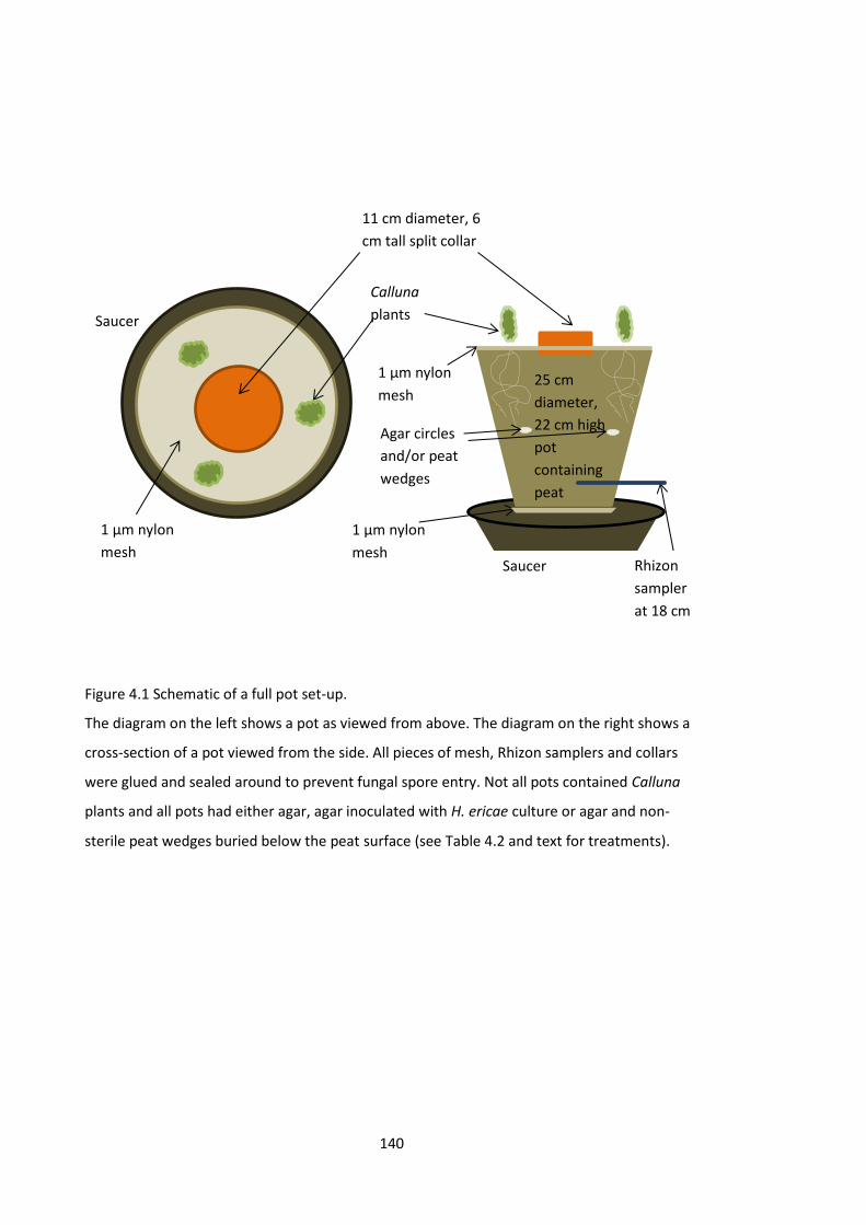
140

Calluna

plants

11 cm diameter, 6

cm tall split collar

25 cm

pot

Saucer

25 cm

diameter,

22 cm high

pot

containing

peat

Rhizon

sampler

at 18 cm

1 µm nylon

mesh

Saucer

Agar circles

and/or peat

wedges

1 µm nylon

mesh

1 µm nylon

mesh

Figure 4.1 Schematic of a full pot set-up.

The diagram on the left shows a pot as viewed from above. The diagram on the right shows a

cross-section of a pot viewed from the side. All pieces of mesh, Rhizon samplers and collars

were glued and sealed around to prevent fungal spore entry. Not all pots contained Calluna

plants and all pots had either agar, agar inoculated with H. ericae culture or agar and non-

sterile peat wedges buried below the peat surface (see Table 4.2 and text for treatments).

141

Table 4.1 Dates (all in 2015) when plant pots were measured for CO2 and CH4 and when water

samples were collected from the pots.

Water samples were tested for DOC and absorbency at various wavelengths (see text) with

one month of collection. No CH4 samples were collected for 14C analysis.

Measurement set CO2 measurements CH4 measurements Water samples

Pre-treatment

measurements (all

2015)

22nd January

29th January

30th January

5th February

22nd January

29th January

30th January

5th February

19th January

11th February

Post-treatment

measurements (all

2015)

12th August

13th October

6th November

10th November

19th November

12th August

13th October

6th November

10th November

19th November

12th August

13th October

9th November

13th November

19th November

14C sample

collection (all 2015)

14th October*

15th–16th October

19th October

-

Continuous multiple

collections between

20th and 26th October

*No CO2 sample collection for radiocarbon analysis was made on 14th October; the CO2 fluxes

measured on this date were used in the mass balance equations.

142

subsurface of each pot, weighed and placed in a foil tray in an oven at 80°C until a stable

weight was reached. The water content was calculated from the wet and dry peat weights for

each pot and the dry weight for each pot calculated.

4.2.4 Making charcoal

On 3rd July 2014, all Calluna plants (which were 30-40 cm tall) were cut at the base from a 5 m

x 1 m patch at Whitendale. On 31st July, the air-dried Calluna plants were burnt on a clean

brick barbeque pit, with the burnt Calluna caught underneath in a metal tray lined with

aluminium foil. The burnt Calluna residue was stored in air-tight plastic containers at ambient

temperature. Although this burnt residue is referred to as charcoal throughout the rest of this

thesis, it should be noted that the residue is not solely charcoal; it is likely a mixture of ash and

charcoal (see Section 4.4 for further details).

4.2.5 Culturing ericoid mycorrhizas

Due to its extensive use in laboratory trials, Hymenoscyphus ericae (Read) Korf and Kernam

(Strain He 101; supplied by Dr JR Leake, University of Sheffield) was chosen as the single

ericoid mycorrhiza fungus. The fungus was cultured on Modified Melin Norkrans agar (MMN)

media acidified to pH 4.7 with 10%HCl and containing 50 mg CaCl.2H2O, 25 mg NaCl, 155 mg

MgSO4.7H2O, 250 mg (NH4)2HPO4, 500 mg KH2PO4, 7.2 mg FeCl3.6H2O, 1 mg thiamine, 2.5 g d-

glucose, 10 g malt extract and 15 g agar per litre. The fungal plates were stored at 4°C to slow

growth.

4.2.6 Growing Calluna plants

Seed trays and propagator lids were sterilised with 7.5% calcium hypochlorite solution, in the

same manner as the pots and saucers were (Section 4.2.2). Each tray was filled with sterilised

coarse sand. The sand was sterilised by microwaving when saturated with deionised water in a

900W microwave for 4 min kg-1 sand, as this was deemed quickest and most cost-effective for

killing fungal spores (Ferriss, 1984).

Stem and heel cuttings were taken from young (less than one year old) Calluna plants (Cheviot

Trees, Berwick-upon-Tweed, UK). The lower leaves were stripped off and cuttings were

immediately placed in deionised water to prevent desiccation. The cuttings were sterilised in

3.25% calcium hypochlorite solution for 5 minutes then rinsed five times in autoclaved (121°C

for 15 minutes) deionised water.

143

The cuttings were planted into the sterilised wet sand with the bottom end of each cutting

dipped into rooting powder (Doff Portland Ltd, Nottingham, UK). Cuttings were watered in

with half-strength ericaceous feed (containing 24% total N, 12% P2O5, 8% K2O, 2% MgO, 0.02%

B, 0.01% Cu, 0.2% Fe, 0.02% Mn, 0.002% Mo and 0.05% Zn; Chempak, Ipswich, UK) mixed with

deionised water and covered with the sterilised propagator lids. Trays were placed inside a

growth cabinet (Sanyo MLR-352, Sanyo Electric Co., Ltd., Tokyo, Japan) with a 16 hour light (at

18°C)/8 hour dark (at 14°C) cycle. The light source was provided from the sides by white

fluorescent tubes with an average light level of 150 µmol m-2 s-1. The day length was reduced

by 2 hours per week in the month prior to removal from the cabinet and temperature was also

lowered: the final settings were 10 hours light (at 12°C)/14 hours dark (at 10°C). Sand was kept

moist by regular addition of deionised water. Half-strength ericaceous feed was added once

every three weeks.

4.2.7 Treatment set-up

The pre-treatment measurements were used to partition the pots into four blocks. The pre-

treatment DOC concentrations showed a pattern which corresponded to the four batches used

to fill the pots. No such patterns were observed in the CO2 or CH4 fluxes. Therefore, four blocks

were defined as the four batches in which the pots were filled.

Treatments were administered between 6th March and 14th April 2015 and randomly allocated

to one pot per block. Each pot received either H. ericae fungal culture (H), a wedge of non-

sterile peat to introduce a mixed natural fungal and microbial community (M) or sterile agar,

and either Calluna plants (C), or not, and charcoal (B), or not. This produced a fully crossed

replicated design of 12 treatments. Treatment codes from Table 4.2 will be used henceforth.

Where a treatment component is generically referred to, the component code parts not

referred to will be represented by X, e.g. XXB represents all pots with charcoal, XC- represents

all pots with Calluna plants and no charcoal.

Burning has been used for grouse moor management since at least the 1850s (Lovat, 1911)

and many moors manage on a 10-20 year cycle (Grant et al., 2012). The Calluna from the 5 m x

1 m patch produced 88 g of charcoal. As the surface area of each pot was 490 cm2, the 3.5 g (±

0.012 g) of charcoal added to each XXB pot was the equivalent of about 4-5 burns, simulating a

site managed by burning over the past 50-100 years. The charcoal was spread evenly across

the peat surface and roughly mixed into the top ~5 cm.

The H. ericae culture was added to the relevant pots by means of punching out approximately

1 cm diameter circles of agar from the growing edges of the culture and burying these about

144

Table 4.2 Codes used for the 12 pot treatments and the components of each pot treatment.

Treatment Code Treatment Components

--- Peat only (and sterile agar)

-C- Calluna plants (and sterile agar)

--B Burnt material/charcoal (and sterile agar)

-CB Calluna plants and burnt material/charcoal (and sterile agar)

H-- H. ericae fungal culture

HC- H. ericae fungal culture and Calluna plants

H-B H. ericae fungal culture and burnt material/charcoal

HCB H. ericae fungal culture, Calluna plants and burnt material/charcoal

M-- Non-sterile peat wedges

MC- Non-sterile peat wedges and Calluna plants

M-B Non-sterile peat wedges and burnt material/charcoal

MCB Non-sterile peat wedges, Calluna plants and burnt material/charcoal

145

5 cm below the peat surface. Three circles were added to each pot, evenly spaced round the

edge. All pots without H. ericae culture addition (including MXX pots) received similar sized

circles of sterile MMN media agar in the equivalent places. Non-sterile peat wedges of

approximately 3 cm x 1 cm x 1 cm were cut from the root zone of a Calluna-covered peat

monolith from Mossdale and inserted in the peat to a similar depth as the agar circles.

A single tray of Calluna plants was initially used for all relevant pots in a block. Plants were

carefully separated and visually sorted by size into three groups based on root size. Three

small slits were cut in the mesh circles. The slits were between the pot edge and collar and

corresponded to the buried agar locations. One plant was pushed through each slit meaning

each pot received one plant from each size group. Calluna plants were fixed in the mesh by

sealing both sides of the slit around the stem with non-toxic aquarium silicone sealant. Once

dry, the central collar was pushed into the peat in the centre of each pot and the peat packed

around the base to ensure a seal. The roots of the three attached plants were buried directly

next to the agar/fungal circles or peat wedges, placing the growing roots in the vicinity of the

fungal mycelium. All pots, including those without plants, received 500 ml of full-strength

ericaceous feed. The mesh circles were then glued to the pot edges and sealed with silicone

sealant to prevent contamination from fungal spores.

Pots were kept in an unheated greenhouse (heaters automatically switched on only when the

greenhouse air temperature dropped below 6°C) and watered by filling the central collars with

deionised water, acidified to pH 3.6 with hydrochloric acid. Once every three weeks, half

strength ericaceous feed was used instead of water until plants were fully established and new

shoots appeared. Some plants did not establish in the pots. On 30th April 2015, 11 dead

Calluna plants were replaced with live ones. To reduce the disturbance to the established

plants, new plants were sealed through a slit in a 2 cm x 2 cm piece of the 1 µm nylon mesh

using a similar method to the initial planting. Dead plants were removed from the pots and

new plants were immediately pushed through the holes and roots buried in the peat. The

extra piece of mesh was glued to the mesh circle and sealed around. All pots were moved

outside to a sheltered courtyard on 29th June 2015. Due to colder temperatures, pots were

returned to the unheated greenhouse on 3rd November 2015.

4.2.8 Pot measurements

Five sets of water sample were collected from the Rhizon samplers in all pots post-treatment

over three months (Table 4.1). The collection procedure and method of measuring absorbency

were identical to those used before treatments were added (see “Pre-treatment

measurements” above). The DOC concentrations were also measured using the same method

146

but were made using a different total carbon analyser (vario TOC cube, Elementar

Analysensysteme GmbH, Hanau, Germany).

The CO2 and CH4 fluxes were measured in parallel five times over three months (Table 4.1).

The methods and equipment were identical to those described in “Pre-treatment

measurements” (see above), apart from flux measurements ranging between 2 and 5 minutes

in length due to lower fluxes in cooler weather. The CO2 fluxes were also measured over 5

minute periods prior to 14C sampling (see next Section).

Soil moisture content was monitored and maintained at 75% (± 5%) by regular weighing of

pots and watering with pH-adjusted (pH 3.6) deionised water. Pots were watered through the

mesh in the central collars and water was removed from the saucers of any overweight pots to

aid drainage. This was to remove soil moisture as a factor in explaining any measured

differences between treatments.

4.2.9 14C sampling

Not all treatments could be sampled for 14C analysis due to funding reasons. As MXX

treatments were expected to exhibit similar effects to HXX treatments, it seemed prudent to

only assess one form of fungal addition. HXX was chosen as it was the more controlled fungal

introduction and therefore the fungal component fluxes from these pots were less likely to

include other potentially confounding component fluxes, such as peatland bacterial

contributions. The selected treatments were ---, --B, H--, HC- and HCB, as this combination

enabled ages of all components to be derived. Three replicates were chosen for each

treatment based on blocks. However, due to total plant death before sampling in two HCB

replicates, a MCB pot was used for one replicate. All selected pots were arranged randomly on

an electric blanket for the entire collection period to facilitate respiration.

When sampling for 14C analysis, it is important to prevent contamination by atmospheric CO2.

As such, 26 cm diameter circles were cut from plastic vacuum storage bags to fit over the mesh

on top of the pots, with a hole in centre so the central collar was not covered. These were

sealed into place with the silicone sealant. For XCX pots, the plastic circles were slit to sit

around the stems and sealed in place. Custom built 20 cm long and 10 cm diameter uPVC

chambers (Biology Mechanical Workshop, University of York, UK) were fixed over the central

collars in the pots by means of thick rubber bands to create an airtight seal. Each chamber had

a male and female auto-shutoff coupling (Colder Products Company, St Paul, MN, USA) glued

into holes 4 cm from the bottom and 4 cm from the top of the chamber, respectively.

147

An established molecular sieve sampling system (MS3; see Hardie et al. (2005) and Garnett &

Murray (2013) for full details) was used to collect samples from 14C analysis. The only

modification to the system was that the IRGA used here contained an integral pump with an

adjustable flow rate, negating the need for a pump in sequence. This reduced the number of

connections and lengths of tubing where potential leaks could occur. The MS3 was coupled to

each chamber in succession and the chamber air was passed through the soda lime cartridge

at 3 L min-1 for 3.5 minutes to remove atmospheric CO2. This scrubbed the chamber air

approximately five times and caused measured CO2 concentrations to fall below 10 ppm.

Scrubbed chambers were left to build up respired CO2, with concentrations periodically

checked. After 28-33 hours (exact time depended on the pot), the chamber air was forced

through a zeolite molecular sieve cartridge (type 13X, 1.6 mm pellets, Sigma-Aldrich, Dorset,

UK) at 500 ml min-1 to capture the CO2. Collection was terminated when the CO2

concentrations in the chamber dropped below 500 ppm to reduce the risk of atmospheric CO2

contamination.

As there was insufficient CO2 retrieved from the first sampling event (based on the measured

chamber CO2 concentrations during CO2 capture), a second collection was made on the same

molecular sieve cartridges. To prevent plant roots becoming oxygen starved due to the plastic

covers on the mesh, there was a two day gap after CO2 collection before the chambers were

resealed, during which the plastic covers were removed. For the second collection period, the

plastic covers were resealed, chambers rescrubbed and left for 6-9 hours to allow respired CO2

to accumulate before collection. Two pots required a third collection event.

The DOC samples for 14C analysis were collected by attaching acid-washed 50 ml luer-lock

syringes to the pot Rhizon samplers. Syringes were held open with a retainer to create a

vacuum. Syringes were placed inside cardboard tubes during collection to prevent photo-

degradation of the DOC. Once full, syringes were emptied into acid-washed bottles (Nalgene,

Thermo Scientific, Rochester, NY, USA) through pre-ashed, pre-rinsed (with deionised water)

0.7 µm glass-fiber filter (Whatman glass microfiber filters, Grade GF/F, 25 mm diameter,

Sigma-Aldrich, Dorset, UK) and reset on the same Rhizon sampler. The DOC concentrations

from 13th October 2015 were used to calculate the minimum water volume required to obtain

sufficient DOC for 14C analysis and appropriately sized samples were taken. Bottled samples

were stored at 4°C in the dark.

The molecular sieve cartridges and DOC samples, along with three peat samples and a charcoal

sample which were obtained before treatment addition, were sent to the NERC Radiocarbon

Facility (East Kilbride, UK). The CO2 was thermally retrieved (500°C), dried and cryogenically

148

purified. The DOC was retrieved by rotary evaporation, freeze-drying and hydrolysis in

hydrochloric acid, and combusted in an elemental analyser (Costech Instruments) for

conversion to CO2. The peat samples were heated with CuO in a sealed quartz tube and

recovered as CO2.

Each sample was split into subsamples. One of each subsample was analysed for 13C/12C ratio

on a dual-inlet isotope ratio mass spectrometer (VG Optima, UK) and expressed ‰ relative to

the Vienna PDB reference standard. Another subsample was converted to graphite by Fe/Zn

reduction and analysed for 14C by accelerator mass spectrometry at the Scottish Universities

Environment Research Centre (SUERC, East Kilbride, UK).

4.2.10 Data analysis

All data manipulation was performed in Microsoft Excel and all statistical analyses were

undertaken in R version 3.3.1 (R Core Team, 2016) unless otherwise stated. Following Zuur et

al. (2009), residuals were plotted against fitted values and visually assessed for normality and

homogeneity of variance. Where values are quoted, these represent the mean (± 95%

confidence intervals). The critical p value chosen for significance was 0.05.

4.2.10.1 Pot measurements (pre- and post-treatment)

Raw DOC concentrations were corrected for machine drift using the standards and blank

samples. All absorbency values were standardised to absorbance units per metre (m-1) by

multiplying the cell length by the appropriate value (here 100). Abs254 was divided by the

weight-adjusted (see below) DOC concentration to obtain specific ultra-violet absorbency

(SUVA254) values and expressed in L mgC-1 m-1 kg dry soil-1. SUVA254 is often used by water

companies as a proxy for the aromaticity of DOC and to determine the need for or amounts of

enhanced coagulation and softening prior to treatment (Weishaar et al., 2003). Water colour

was expressed in Hazen units by multiplying Abs400 by 12, following (Watts et al., 2001). The

relative proportions of fulvic to humic acids were expressed as E4/E6 ratios (Thurman, 1985)

by dividing Abs465 by Abs665.

The LiCor Viewer software was used to derive the CO2 fluxes from the most linear 50 s portion

of each measurement. Similarly, CH4 fluxes were derived by regressing the most linear 30-60 s

section of each measurement over time and calculating the increase in CH4 s-1. With CH4, the

flux was discarded and recorded as zero if the linear relationship gave R2 < 0.4 (there were no

such problems for CO2). Whilst this R2value is low, this was due to very low CH4 fluxes meaning

that measurement variability was very large. All fluxes were also assessed by eye to verify the

linear trend.

149

All weight-dependent values were adjusted to compensate for the different amounts of peat

in each pot using:

𝑉𝑐𝑜𝑟𝑟 =𝑉

𝑃𝐷𝑊 Eq.4.1

where V is the pot CO2 or CH4 flux or DOC concentration, PDW is the dry weight of peat in the

pot in kg and Vcorr is V per kg of dry peat.

4.2.10.2 14C processing

Following convention (Stuiver & Polach, 1977), all 14C data were normalised to -25‰ δ13C to

correct for mass-dependent isotopic fractionation and were expressed as %Modern relative to

the activity of the NBS Oxalic Acid international radiocarbon standard. One --B replicate was

removed from both the 14CO2 and DO14C analyses due to producing unrealistically high values

(i.e. values of 110.99 and 111.81 %Modern, which were substantially higher than both the

peat and charcoal components, suggesting significant pot contamination from a bomb-peak C

source).

A multi-component isotope mass balance approach, based on the two- and three-component

mass balance approaches used by Hardie et al. (2009), was employed to derive the fluxes and

isotopic concentrations of each pot component. The full equation was:

𝐷𝐸𝐹𝐸 = 𝐷𝑃𝐹𝑃 + 𝐷𝐻𝐹𝐻 + 𝐷𝐶𝐹𝐶 + 𝐷𝐵𝐹𝐵 Eq.4.2

where D represents the average isotopic concentration (14C %modern) and F the average flux

(either DOC or CO2) kg dry soil-1 (see Eq.4.1) apportioned to each component. E represents the

concentration or flux from the whole ‘pot ecosystem’, P represents that from the peat

component, H that from the H. ericae fungus component (or natural mixed fungal community

in one case), C that from the Calluna root component and B that from the burnt

material/charcoal. The CO2 fluxes used were measured less than 24 hours prior to CO2

collection for radiocarbon analysis (Table 4.1) and the DOC concentrations used were those

measured in the water samples taken for 14C analysis. For pots only containing some

components, appropriate simpler mass balance equations were used. It was assumed that FE

from the --- pots represented the FP in all other pots meaning that:

𝐹𝐻 = 𝐹𝐸 − 𝐹𝑃 Eq.4.3

where FE represented the average flux of the H-- pots. The isotopic concentration of the H.

ericae fungal component was calculated using:

150

𝐷𝐻 =𝐷𝐸𝐹𝐸−𝐷𝑃𝐹𝑃

𝐹𝐻 Eq.4.4

where DE represented the average isotopic concentration of the H-- pots. Similarly, DB and FB

were calculated using Eq. 4.3 and 4.4 but substituting DB for DH and FB for FH and using DE and

FE from the --B pots. As the -C- pots were not sampled for 14C, the Calluna component flux and

isotopic concentration were calculated using:

𝐹𝐶 = 𝐹𝐸(𝐻𝐶 −) − 𝐹𝐸(𝐻 − −) Eq.4.5

and

𝐷𝐶 =𝐷𝐸(𝐻𝐶−)𝐹𝐸(𝐻𝐶−)−𝐷𝐸(𝐻−−)𝐹𝐸(𝐻−−)

𝐹𝐶 Eq.4.6

where DE(HC-) and DE(H--) represent the average isotopic concentrations from HC- and H--

pots, respectively, and FE(HC-) and FE(H--) represent the average fluxes from HC- and H-- pots,

respectively. Similarly, DB and FB were calculated using Eq. 4.5 and 4.6 but substituting DB for

DC, FB for FC, DE(HCB) and FE(HCB) for DE(HC-) and FE(HC-), and DE(HC-) and FE(HC-) for DE(H--)

and FE(H--).

The component ages were determined using:

𝑌𝑒𝑎𝑟𝑠 𝐵𝑃 = −8033 ln𝐷

100 Eq.4.7

where ‘Years BP’ is the radiocarbon age in years before present, where 0 years BP = AD 1950,

and 8033 represents the mean lifetime of 14C (Stuiver & Polach, 1977). Any samples or

components for which the 14C content was >100 %Modern, radiocarbon ages were derived

using data from Levin et al. (2008) (see Hardie et al. (2009) for details).

4.2.10.3 Statistical analysis

Linear mixed effects models employing the “lmer” function from the “lmerTest” package

(Kuznetsova et al., 2016) were used to test for treatment effects on the CO2 and CH4 fluxes,

DOC concentrations, SUVA254 values, Hazen units, E4/E6 ratios and ecosystem 14CO2 and

ecosystem DO14C content. The treatment, the pre-treatment/post-treatment period and

interaction between them were the fixed effects (except for the 14CO2 and DO14C content

which were only measured post-treatment). For all tests apart from 14CO2 and DO14C content,

random terms were included for pot (as a repeated measure) and block. For 14CO2 and DO14C

content, the block was the random term.

151

Following the 10-step protocol in section 5.10 of Zuur et al. (2009), models were checked to

determine whether a variable should be kept by removing variables stepwise from each linear

mixed effects model and assessing the log-likelihood ratio and AIC value. The “glht” function

with the “Tukey” option from the “multcomp” package (Hothorn et al., 2008) was used to

determine between which treatments significant differences occurred.

Linear regression tests (employing the function “lm” in the R “stats” package; R Core Team,

2016) were used to determine whether there was a relationship between the DOC

concentrations and any of the measured water quality indicators (Abs254, Abs400, Abs465 and

Abs665). Separate linear regressions were used for each wavelength in each period (pre- and

post-treatment).

4.3 Results

4.3.1 Water measurements

The DOC concentrations in the soil pore water of the pots averaged 99.2 mgC L-1 kg dry soil-1

before treatment addition, which was significantly higher (F1,3 = 173.77, p = 0.0009) than the

post-treatment average of 20.7 mgC L-1 kg dry soil-1. However, the DOC concentrations did not

differ significantly between treatments either pre- or post-treatment (F11,34 = 0.78, p = 0.66;

Table 4.3).

Similarly, there was no significant interaction in SUVA254 between treatment and period (F11,46

= 0.85, p = 0.59; Table 4.3). In contrast, SUVA254 was significantly higher post-treatment (F1,32 =

422.28, p < 0.0001), with an average of 7.2 L mgC-1 m-1 kg dry soil-1 compared to 2.0 L mgC-1 m-1

kg dry soil-1 pre-treatment.

The colour of the water samples ranged from almost clear to tea-brown which measured 63 to

773 Hazen units, with an average of 270 Hazen. The E4/E6 ratios were between 0.99 and 5.16

with a mean of 2.44. Although both Hazen units and E4/E6 ratios were slightly higher post-

treatment, these increases were not significant (F1,3 = 1.72, p = 0.28 and F1,3 = 5.52, p = 0.10,

respectively). There was also no significant interaction between the periods and the

treatments (F11,60 = 0.68, p = 0.75 and F11,48 = 0.53, p = 0.87, respectively; Table 4.3).

There was no significant relationship between DOC concentration and absorbance at any

wavelength pre-treatment (R2 < 0.01, p > 0.18 for all). Post-treatment, there was a significant

linear relationship between DOC concentration and absorbance at all wavelengths measured.

The relationship was strongest between DOC concentration and Abs254 (R2 = 0.76, p < 0.0001)

152

Tab

le 4

.3 P

ot

trea

tmen

t av

erag

es in

th

e p

re-

and

po

st-t

reat

men

t p

erio

ds

of

the

DO

C c

on

cen

trat

ion

s, S

UV

A2

54 v

alu

es, H

azen

un

its,

E4

/E6

rat

ios

and

CH

4 f

luxe

s.

Nu

mb

ers

in b

rack

ets

are

95%

co

nfi

den

ce in

terv

als.

Tre

atm

ent

cod

es a

re e

xpla

ined

in T

able

4.2

.

153

and became progressively weaker at higher wavelengths (DOC and Abs400: R2 = 0.57, p <

0.0001; DOC and Abs465: R2 = 0.44, p < 0.0001; DOC and Abs665: R2 = 0.17, p < 0.0001).

4.3.2 Gas flux measurements

As with the DOC concentrations, CO2 fluxes from the pots reduced significantly following

treatment addition (F1,370 = 87.77, p < 0.0001; Figure 4.2). There was also a significant

interaction between the pre- and post-treatment periods and the treatments (F11,370 = 3.54, p <

0.0001). However, the post-hoc test revealed that this was due to significant differences

between treatments in different time periods. Due to the apparent pattern of fluxes post-

treatment, with all pots containing Calluna plants exhibiting greater CO2 fluxes than those

without (Figure 4.2), the same test using only the post-treatment CO2 fluxes showed a

significant difference between treatments (F11,33 = 2.69, p = 0.0138). Fluxes from HCB and -CB

pots were significantly higher than fluxes from --B and --- pots (p < 0.04 for all).

The CH4 fluxes ranged from -0.590 to 0.691 nmol m-2 s-1 kg dry soil-1, although many pots had

no discernible CH4 flux (i.e. the fluxes were 0). The average post-treatment CH4 flux (-0.009

nmol m-2 s-1 kg dry soil-1) was slightly lower than the average pre-treatment flux (-0.002 nmol

m-2 s-1 kg dry soil-1) but there was no significant difference between the two time periods (F1,372

= 0.89, p =0.35). There was also no significant interaction between treatment and time period

(F11,372 = 1.14, p = 0.33; Table 4.3).

4.3.3 14C measurements

The pot ecosystem CO2 effluxes differed significantly between the five treatments chosen for

radiocarbon analysis (F4,7 = 6.90, p = 0.0130), with the pots containing Calluna plants producing

significantly higher fluxes than the --- and --B pots (p < 0.016 for all; Figure 4.3). The HCB pots

also produced significantly higher fluxes than the H-- pots (p = 0.013). Similarly, the 14CO2

content differed between treatments (F4,9 = 11.73, p = 0.0013), with pots containing Calluna

showing significantly higher enrichment (p < 0.045 for all; Figure 4.3). The MCB pot was

included in analysis as if it were a HCB pot, although it was noted that the pot ecosystem 14CO2

content was 10 %Modern lower than that of the two HCB pots (74.79 %Modern compared to

84.68 %Modern; see Appendix D for full list of individual pot ecosystem 14C content,

publication codes and sample types), equating to a difference of 1000 years.

The presence of charcoal slightly reduced the DOC concentrations, especially when in

combination with Calluna and mycorrhizal fungi, although there was no significant difference

in DOC production between treatments (F4,9 =0.50, p = 0.73; Figure 4.4). Conversely, the DOC

concentrations in the HCB pots contained the highest 14C content. Despite there being

154

Figure 4.2 Pot treatment averages in the pre- and post-treatment periods of the CO2 fluxes.

Error bars are 95% confidence intervals. Treatment codes are explained in Table 4.2. Different

letters indicate significant differences between managements. There were no significant

differences post-treatment (all “a”).

155

Figure 4.3 Pot treatment averages of the CO2 fluxes (grey bars), taken the day before

radiocarbon sampling, and the 14C content of the CO2 (white diamonds).

Error bars are 95% confidence intervals. Treatment codes are explained in Table 4.2. Note the

different scales on the two axes.

156

Figure 4.4 Pot treatment averages of the DOC concentrations (grey bars), measured in the

water samples taken for radiocarbon sampling, and the 14C content of the DOC (white

diamonds).

Error bars are 95% confidence intervals. Treatment codes are explained in Table 4.2. Note the

different scales on the two axes.

157

substantially less variability in the 14C content of DOC than of CO2, the pot ecosystem DO14C

content also differed significantly between treatments (F4,9 = 7.66, p = 0.0057). HCB pots

showed significantly more 14C enrichment than --B, H-- and --- pots (p < 0.035 for all; Figure

4.4) and HC- pots had a higher DOC 14C content than --B pots (p < 0.001; Figure 4.4). There was

however no difference in the DO14C content between the MCB pot and the two HCB pots

(74.94 %Modern and 74.92 %Modern, respectively; see Appendix D).

The Calluna-associated CO2 flux calculated by the mass balance approach showed that the

Calluna contributed 45% of the flux in the HCB pots and 54% in the HC- pots. The Calluna

contribution to the DOC concentration was much smaller, accounting for 13% of the

concentration produced by the HCB pots (although this assumes the lower DOC concentration

in these pots was entirely caused by the charcoal causing a reduction, see below) and 8%

produced by the HC- pots. Similarly, although smaller than the Calluna contributions, the H.

ericae fungal contributions were much smaller to the DOC concentrations than to the CO2

fluxes, comprising 5% (again assuming concentration reduction by charcoal) and 3% of the HCB

and HC- pot DOC concentrations, respectively, and 16% and 19% of the CO2 fluxes,

respectively. Notably, 41% of the CO2 flux of the H-- pots was attributable to H. ericae fungi,

despite the fungal DOC contribution to the H-- pots being only 3%.

Due to the combination of treatments chosen for radiocarbon analysis, the charcoal

component flux contributions could be calculated in two different ways. When the --B and ---

pots were used (Eq.4.3), both the charcoal CO2 flux and DOC concentration contributions were

negative, reducing the flux and concentration by 64% and 12%, respectively, relative to the ---

pots. However, when calculated using the HCB and HC- pots (Eq. 4.5), 16% of the CO2 flux from

the HCB pots could be attributed to the charcoal component, although the presence of

charcoal reduced the DOC concentration by 39%.

The respired CO2 from the peat was over 300 years older than the bulk peat sample (3021 ± 91

years old, i.e. 68.66 ± 0.78 %Modern) whereas the DOC was almost 400 years younger (Table

4.4). The mass balance calculations revealed that Calluna plant respiration was modern

(100.85 %Modern) and Calluna-attributable DOC was only 73 years BP (99.10 %Modern).

Strikingly, both the H. ericae fungal respiration (62.37 %Modern) and the DOC portion

attributable to the fungus (71.24 %Modern) were older than the respective peat components

by 436 and 101 years, respectively (Table 4.4).

The bulk charcoal sample was modern, with an average age of about 8 years old

(approximately from the year 2009; 104.95 ± 0.48 %Modern; 40.9% C content by weight). Due

to the combination of dated treatments, the charcoal component contributions could be

158

Table 4.4 Radiocarbon (14C) ages in years BP and the associated CO2 and DOC contributions for

each treatment component calculated using the mass balance approach.

The first values for the charcoal-induced component were calculated using --B and --- pots and

the second using HCB and HC- pots. All values are derived from averages of three pots apart

from the first charcoal-induced age and flux which only used two pots in the --B average.

Component

Radiocarbon

age of CO2

(years BP)

Radiocarbon

age of DOC

(years BP)

CO2 flux

(µmol m-2 s-1

kg dry soil-1)

DOC concentration

(mgC L-1 kg dry soil-1)

Peat 3356 2623 0.13 13.46

H. ericae fungus 3792 2724 0.09 0.46

Calluna plants Modern 73 0.26 1.23

Charcoal 4172 or 3042 865 or 2493 -0.05 or 0.09 -1.65 or -5.91

159

calculated in two different ways. Using the --B and --- pots (giving the base effect of charcoal

addition to peat) produced ages of 4172 and 865 years BP (59.49 and 89.79 %Modern) for CO2

and DOC respectively, whereas when the HCB and HC- pots were used, the charcoal CO2 and

DOC components were calculated as 3042 and 2493 years BP (68.48 and 73.32 %Modern)

respectively. As all calculated charcoal CO2 and DOC ages are substantially older than the

charcoal sample, they cannot be derived directly from the charcoal and therefore should be

considered as charcoal-induced component ages (and fluxes). Additionally, since only the

latter value for the CO2 age was calculated using a positive flux (both DOC charcoal-induced

component concentrations were negative), these ages should be treated with caution.

4.4 Discussion

4.4.1 Treatment effects on water quality

The five-fold reduction in DOC concentrations from the pre-treatment to post-treatment

measurements (Table 4.3) was unexpected as the rehydrated peat was rinsed thoroughly,

which should have removed any labile C liberated during gamma-irradiation (Genney et al.,

2000). The treatment addition did not cause the observed reduction in DOC concentrations

because otherwise the --- pots would have still produced high concentrations post-treatment.

It is possible that the labile C was not fully removed through rinsing, with the remainder

gradually washing out over time, or oxidising and being released as CO2. The lack of

relationship between DOC concentration and the UV absorbance at any wavelength in the pre-

treatment measurements supports the conjecture that the gamma-irradiation procedure

disrupted the peat structure, although the strong relationships post-treatment suggest this

disruption was temporary.

However, the reduction in DOC concentrations from pre- to post-treatment is likely to be due,

at least in part, to the pre-treatment DOC samples being collected when the pots were inside

whereas post-treatment DOC samples were collected when pots were either outside or in an

unheated greenhouse. The higher temperatures the pots were exposed to pre-treatment

would have enhanced decomposition (Freeman et al., 2001a) and hence DOC production.

Although the pots were regularly watered throughout the whole experiment, the warm

conditions likely caused more transpiration, leading to greater fluctuations in WTD and lower

WTDs, which would have also increased oxygen infiltration and decomposition (Freeman et al.,

2001b). The peat in all pots probably contained some microorganisms as, although gamma-

irradiation should have killed all existing microbes and most spores, the peat was unavoidably

exposed to the air during the potting process and so is likely to have gained some sort of

160

microbial assemblage which would enhance decomposition. The change from a low SUVA pre-

treatment to a higher SUVA post-treatment also suggests that temperature and lower WTDs

played a role in regulating the dissolved organic matter in the water, as microbial activity is

higher under warmer and drier conditions which increases the amount of non-coloured

hydrophilic components in soil water, leading to lower SUVA (Scott et al., 1998).

Although Calluna plants are associated with higher DOC production than other peatland plants

(Vestgarden et al., 2010; Armstrong et al., 2012), it has been suggested that areas of bare peat

are responsible for higher DOC concentrations than vegetated areas (Yallop & Clutterbuck,

2009), due to greater erosion (Imeson, 1971) and faster runoff (Holden et al., 2008).

Therefore, pots without plants were expected to produce more DOC than pots containing

plants, yet this was not the case (Table 4.3). This may be due to the mesh covering preventing

plant litter input to the planted pots, as litter decomposition products contribute to DOC

production (Bragazza et al., 2006). However, plant root exudates would also be expected to

contribute to DOC (Billett et al., 2011) but appeared not to here. Although the HCB treatment

did produce the lowest average DOC (and was consistently the lowest over time), the -CB pots

produced the highest concentrations, meaning that it is unlikely that the difference was

caused by the vegetation. It is also unlikely that any differences were caused by either type of

fungal inoculation or by charcoal, as there was remarkably little variation between any

treatments in relation to DOC and there was no consistency in which treatment components

the pots with higher DOC concentrations contained.

There are many possible reasons for this. One is that, as the pots were not on a slope and

therefore there was little opportunity for erosion and runoff to occur, the plants had no

capacity to alter the DOC export. This is particularly pertinent as DOC concentrations were

sampled from the soil pore water rather than from a stream as exported DOC, where surface

roughness plays a role in overland flow (Holden et al., 2008) and therefore in the rates at

which C is moved and exported. Regardless of the DOC export, the lack of difference in DOC

concentrations within the soil between pots containing Calluna plants and not, either free-

living or mycorrhizal H. ericae fungal hyphae or a natural microbial community or neither, or

pots containing charcoal or not, suggests that none of the components were instrumental in

the production of DOC.

A second possibility is that it was not the quantity of C in the water that differed but the

fractions and compounds within the C that differed. Although there were visual differences in

the colour of the samples, it appears that this is not the case as there were no significant

differences between the treatments in SUVA254 or Hazen units or in the E4/E6 ratios, nor did

161

the differences in colour relate consistently to the treatments. This was unexpected as,

previously, field studies have recorded differences in E4/E6 ratios (Qassim et al., 2014) and

water colour (Wallage & Holden, 2010) between vegetated and unvegetated areas. The

absence of a difference also contradicts the hypothesis that the ericoid fungi would alter the

DOC composition by breaking down recalcitrant compounds which should remain intact in the

non-fungal pots.

SUVA254 is related to DOC, in that the DOC concentration is used in its calculation, but it takes

into account the chemical composition. Despite SUVA254 commonly being used by water

companies and being a good indicator of aromaticity (Weishaar et al., 2003), there are

suggestions that wavelengths below 300 nm can give noisy signals when used to measure DOC

(Grayson & Holden, 2012), which might explain the apparent lack of difference in SUVA254

here. However, there was a strong linear relationship between the DOC concentration and

Abs254 post-treatment suggesting that there was no treatment effect on SUVA254. Additionally,

given that the relationship between DOC and absorbance was weaker at higher wavelengths, it

appears that wavelengths below 300 nm do not necessarily introduce noise. The linear

relationship between DOC concentrations and Abs400 may explain why the Hazen units were

also similar between treatments (Table 4.3).

The E4/E6 ratio represents the relative proportion of fulvic to humic acid, with lower ratios (2

to 5) indicating more mature (i.e. more decomposed) humic acids and higher ratios (8 to 10)

containing more of the less mature fulvic acids (Thurman, 1985). As the highest E4/E6 ratio for

any pot on any given measurement day was 5.16, this suggests the peat was highly humified,

which would be consistent with the fact that the peat was approximately 3000 years old. The

higher range of E4/E6 ratios post-treatment (1.14 to 5.16) compared to pre-treatment (0.99 to

2.47) suggests there was some structural disturbance caused by gamma-irradiation which

resulted in some of the more highly decomposed fraction being flushed out over time. The XCX

pots were expected to have higher E4/E6 ratios due to newly plant-derived compounds mainly

contributing fulvic acids (Wallage et al., 2006b). Conversely, if anything, the XCX pots showed

slightly (although not significantly) lower E4/E6 ratios than pots without plants.

However, greater proportions of fulvic acids are thought to be associated with higher levels of

microbial activity (Wallage et al., 2006b) and, in general, fresh C inputs such as plant root

exudates have been shown to stimulate microbial decomposition (Fontaine et al., 2007).

Therefore, another possibility as to why there were no observed differences in DOC

concentrations is that there were differences in the amount of DOC, or in the composition of

162

the DOC, produced in the different treatments but that these differences were not detected

due to conversion of the DOC to gas (either CO2 or CH4) shortly after production.

Worrall & Moody (2014) showed a decline in DOC concentrations in stream water of 65% over

a 70 h period, with much of the decrease occurring within 10 h of entering the stream. Whilst

a large portion of the loss was attributed to photic processes, they demonstrated DOC

conversion both to CO2 (or CH4) and from labile to more refractory forms (Worrall & Moody,

2014). Although there would have been little, if any, light below the peat surface in the pots

and therefore photodegradation of DOC would have been negligible or absent, biodegradation

is possible. Wickland et al. (2007) measured a 6-15% conversion of soil pore water DOC to CO2

and a 10-90% of vegetation-litter-derived DOC to CO2 in a month long dark incubation

experiment using water and vegetation samples from Alaskan black spruce forest. As already

discussed, the pots did not have litter input, and so are unlikely to have litter-derived DOC, but

XCX pots would have received root exudates. Based on the range of biodegradability of both

the soil pore DOC and vegetation litter DOC in Wickland et al.'s (2007) experiment, the plant or

fungal components in the pots may have produced additional DOC to the base rate of

production which was decomposed faster than that produced by the peat and released.

Alternatively, the physical and chemical conditions in the pots may have differed between

treatments, which may subsequently have altered the quantity and proportions of organic

matter in solution. The amounts and fractions of dissolved organic matter in soils are

influenced by the soil solution pH and ionic strength (Kipton et al., 1992). Despite the WTD of

all pots being kept relatively constant, the presence of plants likely increased transpiration,

leading to drier peat which is known to suppress the mobility of DOC (Clark et al., 2005), hence

any additional DOC produced by the plants would have remained in the soil and not have been

detectable in the soil water. As more of the darker hydrophobic humic acids are released into

solution at lower ionic strengths (Kipton et al., 1992), the plants may have taken up (i.e.

removed) nutrients supplied by the ericaceous feed from the peat, resulting in a lower ionic

strength than in the other pots and causing the lower than expected E4:E6 ratios. Similarly, the

ash content of the charcoal component probably added additional nutrients, as ash is used as

a fertiliser and can increase the pH of the soil solution (Naylor & Schmidt, 1986), again altering

the amount and composition of DOC in the sampled soil pore water. It is therefore possible

that, even if the different treatment components did alter the DOC production and

composition, these differences were not detected in the water extracted from the peat due to

these same components also altering the physico-chemical properties of the peat and

preventing or promoting DOC release.

163

4.4.2 Treatment effects on gas fluxes

The CH4 results do not support the theory that DOC is broken down into gases, mainly due to

the paucity of positive (or indeed negative) CH4 fluxes, which resulted in no differences

between treatments (Table 4.3). This is probably due to the peat in the pots being much drier

than on a natural blanket bog, although the WTD was similar to the summer WTDs observed

on the three managed peatland sites in Chapters 2 and 3. In part, this dryness is due to a

moderately low WTD (18 cm) but also because the gamma-irradiated peat did not fully

rehydrate, despite being submerged in water for two weeks. Although CH4 production can still

occur at lower WTDs, it is often outweighed by CH4 consumption which causes lower net

emissions (Sundh et al., 1994). This is likely to have occurred in the pots to produce the very

small and negative fluxes.

However, the CO2 results could support the explanation that additional DOC produced by the

different components was rapidly decomposed and released in gaseous form (Figure 4.2).

Although only the HCB and -CB pots had significantly higher CO2 fluxes than --B and --- pots,

there is a clear trend within the post-treatment fluxes, with XCB pots showing the highest CO2

fluxes, followed by the XC- pots and then non-Calluna pots having the lowest fluxes. The

Calluna plants were over two years old by the final set of measurements meaning that the

roots systems were well developed, hence the majority of the additional CO2 from the XCX

plots was probably directly attributable to root respiration. However, this does not preclude

the possibility that plant exudates or plant-derived DOC encouraged, or primed, microbial

activity, increasing the CO2 emissions and decreasing DOC concentrations. As previously

mentioned, the main DOC fractions in plant root exudates are fulvic acids (Wallage et al.,

2006b), which are less decomposed (Thurman, 1985) and hence more easily broken down.

Combined with the relatively dry soil in the pots, it is highly likely that there was at least some

microbial priming by plant-derived DOC, particularly since the aerated conditions caused by

the lower soil moisture are likely to have enabled the enzyme phenol oxidase to remove

phenolic compounds, which inhibit decomposition processes (Wetzel, 1992), at a faster rate

due to increased oxygen infiltration (Freeman et al., 2001b).

Conversely, ericoid fungi do not add C in the same way, due to not being primary producers. It

was hypothesised that the fungi, both in mycorrhizal association with the plants and as free-

living fungi and both as a single fungal species (H. ericae) and as part of a natural mixed

community, would break down recalcitrant organic matter, both in the form of peat and

charcoal. There is extensive evidence that ericoid fungi can break down lignins and phenolic

compounds in controlled laboratory conditions (Haselwandter et al., 1990; Varma & Bonfante,

164

1994; Bending & Read, 1997; Burke & Cairney, 1998). Whilst not significantly higher, the H--

and M-- pots produced more CO2 than the --- pots and the H-B and M-B did likewise compared

to the --B pots (Figure 4.2). This may be purely by chance, especially since the difference was

small, but the effect was observed for all five full sets of CO2 measurements, suggesting that

the fungi’s saprotrophic capabilities were being utilised to break down the peat.

The effect was not so clear when Calluna plants were present, with -CB pots actually having

the highest fluxes (Figure 4.2). It is possible that there was fungal contamination of the soil or

plants (which, due to time constraints, it was not possible to verify) but it may instead be that

when plants are present, the fungi form mycorrhizal associations and use the more easily

accessible plant C inputs for energy, thereby greatly reducing the need to break down C other

than that from the plants. Nutrient solution was added to all pots in order to sustain the non-

mycorrhizal plants and may have been adequate to meet the plants’ needs, meaning that the

mycorrhizal plants had little need for the fungi to acquire additional N or P from complexes

within the soil. This could explain the lack of difference in the CO2 fluxes between the non-

mycorrhizal and mycorrhizal Calluna pots. Alternatively, viewed again from the angle that the

plants had sufficient nutrients to not require any additional breakdown from mycorrhizas, it

may be that the fungi in the HCX and MCX pots effectively outcompeted the bacteria which

were utilising the plant exudates in the -CX pots, meaning that CO2 fluxes were similar because

heterotrophic respiration in all Calluna XCX pots was mainly of broken down plant C inputs,

albeit respired by different organisms.

The results do not seem to show any consistent effect of charcoal addition. As mentioned in

Section 4.2.4, the charcoal was likely a mixture of charcoal and ash. Given that the C content of

the charcoal used for 14C analysis was 40.9%, compared to a C content of 52.3% for unburnt

Calluna plants (see Chapter 3), and there were visible pieces of charred plant material, the

proportion of charcoal is likely to be substantial, although this was not determined.

Nevertheless, the burnt plant residue would have included at least some ash, which might

explain the inconsistent effect of charcoal addition as each pot may have received a different

proportion of ash and charcoal, despite being mixed well before distribution.

Ash is typically used as a fertiliser (Naylor & Schmidt, 1986) meaning that all pots with charcoal

addition probably had a higher nutrient content than those without. The H-B pots produced

very slightly more CO2 than the H-- pots but the M-B and M-- pots showed the reverse,

indicating that the free-living fungi did not break down charcoal, nor did their growth appear

to be enhanced by any additional available nutrients the ash added. On average, the XCB pots

emitted more CO2 than the XC- pots suggesting that mycorrhizal fungi may decompose

165

charcoal. Research on biochar, which is essentially charcoal produced under specific

conditions, showed that saprophytes and mycorrhizas responded differently to biochar

addition (Thies & Rillig, 2009). Therefore, in the presence of plants, ericoid fungal processes

may switch from saprophytic to mycorrhizal, thereby altering the fungi’s interaction with the

charcoal. Additionally, or alternatively, the plants may have utilised any nutrients provided by

the ash component of the added burnt residue, either by directly taking the nutrients up or

acquiring them via the mycorrhizal fungi, which could therefore have increased plant growth,

hence increasing respiration.

The trend of higher CO2 fluxes from XCB pots compared to XC- pots was not consistent across

all sampling dates and, if the assumption that mycorrhizal fungi had no need to break down

soil C complexes due to plant C inputs being easier to utilise was true, then it would seem odd

for them to switch from plant exudates to breaking down charcoal. This effect was also greater

in the non-fungal pots with -CB pots producing more CO2 than -C- pots. Mahmood et al. (2003)

observed that the addition of biochar (charcoal) to pine seedlings increased plant growth

regardless of mycorrhizal status, which would increase plant respiration. Similarly, (Strandberg

& Johansson, 1999) found that growth of Calluna plants was higher with fertiliser (N, K or

both) whether or not the plants had mycorrhizal associations. Therefore, the difference in CO2

fluxes between Calluna pots with and without charcoal addition is likely to be directly

attributable to the charcoal (or nutrients from the ash component) and not the fungi.

4.4.3 Treatment effects on radiocarbon age

The 14C enrichment and calculated ages of both the bulk peat and charcoal samples were

consistent with expectations. The estimated peat age of 3000 years BP was encompassed

within the error term for the measured peat age, facilitating interpretation of the results

because the old age provides a strong contrast against the Calluna plants and H. ericae culture,

which were both grown with access to modern C, and the charcoal, which was approximately

eight years old.

Therefore it was surprising that the mass balance revealed that the H. ericae culture

contributed DOC and CO2 that was older than the respective ages of the peat DOC and CO2,

despite these being substantially different from one another (Table 4.4). Given that the H.

ericae fungus was cultured on d-glucose which was believed to be a modern C source, the only

reasonable explanation incorporating both the increases in DOC and CO2 attributed to the

fungi (Table 4.4) and the apparently millennial age of the H. ericae contribution is that this C

came from very old peat. Therefore, despite initially rejecting the hypothesis that the ericoid

fungi would increase the DOC concentration by breaking down recalcitrant compounds (see

166

Section 4.4.1 above), the radiocarbon data instead support this hypothesis, as well as

strengthen the rather uncertain suggestion that ericoid fungi also respired peat-derived CO2.

Previous studies have shown that release of old C occurs in peatlands in the presence of

enchytraeid worms (Briones et al., 2010) and that microbes are capable of breaking down old

recalcitrant C in a variety of systems (e.g. Bardgett et al., 2007; Fontaine et al., 2007; Wild et

al., 2016). However, although postulated by Walker et al. (2016) and evidenced under

laboratory conditions that ericoid mycorrhizas can break down recalcitrant compounds (see

review by Read et al., 2004), it appears that this is the first demonstration that ericoid fungi

break down and use recalcitrant ancient peat as a C source. As the WTD in the pot ecosystems

was -18 cm and the conditions therefore more represented a drained or heavily managed bog,

this conclusion is consistent with the understanding that peat drainage increases peat

decomposition (Frolking et al., 2011), and contributes another mechanism to explain it.

Investigation under more anaerobic and wetter conditions is needed to further elucidate the

role ericoid fungi play in the cycling and breakdown of recalcitrant organic C compounds in

peat.

As autotrophs, the Calluna plants were expected to add only recently fixed C (atmospheric 14C

content was estimated to be approximately 102.76 %Modern at sample collection based on

extrapolation of data from Levin et al. (2008), as assumed by other 14C mass balance studies,

e.g. Gaudinski et al., 2000; Hardie et al., 2009; Walker et al., 2016). This meant the plant C

should be substantially more 14C enriched than the peat (which was 68.66 %Modern) and

therefore only a relatively small C contribution from the Calluna would result in a relatively

large change to the average age of the pot. Although only significantly higher than the --B pots,

the HC- treatment showed 14C enrichment that was very similar to the HCB pots and higher

than either the H-- or --- treatments (Figure 4.4). This suggests that the Calluna plants did

contribute to DOC production, thereby elevating the DO14C content in the HCX treatments, but

this DOC addition was not detected in the water sample analyses.

From the mass balance calculations, it appears that Calluna contributed 13% of the DOC

produced in the HCB pots. However, HCB pots produced the lowest DOC concentration (Figure

4.4) which potentially means that any one component, or any combination of the three

components, could have reduced the DOC concentration relative to the control pots. As the --

B treatment also produced less DOC than the --- pots, it was assumed that the lower

concentrations measured in the HCB pots were entirely due to the charcoal, since a plant

contribution was detected in the DO14C and the HC- pots showed a similar enrichment but a

higher DOC concentration.

167

However, the DOC concentration of the -CB pots (which were not chosen for 14C analysis)

exhibited the highest average DOC concentration of any treatment meaning that either the

plant contribution in these pots was very high or that charcoal contributed to the DOC release.

Alternatively, as previously mentioned, changes in the pH and ionic strength of the soil

solution may have altered the amount of DOC released. It is possible that the charcoal

component in the -CB pots had a higher ash content than other pots meaning that the pH

could have been higher, causing a greater release of DOC (Clark et al., 2005; Evans et al.,

2012). Although the plant did not appear larger in the HCB pots compared to the -CB pots, the

belowground parts of the plants may have been more well developed, whether because of the

mycorrhizal fungi or by chance, and caused increased transpiration, drying the peat. Drier peat

induces sulphate release, which decreases pH, thereby decreasing DOC release into the soil

solution (Clark et al., 2005). This could explain the lower DOC concentrations from the HCB

pots (and the higher concentrations in the -CB pots), whilst still allowing for a plant

contribution to the DO14C, as a proportion of the plant produced DOC would have been

released into the soil solution.

The DO14C content calculated for the Calluna component was 99.10 %Modern which equates

to an age of 73 years BP, substantially older than the two-year-old plants. This means that the

plant contribution contained C from before the peak in bomb-14C as it was 3.66 %Modern

lower than the atmospheric concentration estimated during sampling. Hardie et al. (2009)

similarly discovered that the plant respiration component of their field 14CO2 measurements

was older than the plants and concluded that the additional older respired C was plant-

induced but not directly respired from the plant. Under the reasonable assumption that the

Calluna plants only added recent fixed C and following the reasoning of Hardie et al. (2009),

the Calluna component age calculated here strongly suggests an element of plant-induced

DOC production, i.e. a priming effect. This corroborates with research by Fontaine et al.

(2007), who demonstrated that fresh plant C inputs primed microbial decomposition of

ancient C, and supports the conclusions drawn above from the pot water quality monitoring.

Further to this, the CO2 fluxes of the HCB pots used for the mass balance approach were

significantly higher than all other treatments except HC- and both HCB and HC- pots showed

significantly higher 14C enrichment than pots not containing Calluna (Figure 4.3). The Calluna

component 14C enrichment of the CO2 was 1.91 %Modern less than that expected from the

actual age of the plants, again demonstrating that there was Calluna-induced respiration of

older peat, which agrees with field-based research that specifically showed Calluna (as

opposed to other peatland vegetation) to exhibit priming effects in peat (Walker et al., 2016).

The lower 14C enrichment from the HCX pots of the DOC compared to the 14C enrichment of

168

the CO2, combined with the high CO2 fluxes and the apparently smaller amount of priming

detected in the 14CO2, verifies the assumptions made above that either the plants altered the

physico-chemical conditions within the peat to change the amount of DOC released or that

much of the plant associated DOC was not detected in the DOC concentration, as it was

mineralised and respired as CO2 by microbes and that the plant C inputs caused microbial

priming.

Fridborg et al. (1978) demonstrated with plant-tissue culture that activated charcoal adsorbed

toxic C compounds, which would be expected to increase microbial activity due to the removal

of inhibitory substances. However, both the ages and fluxes of charcoal containing pots

showed contradictory effects. The HCB treatment had a lower DOC concentration than the --B

pots, suggesting that the charcoal had a greater DOC reduction effect when the mycorrhizal

plants were present. Conversely, the charcoal seemed to cause an increase in the CO2 flux in

the presence of mycorrhizal plants but still decreased the flux in relation to the control in the -

-B pots. Additionally, the charcoal addition alone reduced the DOC age but increased the CO2

age relative to the control whereas the DOC age was barely affected by charcoal addition to

mycorrhizal plants.

There is evidence that soil containing biochar can adsorb nearly 50% more DOC than

unamended soil as well as decrease soil respiration by altering enzyme activity and microbial C

use efficiency (Jin, 2010). This could explain the charcoal-associated reduction in DOC, both

with and without plants, and the lower respiration rate without plants, although it is unclear

whether these effects would continue as the charcoal aged or whether any stored DOC would

be released over time. Since biochar can have variable effects on mycorrhizas (Warnock et al.,

2007) and has been shown to positively affect some ericoid species (Duclos & Fortin, 1983),

the increased respiration in the HCB pots could be a combination of the increased fresh C

inputs, the removal of inhibitory compounds by charcoal and the increased activity of the

mycorrhizal fungi. Whilst this does not address the different ages, the DOC and CO2 ages from

the --B pots are virtually identical (0.15 %Modern difference; Figures 4.3 and 4.4), suggesting

that it is the ages of the other pots which vary, and the decrease in age of the 14CO2 from HCB

pots relative to HC- pots could be a combination of the charcoal removing inhibitory

compounds and the Calluna adding labile C which enabled the fungi to further break down

peat as well as plant compounds.

However, as previously mentioned, not all of the charcoal component was necessarily

charcoal; some was probably ash and therefore this may have altered both the pH and ionic

strength, causing differences in DOC release, and this effect may have differed when other

169

components were present. Younger C inputs may have had a different hydrophobicity to older

C compounds and therefore changes in the pH or soil moisture caused by addition of the

charcoal component may have altered the proportional release of these compounds (Scott et

al., 1998), causing some of the unexpected age differences between treatments and making

the charcoal component appear ancient (Table 4.4).

4.4.4 General caveats and limitations

The aim of this experiment was not to determine the actual age of DOC or CO2 emissions but

to investigate which components formed and released these products and from which sources

they were derived. Therefore, the measured ages of the pot ecosystems - and therefore the

calculated ages of each component DOC and CO2 contribution - should not be taken at face

value and should only be used relatively to one another. In a peatland, the peat age increases

gradually with depth (e.g. McCarroll et al., 2015) whereas the pot ecosystems consisted of only

old homogenised peat. If a similar experiment were to be conducted in situ, the ages produced

would likely differ due to a large younger layer of C at the peat surface.

Additionally, results for an intact bog may differ slightly due to the peat being wetter and not

disturbed. In order to effectively remove fungal spores and sterilise the soil, the drying and

gamma-irradiation processes inevitably caused disturbance and resulted in peat which would

not fully rehydrate. Therefore, similar field experiments would likely show decreased CO2

release but may produce consistently positive CH4 fluxes, which are an important part of

peatland C cycling but were largely absent in the pots. It should also be noted that the Rhizon

samplers used have a pore size of 0.23 µm, meaning that, although the cut-off for DOC is

arbitrary, the DOC results may not be directly comparable with other studies as the standard

cut-off is 0.45 µm.

It would be interesting to use runoff or stream DOC since it appears here as though there were

no differences in soil pore water DOC concentrations due to some of the DOC produced either

being oxidised to CO2 before it could be measured or held in the solid phase in the soil instead

of being released into solution. It is also DOC export which is most important for water

companies, as it is this they have to treat, and for peatland C budgets as it is possible that in

wetter, more intact peat, soil DOC is cycled as CH4 or possibly CO2 below the surface, with very

little being released. Alternatively, the wetter conditions could cause greater release of DOC or

a change in the proportions of humic substances released, which might help elucidate the

effect each component has on DOC production and release. However, the difficulty of

excluding ericoid fungi in a field would require careful consideration.

170

4.4.5 Conclusions

Over the past 50 years, there has been a concerning increase in the amount of DOC and in the

colour of the water leaving peat-covered catchments (Monteith et al., 2007). Bragazza et al.

(2013) suggested that “the quantity and quality of DOC might be controlled by vascular plants

through a greater rhizodeposition of labile C compounds”. There is also mounting evidence

that both warming (Dorrepaal et al., 2009) and certain types of vegetation (Walker et al.,

2016) can cause the liberation of old carbon from peatlands which, amongst other pressures

such as drainage and burning, casts doubt upon the longevity of peat as a stable long-term C

store.

The results in this study strongly suggest that the ericoid mycorrhizal fungus, H. ericae, broke

down old recalcitrant C compounds in peat and released this C both as DOC and CO2. This is

evidenced by the ages of the H. ericae component CO2 and DOC being older than the base peat

component CO2 and DOC ages. Although the fungal contributions to soil DOC were very low

and the contributions to CO2 were less when plants were present, the function of ericoid fungi

in decomposition of recalcitrant organic matter should be considered in the context of

peatland C cycling. Given that one of the HCB replicates used in the radiocarbon sampling was

actually a MCB pot and yet produced DOC of a very similar age and CO2 of an older age than

the HCB pots, it is likely that the mixed microbial and fungal community broke down more old

compounds than the single ericoid fungus.

Despite the heterotrophic component strongly influencing the age of the CO2 and DOC, the

Calluna plants had a far greater influence on the quantity of CO2 and DOC produced, partially

due directly to the plant inputs but also because these inputs primed microbial decomposition

of older organic matter. In light of the expectation that climate change is expected to increase

plant growth, that greater plant growth is associated with a larger priming effect (Hartley et

al., 2012) and that Calluna appears to exhibit greater priming effects than other peatland

vegetation (Walker et al., 2016), these results demonstrate that Calluna may threaten the

longevity of the peatland C store. Conversely, burning may counteract some of this effect since

charcoal made from Calluna plants appears to reduce DOC by over a third (Figure 4.4) whilst

only increasing CO2 emissions by about a fifth (Figure 4.3). Additionally, burning reduces

Calluna cover and fungal biomass but increases plant C uptake and C transfer to soil microbes

(Ward et al., 2012). However, at least some of the apparent charcoal effect is likely to be due

to the charcoal and ash changing some of the physico-chemical conditions in the peat. This

raises the question as to whether the apparent effects of charcoal addition would be the same

under a higher WTD and whether these effects would continue as the charcoal aged.

171

Therefore, there is an urgent need to investigate the seemingly varied effects of charcoal, and

its interactions with other vegetation and microbes, as well as the effects of ericoid fungi in

the field on peatland C dynamics in order to solve this apparent conundrum.

172

5 General Discussion

5.1 Summary of findings

This thesis has combined catchment scale field manipulations with smaller scale experiments

at both pot and plot level to investigate the impacts of different methods of Calluna vulgaris

management on the carbon (C) balance and vegetation composition of upland peatlands, and

has further explored the relationship between mycorrhizal fungi and Calluna in the context of

C cycling and water quality.

In Chapter 2, field trials on three Calluna dominated blanket bogs in north west England were

used to examine the impacts of different methods of grouse moor management on the net

ecosystem C balance (NECB) and on the components of the NECB. The traditional practice of

rotational burning (FI) was compared to the main alternative of mowing (LB) and to

unmanaged control (DN) areas on a catchment scale and was combined with plot scale

manipulations involving leaving (LB) or removing (BR) brash and adding Sphagnum propagules

(LB+Sph and BR+Sph) after mowing. The NECBs calculated for each of the three sites

demonstrated that blanket bogs which are managed as grouse moors can act as either a C

source or a C sink and that both the strength and direction of the net C transfer between the

ecosystem and the atmosphere can vary from year to year. The NECBs calculated for the

managements investigated on the catchment scale showed that, once the loss of plant

biomass and the C released from tractor fuel was taken into account, areas under FI

management lost more C than areas under LB management. The main difference between FI

and LB NECBs was the size of the net ecosystem exchange (NEE) in different years,

demonstrating that mowing results in a more delayed release of C by more rapid recovery of

plants, and making this the first study to provide a C balance for mowing on a blanket bog and

comparing this to the C balance for burning. The plot scale measurement showed that there

was little difference between the mowing manipulations but confirmed that some mowing

managements had significantly different effects than burning on the NEE flux.

Chapter 3 used the same sites and experimental design to assess the impact of four of the

different management manipulations (DN, FI, LB and BR) on vegetation composition and on

Calluna growth and nutrient content. Vegetation surveys showed that FI plots had both lower

Calluna cover and shorter Calluna plants than LB or BR plots, bringing into question the merits

of burning for grouse management. Mown areas also had a higher cover of Eriophorum

vaginatum, a typical bog plant, and more generally had a higher proportion of vegetated

ground than FI plots. Leaves from Calluna plants on FI, LB and BR plots had a significantly

173

higher content of N, P, K, Mg and Mn than leaves from Calluna on DN plots, demonstrating the

importance of management in providing nutrient rich shoots for red grouse. There was no

difference between nutrient content in Calluna leaves from burnt or mown plots, apart from FI

plots having a significantly higher K content. Taking into account differences in Calluna cover

and height, mowing appeared to provide a greater number of nutritious Calluna shoots for

grouse than burning, as well as encouraging more typical blanket bog vegetation.

In Chapter 4, a pot experiment, in conjunction with 14C measurements of CO2 and DOC, was

used to establish whether ericoid fungi, both when in mycorrhizal association with Calluna

plants and as free-living fungi, could decompose recalcitrant organic matter. A fully crossed

replicated design containing Calluna plants, charcoal and ericoid fungi was employed to

compare the ability of a single cultured ericoid fungus, Hymenoscyphus ericae, to that of a

natural mixed microbial community to break down charcoal, peat or both. The radiocarbon

dates strongly indicated that the ericoid fungus, H. ericae, broke down old recalcitrant C

compounds in the peat and released this C as both CO2 and dissolved organic carbon (DOC).

Furthermore, this ability was not restricted to the single cultured fungus, thus providing the

first demonstration that ericoid fungi can utilise ancient peat as a C source. The Calluna plants

caused an increase in both CO2 and DOC release, due to the plant inputs priming microbial

decomposition, whilst the presence of charcoal reduced DOC concentrations whilst only

showing a small positive effect on CO2 release, suggesting that high Calluna cover may be

detrimental to peatlands but burning may partially mask this effect, at least in the short term.

Collectively, the findings presented in this thesis show that grouse moor management in

general can have negative impacts on the C store within the peat when performed on blanket

bogs. However, the results also demonstrate that the different types of management have

different effects on vegetation, which is the main builder and maintainer of peat, and that not

all effects are negative. These findings could inform gamekeepers, land managers, peatland

restoration projects and policy of the benefits and drawbacks of management for both red

grouse and C storage. In order to fully understand the impacts of Calluna management on

blanket bogs, a longer monitoring period and further research into some aspects is required.

The remainder of this chapter draws together the results and discusses their implications for

peatlands and for grouse management, as well as making suggestions of future research areas

and needs.

174

5.2 Impacts of different methods of Calluna management on peatlands

and C cycling

The results from both field and pot experiments suggested that Calluna management could

harm the peatland C balance. The field manipulations demonstrated that, over the first three

years following management, both burnt and mown areas released more C (Chapter 2) and

had a lower proportion of vegetated ground (Chapter 3) than unmanaged areas. The pot

experiment demonstrated that the presence of Calluna plants, which management is designed

to encourage, primed microbial decomposition and resulted in greater CO2 and DOC release

and that ericoid fungi, which are associated with Calluna, broke down recalcitrant matter,

albeit in rather dry peat (Chapter 4). However, there were also indications that not all

managements were necessarily detrimental to all aspects of peatland C. Charcoal created from

Calluna burning appeared to reduce the DOC loss from the pot ecosystems (Chapter 4) whilst

mowing prevented the conversion of approximately 58 g C m-2 y-1 from Calluna plants to CO2

(cf. releasing only 14 g C m-2 y-1 from tractor fuel during mowing) and encouraged E. vaginatum

expansion (Chapter 3).

Given that burning has converted all three sites studied here, as well as many others across

the UK (Natural England, 2010), from Sphagnum dominated blanket bogs to Calluna

dominated peatlands over 100-200 years (Thompson et al., 1995), returning the sites back to

their original vegetation state in order to increase C sequestration would probably take

decades to centuries. Simply leaving these ecosystems in their altered state would likely result

in degenerate Calluna, which is not greatly productive (Gimingham, 1960), and this would

increase the fuel load, thereby increasing the risk of wildfire intensity and severity (Albertson

et al., 2010), which could ultimately result in a greater C loss than management by burning

(Allen et al., 2013). Additionally, this could have negative consequences for breeding waders,

as has happened in the Berwyn Special Area for Conservation in Wales (Warren & Baines,

2014).

Thus, it would appear that any change in the state of these peatlands systems would require

some form of management intervention. However, despite primarily being used as grouse

moors, these areas are still peatlands. This means that in many of the wetter areas there still is

a viable cover of Sphagnum which could recolonise the peat surface, increasing C

sequestration. This process is more likely to happen with little or no management intervention

and may still be possible on drier areas of peatland if taller and denser Calluna is first removed

to reduce water loss via transpiration and allow light down to the moss layer. Although any

175

reduction in Calluna is unlikely to be popular either with the shooting community or with the

public at large - due to Calluna moorland being valued as a habitat for red grouse, amongst

other species, and for its aesthetic value (Bonn et al., 2009) - encouraging Sphagnum will not

necessarily reduce Calluna cover as Calluna is able to regenerate by layering (MacDonald et al.,

1995). Additionally, the quantity of C stored within the peat and the other ecosystem services

provided by peatlands are good reasons for wanting to restore and preserve these blanket

bogs, regardless of any desire for Calluna moorland. There is already recognition that many

other activities impacting blanket bogs are not sustainable or beneficial long term and there

have been substantial efforts made in some areas to improve conditions and reduce these

activities and the impacts they have.

Grip blocking has been implemented across a number of peatlands across the UK, with over

€250 million spent on peatland drain blocking since the late 1980s (Armstrong et al., 2009).

This has raised water tables in many areas and slowed water flow, allowing Sphagnum

recolonisation and recovery of other vegetation (Armstrong et al., 2008). This may also provide

benefits in terms of water quality by reducing the DOC concentrations in and exports via

stream water (Gibson, 2006; Armstrong et al., 2010). There have been calls from the

government to phase out peat use for horticultural applications (HM Government, 2011) and a

widespread reduction in SO2 deposition (Fowler et al., 2005), both of which can reduce bare

ground and erosion. Additionally, organisations, such as Moors for the Future

(www.moorsforthefuture.org.uk), have initiated revegetation across large areas of bare and

eroding peat.

The main difference between many of the activities detrimental to blanket bogs and burning is

that there is direct evidence of the damage caused and clear links to the activities, e.g. cutting

drainage ditches through peat lowers the water table depth (WTD) and causes erosion,

whereas the evidence is less clear and sometimes contradictory for burning. There are some

studies suggesting a relationship between burning and an increase in DOC production

(Clutterbuck & Yallop, 2010), whilst others have observed no effect (Ward et al., 2007) or that

burning decreases DOC (Worrall et al., 2007). That two studies on the same sites can find

different effects of burning on the same metrics (both Ward et al. (2007) and Worrall et al.

(2007) conducted studies at Moor House National Nature Reserve (NNR)) does not provide

impetus to land managers to alter their management practices.

Although the present study did not find differences in the DOC concentrations (Chapter 2) or

Sphagnum cover (Chapter 3) between areas under burning and unmanaged areas, there were

differences in the NECB. Crucially, when taking into account the quantity of C lost by burning

176

the biomass (even when offset by the quantity of diesel combusted by the tractors during

mowing), mowing released less C than burning (Chapter 2) and encouraged E. vaginatum

growth (Chapter 3), which also is a peat forming species (Bain et al., 2011). The effects of these

management methods are likely to alter over time as the vegetation community changes and

dead matter decomposes. It is possible that the brash on LB plots will release significant

amounts of CO2 as it breaks down, and may also become a source of DOC. Depending on the

location and precise method of mowing, this brash could be removed and baled for use in

restoration work, especially as this technique is one of the more effective and acceptable

methods of grip blocking (Armstrong et al., 2009). However, if the brash provides a nursery

environment for Sphagnum mosses by increasing the surface roughness and slowing water

flow, there is potential for Sphagnum to grow over the brash, ultimately integrating it into

newly formed peat and storing this C instead.

If the latter is the case, this could have positive and wide ranging implications for the UK and

beyond. The storage of C, or in this case the prevention of additional C release, by brash aiding

formation of new peat could exert a negative feedback on the climate (opposite to that

described by Davidson & Janssens, 2006) by raising the water table, thereby preventing

release of C as CO2 and encouraging CO2 uptake through more rapid regeneration of peat

forming blanket bog species. This in turn could have multiple benefits, cooling the climate,

storing water and releasing it more slowly which could prevent flooding, improving water

quality and conserving the biodiversity and landscapes people value (Maltby, 2010).

As red grouse are endemic to the British Isles and the UK holds over 75% of the world’s Calluna

moorland (Tallis et al., 1998), it is probably the only country in which peatlands are managed

in such an intensive manner and have been for so long. Therefore, extrapolating findings with

regards to NECBs (Chapter 2) or vegetation changes (Chapter 3) to other countries may not be

directly applicable. However, UK peatlands store over 3 Gt C (Lindsay, 2010; Bain et al., 2011)

indicating that there could be substantial changes in global C dynamics should this C store be

lost. Additionally, although both the peat material and local climate are very different, large

areas of tropical peatlands are burnt to clear vegetation, which can have detrimental effects

on the C balance of these areas (Fargione et al., 2008). If the primary aim is to clear vegetation,

some links could be drawn from this study.

More pertinently, 70% of the UK’s drinking water is derived from surface waters, which mainly

come from peat dominated upland catchments (Bain et al., 2011), and the colour of this water

has been increasing since at least 1962 (Worrall et al., 2003a), making it more difficult, and

hence expensive, for water companies to treat (Clay et al., 2012). Water quality regulations

177

were introduced in 1981 (Drinking Water Directive (80/778/EC)), with later revision of this

legislation, shifting the focus from the tap to the environment the water was derived from

(Defra, 2016). Although the results in the present study do not show benefits from mowing

peatlands compared to burning them in terms of DOC, and in fact may show a slight rise in

DOC concentrations (Chapter 2), there may be benefits longer term if the brash left by mowing

increased water retention and encouraged greater Sphagnum establishment.

Additionally, the revelation that ericoid fungi, which form mycorrhizal associations with

Calluna roots, are capable of breaking down recalcitrant ancient organic matter and releasing

this as DOC (Chapter 4), demonstrates that increased Calluna cover, regardless of the method

used to encourage it, may be detrimental to water quality. These effects were observed with

both mycorrhizal and free-living fungi (Chapter 4), and therefore may occur in pristine

peatlands if ericoid fungi function similarly under wet conditions as they do under relatively

dry and disturbed conditions, as in the pots. As Calluna has a high transpiration rate which can

dry the surrounding peat (Worrall et al., 2007), an increase in Calluna cover is likely to increase

the fungal biomass, leading to more degradation of recalcitrant matter which is likely to

increase DOC and POC concentrations in runoff and stream water, especially following heavy

rain events. Therefore, as mowing encourages more typical blanket bog species such as E.

vaginatum, this may counter some of the effects Calluna exerts on the WTD, thus preventing

the release of the broken down recalcitrant peat from ericoid fungi, enabling the molecules to

be recycled by other microbes (e.g. as with CH4 cycling, Whalen & Reeburgh, 2000) and remain

part of the peat complex.

5.3 Implications of different methods of Calluna management for

landowners and their grouse

A central component of this thesis has been grouse moor management techniques. Therefore,

the impacts of these techniques must be considered on the grouse themselves as well as on

those who manage the land, or pay for the land to be managed, for grouse. Without the good

will and permission of the land owners, new land management techniques cannot be trialled.

Likewise, a lack of support from land owners, or a lack of land owner confidence or

understanding in the benefits a particular management may offer them, could result in reams

of evidence being produced in favour of an alternative without any uptake or adoption.

Consultation processes, such as that of Dougill et al. (2006) can result in conflicting problems

and complexities being addressed by both stakeholders and researchers, but these

consultations can take a very long time.

178

The present study was largely concerned with grouse moor management techniques.

Therefore, as grouse eat mainly Calluna, the main attempt that this study employed to

produce results which land owners and managers could directly relate to, was to consider both

the quantity and the quality of the Calluna produced as a result of the different management

techniques (Chapter 3). Not only was the nutrient content of Calluna from burnt and mown

areas very similar, but mowing actually increased Calluna cover and height in relation to

burning. Additionally, mowing increased the cover of E. vaginatum which can provide N- and

P-rich flower buds in spring (Pulliainen & Tunkkari, 1991), which could prove beneficial to

laying hens as these nutrients may be instrumental in breeding success (Jenkins et al., 1965).

Should these differences extend beyond the three years after management implementation

considered here, this could provide incentive for a widespread adoption of mowing Calluna as

a technique for managing grouse moors.

There are other features of the study which may engage with land owners and managers, not

all being initially planned. Apart from the obvious benefits to drinking water quality and cost

that reducing DOC concentrations may have, increasing surface roughness by leaving brash

and thus retaining more water can have beneficial effects on certain insect populations.

Craneflies (Diptera: Tipulidae) are an important component of red grouse chick diet and high

soil moisture is necessary to produce a high cranefly abundance (Carroll et al., 2011). As the

main aim of grouse moors is to produce a shootable surplus of grouse, chick survival is

important. The smaller amount of bare ground and the greater cover of E. vaginatum on

mown areas combined with the layer of brash (Chapter 3) may result in lower evaporation

rates from mown areas compared to burnt areas, thus providing craneflies with higher and

more stable soil moisture.

An additional, and less expected, outcome of the study which certainly appealed to one land

owner relates to the potential that brash from mowing could help to prevent erosion and C

loss. Managing moorlands responsibly, whether or not they overlay deep peat is vital for the

conservation of soil in which the Calluna plants grow. High instability or great loss of this soil is

likely to be detrimental to the Calluna and, if erosion reaches the bedrock, could ultimately

prevent rooting of any plants. Additionally, the vast quantities of C which would be released to

the atmosphere as a result of long term severe erosion could accelerate climate change

(Davidson & Janssens, 2006). Upon having these links highlighted, this particular land owner

who had initially appeared sceptical at best that the study could provide benefit to his grouse

moor, became one of the most enthusiastic stakeholders involved in the project (A.

Heinemeyer, pers. comm.). It appears that this was as a result of him understanding that the

actions he and his land managers undertook to manage the grouse moor today could have

179

profoundly negative consequences for future generations. Therefore, it may be beneficial for

any future studies considering the impacts of land management to ensure that all stakeholders

are informed of the positive and negative implications of all of the options which are being

studied or considered in order to engage them and increase the likelihood that they will heed

the outcomes.

However, regardless of whether a land owner or manager is convinced that a particular type of

management has more benefits than another, there are other considerations. Many grouse

moors in England are run at the margins of financial limits, some even qualifying for subsidies,

particularly in the highly degraded Peak District National Park (Dougill et al., 2006). If an estate

does not already own a tractor and mowing equipment, a change in management from

burning to mowing would require an initial outlay of tens of thousands of pounds. Employing a

contractor to mow could be a cheaper alternative, at least short term, but even this may cause

the estate to make a net financial loss. Although government subsidy payments could be used

as an incentive to alter management practices, this may not prove popular with the public who

may not understand the full implications. Alternatives include funding from water companies,

restoration carbon offsetting schemes (IUCN Peatland Programme, 2015) or a ‘tourist tax’

(Bonn et al., 2009).

Instead of paying subsidies as encouragement to change management, there could be tighter

regulations with fines imposed if these are not followed. There has been a recent debate held

within the British parliament on grouse shooting, in response to a petition calling for a ban on

shooting (Vaughan, 2016). Whilst the outcome of this debate is not yet known, there are other

petitions calling for a ban on burning following flooding in Hebden Bridge. Given the link

between burning, eroding peatlands and flooding (e.g. Worrall et al., 2007), this may mean

alternative management practices are considered.

However, whether or not burning is banned outright or the regulations tightened, there are

drier areas which may require management to reduce fuel load and prevent wildfires (Allen et

al., 2013) but where it is not practical or possible to take a tractor. These areas include steep

slopes and ground with a large number of rocks protruding. In these cases, careful burning on

long rotation may prove necessary, although cutting small areas by hand to act as a fire break

should be considered and encouraged where possible.

5.4 Further considerations

The findings in Chapters 2 and 3 only cover one pre-management year and three years after

management implementation. Therefore, any conclusions drawn from the results presented in

180

these studies should take into account the fact that these peatlands have formed over

millennia (Charman, 2002) and have been managed over centuries (Holden et al., 2007a);

three years is a very short period and it may be decades before the full implications of the

management techniques used here are seen. Additionally, the management cycles were

designed on a 10 year rotation meaning that monitoring has occurred for less than half the

cycle. Although there were different management responses, particularly with regards to

vegetation (Chapter 3), there may be further differences in the responses which could lead to

a different conclusion long term. Therefore, ideally monitoring should continue with regards to

C, water quality and vegetation for at least the next seven years in order to capture the effects

of a full management rotation. If regular monitoring is not possible, ensuring commitment

from the three sites to continue managing the catchments in the pre-specified way and

revisiting the sites to acquire further measurements in 2023 or beyond, would enable any

longer term effect to be revealed.

However, this study exhibit advantages over other similar studies and proves a robust basis for

statistical analysis. Many studies only take measurements for one or sometimes two years

when measuring NECBs (e.g. Ward et al., 2007; Clay et al., 2010; Dinsmore et al., 2010),

meaning that annual variation is poorly quantified. The present study encompasses annual

variations over four years, which gives more credence to future extrapolation, although

further monitoring would be beneficial.

Another advantage is that this manipulative experiment was based on the before-after

control-impact (BACI) design, first suggested by Green (1979) as the “optimal impact study

design”. One criticism of the BACI approach is that it is usually unreplicated meaning that it is

difficult to tell whether a measured feature has changed due to the impact or due to natural

variation (Underwood, 1992). However, this problem is usually compounded because the

control and impact sites are spatially distant meaning that the sites may be affected by

different natural occurrences, such as storms. The present study countered this problem by

using three sites, thus providing replication. Each site had two sub-catchments, thus providing

both control and impact areas within each site. Although the sites were not located adjacent

to one another, the pairs of sub-catchments were. This minimised the chance of random

natural events affecting the control without affecting the impact areas, and vice versa. Further,

the three-fold replication could be seen to have militated against the probability that natural

changes were more variable than the changes caused by management, due to the pre-

management year revealing substantial differences between the sites. This therefore

emphasises the consistent results arising from each management at all sites, meaning that

181

these results are likely to be applicable to other blanket bog sites managed as grouse moors

across England and, perhaps, the rest of the UK.

The pot experiment (Chapter 4) enabled a fully crossed design by manipulation of the

components in each pot. Despite the results indicating that for the first time that ericoid fungi

break down recalcitrant matter, the peat in the pot ecosystems had been subject to gamma-

irradiation and drying, likely altering the structure. As ericoid mycorrhizas typically only

extend a few millimetres from roots they have colonised (J. Leake, pers. comm.), partitioning

in situ is unlikely to be achievable. However, further work into the belowground interactions

and processes in blanket bogs, and their responses to disturbance such as management

activity, urgently requires further investigation, particularly in light of increasing DOC

concentrations (Worrall et al., 2003a) and as climate change is likely to affect bogs, regardless

of whether management practices are altered.

5.5 Concluding remarks

The management of blanket bogs provides a great challenge for the future. There is extensive

evidence that the vast majority of the UK’s blanket bogs are damaged. However, there have

been major inroads made into reversing some of the damage caused, particularly with regard

to grip blocking to raise water tables. With grouse moors management, there is a growing

awareness of the problems but, as yet, very little evidence on alterative options.

This thesis has presented findings which demonstrated that management of Calluna-

dominated blanket bogs for grouse by burning is not necessarily the best management. In

terms of C cycling, mowing resulted in a lower net release of C than burning, largely because

more rapid regeneration of both Calluna and E. vaginatum resulted in a greater C uptake via

photosynthesis. The greater cover of Calluna and E. vaginatum also resulted in less bare

ground, which could prevent POC release and erosion, as well as offering a greater quantity of

nutritious food for red grouse. The revelation that ericoid mycorrhizas can break down ancient

recalcitrant matter in peat, increasing both CO2 and DOC release, is worrying in a system which

is already under much pressure. However, the greater cover of vegetation in mown areas

compared to burnt areas may aid Sphagnum recovery, slow water flow and raise the water

table, preventing much of the DOC produced by the ericoid fungi leaving the catchment.

The three multi-annual NECBs for intensively managed blanket bogs will greatly contribute to

the understanding of annual variation in the C dynamics of these systems. The multi-annual

NECBs, combined with the vegetation dynamics, for areas under burning, mowing and no

management will contribute greatly to the understanding of what the benefits and drawbacks

182

to each of these managements entail. The finding that ericoid fungi break down old

recalcitrant matter will enhance understanding of belowground C cycling, as well as raising

further questions.

Overall, there is a need to appreciate the many benefits that properly functioning blanket bogs

can provide, whilst also recognising that grouse shooting forms a prominent part of upland

culture and the rural economy. Whilst this may appear initially to not be possible, the results

from this study suggest that, in conjunction with measures such as ditch blocking and in

collaboration with the people who own and manage the land, mowing may provide an

opportunity to both improve the condition of blanket bogs without negatively impacting upon

the grouse on which the shooting community rely.

183

Appendix A - Upscaling NEE flux measurements to annual budgets

In Chapter 2, the NEE fluxes were upscaled from fluxes measured in the field over 5 minutes

across a range of light levels to annual NEE estimates. This was performed separately for the

FI, LB and DN managements at each of the three sites. For each measurement date, a light

response curve was modelled for each of the three selected managements at each site (i.e. a

curve was modelled for FI measurements at Nidderdale in July 2012, a separate curve for FI

measurements at Nidderdale for October 2012, etc.), using the equation:

CO2 flux=Pmax×PAR

PAR+Km+R

eco Eq.A.1

where CO2 flux is the modelled CO2 flux at a particular light level, Pmax is the maximum CO2

uptake of the curve, PAR is the amount of light in µmol m-2 s-1, Km is a calculated constant and

Reco is the modelled maximum CO2 release (equivalent to the Reco measurement with the dark

chamber cover). Following Brown (2001), Pmax, Km and Reco were calculated using the Solver

function in Excel (Microsoft, 2010), which was set to maximise the R2 of the modelled curve

through the measured data points (see Figure A.1 for comparison of measured versus

modelled light response curves for Nidderdale DN plots in October 2012; Nidderdale DN plots

in 2012 will be used as an illustrative example throughout this explanation).

This enabled filling in of all terms except PAR in Eq. A.1. For Nidderdale DN plots in October

2012, this gave the equation:

CO2 flux= -10 ×PAR

PAR+1010+2.6 Eq.A.2

There were three set of NEE measurements made in 2012 and four sets in each of the other

three years. For each year, the calculated Pmax values for each site and management

combination were regressed against the average air temperature inside the chamber during

that measurement set (e.g. the average air temperature in the chamber for all DN plots

measured at Nidderdale in October 2012), giving a linear equation (Figure A.2a). Similarly, the

calculated Reco values were regressed against the same chamber temperature averages,

producing exponential equations (Figure A.2b).

Monthly averages of PAR were calculated from the hourly measured AWS recordings at each

site. For each year, the Km values for each site and management combination were regressed

against the monthly PAR measurements for the months in which NEE measurements occurred.

This produced a linear equation for which the intercept was set to zero (Figure A.3).

184

Figure A.1 Comparison of the measured CO2 fluxes at different PAR levels to the modelled

values which were used to construct the light response curve for Nidderdale DN plots in

October 2012, and from which the parameters Pmax, Km and Reco are derived in Eq. A.1.

Figure A.2 Regression between chamber air temperature and A) the calculated Pmax values

(linear) and B) the calculated Reco values (exponential) for Nidderdale DN plots in 2012.

The points incorporating the calculated Pmax and Reco values from Eq.A.2 are in black to enable

identification. The regression equations are displayed with R2 values.

-4

-2

0

2

4

6

8

0 200 400 600 800 1000 1200CO

2fl

ux

(µm

ol m

-2s-1

)

PAR (µmol m-2 s-1)

Modelled values

Measured values

y = -0.4183x - 4.4347R² = 0.9967

-16

-14

-12

-10

-8

-6

-4

-2

0

0 10 20 30

Cal

cula

ted

Pm

ax

Air temperature within chamber (°C) y = 0.4992e0.1061x

R² = 0.9839

0

1

2

3

4

5

6

7

8

0 10 20 30

Cal

cula

ted

Rec

o

Air temperature within chamber (°C)

A B

185

Values for Reco (the maximum C release) and Pmax (the maximum C uptake) were calculated on

an hourly basis for each site and management using the equations derived from regression

with chamber temperature (Figure A.2), where x was the hourly air temperature recorded by

the AWS. Likewise, the equation derived from the regression of Km and PAR (Figure A.3) was

used with the average monthly PAR measurements from the AWS to calculate a value of Km for

each month of each year for each site and management combination.

These values were used in Eq.A.1 to calculate the NEE flux for each hour of each year and for

each management within each site. The hourly calculated NEE fluxes were summed to derive

the monthly (Figure A.4) and yearly net C budgets. Fluxes were converted from µmol CO2 m-2 s-

1 to g C m-2 y-1.

The modelled NEE fluxes were compared to the measured fluxes in order to validate the

accuracy of the annual NEE budgets. The average was taken of the measured NEE fluxes (only

the Full Light portion was used as the shaded portions were only needed to fit the light

response curves) for each site and management combination on each measurement date. The

corresponding modelled fluxes were calculated by taking the average of the hourly calculated

values for the period covering the whole measurement period. This was assumed to be the

same period for each group of measurements for the same site and management

combination. Specifically, the time periods used for Nidderdale were 09.30-13.30 for DN and

LB plots and 12.30-15.30 for FI plots, those for Mossdale were 08.30-13.30 for DN and LB plots

and 12.30-15.30 for FI plots, and those for Whitendale were 10.30-15.30 for DN and LB plots

and 08.30-11.30 for FI plots.

A paired Student’s t-test (using the function “t.test” in the R “stats” package; R Core Team,

2016) was used to determine whether the measured NEE fluxes were significantly different

from the modelled fluxes. Although modelled fluxes tended to be closer to zero than the

measured fluxes were (Figure A.5), there was no significant difference between the measured

and modelled NEE fluxes (t134 = 1.64, p = 0.1043). This suggested that the model was adequate

to be used to upscale the NEE fluxes.

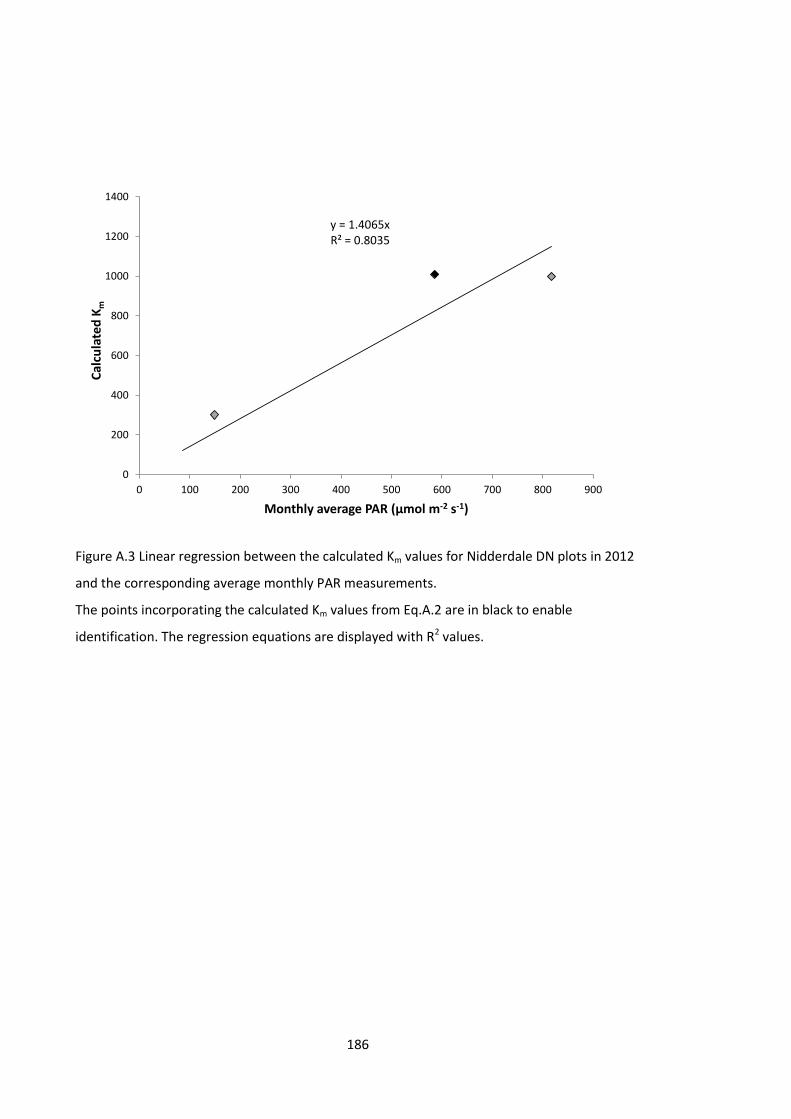
186

Figure A.3 Linear regression between the calculated Km values for Nidderdale DN plots in 2012

and the corresponding average monthly PAR measurements.

The points incorporating the calculated Km values from Eq.A.2 are in black to enable

identification. The regression equations are displayed with R2 values.

y = 1.4065xR² = 0.8035

0

200

400

600

800

1000

1200

1400

0 100 200 300 400 500 600 700 800 900

Cal

cula

ted

Km

Monthly average PAR (µmol m-2 s-1)

187

Figu

re A

.4 M

on

thly

mo

del

led

NEE

flu

xes

for

each

of

the

thre

e u

psc

aled

man

agem

ents

(FI

, LB

an

d D

N)

at e

ach

of

the

thre

e s

ite

s.

188

Appendix B - Redundancy analyses using year, site or block as

constraining variables

In Chapter 3, redundancy analyses (RDAs) were performed on the vegetation percentage cover

data to assess the effects of management on the vegetation composition. As the site and block

in which the plots were located and the year of measurement were also expected to affect the

vegetation composition, these were applied separately as constraining variables to RDAs. The

results of the RDAs using year, site or block as the constraining variable are outlined in Section

3.3.1, shown in Figures B.1-3 and discussed in Section 3.4.2. Although year, site and block are

used as the constraining variables in Figures B.1-3, the dots (which represent the position of

each individual plot in a given year) are coloured according to management to demonstrate

that, whilst year, site and block explain a significant portion of the data in the vegetation

matrix, these factors contain plots from all managements.

189


post-management) with year as the constraining variable.

Blue crosses represent the centroids of the years. Red crosses represent the positions of

individual species. The most influential are labelled with the first three letters of the genus

name and species name (for plant species; Bsh_dd is brash/dead/burnt material). Coloured

dots represent the position of each individual plot in a given year where dark green is for DN

managed plots, orange is for FI, blue is for BR and pink is for LB (see Section 3.2.5 for

management codes). The groups assigned by k-means partitioning are shown by the polygons.

190


post-management) with site as the constraining variable.

Blue crosses represent the centroids of the sites. Red crosses represent the positions of


name and species name (for plant species; Bare is bare ground). Coloured dots represent the

position of each individual plot in a given year where dark green is for DN managed plots,

orange is for FI, blue is for BR and pink is for LB (see Section 3.2.5 for management codes). The

groups assigned by k-means partitioning are shown by the polygons.

191


post-management) with block as the constraining variable.

Blue crosses represent the centroids of the blocks. Red crosses represent the positions of


name and species name (for plant species; Bsh_dd is brash/dead/burnt material). Coloured

dots represent the position of each individual plot in a given year where dark green is for DN

managed plots, orange is for FI, blue is for BR and pink is for LB (see Section 3.2.5 for

management codes). No polygons are shown as the data were too clustered to satisfactorily

divide the observations into groups.

192

Appendix C - Plant nutrient content minimum and maximum

values

In Chapter 3, the nutrient content was determined for Calluna plants on all plots at all sites

during 2012 and 2015, representing the pre- and post-management periods, respectively.

Concentrations of 11 different elements were measured in the Calluna leaves. These elements

were N, P, K, Na, Mg, Ca, Fe, Al, Mn, Zn and Cu. Results of the statistical analysis to determine

whether there was a significant difference in concentration of each nutrient on different

management and different sites pre- or post-management are detailed in Section 3.3.4. To

facilitate interpretation of the results and to allow comparison to other studies, the minimum,

maximum and average concentrations of each element for each site in the two time periods

are shown in Table C.1 and the same values for each management in the two time periods are

shown in Table C.2.

193


11 elements measured in Calluna leaves for each site pre- and post-management.

Site abbreviations are used where Nidd is a contraction of Nidderdale, Moss is a contraction of

Mossdale and Whit is a contraction of Whitendale. Concentrations are given as percentages

(%) for nitrogen (N), phosphorus (P), potassium (K), sodium (Na), magnesium (Mg) and calcium

(Ca), and as µg g-1 of oven-dried leaf material for iron (Fe), aluminium (Al), manganese (Mn),

zinc (Zn) and copper (Cu).

Site and period

Value % µg g-1

N P K Na Mg Ca Fe Al Mn Zn Cu

Nidd pre

Min 1.02 0.05 0.12 0.03 0.10 0.18 121 91.5 70.1 28.2 8.71

Max 1.53 0.15 0.22 0.09 0.22 0.59 214 134 383 106 14.8

Av 1.23 0.09 0.16 0.05 0.16 0.40 160 108 214 49.8 12.4

Nidd post

Min 1.08 0.04 0.15 0.04 0.12 0.15 47.0 19.1 174 17.3 5.92

Max 2.82 0.16 0.58 0.24 0.33 0.54 581 134 1753 125 15.3

Av 1.84 0.10 0.40 0.12 0.25 0.42 155 56.1 899 59.1 12.1

Moss pre

Min 0.95 0.06 0.12 0.06 0.15 0.30 93.6 93.0 68.6 24.4 8.67

Max 1.22 0.14 0.23 0.31 0.20 0.44 213 156 366 205 13.1

Av 1.07 0.10 0.19 0.14 0.18 0.38 143 109 211 43.1 11.1

Moss post

Min 0.94 0.04 0.29 0.05 0.18 0.30 74.8 21.7 105 23.9 9.99

Max 2.92 0.25 0.83 0.21 0.38 0.56 148 190 1900 62.2 15.8

Av 1.81 0.12 0.46 0.12 0.26 0.40 102 44.1 1122 37.5 12.0

Whit pre

Min 1.18 0.06 0.13 0.04 0.11 0.18 97.2 91.9 54.6 28.2 10.3

Max 1.75 0.17 0.28 0.13 0.20 0.42 424 249 571 75.2 17.5

Av 1.41 0.11 0.19 0.08 0.14 0.27 197 133 204 42.1 13.9

Whit post

Min 1.34 0.06 0.24 0.04 0.17 0.26 88.7 34.7 125 30.9 9.73

Max 2.76 0.17 0.66 0.20 0.35 0.59 356 186 1649 110 16.6

Av 2.01 0.10 0.41 0.12 0.27 0.44 156 67.4 834 50.5 12.2

194


11 elements measured in Calluna leaves for each managment pre- and post-management.

Management codes are used when DN represents unmanaged, BR represents mown plots with

the brash removed, LB represents mown plots with the brash left and FI represents burnt.

Concentrations are given as percentages (%) for nitrogen (N), phosphorus (P), potassium (K),

sodium (Na), magnesium (Mg) and calcium (Ca), and as µg g-1 of oven-dried leaf material for

iron (Fe), aluminium (Al), manganese (Mn), zinc (Zn) and copper (Cu).

Mgmt and period

Value % µg g-1

N P K Na Mg Ca Fe Al Mn Zn Cu

DN pre Min 0.96 0.06 0.12 0.05 0.11 0.18 116 93.0 54.6 35.3 10.4

Max 1.51 0.13 0.23 0.31 0.19 0.51 216 145 383 105 16.5

Av 1.20 0.10 0.18 0.10 0.15 0.34 164 113 227 52.5 13.2

DN post

Min 0.94 0.04 0.24 0.05 0.18 0.33 87.8 35.8 105 30.6 10.1

Max 1.81 0.10 0.49 0.13 0.26 0.52 344 186 639 110 14.9

Av 1.33 0.07 0.33 0.08 0.21 0.40 152 81.4 290 50.7 11.7

BR pre Min 1.02 0.05 0.12 0.03 0.10 0.19 113 95.3 68.6 24.9 8.71

Max 1.65 0.13 0.24 0.19 0.19 0.51 266 165 571 74.9 16.0

Av 1.25 0.09 0.18 0.09 0.16 0.34 164 115 215 41.4 11.8

BR post

Min 1.43 0.04 0.15 0.04 0.12 0.15 47.0 19.1 272 17.3 5.92

Max 2.92 0.15 0.68 0.20 0.32 0.53 356 190 1753 78.9 16.6

Av 1.98 0.11 0.41 0.12 0.26 0.42 121 54.3 1059 44.2 12.0

LB pre Min 0.95 0.06 0.13 0.03 0.10 0.18 113 91.5 98.9 24.4 10.0

Max 1.75 0.15 0.24 0.22 0.22 0.59 424 249 549 50.2 17.5

Av 1.24 0.10 0.18 0.09 0.16 0.36 183 123 205 39.2 13.3

LB post

Min 1.41 0.07 0.27 0.05 0.17 0.26 74.8 21.7 450 32.0 9.47

Max 2.55 0.17 0.57 0.21 0.35 0.54 341 118 1900 114 15.8

Av 1.93 0.12 0.42 0.13 0.27 0.40 132 48.8 1047 44.5 12.2

FI pre Min 1.04 0.06 0.12 0.05 0.15 0.23 93.6 91.9 78.9 28.2 8.67

Max 1.52 0.17 0.28 0.13 0.20 0.51 213 156 253 99.7 13.3

Av 1.21 0.11 0.20 0.08 0.18 0.36 143 110 189 43.2 11.5

FI post Min 1.62 0.09 0.35 0.06 0.23 0.37 88.7 25.3 644 32.3 10.1

Max 2.76 0.17 0.83 0.24 0.38 0.59 197 81.8 1875 125 15.0

Av 2.16 0.13 0.55 0.13 0.29 0.49 128 47.5 1218 64.5 12.7

195

Appendix D - Raw 14C values and publication codes

In Chapter 4, radiocarbon analyses were performed on 15 CO2 and 15 DOC samples collected

from the pot ecosystems to determine the age of the samples. Additionally, three

homogenised peat samples (i.e. containing a mixture of peat from all pots) and one sample of

charcoal created from burning Calluna plants were also dated. All 14C data were normalised to

-25‰ δ13C to correct for mass-dependent isotopic fractionation and were expressed as

%Modern relative to the activity of the NBS Oxalic Acid international radiocarbon standard,

following convention (Stuiver & Polach, 1977). The normalised 14C values, the measured δ13C

content and the Scottish Universities Environmental Research Centre (SUERC) publication

codes are detailed in Table D.1 for all of the samples sent for radiocarbon dating.

196

Table D.1 Scottish Universities Environmental Research Centre (SUERC) publication codes and

sample types.

The 14C and δ13C content of each sample are shown. Treatment codes refer to the pot

treatments, which are laid out in full in Table 4.2.

Publication code

Sample type

Treatment code

14C content (%Modern ± 1σ)

δ13C content (‰)

SUERC-64843 CO2 H-- 62.96 ± 0.34 -24.3

SUERC-64844 CO2 --- 61.67 ± 0.34 -24.7

SUERC-64848 CO2 HCB 83.45 ± 0.39 -26.6

SUERC-64849 CO2 --B 73.23 ± 0.36 -19.7

SUERC-64850 CO2 HC- 89.25 ± 0.41 -27.1

SUERC-67911 CO2 --- 68.03 ± 0.35 -19.9

SUERC-67912 CO2 HC- 83.68 ± 0.37 -27.0

SUERC-67913 CO2 --B 110.99 ± 0.51 -20.7

SUERC-67917 CO2 H-- 62.97 ± 0.35 -23.9

SUERC-67918 CO2 HCB 85.91 ± 0.40 -26.8

SUERC-67919 CO2 --- 67.86 ± 0.33 -21.2

SUERC-67920 CO2 H-- 67.31 ± 0.34 -22.3

SUERC-67921 CO2 HC- 78.84 ± 0.38 -21.9

SUERC-67922 CO2 --B 66.43 ± 0.35 -24.3

SUERC-67923 CO2 MCB 74.79 ± 0.37 -26.6

SUERC-65920 DOC H-- 71.57 ± 0.33 -26.5

SUERC-65921 DOC --- 71.80 ± 0.32 -27.0

SUERC-65922 DOC HCB 75.36 ± 0.33 -26.7

SUERC-65923 DOC --B 67.99 ± 0.32 -27.7

SUERC-65924 DOC HC- 74.30 ± 0.33 -25.9

SUERC-67898 DOC --- 74.00 ± 0.34 -26.6

SUERC-67899 DOC HC- 74.34 ± 0.33 -26.9

SUERC-67900 DOC --B 111.81 ± 0.49 -27.6

SUERC-67901 DOC H-- 72.53 ± 0.33 -26.8

SUERC-67902 DOC HCB 74.48 ± 0.34 -26.8

SUERC-67903 DOC --- 70.64 ± 0.33 -27.4

SUERC-67907 DOC H-- 72.25 ± 0.33 -27.3

SUERC-67908 DOC HC- 74.26 ± 0.34 -26.8

SUERC-67909 DOC --B 71.38 ± 0.31 -27.0

SUERC-67910 DOC MCB 74.94 ± 0.33 -27.0

SUERC-65527 Peat n/a 69.54 ± 0.32 -27.7

SUERC-65528 Peat n/a 68.06 ± 0.31 -27.8

SUERC-67897 Peat n/a 68.38 ± 0.32 -27.5

SUERC-68198 Charcoal n/a 104.95 ± 0.48 -30.2

197

References

Aerts R, Berendse F, de Caluwe H, Schmitz M (1990) Competition in heathland along an

experimental gradient of nutrient availability. Oikos, 57, 310–318.

Albertson K, Aylen J, Cavan G, McMorrow J (2010) Climate change and the future occurrence

of moorland wildfires in the Peak District of the UK. Climate Research, 45, 105–118.

Allen SE (1964) Chemical Aspects of Heather Burning. Journal of Applied Ecology, 1, 347–367.

Allen KA, Harris MPK, Marrs RH (2013) Matrix modelling of prescribed burning in Calluna

vulgaris-dominated moorland: short burning rotations minimize carbon loss at

increased wildfire frequencies. Journal of Applied Ecology, 50, 614–624.

Amphlett A, Payne S (2010a) Sphagnum tenellum. In: Mosses and Liverworts of Britain and

Ireland a field guide (eds Atherton I, Bosanquet S, Lawley M), p. 301. British Bryological

Society, Plymouth, UK.

Amphlett A, Payne S (2010b) Sphagnum fallax. In: Mosses and Liverworts of Britain and Ireland

a field guide (eds Atherton I, Bosanquet S, Lawley M), p. 306. British Bryological

Society, Plymouth, UK.

Armstrong A, Holden J, Stevens C (2008) The differential response of vegetation to grip-

blocking. Report for Peatscapes, North Pennine AONB.

Armstrong A, Holden J, Kay P, Foulger M, Gledhill S, McDonald AT, Walker A (2009) Drain-

blocking techniques on blanket peat: A framework for best practice. Journal of

Environmental Management, 90, 3512–3519.

Armstrong A, Holden J, Kay P et al. (2010) The impact of peatland drain-blocking on dissolved

organic carbon loss and discolouration of water; results from a national survey. Journal

of Hydrology, 381, 112–120.

Armstrong A, Holden J, Luxton K, Quinton JN (2012) Multi-scale relationship between peatland

vegetation type and dissolved organic carbon concentration. Ecological Engineering,

47, 182–188.

Bain C, Bonn A, Stoneman R et al. (2011) IUCN UK Commission of Inquiry on Peatlands. IUCN

UK Peatland Programme, Edinburgh.

Baird AJ, Holden J, Chapman PJ (2009) A Literature Review of Evidence on Emissions of

Methane in Peatlands. Defra Project SP0574. University of Leeds, UK.

Ball DF (1964) Loss-on-ignition as an estimate of organic matter and organic carbon in non-

calcareous soils. Journal of Soil Science, 15, 84–92.

Bardgett RD, Richter A, Bol R et al. (2007) Heterotrophic microbial communities use ancient

carbon following glacial retreat. Biology Letters, 3, 487–490.

198

Bartlett KB, Harriss RC (1993) Review and assessment of methane emissions from wetlands.

Chemosphere, 26, 261–320.

Belyea LR, Malmer N (2004) Carbon sequestration in peatland: patterns and mechanisms of

response to climate change. Global Change Biology, 10, 1043–1052.

Bending GD, Read DJ (1997) Lignin and soluble phenolic degradation by ectomycorrhizal and

ericoid mycorrhizal fungi. Mycological Research, 101, 1348–1354.

Bengtson H (2010) Open Channel Flow over V-Notch Weir Calculations. Bright Hub

Engineering.

Billett MF, Palmer SM, Hope D et al. (2004) Linking land-atmosphere-stream carbon fluxes in a

lowland peatland system. Global Biogeochemical Cycles, 18, GB1024.

Billett MF, Charman DJ, Clark JM et al. (2010) Carbon balance of UK peatlands: current state of

knowledge and future research challenges. Climate Research, 45, 13–29.

Billett MF, Garnett MH, Dinsmore KJ et al. (2011) Age and source of different forms of carbon

released from boreal peatland streams during spring snowmelt in E. Finland.

Biogeochemistry, 111, 273–286.

Billett MF, Garnett MH, Dinsmore KJ (2015) Should Aquatic CO2 Evasion be Included in

Contemporary Carbon Budgets for Peatland Ecosystems? Ecosystems, 18, 471–480.

Bonn A, Rebane M, Reid C (2009) A new rationale for conservation of upland environments. In:

Drivers of Environmental Change in Uplands (eds Bonn A, Allott TEH, Hubacek K,

Stewart J), pp. 448–474. Routledge, Abingdon, UK.

Bord na Móna Milled Peat Production 1.

Borren W, Bleuten W, Lapshina ED (2004) Holocene peat and carbon accumulation rates in the

southern taiga of western Siberia. Quaternary Research, 61, 42–51.

Børsheim K., Christensen B., Painter T. (2001) Preservation of fish by embedment in Sphagnum

moss, peat or holocellulose: experimental proof of the oxopolysaccharidic nature of

the preservative substance and of its antimicrobial and tanning action. Innovative Food

Science & Emerging Technologies, 2, 63–74.

Bortoluzzi E, Epron D, Siegenthaler A, Gilbert D, Buttler A (2006) Carbon balance of a European

mountain bog at contrasting stages of regeneration. New Phytologist, 172, 708–718.

Bosatta E, Ågren GI (1999) Soil organic matter quality interpreted thermodynamically. Soil

Biology and Biochemistry, 31, 1889–1891.

Bragazza L, Freeman C, Jones T et al. (2006) Atmospheric nitrogen deposition promotes carbon

loss from peat bogs. Proceedings of the National Academy of Sciences, 103, 19386–

19389.

199

Bragazza L, Parisod J, Buttler A, Bardgett RD (2013) Biogeochemical plant-soil microbe

feedback in response to climate warming in peatlands. Nature Climate Change, 3, 273–

277.

Breeuwer A, Robroek BJM, Limpens J, Heijmans MMPD, Schouten MGC, Berendse F (2009)

Decreased summer water table depth affects peatland vegetation. Basic and Applied

Ecology, 10, 330–339.

Briones MJI, Garnett MH, Ineson P (2010) Soil biology and warming play a key role in the

release of “old C” from organic soils. Soil Biology and Biochemistry, 42, 960–967.

Brooks S, Stoneman R (eds.) (1997) Conserving bogs: the management handbook. The

Stationary Office, Edinburgh.

Brown DA (1995) Carbon Cycling in Peat and the Implications for the Rehabilitation of Bogs. In:

Wetlands: Archaeology and Nature Conservation, pp. 99–107. HMSO, London.

Brown AM (2001) Nonlinear regression analysis of data using a spreadsheet. American

Biotechnology Laboratory, 19, 58–60.

Brown A, MacFadyen A (1969) Soil Carbon Dioxide Output and Small-Scale Vegetation Pattern

in a Calluna heath. Oikos, 20, 8–15.

Burch J (2008) The relationship of bryophyte regeneration to heather canopy height following

moorland burning on the North York Moors. Journal of Bryology, 30, 208–216.

Burke RM, Cairney JWG (1998) Carbohydrate oxidases in ericoid and ectomycorrhizal fungi: a

possible source of Fenton radicals during the degradation of lignocellulose. New

Phytologist, 139, 637–645.

Calhoun A, King GM (1997) Regulation of root-associated methanotrophy by oxygen

availability in the rhizosphere of two aquatic macrophytes. Applied and Environmental

Microbiology, 63, 3051–3058.

Campeau S, Rochefort L (1996) Sphagnum Regeneration on Bare Peat Surfaces: Field and

Greenhouse Experiments. Journal of Applied Ecology, 33, 599–608.

Carleer A, Wolff E (2004) Exploitation of very high resolution satellite data for tree species

identification. Photogrammetric Engineering and Remote Sensing, 70, 135–140.

Carroll MJ, Dennis P, Pearce-Higgins JW, Thomas CD (2011) Maintaining northern peatland

ecosystems in a changing climate: effects of soil moisture, drainage and drain blocking

on craneflies. Global Change Biology, 17, 2991–3001.

Chapin FS, Woodwell GM, Randerson JT et al. (2006) Reconciling Carbon-cycle Concepts,

Terminology, and Methods. Ecosystems, 9, 1041–1050.

Charman DJ (2002) Peatlands and environmental change. John Wiley & Sons, New York, NY.

200

Clark JM, Chapman PJ, Adamson JK, Lane SN (2005) Influence of drought-induced acidification

on the mobility of dissolved organic carbon in peat soils. Global Change Biology, 11,

791–809.

Clay GD, Worrall F, Fraser EDG (2009) Effects of managed burning upon dissolved organic

carbon (DOC) in soil water and runoff water following a managed burn of a UK blanket

bog. Journal of Hydrology, 367, 41–51.

Clay GD, Worrall F, Rose R (2010) Carbon budgets of an upland blanket bog managed by

prescribed fire. Journal of Geophysical Research: Biogeosciences, 115, G04037.

Clay GD, Worrall F, Aebischer NJ (2012) Does prescribed burning on peat soils influence DOC

concentrations in soil and runoff waters? Results from a 10 year chronosequence.

Journal of Hydrology, 448–449, 139–148.

Clay GD, Worrall F, Aebischer NJ (2015) Carbon stocks and carbon fluxes from a 10-year

prescribed burning chronosequence on a UK blanket peat. Soil Use and Management,

31, 39–51.

Clutterbuck B, Yallop AR (2010) Land management as a factor controlling dissolved organic

carbon release from upland peat soils 2: Changes in DOC productivity over four

decades. Science of The Total Environment, 408, 6179–6191.

Clymo RS (1963) Ion Exchange in Sphagnum and its Relation to Bog Ecology. Annals of Botany,

27, 309–324.

Clymo RS (1987) The ecology of peatlands. Science Progress, 71, 593–614.

Clymo RS (1992) Models of peat growth. Suo, 43, 127–136.

Clymo RS, Gore AJP (1983) Peat. In: Mires, Swamp, Fen and Moor (ed Gore AJP), pp. 159–224.

Elsevier Sciencific, Amsterdam.

Clymo RS, Hayward PM (1982) The Ecology of Sphagnum. In: Bryophyte Ecology (ed Smith AJE).

Chapman and Hall, London.

Clymo RS, Pearce DME (1995) Methane and Carbon Dioxide Production in, Transport through,

and Efflux from a Peatland. Philosophical Transactions: Physical Sciences and

Engineering, 351, 249–259.

Clymo RS, Turunen J, Tolonen K (1998) Carbon Accumulation in Peatland. Oikos, 81, 368–388.

Condliffe I (2009) Policy change in the uplands. In: Drivers of environmental change in uplands

(eds Bonn A, Allott TEH, Hubacek K, Stewart J), pp. 59–90. Routledge, London.

Cooper MDA, Evans CD, Zielinski P et al. (2014) Infilled Ditches are Hotspots of Landscape

Methane Flux Following Peatland Re-wetting. Ecosystems, 17, 1–15.

Cotton DE, Hale WHG (1994) Effectiveness of Cutting as an Alternative to Burning in the

Management of Calluna vulgaris Moorland: Results of an Experimental Field Trial.

Journal of Environmental Management, 40, 155–159.

201

Couwenberg J, Thiele A, Tanneberger F et al. (2011) Assessing greenhouse gas emissions from

peatlands using vegetation as a proxy. Hydrobiologia, 674, 67–89.

Crowe SK, Evans MG, Allott TEH (2008) Geomorphological controls on the re-vegetation of

erosion gullies in blanket peat: implications for bog restoration. Mires and Peat, 3, 1–

14.

Daniels RE, Eddy A (1990) Handbook of European Sphagna. HMSO, London, 263 pp.

DART Computing, Smart S (2014) Modular analysis vegetation information system MAVIS Plot

Analyser. Centre for Ecology and Hydrology.

Davidson EA, Janssens IA (2006) Temperature sensitivity of soil carbon decomposition and

feedbacks to climate change. Nature, 440, 165–173.

Davies GM, Gray A, Rein G, Legg CJ (2013) Peat consumption and carbon loss due to

smouldering wildfire in a temperate peatland. Forest Ecology and Management, 308,

169–177.

Dawson JJC, Malcolm IA, Middlemas SJ, Tetzlaff D, Soulsby C (2009) Is the Composition of

Dissolved Organic Carbon Changing in Upland Acidic Streams? Environmental Science

& Technology, 43, 7748–7753.

Defra (2007) The Heather and Grass Burning Code. Defra.

Defra (2016) The Water Supply (Water Quality) Regulations 2016. 2016 No. 614.

Denmead OT (2008) Approaches to measuring fluxes of methane and nitrous oxide between

landscapes and the atmosphere. Plant and Soil, 309, 5–24.

Dinsmore KJ, Skiba UM, Billett MF, Rees RM, Drewer J (2009) Spatial and temporal variability in

CH4 and N2O fluxes from a Scottish ombrotrophic peatland: Implications for modelling

and up-scaling. Soil Biology and Biochemistry, 41, 1315–1323.

Dinsmore KJ, Billett MF, Skiba UM, Rees RM, Drewer J, Helfter C (2010) Role of the aquatic

pathway in the carbon and greenhouse gas budgets of a peatland catchment. Global

Change Biology, 16, 2750–2762.

Dixon SD, Worrall F, Rowson JG, Evans MG (2015) Calluna vulgaris canopy height and blanket

peat CO2 flux: Implications for management. Ecological Engineering, 75, 497–505.

Dorrepaal E, Toet S, van Logtestijn RSP, Swart E, van de Weg MJ, Callaghan TV, Aerts R (2009)

Carbon respiration from subsurface peat accelerated by climate warming in the

subarctic. Nature, 460, 616–619.

Dougill AJ, Fraser EDG, Holden J et al. (2006) Learning from Doing Participatory Rural Research:

Lessons from the Peak District National Park. Journal of Agricultural Economics, 57,

259–275.

Dray S (2013) packfor: Forward selection with permutation (Canoco p.46).

202

Duclos J l., Fortin JA (1983) Effect of Glucose and Active Charcoal on in Vitro Synthesis of

Ericoid Mycorrhiza with Vaccinium Spp. New Phytologist, 94, 95–102.

Dunn C, Jones TG, Roberts S, Freeman C (2015) Plant Species Effects on the Carbon Storage

Capabilities of a Blanket bog Complex. Wetlands, 36, 47–58.

Equihua M, Usher MB (1993) Impact of Carpets of the Invasive Moss Campylopus Introflexus

on Calluna Vulgaris Regeneration. Journal of Ecology, 81, 359–365.

Evans MG, Burt TP, Holden J, Adamson JK (1999) Runoff generation and water table

fluctuations in blanket peat: evidence from UK data spanning the dry summer of 1995.

Journal of Hydrology, 221, 141–160.

Evans CD, Monteith DT, Cooper DM (2005) Long-term increases in surface water dissolved

organic carbon: Observations, possible causes and environmental impacts.

Environmental Pollution, 137, 55–71.

Evans M, Warburton J, Yang J (2006) Eroding blanket peat catchments: Global and local

implications of upland organic sediment budgets. Geomorphology, 79, 45–57.

Evans CD, Freeman C, Cork LG et al. (2007) Evidence against recent climate-induced

destabilisation of soil carbon from 14C analysis of riverine dissolved organic matter.

Geophysical Research Letters, 34, L07407.

Evans CD, Jones TG, Burden A et al. (2012) Acidity controls on dissolved organic carbon

mobility in organic soils. Global Change Biology, 18, 3317–3331.

Evans CD, Bonn A, Holden J et al. (2014) Relationships between anthropogenic pressures and

ecosystem functions in UK blanket bogs: Linking process understanding to ecosystem

service valuation. Ecosystem Services, 9, 5–19.

Evans CD, Renou-Wilson F, Strack M (2015) The role of waterborne carbon in the greenhouse

gas balance of drained and re-wetted peatlands. Aquatic Sciences, 78, 573–590.

Evans CD, Malcolm IA, Shilland EM et al. (2016) Sustained Biogeochemical Impacts of Wildfire

in a Mountain Lake Catchment. Ecosystems, 1–17.

Ewen J, Geris J, O’Connell E, O’Donnell G, Mayes W (2015) Multiscale experimentation,

monitoring and analysis of long-term land use changes and flood risk. Environment

Agency, Bristol.

Fargione J, Hill J, Tilman D, Polasky S, Hawthorne P (2008) Land Clearing and the Biofuel

Carbon Debt. Science, 319, 1235–1238.

Fenner N, Williams R, Toberman H, Hughes S, Reynolds B, Freeman C (2011) Decomposition

“hotspots” in a rewetted peatland: implications for water quality and carbon cycling.

Hydrobiologia, 674, 51–66.

Ferguson P, Lee JA (1983) Past and present sulphur pollution in the southern Pennines.

Atmospheric Environment (1967), 17, 1131–1137.

203

Ferriss RS (1984) Effects of microwave oven treatment on microorganisms in soil.

Phytopathology, 74, 121–126.

Field CD, Dise NB, Payne RJ et al. (2014) The Role of Nitrogen Deposition in Widespread Plant

Community Change Across Semi-natural Habitats. Ecosystems, 17, 864–877.

Fischer A, Marshall K (2010) Framing the landscape: Discourses of woodland restoration and

moorland management in Scotland. Journal of Rural Studies, 26, 185–193.

Fontaine S, Barot S, Barré P, Bdioui N, Mary B, Rumpel C (2007) Stability of organic carbon in

deep soil layers controlled by fresh carbon supply. Nature, 450, 277–280.

Forrest GI (1971) Structure and Production of North Pennine Blanket Bog Vegetation. Journal

of Ecology, 59, 453–479.

Fowler D, Smith RI, Muller JBA, Hayman G, Vincent KJ (2005) Changes in the atmospheric

deposition of acidifying compounds in the UK between 1986 and 2001. Environmental

Pollution, 137, 15–25.

Fox AM, Huntley B, Lloyd CR, Williams M, Baxter R (2008) Net ecosystem exchange over

heterogeneous Arctic tundra: Scaling between chamber and eddy covariance

measurements. Global Biogeochemical Cycles, 22, GB2027.

Freeman C, Evans CD, Monteith DT, Reynolds B, Fenner N (2001a) Export of organic carbon

from peat soils. Nature, 412, 785–785.

Freeman C, Ostle N, Kang H (2001b) An enzymic “latch” on a global carbon store. Nature, 409,

149–149.

Fridborg G, Pedersén M, Landström L-E, Eriksson T (1978) The Effect of Activated Charcoal on

Tissue Cultures: Adsorption of Metabolites Inhibiting Morphogenesis. Physiologia

Plantarum, 43, 104–106.

Frolking S, Talbot J, Jones MC, Treat CC, Kauffman JB, Tuittila E-S, Roulet N (2011) Peatlands in

the Earth’s 21st century climate system. Environmental Reviews, 19, 371–396.

Fyfe RM, Brown AG, Rippon SJ (2003) Mid- to late-Holocene vegetation history of Greater

Exmoor, UK: estimating the spatial extent of human-induced vegetation change.

Vegetation History and Archaeobotany, 12, 215–232.

Gallego-Sala AV, Prentice IC (2013) Blanket peat biome endangered by climate change. Nature

Climate Change, 3, 152–155.

Garnett M, Murray C (2013) Processing of CO2 Samples Collected Using Zeolite Molecular

Sieve for 14C Analysis at the NERC Radiocarbon Facility (East Kilbride, UK).

Radiocarbon, 55, 410–415.

Garnett MH, Ineson P, Stevenson AC (2000) Effects of burning and grazing on carbon

sequestration in a Pennine blanket bog, UK. The Holocene, 10, 729–736.

204

Garnett MH, Ineson P, Stevenson AC, Howard DC (2001) Terrestrial organic carbon storage in a

British moorland. Global Change Biology, 7, 375–388.

Gaudinski JB, Trumbore SE, Davidson EA, Zheng S (2000) Soil carbon cycling in a temperate

forest: radiocarbon-based estimates of residence times, sequestration rates and

partitioning of fluxes. Biogeochemistry, 51, 33–69.

Genney DR, Alexander IJ, Hartley SE (2000) Exclusion of grass roots from soil organic layers by

Calluna: the role of ericoid mycorrhizas. Journal of Experimental Botany, 51, 1117–

1125.

Gibson H (2006) Sources and management of water colour in the river Tees. Doctoral, Durham

University, 371p. p.

Gimingham CH (1960) Calluna Salisb. Journal of Ecology, 48, 455–483.

Gimingham CH (1975) An introduction to heathland ecology, Vol. 539. Oliver & Boyd

Edinburgh.

Glaser PH, Chanton JP, Morin P et al. (2004) Surface deformations as indicators of deep

ebullition fluxes in a large northern peatland. Global Biogeochemical Cycles, 18,

GB1003.

Glime JM (2007) Chapter 13: Decomposition. In: Bryophyte ecology, Vol. 1: Physiological

ecology. Ebook sponsored by Michigan Technological University and the International

Association of Bryologists.

González E, Rochefort L (2014) Drivers of success in 53 cutover bogs restored by a moss layer

transfer technique. Ecological Engineering, 68, 279–290.

Gorham E (1991) Northern Peatlands: Role in the Carbon Cycle and Probable Responses to

Climatic Warming. Ecological Applications, 1, 182–195.

Grace J, Woolhouse HW (1973) A Physiological and Mathematical Study of the Growth and

Productivity of a Calluna-sphagnum Community. II. Light Interception and

Photosynthesis in Calluna. Journal of Applied Ecology, 10, 63–76.

Grant SA, Hunter RF, Cross C (1963) The Effects of Muirburning Molinia-Dominant

Communities. Grass and Forage Science, 18, 249–257.

Grant MC, Mallord J, Stephen L, Thompson PS (2012) The costs and benefits of grouse moor

management to biodiversity and aspects of the wider environment: a review. Sandy,

UK.

Gray A, Levy PE, Cooper MDA et al. (2013) Methane indicator values for peatlands: a

comparison of species and functional groups. Global Change Biology, 19, 1141–1150.

Grayson R, Holden J (2012) Continuous measurement of spectrophotometric absorbance in

peatland streamwater in northern England: implications for understanding fluvial

carbon fluxes. Hydrological Processes, 26, 27–39.

205

Grayson R, Holden J, Rose R (2010) Long-term change in storm hydrographs in response to

peatland vegetation change. Journal of Hydrology, 389, 336–343.

Green RM (1979) Sampling design and statistical methods for environmental biologists. John

Wiley & Sons, New York.

Greenup AL, Bradford MA, McNamara NP, Ineson P, Lee JA (2000) The role of Eriophorum

vaginatum in CH4 flux from an ombrotrophic peatland. Plant and Soil, 227, 265–272.

Hahn V, Högberg P, Buchmann N (2006) 14C – a tool for separation of autotrophic and

heterotrophic soil respiration. Global Change Biology, 12, 972–982.

Hall JA (1979) The distribution of Tilia cordata and variations in the composition of the forests

in upper Swaledale and Wensleydale during the Atlantic period. MSc thesis, Durham

University, Durham.

Hanson PJ, Edwards NT, Garten CT, Andrews JA (2000) Separating root and soil microbial

contributions to soil respiration: A review of methods and observations.


Hardie SML, Garnett MH, Fallick AE, Rowland AP, Ostle NJ (2005) Carbon dioxide capture using

a zeolite molecular sieve sampling system for isotopic studies (13C and 14C) of

respiration. Radiocarbon, 47, 441–451.

Hardie SML, Garnett MH, Fallick AE, Ostle NJ, Rowland AP (2009) Bomb-14C analysis of

ecosystem respiration reveals that peatland vegetation facilitates release of old

carbon. Geoderma, 153, 393–401.

Hargreaves K., Fowler D (1998) Quantifying the effects of water table and soil temperature on

the emission of methane from peat wetland at the field scale. Atmospheric

Environment, 32, 3275–3282.

Harris MPK, Allen KA, McAllister HA, Eyre G, Le Duc MG, Marrs RH (2011) Factors affecting

moorland plant communities and component species in relation to prescribed burning.

Journal of Applied Ecology, 48, 1411–1421.

Hartley IP, Garnett MH, Sommerkorn M et al. (2012) A potential loss of carbon associated with

greater plant growth in the European Arctic. Nature Climate Change, 2, 875–879.

Haselwandter K, Bobleter O, Read DJ (1990) Degradation of 14C-labelled lignin and

dehydropolymer of coniferyl alcohol by ericoid and ectomycorrhizal fungi. Archives of

Microbiology, 153, 352–354.

Heal OW, Perkins DF (1978) Production Ecology of British Moors and Montane Grasslands.

Springer-Verlag, Berlin.

Hector A, Schmid B, Beierkuhnlein C et al. (1999) Plant Diversity and Productivity Experiments

in European Grasslands. Science, 286, 1123–1127.

206

Heinemeyer A, Croft S, Garnett MH, Gloor E, Holden J, Lomas MR, Ineson P (2010) The

MILLENNIA peat cohort model: predicting past, present and future soil carbon budgets

and fluxes under changing climates in peatlands. Clim Res, 45, 207–226.

Helfter C, Campbell C, Dinsmore KJ et al. (2015) Drivers of long-term variability in CO2 net

ecosystem exchange in a temperate peatland. Biogeosciences, 12, 1799–1811.

Hill MO, Preston CD, Bosanquet SDS, Roy DB (2007) BRYOATT. Attributes of British and Irish

Mosses, Liverworts and Hornworts. NERC Centre for Ecology and Hydrology.

Wallingford, UK, 88.

HM Government (2011) The Natural Choice: securing the value of nature. The Stationary Office

Limited, UK.

Hobbs RJ (1984) Length of Burning Rotation and Community Composition in High-Level

Calluna-Eriophorum Bog in N England. Vegetatio, 57, 129–136.

Hobbs RJ, Gimingham CH (1984) Studies on Fire in Scottish Heathland Communities II. Post-

Fire Vegetation Development. Journal of Ecology, 72, 585–610.

Holden J, Chapman PJ, Labadz JC (2004) Artificial drainage of peatlands: hydrological and

hydrochemical process and wetland restoration. Progress in Physical Geography, 28,

95–123.

Holden J, Shotbolt L, Bonn A et al. (2007a) Environmental change in moorland landscapes.

Earth Science Reviews, 82, 75–100.

Holden J, Gascoign M, Bosanko NR (2007b) Erosion and natural revegetation associated with

surface land drains in upland peatlands. Earth Surface Processes and Landforms, 32,

1547–1557.

Holden J, Kirkby MJ, Lane SN, Milledge DG, Brookes CJ, Holden V, McDonald AT (2008)

Overland flow velocity and roughness properties in peatlands. Water Resources

Research, 44, W06415.

Holden J, Chapman PJ, Palmer SM, Kay P, Grayson R (2012) The impacts of prescribed

moorland burning on water colour and dissolved organic carbon: A critical synthesis.

Journal of Environmental Management, 101, 92–103.

Holden J, Wearing C, Palmer S, Jackson B, Johnston K, Brown LE (2014) Fire decreases near-

surface hydraulic conductivity and macropore flow in blanket peat. Hydrological

Processes, 28, 2868–2876.

Holland EA, Robertson GP, Greenberg J, Groffman PM, Boone RD, Gosz JR (1999) Soil CO2,

N2O, and CH4 exchange. In: Standard soil methods for long-term ecological research

(eds Robertson GP, Coleman DC, Bledsoe CS, Sollins P), pp. 185–201. Oxford University

Press, Oxford.

207

Hope D, Palmer SM, Billett MF, Dawson JJC (2001) Carbon dioxide and methane evasion from a

temperate peatland stream. Limnology and Oceanography, 46, 847–857.

Hothorn T, Bretz F, Westfall P (2008) Simultaneous Inference in General Parametric Models.

Biometrical Journal, 50, 346–363.

Houghton RA (2007) Balancing the Global Carbon Budget. Annual Review of Earth and

Planetary Sciences, 35, 313–347.

Hutchinson JN (1980) The Record of Peat Wastage in the East Anglian Fenlands at Holme Post,

1848-1978 A.D. Journal of Ecology, 68, 229–249.

Huttunen JT, Nykänen H, Turunen J, Martikainen PJ (2003) Methane emissions from natural

peatlands in the northern boreal zone in Finland, Fennoscandia. Atmospheric

Environment, 37, 147–151.

Imeson AC (1971) Heather Burning and Soil Erosion on the North Yorkshire Moors. Journal of

Applied Ecology, 8, 537–542.

Ingram HAP (1982) Size and shape in raised mire ecosystems: a geophysical model. Nature,

297, 300–303.

Ingram HAP, Bragg OM (1984) The diplotelmic mire: some hydrological consequences

reviewed. In: Proceedings of the 7th International Peat Congress, Dublin, Vol. 1, pp.

220–234.

IUCN Peatland Programme (2015) The Peatland Code. UK Peatland Code 1.0. Peatland

Programme of IUCN UK.

Ivanov KE (1981) Water movement in mirelands. (trans Thomson A, Ingram HAP). Academic

Press Inc, London, 276 pp.

Jenkins D, Watson A, Miller GR (1963) Population Studies on Red Grouse, Lagopus lagopus

scoticus (Lath.) in North-East Scotland. Journal of Animal Ecology, 32, 317–376.

Jenkins D, Watson A, Picozzi N (1965) Red grouse chick survival in captivity and in the wild. In:

Transactions of the VIth Congress of the International Union of Game Biologists (ed

Blank TH), pp. 63–70. The Nature Conservancy, Bournemouth.

Jin H (2010) Characterization Of Microbial Life Colonizing Biochar And Biochar-Amended Soils.

PhD thesis, Cornell University, Ithaca, NY.

Joosten H, Clarke D (2002) Wise use of mires and peatlands: Background and principles

including a framework for decision-making. International Mire Conservation Group

and International Peat Society.

Kayll AJ, Gimingham CH (1965) Vegetative Regeneration of Calluna Vulgaris after Fire. Journal

of Ecology, 53, 729–734.

Kidd A, Cooper A, Brayson J (2007) Your Dales Rocks: Local Geodiversity Action Plan. North

Yorkshire Geodiversity Partnership, Skipton, UK.

208

Kindt R, Coe R (2005) Analysis of ecological distance by ordination. In: Tree diversity analysis. A

manual and software for common statistical methods for ecological and biodiversity

studies., pp. 153–196. World Agroforestry Centre (ICRAF), Nairobi, Kenya.

Kipton H, Powell J, Town RM (1992) Solubility and fractionation of humic acid; effect of pH and

ionic medium. Analytica Chimica Acta, 267, 47–54.

Kuhry P (1994) The Role of Fire in the Development of Sphagnum-Dominated Peatlands in

Western Boreal Canada. Journal of Ecology, 82, 899–910.

Kuznetsova A, Brockhoff PB, Christensen RHB (2016) lmerTest: Tests in Linear Mixed Effects

Models.

Lafleur PM, Roulet NT, Bubier JL, Frolking S, Moore TR (2003) Interannual variability in the

peatland-atmosphere carbon dioxide exchange at an ombrotrophic bog. Global

Biogeochemical Cycles, 17, 1036.

Lai DYF (2009) Methane Dynamics in Northern Peatlands: A Review. Pedosphere, 19, 409–421.

Lai DYF, Moore TR, Roulet NT (2014) Spatial and Temporal Variations of Methane Flux

Measured by Autochambers in a Temperate Ombrotrophic Peatland. Journal of

Geophysical Research: Biogeosciences, 2013JG002410.

Lee H, Alday JG, Rose RJ, O’Reilly J, Marrs RH (2013) Long-term effects of rotational prescribed

burning and low-intensity sheep grazing on blanket-bog plant communities. Journal of


Legendre P, Gallagher ED (2001) Ecologically meaningful transformations for ordination of

species data. Oecologia, 129, 271–280.

Levin I, Hammer S, Kromer B, Meinhardt F (2008) Radiocarbon observations in atmospheric

CO2: Determining fossil fuel CO2 over Europe using Jungfraujoch observations as

background. Science of The Total Environment, 391, 211–216.

Levy PE, Burden A, Cooper MDA et al. (2012) Methane emissions from soils: synthesis and

analysis of a large UK data set. Global Change Biology, 18, 1657–1669.

Liblik LK, Moore TR, Bubier JL, Robinson SD (1997) Methane emissions from wetlands in the

zone of discontinuous permafrost: Fort Simpson, Northwest Territories, Canada.

Global Biogeochemical Cycles, 11, 485–494.

Li-Cor Biosciences (2007) LI-8100 automated soil CO2 flux system & LI-8150 multiplexer

instruction manual.

Liepert C, Gardner SM, Rees S (1993) Managing heather moorland: impacts of burning and

cutting on Calluna regeneration. Journal of Environmental Planning and Management,

36, 283–293.

209

Limpens J, Berendse F, Blodau C et al. (2008) Peatlands and the carbon cycle: from local

processes to global implications ? a synthesis. Biogeosciences Discussions, 5, 1379–

1419.

Lindén A, Heinonsalo J, Buchmann N, Oinonen M, Sonninen E, Hilasvuori E, Pumpanen J (2013)

Contrasting effects of increased carbon input on boreal SOM decomposition with and

without presence of living root system of Pinus sylvestris L. Plant and Soil, 377, 145–

158.

Lindsay R (1995) Bogs: the ecology, classification and conservation of ombrotrophic mires.

Scottish Natural Heritage, Edinburgh.

Lindsay R (2010) Peatbogs and carbon: a critical synthesis to inform policy development in

oceanic peat bog conservation and restoration in the context of climate change.

Environmental Research Group, University of East London, London.

Lindsay R, Ross S (1993) Monitoring of peat bog systems. Biologiezentrum, Linz/Austria.

Lindsay R, Charman DJ, Everingham F, O’Reilly RM, Palmer MA, Rowell TA, Stroud DA (1988)

The Flow Country: The peatlands of Caithness and Sutherland. Nature Conservancy

Council, Peterborough.

Livingston GP, Hutchinson GL (1995) Enclosure-based measurement of trace gas exchange:

applications and sources of error. In: Biogenic Trace Gases: Measuring Emissions from

Soil and Water (eds Matson PA, Harriss RC). Marston Lindsey Ross International Ltd.,

Oxford.

Lovat, Lord (1911) Heather - Burning. In: The Grouse in Health and Disease, Vol. 1 (ed Lovat,

Lord), pp. 392–413. Smith, Elder & Co., London.

MacDonald AJ, Kirkpatrick AH, Hester AJ, Sydes C (1995) Regeneration by Natural Layering of

Heather (Calluna vulgaris): Frequency and Characteristics in Upland Britain. Journal of


MacDonald JA, Fowler D, Hargreaves KJ, Skiba U, Leith ID, Murray MB (1998) Methane

emission rates from a northern wetland; response to temperature, water table and

transport. Atmospheric Environment, 32, 3219–3227.

Mahmood S, Finlay RD, Fransson A-M, Wallander H (2003) Effects of hardened wood ash on

microbial activity, plant growth and nutrient uptake by ectomycorrhizal spruce

seedlings. FEMS Microbiology Ecology, 43, 121–131.

Mallik AU, Gimingham CH (1985) Ecological Effects of Heather Burning: II. Effects on Seed

Germination and Vegetative Regeneration. Journal of Ecology, 73, 633–644.

Maltby E (2010) Effects of climate change on the societal benefits of UK upland peat

ecosystems: applying the ecosystem approach. Climate Research, 45, 249–259.

210

Mauquoy D, Engelkes T, Groot MHM, Markesteijn F, Oudejans MG, van der Plicht J, van Geel B

(2002) High-resolution records of late-Holocene climate change and carbon

accumulation in two north-west European ombrotrophic peat bogs. Palaeogeography,

Palaeoclimatology, Palaeoecology, 186, 275–310.

McCarroll J, Chambers FM, Webb JC, Thom T (2015) Application of palaeoecology for peatland

conservation at Mossdale Moor, UK. Quaternary International, In press, corrected

proof.

McNamara NP, Plant T, Oakley S, Ward S, Wood C, Ostle N (2008) Gully hotspot contribution to

landscape methane (CH4) and carbon dioxide (CO2) fluxes in a northern peatland.

Science of The Total Environment, 404, 354–360.

McVeigh P, Sottocornola M, Foley N, Leahy P, Kiely G (2014) Meteorological and functional

response partitioning to explain interannual variability of CO2 exchange at an Irish

Atlantic blanket bog. Agricultural and Forest Meteorology, 194, 8–19.

Meyers-Schulte KJ, Hedges JI (1986) Molecular evidence for a terrestrial component of organic

matter dissolved in ocean water. Nature, 321, 61–63.

Microsoft (2010) Microsoft Excel. Microsoft Corporation, Redmond, WA, USA.

Millennium Ecosystem Assessment (2005) Ecosystems and Human Well-being: Synthesis. Island

Press, Washington, DC.

Miller GR, Miles J (1970) Regeneration of Heather (Calluna vulgaris (L.) Hull) at Different Ages

and Seasons in North-East Scotland. Journal of Applied Ecology, 7, 51–60.

Milligan AL, Putwain PD, Cox ES, Ghorbani J, Le Duc MG, Marrs RH (2004) Developing an

integrated land management strategy for the restoration of moorland vegetation on

Molinia caerulea-dominated vegetation for conservation purposes in upland Britain.

Biological Conservation, 119, 371–385.

Monteith DT, Stoddard JL, Evans CD et al. (2007) Dissolved organic carbon trends resulting

from changes in atmospheric deposition chemistry. Nature, 450, 537–540.

Moore PD (1973) The Influence of Prehistoric Cultures upon the Initiation and Spread of

Blanket Bog in Upland Wales. Nature, 241, 350–353.

Moss R (1967) Aspects of grouse nutrition. PhD thesis, University of Aberdeen, Scotland.

Moss R (1969) A Comparison of Red Grouse (Lagopus L. scoticus) Stocks with the Production

and Nutritive Value of Heather (Calluna vulgaris). Journal of Animal Ecology, 38, 103–

122.

Moss R (1972) Food Selection by Red Grouse (Lagopus lagopus scoticus (Lath.)) in Relation to

Chemical Composition. Journal of Animal Ecology, 41, 411–428.

Moss R (1977) The Digestion of Heather by Red Grouse during the Spring. The Condor, 79,

471–477.

211

Moss R, Watson A, Parr R (1975) Maternal Nutrition and Breeding Success in Red Grouse

(Lagopus lagopus scoticus). Journal of Animal Ecology, 44, 233–244.

Murphy JM, Sexton DM, Jenkins GJ et al. (2009) UK climate projections science report: climate

change projections. Met Office Hadley Centre, Exeter, UK.

Myhre G, Shindell D, Breon F-M et al. (2013) Anthropogenic and natural radiative forcing. In:

Climate change 2013: the physical science basis. Contribution of Working Group I to

the fifth assessment report of the intergovernmental panel on climate change.

Cambridge University Press, Cambridge.

National Research Council (1994) Nutrient Requirements of Poultry, Ninth Revised Edition.

National Academy Press, Washington, D. C.

Natural England (2010) England’s peatlands - carbon storage and greenhouse gases.

Naylor LM, Schmidt EJ (1986) Agricultural Use of Wood Ash as a Fertilizer and Liming Material.

Tappi, 69:10.

Neal C, Robson AJ, Neal M, Reynolds B (2005) Dissolved organic carbon for upland acidic and

acid sensitive catchments in mid-Wales. Journal of Hydrology, 304, 203–220.

Nilsson M, Sagerfors J, Buffam I et al. (2008) Contemporary carbon accumulation in a boreal

oligotrophic minerogenic mire – a significant sink after accounting for all C-fluxes.

Global Change Biology, 14, 2317–2332.

Oksanen J, Blanchet FG, Kindt R et al. (2016) vegan: Community Ecology Package.

O’Reilly C (2008) Peatscapes Project: Sphagna as management indicators research. Ptyxis

Ecology.

Orlikowski LB, Sroczyński M, Szkuta G (2004) First notice of Phytophthora tip blight of Calluna

vulgaris. Phytopathologia Polonica, 31, 67–71.

Orwin KH, Ostle NJ (2012) Moss species effects on peatland carbon cycling after fire.

Functional Ecology, 26, 829–836.

Owens EH, Sergy GA (1994) Field Guide to the Documentation and Description of Oiled

Shorelines. Environment Canada, Edmonton, Alberta, Canade.

Page SE, Rieley JO, Banks CJ (2011) Global and regional importance of the tropical peatland

carbon pool. Global Change Biology, 17, 798–818.

Parker FE, Vincent JM (1981) Sterilization of peat by gamma radiation. Plant and Soil, 61, 285–

293.

Peichl M, Sonnentag O, Nilsson MB (2014) Bringing Color into the Picture: Using Digital Repeat

Photography to Investigate Phenology Controls of the Carbon Dioxide Exchange in a

Boreal Mire. Ecosystems, 1–17.

Petrescu AMR, van Beek LPH, van Huissteden J et al. (2010) Modeling regional to global CH4

emissions of boreal and arctic wetlands. Global Biogeochemical Cycles, 24, GB4009.

212

Picozzi N (1968) Grouse Bags in Relation to the Management and Geology of Heather Moors.

Journal of Applied Ecology, 5, 483–488.

Pohlert T (2014) The Pairwise Multiple Comparison of Mean Ranks Package (PMCMR).

Pulliainen E, Tunkkari PS (1991) Responses by the capercaillie Tetrao urogallus, and the willow

grouse Lagopus lagopus, to the green matter available in early spring. Ecography, 14,

156–160.

Qassim SM, Dixon SD, Rowson JG, Worrall F, Evans MG, Bonn A (2014) A 5-year study of the

impact of peatland revegetation upon DOC concentrations. Journal of Hydrology, 519,

Part D, 3578–3590.

R Core Team (2016) R: A language and environment for statistical computing. R Foundation for

Statistical Computing, Vienna, Austria.

Rackham O (1986) The History of the Countryside. Phoenix Press, London.

Radley J (1965) Significance of Major Moorland Fires. Nature, 205, 1254–1259.

Ratcliffe DA, Thompson DBA (1988) The British uplands: their ecological character and

international significance. In: Ecological Change in the Uplands (eds Usher MB,

Thompson DBA), pp. 9–36. Blackwell Scientific, Oxford, UK.

Read DJ (1991) Mycorrhizas in ecosystems. Experientia, 47, 376–391.

Read DJ, Leake JR, Perez-Moreno J (2004) Mycorrhizal fungi as drivers of ecosystem processes

in heathland and boreal forest biomes. Canadian Journal of Botany, 82, 1243–1263.

Richards PW (1963) Campylopus introflexus (Hedw.) Brid. and C. polytrichoides De Not. in the

British Isles; a preliminary account. Transactions of the British Bryological Society, 4,

404–417.

Rodwell JS (1991) British plant communities, vol 2. Mires and heaths. Cambridge University

Press, Cambridge.

Rothero G (2010) Campylopus introflexus. In: Mosses and Liverworts of Britain and Ireland a

field guide (eds Atherton I, Bosanquet S, Lawley M), p. 400. British Bryological Society,

Plymouth, UK.

Roulet NT, Lafleur PM, Richard PJH, Moore TR, Humphreys ER, Bubier J (2007) Contemporary

carbon balance and late Holocene carbon accumulation in a northern peatland. Global

Change Biology, 13, 397–411.

Rowell TA (1988) The peatland management handbook. Nature Conservancy Council,

Peterborough.

Rydin H, Jeglum JK (2006) The Biology of Peatlands. Oxford University Press, Oxford, UK.

Salonius PO, Robinson JB, Chase FE (1967) A comparison of autoclaved and gamma-irradiated

soils as media for microbial colonization experiments. Plant and Soil, 27, 239–248.

213

Savory CJ (1974) The feeding ecology of red grouse in N. E. Scotland. PhD thesis, University of

Aberdeen, Scotland.

Savory CJ (1977) The Food of Red Grouse Chicks Lagopus L. Scoticus. Ibis, 119, 1–9.

Savory CJ (1978) Food Consumption of Red Grouse in Relation to the Age and Productivity of

Heather. Journal of Animal Ecology, 47, 269–282.

Scandrett E, Gimingham CH (1991) The Effect of Heather Beetle Lochmaea suturalis on

Vegetation in a Wet Heath in NE Scotland. Holarctic Ecology, 14, 24–30.

Schnitzer M, Khan SU (1972) Humic Substances in the Environment. Books on Demand, 334 pp.

Scott MJ, Jones MN, Woof C, Tipping E (1998) Concentrations and fluxes of dissolved organic

carbon in drainage water from an upland peat system. Environment International, 24,

537–546.

Simmons IG (2003) The Moorlands of England and Wales: An Environmental History 8000 BC–

AD 2000. Edinburgh University Press, Edinburgh, UK.

Singer PC (1999) Humic substances as precursors for potentially harmful disinfection by-

products. Water Science and Technology, 40, 25–30.

Skjelkvåle BL, Mannio J, Wilander A, Andersen (2001) Recovery from acidification of lakes in

Finland, Norway and Sweden 1990–1999. Hydrology and Earth System Sciences, 5,

327–337.

Skjelkvåle BL, Stoddard JL, Jeffries DS et al. (2005) Regional scale evidence for improvements in

surface water chemistry 1990–2001. Environmental Pollution, 137, 165–176.

Smart PJ, Wheeler BD, Willis AJ (1986) Plants and Peat Cuttings: Historical Ecology of a Much

Exploited Peatland - Thorne Waste, Yorkshire, Uk. New Phytologist, 104, 731–748.

Somerset County Council (2009) Somerset Peat Paper - Issues consultation for the Minerals

Core Strategy.

Spilke J, Piepho H-P, Hu X (2005) A Simulation Study on Tests of Hypotheses and Confidence

Intervals for Fixed Effects in Mixed Models for Blocked Experiments with Missing Data.

Journal of Agricultural, Biological, and Environmental Statistics, 10, 374–389.

Stoddard JL, Karl JS, Deviney FA et al. (2003) Response of surface water chemistry to the Clean

Air Act Amendments of 1990. Report EPA 620/R-03/001. United States Environmental

Protection Agency, North Carolina, USA.

Strandberg M, Johansson M (1999) Uptake of nutrients in Calluna vulgaris seed plants grown

with and without mycorrhiza. Forest Ecology and Management, 114, 129–135.

Ström L, Ekberg A, Mastepanov M, Røjle Christensen T (2003) The effect of vascular plants on

carbon turnover and methane emissions from a tundra wetland. Global Change

Biology, 9, 1185–1192.

Stuiver M, Polach HA (1977) Reporting of 14C data. Radiocarbon, 19, 355–363.

214

Sundh I, Nilsson M, Granberg G, Svensson BH (1994) Depth distribution of microbial

production and oxidation of methane in northern boreal peatlands. Microbial Ecology,

27, 253–265.

Tallis JH, Meade R, Hulme PD (eds.) (1998) Introduction. In: Proceedings, Blanket Mire

Degradation, pp. 1–2. British Ecological Society, Manchester.

Tallis JH (1991) Forest and Moorland in the South Pennine Uplands in the Mid-Flandrian

Period.: III. The Spread of Moorland--Local, Regional and National. Journal of Ecology,

79, 401–415.

Tallis JH (1995) Blanket mires in the upland landscape. In: Restoration of temperate wetlands

(eds Wheeler BD, Shaw SC, Fojt WJ, Robertson A), pp. 495–508. John Wiley & Sons,

Chichester, UK.

Terry RD, Chilingar GV (1955) Summary of “Concerning Some Additional Aids in Studying

Sedimentary Formations” by M. S. Shvetsov. Journal of Sedimentary Petrology, 25,

229–234.

The Scottish Government (2011) The Muirburn Code. Edinburgh.

Thies J, Rillig M (2009) Characteristics of biochar: biological properties. Chapter 6. In: Biochar

for environmental management science and technology (eds Lehmann J, Joseph S), pp.

85–106. Earthscan, London.

Thirgood S, Redpath S, Newton I, Hudson P (2000) Raptors and Red Grouse: Conservation

Conflicts and Management Solutions. Conservation Biology, 14, 95–104.

Thompson DBA, MacDonald AJ, Marsden JH, Galbraith CA (1995) Upland heather moorland in

Great Britain: A review of international importance, vegetation change and some

objectives for nature conservation. Biological Conservation, 71, 163–178.

Thurman EM (1985) Organic geochemistry of natural waters. Kluwer Academic Publishers,

Dordrecht, 524 pp.

Tokida T, Miyazaki T, Mizoguchi M, Nagata O, Takakai F, Kagemoto A, Hatano R (2007) Falling

atmospheric pressure as a trigger for methane ebullition from peatland. Global

Biogeochemical Cycles, 21, GB2003.

Trevors JT (1996) Sterilization and inhibition of microbial activity in soil. Journal of

Microbiological Methods, 26, 53–59.

Turetsky MR, Donahue WF, Benscoter BW (2011) Experimental drying intensifies burning and

carbon losses in a northern peatland. Nature Communications, 2, 514.

Turunen J, Tolonen K, Tolvanen S, Remes M, Ronkainen J, Jungner H (1999) Carbon

accumulation in the mineral subsoil of boreal mires. Global Biogeochemical Cycles, 13,

71–79.

215

Turunen J, Tomppo E, Tolonen K, Reinikainen A (2002) Estimating carbon accumulation rates of

undrained mires in Finland–application to boreal and subarctic regions. The Holocene,

12, 69–80.

Underwood AJ (1992) Beyond BACI: the detection of environmental impacts on populations in

the real, but variable, world. Journal of Experimental Marine Biology and Ecology, 161,

145–178.

Varma A, Bonfante P (1994) Utilization of cell-wall related carbohydrates by ericoid

mycorrhizal endophytes. Symbiosis (USA), 16, 301–313.

Vaughan A (2016) MPs to debate ban on grouse shooting. The Guardian.

Vestgarden LS, Austnes K, Strand LT (2010) Vegetation control on DOC, DON, and DIN

concentrations in soil water from a montane system, southern Norway. Boreal

Environment Research, 15, 565–578.

Walker TN, Garnett MH, Ward SE, Oakley S, Bardgett RD, Ostle NJ (2016) Vascular plants

promote ancient peatland carbon loss with climate warming. Global Change Biology,

22, 1880–1889.

Wallage ZE, Holden J (2010) Spatial and temporal variability in the relationship between water

colour and dissolved organic carbon in blanket peat pore waters. Science of The Total

Environment, 408, 6235–6242.

Wallage ZE, Jones T, Holden J (2006a) Determining the effect of peatland drainage and

restoration on the rate of microbial activity in an upland blanket peat. Geophysical

Research Abstracts, 8, 02691.

Wallage ZE, Holden J, McDonald AT (2006b) Drain blocking: An effective treatment for

reducing dissolved organic carbon loss and water discolouration in a drained peatland.

Science of The Total Environment, 367, 811–821.

Ward SE, Bardgett RD, McNamara NP, Adamson JK, Ostle NJ (2007) Long-Term Consequences

of Grazing and Burning on Northern Peatland Carbon Dynamics. Ecosystems, 10, 1069–

1083.

Ward SE, Ostle NJ, Oakley S et al. (2012) Fire Accelerates Assimilation and Transfer of

Photosynthetic Carbon from Plants to Soil Microbes in a Northern Peatland.

Ecosystems, 15, 1245–1257.

Warnock DD, Lehmann J, Kuyper TW, Rillig MC (2007) Mycorrhizal responses to biochar in soil

– concepts and mechanisms. Plant and Soil, 300, 9–20.

Warren P, Baines D (2014) Changes in the abundance and distribution of upland breeding birds

in the Berwyn Special Protection Area, North Wales 1983-2002. Birds in Wales, 11, 32–

42.

216

Watts CD, Naden PS, Machell J, Banks J (2001) Long term variation in water colour from

Yorkshire catchments. Science of The Total Environment, 278, 57–72.

Weishaar JL, Aiken GR, Bergamaschi BA, Fram MS, Fujii R, Mopper K (2003) Evaluation of

specific ultraviolet absorbance as an indicator of the chemical composition and

reactivity of dissolved organic carbon. Environmental Science & Technology, 37, 4702–

4708.

Wetzel RG (1992) Gradient-dominated ecosystems: sources and regulatory functions of

dissolved organic matter in freshwater ecosystems. Hydrobiologia, 229, 181–198.

Whalen SC, Reeburgh WS (2000) Methane Oxidation, Production, and Emission at Contrasting

Sites in a Boreal Bog. Geomicrobiology Journal, 17, 237–251.

Wickland KP, Neff JC, Aiken GR (2007) Dissolved Organic Carbon in Alaskan Boreal Forest:

Sources, Chemical Characteristics, and Biodegradability. Ecosystems, 10, 1323–1340.

Wieder RK, Vitt DH (2006) Boreal peatland ecosystems. Springer, Berlin.

Wild B, Gentsch N, Čapek P et al. (2016) Plant-derived compounds stimulate the

decomposition of organic matter in arctic permafrost soils. Nature Scientific Reports, 6,

25607.

Wilson EA, Leslie AS (1911) Observations on the food of grouse, based on an examination of

crop contents. In: The Grouse in Health and Disease, Vol. 1 (ed Lovat, Lord), pp. 67–87.

Smith, Elder & Co., London.

Woolf D, Amonette JE, Street-Perrott FA, Lehmann J, Joseph S (2010) Sustainable biochar to

mitigate global climate change. Nature Communications, 1, 56.

Worrall F, Burt T (2004) Time series analysis of long-term river dissolved organic carbon

records. Hydrological Processes, 18, 893–911.

Worrall F, Burt TP (2007) Trends in DOC concentration in Great Britain. Journal of Hydrology,

346, 81–92.

Worrall F, Burt TP (2009) Changes in DOC treatability: Indications of compositional changes in

DOC trends. Journal of Hydrology, 366, 1–8.

Worrall F, Moody CS (2014) Modeling the rate of turnover of DOC and particulate organic

carbon in a UK, peat-hosted stream: Including diurnal cycling in short-residence time

systems. Journal of Geophysical Research: Biogeosciences, 119, 2014JG002671.

Worrall F, Burt T, Shedden R (2003a) Long term records of riverine dissolved organic matter.


Worrall F, Reed M, Warburton J, Burt T (2003b) Carbon budget for a British upland peat

catchment. Science of The Total Environment, 312, 133–146.

Worrall F, Burt T, Adamson J (2004) Can climate change explain increases in DOC flux from

upland peat catchments? Science of The Total Environment, 326, 95–112.

217

Worrall F, Armstrong A, Adamson JK (2007) The effects of burning and sheep-grazing on water

table depth and soil water quality in a upland peat. Journal of Hydrology, 339, 1–14.

Worrall F, Burt TP, Rowson JG, Warburton J, Adamson JK (2009) The multi-annual carbon

budget of a peat-covered catchment. Science of The Total Environment, 407, 4084–

4094.

Worrall F, Clay GD, Marrs R, Reed MS (2011) Impacts of Burning Management on Peatlands,

Scientific Review. Edinburgh.

Yallop AR, Clutterbuck B (2009) Land management as a factor controlling dissolved organic

carbon release from upland peat soils 1: Spatial variation in DOC productivity. Science

of The Total Environment, 407, 3803–3813.

Yallop AR, Thacker JI, Thomas G, Stephens M, Clutterbuck B, Brewer T, Sannier C a. D (2006)

The extent and intensity of management burning in the English uplands. Journal of


Yu Z, Turetsky M., Campbell I., Vitt D. (2001) Modelling long-term peatland dynamics. II.

Processes and rates as inferred from litter and peat-core data. Ecological Modelling,

145, 159–173.

Yu Z, Loisel J, Brosseau DP, Beilman DW, Hunt SJ (2010) Global peatland dynamics since the

Last Glacial Maximum. Geophysical Research Letters, 37, L13402.

Zuur AF, Ieno EN, Walker NJ, Saveliev AA, Smith GM (2009) Mixed Effects Models and

Extensions in Ecology with R. Springer, New York.

A Burning Issue: - White Rose eTheses Online

Documents

Transcript of A Burning Issue: - White Rose eTheses Online