R u t c o rResearchR e p o r t

RUTCORRutgers Center forOperations ResearchRutgers University640 Bartholomew RoadPiscataway, New Jersey08854-8003Telephone: 732-445-3804Telefax: 732-445-5472Email: rrr@rutcor.rutgers.eduhttp://rutcor.rutgers.edu/�rrr

A Branch and Bound Method forStochastic Integer Problemsunder Probabilistic ConstraintsPatrizia Beraldi a Andrzej Ruszczy�nski bRRR 16-2001, February, 2001aDipartimento di Elettronica, Informatica e Sistemistica, Universit�a dellaCalabria, 87036 Rende (CS), ItalybRUTCOR - Rutgers Center for Operations Research, 640 BartholomewRoad, Piscataway, NJ 08854-8003

Rutcor Research ReportRRR 16-2001, February, 2001A Branch and Bound Method forStochastic Integer Problems underProbabilistic ConstraintsPatrizia Beraldi Andrzej Ruszczy�nski

Abstract. Stochastic integer programming problems under probabilistic con-straints are considered. Deterministic equivalent formulations of the original prob-lem are obtained by using p-e�cient points of the probability distribution function.A branch and bound solution method is proposed based on a partial enumerationof the set of these points. The numerical experience with the probabilistic lot-sizingproblem shows the potential of the solution approach and the e�ciency of the algo-rithms implemented.

1 IntroductionStochastic integer programming problems under probabilistic constraints, or probabilisticinteger programs (PIP in short), are characterized by two sources of di�culty: the �rstone related to the combinatorial nature of the problem, the second to the probabilisticconstraints. Nevertheless, the high complexity of this class of problems is repaid by theversatility of the resulting optimization model: combinatorial problems occur in almost allareas of management (e.g. �nance, production, scheduling, inventory control), and, for manyof these problems, where data are subject to a signi�cant uncertainty, the determination ofa \reliable" solution may be required [24].The (PIP) model considered throughout can be formulated as follows:min cTx (1)s:t: PfTx� �g � p (2)Ax � b (3)x � 0 integer (4)Here T is a m � n integer matrix, A is a q � n matrix, c; x 2 Rn, b 2 Rq, and P denotesprobability. The right hand side vector � is an m-dimensional integer-valued random vector.The assumption that � is integer does not involve any loss of generality when T has integerentries, as shown in [11]. The probabilistic constraints (2) can be viewed as a statisticalrelaxation of the worst case constraints. They require the satisfaction of the constraintsTx � � within a prescribed level of reliability p 2 (0; 1). We stress that (2) is a jointconstraint, i.e. it is imposed on all inequalities, and thus it is much more di�cult to dealwith than individual chance constraints [24]. In the following, we shall use ZZ and j � j1 todenote the set of integers and the `1 norm, respectively. Furthermore, the inequality \ � "for vectors will be understood coordinate-wise.The importance of the (PIP) model results not only from its wide applicability, butalso from its theoretical and algorithmic relevance. Indeed, while the literature on linearstochastic programming models with � having a continuous probability distribution is well-established ([7], [8], [16], [21], [22], [24]), only few papers deal with a discrete distribution([23],[25],[26]). Furthermore, the case of integer programs with probabilistic constraints isquite unexplored ([3],[11]) and represents a challenging area of stochastic programming.The main idea of our solution methods for the (PIP) problems is to derive nonnconvexdeterministic equivalent formulations of the original problem and apply specialized branchand bound methods to solve these problems. In this approach the crucial rule is played byso-called p-e�cient points of a probability distribution function.In Section 2 we introduce conditional bounds which can be used to characterize suchpoints and we analyze the structure of the feasible set of the (PIP) problem. Section 3is devoted to the presentation of the main strategies developed for the enumeration of thep-e�cient points for integer random vectors.In Section 4 we describe the branch and bound solution method, devoting particularattention to relaxation schemes (Section 4.1) and to heuristic strategies for determining the

Page 2 RRR 16-2001initial incumbent value (Section 4.2). In Section 5 we describe a speci�c application of thegeneral (PIP) model: the probabilistic lot-sizing problem. Finally, Section 6 is devoted to thediscussion of the computational issues and to the presentation and analysis of the numericalresults.2 Conditional BoundsThe p-e�cient points of a probability distribution function represent the key tool used tocharacterize the feasible set of the (PIP) problem.Let F (�) denote the probability distribution function of �, F (z) = Pf� � zg, and let Fi(�)be the marginal distribution function of �i, Fi(z) = Pf�i � zig, for i = 1; : : : ;m.De�nition 2.1 For p 2 (0; 1) a point s 2 ZZm is called a p-e�cient point (PEP) of theprobability distribution function F , if F (s) � p and there is no y � s, y 6= s, such thatF (y) � p.The previous de�nition was introduced in [23] and Dentcheva et al. showed in [11] that,for each p 2 (0; 1), the set of PEPs of an integer random vector is nonempty and �nite.An alternative characterization of the p-e�cient points is provided by the conditionalbound, introduced for binary random vectors in [3]. Such bounds are computed by theconditional marginal distribution functions, denoted by Fi(vi j � � w) = Pf�i � vi j � � wg,for i = 1; : : : ;m. The main properties of the conditional bounds are summarized in thefollowing Lemma.Lemma 2.1 Let p 2 (0; 1) and let w 2 ZZm be such that F (w) � p. De�ne li to be thepF (w)-e�cient point of the conditional marginal Fi(vij � � w), that isli(w) = argminfjijFi(jij � � w) � p=F (w)g i = 1; : : : ;m: (5)Then(i) for every p-e�cient point v � w we have v � l(w);(ii) if z � w then l(z) � l(w);(iii) w is p-e�cient if and only if l(w) = w.Proof. For any vector v � w and for any i we haveF (v) = F (w)Pf� � v j � � wg � F (w)Pf�i � vi j � � wg = F (w)Fi(vi j � � w):Therefore, if v is p e�cient, we must haveFi(vi j � � w) � p=F (w):

RRR 16-2001 Page 3As a consequence, vi � li(w). This proves (i).Let us prove (ii). Let li(w) = ti. If z � w, thenFi(ti j � � z)F (z) = Pf�i = ti j � � zgPf� � zg= Pf�i = ti; � � zg� Pf�i = ti; � � wg= Pf�i = ti j � � wgPf� � wg= Fi(ti j � � w)F (w):Therefore l(z) � l(w), as required.We prove (iii) by contradiction. Let us assume li(w) = ti < wi for some i = 1; : : :m. Wede�ne �w = (w1; : : : ; wi�1; ti; wi+1; : : : ; wm). ButF ( �w) = F (w)Fi(ti j � � w) � p;and, thus, w cannot be p-e�cient.Given a prescribed level of probability p 2 (0; 1), let us denote by J the �nite index setsuch that sj, j 2 J , are all PEP. Such a set can be used to derive deterministic equivalentformulations of the original problem. The probabilistic constraint (2) can be rewritten asTx � sj for at least one j 2 Jor equivalently Tx 2 Zpwhere Zp = [j2J Kj with Kj = sj +Rm+.Clearly, the disjunctive set Zp is not convex. In the (PIP) model, this source of non-convexity is added to that introduced by the integrality condition on the decision variables.However, it is possible to prove that, if the probability distribution function F satis�es ther-concavity properties [12], then only the second source of nonconvexity remains. Morespeci�cally, the following result holds.Lemma 2.2 Let Z denote the set of all possible values that the integer vector � can take. Ifthe distribution function F of � is r-concave on Z + ZZm+ for some r 2 [�1;+1], thenZp \ ZZm+ = convZp \ ZZm+ :Proof. It is su�cient to show that every integer vector z 2 convZp is an element of Zp. Letz �Xj2J �jsj (6)where sj, j 2 J , denote the PEPs of F and Pj2J �j = 1, �j � 0. We have to prove that, forany integer z satisfying (6), Pf� � zg � p. This can be done by using the same argumentsintroduced in Theorem 3.4 of [12].

Page 4 RRR 16-20013 Enumeration Strategies for p-e�cient pointsAll the methods proposed for the solution of the (PIP) problem are based on a partial or fullenumeration of the PEPs. In this section we present the main ideas behind the enumerationstrategies for integer random vectors.A conceptual enumerative algorithm for discrete random variables was proposed in [25].The scheme uses a nested loop with respect to the size of the random vector. However, thelack of numerical results for dependent random variables does not allow for a computationalcomparison with the approaches proposed here.For binary random variables e�cient enumeration schemes have been proposed by theauthors in [3]. The strategies presented here can be viewed as generalizations of the methodsfor the binary case.Throughout, we shall assume that each component �i, i = 1; : : : ;m, of the vector � cantake the values 0; 1; : : : ; hi. This assumption does not involve any loss of generality. Indeed,given a random variable �i with values in Zi = fzi0; : : : ; zikig, such that zij+1 > zij, we cande�ne a new random variable �i = j, if �i = zij. The distribution functions of � and � arerelated as follows: F�(z1j1; z2j2; : : : ; zmjm) = F�(j1; j2; : : : ; jm) with ji = 0; 1; : : : hi, for eachi = 1; : : :m. For the sake of clarity, in the following we shall refer to Z and Z� as the setsfz1j1; z2j2; : : : ; zmjmg and fj1; j2; : : : ; jmg, respectively.The key idea of the proposed strategies is to translate the enumeration of the PEPs intoa graph search problem. Let us introduce the following de�nition.De�nition 3.1 A vector w 2 Z� is said to belong to level j if jwj1 = j.The search graph is de�ned by a setN of nodes corresponding to integer vectors and a setA of arcs connecting nodes of consecutive levels. The resulting graph is direct, acyclic andincludes two special nodes, source and sink, corresponding to the integer vectors of lowestand highest level, respectively. For each node v at level j there are arcs (v;w) to all nodesw at level j + 1 which di�er from v at exacly one coordinate.The de�nition of PEP suggests a natural enumeration strategy: a breadth-�rst search ofthe graph. According to the di�erent starting node (either source or sink), it is possible toderive two algorithmic schemes.In the �rst one, referred to as forward, the search starts from the source and proceedsfrom one level to the next one until no other nodes can be explored. In order to establishp-e�ciency of a new point v we need to check that it is not dominated by a p-e�cient pointat lower levels (which are all known at this stage) and that the value of the distributionfunction at v is greater or equal than p. However, the computational e�ciency of such ascheme can be poor if the PEPs are located at high levels (as it often happens), since theexploration of many earlier levels can be fruitless [3].In the backward enumeration scheme, the search is performed starting from the sink node� = (h1; : : : ; hm) and proceeds through decreasing levels of the search graph. In this casethe condition of the p-e�ciency is more di�cult to verify: the distribution function valueof at least p is a necessary, but not a su�cient condition for p-e�ciency. We shall verify

RRR 16-2001 Page 5the p-e�ciency of a point by computing the conditional bounds and applying part (iii) ofLemma 2.1.Backward enumeration schemeStep 0. Let � = (h1; : : : ; hm). Set:k = j�j1 level counter;Sk = ; set of PEPs at level k;Ck = f�g set of candidate points at level k;J = ; set of all PEPs.Step 1. For each v 2 Ck generate its predecessors and add them to Ck�1.Step 2. For each v 2 Ck�1 compute the conditional lower bound l(v). If l(v) = v movethe point from Ck�1 to Sk�1.Step 3. Set J = J [ Sk�1. If Ck�1 = ;, Stop; otherwise decrease k by 1 and go to Step1.The backward enumeration scheme consists of two main phases. In the �rst one (Step 1)starting from the candidate points of the a given level we generate all the predecessors. Inthe second one (Step 2), we establish the nature of the points by performing a p-e�ciencytest based on the computation of the lower bound vector. We note that at Step 1 thegeneration means the exploration of the previous level nodes. The implementation detailsof the generation procedure are discussed in Section 6.1. An important issue is to avoidgenerating the same point twice.Obviously, the proposed algorithm terminates in a �nite number of iterations, since thenumbers of levels and nodes generated at each level are �nite.As far as e�ciency is concerned, it is related to the portion of the overall graph exploredduring the computation. A way to improve the e�ciency of the basic scheme reported aboveis, for example, to exploit the conditional bound vector l = l(�) in the generation of thecandidate nodes (see [3]).4 Branch and Bound Solution MethodsThe simplest approach to solve the (PIP) problem is to consider a pure enumeration scheme.Such an approach is based on the knowledge of the complete set of PEPs: the optimalsolution of the original problem is the best among the jJ j solutions obtained by solving the

Page 6 RRR 16-2001problem min cTxs:t: Tx � sj (7)Ax � bx � 0 integerfor di�erent right-hand side vectors sj, j 2 J .To the conceptual simplicity of the pure approach corresponds, however, a poor com-putational e�ciency: the high complexity related to the solution of an integer problem isampli�ed by the large number of PEPs, and of the associated problems to be considered.To design a more e�cient solution method we need to reduce one or both sources ofcomplexity.The cone generation method proposed in [11] uses the convexi�cation of the disjunctiveformulation to derive valid lower bounds. It avoids the enumeration of the whole set of PEPsby solving auxiliary problems to generate new PEPs of interest. The main di�culty is in thefact that these problems are hard for dependent random variables (although easy to solvereformulations can be derived for the case of independent random variables). In fact, ourapproach can be also viewed as a combinatorial method for solving these auxiliary problems.Our solution strategy is based on a di�erent idea: the solution of a relaxation of problem(7) to be used within a branch and bound scheme. According to the number of PEPsconsidered (all or a limited number), it is possible to distinguish either complete or hybridbranch and bound schemes. Hereafter, we shall consider the hybrid case. For a detaileddescription of the complete case in the binary case and the analysis of the computationalperformance, the reader is referred to [3].In the hybrid method the computation consists of macrophases de�ned by two distinctmicrophases, enumeration and solution.Let us consider the k-th macroiteration of the method. Having enumerated the predeces-sors v of the candidate nodes at level k of the search graph, we proceed to the computationof the conditional bounds l(v). Such a vector is used to derive a lower bound value by solvinga relaxation of the problem: z(l�(v)) = min cTxTx � l�(v) (8)Ax � bx � 0 integerwhere l�(v) denotes the smallest vector with values in Z and such that l�(v) � l(v). Wenote that the value z(l�(v)) represents a lower bound on the optimal solution of all thepredecessors generated starting from v and it can be used to screen the candidate nodes forthe next iterations.Let zI denote the best known feasible solution of the (PIP) problem (incumbent value).The following cases can occur:

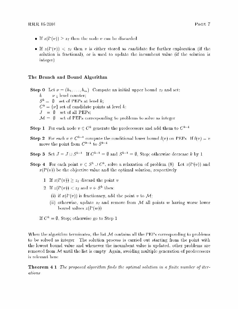
RRR 16-2001 Page 7� If z(l�(v)) � zI then the node v can be discarded.� If z(l�(v)) < zI then v is either stored as candidate for further exploration (if thesolution is fractional), or is used to update the incumbent value (if the solution isinteger).The Branch and Bound AlgorithmStep 0. Let � = (h1; : : : ; hm). Compute an initial upper bound zI and set:k = j�j1 level counter;Sk = ; set of PEPs at level k;Ck = f�g set of candidate points at level k;J = ; set of all PEPs;M = ; set of PEPs corresponding to problems to solve as integer.Step 1. For each node v 2 Ck generate the predecessors and add them to Ck�1.Step 2. For each v 2 Ck�1 compute the conditional lower bound l(v) on PEPs. If l(v) = vmove the point from Ck�1 to Sk�1.Step 3. Set J = J [ Sk�1. If Ck�1 = ; and Sk�1 = ;, Stop; otherwise decrease k by 1.Step 4. For each point v 2 Sk [ Ck, solve a relaxation of problem (8). Let z(l�(v)) andx(l�(v)) be the objective value and the optimal solution, respectively.1. If z(l�(v)) � zI discard the point v.2. If z(l�(v)) < zI and v 2 Sk then:(i) if x(l�(v)) is fractionary, add the point v to M;(ii) otherwise, update zI and remove from M all points w having worse lowerbound values z(l�(w)) .If Ck = ;, Stop; otherwise go to Step 1.When the algorithm terminates, the listM contains all the PEPs corresponding to problemsto be solved as integer. The solution process is carried out starting from the point withthe lowest bound value and whenever the incumbent value is updated, other problems areremoved fromM until the list is empty. Again, avoiding multiple generation of predecessorsis relevant here.Theorem 4.1 The proposed algorithm �nds the optimal solution in a �nite number of iter-ations.

Page 8 RRR 16-2001Proof. Since the number of levels and points explored within each level is �nite, the algo-rithm terminates after �nitely many steps. The optimality of the solution follows from thevalidity of the lower and upper bounds used.As in any branch and bound method (actually here only the bounding part is considered),the performance of the algorithm depend on several issues associated with the computation.The �rst one concerns the choice of the relaxation. Di�erent approaches can be consideredhere. The �rst one consists in dropping the integrality condition on the decision variables.The main advantage of the linear relaxation is related to good computational performanceof the solution process. The relaxed problems di�er in the right hand side only and canbe e�ciently solved by a dual method exploiting, each time, the advanced basis of theprevious optimization step. The second approach is represented by a Lagrangian relaxation:\complicating" constraints are moved into the objective function obtaining a considerablyeasier problem to solve. The bound provided by a Lagrangian relaxation can be tighterthan that found by the linear one, but only at the expense of solving integer problems.Furthermore, the selection of the constraints to relax is problem-dependent. In our branchand bound method we have used a combined relaxation (see Section 4.1).The second issue is related to the computation of the �rst upper bound value zI . Such avalue is obtained by selecting the �rst PEP, s0, and by solving the integer problem (7) withs0 as the right hand side. The choice of a good initial upper bound value strongly a�ects thealgorithm's performance: the better the value, the smaller graph portion is explored. Thecomputation of zI by applying speci�c heuristic techniques is discussed in Section 4.2.The third issue is the use of preprocessing or presolving techniques aimed at \improving" agiven integer programming formulation to facilitate the solution process. A detailed descrip-tion of the main techniques proposed in literature for the general case of integer problemscan be found in the survey papers of Crowder, Johnson and Padberg [10], in the textbookNemhauser and Wolsey [17] and the references therein. Special problems o�er additionalpotential for designing speci�c techniques that can take further advantage of the model'sstructure.4.1 The combined relaxationThe choice of the relaxation constitutes a crucial issue because of the large number of prob-lems to be solved. Indeed, in our branch and bound scheme we solve at each level k of thesearch graph jSk [ Ckj problems (see Step 4). This prompts the need to design e�cientrelaxation techniques aimed at reducing the solution time per problem and providing, at thesame time, good bounds. We have developed a \dual-primal" relaxation scheme.Let us consider the following instance of problem (7)min cTxs:t:Tx � �� (9)x � 0 integer

RRR 16-2001 Page 9where �� = (z1j1; z2j2; : : : ; zmjm) and the deterministic constraints are not included for thesake of simplicity. Let us denote by (LP) the linear relaxation of (9) and by (DP) its dual.(LP) min cTx (DP) max ��T�s:t: Tx � �� s:t: TT� � cx � 0 � � 0The optimal solution �� of (DP) can be used to de�ne a dual function C(�) which will serveas \pruning" criterion in the branch and bound scheme. For each node v 2 Sk [Ck at levelk, the dual function is de�ned as: C(l�(v)) = ��T l�(v):The value C(l�(v)) provides a lower bound on the optimal solution of the instance of problem(9) having l�(v) as right-hand side:zI(l�(v)) � zLP (l�(v)) � zDP (l�(v)) � C(l�(v))where the last inequality holds because �� is a feasible solution for all problems of the searchgraph.The main advantage of the basic dual function C is its easy computability: it requiresthe multiplication of a vector of dual variables, computed once for all, by the lower boundvector l�(v) corresponding to the selected node. On the other hand such a bound can berather weak. Di�erent strategies can be used to improve its quality.One possibility is to use \updated" multipliers. The multipliers associated with a givennode v at level k can be used to derive tighter lower bounds for all predecessors of v at lowerlevels. In order to reduce the solution time the computation of the multipliers can be carriedout periodically. The main drawback of this strategy is related to the increase of memoryrequirement, because we need to store many vectors of multipliers taking trace of the nodesthey belong to.Another possibility is to improve the dual function C by using \partial" information. Let�i, i 2 I, be the dual multipliers associated to the solution of the problems corresponding tothe predecessors of the sink in the search graph. Let us denote by Di(�) the dual functionscomputed by using the corresponding multipliers. For each node v, we de�ne the improveddual function C as follows:C(l�(v)) = maxfC(l�(v));maxi2I fDi(l�(v))ggIt is clear that zI(l�(v)) � zLP (l�(v)) � zDP (l�(v)) � C(l�(v)) � C(l�(v)):In our branch and bound method we have implemented a \dual-primal" relaxation. Thebound computed by the improved dual function is used to perform a �rst screen of thecandidate points. Only for candidate points having better bounds than the best feasiblesolution, we solve the corresponding linear programming relaxation.

Page 10 RRR 16-20014.2 Heuristic strategies for computing the upper bound valueThe computational performance of the branch and bound method is highly in uenced bythe upper bound used to initialize the incumbent value zI. Such a bound can be obtained bysolving either exactly or approximately problem (7) with a �rst PEP as the right-hand side.The determination of this point can be carried out by performing a depth visit of the searchgraph. More speci�cally, according to cost function evaluation, we can distinguish betweensimple and dual heuristic techniques.In the �rst case, starting from the initial vector �, the index selection is performed in arandom fashion, without taking advantage of any speci�c cost information.Simple heuristicStep 0. Set s0 = � and the iteration counter k = 0.Step 1. Compute the conditional bound vector l(sk) by (5). If l(sk) = sk Stop, sk isPEP; otherwise select an index ik, among all the coordinates i 2 f1; : : : ;mg such thatli(sk) < ski . Set: sk+1i = � ti if i = ikski otherwise i = 1; : : : ;m;where ti is computed by (5) (with sk in place of w).Step 2. Increase k by 1 and go to Step 1.In the dual heuristic, the index selection (Step 1) is performed by using dual cost in-formation. At each iteration of the heuristic scheme, we select among all the coordinatesi 2 f1; : : : ;mg such that li(sk) < ski , the one with the maximum dual variable ��i. The intu-ition behind this strategy is clear: dual variables can be used to compute a (lower) boundon the optimal solution and we direct our choice towards lowest bound solutions.Another heuristic scheme can be de�ned as a re�nement of the dual one. The basic ideais to run the dual heuristic starting from each index i 2 f1; : : : ;mg such that li(s0) < s0i .The main advantage of such scheme, referred in the sequel as multistart, is the improvementof the bound's quality at the expense of an increase of the computational time.5 The Probabilistic Lot-Sizing ProblemMany combinatorial optimization problems have their probabilistic counterparts. In thissection we focus our attention on the lot-sizing problem and we formulate a probabilisticversion of the problem by incorporating constraints on the probability of stockout. Ourstarting point is the classical Wagner{Whitin model [28], one of the most fundamental modelswidely used in inventory management (see, for example, [28, 29] and [5] for a classi�cationof lot-sizing models).

RRR 16-2001 Page 11Before de�ning the probabilistic lot-sizing model, we introduce the notation of the deter-ministic version:T { the time horizon;Mt { an upper bound on the number of units produced in period t;ct { the unit production cost at period t;ht { the unit holding cost at period t;kt { the �xed setup cost per production run;dt { the demand at period t;I0 { the initial inventory;It { the inventory carried out from period t to t+ 1;xt { the number of units to be produced at period t;yt { 1 if a setup is performed at period t, 0 otherwise.The deterministic lot-sizing problem can be mathematically formulated as follows:min TXt=1fktyt + htIt + ctxtg (10)s:t: It = It�1 + xt � dt t = 1; : : : ; T (11)xt �Mtyt t = 1; : : : ; T (12)xt � 0; It � 0 t = 1; : : : ; T (13)yt 2 f0; 1g t = 1; : : : ; T (14)The problem consists in determining a production schedule that minimizes the total cost(10) satisfying both ow balance equations (11) and capacity constraints (12).Model (10-14) relies on the assumption that at the beginning of the planning horizonthe demand in the successive periods is known with certainty. Such an assumption is quiterestrictive, since there exist several factors that can cause signi�cant uctuations of theestimated demand (price changes, market competition, etc.).Stochastic lot-sizing models address the random demand case. The literature dealingwith this case is quite rich. For an introduction to stochastic inventory theory, the reader isreferred to the survey paper [20]. We also cite the papers by Klein Haneveld [14] and Peterset al. [18] who have formulated the problem (in the multi-item case) as a stochastic pro-gramming model with recourse. More recently, multi-stage stochastic programming modelsand solution approaches for capacity expansion problems have been proposed in [1].

Page 12 RRR 16-2001Most of the stochastic lot-sizing models proposed in the literature assume that the un-certain demands fdtg are continuous random variables mutually independent and (approxi-mately) normally distributed [20]. In our probabilistic model we suppose that demands areinteger random variables. The use of this type of variables is meaningful when indivisiblegoods are produced.Let us now pass to formulate the probabilistic lot-sizing model. For each period t the ow balance constraints (11) can be rewritten as:It = I0 + tXi=1 xi �Dt; (15)where Dt = tXi=1 didenotes the cumulative demand up to time t. Since It is a random variable, we need tocorrectly formulate the constraint It � 0, t = 1 : : : ; T .One way is to assume that it holds for every realization of the demand, but such aworst case assumption is very restrictive and may lead to excessive inventory levels. Thesecond approach is treat this constraint as `soft' by assuming that all unsatis�ed demandis backlogged. Then the real inventory level at time t is max(0; It) and the backlog ismax(0;�It), where It is given by (15). By adding a backlog cost to the objective onemay formulate a meaningful model of minimizing the expected sum of all costs, comprisingproduction, setup, holding and backlog costs.We consider a di�erent model by limiting the probability of stockout to a prescribedsmall number 1 � p. To formulate the objective we use the approximationE TXt=1 htmax(0; It) � E TXt=1 htIt = TXt=1 ht tXi=1 xi � TXt=1 htEfDtg = TXt=1 Htxt + C;where Ht = TXi=t hiand C is a constant.

RRR 16-2001 Page 13As a result we obtain the following probabilistic lot-sizing model:min TXt=1fktyt + (ct +Ht)xtgs:t: P 0BBBBBBB@x1 � D1x1 + x2 � D2x1 + x2 + x3 � D3... . . ....x1 + x2 + x3 : : : : : : xT � DT1CCCCCCCA � p (16)xt �Mtyt t = 1; : : : ; Txt � 0 integer t = 1; : : : ; Tyt 2 f0; 1g t = 1; : : : ; TWe assume, for the sake of simplicity, that the initial inventory level is 0.Constraint (16) can be viewed as a service level constraint: it ensures that the netinventory remains nonnegative thoughout the entire planning period with the probabilitylevel of at least p.A di�erent probabilistic lot-sizing model with continuous random variables, not includ-ing capacity constraints was proposed in [6]. However, that model considers probabilisticconstraints individually imposed on the single inequalities and is thus easily convertible in adeterministic model of the same form of the original one.The probabilistic model introduced above belongs to the broader class of (PIP) prob-lems. Compared with the general model (1-4), the objective function is replaced by theexpected value and the deterministic constraints include the additional variables y. In fact,the integrality condition on the decision variables x may be omitted here, because it will beautomatically satis�ed by the speci�c structure of the contraint matrix and the integralityof the p-e�cient points.6 Numerical IllustrationThis section is devoted to the discussion of the computational issues of the proposed solutionmethods and to the presentation and analysis of the numerical results collected for theprobabilistic lot-sizing problem.6.1 Computational IssuesEnumeration and solution represent the two main ingredients of the proposed methods.

Page 14 RRR 16-2001Let us �rst analyze the enumeration. In the backward scheme, the search starts from thenode � = (h1; : : : ; hm) and proceeds from one level to the previous one until the terminationcondition is reached. The basic idea of the generation scheme, which avoids the multiplegeneration of the same node, is the following. With each generated node v we associate theindex s(v) 2 f1; : : : ;mg that di�ers it from the successor from which v has been obtained.For example, for nodes v1 = (h1 � 1; h2; : : : ; hm), v2 = (h1; h2 � 1; : : : ; hm), : : : , vm =(h1; h2; : : : ; hm � 1) generated from the sink node, the corresponding index is s(v1) = 1,s(v2) = 2, : : : , s(vm) = m. Starting from v with index s(v) the generation of previouslevel points is performed according to the following rule: if vs(v) � 0 then we enumeratem � s(v) + � points, where � is equal to 1 if s(v) > 0 and to 0, otherwise. Such points areobtained decreasing by 1 the components vi, i = s(v)� � + 1; : : : ;m. By construction, sucha scheme avoids the generation of duplicate points. The same ideas can be applied in thecase of the forward search. The starting node is � = (0; : : : ; 0) and the points are obtainedby increasing by 1 the selected indices.An important issue in the enumeration phase is the computation and storage of theprobability distribution function. In the case of independent random variables, the value ofthe distribution function at a given point is easily computed as the product of the marginaldistributions, which represent the only information to store. In the general case of dependentrandom variables, the computation is much more di�cult and the storage of the informationneeded requires the use of speci�c data structures.The solution phase consists in solving a family of problems that di�er in the right-hand side. As explained in Section 4.1, an e�cient way to proceed is to use a \dual-primal" relaxation scheme where the \primal" phase is carried out by a dual simplex methodexploiting, each time, the advanced basis of the previous optimization step. The use ofpreprocessing techniques can also improve the solution phase. In the case of the lot-sizingproblem, there exist some reformulations whose linear relaxations provide the solution of theinteger problem [2, 15, 19].6.2 Test ProblemsIn order to evaluate the performance of the solution methods, we have considered two nu-merical examples. We note that the lack of a library of test problems (like the Holmes' one[13]) to use as a benchmark, makes the testing phase quite di�cult.The two examples below have been generated by ourselves by exploiting both the randomand the deterministic sides of the problem.The random side is typically problem dependent. In the case of the lot-sizing problem,uncertainty a�ects the demands at the successive periods of the time horizon. Let us denoteby dt the random demand at period t = 1; : : : T , and let us assume that fdtg are independentinteger random variables with the Poisson distribution. The cumulative demand Dt at timet is de�ned as the sum of random variables:Dt = tXi=1 di:

RRR 16-2001 Page 15Table 1: Characteristics of test problem Test1Period 1 2 3 4 5 6 7 8�t 2 1 3 4 2 1 3 2ct 5.6 4.2 3.0 2.0 1.2 0.6 0.4 0.2Table 2: Characteristics of test problem Test2Period 1 2 3 4 5 6 7 8 9 10�t 2 1 3 4 2 1 3 2 4 3ct 9.7 9.4 9.1 8.8 8.3 8.0 7.7 7.4 7.1 6.5We have generated two test problems by considering a time horizon of 8 and 10 periods,respectively. The parameters of the Poisson distribution used in the experiments are reportedin the �rst row of Tables 1 and 2. For each period of the planning horizon, the number ofrealizations of the independent random variables has been �xed to 5 and 4 for the two testproblems, respectively.The deterministic side of the problem is less di�cult to deal with. A library of tests fora wide variety of lot-sizing models is maintained by Belvaux and Wolsey [5].For our computational experiments we have considered two di�erent instances (Test1,Test2) of the uncapacited single-item lot-sizing problem. The �rst one is a modi�ed versionof the example reported in [27], whereas the second one is randomly generated. For bothtests, the initial inventory level is set to 0. The holding and set-up costs are assumed to beconstant and equal to $0.50 and $48, respectively. Furthermore, the the production capacityhas been set to 50 units per period. The second row of Tables 1 and 2 report, for the twotests, the variable production cost for all the periods of the time horizon. We stress thatthe aim of this paper is to present the �rst approach for the solution of the (PIP) problemsrather than to compare the e�ciency of our method with other existing algorithmic schemes.This motivates the choice of two simple, although non trivial, instances for our preliminarycomputational experience.6.3 Numerical ResultsThe computational experiments have been carried out on a R10K processor of the super-computer Origin2000, consisting of 4 nodes each with a cache memory of 4 MB and a RAMof 128 MB. All the codes have been written in the C programming language and use thestate-of-the-art solver CPLEX 6.5 [9].Table 3 reports the number of PEPs enumerated for two di�erent values of the service

Page 16 RRR 16-2001level p. Time refers to the execution time, measured in seconds, of the backward enumerationalgorithm. Table 3: p-E�cient PointsTest Problem p PEP TimeTest1 0.98 216 32.25Test1 0.95 767 145.13Test2 0.98 707 120.19Test2 0.95 2171 434.21The numerical results provide an evidence that, even for a small size of the random vector,the number of PEPs can be large. Furthermore, their number increases as the probabilitylevel is decreased, amplifying the complexity of the solution process. This strengthens themotivation to design methods based on a partial enumeration of the PEPs to e�ciently solve(PIP) problems.Below we report the numerical results of the branch and bound method (see Section4). They have been collected by using the combined relaxation to determine the lowerbound values and the di�erent heuristic schemes introduced in Section 4.2 to initialize theincumbent value.Tables 4, 5, 6 report the service level p, the initial incumbent value zI , the number ofenumerated PEPs, the number of linear (LP) and integer problems (IP) solved, the optimalvalue (z�) and the execution time measured in seconds.The �rst general observation concerns the e�ects of the probabilistic relaxation of theworst case constraints. Figure 1 shows, for the test problem Test2, how the objective functionvalue varies with the service level p. For example, by choosing the probability level of 0:98the reduction in the objective function is 12.3 %. Lower values of p allow higher savings inthe costs. Nevertheless, the choice of p is up to the decision maker and re ects the trade-o�between an acceptable constraint violation probability and the cost reduction.Other speci�c considerations concern the performance of the solution method. First ofTable 4: Branch and Bound method with simple heuristicTest Problem p zI PEP LP IP z� TimeTest1 0.98 259.2 112 63 12 246.6 17.28Test1 0.95 250.5 360 190 28 234.0 69.62Test2 0.98 439.5 376 228 30 395.10 66.10Test2 0.95 384.0 1411 745 87 361.80 295.27

RRR 16-2001 Page 17Table 5: Branch and Bound method with dual heuristicTest Problem p zI PEP LP IP z� TimeTest1 0.98 255.6 84 39 8 246.6 13.06Test1 0.95 246.0 314 109 23 234.0 61.56Test2 0.98 417.3 282 145 21 395.10 52.21Test2 0.95 384.0 933 348 66 361.80 194.77Figure 1: Cost-reliability trade-o�0.85

0.9

0.95

1

250 300 350 400 450

Cost

Rel

iab

ility

Page 18 RRR 16-2001Table 6: Branch and Bound solution with multistart heuristicTest Problem p zI PEP LP IP z� TimeTest1 0.98 249.6 56 20 5 246.6 11.12Test1 0.95 234.0 245 48 3 234.0 51.18Test2 0.98 406.2 218 75 17 395.10 43.80Test2 0.95 372.9 738 148 51 361.80 175.76all, we note that the method enumerates only a small percentage of the total number ofPEPs. Neverthless, this number is related to the initial upper bound value. The betterthis value, the lower the number of points, and, as a consequence, the number of linear andinteger problems solved. The advantage from such a reduction becomes more relevant asthe solution time per problem increases. For our numerical illustration we have consideredsmall examples (the solution times of an integer instance of the two problems are 0:05 and0:07 seconds, respectively) and, thus, the savings in the solution time are not so high.Better performance can be obtained by improving the initial upper bound value. Table 6reports the results collected by using the dual multistart heuristic. We note, however, thatthe determination of the improved initial bound is more computationally expensive and thereduction of the total solution time is not so evident.7 ConclusionsIn this paper we have proposed a branch and bound method for the solution of the class ofinteger problems under probabilistic constraints. E�cient strategies for the determination ofboth the lower and upper bound values have been designed. The preliminary numerical re-sults collected on an probabilistic instance of the classical lot-sizing problem are encouragingand show the e�ciency of the algorithms implemented.References[1] S. Ahmed, A.J. King, G. Parija, A Multi-Stage Integer Programming Approach forCapacity Expansion under Uncertainty, Working paper, Department of Chemical Engi-neering, University of Illinois, 2000.[2] I. Barany, T. Van Roy, L.A. Wolsey, Uncapacited lot-sizing: The Convex Hull of Solu-tions, Mathematical Programming Study, 22 (1984) 32{43.[3] P. Beraldi, A. Ruszczy�nski, The Probabilistic Set Covering Problem, RUTCOR-RutgersCenter for Operations Research RRR 08-99, Rutgers University, 640 Bartholomew RoadPiscataway, New Jersey, 08854-8003 USA.

RRR 16-2001 Page 19[4] D. P. Bertsekas, J. N. Tsitsiklis, C. Wu, Rollout Algorithms for Combinatorial Opti-mization, Journal of Heuristics 3 (1997) 245{262.[5] G. Belvaux, L.A. Wolsey, LOTSIZELIB: A Library of Models and Matrices for Lot-Sizing Problems, Internal Report, Center for Operations Research and Econometrics,Universite Catholique de Louvain (1999).[6] J. H. Bookbinder, J-Y. Tan, Strategies for the probabilistic lot-sizing problem withservice-level constraints, Management Science 34 (1988) 1096{1108.[7] A. Charnes, W. W. Cooper, Chance-Constrained Programming, Management Science5 (1958) 73{79.[8] A. Charnes, W. W. Cooper, G. H. Symonds, Cost Horizons and Certainty Equivalents:an Approach to Stochastic Programming of Heating Oil, Management Science 4 (1958)235{263.[9] CPLEX, ILOG CPLEX 6.5: User's Manual, CPLEX Optimization, Inc., Incline Village,NV, 1999.[10] H. P. Crowder, E. L. Johnson, M. W. Padberg, Solving large-scale zero-one linear pro-gramming problems, Operations Research 31 (1983) 803-834.[11] D. Dentcheva, A. Pr�ekopa, A. Ruszczy�nski, Bounds for Probabilistic Integer Program-ming Problems, RUTCOR-Rutgers Center for Operations Research RRR 31-99, RutgersUniversity, 640 Bartholomew Road Piscataway, New Jersey, 08854-8003 USA.[12] D. Dentcheva, A. Pr�ekopa, A. Ruszczy�nski, Concavity and E�cient Points of DiscreteDistributions in Probabilistic Programming, Mathematical Programming 89 (2000) 55{77.[13] D. Holmes, A collection of stochastic programming problems, Technical Report 94{11(1994), Department of Industrial and Operations Engineering, University of Michigan,USA.[14] W. K. Klein Haneveld, A stochastic programming approach to multiperiod productionplanning, Technical Report 276 (1988), Institute of Economic Research, University ofGroningen, The Netherlands.[15] R.K. Martin, Generating Alternative Mixed-Integer Programming Models Using Vari-able Rede�nition, Operations Research, 35 (1987) 820{831.[16] L.B. Miller, H. Wagner, Change-Constrained Programming with Joint Constraints, Op-erations Research 13 (1965) 930{945.[17] G.L. Nemhauser, L.A. Wolsey, Integer and Combinatorial Optimization, John Wiley &Sons, New York, 1988.

Page 20 RRR 16-2001[18] R.J. Peters, K. Boskama, H.A.E. Kupper, Stochastic programming in production plan-ning: a case with non-simple recourse, Statistica Neerlandica 31 (1977) 113{126.[19] Y. Pochet, L.A. Wolsey, Lot-Size Models With Backlogging: Strong Reformulations andCutting Planes, Mathematical Programming, 40 (1988) 317{335.[20] E. L. Porteus, Stochastic Inventory Theory, Handbooks in Operations Research andManagement Science, Noth-Holland (1990) 605{652.[21] A. Pr�ekopa, On Probabilistic Constrained Programming, Proceedings of the PrincetonSymposium on Mathematical Programming, Princeton University Press (1970) 113{138.[22] A. Pr�ekopa, Contributions to the Theory of Stochastic Programming, MathematicalProgramming 4 (1973) 202{221.[23] A. Pr�ekopa, Dual Method for Solution of One-Stage Stochastic Programming with Ran-dom Rhs Obeying a Discrete Probability Distribution, Zeitschrift fur Operations Re-search 34 (1990) 441{461.[24] A. Pr�ekopa, Stochastic Programming, Kluwer Academic Publishers, Boston, 1995.[25] A. Pr�ekopa, D. Vizv�ari, T. Badics, Programming under Probabilistic Constraint withDiscrete Random Variable, New Trends in mathematical programming F. Giannesi,Kluwer Academic Publishers (1998) 235{255.[26] S. Sen, Relaxations for the Probabilistically Constrained Programs with Discrete Ran-dom Variables, Operations Research Letters 11 (1992) 81{86.[27] C. R. Sox, Dynamic Lot-Sizing with Random Demand and Not-Stationary Costs, Annalsof Operations Research 20 (1997) 155{164.[28] H. M. Wagner, T. M. Whitin, Dynamic Version of the Economic Lot Size Model, Man-agement Science 5 (1958) 89{96.[29] H. Wagelmans, S. V. Hoesel, A. Kolen, Economic Lot Sizing: an O(n log n) algorithmthat runs in linear time in the Wagner{Whitin case, Operations Research 40 (1992)145{156.