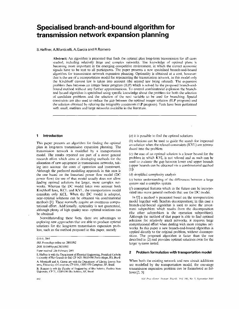
Specialised branch-and-bound algorithm for transmission network expansion planning

S.Haffner, A.Monticelli, A.Garcia and R.Romero

Abstract: An algorithm is presented that finds the optimal plan long-term transmission for all cases studied, including relatively large and complex networks. The knowledge of optimal plans is becoming more important in the emerging competitive environment, in which the correct economic signals have to be sent to all participants. The paper presents a new specialised branch-and-bound algorithm for transmission network expansion planning. Optimality is obtained at a cost, however: that is the use of a transportation model for representing the transmission network, in this model only the Kirchhoff current law is taken into account (the second law being relaxed). The expansion problem then becomes an integer linear program (ILP) which is solved by the proposed branch-and- bound method without any further approximations. To control combinatorial explosion the branch- and bound algorithm is specialised using specific knowledge about the problem for both the selection of candidate problems and the selection of the next variable to be used for branching. Special constraints are also used to reduce the gap between the optimal integer solution (ILP program) and the solution obtained by relaxing the integrality constraints (LP program). Tests have been performed with small, medium and large networks available in the literature.

1 introduction

This paper presents an algorithm for finding the optimal plan in long-term transmission expansion planning. The transmission network is modelled by a transportation model. The results reported are part of a more general research effort which aims at developing methods for the allocation of new equipment in transmission networks, tak- ing into account the costs of operation and investment. Although the preferred modelling approach in this area is the one based on the linearised power flow model (DC power flow) the use of that model usually does not allow finding optimal solutions for larger, more complex net- works. Whereas the DC model takes into account both Kirchhoff laws, KC L and KVL, the transportation model considers only KCI,. When the DC model is adopted, near-optimal solutions can be obtained via combinatorial methods [I]. These normally require an enormous compu- tational effort. Additionally, optimality is not guaranteed, although plenty of high quality near- optimal solutions can be obtained.

Notwithstanding these facts, there are advantages to exploring new apprclaches that are able to produce optimal solutions for the long-term transmission expansion prob- lem, such as the method proposed in this paper, namely

0 LEE, 2001 IEE Proceeding online no. 20010502 DOL 10.1O49/iggtd:20010502 Paper received 12th Febmtry 2001 S. Haffner is with the Department of Electrical Engineering, Pontifical Catholic University of Rio Grande do Sul, CP 1429,90619-900 Port0 Alegre, RS, Brazil A. Monticelli and A. Garcia are with the Department of Electric Energy Sys- tems, University of Campinas, CP 6101, 13081-970 Campinas, SP, Brazil R. Romero is wth the Fasulty of Engineering of Ilha Solteira, Paulista State University, CP 31, 15385-000 Ilha Solteira, SP, B d

(U) it is possible to find the optimal solutions (b) solutions can be used to guide the search for improved an solution when the relaxed constraints (KVL) are reintro- duced into the problem (c) the cost of an optimal solution is a lower bound for the problem in which KVL is not relaxed and as such can be used to evaluate the gap between lower and upper bounds (upper bounds can be obtained via a combinatorial method

(4 simplified complexity analysis (e) better understanding of the differences between a large system and a complex system v) conceptual features which in the future can be incorpo- rated into more general methods that use the DC model.

In [2] a method is presented based on the transportation model together with Benders decomposition; in this case a branch-and-bound algorithm is used to solve the invest- ment subproblem which results from the decomposition (the other subproblem is the operation subproblem). Although the method of that paper is able to find optimal solutions for relatively small networks, it requires large computational effort when dealing with more complex net- works. In this paper a new branch-and-bound algorithm is applied directly to the original problem, without decompo- sition. The proposed algorithm is faster than the one described in [2] and provides optimal solutions even for the larger systems tested.

[11>

2 Problem formulation with transportation model

When both the existing network and new circuit additions are modelled by the transportation model, the one-stage transmission expansion problem can be formulated as fol- lows [2, 31:

I E E Pror -Genet Tranrm Dutrrh Vol I48 Nu 5 September 2001 482

Min U = cijnXJ

(z,j)€n subject to Sf + g = d

IhJ I 5 b i j + 4$7ij

0591s 0 5 nij 5 Eij

n,j integer, f i j unbound b'(i,j) E R

(1) where cq, nq, n:, A; and fq represent, respectively, the cost of a circuit that can be added to right-of-way i - j , the number of circuits added, the number of circuits in the base case, the power flow, and the corresponding maximum power flow. v is the total investment, S is the branch-node incidence matrix, j is a vector with elements f;i (power flows), g is a vector with elements gk (generation in bus k) whose maximum value is g, nq is the maximum number of circuits that can be added in right-of-way i -,j, and Q is the set of all rights-of-way. The problem defined above is an integer linear problem (ILP) that can be solved by the branch-and-bound algorithm described in the following.

3 Branch-and-bound algorithm

The algorithm is an enumerative algorithm based on a binary search tree where the nodes represent candidate problems and the branches correspond to decisions taken so far in a given path. All integer solutions are explicitly or implicitly represented in that tree which guarantees that all optimal solutions will eventually be reached by the algo- rithm. The algorithm deals with the basic procedures: sepa- ration (or branching), relaxation and fathoming (or bounding) [4, 51. The branch-and-bound algorithm that has been actually implemented draws on search techniques dis- cussed in [6].

The branching operation consists of dividing the current problem (a node in the decision tree) into two descendants (the current node is also called the parent node). The descendant problems are easier to solve than the parent problem since one of its variables is defined in the two descendent nodes; one additional constraint on the separa- tion variable is added to each of the descendant problems. A separation variable is a variable that assumes a noninteger value in the current node and can be fured at the values of either neighbouring integer values; in both cases a new constraint is then added to the current problem (contradictory constraints). The current problem is then excluded from the list of candidate problems and the two descendent problems are added to the list (as a result of the branching operation).

The relaxation operation consists of temporarily ignoring (or relaxing) some complicating constraints of the original problem to make it easier to solve. As a rule, by the elimi- nation of the integrality constraints the ILP is transformed into a LP (linear problem), which is called the correspond- ing LP.

The fathoming operation consists of verifying which of the candidate problems can be eliminated (or fathomed) from the list of candidates. A candidate is fathomed when it cannot possibility lead to a solution that will be better than the incumbent solution, i.e. the best solution found so far.

In the transmission expansion problem, the investment variables no are the integer variables of the problem, whereas the real variables are the operation variables Jj and

g. Initially, by relaxation, one assumes that is possible to make noninteger investments, which turns the ILP problem into a LP problem. As a result the optimal solution for this LP problem presents investment variables with noninteger values. Among these variables one is chosen as the next separation variable. The separation leads to the creation of two new candidate problems which are simpler to solve than its parent problem. The next step consists of choosing a new candidate to be examined among the candidates in the list; the selected candidate will be either branched or eliminated from consideration if it passes a fathoming test. This procedure is repeated until the list of candidates becomes empty. The algorithm is summarised in the following.

3. I Basic algorithm 1. Initialisation: Make k = 0, define the initial incumbent solution v* and set the initial list of candidate problems as composed of the solution of the corresponding LP (i.e. problem given by eqn. 1 without the integrality con- straints). 2. Convergence test: If the list of candidates is empty the search is finished and the current incumbent solution is the optimal solution. Otherwise, go to the next step. 3. Selection of the candidate problem to be examined: Select one candidate not fathomed from the list of candidates. Solve the LP for this candidate and store the optimfl solu- tion as a lower bound for its descendants, vl(l,,wprer = v L p . 4. Fathoming test: The candidate problem under considera- tion is fathomed is one of the following conditions is satis- fied: (a) the problem is unfeasible (b) if vlowe,. > v*

(c) if the optimal solution of the relaxed problem satisfies the integrality constraints, i.e. it is a feasible solution of problem 1. If so, if the*optimum is less than that of the incumbent, then make v = vlollJeu and apply test (b) for all Candidates not fathomed yet. If the candidate under examination has been fathomed, return to step 2. 5. Brunching: Among the integer variables that still assume noninteger values select one for separation. Let nii be the selected variable (its current value is n l ) . Two new prob- lems are generated by including either of the following con- straints:

descendant k + 1 : nZ3 5 [4] descendant k + 2 : n,j 2 [nZ*,] + 1

where [ ) t i ] is the biggest integer of n i . Make k = k + 2 and return to step 3.

3.2 Complexity issues The complexity of the ILP problem solved by the branch- and-bound algorithm depends on factors such as: the gap between the optimum of the original ILP program, which is unknown, and the corresponding LP, a program in which the integrality constraints are relaxed; the number of decision variables nii that assume nonzero value at the opti- mal solution, which is unknown too; and the presence of variables with nearly equivalent quality or influence on the final solution.

An approximation for the gap can be obtained determin- ing an upper bound for the optimal cost using a fast con- structive algorithm (a lower bound is given by the solution of the corresponding LP, subproblem Po). When the gap is

I E E Proc.-Gener. Trunsnr. Distrrh., Vol. 148, No. 5, Septprernber 2001 483

large with respect to the coefficients (costs) of the decision variables it means that the number of variables to be ana- lysed is also large. 111 this case it is even more important to determine an upper bound with good quality to keep com- plexity at a minimum.

The number of nonzero variables at the optimal solution also affects complexity since it affects the depth of the search tree; the number of these variables is directly related to the number of variables for which separation has to be performed. For example, if the optimal solution for the expansion problem has 40 nonzero decision variables, it means that the search tree that has been explored has approximately the same number of levels. (Notice that some of the decision variables may assume integer values without requiring an explicit separation; also, one may reach the optimal solution with separations that have set decision variables at zero.)

The presence of decision variables with nearly the same impact on the optimal solution also makes the problem more complex since all competing alternatives have to be considered in the search process, in most cases explicitly.

To improve the efficiency of the branch-and-bound algo- rithm, the difficulties discussed have to be addressed. We do this by using specific knowledge about the transmission expansion problem. To reduce the gap between UB (the upper bound) and ILB (the lower bound) a heuristic con- structive algorithm based on Garver's method has been adopted [3]; this method is used to find a good initial incumbent UB. To improve the quality of the solution given by the corresponding LP problem, special constraints are added to this problem (the fencing constraints, described subsequently).

4 Specialised branch-and-bound algorithm

The overall efficiency of a branch-and-bound algorithm is directly associated with the method used for selecting (step 3 of the algorithm) the next problem to be examined, in terms of the search tree, the next node to be fathomed (step 4) or branched (step 5). In [2] tests were performed that led to the conclusion that the use of pseudocosts is the best option for the seleclion of new candidates in the transmis- sion expansion planning problem.

Additional improvements can be obtained by the use of special constraints, which take advantage of the specific features of the transmission expansion problem. One of these is the so called fencing constraints which result from the application of KCL to selected nodes and supernodes of the transmission network.

4. I Use of pseudocosts Several alternatives 'have been suggested in the literature for the selection of the next problem to be examined in branch- and-bound algorithms. A popular option is the LIFO mechanism, last in first out. Although simple and requiring minimum temporary storage, this strategy normally requires a high computational effort. An alternative has shown good results in practice based on pseudocosts (for the definition and iipplications of pseudocosts see [7, 81). Pseudocosts can be used to obtain the best estimate for the objective function. For complex problems, however, this may lead to an excessive number of candidate problems to be stored during the solution process. Hence, in this paper a hybrid strategy has been adopted: if the number of stored candidate problems is less than a prespecified value ntop the next candidate is selected based of the best estimate of the objective function based on pseudocosts; otherwise the LIFO rule is used for selecting the next candidate.

484

The selection of the variable of the current candidate problem which will be used for branching the variable whose largest estimated degradation is maximum. The set of variables that are considered for separation are those that have real values not too close to the upperllower near- est integer values. This selection criterion usually speeds-up the fathoming process. As for variables that currently have values close to integer values, it is expected that they will naturally tend to an integer value as the search process pro- ceeds. In the actual implementation this is controlled by a user specified parameter rp which gives the threshold for the difference of the real value and the closest integer value for a variable considered for separation.

4.2 Use of special constraints Fencing constraints result from the application of KCL to selected individual nodes or sets of nodes (supernodes) of the transmission network. Three types of fences have been considered: single node, a node and one of its neighbours, and a node and all its neighbours. Notice that a neighbour- hood is defined in terms of the existing network and all possible additions (see, for example, Fig. 1).

g, =50

t t80

/

\ :..a * -. fences . . .+ 160

- 1

- *

........................................ Fig. 1 Bcrsic conjgura~ion of Gcirver's network witiiitllfences

Once a fence has been topologically defined the corre- sponding constraint has to be built. This is done by esti- mating the deficit of transmission capacity in the corresponding node or supernode considering the most favourable case. For example, in Fig. 1, there is a demand of 240MW at bus 5 and there are two circuits crossing the fence around bus 5, each with l0OMW capacity. In the most favourable case both circuits are used to supply the load of bus 5 carrying lOOMW each. The deficit is of 40MW. This means that at least an additional circuit is needed. Mathematically this can be translated as the fol- lowing constraint: nI5 + n25 + n35 + n45 + n56 2 1. Hence, the three fences of Fig. 1 lead to the following constraints:

7215 + 7225 + 7235 + 7245 + 1256 L 1

1214 + 1224 + 7234 + 1245 + n16 + 1226 + 7236 + 7256 2 3 n16 + 1226 + 7236 + n 4 6 + n 5 6 L 6

( 2 ) I E E P m c -Gerie.r Transm Disfrrh Vol 148 No 5 Septenzher 2001

Although the fencing constraints are redundant with respect to the ILP problem formulated in eqn. 1 they are very important for the corresponding LP problem and its successors since it serves to reduce the gap between prob- lem UB and LB, and it forces some of the decision varia- bles to assume integer values even when the relaxed LP program is solved without requiring the corresponding sep- aration being carried out. That is to say, the use of fencing constraints can significantly reduce the complexity of the problem being solved. This is particularly true in networks with a high degree of islanding (Garver’s and the North- eastern networks, see Section 5).

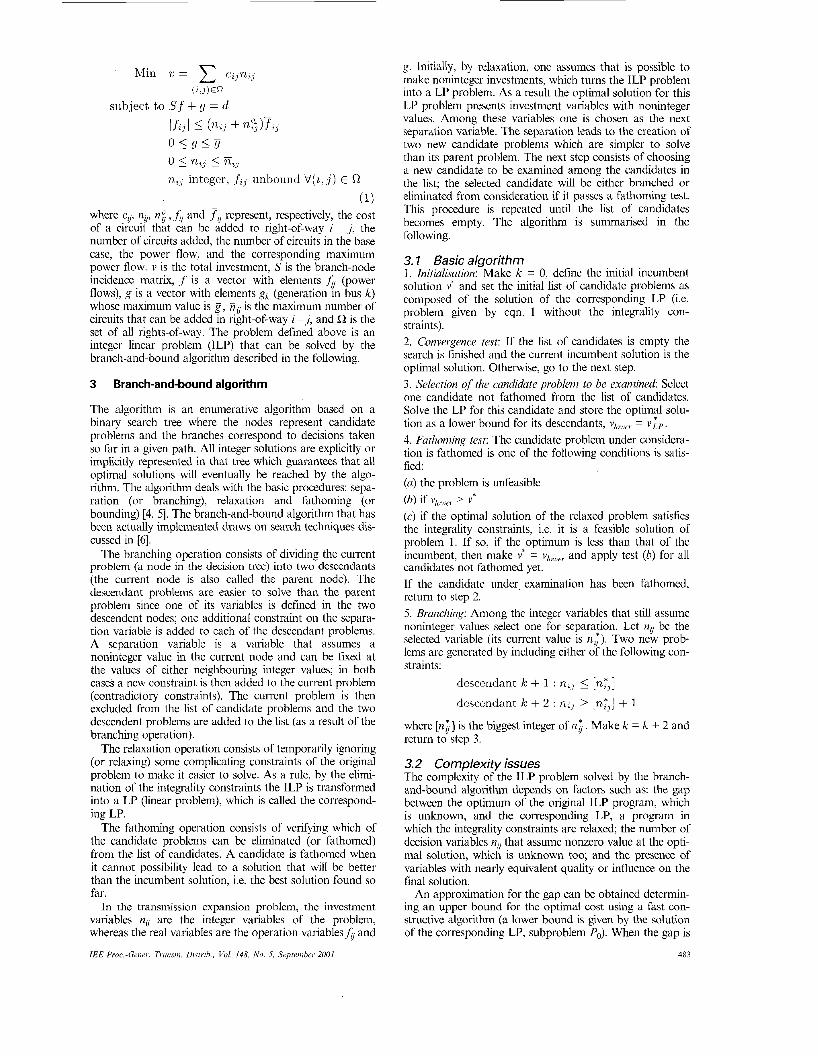
In Fig. 2 vLP is a solution of the corresponding LP, vLPF is the solution of the corresponding LP with the fencing constraints added to the problem, voP is the optimal solu- tion for the original ILP problem and vUB is an upper bound which is the incumbent solution, initially this solu- tion is found using a heuristic constructive algorithm based on Gamer’s method. The Figure illustrates the fact that the fencing constraints reduce the gap between the solution of the corresponding LP and the solution of the original ILP problem (eqn. 1). The closer vLPF is to p o p the more impor- tant is the role played by the fencing constraints. For the network of Fig. 1, and considering the three fences shown, the following values were found: vLp = 171, vLPF = 200, voP = 200 and vuB = 200 (this last value was obtained via the constructive Gamer’s algorithm). In this case the fencing constraints have eliminated the gap between the solution of the corresponding LP and the solution of the ILP problem. This means that with the fencing constraints this example can be solved with a single LP solution, without it being necessary to use the constructive methods to find an initial incumbent solution and without looking for alternative optimal solutions. In this case, besides eliminating the gap, the fencing constraints forced some of the decision varia- bles to assume integer values. Notice however that this behaviour depends on the LP algorithm used to solve the corresponding LP problem since; in this example the cost v = 200 may represent several alternative optimal solutions (both integer and non-integer).

v~~~ --+ increase of v VUE 0 - - 0

VLP VOP Fig. 2 Meunuig ofgup UI trumportution modrl

Remark: in [2] an additional type of special constraint is discussed, related to new paths (a path is the combined addition of transformers and lines connecting two points). Although these constraints have proven to be valuable in solving the investment subproblem that results from the application of the Benders decomposition, they do not yield quite the same benefits when applied to the original prob- lem (undecomposed problem as formulated in eqn. 1).

5 Test results

To illustrate the performance of the proposed algorithm, as well as the impact of the complexity on the solution proc- ess, tests were performed with systems of different sizes and structures. The three larger systems correspond to parts of the Brazilian interconnected network.

5. I Gatver‘s six-bus system This system has six buses and 15 rights-of-way for the addi- tion of new circuits. The demand is of 760MW and the rel- evant data are given in [2, 31. From the basic topology, two problems can be formulated: expansion without consider- ing generation redispatch, and expansion with gencration

IEE Proc -Gerier T t a n m Drstr rb Vol 148, N o 5, September 2001

redispatch. The first case was studied in detail in [2-91, hence only the case with redispatch is considered.

Table 1: Optimal solutions obtained for Garver’s network

No. Circuits added Investment cost

n26 n35 n46 V

1 0 1 3 110

2 3 1 0 110

3 1 1 2 110

4 2 1 1 110

g,=120

1

v*=110

300 ---c

4 160

‘I 6 n46=3 g6=300

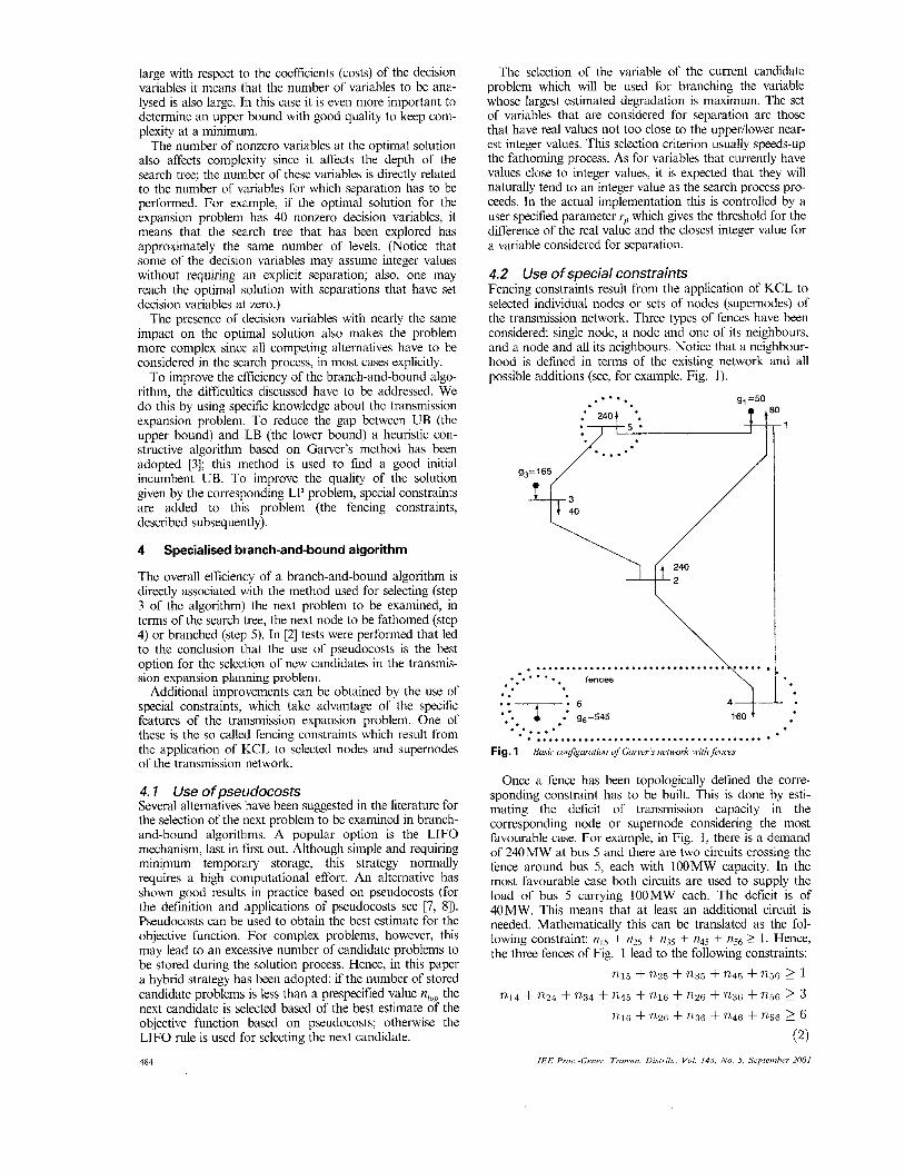
Fig.3 Optinuzl solutwn,/or Gurwrk network

g,=150

80 240

5 c 70 1 J n,5=1

/ v*=190

90

160 -+

/ I I

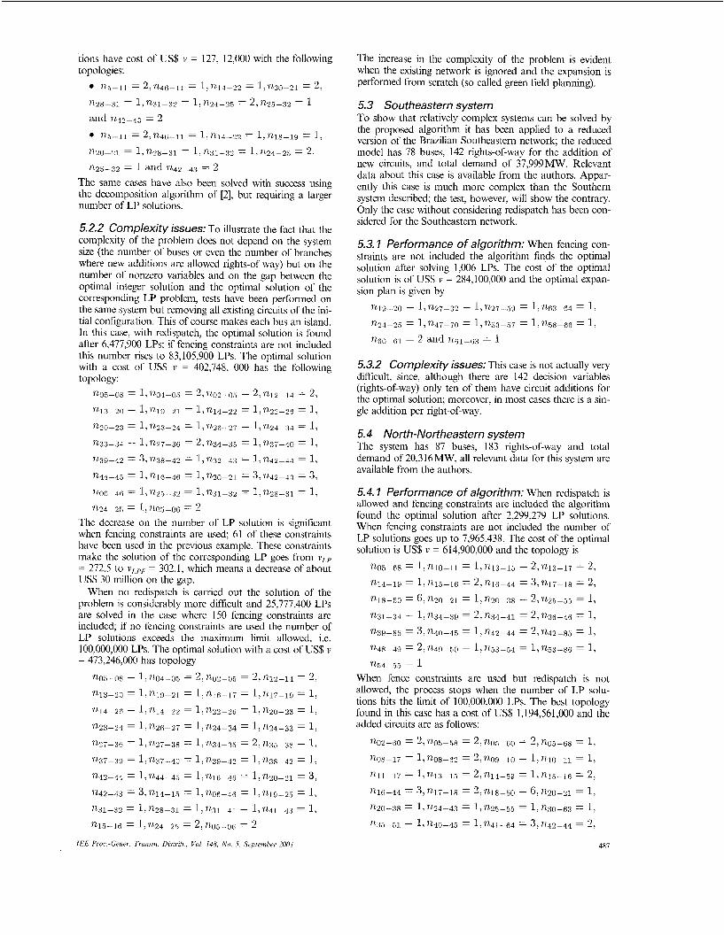
Fig. 4 Optirul solution for Gurveri network with initial network removed

The algorithm has found four optimal solutions as sum- marised in Table 1. The first of these, shown in Fig. 3, is also the optimal solution for the DC model. The algorithm

485

converged after 112 LP solutions without using fencing constraints. (As discussed in the previous Section, when fencing is used the solution becomes trivial and an optimal solution is obtained with a single LP solution.)

This example serves to illustrate the fact that the trans- portation model is particularly useful when the network is islanded. In this case the fencing constraints also play an important role in the overall eficiency of the branch-and- bound algorithm. To illustrate this fact Garver’s network was modified by removing all existing circuits which made all network buses islanded. Under these conditions, and considering generation redispatch, the algorithm found the optimal solution of Fig. 4 after 82 LP solutions, without considering fencing constraints and without using an initial incumbent solution. The optimal cost is v = 190 and the following circuits are added:

1215 1 1. ~ ~ 2 3 1 2 , ~ ~ 2 6 = 1,1235 = 2, and 1246 = 2

Notice that this topology is also the optimal one for the DC model since it corresponds to a radial network.

5.2 Southern system This system is a middle size system with 46 buses and 79 rights-of-way for the addition of new circuits (relevant data can be found in [2-101). The basic topology and the set of branches where new additions are possible are shown in Fig. 5. The total demand for this system is 6,880MW.

5.2. I Performance of algorithm: When redispatch is allowed the algorithm found the optimal solution with cost of US$ v = 53,334,000 after solving 269 LPs (without using fencing constraints and without obtaining an initial incum- bent); the circuits added are

n33-34 = 1,n~o-21 = 2,1242-43 = 1,n05-11 = 2, and 1246-11 = 1

When redispatch is not allowed the complexity of the prob- lem increases significantly. If fencing constraints are not used and an attractive initial incumbent is not determined, the algorithm finds the optimal solutions after 3500 LPs; using fencing constraints and an initial incumbent this number is reduced to 1220 LPs. The multiple optimal solu-

0 230kV 0 500kV

I ..............

........ . . . . . . - 1 - m ............

- . . . . . . . . . ......... . . @ - ....... ~

..................... . . ..

1 I

Fig.5 Bmic o+ generation + load

486 IEE ProcGener . Transni DDtrih., Vol. 148. No. 5 , September 2001

tions have cost of US$ v = 127, 12,000 with the following topologies:

0 125-11 = 2,1246-11 = 1,1214-22 = 1,1220-21 = 2, 1128-31 = 1,1131-32 = 1,1224-25 = 2, 1225-32 = 1 and 1242-43 = 2 0 115-11 = 2,1246-1l = 1,1214-22 = 1,1118-19 = 1,

n20-21 = 1, n128-31 = 1 , 7x3 1-32 = 1, 1124-25 = 2, n25-32 = 1 and 1242-43 = 2

The same cases have also been solved with success using the decomposition algorithm of [2], but requiring a larger number of LP solutions.

5.2.2 Complexity issues: To illustrate the fact that the complexity of the problem does not depend on the system size (the number of buses or even the number of branches where new additions are allowed rights-of way) but on the number of nonzero variables and on the gap between the optimal integer solution and the optimal solution of the corresponding LP problem, tests have been performed on the same system but removing all existing circuits of the ini- tial configuration. This of course makes each bus an island. In this case, with redispatch, the optimal solution is found after 6,477,900 LPs; if fencing constraints are not included this number rises to 83,105,900 LPs. The optimal solution with a cost of US$ v = 402,748, 000 has the following topology:

1205-08 = 1, 1204-05 2,1202-05 = 2, 1212-14 = 2: 1213-20 = 1, 1119-21 1 1,1214-22 = 1,1222-26 = 1; 1~20-23 = 1,1123-24 = 1,1126-27 = 1,7224-34 = 1,

1233-34 = 1,1227-36 = 2,1234-35 = 1, 1237-40 = 1, 1139-42 = 3, ~ 3 8 - 4 2 = 1,1132-43 = 1, 1242-44 = 1, 1244-45 = 1,1216-46 = 1, ~ ~ 2 0 - 2 ~ = 3,17.42-43 = 3,

7206-46 = 1,1225-32 = 1,1231-32 = 1,1228-31

7224-25 1 1, ?105-06 z r 2 1,

The decrease on the number of LP solution is significant when fencing constraints are used; 61 of these constraints have been used in the previous example. These constraints make the solution of the corresponding LP goes from vLp = 272.5 to vLpF = 302.1, which means a decrease of about US$ 30 million on the gap.

When no redispatch is carried out the solution of the problem is considerably more dificult and 25,777,400 LPs are solved in the case where 150 fencing constraints are included; if no fencing constraints are used the number of LP solutions exceeds the maximum limit allowed, i.e. 100,000,000 LPs. The optimal solution with a cost of US$ v = 473,246,000 has topology

7205-08 = 1,1204-05 = 2,1202-05 = 2 , 1212-14 = 2,

1213-20 = 1,7119-21 = 1,1216-17 = l 1 n 1 7 - 1 g = 1, 1214-26 = 1, 1114-22 = 1,7222-26 = 1, 7120-23 = 1,

7123-24 = 1,7126-27 = 1,1124-34 = 1,1224-33 = 1, 1127-36 = 1,1227-38 = 1, n34-35 = 2,1135-38 = 1,

7137-39 = 1, 1237-40 = 1, 1239-42 1, 1238-42 1, 1242-44 1,1?,44-45 = 1,1216-46 =I 1, 1220-21 = 3, 1242-43 = 3,1214-15 = 1,1206-46 = 1,7219-25 = 1, 1131-32 = 1, 1228-31 = 1, 1231-41 = 1,1241-43 = 1,

1215-16 =I 1, 1224-25 = 2, 1205-06 = 2 IEE Proc.-Genrr Tunistn. Distrib., Vol. 148, N o . 5 , Srpteniber 2001

The increase in the complexity of the problem is evident when the existing network is ignored and the expansion is performed from scratch (so called green field planning).

5.3 Southeastern system To show that relatively complex systems can be solved by the proposed algorithm it has been applied to a reduced version of the Brazilian Southeastern network; the reduced model has 78 buses, 142 rights-of-way for the addition of new circuits, and total demand of 37,999MW. Relevant data about this case is available from the authors. Appar- ently this case is much more complex than the Southern system described; the test, however, will show the contrary. Only the case without considering redispatch has been con- sidered for the Southeastern network.

5.3. I Performance of algorithm: When fencing con- straints are not included the algorithm finds the optimal solution after solving 1,006 LPs. The cost of the optimal solution is of US$ v = 284,100,000 and the optimal expan- sion plan is given by

?119-20 = 1, 1227-32 = 1, 1227-59 = 1,1263-64 = 1,

1224-25 1,1247-70 = 1,7253-57 = 1,1158-66 = 1, 1260-61 = 2 and 1261-63 = 1

5.3.2 Complexity issues: This case is not actually very difficult, since, although there are 142 decision variables (rights-of-way) only ten of them have circuit additions for the optimal solution; moreover, in most cases there is a sin- gle addition per right-of-way.

5.4 North-Northeastern system The system has 87 buses, 183 rights-of-way and total demand of 20,316MW, all relevant data for this system are available from the authors.

5.4, I Performance of algorithm: When redispatch is allowed and fencing constraints are included the algorithm found the optimal solution after 2,299,279 LP solutions. When fencing constraints are not included the number of LP solutions goes up to 7,965,438. The cost of the optimal solution is US$ v = 614,900,000 and the topology is

7105-68 = 1,nlO-ll 1,1213-15 = 2,1213-17 21 1214-19 1, n15-16 = 2,1116-44 3,1217-18 = 2 , 7218-50 = 6,1220-21 = 1 ,nZ0-38 = 2,1225-55 = 1,

1239-86 = 3, 1240-45 = 1,1242-44 = 2,1242-85 = 1,

7254-55 = 1

1231-34 = 1; 1234-39 = 2,1234-41 = 2,1136-46 = 1,

1248-49 = 2 , 1249-50 = 1,7253-54 = 1,1253-86 1,

When fence constraints are used but redispatch is not allowed, the process stops when the number of LP solu- tions hits the limit of 100,000,000 LPs. The best topology found in this case has a cost of US$ 1,194,561,000 and the added circuits are as follows:

1202-60 = 2 , 1205-58 2 , 1205-60 = 2 , 1205-68 = 1, 1208-17 = 1,7108-62 = 2, 1209-10 = 1, 1210-11 = 1, 1211-17 = 1,1213-15 = 2,1214-59 = 1,1215-16 21

n16-44 = 3, 1217-18 = 2,1218-50 = 6,7220-21 = 1, 1220-38 = 1,1224-43 = 1,1125-55 = 1,1230-63 = 1,

1235-51 = 1, 1240-45 = 1,1241-64 = 31 1242-44 = 2,

487

5.4.2 Complexity issues: Although this system has about the same number of buses as the previous one, and the total load is indeed smaller than the earlier case. It is especially complex the to the degree of islanding of the ini- tial network and the number of circuit additions necessary to obtain a feasible solution. The increase in computational effort as compared with the previous cases is evident. Notice that the algorithm of [2] does not work for this case. The new algorithm was able to solve both this difficult case as well as the case for the Southern system with no initial network (green field expansion). In both cases, however, the computational (effort was very high. In complex cases such as these there is a limit for the number of candidate problems that can be stored: 64,000 candidates. If this number is reached the selection of the next candidate to be analysed is switched to the LIFO procedure, as discussed earlier in the paper.

6 Conclusions

A new algorithm for determining the optimal expansion plan for a transmission system has been discussed. The network is modelled by a transportation model. The solu- tion approach is a specialised branch-and-bound algorithm. Optimal solutions fbr relatively large and complex network have been obtained. The paper also discussed the main factors that affect the complexity of the problem.

7 Acknowledgments

This project was partly supported by FAPESP, FundaqZo de Amparo a Pesquisa do Estado de SFio Paulo, and by CNPq, Conselho Nacional de Desenvolvimento Cientifico e Tecnologico.

8

1

2

3

4

5

6

7

8

9

10

References

GALLEGO, R.A., MONTICELLI, A., and ROMERO, R.: ‘Com- parative studies of non-convex optimization methods for transmission network expansion planning’, IEEE Truns. Power Sy.st., 1998, 13, (2), pp. 822-828

TOVANI, J., and ROMERO, R.: ‘Branch and bound algorithm for transmission system expansion planning using a transportation model’, IEE Proc. Gener., Transni. Distrib., 2000, 147, (3), pp. 149-156 GARVER, L.L.: ‘Transmission network estimation using linear pro- gramming’, IEEE Trans. Power App. Syst., 1970, 89, (7), pp. 1688- 1697 GEOFFRION, A.M., and MARSTEN, R.E.: ‘Integer programming algorithms: a framework and state-of-the-art survey’, Manage. Sci., 1972, 18, (9), pp. 465-491 HILLIER, F.S., and LIEBERMAN, G.J.: ‘Introduction to operations research’ (McGraw Hill, 1995) BAAR, A., and FEIGENBAUM, E.A.: ‘The handbook of artificial intelligence’, vol. 1 (Addison-Wesley, New York, 1981) GAUTHIER, J.M., and RIBIERE, G.: ‘Experiments in mixed-integer linear programming using pseudocosts’, Math. Program., 1977,12, (l), pp. 26-47 LINDEROTH, J.T., and SAVELSBERGH, M.W.P.: ‘A computa- tional study of search strategies for mixed integer programming’, INFORMS J. Comput., 1999, 11, (25), pp. 173-187 ROMERO, R., and MONTICELLI, A.: ‘A hierarchical decomposi- tion approach for transmission network expansion planning’, IEEE Trans. Power Syst., 1994, 9, (I) , pp. 373-380 PEREIRA, M.V.F., PINTO, L.M.V.G., OLIVEIRA, G.C., and CUNHA, S.H.F.: ‘Composite generation-transmission expansion planning’. EPRI research project 2473-9, Stanford University, 1987

HAFFNER, S., MONTICELLI, A., GARCIA, A.: MAN-

488 IEE Proc.-Gener. Trunsm. Distril].. Vol. 148. No. 5 , September 2001