A branch and bound method for stochastic global optimization

Working Paper

A Branch and Bound Method

for Stochastic Global Optimization

Vladimir I. Norkin

Georg Ch. P ug

Andrzej Ruszczy�nski

WP-96-xxx

April 1996

�IIASAInternational Institute for Applied Systems Analysis A-2361 Laxenburg Austria

Telephone: 43 2236 807 Fax: 43 2236 71313 E-Mail: [email protected]



Vladimir I. Norkin

Georg Ch. P ug


WP-96-xxx

April 1996

Working Papers are interim reports on work of the International Institute for Applied

Systems Analysis and have received only limited review. Views or opinions expressed

herein do not necessarily represent those of the Institute, its National Member

Organizations, or other organizations supporting the work.

�IIASAInternational Institute for Applied Systems Analysis A-2361 Laxenburg Austria

Telephone: 43 2236 807 Fax: 43 2236 71313 E-Mail: [email protected]

Abstract

A stochastic version of the branch and bound method is proposed for solving stochas-

tic global optimization problems. The method, instead of deterministic bounds, uses

stochastic upper and lower estimates of the optimal value of subproblems, to guide the

partitioning process. Almost sure convergence of the method is proved and random ac-

curacy estimates derived. Methods for constructing random bounds for stochastic global

optimization problems are discussed. The theoretical considerations are illustrated with

an example of a facility location problem.

Key words. Stochastic Programming, Global Optimization, Branch and

Bound Method, Facility Location.

iii



Vladimir I. Norkin

Georg Ch. P ug


1 Introduction

Stochastic optimization problems belong to the most di�cult problems of mathematical

programming. Their solution requires either simulation-based methods, such as stochastic

quasi-gradient methods [2], if one deals with a general distribution of the random parame-

ters, or special decomposition methods for very large structured problems [1, 8, 14, 15], if

the distribution is approximated by �nitely many scenarios. Most of the existing compu-

tational methods (such as, e.g., all decomposition methods) are applicable only to convex

problems. The methods that can be applied to multi-extremal problems, like some stochas-

tic quasi-gradient methods of [7], usually converge to a local minimum.

There are, however, many important applied optimization problems which are, at the

same time, stochastic and non-convex. One can mention here, for example, optimization

of queueing networks, �nancial planning problems, stochastic optimization problems in-

volving indivisible resources, etc. The main objective of this paper is to adapt the idea of

the branch and bound method to such stochastic global optimization problems.

We consider problems of the following form:

minx2X\D

[F (x) = IEf(x; �(!))]; (1:1)

where X is a compact set in an n-dimensional Euclidean space IRn, D is a closed subset of

IRn, �(!) is an m-dimensional random variable de�ned on a probability space (;�; IP), f :

X� IRm ! IR is continuous in the �rst argument and measurable in the second argument,

and IE denotes the mathematical expectation operator. We assume that f(x; �(!)) � �f(!)

for all x 2 X, and IE �f < 1, so that the expected value function in (1.1) is well-de�ned

and continuous.

The reason for distinguishing the sets X and D is that we are going to treat X directly,

as a `simple' set (for example, a simplex, a parallelepiped, the integer lattice, etc.), while

D can be de�ned in an implicit way, by some deterministic constraints.

Example 1.1. The customers are distributed in an area X � IRm according to some

probability measure IP. The cost of serving a customer located at � 2 X from a facility

1

at x 2 X equals '(x; �), where ' : X �X ! IR is quasi-convex in the �rst argument for

IP-almost all �. If there are n facilities located at x1; : : : ; xn 2 X, the cost is

f(x1; : : : ; xn; �) = min1�j�n

'(xj; �):

The objective is to place n facilities in such a way that the expected cost

F (x1; : : : ; xn) = IE

�min1�j�n

'(xj; �)

�

is minimized. Since the objective function is invariant with respect to permutations of

the locations x1; : : : ; xn, we can de�ne D in a way excluding such permutations, e.g.,

D = f(x1; : : : ; xn) 2 IRmn : cTxj � cTxj+1; j = 1; : : : ; n� 1g, where c 2 IRm.

In the special case of n = 1 and

'(x; �) =

(0 if d(x; �) � �;

1 otherwise;(1:2)

with some convex distance function d, one obtains the problem of maximizing the proba-

bility of the event A(x) = f! 2 : d(x; �(!)) � �g.

Example 1.2. A portfolio consists of n asset categories. In time period t the value of

assets in category j grows by a factor �j(t), where �(t); t = 1; 2; : : : ; T , is a sequence of

n-dimensional random variables. In the �xed mix policy one re-balances the portfolio after

each time period to keep the proportions of the values of assets in various categories (the

mix) constant. Each selling/buying assets induces transaction costs of a fraction �j of the

amount traded (for example). The problem is to �nd the mix that maximizes the expected

wealth after T periods.

Denote the mix by x 2 X = fx 2 IRn : xj � 0; j = 1; : : : ; n;Pn

j=1 xj = 1g and

the wealth at the beginning of period t by W (t). Then at the end of period t the wealth

in category j equals W (t)xj�j(t), while the transaction costs necessary to re-establish the

proportion xj are equal to �j jW (t)xj�j(t)� xjW (t)Pn

�=1 x��(t)j. Thus

W (t+ 1) = W (t)nX

j=1

(xj�j(t)� �jjxj�j(t)� xjPn

�=1x��(t)j) :

The objective (to be maximized) has therefore the form:

F (x) = IE

8<:

TYt=1

nXj=1

(xj�j(t)� �j jxj�j(t)� xjPn

�=1x��(t)j)9=; :

Again, the set D may express additional requirements on the investments.

Other examples of stochastic global optimization problems, in which multi-extremal nature

of the problem results from integrality constraints on decision variables, can be found in

[10].

All these examples have common features:

2

� the objective function is multi-extremal;

� the calculation of the value of the objective requires evaluating a complicated multi-

dimensional integral.

It is clear that we need special methods for stochastic global optimization to be able to

solve problems of this sort. The approach proposed in this paper is a specialized branch

and bound method for stochastic problems.

The main idea, as in the deterministic case, is to subdivide the set X into smaller

subsets and to estimate from above and from below the optimal value of the objective

within these subsets. In the stochastic case, however, deterministic lower and upper bounds

are very di�cult to obtain, so we con�ne ourselves to stochastic lower and upper bounds:

some random variables whose expectations constitute valid bounds. They are used in the

method to guide the partitioning and deletion process. Since it is far from being obvious

that replacing deterministic bounds by their stochastic counterparts leads to meaningful

results, the analysis of this question constitutes the main body of the paper.

In section 2 we describe the stochastic branch and bound method in detail and we

make a number of assumptions about the stochastic bounds. Section 3 is devoted to the

convergence analysis; we prove convergence with probability one, derive con�dence inter-

vals, and develop probabilistic deletion rules. In section 4 the problem of constructing

stochastic bounds is discussed. We show that for many stochastic global optimization

problems stochastic bounds can be easily obtained, while deterministic bounds and prac-

tically unavailable. Finally, in section 5 the theoretical considerations are illustrated with

a computational example.

2 The method

2.1 Outline of the method

In the branch and bound method the original compact set X is sequentially subdivided

into compact subsets Z � X generating a partition P of X, such thatSZ2P Z = X.

Consequently, the original problem is subdivided into subproblems

minx2Z\D

[F (x) = IEf(x; �(!))]; Z 2 P:

Let F �(Z \D) denote the optimal value of this subproblem. Clearly, the optimal value of

the entire problem equals

F � = F �(X \D) = minZ2P

F �(Z \D):

The main idea of the stochastic branch and bound method is to iteratively execute three

operations:

� partitioning into smaller subsets,

� stochastic estimation of the objective within the subsets,

3

� removal of some subsets.

In the basic algorithm the procedure continues in�nitely, but at each iteration one has a

probabilistic estimate of the accuracy of the current approximation to the solution.

Let us now describe in detail the concepts of partitioning and stochastic bounds.

Assume that partitioning is done by some deterministic rule : for every closed subset

Z � X, (Z) is a �nite collection of closed subsets Z i of Z such thatSi Z

i = Z. We

consider the countable set S of subsets obtained from X by sequential application of the

rule to all subsets arising in this process. The family S can be organized in a tree T (X).

The set X is the root node with assigned level 1, at level 2 there are nodes corresponding

to the subsets of (X), etc. For each set Z 2 S, we denote by lev(Z) the location depth

of Z in T (X).

We make the following assumptions A1-A4.

A1. For every sequence of sets Zi 2 S, i = 1; 2; : : :, if lev(Zi)!1 then diam(Zi)! 0.

A2. There exist real-valued functions L and U de�ned od the collection of compact Z � X

with Z \D 6= ;, such that for every Z

L(Z) � F �(Z \D) � U(Z);

and for every singleton z 2 X \D

L(fzg) = U(fzg) = F (z):

A3. There are random variables �k(Z;!), �k(Z;!), k = 1; 2; : : : ; de�ned on some proba-

bility space (;�; IP) such that for all compact Z � X with Z \D 6= ; and for every

k

IE�k(Z;!) = L(Z);

IE�k(Z;!) = U(Z);

and for all compact Z;Z 0 � X with Z \D 6= ; and Z 0 \D 6= ;,

j�k(Z;!)� �k(Z0; !)j � �K(!) � g(dist(Z;Z 0));

j�k(Z;!)� �k(Z0; !)j � �K(!) � g(dist(Z;Z 0));

where g : IR! IR is a monotone function such that g(�) # 0 as � # 0, and IE �K(!) <

1.

Here dist(Z;Z 0) denotes the Hausdor� distance between sets Z and Z 0:

dist(Z;Z 0) = max

supz2Z

infz02Z0

kz � z0k; supz02Z0

infz2Z

kz � z0k!:

4

A4. There exists a selection mapping s which assigns to each compact Z � X with Z\D 6=; a point

s(Z) 2 Z \D

such that

F (s(Z)) � U(Z):

Remark 2.1. Notice that assumptions A2, A3 imply that the deterministic functions

F (z), L(Z) and U(Z) also satisfy the generalized Lipschitz property:

jF (z)� F (z0)j � K � g(kz � z0k);

jL(Z)� L(Z 0)j � K � g(dist(Z;Z 0));jU(Z) � U(Z 0)j � K � g(dist(Z;Z 0));

for all compact Z;Z 0 � X with Z \ D 6= ; and Z 0 \ D 6= ;, and all z; z0 2 X, where

K = IE �K(!).

In Section 4 we shall discuss some ways of constructing a lower bound function L. Random

functions ~L(Z; �(!)) will be constructed, such that

IE~L(Z; �(!)) = L(Z):

Then �k(Z) satisfying A3 can be taken in the form

�k(Z) =1

nk

nkXi=1

~L(Z; �i); nk � 1; (2:1)

where �i, i = 1 : : : ; nk, are i.i.d. observations of �(!).

It is also worth noting that if the random function f(�; �(!)) and the mapping s(�)satisfy the generalized Lipschitz condition

jf(y; �(!))� f(y0; �(!))j � K(�(!)) � g(ky � y0k) 8y; y0 2 X; (2:2)

and for all compact Z;Z 0 � X having nonempty intersection with D,

ks(Z)� s(Z 0)k �M � dist(Z;Z 0); (2:3)

with some monotone g, such that g(�) # 0 as � # 0, some constant M 2 R1+ and some

square integrable K(�(!)), then the function

U(Z) = F (s(Z))

and the estimates

�k(Z) =1

nk

nkXi=1

f(s(Z); �i); nk � 1; (2:4)

where �i, i = 1; : : : ; nk, are i.i.d. observations of �(!), satisfy A2-A4.

5

2.2 The algorithm

Let us now describe the stochastic branch and bound algorithm in more detail. For brevity,

we skip the argument ! from random partitions and random sets.

Initialization. Form initial partition P1 = fXg. Observe independent random variables

�1(X), �1(X) and put L1(X) = �1(X), U1(X) = �1(X). Set k = 1.

Before iteration k we have partition Pk and bound estimates Lk(Z), Uk(Z), Z 2 Pk.

Partitioning. Select the record subset

Yk 2 argminfLk(Z) : Z 2 Pkg

and approximate solution xk = s(Xk) 2 Xk \D,

Xk 2 argminfUk(Z) : Z 2 Pkg:

Construct a partition of the record set, (Yk) = fY ik ; i = 1; 2; : : :g such that Yk =

[iYik . De�ne a new full partition

P 0

k = (PknYk) [ (Yk):

Deletion. Clean partition P 0

k of non-feasible subsets, de�ning

Pk+1 = P 0

knfZ 2 P 0

k : Z \D = ;g:

Bound estimation. For all Z 2 Pk+1 observe random variables �k+1(Z), independently

observe �k+1(Z) and recalculate stochastic estimates

Lk+1(Z) = (1� 1

k + 1)Lk(Z) +

1

k + 1�k+1(Z);

Uk+1(Z) = (1 � 1

k + 1)Uk(Z) +

1

k + 1�k+1(Z);

where Z is such that Z � Z 2 Pk.

Set k := k + 1 and go to Partitioning.

3 Convergence

Convergence of the stochastic branch and bound method requires some validation because

of the probabilistic character of bound estimates.

6

3.1 Convergence a.s.

Let us introduce some notation. Remind that the partition tree T (X) consists of a count-

able set S of subsets Z � X. For a �xed level l in T (X) we de�ne

Sl = fZ 2 S j lev(Z) = lg;

and

dl = maxZ2Sl

diam(Z): (3:1)

By condition A1,

liml!1

dl = 0:

For a given l and all Z 2 S denote

�l(Z) =

(Z; if lev(Z) < l;

S 2 Sl; if lev(Z) � l and Z � S 2 Sl:

Correspondingly, introduce the projected partition

Pl

k(!) = f�l(Z) j Z 2 Pk(!)g:

Let us observe that after a �nite number of iterations, say � l(!), the projected partition

P l

k(!) becomes stable (does not change for k > � l(!)). Indeed, partitioning an element of

Pk whose level is larger or equal than l does not change the projected partition, and the

elements located above level l can be partitioned only �nitely many times.

For a given element Z 2 Pk(!) we denote by fSi(Z)g the sequence of parental subsetsSi(Z) 2 Pi(!); Z � Si(Z); i = 1; : : : ; k: Analogously, we denote by fSl

i(Z)g the sequenceof sets Si(Z) 2 Pl

i(!) such that Z � Si(Z); i = 1; : : : ; k: Thus for Z 2 Pk(!)

Lk(Z) =1

k

kXi=1

�i(Si(Z));

Uk(Z) =1

k

kXi=1

�i(Si(Z)):

In the analysis we shall exclude from some pathological subsets of measure zero,

namelyZ = f! 2 j limk!1

1k

Pki=1 �i(Z) 6= L(Z)g;

�i = f! 2 j�i(�x) is unboundedg;�i = f! 2 j�i(�x) is unboundedg; �K = f! 2 j �K(!) is unboundedg;

(�x is some �xed point in X), i.e. de�ne

0 = n" [Z2S

Z [[i

�i [[i

�i [ �K

#:

7

By the Law of Large Numbers IP(Z) = 0. By the integrability of �i, �i and �K(!) we have

IP(�i) = IP(�i) = IP( �K) = 0. Due to the countable number of exluded set of measure

zero we have

IP(0) = 1:

Lemma 3.1. Let Zk(!) 2 Pk(!), k = 1; 2 : : :. Then for all! 2 0

(i) limk!1 jL(Zk(!))� Lk(Zk(!))j = 0;

(ii) limk!1 jU(Zk(!))� Uk(Zk(!))j = 0.

Proof. Let us �x some l > 0. We have

jL(Zk)� Lk(Zk)j =��L(Zk)� 1

k

kXi=1

�i(Si(Zk))

��L(�l(Zk))� 1

k

kXi=1

�i(Sl

i(Zk))

��+��L(Zk)� L(�l(Zk))

��+

��1kkXi=1

(�i(Sl

i(Zk))� �i(Si(Zk)))

�� : (3.2)

We shall estimate the components on the right hand side of (3.2). By Remark 2.1,

jL(Zk)� L(�l(Zk))j � Kg(dist(Zk;�l(Zk)) � Kg(dl); (3:3)

where dl is given by (3.1). Similarly, by assumption A3, for the third component of (3.2)

one has ��1kkXi=1

(�i(Sl

i(Zk))� �i(Si(Zk)))

�� 1

k

kXi=1

�K(!)g(dist(Sl

i(Zk); Si(Zk)))

� g(dl) �K(!): (3.4)

The �rst component at the right side of (3.2) for k > � l(!) can be estimated as follows:

��L(�l(Zk))� 1

k

kXi=1

�i(Sl

i(Zk))

��L(�l(Zk))� 1

k

kXi=� l(!)

�i(Sl

i(Zk))

��+��1

k

� l(!)�1Xi=1

�i(Sl

i(Zk))

��L(�l(Zk))� 1

k

kXi=� l(!)

�i(Sl

i(Zk))

��+��1

k

� l(!)�1Xi=1

[�i(f�xg) + �K(!)g(diam(X))]

�� ; (3.5)

where �x is the �xed point in X appearing in the de�nition of 0.

Since Zk 2 Pk, by the de�nition of � l(!) the set �l(Zk) is an element of P l

i for all

i 2 [� (!); k]. Thus Si(Zk) � �l(Zk) for these i. Consequently,

�l(Zk) = Sl

i(Zk); i 2 [� l(!); k]:

8

For all ! 2 0 and all k the sets �l(Zk(!)) can take values only from the �nite family

fZ 2 S : lev(Z) � lg. Therefore��L(�l(Zk))� 1

k

kXi=� l(!)

�i(Sl

i(Zk))

�� maxlev(Z)�l

��L(Z)�1

k

kXi=� l(!)

�i(Z)

�� :Substituting the above inequality into (3.5) and passing to the limit with k !1 we obtain

limk!1

��L(�l(Zk(!)))� 1

k

kXi=1

�i(Sl

i(Zk(!)))

�� = 0; ! 2 0: (3:6)

Using (3.3), (3.4) and (3.6) in (3.2) we conclude that with probability 1

limk!1

jL(Zk)� Lk(Zk)j � (K + �K)g(dl):

Since l was arbitrary, by A1 and A3 we can make g(dl) arbitrarily small, which proves

assertion (i). The proof of (ii) is identical. 2

Theorem 3.1. Assume A1-A4. Then

(i) limk!1 Lk(Yk(!)) = F � a.s.,

(ii) all cluster points of the sequence fYk(!)g belong to the solution set X� a.s., i.e.

lim supk!1

Yk(!) = fy : 9kn !1; ykn 2 Ykn ; ykn ! yg � X� a:s:;

(iii) limk!1 Uk(Xk(!)) = F � a.s.,(iv) all accumulation points of the sequence of approximate solutions fxk(!)g belong to

X� a.s..

Proof. Let x� 2 X�. Let us �x ! 2 0 and choose a sequence of sets Zk(!) 2 Pk(!) in

such a way that x� 2 Zk(!) for k = 1; 2 : : :. By construction

L(Zk) � F �; k = 1; 2; : : : :

By Lemma 3.1,

lim supk!1

Lk(Zk) = lim supk!1

L(Zk) � F �:

By the de�nition of the record set, Lk(Yk) � Lk(Zk), so

lim supk!1

Lk(Yk) � F �:

Using Lemma 3.1 again we see that

lim supk!1

L(Yk) � F �: (3:7)

Assume that there exists a subsequence fYkj (!)g, where kj ! 1 as j ! 1, such that

limL(Ykj (!)) < F �. With no loss of generality we can also assume that there is a subse-

quence ykj (!) 2 Ykj (!) convergent to some y1(!). Since diam(Yk)! 0,

limj!1

dist(Ykj (!); fy1(!)g) = 0: (3:8)

9

Thus, with a view to Remark 2.1 and A2,

limj!1

L(Ykj (!)) = L(fy1(!)g) = F (y1(!)) � F �; (3:9)

a contradiction. Therefore

lim infk!1

L(Yk) � F �: (3:10)

Combining (3.7) with (3.10) yields

limk!1

L(Yk) = F �: (3:11)

Using Lemma 3.1(i) we obtain assertion (i).

Since for every y1(!) 2 lim supYk(!) one can �nd a subsequence fYkjg satisfying (3.8),from (3.9) and (3.11) we get

F (y1(!)) = L(fy1(!)g) = limj!1

L(Ykj (!)) = F �;

which proves assertion (ii).

Let us consider the sequence fXk(!)g. By construction,

Uk(Xk(!)) � Uk(Yk(!)):

Proceeding similarly to the proof of (3.11) one obtains

limk!1

U(Yk) = F �:

Combining the last two relations and using Lemma 3.1(ii) we conclude that

lim supk!1

Uk(Xk) � F �:

On the other hand, by Lemma 3.1

lim infk!1

Uk(Xk) = lim infk!1

U(Xk) � lim infk!1

L(Xk)

= lim infk!1

Lk(Xk) � lim infk!1

Lk(Yk) = F �;

where in the last equality we used (i). Consequently,

limk!1

Uk(Xk) = limk!1

U(Xk) = F �;

i.e. assertion (iii) holds. Finally,

F (xk) � U(Xk)! F �;

which proves (iv). 2

10

3.2 Accuracy estimates

Probabilistic accuracy estimates of current approximations s(Xk) can be obtained under

the following additional assumptions.

A5. For each Z 2 S the random variables �k(Z), �k(Z), Z 2 S, k = 0; 1; : : :, are

independent and normally distributed with means L(Z), U(Z) and variances �k(Z),

�k(Z) correspondingly.

A6. For the variances �k(Z), �k(Z), Z 2 S, some upper bounds are known:

�k(Z) � �k(Z); �k(Z) � �k(Z):

Remark 3.1. In section 4 we outline some methods to construct (in general not normal)

random estimates ~L(Z; �(!)), ~U (Z; �(!)) (with expected values L(Z), U(Z)) satisfying the

Lipschitz condition. Suppose that the variances of ~L(Z; �(!)), ~U(Z; �(!)) are bounded by

some quantities �(Z) and �(Z), respectively (in practice we can use empirical estimates

for variances). Now (approximately) normal estimates �k(Z), �k(Z) of L(Z), U(Z) can be

obtained by averaging several (say nk) independent observations of ~L(Z; �(!)), ~U(Z; �(!)):

�k(Z) =1

nk

nkXi=1

~L(Z; �i);

�k(Z) =1

nk

nkXj=1

~U (Z; �j);

where �i and �j are i.i.d. observations of �(!).

Additionally, we obtain tighter bounds for variances of �k(Z), �k(Z):

ID�k(Z) � 1pnk�(Z) = �k(Z);

ID�k(Z) � 1pnk�(Z) = �k(Z):

2

Let us take con�dence bounds for L(Z), U(Z) in the form:

�k(Z) = �k(Z)� ck�k(Z);

and

�k(Z) = �k(Z) + ck�k(Z);

where constants ck; k = 0; 1; : : : ; are such that

�(ck) =1p2�

Z ck

�1

e��2=2d� = 1� �k; 0 < �k < 1:

11

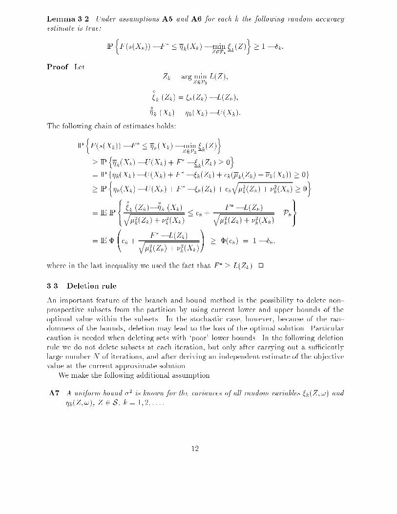
Lemma 3.2. Under assumptions A5 and A6 for each k the following random accuracy

estimate is true:

IP

�F (s(Xk))� F � � �k(Xk)� min

Z2Pk�k(Z)

�� 1 � �k:

Proof. Let

Zk = arg minZ2Pk

L(Z);

�

�k (Zk) = �k(Zk)� L(Zk);

�

�k (Xk) = �k(Xk)� U(Xk):

The following chain of estimates holds:

IP

�F (s(Xk))� F � � �k(Xk)� min

Z2Pk�k(Z)

�

� IPn�k(Xk) � U(Xk) + F � � �

k(Zk) � 0

o= IP f�k(Xk)� U(Xk) + F � � �k(Zk) + ck(�k(Zk) + �k(Xk)) � 0g� IP

��k(Xk)� U(Xk) + F � � �k(Zk) + ck

q�2k(Zk) + �2k(Xk) � 0

�

= IE IP

8><>:

�

�k (Zk)��

�k (Xk)q�2k(Zk) + �2k(Xk)

� ck +F � � L(Zk)q

�2k(Zk) + �2k(Xk)

�� Pk

9>=>;

= IE �

0@ck + F � � L(Zk)q

�2k(Zk) + �2k(Xk)

1A � �(ck) = 1 � �k;

where in the last inequality we used the fact that F � � L(Zk). 2

3.3 Deletion rule

An important feature of the branch and bound method is the possibility to delete non-

prospective subsets from the partition by using current lower and upper bounds of the

optimal value within the subsets. In the stochastic case, however, because of the ran-

domness of the bounds, deletion may lead to the loss of the optimal solution. Particular

caution is needed when deleting sets with `poor' lower bounds. In the following deletion

rule we do not delete subsets at each iteration, but only after carrying out a su�ciently

large number N of iterations, and after deriving an independent estimate of the objective

value at the current approximate solution.

We make the following additional assumption.

A7. A uniform bound �2 is known for the variances of all random variables �k(Z;!) and

�k(Z;!), Z 2 S, k = 1; 2; : : : :

12

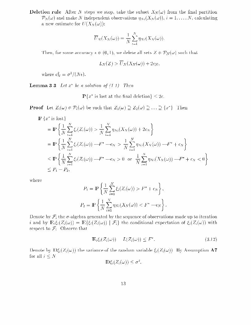
Deletion rule. After N steps we stop, take the subset XN (!) from the �nal partition

PN(!) and make N independent observations �Ni(XN (!)), i = 1; : : : ; N , calculating

a new estimate for U(XN (!)):

UN(XN (!)) =1

N

NXi=1

�Ni(XN (!)):

Then, for some accuracy � 2 (0; 1), we delete all sets Z 2 PN(!) such that

LN (Z) > UN (XN (!)) + 2cN ;

where c2N = �2=(N�):

Lemma 3.3. Let x� be a solution of (1.1). Then

Pfx� is lost at the �nal deletiong � 2�:

Proof. Let Zi(!) 2 Pi(!) be such that Z1(!) � Z2(!) � : : : � fx�g. Then

IP fx� is lostg

= IP

(1

N

NXi=1

�i(Zi(!)) >1

N

NXi=1

�Ni(XN (!)) + 2cN

)

= IP

(1

N

NXi=1

�i(Zi(!))� F � � cN >1

N

NXi=1

�Ni(XN (!)) � F � + cN

)

� IP

(1

N

NXi=1

�i(Zi(!))� F � � cN > 0 or1

N

NXi=1

�Ni(XN (!))� F � + cN < 0

)

� P1 + P2;

where

P1 = IP

(1

N

NXi=1

�i(Zi(!)) > F � + cN

);

P2 = IP

(1

N

NXi=1

�Ni(XN (!)) < F � � cN

):

Denote by Fi the �-algebra generated by the sequence of observations made up to iteration

i and by IEi�i(Zi(!)) = IEf�i(Zi(!)) j Fig the conditional expectation of �i(Zi(!)) with

respect to Fi. Observe that

IEi�i(Zi(!)) = L(Zi(!)) � F �: (3:12)

Denote by ID�i(Zi(!)) the variance of the random variable �i(Zi(!)). By Assumption A7

for all i � N

ID�i(Zi(!)) � �2:

13

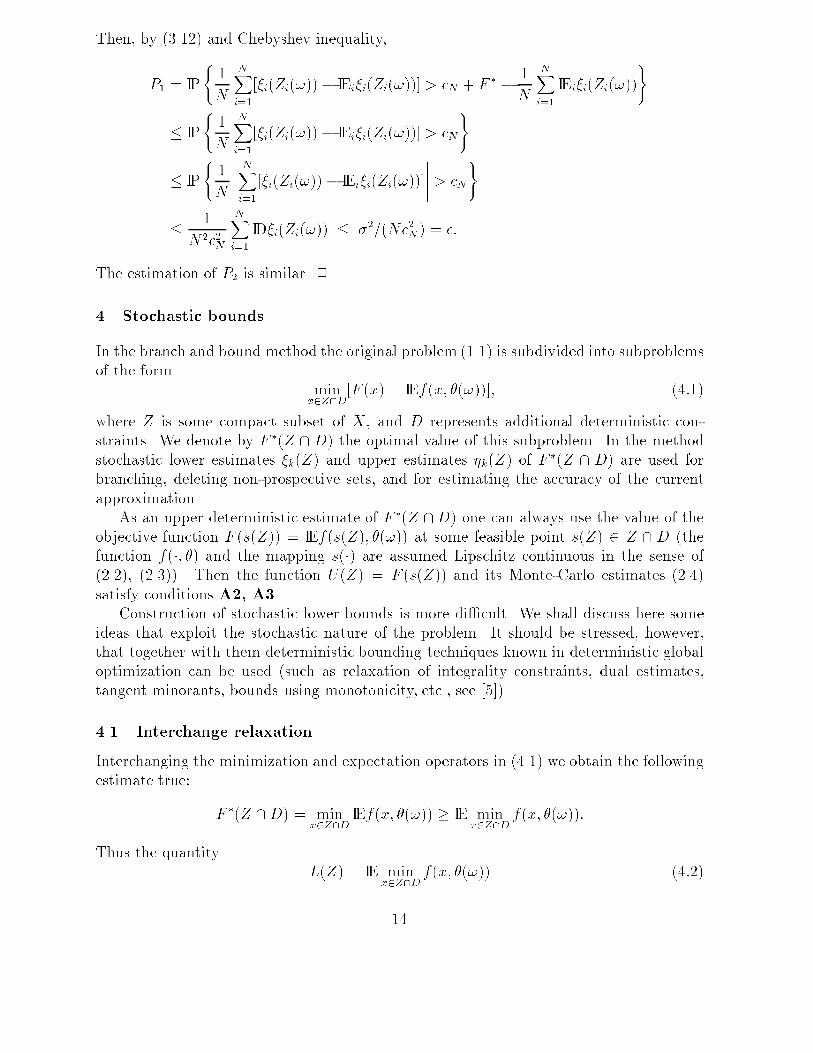
Then, by (3.12) and Chebyshev inequality,

P1 = IP

(1

N

NXi=1

[�i(Zi(!))� IEi�i(Zi(!))] > cN + F � � 1

N

NXi=1

IEi�i(Zi(!))

)

� IP

(1

N

NXi=1

[�i(Zi(!))� IEi�i(Zi(!))] > cN

)

� IP

(1

N

��NXi=1

[�i(Zi(!))� IEi�i(Zi(!))]

�� > cN

)

� 1

N2c2N

NXi=1

ID�i(Zi(!)) � �2=(Nc2N ) = �:

The estimation of P2 is similar. 2

4 Stochastic bounds

In the branch and bound method the original problem (1.1) is subdivided into subproblems

of the form

minx2Z\D

[F (x) = IEf(x; �(!))]; (4:1)

where Z is some compact subset of X, and D represents additional deterministic con-

straints. We denote by F �(Z \ D) the optimal value of this subproblem. In the method

stochastic lower estimates �k(Z) and upper estimates �k(Z) of F�(Z \ D) are used for

branching, deleting non-prospective sets, and for estimating the accuracy of the current

approximation.

As an upper deterministic estimate of F �(Z \D) one can always use the value of the

objective function F (s(Z)) = IEf(s(Z); �(!)) at some feasible point s(Z) 2 Z \ D (the

function f(�; �) and the mapping s(�) are assumed Lipschitz continuous in the sense of

(2.2), (2.3)). Then the function U(Z) = F (s(Z)) and its Monte-Carlo estimates (2.4)

satisfy conditions A2, A3.

Construction of stochastic lower bounds is more di�cult. We shall discuss here some

ideas that exploit the stochastic nature of the problem. It should be stressed, however,

that together with them deterministic bounding techniques known in deterministic global

optimization can be used (such as relaxation of integrality constraints, dual estimates,

tangent minorants, bounds using monotonicity, etc., see [5]).

4.1 Interchange relaxation

Interchanging the minimization and expectation operators in (4.1) we obtain the following

estimate true:

F �(Z \D) = minx2Z\D

IEf(x; �(!)) � IE minx2Z\D

f(x; �(!)):

Thus the quantity

L(Z) = IE minx2Z\D

f(x; �(!)) (4:2)

14

is a valid deterministic lower bound for the optimal value F �(Z \D). A stochastic lower

bound can be obtained by Monte-Carlo simulation: for i.i.d. observations �i of �, i =

1; : : : ; N , one de�nes

�(Z) =1

N

NXi=1

minx2Z\D

f(x; �i): (4:3)

In many cases, for a �xed �i, it is easy to solve the minimization problems at the right

hand side of (4.3). In particular, if the function f(�; �) is quasi-convex, stochastic lower

bounds can be obtained by convex optimization methods.

Example 4.1. Consider the facility location problem of Example 1.1. The application of

(4.3) yields the following stochastic lower bound:

�(Z) =1

N

NXi=1

minx2Z\D

f(x1; : : : ; xn; �i) =1

N

NXi=1

minx2Z\D

min1�j�n

'(xj; �i)

=1

N

NXi=1

min1�j�n

minx2Z\D

'(xj; �i): (4.4)

If '(�; �) is quasi-convex and Z \ D is convex, the inner minimization problem can be

solved by convex programming methods, or even in a closed form (if Z \D has a simple

structure). The minimumover j can be calculated by enumeration, so the whole evaluation

of the stochastic lower bound is relatively easy.

Example 4.2. For the �xed mix problem of Example 1.2 the application of (4.2) (with

obvious changes re ecting the fact that we deal with a maximization problem) yields

F �(Z \D) � IE maxx2Z\D

8<:

TYt=1

nXj=1

(xj�j(t)� �jjxj�j(t)� xjPn

�=1x��(t)j)9=;

� IE

8<: max

x(t)2Z\D;

t=1;:::;T+1

TYt=1

nXj=1

(xj(t)�j(t)� �j jxj(t)�j(t)� xj(t+ 1)Pn

�=1x�(t)��(t)j)9=; ; (4.5)

where in the last inequality we additionally split the decision vector x into x(t), t =

1; : : : ; T + 1. Let

Z \D � fx 2 IRn : aj � xj � bj; j = 1; : : : ; ng:

Then the optimal value of the optimization problem inside (4.5) can be estimated as

follows. Denote by wj(t) the wealth at the beginning of period t in assets j, and by pj(t)

and sj(t) the amounts of money spent on purchases and obtained from sales in category

j after period t. The optimal value of our problem can be calculated by solving the linear

program:

maxW (T + 1)

W (t) =nX

j=1

wj(t); t = 1; : : : ; T + 1;

15

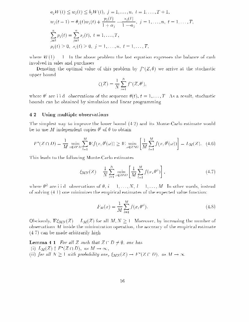
ajW (t) � wj(t) � bjW (t); j = 1; : : : ; n; t = 1; : : : ; T + 1;

wj(t+ 1) = �j(t)wj(t) +pj(t)

1 + �j� sj(t)

1 � �j; j = 1; : : : ; n; t = 1; : : : ; T;

nXj=1

pj(t) =nX

j=1

sj(t); t = 1; : : : ; T;

pj(t) � 0; sj(t) � 0; j = 1; : : : ; n; t = 1; : : : ; T;

where W (1) = 1. In the above problem the last equation expresses the balance of cash

involved in sales and purchases.

Denoting the optimal value of this problem by f�(Z; �) we arrive at the stochastic

upper bound

�(Z) =1

N

NXi=1

f�(Z; �i);

where �i are i.i.d. observations of the sequence �(t), t = 1; : : : ; T . As a result, stochastic

bounds can be obtained by simulation and linear programming.

4.2 Using multiple observations

The simplest way to improve the lower bound (4.2) and its Monte-Carlo estimate would

be to use M independent copies �l of � to obtain

F �(Z \D) =1

Mmin

x2Z\D

MXl=1

IEf(x; �l(!)) � IE minx2Z\D

"1

M

MXl=1

f(x; �l(!))

#= LM (Z): (4:6)

This leads to the following Monte-Carlo estimates

�MN (Z) =1

N

NXi=1

minx2Z\D

"1

M

MXl=1

f(x; �il)

#; (4:7)

where �il are i.i.d. observations of �, i = 1; : : : ; N , l = 1; : : : ;M . In other words, instead

of solving (4.1) one minimizes the empirical estimates of the expected value function:

FM(x) =1

M

MXl=1

f(x; �il): (4:8)

Obviously, IE�MN (Z) = LM(Z) for all M;N � 1. Moreover, by increasing the number of

observations M inside the minimization operation, the accuracy of the empirical estimate

(4.7) can be made arbitrarily high.

Lemma 4.1. For all Z such that Z \D 6= ;, one has

(i) LM (Z) " F �(Z \D); as M !1,

(ii) for all N � 1 with probability one, �MN (Z)! F �(Z \D); as M !1.

16

Proof. To prove the monotonicity of the sequence fLM (Z)g, note that

LM (Z) =1

M + 1

M+1Xj=1

IE minx2Z\D

264 1

M

M+1Xl=1l6=j

f(x; �l(!))

375

= IE1

M + 1

M+1Xj=1

minx2Z\D

264 1

M

M+1Xl=1l6=j

f(x; �l(!))

375

� IE minx2Z\D

264 1

M(M + 1)

M+1Xj=1

M+1Xl=1l6=j

f(x; �l(!))

375

= IE minx2Z\D

"1

M + 1

M+1Xl=1

f(x; �l(!))

#= LM+1(Z):

Since f(�; �) is continuous and bounded by an integrable function, by Lemma A1 of

Rubinstein-Shapiro, with probability 1,

limM!1

1

M

MXl=1

f(x; �l) = IEf(x; �(!));

uniformly for x 2 X. Taking the minimum of both sides with respect to x 2 Z \D one

obtains (ii). Assertion (i) follows then from the Lebesque theorem. 2

However, the optimization problems appearing in (4.7) can be very di�cult for non-

convex f(�; �), and this is exactly the case of interest for us. Still, in some cases (like integer

programming problems) these subproblems may prove tractable, or some deterministic

lower bounds may be derived for them.

Using empirical estimates (4.8) is not the only possible way to use multiple observations.

Let again �l, l = 1; : : : ;M; be independent copies of � and let f(x; �) � 0 for all x and

�. Let us assume (for reasons that will become clear soon) that the original problem is

a maximization problem. Then the problem of maximizing IEf(x; �(!)) is equivalent to

maximizing the function

(F (x))M = (IEf(x; �(!)))M=

MYl=1

IEf(x; �l(!)) = IE

(MYl=1

f(x; �l(!))

);

where in the last equation we used the independence of �l, l = 1; : : : ;M . Interchange of

the maximization and expectation operators leads to the following stochastic bound

�maxx2Z\D

(F (x))

�M= max

x2Z\D(F (x))M � IE�MN (Z);

where

�MN(Z) =1

N

NXi=1

maxx2Z\D

MYl=1

f(x; �il); (4:9)

17

where �il are i.i.d. observations of �, i = 1; : : : ; N , l = 1; : : : ;M . Products of some quasi-

concave functions may be still quasi-concave, so the optimization problem inside (4.9) may

be easier to solve than (4.7). In particular, if ln f(�; �) is concave, the problem in (4.9) is

equivalent to the convex optimization problem

maxx2Z\D

MXl=1

ln f(x; �il):

There is a broad class of so-called log-concave or �-concave functions for which similar

transformations can be made (see [9, 13]).

Example 4.3. Consider the facility location problem of Example 1.1 again, but now with

n = 1 and ' given by (1.2), and assume that the partition elements Z are convex. For

f(x; �) = 1� '(x; �) the problem is equivalent to maximizing the function

(F (x))M = IE

(MYl=1

f(x; �l(!))

);

i.e. maximizing the probability of the event

AM(x) =n! 2 : d(x; �l(!)) � �; l = 1; : : : ;M

o:

A stochastic upper bound for IPfAM(x)g over x 2 Z \ D can be obtained as follows.

We generate i.i.d. observations �il, i = 1; : : : ; N , l = 1; : : : ;M , and use (4.9) to get the

stochastic bound

�(Z) =1

N

NXi=1

�(Z; �i1; : : : ; �iM ); (4:10)

where

�(Z; �i1; : : : ; �iM ) = maxx2Z\D

MYl=1

f(x; �il):

Denoting

Y (Z; �i1; : : : ; �iM) = fx 2 Z \D : d(x; �l) � �; l = 1; : : : ;Mg:we see that

�(Z; �i1; : : : ; �iM) =

(1 if Y (Z; �i1; : : : ; �iM) 6= ;;0 otherwise:

Since Y (Z; �i1; : : : ; �iM) is convex, calculation of the value of � and of the corresponding up-

per bound (4.10) on the probability of M successes can be carried out by convex program-

ming methods. In the special case ofM = 1 we obtain the basic bound (4.3). Its calculation

requires only veryfying for each observation �i whether Z \D \ fx : d(x; �i) � �g 6= ;.

18

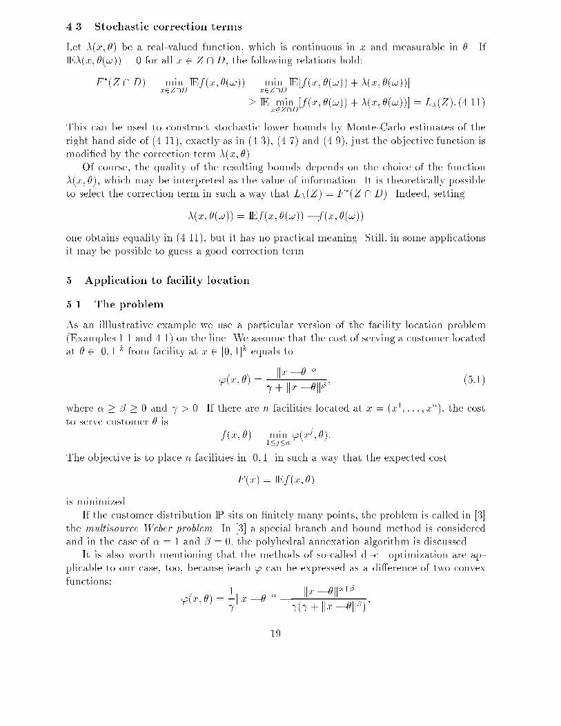
4.3 Stochastic correction terms

Let �(x; �) be a real-valued function, which is continuous in x and measurable in �. If

IE�(x; �(!)) = 0 for all x 2 Z \D, the following relations hold:

F �(Z \D) = minx2Z\D

IEf(x; �(!)) = minx2Z\D

IE[f(x; �(!)) + �(x; �(!))]

� IE minx2Z\D

[f(x; �(!)) + �(x; �(!))] = L�(Z): (4.11)

This can be used to construct stochastic lower bounds by Monte-Carlo estimates of the

right hand side of (4.11), exactly as in (4.3), (4.7) and (4.9), just the objective function is

modi�ed by the correction term �(x; �).

Of course, the quality of the resulting bounds depends on the choice of the function

�(x; �), which may be interpreted as the value of information. It is theoretically possible

to select the correction term in such a way that L�(Z) = F �(Z \D). Indeed, setting

�(x; �(!)) = IEf(x; �(!))� f(x; �(!))

one obtains equality in (4.11), but it has no practical meaning. Still, in some applications

it may be possible to guess a good correction term.

5 Application to facility location

5.1 The problem

As an illlustrative example we use a particular version of the facility location problem

(Examples 1.1 and 4.1) on the line. We assume that the cost of serving a customer located

at � 2 [0; 1]k from facility at x 2 [0; 1]k equals to

'(x; �) =kx� �k�

+ kx� �k� ; (5:1)

where � � � � 0 and > 0. If there are n facilities located at x = (x1; : : : ; xn), the cost

to serve customer � is

f(x; �) = min1�j�n

'(xj; �):

The objective is to place n facilities in [0; 1] in such a way that the expected cost

F (x) = IEf(x; �)

is minimized.

If the customer distribution IP sits on �nitely many points, the problem is called in [3]

the multisource Weber problem. In [3] a special branch and bound method is considered

and in the case of � = 1 and � = 0, the polyhedral annexation algorithm is discussed.

It is also worth mentioning that the methods of so-called d.-c. optimization are ap-

plicable to our case, too, because ieach ' can be expressed as a di�erence of two convex

functions:

'(x; �) =1

kx� �k� � kx� �k�+�

( + kx� �k�) ;

19

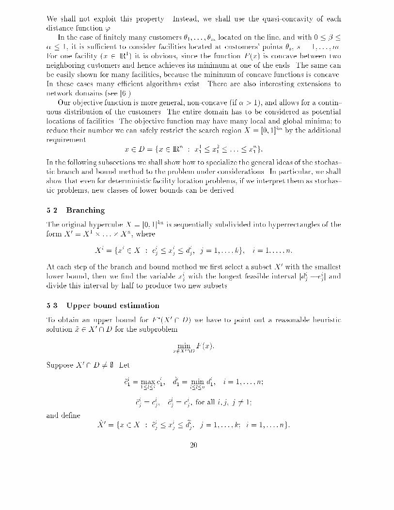
We shall not exploit this property. Instead, we shall use the quasi-concavity of each

distance function '.

In the case of �nitely many customers �1; : : : ; �m located on the line, and with 0 � � �� 1, it is su�cient to consider facilities located at customers' points �s, s = 1; : : : ;m.

For one facility (x 2 IR1) it is obvious, since the function F (x) is concave between two

neighboring customers and hence achieves its minimum at one of the ends. The same can

be easily shown for many facilities, because the minimum of concave functions is concave.

In these cases many e�cient algorithms exist. There are also interesting extensions to

network domains (see [6]).

Our objective function is more general, non-concave (if � > 1), and allows for a contin-

uous distribution of the customers. The entire domain has to be considered as potential

locations of facilities. The objective function may have many local and global minima; to

reduce their number we can safely restrict the search region X = [0; 1]kn by the additional

requirement

x 2 D = fx 2 IRn : x11 � x21 � : : : � xn1g:In the following subsections we shall show how to specialize the general ideas of the stochas-

tic branch and bound method to the problem under considerations. In particular, we shall

show that even for deterministic facility location problems, if we interpret them as stochas-

tic problems, new classes of lower bounds can be derived.

5.2 Branching

The original hypercube X = [0; 1]kn is sequentially subdivided into hyperrectangles of the

form X 0 = X1 � : : :�Xn, where

X i = fxi 2 X : cij � xij � dij; j = 1; : : : ; kg; i = 1; : : : ; n:

At each step of the branch and bound method we �rst select a subset X 0 with the smallest

lower bound, then we �nd the variable xij with the longest feasible interval jdij � cijj anddivide this interval by half to produce two new subsets.

5.3 Upper bound estimation

To obtain an upper bound for F �(X 0 \ D) we have to point out a reasonable heuristic

solution ~x 2 X 0 \D for the subproblem

minx2X 0\D

F (x):

Suppose X 0 \D 6= ;. Let

~ci1 = max1�l�i

cl1;~di1 = min

i�l�ndl1; i = 1; : : : ; n;

~cij = cij; ~cij = cij; for all i; j; j 6= 1;

and de�ne~X 0 = fx 2 X : ~cij � xij � ~dij ; j = 1; : : : ; k; i = 1; : : : ; ng:

20

Clearly,X 0\D = ~X 0\D. We assume that the customers lie in a �nite set � = f�1; : : : ; �mg.To �nd a heuristic solution we associate each customer with at least one of the sets [~ci; ~di],

i = 1; : : : ; n, in the following way. Denote

dist(�; [c; d]) = minx2[c;d]

'(x; �)

and de�ne for each index i the subset

�i =

�� 2 � : dist(�; [~ci; ~di]) = min

1�j�ndist(�; [~cj; ~dj ])

�:

Let us try to locate the facility xi 2 [~ci; ~di] to satisfy customers � 2 �i 6= ; in the best

way. This is equvalent to solving the problem

minxi2[~ci; ~di]

[Fi(xi) =

X�2�i

'(xi; �)]; (5:2)

but except for the discrete case, when the solution is known to lie either at one of the ends

~ci, ~di or in � 2 �i \ [~ci; ~di], one has to resort to a heuristics. The simplest and relatively

e�ective one is to take the point

~xi =

(IEfxi(�)j �ig; �i 6= ;;(~ci + ~di)=2; otherwise:

5.4 Lower bound estimation

We shall use the interchange relaxation of section 4.1. Notice that X 0 \D � ~X 0. Then, as

in Example 4.1,

F �(X 0 \D) � IE minx2 ~X 0

min1�i�n

'(xi; �) = IE min1�i�n

minx2 ~X 0

'(xi; �) = L1(X0):

We shall also use lower bounds with double sampling (see (4.6)) which take on the form:

L2(X0) =

1

2IE�1IE�2 min

x2 ~X 0( min1�i�n

'(xi; �1) + min1�j�n

'(xj; �2)):

In the case of �nitely many locations of customers �1; : : : ; �m taken with probabilities

p1; : : : ; pm the above lower bound can be written as follows:

L2(X0) =

1

2

mXs;t=1

psptmin

(min1�i�m

minxi2 ~X 0

i

('(xi; �s1) + '(xi; �t2));

min1�i;j�m

i6=j

(minxi2X 0

i

'(xi; �s1) + minxj2X 0

j

'(xj; �t2))

):

To calculate it one has to solve (quasi-convex) problems of the form

minxi2X 0

i

'(xi; �);

which ere easy (simply project � on the set X 0

i), and non-convex problems of the form

minxi2 ~X 0

i

('(xi; �1) + '(xi; �2));

which are more di�cult, but for which simple lower bounds can be calculated.

21

5.5 Deletion rule

There are two reasons to delete a subset X 0 from the current partition Pk: `infeasibility',

i.e. X 0 \D = ;, and `nonprospectiveness', i.e. L(X 0) > F (x) for some point x 2 X \D.

The feasibility test for our set D amounts to checking the inequalities ~ci1 � ~di1, i =

1; : : : ; n.

If the lower bounds L(X 0), X 0 2 Pk, are calculated exactly as in the case of discrete

distribution of customers, then `nonprospective' subsets can be safely deleted from the

current partition. If we have only stochastic estimates �k(X0) of lower bounds L(X 0)

then deletion of sets X 0 such that �k(X0) > F (x) leads to a heuristic branch and bound

algorithm, which, nevertheless, can be helpful, if we apply it many times to the same

problem.

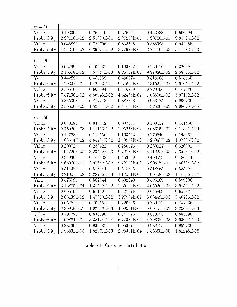
5.6 Numerical results

To illustrate the properties of the method let us consider the facility location problem on

the line with the distance function (5.1) with � = � = 2 and = 0:1. The locations of the

customers �1; : : : ; �m were drawn from the uniform distribution in [0; 1]. For each customer

�s, its relative weight ws was drawn from the uniform distribution in [0; �s(1 � �s)2], so

that the weight had the Beta distribution in [0; 1] with parameters (2,3). To allow an easy

probabilistic interpretation the weights were normalized to get ps = ws=Pm

l=1wl. All data

are collected in Table 1.

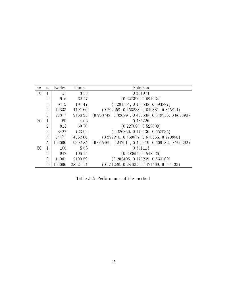
The performance of the method is summarized in Table 2. The method terminated

when the size of the record set was below 10�3 for each facility, or when the maximum

number of iterations (105) was reached.

We see that the method is capable of solving within a reasonable time problems with

highly non-convex functions and with a large number of local minima.

22

References

[1] Birge J.R. (1985), Decomposition and partitioning methods for multistage stochastic

linear programs, Operations Research 33(1985) 989-1007.

[2] Ermoliev Yu.M. (1983), Stochastic quasi-gradient methods and their application to

systems optimization, Stochastics 4, 1-37.

[3] Hansen P., B. Jaumard and H. Tuy (1995), Global optimization in location,1995), in:

Facility Location - A Survey of Applications and Methods, Z. Drezner (ed.), Springer

Serier in Operations Research, Springer-Verlag, Berlin, pp. 43-68.

[4] Horst R. and H. Tuy (1990), Global Optimization, Springer-Verlag, Berlin.

[5] Horst R. and P.M. Pardalos (eds.) (1994), Handbook of Global Optimization, Kluwer

Academic Publishers.

[6] Labb�e M., D. Peeters and J.-F. Thisse (1995), Location on Networks, Ch. 7 of Hand-

books in OR & MS, Vol. 8, M.O. Ball (ed.), Elsevier, Amsterdam, pp. 551-624.

[7] Mikhalevich V.S., A.M. Gupal and V.I. Norkin (1987), Methods of Non-Convex Op-

timization, Nauka, Moscow (in Russian).

[8] Mulvey J.M. and A. Ruszczy�nski (1995), A new scenario decomposition method for

large-scale stochastic optimization, Operations Research 43(1995) 477-490.

[9] Norkin V.I. (1993), The analysis and optimization of probability functions, Work-

ing Paper WP-93-6, International Institute for Applied System Analysis, Laxenburg,

Austria.

[10] Norkin V.I., Yu.M. Ermoliev and A. Ruszczy�nski (1994), On Optimal Allocation of

Indivisibles Under Uncertainty , Working Paper WP-94-21, International Institute for

Applied System Analysis, Laxenburg, Austria.

[11] P ug G. Gh. (1994), Adaptive Designs in Discrete Stochastic Optimization, Working

Paper WP-94-59, International Institute for Applied System Analysis, Laxenburg,

Austria.

[12] Pijavskii S.A. (1972), An algorithm for searching for the absolute extremum of a

function, Zh. Vychisl. Mat. Mat. Fiz., Vol. 12, No. 4, pp. 888-896. (In Russian).

[13] Prekopa A. (1980), Logarithmic concave measures and related topics, in: M.A.H.

Dempster (ed.), Stochastic Programming, Academic Press, London, pp. 63-82.

[14] Rockafellar R.T. and R.J.-B. Wets (1991), Scenarios and policy aggregation in opti-

mization under uncertainty, Mathematics of Operations Research 16(1991) 1-23.

[15] R.J.-B. Wets (1988), Large scale linear programming techniques, in: Yu. Ermoliev and

R.J.-B. Wets (eds.), Numerical Methods in Stochastic Programming (Springer-Verlag,

Berlin, 1988) pp. 65-94.

23

m = 10

Value 0.193362 0.260176 0.326991 0.453538 0.606194

Probability 2.99106E-02 2.51909E-01 2.97208E-01 1.90780E-01 9.85524E-02

Value 0.646899 0.720796 0.835398 0.885398 0.933185


m = 20

Value 0.03799l 0.100437 0.193362 0.260176 0.326991


Value 0.442882 0.453538 0.480874 0.518605 0.518865


Value 0.595109 0.606194 0.646899 0.720796 0.747336


Value 0.835398 0.847773 0.885398 0.933185 0.999739


m = 50

Value 0.030084 0.036942 0.037991 0.100437 0.141456


Value 0.147532 0.149556 0.163543 0.179640 0.193362


Value 0.209725 0.250422 0.260176 0.269027 0.326991


Value 0.389365 0.442882 0.453130 0.453538 0.480874


Value 0.514380 0.518344 0.518605 0.518865 0.555292


Value 0.575999 0.587544 0.592240 0.595109 0.599090


Value 0.606194 0.611501 0.627076 0.646899 0.655837


Value 0.657526 0.703552 0.720796 0.739772 0.747336


Value 0.797293 0.835398 0.847773 0.880528 0.885398


Value 0.887304 0.933185 0.953974 0.988455 0.999739


Table 5.1: Customer distribution.

24

m n Nodes Time Solution

10 1 51 3.33 0.351974

2 916 62.27 (0.327390, 0.691934)

3 9419 194.47 (0.291554, 0.453538, 0.693887)

4 42333 4701.66 (0.292259, 0.453538, 0.649881, 0.865814)

5 23347 2168.23 (0.253749, 0.326991, 0.453538, 0.649556, 0.865890)

20 1 60 4.06 0.486726

2 813 59.70 (0.227088, 0.529698)

3 8427 723.99 (0.226360, 0.470136, 0.658535)

4 84471 14352.06 (0.227246, 0.469872, 0.610555, 0.790888)

5 100000 19392.85 (0.045469, 0.242011, 0.469479, 0.609782, 0.790392)

50 1 106 8.86 0.391113

2 943 106.15 (0.203609, 0.548336)

3 14901 2409.89 (0.202405, 0.470259, 0.635109)

4 100000 28924.74 (0.151286, 0.284003, 0.471469, 0.634133)

Table 5.2: Performance of the method.

25

A branch and bound method for stochastic global optimization

Documents

Transcript of A branch and bound method for stochastic global optimization