A boundary face method for potential problems in three dimensions

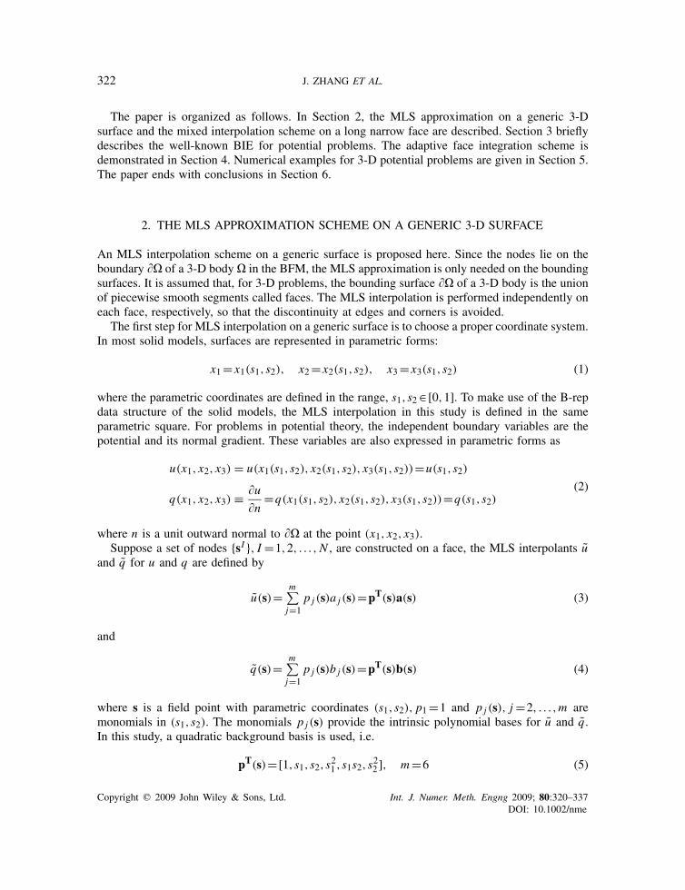
INTERNATIONAL JOURNAL FOR NUMERICAL METHODS IN ENGINEERINGInt. J. Numer. Meth. Engng 2009; 80:320–337Published online 28 April 2009 in Wiley InterScience (www.interscience.wiley.com). DOI: 10.1002/nme.2633

A boundary face method for potential problemsin three dimensions

Jianming Zhang∗,†, Xianyun Qin, Xu Han and Guangyao Li

State Key Laboratory of Advanced Design and Manufacturing for Vehicle Body, College of Mechanical and VehicleEngineering, Hunan University, Changsha 410082, China

SUMMARY

This work presents a new implementation of the boundary node method (BNM) for numerical solu-tion of Laplace’s equation. By coupling the boundary integral equations and the moving least-squares(MLS) approximation, the BNM is a boundary-type meshless method. However, it still uses the stan-dard elements for boundary integration and approximation of the geometry, thus loses the advantagesof the meshless methods. In our implementation, here called the boundary face method, the boundaryintegration is performed on boundary faces, which are represented in parametric form exactly as theboundary representation data structure in solid modeling. The integrand quantities, such as the coordinatesof Gauss integration points, Jacobian and out normal are calculated directly from the faces rather thanfrom elements. In order to deal with thin structures, a mixed variable interpolation scheme of 1-D MLSand Lagrange Polynomial for long and narrow faces. An adaptive integration scheme for nearly singularintegrals has been developed. Numerical examples show that our implementation can provide much moreaccurate results than the BNM, and keep reasonable accuracy in some extreme cases, such as very irregulardistribution of nodes and thin shells. Copyright q 2009 John Wiley & Sons, Ltd.

Received 24 November 2008; Revised 21 February 2009; Accepted 13 March 2009

KEY WORDS: meshless methods; boundary node method; moving least-squares approximation; boundaryface method

1. INTRODUCTION

Meshless techniques to obtain numerical solutions for PDEs without resorting to an element framehave been popular throughout the computational mechanics community for the past two decades.This is because that, with mesh-based techniques as the finite element method (FEM) or the

∗Correspondence to: Jianming Zhang, State Key Laboratory of Advanced Design and Manufacturing for VehicleBody, College of Mechanical and Vehicle Engineering, Hunan University, Changsha 410082, China.

†E-mail: [email protected]

Contract/grant sponsor: National Science Foundation of China; contract/grant numbers: 10725208, 60635020,50625519

Copyright q 2009 John Wiley & Sons, Ltd.

A BOUNDARY FACE METHOD FOR 3D POTENTIAL PROBLEMS 321

boundary element method (BEM), the task of mesh generation for complex geometries is oftentime-consuming and prone to errors, and the difficulties with re-meshing in problems involvingmoving boundaries, large deformations or crack propagation is crucial. Many kinds of meshlessmethod have been proposed so far [1–10]. These methods can be simply sorted into two categories:the domain type and the boundary type. The domain-type meshless methods are represented bythe element-free Galerkin method (EFG) [2] which uses a global symmetric weak form and theshape functions from the moving least-squares approximation. A feature of this method is thatit uses a background cell structure for the ‘energy’ integration. Atluri and his co-workers havedeveloped two meshless methods of domain type: the meshless local boundary integral equation(MLBIE) [3] and the meshless local Petrov-Galerkin (MLPG) approach [4]. Both methods uselocal weak form over local sub-domains, so that integrals can be evaluated over regularly shapeddomains (for example, circles in 2-D problems and spheres in 3-D problems) and their boundaries.They called their method ‘truly meshless method’.

The boundary-type meshless methods can be represented by the boundary node method(BNM) [5, 6] and the Hybrid Boundary Node Method (HdBNM) [7–10]. The BNM couples themoving least-squares (MLS) and the boundary integral equations (BIE), and uses background cellsfor boundary integration as the EFG, while the HdBNM combines the MLS interpolation schemewith the hybrid displacement variational formulation, and uses local form as the MLPG to avoidthe use of background cells. However, the using of background cells should not be considered asa drawback of meshless methods if the background cells can be generated without much efforts.As a matter of fact, in ‘truly meshless’ methods, as each sub-domain usually includes onlyone node, the radius has to be properly chosen. To determine the radius of a sub-domain for anode, one has to calculate the distances between its neighboring nodes. This leads to a fact thatgeneration of the sub-domains in many cases may need more work than background meshing.Therefore, the BNM may be a better option than the HdBNM for numerical solution of boundaryvalue problems. Unfortunately, in the implementation of the BNM for 3-D cases [6], the authorsdid not use background cells but the standard elements of FEM or BEM to approximate geometryof the domain and performed the integration on these elements. In this paper, we present a newimplementation of the BNM. In our implementation, here called the boundary face method (BFM),the boundary of the domain is represented by faces in parametric form exactly the same as theB-rep data structure in standard solid modeling packages. Both MLS and boundary integration areperformed in the parametric spaces of the faces. For numerical integration, the faces are meshedwith isoparametric lines and the geometric data, such as the coordinates of Gauss integrationpoints, the Jacobian and the surface normal at the integration point are calculated directly from theface, and thus no geometric error is introduced. As the background cells can be so easily obtained,even easier than the sub-domains in the HdBNM, the new method can seamlessly interact withCAD packages, which is considered as a demanding feature for solving practical engineeringproblems by the computation research community [11].

Formulations of the MLS approximation on a generic surface are developed. To deal with thinshells, we have developed a mixed variable interpolation scheme of MLS and Lagrange Polynomialfor variable interpolation on long and narrow faces and an adaptive integration scheme for nearlysingular integrals. A number of numerical examples with various geometries are presented, inwhich computations are carried out with regular and irregular distribution of nodes. In addition,we have compared the present method with the BNM with regard to accuracy, convergence andthe sensitivity of the results to the relative location of the source node in a cell. All results haveshown very attractive features of the method.

Copyright q 2009 John Wiley & Sons, Ltd. Int. J. Numer. Meth. Engng 2009; 80:320–337DOI: 10.1002/nme

322 J. ZHANG ET AL.

The paper is organized as follows. In Section 2, the MLS approximation on a generic 3-Dsurface and the mixed interpolation scheme on a long narrow face are described. Section 3 brieflydescribes the well-known BIE for potential problems. The adaptive face integration scheme isdemonstrated in Section 4. Numerical examples for 3-D potential problems are given in Section 5.The paper ends with conclusions in Section 6.

2. THE MLS APPROXIMATION SCHEME ON A GENERIC 3-D SURFACE

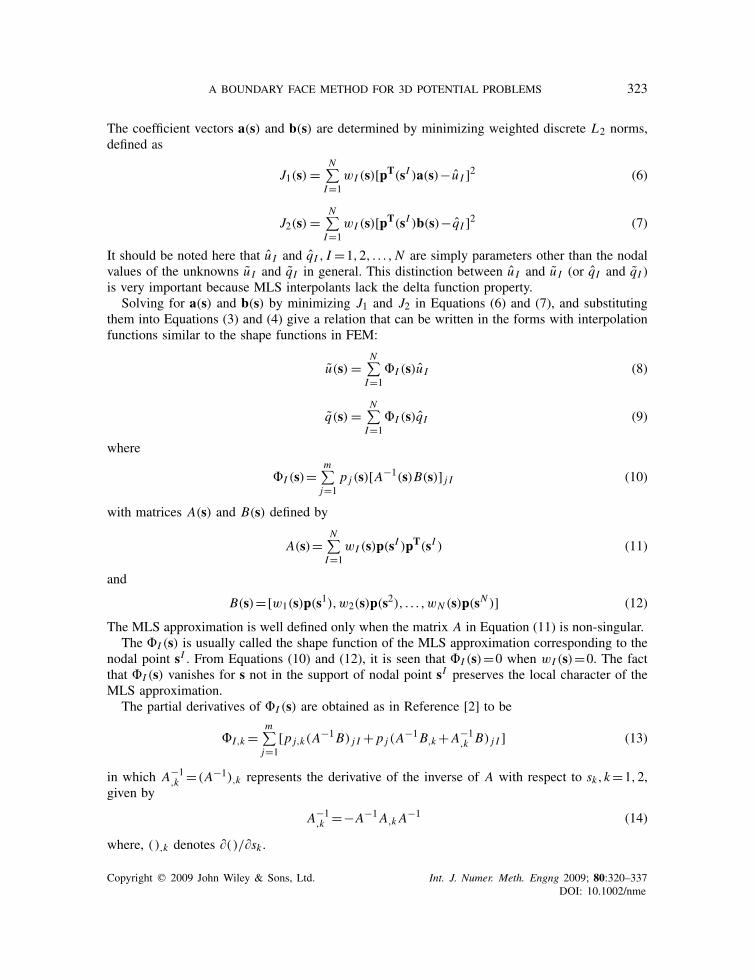
An MLS interpolation scheme on a generic surface is proposed here. Since the nodes lie on theboundary �� of a 3-D body � in the BFM, the MLS approximation is only needed on the boundingsurfaces. It is assumed that, for 3-D problems, the bounding surface �� of a 3-D body is the unionof piecewise smooth segments called faces. The MLS interpolation is performed independently oneach face, respectively, so that the discontinuity at edges and corners is avoided.

The first step for MLS interpolation on a generic surface is to choose a proper coordinate system.In most solid models, surfaces are represented in parametric forms:

x1= x1(s1,s2), x2= x2(s1,s2), x3= x3(s1,s2) (1)

where the parametric coordinates are defined in the range, s1,s2∈[0,1]. To make use of the B-repdata structure of the solid models, the MLS interpolation in this study is defined in the sameparametric square. For problems in potential theory, the independent boundary variables are thepotential and its normal gradient. These variables are also expressed in parametric forms as

u(x1, x2, x3) = u(x1(s1,s2), x2(s1,s2), x3(s1,s2))=u(s1,s2)

q(x1, x2, x3) ≡ �u�n

=q(x1(s1,s2), x2(s1,s2), x3(s1,s2))=q(s1,s2)(2)

where n is a unit outward normal to �� at the point (x1, x2, x3).Suppose a set of nodes {sI }, I =1,2, . . . ,N , are constructed on a face, the MLS interpolants u

and q for u and q are defined by

u(s)=m∑j=1

p j (s)a j (s)=pT(s)a(s) (3)

and

q(s)=m∑j=1

p j (s)b j (s)=pT(s)b(s) (4)

where s is a field point with parametric coordinates (s1,s2), p1=1 and p j (s), j=2, . . . ,m aremonomials in (s1,s2). The monomials p j (s) provide the intrinsic polynomial bases for u and q .In this study, a quadratic background basis is used, i.e.

pT(s)=[1,s1,s2,s21 ,s1s2,s22 ], m=6 (5)



The coefficient vectors a(s) and b(s) are determined by minimizing weighted discrete L2 norms,defined as

J1(s) =N∑I=1

wI (s)[pT(sI )a(s)− u I ]2 (6)

J2(s) =N∑I=1

wI (s)[pT(sI )b(s)− qI ]2 (7)

It should be noted here that u I and qI , I =1,2, . . . ,N are simply parameters other than the nodalvalues of the unknowns u I and qI in general. This distinction between u I and u I (or qI and qI )is very important because MLS interpolants lack the delta function property.

Solving for a(s) and b(s) by minimizing J1 and J2 in Equations (6) and (7), and substitutingthem into Equations (3) and (4) give a relation that can be written in the forms with interpolationfunctions similar to the shape functions in FEM:

u(s) =N∑I=1

�I (s)u I (8)

q(s) =N∑I=1

�I (s)qI (9)

where

�I (s)=m∑j=1

p j (s)[A−1(s)B(s)] j I (10)

with matrices A(s) and B(s) defined by

A(s)=N∑I=1

wI (s)p(sI )pT(sI ) (11)

and

B(s)=[w1(s)p(s1),w2(s)p(s2), . . . ,wN (s)p(sN )] (12)

The MLS approximation is well defined only when the matrix A in Equation (11) is non-singular.The �I (s) is usually called the shape function of the MLS approximation corresponding to the

nodal point sI . From Equations (10) and (12), it is seen that �I (s)=0 when wI (s)=0. The factthat �I (s) vanishes for s not in the support of nodal point sI preserves the local character of theMLS approximation.

The partial derivatives of �I (s) are obtained as in Reference [2] to be

�I,k =m∑j=1

[p j,k(A−1B) j I + p j (A

−1B,k+A−1,k B) j I ] (13)

in which A−1,k =(A−1),k represents the derivative of the inverse of A with respect to sk,k=1,2,

given by

A−1,k =−A−1A,k A

−1 (14)

where, (),k denotes �()/�sk .


324 J. ZHANG ET AL.

In implementing the MLS approximation, the weight functions should be chosen at first. Severalkinds of weight functions can be found in the literatures; the choice of weight functions and theconsequences of a choice are discussed in detail elsewhere [3]. In this study, we use the Gaussianweight function. The Gaussian weight function corresponding to a node sI can be written by

wI (s)=

⎧⎪⎨⎪⎩exp[−(dI /cI )2]−exp[−(dI /cI )2]

1−exp[−(dI /cI )2], 0�dI�dI

0, dI�dI

(15)

where cI is a constant controlling the shape of the weight function, and dI is the size of the supportfor the weight function wI . It can be seen from the above equation that the weight function has acompact support determined by the parameter dI . The compact support is also an associated rangeof influence of each node. In the past, the shape of the compact support is usually chosen to becircle in meshless literatures, while in this study, we choose ellipse for the shape of the compactsupport with dI being the half-length of major axis of the ellipse. Denoting the half-length ofminor axis by d ′

I , we have the following expression for dI :

dI =√√√√(s1−s I1 )2+ d2I

d ′2I

(s2−s I2 )2 (16)

In order to ensure the regularity of A, the dI and d ′I should be chosen in such a way that they are

large enough to have a sufficient number of nodes which are covered in the domain of definitionof every sample point (N�m). But too large dI and d ′

I will lose the local character of the MLSinterpolation, or even lead to an ill-conditioned matrix A. In this study, dI and d ′

I are chosen suchthat 4m–8m nodes are included in the support of a node.

However, even if the condition (N�m) is satisfied, but the N nodes in the domain of dependenceof the sample point lie on a straight line on the face, then the matrix A becomes singular.This indicates that the MLS is not applicable to narrow strip surfaces, which exist in many thinshell structures. To handle this problem, we proposed a mixed interpolation scheme of 1-D MLSand Lagrange polynomial. Here take a strip surface as an example, which is assumed thin in thes1 direction and long in the s2 direction. We construct k (3�k�1, and determined by the widthof the strip) rows of nodes on the strip in the s2 direction. The coordinate of s1 and the numberof nodes of each row are sk1 and Nk(Nk�4), respectively. Then the potential u at a point s(s1,s2)can be interpolated by Lagrange polynomials in the s1 direction:

u(s)=k∑j=1

ln, j (s1)uj (s2) (17)

where ln, j (s1)=∏j �=i ((s1−s j1 )/(si1−s j1 )), u j (s2) can be obtained by 1-D MLS approximation

within each row of nodes independently, using the following formula:

u j (s2)=Nk∑I=1

�I (s2)ukI (18)

here, �I (s2) is the shape function of the 1-D MLS approximation. For 1-D MLS and its derivative,please refer References [5, 7].



For a face that is small in size in both directions, and thus the numbers of nodes distributedin the two directions are both less than 4, we interpolate the variables by Lagrange polynomialsin two directions. In this case, actually, the face degenerates to a constant, a linear or a quadraticelement of the standard BEM.

3. BOUNDARY INTEGRAL EQUATIONS AND DISCRETIZATIONS

The potential problem in three dimensions governed by Laplace’s equation with boundary condi-tions is written as

u,i i = 0 ∀x ∈�

u = u ∀x ∈�u

u,i ni ≡ q= q ∀x ∈�q

(19)

where the domain � is enclosed by �=�u+�q , u and q are the prescribed potential and thenormal flux, respectively, on the essential boundary �u and on the flux boundary �q , and n is theoutward normal direction to the boundary �, with components ni , i=1,2,3.

The problem can be recast into an integral equation on the boundary. The well-known self-regularBIE for potential problems in 3-D is

0=∫

�(u(s)−u(y))qs(s,y)d�−

∫�q(s)us(s,y)d� (20)

where q=�u/�n,y is the source point and s the field point on the boundary. us(s,y) and qs(s,y)are the fundamental solutions. For 3-D potential problems,

us(s,y) = 1

4�

1

r(s,y)(21)

qs(s,y) = �us(s,y)�n

(22)

with r being the Euclidean distance between the source and field points.The MLS interpolations or the mixed interpolations derived in Section 2 will be used to approx-

imate u and q on the boundary �. The bounding surface is discretized into cells by isoparametriclines face by face. Substituting Equations (8) and (9) into Equation (20) and dividing � into Nccells, we have

0=−Nc∑j=1

∫� j

qs(s,y)N∑I=1

(�I (s)−�I (y))u I d�+Nc∑j=1

∫� j

us(s,y)N∑I=1

�I (s)qI d� (23)

where �I (y) and �I (s) are the contributions from the I th node to the collocation point y andfield point s, respectively. The first term on the right side of Equation (23) is regular in any case.Therefore, regular Gaussian integration can be used to evaluate it over each cell. However, specialintegration techniques are required for the second term, since it will become weakly singularas s approaches y. When y and s belong to the same cell, the cell is treated as a singular celland the special techniques developed in the next section are used to carry out the integration.


326 J. ZHANG ET AL.

Our integration scheme is different from that developed by Chati and Mukherjee [6] and mayprovide better accuracy. This is because we carry out the integrations directly in the parametricspace of a face other than over elements, and thus no geometric error will be introduced.

Even when y and s belong to different cells, they can still be very close to each other. In thiscase, the second term on the right side of Equation (23) becomes nearly-singular. This case occurswhen thin structures are involved and when the distribution of nodes is very irregular. We havealso developed an adaptive scheme to calculate nearly singular integrals in the next section.

Equation (23) can be put in a matrix form as

Hu−Gq=0 (24)

where u and q contain the approximations to the nodal values of u and q at the boundary nodes. Awell-posed boundary value problem can be solved using Equation (24). However, transformationsbetween u I and u I , qI and qI is necessary because the MLS interpolants lack the delta functionproperty of the usual BEM shape functions as mentioned in Section 2. For the panels where u isprescribed, u I is related to u I by

u I =N∑

J=1RI J u J =

N∑J=1

RI J u J (25)

and for the panels where q is prescribed, qI is related to qI by

qI =N∑

J=1RI J qJ =

N∑J=1

RI J qJ (26)

where RI J =[�J (sI )]−1.The computational efficiency of the proposed method in comparison with 3D domain schemes,

e.g. FEM or EFG, is similar to that of BEM. Actually, considering a 3D mesh with n3 nodes, thenumber of boundary nodes is around n2, both the operation count and the memory requirementsfor the buildup of matrix equation (24) are of the order O(n4). The operation count increasesto O(n6) if we attempt to solve the equation with conventional direct solvers such as Gaussianelimination. Therefore, although the dimensionality of a problem at hand is reduced by one, it isless computationally efficient than domain schemes. However, the proposed method significantlyreduces the human-labor cost of introducing geometric meshes in complex-shaped structures,which is the aim of the development of a new class of computer methods, the so-called meshlessor element-free methods. Moreover, the computational efficiency of the BFM can be enhanceddramatically if it is combined with the fast multipole method (FMM) [12–14].

4. WEAKLY AND NEARLY SINGULAR INTEGRATION SCHEMES

4.1. Weakly singular integration

The second term on the right side of Equation (23) becomes a weakly singular integral when y ands belong to a same cell, and the cell is treated as a singular cell. There have been various methodsproposed in the past to handle weakly singular integrals arising in BEM. Chati and Mukherjeehave used a method suggested by Nagaranjan and Mukherjee [15] to carry out the weakly singularintegration in BNM. Here we propose a new method without using elements. The details follow.



0 01 2( , )s s

1 2( , )s s

1 2( , )a as s

1 11 2( , )s s

2 21 2( , )s s

1s

2s

1 2( , )b bs s

αβ0 0

1 2( , )s s

(a) (b)

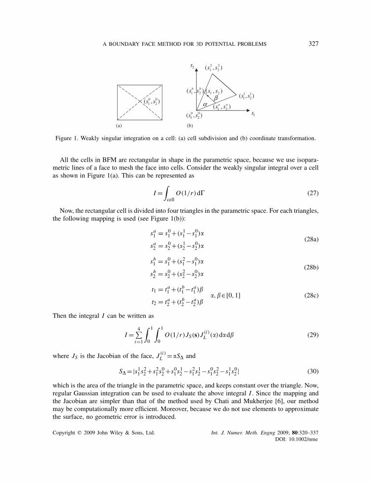
Figure 1. Weakly singular integration on a cell: (a) cell subdivision and (b) coordinate transformation.

All the cells in BFM are rectangular in shape in the parametric space, because we use isopara-metric lines of a face to mesh the face into cells. Consider the weakly singular integral over a cellas shown in Figure 1(a). This can be represented as

I =∫cell

O(1/r)d� (27)

Now, the rectangular cell is divided into four triangles in the parametric space. For each triangles,the following mapping is used (see Figure 1(b)):

sa1 = s01 +(s11 −s01)�

sa2 = s02 +(s12 −s02)�(28a)

sb1 = s01 +(s21 −s01)�

sb2 = s02 +(s22 −s02)�(28b)

t1 = ta1 +(tb1 − ta1 )�

t2 = ta2 +(tb2 − ta2 )��,�∈[0,1] (28c)

Then the integral I can be written as

I =4∑

i=1

∫ 1

0

∫ 1

0O(1/r)JS(s)J

(i)L (�)d�d� (29)

where JS is the Jacobian of the face, J (i)L =�S� and

S� =|s11s22 +s21s02 +s01s

12 −s21s

12 −s01s

22 −s11s

02 | (30)

which is the area of the triangle in the parametric space, and keeps constant over the triangle. Now,regular Gaussian integration can be used to evaluate the above integral I . Since the mapping andthe Jacobian are simpler than that of the method used by Chati and Mukherjee [6], our methodmay be computationally more efficient. Moreover, because we do not use elements to approximatethe surface, no geometric error is introduced.


328 J. ZHANG ET AL.

(0.0, 0.0) (1.0, 0.0)

(1.0, 1.0)(0.0, 1.0)

P

Figure 2. Subdivision of a cell in parametric space corresponding to a source point P .

4.2. Nearly singular integration

Nearly singularities arise in the BIE when slender or thin structures are considered and in caseswhere the boundary node distribution on a surface is very irregular, namely the densities of nodesalong the two directions in parametric space are very different. Accurate evaluation of nearlysingular integrals is a demanding task for successful implementation of BIE analyses. So far manytechniques for dealing with nearly singular integrals have been proposed [16, 17]. Some of themare effective but involve complicated mathematic transformations of the integrals for a specificfundamental solution. To provide a general approach that is independent of the problem to besolved, here we developed an adaptive integration scheme based on the cell subdivision method.In this scheme, we first calculate the diagonal length of the integration cell, l, and the distancebetween the source point and the center of the cell, d , in the real-world-coordinate system. If lis smaller than d , this cell is taken as a regular integration patch, or it is divided into four equalsubcells (see Figure 2). Then for each subcell, we repeat the above procedure until all patchesbecome regular. Finally, using Gaussian quadrature for all patches, we can evaluate the integralsin Equation (23) very accurately even when the source point is very close to the integration cells.It should be pointed out that the patches are not like the elaborately constructed elements in theBEM and FEM. The subdivided patches of a same cell change for different source points. Theycan be easily constructed in the parametric space. Therefore, using these patches does not affectthe fact that the BFM is a meshless method.

5. ILLUSTRATIVE NUMERICAL RESULTS

The current method has been tested thoroughly for three types of 3-D geometrical objects: a sphere,a cube, and an elbow pipe. To compare the current method with the BNM, the former two modelsare taken from Reference [6]. And the last one, a more geometrically complicated one, is added toshow the advantage of the meshless nature of the present method. In order to assess the accuracyof the present method, we have used the following three analytical fields, which are also takenfrom [6]:(i) Linear solution:

u= x+ y+z (31)

(ii) Quadratic solution-1:

u= xy+ yz+zx (32)



(iii) Quadratic solution-2:

u=−2x2+ y2+z2 (33)

(iv) Cubic solution:

u= x3+ y3+z3−3yx2−3xz2−3zy2 (34)

In all cases, Laplace’s equation ∇2u=0 is solved, together with appropriately prescribed boundaryconditions corresponding to the above analytical solutions.

For the purpose of error estimation and convergence study, a ‘global’ L2 norm error, normalizedby |v|max is defined as follows [6]:

e= 1

|v|max

√1

N

N∑i=1

(v(e)i −v

(n)i )2 (35)

where |v|max is the maximum value of u or q over N sample points, the superscripts (e) and (n)

refer to the exact and numerical solutions, respectively.In all computations, unless indicated otherwise, the support size of the weight function, dI in

Equation (15), is taken to be 4.0h, with h being the minimum distance between the neighboringpoints, and the parameter cI is taken to be such that dI /cI is constant and equal to 4.0.

5.1. Dirichlet problems on a sphere

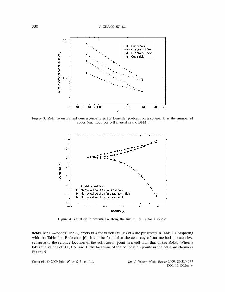
The first example considers problems in a sphere of radius 2 unit, centered at the origin. The usualspherical polar coordinates � and � are used. The linear, quadratic and cubic fields (Equations (31)–(34)) are used as exact solutions. In each case, the Dirichlet boundary conditions corresponding tothe exact solutions are imposed on the surface of the sphere. The results have been obtained forthree sets of nodes: (a) 74 nodes, (b) 143 nodes, and (c) 286 nodes. The L2 errors of nodal valuesof q , evaluated using Equation (35), for different sets of nodes and fields are shown in Figure 3.It can be seen that our method yields very accurate results and have high convergence rate. Figures 4and 5 show variation in the potential and its directional derivative at locations inside the sphere.The results are obtained using 74 nodes. The gradient is dotted with the diagonal (x= y= z) inorder to get the directional derivative along this line. Values of u and q , at internal points that areclose to the surface of the body, are calculated by the nearly singular integration scheme describedin Section 4.1. It is seen that results are accurate even when the points are very close to theboundary.

It has been observed in BNM that the choice of the locations of the collocation nodes on eachcell is an important ingredient for successful implementation of BNM. To compare with the BNM,we have also studied the influence of the locations of the collocation nodes on the accuracy of theBFM. In this study, the location of the collocation node on a cell is determined by a parameter�,0��1, using the following equation:

sP =sL+�(sR−sL)/2 (36)

where, sP is the collocation point, sL and sR are the lower-left and the upper-right corner points,respectively. Obviously, the collocation point is at the center of the cell when �=1 and at thelower-left corner of the cell when �=0. Computations have been performed for all the analytical


330 J. ZHANG ET AL.

Figure 3. Relative errors and convergence rates for Dirichlet problem on a sphere. N is the number ofnodes (one node per cell is used in the BFM).

Figure 4. Variation in potential u along the line x= y= z for a sphere.

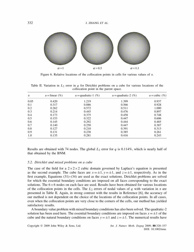
fields using 74 nodes. The L2 errors in q for various values of � are presented in Table I. Comparingwith the Table I in Reference [6], it can be found that the accuracy of our method is much lesssensitive to the relative location of the collocation point in a cell than that of the BNM. When �takes the values of 0.1, 0.5, and 1, the locations of the collocation points in the cells are shown inFigure 6.



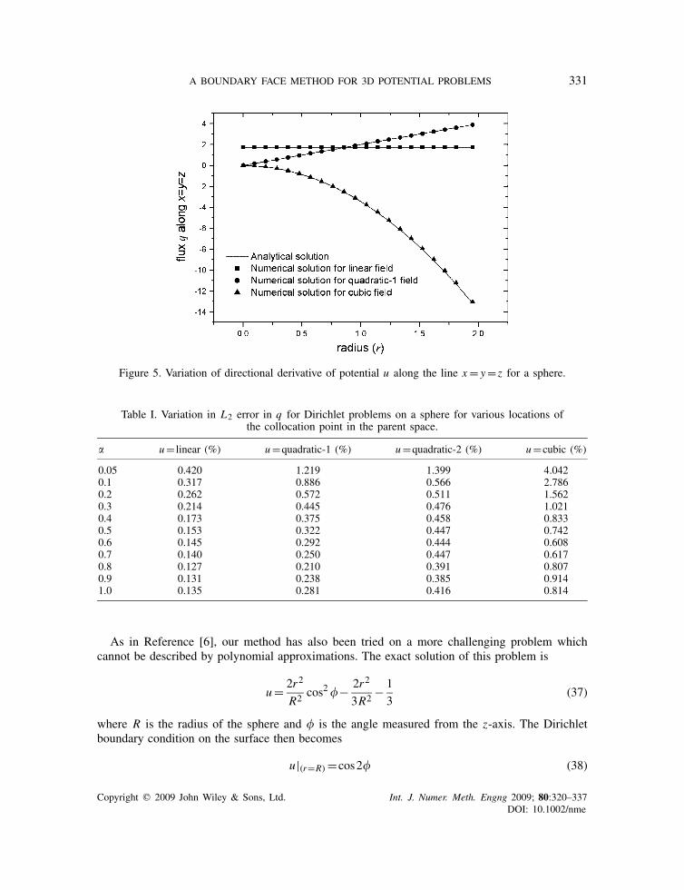
Figure 5. Variation of directional derivative of potential u along the line x= y= z for a sphere.

Table I. Variation in L2 error in q for Dirichlet problems on a sphere for various locations ofthe collocation point in the parent space.

� u= linear (%) u=quadratic-1 (%) u=quadratic-2 (%) u=cubic (%)

0.05 0.420 1.219 1.399 4.0420.1 0.317 0.886 0.566 2.7860.2 0.262 0.572 0.511 1.5620.3 0.214 0.445 0.476 1.0210.4 0.173 0.375 0.458 0.8330.5 0.153 0.322 0.447 0.7420.6 0.145 0.292 0.444 0.6080.7 0.140 0.250 0.447 0.6170.8 0.127 0.210 0.391 0.8070.9 0.131 0.238 0.385 0.9141.0 0.135 0.281 0.416 0.814

As in Reference [6], our method has also been tried on a more challenging problem whichcannot be described by polynomial approximations. The exact solution of this problem is

u= 2r2

R2cos2�− 2r2

3R2− 1

3(37)

where R is the radius of the sphere and � is the angle measured from the z-axis. The Dirichletboundary condition on the surface then becomes

u|(r=R) =cos2� (38)


332 J. ZHANG ET AL.

Figure 6. Relative locations of the collocation points in cells for various values of �.

Table II. Variation in L2 error in q for Dirichlet problems on a cube for various locations of thecollocation point in the parent space.

� u= linear (%) u=quadratic-1 (%) u=quadratic-2 (%) u=cubic (%)

0.05 0.420 1.219 1.399 0.9370.1 0.317 0.886 0.566 0.9280.2 0.262 0.572 0.511 1.0000.3 0.214 0.445 0.476 0.8970.4 0.173 0.375 0.458 0.7480.5 0.153 0.322 0.447 0.6060.6 0.145 0.292 0.444 0.4850.7 0.140 0.250 0.447 0.3870.8 0.127 0.210 0.391 0.3130.9 0.131 0.238 0.385 0.2611.0 0.135 0.281 0.416 0.243

Results are obtained with 74 nodes. The global L2 error for q is 0.114%, which is nearly half ofthat obtained by the BNM.

5.2. Dirichlet and mixed problems on a cube

The case of the field for a 2×2×2 cubic domain governed by Laplace’s equation is presentedas the second example. The cube faces are x=±1, y=±1, and z=±1, respectively. As in thefirst example, Equations (31)–(34) are used as the exact solutions. Dirichlet problems are solvedfor which the essential boundary conditions are imposed on all faces corresponding to the exactsolutions. The 6×6 nodes on each face are used. Results have been obtained for various locationsof the collocation points in the cells. The L2 errors of nodal values of q with variation in � arepresented in Table II. Again, in strong contrast with the results in Reference [6], the accuracy ofour method is not dependent on the choice of the locations of the collocation points. In all cases,even when the collocation points are very close to the corners of the cells, our method has yieldedsatisfactory results.

A boundary value problem with mixed boundary conditions has also been solved. The quadratic-2solution has been used here. The essential boundary conditions are imposed on faces x=±1 of thecube and the natural boundary conditions on faces y=±1 and z=±1. The numerical results have



Figure 7. Relative errors of u and q and convergence rate for Dirichlet problem on a cube.

Figure 8. Node distributions on a cube: (a) 12×12 regular nodes; (b) 8×18 irregularnodes; and (c) 4×36 irregular nodes.

been obtained using three sets of nodes: (a) 4×4 nodes on each face (totally 96 cells), (b) 5×5 nodeson each face (totally 150 cells), and (c) 6×6 nodes on each face (totally 216 cells). Figure 7 shows theL2 errors of nodal values of u and q when different numbers of nodes are used. It can be clearly seenthat excellent results have been obtained and high convergence rates achieved.

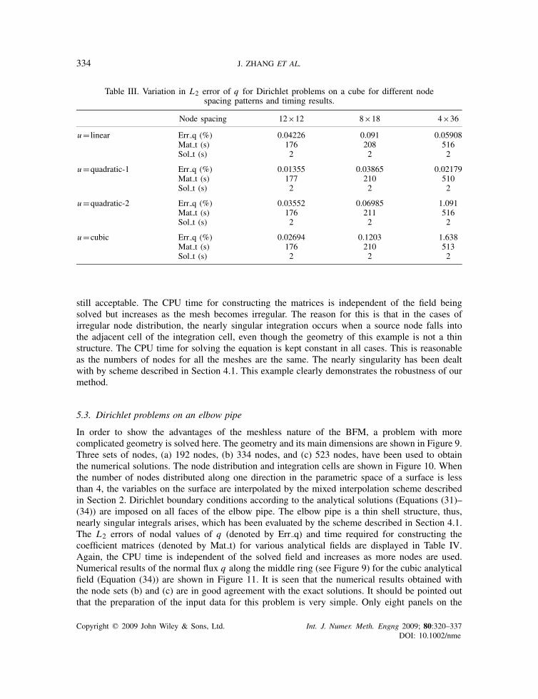
In order to understand the effect of node distribution on the accuracy of the obtained results, a newcase has been studied. In the case study, totally 864 nodes are used, of which three spacing patternson each face are considered: (a) 12×12 regular distribution, (b) 8×18 irregular distribution, and(c) 4×36 very irregular distribution. The node distributions are shown in Figure 8. The analyticalfields expressed by Equations (31)–(34) have been tested. The L2 errors of nodal values for q(denoted by Err q) and time required for constructing the coefficient matrices (denoted by Mat t)and solving the equation (denoted by Sol t) are presented in Table III. The results obtained withthe meshes (a) and (b) are very accurate. Even for the very irregular mesh (c), the results are


334 J. ZHANG ET AL.

Table III. Variation in L2 error of q for Dirichlet problems on a cube for different nodespacing patterns and timing results.

Node spacing 12×12 8×18 4×36

u= linear Err q (%) 0.04226 0.091 0.05908Mat t (s) 176 208 516Sol t (s) 2 2 2

u=quadratic-1 Err q (%) 0.01355 0.03865 0.02179Mat t (s) 177 210 510Sol t (s) 2 2 2

u=quadratic-2 Err q (%) 0.03552 0.06985 1.091Mat t (s) 176 211 516Sol t (s) 2 2 2

u=cubic Err q (%) 0.02694 0.1203 1.638Mat t (s) 176 210 513Sol t (s) 2 2 2

still acceptable. The CPU time for constructing the matrices is independent of the field beingsolved but increases as the mesh becomes irregular. The reason for this is that in the cases ofirregular node distribution, the nearly singular integration occurs when a source node falls intothe adjacent cell of the integration cell, even though the geometry of this example is not a thinstructure. The CPU time for solving the equation is kept constant in all cases. This is reasonableas the numbers of nodes for all the meshes are the same. The nearly singularity has been dealtwith by scheme described in Section 4.1. This example clearly demonstrates the robustness of ourmethod.

5.3. Dirichlet problems on an elbow pipe

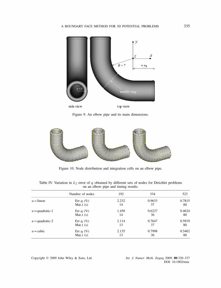
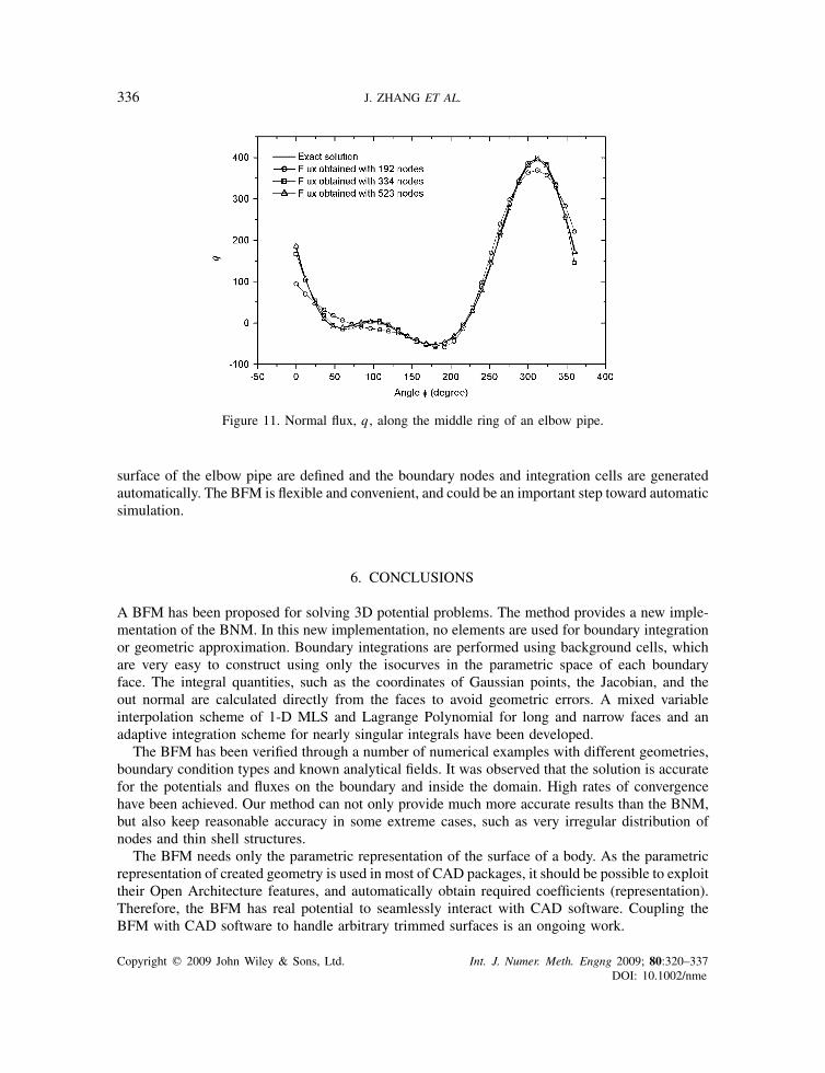
In order to show the advantages of the meshless nature of the BFM, a problem with morecomplicated geometry is solved here. The geometry and its main dimensions are shown in Figure 9.Three sets of nodes, (a) 192 nodes, (b) 334 nodes, and (c) 523 nodes, have been used to obtainthe numerical solutions. The node distribution and integration cells are shown in Figure 10. Whenthe number of nodes distributed along one direction in the parametric space of a surface is lessthan 4, the variables on the surface are interpolated by the mixed interpolation scheme describedin Section 2. Dirichlet boundary conditions according to the analytical solutions (Equations (31)–(34)) are imposed on all faces of the elbow pipe. The elbow pipe is a thin shell structure, thus,nearly singular integrals arises, which has been evaluated by the scheme described in Section 4.1.The L2 errors of nodal values of q (denoted by Err q) and time required for constructing thecoefficient matrices (denoted by Mat t) for various analytical fields are displayed in Table IV.Again, the CPU time is independent of the solved field and increases as more nodes are used.Numerical results of the normal flux q along the middle ring (see Figure 9) for the cubic analyticalfield (Equation (34)) are shown in Figure 11. It is seen that the numerical results obtained withthe node sets (b) and (c) are in good agreement with the exact solutions. It should be pointed outthat the preparation of the input data for this problem is very simple. Only eight panels on the



Figure 9. An elbow pipe and its main dimensions.

Figure 10. Node distribution and integration cells on an elbow pipe.

Table IV. Variation in L2 error of q obtained by different sets of nodes for Dirichlet problemson an elbow pipe and timing results.

Number of nodes 192 334 523

u= linear Err q (%) 2.232 0.9633 0.7815Mat t (s) 14 37 80

u=quadratic-1 Err q (%) 1.458 0.6227 0.4624Mat t (s) 14 36 80

u=quadratic-2 Err q (%) 2.114 0.7647 0.5919Mat t (s) 13 37 80

u=cubic Err q (%) 2.135 0.7998 0.5462Mat t (s) 13 36 80


336 J. ZHANG ET AL.

Figure 11. Normal flux, q , along the middle ring of an elbow pipe.

surface of the elbow pipe are defined and the boundary nodes and integration cells are generatedautomatically. The BFM is flexible and convenient, and could be an important step toward automaticsimulation.

6. CONCLUSIONS

A BFM has been proposed for solving 3D potential problems. The method provides a new imple-mentation of the BNM. In this new implementation, no elements are used for boundary integrationor geometric approximation. Boundary integrations are performed using background cells, whichare very easy to construct using only the isocurves in the parametric space of each boundaryface. The integral quantities, such as the coordinates of Gaussian points, the Jacobian, and theout normal are calculated directly from the faces to avoid geometric errors. A mixed variableinterpolation scheme of 1-D MLS and Lagrange Polynomial for long and narrow faces and anadaptive integration scheme for nearly singular integrals have been developed.

The BFM has been verified through a number of numerical examples with different geometries,boundary condition types and known analytical fields. It was observed that the solution is accuratefor the potentials and fluxes on the boundary and inside the domain. High rates of convergencehave been achieved. Our method can not only provide much more accurate results than the BNM,but also keep reasonable accuracy in some extreme cases, such as very irregular distribution ofnodes and thin shell structures.

The BFM needs only the parametric representation of the surface of a body. As the parametricrepresentation of created geometry is used in most of CAD packages, it should be possible to exploittheir Open Architecture features, and automatically obtain required coefficients (representation).Therefore, the BFM has real potential to seamlessly interact with CAD software. Coupling theBFM with CAD software to handle arbitrary trimmed surfaces is an ongoing work.



By coupling with the FMM [12–14], the BFM may be able to perform large-scale computationsfor complicated structures. This is planned in the near future.

ACKNOWLEDGEMENTS

This work is supported by the National Science Foundation of China under grants 10725208, 60635020and 50625519.

REFERENCES

1. Nayroles B, Touzot G, Villon P. Generalizing the finite element method: diffuse approximation and diffuseelement. Computational Mechanics 1992; 10:307–318.

2. Belytchko T, Lu YY, Gu L. Element free Galerkin methods. International Journal for Numerical Methods inEngineering 1994; 37:229–256.

3. Zhu T, Zhang J, Atluri SN. A local boundary integral equation (LBIE) method in computation mechanics, anda meshless discretization approach. Computational Mechanics 1998; 21:223–235.

4. Atluri SN, Zhu T. A new meshless local Petrov–Galerkin approach in computational mechanics. ComputationalMechanics 1998; 22:117–127.

5. Mukherjee YX, Mukherjee S. The boundary node method for potential problems. International Journal forNumerical Methods in Engineering 1997; 40:797–815.

6. Chati MK, Mukherjee S. The boundary node method for three-dimensional problems in potential theory.International Journal for Numerical Methods in Engineering 2000; 47:1523–1547.

7. Zhang JM, Yao ZH, Li H. A hybrid boundary node method. International Journal for Numerical Methods inEngineering 2002; 53:751–763.

8. Zhang JM, Yao ZH. Meshless regular hybrid boundary node method. Computer Modeling in Engineering andSciences 2001; 2:307–318.

9. Zhang JM, Yao ZH, Tanaka M. The meshless regular hybrid boundary node method for 2-D linear elasticity.Engineering Analysis with Boundary Elements 2003; 27:259–268.

10. Zhang JM, Yao ZH. Analysis of 2-D thin structures by the meshless regular hybrid boundary node method. ActaMechanica Sinica 2002; 15:36–44.

11. Hughes TJR, Cottrell JA, Bazilevs Y. Isogeometric analysis: CAD, finite elements, NURBS, exact geometry andmesh refinement. Computer Methods in Applied Mechanics and Engineering 2005; 194:4135–4195.

12. Zhang JM, Tanaka M, Endo M. The hybrid boundary node method accelerated by fast multipole method for 3Dpotential problems. International Journal for Numerical Methods in Engineering 2005; 63:660–680.

13. Zhang JM, Tanaka M. Fast HdBNM for large-scale thermal analysis of CNT-reinforced composites. ComputationalMechanics 2008; 41:777–787.

14. Zhang JM, Tanaka M. Adaptive spatial decomposition in fast multipole method. Journal of Computational Physics2007; 226:17–28.

15. Nagaranjan A, Mukherjee S. A mapping method for numerical evaluation of two-dimensional integrals with 1/rsingularity. Computational Mechanics 1993; 12:19–26.

16. Liu YJ. Analysis of shell-like structures by the boundary element method based on 3-D elasticity: formulationand verification. International Journal for Numerical Methods in Engineering 1998; 41:541–558.

17. Chen JT, Hong HK. Review of dual boundary element methods with emphasis on hypersingular integrals anddivergent series. Applied Mechanics Reviews 1999; 52(1):17–33.


A boundary face method for potential problems in three dimensions

Documents

Transcript of A boundary face method for potential problems in three dimensions