A Binary Intuitionistic Fuzzy Relation: Some New Results, a General Factorization, and Two...

Hindawi Publishing CorporationInternational Journal of Mathematics and Mathematical SciencesVolume 2009, Article ID 580918, 38 pagesdoi:10.1155/2009/580918

Research ArticleA Binary Intuitionistic Fuzzy Relation:Some New Results, a General Factorization,and Two Properties of Strict Components

Louis Aime Fono,1 Gilbert Njanpong Nana,2 Maurice Salles,3and Henri Gwet4

1 Departement de Mathematiques et Informatique, Faculte des Sciences, Universite de Douala,B.P. 24157 Douala, Cameroon

2 Laboratoire de Mathematiques Appliquees aux Sciences Sociales, Departement de Mathematiques,Faculte des Sciences, Universite de Yaounde I, B.P. 15396 Yaounde, Cameroon

3 MRSH, University of Caen, CREM-UMR 6211, CNRS, 14032 Caen Cedex, France4 Department of Mathematics, National Polytechnic Institute, P.O. Box 8390, Yaounde, Cameroon

Correspondence should be addressed to Louis Aime Fono, [email protected]

Received 3 July 2008; Revised 24 December 2008; Accepted 15 June 2009

Recommended by Andrzej Skowron

We establish, by means of a large class of continuous t-representable intuitionistic fuzzy t-conorms,a factorization of an intuitionistic fuzzy relation (IFR) into a unique indifference component anda family of regular strict components. This result generalizes a previous factorization obtained byDimitrov (2002) with the (max,min) intuitionistic fuzzy t-conorm. We provide, for a continuoust-representable intuitionistic fuzzy t-normT, a characterization of theT-transitivity of an IFR. Thisenables us to determine necessary and sufficient conditions on a T-transitive IFR R under which astrict component of R satisfies pos-transitivity and negative transitivity.

Copyright q 2009 Louis Aime Fono et al. This is an open access article distributed under theCreative Commons Attribution License, which permits unrestricted use, distribution, andreproduction in any medium, provided the original work is properly cited.

1. Introduction

In the real life, individual or collective preferences are not always crisp; they can be alsoambiguous. Since 1965 when Zadeh [1] introduced fuzzy set theory, researchers [2–11]modelled such preferences by (binary) fuzzy relation (simply denoted by FR) on X, thatis, a function R : X × X → [0, 1] where X is a set of alternatives with Card(X) = |X| ≥ 3.In this case, for (x, y) ∈ X2, R(x, y) is interpreted as the degree to which x is “at least asgood as” y. If ∀x, y ∈ X, R(x, y) ∈ {0, 1}, then R is crisp, and we denote R(x, y) = 1 by xRyand R(x, y) = 0 by not(xRy). Literature on the theory of fuzzy relations and on applicationsof fuzzy relations in other fields such as economics and in particular social choice theory isgrowing.

2 International Journal of Mathematics and Mathematical Sciences

Since 1983 when Atanassov [12, 13] introduced intuitionistic fuzzy sets (IFSs), somescholars [14–19] modelled ambiguous preferences by a (binary) intuitionistic fuzzy relation(IFR) on X, that is, a function R : X × X → L∗ = {(a1, a2) ∈ [0, 1]2, a1 + a2 ≤ 1} where∀x, y ∈ X, R(x, y) = (μR(x, y), νR(x, y)). In this case, μR(x, y) is the degree to which x is “atleast as good as” y, and νR(x, y) is the degree to which x is not “at least as good as” y. Thepositive real number πR(x, y) = 1 − μR(x, y) − νR(x, y) (since μR(x, y) + νR(x, y) ≤ 1), usuallycalled fuzzy index, indicates the degree of incomparability between x and y. In this paper, wesimply write ∀x, y ∈ X, R(x, y) = (μR(x, y), νR(x, y)). Clearly, we have two particular cases:(i) if ∀(x, y) ∈ X ×X, πR(x, y) = 0, that is, νR(x, y) = 1−μR(x, y), then R becomes an FR on X,and (ii) if ∀(x, y) ∈ X ×X, πR(x, y) = 0 and νR(x, y) ∈ {0, 1}, then R becomes the well-known(binary) crisp relation. In the first case, we simply write R(x, y) = μR(x, y), and in the secondcase, we have xRy ⇔ μR(x, y) = 1 (i.e., νR(x, y) = 0).

A factorization of a binary relation is an important question in preference modelling.In that view, Dimitrov [18] established a factorization of an IFR into an indifference and astrict component in the particular case where the union is defined bymeans of the (max,min)t-representable intuitionistic fuzzy t-conorm. Recently, Cornelis et al. [20] established someresults on t-representable intuitionistic fuzzy t-norms (i.e., T = (T, S) where S is a fuzzy t-conorm, and T is a fuzzy t-norm satisfying ∀a, b ∈ [0, 1], T(a, b) ≤ 1 − S(1 − a, 1 − b)), ont-representable intuitionistic fuzzy t-conorms (i.e., J = (S, T)) and on intuitionistic fuzzyimplications. Thereby, our goal is to generalize Dimitrov’s framework [18] and to establishsome results on IFRs by means of continuous t-representable intuitionistic fuzzy t-norms andt-conorms.

The aim of this paper is (i) to study the standard completeness of an IFR, (ii) toestablish a characterization of the T-transitivity of an IFR, (iii) to generalize the factorizationof an IFR established by Dimitrov [18], and (iv) to determine necessary and sufficientconditions on a T-transitive IFR R under which a given strict component of R (obtained inour factorization) satisfies respectively pos-transitivity and negative transitivity.

First we establish some useful results on t-representable intuitionistic fuzzy t-norms,t-representable intuitionistic fuzzy t-conorms, and intuitionistic fuzzy implications.

The paper is organized as follows. In Section 2, we recall some basic notions andproperties on fuzzy operators and intuitionistic fuzzy operators which we need throughoutthe paper. We also establish some useful results on fuzzy implications and intuitionisticfuzzy implications. Section 3 has three subsections. In Section 3.1, we recall some basic anduseful definitions on IFRs. In Section 3.2, we introduce the standard completeness, namely, a(S, T)-completeness of an IFR. We make clear that the notion of completeness introducedby Dimitrov [18] is not standard, but it is weaker than a standard one. In Section 3.3,we establish, for a given T, a characterization of the T-transitivity of an IFR. Section 4is devoted to a new factorization of an IFR, and it has two subsections. In Section 4.1,we recall the factorization of an IFR established by Dimitrov [18] with the (max,min)intuitionistic fuzzy t-conorm. We point out some intuitive difficulties of the strict componentobtained in [18]. In Section 4.2, we introduce definitions of an indifference and a strictcomponent of an IFR, and we establish a general factorization of an IFR for a large class ofcontinuous t-representable intuitionistic fuzzy t-conorms. Section 5 contains two subsections.In Section 5.1, we introduce intuitionistic fuzzy counterparts of pos-transitivity and negativetransitivity of a crisp relation. We justify that there exists some IFRs (noncrisp and nonFRs) which violate each of these two properties. This forces us in Section 5.2 to establishnecessary and sufficient conditions on a T-transitive IFR R, such that a strict componentof R satisfies, respectively, pos-transitivity and negative transitivity. Section 6 contains some

International Journal of Mathematics and Mathematical Sciences 3

concluding remarks. The proofs of our results are in the Appendix. (This was suggested byan anonymous referee.)

2. Preliminaries on Operators

Let ≤L∗ be an order in L∗ defined by ∀(a1, a2), (b1, b2) ∈ L∗, (a1, a2)≤L∗(b1, b2) ⇔ (a1 ≤ b1 anda2 ≥ b2). (L∗,≤L∗) is a complete lattice. 0L∗ = (0, 1) and 1L∗ = (1, 0) are the units of L∗.

In the following section, we recall some definitions, examples, and well-known resultson fuzzy t-norms, fuzzy t-conorms, fuzzy implications, and fuzzy coimplicators.

2.1. Review on Fuzzy Operators

We firstly recall notions on fuzzy t-norms and fuzzy t-conorms (see [21, 22]).A fuzzy t-norm (resp. a fuzzy t-conorm) is an increasing, commutative, and associative

binary operation on [0, 1] with a neutral 1 (resp. 0). The dual of a fuzzy t-norm T is a fuzzyt-conorm S, that is, ∀a, b ∈ [0, 1], T(a, b) = 1 − S(1 − a, 1 − b).

Let us recall two usual families of fuzzy t-norms and fuzzy t-conorms. The Frank t-norms (Tl

F)l∈[0,∞], that is, ∀l ∈ [0,∞], ∀a, b ∈ [0, 1],

TlF(a, b) =

⎧⎪⎪⎪⎪⎪⎪⎪⎪⎪⎨

⎪⎪⎪⎪⎪⎪⎪⎪⎪⎩

TM(a, b) = min(a, b) = a ∧ b, if l = 0,

TP(a, b) = a × b, if l = 1,

TL(a, b) = max(a + b − 1, 0), if l = +∞,

logl

(

1 +(la − 1)

(lb − 1

)

l − 1

)

, otherwise,

(2.1)

where TM, TP, and TL are the minimum fuzzy t-norm, the product fuzzy t-norm, andthe Łukasiewicz fuzzy t-norm, respectively. The Frank t-conorms (Sl

F)l∈[0,∞], that is, ∀l ∈[0,∞], ∀a, b ∈ [0, 1],

SlF(a, b) =

⎧⎪⎪⎪⎪⎪⎪⎪⎪⎪⎨

⎪⎪⎪⎪⎪⎪⎪⎪⎪⎩

SM(a, b) = max(a, b) = a ∨ b, if l = 0,

SP(a, b) = a + b − a × b, if l = 1,

SL(a, b) = min(a + b, 1), if l = +∞,

1 − logl

(

1 +

(l1−a − 1

)(l1−b − 1

)

l − 1

)

, otherwise,

(2.2)

where SM, SP, and SL are the maximum fuzzy t-conorm, the product fuzzy t-conorm, and theŁukasiewicz fuzzy t-conorm, respectively.

A fuzzy t-norm T (fuzzy t-conorm S) is strict if ∀a, b ∈ [0, 1], ∀c ∈]0, 1], a < b impliesT(a, c) < T(b, c) (resp. ∀a, b ∈ [0, 1], ∀c ∈ [0, 1[, a < b implies S(a, c) < S(b, c)). The productfuzzy t-norm (resp. the product fuzzy t-conorm) is an example of a strict fuzzy t-norm (resp.fuzzy t-conorm).


We have the following properties:

∀a, b ∈ [0, 1],

⎧⎨

⎩

(i) T(a, b) ≤ min(a, b)

(ii) max(a, b) ≤ S(a, b).(2.3)

Throughout the paper, T is a continuous fuzzy t-norm, and S is a continuous fuzzyt-conorm.

In the following, we recall some definitions and examples on fuzzy implications andfuzzy coimplicators based on fuzzy t-norms and fuzzy t-conorms, respectively (see [21–23]).

The fuzzy R-implication IT associated to T is a binary operation on [0, 1] defined by∀a, b ∈ [0, 1], IT (a, b) = max{t ∈ [0, 1], T(a, t) ≤ b}. The fuzzy coimplicator JS associated to Sis a binary operation on [0, 1] defined by ∀a, b ∈ [0, 1], JS(a, b) = min{t ∈ [0, 1], b ≤ S(a, t)}.

Let us recall some usual examples of these fuzzy operators.The fuzzy R-implication associated to TM is defined by

∀a, b ∈ [0, 1], ITM =

⎧⎨

⎩

1, if a ≤ b,

b, if a > b.(2.4)

The fuzzy coimplicator associated to SM is defined by

∀a, b ∈ [0, 1], JSM(a, b) =

⎧⎨

⎩

b, if a < b,

0, if a ≥ b.(2.5)

The fuzzy R-implication associated to TL is defined by

∀a, b ∈ [0, 1], ITL(a, b) =

⎧⎨

⎩

1, if a ≤ b,

1 − a + b, if a > b.(2.6)

The fuzzy coimplicator associated to SL is defined by

∀a, b ∈ [0, 1], JSL(a, b) =

⎧⎨

⎩

b − a, if a < b,

0, if a ≥ b.(2.7)

The fuzzy R-implication associated to TP is defined by

∀a, b ∈ [0, 1], ITP(a, b) =

⎧⎪⎨

⎪⎩

1, if a ≤ b,

b

a, if a > b.

(2.8)


The fuzzy coimplicator associated to SP is defined by

∀a, b ∈ [0, 1], JSP(a, b) =

⎧⎪⎨

⎪⎩

b − a

1 − a, if a < b,

0, if a ≥ b.

(2.9)

We complete the previous examples by giving expressions of fuzzy R-implications ofthe other Frank fuzzy t-norms and fuzzy coimplicators of the other Frank fuzzy t-conorms:

∀l ∈]0, 1[∪]1,+∞[, ∀a, b ∈ [0, 1], ITlF(a, b) =

⎧⎪⎪⎨

⎪⎪⎩

1, if a ≤ b,

logl

(

1 +(l − 1)

(lb − 1

)

la − 1

)

, if a > b,

JSlF(a, b) =

⎧⎪⎪⎨

⎪⎪⎩

0, if a ≥ b,

1 − logl

(

1 +(l − 1)

(l1−b − 1

)

l(1−a) − 1

)

, if a < b.

(2.10)

We recall some useful properties on fuzzy implications and fuzzy coimplicators.

Proposition 2.1 (See [4, 5, 9, 21, 23]). For all a, b, c ∈ [0, 1],

(1) IT (a, a) = 1; JS(a, a) = 0, and JS(a, b) ≤ b ≤ IT (a, b);

(2) T(a, IT(a, b)) = min(a, b), and S(a, JS(a, b)) = max(a, b);

(3)

b < a ⇐⇒ IT (a, b) < 1,

a < b ⇐⇒ JS(a, b) > 0;(2.11)

(4)

a ≤ b =⇒

⎧⎨

⎩

IT (b, c) ≤ IT (a, c),

IT (c, a) ≤ IT (c, b);(2.12)

(5)

a ≤ b =⇒

⎧⎨

⎩

JS(b, c) ≤ JS(a, c),

JS(c, a) ≤ JS(c, b);(2.13)

In the following, we recall some useful definitions and results on intuitionistic fuzzyoperators.


2.2. Review on Intuitionistic Fuzzy Operators

Definition 2.2 (See [20]). (1)An intuitionistic fuzzy t-norm is an increasing, commutative, andassociative binary operation T on L∗ satisfying ∀(a, b) ∈ L∗, T((a, b), (1, 0)) = (a, b).

(2) An intuitionistic fuzzy t-conorm is an increasing, commutative, associative binaryoperation J on L∗ satisfying ∀(a, b) ∈ L∗, J((a, b), (0, 1)) = (a, b).

Cornelis et al. [20] introduced an important class of intuitionistic fuzzy t-norms (resp.t-conorms) based on fuzzy t-norms (resp. fuzzy t-conorms).

Definition 2.3. An intuitionistic fuzzy t-norm T (resp. t-conorm J) is called t-representable ifthere exists a fuzzy t-norm T and a fuzzy t-conorm S (resp. a fuzzy t-conorm S and fuzzyt-norm T) such that ∀a = (a1, a2), b = (b1, b2) ∈ L∗, T(a, b) = (T(a1, b1), S(a2, b2)) (resp.J(a, b)) = (S(a1, b1), T(a2, b2)).

T and S (resp. S and T) are called the representants of T (resp. J).

The theorem below states conditions under which a pair of connectives on [0, 1] givesrise to a t-representable intuitionistic fuzzy t-norm (t-conorm).

Theorem 2.4 (see Cornelis et al. [20, Theorem 2, pages 60–61]). Given a fuzzy t-norm T and afuzzy t-conorm S satisfying ∀a1, a2 ∈ [0, 1], T(a1, a2) ≤ 1 − S(1 − a1, 1 − a2).

The mappings T and J defined by, for x = (x1, x2) and y = (y1, y2) in L∗ : T(x, y) =(T(x1, y1), S(x2, y2)) and J(x, y) = (S(x1, y1), T(x2, y2)), are, respectively, a t-representableintuitionistic fuzzy t-norm and t-representable intuitionistic fuzzy t-conorm.

Throughout the paper, we consider only continuous t-representable intuitionisticfuzzy t-conorms (shortly if-t-conorm) and continuous t-representable intuitionistic fuzzy t-norms (shortly if-t-norm). They are denoted by J = (S, T) and T = (T, S), respectively, where∀a, b ∈ [0, 1], S(a, b) ≤ 1 − T(1 − a, a − b).

From the previous result, we deduce some examples of if-t-norms and if-t-conorms.

Example 2.5. (1) TM = (TM, SM) and JM = (SM, TM) are, respectively, if-t-norm and if-t-conorm associated to TM and SM since ∀a, b ∈ [0, 1], TM(a, b) ≤ 1 − SM(1 − a, 1 − b).

(2) TL = (TL, SL) and JL = (SL, TL) are, respectively, if-t-norm and if-t-conormassociated to TL and SL since ∀a, b ∈ [0, 1], TL(a, b) ≤ 1 − SL(1 − a, 1 − b).

(3) TP = (TP, SP) and JP = (SP, TP) are, respectively, if-t-norm and if-t-conormassociated to TP and SP since ∀a, b ∈ [0, 1], TP(a, b) ≤ 1 − SP(1 − a, 1 − b).

Definition 2.6 (see Cornelis et al. [20, Definition 8, page 64]). (1) The intuitionistic fuzzy R-implication (shortly if-R-implication) associated with an if-t-norm T = (T, S) is a binaryoperation on L∗ defined by: ∀x = (x1, x2), y = (y1, y2) ∈ L∗, IT(x, y) = sup{z ∈L∗, T(x, z)≤L∗y} = sup{z = (z1, z2) ∈ L∗, T(x1, z1) ≤ y1 and S(x2, z2) ≥ y2}.

(2) The intuitionistic fuzzy coimplicator (shortly if-coimplicator) associated with anif-t-conorm J = (S, T) is a binary operation on L∗ defined by: ∀x = (x1, x2), y =(y1, y2) ∈ L∗, JJ(x, y) = inf{z ∈ L∗, y≤L∗J(x, z)} = inf{z = (z1, z2) ∈ L∗/y1 ≤S(x1, z1) and y2 ≥ T(x2, z2)}.

We establish in the sequel some new and basic results on the previous implications.These results will be useful later.


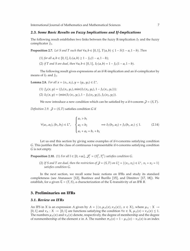
2.3. Some Basic Results on Fuzzy Implications and If-Implications

The following result establishes two links between the fuzzy R-implication IT and the fuzzycoimplicator JS.

Proposition 2.7. Let S and T such that ∀a, b ∈ [0, 1], T(a, b) ≤ 1 − S(1 − a, 1 − b). Then

(1) for all a, b ∈ [0, 1], IT (a, b) ≥ 1 − JS(1 − a, 1 − b);

(2) if T and S are dual, then ∀a, b ∈ [0, 1], IT (a, b) = 1 − JS(1 − a, 1 − b).

The following result gives expressions of an if-R-implication and an if-coimplicator bymeans of IT and JS.

Lemma 2.8. For all x = (x1, x2), y = (y1, y2) ∈ L∗,

(1) JJ(x, y) = (JS(x1, y1),min(IT (x2, y2), 1 − JS(x1, y1)));

(2) IT(x, y) = (min(IT (x1, y1), 1 − JS(x2, y2)), JS(x2, y2)).

We now introduce a new condition which can be satisfied by a if-t-conorm J = (S, T).

Definition 2.9. J = (S, T) satisfies condition G if

∀(a1, a2), (b1, b2) ∈ L∗,

⎧⎪⎪⎪⎨

⎪⎪⎪⎩

a1 > b1

a2 < b2

a1 + a2 = b1 + b2

=⇒ IT (b2, a2) + JS(b1, a1) ≤ 1. (2.14)

Let us end this section by giving some examples of if-t-conorms satisfying conditionG. This justifies that the class of continuous t-representable if-t-conorms satisfying conditionG is not empty.

Proposition 2.10. (1) For all l ∈ [0,+∞], JFl = (SF

l , TFl ) satisfies condition G.

(2) If S and T are dual, then the restriction of J = (S, T) on L∗1 = {(x1, x2) ∈ L∗, x1 + x2 = 1}

satisfies condition G.

In the next section, we recall some basic notions on IFRs and study its standardcompleteness (see Atanassov [12], Bustince and Burillo [15], and Dimitrov [17, 18]). Weestablish, for a given T = (T, S), a characterization of the T-transitivity of an IFR R.

3. Preliminaries on IFRs

3.1. Review on IFRs

An IFS in X is an expression A given by A = {〈x, μA(x), νA(x)〉, x ∈ X}, where μA : X →[0, 1] and νA : X → [0, 1] are functions satisfying the condition ∀x ∈ X, μA(x) + νA(x) ≤ 1.The numbers μA(x) and νA(x) denote, respectively, the degree of membership and the degreeof nonmembership of the element x in A. The number πA(x) = 1 − μA(x) − νA(x) is an index


of the element x in X. Obviously, when ∀x ∈ X, νA(x) = 1 − μA(x), that is, πA(x) = 0, the IFSA is a fuzzy set (simply denoted by FS) in X. In this case, ∀x ∈ X, A(x) = μA(x).

Let A and B be two IFSs, and let J = (S, T). The intuitionistic fuzzy union A∪JBassociated to J is an IFS defined by

∀x ∈ X,

⎧⎨

⎩

μA∪JB(x) = S(μA(x), μB(x)

),

νA∪JB(x) = T(νA(x), νB(x))(3.1)

(we recall that if A and B are FSs, and T and S are dual, then A∪JB becomes the well-knownfuzzy union A∪SB defined by ∀x ∈ X, A∪SB(x) = S(A(x), B(x)). And if A and B are crisp,A∪JB = A∪SB becomes the crisp union). As defined in the Introduction, an IFR inX is an IFSin X ×X.

We complete some basic definitions on IFRs.

Definition 3.1. Let R be an IFR.

(1) R is reflexive if ∀x ∈ X, μR(x, x) = 1.

(2) R is symmetric if ∀x, y ∈ X, μR(x, y) = μR(y, x) and νR(x, y) = νR(y, x).

(3) R is π-symmetric if ∀x, y ∈ X, πR(x, y) = πR(y, x).

(4) R is perfect antisymmetric if ∀(x, y) ∈ X ×X, x /=y,

⎛

⎜⎜⎝

μR

(x, y)> 0

or(μR

(x, y)= 0, νR

(x, y)< 1)

⎞

⎟⎟⎠ =⇒

⎧⎨

⎩

μR

(y, x)= 0,

νR(y, x)= 1.

(3.2)

(5) The converse of R is the IFR denoted R−1 and defined by ∀x, y ∈ X, μR−1(x, y) =μR(y, x) and νR−1(x, y) = νR(y, x).

In the following, we recall the well-known notion of completeness of a crisp relationin X. We then present definition of the standard completeness of a FR and its two usualand particular cases (weak completeness and strong completeness). Following that line, weintroduce the definition of the standard completeness of an IFR. We establish a link betweenthat standard definition and the one introduced by Dimitrov (see [17, 18]). And we write thetwo particular cases of that standard definition.

3.2. Intuitionistic Fuzzy Standard Completeness (J-Completeness)

Let R be a reflexive IFR and J = (S, T).WhenR is a crisp relation,R is complete ifR∪R−1 = X2, that is, ∀x, y ∈ X, xRy or yRx.When R is a FR, for the fuzzy t-conorm S,R is S-complete if R∪SR

−1 = X2, that is,∀x, y ∈ X, S(R(x, y), R(y, x)) = 1. In particular, if S = SM, we simply say that R is stronglycomplete, that is, ∀x, y ∈ X, max(R(x, y), R(y, x)) = 1. If S = SL, we simply say that R isweakly complete, that is, ∀x, y ∈ X, R(x, y)+R(y, x) ≥ 1 (see Fono and Andjiga [7, Definition2, page 375]).


In the general case where R is an IFR and J = (S, T), we have the following genericversion of the standard completeness of R.

Definition 3.2. R is J-complete if R∪JR−1 = X2, that is,

∀x, y ∈ X,

⎧⎨

⎩

S(μR

(x, y), μR

(y, x))

= 1,

T(νR(x, y), νR(y, x))

= 0.(3.3)

Remark 3.3. If an IFRR becomes a FR, and S and T are dual, then (S, T)-completeness becomesS-completeness. Furthermore, if R becomes crisp, then J-completeness and S-completenessbecome crisp completeness.

Dimitrov (see [17, Definition 2, page 151]) introduced the following version ofcompleteness of an IFR: R is D-complete if ∀x, y ∈ X,

[(μR

(x, y), νR(x, y))

= (0, 1)]=⇒[μR

(y, x)> 0, νR

(y, x)< 1]. (3.4)

It is important to notice that D-completeness is not a version of the standardcompleteness. However, the following result shows that it is weaker than each version ofthe standard completeness.

Proposition 3.4. If R is (S, T)-complete, then R is D-complete.

As for FRs, we deduce the two following interesting particular cases of J-completeness when J ∈ {JM,JL}.

Example 3.5. Let R be a reflexive IFR and J = (S, T).

(1) If J = JM = (max,min), then R is J-complete if ∀x, y ∈ X,

max(μR

(x, y), μR

(y, x))

= 1,

min(νR(x, y), νR(y, x))

= 0.(3.5)

In this case, we simply say that R is strongly complete.

(2) If J = JL = (SL, TL), then R is J-complete if ∀x, y ∈ X,

min(1, μR

(x, y)+ μR

(y, x))

= 1,

max(0, νR

(x, y)+ νR

(y, x)− 1)= 0,

i.e.,

⎧⎨

⎩

μR

(x, y)+ μR

(y, x)≥ 1,

νR(x, y)+ νR

(y, x)≤ 1.

(3.6)

In this case, we simply say that R is weakly complete.

We notice that, if R becomes a FR, then intuitionistic strong completeness of R andthe intuitionistic weak completeness of R become, respectively, fuzzy strong completenessof R and fuzzy weak completeness of R. Furthermore, as for FRs, intuitionistic strongcompleteness implies intuitionistic weak completeness.


Throughout the paper, R is a reflexive, weakly complete, and π-symmetric IFR.In the sequel, we define T-transitivity of an IFR R. We introduce and analyze four

elements of L∗. They enable us to obtain a characterization of the T-transitivity of R whichgeneralizes the one obtained earlier by Fono and Andjiga [7] for FRs.

3.3. T-transitivity of an IFR: Definition and Characterization

Let T = (T, S) and IT be the if-R-implication associated to T.

Definition 3.6. R is T-transitive if ∀x, y, z ∈ X,

T(R(x, y), R(y, z))≤L∗R(x, z), i.e.,

⎧⎨

⎩

μR(x, z) ≥ T(μR

(x, y), μR

(y, z)),

νR(x, z) ≤ S(νR(x, y), νR(y, z)).

(3.7)

If R becomes a FR and T and S are dual, then the T-transitivity becomes the usualT -transitivity, that is, ∀x, y, z ∈ X, R(x, z) ≥ T(R(x, y), R(y, z)). If R becomes a crisp relation,then the T-transitivity and the T -transitivity become the crisp transitivity, that is, ∀x, y, z ∈X, (xRy and yRz) ⇒ xRz.

We write the particular case of the T-transitivity where T = TM.

Example 3.7. If T = TM, then R is TM-transitive if ∀x, y, z ∈ X,

μR(x, z) ≥ min(μR

(x, y), μR

(y, z)),

νR(x, z) ≤ max(νR(x, y), νR(y, z)).

(3.8)

We simply say that R is transitive.

To establish a characterization of the T-transitivity of R, we need the following fourelements of [0, 1]2 associated to R.

Let us introduce and analyze these elements of [0, 1]2.

Definition 3.8. For all x, y, z ∈ X,

(1) (α1(x, y, z), β1(x, y, z)) = (T(μR(z, y), μR(y, x)), S(νR(z, y), νR(y, x)));

(2) (α2(x, y, z), β2(x, y, z)) = (T(μR(x, y), μR(y, z)), S(νR(x, y), νR(y, z)));

(3) (α3(x, y, z), β3(x, y, z)) =min(IT[(μR(y, z), νR(y, z)), (μR(y, x), νR(y, x))], IT[(μR(x,y), νR(x, y)), (μR(z, y), νR(z, y))]);

(4) (α4(x, y, z), β4(x, y, z)) =min(IT[(μR(y, x), νR(y, x)), (μR(y, z), νR(y, z))], IT[(μR(z,y), νR(z, y)), (μR(x, y), νR(x, y))]).

The next result shows that (αi(x, y, z), βi(x, y, z))i∈{1,2,3,4} are elements of L∗ anddeduces expressions of α3(x, y, z), β3(x, y, z), α4(x, y, z) and β4(x, y, z).


Proposition 3.9. (1) For all i ∈ {1, 2, 3, 4}, (αi(x, y, z), βi(x, y, z)) ∈ L∗.

(2) (i) α3(x, y, z) is the minimum of min[IT (μR(x, y), μR(z, y)), 1 − JS(νR(x, y),νR(z, y))] and min[IT (μR(y, z), μR(y, x)), 1 − JS(νR(y, z), νR(y, x))].

(ii) β3(x, y, z) = max(JS(νR(y, z), νR(y, x)), JS(νR(x, y), νR(z, y))).(iii) α4(x, y, z) is the minimum of min[IT (μR(z, y), μR(x, y)), 1 − JS(νR(z, y),

νR(x, y))] and min[IT (μR(y, x), μR(y, z)), 1 − JS(νR(y, x), νR(y, z)))].(iv) β4(x, y, z) = max(JS(νR(y, x), νR(y, z)), JS(νR(z, y), νR(x, y))).

The following remark gives some comparisons of those elements of L∗.

Remark 3.10. For all x, y, z ∈ X,

(1) (α1(x, y, z), β1(x, y, z))≤L∗(α3(x, y, z), β3(x, y, z));

(2) (α2(x, y, z), β2(x, y, z))≤L∗(α4(x, y, z), β4(x, y, z)).

The following result shows that in the particular case where R is strongly complete,the four reals α3(x, y, z), α4(x, y, z), β3(x, y, z) and β4(x, y, z) become simple.

Corollary 3.11. Let R be an IFR, and let x, y, z ∈ X.

(1) If R is strongly complete and

⎛

⎝

⎧⎨

⎩

μR

(y, x)< μR

(x, y)

μR

(z, y)< μR

(y, z) or

⎧⎨

⎩

μR

(y, x)= μR

(x, y)

μR

(z, y)< μR

(y, z) or

⎧⎨

⎩

μR

(y, x)< μR

(x, y)

μR

(z, y)= μR

(y, z)

⎞

⎠, (3.9)

then

α1(x, y, z

)= T(μR

(z, y), μR

(y, x))

< 1,

α3(x, y, z

)= min

(μR

(y, x), μR

(z, y)),

α2(x, y, z

)= α4

(x, y, z

)= 1.

(3.10)

(2) If R is strongly complete and

⎛

⎝

⎧⎨

⎩

νR(y, x)> νR

(x, y)

νR(z, y)> νR

(y, z) or

⎧⎨

⎩

νR(y, x)= νR

(x, y)

νR(z, y)> νR

(y, z) or

⎧⎨

⎩

νR(y, x)> νR

(x, y)

νR(z, y)= νR

(y, z)

⎞

⎠, (3.11)

then

β1(x, y, z

)= S(νR(z, y), νR(y, x))

> 0,

β3(x, y, z

)= max

(νR(y, x), νR(z, y)),

β2(x, y, z

)= β4

(x, y, z

)= 0.

(3.12)


In the particular case where T and S are dual and R becomes a FR, we have some linksbetween αi and βi for i ∈ {1, 2, 3, 4}. Furthermore, we obtain expressions of (αi(x, y, z))i∈{1,2,3,4}introduced earlier by Fono and Andjiga (see [7, page 375]).

Corollary 3.12. If T and S are dual and R is a FR, then ∀x, y, z ∈ X,

(1)

β1(x, y, z

)= 1 − α1

(x, y, z

),

β2(x, y, z

)= 1 − α2

(x, y, z

),

β3(x, y, z

)= 1 − α3

(x, y, z

),

β4(x, y, z

)= 1 − α4

(x, y, z

).

(3.13)

(2)

α1(x, y, z

)= T(μR

(z, y), μR

(y, x)),

α2(x, y, z

)= T(μR

(x, y), μR

(y, z)),

α3(x, y, z

)= min

(IT(μR

(x, y), μR

(z, y)), IT(μR

(y, z), μR

(y, x)))

,

α4(x, y, z

)= min

(IT(μR

(y, x), μR

(y, z)), IT(μR

(z, y), μR

(x, y)))

.

(3.14)

We end this section by establishing by means of those four elements of L∗ acharacterization of the T-transitivity of an IFR R. Before that, let us recall a characterizationof the T -transitivity of a FR: ∀x, y, z ∈ X, if T and S are dual, and the IFR Rbecomes a FR, then Fono and Andjiga (see [7, Lemma 1, page 375]) used the four realsα1(x, y, z), α2(x, y, z), α3(x, y, z), and α4(x, y, z) defined in Corollary 3.12, to obtain thefollowing characterization of the T -transitivity of R.

R is T -transitive on {x, y, z} if and only if

R(x, z) = μR(x, z) ∈[α2(x, y, z

), α4(x, y, z

)],

R(z, x) = μR(z, x) ∈[α1(x, y, z

), α3(x, y, z

)].

(3.15)

We generalize that result for an IFR. Therefore, we obtain our first key result.

Lemma 3.13. Let {x, y, z} ⊆ X.The two following statements are equivalent:

(i) R is T-transitive on {x, y, z};(ii)

μR(x, z) ∈[α2(x, y, z

), α4(x, y, z

)], νR(x, z) ∈

[β4(x, y, z

), β2(x, y, z

)],

μR(z, x) ∈[α1(x, y, z

), α3(x, y, z

)], νR(z, x) ∈

[β3(x, y, z

), β1(x, y, z

)].

(3.16)


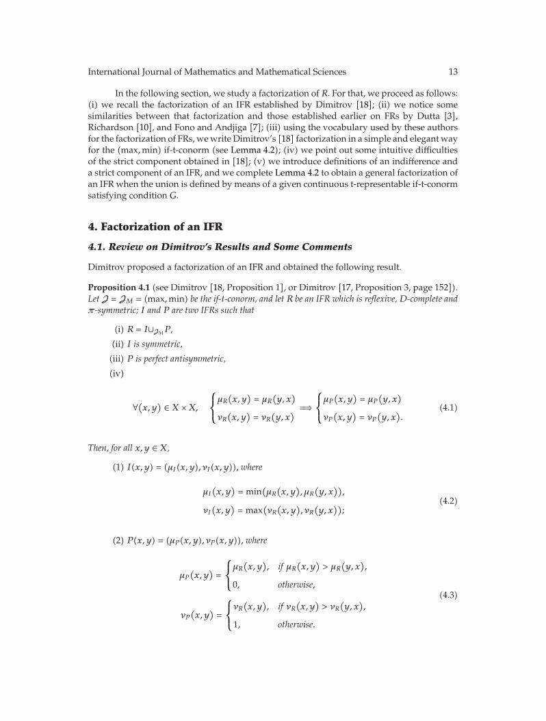
In the following section, we study a factorization of R. For that, we proceed as follows:(i) we recall the factorization of an IFR established by Dimitrov [18]; (ii) we notice somesimilarities between that factorization and those established earlier on FRs by Dutta [3],Richardson [10], and Fono and Andjiga [7]; (iii) using the vocabulary used by these authorsfor the factorization of FRs, wewrite Dimitrov’s [18] factorization in a simple and elegant wayfor the (max,min) if-t-conorm (see Lemma 4.2); (iv) we point out some intuitive difficultiesof the strict component obtained in [18]; (v) we introduce definitions of an indifference anda strict component of an IFR, and we complete Lemma 4.2 to obtain a general factorization ofan IFR when the union is defined by means of a given continuous t-representable if-t-conormsatisfying condition G.

4. Factorization of an IFR

4.1. Review on Dimitrov’s Results and Some Comments

Dimitrov proposed a factorization of an IFR and obtained the following result.

Proposition 4.1 (see Dimitrov [18, Proposition 1], or Dimitrov [17, Proposition 3, page 152]).Let J = JM = (max,min) be the if-t-conorm, and let R be an IFR which is reflexive,D-complete andπ-symmetric; I and P are two IFRs such that

(i) R = I∪JMP ,

(ii) I is symmetric,

(iii) P is perfect antisymmetric,

(iv)

∀(x, y)∈ X ×X,

⎧⎨

⎩

μR

(x, y)= μR

(y, x)

νR(x, y)= νR

(y, x) =⇒

⎧⎨

⎩

μP

(x, y)= μP

(y, x)

νP(x, y)= νP

(y, x).

(4.1)

Then, for all x, y ∈ X,

(1) I(x, y) = (μI(x, y), νI(x, y)), where

μI

(x, y)= min

(μR

(x, y), μR

(y, x)),

νI(x, y)= max

(νR(x, y), νR(y, x));

(4.2)

(2) P(x, y) = (μP (x, y), νP (x, y)), where

μP

(x, y)=

⎧⎨

⎩

μR

(x, y), if μR

(x, y)> μR

(y, x),

0, otherwise,

νP(x, y)=

⎧⎨

⎩

νR(x, y), if νR

(x, y)> νR

(y, x),

1, otherwise.

(4.3)


After a careful check, we notice that, in the particular case where R becomes a FR,conditions (4.1) and (4.3) become some known notions introduced earlier by Dutta [3] and,used by Richardson [10] and, Fono and Andjiga [7].

Let R be an IFR.

(1) If R becomes a FR, the strict component P of R becomes the fuzzy strict componentof R and thus, condition (4.1) of the previous result becomes condition “P issimple,” that is, ∀(x, y) ∈ X ×X,

R(x, y)= μR

(x, y)= R(y, x)= μR

(y, x)

=⇒ P(x, y)= μP

(x, y)= P(y, x)= μP

(y, x).

(4.4)

For convenience and as in fuzzy case, we also call condition (4.1): “P is simple.”

(2) The strict component P of R obtained in the previous result satisfies the followingcondition:

∀x, y ∈ X,

⎧⎨

⎩

μR

(x, y)≤ μR

(y, x)

νR(x, y)≥ νR

(y, x) ⇐⇒

⎧⎨

⎩

μP

(x, y)= 0

νP(x, y)= 1.

(4.5)

IfR becomes a FR, condition (4.5) becomes the condition “P is regular,” that is, ∀(x, y) ∈ X×X,

R(x, y)= μR

(x, y)≤ R(y, x)= μR

(y, x)=⇒ P

(x, y)= μP

(x, y)= 0. (4.6)

For convenience and as in fuzzy case, we also call condition (4.5): “P is regular.”With these remarks on the intuitionistic fuzzy strict component obtained in Dimitrov

[18], we rewrite Proposition 4.1 as follows:

“P is regular and I is defined by (4.2) if P is perfect antisymmetric and simple, I issymmetric, and R = I∪JP for J = JM = (max,min).”

An interesting question is to check if this version of Dimitrov’s result remains true forJ = (S, T).

The following result shows that this is true. More precisely, it establishes ageneralization of the previous version of Dimitrov’s result. And we obtain our second keyresult.

Lemma 4.2. Let J = (S, T), R be a reflexive, weakly complete and π-symmetric IFR; I and P are twoIFRs such that: (i) R = I∪JP , (ii) I is symmetric, (iii) P is perfect antisymmetric, (iv) P is simple.Then,

(1) I is defined by (4.2);

(2) P is regular.

Otherwise, let us also point out some intuitive difficulties of the strict componentobtained by Dimitrov in the factorization of Proposition 4.1.


(1) The component P defined by (4.3) is obtained for the particular t-representable if-t-conorm J = JM = (max,min).

(2) The discontinuity of P, that is,

(i) for all x, y ∈ X, the degree μP (x, y) is insensitive for the variability ofμR(x, y) and μR(y, x). For illustration, if (μR(x, y), μR(y, x)) = (1, 0.999) or(μR(x, y), μR(y, x)) = (1, 0), then μP (x, y) = 1. But if (μR(x, y), μR(y, x)) =(1, 1), then μP (x, y) = 0;

(ii) for all x, y ∈ X, the degree νP (x, y) is insensitive for the variability ofνR(x, y) and νR(y, x). For illustration, if (νR(x, y), νR(y, x)) = (0, 0.001) or(νR(x, y), νR(y, x)) = (0, 1), then νP (x, y) = 0. But if (νR(x, y), νR(y, x)) = (0, 0),then νP (x, y) = 1.

The previous observations force us to complete and generalize the factorization ofDimitrov for a if-t-conorm J = (S, T) satisfying condition G.

4.2. A New and General Factorization of an IFR

First at all, we introduce formally a definition of “indifference of an IFR” and “strictcomponent of an IFR.”

Definition 4.3. Let J = (S, T) satisfying condition G,R be an IFR; I and P are two IFRs. I andP are “indifference of R” and “strict component of R” associated to J, respectively, if thefollowing conditions are satisfied:

R = I∪(S,T)P,

P is simple and perfect antisymmetric,

I is symmetric.

(4.7)

With the results of Lemma 4.2, the equality of (4.7) becomes the following equation:

∀x, y ∈ X,(μR

(x, y), νR(x, y))

= J[(μR

(y, x), νR(y, x)), (a, b)

](4.8)

which is equivalent to the following system:

a + b ≤ 1,

S(μR

(y, x), a)= μR

(x, y)

(E1),

T(νR(y, x), b)= νR

(x, y)

(E2).

(4.9)

To establish a new and general factorization, we need the following lemma which isour third key result.


Lemma 4.4. Let J = (S, T), R be an IFR, and let x, y ∈ X such that

μR

(x, y)> μR

(y, x),

νR(x, y)< νR

(y, x).

(4.10)

Then,

(i) (4.9)(E1) and (4.9)(E2) have at least one solution;

(ii) each solution of (4.9)(E1) is strictly positive, and each solution of (4.9)(E2) is strictly leastthan 1;

(iii) if J satisfies condition G, then (4.8) or (4.9) has at least one solution;

(iv) ifJ satisfies conditionG, then the element (JS(μR(y, x), μR(x, y)), IT (νR(y, x), νR(x, y)))is the optimal solution of (4.8) or (4.9), that is, IT (νR(y, x), νR(x, y)) is the upper solutionof (4.9)(E2), and JS(μR(y, x), μR(x, y)) is the lowest solution of (4.9)(E1).

(v) furthermore, if J = JM = (max,min) or J is a strict if-t-conorm (i.e., S and T are strict)satisfying condition G, then (JS(μR(y, x), μR(x, y)), IT (νR(y, x), νR(x, y))) is the uniquesolution of (4.8) or (4.9).

We now establish the result of factorization which is the first main result of our paper.

Theorem 4.5. Let J = (S, T) satisfying condition G,R be an IFR; I and P are two IFRs.The two following statements are equivalent:

(1) I and P are “indifference” and “strict component of R” associated to J, respectively;

(2) (i)

∀x, y ∈ X,

⎧⎨

⎩

μI

(x, y)= μI

(y, x)= min

(μR

(x, y), μR

(y, x)),

νI(x, y)= νI(y, x)= max

(νR(x, y), νR(y, x)),

(4.11)

(ii) ∀x, y ∈ X, ∃(cxy, gxy) ∈ L∗ such that cxy > 0, cxy is a solution of (4.9)(E1), gxy <1, gxy is a solution of (4.9)(E2), and

μP

(x, y)=

⎧⎨

⎩

0, if μR

(x, y)≤ μR

(y, x),

cxy, otherwise,

νP(x, y)=

⎧⎨

⎩

1, if νR(x, y)≥ νR

(y, x),

gxy, otherwise.

(4.12)

The previous factorization gives a unique indifference of R.However, as in fuzzy caseand contrary to the crisp case, for an IFR R and for J = (S, T) satisfying G, the previous resultgenerates a family of strict components of R. More interesting is that family has an optimalelement called the optimal strict component P of R associated to J.


Let us give expressions of optimal intuitionistic fuzzy strict components P of Rassociated to J in the general case and for the three particular cases where J ∈ {JM,JL,JP}.

Example 4.6. (1) If J = (S, T) satisfying G, then Theorem 4.5 implies that R has an optimalstrict component P defined by, ∀a, b ∈ X,

μP (a, b) = JS(μR(b, a), μR(a, b)

),

νP (a, b) = IT (νR(b, a), νR(a, b)).(4.13)

(2) If J = JM = (SM, TM), then the optimal strict component P of R is defined by,∀a, b ∈ X,

μP (a, b) = JSM

(μR(b, a), μR(a, b)

)

=

⎧⎪⎨

⎪⎩

0, if μR(a, b) ≤ μR(b, a)

μR(a, b), otherwise,

νP (a, b) = ITM(νR(b, a), νR(a, b))

=

⎧⎪⎨

⎪⎩

1, if νR(a, b) ≥ νR(b, a),

νR(a, b), otherwise.

(4.14)

This version is the one obtained by Dimitrov (see [18] or Proposition 4.1).

(3) If J = JL = (SL, TL), then the optimal strict component P of R is defined by, ∀a, b ∈X,

μP (a, b) = JSL


)

=

⎧⎪⎨

⎪⎩

0, if μR(a, b) ≤ μR(b, a)

μR(a, b) − μR(b, a), otherwise,

νP (a, b) = ITL(νR(b, a), νR(a, b))

=

⎧⎪⎨

⎪⎩

1, if νR(a, b) ≥ νR(b, a),

1 + νR(a, b) − νR(b, a), otherwise.

(4.15)


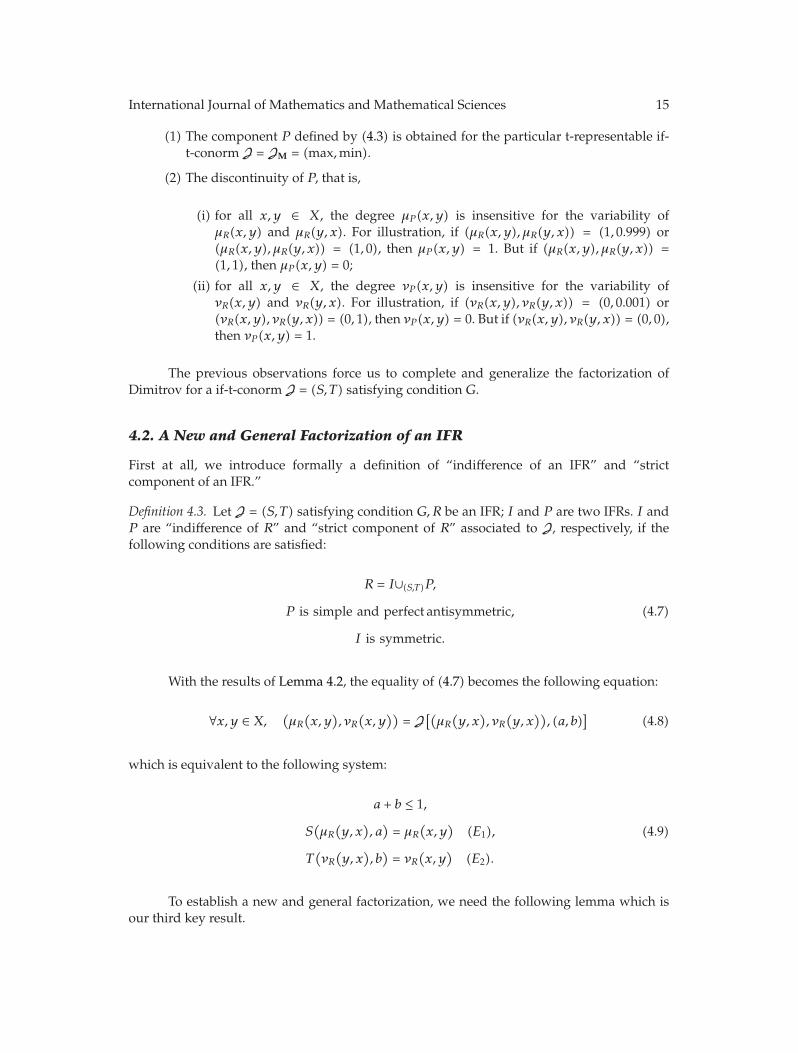
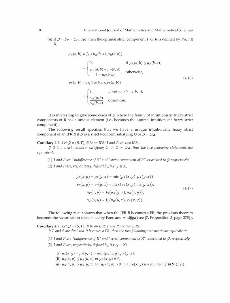
(4) If J = JP = (SP, TP), then the optimal strict component P of R is defined by, ∀a, b ∈X,

μP (a, b) = JSP


)

=

⎧⎪⎨

⎪⎩

0, if μR(a, b) ≤ μR(b, a),

μR(a, b) − μR(b, a)1 − μR(b, a)

, otherwise,

νP (a, b) = ITP(νR(b, a), νR(a, b))

=

⎧⎪⎨

⎪⎩

1, if νR(a, b) ≥ νR(b, a),

νR(a, b)νR(b, a)

, otherwise.

(4.16)

It is interesting to give some cases of J where the family of intuitionistic fuzzy strictcomponents of R has a unique element (i.e., becomes the optimal intuitionistic fuzzy strictcomponent).

The following result specifies that we have a unique intuitionistic fuzzy strictcomponent of an IFR R if J is a strict t-conorm satisfying G or J = JM.

Corollary 4.7. Let J = (S, T), R be an IFR; I and P are two IFRs.If J is a strict t-conorm satisfying G, or J = JM, thus the two following statements are

equivalent:

(1) I and P are “indifference of R” and “strict component of R” associated to J respectively.

(2) I and P are, respectively, defined by, ∀x, y ∈ X,

μI

(x, y)= μI

(y, x)= min

(μR

(x, y), μR

(y, x)),

νI(x, y)= νI(y, x)= max

(νR(x, y), νR(y, x)),

μP

(x, y)= JS

(μR

(y, x), μR

(x, y)),

νP(x, y)= IT(νR(y, x), νR(x, y)).

(4.17)

The following result shows that when the IFR R becomes a FR, the previous theorembecomes the factorization established by Fono and Andjiga (see [7, Proposition 3, page 378]).

Corollary 4.8. Let J = (S, T), R be an IFR; I and P are two IFRs.If T and S are dual and R becomes a FR, then the two following statements are equivalent:

(1) I and P are “indifference of R” and “strict component of R” associated to J, respectively.

(2) I and P are, respectively, defined by, ∀x, y ∈ X;

(i) μI(x, y) = μI(y, x) = min(μR(x, y), μR(y, x));(ii) μR(x, y) ≤ μR(y, x) ⇔ μP (x, y) = 0;(iii) μR(x, y) > μR(y, x) ⇔ (μP (x, y) > 0, and μP (x, y) is a solution of (4.9)(E1)).


In this case, “indifference of an IFR” and “strict component of an IFR” become“indifference of a FR” and “strict component of a FR” associated to S, respectively.

In the rest of the paper, we study two properties of a given strict component of an IFR.In literature of (binary) crisp relations, it is well-known that the unique strict

component P of a given reflexive, complete, and transitive crisp relation R satisfiesthose two interesting and usual properties, namely, pos-transitivity, that is, ∀x, y, z ∈X, (xPy and yPz) ⇒ xPz and negative transitivity, that is, ∀x, y, z ∈ X, xPz ⇒(xPy or yPz).

Fono and Andjiga [7] showed that this result is no true in the fuzzy case. Moreprecisely, they introduced fuzzy versions of these properties (see [7, Definition 5, page 379]),showed that some strict components violate these fuzzy versions (see [7, Example 2, page383]). They determined necessary and sufficient conditions on a reflexive, weakly completeand T -transitive FR R such that a regular fuzzy strict component of R satisfies each of theseproperties (see [7, Propositions 6 and 7, page 381]).

Following this line, the aim of the sequel is to (i) introduce a version of pos-transitivityfor IFRs and a version of negative transitivity for IFRs and (ii) determine necessary andsufficient conditions on a given T-transitive IFR R under which a strict component of Rsatisfies the introduced properties.

5. Properties of a Strict Component of an IFR

5.1. Definitions and Examples of Properties, and New Conditions on an IFR

Definition 5.1. Let R be an IFR, and let P be a strict component of R.

(1) P is pos-transitive if ∀x, y, z ∈ X,

⎛

⎝

⎧⎨

⎩

μP

(x, y)> 0

νP(x, y)< 1,

⎧⎨

⎩

μP

(y, z)> 0

νP(y, z)< 1

⎞

⎠ imply

⎧⎨

⎩

μP (x, z) > 0

νP (x, z) < 1.(5.1)

(2) P is negative transitive if ∀x, y, z ∈ X,

⎛

⎝

⎧⎨

⎩

μP

(x, y)= 0

νP(x, y)= 1,

⎧⎨

⎩

μP

(y, z)= 0

νP(y, z)= 1

⎞

⎠ imply

⎧⎨

⎩

μP (x, z) = 0

νP (x, z) = 1.(5.2)

Let us give the following remark on these definitions.

Remark 5.2. (1) As P is regular, we can rewrite the pos-transitivity as follows: ∀x, y, z ∈ X,

(i)

⎧⎨

⎩

μR

(x, y)> μR

(y, x)

μR

(y, z)> μR

(z, y) imply μR(x, z) > μR(z, x),

(ii)

⎧⎨

⎩

νR(x, y)< νR

(y, x)

νR(y, z)< νR

(z, y) imply νR(x, z) < νR(z, x).

(5.3)


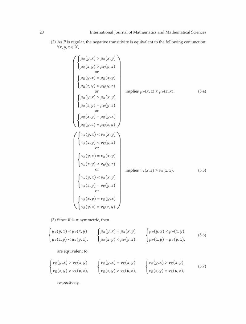
(2) As P is regular, the negative transitivity is equivalent to the following conjunction:∀x, y, z ∈ X,

⎛

⎜⎜⎜⎜⎜⎜⎜⎜⎜⎜⎜⎜⎜⎜⎜⎜⎜⎜⎜⎜⎜⎜⎜⎜⎜⎝

⎧⎨

⎩

μR

(y, x)> μR

(x, y)

μR

(z, y)> μR

(y, z)

or⎧⎨

⎩

μR

(y, x)= μR

(x, y)

μR

(z, y)> μR

(y, z)

or⎧⎨

⎩

μR

(y, x)> μR

(x, y)

μR

(z, y)= μR

(y, z)

or⎧⎨

⎩

μR

(x, y)= μR

(y, x)

μR

(y, z)= μR

(z, y)

⎞

⎟⎟⎟⎟⎟⎟⎟⎟⎟⎟⎟⎟⎟⎟⎟⎟⎟⎟⎟⎟⎟⎟⎟⎟⎟⎠

implies μR(x, z) ≤ μR(z, x), (5.4)

⎛

⎜⎜⎜⎜⎜⎜⎜⎜⎜⎜⎜⎜⎜⎜⎜⎜⎜⎜⎜⎜⎜⎜⎜⎜⎜⎜⎜⎝

⎧⎨

⎩

νR(y, x)< νR

(x, y)

νR(z, y)< νR

(y, z)

or⎧⎨

⎩

νR(y, x)= νR

(x, y)

νR(z, y)< νR

(y, z)

or⎧⎨

⎩

νR(y, x)< νR

(x, y)

νR(z, y)= νR

(y, z)

or⎧⎨

⎩

νR(x, y)= νR

(y, x)

νR(y, z)= νR

(z, y)

⎞

⎟⎟⎟⎟⎟⎟⎟⎟⎟⎟⎟⎟⎟⎟⎟⎟⎟⎟⎟⎟⎟⎟⎟⎟⎟⎟⎟⎠

implies νR(x, z) ≥ νR(z, x). (5.5)

(3) Since R is π-symmetric, then

⎧⎨

⎩

μR

(y, x)< μR

(x, y)

μR

(z, y)< μR

(y, z),

⎧⎨

⎩

μR

(y, x)= μR

(x, y)

μR

(z, y)< μR

(y, z),

⎧⎨

⎩

μR

(y, x)< μR

(x, y)

μR

(z, y)= μR

(y, z),

(5.6)

are equivalent to

⎧⎨

⎩

νR(y, x)> νR

(x, y)

νR(z, y)> νR

(y, z),

⎧⎨

⎩

νR(y, x)= νR

(x, y)

νR(z, y)> νR

(y, z),

⎧⎨

⎩

νR(y, x)> νR

(x, y)

νR(z, y)= νR

(y, z),

(5.7)

respectively.


One of the main questions is to wonder if a strict component of a given IFR, which isnot a FR, satisfies each of these two properties.

In the following, we justify that there exists an IFR R (distinct to FRs) such that somestrict components of R violate each of these properties.

Example 5.3. Let X = {x, y, z} and JL (thus by Proposition 2.10, JL satisfies condition G).(1)We determine an IFR R onX such that there exists a strict component P of Rwhich

violates pos-transitivity, (i.e., P satisfies: there exists u, v,w ∈ X such that

⎧⎪⎨

⎪⎩

μP (u, v) > 0

νP (u, v) < 1,

⎧⎪⎨

⎪⎩

μP (v,w) > 0

νP (v,w) < 1,

(μP (u,w) = 0 or νP (u,w) = 1

).

(5.8)

Let R be defined by, ∀d ∈ X, R(d, d) = (1, 0); R(x, y) = (0.7, 0.2); R(y, x) =(0.5, 0.4); R(y, z) = (0.6, 0.2); R(z, y) = (0.5, 0.3); R(x, z) = (0.5, 0.4); R(z, x) = (0.8, 0.1).

Clearly, R is reflexive, weakly complete, and π-symmetric. By Theorem 4.5, R has anoptimal strict component PL defined by (4.15).

We have: μPL(x, y) = μR(x, y)−μR(y, x) = 0.2 > 0; μPL(y, z) = μR(y, z)−μR(z, y) = 0.1 >

0; νPL(x, y) = 1 + νR(x, y) − νR(y, x) = 0.8 < 1 and νPL(y, z) = 1 + νR(y, z) − νR(z, y) = 0.9 < 1,whereas μPL(x, z) = 0 and νPL(x, z) = 1.

In other words, x is strictly preferred to y (since μPL(x, y) > 0 and νPL(x, y) < 1), andy is strictly preferred to z (since μPL(y, z) > 0 and νPL(y, z) < 1), but x is not strictly preferredto z (since μPL(x, z) = 0 and νPL(x, z) = 1).

Hence PL violates pos-transitivity.(2)We determine an IFR R onX such that there exists a strict component P of Rwhich

violates negative transitivity, (i.e., P satisfies: there exists u, v,w ∈ X such that

⎧⎪⎨

⎪⎩

μP (u, v) = 0

νP (u, v) = 1,

⎧⎪⎨

⎪⎩

μP (v,w) = 0

νP (v,w) = 1,

(μP (u,w) > 0 or νP (u,w) < 1

).

(5.9)

Let R be defined by, ∀d ∈ X, R(d, d) = (1, 0); R(x, y) = (0.5, 0.4); R(y, x) =(0.7, 0.2); R(y, z) = (0.4, 0.5); R(z, y) = (0.8, 0.1); R(x, z) = (0.6, 0.1); R(z, x) = (0.4, 0.3).

Clearly, R is reflexive, weakly complete, and π-symmetric. By Theorem 4.5, R has anoptimal strict component PL defined by (4.15).

We have μPL(x, y) = μPL(y, z) = 0 and νPL(x, y) = νPL(y, z) = 1, whereas μPL(x, z) =μR(x, z) − μR(z, x) = 0.2 > 0, and νPL(x, z) = 1 + νR(x, z) − νR(z, x) = 0.8 < 1.

In other words, x is strictly preferred to z (since μPL(x, z) > 0 and νPL(x, z) < 1), butx is not strictly preferred to y (since μPL(x, y) = 0 and νPL(x, y) = 1), and y is not strictlypreferred to z (since μPL(y, z) = 0 and νPL(y, z) = 1).

Hence PL violates negative transitivity.


This enables us to determine necessary and sufficient conditions on an IFR R suchthat a given strict component PR of R is pos-transitive and negative transitive. For that weintroduce the following conditions.

Definition 5.4. Let R be an IFR.

(1) (i) R satisfies condition CμR

1 if ∀x, y, z ∈ X,

μR

(y, x)< μR

(x, y)

μR

(z, y)< μR

(y, z) =⇒

⎛

⎝

⎧⎨

⎩

μR(x, z) ∈[α2(x, y, z

), α3(x, y, z

)]

μR(z, x) ∈[α2(x, y, z

), α3(x, y, z

)] =⇒ μR(z, x) < μR(x, z)

⎞

⎠.

(5.10)

(ii) R satisfies condition CνR1 if ∀x, y, z ∈ X,

νR(y, x)> νR

(x, y)

νR(z, y)> νR

(y, z) =⇒

⎛

⎝

⎧⎨

⎩

νR(x, z) ∈[β3(x, y, z

), β2(x, y, z

)]

νR(z, x) ∈[β3(x, y, z

), β2(x, y, z

)] =⇒ νR(z, x) > νR(x, z)

⎞

⎠.

(5.11)

(2) (i) R satisfies condition CμR

2 if ∀x, y, z ∈ X,

⎛

⎝

⎧⎨

⎩

μR

(y, x)= μR

(x, y)

μR

(z, y)< μR

(y, z) or

⎧⎨

⎩

μR

(y, x)< μR

(x, y)

μR

(z, y)= μR

(y, z)

⎞

⎠

=⇒

⎛

⎜⎜⎜⎜⎜⎜⎝

⎧⎨

⎩

μR(x, z) ∈[α2(x, y, z

), α3(x, y, z

)]

μR(z, x) ∈[α2(x, y, z

), α3(x, y, z

)]

⇓μR(z, x) < μR(x, z)

⎞

⎟⎟⎟⎟⎟⎟⎠

.

(5.12)

(ii) R satisfies condition CνR2 if ∀x, y, z ∈ X,

⎛

⎝

⎧⎨

⎩

νR(y, x)= νR

(x, y)

νR(z, y)> νR

(y, z) or

⎧⎨

⎩

νR(y, x)> νR

(x, y)

νR(z, y)= νR

(y, z)

⎞

⎠

=⇒

⎛

⎜⎜⎜⎜⎜⎜⎝

⎧⎨

⎩

νR(x, z) ∈[β3(x, y, z

), β2(x, y, z

)]

νR(z, x) ∈[β3(x, y, z

), β2(x, y, z

)]

⇓νR(z, x) > νR(x, z)

⎞

⎟⎟⎟⎟⎟⎟⎠

.

(5.13)

The next result shows that a strongly complete IFR R satisfies the previous conditions.


Proposition 5.5. Let R be an IFR.If R is strongly complete, then R satisfies conditions CμR

1 , CνR1 , C

μR

2 , and CνR2 .

5.2. Characterization of Some Properties of a Strict Component of an IFR

We now establish, using CμR

1 and CνR1 , our second main result which determines all T-

transitive IFRs whose strict components are pos-transitive.

Theorem 5.6. Let R be a T-transitive IFR, and let P be a strict component of R. Then

⎛

⎜⎜⎜⎝

R satisfies condition CμR

1

or

R satisfies condition CνR1

⎞

⎟⎟⎟⎠

⇐⇒ (P is pos-transitive). (5.14)

In the particular case where R is strongly complete, the previous result becomes asfollows:

Corollary 5.7. Let R be a T-transitive IFR, and let P be a strict component of R.If R is strongly complete, then P is pos-transitive.

Given a T-transitive IFR R, the next result establishes an equivalence betweenconditions CμR

2 and CνR2 , and two properties of P .

Lemma 5.8. Let R be a T-transitive IFR, and let P be a strict component of R.The two following statements are equivalent:

(1) R satisfies condition CμR

2 or condition CνR2 ;

(2)

∀x, y, z ∈ X

⎛

⎜⎜⎜⎜⎜⎜⎜⎜⎜⎜⎜⎜⎜⎜⎜⎝

(i)

⎛

⎜⎝

⎧⎪⎨

⎪⎩

μP

(x, y)> 0

νP(x, y)< 1

,

⎧⎪⎨

⎪⎩

μP

(y, z)= μP

(z, y)= 0

νP(y, z)= νP

(z, y)= 1

⎞

⎟⎠

or

(ii)

⎛

⎜⎝

⎧⎪⎨

⎪⎩

μP

(x, y)= μP

(y, x)= 0

νP(x, y)= νP

(y, x)= 1

,

⎧⎪⎨

⎪⎩

μP

(y, z)> 0

νP(y, z)< 1

⎞

⎟⎠

⎞

⎟⎟⎟⎟⎟⎟⎟⎟⎟⎟⎟⎟⎟⎟⎟⎠

=⇒

⎧⎪⎨

⎪⎩

μP (x, z) > 0

νP (x, z) < 1.

(5.15)


It is important to notice that as P is regular andR is π-symmetric, we can rewrite (5.15)as follows:

∀x, y, z ∈ X,

⎛

⎜⎜⎜⎜⎜⎜⎜⎜⎜⎜⎜⎜⎜⎝

(i)

⎛

⎜⎝

⎧⎪⎨

⎪⎩

μR

(y, x)= μR

(x, y)

μR

(z, y)< μR

(y, z)

or

⎧⎪⎨

⎪⎩

μR

(y, x)< μR

(x, y)

μR

(z, y)= μR

(y, z)

⎞

⎟⎠ =⇒ μR(x, z) > μR(z, x)

or

(ii)

⎛

⎜⎝

⎧⎪⎨

⎪⎩

νR(y, x)= νR

(x, y)

νR(z, y)> νR

(y, z)

or

⎧⎪⎨

⎪⎩

νR(y, x)> νR

(x, y)

νR(z, y)= νR

(y, z)

⎞

⎟⎠ =⇒ νR(x, z) < νR(z, x)

⎞

⎟⎟⎟⎟⎟⎟⎟⎟⎟⎟⎟⎟⎟⎠

.

(5.16)

The third and last main result of our paper determines all T-transitive IFRs whosestrict components are negative transitive.

Theorem 5.9. Let R be a T-transitive IFR, and let P be a strict component of R. Then

⎛

⎜⎜⎝

R satisfies conditions CμR

1 and CμR

2

or

R satisfies conditions CνR1 and CνR

2

⎞

⎟⎟⎠⇐⇒ (P is negative transitive). (5.17)

In the particular case where R is strongly complete, the previous result becomes asfollows:

Corollary 5.10. Let R be a T-transitive IFR, and let P be a strict component of R.If R is strongly complete, then P is negative transitive.

6. Concluding Remarks

In this paper, we establish a characterization of the T-transitivity of R. We also establisha general factorization of an intuitionistic fuzzy binary relation when the union is definedby a continuous t-representable intuitionistic fuzzy t-conorm satisfying condition G. Thisfactorization gives a family of regular strict components. Furthermore, given an IFR R, weintroduce two conditions C

μR

1 and CμR

2 (or equivalently CνR1 and CνR

2 ). And we show that,when R isT-transitive, these conditions are necessary and sufficient to obtain pos-transitivityand negative transitivity of a given strict component of R.

An open problem is to apply these results especially in social choice theory whenindividual and social preferences are modelled by reflexive, weakly complete, and T-transitive IFRs. Another open problem is to study the properties of the class of continuoust-representable intuitionistic fuzzy t-conorms satisfying condition G.


Appendix

The Proofs of our Results

Proof of Proposition 2.7. (1) Let a, b ∈ [0, 1]. Since T(a, b) ≤ 1−S(1−a, 1−b), then {t ∈ [0, 1], 1−S(1 − a, 1 − t) ≤ b} ⊆ {t ∈ [0, 1], T(a, t) ≤ b}. Set t′ = 1 − t, we have IT (a, b) ≥ max{t ∈[0, 1], 1 − S(1 − a, 1 − t) ≤ b} = max{t ∈ [0, 1], S(1 − a, 1 − t) ≥ 1 − b} = max{1 − t′ ∈[0, 1], S(1 − a, t′) ≥ 1 − b} = 1 −min{t′ ∈ [0, 1], S(1 − a, t′) ≥ 1 − b} = 1 − JS(1 − a, 1 − b).

(2) The proof is obvious.

Proof of Lemma 2.8. (1) Let x = (x1, x2), y = (y1, y2) ∈ L∗. Set A={z = (z1, z2) ∈ L∗, y1 ≤S(x1, z1) and y2 ≥ T(x2, z2)}/= ∅. That is to show that infA = (min{z1 ∈ [0, 1], y1 ≤S(x1, z1)}, min(max{z2 ∈ [0, 1], T(x2, z2) ≤ y2}, 1 −min{z1 ∈ [0, 1], y1 ≤ S(x1, z1)})).

Since A ⊆ L∗ and (L∗,≤L∗) is a complete lattice, and T and S are continuous functionson the compact [0, 1] × [0, 1], then the definition of lower limit in L∗ gives

infA =(inf{z1 ∈ [0, 1], ∃t1 ∈ [0, 1], (z1, t1) ∈ A}, sup{z2 ∈ [0, 1], ∃t2 ∈ [0, 1], (t2, z2) ∈ A}

)

=

⎛

⎜⎜⎜⎝

inf

⎧⎪⎪⎪⎨

⎪⎪⎪⎩

z1 ∈ [0, 1], ∃t1 ∈ [0, 1],

⎧⎪⎪⎪⎨

⎪⎪⎪⎩

y1 ≤ S(x1, z1)

y2 ≥ T(x2, t1)

z1 + t1 ≤ 1

⎫⎪⎪⎪⎬

⎪⎪⎪⎭

,

sup

⎧⎪⎪⎪⎨

⎪⎪⎪⎩

z2 ∈ [0, 1], ∃t2 ∈ [0, 1],

⎧⎪⎪⎪⎨

⎪⎪⎪⎩

y1 ≤ S(x1, t2)

y2 ≥ T(x2, z2)

z2 + t2 ≤ 1

⎫⎪⎪⎪⎬

⎪⎪⎪⎭

⎞

⎟⎟⎟⎠

=

⎛

⎜⎜⎜⎝

min

⎧⎪⎪⎪⎨

⎪⎪⎪⎩

z1 ∈ [0, 1], ∃t1 ∈ [0, 1],

⎧⎪⎪⎪⎨

⎪⎪⎪⎩

y1 ≤ S(x1, z1)

y2 ≥ T(x2, t1)

z1 + t1 ≤ 1

⎫⎪⎪⎪⎬

⎪⎪⎪⎭

,

max

⎧⎪⎪⎪⎨

⎪⎪⎪⎩

z2 ∈ [0, 1], ∃t2 ∈ [0, 1],

⎧⎪⎪⎪⎨

⎪⎪⎪⎩

y1 ≤ S(x1, t2)

y2 ≥ T(x2, z2)

z2 + t2 ≤ 1

⎫⎪⎪⎪⎬

⎪⎪⎪⎭

⎞

⎟⎟⎟⎠

.

(A.1)

Otherwise, with the second result of Proposition 2.1, we have

⎧⎪⎪⎪⎨

⎪⎪⎪⎩

y1 ≤ S(x1, z1)

y2 ≥ T(x2, t1)

z1 + t1 ≤ 1

⇐⇒

⎧⎪⎪⎪⎨

⎪⎪⎪⎩

z1 ∈[JS(x1, y1

), 1]

t1 ∈[0, IT

(x2, y2

)]

z1 + t1 ≤ 1,⎧⎪⎪⎨

⎪⎪⎩

y1 ≤ S(x1, t2)

y2 ≥ T(x2, z2)

z2 + t2 ≤ 1

⇐⇒

⎧⎪⎪⎨

⎪⎪⎩

t2 ∈[JS(x1, y1

), 1]

z2 ∈[0, IT

(x2, y2

)]

z2 + t2 ≤ 1.

(A.2)


We distinguish three cases.

(i) If x1 < y1 and x2 ≤ y2, then with the third result of Proposition 2.1, we haveJS(x1, y1) > 0 and IT (x2, y2) = 1. This implies IT (x2, y2) > 1 − JS(x1, y1). Thus,

min

⎧⎪⎪⎪⎨

⎪⎪⎪⎩

z1 ∈ [0, 1], ∃t1 ∈ [0, 1],

⎧⎪⎪⎪⎨

⎪⎪⎪⎩

y1 ≤ S(x1, z1)

y2 ≥ T(x2, t1)

z1 + t1 ≤ 1

⎫⎪⎪⎪⎬

⎪⎪⎪⎭

= JS(x1, y1

),

max

⎧⎪⎪⎪⎨

⎪⎪⎪⎩

z2 ∈ [0, 1], ∃t2 ∈ [0, 1],

⎧⎪⎪⎪⎨

⎪⎪⎪⎩

y1 ≤ S(x1, t2)

y2 ≥ T(x2, z2)

z2 + t2 ≤ 1

⎫⎪⎪⎪⎬

⎪⎪⎪⎭

= 1 − JS(x1, y1

).

(A.3)

Hence JJ(x, y) = (JS(x1, y1), 1 − JS(x1, y1)).

(ii) If (x1 ≥ y1 and x2 ≤ y2) or (x1 ≥ y1 and x2 > y2), then with the third result ofProposition 2.1, it is easy to show that

min

⎧⎪⎪⎪⎨

⎪⎪⎪⎩

z1 ∈ [0, 1], ∃t1 ∈ [0, 1],

⎧⎪⎪⎪⎨

⎪⎪⎪⎩

y1 ≤ S(x1, z1)

y2 ≥ T(x2, t1)

z1 + t1 ≤ 1

⎫⎪⎪⎪⎬

⎪⎪⎪⎭

= JS(x1, y1

),

max

⎧⎪⎪⎪⎨

⎪⎪⎪⎩

z2 ∈ [0, 1], ∃t2 ∈ [0, 1],

⎧⎪⎪⎪⎨

⎪⎪⎪⎩

y1 ≤ S(x1, t2)

y2 ≥ T(x2, z2)

z2 + t2 ≤ 1

⎫⎪⎪⎪⎬

⎪⎪⎪⎭

= IT(x2, y2

)≤ 1 − JS

(x1, y1

).

(A.4)

Hence JJ(x, y) = (JS(x1, y1), IT (x2, y2)).

(iii) If x1 < y1 and x2 > y2, then with the third result of Proposition 2.1, JS(x1, y1) > 0,and IT (x2, y2) < 1. We distinguish two cases.

(a) If IT (x2, y2) ≤ 1 − JS(x1, y1), thus

min

⎧⎪⎪⎪⎨

⎪⎪⎪⎩

z1 ∈ [0, 1], ∃t1 ∈ [0, 1],

⎧⎪⎪⎪⎨

⎪⎪⎪⎩

y1 ≤ S(x1, z1)

y2 ≥ T(x2, t1)

z1 + t1 ≤ 1

⎫⎪⎪⎪⎬

⎪⎪⎪⎭

= JS(x1, y1

),

max

⎧⎪⎪⎪⎨

⎪⎪⎪⎩

z2 ∈ [0, 1], ∃t2 ∈ [0, 1],

⎧⎪⎪⎪⎨

⎪⎪⎪⎩

y1 ≤ S(x1, t2)

y2 ≥ T(x2, z2)

z2 + t2 ≤ 1

⎫⎪⎪⎪⎬

⎪⎪⎪⎭

= IT(x2, y2

).

(A.5)

Hence JJ(x, y) = (JS(x1, y1), IT (x2, y2)).


(b) If IT (x2, y2) > 1 − JS(x1, y1), thus

min

⎧⎪⎪⎪⎪⎪⎨

⎪⎪⎪⎪⎪⎩

z1 ∈ [0, 1], ∃t1 ∈ [0, 1],

⎧⎪⎪⎪⎪⎪⎨

⎪⎪⎪⎪⎪⎩

y1 ≤ S(x1, z1)

y2 ≥ T(x2, t1)

z1 + t1 ≤ 1

⎫⎪⎪⎪⎪⎪⎬

⎪⎪⎪⎪⎪⎭

= JS(x1, y1

),

max

⎧⎪⎪⎪⎪⎪⎨

⎪⎪⎪⎪⎪⎩

z2 ∈ [0, 1], ∃t2 ∈ [0, 1],

⎧⎪⎪⎪⎪⎪⎨

⎪⎪⎪⎪⎪⎩

y1 ≤ S(x1, t2)

y2 ≥ T(x2, z2)

z2 + t2 ≤ 1

⎫⎪⎪⎪⎪⎪⎬

⎪⎪⎪⎪⎪⎭

= 1 − JS(x1, y1

).

(A.6)

Hence JJ(x, y) = (JS(x1, y1), 1 − JS(x1, y1)).

Finally, we obtain JJ(x, y) = (JS(x1, y1),min(IT (x2, y2), 1 − JS(x1, y1))).(2) The proof of the second result is analogous to the previous one.

Proof of Proposition 2.10. (1) Let (a1, a2), (b1, b2) ∈ L∗ such that

a1 > b1,

a2 < b2,

a1 + a2 = b1 + b2.

(A.7)

(i) Since JF0 = JM, JF

1 = JP and JF∞ = JL,with Example 2.5, it is obvious to show that

∀l ∈ {0, 1,+∞}, JFl satisfies condition G.

(ii) Assume that l ∈]0, 1[, and let us show that JFl= (Sl

F, TlF) satisfies condition G, that

is, IT (b2, a2) + JS(b1, a1) ≤ 1. It suffices to show that ∀l ∈]0, 1[, logl(1 + ((l − 1)(la2 −1))/(lb2 − 1)) ≤ logl(1 + (l − 1)(l1−a1 − 1)/(l1−b1 − 1)). Set c = a1 + a2 = b1 + b2.

(a) Since a1 > b1 and the mapping lt is decreasing, then la1 ≤ lb1 , that is, l−b1 ≤ l−a1 .

(b) Since lc − l ≥ 0, we obtain l−b1(lc − l) ≤ l−a1(lc − l), that is, lb2 + l1−a1 ≤ la2 + l1−b1 .

(c) Since a2 − b1 = b2 −a1, the previous inequality becomes l1+a2−b1 − la2 − l1−b1 + 1 ≤l1+b2−a1 − lb2 − l1−a1 + 1, that is, (la2 − 1)(l1−b1 − 1) ≤ (lb2 − 1)(l1−a1 − 1), that is,(la2 − 1)/(lb2 − 1) ≤ (l1−a1 − 1)/(l1−b1 − 1), that is, 1 + (l − 1)(la2 − 1)/(lb2 − 1) ≥1 + (l − 1)(l1−a1 − 1)/(l1−b1 − 1). And we have logl(1 + (l − 1)(la2 − 1)/(lb2 − 1)) ≤logl(1 + (l − 1)(l1−a1 − 1)/(l1−b1 − 1)).

(iii) The proof of the case l ∈]1,+∞[ is similar to theprevious one.


(2) Let J′ be a restriction of J = (S, T) on L∗1 = {(x1, x2) ∈ L∗, x1 +x2 = 1}.Assume that

S and T are dual and show that J′ satisfies G. Let (a1, a2), (b1, b2) ∈ L∗1 such that

a1 > b1,

a2 < b2,

a1 + a2 = b1 + b2 = 1.

(A.8)

Let us show that IT (b2, a2) + JS(b1, a1) ≤ 1.Since a1 +a2 = b1 + b2 = 1 and S are T are dual, then IT (b2, a2) = IT (1− b1, 1−a1). Thus,

IT (b2, a2) + JS(b1, a1) = IT (1 − b1, 1 − a1) + JS(b1, a1) = 1. Hence the result.

Proof of Proposition 3.4. Suppose that R is (S, T)-complete and let us show that R is D-complete.

Let (x, y) ∈ X × X such that (μR(x, y), νR(x, y)) = (0, 1). Thus S(0, μR(y, x)) = 1 andT(1, νR(y, x)) = 0. Since S(0, μR(y, x)) = μR(y, x) and T(1, νR(y, x)) = νR(y, x), we haveμR(y, x) = 1 and νR(y, x) = 0. Hence μR(y, x) > 0 and νR(y, x) < 1.

Proof of Proposition 3.9. For all x, y, z ∈ X, we have the following.

(1) Let us show that (α1(x, y, z), β1(x, y, z)) ∈ L∗. In fact, (α1(x, y, z), β1(x, y, z))= (T(μR(z, y), μR(y, x)), S(νR(z, y), νR(y, x))) = T[(μR(z, y), νR(z, y)), (μR(y, x),νR(y, x))] ∈ L∗ since T is a t-norm on L∗.

(a) Let us show that (α3(x, y, z), β3(x, y, z)) ∈ L∗. In fact, (α3(x, y, z), β3(x, y, z)) =min(IT[(μR(y, z), νR(y, z)), (μR(y, x), νR(y, x))], IT[(μR(x, y), νR(x, y)), (μR(z,y), νR(z, y))]). Since, IT[(μR(y, z), νR(y, z)),(μR(y, x), νR(y, x))]∈L∗, IT[(μR(x,y), νR(x, y)), (μR(z, y), νR(z, y))] ∈ L∗ and Min = (min,max) is a t-norm in L∗,then (α3(x, y, z), β3(x, y, z)) ∈ L∗.

(b) The proofs of the assertions (α2(x, y, z), β2(x, y, z)) ∈ L∗ and (α4(x, y, z),β4(x, y, z)) ∈ L∗ are analogous to the previous ones.

(2) The proof of the last result is deduced from the second result of Lemma 2.8.

Proof of Corollary 3.11. Assume that R is strongly complete.

(1) Assume also that R satisfies (3.9). And in the three cases, we have μR(x, y) =μR(y, z) = 1, and νR(x, y) = νR(y, z) = 0. This implies JS(νR(z, y), νR(x, y)) =JS(νR(y, x), νR(y, z)) = 0, JS(νR(x, y), νR(z, y)) = νR(z, y), JS(νR(y, z), νR(y, x)) =νR(y, x) and IT (μR(z, y), μR(x, y)) = IT (μR(y, x), μR(y, z)) = 1, IT (μR(x, y),μR(z, y)) = μR(z, y), IT (μR(y, z), μR(y, x)) = μR(y, x). And we obtain α2(x, y, z) =α4(x, y, z) = 1, and α3(x, y, z) = min(μR(y, x), μR(z, y)). Thus α1(x, y, z) < 1 andα3(x, y, z) < 1.

(2) Assume that R satisfies (3.11). Thus νR(x, y) = νR(y, z) = 0 and (νR(y, x) > 0 orνR(z, y) > 0). Thus, β2(x, y, z) = S(νR(x, y), νR(y, z)) = S(0, 0) = 0.

Assume to the contrary that β1(x, y, z) = 0. We have max(νR(z, y), νR(y, x)) ≤ S(νR(z, y),νR(y, x)) = β1(x, y, z) = 0. Hence νR(y, x) = 0 and νR(z, y) = 0. This contradicts the assertion(νR(y, x) > 0 or νR(z, y) > 0).


Let us show that β3(x, y, z) = max(νR(y, x), νR(z, y)) and β4(x, y, z) = max(0, 0) = 0.Proposition 3.9 implies that

β3(x, y, z

)= max

(JS(0, νR

(y, x)), JS(0, νR

(z, y)))

,

β4(x, y, z

)= max

(JS(νR(y, x), 0), JS(νR(z, y), 0)).

(A.9)

By definition, JS(0, νR(y, x)) = min{t ∈ [0, 1]/S(0, t) ≥ νR(y, x)} = min{t ∈ [0, 1]/t ≥νR(y, x)} = min[νR(y, x), 1] = νR(y, x) and JS(νR(y, x), 0) = min{t ∈ [0, 1]/S(νR(y, x), t) ≥0} = min[0, 1] = 0.

Analogously, JS(0, νR(z, y)) = νR(z, y) and JS(νR(z, y), 0)) = 0. Thus β3(x, y, z) =max(νR(y, x), νR(z, y)), and β4(x, y, z) = max(0, 0) = 0.

Proof of Corollary 3.12. Assume that T and S are dual and R is a FR. Let x, y, z ∈ X.

(1) (i) Let us show that β1(x, y, z) = 1 − α1(x, y, z).

By definition, β1(x, y, z) = S(νR(z, y), νR(y, x)) and α1(x, y, z) = T(μR(z, y), μR(y, x)). SinceR is a FR, we have νR(z, y) = 1 − μR(z, y) and νR(y, x) = 1 − μR(y, x). Otherwise, since T andS are dual, we have S(νR(z, y), νR(y, x)) = 1 − T(1 − νR(z, y), 1 − νR(y, x)). Thus β1(x, y, z) =1 − T(1 − (1 − μR(z, y)), 1 − (1 − μR(y, x))) = 1 − T(μR(z, y), μR(y, x)) = 1 − α1(x, y, z). Hencethe result.

(ii) The proof of equality β2(x, y, z) = 1 − α2(x, y, z) is analogous to the previous one.

(iii) Let us show that β3(x, y, z) = 1 − α3(x, y, z).

With the previous proposition, β3(x, y, z) = max(JS(νR(y, z), νR(y, x)), JS(νR(x, y), νR(z, y))).Since R is a FR, we have νR(y, z) = 1−μR(y, z), νR(z, y) = 1−μR(z, y), νR(y, x) = 1−μR(y, x),and νR(x, y) = 1−μR(x, y). Otherwise, since T and S are dual, we have JS(νR(y, z), νR(y, x)) =1 − IT (1 − νR(y, z), 1 − νR(y, x)) and JS(νR(x, y), νR(z, y)) = 1 − IT (1 − νR(x, y), 1 − νR(z, y)).Thus β3(x, y, z) = max(1 − IT (1 − (1 − μR(y, z)), 1 − (1 − μR(y, x))), 1 − IT (1 − (1 −μR(x, y)), 1 − (1 − μR(z, y)))) = max(1 − IT (μR(y, z), μR(y, x)), 1 − IT (μR(x, y), μR(z, y))) =1 −min(IT (μR(y, z), μR(y, x)), IT (μR(x, y), μR(z, y))).

Otherwise, α3(x, y, z) = min[min(IT (μR(y, z), μR(y, x)), 1 − JS(νR(y, z), νR(y, x))),min(IT (μR(x, y), μR(z, y)), 1 − JS(νR(x, y), νR(z, y)))] = min[min(IT (μR(y, z), μR(y, x)),I1T (1 − νR(y, z), 1 − νR(y, x))), min(IT (μR(x, y), μR(z, y)), IT (1 − νR(x, y), 1 − νR(z, y)))]= min[min(IT (μR(y, z), μR(y, x)), IT (μR(y, z), μR(y, x))),min(IT (μR(x, y), μR(z, y)),IT (μR(x, y), μR(z, y)))] = min[IT (μR(y, z), μR(y, x)), IT (μR(x, y), μR(z, y))] = 1 − β3(x, y, z).Hence the result.

(iv) The proof of the equality β4(x, y, z) = 1 − α4(x, y, z) is analogous to the previousone.

(2) The proof of the last result is obvious.

Proof of Lemma 3.13. (i)⇒(ii): Assume that R is T-transitive on {x, y, z} and show that (3.16).


Since R is T-transitive on {x, y, z}, then we have the following twelve inequalities:

(i) νR(x, z) ≤ S(νR(x, y), νR(y, z)); νR

(x, y)≤ S(νR(x, z), νR

(z, y));

νR(y, z)≤ S(νR(y, x), νR(x, z)

);

(ii) νR(z, x) ≤ S(νR(z, y), νR(y, x)); νR

(z, y)≤ S(νR(z, x), νR

(x, y));

νR(y, x)≤ S(νR(y, z), νR(z, x)

);

(iii) μR(x, z) ≥ T(μR

(x, y), μR

(y, z)); μR

(x, y)≥ T(μR(x, z), μR

(z, y));

μR

(y, z)≥ T(μR

(y, x), μR(x, z)

);

(iv) μR(z, x) ≥ T(μR

(z, y), μR

(y, x)); μR

(z, y)≥ T(μR(z, x), μR

(x, y));

μR

(y, x)≥ T(μR

(y, z), μR(z, x)

).

(A.10)

Let us show that μR(x, z) ∈ [α2(x, y, z), α4(x, y, z)].By definition of IT , the two first inequalities of (iii) of (A.10) imply α2(x, y, z) =

T(μR(x, y), μR(y, z)) ≤ μR(x, z) ≤ IT (μR(z, y), μR(x, y)). And the second inequalities of (i)give JS(νR(z, y), νR(x, y)) ≤ νR(x, z) ≤ 1−μR(x, z), that is, μR(x, z) ≤ 1−JS(νR(z, y), νR(x, y)).Thus, α2(x, y, z) ≤ μR(x, z) ≤ min(IT (μR(z, y), μR(x, y)), 1 − JS(νR(z, y), νR(x, y))).

Otherwise, the third inequality of (iii) gives μR(x, z) ≤ IT (μR(y, x), μR(y, z)). Thethird inequality of (i) gives JS(νR(y, x), νR(y, z)) ≤ νR(x, z) ≤ 1 − μR(x, z). Thus, μR(x, z) ≤min(IT (μR(y, x), μR(y, z)), 1 − JS(νR(y, x), νR(y, z))). Hence the result.

With the two first inequalities of (iv) of (A.10), the second inequality of (ii) of (A.10),the third inequality of (iv) of (A.10), and the third inequality of (ii) of (A.10), we showanalogously that μR(z, x) ∈ [α1(x, y, z), α3(x, y, z)].

With the two first inequalities of (i) of (A.10) and the third inequality of (i) of (A.10),we show analogously that νR(x, z) ∈ [β4(x, y, z), β2(x, y, z)].

With the two first inequalities of (ii) of (A.10) and the third inequality of (ii) of (A.10),we show analogously that νR(z, x) ∈ [β3(x, y, z), β1(x, y, z)]. Hence the result.

(ii)⇒(i): Assume (3.16), and let us show that R is T-transitive on {x, y, z}. That is toshow the twelve inequalities of (A.10).

The assertion μR(z, x) ∈ [α1(x, y, z), α3(x, y, z)] implies α1(x, y, z) =T(μR(z, y), μR(y, x)) ≤ μR(z, x), μR(z, x) ≤ IT (μR(y, z), μR(y, x)) and μR(z, x) ≤IT (μR(x, y), μR(z, y)). Thus, the second result of Proposition 2.1 and the last inequalitiesimply μR(z, y) ≥ T(μR(z, x), μR(x, y)) and μR(y, x) ≥ T(μR(y, z), μR(z, x)). Hence (iv) of(A.10).

Analogously, the assertion μR(x, z) ∈ [α2(x, y, z), α4(x, y, z)] and the second resultof Proposition 2.1 imply (iii) of (A.10); the assertion νR(x, z) ∈ [β4(x, y, z), β2(x, y, z)]and the second result of Proposition 2.1 imply (i) of (A.10); the assertion νR(z, x) ∈[β3(x, y, z), β1(x, y, z)], and the second result of Proposition 2.1 imply (ii) of (A.10).

Proof of Lemma 4.2. Let x, y ∈ X.

(1) Let us show that νI(x, y) = max(νR(x, y), νR(y, x)).

Since R = I∪JP and I is symmetric, thus νR(x, y) = T(νI(x, y), νP (x, y)) and νR(y, x) =T(νI(x, y), νP (y, x)). We distinguish two cases.


(i) Suppose that μP (x, y) > 0 or (μP (x, y) = 0 and νP (x, y) < 1).

The perfect antisymmetric of P implies νP (y, x) = 1. Since T is a t-norm, νR(y, x) =T(νI(x, y), 1) = νI(x, y). This last equality and (i) of (2.3) imply νR(x, y) =T(νI(x, y), νP (x, y)) = T(νR(y, x), νP (x, y)) ≤ νR(y, x) = νI(x, y). Thus, νI(x, y) = νR(y, x) =max[νR(x, y), νR(y, x)].

(ii) Suppose that μP (x, y) = 0 and νP (x, y) = 1.

Since T is a t-norm and I is symmetric, νR(x, y) = T(νI(x, y), νP (x, y)) = T(νI(x, y), 1) =νI(x, y). This equality and (i) of (2.3) imply νR(y, x) = T(νI(x, y), νP (y, x)) ≤ νI(x, y) =νR(x, y). Thus, νI(x, y) = νR(x, y) = max[νR(x, y), νR(y, x)].

The proof of the equality μI(x, y) = min(μR(x, y), μR(y, x)) is similar to the previousone.

(2) Let us show that νR(x, y) ≥ νR(y, x) ⇔ νP (x, y) = 1.

Since R = I∪JP , thus νR(x, y) = T(νI(x, y), νP (x, y)) and νR(y, x) = T(νI(y, x), νP (y, x)).(⇒): Assume to the contrary that νR(x, y) ≥ νR(y, x) and νP (x, y) < 1.

Since P is perfect antisymmetric and νP (x, y) < 1, we have νP (y, x) = 1. Thus νR(y, x) =T(νI(y, x), νP (y, x)) = νI(y, x). Since νR(x, y) ≥ νR(y, x), the previous result gives νI(x, y) =max(νR(x, y), νR(y, x)) = νR(x, y). Since I is symmetric, the two previous equalities implyνR(x, y) = νR(y, x). The π-symmetric of R and the previous equality imply μR(x, y) =μR(y, x). Thus, since P is simple, the two previous equalities imply νP (x, y) = νP (y, x) = 1,which contradicts the hypothesis νP (x, y) < 1. Finally, νR(x, y) ≥ νR(y, x) ⇒ νP (x, y) = 1.

(⇐): The proof of converse is obvious.The proof of the equivalence μR(x, y) ≤ μR(y, x) ⇔ μP (x, y) = 0 is analogous to the previousone.

Proof of Lemma 4.4. Suppose that μR(x, y) > μR(y, x) and νR(x, y) < νR(y, x).

(i) Consider the function f defined over [0, 1] by f(t) = S(t, μR(y, x)), thus f(0) =μR(y, x) and f(1) = 1. f is continuous and monotone because S is continuous andmonotone. Then f takes all values between μR(y, x) and 1. In particular, f has thevalue μR(x, y) for μR(x, y) > μR(y, x). Thus (4.9)(E1) has at least a solution.

By considering the function g defined over [0, 1] by g(t) = T(t, νR(y, x)), we analogouslyshow that (4.9)(E2) has at least a solution.

(ii) Let us show that each solution of (4.9)(E1) is strictly positive. Let t1 be a solution of(4.9)(E1).

Assume to the contrary that t1 = 0. Thus, μR(x, y) = S(μR(y, x), t1) = S(μR(y, x), 0) = μR(y, x),that is, μR(x, y) = μR(y, x) which contradicts μR(x, y) > μR(y, x). And we have t1 > 0.

Let us show that each solution of (4.9)(E2) is least than 1. Let t2 be a solutionof (4.9)(E2). Assume to the contrary that t2 = 1. Thus, νR(x, y) = T(νR(y, x), t2) =T(νR(y, x), 1) = νR(y, x), that is, νR(x, y) = νR(y, x) which contradicts νR(x, y) < νR(y, x).And we have t2 < 1.


(iii) Assume that J satisfies condition G. We can remark by (2) of Proposition 2.1that S(μR(y, x), JS(μR(y, x), μR(x, y))) = μR(x, y) and T(νR(y, x), IT (νR(y, x),νR(x, y))) = νR(x, y). Since R is π-symmetric, μR(x, y) + νR(x, y) = μR(y, x) +νR(y, x). Because J satisfies condition G, then μR(x, y) > μR(y, x), νR(x, y) <νR(y, x), and the previous equality imply JS(μR(y, x), μR(x, y)) + IT (νR(y, x),νR(x, y)) ≤ 1. Hence (JS(μR(y, x), μR(x, y)), IT (νR(y, x), νR(x, y))) is a solution of(4.8).

(iv) Assume that J satisfies condition G, and let us show that JS(μR(y, x), μR(x, y)) isthe lowest solution for (4.9)(E1).

Consider t1 another solution of (4.9)(E1). Thus we have S(t1, μR(y, x)) = μR(x, y) whichimplies t1 ∈ {t ∈ [0, 1], S(t, μR(y, x)) ≥ μR(x, y)}. Since JS(μR(y, x), μR(x, y)) = min{t ∈[0, 1], S(t, μR(y, x)) ≥ μR(x, y)}, we deduce that JS(μR(y, x), μR(x, y)) ≤ t1.

We analogously show that IT (νR(y, x), νR(x, y)) is the upper solution for (4.9)(E2).

(v) IfJ = (max,min),we easily show that (JS(μR(y, x), μR(x, y)), IT (νR(y, x), νR(x, y)))is the unique solution of (4.8).

Suppose that J = (S, T) is a strict t-conorm on L∗ satisfying condition G.The previous functions f and g defined in (i) are, respectively, the bijections

from [0, 1] to [μR(y, x), 1] and from [0, 1] to [0, νR(y, x)]. We easily show that (t1, t2) =(JS(μR(y, x), μR(x, y)), IT (νR(y, x), νR(x, y))) is the unique solution of (4.8).

Proof of Theorem 4.5. (1)⇒(2): Lemma 4.2 implies (i).Let us show (ii). ∀x, y ∈ X, suppose that μR(x, y) > μR(y, x) and νR(x, y) < νR(y, x).

(iii) of Lemma 4.4 implies that (4.8) has at least one solution. Set (cxy, gxy) ∈ L∗ one of thesesolutions. Thus cxy is a solution of (4.9)(E1), and gxy is a solution of (4.9)(E2). With (ii) ofLemma 4.4, we have cxy > 0 and gxy < 1. Since the equalityR = I∪JP is equivalent to equation(μR(x, y), νR(x, y)) = J[(μR(y, x), νR(y, x)), (μP (x, y), νP (x, y))], hence μP (x, y) = cxy andνP (x, y) = gxy.

For the case where μR(x, y) ≤ μR(y, x) and νR(x, y) ≥ νR(y, x), we easily show thatLemma 4.2 implies that μP (x, y) = 0 and νP (x, y) = 1.

(2)⇒(1): Let x, y ∈ X.(i) implies that μI(x, y) = μI(y, x), and νI(x, y) = νI(y, x) which show that I is

symmetric.Let us show that R = I∪JP, that is, S(μI(x, y), μP (x, y)) = μR(x, y) and T(νI(x, y), νP (x, y)) =νR(x, y). Since R is π-symmetric, we distinguish two cases.

(a) If μR(x, y) ≤ μR(y, x) and νR(x, y) ≥ νR(y, x), thus (i) implies μI(x, y) = μR(x, y),and νI(x, y) = νR(x, y), and the definition of P gives μP (x, y) = 0 and νP (x, y) = 1.We have S(μI(x, y), μP (x, y)) = S(μR(x, y), 0) = μR(x, y) and T(νI(x, y), νP (x, y)) =T(νR(x, y), 1) = νR(x, y).

(b) If μR(x, y) > μR(y, x) and νR(x, y) < νR(y, x), thus (ii) implies that μP (x, y)is a solution of (4.9)(E1), and νP (x, y) is a solution of (4.9)(E2); we haveS(μR(y, x), μP (x, y)) = μR(x, y) and T(νR(y, x), νP (x, y)) = νR(x, y). Furthermore,as μR(x, y) > μR(y, x), and νR(x, y) < νR(y, x), (i) implies μI(x, y) = μR(y, x) andνI(x, y) = νR(y, x). Then S(μI(x, y), μP (x, y)) = S(μR(y, x), μP (x, y)) = μR(x, y)and T(νI(x, y), νP (x, y)) = T(νR(y, x), νP (x, y)) = νR(x, y).


It is easy to show that P is simple and P is perfect antisymmetric.

Proof of Corollary 4.7. The proof of this corollary is deduced from Theorem 4.5 and the lastresult of Lemma 4.4.

Proof of Corollary 4.8. The proof is deduced from Lemma 4.2, Theorem 4.5, and the last resultof Proposition 3.9.

Proof of Proposition 5.5. Let x, y, z ∈ X. Since R is strongly complete, Corollary 3.11 impliesα3(x, y, z) < α2(x, y, z) and β2(x, y, z) < β3(x, y, z).

Proof of Theorem 5.6. As R is π-symmetric, (i) of (5.3) and (ii) of (5.3) are equivalent.Therefore, to show (5.3)means to show (i) of (5.3) or (ii) of (5.3).

(⇒): We distinguish two cases.

(1) Suppose that R satisfies condition CμR

1 , and let us show that P is pos-transitive.We show (i) of (5.3). Let x, y, z ∈ X such that μR(x, y) > μR(y, x) and μR(y, z) >μR(z, y). Let us show that μR(x, z) > μR(z, x). Since R is T-transitive on {x, y, z},Lemma 3.13 implies

μR(x, z) ∈[α2(x, y, z

), α4(x, y, z

)],

μR(z, x) ∈[α1(x, y, z

), α3(x, y, z

)].

(A.11)

We distinguish two cases.

(a) Suppose that α3(x, y, z) < α2(x, y, z) or μR(z, x) < α2(x, y, z) < α3(x, y, z) orα2(x, y, z) < α3(x, y, z) < μR(x, z); thus (A.11) implies μR(x, z) > μR(z, x).

(b) Suppose that α2(x, y, z) ≤ α3(x, y, z) and μR(z, x), μR(x, z) ∈ [α2(x, y, z),α3(x, y, z)]; thus, since μR(x, y) > μR(y, x), μR(y, z) > μR(z, y) and R satisfiescondition C

μR

1 , we deduce that μR(x, z) > μR(z, x).

(2) With Lemma 4.2, the proof is analogous to the previous one.

(⇐) Suppose that P is pos-transitive, and let us show that R satisfies CμR

1 or CνR1 .

Since P is pos-transitive, we have (5.3), that is, (i) of (5.3) or (ii) of (5.3). We distinguish twocases.

(a) Suppose (ii) of (5.3), and let us show that R satisfies CνR1 . Suppose that R verifies

νR(y, x)> νR

(x, y),

νR(z, y)> νR

(y, z),

(A.12)

and νR(x, z), νR(z, x) ∈ [β3(x, y, z), β2(x, y, z)]. Let us show that νR(x, z) < νR(z, x).Since R satisfies

νR(y, x)> νR

(x, y),

νR(z, y)> νR

(y, z),

(A.13)

the two previous inequalities and (ii) of (5.3) imply νR(x, z) < νR(z, x).

(b) With (i) of (5.3), we show analogously that R satisfies CμR

1 .


Proof of Corollary 5.7. SinceR is strongly complete, then Proposition 5.5 implies thatR satisfiescondition C

μR

1 . Hence, Theorem 5.6 implies that P is pos-transitive.

Proof of Lemma 5.8. To establish (5.15) is equivalent to establish (5.16).We remark that as R is π-symmetric, (i) of (5.16) and (ii) of (5.16) are equivalent.(1)⇒(2): We distinguish two cases.


2 , and let us show (5.16). We show (i) of (5.16).Let x, y, z ∈ X such that

{μR

(y, x)= μR

(x, y)

μR

(z, y)< μR

(y, z) or

{μR

(y, x)< μR

(x, y)

μR

(z, y)= μR

(y, z).

(A.14)

Let us show that μR(x, z) > μR(z, x). SinceR isT-transitive on {x, y, z}, Lemma 3.13implies (A.11). We distinguish two cases.

(a) Suppose that α3(x, y, z) < α2(x, y, z) or μR(z, x) < α2(x, y, z) < α3(x, y, z) orα2(x, y, z) < α3(x, y, z) < μR(x, z); thus (A.11) implies μR(x, z) > μR(z, x).

(b) Suppose that α2(x, y, z) ≤ α3(x, y, z) and μR(z, x), μR(x, z) ∈ [α2(x, y, z),α3(x, y, z)]. With (A.14), the condition C

μR

2 implies that μR(x, z) > μR(z, x).

(2) Suppose thatR satisfies conditionCνR2 , and let us show (5.16). We show (ii) of (5.16).

Let x, y, z ∈ X such that

{νR(y, x)= νR

(x, y)

νR(z, y)> νR

(y, z) or

{νR(y, x)> νR

(x, y)

νR(z, y)= νR

(y, z).

(A.15)

Let us show that νR(x, z) < νR(z, x). Since R is T-transitive on {x, y, z}, Lemma 4.2implies

νR(x, z) ∈[β4(x, y, z

), β2(x, y, z

)],

νR(z, x) ∈[β3(x, y, z

), β1(x, y, z

)].

(A.16)

We distinguish two cases.

(a) Suppose that β3(x, y, z) > β2(x, y, z) or νR(z, x) > β2(x, y, z) > β3(x, y, z) orβ2(x, y, z) > β3(x, y, z) > νR(x, z); thus (A.16) implies that νR(x, z) < νR(z, x).

(b) Suppose that β2(x, y, z) ≥ β3(x, y, z) and νR(z, x), νR(x, z) ∈ [β3(x, y, z),β2(x, y, z)]. With (A.15), the condition CνR

2 implies that νR(x, z) < νR(z, x).

(2)⇒(1) Suppose (5.16), and let us show that R satisfies CμR

2 or CνR2 . We distinguish

two cases.

(a) Suppose (i) of (5.16), and let us show that R satisfies CμR

2 . Suppose (A.14), andμR(x, z), μR(z, x) ∈ [α2(x, y, z), α3(x, y, z)]. Let us show that μR(x, z) > μR(z, x).With (A.14), (i) of (5.16) implies μR(x, z) > μR(z, x).

(b) With (ii) of (5.16), we show analogously that R satisfies CνR1 .


Proof of Theorem 5.9. As R is π-symmetric, Remark 5.2 implies that (5.4) and (5.5) areequivalent. Therefore, to show (5.4) means to show (5.4) or (5.5).

(⇒): We distinguish two cases.


1 and CμR

2 , and let us show that P is negativetransitive. We show (5.4). Let x, y, z ∈ X. We distinguish three cases.

(a) Suppose

μR

(y, x)< μR

(x, y),

μR

(z, y)< μR

(y, z),

(A.17)

and let us show that μR(x, z) ≥ μR(z, x). Since R satisfies condition CμR

1 ,Theorem 5.6 implies that P is pos-transitive. Thus,

μR

(y, x)< μR

(x, y),

μR

(z, y)< μR

(y, z),

(A.18)

and the pos-transitivity of P imply that μR(x, z) > μR(z, x). Hence μR(x, z) ≥μR(z, x).

(b) Suppose (A.14) and let us show that μR(x, z) ≥ μR(z, x). Since R satisfiescondition C

μR

2 and (A.14), then Lemma 5.8 implies that μR(x, z) > μR(z, x).Hence μR(x, z) ≥ μR(z, x).

(c) Suppose that μR(x, y) = μR(y, x) and μR(y, z) = μR(z, y), and let us show thatμR(x, z) ≥ μR(z, x). Assume to the contrary that μR(x, z) < μR(z, x). Thus,μR(x, y) = μR(y, x) and μR(x, z) < μR(z, x), that is,

μR(x, z) < μR(z, x),

μR

(x, y)= μR

(y, x).

(A.19)

Since R satisfies condition CμR

2 and

μR(x, z) < μR(z, x),

μR

(x, y)= μR

(y, x),

(A.20)

then Lemma 5.8 implies that μR(z, y) > μR(y, z) which contradicts thehypothesis μR(y, z) = μR(z, y).

(2) Suppose that R satisfies condition CνR1 and CνR

2 , and let us show that P is negativetransitive. We show (5.5). Let x, y, z ∈ X. We distinguish three cases.


(a) Suppose that R verifies

νR(y, x)> νR

(x, y),

νR(z, y)> νR

(y, z),

(A.21)

and let us show that νR(x, z) ≤ νR(z, x). Since R satisfies condition CνR1 ,

Theorem 5.6 implies that P is pos-transitive. Thus,

νR(y, x)> νR

(x, y),

νR(z, y)> νR

(y, z),

(A.22)

and the pos-transitivity of P imply that νR(x, z) < νR(z, x). Hence νR(x, z) ≤νR(z, x).

(b) Suppose (A.15), and let us show that νR(x, z) ≤ νR(z, x). Since R satisfiescondition CνR

2 and (A.15), then Lemma 5.8 implies that νR(x, z) < νR(z, x).Hence νR(x, z) ≤ νR(z, x).

(c) Suppose that νR(x, y) = νR(y, x) and νR(y, z) = νR(z, y); and let us show thatνR(x, z) ≤ νR(z, x). Assume to the contrary that νR(x, z) > νR(z, x). Thus,

νR(x, z) > νR(z, x),

νR(x, y)= νR

(y, x).

(A.23)

Since R satisfies condition CνR2 and

νR(x, z) > νR(z, x),

νR(x, y)= νR

(y, x),

(A.24)

then Lemma 5.8 implies νR(z, y) < νR(y, z) which contradicts hypothesisνR(y, z) = νR(z, y).

(⇐) Suppose that P is negative transitive, and let us show that R satisfies (CμR

1 andC

μR

2 ) or (CνR1 and CνR

2 ).Since P is negative transitive, we have (5.4) and (5.5), that is, (5.4) or (5.5) as R is π-symmetric. We distinguish two cases.

(i) Suppose (5.4), and let us show that R satisfies CμR

1 and CμR

2 . Suppose thatμR(x, z), μR(z, x) ∈ [α2(x, y, z), α3(x, y, z)] and (3.9). Let us show that μR(x, z) >μR(z, x). In fact, (3.9) and (5.4) imply μR(x, z) ≥ μR(z, x). Assume to the contrarythat μR(x, z) = μR(z, x). With (3.9), we distinguish two cases.

(a) If μR(x, y) > μR(y, x) and μR(y, z) ≥ μR(z, y); thus we have μR(x, z) = μR(z, x)and μR(y, z) ≥ μR(z, y). Hence the negative transitivity of P implies μR(y, x) ≥μR(x, y) which contradicts the hypothesis μR(x, y) > μR(y, x).


(b) If μR(x, y) = μR(y, x) and μR(y, z) > μR(z, y); thus we have μR(x, z) = μR(z, x)and μR(y, z) = μR(z, y). Hence the negative transitivity of P implies μR(z, y) ≥μR(y, z) which contradicts the hypothesis μR(y, z) > μR(z, y).

(ii) Suppose (5.5) and let us show that R satisfies CνR1 and CνR

2 . Suppose (3.11) andνR(x, z), νR(z, x) ∈ [β3(x, y, z), β2(x, y, z)]. Let us show that νR(x, z) < νR(z, x).In fact, (3.11) and (5.5) imply νR(x, z) ≤ νR(z, x). Assume to the contrary thatνR(x, z) = νR(z, x). With (3.11), we distinguish two cases.

(a) If νR(x, y) < νR(y, x) and νR(y, z) ≤ νR(z, y); thus we have νR(x, z) = νR(z, x)and νR(y, z) ≤ νR(z, y). Hence the negative transitivity of P implies νR(y, x) ≤νR(x, y) which contradicts the hypothesis νR(x, y) < νR(y, x).

(b) If νR(x, y) = νR(y, x) and νR(y, z) < νR(z, y); thus we have νR(x, z) = νR(z, x)and νR(y, z) = νR(z, y). Hence the negative transitivity of P implies νR(z, y) ≤νR(y, z) which contradicts the hypothesis νR(y, z) < νR(z, y).

Proof of Corollary 5.10. The proof is deduced from Proposition 5.5 and Theorem 5.9.

Acknowledgments

The authors are thankful to the members of Laboratoire MASS and those of CREM fortheir help and advice. The second author thanks French Governement and AUF (AgenceUniversitaire de la Francophonie). This work was achieved when he was student atUniversite de Caen Basse-Normandie France, under the research grants “Bourse de formationa la recherche de la Francophonie 2007-2008” and “Bourse de doctorat du SCAC-Yaounde2007-2008”.

References

[1] L. A. Zadeh, “Fuzzy sets,” Information and Computation, vol. 8, pp. 338–353, 1965.[2] B. De Baets, E. Kerre, and B. Van de Walle, “Fuzzy preference structures and their characterization,”

Journal of Fuzzy Mathematics, vol. 3, no. 2, pp. 373–381, 1995.[3] B. Dutta, “Fuzzy preferences and social choice,” Mathematical Social Sciences, vol. 13, no. 3, pp. 215–

229, 1987.[4] J. Fodor and M. Roubens, Fuzzy Preference Modelling and Multicriteria Decision Support, Kluwer

Academic Publishers, Dordrecht, The Netherlands, 1994.[5] L. A. Fono, H. Gwet, and S. Fotso, “On strict lower and upper sections of weakly complete fuzzy

pre-orders based on co-implication,” Fuzzy Sets and Systems, vol. 159, no. 17, pp. 2240–2255, 2008.[6] L. A. Fono and N. G. Andjiga, “Utility function of fuzzy preferences on a countable set under max-∗-

transitivity,” Social Choice and Welfare, vol. 28, no. 4, pp. 667–683, 2007.[7] L. A. Fono and N. G. Andjiga, “Fuzzy strict preference and social choice,” Fuzzy Sets and Systems, vol.

155, no. 3, pp. 372–389, 2005.[8] L. A. Fono, Relation binaire floue et application au choix social, These de Doctorat, Departement de

Mathematiques, Faculte de Sciences, Universite de Yaounde I, Yaounde, Cameroon, 2004.[9] L. A. Fono and H. Gwet, “On strict lower and upper sections of fuzzy orderings,” Fuzzy Sets and

Systems, vol. 139, no. 3, pp. 583–599, 2003.[10] G. Richardson, “The structure of fuzzy preferences: social choice implications,” Social Choice and

Welfare, vol. 15, no. 3, pp. 359–369, 1998.[11] M. Salles, “Fuzzy Utility,” in Handbook of Utility Theory, Principles, vol. 1, pp. 321–344, Kluwer

Academic Publishers, Boston, Mass, USA, 1998.[12] K. T. Atanassov, “Intuitionistic fuzzy sets,” Fuzzy Sets and Systems, vol. 20, no. 1, pp. 87–96, 1986.


[13] K. T. Atanassov and S. Stoeva, “Intuitionistic fuzzy sets,” in Proceedings of the Polish Symposium onInterval and Fuzzy Mathematics, Poznan, Poland, 1983.

[14] H. Bustince, “Construction of intuitionistic fuzzy relations with predetermined properties,” FuzzySets and Systems, vol. 109, no. 3, pp. 379–403, 2000.

[15] H. Bustince and P. Burillo, “Structures on intuitionistic fuzzy relations,” Fuzzy Sets and Systems, vol.78, no. 3, pp. 293–303, 1996.

[16] G. Deschrijver and E. E. Kerre, “On the composition of intuitionistic fuzzy relations,” Fuzzy Sets andSystems, vol. 136, no. 3, pp. 333–361, 2003.

[17] D. Dimitrov, “The Paretian liberal with intuitionistic fuzzy preferences: a result,” Social Choice andWelfare, vol. 23, no. 1, pp. 149–156, 2004.

[18] D. Dimitrov, “Intuitionistic fuzzy preferences: a factorization,” Advanced Studies in ContemporaryMathematics, vol. 5, no. 1, pp. 93–104, 2002.

[19] Z. Xu, “Intuitionistic preference relations and their application in group decisionmaking,” InformationSciences, vol. 177, no. 11, pp. 2363–2379, 2007.

[20] C. Cornelis, G. Deschrijver, and E. E. Kerre, “Implication in intuitionistic fuzzy and interval-valued fuzzy set theory: construction, classification, application,” International Journal of ApproximateReasoning, vol. 35, no. 1, pp. 55–95, 2004.

[21] L. A. Fono, H. Gwet, and B. Bouchon-Meunier, “Fuzzy implications operators for differenceoperations for fuzzy sets and cardinality-based measures of comparaison,” European Journal ofOperational Research, vol. 183, pp. 314–326, 2008.

[22] E. P. Klement, R. Mesiar, and E. Pap, Triangular Norms, vol. 8 of Trends in Logic—Studia Logica Library,Kluwer Academic Publishers, Dordrecht, The Netherlands, 2000.

[23] B. De Baets, “Coimplicators, the forgotten connectives,” TatraMountainsMathematical Publications, vol.12, pp. 229–240, 1997.

Advances in Difference Equations

Special Issue on

Abstract Differential and Difference Equations

Call for Papers

The purpose of this special issue is to highlight currentprogress in abstract differential and difference equationsand their applications. Survey articles devoted to importantproblems in the field are welcome.

This special issue will focus on the following topics:

• Almost periodic and almost automorphic solutions• Topological methods• Equations with multivalued operators• Infinite dimensional dynamical systems with discrete

or continuous time• Particular solutions such as standing and traveling

waves• Applications to mathematical physics, engineering,

and biology

Articles published in this special issue will be granted 50%reduction on the applied Article Processing Charges.

Before submission authors should carefully read over thejournal’s Author Guidelines, which are located at http://www.hindawi.com/journals/ade/guidelines.html. Prospective au-thors should submit an electronic copy of their completemanuscript through the journal Manuscript Tracking Sys-tem at http://mts.hindawi.com/ according to the followingtimetable:

Manuscript Due February 1, 2010

First Round of Reviews May 1, 2010

Publication Date August 1, 2010

Lead Guest Editor

G. M. N’Guérékata, Department of Mathematics, MorganState University, Baltimore, MD 21251, USA;gaston.n’[email protected]

Guest Editors

T. Diagana, Department of Mathematics, HowardUniversity,Washington, DC 20005, USA;[email protected]

A. Pankov, Department of Mathematics, Morgan StateUniversity, Baltimore, MD 21251, USA;[email protected]

Hindawi Publishing Corporationhttp://www.hindawi.com

http://www.hindawi.com/journals/ade/guidelines.html

http://www.hindawi.com/journals/ade/guidelines.html

http://mts.hindawi.com/

mailto:gaston.n'[email protected]

mailto:[email protected]


Mathematical Problems in Engineering

Special Issue on

Nonlinear Time Series: Computations and Applications

Call for Papers

Nonlinear time series attracts researchers from many areasof sciences and technologies, ranging from mathematics andphysics to computer science. Two categories of nonlineartime series will be considered in this special issue. The one isfractal time series with power law; the other is chaotic series.

The focus of this special issue is on the computationsof nonlinear time series toward the applications to variousissues in science and engineering. It would be an opportunityof extending the research field of fractals, chaos, wavelets,applied mathematics, and applied statistics in all aspects oftheoretical and practical study.

We are soliciting original high-quality research papers ontopics of interest connected with the nonlinear time seriesthat include, but are not limited to the following main topics:

• Fractal or chaotic time series, its modeling, and comp-utations

• Dynamical systems relating to fractal or chaotic timeseries

• Wavelet analysis and its application to nonlinear timeseries

In addition, applications to pulses, the Internet, bio-engineering, industrial management science, cryptographyand information security, control engineering, and complexnetworks are welcome.

Before submission authors should carefully read over thejournal’s Author Guidelines, which are located at http://www.hindawi.com/journals/mpe/guidelines.html. Prospective au-thors should submit an electronic copy of their completemanuscript through the journal Manuscript Tracking Sys-tem at http://mts.hindawi.com/ according to the followingtimetable:

Manuscript Due February 1, 2010

First Round of Reviews May 1, 2010

Publication Date August 1, 2010

Lead Guest Editor

Ming Li, School of Information Science & Technology,East China Normal University, No. 500, Dong-Chuan Road,Shanghai 200241, China; [email protected]

Guest Editors

Massimo Scalia, Dipartimento di Matematica,Sapienza Università di Roma, Roma, Italy;[email protected]

Cristian Toma, Faculty of Applied Sciences, PolitehnicaUniversity of Bucharest, Hagi-Ghita 81, 060032 Bucharest,Romania; [email protected]


http://www.hindawi.com/journals/mpe/guidelines.html

http://www.hindawi.com/journals/mpe/guidelines.html





Fixed Point Theory and Applications

Special Issue on

Impact of Kirk’s Results in the Development ofFixed Point Theory

Call for Papers

Kirk’s fixed point theorem published in 1965 had a profoundimpact in the development of the fixed point theory over thelast 40 years. Through the concept of generalized distance,Tarski’s classical fixed point theorem may be seen as a variantof Kirk’s fixed point theorem in discrete sets. This showsamong other things the power of this theorem.

This special issue will focus on any type of applications ofKirk’s fixed point theorem. It includes:

• Nonexpansive mappings in Banach and metric spaces• Multivalued mappings in Banach and metric spaces• Monotone mappings in ordered sets• Multivalued mappings in ordered sets• Applications to nonmetric spaces like modular func-

tion spaces• Applications to logic programming and directed gra-

phs

Before submission authors should carefully read over thejournal’s Author Guidelines, which are located at http://www.hindawi.com/journals/fpta/guidelines.html. Articles publis-hed in this Special Issue shall be subject to a reducedArticle Processing Charge of C200 per article. Prospectiveauthors should submit an electronic copy of their completemanuscript through the journal Manuscript Tracking Sys-tem at http://mts.hindawi.com/ according to the followingtimetable:

Manuscript Due October 1, 2009

First Round of Reviews January 1, 2010

Publication Date April 1, 2010

Lead Guest Editor

M. A. Khamsi, Department of Mathematical Science,University of Texas at El Paso, El Paso, TX 79968, USA;[email protected]

Guest Editor

Tomas Domínguez-Benavides, Departamento de AnálisisMatemático, Universidad de Sevilla, 41080 Sevilla, Spain;[email protected]


http://www.hindawi.com/journals/fpta/guidelines.html

http://www.hindawi.com/journals/fpta/guidelines.html




A Binary Intuitionistic Fuzzy Relation: Some New Results, a General Factorization, and Two...

Documents

Transcript of A Binary Intuitionistic Fuzzy Relation: Some New Results, a General Factorization, and Two...