A 3D Continuum-Mechanical Model for Forward-Dynamics ...
193
A 3D Continuum-Mechanical Model for Forward-Dynamics Simulations of the Upper Limb Michael Sprenger This work introduces forward-dynamics simulations of a musculoskeletal system, in which all components are represented as volumetric objects. Furthermore, the mechanical behaviour of the muscle-tendon complexes are modelled using the theory of finite elasticity. To demonstrate the feasibility of the framework the Upper Limb Model is introduced. It consists of three bones (humerus, ulna and radius), a one- degree-of-freedom elbow joint, and an antagonistic muscle pair (biceps and triceps brachii), and takes into consideration the contact between the muscles and the humerus. Numerical studies have shown that the proposed Upper Limb Model is capable of predicting realistic arm moments and muscle forces for the entire range of muscle activation and arm motion. Additionally, first realistic insights in muscle-bone contact forces and fibre stretch distribu- tions are possible. CBM-02 (2015) Modelling the Musculoskeletal System M. Sprenger Michael Sprenger ISBN 978-3-946412-01-4
-
Upload
khangminh22 -
Category
Documents
-
view
1 -
download
0
Transcript of A 3D Continuum-Mechanical Model for Forward-Dynamics ...

A 3D Continuum-Mechanical Modelfor Forward-Dynamics Simulations
of the Upper Limb
Michael Sprenger
This work introduces forward-dynamics simulations of a musculoskeletalsystem, in which all components are represented as volumetric objects.Furthermore, the mechanical behaviour of the muscle-tendon complexesare modelled using the theory of finite elasticity.To demonstrate the feasibility of the framework the Upper Limb Model isintroduced. It consists of three bones (humerus, ulna and radius), a one-degree-of-freedom elbow joint, and an antagonistic muscle pair (bicepsand triceps brachii), and takes into consideration the contact betweenthe muscles and the humerus.Numerical studies have shown that the proposed Upper Limb Model iscapable of predicting realistic arm moments and muscle forces for theentire range of muscle activation and arm motion. Additionally, firstrealistic insights in muscle-bone contact forces and fibre stretch distribu-tions are possible.
CBM
-02(2
015)
Modellingth
eM
usculosk
eletalSystem
M.Sprenger
Michael Sprenger ISBN 978-3-946412-01-4
1

A 3D Continuum-Mechanical Model for
Forward-Dynamics Simulations
of the Upper Limb
Von der Fakultat Bau- und Umweltingenieurwissenschaften und
dem Stuttgart Research Centre for Simulation Technology
der Universitat Stuttgart zur Erlangung der Wurde
eines Doktor-Ingenieurs (Dr.-Ing.)
genehmigte Abhandlung
von
Dipl.-Ing. Michael Sprenger
aus
Aalen
Hauptberichter: Prof. Oliver Rohrle, PhD
1. Mitberichter: Prof. Dr.-Ing. Stefan Diebels
2. Mitberichter: Jun.-Prof. Dr. Syn Schmitt
Tag der mundlichen Prufung: 9. Oktober 2015
Institut fur Mechanik (Bauwesen) der Universitat Stuttgart
Research Group on Continuum Biomechanics and Mechanobiology
Prof. Oliver Rohrle, Ph. D.2015
Report No.: CBM-02Institut fur MechanikLehrstuhl fur KontinuumsmechanikResearch Group on Continuum Biomechanics and MechanobiologyUniversitat Stuttgart, Germany, 2015
Editor:Prof. O. Rohrle, Ph. D.
c© Michael SprengerInstitut fur MechanikLehrstuhl fur KontinuumsmechanikResearch Group on Continuum Biomechanics and MechanobiologyUniversitat StuttgartPfaffenwaldring 770569 Stuttgart, Germany
All rights reserved. No part of this publication may be reproduced, stored in a retrievalsystem, or transmitted, in any form or by any means, electronic, mechanical, photocopy-ing, recording, scanning or otherwise, without the permission in writing of the author.
ISBN 978–3–946412–01–4(D93 – Dissertation, Universitat Stuttgart)

Acknowledgements
Diese Arbeit ist im Rahmen meiner Tatigkeit als wissenschaftlicher Mitarbeiter bei derSimTech Research Group fur Continuum Biomechanics and Mechanobiology am Institutfur Mechanik (Bauwesen), Lehrstuhl II der Universitat Stuttgart entstanden. Wahrenddieser Zeit haben viele Menschen inner- aber auch außerhalb der Uni zur Realisierungdieser Arbeit beigetragen und dafur mochte ich allen danken. Obwohl hier nicht Allepersonlich angesprochen werden konnen, geziehmt es sich doch, auf die ein oder anderePerson einzugehen.
Zu aller erst mochte ich naturlich meinem Chef und Doktorvater Oliver Rohrle danken,der die Ehre hatte meinen Kollegen Thomas Heidlauf und mich als seine ersten Dok-toranden betreuen zu durfen. Uber die vielen Jahre hatte er nicht nur immer ein offenesOhr fur fachliche Belange, sondern auch fur alle Anderen. Niemand wird gerne standigverbessert oder angewiesen etwas anders zu machen. Aber mit etwas Abstand kann ichsagen, dass ich immer von seinem Rat profitiert habe.
Zum Gluck hat sich der kollegiale Austausch am Institut nicht immer nur auf das Fach-lichliche beschrankt, sondern hat sich bei vielen sich bietenden Gelegenheiten sehr vielbunter gestaltet. Von allen Kollegen habe ich wohl am meisten Zeit mit meinen langjahri-gen Burokollegen, Thomas Heidlauf und Sergio Morales Ortuno, verbracht. Obwohl dieBuros im Laufe der Zeit immer kleiner zu werden schienen, war die Atmosphare immerproduktiv und entspannt. Spater sogar musikalisch. Eigentlich musste man den Kreisder Kollegen sogar noch erweitern. Denn zu Beginn meiner Promotion gab es eine engeZusammenarbeit mit der Abteilung fur Modellierung und Simulation im Sport des Insti-tuts fur Sport- und Bewegungswissenschaften und Nils Karajan. Ich glaube, alle habenvon der Weltsicht der jeweils anderen profitiert. Aus dieser produktiven Gemeinschaft istz.B. der Workshop fur junge Nachwuchswissenschaftler in der Mechanik mit dem Schwer-punkt Biomechanik entstanden, der zufallig immer in der nahe eines Skigebietes stattfand.
Danken muss ich naturlich auch unseren Computeradministratoren insbesondere DavidKoch, Maik Schenke, Patrick Schroder und Reiner Dietz. Wie wichtig sie sind, merktman immer erst, wenn etwas nicht mehr geht.
Speziellen Dank gilt auch jenen, die versucht haben meine Dissertation sprachlich ade-quat anzupassen. Namentlich waren dies Sook-Yee Chong, Daniel Wirtz, Mylena Mord-horst, Kai Haberle, Michelle Zasada, Ellankavi Ramasamy und naturlich Cecile Lascaux.
Further, I would like to thank the guys from the Gold Coast Campus at the GriffithUniversity in Australia where I stayed for three beautiful months. First, Prof. DavidLloyd for providing the opportunity to stay at his institute and Meg for helping mewith organisational details. David Saxby, Hoa and Gramsy always had a helping hand,especially when I needed help conducting my experiments. Pauline and Massimo helpedme to process and analyse my data by providing the forward-inverse model adapted tomy needs. Wenx made my stay a real pleasure by offering me a room in her beach house.
Und naturlich mochte ich auch meiner Familie danken, die es mir in den letzten Jahren

4
zwar nicht immer leicht gemacht hat, aber mir trotzdem immer einen Ruckhalt bot undmir alles gegeben hat, was sie konnte. Ganz zu schweigen von einer unbekummertenKindheit und Jugend.
Zuletzt mochte ich der Deutschen Forschungsgemeinschaft (DFG) danken, die den er-sten Teil meiner Arbeit im Rahmen des Exzellenzclusters Simulation Technology (EXC310/1-2) an der Universitat Stuttgart finanziert hat. Spater wechselte die Finanzierungund deshalb mochte ich mich auch dem European Research Council under the EuropeanUnion’s Seventh Framework Programme (FP7/2007-2013), ERC Starting Grant LEADunder grant agreement n 306757 danken.

Contents
Deutsche Zusammenfassung I
Nomenclature VConventions . . . . . . . . . . . . . . . . . . . . . . . . . . . . . . . . . . . . . . VSymbols . . . . . . . . . . . . . . . . . . . . . . . . . . . . . . . . . . . . . . . . VIAcronyms . . . . . . . . . . . . . . . . . . . . . . . . . . . . . . . . . . . . . . . XAnatomical directional terms . . . . . . . . . . . . . . . . . . . . . . . . . . . . XI
1 Introduction and Overview 11.1 Motivation . . . . . . . . . . . . . . . . . . . . . . . . . . . . . . . . . . . . 11.2 State-of-the-Art Musculoskeletal System Modelling . . . . . . . . . . . . . 2
1.2.1 Skeletal Muscle Modelling . . . . . . . . . . . . . . . . . . . . . . . 21.2.2 Modelling the Upper Limb . . . . . . . . . . . . . . . . . . . . . . . 7
1.3 Outline of the Thesis . . . . . . . . . . . . . . . . . . . . . . . . . . . . . . 9
2 Musculoskeletal System 112.1 Bones . . . . . . . . . . . . . . . . . . . . . . . . . . . . . . . . . . . . . . 112.2 Joints . . . . . . . . . . . . . . . . . . . . . . . . . . . . . . . . . . . . . . 132.3 Ligaments . . . . . . . . . . . . . . . . . . . . . . . . . . . . . . . . . . . . 162.4 Skeletal Muscle-Tendon Complex . . . . . . . . . . . . . . . . . . . . . . . 17
2.4.1 Skeletal Muscle Anatomy . . . . . . . . . . . . . . . . . . . . . . . . 182.4.2 Skeletal Muscle Physiology . . . . . . . . . . . . . . . . . . . . . . . 202.4.3 Electromyography . . . . . . . . . . . . . . . . . . . . . . . . . . . . 242.4.4 Tendon Tissue . . . . . . . . . . . . . . . . . . . . . . . . . . . . . . 242.4.5 Macroscopic Muscle-Tendon-Complex Properties . . . . . . . . . . . 25
3 Continuum-Mechanical Fundamentals 293.1 Finite Elasticity . . . . . . . . . . . . . . . . . . . . . . . . . . . . . . . . . 29
3.1.1 Kinematical Relations . . . . . . . . . . . . . . . . . . . . . . . . . 293.1.2 Deformation and Strain Measures . . . . . . . . . . . . . . . . . . . 303.1.3 Stress Measures . . . . . . . . . . . . . . . . . . . . . . . . . . . . . 32
3.2 Balance Relations . . . . . . . . . . . . . . . . . . . . . . . . . . . . . . . . 333.2.1 Mass Balance . . . . . . . . . . . . . . . . . . . . . . . . . . . . . . 343.2.2 Momentum Balance . . . . . . . . . . . . . . . . . . . . . . . . . . . 343.2.3 Moment of Momentum Balance . . . . . . . . . . . . . . . . . . . . 343.2.4 Energy Balance . . . . . . . . . . . . . . . . . . . . . . . . . . . . . 35
4 Constitutive Model 374.1 Skeletal Muscle Constitutive Modelling Assumptions . . . . . . . . . . . . 37
5
6 Contents
4.2 Constitutive Model Principles . . . . . . . . . . . . . . . . . . . . . . . . . 384.3 Skeletal Muscle Model . . . . . . . . . . . . . . . . . . . . . . . . . . . . . 414.4 Muscle-Tendon Complex Model . . . . . . . . . . . . . . . . . . . . . . . . 44
5 Finite Element Method in Space 475.1 Fundamentals . . . . . . . . . . . . . . . . . . . . . . . . . . . . . . . . . . 475.2 Realisation within CMISS . . . . . . . . . . . . . . . . . . . . . . . . . . . 52
6 Contact Mechanics 556.1 Contact Mechanics Theory . . . . . . . . . . . . . . . . . . . . . . . . . . . 55
6.1.1 Weak formulation of the Contact Problem . . . . . . . . . . . . . . 586.1.2 Regularisation . . . . . . . . . . . . . . . . . . . . . . . . . . . . . . 596.1.3 Linearisation . . . . . . . . . . . . . . . . . . . . . . . . . . . . . . 60
6.2 Numerical Implementation within CMISS . . . . . . . . . . . . . . . . . . . 606.2.1 Linearisation . . . . . . . . . . . . . . . . . . . . . . . . . . . . . . 626.2.2 Surface Integration . . . . . . . . . . . . . . . . . . . . . . . . . . . 626.2.3 Solution Procedure . . . . . . . . . . . . . . . . . . . . . . . . . . . 62
7 Upper Limb Model 657.1 Anatomy of the Upper Limb . . . . . . . . . . . . . . . . . . . . . . . . . . 657.2 Upper Limb Model Assumptions . . . . . . . . . . . . . . . . . . . . . . . . 69
7.2.1 Rigid-Tendon Model . . . . . . . . . . . . . . . . . . . . . . . . . . 727.2.2 Muscle-Tendon-Complex Model . . . . . . . . . . . . . . . . . . . . 73
7.3 Equivalent Static System . . . . . . . . . . . . . . . . . . . . . . . . . . . . 747.4 Calculation Example of the Upper Limb . . . . . . . . . . . . . . . . . . . 777.5 Muscle Force Dyname . . . . . . . . . . . . . . . . . . . . . . . . . . . . . 79
8 Multi-Muscle Forward-Dynamics Simulations 838.1 Prescribed Forward-Dynamics Model . . . . . . . . . . . . . . . . . . . . . 83
8.1.1 Position-Driven Scenario . . . . . . . . . . . . . . . . . . . . . . . . 848.1.2 Activation-Driven Scenario . . . . . . . . . . . . . . . . . . . . . . . 848.1.3 Force-Driven Scenario . . . . . . . . . . . . . . . . . . . . . . . . . 858.1.4 Simulation Procedure . . . . . . . . . . . . . . . . . . . . . . . . . . 85
8.2 EMG-driven Forward-Dynamics Model: Employing a Forward-Inverse Model 878.2.1 Experiments . . . . . . . . . . . . . . . . . . . . . . . . . . . . . . . 888.2.2 EMG-Data Processing . . . . . . . . . . . . . . . . . . . . . . . . . 898.2.3 Muscle-Tendon-Complex Mechanics . . . . . . . . . . . . . . . . . . 918.2.4 OpenSim Model . . . . . . . . . . . . . . . . . . . . . . . . . . . . . 928.2.5 Forward-Inverse-Dynamics Model and Optimisation . . . . . . . . . 93
8.3 Multi-Body Simulation-Driven Multi-Muscle Model . . . . . . . . . . . . . 94
9 Results 979.1 Single Muscle . . . . . . . . . . . . . . . . . . . . . . . . . . . . . . . . . . 97
9.1.1 Rigid-Tendon Model . . . . . . . . . . . . . . . . . . . . . . . . . . 979.1.2 Muscle-Tendon-Complex Model . . . . . . . . . . . . . . . . . . . . 1119.1.3 Muscle Resulting Elbow Moment . . . . . . . . . . . . . . . . . . . 122
Contents 7
9.2 Prescribed Forward-Dynamics Model . . . . . . . . . . . . . . . . . . . . . 1279.2.1 Position-Driven Scenario . . . . . . . . . . . . . . . . . . . . . . . . 1289.2.2 Activation-Driven Scenario . . . . . . . . . . . . . . . . . . . . . . . 1299.2.3 Force-Driven Scenario . . . . . . . . . . . . . . . . . . . . . . . . . 1309.2.4 Comparing the Resulting Equilibrium Angles . . . . . . . . . . . . 131
9.3 EMG-driven Forward-Dynamics Model . . . . . . . . . . . . . . . . . . . . 1359.3.1 Results of the Forward-Inverse Model . . . . . . . . . . . . . . . . . 1359.3.2 Comparing the Results of the Forward-Inverse Model and the Upper
Limb Model . . . . . . . . . . . . . . . . . . . . . . . . . . . . . . . 137
10 Discussion 143
11 Summary and Outlook 15511.1 Summary . . . . . . . . . . . . . . . . . . . . . . . . . . . . . . . . . . . . 15511.2 Own Contributions . . . . . . . . . . . . . . . . . . . . . . . . . . . . . . . 15611.3 Outlook . . . . . . . . . . . . . . . . . . . . . . . . . . . . . . . . . . . . . 157
Bibliography 159


Deutsche Zusammenfassung
Jeder Mensch braucht seinen Bewegungsapparat – zu fast allen Aktivitaten. Solange erreibungslos funktioniert, macht man sich daruber kaum Gedanken. Sobald sich das aberandern sollte und man nach den Ursachen sucht, merkt man schnell wie komplex derganze Bewegungsapparat ist.
Untersuchungen am Lebewesen sind immer heikel, insbesondere am Lebenden.Zusatzlich zu dem schon komplexen Normalzustand, wie auch immer dieser zu definierenist, gibt es noch eine fast unendliche Vielfalt an Abnormalitaten. Will man die Kinetikvon Bewegungsapparaten, also die Bewegung von unter Einwirkung von Kraften beschleu-nigten Korpern, untersuchen, kann man ohne in den Korper hinein zu schauen nur außereKrafte messen. Ist man aber z.B. daran interessiert wie groß die Krafte sind, die aufeinen Prothesenstumpf, auf eine Bandscheibe oder auf eine Huftgelenkspfanne wirken, istman immer mit dem Problem konfrontiert, dass man den Bewegungsapparat nicht einfachmessen oder in ihn hineinschauen kann. Also was tun?
Der erste Schritt den Bewegungsapparat zu untersuchen waren, in vitro Experimente;also Untersuchungen am Objekt, das sich nicht in seiner naturlichen Umgebung befindet.Da diese nur sehr eingeschrankt uber die wirklich vorherrschenden Zustande Einsichtgeben konnen, bemuht man sich schon seit vielen Jahrzehnten um mathematische Modellevon Bewegungsapparaten. Da diese Modelle schnell Gleichungssysteme hervorbringen,die nicht mehr analytisch zu losen sind, kann der Computer behilflich sein, diese Systemenumerisch zu losen.
Der Stand der Technik von Computermodellen, die den menschlichen Bewegungsap-parat abbilden, basieren fast ausschließlich auf Mehrkorpersimulationen. Dabei wer-den die starren Korper zu Massenpunkten mit dazugehorigem Flachentragheitstensorreduziert. Die Bewegungen der einzelnen Korper erfullen die Newton-Euler Gleichun-gen. Die Modelle fur die berucksichtigten Muskeln basieren weitestgehend auf der Ideevon Hill (1938) und werden durch ein mechanisches Ersatzsystem beschrieben. DieseMuskelmodelle konnen mittels gewohnlichen Differentialgleichungen formuliert werden(Hardt, 1978; Patriarco et al., 1981; Zajac, 1989; Gunther et al., 2007). Geometrisch wirdderen Wirkungslinie durch einen Ansatz- und einen Endpunkt definiert. Neuere Modellebeinhalten via-Punkte und Umlenkflachen an denen die Richtung des Muskels angepasstwerden kann (Garner and Pandy, 2000). Trotzdem oder gerade wegen ihrer Einfach-heit sind diese Modelle im Stande mehrere zig Muskeln zu berucksichtigen und damit denmenschlichen Bewegungsapparat so realitatsnah abzubilden, dass ganze Bewegungsmusteruntersucht werden konnen (Pandy et al., 1990; Gunther and Ruder, 2003). Aufgrund ihrergeometrischen Reduktion sind Mehrkorpersimulationen jedoch nur sehr eingeschrankt inder Lage Fragestellungen, wie z.B. die Kontaktkrafte zwischen verschiedenen Objekten,die Druckverteilung in einem Prothesenstumpf oder die Druckverteilung in einem Huft-gelenk, zu erortern.
Kontinuumsmechanische Ansatze sind dazu generell besser in der Lage, da sie struk-
I

II Deutsche Zusammenfassung
turelle und lokale Effekte sowie verschiedene Eigenschaften, wie z.B. komplexe Muskel-geometrien, Faserverlaufe, Muskelaktivierungsprinzipien, Mikrostrukturen und Muskel-knochenkontakt, berucksichtigen konnen. Aufgrund des erheblich hoheren Rechenaufwan-des ist der kontinuumsmechanische Ansatz jedoch nur sehr eingeschrankt einsetzbar. De-shalb ist es wichtig, geeignete Losungsstrategien zu entwickeln, um das Potential diesesAnsatzes besser ausschopfen zu konnen.
Der aktuelle Stand der Technik von kontinuumsmechanischen Modellen bemuht sichnoch fast ausschließlich mit der Untersuchung einzelner Muskeln. Die bekanntenMuskelmodelle unterscheiden sich methodologisch in unterschiedlichen Bereichen in ihrerKomplexitat, da ein gesamtheitliches Modell noch zu vielschichtig ware. Die wichtig-sten Arbeiten berucksichtigen den elektrochemischen Zellzustand und koppeln ihn zurMechanik (Heidlauf and Rohrle, 2014; Rohrle et al., 2008), zusatzlich zum reinen Muskel-gewebe auch die Sehne (Lemos et al., 2005), komplexe Muskelgeometrien (Bol et al.,2011), komplexe Faserverteilungen (Blemker and Delp, 2005; Fernandez et al., 2012),Mikrostrukturen (Sharafi and Blemker, 2010; Sharafi et al., 2011) oder Kontakt (Fernan-dez and Hunter, 2005). Aufgrund der Vor- aber auch der Nachteile der, wie bereits zuvormotiviert, verschiedenen Ansatze gilt es sich neuartige Losungsstrategien auszudenken,die es ermoglichen offene Fragestellungen zu erortern und zu beantworten.
Es is ein intrinsisches Problem des Bewegungsapparates, dass jedes Gelenk im Korperweniger Freiheitsgrade besitzt als Muskeln an ihm agieren. Deshalb stellt sich immerdas mathematisch nicht eindeutig zu losende Problem, wie die jeweiligen Gelenkmomenteauf die agierenden Muskeln verteilt werden mussen. Das daraus entstehende sogenan-nte Muskelredundanzproblem lasst sich mit zwei Ansatzen beschreiben: vorwarts- oderinvers-dynamisch. Die Ansatze unterscheiden sich darin, dass beim vorwarts-dynamischenAnsatz die Muskelaktivitat bekannt ist oder fur eine Bewegung mit vorgegebenen Start-und Zielpunkt bestimmt werden mussen. Die daraus resultierenden Muskelkrafte ergebeneine Bewegung. Beim inversen Ansatz wird die Bewegung vorgegeben und es mussendie Muskelkrafte oder -momente bestimmt werden, um die die vorgegebene Bewegung zuermoglichen. Beide Ansatze haben ihre Vor- und Nachteile (Erdemir et al., 2007; Otten,2003).
Das Ziel dieser Dissertation ist es, einen ersten Ansatz zu entwickeln, der es ermoglicht,kontinuumsmechanische Muskelmodelle zu verwenden, um deren Vorteile bei der Unter-suchung (von Teilen) des Bewegungsapparates zu nutzen. Da kontinuumsmechanischeModelle auch in naher Zukunft noch zu rechenintesiv sein werden, um das Muskelredun-danzproblem zu losen, mussen neue Methoden entwickelt werden. So kann das Modelldurch geschickte Modellannahmen soweit vereinfacht werden, bis es losbar wird und den-noch die Realitat ausreichend abbilden kann. Als Alternative konnte eine Kopplung zuanderen Methoden geschaffen werden.
Um ein Modell mit kontinuumsmechanischen Muskeln zu entwickeln, das sowohl alseigenstandiges Modell verwendet werden kann als auch zu anderen Modellansatzen gekop-pelt werden kann, wird ein moglichst einfacher Teil des Bewegungsapparates gewahlt. Furdiese Arbeit wird der rechte Arm, bestehend aus Humerus, Radius und Ulna gewahlt.Dabei bilden die drei Knochen im Ellbogen ein einfaches eindimensionales Scharnierge-lenk. Da ein Scharniergelenk nur einen Rotationsfreiheitsgrad besitzt, reicht ein antago-nistisches Muskelpaar, um eindeutige Bewegungen zu ermoglichen. Als antagonistischesMuskelpaar werden Triceps und Biceps Brachii gewahlt. Somit umgeht man auch das
Deutsche Zusammenfassung III
Muskelredundanzproblem. Weitere Synergisten werden vernachlassigt. Mit Hilfe desgewahlten mechanischen Ersatzsystems ist es nun moglich, das eingefuhrte Armmodellmit Berucksichtigung der Momentenbilanz des Unterarms, der sich aus Ulna und Radiusbildet, bezuglich des Ellbogenrotationszentrums zu untersuchen. Da den Muskeln dieMuskelaktivitat vorgegeben wird und die sich einstellende Gleichgewichtsposition unter-sucht wird, handelt es sich bei dem hier vorgestellten Modell um einen vorwartsdynamis-chen Ansatz.
Dazu wird in Kapitel 1 der aktuelle Stand der Forschung, fur die Untersuchungdes Bewegungsapparates im Allgemeinen und fur den Arm im Speziellen, vorgestellt.Um die Komplexitat des menschlichen Bewegungsapparates und deren Komponentendarzustellen, werden in Kapitel 2 die anatomischen und physiologischen Grundlagen desBewegungsapparates vorgestellt. Da biologische Gewebe, so auch Muskeln, großen De-formationen ausgesetzt sind, wird in Kapitel 3 das kontinuumsmechanische Konzept derFiniten Elastizitat eingefuhrt. In Kapitel 4 wird das Konstitutivmodell fur den Muskelund den Muskel-Sehnen Apparat entwickelt. Das entstehende Randwertproblem lasstsich leider nur numerisch losen. Deshalb wird in Kapitel 5 die Finite Elemente Meth-ode eingefuhrt, die zur raumlichen Diskretisierung verwendet wird. Um das Potentialdes volumetrischen Ansatzes voll auszuschopfen, wird zwischen den agierenden Muskelnund dem Humerus Kontakt berucksichtigt. Die kontaktmechanischen, -physikalischenbzw. die -numerischen Grundlagen werden in Kapitel 6 vorgestellt. In Kapitel 7 wirddas Oberarmmodell entwickelt. Es beginnt mit der Einfuhrung der Anatomie des Ober-arms, und beinhaltet des Weiteren die Modellannahmen fur die beteiligten Objekte, dieangewandten Randbedingungen, die verwendeten Muskelsehnenmaterialparameter unddas mechanische Ersatzsystem, um nach einem physiologischen Gleichgewicht losen zukonnen. Da die Hebelarme eine wichtige Große zur Bestimmung des Gelenkmomentessind, werden zwei verschiedene Methoden vorgestellt. Die erste Methode, die von Anet al. (1984) entwickelt wurde, wird schon viele Jahre in der Forschung verwendet undzeigte gute Resultate. Die zweite Methode wird erst durch die Verwendung eines vol-umetrischen Ansatzes und durch die vektorielle Beschreibung moglich. In Kapitel 8werden drei Alternativen zur Losung des Muskelredundanzproblem dargestellt. Dafurwird im ersten Schritt die Muskelaktivitat vorgegeben und untersucht, ob das Armmodelleinen Gleichgewichtszustand finden kann. Im zweiten Schritt wird ein vorwarts-invers-dynamisches Modell verwendet, um realistische Muskelaktivitaten zu generieren. Dazuwurden Messungen durchgefuhrt, bei denen mit einem Dynamometer das Elbogenmo-ment und die Korperhaltung und mit EMG-Elektroden die Muskelaktivitat gemessenwurde. Eine dritte Moglichkeit, die Kopplung von kontinuumsmechanischen Modellenzu Mehrkorpersimulationen, wird nur skizziert, ist aber einen vielversprechenden Ansatzfur zukunftige Forschung. Kapitel 9 stellt die Ergebnisse der beiden Muskel uber ihrenkompletten Bewegungsraum dar. Dabei wurden Muskelkrafte, Faserstretchverteilungenund die Auswirkungen der Kraftschraube ermittelt. In Kapitel 9.2 wird gezeigt, dass dasArmmodell eine Gleichgewichtslage findet. Des Weiteren wird das Konvergenzverhaltenund der Einfluss der verschieden Hebelarme untersucht. In Kapitel 9.3 werden die Ergeb-nisse des vorwarts-invers-dynamischen Modells vorgestellt um es mit den Ergebnissen desArmmodells zu vergleichen. Kapitel 10 diskutiert die Ergebnisse und setzt sie in Relationzueinander. Kapitel 11 zieht ein Fazit und gibt Anregungen fur die Fortfuhrung dieserArbeit.

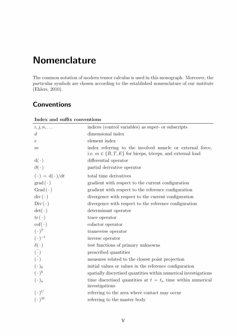
Nomenclature
The common notation of modern tensor calculus is used in this monograph. Moreover, theparticular symbols are chosen according to the established nomenclature of our institute(Ehlers, 2010).
Conventions
Index and suffix conventions
i, j, n, . . . indices (control variables) as super- or subscripts
d dimensional index
e element index
m index referring to the involved muscle or external force,i.e. m ∈ B, T,E for biceps, triceps, and external load
d( · ) differential operator
∂( · ) partial derivative operator·
( · ) = d( · )/dt total time derivatives
grad ( · ) gradient with respect to the current configuration
Grad ( · ) gradient with respect to the reference configuration
div ( · ) divergence with respect to the current configuration
Div ( · ) divergence with respect to the reference configuration
det( · ) determinant operator
tr ( · ) trace operator
cof( · ) cofactor operator
( · )T transverse operator
( · )−1 inverse operator
δ( · ) test functions of primary unknowns¯( · ) prescribed quantities˜( · ) measures related to the closest point projection
( · )0 initial values or values in the reference configuration
( · )h spatially discretised quantities within numerical investigations
( · )n time discretised quantities at t = tn time within numericalinvestigations
( · )C referring to the area where contact may occur
( · )M referring to the master body
V

VI Nomenclature
( · )S referring to the slave body
( · )χ referring to the mechanical primary variable
( · )p referring to the hydrostatic pressure as primary variable
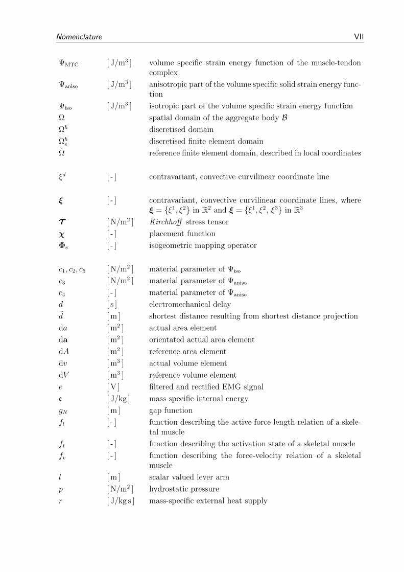
Symbols
The order of the table is Greek before Latin following calligraphic letters. Small lettersprecede capital letters.
Symbol Unit Description
α [ - ] muscle activation
β1, β2, β3 [ - ] coefficients defining the second-order activation dynamics
γ1, γ2 [ - ] coefficients defining the second-order activation dynamics
γM [ - ] material parameter distinguishing between muscle and tendontissue
γST [ - ] material parameter distinguishing between muscle-tendon orother isotropic soft tissue
εN [ N/m3 ] contact penalty factor
ε threshold parameter
θ [ ] elbow flexion angle
λi [ - ] eigenvalues of a tensor
λ [ - ] fibre stretch
λf [ - ] muscle fibre stretch
λoptf [ - ] optimal muscle fibre stretch
µ [ N/m3 ] shear modulus
νasc/desc [ - ] material parameter of Ψactive that influences the steepness ofthe belly curve
ρ [ kg/m3 ] material density
σmax [ N/m2 ] stress that a maximally activated muscle can produce at op-timal length λopt
f
φ [ - ] vector valued global basis function for the ansatz function
ψ [ - ] vector valued global basis function for the test function
∆Wasc/desc [ - ] material parameter of Ψactive that influences the width of thebelly curve
Γ spatial boundary of the aggregate body BΓC boundary, where contact may occur
Γσ boundary, where Neumann boundary conditions apply
Γu boundary, where Dirichlet boundary conditions apply
Ψ [ J/m3 ] volume specific strain energy function
Ψmuscle [ J/m3 ] volume specific strain energy function of the muscle
Nomenclature VII
ΨMTC [ J/m3 ] volume specific strain energy function of the muscle-tendoncomplex
Ψaniso [ J/m3 ] anisotropic part of the volume specific solid strain energy func-tion
Ψiso [ J/m3 ] isotropic part of the volume specific strain energy function
Ω spatial domain of the aggregate body BΩh discretised domain
Ωhe discretised finite element domain
Ω reference finite element domain, described in local coordinates
ξd [ - ] contravariant, convective curvilinear coordinate line
ξ [ - ] contravariant, convective curvilinear coordinate lines, whereξ = ξ1, ξ2 in R2 and ξ = ξ1, ξ2, ξ3 in R3
τ [ N/m2 ] Kirchhoff stress tensor
χ [ - ] placement function
Φe [ - ] isogeometric mapping operator
c1, c2, c5 [ N/m2 ] material parameter of Ψiso
c3 [ N/m2 ] material parameter of Ψaniso
c4 [ - ] material parameter of Ψaniso
d [ s ] electromechanical delay
d [ m ] shortest distance resulting from shortest distance projection
da [ m2 ] actual area element
da [ m2 ] orientated actual area element
dA [ m2 ] reference area element
dv [ m3 ] actual volume element
dV [ m3 ] reference volume element
e [ V ] filtered and rectified EMG signal
e [ J/kg ] mass specific internal energy
gN [ m ] gap function
fl [ - ] function describing the active force-length relation of a skele-tal muscle
ft [ - ] function describing the activation state of a skeletal muscle
fv [ - ] function describing the force-velocity relation of a skeletalmuscle
l [ m ] scalar valued lever arm
p [ N/m2 ] hydrostatic pressure
r [ J/kg s ] mass-specific external heat supply
VIII Nomenclature
t [ s ] time
tN [ N/m2 ] normal (frictionless) contact pressure
u [ - ] neural activation
wk [ - ] weighting factor at Gauss point k
A [ - ] shape factor defining muscle activation
E [ - ] finite number of discrete, non-overlapping finite elements
Eeff [ - ] effective value of the Green-Lagrangean strain tensor
Fm [ N ] scalar valued force
F 0m [ N ] maximum isometric muscle force
I1, I2, I3, I4 [ - ] principal invariants of the deformation tensors
J [ - ] Jacobian determinant
LM [ m ] muscle length
LM [ m/s ] muscle contraction velocity
M [ Nm ] moment or torque
MFD [ Nm ] moment resulting from the forward dynamics model
MID [ Nm ] moment resulting from the inverse dynamics model
N [ - ] number of DoFs
NF [ - ] number of arbitrary forces
Ni [ - ] nodal basis function
a preferred fibre direction in the current configuration
b [ kg/s2 ] mass specific body force vector
dfs [ N ] incremental surface force
ei [ - ] (Cartesian) basis of orthonormal vectors
li tangent vectors of the convective surface coordinates
lm [ m ] lever arm vector of muscle m
mi [ - ] eigenvectors of C related to the reference configuration
n [ - ] outward-oriented unit surface normal vector
ni [ - ] eigenvectors of B related to the actual configuration
q [ J/m2 s ] heat flux vector
r [ m ] vector pointing from xs to the point of action, xm, where theresulting moment is minimal
t [ N ] surface traction vector
u,v,w solution vector of primary variables
u [ m ] displacement vector
x(X, t) [ m ] actual position vector
x(X, t) [ m/s ] velocity vector
x(X, t) [ m/s2 ] acceleration vector

Nomenclature IX
xe,Xe [ m ] nodal values of nodes belonging to an element e
xs [ m ] barycentre
A [ N/m2 ] Almansian strain tensor
B [ - ] left Cauchy-Green deformation tensor
C [ - ] right Cauchy-Green deformation tensor
E [ - ] Green-Lagrangean strain tensor
F [ - ] deformation gradient
Fm [ N ] force vector of muscle m
I [ - ] tensor identity
Je [ - ] Jacobian of the isogeometric mapping
K generalised stiffness matrix
L [ 1/s ] spatial velocity gradient
M [ Nm ] resulting moment vector
M⊥ [ Nm ] the perpendicular part of the resulting moment where M⊥ ⊥R
M‖ [ Nm ] the parallel part of the resulting moment where M‖‖RNe [ - ] set of nodal basis functions Ni for the element e
P [ N/m2 ] 1st Piola-Kirchhoff stress tensor
Q [ - ] proper orthogonal rotation tensor
Qξ [ - ] reflexion tensor
Q(φ)
ξ[ - ] rotation matrix inducing rotation by φ
Ri,R [ N ] nodal and total residual vector
Rm [ N ] resulting muscle force
S [ N/m2 ] 2nd Piola-Kirchhoff stress tensor
T [ N/m2 ] Cauchy stress tensor
U,V [ - ] right and left stretch tensors of the polar decomposition of F
X [ m ] reference position vector
B aggregate body
G overall variational formulation containing the weak forms
Gχ variational formulation containing the weak forms of the me-chanical problem
Gp variational formulation containing the weak forms of the in-compressibility constraint
GC variational formulation containing the weak forms of the con-tact problem
H1 Sobolev space
M [ - ] structural tensor

X Nomenclature
O fixed origin in an Euclid ian space
O3 group of all orthogonal transformations
P material point of aggregate BR response functions
S space of the ansatz or trial functions
SG3 symmetry groups
SO3 group of all proper orthogonal transformations
T space of the test functions
V process variables
W force wrench
f generalised right-hand side vector of the resulting global sys-tem of equation
g generalised matrix resulting from the algebraic side condition
K generalised stiffness matrix
Acronyms
Symbol Description
2-d two-dimensional
3-d three-dimensional
DoF degree of freedom
DoFs degrees of freedom
ACh chemical messenger or neurotransmitter
ACSA anatomical cross-section area of a skeletal muscle
ADP adenosine diphosphate
ATP adenosine triphosphate
BC boundary condition
BVP boundary-value problem
Ca2+ calcium ion
CE contractile element
Cl− chloride ion

Nomenclature XI
CMISS An interactive computer program for Continuum Mechanics,Image analysis, Signal processing and System Identification
ECM extracellular matrix
EMG electromyography
FEM finite element method
FIM Forward-Inverse model
IBVP initial-boundary-value problem
K+ potassium ions
MBS multi-body simulation
MVC maximum voluntary contraction
MTC muscle-tendon complex
Na+ sodium ion
ODE ordinary differential equations
PCSA physiological cross-section area of a skeletal muscle
PDE partial differential equations
PEE parallel elastic element
SSE serial elastic element
TDM tendon displacement method
VRLA vector-resulting lever arm
VRLA+ vector-resulting lever arm determined by including the effectsof the muscle force wrench
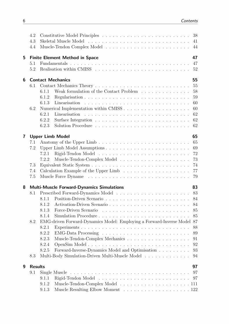
Anatomical directional terms
cranial
posterioror dorsal
anterioror ventral
caudal
superior
inferior
distal
distal
proximal
proximal
mediallateral
right left
(a) directional terms
sagittalplane
coronalplane
transverseplane
(b) human planes
Figure 0.1: Anatomical directional terms, adapted from OpenStax College (2013).


1 Introduction and Overview
1.1 Motivation
For engineers, the motivation to answer unresolved questions often comes from a combina-tion of a lack of knowledge and technology and curiosity. The process of finding a solutionto this questions always goes hand in hand with developing new methods. Answering thesequestions regarding the anatomy and physiology of biological tissues are especially chal-lenging. Nevertheless, this thesis tries to contribute to get a better understanding of thecomplexities of the musculoskeletal system.
In the past, many anatomically related questions could be answered by in-vitro ex-periments. Yet, physiological and functional tissues are mostly only investigated in alimited sense in abnormal conditions or outside their normal biological context. In-vivoexperiments are rarely applicable for ethical reasons. For approximately the last 50 years,in-silico experiments widened the possibilities to investigate biological tissues. Computa-tional models enable to toy with functional parameters so as to test, verify and understandnatural phenomena. Obviously, investigations using computational models are only asgood as their models. Here, verification and validation play a crucial role. However, theproblem is conducting biological experiments on living tissues is rather difficult. Hence,only limited data for comparison is available.
This thesis focuses on the musculoskeletal apparatus. Status quo attempts to simulate(parts of) the musculoskeletal system are based on multi-body simulations. They includethe use of lumped-parameter models to represent muscle-tendon complexes to investigatethe kinetics of the musculoskeletal system. Multi-body models use a discrete modellingapproach, in which the components of the musculoskeletal system are typically assumed tobe rigid. From a mechanical point of view, they are characterised by discrete mass pointsand their respective moments of inertia. The Hill -type muscle models have gained accep-tance for adequately representing the muscle-tendon complexes as a lumped-parametermodelling approach. As they have been successfully applied for many decades, they arewell validated by experiments. Geometrically, they are linear objects that span from themuscles’ origin to their insertion points and they lack any contour or volumetric represen-tation. While the path of the muscle force can be enhanced by defining wrapping surfacesor via-points to improve muscle force orientation, such lumped-parameter models are notcapable of representing detailed structural characteristics. Due to the relatively smallnumber of DoFs, multi-body models are computational feasible. Hence, a large numberof muscles can be utilised to investigate movements.
Yet, experimental measurements have shown that structural characteristics have astrong impact on the overall behaviour of biological soft tissues. Burkholder et al. (1994)states that the fibre length and fibre type distribution are the most functionally significantparameters in determining skeletal muscle mechanics, whereas the architectural proper-ties of fibres are the most structurally significant parameters. Furthermore, Holzapfel
1
2 Chapter 1: Introduction and Overview
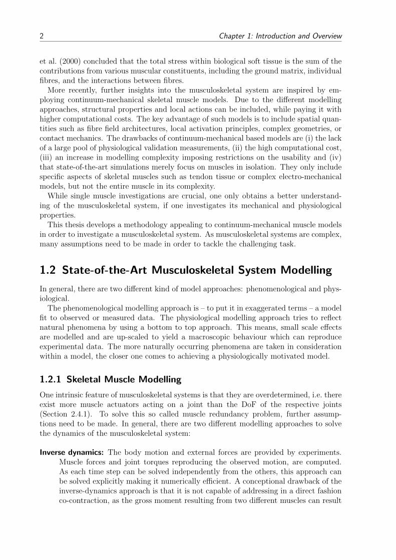
et al. (2000) concluded that the total stress within biological soft tissue is the sum of thecontributions from various muscular constituents, including the ground matrix, individualfibres, and the interactions between fibres.
More recently, further insights into the musculoskeletal system are inspired by em-ploying continuum-mechanical skeletal muscle models. Due to the different modellingapproaches, structural properties and local actions can be included, while paying it withhigher computational costs. The key advantage of such models is to include spatial quan-tities such as fibre field architectures, local activation principles, complex geometries, orcontact mechanics. The drawbacks of continuum-mechanical based models are (i) the lackof a large pool of physiological validation measurements, (ii) the high computational cost,(iii) an increase in modelling complexity imposing restrictions on the usability and (iv)that state-of-the-art simulations merely focus on muscles in isolation. They only includespecific aspects of skeletal muscles such as tendon tissue or complex electro-mechanicalmodels, but not the entire muscle in its complexity.
While single muscle investigations are crucial, one only obtains a better understand-ing of the musculoskeletal system, if one investigates its mechanical and physiologicalproperties.
This thesis develops a methodology appealing to continuum-mechanical muscle modelsin order to investigate a musculoskeletal system. As musculoskeletal systems are complex,many assumptions need to be made in order to tackle the challenging task.
1.2 State-of-the-Art Musculoskeletal System Modelling
In general, there are two different kind of model approaches: phenomenological and phys-iological.
The phenomenological modelling approach is – to put it in exaggerated terms – a modelfit to observed or measured data. The physiological modelling approach tries to reflectnatural phenomena by using a bottom to top approach. This means, small scale effectsare modelled and are up-scaled to yield a macroscopic behaviour which can reproduceexperimental data. The more naturally occurring phenomena are taken in considerationwithin a model, the closer one comes to achieving a physiologically motivated model.
1.2.1 Skeletal Muscle Modelling
One intrinsic feature of musculoskeletal systems is that they are overdetermined, i.e. thereexist more muscle actuators acting on a joint than the DoF of the respective joints(Section 2.4.1). To solve this so called muscle redundancy problem, further assump-tions need to be made. In general, there are two different modelling approaches to solvethe dynamics of the musculoskeletal system:
Inverse dynamics: The body motion and external forces are provided by experiments.Muscle forces and joint torques reproducing the observed motion, are computed.As each time step can be solved independently from the others, this approach canbe solved explicitly making it numerically efficient. A conceptional drawback of theinverse-dynamics approach is that it is not capable of addressing in a direct fashionco-contraction, as the gross moment resulting from two different muscles can result
1.2 State-of-the-Art Musculoskeletal System Modelling 3
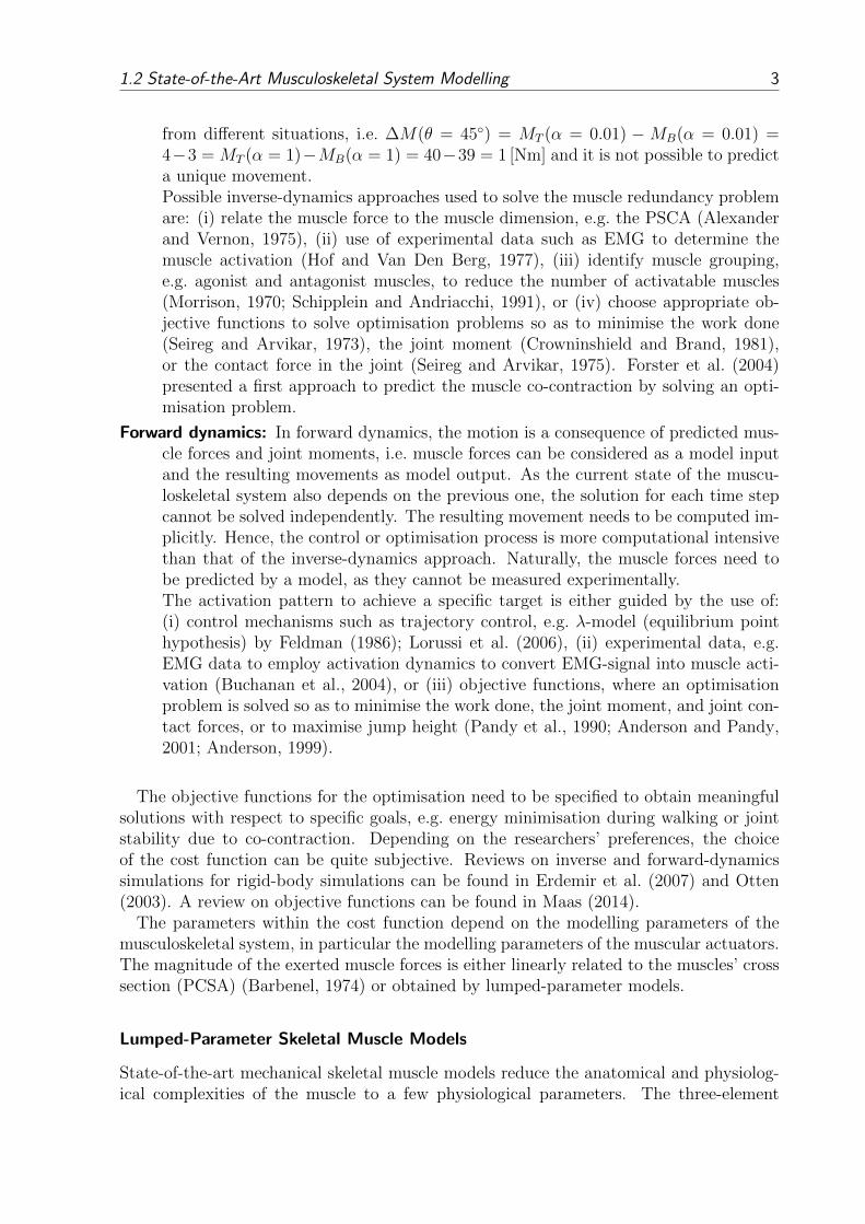
from different situations, i.e. ∆M(θ = 45) = MT (α = 0.01) −MB(α = 0.01) =4−3 = MT (α = 1)−MB(α = 1) = 40−39 = 1 [Nm] and it is not possible to predicta unique movement.Possible inverse-dynamics approaches used to solve the muscle redundancy problemare: (i) relate the muscle force to the muscle dimension, e.g. the PSCA (Alexanderand Vernon, 1975), (ii) use of experimental data such as EMG to determine themuscle activation (Hof and Van Den Berg, 1977), (iii) identify muscle grouping,e.g. agonist and antagonist muscles, to reduce the number of activatable muscles(Morrison, 1970; Schipplein and Andriacchi, 1991), or (iv) choose appropriate ob-jective functions to solve optimisation problems so as to minimise the work done(Seireg and Arvikar, 1973), the joint moment (Crowninshield and Brand, 1981),or the contact force in the joint (Seireg and Arvikar, 1975). Forster et al. (2004)presented a first approach to predict the muscle co-contraction by solving an opti-misation problem.
Forward dynamics: In forward dynamics, the motion is a consequence of predicted mus-cle forces and joint moments, i.e. muscle forces can be considered as a model inputand the resulting movements as model output. As the current state of the muscu-loskeletal system also depends on the previous one, the solution for each time stepcannot be solved independently. The resulting movement needs to be computed im-plicitly. Hence, the control or optimisation process is more computational intensivethan that of the inverse-dynamics approach. Naturally, the muscle forces need tobe predicted by a model, as they cannot be measured experimentally.The activation pattern to achieve a specific target is either guided by the use of:(i) control mechanisms such as trajectory control, e.g. λ-model (equilibrium pointhypothesis) by Feldman (1986); Lorussi et al. (2006), (ii) experimental data, e.g.EMG data to employ activation dynamics to convert EMG-signal into muscle acti-vation (Buchanan et al., 2004), or (iii) objective functions, where an optimisationproblem is solved so as to minimise the work done, the joint moment, and joint con-tact forces, or to maximise jump height (Pandy et al., 1990; Anderson and Pandy,2001; Anderson, 1999).
The objective functions for the optimisation need to be specified to obtain meaningfulsolutions with respect to specific goals, e.g. energy minimisation during walking or jointstability due to co-contraction. Depending on the researchers’ preferences, the choiceof the cost function can be quite subjective. Reviews on inverse and forward-dynamicssimulations for rigid-body simulations can be found in Erdemir et al. (2007) and Otten(2003). A review on objective functions can be found in Maas (2014).
The parameters within the cost function depend on the modelling parameters of themusculoskeletal system, in particular the modelling parameters of the muscular actuators.The magnitude of the exerted muscle forces is either linearly related to the muscles’ crosssection (PCSA) (Barbenel, 1974) or obtained by lumped-parameter models.
Lumped-Parameter Skeletal Muscle Models
State-of-the-art mechanical skeletal muscle models reduce the anatomical and physiolog-ical complexities of the muscle to a few physiological parameters. The three-element

4 Chapter 1: Introduction and Overview
Hill -type models (Zajac, 1989; Anderson and Pandy, 2001) are by far the most commonlyused skeletal muscle models for analysing movement.
These lumped-parameter models are simple but well established. These models havebeen employed in numerical simulations for several decades to investigate locomotion (ofparts) of the musculoskeletal system due to their comparatively small number of DoFs.
The development of the prominent muscle models was first introduced by Hill (1938).Hill performed quick-release experiments on a sartorius muscle of a frog to determine thenecessary parameters of Equation (1.1). In quick release experiments, fully activated mus-cles are pre-stretched and subjected to a constant load. While releasing the muscle, themuscle’s contraction velocity and force are measured. This relation can be mathematicallyexpressed as
(Lm + b) (Fm + a) = b (F 0m + a) . (1.1)
Herein, a and b are muscle parameters and F 0m is the maximal force at a current deflec-
tion length Lm. The maximal force F 0m depends on Lm because the number of possible
attachable cross-bridges within muscle fibres strongly depends on the stretch of a musclefibre, see Section 2.4.2 and Figure 2.10.
Equation (1.1) demonstrates a hyperbolic relation between the force, Fm, and the con-traction velocity, Lm: i.e. the higher the load applied to the muscle, the lower the contrac-tion velocity, see Figure 1.1a. His model employs an equation of state, initially introducedby van der-Waals for real gas to describe the contraction of a fully tetanised muscle.
Hill ’s mathematical model, describing only fully tetanised muscles, was extended to arheological model (lumped-parameter model) using three mechanical elements, see Fig-ure 1.1b. The model consists of a contractile element, CE, which reflects the active con-tractile contribution of the muscle described in Equation (1.1), a spring in parallel, PEE,representing the intrinsic elasticity of the muscle fibre’s connective tissue, while a secondspring in series, SEE, describes the muscle’s passive behaviour (inactivated stretching ofthe muscle) and the tendons. This relatively simple lumped-parameter model is also ableto represent single twitches, and can be further extended by the utilisation of springs anddash-pots for more accurate representations, e.g. viscoelastic behaviour (Gunther et al.,2007). With time, many suggestions have been made to improve the material descriptionby adding springs and dampers to the system.
LmL0m
Fm
F 0m
(a) force-velocity rela-tion described byEquation (1.1)
SEECE
PEEm
(b) 3-element Hill-type mus-cle model
Figure 1.1: Components of the Hill-type muscle model.
The small number of DoFs enables the study of complex movement patterns. Eachmuscle can be described by a set of ordinary differential equations. The input parameters

1.2 State-of-the-Art Musculoskeletal System Modelling 5
for one-dimensional Hill -type like skeletal muscle models are the muscle activation α, themuscle length Lm and the muscle contraction velocity Lm. The output is the muscle force,Fm.
State-of-the-art investigations on the human musculoskeletal system are carried outusing multi-body or rigid-body simulations. These are discrete modelling approaches,where the components of the musculoskeletal system are assumed to be rigid. They aremechanically characterised by discrete mass points and their moments of inertia. TheNewton-Euler equations are solved to describe the combined translational and rotationaldynamics of rigid bodies. By including up to several tens of Hill -type muscle models,the resulting multi-body models enable investigations into kinetics of musculoskeletalsystems of daily movements, e.g. human walking (Hardt, 1978; Patriarco et al., 1981).These models be used in either forward or inverse-dynamics approaches (Erdemir et al.,2007).
Geometrically speaking, the Hill -type muscle models are linear objects that are spannedbetween the muscles’ origin and insertion points within the rigid-body model. The pointof origin, the direction of force, and the muscle insertion define the line of action of thelumped-parameter skeletal muscle models. The muscles’ line of action may be redirectedthrough via-points or wrapping surfaces (Garner and Pandy, 2000).
The most significant drawback of this approach is the large geometrical simplificationlike for the pennation angle of a muscle. Hereby, neither geometrical nor local effects canbe considered. For pennation angles smaller than 20, the impact is usually neglected(Schmitt, 2006). For larger angles, a constant pennation angle is considered to includethe muscle fibre architecture.
The big advantage of the resulting rigid-body simulations is its computational feasibility.Due to the relatively small number of DoFs in rigid-body models, including Hill -typemuscle models, the indeterminate system can be solved either by an inverse or a forward-dynamics optimisation approach.
Volumetric Skeletal Muscle Models
More recently, further insights into the musculoskeletal system are aspired by employingcontinuum-mechanical skeletal muscle models. Due to the different modelling approach,structural properties and local actions can be included, yet paying it in form of the lackof a large pool of physiological validation measurements, with high computational costs,with the increase in modelling complexities imposing restrictions to the usability, and therestriction that state-of-the-art simulations focus on muscles in isolation (Blemker et al.,2005; Bol and Reese, 2008; Oomens et al., 2003; Lemos et al., 2001; Wang et al., 2013).Only specific skeletal muscle aspects are included, e.g. tendon tissue (Lemos et al., 2005),micro-mechanical considerations (Yucesoy et al., 2002; Sharafi and Blemker, 2010; Sharafiet al., 2011), or complex electro-mechanical models (Rohrle et al., 2008; Rohrle, 2010;Heidlauf and Rohrle, 2014), complex geometries (Bol et al., 2011), or contact mechanics(Fernandez and Hunter, 2005), but not the muscle in its entire complexity.
While early muscle models were mostly lumped-parameter models, Van Leeuwen andSpoor (1992) published a study that reports a first step towards investigating skeletalmuscles using a numerically stable solution scheme to predict the spatially varying hydro-static pressure and the shape of a muscle. They pointed out, that some existing models forpennate muscles violate mechanical equilibrium, and it is not enough to define a unique

6 Chapter 1: Introduction and Overview
pennation angle that is valid for the whole muscle. Their approach involves a descriptionof single fibres and its curvature, to investigate different 2-dimensional fibre architectures.Each fibre attaches to tendinous sheets while all tendinous sheets unite at the centraltendon. Due to fibre contraction, the fibre bends and the interstitial fluid builds up thehydrostatic pressure.
Van Donkelaar et al. (1995) created a finite element mesh of a rat’s gastrocnemiusmedialis muscle using medical images. The muscle includes muscle tissue, and special carewas taken to mesh the tendinous tissue. Vankan et al. (1995) used the mesh to simulateblood flow through the muscle, which is considered to be a fully saturated porous medium.In this study, the muscle tissue is assumed to behave linearly elastic.
The first model using a finite element approach to investigate the mechanical behaviourof skeletal muscles was presented by Johansson et al. (2000). For the dynamic formula-tion, which was implemented in ANSYS and solved explicitly, a nearly isovolumetricpressure-displacement formulation was used. The main purpose of the investigation wasto investigate the impact of the muscle mass on the dynamic response of the muscle. Theuser material for the muscle stress is additively split into an isotropic part σfib, whichrepresents the muscle matrix, and an anisotropic part, which represents the impact of themuscle fibre. A hyperelastic Mooney-Rivlin material was chosen for the matrix. The fibrecontribution, σfib, is introduced to
σfib = σmax ft fv(Lm) fl(Lm) + σpas . (1.2)
The fibre term is split into two terms: one for the active and one for passive fibre contribu-tion (σpas). The active contribution includes σmax, which is the maximum isometric stressat optimal fibre length, and three functions ft, fv, fl, describing the muscle’s activationstate, the force-velocity relation, and the force-length relation, respectively. The state ofactivation is determined by a charge wave form function. The velocity-dependent func-tion, fv, is split into two parts: The concentric behaviour is described by the Hill relation(1.1), and the eccentric behaviour is determined by an adapted yield stress criteria. Thepassive contribution, σpas, depends on the strain components.
Yucesoy et al. (2002) introduced a two-domain approach to investigate the effects offorce transmission between muscle fibres and extracellular matrix. The two domains arerepresented by two separate meshes that are linked elastically to account for the trans-sarcolemmal attachments of the muscle fibres cytoskeleton and extracellular matrix.
Oomens et al. (2003) assumed a superposition of the muscle stress by a passive stress(reflecting the collagen and intrinsic fibre stiffness) and an active stress (reflecting thecontractile property of the muscle). Within the passive term, the matrix component isdescribed using a Neo-Hookean material law, while a nonlinear contribution takes careof the fibre contribution. At the cost of increased numerical expenses, they substitutedthe Hill relation by a more physiologically based force-velocity relation. They employeda Huxley-like model based on the sliding-filament theory, see Section 2.4.2. The Huxleymodel is a two-state model (attached or detached state) which determines the inducedstress resulting from the degree of activation. The model unknowns are the bindingdistribution, a dimensionless attachment length, a scaled shortening velocity of a halfsarcomere, an activation factor, which depends on the calcium level, and an overlap factor,which is a function of the actual length of a sarcomere to determine the potentially possiblecross-bridges. The Huxley model is a system of ordinary differential equations, which

1.2 State-of-the-Art Musculoskeletal System Modelling 7
needs to be evaluated for every point of the 3D model. Herein, the determined activecontribution of the stress will be transmitted to the mechanical equilibrium equations,which are solved by the FE model.
Lemos et al. (2005) also split the stress into a passive and an active part. The passivematerial behaviour is described by an isovolumetric Mooney-Rivlin material law. Addi-tionally, tendinous tissue is considered in their model. The unwrinkling of fibrous tendontissue is included by an exponential constitutive law. This work focused on modellingthe force-length relation. The standard force-length relation for the active contributionis enhanced by including a concept for the residual force enhancement. If the musclechanges its length while maintaining muscle stimulation, the active stress does not be-have as described in the force-length relation. Instead, the residual force enhancementcauses the stress to linearly increase with the stiffness of the muscle tissue.
To conclude the isolated muscle investigations, the presented models are all based ona phenomenological approach. The muscle stress consists of two terms: an isotropicmatrix term and an anisotropic fibre term. The isotropic term is described using a rubberlike material. The fibre term has considerable differences. The approaches differ in usingdifferent force-length relations, different force-velocity relations and/or different activationprinciples.
For musculoskeletal system models appealing to continuum mechanical principles, Fer-nandez and Hunter (2005) solved the wrapping of leg muscles around the knee articulationincluding the patella and cartilage tissue with an inverse-dynamics approach. The rigidbodies are coupled through contact mechanics. In addition, Lee et al. (2009) presented arelatively simple muscle model, which employs linear mechanics, to visualise the motionof skin for animation purposes.
To the best knowledge of the author, Wu et al. (2013) were the first to describe muscleactivation for visualising facial expressions. This was achieved by embedding muscletissues via a finite-element mapping procedure. However, for musculoskeletal systems,such as the upper or lower limb, antagonistic muscle pairs are essential for movements.Unlike the facial simulations, joint moment equilibrium positions do not need to be takeninto account.
The basis for musculoskeletal models appealing to continuum mechanical principlesto simulate movements is rather sparse. Considering the advantages of continuum-mechanical principles, the following question arises: Is it possible to find a way to bothbenefit from using continuum-mechanical models while maintaining reasonable computa-tional costs?
1.2.2 Modelling the Upper Limb
Before upper limb models were able to predict muscle forces acting in the upper limbsystem, first models focused on developing the kinematics of the upper limb. Therefore,geometrical relations for bones, joints, and muscle-tendon complexes were analysed andprescribed by dissecting cadavers (Messier et al., 1971; Amis et al., 1979). Later, modelswere developed that were capable of reproducing the musculoskeletal kinematics (Murrayet al., 1995). It became apparent that joint motions, muscle paths, and lever arms areessential to predict forces acting in the musculoskeletal systems (Van der Helm et al.,1992; Maurel et al., 1996).

8 Chapter 1: Introduction and Overview
Amis et al. published in 1979 already a model for predicting the muscle forces andmoments acting on the elbow and wrist. The model was established while developingan elbow prosthesis. In this work, the muscle paths were reconstructed by following themuscle centroid of cross-sections perpendicular to the longitudinal axis of the muscle. Themethod used to estimate the moment arms is a combination of centroid and straight-linepaths, i.e. that a line between the barycentre of the muscle origin and the barycentre ofthe muscle insertion is assumed. The muscle forces are estimated by using the work ofAlexander and Vernon (1975), which relates the muscle force to the muscle cross-section.
The development of physiological models predicting lever arms and muscle length con-tinued for many years. Murray et al. (1995) presented a three-dimensional computermodel to evaluate the muscle kinematics of the arm muscles as a function of elbow an-gle and supination/pronation. The kinematic model was extensively used in rigid-bodysimulation for both inverse and forward-dynamics approaches.
The first skeletal muscle forces were predicted experimentally by (Messier et al., 1971)and (Amis et al., 1979). Messier et al. (1971) investigated the relation of EMG dataof biceps brachii and triceps brachii to muscle tension. Therefor, isometric tests wereconducted. The resulting tensions, given as functions of applied load and elbow angle,were used to conclude that the muscle force is directly proportional to the averagedelectromyogram and that the parameter describing the slope is independent of the musclelength. Yet, the muscle tension increases with increasing muscle length.
Buchanan et al. (1986) investigated the elbow torque for a two DoFs joint during iso-metric contractions. The levels of EMG activity were observed to increase with increasingjoint torque in an approximately linear manner. In polar plots, conclusions were madeabout the participation of the different muscles for different arm movements. Muscleforces are not explicitly identified.
The group of van Zuylen et al. (1988) developed a musculoskeletal system for the upperlimb. He included the biceps brachii, brachialis and brachioradialis to investigate theircontribution to the overall elbow torque. The muscle dynamics was modelled with Hill -type models. He performed experiments to measure torques generated by twitches ofmotor units instead of tetanic generated torques of the whole muscle.
An et al. (1989) introduced an analytical model of the upper limb to determine themuscle force distribution across the elbow joint for various configurations. The introducedmuscle model can incorporate muscles with different architectures. The three main flexorcontributors were biceps brachii, brachialis and brachioradialis. Their length and leverarms are determined by experimental data.
Challis and Kerwin (1993) introduced an inverse-dynamics, rigid-body model of theupper limb. The acting flexor muscles are biceps brachii, brachialis, and brachioradialis.The muscle forces based on 15 different objective functions were compared to predictionsestimated by a validated muscle model. As the objective functions showed poor corre-spondence, a less restrictive and simple objective function was introduced which yieldedbetter correlation to the validated model. This objective function assumed fully activatedmuscles and a constant muscle force ratio determined by muscle force and the maximalexerted muscle force for each included muscle. The skeletal muscle model was Hill -typelike, including force-length and force-velocity relations. The muscles were assumed tobe maximally activated throughout the range of the movement. The kinematics of thesystem is determined analytically using the shortest distance between muscle origin and
1.3 Outline of the Thesis 9
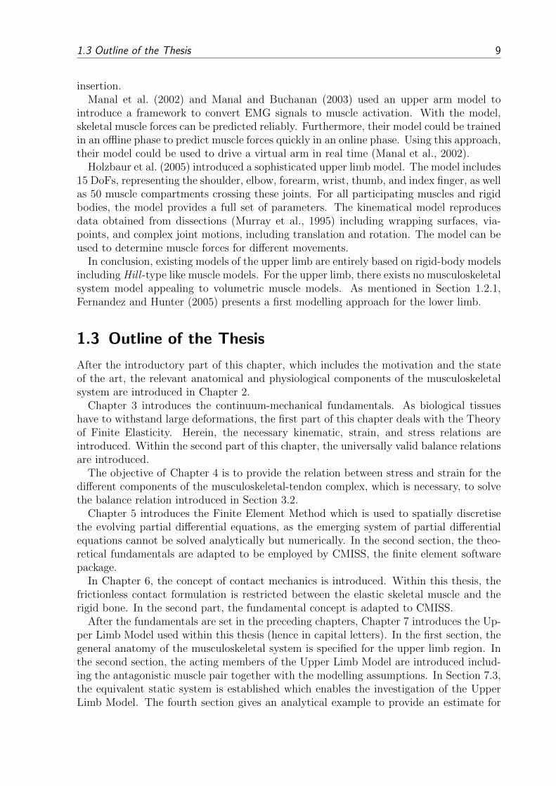
insertion.Manal et al. (2002) and Manal and Buchanan (2003) used an upper arm model to
introduce a framework to convert EMG signals to muscle activation. With the model,skeletal muscle forces can be predicted reliably. Furthermore, their model could be trainedin an offline phase to predict muscle forces quickly in an online phase. Using this approach,their model could be used to drive a virtual arm in real time (Manal et al., 2002).
Holzbaur et al. (2005) introduced a sophisticated upper limb model. The model includes15 DoFs, representing the shoulder, elbow, forearm, wrist, thumb, and index finger, as wellas 50 muscle compartments crossing these joints. For all participating muscles and rigidbodies, the model provides a full set of parameters. The kinematical model reproducesdata obtained from dissections (Murray et al., 1995) including wrapping surfaces, via-points, and complex joint motions, including translation and rotation. The model can beused to determine muscle forces for different movements.
In conclusion, existing models of the upper limb are entirely based on rigid-body modelsincluding Hill -type like muscle models. For the upper limb, there exists no musculoskeletalsystem model appealing to volumetric muscle models. As mentioned in Section 1.2.1,Fernandez and Hunter (2005) presents a first modelling approach for the lower limb.
1.3 Outline of the Thesis
After the introductory part of this chapter, which includes the motivation and the stateof the art, the relevant anatomical and physiological components of the musculoskeletalsystem are introduced in Chapter 2.
Chapter 3 introduces the continuum-mechanical fundamentals. As biological tissueshave to withstand large deformations, the first part of this chapter deals with the Theoryof Finite Elasticity. Herein, the necessary kinematic, strain, and stress relations areintroduced. Within the second part of this chapter, the universally valid balance relationsare introduced.
The objective of Chapter 4 is to provide the relation between stress and strain for thedifferent components of the musculoskeletal-tendon complex, which is necessary, to solvethe balance relation introduced in Section 3.2.
Chapter 5 introduces the Finite Element Method which is used to spatially discretisethe evolving partial differential equations, as the emerging system of partial differentialequations cannot be solved analytically but numerically. In the second section, the theo-retical fundamentals are adapted to be employed by CMISS, the finite element softwarepackage.
In Chapter 6, the concept of contact mechanics is introduced. Within this thesis, thefrictionless contact formulation is restricted between the elastic skeletal muscle and therigid bone. In the second part, the fundamental concept is adapted to CMISS.
After the fundamentals are set in the preceding chapters, Chapter 7 introduces the Up-per Limb Model used within this thesis (hence in capital letters). In the first section, thegeneral anatomy of the musculoskeletal system is specified for the upper limb region. Inthe second section, the acting members of the Upper Limb Model are introduced includ-ing the antagonistic muscle pair together with the modelling assumptions. In Section 7.3,the equivalent static system is established which enables the investigation of the UpperLimb Model. The fourth section gives an analytical example to provide an estimate for
10 Chapter 1: Introduction and Overview
the magnitude of the muscle force and lever arms. In Section 7.5, the concept of the forcewrench is used to investigate the mechanical behaviour of a skeletal muscle. The conceptcan further be used to determine the point of action of newly defined traction force andthe muscle’s line of action.
In Chapter 8, possible applications for the Upper Limb Model are introduced. Findingan equilibrium position is a very computationally expensive endeavour, as the muscleredundancy problem needs to be solved. To circumvent solving the muscle redundancyproblem of the continuum-mechanical model, it is necessary to come up with new ap-proaches. Within this thesis, three possibilities are outlined to investigate the convergingbehaviour of the selected musculoskeletal system towards an equilibrium position andwhether the equilibrium position is physiologically reasonable. Section 8.1 assumes andprescribes muscle activations to circumvent solving an optimisation problem and to testwhether the Upper Limb Model is able to find an equilibrium position. Alternatively toprescribing the muscle activation, in Section 8.2, both experimental data and a multi-body simulation are introduced to determine the muscle activation. For this purpose, theauthor was designing, conducting, and analysing experiments at Prof. Lloyd’s Centre forMusculoskeletal Research at the Griffith University, Australia. The forward-inverse modelwas made available by the Musculoskeletal Research Group and used to analyse the ex-perimental data. In the last section of this chapter, one of the most promising approachesto employ continuum-mechanical models is outlined. By coupling continuum-mechanicalsimulations to rigid-body simulations, benefits of both model worlds can be encompassed.
In the first section of Chapter 9, the results for both the rigid-tendon model as well asthe muscle-tendon-complex model are presented. Section 9.2 presents the lever arms re-sulting from the tendon-displacement method and the vector-resulting lever arm method,the resulting elbow moments as well as the equilibrium positions, and the convergencebehaviour of the in Section 8.1 introduced procedure. In Section 9.3, the conducted ex-periments are investigated using the forward-inverse model. Its results can further beutilised to compare the resulting muscle forces and moments determined by the differentmodels, assumptions, and lever arms.
Chapter 10 discusses the assumptions this model is based on and reports on the resultingbenefits and drawbacks. Furthermore, the results of Chapter 9 are discussed individually,are compared to the results of different model assumptions, and are compared to alreadyexisting results of the literature.
Chapter 11 gives a short summary and an outlook to proceed with modelling the mus-culoskeletal system appealing to a continuum-mechanical approach.
2 Musculoskeletal System
Form and intrinsic properties of biological tissues strongly influence the mechanical be-haviour of interest. To set up a mechanical model, form (anatomy) and function (physi-ology) of the musculoskeletal system need to be introduced.
The human musculoskeletal system is a complex and dynamic system. Its primary func-tions are to provide form, support, protection, stability and movement. It is made up ofbones, muscles, tendons, ligaments, joints and other soft connective tissues that supportand bind tissues and organs together. The skeleton provides the structure while joints ar-ticulate individual bones and allow them to move against each other to cause movement.Yet, without the ability of skeletal muscles to voluntarily contract, the musculoskeletalsystem could only move passively. As this work focuses on modelling skeletal muscles, abrief overview is given on the anatomy of bones, ligaments and joints, whereas a moredetailed description of the skeletal muscles’ structure and function is given. More informa-tion about anatomic, biologic and functional fundamentals regarding the musculoskeletalsystem can be found in e.g. Fung (1981) or MacIntosh et al. (2006).
2.1 Bones
Bones have two basic structural components: the cortical (or compact) bone and thecancellous (or trabeculaer) interior bone, which is a spongy or honeycomb like structure.The cortical bone is a solid, dense material comprising the walls at the distal ends andthe external surfaces. This type of bone is strong and resistant to bending. Cancellousbone is formed by thin bone structures, called trabeculae. These trabeculae have beenobserved to orient in the direction of the forces applied to the bone (Wolff ’s law). Thespongy-like structure fills the inner part of the bone, is light, and can withstand highloads.
Cartilage covers articular bony surfaces to reduce frictional forces, wear, and absorbscompressive shocks, see also Chapter 2.2. Cartilage is an avascular material, which ap-pears to be glassy and smooth. Like all soft tissues, cartilage consists of a ground sub-stance. The cells produce the extracellular matrix, which determines the mechanicalproperties of the connective tissue. The ground substance typically contains proteogly-cans and is mostly composed of chondrocytes.
There are at least 206 bones in a typical adult with different sizes, shapes, composi-tions, and therefore, different mechanical properties. Five different types of bones can beclassified:
Long bones are characterised by the diaphysis, or long shaft, which is much longer thanthe cross-section is wide, and the epiphysis, or heads at each end, see Figure 2.1.Most of the limb bones are long bones for example.
11

12 Chapter 2: Musculoskeletal System
Short bones are more cube-shaped with a thin cortical bone layer surrounding a trabec-ulaer interior. Examples can be found in the ankle or the wrist.
Flat bones, as the name indicates, have two layers of cortical bone housing a trabeculaerinner bone. Examples are the sternum or the bones of the skull.
Sesamoid bones are embedded within tendons to increase the lever arm of the muscle-tendon complex. An example is the patella.
Irregular bones categorise the remaining complex shaped bones. Examples are the pelvisor the vertebras.
Trabeculaer bone
Meduallary cavity
Cortical bone
Figure 2.1: The structure of the femur as an example of a typical long bone. Source: adaptedfrom Blausen gallery 2014 (2014)
Bones have a large variety of functions. The most important ones are of mechanical,synthetical and metabolic nature.One of the key mechanical functions of bones is to build the skeleton system. It provides
• “rigid” kinematic chains by connecting bones to build joints, see Chapter 2.2,
• muscle-tendon complexes and ligaments attachment sites to transfer forces, and
• the ability to maintain an upright stance, and to protect organs.
The synthetical function of bones consists of producing blood components. Red andwhite blood cells are made in the bone marrow, located at the medullary cavity, withinthe trabeculae.One of the most important metabolic function is to store minerals and fatty acids withinthe bone marrow. For example, by storing and releasing alkaline salts a pH-buffer can beprovided. By adsorbing heavy metals from the blood, soft tissue can be detoxicated.
Normal human bones consist of the ground matrix, fibres and the extracellular matrix(ECM). The ground matrix is made up of minerals or inorganic substances that consistprimarily of calcium and phosphate.The ECM is also a composite material consisting of fibres and a liquid including macromolecules such as proteoglycans and polysaccharides in combination to proteins.Minerals account for 60 to 70% of its weight, while water accounts for 5 to 8% and organiccomponents including collagen make up the remainder of the tissue.As mentioned above, the contents’ ratio varies and bones are strongly able of adaptingwith environmental needs.
From a mechanical point of view, bone is a relatively hard and light composite mate-rial. In the physiological range of normal, healthy loading, the macroscopic strain-stress

2.2 Joints 13
relation can be considered as linear. Further, bone is a relatively brittle material withfailure at strains in the range of 1–1.5%. The compressive strength is much higher thanthe tensile strength, which are in the range of 170 MPa and around 100 MPa, respectively.As the shear modulus is quite low (∼ 50 MPa), bones can withstand high compressingforces and only small tensile and torsional forces.
2.2 Joints
The joint or articulation is defined as the location at which bones connect. The joints areconstructed to allow movement and provide mechanical support. They can be classified ina structural (specifying the bone connection) or functional way (specifying the allowabledegrees of freedom). Due to the numerous bone shapes, there is a large number of differentjoint types, where form follows function and classifications have overlaps. There are threestructural types:
Fibrous joints are connected by fibrous tissues and therefore almost immovable. Anexample is the connection of bones in the skull.
Cartilaginous joints entirely connect bones with cartilaginous tissues. Hereby, only smallmovements are possible. An example of a cartilaginous joint would be the connectionof the ribs at the sternum (chest).
Synovial joints, see Figure 2.2, are the most common joints and allow the largest relativemotion between the bones. The difference between this joint and the first two typesis that it is encapsulated by an outer membrane, which may contain ligaments,tendons, and muscles, and an inner synovial membrane, which includes the synovialfluid. The synovial fluid acts as a shock absorber, reducing the friction of thecartilage to a minimum and supplying the avascular articular capsule with nutrientsby diffusion or induced convection (bone motion). Additionally, synovial jointsmay contain articular discs or menisci (knee), articular fat pads (knee), tendons,ligaments, and busae, which are small fluid filled capsules placed in such a way thatthey reduce friction and stress.
Synovial joints are the joints which one typically has in mind if one thinks of joints.From here on, this work is focused on this kind of joints.There are six types of synovial joints. The form of the joint defines the DoFs for the bonesto move with respect to each other. Less mobile joints are more stable and less frail toinjuries.
Plane joints allow only in-plane gliding within the articular capsule, cf. Figure 2.3d.The opposite articular surfaces are almost flat. They are commonly small joints.This type is quite numerous and can be found for example in the hand, ankle, andvertebral processes.
Hinge joints allow a rotational motion only in one plane, cf. Figure 2.3b. The articularsurfaces are strongly connected by surrounding ligaments. A good example for thehinge joint is the joint which is formed by connecting humerus and ulna. The kneejoint is the largest hinge joint in the human body. Though, it allows to the one idealhinge joint rotation additionally rotational and lateral DoFs or motions.

14 Chapter 2: Musculoskeletal System
Figure 2.2: Example of a typical synovial joint. Source: OpenStax College (2013)
Pivot joints allow rotations of a socket around a pivot element, cf. Figure 2.3a. Themain difference to the hinge joint is that the rotation in a pivot joint is only parallelto the longitudinal axis of the proximal and distal bones. Examples for such jointsare the proximal and distal radioulnar joint which allow pronation and supinationof the forearm.
Condyloid joints or ellipsoidal joints are joints where convex and concave bone ends allowflexion-extension and abduction-adduction movements, and a combination of bothmotion types, named circumduction, cf. Figure 2.3e. An example for a condyloidjoint is the wrist joint. Hinge and pivot joints can both be considered as a subtypeof the cylindrical joint.In a saddle joint, the opposing surfaces are reciprocally concave-convex, cf. Fig-ure 2.3c. It has the same DoFs as the condyloid joint. Yet, due to the openstructure, it allows a wider range of motion.
Ball and socket joints, as the name already induces, consist of a ball which is placed in asocket, cf. Figure 2.3f. Hereby, all rotational DoFs are possible whereas translationalmovements are restricted. Examples are the shoulder and hip joints.
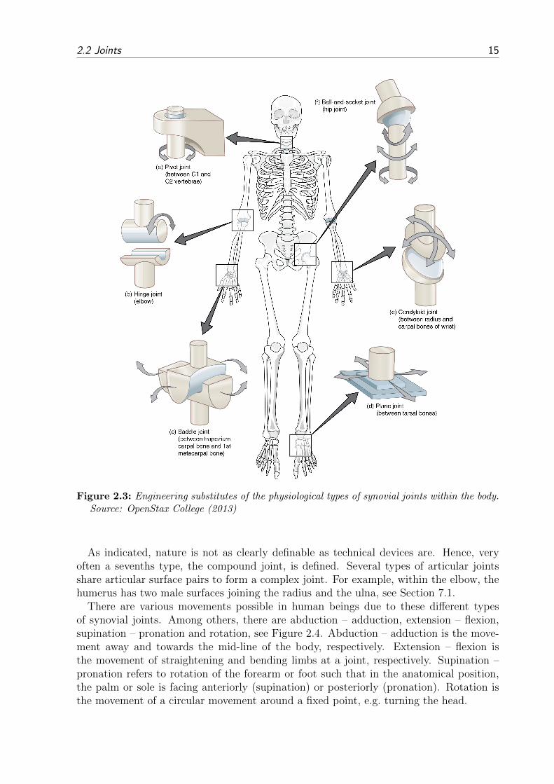
2.2 Joints 15
Figure 2.3: Engineering substitutes of the physiological types of synovial joints within the body.Source: OpenStax College (2013)
As indicated, nature is not as clearly definable as technical devices are. Hence, veryoften a sevenths type, the compound joint, is defined. Several types of articular jointsshare articular surface pairs to form a complex joint. For example, within the elbow, thehumerus has two male surfaces joining the radius and the ulna, see Section 7.1.
There are various movements possible in human beings due to these different typesof synovial joints. Among others, there are abduction – adduction, extension – flexion,supination – pronation and rotation, see Figure 2.4. Abduction – adduction is the move-ment away and towards the mid-line of the body, respectively. Extension – flexion isthe movement of straightening and bending limbs at a joint, respectively. Supination –pronation refers to rotation of the forearm or foot such that in the anatomical position,the palm or sole is facing anteriorly (supination) or posteriorly (pronation). Rotation isthe movement of a circular movement around a fixed point, e.g. turning the head.

16 Chapter 2: Musculoskeletal System
Figure 2.4: Selection of possible joint motions. Source: OpenStax College (2013)
2.3 Ligaments
Healthy joints allow a nearly effortless motion along preferred anatomical directions, yetabnormal motion should be prevented. As mentioned in the last section, the direction andrange of motion is strongly defined by the articular surfaces. Soft tissues wrapping aroundthe articular capsule stabilise and keep the articular surfaces together. One of the mostimportant tissue types for this purpose are ligaments. Ligaments are arranged around thejoints in such a way that they are already stretched in the neutral joint position. Further,at least one ligament band is under tension to stabilise the joint in any position of thejoint. They can be subjected to extreme loads while performing their duty in restrictinganatomical motions. In case of overstretching, ligaments may rupture which can lead tosevere joint instabilities.
Ligaments are short bands of tough connective tissues consisting of parallel bundled

2.4 Skeletal Muscle-Tendon Complex 17
fibres embedded into the ground matrix, trapping a large amount of water. They consistof up to two-thirds of water. The dry mass consists of up to 90% collagen and some elastin.Collagen is a hierarchical structure where the fibres are mostly aligned parallel. It is themain load carrying element in soft tissues. Elastin has a non-hierarchical structure. It hasa coiled organisation, is less stiff than collagen but can withstand large deformations. Thefibres are embedded into the ground matrix, the extracellular matrix, which has a similarcomposition as in bones, including proteoglycans, glycolipids, and fibroplasts. Within theECM, water forms a gel-like liquid.
Ligaments show a time and history dependent viscoelastic effect. Responsible for thoseeffects is the high amount of water. Within the ligament tissue, the water’s mobility isinhibited by long, charged proteoglycan molecules.
An extensive mechanically-based review can be found in Weiss and Gardiner (2001).
2.4 Skeletal Muscle-Tendon Complex
There are three different types of muscles in the human body. There are:
skeletal or striated muscles, which are attached to the bones and are responsible tomake the skeleton move,
cardiac muscles, which form the heart tissue, and
smooth muscles, which can be found in internal organs and in the walls of blood vessels.
All muscles have the ability in common that they can contract. Yet, they distinguish inshape, structure, and excitation. The first group can be voluntarily controlled, whereasthe latter two groups are controlled unconsciously. As this thesis deals with movements ofthe musculoskeletal system, the next section focuses on skeletal muscle or straited muscle.
A human being has around 650 different skeletal muscles. The overall muscles’ livingweight accounts for around 40-50% of our body weight. Around 50% of the energy gainedby metabolic activity is spend to supply skeletal muscles. Some muscles are attachedto bony processes and others to broad sheets of connective tissue, but all are directlyor indirectly linked with the skeletal system. The shape or appearance of each muscleprovides clues to its primary function, as form follows function. Muscles responsible forlocomotion or posture are wrapped around joints. Those that support soft tissues formslings or sheets between relatively stable bony elements, e.g. the abdominal wall and thefloor of the pelvic cavity consist of layers of skeletal muscles. Others guard an entranceor exit, completely encircling the opening and provide voluntary control over swallowing,defecation and urination.
As mentioned, skeletal muscles can only contract. So in order to make a joint move indifferent directions more muscles need to act at once. Muscles acting in opposite directionsare called an antagonistic muscle pair and consist of an agonist and an antagonist. Whilethe agonist produces a force in the primary direction of the motion, the antagonist controlsthe motion, slowing it down, or returning a limb to its initial position. If the motion isreversed, the muscles switch their functions. Very often, the agonist and/or the antagonistcan consist of several muscles and compose a redundant system. Those groups of musclecausing a same effect are called synergists.
The muscle-tendon-complex attachment sites are defined to be the origin and the in-sertion of a muscle. By definition, the origin is the point where the muscle is attached to
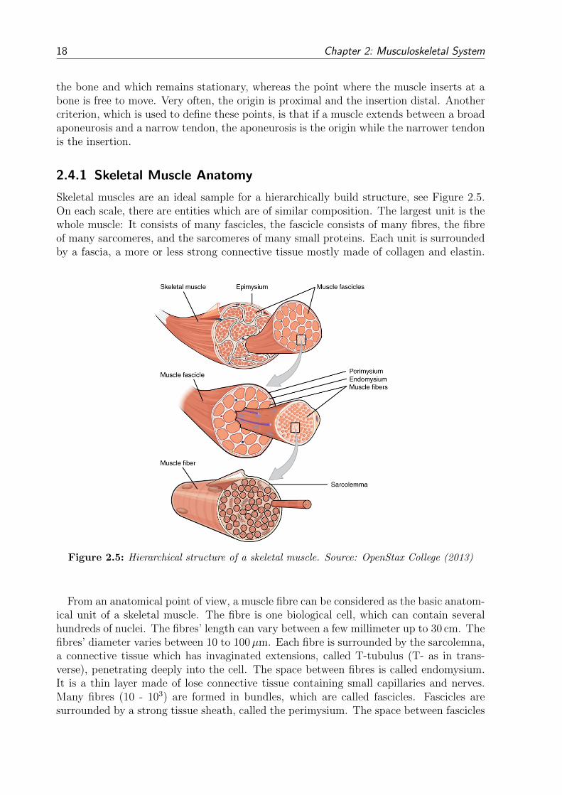
18 Chapter 2: Musculoskeletal System
the bone and which remains stationary, whereas the point where the muscle inserts at abone is free to move. Very often, the origin is proximal and the insertion distal. Anothercriterion, which is used to define these points, is that if a muscle extends between a broadaponeurosis and a narrow tendon, the aponeurosis is the origin while the narrower tendonis the insertion.
2.4.1 Skeletal Muscle Anatomy
Skeletal muscles are an ideal sample for a hierarchically build structure, see Figure 2.5.On each scale, there are entities which are of similar composition. The largest unit is thewhole muscle: It consists of many fascicles, the fascicle consists of many fibres, the fibreof many sarcomeres, and the sarcomeres of many small proteins. Each unit is surroundedby a fascia, a more or less strong connective tissue mostly made of collagen and elastin.
Figure 2.5: Hierarchical structure of a skeletal muscle. Source: OpenStax College (2013)
From an anatomical point of view, a muscle fibre can be considered as the basic anatom-ical unit of a skeletal muscle. The fibre is one biological cell, which can contain severalhundreds of nuclei. The fibres’ length can vary between a few millimeter up to 30 cm. Thefibres’ diameter varies between 10 to 100µm. Each fibre is surrounded by the sarcolemna,a connective tissue which has invaginated extensions, called T-tubulus (T- as in trans-verse), penetrating deeply into the cell. The space between fibres is called endomysium.It is a thin layer made of lose connective tissue containing small capillaries and nerves.Many fibres (10 - 103) are formed in bundles, which are called fascicles. Fascicles aresurrounded by a strong tissue sheath, called the perimysium. The space between fascicles
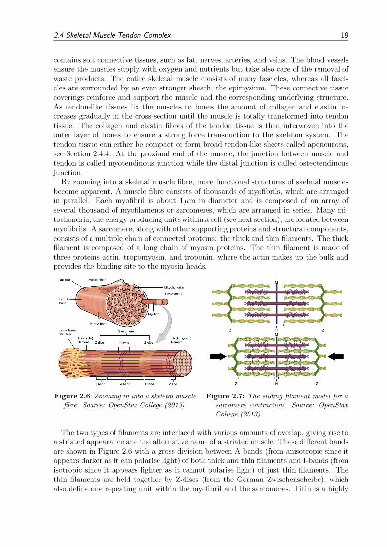
2.4 Skeletal Muscle-Tendon Complex 19
contains soft connective tissues, such as fat, nerves, arteries, and veins. The blood vesselsensure the muscles supply with oxygen and nutrients but take also care of the removal ofwaste products. The entire skeletal muscle consists of many fascicles, whereas all fasci-cles are surrounded by an even stronger sheath, the epimysium. These connective tissuecoverings reinforce and support the muscle and the corresponding underlying structure.As tendon-like tissues fix the muscles to bones the amount of collagen and elastin in-creases gradually in the cross-section until the muscle is totally transformed into tendontissue. The collagen and elastin fibres of the tendon tissue is then interwoven into theouter layer of bones to ensure a strong force transduction to the skeleton system. Thetendon tissue can either be compact or form broad tendon-like sheets called aponeurosis,see Section 2.4.4. At the proximal end of the muscle, the junction between muscle andtendon is called myotendinous junction while the distal junction is called osteotendinousjunction.
By zooming into a skeletal muscle fibre, more functional structures of skeletal musclesbecome apparent. A muscle fibre consists of thousands of myofibrils, which are arrangedin parallel. Each myofibril is about 1µm in diameter and is composed of an array ofseveral thousand of myofilaments or sarcomeres, which are arranged in series. Many mi-tochondria, the energy producing units within a cell (see next section), are located betweenmyofibrils. A sarcomere, along with other supporting proteins and structural components,consists of a multiple chain of connected proteins: the thick and thin filaments. The thickfilament is composed of a long chain of myosin proteins. The thin filament is made ofthree proteins actin, tropomyosin, and troponin, where the actin makes up the bulk andprovides the binding site to the myosin heads.
Figure 2.6: Zooming in into a skeletal musclefibre. Source: OpenStax College (2013)
Figure 2.7: The sliding filament model for asarcomere contraction. Source: OpenStaxCollege (2013)
The two types of filaments are interlaced with various amounts of overlap, giving rise toa striated appearance and the alternative name of a striated muscle. These different bandsare shown in Figure 2.6 with a gross division between A-bands (from anisotropic since itappears darker as it can polarise light) of both thick and thin filaments and I-bands (fromisotropic since it appears lighter as it cannot polarise light) of just thin filaments. Thethin filaments are held together by Z-discs (from the German Zwischenscheibe), whichalso define one repeating unit within the myofibril and the sarcomeres. Titin is a highly

20 Chapter 2: Musculoskeletal System
elastic protein which anchors the thin filaments to the Z-discs and the myosin in thecentre to the M-line. The M-line defines the centre of the H-zone (from the German helleZone), which defines the gap between opposing thin filaments, cf. Figure 2.7. The reasonwhy skeletal muscles are also called straighted muscles is based on the reoccurring lighter(I-band) and darker (A-band) zones within a myofibril.
The cell membrane of muscle fibres is called the sarcolemma. It is a selective permeablemembrane, which under certain conditions can let pass water molecules or ions such assodium (Na+), potassium (K+), calcium (Ca2+) and chlorine (Cl−) through small open-ings, the so-called ion channels. The sarcoplasmic reticulum, surrounding the myofibril,stores, releases, and retrieves calcium ions (Ca2+).
2.4.2 Skeletal Muscle Physiology
The ingenious property of skeletal muscles is the ability to contract. Within the muscle,chemical energy provided in the form of ATP is converted to tension-producing energy.The relative motion takes place in the smallest scale within skeletal muscles, betweenthe thick and thin filaments. As a whole skeletal muscle consists of a long series offunctional units, the small contraction of a single sarcomere (approx. 10 nm) sums up, toa degree, where macroscopic changes in length lead to forces acting on bones. The bonesare used as levers, the joints as fulcrum and the skeleton as a rigid system to be moved,see Section 2.4.5.
Within the next section, the underlying principles which lead to a controlled contractionare briefly introduced. Despite the rather complex sequences of events, an attempt is madeto sketch it in a compact manner.
After deciding to contract a skeletal muscle, motor neurons fire from the brain stemand/or the spinal cord, depending on the muscle and the physiological need. The signalsare travelling along axons, where a bundle axons build a nerve, arriving at the axonterminal. At the terminal, the motor neuron reaches to the fibre’s neuromascular junctionwhere the signal is fanned. Both neurons and skeletal muscle cells are electrically excitable,i.e. they are able to develop transmembrane potentials, as both are surrounded by aselective membrane enabling a potential difference between extracellular and intracellularspace. An action potential is a special type of electrical signal that can travel, as a wave,along a cell membrane. This allows a signal to be transmitted quickly at long distances.
If the stimulation of the motor neuron is strong or long enough, the transmembranepotential increases sufficiently to cross the excitation threshold. After exceeding thatthreshold, a self-sustaining process arises during which the membrane depolarises andreverses its polarity.
Skeletal muscle fibres that are innervated by a motor neuron, coming from the sameaxon terminal in order to contract, are from the same motor unit. The number of musclefibres within a motor unit is variable depending on the nature of the muscle. Commonly,it is exponentially distributed, where there are a large number of motor units including asmall number of muscle fibres and a small number of motor units including a large numberof muscle fibres. Smaller motor units have a lower threshold for the motor neurons toexcite. Large motor units have a higher excitation threshold. So in order to produce asmooth increase of muscle force, the small motor units are recruited first, while the largeronce kick in only at a high recruiting frequency and when a high force is in demand. Very

2.4 Skeletal Muscle-Tendon Complex 21
often, the small motor units include muscle fibre of type I while large motor units includetype II fibres.
The action potential is transferred from the neuromuscular junction to the other sideof the motor end-plate, the sarcolemna, by opening Na+-ion channels. This process istriggered by a chemical messenger or neurotransmitter, called ACh. Once the actionpotential arrives at the sarcolamna, the Na+-ion channels trigger the action potential totravel in both directions along the fibre. At each location along the fibre, the rising actionpotentials travel along the T-tubulus inside the cell to trigger the release of calcium ionsfrom the sarcoplasmic reticulum. Ca2+-ions bind with troponin (thin filament) to open thebinding site blocked by tropomyosin. Once the binding side is free, a connection betweenthe actin and myosin head occurs. This connection is called cross-bridge, Figure 2.8.While the myosin heads are pulling, the overlapping region, the H-band, reduces and thesarcomere shortens, cf. Figure 2.7. The reoccurring process of attaching, pulling (powerstroke), and detaching between thin and thick filaments is known as a cross-bridge cycle.
ATP keeps the cross-bridge cycling running and makes the myosin pull on the actinstructure. The muscle fibre will continue to shorten to an anatomical and mechanicallimit, as long as the neural signaling from the motor neuron does not end and as long asATP is available to drive the cross-bridge cycling as Ca2+-ions remain in the sarcoplasmto bind to troponin and to keep the actin-binding sites open. The zone where thin andthick filaments overlap has an important impact on the muscle contraction, as it influencesthe amount of possible cross-bridges, cf. Figure 2.7.
For the aerobic respiration, the energy to maintain the cycling is provided by themitochondria. Their main function is to consume oxygen and substrates to generate thevast majority of ATP while producing reactive oxygen species in the process, yet theyalso participate in a wide range of other cellular processes, including signal transduction,cell cycle regulation, oxidative stress, thermogenesis, and apoptosis.
In the decline phase of the action potential, Ca2+-ions are adsorbed by the sarcoplasmicreticulum (reloading for the next contraction), the cross-bridge opens (the muscle relaxes),tropomyosin restores the blockage, and the contraction ends.
The muscle contraction force can be controlled by two factors: (i) the number of motorunits involved in contraction and (ii) the amount of stimulus from the nervous system, seeFigure 2.9. A single nerve impulse of a motor neuron will cause a motor unit to contractbefore relaxing. This small contraction is known as a twitch contraction. If the motorneuron provides several signals with a large enough excitation frequency, the strengthand duration of the muscle contraction increases. This phenomenon is known as wavesummation. If the motor neuron provides many nerve impulses with a large excitationfrequency, the muscle may enter the state of tetanus, or complete and lasting contraction.A muscle will remain in tetanus until the excitation frequency reduces or the musclebecomes too fatigued to maintain the tetanic state.
As the electrical signal spreads quickly longitudinally along the fibre and the electri-cal conductivity is very low transversely, muscle fibre are coupled mechanically but notelectro-physiologically with each other.
Due to small variations in the properties of functional units within the skeletal muscle,different fibre types can by classified by histochemical, physiological, morphological, ormechanical criteria. Most commonly, muscle fibre types are grouped histochemically –for their ATPase sensitivity – i.e. how glucose is transformed into energy. ATPase are
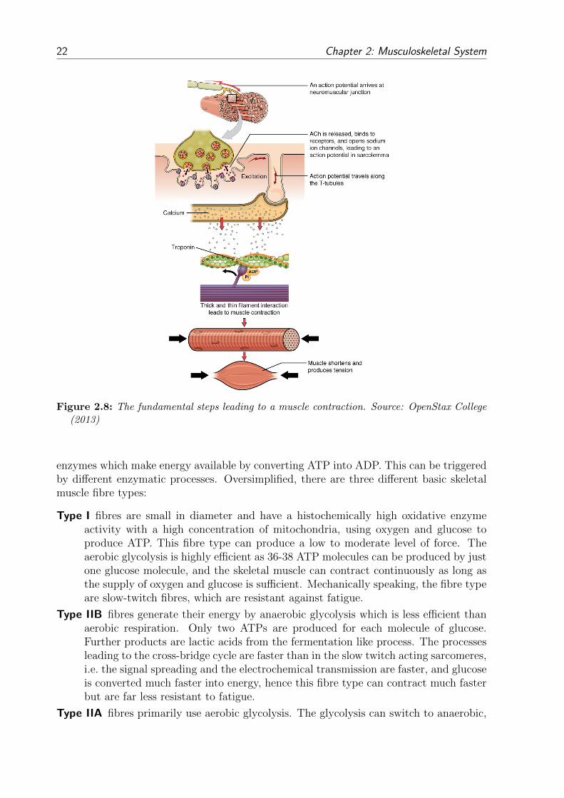
22 Chapter 2: Musculoskeletal System
Figure 2.8: The fundamental steps leading to a muscle contraction. Source: OpenStax College(2013)
enzymes which make energy available by converting ATP into ADP. This can be triggeredby different enzymatic processes. Oversimplified, there are three different basic skeletalmuscle fibre types:
Type I fibres are small in diameter and have a histochemically high oxidative enzymeactivity with a high concentration of mitochondria, using oxygen and glucose toproduce ATP. This fibre type can produce a low to moderate level of force. Theaerobic glycolysis is highly efficient as 36-38 ATP molecules can be produced by justone glucose molecule, and the skeletal muscle can contract continuously as long asthe supply of oxygen and glucose is sufficient. Mechanically speaking, the fibre typeare slow-twitch fibres, which are resistant against fatigue.
Type IIB fibres generate their energy by anaerobic glycolysis which is less efficient thanaerobic respiration. Only two ATPs are produced for each molecule of glucose.Further products are lactic acids from the fermentation like process. The processesleading to the cross-bridge cycle are faster than in the slow twitch acting sarcomeres,i.e. the signal spreading and the electrochemical transmission are faster, and glucoseis converted much faster into energy, hence this fibre type can contract much fasterbut are far less resistant to fatigue.
Type IIA fibres primarily use aerobic glycolysis. The glycolysis can switch to anaerobic,

2.4 Skeletal Muscle-Tendon Complex 23
single twitch wave summation unfused tetanus fused tetanus
time[m
s]
force[N
]AP
[∆V]
Figure 2.9: The muscle force develops depending on the recruitment frequency: The resultof a single twitch contraction can be seen in the first fraction. The force resulting fromtwo single twitches can be seen in the second fraction. The resulting force depends bothon the recruitment frequency and the duration of recruitment (number of twitches). For arecruitment frequency above 50 Hz the muscle reaches a tetanised state where the single twitchcannot be recognised anymore.
when a high level of force is in demand, as the muscle contracts so tightly thatoxygen carrying blood cannot enter the muscle. Depending on the respiration oftype IIA, the characteristic of the fibre resembles more fibre type I or type IIB.Concluding, type IIA fibres are capable of being fatigue resistant while being ableto twitch quickly at the same time.
Within a skeletal muscle, all muscle fibre types are present. Yet, depending on thelocation, functional requirements, and the development stage, a fibre type distributioncan range from having a mosaic of all three types to a dominance of only one fibre type.
The number of muscle fibres is genetically defined. Therefore, the strength which amuscle can perform depends on the changing number of myofibrils and sarcomeres withina muscle fibre. An increase of muscle bulk or mass is called hypertrophy, a decreaseatrophy.
The force which a sarcomere can generate depends on the overlap of thin and thickfilaments or the size of the H-zone, respectively. In Figure 2.10, the sarcomere force-length relation is shown which was established in in-vitro experiments on sarcomeres.
Having the cross-bridge model in mind, the shape of the extreme points of the relationcan easily be explained. A sarcomere generates the maximum force at the optimal sarcom-ere length. The optimal length is the length at which the number of possible cross-bridgesis at a maximum. For both, compressing and stretching the sarcomere, the number ofpossible cross-bridges reduces, so does the generated sarcomere force, cf. Figure 2.10. Thepossible number of available cross-bridge connection sites at less than approximately 60%and more than 170% strain are zero.

24 Chapter 2: Musculoskeletal System
Figure 2.10: The force-length relation for a single sarcomere. Source: OpenStax College (2013)
2.4.3 Electromyography
Electromyography (EMG) is a technique for evaluating and recording the electrical ac-tivity produced within skeletal muscles. The electrical activity can be recorded either bysurface electrodes on the skin or intramuscular using fine-wire needles. Placing surfaceelectrodes is restricted to recording only superficial muscles. Even though, needles maybe placed within living tissue, it is a non-invasive method to measure the activity of oneor more underlying muscle groups. Placing needles into soft tissue can be painful, butenables the recording of deep muscles. As outlined in Section 2.4.2, muscle fibres cancontract due to action potentials. EMG electrodes can measure the sum of the electricalactivity of all fibres, motor unites, fascicles. The interpretation of the resulting mea-surements, the electromyograms, is a whole field for research itself as several problemsarise while recording. Overlaying soft tissue, like skin and a varying fat layer and musclecross-talk make it difficult to asses electrical signals to muscles.
To correlate the muscle activation to the measured EMG signals, an important param-eter being used for reference purposes is the maximum voluntary contraction (MVC), seeSection 8.2.2. Here, the muscle is tetanised and produces the maximum possible muscleforce at a given length.
2.4.4 Tendon Tissue
The main function of tendon tissue is the force transmission between muscle and bonewhile they have to sustain high tensile stresses. While tendons are long cylindrical struc-tures, aponeuroses are layers of flat, broad tendon tissue. The primary function of theaponeurosis is to join muscles fibres. The aponeurosis can either join to the main tendonor directly connect to bone. Naturally, their mechanical properties vary with shape andstructural organisation and shape.
Tendons are, as well as skeletal muscles, hierarchically structured, i.e. a compound ofsmall units build bigger compounds and each compound is surrounded by a strong tissuesheath. The tendon hierarchy is: collagen fibrils build collagen fibres, which build primary,secondary, and tertiary fibre bundles. Several tertiary bundles finally build the tendon.
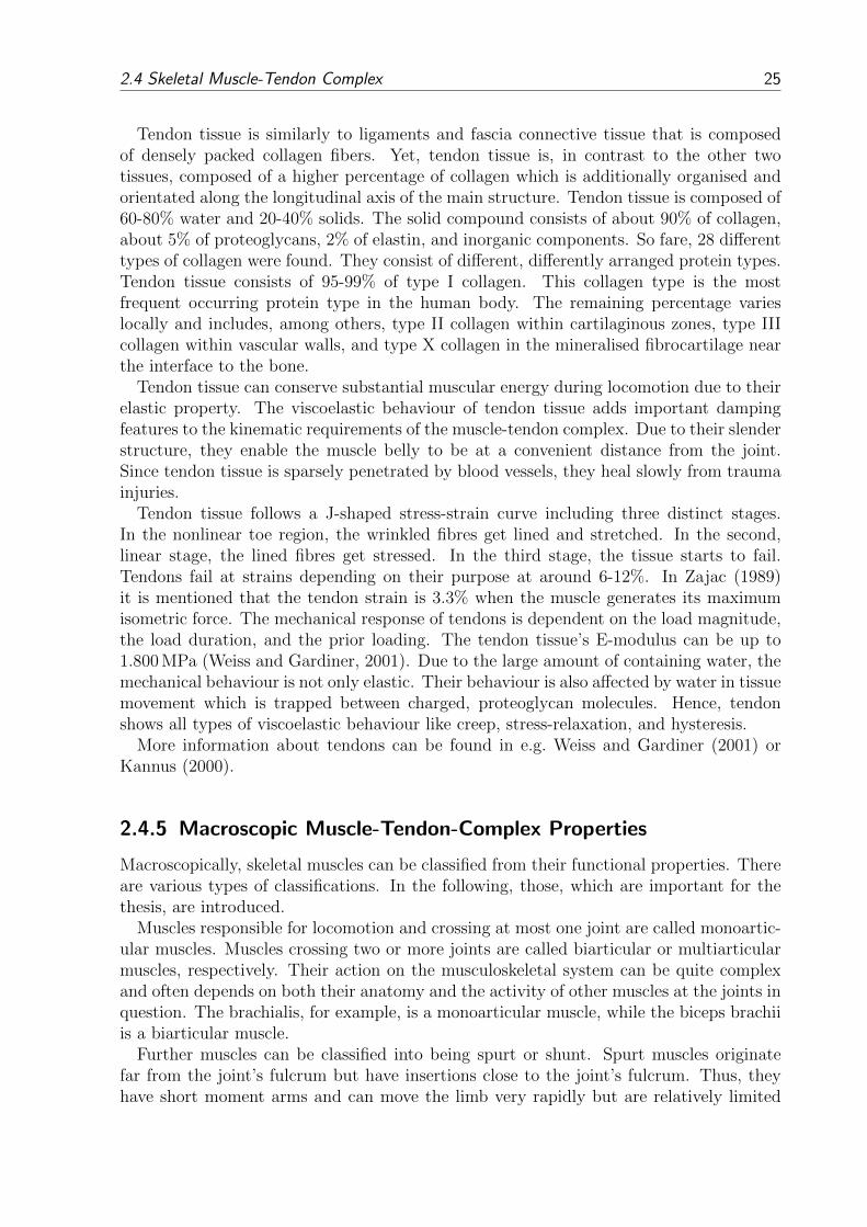
2.4 Skeletal Muscle-Tendon Complex 25
Tendon tissue is similarly to ligaments and fascia connective tissue that is composedof densely packed collagen fibers. Yet, tendon tissue is, in contrast to the other twotissues, composed of a higher percentage of collagen which is additionally organised andorientated along the longitudinal axis of the main structure. Tendon tissue is composed of60-80% water and 20-40% solids. The solid compound consists of about 90% of collagen,about 5% of proteoglycans, 2% of elastin, and inorganic components. So fare, 28 differenttypes of collagen were found. They consist of different, differently arranged protein types.Tendon tissue consists of 95-99% of type I collagen. This collagen type is the mostfrequent occurring protein type in the human body. The remaining percentage varieslocally and includes, among others, type II collagen within cartilaginous zones, type IIIcollagen within vascular walls, and type X collagen in the mineralised fibrocartilage nearthe interface to the bone.
Tendon tissue can conserve substantial muscular energy during locomotion due to theirelastic property. The viscoelastic behaviour of tendon tissue adds important dampingfeatures to the kinematic requirements of the muscle-tendon complex. Due to their slenderstructure, they enable the muscle belly to be at a convenient distance from the joint.Since tendon tissue is sparsely penetrated by blood vessels, they heal slowly from traumainjuries.
Tendon tissue follows a J-shaped stress-strain curve including three distinct stages.In the nonlinear toe region, the wrinkled fibres get lined and stretched. In the second,linear stage, the lined fibres get stressed. In the third stage, the tissue starts to fail.Tendons fail at strains depending on their purpose at around 6-12%. In Zajac (1989)it is mentioned that the tendon strain is 3.3% when the muscle generates its maximumisometric force. The mechanical response of tendons is dependent on the load magnitude,the load duration, and the prior loading. The tendon tissue’s E-modulus can be up to1.800 MPa (Weiss and Gardiner, 2001). Due to the large amount of containing water, themechanical behaviour is not only elastic. Their behaviour is also affected by water in tissuemovement which is trapped between charged, proteoglycan molecules. Hence, tendonshows all types of viscoelastic behaviour like creep, stress-relaxation, and hysteresis.
More information about tendons can be found in e.g. Weiss and Gardiner (2001) orKannus (2000).
2.4.5 Macroscopic Muscle-Tendon-Complex Properties
Macroscopically, skeletal muscles can be classified from their functional properties. Thereare various types of classifications. In the following, those, which are important for thethesis, are introduced.
Muscles responsible for locomotion and crossing at most one joint are called monoartic-ular muscles. Muscles crossing two or more joints are called biarticular or multiarticularmuscles, respectively. Their action on the musculoskeletal system can be quite complexand often depends on both their anatomy and the activity of other muscles at the joints inquestion. The brachialis, for example, is a monoarticular muscle, while the biceps brachiiis a biarticular muscle.
Further muscles can be classified into being spurt or shunt. Spurt muscles originatefar from the joint’s fulcrum but have insertions close to the joint’s fulcrum. Thus, theyhave short moment arms and can move the limb very rapidly but are relatively limited

26 Chapter 2: Musculoskeletal System
in the magnitude of effective strength. Shunt muscles, on the other hand, originate closeto the joint and have insertions far from the joint. This entails large moment arms andstabilising effects on the joint. Example for both types can be found at the upper limb;the biceps brachii is a spurt muscle and the brachioradialis is a shunt muscle.
Muscles can also be described by the direction the muscle fibres run in. While the musclefibres within a single fascicle are parallel, the organisation of fascicles in the skeletal musclecan vary, as can the relationship between the fascicles and the associated tendon. Thereare four distinct patterns of fascicle organisation in the skeletal muscle. They can formparallel muscles, convergent muscles, pennate muscles and circular muscles. Each of thedifferent muscle architectures are depicted in Figure 2.11 by means of one representativemuscle.
Figure 2.11: The macroscopic arrangement of fibres is called the muscle fibre architecture.Possible architectures are shown including a specific muscle as an example. Source: OpenStaxCollege (2013)
Most of the skeletal muscles in the human body are parallel muscles (Martini andNath, 2008). In a parallel muscle, the fascicles are arranged axially along the musclesbelly. Some are flat bands with broad attachments at each end. Others are plump andcylindrical with tendons at one or both ends. For that case, the muscle is spindle-shapedand is called fusiform, cf. Figure 2.11 on the middle-left or in Figure 2.12a, with a centralbody, also known as the belly or gaster. As the fibres are parallel to the muscles belly, acontracting muscle roughly shortens to the same amount than fibres do (ca. 30%).
In a convergent muscle, see Figure 2.11, the muscle fibres typically spread out, like a

2.4 Skeletal Muscle-Tendon Complex 27
fan or a broad triangle. All fibres converge at a common attachment site. A convergentmuscle has a larger versatility in its line of action, because the stimulation of only onecompartment of the muscle can strongly change the direction of pull. However, whenthe entire muscle contracts, the muscle fibres do not pull as hard on the attachment siteas a parallel muscle of same size, because it does not have one prominent muscle fibredirection.
In a pennate muscle, the fascicles form a common angle with the tendon, the pennationangle. If all muscle fibres are on the same side of the tendon, the pennate muscle is calledunipennate, see Figure 2.11 and Figure 2.12b. As the pennate muscle fibres pull at thisangle, the variation of the fibre length will be smaller than in a parallel muscle. Yet, theresulting force is larger, as the number of possible contracting fibres in the same cross-section is larger in a pennate muscle than in a parallel muscle. Bipennate muscles, seeFigure 2.11 and Figure 2.12c, have fibres on both sides of the tendon. When the tendonbranches within a pennate muscle, the muscle is said to be multipennate, see Figure 2.11.
Due to the anisotropic properties of skeletal muscle, the muscle cross-section can bedescribed in two different ways. The physiological cross-sectional area (PCSA) is thearea of the cross section of a muscle perpendicular to its fibres, generally at its largestpoint. It is typically used to describe the contraction properties of pennate muscles. Theanatomical cross-sectional area (ACSA), on the other hand, is the area of the cross-sectionof a muscle perpendicular to its longitudinal axis. In a non-pennate muscle, in which thefibres are parallel to the longitudinal axis, the PCSA coincides with the ACSA, compareFigure 2.12.
(a) fusiform (b) unipennate (c) bipennate (d) multi-pennate
Figure 2.12: Different fibre architectures are indicated by the orientation of the red lines whichrepresent the fibre running from origin to insertion. The black, bold lines indicate the tendontissue. The difference between PCSA (green) and ACSA (blue) is defined by their differentorientation with respect to the muscle longitudinal line and muscle fibre, respectively.
When a muscle fibre is stimulated, it contracts. Yet, the macroscopic behaviour ofthe muscle does not have to shorten. Therefore, voluntary muscular contractions may beclassified according to length changes (concentric, eccentric, and isometric), force levels(isotonic), or contraction dynamics (isokinetic): A contraction is considered
concentric, when the muscle force and the resulting motion are in the same direction,

28 Chapter 2: Musculoskeletal System
i.e., the sarcomere and the muscle shorten.
eccentric, when the muscle force and the resulting motion are contradicting, i.e., eventhough the sarcomeres are pulling, the length of the muscle increases.
isometric, when the muscle force does not lead to a resulting motion, i.e., even thoughthe sarcomeres are pulling, the length of the muscle is constant.
isotonic, when the muscle force is constant independent of the direction of motion of themuscle.
isokinetic, when the muscle changes its length with constant speed.
In a musculoskeletal system, locomotion is enabled by linking muscle-tendon tissue tobones. In conjunction with joints, these three elements build a lever system. A lever isa rigid rod or beam that is able to rotate about a fixed point called the fulcrum whereboth a force (or an effort) and a load (or a resistance) act. The force which moves thelever is called the effort. The force to be moved or overcome is called the resistance. Theperpendicular distance between the load and effort to the fulcrum is called lever arm.Depending on the relative position to each other, three different types can be categorisedleading to different specifications:
effort resistancefulcrum
(a) Class 1 lever
effort resistance fulcrum
(b) Class 2 lever
effortresistance fulcrum
(c) Class 3 lever
Figure 2.13: Depending on the set-up of effort, resistance, and fulcrum different types of leverscan be defined. Each type has its advantages and disadvantages.
Class 1: The fulcrum lies between the effort and the resistance. Depending on the lengthof each lever arm the effort to resistance ratio is larger or smaller than one. Whenthe lever arm of the effort equals the one of the resistance, then the ratio is one. Anexample in our body is when the triceps brachii pulls on the forearm.
Class 2: The resistance lies in the middle. Hereby, the effort’s lever arm is always largerthan the one of the resistance. This leads to a low effort to resistance ratio andimplies a slow resulting motion as the effort needs to move more than the resistance.On the other hand, high resistances can be overcome. An example can be found inour feet when we stand on our toes and lift our heels off the ground.
Class 3: The effort lies in the middle. Hereby, the resistance’s lever is always longer thanthe one of the effort. This leads to high efforts to resistance ratios and implies arapid resulting motion. An example is the biceps brachii pulling on the forearm.

3 Continuum-Mechanical Fundamentals
As biological tissue can undergo large deformations, the Theory of Finite Elasticity pro-vides the mathematical framework to describe the deformed state of the system to inves-tigate. For theoretical aspects leading beyond the presented theory, the reader is referredto standard continuum mechanics text books such as for example Holzapfel (2000) orFung and Tong (2001).
3.1 Finite Elasticity
3.1.1 Kinematical Relations
The material body B is a manifold of connected material points P . This material bodyis embedded in an Euclid ian space including a fixed origin O. Every material point Pin B has at any time t a unique position defined by its placement function χ(P , t) = x.For all material points in B, this state is called the current configuration. At the initialtime t0 = 0, the material points P are said to be in their reference configuration which isdefined by X = χ(P , t0).
The material points at the boundary of B define the surface ΓB. At the surface differentkinds of boundary conditions can be applied. The boundary where Dirichlet conditionsare applied is called ΓuB and the boundary where Neumann conditions are applied is calledΓσB. These boundaries are mutually exclusive and together form the entire surface, thatis ΓB = ΓuB ∪ ΓσB and ΓuB ∩ ΓσB = ∅.
e1
e2
e3
X x
u
χ(P, t)
P
P
ΓuB
ΓσB
B0
t = t0 t > t0
reference configuration actual configuration
O
Figure 3.1: Kinematics of a body B.
The motion of a material point can be described in different ways. In a material orLagrangean description the behaviour refers to a material point, whereas in a spatial
29
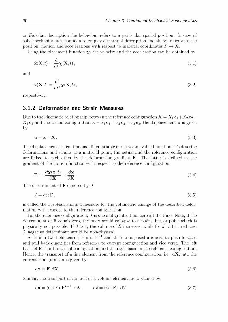
30 Chapter 3: Continuum-Mechanical Fundamentals
or Euler ian description the behaviour refers to a particular spatial position. In case ofsolid mechanics, it is common to employ a material description and therefore express theposition, motion and accelerations with respect to material coordinates P → X.
Using the placement function χ, the velocity and the acceleration can be obtained by
x(X, t) =d
dtχ(X, t) , (3.1)
and
x(X, t) =d2
dt2χ(X, t) , (3.2)
respectively.
3.1.2 Deformation and Strain Measures
Due to the kinematic relationship between the reference configuration X = X1 e1+X2 e2+X3 e3 and the actual configuration x = x1 e1 + x2 e2 + x3 e3, the displacement u is givenby
u = x−X . (3.3)
The displacement is a continuous, differentiable and a vector-valued function. To describedeformations and strains at a material point, the actual and the reference configurationare linked to each other by the deformation gradient F. The latter is defined as thegradient of the motion function with respect to the reference configuration:
F :=∂χ(x, t)
∂X=∂x
∂X. (3.4)
The determinant of F denoted by J ,
J = det F , (3.5)
is called the Jacobian and is a measure for the volumetric change of the described defor-mation with respect to the reference configuration.
For the reference configuration, J is one and greater than zero all the time. Note, if thedeterminant of F equals zero, the body would collapse to a plain, line, or point which isphysically not possible. If J > 1, the volume of B increases, while for J < 1, it reduces.A negative determinant would be non-physical.
As F is a two-field tensor, F and F−1 and their transposed are used to push forwardand pull back quantities from reference to current configuration and vice versa. The leftbasis of F is in the actual configuration and the right basis in the reference configuration.Hence, the transport of a line element from the reference configuration, i.e. dX, into thecurrent configuration is given by:
dx = F dX . (3.6)
Similar, the transport of an area or a volume element are obtained by:
da = (det F) FT−1 dA , dv = (det F) dV . (3.7)

3.1 Finite Elasticity 31
With the definition of the deformation gradient and the transport equations of the cur-rent line element, the Cauchy-Green deformation tensors can be introduced. Consideringthe squared lengths of a line element in the current and reference configuration,
‖dx ‖2 = dx · dx = (F dX) · (F dX) = dX · (FTF) dX
= dX ·C dX , (3.8)
‖dX ‖2 = dX · dX = (F−1 dx) · (F−1 dx)
= dx · (FT−1F−1) dx
= dx ·B−1 dx , (3.9)
the right Cauchy-Green deformation tensor, C, in reference configuration, and the leftCauchy-Green deformation tensor, B, in the current configuration are defined.
By replacing the right and left Cauchy-Green deformation tensor by the product of Fand conducting the polar decomposition on F, the right and left Cauchy-Green deforma-tion tensor can be transformed to:
C = FTF = (QU)TQU = UT (QTQ)U = UU , (3.10)
B = FFT = VQ(VQ)T = V(QQT )VT = VV , (3.11)
where Q ∈ SO3 is a proper orthogonal rotation tensor with the properties det Q = 1 andQT = Q−1, while U and V are the symmetric positive definite right (material) and left(spatial) stretch tensors, respectively. One can see that the Cauchy-Green deformationtensors only depend on the stretch tensors and not on the rigid-body rotations. Thisproperty will be used later on for the material objectivity in Section 4.2.
While the deformation tensors describe the state of deformation itself, a strain measurerelates the length in the current configuration to the length in the reference configuration.Therefore, by relating the length of infinitesimal small line elements, i.e.,
‖ dx‖2 − ‖ dX‖2 = dX ·C dX− dX · dX = dX · (C− I) dX ,
= dx · dx− dx ·B−1 dx = dx · (I−B−1) dx .(3.12)
the Green-Lagrangean strain tensor E and the Almansian strain tensor A can be definedby:
E := 12(C− I) and A := 1
2(I−B−1) . (3.13)
The factor one half is historically motivated and results from the fact, that the lin-earisation of E and A around the natural state (zero deformation) should result in theengineering strain tensor ε.
Spectral Representation of the Deformation Tensors
It is often convenient to employ the spectral representation of the deformation tensorsto describe constitutive laws for the material behaviour. This is particularly the case forhyperelastic material laws.
As introduced in Equation (3.10) and (3.11), C and B are both products of F, and varyonly by a proper orthogonal rotation, i.e. by Q and QT . Therefore, it can be shown that

32 Chapter 3: Continuum-Mechanical Fundamentals
C and B have the same eigenvalues λi, which are the squares of the principle stretches.Furthermore, due to the relation of U to C and V to B, they all have the same mutuallyorthogonal eigenvectors mi and ni, i.e.
(C− λi I) mi = 0 ,
(B− λi I) ni = 0 .(3.14)
Applying the Caley-Hamilton theorem to
det(C− λiI) = det(B− λiI) = λ3i − I1 λ
2i + I2 λi − I3 = 0 , (3.15)
one obtains
I1 = tr C = tr B = F · F ,I2 = tr (cof C) = tr (cof B) = cof F · cof F ,
I3 = det C = det B = (det F )2 ,
(3.16)
where cof(·) is the cofactor of a tensor.Three real-valued eigenvalues λi with i = 1, 2, 3 are obtained from the symmetric de-
formation tensors. The invariants can be related to the eigenvalues by
I1 = λ1 + λ2 + λ3 ,
I2 = λ1 λ2 + λ2 λ3 + λ1 λ3 ,
I3 = λ1 λ2 λ3 .
(3.17)
3.1.3 Stress Measures
While a material body is deformed, stress is the quantity expressing the internal, mechan-ical state of each material point P to its neighbours within the body B. The unit of stressis force per area. As forces can be related to areas in the reference or actual configuration,different stress tensors can be introduced.
Cauchy ’s fundamental lemma states that a tension vector t can be found at any cutfree surface of a body, that depends in time, space and orientation on the surface normalvector n, i.e.
t(x,n, t) = −t(x,−n, t) . (3.18)
The traction vector t describes the impact of the force acting on the surface ΓB of the bodyB. If one observes the static equilibrium at an infinitesimal tetrahedron, one obtains theCauchy theorem. It reformulates the surface traction vector t(x,n, t) in a more convenientquantity, the stress tensor T(x, t). The traction vector t is the projection of T on theoutward unit surface vector n in the current configuration. The stress tensor T is calledCauchy or true stress tensor. Cauchy ’s theorem states:
t(x,n, t) = T(x, t) n . (3.19)
The incremental surface force, dfs, is given by
dfs = t da = (T n) da = T da. (3.20)

3.2 Balance Relations 33
n
-n
x
x
t (x,n, t)
−t (x,−n, t)
Figure 3.2: Cauchy’s Fundamental Lemma: Cut off surface of a body.
Introducing a weighted area da =dV
dvda = (det F)−1 da, one obtains the weighted or
Kirchhoff stress τ ,
dfs = T (det F) da = τ da. (3.21)
Pulling the second basis of the Kirchhoff stress back by a co-variant transport, one getsthe nominal or 1st Piola-Kirchhoff stress P. This tensor is a two-field tensor with onebasis in each configuration and therefore not symmetric. Yet, for experimental purposes,it is very often convenient, as it relates the measured force to the area in reference con-figuration.Further, pulling back the first basis of the 1st Piola-Kirchhoff stress, one obtains the 2nd
Piola-Kirchhoff stress. As both basis of this stress tensor are in the reference configura-tion, the stress tensor is symmetric:
P = τ FT−1 = (det F) T FT−1 , (3.22)
and
S = F−1 P = (det F) F−1 T FT−1 . (3.23)
3.2 Balance Relations
Conservation equations are based on the fact that conserved quantities cannot be producednor lost in a closed system. If additional external influences, as fluxes and productionterms, on the system are taken into account, one speaks of balance equations, i.e. thebalance of mass, momentum, moment of momentum, and energy. Each balance law canbe stated in a global or local form.
34 Chapter 3: Continuum-Mechanical Fundamentals
3.2.1 Mass Balance
For this work, the mass balance is not employed explicitly. The mass balance in its globaland conserved form for the body B is axiomatically introduced by
d
dt
∫ΩB
ρ dv = 0 . (3.24)
After some mathematical transformations, the local form can be stated as
ρ+ ρ div x = 0 , (3.25)
where ρ = ρ J−1 for solid mechanics. This equation can be interpreted as the temporalchange of mass, which has to be zero for a closed system, and is equal to the sum of whatflows into and leaves the system.
3.2.2 Momentum Balance
The second balance equation is the momentum balance, in which the temporal change ofthe momentum ρ x is balanced with the surface and body forces acting on the body B.In global form, the balance equation is defined by
d
dt
∫ΩB
ρ x dv =
∫ΓB
T n da+
∫ΩB
ρb dv . (3.26)
Reformulating the momentum balance by inserting the mass balance, employing Cauchy ’stheorem (3.18), and the divergence theorem for the flux term, Equation (3.26) yields,∫
ΩB
ρ x dv =
∫ΩB
div T dv +
∫ΩB
ρb dv . (3.27)
This relation holds for any volume dv. Hence, the local form reduces to:
ρ x = div T + ρb , (3.28)
which is valid for every point x within the volume dv at time t.
3.2.3 Moment of Momentum Balance
The moment of momentum balance or angular momentum balance accounts for the tem-poral change of the moment of momentum x × ρx with the inner and outer momentsacting on the body. In global form, the balance reads
d
dt
∫ΩB
(x× ρx) dv =
∫ΓB
(x×T)n da+
∫ΩB
(x× ρb) dv . (3.29)
By transforming the global balance, using the integral theorem and the momentum bal-ance as lower balance equation, the local form yields
0 = I×T ⇐⇒ T = TT . (3.30)
Equation (3.30) yields that the Cauchy stress tensor is symmetric.

3.2 Balance Relations 35
3.2.4 Energy Balance
The energy balance, also known as the first thermodynamical balance law, indicates theconservation of energy. If a non-isothermal problem is considered, energetic quantities alsohave to be balanced. The equation balances the temporal change of the sum of internaland kinetic energy with the power resulting from the surface and body forces as well asthe heat efflux over the boundary and the heat supply in the body. The global energybalance reads
d
dt
∫ΩB
(e + 12x · x) dv =
∫ΓB
[(T x− q) · n ] da+
∫ΩB
[ρ (x · b) + r] dv . (3.31)
Therein, e represents the mass specific internal energy, q is the heat efflux and r is theexternal heat supply from a distance. The local balance reads after using the lowerbalances and the integral theorem as follows:
ρ e = T · L− div q + ρ r . (3.32)
Herein, L is the spatial velocity gradient, T ·L is the stress power, and div q representsthe heat flux over the boundary, respectively.
Stress Power and Energetic Conjugates
The product of stress and strain rates are often called the rate of internal work or thestress power, as it was introduced in Equation (3.32).
If only mechanically-related quantities are considered in Equation (3.32), this equationcan be rewritten to
d
dt
∫ΩB
1
2ρ x · x dv +
∫ΩB
T · L dv =
∫ΓB
t · x da+
∫ΩB
ρb · x dv . (3.33)
The first term defines the kinetic energy of B, the second term the internal mechanicalpower, or stress power, and the right-hand side defines the external mechanical power.
Further, it can be observed that the scalar product of stress and strain in the secondterm and their rates within the same configuration are invariant with respect to thetransport to another configuration. These pairs are called energetic conjugates if theirdot product accurately reflects the stored strain energy in the system. As in a Lagrangeansetting, the specific stress power is defined with respect to the reference configuration, theconjugate pair, defined by T · L, can be pulled back to
Pint =
∫ΩB
T · L dv =
∫ΩB
T · L det F dV =
∫ΩB
τ · L dV . (3.34)
With some algebraic tensor transformations, conjugate pairs for P and S, i.e. P, F andS, E, can be formulated in a similar way.
For conserved systems, the same procedure can be done for the mechanical or strainenergy. The resulting conjugate pairs are τ ,A, P,F, and S,E.

4 Constitutive Model
In the preceding theoretical parts of this thesis, the fundamentals for the kinetics(Section 3.1.1) and balance relations (Section 3.2) are derived materially independent.By the introduced balance relations, the emerging initial-boundary-value-problem (IVBP)can only be solved if the problem is well posed. This property poses several requests onthe partial differential equations, the initial, and boundary conditions. One of the moretrivial requests are that the number of unknowns need to equal to the number of posedequations. In order to solve the momentum balance a relation between stress and strainneeds to be provided. In the following chapter, the mechanical material behaviour of askeletal muscle is introduced to meet this requirement.
4.1 Skeletal Muscle Constitutive Modelling Assumptions
Following the status quo of skeletal muscle modelling, the mechanical behaviour of askeletal muscle can be deduced from the physiological character of the skeletal muscle.In general, there are two possible approaches: a phenomenological and a biophysical, seeSection 1.2.1. Within this thesis, a purely phenomenological approach is chosen.
As this thesis deduces a framework for a multi-muscle musculoskeletal system employingcontinuum mechanical muscles, the choice of a specific skeletal muscle model is not of firstpriority. Hence, a rather simple skeletal muscle model is employed, in which the muscleactivation dynamics and cellular effects are neglected. This shall not be a limitation tothis work. All methodologies developed as part of this work also hold for more complexskeletal muscle models like the chemo-electro-mechanical skeletal muscle model proposedby Heidlauf and Rohrle (2014).
From a continuum-mechanical point of view, skeletal muscles are commonly assumedto be hyperelastic and transversely isotropic. Most of biological materials, so are skele-tal muscles, are water saturated and under natural occurring loads incompressible, seeSection 1.2.1.
As the muscle is assumed to be hyperelastic, all processes are assumed to be reversibleand isothermal. Hence, firstly, hysteresis effects are not considered. Secondly, even thoughthe muscle activates and contracts, no energy dissipating effect are taken into considera-tion. Furthermore, as the velocities and accelerations are assumed to be small (x, x ≈ 0),only slow motions are considered. Therefore, inertia terms and viscous effects are ne-glected and a quasi-static formulation is chosen. Furthermore, as the velocity is consid-ered to be small, the muscle’s behaviour is independent of the contraction velocity andthe force-velocity relation does not need to be considered.
The derivation of the most important anatomical skeletal muscle specific properties,such as the fibre distribution, the fibre orientation, the prestretch, and the definition ofthe values for different mechanical contributions, are defined in Chapter 7.
37

38 Chapter 4: Constitutive Model
4.2 Constitutive Model Principles
To define a thermodynamically consistent set of constitutive equations and to approximatethe observed behaviour of a real material under specific conditions, some requirementsneed to be set. These requirements are:
Determinism: The set of undetermined response functions, which have to be uniquelydefined at any time t is:
R = Ψ . (4.1)
As in this thesis only elastic effects are considered, the set of responds functionsreduces to a minimum.
Equipresence: The response functions may depend on the whole set of process variablesV , which are uniquely characterising the current and history state of the overallsystem with respect to temperature, chemical potentials, deformation and structuralcomposition. Considering the before mentioned assumptions, the set of processvariables reduces to
V = F,M,X, α , (4.2)
where M denotes the structural tensor. This set of variables uniquely definesany state of the overall body B. It represents the geometry in the current state(deformation), the reference state (to consider inhomogeneities as e.g. locally varyingfibre types), as well as the locally varying fibre field orientation of the skeletal muscle.
Local action: An object is only influenced directly by its immediate surrounding.
Material frame indifference: This principle is also called material objectivity. It statesthat material properties and therefore also the constitutive equations should notdepend on the position of the observer. The mathematical interpretation of suchan objectivity condition states that constitutive equations have to be invariant torigid-body rotations, for e.g. a rotation Q of the actual configuration.
?
Ψ (V) = Ψ(?
V) , (4.3)
where?
(·) indicates that the quantity in the actual configuration is rotated by Q ∈SO3. Following this requirements, some important implications for the constitutivelaw can be deduced.
The position vector in actual configuration reads,?x= Qx. Following this procedure,
the consequences for the deformation gradient are:
?
F=∂
?x
∂X=∂
?x
∂x
∂x
∂X= Q F with Q =
∂?x
∂x∈ SO3 . (4.4)
By this definition, F is not sufficing the material objectivity restriction. Further,it can be shown, that the structural tensor M and the reference position vector X
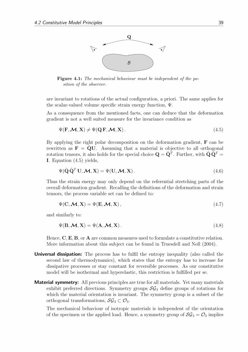
4.2 Constitutive Model Principles 39
Q
B
Figure 4.1: The mechanical behaviour must be independent of the po-sition of the observer.
are invariant to rotations of the actual configuration, a priori. The same applies forthe scalar-valued volume specific strain energy function, Ψ.
As a consequence from the mentioned facts, one can deduce that the deformationgradient is not a well suited measure for the invariance condition as
Ψ(F,M,X) 6= Ψ(Q F,M,X) . (4.5)
By applying the right polar decomposition on the deformation gradient, F can berewritten as F = QU. Assuming that a material is objective to all orthogonalrotation tensors, it also holds for the special choice Q = QT . Further, with Q QT =I. Equation (4.5) yields,
Ψ(Q QT U,M,X) = Ψ(U,M,X) . (4.6)
Thus the strain energy may only depend on the referential stretching parts of theoverall deformation gradient. Recalling the definitions of the deformation and straintensors, the process variable set can be defined to:
Ψ(C,M,X) = Ψ(E,M,X) , (4.7)
and similarly to:
Ψ(B,M,X) = Ψ(A,M,X) . (4.8)
Hence, C,E,B, or A are common measures used to formulate a constitutive relation.More information about this subject can be found in Truesdell and Noll (2004).
Universal dissipation: The process has to fulfil the entropy inequality (also called thesecond law of thermodynamics), which states that the entropy has to increase fordissipative processes or stay constant for reversible processes. As our constitutivemodel will be isothermal and hyperelastic, this restriction is fulfilled per se.
Material symmetry: All previous principles are true for all materials. Yet many materialsexhibit preferred directions. Symmetry groups SG3 define groups of rotations forwhich the material orientation is invariant. The symmetry group is a subset of theorthogonal transformations, SG3 ⊂ O3.
The mechanical behaviour of isotropic materials is independent of the orientationof the specimen or the applied load. Hence, a symmetry group of SG3 = O3 implies

40 Chapter 4: Constitutive Model
that the only possible structural tensor is M = I, and hence refers to an isotropicmaterial.
Materials for which the mechanical behaviour depends on the direction of eitherload or orientation of the specimen can be categorised into different classes in,e.g. transversely isotropy, orthotropy or prismatic isotropy.
Skeletal muscles are fibre reinforced materials with one or more preferred fibre di-rections, see Section 2.4.1. For this thesis, only muscles with one fibre family areconsidered, see Section 4.1. Materials with one fibre family are called transverselyisotropic. The symmetry group for transversely isotropic materials depends on theone preferred fibre direction, a0. The orientation of the fibre within B is defined bythe structural tensor, M = a0 ⊗ a0. For the structural tensor holds
M = MT , M = MM , trM = 1 . (4.9)
In consequence, SG3 for transverse isotropy is defined by
SG3 = ±I,Qξ1,Qξ2
,Qξ3,Q
(φ1)
ξ1
,Q(π)
ξ2
,Q(π)
ξ3
, ∀ 0 ≤ φ1 < 2π , (4.10)
where Qξ denotes the reflection tensor,
Qξ = I− 2 ξ ⊗ ξ ∀ ξ ∈ ξ1, ξ2, ξ3 . (4.11)
Here, ξ are mutually orthogonal unit vectors, and Q(φ)
ξcan be determined by the
Euler-Rodrigues formulas, i.e.
Q(φ)
ξ= ξ ⊗ ξ + sinφ (ξ × I) + cosφ(I− ξ ⊗ ξ) ∀ ξ ∈ ξ1, ξ2, ξ3 . (4.12)
ξ1
ξ2
ξ3
Q(φ1)
ξ1
Q(π)
ξ2
Q(π)
ξ3
B
Figure 4.2: Material symmetry for transversely isotropic materials.
Further information can be found in Spencer (1971) and the references therein.
As a consequence from the material symmetry, further invariants, other than the threeinvariants defined in 3.1.2, need to be introduced. Possible invariants for describing atransversely isotropic material are
tr C, tr C2, tr C3, trM, trM2, trM3 ,
tr (MC), tr (MC2), tr (M2 C), tr (M2 C2) .(4.13)
4.3 Skeletal Muscle Model 41
Remembering the properties of M, defined in Equation (4.9), some of the above men-tioned invariants do not need to be considered. Hence, the list of integrity bases reducesto
tr C, tr C2, tr C3 , tr (MC), tr (MC2) . (4.14)
The first three invariants of (4.14) do not provide any further information if compared tothe three invariance which are defined for the isotropic material in Section 3.1.2. There-fore, the following two additional invariants of (4.14)
I4 = tr (MC) , (4.15)
I5 = tr (MC2) , (4.16)
are sufficient to describe the transversely isotropic material behaviour. By reformulating(4.15), I4 yields,
I4 = tr (MC) = (a0 ⊗ a0)T ·C = a0 ·C a0 = F a0 · F a0 = a · a . (4.17)
Herein, I4 is the squared of the fibre stretch, where the stretch describes the actual lengthof the fibre. Hence, the fibre stretch, λ, can be determined by λ =
√I4. The remaining
invariant I5 has no physical meaning and will be omitted within this thesis.
4.3 Skeletal Muscle Model
As stated in Section 4.1, skeletal muscles are considered to behave hyperelastic. Hy-perelasticity implies, that the material behaves elastic (reversible) and that the currentdeformation state only depends on the current state and not on any history dependentvariables, i.e., a certain deformation state is not path dependent and reversible. Thisfurther implies, that the entropy η stays constant and that a potential energy exists. Thispotential is a measure for the elastic energy stored in the material. For an isothermaland isentropic1 system it can be shown, that the volume-specific strain energy function,Ψ, is a potential representing the mechanical energy. Therefore, by deriving the potentialenergy with respect to C, the 2nd Piola-Kirchhoff stress tensor deduces from the energeticconjugates by,
S =∂Ψ(E)
∂E=∂Ψ(C)
∂C
∂C
∂E= 2
∂Ψ(C)
∂C. (4.18)
For incompressible materials, Ψ can be decomposed into an isochoric and an deviatoricpart, i.e.
S = 2∂Ψ(I1, I2, I4)
∂C− ∂ [p (I3 − 1)]
∂C
= 2∂Ψ(I1, I2, I4)
∂C− pC−1 ,
(4.19)
1Characterises the constant amount of entropy of a system within a process.

42 Chapter 4: Constitutive Model
where the hydrostatic pressure p, is included as a Lagrangian multiplier to enable theincompressible condition det F − 1 = 0, see, for example, Holzapfel (2000). This incom-pressibility condition is subjected to the material as an internal constraint. This algebraicconstraint,
(√I3 − 1) = 0 , (4.20)
is employed by introducing the hydrostatic pressure, p, as an additional independentvariable. It can only be determined uniquely from the equilibrium equations and theboundary conditions.
Commonly, the overall strain energy for skeletal muscles is additively split into anisotropic matrix and an anisotropic term representing the mechanical behaviour in thedirection of the fibres, see Section 1.2.1 or Blemker et al. (2005); Oomens et al. (2003);Lemos et al. (2005); Rohrle et al. (2008):
Ψmuscle(I1, I2, I4) = Ψiso(I1, I2) + Ψaniso(I4) . (4.21)
For the isotropic contribution an incompressible Mooney-Rivlin (Rivlin, 1948; Mooney,1940) material formulation is chosen such that
Ψiso(I1, I2) = c1 (I1 − 3) + c2 (I2 − 3) . (4.22)
Herein, c1 and c2 are material parameters that are related to each other by the shearmodulus, µ = 2 (c1 + c2). The Mooney-Rivlin material description only fulfils the entropyinequality for c1 and c2 greater than zero. For more information about material laws usinginvariants, see Spencer (1971) or Holzapfel (2000).
The anisotropic term can be split into a passive and an active contribution, where theactive part is multiplied by the homogenised muscle activation parameter α = [0, 1]. Forα = 0 the muscle is passive or inactivated while for α = 1, the muscle is considered to befully activated or tetanised. For values 0 < α < 1, the activate contribution is linearlyinterpolated. The prescription of the muscle’s activation state is rather simple. Yet,including a more complex activation dynamics would further increase the numerical costswithout a methodological effect on the multi-muscle musculoskeletal system as proposedwithin this thesis. In summary, the anisotropic part of the strain energy function is definedby
Ψaniso(I4) = Ψpassive(I4) + α Ψactive(I4) . (4.23)
The strain energy function defining the passive force-length relation, Ψpassive, follows aJ-shaped material behaviour. It is approximated by a polynomial energy function intro-duced by Markert et al. (2005). The energy function meets the requirements of polycon-vexity (i.e. to guarantee the existence of a minimum), coercivity (i.e. the strain energy isconsistent with the growth conditions; Ψ → ∞ for I4 → 0 or I4 → ∞), and a stress-freereference state and is given by
Ψpassive =
c3
c4
(λ c4f − 1)− c3 lnλf if λf ≥ 1
0 else ,(4.24)

4.3 Skeletal Muscle Model 43
where λf is the muscle fibre stretch, i.e. λf =√I4, and c3 and c4 are material parameters.
The strain energy defining the force-length relation for the activated muscle, Ψactive, isdefined as a dimensionless force-length relation following the idea of Hatze (1978):
Ψactive = −σmax
νi(λopt
f ∆Wi)− 1νi
∞∫1
λoptf
∆Wiλνif
λ1νi−1
f e−λf dλf , (4.25)
where σmax is the stress which a maximally activated muscle can produce at optimal lengthλoptf , νi is the exponent and influences the steepness of the belly curve, and ∆Wi influences
the width of the belly curve. Both νi and ∆Wi do have an index i which represents thedata set for the ascending and descending part of the belly curve, respectively. Theexponential-like approach of Equation (4.25) replaces the more commonly used paraboliccharacteristic.
Taking the derivative of the strain energy functions with respect to the right Cauchy-Green tensor, cf. Equation (4.19), the separate terms of the 2nd Piola-Kirchhoff of theisotropic part is given by
Siso = 2 (c1 + I1 c2) I− 2 c2 C . (4.26)
To obtain the stress distribution of the anisotropic part, one needs to employ the chainrule as Ψaniso depends on λf . Hence,
Saniso(λf ) = 2∂Ψaniso
∂C= 2
∂Ψaniso
∂λf
∂λf∂I4
∂I4
∂C=
1
λf
∂Ψaniso
∂λfM =
1
λfPaniso M . (4.27)
In general, the nominal stress, P, is defined with respect to the principal directions,d = 1, 2, 3 by Pd = ∂Ψ(λd)
∂λd. As in this special case, the strain energy functions are scalar-
valued functions acting only along the fibre direction, the nominal stress, P, reduces to thescalar-valued function, Paniso, multiplied by the structural tensor M to take into accountlocal heterogeneities in the fibre distribution.Replacing P by the Cauchy stress, σ, Equation (4.27) results to
Saniso(λf ) =1
λ 2f
σaniso M . (4.28)
Inserting Equation (4.24) into Equation (4.27), the passive contribution of S is:
Spassive =
1
λ 2f
c3
(λ c4f − 1
)M if λf ≥ 1
0 else .(4.29)
The same applies for the active contribution of S, which is given by the following:
Sactive =
σmax
λ 2f
exp
−∣∣∣∣∣∣λf
λoptf
− 1
∆Wasc
∣∣∣∣∣∣νascM if λf ≤ λopt
f
σmax
λ 2f
exp
−∣∣∣∣∣∣λf
λoptf
− 1
∆Wdesc
∣∣∣∣∣∣νdescM if λf > λopt
f .
(4.30)

44 Chapter 4: Constitutive Model
The advantage of choosing this formulation over the other ones is the fact that one obtainsfor the single component a C1-continuous function. The qualitative stress contributionsare depicted for uniaxial constraints in Figure 4.3.
0.6 0.8 1 1.2 1.4 1.6−0.1
0
0.1
0.2
0.3
0.4
0.5
0.6
fibre stretch λ [−]
stre
ss [N
/mm
2 ]
isopassiveactivetotal
Figure 4.3: A qualitative representation of the Cauchy stress contributions for the uniaxial case.
If a stress free initial configuration is assumed, the initial pressure can be determinedby
Smuscle(χ, t = 0) = 2∂Ψmuscle(I1, I2, I4)
∂C− pC−1 = 0
= 2 (c1 + I1 c2) I− 2 c2 I + 0− p I .(4.31)
Using I1(t = 0) = 3, (4.31) reduces to the initial, scalar-valued pressure
p(χ, t = 0) = 2 c1 + 4 c2 . (4.32)
4.4 Muscle-Tendon Complex Model
In the following, a resourceful manner of defining a material constitutive equation fora muscle-tendon complex is introduced. This is achieved by introducing only two moreparameters to the skeletal muscle tissue constitutive equations introduced in Section 4.3.The first material parameter, called γM, distinguishes whether the tissue is muscle (γM =1) or tendon (γM = 0) and the second parameter, called γST, determines if the tissue ismuscle-tendon tissue (γST = 0) or some other soft tissue (γST = 1), like, for example, fat.Hence, the strain energy for tissue consisting of muscle, tendon and other soft tissue is isgiven by
ΨMTC = Ψiso + (Ψpassive + α γM Ψactive) (1− γST) . (4.33)
The different contributions of ΨMTC are exactly the same as defined in Section 4.3. Ap-plying Equation (4.19), the 2nd Piola-Kirchhoff of the muscle-tendon complex is,
SMTC = Siso + (Spassive + α γM Sactive) (1− γST) . (4.34)

4.4 Muscle-Tendon Complex Model 45
For γST = 1, the anisotropic part of the material behaviour vanishes. The soft tissue isassumed to behave as the isotropic part of the muscle tissue. Hereby, a relatively softmaterial is defined, where compressive forces will dominate due to the incompressibilitybehaviour of the tissue. For 0 < γST < 1, the material exhibits anisotropic behaviour.For γST = 0 and γM = 1, the material behaves to 100% like skeletal muscle tissue andcoincides with the material behaviour introduced in Section 4.3. For γST = 0 and γM =0, the material reduces to tendon tissue. For any other values between zero and one,a homogenised material behaviour of the mixture is obtained by linear interpolation.Further, the different tissue material parameters are enforced by a linear interpolation:
c1 = γM c1M + (1− γM) c1T ,
c2 = γM c2M + (1− γM) c2T ,
c3 = γM c3M + (1− γM) c3T ,
c4 = γM c4M + (1− γM) c4T .
(4.35)
Herein, ciM and ciT are the material parameters defined in Section 4.3 for the skeletalmuscle tissue and tendon tissue, respectively.

5 Finite Element Method in Space
Chapter 3 and 4 provide the fundamentals for the initial boundary value problem. Itconsists of the
• kinematic relations, providing the suitable strain measures (Section 3.1),
• definitions of stress (Section 3.1.3),
• local balance relations (Section 3.2), and
• constitutive equations for the skeletal muscle tissue (Chapter 4).
As quasi-static conditions are assumed, time contributions can be neglected. However,it is common to successively change the boundary conditions. Hereby, successively newBVP are declared to pretend a pseudo time-transient problem. Hence, all derivationswithin this chapter are carried out for one instant in time and the variable t indicating thecurrent deformation is omitted. While body forces are assumed to be small in comparisonto the internal forces, the strong formulation of the governing system reduces to:
div T = 0 . (5.1)
As it will be convenient for the contact formulation later on, Equation (5.1) is pulledback to the reference configuration, see Holzapfel et al. (2005). For the pull-back opera-tion, (5.1) is reformulated to its global form and the area and volume elements are pulledback using Equation (3.7). As the obtained formulation is independent of the choice ofthe volume element, the moment balance reads:
Div P(X) = 0 , where Div (·) :=∂(·)∂X· I . (5.2)
By including the constitutive behaviour and a complex geometry, the resulting systemleads to a second-order partial differential equation for the current position, x = χ(X).As this system cannot be analytically solved for most BVPs, an adequate numericalframework needs to be introduced. Here, the finite element method is used to discretisethe governing equations and the geometry. More information can be found in standardtext books of, for example, Bonet (1997) or Zhu et al. (2005).
5.1 Fundamentals
When the finite element method is applied to a boundary value problem, the procedurecan be classified into several distinct steps. Each of them will be briefly outlined. Thenumerical treatment is realised within CMISS and outlined in Section 5.2.
(i) Form the weak formulation based on the governing equations, here given in Equa-tion (5.2),
47

48 Chapter 5: Finite Element Method in Space
(ii) chose a suitable finite element ansatz (basis functions, Galerkin weights),
(iii) evaluate element integrals (calculate the element stiffness matrices and right-handside vectors),
(vi) assemble the global matrix,
(v) apply boundary conditions, and
(vi) solve the global system.
The first step is to formulate the weak formulation of the current problem. This step isimportant, as it is often impossible to find the correct solution of the strong formulation forthe primary variables of the PDE using efficient and suitable discretisation schemes. Theprimary variables are the unknowns, i.e. in our case the current position, x = χ(X) and thehydrostatic pressure, p, arising from the incompressibility condition of Equation (4.20).The generalised assembled strong or local form of the PDEs can be represented by:
Div P(X) = 0 ,√I3(X)− 1 = 0 .
(5.3)
To derive the weak formulation, the PDEs are multiplied by test functions δχ and δp andintegrated over the domain Ω0 resulting in the following equivalent global system,
Gχ =
∫Ω0
Div P(X) · δχ dV = 0 ,
Gp =
∫Ω0
(J(X)− 1) δp dV = 0 .(5.4)
Since Equation (5.3) has to be true, Equation (5.4) is true for any choice of δχ and δp.By integrating Equation (5.4)1 by parts, the order of the operator of the primary variableis lowered by one and the order of the operator of the test function is increased by one:
Gχ =
∫Ω0
Div P(X) · δχ dV
=
∫Ω0
P(X) ·Grad δχ dV −∫Γ0
t0 · δχ dA = 0 .
(5.5)
As a result of the integration by parts, Gχ now contains a volumetric part and a partassociated with the boundary, at which the initial traction vector t0 is applied as Neumannboundary condition. Equation (5.4)2 of Gp is left untouched.
As the following procedure is in principle the same for both equations in Equation (5.4),the following procedure will be exemplarily explained using Equation (5.4)1.
In order to obtain bounded results for the variational formulation, the first derivativesof the trial functions, Sχ and test functions Sp need to be square-integrable on the domainΩ0. This requirement is satisfied, if the functions are assumed to be H1(Ω).
S := χ ∈ H1(Ω)d : χ(X) = χ(X) on Γ ,T := δχ ∈ H1
0(Ω)d : δχ(X) = 0 on Γ , (5.6)

5.1 Fundamentals 49
Herein, d ∈ 1, 2, 3 is an integer denoting the dimensions in space and χ denote thevalue of the Dirichlet boundary condition as the Dirichlet boundary conditions need tobe satisfied exactly.
The defined trial spaces, S, and test spaces, T , have to be approximated by an N-dimensional subspace Sh and T h, respectively. The discrete trial and test function aredefined by:
χ(X) ≈ χh(X) = χh(X) +N∑i=1
φhi (X) Ci ∈ S ,
δχ(X) ≈ δχh(X) =N∑i=1
ψhi (X) δCi ∈ T ,
(5.7)
where χh denotes the Dirichlet boundary condition, φhi and ψhi are the global basis
functions of the respective ansatz and test functions for the node i, which only dependon X, N indicates the total number of nodal points in the mesh, and Ci and δCi arethe vector-valued coefficients of dimension RN×1 of the discretised geometrical primaryvariables.
The basis functions are linearly independent and chosen in such a way, that the nodalvalue is equal to one at the node itself, while the nodal value for all surrounding nodesare equal to zero.
φhi (Xj) = δij with i, j = 1, . . . , N . (5.8)
With this property, the coefficients of the discretised primary variables coincide with thenodal values of the primary variables, χ(Xi) and the nodal values of the test function,δχi. Hence,
Ci ≡ χ(Xi) , and δCi ≡ δχ(Xi) . (5.9)
With this definition at hand, Equation (5.5) is discretised. As the number of unknownsequals the number of equations, the discretised PDE is, in principle, ready to be solved.Yet, the integration of Equation (5.5) still poses a problem. The finite element methodprovides a widely used solution to this issue. By partitioning the solution space of theproblem into a sum of small problems, Equation (5.5) is formulated with respect to asubdomain Ωe of finite size. The domain Ω0 is approximated by a spatially discretiseddomain Ωh, which consists of E discretised, non-overlapping elements of finite size, Ωh
e ,
Ω0 ≈ Ωh =E⋃e=1
Ωhe . (5.10)
The discretised small domains, Ωhe , are called finite elements. The union of Ωh
e forms theFE mesh. The elements are spanned by the nodes Ne, belonging to the element Ωh
e . Asthe choice of the basis functions to represent the different primary variables does not haveto be the same, the number of nodes, Ne, where the primary variable are defined, canvary. The number of nodes for the spatial variable and for the hydrostatic pressure is Nχ
e
and Npe , respectively.
50 Chapter 5: Finite Element Method in Space
To discretise the nodal values within an element, the isogeometric mapping is employed.The basic idea of the isogeometric mapping is to map a discretised, arbitrary element,Ωhe , into a reference element Ω. If the element geometry is transformed by a function
of the same polynomial order as the ansatz function, the mapping describes the isopara-metric concept. If the order of the geometric transformation is higher, one refers to it assuper-parametric. In general, for each independent variable a different parametric trans-formation can be chosen. Within the scope of this work, the geometry and the currentconfiguration use quadratic ansatz functions and an isoparametric concept is chosen forthe placement function. The pressure is assumed to change linearly within an elementresulting in a super-parametric concept for the pressure. The reference element is definedby
Ne : Ω→ [0, 1]d , (5.11)
where Ne is the set of nodal basis functions for an element e,
Ne :=[N1(ξ), . . . , NNDoF
e(ξ)]T
, ∈ RNDoFe ×1 , (5.12)
where ξ are the local coordinates of the reference element. Furthermore, the nodal valuesof the nodes belonging to an element e are defined by
Xe :=[Xe1, . . . ,XeNDoF
e
], ∈ R3×NDoF
e . (5.13)
to utilise the isogeometric mapping,
Φe : Ω→ Ωhe , (5.14)
ξ 7→ Xe Ne(ξ) , with e = 1, . . . , E . (5.15)
The mapping satisfies,
Ωhe = Φe(Ω) , with e = 1, . . . , E . (5.16)
and has the Jacobian
Je = ∇Φe(ξ) = Xe
∇N1(ξ)...
∇NNDoFe
(ξ)
= Xe ∇Ne , ∈ R3×3 . (5.17)
Note, the basis functions, φhi , consist of contributions from Ne defined on differentelements.
With the definitions (5.11) to (5.15), the ansatz functions of an element Ωh can nowbe specified by choosing the appropriate nodal contributions belonging to this particularelement.
Separating the variational formulation into a sum over small domains, the problem isdefined by
f : Ω0 → R with f see Gχ,Gp from (5.4) , (5.18)∫Ω0
f dV ≈∫Ωh
f dV(5.10)=
E∑e=1
∫Ωhe
dVe
=E∑e=1
∫Ωhe
(5.16)= Φe(Ω)
f dVe =E∑e=1
∫Ω
f(Φe) | det(Φe)| dVe . (5.19)

5.1 Fundamentals 51
Herein, the first part is the exact statement and f is a placeholder for the variationalformulations. With the first step, the solution is approximated by the discretised solutionspace. The integration of the discretised domain is split into a sum of many small domainsusing Equation (5.10). Each of the E elements is mapped by the element routine from Ωh
e
to the reference element Ω by the isogeometric mapping, which is visualised in Figure 5.1.
ξ2
ξ1
x2
x1
Φe
Φ−1e
Ωhe
Ω
global
Figure 5.1: Geometric transformation of an arbitrary rectangular 2-d element with quadraticbasis functions Ωh
e to the reference element Ω, defined in local coordinates ξ.
Within the reference element, a numerical integration scheme, such as the Gauss ianquadrature scheme, is employed to compute the respective integrals. The numerical inte-gration, within one element, is carried out using K Gauss points. Each point k is weightedby the Gauss ian quadrature weights, wk, and the sum of the weighting factors is one. Theapproximation of the integration for one element reads:
(5.19) ≈E∑e=1
K∑k=1
wk f(Φe) | det(Φe)| (5.20)
Due to the fact that this integration is carried out on the element level with respect tothe spatial reference element, the integration points and the weighting factors are alwaysthe same.
Dirichlet and Neumann boundary conditions are considered in the global system. ForDirichlet boundary conditions, the nodes are known. Hence, its contribution can betransferred to the right-hand side and the matrix can be reduced. For the Neumannboundary conditions, the respective force contribution is directly added to the right-handside.
To solve the global problem, the element independent variable vectors are defined in 3dimensions as:
ue :=[χh(X1), . . .χh(XNχ
e)]T ∈ RNχ
e ×3 ,
ve :=[ph(X1), . . . ph(XNp
e)]T ∈ RNp
e ,
we :=[uTe ,v
Te
]T,
(5.21)
Even though the dimension of the we is not consistent, when a mixed-element formulationis used, the primary unknowns are stringed together to define the vectors, we on the

52 Chapter 5: Finite Element Method in Space
element level, and w on the global level. The global solution variable vectors are definedto:
u := [u1, . . . ,uNχe]T ∈ RNχ×3 ,
v := [v1, . . . ,vNpe]T ∈ RNp
,
w :=[uT1 , . . . ,u
TNχe, vT1 , . . . ,v
TNpe
]T.
(5.22)
After the PDE is spatially discretised, the emerging system is of size 3Nχ + Np andthe emerging global system of equations can be written as
Gχ = K(u)− f = 0 ,
Gp = g(v) = 0 ,(5.23)
where (5.23)2 is the algebraic side condition emerging from the incompressibility condition.Within the framework of finite elasticity, the emerging equations are still nonlinear.
Hence, linearisation is necessary. The Newton-Raphson method has proven to efficientlysolve the nonlinear set of equations. The Newton-Raphson method requires the firstderivative or tangent of the nonlinear functions. As the functions depend on more thanjust one variable, the directional derivative has to be applied, i.e. the observed function isderived with respect to each variable keeping the other variable constant at a distinct lo-cation. The tangent can be computed numerically or analytically. Within this framework,the constitutive equations are linearised numerically while the contact formulation usesan analytic tangent, cf. Section 6.1.3. As the numerical tangent is, within this framework,always determined in the reference configuration, the balance of momentum is used in thereference configuration.
5.2 Realisation within CMISS
The governing equations of finite elasticity for the FE muscle model are solved usingthe software package CMISS (Continuum Mechanics, Image analysis, Signal processingand System Identification), which is developed at the Auckland Bioengineering Institute,University of Auckland, New Zealand. The computational core of CMISS is called CM,which provides the necessary routines to assemble and solve the linear system. CMISS wasoriginally designed for modelling cardiac tissue in the late 1970s and was later extendedto model various biological soft tissues.
After sketching in the last section a general procedure of the finite element method, thefollowing section provides CMISS-specific implementation details. CM solves the global-assembled system of equations using the nodal residuals.
For this work, a Bubnov-Galerkin method is chosen. This implies that the same typeof basis functions for trial and test functions are chosen, i.e.
ψhi ≡ φhi . (5.24)
Assuming zero Neumann boundary in Equation (5.5), the nodal residual, Ri, can be

5.2 Realisation within CMISS 53
defined to:
Rχi =
∫Ωh
P(Xi)∂φχ,hi∂X
dV , ∈ R3 , with i = 1, . . . , Nχ . (5.25)
In case of a constrained node, the residuum at the constraint nodes represents the re-action force. Hence, after successfully solving the set of equations, by evaluating theseequations, which have been deleted during the matrix condensation, the node reactionforces are directly evaluable. Very often, so in this case, these forces are of big interestfor investigating the mechanical characteristics of the investigated system.
Following previous works using CMISS, the hydrostatic pressure is discretised linearlyfor optimally satisfying the inf-sub- or LBB (Ladyschenskaja-Babuska-Brezzi) condition(Nash and Hunter, 2000; Chung, 2008) as the spatial variables are discretised quadrati-cally. The residual for the hydrostatic pressure is defined to:
Rpi =
∫Ωh
(J(Xi)− 1) φp,hi (Xi) dV ∈ R1 , with i = 1, . . . , Np . (5.26)
Uniting the residuals emerging from Equation (5.4)1 and (5.4)2 similarly to the globalsolution vector of Equation (5.22)3, the element residual reads:
Re = [Rχe1T , . . . ,Rχ
eNχe
T , Rpe1T , . . . , Rp
eNpe
T ]T . (5.27)
The emerging system of equations is nonlinear in the sense, that it cannot be solved ina closed-form expression. Hence, a linearisation needs to be conducted. Within CMISS,the tangent stiffness matrix, K is computed by directly linearising the residuum using aNewton-Raphson method within each element. The element stiffness matrix, Ke is definedby
Ke =∂Re
∂we
=
∂Rχe1
∂χh(X1). . .
∂Rχe1
∂χh(XNχe)
∂Rχe1
∂p1
. . .∂Rχ
e1
∂pNpe
.... . .
......
. . . . . .
∂RχeNχ
e
∂χh(X1). . .
∂RχeNχ
e
∂χh(XNχe)
∂RχeNχ
e
∂p1
. . .∂Rχ
eNχe
∂pNpe
∂Rpe1
∂χh(X1). . .
∂Rpe1
∂χh(XNχe)
∂Rpe1
∂p1
. . .∂Rp
e1
∂pNpe
.... . .
......
. . . . . .
∂RpeNp
e
∂χh(X1). . .
∂RpeNp
e
∂χh(XNχe)
∂RpeNp
e
∂p1
. . .∂Rp
eNpe
∂pNpe
. (5.28)
Note that the elements, Rχei, within Re are vectors in space (Rχ
i ∈ R3), and that the
elements of the element stiffness matrix are∂Rχ
e1
∂χh(X2)∈ R3×3. Exemplary, the element
54 Chapter 5: Finite Element Method in Space
residual for node number one which is derived with respect to the geometric DoF of nodenumber two is
∂Rχe1
∂χh(X2)=
∂R1x
∂x2
∂R1x
∂y2
∂R1x
∂z2∂R1y
∂x2
∂R1y
∂y2
∂R1y
∂z2∂R1z
∂x2
∂R1z
∂y2
∂R1z
∂z2
. (5.29)
The tangent stiffness matrix can be approximated by a finite difference method
Kχeijd = ∂Rχ
ei
∂χh(Xj)≈ Rχ
ei(χh(Xj)+δed)−Rχ
ei(χh(Xj))
‖δed‖
with
e = 1, ..., E ,
i, j = 1, ..., (3Nχe ) ,
d = 1, 2, 3 ,
(5.30)
where δed is a small perturbation in a coordinate direction. Due to the algebraic side(incompressibility) condition, the resulting tangent stiffness matrix is not positive-definite(Hughes, 2012).
The measures defined on element level are assembled to a global matrix and vectors.With these measures at hand, the global system of linearised equations is given by:
K ∆w = −R with
K ∈ R(3Nχ+Np)×(3Nχ+Np) ,
∆w,R ∈ R(3Nχ+Np) ,(5.31)
where ∆w is the solution update. The initial estimate is typically set to be identicalto the reference configuration, while additionally the Dirichlet and Neumann boundaryconditions are applied. The initial pressure is, for a stress-free initial condition, definedby Equation (4.31).
The solution update is derived by inserting the global version of (5.28) in (5.31). Whenthe resulting equation is solved for witer+1, the solution update reads:
witer+1 = witer −(∂R
∂w
)−1
R = witer −K−1 R , (5.32)
until ‖R‖ < ε or ‖∆w‖ < ε. Within this work, the linearised system of equations issolved using a LU decomposition.

6 Contact Mechanics
In order to fully take advantage of the volumetric approach, a contact formulation isconsidered. The contact formulation provides a framework which enables the mechanicaldescription of the interaction of two or more deformable bodies. Therefore, including acontact formulation into a continuum-mechanical approach opposes purely kinematic anddynamic descriptions of contact, which would occur between rigid bodies.
The contact mechanical framework can be considered as an additional module withinthe continuum-mechanical finite element framework. There exists already a wide rangeof contact mechanics formulations including friction, adhesion and/or wear within static,quasi-static, or even under dynamic conditions, see Wriggers (2002) or Laursen (2002)and the references therein. These concepts can be decomposed into phenomena acting incontact normal direction, such as, for example, gap-functions, contact pressure, adhesion,or in tangential contact surface direction, such as friction or more complex actions suchas wear.
However, as the focus of this work is not on contact mechanics, a relatively simplecontact formulation is employed to describe the interaction of skeletal muscles and bones.Within this work, the contact formulation of Chung (2008) is used. The assumptions forthe contact formulation are:
(i) A quasi-static formulation is chosen for both the standard continuum-mechanicalframework as well as for the contact formulation.
(ii) Since bones (Section 2.1) are much stiffer than skeletal muscles (Section 7.2.2),bones are considered to be rigid, whereas the skeletal muscles are not.
(iii) An idealised frictionless contact formulation was chosen as frictional forces betweenbone and muscle are considered to be much smaller than the other acting forces.
It was not part of this thesis to develop and improve existing contact mechanics formula-tions. Yet, as the contact formulation is numerically quite challenging, a brief introductioninto the employed contact mechanics formulation is given in the following chapter. Fur-ther information on the specific implementation of contact within CMISS can be foundin Chung (2008), Rajagopal et al. (2008), or Saini (2012) and, of course, in standard textbooks, such as Wriggers (2002) or Laursen (2002).
6.1 Contact Mechanics Theory
For a contact-free formulation, the boundary conditions (displacements or force condi-tions) and their location of action are known a priori. For a formulation including con-tact, this is in general not the case, i.e. the locations of possible interactions, the resultingforces, or the subsequent motion of the boundaries need to be determined as a part of thesolution itself.
55

56 Chapter 6: Contact Mechanics
In Figure 6.1, the kinematics for a system of two bodies including contact is shownfor the time interval t ∈ [t0, t]. The first body BM , which is assumed to be rigid, iscalled “master”, whereas the second, elastic body BS is called “slave”. Each body has itsindependent placement function χi, i = M, S. Material points in BM are denoted byxM and material points in BS by xS.
e1
e2
e3
xS
xM
χS(XS , t)
χM (XM , t)
PS
PM
Γu
BS0
Γσ
BS0
ΓC
BS0
BS0
ΓC
BM0
BM0
t = t0 t > t0
reference configuration actual configuration
O
Figure 6.1: Kinematics of contacting bodies BM and BS, where contact might occur on thepredefined boundary is denoted by ΓCi , i = M, S.
While contact is included, a third section ΓCi , where possible contact may occur, needsto be introduced. Following the same conventions as for one body, the boundaries’ surfacesets are mutually exclusive and together constitute the entire surface:
Γi = Γui ∪ Γσi ∪ ΓCi
∅ = Γui ∩ Γσi ∩ ΓCi
for i = BM , BS . (6.1)
The concept of possible contact between the two bodies introduces new constraints thatare based on the following physical assumptions:
(i) Any material point of one body cannot occupy the same physical location as anymaterial point of the other body.
(ii) Any force resulting from one body penetrating the other is compressive and acts incontact surface normal direction of the imposing body.
In order to formulate these contact constraints, it is convenient to assign one surfaceas the one over which contact is parametrised. Here, the master surface is chosen tobe monitored with respect to the parametrised slave surface. Therefore, the contactconstraints are parametrised by xS ∈ ΓCBS , while the opposing surface ΓCBM needs to provide

6.1 Contact Mechanics Theory 57
O
xS
xM
nS
lS
1
lS
2
ξ1
ξ2
ΓCBS
ΓCBM
Figure 6.2: Minimum distance problem for two possibly interacting bodies. The slave surfaceis discretised by a 2-dimensional, generalised coordinate system ξ. The normal vector directsoutwards towards the master surface.
the additional information to complete the definitions. To determine the interactionbetween the opposing surfaces, first the corresponding points of xM on ΓBS need to beidentified.
In general, this is done according to the closest point projection. For a given pointxM ∈ ΓCBM , the closest point on the slave surface can be determined by finding the
shortest distance, d, between xM and a point xS at ΓCBS by:
dS =∥∥xM − xS
∥∥ = minxS(ξ)∈ΓCS
∥∥xM − xS(ξ)∥∥ ∀ xM ∈ ΓCBM , (6.2)
where ξ := ξ1, ξ2 denotes a parametrisation of the slave surface of a two-dimensionalconvective coordinate system, which is attached to the surface and therefore changes withthe deformation of the body.
The shortest distance can also be used to define the gap or penetration between thetwo functions. The point xS(ξ) at ΓCBS , having the shortest distance to the point xM atΓCBM is found by the necessary condition for the minimum of the distance function (6.2),which reads:
d
dξddS(ξ) =
xM − xS(ξ)∥∥xM − xS(ξ)∥∥ · ∂xS(ξ)
∂ξd= 0 for d = 1, 2 . (6.3)
The solution of (6.3) requires orthogonality between the two terms. As the covarianttangent vectors, lSd , of the convective coordinates lines, ξd, can be determined by,
lSd =∂xS(ξ)
∂ξdfor d = 1, 2 , (6.4)
which is the second term in (6.3), the first term in (6.3) must be parallel to the normalvector nS at xS, resulting in the location (ξ1, ξ2) on ΓCBS that exhibits the smallest gap ordistance. As a consequence, from (6.3) the condition can be reformulated to
−nS(ξ) · lSd (ξ) = 0 for d = 1, 2 , (6.5)

58 Chapter 6: Contact Mechanics
i.e. the current slave point xS(ξ) is the orthogonal projection of a given master point xM
onto the current slave surface ΓCBS . Employing the outward projection of the slave surface
at the location of the shortest distance (·), the outward unit normal vector can also bedetermined by:
nS =(lS
1 × lS
2 )∥∥∥lS1 × lS
2
∥∥∥ or nS =xM − xS(ξ)∥∥∥xM − xS(ξ)
∥∥∥ . (6.6)
Both relations can be used to determine the normal vector, nS. The second alternativeis a consequence from Equation (6.3) and (6.5). This alternative may be more convenientfor a penalty method, however it has the drawback that the outward unit normal vectoris not defined for d = 0, cf. Wriggers (2002).
After finding the location xS on ΓCBS , the gap function gN is defined by:
gN = nS · (xM − xS) . (6.7)
Note that a positive value of gN denotes penetration as nS is the unit outward normalvector, defined on the slave surface ΓCBS .
With the gap function at hand, the unregularised description of the frictionless contactformulation, also know as the Kuhn-Tucker conditions,
gN ≤ 0 ,tN ≥ 0 ,
tN gN = 0 .(6.8)
are defined. The first condition states that the gap function is always smaller than zero,i.e. no penetration is allowed (→ impenetrability condition). The second condition statesthat the emerging contact pressure, tN , is always positive and compressive. The last con-dition is called complementary condition and states that there should be only a contactcompression pressure, when contact really occurs. The conditions are visualised in Fig-ure 6.3. The first condition states that the red line is only on the negative wing of theaxis. The second condition states that the contact pressure rises vertically in the positivedirection. The third condition states the fact, that, for the unregularised description, acontact pressure only arises if gN = 0.
6.1.1 Weak formulation of the Contact Problem
First, recall that Equation (5.5) defines the principle of virtual work for one elastic body,i.e.
Gχ =
∫B0
P ·Grad δχ dV −∫
ΓB0
t0 · δχ dA ,
X = X on Γu ,
t0 = t0 on Γσ .
(6.9)
Considering contact mechanics between two bodies, a master BM and a slave BS, theoverall virtual work Gcoupled is defined by:
Gcoupled = GMχ + GSχ + GC , (6.10)

6.1 Contact Mechanics Theory 59
where GMχ and GSχ are the virtual work of the master and the slave, respectively, andGC is the contact residual which couples the two bodies, and completes the overall virtualwork for the contact problem. According to Laursen (2002), the contact residual GC forthe frictionless case is defined by
GC =
∫ΓCBS
tN δgN dA , (6.11)
where δgN is the variation of the gap function. The variation of the gap function δgN isdefined similarly to Equation (6.7) by
δgN = nS · (δχM − δχS) , (6.12)
where δχ is each body’s virtual displacements. The integral of Equation (6.11) is formu-lated on the slave surface ΓCBS , as the contact points are defined within that face.
6.1.2 Regularisation
The regularisation of a frictionless contact description (Kuhn-Tucker condition) is con-ducted employing the penalty method. Following Chung et al. (2008), a penalty method ischosen, which, compared to an augmented Lagrangean method, provides sufficient enoughaccuracy while reducing calculation effort. The regularised contact pressure is:
tN =
εN gN if gN ≥ 0
0 else ,(6.13)
where εN is a penalty factor. Note, for εN → ∞, the exact solution would be achieved.An εN that is chosen too small in comparison to the acting forces might allow the bodiesto penetrate. A too large εN might lead to a system that reacts too stiff and convergencemight fail.
tN
ǫN
0
“1”
gN
Figure 6.3: Regularisation of the penalty contact problem by a penalty approximation.

60 Chapter 6: Contact Mechanics
6.1.3 Linearisation
As the resulting system is nonlinear, it can be solved like before using the Newton-Raphsonmethod. Therefore, the directional derivative of Equation (6.11) for the frictionless con-tact formulation, using the penalty method for regularisation, needs to be defined. Incontrast to the non-contact contributions, the contact contribution is linearised by deriv-ing the analytical tangent according to Laursen (2002). The linearised term, ∆tN , for thecontact pressure, tN is defined by:
∆tN = εN H(gN) ∆gN , (6.14)
where H is the Heaviside step function.
6.2 Numerical Implementation within CMISS
According to Chung (2008), the numerical contact implementation within CMISS is basedon the node-to-face approach derived by Laursen (2002) which is identical to the closestpoint projection. The discretisation of the contact surfaces is defined similarly to the dis-cretisation of the volume. The only difference is obviously the reduction of one dimension,as surfaces are 2-dimensional objects.
Within the contact face of the master, NCe contact points (including the nodes) are
defined for each element. The contact points are equally spaced with respect to the localξ-coordinates. These contact points are projected onto the discretised face of the slaveto evaluate the gap function. Furthermore, the contact points serve as integration pointsover which the contact residuals for each element face RC
e are evaluated.Note that for this work, the order of geometric discretisation is chosen to be quadratic.
The elements are 27-node (tri-quadratic) hexahedrons, see Section 5.2. The face of suchan element contains 9 nodes. To allow an equally spaced number of contact points withinthat face, the number of contact points need to be odd. The number of contact points,NCe , is chosen to be NC
e = 7 · 7 = 49.The local coordinates are chosen to coincide with the convective coordinate system.
The location of the nodes at the master face of one element is described with respect tothe χ-coordinate and defined by
xMe (ξ) =9∑i=1
Ni(ξ) xMei . (6.15)
Herein, xe is similarly defined to Xe namely consisting of the set of nodes belonging toelement’s surface.
Using the closest projection algorithm, the surface contact points of the master are pro-jected onto the slave surface. The location of the projected nodes are defined identicallyto the nodes on the master surface. To distinguish the coordinates of the master and theslave, the coordinate of the slave are denoted by ξ to emphasise that the projected con-tact points are not pre-determined and equally spaced but determined by the projectionEquation (6.2). The discretisation is defined by
xSe (ξ) =9∑i=1
Ni(ξ) xSei . (6.16)

6.2 Numerical Implementation within CMISS 61
The tangent vectors at the projected points (on the slave surface) are computed usingthe discretisation scheme:
lSd =∂xS
∂ξd=
NCe∑
i=1
∂Ni(ξ)
∂ξdxSei for d = 1, 2 . (6.17)
These formulations are sufficient to compute for each contact point on the mastersurface the unit normal vector, n, which derives by (6.6), the coordinates of the projectedpoint at the slave surface xS(ξ), and the gap function, using Equation (6.7).
Further, for the non-contact contributions, also the virtual displacement for includingcontact is discretised by
δχje(ξ) =9∑i=1
Ni(ξ) δχjei for j = M,S . (6.18)
Inserting (6.18) into (6.12), δgN can be computed by
δgN(ξ) = n ·
(9∑
n=1
Ni(ξ) δχMei −9∑
n=1
Ni(ξ) δχSei
)= −δχC · φC ,
(6.19)
where χC and φC,h are introduced by
δχCe =[δχSe1, . . . , δχ
Se9, δχ
Se1, . . . , δχ
Se9
]T,
φCe =[NM
1 n, . . . , NM9 n,−NS
1 n, . . . ,−NS9 n]T
,(6.20)
to enable a compact formulation of Equation (6.19).Using the introduced measures, the contact residual can be introduced via the contact
contribution of the virtual work:
GC =
∫ΓCBS
tN δgN dA
= δχC∫
ΓCBS
tN φC dA
= δχC RC .
(6.21)
Whereas the contact residual is defined as,
RC =
∫ΓCBS
tN φC dA . (6.22)

62 Chapter 6: Contact Mechanics
6.2.1 Linearisation
Section 6.1.3 introduces in Equation (6.14) the linearised term of the contact stress. Itrequires the computation of the linearised gap function, ∆gN , that is similarly defined asthe variation of the gap function, δgN , i.e.
∆gN = nS · (∆χM −∆χS)
= nS ·
(9∑i=1
NMi (ξ) ∆χMei −
9∑i=1
NSi (ξ) ∆χSei
)= (∆χC)TφC ,
(6.23)
with
∆χC =[∆χMe1 , . . . ,∆χ
Me9 ,∆χ
Se1, . . . ,∆χ
Se9
]T. (6.24)
After defining the variation of the gap function, the linearised contact residual can beintroduced using Equation (6.14) and Equation (6.23) by
∆tN δgN = εN H(gN) ∆gN δgN
= εN H(gN) (δχC)T φC (φC)T ∆χC
= (δχC)T KC∆χC .
(6.25)
This relation is used to introduce the discretised form of contact stiffness matrix KC ,
KC = εN H(gN) φC (φC)T . (6.26)
In summary, the linearised contact residual is
∆GC =
∫ΓCBS
(δχC)TKC δχC dAS . (6.27)
Note that the relation only holds for the penalty method without friction between theinteracting bodies.
6.2.2 Surface Integration
The evaluation of the tangent stiffness matrix and the contact residuals surface integralsover the slave contact face are required. In contrast to the volume integrals, a rectangu-lar integration rule is used for the surface contact integrals. The quadrature scheme ispreferred for the contact mechanics as it captures well the sharp gradients of the contactpressure fields for the fine grids of contact points (Chung, 2008). The contact points areused as integration points. For more details, see Chung (2008).
6.2.3 Solution Procedure
Recalling Equation (6.10) and (6.11), the overall virtual work, Gcoupled consists of contribu-tions of the master GS, of the slave GS, and the interaction of both bodies. The element
6.2 Numerical Implementation within CMISS 63
residual vectors and linearised stiffness matrices for each elastic body are combined toRcoupled and Kcoupled. The virtual work, due to contact, is determined with respect tothe slave surface. This decision is however arbitrary. The element residual vectors andlinearised stiffness matrices, resulting from the contact formulation are denoted by RC
and KC . If penetration occurs, contributions of RC and KC arise at these nodes locationwithin the matrices. As the size of RC and Rcoupled are the same, all nodes, which arenot contributing to contact, are zero. Hence, (·)coupled and (·)C are of the same size andthe global system can be written as
(Kcoupled + KC) ∆wcoupled = −(Rcoupled + RC
). (6.28)
Using vector and matrix notation, the contributors can be written in a compact form:
Kcoupled =
[KS 00 KM
], KC =
[KCS 0
0 KCM
], (6.29)
where the size of KS and KM depend on the mesh of each body.The coupled solution update vectors ∆wcoupled, coupled residual vector Rcoupled, and
the contact residual vector RC are
∆wcoupled =
[∆wS
∆wM
], Rcoupled =
[RS
RM
], and RC =
[RCS
RCM
]. (6.30)
Note that if one of the bodies is assumed to be rigid, its contribution is zero and the sizeof the overall matrix reduces to the size of the elastic body.
The whole solution procedure is visualised in Figure 6.4 as a flow chart.

64 Chapter 6: Contact Mechanics
Load step tn for master and slave
Apply boundary conditions, guess initial solution
Compute the residual vector R and thetangent stiffness matrix K for each body
Solve minimal distance problem to project the con-tact points from the master to the slave surface
With the projected points, calculate the contact resid-uals RC and the contact tangent stiffness matrix KC
Assemble the global residual vector and the stiffnesstangent matrix for the M,S and C contributions
Solve the coupled global system for ∆wcoupled
Update: wcoupledn+1 = wcoupled
n + ∆wcoupled
Check forconvergence in anappropriate norm:∥∥∆wcoupled
∥∥ < εor ‖R‖ < ε
Solution for tn+1
yes
no
Figure 6.4: Overall solution procedure including contact.
7 Upper Limb Model
The goal of this thesis is to introduce a novel multi-muscle musculoskeletal system frame-work, in which the bodies are modelled as 3-dimensional continuum-mechanical objectsand discretised using the finite element method.
Within this chapter, a carefully chosen model of a fraction of the musculoskeletal sys-tem is chosen such that it is possible to perform simulations of a continuum-mechanicalmusculoskeletal system. To start off, the upper limb is chosen as a 2-muscle musculoskele-tal system. It consists of the triceps brachii, the biceps brachii, and the elbow joint ashinge joint. The system is fixed by clamping the humerus in the shoulder.
First, the anatomy of the upper limb is introduced. Hereby, the fundamentals of Chap-ter 2, where generalised definitions of the anatomy were introduced, are specified for theupper limb. Section 7.2 combines all information and introduces model assumptions tofacilitate in silico experiments on the Upper Limb Model. In Chapter 7.3, a simple equiv-alent static system is introduced to define the kinematics of the model and to balance themomentum of the Upper Limb Model. In Section 7.4, a simple analytical example of asystem similar to the Upper Limb Model is used to estimate the kinematic and kineticconditions in an elbow joint. In Section 7.5, the force wrench is introduced to investigatethe muscle’s mechanical characteristic.
7.1 Anatomy of the Upper Limb
The upper extremity or the upper limb is the region extending from the deltoid region tothe hand. The term “upper arm” officially only refers to the structures from the shoulderto the elbow. However, in causal usage, the term upper arm is often used interchangeably.
Depending on the later need, the anatomical structures are introduced using a differentdegree of detailing, where the order of introduction follows the mechanical chain from theshoulder to the hand. The chain is composed of the shoulder girdle, the shoulder joint,the upper arm, the elbow joint, the forearm, and finally the hand. Figure 7.1 depicts themost important bony components of the upper limb that are mentioned in the followingdescription.
The shoulder girdle consists of the clavicle and the scapula and connects the upperlimb to the trunk through the sternoclavicular joint, a ball-socket joint which is located atthe front side at the top of the sternum. This joint is the only bony connection from theupper limb to the trunk. The clavicle can move in the coronal plane and the transverseplane and is able to rotate around its own axis. It is stabilised by several ligaments.The junction between clavicle and scapula is called acromioclavicular joint. It is alsostrengthened by strong ligaments, which prevent large lateral and medial movements.Together, these two joints allow the shoulder girdle a wide range of movement. Thisis largely attributed to the lack of a bone-to-bone contact between the scapula and thetrunk. The mobility of the shoulder girdle is supported by a large number of muscles. The
65
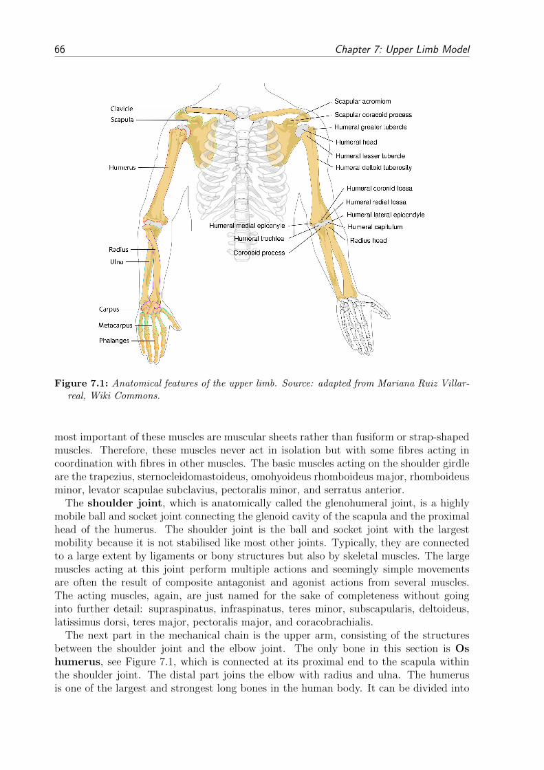
66 Chapter 7: Upper Limb Model
Figure 7.1: Anatomical features of the upper limb. Source: adapted from Mariana Ruiz Villar-real, Wiki Commons.
most important of these muscles are muscular sheets rather than fusiform or strap-shapedmuscles. Therefore, these muscles never act in isolation but with some fibres acting incoordination with fibres in other muscles. The basic muscles acting on the shoulder girdleare the trapezius, sternocleidomastoideus, omohyoideus rhomboideus major, rhomboideusminor, levator scapulae subclavius, pectoralis minor, and serratus anterior.
The shoulder joint, which is anatomically called the glenohumeral joint, is a highlymobile ball and socket joint connecting the glenoid cavity of the scapula and the proximalhead of the humerus. The shoulder joint is the ball and socket joint with the largestmobility because it is not stabilised like most other joints. Typically, they are connectedto a large extent by ligaments or bony structures but also by skeletal muscles. The largemuscles acting at this joint perform multiple actions and seemingly simple movementsare often the result of composite antagonist and agonist actions from several muscles.The acting muscles, again, are just named for the sake of completeness without goinginto further detail: supraspinatus, infraspinatus, teres minor, subscapularis, deltoideus,latissimus dorsi, teres major, pectoralis major, and coracobrachialis.
The next part in the mechanical chain is the upper arm, consisting of the structuresbetween the shoulder joint and the elbow joint. The only bone in this section is Oshumerus, see Figure 7.1, which is connected at its proximal end to the scapula withinthe shoulder joint. The distal part joins the elbow with radius and ulna. The humerusis one of the largest and strongest long bones in the human body. It can be divided into

7.1 Anatomy of the Upper Limb 67
three sections: a rounded head, a long shaft, and the distal head. The smooth, dome-shaped head of the bone lies at an angle to the shaft and fits into a shallow socket of thescapula (shoulder blade) to form the shoulder joint. Below the head, the bone narrows toform a cylindrical shaft. It flattens and widens at the lower end and, at its base, it joinswith the bones of the lower arm (the ulna and radius) to unite the elbow.
The elbow joint is a complex hinge joint that connects the distal end of the humerusand the proximal ends of the ulna and radius in the forearm. The distal head of thehumerus is divided into two joint processes: the trochlea on the medial side and thecapitulum on the lateral side. The pulley-shaped trochlea forms a tight hinge joint withthe trochlea concave dent of the ulna surrounding it, called humeroulna joint. On thelateral side, the concave end of the head of the radius meets the rounded, convex capitulumto complete the elbow, resulting in a ball and socket joint, called humeroradial joint. Theloose union of the capitulum of the humerus and the head of the radius allows the radiusto pivot as well as flex and extend. The pivoting of the radius allows for the supinationand pronation of the hand at the wrist. Therefore, ulna and radius form a third joint(next to the hinge joint between humerus and ulna and the ball and socket joint betweenhumerus and radius) a pivot joint with the humerus (proximal) and the carpus (distal)to allow rotation of the forearm and the wrist. This pivot joint at the elbow is calledsuperior radioulnar joint. The hinge joint of the elbow allows a flexion and extension ofthe forearm relative to the humerus or the upper arm. The range of motion of the elbowis limited by the olecranon, the posterior process of the ulna. Flexion is only limited bythe soft tissue which is clamped between the forearm and the upper arm; hence the rangeof motion for active flexion is smaller due to the hardened muscle tissue. In general, therange of flexion can be assumed to be around 140.
An extensive network of ligaments, surrounding the joint capsule, helps the elbow jointto maintain its stability, while resisting dislocation of the bones, and accommodatingfor mechanical stresses. The ligaments on either side of the elbow are triangular bandswhich also participate in forming the elbow joint capsule. Due to their important roleof forming the joint capsule, the capsule is strongly structured on the sides whereas itis comparatively weak on the front and back. The radial and ulnar collateral ligaments(medial and lateral ligament) connect and maintain the position of the radius and ulnarelative to the epicondyles of the humerus. The annular ligament of the elbow extendsfrom the ulna around the head of the radius to maintain contact between the radiusand the humerus. These ligaments lie across the transverse joint axis and are, therefore,always relatively tense and impose strict limitations on abduction, adduction, and axialrotation at the elbow.
Following the same structure, only the skeletal muscles involved in acting on the elbowjoint are mentioned in this paragraph.The triceps brachii, has, as the name indicates, three muscle heads – a long, a lateral,and a medial head. The long head arises from the scapula. The lateral head arises highup on the lateral side of the posterior humerus. The medial head arises from a broadarea lower down and more medially at the humerus. Each of the three heads has its ownmotor neuron sub-nucleus in the motor column in the spinal cord. The medial head isformed predominantly by small type I fibres and small motor units, the lateral head oflarge type IIB fibres and large motor units and the long head of a mixture of fibre typesand motor units. The three heads unite and towards the end they build one broad tendon

68 Chapter 7: Upper Limb Model
which inserts at the olecranon process at the back of the ulna. The three heads are themain extensor of the elbow. But with its origin on the scapula, the long head also acts onthe shoulder joint and is also involved in retroversion and adduction of the arm. Whileprecisely coordinated forearm or hand movement need to be performed the triceps brachiicontracts to fixate the elbow joint (co-contraction).
The anconeus is a very minor elbow extensor and ulna abductor. It originates at thelateral epicondyle and inserts at the lateral aspect of the proximal ulna. Some anatomistsconsider it just as a continuation of the triceps brachii. It forms the joint capsule at theolecranon fossa during extension.
Biceps brachii, as the name already indicates has two muscle heads. The long headarises from the supraglenoid tubercle (directly superior to the glenoid cavity) while thesecond, called the short head, arises from the coracoid process (a small hook-like structureon the lateral edge of the superior anterior portion of the scapula). I.e. both headsoriginate at the shoulder blade and travel down the arm, lying in front of the brachialis.Both heads cross the elbow joint, join, and together insert on the radial tuberiosity, whichis a protuberance below the radius neck. Actually, the biceps brachii is a tri-articulatedmuscle; acting across three joints: (i) the shoulder, (ii) the elbow, and (iii) the proximalradioulnar joint. While the biceps also crosses the shoulder, its main function is flexing theelbow and to supinate the forearm. The functionality of the biceps brachii on the shouldermovement is various (the long head: forward flexion, abduction, external rotation. Theshort head: adduction, stabilisation by carrying high loads).The biceps brachii has a fusiform-like fibre orientation with around 50% of the musclefibres being fast-twitch and slow-twitch fibres.
The brachialis arises from this broad area on the anterior lower half of the humerusand inserts on the coronoid process, which is the front bony profusion of the ulna. Thefibres converge from the wide origin towards the thick tendon inserting at the ulna. Asthe brachialis inserts at the ulna, it only acts as elbow flexor and does not participate insupination and pronation. The muscle is a strong elbow flexor when the palm is pronated.
The brachioradialis originates at the most distal third of the humerus, just below thedeltoid tuberosity, crosses the elbow and inserts at the distal end of the radius. The musclebelly is mostly positioned at the forearm, while only a small excerpt crosses the elbow. Itsjob is to flex the elbow and aid pronation and supination. When the forearm is pronated,the brachioradialis tends to supinate as it flexes. In a supinated position, it tends topronate as it flexes. This also assists the biceps brachii. The brachioradialis is a strongerelbow flexor when the forearm is at 90 between supination and pronation at the radioulnarjoint. When pronated, the brachioradialis is more active during elbow flexion since thebiceps brachii is in a mechanical disadvantage. With the insertion comparatively closeto the fulcrum of the elbow, the brachioradialis does not generate as much joint torqueas the brachialis or the biceps. It is mainly effective when those muscles have alreadypartially flexed the elbow. The action of the brachioradialis is especially in demand whenquick movements are required due to the distribution of fulcrum, effort and load (class 3lever system) and when a weight is lifted during slow flexion of the forearm.
Pronator teres is a small muscle with two heads. The larger one originates just abovethe medial epicondyle of the humerus. The second originates from the medial side of thecoronoid process of the ulna. The muscle ends in a flat tendon and inserts at the middleon the medial surface of the radius. Its main action is pronating the forearm. It is only

7.2 Upper Limb Model Assumptions 69
weakly participating in flexing the elbow.Extensor carpi radialis longus and – brevis arise from the lateral epicondyle of
the humerus and insert on the third metacarpal of the hand. Although they cross theelbow, they are not considered to participate in elbow flexion. They act on extending andabducting the wrist joint and the hand.
The forearm consists of the two bones Os ulna and Os radius, where the ulna is thelarger of the two bones. As mentioned already in the elbow description, the radius pivotsaround the ulna. Most muscles passing along the forearm originate lateral or medial atthe epicondyle of the humerus and insert either at the wrist, hand, or fingers. As theirorigin is so close to the fulcrum of the humerus, they are practically not participating inacting on the elbow joint. Due to the high number of muscles acting on the sophisticatedhand and the fact that these muscles are not of concern for this thesis, the muscles arenot mentioned and discussed in further detail.
Ulna and radius join at the carpus or wrist. The hand consists of 27 bones, 8 of thosebones belong to the carpus. The rest of the bones form the palm (metacarpus) and thefingers (phalanges). All bones intersect in joints. As it is not of interest for this thesis,the complex anatomy of the hand is not discussed any further.
7.2 Upper Limb Model Assumptions
Section 7.1 pointed out how complex and interwoven the real musculoskeletal system ofthe upper limb is. As it is impossible to incorporate all natural phenomena in one model,model assumptions need to be made in order to facilitate simulations of a multi-musclemusculoskeletal system using spatially a volumetric discretisation. In other words, aradical reduction of complexity needs to be introduced.
The Upper Limb Model, as it is shown in Figure 7.2 consists of three bones: Os humerus,Os ulna, and Os radius. The three bones form the elbow joint, which is considered to bean ideal hinge joint. The bones of the hand are not necessarily required for investigatingelbow movements and are therefore not considered. As the Upper Limb Model does notaccount for supination and pronation, the ulna and the radius can be united to buildthe forearm. For two reasons the bones are considered to be rigid without causing severemodel errors: (i) The bones are much stiffer than the rest of the soft tissue. (ii) In thisstudy, only naturally occurring loads rather than high accelerations, as they may resulte.g. in accidents, are considered.
Gravitational forces need not to be considered, as the upper limb position is such thatthe flexing elbow movement is in a horizontal plane. Therefore, the dead weight of thecontributing objects is not of interest.
Without involving synergetic muscle effects, at least one single antagonistic muscle pairneeds to be chosen to enable the movement of an idealised elbow joint.
The choice for the single extensor muscle is simple. In the Upper Limb Model, the threetriceps heads – long, lateral, and medial – are united to build one homogenised skeletalmuscle. It is by far the most powerful elbow extensor. Unfortunately, no informationabout the real fibre orientation was available from the visible human data set. However,to introduce a more realistic fibre structure, the fibres of the triceps brachii are imitatedto arrange bipennate. To establish the fibre structure within the model, first the fibreorientation was determined to be fusiform, i.e. the fibre are aligned along the longitudinal

70 Chapter 7: Upper Limb Model
(a) side view (b) front and back view
Figure 7.2: The upper limb model consists of the bones Os humerus, Os ulna and Os radius,which are considered to be rigid and of the antagonistic muscle pair, triceps brachii and bicepsbrachii. The muscle tissue is coloured dark red and the tendon tissue beige. The geometry isestablished using the virtual human male’s data set (Spitzer et al., 1996).
boarders of the finite elements. The finite elements in the middle are chosen to be thecentral line with a parallel fibre orientation, see Figure 7.3a. Elements to the left andright are rotated by 15 to the left and right, respectively.
The elbow flexor’s choice is more problematic as there are several synergetic actingmuscles. Some elbow flexors are not only responsible for elbow flexion but also for fore-arm supination and pronation. Furthermore, their ability to generate an elbow momentdepends on the posture of the hand. Possible candidates are the biceps brachii, thebrachialis, the brachioradialis, extensor carpi radialis longus, and the pronator teres.Murray et al. (2000) identified the isometric moment-generating capacity building theproduct of the physiological cross-section area ([m2]), the average moment arm ([m]), andthe cosine pennation angle ([-]) of the muscles acting on the elbow joint. They pointed outthat biceps brachii produces the largest moment capacity (20 cm3), followed by brachialis(11.5 cm3), brachioradialis (6.8 cm3), extensor carpi radialis longus (3.2 cm3), and pronatorteres (3.1 cm3). Thus, the biceps brachii is chosen as the flexor in this Upper Limb Modeldue to its highest moment-generating capacity. As well as for the triceps brachii, the twoheads of the biceps brachii are homogenised to a fusiform muscle belly, see Figure 7.3b.
The geometry of the upper limb is established using the virtual human male’s dataset (Spitzer et al., 1996). The data of the virtual human male was acquired in a supine

7.2 Upper Limb Model Assumptions 71
(a) triceps brachii (b) biceps brachii
Figure 7.3: The triceps brachii’s bipennate fibre architecture is established by assuming the mid-dle column of the elements as parallel and the elements to the left and right to be pennated by15 to opposite directions. The biceps brachii is assumed to have a fusiform fibre architecture.
position. The arm was resting on the abdominal belt, where the arms had an elbow flexionangle of approximately 60. The origin of the chosen coordinate system is the intersectionbetween the mid sagittal and mid coronal plane at the most inferior position, where thex-axis points to the right, the y-axis anteriorly, and the z-axis superiorly.
The mesh is generated by a least-square fit introduced by Bradley et al. (1997) usingthe finite element software package CMISS (for more information about CMISS cf. Sec-tion 5.1). The surface fitting procedure has been extensively applied to muscular organmodelling, e.g. in Nash and Hunter (2000) and Rohrle and Pullan (2007). The prelim-inary mesh was discretised using Hermite ansatz functions and converted to quadraticLagrangean shape functions.
Using a continuum-mechanical approach for the musculoskeletal system, the choiceof the muscle’s stretch state, has a strong influence on the mechanical behaviour. Asthere are no comparable continuum-mechanical models available, no experience exists onwhat to choose best. As the choice of the muscle’s prestretch is not uniquely defined,the muscle length is chosen in such a way that the passive muscle does not cause acompressive force for the shortest possible length. Therefore, the muscles’ geometry isshortened by removing a few centimetres from both the proximal and the distal endsof each muscle. Within the prestretch phase, the muscles are stretched to the originallength. The disadvantage of that choice is that the original volume of the muscle reducesdepending on the amount of prestretch, and hereby the maximal reachable muscle force.
The skeletal muscles are represented in two evolution steps. The first one assumes thetendon tissue to be rigid. As a consequence, the tendon tissue is not considered withinthe finite element simulation and just visualised by a rigid mesh. In the second evolutionstep, the tendons are considered to behave as a strong, transversely isotropic material,see Section 4.4.

72 Chapter 7: Upper Limb Model
7.2.1 Rigid-Tendon Model
The skeletal muscle material parameters used for the model, are taken from literature andlisted in Table 7.1. In case of the active muscle parameters, parameter set in Gunther et al.(2007) is chosen as an initial guess and adapted for a continuum-mechanical approach. Astheir parameter set is determined for a Hill -type muscle, the data needed to be adjustedto fit into the continuum-mechanical framework. Adjustments are conducted manuallyuntil an adequate force response was achieved. Material parameters for the isotropic andpassive material behaviour are determined using a least-square fit to experimental data(Hawkins and Bey, 1994; Zheng and Mak, 1999). For the maximum active stress, σmax,the values vary in the literature from 100-500 kPa (Woittiez et al. (1984); Fitts et al.(1991); Van Leeuwen and Spoor (1992)). Here, a value of σmax = 300 kPa is assumed.
Table 7.1: Skeletal muscle tissue parameter set, as introduced in Section 4.3, for triceps andbiceps brachii when the tendons are considered to be rigid.
contribution parameter triceps biceps source
isotropicc1M
c2M
3.56 · 10−2 MPa
3.86 · 10−3 MPa
3.56 · 10−2 MPa
3.86 · 10−3 MPa
Hawkins andBey (1994)
passivec3M
c4M
0.2939 · 10−8 MPa
34.042 [-]
3.5686433 · 10−8 MPa
42.6 [-]
Zheng and Mak(1999)
active
∆Wasc 0.20 [-] 0.25 [-]adapted fromGunther et al.(2007)
∆Wdesc 0.10 [-] 0.15 [-]
νasc 3.00 [-] 3.00 [-]
νdesc 4.00 [-] 4.00 [-]
λoptf 1.13 [-] 1.35 [-] -
σmax 0.30 MPa 0.30 MPa -
The choices of the boundary conditions are delicate, especially at the proximal end ofthe muscle. All nodes at these faces are fixed in the longitudinal muscle direction (z-direction). Some nodes in the centre of these faces are fixed in all three space-coordinatesto maintain sufficient restrictions, see Figure 7.4. As the muscles are at their proximalends in direct contact to the humerus, one has to balance between the restriction and thecompliancy of the muscles’ face. By adapting the number and location of the fixed nodes,the restriction can be locally increased or decreased. It needs to be balanced between anacceptable shape and numerical robustness.
Figure 7.4: Nodal choice of the boundary conditions at the distal and proximal ends of themuscle mesh. The black nodes are fixed longitudinally whereas the grey nodes are fixed in inall directions.

7.2 Upper Limb Model Assumptions 73
7.2.2 Muscle-Tendon-Complex Model
In a second evolution step, muscle and tendon tissue is considered. The centre or belly wasdefined as muscle tissue, the tapering area is defined as a transition zone and the slenderends as tendon tissue. As the constitutive relation of Section 4.4 is purely elastic, allviscoelastic effects of the tendon tissue are neglected. During the discretisation process,the two muscle heads part at the proximal end of the muscle belly. Furthermore, thesimulations were more robust when tendon ends were split in a U-shape and not a V-shape and when filling the gap with isotropic soft tissue. Figure 7.5 depicts the differentzones by different colours.
(a) anterior view of triceps brachii (b) lateral view of biceps brachii
Figure 7.5: The muscle tissue is coloured in dark red. Tendon tissue is shown in beige andother soft tissue in white. The transition zone from tendon to muscle tissue is indicated bya colour between dark red and beige. Standard quadratic Lagrange finite elements are usedto represent the separating muscle heads and the soft tissue between the heads to circumventalternatives as e.g. hanging nodes and to reduce and avoid numerical problems. Between themuscle heads, the elements are tapering towards the muscle’s belly to reflect the V-shape bestpossible. In the middle of the triceps along the longitudinal axis, one row of elements has anincreased tendon tissue ratio to represent the aponeurosis sheet of a bipennate muscle.
In the model, the triceps’ origin combines the two most lateral heads to one strongunited head while the most medial head is separated from the two others. The resultinggap is filled by isotropic soft tissue. The triceps’ insertion unites into one wide tendon atthe olecranon process.For the model of the biceps brachii, its two heads are also combined to form one fusiform

74 Chapter 7: Upper Limb Model
muscle belly with two separate proximal tendons. The gap between the two tendon headsis filled with isotropic soft tissue. The fibre direction in the tendon tissue zone is assumedto behave fusiform-like.
The cross-section at the ends of the muscles is much smaller compared to the endsof the muscle tissue with rigid tendons. Furthermore, the tendons have to withstandrelatively small deformations, hence, at the distal surfaces, all nodes were fixed in allspatial directions.
Bipennate muscles have a slim aponeurotic tissue layer which deeply penetrates into themuscle belly, see Figure 2.12c. The aponeurosis is a very fine and slim tissue layer whichhas a strong impact on the mechanical behaviour of the overall muscle-tendon complex. Torepresent the triceps more realistically, a central line of elements is defined as aponeurotictissue layer, which connects the proximal and distal ends of the muscle. Compared to thethickness of the aponeurosis, the size of the element is large. Therefore, the mechanicalbehaviour of the aponeurotic tissue layer is homogenised using the material variable γM
which is chosen to be γM = 0.99. As the tendon is approximately 1000 times strongerthan muscle tissue, a linear interpolation is not constructive. Imagine a tissue compositionof 10% tendon and 90% muscle where muscle has the stiffness of 1 and tendon of 1000.The interpolated bulk has a stiffness of 100.9 which is still 100 times stiffer than muscle.A tissue consisting of 1% tendon and 99% muscle is still eleven times stiffer than puremuscle tissue. Hence, the chosen material parameter γM is chosen to be γM = 0.99.
Table 7.2: Skeletal muscle material parameter set, as introduced in Section 4.4, for triceps andbiceps brachii when the muscles are considered as a muscle-tendon complex.
tissue contribution parameter triceps biceps source
muscle
isometricc1M
c2M
3.56 · 10−2 MPa
3.86 · 10−3 MPa
3.56 · 10−2 MPa
3.86 · 10−3 MPa
Hawkins andBey (1994)
passivec3M
c4M
4.02 · 10−7 MPa
38.5 [-]
3.57 · 10−8 MPa
42.6 [-]
Zheng and Mak(1999)
active
∆Wasc 0.30 [-] 0.25 [-]adapted fromGunther et al.(2007)
∆Wdesc 0.10 [-] 0.15 [-]
νasc 4.00 [-] 3.00 [-]
νdesc 4.00 [-] 4.00 [-]
λoptf 1.3 [-] 1.35 [-] -
σmax 0.30 MPa 0.30 MPa -
tendon
isotropicc1T
c2T
2.31 MPa
1.15 · 10−6 MPa
2.31 MPa
1.15 · 10−6 MPa
Weiss and Gar-diner (2001)
passivec3T
c4T
7.99 MPa
16.6 [-]
7.99 MPa
16.6 [-]
Weiss and Gar-diner (2001)
7.3 Equivalent Static System
In order to investigate equilibrium positions of the Upper Limb Model, and to avoid alarge and complex system, in which all components are considered to be deformable andin contact, e.g. bone-bone contact within the joint, a reduced equivalent static system isintroduced to investigate equilibrium positions of the Upper Limb Model, see Figure 7.7a.

7.3 Equivalent Static System 75
It consists of the humerus, the forearm, the antagonistic muscle pair, and an externalforce F to increase the DoFs of the system by one. The angle between the humerus andthe forearm is defined as the elbow flexion angle θ and defines the position of the forearm.The humerus is supported in all spatial directions and the forearm rotates around thefulcrum of the elbow joint. The forearm is represented including a rigid, bend-resistantcorner at the fulcrum to represent the location of the olecranon. The muscle attachmentpoints coincide with the volumetric model. The forearm’s rotation matrix is defined byan axis and an angle. The rotation angle is defined to be the elbow flexion angle andthe rotation axis is defined by a vector product of a vector along the humerus and theorientation of a vector from the fulcrum and to the distal end of the forearm.
As both muscles insert at the forearm, the position of the forearm defines the muscles’lengths and lever arms, i.e. the muscles’ kinematics only depend on the elbow angle.
As one only considers an equivalent static system and assumes rigid bones, it is sufficientto identify, for each insertion or origin, one node on each mesh of the ulna and radiusas the muscles’ insertion points. The muscles’ length are defined by the linear distancebetween the origin and insertion points. The origin is fixed whereas the location ofthe insertion point varies depending on the elbow flexion angle. The chosen nodes onthe bone are tracked for the physiologically reasonable range of motion of the forearm,i.e. 10 < θ < 150. The muscle length is defined as change of the distance between originand insertion relative to its initial position at θ0 = 60. Then, for each of the musclelengths relative to the initial position, a separate third-order polynomial has been obtainedusing MATLAB (2014)’s least-squares fitting functionality. The respective relative musclelengths are depicted in Figure 7.6a and Figure 7.6b.
Compared to the triceps brachii, the biceps brachii has a much larger change of length.The reason is that the location of the attachments’ site is further away from the elbow’sfulcrum.
0 50 100 150−40
−20
0
20
40
60
80
elbow angle θ [°]
mu
sc
le d
isp
lac
em
en
t [m
m]
tricepsx
tricepsy
tricepsz
tricepstotal
(a) triceps brachii
0 50 100 150−40
−20
0
20
40
60
80
elbow angle θ [°]
mu
sc
le d
isp
lac
em
en
t [m
m]
bicepsx
bicepsy
bicepsz
bicepstotal
(b) biceps brachii
Figure 7.6: Relative change of muscle length is determined by subtracting the muscle lengthat θ0 = 60 from the current muscle length. As the z-direction is close to parallel to thelongitudinal axis of the muscle, it is dominating the mechanical behaviour of the muscle.
The muscle lever arms are determined using two different methods. The first method,introduced by An et al. (1984), is widely used and its related errors are considered to
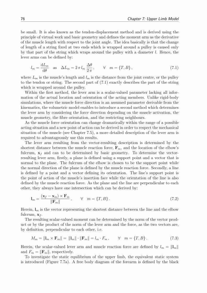
76 Chapter 7: Upper Limb Model
be small. It is also known as the tendon-displacement method and is derived using theprinciple of virtual work and basic geometry and defines the moment arm as the derivativeof the muscle length with respect to the joint angle. The idea basically is that the changeof length of a string fixed at two ends which is wrapped around a pulley is caused onlyby that part of the string which wraps around the pulley with a diameter l. Hence, thelever arms can be defined by:
lm =dLmdθ
as ∆Lm = 2π lm∆θ
2 π, ∀ m = T,B , (7.1)
where Lm is the muscle’s length and lm is the distance from the joint centre, or the pulleyto the tendon or string. The second part of (7.1) exactly describes the part of the stringwhich is wrapped around the pulley.
Within the first method, the lever arm is a scalar-valued parameter lacking all infor-mation of the actual location and orientation of the acting members. Unlike rigid-bodysimulations, where the muscle force direction is an assumed parameter derivable from thekinematics, the volumetric model enables to introduce a second method which determinesthe lever arm by considering the force direction depending on the muscle activation, themuscle geometry, the fibre orientation, and the restricting neighbours.
As the muscle force orientation can change dramatically within the range of a possibleacting situation and a new point of action can be derived in order to respect the mechanicalsituation of the muscle (see Chapter 7.5), a more detailed description of the lever arm isrequired to advantageously use this results.
The lever arm resulting from the vector-resulting description is determined by theshortest distance between the muscle reaction force, Fm, and the location of the elbow’sfulcrum, xf and can to be determined by basic geometry. To determine the vector-resulting lever arm, firstly, a plane is defined using a support point and a vector that isnormal to the plane. The fulcrum of the elbow is chosen to be the support point whilethe normal direction of the plane is defined by the muscle reaction force. Secondly, a lineis defined by a point and a vector defining its orientation. The line’s support point isthe point of action of the muscle’s insertion face while the orientation of the line is alsodefined by the muscle reaction force. As the plane and the line are perpendicular to eachother, they always have one intersection which can be derived by:
lm =(xf − xm)× Fm
‖Fm‖, ∀ m = T,B . (7.2)
Herein, lm is the vector representing the shortest distance between the line and the elbowfulcrum, xf .
The resulting scalar-valued moment can be determined by the norm of the vector prod-uct or by the product of the norm of the lever arm and the force, as the two vectors are,by definition, perpendicular to each other, i.e.
Mm = ‖lm × Fm‖ = ‖lm‖ · ‖Fm‖ = lm · Fm , ∀ m = T,B . (7.3)
Herein, the scalar-valued lever arm and muscle reaction force are defined by lm = ‖lm‖and Fm = ‖Fm‖, respectively.
To investigate the static equilibrium of the upper limb, the equivalent static systemis introduced (Figure 7.7a). A free body diagram of the forearm is defined by the black

7.4 Calculation Example of the Upper Limb 77
FE
θ
B
(a) equivalent staticsystem
FE
θ
B
(b) area of interest
FE
θ
FT
FBEv
Eh
B
(c) acting forces onthe forearm
FE
θ
FT
FB
lT lB
(d) moment equi-librium of theforearm
Figure 7.7: Employing the Upper Limb Model to introduce the equivalent static system of theforearm. By defining a free body diagram of the forearm, a static equilibrium can be defined forthe forearm. The rotation axis is positioned in the fulcrum and points upwards, perpendicularto the paper normal.
loop indicated in Figure 7.7b. The acting forces (Figure 7.7c) are the muscle reactionforces, the elbow contact forces, and an arbitrarily chosen external load FE, which actsas a perturbing moment to the system. A moment balance can be formulated for theforearm with respect to the fulcrum of the elbow. Hereby, one obtains
FT (θ, αT ) lT (θ) + FE lE(θ)− FB(θ, αB) lB(θ) = 0 , (7.4)
where FT and FB are the muscle reaction forces determined by the FE simulation, whichare a function of the elbow flexion angle and the muscle activation, FE is the introducedexternal force and lm are the scalar-valued lever arms for triceps, biceps and the externalforce, respectively.
As the lever arms of the elbow contact forces Eh and Ev are zero, those forces do nothave an impact on the defined momentum balance.
A penalty contact formulation is incorporated as introduced in Chapter 6. Since there isno direct contact between the muscles, the only contact occurring is between each muscletissue and the rigid humerus.
The muscle forces are determined by the continuum mechanical model. The evolvingsystem of partial differential equations is solved using the finite element software packageCMISS as it was introduced in the previous chapters. The muscle reaction forces aredetermined by summing the nodal residuals (cf. Section 5.2) at the muscle’s end cross-section.
7.4 Calculation Example of the Upper Limb
To develop a feeling for the magnitude of the acting muscle forces a simple arithmeticsample calculation is derived in the this section.

78 Chapter 7: Upper Limb Model
Imagine the following scenario: A dead load acting in the hand is sought to extendthe forearm. The biceps brachii is the only flexor muscle acting on the upper limb. Theequivalent static system is depicted in Figure 7.8.
LH
LB
lB
Linsertθ
θ1
FE
Figure 7.8: Upper Limb Model calculation example: adapting Figure 7.7a by neglecting tricepsbrachii and introducing θ1 and Linsert, the distance between the elbow’s fulcrum and the biceps’insertion.
The length of the humerus is LH = 32 cm, the distance from the elbow’s fulcrum to thelocation where the external force acts is LE = 34 cm, and the distance from the elbow’sfulcrum to the biceps’s insertion is Linsert = 9 cm. In addition to the elbow angle, anangle θ1 is needed to define the angle between the humerus and the biceps. Further, it isassumed that the biceps is attached to the top end of the humerus. The necessary muscleforce to maintain the arm in a static position can be calculated using trigonometry andalgebra.
The first step is to sum the moments applied to the fulcrum of the elbow, where theonly two acting forces are the biceps muscle force and the external dead load:
FE lE(θ)− FB(θ) lB(θ) = 0 (7.5)
⇔ FB(θ) =FE lE(θ)
lB(θ). (7.6)
With the help of the law of cosines, the biceps’s length can be determined to:
LB =√L2H + L2
insert + 2LH Linsert cos(180 − θ) . (7.7)
Using Equation (7.1) to determine the lever arm:
lB =∂LB∂θ
=LH Linsert sin (θ)
2LB. (7.8)

7.5 Muscle Force Dyname 79
Alternatively, lB can be geometrically deduced by:
lB = LH sin (θ1) , (7.9)
Linsert =√L2H + L2
B + 2LH LB cos(180 − θ1) , (7.10)
sin(θ1) =√
1− cos2(θ1) , (7.11)
where (7.10) is the law of cosines and (7.11) is the Pythagorean identity. By inserting(7.10) and (7.11) into (7.9) the lever arm can be deduced to:
lB =1
2LB
√4L2
H L2B − (L2
H + L2B − L2
insert)2 . (7.12)
The graphs of Equation (7.8) and (7.12) coincide and demonstrate the applicability ofEquation (7.1).
Having a closer look at the derived relations, one can see that the influence of theratio of the lever arms, lB(θ) and lE(θ), on the demanded muscle force. Furthermore, theresulting muscle force increases linearly with the dead load, cf. Figure 7.9, which depictsthe result for Equation (7.5) for a dead load of 1 kg ≤ F ≤ 12 kg and an elbow angleranging from 0 ≤ θ ≤ 180. Due to the lever class 3, where the effort lies between thefulcrum and the load, the demand in biceps force is quite high and can be up to severalhundred Newton. The advantage of such an order of fulcrum, load, and effort is, as alreadymentioned in Section 2.4.5, that fast movements are feasible.
050
100150
0
100
2000
200
400
600
external load [N]elbow angle [°]
bic
ep
s f
orc
e [
N]
Figure 7.9: The biceps force resulting from the analytical investigation: Equation (7.5) isevaluated for an external dead weight ranging from 1 to 12 kg and an elbow angle 0 < θ <180.
Further information can be found in standard biomechanics books as, for example, inTozeren (2000) or Freivalds (2011).
7.5 Muscle Force Dyname
In contrast to rigid-body models, continuum-mechanical models have the advantage ofspatially distributing mechanical measures. Hence, a continuum-mechanical model can

80 Chapter 7: Upper Limb Model
be applied to investigate the muscle force flowing through the muscle from origin toinsertion. The muscle force’s orientation changes due to muscle-intrinsic phenomena suchas the complex geometry, local distributed material parameters, or the fibre structure.
In the modelling world, skeletal muscle are very often attached to bones at one pointor node. In nature, the attachment areas can be small or wide. This feature, might berepresented in continuum-mechanical approaches by distributing the muscle attachmentsite to several nodes of the bone. Yet in rigid-body systems, geometrically everything isreduced to points and lines. To compensate, very often big muscles are represented byseveral representatives to improve the representation of the muscle length and lever arm.
An alternative idea might be, when continuum-mechanical approaches are coupled torigid-body systems. Continuum-mechanical models might improve the solution of rigid-body systems by returning altered muscle reaction force directions or lever arms to rigid-body models.
Therefore, when skeletal muscle forces need to be exchanged to other frameworks orinsert to the bone, mostly one vectorial force value and on point of action is used to applythe muscle force. Due to the finite element discretisation, a traction vector can be definedfor each muscle’s node at an muscle insertion face. Hence, to transfer the force from oneof the muscle’s end face to a particular location of the bone, either one from all possibleface nodes needs to be selected or one needs to come up with a method to reduce the endface traction vectors to a unified value acting at a particular location.
This section presents a method to investigate the mechanical state of the muscle bycondensing the nodal traction vectors at a face to a unique pair of three-dimensionalvectors.
To investigate the mechanical behaviour of the muscle, the screw theory, introducedby Ball (1900), is used. A screw is a pair of three-dimensional vectors, such as linearand angular velocities for kinematical systems and forces and torques for statical systems.The mechanical description of a statical system, where an arbitrary amount of forces actupon, can be described after choosing a point of reference by only a resulting force and aresulting torque, i.e. by
W =
NF∑i
Fi,Fi × lFi = F,Mx , i = 1, .., NF . (7.13)
Herein, W is the force wrench which is the screw for a static situation, Fi, i ∈ N is one ofNF forces acting on the system, lFi
is the lever arm of the acting force i from its originalpoint of action to the chosen reference point, F is the resulting force, and Mx is theresulting moment with respect to an arbitrary location x.
The reason for obtaining besides the resulting force also a resulting moment is the factthat when the point of action of the force is relocated other than along its line of action,the force generates a torque. Hence, for uniting NF forces in an arbitrary point of action,the perpendicular distance li and the magnitude of the force define the emerging torquefor each force Fi.
Assuming one considers the proximal or distal face, denoted by Γ as depicted in Fig-ure 7.10a, the IVBP determines the stress at Γ. The resulting force, F, on the cross-

7.5 Muscle Force Dyname 81
sectional area, Γint, is determined by
F =
∫Γint
S n0 dA =
∫Γint
t0 dA . (7.14)
The location where the wrench is defined is somehow arbitrary. Yet, often times thesurface’s barycentre, xs is chosen as point of action. The resulting moment with respectto the barycentre of the face is obtained by
Mxs =
∫Γint
(xxi− xs)× t0 dA , (7.15)
where xxiis the coordinate of any node at the surface Γ and dA is the referential cross-
sectional area of interface Γint.Numerically, the integral is computed by summing the nodal traction vectors at the
interface using a Riemann sum. The nodal traction vectors are determined by multiplyingthe stress, determined at the Gauss points, by their appropriate face increment dA andreduces to Equation (7.13).
S
Γ
(a) surface stress distribu-tion
Mxs
F
n0
xs
Γ
(b) resulting screw W
F
M‖
r
xs
Γ
(c) replacing the point of ac-tion
Figure 7.10: The force wrench is establish in two steps: First the surface stress distribution isunified at the surface’s barycentre, xs to a resulting force, F, and moment, Mxs. Second, theinitial point of action, xs, can be relocated by r such that total moment M can be minimisedby getting rid of M⊥. Thereby, M is reduced to M‖, which is the torsional fraction of themoment.
The advantage of the force wrench is that the resulting moment can be reduced byrelocating the force’s point of action. Therefor, first the moment Mxs is split into twocomponents: M‖ and M⊥. The component M‖ points parallel, while M⊥ points perpen-dicular to F. Hence,
Mxs = M‖ + M⊥ . (7.16)

82 Chapter 7: Upper Limb Model
The point of action of F can be moved along a direction r = F×Mxs such that M⊥ ≡ 0.In order to determine the length of r, Equation (7.16) is multiplied by F.
Mxs × F = M‖ × F︸ ︷︷ ︸=0
+ M⊥ × F . (7.17)
By inserting M⊥ = r× F in (7.17), one obtains
Mxs × F = (r× F)× F . (7.18)
as r ⊥ F. By using index notation and the permutation symbol for the cross product,Equation (7.17) can be rearranged to
Mxs × F = F2 r− F ( r · F )︸ ︷︷ ︸=0
. (7.19)
Herein, F2 denotes the inner product of the force, i.e. F2 = F ·F. Equation (7.19) can besolved for r and yields
r =Mxs × F
F2 . (7.20)
At the eccentric point of action, the original wrench F, Mxs reduces to F, M‖,i.e. the resulting moment is just the torsional part of the initial resulting moment. Thebending part is taken care by the new eccentric location of the forces point of action.
Note, this procedure applies not only for the proximal or distal attachment area, but forany cut within the muscle. By cutting the muscle perpendicular to its longitudinal axisat arbitrary locations along that line, a sequence of resulting forces on these incrementalcross-sections along the longitudinal axis of the muscle can be considered as a line of action(Sprenger et al., 2011). The sequential location of the point of action and the magnitudeand orientation of the resulting force can be used to investigate the mechanical exposureof the muscle as it is depicted for example in Figure 10.1.
8 Multi-Muscle Forward-DynamicsSimulations
This section introduces three possible options for continuum-mechanical based muscu-loskeletal system simulations.
In the first option, the muscle activations for the two acting muscles of the Upper LimbModel are prescribed. The purpose of these simulations is to investigate whether themusculoskeletal system, as it is defined, can find a static equilibrium.
In the second option, a forward-inverse model is employed to convert experimental datainto muscle activations. The evaluated muscle activations are applied to the Upper LimbModel and the resulting equilibrium position is compared to the isometric trials of theexperiments.
The last option sketches how volumetric skeletal muscle simulations can be coupledwith rigid-body simulations.
8.1 Prescribed Forward-Dynamics Model
Equation (7.4) describes the moment equilibrium of the elbow:
FT (θ, αT ) lT (θ) + FE lE(θ)− FB(θ, αB) lB(θ) = 0 . (8.1)
The equation includes four DoFs: the elbow angle, θ, the muscle activations, αT andαB, and the external force, FE. The muscle reaction forces are a result of the finiteelement simulation and depend on the elbow angle and the muscle activation. They aredetermined by summing the nodal residuals at the muscle insertion cross-section andtaking the absolute value of the resulting reaction force.
To investigate the Upper Limb Model, a two step procedure is installed. Within thefirst step, a reference solution is determined. This solution will be used to observe, if aperturbed initial state can find the correct equilibrium condition.
To find a static equilibrium position of the upper limb in the first step, three out of fourDoFs are prescribed: θ = θ, αT = αT , and αB = αB. Note, the exerted muscle forces arecompletely based on the results of the finite element simulations. By rearranging (8.1),an external force F can be determined, where the system is in equilibrium:
FE(θ) =FB(θ, αB) lB(θ)− FT (θ, αT ) lT (θ)
lE(θ). (8.2)
The four DoFs, marked with (·), build the reference solution. Subsequently, the systemis disturbed by starting the convergence process by prescribing one of the four DoF witha different value as the ones prescribed in the reference. Only one DoF is changed, as fortwo DoFs an optimisation problem would have to be solved.
83

84 Chapter 8: Multi-Muscle Forward-Dynamics Simulations
After the perturbation, it is determined whether the Upper Limb Model can convergetowards the known equilibrium state. If Equation (8.1) is not in equilibrium, the momentequilibrium exhibits a residual moment,
FT (θ, αT ) lT (θ) + FE lE(θ)− FB(θ, αB) lB(θ) = M . (8.3)
Convergence is monitored by considering the resulting elbow moment as the system error.Depending on the perturbed DoF, the investigation of the Upper Limb Model can becategorised into three scenarios: (i) position-driven, (ii) activation-driven, or (iii) force-driven forward model.
8.1.1 Position-Driven Scenario
In case of the position-driven scenario, a desired angle θ – and therefore the position ofthe forearm – is predescribed and one seeks the level of activation for one muscle, e.g. thelevel of activation of the triceps. Prescribing all DoFs and a random αT ∈ [0, 1] leadsto a non-equilibrium (unless αT has accidentally be chosen such the system would be inequilibrium) and produces a resulting elbow moment.
For the solution process, in which the external force, the biceps’ level of activation,and the elbow angle are kept constant, a Newton-Raphson-iteration scheme is employedto determine an improved approximation for the triceps’ level of activation, i.e. the nextiteration step i+ 1 is given by
α(i+1)T = α
(i)T −
M (i)
∂M(i)
∂αT
, i=1,...,n , (8.4)
where, n ∈ N. For practical purposes, the Newton’s method is replaced with the secantmethod, i.e. by approximating ∂M(i)
∂αTwith the differential quotient
∂M (i)
∂αT≈ ∆M (i)
∆α(i)T
=M (i) −M (i−1)
α(i)T − α
(i−1)T
=F
(i)T − F
(i−1)T
α(i)T − α
(i−1)T
. (8.5)
The last part of the equation is only valid for determining the lever arm with the tendondisplacement method. If the vector resulting lever arm is used, the lever arm also dependson the muscle activation and cannot be cancelled from the ratio.
To determine the differential quotient for i = 1, the residual moement is set to greaterthan the ε, the muscle activation, α
(0)T , is defined as α
(0)T = |α(1)
T − 0.01|. Note, F(0)T needs
to be computed based on α(0)T .
8.1.2 Activation-Driven Scenario
For the activation-driven scenario, one seeks the resulting elbow angle for prescribedactivation levels and a given external force. Based on an initial θ(0), Equation (8.4) isadapted in the following way
θ(i+1) = θ(i) − M (i)
∂M(i)
∂θ
, i=1,...,n , (8.6)
8.1 Prescribed Forward-Dynamics Model 85
to determine the next iterate for the elbow angle. Should θ(i+1) be outside the physiologicalrange, i.e. θ(i+1) < 10 or θ(i+1) > 150, then the minimal or maximal physiological rangevalue are prescribed. Like before, ∂M(i)
∂θis approximated by the following differential
quotient,
∂M (i)
∂θ≈ ∆M (i)
∆θ(i)=M (i) −M (i−1)
θ(i) − θ(i−1). (8.7)
For i = 0, the initial elbow angle is chosen to be θ(0) = 60. The angle θ(1) representsan initial starting value to the iteration procedure. Note, the angle should be within thephysiological range of 10 ≤ θ ≤ 150.
8.1.3 Force-Driven Scenario
By prescribing realistic time-dependent constraints, one needs to solve at each time stepthe equilibrium equations to obtain depending on the chosen scenario a movement in aforward-dynamics fashion.
Within the force-driven scenario, one assumes that the level of activation for the bicepsand triceps remains constant. Now varying the external force applied at the distal endof the forearm results in a change of elbow angle, i.e. an increase in F leads to a forearmextension while a decrease in F leads the forearm to flex. The change of elbow angleresulting due to such a force perturbation can be solved in the same way as described inthe two previous sections.
Note that this methodology of achieving forward-dynamics simulations through one ofthese scenarios only holds for relative slow movements, in particular for movements, inwhich the inertia terms can be neglected.
8.1.4 Simulation Procedure
All the above described iterations aim to find the moment equilibrium of the system. Thesystem is considered to be in equilibrium, if the remaining moment of the system afterthe iteration is less than ε, i.e.,
|M (i+1)| ≤ ε , with ε > 0 . (8.8)
Unless otherwise stated, ε is chosen to be 10−9 Nmm.Figure 8.1 shows the solution procedure of the simulation for the activation-driven
procedure. As explained in Section 7.2, the muscle needs to be brought into the initialposition at θ0 = 60. Hence, in the prestretch phase (green box), the muscle simulationsare started simultaneously and the muscles are pre-stretched to their initial position atθ0 = 60.

86 Chapter 8: Multi-Muscle Forward-Dynamics Simulations
initialise model
start triceps start biceps
define model con-straints αT , αB , FE
prescribe new θ(i+1)
get L(i+1)m , l
(i+1)m
get F(i+1)T get F
(i+1)B
Newton iteration:θ(i) := θ(i+1)
θ(i+1) = θ(i) + ∆θ(i)
equilibrium?|M(i)| < ε
updatingconstraints?
stop
prestretch phase
iteration phase
yes
no
yes
no
Figure 8.1: Iteration flow chart of the Upper Limb Model: The green box indicates the prestretchphase of the skeletal muscles. Within the iteration process, the elbow angle changes until themuscle reaction forces converges to a static equilibrium. The variation of θ is employed by asecant method.

8.2 EMG-driven Forward-Dynamics Model: Employing a Forward-Inverse Model 87
When they reach that position, the iteration phase (yellow box) starts. Herein, thealgorithm prescribes the constraints defined in one of the three introduced scenarios.When the new position is set, first the new boundary conditions (consisting of the locationof the muscles’ distal end and its activation) for the FE simulations need to be determined;i.e. by evaluating the muscle length to the given elbow angle, the FE boundary conditionscan be prescribed. After both FE simulations converged, the muscle reaction forces aredetermined by exploiting the FE simulations’ results. Additionally, the lever arms aredetermined by either evaluating the tendon-displacement method or the vector-resultinglever arm method. After the moment balance is solved and the successive iteration state,(i+1), is determined, within the equilibrium rhombus it is checked whether the equilibriumcriterion is met.
If it is met, it is checked whether a second updating criteria is defined. By defininge.g. successive different constraints a successive change of the position can be established,see Section 8.1.3. For example, for a constant external load FE and a constant bicepsactivation αB and a successively increasing αT , the forearm has to extend. For a succes-sively increasing αB while αT and FE are constant, the forearm has to flex. The same canbe observed for successively increasing or decreasing the external load F , while keepingthe muscle activations fixed.
8.2 EMG-driven Forward-Dynamics Model: Employing aForward-Inverse Model
The wide field of biomechanics has at least one thing in common: the problem validatingtheir models, see e.g. Lewandowski (1982) or Anderson et al. (2007). In Section 9.2, it isshown, that the presented model of the upper limb is able to find an equilibrium position.Yet, the question whether that position is realistic or not is still not touched.
Together with experimental data, the forward-inverse model, introduced by Buchananet al. (2004), is employed to solve the muscle redundancy problem, to extract muscleactivation (see Section 9.3.1), and last but not least to compare the Upper Limb Modelmodel results to the one determined by the forward-inverse model (see Section 9.3.2). Themodel was provided by courtesy of Prof. David Lloyd, who gave the author the chance toget acquainted to the model and perform the experiments at the Gold Coast Campus ofthe Musculoskeletal Research Group, Griffith Health Institute at the Griffith Universityin Australia.
In Figure 8.6, the forward-inverse model is depicted in its hole complexity trying tosketch the interaction of the different parts. The different parts of the model are:
• conducting experiments for collecting EMG data, position data, and elbow jointtorques,
• processing the raw data,
• developing an upper limb OpenSim model, that provides the rigid-body and musclekinematics, see Holzbaur et al. (2005),
• muscle-tendon-complex model to determine the muscle forces, and
• the solution processes for
– the forward-dynamics rigid-body model,
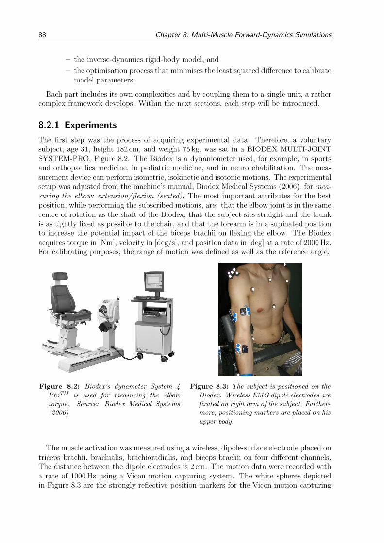
88 Chapter 8: Multi-Muscle Forward-Dynamics Simulations
– the inverse-dynamics rigid-body model, and
– the optimisation process that minimises the least squared difference to calibratemodel parameters.
Each part includes its own complexities and by coupling them to a single unit, a rathercomplex framework develops. Within the next sections, each step will be introduced.
8.2.1 Experiments
The first step was the process of acquiring experimental data. Therefore, a voluntarysubject, age 31, height 182 cm, and weight 75 kg, was sat in a BIODEX MULTI-JOINTSYSTEM-PRO, Figure 8.2. The Biodex is a dynamometer used, for example, in sportsand orthopaedics medicine, in pediatric medicine, and in neurorehabilitation. The mea-surement device can perform isometric, isokinetic and isotonic motions. The experimentalsetup was adjusted from the machine’s manual, Biodex Medical Systems (2006), for mea-suring the elbow: extension/flexion (seated). The most important attributes for the bestposition, while performing the subscribed motions, are: that the elbow joint is in the samecentre of rotation as the shaft of the Biodex, that the subject sits straight and the trunkis as tightly fixed as possible to the chair, and that the forearm is in a supinated positionto increase the potential impact of the biceps brachii on flexing the elbow. The Biodexacquires torque in [Nm], velocity in [deg/s], and position data in [deg] at a rate of 2000 Hz.For calibrating purposes, the range of motion was defined as well as the reference angle.
Figure 8.2: Biodex’s dynameter System 4ProTM is used for measuring the elbowtorque. Source: Biodex Medical Systems(2006)
Figure 8.3: The subject is positioned on theBiodex. Wireless EMG dipole electrodes arefixated on right arm of the subject. Further-more, positioning markers are placed on hisupper body.
The muscle activation was measured using a wireless, dipole-surface electrode placed ontriceps brachii, brachialis, brachioradialis, and biceps brachii on four different channels.The distance between the dipole electrodes is 2 cm. The motion data were recorded witha rate of 1000 Hz using a Vicon motion capturing system. The white spheres depictedin Figure 8.3 are the strongly reflective position markers for the Vicon motion capturing

8.2 EMG-driven Forward-Dynamics Model: Employing a Forward-Inverse Model 89
system. The Vicon system consists of, in this case, 5 cameras, which were positionedaround the subject. The system is calibrated, using a special tripod, to identify thesubject uniquely in space. Additionally, before the data acquisition, the subjects’ markerswere registered and named to make them uniquely recognisable by the system later in thetrials.
Three different classes of trials were conducted: isometric, isokinetic and passive. Thepassive motion was done for both calibrating the Biodex system as well as for determiningthe passive muscle forces. Three different isokinetic trials were done with a velocity of60, 120, and 180 deg/s. In case of the isometric trials, the elbow angle was positioned bythe Biodex from 1 to 140 in 10 steps. Each trial was conducted for 50% and 100%effort. Between each trial, a break of about 2-3 min was met to give the muscle a chanceto recover.
8.2.2 EMG-Data Processing
The purpose of using EMG signals is to solve the muscle redundancy problem by pro-cessing the EMG signals to determine muscle activation. A raw EMG-signal train is avoltage that is both negative and positive in a scale of [mV]. The muscle activation is bydefinition a value α ∈ [0, 1]. Therefore, the raw data need to be normalised, smoothed,and filtered in order to be used to estimate the muscle force.
The transformation of EMG data into muscle activation is not trivial. In the literature,there is a wide range of methods, ranging from assuming a linear transformation of EMGto muscle activation to a complex multi-step nonlinear relation transforming EMG tomuscle activation. The procedure introduced in Buchanan et al. (2004), is one of themore complex ones, including various nonlinear relations. In the following section, thesesteps will be briefly introduced.
The process of transforming raw data into the muscle activation is indicated in Fig-ure 8.3 by the big black arrow pointing from the raw EMG signal to the processed signaltrain. It is possible to classify the EMG signal processing into three steps:
• EMG processing,
• activation dynamics, and
• relating neural activation to muscle activation.
The first step of processing the raw EMG data is rather standard and starts withremoving a DC offset or low frequency noise. This is accomplished by a fourth-orderButterworth high-pass filter of 6 Hz. After high pass filtering, the data need to be rectified.The next important step is to normalise the signal train. The question how to normaliseis controversially debated. Commonly, the maximum voluntary contraction (MVC) ischosen for normalisation. Yet, it is also not clear, how to define MVC: at maximal forcefor each muscle, at maximal joint torque, under dynamic or static conditions, or at thepeak of its force-length curve? Here, for each muscle the maximal rectified value is chosento normalise the signal train. This leads to the fact that the final activation is withinzero and one, see Kendall et al. (1993). The last step in signal processing is to removehigh-frequency noise. Naturally, skeletal muscles act as a low-pass filter, i.e. the resultingforce is smooth and high-frequency signals passing through the muscle initialise slower
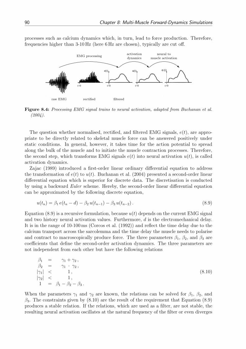
90 Chapter 8: Multi-Muscle Forward-Dynamics Simulations
processes such as calcium dynamics which, in turn, lead to force production. Therefore,frequencies higher than 3-10 Hz (here 6 Hz are chosen), typically are cut off.
t=0 t=0 t=0 t=0
u(t)e(t) α (t)
EMG processingactivationdynamics
neural tomuscle activation
raw EMG rectified filtered
Figure 8.4: Processing EMG signal trains to neural activation, adapted from Buchanan et al.(2004).
The question whether normalised, rectified, and filtered EMG signals, e(t), are appro-priate to be directly related to skeletal muscle force can be answered positively understatic conditions. In general, however, it takes time for the action potential to spreadalong the bulk of the muscle and to initiate the muscle contraction processes. Therefore,the second step, which transforms EMG signals e(t) into neural activation u(t), is calledactivation dynamics.
Zajac (1989) introduced a first-order linear ordinary differential equation to addressthe transformation of e(t) to u(t). Buchanan et al. (2004) presented a second-order lineardifferential equation which is superior for discrete data. The discretisation is conductedby using a backward Euler scheme. Hereby, the second-order linear differential equationcan be approximated by the following discrete equation,
u(tn) = β1 e(tn − d)− β2 u(tn−1)− β3 u(tn−2) . (8.9)
Equation (8.9) is a recursive formulation, because u(t) depends on the current EMG signaland two history neural activation values. Furthermore, d is the electromechanical delay.It is in the range of 10-100 ms (Corcos et al. (1992)) and reflect the time delay due to thecalcium transport across the sarcolemma and the time delay the muscle needs to polariseand contract to macroscopically produce force. The three parameters β1, β2, and β3 arecoefficients that define the second-order activation dynamics. The three parameters arenot independent from each other but have the following relations
β1 = γ1 + γ2 ,β2 = γ1 · γ2 ,|γ1| < 1 ,|γ2| < 1 ,1 = β1 − β2 − β3 .
(8.10)
When the parameters γ1 and γ2 are known, the relations can be solved for β1, β2, andβ3. The constraints given by (8.10) are the result of the requirement that Equation (8.9)produces a stable relation. If the relations, which are used as a filter, are not stable, theresulting neural activation oscillates at the natural frequency of the filter or even diverges
8.2 EMG-driven Forward-Dynamics Model: Employing a Forward-Inverse Model 91
towards infinity. For further details, the reader is referred to Buchanan et al. (2004) andthe citations therein.
The third and last transformation step is performed by converting the neural activa-tion, u(t), into muscle activation α(t). Heckathorne and Childress (1981), Woods andBigland-Ritchie (1983), or Zuniga and Simons (1969) have shown that isometric EMG,and therefore neural activation, is not necessary linearly related to muscle force. Re-membering Figure 2.10, one stimulation pulse will create a twitch response and multiplestimulation pulses will cause multiple twitch responses. If the stimulation frequency in-creases, the twitches will start to fuse and the average force produced by the motor unitwill steadily increase. However, for a further increasing stimulation frequency, the be-haviour of the resulting curve converges more and more towards the tetanus behaviour,where no further force can be produced by the muscle even if the stimulation frequencyincreases. This phenomena leads to the conclusion, that there is a nonlinear relationshipbetween stimulation frequency and force for single motor units. Which is not covered bythe neural activation. This nonlinearity can further be increased by other factors suchas the size effect, where small motor units are recruited at low intensity levels and largerones at higher intensity levels. Manal and Buchanan (2003) came up with a logarithmicfunction relating u(t) to α(t) including four parameters. Manal et al. (2002) and Lloydand Besier (2003b) further extended the before mentioned relation by an alternative for-mulation which yields adequate solutions:
α(t) =eAu(t) − 1
eA − 1, (8.11)
where A is the shape factor, condensing the information of the four parameters to a singlevalue. The shape factor’s value is ranging from [−3, 0), where for the limA→0 the relationsimplifies to a linear relation and for A = −3 the relation behaves highly exponential.
The values for d, γ1, γ2 and A are preset to d = 40 ms, γ1 = γ2 = 0.5, and A = −0.1,respectively, cf. Buchanan et al. (2004). During the calibration process, these values areadapted to find a minimum in the objective function, see Section 8.2.5.
8.2.3 Muscle-Tendon-Complex Mechanics
Within forward-dynamics and inverse-dynamics rigid-body models, the muscle contractiondynamics is determined by a Hill -type muscle model.
The muscle model of Figure 1.1b, like the muscle model employed here, consists of acontractile element, a parallel elastic element, and a serial elastic element to describe thetendon. One significant advantage of this type of muscle model is that it is, in most cases,governed by one ODE for the resulting MTC force
Fm(t) = f(Lm) f(Lm)αm(t)F 0m . (8.12)
Herein, f(Lm) is the dimensionless force-velocity relation, f(Lm) is the dimensionlessforce-length relation, and F 0
m is the maximum isometric muscle force. The force-velocityrelation, f(vm), is an adaption of Hill (1938) and is similar to Figure 1.1a. The differenceof this muscle fibre represented by a 3-element-Hill -type muscle model to the one ofFigure 1.1b is that CE and SEE are connected in parallel and that both are connectedin series to SEE.
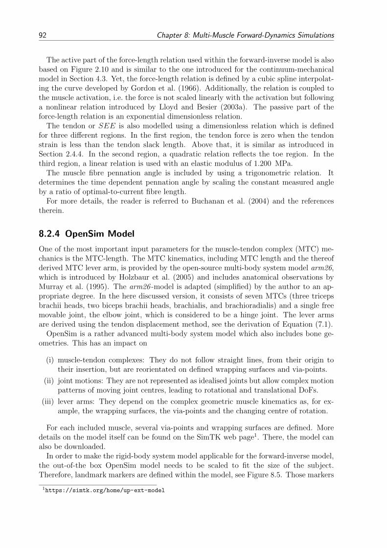
92 Chapter 8: Multi-Muscle Forward-Dynamics Simulations
The active part of the force-length relation used within the forward-inverse model is alsobased on Figure 2.10 and is similar to the one introduced for the continuum-mechanicalmodel in Section 4.3. Yet, the force-length relation is defined by a cubic spline interpolat-ing the curve developed by Gordon et al. (1966). Additionally, the relation is coupled tothe muscle activation, i.e. the force is not scaled linearly with the activation but followinga nonlinear relation introduced by Lloyd and Besier (2003a). The passive part of theforce-length relation is an exponential dimensionless relation.
The tendon or SEE is also modelled using a dimensionless relation which is definedfor three different regions. In the first region, the tendon force is zero when the tendonstrain is less than the tendon slack length. Above that, it is similar as introduced inSection 2.4.4. In the second region, a quadratic relation reflects the toe region. In thethird region, a linear relation is used with an elastic modulus of 1.200 MPa.
The muscle fibre pennation angle is included by using a trigonometric relation. Itdetermines the time dependent pennation angle by scaling the constant measured angleby a ratio of optimal-to-current fibre length.
For more details, the reader is referred to Buchanan et al. (2004) and the referencestherein.
8.2.4 OpenSim Model
One of the most important input parameters for the muscle-tendon complex (MTC) me-chanics is the MTC-length. The MTC kinematics, including MTC length and the thereofderived MTC lever arm, is provided by the open-source multi-body system model arm26,which is introduced by Holzbaur et al. (2005) and includes anatomical observations byMurray et al. (1995). The arm26 -model is adapted (simplified) by the author to an ap-propriate degree. In the here discussed version, it consists of seven MTCs (three tricepsbrachii heads, two biceps brachii heads, brachialis, and brachioradialis) and a single freemovable joint, the elbow joint, which is considered to be a hinge joint. The lever armsare derived using the tendon displacement method, see the derivation of Equation (7.1).
OpenSim is a rather advanced multi-body system model which also includes bone ge-ometries. This has an impact on
(i) muscle-tendon complexes: They do not follow straight lines, from their origin totheir insertion, but are reorientated on defined wrapping surfaces and via-points.
(ii) joint motions: They are not represented as idealised joints but allow complex motionpatterns of moving joint centres, leading to rotational and translational DoFs.
(iii) lever arms: They depend on the complex geometric muscle kinematics as, for ex-ample, the wrapping surfaces, the via-points and the changing centre of rotation.
For each included muscle, several via-points and wrapping surfaces are defined. Moredetails on the model itself can be found on the SimTK web page1. There, the model canalso be downloaded.
In order to make the rigid-body system model applicable for the forward-inverse model,the out-of-the box OpenSim model needs to be scaled to fit the size of the subject.Therefore, landmark markers are defined within the model, see Figure 8.5. Those markers
1https://simtk.org/home/up-ext-model

8.2 EMG-driven Forward-Dynamics Model: Employing a Forward-Inverse Model 93
Figure 8.5: OpenSim multi-body model. The model consists of seven muscles (three for thetriceps, two for the biceps and one for the brachialis and brachioradialis). The cyan colouredobjects are wrapping surfaces and the magenta spheres are representing the position of themarkers. The original model is transparent while the scaled subject-specified model is opaque.
are positioned at the same predefined locations on the subject and specified using theVicon camera system and software. Within the OpenSim software package, it was possibleto scale the initial model to the subject, yielding a subject specific rigid-body model.
8.2.5 Forward-Inverse-Dynamics Model and Optimisation
The heart of the forward-inverse model is the interaction of the forward- and the inverse-dynamics models by optimisation.
The forward-dynamics rigid-body model receives as model inputs the muscle activationsfrom the EMG-data processing, the kinematics from OpenSim, and the muscle contractiondynamics to determine the MTC reaction forces, to finally determine the joint torques,MFD; in this case the elbow torque, see Figure 8.6.
On the other hand, the inverse-dynamics rigid-body model uses the experimental torquedata to determine the joint torque to solve the rigid-body model. The mechanical rigid-body chain for solving the elbow torque is trivial as the elbow torque is measured directlywith the Biodex. Hence, the inverse-dynamics model reduces to the measured elbowtorques, MID.
Within the optimisation process, the sum of the squared difference of the elbow torques

94 Chapter 8: Multi-Muscle Forward-Dynamics Simulations
over all N sample points is minimised, i.e.
minN∑i=1
(M iFD −M i
ID)2 , (8.13)
by adjusting selected model parameters which is indicated in Figure 8.6 by the red arrows.The red arrows point on the activation dynamics and on the MTC model. Within theactivation dynamics, as mentioned already in Section 8.2.2, the model parameters are γ1,γ2, and A to adjust the resulting muscle activation. Within MTC mechanics, the tendonslack length and the maximal isometric force adjust the resulting muscle force. Thematerial parameters are adjusted plus-minus a selectable variation around the initial value.The optimisation uses an simulated annealing scheme. This scheme is a probabilistic,heuristic optimiser appropriate for a discrete space. The parameters are adjusted withinan off-line phase, called calibration.
The number of adjustable parameters should be large enough to fit the experimentaltorque well, but should not be too large to loose its predictability, cf. Buchanan et al.(2004). Too many adjustable parameters reduce the convincing power of a model and willbe suspected to be a mathematical exercise in curve fitting (Heine et al. (2003)).
Once the optimal solution is found for one subject, the trials can be investigated forthe distribution of muscle reaction forces acting on a joint.
8.3 Multi-Body Simulation-Driven Multi-Muscle Model
A further approach to achieve forward-dynamics simulations using three-dimensionalcontinuum-mechanical skeletal muscle models is by using the idea of nested models.Nested models in this context are two models that are compatible and describe thesame physical effects using different underlying physical models. For example, in skele-tal muscle mechanics, the force exerted by a skeletal muscle can be either modelled by aone-dimensional Hill-type skeletal muscle model or by a (chemo-electro) mechanical three-dimensional continuum model. Both models describe, up to the respective modelling error,the same physical phenomena, e.g. muscle force exertion. However, the musculoskeletalsystem appealing to one-dimensional Hill-type muscle models can be solved much fasterthan the system that appeals to three-dimensional continuum-mechanical based skeletalmuscle models.
Hence, it is possible to use the computational less expensive model to solve the forward-dynamics problem to obtain for a particular point in time the respective activation levelsand joint positions. The less expensive model is indicated by the blue box in Figure 8.7and is called a discrete model. These are mostly rigid-body models. Then, in a subse-quent step, the levels of activation and the position of the joint are used as input to thecontinuum-mechanical model (yellow box) as initial guess for the continuum-mechanicalmodel. Now presuming, that the modelling error of the one-dimensional skeletal musclemodel is small, one should have an excellent initial guess for the continuum-mechanicalmodel.

8.3 Multi-Body Simulation-Driven Multi-Muscle Model 95
Figure 8.7: A possible approach to facilitate forward-dynamics simulation of musculoskeletalsystems by coupling two modelling approaches. The left, blue box is representing rigid-bodysimulations, which are mostly used for the discrete modelling approach, the opposing right,yellow box, represents the continuum-mechanical modelling approach. Both models are linkedto each other by a coupling procedure, indicated by the green overlapping area.
As a result, just like with a close initial guess for Newtons method (Kim et al., 2006),one would expect only a few iterations of the more complex model, e.g. the musculoskeletalsystem appealing to continuum-mechanical models, in order to achieve (moment) equilib-rium.
Presuming that the modelling error is smaller for the musculoskeletal system modelappealing to continuum-mechanical muscle models than for the system appealing to one-dimensional models, one could also subsequently compute the resulting muscle forces(including their magnitude and orientation), the varying lever arm, and small changesin the elbow angle determined within the three-dimensional skeletal muscle models toupdate the respective quantities within the discrete model.
As long as there is a significant difference between the two modelling approaches, thetwo models will iterate until common quantities can be found. If that should be the case,the next time step can proceed using again the discrete model as a predictor.
A possible tool to exchange data between the to models could be a web-service linkingthe simulation packages from both modelling worlds. Hereby, both simulation tools onlyneed slight adjustments, while the effort and brain work is in the web-service. A wrapper,the web-service, and an orchestration application are needed to make the green box workexchanging the necessary data while keeping track of the simulation.

96 Chapter 8: Multi-Muscle Forward-Dynamics Simulations
Figure 8.6: The forward-inverse model consist of several components. The three arrays onthe left represent the data acquisition, consisting of measuring the muscle activity with EMGelectrodes, the arm position using either a motion capturing system or the intrinsic positiondata of the Biodex, and the elbow torque using the Biodex.The top left box represents the activation dynamics, i.e. , the data processing from raw EMGto muscle activation.The bottom left box provides the OpenSim model to prepare the kinematics of the muscu-loskeletal system and the Biodex data precessing.The top right box represents the forward-dynamics rigid-body model including the muscle con-traction dynamics. Herein, the model inputs are the muscle activation from the activationdynamics and the muscle kinematics from the OpenSim model. The resulting rigid-body modelis solved for the time sequence of the elbow moment.The bottom right box represents the inverse-dynamics model. In general, the model inputs aremuscle activation, the muscle kinematics, and the external loads to solve the resulting rigid-body system for the joint moment. In this particularly simple example, the inverse-dynamicsmodel is not required, as the elbow moment can be measured directly.The middle-right box is representing the optimisation procedure. The inputs are the timetransient elbow moment from both, the forward-dynamics and inverse-dynamics, model andcomputes the summed least square which are reduced by adapting parameters of the activationdynamics and the muscle contraction dynamics, which is indicated by the red arrow.

9 Results
9.1 Single Muscle
Hill -type muscles are popular within MBS investigating the kinetics of movements. Incontrast finite element simulations can produce spatially varying output. This propertyoffers the possibility to investigate heterogeneities, diseases, or disorders. Using thisadvantage, the next two sections investigate for the rigid-tendon model and for the muscle-tendon-complex model the advantages of the continuum-mechanical approach.
First the ability of the continuum-mechanical muscles to reproduce the upper limbsrange of motion is investigated. Therefore, no moment equilibrium is determined. Themuscles are not coupled to the static equilibrium system. The muscles are tested indepen-dently from each other if the full range of mechanical states, using the constraints givenby the Upper Limb Model, is achievable.
The motion of the forearm is mainly define by the position of the insertion points ofthe skeletal muscles. For the finite element simulation, the forearm position imposes theboundary constraints at the distal end of the skeletal muscles. The solution space isrestricted by:
• the forearm’s range of motion, which is 10 ≤ θ ≤ 150,
• the level of muscle activation, which is 0 ≤ α ≤ 1, and
• whether the effects of contact are considered or not.
To test the full range of motion, increments of ∆θ = 1 and ∆α = 0.1 are tested.In a first model evolution step, the tendons are assumed to be rigid, see Section 7.2.1.The corresponding muscle tissue constitutive law is based on the formulation given inSection 4.3.
In a second evolution step, the whole muscle-tendon complex is considered to be de-formable as introduced in Section 4.4 and Section 7.2.2.
9.1.1 Rigid-Tendon Model
In this section, the model assumptions of Section 7.2.1 are employed. Herein, only muscletissue is considered to be an elastic material. The tendons are visualised but not consideredas an elastic material. Their shape and length is included for visualising purposes only.
The results are split into four sections: visualising the raising arm movement, theresulting muscle reaction forces, the fibre stretch distribution, and the results from theforce wrench.
97

98 Chapter 9: Results
Raising Arm
Figure 9.1 visualises the upper limb for θ = 10, 45, 80, 115, and 150. It might be worthrepeating, that the shown situations do not represent physiological situations, as the elbowmoment balance is not considered. The figures show two muscles at the same joint positionwith the same (random) activation. The top row shows the resulting deformations for thefully activated muscles while considering contact. The bottom row shows the differencebetween considering contact and not considering contact.
To compare the different FE solutions in the bottom row of Figure 9.1, a new versionof the Green-Lagrangean strain tensor is introduced. The Green-Lagrangean strain tensorof (3.13) compares the current configuration with the reference configuration. Therefore,the current nodal coordinates without contact are defined as the “new” reference con-figuration whereas the current nodal coordinates with contact are defined as the “new”actual configuration. With these two new configurations at hand, a “new version” ofthe deformation gradient, as introduced in Equation (3.4), a “new version” of the rightCauchy-Green deformation tensor, as introduced in Equation (3.10), and finally a “newversion” of the Green-Lagrangean strain tensor, Enew, can be determined. To be ableto plot a strain tensor, either a special tensor visualisation procedure is needed or thetensor needs to be converted to a scalar value (Wunsche, 1999). Following the idea of Zheet al. (2004), who defined an effective strain measure similar to the von Mises stress, thefollowing effective strain is introduced
Eeff =2
3
√1
2[(Enew
11 − Enew22 )2 + (Enew
22 − Enew33 )2 + (Enew
11 − Enew33 )2+
+3
2(Enew
122 + Enew
232 + Enew
132)].
(9.1)
For a fully extended forearm, the biceps is slender and slim whereas the triceps is shortand compact, see Figure 9.1a. In Figure 9.1e where the forearm is fully flexed, the tricepsgets stretched and the biceps becomes bulged. While the Figures 9.1a-9.1e show the shapeof the muscle tissue, Figures 9.1f-9.1j highlight the effect of considering contact. The blackgrid lines represents the FE mesh including contact while the coloured, contoured musclerepresents the solution without contact. The contour plot visualises the effective strain –the difference between the two solutions – where red denotes a high deviation (0.5) andblue a small one (0.0). The red arrow at the osteotendinous junction represents the musclereaction force acting at the point of action determined by the methodology introduced inSection 7.5. Depending on the constraints, the force’s offset of the point of action andthe deviation of the orientation changes. The length of the arrow is proportional to itsabsolute value.
For the fully extended forearm, the grid and contour plot deviate for both muscles.The triceps deviates only slightly. But, the triceps’ offset from the point of action is,compared to the biceps, already significant. At the proximal or myotendinous junction,both solutions are deviating about 6.0 mm where contact pushed the whole proximalsurface posteriorly. This offset reduces proximally and is totally vanished at the distal,posterior junction. Furthermore, at the distal, anterior end of the junction, the muscle iscompressed by the humerus by about 3 mm.

9.1 Single Muscle 99
(a)θ
=10
(b)θ
=45
(c)θ
=80
(d)θ
=115
(e)θ
=150
(f)θ
=10
(g)θ
=45
(h)θ
=80
(i)θ
=11
5(j)θ
=150
Figure
9.1:
The
rais
ing
arm
move
men
tdep
icte
dat
five
dis
tin
ctpo
siti
on
sw
ith
full
yact
ivate
dm
usc
les.
The
uppe
rro
wdep
icts
the
def
orm
ati
on
ifco
nta
ctis
con
sider
ed,
the
low
erro
wdep
icts
the
new
lydefi
ned
def
orm
ati
on
mea
sure
inord
erto
com
pare
the
def
orm
ati
on
sw
ith
the
effec
tsof
con
tact
or
wit
hou
tco
nta
ct.
The
effec
tive
stra
inis
scale
dfr
omE
eff∈
[0,0.5
],w
her
esm
all
diff
eren
ces
are
blu
ean
dhig
hare
red.

100 Chapter 9: Results
The biceps’ solution deviates more – especially at the proximal end. Here, the solutionof the mesh is deviating by 9.1 mm anteriorly and by only 7.0 mm posteriorly. At theproximal end, the offset reverses and the mesh is anteriorly pushed by 8.2 mm . On theother hand, the difference of the biceps’ resulting reaction force is small.
For flexing the elbow, the distance between the biceps’ belly and the humerus increasesand contact does not play a crucial role anymore. It is not until the forearm is fullyflexed, when the bulged biceps comes in contact with the humerus. As contact playsonly a minor role, the solution’s meshes almost coincide. On the other hand, the tricepselongates for flexing the forearm and the difference between the two solutions (with andwithout contact) increases. The difference is especially large at the distal end, where thetriceps is pushed against the humerus. At θ = 150, the triceps penetrates the humerusby 11.5 mm. With contact, the distal end of the triceps wraps around the distal head ofthe humerus. Proximal, the surface’s offset is 10.9 mm.
Resulting Muscle Reaction Forces
Probably, the most fundamental and straight forward results of the FE simulations arethe absolute values of the muscle reaction forces. Considering contact, three differentreaction forces can be observed: (i) the resulting muscle reaction force, (ii) the activepart of the resulting muscle reaction force, and (iii) the contact force between muscle andbone. The muscle reaction forces depend on the material description, the geometry, thefibre orientation, the contact formulation, and the boundary conditions.
Figure 9.2 depicts the absolute values of the muscle reaction forces for the biceps andtriceps brachii for different activation levels throughout the full range of motion. The bluecurves always denote the triceps’ curve while the biceps’ curve are denoted by red curves.The bold curve include the effects of contact whereas the thin curves do not. The highestcurve represents the resulting muscle reaction force for a fully activated muscle while thelowest curve represents the purely passive mechanical behaviour of the muscle.
The muscle reaction forces are a result of the finite element simulation and depend onthe elbow angle as well as on the muscle activation. They are determined by taking theEuclidean norm after summing the nodal residual vectors at the muscle’s osteotendinousjunction.
As the activation is proportional to the active stress contribution (see Equation (4.30)),the resulting reaction forces are almost linearly distributed between the curve resultingfrom the fully activated muscle and the curve resulting form the passive muscle.
For the interpretation of the triceps reaction forces, the muscle length has to considered,cf. Figure 7.6a, as it has the strongest impact. As the muscle insertion point, whichdefines the fixed nodes, is tracking the motion of the olecranon of the ulna, the muscleinsertion point does not only change its length but also does a translational movement.Although the overall triceps length is increasing, the z-component does decrease for flexingthe forearm. The z-direction is nearly coinciding with the longitudinal direction of themuscles and hence has the strongest impact on the length of the muscle. The other twodirection cause, depending on their magnitude, only a shear-like movement. Hence, themaximum triceps reaction force is reached between 126 and 128 depending on the level ofactivation. For the fully activated triceps, the maximal value is FT (θ = 128, αT = 1.0) =1026 N, while the maximal value for the purely passive behaviour is T (128, 0.0) = 365 N.
As the biceps is the antagonist of the triceps, its length changes in the opposite direction.

9.1 Single Muscle 101
20 40 60 80 100 120 140
200
400
600
800
1000
elbow angle [°]
mu
sc
le f
orc
e [
N]
triceps
biceps
Figure 9.2: The muscle reaction forces fortriceps and biceps brachii for activationsα = 0.1 i with i = 0..10. The low-est curve is determined by α = 0 andthe highest by α = 1. The aim to pre-stretch the muscles such that no com-pression occurs is not achieved for thebiceps brachii.
0 50 100 150
100
200
300
400
500
600
700
elbow angle [°]
mu
sc
le f
orc
e [
N]
triceps
biceps
Figure 9.3: The active part of the mus-cle reaction forces is determined by sub-tracting the passive muscle reaction forcefrom the muscle reaction forces for α =0.1 i with i = 1..10
After reaching the peak at θ = 20, the biceps’ resulting curve is monotonically decreasing,as the length of the biceps is decreasing, see Figure 7.6b. Unfortunately, due to numericalissues, the biceps’ prestretch could not be chosen such that no compressive force is requiredfor the whole range of motion. Hence, the resulting curves have depending on the degreeof activation a kink at θ ≈ 130. The biceps reaction force reaches its maximal forcevalues for FB(θ = 22, αB = 1.0) = 671.2 N and FB(18, 0.0) = 220.1 N. For the triceps,the influence of contact on the reaction force is close to a constant offset of about 30 N. Atθ ≈ 130, the difference between the solutions reduces and, depending on the activation,also changes the effect, i.e. the solution including contact is larger than the solutionwithout contact. For the biceps, contact has a stronger influence on the reaction force atθ < 50. The difference is maximal with 74.6 N at θ = 10.
The purely active force contribution of a muscle is obtained by subtracting the passivemuscle force from the reaction force where the level of activation is larger than one. Theresulting force is depicted in Figure 9.3.
The maximal active triceps forces is F actT (100, 1.0) = 723.4 N. After an elbow angle
of about 100, the force remains roughly constant up to θ = 150. The maximal activebiceps force is F act
B (46, 1.0) = 470.1 N, The active biceps force slightly reduces when thebiceps is further stretched to its limit at θ = 10. The influence of the effect of contact arerather small. The muscle reaction forces are only slightly larger if no contact is considered.The reason might be due to numerical issues. If no contact is included, it was necessaryto fix more nodes at the osteotendinous junction in all three spatial dimensions. Higherrestrictions at the boundary cause higher reaction forces.
Depending on the elbow angle, the contact forces between the muscle and the bone canbe significant. Figure 9.14 depicts the normalised exerted muscle forces of the biceps andtriceps brachii and its contact forces with respect to the bone. For better comparison, the
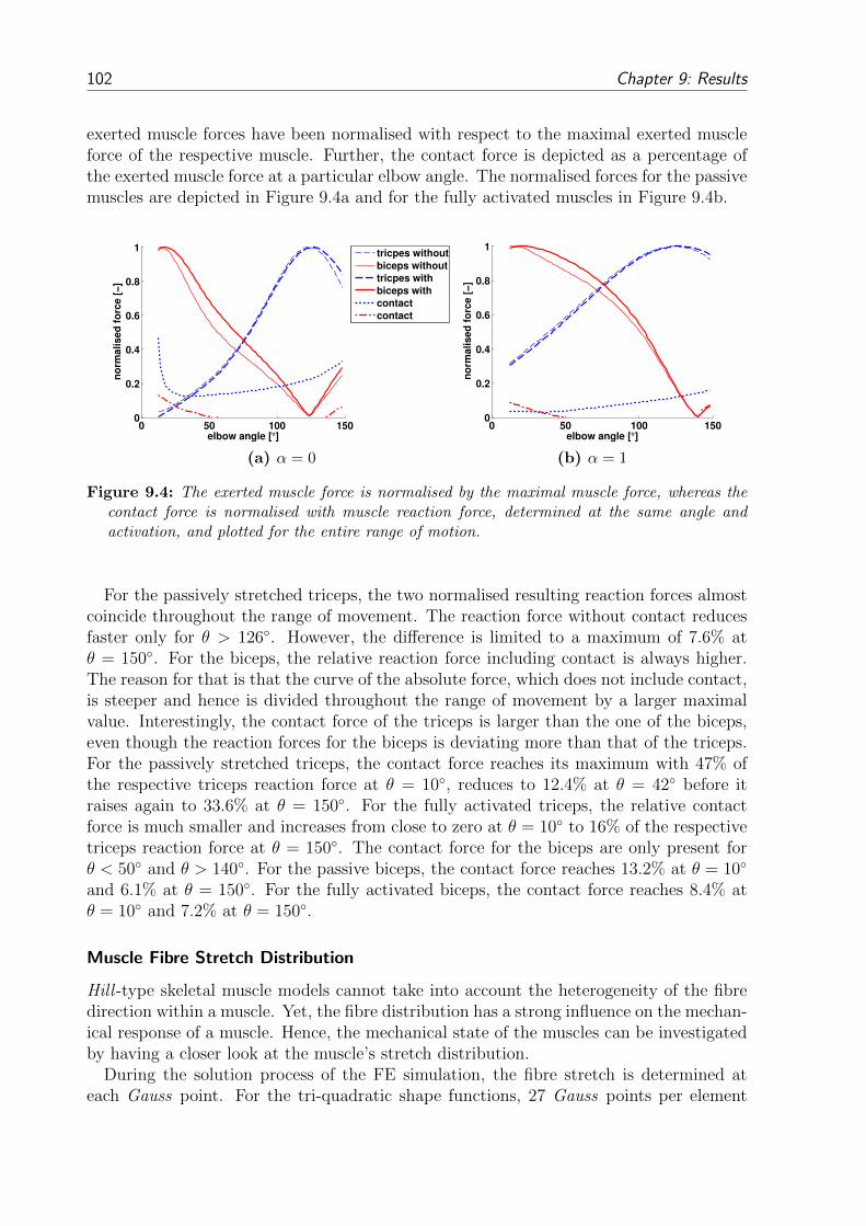
102 Chapter 9: Results
exerted muscle forces have been normalised with respect to the maximal exerted muscleforce of the respective muscle. Further, the contact force is depicted as a percentage ofthe exerted muscle force at a particular elbow angle. The normalised forces for the passivemuscles are depicted in Figure 9.4a and for the fully activated muscles in Figure 9.4b.
0 50 100 1500
0.2
0.4
0.6
0.8
1
elbow angle [°]
no
rma
lis
ed
fo
rce
[−
]
tricpes without
biceps without
tricpes with
biceps with
contact
contact
(a) α = 0
0 50 100 1500
0.2
0.4
0.6
0.8
1
elbow angle [°]
no
rmalised
fo
rce [
−]
(b) α = 1
Figure 9.4: The exerted muscle force is normalised by the maximal muscle force, whereas thecontact force is normalised with muscle reaction force, determined at the same angle andactivation, and plotted for the entire range of motion.
For the passively stretched triceps, the two normalised resulting reaction forces almostcoincide throughout the range of movement. The reaction force without contact reducesfaster only for θ > 126. However, the difference is limited to a maximum of 7.6% atθ = 150. For the biceps, the relative reaction force including contact is always higher.The reason for that is that the curve of the absolute force, which does not include contact,is steeper and hence is divided throughout the range of movement by a larger maximalvalue. Interestingly, the contact force of the triceps is larger than the one of the biceps,even though the reaction forces for the biceps is deviating more than that of the triceps.For the passively stretched triceps, the contact force reaches its maximum with 47% ofthe respective triceps reaction force at θ = 10, reduces to 12.4% at θ = 42 before itraises again to 33.6% at θ = 150. For the fully activated triceps, the relative contactforce is much smaller and increases from close to zero at θ = 10 to 16% of the respectivetriceps reaction force at θ = 150. The contact force for the biceps are only present forθ < 50 and θ > 140. For the passive biceps, the contact force reaches 13.2% at θ = 10
and 6.1% at θ = 150. For the fully activated biceps, the contact force reaches 8.4% atθ = 10 and 7.2% at θ = 150.
Muscle Fibre Stretch Distribution
Hill -type skeletal muscle models cannot take into account the heterogeneity of the fibredirection within a muscle. Yet, the fibre distribution has a strong influence on the mechan-ical response of a muscle. Hence, the mechanical state of the muscles can be investigatedby having a closer look at the muscle’s stretch distribution.
During the solution process of the FE simulation, the fibre stretch is determined ateach Gauss point. For the tri-quadratic shape functions, 27 Gauss points per element

9.1 Single Muscle 103
have been used within this work.To visualise these enormous data, the evaluated fibre stretches are categorised into 0.1-
wide spaced bins ranging from 0 ≤ λf ≤ 2 and normalised with respect to the overallnumber of Gauss points. Independent of the element’s volume, each fibre stretch valueis considered equal. The resulting fibre stretch distributions are depicted in Figure 9.5.Red denotes a high occurrence (20%) and blue a low occurrence. White space denotesthat this event never occured.
The distribution is plotted with the fibre stretch on the abscissa (x-axes) and the elbowflexion angle on the ordinate (y-axis). Hence, a fibre stretch distribution, for a particularelbow position, is obtained by following a horizontal line in each subfigure. The plots showthe fibre stretch distribution including the effects of contact. As contact occurs and asthe resulting fibre distribution is quite complex, it does not make much sense to comparethe fibre stretch distribution with and without contact by comparing figures similar to9.5.
For the triceps, the muscle is shortest at θ = 10 and increases its length with increasingθ. The biceps brachii behaves vice versa. It can be said that the fibre distribution is morecompact for the short and unactivated muscle. The distribution becomes wider and morecomplex for increasing muscle length and muscle activation. In general, it can be observedthat at λf ≈ 1.4 the distribution accumulates. The reason for this phenomenon is thatthe passive fibre contribution starts to dominate around λf = 1.4 preventing through itsstiffness further stretching.
Due to the bipennate fibre architecture of the triceps, a wider stretch spectra can beobserved than for the fusiform biceps. The triceps’ main accumulation is dominated bythe cross-section’s centre, where the fibres are orientated along the longitudinal axes of themuscle. When the activation of the triceps increases, the fanning of the fibres increasesand the fibre stretch spectra becomes wider and less distinct.
The biceps, depicted on the right side of Figure 9.5, is a fusiform muscle and thereforehas a more distinct fibre stretch distribution. When increasing the muscle activation,the contact between the biceps and the humerus increases and, hence bulges. Therefore,the angle between the longitudinal axis of the muscle and the fibre increases. Yet, withincreasing muscle length, the distribution becomes wider.
In Figure 9.6, the muscle’s mean fibre stretch is determined and depicted for α = 0.0, 0.5and 1.0 vs. θ. The bold curves denote the mean fibre average including contact whereasthe thin curves do not include contact.
The triceps’ mean fibre stretch ranges from λf (θ = 10, αT = 1) = 0.933 to λf (θ =124, αT = 0) = 1.177 and each mean curve increases with increasing muscle activation.The biceps’ mean fibre stretch covers a larger area, ranging from λf (θ = 150, αB = 1) =λf = 0.87 to λf (θ = 10, αB = 0) = 1.4 and is close to independent from the muscleactivation. While the triceps’ mean fibre stretch is increasing with increasing musclelength the biceps’ one is not. The reason for this behaviour is due to the bipennate andfusiform fibre architecture.

104 Chapter 9: Results
0.8 1 1.2 1.4 1.6
20
40
60
80
100
120
140
fibre stretch [−]
elb
ow
an
gle
[°]
0
0.05
0.1
0.15
0.2
(a) triceps, α = 0.0
0.8 1 1.2 1.4 1.6
20
40
60
80
100
120
140
fibre stretch [−]
elb
ow
an
gle
[°]
0
0.05
0.1
0.15
0.2
(b) biceps, α = 0.0
0.8 1 1.2 1.4 1.6
20
40
60
80
100
120
140
fibre stretch [−]
elb
ow
an
gle
[°]
0
0.05
0.1
0.15
0.2
(c) triceps, α = 0.5
0.8 1 1.2 1.4 1.6
20
40
60
80
100
120
140
fibre stretch [−]
elb
ow
an
gle
[°]
0
0.05
0.1
0.15
0.2
(d) biceps, α = 0.5
0.8 1 1.2 1.4 1.6
20
40
60
80
100
120
140
fibre stretch [−]
elb
ow
an
gle
[°]
0
0.05
0.1
0.15
0.2
(e) triceps, α = 1.0
0.8 1 1.2 1.4 1.6
20
40
60
80
100
120
140
fibre stretch [−]
elb
ow
an
gle
[°]
0
0.05
0.1
0.15
0.2
(f) biceps, α = 1.0
Figure 9.5: The relative fibre occurrence is plotted vs. the elbow flexion angle θ and the musclefibre stretch λf . The scale for the relative occurrence is limited to 0.2 to resolve also fibreswith less frequent fibre stretch occurrences. A horizontal line represents the muscle’s fibredistribution for one particular position. Hence the sum of all occurrences on a horizontal lineis one.
The central line along the longitudinal axis of the triceps behaves similar to the fusiformbiceps; these fibres are aligned with the longitudinal axis of the muscle and therefore are
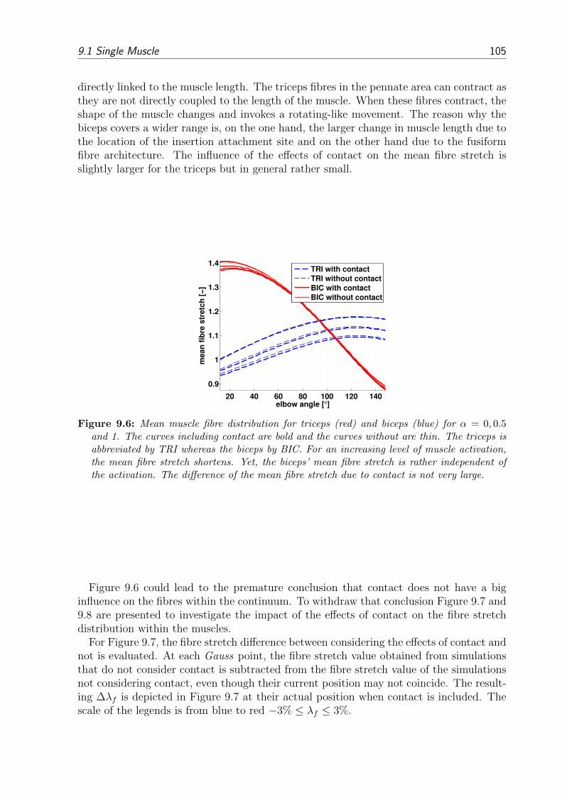
9.1 Single Muscle 105
directly linked to the muscle length. The triceps fibres in the pennate area can contract asthey are not directly coupled to the length of the muscle. When these fibres contract, theshape of the muscle changes and invokes a rotating-like movement. The reason why thebiceps covers a wider range is, on the one hand, the larger change in muscle length due tothe location of the insertion attachment site and on the other hand due to the fusiformfibre architecture. The influence of the effects of contact on the mean fibre stretch isslightly larger for the triceps but in general rather small.
20 40 60 80 100 120 140
0.9
1
1.1
1.2
1.3
1.4
elbow angle [°]
me
an
fib
re s
tre
tch
[−
]
TRI with contact
TRI without contact
BIC with contact
BIC without contact
Figure 9.6: Mean muscle fibre distribution for triceps (red) and biceps (blue) for α = 0, 0.5and 1. The curves including contact are bold and the curves without are thin. The triceps isabbreviated by TRI whereas the biceps by BIC. For an increasing level of muscle activation,the mean fibre stretch shortens. Yet, the biceps’ mean fibre stretch is rather independent ofthe activation. The difference of the mean fibre stretch due to contact is not very large.
Figure 9.6 could lead to the premature conclusion that contact does not have a biginfluence on the fibres within the continuum. To withdraw that conclusion Figure 9.7 and9.8 are presented to investigate the impact of the effects of contact on the fibre stretchdistribution within the muscles.
For Figure 9.7, the fibre stretch difference between considering the effects of contact andnot is evaluated. At each Gauss point, the fibre stretch value obtained from simulationsthat do not consider contact is subtracted from the fibre stretch value of the simulationsnot considering contact, even though their current position may not coincide. The result-ing ∆λf is depicted in Figure 9.7 at their actual position when contact is included. Thescale of the legends is from blue to red −3% ≤ λf ≤ 3%.

106 Chapter 9: Results
(a) fully extended, α =0
(b) fully extended,α = 0.5
(c) fully extended, α =1
∆λf [%]
−3
+3
−1.8
−0.6
+0.6
+1.8
(d) fully flexed, α = 0 (e) fully flexed, α = 0.5 (f) fully flexed, α = 1
∆λf [%]
−3
+3
−1.8
−0.6
+0.6
+1.8
Figure 9.7: The difference between the fibre stretch resulting from simulations considering con-tact and not. The difference are computed at each integration point. The fibre stretch differ-ence is negative (blue), when the fibres in simulations are longer without contact and positive(red) when the fibres are longer in simulations with contact.
For the fully flexed triceps, the fibres close to contact sites at the humerus are shorterwhile the fibre on the posterior side of the triceps are longer. This effect increases foran increasing level of muscle activation. For the fully extended elbow, the triceps fibresexhibit the same behaviour.
For the fully extended biceps, the difference is quite large. For all three activations,the difference in the fibre stretch is more than 3% at the centre of the belly. Only at thedorsal, distal and at the anterior, proximal end of the biceps, the fibres are longer if no

9.1 Single Muscle 107
contact is considered. For the fully flexed elbow, the biceps behaves similar to the triceps,i.e. the fibre difference moves more towards shorter fibre stretches. Yet for the biceps, thedifference is more pronounced for the passive muscle.
Figure 9.8 evaluates the spatial difference by classifying the difference of Gauss ian fibrestretch of simulations that include contact and such that do not include contact intoten equally spaced groups with ∆λf = 0.5%. Hereby, one can investigate how large thedeviation of the fibre stretch at the Gauss points is and how often it occurs. In the firstgroup, the difference of the fibre stretch between simulations that include contact andsuch that do not is zero to 0.5%. In the last group, differences larger than 5.0% can beobserved.
1.002.00
3.004.00
5.00 20 40 60 80 1001201400
0.2
0.4
0.6
elbow angle [°]fibre stetch [%]
rela
tiv
e o
cc
urr
en
ce
[−
]
(a) triceps, α = 0.0
1.002.00
3.004.00
5.00 20 40 60 80 1001201400
0.2
0.4
0.6
0.8
elbow angle [°]fibre stetch [%]
rela
tiv
e o
cc
urr
en
ce
[−
]
(b) biceps, α = 0.0
1.002.00
3.004.00
5.00 20 40 60 80 1001201400
0.1
0.2
0.3
0.4
elbow angle [°]fibre stetch [%]
rela
tiv
e o
cc
urr
en
ce
[−
]
(c) triceps, α = 1.0
1.002.00
3.004.00
5.00 20 40 60 80 1001201400
0.2
0.4
0.6
elbow angle [°]fibre stetch [%]
rela
tiv
e o
cc
urr
en
ce
[−
]
(d) biceps, α = 1.0
Figure 9.8: Relative occurrence of the fibre stretch difference evaluated for Figure 9.7. I.e. thefibre stretch of a particular location determined by simulations not including contact is sub-tracted from the fibre stretches determined by simulations including contact. Their absolutedifference is categorised into ten equally spaced groups and normalised by the number of in-tegration points. Their relative occurrence is plotted vs. the elbow flexion angle θ and thedifference in the muscle fibre stretch ∆λf . The left side depicts the triceps brachii. Theright side depicts the results for biceps brachii. The top row depicts the results of a passivelystretched muscle while the bottom row depicts the fully active muscles.
For the passive triceps, the distribution is rather independent of the elbow angle. Be-tween 60-65% of the muscle fibres deviate less than 0.5%, around 20% deviate less than1%, around 2% deviate less than 2%, and only about 1% of the Gauss points’ fibre

108 Chapter 9: Results
stretches deviate more than 5%. For the active triceps, the deviation increases. Around26% of the fibres have a larger fibre stretch difference than 1%, around 7% deviate morethan 2%, and about 2% of the fibres deviate more than 5%.
For the biceps, the fibre stretch distribution is more complex but very similar for thepassive and the fully activated muscle. A peak emerges in both activation scenarios. Thedifference is that the peak appears about 20 towards higher elbow angles for the fullyactive biceps than for the passive biceps. For elbow angles smaller than 60, close to noneof the fibre stretches are the same. For θ = 10, only 8% of the fibres of the two scenarioshave the same length. A total of 92% of the fibres deviate for at least 1% in their lengtheven though the overall muscle length is not changing.
The Muscle Force Wrench
In contrast to rigid-body models, continuum-mechanical models have the advantage oftaking into account spatial heterogeneities. Hence, a continuum-mechanical model canbe applied to investigate the muscle force flowing through the muscle from origin toinsertion. The muscle force’s orientation changes due to muscle-intrinsic phenomena suchas the complex geometry, locally distributed material parameters, or the fibre structure.
To study these phenomena, the offset of the point of action of the muscle reaction forceis determined using the force wrench procedure introduced in Section 7.5.
Figure 9.9 depicts the amount that the point of action is deflected from the barycentreof the muscle’s proximal surface by minimising the orthogonal fraction of the resultingmoment at the surface, see Equation (7.20).
For rigid tendons, the deviation of the position of the point of action is small andmostly within 3 mm. The impact of the effects of contact are small as the shape of themuscles’ surfaces are similar independent of contact. Yet in case of the triceps, contactinfluences the displacement of the point of action at α = 0 and 1. The biceps’ deviationof the position of the point of action has a big dip at about 120. The cause for thisdip is related to the fact that the magnitude of the reaction force is close to zero in thatregion. Hence, the orientation of the reaction force is more indifferent. Therefore, thenominator of Equation (7.20) becomes dominant and the results are strongly deviating.To summarise, the dip is an effect of the badly defined prestretch. This is also the caseat 10 < θ < 15 for αT = 0. Interestingly, for increasing the biceps activation, the pointof action is less eccentric, hence the muscle force seems to flow more directly through thecentre of the muscle.
To investigate the variance of the orientation of the resulting muscle reaction force, theorientation of the reaction force is compared to the orientation of the line defined by thebarycentre of the origin and insertion point, similar to Rohrle and Pullan (2007). The lo-cation of the origin and the insertion is determined by the barycentre of the myotendinousjunction and the osteotendinous junction, respectively. The deflection angle enclosed bythe two muscle reaction force vectors is determined by:
^ = arccos‖F1 · F2‖‖F1‖ · ‖F2‖
, or ^ = arctan‖F1 × F2‖‖F1‖ · ‖F2‖
. (9.2)
where F1 and F2 are two reaction forces. They are determined by summing all threecomponents of the nodal residuals at the distal and proximal junctions. The second
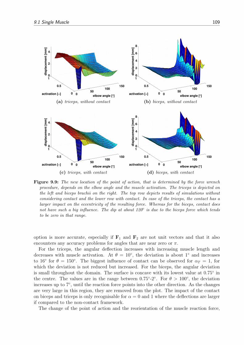
9.1 Single Muscle 109
050
100150
0
0.5
10
2
4
elbow angle [°]activation [−]
dis
pla
ce
me
nt
[mm
]
(a) triceps, without contact
050
100150
0
0.5
10
2
4
6
8
elbow angle [°]activation [−]
dis
pla
ce
me
nt
[mm
]
(b) biceps, without contact
050
100150
0
0.5
10
2
4
elbow angle [°]activation [−]
dis
pla
ce
me
nt
[mm
]
(c) triceps, with contact
050
100150
0
0.5
10
2
4
6
8
elbow angle [°]activation [−]
dis
pla
ce
me
nt
[mm
]
(d) biceps, with contact
Figure 9.9: The new location of the point of action, that is determined by the force wrenchprocedure, depends on the elbow angle and the muscle activation. The triceps is depicted onthe left and biceps brachii on the right. The top row depicts results of simulations withoutconsidering contact and the lower row with contact. In case of the triceps, the contact has alarger impact on the eccentricity of the resulting force. Whereas for the biceps, contact doesnot have such a big influence. The dip at about 120 is due to the biceps force which tendsto be zero in that range.
option is more accurate, especially if F1 and F2 are not unit vectors and that it alsoencounters any accuracy problems for angles that are near zero or π.
For the triceps, the angular deflection increases with increasing muscle length anddecreases with muscle activation. At θ = 10, the deviation is about 1 and increasesto 16 for θ = 150. The biggest influence of contact can be observed for αT = 1, forwhich the deviation is not reduced but increased. For the biceps, the angular deviationis small throughout the domain. The surface is concave with its lowest value at 0.75 inthe centre. The values are in the range between 0.75-2. For θ > 100, the deviationincreases up to 7, until the reaction force points into the other direction. As the changesare very large in this region, they are removed from the plot. The impact of the contacton biceps and triceps is only recognisable for α = 0 and 1 where the deflections are largerif compared to the non-contact framework.
The change of the point of action and the reorientation of the muscle reaction force,

110 Chapter 9: Results
can be seen in a video on the authors website1 and within the supplemental material tothis thesis.
050
100150
0
0.5
10
5
10
15
elbow angle [°]activation [−]
an
gu
lar
de
fle
cti
on
[°]
(a) triceps, without contact
050
100150
0
0.5
10
5
10
elbow angle [°]activation [−]
an
gu
lar
de
fle
cti
on
[°]
(b) biceps, without contact
050
100150
0
0.5
10
5
10
15
elbow angle [°]activation [−]
an
gu
lar
de
fle
cti
on
[°]
(c) triceps, with contact
050
100150
0
0.5
10
5
10
elbow angle [°]activation [−]
an
gu
lar
de
fle
cti
on
[°]
(d) biceps, with contact
Figure 9.10: Deviation of the orientation of the resulting reaction force compared to a one-dimensional representation defined by the barycentre of the origin and insertion point. Theorientation of the muscles’ resulting reaction force is weakly depending on the effects of con-tact.
1 www.mechbau.uni-stuttgart.de/ls2/jrg/people/academic_staff/sprenger/index.html
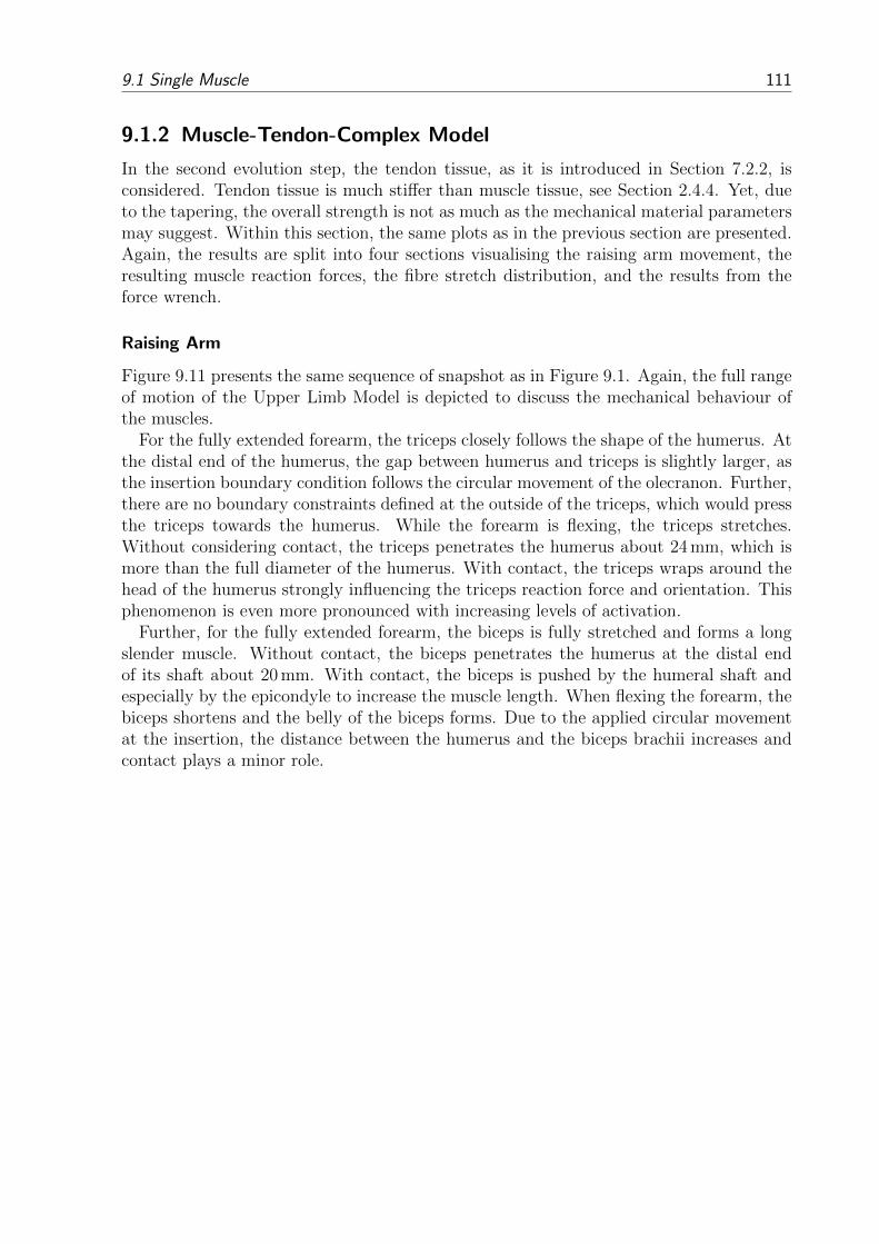
9.1 Single Muscle 111
9.1.2 Muscle-Tendon-Complex Model
In the second evolution step, the tendon tissue, as it is introduced in Section 7.2.2, isconsidered. Tendon tissue is much stiffer than muscle tissue, see Section 2.4.4. Yet, dueto the tapering, the overall strength is not as much as the mechanical material parametersmay suggest. Within this section, the same plots as in the previous section are presented.Again, the results are split into four sections visualising the raising arm movement, theresulting muscle reaction forces, the fibre stretch distribution, and the results from theforce wrench.
Raising Arm
Figure 9.11 presents the same sequence of snapshot as in Figure 9.1. Again, the full rangeof motion of the Upper Limb Model is depicted to discuss the mechanical behaviour ofthe muscles.
For the fully extended forearm, the triceps closely follows the shape of the humerus. Atthe distal end of the humerus, the gap between humerus and triceps is slightly larger, asthe insertion boundary condition follows the circular movement of the olecranon. Further,there are no boundary constraints defined at the outside of the triceps, which would pressthe triceps towards the humerus. While the forearm is flexing, the triceps stretches.Without considering contact, the triceps penetrates the humerus about 24 mm, which ismore than the full diameter of the humerus. With contact, the triceps wraps around thehead of the humerus strongly influencing the triceps reaction force and orientation. Thisphenomenon is even more pronounced with increasing levels of activation.
Further, for the fully extended forearm, the biceps is fully stretched and forms a longslender muscle. Without contact, the biceps penetrates the humerus at the distal endof its shaft about 20 mm. With contact, the biceps is pushed by the humeral shaft andespecially by the epicondyle to increase the muscle length. When flexing the forearm, thebiceps shortens and the belly of the biceps forms. Due to the applied circular movementat the insertion, the distance between the humerus and the biceps brachii increases andcontact plays a minor role.

112 Chapter 9: Results
(a)θ
=10
(b)θ
=45
(c)θ
=80
(d)θ
=11
5(e)θ
=150
(f)θ
=10
(g)θ
=45
(h)θ
=80
(i)θ
=11
5(j)θ
=150
Figure
9.11:
Rais
ing
the
fore
arm
,fo
rdiff
eren
tel
bow
flex
ion
an
gles
at
full
mu
scle
act
ivati
on
.T
he
uppe
rro
wdep
icts
the
scen
ari
ow
hen
con
tact
isco
nsi
der
ed,
whil
eth
elo
wer
row
com
pare
sth
eso
luti
on
sw
hen
con
tact
isco
nsi
der
edan
dn
ot.
The
effec
tive
stra
inis
scale
dsu
chth
atE
eff∈
[0,0.5
],w
her
esm
all
diff
eren
ces
are
dep
icte
din
blu
ean
dhig
hdiff
eren
ces
inre
d.
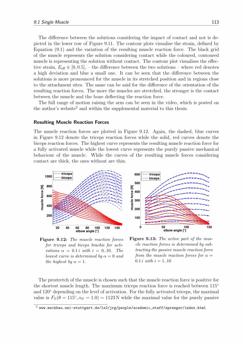
9.1 Single Muscle 113
The difference between the solutions considering the impact of contact and not is de-picted in the lower row of Figure 9.11. The contour plots visualise the strain, defined byEquation (9.1) and the variation of the resulting muscle reaction force. The black gridof the muscle represents the solution considering contact while the coloured, contouredmuscle is representing the solution without contact. The contour plot visualises the effec-tive strain, Eeff ∈ [0, 0.5], – the difference between the two solutions – where red denotesa high deviation and blue a small one. It can be seen that the difference between thesolutions is more pronounced for the muscle in its stretched position and in regions closeto the attachment sites. The same can be said for the difference of the orientation of theresulting reaction forces. The more the muscles are stretched, the stronger is the contactbetween the muscle and the bone deflecting the reaction force.
The full range of motion raising the arm can be seen in the video, which is posted onthe author’s website2 and within the supplemental material to this thesis.
Resulting Muscle Reaction Forces
The muscle reaction forces are plotted in Figure 9.12. Again, the dashed, blue curvesin Figure 9.12 denote the triceps reaction forces while the solid, red curves denote thebiceps reaction forces. The highest curve represents the resulting muscle reaction force fora fully activated muscle while the lowest curve represents the purely passive mechanicalbehaviour of the muscle. While the curves of the resulting muscle forces consideringcontact are thick, the ones without are thin.
20 40 60 80 100 120 140
200
400
600
800
1000
elbow angle [°]
mu
sc
le f
orc
e [
N]
triceps
biceps
Figure 9.12: The muscle reaction forcesfor triceps and biceps brachii for acti-vations α = 0.1 i with i = 0..10. Thelowest curve is determined by α = 0 andthe highest by α = 1.
0 50 100 150
100
200
300
400
500
600
elbow angle [°]
mu
scle
fo
rce [
N]
triceps
biceps
Figure 9.13: The active part of the mus-cle reaction forces is determined by sub-tracting the passive muscle reaction forcefrom the muscle reaction forces for α =0.1 i with i = 1..10
The prestretch of the muscle is chosen such that the muscle reaction force is positive forthe shortest muscle length. The maximum triceps reaction force is reached between 115
and 120 depending on the level of activation. For the fully activated triceps, the maximalvalue is FT (θ = 115, αT = 1.0) = 1123 N while the maximal value for the purely passive
2 www.mechbau.uni-stuttgart.de/ls2/jrg/people/academic_staff/sprenger/index.html

114 Chapter 9: Results
behaviour is FT (118, 0.0) = 508.2 N. The triceps reaction force only depends on the effectsof contact for θ > 90 i.e. when the triceps bends around the distal head of the humerus.Here, the reaction force without contact decreases more as the muscle length increasesincluding contact while it does decrease without contact. The difference between the twosolutions at θ = 150 is for the fully activated triceps 148 N. The biceps reaction forceis monotonically decreasing and reaches its maximal force values for B(θ = 10, αB =1.0) = 716.7 N and B(10, 0.0) = 391.7 N. For the biceps, the reaction force does onlydepend on the contact for θ < 25 when the biceps is in contact with the epicondyle. Thedifference in force between the two solutions is at θ = 10 for the fully activated biceps113 N. The triceps reaction force are below 30 N for FT (θ > 145, αB = 0). The bicepsforce is negative for FB(θ < 145, αB = 0) indicating that a larger prestretch should havebeen defined. A few millimeters larger would have been sufficient.
The purely active force contribution of a muscle is obtained by subtracting the passivemuscle force from the activated muscle force. The results are depicted in Figure 9.13.
For the triceps brachii, the active part is maximal, depending on the level of activation,between θ = 100 and θ = 120. For the biceps brachii, the active force is maximal forelbow angles between θ = 50 and 74. The maximal forces are F active
T (106, 1.0) = 617.8 Nand F active
B (51, 1.0) = 359.6 N.From Figure 9.13, one can clearly observe that for both muscles the active part of the
reaction force does not deviate whether contact is considered or not. Hence, one canconclude that the increase in muscle length, due to contact, just has an impact on thepassive muscle force contribution and not on the active one. Furthermore, the musclesact for the largest portion of their physiological range of motion on the ascending limb ofthe force-length relationship, i.e. the muscle force predominantly increases if the muscleis being stretched. For the biceps, the active part can be zero when the muscle is shortenough.
Depending on the elbow angle, the contact forces between the muscle and the bonecan be significant. Figure 9.14 depicts the normalised exerted muscle forces of the bicepsand triceps brachii and its contact forces with bone. For better comparison, the exertedmuscle forces have been normalised with respect to the maximal exerted muscle force ofthe respective muscle. Further, the contact force is depicted as a percentage of the exertedmuscle force at a particular elbow angle.
For the triceps, the contact forces are significant. For αT = 0, the contact force startsto be considerable at θ ≈ 80. It finally reaches 91% of the muscle reaction force atθ = 150. The spikes at θ = 65, 143, 146 are most probably developing due to jumpsof the element vertices from one side of the humerus to the other (an numerical phantomwhich stores the pressure until it reaches a limit where the element vertices slides overon the other side of the humerus curvature). For the active triceps, at a maximal elbowangle of 150, the contact force is 70.4% of the exerted muscle force at the same angle.Even though, the contact forces for the triceps brachii are quite significant for largerelbow angles, the contact force still measures 23.3% of the exerted muscle force when themaximal muscle force is produced, i.e. at an elbow angle of 115. Note that the triceps ispushing with more than 200 N against the shaft of the humerus.
Since no surrounding tissue was considered within this work and the biceps is a super-ficial muscle, the contact forces between the biceps brachii and the humerus are muchsmaller. Nevertheless, at small and large elbow angles, i.e. at θ < 50 and at θ > 140,

9.1 Single Muscle 115
0 50 100 1500
0.2
0.4
0.6
0.8
1
elbow angle [°]
no
rma
lis
ed
fo
rce
[−
]
tricpes without
biceps without
tricpes with
biceps with
contact
contact
(a) α = 0
0 50 100 1500
0.2
0.4
0.6
0.8
1
elbow angle [°]
no
rmalised
fo
rce [
−]
(b) α = 1
Figure 9.14: Normalised exerted muscle forces vs. contact forces for the entire range of motionassuming fully activated muscles.
the contact forces are still around 40% and 10% of the respective exerted muscle force.
Muscle Fibre Stretch Distribution
The MTC’s fibre stretch distribution is shown in Figure 9.15. Both muscles have anarrower stretch distribution when the muscle is shorter and less activated. The fibrestretch is predominantly close to λf = 1 for the passive muscle in its shortest configuration.Because tendon tissue is much stronger than muscle tissue throughout all configurations,there is an occurrence accumulation at λf = 1 which can, for example, be nicely seenin Figure 9.15f or 9.15e. Further, it can be observed that the fibre stretch tends toaccumulate at λf ≈ 1.4. The reason for this phenomenon is that at around λf = 1.4, thepassive stress starts to dominate and the muscle tissue becomes much stiffer. As a resultother fibres are stretched first, before these fibres are stretched any further.
Due to the transition zone between tendon tissue and muscle tissue, the stretch dis-tribution scatters and it becomes more difficult to assign areas to specific features. Forgrowing muscle length, the fibre stretch distribution spreads out and becomes more di-verse. Due to the bipennate fibre architecture of the triceps, a wider stretch spectrumcan be observed compared to the fusiform biceps. The triceps’ fibres are agglomerating atλf = 1 at its shortest configuration and slightly increases towards λf = 1.2 at is longestconfiguration. For an increasing triceps activation, the distribution is less distinct andmoves towards shorter fibre stretches. For the biceps, the highest fibre stretch occurrencestarts, for the shortest length, with λf ≈ 1 and shifts towards θ = 40 and λf = 1.4.Here, the passive muscle strength starts to dominate and the fibres start to accumulateat λf ≈ 1.4. As well as for the triceps, the biceps’ distribution becomes less distinct forincreasing muscle activation and the fibres stretch moves towards shorter lengths.

116 Chapter 9: Results
0.8 1 1.2 1.4 1.6 1.8 2
20
40
60
80
100
120
140
fibre stretch [−]
elb
ow
an
gle
[°]
0
0.05
0.1
0.15
0.2
(a) triceps, α = 0.0
0.8 1 1.2 1.4 1.6 1.8 2
20
40
60
80
100
120
140
fibre stretch [−]
elb
ow
an
gle
[°]
0
0.05
0.1
0.15
0.2
(b) biceps, α = 0.0
0.8 1 1.2 1.4 1.6 1.8 2
20
40
60
80
100
120
140
fibre stretch [−]
elb
ow
an
gle
[°]
0
0.05
0.1
0.15
0.2
(c) triceps, α = 0.5
0.8 1 1.2 1.4 1.6 1.8 2
20
40
60
80
100
120
140
fibre stretch [−]
elb
ow
an
gle
[°]
0
0.05
0.1
0.15
0.2
(d) biceps, α = 0.5
0.8 1 1.2 1.4 1.6 1.8 2
20
40
60
80
100
120
140
fibre stretch [−]
elb
ow
an
gle
[°]
0
0.05
0.1
0.15
0.2
(e) triceps, α = 1.0
0.8 1 1.2 1.4 1.6 1.8 2
20
40
60
80
100
120
140
fibre stretch [−]
elb
ow
an
gle
[°]
0
0.05
0.1
0.15
0.2
(f) biceps, α = 1.0
Figure 9.15: The relative fibre occurrence is plotted vs. the elbow flexion angle θ and the musclefibre stretch λf . The scale for the relative occurrence is limited to 0.2 to resolve also fibreswith less frequent fibre stretch occurrences. A horizontal line represents the muscle’s fibredistribution for one particular position. Hence the sum of all occurrences on a horizontal lineis one.
The mean triceps and biceps fibre stretch is plotted in Figure 9.16 for α = 0, 0.5 and1. For the passive triceps, the mean fibre stretch covers a range from λf = 1.013− 1.098.

9.1 Single Muscle 117
The shape of the curve does not change with increasing muscle activation. Yet, the meanfibre stretch reduces and the values for the fully activated triceps are shifted about 3.4%towards shorter lengths compared to the passive triceps. The mean fibre stretch for thepassive biceps is between λf = 0.997 and λf = 1.182. The shape of the curve changesonly slightly with increasing muscle activation. Compared to the passive biceps, the curveof the active biceps is less S-shaped. Yet, the mean fibre stretch reduces and the valuesfor the fully activated biceps are shifted about 2.6% towards shorter lengths comparedto the passive biceps. Contact has a larger influence on the triceps especially at higherflexion angles than on the biceps as the curves differ stronger for the triceps than for thebiceps. In their shortest configuration and fully activated, both muscles exhibit meanfibres stretches λf < 1.
20 40 60 80 100 120 140
1
1.05
1.1
1.15
elbow angle [°]
me
an
fib
re s
tre
tch
[−
]
TRI with contact
TRI without contact
BIC with contact
BIC without contact
Figure 9.16: Mean muscle fibre distribution for triceps (red) and biceps (blue) for α = 0, 0.5 and1. The curves including contact are bold and the curves without are thin. For an increasinglevel of muscle activation, the mean fibre stretch shortens. The difference of the mean fibrestretch due to contact is not very large.
Figure 9.16 could lead to the premature conclusion that contact does not have a biginfluence on the fibres within the continuum. To falsify this conclusion, Figure 9.17 and9.18 are presented to investigate the impact of the effects of contact on the fibre stretchdistribution within the muscles.
To compare the impact of the effects of contact on the fibre distribution, the focus is seton the local fibre stretch distribution. By comparing the resulting local fibre stretch dis-tribution including and not including contact, a large spatial deviation can be observed.The difference in fibre stretch between considering the effects of contact and not is de-picted in Figure 9.17. At each Gauss point, the fibre stretch value of the simulations thatconsidered the effects of contact is subtracted from the fibre stretch value of the simula-tions that do not consider the effects of contact, even though their current position maynot coincide. The deviation of their location varies more or less depending on the elbowangle, the muscle activation, and the location within the muscle. The resulting ∆λf isdepicted in Figure 9.17 at their actual position determined including contact. The scaleof the legends is from blue to red −3% ≤ λf ≤ 3%.
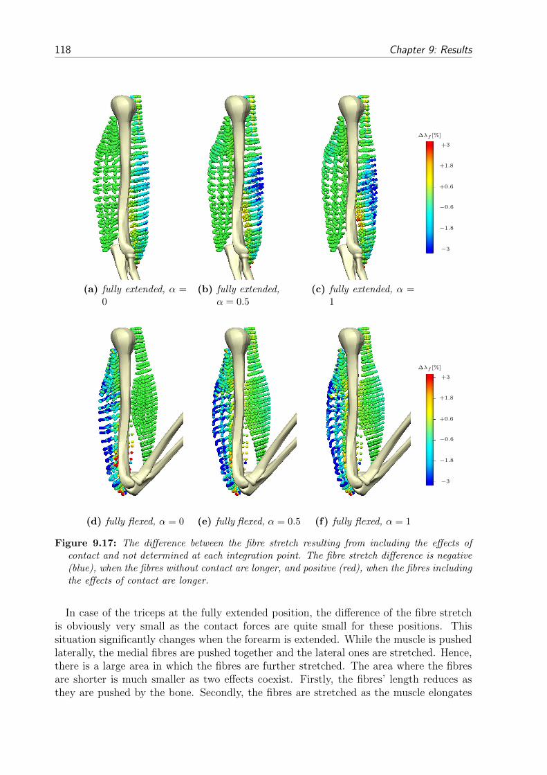
118 Chapter 9: Results
(a) fully extended, α =0
(b) fully extended,α = 0.5
(c) fully extended, α =1
∆λf [%]
−3
+3
−1.8
−0.6
+0.6
+1.8
(d) fully flexed, α = 0 (e) fully flexed, α = 0.5 (f) fully flexed, α = 1
∆λf [%]
−3
+3
−1.8
−0.6
+0.6
+1.8
Figure 9.17: The difference between the fibre stretch resulting from including the effects ofcontact and not determined at each integration point. The fibre stretch difference is negative(blue), when the fibres without contact are longer, and positive (red), when the fibres includingthe effects of contact are longer.
In case of the triceps at the fully extended position, the difference of the fibre stretchis obviously very small as the contact forces are quite small for these positions. Thissituation significantly changes when the forearm is extended. While the muscle is pushedlaterally, the medial fibres are pushed together and the lateral ones are stretched. Hence,there is a large area in which the fibres are further stretched. The area where the fibresare shorter is much smaller as two effects coexist. Firstly, the fibres’ length reduces asthey are pushed by the bone. Secondly, the fibres are stretched as the muscle elongates

9.1 Single Muscle 119
while the humerus forces the muscle to deform. The biceps’ behaviour is similar. Yet,contact is most prominent for the fully extended forearm position. But the effect is thesame. The medial fibres are shorter, where as the lateral are stretched. For the fullyactivated biceps, this effect can be seen even for the fully flexed muscle.
To emphasise the phenomena, Figure 9.18 presents the spatial evaluated differences ofthe classified into ten equal spaced groups. In the first group, the difference between thetwo cases is less then 0.5%. In the last group, the difference is larger than 5.0%. Thedistribution is plotted separately for each muscle (the triceps is left and the biceps right)and for the passive (the upper row) and the fully activated muscle (lower row) over thefull range of movement.
1.002.00
3.004.00
5.0050
1001500
0.5
1
elbow angle [°]fibre stetch classes [%]
rela
tive o
ccu
rren
ce [
−]
(a) triceps, α = 0
1.002.00
3.004.00
5.0050
1001500
0.5
1
elbow angle [°]fibre stetch classes [%]
rela
tive o
ccu
rren
ce [
−]
(b) biceps, α = 0
1.002.00
3.004.00
5.0050
1001500
0.2
0.4
0.6
0.8
elbow angle [°]fibre stetch classes [%]
rela
tive o
ccu
rren
ce [
−]
(c) triceps, α = 1
1.002.00
3.004.00
5.0050
1001500
0.5
1
elbow angle [°]fibre stetch classes [%]
rela
tive o
ccu
rren
ce [
−]
(d) biceps, α = 1
Figure 9.18: Relative occurrence of the fibre stretch difference evaluated for Figure 9.7. I.e. thefibre stretch of a particular location determined by simulations not including contact is sub-tracted from the fibre stretches determined by simulations including contact. Their absolutedifference is categorised into ten equally spaced groups and normalised by the number of in-tegration points. Their relative occurrence is plotted vs. the elbow flexion angle θ and thedifference in the muscle fibre stretch ∆λf . On the left is the triceps brachii and on the rightfor biceps brachii. On the top is the behaviour of the passive muscle and on the bottom theone of the active ones.
For the fully extended forearm, the deviation of the two solutions is very small. Thefibre stretch starts to deviate at θ = 52. For extending the forearm, the impact of thecontact increases and also the deviation of the fibre stretch increases. For the passive

120 Chapter 9: Results
triceps (Figure 9.18a), for example, at θ = 56 the difference is for 98.4% of the fibresless than 0.5%. On the other hand, at θ = 150 the difference is for 68.3% of the fibreslarger than 0.5% and for 6.6% of the fibres larger than 5.0%. For the fully flexed forearm,the biceps is only slightly pressed against the humerus. Hence, the difference of thefibre stretch is smaller compared to the one of the triceps. The deviation of the fibres isoccurring until θ = 40 and increases towards fully extending the forearm. For the fullyactivated biceps (Figure 9.18d), for example at θ = 10, the difference is for 70.6% of thefibres less than 0.5%, for 2.8% of the fibres less than 2.5%, and for 1.2% of the fibres lessthan 3%.
The Muscle Force Wrench
In Figure 9.19, the amount the point of action is deflected from the barycentre of themuscle’s proximal surface is determined by minimising the orthogonal fraction of theresulting moment at the surface, see Equation (7.20).
050
100150
0
0.5
10
5
10
elbow angle [°]activation [−]
dis
pla
ce
me
nt
[mm
]
(a) triceps, without contact
050
100150
0
0.5
10
1
2
3
elbow angle [°]activation [−]
dis
pla
ce
me
nt
[mm
]
(b) biceps, without contact
050
100150
0
0.5
10
5
10
elbow angle [°]activation [−]
dis
pla
ce
me
nt
[mm
]
(c) triceps, with contact
050
100150
0
0.5
10
1
2
3
elbow angle [°]activation [−]
dis
pla
ce
me
nt
[mm
]
(d) biceps, with contact
Figure 9.19: The new location of the point of action, that is determined by the force wrenchprocedure, depends on the elbow angle and the muscle activation. In case of the triceps, thecontact has a larger impact on the eccentricity of the resulting force. Whereas for the biceps,contact does not have much of an influence.
The triceps’ deflection of the point of action (Figure 9.19a and 9.19c) is in the widestrange of θ and α a smooth and slightly increasing surface. For a reducing elbow angle and

9.1 Single Muscle 121
an increasing activation, the maximal value is about 2 mm. Yet, for a very short triceps(θ < 50) and a low activation (αT < 0.5) the amount of deflection rises strongly up to10 mm. In case of considering contact, the deflection increases from the non-contact resultsonly for the long triceps (θ > 130, depending on the level of activation) as the tricepshas to bend around the olecranon by an increase of only a few millimeters. The maximaldeflection of the point of action is 2.1 mm at θ = 150 and αT = 0. The biceps’ deflectionof the point of action is a slightly increasing for the decreasing biceps length, while it isclose to independent of the muscle activation. The maximal deflection is around 3 mm.The difference between contact and non-contact is marginal. There is only an additionalsmall dent at θ = 0.24 where the deflection increases for less than one millimeter.
In Figure 9.20, the deviation of the orientation of the resulting muscle reaction force iscompared to the orientation of the line defined by the barycentre of the muscle’s originand insertion.
050
100150
0
0.5
10
20
40
elbow angle [°]activation [−]
an
gu
lar
de
fle
cti
on
[°]
(a) triceps, without contact
050
100150
0
0.5
10
10
20
elbow angle [°]activation [−]
an
gu
lar
de
fle
cti
on
[°]
(b) biceps, without contact
050
100150
0
0.5
10
20
40
elbow angle [°]activation [−]
an
gu
lar
de
fle
cti
on
[°]
(c) triceps, with contact
050
100150
0
0.5
10
10
20
elbow angle [°]activation [−]
an
gu
lar
de
fle
cti
on
[°]
(d) biceps, with contact
Figure 9.20: Deviation of the orientation of the resulting reaction force compared to a one-dimensional representation line defined by the barycentre of the origin and insertion point.The orientation of the muscles’ resulting reaction force is strongly depending on the effects ofcontact.
For the triceps, the deflection of the orientation of the reaction force increases with-out considering the effects of contact (see Figure 9.20a) slightly towards a short and lowactivated triceps with a maximal deviation of around 4.5. Including contact, the be-haviour of Figure 9.20a is superposed with the strong influence of the triceps wrapping

122 Chapter 9: Results
around the olecranon. Hence, for increasing the triceps length, the triceps’ orientationdeviates from the orientation of the line by up to 40. The biceps’ deflection of the reac-tion force is without contact mostly less than 1 mm, i.e. very small and negligible. Withcontact, the biceps’ deflection superposes for a long biceps the impact of the contact. Fora very extended forearm, the biceps touches the humerus, hence, the deflection increasesto approximately 20.
For the results of the MTC depicted in Figure 9.19 and 9.20, less artifacts are arisingas the muscle reaction forces are not reducing to zero or changing the sign as they do ifrigid tendons are assumed.
9.1.3 Muscle Resulting Elbow Moment
As a joint moment is a product of a lever arm and a force acting on the joint, not onlythe muscle’s force but also the muscle’s lever arm have an impact on the generated jointmoment. Hence, for the determination of an elbow equilibrium, also the two differentmethods to determine the lever arm have to be considered within this investigation. Sobefore convergence studies of the Upper Limb Model are presented, the lever arms andthe resulting muscle elbow moment are shown for the whole variability space.
As the convergence behaviour of the system for rigid and compliant tendons does notconceptionally change, it is not differentiated between the results of the two evolutionsteps. The results, shown here, are produced using the full MTC model.
Employing the Tendon-Displacement Method
Figure 9.21 shows the lever arm resulting from using the tendon-displacement method(TDM). Due to the fact that the muscles’ length relation is smooth, the derivatives arewell behaving and the curves are continuous. As the triceps is an extensor muscle andthe biceps a flexor muscle, the lever arms are of opposite sign. The triceps lever arm ismostly close to -20 mm. The biceps lever arm is in the fully flexed state close to 37 mm,reaches its maximum of 41 mm at 60, and declines to 27 mm at full extension.
The elbow joint moments resulting from the TDM are shown in Figure 9.22. The elbowmoment is a function of the elbow angle and the muscle activation, while the dependencyon contact is small. For the triceps, the maximal moment is MT (θ = 100, αT = 1) =−26.1 kNmm and the minimum is MT (θ = 10, αT = 0) = −0.85 kNmm. As the tricepsacts as an extensor, the moment is defined to be negative and even though the value ofMT (θ = 100, αT = 1) is smaller than the value of MT (θ = 10, αT = 0), the absolute valueis larger. For the biceps, the maximal moment is MB(θ = 28, αB = 1) = 25.2 kNmm andthe minimal is MB(θ = 150, αB = 0) = −0.13 kNmm. The last moment is negative asfor TB(θ > 146, αB = 0) the reaction forces are negative, i.e. the prestretch should bedefined a few millimeters larger.
Vector-Resulting Lever Arm
For the determination of the vector-resulting lever arm (VRLA), Equation (7.2) is solvedand plotted as surface vs. muscle activation and elbow angle as it points out, that the leverarm is not only a function of the elbow angle but also of the muscle activation. The reasonfor the muscle activation dependency is that the muscle force orientation varies with the

9.1 Single Muscle 123
0 50 100 150−40
−20
0
20
40
60
elbow angle θ [°]
mu
sc
le l
ev
er
arm
[m
m]
triceps
biceps
Figure 9.21: The lever arms for tricepsand biceps brachii for the TDM are de-termined by taking the derivative of themuscle lengths with respect to θ.
0 50 100 150
−2
−1
0
1
2
x 104
elbow angle [°]
mu
scle
mo
men
t [N
mm
]
triceps
biceps
Figure 9.22: The product of lever armand muscle force yields the resulting el-bow joint moment which depends on θand α. The thick curves consider con-tact whereas the thin curves do not. Thecurve with the lowest absolute value be-longs to α = 0 and raises in ∆α = 0.1steps up to α = 1 to build 11 curves foreach muscle.
muscle activation and has an impact on the vector-resulting lever arm. Furthermore, thecontact formulation has an influence on the vector-resulting lever arm as it influences theorientation of the reaction force strongly.
For the triceps, see Figure 9.23a and b, the lever arm is, for a flexing elbow, a mono-tonically decreasing surface. Not considering contact, the lever arm is between -8 mm,for large elbow angles, and -30 mm, for small elbow angles. While the muscle activation’sdependency is mostly only weak, it has a strong influence on a fully extended forearm.Towards a passive muscle, the lever arm drops. Considering contact, the overall muscleactivation’s dependency is stronger. Rather significant is the fact, that the lever armincluding contact is less linear. Contact causes a concave bend for the elbow angle de-pendency. For an extended elbow, the lever arm including contact even becomes positive.Furthermore, the distinct kink at the extended elbow towards a passive muscle state isnot existing.
For the biceps, see Figure 9.23b and d, the lever arm values are mostly between 10 and15 mm. For the passive, fully flexed muscle, the muscle reaction force is very close to zero.Hence, its orientation is not clearly defined anymore and therefore, the resulting bicepsreaction force and moment, respectively, are not well defined anymore. When contact isalso considered, the slight decrease towards the fully extended elbow vanishes and thebiceps lever arm is about 13.5 mm and very close to constant.
As the lever arms are determined using the exact vectorial locations, it is possiblenow to incorporate the change of the location of the point of action and the differentorientations of the muscle reaction force. To point out the impact of the change oflocation, in Figure 9.24 the difference between the results of Figure 9.23 are subtracted
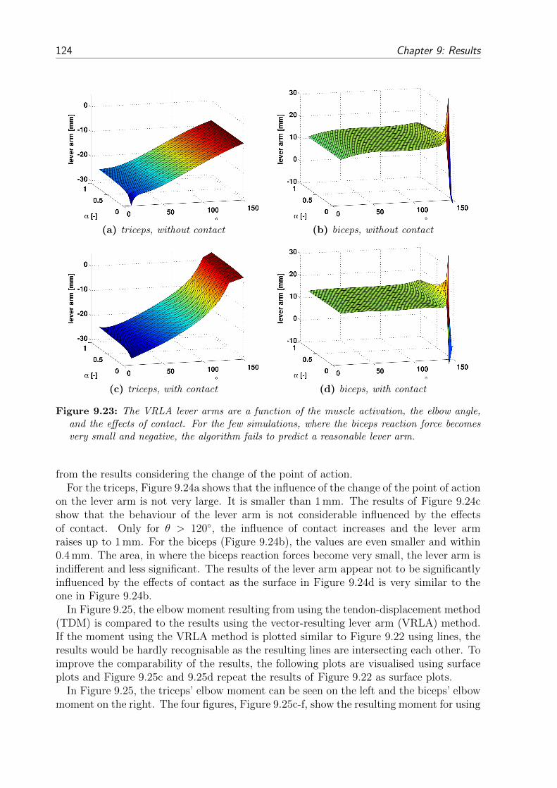
124 Chapter 9: Results
(a) triceps, without contact (b) biceps, without contact
(c) triceps, with contact (d) biceps, with contact
Figure 9.23: The VRLA lever arms are a function of the muscle activation, the elbow angle,and the effects of contact. For the few simulations, where the biceps reaction force becomesvery small and negative, the algorithm fails to predict a reasonable lever arm.
from the results considering the change of the point of action.For the triceps, Figure 9.24a shows that the influence of the change of the point of action
on the lever arm is not very large. It is smaller than 1 mm. The results of Figure 9.24cshow that the behaviour of the lever arm is not considerable influenced by the effectsof contact. Only for θ > 120, the influence of contact increases and the lever armraises up to 1 mm. For the biceps (Figure 9.24b), the values are even smaller and within0.4 mm. The area, in where the biceps reaction forces become very small, the lever arm isindifferent and less significant. The results of the lever arm appear not to be significantlyinfluenced by the effects of contact as the surface in Figure 9.24d is very similar to theone in Figure 9.24b.
In Figure 9.25, the elbow moment resulting from using the tendon-displacement method(TDM) is compared to the results using the vector-resulting lever arm (VRLA) method.If the moment using the VRLA method is plotted similar to Figure 9.22 using lines, theresults would be hardly recognisable as the resulting lines are intersecting each other. Toimprove the comparability of the results, the following plots are visualised using surfaceplots and Figure 9.25c and 9.25d repeat the results of Figure 9.22 as surface plots.
In Figure 9.25, the triceps’ elbow moment can be seen on the left and the biceps’ elbowmoment on the right. The four figures, Figure 9.25c-f, show the resulting moment for using

9.1 Single Muscle 125
(a) triceps, without contact (b) biceps, without contact
(c) triceps, with contact (d) biceps, with contact
Figure 9.24: Investigates the impact of the change of location of the point of action on theVRLA, i.e. the solution of VRLA is subtracted from VRLA+.
the TDM (second row) and the VRLA (third row). The first and the fourth row show theimpact of the effects of contact on the resulting moment using the TDM resulting momentand on the VRLA method resulting moment, respectively. This is done by subtractingthe moment including the effects on contact from the moment not including contact.The second row shows the moment resulting from using the TDM and the third row themoment from using the VRLA method. All four plot include contact.
For the resulting moment using the TDM without contact, the triceps takes its maxi-mum absolute value at |MT (θ = 100, α = 1)| = | − 25.59| kNmm and |MT (θ = 102, α =1)| = |−26.07| kNmm if contact is considered. For the VRLA method, the triceps inducedelbow moment is significantly weaker. The triceps exhibits its largest absolute momentwith |MT (θ = 73, α = 1)| = | − 17.53| kNmm for not taking into account contact and|MT (θ = 73, α = 1)| = | − 16.89| kNmm if contact is considered. Using the VRLAmethod, the triceps’ moment passes the neutral line for a fully flexed elbow, as the valueof the lever arm changes its sign. I.e. for θ > 130, the triceps acts as an elbow flexorthroughout all levels of activations! As the biceps’ VRLA is roughly 2.5 times smallerthan the one determined by the TDM, the resulting elbow moment is also smaller. Whilethe maximum value for the TDM is MB(θ = 10, α = 1) = 24.28 kNmm without contact,the absolute maximal value for contact is MB(θ = 10, α = 1) is 22.22 kNmm.

126 Chapter 9: Results
50100150
0
0.5
1
−2000
−1000
0
α [−]
θ [°]
mu
sc
le m
om
en
t [N
mm
]
(a) triceps, comparing contact, TDM
50
100
150
0 0.2 0.4 0.6 0.8 1
0
500
1000
1500
θ [°]
α [−]
mu
sc
le m
om
en
t [N
mm
]
(b) biceps, comparing contact, TDM
050100150
0
0.5
1
−2
−1
0
x 104
α [−]
θ [°]
mu
sc
le m
om
en
t [N
mm
]
(c) triceps, TDM
50
100
150
0 0.2 0.4 0.6 0.8 1
0.5
1
1.5
2
2.5
x 104
θ [°]
α [−]
mu
sc
le m
om
en
t [N
mm
]
(d) biceps, TDM
050100150
0
0.5
1
−2
−1
0
x 104
α [−]
θ [°]
mu
sc
le m
om
en
t [N
mm
]
(e) triceps, VRLA
50
100
150
0 0.2 0.4 0.6 0.8 1
0
2000
4000
6000
8000
θ [°]
α [−]
mu
sc
le m
om
en
t [N
mm
]
(f) biceps, VRLA
50100150
0
0.5
1
2000
4000
6000
8000
10000
α [−]
θ [°]
mu
sc
le m
om
en
t [N
mm
]
(g) triceps, comparing contact, VRLA
50
100
150
0 0.2 0.4 0.6 0.8 1
0
500
1000
1500
θ [°]
α [−]
mu
sc
le m
om
en
t [N
mm
]
(h) biceps, comparing contact, VRLA
Figure 9.25: The resulting triceps moment is plotted versus the muscle activation and elbowangle. The first two rows are determined using the TDM. The lower two rows are determinedusing the VRLA in addition to considering a changing point of action. For the upper andthe lower row, the moment resulting from considering contact is subtracted from the momentresulting from not considering contact to highlight the influence of contact on the resultingmoment.

9.2 Prescribed Forward-Dynamics Model 127
The moment using the vector-resulting lever arm is MB(θ = 10, α = 1) = 7.134 kNmmwithout contact and MB(θ = 10, α = 1) = 8.532 kNmm with contact. As the VRLAisclose to constant, the resulting elbow moment is very much resembling the biceps reactionforce.
Depending whether the TDM or the VRLA method is used, the influence of the contactformulation on the resulting triceps moment is very different. While the TDM increasesthe extension potential of the triceps at high flexion angles for 2.5 kNmm, the VRLA actsexactly the opposite and the extension potential reduces up to 10 kNmm for high flexionangles.
The influence of the contact formulation on the resulting biceps moment is quite similar,both in shape and magnitude, for using the TDM and the VRLA.
9.2 Prescribed Forward-Dynamics Model
To analyse the performance of the Upper Limb Model, the two step approach of Section 8.1is considered. Therefor, in a first step a reference solution is determined. In a second step,one of the four DoFs will be perturbed and the task will be to investigate whether thealgorithm converges to the correct equilibrium solution (reference solution). If not statedotherwise, the full MTC muscle model including muscle-bone contact and the lever armsresulting from the tendon-displacement method are used.
First, the equilibrium solution for a particular set of activation parameters αT andαB, initial angle θ and applied force FE is determined. This equilibrium solution shallserve in the following as reference solution. By defining θ = θ, αT = αT , and αB = αB,one can solve Equation (8.2) for the fourth DoF, the external force, FE. By choosingαT = 0.29, αB = 0.95, and θ = 71.016, one obtains with lT (θ) = −17.954 mm, lB(θ) =28.311 mm, lE(θ) = −141.25 mm, and the resulting muscle forces FT (θ, αT ) = 503.4 N andFB(θ, αB) = 465.6 N the external force of FE = 22.0013 N. Note, the four DoFs markedwith (·) build the reference solution for the subsequent simulations.
Within the next three sections, the numerical tests aim to solve for equilibrium afterperturbing individual values for one time step. The perturbation within the different sce-narios lead to a non-zero resulting moment. The numerical tests investigate the behaviourof the proposed iteration procedure described in Section 8.1, to find the reference solution,in which the musculoskeletal system is in equilibrium.
To do so, Section 9.2.1 investigates the perturbation of one level of activation for oneof the muscles (e.g. the triceps). The initial values for the other DoFs (θ, αB, andFE) are prescribed as determined for the reference solution, cf. Section 8.1.1. Similarly,Section 9.2.2 investigates the perturbation of the elbow angle while the other DoFs arefixed, cf. Section 8.1.2. Section 9.2.3 aims to describe input for successive time steps inorder to obtain successive equilibrium positions. The results of the successive steps leadto a “quasi-static” movement. Depending on how the input was evaluated, one can speakof a forward-dynamics simulation.
The results presented within this section will particularly focus on convergence studieswithin each time step in order to demonstrate that only a few (typically less than 6)iterations are necessary to achieve equilibrium with respect to a certain threshold. Asone needs to solve for each time step the governing equations of finite elasticity for thetwo muscles as well as to take into account the muscle-bone interaction, a low number of
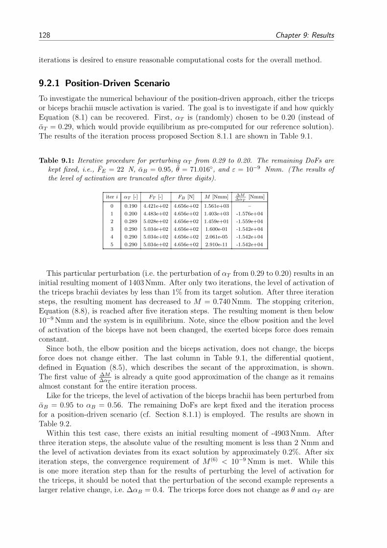
128 Chapter 9: Results
iterations is desired to ensure reasonable computational costs for the overall method.
9.2.1 Position-Driven Scenario
To investigate the numerical behaviour of the position-driven approach, either the tricepsor biceps brachii muscle activation is varied. The goal is to investigate if and how quicklyEquation (8.1) can be recovered. First, αT is (randomly) chosen to be 0.20 (instead ofαT = 0.29, which would provide equilibrium as pre-computed for our reference solution).The results of the iteration process proposed Section 8.1.1 are shown in Table 9.1.
Table 9.1: Iterative procedure for perturbing αT from 0.29 to 0.20. The remaining DoFs arekept fixed, i.e., FE = 22 N, αB = 0.95, θ = 71.016, and ε = 10−9 Nmm. (The results ofthe level of activation are truncated after three digits).
iter i αT [-] FT [-] FB [N] M [Nmm] ∆M∆αT
[Nmm]
0 0.190 4.421e+02 4.656e+02 1.561e+03 –
1 0.200 4.483e+02 4.656e+02 1.403e+03 -1.576e+04
2 0.289 5.028e+02 4.656e+02 1.459e+01 -1.559e+04
3 0.290 5.034e+02 4.656e+02 1.600e-01 -1.542e+04
4 0.290 5.034e+02 4.656e+02 2.061e-05 -1.542e+04
5 0.290 5.034e+02 4.656e+02 2.910e-11 -1.542e+04
This particular perturbation (i.e. the perturbation of αT from 0.29 to 0.20) results in aninitial resulting moment of 1403 Nmm. After only two iterations, the level of activation ofthe triceps brachii deviates by less than 1% from its target solution. After three iterationsteps, the resulting moment has decreased to M = 0.740 Nmm. The stopping criterion,Equation (8.8), is reached after five iteration steps. The resulting moment is then below10−9 Nmm and the system is in equilibrium. Note, since the elbow position and the levelof activation of the biceps have not been changed, the exerted biceps force does remainconstant.
Since both, the elbow position and the biceps activation, does not change, the bicepsforce does not change either. The last column in Table 9.1, the differential quotient,defined in Equation (8.5), which describes the secant of the approximation, is shown.The first value of ∆M
∆αTis already a quite good approximation of the change as it remains
almost constant for the entire iteration process.Like for the triceps, the level of activation of the biceps brachii has been perturbed from
αB = 0.95 to αB = 0.56. The remaining DoFs are kept fixed and the iteration processfor a position-driven scenario (cf. Section 8.1.1) is employed. The results are shown inTable 9.2.
Within this test case, there exists an initial resulting moment of -4903 Nmm. Afterthree iteration steps, the absolute value of the resulting moment is less than 2 Nmm andthe level of activation deviates from its exact solution by approximately 0.2%. After sixiteration steps, the convergence requirement of M (6) < 10−9 Nmm is met. While thisis one more iteration step than for the results of perturbing the level of activation forthe triceps, it should be noted that the perturbation of the second example represents alarger relative change, i.e. ∆αB = 0.4. The triceps force does not change as θ and αT are

9.2 Prescribed Forward-Dynamics Model 129
Table 9.2: Iterative procedure for perturbing αB from 0.95 to 0.56. The remaining DoFs arekept fixed, i.e. FE = 22 N, αT = 0.29, θ = 71.016, and ε = 10−9 Nmm. (The results of thelevel of activation are truncated after three digits).
iter i αB [-] FT [-] FB [-] M [Nmm] ∆M∆αB
[Nmm]
0 0.550 5.034e+02 3.435e+02 -4.903e+03 –
1 0.560 5.034e+02 3.468e+02 -4.773e+03 1.309e+04
2 0.925 5.034e+02 4.584e+02 -2.911e+02 1.229e+04
3 0.948 5.034e+02 4.652e+02 -1.821e+01 1.152e+04
4 0.950 5.034e+02 4.656e+02 -6.736e-02 1.148e+04
5 0.950 5.034e+02 4.656e+02 -1.544e-05 1.147e+04
6 0.950 5.034e+02 4.656e+02 -1.091e-11 1.147e+04
constant. In the last column, the differential quotient ∆M∆αB
is shown. As the moment isnegative, the slope of the differential quotient is positive.
9.2.2 Activation-Driven Scenario
Similar results are observed, for perturbing the initial angle and keeping fixed the levelsof activation, αT and αB, and the external force, FE. To demonstrate this, the angleθ is perturbed from θ to θ = 99 while the remaining DoFs remain as in the referencesolution. Then, the iterative procedure described in Section 8.1.2 is employed. The resultsare presented in Table 9.3.
Table 9.3: Iterative procedure for perturbing θ from θ to θ = 99. The remaining DoFs are keptfixed, i.e., FE = 22 N, αT = 0.29, αB = 0.95, and ε = 10−9 Nmm.
iter i θ [] FT [N] FB [N] M [Nmm] ∆M∆θ
[Nmm/]
0 60.000 4.270e+02 5.199e+02 4.668e+03 –
1 99.000 6.552e+02 3.003e+02 -1.053e+04 -3.896e+02
2 71.981 5.098e+02 4.605e+02 -4.059e+02 -3.745e+02
3 70.897 5.026e+02 4.662e+02 5.002e+01 -4.207e+02
4 71.016 5.034e+02 4.656e+02 -7.541e-02 -4.213e+02
5 71.016 5.034e+02 4.656e+02 -1.322e-05 -4.213e+02
6 71.016 5.034e+02 4.656e+02 7.276e-12 -4.213e+02
After perturbing the elbow angle by ∆θ = +27, 984, a resulting moment of -1.053·104 Nmm is computed. After the first iteration, the angle deviates already by lessthan 1. While the absolute difference of the angle θ between the second iteration andthe exact solution is already less than 0.12, the stopping criterion based on the moment(|M (i)| < 10−9 Nmm) is not reached until completing the fifth iteration. As the exertedmuscle force of both muscles depends on the elbow angle and the contact between themuscle and bone, the muscle forces for both muscles need to be re-computed at everyiteration step.
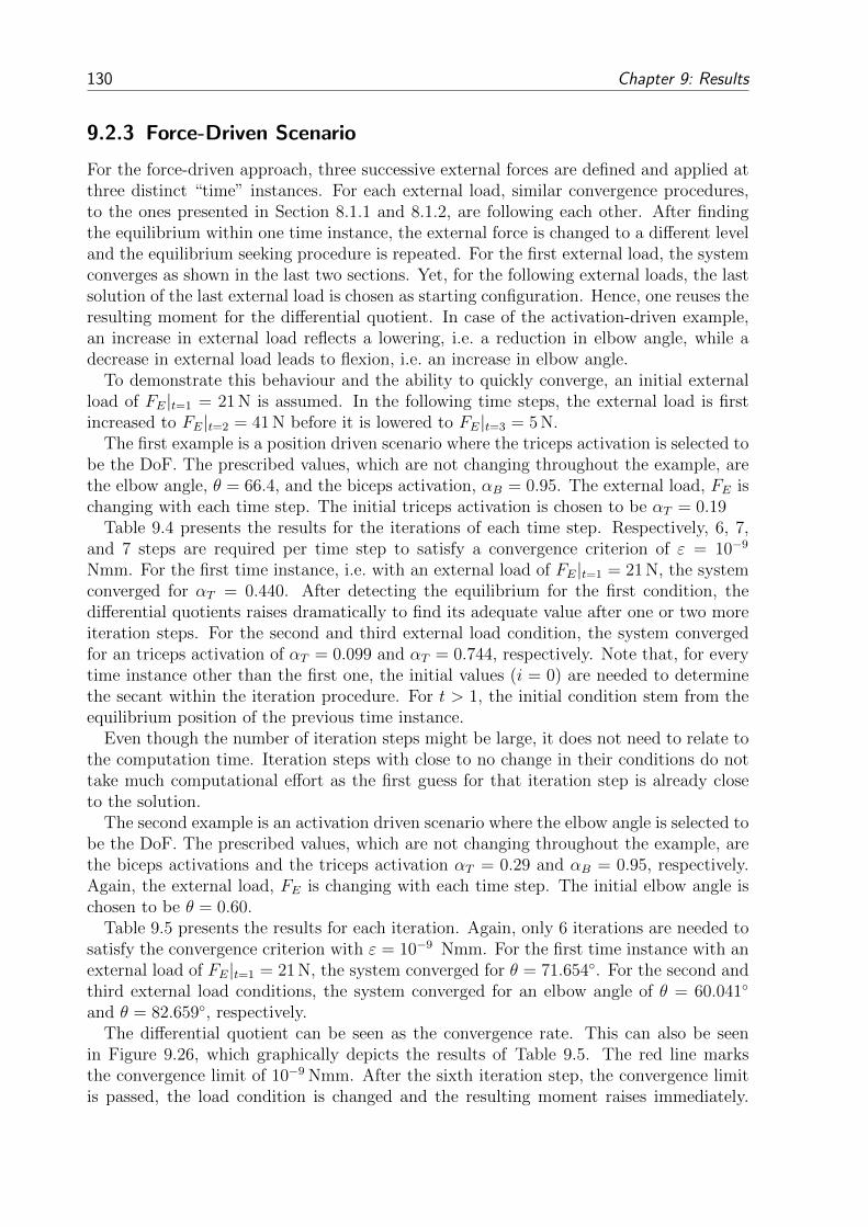
130 Chapter 9: Results
9.2.3 Force-Driven Scenario
For the force-driven approach, three successive external forces are defined and applied atthree distinct “time” instances. For each external load, similar convergence procedures,to the ones presented in Section 8.1.1 and 8.1.2, are following each other. After findingthe equilibrium within one time instance, the external force is changed to a different leveland the equilibrium seeking procedure is repeated. For the first external load, the systemconverges as shown in the last two sections. Yet, for the following external loads, the lastsolution of the last external load is chosen as starting configuration. Hence, one reuses theresulting moment for the differential quotient. In case of the activation-driven example,an increase in external load reflects a lowering, i.e. a reduction in elbow angle, while adecrease in external load leads to flexion, i.e. an increase in elbow angle.
To demonstrate this behaviour and the ability to quickly converge, an initial externalload of FE|t=1 = 21 N is assumed. In the following time steps, the external load is firstincreased to FE|t=2 = 41 N before it is lowered to FE|t=3 = 5 N.
The first example is a position driven scenario where the triceps activation is selected tobe the DoF. The prescribed values, which are not changing throughout the example, arethe elbow angle, θ = 66.4, and the biceps activation, αB = 0.95. The external load, FE ischanging with each time step. The initial triceps activation is chosen to be αT = 0.19
Table 9.4 presents the results for the iterations of each time step. Respectively, 6, 7,and 7 steps are required per time step to satisfy a convergence criterion of ε = 10−9
Nmm. For the first time instance, i.e. with an external load of FE|t=1 = 21 N, the systemconverged for αT = 0.440. After detecting the equilibrium for the first condition, thedifferential quotients raises dramatically to find its adequate value after one or two moreiteration steps. For the second and third external load condition, the system convergedfor an triceps activation of αT = 0.099 and αT = 0.744, respectively. Note that, for everytime instance other than the first one, the initial values (i = 0) are needed to determinethe secant within the iteration procedure. For t > 1, the initial condition stem from theequilibrium position of the previous time instance.
Even though the number of iteration steps might be large, it does not need to relate tothe computation time. Iteration steps with close to no change in their conditions do nottake much computational effort as the first guess for that iteration step is already closeto the solution.
The second example is an activation driven scenario where the elbow angle is selected tobe the DoF. The prescribed values, which are not changing throughout the example, arethe biceps activations and the triceps activation αT = 0.29 and αB = 0.95, respectively.Again, the external load, FE is changing with each time step. The initial elbow angle ischosen to be θ = 0.60.
Table 9.5 presents the results for each iteration. Again, only 6 iterations are needed tosatisfy the convergence criterion with ε = 10−9 Nmm. For the first time instance with anexternal load of FE|t=1 = 21 N, the system converged for θ = 71.654. For the second andthird external load conditions, the system converged for an elbow angle of θ = 60.041
and θ = 82.659, respectively.The differential quotient can be seen as the convergence rate. This can also be seen
in Figure 9.26, which graphically depicts the results of Table 9.5. The red line marksthe convergence limit of 10−9 Nmm. After the sixth iteration step, the convergence limitis passed, the load condition is changed and the resulting moment raises immediately.
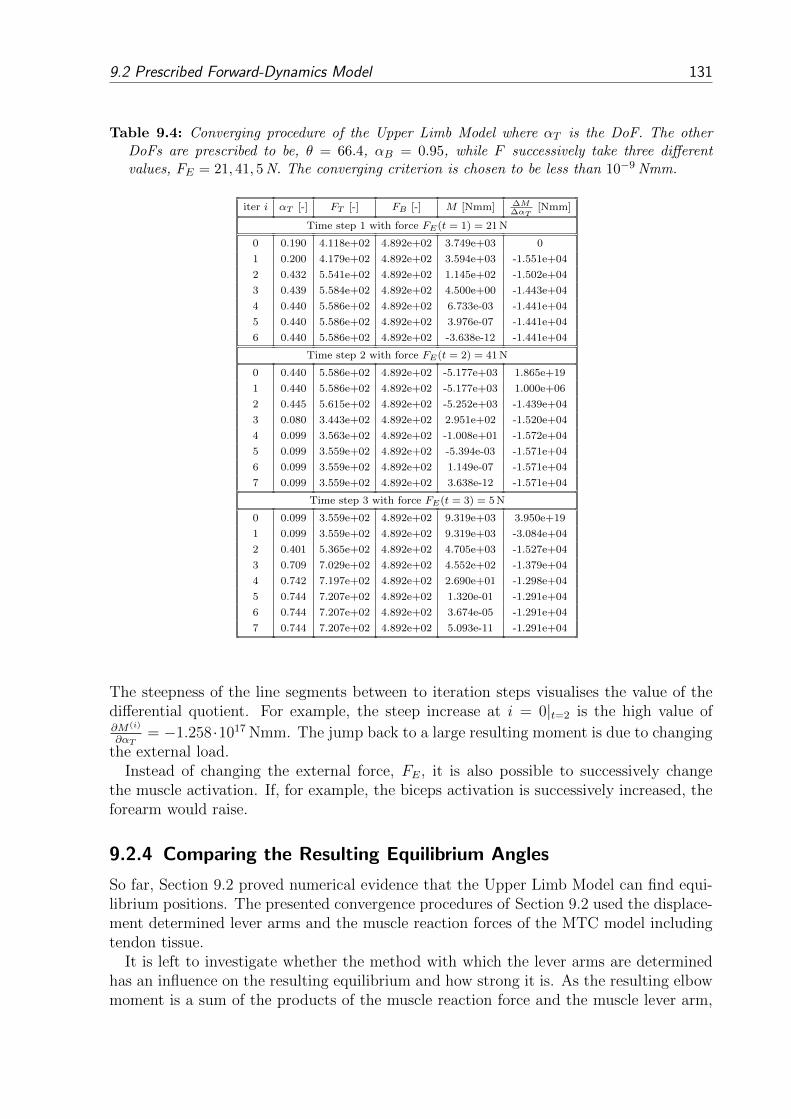
9.2 Prescribed Forward-Dynamics Model 131
Table 9.4: Converging procedure of the Upper Limb Model where αT is the DoF. The otherDoFs are prescribed to be, θ = 66.4, αB = 0.95, while F successively take three differentvalues, FE = 21, 41, 5 N. The converging criterion is chosen to be less than 10−9 Nmm.
iter i αT [-] FT [-] FB [-] M [Nmm] ∆M∆αT
[Nmm]
Time step 1 with force FE(t = 1) = 21 N
0 0.190 4.118e+02 4.892e+02 3.749e+03 0
1 0.200 4.179e+02 4.892e+02 3.594e+03 -1.551e+04
2 0.432 5.541e+02 4.892e+02 1.145e+02 -1.502e+04
3 0.439 5.584e+02 4.892e+02 4.500e+00 -1.443e+04
4 0.440 5.586e+02 4.892e+02 6.733e-03 -1.441e+04
5 0.440 5.586e+02 4.892e+02 3.976e-07 -1.441e+04
6 0.440 5.586e+02 4.892e+02 -3.638e-12 -1.441e+04
Time step 2 with force FE(t = 2) = 41 N
0 0.440 5.586e+02 4.892e+02 -5.177e+03 1.865e+19
1 0.440 5.586e+02 4.892e+02 -5.177e+03 1.000e+06
2 0.445 5.615e+02 4.892e+02 -5.252e+03 -1.439e+04
3 0.080 3.443e+02 4.892e+02 2.951e+02 -1.520e+04
4 0.099 3.563e+02 4.892e+02 -1.008e+01 -1.572e+04
5 0.099 3.559e+02 4.892e+02 -5.394e-03 -1.571e+04
6 0.099 3.559e+02 4.892e+02 1.149e-07 -1.571e+04
7 0.099 3.559e+02 4.892e+02 3.638e-12 -1.571e+04
Time step 3 with force FE(t = 3) = 5 N
0 0.099 3.559e+02 4.892e+02 9.319e+03 3.950e+19
1 0.099 3.559e+02 4.892e+02 9.319e+03 -3.084e+04
2 0.401 5.365e+02 4.892e+02 4.705e+03 -1.527e+04
3 0.709 7.029e+02 4.892e+02 4.552e+02 -1.379e+04
4 0.742 7.197e+02 4.892e+02 2.690e+01 -1.298e+04
5 0.744 7.207e+02 4.892e+02 1.320e-01 -1.291e+04
6 0.744 7.207e+02 4.892e+02 3.674e-05 -1.291e+04
7 0.744 7.207e+02 4.892e+02 5.093e-11 -1.291e+04
The steepness of the line segments between to iteration steps visualises the value of thedifferential quotient. For example, the steep increase at i = 0|t=2 is the high value of∂M(i)
∂αT= −1.258 ·1017 Nmm. The jump back to a large resulting moment is due to changing
the external load.Instead of changing the external force, FE, it is also possible to successively change
the muscle activation. If, for example, the biceps activation is successively increased, theforearm would raise.
9.2.4 Comparing the Resulting Equilibrium Angles
So far, Section 9.2 proved numerical evidence that the Upper Limb Model can find equi-librium positions. The presented convergence procedures of Section 9.2 used the displace-ment determined lever arms and the muscle reaction forces of the MTC model includingtendon tissue.
It is left to investigate whether the method with which the lever arms are determinedhas an influence on the resulting equilibrium and how strong it is. As the resulting elbowmoment is a sum of the products of the muscle reaction force and the muscle lever arm,
132 Chapter 9: Results
Table 9.5: Iterative procedure for assuming three different external loads and seeking the result-ing elbow angles while assuming constant values of αT = 0.29 and αB = 0.95. The externalforce, FE, successively takes three different values, FE = 21, 53, 5 N. The converging criterionis met if the resulting momenent is less than 10−9 Nmm.
iter i θ [] FT [N] FB [N] M [Nmm] ∆M∆θ
[Nmm/]
Time step 1 with force FE(t = 1) = 21 N
0 60.000 4.270e+02 5.199e+02 4.912e+03 0
1 100.00 6.589e+02 2.939e+02 -1.055e+04 -3.865e+02
2 72.710 5.147e+02 4.566e+02 -4.416e+02 -3.703e+02
3 71.518 5.067e+02 4.630e+02 5.712e+01 -4.182e+02
4 71.654 5.077e+02 4.622e+02 -9.921e-02 -4.189e+02
5 71.654 5.077e+02 4.622e+02 -2.099e-05 -4.189e+02
6 71.654 5.077e+02 4.622e+02 1.819e-11 -4.189e+02
Time step 2 with force FE(t = 2) = 41 N
0 71.654 5.077e+02 4.622e+02 -5.363e+03 -1.258e+17
1 71.654 5.077e+02 4.622e+02 -5.363e+03 -5.973e+02
2 62.676 4.459e+02 5.074e+02 -1.233e+03 -4.600e+02
3 59.997 4.269e+02 5.199e+02 2.106e+01 -4.679e+02
4 60.042 4.273e+02 5.197e+02 -2.494e-02 -4.684e+02
5 60.041 4.273e+02 5.197e+02 -2.454e-07 -4.684e+02
6 60.041 4.273e+02 5.197e+02 -7.276e-12 -4.684e+02
Time step 3 with force FE(t = 3) = 5 N
0 60.041 4.273e+02 5.197e+02 8.811e+03 -6.200e+17
1 60.041 4.273e+02 5.197e+02 8.811e+03 -7.680e+02
2 71.514 5.067e+02 4.630e+02 4.345e+03 -3.893e+02
3 82.677 5.766e+02 4.009e+02 -6.918e+00 -3.899e+02
4 82.660 5.765e+02 4.010e+02 -1.491e-01 -3.815e+02
5 82.659 5.765e+02 4.010e+02 8.047e-06 -3.815e+02
6 82.659 5.765e+02 4.010e+02 3.638e-12 -3.815e+02
there are different combinations possible to yield the elbow moment. So far, three differentpossibilities to determine the lever arms have been presented:
1. tendon-displacement method (TDM),
2. vector-resulting lever arm method (VRLA), and
3. vector-resulting lever arm method including the replacement of the point of action(VRLA+).
Just considering the MTC muscle model, the muscle reaction forces have been determinedeither by:
1. considering the effects of contact or by
2. not considering the effects of contact.
In the author’s opinion, the rigid-tendon model will not give any further insights. Asthe rigid-tendon model is just a model simplification without systematic differences, theresulting forces are similar to each other. Hence, no further studies are considered.
In Figure 9.27a, the resulting equilibrium angles are plotted using the TDM, the VRLAmethod, and the VRLA+ method with considering contact. The prescribed values are
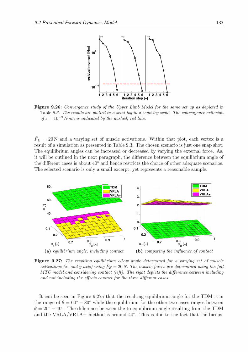
9.2 Prescribed Forward-Dynamics Model 133
1 2 3 4 5 6 1 2 3 4 5 6 1 2 3 4 5 6
10−10
100
iteration step [−]
res
idu
al
mo
me
nt
[Nm
]
t=2 t=3t=1
Figure 9.26: Convergence study of the Upper Limb Model for the same set up as depicted inTable 9.3. The results are plotted in a semi-log in a semi-log scale. The convergence criterionof ε = 10−9 Nmm is indicated by the dashed, red line.
FE = 20 N and a varying set of muscle activations. Within that plot, each vertex is aresult of a simulation as presented in Table 9.3. The chosen scenario is just one snap shot.The equilibrium angles can be increased or decreased by varying the external force. As,it will be outlined in the next paragraph, the difference between the equilibrium angle ofthe different cases is about 40 and hence restricts the choice of other adequate scenarios.The selected scenario is only a small excerpt, yet represents a reasonable sample.
0.1
0.2
0.7 0.8 0.9 1
40
60
80
αB [−]α
T [−]
θ [°]
TDM
VRLA
VRLA+
(a) equilibrium angle, including contact
0.1
0.2
0.7 0.8 0.9 1
0
1
2
3
4
αB [−]α
T [−]
TDM
VRLA
VRLA+
(b) comparing the influence of contact
Figure 9.27: The resulting equilibrium elbow angle determined for a varying set of muscleactivations (x- and y-axis) using FE = 20 N. The muscle forces are determined using the fullMTC model and considering contact (left). The right depicts the difference between includingand not including the effects contact for the three different cases.
It can be seen in Figure 9.27a that the resulting equilibrium angle for the TDM is inthe range of θ = 60 − 80 while the equilibrium for the other two cases ranges betweenθ = 20 − 40. The difference between the to equilibrium angle resulting from the TDMand the VRLA/VRLA+ method is around 40. This is due to the fact that the biceps’

134 Chapter 9: Results
(flexor) lever arm resulting from the TDM is roughly four-times larger than the oneresulting from the VRLA method. The other two methods have very similar equilibriumangles. In this elbow range, the triceps’ (extensor) lever arm is roughly the same for allmethods. For the VRLA method the influence of the updated point of action is includedbut only plays a minor role. The magenta surface and yellow surface are very similar.
Figure 9.27b depicts the importance of the contact for each case. This is done bysubtracting the equilibrium angle obtained from the different methods from each other.As it can be seen, the effects of contact play a minor role for the TDM, especially for therange investigated in this example (60 < θ < 80). For the VRLA method, contact ismore important and changes the equilibrium angle by 2-4. There are two possible reasons:(i) The scenario is in an elbow range where contact becomes more influential. (ii) Theinfluence of contact on the lever arm is more pronounced for the triceps, see Figure 9.23.As the difference between the second and the third case is small, it is assumed that theeffects of contact are influencing both possibilities to the same extend.
Figure 9.28a compares the different methods with each other by depicting the differenceof the results using the VRLA method and the TDM. Figure 9.28b compares the resultsobtained from the vector-resulting lever arm method with and without including the offsetof the point of action by subtracting the equilibrium angles from each other. Figure 9.28shows the difference for considering and not considering contact.
0.1 0.15 0.2 0.25 0.70.8
0.9
40
42
44
46
αB [−]
αT [−]
TDM−VRLA without
TDM−VRLA with
(a) subtracting the results of the TDM casefrom the VRLA case
0.1 0.15 0.2 0.25 0.70.8
0.9−0.2
−0.1
0
0.1
αB [−]
αT [−]
VRLA−VRLA+ without
VRLA−VRLA+ with
(b) subtracting the results of the VRLA+from VRLA
Figure 9.28: Subtracting the results of different cases to see the impact of the different phe-nomena. Green presents the case when no muscle-bone contact is considered and magentawhen contact is taken into account.
The already mentioned deviation of about 40 between the VRLA method and theTDM can be nicely seen. Furthermore, it can be seen that the effects of contact influencethe equilibrium angle by about 2 in Figure 9.28a. The relocation of the point of actionhas only a minor influence (see Figure 9.28b). The deviation is in the range of 0.1.The difference between considering contact has also only a minor impact on the resultingequilibrium angle. The results are only deviating by less than 0.3.
It worth noting again that the change in the point of action cannot be considered withthe TDM as it derives the lever arm by just using the muscle length. If the proximal

9.3 EMG-driven Forward-Dynamics Model 135
and distal relocation of the points of actions are considered, the muscle length would onlychange by negligible amount and the influence on the lever arm would be even smaller.
9.3 EMG-driven Forward-Dynamics Model
To obtain time-dependent activation dynamics from experiments, the experimental dataneed to be processed. This is done by the forward-inverse model proposed by Buchananet al. (2004). By processing the raw EMG of the different muscles, the forward-inversemodel determines next to the muscle activation also the acting elbow torques and reactionforces of the muscles. These data can be used within the Upper Limb Model and themeasured moments and motion can then be subsequently used for validation.
The forward-inverse model, introduced in Section 8.2.5, consists of
• an OpenSim model, providing the model’s kinematics,
• the activation dynamics, converting raw EMG into muscle activation,
• the forward-dynamics model,
• the inverse-dynamics model,
• the optimiser, minimising the difference between the results of the forward- andinverse-dynamics method by changing parameters of the activation dynamics andmuscle dynamics, and last but not least,
• the experimental data, which serve as model input.
In Section 9.3.1, the results of the forward-inverse model are presented whereas inSection 9.3.2, the muscles’ reaction forces of the forward-inverse model are replaced bythose of the Upper Limb Model.
9.3.1 Results of the Forward-Inverse Model
During the measurements, both EMG trains and elbow moments are measured usingdifferent frequencies, see Section 8.2.1. During the processing phase, the frequencies forthe different data are matched. The elbow moment can directly be measured and is usedas golden standard for the results of the forward-inverse model. Figure 9.29 shows thedata train of the measured torques and the torque resulting from the forward-dynamicsmodel. The experimental data, measured by a Biodex, is the reference solution and isrepresented by the blue lines. The green lines in Figure 9.29a and 9.29b are the elbowmoments resulting from two different calibration procedures. The spiky appearing dataare composed by stringing together separate trials. The first trial (spike) is conducted atθ = 10 with 100% effort, whereas the second trial is conducted at the same elbow anglebut with half the effort. Naturally, the 50% effort is hard to estimate for the proband.The sequence is continued with alternating effort at increasing elbow angles of ∆θ = 10
steps. The last trial, starting after about 10.000 time frames, is the passive trial. Here,the arm is moved by the Biodex three times over the full range of motion. It is used toinvestigate the passive properties of the subject’s musculoskeletal system.
The difference between the trails in Figure 9.29 cannot be seen very easily. Yet, whendetails are closely compared, differences become apparent. In general, it can be saidthat the partial effort is reproduced better by the forward-inverse model. For the full

136 Chapter 9: Results
0 2000 4000 6000 8000 10000 12000−10
0
10
20
30
40
50
60
time frames [∆t]
elb
ow
mo
me
nt
[Nm
]
Biodex
FIM
(a) calibration procedure one
0 2000 4000 6000 8000 10000 12000−10
0
10
20
30
40
50
60
time frames [∆t]
elb
ow
mo
me
nt
[Nm
]
Biodex
FIM
(b) calibration procedure two
Figure 9.29: The continuous moment measured by the Biodex (blue) and resulting from theforward-inverse model (green) from different calibration procedures. The first trial (spike) isconducted at θ = 10 with 100% effort whereas the second trial with 50% effort. The sequenceis continued with alternating effort at increasing elbow angles in ∆θ = 10 steps.
effort trials, in particular for 80 ≤ θ ≤ 120, the measured elbow moments are overes-timated whereas for smaller and larger elbow angles the measured elbow moments areunderestimated.
When the results of the isokinematic trials are considered, which are not visualisedhere, it can be seen that the flexing part of the motion is better approximated as theextending part.
The time series for the isometric trials can be averaged to one value per trial. Hence, allbut the last trial, which is the passive movement, can be condensed to a single mean value.For the full effort trials, the resulting mean is shown in Figure 9.30. Again, the measuredtorque is the blue curve and the results of the forward-dynamics model is depicted in green.As different calibrations produce different results, two calibrations are shown, exemplary.The average of the two calibrations is depicted by the black curve. It can be seen thatthe difference between the two different calibration procedures is very small. Hence, itwill not be further differentiated between different calibration procedures. Furthermore,the presented results are always the mean of the two calibration procedures from here on.
In order to extract the muscle activation and the muscle forces from the forward-inversemodel, the model solves the Newton-Euler equations for each time increment. Hence, atime continuous series of data for the resulting muscle activation and resulting musclereaction force does exist for each trial. Exemplarily, Figure 9.31a and 9.31b show thetime series for the full effort trial at θ = 10 of the first calibration procedure.
The muscle activation ramps up from the resting state to reach its isometric contractionstate. For the data processing, the toe region in the beginning and the end is cut off byselecting a threshold criterion which demands a certain elbow torque requirement. Hence,a relatively nice plateau region is left for the investigations. For the results of Figure 9.31,the flexor activation is in the range between 40 – 60% while the extensor activation isaround 20%.
The resulting muscle forces are of course coupled to the muscle activation by the muscle
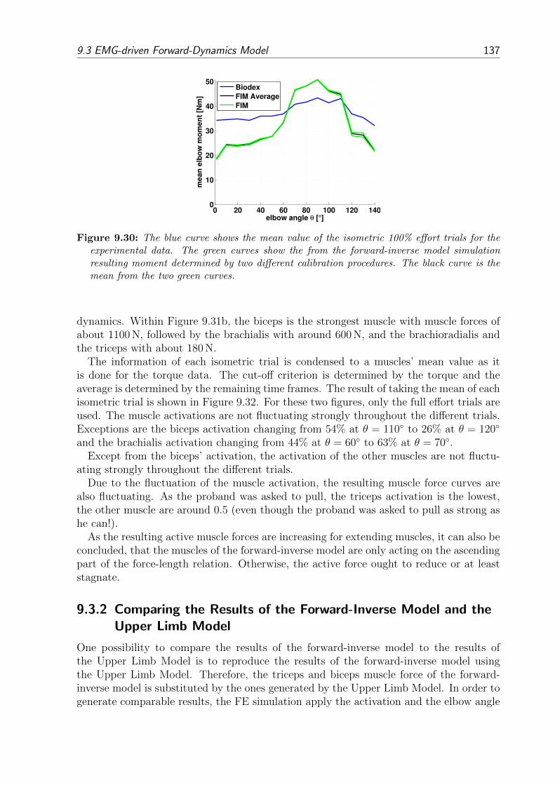
9.3 EMG-driven Forward-Dynamics Model 137
0 20 40 60 80 100 120 1400
10
20
30
40
50
elbow angle θ [°]
mean
elb
ow
mo
men
t [N
m]
Biodex
FIM Average
FIM
Figure 9.30: The blue curve shows the mean value of the isometric 100% effort trials for theexperimental data. The green curves show the from the forward-inverse model simulationresulting moment determined by two different calibration procedures. The black curve is themean from the two green curves.
dynamics. Within Figure 9.31b, the biceps is the strongest muscle with muscle forces ofabout 1100 N, followed by the brachialis with around 600 N, and the brachioradialis andthe triceps with about 180 N.
The information of each isometric trial is condensed to a muscles’ mean value as itis done for the torque data. The cut-off criterion is determined by the torque and theaverage is determined by the remaining time frames. The result of taking the mean of eachisometric trial is shown in Figure 9.32. For these two figures, only the full effort trials areused. The muscle activations are not fluctuating strongly throughout the different trials.Exceptions are the biceps activation changing from 54% at θ = 110 to 26% at θ = 120
and the brachialis activation changing from 44% at θ = 60 to 63% at θ = 70.Except from the biceps’ activation, the activation of the other muscles are not fluctu-
ating strongly throughout the different trials.Due to the fluctuation of the muscle activation, the resulting muscle force curves are
also fluctuating. As the proband was asked to pull, the triceps activation is the lowest,the other muscle are around 0.5 (even though the proband was asked to pull as strong ashe can!).
As the resulting active muscle forces are increasing for extending muscles, it can also beconcluded, that the muscles of the forward-inverse model are only acting on the ascendingpart of the force-length relation. Otherwise, the active force ought to reduce or at leaststagnate.
9.3.2 Comparing the Results of the Forward-Inverse Model and theUpper Limb Model
One possibility to compare the results of the forward-inverse model to the results ofthe Upper Limb Model is to reproduce the results of the forward-inverse model usingthe Upper Limb Model. Therefore, the triceps and biceps muscle force of the forward-inverse model is substituted by the ones generated by the Upper Limb Model. In order togenerate comparable results, the FE simulation apply the activation and the elbow angle
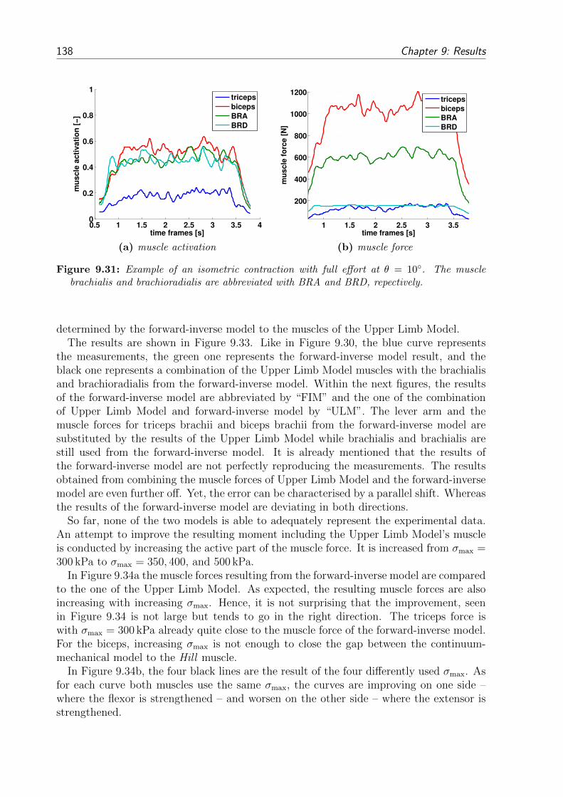
138 Chapter 9: Results
0.5 1 1.5 2 2.5 3 3.5 40
0.2
0.4
0.6
0.8
1
time frames [s]
mu
sc
le a
cti
va
tio
n [
−]
triceps
biceps
BRA
BRD
(a) muscle activation
1 1.5 2 2.5 3 3.5
200
400
600
800
1000
1200
time frames [s]
mu
sc
le f
orc
e [
N]
triceps
biceps
BRA
BRD
(b) muscle force
Figure 9.31: Example of an isometric contraction with full effort at θ = 10. The musclebrachialis and brachioradialis are abbreviated with BRA and BRD, repectively.
determined by the forward-inverse model to the muscles of the Upper Limb Model.The results are shown in Figure 9.33. Like in Figure 9.30, the blue curve represents
the measurements, the green one represents the forward-inverse model result, and theblack one represents a combination of the Upper Limb Model muscles with the brachialisand brachioradialis from the forward-inverse model. Within the next figures, the resultsof the forward-inverse model are abbreviated by “FIM” and the one of the combinationof Upper Limb Model and forward-inverse model by “ULM”. The lever arm and themuscle forces for triceps brachii and biceps brachii from the forward-inverse model aresubstituted by the results of the Upper Limb Model while brachialis and brachialis arestill used from the forward-inverse model. It is already mentioned that the results ofthe forward-inverse model are not perfectly reproducing the measurements. The resultsobtained from combining the muscle forces of Upper Limb Model and the forward-inversemodel are even further off. Yet, the error can be characterised by a parallel shift. Whereasthe results of the forward-inverse model are deviating in both directions.
So far, none of the two models is able to adequately represent the experimental data.An attempt to improve the resulting moment including the Upper Limb Model’s muscleis conducted by increasing the active part of the muscle force. It is increased from σmax =300 kPa to σmax = 350, 400, and 500 kPa.
In Figure 9.34a the muscle forces resulting from the forward-inverse model are comparedto the one of the Upper Limb Model. As expected, the resulting muscle forces are alsoincreasing with increasing σmax. Hence, it is not surprising that the improvement, seenin Figure 9.34 is not large but tends to go in the right direction. The triceps force iswith σmax = 300 kPa already quite close to the muscle force of the forward-inverse model.For the biceps, increasing σmax is not enough to close the gap between the continuum-mechanical model to the Hill muscle.
In Figure 9.34b, the four black lines are the result of the four differently used σmax. Asfor each curve both muscles use the same σmax, the curves are improving on one side –where the flexor is strengthened – and worsen on the other side – where the extensor isstrengthened.
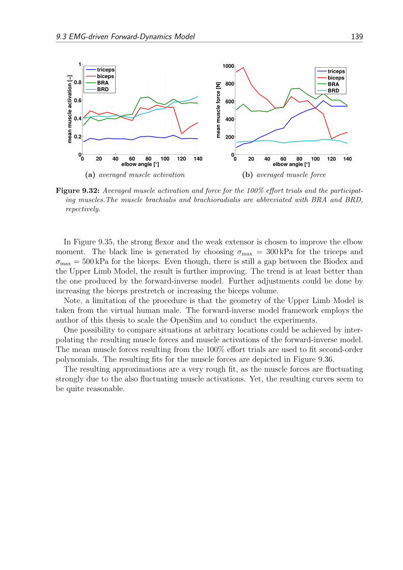
9.3 EMG-driven Forward-Dynamics Model 139
0 20 40 60 80 100 120 1400
0.2
0.4
0.6
0.8
1
elbow angle [°]
me
an
mu
sc
le a
cti
va
tio
n [
−]
triceps
biceps
BRA
BRD
(a) averaged muscle activation
0 20 40 60 80 100 120 1400
200
400
600
800
1000
elbow angle [°]
me
an
mu
sc
le f
orc
e [
N]
triceps
biceps
BRA
BRD
(b) averaged muscle force
Figure 9.32: Averaged muscle activation and force for the 100% effort trials and the participat-ing muscles.The muscle brachialis and brachioradialis are abbreviated with BRA and BRD,repectively.
In Figure 9.35, the strong flexor and the weak extensor is chosen to improve the elbowmoment. The black line is generated by choosing σmax = 300 kPa for the triceps andσmax = 500 kPa for the biceps. Even though, there is still a gap between the Biodex andthe Upper Limb Model, the result is further improving. The trend is at least better thanthe one produced by the forward-inverse model. Further adjustments could be done byincreasing the biceps prestretch or increasing the biceps volume.
Note, a limitation of the procedure is that the geometry of the Upper Limb Model istaken from the virtual human male. The forward-inverse model framework employs theauthor of this thesis to scale the OpenSim and to conduct the experiments.
One possibility to compare situations at arbitrary locations could be achieved by inter-polating the resulting muscle forces and muscle activations of the forward-inverse model.The mean muscle forces resulting from the 100% effort trials are used to fit second-orderpolynomials. The resulting fits for the muscle forces are depicted in Figure 9.36.
The resulting approximations are a very rough fit, as the muscle forces are fluctuatingstrongly due to the also fluctuating muscle activations. Yet, the resulting curves seem tobe quite reasonable.

140 Chapter 9: Results
0 20 40 60 80 100 120 140
20
30
40
50
elbow angle [°]
elb
ow
mo
me
nt
[Nm
]
Biodex
FIM
ULM
Figure 9.33: Comparing the model results. The blue curve is the Biodex data. The green curveis the result of the forward-inverse model (FIM). The black curve is the result of using themuscle forces from the Upper Limb Model (ULM) using σmax = 300 kPa.
0 20 40 60 80 100 120 1400
200
400
600
800
1000
elbow angle [°]
mu
sc
le R
F [
N]
FIM−TRI
FIM−BIC
ULM−TRI
ULM−BIC
(a) triceps and biceps muscle reaction force
0 20 40 60 80 100 120 140
20
30
40
50
elbow angle [°]
elb
ow
mo
me
nt
[Nm
]
Biodex
FIM
ULM
(b) resulting model elbow moments
Figure 9.34: To investigate the influence the Upper Limb Model muscle reaction forces on theresulting elbow moment, σmax is changed from 300 kPa to 350, 400, and 500 kPa. As theflexor and extensor are changed to both extend, the model improvement is limited.

9.3 EMG-driven Forward-Dynamics Model 141
0 20 40 60 80 100 120 140
20
30
40
50
elbow angle [°]
elb
ow
mo
me
nt
[Nm
]
Biodex
FIM
ULM adjusted
Figure 9.35: Using the strengthened biceps (σmax = 500 kPa) and the weak triceps σmax =300 kPa, the Upper Limb Model resulting elbow moment can be improved considerably.
0 50 100 1500
200
400
600
800
1000
elbow angle [°]
me
an
TR
I fo
rce
fit
[N
]
0 50 100 1500
200
400
600
800
1000
elbow angle [°]
me
an
BIC
fo
rce
fit
[N
]
0 50 100 1500
200
400
600
800
1000
elbow angle [°]
me
an
BR
A f
orc
e f
it [
N]
0 50 100 1500
200
400
600
800
1000
elbow angle [°]
me
an
BR
D f
orc
e f
it [
N]
Figure 9.36: Polynomial fit to the from the forward-inverse model resulting muscle forces. Theabbreviations used are TRI for triceps, BIC for biceps, BRA for brachialis, and BRD forbrachioradialis.


10 Discussion
This work presents a first attempt to model a part of the musculoskeletal system using acontinuum-mechanical approach. The Upper Limb Model and its equivalent static systemis a strongly simplified model. Yet, it enables first investigations of an antagonistic musclepair acting within a realistic musculoskeletal system. As it is the first investigation of itskind, there are no studies or methods to compare with. The author will outline theassumptions this model is based on and report on the resulting benefits and drawbacks.As the results are already presented and to some degree discussed in Section 9, thischapter will focus on the model assumptions, model limitation and the concatenation ofthe results. The discussion is methodologically differentiated into different sections.
Mechanical Model
The Theory of Finite Elasticity has proven to provide an adequate framework for thecontinuum to represent large deformations occurring in soft biological tissues such asskeletal muscles. In combination with the finite element method, which provides a welldeveloped and powerful discretisation method, biological soft tissue such as muscles, innerorgans, skin, bone, and close to everything else could be mechanically investigated.
Furthermore, the finite element method enables to modularly include a contact formu-lation. In this case here, contact is defined to occur between the skeletal muscle tissueand the bones, which are assumed to be rigid.
Muscle-bone contact forces can be several hundreds of Newtons, see Figure 9.14. TheCoulomb friction coefficient between bone and muscle are about 0.3, see (Shacham et al.,2010). As soft tissues between the biceps and the triceps brachii and the humerus arenot considered, it is uncertain whether the model correctly represents the contactingsurfaces and whether the model predictions are in good agreement with reality. However,experimental measurements of these contact forces are nearly impossible. This is certainlytrue for the superficial biceps brachii, which is just of other flexor muscles adjacent tothe humerus and the biceps’s muscle tissue. Due to these deficiencies, the restriction ofa frictionless contact formulation is considered to be acceptable. The advantage of thechosen framework is that it provides a way to in silico investigate the impact of frictionbetween muscle and bone may be.
Within the considered model, contact between muscles does not occur, as the humerusseparates the considered muscles. This is no longer true,if multiple muscles are consid-ered. Even though, muscle-muscle contact would be challenging, it should be consideredwhen synergistic muscles effects are taken into account in an extended model. Further,considering bone-bone contact within the joint would provide additional realism, but alsotremendously increase the complexity of the model. However, to make the joint movementrealistic and natural, the surrounding tissue (i.e. ligaments, cartilage, and further muscles)that restrains and pulls needs to be included. Hereby, both the model complexity as wellas the model DoFs would increase to a degree, which makes the model nearly unsolvable.
143

144 Chapter 10: Discussion
Speed-ups are possible, but they require the optimisation of the existing code, use ananalytical tangent, and/or the use of massively parallel simulations on larger computercluster.
Muscle Model
The muscle tissue’s constitutive model is based on approaches without further innovations.The muscles’ activation state is a scalar-valued function, which is spatially not varying.The addition of a more complex activation-dynamics model, such as, for example intro-duced by Heidlauf and Rohrle (2014), would increase the numerical costs and complexitieswithout any methodological effect on the multi-muscle musculoskeletal system.
The muscle model, established in Section 4.3, is adequate to represent the rigid-tendonmodel consisting of only muscle tissue. Only two more material parameters, namely γM
and γST are needed, to extend the rigid-tendon model to represent next to muscle tissuealso tendon, and other soft tissue, see of Section 4.4. The stiffness of tendon tissue isabout a thousand times higher than the stiffness of muscle tissue. The physiologicalstrain of tendons is smaller than 5%. The muscle’s strain raises easily up to 50%. Locally,due to highly different material behaviour, the numerical challenge becomes considerable.Yet, macroscopically, when the muscle belly gradually tapers and changes towards tendontissue, the connective tissue ratio increases while the cross-section area reduces. Therefore,as the tendon cross-section is much smaller than the muscle belly cross-section, the overallstiffness of the different muscle compartments may not change as dramatically as therelative material stiffness may indicate. Furthermore, a change of the muscle’s level ofactivation changes the ratio between muscle and tendon tissue stiffness changes. It wasobserved, that while the muscle belly’s stiffness is weaker than the tendons’ stiffness forlow activation, the stiffness ratio may assimilate for muscle activations close to one.
As there is hardly any data available for describing the muscle-connective tissue ratio,a possibility to overcome that absence of information is to relate the change of the musclecross-section area to the muscle-connective tissue ratio (Sprenger et al., 2013). Thereby,the transition zones can be used to define a gradual change of the material parameter, γM.Though, due to the large difference in the stiffness between the muscle and the tendontissue, special care has to be taken by defining a transition zone to achieve realisticdeformations, realistic muscle reaction forces, and a robust finite element simulation.
The material parameters for the passive contribution of the material law could bedetermined by fitting the presented relations to experimental data. Yet, it was necessary toincrease c1 by a factor of 102 to prevent numerical stability issues. Not increasing c1 leadsto a too large ratio between the along-fibre stiffness and the transverse-fibre stiffness. As aconsequence of increasing the isotropic parameter, the muscles bulk behaviour predictionis too stiff. This is especially true for the compressive region. Here, it is assumed thatthe muscle tissue behaves much softer. Unfortunately, the basis for such fittings is verybad. For example, no data for the compressive region exist for both the isotropic andthe transverse isotropic contributions. Hence, it is not possible to fit the muscle to amore realistic behaviour. The experimental data for the biceps and triceps are verydiverse and obviously not matching to the Virtual Human Male data set. Hence, theparameters for the active contribution are adopted manually to provide a realistic activeforce contribution. Different material parameters are used for both muscles, see Table 7.1for the rigid-tendon model and 7.2 for the MTC model.

145
When material parameters are changed within the elements, stress and strain os-cillations are observed. The reason for that observation lies in the definition of theincompressible Mooney-Rivlin constitutive law (Equation (4.22)), the initial pressure(Equation (4.32)) and the fact that the primary variables (space and hydrostatic pressure)are discretised using differently ordered shape functions (2nd order in space and one orderless for the hydrostatic pressure to fulfil the LBB condition). For an incompressible mate-rial, the initial pressure was defined by Equation (4.32) to p(χ, t = 0) = 2 c1 + 4 c2. Whenthe material parameters, within an element, are distributed with a higher-order functionthan a linear one, then the hydrostatic pressure with its linear interpolation is not able to(pointwise) fulfil the zero initial stress condition throughout each element (at each Gausspoint). To get rid of the inconsistency, the compressible formulation is employed insteadof the incompressible formulation of the Mooney-Rivlin material. Note, the compressibleformulation of the Mooney-Rivlin is used within an incompressible material description.The advantage of the compressible formulation is that it needs to be able to equal the ini-tial stress to zero by itself as within an compressible formulation an hydrostatic pressuredoes not exist. To intrinsically set the initial stress to zero, one more material parameteris included:
Ψiso(I1, I2, I3) = c1 (I1 − 3)− c2 (I2 − 3) + c5 (J − 1)2 . (10.1)
The additional material parameter, c5, is according to Equation (4.32) adequately deter-mined such that the hydrostatic pressure is zero for the initial condition, i.e.
c5 = 2 c1 + 4 c2 . (10.2)
Thereby, the issue regarding the choice of the different ordered shape functions is resolved.The only drawback is that one more parameter and one more term in the isotropic partof the constitutive law has to be evaluated throughout the simulation. Compared to theoverall amount of evaluations, that carries little weight.
Muscle Mesh
As mentioned in Section 7.2, the original mesh, derived from the Virtual Human Maledata set was established by the Auckland Bioengineering Institute. Initially, the geometrywas described using tri-cubic Hermite shape functions. For this work, the cubic-Hermiteshape functions are substituted by quadratic shape functions. Here, 27-node hexahe-dron elements are used to represent the mesh. The reason for the conversion are (i) thereduction of DoFs, as tri-cubic Hermite elements have more DoFs than quadratic ones(Hermites have 192 DoFs per element and 27-node hexahedrons have 81 DoFs per ele-ment) and (ii) avoiding C1-continuity of the tri-cubic Hermite shape functions, for thestress continuity across element boundaries. As, if material parameters vary element-wisewithin the muscle, the solution space should also be able to reflect element-wise jumps ofthe stress and therefore also sharp corners at the element vertices.
During the development of the muscles’ mesh, it turned out that the simulations aremore robust if the tendon heads are changed at the junction of the muscle heads from V-shaped to U-shaped geometries. Further, for numerical reasons, the emerging gap betweenthe different heads is filled with isotropic soft tissue to avoid singularities in the corners.Due to the definition of the muscle-tendon-complex constitutive model (Section 4.4), the

146 Chapter 10: Discussion
soft tissue is defined using the isotropic behaviour of the muscle tissue, which is very softcompared to the overall behaviour and will not have any further impact on the overallmechanical behaviour of the muscle. This can be validated by checking the nodal residualsat the insertion sites. The soft tissues nodal residuals are small compared to the tendontissue ones.
To fulfil the requirements of a thorough finite element analysis, it would be necessary toinvestigate the behaviour of the solution when the mesh is refined similar to Rohrle et al.(2008). However, as the generation of a mesh is very time consuming and challenging. Thefocus of this work however was on enabling a musculoskeletal system simulation appealingto continuum-mechanical muscles and not on mesh quality.
The mesh for the rigid-tendon model consists of 144 elements and 1625 nodes for thetriceps, and 64 elements and 765 nodes for the biceps, see Figure 7.3. The muscle-tendon-complex model’s mesh (cf. Figure 7.5) has the same number of elements and nodes thanthe rigid-body model. Yet, the MTC model has to cover a larger volume and hencethe mesh is less fine. The stated number of elements and nodes is not a really highnumber, yet the computation time for the simulation of one raising arm movement tookmore than one day on an AMD SR5670/SP5100 CPU core of 3,2 GHz with 128 GB ofRAM. A speed up can be achieved through providing an analytical material tangent orthrough a parallelised computation as it is introduced in OpenCMISS, the successiveversion of CMISS. OpenCMISS is a new open-source software library based on OpenMPIand OpenMP, see Bradley et al. (2011).
Unfortunately, an authentic fibre field orientation for the biceps and triceps brachii isnot available. A study by Fernandez et al. (2012) compared the influence of an artificiallychosen fibre orientation with a fibre field, determined by diffusion tensor MRI (DT) data,on the resulting muscle shape. Their results showed, that fibre distributions resultingfrom DT-MRI are able to reproduce much more realistic muscle shapes than the artificialchosen orientation. Further, the fibre orientation does not only have a strong influenceon the muscle’s shape but also on the numerical robustness. Hence, special care has tobe taken by defining the muscle’s fibre orientation. The chosen fibre distribution withinthe Upper Limb Model is based on anatomical features, yet geometrically simplified tocapture the key characteristics.
Last but not least, the mesh may also influence the quality of the contact mechanicalresults. If the elements are too big, the number of contact points, defined within thecontact faces, are to small for a good representation of the contact surfaces. By increasingthe number of elements, it is easier for the slave’s geometry to follow the master’s shape.As it could be seen in Figure 9.14a, when the elements vertices suddenly move over thebones surface, force peaks can emerge. These effects are artificial and due to numericalartifacts. These jumps will not occur in reality.
The central aponeurosis is defined for the triceps only in the MTC model. Without theaponeurosis layer, the triceps muscle reaction forces are too low, the deformation of themuscle tissue are too high, and the deformations in the tendon tissue region are too low.The central aponeurotic layer, with its high stiffness, solved all these problems at once.
Muscle Prestretch
In non-linear mechanics, the definition of the initial state is very important as it has a biginfluence on the mechanical behaviour of the system. For biological systems, the definition

147
of the initial state is one of the most basic but also one of the most difficult one. In theliterature, a recipe of how to determine the initial configuration does not exist and may bevery hard to establish as it also varies for different applications. First attempts are madefor some soft tissues and artery walls by Holzapfel and Weizsacker (1998); Zamir andTaber (2004); Cardamone et al. (2009), or Schroder and Brinkhues (2014). For muscles,the continuum-mechanical community has not assessed the amount of prestretch yet. Themethodology to include pre-stretched Hill -type muscle models is totally different and notuseful for continuum-mechanical purposes. This may also explain why experimental set-ups have not provided information for the continuum-mechanics community.
For this work, it is assumed that each muscle does not produce a compressive forcewithin its range of motion. Each muscle is always under tension. To the author’s opinion,this is the best choice, as a living organisms should not invest energy to push a muscle.Muscles are antagonistic to enable movements of the articulation in several directions anddo not waste energy due to compressive loads of antagonistic muscles.
Besides the chosen solution to establish the desired prestretch (see Section 7.2), thereare alternatives which might have advantages. The first alternative is probably the easiestbut also mechanically incorrect. CMISS offers a functionality to change the initial fibrestretch. Unfortunately, the definition of the subroutine is not general enough to apply itto this BVP. Hereby, it would have been very simple to change the fibre’s prestretch state.The disadvantages of this option are (i) that the deformation is uniquely spread over thegeometry, which is unrealistic in a complex geometry and (ii) that the deformation state isnot coherently defined throughout the different material law contributions. The reason isthat only the anisotropic contributions depend on the fibre stretch whereas the isotropicpart does not. Hence, while the fibre contribution can be influenced in its initial condition,the isotropic contribution cannot.
Perhaps, the best alternative to determine the pre-stretched state would have been torun a simulation to change the muscle length to its target length, and redefine the resultingcurrent configuration to a new initial configuration. This procedure would have severaladvantages compared to other options. First, for pragmatic reasons, it would be quitesimple to change the prestretch state. One has to just select a new initial target length,run the simulation, and redefine the initial state. Second, the resulting muscle stateincludes all mechanical complexities: the orientation of resulting fibres is inhomogeneous,the strain is locally varying, and as the material is hyperelastic, the mechanical statesare reversible. Third, by compressing the muscle to its shortest length, it would appearquite bulgy in its prestretch state, as it needs to be compressed compared to the otheralternatives. On the other hand, the biceps would not appear too slim and slender, as itdoes e.g. in Figure 9.11a, when the forearm is fully extended. Maybe the most importantreason for that alternative is that by changing the muscle’s length, the initial volume ofthe muscle is preserved and hence also the muscle’s producing force capacity would bepreserved. Unfortunately, this is not the case for the choice made in this thesis, compareSection 7.2.
Upper Limb Model
One of the main challenges investigating musculoskeletal systems is the fact that it consistsof more unknowns than there are equations. In order to solve such a system, moreequations need to be defined in order to find the best among all feasible solutions. This is
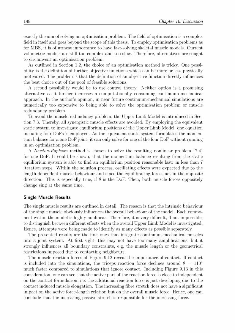
148 Chapter 10: Discussion
exactly the aim of solving an optimisation problem. The field of optimisation is a complexfield in itself and goes beyond the scope of this thesis. To employ optimisation problems asfor MBS, it is of utmost importance to have fast-solving skeletal muscle models. Currentvolumetric models are still too complex and too slow. Therefore, alternatives are soughtto circumvent an optimisation problem.
As outlined in Section 1.2, the choice of an optimisation method is tricky. One possi-bility is the definition of further objective functions which can be more or less physicallymotivated. The problem is that the definition of an objective function directly influencesthe best choice out of the pool of feasible solutions.
A second possibility would be to use control theory. Neither option is a promisingalternative as it further increases a computationally consuming continuum-mechanicalapproach. In the author’s opinion, in near future continuum-mechanical simulations arenumerically too expensive to being able to solve the optimisation problem or muscleredundancy problem.
To avoid the muscle redundancy problem, the Upper Limb Model is introduced in Sec-tion 7.3. Thereby, all synergistic muscle effects are avoided. By employing the equivalentstatic system to investigate equilibrium positions of the Upper Limb Model, one equationincluding four DoFs is employed. As the equivalent static system formulates the momen-tum balance for a one DoF joint, it can only solve for one of the four DoF without runningin an optimisation problem.
A Newton-Raphson method is chosen to solve the resulting nonlinear problem (7.4)for one DoF. It could be shown, that the momentum balance resulting from the staticequilibrium system is able to find an equilibrium position reasonable fast: in less than 7iteration steps. Within the solution process, oscillating effects were expected due to thelength-dependent muscle behaviour and since the equilibrating forces act in the oppositedirection. This is especially true, if θ is the DoF. Then, both muscle forces oppositelychange sing at the same time.
Single Muscle Results
The single muscle results are outlined in detail. The reason is that the intrinsic behaviourof the single muscle obviously influences the overall behaviour of the model. Each compo-nent within the model is highly nonlinear. Therefore, it is very difficult, if not impossible,to distinguish between different effects when the overall Upper Limb Model is investigated.Hence, attempts were being made to identify as many effects as possible separately.
The presented results are the first ones that integrate continuum-mechanical musclesinto a joint system. At first sight, this may not have too many amplifications, but itstrongly influences all boundary constraints, e.g. the muscle length or the geometricalrestrictions imposed due to contacting neighbours.
The muscle reaction forces of Figure 9.12 reveal the importance of contact. If contactis included into the simulations, the triceps reaction force declines around θ = 110
much faster compared to simulations that ignore contact. Including Figure 9.13 in thisconsideration, one can see that the active part of the reaction force is close to independenton the contact formulation, i.e. the additional reaction force is just developing due to thecontact induced muscle elongation. The increasing fibre stretch does not have a significantimpact on the active force-length relation but on the overall muscle force. Hence, one canconclude that the increasing passive stretch is responsible for the increasing force.

149
It is often discussed whether the muscles are acting on the ascending or descendingbranch of the force-length relation. Even though the discussion is always difficult, it isslightly easier for Hill-type muscle models than for continuum-mechanical models. Hill-type models use a lumped-muscle length which holds for the bulk of the muscle. Whenthis value is smaller than the optimal muscle length, the muscle is on the ascending part ofthe relation. When it is larger than the optimal muscle length, it is on the descending partof the force-length relation. Hence, it is much easier to tell whether the force contributionis increasing or decreasing due to a changing muscle length or whether the muscle acts onthe ascending or descending part of the force-length curve.
For continuum-mechanical models, the behaviour becomes more complex as the lengthdependency exists at each integration point. Therefore, it is possible that in some partsof the muscle, the muscle acts on the ascending part of the force-length relation while inother locations of the muscle, the fibre stretch is much larger and the muscle acts on thedescending part of the force-length relation, compare Figure 9.15. Hence, the macroscopicresponse of the muscle is probably not as clearly distinguishable as several microscopicphenomena take place at the same time.
The triceps’ active force including the tendon reduces by about 100 N after reachingthe maximum while the biceps’ active force only reduces by about 50 N. As the numberof triceps muscle fibres which exceed the optimal length is very small (see Figure 9.15),the decline in the active force is due to a reducing muscle and fibre stretch length. Forthe biceps, the overall length always increases. As the number of fibres trespassing λopt
f
is quite numerous (see Figure 9.15), it is very likely that the resulting decline is causedby the descending part of the force-length curve.
Another phenomenon can be seen in Figure 9.3 and 9.13. As the activation is propor-tional to the active stress contribution in Equation (4.23), the resulting reaction forces areclose of being equally-distributed between the passive and the fully activated curves. Yeton the other hand, as the active stress contribution is proportional to α, the minimal andmaximal fibre stretch where the active force contribution starts and ends, should alwaysbe the same. The results of Figure 9.3 and 9.13 reveal a different behaviour especiallyfor the biceps. Here, the elbow angle where the active force contribution begins, stronglychanges with the biceps’ level of activation. This result is similar to experimental obser-vations by e.g. Guimaraes et al. (1994). Even if it is not exactly the same, it is shownthat, by linearly scaling the muscle force-length relation with the muscle activation, themacroscopic result varies strongly with the input. Due to the complex model, the param-eters responsible to convert the simple input to the macroscopic output is unknown. Butwhen the model results are like this, they may also change to something else that is moresimilar to the measurements of Guimaraes et al. (1994).
To the author’s knowledge, there is no clear definition of the state when a muscle actsmaximally on a joint. Sometimes, the muscle is said to produce its maximal force whenthe muscle is at its resting length or when the joint is in its neutral position. Experimentson the elbow show that the joint angle, where the elbow torques at its maximum isbetween 60 (Amis et al., 1980) and 100 (Buchanan et al., 1998). Mechanically, themuscle’s optimum can be defined when either the muscle reaction force is maximal, wherethe active contribution of the muscle reaction force is maximal, where the moment of onemuscle acting an a joint is maximal, or where the moment of all muscles acting on a jointis maximal.

150 Chapter 10: Discussion
Traditionally in skeletal muscle modelling, the optimal length of a muscle is the lengthat which it produces its highest force. This value can be evaluated in experiments bydissecting one muscle from its system. However, how good can the realistic operatingrange in the in vitro experiments be reproduced? And how is that possible consideringthe results of Section 9.1.1 and 9.1.2?
For the triceps and the biceps brachii, the ranges of operation are very similar to theresults presented by Murray et al. (2000). The optimal elbow joint angle is always to-wards the end of either flexion or extension. Is it possible for an isolated muscle to haveits maximal force somewhere in the middle of its range of motion while the passive con-tribution increases with further stretching the muscle? When the results of Figure 9.34aare consulted, one has to conclude that the force is increasing when the muscle lengthis increasing. Hence, when a muscle’s optimal angle is in its mid range of motion, themuscle length is no longer monotonically increasing, as it is the case for the triceps’ length(cf. Figure 7.6a). Murray et al. (2000) presents a range of motion that is much larger forthe biceps than for the triceps. The biceps is mostly acting on the ascending part of theforce-length curve or at least has a monotonically increasing reaction force. In contrary,the triceps’s force decreases with increasing flexion angle. The triceps’ range of motionis, referring to Murray et al. (2000), on the last part of the ascending and the beginningof the descending part of the force-length relation. However, maybe the choice of theoptimal length is not the only possible explanation and also the reduction of the tricepslength and the fibre length contributes to that characteristic?
It can be measured that the elbow torque a human being can generate is maximalbetween θ = 90 and 100. Yet, is it most likely not possible to reach a maximal elbowtorque at θ = 90− 100 for a single muscle. Can it be only a product from the interplayof several acting muscles? To push the optimal elbow angle for a single muscle moretowards θ = 90 or θ = 100, a first, naive idea would be to either increase the prestretchof the muscle or by choosing a smaller optimal fibre stretch to adapt the muscle forceaccordingly. Unfortunately, both options do not lead to the desired result as on the onehand, the active part of the muscle moves towards the middle of its range of action,yet, on the other hand, the passive behaviour of the muscle starts to dominate earlier.Hereby, the muscle reaction forces are only dominated by the passive force, which isdefinitely not physiologically motivated. Of course, also the muscle lever arms have astrong impact on the resulting muscle moment. Yet, the resulting biceps moment ofFigure 9.25b demonstrates that the moment is linearly increasing with increasing musclestretch or forearm flexion. Therefore, one can only conclude that an optimal elbow angleof 90 to 100 can only be achieved from the interplay of several muscles acting at thesame time. Last but not least, the impact of the lever arm is also contributing strongly.
Comparing Rigid-Tendon Model Results to Muscle-Tendon-Complex Model Results
For single muscle simulations, tendons might not be that important. Hence in thecontinuum-mechanics muscle community, tendons are very often assumed to be rigid andneglected Van Loocke et al. (2006). It is claimed that due to the tendon stiffness, theresulting small deformations do not have a strong influence on the overall skeletal muscle.However, by comparing the results of the raising arm movement of the rigid-tendon modelwith the results of the MTC model, tendons have a strong influence on skeletal musclemechanics even though the strain in the tendon material is quite small, see also Scheepers

151
et al. (1997).Considering Section 2.4 and modelling aspects, the main elements when muscle-tendon
complexes act on a joint are the following:
(i) Due to their slender structure, they strongly influence the lever arm and the muscle’sline of action.
(ii) Much more realistic muscle attachment site can be defined when tendons are in-cluded. Smaller attachment faces provide less restrictions to the muscle geometryand the area of fixed nodes is smaller.
(iii) A consequence from the last two items is that tendons increase the deformationmodes of the muscle belly, i.e. the slender tendon shape provides more modes ofdeformation by rotational and translational movements of the belly.
(iv) Within the different muscle tissues, i.e. tendon tissue, muscle tissue, or the transitionzone, structural properties such as the connective tissue ratio, material parameters,and the fibre orientation vary strongly.
When the deviation of the reaction force’s orientation of the MTC and rigid-tendonmodel is compared, several observations can be made to underpin the importance of (i).First the rigid-tendon model exhibits deviations that are nearly independent to contact.For the biceps, the results of Figure 9.10 are dominated by the badly defined prestretchas the surface rise where the reaction forces are close to zero. Before the orientation ofthe reaction force becomes indifferent, the deviation of the orientation is in the range of afew degrees. For the triceps, the deviation increases up to 15, independent of contact. Incase of the MTC model, the deviation strongly depends on the effects of contact. Withoutconsidering contact, the deviation is only a few degrees. The deviation increases up to40 for the triceps and up to 20 for the biceps when contact is included. The differencecan also be nicely seen in the bottom row of Figure 9.1 and Figure 9.11.
The relocation of the point of action is for both muscles and both models independentof the effects of contact. Yet, even though the cross-section of the insertion sites of theMTC complex are much smaller, the relocation of the point of action are very similar inboth models. For the triceps, the relocation within the MTC model is larger than withinthe rigid-tendon model. So, item (ii) not only enables a more natural attachment site,but also does not seem to mechanically penalise the slenderness.
When the simulations of the raising arm movement of Figure 9.1 is compared to Fig-ure 9.11, it can be seen that the biceps moves differently at different attachment sites.This also influences the way the muscle and the bone interact with each other. Contactlooks much more natural. One probable reason for this is that due to the long and slendertendons, translational movements of the belly are much more likely, see item (iii).
Item (iv) can probably be best explained by comparing the results of Figure 9.5 withthose in Figure 9.15. The rigid-tendon model can only reflect the fibre stretch distributionof the muscle belly. As the MTC model does not only include the muscle belly but alsothe tendon region and the transition zones, the resulting patterns of Figure 9.15 are morecomplex. Yet, the patterns of the belly are still distinguishable.

152 Chapter 10: Discussion
Lever Arm
Besides the muscle reaction force, the second parameter directly influencing the jointmoment is the muscle lever arm. Before the tendon-displacement method derived leverarm is employed, two alternatives were considered.
In the first attempt, the lever arm was determined by utilising experimental resultsfrom Amis et al. (1979) and Murray et al. (2002). The second attempt was an analyticalrelation on the basis of the static equilibrium system using trigonometry. Unfortunately,both methods provided a lever arm with which the equivalent static system failed to findan equilibrium position. The reason for this failure was never identified or understood.The tendon-displacement was the third attempt and an equilibrium position was found.A possible reason for the tendon-displacement method and the vector-resulting lever armto work, and the measured data and the analytical relation not is that it seems to beimportant, that the used data set is coherent.
The lever arm derived from the tendon-displacement method only depends on the linearmuscle length between muscle origin and insertion. Therefore, only the geometry andsize of the humerus, ulna, radius, and the muscle attachment sites influence the musclelever arms. Within the Upper Limb Model, the line from muscle origin to insertion isneither deflected by surrounding muscles nor other soft tissues or bones. Hence, this linearassumption is the most accurate choice to approximate the muscle length. Nevertheless,the tendon-displacement method has proven over several decades to give reasonably goodresults, and the lever arm resulting from this approach are in agreement with the leverarm mentioned in Section 1.2.2.
An improvement of the tendon-displacement method could be achieved by using thecontinuum-mechanical muscle model and the idea of the line of action which is introducedin Section 7.5. Assuming that the evolving muscles’ line-of-action is not always straightbut curved, the muscle length deviates from the line approach. By determining the pointof action incrementally along the longitudinal muscle axis, (similar to the one depicted inFigure 10.1b), the adapted muscle length could also be determined piecewise linear. Asthe adapted length will vary for different fibre orientations, muscle shapes, and the levelof activation, the lever arm resulting from the tendon-displacement method differs fromthe “linear” version.
The problem with this method is that it worked for nicely shaped cubes. But duringstrong deformations, as it can be seen in Figure 10.1b, the cross-section on which theintegration is evaluated is not plain any more. This problem becomes severe when thegeometry becomes arbitrary as is no longer straight forward to define intersecting planesto evaluate the stress. In theory, the finite element method allows to evaluate the stresstensor at every point, yet in reality, this becomes difficult.
The vector-resulting lever arms differ quite strongly from the lever arms resulting fromthe tendon-displacement method. For the biceps, despite the strong deviation of theorientation of the reaction force when considering contact, the lever arm remains closeto constant over the whole input space (10 ≤ θ ≤ 150 and 0 ≤ α ≤ 1). In theliterature, the biceps lever arm is strongly dependent on the elbow flexion angle (Murrayet al., 1995; Amis et al., 1979). As it is already mentioned, the lever arms resulting fromthe tendon-displacement method are in agreement with the literature, cf. Murray et al.(1995) or Amis et al. (1979). However, mathematically speaking, the lever arm obtainedby means of taking the actual position and the actual orientation of the force is exact.
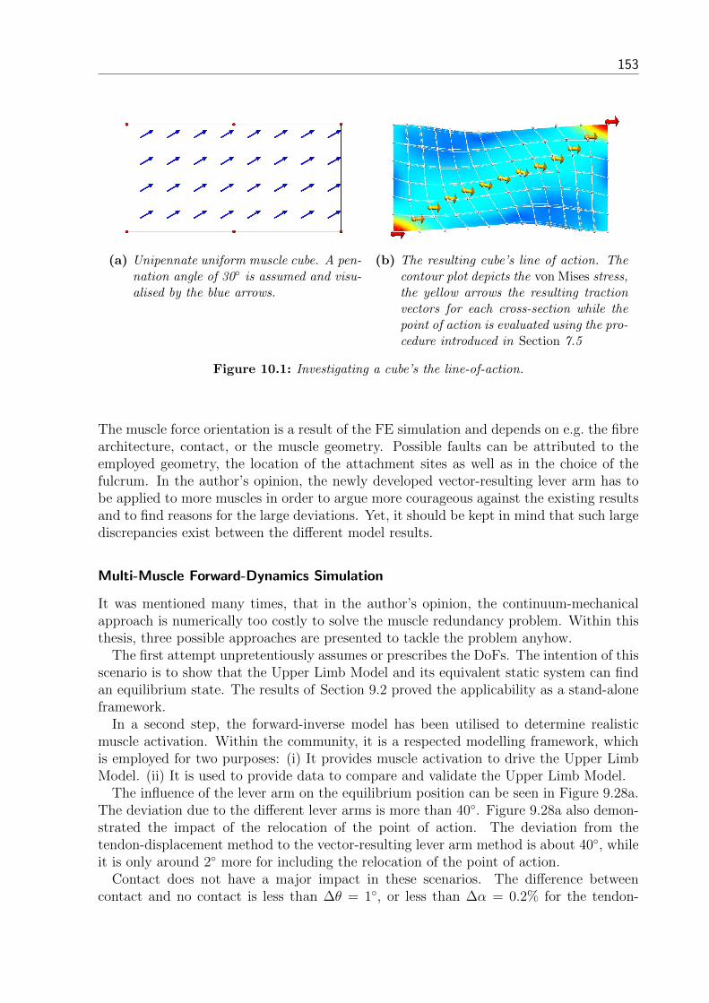
153
(a) Unipennate uniform muscle cube. A pen-nation angle of 30 is assumed and visu-alised by the blue arrows.
(b) The resulting cube’s line of action. Thecontour plot depicts the von Mises stress,the yellow arrows the resulting tractionvectors for each cross-section while thepoint of action is evaluated using the pro-cedure introduced in Section 7.5
Figure 10.1: Investigating a cube’s the line-of-action.
The muscle force orientation is a result of the FE simulation and depends on e.g. the fibrearchitecture, contact, or the muscle geometry. Possible faults can be attributed to theemployed geometry, the location of the attachment sites as well as in the choice of thefulcrum. In the author’s opinion, the newly developed vector-resulting lever arm has tobe applied to more muscles in order to argue more courageous against the existing resultsand to find reasons for the large deviations. Yet, it should be kept in mind that such largediscrepancies exist between the different model results.
Multi-Muscle Forward-Dynamics Simulation
It was mentioned many times, that in the author’s opinion, the continuum-mechanicalapproach is numerically too costly to solve the muscle redundancy problem. Within thisthesis, three possible approaches are presented to tackle the problem anyhow.
The first attempt unpretentiously assumes or prescribes the DoFs. The intention of thisscenario is to show that the Upper Limb Model and its equivalent static system can findan equilibrium state. The results of Section 9.2 proved the applicability as a stand-aloneframework.
In a second step, the forward-inverse model has been utilised to determine realisticmuscle activation. Within the community, it is a respected modelling framework, whichis employed for two purposes: (i) It provides muscle activation to drive the Upper LimbModel. (ii) It is used to provide data to compare and validate the Upper Limb Model.
The influence of the lever arm on the equilibrium position can be seen in Figure 9.28a.The deviation due to the different lever arms is more than 40. Figure 9.28a also demon-strated the impact of the relocation of the point of action. The deviation from thetendon-displacement method to the vector-resulting lever arm method is about 40, whileit is only around 2 more for including the relocation of the point of action.
Contact does not have a major impact in these scenarios. The difference betweencontact and no contact is less than ∆θ = 1, or less than ∆α = 0.2% for the tendon-

154 Chapter 10: Discussion
displacement method and about ∆θ = 2 for the vector-resulting lever arm.When the measured elbow moment is compared to the reproduced elbow moment of
both models, it can be said that the quality of the forward-inverse model is not optimalyet. The resulting elbow moment is too small for elbow angles smaller than 60 andlarger than 120 and too large for 80 < θ < 120, see Figure 9.34a. The results may beimproved by increasing the range of the parameters determined in the calibration phase.The deviation of the results of the Upper Limb Model may be larger, yet the shape of theresulting elbow moment better resembles the experimental data.
As already discussed, the muscle forces of the different models are already similar. Thediscrepancy between the different resulting elbow moments may be due to different musclelever arms. Hence, the lever arms of the OpenSim model are compared to the lever armsdetermined from the tendon-displacement method in Figure 10.2.
0 50 100 150
−20
0
20
40
60
80
θ [°]
lever
arm
[m
m]
TRIFIM
BICFIM
BRAFIM
BRDFIM
TRIULM
BICULM
Figure 10.2: Comparing the lever arms of the forward-inverse model and the Upper Limb Model.
It can be seen that the triceps’ lever arms are similar. The biceps’ lever arm, on theother hand, deviates up to 50% (or 20 mm). This obviously has a big impact on theresulting elbow moment as the biceps is the strongest elbow flexor. For example, whenthe biceps lever arm of the Upper Limb Model is replaced by the one of the forward-inversemodel, the Upper Limb Model’s resulting moment is improving considerably as the flexorbecomes about 50% more powerful.
When the biceps reaction forces resulting from the forward-inverse model and the UpperLimb Model of Figure 9.34a are compared, a methodological difference becomes apparent.Not only is the biceps force from the forward-inverse model stronger than the force fromthe Upper Limb Model but more importantly for the fully flexed elbow, the biceps reactionforce from the forward-inverse model is greater than 200 N while the Upper Limb Model’sbiceps reaction force is only around 50 N. A possible explanation for the overall smallermuscle force is that the biceps’ force of the different subjects within the forward-inversemodel and the Upper Limb Model are not coinciding. By increasing within the continuum-mechanical skeletal muscle model of the biceps the parameter σmax, the biceps reactionforce increases and reduces the gap between the two model solutions. On the other hand,the Upper Limb Model’s reaction force still tends towards zero for flexing the forearm. Thecause for the difference is that the active force-length relation of the forward-inverse modelis wider. This implies that the biceps of the forward-inverse model is able to generate aforce in a fully flexed forearm position and the biceps of the Upper Limb Model not.

11 Summary and Outlook
11.1 Summary
In this thesis, a suitable theoretical modelling procedure was presented, providing numer-ical simulations of the material behaviour of muscle-tendon complexes that are includedinto an articulation. In order to do that, it was first necessary to introduce the anatomicaland physiological fundamentals of the musculoskeletal system and in particular the upperlimb. Caused by the complex microscopic property of the participating muscles, appro-priate constitutive equations for the muscle, tendon, and other soft tissues were presentedand embedded into the Theory of Finite Elasticity which provides a suitable frameworkin describing the finite deformation regime.
The resulting set of coupled partial differential equations was spatially discretised usingthe finite element method, which has proven to provide a powerful numerical techniquefor finding approximate solutions to such BVP. A contact formulation was modularly in-cluded to the finite element method to consider contact between the elastic muscle-tendoncomplexes and rigid bones. The solution of the subject specific BVP was achieved withinCMISS. The resulting system of equations was solved in a monolithic manner. Whilethe material mechanical contribution was linearised numerically, the contact mechanicalcontribution was linearised analytically.
The geometry of the Upper Limb Model was established from the virtual human dataset. By introducing the Upper Limb Model with its static equivalent system, a continuum-mechanically based framework could be established. This enabled stand-alone investiga-tions as well as a coupling to other frameworks. Three different concepts to facilitatethe muscle activation were presented in order to use the Upper Limb Model and theequivalent static system. In a first step, muscle activation was prescribed to demonstratethe feasibility of the system and investigated its convergence behaviour as a stand-aloneframework. In a second step, the Upper Limb Model was linked to the forward-inversemodel established by Prof. David Lloyd’s Musculoskeletal Research Group. Therefore,experimental data is acquired and processed. The results of the forward-inverse modelare compared to those of the Upper Limb Model. The third step was conceptually intro-duced but not implemented. Yet, this concept of coupling FE simulations to MBS is verypromising.
Besides the well known tendon-displacement method, a second method to determinethe lever arm was established by employing properties of the muscle force such as its pointof action and orientation.
The in silico experiments produced muscle reaction forces, muscle fibre stretch distri-butions, lever arms, and equilibrium positions. In addition, the impact of contact on amusculoskeletal system was investigated. These results were elaborately visualised anddiscussed to provide a better mechanical understanding of the examined musculoskeletalsystem.
155
156 Chapter 11: Summary and Outlook
11.2 Own Contributions
The purpose of this section is to emphasise the newly introduced achievements withinthis thesis. The main focus of this dissertation is to introduce a first approach towardsmodelling a musculoskeletal system appealing to continuum-mechanical muscles.
The continuum-mechanical description of the muscle-tendon complex itself is specifiedby a constitutive relation embedded in the Theory of Finite Elasticity. The constitutiverelation for the muscle tissue is a state-of-the-art continuum-mechanical approach. Yet, Iextended this approach to represent a full muscle-tendon complex, including muscle tissue,tendon tissue, and transition zones, by only introducing two more material parameters.
State-of-the-art musculoskeletal system models are based on rigid-body simulations.To enable investigations of a continuum-mechanically based framework as a stand-aloneframework and to enable the coupling of this framework to other frameworks, the first stepis to choose a relatively simple part of the musculoskeletal system that is representativeof the musculoskeletal system. Probably, the most simple joint is a 1-DoF hinge jointdriven by an antagonistic muscle pair. For this thesis, I choose the upper limb as themusculoskeletal system of interest.
The Upper Limb Model involves three rigid bones (humerus, radius, and ulna) articu-lating in the elbow joint. To keep the system simple, the elbow is assumed to be a one-DoFjoint that is driven by the antagonistic muscle pair (biceps brachii and triceps brachii). Toenable investigations of the Upper Limb Model as a stand-alone continuum-mechanicallybased framework and to enable the coupling to other frameworks, the equivalent staticsystem is introduced in Section 7.3.
Three different concepts to facilitate the muscle activation are presented in order touse the Upper Limb Model and the equivalent static system. In a first step, the muscleactivation is prescribed to test the feasibility of the Upper Limb Model and test its conver-gence behaviour. In a second step, the Upper Limb Model is linked to the forward-inversemodel established by Prof. David Lloyd’s Musculoskeletal Research Group. Therefore,experimental data is acquired and processed. The results of the forward-inverse modelare compared to those of the Upper Limb Model.
When static conditions of musculoskeletal systems are investigated, the joint momentneed to be balanced for the participating members. Besides the muscle reaction force, thesecond term contributing to the muscle moment acting on a joint is the muscle lever arm.Rigid-body simulations are restricted to the tendon-displacement method to determinethe lever arms. Due to the geometric concept that was used within this work, a secondmethod to determine the muscle lever arms could be established by employing intrinsicproperties of the muscle force, namely the muscle reaction force’s point of action and itsorientation.
So far, volumetric muscle are only investigated within isolation. The single muscleresults of Section 9.1 demonstrate how outreaching the consequences of a single muscleare that is included into a musculoskeletal system. The musculoskeletal system definesby specifying the kinematics of the bones the muscle’s range of motion and the impact ofthe contact formulation on the muscles.
Furthermore, the author provides an idea to unite rigid-body simulations and finiteelement simulations to one modelling framework. The idea is based on nested iterationprocedures. A rigid-body simulation solves the musculoskeletal system and delivers an
11.3 Outlook 157
initial guess to a FE muscle simulation. The FE model solves the system based on de-tailed geometrical measures, which can again serve as inputs to improve the physiologicalreliability of MBS.
11.3 Outlook
Up to now, the Upper Limb Model and its static equivalent system showed that simu-lations of the musculoskeletal system based on continuum-mechanical muscle models arepossible. The model can be utilised as a stand-alone framework and could also be asso-ciated to other frameworks. As the Upper Limb Model is a rudimentary model, there isstill plenty of potential for improvement.
One of the most fundamental improvement may be achieved with new in vivo muscleexperiments. Most of the state-of-the-art experiments on muscles are adapted to the needsof Hill -type muscle models. As continuum-mechanical based muscle models have differentneeds, it would be a major leap forward to find (i) a reliable initial state or pre-stretchedstate, (ii) data where the geometry corresponds to a full set of mechanical tests (includingin-fibre, transfers-fibre tension and compression tests as well as the standard isometric,quick-release, eccentric, and concentric activation experiments), and (iii) correspondingfibre field orientation of the tested muscle. Hereby, the muscle models could reproduce amuch more realistic and natural muscle behaviour.
The strong impact of the fibre field orientation on the resulting muscle behaviour iswell known. Hence, a large improvement would be possible if a fibre field orientationwas established by employing diffusion MRI data. These optical data could also beused to spatially distinguish between different muscle, connective, and other soft tissuecontributions.
A conceptual improvement would be the extension of the current quasi-static limitationto a fully dynamic formulation. This would not only enable to investigate fast movementsbut also inertial forces. As wobbling masses are considered to be an important dampingfeature within the musculoskeletal system, it would be interesting to investigate such phe-nomena within a continuum-mechanical based framework. Additionally, a fully dynamicmodel would simplify the comparison with a dynamic rigid-body model.
As the single muscle results of Section 9.1 put in evidence, the contact forces can beup to 350 N. Thus, their impact cannot be considered negligible. Shacham et al. (2010)showed that the muscle-bone Coulomb friction coefficient is about 0.3. Therefore, it couldbe worth investigating how muscles change their shape and mechanical behaviour duemuscle-bone friction. As CMISS already consists of a frictional formulation, the effort toconduct this investigation are unlikely to be very complex and time consuming.
In the author’s opinion, it may not be possible to substitute the static equivalent systemwith a full continuum-mechanical framework, as it is very challenging to achieve a realisticand natural articular movement by constraining the bones to all required or naturallyoccurring forces. To achieve the joint movement, it may be necessary to include thewhole articular capsule within such a model, i.e. all ligaments and surrounding muscles.Yet, it should be possible to add some of these components to the Upper Limb Modelor to a similar model in the near future. Synergistic muscles would be possibly the mostinteresting components to add. Synergistic muscles increase the number of muscle forcesacting on a joint and the contact formulation would become even more important for the
158 Chapter 11: Summary and Outlook
resulting system, as there is not only muscle-bone contact but also muscle-muscle contact.Yet, as more muscles are acting within one system, it becomes even more important tocouple the continuum-mechanical based model to other frameworks as muscle redundancyplays a crucial role again. As the different muscles are strongly interacting, a promisingapproach could be to assume several synergistic muscles as one FE grid. Thereby, muscle-muscle contact is intrinsically included in the FE model. The differentiation betweendifferent muscles could be established by locally defining the fibre orientation and materialparameters, as it was done for the MTC model. Yet, special care should be taken whenthe mesh is defined. It is advisable to define the mesh vertices along the different muscles.
The framework of how to couple simulations of the musculoskeletal system appealing tocontinuum-mechanical muscle and Hill -type muscle was already introduced in Section 8.3.For realisation, a software engineer student already set up an appropriate web-serviceduring his master-thesis project. This web-service includes a wrapper and an orchestrationapplication which are needed to exchange the necessary data between the frameworkswhile keeping track of the simulation status. Furthermore, this web-service is programmedsuch that it enables the necessary flexibility. Special care has to be taken for the differentmodel results. It is very important to investigate every modelling framework independentfrom each other in a first step. In a second step, the results of the different modellingframeworks should be compared to ensure similar solutions. If the modelling results arenot similar, both modelling frameworks may not match their solutions.
It has been argued that musculoskeletal systems appealing to continuum-mechanicalmuscle models are computationally too expensive to solve the muscle redundancy problemor other optimisation problems. One option to circumvent the coupling of a continuum-mechanical based framework to other frameworks is a dramatic computational speed upusing model reduction techniques (Wirtz, 2013). Hereby, the muscle mechanics could beintensively investigated in an offline phase. The trained reduced model is able to reproducethe muscle simulations much faster in an online phase. This may enable investigations ona multi-muscle musculoskeletal system as a stand-alone framework.

Bibliography
Alexander, R. M. and Vernon, A. (1975). The dimensions of knee and ankle muscles andthe forces they exert. Journal of Human Movement Studies, 1(1):115–123.
Amis, A. A., Dowson, D., and Wright, V. (1979). Muscle strengths and musculoskeletalgeometry of the upper limb. Engineering in Medicine, 8(1):41–48.
Amis, A. A., Dowson, D., and Wright, V. (1980). Analysis of elbow forces due to high-speed forearm movements. Journal of Biomechanics, 13(10):825–831.
An, K. N., Kaufman, K. R., and Chao, E. Y. S. (1989). Physiological considerations ofmuscle force through the elbow joint. Journal of Biomechanics, 22(11):1249–1256.
An, K. N., Takahashi, K., Harrigan, T. P., and Chao, E. Y. (1984). Determination of mus-cle orientations and moment arms. Journal of biomechanical engineering, 106(3):280–282.
Anderson, A. E., Ellis, B. J., and Weiss, J. A. (2007). Verification, validation and sensi-tivity studies in computational biomechanics. Computer Methods in Biomechanics andBiomedical Engineering, 10:171–184.
Anderson, F. C. (1999). A dynamic optimization solution for a complete cycle of normalgait. PhD thesis, University of Texas at Austin.
Anderson, F. C. and Pandy, M. G. (2001). Static and dynamic optimization solutions forgait are practically equivalent. Journal of biomechanics, 34(2):153–161.
Ball, R. S. (1900). A Treatise on the Theory of Screws. Cambridge University Press.
Barbenel, J. C. (1974). The mechanics of the temporomandibular jointa theoretical andelectromyographical study. Journal of Oral Rehabilitation, 1(1):19–27.
Biodex Medical Systems, I. (2006). BIODEX MULTI-JOINT SYSTEM - PRO, SETUPand OPERATION MANUAL. www.biodex.com.
Blausen gallery 2014 (2014). Blausen.com staff. Wikiversity Journal of Medicine.
Blemker, S. S. and Delp, S. L. (2005). Three-dimensional representation of complex musclearchitectures and geometries. Annals of biomedical engineering, 33(5):661–673.
Blemker, S. S., Pinskya, P. M., and Delp, S. L. (2005). A 3d model of muscle reveals thecauses of nonuniform strains in the biceps brachii. Journal of Biomechanics, 38:657–665.
Bol, M. and Reese, S. (2008). Micromechanical modelling of skeletal muscles based on thefinite element method. Computer methods in biomechanics and biomedical engineering,11(5):489–504.
159

160 Bibliography
Bol, M., Sturmat, M., Weichert, C., and Kober, C. (2011). A new approach for the valida-tion of skeletal muscle modelling using mri data. Computational Mechanics, 47(5):591–601.
Bonet, J. (1997). Nonlinear continuum mechanics for finite element analysis. Cambridgeuniversity press.
Bradley, C., Bowery, A., Britten, R., Budelmann, V., Camara, O., Christie, R., Cookson,A., Frangi, A. F., Gamage, T. B., Heidlauf, T., et al. (2011). Opencmiss: a multi-physics& multi-scale computational infrastructure for the vph/physiome project. Progress inbiophysics and molecular biology, 107(1):32–47.
Bradley, Chris, P., Pullan, Andrew, J., and Hunter, P. J. (1997). Geometric modelingof the human torso using cubic hermite elements. Annals of Biomedical Engineering,25:96–111.
Buchanan, T. S., Almdale, D. P. J., Lewis, J. L., and Rymer, W. Z. (1986). Characteristicsof synergic relations during isometric contractions of human elbow muscles. Journal ofNeurophysiology, 56(5):1225–41.
Buchanan, T. S., Delp, S. L., and Solbeck, J. A. (1998). Muscular resistance to varus andvalgus loads at the elbow. Journal of biomechanical engineering, 120(5):634–639.
Buchanan, T. S., Lloyd, D. G., Manal, K., and Besier, T. F. (2004). Neuromusculoskele-tal modeling: estimation of muscle forces and joint moments and movements frommeasurements of neural command. Journal of applied biomechanics, 20(4):367.
Burkholder, T. J., Fingado, B., Baron, S., and Lieber, R. L. (1994). Relationship betweenmuscle fiber types and sizes and muscle architectural properties in the mouse hindlimb.Journal of Morphology, 221(2):177–190.
Cardamone, L., Valentin, A., Eberth, J., and Humphrey, J. (2009). Origin of axial pre-stretch and residual stress in arteries. Biomechanics and modeling in mechanobiology,8(6):431–446.
Challis, J. H. and Kerwin, D. G. (1993). An analytical examination of muscle forceestimations using optimization techniques. Proceedings of the Institution of MechanicalEngineers, Part H: Journal of Engineering in Medicine, 207(3):139–148.
Chung, J.-H. (2008). Modelling Mammographic Mechanics. PhD thesis, Auckland Bio-engineering Institute - The University of Auckland - New Zealand.
Chung, J.-H., Rajagopal, V., Nielsen, P. M. F., and Nash, M. P. (2008). A biomechanicalmodel of mammographic compressions. Biomechanics and modeling in mechanobiology,7(1):43–52.
CMISS (1979-now). An interactive computer program for Continuum Mechanics, Imageanalysis, Signal processing and System Identification. In CMISS (now).
Bibliography 161
Corcos, D. M., Gottlieb, G. L., Latash, M. L., Almeida, G. L., and Agarwal, G. C. (1992).Electromechanical delay: An experimental artifact. Journal of Electromyography andKinesiology, 2(2):59–68.
Crowninshield, R. D. and Brand, R. A. (1981). A physiologically based criterion of muscleforce prediction in locomotion. Journal of biomechanics, 14(11):793–801.
Ehlers, W. (2010). Vector and tensor calculus: An introduction. Technical report, Institutfur Mechanik.
Erdemir, A., McLean, S., Herzog, W., and van den Bogert, A. J. (2007). Model-basedestimation of muscle forces exerted during movements. Clinical Biomechanics, 22(2):131– 154.
Feldman, A. G. (1986). Once more on the equilibrium-point hypothesis (λ model) formotor control. Journal of motor behavior, 18(1):17–54.
Fernandez, J., Shim, V., Hunter, P., and Mithraratne, K. (2012). Diffusion tensor imagingof lower limb muscle architecture to inform muscle mechanics. Journal of Biomechanics,45:S453.
Fernandez, J. W. and Hunter, P. J. (2005). An anatomically based patient-specific finiteelement model of patella articulation: towards a diagnostic tool. Biomechanics andmodeling in mechanobiology, 4(1):20–38.
Fitts, R. H., McDonald, K. S., and Schluter, J. M. (1991). The determinants of skeletalmuscle force and power: Their adaptability with changes in activity pattern. Journal ofBiomechanics, 24, Supplement 1(0):111 – 122. Proceedings of the NASA Symposiumon the Influence of Gravity and Activity on Muscle and Bone.
Forster, E., Simon, U., Augat, P., and Claes, L. (2004). Extension of a state-of-the-artoptimization criterion to predict co-contraction. Journal of Biomechanics, 37(4):577 –581.
Freivalds, A. (2011). Biomechanics of the upper limbs: mechanics, modeling and muscu-loskeletal injuries. CRC press.
Fung, Y. C. (1981). Biomechanics - Mechanical Properties of Living Tissues. Springer-Verlag.
Fung, Y. C. and Tong, P. (2001). Classical and Computational Solid Mechanics. WorldScientific.
Garner, B. A. and Pandy, M. G. (2000). The obstacle-set method for representing musclepaths in musculoskeletal models. Computer methods in biomechanics and biomedicalengineering, 3(1):1–30.
Gordon, A. M., Huxley, A. F., and Julian, F. J. (1966). The variation in isometrictension with sarcomere length in vertebrate muscle fibres. The Journal of physiology,184(1):170–192.
162 Bibliography
Guimaraes, A. C., Herzog, W., Hulliger, M., Zhang, Y. T., and Day, S. (1994). Effectsof muscle length on the emg-force relationship of the cat soleus muscle studied usingnon-periodic stimulation of ventral root filaments. The Journal of experimental biology,193(1):49–64.
Gunther, M. and Ruder, H. (2003). Synthesis of two-dimensional human walking: a testof the λ-model. Biological Cybernetics, 8:89–106.
Gunther, M., Schmitt, S., and Wank, V. (2007). High-frequency oscillations as a conse-quence of neglected serial damping in hill-type muscle models. Biological Cybernetics,97(1):63–79.
Hardt, D. E. (1978). Determining muscle forces in the leg during normal human walkinganapplication and evaluation of optimization methods. Journal of Biomechanical Engi-neering, 100(2):72–78.
Hatze, H. (1978). A general myocybernetic control model of skeletal muscle. Biologicalcybernetics, 28(3):143–157.
Hawkins, D. and Bey, M. (1994). A comprehensive approach for studying muscle-tendonmechanics. Journal of biomechanical engineering, 116(1):51–55.
Heckathorne, C. W. and Childress, D. S. (1981). Relationships of the surface electromyo-gram to the force, length, velocity, and contraction rate of the cineplastic human bi-ceps1. American Journal of Physical Medicine & Rehabilitation, 60(1):1–19.
Heidlauf, T. and Rohrle, O. (2014). A multiscale chemo-electro-mechanical skeletal musclemodel to analyze muscle contraction and force generation for different muscle fiberarrangements. Frontiers in Physiology, 5(498):1–14.
Heine, R., Manal, K., and Buchanan, T. S. (2003). Using hill-type muscle models and emgdata in a forward dynamic analysis of joint moment: Evaluation of critical parameters.Journal of Mechanics in Medicine and Biology, 3(02):169–186.
Hill, A. V. (1938). The heat of shortening and the dynamic constants of muscle. Proc.R. Soc. Lond. Ser. B Biol. Sci., 126(843):136–195.
Hof, A. L. and Van Den Berg, J. W. (1977). Linearity between the weighted sum ofthe emgs of the human triceps surae and the total torque. Journal of biomechanics,10(9):529–539.
Holzapfel, G. A. (2000). Nonlinear Solid Mechanics: A Continuum Approach for Engi-neering. John Wiley & Sons.
Holzapfel, G. A., Gasser, T. C., and Ogden, R. W. (2000). A new constitutive frameworkfor arterial wall mechanics and a comparative study of material models. Journal ofelasticity and the physical science of solids, 61(1-3):1–48.
Holzapfel, G. A., Schulze-Bauer, C. A. J., Feigl, G., and Regitnig, P. (2005). Mono-lamellar mechanics of the human lumbar annulus fribosus. Biomechanics and Modelingin Mechanobiology, 3:125–140.
Bibliography 163
Holzapfel, G. A. and Weizsacker, H. W. (1998). Biomechanical behavior of the arterial walland its numerical characterization. Computers in biology and medicine, 28(4):377–392.
Holzbaur, K. R. S., Murray, W. M., and Delp, S. L. (2005). A model of the upperextremity for simulating musculoskeletal surgery and analyzing neuromuscular control.Annals of Biomedical Engineering, 33(6):829–840.
Hughes, T. J. R. (2012). The finite element method: linear static and dynamic finiteelement analysis. Courier Dover Publications.
Johansson, T., Meier, P., and Blickhan, R. (2000). A finite-element model for the me-chanical analysis of skeletal muscles. Journal of theoretical Biology, 106:131–149.
Kannus, P. (2000). Structure of the tendon connective tissue. Scandinavian journal ofmedicine & science in sports, 10(6):312–320.
Kendall, F. P., McCreary, E. K., Provance, P. G., and Rodgers, M. (1993). Muscles,testing and function: with posture and pain. Williams & Wilkins Baltimore, MD.
Kim, S. D., Lee, C.-O., Manteuffel, T. A., McCormick, S. F., and Rohrle, O. (2006).First-order system least squares for the oseen equations. Numerical Linear Algebrawith Applications, 13(7):523–542.
Laursen, T. A. (2002). Computational contact and impact mechanics: fundamentals ofmodeling interfacial phenomena in nonlinear finite element analysis. Springer Science& Business Media.
Lee, S.-H., Sifakis, E., and Terzopoulos, D. (2009). Comprehensive biomechanical model-ing and simulation of the upper body. ACM Transactions on Graphics (TOG), 28(4):99.
Lemos, R., Epstein, M., Herzog, W., and Wyvill, B. (2001). Realistic skeletal muscledeformation using finite element analysis. In Computer Graphics and Image Processing,2001 Proceedings of XIV Brazilian Symposium on, pages 192–199. IEEE.
Lemos, R. R., Rokne, J., Baranoski, G. V. G., Kawakami, Y., and Kurihara, T. (2005).Modeling and simulating the deformation of human skeletal muscle based on anatomyand physiology. Comptater Animation and Virtual Worlds, 16:319–330.
Lewandowski, A. (1982). Issues in model validation. International Institute for AppliedSystems Analysis.
Lloyd, D. G. and Besier, T. F. (2003a). An emg-driven musculoskeletal model for estima-tion of the human knee joint moments across varied tasks. Journal of Biomechanics,36:765–776.
Lloyd, D. G. and Besier, T. F. (2003b). An emg-driven musculoskeletal model to estimatemuscle forces and knee joint moments in vivo. Journal of biomechanics, 36(6):765–776.
Lorussi, F., Galatolo, S., Caudai, C., Tognetti, A., and De Rossi, D. (2006). Compliancecontrol and feldman’s muscle model. In Biomedical Robotics and Biomechatronics,2006. BioRob 2006. The First IEEE/RAS-EMBS International Conference on, pages1194–1199. IEEE.

164 Bibliography
Maas, R. (2014). Biomechanics and optimal control simulations of the human upperextremity. PhD thesis, Friedrich-Alexander-Universitat Erlangen-Nurnberg.
MacIntosh, B. R., Gardiner, P. F., and McComas, A. J. (2006). Skeletal Muscle - Formand Function. Human Kinetics.
Manal, K. and Buchanan, T. S. (2003). A one-parameter neural activation to muscleactivation model: estimating isometric joint moments from electromyograms. Journalof Biomechanics, 36(8):1197 – 1202.
Manal, K., Gonzalez, R. V., Lloyd, D. G., and Buchanan, T. S. (2002). A real-timeemg-driven virtual arm. Computers in Biology and Medicine, 32(1):25 – 36.
Markert, B., Ehlers, W., and Karajan, N. (2005). A general polyconvex strain-energyfunction for fiber-reinforced materials. PAMM, 5(1):245–246.
Martini, F. H. and Nath, J. L. (April 2008). Fundamentals of Anatomy and Physiology.Pearson Education.
MATLAB (2014). version 8.3.0 (R2014a). The MathWorks Inc., Natick, Massachusetts.
Maurel, W., Thalmann, D., Hoffmeyer, P., Beylot, P., Gingins, P., Kalra, P., and Magne-nat Thalmann, N. (1996). A biomechanical musculoskeletal model of human upper limbfor dynamic simulation. In Boulic, R. and Hgron, G., editors, Computer Animation andSimulation 96, Eurographics, pages 121–136. Springer Vienna.
Messier, R. H., Duffy, J., Litchman, H. M., Paslay, P. R., Soechting, J. F., and Stewart,P. A. (1971). The electromyogram as a measure of tension in the human biceps andtriceps muscles. International Journal of Mechanical Sciences, 13(7):585–598.
Mooney, M. (1940). A theory of large elastic deformation. Journal of applied physics,11(9):582–592.
Morrison, J. B. (1970). The mechanics of the knee joint in relation to normal walking.Journal of biomechanics, 3(1):51–61.
Murray, W. M., Buchanan, T. S., and Delp, S. L. (2000). The isometric functional capacityof muscles that cross the elbow. Journal of Biomechanics, 33(8):943 – 952.
Murray, W. M., Buchanan, T. S., and Delp, S. L. (2002). Scaling of peak moment armsof elbow muscles with upper extremity bone dimensions. Journal of Biomechanics,35(1):19–26.
Murray, W. M., Delp, S. L., and Buchanan, T. S. (1995). Variation of muscle momentarms with elbow and forearm position. Journal of biomechanics, 28(5):513–525.
Nash, M. P. and Hunter, P. J. (2000). Computational mechanics of the heart. Journal ofelasticity and the physical science of solids, 61(1-3):113–141.
Oomens, C. W. J., Maenhout, M., van Oijen, C. H., Drost, M. R., and Baaijens, F. P.(2003). Finite element modelling of contracting skeletal muscle. Philosophical Trans-action of the Royal Society B, 358:1453–1460.

Bibliography 165
OpenStax College (2013). Skeletal Muscle. OpenStax College, http://cnx.org/content/-m46476/1.3/. OpenStax-CNX.
Otten, E. (2003). Inverse and forward dynamics: models of multi–body systems. Philo-sophical Transactions of the Royal Society of London. Series B: Biological Sciences,358(1437):1493–1500.
Pandy, M. G., Zajac, F. E., Sim, E., and Levine, W. S. (1990). An optimal control modelfor maximum-height human jumping. Journal of biomechanics, 23(12):1185–1198.
Patriarco, A. G., Mann, R. W., Simon, S. R., and Mansour, J. M. (1981). An evaluation ofthe approaches of optimization models in the prediction of muscle forces during humangait. Journal of Biomechanics, 14(8):513–525.
Rajagopal, V., Lee, A., Chung, J.-H., Warren, R., Highnam, R. P., Nash, M. P., andNielsen, P. M. (2008). Creating individual-specific biomechanical models of the breastfor medical image analysis. Academic Radiology, 15(11):1425–1436.
Rivlin, R. S. (1948). Large elastic deformations of isotropic materials. iv. further develop-ments of the general theory. Philosophical Transactions of the Royal Society of London.Series A, Mathematical and Physical Sciences, 241(835):379–397.
Rohrle, O. (2010). Simulating the electro-mechanical behavior of skeletal muscles. IEEEComputing in Science and Engineering, 12(6):48–58.
Rohrle, O., Davidson, J. B., and Pullan, A. J. (2008). Bridging scales: A three-dimensionalelectromechanical finite element model of skeletal muscle. Journal on Scientific Com-puting, 30:2883–2904.
Rohrle, O. and Pullan, A. J. (2007). Three-dimensional finite element modelling of muscleforces during mastication. Journal of biomechanics, 40(15):3363–3372.
Saini, H. S. (2012). Analysis of contact between molars during clenching with 3d fea.Master’s thesis, University of Stuttgart.
Scheepers, F., Parent, R. E., Carlson, W. E., and May, S. F. (1997). Anatomy-basedmodeling of the human musculature. In Proceedings of the 24th annual conference onComputer graphics and interactive techniques, pages 163–172. ACM Press/Addison-Wesley Publishing Co.
Schipplein, O. and Andriacchi, T. P. (1991). Interaction between active and passive kneestabilizers during level walking. Journal of Orthopaedic Research, 9(1):113–119.
Schmitt, S. (2006). Uber die Anwendung und Modifikation des Hill’schen Muskelmodellsin der Biomechanik. PhD thesis, Institut fur Astronomie und Astrophysik, Eberhard-Karls-Universitat Tubingen.
Schroder, J. and Brinkhues, S. (2014). A novel scheme for the approximation of residualstresses in arterial walls. Archive of Applied Mechanics, 84(6):881–898.

166 Bibliography
Seireg, A. and Arvikar, R. (1975). The prediction of muscular load sharing and jointforces in the lower extremities during walking. Journal of Biomechanics, 8(2):89 – 102.
Seireg, A. and Arvikar, R. J. (1973). A mathematical model for evaluation of forces inlower extremeties of the musculo-skeletal system. Journal of biomechanics, 6(3):313–326.
Shacham, S., Castel, D., and Gefen, A. (2010). Measurements of the static frictioncoefficient between bone and muscle tissues. Journal of biomechanical engineering,132(8):084502.
Sharafi, B., Ames, E. G., Holmes, J. W., and Blemker, S. S. (2011). Strains at themyotendinous junction predicted by a micromechanical model. Journal of biomechanics,44(16):2795–2801.
Sharafi, B. and Blemker, S. S. (2010). A micromechanical model of skeletal muscle toexplore the effects of fiber and fascicle geometry. Journal of Biomechanics, 43(16):3207–3213.
Spencer, A. J. M. (1971). Theory of invariants. Continuum physics, 1(Part III):239–352.
Spitzer, V., Ackerman, M. J., Scherzinger, A. L., and Whitlock, D. (1996). The vis-ible human male: A technical report. Journal of the American Medical InformaticsAssociation, 3:118–130.
Sprenger, M., Karajan, N., Schmitt, S., and Rohrle, O. (2011). On the coupling of 3d-1dmuscle models for lumbar spine mechanics. PAMM, 11(1):125–126.
Sprenger, M., Schmitt, S., and Rohrle, O. (2013). Towards modelling the dynamics of a3d continuum-mechanical two-muscle musculoskeletal system. PAMM, 13(1):65–66.
Tozeren, A. (2000). Human body dynamics: classical mechanics and human movement.Springer.
Truesdell, C. and Noll, W. (2004). The non-linear field theories of mechanics. Springer.
Van der Helm, F. C. T., Veeger, H. E. J., Pronk, G. M., Van der Woude, L. H. V., andRozendal, R. H. (1992). Geometry parameters for musculoskeletal modelling of theshoulder system. Journal of Biomechanics, 25(2):129 – 144.
Van Donkelaar, C. C., Drost, M. R., Van Mameren, H., Tuinenburg, C. F., Janssen, J. D.,and Huson, A. (1995). Three-dimensional reconstruction of the rat triceps surae muscleand finite element mesh generation of the gastrocnemius medialis muscle. Europeanjournal of morphology, 34(1):31–37.
Van Leeuwen, J. L. and Spoor, C. W. (1992). Modelling mechanically stable musclearchitectures. Philosophical Transactions of the Royal Society of London. Series B:Biological Sciences, 336(1277):275–292.
Van Loocke, M., Lyons, C. G., and Simms, C. K. (2006). A validated model of passivemuscle in compression. Journal of biomechanics, 39(16):2999–3009.

Bibliography 167
van Zuylen, E. J., van Velzen, A., and Denier van der Gon, J. J. (1988). A biomechanicalmodel for flexion torques of human arm muscles as a function of elbow angle. Journalof Biomechanics, 21(3):183 – 190.
Vankan, W. J., Huyghe, J. M., Janssen, J. D., and Huson, A. (1995). A 3-d finiteelement model of blood perfused rat gastrocnemius medialis muscle. European journalof morphology, 34(1):19–24.
Wang, Y. K., Nash, M. P., Pullan, A. J., Kieser, J. A., and Rohrle, O. (2013). Model-based identification of motion sensor placement for tracking retraction and elongationof the tongue. Biomechanics and modeling in mechanobiology, 12(2):383–399.
Weiss, J. A. and Gardiner, J. C. (2001). Computational modeling of ligament mechanics.Critical Reviews in Biomedical Engineering, 29(3):303–371.
Wirtz, D. (2013). Model Reduction for Nonlinear Systems: Kernel Methods and ErrorEstimation. PhD Thesis, University of Stuttgart.
Woittiez, R. D., Huijing, P. A., Boom, H. B. K., and Rozendal, R. H. (1984). A three-dimensional muscle model: A quantified relation between form and function of skeletalmuscles. Journal of Morphology, 182(1):95–113.
Woods, J. J. and Bigland-Ritchie, B. (1983). Linear and non-linear surface emg/forcerelationships in human muscles: An anatomical/functional argument for the existenceof both. American Journal of Physical Medicine & Rehabilitation, 62(6):287–299.
Wriggers, P. (2002). Computational Contact Mechanic. Wiley, New York.
Wu, T., Hung, A. P.-L., Hunter, P., and Mithraratne, K. (2013). Modelling facial expres-sions: A framework for simulating nonlinear soft tissue deformations using embedded3d muscles. Finite Elements in Analysis and Design, 76:63–70.
Wunsche, B. (1999). The visualization of 3d stress and strain tensor fields. In Proceedingsof the 3rd New Zealand Computer Science Research Student Conference, University ofWaikato, Hamilton, New Zealand, Apirl, pages 109–116.
Yucesoy, C. A., Koopman, B. H. F. J. M., Huijing, P. A., and Grootenboer, H. J. (2002).Three-dimensional finite element modeling of skeletal muscle using a two-domain ap-proach: linked fiber-matrix mesh model. Journal of biomechanics, 35(9):1253–1262.
Zajac, F. E. (1989). Muscle and tendon: properties, models, scaling, and application tobiomechanics and motor control. Critical reviews in biomedical engineering, 17(4):359–411.
Zamir, E. A. and Taber, L. A. (2004). On the effects of residual stress in microindentationtests of soft tissue structures. Journal of biomechanical engineering, 126(2):276–283.
Zhe, Z., Ling-li, Q., Wen-bin, H., and Hong-wei, W. (2004). Effective stress and strain infinite deformation. Applied Mathematics and Mechanics, 25(5):595–604.

168 Bibliography
Zheng, Y. and Mak, A. F. T. (1999). Objective assessment of limb tissue elasticity:development of a manual indentation procedure. Journal of Rehabilitation Research &Development, 36(2).
Zhu, J., Taylor, Z. R. L., and Zienkiewicz, O. C. (2005). The finite element method: itsbasis and fundamentals. Butterworth-Heinemann.
Zuniga, E. N. and Simons, E. G. (1969). Nonlinear relationship between averaged elec-tromyogram potential and muscle tension in normal subjects. Archives of physicalmedicine and rehabilitation, 50(11):613–620.
Curriculum Vitae
Personal Data:
Name: Michael Sprenger
Parents: Dieter Sprenger and Barbara Forstmann
Siblings: Carola Schade
Date of birth: July 11, 1981
Place of birth: Aalen, Germany
Nationality: German
Marital status: unmarried
Education:
09/1988 – 07/1992 Grundschule Gultlingen
09/1992 – 06/2002 Andreae Gymnasium Herrenberg
06/2002 degree: “Allgemeine Hochschulreife”
10/2003 – 07/2009 studies in “Umweltschutztechnik” at the University of Stuttgart
07/2006 – 06/2007 ERASMUS at NTNU Trondheim, Norway
07/2009 degree: “Diplom-Ingenieur (Dipl.-Ing.) Umweltschutztechnik”
Internships:
05/2008 – 07/2008 StatoilHydro, Bergen, Norway
07/2007 student assistant at the Department of Civil and Transport Engi-neering, NTNU Trondheim, Norway
03/2007 research project at the Department of Arctic Technology at UNIS,Svalbard, Norway
10/2004 – 06/2006 student assistant at the Institute of Applied Mechanics (CE),Chair II, University of Stuttgart, Germany
05/2003 – 06/2003 A-D-W, Wildberg, Germany
Civilian Service:
07/2002 – 04/2003 DRK-Pflegeheim Franziska-von-Hohenheim-Stift, Jettingen,Germany
Professional Occupation:
08/2009 – 10/2015 teaching and research assistant at the Continuum Biomechan-ics and Mechanobiology Research Group at the Institute of Ap-plied Mechanics (CE) at the University of Stuttgart, Germanyand at the Stuttgarter Research Centre for Simulation Technol-ogy (SimTech - Cluster of Excellence), University of Stuttgart


Released Report Series
CBM-01 Thomas Heidlauf: Chemo-Electro-Mechanical Modelling of the NeuromuscularSystem, September 2015
CBM-02 Michael Sprenger: A 3D Continuum-Mechanical Model for Forward-DynamicsSimulations of the Upper Limb, October 2015
171