
88260.pdf - Fisheries and Oceans Canada Library
26
Not to be cited without permission of the authors l Canadian Atlantic Fisheries Scientific Advisory Committee CAFSAC Research Document 85/62 Ne pas citer sans autorisation des auteurs l Comite scientifique consultatif des peches canadiennes dans l'Atlantique CSCPCA Document de recherche 85/62 Acoustic estimation of fish abundance in a large aggregation of herring by U. Buerkle Marine Fish Division Fisheries Research Branch Biological Station Department of Fisheries and Oceans St. Andrews, New Brunswick EOG 2X0 1 This series documents the scientific basis for fisheries management advice in Atlantic Canada. As such, it addresses the issues of the day in the time frames required and the Research Documents it contains are not intended as definitive statements on the subjects addressed but rather as progress reports on ongoing investigations. Research Documents are produced in the official language in which they are provided to the Secretariat by the author. 1 Cette serie documente les bases scientifiques des conseils de gestion des peches sur la c6te atlantique du Canada. Comme telle, elle couvre les problemes actuels selon les echeanciers voulus et les Documents de recherche qu'elle contient ne doivent pas etre considers comme des enonces finals sur les sujets traits mais plutot comme des rapports d'etape sur les etudes en cours. Les Documents de recherche sont publics dans la langue officielle utilisee par les auteurs dans le manuscrit envoye au secretariat.
-
Upload
khangminh22 -
Category
Documents
-
view
0 -
download
0
Transcript of 88260.pdf - Fisheries and Oceans Canada Library

Not to be cited withoutpermission of the authors l
Canadian Atlantic FisheriesScientific Advisory Committee
CAFSAC Research Document 8562
Ne pas citer sansautorisation des auteurs l
Comite scientifique consultatif despeches canadiennes dans lAtlantique
CSCPCA Document de recherche 8562
Acoustic estimation of fish abundance ina large aggregation of herring
by
U BuerkleMarine Fish Division
Fisheries Research BranchBiological Station
Department of Fisheries and OceansSt Andrews New Brunswick
EOG 2X0
1 This series documents the scientificbasis for fisheries management advicein Atlantic Canada As such itaddresses the issues of the day inthe time frames required and theResearch Documents it contains are notintended as definitive statements onthe subjects addressed but rather asprogress reports on ongoinginvestigations
Research Documents are produced inthe official language in which theyare provided to the Secretariat bythe author
1 Cette serie documente les basesscientifiques des conseils degestion des peches sur la c6teatlantique du Canada Comme telleelle couvre les problemes actuelsselon les echeanciers voulus et lesDocuments de recherche quellecontient ne doivent pas etreconsiders comme des enonces finalssur les sujets traits mais plutotcomme des rapports detape sur lesetudes en cours
Les Documents de recherche sontpublics dans la langue officielleutilisee par les auteurs dans lemanuscrit envoye au secretariat
2
ABSTRACT
A large aggregation of herring located in the southern part of
Chedabucto Bay N S during February 1984 was surveyed acoustically
Repeated zig-zag transects were run across the aggregation during three
consecutive nights Herring were caught by midwater trawl for
identification and measurement The size and density of the aggregation
changed over time and these two factors were not inversely related
Acoustic estimates of abundance made at different times may vary by a factor
of 30 Thus acoustic estimates of abundance based on a single observation
of an aggregation may be seriously biased
RESUME
En fevrier 1984 on a fait le releve par acoustique dune importante
agregation de harengs localisee dans le sud de la baie Chedabucto (N-E)
Pendant trois nuits consecutives on a parcouru A plusieurs reprises des
transects en zig-zag traversant lagregation On a capture des specimens au
chalut flottant pour les identifier et les mesurer On a constate que letendue
et la densite de lagregation variaient et que ces deux facteurs netaient pas
en relation inverse Labondance des poissons estimee dapres les resultats
des sondages acoustiques peut varier par un facteur de 30 Lestimation de
labondance dapres un seul sondage peut donc etre fortement biaisee
3
INTRODUCTION
The optimum conditions for acoustic fish abundance surveys include a
thorough understanding of the distribution in time and space of the fish
population concerned (Jakobsson 1983) and the design of surveys aimed at
providing absolute estimates of abundance requires a thorough knowledge of
the biology distribution and behaviour of the fish (Johannesson and Mitson
1983) This is particularly important in highly migratory pelagic stocks
such as the Icelandic capelin (Vilkjalmsson et al 1983) and the Icelandic
summer spawning herring (Jakobsson 1983) where successful acoustic estimates
depend more on being in the right place at the right time than on
statistically based sampling methods Hence it is reasonable to conclude
that the same constraints apply to the highly mobile herring stocks in
Atlantic Canada
Additional evidence for this can be observed in the Atlantic herring
fishery itself The major catches are made by purse seine at night because
the fish are usually not available to seiners nor can they be detected by
sonar during the day When fishing the seiners do not simply steam to the
fishing grounds hunt for a school and make a set Often they must wait in
an area for the right conditions and they frequently return to port without
making a set In other words although the fish are not detected by the
seiners sounders and sonars in sufficient quantity to warrant a set the
fishermen know that the fish are present and will wait for the right
conditions Usually this means that the fish are close to the bottom but
might rise later so that the quantity can be appraised and if sufficient a
set made This strongly suggests that these fish are not accessible to
acoustic estimation at all times It also suggests that the first condition
4
for reliable abundance estimates that the fish stock is known to be
available for acoustic measurement in the survey area (Johannesson and
Mitson 1983) is not fulfilled in this situation
The acoustic measurements presented in this report quantify the change
in biomass in ten replicate surveys of a large concentration of herring
The greater portion of the change is attributed to variable acoustic
availability of the fish rather than to measurement and sampling errors
The total biomass in the concentration is therefore best estimated by the
maximum of the replicates rather than the mean
MATERIALS AND METHODS
A large aggregation of herring was located in Chedabucto Bay N S
(45 deg 22N 61 deg 10W) during Feburary 1984 The aggregation was surveyed using
acoustic instruments and midwater trawl by the RV EE PRINCE from 3-6
February Echograms (Fig 1) showed the herring to form a coherent
aggregation during the nights The aggregation was about 11 km long by 4 km
wide with the long axis in an approximately east-west direction The
vertical distribution at night was from the sea bed (about 50 m depth) to
within about 15 m of the surface During daylight the distribution was
patchy or not visible on the echosounder (Fig 1)
The acoustic equipment used consisted of a transducer (Ameteck Straza
SPLT-5) in a towed body (Fathom Inc) an echosounder (Simrad EK50) and a
data logging system The transducer was calibrated in the body for transmit
and receive sensitivity and for beam pattern by standard reference
hydrophone at the calibration facility (DREA) in Bedford Basin N S The
rest of the equipment and its calibration is described in Buerkle (1984)
5
Digitized acoustic data from the aggregation were recorded at night
while steaming series of transects across the aggregation at 8 knots with
the transducer at about 5 m depth The aggregation was covered repeatedly
in easterly and westerly directions The easterly running transects were
approximately NE and SE The westerly running transects were approximately
NW and SW Changes in course from one transect to the next were made after
the echo sounder showed the edge of the aggregation On a few occassions
the herring were closer inshore than the boat could safely navigate (about
about 10 m depth and about 200 m from shore) In those cases a new transect
was started before the edge of the fish aggregation was reached
A log of position every 15 min was kept and this was coordinated with
time marks on the echo-sounder charts
Fish samples were collected by five tows with an Engel 400 mesh
midwater trawl The echo-sounder chart records were edited by a digitizing
process to specify the time and depth windows of herring echoes in the
acoustic records By using a digitizing table the start time and time of
each patch of fish on the sounder chart as well as the time and depth of
each change in bottom profile were recorded in a data file This editing
allows unwanted echoes from unidentified sources and noise to be excluded
from further processing It also allows fish signals near the sea bed to be
separated from the sea bottom echoes When fish are dense the bottom pulse
generated by echo sounders may be triggered by fish echoes rather than by
the bottom echo and the portion of the fish signals below this false
bottom pulse are lost to further processing To prevent this the threshold
controlling the generation of the bottom pulse can be raised This will
cause the bottom echoes to be too weak to trigger the bottom pulse in some
pulses and the bottom signal will be added to the fish signals To avoid
6
this the editing process establishs a bottom contour in each fish patch
which is used to stop integration and is particularly useful when fish occur
close to rough bottom
The digital acoustic records were processed by software that uses the
edit data and the time and position data recorded during the survey The
program calculates the latitude and longitude of the start of the school and
the end of the school In each transect through the aggregation It
calculates the average area scattering coefficient in each transect (Forbes
and Nakken 1972 Craig 1981) and its standard deviation It also prints a
histogram of the frequency distribution of echo levels in the transect
The average area scattering coefficient for each coverage was
calculated from the average area scattering of the individual transects in
the coverage weighted by transect length (Table 2) by
Sa = Wisai (2)
where Sa is the weighted mean area scattering for the area s`ai is the
average area scattering in the ith transect and
1WI = f (3)
where Wi is the weighting factor and li is the length of the ith
transect The standard error for the weighted mean (E) was calculated after
Snedecor and Cockran (1967) by
S2
E = ^Wi n i (4)
where S 2i is the variance of sai and ni is the number of -
pulses in the ith transect
The geographic position of transects were plotted on charts and the
edge of the aggregation was delimited by eye-fitted curves joining the ends
of the transects for each coverage of the aggregation The area of the
aggregation for each coverage was estimated by counting dots on plastic
overlays (Bruning Areagraph)
RESULTS
Herring caught in five midwater tows were measured for length and
weight The herring ranged in length from 15 cm to 40 cm with a mean
length of 289 cm The length frequency distribution (Fig 2) was
approximately normal This length-weight relationship (Fig 3) was
calculated to be
Wtkg = 4834 1cm31199 x 10-6 (1)
by the least squares method (r 2 = 975)
The herring aggregation was crossed by a total of 70 transects during
the nights of February 3-4 February 4-5 and February 5 -6 Figures 4 5
and 6 respectively These figures show the portions of the transects that
crossed the fish aggregations and the aggregation boundaries for the three
or four coverages made each night The transects are marked with the time
at the midpoint of the transect to help identify the series of transects
that make up individual coverages The 10 coverages with times from
beginning to end the number of transects and the estimated area are listed
in Table 1
7
E1
The aggregation did not move appreciably during the three nights but
did change in shape The shapes assumed by the aggregation during
individual nights are quite similar to each other the changes in shape from
night to night are more pronounced A similar pattern can be seen in the
estimated areas (Table 1)
A quantitative estimate of the error in the area estimates cannot be
made The boundary of the aggregation may not follow the smooth curve
between transect ends which are assumed in the area estimates The actual
areas could be somewhat larger or smaller but to be greatly in error this
would imply that major bulges and indentations in the actual aggregation
boundaries occurred that were undetected by the transects The transects in
the different coverages cross different sections of the aggregation so that
a major extension or indentation in the boundary between transect ends in
one coverage would be expected to show up in the next coverage Instead the
transects indicate a fairly smooth change in shape and area with time that
is fairly well tracked by the repeated coverages
The acoustic estimates for each of the 70 transects through the
aggregation are presented in Table 2 In addition to these a frequency
distribution of area scattering coefficients in each transect was produced
A sample of these distributions is shown in Fig 7 where their frequency of
occurrence is plotted against scattering level in class intervals of one
half standard deviation from the mean Some of these distributions are
approximately normal while others deviate from normal to various degrees A
high frequency of one of the lower levels of scattering such as indicated by
transect 34 indicates that the transect covered a portion of the
aggregation where scattering was lower This is verified by the
corresponding of sections of lighter markings on the echograms Obviously
9
in an aggregation of this size patchiness of acoustic scattering should be
expected This may be due to patchiness of aggregation density of size
distribution or even of behaviour
The estimates of mean area scattering and variance in each transect
(Table 2) are based on the assumption of reasonably normal distributions of
area scattering levels Since the distributions at least in some
transects are not normal the mean and the variance estimates may be in
error and result in errors in the biomass estimates In relation to other
possible errors associated with this method the errors due to non-normal
distribution of area scattering are likely insignificant
The coefficient of variation of all 71 transects (Table 2) show a
strong central tendency with 63 of the values between 04 and 07 When
mean scattering coefficients are estimated for transects through patchy fish
distribution rather than for transects within a coherent fish aggregation as
done here the coefficients of variation are almost an order of magnitude
larger (Suomala 1983) This indicates that estimates of mean scattering
coefficients for transects in patchy fish distributions have large
confidence intervals and that abundance estimates based on such transects
are of questionable value A more meaningful approach might be to determine
mean scattering coefficients within the patches of fish and estimate the
proportion of the survey area occupied by patches
The standard errors of the mean area scattering coefficients in this
aggregation are small (Table 1) the 95 confidence limits for the means are
about + 3 of the mean It appears that mean acoustic scattering of a
herring aggregation can be estimated with high precision
The aggregation biomass is proportional to the product of average area
scattering and the area of the aggregation This product is shown as
10
relative biomass for each of the 10 coverages as a proportion of the largest
one obtained in Table 1 As with aggregation shapes and areas the range of
biomass estimates during different nights is greater than that during each
night The biomass estimated during different nights varied by a factor of
more than three A single estimate of biomass in a herring aggregation
even when based on multiple transects through the aggregation may be only
one third of what it might be on another occasion
This poses a number of questions are these changes due to measurement
errors do they represent actual changes in biomass or are they due to other
causes Sources of measurement error are the estimates of mean scattering
coefficients (in which we have high confidence) and the estimates of area of
the aggregation for which there are no error estimates If the variations
in biomass estimates were due to errors in the area estimates the actual
areas would have to be in error by as much as 347 and as little as 56
This magnitude of error is highly unlikely Therefore the major variation
in biomass estimates most probably reflects real changes in the biomass
sonified or is due to other causes
Real changes in the biomass of herring sonified of this magnitude
implies a movement of large quantities of fish into and out of the survey
area This is unlikely because the edges of the aggregation were so well
defined (Fig 1) and no signs of fish were observed outside these bounds
If the herring do remain in the area then they cannot be equally accessible
for acoustic estimation at all times
The daytime distribution of the herring in this area indicates that
they go close to the bottom where they are not detected by acoustic
instruments A single 15 min tow with a bottom trawl in the area where no
traces of fish showed on the echo sounder caught about 300 kg of herring
11
(Shotton pers comm) Therefore a reasonable explanation for the variation in
biomass estimates is that a variable proportion of the herring remain
undetected near the bottom Another explanation might be a change in
behaviour affecting target strength Changes in tilt angle which would
produce a threefold increase or decrease in acoustic back scattering would
have to be pronounced No evidence for such changes was evident in
in situ photographs of herring (Buerkle unpublished)
In total the results suggests that the herring in this aggregation are
not equally accessible for acoustic estimation at all times even during
single nights This could be a characteristic of herring in general and
would mean that abundance estimates based on unreplicated acoustic survey
results may have little relation to actual abundance In replicated surveys
it implies that most of the variation between replicates is not due to
measurement or sampling errors but rather to changes in the sampled
population Normal statistical procedures do not apply and biomass estimates
should simply be based on the largest replicate
The largest estimate in this survey was obtained from coverage 5 (Table
1) where the average area scattering was 0001407 sr -1 and the estimated
area was 450 km2 whose product gives a total scattering of 61726 m 2sr-1
Total scattering (m 2sr-1 ) can be converted to biomass (kg) if
the average target strength (m2sr-lkg-1 ) of the surveyed fish is
known The target strength of herring was a special topic of the ICES
Fisheries Acoustics Science and Technology Working Group Meeting in 1983
The report of the working group lists eight relationships of herring target
strength and fish length that are in common use It concludes that none of
them could be recommended for universal application and that one should if
12
possible obtain in situ data for all assessment work Without such data
an absolute biomass estimate cannot be calculated however the range of
possible biomass indicated by the eight relationships however can be
calculated
By using the lengthmdashweight relationship of the herring in the
aggregation (Equation 1) the target strengthmdashlength relationships for
individual fish (in the working group report) were converted to the target
strengthmdashlength relationships per kilogram of fish The average fish length
of 289 cm was then used to calculated the target strength for this herring
aggregation from each of the eight relationships The results together with
the estimated biomass are shown in Table 3
The estimates vary by a factor of almost three Of the eight
relationships considered only those of Halldorsson and Reynisson (1982) and
Halldorsson (1983) are derived from in situ measurements as recommended by
the working group Both are based on the same measurements made on winter
adult herring during the night The 1983 relationship differs in that it
includes the effect of depth on target strength
Halldorssons (1983) target strength estimate seems the most fitting to
convert the Chedabucto Bay total scattering estimate to biomass The 95
confidence interval for Halldorssonss (1983) target strength can be
calculated to be about + 1 dB This margin of error is small and suggests
that measurement errors are not the cause for the large spread in estimates
from the different sources However these target strength measurements
were made at 38 kHz while the system used for this survey used sound of 50
kHz Target strengths in general have been shown to decrease with
frequency Love (1971) gives the frequency dependence of dorsal aspects
target strength in decibels as 9 logX where X is the wavelength According
13
to this relationship the target strength calculated from Halldorssons
equation is about 24 higher than it would be at 50 kHz The biomass
estimate of 447 000 t is therefore 24 too low and should be adjusted to
about 458 000 t
In addition to the herring described in this aggregation two other
areas with herring were found in Chedabucto Bay One was located south of
Green Island the other was located in the middle of the mouth of the Bay
These areas were crossed by repeated transects similar to those in the large
aggregation but weather and herring behavior did not permit good area
coverages or replicate estimates Treating the data that were available in
the same way as that for the large aggregation resulted in biomass estimates
of about 75 000 t in the Green Island area and about 12 000 t in the mouth
of the Bay
Within the constraints of the uncertainty about target strength the
total biomass of herring in Chedabucto Bay in February 1984 is estimated to
have been about 545 000 t
ACKNOWLEDGMENTS
This work was done with help from J Trynor in maintaining and
operating the acoustic instrumentation from C A Dickson in organizing the
field work and editing and processing the acoustic records from Capt
Garland and the crew of the EE PRINCE in doing good work under adverse
conditions and from G Black and M Powers in software development The
manuscript was reviewed and improved by R Shotton
14
REFERENCES
Buerkle U 1984 Calibration of time-varied gain echosounder receivers
Can Tech Rep Fish Aquat Sci 1298 iii + 6 p
Craig R E 1981 Units symbols and definitions in fisheries acoustics
In J B Suomala (ed) Meeting on hydroacoustical methods for the
estimation of marine fish populations 25-29 June 1979 II
Contributed papers discussion and comments The Charles Stark Draper
Laboratory IN Cambridge Mass USA 964 pp
Dalen J A Raknes and I Rottingen 1976 Target strength measurements
and acoustic biomass estimation of capelin and O-group fish ICES CM
1976B37 13 pp (mimeo)
Edwards L I and F Armstrong 1982 Target strength measurements in
live herring sprats and mackerel FAO Fish Rep (300) pp 69-77
Forbes S T and O Nakken (eds) 1972 Manual of methods for fisheries
resource survey and appraisal Part 2 The use of acoustic
instruments for fish detection and abundance estimation FAO Man
Fish Sci (5) 138 p
Halldorsson O 1983 On the behaviour of the Icelandic summer spawning
herring (pound harengus L) during echo surveying and depth dependence of
acoustic target strength in situ ICES CM1983H36 35 pp
Halldorsson O and P Reynisson 1982 Target strength measurements of
herring and capelin in situ at Iceland FAO Fish Rep (300) pp
78-84
15
Jakobsson J 1983 Echo surveying of the Icelandic summer spawning
herring 1973-1982 FAO fish Rep (300) pp 240-248
Johannesson K A and R B Mitson 1983 Fisheries Acoustics A
practical manual for aquatic biomass estimation FAO Fish Tech Rep
(240) 249 p
Love R H 1971 Dorsal aspect target strength of individual fish J
Acoust Soc Am 49(3) pp 16-23
Nakken O and K Olsen 1973 Target strength measurements of fish
Rapp P-v Riun CIEM 170 52-69
Snedecor G W and C G Cochran 1967 Statistical Methods (Sixth
Edition) Iowa State University Press
Suomala J B 1983 Pers comm Two pages of sample results collected
with the Koden CVS-886 acoustic system
Vikhj81msson R Reynisson J Amare and I Rottingen 1983 Acoustic
abundance estimation of the Icelandic stock of capelin 1978-1982 FAO
Fish Rep (300) pp 208-216
Table 1 Summary of measurement results in ten replicate area coverage of a large aggregation ofherring
CoverageTime
from toNumber
transectsofpulses
Areakm2
Averagescattering
(sr-1)Standarderror
Relativebiomass
1 2221 2348 7 1978 312 987 E-3 198 E-4 492 2340 0414 5 3122 316 585 E-3 118 E-4 293 0410 0511 4 3592 233 773 E-3 153 E-4 29
4 1857 2246 8 7883 354 961 E-3 207 E-4 545 2238 0020 6 3554 450 141 E-2 214 E-4 1006 0011 0235 8 6762 440 121 E-2 201 E-4 847 0225 0557 9 7389 467 124 E-2 258 E-4 91
8 2113 0114 12 9117 433 119 E-2 196 E-4 319 0109 0330 12 5534 395 985 E-3 223 E-4 62
10 0318 0625 9 4396 343 141 E-2 251 E-4 77
C
Table 2 Detailed results in 71 transects through a large aggregation ofherring
Averagearea
Transects scattering CoefficientPulses Miles (sr-1) Variance of variation
1 214 616 127 E-3 558 E-8 592 1204 3105 103 E-2 415 E-6 633 85 220 923 E-3 248 E-6 544 31 072 121 E-3 121 E-7 915 14 029 203 E-3 156 E-7 626 31 070 410 E-3 182 E-7 337 710 1601 114 E-2 245 E-6 438 399 967 128 E-2 286 E-6 429 538 1459 478 E-3 686 E-7 45
10 1380 3164 498 E-3 942 E-7 6211 621 1696 459 E-3 930 E-7 6612 181 332 534 E-4 918 E-9 5713 750 1885 179 E-3 292 E-7 9514 1121 2699 122 E-2 526 E-6 5915 537 1259 893 E-3 186 E-6 4816 390 965 937 E-3 213 E-6 4917 673 1937 131 E-2 190 E-6 3318 1408 3716 970 E-3 306 E-6 5719 510 1535 618 E-3 517 E-6 11620 151 363 113 E-2 405 E-6 5621 151 347 305 E-3 426 E-7 6822 273 759 322 E-3 255 E-7 5023 794 2213 123 E-2 260 E-6 4124 964 2494 147 E-2 294 E-6 3725 683 2216 204 E-2 324 E-6 2826 56 183 116 E-2 212 E-6 4027 482 1055 157 E-2 402 E-6 4028 728 1836 205 E-2 947 E-7 1529 1023 2267 119 E-2 275 E-6 4430 572 1524 124 E-2 401 E-6 5131 328 910 937 E-3 209 E-6 4932 1039 2208 745 E-3 201 E-6 6033 179 466 816 E-3 287 E-6 6634 241 621 423 E-3 187 E-6 10235 986 2406 499 E-3 272 E-6 105
17
Table 2 (continued)
Averagearea
Transects scattering CoefficientPulses Miles (sr-1) Variance of variation
36 974 2628 765 E-3 346 E-6 7737 820 1857 119 E -2 438 E -6 5638 720 1871 192 E-2 630 E-6 4139 354 737 136 E-2 101 E-5 7440 404 953 258 E-2 433 E-6 2641 541 956 249 E -2 454 E-6 2742 877 2090 148 E -2 225 E-6 3243 100 264 102 E-2 239 E-6 4844 812 2094 176 E-2 234 E-6 2745 264 583 146 E-2 388 E-6 4346 74 160 524 E-4 109 E -8 6347 414 1059 524 E-4 109 E -8 5948 67 159 718 E-3 795 E-7 3949 1271 2678 156 E-2 486 E-6 4550 533 1385 101 E-2 251 E-6 5051 763 2155 243 E-3 416 E -7 8452 191 553 443 E-3 106 E-6 7353 49 123 421 E-3 906 E-7 7154 336 624 296 E-3 595 E-7 8255 500 1652 423 E-3 571 E-7 5656 24 049 404 E-3 635 E-7 6257 615 1402 129 E -2 404 E-6 4958 49 125 283 E-2 329 E -6 2059 122 406 149 E-2 192 E-6 2960 685 1950 117 E-2 132 E-6 3161 529 1180 142 E-2 505 E-6 5062 144 349 612 E-3 113 E-6 5563 563 1541 143 E-2 662 E-6 5764 250 623 722 E-3 131 E-6 5065 624 1585 111 E-2 499 E-6 6466 1191 2664 161 E-2 316 E -6 3567 611 1300 171 E-2 472 E-6 4068 682 1379 174 E-2 253 E-6 2969 295 756 129 E-2 479 E -6 5470 47 063 311 E-3 382 E-7 6371 126 291 368 E-3 460 E-7 58
18
19
Table 3 Biomass calculated from the maximum total scattering (coverage5 of this survey) and the eight target strength-length relationshipslisted in the 1984 ICES Fisheries Acoustics Science and TechnologyWorking Group report
RelationshipTarget strength BiomassdB re m2sr-lkg-1 tonnes
North Sea Group (1983) -344 170 000Dalen et al (1976) -345 174 000Edwards amp Armstrong (1982) -351 200 000Nakken amp Olsen (1973) -353 209 000Halldorsson amp Reynisson (1982) -362 257 000Edwards amp Armstrong (1982) -378 372 000Halldorsson (1983) -386 447 000Anon (Norway) -390 490 000
I
1
- i
middot1middotmiddot
oA
50
E - s C CD
-F - I l__ _u _ bull - - bullbullbullbullbull -
~ lIT middot1 laquoiIImiddot middotmiddotmiddotI_~ I 0
bull bull ~ ~ bull _ bull bull I
bull1 - - ii ~ ___~middotI
BrJZfUiPi r~~ 1r -rll~ t ~~j p~imiddotriqlt rh sasa4 fyentJi1Au4taz n~eZl- x
1deg-I ~ JiIilJ -i -amp1 Tj1 -1M J J 50 r -Ill l shy -l
-
bull Il ~ tt I
_1 ~ i J ~cent1~ ~ 4k
N a
Fig 1 Sample echogram of the vertical distribution of herring at night
(A) and during the day (B)
20
bull I f
I I
J co-u
--o 10 Q) Il e I Z
oW pn fyend2Y~ 15 20 25 30 36
I-Length (em) N
Fig 2 Length frequency distribution of the 250 herring sampled fro~
catches of 5 midwater tows
bull bull bull bull
bull bull
bull bull
400
350
300 e E-s 0) -c
Jbull 250
It 200
N N
bull
bullbull
bull
bullbull 0
bull bullbull rmiddot 7 middot middot
bullJ f bull bull -( shy ~ bullbull ~_t bull
bull L~ ~ ~-v ~
0 ~
bull t
~
_6 aa 4834 x10 b=311987
2r =9776
100 200 300 400 Weight (gm)
Fig 3 Length-weight relationship of the 250 herring sampled
) i
o - 0middot 1
_ l bullbull
~ -
- -r- - --- - - ~
__ I - N- Mbullbull-_u--~~ t
lt------ shyo
N W
Fig 4 Acoustic transects and aggregation boundaries for three coverages
of the herring aggregation during the night of February 3-4
shyshy
i ~ 0 0 I
-~ iI
) 7 f- bullbullbull x~o I bullbullbullbullbullbullbullbullbullbullbullbullbullbull - bullbullbullbullbulll -- L
_bullbullbullbull- oc-~ bull 1middotmiddotmiddotmiddotshy~ _--~ bullbullbullbullbullbullbullbullbullbullfI IIbull o 1 I
J
Fig 6 Acoustic transects and aggregation boundaries for three coverages
of the herring aggregation during the night of February 5-6 IshyIV
~- _ -IX --~--shy
4 00
bull gt bull ~ i __ ____ ______ i----- I- ~ --pound--yen- ------ ---_gt-
) ___ l bull bull_I ioo ------ ___ ~~bull_ltr- -- 1
gt1_ ~- N bull tbullbull
012 L_ I
Fig 5 Acoustic transects and aggregation boundaries for four coverages of N
the herring aggregation during the night of February 4-5 lJ1
26
Transect 24 30tshy
Tranbullbullct 15 n=683n=390
20~
101shy
I I Io ---_ II 111I-II1-aI
c 0 1- -2 -1 1 2 -2 -1 0 2CD (J shyCD c
Tranect 34 ~ (J
n=986amp 40~ s a Q) shyu
30 rooshy
201shy
101shy
o___LLILampampoIshy-2-1 0 1 2
Fig 7 Representative saillple In six tralHiCcts of the Irt(luclHY
distribution of acoustic scattering levels
Tranbullbullct 21 n=273
I 11 -2 -1 0 1 2
-
-
Transect 9
n=1380
bull -2 -1 0 1 2
Standard Deviations
Transect 22 n=794
1 I bull
-2 -1 0 1 2
- Page 1
- Page 2
- Page 3
- Page 4
- Page 5
- Page 6
- Page 7
- Page 8
- Page 9
- Page 10
- Page 11
- Page 12
- Page 13
- Page 14
- Page 15
- Page 16
- Page 17
- Page 18
- Page 19
- Page 20
- Page 21
- Page 22
- Page 23
- Page 24
- Page 25
- Page 26
-
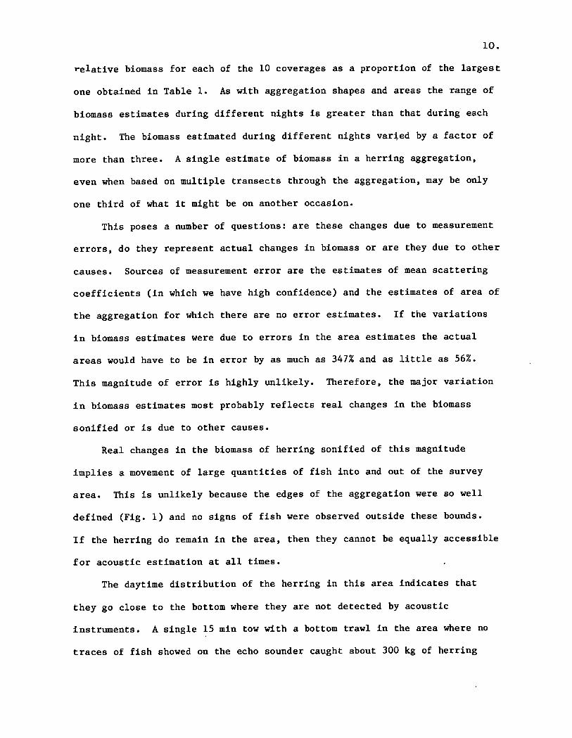
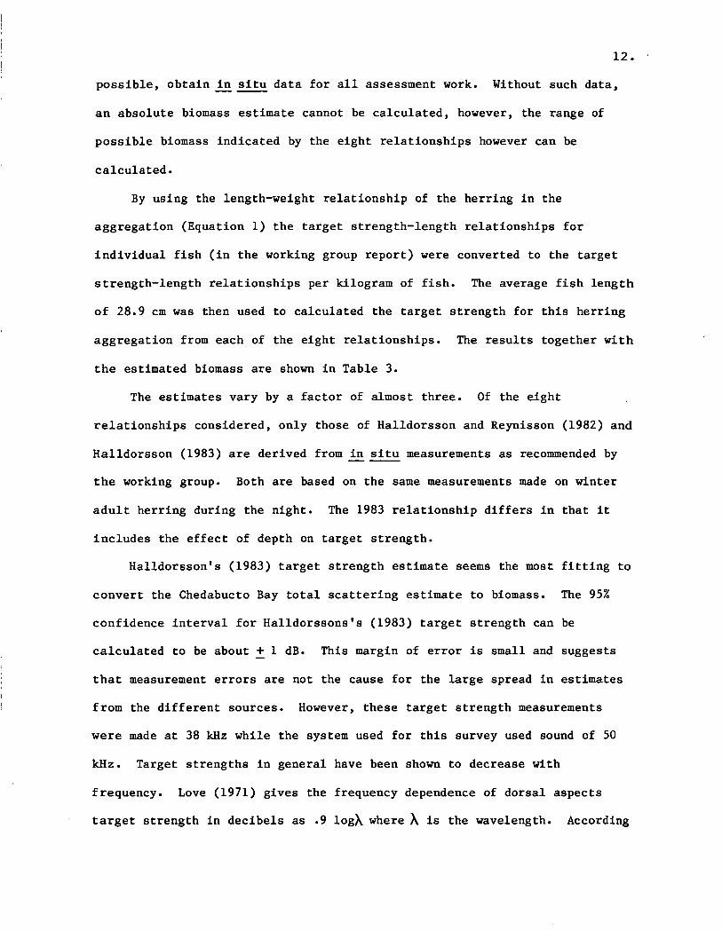
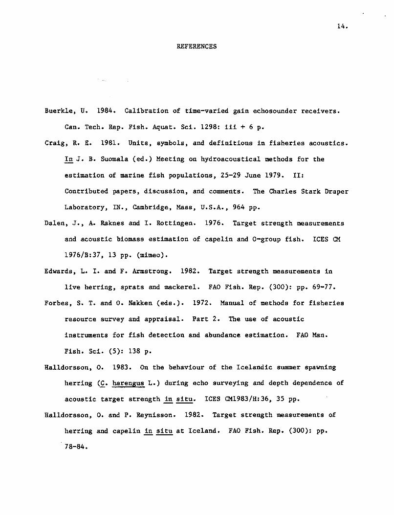
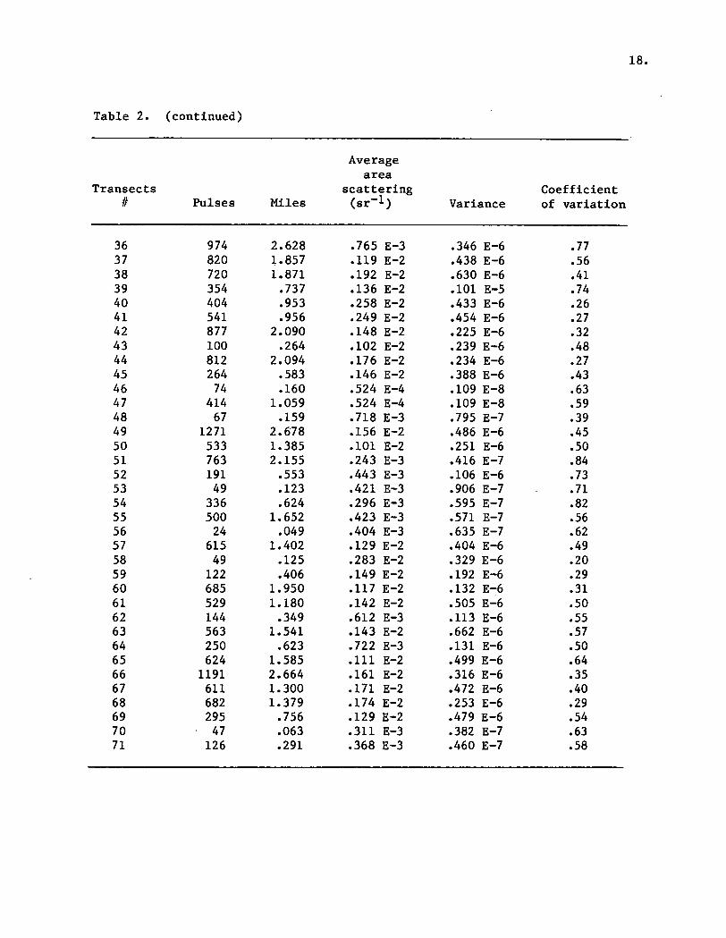
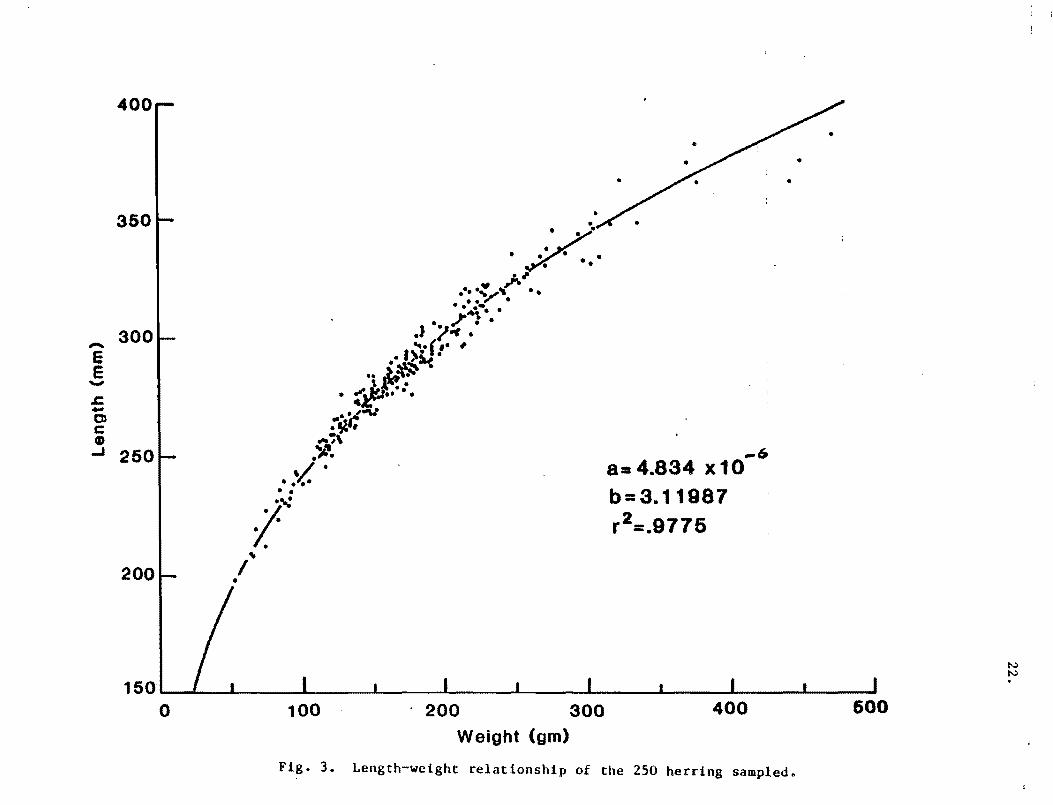