6 Cam Design
54
6 Cam Design 6.1 INTRODUCTION In previous chapters, we have learned how to analyze the kinematic characteristics of a given mechanism. We were given the design of a mechanism, and we studied ways to determine its mobility, its posture, its velocity, and its acceleration, and we even discussed its suitability for given types of tasks. However, we have said little about how the mechanism is designed—that is, how the sizes and shapes of the links are chosen by the designer. The next several chapters introduce this design point of view as it relates to mechanisms. We will find ourselves looking more at individual types of machine components and learning when and why such components are chosen and how they are sized. In Chap. 6, which is devoted to the design of cams, for example, we assume that we know the task to be accomplished. However, we do not know but we seek techniques to help discover the size and shape of the cam to perform this task. Of course, there is the creative step of deciding whether a cam should be used in the first place, as opposed to a gear train, a linkage, or some other mechanical device. This question often cannot be answered on the basis of scientific principles alone; it requires experience and imagination, and involves such factors as economics, marketability, reliability, maintenance, esthetics, ergonomics, ability to manufacture, and suitability for the task. These aspects are not well studied by a general scientific approach; they require human judgment of factors that are often not easily reduced to numbers or formulae. There is usually not a single “right” answer, and generally these questions cannot be answered by this or any other text or reference book. On the other hand, this is not to say that there is no place for a general science-based approach in design situations. Most mechanical design is based on repetitive analysis. 297
-
Upload
khangminh22 -
Category
Documents
-
view
3 -
download
0
Transcript of 6 Cam Design

6 Cam Design
6.1 INTRODUCTION
In previous chapters, we have learned how to analyze the kinematic characteristics ofa given mechanism. We were given the design of a mechanism, and we studied waysto determine its mobility, its posture, its velocity, and its acceleration, and we evendiscussed its suitability for given types of tasks. However, we have said little about howthe mechanism is designed—that is, how the sizes and shapes of the links are chosen bythe designer.
The next several chapters introduce this design point of view as it relates tomechanisms. We will find ourselves looking more at individual types of machinecomponents and learning when and why such components are chosen and how they aresized. In Chap. 6, which is devoted to the design of cams, for example, we assume that weknow the task to be accomplished. However, we do not know but we seek techniques tohelp discover the size and shape of the cam to perform this task.
Of course, there is the creative step of deciding whether a cam should be usedin the first place, as opposed to a gear train, a linkage, or some other mechanicaldevice. This question often cannot be answered on the basis of scientific principlesalone; it requires experience and imagination, and involves such factors as economics,marketability, reliability, maintenance, esthetics, ergonomics, ability to manufacture, andsuitability for the task. These aspects are not well studied by a general scientific approach;they require human judgment of factors that are often not easily reduced to numbers orformulae. There is usually not a single “right” answer, and generally these questions cannotbe answered by this or any other text or reference book.
On the other hand, this is not to say that there is no place for a general science-basedapproach in design situations. Most mechanical design is based on repetitive analysis.
297

298 CAM DESIGN
Therefore, in Chap. 6 and in several of the upcoming chapters, we will use the principles ofanalysis presented in Part 1 of the book. Also, we will use the governing analysis equationsto help in our choices of part sizes and shapes, and to help us assess the quality of our designas we proceed. It is important to point out that the forthcoming chapters are still based onthe laws of mechanics. The primary shift for Part 2 is that the component dimensions areoften the unknowns of the problem, whereas the input and output speeds, for example,may be given information. In Chap. 6, we will discover how to determine a cam contour,or profile, that delivers a specified motion characteristic.
6.2 CLASSIFICATION OF CAMS AND FOLLOWERS
A cam is a machine element used to drive another element, called a follower, througha specified motion by direct contact. Cam-and-follower mechanisms are simple andinexpensive, have few moving parts, and occupy very little space. Furthermore, followermotions having almost any desired characteristics are not difficult to design. For thesereasons, cam mechanisms are used extensively in modern machinery.
The versatility and flexibility in the design of cam systems are among their moreattractive features, yet this also leads to a wide variety of shapes and forms, and the needfor terminology to distinguish them.
Sometimes, cams are classified according to their basic shapes. Figure 6.1 shows fourdifferent types of cams:
(a) A plate cam, also called a disk cam or a radial cam.(b) A wedge cam.(c) A cylindric cam or barrel cam.(d) An end cam or face cam.
The least common of these in practical applications is the wedge cam, because of its needfor a reciprocating motion rather than a continuous input motion. By far the most commonis the plate cam. For this reason, most of the remainder of Chap. 6 specifically addressesplate cams, although the concepts presented pertain universally.
Cam systems can also be classified according to the basic shape of the follower.Figure 6.2 shows plate cams actuating four different types of followers:
(a) A knife-edge follower.(b) A flat-face follower.(c) A roller follower.(d) A spheric-face or curved-shoe follower.
Note that the follower face is usually chosen to have a simple geometric shape, and themotion is achieved by careful design of the shape of the cam to mate with it. This isnot always the case, and examples of inverse cams, where the follower is machined to acomplex shape, can be found.
Another method of classifying cams is according to the characteristic output motionproduced between the follower and the frame. Thus, some cams have reciprocating(translating) followers, as in Figs. 6.1a, b, and d, and Figs. 6.2a and b, whereas others

6.2 CLASSIFICATION OF CAMS AND FOLLOWERS 299
Q
Y
(a)
11
Y
Q
(b)
11
1
Y
Q
(c)
1
Q
Y
(d)
1
1
Figure 6.1 (a) Plate cam; (b) wedge cam; (c) barrel cam; (d) face cam.
Q
Y
(a)
Θ
(c)
Y
Y
(b)
Θ
Θ
(d)
Y
1 1
Figure 6.2 Plate cams with (a) an offset reciprocating knife-edge follower; (b) a reciprocatingflat-face follower; (c) an oscillating roller follower; (d) an oscillating curved-shoe follower.

300 CAM DESIGN
Θ
Y
(a)
Θ
Y
(b)
1
Figure 6.3(a) Constant-breadth cam witha reciprocating flat-facefollower; (b) conjugate camswith an oscillating rollerfollower.
have oscillating (rotating) followers, as in Figs. 6.1c, 6.2c, and 6.2d. Further classificationof reciprocating followers distinguishes whether the centerline of the follower stem relativeto the center of the cam is offset, as in Fig. 6.2a, or radial, as in Fig. 6.2b.
In all cam systems, the designer must ensure that the follower maintains contact withthe cam at all times. This can be accomplished by depending on gravity, by the inclusionof a suitable spring, or by a mechanical constraint. In Fig. 6.1c, the follower is constrainedby a groove. Figure 6.3a shows an example of a constant-breadth cam, where two contactpoints between the cam and the follower provide the constraint. Mechanical constraint canalso be introduced by employing dual or conjugate cams in an arrangement such as thatshown in Fig. 6.3b. Here each cam has its own roller, but the rollers are mounted on acommon follower.
Throughout this chapter we use the symbol Θ to represent the total motion of the camand the symbol Y to represent the total displacement of the follower. To investigate thedesign of cams in general, we denote the known input variable by Θ(t) and the outputvariable by Y . A review of Figs. 6.1, 6.2, and 6.3 will demonstrate the definitions of Θand Y for various types of cams. These figures show that the input, Θ , is an angle for mostcams, but it can be a distance, as in Fig. 6.1b. Also, the output, Y , is a translation distancefor a reciprocating follower, but it is an angle for an oscillating follower.
6.3 DISPLACEMENT DIAGRAMS
Despite the wide variety of cam types used and their differences in form, they also havecertain features in common that allow a systematic approach to their design. Usually a camsystem is a single-degree-of-freedom device. It is driven by a known input motion, usuallya shaft that rotates at constant speed, and it is intended to produce a certain desired periodicoutput motion for the follower.
During the rotation of a cam through one cycle, the follower executes a series of eventsas demonstrated in graphic form in the displacement diagram of Fig. 6.4. In such a diagram,the abscissa represents one cycle of the input, Θ (usually, one revolution of the cam), andis drawn to any convenient scale. The ordinate represents the follower travel, Y, and, for areciprocating follower, is usually drawn at full scale to help in the layout of the cam. On adisplacement diagram, it is possible to identify a portion of the graph called the rise, wherethe displacement of the follower is away from the cam center. The total rise is called the

6.3 DISPLACEMENT DIAGRAMS 301
Lift y
Rise Dwell Return
360�0 θ β1 β2 β3 β4
Y–Y0
Θ –Θ0
Dwell
Figure 6.4 Displacement diagram for a cam.
lift. The return is the portion in which the displacement of the follower is toward the camcenter. Portions of the cycle during which the follower is at rest are referred to as dwells.
For a particular motion segment (say, segment number k) of the total cam, the rotationlies in the range starting with Θk and extending by θ within the segment to
Θk+1 =Θk +βk, (a)
where βk is the total cam angle for segment k.Similarly, the displacement of the follower is in the range starting from Yk + y(0) and
extending by y(θ) within the segment to
Yk+1 = Yk + y(βk). (b)
Thus, within a segment, we can write
y= y(θ). (6.1)
Many of the essential features of a displacement diagram, such as the total lift andthe placement and duration of dwells, are usually dictated by the requirements of theapplication. There are, however, many possible choices of follower motions that mightbe used for the rise and return segments, and some are preferable over others, dependingon the situation. One of the key steps in the design of a cam is the choice of suitable formsfor these motions. Once the motions have been chosen—that is, once the exact relationshipis set between the inputΘ and the output Y—the displacement diagram can be constructedprecisely and is a graphic representation of the functional relationship
Y = Y (Θ).
This equation has stored within it the exact nature of the shape of the final cam: thenecessary information for its layout and manufacture, and also the important characteristicsthat determine the quality of its dynamic performance. Before looking further at thesetopics, however, we will describe graphic methods of constructing the displacementdiagrams for the following rise motions and the similar return motions: uniform motion,parabolic motion, simple harmonic motion, and cycloidal motion.
The displacement diagram for uniform motion is a straight line with constant slope.Thus, for constant input speed, the velocity of the follower is also constant. This motion

302 CAM DESIGN
(a)
b1
L1
L2
L3
L
y
u
b2 b3
b32
b12
(b)
b1
L1
1
1
2 3 4 5
y
u
2345
Figure 6.5 (a) Parabolic motion interfaces with uniform motion; (b) graphic construction.
is not useful for the full lift because of the sharp corners produced at the junctions withneighboring segments of the displacement diagram. It is often used, however, betweenother curve segments that eliminate the corners (called modified uniform motion).
Parabolic motion is one possible example of modified uniform motion, and thedisplacement diagram for this motion is shown in Fig. 6.5a. The central portion of thediagram, bounded by the cam angle β2 and with lift L2, is uniform motion. The twoends, with cam angles β1 and β3, and with corresponding lifts L1 and L3, are shaped todeliver parabolic motion to the follower. Soon we shall learn that these produce constantacceleration for the follower. Figure 6.5a shows a graphic method for matching the slopesof parabolic motions with that of uniform motion. With the cam angles β1, β2, β3, and thetotal lift, L, known, individual lifts L1, L2, and L3 are determined by locating the midpointsof the β1 and β3 segments and constructing a straight line as indicated. Figure 6.5b showsa graphic construction for a parabola to fit within a given rectangular boundary defined,first by L1 and β1, and then by L3 and β3. The abscissa and ordinate are divided into aconvenient but equal number of divisions and numbered as indicated. The construction ofeach point of the parabola then follows that indicated by dashed lines for point 3.
In the layout of an actual cam, if this might be done graphically, a great many divisionsare usually used to obtain good accuracy. At the same time, the drawing is made to a largescale, perhaps ten times full size, and then reduced to actual size by a pantographic method.However, for clarity in reading, the figures in this chapter are shown with fewer divisionsto define the curves and illustrate the graphic techniques.
The displacement diagram for simple harmonic motion is shown in Fig. 6.6. Thegraphic construction makes use of a semicircle having a diameter equal to lift L of thesegment. The semicircle and abscissa are divided into an equal number of divisions, andthe construction then follows that indicated by dashed lines for division number 2.
Cycloidal motion obtains its name from the geometric curve called a cycloid. As shownon the left-hand side of Fig. 6.7, a circle of radius L/2π , where L is the lift of the segment,makes exactly one revolution by rolling along the ordinate from the origin, y = 0, to fulllift, y= L. Point P of the circle, originally located at the origin, traces a cycloid, as shown.As the circle rolls without slip, the graph of the vertical displacement, y, of the point versusthe rotation angle, θ , gives the displacement diagram shown at the right of Fig. 6.7. We find

6.4 GRAPHIC LAYOUT OF CAM PROFILES 303
0 11
2
2
3
3
b4
4
L
y
5
5
6
6
u
Figure 6.6 Simple harmonic motion displacement diagram; graphic construction.
0
Cycloid
01 2 3 4
1
3
4 5
0, 6
5 6 ub
L
B
OP
y
1
2
3
4
5
6
r =2L
2p
Figure 6.7 Cycloidal motion displacement diagram; graphic construction.
it much more convenient for graphic purposes to draw the circle only once, using either theorigin, O, or point B as its center. After dividing the circle and the abscissa into an equalnumber of divisions and numbering them as indicated, we project each point of the circlehorizontally until it intersects the ordinate; next, from the ordinate, we project parallel tothe diagonal OB to obtain the corresponding point on the displacement diagram.
6.4 GRAPHIC LAYOUT OF CAM PROFILES
Let us now study the problem of determining the exact shape of the cam profile requiredto deliver a specified follower motion. We assume here that the required motion hasbeen completely defined—graphically, analytically, or numerically—as discussed in latersections. Thus, a complete displacement diagram can be drawn to scale for the entire camrotation. The requirement now is to lay out the proper cam profile to achieve the followermotion represented by this displacement diagram.

304 CAM DESIGN
Y–Y0
0 1 2 3 4 5 6 7 8 9 10 11 0
Lift
12
3
4
5
6
7
8
9
10
110
Trace point
Base circle
Prime circle
Cam profileCam rotation
Pitch curve
Ro
Θ
Θ
1
Figure 6.8 Cam nomenclature. The cam surface is developed by holding the cam stationary and rotating the follower fromstation 0 through stations 1, 2, 3, and so on.
We explain the procedure using the case of a plate cam with a radial roller follower, asshown in Fig. 6.8. Let us first note some additional nomenclature, illustrated in Fig. 6.8.
The trace point is a theoretic point of the follower, useful primarily in graphicconstructions; it corresponds to the tip of a fictitious knife-edge follower. It is locatedat the center of a roller follower or along the surface of a flat-face follower.
The pitch curve is the locus generated by the trace point as the follower moves withrespect to the cam. For a knife-edge follower, the pitch curve and cam profile are identical.For a roller follower they are separated by the radius of the roller.
The prime circle is the smallest circle that can be drawn tangent to the pitch curve witha center at the cam rotation axis. The radius of this circle is denoted R0.
The base circle is the smallest circle tangent to the cam profile centered on the camrotation axis. For a roller follower, it is smaller than the prime circle by the radius of theroller; for a knife-edge or flat-face follower, it is identical to the prime circle.
In constructing the cam profile, we employ the principle of kinematic inversion. Weimagine the sheet of paper on which we are working to be fixed to the cam, and wenote that, as the cam rotates, the follower appears to rotate (with respect to the paper)opposite to the direction of cam rotation. As shown in Fig. 6.8, we divide the prime circleinto a number of divisions and assign station numbers to these divisions. Dividing thedisplacement-diagram abscissa into corresponding divisions, we transfer Y−Y0 distancesfrom the displacement diagram directly onto the cam layout, measured along radial linesfrom the base circle to the trace point. The smooth curve through these points is the pitch

6.4 GRAPHIC LAYOUT OF CAM PROFILES 305
Ro
Θ
11
11
10
10
99
8
8
7
7
6
6
5
5
4
4
3 3
2
1 1
2
012'
11'10'
1'2'
9' 3'
8' 4'7' 5'6'
12 Trace point
Offset
L
Prime circle
Cam rotation
Offset circle
Cam profile
Pitch curve
Figure 6.9 Graphic layout of a plate-cam profile with an offset reciprocating roller follower.
curve. For the case of a roller follower, as in this example, we simply draw the roller in itsproper location at each station and then construct the cam profile as a smooth curve tangentto all of these roller locations.
Figure 6.9 shows how the method of construction is modified for an offset rollerfollower. We begin by constructing an offset circle, using a radius equal to the offsetdistance. After identifying station numbers around the prime circle, the centerline ofthe follower is constructed for each station, making it tangent to the offset circle. Theroller centers for each station are established by transferring Y−Y0 distances from thedisplacement diagram directly to these follower centerlines, always measuring positiveoutward from the prime circle. An alternative procedure is to identify points 0′, 1′, 2′, andso on, on a single follower centerline and then to rotate them about the cam center to thecorresponding follower centerline locations. In either case, the roller circle locations aredrawn next and a smooth curve tangent to all roller locations is the required cam profile.
Figure 6.10 shows the construction for a plate cam with a reciprocating flat-facefollower. The pitch curve is constructed using a method similar to that used for the rollerfollower in Fig. 6.8. Instead of roller locations, however, a line representing the flat face ofthe follower is constructed at each station. The cam profile is a smooth curve drawn tangentto all the follower location lines. It may be helpful to extend each straight line representing

306 CAM DESIGN
11
10
9
8
12 0
76
5
4
3
21
Trace point
Prime circle
Pitch curve
Cam rotation
Ro
ΘCam profile
L
Figure 6.10 Graphic layout ofa plate-cam profile with areciprocating flat-face follower.
a location of the follower face to form a series of triangles. If these triangles are lightlyshaded, as suggested in the illustration, it may be easier to draw the cam profile insideall the shaded triangles and tangent to the inner sides of the triangles. Note that the camprofile need not pass through points 0, 1, 2, 3, and so on, constructed from the displacementdiagram.
Figure 6.11 shows the layout of the profile of a plate cam with an oscillating rollerfollower. In this case, to develop the cam profile, we must rotate the fixed pivot center of thefollower opposite to the direction of cam rotation. To perform this inversion, first, a circle isdrawn about the cam-shaft center through the fixed pivot of the follower. This circle is thendivided and given station numbers to correspond to divisions on the displacement diagram.Next, arcs are drawn about each of these centers, all with equal radii corresponding to thelength of the follower.
In the case of an oscillating follower, the ordinate values Y−Y0 of the displacementdiagram represent angular movements of the follower. If the ordinate scale of thedisplacement diagram is properly chosen initially, however, and if the total lift of thefollower is a reasonably small angle, then ordinate distances from the displacementdiagram at each station can be transferred directly to the corresponding arc traveled by theroller center using dividers and measuring positive outward along the arc from the primecircle to locate the trace point for each station. Finally, a circle representing the rollerlocation is drawn with its center at the trace point for each station, and the cam profile isconstructed as a smooth curve tangent to each of these roller locations.
From the examples presented in this section, it should be clear that each differenttype of cam-and-follower system requires its own graphic method of construction to

6.5 KINEMATIC COEFFICIENTS OF FOLLOWER 307
ΘCam rotation
10
10
6'5'4'
7'8'9'
10'
3'
2'
11', 1' 12', 0'
Cam profile
Ro
11
11
12
12
0
0
1
1
3
3
4
4
5
56
6
7
7
8
8
9
9
2
2
L Trace point
Pitch curve
Prime circle
Figure 6.11 Graphic layout of a plate-cam profile with an oscillating roller follower.
determine the cam profile from the displacement diagram. The examples presented hereare not intended to be exhaustive of those possible, but they illustrate the general approach.They also illustrate and reinforce the discussion of the previous section; it is now clearthat much of the detailed shape of the cam itself results directly from the displacementdiagram. Although different types of cams and followers have different shapes for thesame displacement diagram, once a few parameters are chosen, such as the prime-circleradius, which determines the size of a cam, the remainder of its shape results directly fromthe motion requirements specified in the displacement diagram.
6.5 KINEMATIC COEFFICIENTS OF FOLLOWER
We have seen that, regardless of the type of cam or the type of follower, the displacementdiagram is plotted with the cam input angle, Θ , as the abscissa and the follower outputdisplacement, Y−Y0, as the ordinate. This diagram is made up of a number of segments.In each segment, the abscissa is designated as θ and the ordinate as y. The displacementdiagram is, therefore, a graph representing some mathematical function relating the input,

308 CAM DESIGN
Θ , and output, Y, motions of the cam system. In general terms, one segment of thisrelationship is given by Eq. (6.1):
y= y(θ).
Additional graphs can be plotted representing the derivatives of y with respect tothe input θ—that is, the kinematic coefficients of the follower. The first-order kinematiccoefficient of a segment is denoted
y′ (θ)= dy
dθ(6.2)
and represents the slope of the displacement diagram at the input position, θ , in thesegment. The combined graph of first-order kinematic coefficients of all segments,although it may seem to be of little practical value, is a measure of the “steepness” ofthe displacement diagram throughout the cycle. We will find later that this is closelyrelated to the mechanical advantage of the cam system and manifests itself in suchthings as the pressure angle (Sec. 6.10). If we consider a wedge cam (Fig. 6.1b) with aknife-edge follower (Fig. 6.2a), the displacement diagram itself is of the same shape asthe corresponding cam. In such a case, we can visualize that difficulties will occur if anysegment of the cam is too steep—that is, if the first-order kinematic coefficient y′ of anysegment has too high a value.
The second-order kinematic coefficient (that is, the second derivative of y with respectto input variable θ ) of each segment is also significant. The second-order kinematiccoefficient within a segment is denoted
y′′ (θ)= d2y
dθ2. (6.3)
Although it is not as easy to visualize the reason, the second-order kinematic coefficientis very closely related to the curvature of the cam at locations along its profile. Recall thatcurvature is the reciprocal of the radius of curvature, [Sec. 4.1, Eq. (e)]. Therefore, if y′′becomes large, the radius of curvature becomes small. In particular, if the second-orderkinematic coefficient becomes infinite, then the radius of curvature becomes zero; that is,the cam profile at such a position becomes pointed. This would be a highly unsatisfactorycondition from the point of view of contact stress between the cam and the follower, andwould very quickly cause surface damage.
The third-order kinematic coefficient of a segment, denoted
y′′′ (θ)= d3y
dθ3, (6.4)
can also be plotted if desired. Although it is not easy to describe geometrically, thisdemonstrates the rate of change of y′′ with respect to input variable θ . We will see thatthe third-order kinematic coefficient can also be controlled when choosing the detailedshape of the displacement diagram.
6.5 KINEMATIC COEFFICIENTS OF FOLLOWER 309
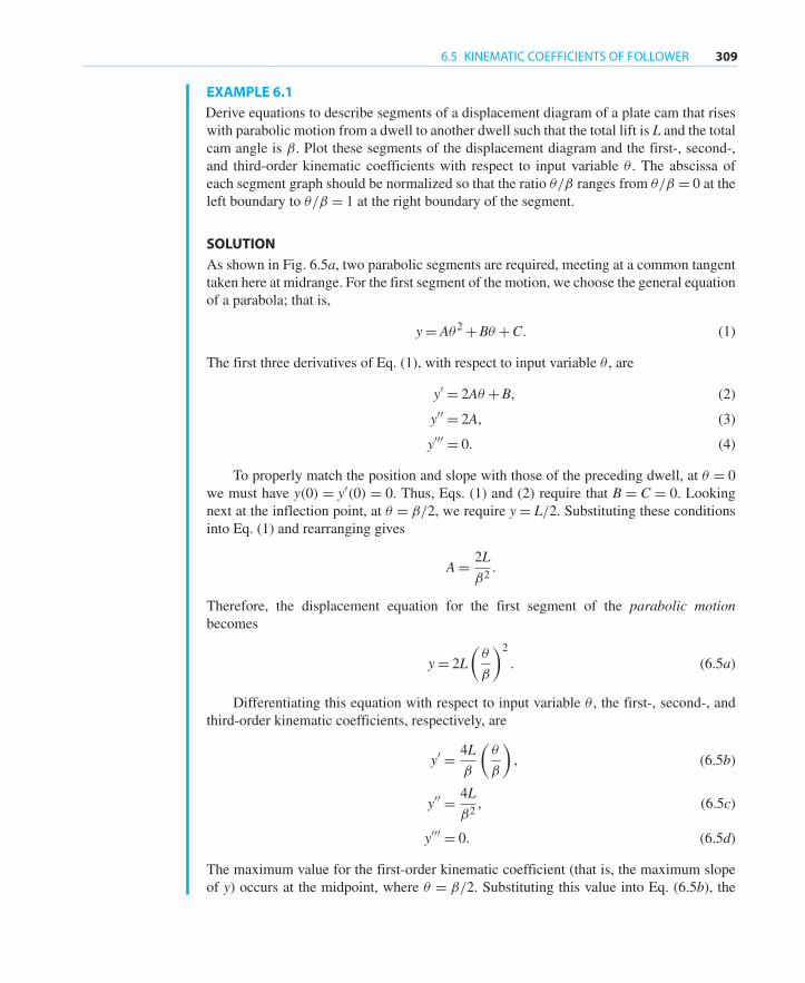
EXAMPLE 6.1
Derive equations to describe segments of a displacement diagram of a plate cam that riseswith parabolic motion from a dwell to another dwell such that the total lift is L and the totalcam angle is β. Plot these segments of the displacement diagram and the first-, second-,and third-order kinematic coefficients with respect to input variable θ . The abscissa ofeach segment graph should be normalized so that the ratio θ/β ranges from θ/β = 0 at theleft boundary to θ/β = 1 at the right boundary of the segment.
SOLUTION
As shown in Fig. 6.5a, two parabolic segments are required, meeting at a common tangenttaken here at midrange. For the first segment of the motion, we choose the general equationof a parabola; that is,
y= Aθ2 +Bθ +C. (1)
The first three derivatives of Eq. (1), with respect to input variable θ , are
y′ = 2Aθ +B, (2)
y′′ = 2A, (3)
y′′′ = 0. (4)
To properly match the position and slope with those of the preceding dwell, at θ = 0we must have y(0) = y′(0) = 0. Thus, Eqs. (1) and (2) require that B = C = 0. Lookingnext at the inflection point, at θ = β/2, we require y= L/2. Substituting these conditionsinto Eq. (1) and rearranging gives
A= 2L
β2.
Therefore, the displacement equation for the first segment of the parabolic motionbecomes
y= 2L
(θ
β
)2
. (6.5a)
Differentiating this equation with respect to input variable θ , the first-, second-, andthird-order kinematic coefficients, respectively, are
y′ = 4L
β
(θ
β
), (6.5b)
y′′ = 4L
β2, (6.5c)
y′′′ = 0. (6.5d)
The maximum value for the first-order kinematic coefficient (that is, the maximum slopeof y) occurs at the midpoint, where θ = β/2. Substituting this value into Eq. (6.5b), the
310 CAM DESIGN
maximum value for the first-order kinematic coefficient is
y′max = 2L
β. (5)
For the second segment of the parabolic motion, we return to the general equations(1) through (4) for a parabola. Substituting the conditions that y = L and y′ = 0 at θ = βinto Eqs. (1) and (2) gives
L= Aβ2 +Bβ+C, (6)
0= 2Aβ+B. (7)
Since the slope must match that of the first parabola at θ = β/2, then from Eqs. (2) and (5)we have
2L
β= 2A
β
2+B. (8)
Solving Eqs. (6), (7), and (8) simultaneously gives
A= −2L
β2, B= 4L
β, C= −L. (9)
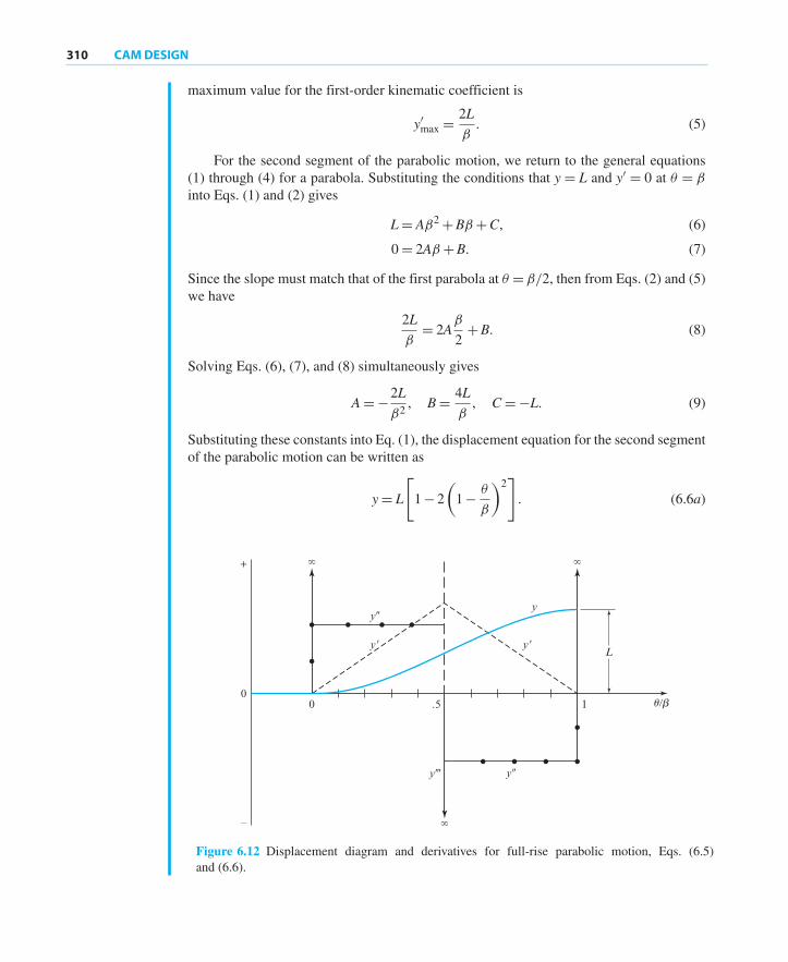
Substituting these constants into Eq. (1), the displacement equation for the second segmentof the parabolic motion can be written as
y= L
[1− 2
(1− θβ
)2]. (6.6a)
� �
�
L
y
y� y�
y�
y�y
ub1.500
–
+
Figure 6.12 Displacement diagram and derivatives for full-rise parabolic motion, Eqs. (6.5)and (6.6).

6.5 KINEMATIC COEFFICIENTS OF FOLLOWER 311
Also, substituting Eqs. (9) into Eqs. (2), (3), and (4), the first-, second-, and third-orderkinematic coefficients for the second segment of the parabolic motion, respectively, are
y′ = 4L
β
(1− θβ
), (6.6b)
y′′ = −4L
β2, (6.6c)
y′′′ = 0. (6.6d)
The displacement diagram and the first-, second-, and third-order kinematic coefficientsfor this example of full-rise parabolic motion are shown in Fig. 6.12.
The previous discussion relates to the kinematic coefficients of the follower motion.These coefficients are derivatives with respect to the input variable, θ , and relate to thegeometry of the cam system. Let us now consider the derivatives of the follower motionwith respect to time. First, we assume that the time variation of the input motion, Θ(t),and, therefore, θ(t), is known. The angular velocity, ω = dθ/dt, the angular acceleration,α = d2θ/dt2, and the next derivative (often called angular jerk or second angularacceleration), α = d3θ/dt3, are all assumed to be known. Usually, a plate cam is driven bya constant-speed input shaft. In this case, ω is a known constant, θ = ωt, and α = α = 0.During start-up of the cam system, however, this is not the case, and we will consider themore general situation first.
From the general equation of the displacement diagram, for chosen segment numberk, we can write from Eqs. (a) and (b) in Sec. 6.3
y= Y−Yk = y(θ) and θ =Θ −Θk = θ (t) . (6.7)
Therefore, we can differentiate to find the time derivatives of the follower motion. Thevelocity of the follower, for example, is given by
y= dy
dt=(dy
dθ
)(dθ
dt
),
which, using the first-order kinematic coefficient, can be written as
y= y′ω. (6.8)
Similarly, the acceleration and the jerk (the third time derivative) of the follower can bewritten, respectively, as
y= d2y
dt2= y′′ω2 + y′α (6.9)
and
...y = d3y
dt3= y′′′ω3 + 3y′′ωα+ y′α. (6.10)

312 CAM DESIGN
When the camshaft speed is constant, then α = 0, and Eqs. (6.8) through (6.10)reduce to
y= y′ω, y= y′′ω2,...y = y′′′ω3. (6.11)
For this reason, it has become somewhat common to refer to the graphs of the kinematiccoefficients y′, y′′, y′′′, such as those shown in Fig. 6.12, as the “velocity,” “acceleration,”and “jerk” curves for a given segment of the motion. These are only appropriate names for aconstant-speed cam, and then only when scaled byω,ω2, andω3, respectively.∗ However, itis helpful to use these names for the kinematic coefficients when considering the physicalimplications of a certain choice of displacement diagram. For example, considering theparabolic motion of Fig. 6.12, it is intuitively meaningful to say that the “velocity” of thefollower rises linearly to a maximum at the midpoint θ = β/2 and then decreases linearlyto zero. The “acceleration” of the follower is zero during the initial dwell and changesabruptly (that is, a step change) to a constant positive value upon beginning the rise. Thereare two more step changes in the “acceleration” of the follower—namely, at the midpointand at the end of the rise. At each of these three step changes in the “acceleration” of thefollower, the “jerk” of the follower becomes infinite.
6.6 HIGH-SPEED CAMS
Continuing with our discussion of parabolic motion, let us consider briefly the implicationsof the “acceleration” curve segments of Fig. 6.12 on the dynamic performance of the camsystem. Any real follower, of course, has at least some mass and, when this is multipliedby acceleration, exerts an inertia force (Chap. 12). Therefore, the “acceleration” curve ofFig. 6.12 can also be thought of as indicating the inertia force of the follower, which,in turn, is felt at the follower bearings and at the contact point on the cam surface. An“acceleration” curve with abrupt changes (that is, where the “jerk” becomes infinite), suchas those demonstrated for parabolic motion, exert abruptly changing contact stresses at thebearings and on the cam surface, and will lead to noise, surface wear, and early failure.Thus, it is very important in choosing and joining segments of a displacement diagram toensure that the first- and second-order kinematic coefficients (that is, the “velocity” and“acceleration” curves) are continuous—meaning, that they contain no step changes.
Sometimes in low-speed cam applications compromises are made with the “velocity”and “acceleration” relationships. It is sometimes simpler to employ a reverse procedure anddesign the cam shape first, obtaining the displacement diagram as a second step. Such camsare sometimes composed of a combination of curves, such as straight lines and circulararcs, which are readily produced by machine tools. Two examples are the circle-arc camand the tangent cam shown in Fig. 6.13. The design approach is by iteration. A trial camis designed and its kinematic characteristics are found. The process is then repeated until acam with acceptable characteristics is obtained. Points A, B, C, and D of the circle-arc cam
∗ Accepting the word “velocity” literally, for example, leads to consternation when it is discoveredthat, for a plate cam with a reciprocating follower, the units of “velocity” y′ are length per radian.Multiplying these units by radians per second, the units of ω, gives units of length per second for y,however.

6.7 STANDARD CAM MOTIONS 313
(a) (b)
C
B
A
r2
r1D
C
B
A
r2
r2 r1
D r3
Figure 6.13 (a) Circle-arccam; (b) tangent cam.
and the tangent cam are points of tangency or blending points. It is worth noting, as withthe previous parabolic-motion example, that the acceleration changes abruptly at each ofthe blending points because of the instantaneous change in the radius of curvature of thecam profile.
Although cams with discontinuous acceleration characteristics have sometimes beenaccepted to save cost in low-speed applications, such cams have invariably exhibited majordifficulties at some later time when the input speed of the machine was raised to increasethe productivity of the application. For any high-speed cam application, it is extremelyimportant that not only the displacement and “velocity” curves, but also the “acceleration”curve be made continuous for the entire motion cycle. No discontinuities should be allowedwithin or at the junctions of different segments of a cam.
As confirmed by Eq. (6.11), the importance of continuous derivatives becomes moreserious as the cam-shaft speed is increased. The higher the speed, the greater the need forsmooth curves. At very high speeds, it might also be desirable to require that jerk, which isrelated to rate of change of force, and perhaps even higher derivatives, be made continuousas well. In many applications, however, this is not necessary.
There is no simple answer as to how high a speed one must have before consideringthe application to require high-speed design techniques. The answer depends not onlyon the mass of the follower, but also on the stiffness of the return spring, the materialsused, the flexibility of the follower, and many other factors [9]. Further analysistechniques on cam dynamics are presented in Secs. 6.11 to 6.16. Still, with the methodspresented here, it is not difficult to achieve continuous displacement diagrams withcontinuous derivatives. Therefore, it is recommended that this be undertaken as standardpractice. Cycloidal-motion cams, for example, are no more difficult to manufacture thanparabolic-motion cams, and there is no good reason for use of the latter. The circle-arc camand the tangent cam may be easy to produce, but, with modern machining methods, cuttingmore complex cam shapes is not expensive and is recommended.
6.7 STANDARD CAM MOTIONS
Example 6.1 in Sec. 6.5 gave a detailed derivation of the equations for parabolic motionand its first three derivatives [Eqs. (6.5) and (6.6)]. Then, in Sec. 6.6, reasons were provided

314 CAM DESIGN
for avoiding the use of parabolic motion in high-speed cam systems. The purpose of thissection is to present equations for a number of standard types of displacement curvesegments that can be used to address most high-speed cam-motion requirements. Thederivations parallel those of Example 6.1 and are not presented.
The displacement equation and the first-, second-, and third-order kinematic coeffi-cients for a full-rise simple harmonic motion segment are
y= L
2
(1− cos
πθ
β
), (6.12a)
y′ = πL2β
sinπθ
β, (6.12b)
y′′ = π2L
2β2cosπθ
β, (6.12c)
y′′′ = −π3L
2β3sinπθ
β. (6.12d)
The displacement diagram and the first-, second-, and third-order kinematic coefficientsfor a full-rise simple harmonic motion segment are shown in Fig. 6.14. Unlike parabolicmotion, simple harmonic motion exhibits no discontinuity at the inflection point, but itdoes contain nonzero “accelerations” at its two boundaries.
The displacement equation and the first-, second-, and third-order kinematic coeffi-cients for a full-rise cycloidal motion segment are
y= L
(θ
β− 1
2πsin
2πθ
β
), (6.13a)
y′ = L
β
(1− cos
2πθ
β
), (6.13b)
y′′ = 2πL
β2sin
2πθ
β, (6.13c)
Ly
00.5 1
+
–
y�
u/b
y'"y''
Figure 6.14 Displacement diagram and derivatives for a full-rise simple harmonic motion segment,Eqs. (6.12).

6.7 STANDARD CAM MOTIONS 315
y′′′ = 4π2L
β3cos
2πθ
β. (6.13d)
The displacement diagram and the first-, second-, and third-order kinematic coef-ficients for a full-rise cycloidal motion segment are shown in Fig. 6.15. Note that allderivatives at the boundaries of this segment have zero values. Note also that this is theonly standard motion with zeroes for all derivatives at the boundaries. However, the peak“velocity,” “acceleration,” and “jerk” values are higher than those for a simple harmonicmotion segment.
The displacement equation and the first-, second-, and third-order kinematic coeffi-cients for a full-rise eighth-order polynomial motion segment are
y= L
[6.097 55
(θ
β
)3− 20.780 40
(θ
β
)5+ 26.731 55
(θ
β
)6
− 13.609 65
(θ
β
)7+ 2.560 95
(θ
β
)8], (6.14a)
y′ = L
β
[18.292 65
(θ
β
)2− 103.902 00
(θ
β
)4+ 160.389 30
(θ
β
)5
− 95.267 55
(θ
β
)6+ 20.487 60
(θ
β
)7], (6.14b)
y′′ = L
β2
[36.585 30
(θ
β
)− 415.608 00
(θ
β
)3+ 801.946 50
(θ
β
)4
− 571.605 30
(θ
β
)5+ 143.413 20
(θ
β
)6], (6.14c)
Ly
00.5 1
+
–
y'
ub
y'"
y''
Figure 6.15 Displacement diagram and derivatives for a full-rise cycloidal motion segment,Eqs. (6.13).

316 CAM DESIGN
y′′′ = L
β3
[36.585 30− 1 246.824 00
(θ
β
)2+ 3 207.786 00
(θ
β
)3
−2 858.026 50
(θ
β
)4+ 860.479 20
(θ
β
)5]. (6.14d)
The displacement diagram and the first-, second-, and third-order kinematic coefficientsfor the full-rise motion segment formed from an eighth-order polynomial are shown inFig. 6.16. Equations (6.14) have seemingly awkward coefficients, since they have beenspecially derived to have many “nice” properties [6]. Among these, Fig. 6.16 shows notonly that several of the kinematic coefficients are zero at both ends of the segment, butalso that the “acceleration” characteristics are nonsymmetric. Also, the peak values of“acceleration” are kept as small as possible (that is, the magnitudes of the positive andnegative peak “accelerations” are equal).
The displacement diagrams of simple harmonic, cycloidal, and eighth-order polyno-mial motions segments look quite similar at first glance. Each rises through a lift of L ina cam rotation angle of β, and each begins and ends with zero slope. For these reasons,they are all referred to as full-rise motion segments. However, their “acceleration” curvesare quite different. A simple harmonic motion segment has nonzero “acceleration” at theboundaries, a cycloidal motion segment has zero “acceleration” at both boundaries, andan eighth-order polynomial motion segment has one zero and one nonzero “acceleration”at its two boundaries. This variety provides the selections necessary when matching thesecurves with neighboring curves of different types.
Full-return motion segments of the same three types are shown in Figs. 6.17through 6.19.
Ly
00.5 1
+
–
y'
ub
y'"
y''
Figure 6.16 Displacement diagram and derivatives for a full-rise eighth-order polynomial motionsegment, Eqs. (6.14).

6.7 STANDARD CAM MOTIONS 317
L
y
0.5 1
+
–
y�
ub
y
y�
Figure 6.17 Displacement diagram and derivatives for a full-return simple harmonic motionsegment, Eqs. (6.15).
L
y
0.5 1
+
–
y�
u/b
y
y�
Figure 6.18 Displacementdiagram and derivatives for afull-return cycloidal motionsegment, Eqs. (6.16).
L
y
0.50 1
+
–
y�
ub
y
y�
Figure 6.19 Displacementdiagram and derivatives for afull-return eighth-orderpolynomial motion segment,Eqs. (6.17).

318 CAM DESIGN
The displacement equation and the first-, second-, and third-order kinematic coeffi-cients for a full-return simple harmonic motion segment are
y= L
2
(1+ cos
πθ
β
), (6.15a)
y′ = −πL2β
sinπθ
β, (6.15b)
y′′ = −π2L
2β2cosπθ
β, (6.15c)
y′′′ = π3L
2β3sinπθ
β. (6.15d)
For a full-return cycloidal motion segment, the displacement equation and the first-,second-, and third-order kinematic coefficients are
y= L
(1− θβ
+ 1
2πsin
2πθ
β
), (6.16a)
y′ = −L
β
(1− cos
2πθ
β
), (6.16b)
y′′ = −2πL
β2sin
2πθ
β, (6.16c)
y′′′ = −4π2L
β3cos
2πθ
β. (6.16d)
For a full-return eighth-order polynomial motion segment, the displacement equationand the first-, second-, and third-order kinematic coefficients are
y= L
[1.000 00− 2.634 15
(θ
β
)2+ 2.780 55
(θ
β
)5
+ 3.170 60
(θ
β
)6− 6.877 95
(θ
β
)7+ 2.560 95
(θ
β
)8], (6.17a)
y′ = −L
β
[5.268 30
θ
β− 13.902 75
(θ
β
)4− 19.023 60
(θ
β
)5
+ 48.145 65
(θ
β
)6− 20.487 60
(θ
β
)7], (6.17b)
6.7 STANDARD CAM MOTIONS 319
y′′ = − L
β2
[5.268 30− 55.611 00
(θ
β
)3− 95.118 00
(θ
β
)4
+ 288.873 90
(θ
β
)5− 143.413 20
(θ
β
)6], (6.17c)
y′′′ = L
β3
[166.833 00
(θ
β
)2+ 380.472 00
(θ
β
)3
− 1 444.369 50
(θ
β
)4+ 860.479 20
(θ
β
)5]. (6.17d)
Polynomial displacement equations of much higher order, and meeting many moreconditions than those presented here are also in common use. Automated procedures fordetermining the coefficients have been developed by Stoddart [8], who also indicates howthe choice of coefficients can be made to compensate for elastic deformation of the followersystem under dynamic conditions. Such cams are referred to as polydyne cams.
In addition to the full-rise and full-return motions presented earlier, it is also usefulto have a selection of standard half-rise and half-return motion segments available. Theseare curves for which one segment boundary has a nonzero slope and can be used to blendwith uniform motion. The displacement diagrams and the first-, second-, and third-orderkinematic coefficients for half-rise simple harmonic motion segments, sometimes calledhalf-harmonic rise motion segments, are shown in Fig. 6.20. The equations correspondingto Fig. 6.20a are
y= L
(1− cos
πθ
2β
), (6.18a)
y′ = πL2β
sinπθ
2β, (6.18b)
y′′ = π2L
4β2cosπθ
2β, (6.18c)
y′′′ = −π3L
8β3sinπθ
2β. (6.18d)
The displacement equation and the first-, second-, and third-order kinematic coefficientscorresponding to the half-rise simple harmonic motion segments of Fig. 6.20b are
y= Lsinπθ
2β, (6.19a)
y′ = πL2β
cosπθ
2β, (6.19b)

320 CAM DESIGN
Ly
10
+
–
y�
ub
y
y�
(a)
L
y
10
+
–
y'
ub
y'"y''
(b)
Figure 6.20 Displacement diagram and derivatives for half-rise simple harmonic motion segments:(a) Eqs. (6.18); (b) Eqs. (6.19).
y′′ = −π2L
4β2sinπθ
2β, (6.19c)
y′′′ = −π3L
8β3cosπθ
2β. (6.19d)
The curves for half-return simple harmonic motion segments are shown in Fig. 6.21.The equations corresponding to Fig. 6.21a are
y= Lcosπθ
2β, (6.20a)
y′ = −πL2β
sinπθ
2β, (6.20b)
y′′ = −π2L
4β2cosπθ
2β, (6.20c)
y′′′ = π3L
8β3sinπθ
2β. (6.20d)
The displacement equation and the first-, second-, and third-order kinematic coefficientscorresponding to the half-return simple harmonic motion segments of Fig. 6.21b are
y= L
(1− sin
πθ
2β
), (6.21a)
y′ = −πL2β
cosπθ
2β, (6.21b)
y′′ = π2L
4β2sinπθ
2β, (6.21c)
y′′′ = π3L
8β3cosπθ
2β. (6.21d)
6.7 STANDARD CAM MOTIONS 321
L
y
10
+
–
y�
ub
y
y�
(a)
L
y
10
+
–
y�
u/b
yy�
(b)
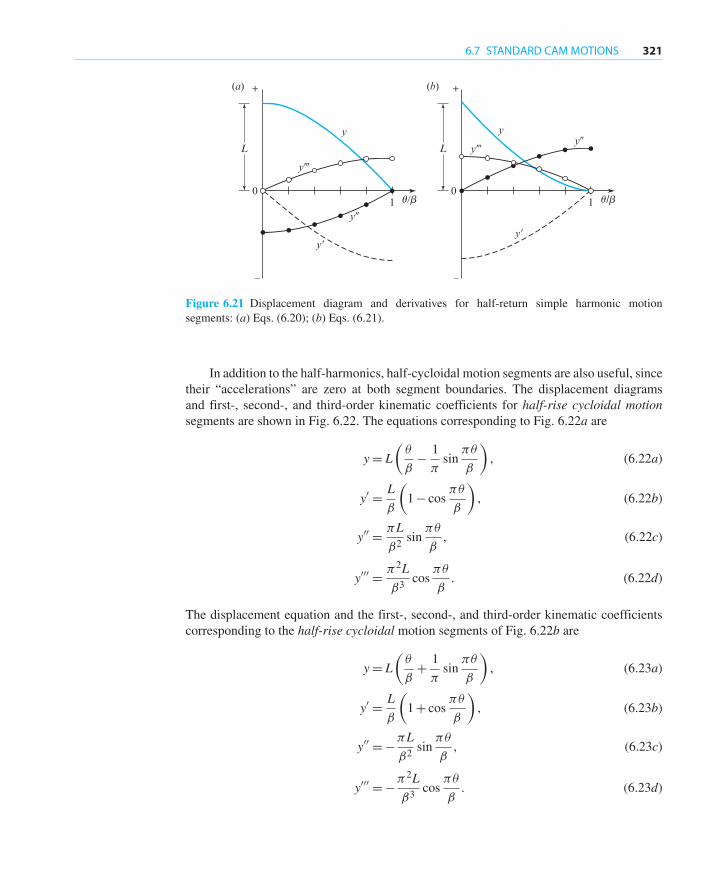
Figure 6.21 Displacement diagram and derivatives for half-return simple harmonic motionsegments: (a) Eqs. (6.20); (b) Eqs. (6.21).
In addition to the half-harmonics, half-cycloidal motion segments are also useful, sincetheir “accelerations” are zero at both segment boundaries. The displacement diagramsand first-, second-, and third-order kinematic coefficients for half-rise cycloidal motionsegments are shown in Fig. 6.22. The equations corresponding to Fig. 6.22a are
y= L
(θ
β− 1
πsinπθ
β
), (6.22a)
y′ = L
β
(1− cos
πθ
β
), (6.22b)
y′′ = πLβ2
sinπθ
β, (6.22c)
y′′′ = π2L
β3cosπθ
β. (6.22d)
The displacement equation and the first-, second-, and third-order kinematic coefficientscorresponding to the half-rise cycloidal motion segments of Fig. 6.22b are
y= L
(θ
β+ 1
πsinπθ
β
), (6.23a)
y′ = L
β
(1+ cos
πθ
β
), (6.23b)
y′′ = −πLβ2
sinπθ
β, (6.23c)
y′′′ = −π2L
β3cosπθ
β. (6.23d)

322 CAM DESIGN
Ly
10
+
–
y�
u/b
y
y�
(a)
L
y
10
+
–
y�
ub
y
y�
(b)
Figure 6.22 Displacement diagram and derivatives for half-rise cycloidal motion segments: (a)Eqs. (6.22); (b) Eqs. (6.23).
The curves for half-return cycloidal motion segments are shown in Fig. 6.23. Theequations corresponding to Fig. 6.23a are
y= L
(1− θβ
+ 1
πsinπθ
β
), (6.24a)
y′ = −L
β
(1− cos
πθ
β
), (6.24b)
y′′ = −πLβ2
sinπθ
β, (6.24c)
y′′′ = −π2L
β3cosπθ
β. (6.24d)
The displacement equation and the first-, second-, and third-order kinematic coefficientscorresponding to the half-return cycloidal motion segments of Fig. 6.23b are
y= L
(1− θβ
− 1
πsinπθ
β
), (6.25a)
y′ = −L
β
(1+ cos
πθ
β
), (6.25b)
y′′ = πLβ2
sinπθ
β, (6.25c)
y′′′ = π2L
β3cosπθ
β. (6.25d)
We will see shortly how the “standard” segment graphs and equations presented in thissection can greatly reduce the analytic effort involved in designing the full displacement
6.8 MATCHING DERIVATIVES OF DISPLACEMENT DIAGRAMS 323
L
y
10
+
–
y�
ub
y
y�
(a)
L
y
10
+
–
y�
ub
y
y�
(b)
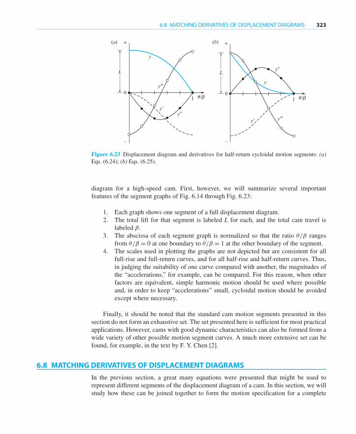
Figure 6.23 Displacement diagram and derivatives for half-return cycloidal motion segments: (a)Eqs. (6.24); (b) Eqs. (6.25).
diagram for a high-speed cam. First, however, we will summarize several importantfeatures of the segment graphs of Fig. 6.14 through Fig. 6.23:
1. Each graph shows one segment of a full displacement diagram.2. The total lift for that segment is labeled L for each, and the total cam travel is
labeled β.3. The abscissa of each segment graph is normalized so that the ratio θ/β ranges
from θ/β = 0 at one boundary to θ/β = 1 at the other boundary of the segment.4. The scales used in plotting the graphs are not depicted but are consistent for all
full-rise and full-return curves, and for all half-rise and half-return curves. Thus,in judging the suitability of one curve compared with another, the magnitudes ofthe “accelerations,” for example, can be compared. For this reason, when otherfactors are equivalent, simple harmonic motion should be used where possibleand, in order to keep “accelerations” small, cycloidal motion should be avoidedexcept where necessary.
Finally, it should be noted that the standard cam motion segments presented in thissection do not form an exhaustive set. The set presented here is sufficient for most practicalapplications. However, cams with good dynamic characteristics can also be formed from awide variety of other possible motion segment curves. A much more extensive set can befound, for example, in the text by F. Y. Chen [2].
6.8 MATCHING DERIVATIVES OF DISPLACEMENT DIAGRAMS
In the previous section, a great many equations were presented that might be used torepresent different segments of the displacement diagram of a cam. In this section, we willstudy how these can be joined together to form the motion specification for a complete
324 CAM DESIGN
cam. The procedure is one of solving for proper values of L and β for each segment sothat:
1. The motion requirements of the particular application are met.2. The displacement diagram, as well as the diagrams of the first- and second-order
kinematic coefficients, are continuous across the boundaries of the mergedsegments. The diagram of the third-order kinematic coefficient may be alloweddiscontinuities if necessary, but must not become infinite; that is, the “accelera-tion” curve may contain corners but not discontinuities (jumps).
3. The maximum magnitudes of the “velocity” and “acceleration” peaks are kept aslow as possible consistent with the first two conditions.
The procedure may best be understood through an example.
EXAMPLE 6.2
A plate cam with a reciprocating follower is to be driven by a constant-speed motor at150 rpm. The follower is to start from a dwell, accelerate to a uniform velocity of 25 in/s,maintain this velocity for 1.25 in of rise, decelerate to the top of the lift, return, and thendwell for 0.10 s. The total lift is to be 3.00 in. Determine the complete specifications ofthe displacement diagram.
SOLUTION
The speed of the input shaft is
ω= 150 rev/min= 15.707 96 rad/s. (1)
Using Eq. (6.8), the first-order kinematic coefficient (that is, the slope of the uniform“velocity” segment) is
y′ = y
ω= 25 in/s
15.707 96 rad/s= 1.591 55 in/rad. (2)
Since this “velocity” is held constant for 1.25 in of rise, the total cam rotation in thissegment is
β2 = L2y′
= 1.25 in
1.591 55 in/rad= 0.785 40 rad= 45.000◦. (3)
Similarly, from Eq. (1), the total cam rotation during the final dwell is
β5 = 0.10 s (15.707 96 rad/s)= 1.570 796 rad= 90.000◦. (4)
Note that several digits of accuracy higher than usual are utilized here andare recommended as standard practice when matching cam motion derivatives. Anyinaccuracies in the L and β values result in discontinuities in the smoothness of derivativesat the boundaries of the segments and discontinuities in force, as explained in Sec. 6.6.
6.8 MATCHING DERIVATIVES OF DISPLACEMENT DIAGRAMS 325
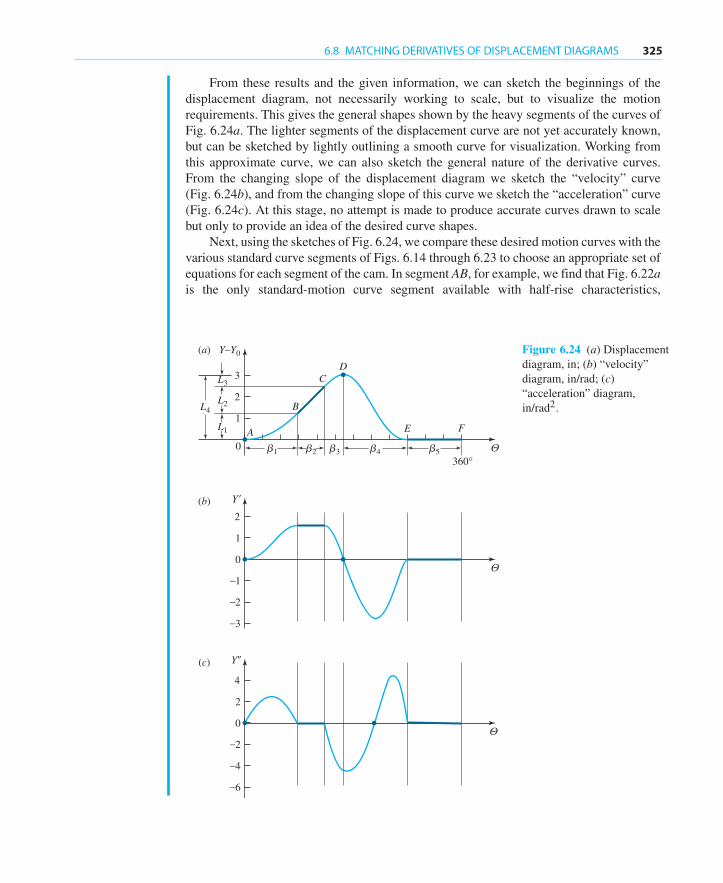
From these results and the given information, we can sketch the beginnings of thedisplacement diagram, not necessarily working to scale, but to visualize the motionrequirements. This gives the general shapes shown by the heavy segments of the curves ofFig. 6.24a. The lighter segments of the displacement curve are not yet accurately known,but can be sketched by lightly outlining a smooth curve for visualization. Working fromthis approximate curve, we can also sketch the general nature of the derivative curves.From the changing slope of the displacement diagram we sketch the “velocity” curve(Fig. 6.24b), and from the changing slope of this curve we sketch the “acceleration” curve(Fig. 6.24c). At this stage, no attempt is made to produce accurate curves drawn to scalebut only to provide an idea of the desired curve shapes.
Next, using the sketches of Fig. 6.24, we compare these desired motion curves with thevarious standard curve segments of Figs. 6.14 through 6.23 to choose an appropriate set ofequations for each segment of the cam. In segment AB, for example, we find that Fig. 6.22ais the only standard-motion curve segment available with half-rise characteristics,
Y–Y0
ΘA
B
CD
E F1
2
3L3
b1 b2 b3 b4 b5
L2L4
L1
0
360°
Y�
Θ
1
–1
2
0
–2
–3
Y�
Θ
2
–2
4
0
–4
–6
(a)
(c)
(b)
Figure 6.24 (a) Displacementdiagram, in; (b) “velocity”diagram, in/rad; (c)“acceleration” diagram,in/rad2.
326 CAM DESIGN
an appropriate slope curve, and the necessary zero “acceleration” at both boundaries of thesegment. Thus, we choose the half-rise cycloidal motion of Eq. (6.22) for this segment ofthe cam. There are two sets of choices possible for segments CD and DE. One set might bethe choice of Fig. 6.22bmatched with Fig. 6.18. However, to keep the peak “accelerations”low and to keep the “jerk” curves as smooth as possible, we choose Fig. 6.20b matchedwith Fig. 6.19. Thus, for segment CD, we will use the half-rise harmonic motion ofEq. (6.19), and for segment DE, we choose the eighth-order polynomial return motionof Eq. (6.17).
Choosing the curve types, however, is not sufficient to fully specify the segmentcharacteristics. We must also find values for the unknown parameters of the segmentequations; these are L1, L3, β1, β3, and β4. We do this by equating the kinematiccoefficients at each nonzero segment boundary. For example, to match the “velocities”at point B we must equate the first-order kinematic coefficient from Eq. (6.22b) at the ABsegment right boundary (that is, at θ1/β1 = 1) with the first-order kinematic coefficient ofthe BC segment; that is,
y′B = 2L1β1
= L2β2
= 1.25 in
0.785 40 rad= 1.591 55 in/rad
or
L1 = (0.795 77 in/rad)β1. (5)
Similarly, to match the “velocities” at point C, we equate the first-order kinematiccoefficient of segment BC with the first-order kinematic coefficient of Eq. (6.19b) at theCD segment left boundary (that is, at θ3/β3 = 0). This gives
y′C = L2β2
= πL32β3
= 1.591 55 in/rad
or
L3 = (1.013 21 in/rad)β3. (6)
To match the “accelerations” (that is, the curvatures) at point D, we equate thesecond-order kinematic coefficient of Eq. (6.19c) at the CD segment right boundary (thatis, at θ3/β3 = 1) with the second-order kinematic coefficient of Eq. (6.17c) at the DEsegment left boundary (that is, at θ4/β4 = 0). This gives
y′′D = −π2L34β23
= −5.268 30L4β24
,
where the total lift is L4 = 3 in. Substituting Eq. (6) and the total lift into this result andrearranging gives
β3 = 0.158 18β24 . (7)
Finally, for geometric compatibility, we have the constraints
L1 +L3 = L4 −L2 = 1.750 in, (8)

6.9 PLATE CAM WITH RECIPROCATING FLAT-FACE FOLLOWER 327
and, considering Eqs. (3) and (4),
β1 +β3 +β4 = 2π −β2 −β5 = 3.926 99 rad. (9)
Solving the five equations—that is, Eqs. (5) through (9)—simultaneously for the fiveunknowns, L1, L3, β1, β3, and β4, provides the proper values for the remaining parameters.In summary, the segment parameters are
L1 = 1.183 1 in, β1 = 1.486 74 rad= 85.184◦,L2 = 1.250 0 in, β2 = 0.785 40 rad= 45.000◦,L3 = 0.566 9 in, β3 = 0.559 51 rad= 32.058◦,L4 = 3.000 0 in, β4 = 1.880 74 rad= 107.758◦,L5 = 0.000 0 in, β5 = 1.570 80 rad= 90.000◦. Ans.
At this time, an accurate layout of the displacement diagram and, if desired, the kinematiccoefficients can be made to replace the sketches. The curves of Fig. 6.24 have been drawnto scale using these values.
6.9 PLATE CAM WITH RECIPROCATING FLAT-FACE FOLLOWER
Once the displacement diagram of a cam system has been completely determined, asdescribed in Sec. 6.8, the layout of the actual cam shape can be attempted, as demonstratedin Sec. 6.4. In laying out the cam, however, we find the need for a few more parameters,depending on the type of cam and follower—for example, the prime-circle radius, anyoffset distance, the roller radius, and so on. Also, as we will see, each different typeof cam-and-follower system can be subject to certain further difficulties unless theseremaining parameters are properly chosen.
In this section, we study the troubles that may be encountered in the design of a platecam with a reciprocating flat-face follower. The geometric parameters of such a systemthat must yet be chosen are the prime-circle radius, R0, the offset (eccentricity), ε, of thefollower stem, and the width of the follower face.
Figure 6.25 shows the layout of a plate cam with a radial reciprocating flat-facefollower. In this illustration, the displacement chosen was a full-rise cycloidal motionsegment with L1 = 100 mm during β1 = 90◦ of cam rotation, followed by a full-returncycloidal motion segment during the remaining β2 = 270◦ of cam rotation. The layoutprocedure of Fig. 6.10 was followed to develop the cam shape, and the radius chosen forthe prime circle was R0 = 25 mm. Obviously, there is a problem, since the resulting camprofile intersects itself. During machining, part of the cam shape is lost, and, when inoperation, the intended cycloidal motion is not fully achieved. Such a cam is said to beundercut.
Why did undercutting occur in this example and how can it be avoided? It resultedfrom attempting to achieve too great a lift in too little cam rotation with too small a cam.One possible cure for this trouble is to decrease the desired lift, L1, or to increase the camrotation angle, β1. However, this is not possible while still achieving the original designspecifications. Another cure is to continue with the same displacement characteristics but

328 CAM DESIGN
RoL
vc
w
Q
e
Ro
Y R
r
u
X
u
1
υ
C
r
υs
Figure 6.25 Undercut plate-camprofile layout with reciprocatingflat-face follower.
Figure 6.26 Vectors for plate-cam profilewith reciprocating flat-face follower.
to increase the prime-circle radius, R0, to avoid undercutting. This does produce a largercam, but with sufficient increase, it does overcome the undercutting difficulty.
The minimum value of R0 that avoids undercutting can be found by developingan equation for the radius of curvature of the cam profile. We start by writing theloop-closure equation using the vectors shown in Fig. 6.26. Using complex polar notation,the loop-closure equation for a general plate cam with a reciprocating flat-face follower is
R= rej(Θ+ϕ)+ jρ = j(R0 +Y)+ s. (a)
Recall that the symbol Θ represents the total rotation of a general plate cam.We have carefully chosen the vectors so that point C is located at the instantaneous
center of curvature, and ρ is the radius of curvature corresponding to the current contactpoint. The line along the u axis that separates the angles Θ and ϕ is fixed on the cam andis horizontal for the cam posture Θ = 0. The value of Y0 is zero. The angle Θ specifies therotation of the cam, and the u and v axes rotate with the cam.
Separating Eq. (a) into real and imaginary parts, respectively, gives
r cos(Θ +ϕ)= s, (b)
r sin(Θ +ϕ)+ρ = R0 +Y . (c)

6.9 PLATE CAM WITH RECIPROCATING FLAT-FACE FOLLOWER 329
Since point C is the center of curvature, the magnitudes of r, ϕ, and ρ do not changefor a small increment in cam rotation;∗ that is,
dr
dΘ= dϕ
dΘ= dρ
dΘ= 0.
Therefore, differentiating Eq. (a) with respect to the cam rotation angle, Θ , gives
jrej(Θ+ϕ) = jY ′ + s′, (d)
where Y ′ = dY/dΘ = dy/dθ = y′ and s′ = ds/dΘ = ds/dθ . Separating Eq. (d) into realand imaginary parts, the first-order kinematic coefficients are
−r sin(Θ +ϕ)= s′, (e)
r cos(Θ +ϕ)= y′. (f)
Equating Eqs. (b) and (f ), we find the location of the trace point along the surface ofthe follower as
s= y′. (6.26)
Differentiating this equation with respect to the cam rotation angle, Θ , we find
s′ = y′′. (g)
Substituting Eq. (g) into Eq. (e) and then substituting the result into Eq. (c), the radius ofcurvature of the cam profile can be written as
ρ = R0 +Y+ y′′. (6.27)
We should carefully note the importance of Eq. (6.27); it states that the radius ofcurvature of the cam profile can be obtained for each cam rotation angle, Θ , directlyfrom the displacement equations, before laying out the cam profile. All that is neededis the choice of the prime-circle radius, R0, and values for the displacement, Y , and thesecond-order kinematic coefficient, y′′.
We can use Eq. (6.27) to select a value for R0 that will avoid undercutting. Whenundercutting occurs, the radius of curvature of the cam profile switches sign from positiveto negative. On the verge of undercutting, the cam comes to a point, and the radius ofcurvature becomes zero for some value of the cam rotation angle, Θ . However, we canchoose R0 large enough that this is never the case. In fact, to avoid high contact stresses,we may wish to ensure that ρ is everywhere larger than some specified value, ρmin. To dothis, from Eq. (6.27), we require that
ρ = R0 +Y+ y′′ > ρmin.
∗ The values of r, ϕ, and ρ are not truly constant but are currently at stationary values; their higherderivatives are nonzero.
330 CAM DESIGN
Since R0 and Y are always positive, the critical situation occurs at or near the posturewhere the second-order kinematic coefficient, y′′, has its largest negative value. Denotingthis minimum value of y′′ as y′′min and remembering that Y corresponds to the same posture,defined by cam angle Θ , we have the condition
R0 > ρmin −Y− y′′min, (6.28)
which must be satisfied. This can easily be checked once the displacement equations havebeen established, and an appropriate value of R0 can be chosen before the cam layout isattempted.
Returning now to Fig. 6.26, we see that Eq. (6.26) can also be of value. This equationstates that the length of travel of the point of contact on either side of the cam rotationcenter corresponds precisely to the plot of the first-order kinematic coefficient. Thus, theminimum face width for a flat-face follower must extend at least y′max to the right and−y′minto the left of the camshaft center to maintain contact; that is,
Face width> y′max − y′min. (6.29)
EXAMPLE 6.3
Assuming that the displacement characteristics in Example 6.2 are to be achieved bya plate cam with a reciprocating flat-face follower, determine the minimum face widthand the minimum prime-circle radius to ensure that the radius of curvature of the cam iseverywhere greater than ρmin = 0.25 in.
SOLUTION
From Fig. 6.24b, the maximum “velocity” (that is, the maximum value of the first-orderkinematic coefficient) occurs in segment BC and is
y′max = L2β2
= 1.250 0 in
0.785 40 rad= 1.592 in/rad. (1)
The minimum “velocity” occurs in segment DE at approximately θ/β4 = 0.5. FromEq. (6.17b), the minimum value of the first-order kinematic coefficient is approximately
y′min ≈ y′ (θ/β4 = 0.5)= −2.812 in/rad. (2)
Substituting Eqs. (1) and (2) into Eq. (6.29), the minimum face width is
Face width> (1.592 in)− (−2.812 in)= 4.404 in. Ans.
Therefore, the follower would be positioned 1.592 in to the right and 2.812 in to the left ofthe cam rotation axis, and some appropriate additional allowance may be added on eachside.

6.9 PLATE CAM WITH RECIPROCATING FLAT-FACE FOLLOWER 331
The largest negative “acceleration” (the minimum value of the second-order kinematiccoefficient) occurs at D and can be obtained from Eq. (6.19c) at θ/β3 = 1; that is,
y′′min = −π2L34β23
= − π2(0.566 9 in)
4(0.559 51 rad)2= −4.468 18 in/rad2.
Substituting this result and the known parameters into Eq. (6.28), the minimumprime-circle radius is
R0 > 0.250 in− (−4.468 in)− 3.000 in= 1.718 in. Ans.
From this calculation, we would choose the actual prime-circle radius as, say, R0 = 1.75 in.
We see that the eccentricity of the flat-face follower stem does not affect the geometryof the cam. This eccentricity is usually chosen to avoid high bending stress in the follower.Also, there may be a higher load in the follower during the working stroke, say the liftstroke, than during the return motion. In such a case, the eccentricity may be chosen tolocate the follower stem more centrally over the contact point during the lift portion of themotion cycle.
Looking again at Fig. 6.26, we can write another loop-closure equation; that is,
uejΘ + vej(Θ+π/2) = j(R0 +Y)+ s,
where we recall that u and v denote the coordinates of the contact point in a coordinatesystem attached to the cam. Dividing this equation by ejΘ gives
u+ jv= j(R0 +Y)e−jΘ + se−jΘ .
Using Eq. (6.26), the real and imaginary parts of this equation can be written as
u= (R0 +Y)sinΘ + y′ cosΘ , (6.30a)
v= (R0 +Y)cosΘ − y′ sinΘ . (6.30b)
These two equations give the coordinates of the cam profile and provide an alternativeto the graphic layout procedure of Fig. 6.10. They can be used to generate a tableof numeric rectangular coordinate data from which the cam can be machined. Polarcoordinate equations for this same curve are
R=√(R0 +Y)2 + (y′)2 (6.31a)
and
ψ = π2
−Θ − tan−1 y′
R0 +Y. (6.31b)
332 CAM DESIGN
6.10 PLATE CAM WITH RECIPROCATING ROLLER FOLLOWER
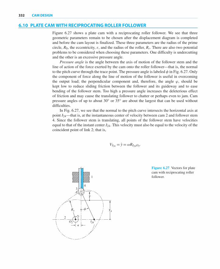
Figure 6.27 shows a plate cam with a reciprocating roller follower. We see that threegeometric parameters remain to be chosen after the displacement diagram is completedand before the cam layout is finalized. These three parameters are the radius of the primecircle, R0, the eccentricity, ε, and the radius of the roller, Rr. There are also two potentialproblems to be considered when choosing these parameters. One difficulty is undercuttingand the other is an excessive pressure angle.
Pressure angle is the angle between the axis of motion of the follower stem and theline of action of the force exerted by the cam onto the roller follower—that is, the normalto the pitch curve through the trace point. The pressure angle is labeled φ in Fig. 6.27. Onlythe component of force along the line of motion of the follower is useful in overcomingthe output load; the perpendicular component and, therefore, the angle ϕ, should bekept low to reduce sliding friction between the follower and its guideway and to easebending of the follower stem. Too high a pressure angle increases the deleterious effectof friction and may cause the translating follower to chatter or perhaps even to jam. Campressure angles of up to about 30◦ or 35◦ are about the largest that can be used withoutdifficulties.
In Fig. 6.27, we see that the normal to the pitch curve intersects the horizontal axis atpoint I24—that is, at the instantaneous center of velocity between cam 2 and follower stem4. Since the follower stem is translating, all points of the follower stem have velocitiesequal to that of the instant center I24. This velocity must also be equal to the velocity of thecoincident point of link 2; that is,
VI24 = y= ωRI24O2.
f
e
Y
Y0
A
Ro
l24O2
43
2
1
Figure 6.27 Vectors for platecam with reciprocating rollerfollower.

6.10 PLATE CAM WITH RECIPROCATING ROLLER FOLLOWER 333
Dividing this equation by the angular velocity of the cam, ω [Eq. (6.11)], the first-orderkinematic coefficient is
y′ = y
ω= RI24O2 .
This first-order kinematic coefficient can also be expressed in terms of the eccentricity ofthe follower stem and the pressure angle of the cam as
y′ = ε+ (Y0 +Y) tanφ, (a)
where, as shown in Fig. 6.27, the vertical distance from the cam axis to the prime circle is
Y0 =√R20 − ε2. (b)
Substituting Eq. (b) into Eq. (a) and rearranging, the pressure angle of the cam can bewritten as
φ = tan−1
⎛⎝ y′ − εY+
√R20 − ε2
⎞⎠ . (6.32)
From this equation, we observe that, once the displacement equations and the first-orderkinematic coefficient have been determined, the two parameters, R0 and ε, can be adjustedto seek a suitable pressure angle. We also note that the pressure angle is continuouslychanging as the cam rotates, and therefore we are particularly interested in studying itsextreme values.
Let us first consider the effect of eccentricity. From Eq. (6.32), we observe thatincreasing ε either increases or decreases the magnitude of the numerator, depending onthe sign of the first-order kinematic coefficient y′. Thus, a small eccentricity, ε, can be usedto reduce the pressure angle, φ, during the rise motion when y′ is positive, but only at theexpense of an increased pressure angle during the return motion when y′ is negative. Still,since the magnitudes of the forces are usually greater during rise, it is common practice tooffset the follower to take advantage of this reduction in pressure angle.
A much more significant effect can be made in reducing the pressure angle byincreasing the prime-circle radius, R0. To study this effect, let us take the conservativeapproach and assume a radial follower—that is, where there is no eccentricity. Substitutingε = 0 into Eq. (6.32), the equation for the pressure angle reduces to
φ = tan−1(
y′
Y+R0
). (6.33)
To find the extremum values of the pressure angle, it is possible to differentiate thisequation with respect to the cam rotation angle and equate it to zero, thus finding the valuesof the rotation angle, Θ , that yield the maximum and the minimum pressure angles. Thisis a tedious process, however, and can be avoided by using the nomogram of Fig. 6.28.This nomogram was produced by searching out on a digital computer the maximum value

334 CAM DESIGN
40
5
5
10
15
20
2530
3540 45 50 55
6065
70
75
80
85
360300
200
10090
8070
60503530
2520
15
10
25
25 10 5 4 3 2 1 0.5
10 5 4 3 2 1 0.5
fmax–degrees
b–degrees
RoL-Cycloidal or 8th-orderpolynomial motion
RoL-Simple harmonic motion
Figure 6.28 Nomogramrelating the maximum pressureangle, φmax, to the prime-circleradius, R0, lift, L, and segmentangle, β, for radialreciprocating roller-followercams with full-rise orfull-return simple harmonic,cycloidal, or eighth-orderpolynomial motion.
of φ from Eq. (6.33) for each of the standard full-rise and full-return motion curves ofSec. 6.7. With the nomogram, it is possible to use the known values of L and β for eachsegment of the displacement diagram and to read directly the maximum pressure angleoccurring in that motion segment for a particular choice of R0. Alternatively, a desiredmaximum pressure angle can be chosen, and a corresponding minimum value of R0 can bedetermined. The process is best illustrated by an example.
EXAMPLE 6.4
Assuming that the displacements determined in Example 6.2 are to be achieved by a platecam with a reciprocating radial roller follower, determine the minimum prime-circle radiusthat ensures that the pressure angle is everywhere less than 30◦.
SOLUTION
Each segment of the displacement diagram can be checked in succession using thenomogram of Fig. 6.28.
For segment AB of Fig. 6.24, we have half-rise cycloidal motion with L1 = 1.183 inand β1 = 85.184◦. Since this is a half-rise curve, whereas the nomogram of Fig. 6.28 wasdeveloped only for full-rise curves, it is necessary to double both L1 and β1, thus imaginingthat the curve is full rise. This gives L∗
1 = 2.366 in and β∗1 ≈ 170◦. Next, connecting a
straight line from β∗ = 170◦ to φmax = 30◦, we read from the upper scale on the centralaxis of the nomogram a value of R0/L∗
1 ≈ 0.75, from which
R0 ≥ 0.75(2.366 in)= 1.775 in. (1)
The segment BC need not be checked, since the maximum pressure angle for thissegment occurs at boundary B and cannot be greater than that for segment AB.
Segment CD has half-rise harmonic motion with L3 = 0.567 in and β3 = 32.058◦.Again, since this is a half-rise curve, these values are doubled, and L∗
3 = 1.134 in and
6.10 PLATE CAM WITH RECIPROCATING ROLLER FOLLOWER 335
β∗3 ≈ 64◦ are used instead. Then, from the nomogram, we find R∗
0/L∗3 ≈ 2.15, from which
R∗0 ≥ 2.15(1.134 in)= 2.438 in.
However, here we must be careful. This value is the radius of a fictitious prime circle forwhich the horizontal axis of our fictional doubled “full-rise” harmonic curve would havey = 0. This is not the R0 we seek, since our imagined full-harmonic curve has a nonzeroY∗ value at its base. Referring to Fig. 6.24, we find
Y∗3 = YD − 2L3 = 3.000− 1.134 = 1.866 in.
The appropriate value of R0 for this segment is
R0 ≥ 2.438− 1.866 = 0.572 in. (2)
Next we check segment DE, which has eighth-order polynomial motion withL4 = 3.000 in and β4 = 107.758◦. Since this is a full-return motion curve with y = 0 atits base, no adjustments are necessary for use of the nomogram. We find R0/L4 ≈ 1.3 and
R0 ≥ 1.3(3.000 in)= 3.900 in. (3)
To ensure that the pressure angle does not exceed 30◦ throughout all segments of thecam motion, we must chose the prime-circle radius to be at least as large as the maximumof these discovered values, Eqs. (1), (2), and (3). Remembering the inability to read thenomogram with great precision, we might choose a yet larger value, such as
R0 = 4.000 in. Ans.
Once a final value has been chosen, we can use Fig. 6.28 again to find the actualmaximum pressure angle in each segment of the motion:
AB :R0L∗1
= 4.000
2.366= 1.691 β∗
1 = 170◦ φmax = 18◦,
CD :R∗0
L∗3
= 5.866
1.134= 5.173 β∗
3 = 64◦ φmax = 14◦,
DE :R0L4
= 4.000
3.000= 1.333 β4 = 108◦ φmax = 29◦.
Although the prime circle has been sized to give a satisfactory pressure angle, thefollower may still not complete the desired motion. It is still possible that the curvature ofthe pitch curve is too sharp and that the cam profile may be undercut. Figure 6.29a showsa portion of a cam pitch curve and two cam profiles generated by two different-size rollers.It is clear from Fig. 6.29a that a small roller moving on the given pitch curve generates asatisfactory cam profile. The cam profile generated by the larger roller, however, intersectsitself and is said to be undercut. The result, after machining, is a pointed cam that doesnot produce the desired motion. Still, if the prime circle and thus the cam size is increasedenough, even the larger roller generates a cam profile that operates satisfactorily.

336 CAM DESIGN
R�r
Actual path oflarge roller
Pitch curve
Cam profile(small roller)
Cam profile(large roller)
Rr
(a)
Pitch curve
Cam profile
Rr
(b)
Figure 6.29 (a) Undercut; (b) pointed cam profile.
In Fig. 6.29b, we see that the cam profile becomes pointed when the roller radius, Rr isequal to the magnitude∗ of the radius of curvature of the pitch curve. Therefore, to achievesome chosen minimum size, ρ∗, for the radius of curvature of the cam profile, the radiusof curvature of the pitch curve must be of greater magnitude than this value by the radiusof the roller; that is,
|ρ| ≥ ρ∗ +Rr. (c)
Recall Sec. 4.17, where the radius of curvature of a point trajectory was given by Eq. (4.56).In concept, it is possible to search out the minimum value |ρ|min for a particular
choice of the displacement equation, Y, and a particular prime-circle radius, R0. However,since it would be burdensome to perform such a search for each new cam design, theminimum-size radius of curvature (normalized with respect to R0) has been sought out bya digital computer program for each of the standard cam motions of Sec. 6.7. The resultsare presented graphically in Fig. 6.30 through Fig. 6.34. Each of these figures shows agraph of (|ρ|min + Rr)/R0 versus β for one type of standard-motion curve with variousratios of R0/L. Since we have already chosen the displacement equations and have founda suitable value of R0, each segment of the cam can now be checked to find its minimumradius of curvature.
Saving even more effort, it is not necessary to check those segments of the cam wherethe second-order kinematic coefficient y′′ remains positive throughout the segment, suchas the half-rise motions of Eqs. (6.18) and (6.22) or the half-return motions of Eqs. (6.21)and (6.25). Assuming that the “acceleration” curve is continuous, the minimum radius ofcurvature of the cam cannot occur in these segments. For each of these segments,
|ρ|min = R0 −Rr. (6.34)
∗ Remember that radius of curvature can have either a positive or a negative value (Sec. 4.17).However, here we are only concerned with its size—that is, its absolute value.
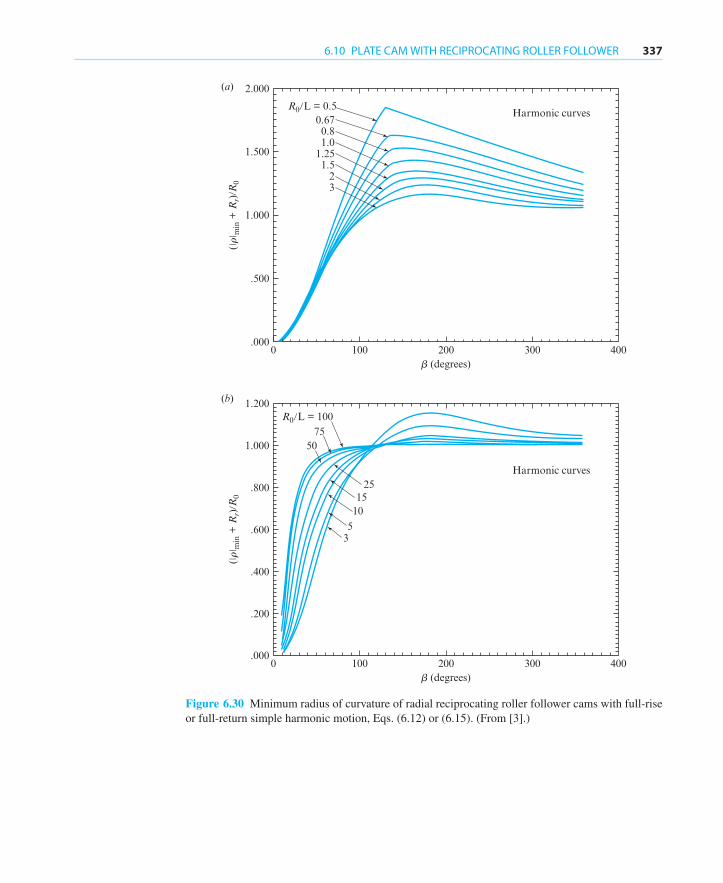
6.10 PLATE CAM WITH RECIPROCATING ROLLER FOLLOWER 337
2.000
1.500
1.000
.500
.0000 100 200 300 400
(�r� m
in +
Rr)
R0
b (degrees)
Harmonic curves
32
1.5
1.00.8
R0L = 0.50.67
1.25
R0L = 1001.200
1.000
.0000 100 200 300 400
(�r� m
in +
Rr)
R0
b (degrees)
Harmonic curves
.800
.600
.400
.200
7550
2515
105
3
(a)
(b)
Figure 6.30 Minimum radius of curvature of radial reciprocating roller follower cams with full-riseor full-return simple harmonic motion, Eqs. (6.12) or (6.15). (From [3].)
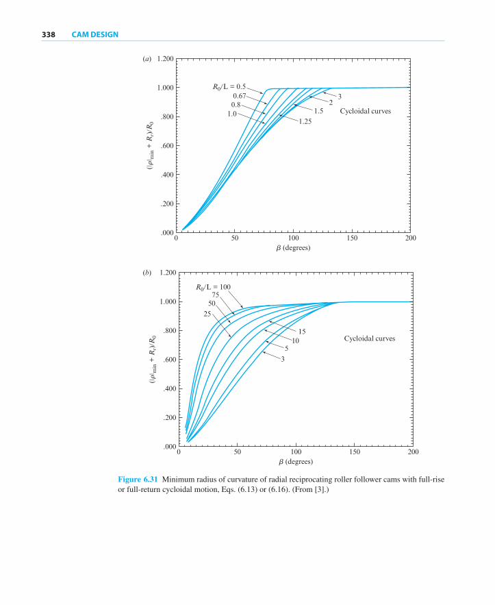
338 CAM DESIGN
0
(a)
50 100b (degrees)
(�r� m
in +
Rr)
R0
150 200
1.200
1.000
.800
.600
.400
.200
.000
1.251.5
23
1.00.80.67
R0L = 0.5
Cycloidal curves
0
(b)
50 100b (degrees)
(�r� m
in +
Rr)
R0
150 200
1.200
1.000
.800
.600
.400
.200
.000
3
Cycloidal curves5
1015
7550
25
R0L = 100
Figure 6.31 Minimum radius of curvature of radial reciprocating roller follower cams with full-riseor full-return cycloidal motion, Eqs. (6.13) or (6.16). (From [3].)

6.10 PLATE CAM WITH RECIPROCATING ROLLER FOLLOWER 339
1.200
1.000
.800
.600
(�r� m
in +
Rr)
/Ro
.400
.200
.000
1.200
1.000
.800
.600
(�r� m
in +
Rr)
/Ro
.400
.200
.000
0 50 100
Eighth-OrderPolynomial Curves
Eighth-OrderPolynomial Curves
1.251.5
23
1510
53
Ro/L = 100
7550
25
Ro/L = 0.50.670.8
1.0
b (degrees)
(a)
150 200
0 50 100
b (degrees)
(b)
150 200
Figure 6.32 Minimum radius of curvature of radial reciprocating roller follower cams with full-riseor full-return eighth-order polynomial motion, Eqs. (6.14) or (6.17). (From [3].)

340 CAM DESIGN
0
(a)
50 100b (degrees)
(�r� m
in +
Rr)
R0
150 200
1.200
1.000
.800
.600
.400
.200
.000
10 5 3 21.0
1.251.5
R0/L = 0.8
Half-harmonic curves
0
(b)
50 100b (degrees)
(�r� m
in +
Rr)
R0
150 200
1.200
1.000
.800
.600
.400
.200
.000
5025
105
75100
150R0L = 200
Half-harmonic curves
Figure 6.33 Minimum radius of curvature of radial reciprocating roller follower cams withhalf-harmonic motion, Eqs. (6.19) or (6.20). (From [3].)

6.10 PLATE CAM WITH RECIPROCATING ROLLER FOLLOWER 341
0
(a)
50 100b (degrees)
(�r� m
in +
Rr)
R0
150 200
1.200
1.000
.800
.600
.400
.200
.000
101.0
1.251.5
5 3 2R0L = 0.8
Half-cycloidal curves
0
(b)
50 100b (degrees)
(�r� m
in +
Rr)
R0
150 200
1.200
1.000
.800
.600
.400
.200
.000
Half-cycloidal curves
10
75100
150R0L = 200
5
2550
Figure 6.34 Minimum radius of curvature of radial reciprocating roller follower cams withhalf-cycloidal motion, Eqs. (6.23) or (6.24). (From [3].)

342 CAM DESIGN
EXAMPLE 6.5
Assuming that the displacement characteristics of Example 6.2 are to be achieved by aplate cam with a reciprocating roller follower, determine the minimum radius of curvatureof the cam profile if a prime-circle radius of R0 = 4.000 in (from Example 6.4) and a rollerradius of Rr = 0.500 in are used.
SOLUTION
For the segment AB of Fig. 6.24, we find from Eq. (6.34) that
|ρ|min = R0 −Rr = 4.000 in− 0.500 in= 3.500 in. (1)
For the segment CD, we have half-harmonic rise motion with L3 = 0.566 9 in andβ3 = 32.058◦, from which we find
R∗0
L3= 4.000 in+ (L1 +L2)
L3= 6.433 in
0.567 in= 11.346,
where R∗0 was adjusted by Y3 = (L1 +L2), since the curves of Fig. 6.33 were plotted for
the condition where Y = 0 at the base of each motion segment. Now, using Fig. 6.33b, wefind (|ρ|min +Rr)/R∗
0 ≈ 0.66. Therefore,
|ρ|min ≈ 0.66R∗0 −Rr = 0.66(6.433 in)− 0.500 in= 3.746 in, (2)
where, again, the adjusted value of R∗0 is used.
For the segment DE, we have eighth-order polynomial motion with L4 = 3.000 0 inand β4 = 107.758◦, from which R0/L4 = 1.33. Using Fig. 6.32a, we find (|ρ|min +Rr)/R0 ≈ 0.80, and
|ρ|min ≈ 0.80R0 −Rr = 0.80(4.000 in)− 0.500 in= 2.700 in. (3)
Choosing the smallest value among Eqs. (1), (2), and (3), the minimum size of theradius of curvature of the entire cam profile is
|ρ|min = 2.700 in. Ans.
To machine the cam to the proper shape, we need the coordinates of the cam surfacein the rotating uv coordinate system attached to the cam. The rectangular coordinates ofthe follower center (the pitch curve) of a plate cam with a reciprocating roller follower inthe rotating uv coordinate system are
u=(√
R20 − ε2 +Y
)sinΘ + ε cosΘ , (d)
v=(√
R20 − ε2 +Y
)cosΘ − ε sinΘ . (e)

6.10 PLATE CAM WITH RECIPROCATING ROLLER FOLLOWER 343
Differentiating these with respect to the rotation of the cam, the first-order kinematiccoefficients of the follower center are
u′ = y′ sinΘ +(√
R20 − ε2 +Y
)cosΘ − ε sinΘ , (f )
v′ = y′ cosΘ −(√
R20 − ε2 +Y
)sinΘ − ε cosΘ , (g)
and, differentiating again, the second-order kinematic coefficients of the followercenter are
u′′ = y′′ sinΘ + 2y′ cosΘ −(√
R20 − ε2 +Y
)sinΘ − ε cosΘ , (h)
v′′ = y′′ cosΘ − 2y′ sinΘ −(√
R20 − ε2 +Y
)cosΘ + ε sinΘ . (i)
We note that positive (counterclockwise) rotation of the cam causes the center point ofthe follower to increment in the clockwise direction around the pitch curve of the cam inthe rotating uv coordinate system. This defines the positive sense of the unit tangent vectorut for the pitch curve, and the unit normal vector is then given by un = k× ut in the rotatingcoordinate system. Since this unit normal points away from the center of curvature of thepitch curve, the radius of curvature of the pitch curve has a negative value.
To normalize Eqs. (f ) and (g), we define
w′ = +√u′2 + v′2 (6.35)
or
w′ = +[(y′ − ε)2 +
(√R20 − ε2 +Y
)2]1/2
, (j)
and with this we find the unit tangent,
ut =(u′
w′
)i+(v′
w′
)j, (k)
and the unit normal,
un =(−v′w′
)i+(u′
w′
)j, (l)
in the rotating uv coordinate system attached to the cam.The coordinates of the point of contact between the cam and the roller follower in the
rotating coordinate system of the cam can now be written as
ucam = u+Rr
(v′
w′
)and vcam = v−Rr
(u′
w′
). (6.36)

344 CAM DESIGN
The radius of curvature of the pitch curve can be written from Eq. (4.57) as
ρ = w′3
u′v′′ − v′u′′ . (6.37)
Remembering that the radius of curvature of the pitch curve is expected to have a negativevalue, as explained earlier, the radius of curvature of the cam profile is
ρcam = ρ+Rr. (6.38)
Note that Eq. (6.38) still yields a negative value, although smaller than Eq. (6.37), sincethe unit normal vector still points away from the center of curvature of the cam.
The unit vector in the direction of motion of the follower (the Y direction), whenexpressed in the rotating uv coordinate system, is
uY = sinΘ i+ cosΘ j. (m)
The pressure angle can be written from Fig. 6.27 with the aid of Eqs. (l) and (m) as
cosφ = un · uY = −(v′
w′
)sinΘ +
(u′
w′
)cosΘ . (6.39)
EXAMPLE 6.6
A plate cam with a reciprocating radial roller follower is to be designed such that thedisplacement of the follower is
Y = 15(1− cos2Θ) mm.
The prime-circle radius is to be R0 = 40 mm, and the roller is to have a radius ofRr = 12 mm. The cam is to rotate counterclockwise. For the cam rotation angle Θ = 30◦,determine the following:
(a) The coordinates of the point of contact between the cam and the follower in therotating coordinate system.
(b) The radius of curvature of the cam profile.(c) The pressure angle of the cam.
SOLUTION
At the cam rotation angleΘ = 30◦, the lift of the follower from the specified displacementequation is
Y = 15(1− cos2Θ) mm= 7.500 mm. (1)

6.10 PLATE CAM WITH RECIPROCATING ROLLER FOLLOWER 345
By differentiating the displacement equation with respect to the cam rotation angle, wefind
y′ = 30sin2Θ mm/rad= 25.981 mm/rad, (2a)
y′′ = 60cos2Θ mm/rad2 = 30.000 mm/rad2. (2b)
From Eqs. (d) and (e), with offset ε= 0, the coordinates of the roller center in the rotatingcoordinate system attached to the cam are
u= (R0 +Y)sinΘ = (55− 15cos2Θ)sinΘ mm= 23.750 mm, (3a)
v= (R0 +Y)cosΘ = (55− 15cos2Θ)cosΘ mm= 41.136 mm. (3b)
Then, from Eqs. (f ) and (g), the first-order kinematic coefficients of the trace pointare
u′ = y′ sinΘ + (R0 +Y)cosΘ
= (25.981 mm/rad)sinΘ + (47.500 mm)cosΘ = 54.127 mm/rad, (4a)
v′ = y′ cosΘ − (R0 +Y)sinΘ
= (25.981 mm/rad)cosΘ − (47.500 mm)sinΘ = −1.250 mm/rad, (4b)
and, from Eqs. (h) and (i), the second-order kinematic coefficients of the trace point are
u′′ = y′′ sinΘ + 2y′ cosΘ − (R0 +Y)sinΘ
=(30.000 mm/rad2
)sinΘ + (51.962 mm/rad)cosΘ − (47.500 mm)sinΘ
= 36.250 mm/rad2, (5a)
v′′ = y′′ cosΘ − 2y′ sinΘ − (R0 +Y)cosΘ
=(30.000 mm/rad2
)cosΘ − (51.962 mm/rad)sinΘ − (47.500 mm)cosΘ
= −41.136 mm/rad2, (5b)
From Eq. (6.35) we have
w′ = +√u′2 + v′2
= +√(54.127 mm/rad)2 + (−1.250 mm/rad)2 = +54.141 mm/rad, (6)
(a) Substituting Eqs. (3), (4), and (6), and the given dimensions into Eqs. (6.36),the coordinates of the point of contact between the cam and the roller follower,in the rotating coordinate system, are
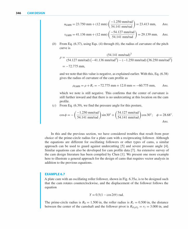
346 CAM DESIGN
ucam = 23.750 mm+ (12 mm)
(−1.250 mm/rad
54.141 mm/rad
)= 23.413 mm, Ans.
vcam = 41.136 mm+ (12 mm)
(−54.127 mm/rad
54.141 mm/rad
)= 29.139 mm. Ans.
(b) From Eq. (6.37), using Eqs. (4) through (6), the radius of curvature of the pitchcurve is
ρ = (54.141 mm/rad)3
(54.127 mm/rad)(−41.136 mm/rad2
)− (−1.250 mm/rad)(36.250 mm/rad2
)= −72.775 mm,
and we note that this value is negative, as explained earlier. With this, Eq. (6.38)gives the radius of curvature of the cam profile as
ρcam = ρ+Rr = −72.775 mm+ 12.0 mm= −60.775 mm, Ans.
which we note is still negative. This confirms that the center of curvature isstill further inward and that there is no undercutting at this location on the camprofile.
(c) From Eq. (6.39), we find the pressure angle for this posture,
cosφ = −(−1.250 mm/rad
54.141 mm/rad
)sin30◦ +
(54.127 mm/rad
54.141 mm/rad
)cos30◦; φ = 28.68◦.
Ans.
In this and the previous section, we have considered troubles that result from poorchoice of the prime-circle radius for a plate cam with a reciprocating follower. Althoughthe equations are different for oscillating followers or other types of cams, a similarapproach can be used to guard against undercutting [5] and severe pressure angle [4].Similar equations can also be developed for cam profile data [7]. An extensive survey ofthe cam design literature has been compiled by Chen [1]. We present one more examplehere to illustrate a general approach for the design of cams that requires vector analysis inaddition to the previous equations.
EXAMPLE 6.7
A plate cam with an oscillating roller follower, shown in Fig. 6.35a, is to be designed suchthat the cam rotates counterclockwise, and the displacement of the follower follows theequation
Y = 0.5(1− cos2Θ) rad.
The prime-circle radius is R0 = 1.500 in, the roller radius is Rr = 0.500 in, the distancebetween the center of the camshaft and the follower pivot is RO4O2 = r1 = 3.000 in, and
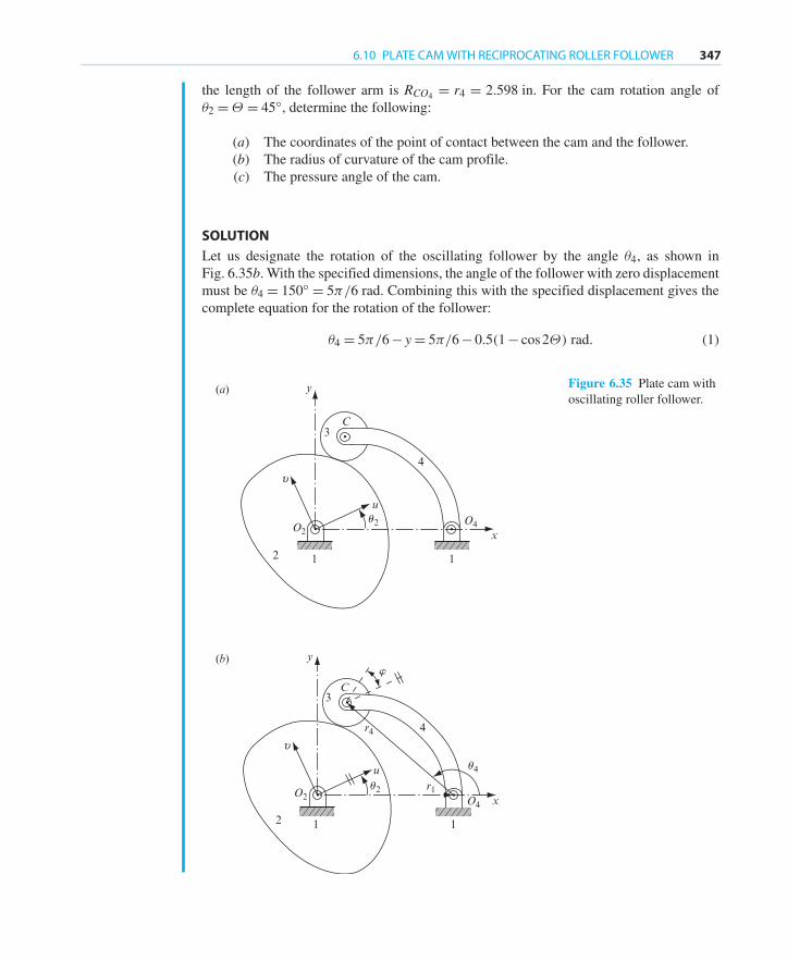
6.10 PLATE CAM WITH RECIPROCATING ROLLER FOLLOWER 347
the length of the follower arm is RCO4 = r4 = 2.598 in. For the cam rotation angle ofθ2 =Θ = 45◦, determine the following:
(a) The coordinates of the point of contact between the cam and the follower.(b) The radius of curvature of the cam profile.(c) The pressure angle of the cam.
SOLUTION
Let us designate the rotation of the oscillating follower by the angle θ4, as shown inFig. 6.35b. With the specified dimensions, the angle of the follower with zero displacementmust be θ4 = 150◦ = 5π/6 rad. Combining this with the specified displacement gives thecomplete equation for the rotation of the follower:
θ4 = 5π/6− y= 5π/6− 0.5(1− cos2Θ) rad. (1)
y
y
C
C
3
3
4
4
2 1 1
1 1
(a)
(b)
2
υ
υ
u
u
u2
u2
r4
r1
u4
w
O2
O2
O4x
O4 x
Figure 6.35 Plate cam withoscillating roller follower.
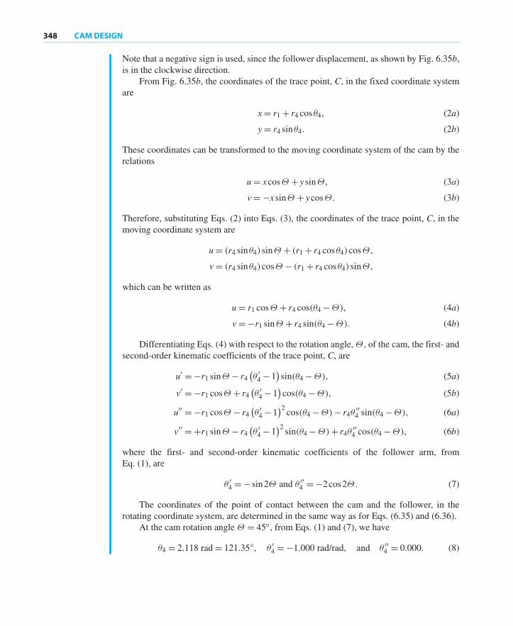
348 CAM DESIGN
Note that a negative sign is used, since the follower displacement, as shown by Fig. 6.35b,is in the clockwise direction.
From Fig. 6.35b, the coordinates of the trace point, C, in the fixed coordinate systemare
x= r1 + r4 cosθ4, (2a)
y= r4 sinθ4. (2b)
These coordinates can be transformed to the moving coordinate system of the cam by therelations
u= xcosΘ + ysinΘ , (3a)
v= −xsinΘ + ycosΘ . (3b)
Therefore, substituting Eqs. (2) into Eqs. (3), the coordinates of the trace point, C, in themoving coordinate system are
u= (r4 sinθ4)sinΘ + (r1 + r4 cosθ4)cosΘ ,
v= (r4 sinθ4)cosΘ − (r1 + r4 cosθ4)sinΘ ,
which can be written as
u= r1 cosΘ + r4 cos(θ4 −Θ), (4a)
v= −r1 sinΘ + r4 sin(θ4 −Θ). (4b)
Differentiating Eqs. (4) with respect to the rotation angle,Θ , of the cam, the first- andsecond-order kinematic coefficients of the trace point, C, are
u′ = −r1 sinΘ − r4(θ ′4 − 1
)sin(θ4 −Θ), (5a)
v′ = −r1 cosΘ + r4(θ ′4 − 1
)cos(θ4 −Θ), (5b)
u′′ = −r1 cosΘ − r4(θ ′4 − 1
)2 cos(θ4 −Θ)− r4θ′′4 sin(θ4 −Θ), (6a)
v′′ = +r1 sinΘ − r4(θ ′4 − 1
)2 sin(θ4 −Θ)+ r4θ′′4 cos(θ4 −Θ), (6b)
where the first- and second-order kinematic coefficients of the follower arm, fromEq. (1), are
θ ′4 = −sin2Θ and θ ′′4 = −2cos2Θ . (7)
The coordinates of the point of contact between the cam and the follower, in therotating coordinate system, are determined in the same way as for Eqs. (6.35) and (6.36).
At the cam rotation angle Θ = 45◦, from Eqs. (1) and (7), we have
θ4 = 2.118 rad= 121.35◦, θ ′4 = −1.000 rad/rad, and θ ′′4 = 0.000. (8)

6.10 PLATE CAM WITH RECIPROCATING ROLLER FOLLOWER 349
Substituting Eqs. (8) into Eqs. (4), the coordinates of the trace point, C, are
u= (3.000 in)cos45◦ + (2.598 in)cos(121.35◦ − 45◦)= 2.734 in, (9a)
v= −(3.000 in)sin45◦ + (2.598 in)sin(121.35◦ − 45◦)= 0.403 in. (9b)
Substituting Eqs. (8) and the given geometry into Eqs. (5), the first-order kinematiccoefficients of the trace point are
u′ = −(3.000 in)sin45◦ − (2.598 in)(−2.000)sin(121.35◦ − 45◦)= 2.928 in/rad, (10a)
v′ = −(3.000 in)cos45◦ + (2.598 in)(−2.000)cos(121.35◦ − 45◦)= −3.347 in/rad,(10b)
and from Eq. (6.35), we have
w′ = +√(2.928 in/rad)2 + (−3.347 in/rad)2 = 4.447 in/rad. (11)
(a) Then, substituting Eqs. (9) through (11) into Eqs. (6.36), the coordinates ofthe contact point between the cam and the follower in the rotating coordinatesystem are
ucam = (2.734 in)+ (0.5 in)(−3.347 in/rad
4.447 in/rad
)= 2.358 in, Ans.
vcam = (0.403 in)− (0.5 in)(2.928 in/rad
4.447 in/rad
)= 0.074 in. Ans.
(b) In the rotating coordinate system of the cam, the direction of motion of theroller center, C, is defined by angle φ (Fig. 6.35b), which can be written as
ϕ = θ4 − 90◦ − θ = 121.35◦ − 90◦ − 45◦ = −13.65◦. (12)
Therefore, from Eq. (6.39), the pressure angle of the cam can be written as
cosφ =(
− v′
w′
)cosϕ+
(u′
w′
)sinϕ.
Substituting Eqs. (10), (11), and (12) into this equation, the pressure angle (atthe cam rotation angle θ = 45◦) is
φ = 54.83◦. Ans.
(c) Substituting Eqs. (8) and the given geometry into Eqs. (6), the second-orderkinematic coefficients of the follower center are
u′′ = −(3.000 in)cos45◦ − (2.598 in)(−2.000)2 cos(121.35◦ − 45◦)
= −4.573 in/rad2, (13a)
v′′ = (3.000 in)sin45◦ − (2.598 in)(−2.000)2 sin(121.35◦ − 45◦)
= −7.977 in/rad2. (13b)
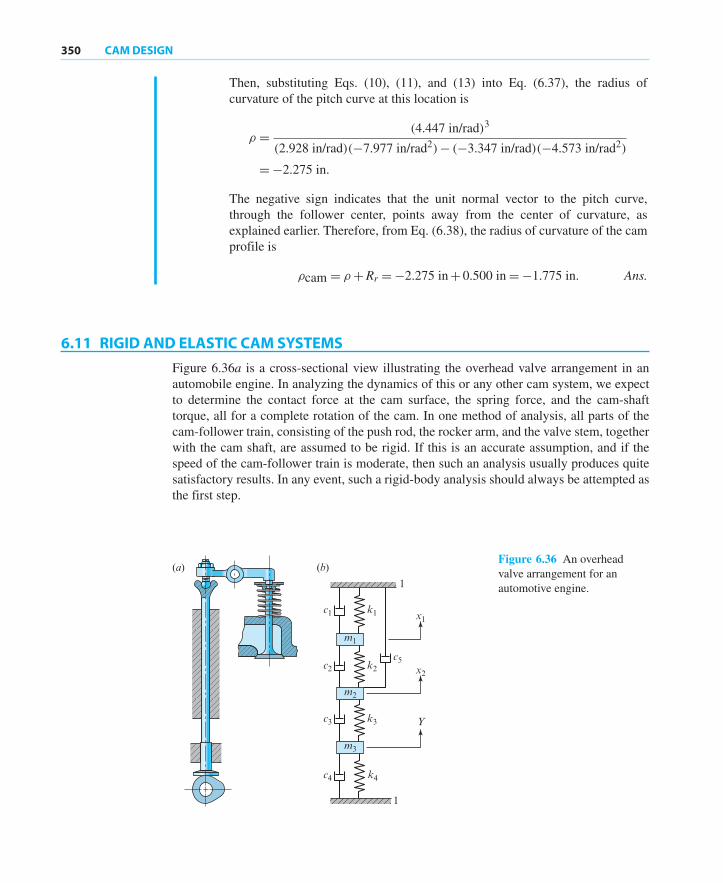
350 CAM DESIGN
Then, substituting Eqs. (10), (11), and (13) into Eq. (6.37), the radius ofcurvature of the pitch curve at this location is
ρ = (4.447 in/rad)3
(2.928 in/rad)(−7.977 in/rad2)− (−3.347 in/rad)(−4.573 in/rad2)
= −2.275 in.
The negative sign indicates that the unit normal vector to the pitch curve,through the follower center, points away from the center of curvature, asexplained earlier. Therefore, from Eq. (6.38), the radius of curvature of the camprofile is
ρcam = ρ+Rr = −2.275 in+ 0.500 in= −1.775 in. Ans.
6.11 RIGID AND ELASTIC CAM SYSTEMS
Figure 6.36a is a cross-sectional view illustrating the overhead valve arrangement in anautomobile engine. In analyzing the dynamics of this or any other cam system, we expectto determine the contact force at the cam surface, the spring force, and the cam-shafttorque, all for a complete rotation of the cam. In one method of analysis, all parts of thecam-follower train, consisting of the push rod, the rocker arm, and the valve stem, togetherwith the cam shaft, are assumed to be rigid. If this is an accurate assumption, and if thespeed of the cam-follower train is moderate, then such an analysis usually produces quitesatisfactory results. In any event, such a rigid-body analysis should always be attempted asthe first step.
(b)
m1
m2
m3
c4 k4
c3 k3
x2
x1
Y
c2c5k2
c1 k1
1
1
(a)Figure 6.36 An overheadvalve arrangement for anautomotive engine.