5–8 Dec 2017 | Kuala Lumpur, Malaysia ISSN: 2305-249X

5–8 Dec 2017 | Kuala Lumpur, Malaysia ISSN: 2305-249X

5-8 DEC 2017 MISTA 2017 PROCEEDINGS

MISTA 2017

Proceedings of the

8th Multidisciplinary International Conference on Scheduling: Theory and Applications

5 – 8 December 2017 Kuala Lumpur, Malaysia

Edited by Aldy Gunawan, Singapore Management University Graham Kendall, University of Nottingham, Malaysia and UK Lai Soon Lee, Universiti Putra Malaysia Barry McCollum, Queens University Belfast, UK Hsin-Vonn Seow, University of Nottingham Malaysia Campus

MISTA 2017 Conference Program Committee

Abdullah, Salwani (Universiti Kebangsaan Malaysia)

Artigues, Christian (LAAS-CNRS)

Ayob, Masri (University Kebangsaan Malaysia)

Bai, Ruibin (University of Nottingham Ningbo Campus)

Bartak, Roman (Charles University)

Berghman, Lotte (Toulouse Business School)

Blazewicz, Jacek (Poznan University of Technology)

Briand, Cyril (Universite Paul Sabatier)

Burke, Edmund (Queen Mary University of London)

Cai, Xiaoqiang (The Chinese University of Hong Kong )

Ceschia, Sara (University of Udine)

Chen, Zhi-Long (University of Maryland)

Chong, Siang Yew (University of Nottingham Malaysia Campus)

De Causmaecker, Patrick (KU Leuven)

Dell'Amico, Mauro (University of Modena and Reggio Emilia)

Drozdowski, Maciej (Poznan University of Technology)

Goossens, Dries (Ghent University)

Gunawan, Aldy (Singapore Management University) Hanzalek, Zdenek (Czech Technical University)

Hao, Jin-Kao (University of Angers)

Herrmann, Jeffrey (University of Maryland)

Hoogeveen, Han (Utrecht University)

Kendall, Graham (University of Nottingham Malaysia Campus)

Kingston, Jeffrey (University of Sydney)

Knust, Sigrid (University of Osnabrueck)

Kubiak, Wieslaw (Memorial University)

Kwan, Raymond (University of Leeds)

Lee, Lai Soon (Universiti Putra Malaysia)

Levner, Eugene (Ashkelon Academic College)

McCollum, Barry (Queens University Belfast)

McMullan, Paul (Queen's University)

Moench, Lars (University of Hagen )

Ozcan, Ender (University of Nottingham)

Pesch, Erwin (University of Siegen)

Petrovic, Sanja (University of Nottingham)

Pillay, Nelishia (University of KwaZulu-Natal)

Qu, Rong (University of Nottingham)

Ribeiro, Celso (Universidade Federal Fluminense)

Rossi, Andre (Université d'Angers)

Rudová, Hana (Masaryk University)

Sagir, Mujgan (Eskisehir Osmangazi University) Schaerf, Andrea (University of Udine)

Seow, Hsin-Veow (University of Nottingham Malaysia Campus)

Šucha, Premysl (Czech Technical University)

8th Multidisciplinary International Conference on Scheduling : Theory and Applications (MISTA 2017) 5-8 December 2017, Kuala Lumpur, Malaysia

- 1 -

Thompson, Jonathan (Cardiff University)

T'Kindt, Vincent (Laboratoire d'Informatique)

Trautmann, Norbert (University of Bern)

Trick, Michael (Carnegie Mellon University)

Trystram, Denis (Grenoble university)

Urrutia, Sebastián (Universidade Federal de Minas Gerais)

Vanden Berghe, Greet (KU Leuven)

Vansteenwegen, Pieter (KU Leuven)

Wauters, Tony (KU Leuven )

Yu, Vincent F. (National Taiwan University of Science and Technology)

Yugma, Claude (Ecole des Mines de Saint-Etienne)

Zimmermann, Jürgen (Clausthal University of Technology)

Zinder, Yakov (University of Technology)


- 2 -

MISTA 2015 International Advisory Committee

• Graham Kendall (chair) • Abdelhakim Artiba, Facultes Universitares Catholiques de Mons (CREGI - FUCAM),

Belguim • James Bean, University of Michigan, USA • Jacek Blazewicz, Institute of Computing Science, Poznan University of Technology,

Poland • Edmund Burke, The University of Nottingham, UK • Xiaoqiang Cai, The Chinese University of Hong Kong, Hong Kong • Ed Coffman, Columbia University, USA • Moshe Dror, The University of Arizona, USA • David Fogel, Natural Selection Inc., USA • Michel Gendreau, University of Montreal, Canada • Fred Glover, Leeds School of Business, University of Colorado, USA • Bernard Grabot, Laboratoire Génie de Production - ENIT, Tarbes, France • Toshihide Ibaraki, Kyoto University, Japan • Claude Le Pape, ILOG, France • Ibrahim Osman, American University of Beirut, Lebanon • Michael Pinedo, New York University, USA • Jean-Yves Potvin, Université de Montréal, Canada • Michael Trick, Graduate School of Industrial Administration, Carnegie Mellon

University, USA • Stephen Smith, Carnegie Mellon University, USA • Steef van de Velde, Erasmus University, Netherlands • George White, University of Ottawa, Canada • Gerhard Woeginger, University of Twente, Netherlands


- 3 -

Acknowledgements This conference would not have been possible without the assistance of a great many people. Any scientific conference is underpinned by the quality of the papers that it publishes. This is largely the responsibility of the Program Committee, who give up their time and expertise to assist us. MISTA is fortunate enough to have many of the world’s scheduling experts who help us by serving on the Program Committee. We are extremely grateful for the time and effort that they devote to making MISTA the success it is. The editors would also like to thank the international advisory committee for their continued help and advice as we seek to develop the MISTA series year-on-year. Their comments are always insightful and made in the best interests of the conference. We are grateful to the chairs of the special sessions on Routing Problems with Profits (Aldy Gunawan, Pieter Vansteenwegen and Hoong Chuin Lau) and Airline Crew & Fleet Scheduling (Per Sjögren and Björn Thalén) for taking the time to collect together an excellent set of papers. We really appreciate the time and effort you gave to the conference. We greatly appreciate the support that we have received from EventMap Ltd., which have supported the conference once again. We are also grateful to the University of Nottingham for their continued support of this conference series. We would also like to thank the Journal of the Operational Research Society by allowing us to guest edit a special issue of the journal which is associated with the conference. This certainly adds to the conference and the post-conference opportunities. Our sincere thanks must also go to a dedicated local team. Without their support, MISTA would not happen, and certainly not as smoothly as it would without their hard work. At the risk of missing people out, we would like to mention Anitapadmani Pathmathasan, Deepa Kumari Veerasingam and Mashael Elmasry who made our lives a lot easier than they can imagine. As in previous years, the conference owes a great deal to Debbie Pitchfork. She has worked tirelessly since performing similar tasks for MISTA 2009, 2011, 2013 and 2015. If it were not for Debbie this conference would not have taken place. Thank you, from all who are involved in MISTA 2017, whether as part of the organisational team, or the delegates.


- 4 -

Table of Contents Plenary Presentations

Blazewicz J. Multi-agent based approach for the origins of life hypothesis ............................. 9

Özcan E. A Review of Selection Hyper-heuristics: Recent Advances ...................................... 10

Lau H. C. Combining Machine Learning and Optimization for Real-World Scheduling Applications ......................................................................................................................... 11

Papers

Li H., Xu X. and Zhao Y. Customer Order Scheduling on Unrelated Parallel Machines to Minimize Total Weighted Completion Time ........................................................................ 13

Emeretlis A., Theodoridis G., Alefragis P. and Voros N. Exploration of Logic-Based Benders Decomposition Approach for Mapping Applications on Heterogeneous Multi-Core Platforms ............................................................................................................................. 30

Saw V., Rahman A. and Ong W. E. A Weight Assignment Approach for Solving Multicriteria Global Path Planning of Unmanned Combat Vehicles ....................................................... 43

Moll M., Pickl S., Raap M. and Zsifkovits M. Optimal Interdiction of Vehicle Routing on a Dynamic Network ................................................................................................................ 59

Srour A. and De Causmaecker P. Evolving Adaptive Evolutionary Algorithms ..................... 70

Zahout B., Soukhal A. and Martineau P. Fixed jobs scheduling on a single machine with renewable resources ............................................................................................................ 84

Liu Y. and Cao B. Improving Ant Colony Optimization algorithm with Levy Flight ............. 93

Ilagan I. F. A and Sy C. L. A Robust Crew Pairing Model for Airline Operations using Crew Swaps and Slack Times ..................................................................................................... 103

Smet P., Mosquera F., Toffolo T. A. M. and Vanden Berghe G. Integer programming for home care scheduling with flexible task frequency and controllable processing times.... 121

Nezami F. G., Heydar M. and Berretta R. Optimizing Production Schedule with Energy Consumption and Demand Charges in Parallel Machine Setting .................................... 133

Schulte J., Günther M. and Nissen V. Evolutionary Bilevel Approach for Integrated Long-Term Staffing and Scheduling ........................................................................................... 144

Oddi A., Rasconi R. and Gonzalez M. A. A constraint programming approach for the energy-efficient job shop scheduling problem .................................................................. 158

Oude Vrielink R., Jansen E., Gort E., van Hillegersberg J. and Hans E. Towards improving tenders for Higher Education timetabling software: Uncovering the selection criteria of HEIs when choosing timetabling applications, using ERP as a reference ....................... 173


- 5 -

Barták R., Švancara J. and Vlk M. Scheduling Models for Multi-Agent Path Finding ......... 189

Gomes F. R. A. and Mateus G. R. Mathematical Formulation for Minimizing Total Tardiness in a Scheduling Problem with Parallel Machines ............................................................. 201

Trung H. T., Dung P. Q., Demirovic E., Clement M. and Inoue K. Balanced clustering based decomposition applied to Master thesis defense timetabling problem ............................. 214

Gunawan A., Yu V. F., Redi A. A. N. P., Jewpanya P. and Lau H. C. A Selective-Discrete Particle Swarm Optimization Algorithm for Solving a Class of Orienteering Problems .. 229

Gunawan A., Lau H. C. and Lu K. Home Health Care Delivery Problem ........................... 244

Han K. and McMullan P. Hyper-heuristics using Reinforcement Learning for the Examination Timetabling Problem ................................................................................... 256

Wangsom P., Lavangnananda K. and Bouvry P. The Application of Nondominated Sorting Genetic Algorithm (NSGA-III) for Scientific-workflow Scheduling on Cloud .................. 269

Bai R., Xue N., Li X. and Cui T. Responsive Single Bus Corridor Scheduling Based on Machine Learning and Optimisation ................................................................................ 288

Vlk M., Barták R. and Hebrard E. Benders Decomposition in SMT for Rescheduling of Hierarchical Workflows .................................................................................................... 295

Abstracts

Leus R., Rostami S. and Creemers S. Optimal solutions for minimum-cost sequential system testing ................................................................................................................................ 312

Edwards S., Baatar D., Bowly S. and Smith-Miles K. Symmetry breaking in a special case of the RCPSP/max ................................................................................................................. 315

Jamaluddin N. F., Aizam N. A. H. and Aziz N. L. A. Mathematical model for a high quality examination timetabling problem: case study of a university in Malaysia ....................... 319

Aziz N. L. A., Aizam N. A. H. and Jamaluddin N. F. Variation of Demands for a New Improvised University Course Timetabling Problem Mathematical Model ..................... 320

Kwan R. S. K., Lin Z., Copado-Mendez P. J. and Lei L. Multi-commodity flow and station logistics resolution for train unit scheduling .................................................................... 321

Bulhões T., Sadykov R., Uchoa E. and Subramanian A. On the exact solution of a large class of parallel machine scheduling problems ......................................................................... 325

Gultekin H., Gurel S. and Akhlaghi V. E. Robotic Cell Scheduling Considering Energy Consumption of Robot Moves ........................................................................................... 329

Thanos E., Wauters T. and Vanden Berghe G. Scheduling container transportation through conflict-free trajectories in a warehouse layout: A local search approach ...................... 330

Tsuboi T., Nishi T., Tanimizu Y. and Kaihara T. An Integrated Optimization of Dynamic Product Family Configuration and Supply Chain Configuration ..................................... 336


- 6 -

Tamssaouet K., Dauzère-Pérès S., Yugma C. and Pinaton J. A Batch-oblivious Approach For Scheduling Complex Job-Shops with Batching Machines: From Non-delay to Active Scheduling ......................................................................................................................... 340

Cantais B., Jouglet A. and Savourey D. Three upper bounds for the speed meeting problem

.... ............................................................................................................................................ 344

Yang X. F., Ayob M. and Nazri M. Z. A. Modeling a Practical University Course Timetabling Problem with Reward and Penalty Objective Function: Case Study FTSM-UKM .................................................................................................................................. 348

Rocholl J. and Mönch L. Hybrid Heuristics for Multiple Orders per Job Scheduling Problems with Parallel Machines and a Common Due Date ........................................................... 358

Bach L., Kjenstad D. and Mannino C. The "Orchestrator" approach to multimodal continental trip planning. .................................................................................................. 362

Kiefer A., Schilde M. and Doerner K. E. Scheduling of maintenance tasks of a large-scale tram network ..................................................................................................................... 367

Fuchigami H. Y. A parametric priority rule for just-in-time scheduling problem with sequence-dependent setup times ....................................................................................... 370

Bach L. and Cuervo D. P. Railway Rolling Stock Maintenance ............................................ 373

Novak A., Sucha P. and Hanzalek Z. Efficient algorithms for non-preemptive mixed-criticality match-up scheduling problem .......................................................................... 377

Armellini D., Borzone P., Ceschia S., Di Gaspero L. and Schaerf A. Modeling and Solving the Steelmaking and Casting Planning and Scheduling Problem ..................................... 380

Liang Y-C., Gunawan A., Chen H-C. and Juarez J. R. C. Solving Tourist Trip Design Problems Using a Virus Optimization Algorithm ............................................................. 384

Homayouni S. M. and Fontes B. B. M. M. Integrated Scheduling of Machines, Vehicles, and Storage Tasks in Flexible Manufacturing Systems ........................................................... 389

Kheiri A., Daffalla A., Noureldien Y. and Özcan E. Selection Hyper-heuristics for Solving the Wind Farm Layout Optimisation Problem .................................................................. 393


- 7 -

Plenary Presentations


- 8 -

Jacek Blazewicz Multi-agent based approach for the origins of life hypothesis

Abstract

Multi-agent systems have been used extensively in scheduling, but the methodology has many other applications. One of those appears to be the analysis of the origins of life hypothesis. One of the most recognized hypotheses for the origins of life is the RNA world hypothesis. Laboratory experiments have been conducted to prove some assumptions of that hypothesis. However, despite some successes in the "wet-lab" experiments, we are still far from a complete explanation. Bioinformatics, supported by operations research and in particular by multi-agent approach, appears to provide perfect tools to model and test various scenarios of the origins of life where wet-lab experiments cannot reflect the true complexity of the problem. This paper illustrates some recent advancements in that area and points out possible directions for further research.


- 9 -

Ender Özcan A Review of Selection Hyper-heuristics: Recent Advances

Abstract

Hyper-heuristics emerged as general purpose optimisation methodologies that search the space of heuristics, rather than candidate solutions directly, for solving computationally difficult problems. The current state-of-the-art in hyper-heuristic development involves designing adaptive search methods that are applicable to instances with different characteristics not only from a single problem domain, but also across multiple domains. A key goal is enabling ‘plug-and-play’ search components, including data science techniques (e.g., machine learning and statistics) to be applied to optimisation without them having to be re-implemented for every problem domain. Selection hyper-heuristics separate the high level automated search control embedding learning heuristic selection and move acceptance methods from the low level problem domain details. In the last two decades, particularly after the cross-domain heuristic search challenge in 2011, there has been an extremely rapid growth in this area of research, leading to many highly-effective selection hyper-heuristics applied to various problem domains. As a means of achieving generality, the initially proposed interface between the selection hyper-heuristic and domain layers was extremely restrictive allowing no problem specific information flow. However, there is a current trend towards moving away from this type of interface to facilitate more expressive selection hyper-heuristics capable of operating in an information rich environment, whilst still maintaining domain independence of the search control. This talk provides a review of selection hyper-heuristics focusing on the recent advances in the field.


- 10 -

Hoong Chuin Lau Combining Machine Learning and Optimization for Real-World Scheduling Applications

Abstract

In this Big Data era, data can and should be exploited for more effective resource scheduling. In this talk, I will discuss a framework that combines data analytics, machine learning and optimization to solve real-world complex scheduling problems effectively. I will illustrate with three diverse scheduling problems ranging from crowd logistics to police officer scheduling to maritime traffic coordination, showing how spatial-temporal patterns can be learnt from data (both historical and real-time), and utilized to generate effective schedules.


- 11 -

Papers


- 12 -

MISTA 2017

Customer Order Scheduling on Unrelated Parallel

Machines to Minimize Total Weighted Completion Time

Haidong Li · Xiaoyun Xu · Yaping Zhao

Abstract This paper considers a customer order scheduling problem in unrelated

parallel machine environment. The objective is to minimize the total weighted com-

pletion time of orders. Several optimality properties of this problem are derived, and

a computable lower bound of the objective function is established. Due to the NP-

completeness of the problem, two heuristic algorithms are proposed. Theoretical analy-

sis shows that the worst-case performances of both algorithms are bounded. Numerical

studies are carried out to demonstrate the effectiveness of the lower bound and the

proposed heuristics.

1 Introduction

This paper considers a customer order scheduling problem on unrelated parallel ma-

chines to minimize total weighted completion time. To be specific, there are n order-

s J = 1, 2, ..., n with each one consisting of various different product types T =

1, 2, ..., t. The workload of product type k in order j is pjk,∀j ∈ J, ∀k ∈ T. The

release times of all orders are considered as 0 in this study, and order j has a positive

weight Wj ,∀j ∈ J. Consider a facility with m unrelated machines M = 1, 2, ..., m

in parallel. Each machine can produce all types of products, and the workload of each

product type can be split arbitrarily over all machines. The workload of each order can

be processed independently on each machine, and preemptions are allowed. Machine i

processes product type k at speed vik, ∀i ∈ M, ∀k ∈ T, which are predetermined and

heterogeneous across all the product type-machine pairs. The completion time of order

j, denoted as Cj , is the time when all product types of order j have been finished. The

Haidong LiDepartment of Industrial Engineering and Management, Peking University, Beijing, ChinaE-mail: [email protected]

Xiaoyun XuDepartment of Industrial Engineering and Management, Peking University, Beijing, ChinaE-mail: [email protected]

Yaping ZhaoDepartment of Industrial Engineering and Management, Peking University, Beijing, ChinaE-mail: [email protected]


- 13 -

objective is to schedule the orders on the machines so as to minimize total weighted

completion time∑

WjCj . According to the notation system introduced in [3], this

problem is represented as Rm|O|∑

WjCj , where “O” represents “order”.

In recent years, customer order scheduling problem has received an enormous

amount of attention in the literature. The concept of customer order scheduling is first

introduced by [7]. The authors consider a single machine problem with the objective

of minimizing the total completion time of orders, and provide a dynamic program-

ming algorithm for the problem with two product types and a given order processing

sequence. For single machine environment, variations of customer order scheduling

problems with different objectives have been well explored in the literature [10], [1],

[11], [4], [2], [12].

For parallel machine environment, Leung et al. [8] provide a thorough review on

customer order scheduling problem and classify the problem into three categories: 1)

the fully dedicated case, in which each machine can produce one and only one type

of product; 2) the fully flexible case, in which all the machines are identical and each

machine is capable of producing all the products; 3) the arbitrary case, in which all

the machines are unrelated and each machine is capable of producing all the products.

For dedicated parallel machine environment, there are several papers dealing with

customer order scheduling problem to minimize total weighted completion time. Sung

and Yoon [14] show that the problem of minimizing total weighted completion time

is NP-hard in the strong sense. They also show that the worst-case performance of

the weighted shortest processing time (WSPT) rule for permutation schedules is 2 for

the case of two machines. Wang and Cheng [15] establish three heuristics based on

WSPT rule and show that all of them have an m worst-case bound for the case of m

machines. Leung et al. [9] modify the SPTL and ECT heuristics by taking the weights

of orders into account and also provide the worst-case bound of these heuristics. For

unrelated parallel machine environment, much fewer related works have been found.

As concerns the unweighted cases, Yang [17] establishes the complexity of customer

order scheduling problem in the unrelated parallel machine environment. He prove

the NP-completeness of the problem with two machines to minimize total completion

time. Xu et al. [16] also consider the customer order scheduling problem to minimize

total completion time. They propose three heuristics and show that their worst-case

performances are bounded. To the knowledge of the authors, no additional result on

the problem in this paper has been reported in the literature.

This paper investigates the customer order scheduling problem on unrelated parallel

machines to minimize total weighted completion time of orders. In this study, the

scheduling problem is formulated as a Mixed Integer Programming (MIP). A non-

trivial lower bound on the objective is established, and two heuristic algorithms are

also proposed to solve this problem. The worst-case performance of each algorithm is

shown to be bounded. Numerical studies are conducted to demonstrate the performance

of the proposed heuristics under various application scenarios.

The remainder of this paper is organized as follows. Section 2.1 formulates the

problem Rm|O|∑

WjCj as a Mixed Integer Programming (MIP). In Section 2.2, a

lower bound on the objective function is established. In Section 3, two heuristics are

proposed to solve the problem and their worst-case performance bounds are also con-

structed. Section 4 presents the numerical study and demonstrates the effectiveness of

the proposed heuristics. Concluding remarks are given in Section 5.


- 14 -

2 Theoretical Study

2.1 Mathematical Programme for Rm|O|∑

WjCj

In this section, this paper formulates the problem Rm|O|∑

WjCj as a mathematical

programme. To facilitate the formulation, two optimality properties of the studied

problem are presented first in the following two lemmas.

Lemma 1 For Rm|O|∑

WjCj , in any optimal schedule, all machines must complete

all workloads simultaneously.

Proof The proof is inspired by the optimality analysis in [16]. By contradiction. Sup-

pose that there exists an optimal schedule such that m machines do not complete all

workloads simultaneously, and order j is the order with maximum completion time. A

feasible schedule can always be constructed by assigning part of the workload of order

j on the latest finishing machine to other machines so that the completion time of

order j is not increasing. Repeating this procedure till a better schedule is constructed

where all m machines complete all workloads simultaneously. A contradiction. ⊓⊔

Lemma 2 For Rm|O|∑

WjCj , there exists an optimal schedule in which all machines

process the customer orders in the same sequence and without preemptions.

Proof By contradiction. Suppose that there exists no optimal schedule such that all

machines process the customer orders in the same sequence and without preemptions.

Let machine i be the latest finishing machine in one optimal schedule πopt, i.e., all

other machines finish at the same time as or earlier than machine i. Let order j be the

order that finishes last on machine i. For each machine, move all workloads of order j

to finish last. This operation will not change the completion time of order j. However,

each of the order l 6= j finishes at the same time as or earlier than before. Then, delete

the last order and consider only the first (n− 1) orders.

By repeating the above operation, a new schedule π∗ is then constructed with the

objective function no worse than πopt, and all machines in π∗ process the customer

orders in the same sequence and without preemptions. A contradiction. ⊓⊔

To obtain the optimal schedule described in Lemma 2, three sets of decision vari-

ables are defined: (i) xij for i, j ∈ J: a binary variable that takes a value of 1 if order i

is processed before order j and takes a value of 0 otherwise; (ii) sjm for j ∈ J, m ∈ M:

a variable that represents the starting time of order j on machine m; (iii) ymtj for

m ∈ M, t ∈ T, j ∈ J: a variable that represents the portion of type t in order j pro-

cessed by machine m. In terms of these variables, a Mixed Integer Programming (MIP)

formulation of the problem is established as follows.


- 15 -

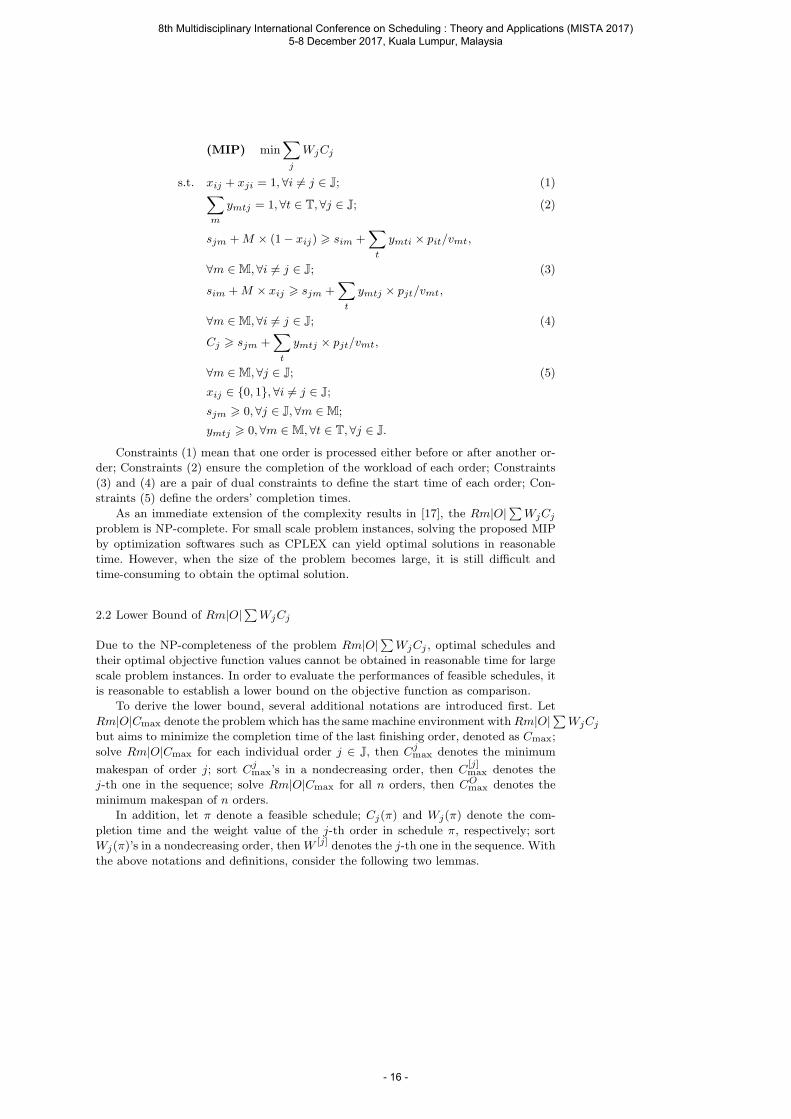
(MIP) min∑

j

WjCj

s.t. xij + xji = 1, ∀i 6= j ∈ J; (1)∑

m

ymtj = 1,∀t ∈ T,∀j ∈ J; (2)

sjm +M × (1− xij) > sim +∑

t

ymti × pit/vmt,

∀m ∈ M,∀i 6= j ∈ J; (3)

sim +M × xij > sjm +∑

t

ymtj × pjt/vmt,

∀m ∈ M,∀i 6= j ∈ J; (4)

Cj > sjm +∑

t

ymtj × pjt/vmt,

∀m ∈ M,∀j ∈ J; (5)

xij ∈ 0, 1, ∀i 6= j ∈ J;

sjm > 0,∀j ∈ J,∀m ∈ M;

ymtj > 0,∀m ∈ M,∀t ∈ T,∀j ∈ J.

Constraints (1) mean that one order is processed either before or after another or-

der; Constraints (2) ensure the completion of the workload of each order; Constraints

(3) and (4) are a pair of dual constraints to define the start time of each order; Con-

straints (5) define the orders’ completion times.

As an immediate extension of the complexity results in [17], the Rm|O|∑

WjCj

problem is NP-complete. For small scale problem instances, solving the proposed MIP

by optimization softwares such as CPLEX can yield optimal solutions in reasonable

time. However, when the size of the problem becomes large, it is still difficult and

time-consuming to obtain the optimal solution.

2.2 Lower Bound of Rm|O|∑

WjCj

Due to the NP-completeness of the problem Rm|O|∑

WjCj , optimal schedules and

their optimal objective function values cannot be obtained in reasonable time for large

scale problem instances. In order to evaluate the performances of feasible schedules, it

is reasonable to establish a lower bound on the objective function as comparison.

To derive the lower bound, several additional notations are introduced first. Let

Rm|O|Cmax denote the problem which has the same machine environment with Rm|O|∑

WjCj

but aims to minimize the completion time of the last finishing order, denoted as Cmax;

solve Rm|O|Cmax for each individual order j ∈ J, then Cjmax denotes the minimum

makespan of order j; sort Cjmax’s in a nondecreasing order, then C

[j]max denotes the

j-th one in the sequence; solve Rm|O|Cmax for all n orders, then COmax denotes the

minimum makespan of n orders.

In addition, let π denote a feasible schedule; Cj(π) and Wj(π) denote the com-

pletion time and the weight value of the j-th order in schedule π, respectively; sort

Wj(π)’s in a nondecreasing order, then W [j] denotes the j-th one in the sequence. With

the above notations and definitions, consider the following two lemmas.


- 16 -

Lemma 3 For any optimal schedule πopt of Rm|O|∑

WjCj , the following two in-

equalities must hold:

Cn−j(πopt) > Cn(π

opt)−

n∑

k=n−j+1

C[k]max,

∀j ∈ 1, 2, . . . , n− 1; (6)

Cj(πopt) > C

[j]max,∀j ∈ 1, 2, . . . , n. (7)

Proof The detailed proof can be referred to Theorem 2 and Theorem 3 in [16]. ⊓⊔

Lemma 4 (Rearrangement Inequality from [5]) Suppose that x1 6 x2 6 . . . 6

xn, y1 6 y2 6 . . . 6 yn and z1, z2, . . . , zn is any rearrangement of y1, y2, . . . , yn. Then

x1yn + x2yn−1 + . . .+ xny1 6 x1z1 + x2z2 + . . .+ xnzn

6 x1y1 + x2y2 + . . .+ xnyn.

According to Lemma 3 and Lemma 4, a lower bound of the optimal objective

function value is shown in the following theorem.

Theorem 1 Problem Rm|O|∑

WjCj has the following lower bound

LB =

n−1∑

j=1

W [n−j+1] ×max

COmax −

n∑

k=j+1

C[k]max, C

[j]max

+W [1]COmax

6 OBJ(πopt),

where OBJ(πopt) =∑n

j=1 Wj(πopt)Cj(π

opt).

Proof It is obvious that for any optimal schedule πopt, Cn(πopt) > CO

max. Therefore,

according to Lemma 3, it can be obtained that

OBJ(πopt) >

n−1∑

j=1

Wj(πopt)×max

COmax −

n∑

k=j+1

C[k]max, C

[j]max

+Wn(πopt)CO

max.

Let aj = max

COmax −

∑nk=j+1 C

[k]max, C

[j]max

,∀j ∈ 1, 2, . . . , n − 1 and an =

COmax. It will be shown through Case #1 to Case #3 that the sequence aj

nj=1 is

nondecreasing.

Case #1: Suppose that

COmax −

n∑

k=j+1

C[k]max > C

[j]max,∀j ∈ 1, 2, . . . , n− 1.

Then

aj = COmax −

n∑

k=j+1

C[k]max,∀j ∈ 1, 2, . . . , n− 1.

It is obvious that the sequence ajn−1j=1 is nondecreasing.


- 17 -

Case #2: Suppose that

COmax −

n∑

k=j+1

C[k]max < C

[j]max,∀j ∈ 1, 2, . . . , n− 1.

Then

aj = C[j]max,∀j ∈ 1, 2, . . . , n− 1.

It is obvious that the sequence ajn−1j=1 is nondecreasing.

Case #3: There exists an adjacent number pair (i, i+ 1) such that

COmax −

n∑

k=i+1

C[k]max < C

[i]max

and

COmax −

n∑

k=i+2

C[k]max > C

[i+1]max .

Then,n∑

k=i+1

C[k]max 6 CO

max <

n∑

k=i

C[k]max.

Thus, for j ∈ 1, 2, . . . , i, aj = C[j]max, and the sequence aj

ij=1 is nondecreasing; for

j ∈ i+ 1, i+ 2, . . . , n− 1, aj = COmax −

∑nk=j+1 C

[k]max, and the sequence aj

n−1j=i+1

is nondecreasing. Moreover, it is obvious that

ai = C[i]max 6 C

[i+1]max 6 CO

max −

n∑

k=i+2

C[k]max = ai+1.

Therefore, the sequence ajn−1j=1 is nondecreasing.

Concluded from the discussion of the above three cases, the sequence ajn−1j=1 is

nondecreasing. In addition, it is trivial to show that

an = COmax > max

COmax − C

[n]max, C

[n−1]max

= an−1.

Therefore, the sequence ajnj=1 is nondecreasing.

Replacing xj and yj in Lemma 4 with W [j] and aj , respectively, Lemma 4 suggests

thatn∑

j=1

Wj(πopt)aj >

n∑

j=1

W [n−j+1]aj .

Therefore,

OBJ(πopt) >

n∑

j=1

Wj(πopt)aj >

n∑

j=1

W [n−j+1]aj = LB.

⊓⊔

The tightness of the above lower bound is of great concern in both theoretical and

computational studies. In order to demonstrate the tightness of LB, in the following

corollary, it is shown that LB equals global optimum under certain mild conditions.


- 18 -

Corollary 1 When the machine environment is identical (Pm) or uniform (Qm),

LB = OBJ(πopt) if (Cimax − Cj

max)(Wi −Wj) < 0, ∀i, j ∈ J.

Proof The proof is an immediate consequence of Theorem 1 and thus omitted for

brevity. ⊓⊔

3 Heuristics for Rm|O|∑

WjCj

For small scale problem instances, solving the MIP in Section 2.1 can yield the optimal

solution in reasonable time. When the size of the problem becomes large, obtaining the

optimal solution could be very time-consuming. As alternative methods, two heuristics

for Rm|O|∑

WjCj are proposed to solve the problem. The designs of both heuristics

are based on insights from the optimality properties shown in the previous section, and

both of them can be implemented quite easily.

3.1 Heuristic H1

The first heuristic, named H1, is a constructive method. The design of this heuristic

is inspired by Corollary 1. To be specific, in order to solve the studied problem with

a total of n orders, heuristic H1 first proceeds by solving n subproblems individual-

ly, each with a single order. In each subproblem, H1 minimizes the completion time

of that particular order, that is, solves Rm|O|Cmax with a single order. It is trivial

to show that the starting and ending times on all machines are identical in each of

n subproblems, resulting in forming n individual “processing blocks”. These block-

s are then reassembled together according to the Weighted-Shortest-Processing-Time

(WSPT) rule as if they were individual jobs. Formally, heuristic H1 is described as

follows.

1. Solve subproblem Rm|O|Cmax optimally for each single order j individually. Obtain

πjsub

’s and their corresponding Cjmax, ∀j ∈ J. Here πj

subis the processing block of

order j with identical starting and finishing time on all machines.

2. Sort n orders according to the WSPT rule based on values of weight Wj and Cjmax.

3. Construct a nondelayed feasible schedule π by combining all processing blocks

πjsub

, ∀j ∈ J in the WSPT sequence.

It is clear that heuristic H1 is optimal when the parallel machine environment

is identical (Pm) or uniform (Qm). For the arbitrary case where all machines are

unrelated (Rm), heuristic H1 has the following worst-case performance bound:

Theorem 2 For Rm|O|∑

WjCj , the worst-case performance bound for heuristic H1

is

OBJ(πH1)

OBJ(πopt)6

(∑n

j=1 jW[j])× (

∑nj=1 C

[j]max)

n×∑n

j=1 W[n−j+1]C

[j]max

,

where OBJ(πH1) denotes the objective function value of H1.

Proof See Appendix. ⊓⊔


- 19 -

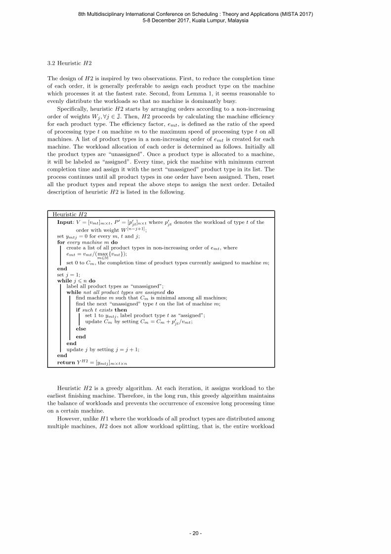
3.2 Heuristic H2

The design of H2 is inspired by two observations. First, to reduce the completion time

of each order, it is generally preferable to assign each product type on the machine

which processes it at the fastest rate. Second, from Lemma 1, it seems reasonable to

evenly distribute the workloads so that no machine is dominantly busy.

Specifically, heuristic H2 starts by arranging orders according to a non-increasing

order of weights Wj ,∀j ∈ J. Then, H2 proceeds by calculating the machine efficiency

for each product type. The efficiency factor, emt, is defined as the ratio of the speed

of processing type t on machine m to the maximum speed of processing type t on all

machines. A list of product types in a non-increasing order of emt is created for each

machine. The workload allocation of each order is determined as follows. Initially all

the product types are “unassigned”. Once a product type is allocated to a machine,

it will be labeled as “assigned”. Every time, pick the machine with minimum current

completion time and assign it with the next “unassigned” product type in its list. The

process continues until all product types in one order have been assigned. Then, reset

all the product types and repeat the above steps to assign the next order. Detailed

description of heuristic H2 is listed in the following.

Heuristic H2

Input: V = [vmt]m×t, P ′ = [p′jt]n×t where p′jt denotes the workload of type t of the

order with weight W [n−j+1];set ymtj = 0 for every m, t and j;for every machine m do

create a list of all product types in non-increasing order of emt, whereemt = vmt/(max

m∈M

vmt);

set 0 to Cm, the completion time of product types currently assigned to machine m;end

set j = 1;while j 6 n do

label all product types as “unassigned”;while not all product types are assigned do

find machine m such that Cm is minimal among all machines;find the next “unassigned” type t on the list of machine m;if such t exists then

set 1 to ymtj , label product type t as “assigned”;update Cm by setting Cm = Cm + p′jt/vmt;

else

end

end

update j by setting j = j + 1;end

return Y H2 = [ymtj ]m×t×n

Heuristic H2 is a greedy algorithm. At each iteration, it assigns workload to the

earliest finishing machine. Therefore, in the long run, this greedy algorithm maintains

the balance of workloads and prevents the occurrence of excessive long processing time

on a certain machine.

However, unlike H1 where the workloads of all product types are distributed among

multiple machines, H2 does not allow workload splitting, that is, the entire workload


- 20 -

of each product type will be processed by one machine only. The “non-splitting work-

load” feature in heuristic H2 is very desirable in many manufacturing practices. For

example, in textile industry where products are not allowed to be separated, heuristic

H2 becomes the only heuristic proposed in this study that is feasible to apply.

Although no workload splitting is allowed in H2, the performance of heuristic H2

is still bounded, as shown by the following theorem.

Theorem 3 For Rm|O|∑

WjCj , the worst-case performance bound for heuristic H2

is

OBJ(πH2)

OBJ(πopt)6

∑nj=1 Wj(π

H2)× [(∑j−1

k=1Tmax

k )m + Tmax

j ]

LB,

where OBJ(πH2) denotes the objective function value of H2, LB is obtained from

Theorem 1 and Tmaxj is the sum of the largest processing time of each product type in

the j-th order.

Proof See Appendix. ⊓⊔

4 Computational Experiment

4.1 Experiment Design

This experimental study aims to examine the quality of the lower bound as well as the

performance of the two proposed heuristics. The scale of testing instances generated

in this computational study is listed as follows:

– Number of machines m = 5, 20.

– Number of orders n = 5, 10, 50.

– Number of product types t = 50, 100.

To simulate the unrelated machine environment, all the machines can process any

product type and speed vik ’s are randomly generated from the uniform distribution

[40, 60]. Furthermore, order weight Wj ’s are randomly generated from the normal

distribution N(µ = 5, σ = 1) and take the absolute values.

To evaluate the impact of workload variability on the heuristic performances, the

following two scenarios are considered:

– Relatively Uniform Workload (RUW): The workload of each product type in

every order is randomly generated from the uniform distribution U [400, 600]. The

coefficient of variation (CV, the standard deviation divided by the mean) equals

approximately 0.1 under such circumstances, and this setting represents the case

when workloads of all orders are relatively uniform.

– Highly Variant Workload (HVW): The workload of each product type in every

order is randomly generated from the uniform distribution U [1, 1000]. CV under

such circumstances equals approximately 0.6, which, as stated in [6], indicates that

there exists high variability in workloads. This setting represents the cases when

workloads are highly variant among different orders.

There are |m|×|n|×|t| = 2×3×2 = 12 cases tested under each of the two scenarios

listed above, and 5 independent replicates are randomly generated for each individual


- 21 -

case. Therefore, a total of 2× 3× 2× 2× 5 = 120 replicates need to be constructed in

the entire computational experiment.

The performance of the proposed heuristic algorithms is evaluated using the fol-

lowing two criteria:

-Performance gap

Since the problem Rm|O|∑

WjCj is NP-complete, it could be computationally

challenging to obtain the optimal solution for large scale problem instances. However,

since the calculation of the proposed LB mainly requires solving a linear programming,

LB can be obtained within polynomial time and used to evaluate the performance of

each heuristic algorithm. Therefore, the heuristic performance is gauged with reference

to the lower bound as follows:

Performance Gap (%) =OBJ(πH)− LB

LB× 100%,

where OBJ(πH) denotes the objective function value of heuristic.

-Computational Time

The running time of heuristic is recorded in CPU seconds (sec) to measure compu-

tational efficiency.

The simulation is coded using Matlab, and runs on a desktop computer with

3.40GHz CPU and 8G memory.

4.2 Experiment Results and Analysis

4.2.1 Analysis of Lower Bound Performance

As lower bound is involved in the calculation of performance gaps of heuristics, in

order to provide convincing perspective, it is helpful to elaborate the efficiency of the

proposed lower bound. The efficiency is measured by the gap between lower bound and

optimal solution, which is shown in Table 1.

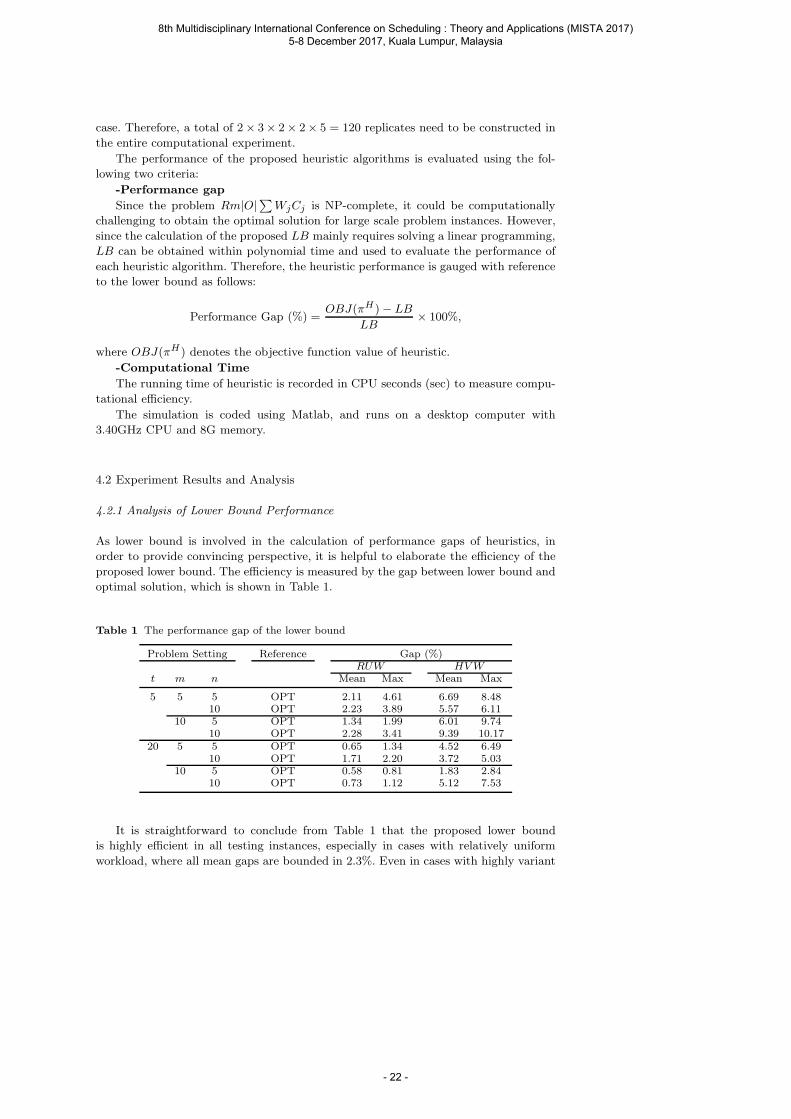
Table 1 The performance gap of the lower bound

Problem Setting Reference Gap (%)RUW HVW

t m n Mean Max Mean Max

5 5 5 OPT 2.11 4.61 6.69 8.4810 OPT 2.23 3.89 5.57 6.11

10 5 OPT 1.34 1.99 6.01 9.7410 OPT 2.28 3.41 9.39 10.17

20 5 5 OPT 0.65 1.34 4.52 6.4910 OPT 1.71 2.20 3.72 5.03

10 5 OPT 0.58 0.81 1.83 2.8410 OPT 0.73 1.12 5.12 7.53

It is straightforward to conclude from Table 1 that the proposed lower bound

is highly efficient in all testing instances, especially in cases with relatively uniform

workload, where all mean gaps are bounded in 2.3%. Even in cases with highly variant


- 22 -

workload, the mean gaps are still bounded in 10%. This phenomenon also demonstrates

the slight influence that workload variance causes on lower bound performance.

Problem scale can also affect the efficiency of the lower bound. Given that the

numbers of machines (m) and orders (n) are fixed, the mean gaps decrease as the

number of product types (t) grows under all the testing scenarios. For example, for the

case m = 5, n = 5 with relatively uniform workload, the mean gap plunges from around

2.11% to no more than 0.65%, when the product type number (t) increases from 5 to

20. This phenomenon can be heuristically interpreted as the “balance effect” of product

types, which means a large number of product types will erode the heterogeneity of

machines. This characteristic inspires more confidence in taking the lower bound as

reference to evaluate the two heuristics when the target problem involves a large number

of product types.

The maximum gaps shown in Table 1 provide an additional insight. In each problem

scale, consider the 5 replications of every testing scenario as a group. It can be observed

that the absolute difference between the mean and maximum gaps is bounded in 3.73%.

This observation suggests the performance of the lower bound is stable within group.

Furthermore, under the same problem scale, the absolute difference between the mean

and maximum gaps has no significant variance across two different scenarios (RUW

and HVW). This shows that the performance of the proposed lower bound is robust

over all scenarios considered.

4.2.2 Analysis of Heuristic Performance

The efficiency of heuristic is measured by both of the performance gap with lower

bound and the computational time. The proposed heuristics are investigated in 2 testing

scenarios under 12 problem settings. Results of two scenarios are reported in Table 2

and Table 3, respectively. The best dispatching method between heuristics H1 and H2

has also been demonstrated in column “minH1,H2” of Table 2 and Table 3.

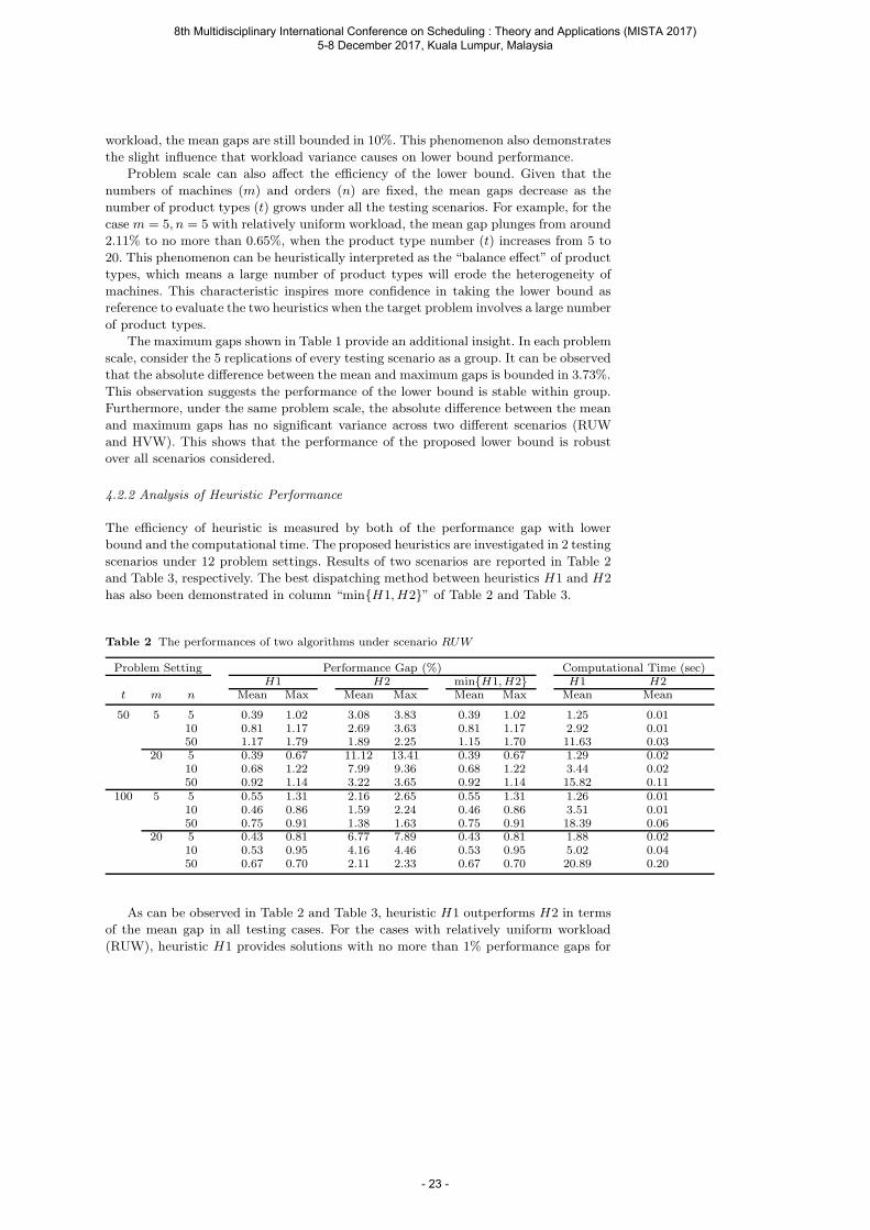
Table 2 The performances of two algorithms under scenario RUW

Problem Setting Performance Gap (%) Computational Time (sec)H1 H2 minH1, H2 H1 H2

t m n Mean Max Mean Max Mean Max Mean Mean

50 5 5 0.39 1.02 3.08 3.83 0.39 1.02 1.25 0.0110 0.81 1.17 2.69 3.63 0.81 1.17 2.92 0.0150 1.17 1.79 1.89 2.25 1.15 1.70 11.63 0.03

20 5 0.39 0.67 11.12 13.41 0.39 0.67 1.29 0.0210 0.68 1.22 7.99 9.36 0.68 1.22 3.44 0.0250 0.92 1.14 3.22 3.65 0.92 1.14 15.82 0.11

100 5 5 0.55 1.31 2.16 2.65 0.55 1.31 1.26 0.0110 0.46 0.86 1.59 2.24 0.46 0.86 3.51 0.0150 0.75 0.91 1.38 1.63 0.75 0.91 18.39 0.06

20 5 0.43 0.81 6.77 7.89 0.43 0.81 1.88 0.0210 0.53 0.95 4.16 4.46 0.53 0.95 5.02 0.0450 0.67 0.70 2.11 2.33 0.67 0.70 20.89 0.20

As can be observed in Table 2 and Table 3, heuristic H1 outperforms H2 in terms

of the mean gap in all testing cases. For the cases with relatively uniform workload

(RUW), heuristic H1 provides solutions with no more than 1% performance gaps for


- 23 -

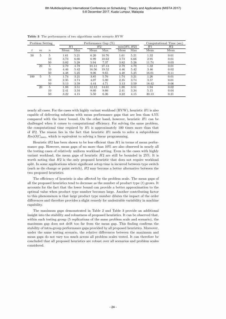
Table 3 The performances of two algorithms under scenario HVW

Problem Setting Performance Gap (%) Computational Time (sec)H1 H2 minH1, H2 H1 H2

t m n Mean Max Mean Max Mean Max Mean Mean

50 5 5 1.61 5.21 6.20 10.76 1.61 5.21 1.32 0.0110 3.73 6.66 6.99 10.62 3.73 6.66 2.95 0.0150 3.82 5.28 5.94 7.37 3.82 5.28 11.74 0.03

20 5 2.79 4.79 24.14 27.13 2.79 4.79 1.32 0.0110 4.46 5.42 16.56 19.52 4.46 5.42 3.46 0.0250 4.48 5.25 9.06 9.65 4.48 5.25 16.01 0.11

100 5 5 1.74 3.21 3.85 5.76 1.74 3.21 1.26 0.0110 2.35 3.74 4.07 5.90 2.35 3.74 3.57 0.0150 3.13 3.59 4.44 4.71 3.13 3.59 18.42 0.06

20 5 1.88 3.51 12.12 14.61 1.88 3.51 1.94 0.0210 2.41 3.34 8.60 9.66 2.41 3.34 5.15 0.0450 3.22 4.15 5.50 6.36 3.22 4.15 30.13 0.21

nearly all cases. For the cases with highly variant workload (HVW), heuristic H1 is also

capable of delivering solutions with mean performance gaps that are less than 4.5%

compared with the lower bound. On the other hand, however, heuristic H1 can be

challenged when it comes to computational efficiency. For solving the same problem,

the computational time required by H1 is approximately 100 times more than that

of H2. The reason lies in the fact that heuristic H1 needs to solve n subproblems

Rm|O|Cmax, which is equivalent to solving a linear programming.

Heuristic H2 has been shown to be less efficient than H1 in terms of mean perfor-

mance gap. However, mean gaps of no more than 10% are also observed in nearly all

the testing cases of relatively uniform workload setting. Even in the cases with highly

variant workload, the mean gaps of heuristic H2 are still be bounded in 25%. It is

worth noting that H2 is the only proposed heuristic that does not require workload

split. In some applications where significant setup time is incurred between type switch

(such as die change or paint switch), H2 may become a better alternative between the

two proposed heuristics.

The efficiency of heuristic is also affected by the problem scale. The mean gaps of

all the proposed heuristics tend to decrease as the number of product type (t) grows. It

accounts for the fact that the lower bound can provide a better approximation to the

optimal value when product type number becomes large. Another contributing factor

to this phenomenon is that large product type number dilutes the impact of the order

differences and therefore provides a slight remedy for undesirable variability in machine

capability.

The maximum gaps demonstrated in Table 2 and Table 3 provide an additional

insight into the stability and robustness of proposed heuristics. It can be observed that,

within each testing group (5 replications of the same problem scale and scenario), the

maximum gap does not drift too far from the mean gap. This finding confirms the

stability of intra-group performance gaps provided by all proposed heuristics. Moreover,

under the same testing scenario, the relative differences between the maximum and

mean gaps do not vary too much across all problem scales tested. It can therefore be

concluded that all proposed heuristics are robust over all scenarios and problem scales

considered.


- 24 -

5 Conclusion

This study addresses a customer order scheduling problem in unrelated parallel machine

environment. The objective is to minimize the total weighted completion time of all

customer orders. In this study, several important optimality properties of the studied

problem have been derived. Based on these properties, a computable lower bound of

the objective function has been established. Numerical studies suggest that this lower

bound provides a good approximation to the optimal value and performs even better

as the number of product types grows.

Two heuristics are also proposed to solve the customer order scheduling problem.

Numerical studies provide additional insights into the heuristic performance under

various scenarios and problem settings. Both heuristic H1 and H2 can be implemented

quite easily. Heuristic H1 behaves quite well and outperforms heuristic H2 in terms of

the performance gap in most cases. Heuristic H2 shows its advantage in applications

where significant penalty is incurred between type switch. In addition, the performance

of both heuristics improves as the number of product type grows.

Further research on this topic may involve some other important criteria to evaluate

the quick responsiveness of industries. Another possible generalization, which is of

interest during recent years, would be taking setup time between product type exchange

and resource constraints into consideration. The problem considered in this study can

also be extended to more complex production environments, such as flow-shop, job-

shop and so forth.

6 APPENDIX

6.1 Proof of Theorem 2

Proof It is obvious that

maxCOmax −

n∑

k=j+1

C[k]max, C

[j]max > C

[j]max,

∀j ∈ 1, 2, . . . , n− 1, and COmax > C

[n]max. Thus, a lower bound for LB can be obtained

that

LB >

n∑

j=1

W [n−j+1]C[j]max. (8)

Consider the 1||∑

WjCj problem where the job size pj = C[j]max, j ∈ 1, 2, . . . , n.

It is known from [13] that applying the WSPT rule can obtain the optimal solution

to 1||∑

WjCj problem. Therefore, among all possible sequences of pj = C[j]max, j ∈

1, 2, . . . , n, the summation of weighted completion time of the sequence according to

WSPT rule is minimum.


- 25 -

Consider the following n sequences of C[j]max’s:

Sequence#1 : C[1]max → C

[2]max → · · · → C

[n−1]max → C

[n]max;

Sequence#2 : C[2]max → C

[3]max → · · · → C

[n]max → C

[1]max;

...

Sequence#n : C[n]max → C

[1]max → · · · → C

[n−2]max → C

[n−1]max .

Let V [j] denote the weight value corresponding to the job size pj = C[j]max. Con-

sider the summation of weighted completion time of the Sequence #1, the WSPT rule

guarantees that:

OBJ(πH1) 6

n∑

j=1

(V [j] ×

j∑

i=1

C[i]max).

From Lemma 4, an upper bound for the summation of weighted completion time

of the Sequence #1 can be obtained as:

n∑

j=1

(V [j] ×

j∑

i=1

C[i]max) 6

n∑

j=1

(W [j] ×

j∑

i=1

C[i]max).

Therefore,

OBJ(πH1) 6

n∑

j=1

(W [j] ×

j∑

i=1

C[i]max).

In order to express other sequences expediently, it is necessary to extend the defi-

nition of C[i]max such that

C[i]max = C

[i−n]max ,∀i ∈ n+ 1, n+ 2, . . . , n+ n− 1.

In the same way, n inequalities can be obtained:

OBJ(πH1) 6

n∑

j=1

(W [j] ×

j∑

i=1

C[i]max);

OBJ(πH1) 6

n∑

j=1

(W [j] ×

j+1∑

i=2

C[i]max);

...

OBJ(πH1) 6

n∑

j=1

(W [j] ×

j+n−1∑

i=n

C[i]max).

Summing the above inequalities, one can obtain that:

n×OBJ(πH1) 6 (

n∑

j=1

jW [j])× (

n∑

j=1

C[j]max).


- 26 -

Therefore,

OBJ(πH1) 61

n(

n∑

j=1

jW [j])× (

n∑

j=1

C[j]max).

The worst-case performance bound for heuristic H1 can be obtained that

OBJ(πH1)

OBJ(πopt)6

(∑n

j=1 jW[j])× (

∑nj=1 C

[j]max)

n× LB

=(∑n

j=1 jW[j])× (

∑nj=1 C

[j]max)

n×∑n

j=1 W[n−j+1]C

[j]max

.

6.2 Proof of Theorem 3

Proof Let Cij denote the completion time of the first j orders on machine i. Moreover,

let

Cminj = min

i∈M

Cij, j ∈ 1, 2, . . . , n.

The following proof proceeds in two steps.

First, it is shown that

Cj(πH2) 6 Cmin

j−1 + Tmaxj , j ∈ 1, 2, . . . , n.

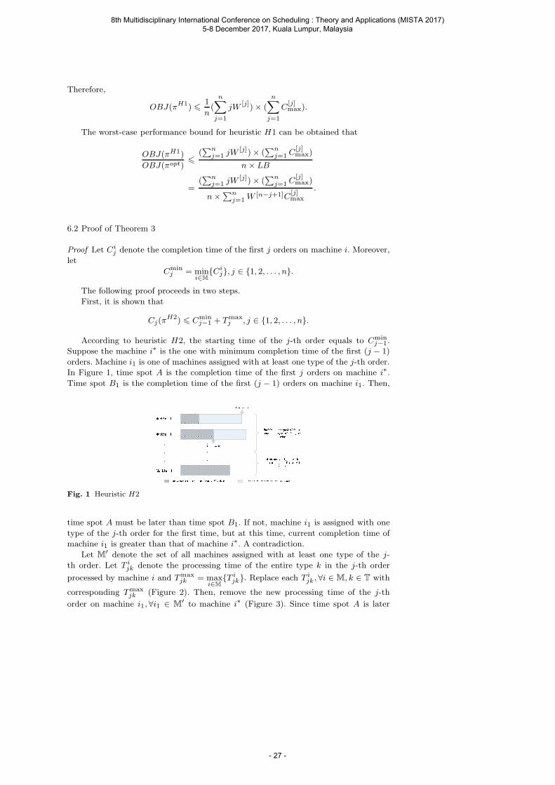
According to heuristic H2, the starting time of the j-th order equals to Cminj−1.

Suppose the machine i∗ is the one with minimum completion time of the first (j − 1)

orders. Machine i1 is one of machines assigned with at least one type of the j-th order.

In Figure 1, time spot A is the completion time of the first j orders on machine i∗.

Time spot B1 is the completion time of the first (j − 1) orders on machine i1. Then,

Fig. 1 Heuristic H2

time spot A must be later than time spot B1. If not, machine i1 is assigned with one

type of the j-th order for the first time, but at this time, current completion time of

machine i1 is greater than that of machine i∗. A contradiction.

Let M′ denote the set of all machines assigned with at least one type of the j-

th order. Let T ijk denote the processing time of the entire type k in the j-th order

processed by machine i and Tmaxjk = max

i∈M

T ijk. Replace each T i

jk ,∀i ∈ M, k ∈ T with

corresponding Tmaxjk (Figure 2). Then, remove the new processing time of the j-th

order on machine i1,∀i1 ∈ M′ to machine i∗ (Figure 3). Since time spot A is later


- 27 -

Fig. 2 Replace each T ijk

with corresponding Tmaxjk

Fig. 3 Remove the new processing time of the j-th order

than time spot B1, it is trivial to show that the new completion time of the first j

orders on machine i∗ is greater than Ci1j ,∀i1 ∈ M

′. Since Cj(πH2) = max

i∈M′

Cij, the

new completion time of the first j orders on machine i∗ is greater than Cj(πH2).

Therefore,

Cj(πH2) 6 Cmin

j−1 +

t∑

k=1

Tmaxjk

= Cminj−1 + Tmax

j , j ∈ 1, 2, . . . , n.

Second, it is shown that

Cminj 6

1

m

j∑

k=1

Tmaxk , j ∈ 1, 2, . . . , n.

Since Cminj = min

i∈M

Cij, it is obvious that

m× Cminj 6

m∑

i=1

Cij .

Moreover,m∑

i=1

Cij 6

j∑

n=1

t∑

k=1

Tmaxnk =

j∑

k=1

Tmaxk .

Therefore,

Cminj 6

1

m

j∑

k=1

Tmaxk , j ∈ 1, 2, . . . , n.


- 28 -

From the above two steps, one can obtain the following upper bound for Cj(πH2):

Cj(πH2) 6 (

1

m

j−1∑

k=1

Tmaxk ) + Tmax

j , j ∈ 1, 2, . . . , n.

Therefore,

OBJ(πH2) 6

n∑

j=1

Wj(πH2)× [(

1

m

j−1∑

k=1

Tmaxk ) + Tmax

j ].

References

1. Bagchi, U., Julien, F.M., Magazine, M.J.: Note: Due-date assignment to multi-job customerorders. Management Science 40(10), 1389–1392 (1994)

2. Gerodimos, A.E., Glass, C.A., Potts, C.N., Tautenhahn, T.: Scheduling multi-operationjobs on a single machine. Annals of Operations Research 92, 87–105 (1999)

3. Graham, R.L., Lawler, E.L., Lenstra, J.K., Kan, A.H.G.R.: Optimization and approxima-tion in deterministic sequencing and scheduling: a survey. Annals of Discrete Mathematics5(2), 287–326 (1979)

4. Gupta, J.N.D., Ho, J.C., van der Veen, J.A.A.: Single machine hierarchical schedulingwith customer orders and multiple job classes. Annals of Operations Research 70, 127–143 (1997)

5. Hardy, G.H., Littlewood, J.E., Polya, G.: Inequalities. Cambridge university press (1952)6. Hopp, W.J., Spearman, M.L.: Factory physics, vol. 2. McGraw-Hill Irwin New York (2008)7. Julien, F.M., Magazine, M.J.: Scheduling customer orders–an alternative production

scheduling approach. Journal of Manufacturing and Operations Management 3, 177–199(1990)

8. Leung, J.Y.T., Li, H., Pinedo, M.: Order scheduling models: an overview. In: Multidisci-plinary Scheduling: Theory and Applications, pp. 37–53. Springer (2005)

9. Leung, J.Y.T., Li, H., Pinedo, M.: Scheduling orders for multiple product types to minimizetotal weighted completion time. Discrete Applied Mathematics 155(8), 945–970 (2007)

10. Liao, C.J.: Tradeoff between setup times and carrying costs for finished items. Computers& Operations Research 20(7), 697–705 (1993)

11. Liao, C.J., Chuang, C.H.: Sequencing with setup time and order tardiness trade-offs. NavalResearch Logistics (NRL) 43(7), 971–984 (1996)

12. Mason, S.J., Chen, J.S.: Scheduling multiple orders per job in a single machine to minimizetotal completion time. European Journal of Operational Research 207(1), 70–77 (2010)

13. Pinedo, M.L.: Scheduling: theory, algorithms, and systems. Springer (2012)14. Sung, C.S., Yoon, S.H.: Minimizing total weighted completion time at a pre-assembly stage

composed of two feeding machines. International Journal of Production Economics 54(3),247–255 (1998)

15. Wang, G., Cheng, T.: Customer order scheduling to minimize total weighted completiontime. In proceedings of the 1-st Multidiscriplinary Conference on Scheduling Theory andApplications pp. 409–416 (2003)

16. Xu, X., Ma, Y., Zhou, Z., Zhao, Y.: Customer order scheduling on unrelated parallelmachines to minimize total completion time. IEEE Transactions on Automation Scienceand Engineering 12(1), 244–257 (2014)

17. Yang, J.: The complexity of customer order scheduling problems on parallel machines.Computers & Operations Research 32(7), 1921–1939 (2005)


- 29 -

MISTA

2017

Exploration of Logic-Based Benders Decomposition Approach for

Mapping Applications on Heterogeneous Multi-Core Platforms

Andreas Emeretlis • George Theodoridis • Panayiotis Alefragis • Nikolaos Voros

Abstract The proper mapping of an application on a multi-core platform and the scheduling of

its tasks is a key element to achieve the maximum performance. To obtain optimal mapping

solutions, the logic-based Benders decomposition principle is employed for applications

described by Directed Acyclic Graphs (DAGs). The approach combines integer linear

programming (ILP) and constraint programming (CP) for the assignment of the tasks to the cores

of the platform and their scheduling per core, respectively. Its performance mainly relies on

enriching the assignment sub-problem with parts of the scheduling problem in order to identify

infeasible solutions. The purpose of this work is to study and experimentally evaluate through

computational results the effect of different aspects of the method to its overall performance in

terms of solution time. The introduced approach is compared with a pure ILP model achieving

speedups of orders of magnitude. In addition, it is employed as a cut generation scheme for the

pure ILP model in a hybrid solution method. The latter optimally solves problems that cannot

be solved by any of the integrated methods alone, while the overall solution time is also

decreased.


- 30 -

1 Introduction

The mapping of an application on a multi-core platform refers to finding an assignment of its

tasks to the cores of the platform and their scheduling per core in order to optimize one or more

metrics, such as performance, power dissipation, and system cost. In its general form, this is a

well-known NP-complete problem. Moreover, the design of modern multi-core systems leans

towards the use of heterogeneous cores, whose features can be exploited to satisfy the diverse

functionality of the applications. However, when the platform consists of heterogeneous cores,

the complexity of the problem increases since the execution time of each task is not the same for

all cores.

In the case of multi-core computing, the applications can be considered as a set of many

tasks that need to be distributed on multiple cores and can be represented as a Directed Acyclic

Graph (DAG). The nodes of the DAG correspond to the tasks and the edges represent data

dependencies between them. When the mapping is static, that is the application’s characteristics

are known in advance and the DAG does not change during its execution, reasonable design

effort and time can be spent to obtain an optimal or near-optimal solution. Moreover, in the

context of auto parallelization when high level description languages are used as input,

intermediate representations generate extremely complex DAGs that need to be mapped and

scheduled in heterogeneous architectures[1][2].

The above problem has been studied extensively in the past [3] and a detailed survey is

provided in [4]. Due to its increased complexity, the vast majority of the adopted methods that

target the mapping problem are based on heuristic approaches, such as list scheduling [5, 6], or

stochastic search algorithms, such as genetic algorithms [7]. These methods have low

computational complexity and are able to produce a good solution in reduced time, without

guaranteeing that it is the optimal one.

On the other hand, methods that always produce an optimal solution are based on Integer

Linear Programming (ILP) [8, 9] or Constraint Programming (CP) models [10, 11]. These

methods always provide an optimal solution, but they suffer from large computational

complexity; thus their solution time may be prohibitive even for relatively small-scale problems.

In this direction, some approaches have been proposed trying to speed up the solution process

of the above methods.

One approach that has been proven very effective in solving complex optimization

problems integrates ILP and CP models reducing significantly the solution time. This approach

is based on the Benders decomposition principle and has been employed in many kinds of

scheduling problems, achieving significant speedups in terms of the solution time (orders of

magnitude in many cases) [12, 13].

In this paper, a hybrid approach based on integrating the Logic-Based Benders

Decomposition (LBBD) principle [14] with the pure ILP-based approach to map static

applications represented as DAGs on heterogeneous multi-core platforms is discussed. The

LBBD model employs two complementary optimization techniques (ILP and CP) to iteratively

solve the assignment and scheduling problems, respectively. The master problem is enriched

with various relaxations of the scheduling problem to exclude in advance infeasible solutions,

while the sub-problems communicate through Benders cuts that are strengthened by a refinement

procedure. The effect of each aspect of the method is evaluated through computational results.

The rest of the paper is organized as follows. In Section 2 the related work concerning the

applications of logic-based Benders decomposition is discussed. In Section 3 the target mapping

problem is defined and the corresponding ILP model is introduced. In Sections 4 and 5, the logic-

based Benders decomposition approach as well as the Hybrid approach are explained. The

experimental results and the corresponding discussion are presented in Section 6. Finally,

Section 7 concludes the paper.


- 31 -

2 Related Work

Many methods based on the logic-based Benders decomposition principle have been proposed

and applied in different kinds of scheduling problems, where jobs have to be assigned to multiple

processing elements so that a specific metric is optimized. In [15], the approach is studied in the

general case, combining ILP and CP in order to map a set of unrelated non-preemptive jobs

given release times and deadlines to a set of homogeneous facilities with a certain capacity. The

problem is considered with respect to three different optimization criterions, namely the total

cost, the makespan, and the total tardiness. The highlights of the method are illustrated while

regarding different cost functions and focusing on the cuts generation scheme.

In [16] a set of independent tasks is mapped on a set of machines having different

processing time on each machine and sequence-dependent setup time aiming at optimizing the

total execution time. The problem is decomposed into the assignment of jobs to machines and

their sequencing, which are performed through an ILP model and a specialized solver for the

traveling salesman problem, respectively. In [17], the problem of mapping an application

represented by a DAG to a homogeneous multi-core platform is considered so that their

deadlines of each task are met and it complies to a real-time system. The authors follow a two-

stage decomposition approach based on CP models and focus on finding strong cuts by providing

efficient explanations for the infeasibility of the solution after each iteration.

In [18], a homogeneous multi-core platform is assumed and the goal is the minimization of

the makespan considering the communication delay between tasks on different cores, and the

corresponding memory requirements. The problem is also decomposed into the assignment of

the tasks to the cores by minimizing the data on the communication resources followed by the

model that performes the final scheduling. This work is extended in [19], where a three-stage

approach is proposed by further decomposing the allocation stage into the assignment of the

tasks and the communication memory. The scheduling problem was formulated by a CP model

while the others by ILP ones. A set of novel methods for the Benders cuts generation along with

novel search and filtering methods for the CP model are introduced.

Most of the above works consider homogeneous facilities, which simplifies the solution

process compared to the heterogeneous case. Specifically, the produced Benders cuts are much

stronger since they can exclude many equivalent solutions at once by applying a symmetry

breaking procedure [19]. Moreover, the complexity of the assignment sub-problem is small,

since it considers only one processing time for each task and has to assess fewer assignment

combinations. Finally, in [16] that targets a heterogeneous environment as well as in [15] for the

homogeneous case, precedence relations are not considered between the jobs.

In our previous work an approach targeting the problem of mapping applications on

heterogeneous multi-core platforms was presented [20] based on the Benders decomposition

principle This approach was extended and combined with a pure ILP approach creating a hybrid

solution method [21]. It is the only prior works that addresses the heterogeneous case with exact

methods that always find the optimal solution and exhibits significant speedups of the proposed

approach compared to an ILP model. This work augments the model by introducing additional

relaxation constraints in the master problem that helps to exclude infeasible solutions in advance.

The effectiveness of the introduced relaxations as well as the generated Benders cuts are studied

through experimental results and the different aspects of the solution method are highlighted.

3 Problem Definition and ILP Model

The problem considered in this work is the allocation of the tasks of an application to a set of

heterogeneous cores P = 1, 2, …, m and the determination of their execution sequence. An

application is usually described by a Directed Acyclic Graph (DAG), G = (V, E), where

V = v1, v2, …, vn is the set of nodes and E = e1, e2, …, enE the set of directed edges. Each

node of the DAG corresponds to a task of the application and each edge, e = (vi, vj), represents


- 32 -

a data dependency from task vi to vj. Due to the heterogeinity of the platform, the execution time,

Dip, of task vi on different cores is not the same.

It is assumed that a task starts its execution when all its predecessor tasks have finished

theirs and completes it without preemption. In addition, the communication between the cores

is performed asynchronously via a rich and low-latency interconnection network; thus the

communication overhead is ignored. The goal is to find an assignment of the tasks to the cores

and their execution scheduling that minimizes the total execution time (makespan) of the DAG.

The above problem can be formulated by the ILP model (1)-(5), where ILP solvers can find

an optimal solution given plenty of time. In the following formulation, tsink is the start time of a

virtual sink node with zero execution time to which all tasks with zero out-degree connect. The

variable ti denotes the start time of task vi, while xip is a binary decision variable that equals to 1

when task vi is assigned to core p, otherwise xip = 0. The set ON(vi) contains the tasks that are

independent of task vi.

min sinkt (1)

1i ipp Pv V x

(2)

( , )i j i ip ip jp Pe v v E t D x t

(3)

, ( ) 3j i i ip ip j ip jp ijp Pp P v ON v t D x t x x a M

(4)

, ( ) 2j i j jp ip i ip jp ijp Pp P v ON v t D x t x x a M

(5)

Equation (2) ensures that each task is assigned to exactly one core, while (3) enforces that

for an edge e = (vi, vj), task vj starts its execution after the execution of task vi. A non-overlapped

in time execution sequence between two independent tasks vi, vj is imposed by (4) and (5), when

they are assigned to the same core. Specifically, αij is a binary decision variable that equals to 1

when vj is executed after vi, and to 0 in the opposite case; M is a large integer constant.

Because of the existence of (4) and (5), it is often difficult for an ILP solver to find the

optimal solution in reasonable time. Specifically, the big-M constraints in (4), (5) lead to large

integrality gaps between the integer solution and the relaxed linear solution so that branch-and-

bound may require an enormous amount of enumeration, making it impractical even on a very

fast computer [22].

4 Logic-based Benders Decomposition Approach

The Logic-Based Benders Decomposition (LBBD) approach is an iterative process that

decomposes the initial problem in two (or more) loosely connected sub-problems and solves

them sequentially [14]. Each sub-problem is solved to optimality and fixes a subset of the

problem’s variables, which are used by the subsequent one. After each iteration, extra constraints

are derived by inference from the solution of the final sub-problem. These constraints, called

Benders cuts, are added to the first solved sub-problem, cutting the solution space.

Assume an optimization problem (Primal Problem – PP) in the form of (6).

),(..

),(min

yxCts

yxfz (6)

where x and y are the variables, z = f(x, y) is the cost function and C(x, y) is the set of the

constraints. As mentioned, the principle of LBBD is to decompose the PP into two (or more)

sub-problems that are solved sequentially. The first sub-problem, which is called the Master

Problem (MP), is a relaxation of the PP in the form of (7). It contains only the variables, x, a

subset C1(x) of the constraints, and a relaxed cost function w = g(x).

1

min ( )

. . ( )

w g x

s t C x

(7)

After the solution of MP, the decision variables have specific values x = x* and are fed to

the Sub-Problem (SP), which has the form of (8). In addition, the cost value of the MP,


- 33 -

w* = g(x*), serves as a lower bound of the global solution, since it is produced by a relaxed

version of the initial cost function.

min ( *, )

. . ( *, )

z f x y

s t C x y

(8)

The SP may be feasible, producing a new better solution for the whole problem, or it may

be infeasible. In either case, Benders cuts are generated by inference and inserted to the MP.

Their purpose is to guide the MP to produce a solution in the next iteration that will render the

SP feasible so that the global cost value is improved. The iterative process terminates when the

MP becomes infeasible or the cost value of the SP, z*=f(x*, y*), becomes equal to its lower

bound w* = g(x*).

The efficiency of the above method is based on the concept that the sub-problems are

significantly simpler and easier to solve. Moreover, the modeling and solution method is

independent for every sub-problem, allowing to exploit different paradigms depending on each

specific sub-problem. However, its performance strongly relies on the efficiency of the

generated cuts in every iteration to drastically prune the remaining search space. In addition, due

to the loose interaction between the sub-problems, the MP is usually enriched with a relaxation

of the SP in order to have an insight of the remaining problem and produce more suitable

solutions.

4.1 Decomposition of the target mapping problem

The problem under consideration is to find an assignment of each task to a core and an execution

sequence so that the completion time is minimized. Given a specific assignment, the problem of

finding an execution sequence per core (task scheduling) for dependent and independent tasks

is much easier. Therefore, the MP should provide the assignment according to which the SP find

a feasible execution sequence, that is a schedule that improves the best-found cost value

(makespan).

Based on the above decomposition, the purpose of the MP is to find an assignment of the

tasks to the cores according to some optimization criterion. The chosen criterion is a relaxed

version of the makespan, meaning that the MP should minimize the start time of the sink node

by satisfying only the tasks’ dependencies. Hence, it has to optimize (9) subject to(10), and (11)

. As the constraints of the MP are simple linear constraints without big-Ms, it is modeled through

the same ILP formulation.

On the other hand, the SP should find a feasible execution schedule by deciding about the

sequencing of independent tasks assigned on the same core and respecting the data dependencies

between the tasks so that the makespan is minimized. The SP is modeled through the following

Constraint Programming (CP) formulation, which replaces the big-M constraints ((4), (5)) of the

initial ILP formulation.

min sinkt (9)

,i j i i je v v E t D t (10)

|j i i j i i j j j iv ON v X X t D t t D t (11)

In the above formulation, tsink, ti are in agreement with the initial ILP model. Xi and Di are

positive integers that denote the assignment and execution time of task vi, respectively, whose

values are derived by the solution of MP. The objective function and the precedence constraints

are the same as in the MP. In more details, (10) corresponds to(3), while (11) replaces (4) and

(5), and states a disjunctive relation on independent tasks that are assigned on the same

processor.

According to the above decomposition, the MP totally ignores the sequencing of

independent tasks that may be assigned on the same core. Thus, a relaxed version of the SP

should be included in the MP in order to exclude assignment combinations that will definitely


- 34 -

render the SP infeasible [15, 23]. Finally, an important point of the decomposition approach is

the generation of the initial solution, since there may be a great gap between the solutions of the

sub-problems especially during the first iterations. To overcome this limitation, a heuristically-

generated initial solution was used employing the HEFT heuristic [5].

4.2 Enriching Master with Sub-Problem Relaxation

The relaxation of the sequencing problem should be able to identify assignment combinations

of independent tasks that will definitely result in an infeasible SP or, in our case, in a worse

makespan value. Instead of performing a simple overload cheking, a more sophisticated

procedure has been proposed in [24, 25] as a pre-processing algorithm. The introduced procedure

is based on examining the time windows in which several tasks can be executed. Then, it builds

constraints for the tasks that can be assigned on the same core so that their bounds are satisfied

when they are executed sequentially. The time window for the execution of each task is defined

by its release (RL) time and its deadline (DL). This algorithm produces knapsack constraints in

the form of (12), where K is the set of tasks that can be executed inside the time window [DLK,

RLK]. Moreover, it consists of an additional stage that produces cover constraints on tasks that

where not examined during the computation of knapsacks.

ip ip K Ki K

p P D x DL RL

(12)

In order to apply the preprocessing algorithm of [24, 25] to the current problem, the release

time (RL) and the deadline (DL) of each task are considered as the earliest start and latest finish

time, respectively. These values can be derived directly from the DAG, since each task can start

its execution when all its predecessors have finished theirs, whereas it must complete it so that

enough time remains for its successors to complete theirs without increasing the makespan.

Thus, the earliest start time of every task is the defined by the maximum value of the earliest

completion time among its predecessors, while the latest completion time or deadline is defined

by the latest start time of its successors. Hence, they can be computed by simply traversing the

DAG.

The deadline for the sink node is set to zbest –1, where zbest is the best-found solution until

that point of the iterative process, stating that the desired solution should be better than the best-

found one. The deadline of the other tasks is also computed as a function of the best-found

solution, meaning that it can be defined by a value di that should be subtracted from zbest so that

DLi = zbest – di, where dsink = 1.

However, the core with the minimum execution time may be the same for two or more

predecessor tasks or the number of predecessor tasks may be larger than the number of the

available cores. Both these situations are not taken into account when computing the execution

window of each task by traversing the DAG, whereas they are captured by the following ILP

model, whose purpose is to compute the minimum completion time of a set of independent tasks.

min z (13)

1i

j jpp Pv V x

(14)

, s jp jpj ss S p P r D x z

(15)

In the above formulation, z is the makespan of the set of independent tasks, Vi. This set

corresponds either to the set of direct predecessors or the successors of a task if it refers to the

computation of the release time or the deadline, respectively. Set S contains all the subsets of

tasks that are created based on the different release values of the tasks. In detail, for every distinct

value, the tasks whose release time is greater or equal than this value are contained in a subset.

Finally, rs is the earliest start time of the subset s. The same formulation can be used to compute

the value di that should be subtracted from zbest in order to compute the deadline for every task.

Since the earliest start and latest finish time of every task consider the sequencing of the


- 35 -

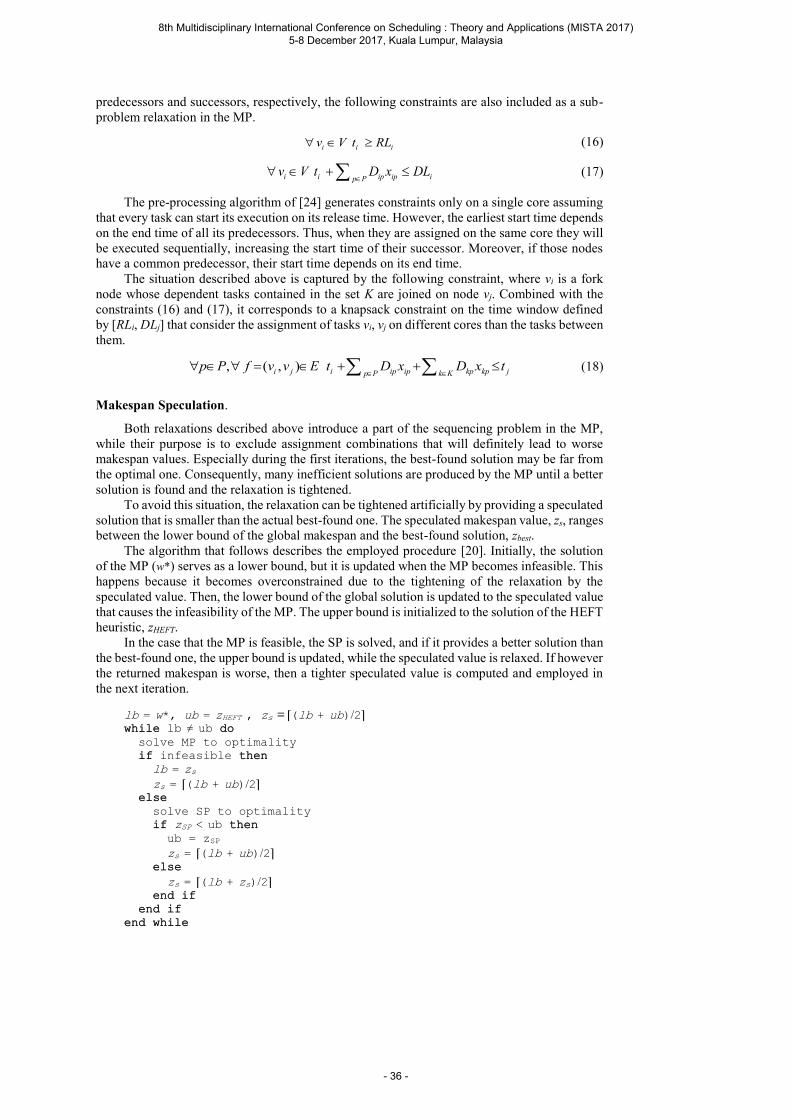
predecessors and successors, respectively, the following constraints are also included as a sub-

problem relaxation in the MP.

i i iv V t RL (16)

i i ip ip ip Pv V t D x DL

(17)

The pre-processing algorithm of [24] generates constraints only on a single core assuming

that every task can start its execution on its release time. However, the earliest start time depends

on the end time of all its predecessors. Thus, when they are assigned on the same core they will

be executed sequentially, increasing the start time of their successor. Moreover, if those nodes

have a common predecessor, their start time depends on its end time.

The situation described above is captured by the following constraint, where vi is a fork

node whose dependent tasks contained in the set K are joined on node vj. Combined with the

constraints (16) and (17), it corresponds to a knapsack constraint on the time window defined

by [RLi, DLj] that consider the assignment of tasks vi, vj on different cores than the tasks between

them.

, ( , )i j i ip ip kp kp jp P k Kp P f v v E t D x D x t

(18)

Makespan Speculation.

Both relaxations described above introduce a part of the sequencing problem in the MP,

while their purpose is to exclude assignment combinations that will definitely lead to worse

makespan values. Especially during the first iterations, the best-found solution may be far from

the optimal one. Consequently, many inefficient solutions are produced by the MP until a better

solution is found and the relaxation is tightened.

To avoid this situation, the relaxation can be tightened artificially by providing a speculated

solution that is smaller than the actual best-found one. The speculated makespan value, zs, ranges

between the lower bound of the global makespan and the best-found solution, zbest.

The algorithm that follows describes the employed procedure [20]. Initially, the solution

of the MP (w*) serves as a lower bound, but it is updated when the MP becomes infeasible. This

happens because it becomes overconstrained due to the tightening of the relaxation by the

speculated value. Then, the lower bound of the global solution is updated to the speculated value

that causes the infeasibility of the MP. The upper bound is initialized to the solution of the HEFT

heuristic, zHEFT.

In the case that the MP is feasible, the SP is solved, and if it provides a better solution than

the best-found one, the upper bound is updated, while the speculated value is relaxed. If however

the returned makespan is worse, then a tighter speculated value is computed and employed in

the next iteration.

lb = w*, ub = zHEFT , zs = ⌈(lb + ub)/2⌉ while lb ≠ ub do

solve MP to optimality

if infeasible then

lb = zs

zs = ⌈(lb + ub)/2⌉ else

solve SP to optimality

if zSP < ub then

ub = zSP

zs = ⌈(lb + ub)/2⌉ else

zs = ⌈(lb + zs)/2⌉ end if

end if

end while


- 36 -

The speculated value that causes the infeasibility of the MP is larger than the solution that

is normally returned by the MP, since it is based on a relaxation of the sub-problem. Therefore,

this procedure also provides better information about the bounds where the optimal solution

might lie. Finally, every time when the speculated value is relaxed, the cover constraints of the

SP relaxation that where added earlier are removed, whereas the right hand side of the knapsack

constraints is updated.

4.3 Benders Cuts

After each iteration where the sub-problems have been sequentially executed, extra constraints

are generated and added in the master problem for the subsequent iteration. The purpose of these

constraints, called Benders cuts, is exclude the previous solution so that another one is generated.

This can be achieved with a simple constraint of the form of (19) that excludes only the current

assignment.

* *

*1, 1,ip ipi Vx n x p P

(19)

However, the above constraint is very weak since it excludes only one combination of xip

variables. If the cardinality of the assignment constraint is reduced, that is it contains less

decision variables, it becomes significantly stronger. This can be done by gradually adding

variables in a set and checking the feasibility of the SP considering only the variables of the set

until a failure is detected. The order according to which the variables are inserted in the set is

defined by a chosen criterion. In our case, the tasks are sorted in a non-decreasing order

according to their slack, which is defined by the difference between their latest and earliest start

time.

Even though the cardinality of the conflict set is reduced, its computation imposes a

significant time overhead. In order to reduce it, the conflict set C is initialized with the tasks

whose slack equals zero. The others are sorted and gradually added to the set until the

infeasibility is detected according to the following procedure.

feed SP with C and solve to feasibility

while feasible do

add next task to C


end while

The resulting conflict set can be further reduced employing the algorithm provided in [26].

However, this algorithm also imposes significant time overhead, since it should be used in every

iteration. Instead, the following procedure was employed, which considers the task that caused

the infeasibility an important one. Then, it adds it to the refined conflict set R, which is initialized

with the tasks whose slack equals zero. Afterwards, the remaining tasks are added gradually until

the infeasibility is detected. The procedure terminates if less than two tasks have been added in

the conflict set until reaching the infeasibility, so the set cannot be further reduced.

while |R|<|C|-2 do

add last task of C to R, set C = R


while feasible do

add next task to C


end while

end while


- 37 -

The main core of the previous algorithms is the solution of the SP considering different

sets of tasks until it becomes infeasible. In order to further decrease the overhead that is caused

by this procedure, it was performed in parallel launching multiple CP models and collecting the

results. This way, the demanded conflict set was smallest among the infeasible models.

5 Hybrid Approach

The logic-based Benders decomposition approach, when applied to the problem of mapping and

scheduling of DAGs on heterogeneous cores, has achieved remarkable speedups in terms of

solution time and has managed to find the optimal solutions in problems where other methods

have failed to do so [20]. However, this method has some limitations that arise due to the

decomposition of the original problem. As the solution procedure progresses and a good or even

the optimal solution has been found, many assignment combinations are left to be evaluated that

cannot be excluded by the relaxation of the sub-problem that is included in the MP.

In that above case, the method relies only to the Benders cuts in order to prune the

remaining search space. As these cuts may be not so strong to drastically prune the solution

space, the MP produces many equivalent solutions that do not lead to better makespan values.

In this case, the process terminates after all the remaining assignment combinations are

enumerated. On the other hand, the pure ILP approach suffers from poor LP relaxations and

large integrality gaps when big-M constraints are used. Consequently, without being able to

generate efficient cutting planes, the branch-and-bound tree becomes enormous and the problem

intractable. Nevertheless, if the search space is reduced by an external source, this method can

generate strong cutting planes and can be very efficient in improving the solution or proving the

optimality of the best-found one.

To combine the strengths of the solution methods, the LBBD approach presented in the

previous section is employed as a cut generation scheme. The iterative process is stopped at

some point and the pure ILP model is launched while containing the extra constraints that were

generated by the LBBD method. Then, it runs with a time limit so that it is stopped when it

cannot quickly close the gap and reach the optimality. Even though the ILP model may not end

the solution process, it may produce a feasible solution, that is a solution that improves the best-

found makespan up to that point. In this case, a cover cut is derived from this solution using the

algorithms of the previous section. The LBBD method is launched again trying to produce more

cuts or find the optimal solution [21].

6 Experimental Results and Discussion

The introduced approaches were evaluated on randomly generated DAGs by an in-house

software tool. The tool takes as input the number of nodes, minimum and maximum execution

times per node, minimum and maximum depth between start and sink nodes, the minimum and

maximum number of edges and the distribution policy of edges between nodes and the number

of DAG to generate. All models were developed using the FICO Xpress Optimization suite [27].

The experiments were run on an i7 6-core PC operating at 3.2 GHz with 16 GB installed memory

and a Time Limit (TL) equal to two hours was set.

The experimental results are shown in Table 1 for the ILP, the LBBD, and the Hybrid

approaches. The initial solution provided by the HEFT heuristic was also used as an upper bound

on the solution in the ILP model, which is referred to as HILP in Table 1. Each row of the table

represents 10 DAG instances, resulting in the total amount of 60 instances. Table 1 shows the

number of instances that were solved optimally (OPT) and the ones that reached the time limit

(TL) without finding the optimal solution, as well as their average solution time for each group

defined by the number of tasks and cores. For the computation of the average time, the solution

time of the instances that were not solved within the time limit was set equal to the limit.

By the results of Table 1, it can be observed that the pure ILP model is not able to find the

optimal solution for the majority of cases, while it fails even in most of the small-scale problems.


- 38 -

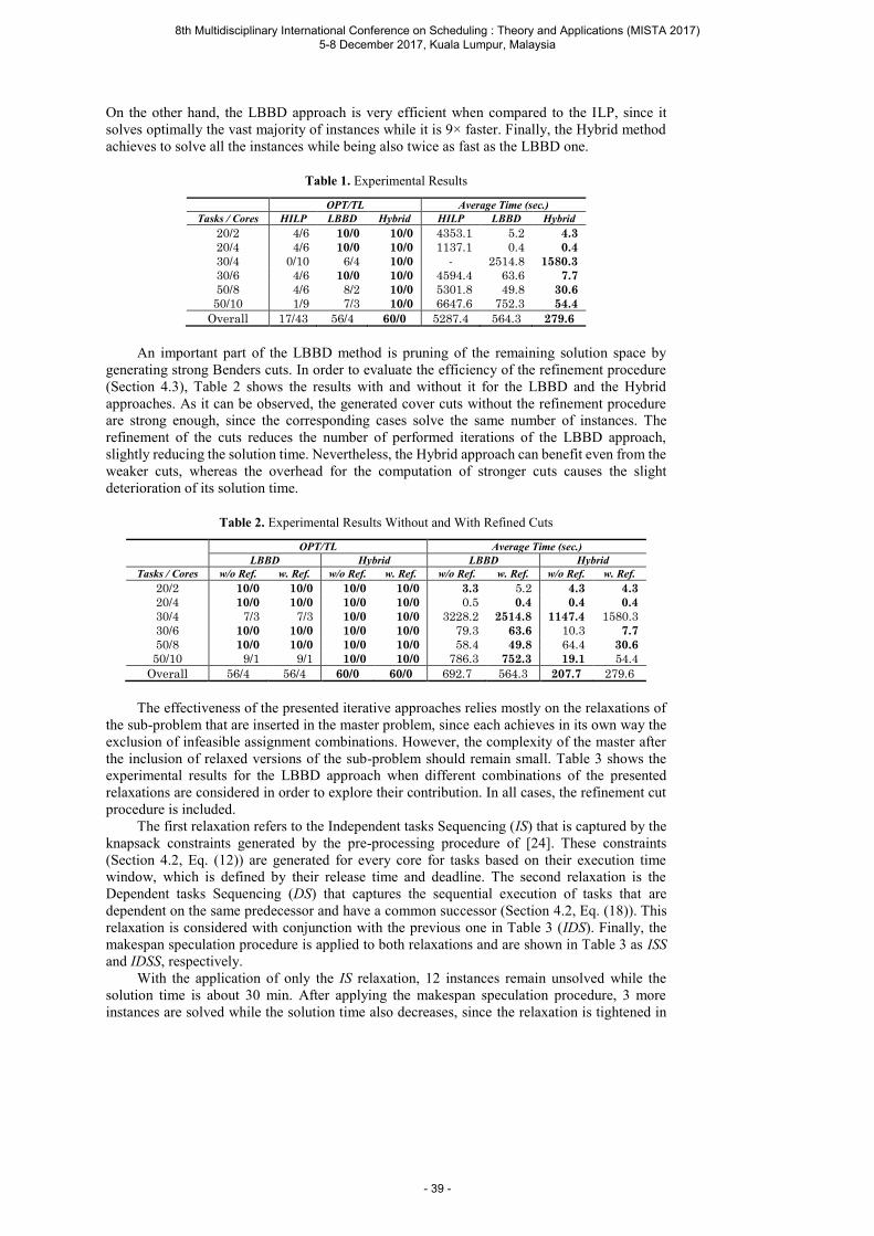
On the other hand, the LBBD approach is very efficient when compared to the ILP, since it

solves optimally the vast majority of instances while it is 9× faster. Finally, the Hybrid method

achieves to solve all the instances while being also twice as fast as the LBBD one.

Table 1. Experimental Results

OPT/TL Average Time (sec.)

Tasks / Cores HILP LBBD Hybrid HILP LBBD Hybrid

20/2 4/6 10/0 10/0 4353.1 5.2 4.3

20/4 4/6 10/0 10/0 1137.1 0.4 0.4

30/4 0/10 6/4 10/0 - 2514.8 1580.3

30/6 4/6 10/0 10/0 4594.4 63.6 7.7

50/8 4/6 8/2 10/0 5301.8 49.8 30.6

50/10 1/9 7/3 10/0 6647.6 752.3 54.4

Overall 17/43 56/4 60/0 5287.4 564.3 279.6

An important part of the LBBD method is pruning of the remaining solution space by

generating strong Benders cuts. In order to evaluate the efficiency of the refinement procedure

(Section 4.3), Table 2 shows the results with and without it for the LBBD and the Hybrid

approaches. As it can be observed, the generated cover cuts without the refinement procedure

are strong enough, since the corresponding cases solve the same number of instances. The

refinement of the cuts reduces the number of performed iterations of the LBBD approach,

slightly reducing the solution time. Nevertheless, the Hybrid approach can benefit even from the

weaker cuts, whereas the overhead for the computation of stronger cuts causes the slight

deterioration of its solution time.

Table 2. Experimental Results Without and With Refined Cuts


LBBD Hybrid LBBD Hybrid

Tasks / Cores w/o Ref. w. Ref. w/o Ref. w. Ref. w/o Ref. w. Ref. w/o Ref. w. Ref.

20/2 10/0 10/0 10/0 10/0 3.3 5.2 4.3 4.3

20/4 10/0 10/0 10/0 10/0 0.5 0.4 0.4 0.4

30/4 7/3 7/3 10/0 10/0 3228.2 2514.8 1147.4 1580.3

30/6 10/0 10/0 10/0 10/0 79.3 63.6 10.3 7.7

50/8 10/0 10/0 10/0 10/0 58.4 49.8 64.4 30.6

50/10 9/1 9/1 10/0 10/0 786.3 752.3 19.1 54.4

Overall 56/4 56/4 60/0 60/0 692.7 564.3 207.7 279.6

The effectiveness of the presented iterative approaches relies mostly on the relaxations of

the sub-problem that are inserted in the master problem, since each achieves in its own way the

exclusion of infeasible assignment combinations. However, the complexity of the master after

the inclusion of relaxed versions of the sub-problem should remain small. Table 3 shows the

experimental results for the LBBD approach when different combinations of the presented

relaxations are considered in order to explore their contribution. In all cases, the refinement cut

procedure is included.

The first relaxation refers to the Independent tasks Sequencing (IS) that is captured by the

knapsack constraints generated by the pre-processing procedure of [24]. These constraints

(Section 4.2, Eq. (12)) are generated for every core for tasks based on their execution time

window, which is defined by their release time and deadline. The second relaxation is the

Dependent tasks Sequencing (DS) that captures the sequential execution of tasks that are

dependent on the same predecessor and have a common successor (Section 4.2, Eq. (18)). This

relaxation is considered with conjunction with the previous one in Table 3 (IDS). Finally, the

makespan speculation procedure is applied to both relaxations and are shown in Table 3 as ISS

and IDSS, respectively.

With the application of only the IS relaxation, 12 instances remain unsolved while the

solution time is about 30 min. After applying the makespan speculation procedure, 3 more

instances are solved while the solution time also decreases, since the relaxation is tightened in


- 39 -

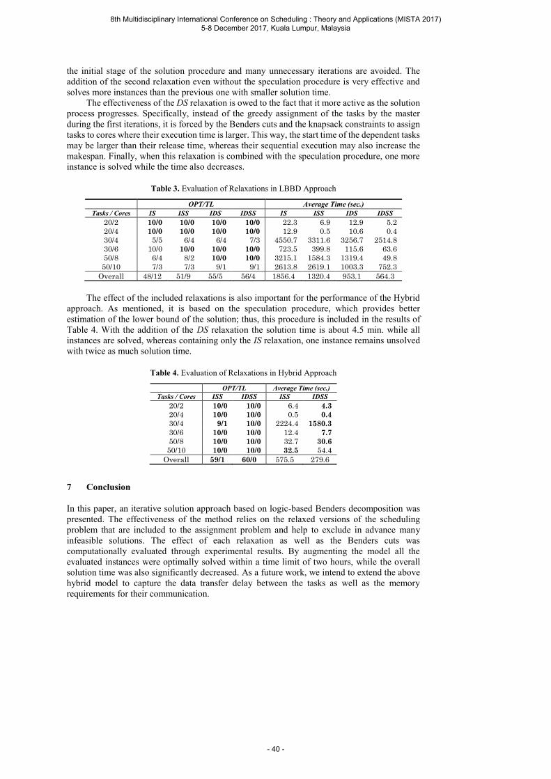
the initial stage of the solution procedure and many unnecessary iterations are avoided. The

addition of the second relaxation even without the speculation procedure is very effective and

solves more instances than the previous one with smaller solution time.

The effectiveness of the DS relaxation is owed to the fact that it more active as the solution

process progresses. Specifically, instead of the greedy assignment of the tasks by the master

during the first iterations, it is forced by the Benders cuts and the knapsack constraints to assign

tasks to cores where their execution time is larger. This way, the start time of the dependent tasks

may be larger than their release time, whereas their sequential execution may also increase the

makespan. Finally, when this relaxation is combined with the speculation procedure, one more

instance is solved while the time also decreases.

Table 3. Evaluation of Relaxations in LBBD Approach


Tasks / Cores IS ISS IDS IDSS IS ISS IDS IDSS

20/2 10/0 10/0 10/0 10/0 22.3 6.9 12.9 5.2

20/4 10/0 10/0 10/0 10/0 12.9 0.5 10.6 0.4

30/4 5/5 6/4 6/4 7/3 4550.7 3311.6 3256.7 2514.8

30/6 10/0 10/0 10/0 10/0 723.5 399.8 115.6 63.6

50/8 6/4 8/2 10/0 10/0 3215.1 1584.3 1319.4 49.8

50/10 7/3 7/3 9/1 9/1 2613.8 2619.1 1003.3 752.3

Overall 48/12 51/9 55/5 56/4 1856.4 1320.4 953.1 564.3

The effect of the included relaxations is also important for the performance of the Hybrid

approach. As mentioned, it is based on the speculation procedure, which provides better

estimation of the lower bound of the solution; thus, this procedure is included in the results of

Table 4. With the addition of the DS relaxation the solution time is about 4.5 min. while all

instances are solved, whereas containing only the IS relaxation, one instance remains unsolved

with twice as much solution time.

Table 4. Evaluation of Relaxations in Hybrid Approach


Tasks / Cores ISS IDSS ISS IDSS

20/2 10/0 10/0 6.4 4.3

20/4 10/0 10/0 0.5 0.4

30/4 9/1 10/0 2224.4 1580.3

30/6 10/0 10/0 12.4 7.7

50/8 10/0 10/0 32.7 30.6

50/10 10/0 10/0 32.5 54.4

Overall 59/1 60/0 575.5 279.6

7 Conclusion

In this paper, an iterative solution approach based on logic-based Benders decomposition was

presented. The effectiveness of the method relies on the relaxed versions of the scheduling

problem that are included to the assignment problem and help to exclude in advance many

infeasible solutions. The effect of each relaxation as well as the Benders cuts was

computationally evaluated through experimental results. By augmenting the model all the

evaluated instances were optimally solved within a time limit of two hours, while the overall

solution time was also significantly decreased. As a future work, we intend to extend the above

hybrid model to capture the data transfer delay between the tasks as well as the memory

requirements for their communication.


- 40 -

Acknowledgements This work was funded by the European Union under the Horizon 2020

Framework Program under grant agreement ICT-2015-688131, project “WCET-Aware

Parallelization of Model-Based Applications for Heterogeneous Parallel Systems (ARGO)”.

References

1. Stripf, T., Oey, O., Bruckschloegl, T., Becker, J., Rauwerda, G., Sunesen, K., Goulas,

G., Alefragis, P., Voros, N.S., Derrien, S., Sentieys, O., Kavvadias, N., Dimitroulakos,

G., Masselos, K., Kritharidis, D., Mitas, N., Perschke, T.: Compiling Scilab to high

performance embedded multicore systems. Microprocess. Microsyst. 37, 1033–1049

(2013).

2. Derrien, S., Puaut, I., Alefragis, P., Bednara, M., Bucher, H., David, C., Debray, Y.,

Durak, U., Fassi, I., Ferdinand, C., Hardy, D., Kritikakou, A., Rauwerda, G., Reder, S.,

Sicks, M., Stripf, T., Sunesen, K., ter Braak, T., Voros, N., Becker, J.: WCET-aware

parallelization of model-based applications for multi-cores: The ARGO approach. In:

Design, Automation & Test in Europe Conference & Exhibition (DATE), 2017. pp.

286–289. IEEE, Lausanne, Switzerland (2017).

3. Canon, L.-C., Jeannot, E., Sakellariou, R., Zheng, W.: Comparative Evaluation Of The

Robustness Of DAG Scheduling Heuristics. In: Grid Computing. pp. 73–84. Springer

US, Boston, MA (2008).

4. Singh, A.K., Shafique, M., Kumar, A., Henkel, J.: Mapping on multi/many-core

systems. In: Proceedings of the 50th Annual Design Automation Conference on - DAC

’13. p. 1. ACM Press, New York, New York, USA (2013).

5. Topcuoglu, H., Hariri, S., Wu, M.-Y.: Performance-Effective and Low-Complexity

Task Scheduling for Heterogeneous Computing. IEEE Trans. Parallel Distrib. Syst. 13,

260–274 (2002).

6. Bittencourt, L.F., Sakellariou, R., Madeira, E.R.M.: DAG Scheduling Using a

Lookahead Variant of the Heterogeneous Earliest Finish Time Algorithm. 2010 18th

Euromicro Conf. Parallel, Distrib. Network-based Process. 27–34 (2010).

7. Gupta, S., Kumar, V., Agarwal, G.: Task Scheduling in Multiprocessor System Using

Genetic Algorithm. In: 2nd International Conference on Machine Learning and

Computing. pp. 267–271. IEEE (2010).

8. Theodoridis, G., Vassiliadis, N., Nikolaidis, S.: An integer linear programming model

for mapping applications on hybrid systems. IET Comput. Digit. Tech. 3, 33 (2009).

9. Jovanovic, O., Kneuper, N., Engel, M., Marwedel, P.: ILP-based Memory-Aware

Mapping Optimization for MPSoCs. In: 2012 IEEE 15th International Conference on

Computational Science and Engineering. pp. 413–420. IEEE (2012).

10. Kuchcinski, K.: Constraints-Driven Scheduling and Resource Assignment. ACM Trans.

Des. Autom. Electron. Syst. 8, 355–383 (2003).

11. Martin, K., Wolinski, C., Kuchcinski, K., Floch, A., Charot, F.: Constraint Programming

Approach to Reconfigurable Processor Extension Generation and Application

Compilation. ACM Trans. Reconfigurable Technol. Syst. 5, 1–38 (2012).

12. Hooker, J.N.: Integrated Methods for Optimization. Springer US, Boston, MA (2012).

13. van Hentenryck, P., Milano, M. eds: Hybrid Optimization. Springer New York, New

York, NY (2011).

14. Hooker, J.N., Ottosson, G.: Logic-Based Benders Decomposition. Math. Program.

(2003).

15. Hooker, J.N.: Planning and Scheduling by Logic-Based Benders Decomposition. Oper.

Res. 55, 588–602 (2007).

16. Tran, T.T., Beck, J.C.: Logic-Based Benders Decomposition for Alternative Resource

Scheduling with Sequence Dependent Setups. Front. Artif. Intell. Appl. 242, 774–779

(2012).

17. Cambazard, H., Hladik, P.-E., Déplanche, A.-M., Jussien, N., Trinquet, Y.:

Decomposition and Learning for a Hard Real Time Task Allocation Problem. In:


- 41 -

Principles and Practice of Constraint Programming – CP 2004. pp. 153–167 (2004).

18. Ruggiero, M., Guerri, A., Bertozzi, D., Milano, M., Benini, L.: A Fast and Accurate

Technique for Mapping Parallel Applications on Stream-Oriented MPSoC Platforms

with Communication Awareness. Int. J. Parallel Program. 36, 3–36 (2008).

19. Benini, L., Lombardi, M., Milano, M., Ruggiero, M.: Optimal resource allocation and

scheduling for the CELL BE platform. Ann. Oper. Res. 184, 51–77 (2011).

20. Emeretlis, A., Theodoridis, G., Alefragis, P., Voros, N.: A Logic-Based Benders

Decomposition Approach for Mapping Applications on Heterogeneous Multicore

Platforms. ACM Trans. Embed. Comput. Syst. 15, 1–28 (2016).

21. Emeretlis, A., Theodoridis, G., Alefragis, P., Voros, N.: A Hybrid Approach for

Mapping and Scheduling on Heterogeneous Multicore Systems. In: 2016 International

Conference on Embedded Computer Systems: Architectures, Modeling, and Simulation

(SAMOS). , Samos (2016).

22. Nemhauser, G.L., Wolsey, L.A.: Integer and Combinatorial Optimization. John Wiley

& Sons, Inc. (1999).

23. Hooker, J.N.: A Hybrid Method for the Planning and Scheduling. Constraints. 10, 385–

401 (2005).

24. Maravelias, C.T.: A decomposition framework for the scheduling of single- and multi-

stage processes. Comput. Chem. Eng. 30, 407–420 (2006).

25. Sadykov, R., Wolsey, L. a.: Integer Programming and Constraint Programming in

Solving a Multimachine Assignment Scheduling Problem with Deadlines and Release

Dates. INFORMS J. Comput. 18, 209–217 (2006).

26. Junker, U.: QuickXplain: Preferred Explanations and Relaxations for Over-Constrained

Problems. In: AAAI’04 Proceedings of the 19th national conference on Artifical

intelligence. pp. 167–172 (2004).

27. FICO®: FICO Xpress Optimization Suite.


- 42 -

MISTA 2017

A Weight Assignment Approach for Multicriteria GlobalPath Planning of an Unmanned Combat Vehicle

Veekeong Saw · Amirah Rahman · Wen Eng Ong

Abstract In path planning of an unmanned combat vehicle, we aim to find solution

paths that visit all checkpoints while minimizing the accumulated cost factors. In this

paper, we consider the global path planning problem of an unmanned combat vehicle

which has been modeled into a multiple criteria traveling salesman path problem on

a grid network. An algorithm using weight assignment approach is proposed to find a

solution path. To demonstrate the proposed algorithm, computational experiments are

conducted on simulated maps. Initial experimentation demonstrates that the solution

path generated for different problem instances are affected by the weight assignment

of different attributes as well as the tabulation of the terrain and the positioning of the

checkpoints.

1 Introduction

An unmanned combat vehicle (UCV) is an armed robotic vehicle used to substitute

human participation in high risk military operations. A UCV is controlled via wire-

less communication signal from an external control station. The path planning and

navigation process of a UCV is controlled by operators through user interface in the

control center [8]. The navigation control of a UCV is divided into local path planning

(LPP) and global path planning (GPP). LPP is a real-time process that maintains

the stability and safety of UCV throughout the journey. On the other hand, GPP is

a deliberate process of searching for feasible travel paths based on user requirements.

Modern UCVs are equipped with LPP navigation systems, thus no human intervention

is needed to ensure the stability of the UCV throughout the mission. Hence, in this

Veekeong SawSchool of Mathematical Sciences, Universiti Sains MalaysiaE-mail: kentvk [email protected]

Amirah RahmanSchool of Mathematical Sciences, Universiti Sains MalaysiaE-mail: [email protected]

Wen Eng OngSchool of Mathematical Sciences, Universiti Sains MalaysiaE-mail: [email protected]


- 43 -

study, we assume that the UCV is equipped with LPP navigation system, where it can

perform obstacle avoidance, stability maintenance and direction changes by itself.

To perform the GPP process, the terrain map needs to be represented in a form

where a path searching algorithm can be implemented. There are three main rep-

resentation methods used: cell decomposition, roadmap, and potential field. Among

these three methods, cell decomposition method is the most frequently used due to its

simplicity and flexibility [3]. By using cell decomposition method, the map of area of

interest (AOI) is inscribed into a grid made of uniformly arranged cells. The terrain

information of the region inscribed in the particular cell is associated to the correspond-

ing cell. Then, the path searching algorithm is conducted based on user input and the

data associated to the grid. If a solution path is found, the algorithm will generate the

path and project it onto the map. Otherwise it will report failure.

In general, the GPP of a UCV has the objective of finding a travel path that

minimizes resource consumption. Note that the resources are not limited to physical

attributes such as traveling distance, fuel consumption or ammunition consumption. It

can represent non-physical attributes such as potential threat level, terrain sloppiness,

or signal strength. In the grid, the traveling paths are described as a sequence of

cells that the UCV needs to pass through. The resource consumption for the UCV

throughout the journey can be estimated by the cumulative costs of various attributes

along the traveling path. GPP problems with single attribute are known as single

criteria problem, while GPP problems that involve multiple attributes are known as

multicriteria problems.

The GPP problems with only two checkpoints (origin and destination points) are

often modeled as shortest path problems [4], [7]. Also, GPP problems with multiple

(more than two) checkpoints are mostly modeled as traveling salesman problem (TSP)

or one of its variants [1], [5], [11], [12]. Single criteria GPP problems that modeled

as TSPs has been solved using Christofides algorithm [2], convex hull method [6],

and various heuristics as reported by [9] in his review paper. On the other hand,

multicriteria GPPs that modeled as TSP has been discussed by [1], [11].

In this paper, we consider the GPP problem with multiple checkpoints on a grid

map. The objective is to find a path that travels all checkpoints with unique starting

and destination point, that minimizes the cumulative cost of the attributes. Our prob-

lem is modeled as a traveling salesman path problem (TSPP) with 2 unique endpoints

in a grid network. The TSPP with 2 unique endpoints is a variation of the TSP, which

search for least cost Hamilton path with 2 unique endpoints, instead of searching for

least cost Hamilton cycle as in TSP.

We make the following assumptions:

1. Each attribute is assigned a weight by the user that represent its importance relative

to one another.

2. The UCV is in good condition before it starts its journey, so there is no need to

return to base for servicing during the mission.

3. The grid is eight-connected, meaning that the UCV can move freely to any one of

the eight adjacent cells in the grid if available.

4. The cells in the grid can be traversed more than once if necessary.

Figure 1 shows an example map for a GPP problem, where a series of checkpoints

(depicted as flags) are required to be visited, where s and t are starting and ending

locations respectively. Throughout the journey, the UCV has to avoid enemy territory

and enemy detection (depicted as rifles and radars respectively).


- 44 -

𝑠𝑠 𝑡𝑡

Fig. 1: An example of a satellite terrain map with checkpoints and attributes.

2 Problem Description

In this study, the area of interest is inscribed into an N×N grid, where each cell in the

grid stores the cost value of traverse time (time required to pass through a terrain),

risk level (likelihood of an UCV to face a threat), and signal interference level (level of

signal interruption encountered by UCV) of the corresponding region. For simplicity,

we call these attributes as attribute 1, 2, and 3 respectively. The grid is modeled into

an undirected graph G. The terminology, notation, and definitions related to graph G

are listed as follows:

G Undirected graph G = (V,E, c)

V Set of N ×N vertices representing the cells in the grid

E Set of edges representing the link between two adjacent cells,i.e. E = (i, j)|i, j ∈ V

c Cost function c : V → R3 that maps vertex i to cost vector c(i) = (c1i , c2i , c

3i ),

where cki represent the cost of attributes k = 1, 2, 3 for vertex i

Λ Set of n+ 2 checkpoints need to be visited, i.e. Λ = s, v1, v2, . . . , vn, t ( V

s, t Unique starting and ending points

v1, v2, . . . , vn Intermediate points

πi,j Path from vertex i to j, written as a sequence of vertices πi,j =< i, . . . , j >

Ci,j Cost of path πi,j , given by the addition of cost vectors of alltraversed vertices, i.e. Ci,j =

∑k∈πi,j

c(k)

⊕ Path concatenation operator: a concatenation of path πi,j and πj,k,denoted by πi,j ⊕ πj,k, gives path πi,k =< i, . . . , j, . . . , k >

Suc(i) Set of successors of vertex i, i.e. Suc(i) = j|(i, j) ∈ E

Pre(i) Set or predecessors of vertex i, i.e. Pre(i) = j|(j, i) ∈ E


- 45 -

πi,j , i, j ∈ Λ Partial path: a path between two vertices in Λ

π∗s,t Complete path: a path that joins s to t and pass through all theintermediate points in Λ. i.e. π∗s,t =< s, . . . , vi1 , . . . , vi2 , . . . , vin , . . . , t >,where vi1 , vi2 , . . . , vin are all the intermediate points

Note that a complete path π∗s,t =< s, . . . , vi1 , . . . , vi2 , . . . , vin−1, . . . , vin , . . . , t >

that contains |Λ| = n + 2 checkpoints is a concatenation of n + 1 partial paths

πs,vi1 ⊕ πvi1 ,vi2 ⊕ . . .⊕ πin−1,vin⊕ πvin ,t, where vi1 , vi2 , . . . , vin−1

, vin are all the in-

termediate points in Λ.

Let xi be defined by

xi =

1, if vertex i was traversed in the path,

0, otherwise.

Our problem is formulated as follows:

Minimize∑i∈V

xic1i (1)

Minimize∑i∈V

xic2i (2)

Minimize∑i∈V

xic3i (3)

subject to ∑j∈Suc(i)

xj ≥ 1, ∀ i ∈ Λ\t (4)

∑j∈Suc(t)

xj ≥ 0, (5)

∑j∈Pre(i)

xj ≥ 1, ∀ i ∈ Λ\s (6)

∑j∈Pre(s)

xj ≥ 0, (7)

∑j∈Suc(i)

xj +∑

j∈Pre(i)

xj = 2k, k ≥ 0,∀ i ∈ V \s, t (8)

∑j∈Suc(i)

xj +∑

j∈Pre(i)

xj = 2k + 1, k ≥ 0, i = s, t (9)

∑i∈S

∑j∈Suc(i)∩S′

xj ≥ 1, ∀S ( V, S 6= ∅ (10)

xi ∈ 0, 1, ∀i ∈ V (11)

Objective functions (1) to (3) represent the three cost factors (traverse time, risk level,

signal interference level) to be minimized. Constraints (4) and (5) ensure that the path

leaves every checkpoint in Λ at least once (except vertex t, which will only be traversed

if necessary). Constraints (6) and (7) ensure that the path enters every checkpoint in Λ

at least once (except vertex s, which will only be traversed if necessary). Constraints (8)

and (9) preserve flow conservation throughout the path. Constraints (10) prevents the

solution path from forming subtours.


- 46 -

3 Solution Approach

In Section 2, the GPP problem was formulated as a multicriteria optimization problem.

We propose a heuristic based on additive weighting method to reduce our multicriteria

optimization problem into a single criteria optimization problem. We solve our problem

using an extended version f the two phase heuristic method proposed in [10]. The

extension exists in the form of a preprocessing stage where the multiple attributes are

reduced to a single attribute using user defined weights.

3.1 Preprocessing stage

In a terrain map, the costs of different attributes may be assigned in different scales,

depending on the map source. To ensure that all attributes have an equal level of

significance, the cost of each attribute is normalized into a common range of [0, 1].

Here, we implement min-max normalization method to transform original cost vectors

into the normalized cost vector for all vertices in the graph. The normalized cost vector

correspond to vertex i ∈ V is defined as c(i) = (c1i , c2i , c

3i ), such that

cki =cki − c

kmin

ckmax − ckmin,

where ckmin and ckmax represent the minimum and maximum cost value for attribute

k = 1, 2, 3.

Let the user defined weight vector be w = (w1, w2, w3), where w1, w2, and w3

represent the weights for attribute k = 1, 2, 3 respectively, such that∑3k=1 wk = 1 for

w1, w2, w3 ≥ 0. By using additive weighting method on the graph G with normalized

cost vector, we construct the graph G′ = (V ′, E′, c′) in the following manner

1. V ′ = V,E′ = E.

2. c′ : V → R is a additive weighing cost function such that for i ∈ V ′,c′(i) = w[c(i)]T =

∑3k=1 wk c

ki .

3. The cost of path between vertex i and j in G′ is C′i,j =∑k∈πi,j

c′(k).

4. The definition for path, path concatenation, successor set, predecessor set in G′ are

similarly defined as in G.

Based on the graph G′, our problem can be reformulated as single criteria opti-

mization problem that minimizes the objective function

w1

∑i∈V

xic1i + w2

∑i∈V

xic2i + w3

∑i∈V

xic3i

subject to the constraints set in Section 2.

The reduced GPP problem formulation above is an s-t traveling salesman path

problem (stTSPP), which is a variation of traveling salesman problem (TSP). In this

study, we relax the Hamiltonian property restriction on the solution generated in as we

have already made the assumption that the vertices may be visited more than once. In

stTSPP, a complete undirected weighted graph is provided and the objective is to find

a path that starts and ends at uniquely given endpoints and passes through all other

points, such that the total travel cost is minimized. The two phase heuristic used to

solve the problem was proposed in [10]. We present the detailed explanation for the

procedure in the following subsections.


- 47 -

3.2 Phase 1: Generating the complete graph GK

In Phase 1, we find the shortest partial path between all pairs of checkpoints i, j ∈ Λon G′. As G′ is undirected, C′i,j = C′j,i for all pairs of checkpoints. In total, there are(n+22

)non-directed paths connecting all pairs of checkpoints. We implement Dijkstra’s

algorithm to find all these shortest paths. Note that in typical shortest path problem,

the cost is associated on the edges of the graph and the path cost is calculated by

summing up the cost of traversed edges. However, in G′ the cost value is associated on

vertices of the graph. Hence, while applying the Dijkstra’s algorithm, the path cost is

calculated by adding the cost associated to the vertices instead of edges.

Let ΛR be defined as ΛR = p1, p2, . . . , pn+2 such that p1 = s, pk = vk−1 for

k = 2, 3, . . . , n + 1 and pn+2 = t. The details of Dijkstra’s algorithm is shown in

Algorithm 1. For each pair of checkpoints pi, pj ∈ ΛR, the minimum cost of path

between pi and pj is C′pi,pj , and its path πpi,pj can be found by using procedure

Generate Path described in Algorithm 2.

Algorithm 1 Dijkstra’s algorithm

Require: G′ = (V ′, E′, c′), ΛR = p1, . . . , pn+21: for all pi, pj ∈ ΛR, (i 6= j, i > j) do2: S∗ ← ∅ . S∗: Set of vertices k of which minimum C′pi,k is obtained

3: S ← V ′ . S: Set of vertices k of which minimum C′pi,k is not obtained yet

4: C′pi,pi ← c(pi)

5: C′pi,k ←∞ for all k ∈ V ′\pi6: while pj 6∈ S∗ do7: i∗ ← arg mink∈SC′pi,k . i∗: Vertex k ∈ S with minimum C′pi,k8: S ← S − i∗, S∗ ← S∗ ∪ i∗9: for all v ∈ Suc(i∗) do

10: if C′pi,v > C′pi,i∗ + c(v) then

11: C′pi,v ← C′pi,i∗ + c(v)

12: Prev(v)← i∗

13: end if14: end for15: end while16: perform Generate Path17: end for

Algorithm 2 Generate Path

1: πpi,pj ← empty stack2: u← pj . u: Variable used to store the predecessor vertices3: while Prev(u) exist do4: insert u into πpi,pj5: u← Prev(u)6: end while7: insert u into πpi,pj


- 48 -

3.3 Phase 2: Search for the best complete path

In Phase 1, the shortest path between all pairs of checkpoints in G′ is found using

Dijkstra’s algorithm. We use all the paths to construct a complete graph GK . The

construction of complete graph GK = (VK , EK , cK) is defined as follows:

1. The vertex set, VK = Λ.

2. The edge set, EK = (i, j)|i, j ∈ Λ , where |EK | =(n+22

).

3. The edge cost function, cK : EK → R is defined as cK(i, j) = C′i,j − c′(i)− c′(j).

4. For i, j ∈ VK , the path from i to j, Πi,j is an alternating series of vertex

and edges, such that Πi,j =< i, (i, u1), u1, (u1, u2), u2, . . . , ux, (ux, j), j >, where

u1, u2, . . . , ux ∈ VK . For simplicity, we write Πi,j =< i, u1, u2, . . . , ux, j >.

5. The cost of the pathΠi,j , denoted by CKi,j , is given by CKi,j =∑

(u,v)∈Πi,jcK(u, v)+∑

k∈Πi,jc′(k).

6. A cycle that starts at vertex i, denoted by Cyc(i), is a path that begins and ends

with vertex i. The cost of Cyc(i) is given by CKCyc(i) =∑

(u,v)∈Cyc(i) cK(u, v) +∑k∈Cyc(i) c

′(k).

7. The concatenation of two paths Πi,j =< i, (i, u1), u1, . . . , ux, (ux, j), j > and

Πj,k =< j, (j, ux+1), ux+1, . . . , uy, (uy, k), k >, denoted by Πi,j ⊕Πj,k, is given by

Πi,j ⊕Πj,k =< i, (i, u1), u1, . . . , ux, (ux, j), j, (j, ux+1), ux+1, . . . , uy, (uy, k), k >.

The stTSPP is equivalent to the standard TSP in which the edge cost con-

necting s and t, is replaced by −M , where M is a sufficiently large value

such that M > max(i,j)6=(s,t)cK(i, j). Hence, solution for standard TSP on

GK = (VK , EK , cK) with cK(s, t) = −M corresponds to the solution path for stTSPP

on GK = (VK , EK , cK) with cK(i, j) remain unchanged for all i, j ∈ VK .

We solve our TSP using the nearest neighbor algorithm (NNA). The NNA starts

by randomly selects a vertex i as a starting point and visits the immediate best (least

cost) vertex until all the vertices are visited and finally returns to the initial vertex.

This forms a least cost cycle that passes through all vertices. However, as NNA is a

greedy algorithm, the least cost edges are always selected first, which leaves high cost

edges to be chosen in later. Hence, NNA does not guarantee an optimal solution is

found. The procedure of NNA for TSP on GK = (VK , EK , cK) with cK(s, t) = −M is

given in Algorithm 3.

Algorithm 3 Nearest Neighbor Algorithm (NNA)

Require: GK = (VK , EK , cK) with cK(s, t) = −M , ΛR = p1, . . . , pn+21: S ← ΛR . S: Set of vertices not selected yet2: Select a random pi ∈ S3: S ← ΛR − pi4: Cyc(pi)←< pi >,C

KCyc(pi)

← c′(pi)

5: while S 6= ∅ do6: l← last vertex in Cyc(pi)7: i∗ ← arg mink∈ScK(l, k) . i∗: Vertex k ∈ S with least cK(l, k)8: S ← S − i∗9: Cyc(pi)← Cyc(pi)⊕ (l, i∗)

10: CKCyc(pi)

← CKCyc(pi)

+ cK(l, i∗) + c′(i∗)

11: end while12: l← last vertex in Cyc(pi)13: Cyc(pi)← Cyc(pi)⊕ l, pi14: CK

Cyc(pi)← CK

Cyc(pi)+ cK(l, pi)


- 49 -

To increase the likelihood in obtaining a better solution, an improvement technique

known as repetitive nearest neighbor algorithm (RNNA) is performed. RNNA conducts

NNA n+ 2 times by starting at each checkpoint in Λ once. This gives n+ 2 least cost

cycles Cyc(i) that pass through all checkpoints. Among these n + 2 cycles, the cycle

with least cost is chosen. Then, the edge (s, t) is removed from the selected cycle. This

forms the least cost path Πs,t that connects s to t and passes through all checkpoints,

which is the solution for stTSPP in GK . The algorithm for RNNA is described in

Algorithm 4.

Algorithm 4 Repetitive Nearest Neighbor Algorithm (RNNA)

Require: GK = (VK , EK , cK) with cK(s, t) = −M , ΛR = p1, . . . , pn+21: Cyc∗ ← empty sequence . Cyc∗: Least cost cycle among Cyc(i), ∀i ∈ ΛR.2: for all point pi ∈ ΛR do3: Perform NNA . Line 2 of NNA: select pi instead of randomly select a vertex in S.4: end for5: Cyc∗ ← arg minpi∈ΛR

CKCyc(pi)

6: Remove edge (s, t) from Cyc∗ to form a path Πs,t =< s, . . . , t >.7: CKs,t ← CKCyc∗ +M

To trace the complete path π∗s,t on terrain map, the corresponding edges in Πs,tare concatenated, such that π∗s,t = πs,vi1 ⊕ πvi1 ,vi2 ⊕ . . .⊕ πvin−1

,vin ⊕ πvin ,t, where

πu,v is the shortest path between the vertex u and v as found in Dijkstra’s algorithm.

The total cost of the complete path in terrain map is given by Cs,t =∑k∈πs,t

c(k).

4 Results and Discussion

In this section, a GPP problem demonstration and computational experiments are con-

ducted using a simulated terrain. The terrain was designed by using Wolfram Math-

ematicar software and all the algorithms are coded in C++. The details of problem

demonstration and computational experiments are explained as follows.

4.1 Algorithm Implementation

We demonstrate our proposed algorithm using the simulated terrain as shown in Fig-

ure 2(a). The terrain is inscribed onto a 15 × 15 grid in Figure 2(b) with the set of

checkpoints Λ being marked and their coordinates stated. The distribution of attributes

in the terrain are shown in Figure 3. The costs of each cells are assigned with integers

ranging from 0 to 9. Then, the grid is modeled into the graph G = (V,E, c) as in

Figure 4. Note that the cell (i, j) in the grid corresponds to vertex 15(i − 1) + j in G

for i, j ∈ 1, 2, . . . , 15. The corresponding vertex number for all the checkpoints are

listed in Figure 4. We assign the weight vector to be w = (0.7, 0.2, 0.1).


- 50 -

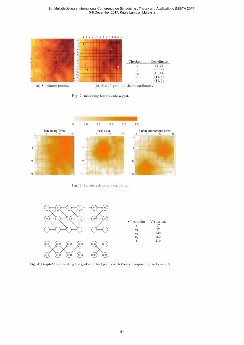
(a) Simulated terrain.

Checkpoint Coordinates (2, 2)v1 (4, 12)v2 (10, 14)v3 (11, 3)t (15, 9)

(b) 15× 15 grid and their coordinates.

Fig. 2: Inscribing terrain onto a grid.

Fig. 3: Terrain attribute distribution.

211 212 213 214 224 225

196 197 198 199 209 210

16 17 18 19 29 30

1 2 3 4 14 15

Checkpoint Vertex no.s 17v1 57v2 149v3 153t 219

Fig. 4: Graph G representing the grid and checkpoints with their corresponding vertices in G.


- 51 -

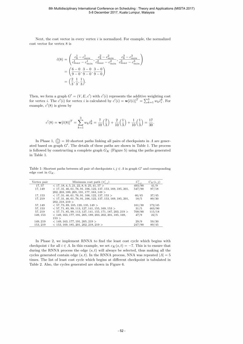
Next, the cost vector in every vertex i is normalized. For example, the normalized

cost vector for vertex 8 is

c(8) =

(c18 − c1minc1max − c1min

,c28 − c2minc2max − c2min

,c38 − c3minc3max − c3min

)

=

(6− 0

9− 0,

3− 0

9− 0,

3− 0

9− 0

)=(

2

3,

1

3,

1

3

).

Then, we form a graph G′ = (V,E, c′) with c′(i) represents the additive weighting cost

for vertex i. The c′(i) for vertex i is calculated by c′(i) = w[c(i)]T =∑3k=1 wk c

ki . For

example, c′(8) is given by

c′(8) = w[c(8)]T =

3∑k=1

wk ck8 =

7

10

(2

3

)+

2

10

(1

3

)+

1

10

(1

3

)=

17

30.

In Phase 1,(52

)= 10 shortest paths linking all pairs of checkpoints in Λ are gener-

ated based on graph G′. The details of these paths are shown in Table 1. The process

is followed by constructing a complete graph GK (Figure 5) using the paths generated

in Table 1.

Table 1: Shortest paths between all pair of checkpoints i, j ∈ Λ in graph G′ and correspondingedge cost in GK .

Vertex pair Minimum cost path (π′i,j) C′i,j CK(i, j)

17, 57 < 17, 18, 4, 5, 21, 22, 8, 9, 25, 41, 57 > 493/90 41/917, 149 < 17, 31, 46, 61, 76, 91, 106, 122, 137, 153, 169, 185, 201, 547/90 97/18

202, 203, 189, 205, 191, 177, 163, 149 >17, 153 < 17, 31, 46, 61, 76, 91, 106, 122, 137, 153 > 46/45 37/4517, 219 < 17, 31, 46, 61, 76, 91, 106, 122, 137, 153, 169, 185, 201, 18/5 89/30

202, 218, 219 >57, 149 < 57, 73, 89, 105, 120, 135, 149 > 161/30 172/4557, 153 < 57, 71, 85, 99, 113, 127, 141, 155, 169, 153 > 31/5 463/9057, 219 < 57, 71, 85, 99, 113, 127, 141, 155, 171, 187, 203, 219 > 709/90 115/18149, 153 < 149, 163, 177, 191, 205, 189, 203, 202, 201, 185, 169, 47/9 22/5

153 >149, 219 < 149, 163, 177, 191, 205, 219 > 29/9 59/30153, 219 < 153, 169, 185, 201, 202, 218, 219 > 247/90 89/45

In Phase 2, we implement RNNA to find the least cost cycle which begins with

checkpoint i for all i ∈ Λ. In this example, we set cK(s, t) = −7. This is to ensure that

during the RNNA process the edge (s, t) will always be selected, thus making all the

cycles generated contain edge (s, t). In the RNNA process, NNA was repeated |Λ| = 5

times. The list of least cost cycle which begins at different checkpoint is tabulated in

Table 2. Also, the cycles generated are shown in Figure 6.


- 52 -

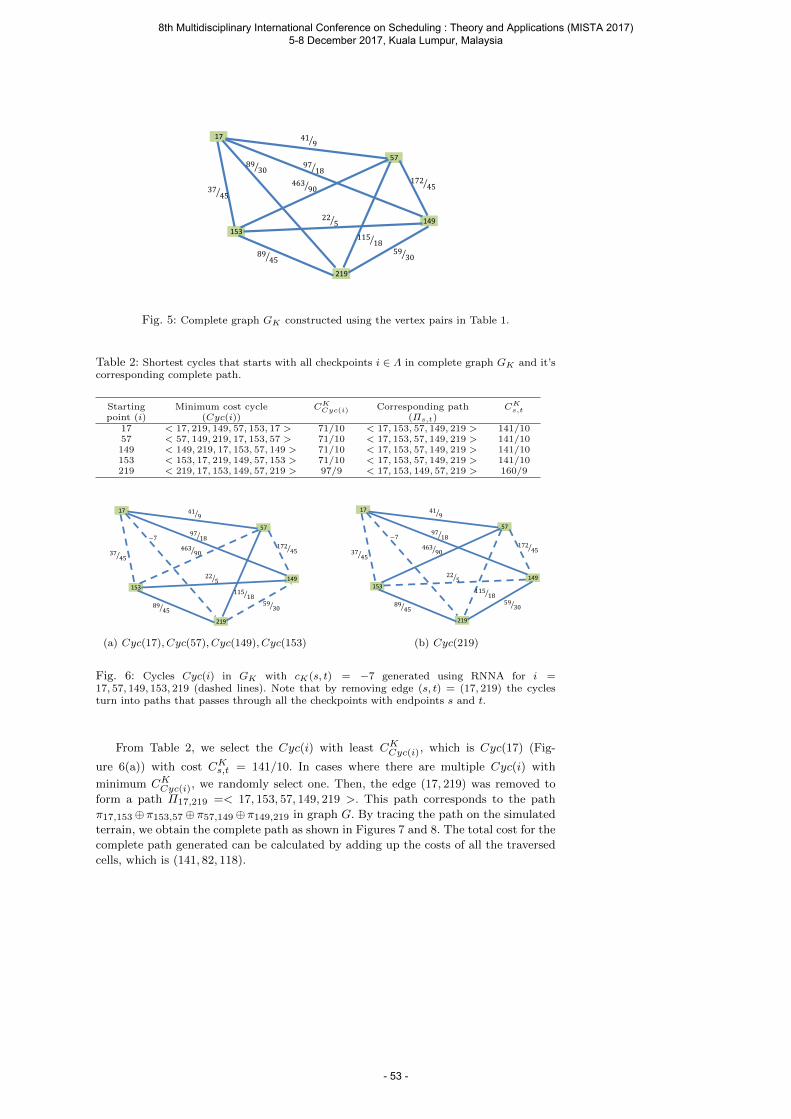
17

57

149153

219

419

9718

17245

5930

11518

8945

225

8930

46390 37

45

Fig. 5: Complete graph GK constructed using the vertex pairs in Table 1.

Table 2: Shortest cycles that starts with all checkpoints i ∈ Λ in complete graph GK and it’scorresponding complete path.

Startingpoint (i)

Minimum cost cycle(Cyc(i))

CKCyc(i) Corresponding path

(Πs,t)CK

s,t

17 < 17, 219, 149, 57, 153, 17 > 71/10 < 17, 153, 57, 149, 219 > 141/1057 < 57, 149, 219, 17, 153, 57 > 71/10 < 17, 153, 57, 149, 219 > 141/10149 < 149, 219, 17, 153, 57, 149 > 71/10 < 17, 153, 57, 149, 219 > 141/10153 < 153, 17, 219, 149, 57, 153 > 71/10 < 17, 153, 57, 149, 219 > 141/10219 < 219, 17, 153, 149, 57, 219 > 97/9 < 17, 153, 149, 57, 219 > 160/9

17

57

149153

219

419

9718

17245

5930

11518

8945

225

46390 37

45

−7

(a) Cyc(17), Cyc(57), Cyc(149), Cyc(153)

17

57

149153

219

419

9718

17245

5930

11518

8945

225

46390 37

45

−7

(b) Cyc(219)

Fig. 6: Cycles Cyc(i) in GK with cK(s, t) = −7 generated using RNNA for i =17, 57, 149, 153, 219 (dashed lines). Note that by removing edge (s, t) = (17, 219) the cyclesturn into paths that passes through all the checkpoints with endpoints s and t.

From Table 2, we select the Cyc(i) with least CKCyc(i), which is Cyc(17) (Fig-

ure 6(a)) with cost CKs,t = 141/10. In cases where there are multiple Cyc(i) with

minimum CKCyc(i), we randomly select one. Then, the edge (17, 219) was removed to

form a path Π17,219 =< 17, 153, 57, 149, 219 >. This path corresponds to the path

π17,153⊕π153,57⊕π57,149⊕π149,219 in graph G. By tracing the path on the simulated

terrain, we obtain the complete path as shown in Figures 7 and 8. The total cost for the

complete path generated can be calculated by adding up the costs of all the traversed

cells, which is (141, 82, 118).


- 53 -

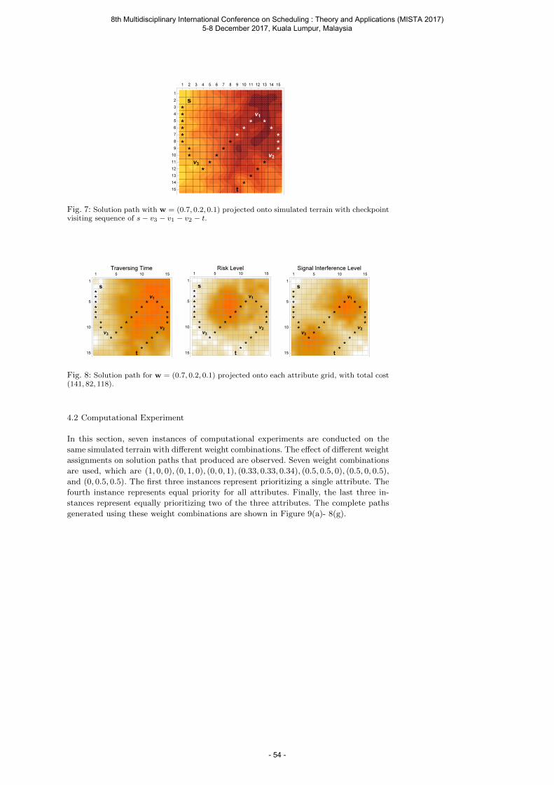
Fig. 7: Solution path with w = (0.7, 0.2, 0.1) projected onto simulated terrain with checkpointvisiting sequence of s− v3 − v1 − v2 − t.

Fig. 8: Solution path for w = (0.7, 0.2, 0.1) projected onto each attribute grid, with total cost(141, 82, 118).

4.2 Computational Experiment

In this section, seven instances of computational experiments are conducted on the

same simulated terrain with different weight combinations. The effect of different weight

assignments on solution paths that produced are observed. Seven weight combinations

are used, which are (1, 0, 0), (0, 1, 0), (0, 0, 1), (0.33, 0.33, 0.34), (0.5, 0.5, 0), (0.5, 0, 0.5),

and (0, 0.5, 0.5). The first three instances represent prioritizing a single attribute. The

fourth instance represents equal priority for all attributes. Finally, the last three in-

stances represent equally prioritizing two of the three attributes. The complete paths

generated using these weight combinations are shown in Figure 9(a)- 8(g).


- 54 -

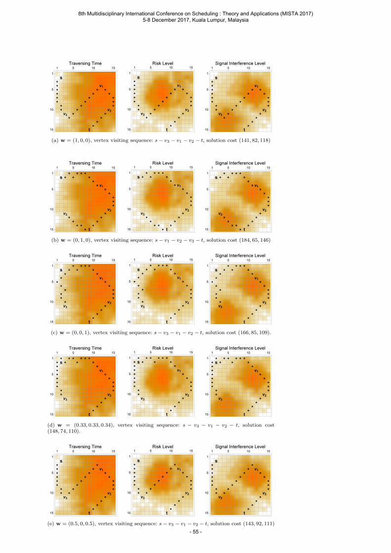
(a) w = (1, 0, 0), vertex visiting sequence: s− v3 − v1 − v2 − t, solution cost (141, 82, 118)

(b) w = (0, 1, 0), vertex visiting sequence: s− v1 − v2 − v3 − t, solution cost (184, 65, 146)

(c) w = (0, 0, 1), vertex visiting sequence: s− v3 − v1 − v2 − t, solution cost (166, 85, 109).

(d) w = (0.33, 0.33, 0.34), vertex visiting sequence: s − v3 − v1 − v2 − t, solution cost(148, 74, 110).

(e) w = (0.5, 0, 0.5), vertex visiting sequence: s− v3 − v1 − v2 − t, solution cost (143, 92, 111)


- 55 -

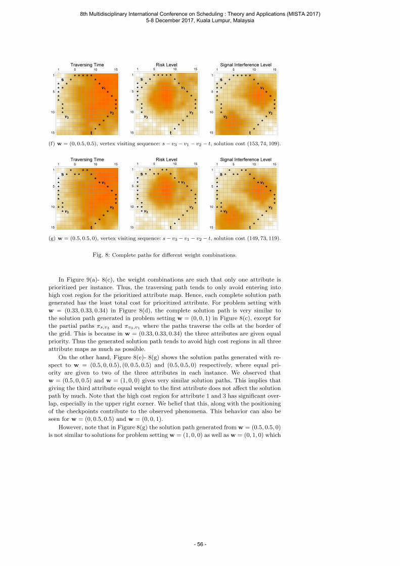
(f) w = (0, 0.5, 0.5), vertex visiting sequence: s− v3 − v1 − v2 − t, solution cost (153, 74, 109).

(g) w = (0.5, 0.5, 0), vertex visiting sequence: s− v3 − v1 − v2 − t, solution cost (149, 73, 119).

Fig. 8: Complete paths for different weight combinations.

In Figure 9(a)- 8(c), the weight combinations are such that only one attribute is

prioritized per instance. Thus, the traversing path tends to only avoid entering into

high cost region for the prioritized attribute map. Hence, each complete solution path

generated has the least total cost for prioritized attribute. For problem setting with

w = (0.33, 0.33, 0.34) in Figure 8(d), the complete solution path is very similar to

the solution path generated in problem setting w = (0, 0, 1) in Figure 8(c), except for

the partial paths πs,v3 and πv3,v1 where the paths traverse the cells at the border of

the grid. This is because in w = (0.33, 0.33, 0.34) the three attributes are given equal

priority. Thus the generated solution path tends to avoid high cost regions in all three

attribute maps as much as possible.

On the other hand, Figure 8(e)- 8(g) shows the solution paths generated with re-

spect to w = (0.5, 0, 0.5), (0, 0.5, 0.5) and (0.5, 0.5, 0) respectively, where equal pri-

ority are given to two of the three attributes in each instance. We observed that

w = (0.5, 0, 0.5) and w = (1, 0, 0) gives very similar solution paths. This implies that

giving the third attribute equal weight to the first attribute does not affect the solution

path by much. Note that the high cost region for attribute 1 and 3 has significant over-

lap, especially in the upper right corner. We belief that this, along with the positioning

of the checkpoints contribute to the observed phenomena. This behavior can also be

seen for w = (0, 0.5, 0.5) and w = (0, 0, 1).

However, note that in Figure 8(g) the solution path generated from w = (0.5, 0.5, 0)

is not similar to solutions for problem setting w = (1, 0, 0) as well as w = (0, 1, 0) which


- 56 -

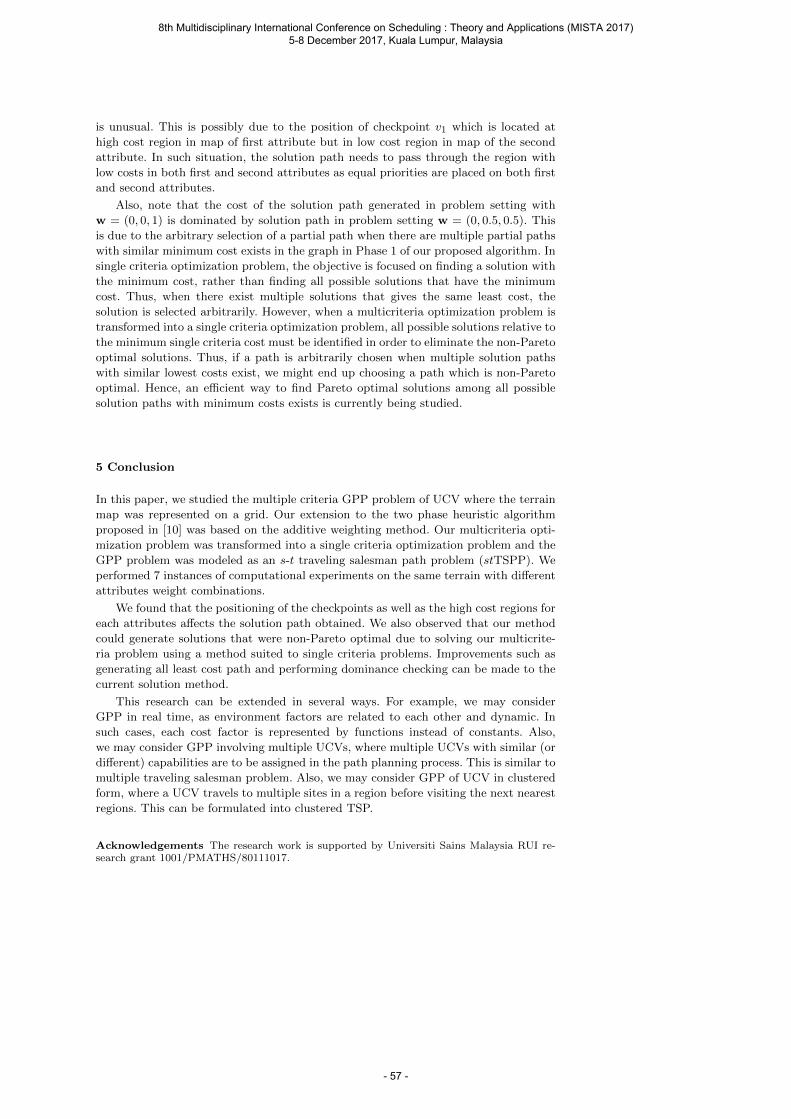
is unusual. This is possibly due to the position of checkpoint v1 which is located at

high cost region in map of first attribute but in low cost region in map of the second

attribute. In such situation, the solution path needs to pass through the region with

low costs in both first and second attributes as equal priorities are placed on both first

and second attributes.

Also, note that the cost of the solution path generated in problem setting with

w = (0, 0, 1) is dominated by solution path in problem setting w = (0, 0.5, 0.5). This

is due to the arbitrary selection of a partial path when there are multiple partial paths

with similar minimum cost exists in the graph in Phase 1 of our proposed algorithm. In

single criteria optimization problem, the objective is focused on finding a solution with

the minimum cost, rather than finding all possible solutions that have the minimum

cost. Thus, when there exist multiple solutions that gives the same least cost, the

solution is selected arbitrarily. However, when a multicriteria optimization problem is

transformed into a single criteria optimization problem, all possible solutions relative to

the minimum single criteria cost must be identified in order to eliminate the non-Pareto

optimal solutions. Thus, if a path is arbitrarily chosen when multiple solution paths

with similar lowest costs exist, we might end up choosing a path which is non-Pareto

optimal. Hence, an efficient way to find Pareto optimal solutions among all possible

solution paths with minimum costs exists is currently being studied.

5 Conclusion

In this paper, we studied the multiple criteria GPP problem of UCV where the terrain

map was represented on a grid. Our extension to the two phase heuristic algorithm

proposed in [10] was based on the additive weighting method. Our multicriteria opti-

mization problem was transformed into a single criteria optimization problem and the

GPP problem was modeled as an s-t traveling salesman path problem (stTSPP). We

performed 7 instances of computational experiments on the same terrain with different

attributes weight combinations.

We found that the positioning of the checkpoints as well as the high cost regions for

each attributes affects the solution path obtained. We also observed that our method

could generate solutions that were non-Pareto optimal due to solving our multicrite-

ria problem using a method suited to single criteria problems. Improvements such as

generating all least cost path and performing dominance checking can be made to the

current solution method.

This research can be extended in several ways. For example, we may consider

GPP in real time, as environment factors are related to each other and dynamic. In

such cases, each cost factor is represented by functions instead of constants. Also,

we may consider GPP involving multiple UCVs, where multiple UCVs with similar (or

different) capabilities are to be assigned in the path planning process. This is similar to

multiple traveling salesman problem. Also, we may consider GPP of UCV in clustered

form, where a UCV travels to multiple sites in a region before visiting the next nearest

regions. This can be formulated into clustered TSP.

Acknowledgements The research work is supported by Universiti Sains Malaysia RUI re-search grant 1001/PMATHS/80111017.


- 57 -

References

1. Bae, K. Y., Kim, Y. D., and Han, J. H. (2015). Finding a risk-constrained shortest pathfor an unmanned combat vehicle, Computers & Industrial Engineering, Vol. 80, 245-253.

2. Christofides, N. (1976) Worst-case analysis of a new heuristic for the travelling salesmanproblem. Management Science Research Report No. 388. Carnegie-Mellon University Pitts-burgh.

3. Giesbrecht, J. (2004). Global path planning for unmanned ground vehicles. No. DRDC-TM-2004-272. Defence Research and Development Suffield (Alberta).

4. Han, D. H., Kim, Y. D., and Lee, J. Y. (2014). Multiple-criterion shortest path algorithmsfor global path planning of unmanned combat vehicles, Computers & Industrial Engineering,Vol. 71, pg 57-69.

5. He, F., Qi, H., Fan, Q. (2007). An evolutionary algorithm for the multi-objective shortestpath problem. International Conference on International Systems and Knowledge Engineer-ing proceedings.

6. Kai, A., Mingrui, X. (2012). A Simple Algorithm for Solving Travelling Salesman Prob-lem. 2012 Second International Conference on Instrumentation & Measurement, Computer,Communication and Control, pg 931-935. IEEE.

7. Kuby, M., Araz, O. M., Palmer, M., Capar, I. (2014). An efficient online mapping toolfor finding the shortest feasible path for alternative-fuel vehicles. International Journal ofHydrogen Energy, Vol. 39(32), pg 18433-18439.

8. Lee, H. J., Lee, Y. I., Park, Y. W. (2009). User Interface for Unmanned Combat VehicleBased on Mission Planning and Global Path Planning. Journal of the Korea Institute ofMilitary Science and Technology, Vol. 12(6), pg 689-696.

9. Nilsson, C. (2003). Heuristics for the Traveling Salesman Problem. Linkoping University.10. Saw, V., Amirah, R., Ong, W. E. (2017). Shortest path problem on a grid network with

unordered intermediate points. Journal of Physics: Conference Series Vol. 893, 012066.11. Shetty, V. K., Sudit, M., Nagi, R. (2008). Priority-based assignment and routing of a

fleet of unmanned combat aerial vehicles. Computers & Operations Research, Vol. 35(6), pg1813-1828.

12. Xiaofeng, L., Zhongren, P., Zhang, L., Li, L. (2012). Unmanned aerial vehicle route plan-ning for traffic information collection. Journal of Transportation Systems Engineering andInformation Technology, Vol. 12(1), pg 91-97.


- 58 -

MISTA 2017

Optimal Interdiction of Vehicle Routing on a DynamicNetwork

Maximilian Moll · Stefan Pickl · Manon Raap ·Martin Zsifkovits

Abstract Network interdiction problems are often defined on a network with instantaneousflow. In vehicle routing applications, however, the flow is time dependent instead of instan-taneous. Moreover, the properties of a transportation network are likely to vary over timeand, hence, such a network is dynamic. In this work, we consider the extension of a staticnetwork interdiction problem to a dynamic network. To solve this problem, we propose anefficient solution by means of complementary slackness constraints, a reformulation of thedynamic network to a static time-expanded network, and finally a linearization of compli-cating non-convex constrains. The result consists of a mixed integer linear programmingformulation. We show the applicability of this method in a computational experiment withtwo small but significant examples.

1 Introduction

We consider a Stackelberg game on a dynamic network, in which the player moving firsttries to reduce capacities on edges to best miminize the obtainable profit of the secondmoving player, who tries to maximize profit, by solving a min-cost-flow problem. The lattercan be seen as model for a company, who can choose to deliver goods to various distributionpoints up to a certain demand from various sources. The network under consideration isdynamic in the sense that edge traversal times and costs are variant and the reward obtainedby delivering commodities is time dependent, such that e.g. late delivery is penalized. It

Maximilian MollUniversity der Bundeswehr, MunichE-mail: [email protected]

Stefan PicklUniversity der Bundeswehr, MunichE-mail: [email protected]

Manon RaapUniversity der Bundeswehr, MunichE-mail: [email protected]

Martin ZsifkovitsUniversity der Bundeswehr, MunichE-mail: [email protected]


- 59 -

should be noted, that the we assume that for each destination there is only one commodity,making it essentially a single commodity problem. In this paper we do not assume an upper-bound on the number of vehicles that would be required to implement the optimal solutionobtained, but this extension could be made without too much work. This is an extension ofthe static network interdiction problem [1] to a dynamic network with time horizon T .

The problem of optimal routing of a fleet of transportation vehicles has been first pro-posed in an abstract manner by Ford and Fulkerson [2] as the maximal flow through a net-work. The following approaches for the interdiction of such a flow exist: Wood [3] showsthat the problem is NP-complete and proposes integer models for variations of the problemon a static network. Israeli and Wood [4] propose a mixed integer programming formulationto maximize the shortest path from a source to a sink and develop more efficient decompo-sition algorithms, e.g. an enhanced Benders’ decomposition method. Royset and Wood [5]consider a bi-objective version of the problem: minimizing total interdiction cost and mini-mizing maximum flow. They propose a branch-and-bound method exploiting Lagrangian re-laxation for solving the problem. Wood [6] provides an overview of basic theoretical modelsand solution techniques for bilevel network interdiction. The problem extension of optimalinterdiction of a flow on a dynamic network has been studied in the following works. Lun-day and Sherali [7] propose a mixed integer non-linear problem formulation for a dynamicnetwork interdiction problem that can be solved directly using a commercial solver or by aproposed heuristic. Szeto and Lo [8] consider time variant network properties and proposemodels and algorithms applied to not only flow interdiction games but to an entire classof Stackelberg games on networks. Rad and Kakhki [9] consider the problem with varianttraversal times for each edge. They present a new formulation based on the concept of Tem-porally Repeated Flow to interrupt the flow of a single commodity and solve the problemusing a Benders’ decomposition approach.

In this work, we assume a fleet of vehicles to transport multiple commodities on a net-work with variant edge traversal times and time dependent delivery rewards. The proposedmethod for optimal interdiction consists of a mixed integer linear program, which can besolved efficiently using a commercial solver. It is easy to implement as the need for de-composition algorithms is omitted. Furthermore, optimal solutions are found as opposed toheuristic solution methods.

The remainder of this paper is structured as follows. First, a formal description of theproblem is given in section 2. The proposed method for optimal flow interdiction on a dy-namic network is then presented in section 3. Computational experiments are described insection 4 and, finally, this paper is concluded in section 5.


Let T= 1, . . . ,T be the makespan defined by T . The dynamic networkN =(V,V+,V−,E,w,τ,d,c,r) consists of the directed graph (V,E), capacities wi j ≥ 0,(i, j)∈E, a transit times τi j ∈ T,(i, j) ∈ E, demands di ≥ 0, i ∈ V+, costs at each time ci j(t) ≥0,(i, j)∈ E, t ∈T, and rewards at each time ri(t)≥ 0, i∈V+, t ∈T. Here V− ⊂V is the set ofpossible source nodes and V+⊂V the set of sink nodes. Intermediate nodes are referred to byV∗ = V \ (V−∪V+). We aim to find an optimal interdiction plan qi j(t) ∈ N,(i, j) ∈ E, t ∈ Tthat minimizes the maximally obtainable profit, i.e. the difference of the sums of rewardsand costs. The latter is the solution to the min-cost-flow problem from sinks to sources, re-stricted by capacities and demand and subject to costs and rewards. Here, an interdictionplan indicates the amount by which the capacities wi j are reduced on each edge and at each


- 60 -

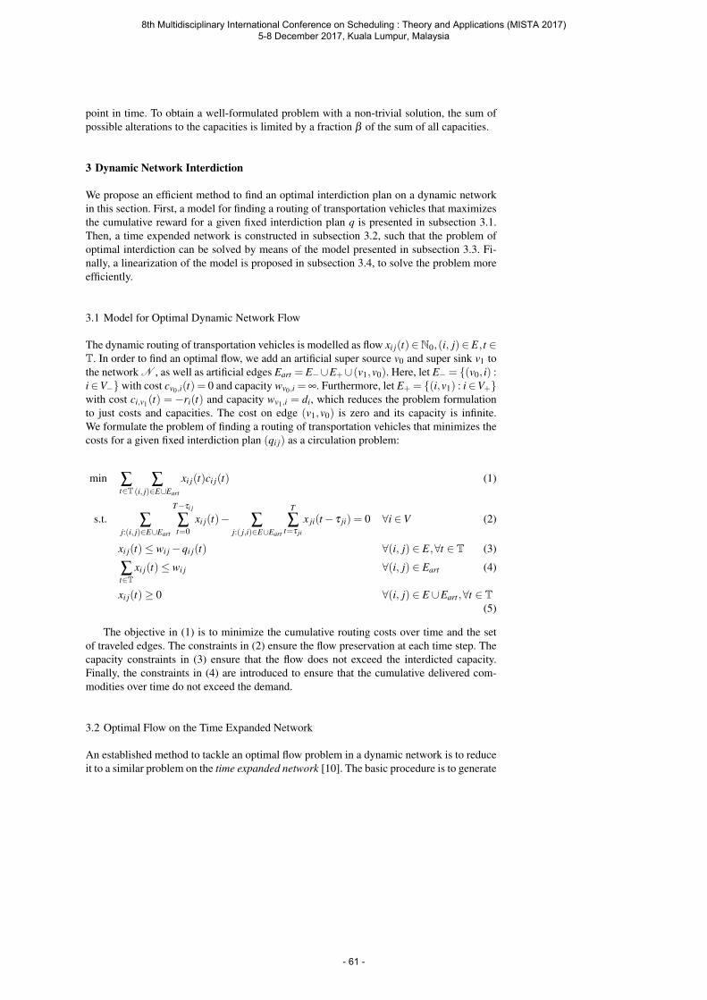
point in time. To obtain a well-formulated problem with a non-trivial solution, the sum ofpossible alterations to the capacities is limited by a fraction β of the sum of all capacities.

3 Dynamic Network Interdiction

We propose an efficient method to find an optimal interdiction plan on a dynamic networkin this section. First, a model for finding a routing of transportation vehicles that maximizesthe cumulative reward for a given fixed interdiction plan q is presented in subsection 3.1.Then, a time expended network is constructed in subsection 3.2, such that the problem ofoptimal interdiction can be solved by means of the model presented in subsection 3.3. Fi-nally, a linearization of the model is proposed in subsection 3.4, to solve the problem moreefficiently.

3.1 Model for Optimal Dynamic Network Flow

The dynamic routing of transportation vehicles is modelled as flow xi j(t)∈N0,(i, j)∈ E, t ∈T. In order to find an optimal flow, we add an artificial super source v0 and super sink v1 tothe network N , as well as artificial edges Eart = E−∪E+∪(v1,v0). Here, let E− = (v0, i) :i∈V− with cost cv0,i(t) = 0 and capacity wv0,i = ∞. Furthermore, let E+ = (i,v1) : i∈V+with cost ci,v1(t) = −ri(t) and capacity wv1,i = di, which reduces the problem formulationto just costs and capacities. The cost on edge (v1,v0) is zero and its capacity is infinite.We formulate the problem of finding a routing of transportation vehicles that minimizes thecosts for a given fixed interdiction plan (qi j) as a circulation problem:

min ∑t∈T

∑(i, j)∈E∪Eart

xi j(t)ci j(t) (1)

s.t. ∑j:(i, j)∈E∪Eart

T−τi j

∑t=0

xi j(t)− ∑j:( j,i)∈E∪Eart

T

∑t=τ ji

x ji(t− τ ji) = 0 ∀i ∈V (2)

xi j(t)≤ wi j−qi j(t) ∀(i, j) ∈ E,∀t ∈ T (3)

∑t∈T

xi j(t)≤ wi j ∀(i, j) ∈ Eart (4)

xi j(t)≥ 0 ∀(i, j) ∈ E ∪Eart ,∀t ∈ T(5)

The objective in (1) is to minimize the cumulative routing costs over time and the setof traveled edges. The constraints in (2) ensure the flow preservation at each time step. Thecapacity constraints in (3) ensure that the flow does not exceed the interdicted capacity.Finally, the constraints in (4) are introduced to ensure that the cumulative delivered com-modities over time do not exceed the demand.

3.2 Optimal Flow on the Time Expanded Network

An established method to tackle an optimal flow problem in a dynamic network is to reduceit to a similar problem on the time expanded network [10]. The basic procedure is to generate


- 61 -

replica of each node for all time steps and connect the edges according to E and τ; this isnot done for v0 and v1. Furthermore, extra care needs to be taken when treating the nodes inV+. While they are replicated for each timestep as well, a new set of nodes V T

1+ needs to begenerated, which in essence is a copy of V+, where we denote the new node correspondingto i ∈V+ by v1i ∈V T

1+. Edges are added between it ∈V T+ and v1i ∈V T

1+ with cit ,v1i =−ri(t),wit ,v1i = ∞, and between v1i ∈V T

1+ and v1 with cv1i,v1 = 0, wv1i,v1 = di. This ensures that thedemand remains valid across all time steps, while the reward is time dependent. The timeexpanded network N T is then constructed along the lines presented by [10] as follows:

V T+ := it : i ∈V+, t ∈ T

V T− := it : i ∈V−, t ∈ T

V T∗ := it : i ∈V∗, t ∈ T

vT0 := v0

vT1 := v1

V T1+ :=V1+

V T :=V T+ ∪V T

− ∪V T∗ ∪ vT

0 ∪ vT1 ∪V T

1+wT

i j := wi j for (i, j) ∈ EcT

i j(t) := ci j(t) for (i, j) ∈ E

qTi j(t) := qi j(t) for (i, j) ∈ E

dTi j := di j for (i, j) ∈ Eart

rTi j(t) := ri j(t) for (i, j) ∈ Eart

ET := (it , jt+τi j

),(i, j) ∈ E,0≤ t ≤ T −

τi j∪(it , it+1) : i ∈V,0≤ t < TET− := (v0, it), for it ∈V T

− ET+ := (it ,v1i), for it ∈V T

+ ET

1+ := (it ,v1i), for i ∈V T+

ETart := ET

− ∪ET+ ∪ (v1,v0)∪ET

1+

The optimal flow circulation problem on the time expanded network is then formulatedas:

min ∑(i, j)∈ET ∪ET

art

xi jcTi j (6)

s.t. ∑(i, j)∈E∪ET

art

xi j− ∑( j,i)∈ET ∪ET

art

x ji = 0 ∀i ∈V T (7)

xi j ≤ wTi j −qT

i j ∀(i, j) ∈ ET (8)

xi j ≤ wTi j ∀(i, j) ∈ ET

art (9)

xi j ≥ 0 ∀(i, j) ∈ ET ∪ETart (10)

This problem formulation is very similar to the formulation for the problem on the dynamicnetwork (1)-(5). The single difference is that the time component can be omitted and weyield exactly the formulation as presented by [1] for the problem on a static network. In thenext subsection, we drop the invariably of the interdiction plan qT and present a model thatyields an optimal interdiction plan.

3.3 Model for Dynamic Network Interdiction

First, associate dual variables λ = λi : i ∈ V T with the constraints in (7), dual variablesµ = µi j : (i, j) ∈ ET ∪ET

art with the constraints in (8) and (9). Furthermore, add slackvariables z(1)i j to the left hand side of each constraint in (8) and (9) to bring (6)-(10) in stan-dard form. By formulation of the dual of (6)-(10) as presented by [1] and by complementaryslackness, the constraints (12)-(17) are the optimality conditions for x,λ and µ . Hence, afeasible solution x,λ and µ that maximizes the profit of the fleet is optimal if these condi-tions hold. An optimal interdiction plan can then be obtained by solving the following mixedinteger nonlinear program (MINLP):


- 62 -

max ∑(i, j)∈ET ∪ET

art

xi jcTi j (11)

s.t. ∑(i, j)∈E∪ET

art


art

x ji = 0 ∀i ∈V T (12)

xi j + z(1)i j = wTi j −qi j ∀(i, j) ∈ ET (13)

xi j + z(1)i j = wTi j ∀(i, j) ∈ ET

art (14)

λi−λ j +µi j + z(2)i j = cTi j ∀(i, j) ∈ ET ∪ET

art (15)

µi jz(1)i j = 0 ∀(i, j) ∈ ET ∪ET

art (16)

xi jz(2)i j = 0 ∀(i, j) ∈ ET ∪ET

art (17)

∑(i, j)∈ET

qi j ≤ β ∑(i, j)∈ET

wTi j (18)

xi j,z(1)i j ,z(2)i j ≥ 0 ∀(i, j) ∈ ET ∪ET

art (19)

µi j ≤ 0 ∀(i, j) ∈ ET ∪ETart (20)

λi ∈ R ∀i ∈V T (21)

qi j ∈ N0 ∀(i, j) ∈ ET (22)

Here, the objective (11) is to minimize the profit of the fleet. Constraints (12)-(17) are theoptimality conditions that ensure that the flow x is indeed the optimal response of the fleetto the interdiction plan q. Constraint (18) ensures that the total interdiction does not exceeda given fraction β of the cumulative network capacity.

It should be noted that in this formulation wTi j and qi j have to be interpreted as being

checked when entering the edge at the given time, not as being valid at this point in timefor the entire flow on the edge. If that were the intention, constraint (14) would need to bereplaced by

τi j−1

∑s=0

xi j(t− s)+ z(1)i j = wTi j −qi j ∀(i, j) ∈ ET ,

and constraint (15) would need to be adjusted accordingly.

3.4 Optimal Dynamic Network Interdiction

A mixed integer non-linear problem is difficult to solve in general. To solve the MINLP in(11)-(22) more efficiently, we propose a new formulation containing only linear constraints.The two sets of constraints in (16) and (17) are the quadratic constraints which will bereplaced by a total of six linear sets of constraints. To this end, four binary auxiliary decisionvariables ai j,a′i j,a

′′i j,a

′′′i j ∈ 0,1 are introduced. The derivation of the linear constraints is

explained in detail by [1]. The two original quadratic constraints are replaced by the sixresulting linear constraints in (28)-(33) in the following mixed integer linear programming(MILP) formulation:

max ∑(i, j)∈ET ∪ET

art

xi jcTi j (23)


- 63 -

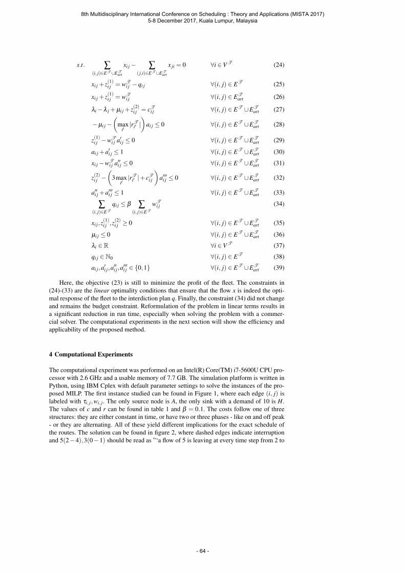
s.t. ∑(i, j)∈ET ∪ET

art


art

x ji = 0 ∀i ∈V T (24)

xi j + z(1)i j = wTi j −qi j ∀(i, j) ∈ ET (25)

xi j + z(1)i j = wTi j ∀(i, j) ∈ ET

art (26)

λi−λ j +µi j + z(2)i j = cTi j ∀(i, j) ∈ ET ∪ET

art (27)

−µi j−(

maxi′|rT

i′ |)

ai j ≤ 0 ∀(i, j) ∈ ET ∪ETart (28)

z(1)i j −wTi j a′i j ≤ 0 ∀(i, j) ∈ ET ∪ET

art (29)

ai j +a′i j ≤ 1 ∀(i, j) ∈ ET ∪ETart (30)

xi j−wTi j a′′i j ≤ 0 ∀(i, j) ∈ ET ∪ET

art (31)

z(2)i j −(

3maxi′|rT

i′ |+ cTi j

)a′′′i j ≤ 0 ∀(i, j) ∈ ET ∪ET

art (32)

a′′i j +a′′′i j ≤ 1 ∀(i, j) ∈ ET ∪ETart (33)

∑(i, j)∈ET

qi j ≤ β ∑(i, j)∈ET

wTi j (34)

xi j,z(1)i j ,z(2)i j ≥ 0 ∀(i, j) ∈ ET ∪ET

art (35)

µi j ≤ 0 ∀(i, j) ∈ ET ∪ETart (36)

λi ∈ R ∀i ∈V T (37)

qi j ∈ N0 ∀(i, j) ∈ ET (38)

ai j,a′i j,a′′i j,a

′′′i j ∈ 0,1 ∀(i, j) ∈ ET ∪ET

art (39)

Here, the objective (23) is still to minimize the profit of the fleet. The constraints in(24)-(33) are the linear optimality conditions that ensure that the flow x is indeed the opti-mal response of the fleet to the interdiction plan q. Finally, the constraint (34) did not changeand remains the budget constraint. Reformulation of the problem in linear terms results ina significant reduction in run time, especially when solving the problem with a commer-cial solver. The computational experiments in the next section will show the efficiency andapplicability of the proposed method.

4 Computational Experiments

The computational experiment was performed on an Intel(R) Core(TM) i7-5600U CPU pro-cessor with 2.6 GHz and a usable memory of 7.7 GB. The simulation platform is written inPython, using IBM Cplex with default parameter settings to solve the instances of the pro-posed MILP. The first instance studied can be found in Figure 1, where each edge (i, j) islabeled with τi, j,wi, j. The only source node is A, the only sink with a demand of 10 is H.The values of c and r can be found in table 1 and β = 0.1. The costs follow one of threestructures: they are either constant in time, or have two or three phases - like on and off peak- or they are alternating. All of these yield different implications for the exact schedule ofthe routes. The solution can be found in figure 2, where dashed edges indicate interruptionand 5(2−4),3(0−1) should be read as ”‘a flow of 5 is leaving at every time step from 2 to


- 64 -

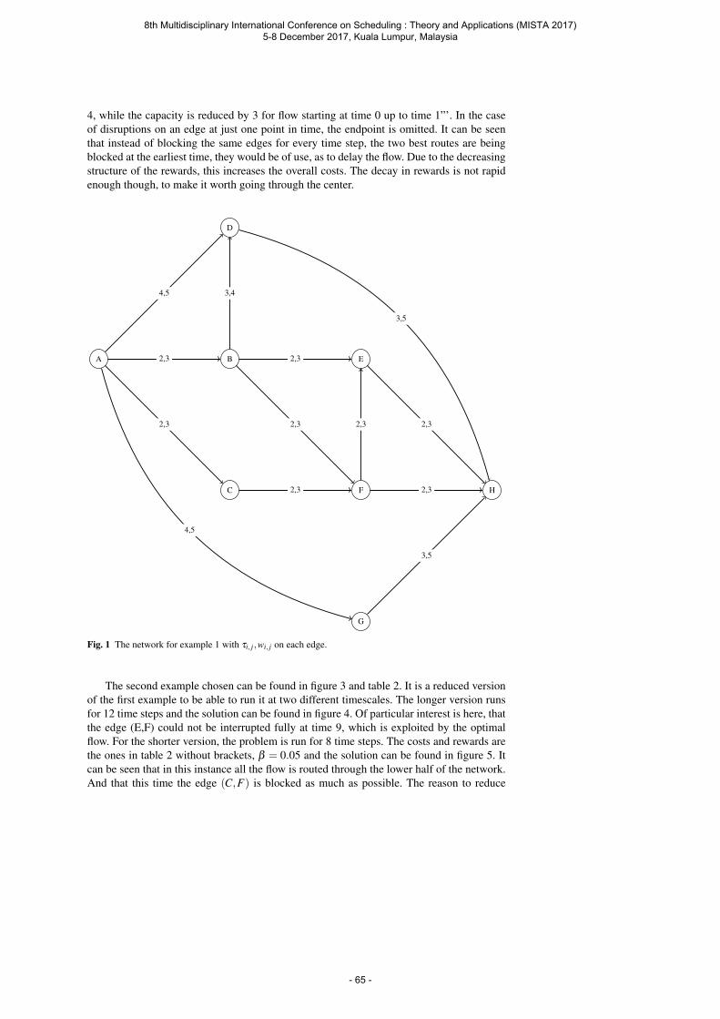
4, while the capacity is reduced by 3 for flow starting at time 0 up to time 1”’. In the caseof disruptions on an edge at just one point in time, the endpoint is omitted. It can be seenthat instead of blocking the same edges for every time step, the two best routes are beingblocked at the earliest time, they would be of use, as to delay the flow. Due to the decreasingstructure of the rewards, this increases the overall costs. The decay in rewards is not rapidenough though, to make it worth going through the center.

A B

C

D

E

F

G

H

2,3

2,3

4,5 3,4

2,3

2,3

2,3

2,32,3

2,3

3,5

3,5

4,5

Fig. 1 The network for example 1 with τi, j,wi, j on each edge.

The second example chosen can be found in figure 3 and table 2. It is a reduced versionof the first example to be able to run it at two different timescales. The longer version runsfor 12 time steps and the solution can be found in figure 4. Of particular interest is here, thatthe edge (E,F) could not be interrupted fully at time 9, which is exploited by the optimalflow. For the shorter version, the problem is run for 8 time steps. The costs and rewards arethe ones in table 2 without brackets, β = 0.05 and the solution can be found in figure 5. Itcan be seen that in this instance all the flow is routed through the lower half of the network.And that this time the edge (C,F) is blocked as much as possible. The reason to reduce


- 65 -

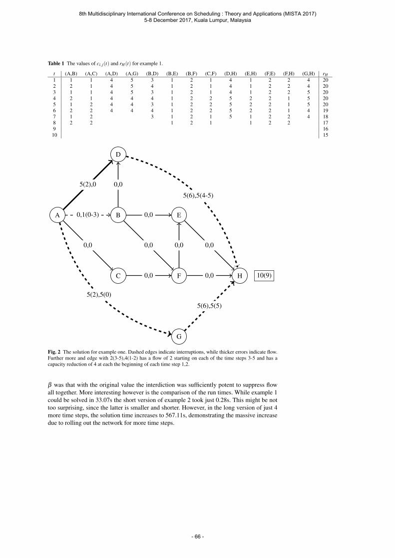
Table 1 The values of ci, j(t) and rH(t) for example 1.

t (A,B) (A,C) (A,D) (A,G) (B,D) (B,E) (B,F) (C,F) (D,H) (E,H) (F,E) (F,H) (G,H) rH1 1 1 4 5 3 1 2 1 4 1 2 2 4 202 2 1 4 5 4 1 2 1 4 1 2 2 4 203 1 1 4 5 3 1 2 1 4 1 2 2 5 204 2 1 4 4 4 1 2 2 5 2 2 1 5 205 1 2 4 4 3 1 2 2 5 2 2 1 5 206 2 2 4 4 4 1 2 2 5 2 2 1 4 197 1 2 3 1 2 1 5 1 2 2 4 188 2 2 1 2 1 1 2 2 179 1610 15

A B

C

D

E

F

G

H

0,1(0-3)

0,0

5(2),0 0,0

0,0

0,0

0,0

0,00,0

0,0

5(6),5(5)

5(6),5(4-5)

5(2),5(0)

10(9)

Fig. 2 The solution for example one. Dashed edges indicate interruptions, while thicker errors indicate flow.Further more and edge with 2(3-5),4(1-2) has a flow of 2 starting on each of the time steps 3-5 and has acapacity reduction of 4 at each the beginning of each time step 1,2.

β was that with the original value the interdiction was sufficiently potent to suppress flowall together. More interesting however is the comparison of the run times. While example 1could be solved in 33.07s the short version of example 2 took just 0.28s. This might be nottoo surprising, since the latter is smaller and shorter. However, in the long version of just 4more time steps, the solution time increases to 567.11s, demonstrating the massive increasedue to rolling out the network for more time steps.


- 66 -

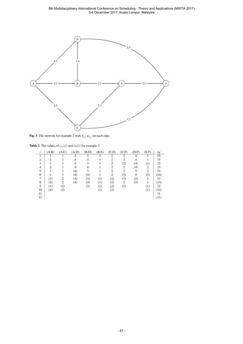
A B

C

D

E F2,3

2,3

4,5 3,4

2,3

2,3

2,3

4,5

3,2

Fig. 3 The network for example 2 with τi, j,wi, j on each edge.

Table 2 The values of ci, j(t) and rH(t) for example 2.

t (A,B) (A,C) (A,D) (B,D) (B,E) (C,E) (C,F) (D,F) (E,F) rH1 1 1 4 3 1 2 2 4 1 152 2 1 4 4 1 2 2 4 1 153 1 1 4 3 1 2 (2) (4) (1) 154 2 1 4 4 1 2 3 (4) 2 155 1 1 (4) 3 1 2 3 5 2 146 2 1 (4) (4) 1 2 (3) 5 (2) (14)7 (1) 2 (4) (3) (1) (2) (3) (5) 1 138 (2) 2 (4) (4) (1) (2) 2 (5) 1 (13)9 (1) (2) (3) (1) (2) (2) (1) 1210 (2) (2) (1) (2) (1) (12)11 1112 (11)


- 67 -

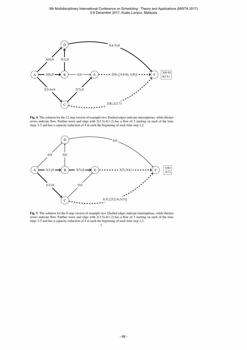
A B

C

D

E F3(0),0

2(5-6),0

3(0),0 3(2),0

0,0

2(7),0

2(9),3(4-8), 1(9)

3(4-5),0

2(8),2(2-7)

3(8-9)4(11)

Fig. 4 The solution for the 12 step version of example two. Dashed edges indicate interruptions, while thickererrors indicate flow. Further more and edge with 2(3-5),4(1-2) has a flow of 2 starting on each of the timesteps 3-5 and has a capacity reduction of 4 at each the beginning of each time step 1,2.

A B

C

D

E F3(1),0

1(1),0

0,0 0,0

3(3),0

0,0

3(5),3(4)

0,0

1(3),2(2,4),1(3)

1(6)3(7)

Fig. 5 The solution for the 8 step version of example two. Dashed edges indicate interruptions, while thickererrors indicate flow. Further more and edge with 2(3-5),4(1-2) has a flow of 2 starting on each of the timesteps 3-5 and has a capacity reduction of 4 at each the beginning of each time step 1,2.

s


- 68 -

5 Conclusion

In this paper we have extended our previous work on network interdiction by making theunderlying network dynamic. In order to be able to transfer the approach, the network isbeing rolled out in time first, to obtain a static network again. The experiments not onlyshow, that this approach works, but also demonstrate that this procedure incurs a rather highcomputational cost.

Future work should focus on finding a more efficient way to find the solution in problemswith larger time horizons to make this approach more relevant to practical applications. Thiscould go several ways. If the considered time frame is for example much longer than thelongest time it takes from any source to any sink, then the problem could be decomposed toa set of potentially overlapping episodes of shorter length. Another option would be to tryto exploit this kind of symmetry by decomposition methods. Finally, it can be consideredto try a completely different approach like dynamic programming or some form of hybridmethod.

References

1. M. Raap, M. Moll, S. Pickl, in Sustainable Logistics and Transportation: Optimization Models andAlgorithms, ed. by D.D. Cinar, D.K. Gakis, D.P.P.M. Pardalos (Springer, 2017). (In press)

2. L.R. Ford, D.R. Fulkerson, Canadian journal of Mathematics 8(3), 399 (1956)3. R.K. Wood, Mathematical and Computer Modelling 17(2), 1 (1993)4. E. Israeli, R.K. Wood, Networks 40(2), 97 (2002)5. J.O. Royset, R.K. Wood, INFORMS Journal on Computing 19(2), 175 (2007)6. R.K. Wood, Wiley Encyclopedia of Operations Research and Management Science (2011)7. B.J. Lunday, H.D. Sherali, Informatica 21(4), 553 (2010)8. W.Y. Szeto, H.K. Lo, Transportation Research Part A: Policy and Practice 42(2), 376 (2008)9. M.A. Rad, H.T. Kakhki, Computers & Industrial Engineering 65(4), 531 (2013)

10. D. Lozovanu, D. Stratila, in Analysis and optimization of differential systems (Springer, 2003), pp. 247–258


- 69 -

MISTA

2017

Evolving Adaptive Evolutionary Algorithms

Ayman Srour • Patrick De Causmaecker.

Abstract This paper presents a Grammatical Evolution framework for the automatic design of

Adaptive Evolutionary Algorithms. The grammar adopted by this framework can generate a

novel adaptive parameter control strategy, aiming to evolve the design of evolutionary

algorithms. The Travelling Salesman Problem is used to investigate the potential of the proposed

framework to evolve the adaptive evolutionary algorithms. Results show that the proposed

framework is capable of not only generating new adaptive evolutionary algorithms but also

confirms that automating the design of adaptive evolutionary algorithm can outperform the

standard evolutionary algorithm.

1 Introduction

Evolutionary Algorithms (EAs), as there are genetic algorithms, genetic programming and

evolution strategy based methods, are general population-based metaheuristics inspired by

biological evolution and natural selection [1]. When applying EAs to optimization problems

many different parameter configurations have to be set to achieve optimal performance. The

choice of different genetic operators and their relative rates is usually based on experience. It

has been argued that different parameter values may be optimal at different optimization stages

[2-4], which makes the current research more focused on tackling the issue by using adaptive

parameter control. Adaptive Parameter Control (APC) is used to tune the parameters in an online

manner and during the algorithm execution by considering feedback from an EA run - such as

solution quality- to monitor the algorithm performance and adjust the parameter values for future

iterations.

Recently, EA parameter control has been widely studied, and many of APC methods have

been proposed in the literature [5, 6]. The variation in these methods (regarding its performance

and structure) makes the choice of suitable APC methods for a specific problem or instance non-

trivial, as there exists no general optimal APC method for EAs. As a consequence, for EAs, the


- 70 -

optimal APC method can considerably vary depending on the problem or instance at hand. Some

of the previous work ([7] and [8]) tried to combine different APC methods to improve EA

performance. Several alternative combinations of APC methods remain unexplored. In the

context of EAs, reference [6] has presented a vital survey of parameter control methods. The

authors concluded that more research on the combination of different control mechanisms could

be performed and that developing a generic framework for APC could be helpful.

Reference [5] proposes a generic model of the state-of-the-art APC methods based on a

comprehensive review of the literature. The authors distinguish between the optimization

process and the control process of the Adaptive Evolutionary Algorithms (AdEA). The control

process is further divided into four components, namely, feedback collection, effect assessment,

quality attribution, and selection (see section II-A). Each component represents a stage of the

parameter control accompanying with several possible adaptive strategies for each stage.

Considering this model, the architecture of every AdEA can be mapped into the four

components. Thus, a complete design on any AdEA should have at least one strategy for each

component, and each strategy can be implemented by using one of many predefined rules or

methods. In fact, we can use the model to facilitate the design of any new AdEA, but it is still

time-consuming to perform this task manually. Several non-trivial selections or combinations of

the most suitable variants of strategies (and so its rules) are needed to optimally specify each

component with respect to the problem at hand.

In recent years, several automatic designs of the algorithm were presented to overcome this

limitation. Reported in literature, a range of approaches are used to automate the algorithm

design. An example of automatic design, Grammatical Evolution (GE) has been used to evolve

an algorithm such as presented by [9] for evolving data mining algorithms, and [10] used GE for

evolving new local search algorithms for the bin-baking problem. More recently, GE has been

used to evolve the design of EAs for solving Royal Road Functions [11], Integration and Test

Order problems [12].

In this paper, we propose a Grammatical Evolution framework to evolve the design of

AdEA. GE automates the design of AdEA by defining a grammar guiding the selection of an

APC strategy for different EA parameters and defining the corresponding implementations. The

main aim of the automatic design of AdEA is to surrogate the human design leading to significant

performance improvement. We introduced a set of experiments to examine the evolved AdEAs

for solving the Traveling Salesman Problem (TSP).

The structure of the paper is as follows: section 2 presents related work of AdEA and the

automatic design of algorithms. In section 3 we introduce the Grammatical Evolution framework

for Adaptive Evolutionary Algorithms (GE-AdEA) including APC components description and

the grammar definition. Section 4 presents the experimental results and analyses, and finally, the

conclusion and future work are presented in section 5.

2 Background

2.1 Adaptive Parameter Control Design Model

The problem of finding optimal parameter configuration for an algorithm is a nontrivial

optimization problem. Currently, the study of techniques for automatic parameter tuning is an

active research area [5, 6, 13, 14]. One distinguishes parameter tuning and parameter control

[14]. The former assigns parameter values before algorithm execution, while the latter decides

on optimal parameter values during algorithm execution. According to [14], parameter control

can be further classified into deterministic, adaptive and self-adaptive. Deterministic parameter

control means the parameter value is assigned based on deterministic rules without further


- 71 -

knowledge about the search progress. Self-adaptive parameter control combines the search of

optimal parameter values with the solution search, i.e., encodes the parameter values in the

genome to enable them to co-evolve with the solutions. According to [5], APC separates the

search for optimal parameter values from the solution search, monitors algorithm properties

during the optimization process and adjusts the parameter values accordingly. The set of

algorithm parameters that need to be tuned can be formulated as a 𝑃 = 𝑣1, 𝑣2, . . , 𝑣𝑛, where 𝑛

denotes to the parameter numbers. Each 𝑣𝑖 has a set of values 𝑣𝑖 = 𝑣𝑖1, 𝑣𝑖2 , . . , 𝑣𝑖𝑚 that could

be either a discrete number or intervals continues numbers. Note that 𝑚 refers to the number of

values associated with each parameter 𝑣𝑖. For example, assume that 𝑣𝑖 represents a crossover

parameter in EA, then the value 𝑣𝑖1could be the single point crossover and the value 𝑣𝑖2 could

be the uniform crossover. However, the parameter control aims to find the best next parameter

value 𝑣𝑖𝑗 to optimize algorithm performance.

Over the past two decades, a wide variety of APC has been proposed with several

adaptation strategies. A comprehensive study of the research direction of parameter control

methods has been shown a significant number of research conducted in the field in the recent

years [5, 6, 15, 16]. In the context of EA, more sophisticated literature reviews, such as [5, 17],

have focused on studying the design structure of the existing APC methods and tried to

decompose the APC process into several elements or components. The components that play a

role to generalize the design strategies of the most existing APC methods. Corriveau et al. 2016

[17] divides the adaptive parameter control process in EA into four essential elements, namely,

parameters involved (the type and states of the parameters involved), feedback indicators (used

to evaluate the impact of the current state of the involved parameters), credit assignment schemes

(used to convert feedback information into a suitable reward) and parameter selection rules (used

to update parameter states).

Aleti et al. 2015 [5].proposed a more sophisticated and comprehensive conceptual

model of APC which also consists of four main components. Fig. 1 illustrates the general

algorithmic flow and components involved in the AdEA [5]. The algorithm starts with a

population (initial solutions). This population is evolving during algorithm execution until the

stopping criterion is reached. The EA parameters, such as population size, genetic operators and

the probabilities of performing of the genetic operators, the number of offspring, etc., can be

adjusted by the parameter control methods. At each cycle in the optimization process, the

generated solutions are evaluated by using the fitness function(s), which provides valuable

information about the algorithm performance as a feedback to guide the parameter control

method. The feedback information can be used by effect assessment strategy to assess the cause

of a change of the properties of the solutions during the run by measuring the effects of each

parameter values on the algorithm performance. The vector of all parameter effects can be

defined as 𝑒 = 𝑒(𝑣11), 𝑒(𝑣12), … , 𝑒(𝑣1𝑛), … 𝑒(𝑣𝑚𝑛𝑛). The aim is to adapt the vector of

probabilities 𝑝 such that the expected value of the cumulative effect 𝐸[𝑒] = ∑ 𝑒(𝑣𝑖𝑗)𝑛𝑗=1 is

maximized. The information is then used by quality attribution components to estimate the

quality of each parameter value 𝑞(𝑣ij). The vector of quality estimates for all parameter values

is denoted as = 𝑞(𝑣11), 𝑞(𝑣12), … , 𝑞(𝑣1𝑛), … 𝑞(𝑣𝑚𝑛𝑛). However, the selection comment

will use for selecting a good parameter value for future iterations.


- 72 -

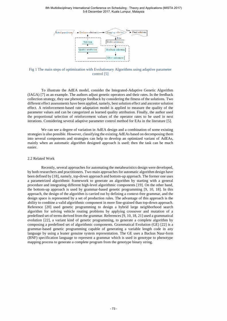
Fig 1 The main steps of optimization with Evolutionary Algorithms using adaptive parameter

control [5]

To illustrate the AdEA model, consider the Integrated-Adaptive Genetic Algorithm

(IAGA) [7] as an example. The authors adjust genetic operators and their rates. In the feedback

collection strategy, they use phenotype feedback by considering the fitness of the solutions. Two

different effect assessments have been applied, namely, best solution effect and ancestor solution

effect. A reinforcement-based rate adaptation model is applied to measure the quality of the

parameter values and can be categorized as learned quality attribution. Finally, the author used

the proportional selection of reinforcement values of the operator rates to be used in next

iterations. Considering several adaptive parameter control method for EAs in the literature [5].

We can see a degree of variation in AdEA design and a combination of some existing

strategies is also possible. However, classifying the existing AdEAs based on decomposing them

into several components and strategies can help to develop an optimized variant of AdEAs,

mainly when an automatic algorithm designed approach is used; then the task can be much

easier.

2.2 Related Work

Recently, several approaches for automating the metaheuristics design were developed,

by both researchers and practitioners. Two main approaches for automatic algorithm design have

been defined by [18], namely, top-down approach and bottom-up approach. The former one uses

a parametrized algorithmic framework to generate an algorithm by starting with a general

procedure and integrating different high-level algorithmic components [19]. On the other hand,

the bottom-up approach is used by grammar-based genetic programming [9, 10, 18]. In this

approach, the design of the algorithm is carried out by defining a context-free grammar, and the

design space is represented by a set of production rules. The advantage of this approach is the

ability to combine a valid algorithmic component in more fine-grained than top-down approach.

Reference [20] used genetic programming to design a hybrid large neighborhood search

algorithm for solving vehicle routing problems by applying crossover and mutation of a

predefined set of terms derived from the grammar. References [9, 10, 18, 21] used a grammatical

evolution [22], a variant kind of genetic programming, to generate a complete algorithm by

composing a predefined set of algorithmic components. Grammatical Evolution (GE) [22] is a

grammar-based genetic programming capable of generating a variable length code in any

language by using a leaner genuine system representation. The GE uses a Backus Naur-form

(BNF) specification language to represent a grammar which is used in genotype to phenotype

mapping process to generate a complete program from the genotype binary string.


- 73 -

3 The Evolutionary Framework

As aforementioned, the EA parameter control has been studied intensively, and many parameter

control approaches have also been proposed recently. The momentum of research in this field is

still increasing because developing a new or applying an existing APC strategy for different

optimization problems is always in demand [5, 6] as literature witnesses the success of AdEAs

in many applications. In fact, developing a robust AdEA leads us to consider several issues such

as the nature of a problem, the difficulty of target instances and the decision which APC strategy

for a specific parameter in AdEA should be adopted, which is, of course, affecting the

performance of the AdEA. All of these issues also make the design of AdEA a difficult task.

The difficulty is because several APC strategies exist today and deciding the optimal among

many alternatives, for a specific problem or even for a specific problem instance, is infeasible

by considering the human design alone. Using an automatic algorithm design is an affordable

alternative approach that not only helps to reduce the difficulty of selecting the best among

several algorithm components but also can help to generate a novel algorithmic design which is

in many cases superior to the standard algorithms.

Recent research work in the literature [11, 12, 23] used the GE framework to evolve

the design of EAs. These focus on automating the design and the tuning of EA parameters

utilizing from the GE grammar to generate EAs with different architectures. In this work, the

idea of using GE to evolve AdEA has been inspired by work presented in [11, 12, 23]. Their

results confirm that GE has a capacity of generating a novel design of EAs with better

performance comparing to human design (standard EA). Therefore, the grammatical evolution

framework GE-AdEA is used to evolve AdEAs by adopting different APC strategies. The

framework is composed of two main components: GE Optimizer (GEO) and AdEA Executor

(AdEA-EX). The task of GE-O is to evolve individuals that encode effective APC strategies for

AdEA, whereas AdEA-EX responsible for executing many possible AdEA architectures based

on the newly generated APC strategies (GE individuals) from GEO. The component is necessary

for evaluating the generated solutions by assigning fitness to each individual by training it on

TSP problem instances.

The GE-O adopts the standard architecture of GE, which consists of a search engine, a

mapper function, and a BNF grammar. GE uses a standard genetic algorithm as its search engine

[22]. The chromosome (genotype) is represented by a variable length binary string, The gene in

each chromosome (so-called codon) has 8-bit binary values which are later decoded into an

integer (in the range between 0 to 28-1). Repeatedly, the integer values produced by a

chromosome can be used to convert all terminal to non-terminal symbols via a mapper function.

The fitness of each chromosome is then evaluated by executing its corresponding program. The

mapper function converts the genotype to phenotype by taking a binary string and BNF grammar

as input and map it to the corresponding program.

The BNF grammar should be defined according to the four adaptive parameter control

components, namely, Feedback Collection (FC), Effect Assessment (EFA), Quality Attribution

(QA) and Selection (SE). The four components have been selected based on the conceptual

model proposed by [5], and are reflecting the actual design of variant APC strategies of AdEA

in the literature. Each of these components has its own set of adaptive parameter control

strategies. These are explained as follows:

1. Feedback collection (FC): the feedback collection provides valuable information

about the algorithm performance as feedback to guide the parameter control method.

This kind of information can be processed in the feedback collection strategy, which

can measure and record a specific property of the algorithm performance during the

execution, such as phenotype/genotype quality and phenotype/genotype diversity. We

have employed several feedback collections methods. The feedback collection that is


- 74 -

used in our framework has been widely used in the literature [5] and is presented in

Table 1. Note that in the proposed framework, we use Phenotype and Genotype

feedback strategies to provide information for adaptive crossover and mutation

operators effect assessment, while the Phenotype and Genotype diversity feedback

strategies are used to control crossover and mutation rates directly.

Table 1 The feedback collection strategies description used in the proposed framework

Feedback

Strategy Description

Phenotype Refers to the fitness function of solutions. The effect assessment will rely on

fitness value differences among solutions, i.e., best, worst average fitness

Genotype Provides feedback information about the solution components (genome

information) of a given solution. We used a Hamming distance to measure the

distance between two solutions as follows:

𝑑𝑖𝑗 = ∑ |𝑖𝑘−𝑗𝑘|𝑛

𝑘=1

Phenotype

diversity

To measure the diversity in the population The population diversity measure

by [24]:

𝑐𝑢𝑟𝑟_𝑣𝑎𝑙 =𝑓𝑏𝑒𝑠𝑡 − 𝑓𝑎𝑣𝑔

𝑓𝑏𝑒𝑠𝑡 − 𝑓𝑤𝑜𝑟𝑠𝑡

,

𝑝𝑟𝑒𝑣_𝑣𝑎𝑙 = 𝑐𝑢𝑟𝑟_𝑣𝑎𝑙, 𝑖𝑓𝑐𝑢𝑟𝑟_𝑣𝑎𝑙 > 𝑝𝑟𝑒𝑣_𝑣𝑎𝑙 𝑢𝑛𝑐ℎ𝑎𝑛𝑐ℎ𝑒 , 𝑒𝑙𝑠𝑒

𝑤 = (𝑐𝑢𝑟𝑟_𝑣𝑎𝑙

𝑝𝑟𝑒𝑣_𝑣𝑎𝑙)

2

,

Where 𝑐𝑢𝑟𝑟_𝑣𝑎𝑙 and 𝑝𝑟𝑒𝑣_𝑣𝑎𝑙 represent the fitness of the current value and

previous value of the best solution, respectively.

If the value of 𝑤 reaches 1.0 that means the solution population is highly

diverse.

Genotype

diversity

To measure the diversity in the solution components over a set of solutions.

The population diversity measured by [26]:

𝑑𝑖𝑋 = √∑ (|𝑖𝑘−𝑏𝑘|)2𝑛

𝑘=1

𝑎𝑣𝑔(𝑑𝑖𝑋) =1

𝑁𝑋

∑ 𝑑𝑖𝑋

𝑁𝑋 is the number of operator applications of type 𝑥. 𝑖 is the current solution

and, 𝑏 is the best solution generated by operator 𝑥

2. Effect Assessment (EFA): The parameter control utilizes the effect assessment

information to determine which parameter values will potentially perform well in future

iterations by using a specific rule. The main difference between the existing effect

assessment methods, however, is how they evaluate the success of parameter values.

For instance, the effect assessment method presented in [25] calculates the effect of the

parameters using quality differences between the generated solutions compared to their

parents, while [26] used the overall best solution and [27] used median. A brief

description of each APC component and its related strategies, adopted from [5], is

presented in Table 2


- 75 -

Table 2 The effect assessment strategies description used in the proposed framework

Effect Assessment

Strategy Description

Ancestor The effect of operator 𝑋𝑖 calculated as :

𝑒𝑖𝑋𝐺 =

𝑓𝑃𝑎𝑟𝑒𝑛𝑡 − 𝑓𝑐𝑗 , 𝑖𝑓 𝑓𝑃𝑎𝑟𝑒𝑛𝑡 ≥ 𝑓𝑐𝑗

0, 𝑒𝑙𝑠𝑒

Where 𝑓𝑃𝑎𝑟𝑒𝑛𝑡 denotes to the parent fitness, 𝑓𝑐𝑗 fitness of the child 𝑐𝑗 that is

generated using operator 𝑋𝑖 on generation G.

Ancestor Best The effect of operator 𝑋𝑖 calculated as :

𝑆𝑖𝑋𝐺 =

𝑓𝑃𝑎𝑟𝑒𝑛𝑡 − 𝑓𝑐𝑗

𝑓𝑃𝑎𝑟𝑒𝑛𝑡 − 𝑓𝑏𝑒𝑠𝑡

, 𝑖𝑓 𝑓𝑃𝑎𝑟𝑒𝑛𝑡 ≥ 𝑓𝑐𝑗

0, 𝑒𝑙𝑠𝑒

Where 𝑓𝑏𝑒𝑠𝑡 is the best parent fitness used by operator 𝑋𝑖 , 𝑓𝑃𝑎𝑟𝑒𝑛𝑡 is the best

parent fitness, 𝑓𝑐𝑗 is the fitness of the child 𝑐𝑗 that is generated using

operator 𝑋𝑖 on generation G.

Ancestor Median The effect of operator 𝑋𝑖 calculated as :

𝑒𝑖𝑋𝐺 =

𝑓𝑚𝑒𝑑𝑖𝑎𝑛 − 𝑓𝑐𝑖 , 𝑖𝑓 𝑓𝑚𝑒𝑑𝑖𝑎𝑛 ≥ 𝑓𝑐𝑖 0, 𝑒𝑙𝑠𝑒

Where 𝑓𝑚𝑒𝑑𝑖𝑎𝑛 is the median parent fitness used by operator 𝑋𝑖, 𝑓𝑐𝑗 is the

fitness of the child 𝑐𝑗 that generated using operator 𝑋𝑖 on generation G

Ancestor Worst The effect of operator 𝑋𝑖 calculated as :

𝑒𝑖𝑋𝐺 =

𝑓𝑐𝑗 − 𝑓𝑤𝑜𝑟𝑠𝑡 , 𝑖𝑓 𝑓𝑤𝑜𝑟𝑠𝑡 ≤ 𝑓𝑐𝑗

0, 𝑒𝑙𝑠𝑒

Where 𝑓𝑤𝑜𝑟𝑠𝑡 is the worst parent fitness used by operator 𝑋𝑖 , 𝑓𝑐𝑗 is the


Current The effect of operator 𝑋𝑖 is calculated by using the current fitness of the children as:

𝑒𝑖𝑋𝐺 = 𝑓𝑐𝑗

Where 𝑓𝑐𝑗 is the fitness of the child 𝑐𝑗 that is generated using operator 𝑋𝑖 on

generation G.

Current Best The effect of operator 𝑋𝑖 calculated as :

𝑒𝑖𝑋𝐺 =

𝑓𝑏𝑒𝑠𝑡 − 𝑓𝑐𝑖 , 𝑖𝑓 𝑓𝑏𝑒𝑠𝑡 ≥ 𝑓𝑐𝑖 0, 𝑒𝑙𝑠𝑒

Where 𝑓𝑏𝑒𝑠𝑡 is the best child fitness generated by operator 𝑋𝑖 , 𝑓𝑐𝑗 is the


Current Median The effect of operator 𝑋𝑖 calculated as:

𝑒𝑖𝑋𝐺 =

𝑓𝑚𝑒𝑑𝑖𝑎𝑛 − 𝑓𝑐𝑖 , 𝑖𝑓 𝑓𝑚𝑒𝑑𝑖𝑎𝑛 ≥ 𝑓𝑐𝑖 0, 𝑒𝑙𝑠𝑒

Where 𝑓𝑚𝑒𝑑𝑖𝑎𝑛 is the median child fitness generated by operator 𝑋𝑖 , 𝑓𝑐𝑗 is

the fitness of the child 𝑐𝑗 that generated using operator 𝑋𝑖 on generation G

Current Worst The effect of operator 𝑋𝑖 calculated as :

𝑒𝑖𝑋𝐺 =

𝑓𝑐𝑖 − 𝑓𝑤𝑜𝑟𝑠𝑡 , 𝑖𝑓 𝑓𝑤𝑜𝑟𝑠𝑡𝑖 ≤ 𝑓𝑐𝑖 0, 𝑒𝑙𝑠𝑒

Where 𝑓𝑤𝑜𝑟𝑠𝑡 is the worst child fitness used by operator 𝑋𝑖 , 𝑓𝑐𝑗 is the fitness

of the child 𝑐𝑗 that generated using operator 𝑋𝑖 on generation G

The average effect of operator 𝑋𝑖calculated as:

𝑒𝑋𝐺 =

∑ 𝑒𝑖𝑋𝐺

𝑁𝑥

3. Quality Attribution (QA): this component is built from the rules used in the effect

assessment strategy. The parameter quality attribution is useful to estimate the quality

of parameter values as it can help to choose the next parameter values. Two quality

attribution strategies adopted in our framework, namely immediate and learned quality

attribution. In the immediate quality attribution, the quality of a parameter referred

directly to the effect value of that parameter, as

𝑞(𝑣𝑖) = 𝑒(𝑣𝑖) (1)


- 76 -

However, in the learned quality attribution, the quality of a parameter can be measured

using accumulative information, the information from what the algorithm has learned

in the previous iteration. So the quality of any parameter can be calculated by

computing the ratio of 𝑒(𝑣𝑖𝑗) with respect to the average effects of all parameters,

using the following equation [28]:

𝑞(𝑣𝑖) = 𝑒(𝑣𝑖𝑗)

∑ 𝑒(𝑣𝑖𝑗)𝑗=1

∗ 𝑃𝑂𝑝𝑒𝑟𝑎𝑡𝑜𝑟 (2)

4. Selection (SE): the parameter selection strategy is used to determine which of the

parameter values will be used for future iterations. In our framework, we used two

different parameter selection strategies. The first is quality proportionate which uses

parameter quality values to estimate the selection probability of each parameter value

for next iterations. The second is quality proportionate with a minimum probability

which differs from the prior one by assigning a minimum selection probability to each

parameter value to avoid missing some parameter values with inferior quality.

𝑞(𝑣𝑖) = 𝑞(𝑣𝑖) ∗ (𝑃𝑂𝑝𝑒𝑟𝑎𝑡𝑜𝑟 − 𝑖 ∗ 𝛿) − 𝛿 (3)

3.1 Grammar Definition

The objective of the proposed framework is to generate an AdEA. Its grammar contains rules

that define the adaptive parameter control strategies for EA parameters and EA parameter

configuration for parameters that are not selected for adaptation; such grammar is presented in

Fig. 1. Every item placed between “<” and “>” is a non-terminal. Items without “<” and “>”

represents terminal nodes. Everything coming after “::=” represents an option. “|” presents

alternative options that can be assigned to a specific rule. More formally, the grammar can be

formulated as a tuple <T, N, S, P>, where T denotes the terminal set (in our case represents a set

of values), N denotes the non-terminal set (a set of APC strategies and a set of EA parameters).

S is the start symbol (in our case “<Start>”). Finally, P denotes the production rules that map the

elements of N to T (in our case, the production rules that used to generate a variant kind of APC

strategies).

The rules of the presented grammar consist of all APC components and parameters that

can be used to construct a valid AdEA. Each terminal consists of a value of parameters or an

implementation of an Adaptive strategy that can be assigned to a specific parameter. For

example, “<Crossover_opr>” denotes the crossover operator parameter. All options after “::=”

might be either a terminal (a value of the parameter) or non-terminal. “OXCrossover” or “0.8”

could be an example for a terminal option which is denoting that the parameter should have a

fixed value making the parameter turn to non-adaptive mode. In the other hand,

“<AdaptiveStrategy>” shown an example of a non-terminal optinon that can be used to extract

the adaptive parameter control strategy that makes crossover operators in adaptive mode.


- 77 -

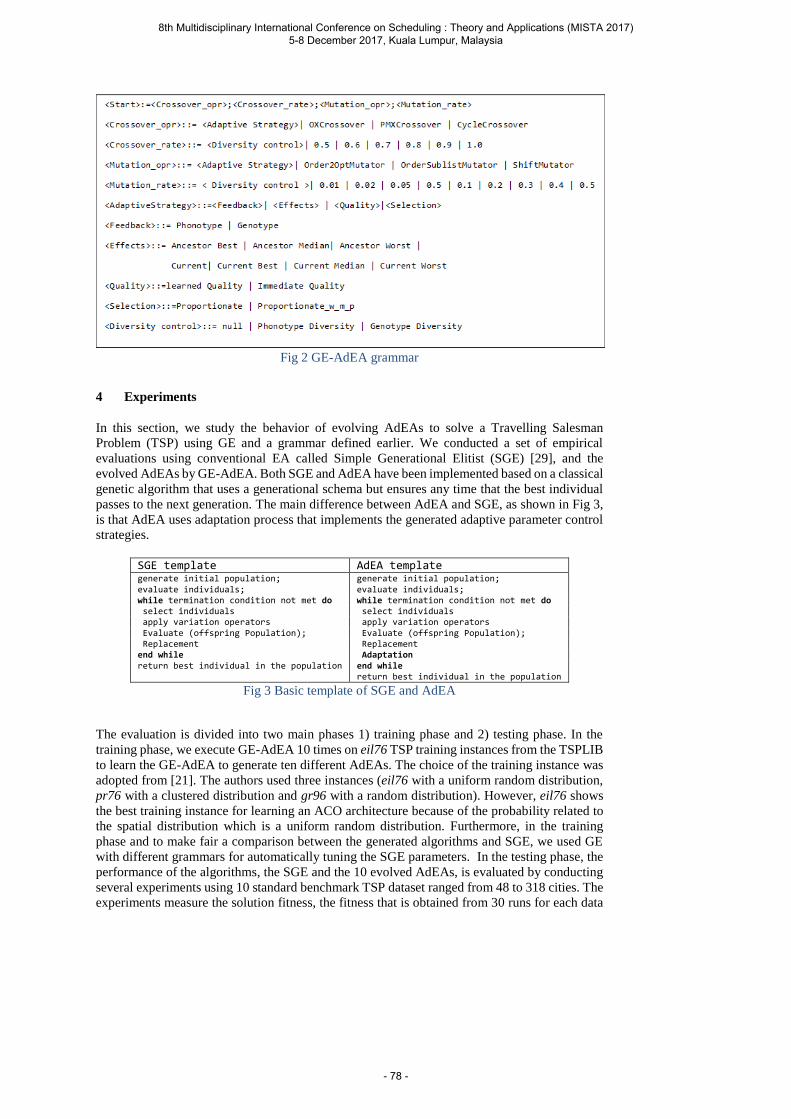
Fig 2 GE-AdEA grammar

4 Experiments

In this section, we study the behavior of evolving AdEAs to solve a Travelling Salesman

Problem (TSP) using GE and a grammar defined earlier. We conducted a set of empirical

evaluations using conventional EA called Simple Generational Elitist (SGE) [29], and the

evolved AdEAs by GE-AdEA. Both SGE and AdEA have been implemented based on a classical

genetic algorithm that uses a generational schema but ensures any time that the best individual

passes to the next generation. The main difference between AdEA and SGE, as shown in Fig 3,

is that AdEA uses adaptation process that implements the generated adaptive parameter control

strategies.

SGE template AdEA template generate initial population; generate initial population; evaluate individuals; evaluate individuals; while termination condition not met do while termination condition not met do select individuals select individuals apply variation operators apply variation operators Evaluate (offspring Population); Evaluate (offspring Population); Replacement Replacement end while Adaptation return best individual in the population end while return best individual in the population

Fig 3 Basic template of SGE and AdEA

The evaluation is divided into two main phases 1) training phase and 2) testing phase. In the

training phase, we execute GE-AdEA 10 times on eil76 TSP training instances from the TSPLIB

to learn the GE-AdEA to generate ten different AdEAs. The choice of the training instance was

adopted from [21]. The authors used three instances (eil76 with a uniform random distribution,

pr76 with a clustered distribution and gr96 with a random distribution). However, eil76 shows

the best training instance for learning an ACO architecture because of the probability related to

the spatial distribution which is a uniform random distribution. Furthermore, in the training

phase and to make fair a comparison between the generated algorithms and SGE, we used GE

with different grammars for automatically tuning the SGE parameters. In the testing phase, the

performance of the algorithms, the SGE and the 10 evolved AdEAs, is evaluated by conducting

several experiments using 10 standard benchmark TSP dataset ranged from 48 to 318 cities. The

experiments measure the solution fitness, the fitness that is obtained from 30 runs for each data


- 78 -

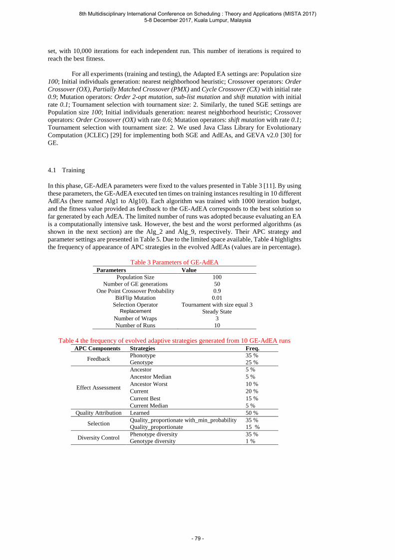
set, with 10,000 iterations for each independent run. This number of iterations is required to

reach the best fitness.

For all experiments (training and testing), the Adapted EA settings are: Population size

100; Initial individuals generation: nearest neighborhood heuristic; Crossover operators: Order

Crossover (OX), Partially Matched Crossover (PMX) and Cycle Crossover (CX) with initial rate

0.9; Mutation operators: Order 2-opt mutation, sub-list mutation and shift mutation with initial

rate 0.1; Tournament selection with tournament size: 2. Similarly, the tuned SGE settings are

Population size 100; Initial individuals generation: nearest neighborhood heuristic; Crossover

operators: Order Crossover (OX) with rate 0.6; Mutation operators: shift mutation with rate 0.1;

Tournament selection with tournament size: 2. We used Java Class Library for Evolutionary

Computation (JCLEC) [29] for implementing both SGE and AdEAs, and GEVA v2.0 [30] for

GE.

4.1 Training

In this phase, GE-AdEA parameters were fixed to the values presented in Table 3 [11]. By using

these parameters, the GE-AdEA executed ten times on training instances resulting in 10 different

AdEAs (here named Alg1 to Alg10). Each algorithm was trained with 1000 iteration budget,

and the fitness value provided as feedback to the GE-AdEA corresponds to the best solution so

far generated by each AdEA. The limited number of runs was adopted because evaluating an EA

is a computationally intensive task. However, the best and the worst performed algorithms (as

shown in the next section) are the Alg_2 and Alg_9, respectively. Their APC strategy and

parameter settings are presented in Table 5. Due to the limited space available, Table 4 highlights

the frequency of appearance of APC strategies in the evolved AdEAs (values are in percentage).

Table 3 Parameters of GE-AdEA

Parameters Value

Population Size 100

Number of GE generations 50

One Point Crossover Probability 0.9

BitFlip Mutation 0.01

Selection Operator Tournament with size equal 3 Replacement Steady State

Number of Wraps 3

Number of Runs 10

Table 4 the frequency of evolved adaptive strategies generated from 10 GE-AdEA runs

APC Components Strategies Freq.

Feedback Phonotype 35 %

Genotype 25 %

Effect Assessment

Ancestor 5 %

Ancestor Median 5 %

Ancestor Worst 10 %

Current 20 %

Current Best 15 %

Current Median 5 %

Quality Attribution Learned 50 %

Selection Quality_proportionate with_min_probability 35 %

Quality_proportionate 15 %

Diversity Control Phenotype diversity 35 %

Genotype diversity 1 %


- 79 -

Table 5 Parameters control strategy of the best and worst Evolved algorithm

Parameter Bestalg_2 WorstAlg_ 9

Crossover

operator

Adaptive

Feedback collection :Genotype;

Effect Asses. : Current Midian;

Quality attribution: Learned quality;

Selection Proportionate with min. prob.;

Non adaptive value: OX

Crossover

Crossover rate Non adaptive value: 0.4 Non adaptive value: 0.9

Mutation

Operator

Adaptive

Feedback collection :Phenotype;

Effect Asses. : Ancestor;

Quality attribution: Learned quality;

Selection Proportionate with min. prob.;

Non adaptive value: 2opt

mutation

Mutation rate Non adaptive value: 0.3 Non adaptive value: 0.09

4.2 Testing

To validate the evolved AdEAs in an optimization scenario, this section provides the comparison

results between tuned SGE and the evolved AdEAs. The testing is essential to measure the

effectiveness of the evolved algorithms in different TSP instances. Ten TSP instances were

selected to assess the performance, namely, att48, eil51, berlin52, kroA100, lin105, gr137, u159,

d198, pr226 and lin318.

Table 6 presents the experimental results of the tuned SGE and the evolved algorithms

on 10 TSP instances. The result values are expressed by the percentage deviation of the best

solutions generated by 10,000 iterations of all algorithms compared to the best-known solutions

of the instances. It can be seen that the results of the evolved algorithm are generally better than

SGE in most instances. From the table, we can also see an expectable degree of variation in the

performance of the evolved algorithm which is confirmed that the GE-AdEA can generate

AdEAs with different adaptive control strategies as well as with different optimization

performance. Looking at the algorithms ranking presented in Table 6 and calculated by using

the ranking method [31] based on the mean of the best fitness for each algorithm, we can see

that 2 out of 10 evolved AdEAs had a better performance when they compared with SGE.

However, the results obtained reveal that GE-AdEA can generate AdEAs with a novel adaptation

strategy and 20% of them have a superior performance comparing to SGE.

To see if there is any statistical difference between the evolved AdEAs and SGE, we

used the results of the mean fitness values obtained from the experiments in the testing phase

and examines the statistical difference using the pair-wise t-Test with a significance level

α=0.05. Table 7 demonstrates the significance of the statistical results of all datasets. A “++”

symbol denotes to the significant differences in the mean values with superior performance

comparing to SGE, “+” denotes to the significant differences in the mean values but with worst

performance comparing to SGE and finally “~” denotes to no significant difference in the mean.

Table 7 statistical results show that both Alg_1 and Alg_2 have a significant difference with

superior performance in the majority of datasets. The analysis also reveals that three of evolved

AdEAs namely Alg_3, Alg_4, and Alg_6, have a comparable or equal performance with SGE.

However, the rest, which is five evolved AdEAs, have worst performance.


- 80 -

Table 6 Optimization results of evolved AdEA, with 10000 iterations for 30runs

Pro

ble

m

SG

E

Alg

_1

Alg

_2

Alg

_3

Alg

_4

Alg

_5

Alg

_6

Alg

_7

Alg

_8

Alg

_9

Alg

_10

att48 B 1.24 0.88 3.10 3.10 1.60 1.11 0.88 0.88 0.52 1.47 2.16

M 4.76 3.07 3.06 5.14 4.51 3.07 3.05 3.05 3.00 3.60 3.10

eil51 B 2.58 2.58 3.05 3.05 3.05 2.58 2.35 3.05 1.41 3.05 2.58

M 4.15 4.08 4.23 5.69 4.37 4.08 3.85 4.16 4.12 4.81 4.64

berlin52 B 0.00 0.00 0.00 0.00 0.00 0.00 0.00 0.00 0.00 1.30 0.00

M 2.71 3.33 3.47 4.76 4.16 3.33 2.88 2.25 1.56 5.08 3.38

kroA100 B 1.41 1.37 1.41 1.41 2.92 1.41 1.41 1.41 1.41 2.18 1.41

M 4.87 3.70 3.49 6.16 4.22 3.70 4.06 4.29 4.62 4.44 4.14

lin105 B 1.48 2.60 1.72 3.89 1.97 1.57 2.37 1.89 1.37 5.08 1.72

M 5.30 5.21 4.48 7.83 5.90 5.21 5.51 5.40 4.73 6.95 4.89

gr137 B 7.78 10.13 8.91 11.99 10.41 10.96 8.47 11.10 9.76 12.03 10.29

M 11.87 13.99 12.57 15.25 12.28 13.99 13.29 15.01 15.43 16.88 16.54

u159 B 10.05 10.30 9.83 10.20 9.83 8.87 10.08 9.88 10.49 11.30 10.64

M 11.10 10.86 10.50 11.73 10.99 10.86 11.32 11.55 11.84 12.64 11.86

d198 B 5.71 7.31 5.14 5.01 5.28 5.64 5.90 7.00 6.45 6.39 6.91

M 7.41 7.28 6.50 7.15 6.17 7.28 7.51 8.70 9.19 9.47 8.38

pr226 B 4.01 6.12 3.45 5.46 3.57 4.18 4.05 7.08 7.16 7.45 6.35

M 6.07 7.31 5.54 7.88 5.86 7.31 7.38 9.26 9.31 8.90 10.13

lin318 B 11.67 10.94 10.85 9.89 11.09 12.08 12.52 12.37 13.08 12.72 11.67

M 11.04 11.67 10.94 10.85 9.89 11.09 12.08 12.52 12.37 13.08 12.72

Algorithm

ranking

B 3.6 6.2 3.0 6.4 6.0 4.9 5.0 7.4 5.6 9.9 8.0

M 4.6 3.9 3.3 8.4 5.0 4.9 4.9 6.4 6.1 10.1 8.3

Table 7 Results of the pair-wise t-Test at a significance level 𝛼 = 0.05

Problem SGE-

Alg_1

SGE-

Alg_2

SGE-

Alg_3

SGE-

Alg_4

SGE-

Alg_5

SGE-

Alg_6

SGE-

Alg_7

SGE-

Alg_8

SGE-

Alg_9

SGE-

Alg_10

att48 ++ ++ ~ ++ ++ ++ ~ ++ ++ ++

eil51 ~ + + + ++ ++ + ~ + +

berlin52 ~ + + + + ~ ~ ~ + +

kroA100 ~ ++ ~ ++ ++ ~ ++ ~ ~ ~

lin105 ++ ++ + + ++ ~ + ++ + ++

gr137 + + + + + + + + + +

u159 ++ ++ ~ ++ ++ ~ ++ + + +

d198 ++ ++ ++ ~ ++ ~ + + + +

pr226 + ++ + ++ + + + + + +

lin318 ++ ++ + ~ + + + + + +

The structure analysis of the best and worst ranked algorithms (See Table 5) reveals that the best

algorithm Alg_2 used an adaptive strategy for crossover and mutation operators. By this, the

algorithm can select different operator types, i.e., OX, BMX or CX operators for crossover and

2opt, sub-list or shift operators for mutation, in each iteration relying on their quality values.

However, as shown in Table 5, the difference of structure and parameter setting of the best and

worst algorithm is clear regarding their parameter adaptability, we can see that the Alg_2

structure uses two different parameter control strategies. It applies the genotype as a feedback

collection, and the current median as an effect assessment for crossover operator, and phenotype

as a feedback and ancestor effect as an assessment for mutation operator. For the quality

attribution and selection strategies, the crossover and mutilation operators used the learned

quality attribution and propionate with minimum probability selection, respectively. Alg_9 has

never used any adaptive parameter control strategy for its parameters. Finally, we believe that

GE-AdEA can produce an AdEA with a comparable optimization performance.


- 81 -

4 Conclusion

In this paper, Grammatical Evolution framework for Adaptive Evolutionary Algorithms (GE-

AdEA) has been proposed. GE-AdEA uses a grammar with several Adaptive parameter control

strategies adopted from an adaptive parameter control model and parameter settings to generate

AdEAs. During the evolution, the GE-AdEA executes the generated AdEAs as a training process

and produces the best-trained AdEAs based on their fitness’s. The best-trained algorithm can be

used later to solve the problem. In the training phase, GE-AdEA shows its capacity to generate

not only good performance AdEAs but also novel designs of AdEA architectures.

The results of the experiments using several traveling salesman problem instances

confirmed that GE-AdEA has a potential to improve the adaptive parameter control strategy for

crossover and mutation operators and their rates. The results also revealed that some of the

generated AdEAs outperform a tuned SGE. Finally, the work presented in this paper

demonstrates that automatic evolution of AdEA is feasible. To test the framework in its

generality, in future work, we aim to enrich this approach with more sophisticated adaptive

parameter control strategies, and to test it with different optimization problems and with several

benchmark algorithms. Also, we will study the influence of using different training instances

considering their characteristics (e.g., instance size, structure and degree of difficulty) on the

performance of the evolved AdEAs rather than using one training instance; this will lead us to

gain more perception on how to design the most effective training environment.

References

1. Eiben, A.E. and J.E. Smith, Introduction to evolutionary computing. Vol. 53. 2003: Springer. 2. Bäck, T. The Interaction of Mutation Rate, Selection, and Self-Adaptation Within a Genetic Algorithm. in

PPSN. 1992. 3. Hesser, J. and R. Männer. Towards an optimal mutation probability for genetic algorithms. in International

Conference on Parallel Problem Solving from Nature. 1990. Springer.

4. Smith, J. and T.C. Fogarty. Self adaptation of mutation rates in a steady state genetic algorithm. in Evolutionary Computation, 1996., Proceedings of IEEE International Conference on. 1996. IEEE.

5. Aleti, A. and I. Moser, A Systematic Literature Review of Adaptive Parameter Control Methods for

Evolutionary Algorithms. ACM Computing Surveys (CSUR), 2016. 49(3): p. 56. 6. Karafotias, G., M. Hoogendoorn, and Á.E. Eiben, Parameter control in evolutionary algorithms: Trends

and challenges. IEEE Transactions on Evolutionary Computation, 2015. 19(2): p. 167-187.

7. Luchian, H. and O. Gheorghieş. Integrated-adaptive genetic algorithms. in European Conference on Artificial Life. 2003. Springer.

8. Vafaee, F. and P.C. Nelson. A genetic algorithm that incorporates an adaptive mutation based on an

evolutionary model. in Machine Learning and Applications, 2009. ICMLA'09. International Conference on. 2009. IEEE.

9. Pappa, G.L. and A.A. Freitas, Automating the Design of Data Mining Algorithms, 2010, Springer-Verlag

Berlin Heidelberg. 10. Burke, E.K., M.R. Hyde, and G. Kendall, the Grammatical evolution of local search heuristics. IEEE

Transactions on Evolutionary Computation, 2012. 16(3): p. 406-417.

11. Lourenço, N., F. Pereira, and E. Costa. Evolving evolutionary algorithms. in Proceedings of the 14th annual conference companion on Genetic and evolutionary computation. 2012. ACM.

12. Mariani, T., et al. A grammatical evolution hyper-heuristic for the integration and test order problem. in

Genetic and Evolutionary Computation Conference. 2016. 13. De Jong, K., Parameter setting in EAs: a 30 year perspective, in Parameter setting in evolutionary

algorithms. 2007, Springer. p. 1-18.

14. Eiben, A.E., et al., Parameter control in evolutionary algorithms, in Parameter setting in evolutionary algorithms. 2007, Springer. p. 19-46.

15. Smith, J.E. and T.C. Fogarty, Operator and parameter adaptation in genetic algorithms. Soft computing,

1997. 1(2): p. 81-87. 16. Eiben, G. and M.C. Schut, New ways to calibrate evolutionary algorithms, in Advances in metaheuristics

for hard optimization. 2007, Springer. p. 153-177.

17. Corriveau, G., et al., Bayesian network as an adaptive parameter setting approach for genetic algorithms. Complex & Intelligent Systems, 2016. 2(1): p. 1-22.

18. Mascia, F., et al., Grammar-based generation of stochastic local search heuristics through automatic

algorithm configuration tools. Computers & operations research, 2014. 51: p. 190-199.


- 82 -

19. López-Ibánez, M. and T. Stutzle, The automatic design of multiobjective ant colony optimization

algorithms. IEEE Transactions on Evolutionary Computation, 2012. 16(6): p. 861-875. 20. Caseau, Y., G. Silverstein, and F. Laburthe, Learning hybrid algorithms for vehicle routing problems.

arXiv preprint cs/0405092, 2004.

21. Tavares, J. and F.B. Pereira. Automatic design of ant algorithms with grammatical evolution. in European Conference on Genetic Programming. 2012. Springer.

22. O'Neill, M. and C. Ryan, Grammatical evolution. IEEE Transactions on Evolutionary Computation, 2001.

5(4): p. 349-358. 23. Lourenço, N., F.B. Pereira, and E. Costa. The importance of the learning conditions in hyper-heuristics. in

Proceedings of the 15th annual conference on Genetic and evolutionary computation. 2013. ACM.

24. Budin, L., M. Golub, and D. Jakobović. Parallel adaptive genetic algorithm. in International ICSC/IFAC Symposium on Neural Computation, NC'98. 1998.

25. Hong, T.-P., et al., Evolution of appropriate crossover and mutation operators in a genetic process.

Applied Intelligence, 2002. 16(1): p. 7-17. 26. Giger, M., D. Keller, and P. Ermanni, AORCEA–An adaptive operator rate controlled evolutionary

algorithm. Computers & Structures, 2007. 85(19): p. 1547-1561.

27. Julstrom, B.A., What have you done for me lately?A adapting operator probabilities in a steady-state genetic algorithm. 1995.

28. Hong, T.-P. and H.-S. Wang. A dynamic mutation genetic algorithm. in Systems, Man, and Cybernetics,

1996., IEEE International Conference on. 1996. IEEE. 29. Ventura, S., et al., JCLEC: a Java framework for evolutionary computation. Soft Computing-A Fusion of

Foundations, Methodologies and Applications, 2008. 12(4): p. 381-392.

30. O'Neill, M., et al., GEVA: grammatical evolution in Java. ACM SIGEVOlution, 2008. 3(2): p. 17-22. 31. Brazdil, P.B. and C. Soares. A comparison of ranking methods for classification algorithm selection. in

European conference on machine learning. 2000. Springer.


- 83 -

MISTA 2017

Fixed jobs scheduling on a single machine with renewableresources

Boukhalfa ZAHOUT · Ameur SOUKHAL ·Patrick MARTINEAU

Abstract This paper deals with scheduling n jobs on a single machine. Job Ji is de-

fined by: a fixed start time si, a fixed finish time fi, an amount of resource requirements

qi,j of type j = 1 . . . k. The jobs are independent and should be processed without pre-

emption during their time interval [si, fi] (processing time of job Ji is pi = fi−si). The

single machine continuously available in [0,∞) owns Qj units of renewable resource

of type Rj necessary to carry out jobs. A machine can process more than one job at

a time, provided the resource consumption does not exceed Qj for all j = 1 . . . k. In

this context, the objective is to find an optimal schedule minimizing the number of re-

jected jobs. We show that this problem is NP-hard. An Integer Linear Program (ILP)

is proposed to solve optimally the studied scheduling problem. Three greedy heuristics

are also developed. Proposed algorithms are implemented and experimental results are

conducted on a set of randomly generated instances. The obtained solutions show the

efficiency of the proposed resolution methods.

Keywords : Scheduling; Single machine; Fixed job scheduling; Resources allocation;

Complexity; ILP; Greedy heuristics.

1 Introduction

In a classical scheduling problem, a set of independent jobs characterized by processing

times should be scheduled on a machine while respecting the constraints to optimize a

given criterion. The machine can process at most one job at a time (see Brucker et al.[5]

and Blazewicz et al.[3]). In this study, a set of n independent jobs should be scheduled

without preemption on a single machine. Additional renewable resources are however

necessary to process each job. Several types of such resources are needed, denoted

Rj , j = 1 . . . k. Hence, at execution time of job i, qij units of available resource are

required. For each job i, the start time si and its finished time fi (i = 1, . . . , n) are fixed

Boukhalfa ZAHOUT, Ameur SOUKHAL, Patrick MARTINEAUROOT ERL-CNRS 6305Computer Science Laboratory of Tours EA 6300IT department- Polytech Tours64 avenue Jean Portalis 37200 Tours, FranceE-mail: (boukhalfa.zahout, ameur.soukhal, patrick.martineau) @univ-tours.fr


- 84 -

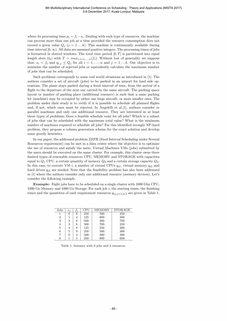
where its processing time pi = fi−si. Dealing with each type of resources, the machine

can process more than one job at a time provided the resource consumption does not

exceed a given value Qj (j = 1 . . . k). This machine is continuously available during

time interval [0,∞). All data are assumed positive integers. The processing times of jobs

is formatted in slotted windows. The total time period [0, T ] is partitioned into equal

length slots (l0) with T = maxi,i=1,...,n(fi). Without lost of generality we suppose

that: si < fi and qi,j ≤ Qj for all i = 1, . . . , n and j = 1 . . . k. Our objective is to

minimize the number of rejected jobs or equivalently calculate the maximum number

of jobs that can be scheduled.

Such problems corresponds to some real world situations as introduced in [1]. The

authors consider a set of aircraft (jobs) to be parked in an airport for land side op-

erations. The plane stays parked during a fixed interval of time, from the arrival of a

flight to the departure of the next one carried by the same aircraft. The parking space

layout or number of parking place (additional resource) is such that a same parking

lot (machine) may be occupied by either one large aircraft, or more smaller ones. The

problem under their study is to verify if it is possible to schedule all planned flights

and, if not, which ones must be rejected. In Angelelli et al.[1], authors consider m

parallel machines and only one additional resource. They are interested in at least

three types of problems: Does a feasible schedule exist for all jobs? Which is a subset

of jobs that can be scheduled with the maximum total value? What is the minimum

number of machines required to schedule all jobs? For this identified strongly NP-hard

problem, they propose a column generation scheme for the exact solution and develop

some greedy heuristics.

In our paper, the addressed problem ISSR (fixed Interval Scheduling under Several

Resources requirement) can be met in a data center where the objective is to optimize

the use of resources and satisfy the users. Virtual Machines VMs (jobs) submitted by

the users should be executed on the same cluster. For example, this cluster owns three

limited types of renewable resources CPU, MEMORY and STORAGE with capacities

equal to Q1 CPU, a certain quantity of memory Q2 and a certain storage capacity Q3.

In this case, to execute VM i, a number of virtual CPUs qi1, virtual memory qi2 and

hard drives qi3 are needed. Note that the feasibility problem has also been addressed

in [1] where the authors consider only one additional resource (memory devices). Let’s

consider the following example.

Example: Eight jobs have to be scheduled on a single cluster with 1000 Ghz CPU,

1000 Go Memory and 1000 Go Storage. For each job i, the starting times, the finishing

times and the quantities of each requirement resources qij;j=1,2,3 are given in Table 1.

Jobs sj fj CPU MEMORY STORAGE1 0 6 250 500 2502 1 4 125 600 3003 3 8 500 300 7004 3 6 500 700 2505 4 8 125 250 2006 5 9 250 500 3007 0 4 500 300 4008 1 5 250 800 600

Table 1: Instance with 8 jobs and 3 resources.


- 85 -

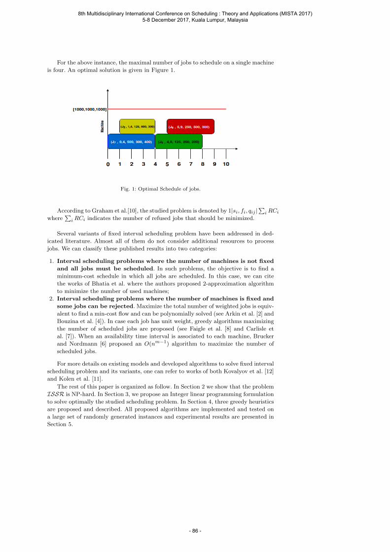
For the above instance, the maximal number of jobs to schedule on a single machine

is four. An optimal solution is given in Figure 1.

Fig. 1: Optimal Schedule of jobs.

According to Graham et al.[10], the studied problem is denoted by 1|si, fi, qij |∑

iRCi

where∑

iRCi indicates the number of refused jobs that should be minimized.

Several variants of fixed interval scheduling problem have been addressed in ded-

icated literature. Almost all of them do not consider additional resources to process

jobs. We can classify these published results into two categories:

1. Interval scheduling problems where the number of machines is not fixed

and all jobs must be scheduled. In such problems, the objective is to find a

minimum-cost schedule in which all jobs are scheduled. In this case, we can cite

the works of Bhatia et al. where the authors proposed 2-approximation algorithm

to minimize the number of used machines;

2. Interval scheduling problems where the number of machines is fixed and

some jobs can be rejected. Maximize the total number of weighted jobs is equiv-

alent to find a min-cost flow and can be polynomially solved (see Arkin et al. [2] and

Bouzina et al. [4]). In case each job has unit weight, greedy algorithms maximizing

the number of scheduled jobs are proposed (see Faigle et al. [8] and Carlisle et

al. [7]). When an availability time interval is associated to each machine, Brucker

and Nordmann [6] proposed an O(nm−1) algorithm to maximize the number of

scheduled jobs.

For more details on existing models and developed algorithms to solve fixed interval

scheduling problem and its variants, one can refer to works of both Kovalyov et al. [12]

and Kolen et al. [11].

The rest of this paper is organized as follow. In Section 2 we show that the problem

ISSR is NP-hard. In Section 3, we propose an Integer linear programming formulation

to solve optimally the studied scheduling problem. In Section 4, three greedy heuristics

are proposed and described. All proposed algorithms are implemented and tested on

a large set of randomly generated instances and experimental results are presented in

Section 5.


- 86 -

2 NP-completeness results

In what follows, we show that the scheduling problem 1|si, fi, qij |∑

iRCi with identical

time intervals and is NP-hard.

Proposition the problem 1|si, fi, qij |∑

iRCi is NP-hard.

Proof The proof is given by reduction from the Partition problem with Equal

Size (PES) which is known to be NP-complete [9]. We denote by ISSRD the decision

problem associated to 1|si, fi, qij |∑

iRCi. ISSRD is defined by:

Data: A set N of n jobs, identical time intervals [si, fi] = [s, f ], ∀i, 1 ≤ i ≤ n and

an integer value Y .

Question: Is there a machine schedule σ for N such that∑

iRCi ≤ Y ? (RCi = 1

if job Ji is rejected).

We prove that PES ∝ ISSRD.

PES problem is defined by:

Data: A set I = a1, . . . , ai, . . . , an, . . . , a2n of 2n integers and an integer value B

such that∑2n

i=1 ai = 2B

Question: Does there exist a partition of I into two subsets I1 and I2 such that∑i∈I1 ai =

∑i∈I2 ai = B and |I1| = |I2|?

Given an arbitrary instance of PES problem, we construct an instance of ISSRDproblem as presented in Table 2.

Jobs si fi qi1 qi2 qi3ji, i = 1, . . . , 2n s f ai B − ai ai

Table 2: An instance of ISSRD problem

Let Y = n and the maximum capacity of the first, second and third resources are

Q1 = B, Q2 = (n− 1)B and Q3 = B respectively.

In the following, we show that there exists a schedule of jobs on one machine, if,

and only if, PES problem has a solution.

– Let us suppose that the answer to PES problem is ’yes’. Let I1 and I2 be the

solution. Hence, by considering I1 a subset of the corresponding jobs that are

scheduled, we have |I1| = n ≤ Y . This solution is a feasible solution because

the quantity of each consumed resource does not exceed the available threshold:∑i∈I1 ai = B = Q1 = Q3 and

∑i∈I1(B − ai) = nB −

∑i∈I1 ai = (n− 1)B = Q2.

Thus, I1 is the subset of scheduled jobs for which the answer to ISSRD problem

is ’yes’.

– Now suppose that the answer to ISSRD problem is ’yes’ for sequence σ. We have:∑ni=1RCi ≤ Y . Let I1 be a subset of scheduled jobs. Then |I1| ≥ Y = n and∑i∈I1 ai ≤ B.

Suppose that |I1| = k > n. In this case the total quantity of consumed resource of

R2 is then: kB −∑

i∈I1 ai > kB −B > (n− 1)B, which is a contradiction. Hence

|I1| = n.


- 87 -

Dealing with R2, we have∑

i∈I1(B−ai) ≤ (n−1)B. Suppose that∑

i∈I1(B−ai) <(n − 1)B. In this case, we have

∑i∈I1 ai > B, which is in contradiction with the

maximum available capacities of R1 and R3.

Hence, we have∑

i∈I1 ai = B and |I1| = n and I1 is also a solution for PESproblem. Consequently, the answer for the question of the PES problem is ’yes’.

3 Integer linear programming formulation

We present in this section a time indexed integer linear programming formulation (ILP)

for solving the scheduling problem. We define two types of binary decision variables.

1. xi a binary variable equal to 1 if job Ji is rejected, 0 otherwise.

2. yit a binary variable equal to 1 if job Ji is executed at time t, and 0 otherwise.

The general formulation of the time-indexed ILP is the following.

Minimize:∑i∈N

xi

subject to:

fi∑t=si

yit = (fi − si) ∗ (1− xi) ; ∀i ∈ N (1)

∑i∈N

yit ∗ qij ≤ Qj ; ∀j ∈ R ; ∀t ∈ [0, T ] (2)

xi ∈ 0, 1, yit ∈ 0, 1 , ∀i ∈ N , ∀t ∈ [0, T ].

N is the set of n jobs andR is the set of type of resource. [0, T ] (T = maxi,i=1,...,n(fi))

is the time period to schedule all jobs.

The constraints (1) ensure that if job Ji is not rejected then it is scheduled during

its time interval. The constraints (2) ensure that no more than Qj quantities of the

required resources are consumed at time t.

4 Greedy heuristics

The scheduling algorithms in this study have many applications, but they were mo-

tivated by research into on line system and integrated-services networks. Hence, the

resolution method must have low complexity, not just polynomial complexity, and to

the extent possible, it should accommodate diverse performance objectives. Further-

more, in many important models that are relevant to the study of integrated-services

networks and on line system, the number of jobs to be processed can be extremely large,

so low complexity is essential. In this section, we presente low-complexity (O(n2) or

better) greedy algorithm to solve fixed interval jobs scheduling problems. Roughly, this

algorithm works as follow: at first, jobs are sorted according to a given priority rule

Π. At each new event t (new job is available to be processed), we try to schedule this

job with respect to constraints of resources availability at time t. This job is rejected if

its assignement causes an unfeasible solution. This procedure is repeated until the last

job. Algorithm 1 describes the proposed global greedy heuristic.


- 88 -

4.1 Priority rules

To calculate set L (see Algorithm 1), we describe here three priority rules that were

implemented.

1. Shortest Processing Time (SPT ): Jobs are sorted in non-decreasing order of

their processing times pi = fi− si ∀i ∈ N , in case of ties, the job with the smallest

finished time come first, otherwise lexicographical order is considered. This SPT

rule allows resources to be released as soon as possible.

2. Capacity-makespan (CCmax): Jobs are sorted in non-decreasing order of their

occupied space given by the following formula:∑

j∈R qij ∗ (fi− si) ∀i ∈ N , in case

of ties, the job with the smallest finished time come first, otherwise lexicographical

order is considered. The idea of using CCmax rule is to minimize the space occupied

by jobs defined by processing time per quantities of consumed resources.

3. Average Resources Consumed (ARC): Jobs are sorted in non-increasing order

of resources requirement per unit time during [si, fi] given by the following formula:∑j∈R qij/(fi − si) ∀i ∈ N , in case of ties, the job with the smallest finished time

come first, otherwise lexicographical order is considered. The idea of using ARC

rule is to minimize the average resources consumed by job per unit of time.

Algorithm 1: Global greedy heuristic

- Let L be the set of jobs sorted according to rule Π

- Let S∗ be the set of scheduled jobs; Initially, S∗ = ∅ ;

while L 6= ∅ doLet Jk be the next available job

Let S ⊆ S∗ be the subset of overlapping jobs during [sk, fk] (i.e their

processing intervals have a nonempty intersection)

if (∑

i∈S qij + qkj ≤ Qj ;∀j ∈ R ) thenSchedule k

S∗ = S∗ ∪ kend

1 L = L\k (Jk is rejected)

end

5 Computational experiments

In this section we present the computational expriments we made in order to analyze

the performance of both exact method ILP and proposed heuristics. All heuristics have

been implemented in C++. IBM ILOG CPLEX Optimization Studio V12.6.3 is used

to solve the ILP formulation. All experiments are conducted on a Pentium i7 computer

with 2.80GHz x 8 cores (1 CPU) and 8 GB memory.

The performance evaluation of the algorithms under study has been carried out

with 100 instances, with a number of jobs n ∈ 20, 40, 60, . . . , 200 (10 instances are

generated per n). Without lost of generality, we normalize the units of a renewable

resource to 1000. Hence, Q1 = Q2 = Q3 = 1000 and for each job qij (i = 1, . . . , n

and j = 1, 2, 3) have been generated using a discrete uniform distribution between

1 and 1000. The jobs-starting times si have been generated using a discrete uniform

distribution between 0 and 1440 mn (one day). Then, the jobs-finishing times have

been generated using a discrete uniform distribution between si + 1 and 1440− si.


- 89 -

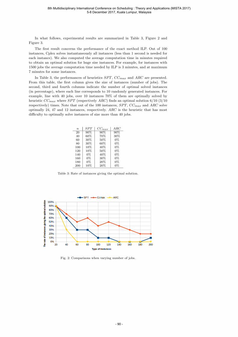
In what follows, experimental results are summarized in Table 3, Figure 2 and

Figure 3.

The first result concerns the performance of the exact method ILP. Out of 100

instances, Cplex solves instantaneously all instances (less than 1 second is needed for

each instance). We also computed the average computation time in minutes required

to obtain an optimal solution for huge size instances. For example, for instances with

1500 jobs the average computation time needed by ILP is 3 minutes, and at maximum

7 minutes for some instances.

In Table 3, the performances of heuristics SPT , CCmax and ARC are presented.

From this table, the first column gives the size of instances (number of jobs). The

second, third and fourth columns indicate the number of optimal solved instances

(in percentage), where each line corresponds to 10 randomly generated instances. For

example, line with 40 jobs, over 10 instances 70% of them are optimally solved by

heuristic CCmax where SPT (respectively ARC) finds an optimal solution 6/10 (3/10

respectively) times. Note that out of the 100 instances, SPT , CCmax and ARC solve

optimally 24, 47 and 12 instances, respectively. ARC is the heuristic that has most

difficulty to optimally solve instances of size more than 40 jobs.

n SPT CCmax ARC20 90% 90% 90%40 60% 70% 30%60 30% 50% 0%80 30% 60% 0%100 10% 40% 0%120 10% 50% 0%140 0% 40% 0%160 0% 30% 0%180 0% 20% 0%200 10% 20% 0%

Table 3: Rate of instances giving the optimal solution.

Fig. 2: Comparisons when varying number of jobs.


- 90 -

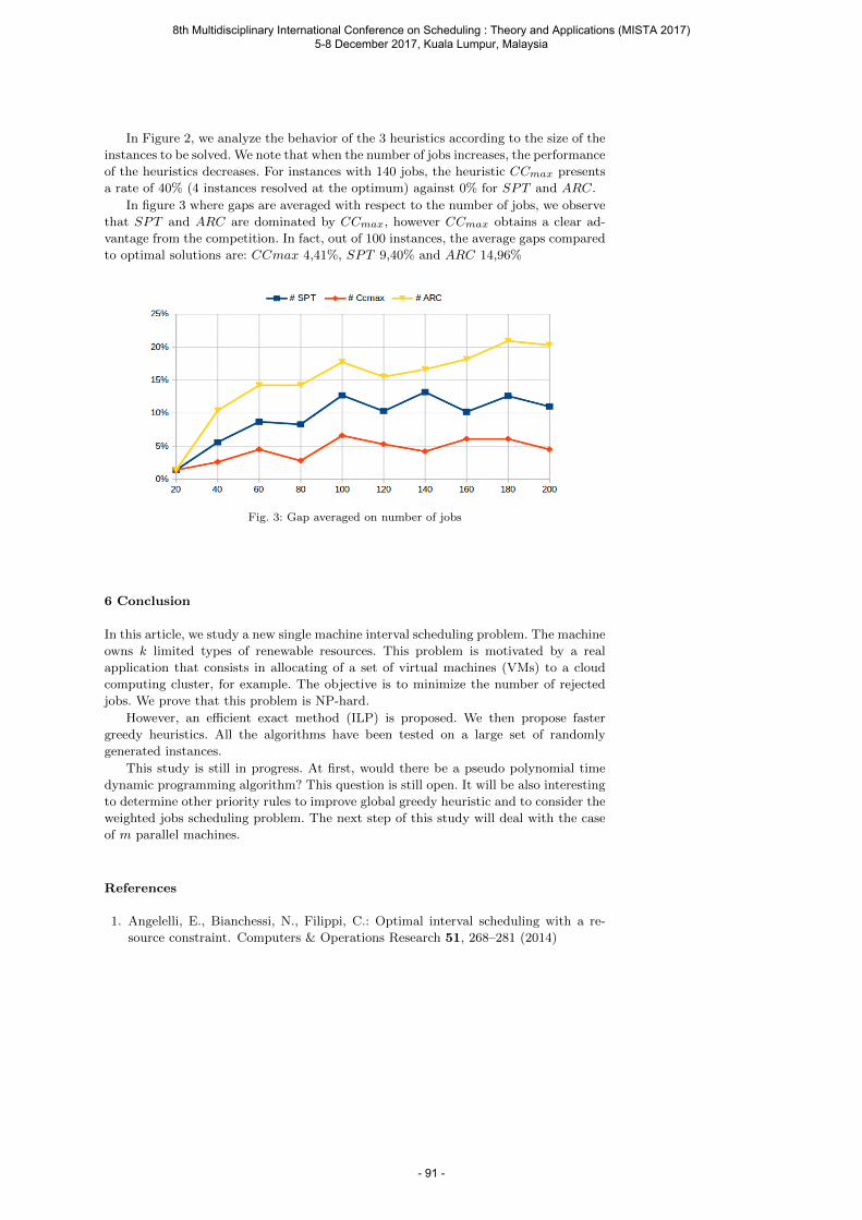
In Figure 2, we analyze the behavior of the 3 heuristics according to the size of the

instances to be solved. We note that when the number of jobs increases, the performance

of the heuristics decreases. For instances with 140 jobs, the heuristic CCmax presents

a rate of 40% (4 instances resolved at the optimum) against 0% for SPT and ARC.

In figure 3 where gaps are averaged with respect to the number of jobs, we observe

that SPT and ARC are dominated by CCmax, however CCmax obtains a clear ad-

vantage from the competition. In fact, out of 100 instances, the average gaps compared

to optimal solutions are: CCmax 4,41%, SPT 9,40% and ARC 14,96%

Fig. 3: Gap averaged on number of jobs

6 Conclusion

In this article, we study a new single machine interval scheduling problem. The machine

owns k limited types of renewable resources. This problem is motivated by a real

application that consists in allocating of a set of virtual machines (VMs) to a cloud

computing cluster, for example. The objective is to minimize the number of rejected

jobs. We prove that this problem is NP-hard.

However, an efficient exact method (ILP) is proposed. We then propose faster

greedy heuristics. All the algorithms have been tested on a large set of randomly

generated instances.

This study is still in progress. At first, would there be a pseudo polynomial time

dynamic programming algorithm? This question is still open. It will be also interesting

to determine other priority rules to improve global greedy heuristic and to consider the

weighted jobs scheduling problem. The next step of this study will deal with the case

of m parallel machines.

References

1. Angelelli, E., Bianchessi, N., Filippi, C.: Optimal interval scheduling with a re-

source constraint. Computers & Operations Research 51, 268–281 (2014)


- 91 -

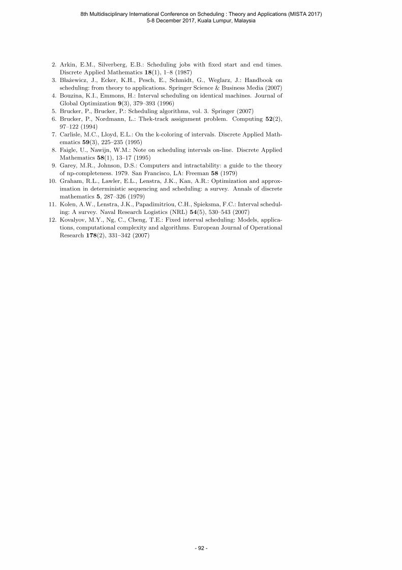
2. Arkin, E.M., Silverberg, E.B.: Scheduling jobs with fixed start and end times.

Discrete Applied Mathematics 18(1), 1–8 (1987)

3. B lazewicz, J., Ecker, K.H., Pesch, E., Schmidt, G., Weglarz, J.: Handbook on

scheduling: from theory to applications. Springer Science & Business Media (2007)

4. Bouzina, K.I., Emmons, H.: Interval scheduling on identical machines. Journal of

Global Optimization 9(3), 379–393 (1996)

5. Brucker, P., Brucker, P.: Scheduling algorithms, vol. 3. Springer (2007)

6. Brucker, P., Nordmann, L.: Thek-track assignment problem. Computing 52(2),

97–122 (1994)

7. Carlisle, M.C., Lloyd, E.L.: On the k-coloring of intervals. Discrete Applied Math-

ematics 59(3), 225–235 (1995)

8. Faigle, U., Nawijn, W.M.: Note on scheduling intervals on-line. Discrete Applied

Mathematics 58(1), 13–17 (1995)

9. Garey, M.R., Johnson, D.S.: Computers and intractability: a guide to the theory

of np-completeness. 1979. San Francisco, LA: Freeman 58 (1979)

10. Graham, R.L., Lawler, E.L., Lenstra, J.K., Kan, A.R.: Optimization and approx-

imation in deterministic sequencing and scheduling: a survey. Annals of discrete

mathematics 5, 287–326 (1979)

11. Kolen, A.W., Lenstra, J.K., Papadimitriou, C.H., Spieksma, F.C.: Interval schedul-

ing: A survey. Naval Research Logistics (NRL) 54(5), 530–543 (2007)

12. Kovalyov, M.Y., Ng, C., Cheng, T.E.: Fixed interval scheduling: Models, applica-

tions, computational complexity and algorithms. European Journal of Operational

Research 178(2), 331–342 (2007)


- 92 -

Yahui Liu School of Software Engineering, Tongji University, Shanghai, China. E-mail: [email protected] Buyang Cao School of Software Engineering, Tongji University, Shanghai, China. E-mail: [email protected]

MISTA 2017

Improving Ant Colony Optimization algorithm with Levy Flight

Yahui Liu • Buyang Cao

Abstract Ant Colony Optimization (ACO) algorithm is a metaheuristic evolved from the foraging behavior of ants, and the swarm intelligence is realized by the behavior of a single ant. ACO algorithm is widely used to solve combinatorial optimization problems. At the same time, the quality of an ACO algorithm depends on the diversity of solutions and the times spent by the algorithm. Some commonly used ACO algorithms such as the Elite ACO and the Rank-based ACO attempt to reduce the computational time of the algorithm by exploring near the current best solution. Other algorithms such as the Max-Min ACO try to explore the diverse solution spaces by limiting the maximal and minimal pheromone. Levy Flight is a type of random walking behavior based on Levy distribution, which is also widely observed in nature like animal feeding routes, circulation logistics (e.g. banknotes). This article describes the ACO algorithm combining with the Levy Flight mechanism, which can balance the convergence rate and the diversity of solutions. The experiment demonstrates that the proposed Levy ACO algorithm obtains better results than the classical ACO algorithm.

1 Introduction

ACO (Ant Colony Optimization) algorithm is a metaheuristic based on ants foraging behavior, and it relies on the foraging behavior of single ant to embody the foraging intelligence of ant colony. ACO algorithm was first proposed in Dorige’s doctoral dissertation in 1992 [1] and more details provided later in 1996[2]. The early version of ACO algorithm was applied to the TSP (Travelling Salesman Problem) problems, and Dorige [2] described how to use ACO algorithm for TSP modeling and the experiments for validations. In his latest paper [3], Dorige surveyed ACO technologies.

Since the birth of the ACO algorithm, there were many researchers carried out in-depth studies, and proposed numerous improved versions, for instance, the Elite Ant Colony algorithm [3], the Rank-based Ant Colony algorithm [4], the Max-Min Ant Colony Optimization algorithm [5]. The core in terms of the efficiency of an ACO algorithm is to balance the diversity of


- 93 -

exploration (Exploration) and the concentration of exploration (Exploitation). Exploration is to explore new solution spaces as much as possible while exploitation is to search the areas near the current best solution as fast as possible, In the above mentioned algorithms, the Elite Ant Colony algorithm [3] and the Rank-based Ant Colony algorithm [4] focus on the exploitation of current best solution, while the Max-Min ACO algorithm [5] balances the exploration and the exploitation by setting the maximum and minimum pheromone and gets better performance. Furthermore, ACO algorithm is not only applied for solving TSP [6-11,29] but also other optimization problems such as VRP (Vehicle Routing Problem) [12-17], QAP (Quadratic Assignment Problem) [18,19], JSP (Job-shop Problem) [20-22].

The random mechanism is embedded in ACO algorithms, where the probability distribution plays a great role. Some common distributions of continuous distributions include uniform, normal, exponential ones, etc. One class of continuous distribution we are interested has the property called fat-tail, which means the tail is thicker than others such as the normal and the exponential ones. Its randomness is weaker, so that a tail value that is rarely selected in normal situation could be chosen with a higher probability. From our aspect (will be discussed below), it increases the diversity of solutions that would contribute to better solutions. Specifically Levy distribution is a kind of typical fat-tailed distribution.。

Levy Flight [23] is a type of random walking patterns that conforms to the Levy distribution, which was named after the French mathematician Paul Lévy, and the step length has the fat-tailed distribution. The walking steps are isotropic random directions when walking in a space with the number of dimensions greater than 1. Many animal's foraging movements also possess the Levy Flight features, e.g. most of the feeding time is spent around known food sources, and occasionally a long-distance flight is needed to find other food sources [24] [26].

2 Integration of Levy Flight and ACO

2.1 Problems background

In this paper, the concrete application for which the Levy ACO will be applied is the Traveling Salesman Problem (TSP). When solving TSP, ACO algorithm utilizes the positive feedback by accumulating the pheromone to focus on possible better solutions and the negative feedback by evaporating pheromone to reduce the history solution effect for exploring more search spaces. The framework of an ACO algorithm is shown in figure 1.

Similar other metaheuristics, ACO not only needs to explore more diverse solution spaces to avoid being trapped at a local optimum, but also attempts to speed up the solution procedure to reduce the time spent. In summary, a good ACO should be able to find higher quality solution within shorter period.

In the ACO algorithm shown in figure 2, the uniform distribution is employed to for each single ant to select the next site from the possible sites (assuming we are solving a TSP) in step 2. At this time, the attractant factor derived from the attraction and pheromone values for each candidate will accumulated to 100%，please refer to formula (1). Each single ant will select the next site according to the random number uniformly distributed between 0 and 1. However, because attractant factors for candidate sites vary, and they are normally or exponentially distributed after sorted, the selection probability of a candidate site will decline quickly and be close to zero as the number of ranks increases. Statistically the candidate sites with small attraction factors then could be two or more standard deviations from the mean and would rarely be selected since their selection probabilities are very low. As the result, the algorithm always focuses on candidate sites with higher attractant and it is hard to achieve diverse solutions.

( ) = ( ) ( )

∑ [ ( )] [ ( )]∈

∈ （1）


- 94 -

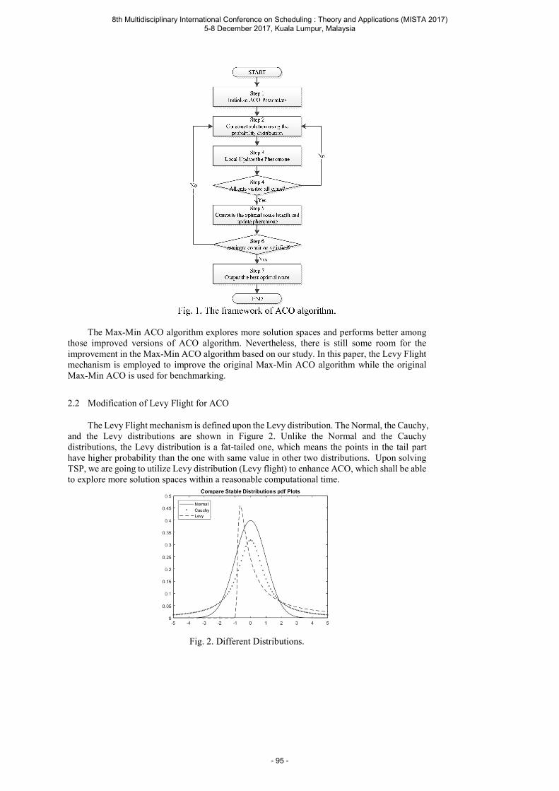
START

Step 1Initialize ACO Parameters

Step 2Construct solution using the

probability distribution

Step 3Local Update the Pheromone

Step 4All ants visited all cities?

Step 5Compute the optimal route length and

update pheromone

Step 6Terminate condition satisfied?

Step 7Output the best optimal route

END

Yes

Yes

No

No

Fig. 1. The framework of ACO algorithm.

The Max-Min ACO algorithm explores more solution spaces and performs better among

those improved versions of ACO algorithm. Nevertheless, there is still some room for the improvement in the Max-Min ACO algorithm based on our study. In this paper, the Levy Flight mechanism is employed to improve the original Max-Min ACO algorithm while the original Max-Min ACO is used for benchmarking.

2.2 Modification of Levy Flight for ACO

The Levy Flight mechanism is defined upon the Levy distribution. The Normal, the Cauchy, and the Levy distributions are shown in Figure 2. Unlike the Normal and the Cauchy distributions, the Levy distribution is a fat-tailed one, which means the points in the tail part have higher probability than the one with same value in other two distributions. Upon solving TSP, we are going to utilize Levy distribution (Levy flight) to enhance ACO, which shall be able to explore more solution spaces within a reasonable computational time.

Fig. 2. Different Distributions.


- 95 -

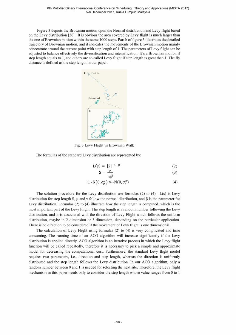
Figure 3 depicts the Brownian motion upon the Normal distribution and Levy flight based on the Levy distribution [26]. It is obvious the area covered by Levy flight is much larger than the one of Brownian motion within the same 1000 steps. Part b of figure 3 illustrates the detailed trajectory of Brownian motion, and it indicates the movements of the Brownian motion mainly concentrate around the current point with step length of 1. The parameters of Levy flight can be adjusted to balance effectively the diversification and intensification. It’s a Brownian motion if step length equals to 1, and others are so called Levy flight if step length is great than 1. The fly distance is defined as the step length in our paper.

Fig. 3 Levy Flight vs Brownian Walk

The formulas of the standard Levy distribution are represented by:

L( ) = | | (2)

S = | |

(3)

μ~N 0, , ν~N(0, ) (4)

The solution procedure for the Levy distribution use formulas (2) to (4). L(s) is Levy

distribution for step length S, μ and ν follow the normal distribution, and β is the parameter for Levy distribution. Formulas (2) to (4) illustrate how the step length is computed, which is the most important part of the Levy Flight. The step length is a random number following the Levy distribution, and it is associated with the direction of Levy Flight which follows the uniform distribution, maybe in 2 dimension or 3 dimension, depending on the particular application. There is no direction to be considered if the movement of Levy flight is one dimensional.

The calculation of Levy Flight using formulas (2) to (4) is very complicated and time consuming. The running time of an ACO algorithm will increase significantly if the Levy distribution is applied directly. ACO algorithm is an iterative process in which the Levy flight function will be called repeatedly, therefore it is necessary to pick a simple and approximate model for decreasing the computational cost. Furthermore, the standard Levy flight model requires two parameters, i.e., direction and step length, whereas the direction is uniformly distributed and the step length follows the Levy distribution. In our ACO algorithm, only a random number between 0 and 1 is needed for selecting the next site. Therefore, the Levy flight mechanism in this paper needs only to consider the step length whose value ranges from 0 to 1


- 96 -

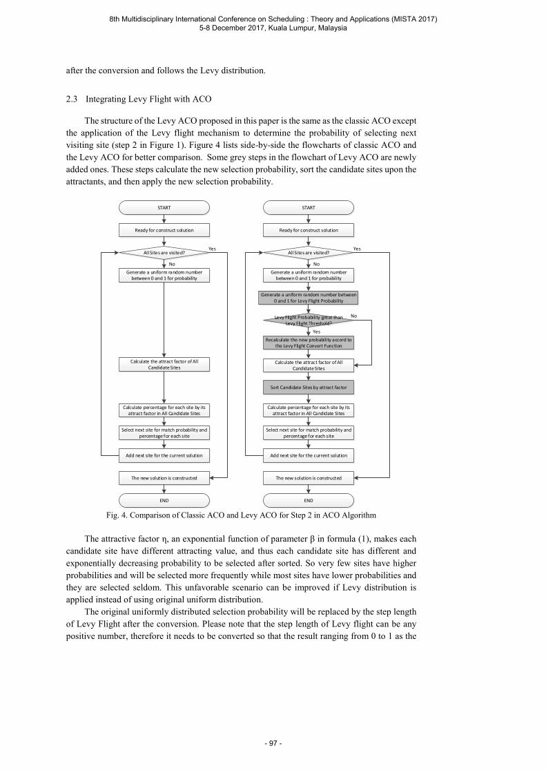
after the conversion and follows the Levy distribution.

2.3 Integrating Levy Flight with ACO

The structure of the Levy ACO proposed in this paper is the same as the classic ACO except the application of the Levy flight mechanism to determine the probability of selecting next visiting site (step 2 in Figure 1). Figure 4 lists side-by-side the flowcharts of classic ACO and the Levy ACO for better comparison. Some grey steps in the flowchart of Levy ACO are newly added ones. These steps calculate the new selection probability, sort the candidate sites upon the attractants, and then apply the new selection probability.

Generate a uniform random number between 0 and 1 for probability

Calculate the attract factor of All Candidate Sites

Calculate percentage for each site by its attract factor in All Candidate Sites

Select next site for match probability and percentage for each site

Add next site for the current solution

All Sites are visited?

START

Ready for construct solution

The new solution is constructed

END

No

Yes

Generate a uniform random number between 0 and 1 for probability

Calculate the attract factor of All Candidate Sites

Calculate percentage for each site by its attract factor in All Candidate Sites

Select next site for match probability and percentage for each site

Add next site for the current solution

All Sites are visited?

START

Ready for construct solution

The new solution is constructed

END

No

Yes

Generate a uniform random number between 0 and 1 for Levy Flight Probability

Recalculate the new probability accord to the Levy Flight Convert Function

Levy Flight Probability great than Levy Flight Threshold?

No

Yes

Sort Candidate Sites by attract factor

Fig. 4. Comparison of Classic ACO and Levy ACO for Step 2 in ACO Algorithm

The attractive factor η, an exponential function of parameter β in formula (1), makes each

candidate site have different attracting value, and thus each candidate site has different and exponentially decreasing probability to be selected after sorted. So very few sites have higher probabilities and will be selected more frequently while most sites have lower probabilities and they are selected seldom. This unfavorable scenario can be improved if Levy distribution is applied instead of using original uniform distribution.

The original uniformly distributed selection probability will be replaced by the step length of Levy Flight after the conversion. Please note that the step length of Levy flight can be any positive number, therefore it needs to be converted so that the result ranging from 0 to 1 as the


- 97 -

probability. Formulas (5) to (7) are designed to convert the step length into the selection probability. In Levy ACO, all candidate sites should be sorted by their attraction factor values (formula (1)) in non-increasing order before applying the converted selection probability. After sorting, obviously the front part contains the candidate sites with higher attractants while the back portion consists of the candidate sites with lower attractants. With the amplification mechanism in our conversion formulas, the new selection probabilities of some candidate sites with lower attractants will be amplified. In this case, these original “unfavorable” sites will more likely be selected and diverse solution spaces can be searched.

Some definitions of the terms used in the conversion formulas:

: New selection probability after Levy flight conversion, it will be used for selecting the next site.

: The original selection probability that is uniformly distributed before the Levy flight conversion.

: The random number uniformly distributed between 0 and 1 is used for switching

Levy flight conversion.

: Threshold ranging from 0 to 1 for Levy flight conversion, which determines if Levy flight conversion is turned on or not after being compared with .

1 − = ∗ ∗ (1 − ) (5)

= 1 − ∗ ∗ (1 − ) (6)

=1 − ∗ ∗ (1 − ), >

, ≤ (7)

The core steps of Levy flight conversion (formulas (5) to (7)): The Levy flight conversion formula (5) is applied to the Levy flight step lengths

that are greater than 1 so that they will be mapped to the values between 0 and 1. The formula (6) is the transformation of formula (5) for calculating . Value and are generated in uniformly distributed between 0 and 1.

Levy flight threshold is set for determining if the selection probability should apply Levy Flight conversion or not.

New selection probability use the value of if is less than

(indicating step length is not greater than 1). In this case is not converted.

The new probability should be recalculated using formula (6) if is

greater than , that is, the Levy flight step length is greater than 1 and Levy flight conversion is turned on.

In the above Levy flight conversion formulas we need two predefined parameters:

(Levy flight threshold) and A (amplification ratio). The new selection probability presented in formula (7) is able to encourage the current ant to choose the candidate sites with original lower selection probabilities to increase the diversity of the solution space with the hope of getting out of local optima.


- 98 -


3.1 Data and environment setting

In the following computational experiments, we compare the results obtained by the Levy ACO proposed in this paper integrates the original Max-Min ACO algorithm with Levy Flight mechanism and the original Max-Min ACO algorithm without Levy Flight mechanism. The code for the Levy ACO proposed in this paper is implemented based on the code for ACO algorithm [5] available at http://www.aco-metaheuristic.org/aco-code/, The Levy threshold and amplification ratio A are set to be 0.8 and 1 respectively. Each benchmark runs 100 times considering the probabilistic factor in ACO algorithms.

The platform configuration for benchmarking: Windows 10 x64, CPU 8 cores 2.7GHz, Memory 32GB, the programming language is C with the original Max-Min ACO algorithm [28] and the Levy ACO algorithm in this paper.

3.2 Benchmarks

3.2.1 Benchmark 1 and 2

The experiments are performed using instance link318 and pcb442 in TSPLIB [27], and here are some observations are illustrated in figure 5 and table 1:

All instances reach the optimal solution 52029 for link318 or 50778 for pcb442, and the average number of iterations to get the best solution for the Levy ACO is lower than the original Max-Min ACO. This result indicates that the Levy ACO can reach the best solution faster.

For the purpose of analyzing the performance of the algorithm, we conduct the statistical analyses for the benchmarks including the maximal iterations, average iterations, median iterations, and minimal iterations to obtain the best solution.

Fig. 5. Benchmark for with/without Levy Flight for link318(left) and pcb442(right)

The statistical results are listed in table 1：

The maximal number of iterations for link318 is reduced from 1395 (without Levy flight) to 539 (with Levy flight), an improvement of 61.36%. The maximal number of iterations for pcb442 is reduced from 72016 (without Levy flight) to 31956 (with Levy flight) with an improvement of 55.63%.

The average number of iterations is reduced by 32.13% or 23.53% with Levy ACO.


- 99 -

The median number of iterations shows the improvement of 9.31% or 20.00% by applying Levy ACO.

Levy ACO runs more consistently as the variance in the number of iterations is reduced by 43.58% or 38.26%, which means the stability of the algorithm is also improved.

The minimal number of iterations for Levy ACO increases a bit for link318 and decrease by 85.19% for pcb442. Please note that for link318, the minimal iteration number is already very low (31), and there is very small space to improve. This is reasonable because ACO algorithm is a probabilistic algorithm.

Table 1. Benchmark for with/without Levy Flight for link318/pcb442

Without Levy Flight With Levy Flight Improve Percentage link318 pcb442 link318 pcb442 link318 pcb442

Max round 1395 72016 539 31956 61.36% 55.63% Average round 216 10403.69 146.59 7956.17 32.13% 23.53%

Mean round 102 7735 92.5 6188 9.31% 20.00%

Min round 31 466 38 69 -22.58% 85.19% Sample variance 230.79 10289.07 130.22 6352.98 43.58% 38.26%

3.2.2 Benchmark 3 and 4

Instance a280 and pr299 in TSPLIB [27] are selected for the other experiment, and the results are illustrated in figure 6 and table 2:

Fig. 6. Benchmark for with/without Levy Flight for a280 (left) and pr299 (right)

Similarly, we can draw the following conclusions

All instances get the best solution 2579 for a280 and 48191 for pr299, and the average number of iterations to get the best solution of the Levy ACO is lower than the original Max-Min ACO. This indicates that the Levy ACO can reach the best solution faster.

The number of average iterations shows 41.53% for a280 and 17.85% for pr299 reduction by applying the Levy ACO.

The median number of iterations of the Levy ACO possesses an improvement 91.50% for a280 and 5.78% for pr299 comparing to the original Max-Min ACO.

It is obvious that the Levy ACO runs more consistently since it has lower variance in the number of iterations. It indicates the stability of the Levy ACO is improved.

The minimal number of iterations of the Levy ACO presents same or some improvement as well with a very small value (2 or 3).


- 100 -

Table 2. Benchmark for with/without Levy Flight for a280 and pr299

Without Levy Flight With Levy Flight Improve Percentage a280 pr299 a280 pr299 a280 pr299

Max round 1846 3035 1221 2779 33.86% 8.43%

Average round 346.96 849.25 202.86 697.63 41.53% 17.85% Mean round 306 606 26 571 91.50% 5.78% Min round 2 3 2 2 0.00% 33.33%

Sample variance 393.71 701.48 275.90 672.74 29.92% 4.10%

4 Conclusions

The paper proposes the Levy ACO algorithm that is developed based on Levy Flight mechanism and classic ACO algorithm. The experiment demonstrates that the proposed algorithm can achieve the best solution more effectively. The capabilities of exploring diverse solution spaces and avoiding local optima contribute the efficiency of the algorithm as a whole. On the average the proposed algorithm can reach the optimal solution with less (reduced by 32.13%, 23.53%, 41.53% and 17.85%) iterations comparing to the original Max-Min ACO algorithm. The computational results demonstrate the superiority of the Levy ACO proposed in the paper. In addition to conducting more computational experiments, for example, using the other instances in TSPLIB, we are planning to tune parameters of the Levy ACO with some smarter methods to further improve the performance of the Levy ACO and to study its applicability for other problems such as VRP.

Acknowledgements We are indebted to three anonymous reviewers for insightful observations and suggestions that have helped to improve our paper. This work was partially supported by CIUC and TJAD [grant number CIUC20150011].

References

1. Dorigo, Marco. "Optimization, learning and natural algorithms." Ph. D. Thesis, Politecnico di Milano, Italy (1992).

2. Dorigo, Marco, Vittorio Maniezzo, and Alberto Colorni. "Ant system: optimization by a colony of cooperating agents." IEEE Transactions on Systems, Man, and Cybernetics, Part B (Cybernetics) 26.1 (1996): 29-41.

3. López-Ibáñez, Manuel, Thomas Stützle, and Marco Dorigo. "Ant colony optimization: A component-wise overview." Handbook of Heuristics (2016): 1-37.

4. Bullnheimer, Bernd, Richard F. Hartl, and Christine Strauss. "A new rank based version of the Ant System. A computational study." (1997).

5. Stützle, Thomas, and Holger H. Hoos. "MAX–MIN ant system." Future generation computer systems 16.8 (2000): 889-914.

6. Dorigo, Marco, and Luca Maria Gambardella. "Ant colony system: a cooperative learning approach to the traveling salesman problem." IEEE Transactions on evolutionary computation 1.1 (1997): 53-66.

7. Dorigo, Marco, and Luca Maria Gambardella. "Ant colonies for the travelling salesman problem." biosystems 43.2 (1997): 73-81.


- 101 -

8. Gambardella, Luca Maria, and Marco Dorigo. "Solving symmetric and asymmetric TSPs by ant colonies." Evolutionary Computation, 1996., Proceedings of IEEE International Conference on. IEEE, 1996.

9. Li, Yong, and Shihua Gong. "Dynamic ant colony optimization for TSP." The International Journal of Advanced Manufacturing Technology 22.7-8 (2003): 528-533.

10. Wu, Hua-feng, et al. "Improved ant colony algorithm based on natural selection strategy for solving TSP problem." Journal of China Institute of Communications 34.4 (2013): 165-170.

11. Ariyasingha, I. D. I. D., and T. G. I. Fernando. "Performance analysis of the multi-objective ant colony optimization algorithms for the traveling salesman problem." Swarm and Evolutionary Computation 23 (2015): 11-26.

12. Gambardella, Luca Maria, Éric Taillard, and Giovanni Agazzi. "MACS-VRPTW: A multiple ant colony system for vehicle routing problems with time windows." (1999).

13. Bell, John E., and Patrick R. McMullen. "Ant colony optimization techniques for the vehicle routing problem." Advanced engineering informatics 18.1 (2004): 41-48.

14. Yu, Bin, Zhong-Zhen Yang, and Baozhen Yao. "An improved ant colony optimization for vehicle routing problem." European journal of operational research 196.1 (2009): 171-176.

15. Reed, Martin, Aliki Yiannakou, and Roxanne Evering. "An ant colony algorithm for the multi-compartment vehicle routing problem." Applied Soft Computing 15 (2014): 169-176.

16. Narasimha, Koushik Venkata, et al. "An ant colony optimization technique for solving min–max multi-depot vehicle routing problem." Swarm and Evolutionary Computation 13 (2013): 63-73.

17. Schyns, Michael. "An ant colony system for responsive dynamic vehicle routing." European Journal of Operational Research 245.3 (2015): 704-718.

18. Gambardella, Luca Maria, É. D. Taillard, and Marco Dorigo. "Ant colonies for the quadratic assignment problem." Journal of the operational research society 50.2 (1999): 167-176.

19. Demirel, Nihan Çetin, and M. Duran Toksarı. "Optimization of the quadratic assignment problem using an ant colony algorithm." Applied Mathematics and Computation 183.1 (2006): 427-435.

20. Zhang, Jun, et al. "Implementation of an ant colony optimization technique for job shop scheduling problem." Transactions of the Institute of Measurement and Control 28.1 (2006): 93-108.

21. Heinonen, J., and F. Pettersson. "Hybrid ant colony optimization and visibility studies applied to a job-shop scheduling problem." Applied Mathematics and Computation 187.2 (2007): 989-998.

22. Huang, Rong-Hwa, Chang-Lin Yang, and Wei-Che Cheng. "Flexible job shop scheduling with due window—a two-pheromone ant colony approach." International Journal of Production Economics 141.2 (2013): 685-697.

23. Shlesinger, Michael F., and Joseph Klafter. "Lévy walks versus Lévy flights." On growth and form. Springer Netherlands, 1986. 279-283.

24. Stanley, H. E. "Levy flight search patterns of wandering albatrosses." Nature 381 (1996): 413415Viswanathan.

25. Reible, Danny, and Sanat Mohanty. "A levy flight—random walk model for bioturbation." Environmental toxicology and chemistry 21.4 (2002): 875-881.

26. Viswanathan, Gandhimohan M. "Ecology: Fish in Lévy-flight foraging." Nature 465.7301 (2010): 1018-1019.

27. http://comopt.ifi.uni-heidelberg.de/software/TSPLIB95/ 28. http://www.aco-metaheuristic.org/aco-code/ 29. Dorigo, Marco, and L. M. Gambardella. "Ant-Q: A reinforcement learning approach to

the traveling salesman problem." Proceedings of ML-95, Twelfth Intern. Conf. on Machine Learning. 2016.


- 102 -

Ian Frederic A. Ilagan De La Salle University – Manila E-mail: [email protected]

Charlle L. Sy De La Salle University – Manila E-mail: [email protected]

MISTA 2017

A Robust Crew Pairing Model for Airline Operations using Crew Swaps and Slack Times

Ian Frederic A. Ilagan • Charlle L. Sy

Abstract The trend in airlines, as more flights are being flown, is that delays have been less from unpredictable events and more from operations. Airlines push to maximize profits by scheduling flights with little to no regard for possible disruptions. Common practices that deal with disruptions, such as purposeful cancellation of flights, and assignment of emergency crew, are usually inefficient. Planning for disruptions in operations, while increasing planned costs, create flight schedules that are capable of handling disruptions. This paper proposes a robust crew pairing model that schedules slack times and crew swaps that can potentially reduce the propagation of delay when a disruption occurs. A mathematical formulation is presented. A small set of flights is presented to show the schedules obtained from the traditional and robust models. The comparison is then made for a set of 1890 flights from a real major airline. The robust model is able to create a solution with higher planned costs but better delay indicators.

1 Background

The time-sensitive nature of service in the airline industry means that several scheduling problems arise during operations. Airline resources work under connectivity and compatibility constraints [1]. Among those resources are the crew members. Scheduling the aircrafts can be extremely costly when being inefficient, and are often inflexible, while airlines have limited control in scheduling passengers. Crew scheduling is both flexible and manageable in cost, and innovations in crew scheduling can lead to improvements in airline operations that are feasible in cost, but still having significant impact.

1.1 Crew pairing

Crew pairing is part of a sequential process done in airline resource management that follows the timetable construction and the assignment of aircrafts. Pairings are constructed by forming sequences of connectable flights within the same fleet that start and end at the same


- 103 -

crew base [2]. Crew pairing finds sets of specified crew that will operate together for the duration of the pairing. The graphical representation of a pairing is shown in Figure 1.

Figure 1: Structure of a crew pairing

A duty period is different from a crew pairing. A duty period is a sequence of flight legs

that can be legally flown by a set of crew with only short rest periods. The crew pairing is a sequence of flight legs, and long rest periods if needed, that can be legally flown by a set of crew, and starts and ends at the same home base. A crew pairing is composed of one or more duty periods.

1.2 Delays and delay propagation

The air transport industry neglects shorter delays (departure and arrivals no later than 15 minutes). In the context of air transport, passengers consider small delays as being negligible [3]. The popular 15-minute margin of tolerance is the viewpoint for significance of lateness. A missed connection is what can increase the significance of lateness from the viewpoint of a passenger, which is why connecting flights are scheduled with ample connection time [4].

Delays are what affect punctuality, an attribute that passengers find satisfaction in. Consistent lack in punctuality causes a reduction in the airline’s market share. There is therefore a cost to lack of punctuality. Flights that are delayed (or cancelled) to an extent beyond the tolerance limit of its passengers will shift service perception of customers wherein switching airlines of preference is likely [5].

Delays in an airline context usually force the company to solve the problem locally where the disruption occurs. While local resources will allow for lessening the effect of the delay, it is still likely to propagate towards those with connected resources occurs [6]. Shown in Figure 2 is the effect delay propagation from single or multiple delays on a schedule.

Figure 2: Flight schedule with propagation from a single delay (left), and from multiple delays (right)

A delay on the first flight will translate to subsequent flights. Mitigation of the delay is

possible if local resources at each flight will allow for catching up, such as if passengers can be boarded quicker than the standard time. This is unlikely for flights that are high-density, which are usually scheduled with no slack. A single delay can at the beginning of a schedule can cause


- 104 -

the same delay to propagate to further flights. In a realistic schedule, flights will often have delays that were created locally and that were propagated from previous flights Figure 2 follows a timeline network representation, further discussed in chapter 2.2

1.3 Planning for disruptions through slack times and crew swaps

A promising area of research is to construct schedules that perform well under irregularities [7]. Robustness is in the form of stability, plans that as least sensitive as possible to disruptions; or flexibility, which gives options for the plan to remain cost-effective given a perceived set of disruption events [8]. Scheduling by providing ample slack times gives stability, while scheduling for possible crew swaps gives flexibility.

Slack times are purposely idle time in the schedule that can possibly absorb delays. Crew swaps are discussed through an example: suppose that Crew A are on standby waiting for their next flight Flight A’s departure time. At the same time, a flight Flight B departing from the same airport is delayed due to Crew B still in transit. An example of a crew swap is scheduling Crew A to take over duties for Flight B, while the in-transit Crew B will take over Flight A when they arrive. While this might result in Flight A being delayed if Crew B takes too long to arrive, the delays between Flight A and Flight B are essentially mitigated and shared between the two.

The prevalent scheduling process in airlines pay insufficient consideration on the impact of uncertainty in operating a complex airline network with multiple interconnected resources [9]. Disruption management as a field has primarily existed as a reactive approach through recovery, which aims to put a schedule back to its original as soon as possible following a disruption. Reactive disruption management uses simple techniques for solving, focuses on having minimal costs during planning, and incurs higher delays when disruptions occur. On the other hand, proactive disruption management in the form of robust schedules incorporates uncertainty of delays into the planning, incurring higher planned costs but often lower delays.

Section 2 discusses on relevant literature, including context on airline resource planning, network representations used in this research, and the traditional modeling approach of the crew pairing problem. Section 3 formulates the robust crew pairing model, an extension of the traditional set partitioning approach. Section 4 discusses on a methodology for solving large instances of the problem. Computational results are shown in Section 5. Emphasis is placed on comparison of the solutions obtained from the robust model and the traditional model. Lastly, conclusions and extensions on the research is discussed in Section 6.

2 Related Literature

2.1 Airline resource planning

The large complexity of scheduling flights, aircrafts, and crew for even just a small set of flights have led to the creation of a sequential process that is now generally applicable for any airline [10].The process, in sequence, is timetable construction, fleet assignment, crew pairing, and crew rostering, illustrated in Figure 3.

Figure 3: The stages of resource planning in the airline industry


- 105 -

A timetable of flights is created first. Expectations from marketing based on analysis of demand is matched with the available fleet, the available crew, and the time slots available for the airline in the different airports. The timetable consists of flight legs (non-stop flights), each with the locations, dates, and times of departure and arrival. Allocation of aircrafts to the flight legs from the timetable is then done based on the expected revenue, passenger demand, and flight distance of each flight leg. Larger aircrafts are assigned to flights with more demand and longer distances. Crew pairings are then constructed by forming sequences of connectable flights within the same fleet that start and end at the same crew base. Crew pairing finds sets of specified crew that will operate together for the duration of the pairing. The structure of a crew pairing is shown in Figure 3. Crew rostering is then done, which assigns selected pairings from the previous step to the airline’s crew. The objective of crew rostering is to cover all pairings, as well as other schedules of the crew including training requirements, vacation days, etc. Work rules and regulations must be satisfied in the rostering [11]. In some airlines, a subset of crew rostering is done known as crew bidding. Crew members bid on their preferred schedules in attempt to satisfy the desires of individual crew members [12].

Disruption management is the monitoring and scheduling of resources close to the day of operations. While disruptions should be resolved with locally available resources, disruptions in the airline industry tend to extend to other flights due to connectivity of resources. Recovering from unexpected events is now a well established part of operations among airlines, and is typically seen as the final stage of airline resource planning.

The timetable construction and the fleet assignment are heavily related to each other, as there is no room for flexibility in the assignment of aircrafts. The goal of constructing timetables and assigning fleets is usually to maximize revenue. For most airlines, this process is repeated semi-annually, accounting for changes in the demand and profitability of each leg [13]. Planning for crew is done much closer to the actual flight legs. A summarization and timeline view of the airline resource planning process is shown in Figure 4.

Figure 4: A timeline view of airline resource planning

2.2 Network representation

Mathematical models used to solve airline planning problems or recovery problems use network representations. These figures provide easy interpretation of airline scheduling problems. The three most common network representations in literature are connection networks, time-band networks, and timeline networks [14]. The primary representation used in this paper is the timeline network.

Timeline networks represent schedules in the most natural way possible. A timeline network has arrows that represent each flight. The arrival or departure of any flight is the beginning or end of an arrow. Time-line networks are inherently activity-on-arrow networks. Horizontal lines are set arbitrarily, pertaining to the different airports in the system. Nodes are placed on a specific line corresponding to the airport of the event. The horizontal location of the start and end of an arrow is set based on the time of the flight. An arrow connecting different


- 106 -

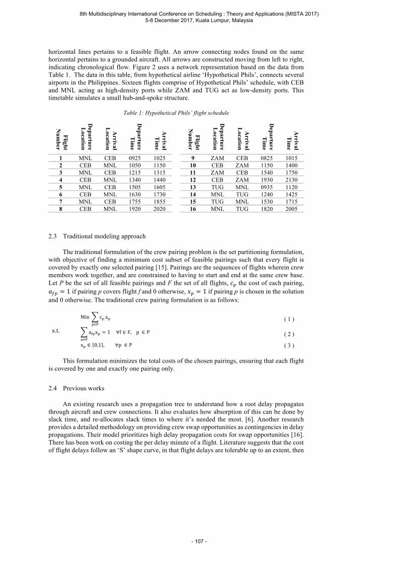
horizontal lines pertains to a feasible flight. An arrow connecting nodes found on the same horizontal pertains to a grounded aircraft. All arrows are constructed moving from left to right, indicating chronological flow. Figure 2 uses a network representation based on the data from Table 1. The data in this table, from hypothetical airline ‘Hypothetical Phils’, connects several airports in the Philippines. Sixteen flights comprise of Hypothetical Phils’ schedule, with CEB and MNL acting as high-density ports while ZAM and TUG act as low-density ports. This timetable simulates a small hub-and-spoke structure.

Table 1: Hypothetical Phils’ flight schedule

Flight N

umber

Departure L

ocation

Arrival

Location

Departure

Tim

e

Arrival T

ime

1 MNL CEB 0925 1025 2 CEB MNL 1050 1150 3 MNL CEB 1215 1315 4 CEB MNL 1340 1440 5 MNL CEB 1505 1605 6 CEB MNL 1630 1730 7 MNL CEB 1755 1855 8 CEB MNL 1920 2020

Flight N

umber

Departure L

ocation

Arrival

Location

Departure

Tim

e

Arrival T

ime

9 ZAM CEB 0825 1015 10 CEB ZAM 1150 1400 11 ZAM CEB 1540 1750 12 CEB ZAM 1930 2130 13 TUG MNL 0935 1120 14 MNL TUG 1240 1425 15 TUG MNL 1530 1715 16 MNL TUG 1820 2005

2.3 Traditional modeling approach

The traditional formulation of the crew pairing problem is the set partitioning formulation, with objective of finding a minimum cost subset of feasible pairings such that every flight is covered by exactly one selected pairing [15]. Pairings are the sequences of flights wherein crew members work together, and are constrained to having to start and end at the same crew base. Let P be the set of all feasible pairings and F the set of all flights, !" the cost of each pairing, #$" = 1 if pairing p covers flight f and 0 otherwise, '" = 1 if pairing p is chosen in the solution and 0 otherwise. The traditional crew pairing formulation is as follows:

Min c-

-∈/

x- ( 1 )

s.t. a2-x--∈/

= 1∀f ∈ F,p ∈ P ( 2 )

x- ∈ 0,1 , ∀p ∈ P ( 3 )

This formulation minimizes the total costs of the chosen pairings, ensuring that each flight is covered by one and exactly one pairing only.

2.4 Previous works

An existing research uses a propagation tree to understand how a root delay propagates through aircraft and crew connections. It also evaluates how absorption of this can be done by slack time, and re-allocates slack times to where it’s needed the most. [6]. Another research provides a detailed methodology on providing crew swap opportunities as contingencies in delay propagations. Their model prioritizes high delay propagation costs for swap opportunities [16]. There has been work on costing the per delay minute of a flight. Literature suggests that the cost of flight delays follow an ‘S’ shape curve, in that flight delays are tolerable up to an extent, then


- 107 -

becomes increasingly dissatisfactory until it reaches very long delays and approaches full customer dissatisfaction [4].

3 Robust crew pairing model

The model is formulated as an extension of the set partitioning formulation of the traditional crew pairing problem (CPP). The objective function involves the computation of costs of pairings, as well as the cost of delay propagations for each flight in each pairing. The model involves two phases, wherein the first selects the pairings for the solution, and the second selects the crew swaps for the solution.

3.1 Assumptions

The following are the assumptions taken in the development of the model in this research:

o The schedules of flights can be known with certainty and cannot be changed. o Minimum ground connection times can be defined for each pair of flights. o Any crew member can be scheduled to any flight. Crew pairings can be formed around

any of the flights within the set of flights being solved in the problem. o Regulations are known with certainty and do not vary. o The cost of each crew pairing can be determined as a deterministic value. o No additional flights need to be added into the timetable. o There are enough crew members to satisfy the pairings to be formed in the model. o All crew swaps to be performed have an available aircraft.

3.2 Definition of parameters

The following are defined in the model:

Sets and notationsP set of all feasible pairings F set of all flights

ρ- f preceding flight of f at pairing p in the same duty period

Q(f, p) set of flights that precede flight f and is in the same duty period as f in pairing p

R(f, p) set of flights that follow flight f and is in the same duty period as f in pairing p

α Q the first flight in the set of flights Q

ω Q the last flight in the set of flights Q M a very large number

System and decision variables ACC2- accumulated flight duty hours after

flying flight f in pairing p PND2- pending flight duty hours after

flying flight f in pairing p DP- delay propagation value for pairing

p s2-2F-F binary variable for checking

possibility of a swap between two flights from different pairings

1 if a swap is possible between flights f and f’ for pairings p and p’, 0 otherwise

x- binary decision variable for selection of pairings 1 if pairing p is selected, 0 otherwise

yH- binary decision variable for linearization of delay propagation requirement; i ∈ 1,2 1 if requirement is not violated; 0 otherwise


- 108 -

Input parametersc- cost of pairing π2- binary variable defining flights

covered by pairings 1 if flight f is covered by pairing p 0 otherwise

g minimum ground connection time r2 arrival time of flight f d2 departure time of flight f reg maximum regulation flight duty

period of crew b briefing period time bP debriefing period time τ2 average delay time of flight f

ap22F binary variable for the location connectivity of two flights 1 if flight f arrives at the same airport as flight f’ departs, 0 otherwise

hb--F binary variable for considering home bases of two pairings 1 if pairing p and p’ has the same home base, 0 otherwise

dpSHT minimum delay propagation level to consider a swap that mitigates delay

dpSUV maximum delay propagation level to consider a swap that absorbs delay

3.3 First phase: Pairing selection

The first phase involves the selection of the pairings into the solution. It has two objective functions that are counteracting, and thus, uses a user-inputted weight for the second objective function.

Min c--∈/

x- ( 4 )

Max DP-x--∈/

( 5 )

Objective function ( 4 ) is taken from the traditional crew pairing problem formulation. It

aims to minimize the total cost of the pairings chosen to cover the set of flights. Objective function ( 5 ) minimizes the total delay propagation value of the chosen pairings. The first expression aims to choose the pairings with the least costs, while the second expression chooses the pairings with least delay propagation. This bi-objective formulation is resolved by using a user-inputted weight to the second objective function.

The following mathematical expressions are the constraints of the model formulated:

π2-x--∈/

= 1 ∀f ∈ F ( 6 )

x- ∈ 0,1 ( 7 )

Constraint ( 6 ) ensures that all flights must be catered to by exactly one pairing. This

constraint is also present in the traditional crew pairing problem formulation. Constraint ( 7 ) states that the decision variable '" is a binary variable. The delay propagation value WX" of the pairings generated is calculated as the pairings are generated. It is calculated using the average historical delays of flights Y$, their scheduled arrival times Z$, and their scheduled departure times [$. The minimum ground connection time \ is also needed. An example of how the delay propagation value WX" is calculated is shown in Figure 5, which takes data from the hypothetical flight schedule in Table 1.


- 109 -

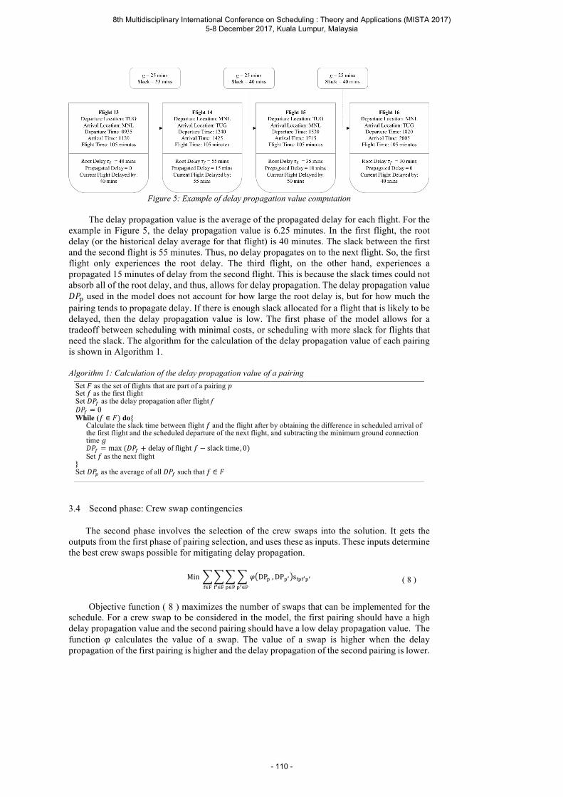
Figure 5: Example of delay propagation value computation

The delay propagation value is the average of the propagated delay for each flight. For the

example in Figure 5, the delay propagation value is 6.25 minutes. In the first flight, the root delay (or the historical delay average for that flight) is 40 minutes. The slack between the first and the second flight is 55 minutes. Thus, no delay propagates on to the next flight. So, the first flight only experiences the root delay. The third flight, on the other hand, experiences a propagated 15 minutes of delay from the second flight. This is because the slack times could not absorb all of the root delay, and thus, allows for delay propagation. The delay propagation value WX" used in the model does not account for how large the root delay is, but for how much the pairing tends to propagate delay. If there is enough slack allocated for a flight that is likely to be delayed, then the delay propagation value is low. The first phase of the model allows for a tradeoff between scheduling with minimal costs, or scheduling with more slack for flights that need the slack. The algorithm for the calculation of the delay propagation value of each pairing is shown in Algorithm 1.

Algorithm 1: Calculation of the delay propagation value of a pairing

3.4 Second phase: Crew swap contingencies

The second phase involves the selection of the crew swaps into the solution. It gets the outputs from the first phase of pairing selection, and uses these as inputs. These inputs determine the best crew swaps possible for mitigating delay propagation.

Min ] DP-, DP-F s2-2F-F-F∈/-∈/2F∈^2∈^

( 8 )

Objective function ( 8 ) maximizes the number of swaps that can be implemented for the

schedule. For a crew swap to be considered in the model, the first pairing should have a high delay propagation value and the second pairing should have a low delay propagation value. The function ] calculates the value of a swap. The value of a swap is higher when the delay propagation of the first pairing is higher and the delay propagation of the second pairing is lower.

Set _ as the set of flights that are part of a pairing ` Set a as the first flight Set WX$ as the delay propagation after flight f WX$ = 0 While (a ∈ _) do

Calculate the slack time between flight a and the flight after by obtaining the difference in scheduled arrival of the first flight and the scheduled departure of the next flight, and subtracting the minimum ground connection time \

WX$ = max(WX$ + delayofflighta − slacktime, 0) Set a as the next flight Set WX" as the average of all WX$ such that a ∈ _


- 110 -

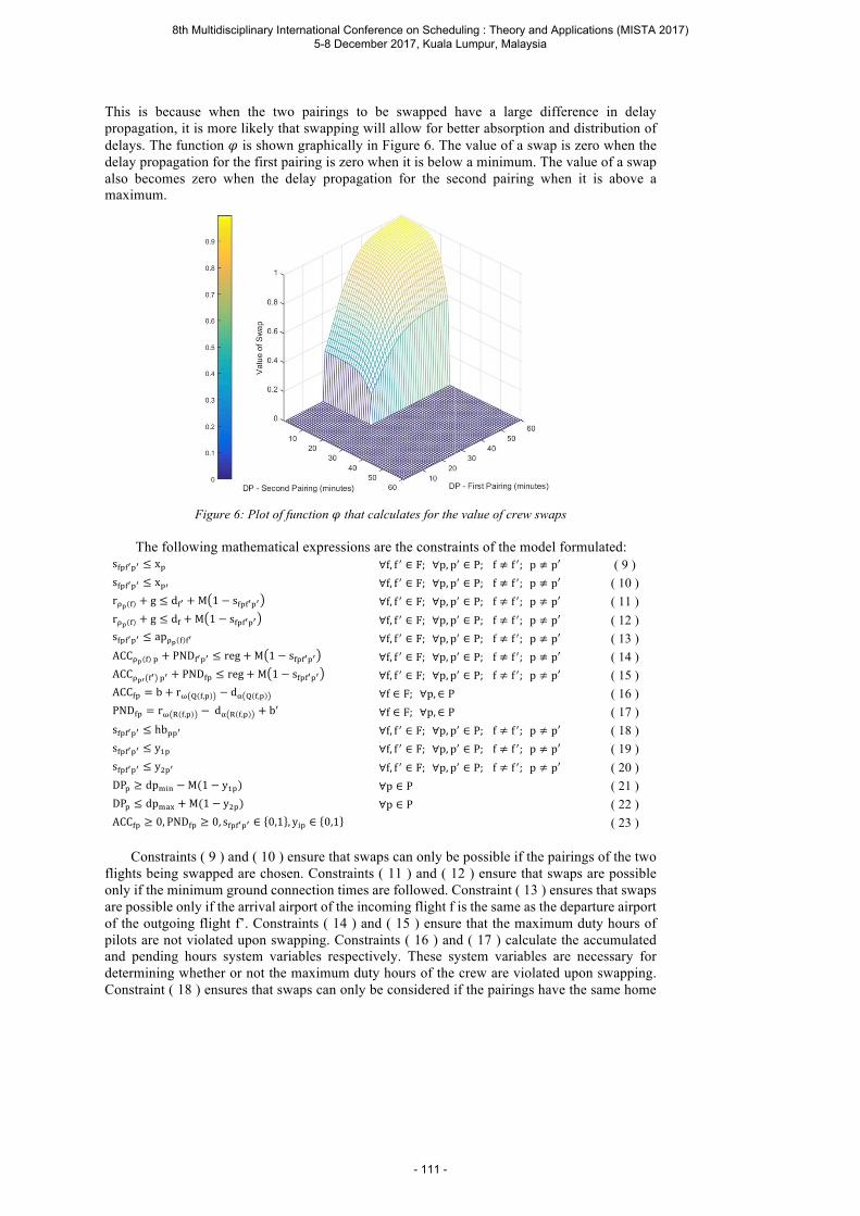
This is because when the two pairings to be swapped have a large difference in delay propagation, it is more likely that swapping will allow for better absorption and distribution of delays. The function ] is shown graphically in Figure 6. The value of a swap is zero when the delay propagation for the first pairing is zero when it is below a minimum. The value of a swap also becomes zero when the delay propagation for the second pairing when it is above a maximum.

Figure 6: Plot of function ] that calculates for the value of crew swaps

The following mathematical expressions are the constraints of the model formulated:

s2-2F-F ≤ x- ∀f, f P ∈ F;∀p, pP ∈ P; f ≠ f P; p ≠ p′ ( 9 ) s2-2F-F ≤ x-P ∀f, f P ∈ F;∀p, pP ∈ P; f ≠ f P; p ≠ p′ ( 10 ) rmn 2 + g ≤ d2F + M 1 − s2-2F-F ∀f, f P ∈ F;∀p, pP ∈ P; f ≠ f P; p ≠ p′ ( 11 ) rmn 2 + g ≤ d2 + M 1 − s2-2F-F ∀f, f P ∈ F;∀p, pP ∈ P; f ≠ f P; p ≠ p′ ( 12 ) s2-2F-F ≤ apmn 2 2F ∀f, f P ∈ F;∀p, pP ∈ P; f ≠ f P; p ≠ p′ ( 13 ) ACCmn 2 - + PND2F-F ≤ reg + M 1 − s2-2F-F ∀f, f P ∈ F;∀p, pP ∈ P; f ≠ f P; p ≠ p′ ( 14 ) ACCmnF 2F -F + PND2- ≤ reg + M 1 − s2-2F-F ∀f, f P ∈ F;∀p, pP ∈ P; f ≠ f P; p ≠ p′ ( 15 ) ACC2- = b + ro p 2,- − dq p 2,- ∀f ∈ F;∀p, ∈ P ( 16 ) PND2- = ro r 2,- − dq r 2,- + bP ∀f ∈ F;∀p, ∈ P ( 17 ) s2-2F-F ≤ hb--F ∀f, f P ∈ F;∀p, pP ∈ P; f ≠ f P; p ≠ p′ ( 18 ) s2-2F-F ≤ ys- ∀f, f P ∈ F;∀p, pP ∈ P; f ≠ f P; p ≠ p′ ( 19 ) s2-2F-F ≤ yt-F ∀f, f P ∈ F;∀p, pP ∈ P; f ≠ f P; p ≠ p′ ( 20 ) DP- ≥ dpSHT − M(1 − ys-) ∀p ∈ P ( 21 ) DP- ≤ dpSUV + M(1 − yt-) ∀p ∈ P ( 22 ) ACC2- ≥ 0, PND2- ≥ 0, s2-2F-F ∈ 0,1 , yH- ∈ 0,1 ( 23 )

Constraints ( 9 ) and ( 10 ) ensure that swaps can only be possible if the pairings of the two

flights being swapped are chosen. Constraints ( 11 ) and ( 12 ) ensure that swaps are possible only if the minimum ground connection times are followed. Constraint ( 13 ) ensures that swaps are possible only if the arrival airport of the incoming flight f is the same as the departure airport of the outgoing flight f’. Constraints ( 14 ) and ( 15 ) ensure that the maximum duty hours of pilots are not violated upon swapping. Constraints ( 16 ) and ( 17 ) calculate the accumulated and pending hours system variables respectively. These system variables are necessary for determining whether or not the maximum duty hours of the crew are violated upon swapping. Constraint ( 18 ) ensures that swaps can only be considered if the pairings have the same home


- 111 -

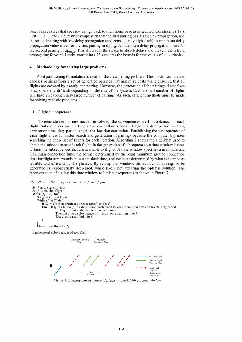
base. This ensures that the crew can go back to their home base as scheduled. Constraints ( 19 ), ( 20 ), ( 21 ), and ( 22 )restrict swaps such that the first pairing has high delay propagation, and the second pairing with low delay propagation (and consequently high slack). A minimum delay propagation value is set for the first pairing in dpSHT. A maximum delay propagation is set for the second pairing in dpSUV. This allows for the swaps to absorb delays and prevent them from propagating forward. Lastly, constraint ( 23 ) ensures the bounds for the values of all variables.

4 Methodology for solving large problems

A set partitioning formulation is used for the crew pairing problem. This model formulation chooses pairings from a set of generated pairings that minimize costs while ensuring that all flights are covered by exactly one pairing. However, the generation of the pairings themselves is exponentially difficult depending on the size of the system. Even a small number of flights will have an exponentially large number of pairings. As such, efficient methods must be made for solving realistic problems.

4.1 Flight subsequences

To generate the pairings needed in solving, the subsequences are first obtained for each flight. Subsequences are the flights that can follow a certain flight in a duty period, meeting connection time, duty period length, and location constraints. Establishing the subsequences of each flight allow for faster search and generation of pairings because the computer bypasses searching the entire set of flights for each iteration. Algorithm 2 shows the algorithm used to obtain the subsequences of each flight. In the generation of subsequences, a time window is used to limit the subsequences that are available to flights. A time window specifies a minimum and maximum connection time, the former determined by the legal minimum ground connection time for flight turnarounds, plus a set slack time, and the latter determined by what is deemed as feasible and efficient by the planner. By setting this window, the number of pairings to be generated is exponentially decreased, while likely not affecting the optimal solution. The representation of setting this time window to limit subsequences is shown in Figure 7.

Algorithm 2: Obtaining subsequences of each flight

Figure 7: Limiting subsequences of flights by establishing a time window

Set _ as the set of flights Set as as the first flight While (as ∈ _) do Set at as the first flight While (at ∈ _) do If (as = at) then break and choose next flight for at Else If at can follow as in a duty period, such that it follows connection time constraints, duty period

length constraints, and location constraints Then set at as a subsequence of as and choose next flight for at Else choose next flight for at Choose next flight for as Enumerate all subsequences of each flight


- 112 -

4.2 Duty tree construction

After generating the subsequences, a duty tree is used to produce the duty periods for generating pairings. The subsequences are used as the building blocks for the duty periods, while the duty periods will be used as the building blocks for the pairings. The duty tree is limited by the maximum number of flights in a duty. Algorithm 3 shows the algorithm used to obtain the valid duty periods of a set of flights.

Duty tree construction can be sped up and limited by specifying the starting and ending locations of the duty periods it generates. A duty period always starts and ends at either a location that is a home base for crew, or at a location that crew stay at for long rests. In a typical airline setting, the home bases are set, and the locations for long rests can be indicated by the planner. For example, a location that is in the rural province that is a 2-hour drive from a major city will never be a starting or ending point of a duty period. It will always be less costly for the airline, and more convenient for the crew, to start and end duty periods at the major city. A major city has more flights connecting through, and thus, any crew that stays here can be more flexibly scheduled. By specifying the home bases and the locations wherein long rests can occur, the number of duty periods can be reduced dramatically. A hub-and-spoke network will have a significantly larger number of spokes than hubs. If the locations for the starting and ending points of duty periods can be limited to the hubs and a few far-off spokes in an airline network, the duty periods that can be generated will be significantly limited while not affecting the optimal solution. Algorithm 3: Constructing duty tree and valid duty periods

4.3 Progressive pairing generation

A concept on column generation can be used to take advantage of the set partitioning model formulation in order to shorten the solution time. Column generation is used when the number of columns in a problem (or the number of possible solutions) is very large. This is typically the case for set partitioning problems. Solution difficulty comes from the large number of possible solutions. If columns were generated iteratively, then the problem can be solved with greater tractability, even though there is no assurance of optimality. The guide for the generation of pairings is the hierarchy of how preferable the types of pairings are. Single-duty pairings are most preferred, then multiple-duty pairings, then pairings that include deadhead. Deadhead is the movement of crew on existing commercial flights of the airline as passengers, but as required by their schedule set by the company and count as working hours with regard to satisfying

Set _ as the set of flights Set vw as the set of subsequences for flight x Set y#'azx\ℎ| as the maximum number of flights in a duty Set as as the first flight While (as ∈ _) do If the series [ as ] satisfies constraints on duty period length then series [ as ] is a valid duty period Set at as the first flight among subsequences of as While (at ∈ vs) do If the series [ as , at ] satisfies constraints on duty period length then series [ as , at ] is a valid duty period Set a~ as the first flight among subsequences of at … While (aÄÅ$ÇwÉÑÖÜ ∈ vÄÅ$ÇwÉÑÖÜás) do If the series [ as, at , … , aÄÅ$ÇwÉÑÖÜás , aÄÅ$ÇwÉÑÖÜ ] satisfies constraints on duty period length Then series [ as, at , … , aÄÅ$ÇwÉÑÖÜás , aÄÅ$ÇwÉÑÖÜ ] is a valid duty period Choose next flight for aÄÅ$ÇwÉÑÖÜ … Choose next flight for at Choose next flight for as Establish duty tree based on valid duty periods


- 113 -

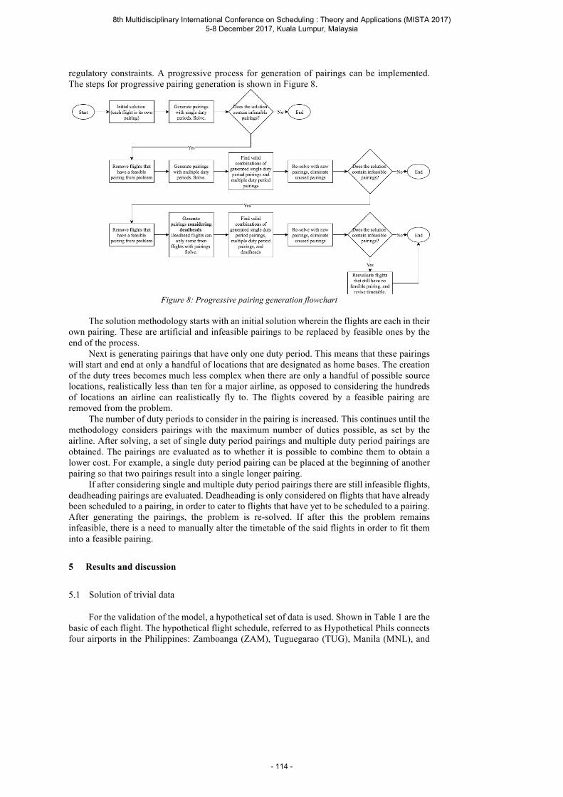
regulatory constraints. A progressive process for generation of pairings can be implemented. The steps for progressive pairing generation is shown in Figure 8.

Figure 8: Progressive pairing generation flowchart

The solution methodology starts with an initial solution wherein the flights are each in their

own pairing. These are artificial and infeasible pairings to be replaced by feasible ones by the end of the process.

Next is generating pairings that have only one duty period. This means that these pairings will start and end at only a handful of locations that are designated as home bases. The creation of the duty trees becomes much less complex when there are only a handful of possible source locations, realistically less than ten for a major airline, as opposed to considering the hundreds of locations an airline can realistically fly to. The flights covered by a feasible pairing are removed from the problem.

The number of duty periods to consider in the pairing is increased. This continues until the methodology considers pairings with the maximum number of duties possible, as set by the airline. After solving, a set of single duty period pairings and multiple duty period pairings are obtained. The pairings are evaluated as to whether it is possible to combine them to obtain a lower cost. For example, a single duty period pairing can be placed at the beginning of another pairing so that two pairings result into a single longer pairing.

If after considering single and multiple duty period pairings there are still infeasible flights, deadheading pairings are evaluated. Deadheading is only considered on flights that have already been scheduled to a pairing, in order to cater to flights that have yet to be scheduled to a pairing. After generating the pairings, the problem is re-solved. If after this the problem remains infeasible, there is a need to manually alter the timetable of the said flights in order to fit them into a feasible pairing.

5 Results and discussion

5.1 Solution of trivial data

For the validation of the model, a hypothetical set of data is used. Shown in Table 1 are the basic of each flight. The hypothetical flight schedule, referred to as Hypothetical Phils connects four airports in the Philippines: Zamboanga (ZAM), Tuguegarao (TUG), Manila (MNL), and


- 114 -

Cebu (CEB). This data is trivial, containing only sixteen flights with CEB and MNL acting as high-density ports while ZAM and TUG act as low-density ports.

Pairings were generated based on the flight schedule. It is assumed that a crew base can exist in all four airports. Two solutions for Hypothetical Phils are obtained, one using the traditional model, and one using the robust crew pairing model. The traditional model obtains a lower planned cost than the robust crew pairing model, as expected.

A scenario is applied to the schedule for Hypothetical Phils based on the input parameters and locations of the flights, wherein flights coming and going to hubs are more likely to be delayed. The scenario assigns independent local delays for each flight. If connecting resources are present between two flights (same crew with insufficient remaining time to connect), delay will propagate. A minimum ground connection time of 25 minutes is used. If the time between the actual arrival of the previous flight and the scheduled departure of the next flight is less than this, the next flight is delayed.

The number of minutes each flight is delayed for for the two solutions are presented in Figure 9. For many of the flights the deviations in the schedule were often greater for the traditional model solution. Flights 12 was the only flight that was larger in delay for the robust crew pairing model solution as compared to the traditional model solution.

Figure 9: Flight delay (minutes) of each solution obtained for each Hypothetical Phils flight

For both solutions, there was a steady increase in delays from flights 1 through 8. This is

because of the short connection time between these flights, and that these flights are between high density hubs. This makes it more likely that these flights become delayed. Swaps taken by the crew pairings in the robust solution were able to lessen the effects of delay propagation. Therefore, despite the additional increase in planned cost, the overall reduction in delay may make it the more desirable solution.

Table 2 shows the comparisons for costs and delays for the two obtained solutions. The cost is obtained using a cost structure based on the duty period lengths (including overtime and fatigue) that simulates crew pay. While planned costs are higher for the robust solution, it has a significantly lower total delay. Even more important is that the traditional model solution has 50% of its flights (8 out of 16) perceived as being late (delayed for more than 15 minutes), and 2 of those flights are perceived being very late (delayed for more than 30 minutes). On the other hand, the crew swap model solution has only 3 of its flight as perceived as late, and none of its flights being excessively late.

This solution serves as a trivial example for showing the effect of mitigation of delay propagation through slack times and crew swaps on an individual flight basis.


- 115 -

Table 2: Cost and delay comparison between the traditional CPP and the crew swap model solutions Traditional CPP Solution Crew Swap Model Solution Planned Cost 17,654 19,830 Total Delay in minutes 184 119 Number of flights delayed for more than 15 minutes

8 3

Number of flights delayed for more than 30 minutes

2 0

5.2 Solution of 1890-flight crew pairing problem

Computational experiments for the solution of realistic data were carried out on a desktop PC with an Intel Core i3 processor with 8GB RAM. The MATLAB Integer Linear Programming solver is used. Each solution of the 1890-flight crew pairing problem from a real airline that spans one week of operations had solution times between 60 to 90 seconds each.

Results for the traditional model in the form of a crew pairing schedule were obtained. To evaluate these crew pairings, they were run through a Monte Carlo Simulation. Data on historical delays of flights were used to obtain the simulated delays for the flights. The pairings constructed determined the propagation of delays. The results for these are shown in Table 3.

Table 3: Monte Carlo simulation results of schedule constructed from the traditional crew pairing model

Planned Cost 695,805.65 Total Delay 48,364.88 minutes Flights with delays less than or equal to 15 minutes 608 flights Flights with 15 minutes < delay ≤ 30 minutes 642 flights Flights with 30 minutes < delay ≤ 45 minutes 381 flights Flights with 45 minutes < delay ≤ 60 minutes 159 flights Flights with delays more than 60 minutes 100 flights

The robust model in this research resolves its multiple objective functions (minimizing cost

and maximizing robustness) by using a user-inputted weight. By varying this weight and obtaining different solutions, solutions of different robustness levels and planned costs are obtained. The robust crew pairing model obtains a large number of solutions by increasing the weight. The next solution obtained is more robust than the last one, but also more expensive in planned costs. Each solution is a set of crew pairings constructed by the model that caters to all flights.

A function is needed to evaluate the severity of a flight delay that properly reflects the costs of flight delay minutes to the airline. A function proposed for the customer’s propensity to switch airlines from a given airline [4] is used as the basis for this function. The graph for this is shown in Figure 10. The ‘S’ shape curve of this function is based on the Kano model that defines a three-tier approach to customer satisfaction requirements [17]. The ‘S’ shape curve shows that a small level of delay is insignificant, the significance of the delay increases once the delay moves past what is tolerable to the customer, and plateaus when delay is very high.

The function to evaluate the severity of a flight delay is shown in expression ( 24 ). The variable h is the hypothetical cost of delay set by the crew planner, and the variable d is the delay of the flight in minutes.

ℎ 1 + âä.åáç.çé èê.êë ás

( 24 )


- 116 -

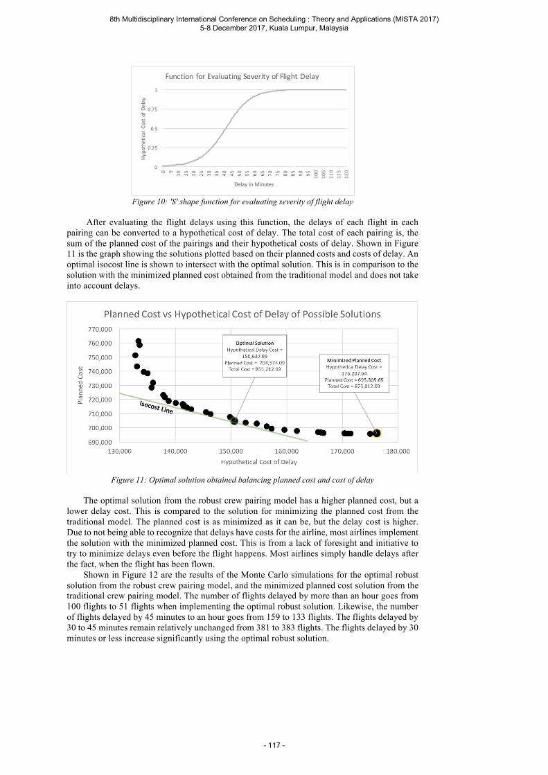
Figure 10: 'S' shape function for evaluating severity of flight delay

After evaluating the flight delays using this function, the delays of each flight in each

pairing can be converted to a hypothetical cost of delay. The total cost of each pairing is, the sum of the planned cost of the pairings and their hypothetical costs of delay. Shown in Figure 11 is the graph showing the solutions plotted based on their planned costs and costs of delay. An optimal isocost line is shown to intersect with the optimal solution. This is in comparison to the solution with the minimized planned cost obtained from the traditional model and does not take into account delays.

Figure 11: Optimal solution obtained balancing planned cost and cost of delay

The optimal solution from the robust crew pairing model has a higher planned cost, but a

lower delay cost. This is compared to the solution for minimizing the planned cost from the traditional model. The planned cost is as minimized as it can be, but the delay cost is higher. Due to not being able to recognize that delays have costs for the airline, most airlines implement the solution with the minimized planned cost. This is from a lack of foresight and initiative to try to minimize delays even before the flight happens. Most airlines simply handle delays after the fact, when the flight has been flown.

Shown in Figure 12 are the results of the Monte Carlo simulations for the optimal robust solution from the robust crew pairing model, and the minimized planned cost solution from the traditional crew pairing model. The number of flights delayed by more than an hour goes from 100 flights to 51 flights when implementing the optimal robust solution. Likewise, the number of flights delayed by 45 minutes to an hour goes from 159 to 133 flights. The flights delayed by 30 to 45 minutes remain relatively unchanged from 381 to 383 flights. The flights delayed by 30 minutes or less increase significantly using the optimal robust solution.

0

0.25

0.5

0.75

1

0 5 10 15 20 25 30 35 40 45 50 55 60 65 70 75 80 85 90 95 100

105

110

115

120

Hypothetica

lCosto

fDelay

DelayinMinutes

Function forEvaluatingSeverityofFlightDelay


- 117 -

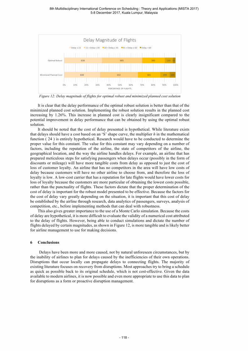
Figure 12: Delay magnitude of flights for optimal robust and minimized planned cost solution

It is clear that the delay performance of the optimal robust solution is better than that of the minimized planned cost solution. Implementing the robust solution results in the planned cost increasing by 1.26%. This increase in planned cost is clearly insignificant compared to the potential improvement in delay performance that can be obtained by using the optimal robust solution.

It should be noted that the cost of delay presented is hypothetical. While literature exists that delays should have a cost based on an ‘S’ shape curve, the multiplier h in the mathematical function ( 24 ) is entirely hypothetical. Research would have to be conducted to determine the proper value for this constant. The value for this constant may vary depending on a number of factors, including the reputation of the airline, the state of competitors of the airline, the geographical location, and the way the airline handles delays. For example, an airline that has prepared meticulous steps for satisfying passengers when delays occur (possibly in the form of discounts or mileage) will have more tangible costs from delay as opposed to just the cost of loss of customer loyalty. An airline that has no competitors in the area will have low costs of delay because customers will have no other airline to choose from, and therefore the loss of loyalty is low. A low-cost carrier that has a reputation for late flights would have lower costs for loss of loyalty because the customers are more particular of obtaining the lowest costs possible, rather than the punctuality of flights. These factors dictate that the proper determination of the cost of delay is important for the robust model presented to be effective. Because the factors for the cost of delay vary greatly depending on the situation, it is important that this cost of delay be established by the airline through research, data analytics of passengers, surveys, analysis of competition, etc., before implementing methods that can deal with robustness.

This also gives greater importance to the use of a Monte Carlo simulation. Because the costs of delay are hypothetical, it is more difficult to evaluate the validity of a numerical cost attributed to the delay of flights. However, being able to conduct simulations and dictate the number of flights delayed by certain magnitudes, as shown in Figure 12, is more tangible and is likely better for airline management to use for making decisions.

6 Conclusions

Delays have been more and more caused, not by natural unforeseen circumstances, but by the inability of airlines to plan for delays caused by the inefficiencies of their own operations. Disruptions that occur locally can propagate delays to connecting flights. The majority of existing literature focuses on recovery from disruptions. Most approaches try to bring a schedule as quick as possible back to its original schedule, which is not cost-effective. Given the data available to modern airlines, it is now possible and even more appropriate to use this data to plan for disruptions as a form or proactive disruption management.

608

638

642

685

381

383

159

133

100

51

0% 10% 20% 30% 40% 50% 60% 70% 80% 90% 100%

MinimizedPlannedCost

OptimalRobust

PERCENTAGEOFFLIGHTS

DelayMagnitudeofFlightsDelay≤15 15<Delay≤30 30<Delay≤45 45<Delay≤60 Delay>60


- 118 -

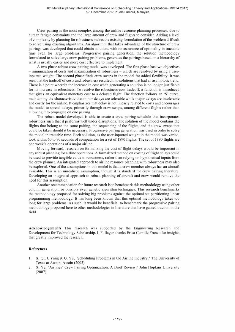
Crew pairing is the most complex among the airline resource planning processes, due to human fatigue constraints and the large amount of crew and flights to consider. Adding a level of complexity by planning for robustness makes the existing formulation of the problem difficult to solve using existing algorithms. An algorithm that takes advantage of the structure of crew pairings was developed that could obtain solutions with no assurance of optimality in tractable time even for large problems. Progressive pairing generation, the solution methodology formulated to solve large crew pairing problems, generates the pairings based on a hierarchy of what is usually easier and more cost effective to implement.

A two-phase robust crew pairing model was developed. The first phase has two objectives – minimization of costs and maximization of robustness – which are resolved by using a user-inputted weight. The second phase finds crew swaps in the model for added flexibility. It was seen that the tradeoff of costs and robustness resulted into solutions that had an asymptotic trend. There is a point wherein the increase in cost when generating a solution is no longer justifiable for its increase in robustness. To resolve the robustness-cost tradeoff, a function is introduced that gives an equivalent monetary cost to a delayed flight. The function follows an ‘S’ curve, maintaining the characteristic that minor delays are tolerable while major delays are intolerable and costly for the airline. It emphasizes that delay is not linearly related to costs and encourages the model to spread delays, primarily through crew swaps, among different flights rather than allowing it to propagate on one pairing.

The robust model developed is able to create a crew pairing schedule that incorporates robustness such that it performs well under disruptions. The solution of the model contains the flights that belong to the same pairing, the sequencing of the flights, and the crew swaps that could be taken should it be necessary. Progressive pairing generation was used in order to solve the model in tractable time. Each solution, as the user-inputted weight in the model was varied, took within 60 to 90 seconds of computation for a set of 1890 flights. The set of 1890 flights are one week’s operations of a major airline.

Moving forward, research on formalizing the cost of flight delays would be important in any robust planning for airline operations. A formalized method on costing of flight delays could be used to provide tangible value to robustness, rather than relying on hypothetical inputs from the crew planner. An integrated approach to airline resource planning with robustness may also be explored. One of the assumptions in this model is that a crew member always has an aircraft available. This is an unrealistic assumption, though it is standard for crew pairing literature. Developing an integrated approach to robust planning of aircraft and crew would remove the need for this assumption.

Another recommendation for future research is to benchmark this methodology using other column generation, or possibly even genetic algorithm techniques. This research benchmarks the methodology proposed for solving big problems against the optimal set partitioning linear programming methodology. It has long been known that this optimal methodology takes too long for large problems. As such, it would be beneficial to benchmark the progressive pairing methodology proposed here to other methodologies in literature that have gained traction in the field.

Acknowledgements This research was supported by the Engineering Research and Development for Technology Scholarship. I. F. Ilagan thanks Erica Camille Franco for insights that greatly improved the research.

References

1. X. Qi, J. Yang & G. Yu, "Scheduling Problems in the Airline Industry," The University of Texas at Austin, Austin (2003)

2. X. Ye, "Airlines’ Crew Pairing Optimization: A Brief Review," John Hopkins University (2007)


- 119 -

3. J. Bates, J. Polak, P. Jones & A. Cook, "The Valuation of Reliability for Personal Travel," Transportation Research Part E, vol. 37, pp. 191-229 (2001)

4. A. Cook, G. Tanner & A. Lawes, "The hidden cost of airline unpunctuality," European Organisation for the Safety of Air Navigation (2009)

5. E. Sauerwein, F. Bailom, K. Matzler & H. H. Hinterhuber, "The Kano model: How to delight your customers," in IX International Working Seminar on Production Economics, Innsbruck (1996)

6. S. AhmadBeygi, A. Cohn and M. Lapp, "Decreasing Airline Delay Propagation by Re-Allocating Scheduled Slack," in Proceedings of the Industry Studies Conference (2008)

7. L. Lee, C. Lee & Y. Tan, "A multi-objective genetic algorithm for robust flight scheduling using simulation," European Journal of Operations Research, vol. 177, pp. 1948–1968 (2007)

8. M. C. Lonzius & A. Lange, "Robust Scheduling: An Empirical Study of Its Impact on Air Traffic Delays," Transportation Research Part E, vol. 100, pp. 98-114 (2017)

9. C.-L. Wu, "Airline Operations and Delay Management – Insights from Airline Economics, Networks and Strategic Schedule Planning," Ashgate, Farnham (2010)

10. U. Özdemir, "Methodology for Crew-Pairing Problem in Airline Crew Scheduling," Bogazici University, Istanbul (2009)

11. E. Andersson, E. Housos, N. Kohl and D. Wedelin, "Crew Pairing Optimization," in Operations research in the airline industry, Kluwer Academic Publishers, Boston, pp. 228-258 (2011)

12. A. Mercier, J.-F. Cordeau and F. Soumis, "A computational study of Benders decomposition for the integrated aircraft routing and crew scheduling problem," Computers and Operations Research, vol. 32, no. 6, pp. 1451-1476 (2005)

13. E. C. Franco, Interviewee, Airline Crew Planner. [Interview]. (20 October 2016) 14. J. Clausen, A. Larsen, J. Larsen and N. J. Rezanova, "Disruption management in the airline

industry—Concepts, models and methods," Computers and Operations Research, vol. 37, pp. 809-821 (2010)

15. İ. Muter, Ş. İ. Birbil, K. Bülbül, G. Şahin, H. Yenigün, D. Taş and D. Tüzün, "Solving a robust airline crew pairing problem with column generation," Computers & Operations Research, vol. 40, no. 3, pp. 815-830 (2013)

16. L. Ionescu and N. Kliewer, "Increasing Flexibility of Airline Crew Schedules," Procedia Social and Behavioral Sciences, vol. 20, pp. 1019-1028 (2011)

17. N. Kano, N. Seraku, F. Takahashi and S. Tsuji, "Attractive quality and must-be quality," Journal of the Japanese Society for Quality Control, vol. 14, no. 2, pp. 147-156 (1984)


- 120 -

MISTA 2017

Integer programming for home care scheduling withflexible task frequency and controllable processing times

Pieter Smet · Federico Mosquera · Tulio

A. M. Toffolo · Greet Vanden Berghe

Abstract Home care scheduling integrates the assignment, sequencing and schedul-

ing of caregivers to household tasks subject to a range of operational constraints and

objectives. Due to the increased scale and complexity of client requests, decision sup-

port models have become an indispensable tool for management to efficiently deploy

available staff. The present paper introduces a time-indexed integer programming for-

mulation for multi-period home care scheduling while considering both flexible task

frequency and controllable processing times. Both of these novel characteristics are

common in practice, but have never been considered by previous academic models. By

using two modeling tools, activity modes and task patterns, these characteristics may

be integrated without any assumptions on their cost functions or general structure.

Extensive computational experiments are performed to analyze the new formulation’s

performance on practical problem instances. The results confirm that it is possible to

solve realistically-sized instances consisting of 25 caregivers and 100 tasks to optimality

within acceptable computation time.

1 Introduction

As home care is steadily becoming the primary source of care for elderly people, there

is a high demand which is increasingly difficult for home care organizations to sat-

isfy. Rich decision support models are quickly becoming indispensable for home care

organizations in order to effectively manage their available staff. In short, home care

scheduling concerns the scheduling and assignment of skilled caregivers to various tasks

at different clients’ homes. The underlying optimization problem integrates assignment,

sequencing and scheduling decisions, subject to a variety of personal and organizational

constraints and objectives. Due to its practical relevance and increased impact in re-

cent years, home care scheduling has received considerable attention in the academic

literature (Fikar and Hirsch, 2016).

The present paper introduces a new integer programming model for scheduling care-

givers in a multi-period setting within which the schedules are constructed for multiple

Pieter Smet, Federico Mosquera, Tulio A. M. Toffolo, Greet Vanden BergheKU Leuven, Department of Computer Science, CODeS & imecE-mail: [email protected]


- 121 -

consecutive days. The proposed model employs time-indexed decision variables, which

are known to result in tight linear programming relaxations for scheduling problems

(Van den Akker et al, 2000). Tasks are used as an abstract concept which generalize

client care requirements. Each task is associated with skill requirements and must be

performed multiple times during the scheduling period. Skill structure is modeled in a

general way such that both hierarchical and arbitrary structures may be considered.

Various other real-world problem characteristics are included such as availabilities,

personal preferences and idle time.

Travel time is an objective commonly considered by academic models for home

(health) care scheduling (Akjiratikarl et al, 2007; Liu et al, 2014; Maya Duque et al,

2015). The proposed model, however, does not explicitly minimize travel time for a

number of reasons. Firstly, home care tasks, such as housekeeping or accompanying a

client to a social activity, are typically very time-consuming. Consequently, caregivers

visit a small number of clients per day, thereby limiting the number of times they

must travel between clients. Secondly, within real-world problem instances, clients are

often clustered in, for example, municipalities. The distance between clients within a

cluster is typically relatively small compared to the distance between clients in different

clusters. The proposed model thus does not explicitly minimize travel time but instead

forbids caregivers to visit clients associated with different clusters on the same day.

Scheduling flexibility is emphasized by considering flexible task frequency (how

many times a task is scheduled) and controllable processing times (the duration of

each scheduled task). For both of these properties, general cost functions may be de-

fined which model the cost of scheduling a task fewer times than required or schedul-

ing a task for less time than required. When considered independently, task rejection

and controllable processing times are known to make polynomially solvable machine

scheduling problems NP-hard (Shabtay and Steiner, 2007; Shabtay et al, 2013). While

these types of flexibility are common practice in home care organizations, there are no

academic models integrating these two properties.

The majority of studies throughout the academic literature address the daily schedul-

ing problem in which only a single period is considered (Rasmussen et al, 2012; Yuan

et al, 2015; Braekers et al, 2016). Only a few authors solve the problem in a multi-

period setting. However, considering multiple days is essential as home care scheduling

concerns human resources. Consequently, not only capacity is important, but also, for

example, sequence, frequency, continuity, assignment spreading and variation of as-

signments. Begur et al (1997) describe an early implementation of a decision support

system for a real-world home care scheduling problem. The problem is addressed by

heuristically solving a series of daily scheduling problems with varying visiting pat-

terns. Such patterns are also used by Cappanera and Scutella (2014) in an integer

programming model for scheduling visits to palliative patients. Trautsamwieser and

Hirsch (2014) present a branch-price-and-cut algorithm for a weekly scheduling prob-

lem. Their model includes a number of employee scheduling constraints concerning

breaks and rest time which allow for flexible working hours. Finally, Nickel et al (2012)

address the planning of home care services at different time horizons. They present a

metaheuristic approach based on constraint programming for both mid- and short-term

planning. There are no approaches in the state of the art academic literature which

consider flexibility both in terms of frequency and duration.

The remainder of this paper is organized as follows. Section 2 presents a formal

definition of the considered home care scheduling problem. Section 3 introduces the

proposed time-indexed integer programming formulation along with detailed examples


- 122 -

of the novel modeling tools which it includes. Section 4 analyzes a series of computa-

tional experiments to gain various insights concerning the model’s performance. Finally,

Section 5 concludes the paper and identifies areas for future research.

2 Problem definition

Let D = 1, ..., |D| be a set of consecutive days which define the scheduling period

and let E = 1, ..., |E| be the set of caregivers. The availability of caregiver e ∈ E

on day d ∈ D is defined as a hard time window [b−ed, b+ed) with 0 ≤ b−ed < b+ed. The

tasks to be scheduled are denoted by J = 1, ..., |J |. For each task j, let Ej ⊆ E be

the subset of caregivers who meet the skill requirements. The time window in which

task j may be scheduled on day d is denoted by [b−jd, b+jd) with 0 ≤ b−jd < b+jd. Let aje

be the cost of assigning task j to caregiver e which represents several soft preferences

such as pet allergies, gender or language proficiency. Travel restrictions for caregivers

are defined by the set J , which contains pairs of tasks (j, j′) which cannot be assigned

to the same caregiver on the same day. Typically, (j, j′) ∈ J if the travel time between

the locations of j and j′ exceeds some given bound.

Each task j ∈ J must be scheduled fj times during the scheduling period. Note that

tasks cannot be scheduled more than this frequency. A cost function pfj : [0, f+j ]→ Rdefines the cost when task j is scheduled x times. The precise definition of pfj (x)

depends on the application context where, for example, scheduling a task at least once

may be of prime importance, whereas reaching the desired frequency is not critical,

or vice versa. Figure 1a illustrates examples of piecewise linear and non-linear cost

functions which may be used to model frequency cost. Note that pfj (x) is not assumed

to be monotonically decreasing but, in practice, often will be.

Each time task j ∈ J is scheduled, its duration should be between d−j and d+j ,

with both bounds considered hard constraints. Similar to the task frequency, a cost

function pdj : [d−j , d+j ]→ R defines the cost of scheduling task j with duration x. Figure

1b shows examples of pdj (x) whose definition is, again, strongly context-dependent and

typically monotonically decreasing.

Times assigned jf

Cos

t

(a) Frequency cost functions

Cost

Duration

jd

jd

(b) Duration cost functions

Fig. 1: Examples of cost functions for flexible frequency and controllable processing

times.


- 123 -

The objective function to be minimized is a weighted sum of five objectives: (i)

frequency cost as calculated by pfj (x), (ii) duration cost as calculated by pdj (x), (iii)

the sum of assignment costs aje, (iv) caregiver idle time and (v) task spreading cost.

Each of these objectives has a weight ω1, ω2, ..., ω5 associated with it.

Task spreading ensures that the days on which a task is scheduled are distributed

evenly throughout the scheduling period. This is an important objective in practice,

where visiting the same client on two consecutive days is generally undesirable. The cost

related to task spreading is calculated as the absolute value of the difference between

the ideal task spread and the actual number of days between two scheduled tasks. The

ideal spread is defined as the quotient of the length of the scheduling period and the

number of times the task is scheduled, rounded down to the nearest integer.

Example 1 Consider a task j1 ∈ J which is scheduled three times throughout a one-

week scheduling period, as illustrated in Figure 2. The ideal spread is calculated as⌊73

⌋= 2, which means that ideally there will be exactly two days between each time j1

is scheduled. Examining the solution in Figure 2 shows that there are two days between

the first and second occurrence of j1 but only one day between the second and third

occurrence. The total spreading cost is therefore |2− 2|+ |2− 1| = 1.

Mon

j1 j1 j1

Tue Wed Thu Fri Sat Sun

2 days in between 1 day in between

Fig. 2: Example of task spreading

Note that, if j1 was scheduled, for example, on Monday and Tuesday, the number

of days in between these two occurrences would be zero and the task spreading cost

would be |⌊72

⌋− 0| = 3.

3 Time-indexed integer linear programming formulation

A time-indexed integer programming formulation is proposed in which scheduling pe-

riod D is discretized into time-slots based on some given granularity φ. Let T =

1, ..., |T | be the set of time-slots representing the complete scheduling period. The

subset of time-slots associated with day d is denoted as Td. The problem’s two novel

complex elements, controllable processing times and flexible task frequency, are mod-

eled as activity modes and task patterns, respectively.

Activity modes are commonly used in resource-constrained project scheduling prob-

lems (Wauters et al, 2016). Let Mj = 1, ..., |M | be the set of feasible modes for task

j, djm the duration of task j in mode m ∈ Mj and pjm = pdj (djm) the cost for using

mode m ∈Mj (Brucker et al, 1999).

Example 2 Consider a task j1 ∈ J with d−j1 = 60 mins and d+j1 = 240 mins. Given a

time granularity φ = 15 mins, task j1 has 13 activity modes in the set Mj1 = 1, ..., 13.The duration of each mode m ∈Mj1 is calculated as dj1m = d−j1 + (m− 1)φ, such that

dj11 = 60 mins, dj12 = 75 mins, dj13 = 90 mins, ..., dj113 = 240 mins.


- 124 -

Task patterns are binary vectors used to represent the days on which a task is

scheduled in the scheduling period. Let R = 1, ..., |R| be the set of all possible

patterns with |R| = 2|D|. A binary value hrd equals one if day d ∈ D is an element of

pattern r. The number of days in pattern r is denoted by qr. Note that R also includes

an empty pattern which has qr = 0. Let Rj ⊆ R be the (sub)set of patterns which

may be selected for task j such that qr ≤ f+j ,∀r ∈ Rj . The cost njr associated with

selecting pattern r for task j is calculated as the weighted sum of pfj (qr) and the spread

of days in r. Finally, let krr′ be the number of days for which patterns r and r′ overlap.

Example 3 For |D| = 7, consider the pattern (1, 0, 0, 1, 1, 0, 0) in which a task is

scheduled on the first, fourth and fifth day of the scheduling period. When selecting this

pattern for task j1 ∈ J with f+j1 = 4 and weights ω1 = 5 and ω5 = 2 , the unweighted

pattern assignment cost is calculated as nj1r = 5(4−3)+2((⌊73

⌋− 2) + (

⌊73

⌋− 0)

)= 9.

The first term calculates the frequency cost, while the second and third terms attribute

the task spread to the pattern cost.

The time-indexed formulation uses a number of additional sets. Let Sjmed be the set

of feasible start time-slots for task j in mode m if assigned to caregiver e on day d, which

considers the time windows of both the task and caregiver. Let Sjme =⋃

d∈D Sjmed

be the union of feasible start time-slots over all days in the scheduling period. Note

that Sjme = ∅ if caregiver e is unqualified for task j. Finally, the set Ojmet contains

all feasible start time-slots for task j in mode m that overlap with time-slot t when

assigned to caregiver e.

The proposed formulation uses the following decision variables:

xjmet =

1 if task j is assigned to caregiver e in mode m starting at time-slot t

0 otherwise

yjr =

1 if pattern r is selected for task j

0 otherwise

z−ed = start time of the first task of caregiver e on day d

z+ed = end time of the last task of caregiver e on day d

idleed = total idle time for caregiver e on day d

The objective function (1) is a weighted sum of (i) preference costs, (ii) deviation

from preferred task duration, (iii) pattern assignment cost and (iv) idle time. Note that

weights ω1, ω2 and ω5 do not explicitly appear in the objective function as they are

captured by mode and pattern costs.

minimize∑j∈J

∑m∈Mj

∑e∈E

∑t∈Sjme

(ω3aje+pjm)xjmet+∑j∈J

∑r∈Rj

njryjr+ω4∑e∈E

∑d∈D

idleed

(1)

Constraints (2) ensure that each task is scheduled at most once per day, and that at

most one mode and one caregiver are selected. Constraints (3) forbid scheduled tasks

to overlap.


- 125 -

∑m∈Mj

∑e∈E

∑t∈Sjmed

xjmet ≤ 1 ∀j ∈ J, d ∈ D (2)

∑j∈J

∑m∈Mj

∑t′∈Ojmet

xjmet′ ≤ 1 ∀e ∈ E, d ∈ D, t ∈ Td (3)

Constraints (4) update the start time variable z−ed based on the first scheduled task

for each caregiver e on each day d. Constraints (5) update end time variable z+ed based

on the last scheduled task for each caregiver e on each day d. Constraints (6) calculate

the total idle time per caregiver per day as the difference between the end time and

start time minus the total duration of scheduled tasks.

∑m∈Mj

∑t∈Sjmed

t xjmet ≥ z−ed − b+ed

1−∑

m∈Mj

∑t∈Sjmed

xjmet

∀j ∈ J, e ∈ E, d ∈ D

(4)∑m∈Mj

∑t∈Sjmed

(t+ djm)xjmet ≤ z+ed ∀j ∈ J, e ∈ E, d ∈ D

(5)

z+ed − z−ed −

∑j∈J

∑m∈Mj

∑t∈Sjmed

djmxjmet = idleed ∀e ∈ E, d ∈ D

(6)

Constraints (7) select one pattern per task. Constraints (8) ensure that the number

of task start times equals the number of days in the selected pattern. Constraints (9)

link the days of the start time variables to the days of the selected pattern.

∑r∈Rj

yjr = 1 ∀j ∈ J (7)

∑e∈E

∑m∈Mj

∑t∈Sjme

xjmet =∑r∈Rj

qr yjr ∀j ∈ J (8)

∑e∈E

∑d∈D

∑m∈Mj

∑t∈Sjmed

hrd xjmet ≥∑

r′∈Rj

krr′ yjr′ ∀j ∈ J, r ∈ Rj (9)

Constraints (10) restrict forbidden task combinations to be assigned to the same

caregiver on the same day.

∑m∈Mj

∑t∈Sjmed

xjmet +∑

m∈Mj′

∑t∈Sj′med

xj′met ≤ 1 ∀e ∈ E, d ∈ D, (j, j′) ∈ J (10)

Finally, Constraints (11)-(13) define the bounds on the decision variables.

xjmet ∈ 0, 1 ∀j ∈ J,m ∈Mj , e ∈ E, t ∈ Sjme (11)

yjr ∈ 0, 1 ∀j ∈ J, r ∈ Rj (12)

z−ed, z+ed, idleed ≥ 0 ∀j ∈ J, e ∈ E, d ∈ D (13)


- 126 -


4.1 Data set and experimental setup

Given the lack of publicly-available benchmark instances for this problem, an instance

generator was developed which allows to generate problem instances in a controlled

manner. Several real-world problem characteristics which were observed in practice are

included in the instance generator in order to obtain a realistic data set. Instances were

generated with 5, 15 and 25 caregivers. All instances consider a scheduling period of one

week in which daily caregiver availability was randomly generated to be between 9am

and 5pm, with deviations of up to 30 minutes permitted. The skill level of caregivers was

varied between 0.5 and 1.0, indicating the percentage of caregivers which are skilled

for each task. The number of tasks in an instance is determined by two interacting

parameters: task length and staffing ratio. Three task length categories were considered:

long (2h30m to 5h), medium-length (1h15m to 2h30m) and short (30m to 1h) tasks.

The staffing ratio is calculated as the fraction of total task demand over total caregiver

availability. If this value is less than one there is overstaffing and it is possible to

completely satisfy demand, otherwise there is understaffing which inevitably results

in unassigned tasks. The data set consists of two instance classes which have staffing

ratios of 1.1 (class A) and 1.6 (class B), thereby representing realistic scenarios. A

higher staffing ratio is obtained by increasing the task frequency while keeping the

task durations fixed. The weights in the objective function were set to ω1 = 10000,

ω2 = ω3 = ω4 = ω5 = 1 to reflect priorities used in practice. All instances are

publicly available at https://people.cs.kuleuven.be/~pieter.smet/homecare.html

to encourage future research. Table 1 details an overview of the two instance classes.

All experiments were conducted on a Dell Poweredge T620, 2x Intel Xeon E5-2670

with 128GB RAM. Gurobi 7.0.2 was used as an integer programming solver, configured

to use eight threads with a time limit of ten hours. The time granularity was set to

φ = 15 mins resulting in 672 time slots.

4.2 Computational results

Table 2 shows computational results for the instances in class A. Details concerning

both the linear programming (LP) relaxation and integer linear programming (ILP) for-

mulation are presented for each individual instance. If no feasible solution was obtained

within the allowed time limit, a dash (-) is shown. Optimal solutions are highlighted

in bold.

The results show that for instances with long tasks, optimal solutions are found

within reasonable calculation time. Even for the more challenging realistically-sized

instances with 25 caregivers, optimal solutions are found within 40 minutes. Note

that for these instances, branching proved unnecessary and the optimal solutions were

obtained by solving the root node. Instances with medium-length tasks were solved

(close) to optimality, with only a single instance showing a significant gap of 3.2%.

Finally, instances with short tasks presented the most challenging scenarios. With a

limited number of caregivers (5-15), these instances could be solved to optimality or

within a small gap of 0.6%. However, when considering 25 caregivers, feasible solutions

were not obtained consistently. Overall, there is no clear trend regarding the influence

of caregiver skill level on required calculation time.


- 127 -

https://people.cs.kuleuven.be/~pieter.smet/homecare.html

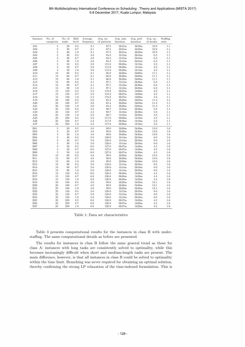
Instance No. of No. of Skill Average Avg. no. Avg. min. Avg. pref. Avg. no. Staffingcaregivers tasks level frequency of patterns duration duration of modes ratio

A01 5 20 0.5 3.1 67.5 2h31m 4h59m 10.9 1.1A02 5 20 0.7 3.1 67.5 2h31m 4h59m 10.9 1.1A03 5 20 1.0 3.1 67.5 2h31m 4h59m 10.9 1.1A04 5 30 0.5 4.0 94.3 1h15m 2h34m 6.3 1.1A05 5 30 0.7 4.0 94.3 1h15m 2h34m 6.3 1.1A06 5 30 1.0 4.0 94.3 1h15m 2h34m 6.3 1.1A07 5 50 0.5 5.0 115.8 0h39m 1h13m 3.3 1.1A08 5 50 0.7 5.0 115.8 0h39m 1h13m 3.3 1.1A09 5 50 1.0 5.0 115.8 0h39m 1h13m 3.3 1.1A10 15 60 0.5 3.1 66.9 2h28m 5h00m 11.1 1.1A11 15 60 0.7 3.1 66.9 2h28m 5h00m 11.1 1.1A12 15 60 1.0 3.1 66.9 2h28m 5h00m 11.1 1.1A13 15 90 0.5 4.1 97.1 1h12m 2h30m 6.2 1.1A14 15 90 0.7 4.1 97.1 1h12m 2h30m 6.2 1.1A15 15 90 1.0 4.1 97.1 1h12m 2h30m 6.2 1.1A16 15 150 0.5 5.3 119.2 0h37m 1h09m 3.2 1.1A17 15 150 0.7 5.3 119.2 0h37m 1h09m 3.2 1.1A18 15 150 1.0 5.3 119.2 0h37m 1h09m 3.2 1.1A19 25 100 0.5 3.0 65.4 2h28m 5h03m 11.3 1.1A20 25 100 0.7 3.0 65.4 2h28m 5h03m 11.3 1.1A21 25 100 1.0 3.0 65.4 2h28m 5h03m 11.3 1.1A22 25 150 0.5 4.2 98.7 1h16m 2h28m 5.8 1.1A23 25 150 0.7 4.2 98.7 1h16m 2h28m 5.8 1.1A24 25 150 1.0 4.2 98.7 1h16m 2h28m 5.8 1.1A25 25 250 0.5 5.2 117.8 0h36m 1h10m 3.3 1.1A26 25 250 0.7 5.2 117.8 0h36m 1h10m 3.3 1.1A27 25 250 1.0 5.2 117.8 0h36m 1h10m 3.3 1.1

B01 5 20 0.5 4.0 99.0 2h30m 5h30m 13.0 1.6B02 5 20 0.7 4.0 99.0 2h30m 5h30m 13.0 1.6B03 5 20 1.0 4.0 99.0 2h30m 5h30m 13.0 1.6B04 5 30 0.5 5.0 120.0 1h14m 2h59m 8.0 1.6B05 5 30 0.7 5.0 120.0 1h14m 2h59m 8.0 1.6B06 5 30 1.0 5.0 120.0 1h14m 2h59m 8.0 1.6B07 5 50 0.5 6.0 127.0 0h37m 1h30m 4.5 1.6B08 5 50 0.7 6.0 127.0 0h37m 1h30m 4.5 1.6B09 5 50 1.0 6.0 127.0 0h37m 1h30m 4.5 1.6B10 15 60 0.5 4.0 99.0 2h30m 5h30m 13.0 1.6B11 15 60 0.7 4.0 99.0 2h30m 5h30m 13.0 1.6B12 15 60 1.0 4.0 99.0 2h30m 5h30m 13.0 1.6B13 15 90 0.5 5.0 120.0 1h14m 2h59m 8.0 1.6B14 15 90 0.7 5.0 120.0 1h14m 2h59m 8.0 1.6B15 15 90 1.0 5.0 120.0 1h14m 2h59m 8.0 1.6B16 15 150 0.5 6.0 126.8 0h38m 1h29m 4.4 1.6B17 15 150 0.7 6.0 126.8 0h38m 1h29m 4.4 1.6B18 15 150 1.0 6.0 126.8 0h38m 1h29m 4.4 1.6B19 25 100 0.5 4.0 99.0 2h28m 5h30m 13.1 1.6B20 25 100 0.7 4.0 99.0 2h28m 5h30m 13.1 1.6B21 25 100 1.0 4.0 99.0 2h28m 5h30m 13.1 1.6B22 25 150 0.5 5.0 120.0 1h13m 2h59m 8.0 1.6B23 25 150 0.7 5.0 120.0 1h13m 2h59m 8.0 1.6B24 25 150 1.0 5.0 120.0 1h13m 2h59m 8.0 1.6B25 25 250 0.5 6.0 126.9 0h37m 1h29m 4.5 1.6B26 25 250 0.7 6.0 126.9 0h37m 1h29m 4.5 1.6B27 25 250 1.0 6.0 126.9 0h37m 1h29m 4.5 1.6

Table 1: Data set characteristics

Table 3 presents computational results for the instances in class B with under-

staffing. The same computational details as before are presented.

The results for instances in class B follow the same general trend as those for

class A: instances with long tasks are consistently solved to optimality, while this

becomes increasingly difficult when short and medium-length tasks are present. The

main difference, however, is that all instances in class B could be solved to optimality

within the time limit. Branching was never required for obtaining an optimal solution,

thereby confirming the strong LP relaxation of the time-indexed formulation. This is


- 128 -

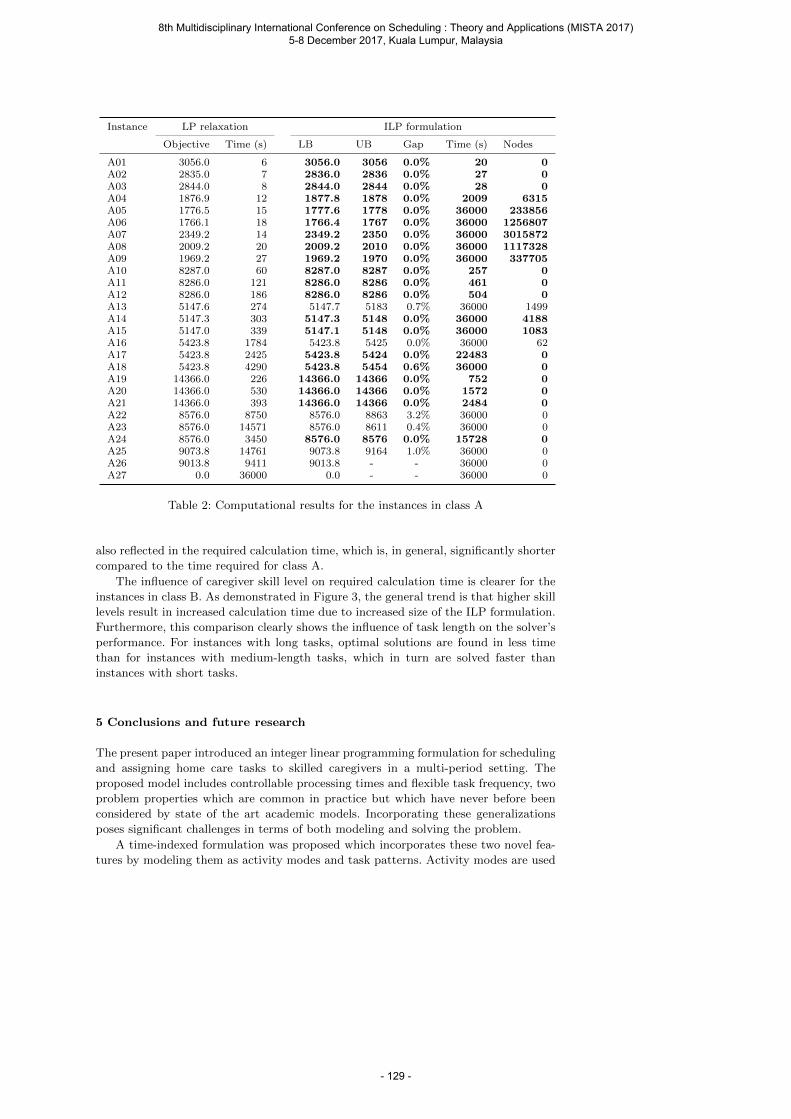
Instance LP relaxation ILP formulation

Objective Time (s) LB UB Gap Time (s) Nodes

A01 3056.0 6 3056.0 3056 0.0% 20 0A02 2835.0 7 2836.0 2836 0.0% 27 0A03 2844.0 8 2844.0 2844 0.0% 28 0A04 1876.9 12 1877.8 1878 0.0% 2009 6315A05 1776.5 15 1777.6 1778 0.0% 36000 233856A06 1766.1 18 1766.4 1767 0.0% 36000 1256807A07 2349.2 14 2349.2 2350 0.0% 36000 3015872A08 2009.2 20 2009.2 2010 0.0% 36000 1117328A09 1969.2 27 1969.2 1970 0.0% 36000 337705A10 8287.0 60 8287.0 8287 0.0% 257 0A11 8286.0 121 8286.0 8286 0.0% 461 0A12 8286.0 186 8286.0 8286 0.0% 504 0A13 5147.6 274 5147.7 5183 0.7% 36000 1499A14 5147.3 303 5147.3 5148 0.0% 36000 4188A15 5147.0 339 5147.1 5148 0.0% 36000 1083A16 5423.8 1784 5423.8 5425 0.0% 36000 62A17 5423.8 2425 5423.8 5424 0.0% 22483 0A18 5423.8 4290 5423.8 5454 0.6% 36000 0A19 14366.0 226 14366.0 14366 0.0% 752 0A20 14366.0 530 14366.0 14366 0.0% 1572 0A21 14366.0 393 14366.0 14366 0.0% 2484 0A22 8576.0 8750 8576.0 8863 3.2% 36000 0A23 8576.0 14571 8576.0 8611 0.4% 36000 0A24 8576.0 3450 8576.0 8576 0.0% 15728 0A25 9073.8 14761 9073.8 9164 1.0% 36000 0A26 9013.8 9411 9013.8 - - 36000 0A27 0.0 36000 0.0 - - 36000 0

Table 2: Computational results for the instances in class A

also reflected in the required calculation time, which is, in general, significantly shorter

compared to the time required for class A.

The influence of caregiver skill level on required calculation time is clearer for the

instances in class B. As demonstrated in Figure 3, the general trend is that higher skill

levels result in increased calculation time due to increased size of the ILP formulation.

Furthermore, this comparison clearly shows the influence of task length on the solver’s

performance. For instances with long tasks, optimal solutions are found in less time

than for instances with medium-length tasks, which in turn are solved faster than

instances with short tasks.

5 Conclusions and future research

The present paper introduced an integer linear programming formulation for scheduling

and assigning home care tasks to skilled caregivers in a multi-period setting. The

proposed model includes controllable processing times and flexible task frequency, two

problem properties which are common in practice but which have never before been

considered by state of the art academic models. Incorporating these generalizations

poses significant challenges in terms of both modeling and solving the problem.

A time-indexed formulation was proposed which incorporates these two novel fea-

tures by modeling them as activity modes and task patterns. Activity modes are used


- 129 -

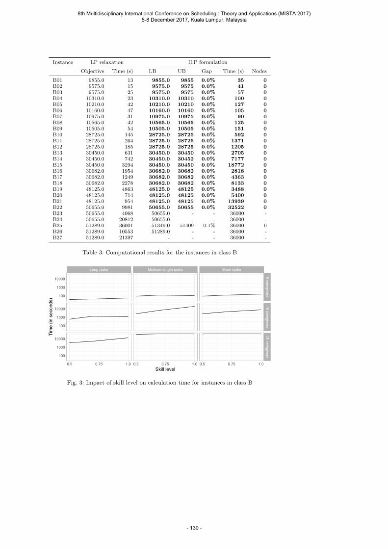
Instance LP relaxation ILP formulation

Objective Time (s) LB UB Gap Time (s) Nodes

B01 9855.0 13 9855.0 9855 0.0% 35 0B02 9575.0 15 9575.0 9575 0.0% 41 0B03 9575.0 25 9575.0 9575 0.0% 57 0B04 10310.0 23 10310.0 10310 0.0% 100 0B05 10210.0 42 10210.0 10210 0.0% 127 0B06 10160.0 47 10160.0 10160 0.0% 105 0B07 10975.0 31 10975.0 10975 0.0% 90 0B08 10565.0 42 10565.0 10565 0.0% 125 0B09 10505.0 54 10505.0 10505 0.0% 151 0B10 28725.0 145 28725.0 28725 0.0% 592 0B11 28725.0 264 28725.0 28725 0.0% 1371 0B12 28725.0 185 28725.0 28725 0.0% 1205 0B13 30450.0 631 30450.0 30450 0.0% 2705 0B14 30450.0 742 30450.0 30452 0.0% 7177 0B15 30450.0 3294 30450.0 30450 0.0% 18772 0B16 30682.0 1954 30682.0 30682 0.0% 2818 0B17 30682.0 1249 30682.0 30682 0.0% 4363 0B18 30682.0 2278 30682.0 30682 0.0% 8133 0B19 48125.0 4863 48125.0 48125 0.0% 3488 0B20 48125.0 714 48125.0 48125 0.0% 5400 0B21 48125.0 954 48125.0 48125 0.0% 13939 0B22 50655.0 9981 50655.0 50655 0.0% 32522 0B23 50655.0 4068 50655.0 - - 36000 -B24 50655.0 20812 50655.0 - - 36000 -B25 51289.0 36001 51349.0 51409 0.1% 36000 0B26 51289.0 10553 51289.0 - - 36000 -B27 51289.0 21397 - - - 36000 -

Table 3: Computational results for the instances in class B

Long tasks Medium-length tasks Short tasks

5 caregivers15 caregivers

25 caregivers

0.5 0.75 1.0 0.5 0.75 1.0 0.5 0.75 1.0

100

1000

10000

100

1000

10000

100

1000

10000

Skill level

Tim

e (in

sec

onds

)

Fig. 3: Impact of skill level on calculation time for instances in class B


- 130 -

to model the different processing times for which a task may be scheduled. This enables

the cost function to be of any form, however, typically, scheduling tasks with a shorter

duration results in increased costs. Task patterns are the second modeling tool included

in the proposed formulation. By selecting a pattern for a task, the days on which it

is scheduled are determined, thereby enabling flexible modeling of task frequency and

spreading throughout the scheduling period.

A series of computational experiments demonstrated that the proposed model could

be solved to optimality for problem instances of realistic size with 25 caregivers and

100 tasks. Further analysis of the results revealed how the formulation’s root node

relaxation is very tight, often resulting in the optimal solution and thus avoiding any

branching to obtain integer solutions. The benchmark data set used in this compu-

tational study has been made publicly available to stimulate further research on this

challenging problem.

The present paper addressed the static, offline version of the problem. However,

in practice, unforeseen events constantly affect the current planning. For example,

caregivers become unavailable, task frequency increases or tasks are canceled. Future

research should turn its attention towards addressing the re-scheduling problem in

home care. This optimization problem imposes an additional restriction concerning

available computation time given how new solutions are typically expected within a

few minutes.

Acknowledgements This research was carried out within the HACES project (Human-centred Automated home CarE Scheduling), realized in collaboration with imec. Projectpartners are Gezinszorg Villers, Landelijke Thuiszorg, thuiszorg vleminckveld, and Tobania,with project support from Agentschap Innoveren & Ondernemen (Flanders Innovation & En-trepreneurship). Editorial consultation provided by Luke Connolly (KU Leuven).

References

Akjiratikarl C, Yenradee P, Drake PR (2007) PSO-based algorithm for home care

worker scheduling in the UK. Computers & Industrial Engineering 53(4):559–583

Van den Akker J, Hurkens CA, Savelsbergh MW (2000) Time-indexed formulations for

machine scheduling problems: Column generation. INFORMS Journal on Computing

12(2):111–124

Begur SV, Miller DM, Weaver JR (1997) An integrated spatial DSS for scheduling and

routing home-health-care nurses. Interfaces 27(4):35–48

Braekers K, Hartl RF, Parragh SN, Tricoire F (2016) A bi-objective home care schedul-

ing problem: Analyzing the trade-off between costs and client inconvenience. Euro-

pean Journal of Operational Research 248(2):428 – 443

Brucker P, Drexl A, Mohring R, Neumann K, Pesch E (1999) Resource-constrained

project scheduling: Notation, classification, models, and methods. European Journal

of Operational Research 112(1):3 – 41

Cappanera P, Scutella MG (2014) Joint assignment, scheduling, and routing mod-

els to home care optimization: a pattern-based approach. Transportation Science

49(4):830–852

Fikar C, Hirsch P (2016) Home health care routing and scheduling: A review. Com-

puters & Operations Research 77:86–95

Liu R, Xie X, Garaix T (2014) Hybridization of tabu search with feasible and infeasible

local searches for periodic home health care logistics. Omega 47:17 – 32


- 131 -

Maya Duque PA, Castro M, Sorensen K, Goos P (2015) Home care service plan-

ning. The case of Landelijke Thuiszorg. European Journal of Operational Research

243(1):292–301

Nickel S, Schroder M, Steeg J (2012) Mid-term and short-term planning support for

home health care services. European Journal of Operational Research 219(3):574–587

Rasmussen MS, Justesen T, Dohn A, Larsen J (2012) The home care crew schedul-

ing problem: Preference-based visit clustering and temporal dependencies. European

Journal of Operational Research 219(3):598 – 610

Shabtay D, Steiner G (2007) A survey of scheduling with controllable processing times.

Discrete Applied Mathematics 155(13):1643–1666

Shabtay D, Gaspar N, Kaspi M (2013) A survey on offline scheduling with rejection.

Journal of Scheduling 16(1):3–28

Trautsamwieser A, Hirsch P (2014) A branch-price-and-cut approach for solving the

medium-term home health care planning problem. Networks 64(3):143–159

Wauters T, Kinable J, Smet P, Vancroonenburg W, Vanden Berghe G, Verstichel J

(2016) The multi-mode resource-constrained multi-project scheduling problem. Jour-

nal of Scheduling 19(3):271–283

Yuan B, Liu R, Jiang Z (2015) A branch-and-price algorithm for the home health care

scheduling and routing problem with stochastic service times and skill requirements.

International Journal of Production Research 53(24):7450–7464


- 132 -

Farnaz Ghazi Nezami Department of Industrial and Manufacturing Engineering, Kettering University, 1700 University Ave., Flint, MI 48504, USA E-mail: [email protected] Mojtaba Heydar University of Newcastle, University Drive, Callaghan, NSW 2308, Australia E-mail: [email protected] Regina Berretta School of Electrical Engineering and Computing, University of Newcastle, University Drive, Callaghan, NSW 2308, Australia E-mail: [email protected]

MISTA 2017

Optimizing Production Schedule with Energy Consumption and Demand Charges in Parallel Machine Setting

Farnaz Ghazi Nezami • Mojtaba Heydar • Regina Berretta

Abstract Environmental sustainability concerns, along with the growing need for electricity and associated costs, make energy-cost reduction an inevitable decision-making criterion in production scheduling. In this research, we study the problem of production scheduling on non-identical parallel machines with machine-dependent processing times and known job release dates to minimize total completion time and energy costs. The energy costs in this study include demand and consumption charges. We present a mixed-integer nonlinear model to formulate the problem. The model is then linearized and its performance is tested through numerical experiments.

1 Introduction

This paper proposes a new energy-aware parallel-machine production scheduling model in order to minimize total production completion time, energy consumption costs and peak power charges. The industrial sector uses 266 quadrillions BTU of energy, which accounts for 51% of total energy consumption in the world1. The breakdown of global energy consumption data reveals that 22% of the total amount of energy used in the industrial sector is electrical energy [1]. In the past 50 years, industrial electricity consumption has doubled [2]. In addition, the US Energy Information Administration (EIA) reports that the price of electricity is expected to

1 https://www.eia.gov/tools/faqs/faq.cfm?id=447&t=1


- 133 -

increase by 18% by 20402. Currently, the cost of electricity for manufacturing in the United States exceeds 100 billion dollars [2], and this number will continue to increase the in future.

The surge in energy prices, along with the scarcity of natural sources, the growth of public awareness of environmental concerns, and the establishment of sustainability-based standards magnify the necessity of incorporating energy consumption and associated costs into planning and scheduling decisions at manufacturing facilities. The increase in energy demand causes difficulty for electrical energy providers, who must keep up with demand, which is particularly difficult during peak-demand periods. Time-of-Use (TOU) tariffs implemented by utility companies aim to shift demand from the expensive peak periods to less-expensive non-peak hours in order to flatten the load curve and decrease the deficit risks in supply.

In general, electricity charges can be categorized into two types: consumption charges and demand charges. Consumption charges are calculated according to the total amount of electrical energy consumed by a company during a given period, based on kilowatt-hour, and may vary throughout the day to motivate a shift of consumption away from peak hours. Demand charges try to address the overhead expenses that utility companies bear to provide the service. This charge is based on the highest level of power demanded over a given period of time during the billing period and is usually calculated as the highest “average fifteen-minute demand” for a month. Energy demand is measured in kilowatts (kW) and often represents a significant percentage of charges on utility bills for the industrial user.

Most of the existing research on energy-aware job scheduling does not differentiate between these two types of energy costs. In addition, in the majority of energy-aware job scheduling studies, the impact of various machine operating modes on decision making output is not considered. In a typical manufacturing system, the machines may be running idle for a significant amount of time waiting for the next job to arrive and be processed. One study showed that in a machining process, 85% of total energy consumption is used when the machine is idling, and only 15% is applied to the actual machining process [3]. The idle energy is used to run the auxiliary components. Therefore, it is critical to study the impact of various operating states on the production schedule, energy requirements, and cost planning. In the past few years, the number of studies investigating the energy-aware production scheduling has increased significantly. A literature survey of studies on energy efficiency in manufacturing companies is provided by [4]. This survey presents a breakdown of studies based on energy coverage (production system, internal and external conversion system), energy supply, energy demand (processing and non-processing energy demand), objective criteria (monetary, non-monetary), the system of objectives (multi/single objectives), the manufacturing model (single machine, parallel machines, flow shop, job shop/project scheduling, or hoist scheduling), the model type (linear, mixed integer linear, mixed integer quadratic constrained, mixed integer non-linear programing, queuing theory and simulation, and other analytical models such as Markov decision model), and solution approach (heuristic, exact, standard solver). To integrate energy concerns into classic scheduling problems, [5] investigated a single machine problem to minimize total energy consumption and maximum tardiness, with the possibility of machine shut-down between consecutive jobs following the break-even period. They considered only processing and idle energy consumption in their model. A bi-objective optimization problem to minimize weighted tardiness and non-process (idle and switch) energy consumption in a job-shop setting is proposed in [6]. Their model also allows for switching off a machine if the idle time is long enough, considering a breakeven time, and they solved the problem using Genetic Algorithm (GA). In another study, a job-shop scheduling problem with machine speed scaling to minimize makespan and energy consumption using GA was proposed by [7]. A job-shop problem with energy threshold and makespan minimization was investigated by [8] using a mixed integer linear model. They considered extra energy consumption at the beginning of the operation, and energy consumption was divided into “peak” and “processing” categories. An energy-aware scheduling model with tool selection and operation sequencing was introduced by [9]. Their bi-objective model minimized total energy consumption (idle, setup, and process

2 http://www.eia.gov/forecasts/aeo/pdf/0383(2015).pdf


- 134 -

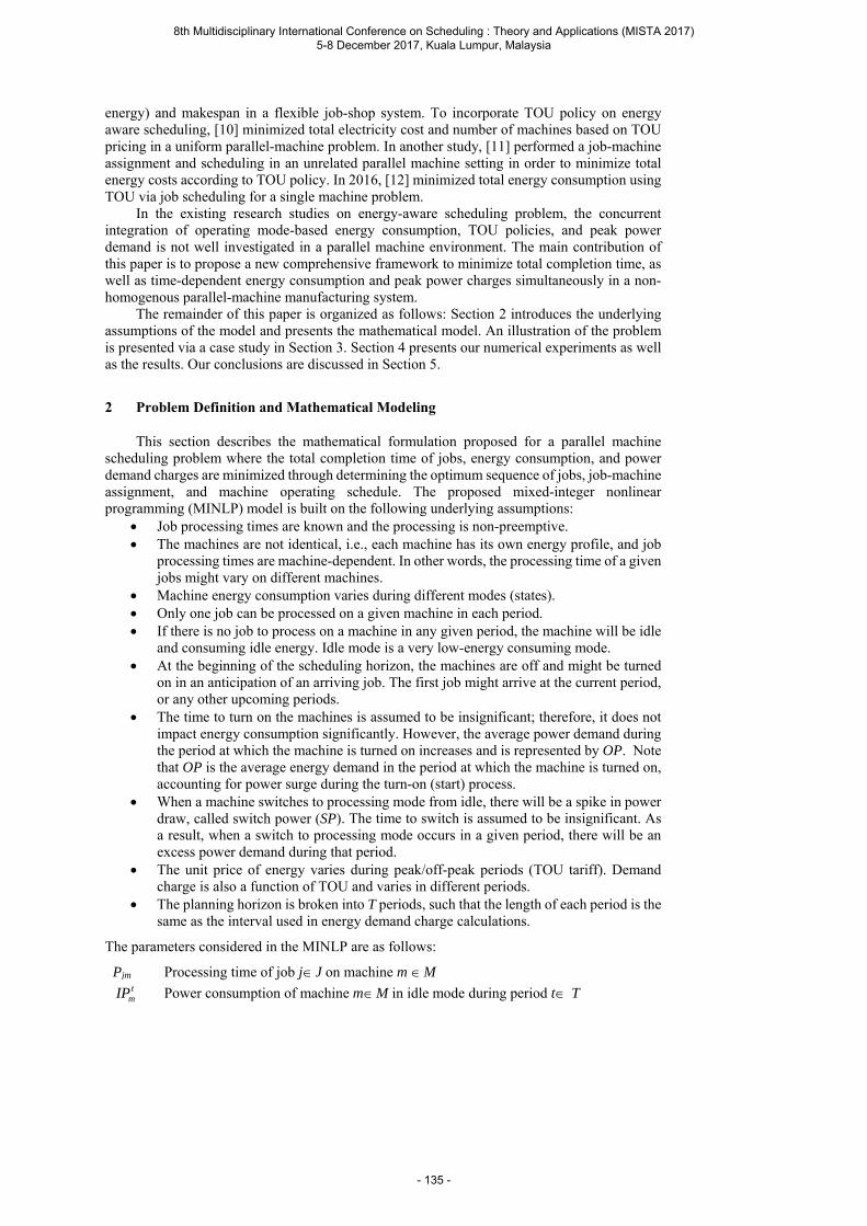
energy) and makespan in a flexible job-shop system. To incorporate TOU policy on energy aware scheduling, [10] minimized total electricity cost and number of machines based on TOU pricing in a uniform parallel-machine problem. In another study, [11] performed a job-machine assignment and scheduling in an unrelated parallel machine setting in order to minimize total energy costs according to TOU policy. In 2016, [12] minimized total energy consumption using TOU via job scheduling for a single machine problem.

In the existing research studies on energy-aware scheduling problem, the concurrent integration of operating mode-based energy consumption, TOU policies, and peak power demand is not well investigated in a parallel machine environment. The main contribution of this paper is to propose a new comprehensive framework to minimize total completion time, as well as time-dependent energy consumption and peak power charges simultaneously in a non-homogenous parallel-machine manufacturing system.

The remainder of this paper is organized as follows: Section 2 introduces the underlying assumptions of the model and presents the mathematical model. An illustration of the problem is presented via a case study in Section 3. Section 4 presents our numerical experiments as well as the results. Our conclusions are discussed in Section 5.

2 Problem Definition and Mathematical Modeling

This section describes the mathematical formulation proposed for a parallel machine scheduling problem where the total completion time of jobs, energy consumption, and power demand charges are minimized through determining the optimum sequence of jobs, job-machine assignment, and machine operating schedule. The proposed mixed-integer nonlinear programming (MINLP) model is built on the following underlying assumptions:

Job processing times are known and the processing is non-preemptive. The machines are not identical, i.e., each machine has its own energy profile, and job

processing times are machine-dependent. In other words, the processing time of a given jobs might vary on different machines.

Machine energy consumption varies during different modes (states). Only one job can be processed on a given machine in each period. If there is no job to process on a machine in any given period, the machine will be idle

and consuming idle energy. Idle mode is a very low-energy consuming mode. At the beginning of the scheduling horizon, the machines are off and might be turned

on in an anticipation of an arriving job. The first job might arrive at the current period, or any other upcoming periods.

The time to turn on the machines is assumed to be insignificant; therefore, it does not impact energy consumption significantly. However, the average power demand during the period at which the machine is turned on increases and is represented by OP. Note that OP is the average energy demand in the period at which the machine is turned on, accounting for power surge during the turn-on (start) process.

When a machine switches to processing mode from idle, there will be a spike in power draw, called switch power (SP). The time to switch is assumed to be insignificant. As a result, when a switch to processing mode occurs in a given period, there will be an excess power demand during that period.

The unit price of energy varies during peak/off-peak periods (TOU tariff). Demand charge is also a function of TOU and varies in different periods.

The planning horizon is broken into T periods, such that the length of each period is the same as the interval used in energy demand charge calculations.

The parameters considered in the MINLP are as follows:

Pjm Processing time of job jJ on machine m M t

mIP Power consumption of machine mM in idle mode during period t T


- 135 -

tmPP Power consumption of machine mM in processing mode during period t T t

mOP Power consumption of machine mM during turn-on process in period t T t

mSP Power consumption of machine mM during switch process from idle to processing mode in period t T

CP Cost of maximum power demand CEt Cost of energy consumption during period t T L Duration of each period Fi Objective function i, i = 1, 2, 3

The decision variables considered in the MINLP are as follows:

Pmax Maximum power demand tjmX 1 if job jJ processing started on machine mM at period t T; zero otherwise

tjmW

1 if job jJ is being processed on machine mM at period t T; zero otherwise

tmZ 1 if machine mM is turned on from off mode at period t T; zero otherwise t

mY 1 if machine mM is idle at period t T; zero otherwise tmU 1 if machine mM is switched from idle mode to processing mode at period t T;

zero otherwise

The following is the proposed mixed-integer nonlinear programming model:

Min

Jj Tt Mm

tjmjm XPt 1 (1)

Min

Jj

tjm

Mm

tm

Mm

tm

Ttt WPPIPCEL (2)

Min maxPCP (3)

Subject to

JjXMm

PT

t

tjm

jm

1

1

1

(4)

TtMmXJj

tjm

,1 (5)

TtMmWJj

tjm

,1 (6)

1,,1,,1

jm

Pt

tjm

tjmjm PTtMmJjWXP

jm

(7)

1,,1,,1

jm

t

jmtjm PtMmJjXW

(8)

TPtMmJjXW jm

t

Ptjm

tjm

jm

,,,,1

(9)

MmZTt

tm

1 (10)

TtMmZXt

mJj

tjm

,0

1

(11)

TtMmYWZ tm

Jj

tjm

t

m

,11

1

(12)


- 136 -

TtMmYW tm

Jj

tjm

,1 (13)

TtMmYZ tm

t

m

,

(14)

1,,1,11 TtMmUYY tm

tm

tm (15)

TtMmUZ tm

tm ,1 (16)

TtPXZIPPP

UPPSPZPPOPWPPYIP

Mm Jj

tjm

tm

tm

tm

Mm

tm

tm

tm

Mm

tm

tm

tm

Jj

tjm

Mm

tm

Mm

tm

tm

max1

(17)

In the proposed multi-objective model, the objective function (1) aims to minimize the total

completion time. The second and third objective functions aim to minimize the cost of time-based energy consumption and maximum power demand, respectively.

Constraint set (4) – (9) are the job scheduling-based constraints: constraints (4) and (5) show that in a given period only one job can be “started” on each machine. Based on constraint (6), each machine can “process” at most one job in a given period. In other words, based on these constraints, there is a one-to-one assignment between job and machine. Note that a job can be processed after it is started, and based on constraint (7), the total number of processing periods for a job is determined by the job processing time. Constraints (8) and (9) show that the job processing is non-preemptive once started [13].

Constraint set (10) – (17) are machine-based constraints and address machine operation and energy planning: constraint (10) indicates that each machine is turned on (from the off mode) at most once during the planning horizon. Constraint (11) indicates that if a job processing is started on a machine in a given period, the machine might have been turned on either during that period or in any other prior periods. It is worth mentioning that for energy demand reduction purposes, a machine might be turned on in a period when there is no job to be processed. This strategy is helpful to flatten the overall peak power demand in parallel machine setting. Constraints (12) and (13) show that if a machine is on, with no job to process, it is in idle mode. According to constraint (14), a machine can be idle if it has been turned on in any of the previous periods. Constraint (15) explains the switch process from idle to processing mode between periods. Constraint (16) indicates that in a given period, either a switch or turn-on process occurs. Constraint (17) is the power demand capacity constraint and accounts for the power demand during processing and idle modes, and spikes during turn-on and switch process. There is an upper bound on total amount of power consumption to prevent supply shortage and over charging. The last term on the left hand side of constraint (17) is nonlinear, which leads to a nonlinear constraint. This equation can be linearized using the following set of constraints:

TtPSIPPP

UPPSPZPPOPWPPYIP

Mm

tm

tm

tm

Mm

tm

tm

tm

Mm

tm

tm

tm

Jj

tjm

Mm

tm

Mm

tm

tm

max

such that

Jj

tjm

tm

tm

Jj

tjm

tm

tm

tm

XZS

XS

ZS

1 (18)


- 137 -

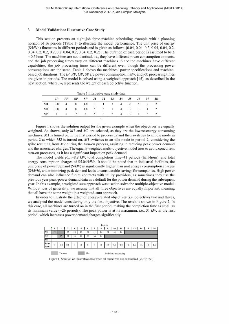
3 Model Validation: Illustrative Case Study

This section presents an eight-job three-machine scheduling example with a planning horizon of 16 periods (Table 1) to illustrate the model performance. The unit price of energy ($/kWh) fluctuates in different periods and is given as follows 0.04, 0.04, 0.2, 0.04, 0.04, 0.2, 0.04, 0.2, 0.2, 0.2, 0.2, 0.04, 0.2, 0.04, 0.2, 0.2. The duration of each period is assumed to be L = 0.5 hour. The machines are not identical, i.e., they have different power consumption amounts, and the job processing times vary on different machines. Since the machines have different capabilities, the job processing times can be different even though the processing power consumptions are the same. Table 1 shows the machines’ power specifications and machine-based job durations. The IP, PP, OP, SP are power consumption in kW, and job processing times are given in periods. The model is solved using a weighted approach [15], as described in the next section, where, wi represents the weight of each objective function.

Table 1 Illustrative case study data

IP PP OP SP J1 J2 J3 J4 J5 J6 J7 J8

M1 0.8 4 8 4.8 3 1 3 4 2 5 2 2

M2 0.8 4 8 4.8 5 5 1 4 3 3 1 2

M3 1 5 15 6 5 3 2 4 3 4 5 2

*.

Figure 1 shows the solution output for the given example when the objectives are equally weighted. As shown, only M1 and M2 are selected, as they are the lowest-energy consuming machines. M1 is turned on in the first period to process J2 and then switches to an idle mode in period 2 at which M2 is turned on. M1 switches to an idle mode in period 2, considering the spike resulting from M2 during the turn-on process, assisting in reducing peak power demand and the associated charges. The equally weighted multi-objective model tries to avoid concurrent turn-on processes, as it has a significant impact on peak demand. The model yields Pmax=8.8 kW, total completion time=41 periods (half-hour), and total energy consumption charges of $5.04/kWh. It should be noted that in industrial facilities, the unit price of power demand ($/kW) is significantly higher than unit energy consumption charges ($/kWh), and minimizing peak demand leads to considerable savings for companies. High power demand can also influence future contracts with utility providers, as sometimes they use the previous year peak-power demand data as a default for the power demand during the subsequent year. In this example, a weighted sum approach was used to solve the multiple-objective model. Without loss of generality, we assume that all three objectives are equally important, meaning that all have the same weight in a weighted-sum approach. In order to illustrate the effect of energy-related objectives (i.e. objectives two and three), we analyzed the model considering only the first objective. The result is shown in Figure 2. In this case, all machines are turned on in the first period, making the completion time as small as its minimum value (=26 periods). The peak power is at its maximum, i.e., 31 kW, in the first period, which increases power demand charges significantly.

Figure 1. Solution of illustrative case when all objectives are considered (w1=w2=w3)

1 2 3 4 5 6 7 8 9 10 11 12 13 14 15 16

M1 J2 J5 J5 J1 J1 J1 J4 J4 J4 J4

M2 J7 J3 J8 J8 J6 J6 J6

M3

Peak load

8 8.8 8.8 8 8 8 8 8 4.5 4.8 4.8 1.6 1.6 1.6 1.6 1.6

Periods

Switch to processingIdleTurn-on


- 138 -

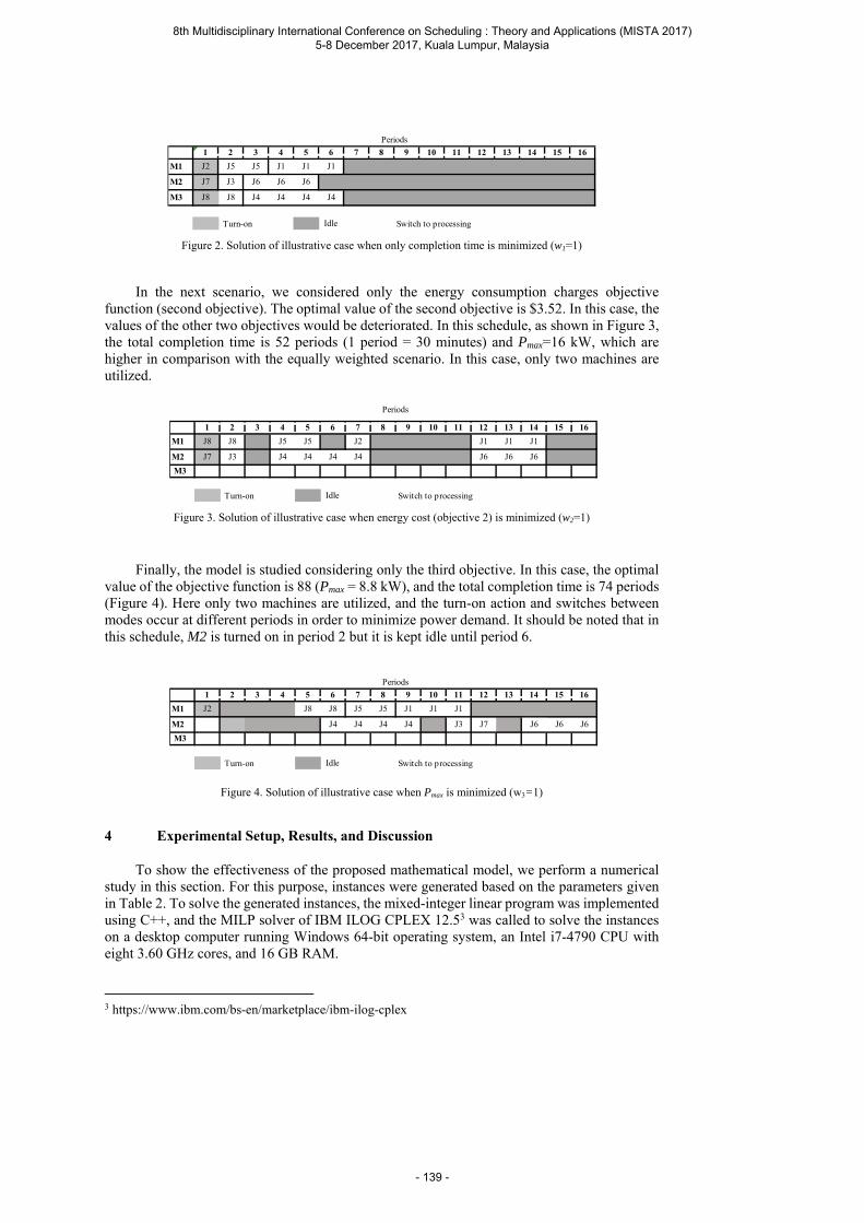
Figure 2. Solution of illustrative case when only completion time is minimized (w1=1)

In the next scenario, we considered only the energy consumption charges objective function (second objective). The optimal value of the second objective is $3.52. In this case, the values of the other two objectives would be deteriorated. In this schedule, as shown in Figure 3, the total completion time is 52 periods (1 period = 30 minutes) and Pmax=16 kW, which are higher in comparison with the equally weighted scenario. In this case, only two machines are utilized.

Figure 3. Solution of illustrative case when energy cost (objective 2) is minimized (w2=1)

Finally, the model is studied considering only the third objective. In this case, the optimal value of the objective function is 88 (Pmax = 8.8 kW), and the total completion time is 74 periods (Figure 4). Here only two machines are utilized, and the turn-on action and switches between modes occur at different periods in order to minimize power demand. It should be noted that in this schedule, M2 is turned on in period 2 but it is kept idle until period 6.

Figure 4. Solution of illustrative case when Pmax is minimized (w3=1)

4 Experimental Setup, Results, and Discussion

To show the effectiveness of the proposed mathematical model, we perform a numerical study in this section. For this purpose, instances were generated based on the parameters given in Table 2. To solve the generated instances, the mixed-integer linear program was implemented using C++, and the MILP solver of IBM ILOG CPLEX 12.53 was called to solve the instances on a desktop computer running Windows 64-bit operating system, an Intel i7-4790 CPU with eight 3.60 GHz cores, and 16 GB RAM.

3 https://www.ibm.com/bs-en/marketplace/ibm-ilog-cplex

1 2 3 4 5 6 7 8 9 10 11 12 13 14 15 16

M1 J2 J5 J5 J1 J1 J1

M2 J7 J3 J6 J6 J6

M3 J8 J8 J4 J4 J4 J4

Periods

Turn-on Idle Switch to processing

1 2 3 4 5 6 7 8 9 10 11 12 13 14 15 16

M1 J8 J8 J5 J5 J2 J1 J1 J1

M2 J7 J3 J4 J4 J4 J4 J6 J6 J6

M3

Periods


1 2 3 4 5 6 7 8 9 10 11 12 13 14 15 16

M1 J2 J8 J8 J5 J5 J1 J1 J1

M2 J4 J4 J4 J4 J3 J7 J6 J6 J6

M3

Periods



- 139 -

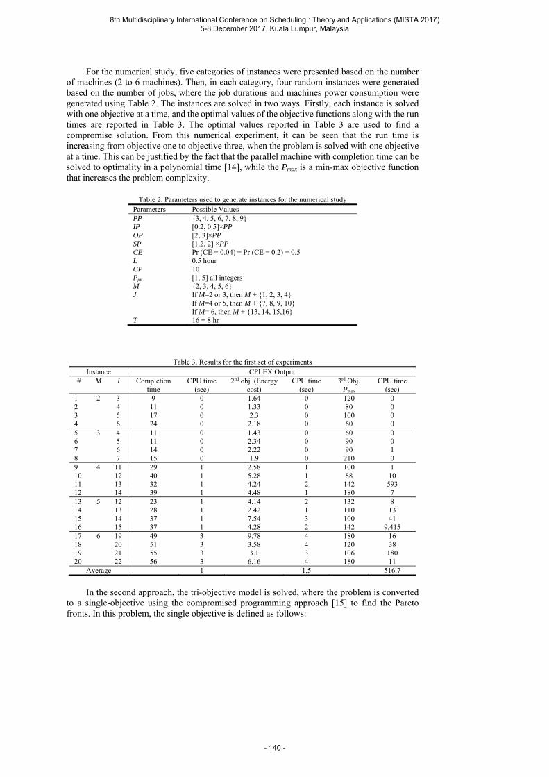
For the numerical study, five categories of instances were presented based on the number of machines (2 to 6 machines). Then, in each category, four random instances were generated based on the number of jobs, where the job durations and machines power consumption were generated using Table 2. The instances are solved in two ways. Firstly, each instance is solved with one objective at a time, and the optimal values of the objective functions along with the run times are reported in Table 3. The optimal values reported in Table 3 are used to find a compromise solution. From this numerical experiment, it can be seen that the run time is increasing from objective one to objective three, when the problem is solved with one objective at a time. This can be justified by the fact that the parallel machine with completion time can be solved to optimality in a polynomial time [14], while the Pmax is a min-max objective function that increases the problem complexity.

Table 2. Parameters used to generate instances for the numerical study

Parameters Possible Values PP 3, 4, 5, 6, 7, 8, 9 IP [0.2, 0.5]×PP OP [2, 3]×PP SP [1.2, 2] ×PP CE Pr (CE = 0.04) = Pr (CE = 0.2) = 0.5 L 0.5 hour CP 10 Pjm [1, 5] all integers M 2, 3, 4, 5, 6 J If M=2 or 3, then M + 1, 2, 3, 4

If M=4 or 5, then M + 7, 8, 9, 10 If M= 6, then M + 13, 14, 15,16

T 16 = 8 hr

Table 3. Results for the first set of experiments

Instance CPLEX Output # M J Completion

time CPU time

(sec) 2nd obj. (Energy

cost) CPU time

(sec) 3rd Obj.

Pmax CPU time

(sec) 1 2 3 9 0 1.64 0 120 0 2 4 11 0 1.33 0 80 0 3 5 17 0 2.3 0 100 0 4 6 24 0 2.18 0 60 0 5 3 4 11 0 1.43 0 60 0 6 5 11 0 2.34 0 90 0 7 6 14 0 2.22 0 90 1 8 7 15 0 1.9 0 210 0 9 4 11 29 1 2.58 1 100 1 10 12 40 1 5.28 1 88 10 11 13 32 1 4.24 2 142 593 12 14 39 1 4.48 1 180 7 13 5 12 23 1 4.14 2 132 8 14 13 28 1 2.42 1 110 13 15 14 37 1 7.54 3 100 41 16 15 37 1 4.28 2 142 9,415 17 6 19 49 3 9.78 4 180 16 18 20 51 3 3.58 4 120 38 19 21 55 3 3.1 3 106 180 20 22 56 3 6.16 4 180 11

Average 1 1.5 516.7

In the second approach, the tri-objective model is solved, where the problem is converted

to a single-objective using the compromised programming approach [15] to find the Pareto fronts. In this problem, the single objective is defined as follows:


- 140 -

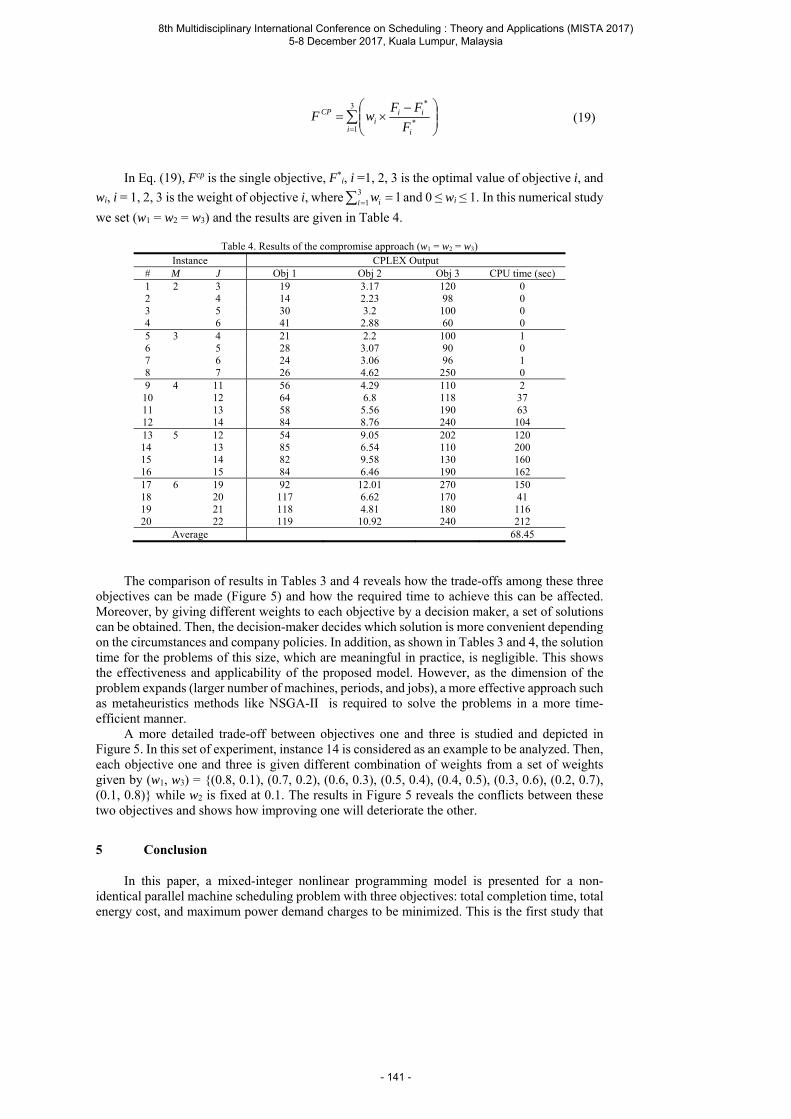
3

1*

*

i i

iii

CP

F

FFwF (19)

In Eq. (19), Fcp is the single objective, F*

i, i =1, 2, 3 is the optimal value of objective i, and

wi, i = 1, 2, 3 is the weight of objective i, where 131 i iw and 0 ≤ wi ≤ 1. In this numerical study

we set (w1 = w2 = w3) and the results are given in Table 4.

Table 4. Results of the compromise approach (w1 = w2 = w3) Instance CPLEX Output

# M J Obj 1 Obj 2 Obj 3 CPU time (sec) 1 2 3 19 3.17 120 0 2 4 14 2.23 98 0 3 5 30 3.2 100 0 4 6 41 2.88 60 0 5 3 4 21 2.2 100 1 6 5 28 3.07 90 0 7 6 24 3.06 96 1 8 7 26 4.62 250 0 9 4 11 56 4.29 110 2 10 12 64 6.8 118 37 11 13 58 5.56 190 63 12 14 84 8.76 240 104 13 5 12 54 9.05 202 120 14 13 85 6.54 110 200 15 14 82 9.58 130 160 16 15 84 6.46 190 162 17 6 19 92 12.01 270 150 18 20 117 6.62 170 41 19 21 118 4.81 180 116 20 22 119 10.92 240 212

Average 68.45

The comparison of results in Tables 3 and 4 reveals how the trade-offs among these three

objectives can be made (Figure 5) and how the required time to achieve this can be affected. Moreover, by giving different weights to each objective by a decision maker, a set of solutions can be obtained. Then, the decision-maker decides which solution is more convenient depending on the circumstances and company policies. In addition, as shown in Tables 3 and 4, the solution time for the problems of this size, which are meaningful in practice, is negligible. This shows the effectiveness and applicability of the proposed model. However, as the dimension of the problem expands (larger number of machines, periods, and jobs), a more effective approach such as metaheuristics methods like NSGA-II is required to solve the problems in a more time-efficient manner.

A more detailed trade-off between objectives one and three is studied and depicted in Figure 5. In this set of experiment, instance 14 is considered as an example to be analyzed. Then, each objective one and three is given different combination of weights from a set of weights given by (w1, w3) = (0.8, 0.1), (0.7, 0.2), (0.6, 0.3), (0.5, 0.4), (0.4, 0.5), (0.3, 0.6), (0.2, 0.7), (0.1, 0.8) while w2 is fixed at 0.1. The results in Figure 5 reveals the conflicts between these two objectives and shows how improving one will deteriorate the other.

5 Conclusion

In this paper, a mixed-integer nonlinear programming model is presented for a non-identical parallel machine scheduling problem with three objectives: total completion time, total energy cost, and maximum power demand charges to be minimized. This is the first study that


- 141 -

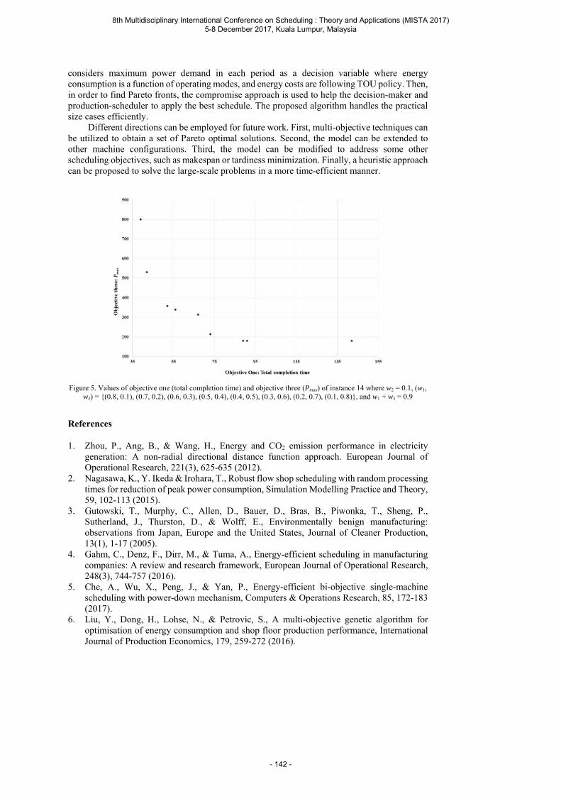
considers maximum power demand in each period as a decision variable where energy consumption is a function of operating modes, and energy costs are following TOU policy. Then, in order to find Pareto fronts, the compromise approach is used to help the decision-maker and production-scheduler to apply the best schedule. The proposed algorithm handles the practical size cases efficiently.

Different directions can be employed for future work. First, multi-objective techniques can be utilized to obtain a set of Pareto optimal solutions. Second, the model can be extended to other machine configurations. Third, the model can be modified to address some other scheduling objectives, such as makespan or tardiness minimization. Finally, a heuristic approach can be proposed to solve the large-scale problems in a more time-efficient manner.

Figure 5. Values of objective one (total completion time) and objective three (Pmax) of instance 14 where w2 = 0.1, (w1, w3) = (0.8, 0.1), (0.7, 0.2), (0.6, 0.3), (0.5, 0.4), (0.4, 0.5), (0.3, 0.6), (0.2, 0.7), (0.1, 0.8), and w1 + w3 = 0.9

References

1. Zhou, P., Ang, B., & Wang, H., Energy and CO2 emission performance in electricity generation: A non-radial directional distance function approach. European Journal of Operational Research, 221(3), 625-635 (2012).

2. Nagasawa, K., Y. Ikeda & Irohara, T., Robust flow shop scheduling with random processing times for reduction of peak power consumption, Simulation Modelling Practice and Theory, 59, 102-113 (2015).

3. Gutowski, T., Murphy, C., Allen, D., Bauer, D., Bras, B., Piwonka, T., Sheng, P., Sutherland, J., Thurston, D., & Wolff, E., Environmentally benign manufacturing: observations from Japan, Europe and the United States, Journal of Cleaner Production, 13(1), 1-17 (2005).

4. Gahm, C., Denz, F., Dirr, M., & Tuma, A., Energy-efficient scheduling in manufacturing companies: A review and research framework, European Journal of Operational Research, 248(3), 744-757 (2016).

5. Che, A., Wu, X., Peng, J., & Yan, P., Energy-efficient bi-objective single-machine scheduling with power-down mechanism, Computers & Operations Research, 85, 172-183 (2017).

6. Liu, Y., Dong, H., Lohse, N., & Petrovic, S., A multi-objective genetic algorithm for optimisation of energy consumption and shop floor production performance, International Journal of Production Economics, 179, 259-272 (2016).


- 142 -

7. Salido, M. A., Escamilla, J., Giret, A., & Barber, F., A genetic algorithm for energy-efficiency in job-shop scheduling, The International Journal of Advanced Manufacturing Technology, 85(5-8), 1303-1314 (2016).

8. Kemmoe, S., Lamy, D., & Tchernev, N., A job-shop with an energy threshold issue considering operations with consumption peaks, IFAC-PapersOnLine, 48(3), 788-793 (2015).

9. He, Y., Li, Y., Wu, T., & Sutherland, J. W., An energy-responsive optimization method for machine tool selection and operation sequence in flexible machining job shops, Journal of Cleaner Production, 87, 245-254 (2015).

10. Zeng, Y., Che, A., & Wu, X., Bi-objective scheduling on uniform parallel machines considering electricity cost, Engineering Optimization, 1-18 (2017).

11. Che, A., Zhang, S., & Wu, X., Energy-conscious unrelated parallel machine scheduling under time-of-use electricity tariffs, Journal of Cleaner Production, 156, 688-697 (2017).

12. Shrouf, F., Ordieres-Meré, J., García-Sánchez, A., & Ortega-Mier, M., Optimizing the production scheduling of a single machine to minimize total energy consumption costs, Journal of Cleaner Production, 67, 197-207 (2014).

13. Zhang, H., Zhao, F., Fang, K., Sutherland, J. W., Energy-conscious flow shop scheduling under time-of-use electricity tariffs, CIRP Annals – Manufacturing Technology, 63, 34-40 (2014).

14. Pinedo, M., Scheduling: Theory, Algorithms, and Systems, 3rd Ed., Springer (2008). 15. Yousefi-Babadi, A., Tavakkoli-Moghaddam, R., Bozorgi-Amiri, A., & Seifi, S., Designing

a reliable multi-objective queuing model of a petrochemical supply chain network under uncertainty: a case study, Computers & Chemical Engineering, 100, 177-197 (2017).


- 143 -

Julian Schulte Technische Universität Ilmenau E-mail: [email protected]

Maik Günther Stadtwerke München GmbH E-mail: [email protected]

Volker Nissen Technische Universität Ilmenau E-mail: [email protected]

MISTA 2017

Evolutionary Bilevel Approach for Integrated Long-Term Staffing and Scheduling

Julian Schulte • Maik Günther • Volker Nissen

Abstract Determining size and structure of a company’s workforce is one of the most challenging tasks in human resource planning, especially when considering a long-term planning horizon with varying demand. In this paper an approach for integrated staffing and scheduling in a strategic long-term context is presented by applying evolutionary bilevel optimization. For demonstration, the example of determining the number of employees in different categories over the period of one year in a midsized call center of a utility is used. In doing so, two contrary objectives were optimized simultaneously: reduce the overall workforce costs and retain a high scheduling quality. The results show that the proposed approach could be used to support corporate decision making related to strategic workforce planning, not only for call centers but for any other kind of workforce planning involving personnel scheduling.

1 Introduction and Related Work

Companies are challenged by the question of how to organize size and structure of their workforce in order to manage upcoming workload most cost-effectively. This is especially the case when entirely new business units are established, existing units are restructured or current and future demand strongly deviate from each other. Examples of a changing workload are found, among others, in the utility sector. Rising requirements for customer service combined with strong cost pressure require measures for utilities to create a cost-efficient workforce structure. Therefore, in this paper the problem of determining the ideal size and structure of a typical inbound call center of an utility is examined. However, it may be noted that the methodology applied in this paper is not limited to the considered call center, but rather can be applied to problems of other companies and business units.


- 144 -

When considering size and structure (e.g. skill-mix and contract types) of a company’s workforce, the purpose of staffing is to determine the adequate future number of employees needed in different categories. As this is already not an easy task with only one type of employee, it gets even more challenging when looking at a heterogeneous workforce due to different types of skills or contracts [7]. Scheduling, as another crucial task in workforce planning, is concerned with getting the right people to the right place at the right time. It is easily recognizable that staffing decisions have direct impact on scheduling quality. Hence, it is reasonable not to look at staffing and scheduling decisions as two consecutive tasks but to employ an integrated planning approach.

In the literature, the number of contributions addressing integrated staffing and scheduling is rather limited, especially compared to literature concentrated on staffing or scheduling problems [7, 16, 25]. There are, however, several approaches differing in methodology and considered planning horizon. Avramidis et al. [2] for example provide a simulation-based algorithm that simultaneously optimizes the staffing and scheduling over one day in a multi-skill call center. They focus on how many agents of each type are needed based on the arrival rates and type of calls at a given day. In the model presented by Brunner and Edenharter [8] a column generation based heuristic is applied to identify the weekly demand of physicians with different experience levels. Even though the authors are targeting a long-term planning horizon of one year, they solve each week independently. Beliën and Demeulemeester [3] propose a branch-and-price approach considering a planning horizon of four weeks with the aim of reducing staffing costs by integrating both processes, operation room scheduling, which determines the required nurse staffing level, and nurse scheduling. A branch-and-price methodology with a planning horizon of four weeks was also used in the integrated model developed by Maenhout and Vanhoucke [16], with the purpose of identifying optimal staffing and scheduling policies in a hospital. In a more recent contribution published by Beliën et al. [4], an enumerative MILP algorithm is proposed for optimizing the team sizes of an aircraft maintenance company in order to minimize the overall labor costs for a period of six weeks.

The proposed methods already deliver detailed insight into the needed workforce at a given day, week or month and therefore a necessary basis for further workforce planning. However, the planning horizons considered are short when a strategic perspective is taken. Thus, the approaches so far cannot provide information about the required overall workforce, especially when considering a long-term period, e.g. one year, with varying demand as well as factors like overtime/flextime and holidays of employees. To fill this gap, in this paper an approach for integrated staffing and scheduling in a strategic long-term context using evolutionary bilevel optimization is presented.

Bilevel optimization can be seen as a form of hierarchical optimization problem. More specifically, an upper-level optimization problem has another optimization problem within its constraints and therefore is dependent on the results of the lower-level problem. This hierarchical relationship is closely related to the problem of Stackelberg [22], where a follower (lower-level problem) optimizes his objective based on the given parameters determined by the leader (upper-level problem). The leader, on the other hand, optimizes his own objective under consideration of the follower’s possible reactions [10]. In the case of integrated staffing and scheduling, staffing will be treated as upper-level problem with the objective to minimize the overall labor costs, i.e. adjusting number and qualification of employees, but at the same time maximizing the quality of personnel schedules. Scheduling, as the lower-level optimization problem, has the objective to maximize scheduling quality based on the staffing decisions made at the upper-level. The quality in this case is assessed by a fitness function that considers the match of staffing demand and allocation of employees with certain skills at given time intervals as well as employee overtime.

Evolutionary bilevel optimization was successfully applied in various practical applications in fields such as economics, transportation, engineering and management, but, to the best of our knowledge, not yet in workforce planning and scheduling problems (see [20] for a comprehensive review). Evolutionary Algorithms (EA) are a common metaheuristic


- 145 -

approach to compute good solutions in an acceptable amount of time, especially when working with real world problems that otherwise cannot be solved to optimality within reasonable computation time [17]. This also applies to workforce planning and scheduling problems, with Genetic Algorithms (GA) as the most often used class of metaheuristics in this domain [7, 25]. Due to its widespread usage and successful application to similar problems, GA were chosen in our case, both to solve the upper-level staffing and the lower-level scheduling problem.

The remainder of the paper is structured as follows: In Section 2 the problem of integrated staffing and scheduling is presented. Section 3 describes the applied evolutionary bilevel approach. In Section 4 the computational results will be discussed. Finally, the conclusions and suggestions for further research are presented in Section 5.


In this section, the problem of integrated staffing and scheduling in the environment of a German utility is presented. We consider a strategic context in which the company has to make its overall workforce planning one year in advance to assure that all required employees with the right qualification are available. Due to internal restrictions of the utility, the presented problem is derived and abstracted from a real world problem commonly found in strategic workforce planning.

2.1 Bilevel Optimization

Bilevel optimization problems are proven to be strongly NP-hard [14] and can generally be formulated as follows [10, 20, 24]: min∈

,

subject to , 0

min∈

,

subject to , 0

where is the vector of decision variables determined by the upper-level problem and is the vector determined by the lower-level problem. Besides, , and , are the objective functions and G , and , the constraints of the upper- and lower-level problem. For each vector , will be the optimization result of the lower-level problem min , . Therefore, min , could also be denoted as [27]. Thus, the result of the upper-level problem is dependent on the result of the lower-level problem, which in turn is dependent on the vector given by the upper-level problem.

For the considered problem of integrated staffing and scheduling, will be the staffing decision made at the upper-level determining the number of employees of each type (combination of skill set and contract type). Based on the given workforce structure, the personnel scheduling will be conducted yielding schedules for each day of the planning horizon. Hence, the objective function at the upper-level min , depends on the costs due to staffing decisions as well as the quality of the created schedules at the lower level.

2.2 Staffing Problem

The here considered call center has a need of three different skill types ∈ with agent, support, supervisor . The skills are considered to be categorical, which means they determine the tasks that can be performed by each employee. However, it is possible to cross-train employees so they can perform more than one type of task [7]. The qualification of an employee can therefore be seen as set of different skill combinations ⊆ . The contract type ∈ of an employee determines his average weekly working time.

(1)


- 146 -

Within its staffing decision, the company has to predefine feasible employee types (see Table 1). Each employee type ∈ is defined by its qualification and contract type . Furthermore, each employee type is linked to costs that arise for employing one employee of this type over the considered planning horizon. Here, the costs of each employee type are represented by a relative factor summing up annual wages, payroll taxes, overhead and training costs. The number of employees of each type is represented by the decision variable . The setting of the staffing problem is shown in Table 1.

The objective here is, as part of the upper-level problem, to minimize the overall staffing costs (2a) subject to the output of the lower-level problem (2b).

Table 1 Setting of the staffing problem

Parameters (staffing)

set of skills (index ) qualification of an employee ⊆ ) set of contract types (index ) set of employee types (index )

costs for an employee of type

Decision variable (staffing)

number of employees of type

Staffing problem (upper level)

min

∈

, (2a)

with

0 ∀ ∈

⊆ , ∈

subject to

(3a) – (3i) (2b)

Contract type Qualification Costs

40 h agent 1

20 h agent 0.6

40 h support 1.1

20 h support 0.65

40 h agent - support 1.3

20 h agent - support 0.75

40 h supervisor 1.4


- 147 -

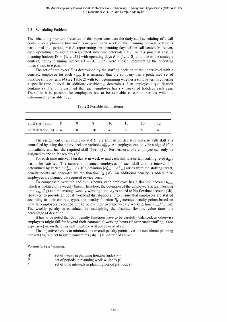
2.3 Scheduling Problem

The scheduling problem presented in this paper considers the daily staff scheduling of a call center over a planning horizon of one year. Each week of the planning horizon ∈ is partitioned into periods ∈ , representing the operating days of the call center. Moreover, each operating day again is segmented into time intervals ∈ . In this practical case, a planning horizon 1, . . . , 52 with operating days 1, . . . , 5 and, due to the strategic context, hourly planning intervals 8, . . . , 17 were chosen, representing the operating times 8 a.m. to 6 p.m.

The set of employees is determined by the staffing decision at the upper-level with a concrete employee for each . It is assumed that the company has a predefined set of possible shift patterns (see Table 2) with determining whether a shift pattern is covering a specific time interval. In addition, variable determines if an employee’s qualification contains skill . It is assumed that each employee has six weeks of holidays each year. Therefore it is possible for employees not to be available at certain periods which is determined by variable .

Table 2 Possible shift patterns

Shift start (a.m.) 8 8 8 10 10 10 12

Shift duration (h) 4 8 10 4 6 8 4

The assignment of an employee ∈ to a shift on day in week with skill is

controlled by using the binary decision variable . An employee can only be assigned if he is available and has the required skill (3b) - (3c). Furthermore, one employee can only be assigned to one shift each day (3d).

For each time interval on day in week and each skill a certain staffing level has to be satisfied. The number of planned employees of each skill at time interval is determined by variable (3e). If a deviation | | arises from the staffing target, penalty points are generated by the function (3f). An additional penalty is added if no employees are planned but required or vice versa.

To compensate overtime and minus hours, each employee has a flextime account , which is updated on a weekly basis. Therefore, the deviation of the employee’s actual working time (3g) and the average weekly working time is added to his flextime account (3h). However, to provide an equal workload distribution and to ensure that employees are staffed according to their contract types, the penalty function generates penalty points based on how far employees exceeded or fall below their average weekly working time ⁄ (3i). The weekly penalty is calculated by multiplying the absolute flextime value times the percentage of deviation.

It has to be noted that both penalty functions have to be carefully balanced, as otherwise employees might fall far beyond their contractual working hours (if over-/understaffing is too expensive) or, on the other side, flextime will not be used at all.

The objective here is to minimize the overall penalty points over the considered planning horizon (3a) subject to given constraints (3b) – (3i) described above.

Parameters (scheduling)

set of weeks in planning horizon (index ) set of periods in planning week w (index ) set of time intervals in planning period (index )


- 148 -

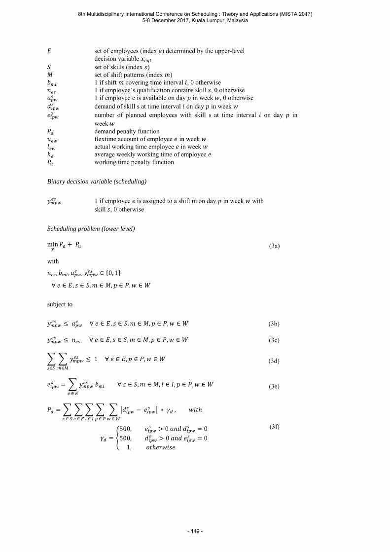
set of employees (index ) determined by the upper-level decision variable

set of skills (index ) set of shift patterns (index )

1 if shift covering time interval , 0 otherwise 1 if employee’s qualification contains skill , 0 otherwise 1 if employee e is available on day in week , 0 otherwise demand of skill s at time interval on day in week number of planned employees with skill s at time interval on day in

week demand penalty function

flextime account of employee in week actual working time employee in week

average weekly working time of employee working time penalty function

Binary decision variable (scheduling)

1 if employee is assigned to a shift m on day in week with skill , 0 otherwise

Scheduling problem (lower level)

min (3a)

with

, , , ∈ 0, 1

∀ ∈ , ∈ , ∈ , ∈ , ∈

subject to

∀ ∈ , ∈ , ∈ , ∈ , ∈ (3b)

∀ ∈ , ∈ , ∈ , ∈ , ∈ (3c)

∈∈

1∀ ∈ , ∈ , ∈ (3d)

∈

∀ ∈ , ∈ , ∈ , ∈ , ∈ (3e)

∗ ∈∈

, ∈∈∈

500, 0 0500, 0 01,

(3f)


- 149 -

∈∈

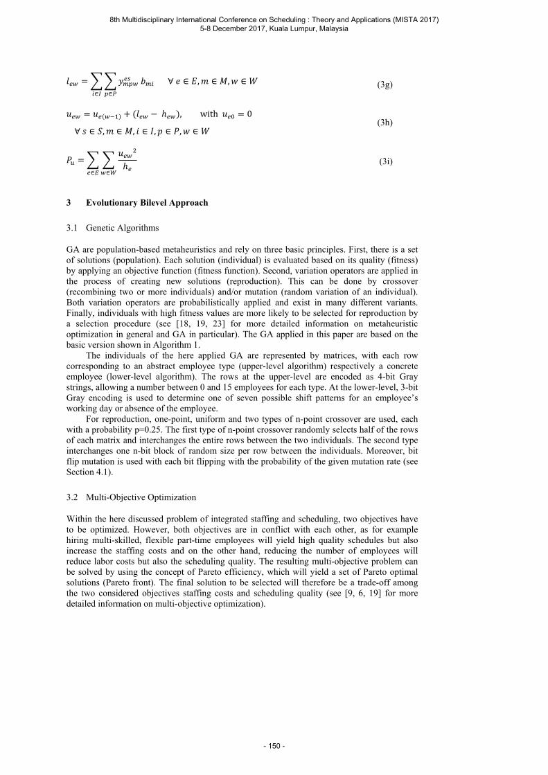
∀ ∈ , ∈ , ∈ (3g)

, with 0

∀ ∈ , ∈ , ∈ , ∈ , ∈ (3h)

∈∈

(3i)

3 Evolutionary Bilevel Approach

3.1 Genetic Algorithms

GA are population-based metaheuristics and rely on three basic principles. First, there is a set of solutions (population). Each solution (individual) is evaluated based on its quality (fitness) by applying an objective function (fitness function). Second, variation operators are applied in the process of creating new solutions (reproduction). This can be done by crossover (recombining two or more individuals) and/or mutation (random variation of an individual). Both variation operators are probabilistically applied and exist in many different variants. Finally, individuals with high fitness values are more likely to be selected for reproduction by a selection procedure (see [18, 19, 23] for more detailed information on metaheuristic optimization in general and GA in particular). The GA applied in this paper are based on the basic version shown in Algorithm 1.

The individuals of the here applied GA are represented by matrices, with each row corresponding to an abstract employee type (upper-level algorithm) respectively a concrete employee (lower-level algorithm). The rows at the upper-level are encoded as 4-bit Gray strings, allowing a number between 0 and 15 employees for each type. At the lower-level, 3-bit Gray encoding is used to determine one of seven possible shift patterns for an employee’s working day or absence of the employee.

For reproduction, one-point, uniform and two types of n-point crossover are used, each with a probability p=0.25. The first type of n-point crossover randomly selects half of the rows of each matrix and interchanges the entire rows between the two individuals. The second type interchanges one n-bit block of random size per row between the individuals. Moreover, bit flip mutation is used with each bit flipping with the probability of the given mutation rate (see Section 4.1).

3.2 Multi-Objective Optimization

Within the here discussed problem of integrated staffing and scheduling, two objectives have to be optimized. However, both objectives are in conflict with each other, as for example hiring multi-skilled, flexible part-time employees will yield high quality schedules but also increase the staffing costs and on the other hand, reducing the number of employees will reduce labor costs but also the scheduling quality. The resulting multi-objective problem can be solved by using the concept of Pareto efficiency, which will yield a set of Pareto optimal solutions (Pareto front). The final solution to be selected will therefore be a trade-off among the two considered objectives staffing costs and scheduling quality (see [9, 6, 19] for more detailed information on multi-objective optimization).


- 150 -

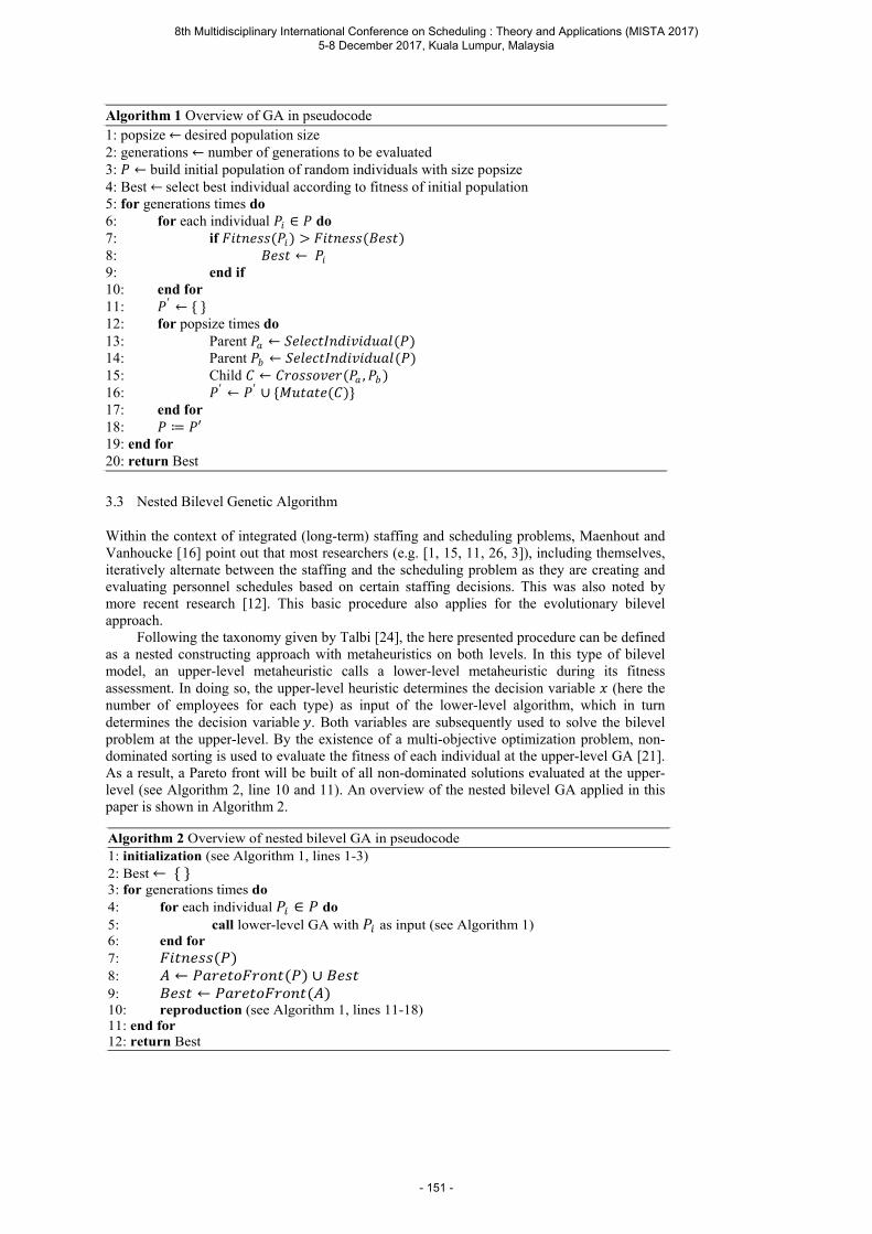
Algorithm 1 Overview of GA in pseudocode 1: popsize ←desired population size 2: generations ← number of generations to be evaluated 3: ← build initial population of random individuals with size popsize 4: Best ←select best individual according to fitness of initial population 5: for generations times do 6: for each individual ∈ do 7: if 8: ← 9: end if 10: end for 11: ′ ← 12: for popsize times do 13: Parent ← 14: Parent ← 15: Child ← , 16: ′ ← ′ ∪ 17: end for 18: ≔ ′ 19: end for 20: return Best

3.3 Nested Bilevel Genetic Algorithm

Within the context of integrated (long-term) staffing and scheduling problems, Maenhout and Vanhoucke [16] point out that most researchers (e.g. [1, 15, 11, 26, 3]), including themselves, iteratively alternate between the staffing and the scheduling problem as they are creating and evaluating personnel schedules based on certain staffing decisions. This was also noted by more recent research [12]. This basic procedure also applies for the evolutionary bilevel approach.

Following the taxonomy given by Talbi [24], the here presented procedure can be defined as a nested constructing approach with metaheuristics on both levels. In this type of bilevel model, an upper-level metaheuristic calls a lower-level metaheuristic during its fitness assessment. In doing so, the upper-level heuristic determines the decision variable (here the number of employees for each type) as input of the lower-level algorithm, which in turn determines the decision variable . Both variables are subsequently used to solve the bilevel problem at the upper-level. By the existence of a multi-objective optimization problem, non-dominated sorting is used to evaluate the fitness of each individual at the upper-level GA [21]. As a result, a Pareto front will be built of all non-dominated solutions evaluated at the upper-level (see Algorithm 2, line 10 and 11). An overview of the nested bilevel GA applied in this paper is shown in Algorithm 2.

Algorithm 2 Overview of nested bilevel GA in pseudocode 1: initialization (see Algorithm 1, lines 1-3) 2: Best ← 3: for generations times do 4: for each individual ∈ do 5: call lower-level GA with as input (see Algorithm 1) 6: end for 7: 8: ← ∪ 9: ← 10: reproduction (see Algorithm 1, lines 11-18) 11: end for 12: return Best


- 151 -

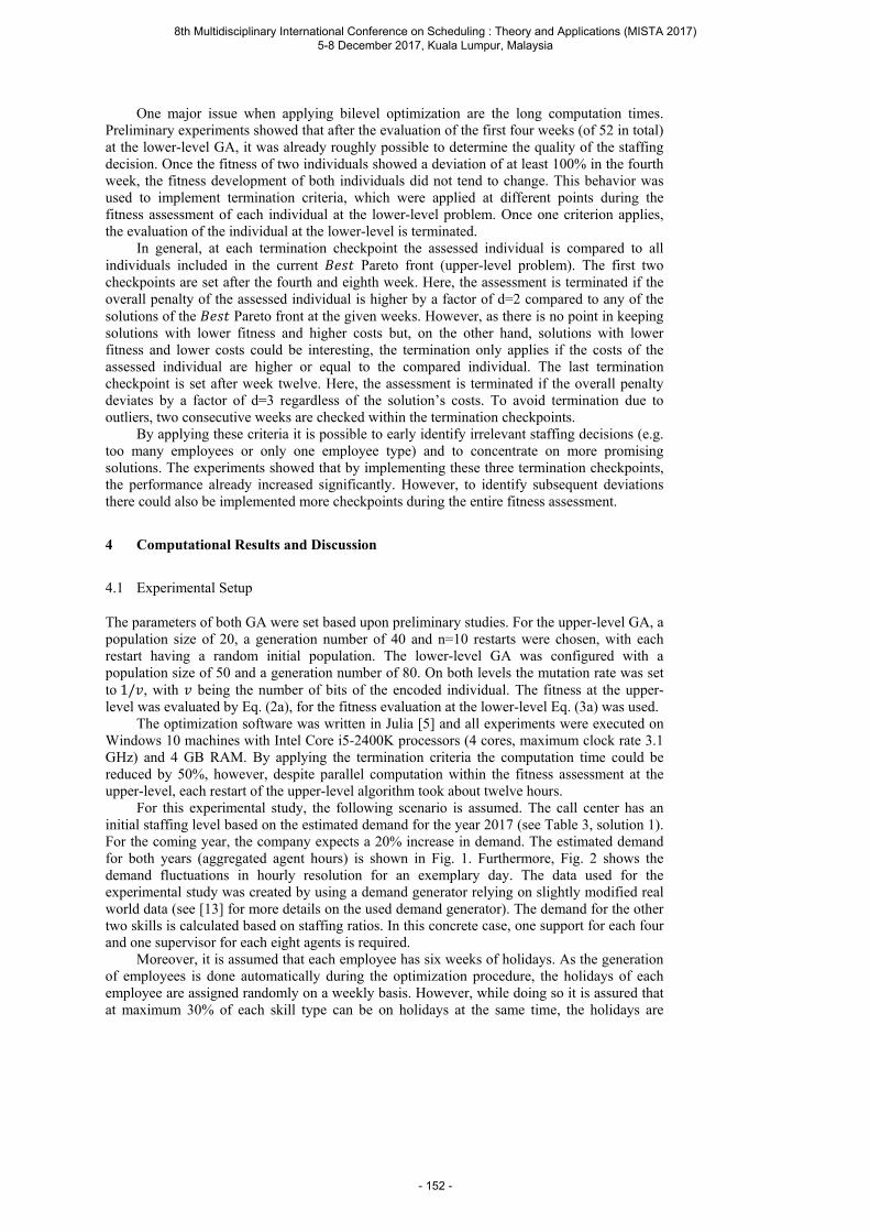
One major issue when applying bilevel optimization are the long computation times. Preliminary experiments showed that after the evaluation of the first four weeks (of 52 in total) at the lower-level GA, it was already roughly possible to determine the quality of the staffing decision. Once the fitness of two individuals showed a deviation of at least 100% in the fourth week, the fitness development of both individuals did not tend to change. This behavior was used to implement termination criteria, which were applied at different points during the fitness assessment of each individual at the lower-level problem. Once one criterion applies, the evaluation of the individual at the lower-level is terminated.

In general, at each termination checkpoint the assessed individual is compared to all individuals included in the current Pareto front (upper-level problem). The first two checkpoints are set after the fourth and eighth week. Here, the assessment is terminated if the overall penalty of the assessed individual is higher by a factor of d=2 compared to any of the solutions of the Pareto front at the given weeks. However, as there is no point in keeping solutions with lower fitness and higher costs but, on the other hand, solutions with lower fitness and lower costs could be interesting, the termination only applies if the costs of the assessed individual are higher or equal to the compared individual. The last termination checkpoint is set after week twelve. Here, the assessment is terminated if the overall penalty deviates by a factor of d=3 regardless of the solution’s costs. To avoid termination due to outliers, two consecutive weeks are checked within the termination checkpoints.

By applying these criteria it is possible to early identify irrelevant staffing decisions (e.g. too many employees or only one employee type) and to concentrate on more promising solutions. The experiments showed that by implementing these three termination checkpoints, the performance already increased significantly. However, to identify subsequent deviations there could also be implemented more checkpoints during the entire fitness assessment.

4 Computational Results and Discussion

4.1 Experimental Setup

The parameters of both GA were set based upon preliminary studies. For the upper-level GA, a population size of 20, a generation number of 40 and n=10 restarts were chosen, with each restart having a random initial population. The lower-level GA was configured with a population size of 50 and a generation number of 80. On both levels the mutation rate was set to1/ , with being the number of bits of the encoded individual. The fitness at the upper-level was evaluated by Eq. (2a), for the fitness evaluation at the lower-level Eq. (3a) was used.

The optimization software was written in Julia [5] and all experiments were executed on Windows 10 machines with Intel Core i5-2400K processors (4 cores, maximum clock rate 3.1 GHz) and 4 GB RAM. By applying the termination criteria the computation time could be reduced by 50%, however, despite parallel computation within the fitness assessment at the upper-level, each restart of the upper-level algorithm took about twelve hours.

For this experimental study, the following scenario is assumed. The call center has an initial staffing level based on the estimated demand for the year 2017 (see Table 3, solution 1). For the coming year, the company expects a 20% increase in demand. The estimated demand for both years (aggregated agent hours) is shown in Fig. 1. Furthermore, Fig. 2 shows the demand fluctuations in hourly resolution for an exemplary day. The data used for the experimental study was created by using a demand generator relying on slightly modified real world data (see [13] for more details on the used demand generator). The demand for the other two skills is calculated based on staffing ratios. In this concrete case, one support for each four and one supervisor for each eight agents is required.

Moreover, it is assumed that each employee has six weeks of holidays. As the generation of employees is done automatically during the optimization procedure, the holidays of each employee are assigned randomly on a weekly basis. However, while doing so it is assured that at maximum 30% of each skill type can be on holidays at the same time, the holidays are


- 152 -

0

100

200

300

400

500

600

1 4 7 10 13 16 19 22 25 28 31 34 37 40 43 46 49 52

Age

nt

hou

rs

Weeks

demand 2017 demand 2018

Fig. 2 Exemplary demand of a single day

Fig. 1 Weekly demand of agent hours over the planning horizon

0

2

4

6

8

10

12

8 9 10 11 12 13 14 15 16 17

# ag

ents

Hours

demand

equally distributed over the whole year and there are two consecutive weeks of holidays during the summer period (June until September).

4.2 Results and Discussion

For the purpose of demonstration and because the Pareto fronts tend to show similar behavior over multiple runs, the upper-level optimization algorithm was executed n=10 times, with each restart yielding a set of Pareto optimal solutions. The combined solutions of all Pareto fronts are shown in Fig. 3. Without the consideration of outliers and solutions that did not pass the termination criteria, a total of 134 possible staffing decisions with different combinations of costs and scheduling penalties were found (based on the demand for 2018). For further discussion, 15 solutions along the new Pareto front were selected. A detailed description of the selected staffing decisions can be found in Table 3.

8

10

12

14

16

18

20

22

10 15 20 25 30 35 40 45 50

Sta

ffin

g co

sts

Scheduling penalty (thousands)

combined Pareto fronts selected solutions

Fig. 3 Possible staffing decisions (n=10 optimization runs)


- 153 -

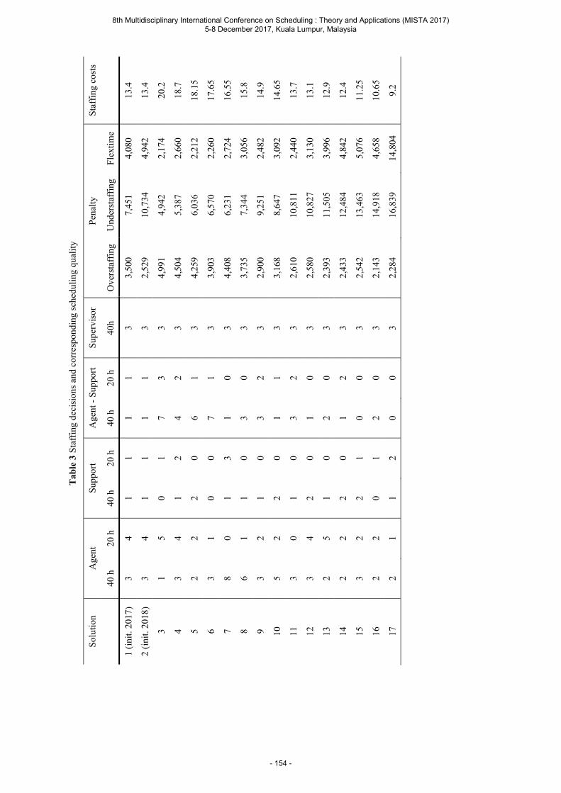
Tab

le 3

Sta

ffin

g de

cisi

ons

and

corr

espo

ndin

g sc

hedu

ling

qual

ity

Sol

utio

n A

gent

S

uppo

rt

Age

nt -

Sup

port

S

uper

viso

r P

enal

ty

Sta

ffin

g co

sts

40

h

20 h

40

h

20 h

40

h

20 h

40

h O

vers

taff

ing

Und

erst

affi

ng

Fle

xtim

e

1 (i

nit.

2017

) 3

4 1

1 1

1 3

3,50

0 7,

451

4,08

0 13

.4

2 (i

nit.

2018

) 3

4 1

1 1

1 3

2,52

9 10

,734

4,

942

13.4

3 1

5 0

1 7

3 3

4,99

1 4,

942

2,17

4 20

.2

4 3

4 1

2 4

2 3

4,50

4 5,

387

2,66

0 18

.7

5 2

2 2

0 6

1 3

4,25

9 6,

036

2,21

2 18

.15

6 3

1 0

0 7

1 3

3,90

3 6,

570

2,26

0 17

.65

7 8

0 1

3 1

0 3

4,40

8 6,

231

2,72

4 16

.55

8 6

1 1

0 3

0 3

3,73

5 7,

344

3,05

6 15

.8

9 3

2 1

0 3

2 3

2,90

0 9,

251

2,48

2 14

.9

10

5 2

2 0

1 1

3 3,

168

8,64

7 3,

092

14.6

5

11

3 0

1 0

3 2

3 2,

610

10,8

11

2,44

0 13

.7

12

3 4

2 0

1 0

3 2,

580

10,8

27

3,13

0 13

.1

13

2 5

1 0

2 0

3 2,

393

11,5

05

3,99

6 12

.9

14

2 2

2 0

1 2

3 2,

433

12,4

84

4,84

2 12

.4

15

3 2

2 1

0 0

3 2,

542

13,4

63

5,07

6 11

.25

16

2 2

0 1

2 0

3 2,

143

14,9

18

4,65

8 10

.65

17

2 1

1 2

0 0

3 2,

284

16,8

39

14,8

04

9.2


- 154 -

The first two solutions shown in Table 3 represent the initial staffing level, optimized with the demand for 2017 and 2018. Solutions 3 to 17 represent the optimized staffing levels based on the demand for 2018. When looking at the results of solution 2, due to the rising demand and therefore an insufficient number of employees, the penalty for understaffing and flextime increased and the overstaffing penalty decreased (compared to solution 1). The resulting scheduling quality of solution 2 now is comparable to the quality of solutions 11 to 13, which furthermore show approximately the same cost level. In case the company wants to retain its service level of 2017 (considering the understaffing penalty of solution 1), the current workforce should be developed towards the staffing level of solution 8. Taking a more general look on the results, it can be noted that no solution below the cost level of 9.2 passed the termination criteria within the fitness assessment. The low costs can simply be explained by the insufficient staffing level, resulting in high understaffing and flextime penalties. Looking at the staffing decisions in Table 3 from bottom to top, it can be seen that the scheduling quality grows with an increasing number of employees and increasing contractual working hours, and, hence, rising staffing costs. Furthermore, when comparing solutions 8 and 7 with 6 to 3, an increased employment of cross-trained and part-time workers can be noticed yielding the highest scheduling quality. However, no solution was found above the cost level of 20.85. This may indicate that there is a point at which scheduling quality cannot be increased under the given staffing and scheduling policies. Thus, measures to further improve the scheduling quality could be, for example, the introduction of new contract types (e.g. contracts with a working time of 30 or 12 hours per week) or more flexible shift patterns to better compensate varying demand over the day (e.g. short 2h shifts).

5 Conclusion and Future Research

In this paper, a model for strategic long-term staffing was presented considering varying demand, different types of employees regarding skills and contractual working times as well as compensation of overtime due to flextime policies. For this purpose, an evolutionary bilevel algorithm with GA on both levels was applied, optimizing the staffing decision at the upper-level and simultaneously evaluating the resulting workforce structure by the creation of personnel schedules over a planning horizon of 52 weeks. This integrated staffing and scheduling approach was demonstrated by the example of the yearly workforce planning of a midsized call center. The computational results indicate that the proposed procedure could be used to support corporate decision making related to strategic workforce planning. Due to the nested structure and independent formulation of the staffing and the scheduling problem, both problems could generically be replaced. Therefore, the model is not limited to the considered call center problem but could be used for any other kind of (strategic) workforce planning involving personnel scheduling.

However, an important limitation arises from the fact that the optimization problem at the lower-level only was executed once, which leads to noisy results. Thus, there is a risk of discarding a possibly good solution due to one “unlucky” optimization run at the lower level. Moreover, it is hard to compare solutions being close to each other (e.g. solutions 4 to 6). These issues could be solved by restarting the lower-level algorithm multiple times, which in turn will lead to a massive increase of computation time. As this is a general challenge when applying bilevel optimization, further research should be aimed at executing the bilevel algorithm more efficiently, e.g. by applying more precise termination criteria, using distributed computation or approximation of the lower-level model. Other opportunities for further research are seen in comparing the here proposed approach to the methods presented in Section 1 (e.g. regarding speed and quality) as well as the consideration of uncertainty and unplanned events during the optimization procedure, such as illness, fluctuation or infra-annual hiring of employees.

As stated in Section 4.2, there may be the need not only to optimize staffing decisions, but also staffing and scheduling policies. The study presented in this paper was limited to optimize the staffing decision as input of the scheduling problem. However, further research


- 155 -

should be conducted addressing the possibility to optimize all framework conditions related to personnel scheduling, such as shift types, overtime and break regulations or any other type of adjustable constraints. This could potentially increase the solution quality attainable, but would in turn raise the complexity of the optimization problem considerably.

References

1. Abernathy WJ, Baloff N, Hershey JC, Wandel S, A Three-Stage Manpower Planning and Scheduling Model—A Service-Sector Example, Operations Research 21(3), 693–711 (1973)

2. Avramidis AN, Chan W, Gendreau M, L’Ecuyer P, Pisacane O, Optimizing daily agent scheduling in a multiskill call center, European Journal of Operational Research 200(3), 822–832 (2010)

3. Beliën J, Demeulemeester E, A branch-and-price approach for integrating nurse and surgery scheduling, European Journal of Operational Research 189(3), 652–668 (2008)

4. Beliën J, Demeulemeester E, Bruecker P de, van den Bergh J, Cardoen B, Integrated staffing and scheduling for an aircraft line maintenance problem, Computers & Operations Research 40(4), 1023–1033 (2013)

5. Bezanson J, Edelman A, Karpinski S, Shah VB, Julia. A Fresh Approach to Numerical Computing, SIAM Rev. 59(1), 65–98 (2017)

6. Branke J (ed.), Multiobjective optimization. Interactive and evolutionary approaches. Lecture Notes in Computer Science, vol. 5252. Springer, Berlin (2008)

7. Bruecker P de, van den Bergh J, Beliën J, Demeulemeester E, Workforce planning incorporating skills. State of the art, European Journal of Operational Research 243(1), 1–16 (2015)

8. Brunner JO, Edenharter GM, Long term staff scheduling of physicians with different experience levels in hospitals using column generation, Health care management science 14(2), 189–202 (2011)

9. Coello Coello CA, Lamont GB, van Veldhuizen DA, Evolutionary algorithms for solving multi-objective problems, 2nd edn. Genetic and evolutionary computation series. Springer, New York, NY (2007)

10. Colson B, Marcotte P, Savard G, An overview of bilevel optimization, Ann Oper Res 153(1), 235–256 (2007)

11. Easton FF, Rossin DF, Borders WS, Analysis of Alternative Scheduling Policies for Hospital Nurses, Production and Operations Management 1(2), 159–174 (1992)

12. Erhard M, Schoenfelder J, Fügener A, Brunner JO, State of the art in physician scheduling, European Journal of Operational Research (2017)

13. Günther M, A Generator for Volatile Demand Profiles. A Brief Description of a Tool. GRIN, Munich (2017)

14. Hansen P, Jaumard B, Savard G, New Branch-and-Bound Rules for Linear Bilevel Programming, SIAM J. Sci. and Stat. Comput. 13(5), 1194–1217 (1992)

15. Henderson JC, Krajewski LJ, Showalter MJ, An integrated approach for manpower planning in the service sector, Omega 10(1), 61–73 (1982)

16. Maenhout B, Vanhoucke M, An integrated nurse staffing and scheduling analysis for longer-term nursing staff allocation problems, Omega 41(2), 485–499 (2013)

17. Nissen V, Applications of Evolutionary Algorithms to Management Problems. In: Moutinho, L., Sokele, M. (eds.) Palgrave Handbook of Innovative Research Methods in Management. Palgrave Macmillan, Basingstoke (2017)

18. Rothlauf F, Design of Modern Heuristics. Springer Berlin Heidelberg, Berlin, Heidelberg (2011)

19. Sean Luke, Essentials of Metaheuristics. Lulu (2013) 20. Sinha A, Malo P, Deb K, A Review on Bilevel Optimization. From Classical to

Evolutionary Approaches and Applications, IEEE Trans. Evol. Computat., 1 (2017)


- 156 -

21. Srinivas N, Deb K, Muiltiobjective Optimization Using Nondominated Sorting in Genetic Algorithms, Evolutionary computation 2(3), 221–248 (1994)

22. Stackelberg H, The theory of market economy. Oxford University Press, Oxford (1952) 23. Talbi E-G, Metaheuristics. From design to implementation. Wiley Series on Parallel and

Distributed Computing, v.74. John Wiley & Sons, Hoboken, NJ (2009) 24. Talbi E-G (ed.), Metaheuristics for Bi-level Optimization. Studies in Computational

Intelligence, vol. 482. Springer, Berlin, Heidelberg (2013) 25. van den Bergh J, Beliën J, Bruecker P de, Demeulemeester E, Boeck L de, Personnel

scheduling. A literature review, European Journal of Operational Research 226(3), 367–385 (2013)

26. Venkataraman R, Brusco MJ, An integrated analysis of nurse staffing and scheduling policies, Omega 24(1), 57–71 (1996)

27. Yin Y, Genetic-Algorithms-Based Approach for Bilevel Programming Models, Journal of Transportation Engineering 126(2), 115–120 (2000)


- 157 -

MISTA 2017

A constraint programming approach for theenergy-efficient job shop scheduling problem

Angelo Oddi · Riccardo Rasconi · Miguel A.

Gonzalez

Abstract Optimising the energy consumption is one of the most important issues in

scheduling nowadays. In this work we consider a multi-objective optimisation for the

well-known job-shop scheduling problem. In particular, we minimise the makespan and

the energy consumption at the same time. We consider a realistic energy model where

each machine can be in off, stand-by, idle or working state. We design a constraint-

programming approach that also uses a piecewise linear programming step to further

optimise the energy consumption of the solutions. Experimental results illustrate the

potential of the proposed method, outperforming the results of the current state of the

art in this problem.

1 Introduction

The job shop is a scheduling problem widely studied in the literature due to the fact

that it is a model which is close to many real production environments. It is proven

that the job shop is NP-hard, and so its resolution is very complex. In the literature

we can find many different solving approaches for the job shop, from exact methods to

all kinds of meta-heuristic algorithms.

Although the makespan is the most studied objective function (see for example

[1], [4] or [18]), energy considerations are increasingly important nowadays, mainly for

economical and environmental reasons. In fact, we can find many recent approaches

that tackle different scheduling problems with energy considerations. For example, in

[5] the authors solve a flexible flow shop scheduling problem with energy costs by using

a genetic-simulated annealing method. In [17] a single machine problem is studied,

Angelo OddiInstitute of Cognitive Sciences and Technologies, ISTC-CNR, ItalyE-mail: [email protected]

Riccardo RasconiInstitute of Cognitive Sciences and Technologies, ISTC-CNR, ItalyE-mail: [email protected]

Miguel A. GonzalezDepartment of Computing, University of Oviedo, SpainE-mail: [email protected]


- 158 -

where the machine can be switched on and off. Other papers, as for example [10], even

consider shifting energy costs.

There are also some papers addressing the energy-efficient job shop. For exam-

ple, in [20] the authors try to minimise both the weighted tardiness and the energy

consumption in a job shop where the processing mode of operations can be modified.

Another approach is that of [14], where the authors consider a simple energy model

where the machines can only be in Working or in Idle state. In [9] the authors improve

the results reported in [14] by using a hybrid evolutionary meta-heuristic and also a

constraint-programming approach. One problem with the last two papers is that the

considered energy model is not too realistic. The model proposed in [15] is much more

interesting, as the machines can be either in the Idle, Working, Off, or switched to a

Stand-by state.

In this paper we consider this last energy model and try to minimize at the same

time the makespan and the energy consumption in a job shop. Although some multi-

objective works consider weighted or lexicographical approaches, probably the most

interesting approaches are those based on the Pareto Front.

In particular, we have designed a set of constraint-based procedures to minimise

both the makespan and the energy consumption, within a well-studied multi-objective

optimisation method to generate the whole Pareto (i.e., the ε-constraint method [16]).

The contribution of the paper is twofold: first, we design a constraint-based model

where we add as decision variables the states of the machines during the no-working

periods (i.e., Idle, Off, or Stand-by states); second, in order to take into account the non-

regularity of the energy objective function, we design a piecewise-linear programming

approach to post-process a full input solution and minimise the energy consumption

within the same makespan.

This paper is organised as follows: Section 2 formulates the problem at hand and

Section 3 describes the solving methods. Then, in Section 4 we analyse our proposals

and we compare them with the state-of-the-art algorithms [15], and finally in Section

5 we report the conclusions of our work and remark some ideas for future work.

2 Problem formulation

The job shop scheduling problem (JSP) consists on scheduling a set of N jobs, J =

J1, . . . , JN in a set of M machines or resources, R = R1, . . . , RM. Each of the jobs

Ji consists of ni tasks (θi1, . . . , θini) that must be scheduled exactly in that particular

order. Each task requires a given resource during all its processing time. Additionally,

no preemption is allowed, so when a resource starts processing a task, it cannot be

interrupted until it ends. Moreover, resources can at most process one task at a time.

The objective of the problem is to minimise some objective functions subject to the

described precedence and capacity constraints. Although we have denoted the tasks as

θij in this problem definition, in the following we will denote them by a single letter,

if possible, in order to simplify the expressions. We denote by Ω the set of tasks, by

pu the processing time of task u, by ru the resource required by task u, and by su the

starting time of task u (which needs to be determined).

As we have seen, the JSP has precedence constraints, defined by the routing of the

tasks within the jobs, that translate into linear inequalities: su + pu ≤ sv, where v is

the next task to u in the job sequence. The problem has also capacity constraints, as

the resources can only process one task at a time, and they translate into disjunctive


- 159 -

constraints: (su + pu ≤ sv) ∨ (sv + pv ≤ su), where u and v are tasks requiring the

same resource. The objective is to build a feasible schedule, i.e. determine a starting

time for each task such that all constraints are fulfilled. In the following, given a

feasible schedule, we will denote with PJv and SJv the predecessor and successor of

v, respectively, in the job sequence, and with PMv and SMv the predecessor and

successor of v, respectively, in its resource sequence. In addition, we will denote with

αk and ωk the first and last operations respectively on machine Rk in the considered

schedule.

The goal of the present analysis is the minimisation of both the energy consumption

and the overall completion time, or makespan. In general, for a minimization problem

with two objective functions fi (i = 1, 2), a solution S is said to be dominated by

another solution S′, denoted S′ ≺ S, if and only if for each objective function fi,

fi(S′) ≤ fi(S) and there exists at least one i such that fi(S

′) < fi(S). However,

the possibly conflicting nature of these two objectives may prevent the existence of a

unique solution S∗ that is optimal w.r.t. both the objectives. Therefore, in this work

we are interested in the set of all optimal “tradeoffs”, which are known as the Pareto

optimal solutions. A Pareto optimal solution is a solution such that the improvement

of one objective necessarily implies the worsening of the other objective. The Pareto

front PS∗ is the set of solutions S, such that for each S ∈ PS∗ there is no solution S′

which dominates S (S′ ≺ S).

The makespan is the first objective function and corresponds to the maximum

completion time of the schedule, that is

maxu∈Ωsu + pu (1)

About the second objective the energy model is taken from [15], where it is supposedthat a resource can be in five different states: Off, Stand-by, Idle, Setup or Working.However, May et al. in their experiments from [15] consider together the times andenergy consumption of the Working and Setup states; as a consequence, we can considera total of four possible states (see Figure 1). The power consumption in each state

for a given resource Rk is denoted by P idlek , P stand-byk and Pworkingk , whereas if themachine is Off it consumes no power. Additionally, we assume that the machine caninstantly switch from Idle to Stand-by, Off or Working, consuming no power. On the

other hand, switching from Off to Idle requires an amount of T ramp-up-offk time units,

whereas switching from Stand-by to Idle requires T ramp-up-stand-byk time units. In both

cases, the power consumed when ramping up is denoted by P ramp-upk . In Figure 1

we show the considered state diagram, which is the same for each machine. Also, weassume that all machines do not consume any energy before the processing of its firsttask assigned. It is easy to see that in the job shop scheduling problem, each resourcemust always process the same set of tasks, and so the working energy consumption isthe same in every possible schedule. Therefore, following [15], in order to reduce theenergy consumption we consider the WEC (Worthless Energy Consumption) measureas the second objective function to minimize, which is defined as follows:

WEC =∑

k=1,...,M

[P idlek tidlek + P stand-byk tstand-byk ] +

∑k=1,...,M

P ramp-upk (nramp-up-standby

k T ramp-up-standbyk + nramp-up-off

k T ramp-up-offk )

(2)

where tidlek is the total amount of time spent by Rk in Idle state, tstand-byk is the total

amount of time spent by Rk in Stand-by state, nramp-up-standbyk is the number of times


- 160 -

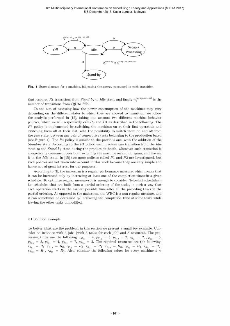
Idle Off

Stand-by

Setup +

Processing

𝑃𝑘𝑟𝑎𝑚𝑝−𝑢𝑝

× 𝑇𝑘𝑟𝑎𝑚𝑝−𝑢𝑝−𝑠𝑡𝑎𝑛𝑑𝑏𝑦

0

𝑃𝑘𝑟𝑎𝑚𝑝−𝑢𝑝

× 𝑇𝑘𝑟𝑎𝑚𝑝−𝑢𝑝−𝑜𝑓𝑓

0 0

0

Fig. 1 State diagram for a machine, indicating the energy consumed in each transition

that resource Rk transitions from Stand-by to Idle state, and finally nramp-up-offk is the

number of transitions from Off to Idle.

To the aim of assessing how the power consumption of the machines may vary

depending on the different states to which they are allowed to transition, we follow

the analysis performed in [15], taking into account two different machine behavior

policies, which we will respectively call P3 and P4 as described in the following. The

P3 policy is implemented by switching the machines on at their first operation and

switching them off at their last, with the possibility to switch them on and off from

the Idle state, between any pair of consecutive tasks belonging to the production batch

(see Figure 1). The P4 policy is similar to the previous one, with the addition of the

Stand-by state. According to the P4 policy, each machine can transition from the Idle

state to the Stand-by state during the production batch, whenever such transition is

energetically convenient over both switching the machine on and off again, and leaving

it in the Idle state. In [15] two more policies called P1 and P2 are investigated, but

such policies are not taken into account in this work because they are very simple and

hence not of great interest for our purposes.

According to [3], the makespan is a regular performance measure, which means that

it can be increased only by increasing at least one of the completion times in a given

schedule. To optimize regular measures it is enough to consider “left-shift schedules”,

i.e. schedules that are built from a partial ordering of the tasks, in such a way that

each operation starts in the earliest possible time after all the preceding tasks in the

partial ordering. As opposed to the makespan, the WEC is a non-regular measure, and

it can sometimes be decreased by increasing the completion time of some tasks while

leaving the other tasks unmodified.

2.1 Solution example

To better illustrate the problem, in this section we present a small toy example. Con-

sider an instance with 3 jobs (with 3 tasks for each job) and 3 resources. The pro-

cessing times are the following: pθ11 = 4, pθ12 = 5, pθ13 = 2, pθ21 = 2, pθ22 = 5,

pθ23 = 3, pθ31 = 4, pθ32 = 7, pθ33 = 3. The required resources are the following:

rθ11 = R1, rθ12 = R2, rθ13 = R3, rθ21 = R1, rθ22 = R3, rθ23 = R2, rθ31 = R2,

rθ32 = R1, rθ33 = R3. Also, consider the following values for every machine k ∈


- 161 -

0 20 15 10 5

R1

R3

R2

21

31 12 23

11 32

22 33 13

Stand-by

Ramp-up Off

Ramp

-up

t

Fig. 2 Feasible solution for an example instance using a “left-shift schedule”.

0 20 15 10 5

R1

R3

R2

21

31 12 23

11 32

22 33 13 Ramp-up Off

Idle

t

Fig. 3 Improving the solution of figure 2 by delaying one task.

1, 2, 3: Pworkingk = 10kW , P idlek = 6kW , P stand-byk = 4kW , P ramp-up

k = 8kW ,

T ramp-up-offk = 3 and T ramp-up-stand-by

k = 1.

Figure 2 shows a feasible solution for this instance. In fact it is a “left-shift sched-

ule”, i.e. every task starts as soon as possible in the considered partial ordering. This

schedule has a makespan of 18 and a WEC of 40 (16 from R2 plus 24 from R3). In

resource R2 we have decided to switch the machine to Stand-by state between the end

of θ31 and the beginning of θ23, because in this case it adds 16 units to the WEC,

whereas if switched Off it would add 24 units and if it remained Idle it would add 18

units. Using the same reasoning we decided to switch R3 off between the end of θ22and the beginning of θ33.

It is easy to see that these “left-shift schedules” can be easily improved by delaying

some tasks. Figure 3 shows the same solution after delaying task θ31. Now there is only

one time unit between the end of θ31 and the beginning of θ23, and so the best option

is to leave the machine in Idle state. The makespan is still 18 but the WEC is reduced

from 40 to 30.

3 The proposed solving method

As we have seen in the previous section, the WEC is a non-regular performance mea-

sure. Moreover, the work [15] only considers “left-shift schedules”, while we have seen

that they can be improved by delaying some tasks, in order to reduce the total en-

ergy consumption. In the next section we describe a two-step procedure that takes

into account the non-regularity of the WEC objective such that an approximation

of the Pareto front is generated by a Constraint Programming (CP) procedure (first


- 162 -

step), which is further improved by a Piecewise Linear Programming post-processing

optimization (PO) procedure (second step). It is worth noting that the proposed CP

approach is in principle able to find an optimal WEC value if given sufficient compu-

tational time (we do not provide any formal proof about this property). Nonetheless,

in our heuristic approach we use the post-processing step to improve the WEC (non-

regular) measure because it allows to reach better solutions in a shorter time, provided

the solution it inherits from CP is good enough. As the experiments confirm, the PO

procedure is able to give better performance over the single-step CP approach.

3.1 Energy optimisation procedure: a Constraint Programming approach

Constraint Programming (CP) is a declarative programming paradigm [2] suitable

for solving constraint satisfaction and optimisation problems. A constraint program is

defined as a set of decision variables, each ranging on a discrete domain of values, and

a set of constraints that limit the possible combination of variable-value assignments.

After a model of the problem is created, the solver interleaves two main steps: constraint

propagation, where inconsistent values are removed from variables domains, and search.

Constraint Programming is particularly suited for solving scheduling problems

where the decision variables are associated to the problem operations. In particular,

each operation variable a is characterised at least by two features: sa representing

its start time, and pa representing its duration. For scheduling problems, a number

of different global constraints have been developed, the most important being the

unary-resource constraint [19] for modelling simple machines, the cumulative re-

source constraint [13] for modelling cumulative resources (e.g., a pool of workers), and

the reservoir [11] for modelling consumable resources (e.g., a fuel tank). In particular,

given unary-resource(A), the constraint holds if and only if all the operations in the

set A never overlap at any time point. A number of propagation algorithms are embed-

ded in the unary-resource constraint for removing probably inconsistent assignments

of operation start-time variables.

We describe a Constraint Programming (CP) model based on the problem defined

in Section 2, where the main decision variables are the start times sa of the operations

a ∈ Ω characterized by a processing time pa. Each start time sa ranges in the interval

[0, H−pa], whereH is the problem’s horizon. The decision variables set is then extended

with the start times sOnOffkof the OnOffk intervals, where each OnOffk interval is

defined as spanning over all the operations executed on machine k. Hence, the sOnOffk

variable represents the first instant when machine k is turned on. The model, whose

utilisation will be described in the experimental section (Section 4), is built on top of the

IBM-ILOG CPLEX Optimization Studio CP Optimizer and its details are presented

below.

Let Ok be the set of problem operations assigned to machine k = 1, . . . ,M and Uk a

set of auxiliary unit-duration operations, assigned to a dummy unary machine mirroring

k (it is worth noting that the two sets Ok and Uk represent separate processing orders

of activities). The introduction of the auxiliary set of operations Uk1 is necessary to

represent the position of each activity a ∈ Ok in the processing orders imposed among

1 We were inspired to adopt this solution by a post on a discussion board on the website www.or-exchange.com about the explicit representation of an interval position in a OPL sequence.At the date of the writing of this note, this discussion board does not seem available anymore.


- 163 -

the operations assigned to each machine k ∈ R. More concretely, the auxiliary unit-

duration operations indirectly implement the definition of a successor function SMa

(returning the successor of each operation a for each total order imposed on the set of

operations Ok assigned to a machine k). To the best of our knowledge, this workaround

is necessary because we want to use the native OPL construct to implement the global

constraints unary-constraint(Ok) for efficiency reasons, and the successor function

is not natively present in the OPL language (see IBM ILOG CPLEX Optimization

Studio OPL Language Reference Manual, Version 12 Release 7.1).

Operationally, the set of unit-duration operations u ∈ Uk can be assigned to the

dummy machine k (in the same fashion of the operations a) so that, for each processing

order imposed on a machine k, a0 ≺ a1, . . . ,≺ ai, . . . ≺ aM , an identical order is

imposed on the unit-duration operations u0 ≺ u1, . . . ,≺ ui, . . . ≺ uM . In this manner,

the position i of the operation ai coincides with the start-time value of the unit-duration

operation ui. For the reasons above, the starting times su of the operations u ∈ Ukmust be added to the model as additional set of decision variables.

SMp =

q ∃v(q) ∈ Uk : sv(q) = su(p) + 1

nil otherwise(3a)

Ekpq =minP idlek dpq,

P stand-byk (dpq − T ramp-up-standbyk ) + P ramp-upk T ramp-up-standby

k ,

P ramp-upk T ramp-up-offk (3b)

WEC =∑

k=1,...,M

∑p∈Ok,

q=SMp, q 6=nil

Ekpq (3c)

Cmax = maxa∈Ωsa + pa (3d)

The definition (3a) represents the successor function SMp such that the position of

the operation p ∈ Ok coincides with the start-time value su(p) of its corresponding

unit-duration operation u(p) ∈ Uk, and the successor q (if exists) corresponds to the

unary activity v(q) ∈ Uk, such that sv(q) = su(p) + 1. Whereas, according to Section 2,

the energy objective WEC (3c) is the sum of the unload energy consumption Ekpq (i.e.,

when a machine is Idle, switched Off, or switched to a Stand-by state) of each pair of

contiguous operations (p, q) assigned on the same machine k (3b), where dpq = sq−ep is

the difference between q’s start time and p’s end time. The makespan objective Cmaxis described at line (3d), and follows the classical definition. Once all the necessary

definitions have been provided and all the variables have been introduced, we present


- 164 -

the CP model (optimisation criteria and constraints).

lex min (WEC, Cmax) (4a)

s.t. :

Cmax ≤ Cε (4b)

sv + pv ≤ sSJv v ∈ Ω \ θ1n1 , . ., θNnN (4c)

span(OnOffk, Ok) k = 1, 2, . .,M (4d)

edp ∈ 0, 1, 2 p ∈ Ω (4e)

SMp = q ∧ edp = 0⇒ sq − ep ≤ T idle-standbyk (4f)

SMp = q ∧ edp = 1⇒ sq − ep > T idle-standbyk ∧ sq − ep ≤ T standby-off

k (4g)

SMp = q ∧ edp = 2⇒ sq − ep > T standby-offk (4h)

same-sequence(Ok,Uk) k = 1, . . . ,M (4i)

su ≤ |Ok| − 1 ∀k (4j)

unary-constraint(Ok)k = 1, . . . ,M (4k)

unary-constraint(Uk)k = 1, . . . ,M (4l)

Line (4a) represents the lexicographic minimisation of the objective pair (WEC, Cmax)

with the energy WEC as primary objective. According to the implemented ε-constraint

method [16] for calculating the Pareto set we optimise the energy WEC, while we

impose an upper bound to the other objective Cmax in the form Cmax ≤ Cε (see

(4b)). The constraints in (4c) represent the linear orderings imposed on the set of

operations Ω by the set of jobs J . Constraints (4d) impose to the set Ok of operations

requiring machine k to be contained in the spanning operations OnOffk, k = 1, . . . ,M .

More specifically, for each operation v ∈ Ok, the following constraints sOnOffk≤ sv

and sv+pv ≤ sOnOffk+pOnOffk

hold, such that operation OnOffk starts together with

the first present operation in Ok according to the order imposed on the k-th machine,

and ends together with the last present operation according to the same order.

Constraints (4f), (4g), (4h), impose respectively, for each pair of contiguous activ-

ities (p, q) on a resource k, the temporal constraint sq − ep ≤ T idle-standbyk , sq − ep >

T idle-standbyk ∧sv−eu ≤ T standby-off

k , or sq−ep > T standby-offk . In turn, such constraints

guarantee that the minimal unload energy state is respectively Idle, Standby or Off be-

tween (p, q). To this purpose, we introduce a set of decision variables edp ∈ 0, 1, 2,p ∈ Ω representing the unload state (i.e., 0 when machine is Idle, 1 when is switched to a

Stand-by state, and 2 when switched Off ) imposed on every pair of contiguous activities

(p, q) on the same machine. We note that, under the hypothesis P stand-byk ≤ P idlek ≤P ramp-upk and T ramp-up-standby

k ≤ T ramp-up-offk , two cut-off values, T idle-standby

k and

T standby-offk can be calculated such that the minimal energy state will be Idle if

sv − eu ∈ [0, T idle-standbyk ], Stand-by when sv − eu ∈ (T idle-standby

k , T standby-offk ], and

Off otherwise; see Figure 4 for a graphical representation of the three energy intervals

determined by the two cut-off values. The constraints in (4i) impose the same order

between the activities in the two sets Ok and Uk by means of the global constraints

same-sequence(Ok,Uk). The constraints in (4j) bound the start-time value of each

unit-duration operation u to |Ok| − 1 operations assigned to the machine k. Finally,

(4k) and (4l) represents the non-overlapping constraints imposed by the machines M to


- 165 -

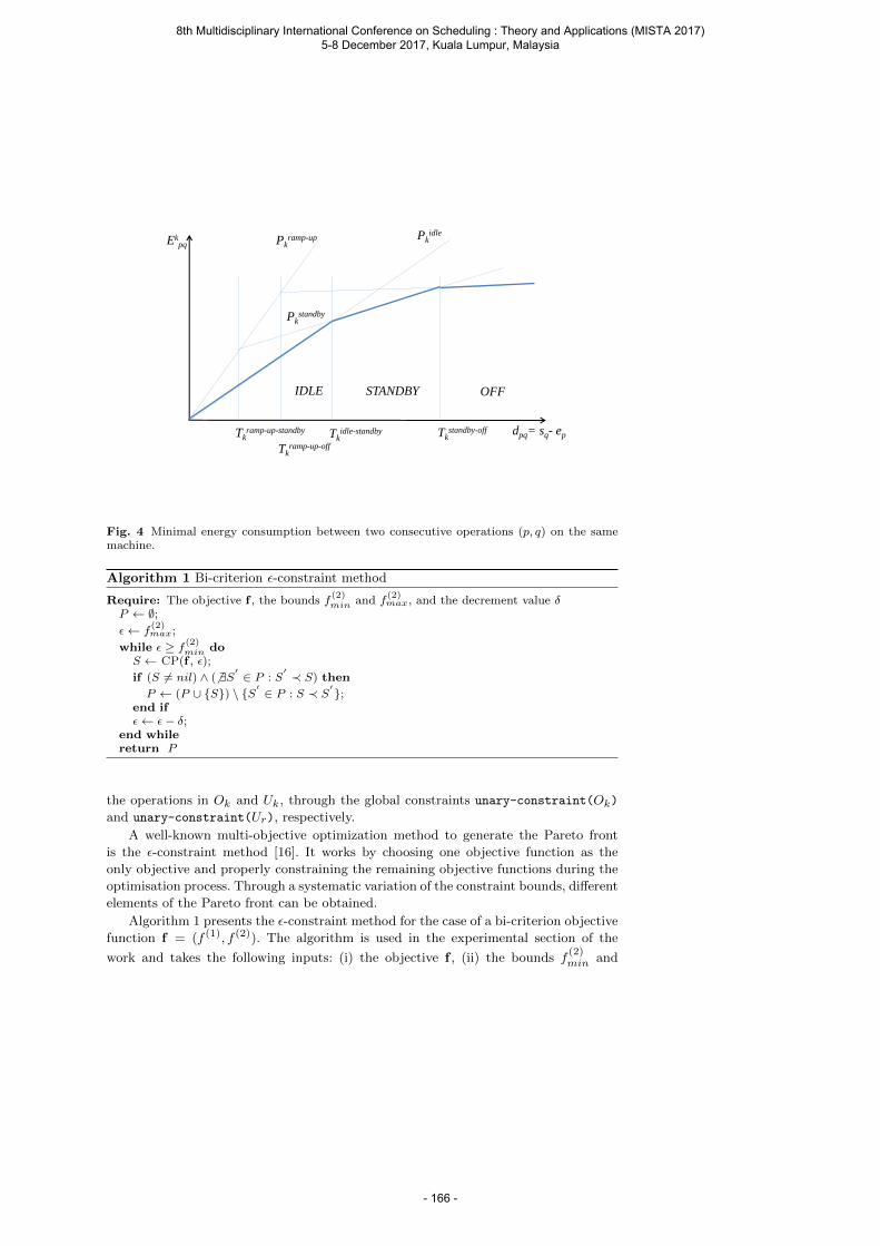
dpq= sq- ep

Ekpq

Tkramp-up-standby

Tkramp-up-off

Tkidle-standby Tk

standby-off

Pkidle

Pkstandby

Pkramp-up

IDLE STANDBY OFF

Fig. 4 Minimal energy consumption between two consecutive operations (p, q) on the samemachine.

Algorithm 1 Bi-criterion ε-constraint method

Require: The objective f , the bounds f(2)min and f

(2)max, and the decrement value δ

P ← ∅;ε← f

(2)max;

while ε ≥ f (2)min doS ← CP(f , ε);

if (S 6= nil) ∧ (6 ∃S′ ∈ P : S′ ≺ S) then

P ← (P ∪ S) \ S′ ∈ P : S ≺ S′;end ifε← ε− δ;

end whilereturn P

the operations in Ok and Uk, through the global constraints unary-constraint(Ok)

and unary-constraint(Ur), respectively.

A well-known multi-objective optimization method to generate the Pareto front

is the ε-constraint method [16]. It works by choosing one objective function as the

only objective and properly constraining the remaining objective functions during the

optimisation process. Through a systematic variation of the constraint bounds, different

elements of the Pareto front can be obtained.

Algorithm 1 presents the ε-constraint method for the case of a bi-criterion objective

function f = (f (1), f (2)). The algorithm is used in the experimental section of the

work and takes the following inputs: (i) the objective f , (ii) the bounds f(2)min and


- 166 -

f(2)max on the second component of the objective, and (iii) the decrement value δ. As

previously mentioned, the method iteratively leverages a procedure provided in input

to solve constrained single-objective problems (the CP() procedure corresponding to

the constraint programming model previously described). The algorithm proceeds as

follows: after initializing the constraint bound ε to the f(2)max value, a new solution S is

computed by calling CP() at each step of the while solving cycle. If S is not dominated

by any of the existing solutions in the current Pareto front P , then S is inserted in

P , and all the solutions possibly dominated by S are removed from P . The rationale

behind this method is to iteratively tighten the constraint bound by a pre-defined

constant δ at each step of the solving cycle. A similar procedure is the adaptive ε-

constraint method described in [12]; the main difference with respect to our algorithm

is that, as soon as a new solution S is found at each iteration, the constraint bound is

tightened by the value f (2)(S). We will test this procedure in a future and extended

version of this work.

3.2 Post-optimization: a piecewise linear programming approach

The solution returned by the energy optimisation procedure described in the previous

Section 3.1, in case the WEC value in not optimal, can be further improved if we

keep the processing ordering of the operations on all the machines and find a differ-

ent assignment of the starting times of the operations in order to possibly obtain a

reduction in the WEC energy consumption. As checking for all these possibilities is

computationally expensive, we choose to apply this idea only to the solutions in the

approximate Pareto front returned by the proposed CP approach. To this end, given

the problem definition of Section 2 and an input solution S, we consider the following

piecewise linear programming problem [8].

minWEC =∑

k=1,...,M

∑p∈Ok,

q=SMp, q 6=nil

Ekpq

s.t. : sv + pv ≤ sSJv v ∈ Ω \ θ1n1 , . ., θNnN (5a)

sv + pv ≤ sSMv v ∈Mk \ ωk, k = 1, . .,M (5b)

0 ≤ sθi1 i = 1, . ., N (5c)

sθini+ pθini

≤ Cmax i = 1, . ., N (5d)

Decision variables are the starting times of the operations sv with v ∈ Ω. Constraints

(5a) represent the linear orderings imposed on the set of operations Ω by the jobs J ,

note that they hold for each operation v ∈ Ω except when v is the last operation of a job

Ji. The processing orderings on the machines in S are represented by constraints (5b),

note that, for each machine k, we do not consider the last activity ωk of the imposed

total ordering. Constraints (5c) impose to the first operation θi1 of each job Ji to start

after the reference value 0, whereas Constraints (5d) impose to the last operations θini

of each job Ji to end before the makespan value Cmax of the input solution S. It is

worth noting that under some restrictive hypotheses, the previous optimisation prob-

lem can be handled through a pure linear programming (LP) approach (e.g., concave

piecewise linear functions in maximization problems) [7]. However, these hypothesis

are not met in our case, and the above optimisation problem must be transformed into

an integer-linear program (ILP), e.g., see Chapter 17 in [8]. This is the approach used


- 167 -

in the following experimental section to implement the aforementioned piecewise lin-

ear program, using the IBM-ILOG CPLEX Optimization Studio. We propose to apply

the given piecewise linear programming approach to all solutions of the Pareto front

obtained with the proposed CP approach as a post-optimization (PO) step, in order

to further improve its final results.

4 Experimental results

In this section we will analyze the results we have obtained with our CP procedure, and

compare such results with the state of the art in [15]. In our work, we test our model

against three well-known JSP instances called, respectively, FT06, FT10 and FT20

(as considered in [15]). These instances were introduced by Fisher and Thompson [6],

and are characterized by different dimensions both for the number of jobs and for the

number of machines. In particular, the FT06 instance has 6 jobs and 6 machines, the

FT10 instance has 10 jobs and 10 machines, and the FT20 instance has 20 jobs and 5

machines. In the literature we can find the optimal makespan of these instances, which

is 55, 930 and 1165, respectively.

In our tests, we have mainly compared our results with those present in [15] and

related to the machine behavior policies P3 and P4 introduced in Section 2, as these

are the most interesting from the energy minimization standpoint. From the analysis

performed in Section 2, it is expected that the solutions obtained with the P4 policy

will exhibit lower energy consumptions that those obtained with the P3 policy.

Figure 5 graphically presents a comparison of the obtained results. The figure shows

6 plots organized in 3 rows (one row for each problem instance) and 2 columns (the

first column depicts the P3 policy results, while the second column depicts the P4

policy results). In particular, the plots labelled “MayEtAl-2015” describe the Pareto

front reported in [15], while the plots labelled “CP+PO” and “CP” describe the results

obtained with our CP model, with and without the Post-optimization (PO) procedure

described in Section 3.2, respectively. Relatively to the last row (FT20), we limited

ourselves to comparing our results with and without post-optimization, as the authors

of [15] did not extend their analysis to the FT20 instance case.

In these tests, for the CP phase we allowed for a maximum 5 minute for each FT06

solution and a maximum 15 minute for each FT10 and FT20 solution, while for the

PO phase we allowed for a maximum 2 minute for every solution (though the optimum

was reached within an average of 10 seconds for almost all instances). Both the CP

and the PO models have been implemented on the IBM-ILOG CPLEX Optimization

Studio V. 12.7.1.0, a state-of-the-art commercial CP development toolkit, and executed

on a Core(TM)2 Duo CPU, 3.33 Ghz under Windows 10 Operating System.

As the Figure 5 shows, our CP model demonstrates a significant improvement over

the existing results, for both the FT06 and the FT10 instances, and for both the P3

and the P4 policy. In particular, the advantage of employing the post-optimization

procedure is clearly visible, especially for the FT10 and FT20 instances, where the

complexity of the solutions and the difficulty of the problem instances leave more room

for further optimization and readjustment of the activity start times associated to

the machine sequences. Relatively to the FT06 instance, the single solutions obtained

with the CP procedure in both policies clearly “kill” the Pareto obtained in [15], and

no further optimization margin is left for the post-optimization procedure (the single


- 168 -

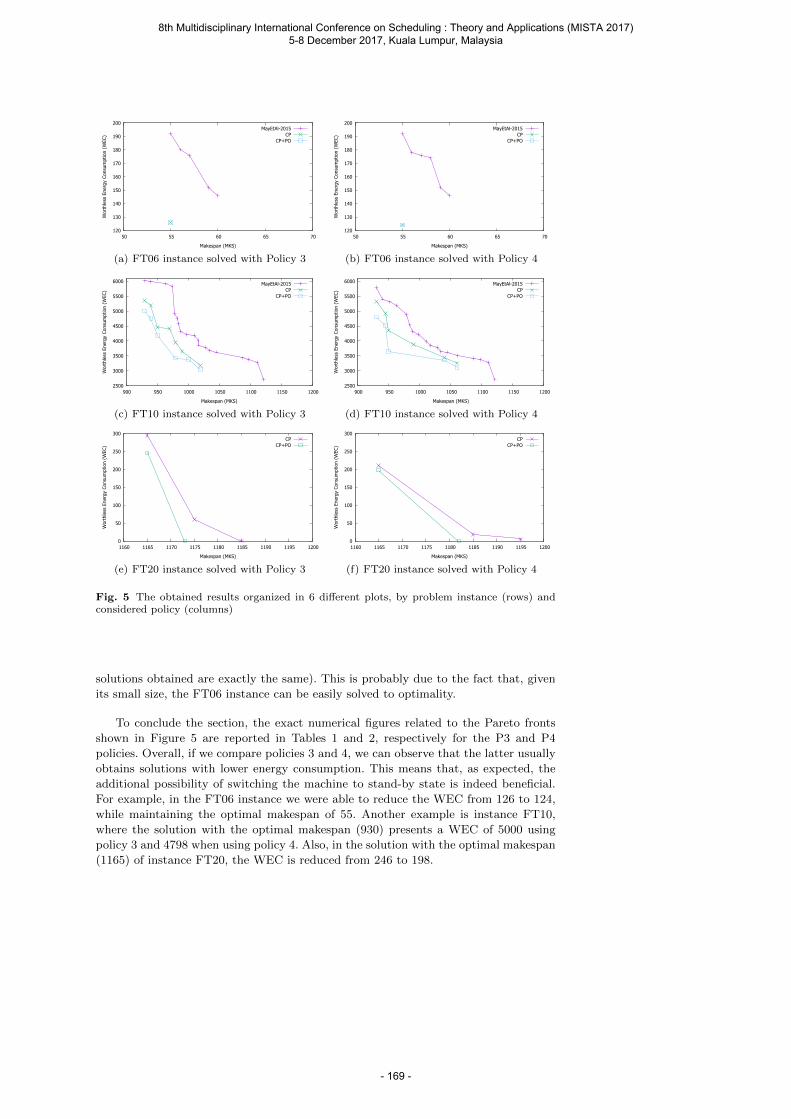
120

130

140

150

160

170

180

190

200

50 55 60 65 70

Wor

thle

ss E

nerg

y Co

nsum

ptio

n (W

EC)

Makespan (MKS)

MayEtAl-2015CP

CP+PO

(a) FT06 instance solved with Policy 3

120

130

140

150

160

170

180

190

200

50 55 60 65 70

Wor

thle

ss E

nerg

y Co

nsum

ptio

n (W

EC)

Makespan (MKS)

MayEtAl-2015CP

CP+PO

(b) FT06 instance solved with Policy 4

2500

3000

3500

4000

4500

5000

5500

6000

900 950 1000 1050 1100 1150 1200

Wor

thle

ss E

nerg

y Co

nsum

ptio

n (W

EC)

Makespan (MKS)

MayEtAl-2015CP

CP+PO

(c) FT10 instance solved with Policy 3

2500

3000

3500

4000

4500

5000

5500

6000

900 950 1000 1050 1100 1150 1200

Wor

thle

ss E

nerg

y Co

nsum

ptio

n (W

EC)

Makespan (MKS)

MayEtAl-2015CP

CP+PO

(d) FT10 instance solved with Policy 4

0

50

100

150

200

250

300

1160 1165 1170 1175 1180 1185 1190 1195 1200

Wor

thle

ss E

nerg

y Co

nsum

ptio

n (W

EC)

Makespan (MKS)

CPCP+PO

(e) FT20 instance solved with Policy 3

0

50

100

150

200

250

300

1160 1165 1170 1175 1180 1185 1190 1195 1200

Wor

thle

ss E

nerg

y Co

nsum

ptio

n (W

EC)

Makespan (MKS)

CPCP+PO

(f) FT20 instance solved with Policy 4

Fig. 5 The obtained results organized in 6 different plots, by problem instance (rows) andconsidered policy (columns)

solutions obtained are exactly the same). This is probably due to the fact that, given

its small size, the FT06 instance can be easily solved to optimality.

To conclude the section, the exact numerical figures related to the Pareto fronts

shown in Figure 5 are reported in Tables 1 and 2, respectively for the P3 and P4

policies. Overall, if we compare policies 3 and 4, we can observe that the latter usually

obtains solutions with lower energy consumption. This means that, as expected, the

additional possibility of switching the machine to stand-by state is indeed beneficial.

For example, in the FT06 instance we were able to reduce the WEC from 126 to 124,

while maintaining the optimal makespan of 55. Another example is instance FT10,

where the solution with the optimal makespan (930) presents a WEC of 5000 using

policy 3 and 4798 when using policy 4. Also, in the solution with the optimal makespan

(1165) of instance FT20, the WEC is reduced from 246 to 198.


- 169 -

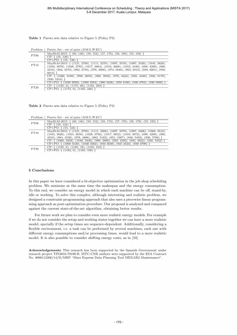
Table 1 Pareto sets data relative to Figure 5 (Policy P3)

Problem Pareto Set - set of pairs (MKS,WEC)

FT06MayEtAl-2015: (60, 146), (59, 152), (57, 176), (56, 180), (55, 192) CP: (55, 126) CP+PO: (55, 126)

FT10MayEtAl-2015: (1121, 2708), (1111, 3270), (1097, 3378), (1087, 3430), (1045, 3626),(1034, 3678), (1028, 3792), (1017, 3864), (1016, 4008), (1010, 4188), (998, 4208), (988,4310), (984, 4570), (982, 4758), (978, 4908), (974, 5840), (963, 5912), (939, 6001), (930,6013) CP: (1020, 3188), (990, 3658), (980, 3950), (970, 4424), (950, 4446), (940, 5178),(930, 5354) CP+PO: (1020 3038), (1000 3384), (980 3428), (950 4186), (940 4762), (930 5000)

FT20CP: (1185, 0), (1175, 60), (1165, 294) CP+PO: (1173, 0), (1165, 246)

Table 2 Pareto sets data relative to Figure 5 (Policy P4)

Problem Pareto Set - set of pairs (MKS,WEC)

FT06MayEtAl-2015: (60, 146), (59, 152), (58, 174), (57, 176), (56, 178), (55, 192) CP: (55, 124) CP+PO: (55, 124)

FT10MayEtAl-2015: (1121, 2708), (1111, 3268), (1097, 3378), (1087, 3406), (1060, 3512),(1045, 3626), (1034, 3658), (1028, 3792), (1017, 3852), (1010, 3972), (998, 4208), (988,4310), (984, 4538), (978, 4886), (963, 5182), (951, 5307), (940, 5402), (930, 5786) CP: (1060, 3258), (1040, 3440), (990, 3880), (950, 4356), (945, 4922), (930, 5332) CP+PO: (1060 3120), (1040 3362), (950 3638), (945 4524), (930 4798)

FT20CP: (1195, 6), (1185, 18), (1165, 210) CP+PO: (1182, 0), (1165, 198)

5 Conclusions

In this paper we have considered a bi-objective optimization in the job shop scheduling

problem. We minimise at the same time the makespan and the energy consumption.

To this end, we consider an energy model in which each machine can be off, stand-by,

idle or working. To solve this complex, although interesting and realistic problem, we

designed a constraint-programming approach that also uses a piecewise linear program-

ming approach as post-optimization procedure. Our proposal is analyzed and compared

against the current state-of-the-art algorithm, obtaining better results.

For future work we plan to consider even more realistic energy models. For example

if we do not consider the setup and working states together we can have a more realistic

model, specially if the setup times are sequence-dependent. Additionally, considering a

flexible environment, i.e. a task can be performed by several machines, each one with

different energy consumptions and/or processing times, would lead to a more realistic

model. It is also possible to consider shifting energy costs, as in [10].

Acknowledgements This research has been supported by the Spanish Government underresearch project TIN2016-79190-R. ISTC-CNR authors were supported by the ESA ContractNo. 4000112300/14/D/MRP “Mars Express Data Planning Tool MEXAR2 Maintenance”.


- 170 -

References

1. Adams J, Balas E, Zawack D (1988) The shifting bottleneck procedure for job shop

scheduling. Managament Science 34:391–401

2. Apt K (2003) Principles of Constraint Programming. Cambridge University Press,

New York, NY, USA

3. Baker K (1974) Introduction to Sequencing and Scheduling. Wiley

4. Beck JC, Feng T, Watson JP (2011) Combining constraint programming and local

search for job-shop scheduling. Informs Journal on Computing 23:1–14

5. Dai M, Tang D, Giret A, Salido MA, Li W (2013) Energy-efficient scheduling

for a flexible flow shop using an improved genetic-simulated annealing algorithm.

Robotics and Computer-Integrated Manufacturing 29:418–429

6. Fisher H, Thomson GL (1963) Probabilistic learning combinations of local job-shop

scheduling rules. In: Muth JF, Thomson GL (eds) Industrial Scheduling, Prentice

Hall, pp 225–251

7. Fourer R (1992) A simplex algorithm for piecewise-linear programming iii: Com-

putational analysis and applications. Mathematical Programming 53(1):213–235,

DOI 10.1007/BF01585703, URL https://doi.org/10.1007/BF01585703

8. Fourer R, Gay DM, Kernighan BW (2003) AMPL: A Modeling Language for Math-

ematical Programming. Duxbury-Thomson

9. Gonzalez MA, Oddi A, Rasconi R (2017) Multi-objective optimization in a job shop

with energy costs through hybrid evolutionary techniques. In: Proceedings of the

Twenty-Seventh International Conference on Automated Planning and Scheduling

(ICAPS-2017), AAAI Press, Pittsburgh, pp 140–148

10. Grimes D, Ifrim G, O’Sullivan B, Simonis H (2014) Analyzing the impact of elec-

tricity price forecasting on energy cost-aware scheduling. Sustainable Computing:

Informatics and Systems 4(4):276–291

11. Laborie P (2003) Algorithms for propagating resource constraints in AI planning

and scheduling: Existing approaches and new results. Artif Intell 143(2):151–188

12. Laumanns M, Thiele L, Zitzler E (2006) An efficient, adaptive parameter varia-

tion scheme for metaheuristics based on the epsilon-constraint method. European

Journal of Operational Research 169(3):932 – 942, DOI http://dx.doi.org/10.1016/

j.ejor.2004.08.029, URL http://www.sciencedirect.com/science/article/pii/

S0377221704005715

13. Le Pape C, Baptiste P, Nuijten W (2001) Constraint-Based Scheduling: Apply-

ing Constraint Programming to Scheduling Problems. Springer Science+Business

Media, New York, NY, USA

14. Liu Y, Dong H, Lohse N, Petrovic S, Gindy N (2014) An investigation into minimis-

ing total energy consumption and total weighted tardiness in job shops. Journal of

Cleaner Production 65:87–96

15. May G, Stahl B, Taisch M, Prabhu V (2015) Multi-objective genetic algorithm for

energy-efficient job shop scheduling. International Journal of Production Research

53(23):7071–7089

16. Miettinen K (2012) Nonlinear Multiobjective Optimization. International Series in

Operations Research & Management Science, Springer US, URL https://books.

google.it/books?id=bnzjBwAAQBAJ

17. Mouzon G, Yildirim MB, Twomey J (2007) Operational methods for minimiza-

tion of energy consumption of manufacturing equipment. International Journal of

Production Research 45(18–19):4247–4271


- 171 -

18. Nowicki E, Smutnicki C (2005) An advanced tabu search algorithm for the job

shop problem. Journal of Scheduling 8(2):145–159

19. Vilım P, Bartak R, Cepek O (2004) Unary resource constraint with optional ac-

tivities. In: Principles and Practice of Constraint Programming - CP 2004, 10th

International Conference, CP 2004, Toronto, Canada, September 27 - October 1,

2004, Proceedings, pp 62–76

20. Zhang R, Chiong R (2016) Solving the energy-efficient job shop scheduling prob-

lem: a multi-objective genetic algorithm with enhanced local search for minimizing

the total weighted tardiness and total energy consumption. Journal of Cleaner

Production 112:3361–3375


- 172 -

MISTA 2017

Towards improving tenders for Higher Education timetabling software

“Uncovering the selection criteria of HEIs when choosing timetabling

applications, using ERP as a reference”

Rudy Oude Vrielink • Erik Jansen • Ewout Gort • Jos van Hillegersberg • Erwin Hans

Abstract Higher Education Institutions (HEIs) are under constant competitive pressure,

resulting in the increased importance of achieving both efficiency and effectiveness in such

organizations. This intensifies the importance of selecting a suitable timetabling software

application, which can be considered to be at the heart of the organization, as it supports

organizing the primary process. The timetable software regulates the scheduling of teachers,

students and staff, and thus significantly impacts on their effectiveness and efficiency. The

selection of such an important application is an essential first step for managing and controlling

the schedules.


- 173 -

mailto:[email protected]





The contribution of this paper is threefold. First, we decide on a method for comparing

the criteria found in tenders to software selection theory. We select and analyze an existing

model for selecting ERP software from the literature. Second, we evaluate public tenders

submitted in several northwest European countries from 2003 to 2016 and demonstrate that HEIs

use a varied and incomplete set of tender criteria. Third, we apply the ERP software selection

model to the selection criteria of timetabling applications in HEIs. We present and discuss the

model as the approach for HEIs to select timetabling applications in a more structured and

consistent way, intended to lead ultimately to use resources more effectively and efficiently.

Keywords Higher education, timetabling, public tenders, selection criteria, ERP

1 Introduction

Timetabling applications are essential for HEIs to control the effective and efficient deployment

of teachers, staff and other resources (SURF, 2014), as HEIs are in a constant race to lower costs

while attracting more students at both the national and international levels (Jacob, 2015). This

results in an increasing demand for flexibility, meaning more student- or individual-centered

timetabling practices (Cook-Sather, Bovill, & Felten, 2014) (Oude Vrielink, Schepers, & Jansen,

2016). Selecting a suitable timetabling application that maximizes the efficiency and

effectiveness of a HEI is therefore critical.

Timetabling applications are concerned with “the allocation of resources to specific objects

being placed in space and time, in such a way as to satisfy as nearly as possible a set of desirable

objectives, subjected to constraints” (Wren, 1996). A timetable is not acceptable when any hard

constraint is violated, whereas it is considered feasible when no hard constraint, but only some

of the soft constraints are violated, which is usually the case. Timetabling tries to approximate

optimal solutions as it is an NP hard problem (Moura & Scaraficci, 2010) (Bettenelli, Cacchiani,

Roberti, & et al., 2015), meaning that for large instances only feasible rather than optimal

solutions can be found in limited time. Three categories of university timetabling can be

distinguished: Examination Timetabling, Post-Enrolment-Based Course Timetabling and

Curriculum-Based Course Timetabling (Second International Timetabling Competition, 2007)

(Di Gaspero, McCollum, & Schaerf, 2007). We consider software applications dealing with one

or more of these categories to be timetabling software applications.

HEIs regularly re-evaluate their current timetabling software and make a decision on

whether they should keep it as-is, modify it or replace it. A public tender must be issued when

the decision is made to acquire a new application and the value of the contract exceeds the

threshold that is laid down in EU regulations. This threshold was €209,000 in 2016 for the total

costs of purchase, implementation, maintenance and other additional costs, combined over a

time period of 5 years (Europa.eu, 2016). This means that HEIs will generally have to issue a

tender when acquiring new timetabling software. At the end of such a tender process, the contract

is awarded to the vendor who best meets the requirements set out in the tender.

This paper first surveys the literature on selecting timetabling software applications for HEIs.

Second, a suitable model is proposed incorporating criteria for selecting timetabling software

applications. For this purpose, we analysed ERP theory, as timetabling is considered to be a form

of an ERP process (Rabaa'i, Bandara, & Gable, 2009), and, where in contrast with timetabling

theory and practices, there is an extensive knowledge base. Third, this paper examines the

currently used selection criteria by HEIs in selecting timetabling software applications and

compares these criteria to the theoretical model. Finally, we demonstrate that the model is

applicable when combining the findings from literature and looking at practical relevance. We

propose that applying this specific ERP model in the selection process of timetabling

applications is a good step towards improving timetabling application selection and

consequently towards improving the competitiveness of the HEI as a whole. This results in the

following research question:


- 174 -

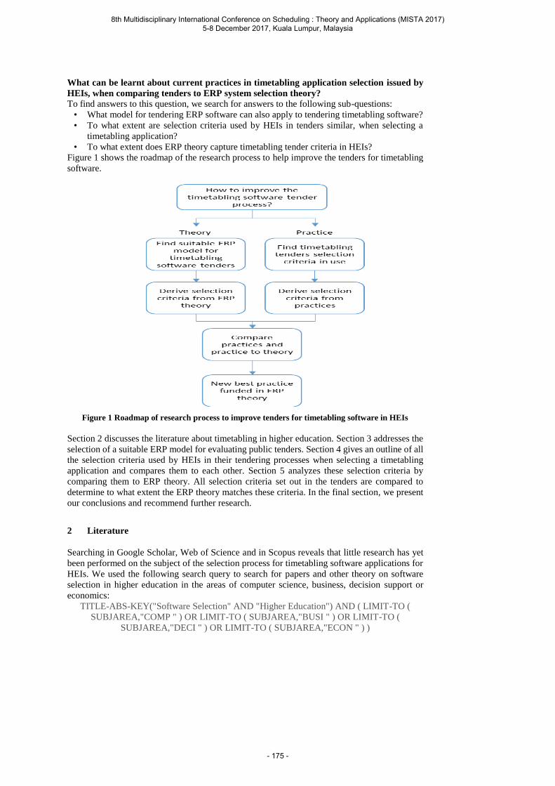
What can be learnt about current practices in timetabling application selection issued by

HEIs, when comparing tenders to ERP system selection theory? To find answers to this question, we search for answers to the following sub-questions:

• What model for tendering ERP software can also apply to tendering timetabling software?

• To what extent are selection criteria used by HEIs in tenders similar, when selecting a

timetabling application?

• To what extent does ERP theory capture timetabling tender criteria in HEIs?

Figure 1 shows the roadmap of the research process to help improve the tenders for timetabling

software.

Figure 1 Roadmap of research process to improve tenders for timetabling software in HEIs

Section 2 discusses the literature about timetabling in higher education. Section 3 addresses the

selection of a suitable ERP model for evaluating public tenders. Section 4 gives an outline of all

the selection criteria used by HEIs in their tendering processes when selecting a timetabling

application and compares them to each other. Section 5 analyzes these selection criteria by

comparing them to ERP theory. All selection criteria set out in the tenders are compared to

determine to what extent the ERP theory matches these criteria. In the final section, we present

our conclusions and recommend further research.

2 Literature

Searching in Google Scholar, Web of Science and in Scopus reveals that little research has yet

been performed on the subject of the selection process for timetabling software applications for

HEIs. We used the following search query to search for papers and other theory on software

selection in higher education in the areas of computer science, business, decision support or

economics:

TITLE-ABS-KEY("Software Selection" AND "Higher Education") AND ( LIMIT-TO (

SUBJAREA,"COMP " ) OR LIMIT-TO ( SUBJAREA,"BUSI " ) OR LIMIT-TO (

SUBJAREA,"DECI " ) OR LIMIT-TO ( SUBJAREA,"ECON " ) )


- 175 -

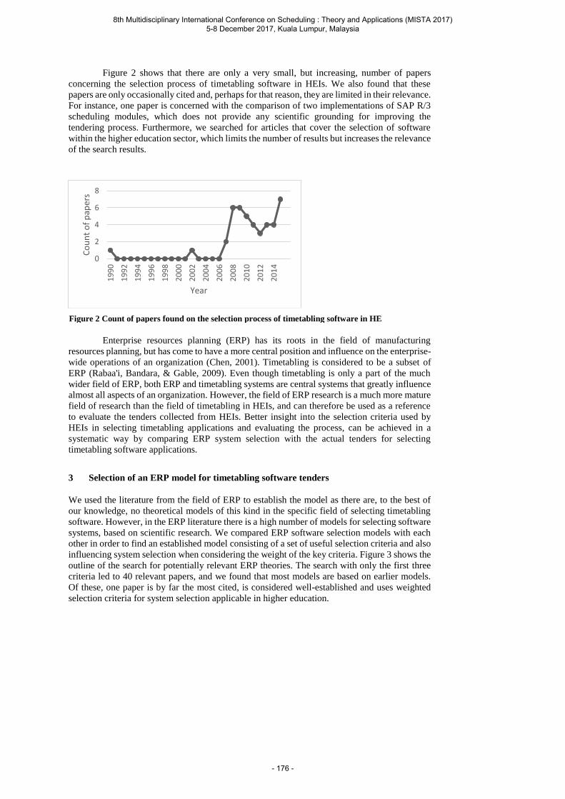
Figure 2 shows that there are only a very small, but increasing, number of papers

concerning the selection process of timetabling software in HEIs. We also found that these

papers are only occasionally cited and, perhaps for that reason, they are limited in their relevance.

For instance, one paper is concerned with the comparison of two implementations of SAP R/3

scheduling modules, which does not provide any scientific grounding for improving the

tendering process. Furthermore, we searched for articles that cover the selection of software

within the higher education sector, which limits the number of results but increases the relevance

of the search results.

Enterprise resources planning (ERP) has its roots in the field of manufacturing

resources planning, but has come to have a more central position and influence on the enterprise-

wide operations of an organization (Chen, 2001). Timetabling is considered to be a subset of

ERP (Rabaa'i, Bandara, & Gable, 2009). Even though timetabling is only a part of the much

wider field of ERP, both ERP and timetabling systems are central systems that greatly influence

almost all aspects of an organization. However, the field of ERP research is a much more mature

field of research than the field of timetabling in HEIs, and can therefore be used as a reference

to evaluate the tenders collected from HEIs. Better insight into the selection criteria used by

HEIs in selecting timetabling applications and evaluating the process, can be achieved in a

systematic way by comparing ERP system selection with the actual tenders for selecting

timetabling software applications.

3 Selection of an ERP model for timetabling software tenders

We used the literature from the field of ERP to establish the model as there are, to the best of

our knowledge, no theoretical models of this kind in the specific field of selecting timetabling

software. However, in the ERP literature there is a high number of models for selecting software

systems, based on scientific research. We compared ERP software selection models with each

other in order to find an established model consisting of a set of useful selection criteria and also

influencing system selection when considering the weight of the key criteria. Figure 3 shows the

outline of the search for potentially relevant ERP theories. The search with only the first three

criteria led to 40 relevant papers, and we found that most models are based on earlier models.

Of these, one paper is by far the most cited, is considered well-established and uses weighted

selection criteria for system selection applicable in higher education.

0

2

4

6

8

19

90

19

92

19

94

19

96

19

98

20

00

20

02

20

04

20

06

20

08

20

10

20

12

20

14

Co

un

t o

f p

aper

s

Year

Figure 2 Count of papers found on the selection process of timetabling software in HE


- 176 -

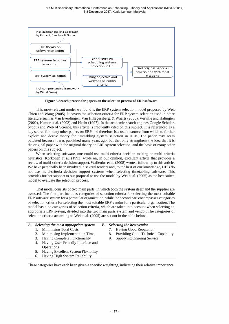
Figure 3 Search process for papers on the selection process of ERP software

This most-relevant model we found is the ERP system selection model proposed by Wei,

Chien and Wang (2005). It covers the selection criteria for ERP system selection used in other

literature such as Van Everdingen, Van Hillegersberg, & Waarts (2000), Verville and Halingten

(2002), Kumar et al. (2003) and Hecht (1997). In the academic search engines Google Scholar,

Scopus and Web of Science, this article is frequently cited on this subject. It is referenced as a

key source for many other papers on ERP and therefore is a useful source from which to further

explore and derive theory for timetabling system selection in HEIs. The paper may seem

outdated because it was published many years ago, but that only strengthens the idea that it is

the original paper with the original theory on ERP system selection, and the basis of many other

papers on this subject.

When selecting software, one could use multi-criteria decision making or multi-criteria

heuristics. Korkonen et al. (1992) wrote an, in our opinion, excellent article that provides a

review of multi-criteria decision support. Wallenius et al. (2008) wrote a follow-up to this article.

We have personally been involved in several tenders and, to the best of our knowledge, HEIs do

not use multi-criteria decision support systems when selecting timetabling software. This

provides further support to our proposal to use the model by Wei et al. (2005) as the best suited

model to evaluate the selection process.

That model consists of two main parts, in which both the system itself and the supplier are

assessed. The first part includes categories of selection criteria for selecting the most suitable

ERP software system for a particular organization, while the second part encompasses categories

of selection criteria for selecting the most suitable ERP vendor for a particular organization. The

model has nine categories of selection criteria, which are taken into account when selecting an

appropriate ERP system, divided into the two main parts system and vendor. The categories of

selection criteria according to Wei et al. (2005) are set out in the table below.

A. Selecting the most appropriate system B. Selecting the best vendor

1. Minimising Total Costs 7. Having Good Reputation

2. Minimising Implementation Time 8. Providing Good Technical Capability

3. Having Complete Functionality 9. Supplying Ongoing Service

4. Having User-Friendly Interface and

Operations

5. Having Excellent System Flexibility

6. Having High System Reliability

These categories have each been given a specific weighting, indicating their relative importance.


- 177 -

3.1 Most suitable system selection criteria

We first discuss the six categories for selecting the most suitable system.

3.1.1. Minimizing Total Costs

This category of selection criteria encompasses factors contributing to the costs of the system.

The model makes a distinction between (1) price, (2) maintenance costs, (3) infrastructure costs,

and (4) consulting expenses. We consider price to be the direct cost of gaining the right to use

the software. Maintenance costs are considered the costs brought about by repairs and fixes to

keep the system performing as expected, not to be confused with infrastructure costs which are

the costs of the support systems that enable the software to run. Consulting expenses are the

costs of consultancy, mainly during the implementation phase.

3.1.2. Minimizing Implementation Time

This category includes selection criteria concerned with the implementation time of the system.

It contains criteria related to the (1) planning and (2) implementation timeframe for the system

in the organization.

3.1.3. Having Complete Functionality

This category contains criteria contributing to ensuring complete functionality of the system.

The model makes a distinction between (1) module completeness, (2) function fitness, and (3)

security. Module completeness criteria ensure that the system contains all the modules the HEI

expects it to have. Function fitness ensures that the implementation fits within the current

timetabling process. For instance, the criterion that a system can import student data is therefore

a module completeness criterion, while the criterion that the system should be able to handle at

least 40,000 students is considered to be part of function fitness. The final subcategory of these

selection criteria, namely security, contains criteria which ensure the security of the data held

and produced in the system in terms of both unlawful external access and unlawful internal

access.

3.1.4. Having a User-Friendly Interface and Operations

This category of selection criteria encompasses factors contributing to the user-friendliness of

both the interface and the operations of the system. The model makes a distinction between (1)

ease of operation, and (2) ease of learning. Ease of operation means that operations within the

system can be done in a sufficiently easy and quick manner. Ease of learning means the effort

that users of the system -especially new users- have to put in to learn to use the system.

3.1.5. Having Excellent System Flexibility

This category encompasses all the selection criteria contributing to the flexibility of the system.

The model makes a distinction between (1) ease of integration, (2) upgrade ability and (3) ease

of in-house development. Ease of Integration concerns the connectivity of the system to other

systems already in place. Upgrade Ability deals with the ease of upgrading, such as the ability

to develop and implement upgrades. Ease of In-House development concerns the extent to which

the system can also be upgraded and adapted by the HEI itself.

3.1.6. Having High System Reliability

This category encompasses all the factors contributing to the reliability of the system. The model

makes a distinction between (1) stability, and (2) recovery ability. Stability concerns the

selection criteria ensuring that the system will not stop functioning when faced with unexpected

internal and external influences. This in contrast to recovery ability which concerns the criteria

that will ensure the system is able to recover back to a functioning state after it stopped

functioning.


- 178 -

3.2 Best vendor selection criteria

Next, we discuss the three categories of selection criteria that involve choosing the most

suitable vendor.

3.2.1. Having Good Reputation

This category of selection criteria encompasses all the factors contributing to the reputation of

the vendor. The model makes a distinction between (1) the scale of the vendor, (2) financial

condition, and (3) market share. Scale of vendor criteria are concerned with the size of the

vendor. Financial condition criteria are concerned with the financial standing of the vendor.

Market share criteria concern the number of other organizations using the system.

3.2.2. Technical Capability

This category encompasses all the factors contributing to the perceived technical capabilities of

the vendor. The model makes a distinction between (1) research and development ability, (2)

technical support capability, and (3) implementation ability. The ability of the vendor to research

and develop new technologies is classified as a Research and Development criterion. Technical

support capability criteria are concerned with the ability of the vendor to deal with technical

difficulties while implementation ability criteria are concerned with the ability of the vendor to

implement agreed and specified functionality.

3.2.3. Service

This category encompasses all the factors contributing to the vendor providing ongoing services.

The model makes a distinction between (1) warranties, (2) consultancy services, (3) training

services and (4) service speed. Warranty criteria are concerned with the warranties the vendor

provides in case the system or the implementation process do not meet the promised levels.

Consultancy services cover the criteria ensuring the number of consultants and experience of the

consultants working at the vendor. Criteria concerned with the amount of training time and the

quality of the trainings are bundled into training service criteria. Service speed is concerned with

the required response time of the various services.

4 Selection of tenders used in higher education

This section is concerned with the evaluation of the tenders and grouping the information in

these tenders to find out the selection criteria used in tenders for timetabling software in HE.

First, we searched for suitable tenders. Then, we listed all demands and requirements in these

tenders and grouped them. We searched for similarities and differences used in these actual

tenders from HEIs and compared them to the ERP model to find out to what extent tenders can

be improved by learning from each other and from theory. We considered tenders that comply

with the following three rules:

1. The tender is for a timetabling application (may also be termed a timetabling system)

2. To achieve comparability, the tender is issued by an HEI located in the North-West region

of Europe (i.e. Benelux, Scandinavia, Germany, UK and Ireland)

3. Not only the RFP, but also more explanation in accompanying tender documents are

available.

The tenders were gathered by searching the “online version of the 'Supplement to the Official

Journal' of the EU, dedicated to European public procurement” (TED, n.d.). The selection

criteria were then extracted from the tenders in order to be able to compare them to each other

and analyze them using the ERP selection model.


- 179 -

4.1 Analysis of the categorized selection criteria

The categorized selection criteria were analyzed to determine to what extent the requirements of

the actual tenders can be labelled employing the criteria of the ERP software selection model,

and, vice versa, to what extent the categories of the ERP software selection model can be found

in the tenders. To achieve this in both directions, means that we maximized the opportunities to

learn from both theory and practice. Possible categories presented in the tenders that are not

present in the ERP software selection model, were found by evaluating the newly created

category ‘Miscellaneous’, which contained selection criteria from tenders that could not

immediately be allocated to an existing category. In addition, the weight of the categories

relative to each other was analyzed and compared to those used in our ERP evaluation model.

5 Analysis of timetabling tenders

Eighteen tenders were collected for this research, from The Netherlands, Belgium, the United

Kingdom, Ireland and Norway, and which were published between 2003 and 2016. The process

of extracting the selection criteria from the tenders was difficult because of the very different

formats and structures of the tenders. It became apparent that they lack consistency and do not

use any kind of general framework.

Figure 4 Map of the origin and the number of tenders found on timetabling in HEIs

5.1 Cleaning the data

A first indicator for the quality of a tender is the number of categories of selection criteria it

addresses. Figure 5 shows how many tenders addressed how many categories. Of the tenders

evaluated, one outlier only addressed two categories. The remaining 17 tenders addressed on

average 7.4 of the 9 categories from the model, ranging from 5 up to the full 9 out of 9 categories.

The outlier is therefore eliminated from the dataset as we suspect there is incomplete

documentation. The remaining dataset consisting of 2,190 selection criteria was divided into the

9 different selection categories from the ERP model, and 46 selection criteria did not fit in any

of these categories and were thus classified as ‘Miscellaneous’. This accounts for an average of

132 selection criteria per tender for a total of 17 usable tenders.


- 180 -

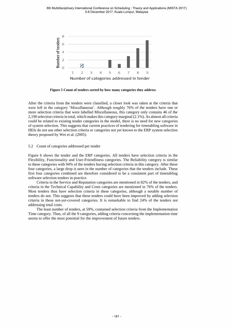
Figure 5 Count of tenders sorted by how many categories they address

After the criteria from the tenders were classified, a closer look was taken at the criteria that

were left in the category ‘Miscellaneous’. Although roughly 76% of the tenders have one or

more selection criteria that were labelled Miscellaneous, this category only contains 46 of the

2,190 selection criteria in total, which makes this category marginal (2.1%). As almost all criteria

could be related to existing tender categories in the model, there is no need for new categories

of system selection. This suggests that current practices of tendering for timetabling software in

HEIs do not use other selection criteria or categories not yet known to the ERP system selection

theory proposed by Wei et al. (2005).

5.2 Count of categories addressed per tender

Figure 6 shows the tender and the ERP categories. All tenders have selection criteria in the

Flexibility, Functionality and User-Friendliness categories. The Reliability category is similar

to these categories with 94% of the tenders having selection criteria in this category. After these

four categories, a large drop is seen in the number of categories that the tenders include. These

first four categories combined are therefore considered to be a consistent part of timetabling

software selection tenders in practice.

Criteria in the Service and Reputation categories are mentioned in 82% of the tenders, and

criteria in the Technical Capability and Costs categories are mentioned in 76% of the tenders.

Most tenders thus have selection criteria in these categories, although a notable number of

tenders do not. This suggests that these tenders could have been improved by adding selection

criteria in these not-yet-covered categories. It is remarkable to find 24% of the tenders not

addressing total costs.

The least number of tenders, at 59%, contained selection criteria from the Implementation

Time category. Thus, of all the 9 categories, adding criteria concerning the implementation time

seems to offer the most potential for the improvement of future tenders.


- 181 -

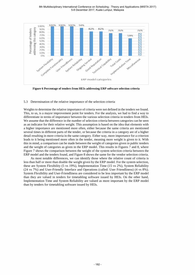
Figure 6 Percentage of tenders from HEIs addressing ERP software selection criteria

5.3 Determination of the relative importance of the selection criteria

Weights to determine the relative importance of criteria were not defined in the tenders we found.

This, to us, is a mayor improvement point for tenders. For the analysis, we had to find a way to

differentiate in terms of importance between the various selection criteria in tenders from HEIs.

We assume that the difference in the number of selection criteria between categories can be seen

as an indicator for their relative weight. This assumption is based on the idea that elements with

a higher importance are mentioned more often, either because the same criteria are mentioned

several times in different parts of the tender, or because the criteria in a category are of a higher

detail resulting in more criteria in the same category. Either way, more importance for a criterion

leads to it being mentioned more often in the tender, meaning more weight is given to it. With

this in mind, a comparison can be made between the weight of categories given in public tenders

and the weight of categories as given in the ERP model. This results in Figures 7 and 8, where

Figure 7 shows the comparison between the weight of the system selection criteria between the

ERP model and the tenders found, and Figure 8 shows the same for the vendor selection criteria.

As most notable differences, we can identify those where the relative count of criteria is

less than half or more than double the weight given by the ERP model. For the system selection,

these are System Flexibility (5 vs 19%), Implementation Time (15 vs 2%), System Reliability

(24 vs 7%) and User-Friendly Interface and Operations (called: User Friendliness) (4 vs 8%).

System Flexibility and User-Friendliness are considered to be less important by the ERP model

than they are valued in tenders for timetabling software issued by HEIs. On the other hand,

Implementation Time and System Reliability are valued as more important by the ERP model

than by tenders for timetabling software issued by HEIs.


- 182 -

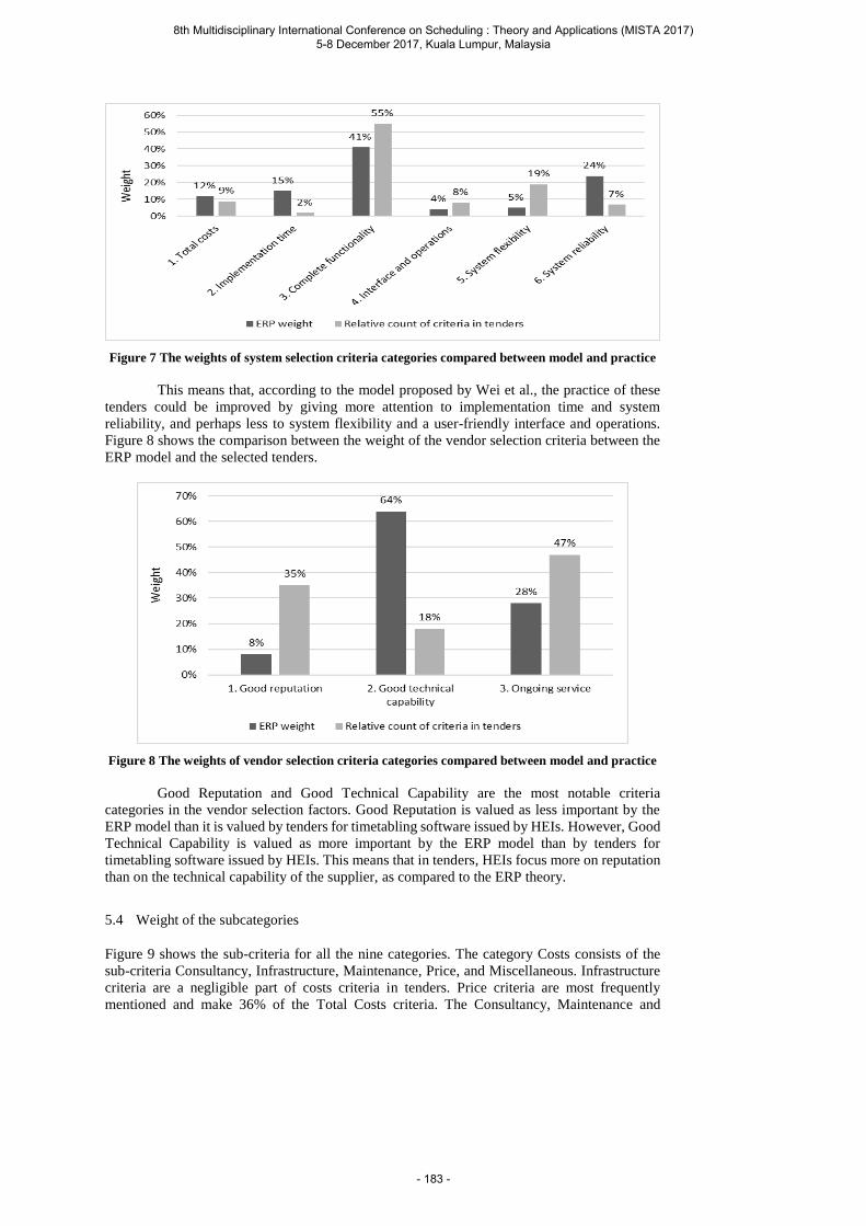
Figure 7 The weights of system selection criteria categories compared between model and practice

This means that, according to the model proposed by Wei et al., the practice of these

tenders could be improved by giving more attention to implementation time and system

reliability, and perhaps less to system flexibility and a user-friendly interface and operations.

Figure 8 shows the comparison between the weight of the vendor selection criteria between the

ERP model and the selected tenders.

Figure 8 The weights of vendor selection criteria categories compared between model and practice

Good Reputation and Good Technical Capability are the most notable criteria

categories in the vendor selection factors. Good Reputation is valued as less important by the

ERP model than it is valued by tenders for timetabling software issued by HEIs. However, Good

Technical Capability is valued as more important by the ERP model than by tenders for

timetabling software issued by HEIs. This means that in tenders, HEIs focus more on reputation

than on the technical capability of the supplier, as compared to the ERP theory.

5.4 Weight of the subcategories

Figure 9 shows the sub-criteria for all the nine categories. The category Costs consists of the

sub-criteria Consultancy, Infrastructure, Maintenance, Price, and Miscellaneous. Infrastructure

criteria are a negligible part of costs criteria in tenders. Price criteria are most frequently

mentioned and make 36% of the Total Costs criteria. The Consultancy, Maintenance and


- 183 -

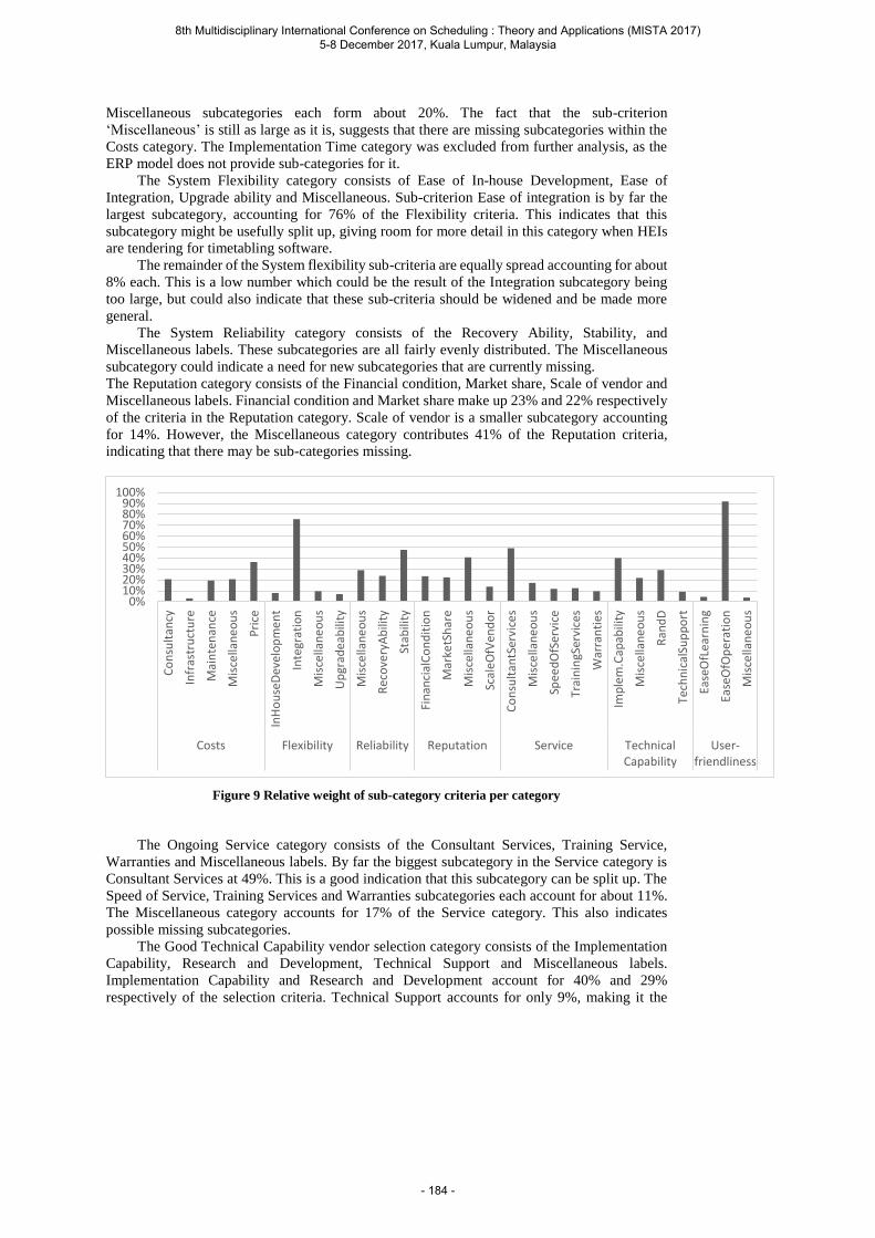
Miscellaneous subcategories each form about 20%. The fact that the sub-criterion

‘Miscellaneous’ is still as large as it is, suggests that there are missing subcategories within the

Costs category. The Implementation Time category was excluded from further analysis, as the

ERP model does not provide sub-categories for it.

The System Flexibility category consists of Ease of In-house Development, Ease of

Integration, Upgrade ability and Miscellaneous. Sub-criterion Ease of integration is by far the

largest subcategory, accounting for 76% of the Flexibility criteria. This indicates that this

subcategory might be usefully split up, giving room for more detail in this category when HEIs

are tendering for timetabling software.

The remainder of the System flexibility sub-criteria are equally spread accounting for about

8% each. This is a low number which could be the result of the Integration subcategory being

too large, but could also indicate that these sub-criteria should be widened and be made more

general.

The System Reliability category consists of the Recovery Ability, Stability, and

Miscellaneous labels. These subcategories are all fairly evenly distributed. The Miscellaneous

subcategory could indicate a need for new subcategories that are currently missing.

The Reputation category consists of the Financial condition, Market share, Scale of vendor and

Miscellaneous labels. Financial condition and Market share make up 23% and 22% respectively

of the criteria in the Reputation category. Scale of vendor is a smaller subcategory accounting

for 14%. However, the Miscellaneous category contributes 41% of the Reputation criteria,

indicating that there may be sub-categories missing.

Figure 9 Relative weight of sub-category criteria per category

The Ongoing Service category consists of the Consultant Services, Training Service,

Warranties and Miscellaneous labels. By far the biggest subcategory in the Service category is

Consultant Services at 49%. This is a good indication that this subcategory can be split up. The

Speed of Service, Training Services and Warranties subcategories each account for about 11%.

The Miscellaneous category accounts for 17% of the Service category. This also indicates

possible missing subcategories.

The Good Technical Capability vendor selection category consists of the Implementation

Capability, Research and Development, Technical Support and Miscellaneous labels.

Implementation Capability and Research and Development account for 40% and 29%

respectively of the selection criteria. Technical Support accounts for only 9%, making it the

0%10%20%30%40%50%60%70%80%90%

100%

Co

nsu

ltan

cy

Infr

astr

uct

ure

Mai

nte

nan

ce

Mis

cella

ne

ou

s

Pri

ce

InH

ou

seD

evel

op

me

nt

Inte

grat

ion

Mis

cella

ne

ou

s

Up

grad

eab

ility

Mis

cella

ne

ou

s

Rec

ove

ryA

bili

ty

Stab

ility

Fin

anci

alC

on

dit

ion

Mar

ketS

har

e

Mis

cella

ne

ou

s

Scal

eO

fVen

do

r

Co

nsu

ltan

tSer

vice

s

Mis

cella

ne

ou

s

Spee

dO

fSer

vice

Trai

nin

gSer

vice

s

War

ran

ties

Imp

lem

.Cap

abili

ty

Mis

cella

ne

ou

s

Ran

dD

Tech

nic

alSu

pp

ort

Ease

OfL

ear

nin

g

Ease

OfO

per

atio

n

Mis

cella

ne

ou

sCosts Flexibility Reliability Reputation Service Technical

CapabilityUser-

friendliness


- 184 -

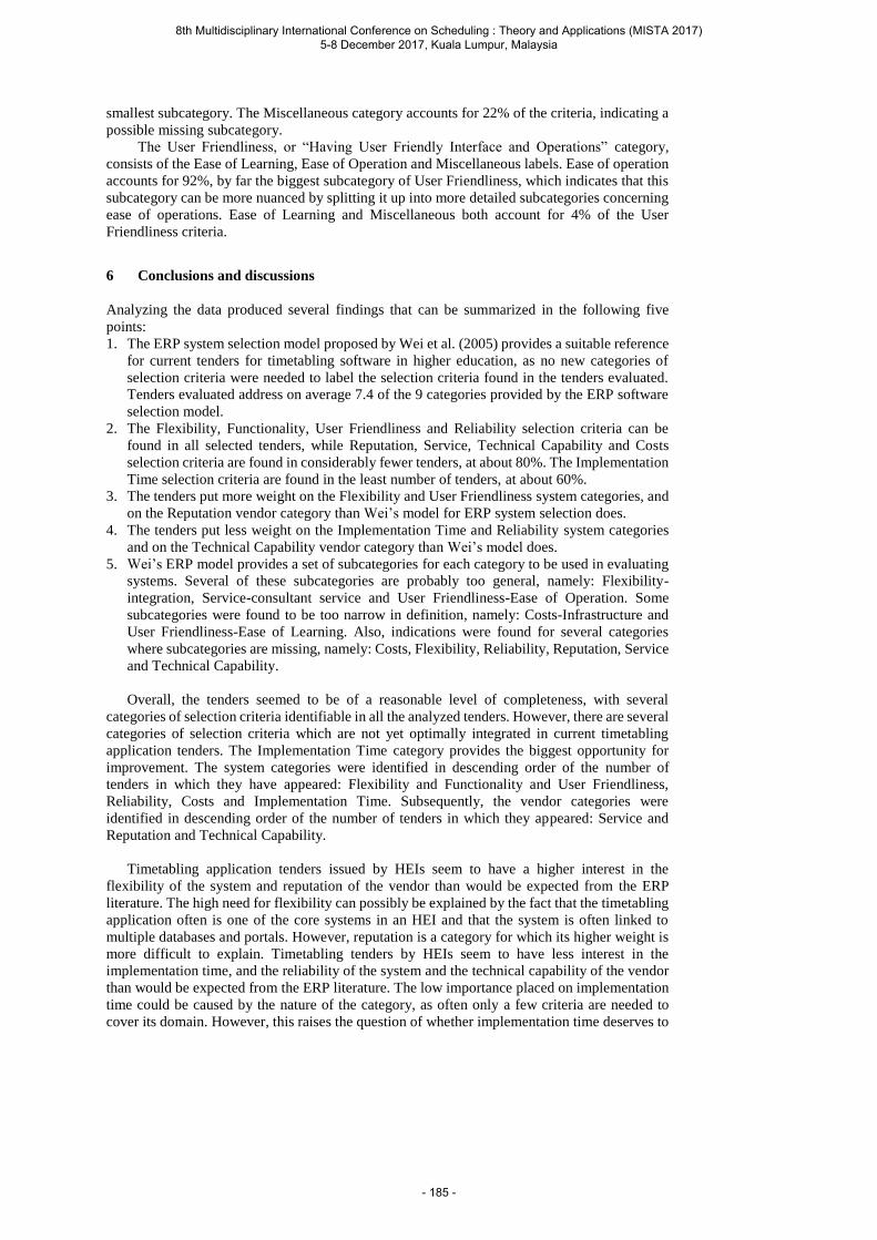
smallest subcategory. The Miscellaneous category accounts for 22% of the criteria, indicating a

possible missing subcategory.

The User Friendliness, or “Having User Friendly Interface and Operations” category,

consists of the Ease of Learning, Ease of Operation and Miscellaneous labels. Ease of operation

accounts for 92%, by far the biggest subcategory of User Friendliness, which indicates that this

subcategory can be more nuanced by splitting it up into more detailed subcategories concerning

ease of operations. Ease of Learning and Miscellaneous both account for 4% of the User

Friendliness criteria.

6 Conclusions and discussions

Analyzing the data produced several findings that can be summarized in the following five

points:

1. The ERP system selection model proposed by Wei et al. (2005) provides a suitable reference

for current tenders for timetabling software in higher education, as no new categories of

selection criteria were needed to label the selection criteria found in the tenders evaluated.

Tenders evaluated address on average 7.4 of the 9 categories provided by the ERP software

selection model.

2. The Flexibility, Functionality, User Friendliness and Reliability selection criteria can be

found in all selected tenders, while Reputation, Service, Technical Capability and Costs

selection criteria are found in considerably fewer tenders, at about 80%. The Implementation

Time selection criteria are found in the least number of tenders, at about 60%.

3. The tenders put more weight on the Flexibility and User Friendliness system categories, and

on the Reputation vendor category than Wei’s model for ERP system selection does.

4. The tenders put less weight on the Implementation Time and Reliability system categories

and on the Technical Capability vendor category than Wei’s model does.

5. Wei’s ERP model provides a set of subcategories for each category to be used in evaluating

systems. Several of these subcategories are probably too general, namely: Flexibility-

integration, Service-consultant service and User Friendliness-Ease of Operation. Some

subcategories were found to be too narrow in definition, namely: Costs-Infrastructure and

User Friendliness-Ease of Learning. Also, indications were found for several categories

where subcategories are missing, namely: Costs, Flexibility, Reliability, Reputation, Service

and Technical Capability.

Overall, the tenders seemed to be of a reasonable level of completeness, with several

categories of selection criteria identifiable in all the analyzed tenders. However, there are several

categories of selection criteria which are not yet optimally integrated in current timetabling

application tenders. The Implementation Time category provides the biggest opportunity for

improvement. The system categories were identified in descending order of the number of

tenders in which they have appeared: Flexibility and Functionality and User Friendliness,

Reliability, Costs and Implementation Time. Subsequently, the vendor categories were

identified in descending order of the number of tenders in which they appeared: Service and

Reputation and Technical Capability.

Timetabling application tenders issued by HEIs seem to have a higher interest in the

flexibility of the system and reputation of the vendor than would be expected from the ERP

literature. The high need for flexibility can possibly be explained by the fact that the timetabling

application often is one of the core systems in an HEI and that the system is often linked to

multiple databases and portals. However, reputation is a category for which its higher weight is

more difficult to explain. Timetabling tenders by HEIs seem to have less interest in the

implementation time, and the reliability of the system and the technical capability of the vendor

than would be expected from the ERP literature. The low importance placed on implementation

time could be caused by the nature of the category, as often only a few criteria are needed to

cover its domain. However, this raises the question of whether implementation time deserves to


- 185 -

be a category on its own. The apparent low interest in reliability and technical capability of the

vendor is surprising, and cannot easily be explained. This probably indicates an opportunity for

the improvement of HEI timetabling application tenders.

This paper aimed to provide insight in the selection criteria used by HEIs to select

timetabling applications. This can be the first step in improving this selection process, leading

to a better understanding of ways to control effectiveness and efficiency in education. The paper

identified the various categories of selection criteria appearing in public tenders for timetabling

applications in HEIs located in North-Western Europe. This was done by comparing these

tenders with a well-established and well-regarded ERP software selection model. This paper also

provided some further insight into the relative weights given to the categories. Finally, a first

critical view of possible subcategories was made.

7 Further research

Possible additional subcategories were discussed in the conclusion and discussion. Further

labelling of the dataset could provide a more thorough insight in the subcategories specific to

tenders for timetabling application by HEIs. When comparing the tenders that were researched,

we found large differences between them. A generally accepted framework seems to be missing,

which would provide a great opportunity to increase the efficiency and effectiveness of the

timetabling application tender processes within HEIs. A framework encompassing all the

various aspects of the tendering processes, including the selection criteria, should be established.

The findings of this paper can be a good starting point for such a framework.

Further steps for future research would be first to collect more tenders from other countries

to facilitate a more accurate analysis. Second, tenders from other parts of the world, such as

North-America, Australia and New Zealand, would have to be looked at to see differences in

tendering between countries in different parts of the world. Third, a close look at which supplier

actually won which tender would be helpful for further analysis. Conclusions can be drawn from

the outcomes of the tendering process, and the contents and quality of winning tenders.

References

[1] SURF, “Onderwijslogistiekmodel. Beter communiceren door gemeenschappelijke taal.

(Education Logistics model. Better communication through common language.),” SIG

Education Logistics, Utrecht (2014).

[2] W. J. Jacob, “Globalization and higher education policy reform,” in Second International

Handbook on Globalisation, Education and Policy Research, Springer Netherlands, pp.

151-165 (2015).

[3] A. Cook-Sather, C. Bovill and P. Felten, Engaging Students as Partners in Learning and

Teaching: A Guide for Faculty, John Wiley & Sons, Inc. (2014).

[4] A. Wren, “Scheduling, timetabling and rostering - a special relationship?,” in Practice

and theory of automated timetabling, Heidelberg (1996).


- 186 -

[5] A. Moura and R. Scaraficci, “A GRASP strategy for a more constrained School

Timetabling Problem,” International Journal of Operational Research, vol. 7, no. 2, pp.

152-170 (2010).

[6] A. Bettenelli, V. Cacchiani, R. Roberti and et al., “Rejoinder on: an overview of

curriculum-based course timetabling,” TOP, vol. 23, no. 2, pp. 366-368 (2015).

[7] Second International Timetabling Competition, “organised by the European

Metaheuristics Network,” [Online]. Available: http://www.cs.qub.ac.uk/itc2007/ (2007).

[8] L. Di Gaspero, B. McCollum and A. Schaerf, “The second international timetabling

competetion (ITC-2007): Curriculum-based course timetabling (track 3),” in Technical

Report QUB/IEEE/Tech/ITC2007/CurriculumCTT/v1. 0, Belfast, United Kingdom

(2007).

[9] Europa.eu, “Rules and procedures in public tendering across Europe,” [Online].

Available: http://europa.eu/youreurope/business/public-tenders/rules-procedures/ (2016).

[10] A. A. Rabaa'i, W. Bandara and G. Gable, “ERP systems in the higher education sector: a

descriptive study,” in Proceedings of the 20th Australasian Conference on Information

Systems, Melbourne, Caulfield Campus (2009).

[11] I. Chen, “Planning for ERP systems: analysis and future trend,” Business process

management journal, vol. 7, no. 5, pp. 374-386 (2001).

[12] B. Hecht, “Choose the right ERP software - ERP vendor selection can be filled with

vendor hype, internal political agendas, and unmet expectations,” Datamination, vol. 43,

no. 3, pp. 56-61 (1997).

[13] P. Korhonen, H. Moskowitz and J. Wallenius, “Multiple criteria decision support - A

review,” European Journal of Operation Research, vol. 63, no. 3, pp. 361-375 (1992).

[14] C. Wei, C. Chien and M. Wang, "An AHP-based approach to ERP system selection,"

International journal of production economics, vol. 96, no. 1, pp. 47-62 (2005).

[15] Y. Everdingen, van, J. Hillegersberg, van and E. Waarts, “Enterprise resource planning:

ERP adoption by European midsize companies,” Communications of the ACM, vol. 43,

no. 4, pp. 27-31 (2000).

[16] J. Wallenius, J. Dyer, P. Fishburn, R. Steuer, S. Zionts and K. Deb, "Multiple criteria

decision making, multivariate utility theory: Recent accomplishments and what lies

ahead," Management Science, vol. 54, no. 7, pp. 1336-1349 (2008).

[17] J. Verville and A. Halingten, “An investigation of the decision process for selecting an

ERP software: The case of ESC,” Management Decision, vol. 40, no. 3, pp. 206-216

(2002).


- 187 -

[18] V. Kumar, B. Maheswari and U. Kumar, “An investigation of critical management

issues in ERP implementation: emperical evidence from Canadian organizations,”

Technovation, vol. 23, no. 10, pp. 793-807 (2003).

[19] R. A. Oude Vrielink, D. Schepers and E. A. Jansen, “Practices in Timetabling in Higher

Education Institutions: a systematic review,” in Proceedings of the 11th international

conference on the Practice and Theory of Automated Timetabling, Udine (2016).

[20] TED, “Tenders Electronic Daily,” [Online]. Available:

http://ted.europa.eu/TED/misc/aboutTed.do (n.d.).


- 188 -

MISTA 2017

Scheduling Models for Multi-Agent Path Finding

Roman Bartak · Jirı Svancara · Marek Vlk

Abstract Multi-agent path finding (MAPF) deals with the problem of finding a colli-

sion free path for a set of agents. The agents are located at nodes of a directed graph,

they can move over the arcs, and each agent has its own destination node. It is not

possible for two agents to be at the same node at the same time. This paper suggests

to model the MAPF problem using scheduling techniques, namely, nodes are seen as

unary resources. We present three models of the problem. One model is motivated by

network flows, another model uses classical unary resource constraints together with

path constraints, and the last model works with optional activities. We compare the

efficiency of models experimentally.

1 Introduction

There exist numerous practical situations, where a set of agents is moving in a shared

environment, each agent having its own destination. For example, traffic junctions and

large warehouses are typical examples of congested environments, where agents are

moving between locations while sharing paths. In the era of autonomous systems, it is

important to have efficient solutions for coordinating such agents.

The above problem is known as multi-agent path finding (MAPF) or cooperative

path finding (CPF) [8]. The problem can be formalized as a (directed) graph, where

agents are initially distributed at some nodes, each agent having a destination node

to reach, and the task is to find a plan of movements for each agent to reach the

destination node while not being at the same node as another agent at the same time.

A frequent abstraction assumes that agents are moving synchronously and distances

between the nodes are identical. Then, at each time step, each agent either moves to a

neighboring node or stays in the current node. Grid worlds (such as the famous Lloyd

15-puzzle) are satisfying this assumption. This model makes it natural to use solving

techniques based on Boolean satisfiability or state-space search, which are currently

two leading approaches to solve MAPF. On the other hand, such an abstraction might

Roman Bartak, Jirı Svancara, Marek VlkCharles University, Faculty of Mathematics and Physics, Prague, Czech RepublicE-mail: [email protected]


- 189 -

be too restrictive as distances between the nodes might be important (and different)

in some practical applications.

In this paper, we suggest models of MAPF that borrow ideas from scheduling and

routing problems. We see the nodes (and possibly also the arcs) as resources with

limited capacity, which is one in this particular setting but could be larger in future

applications. We model the movements of agents using various techniques, namely

as network flows, as paths, and as optional activities. The motivation is supporting

richer (in comparison to traditional MAPF) temporal and capacity constraints, which

makes the models closer to reality. On the other side, there is one extra restriction

of our current models with respect to traditional MAPF formulation - the models are

designed such that no agent visits the same node more than once.

2 Background on Multi-Agent Path Finding

The MAPF problem is formulated by a graph and a set of packages (agents) sitting at

certain nodes. The task is to transport packages to their destination nodes – each pack-

age moves itself – while satisfying some capacity constraints, namely no two packages

meet at the same node at the same time. The difference from usual MAPF definition

is that in the rest of the paper, we will also assume that no package enters any node

more than once.

Let G = (V,E,w) be a directed arc-weighted graph and P be a set of packages.

The weight w(a) indicates the duration of moving a package over the arc a. In many

MAPF formulations, this duration is expected to be one. For each package p we denote

orig(p) ∈ V the original location (node) of the package and dest(p) ∈ V its destination

node. Let InArcs(x ) be the set of incoming arcs to x and OutArcs(x ) be the set of

outgoing arcs from x. Formally,

InArcs(x ) = (y , x ) | (y , x ) ∈ E,OutArcs(x ) = (x , y) | (x , y) ∈ E

The solution for MAPF problem as described above is a sequence of positions in

time for each package that satisfies the condition that no two packages are at the same

node at the same time. In this paper, we will focus on solutions that are makespan

optimal – the total time until the last package reaches its destination is minimized.

The classical MAPF is usually solved by algorithms that can be divided into two

categories:

1. Reduction based solvers. Many solvers reduce MAPF to another known problem

such as SAT [10], inductive logic programming [12] and answer set programming

[3]. These approaches are based on fast solvers that work very well with unit cost

parameters.

2. Search-based solvers. On the other hand, many recent solvers are search-based.

Some are variants of A* over a global search space – all possibilities how to place

agents into the nodes of the graph [9]. Other make use of novel search trees [7,2,

6].


- 190 -

3 Flow Model

The Flow model is motivated by the model for the closely related problem of multiple-

origin multiple-destination problem [1]. The model consists of two parts, a logical one

and a numerical one. The logical part describes a valid path for each package using the

idea of network flows. The numerical part describes temporal and resource constraints,

namely that paths for different packages do not overlap in time and space.

3.1 The Logical Part (Modeling Paths)

For each package p ∈ P and for each arc a ∈ E we introduce a Boolean decision variable

Used [a, p] that indicates whether or not arc a is used to transport package p. For each

package p ∈ P and for each vertex x ∈ V a Boolean variable Flow [x , p] indicates

whether or not the transport of package p goes through the vertex x.

To model a transport path for a package we specify the flow preservation con-

straints. These constraints describe that each package must leave its origin and must

arrive at its destination, and if the package goes through some vertex then it must en-

ter the vertex and leave it (both exactly once). In the case of origin, the package only

leaves it and, similarly, in the case of destination, the package only enters it. Formally,

for each package p ∈ P we introduce the following flow preservation constraints (recall

that domains of all the variables are Boolean, that is, 0, 1):

∀a ∈ InArcs(orig(p)) : Used [a, p] = 0 (1)

∀a ∈ OutArcs(dest(p)) : Used [a, p] = 0 (2)

Flow [orig(p), p] = 1 (3)

Flow [dest(p), p] = 1 (4)

∀x ∈ V \ orig(p) :∑

a∈InArcs(x)

Used [a, p] = Flow [x , p] (5)

∀x ∈ V \ dest(p) :∑

a∈OutArcs(x)

Used [a, p] = Flow [x , p] (6)

3.2 The Numerical Part (Modeling Nodes as Resources)

The numerical part specifies non-overlapping constraints, namely two packages do not

meet at the same node at the same time, and travel time between the nodes that is

expressed by weights of arcs. To model the time interval when a package p ∈ P stays in

a node x ∈ V , we introduce two numerical variables InT [x, p] and OutT [x, p] modeling

the time when the package enters the node and when it leaves the node respectively.

We can describe the travel time of package p between the nodes x and y through the

arc a as follows:

Used [a, p]⇒ OutT [x , p] + w(a) = InT [y , p]. (7)

If the package p is going through the node x then the package cannot enter the node

before it leaves it:

InT [x , p] ≤ OutT [x , p]. (8)


- 191 -

Let sp(x, y) be the length of the shortest path from node x to node y. Then we can

calculate bounds of the time variables as follows:

∀x ∈ V \ orig(p) : Flow [x , p]⇒ OutT [orig(p), p] + sp(orig(p), x ) ≤ InT [x , p] (9)

∀x ∈ V \ dest(p) : Flow [x , p]⇒ OutT [x , p] + sp(x , dest(p)) ≤ InT [dest(p), p] (10)

Let MKSP be the time when each package must be in its destination - it corresponds

to makespan of the schedule. Then we set the times in package’s origin and destination

as follows:

InT [orig(p), p] = 0 (11)

OutT [dest(p), p] = MKSP (12)

Finally, to model that two packages p1 and p2 do not meet at the same node x, we

need to specify that their times of visit do not overlap:

(Flow [x , p1 ] ∧ Flow [x , p2 ])⇒ (OutT [x , p1 ] < InT [x , p2 ] ∨OutT [x , p2 ] < InT [x , p1 ])

(13)

3.3 Model Soundness

It is easy to prove that the Flow model is sound, that is, every consistent instantiation

of variables defines a solution to the MAPF problem. The constraints (1)-(6) define a

single path from origin to destination for each package, i.e., the variables Flow and Used

are equal to one for nodes and arcs used on the path and equal to zero for all other nodes

and arcs. The origin and destination must be on the path due to constraints (3) and

(4). The path must continue from origin due to (6) and must reach the destination due

to (5). The path cannot start and cannot finish in any other node due to constraints

(5) and (6). The flow constraints allow a loop to be formed in the graph, but such

loops are forbidden by temporal constraints (7) and (8). Each package starts its tour

at time zero (11) and finishes at time MKSP (12) and two packages cannot meet at the

same node at the same time due to constraint (13). Hence each solution to the above

constraint satisfaction problem defines conflict free paths for all packages.

4 Path Model

The disjunctive non-overlap constraint (13) from the Flow model is a classical expres-

sion of a unary (disjunctive) resource. In constraint programming, these disjunctive

constraints are known to propagate badly and special global constraints modeling re-

sources have been proposed [11]. Hence it seems natural to exploit such constraints in

a model, where the presence of a package at a node is modeled as an activity. These

activities must be connected via temporal constraint to define a path from origin to

destination.

Formally, for each package p ∈ P and each node x ∈ V , we introduce an ac-

tivity N [x, p] describing time that the package p spends in the node x. We denote

StartOf(N [x, p]) the start time of the activity - it corresponds to InT [x, p] in the

Flow model - and similarly EndOf(N [x, p]) denotes the end time of activity corre-

sponding to OutT [x, p] in the Flow model. The start time of activity corresponding to


- 192 -

the origin of the package is set to zero, while the end time of activity corresponding to

the destination of the package is set to MKSP , which is the makespan of the schedule:

StartOf (N [orig(p), p]) = 0 (14)

EndOf (N [dest(p), p]) = MKSP . (15)

4.1 The Path Part

To model the path from origin to destination, we will use a double-link model describing

predecessors and successors of activities. The real path will be completed to form a

loop by assuming that the origin directly follows the destination. The activities (nodes)

that are not used in the path will form self-loops (the node will be its own predecessor

and successor).

Formally, for each package p ∈ P and for each node x ∈ V we will use two variables

Prev[x, p] and Next[x, p] describing the predecessor and successor of node x on the

path of package p. The domain of the variable Prev[x, p] consists of all nodes y such

that (y, x) ∈ E plus the node x. Similarly, the domain of variable Next[x, p] consists

of nodes z such that (x, z) ∈ E plus the node x. To ensure that the variables are

instantiated consistently, we introduce the constraint:

Prev [x , p] = y ⇔ Next [y , p] = x . (16)

To close the loop, we will use the following constraints:

Prev [orig(p), p] = dest(p) (17)

Next [dest(p), p] = orig(p). (18)

It remains to connect information about the path with the activities over the path,

namely to properly connect times of the activities so they are ordered correctly in time.

This will be realized by the constraint:

EndOf (N [x , p]) + w(x ,Next [x , p]) = StartOf (N [Next [x , p], p]), (19)

where w(x, y) is the length of arc from x to y. We set

w(x, x) = −1 (20)

w(dest(p), orig(p)) = −MKSP . (21)

In order to prune the search space, we add for all x ∈ V \ orig(p) the following

constraints:

Next [x , p] 6= x ⇒ EndOf (N [orig(p), p]) + sp(orig(p), x ) ≤ StartOf (N [x , p]), (22)

and for all x ∈ V \ dest(p), we add:

Next [x , p] 6= x ⇒ EndOf (N [x , p]) + sp(x , dest(p)) ≤ StartOf (N [dest(p), p]). (23)


- 193 -

4.2 The Resource Part

For each node x ∈ V , we add the following constraint encoding that the visits of the

node x are not overlapping:

NoOverlap(⋃p∈P

N [x , p]). (24)

4.3 Model Soundness

Any solution to the Path constraint model defines a solution of the MAPF problem and

vice versa. For each package, each node (activity) has some predecessor and successor

and they are defined consistently thanks to constraint (16), i.e., if x is a predecessor

of y then y is the successor of x. It means that all nodes of the graph are covered by

loops. Moreover, the origin and destination nodes are part of the same loop due to

constraints (17) and (18). All other loops must be of length one due to constraints (19)

and (20). Note that durations of activities are only restricted to be positive numbers

and as regular arcs also have positive lengths, the only way to satisfy the constraints

(19) over the loop is to include an arc with a negative length. Only the arcs (x, x)

and (dest(p), orig(p)) have negative lengths as specified in constraints (20) and (21).

Finally, each path starts at time zero (14) and finishes at time MKSP (15) and no

two paths overlap at any node at any time due to constraint (24). Note that activities

that are not used at any path (they are part of loops of length one) are still allocated

to unary resource modeling the node. The duration of such activities is one due to

constraints (19) and (20). However, as their start and end times are not restricted by

bounds 0 and MKSP , such activities can be shifted to future (after MKSP).

5 Opt Model

The Path model uses classical activities. Some of them are used on the packages’ paths

from origins to destinations, while others are not necessary (those that are part of

loops of length one). These are dummy activities that are part of the model as we do

not know in advance which activities will be necessary (which nodes will be visited).

In scheduling there exists a concept of optional activities that is used to model exactly

the same problem. We will exploit optional activities in the Opt model. Now, unlike

in the Path model, we do not use variables Next and Prev in order to find the path,

but the succeeding and preceding nodes will be entailed by whether or not an activity

corresponding to the arc and the package is present. All the activities in this model

are optional.

Formally, for each package p ∈ P and each node x ∈ V , we introduce three optional

activities N [x, p], Nout [x, p], and N in [x, p]. As in the Path model, the activity N [x, p]

corresponds to the time of a package p spent at node x. The activities N in [x, p] and

Nout [x, p] describe the time spent in the incoming and outgoing arcs. Next, for each

package p ∈ P and each arc (x, y) ∈ E, we introduce an optional activity A[x, y, p].

Again, we use an integer variable MKSP to denote the end of schedule (makespan).


- 194 -

5.1 The Path Part

The idea is that the path of a package corresponds to the activities that are present

in the solution and that in turn correspond to the nodes and arcs in the path. In

the terminology of hierarchical scheduling, it can be conceived such that each activity

Nout [x, p] has the activities A[x, y, p] corresponding to the arcs outgoing from the node

x as its children, and symmetrically, N in [x, p] has the activities A[y, x, p] corresponding

to the arcs incoming to the node x as its children. Hence each activity A[x, y, p] has

two parents: Nout [x, p] and N in [y, p] as the arc (x, y) is an outgoing arc for node x

and an incoming arc for node y.

Formally, for each package p ∈ P , the following logical constraints are introduced:

PresenceOf (N [orig(p), p]) = 1 (25)

PresenceOf (N [dest(p), p]) = 1 (26)

PresenceOf (N in [orig(p), p]) = 0 (27)

PresenceOf (N out [dest(p), p]) = 0 (28)

∀x ∈ V \ orig(p) : PresenceOf (N [x , p])⇔ PresenceOf (N in [x , p]) (29)

∀x ∈ V \ dest(p) : PresenceOf (N [x , p])⇔ PresenceOf (N out [x , p]) (30)

∀x ∈ V \ orig(p) : Alternative(N in [x , p],⋃

(y,x)∈E

A[y , x , p]) (31)

∀x ∈ V \ dest(p) : Alternative(N out [x , p],⋃

(x ,y)∈E

A[x , y , p]) (32)

The constraint Alternative enforces that if the activity given as the first argument

is present, then exactly one activity from the set of activities given as the second

argument is present. In addition, it ensures that the start and end times of the present

activities are equivalent. Since this implication goes only in one direction, we have to

impose the following constraints in order to find the path:

∀(x , y) ∈ E : PresenceOf (A[x , y , p])⇒ PresenceOf (N in [y , p]) (33)

∀(x , y) ∈ E : PresenceOf (A[x , y , p])⇒ PresenceOf (N out [x , p]) (34)

The processing times of activities A[x, y, p] are fixed to the weights of the arcs w(x, y),

whereas the processing times of activities N , Nout , and N in are to be found. Thanks to

the Alternative constraints, the processing times of activities Nout and N in will span

over the child activity A that will be present, and for the rest, the following constraints

need to be added:

∀x ∈ V \ orig(p) : StartOf (N [x , p]) = EndOf (N in [x , p]) (35)

∀x ∈ V \ dest(p) : EndOf (N [x , p]) = StartOf (N out [x , p]) (36)

StartOf (N [orig(p), p]) = 0 (37)

EndOf (N [dest(p), p]) = MKSP (38)

Again, in order to prune the search space, we add the following constraints:

∀x ∈ V \ orig(p) : EndOf (N [orig(p), p]) + sp(orig(p), x ) ≤ StartOf (N [x , p]) (39)

∀x ∈ V \ dest(p) : EndOf (N [x , p]) + sp(x , dest(p)) ≤ StartOf (N [dest(p), p]) (40)


- 195 -

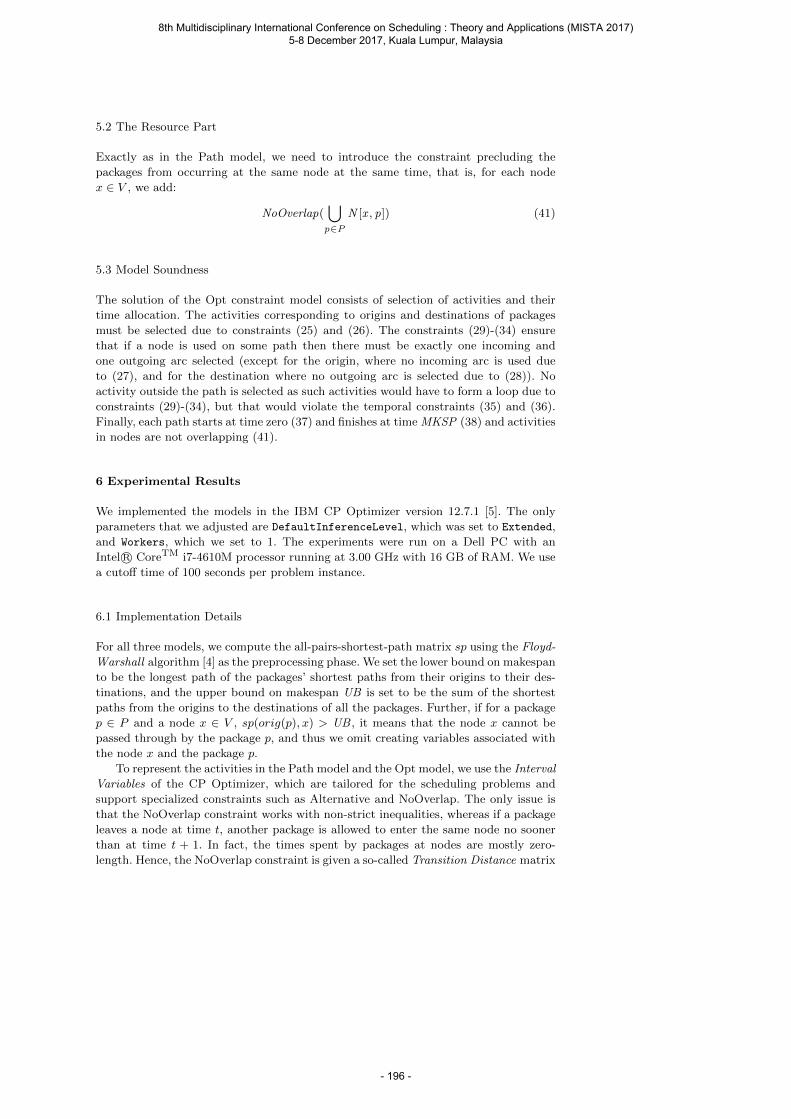
5.2 The Resource Part

Exactly as in the Path model, we need to introduce the constraint precluding the

packages from occurring at the same node at the same time, that is, for each node

x ∈ V , we add:

NoOverlap(⋃p∈P

N [x , p]) (41)

5.3 Model Soundness

The solution of the Opt constraint model consists of selection of activities and their

time allocation. The activities corresponding to origins and destinations of packages

must be selected due to constraints (25) and (26). The constraints (29)-(34) ensure

that if a node is used on some path then there must be exactly one incoming and

one outgoing arc selected (except for the origin, where no incoming arc is used due

to (27), and for the destination where no outgoing arc is selected due to (28)). No

activity outside the path is selected as such activities would have to form a loop due to

constraints (29)-(34), but that would violate the temporal constraints (35) and (36).

Finally, each path starts at time zero (37) and finishes at time MKSP (38) and activities

in nodes are not overlapping (41).

6 Experimental Results

We implemented the models in the IBM CP Optimizer version 12.7.1 [5]. The only

parameters that we adjusted are DefaultInferenceLevel, which was set to Extended,

and Workers, which we set to 1. The experiments were run on a Dell PC with an

Intel R© CoreTM i7-4610M processor running at 3.00 GHz with 16 GB of RAM. We use

a cutoff time of 100 seconds per problem instance.

6.1 Implementation Details

For all three models, we compute the all-pairs-shortest-path matrix sp using the Floyd-

Warshall algorithm [4] as the preprocessing phase. We set the lower bound on makespan

to be the longest path of the packages’ shortest paths from their origins to their des-

tinations, and the upper bound on makespan UB is set to be the sum of the shortest

paths from the origins to the destinations of all the packages. Further, if for a package

p ∈ P and a node x ∈ V , sp(orig(p), x) > UB , it means that the node x cannot be

passed through by the package p, and thus we omit creating variables associated with

the node x and the package p.

To represent the activities in the Path model and the Opt model, we use the Interval

Variables of the CP Optimizer, which are tailored for the scheduling problems and

support specialized constraints such as Alternative and NoOverlap. The only issue is

that the NoOverlap constraint works with non-strict inequalities, whereas if a package

leaves a node at time t, another package is allowed to enter the same node no sooner

than at time t + 1. In fact, the times spent by packages at nodes are mostly zero-

length. Hence, the NoOverlap constraint is given a so-called Transition Distance matrix


- 196 -

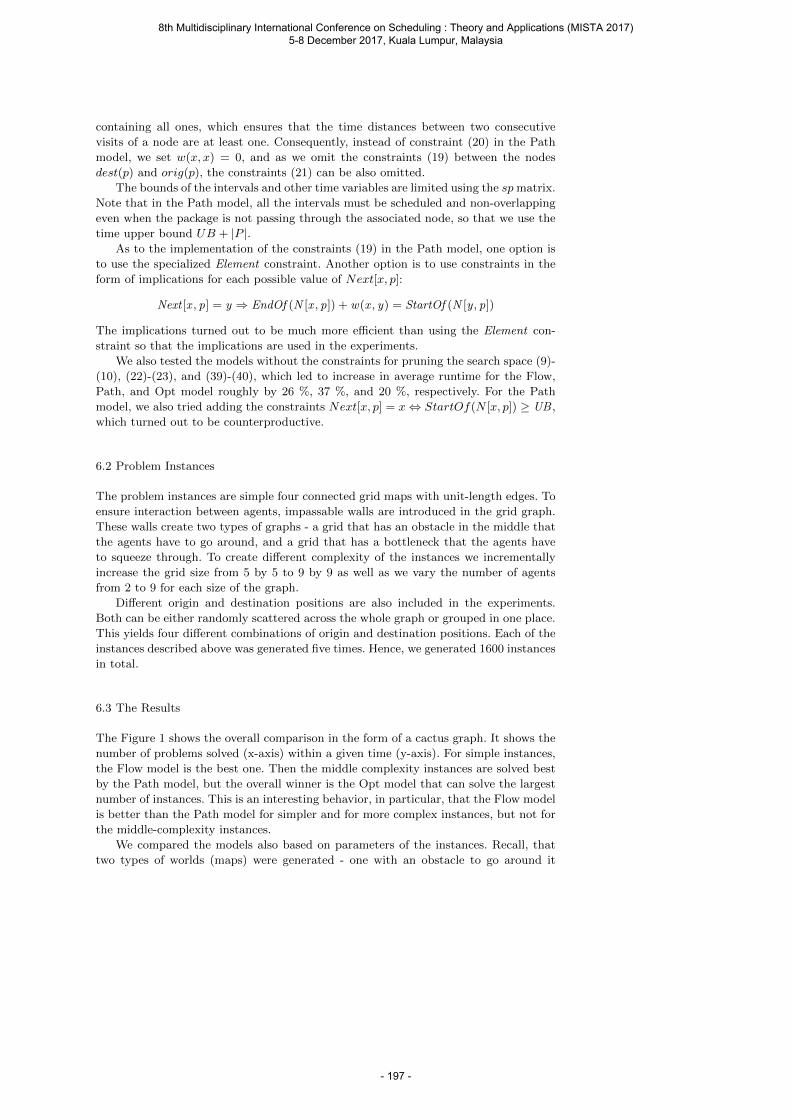
containing all ones, which ensures that the time distances between two consecutive

visits of a node are at least one. Consequently, instead of constraint (20) in the Path

model, we set w(x, x) = 0, and as we omit the constraints (19) between the nodes

dest(p) and orig(p), the constraints (21) can be also omitted.

The bounds of the intervals and other time variables are limited using the sp matrix.

Note that in the Path model, all the intervals must be scheduled and non-overlapping

even when the package is not passing through the associated node, so that we use the

time upper bound UB + |P |.As to the implementation of the constraints (19) in the Path model, one option is

to use the specialized Element constraint. Another option is to use constraints in the

form of implications for each possible value of Next[x, p]:

Next [x , p] = y ⇒ EndOf (N [x , p]) + w(x , y) = StartOf (N [y , p])

The implications turned out to be much more efficient than using the Element con-

straint so that the implications are used in the experiments.

We also tested the models without the constraints for pruning the search space (9)-

(10), (22)-(23), and (39)-(40), which led to increase in average runtime for the Flow,

Path, and Opt model roughly by 26 %, 37 %, and 20 %, respectively. For the Path

model, we also tried adding the constraints Next[x, p] = x⇔ StartOf(N [x, p]) ≥ UB ,

which turned out to be counterproductive.

6.2 Problem Instances

The problem instances are simple four connected grid maps with unit-length edges. To

ensure interaction between agents, impassable walls are introduced in the grid graph.

These walls create two types of graphs - a grid that has an obstacle in the middle that

the agents have to go around, and a grid that has a bottleneck that the agents have

to squeeze through. To create different complexity of the instances we incrementally

increase the grid size from 5 by 5 to 9 by 9 as well as we vary the number of agents

from 2 to 9 for each size of the graph.

Different origin and destination positions are also included in the experiments.

Both can be either randomly scattered across the whole graph or grouped in one place.

This yields four different combinations of origin and destination positions. Each of the

instances described above was generated five times. Hence, we generated 1600 instances

in total.

6.3 The Results

The Figure 1 shows the overall comparison in the form of a cactus graph. It shows the

number of problems solved (x-axis) within a given time (y-axis). For simple instances,

the Flow model is the best one. Then the middle complexity instances are solved best

by the Path model, but the overall winner is the Opt model that can solve the largest

number of instances. This is an interesting behavior, in particular, that the Flow model

is better than the Path model for simpler and for more complex instances, but not for

the middle-complexity instances.

We compared the models also based on parameters of the instances. Recall, that

two types of worlds (maps) were generated - one with an obstacle to go around it


- 197 -

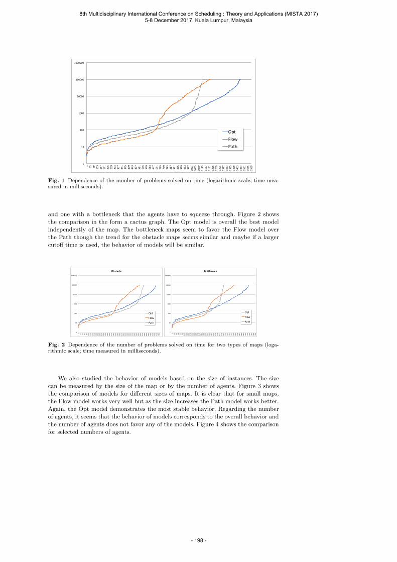
1

10

100

1000

10000

100000

1000000

1 35 69 103

137

171

205

239

273

307

341

375

409

443

477

511

545

579

613

647

681

715

749

783

817

851

885

919

953

987

1021

1055

1089

1123

1157

1191

1225

1259

1293

1327

1361

1395

1429

1463

1497

1531

1565

1599

OptFlowPath

Fig. 1 Dependence of the number of problems solved on time (logarithmic scale; time mea-sured in milliseconds).

and one with a bottleneck that the agents have to squeeze through. Figure 2 shows

the comparison in the form a cactus graph. The Opt model is overall the best model

independently of the map. The bottleneck maps seem to favor the Flow model over

the Path though the trend for the obstacle maps seems similar and maybe if a larger

cutoff time is used, the behavior of models will be similar.

1

10

100

1000

10000

100000

1000000

1 21 41 61 81 101

121

141

161

181

201

221

241

261

281

301

321

341

361

381

401

421

441

461

481

501

521

541

561

581

601

621

641

661

681

701

721

741

761

781

Obstacle

Opt

Flow

Path

1

10

100

1000

10000

100000

1000000

1 20 39 58 77 96 115

134

153

172

191

210

229

248

267

286

305

324

343

362

381

400

419

438

457

476

495

514

533

552

571

590

609

628

647

666

685

704

723

742

761

780

799

Bottleneck

Opt

Flow

Path

Fig. 2 Dependence of the number of problems solved on time for two types of maps (loga-rithmic scale; time measured in milliseconds).

We also studied the behavior of models based on the size of instances. The size

can be measured by the size of the map or by the number of agents. Figure 3 shows

the comparison of models for different sizes of maps. It is clear that for small maps,

the Flow model works very well but as the size increases the Path model works better.

Again, the Opt model demonstrates the most stable behavior. Regarding the number

of agents, it seems that the behavior of models corresponds to the overall behavior and

the number of agents does not favor any of the models. Figure 4 shows the comparison

for selected numbers of agents.


- 198 -

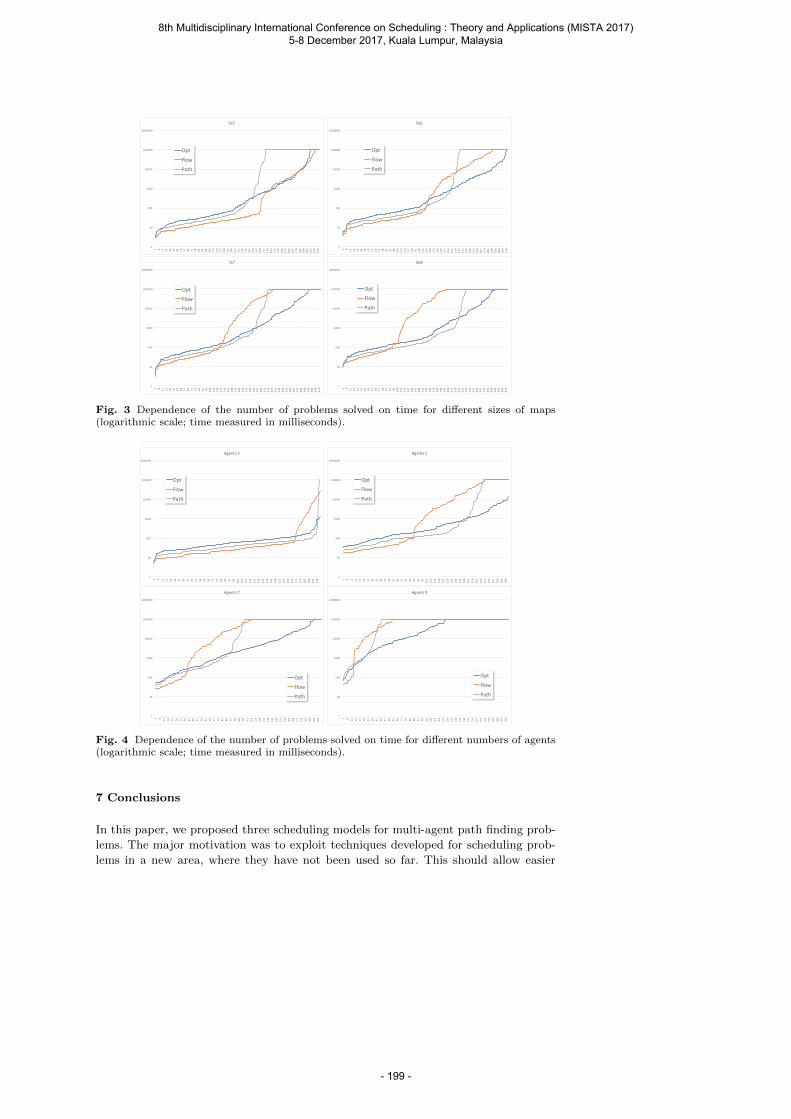
1

10

100

1000

10000

100000

1000000

1 8 15 22 29 36 43 50 57 64 71 78 85 92 99 106

113

120

127

134

141

148

155

162

169

176

183

190

197

204

211

218

225

232

239

246

253

260

267

274

281

288

295

302

309

316

5x5

Opt

Flow

Path

1

10

100

1000

10000

100000

1000000

1 8 15 22 29 36 43 50 57 64 71 78 85 92 99 106

113

120

127

134

141

148

155

162

169

176

183

190

197

204

211

218

225

232

239

246

253

260

267

274

281

288

295

302

309

316

6x6

Opt

Flow

Path

1

10

100

1000

10000

100000

1000000

1 8 15 22 29 36 43 50 57 64 71 78 85 92 99 106

113

120

127

134

141

148

155

162

169

176

183

190

197

204

211

218

225

232

239

246

253

260

267

274

281

288

295

302

309

316

7x7

Opt

Flow

Path

1

10

100

1000

10000

100000

1000000

1 8 15 22 29 36 43 50 57 64 71 78 85 92 99 106

113

120

127

134

141

148

155

162

169

176

183

190

197

204

211

218

225

232

239

246

253

260

267

274

281

288

295

302

309

316

8x8

Opt

Flow

Path

Fig. 3 Dependence of the number of problems solved on time for different sizes of maps(logarithmic scale; time measured in milliseconds).

1

10

100

1000

10000

100000

1000000

1 6 11 16 21 26 31 36 41 46 51 56 61 66 71 76 81 86 91 96 101

106

111

116

121

126

131

136

141

146

151

156

161

166

171

176

181

186

191

196

Agents3

Opt

Flow

Path

1

10

100

1000

10000

100000

1000000

1 6 11 16 21 26 31 36 41 46 51 56 61 66 71 76 81 86 91 96 101

106

111

116

121

126

131

136

141

146

151

156

161

166

171

176

181

186

191

196

Agents5

Opt

Flow

Path

1

10

100

1000

10000

100000

1000000

1 6 11 16 21 26 31 36 41 46 51 56 61 66 71 76 81 86 91 96 101

106

111

116

121

126

131

136

141

146

151

156

161

166

171

176

181

186

191

196

Agents7

Opt

Flow

Path

1

10

100

1000

10000

100000

1000000

1 6 11 16 21 26 31 36 41 46 51 56 61 66 71 76 81 86 91 96 101

106

111

116

121

126

131

136

141

146

151

156

161

166

171

176

181

186

191

196

Agents9

Opt

Flow

Path

Fig. 4 Dependence of the number of problems solved on time for different numbers of agents(logarithmic scale; time measured in milliseconds).

7 Conclusions

In this paper, we proposed three scheduling models for multi-agent path finding prob-

lems. The major motivation was to exploit techniques developed for scheduling prob-

lems in a new area, where they have not been used so far. This should allow easier


- 199 -

solving of more realistic problems with various resource and temporal constraints such

as non-uniform distances between the nodes and various capacities of nodes (and arcs).

The model with optional activities seems the most stable, in particular when the prob-

lems are becoming larger. There is an interesting behavior of the Flow model, which is

the best for small instances, then it is the worst model for middle-size instances, but

the runtime increase seems smaller for larger instances in comparison to other models.

This model is more influenced by the size of the graph than the other two models.

There is one significant restriction of the presented models - no agent (package)

can return to any node. A future research can study how to extend the models to allow

re-visits of the nodes, which is supported by existing solving approaches to MAPF.

Acknowledgements Research is supported by the Czech-Israeli Cooperative Scientific Re-search Project 8G15027, by the Czech Science Foundation under the project P202/12/G061,by SVV project number 260 453, and by the Charles University, project GA UK No. 158216.

References

1. Roman Bartak, Agostino Dovier, Neng-Fa Zhou, Multiple-Origin-Multiple-Destination PathFinding with Minimal Arc Usage: Complexity and Models. ICTAI 2016: 91-97 (2016)

2. Eli Boyarski, Ariel Felner, Roni Stern, Guni Sharon, David Tolpin, Oded Betzalel, SolomonEyal Shimony, ICBS: Improved Conflict-Based Search Algorithm for Multi-Agent Pathfind-ing. IJCAI (2015)

3. Esra Erdem, Doga Gizem Kisa, Umut Oztok, Peter Schuller, A General Formal Frameworkfor Pathfinding Problems with Multiple Agents. AAAI (2013)

4. Robert W. Floyd, Algorithm 97: shortest path, Communications of the ACM 5.6 (1962)5. Philippe Laborie, IBM ILOG CP Optimizer for detailed scheduling illustrated on three

problems, International Conference on AI and OR Techniques in Constraint Programmingfor Combinatorial Optimization Problems, Springer, Berlin, Heidelberg, 148-162 (2009)

6. Guni Sharon, Roni Stern, Meir Goldenberg, Ariel Felner, The increasing cost tree searchfor optimal multi-agent pathfinding. Artif. Intell. 195: 470-495 (2013)

7. Guni Sharon, Roni Stern, Ariel Felner, Nathan R. Sturtevant, Conflict-based search foroptimal multi-agent pathfinding. Artif. Intell. 219: 40-66 (2015)

8. David Silver, Cooperative Pathfinding. AIIDE 2005: 117-122 (2005)9. Trevor Scott Standley, Finding Optimal Solutions to Cooperative Pathfinding Problems.

AAAI (2010)10. Pavel Surynek, Towards optimal cooperative path planning in hard setups through satis-

fiability solving, PRICAI, 564576, (2012)11. Petr Vilım, Roman Bartak, Ondrej Cepek, Extension of O(n log n) filtering algorithms for

the unary resource constraint to optional activities, Constraints 10.4: 403-425, (2005)12. Ko-Hsin Cindy Wang, Adi Botea, MAPP: a Scalable Multi-Agent Path Planning Algo-

rithm with Tractability and Completeness Guarantees. J. Artif. Intell. Res. 42: 55-90 (2011)


- 200 -

Francisco Regis Abreu Gomes Graduate Program in Production Engineering, Federal University of Minas Gerais, Brazil and Federal

Institute of Education, Science and Technology of Ceará (IFCE), Brazil E-mail: [email protected]

Geraldo Robson Mateus Computer Science Department, Federal University of Minas Gerais (UFMG), Brazil E-mail: [email protected]

MISTA 2017

Mathematical Formulation for Minimizing Total Tardiness in a

Scheduling Problem with Parallel Machines

Francisco Regis Abreu Gomes • Geraldo Robson Mateus

Abstract This paper addresses the NP-hard parallel machine scheduling problem with

sequence and machine-dependent setup times for minimizing total tardiness. Mathematical

models for this problem often use a constant known as big-M on account of the disjunctive

constraints. This yields very weak lower bounds that make it difficult to obtain the optimal

solution, even for small-size instances. To address this problem, we propose a mathematical

formulation that does not use the big-M constant. To this end, we present an approach that uses

dummy jobs instead of the big-M constant. Additionally, an optimality condition method that

reduces the solution space of the problem is proposed. Experiments conducted on two instance

types produced computational proof of the superiority of the proposed model compared to

models based on Wagner’s (1959) and Manne’s (1960) formulations. The proposed model

produced 153 optimal solutions compared to 81 and 42 of Wagner’s and Manne’s models,

respectively, and it was up to three orders of magnitude faster in the 180 instances that were

tested.

1 Introduction

In today’s competitive business environment of manufacturing and services, efficient

scheduling is one of the most critical issues [1]. The parallel machine scheduling problem

(PMSP) is broadly applied in many manufacturing and service systems. Therefore, it has been

a subject of continuing interest for researchers and practitioners [2]. Many types of PMSPs

have been proposed in the literature. They can be classified into identical, uniform, and

unrelated parallel machine categories [3]. Of these types, the PMSP which includes the

machine and sequence-dependent setup times and total tardiness as criterion has received less

attention than other PMSPs [4]. However, with the adoption by companies of the just-in-time

philosophy, an increasing amount of research in the past two decades has involved tardiness

[5]. Nevertheless, tardiness is a difficult criterion with which to work, even in the single-

machine environment [6]. Applications of all PMSP types are common in many industries,


- 201 -

including painting, plastic, textile, glass, semiconductor, chemical, and paper manufacturing

[7].

Exact mathematical programming approaches for scheduling problems use two distinct

types of formulations [8]: (1) formulations whereby the job sequence is represented by binary

variables and completion times are denoted by continuous variables; and (2) time-indexed

formulations, whereby the completion time of each job is represented by binary variables

indexed over a discrete time horizon [9]. The formulations of type (2) are known to yield tight

linear relaxations; however, they cannot be directly applied to many instances on account of

their pseudo-polynomially large number of variables. The formulations of type (1) are compact

in that they involve a polynomial number of variables and constraints. On the other hand, they

yield poor linear relaxations. This is notoriously due to the big-M constant used to linearize the

disjunctive constraints [10]. The formulations of type (2), on the other hand, do not use this

constant.

Avalos-Rosales et al. [11] proposed several mixed integer formulations of type (1) for a

PMSP to minimize the makespan. These formulations outperform the previously published

formulations in terms of the instance size and computational time for reaching optimal

solutions. Using these models, it is possible to solve instances up to 60 jobs and five machines

that are six times larger than was previously solved. In addition, they enable attainment of

optimal solutions for instances of the same size up to four orders of magnitude faster. This is

only possible because those authors proposed an additional constraint to calculate the

makespan that does not use the big-M constant. We emphasize that these formulations still use

this constant in the disjunctive constraints. Unfortunately, these formulations thus cannot be

used when the criterion is the minimization of total tardiness once the new linearization applies

only to computing the makespan. To the best of our knowledge, it does not exist a formulation

of type (1) for PMSPs with tardiness as a criterion that does not use the big-M.

Inspired by the performance achieved by the formulation of Avalos-Rosales et al. [11],

we propose a mathematical formulation for the problem under study that does not use the big-

M constant. To this end, we employ dummy jobs instead of the big-M constant to linearize the

computation of the total tardiness of the jobs. We additionally propose an optimality condition

that reduces the solution space of the problem. Computational results showed that the proposed

model obtained tight linear relaxations, more optimal solutions, and smaller runtimes when

compared to models from the literature. These are the main contributions of this paper.

The remainder of this paper is organized as follows. Section 2 reviews the solution

approaches for PMSPs. Section 3 presents two mathematical models from the literature and a

new mathematical formulation is proposed. Section 4 describes the computational experiments

comparing the mathematical formulations from the literature, and the proposed formulation,

and the results are reported. In Section 5, the conclusions are presented.

2 Literature review

This section reviews the previous studies on applying PMSPs. Our review is restricted to

PMSPs with the due date and setup times because these features are considered in this paper.

For more details, on parallel machine scheduling problems considering due date as a criterion,

and setup time, see [12], [13], and [14].

Most previous studies have been conducted on identical or uniform PMSPs only with

sequence-dependent setup times. Lee and Pinedo [15] suggest a three-phase heuristic using the

apparent tardiness cost with setups (ATCS) rule, a dispatching rule, and a simulated annealing

algorithm for minimizing the sum of the weighted tardiness. For minimizing the total tardiness,

Park et al. [16] improve the dispatching rule using look-ahead parameters calculated by a

neural network. Bilge et al. [17] propose a tabu search approach, whereby the candidate list

strategies, tabu classifications, tabu tenures, and intensification/diversification strategies are

investigated. Anghinolfi and Paolucci [18] propose a hybrid metaheuristic that incorporates the


- 202 -

core features of simulated annealing, tabu search, and variable neighborhood search.

Armentano and de França Filho [19] propose GRASP (Greedy Randomized Adaptive Search

Procedure)-based search heuristics that incorporate adaptive memory principles.

For the unrelated PMSP with only sequence-dependent setup times, Kim et al. [20]

suggest a simulated annealing algorithm with various interchange and insertion methods for

minimizing the total tardiness. For minimizing the weighted number of tardy jobs, M’Hallah

and Bulfin [21] propose branch and bound algorithms, while Chen and Chen [22] propose

hybrid metaheuristics that integrate the tabu search and variable neighborhood descent

approach. In addition, Chen [23] presents several iterated hybrid metaheuristic algorithms,

while Zhu and Heady [24] propose a mixed integer programming model to minimize the sum

of earliness and tardiness penalties.

For the unrelated PMSP with the machine and sequence-dependent setup time, few

studies have been performed. For minimizing the total tardiness, Chen [25] considers the

problem with an additional strict due date constraint for some jobs. That author proposes a

simulated annealing algorithm that incorporates the feasibility improvement method. In

addition, Lin et al. [26] propose an iterated greedy algorithm and a simple dispatching rule,

which are respectively referred to as primary customers and the shortest completion time, to

generate the initial solution.

Meanwhile, Rocha et al. [27] propose a branch and bound algorithm and a GRASP

metaheuristic for minimizing the makespan added to the weighted tardiness. Paula et al. [28]

propose a non-delayed relax-and-cut algorithm based on a Lagrangian relaxation of a time-

indexed formulation to minimize the total weighted tardiness. For minimizing the total

earliness and tardiness penalties, Nogueira et al. [29] propose three different heuristics based

on the GRASP metaheuristic, and Zeidi and Hosseini [30] propose a genetic algorithm with a

simulated annealing method as a local search procedure to improve the solution quality.

3 Parallel machine scheduling problem for minimizing total tardiness

3.1 Problem description

The scheduling problem investigated in this study considers n independent jobs, J = 1, 2,

. . . , n, on m unrelated or uniform parallel machines, I = 1, 2, . . . , m. Each machine i I is

ready at time zero and can process all jobs. Each job j J is processed by exactly one of the

machines with processing times pij (i I), is available in time zero, and it has a due date dj. A

machine and sequence-dependent setup time, sijl, is incurred between two different jobs, j l. The machine setup can be started and completed during the idle time, as commonly assumed in

the literature [31]. All the parameters are deterministic non-negative integers. A job sequence

is a subset of J processed by a machine in a sequence, in which each job is non-preemptively

processed only once. Each job in a sequence has a completion time, Cj, and tardiness is defined

as Tj = max0, Cj – dj. The aim is to find the set of job sequences that processes all jobs and

minimizes their total tardiness. In the standard three-field notation, this problem is denoted as

R or Q/sijl/ΣTj. It is NP-hard because it is an extension of the NP-hard 1//ΣTj [32].

3.2 Wagner’s model

Rocha et al. [27] adapted for the parallel machine scheduling problem the models based

on sequence-position variables proposed by Wagner [33] and precedence variables proposed

by Manne [34], both of which were originally proposed for the job shop problem. In Wagner’s

model, ijp is one if job j is processed in machine i in the p-th position (and zero, otherwise),

ijlp is one if jobs j and l are processed by machine i at the p-th and (p + 1)-th positions,


- 203 -

respectively, (and zero, otherwise), and tip denotes the starting time in machine i in the p-th

position. In this model, the position amount p is equal to the number of jobs. The model itself

is the following:

The objective function (1) minimizes the total tardiness of the jobs. Constraints (2) ensure

that each job is assigned to only one machine and one position. Constraints (3) ensure that no

more than one job is assigned to each position of a machine. Constraints (4) ensure that if a job

is assigned to a position p, p ≥ 2, another job is assigned to position p − 1 of the same machine.

Constraints (5) determine the sequence of jobs on the machines. Constraints (6) calculate the

start time of the positions on each machine. Constraints (7) calculate the tardiness of each job.

Finally, the constraints (8) to (10) define the conditions of non-negativity and integrality of the

variables.

3.3 Manne’s model

In the Manne’s model, ij is one if job j is processed in machine i (and zero, otherwise),

ijl is one if the job l is processed after (not necessarily immediately after) job j in machine i

(and zero, otherwise), and tj denotes the starting time of job j. The model itself is the

following:


- 204 -

The objective function (11) minimizes the total tardiness of the jobs. Constraints (12)

ensure that each job is processed by only one machine. Constraints (13) and (14) describe the

precedence relationship between the jobs, i.e., for each pair of jobs, (l, j) or j is processed after

l, or l is processed after j. Constraints (15) calculate the tardiness of each job. Finally,

constraints (16) to (19) define the non-negativity and integrality of the variables.

3.4 Positional model

The proposed model uses the same type of positional variable proposed by Wagner [33].

Hence, it was given the “positional model” name. As Wagner’s model, the number of positions

per machine is equal to the number of jobs of the problem. The big-M constant is used to

determine which of the available positions is occupied. In practice, only a portion of the

positions is occupied by jobs. In the positional model, the positions not occupied by jobs

(called “real jobs”) are now occupied by a job created exclusively for this purpose, called the

“dummy job.” Thus, all positions are occupied by real or dummy jobs.

The dummy job is represented by zero. The real jobs are allocated to only one position of

a machine. The dummy job can be allocated to no position of a machine or to no more than

one. The dummy job does not affect the objective function value of the problem; thus, its

parameters d0, pi0, and si0j must have values equals to zero, and parameters sij0 have large

values. Therefore, the dummy job is allocated in the first position, and the real jobs are

allocated after the dummy job (S1 = 0, j1, j2, ...). In this case, the setup time that occurs is si0j,

which is equal to zero. Consequently, it does not affect the value of the objective function. If

the dummy job is allocated between real jobs (S2 = j1,..., 0, .., j2, ...), one of the setup times

that occurs is sij0, which is a very large value. It is so large that it greatly increases the value of

the objective function. Thus, the solution process is induced to place the dummy job before the

real jobs and never between them.

The first innovation of the positional model in relation to the presented models is to not

use the big-M constant to linearize the disjunctive constraints (or precedence constraints). Then, the model is originally linear and can therefore be quickly resolved [35]. The model has

the following variables: is one if job j is processed in machine i in the p-th position (and

zero, otherwise), zijlp is one if jobs j and l are processed by machine i at the p-th and (p + 1)-th


- 205 -

positions, respectively, (and zero, otherwise), is the completion time in the p-th position in

machine i, and is tardiness in the p-th position in machine i.

The second innovation of the positional model is to use a number of positions per

machine (k) that is smaller than the total number of real jobs. The aim is to make the most

compact model. This is possible because, in practice, the number of jobs allocated by the

machine is smaller than the total number of jobs. This is because the problem has more than

one machine. This restricts the search space, which can eliminate the optimal solution.

Therefore, an optimality condition must be developed in this case.

Proposition 1: The optimality condition defines that, if there is at least one dummy job

allocated per machine in the job sequences of all machines, the optimal solution identified

when k < n is equal to the optimal solution when k = n.

Proof: Suppose there is an optimal solution for k = n. Let sk be a set of optimal sequences

for the PMSP with k < n, and the sequence of each machine contains a dummy job. In this

case, any real job could be reallocated at any position or in place of a dummy job of some

other sequence. If this new solution has a lower cost we have a contradiction, because sk is an

optimal solution. Therefore, sk is really an optimal solution for k < n and also for k = n.

Suppose now there is a sequence in sk, for any machine, with k real jobs and no dummy job. In

this case, increasing the number of positions from k to k+1, there may be a real job that if

reallocated to this sequence would generate a lower cost solution. Therefore, the optimality of

sk is not guaranteed for k < n, and it is necessary to increase the value of k until there is a

dummy job for each sequence or until k = n.

It is not known in advance how many jobs will be allocated per machine. Therefore, the

number of positions per machine should be adequate for all the real jobs allocated, and at least

one dummy job is allocated per machine. In this study, we used the empirical formula 1:

, where is the largest amount of jobs found to any of i machines after run the

linear relaxation of the model using the position number equal to n. However, if it fails, add

one position and run the model again until the optimality condition be met. Then, the

positional model considered p positions P = 1, 2, . . . , k. The positional model is presented

as follows.


- 206 -

The objective function (20) minimizes the total tardiness in all positions and,

consequently, of all jobs. Constraints (21) ensure that each real job is processed by only one

machine in one position. Constraints (22) ensure that all positions of all machines are occupied

by only one real or dummy job. Constraints (23) and (24) describe the precedence relationships

between jobs. That is, for each pair of jobs, (l, j) or j is processed immediately after l, or l is

processed immediately after j. Constraints (25) calculate the completion time at the first

position of each machine. Constraints (26) calculate the completion time at all positions except

the first of each machine. Constraints (27) calculate the tardiness in the positions of each

machine. Finally, constraints (28) to (31) define the non-negativity and integrality of the

variables.


Two instances types are generated to evaluate the models, both using the number of jobs,

n 10, 20, 30, and the number of machines, m 2, 3, 4. The first type considers unrelated

parallel machines, and the uniform distribution processing times pij ~ U[10, 80]. The second

type considers uniform parallel machines, with pij = pj/vi, where pj ~ U[10, 200], and vi = i

(machine indices). The setup times are generated for both types using an uniform distribution

sijl ~ U[20, 40], and are corrected to satisfy triangular inequality. The triangular inequality

states that, for any three jobs j, l, k requiring the same resource (machine i), the inequality sijk ≤

sijl + pil + silk is ensured. In order to do that the same procedure from Rocha et al. [27] is used.

The due dates are generated following the method from Rocha et al. [27], dj ~ U[maximal

processing time, 2h/q]. Parameter h is the makespan of identity solution (1, 2, …, n), where

each job is assigned to a machine capable of finishing it first. Parameter q indicates the

congestion level of the production system. The larger the q, the more congested the system will

be, and the more tardy the jobs will be. The values defined for q 1, 3, 5. For each

combination of n, m and q are generated five instances randomly using different seeds. Then,

the tests consist of 90 instances for each type.

The mathematical models are implemented with the C++ API for Concert Technology

and are solved with IBM ILOG CPLEX 12.5. Tests are performed on a Dell Inspiron

notebook, Intel Core i5-2430M 2.40-GHz processor with 4 GB of memory and the Windows 7

operating system. The maximum time allowed for running any model was 3,600 s. If the solver

was unable to find the optimal solution, the best integer solution found is reported.

The methods compared are Wagner’s (W), Manne’s (M), positional using k = n (Pn), and

positional using k ≤ n (Pk) models. The test results are split into two groups, unrelated

instances (Unr), and uniform instances (Unif). The meaning of the table headings is the


- 207 -

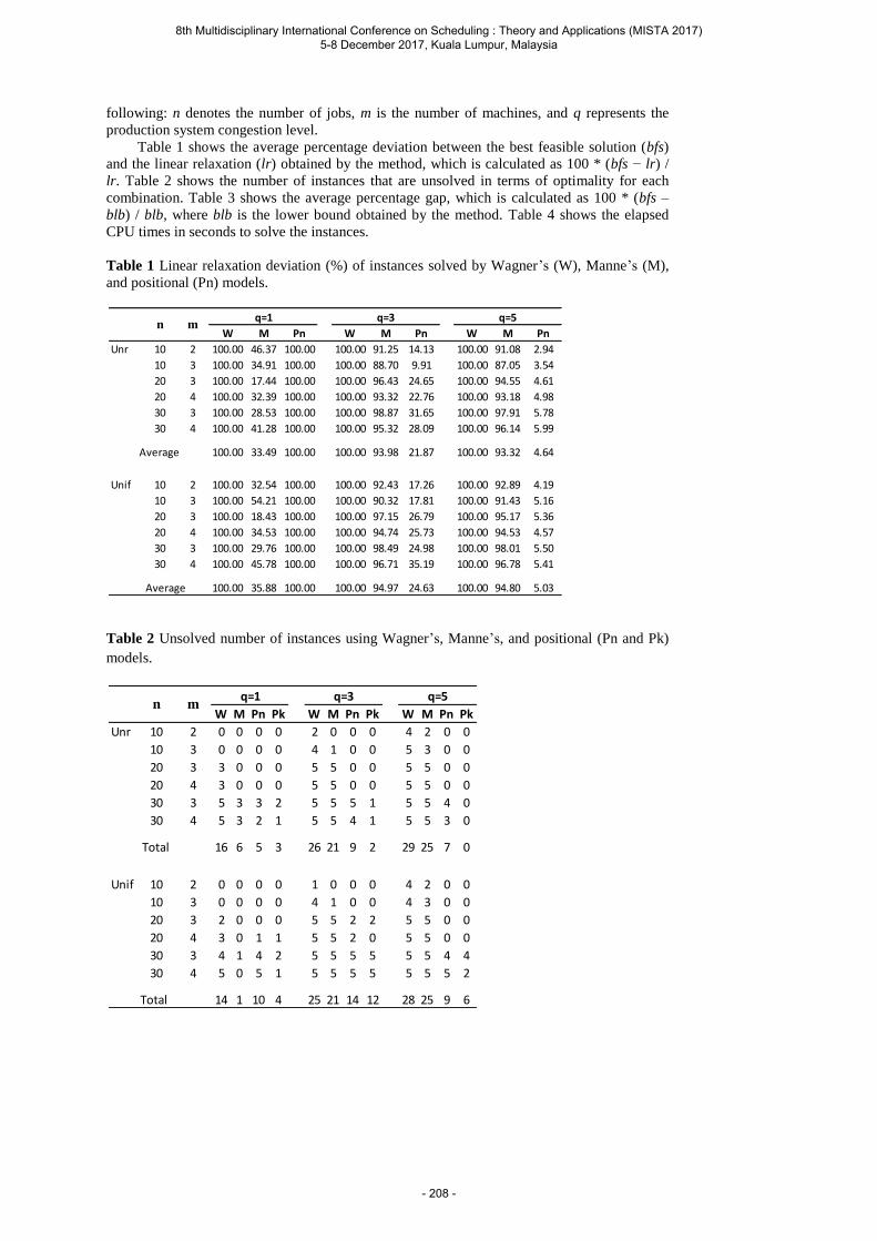
following: n denotes the number of jobs, m is the number of machines, and q represents the

production system congestion level.

Table 1 shows the average percentage deviation between the best feasible solution (bfs)

and the linear relaxation (lr) obtained by the method, which is calculated as 100 * (bfs − lr) /

lr. Table 2 shows the number of instances that are unsolved in terms of optimality for each

combination. Table 3 shows the average percentage gap, which is calculated as 100 * (bfs –

blb) / blb, where blb is the lower bound obtained by the method. Table 4 shows the elapsed

CPU times in seconds to solve the instances.

Table 1 Linear relaxation deviation (%) of instances solved by Wagner’s (W), Manne’s (M),

and positional (Pn) models.

Table 2 Unsolved number of instances using Wagner’s, Manne’s, and positional (Pn and Pk)

models.

W M Pn W M Pn W M Pn

Unr 10 2 100.00 46.37 100.00 100.00 91.25 14.13 100.00 91.08 2.94

10 3 100.00 34.91 100.00 100.00 88.70 9.91 100.00 87.05 3.54

20 3 100.00 17.44 100.00 100.00 96.43 24.65 100.00 94.55 4.61

20 4 100.00 32.39 100.00 100.00 93.32 22.76 100.00 93.18 4.98

30 3 100.00 28.53 100.00 100.00 98.87 31.65 100.00 97.91 5.78

30 4 100.00 41.28 100.00 100.00 95.32 28.09 100.00 96.14 5.99

Average 100.00 33.49 100.00 100.00 93.98 21.87 100.00 93.32 4.64

Unif 10 2 100.00 32.54 100.00 100.00 92.43 17.26 100.00 92.89 4.19

10 3 100.00 54.21 100.00 100.00 90.32 17.81 100.00 91.43 5.16

20 3 100.00 18.43 100.00 100.00 97.15 26.79 100.00 95.17 5.36

20 4 100.00 34.53 100.00 100.00 94.74 25.73 100.00 94.53 4.57

30 3 100.00 29.76 100.00 100.00 98.49 24.98 100.00 98.01 5.50

30 4 100.00 45.78 100.00 100.00 96.71 35.19 100.00 96.78 5.41

100.00 35.88 100.00 100.00 94.97 24.63 100.00 94.80 5.03

q=5

Average

n mq=1 q=3

W M Pn Pk W M Pn Pk W M Pn Pk

Unr 10 2 0 0 0 0 2 0 0 0 4 2 0 0

10 3 0 0 0 0 4 1 0 0 5 3 0 0

20 3 3 0 0 0 5 5 0 0 5 5 0 0

20 4 3 0 0 0 5 5 0 0 5 5 0 0

30 3 5 3 3 2 5 5 5 1 5 5 4 0

30 4 5 3 2 1 5 5 4 1 5 5 3 0

Total 16 6 5 3 26 21 9 2 29 25 7 0

Unif 10 2 0 0 0 0 1 0 0 0 4 2 0 0

10 3 0 0 0 0 4 1 0 0 4 3 0 0

20 3 2 0 0 0 5 5 2 2 5 5 0 0

20 4 3 0 1 1 5 5 2 0 5 5 0 0

30 3 4 1 4 2 5 5 5 5 5 5 4 4

30 4 5 0 5 1 5 5 5 5 5 5 5 2

14 1 10 4 25 21 14 12 28 25 9 6Total

q=5n m

q=1 q=3


- 208 -

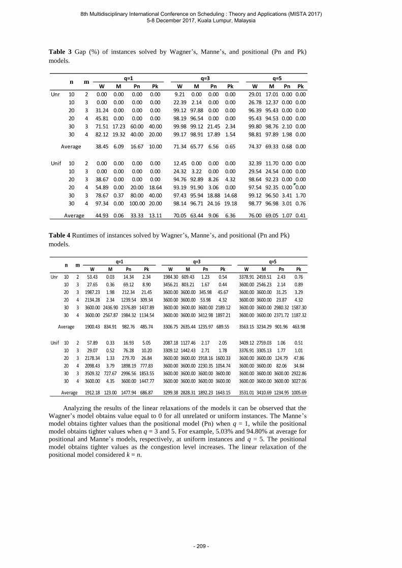
Table 3 Gap (%) of instances solved by Wagner’s, Manne’s, and positional (Pn and Pk)

models.

Table 4 Runtimes of instances solved by Wagner’s, Manne’s, and positional (Pn and Pk)

models.

Analyzing the results of the linear relaxations of the models it can be observed that the

Wagner’s model obtains value equal to 0 for all unrelated or uniform instances. The Manne’s

model obtains tighter values than the positional model (Pn) when q = 1, while the positional

model obtains tighter values when q = 3 and 5. For example, 5.03% and 94.80% at average for

positional and Manne’s models, respectively, at uniform instances and q = 5. The positional

model obtains tighter values as the congestion level increases. The linear relaxation of the

positional model considered k = n.


Unr 10 2 0.00 0.00 0.00 0.00 9.21 0.00 0.00 0.00 29.01 17.01 0.00 0.00

10 3 0.00 0.00 0.00 0.00 22.39 2.14 0.00 0.00 26.78 12.37 0.00 0.00

20 3 31.24 0.00 0.00 0.00 99.12 97.88 0.00 0.00 96.39 95.43 0.00 0.00

20 4 45.81 0.00 0.00 0.00 98.19 96.54 0.00 0.00 95.43 94.53 0.00 0.00

30 3 71.51 17.23 60.00 40.00 99.98 99.12 21.45 2.34 99.80 98.76 2.10 0.00

30 4 82.12 19.32 40.00 20.00 99.17 98.91 17.89 1.54 98.81 97.89 1.98 0.00

Average 38.45 6.09 16.67 10.00 71.34 65.77 6.56 0.65 74.37 69.33 0.68 0.00

Unif 10 2 0.00 0.00 0.00 0.00 12.45 0.00 0.00 0.00 32.39 11.70 0.00 0.00

10 3 0.00 0.00 0.00 0.00 24.32 3.22 0.00 0.00 29.54 24.54 0.00 0.00

20 3 38.67 0.00 0.00 0.00 94.76 92.89 8.26 4.32 98.64 92.23 0.00 0.00

20 4 54.89 0.00 20.00 18.64 93.19 91.90 3.06 0.00 97.54 92.35 0.00 0.00

30 3 78.67 0.37 80.00 40.00 97.43 95.94 18.88 14.68 99.12 96.50 3.41 1.70

30 4 97.34 0.00 100.00 20.00 98.14 96.71 24.16 19.18 98.77 96.98 3.01 0.76

44.93 0.06 33.33 13.11 70.05 63.44 9.06 6.36 76.00 69.05 1.07 0.41Average

q=5n m

q=1 q=3


Unr 10 2 53.43 0.03 14.34 2.34 1984.30 609.43 1.23 0.54 3378.91 2459.51 2.43 0.76

10 3 27.65 0.36 69.12 8.90 3456.21 803.21 1.67 0.44 3600.00 2546.23 2.14 0.89

20 3 1987.23 1.98 212.34 21.45 3600.00 3600.00 345.98 45.67 3600.00 3600.00 31.25 3.29

20 4 2134.28 2.34 1239.54 309.34 3600.00 3600.00 53.98 4.32 3600.00 3600.00 23.87 4.32

30 3 3600.00 2436.90 2376.89 1437.89 3600.00 3600.00 3600.00 2189.12 3600.00 3600.00 2980.32 1587.30

30 4 3600.00 2567.87 1984.32 1134.54 3600.00 3600.00 3412.98 1897.21 3600.00 3600.00 2371.72 1187.32

Average 1900.43 834.91 982.76 485.74 3306.75 2635.44 1235.97 689.55 3563.15 3234.29 901.96 463.98

Unif 10 2 57.89 0.33 16.93 5.05 2087.18 1127.46 2.17 2.05 3409.12 2759.03 1.06 0.51

10 3 29.07 0.52 76.28 10.20 3309.12 1442.43 2.71 1.78 3376.91 3305.13 1.77 1.01

20 3 2178.34 1.33 279.70 26.84 3600.00 3600.00 1918.16 1600.33 3600.00 3600.00 124.79 47.86

20 4 2098.43 3.79 1898.19 777.83 3600.00 3600.00 2230.35 1054.74 3600.00 3600.00 82.06 34.84

30 3 3509.32 727.67 2996.56 1853.55 3600.00 3600.00 3600.00 3600.00 3600.00 3600.00 3600.00 2922.86

30 4 3600.00 4.35 3600.00 1447.77 3600.00 3600.00 3600.00 3600.00 3600.00 3600.00 3600.00 3027.06

1912.18 123.00 1477.94 686.87 3299.38 2828.31 1892.23 1643.15 3531.01 3410.69 1234.95 1005.69

q=1 q=3 q=5

Average

n m


- 209 -

The positional model (Pn and Pk) obtains more optimal solutions than the other models.

This only does not occurred in uniform instances and q = 1. The Pk model fails to find 27

optimal solutions considering all instances, while the Manne’s model no longer obtains 99.

The positional model Pk obtains more optimal solutions than the Pn model, the biggest

difference is in the unrelated instances and q = 3, 30 versus 23, respectively. The number of

unresolved instances until optimality is higher in the uniform type (169) than in the unrelated

type (149) considering all models evaluated. The positional model obtains the optimal solution

for all unrelated instances with 10 and 20 jobs. For the number of jobs equal to 30 the models

have more difficulties to obtain the optimal solutions.

The smaller gaps are presented by Manne’s model for q = 1, while for q = 2 and 3 are

presented by the positional model. The more congested is productive system, the more the jobs

are tardy, and better positional model gaps in comparison to the other models. For example, the

Pk model obtained an average gap 0% versus 60.33% of Manne’s model in unrelated instances

and q = 3.

The positional model presents the shortest computational times between the evaluated

models, except in the uniform instances and q = 1. The more congested is the productive

system, faster the positional model is compared to the other models. This difference is up to

0.51 s versus 2759.03, that is, three orders of magnitude faster, in the uniform instances and q

= 3, considering the Pk and Manne’s models, respectively. The lower number of positions per

machine in the Pk model compared to the Pn model helped to reduce computational time.

Of all the analyzed criteria, Wagner’s model obtains performance well below that of the

positional model and even in relation to the Manne’s model. This aspect would be investigated

if there are other studies with similar results. Thus, the work of Lange and Werner [36] was

found to use models based on precedence and position variables on a parallel machine

approach to minimize the total tardiness of a single-track train scheduling problem. In tests

performed with instances of ten jobs or more, the model based on position variables was not

able to obtain an optimal solution within 2 h of runtime, whereas the model based on

precedence variables obtained the optimal solution in 2.02 s on average.

It was observed into the instances with q = 3 and 5 that the number of jobs allocated by

the machine by linear relaxation (k’i) and by the final solution (ki) maintained the following

relation: . This is because the linear relaxations of these instances are tighter. For

q = 1 this relation was not identified and the relation of formula 1 was maintained.

A brief resume comparing the positional model (Pk) and the best model from the

literature (Manne) is made following. In relation to the mean percentage deviation of the linear

relaxation value and the best integer solution is 42.69% versus 74.41%, this difference is

greater at congestion level q = 3, 4.84% versus 94.06%, in relation to the number of optimal

solutions is 153 versus 81, in relation to the mean gap was 5.09% versus 45.62%, and in

relation to the average runtime was 829.17 s versus 2177.78 s, respectively. The same

comparison can be made between to the Pn and Pk models to observe the impact of reducing

the number of position in model performance is 153 versus 126, 5.09% versus 11.23%, and

829.16 s versus 1287.63 s, respectively.

The above results indicate that the positional model has the expected effect and that,

unlike the time-indexed formulations, the positional model could be solved in a computational

time (see Table 4) as reasonable as those of the models based on the formulation of type 1 (see

Section 1). The positional model uses positional variables, similar to Wagner’s model, and

obtains the best computational performance compared to it and Manne’s model. It is thus

numerically proved that the proposed innovations are the contributing factors of the achieved

improvement.

5 Conclusion

The computational results show that the positional model is more efficient when

compared to other models from literature. This because is eliminated the use of the big-M


- 210 -

constant. Consequently, the model is linear and easier to solve [37]. In addition, reduction of

the number of position (Proposition 1) helps to reduce the computational effort.

The use of unrelated and uniform instances has shown that the positional model obtains

the best performance and formula 1 is always met even with very different processing times.

Therefore, a high degree of variability for the processing times in the uniform instances was

chosen with a variation up to 4 times in the speed between the machines (i = 4). In unrelated

instances the number of jobs allocated per machine varies around an average. While in the

uniform instances the number of jobs allocated to the faster machines (smaller index) is higher

than in the slower machines. This information can be used to define a different k per machine

type in order to reduce the computational time required.

The Pk model is more efficient than the Pn model though it needs to perform the linear

relaxation with n positions per machine to define the value of k before running with the

variables with the integrality condition. To help illustrate this, 153 versus 126 optimal

solutions, 5.09% versus 11.23% mean gap, and 829.16 s versus 1287.63 s runtime, are

obtained for the Pk and Pn models, respectively.

Future work will involve determining a means to eliminate the negative effect that loose

due dates have on decreasing the efficiency of the positional model for q = 1. Other future

work is to develop a decomposition algorithm. In addition, these approaches could be tested in

other scheduling problems that use the big-M constant.

Acknowledgements

The authors would like to thank the National Council for Scientific and Technological

Development (CNPq), Coordination of Personnel Improvement of Higher Education (CAPES),

and Foundation for Research Support of the State of Minas Gerais (FAPEMIG) for their

financial support.

References

1. Afzalirad, M., Shafipour, M., 2015. Design of an efficient genetic algorithm for resource-

constrained unrelated parallel machine scheduling problem with machine eligibility

restrictions. Journal of Intelligent Manufacturing, doi:10.1007/s10845-015-1117-6.

2. Mokotoff, E., 2001. Parallel machine scheduling problems: a survey. Asia-Pacific Journal

of Operational Research 18(2), 193–242.

3. Cheng, T. C. E., Sin, C. C. S., 1990. A State-of-the-Art Review of Parallel-Machine

Scheduling Research. European Journal of Operational Research 47(3), 271–292.

4. Lee, J.-H., Yu, J.-M., Lee, D.-H., 2013. A tabu search algorithm for unrelated parallel

machine scheduling with sequence- and machine-dependent setups: minimizing total

tardiness. The International Journal of Advanced Manufacturing Tecnology 69(9), 2081–

2089.

5. Lin, S.-W., Chou, S.-Y., Ying, K.-C., 2007. A sequential exchange approach for

minimizing earliness-tardiness penalties of single-machine scheduling with a common due

date. European Journal of Operational Research 177(2), 1294-1301.

6. Lin, S.-W, Ying, K.-C., 2007. Solving single machine total weighted tardiness problems

with sequence-dependent setup times by meta-heuristics. International Journal of Advanced

Manufacturing Technology 34(11), 1183-1190.

7. Chang, P.-C., Chen, S.-H., 2011. Integrating dominance properties with genetic algorithms

for parallel machine scheduling problems with setup time. Applied Soft Computing 11(1),

1263-1274.

8. Pessoa, A., Uchoa, E., Aragão, M. P. de, Rodrigues, R., 2010. Exact algorithm over an arc-

time-indexed formulation for parallel machine scheduling problems. Mathematical

Programming Computation 2(3), 259–290.


- 211 -

9. Sousa, J. P., Wolsey, L. A., 1992. A time indexed formulation of non-preemptive single

machine scheduling problems. Mathematical Programming 54(1), 353–367.

10. Koné, O., Artigues, C., Lopez, P., Mongeau, M., 2013. Comparison of mixed integer linear

programming models for the resource-constrained project scheduling problem with

consumption and production of resources. Flexible Services and Manufacturing Journal

25(1), 25–47.

11. Avalos-Rosales, O., Angel-Bello, F., Alvarez, A. M., 2015. Efficient metaheuristic

algorithm and re-formulations for the unrelated parallel machine scheduling problem with

sequence and machine-dependent setup times. The International Journal of Advanced

Manufacturing Tecnology 76(9), 1705-1718.

12. Li, K., Yang, S.-l., 2009. Non-identical parallel-machine scheduling research with

minimizing total weighted completion times: Models, relaxations and algorithms. Applied

Mathematical Modelling 33(4), 2145-2158.

13. Vallada, E., Ruiz, R., Minella, G., 2008. Minimising total tardiness in the m-machine

flowshop problem: A review and evaluation of heuristics and metaheuristics. Computers &

Operations Research 35(4), 1350–1373.

14. Allahverdi, A., Ng, C. T., Cheng, T. C. E., Kovalyov, M. Y., 2008. A survey of scheduling

problems with setup times or costs. European Journal of Operational Research 187(3),

985–1032.

15. Lee, Y. H., Pinedo, M., 1997. Scheduling jobs on parallel machines with sequence-

dependent setup times. European Journal of Operational Research 100(3), 464–474.

16. Park, Y., Kim, S., Lee, Y. H., 2000. Scheduling jobs on parallel machines applying neural

network and heuristics rules. Computers & Industrial Engineering 38, 189–202.

17. Bilge, U., Kirac, F., Kurtulan, M., Pekgun, P., 2004. A tabu search algorithm for parallel

machine total tardiness problem. Computers & Operations Research 31(3), 397–414.

18. Anghinolfi, D., Paolucci, M., 2007. Parallel machine total tardiness scheduling with a new

hybrid metaheuristic approach. Computers & Operations Research 34(11), 3471–3490.

19. Armentano, V. A., de França Filho, M. F., 2007. Minimizing total tardiness in parallel

machines scheduling with setup times: an adaptive memory-based GRASP approach.

European Journal of Operational Research 183(1), 100–114.

20. Kim, D.-W., Kim, K.-H., Jang, W., Chen, F. F., 2002. Unrelated Parallel machine

scheduling with setup times using simulated annealing. Robotics and Computer-Integrated

Manufacturing 18(3-4), 223–231.

21. M’Hallah, R., Bulfin, R. L., 2005. Minimizing the weighted number of tardy jobs on

parallel processors. European Journal of Operational Research 160(2), 471–484.

22. Chen, C. L., Chen, C. L., 2009. Hybrid metaheuristics for unrelated parallel machine

scheduling with sequence-dependent setup times. The International Journal of Advanced

Manufacturing Tecnology 43(1-2), 161–169.

23. Chen, C.-L., 2012. Iterated hybrid metaheuristic algorithms for unrelated parallel machines

problem with unequal ready times and sequence-dependent setup times. The International

Journal of Advanced Manufacturing Tecnology 60(5), 693–705.

24. Zhu, Z., Heady, R. B., 2000. Minimizing the sum of earliness/tardiness in multi-machine

scheduling: a mixed integer programming approach. Computers & Industrial Engineering

38, 297–305.

25. Chen, J. F., 2009. Scheduling on unrelated parallel machines with sequence- and machine-

dependent setup times and due-date constraints. The International Journal of Advanced

Manufacturing Tecnology 44(11), 1204–1212.

26. Lin, S.-W, Lu, C. C., Ying, K.-C., 2011. Minimization of total tardiness on unrelated

parallel machines with sequence- and machine-dependent setup times under due date

constraints. The International Journal of Advanced Manufacturing Tecnology 53(1), 353–

361.

27. Rocha, P. L., Ravetti, M. G., Mateus, G. R., Pardalos, P. M., 2008. Exact algorithms for a

scheduling problem with unrelated parallel machines and sequence and machine-dependent

setup times. Computers & Operations Research 35(4), 1250–1264.


- 212 -

28. Paula, M. R., Mateus, G. R., Ravetti, M. G., 2010. A non-delayed relax-and-cut algorithm

for scheduling problems with parallel machines, due dates and sequence-dependent setup

times. Computers & Operations Research 37(5), 938–949.

29. Nogueira, J. P. de C. M., Arroyo, J. E. C., Villadiego, H. M. M., Gonçalves, L. B., 2014.

Hybrid GRASP Heuristics to Solve an Unrelated Parallel Machine Scheduling Problem

with Earliness and Tardiness Penalties. Electronic Notes in Theoretical Computer Science

302, 53–72.

30. Zeidi, J. R., Hosseini, S. M., 2015. Scheduling unrelated parallel machines with sequence-

dependent setup times. The International Journal of Advanced Manufacturing Tecnology

81(9), 1487–1496.

31. Potts, C. N., Kovalyov, M. Y., 2000. Scheduling with batching: A review. European

Journal of Operational Research 120(2), 228–249.

32. Lawler, E. L., 1977. A “pseudopolynomial” algorithm for sequencing jobs to minimize

total tardiness. Annals of Discrete Mathematics 1, 331–342.

33. Wagner, H. W., 1959. An integer linear-programming model for machine scheduling.

Naval Research Logistic Quarterly 6(2), 131–140.

34. Manne, A. S., 1960. On the job-shop scheduling problem. Operations Research 8(2). 219-

223.

35. Chen, Z. -L., Powell, W. B., 1999a. Solving parallel machine scheduling problems by

column generation. INFORMS Journal on Computing 11(1), 78–94.

36. Lange, J., Werner, F., 2015. A comparison of approaches to modeling train scheduling

problems as job-shops with blocking constraints. Tech. Rep. Preprints 2015-18, Otto-von-

Guericke-University Magdeburg, Institute of Mathematical Optimization.

37. Chen, Z. -L., Powell, W. B., 1999b. A column generation based decomposition algorithm

for a parallel machine just-in-time scheduling problem. European Journal of Operational

Research 116(1), 220–232.


- 213 -

MISTA 2017

Balanced clustering based decomposition applied to Masterthesis defense timetabling problem

Huynh Thanh Trung · Pham Quang Dung · EmirDemirovic · Maxime Clement · Katsumi Inoue

Abstract Timetabling is an area of increasing interest in recent decades due to its practi-cality and complexity. In this paper we present an algorithm using decomposition approachbased on balanced clustering to solve a real-world university exam timetabling problem inVietnam. Essential elements in this problem are the considering of professor - theses simi-larity and workload balancing. The first stage in the algorithm is clustering part of the inputs(theses) while balancing the clusters’ quantity. The second stage involves a metaheuris-tic search that attempts to find the best way to partition the rest of the inputs (professors)through solving the sub-problems in parallel and recomposing partial solutions . Test resultsfor real-world instances are presented.

1 Introduction

Timetabling is a crucial and extremely time consuming task in many educational in-stitutions. The general term university timetabling typically refer to university course andexamination timetabling, both have been studied widely within the academic literature (see[1], [5]). The problem is often formalized as a combinatorial constraint optimization prob-lem which involves finding an assignment of variables to appropriate values, evaluated byconstraints and objective functions.

Huynh Thanh TrungHanoi University of Science and Technology, Hanoi, VietnamE-mail: [email protected]

Pham Quang DungHanoi University of Science and Technology, Hanoi, VietnamE-mail: [email protected]

Emir DemirovicUniversity of Melbourne, AustraliaE-mail: [email protected]

Maxime ClementNational Institute of Informatics Tokyo, JapanE-mail: [email protected]

Katsumi InoueNational Institute of Informatics Tokyo, JapanE-mail: [email protected]


- 214 -

The main contribution of this work consists of a balanced clustering based decomposi-tion approach to solve a real-world examination timetabling problem with the considering ofsimilarity matching and workload balancing, namely the Master Thesis Defense Timetablingproblem (MTDT). This is an arising problem in Vietnamse university education and is stillsolved by human effort. The first stage in the proposed algorithm relates to clustering part ofthe inputs (theses) while balancing the clusters’ quantity, using the K-means balanced clus-tering algorithm. Exploiting the result of the first stage by Bipartite Matching, the secondstage involves a metaheuristic search that attempts to find the best way to partition the restof the inputs (professors) through recomposing partial solutions of sub-problems.

The paper is organized as follows. Section 2 reviews the related work. Section 3 de-scribes the Master defense thesis timetabling problem as it is perceived at the universitiesin Vietnam. This timetabling problem is quite different from most problems encounteredin the literature, since it deals with similarity matching and workload balancing. We arenot aware of any similar problems in literature. We discuss the proposed algorithm usingBalanced-clustering heuristic and Decomposition strategy in Sections 4. Experimental re-sults are presented in Section 5. Section 6 concludes the paper and draws future researchdirections.

2 Related work

Timetabling within a university context has long been recognized as a difficult problemfrom both theoretical and practical perspective. Decomposition is one of the popular solutionmethods for this kind of problem [2]. The main idea of this method is ”divide and conquer”:a large problem is broken into smaller sub-problems which are easier to solve optimally be-cause the search spaces of these sub-problems are significantly diminished. The method hasproved its effectiveness in many works in examination timetabling problems [2,3]. Burkeand Newell (1999) investigated a decomposition approach by using sequential heuristics toassign the first set of exams which were evaluated as the most difficult ones by graph col-oring heuristics. In practice, the algorithm dramatically reduced the time required and alsoprovide high quality solutions on the real-world data [2,3]. Qu and Burke (2007) developeda new general adaptive decomposition technique that partitioned iteratively the problem intotwo subsets, namely the difficult set and the easy set , by the difficulty of scheduling themin previous iterations [4]. Matias Sorensen and al [6] (2013) applied a two-stage decom-position using bipartite matching and integer programming to solve a practical timetablingproblem in Denmark. Magana-Lozano and al [7] (2014) investigated an approach which de-composed a given problem into smaller sub-problems to solve and then sequentially recom-posed the partial solutions into a complete solution. Ali Hmer and al [8] (2014) presentedan multi-phase hybrid metaheuristics approach which decomposed the solving progress ofthe problem into 3 phases: pre-processing, construction and enhancement. However thesealgorithms are often specific and slight changes in the problem definition can raise difficultyin the adaptation of the special purpose algorithms.

Clustering, a process aiming at grouping the data such that homogeneous data fall in thesame group, has long been identified and researched in various fields of data mining, i.e.machine learning, pattern recognition, image analysis, bioinformatics, computer graphics.Clustering itself is not a specific algorithm but the general task to be solved. Among thealgorithms solving this task, K-means clustering algorithm is one of the most popular algo-rithm [12], [13] thanks to its simplicity, efficiency, flexibility and easy implementation [8].Optimization in the K-means often relates to better initialization, avoid the local optimum,


- 215 -

scalability but balancing the quantity between formed clusters is also an interesting aspectto consider. In balanced clustering problem, there are two conflicting objectives to concern:

– Minimizing Mean square error (MSE)– Balancing cluster sizes

The balanced constrained algorithms prior to balancing objective and treat the traditionalminimizing MSE objective as secondary criterion. Bradley and al. (2000) [10] added theconstraints to the original K-means algorithm that force each cluster should have at least apredefined number of points in each cluster, then solve the clustering assignment step as aMinimum Cost Flow (MCF) linear network optimization problem [14]. Zhu and Li (2010)[11] proposed the method that uses additional prior knowledge to constrain the size of eachcluster, then presented a heuristic algorithm to transform size constrained clustering prob-lems into integer linear programming problem. Malinen and Franti (2014) [9] introduced analgorithm that provide us a strictly balanced result. The algorithm replaces the assignmentstep of the traditional k-means clustering by bipartite matching between n data points and npre-allocated cluster slots; each cluster has exact n/k data points. The new assignment stepis solved by using Hungarian algorithm [15]. Although balanced clustering has the potentialto solve various applications, i.e workload balancing, circuit design, image processing [8],it has not been well studied in timetabling in particular and applications in general.

Thesis defense timetabling problem is an arising problem in educational context in theworld. The problem may be various due to the different policy of each country. Kochanikovaet al. (2013) [21] proposed a local search solver to deal with a thesis defense timetablingproblem instance in Czech Republic; their policies is quite different than ours. Battistuttaet al. (2015) [19] also introduced a local search method using Stimulated Annealing to dealwith the thesis defense timetabling problem in Italian universities. For vietnamsese univer-sities, Huynh and al (2012) first addressed this problem, formulated a model for the problemand solved it using genetic algortithm [7]. Bui and al (2012) [20] modeled the problem asa bi-objective then used direction-based multi-objective evolutionary algorithm to tackle.Pham and al (2015) [8] used an updated model for the problem and applied Tabu Searchmetaheuristic along with Constraint-based Local Search architecture to solve. In this paper,we will present an improved model of MTDT problem in which the professors attendingthe defense session are organized into juries, each jury is placed in a room, covers somecommittees of the defense session.

3 MTDT problem


Schedule the timetable for master thesis defense is a struggling mission that staffs mustcarry out in most of Vietnamese universities due to some policies. In each defense session(two or three defense sessions are open each academic year), there is a set of master studentswho will defense their thesis. Each student has one master thesis being scheduled in thedefense session, henceforth, we use thesis-student instead of student or his thesis. The juryof each thesis-student consists of five members: two examiners, a president, a secretary, andan additional member and this jury must be scheduled in one room and a slot of the sessionsatisfying a given set of constraints. Among five members of the jury, there must be twomembers who are not professors/lecturers of the university and who are invited to participate


- 216 -

in the jury: one is an examiner and the other is additional member. The supervisor of a thesis-student cannot be a member of the jury of that thesis-student. Two juries sharing a membermust be scheduled in two different slots. The assignments of the professors/lecturers tojuries should optimize some objectives, for instance, the occurrences of professors/lecturersin juries should be balanced, the theme of a thesis-student should match with the expertiseof two examiners participating in the jury of that thesis-student, etc. We describe in thefollowing section the mathematical formulation of the problem.

3.2 Problem formulation

Input

– S = 0, . . . , n − 1: the set of thesis-students, for each thesis-student s, sup(s) is thesupervisor of s

– IP = 0, . . . ,m1 − 1: set of professors of the university– EP = m1, . . . ,m1 +m2 − 1: set of professors outside the university– P = IP ∪ EP: set of professors participating the defense schedule– l(p): represents the level of professors p, ∀p ∈ P (i.e., 1: doctor, 2: associate professor,

3: full professor)– R = 0, . . . , r − 1: the set of rooms– T = 0, . . . , t− 1: the set of time slots– K = 0, . . . , k − 1: the set of specialization keywords– Ks(s) = [sk1, . . . , skk]: vector represent match between thesis s and keywords, s ∈ S– Kp(p) = [pk1, . . . , pkk]: vector represent match between professor p and keywords,p ∈ S

– m(s, p) = Ks(s).Kp(p)ᵀ: the score that measures the matching of expertise of professorp and the thesis-student s

Decision variables

– xp(s, i) represents the professor assigned in the ith position of the committee of thesis-student s

– xp(s, 1) represents the examiner 1, xp(s, 1) ∈ EP– xp(s, 2) represents the examiner 2, xp(s, 2) ∈ IP– xp(s, 3) represents the president, xp(s, 3) ∈ IP– xp(s, 4) represents the secretary, xp(s, 4) ∈ IP– xp(s, 5) represents the commissioner, xp(s, 5) ∈ EP

– xr(s): room of the jury of the thesis-student s

Invariants

– o(p) = ](i, s) | i ∈ 1, . . . , 5 ∧ s ∈ S ∧ xp(s, i) = p: number of juries that theprofessor p participates in

– e(p) = ](i, s) | i ∈ 1, 2 ∧ s ∈ S ∧ xp(s, i) = p: number of times professor p isscheduled as examiner

– or(r) = ]s | s ∈ S ∧ xr(s) = r: number of committees that the jury in room r covers– minP =minp∈P o(p)– maxP =maxp∈P o(p)


- 217 -

Hard Constraints

– H0. Internal-external member policy: in a commitee, examiner 1 and commissionercome from outside of the host university; examiner 2, chairman and secretary come fromthe host university:xp(s, 1) ∈ EP ∧ xp(s, 2) ∈ IP ∧ xp(s, 3) ∈ IP ∧ xp(s, 4) ∈ IP ∧ xp(s, 5) ∈ EP, ∀s ∈ S

– H1. Member conflict: all members in each committee must be different from eachother:xp(s, i) 6= xp(s, j), ∀1 ≤ i < j ≤ 5, s ∈ S

– H2. Supervisor-member conflict: all members in each committee must be differentfrom the supervisor of the student:xp(s, i) 6= sup(s), ∀s ∈ S, i ∈ 1..5

– H3. Chairman-secretary academic rank policy: in each committee, the academic rankof chairman must be equal or higher than that of secretary:l(xp(s, 3)) ≤ l(xp(s, 4)), ∀s ∈ S

– H4. Examiner appearance restriction: restrict the number of times that each professoris scheduled as examiner:e(p) ≤ λ, ∀p ∈ P

– H5. Room-time conflict: restrict the number of times that each room is used - must beless or equal than the number of time slots:]si ∈ S | xr(si) = r ≤ ]T, r ∈ R

– H6. Jury policy: Each professor must attend only 1 jury, which places in a room:xp(s1, i) = xp(s2, j)⇒ xr(s1) = xr(s2), ∀s1 6= s2 ∈ S, i, j ∈ 1..5

Objective functions

– F1. Professor workload balancing: All professor should be spread over the positionsof committees. The function reflects the gap between the most and the least number ofappearance of professors:F1 = maxP −minP

– F2. Professor-thesis expertise matching: The two examiners should match with thethesis in all committees. The function reflects the total match between examiners andtheses in committees:F2 =

∑s∈S m(s, xp(s, 1)) +m(s, xp(s, 2)

With the above formulation, we can then use the weighted-sum method to calculate thefitness function as defined in formula (1). The goal is then to find a feasible solution thatminimize the fitness function

F = w1 ∗ F1 + w2 ∗ F2 (1)

with w1, w2 is the weight of objective function F1, F2.

The table below illustrates an example of a schedule:


- 218 -

Table 1: Example of a schedule

Table 1 gives an example of the defense with 6 students S0, S1, S2, S3, S4, S5, 6internal professors P0, P1, P2, P3, P4, P5, 4 external professors P6, P7, P8, P9, 2rooms R0, R1 and 3 time slots T0, T1, T2. Column 1 represents the student-thesis, col-umn 2 represents the supervisor of the student. Columns 3-6 represent the members of thecommittees, namely the examiner 1, the examiner 2, the chairman, the secretary and thecommissioner. The schedule partitions the professors into 2 juries: jury 1 with professorsP1, P2, P5, P6, P7 is in charge of committees of students S0, S3, S4, jury 2 with pro-fessors P0, P3, P4, P8, P9 is responsible for committees of students S1, S2, S5. Allcommittees of each jury will take place in only one room (jury 1 in room R0, jury 2 inroom R1), guarantees that the professors don’t have to change the room during the defensesession, thanks to the hard constraint H6. This is an important constraint in practical and animprovement from the work [8]. It saves the professors from moving relentlessly betweenrooms during time slots and avoids the time asynchronous problem (sometimes there areovertime committees). The table is also an example for an ideal solution because all twoobjective functions have the best value: all professors attends the defense session equally (3times) and all examiners are best match with the theses.

4 Proposed Algorithm

The proposed algorithm decomposes the solving of the problem into two main phases.The first phase involves in clustering the theses of students based on their specialization andequally in terms of quantity, each cluster will be assigned to a jury. The second phase of thealgorithm relates to finding best way to partition the professors into juries using decompo-sition and recomposition partial solutions of sub-problems.

Table 2: Overview of the proposed algorithm


- 219 -

4.1 Balanced Clustering Techniques

In general, exam timetabling is the problem of allocating limited resources such as timeslots, rooms to given set of exams. One of the valuable information that can be exploitedis the relation of the exams, i.e: the common students between two exams, the condition offacilities required (room capacity, equipment). This relation affects how the resources shouldbe assigned to the exams; for example exams that shares the same students, same conditionrequired should not be scheduled in the same time slot. Analyzing the structure of feasiblehigh quality solutions can help us to recognize the extra features of these solutions and usingthem in the search strategy by decomposing the original problem into smaller problems tosolve. Note that this method cannot be applied to all problems because two reasons: earlyassignments may lead to later infeasibility and some soft constraints / objective functionscannot be evaluated when the problems are decomposed [1], but if we succeed to overcomethese drawbacks, we can save the great amount of computation because the search spaces ofthe sub-problems are significantly smaller than that of the original problem [15].

In the MTDT problem, we first balanced clustering the thesis-students based on theirspecializations, due to some reasons below:

– In a feasible solution, the thesis-students are splited into clusters, each cluster is takenby a jury, due to constraint H6. Therefore, the theses in a cluster should relevant to eachother and match with the specializations of the members in the jury in order to optimizethe objective F1.

– Balancing the number of thesis-students in each clusters is the best way to balancingthe appearance of the professors - objective F2, because each professor is fixed in a juryand therefore the workload of a professor has close connection to the number of thesis-students taken by his jury, in many cases they are equal when the number of professorin a jury is limited.

– Balancing the number of thesis-students in each cluster helps to always guarantee theconstraint H5 (Room-time conflict) because when the thesis-students are balanced clus-tered, there are no cluster having too much number of student-thesis that may lead to theexceeding usage of time slot.

The sub-problem of balanced clustering the thesis-students by their specialization (phase1-1) can be defined as follow:

Phase 1-1: Clustering the objects (x0, x1, ..., xn−1) which are the set of vectors repre-senting the match between theses and the specialization keywords; into k clusters C =

C1, C2, ..., Ck with k is the number of juries, such as each cluster Ck has n/k objects andoptimizing the WCSS function:

argmCin

k∑i=1

∑x∈Ci

||x− λi||2 (2)

with λi is the centroid of cluster Ci

To tackle the problem defined above, we applied the Balanced K-means clustering algo-rithm, which is introduced in [9]. Because the number of objects in the real instances oftennot so large, we used the K-means++ in the centroid initialization step rather than choosingcentroid randomly as the original algorithm. We named the enhanced algorithm ”BalancedK-means++ clustering” whose pseudo-code is as below:


- 220 -

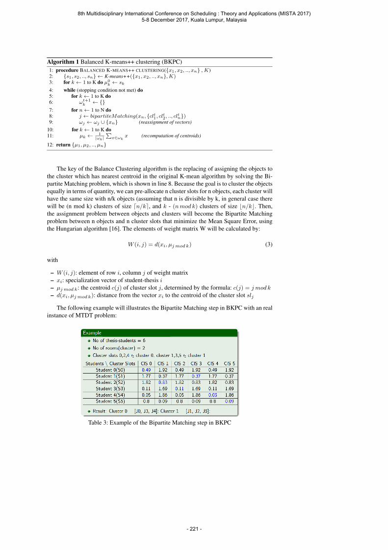
Algorithm 1 Balanced K-means++ clustering (BKPC)1: procedure BALANCED K-MEANS++ CLUSTERING(x1, x2, .., xn , K)2: s1, s2, .., sn ← K-means++(x1, x2, .., xn,K)3: for k ← 1 to K do µ0k ← sk

4: while (stopping condition not met) do5: for k ← 1 to K do6: ωt+1

k ← 7: for n← 1 to N do8: j ← bipartiteMatching(xn, clt1, clt2, .., cltn)9: ωj ← ωj ∪ xn (reassignment of vectors)

10: for k ← 1 to K do11: µk ← 1

|ωk|∑

x∈ωkx (recomputation of centroids)

12: return µ1, µ2, .., µn

The key of the Balance Clustering algorithm is the replacing of assigning the objects tothe cluster which has nearest centroid in the original K-mean algorithm by solving the Bi-partite Matching problem, which is shown in line 8. Because the goal is to cluster the objectsequally in terms of quantity, we can pre-allocate n cluster slots for n objects, each cluster willhave the same size with n/k objects (assuming that n is divisible by k, in general case therewill be (n mod k) clusters of size dn/ke, and k - (nmod k) clusters of size bn/kc. Then,the assignment problem between objects and clusters will become the Bipartite Matchingproblem between n objects and n cluster slots that minimize the Mean Square Error, usingthe Hungarian algorithm [16]. The elements of weight matrix W will be calculated by:

W (i, j) = d(xi, µj mod k) (3)

with

– W (i, j): element of row i, column j of weight matrix– xi: specialization vector of student-thesis i– µj mod k: the centroid c(j) of cluster slot j, determined by the formula: c(j) = j mod k

– d(xi, µj mod k): distance from the vector xi to the centroid of the cluster slot slj

The following example will illustrates the Bipartite Matching step in BKPC with an realinstance of MTDT problem:

Table 3: Example of the Bipartite Matching step in BKPC


- 221 -

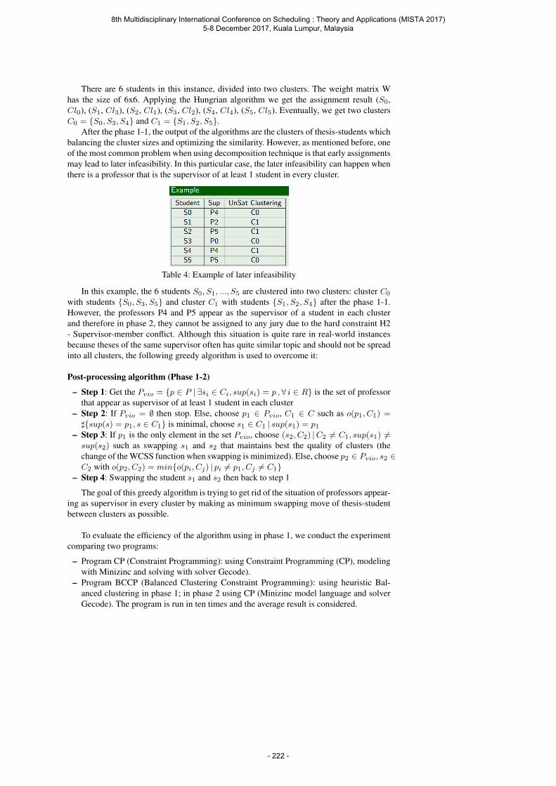
There are 6 students in this instance, divided into two clusters. The weight matrix Whas the size of 6x6. Applying the Hungrian algorithm we get the assignment result (S0,Cl0), (S1, Cl3), (S2, Cl1), (S3, Cl2), (S4, Cl4), (S5, Cl5). Eventually, we get two clustersC0 = S0, S3, S4 and C1 = S1, S2, S5.

After the phase 1-1, the output of the algorithms are the clusters of thesis-students whichbalancing the cluster sizes and optimizing the similarity. However, as mentioned before, oneof the most common problem when using decomposition technique is that early assignmentsmay lead to later infeasibility. In this particular case, the later infeasibility can happen whenthere is a professor that is the supervisor of at least 1 student in every cluster.

Table 4: Example of later infeasibility

In this example, the 6 students S0, S1, ..., S5 are clustered into two clusters: cluster C0

with students S0, S3, S5 and cluster C1 with students S1, S2, S4 after the phase 1-1.However, the professors P4 and P5 appear as the supervisor of a student in each clusterand therefore in phase 2, they cannot be assigned to any jury due to the hard constraint H2- Supervisor-member conflict. Although this situation is quite rare in real-world instancesbecause theses of the same supervisor often has quite similar topic and should not be spreadinto all clusters, the following greedy algorithm is used to overcome it:

Post-processing algorithm (Phase 1-2)

– Step 1: Get the Pvio = p ∈ P | ∃si ∈ Ci, sup(si) = p , ∀ i ∈ R is the set of professorthat appear as supervisor of at least 1 student in each cluster

– Step 2: If Pvio = ∅ then stop. Else, choose p1 ∈ Pvio, C1 ∈ C such as o(p1, C1) =

]sup(s) = p1, s ∈ C1 is minimal, choose s1 ∈ C1 | sup(s1) = p1– Step 3: If p1 is the only element in the set Pvio, choose (s2, C2) |C2 6= C1, sup(s1) 6=sup(s2) such as swapping s1 and s2 that maintains best the quality of clusters (thechange of the WCSS function when swapping is minimized). Else, choose p2 ∈ Pvio, s2 ∈C2 with o(p2, C2) = mino(pi, Cj) | pi 6= p1, Cj 6= C1

– Step 4: Swapping the student s1 and s2 then back to step 1

The goal of this greedy algorithm is trying to get rid of the situation of professors appear-ing as supervisor in every cluster by making as minimum swapping move of thesis-studentbetween clusters as possible.

To evaluate the efficiency of the algorithm using in phase 1, we conduct the experimentcomparing two programs:

– Program CP (Constraint Programming): using Constraint Programming (CP), modelingwith Minizinc and solving with solver Gecode).

– Program BCCP (Balanced Clustering Constraint Programming): using heuristic Bal-anced clustering in phase 1; in phase 2 using CP (Minizinc model language and solverGecode). The program is run in ten times and the average result is considered.


- 222 -

Result 1: Evaluating the balanced-clustering method

From the result table, we can see that:

– Balanced clustering heuristic in BBCP help us to reduce the solving time significantlycomparing to exact method CP.

– There is a trade-off between the time used and the stability of the quality of solution,but this trade-off is acceptable because the quality is reduced slightly while the timeconsumed reduced significantly. Moreover, when it comes to larger instance with thetime restriction, the exact method fails to give the better solution than the heuristic one.

– Although the computation time of BBCP is much more superior to that of CP, BBCPstill seems to struggle to deal with large problem.

4.2 Decomposition and Recomposition Strategies

After phase 1, we have already achieved a way to cluster the theses balancedly in quan-tity and optimally in specialization similarity between theses in each cluster. An natural ideais to assign the members to the juries based on the theses clusters they are in charge of,because of these following reasons:

– After assigning the members to the juries, the problem of input size (n students, m juries)will be broken into m sub-problems of input size [ n

m ] students, 1 jury.– The match between both theses and professors with specialization keywords are repre-

sented by the same way: a k-dimension vector with k is the total number of specializa-tion keywords. Therefore, we can exploit the result of theses clustering through BipartiteMatching the vectors of professor specializations and the centroids of the theses clusters.

Jury members initialization algorithm (Phase 2-1)

– Step 1: Calculate the matrix W with size of n x n with n is the number of professor inthe defense session:

W (i, j) = d(xi, µj mod k) (4)

with:– W (i, j): element of row i, column j of weight matrix– xi: specialization vector of professor i– µj mod k: the centroid c(j) of cluster slot j, determined by the formula: c(j) =

j mod k

– d(xi, µj mod k): distance from the vector xi to the centroid of the cluster slot slj

– Step 2: Applying the Hungarian algorithm to solve the bipartite matching problem be-tween professors and student-thesis clusters


- 223 -

With each way of pre-assign professors to the jury, the original problem of (n students, mjuries) are broken into m sub-problems of [ n

m ] students, 1 jury. The sub-problem not onlyhas significantly reduced input size but also has significantly less complicate model, becausethe room decision variable xr is no longer needed and the hard constraint H6 (Jury policy)is now guaranteed, because there is only 1 jury now.

On the other hand, from m feasible solutions to m sub-problems, we always be able toget a feasible solution for the initial problem, because:

– All hard constraints H0 - Internal-external member policy, H1 - Member conflict, H2 -Supervisor-member conflict, H3 - Chairman-secretary academic rank policy are dependsonly on the schedule for each students. Therefore, if the schedule for each student in thesub-problems don’t violate these constraints, the recomposed solution are feasible forthem.

– Hard constraints H4 - Examiner appearance restriction and H6 - Jury Policy are guaran-teed to not be violated because each professor attends only 1 jury.

– Hard constraint H5 - Room-time conflict is guaranteed to not being violated because thequantity of students in each jury is balanced, therefore there will be no room with toomuch students.

The connections between the objective functions of sub-problems and the original prob-lem are as following:

– F1. Professor workload balancing:

F1 = max(F i1 | i ∈ 1..m) (5)

with F i1 is the value of objective function 1 of sub-problem i

– F2. Professor-thesis expertise matching: The two examiners should match with thethesis in all committees. The function reflects the total match between examiners andtheses in committees:

F2 =

m∑i=1

F i2 (6)

with F i2 is the value of objective function 2 of sub-problem i

As we can see from the above formulas:

– Minimizing the objective function F1 of original problem is equivalent to minimizingthe objective funcions F i

1 of the sub-problems– Maximizing the objective function F2 of original problem is equivalent to maximizing

the objective function F i2 of the sub-problems

Therefore, with each given partition way of professors, our mission is to find the feasibleand optimized solutions for the sub-problems. To evaluate the efficiency of the method, weconduct the experiment comparing two programs:

– Program BCCP (Balanced Clustering Constraint Programming): using heuristic Bal-anced clustering in phase 1; in phase 2 using CP (Minizinc model language and solverGecode) which is an exact method.

– Program BCIPS (Balanced Clustering Initial Partial Solution): using using heuristic Bal-anced clustering in phase 1; in phase 2 using the initial professor partition in Phase 2-1and then solving the sub-problems in parallel with CP (Minizinc model language andsolver Gecode).


- 224 -

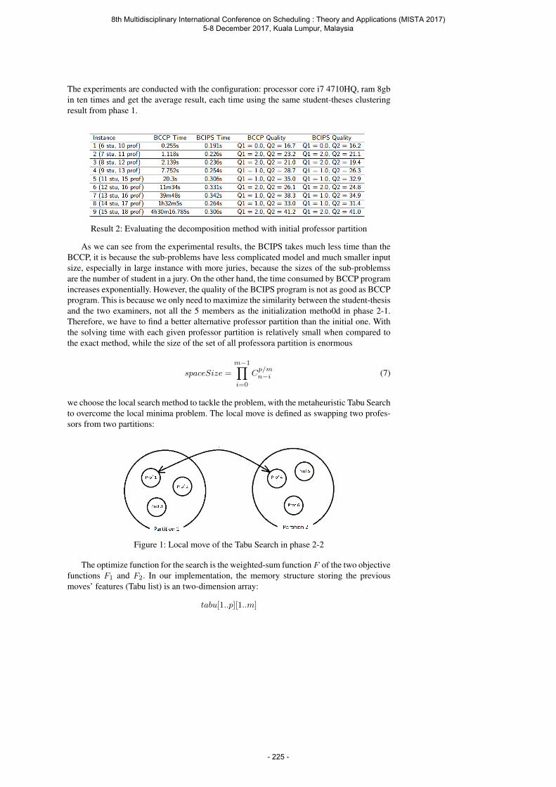
The experiments are conducted with the configuration: processor core i7 4710HQ, ram 8gbin ten times and get the average result, each time using the same student-theses clusteringresult from phase 1.

Result 2: Evaluating the decomposition method with initial professor partition

As we can see from the experimental results, the BCIPS takes much less time than theBCCP, it is because the sub-problems have less complicated model and much smaller inputsize, especially in large instance with more juries, because the sizes of the sub-problemssare the number of student in a jury. On the other hand, the time consumed by BCCP programincreases exponentially. However, the quality of the BCIPS program is not as good as BCCPprogram. This is because we only need to maximize the similarity between the student-thesisand the two examiners, not all the 5 members as the initialization metho0d in phase 2-1.Therefore, we have to find a better alternative professor partition than the initial one. Withthe solving time with each given professor partition is relatively small when compared tothe exact method, while the size of the set of all professora partition is enormous

spaceSize =

m−1∏i=0

Cp/mn−i (7)

we choose the local search method to tackle the problem, with the metaheuristic Tabu Searchto overcome the local minima problem. The local move is defined as swapping two profes-sors from two partitions:

Figure 1: Local move of the Tabu Search in phase 2-2

The optimize function for the search is the weighted-sum function F of the two objectivefunctions F1 and F2. In our implementation, the memory structure storing the previousmoves’ features (Tabu list) is an two-dimension array:

tabu[1..p][1..m]


- 225 -

with p and m is the number of professors and juries. In iteration iter, the local swappingmove professor pi (currently in jury mi) with professor pj (currently in jury mj) can beconsidered as two assignment moves: assign pi to mj and pj to mi, therefore the feature ofthe move can be stored by assigning tabu[pi][mj ] and tabu[pj ][mi] to iter.


To evaluate the proposed algorithm (we name it Balanced Clustering Parallel Tabu Search),we conduct the experiment comparing the 3 programs:

– BCPTS (Balanced Clustering Parallel Tabu Search): using proposed algorithm, which isa heuristic method.

– CP (Constraint Programming): using Constraint Programming (CP), modeling with Miniz-inc and solving with solver Gecode with first-fail strategy and default parameters), whichis an exact method.

– CBLS-TS (Constraint-based local search - Tabu Search): using the constraint-based lo-cal search library OpenCBLS [18] to model the problem and solving by the defaultgeneric Tabu Search, which is a heuristic method.

The three programs are run on the machine with an Intel Core I7 4710HQ, 8gb ram, run-ning Ubuntu 14.04. They are tested with real instances from the defense session in April andOctober 2016 from School of Information and Communication Technology, Hanoi Univer-sity of Science and Technology. For the two approximate algorithm BCPTS and CBLS-TS,each program is run ten times for each instance, the average result and the lower and upperbound of the objective functions are considered:

Result 3: Experimental Result

From the experimental result, the proposed algorithm BCPTS:

– When comparing to the exact algorithm CP:+ The CP program is superior to the BCPTS in both term of speed and quality

when it comes the small instance. However, the computation time of the CP increaseexponentially when the input size become larger and exceed the timeout (60h) whenthere are more than 15 students, while the BCPTS time is feasible for all the instances.

+ There is the trade-off between speed and quality as the solutions given by BCPTSis not reach the best quality for the objective function F2. However, the quality of thesesolutions are quite near to the optimized ones, while the time is reduced extremely,especially for the large instances.

+ For the large instances, the exact method CP can not reach the best solution withinthe timeout period and gives solutions with less quality than the BCPTS.


- 226 -

– When comparing to the approximate algorithm CBLS-TS:+ Both programs are able to generate a feasible solution in short time for all instances+ However, the quality of the solutions given by BCPTS is much better than that of

the CBLS-TS. This is because the MTDT problem is a combinatorial problem with highcomplexity, many variables and constraints and enormous solution space. Therefore,applying directly the metaheuristic Tabu Search to the problem is less effective thanusing more sophisticated techniques as the proposed algorithm.

Therefore, we can confirm that the proposed algorithm BCPTS provide the good trade-off between speed and quality, which has high practical value for the real-world usage.

6 Conclusion

In this paper, a heuristic algorithm using decomposition approach based on balanced clus-tering for a real world Examination Timetabling problem has been shown. This splits thesolving of the original problem into two phases, which reduces the input size and com-plexity significantly. Computational results shows that the proposed algorithm provides agood trade-off between speed and quality and has high practical value. The good result forthe problem prove the potential of decomposition approach in general and especially thebalanced clustering heuristic to the solving of combinatorial problems. It is true that specialstructure is required for applying the decomposition, which limits the set of applicable prob-lems, but if we can attempt to use the method successfully, the advantages gained cannot beunderestimate. In future works, we will consider applying the balanced clustering to moreCSP problem which has workload balancing objective - a popular type of objective in thereal world.

Acknowledgements This work was partially supported by National Institute of Informatics, Japan. Schoolof Information and Communication Technology, Hanoi University of Science and Technology provides usthe data for the experiment.

References

1. Qu, R., Burke, E., McCollum, B., Merlot, L., Lee, S, ”A survey of search methodologies and automatedsystem development for examination timetabling”, Journal of Scheduling 12(1), pp.55-90, (2009).

2. Magaa-Lozano, Dulce J. et al, Decomposition and Recomposition Strategies to Solve Timetabling Prob-lems, (2014).

3. E.K. Burke and J.P. Newall, ”A multi-stage evolutionary algorithm for the timetable problem”, IEEETransactions on Evolutionary Computation, 3(1): pp. 63-74, (1999).

4. R. Qu and E.K. Burke (2007). Adaptive Decomposition and Construction for Examination TimetablingProblems. Multidisciplinary International Scheduling: Theory and Applications 2007 (MISTA07), Paris,France, pp.418-425, (Aug 2007).

5. M.W. Carter, G. Laporte, Recent development in practical course timetabling, in: Selected and RevisedPapers of the Second International Conference on Practice and Theory of Automated Timetabling, (PATAT1997), LNCS, vol. 1408, Springer, Toronto, pp.3-19, (1998).

6. Matias Srensen, Florian H. W. Dahms. A Two-Stage Decomposition of High School Timetabling appliedto cases in Denmark. Journal Computers and Operations Research archive Volume 43, March, 2014, pp.36-49, (2014).

7. T. T. B. Huynh, Q. D. Pham and D. D. Pham, ”Genetic Algorithm for Solving the Master ThesisTimetabling Problem with Multiple Objectives,” 2012 Conference on Technologies and Applications ofArtificial Intelligence, Taiwan, 2012, pp. 74-79. (2012).

8. Divya Saini1, Manoj Singh, ”Achieving Balance in Clusters- A Survey”, International Research Journalof Engineering and Technology (IRJET), (2015).


- 227 -

9. Mikko I. Malinen and Pasi Frnti, Balanced KMeans for Clustering, Volume 8621 of the series LectureNotes in Computer Science pp.32-41 and Proceedings of the Joint IAPR International Workshop, S+SSPR2014, Joensuu, Finland, (2014).

10. P. S. Bradley, K. P. Bennett, A. Demiriz, Constrained k-means clustering, Tech.rep., MSRTR-2000-65,Microsoft Research, (2000).

11. S. Zhu, D. Wang, T. Li, Data clustering with size constraints. Knowledge-Based Systems 23(8), pp.883889, (2010).

12. E.W.Forgy, Cluster analysis of multivariate data: efficiency v/s interpretability of classifications, Biomet-rics, 21, pp.768-769, (1965).

13. X. Wu et al. Top 10 algorithms in data mining, Knowledge and Information Systems, 14(1), pp. 1-37,(2008).

14. D. P. Bertsekas. ”Linear Network Optimization”. MIT Press, Cambridge, MA, (1991).15. M.W. Carter. A decomposition algorithm for practical timetabling problems. Technical Paper 83-06,

Department of Industrial Engineering, University of Toronto.(1983)16. Burkhard, R., DellAmico, M., Martello, S. Assignment Problems (Revised reprint), SIAM (2012)17. Nicholas Nethercote, Peter Stuckey, et al :MiniZinc: Towards a standard CP modelling language. Princi-

ples and Practice of Constraint Programming CP 200718. Pham Quang Dung, Huynh Thanh Trung, Ta Duy Hoang, Nguyen Thanh Hoang. A Java library for

Constraint-Based Local Search: Application to the master thesis defense timetabling problem. Proceedingsof the Sixth International Symposium on Information and Communication Technology, pp 67-74, (2015)

19. Michele Battistutta, Sara Ceschia, Fabio De Cesco, and Andrea Schaerf. Thesis defense timetabling. In7th Multidisciplinary International Con- ference on Scheduling : Theory and Applications (MISTA 2015),pages 507-514, (2015).

20. Lam T Bui and Viet Hoang. A multi-objective approach for masters thesis committees scheduling usingDMEA. In Asia-Pacific Conference on Simulated Evolution and Learning, pages 450-459. Springer, (2012).

21. Kochanikova and Rudova. Student scheduling for bachelor state examinations. In Proc. of the 6th Mul-tidisciplinary International Conference on Scheduling : Theory and Applications (MISTA 2013), pages762-766, (2013).


- 228 -

MISTA 2017

A Selective-Discrete Particle Swarm OptimizationAlgorithm for Solving a Class of Orienteering Problems

Aldy Gunawan · Vincent. F. Yu · A. A. N.

Perwira Redi · Parida Jewpanya · Hoong

Chuin Lau

Abstract This study addresses a class of NP-hard problem called the OrienteeringProblem (OP), which belongs to a well-known class of vehicle routing problems.In the OP, a set of nodes that associated with a location and a score is given. Thetime required to travel between each pair of nodes is known in advance. The totaltravel time is limited by a predetermined time budget. The objective is to selecta subset of nodes to be visited that maximizes the total collected score withina path. The Team OP (TOP) is an extension of OP that incorporates multiplepaths. Another widely studied OP extension is the Team OP with Time Windows(TOPTW) that adds the time windows constraint. We introduce a discrete versionof Particle Swarm Optimization (PSO), namely Selective-Discrete PSO (S-DPSO)to solve TOP and TOPTW. S-DPSO has a different movement compared withother DPSO algorithms reported in the literature. S-DPSO considers four differentmovement schemes: (a) following its own position, (b) moving towards its personalbest position, (c) moving towards the global best position, and (d) moving towardsthe combination of three above-mentioned schemes. The best movement schemeis selected in order to determine the next position of the particle. The S-DPSOalgorithm is tested on the benchmark instances. The experiment results show that

Aldy GunawanSingapore Management UniversityE-mail: [email protected]

Vincent. F. YuNational Taiwan University of Science and TechnologyE-mail: [email protected]

A. A. N. Perwira RediNational Taiwan University of Science and TechnologyE-mail: [email protected]

Parida JewpanyaRajamangala University of Technology LannaE-mail: [email protected]

Hoong Chuin LauSingapore Management UniversityE-mail: [email protected]


- 229 -

S-DPSO performs well in solving benchmark instances. S-DPSO is promising andcomparable to the state-of-the-art algorithms.

1 Introduction

The OP was first introduced by Tsiligirides [33]. In OP, a set of nodes that asso-ciated with a location and a score is given. The time required to travel betweeneach pair of nodes is known in advance. The total travel time is limited by a pre-determined time budget. The objective is to select a subset of nodes to be visitedthat maximizes the total collected score in a path. An OP extension is the TeamOP (TOP) that incorporates multiple paths. TOP is considered as a class of theVehicle Routing Problem (VRP) with profits and multiple vehicles. Each vehicleis represented as a path with the aim of selecting customers so as to maximize thecollected profits and subject to a travel time restriction [1,9].

Another widely studied OP extension is the Team OP with Time Windows(TOPTW). The TOPTW adds the time windows constraint. A visit to a particularnode has to be made within its time window. A comprehensive survey about theOP can be found in Vansteenwegen et al. [34]. Recently, Gunawan et al. [11] extendthe survey by including latest variants of the OP, including the proposed solutionapproaches and the most recent applications of the OP, such logistics, trip plannerand other areas. Only limited population-based algorithms have been introducedto solve the OP and its variants [11].

We introduce a discrete version of Particle Swarm Optimization (PSO), namelySelective-DPSO (S-DPSO). PSO is a population-based metaheuristic algorithmthat originates from studies of synchronous bird flocking, fish schooling, and beesbuzzing [14]. It evolves a population or swarm of individuals called particles. Themain characteristic of PSO is the capability to solve a problem by moving eachparticle in the search space based on its velocity, its personal best position, andthe particle swarm’s global best position.

PSO is designed for solving continuous optimization problems; therefore, itis not suitable for the combinatorial optimization problems. The main reason isthat it is not possible for particles to continuously ”fly” through a discrete-valuedspace [13]. However, its fast convergence and easy implementation have drivenresearchers to extend the continuous PSO to discrete problems. In order to solvediscrete optimization problems, some researchers use a discrete particle represen-tation and create a discrete position procedure by following an analogous structureof the classical PSO equations, known as Discrete PSO (DPSO) [21,19]. Severalvariants of PSO that are used to solve discrete optimization problems can be seenin various problem domains, such as the traveling salesman problem [29], vehiclerouting problem [30,31,10], scheduling problem [16] and orienteering problem [21,25,8].

Instead of directly following the current position of a particular particle, thepersonal best solution of a particular particle (personal best position) and theglobal best solution taken from all particles (particle swarm’s global best posi-tion), which are commonly used in the DPSO, S-DPSO is designed to allow eachparticle to evaluate one of the position choices generated by the proposed move-ment schemes. Four different movement schemes that follow the analogy of thePSO position updating rule are proposed. The four movement schemes are: (a)


- 230 -

following its own position, (b) moving towards its personal best position, (c) mov-ing towards the global best position, and (d) moving towards the combinationof three above-mentioned schemes. By doing so, each particle has more chancesto move to a better position. S-DPSO is implemented for solving two variants ofthe Orienteering Problem (OP), namely TOP and TOPTW. The results are verypromising and comparable to the ones of the state-of-the-art algorithms.

The rest of this paper is organized as follows. Section 2 summarizes a literatureoverview related to the PSO that has been applied in various domains, includingthe OP. In Section 3, we describe the Selective Discrete-PSO (S-DPSO) algorithm.We also briefly describe TOP and TOPTW. The benchmark instances and exper-imental results are presented in Section 4. Finally, our conclusion and future workare summarized in Section 5.

2 Related Work

This section briefly summarizes several applications of the DPSO algorithm in var-ious combinatorial optimization problems, such as flowshop scheduling, machinescheduling and vehicle routing problems. The most recent applications of PSO inorder to solve variants of the OP are also included.

Liao et al. [16] propose DPSO in order to solve flowshop scheduling problems.The particle and the velocity are redefined. An efficient approach is developed tomove a particle to a new sequence. Furthermore, they incorporate a local searchscheme into the proposed algorithm, called PSO-LS. Comparisons with a continu-ous PSO algorithm and two genetic algorithms are conducted in order to verify theproposed DPSO algorithm. Computational results show that the proposed DPSOalgorithm is very competitive.

Pan et al. [23] introduce DPSO to solve the no-wait flowshop scheduling prob-lem. The main contribution of this work is due to the fact that particles arerepresented as discrete job permutations and a new position update method isdeveloped based on the discrete domain. In addition, the DPSO algorithm is hy-bridized with the Variable Neighborhood Descent (VND) algorithm to furtherimprove the solution quality.

Tseng and Liao [32] propose a DPSO algorithm by incorporating the Net Ben-efit of Movement (NBM) algorithm to solve the lot-streaming flowshop schedulingproblem. This DPSO improves the existing DPSO [16] by introducing an inheri-tance scheme, inspired by a genetic algorithm, into particles construction. Kashanand Karimi [13] present a DPSO algorithm for scheduling parallel machines. Theproposed DPSO uses a discrete combinatorial solution representation and equa-tions analogous to those of the PSO equations. Marinakis and Marinaki [18] pro-pose a hybrid algorithmic nature inspired methodology, namely the hybrid genetic-particle swarm optimization algorithm to solve the vehicle routing problem. Byintroducing an intermediate phase between the two generations, namely the phaseof evolution of the population, the proposed algorithm gives more efficient indi-viduals and, thus, it improves the effectiveness of the algorithm.

Marinakis et al. [19] introduce another hybrid algorithm, namely the hybridparticle swarm optimization (HybPSO), for the vehicle routing problem. It com-bines PSO, the Multiple Phase Neighborhood Search-Greedy Randomized Adap-tive Search Procedure (MPNS-GRASP) algorithm, the Expanding Neighborhood


- 231 -

Search strategy and a Path Relinking strategy. This algorithm is suitable for solv-ing very large-scale vehicle routing problems within short computational times.

Chen et al. [4] introduce an interactive self-learning PSO algorithm for therouting pickup and delivery of multiple products with material handling in multiplecross-docks problem. The concept of self-learning is incorporated so as to attain theoptimal solution within reasonable computational time, and decrease the chanceof being trapped in a local optimum.

Dang et al. [7] propose an effective Particle Swarm Optimization-based MemeticAlgorithm (PSOMA) for TOP. Most MA designs incorporate various local searchtechniques into a global search scheme, e.g. a genetic algorithm. MA and PSO areboth based on social evolution or behavior rather than biological ones, and thereare benefits to be gained from combining techniques into a single form for solvingcombinatorial optimization problems.

Muthuswamy and Lam [21] introduce DPSO for solving the TOP. This DPSOis a modification of PSO that applies a discrete or qualitative distinction betweenvariables. The RVNS and 2-Opt are used as the local search operators. The insertand exchange neighborhoods in the RVNS technique are employed randomly in or-der to update the next generation particles. Dang et al. [8] introduce an effectivePSO-inspired Algorithm (PSOiA) for TOP. This method is based on the prelim-inary study of a PSO-based memetic algorithm (PSOMA). Moreover, a new fastevaluation process based on an interval graph model is introduced. This processenables more iterations for the PSO without increasing the global computationaltime.

3 Selective-Discrete Particle Swarm Optimization

3.1 Particle Swarm Optimization (PSO)

The standard PSO algorithm is initially designed for solving continuous opti-mization problems. In PSO, a solution, which is represented as a particle, movesthrough the search space in order to reach the global optimum. During a particularmovement, each particle adjusts its position based on its own experience and itsneighboring particles. All particles share their information so that they would bedirected towards the best position in the search space.

The formal definitions of PSO are as follows. Let K be a set of particles, wedefine the best solution of particle k ∈ K at iteration t (the personal best position)and the global best solution taken from all particles at iteration t (the particleswarm’s global best position) as ptk−best and gtbest, respectively. At iteration t,

particle k updates its next position xt+1k by using the following equations [21]:

vt+1k = wvtk + c1r1(ptk−best − xtk) + c2r2(gtbest − xtk) (1)

xt+1k = xtk + vt+1

k (2)

vtk and xtk represent the velocity and the position of particle k at iteration t,respectively. w is a constant value for controlling the impact of the previous veloc-ity, c1 is the cognitive parameter for remembering the best particle position thathas been reached so far, c2 is the social parameter controlling the communication


- 232 -

among particles in order to converge towards the global best position, r1 and r2are uniformly distributed random variables between [0,1].

In order to solve combinatorial optimization problems which require a discretesolution space, some transformation techniques are required, such as the inte-ger value [28], the binary coding scheme [22] and a permutation based solutionrepresentation [36]. We extend the DPSO by introducing the Selective - DPSO(S-DPSO) algorithm that considers several movement schemes with the purposeof improving the movement of the particles, instead of directly following its cur-rent position, the personal best position and the global best position, which arecommonly used in DPSO.

In the following subsections, we briefly describe two variants of the OP, TOPand TOPTW, as our case studies, followed by the explanation of how to presentthe solution and construct the initial population of S-DPSO . We then explain theproposed movement schemes for updating the particles’ positions.

3.2 TOP and TOPTW

The TOP and TOPTW are defined as follows. Consider an undirected networkgraph G = (V,A) where V = 1, 2, . . . , |V | is a set of nodes that would be visitedat most once and A = (i, j) : i 6= j ∈ V refers to the set of arcs connecting twodifferent nodes i and j. The non-negative travel time between nodes i and j isrepresented by cij . Each node i ∈ V has a positive score ui that is collected whennode i is visited. In the context of the TOPTW, we include a time window [ei, li]where ei and li refer to the earliest and latest times allowed for starting the visitat node i. In case of an early arrival, a visit will only start when the time windowopens.

Let M = 1, 2, . . . , |M | be a set of paths. If |M | = 1. In the context of VRP,each path represents one vehicle. Each path m ∈M is constrained within the timebudget Tmax. The objective is to maximize the total collected score by visitingnodes in |M | paths. The mathematical models can be found in works of Vansteen-wegen et al. [34] and Gunawan et al. [11].

3.3 Initial Population Construction

The initial population is created by a set of independent particles K. Each particlek ∈ K consists of a set of paths M where each path m ∈ M contains a set ofvisited nodes. Each node only appears at most once in all paths. Pseudo-code forgenerating the initial population is outlined in Algorithm 1.

In this paper, both start and end nodes are assumed to be the same node,which is node 0. Let T be the number of iterations. We define the following stringsfor representing our solutions in the proposed S-DPSO:

– N tk is a string of numbers that consists of |V | nodes and (|M |−1) dummy nodes

at iteration t for particle k ∈ K. The dummy nodes are represented by node 0as well. They are used for separating paths, as proposed by Lin and Yu [17].

– X(N)tk is a string of numbers that consists of visited nodes, (|M | − 1) dummynodes, start and end nodes of particle k ∈ K at iteration t. The length of X(N)tk


- 233 -

Algorithm 1 Initial Population Construction (V , M)

beginfor all k ∈ K do

Generate N0k

Initialize X(N)0k = ∅Initialize X(N)0k ← node 0 (start node)pos := 1while (the end node or the dummy node is not reached yet) do

if the pos-th node of N0k is feasible then

mark the node at the pos-th positionend ifpos := +1

end whileX(N)0k ← X0

k∪ marked nodesp0k−best ← N0

k

X(p)0k ← X(N)0kend forSelect the best X(p)0k and its respective p0

k−best(∀k ∈ K), denoted as X(g)0 and g0best.

return N0k , X

0k, p

0k−best, X(p)0k(∀k ∈ K) and g0

best, X(g)0

end

Fig. 1: Initial Population Construction

can be shorter than the one of N tk since it only includes visited nodes, not the

entire V .– ptk−best is a string of numbers that consists of |V | nodes and (|M | − 1) dummy

nodes for particle k ∈ K at iteration t. It keeps one N t′

k (t′ ∈ 0, . . . , t) that

generates the best X(N)t′

k (e.g. with the highest objective function value).– X(p)tk is a string of numbers that consists of visited nodes, (|M | − 1) dummy

nodes, start and end nodes of particle k ∈ K at iteration t. This string keepsthe feasible solution of ptk−best.

– gtbest is a string of numbers that consists of |V | nodes and (|M |−1) dummy nodes.It keeps the best ptk−best at iteration t that generates the best X(p)tk(∀k ∈ K).

– X(g)t is a string of numbers that consists of visited nodes, (|M | − 1) dummynodes, start and end nodes of particle k ∈ K at iteration t. This string keepsthe feasible solution of gtbest.


- 234 -

In the initial population construction (t = 0), we generate N0k for each particle

k. We randomly generate a permutation of |V | nodes and followed by inserting(|M | − 1) dummy nodes (nodes 0). Figure 1 illustrates N0

1 with n = 10 and onedummy node for particle 1 with |M | = 2. The process of generating the initialfeasible solution for the first path of the first particle is started by selecting the firstnode (e.g. node 2) of N0

1 . If the selected node is feasible (no constraint violation),we then mark this node as the selected node. Other nodes would be added to thepath one by one from left to right to represent the sequence in which they arevisited, by ensuring the feasibility of these allocations. The process of allocatingnodes in a particular path is terminated if one of the following conditions is met:1) the last node of N0

1 is reached or 2) one of dummy nodes is reached.We then update X(N)01 accordingly. It is started by allocating the start node,

node 0. All marked nodes would be allocated in X(N)01. For this example, nodes2, 3, 7 and 0 (dummy node) are allocated. The process for the second path isstarted by considering the first non-dummy node from N0

1 . We start from node 5and repeat the same procedure. Here, we assume that we can only allocate nodes5, 4 and 1. Node 7 cannot be allocated due to the feasibility issue and we alsoreach the dummy node. Finally, we add the end node to X0

1 .There is a special condition if all nodes before the dummy node cannot be

allocated, we jump to the subsequent nodes after the dummy node. p01−best andX(p)01 are then generated which is taken from N0

1 and X(N)01, respectively. Theentire process is repeated for all particles. Among all particles, we select the bestX(p)0k−best including its p0k−best to generate X(g)0 and g0best, respectively.

3.4 Particle Updating Procedure

In both PSO and DPSO, the position of a particular particle is updated by usingequations 1 and 2. In our proposed S-DPSO, at each iteration t, we allow eachparticle k to evaluate three different strings: N t

k, ptk−best and gtbest. By doing so, aparticle has more opportunities to select a better position to move.

At iteration t, the new position N t+1k is updated by considering four different

movement schemes (or the particle velocities), as shown in the following equations.

v(1)t+1k = (w ⊗N t

k)⊕Rtk′ (3)

Rtk′ represents another N t

k′ which is randomly selected (k′ 6= k) .

v(2)t+1k = (c1 ⊗ ptk−best)⊕N t

k (4)

v(3)t+1k = (c2 ⊗ gtbest)⊕N t

k (5)

v(4)t+1k = (c2 ⊗ gtbest)⊕ ((c1 ⊗ ptk−best)⊕ ((w ⊗N t

k)⊕Rtk)) (6)

Each equation represents a different movement scheme. Equation 1 representsthe updated velocity at iteration (t+ 1) which depends on the current N t

k and theacceleration of w (0 < w < 1). Equations 2 and 3 formulate the updated velocitybased on the personal best position ptk−best (with the acceleration of c1 (0 < c1 <

1)) and the global best position gtbest (with the acceleration of c2 (0 < c2 < 1)),


- 235 -

respectively. Equation 4 updates the velocity based on the combination of N tk,

ptkbest and gtbest.The multiplication operator ⊗ is used to randomly select a set of nodes from

N tk, ptk−best and gtbest (refer to equations (3)-(6)) that would be removed. A number

of selected nodes are represented as sw, s1 and s2, respectively. Equations (7)-(9)calculate their values. After removing the nodes from the current N t

k, ptk−best and

gtbest, the addition operator ⊕ is used to add nodes to them.

sw = d(|V |+ |M | − 1)× we (7)

s1 = d(|V |+ |M | − 1)× c1e (8)

s2 = d(|V |+ |M | − 1)× c2e (9)

where dae denotes the smallest integer that is larger than or equal to a.We continue with generating four different feasible solutions, denoted as x(1)t+1

k ,

x(2)t+1k , x(3)t+1

k and x(4)t+1k with respect to v(1)t+1

k , v(2)t+1k , v(3)t+1

k and v(4)t+1k .

They follow the same idea of constructing the initial population (Section 3.3).Their objective function values f are calculated. The best movement scheme thatprovides the best objective function value is selected, as shown in Equation 10.N t+1

k is also updated accordingly.

X(N)t+1k = arg max

xf(x) x ∈ x(1)tk, x(2)tk, x(3)tk, x(4)tk (10)

Take note that if the best objective function value improves the current ob-jective function value of the feasible solution generated by ptk−best, pt+1

k−best and

X(p)t+1k would be updated. The same idea applies to gt+1

best and X(g)t+1. Thisupdating procedure is applied to all particles in K.

Figure 2 illustrates an example of generating N11 . The same approach is applied

to v(2)11, v(3)11 and v(4)11 as well. For example, in order to generate v(1)11, wecalculate sw = d(9 + 2 − 1) × 0.3e = 3 (with w = 0.3). It means that three nodesare removed randomly from N0

1 (e.g. nodes 3, 1 and 6), as shown in Figure 2. Wethen pick one N0

k′(k′ ∈ K \ 1) randomly, denoted as R0

1. We find the positions ofremoved nodes in R0

1 and inserted them back by referring to their sequence in R01.

The new generated string is denoted as v(1)11. We apply the same idea explainedin Section 3.3 to generate x(1)11 and calculate the objective function value. v(1)11replaces N1

1 by assuming v(1)11 provides the best solution. The S-DPSO algorithmis illustrated in Algorithm 2.


We provide a short description of the benchmark instances and the state-of-the-artalgorithms for a comparison purpose. All benchmark instances can be downloadedat http://www.mech.kuleuven.be/en/cib/op. The details of the characteristics ofbenchmark instances can be referred to the survey papers [11,34]. We also describethe experimental setup and the computational results of our experiments.


- 236 -

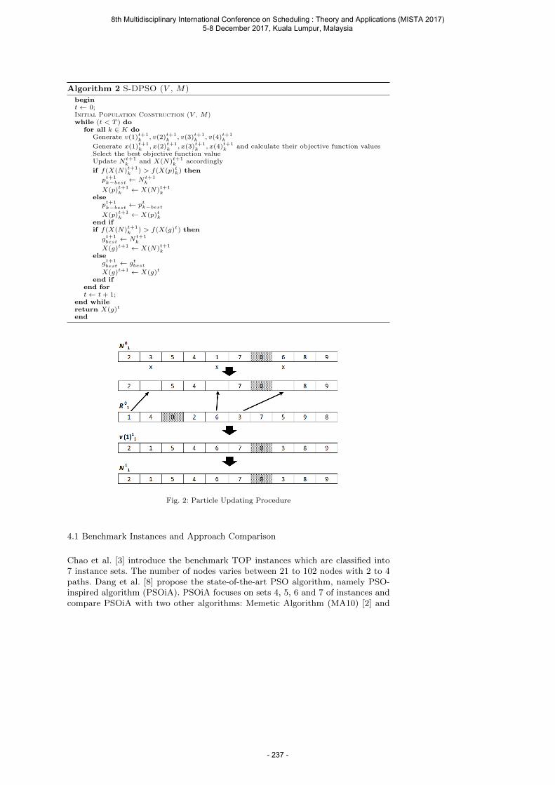
Algorithm 2 S-DPSO (V , M)

begint← 0;Initial Population Construction (V , M)while (t < T ) do

for all k ∈ K doGenerate v(1)t+1

k , v(2)t+1k , v(3)t+1

k , v(4)t+1k

Generate x(1)t+1k , x(2)t+1

k , x(3)t+1k , x(4)t+1

k and calculate their objective function valuesSelect the best objective function valueUpdate Nt+1

k and X(N)t+1k accordingly

if f(X(N)t+1k ) > f(X(p)tk) then

pt+1k−best ← Nt+1

k

X(p)t+1k ← X(N)t+1

kelse

pt+1k−best ← pt

k−best

X(p)t+1k ← X(p)tk

end ifif f(X(N)t+1

k ) > f(X(g)t) then

gt+1best ← Nt+1

k

X(g)t+1 ← X(N)t+1k

elsegt+1best ← gt

best

X(g)t+1 ← X(g)t

end ifend fort← t + 1;

end whilereturn X(g)t

end

Fig. 2: Particle Updating Procedure

4.1 Benchmark Instances and Approach Comparison

Chao et al. [3] introduce the benchmark TOP instances which are classified into7 instance sets. The number of nodes varies between 21 to 102 nodes with 2 to 4paths. Dang et al. [8] propose the state-of-the-art PSO algorithm, namely PSO-inspired algorithm (PSOiA). PSOiA focuses on sets 4, 5, 6 and 7 of instances andcompare PSOiA with two other algorithms: Memetic Algorithm (MA10) [2] and


- 237 -

PSO-based MA (PSOMA) [7]. PSOiA, MA10 and PSOMA are executed 10 timesfor each instance.

Righini and Salani [24] design the OPTW instances by modifying 29 Solomon’sinstances [26] and 10 Cordeau’s instances [5]. Montemanni and Gambardella [20]add another set of 37 instances for the OPTW. The TOPTW instances are gener-ated by extending the OPTW instances with different values of number of paths:2 to 4 paths. The performance of the S-DPSO algorithm is compared with twostate-of-the-art algorithms for the TOPTW: Iterative Three-Component Heuristic(I3CH) [12] and Artificial Bee Colony (ABC) [6]. I3CH is claimed to be superiorthan other algorithms, such as Iterated Local Search (ILS) [35], Slow SimulatedAnnealing (SSA) [17] and Granular Variable Neighborhood Search (GVNS) [15].ABC is selected since ABC is the latest population-based algorithm that has beenproposed for solving the TOPTW. It outperforms the earlier population-basedalgorithm, Ant Colony System (ACS) [20].

4.2 Algorithm Setup and Parameter Setting

The proposed S-DPSO algorithm is coded in C++. All experiments are performedon a PC with a 3.4 GHz processor and 20GB of RAM, under the Windows 7Operating System. Each experiment is performed for 10 runs, for which the bestand average results are presented. Take note that our algorithm uses the numberof iterations as the stopping criterion.

In our S-DPSO, there are five parameters that are used, namely the num-ber of particles |K|, the number of iterations T , three different acceleration val-ues, w, c1 and c2. Since parameter setting may affect the performance of thealgorithm, five instances were randomly selected from TOPTW and TOP in-stances for the parameter analysis. We set initial parameter values as follows:|K| = 15, 30, 60, T = 800, 1000, 1500, w = 0.3, 0.6, 0.9, c1 = 0.3, 0.6, 0.9and c2 = 0.3, 0.6, 0.9. After running preliminary experiments, the parameter val-ues that provide the best performance are: |K| = 30, T = 800, w = 0.9, c1 = 0.6and c2 = 0.6. This set of values would be used for solving the entire benchmarkinstances.

4.3 Computational Results

Table 1 compares S-DPSO with MA10 [2], PSOMA [7] and PSOiA [8]. The Numb

column provides the number of instances in a particular set of instances. Foreach algorithm, we calculate the percentage deviation of the best and averageresults of 10 runs with the best known solutions (BKs) for each instance. We thencalculate the average of both for each instance set, denoted as Pbest and Pavg,respectively. The CPU column represents the average CPU times (in seconds)used by a particular algorithm for solving a particular instance set. Additionally,we also calculate the number of instances in which the best known solutions areobtained, denoted as NBest.


- 238 -

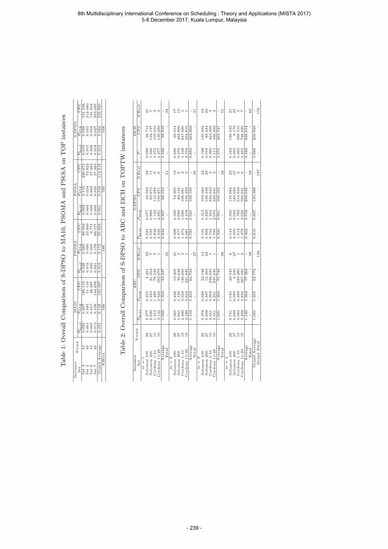
Table

1:

Over

all

Com

pari

son

of

S-D

PSO

toM

A10,

PSO

MA

and

PSO

iAon

TO

Pin

stance

s

Instance

Num

bM

A10

PSO

MA

PSO

iAS-D

PSO

Set

Pbest

Pavg

CPU

Pbest

Pavg

CPU

Pbest

Pavg

CPU

Pbest

Pavg

CPU

Set

454

0.0

30

0.2

07

189.1

19

0.0

26

0.2

85

86.9

94

0.0

02

0.1

10

226.6

73

0.0

16

0.0

29

191.1

08

Set

545

0.0

61

0.0

95

51.1

10

0.0

15

0.0

90

23.9

90

0.0

00

0.0

34

73.9

22

0.0

15

0.0

23

212.0

80

Set

615

0.0

00

0.0

17

28.3

87

0.0

00

0.0

00

9.7

71

0.0

00

0.0

00

37.2

63

0.0

00

0.0

04

131.8

04

Set

743

0.0

13

0.1

06

149.6

56

0.0

21

0.1

79

66.1

77

0.0

00

0.0

30

37.2

63

0.0

18

0.0

27

353.0

97

Grand

Average

0.0

31

0.1

29

123.3

97

0.0

19

0.1

73

55.8

56

0.0

01

0.0

56

112.9

18

0.0

15

0.0

24

235.8

20

NB

est

146

146

156

148

Table

2:

Over

all

Com

pari

son

of

S-D

PSO

toA

BC

and

I3C

Hon

TO

PT

Win

stance

s

Instance

Num

bABC

S-D

PSO

I3CH

Set

Pbest

Pavg

CPU

NB

est

Pbest

Pavg

CPU

NB

est

PCPU

NB

est

m=

1Solo

mon

100

29

0.2

77

0.4

55

4.4

21

22

0.0

23

0.0

77

44.5

93

28

0.6

88

26.7

14

21

Solo

mon

200

27

0.9

30

1.3

23

21.3

52

70.7

23

0.8

68

63.8

72

11

1.3

40

132.1

37

7Cordeau

1-1

010

1.2

12

1.4

89

78.5

40

50.8

38

1.1

22

115.2

93

61.0

72

109.0

10

3Cordeau

11-2

010

3.1

44

3.5

22

103.6

70

12.0

35

2.8

21

100.8

71

64.2

77

130.2

30

3

Average

1.0

09

1.3

03

33.2

47

-0.6

44

0.8

57

68.1

50

-1.4

42

88.6

16

-Total

--

-35

--

-51

--

34

m=

2Solo

mon

100

29

0.2

65

0.4

28

13.0

00

21

0.2

96

0.3

36

72.9

55

19

0.4

90

69.3

14

17

Solo

mon

200

27

0.8

41

1.1

58

30.6

48

30.5

77

0.6

90

84.1

34

60.4

70

463.8

00

10

Cordeau

1-1

010

2.4

99

3.0

34

149.6

90

21.4

73

1.6

86

196.6

91

21.1

08

247.0

60

3Cordeau

11-2

010

3.2

29

3.6

34

221.8

40

12.0

81

2.4

78

194.4

59

32.7

04

304.6

10

1

Average

1.1

53

1.4

52

64.7

34

-0.7

85

0.9

21

109.1

95

-0.8

56

263.8

08

-Total

--

-27

--

-30

--

31

m=

3Solo

mon

100

29

0.3

76

0.6

29

22.5

48

14

0.1

05

0.3

12

104.5

64

22

0.1

98

135.8

52

19

Solo

mon

200

27

0.2

48

0.3

47

12.4

93

22

0.4

92

0.8

29

106.4

48

20

0.0

16

89.2

44

25

Cordeau

1-1

010

2.4

51

2.9

04

228.9

30

10.7

52

1.2

54

334.9

43

30.3

60

424.0

00

3Cordeau

11-2

010

3.5

51

4.2

31

247.6

40

11.7

95

2.0

75

329.6

41

31.1

11

496.9

50

4

Average

1.0

21

1.3

02

75.7

49

-0.5

50

0.8

51

165.1

62

-0.2

75

204.7

21

-Total

--

-38

--

-48

--

51

m=

4Solo

mon

100

29

0.7

41

1.0

45

29.5

45

80.1

44

0.3

33

155.8

84

23

0.1

62

199.5

45

21

Solo

mon

200

27

0.0

00

0.0

00

0.5

30

27

0.0

00

0.0

33

160.0

36

27

0.0

00

0.1

70

27

Cordeau

1-1

010

3.0

83

3.4

89

233.2

80

11.6

14

1.7

82

514.9

43

20.3

65

566.5

10

5Cordeau

11-2

010

3.4

28

3.8

34

267.5

80

21.4

79

2.6

22

569.6

41

60.4

52

728.6

20

7

Average

1.1

40

1.3

62

77.3

64

-0.4

62

0.7

18

259.0

45

-0.1

69

246.6

14

-Total

--

-38

--

-58

--

60

Grand

Average

1.0

81

1.3

55

62.7

74

-0.6

10

0.8

37

150.3

88

-0.6

86

200.9

40

-G

rand

Total

--

-138

--

-187

--

176


- 239 -

We observe that S-DPSO outperforms MA10 and PSOMA in terms of thevalues of Pavg for each instance set except set 6 where PSOMA and PSOiA performbest. In terms of Pbest values, S-DPSO obtains the best values for sets 4 and 5.All algorithms are able to obtain the best known solutions for set 6 instances.On average (referring to ”Grand Average” values), S-DPSO is able to producebetter Pbest and Pavg values compared against those of MA10 and PSOMA. ItsPavg value is only 0.024% while MA10 and PSOMA values are 0.129% and 0.173%,respectively.

S-DPSO is comparable to PSOiA. In terms of Pavg, S-DPSO outperformsPSOiA in all instance sets, except set 6. On the other hand, PSOiA performsbetter than S-DPSO in most instance sets with respect to Pbest values. Note thatboth perform well in solving set 6 (Pmax = 0.000%). Finally, in terms of ”GrandAverage” values, we can draw a similar conclusion. S-DPSO produces a bettervalue of Pavg than the one of PSOiA. On the other hand, PSOiA performs best interms of Pbest.

Since we are not able to obtain the source codes of the state-of-the-art algo-rithms, we report their original CPU times. Dang et al. [8] mention that machineperformances of PSOiA, PSOMA and MA10 are almost the same. It is concludedthat PSOMA is faster than MA10 but less robust than PSOMA since the valueof Pavg is lower. Computational times of PSOiA and MA10 are almost the samebut PSOiA performs better than MA10. Based on this remark, it is worthy tomention that our S-DPSO is more robust than other algorithms but with the costof computational time. Take note that our computer is 1.5 × slower than the oneof PSOiA. In terms of NBest values, S-DPSO is able to obtain 148 best knownsolutions while MA10 and PSOMA only obtain 146 solutions. PSOiA performsbest by reaching 156 solutions.

Table 2 compares the performance of S-DPSO to those of ABC [6] and I3CH[12]. Since I3CH is only run once and we treat its results as the best results of I3CH,we only calculate P for I3CH. S-DPSO outperforms ABC in terms of the values ofPavg and Pbest for all values of m. However, S-DPSO requires more computationaltime. The values are from 0.550% to 0.921% while ABC values are always morethan 1.000%. The overall performances are represented by Grand Average valuesof Pbest and Pavg. S-DPSO is able to obtain 0.610% and 0.837%, respectively. Onthe other hand, ABC obtains 1.081% for Pbest and 1.355% for Pavg.

We compare the values of our Pavg with P values of I3CH. The average resultsPavg represents the average expected quality of the multiple-run algorithm whenit is executed only once [27]. S-DPSO is dominant in solving instances with m =1, but I3CH outperforms S-DPSO for other m values. In terms of computer spec,I3CH is around 2 times faster than ours. I3CH also run in parallel machines due tothe characteristics of the algorithm, while our S-DPSO is run in a sequential basis.We can conclude that S-DPSO spends less computational time than I3CH does.In conclusion, S-DPSO performs well within reasonable computational times.

S-DPSO obtains 187 best known solutions while I3CH and ABC obtain bestknown solutions for 176 and 138 instances, respectively. S-DPSO again outper-forms ABC in terms of NBest. S-DPSO requires more experiments (e.g multipleruns) compared with I3CH does in order to obtain more best known solutions.


- 240 -

5 Conclusion

We propose a discrete version of Particle Swarm Optimization (PSO), namelySelective-Discrete PSO (S-DPSO). We improve DPSO by introducing four differentmovement schemes: (a) following its own position, (b) moving towards its personalbest position, (c) moving towards the global best position, and (d) moving towardsthe combination of three above-mentioned schemes. The best movement schemeis selected in order to determine the next position of each particle. The proposedS-DPSO algorithm is tested on the benchmark instances of the Team OP and theTeam OP with Time Windows.

The results show that S-DPSO is capable of producing high-quality solutions.On four instance sets of TOP instances, an average run has a gap of only 0.024%with the best known solutions. It is able to find 148 (94.3%) best known solutions.For the TOPTW instances, the average gap is around 0.837% from the best knownsolutions. The best known solutions of 70.8% of instances are found. In general,S-DPSO is comparable to the state-of-the-art algorithms.

Future research areas include incorporating local search mechanism in the de-sign of the algorithm and the concept of accepting worse solutions (e.g. SimulatedAnnealing) that may lead us to better solutions. It would be more beneficial torun the algorithm in a parallel version due to the characteristics of the algorithm.The results are encouraging for the application of S-DPSO to solve other variantsof the OP, such as Time Dependent OP and Multi-Objective OP. Finally, it wouldbe interesting to apply the S-DPSO algorithm to solve other combinatorial opti-mization problems with similar characteristics, such as the vehicle routing problemand machine scheduling problems.

References

1. Archetti, C., Speranza, M.G., Vigo, D.: Vehicle routing problems with profits. In: P. Toth,D. Vigo (eds.) Vehicle Routing: Problems, Methods, and Applications, MOS-SIAM Serieson Optimization, chap. 10, pp. 273–298. SIAM, Philadelphia (2014)

2. Bouly, H., Dang, D.C., Moukrim, A.: A memetic algorithm for the team orienteeringproblem. 4OR 8(1), 49–70 (2010)

3. Chao, I.M., Golden, B.L., Wasil, E.A.: The team orienteering problem. European Journalof Operational Research 88(3), 464–474 (1996)

4. Chen, M.C., Hsiao, Y.H., Himadeep Reddy, R., Tiwari, M.K.: The self-learning particleswarm optimization approach for routing pickup and delivery of multiple products withmaterial handling in multiple cross-docks. Transportation Research Part E: Logistics andTransportation Review 91, 208–226 (2016)

5. Cordeau, J.F., Grendreau, M., Laporte, G.: A tabu search heuristic for periodic and multi-depot vehicle routing problems. Networks 30(2), 105–119 (1997)

6. Cura, T.: An artificial bee colony algorithm approach for the team orienteering problemwith time windows. Computers & Industrial Engineering 74, 270–290 (2014)

7. Dang, D.C., Guibadj, R.N., Moukrim, A.: A PSO-based memetic algorithm for the teamorienteering problem. In: C. Di Chio et al. (ed.) Applications of Evolutionary Computation,Lecture Notes in Computer Science, vol. 6625, pp. 471–480. Springer (2011)

8. Dang, D.C., Guibadj, R.N., Moukrim, A.: An effective PSO-inspired algorithm for theteam orienteering problem. European Journal of Operational Research 229(2), 332–344(2013)

9. El-Hajj, R., Dang, D., Moukrim, A.: Solving the team orienteering problem with cuttingplanes. Computers and Operations Research 74, 21–30 (2016)

10. Goksal, F.P., Karaoglan, I., Altiparmak, F.: A hybrid discrete particle swarm optimizationfor vehicle routing problem with simultaneous pickup and delivery. Computers & IndustrialEngineering 65(1), 39–53 (2013)


- 241 -

11. Gunawan, A., Lau, H.C., Vansteenwegen, P.: European Journal of Operational Research255(2), 315–332 (2016)

12. Hu, Q., Lim, A.: An iterative three-component heuristic for the team orienteering problemwith time windows. European Journal of Operational Research 232(2), 276–286 (2014)

13. Kashan, A.H., Karimi, B.: A discrete particle swarm optimization algorithm for schedulingparallel machines. Computers & Industrial Engineering 56(1), 216–223 (2009)

14. Kennedy, J., Eberhart, R.C.: Particle swarm optimization. In: Proceedings of the IEEEInternational Conference on Neural Networks, pp. 1942–1948 (1995)

15. Labadie, N., Mansini, R., Melechovsky, J., Calvo, R.W.: The team orienteering problemwith time windows: an LP-based granular variable neighborhood search. European Journalof Operational Research 220(1), 15–27 (2012)

16. Liao, C.J., Tseng, C.T., Luarn, P.: A discrete version of particle swarm optimizationfor flowshop scheduling problems. Computers & Operations Research 34(10), 3099–3111(2007)

17. Lin, S.W., Yu, V.F.: A simulated annealing heuristic for the team orienteering problemwith time windows. European Journal of Operational Research 217(1), 94–107 (2012)

18. Marinakis, Y., Marinaki, M.: A hybrid genetic-particle swarm optimization algorithm forthe vehicle routing problem. Expert Systems with Applications 37(2), 1446–1455 (2010)

19. Marinakis, Y., Marinaki, M., Dounias, G.: A hybrid particle swarm optimization algorithmfor the vehicle routing problem. Engineering Applications of Artificial Intelligence 23(4),463–472 (2010)

20. Montemanni, R., Gambardella, L.M.: Ant colony system for team orienteering problemwith time windows. Foundations of Computing and Decision Sciences 34(4), 287–306(2009)

21. Muthuswamy, S., Lam, S.S.: Discrete particle swarm optimization for the team orienteeringproblem. Memetic Computing 3(4), 287–303 (2011)

22. Pampara, G., Franken, N., Engelbrecht, A.P.: Combining particle swarm optimisationwith angle modulation to solve binary problems. In: Proceedings of the IEEE Congresson Evolutionary Computation, vol. 1, pp. 89–96 (2005)

23. Pan, Q.K., Fatih Tasgetiren, M.F., Liang, Y.C.: A discrete particle swarm optimizationalgorithm for the no-wait flowshop scheduling problem. Computers & Operations Research35(9), 2807–2839 (2008)

24. Righini, G., Salani, M.: Decremental state space relaxation strategies and initializationheuristics for solving the orienteering problem with time windows with dynamic program-ming. Computers & Operations Research 36(4), 1191–1203 (2009)

25. Sevkli, Z., Sevilgen, F.E.: Discrete particle swarm optimization for the orienteering prob-lem. In: Proceedings of 2010 IEEE Congress on Evolutionary Computation (CEC), pp.1–8 (2010)

26. Solomon, M.: Algorithms for the vehicle routing and scheduling problems with time win-dow constraints. Operations Research 35(2), 254–265 (1987)

27. Souffriau, W., Vansteenwegen, P., Vanden Berghe, G., Oudheusden, D.V.: The multicon-straint team orienteering problem with multple time windows. Transportation Science47(1), 53–63 (2013)

28. Strasser, S., Goodman, R., Sheppard, J., Butcher, S.: A new discrete particle swarm opti-mization algorithm. In: Proceedings of the Genetic and Evolutionary Computation Con-ference 2016, GECCO ’16, pp. 53–60. ACM, New York, NY, USA (2016)

29. Tasgetiren, M.F., Suganthan, P.N., Pan, Q.Q.: A discrete particle swarm optimizationalgorithm for the generalized traveling salesman problem. In: Proceedings of the Geneticand Evolutionary Computation Conference 2007, GECCO ’07, pp. 158–167. ACM, NewYork, NY, USA (2007)

30. The, J.A., Kachitvichyanukul, V.: Particle swarm optimization and two solution repre-sentations for solving the capacitated vehicle routing problem. Computers & IndustrialEngineering 56(1), 380–387 (2009)

31. The, J.A., Kachitvichyanukul, V.: A particle swarm optimization for the vehicle routingproblem with simultaneous pickup and delivery. Computers & Operations Research 36(5),1693–1702 (2009)

32. Tseng, C.T., Liao, C.J.: A discrete particle swarm optimization for lot-streaming flowshopscheduling problem. European Journal of Operational Research 191(2), 360–373 (2008)

33. Tsiligirides, T.: Heuristic methods applied to orienteering. Journal of the OperationalResearch Society 35(9), 797–809 (1984)


- 242 -

34. Vansteenwegen, P., Souffriau, W., Van Oudheusden, D.: The orienteering problem: A sur-vey. European Journal of Operational Research 209(1), 1–10 (2011)

35. Vansteenwegen, P., Souffriau, W., Vanden Berghe, G., Van Oudheusden, D.: Iterated localsearch for the team orienteering problem with time windows. Computers & OperationsResearch 36(12), 3281–3290 (2009)

36. Yu, V.F., Jewpanya, P., Kachitvichyanukul, V.: Particle swarm optimization for the multi-period cross-docking distribution problem with time windows. International Journal ofProduction Research 54(2), 509–525 (2016)


- 243 -

MISTA 2017

Home Health Care Delivery Problem

Aldy Gunawan · Hoong Chuin Lau · Kun Lu.

Abstract We address the Home Health Care Delivery Problem (HHCDP), whichis concerned with staff scheduling in the home health care industry. The goal is toschedule health care providers to serve patients at their homes that maximizes thetotal collected preference scores from visited patients subject to several constraints,such as workload of the health care providers, time budget for each provider andso on. The complexity lies in the possibility of cancellation of patient bookingsdynamically, and the generated schedule should attempt to patients’ preferredtime windows. To cater to these requirements, we model the preference score asa step function which depends on the arrival time of the visit and the resultingproblem as the Team Orienteering Problem (TOP) with soft Time Windows andVariable Profits. We propose a fast algorithm, Iterated Local Search (ILS), whichhas been widely used to solve other variants of the Orienteering Problem (OP). Wefirst solve the modified benchmark Team OP with Time Window instances followedby randomly generated instances. We conclude that ILS is able to provide goodsolutions within reasonable computational times.

1 Introduction

The demand for home health care (HHC) services has increased substantially dueto population aging [20]. HHC provides a wide range of services, including nursingcare, medical, paramedical and social services, that can be provided to patients athome [14,16]. Due to aging populations, the demand for HHC is rapidly increasing.For example, in 2011, more than 4 million patients received HHC services in the

Aldy GunawanSingapore Management UniversityE-mail: [email protected]

Hoong Chuin LauSingapore Management UniversityE-mail: [email protected]

Kun LuSingapore Management UniversityE-mail: [email protected]


- 244 -

U.S. [6]. Ministry of Health (MOH) Singapore introduces Intermediate and Long-Term Care (ILTC) services for patients who require further care and treatmentafter being discharged from an acute hospital as well as community-dwelling seniorresidents who may be frail and need supervision or assistance with their activitiesof daily living. In 2013, MOH developed a set of home care guidelines.

This study addresses a particular application problem of the staff scheduling inthe home health care industry, namely the Home Health Care Delivery Problem(HHCDP), on a daily basis. In the context of the classical scheduling problem,HHCDP is considered as a workforce scheduling and routing problem. Workforcescheduling and routing problem refers to those scenarios involving the mobiliza-tion of personnel in order to perform work related activities at different locations[2]. Staffs are mostly required to travel from one location to other locations inorder to perform the work since the number of works across different locationsis usually larger than the available number of employees. Several real-world re-quirements, such as time windows, transportation modality, start-end locations,skills and qualifications, increase the complexity of the problem. For more detailsabout workforce scheduling and routing problems, the reader can refer to [2]. TheHHCDP is considered as a combination of staff rostering and VRP with timewindows in [25].

In our context, instead of considering as a VRP (which is in essence a demandperspective), we view this problem from the supply perspective as well. While wetry to satisfy as many patients as possible, the number of requests may exceedthe service capacity and some of them may be cancelled after the schedule hasbeen generated. Since we want to maximize the patients’ satisfaction, measuredin terms of scores, our problem can be modelled as a variant of the OrienteeringProblem (OP).

In the standard OP, a set of agents are scheduled to serve a set of customers(e.g. patients). Each agent is limited by the time budget and time windows. Eachcustomer can only be visited at most once. For simplicity, we assume that allagents start and end at the same location (e.g. the hospital). The problem incor-porates other real-world requirements related to the health care industry, such asthe continuity of care, workload fairness and demand uncertainty (due to requestcancellations). We allow the agent to arrive late with a certain penalty value ratherthan not visiting the patient. In the OP term, the collected score is affected by thepenalty value, if any. As some requests from patients may be cancelled due to un-foreseen factors after the schedule has been generated, we express such uncertaintyas a probability of occurrence which is assumed to be known beforehand.

Hence, this paper considers HHCDP from both provider and patient perspec-tives - while we maximize the workload utilization rate of providers without vi-olating their time budgets, we also maximize the satisfaction level of patientswith respect to the number of patients to be visited by allowing late arrivals. Weterm our problem as the Team OP with soft Time Windows and Variable Profits(TOPsTWVP). For a comprehensive review of the OP, the reader can refer to thetwo surveys by Vansteenwegen et al. [23] and Gunawan et al. [10].

We explore the potential of Iterated Local Search (ILS) to solve HHCDP. ILSis a simple but effective metaheuristic [15] and has been applied successfully tosolve different variants of the OP, such as works by Vansteenwegen et al. [24] andGunawan et al. [8,11]. We adopt a similar algorithm [11] with several modifications,


- 245 -

such as tackling variable scores/profits, and soft time window constraints. Here,we name it as Enhanced ILS (EnILS).

The main contributions of this paper are listed below:

– We introduce a new variant of the Team Orienteering Problem with soft TimeWindows and Variable Profits (TOPsTWVP). To the best of our knowledge,this is the first study dealing with both soft Time Windows and VariableProfits. In this problem, late service is allowed with an appropriate penalty thataffects the score/profit. By relaxing the time windows, the number of visitedpatients will increase without affecting patients’ satisfaction significantly.

– Most of interesting applications of the OP are in logistics, tourism and defense.We extend the application of the OP to solve the Home Health Care SchedulingProblem (HHCSP).

– We adopt and implement a fast Iterated Local Search algorithm that has beenused for solving other variants of the OP [11]. Note that some obtained resultsare also feasible for the original TOPTW problem. They are comparable to thestate-of-the-art algorithms.

The remainder of this paper is organized as follows. Section 2 summarizesthe relevant literature. The description of the HHCDP problem including themathematical formulation, is presented in Section 3. The Iterated Local Searchis explained in Section 4. Section 5 presents computational experiments. Finally,Section 6 describes the conclusions, limitations and possible future works of ourresearch.

2 Related Work

Since our problem is an extension of the TOPsTWVP model, we start by review-ing the literature on the OP and its related variants briefly, followed by the relatedresearch on the HHCDP. The OP has been extensively studied in various applica-tions, such as the mobile crowdsourcing problem, the Tourist Trip Design Problem(TTDP), the logistic problem and others [10].

Erdogan and Laporte [5] introduced the OP with Variable Profits (OPVP). Thescore for each node is associated with a parameter that determines the percentageof score collected, either as a discrete or continuous function of the time spent.One example of the OPVP application arises in the fishing sectors. Longer stays atcertain locations may increase the amount of fish caught. In their work, a branch-and-cut algorithm is proposed to solve some modified TSP instances. There is stillroom for improvement since the algorithm requires large computational times andcan only solve small instances.

Mota et al. [18] modeled the operating room scheduling problem in terms ofchoice elective patients, aiming for throughput maximization, as a new variant ofthe TOPTW, namely the TOP double Time Windows (TOPdTW). Both pathsand nodes have a time window to be fulfilled. The number of paths equals to thenumber of operating rooms times the number of shifts times the number of dayswhile the number of nodes refers to the number of operating rooms. A genetic algo-rithm is proposed to solve benchmark TOPTW instances and randomly generatedTOPdTW instances. The computational results are promising although they arestill preliminary.


- 246 -

The Home Health Care problem aims to provide the care and support neededto patients in their own homes [1]. It covers different supports, such as elderlypeople, people with physical disabilities. Cisse et al. [4] classified the Home HealthCare Routing and Scheduling Problem (HHCRSP) process into three differentlevels: strategic, tactical and operational levels, and mapped the into related ORproblems. They extended the earlier review [6] which only covers articles before2016. The details of relevant features, constraints, objectives and methods in theexisting HHCRSP studies are also presented.

Rasmussen et al. [21] looked at the daily home care crew scheduling problem asa generalization of the Vehicle Routing Problem with Time Windows (VRPTW).The problem is formulated as a set partitioning problem and solved by an exactbranch-and-price algorithm. Visit clustering schemes are also developed in orderto reduce computational times significantly, with the cost of the quality of thesolutions. The schemes are able to find solutions of larger instances, which cannotbe solved optimally. Akjiratikarl et al. [1] also considered the home care workerscheduling problem as the VRPTW.

Yuan and Fugenschuh [25] presented a case study on the problem of schedulingnurses on a weekly basis with the objective of minimizing the total cost as wellas the total working time, without compromising the service quality. The problemis treated as a combination of the staff rostering problem and the VRPTW. Theproposed algorithm which is based on local search approaches can produce anestimation of cost reduction up to 10% in solving a real-world instance.

Lin et al. [14] addressed a particular problem of the Home Health Care thatprovides therapy services, namely the Therapist Assignment Problem (TAP). Theproblem is described from patient and therapist perspectives and modeled as amixed-integer programming model. The model is validated by using an instanceextracted from a rehabilitation service provide in Hong Kong and some randomlygenerated instances.

Chen et al. [3] introduced a multi-period Home Health Care Scheduling Prob-lem under stochastic service and travel times. The chance constraints are intro-duced into the formulation in order to cope with uncertainty in durations. Theeffectiveness of the proposed approaches is tested on synthetic instances for bothdeterministic and stochastic scenarios.

Nguyen and Montemanni [19] addressed the nurse home services problem andproposed two mixed integer linear programming models based on Big-M methodand arc timing method, respectively. Both models cater soft and hard time win-dows. Certain penalties would be imposed if the service starts between certainperiods. However, hard time windows are also imposed to avoid unnecessary over-time. Experiments are conducted on a set of randomly generated instances.

3 Home Health Care Delivery Problem (HHCDP)

We formulate the HHCDP as an Integer Linear Programming (ILP) model. TheHHCDP is defined as the following tuple: 〈N,T 〉. Let N be a set of locations,N = Nt ∪ Ns, where Nt and Ns represent a set of patients’ locations and healthcare providers’ start-end locations, respectively. Here, we assume start and endlocations for all providers are at the same location, location 0 (Ns = 0). T is a


- 247 -

symmetric pairwise travel time matrix and tij ∈ T denotes the travel time betweentwo different locations i and j. Let M be a set of health care providers.

Each patient’s location i ∈ Nt has a positive dependent reward uim that wouldbe collected when he/she is visited by provider m. In most cases, patients preferto be visited by their primary provider. This is reflected by a higher reward inour case. Each visit requires a service time Ti and it should be started withina particular time window [ei, li]. ei and li refer to the earliest and latest timesallowed for starting the visit at location i. We allow a late arrival with the costof penalty although this is undesirable. On the other hand, if the provider arrivesbefore ei, the waiting time occurs.

Since we assume location 0 is the start and end locations, therefore u0m =T0 = 0. Each provider m ∈ M is constrained within the time limit [e0, l0]. Wehave e0 = 0 and l0 = Tmax, where Tmax is the time budget or the maximumduration to complete a duty day. The objective is to maximize the expected totalcollected score from visiting patients by all providers. We include the penalty in theobjective function value due to a late visit. The penalty is calculated by multiplyinga certain percentage of reduction to a particular score (R1, R2, . . . , Rn) ∈ [0, 1].For example, if the arrival at location i is late and less than δi, the adjusted scorewould be R1 × uim. The details can be referred below:

uim =

0, if (Sim − li) ≤ 0;

R1 × uim, if 0 < (Sim − li) ≤ δi;R2 × uim, if δi < (Sim − li) ≤ 2× δi;...

Rn × uim, if (n− 1)× δi < (Sim − li) ≤ n× δi.

The following decision variables are used in the mathematical model:

– Xijm = 1 if a visit to patient i is followed by a visit to patient j by providerm, 0 otherwise.

– Yim = 1 if a visit to patient i by provider m, 0 otherwise.– Sim = the start time of service at patient i by provider m.

The HHCDP mathematical formulation is adopted from the work of [11] withseveral modifications:

Maximize∑

m∈M

∑i∈N\0

πiYimuim (1)

∑j∈N\0

X0jm = 1 , ∀m ∈M (2)

∑i∈N\0

Xi0m = 1 , ∀m ∈M (3)

∑i∈N\0

Xikm = Ykm , ∀k ∈ N \ 0,m ∈M (4)

∑j∈N\0

Xkjm = Ykm , ∀k ∈ N \ 0,m ∈M (5)


- 248 -

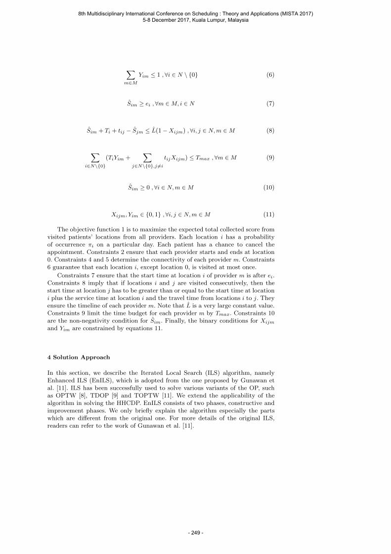
∑m∈M

Yim ≤ 1 , ∀i ∈ N \ 0 (6)

Sim ≥ ei ,∀m ∈M, i ∈ N (7)

Sim + Ti + tij − Sjm ≤ L(1−Xijm) ,∀i, j ∈ N,m ∈M (8)

∑i∈N\0

(TiYim +∑

j∈N\0,j 6=i

tijXijm) ≤ Tmax , ∀m ∈M (9)

Sim ≥ 0 , ∀i ∈ N,m ∈M (10)

Xijm, Yim ∈ 0, 1 ,∀i, j ∈ N,m ∈M (11)

The objective function 1 is to maximize the expected total collected score fromvisited patients’ locations from all providers. Each location i has a probabilityof occurrence πi on a particular day. Each patient has a chance to cancel theappointment. Constraints 2 ensure that each provider starts and ends at location0. Constraints 4 and 5 determine the connectivity of each provider m. Constraints6 guarantee that each location i, except location 0, is visited at most once.

Constraints 7 ensure that the start time at location i of provider m is after ei.Constraints 8 imply that if locations i and j are visited consecutively, then thestart time at location j has to be greater than or equal to the start time at locationi plus the service time at location i and the travel time from locations i to j. Theyensure the timeline of each provider m. Note that L is a very large constant value.Constraints 9 limit the time budget for each provider m by Tmax. Constraints 10are the non-negativity condition for Sim. Finally, the binary conditions for Xijm

and Yim are constrained by equations 11.

4 Solution Approach

In this section, we describe the Iterated Local Search (ILS) algorithm, namelyEnhanced ILS (EnILS), which is adopted from the one proposed by Gunawan etal. [11]. ILS has been successfully used to solve various variants of the OP, suchas OPTW [8], TDOP [9] and TOPTW [11]. We extend the applicability of thealgorithm in solving the HHCDP. EnILS consists of two phases, constructive andimprovement phases. We only briefly explain the algorithm especially the partswhich are different from the original one. For more details of the original ILS,readers can refer to the work of Gunawan et al. [11].


- 249 -

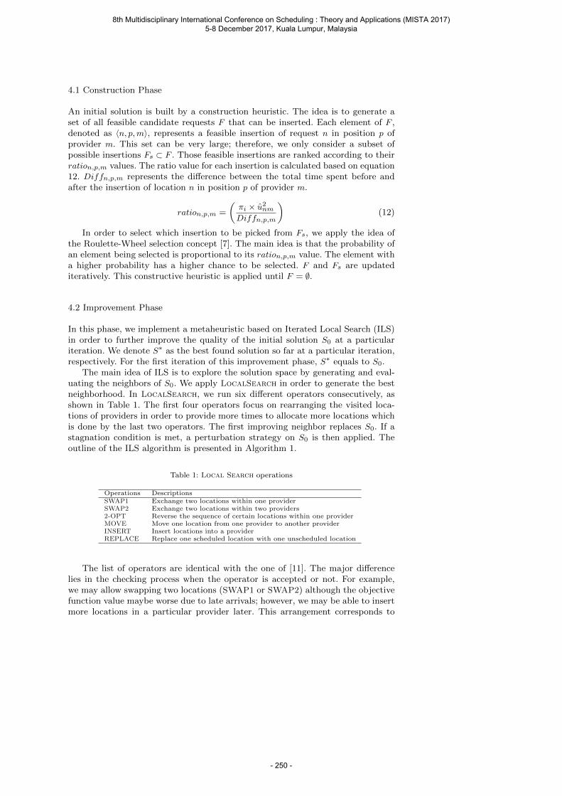
4.1 Construction Phase

An initial solution is built by a construction heuristic. The idea is to generate aset of all feasible candidate requests F that can be inserted. Each element of F ,denoted as 〈n, p,m〉, represents a feasible insertion of request n in position p ofprovider m. This set can be very large; therefore, we only consider a subset ofpossible insertions Fs ⊂ F . Those feasible insertions are ranked according to theirration,p,m values. The ratio value for each insertion is calculated based on equation12. Diffn,p,m represents the difference between the total time spent before andafter the insertion of location n in position p of provider m.

ration,p,m =

(πi × u2nmDiffn,p,m

)(12)

In order to select which insertion to be picked from Fs, we apply the idea ofthe Roulette-Wheel selection concept [7]. The main idea is that the probability ofan element being selected is proportional to its ration,p,m value. The element witha higher probability has a higher chance to be selected. F and Fs are updatediteratively. This constructive heuristic is applied until F = ∅.

4.2 Improvement Phase

In this phase, we implement a metaheuristic based on Iterated Local Search (ILS)in order to further improve the quality of the initial solution S0 at a particulariteration. We denote S∗ as the best found solution so far at a particular iteration,respectively. For the first iteration of this improvement phase, S∗ equals to S0.

The main idea of ILS is to explore the solution space by generating and eval-uating the neighbors of S0. We apply LocalSearch in order to generate the bestneighborhood. In LocalSearch, we run six different operators consecutively, asshown in Table 1. The first four operators focus on rearranging the visited loca-tions of providers in order to provide more times to allocate more locations whichis done by the last two operators. The first improving neighbor replaces S0. If astagnation condition is met, a perturbation strategy on S0 is then applied. Theoutline of the ILS algorithm is presented in Algorithm 1.

Table 1: Local Search operations

Operations DescriptionsSWAP1 Exchange two locations within one providerSWAP2 Exchange two locations within two providers2-OPT Reverse the sequence of certain locations within one providerMOVE Move one location from one provider to another providerINSERT Insert locations into a providerREPLACE Replace one scheduled location with one unscheduled location

The list of operators are identical with the one of [11]. The major differencelies in the checking process when the operator is accepted or not. For example,we may allow swapping two locations (SWAP1 or SWAP2) although the objectivefunction value maybe worse due to late arrivals; however, we may be able to insertmore locations in a particular provider later. This arrangement corresponds to


- 250 -

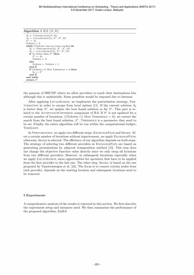
Algorithm 1 ILS (N,M)

S0 ← Construction(N,M)S0 ← LocalSearch(S0, N

∗, N ′,M)S∗ ← S0

NoImpr ← 0while TimeLimit has not been reached do

S0 ← Perturbation(S0, N∗, N ′,M)

S0 ← LocalSearch(S0, N∗, N ′,M)

if S0 better than S∗ thenS∗ ← S0

NoImpr ← 0else

NoImpr ← NoImpr + 1end ifif (NoImpr+1) Mod Threshold = 0 then

S0 ← S∗

end ifend whilereturn S∗

the purpose of HHCDP where we allow providers to reach their destinations latealthough this is undesirable. Some penalties would be imposed due to lateness.

After applying LocalSearch, we implement the perturbation strategy, Per-

turbation in order to escape from local optima [11]. If the current solution S0is better than S∗, we update the best found solution so far S∗. This part is re-lated to the AcceptanceCriterion component of ILS. If S∗ is not updated for acertain number of iterations, ((NoImpr+1) Mod Threshold = 0), we restart thesearch from the best found solution, S∗. Threshold is a parameter that need tobe set. Finally, the entire algorithm will be run within the computational budget,TimeLimit.

In Perturbation, we apply two different steps: ExchangePath and Shake. Af-ter a certain number of iterations without improvement, we apply ExchangePath;otherwise, Shake is selected. The efficiency of our algorithm depends on both steps.The strategy of selecting two different providers in ExchangePath are based ongenerating permutations by adjacent transposition method [13]. This step doesnot change the objective function value directly since we only swap all locationsfrom two different providers. However, in subsequent iterations especially whenwe apply LocalSearch, more opportunities for operators that have to be appliedfrom the first provider to the last one. The other step, Shake, is based on the oneproposed by Vansteenwegen et al. [24]. The focus is to remove certain nodes fromeach provider, depends on the starting location and subsequent locations need tobe removed.

5 Experiments

A comprehensive analysis of the results is reported in this section. We first describethe experiment setup and instances used. We then summarize the performance ofthe proposed algorithm, EnILS.


- 251 -

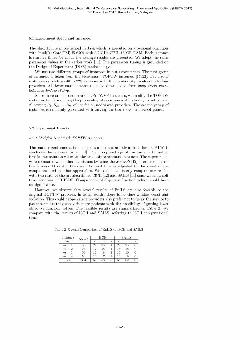
5.1 Experiment Setup and Instances

The algorithm is implemented in Java which is executed on a personal computerwith Intel(R) Core(TM) i5-6500 with 3.2 GHz CPU, 16 GB RAM. Each instanceis run five times for which the average results are presented. We adopt the sameparameter values in the earlier work [11]. The parameter tuning is grounded onthe Design of Experiment (DOE) methodology.

We use two different groups of instances in our experiments. The first groupof instances is taken from the benchmark TOPTW instances [17,22]. The size ofinstances varies from 48 to 228 locations with the number of providers up to fourproviders. All benchmark instances can be downloaded from http://www.mech.

kuleuven.be/en/cib/op.

Since there are no benchmark TOPsTWVP instances, we modify the TOPTWinstances by 1) assuming the probability of occurrence of node i, πi, is set to one,2) setting R1, R2, . . . , Rn values for all nodes and providers. The second group ofinstances is randomly generated with varying the two above-mentioned points.

5.2 Experiment Results

5.2.1 Modified benchmark TOPTW instances

The most recent comparison of the state-of-the-art algorithms for TOPTW isconducted by Gunawan et al. [11]. Their proposed algorithms are able to find 50best known solution values on the available benchmark instances. The experimentswere compared with other algorithms by using the SuperP i [12] in order to ensurethe fairness. Basically, the computational time is adjusted to the speed of thecomputers used in other approaches. We could not directly compare our resultswith two state-of-the-art algorithms: I3CH [12] and SAILS [11] since we allow softtime windows in HHCDP. Comparisons of objective function values would haveno significance.

However, we observe that several results of EnILS are also feasible to theoriginal TOPTW problem. In other words, there is no time window constraintviolation. This could happen since providers also prefer not to delay the service topatients unless they can visit more patients with the possibility of getting lowerobjective function values. The feasible results are summarized in Table 2. Wecompare with the results of I3CH and SAILS, referring to I3CH computationaltimes.

Table 2: Overall Comparison of EnILS to I3CH and SAILS

InstanceNumb

I3CH SAILSSet < = > < = >

m = 1 76 21 25 1 22 25 0m = 2 76 17 18 1 18 18 0m = 3 76 10 8 2 10 10 0m = 4 76 18 7 2 18 9 0Total 304 66 58 6 68 62 0


- 252 -

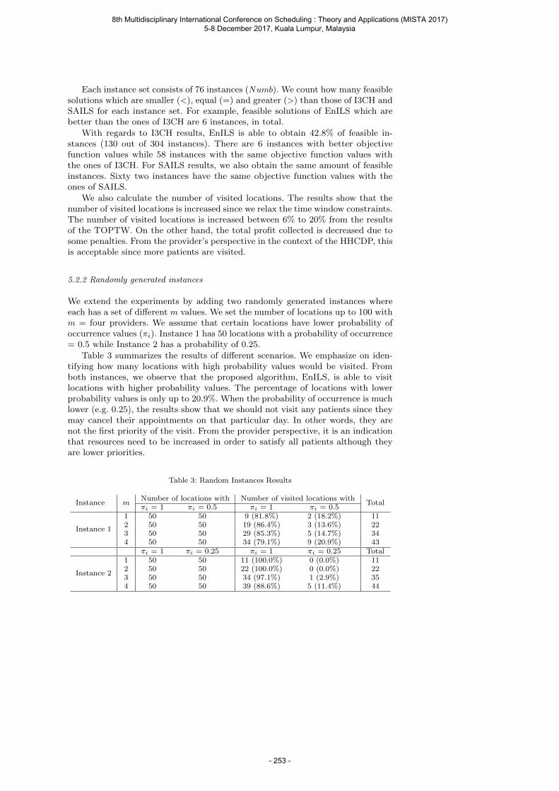
Each instance set consists of 76 instances (Numb). We count how many feasiblesolutions which are smaller (<), equal (=) and greater (>) than those of I3CH andSAILS for each instance set. For example, feasible solutions of EnILS which arebetter than the ones of I3CH are 6 instances, in total.

With regards to I3CH results, EnILS is able to obtain 42.8% of feasible in-stances (130 out of 304 instances). There are 6 instances with better objectivefunction values while 58 instances with the same objective function values withthe ones of I3CH. For SAILS results, we also obtain the same amount of feasibleinstances. Sixty two instances have the same objective function values with theones of SAILS.

We also calculate the number of visited locations. The results show that thenumber of visited locations is increased since we relax the time window constraints.The number of visited locations is increased between 6% to 20% from the resultsof the TOPTW. On the other hand, the total profit collected is decreased due tosome penalties. From the provider’s perspective in the context of the HHCDP, thisis acceptable since more patients are visited.

5.2.2 Randomly generated instances

We extend the experiments by adding two randomly generated instances whereeach has a set of different m values. We set the number of locations up to 100 withm = four providers. We assume that certain locations have lower probability ofoccurrence values (πi). Instance 1 has 50 locations with a probability of occurrence= 0.5 while Instance 2 has a probability of 0.25.

Table 3 summarizes the results of different scenarios. We emphasize on iden-tifying how many locations with high probability values would be visited. Fromboth instances, we observe that the proposed algorithm, EnILS, is able to visitlocations with higher probability values. The percentage of locations with lowerprobability values is only up to 20.9%. When the probability of occurrence is muchlower (e.g. 0.25), the results show that we should not visit any patients since theymay cancel their appointments on that particular day. In other words, they arenot the first priority of the visit. From the provider perspective, it is an indicationthat resources need to be increased in order to satisfy all patients although theyare lower priorities.

Table 3: Random Instances Results

Instance mNumber of locations with Number of visited locations with

Totalπi = 1 πi = 0.5 πi = 1 πi = 0.5

Instance 1

1 50 50 9 (81.8%) 2 (18.2%) 112 50 50 19 (86.4%) 3 (13.6%) 223 50 50 29 (85.3%) 5 (14.7%) 344 50 50 34 (79.1%) 9 (20.9%) 43

πi = 1 πi = 0.25 πi = 1 πi = 0.25 Total

Instance 2

1 50 50 11 (100.0%) 0 (0.0%) 112 50 50 22 (100.0%) 0 (0.0%) 223 50 50 34 (97.1%) 1 (2.9%) 354 50 50 39 (88.6%) 5 (11.4%) 44


- 253 -

6 Conclusion

In this paper, we address the Home Health Care Delivery Problem (HHCDP) andmodel it as a variant of the Orienteering Problem (OP), namely the Team OPwith soft Time Windows and Variable Profit (TOPsTWVP). In HHCDP, we al-low a late visit to the patients. The problem is solved by a fast algorithm, IteratedLocal Search. The ILS algorithm is able to provide good solutions within reason-able computational times for two different sets of instances: modified benchmarkTOPTW instances and randomly generated instances.

We summarize some directions in which future work on this problem can beexplored. The optimal solutions or best known solutions for modified instances andrandomly generated instances are still unknown. Therefore, we consider to developan exact algorithm in order to provide us with the optimal solutions. In order totest the robustness of the proposed algorithm, we will apply the sampling basedapproach in order to simulate the probability of occurrence of demands in certainlocations and analyze the performance of the proposed algorithm. Certain locationsmay have higher probabilities and it is expected that the proposed algorithmselect those locations with higher probabilities. More randomly generated instanceswould be generated in order to provide and capture real world scenarios.

Acknowledgements This research is funded by the National Research Foundation Singaporeunder its Corp Lab @ University scheme and Fujitsu Limited as part of the A*STAR-Fujitsu-SMU Urban Computing and Engineering Centre of Excellence.

References

1. Akjiratikarl, C., Yenradee, P., Drake, P.R.: PSO-based algorithm for home care workerscheduling in the UK. Computers & Industrial Engineering 53, 559–583 (2007)

2. Castillo-Salazar, J.A., Landa-Silva, D., Qu, R.: Workforce scheduling and routing prob-lems: literature survey and computational study. Annals of Operations Research 239(1),39–67 (2016)

3. Chen, C., Rubinstein, Z.B., Smith, S.F., Lau, H.C.: Tackling large-scale home health caredelivery problem with uncertainty. In: Proceedings of the 27th International Conferenceon Automated Planning and Scheduling (ICAPS 2017), 18-23 June 2017, Pittsburgh, USA(2017)

4. Cisse, M., Yalc.indag, S., Kergosien, Y., S. ahin, E., Lene, C., Matta, A.: OR problems relatedto home health care: A review of relevant routing and scheduling problems. OperationsResearch for Health Care (2017). DOI http://dx.doi.org/10.1016/j.orhc.2017.06.001

5. Erdogan, G., Laporte, G.: The orienteering problem with variable profits. Networks 61(2),104–116 (2013)

6. Fikar, C., Hirsch, P.: Home Health Care Routing and Scheduling: A Review. Computers& Operations Research 77, 86–95 (2017)

7. Goldberg, D.E.: Genetic Algorithms in Search, Optimization, and Machine Learning.Addison-Wesley, Reading, Massachusetts (1989)

8. Gunawan, A., Lau, H.C., Lu, K.: An iterated local search algorithm for solving the ori-enteering problem with time windows. In: G. Ochoa, F. Chicano (eds.) proceedings ofthe 15th European Conference on Evolutionary Computation in Combinatorial Optimisa-tion (EvoStar 2015), 8-10 April 2015, Copenhagen, Denmark, Lecture Notes in ComputerScience, vol. 9026, pp. 61–73. Springer-Verlag, Berlin, Germany (2015)

9. Gunawan, A., Lau, H.C., Lu, K.: Enhancing local search with adaptive operator orderingand its application to the time dependent orienteering problem. In: Proceedings of the 11thInternational Conference on the Practice and Theory of Automated Timetabling (PATAT2016), 23-26 August 2016, Udine, Italy (2016)


- 254 -

10. Gunawan, A., Lau, H.C., Vansteenwegen, P.: Orienteering problem: A survey of recentvariants, solution approaches and applications. European Journal of Operational Research255(2), 315–332 (2016)

11. Gunawan, A., Lau, H.C., Vansteenwegen, P., Kun, L.: Well-tuned algorithms for the teamorienteering problem with time windows. Journal of the Operational Research Society68(8), 861–876 (2017)

12. Hu, Q., Lim, A.: An iterative three-component heuristic for the team orienteering problemwith time windows. European Journal of Operational Research 232(2), 276–286 (2014)

13. Johnson, S.M.: Generation of permutations by adjacent transposition. Mathematics ofComputation 17(83), 282–285 (1963)

14. Lin, M., Chin, K.S., Wang, X., Tsui, K.L.: The therapist assignment problem in homehealthcare structures. Expert Systems with Applications 62, 44–62 (2016)

15. Lourenco, H., Martin, O., Stutzle, T.: Iterated local search. In: Handbook of metaheuris-tics, pp. 320–353. Springer (2003)

16. Medicare.gov.: that’s home health care & what should i expect.https://www.medicare.gov/what-medicare-covers/home-health-care/home-health-care-what-is-it-what-to-expect.html (2016)

17. Montemanni, R., Gambardella, L.M.: Ant colony system for team orienteering problemwith time windows. Foundations of Computing and Decision Sciences 34(4), 287–306(2009)

18. Mota, G., Abreu, M., Quintas, A., Ferreira, J., Dias, L.S., Pereira, G.A.B., Oliveira, J.A.:A genetic algorithm for the TOPdTW at operating rooms. In: B. Murgante, S. Misra,M. Carlini, C.M. Torre, H.Q. Nguyen, D. Taniar, B.O. Apduhan, O. Gervasi (eds.) Pro-ceeding of the 13th International Conference on Computational Science and Its Applica-tions (ICCSA 2013), Lecture Notes in Computer Science, vol. 7971, pp. 304–317. Springer(2013)

19. Nguyen, T.V.L., Montemanni, R.: Mathematical programming models for home healthcareservice optimisation. International Journal of Operational Research 25(4), 449–463 (2016)

20. OECD: Health at a glance 2013:OECD indicators. Organization for Economic Cooperationand Development, Paris, France (2013)

21. Rasmussen, M.S., Justesen, T., Dohn, A., Larsen, J.: The home care crew schedulingproblem: Preference-based visit clustering and temporal dependencies. European Journalof Operational Research 219(3), 598–610 (2012)

22. Righini, G., Salani, M.: New dynamic programing algorithms for the resource constrainedelementary shortest path problem. Networks 51(3), 155–170 (2008)

23. Vansteenwegen, P., Souffriau, W., Van Oudheusden, D.: The orienteering problem: A sur-vey. European Journal of Operational Research 209(1), 1–10 (2011)

24. Vansteenwegen, P., Souffriau, W., Vanden Berghe, G., Van Oudheusden, D.: Iterated localsearch for the team orienteering problem with time windows. Computers & OperationsResearch 36(12), 3281–3290 (2009)

25. Yuan, Z., Fugenschuh, A.: Home health care scheduling: a case study. In: Proceedings of the7th Multidisciplinary International Conference on Scheduling : Theory and Applications(MISTA 2015), 25-28 Aug 2015, Prague, Czech Republic, pp. 555–569 (2015)


- 255 -

MISTA 2017

Hyper-heuristics using Reinforcement Learning for the Examination Timetabling Problem

Kehan Han • Paul McMullan

Abstract Selection Hyper-heuristics as general-purpose search methods controlling a set of low level heuristics have

been successfully applied to various problem domains. A key to designing an effective selection Hyper-heuristic is to

find the right combination of heuristic selection and move acceptance methods which are invoked successively under

an iterative single-point-based search framework. The examination timetabling problem is a well-known challenging

real world problem faced recurrently by many educational institutions across the world. In this study, we investigate

various reinforcement learning techniques for heuristic selection embedded into a selection Hyper-heuristic using

simulated annealing with reheating for examination timetabling. Reinforcement learning maintains a utility score for

each low level heuristic. At each iteration, a heuristic is selected based on those adaptively updated utility scores and

applied to the solution at hand with the goal of improvement. All selection Hyper-heuristics using different

reinforcement learning schemes are tested on the examination timetabling benchmark of ITC 2007. The results show

that -decay-Greedy reinforcement learning which chooses a low level heuristic with the maximum utility score with

a decaying probability rate, otherwise choosing a random low level heuristic performs the best. The proposed tuned

approach although does not perform as good as the state-of-the-art, it delivers a better performance than some existing

Hyper-heuristics.

Keyword: reinforcement learning, Hyper-heuristic, exam timetabling

1 Introduction

The research involved in the search for suitable solutions for Examination timetabling problems requires a

combination of practical and experimental-based techniques [1]. The main focus of current Hyper-heuristic research

is towards the design and adaptation of heuristic methods in automating optimisation for hard computational search

problems. Over the last few decades a lot of research has been conducted on the application of Hyper-heuristic

techniques in solving examination timetabling problems. A number of review papers highlighting these efforts have

been published [2], [3]. Experimental results generated by various different techniques in the literature have been

reported, focussing on success measures including generality of the solver and the time cost [2].

For a given examination timetabling problem, whether a technique can generate a feasible and workable solution

within a practical time limit is an important factor in assessing the success level of the technique employed. The

solving process of the examination timetabling problem normally commonly consists of two main stages; the initial

construction stage and the subsequent improvement stage. In this first stage, a feasible solution is constructed. Along

with feasibility, some focus is given to the relative quality of the solution in terms of satisfying the problem, to benefit

the improvement stage which is more computationally time-consuming. Then, in the second stage, the solution

undergoes a series of improvement transformations until the process terminates. In this case this will occur when the

time limit is reached. The improvement process outlined in this paper describes a Hyper-heuristic search methodology

used to search for higher quality solutions when given specific objectives [4].

In the literature, research on the application of Hyper-heuristic techniques to solve examination timetabling

problems has proved the potential of their effectiveness in this area. Certain research has focussed on combining

reinforcement learning with Hyper-heuristics, yielding competitive results which suggest that reinforcement learning

can be applied to improve the performance of Hyper-heuristics in terms of solution quality. However, the work in the


- 256 -

literature mainly focus on bringing reinforcement learning theory into the hyper-heuristic instead of actual

reinforcement learning techniques.

This works aims at investigating how the various Reinforcement Learning algorithms can be used to improve

the performance of Hyper-heuristics. In this work, rather than simply applying reinforcement learning trial-and-error

schemes within the Hyper-heuristic as in the literature, actual algorithms and techniques from Reinforcement Learning

are designed and integrated into the Hyper-heuristic to solve the examination timetabling problem. In the approach

described here, the initial feasible solution is created using Squeaky Wheel construction, with a Hyper-heuristic

employed for the optimization and improvement phase. The Hyper-heuristic methods consists of two levels; one is

the higher heuristic search from the low-level heuristics pool, and the other is the low-level heuristic search process

within the problem domain. For the higher-level heuristics, a Simulated Annealing (SA) method is combined with

different reinforcement learning methods to enable intelligence-based selection of the low level heuristics. In each

iteration information is gathered to establish and record the current total performance of low level heuristics. The

selection methods inspired by the reinforcement learning are three different greedy search methods and the softmax

method, which are compared with a simple random method to analysis performance difference. For the low level

heuristics, we designed six small-move low-level heuristics, three large-move low-level heuristics and two directed

low-level heuristics. This can also be considered as an interesting approach to explore how the generality of the

solution process can be improved using reinforcement learning. An assessment can be made on how the combination

of reinforcement learning algorithms with Hyper-heuristics may widen the application of solvers to other types of

resource allocation problems.

The remainder of the paper is as follows: Section 2 briefly describes the background of this paper, the

examination timetabling problem and the Hyper-heuristic method. Section 3 describes the Squeaky Wheel constructor

and our RL-SA Hyper-heuristic method (Algorithm 1). Section 4 describes the experimental environment and time

parameters used during experimentation. Section 5 presents and discusses the results and section 6 concludes the paper

with a brief discussion on the effectiveness of the technique and potential future research areas.

2 Background

2.1 The Examination Timetabling Problem

Examination timetabling is one of the academic timetabling problems and has been proven to be NP-hard [5].

Solving an examination timetabling problem requires allocating the given exams with suitable timeslots and rooms

under both hard and soft constraints. Among these constraints, all hard constraints must be satisfied in order to achieve

a feasible solution, with the satisfaction of the soft constraints used to determine the quality of a given solution.

Therefore, the solving process consists of two main parts: first, the generation of a feasible solution that meets all the

hard constraints; second, minimization of violations to the soft constraints of the current solution while maintaining

feasibility. What’s more, the quality of (feasible) timetables can be calculated numerically based on the satisfaction

level of the soft constraints which can be used to help in the evaluation of the corresponding algorithms. In the

examination timetabling problems, before the scheduling process all the student enrolment data is generally known,

which allows an accurate use of the available resources during the examination period.

In real-world examination timetabling problems, the type and parameter values of the hard and soft constraints

varies between institutions. In particular, the soft constraints usually reflect an institutions’ different preferences. As

interest has increased on the application of research to examination timetabling problems, benchmarks which identify

the common soft and hard constraints from real world institutions using various standard defined measures have

emerged. These are used to advance the field of research in solving Examination Timetabling problems in providing

a way to allow meaningful scientific comparison and the public exchange of research achievements and expertise in

the domain.

2.2 Hyper-heuristic

The use of Hyper-heuristics involves combining a set of approaches that share the common goal of automating

the design and adaptation of heuristic methods in order to solve hard computational search problems [21]. A heuristic

refers to a whole search algorithm or used to refer to a particular decision process sitting within some repetitive control

structure, while meta-heuristic refers to an overall control strategy exploring a solution search-space [21]. Unlike

meta-heuristics, Hyper-heuristics search in a space of low level heuristics [22].


- 257 -

Specifically, a Hyper-heuristic can be seen as a process which, when given a particular problem instance and a

number of low-level heuristics, manages the selection of which low level heuristic to apply at any given time, until a

stopping condition is met [21]. The Hyper-heuristic operates at a higher level of abstraction without knowledge of the

domain in which it operates. It only has access to a set of low level heuristics [22], simple local search operators or

domain dependent heuristics [22], while the higher level strategy (High Heuristics, for selecting or generating

heuristics) can either be a heuristic, a sophisticated knowledge-based technique, or a learning mechanism [20].

2.3 Related work

The research on solving examination timetabling problems involves a variety of different Hyper-heuristic

methodologies. Graph colouring Hyper-heuristics were investigated as a new constructive Hyper-heuristic method to

solve the examination timetabling problems in [24]. The author utilized the hierarchical hybridizations of four low

level graph colouring heuristics which including largest degree, saturation degree, largest coloured degree and largest

enrolment to produce four ordered lists. The sequence of exams selection for scheduling is based on the generated

lists. Furthermore, a roulette wheel selection mechanism is included in the algorithm to improve the effectiveness of

timeslot selection, aiming at probabilistically selecting an appropriate timeslot for the chosen exam. The proposed

approach was tested upon the Carter benchmarks as well as the ITC2007 benchmarks. The experimental results proved

that the graph colouring constructive Hyper-heuristic is capable of producing good results and outperforming other

approaches on various benchmark instances.

Inspired by the musical improvisation process, the Harmony Search Algorithm (HSA) is a relatively new

metaheuristic algorithm and is used within the Harmony Search-based Hyper-heuristic (HSHH) for solving

examination timetabling problems. The Harmony Search algorithm will operate at a high level of abstraction which

intelligently evolves a series of low-level heuristics in the improvement process. Each low-level heuristic equates to

a move and swap strategy. The authors tested the proposed method using ITC-2007 benchmark datasets, with 12

different datasets of various complexity and size. The proposed method produced strong competitively comparable

results.

Monte Carlo based hyper heuristics are designed and implemented to solve the examination problems in [6].

Simulated annealing involving a reheating scheme was introduced to this Monte Carlo based hyper heuristic. However,

this method compared poorly as compared to other Hyper-heuristic methods. The author believes that the reason for

this is due to fundamental weaknesses such as the choice of appropriate rewarding mechanism and the evaluation of

the utility values used for heuristic selection. The conclusions suggested that the use of a choice function rather than

incorporating Simulated Annealing might improve the method itself.

Burke et al. brings forward the concept of the reinforcement learning process to hyper heuristics in [7]. In this

paper, Hyper-heuristic methodologies were identified to search the heuristic selection space and use selected low level

heuristics to search the problem domain. According to the general definition, their proposed method is an iterative

Hyper-heuristic framework formed of a single candidate solution and multiple perturbative low level heuristics.

Basically, two parts including the heuristic selection and the move acceptance with certain termination criteria formed

this algorithm. Inspired by related work in this area, one of the main focuses of this study is to analyse the working

processes of learning heuristic selection within the automatic search for examination timetabling solutions..

3 RL-SA based Hyper-heuristic Algorithm

The Hyper-heuristic algorithm solving process for this research consists of two stages; first an initial construction

phase which generates a feasible solution, secondly a further improvement phase to ultimately achieve a better solution.

In the construction stage, we use Squeaky Wheel construction [8] & [14] while the optimization stage is based on the

Simulated Annealing process, combining reinforcement learning with the use of Hyper-heuristics.

3.1 RL-SA based Hyper-heuristic Optimization

The Hyper-heuristic consists of three main parts; the move acceptance Simulated Annealing algorithm [10], [11],

[12] & [13], heuristic selection method Reinforcement Learning algorithms and a set of various low level heuristics.

The selection method will select from the low-level heuristics pool to optimize the current solution. The selected low

heuristic will propose a move to optimize the current solution. The move acceptance is the reference for the algorithm


- 258 -

in deciding whether to accept this move or not. For each low heuristic, a utility value is used to represent its

performance and is updated dynamically. The utility update methods are also based on reinforcement learning

algorithms.

Algorithm 1: RL-SA ALGORITHM

Input –u: array holding utility value for each heuristic, totalTime, 𝑇0: initial temperature

1. // initialisation

2. Generate a random complete solution Scurrent ;

3. Initialise utility values;

4. fbest =fcurrent = f0 = quality( Scurrent );Sbest=Scurrent; //Sbest holds the best solution

5. startTime = t = time();

6. Temp=T0;sinceImp=0; numNonImprovingReheat=0;maxReheatTimes,=5;reheatFrequency=1000;

7. bool bImprovementFound=false;

8. // main loop executes until total running time allowed is exceeded

9. while ( t < totalTime ) //while running time still enough

10. // heuristic selection

11. i = selectHeuristic( u ); // select a heuristic using the utility values

12. Stemp = applyHeuristic( i, Scurrent);//update temperare solution using selected low heuristic i

13. ftemp = quality( Stemp );//update temperare evaluate value

14. t = time() – startTime;//update remaining time

15. // move acceptance

16. Δ = ftemp − fcurrent;

17. if (Δ < 0)// improving move

18. u[i] = reward( u[i] );Scurrent = Stemp;

19. else u[i] = punish( u[i] ); // worsening move

20. r ← random ∈ [0,1];

21. if ( Δ < 0 ||r < 𝑃(Δ, Temp) )// accept if non-worsening or with the Boltzmann probability of P

22. if (Δ < 0) Scurrent = Stemp;fcurrent=ftemp; bImprovementFound=true;

23. if (ftemp<fbest) Sbest = Stemp; else sinceImp++;

24. if (sinceImp==reheatFrequency) //when reach non improvement limit

25. sinceImp = 0; //reset since last improvement count to 0

26. if(!bImprovementFound) numNonImprovingReheat++;

27. else bImprovementFound=false;

28. if(numNonImprovingReheat>maxReheatTimes) //when reach max reheating limit

29. numNonImprovingReheat = 0;

30. Temp = (T0 - Temp) / 2.0;

31. fbest = (long)Math.Round(fbest * 1.1);

32. else Temp = Temp / 0.85;//increase temperature

33. else Temp=Temp*0.9;// decrease temperature

34. return Sbest;

3.2 Reinforcement Learning

Reinforcement Learning (RL) is a general term for a set of widely used approaches which provide a learning

mechanism in determining how to behave against certain outcomes, or “how to map situations to actions" through

trial-and-error interactions [9]. The proposed heuristic selection method involved the design of four different selection

methods as well as four different low heuristic utility reward/punish methods inspired by reinforcement learning

algorithms. The detailed design description of different Reinforcement Learning inspired heuristic selection methods

as well as utility update methods are given in the rest of this section. The experimental comparisons are presented in

chapters 5.3 and 5.4 respectively.


- 259 -

3.2.1 Selection methods

(0) Equal Sequence

In this selection method, each low heuristic will be selected in sequence to ensure each will be applied in equal

measure. This is inspired by the Maximize Explore theory used within reinforcement learning.

(1) Greedy

In this selection method, the process checks whether all the low-level heuristics have been selected at least once.

If not, a random low heuristic is selected, with this process continuing until all low-level heuristics have been selected.

From this point the low heuristic with the highest current utility value will be selected. Where there are more than one

low heuristic selected, one is chosen randomly from the contenders.

(2) -Greedy

In this selection method, random selection is employed until all low heuristic has been selected at least once.

After that, if the random probability is smaller than greedy probability , low-level heuristics are selected at random.

Otherwise, the low heuristic with the highest utility value is selected. In determining the most effective value for the

greedy probability , experimental tests were performed with set to 0.1 as well as set to 0.01.

(3) -Decay-Greedy

Similar to the previous method, although the value of the greedy probability is dynamic, decreasing in value as

the optimization process continues. The rational for this is based on the principle that as the Hyper-heuristic algorithm

learns, the random low heuristic will become less necessary. The algorithm for this selection method is outlined in

detail below.

Algorithm 2: e-decay-greedy

input: iteration: current iteration times;llhList: arraylist of all the low-level heuristics

1. int index;//index of low heuristic

2. double edecay = 1 / (System.Math.Sqrt(iteration));

3. Random randDouble = new Random();

4. if (randDouble.NextDouble() < edecay || !checkSelected(llhList))

5. //under edecay probablity, do random select

6. Random randInt = new Random();

7. index = randInt.Next(0, llhList.Count);

8. else

9. index = llhMaxUtilityIndex(llhList);

10. index = randomDuplicateSelectionSum(index, llhList);

11. //select one of the highest utility heuristic

12. return index;

(4) softmax selection

Unlike the previously described selection methods, this calculates the softmax probability value for each low

heuristic and uses this probability value for selecting among the low-level heuristics.

3.2.2 Utility update methods

Within the process of updating the utility values, a positive “reward” (increment) is given to a low heuristic if it

was effective in generating a better solution, otherwise a “punish” value is applied. For all of the utility update methods,

the lower bound of the utility value is set to 0, upper bound set to 40 and initial value of 20. These values were reached

as a result of trial experimentation.

(5) Sum utility

In this method the reward value is +1 and the punish value is -1.

(6) Average utility value/Monte Carlo

In this method the reward value is +1 and the punish value is -1. The sum utility is then divided by the iteration

count to set as an average.

(7) Discount sum

This method is similar to the first utility update method, although the positive reward and negative punish values

are dynamic. The positive reward value is calculated as (+1)*(0.9^ (iteration times)), with the negative punish value

calculated as (-1)*(0.9^ (iteration times)).


- 260 -

Algorithm 3: Discount Sum Utility method

Input: bool flag: reward or punish, int index, llhList: heuristics arrylist, SelectedTimes, discountFactor=0.9.

1. for (int i = 0; i < llhList.Count; i++)

2. if (llhList[i].LlhId == index)

3. if(flag) llhList[i].utility+= (+1) * discountFactorR^selectedTimes;

4. else llhList[i].utility+= (-1) * discountFactorR^selectedTimes;

(8) Temporal difference

The theory of this utility update method is that it will estimate the future possible reward based the current

performance of each low-level heuristics. First, this method will calculate the sum utility with the reward and punish

values (again set as +1 and -1 respectively). Secondly, an estimate reward value is calculated. The selected probability

of the current low heuristic in the next step is 1.0 / (number of low-level heuristics) and the reward Probability (the

probability it might make an improvement in the next iteration if selected) is 0.5 (50%). Therefore the estimate reward

is (selected Probability)*(reward Probability). This estimate reward is then added to the current calculated sum utility

as the low heuristic’s final utility value. The step size value has been experimentally tested between 1 and 5 to

determine the most effective setting.

3.3 Low-level heuristics design

For this work, 19 low-level heuristics were implemented, grouped into four main types of heuristic and described

below. Most of the above low-level heuristics are either 1-opt or 2-opt and there is also a mixture of some randomness

and deterministic selection of exams and slots. We purposely test low-level heuristics with simple moves rather than

low-level heuristic with intelligence and complex moves because we want to make sure that the Hyper-heuristic

can recognise good moves and make an intelligent decision based on these simple moves. Furthermore, we

want to make the problem-domain knowledge heuristics easy to implement and the Hyper-heuristic more

generalised.

3.3.1 Small perturbative moves

Table 1: small heuristics

H1 (random period assignment):

Select a Random Exam in Period P1 with Room assignment R1.

Assign Exam to Random Period P2 (if feasible), do not change Room assignment.

H2 (random room assignment):


Move the Exam to a feasible Random Room R2 – do not change the Period.

H3 (random assignment):


Assign Exam to Random Period P2 (if feasible) and Random Room R2 which can accommodate the exam (if

feasible – exclusive constraint).

H4 (random period swap):

Select 2 Random Exams, one in Period P1 with Room assignment R1 and the other in Period P2 (≠P1) with

Room assignment R2.

Swap them both to the others Periods (if both feasible) – no swapping of Rooms.

H5 (random room swap):

Select 1 Random Exam with Room assignment R1 (ignore the period – ensure not exclusive).

Select another Random Exam with similar capacity requirement assigned to Room R2 (≠R1).

Swap them both to the others Room (if both feasible, e.g. both not exclusive) – no swapping of Periods.

H6 (random exam swap):

Select 1 Random Exam with Room assignment R1 in Period P1.

Select another Random Exam Room assignment R2 in Period P2, Swap them both to the others Room (if both

feasible, e.g. both not exclusive) and swapping their Periods.


- 261 -

3.3.2 Large perturbative moves

Table 2: large heuristics

H7 (random group of exams swap based on period):

Select two Random Periods P1 and P2 and swap ALL exams between them.

H8 (random group of exams move based on period):

Select one Period P1 and move each exam assigned to that period to a new feasible period, one by one (APPLY

H1).

H7_2 (random group of exams swap based on room):

Select two Random Room R1 and R2 and swap ALL exams between them.

H8_2 (random group of exams move based on period):

Select one Room R1 and move each exam assigned to that room to a new feasible room, one by one (APPLY

H2).

H7_3 (random group of exams swap based on timeslot):

Select two Random Timeslot T1 and T2 and swap ALL exams between them.

H8_3 (random group of exams move based on period):

Select one Timeslot T1 and move each exam assigned to that timeslot to a new feasible timeslot, one by one

(APPLY H3).

Note: Timeslot in the above table refers to the combination of period and room.

3.3.3 Very large moves

Table 3: shuffle heuristics

H9 (random group of exams shuffle based on period):

Shuffle all periods at random. Loop over all Periods i=P_1..P_K; H6(i, Random(i+1,K)).

H9_2 (random group of exams shuffle based on room):

Shuffle all rooms at random. Loop over all Rooms i=R_1..R_K; H6(i, Random(i+1,K)).

H9_3 (random group of exams shuffle based on timeslot):

Shuffle all timeslots at random. Loop over all Timeslots i=T_1..T_K; H6(i, Random(i+1,K)).

3.3.4 Directed moves

Table 4: directed heuristics

H10 (ranked exams group move - consider both hard and soft constraint violations):

Generate a weighted-List based on all hard and soft constraint violations for exams.

For the top 10 exams in the list, re-allocate them to a random new timeslot.

The new timeslot is selected from the suitabletimeslot-List.

Update weighted-List whenever a move is made.

H10_2 (ranked exams group swap - consider both hard and soft constraint violations):

Generate a weighted-List based on all hard and soft constraint violations for exams.

From the top 10 exams in the list, select two random exams, swap their timeslot.

Update weighted-List whenever a move is made

H11 (ranked exams group move - consider only soft constraint violations):


- 262 -

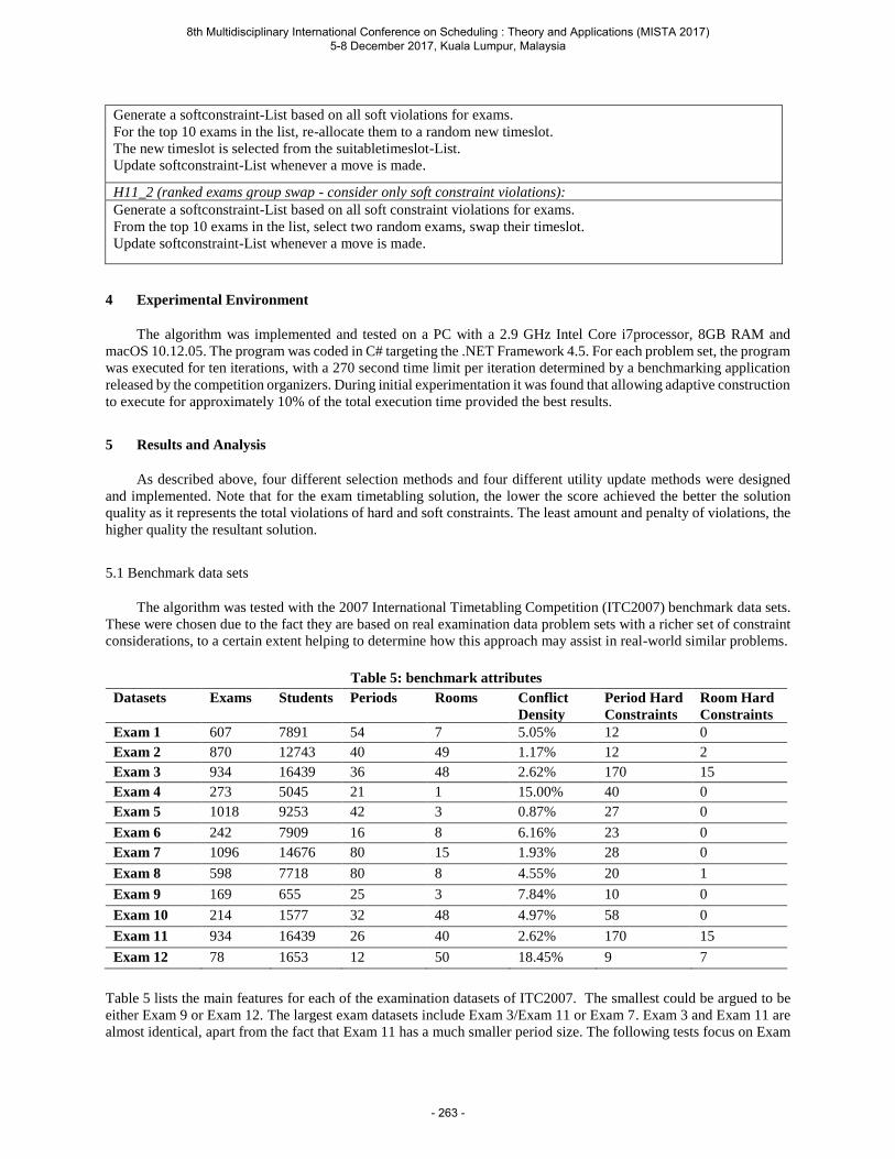
Generate a softconstraint-List based on all soft violations for exams.

For the top 10 exams in the list, re-allocate them to a random new timeslot.

The new timeslot is selected from the suitabletimeslot-List.

Update softconstraint-List whenever a move is made.

H11_2 (ranked exams group swap - consider only soft constraint violations):

Generate a softconstraint-List based on all soft constraint violations for exams.

From the top 10 exams in the list, select two random exams, swap their timeslot.

Update softconstraint-List whenever a move is made.

4 Experimental Environment

The algorithm was implemented and tested on a PC with a 2.9 GHz Intel Core i7processor, 8GB RAM and

macOS 10.12.05. The program was coded in C# targeting the .NET Framework 4.5. For each problem set, the program

was executed for ten iterations, with a 270 second time limit per iteration determined by a benchmarking application

released by the competition organizers. During initial experimentation it was found that allowing adaptive construction

to execute for approximately 10% of the total execution time provided the best results.

5 Results and Analysis

As described above, four different selection methods and four different utility update methods were designed

and implemented. Note that for the exam timetabling solution, the lower the score achieved the better the solution

quality as it represents the total violations of hard and soft constraints. The least amount and penalty of violations, the

higher quality the resultant solution.

5.1 Benchmark data sets

The algorithm was tested with the 2007 International Timetabling Competition (ITC2007) benchmark data sets.

These were chosen due to the fact they are based on real examination data problem sets with a richer set of constraint

considerations, to a certain extent helping to determine how this approach may assist in real-world similar problems.

Table 5: benchmark attributes

Datasets

Exams Students

Periods Rooms Conflict

Density

Period Hard

Constraints

Room Hard

Constraints

Exam 1 607 7891 54 7 5.05% 12 0

Exam 2 870 12743 40 49 1.17% 12 2

Exam 3 934 16439 36 48 2.62% 170 15

Exam 4 273 5045 21 1 15.00% 40 0

Exam 5 1018 9253 42 3 0.87% 27 0

Exam 6 242 7909 16 8 6.16% 23 0

Exam 7 1096 14676 80 15 1.93% 28 0

Exam 8 598 7718 80 8 4.55% 20 1

Exam 9 169 655 25 3 7.84% 10 0

Exam 10 214 1577 32 48 4.97% 58 0

Exam 11 934 16439 26 40 2.62% 170 15

Exam 12 78 1653 12 50 18.45% 9 7

Table 5 lists the main features for each of the examination datasets of ITC2007. The smallest could be argued to be

either Exam 9 or Exam 12. The largest exam datasets include Exam 3/Exam 11 or Exam 7. Exam 3 and Exam 11 are

almost identical, apart from the fact that Exam 11 has a much smaller period size. The following tests focus on Exam


- 263 -

7, 9, 11 and 12 as they include the biggest and smallest data size as well as conflict density and provide a reasonable

variation for testing purposes. The tests on the four datasets were used to guide the design of the final Hyper-heuristic

reheating scheme, selection method and the utility value update method.

5.2 Simulated Annealing operator tests

For the simulated annealing process, four groups of experiments were carried out to define the best settings for

reheating frequency and to determine whether to combine the reheating scheme with the reset of the low-level

heuristics utility value on reaching the maximum reheating count (which is 5).

5.2.1 Reheating frequency

In the literature, the Simulated Annealing value is usually suggested as 10000 [10] & [11]. However in this

approach, to help avoid getting caught within local optima, the reheating times are reduced to 1000, verified as

effective via experimentation. The reheating frequency is tested at values 1000 and 10000 on Exam 7, 9, 11 and 12

with ten runs for each dataset. Here, a simple random selection method and sum utility update method is used, and the

utility value is not reset when the maximum reheating count is reached.

Table 6: reheating frequency tests

Datasets reheat frequency = 1000 reheat frequency = 10000

AVG BEST AVG BEST

Exam 7 8631 8497 8858 8805

Exam 9 1347 1278 1352 1300

Exam 11 35782 35266 35504 35611

Exam 12 5985 5965 6034 5911

The results presented in table 6 above suggest that the reheat frequency of 1000 is generally better. Therefore, in

the following test the reheat frequency is set as 1000.

5.2.2 Reset low-level heuristics value

The utility values of the low-level heuristics can become similar in value after a certain amount of iterations,

which can adversely affect the selection methods and render the process ineffective. We test the approaches of both

resetting and not resetting the utility value of the low-level heuristics when the maximum reheating point has been

reached. This uses a simple -greedy selection method and sum utility update method.

Table 7: reset low-level heuristics utility value tests

Datasets reset No reset

AVG BEST AVG BEST

Exam 7 7530 6721 7890 7528

Exam 9 1340 1320 1520 1506

Exam 11 35733 35519 35673 35375

Exam 12 5995 5955 6015 6165

The results presented in table 7 above suggest that generally the performance is improved by resetting the utility

value of all low-level heuristics on reaching the maximum reheating iteration count. Therefore, this approach is

adopted in the selection method tests outlined in the next section.

5.3 Selection Method test

As described above, four different selection methods were designed, some with differing operators. Tests were

performed on all the selection methods with different operator values on Exam 7, 9, 11 and 12 with ten runs per dataset.


- 264 -

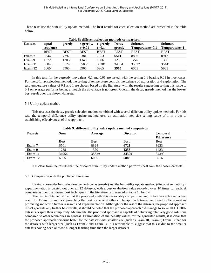
These tests use the sum utility update method. The best results for each selection method are presented in the table

below.

Table 8: different selection methods comparison

Datasets equal

sequence

greedy e-greedy,

e=0.01

e-greedy,

e=0.1

Decay

greedy

Softmax,

Temperature=0.1

Softmax,

Temperature=1

BEST BEST BEST BEST BEST BEST BEST

Exam 7 8644 7792 8381 7953 6501 8856 8912

Exam 9 1372 1303 1343 1306 1288 1276 1396

Exam 11 35840 35295 35038 35281 34054 35832 35441

Exam 12 6065 5965 5965 5965 5965 6065 5965

In this test, for the -greedy two values, 0.1 and 0.01 are tested, with the setting 0.1 beating 0.01 in most cases.

For the softmax selection method, the setting of temperature controls the balance of exploration and exploitation. The

test temperature values of 0.1 and 1 are chosen based on the literature, with the results suggesting setting this value to

0.1 on average performs better, although the advantage is not great. Overall, the decay greedy method has the lowest

best result over the chosen datasets.

5.4 Utility update method

This test uses the decay greedy selection method combined with several different utility update methods. For this

test, the temporal difference utility update method uses an estimation step-size setting value of 1 in order to

establishing effectiveness of this approach.

Table 9: different utility value update method comparison

Datasets Sum Average Discount Temporal

Difference

Best Best Best Best

Exam 7 6501 8824 6721 9233

Exam 9 1288 1370 1258 1423

Exam 11 34954 35529 34390 34399

Exam 12 6065 6065 5883 5916

It is clear from the results that the discount sum utility update method performs best over the chosen datasets.

5.5 Comparison with the published literature

Having chosen the best selection method (decay greedy) and the best utility update method (discount sum utility),

experimentation is carried out over all 12 datasets, with a best evaluation value recorded over 10 times for each. A

comparison over the current best techniques in the literature is presented in table 10 below.

The results obtained show that the proposed method is reasonably competitive, and in fact has achieved a best

result for Exam 10, and is approaching the best for several others. The approach taken can therefore be argued as

promising and worth further research and experimentation. Although for the rest of the datasets, the proposed approach

didn’t generate any further best results, it should be noted that the proposed approach did manage to solve all ITC2007

datasets despite their complexity. Meanwhile, the proposed approach is capable of delivering relatively good solutions

compared to other techniques in general. Examination of the penalty values for the generated results, it is clear that

the proposed approach performs better for the datasets with smaller size (such as Exam 10, Exam 6, Exam 9) than for

the datasets with larger size (such as Exam 7 and Exam 3). It is reasonable to suggest that this is due to the smaller

datasets having been allowed a longer learning time than the larger datasets.


- 265 -

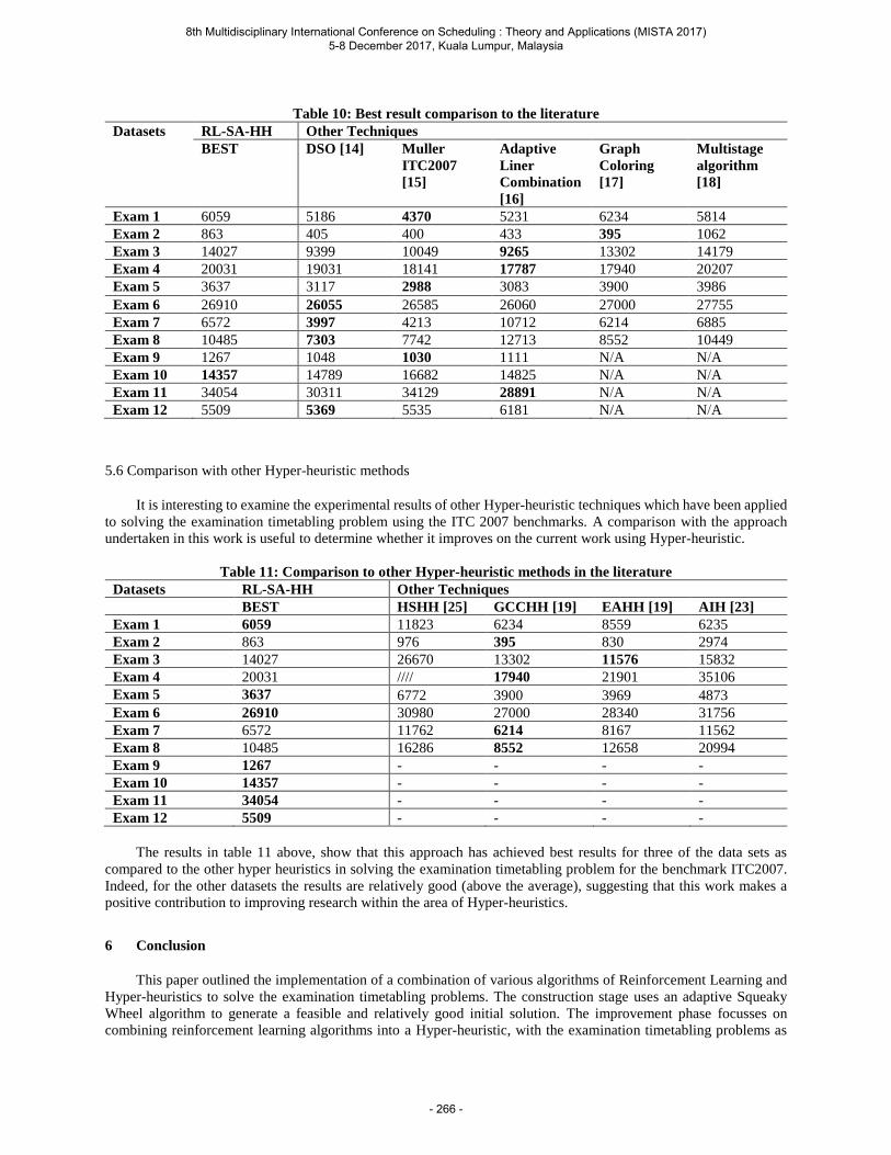
Table 10: Best result comparison to the literature

Datasets RL-SA-HH Other Techniques

BEST DSO [14] Muller

ITC2007

[15]

Adaptive

Liner

Combination

[16]

Graph

Coloring

[17]

Multistage

algorithm

[18]

Exam 1 6059 5186 4370 5231 6234 5814

Exam 2 863 405 400 433 395 1062

Exam 3 14027 9399 10049 9265 13302 14179

Exam 4 20031 19031 18141 17787 17940 20207

Exam 5 3637 3117 2988 3083 3900 3986

Exam 6 26910 26055 26585 26060 27000 27755

Exam 7 6572 3997 4213 10712 6214 6885

Exam 8 10485 7303 7742 12713 8552 10449

Exam 9 1267 1048 1030 1111 N/A N/A

Exam 10 14357 14789 16682 14825 N/A N/A

Exam 11 34054 30311 34129 28891 N/A N/A

Exam 12 5509 5369 5535 6181 N/A N/A

5.6 Comparison with other Hyper-heuristic methods

It is interesting to examine the experimental results of other Hyper-heuristic techniques which have been applied

to solving the examination timetabling problem using the ITC 2007 benchmarks. A comparison with the approach

undertaken in this work is useful to determine whether it improves on the current work using Hyper-heuristic.

Table 11: Comparison to other Hyper-heuristic methods in the literature Datasets RL-SA-HH Other Techniques

BEST HSHH [25] GCCHH [19] EAHH [19] AIH [23]

Exam 1 6059 11823 6234 8559 6235

Exam 2 863 976 395 830 2974

Exam 3 14027 26670 13302 11576 15832

Exam 4 20031 //// 17940 21901 35106

Exam 5 3637 6772 3900 3969 4873

Exam 6 26910 30980 27000 28340 31756

Exam 7 6572 11762 6214 8167 11562

Exam 8 10485 16286 8552 12658 20994

Exam 9 1267 - - - -

Exam 10 14357 - - - -

Exam 11 34054 - - - -

Exam 12 5509 - - - -

The results in table 11 above, show that this approach has achieved best results for three of the data sets as

compared to the other hyper heuristics in solving the examination timetabling problem for the benchmark ITC2007.

Indeed, for the other datasets the results are relatively good (above the average), suggesting that this work makes a

positive contribution to improving research within the area of Hyper-heuristics.

6 Conclusion

This paper outlined the implementation of a combination of various algorithms of Reinforcement Learning and

Hyper-heuristics to solve the examination timetabling problems. The construction stage uses an adaptive Squeaky

Wheel algorithm to generate a feasible and relatively good initial solution. The improvement phase focusses on

combining reinforcement learning algorithms into a Hyper-heuristic, with the examination timetabling problems as


- 266 -

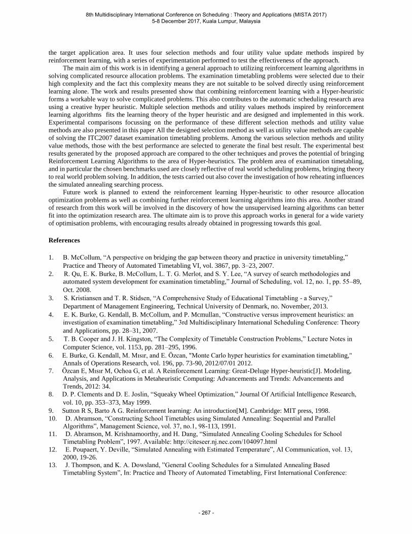
the target application area. It uses four selection methods and four utility value update methods inspired by

reinforcement learning, with a series of experimentation performed to test the effectiveness of the approach.

The main aim of this work is in identifying a general approach to utilizing reinforcement learning algorithms in

solving complicated resource allocation problems. The examination timetabling problems were selected due to their

high complexity and the fact this complexity means they are not suitable to be solved directly using reinforcement

learning alone. The work and results presented show that combining reinforcement learning with a Hyper-heuristic

forms a workable way to solve complicated problems. This also contributes to the automatic scheduling research area

using a creative hyper heuristic. Multiple selection methods and utility values methods inspired by reinforcement

learning algorithms fits the learning theory of the hyper heuristic and are designed and implemented in this work.

Experimental comparisons focussing on the performance of these different selection methods and utility value

methods are also presented in this paper All the designed selection method as well as utility value methods are capable

of solving the ITC2007 dataset examination timetabling problems. Among the various selection methods and utility

value methods, those with the best performance are selected to generate the final best result. The experimental best

results generated by the proposed approach are compared to the other techniques and proves the potential of bringing

Reinforcement Learning Algorithms to the area of Hyper-heuristics. The problem area of examination timetabling,

and in particular the chosen benchmarks used are closely reflective of real world scheduling problems, bringing theory

to real world problem solving. In addition, the tests carried out also cover the investigation of how reheating influences

the simulated annealing searching process.

Future work is planned to extend the reinforcement learning Hyper-heuristic to other resource allocation

optimization problems as well as combining further reinforcement learning algorithms into this area. Another strand

of research from this work will be involved in the discovery of how the unsupervised learning algorithms can better

fit into the optimization research area. The ultimate aim is to prove this approach works in general for a wide variety

of optimisation problems, with encouraging results already obtained in progressing towards this goal.

References

1. B. McCollum, “A perspective on bridging the gap between theory and practice in university timetabling,”

Practice and Theory of Automated Timetabling VI, vol. 3867, pp. 3–23, 2007.

2. R. Qu, E. K. Burke, B. McCollum, L. T. G. Merlot, and S. Y. Lee, “A survey of search methodologies and

automated system development for examination timetabling,” Journal of Scheduling, vol. 12, no. 1, pp. 55–89,

Oct. 2008.

3. S. Kristiansen and T. R. Stidsen, “A Comprehensive Study of Educational Timetabling - a Survey,”

Department of Management Engineering, Technical University of Denmark, no. November, 2013.

4. E. K. Burke, G. Kendall, B. McCollum, and P. Mcmullan, “Constructive versus improvement heuristics: an

investigation of examination timetabling,” 3rd Multidisciplinary International Scheduling Conference: Theory

and Applications, pp. 28–31, 2007.

5. T. B. Cooper and J. H. Kingston, “The Complexity of Timetable Construction Problems,” Lecture Notes in

Computer Science, vol. 1153, pp. 281–295, 1996. 6. E. Burke, G. Kendall, M. Mısır, and E. Özcan, "Monte Carlo hyper heuristics for examination timetabling,"

Annals of Operations Research, vol. 196, pp. 73-90, 2012/07/01 2012.

7. Özcan E, Mısır M, Ochoa G, et al. A Reinforcement Learning: Great-Deluge Hyper-heuristic[J]. Modeling,

Analysis, and Applications in Metaheuristic Computing: Advancements and Trends: Advancements and

Trends, 2012: 34.

8. D. P. Clements and D. E. Joslin, “Squeaky Wheel Optimization,” Journal Of Artificial Intelligence Research,

vol. 10, pp. 353–373, May 1999.

9. Sutton R S, Barto A G. Reinforcement learning: An introduction[M]. Cambridge: MIT press, 1998.

10. D. Abramson, “Constructing School Timetables using Simulated Annealing: Sequential and Parallel

Algorithms”, Management Science, vol. 37, no.1, 98-113, 1991.

11. D. Abramson, M. Krishnamoorthy, and H. Dang, “Simulated Annealing Cooling Schedules for School

Timetabling Problem”, 1997. Available: http://citeseer.nj.nec.com/104097.html

12. E. Poupaert, Y. Deville, “Simulated Annealing with Estimated Temperature”, AI Communication, vol. 13,

2000, 19-26.

13. J. Thompson, and K. A. Dowsland, ”General Cooling Schedules for a Simulated Annealing Based

Timetabling System”, In: Practice and Theory of Automated Timetabling, First International Conference:


- 267 -

Selected Papers, (E. Burke & P. Ross , Eds.), Edinburgh, U.K., August/September 1995. Lecture Notes in

Computer Science 1153, Springer-Verlag, 345-363, 1996.

14. Hamilton-Bryce R, McMullan P, McCollum B. Directed selection using reinforcement learning for the

examination timetabling problem[C]//Proceedings of the 10th International Conference of the Practice and

Theory of Automated Timetabling, York, UK. 2014: 218-232.

15. T. Muller, “ITC2007 solver description: a hybrid approach,” Annals of Operations Research, vol. 172, no. 1,

pp. 429–446, Oct. 2009.

16. S. Abdul Rahman, A. Bargiela, E. K. Burke, E. Ozcan, B. McCollum, and P. McMullan, “Adaptive linear

combination of heuristic orderings in constructing examination timetables,” European Journal of Operational

Research, vol. 232, no. 2, pp. 287–297, Jan. 2014.

17. N. R. Sabar, M. Ayob, R. Qu, and G. Kendall, “A graph coloring constructive hyper-heuristic for examination

timetabling problems,” Applied Intelligence, vol. 37, no. 1, pp. 1–11, Aug. 2011.

18. C. Gogos, P. Alefragis, and E. Housos, “An improved multi-staged algorithmic process for the solution of the

examination timetabling problem,” Annals of Operations Research, vol. 194, no. 1, pp. 203–221, Feb. 2010.

19. N. Pillay. Evolving hyper-heuristics for a highly constrained examination timetabling problem. In Proceedings

of the 8th International Conference on the Practice and Theory of Automated Timetabling (PATAT’10), pages

336–346, 2010.

20. Burke E K, Gendreau M, Hyde M, et al. Hyper-heuristic: A survey of the state of the art[J]. Journal of the

Operational Research Society, 2013, 64(12): 1695-1724.

21. Burke E K, Hyde M, Kendall G, et al. A classification of Hyper-heuristic approaches[M]//Handbook of

metaheuristics. Springer US, 2010: 449-468.

22. Ouelhadj D, Petrovic S. A cooperative Hyper-heuristic search framework[J]. Journal of Heuristics, 2010,

16(6): 835-857.

23. Burke E K, Qu R, Soghier A. Adaptive selection of heuristics for improving exam timetables[J]. Annals of

Operations Research, 2014, 218(1): 129-145.

24. N. R. Sabar, M. Ayob, R. Qu, and G. Kendall, "A graph coloring constructive Hyper-heuristic for examination

timetabling problems," Applied Intelligence, vol. 37, pp. 1-11, 2012.

25. K. Anwar, A. T. Khader, M. A. Al-Betar, and M. A. Awadallah, "Harmony Search-based Hyper-heuristic for

examination timetabling," in Signal Processing and its Applications (CSPA), 2013 IEEE 9th International

Colloquium on, 2013, pp. 176-181.


- 268 -

MISTA 2017

The Application of Nondominated Sorting Genetic Algorithm (NSGA-III)

for Scientific-workflow Scheduling on Cloud

Peerasak Wangsom • Kittichai Lavangnananda • Pascal Bouvry

Abstract Virtual machines on cloud are promising environments for deploying scientific

workflows due to its unlimited on-demand and scalable machines. The pay-per-use model and

a variety of the processing capacity, virtual machines allow large-scale workflows to be

executed with reasonable cost and competitive performance. Efficient allocation of a set of

dependent tasks on such dynamic resources is advantageous as it leads to well utilization

resources. This becomes a multi-objective optimization of task scheduling and has attracted

much interest in recent years. This study is the first attempt to determine solutions for a multi-

objective optimization of scheduling on cloud where Cost, Makespan and VM utilization are

the objectives. Four Scientific Workflows are selected for the study, these are CyberShake,

Epigenomics, LIGO, and Montage. The Nondominated Sorting Genetic Algorithm (NSGA-III)

is selected as the tool. Chromosome representation based on the topological order of the

workflow under consideration and a workflow scheduling algorithm is suggested. The

solutions for the multi-objective optimization are presented and compared with a single

objective solution. Cost and Makespan are the common two objectives for scheduling of task

on cloud, where VM utilization is usually neglected. The study affirms the role of multi-

objective optimization, especially where VM utilization is included.

Keywords : CyberShake, Epigenomics, LIGO, Makespan, Montage, Multi-objective

optimization, Nondominated Sorting Genetic Algorithm (NSGA-III), Scientific

workflow, Task scheduling, VM utilization


- 269 -

1 Introduction

In scientific community, large-scale scientific applications such as bioinformatics, astronomy,

and physics usually imply large volume of data and computation intensive [1]. A common

method to improve the computation efficiency is to split the whole process into multiple tasks

and process them over distributed systems such as cluster, grid and cloud computing. These

multiple tasks are arranged to work together as a workflow and can be represented by a

Directed Acyclic Graph (DAG) model [2]. Tasks are denoted by nodes while their dependency

and order of processing are denoted by directed edges. Having an efficient scheduling would

ensure that workflow is efficiently executed over distributed platforms. However, it is

commonly known that determination of such efficient schedule is an NP-hard problem [3, 4].

Implementing scheduling algorithms for scientific workflow on cluster and grid computing has

become a research field in itself [5].

Over the years, cloud computing is gaining popularity over conventional distributed

systems because of it offers self-management ability to users. Several cloud services are

available such as Infrastructure-as-a-Service (IaaS), Platform-as-a-Service (PaaS), and

Software-as-a-Service (SaaS). IaaS is probably the most suitable service in order to run

scientific workflow because it provides flexible, scalable virtual machines (VMs) that users

can deploy and run workflow on-demand. It is also possible for users to launch both unlimited

and different types of VM. Users are usually charged by considering their used VM time, pay-

per-use model. This allows users to select services according to their budget.

Several scheduling objectives have been studied from different perspectives, including

cloud provider, broker, and user perspective [6, 7]. From the cloud user perspective, Cost and

Makespan (the maximum completion time) are the two common objectives where multi-

objective research in this area is most prolific [6] as they are obvious conflicting objectives.

Nevertheless, other objectives are also significantly important, some of these are respond time,

energy consumption, communication cost and overhead and VM utilization [6-10]. VM

utilization is advantageous in IaaS cloud since it represents how well a scientific workflow is

executed on leased VM. It has an impact to both Cost and Makespan as well. So, scheduling

with VM utilization awareness can help balancing both Cost and Makespan.

Due to its NP-hard nature, evolutionary algorithms (EA) has an application in scheduling

the execution of scientific workflows on cloud, especially when the required schedule is multi-

objective optimization. Ant Colony Optimization (ACO), Particle Swarm Optimization (PSO)

and Nondominated Sorting Genetic Algorithm-II (NSGA-II) are some of the popular

algorithms for solving the multi-objective optimization [6]. NSGA-II [11] attracts some

attention and has been improved to a new version known as NSGA-III [12]. Nevertheless, it

has not been applied to scheduling problem.

This paper presents an application of NSGA-III in multi-objective optimization in

scheduling scientific workflows on IaaS cloud. The multi-objective in this study is to minimize

Cost, Makespan and maximize VMutilization. Four well-known scientific workflows [1],

CyberShake, Epigenomics, LIGO, and Montage, are chosen for illustrating the performance of

NSGA-III in solving this multi-objective optimization.

The organization of the paper is as follows. It begins with the description of workflow

scheduling in Section 2. Related work is discussed in Section 3 and Section 4 describes the

overview of NSGA-III. The detail of proposed implementation is elaborated in Section 5.

Solutions from NSGA-III are shown and discussed in Section 6. The paper is concluded in

Section 7 where future work is also suggested.

2 Workflow Scheduling

Workflow scheduling has been continuously studied and researched in multifarious

perspectives. This includes fields in parallel and distributed system, cluster and grid

computing. Recently, there has been much attention in scheduling in cloud computing. IaaS


- 270 -

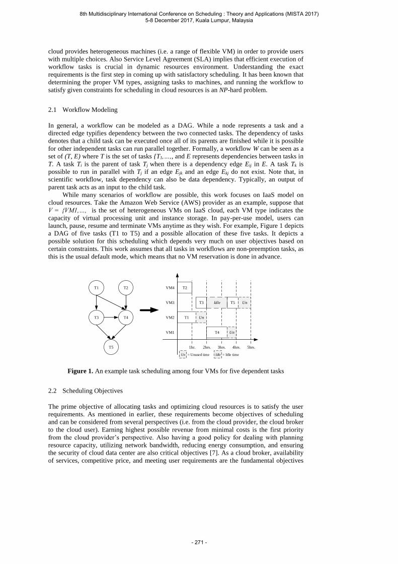
cloud provides heterogeneous machines (i.e. a range of flexible VM) in order to provide users

with multiple choices. Also Service Level Agreement (SLA) implies that efficient execution of

workflow tasks is crucial in dynamic resources environment. Understanding the exact

requirements is the first step in coming up with satisfactory scheduling. It has been known that

determining the proper VM types, assigning tasks to machines, and running the workflow to

satisfy given constraints for scheduling in cloud resources is an NP-hard problem.

2.1 Workflow Modeling

In general, a workflow can be modeled as a DAG. While a node represents a task and a

directed edge typifies dependency between the two connected tasks. The dependency of tasks

denotes that a child task can be executed once all of its parents are finished while it is possible

for other independent tasks can run parallel together. Formally, a workflow W can be seen as a

set of (T, E) where T is the set of tasks T1,…,, and E represents dependencies between tasks in

T. A task Ti is the parent of task Tj when there is a dependency edge Eij in E. A task Tk is

possible to run in parallel with Tj if an edge Ejk and an edge Ekj do not exist. Note that, in

scientific workflow, task dependency can also be data dependency. Typically, an output of

parent task acts as an input to the child task.

While many scenarios of workflow are possible, this work focuses on IaaS model on

cloud resources. Take the Amazon Web Service (AWS) provider as an example, suppose that

V = VM1,…, is the set of heterogeneous VMs on IaaS cloud, each VM type indicates the

capacity of virtual processing unit and instance storage. In pay-per-use model, users can

launch, pause, resume and terminate VMs anytime as they wish. For example, Figure 1 depicts

a DAG of five tasks (T1 to T5) and a possible allocation of these five tasks. It depicts a

possible solution for this scheduling which depends very much on user objectives based on

certain constraints. This work assumes that all tasks in workflows are non-preemption tasks, as

this is the usual default mode, which means that no VM reservation is done in advance.

T2VM4

VM3

VM2

VM1

T1 T2

T4

T5

T3

T4

T3 T5

T1 Un

Un

Un

1hr. 2hrs. 3hrs. 4hrs. 5hrs.

Un = Unused time Idle = Idle time

Idle

Figure 1. An example task scheduling among four VMs for five dependent tasks

2.2 Scheduling Objectives

The prime objective of allocating tasks and optimizing cloud resources is to satisfy the user

requirements. As mentioned in earlier, these requirements become objectives of scheduling

and can be considered from several perspectives (i.e. from the cloud provider, the cloud broker

to the cloud user). Earning highest possible revenue from minimal costs is the first priority

from the cloud provider’s perspective. Also having a good policy for dealing with planning

resource capacity, utilizing network bandwidth, reducing energy consumption, and ensuring

the security of cloud data center are also critical objectives [7]. As a cloud broker, availability

of services, competitive price, and meeting user requirements are the fundamental objectives


- 271 -

[6]. On the other hand, the performance measurements such as makespan, response time are

major concerns from a cloud user’s perspective [6]. Scheduling becomes much more complex

in a large and complex scientific workflow. This entails a list of many possible objectives [6],

Table 1 summarizes some of these objectives from different perspectives, and it is not by any

means an exhaustive one.

Table 1. Cloud Resource Management Objectives

Perspective Objectives

Environment Energy, Peak Power, Thermal, CO2 Emissions

Financial Price, Income, Cost

Performance Respond Time, Uptime, Throughput, Makespan

Resources Energy Source, VM utilization, Data Locality

Others Reliability, Security, Data Center Location

Among the above objectives, Cost and Makespan are two most prolific where

optimization has been carried out. One of the most important objective which should not be

neglected is VM utilization. Nevertheless, there has been no previous work in multi-objective

scheduling of cloud computing has included VM utilization to date. Therefore, this work is the

first attempt in multi-objective scheduling where Cost, Makespan and VM utilization are

considered.

2.2.1 Cost

In IaaS cloud, a user requests to launch VM by selecting types which are provided in a catalog.

VM types indicate the upper bound capacity of virtual processor and their cost. In most cases,

the cost of leased VM is measured in per hour interval where partial VM-hour consumed is

usually billed as a full hour. For most IaaS cloud providers such as AWS, Google App Engine,

and Windows Azure, the communication cost is hidden and almost negligible from user’s

perspective. Therefore, the ‘Cost’ referred to in this work is the VM leased cost which is

usually calculated in number of hours used by VMs. Referring to Figure 1, VM1, VM2 are

charged for two hours, while VM3 and VM4 are charged for four and one hours respectively.

In general, the cost can be determined by equation (1) as below :

𝑇𝑜𝑡𝑎𝑙 𝐶𝑜𝑠𝑡 = ∑ ⌈𝐻𝑜𝑢𝑟𝑠 𝑜𝑓 𝑉𝑀𝑖⌉ × 𝐶𝑜𝑠𝑡𝑝𝑒𝑟 ℎ𝑜𝑢𝑟 𝑜𝑓 𝑉𝑀𝑖𝑛𝑖=1 ……………(1)

where

⌈𝐻𝑜𝑢𝑟𝑠 𝑜𝑓 𝑉𝑀𝑖⌉ is the ceiling of VM running hours

𝐶𝑜𝑠𝑡𝑝𝑒𝑟 ℎ𝑜𝑢𝑟 𝑜𝑓 𝑉𝑀𝑖 is the unit cost per hour

This work adopts the same VM types and cost as in [5] which is based on AWS model as

shown in Table 2. Processing Capacity is represented in MFLOPS (Million Floating Point

Operations Per Second) unit and the Slowdown Ratio is the ratio of performance degradation

comparing to m3.doubleXlarge which is the fastest in term of MFLOPS.


- 272 -

Table 2. List of VM types based on AWS model [5]

VM Type EC2

Units

Processing

Capacity

(MFLOPS)

Cost/Hour Slowdown

Ratio

m1.small 1 4,400 $0.06 26.00

m1.medium 2 8,800 $0.12 13.00

m1.large 4 17,600 $0.24 6.50

m1.xLarge 8 35,200 $0.48 3.25

m3.xLarge 13 57,200 $0.50 2.00

m3.doubleXlarge 26 114,400 $1.00 1.00

2.2.2 Makespan

In execution of a batch of tasks, Makespan, the standard objective, is the maximum completion

time (Cmax) representing the time when the last task in workflow is done [6]. Referring to

Figure 1, Makespan is the time when task T5 is completed. In general, Cmax can be determined

by the following equations :

𝐶𝑚𝑎𝑥 = 𝑚𝑎𝑥𝑗∈𝑇𝐶𝑗 …. (2)

𝐶𝑗 = 𝑇𝑟𝑎𝑛𝑗 + 𝑃𝑗 …. (3)

𝑇𝑟𝑎𝑛𝑗 = ∑ 𝑇𝑟𝑎𝑛𝑖𝑗𝑛𝑖=1 …. (4)

𝑇𝑟𝑎𝑛𝑖𝑗 = 𝐼𝑛𝑝𝑢𝑡𝑆𝑖𝑧𝑒𝑖 ÷ 𝐷𝑇𝑅𝑖𝑗 …. (5)

where

𝐶𝑗 is the completion time of Tj.

𝑇𝑟𝑎𝑛𝑗 is the transfer time

𝑃𝑗 is the processing time.

n is the number of input files generated by all parent tasks of Tj.

𝑇𝑟𝑎𝑛𝑖𝑗 is the transfer time from Ti to Tj.

𝐷𝑇𝑅𝑖𝑗 is the data transfer rate (e.g. 1 Gbps, between Ti and Tj).

𝐼𝑛𝑝𝑢𝑡𝑆𝑖𝑧𝑒𝑖 is the input size generated by Ti.

The assumption is that each task in workflow provides the size of all input files and

transferring of multiple input files is sequential. Values stated in Table 2 is also assumed in

this work, for example, if the processing time 𝑃𝑗 of task Tj is 10 seconds in m3.doubleXlarge

type, it will take 20 seconds in m3.xlarge with 2.00 slowdown ratio.

2.2.3 VM Utilization

In a conventional machine, CPU or processor utilization is a significant issue in term of cost

effectiveness and performance. The idle time is the time running processor without any

productivity. Similarly, in a cloud environment, the idle time of running VM leads to reduction

cost effectiveness and performance. Furthermore, in a per hour period, partial VM-hour

consumed leads to higher cost without utilization. Referring to Figure 1, both idle and unused


- 273 -

time occur in VM3, while VM4 has the best VM utilization. If V is the set of VMs, the

VMutilization in this work is defined as shown in Equation 6 :

𝑉𝑀𝑢𝑡𝑖𝑙𝑖𝑧𝑎𝑡𝑖𝑜𝑛 = 𝑎𝑣𝑒𝑟𝑎𝑔𝑒𝑖∈𝑉(𝑅𝑢𝑛𝑛𝑖𝑛𝑔𝑇𝑖𝑚𝑒 𝑜𝑓 𝑉𝑀𝑖/𝐵𝑖𝑙𝑙𝑒𝑑𝑇𝑖𝑚𝑒 𝑜𝑓 𝑉𝑀𝑖) (6)

Hence, the VMutilization is the ratio of VM running time, without idle time, divided by

VM billed time. This value ranges from 0 to 1. For example, if a VM is used for 90 minutes

and the user is charged for 120 minutes, then VMutilization is 0.75.

2.3 Scheduling Model

Section 2.2 describes the three objectives in this work. Therefore, the multi-objective

scheduling is a solution where Cost is minimized, Makespan (i.e. Cmax) and VMutilization are

maximized in processing a workflow on cloud. The scheduling model can then be formally

represented using the standard three-field notation [4, 13] denoted below :

𝑉𝑀𝑗|𝑃𝑟𝑒𝑐, 𝑃𝑖𝑗|𝐶𝑜𝑠𝑡, 𝐶𝑚𝑎𝑥 , 𝑉𝑀𝑢𝑡𝑖𝑙𝑖𝑧𝑎𝑡𝑖𝑜𝑛 …….…. (7)

where

𝑉𝑀𝑗 is the first field which stands for j parallel VM machines with different speeds.

𝑃𝑟𝑒𝑐, 𝑃𝑖𝑗 is the second field where Prec notates the precedence constraint between tasks

and 𝑃𝑖𝑗 represents a vector of processing time (in second) for task i processed by VMj.

Cost, Cmax, VMutilization is the third field where the list of objectives is stated.

3 Related Work

Efficiency of task scheduling plays a significant role in utilizing resources in distributed

systems in order to achieve satisfactory performance. Literature in optimization of these

resources is quite prolific, especially with the application of evolutionary algorithms (EA).

This leads to a field of its own commonly known as Multi-Objective Evolutionary Algorithms

(MOEA) or Multi-Objective Genetic Algorithms (MOGA) [14]. Solutions to this multi-

objective optimization can be considered from mainly three perspectives, provider, broker and

user perspectives. Brokers can also be seen as users in some scenarios. As most workflow

scheduling problems refer to the use of cloud resources, the two main objectives are Cost (i.e.

the cost of leased VM is measured in per hour interval) and Makespan (i.e. makespan and

execution time). These two objectives are understood as conflicting objectives.

The problem of minimization of both conflicting objectives has been usually focused on

scientific workflows. The work in [15] proposed an auction-based Biobjective Scheduling

Strategy (BOSS) comparing to NSGA-II and Strength Pareto EA-II (SPEA-II) in order to

optimize a bi-objective problem (cost and makespan). Cloud Workflow Scheduling Algorithm

(CWSA) comparing to three well-known algorithms, First Come First Served (FCFS), Easy

Backfilling, and Minimum Completion Time (MCT) was proposed in [16]. Multi-objective

scheduling based on the Vector Ordinal Optimization (VOO) was carried out in [17], while

[18] a scheduling algorithm based on task clustering for scientific workflows in order to

minimize cost and execution time. Scheduling of general DAG was carried out in [19] and

[20]. Improved Differential EA (IDEA) [19] was implemented to handling tasks and their

subtasks in DAG workflows on multiple cloud resources, while [20] adopted two-hierarchical

scheduling strategy, service level, and task level scheduling, for minimizing cost and execution

time. SPEA-II [21] was applied in order to minimize cost and execution time to a particular

workflow known as BPEL (Business Process Execution Language) workflow.

Besides the most two common objectives, Cost and Makespan, energy consumption, data

locality, and communication overhead were other objectives that had been studied in the task

scheduling on cloud. This includes Case Library and Pareto Solution based hybrid GA (CLPS-


- 274 -

GA) was proposed in [8], Cellular GA (CGA) [9]. The work in [10] compared three other EAs,

NSGA-II, MoCell (Multi-objective Cellular), and IBEA (Indicator-based Evolutionary

Algorithm), for workflow scheduling in order to minimize energy consumption and makespan.

Multi-objective Evolutionary Algorithm based on Decomposition (MOEA/D) was introduced

in [22]) for energy and locality-aware multi-job scheduling on cloud. Comparison between

NSGA-II and PSO for execution of scientific workflows satisfying multi-objective

optimization (cost, makespan and communication overhead) on cloud was carried out in [7].

The idea of provisioning a VM as late as possible can help to reduce the leased VM time

and may lead to minimize the cost. To date, no work had considered on VM utilization, with

exception of a few that focused on task scheduling with the deadline of VM provisioning. PSO

based algorithm [5] was introduced to optimize cost and execution time and satisfy deadline

constraints, while [23] presented an adaptive, resource provisioning and scheduling algorithm

in order to minimize cost and meet a user-defined deadline. Both works were carried out on

scientific workflows on cloud. In the cloud resource management, several EA techniques have

been applied in order to deal with the multi-objective optimization problems. A survey of 36

research works [6] was carried out on family of EA techniques, GA, PSO, ACO and NSGA-II.

This affirms that a variety of EA has successfully addressed the multi-objective optimization in

order to optimize cloud resources.

In the multi-objective optimization of task scheduling problems, most of the previous

works had focused on the two most common objectives, Cost and Makespan, due to the need

of a trade-off between them. Nevertheless, as described in Section 2.3, VMutilization is another

objective that ought not be overlooked, especially in the pay-per-use model of IaaS cloud.

Increasing of unused time and idle time (i.e. low VMutilization) may lead to increasing Cost

and Makespan too. Therefore, this study considers VMutilization as another important

objective in optimization of task scheduling in scientific workflows. It is also the first work

which attempts the multi-objective optimization in scheduling on cloud which includes Cost,

Makespan and VMutilization.

4 NSGA-III

As stated in the previous Section, several multi-objective optimization algorithms exist. This

work selects the state-of-the-art evolutionary algorithm known as Nondominated Sorting

Genetic Algorithm-III (NSGA-III). It is specifically designed for multi-objective optimization

and is an improved version of the previous NSGA-II. Its improvement lies in the proposal of a

novel selection operation to acquire a set of well-spread Pareto-optimal solutions.

As a multi-objective optimization usually produces a set of feasible solutions, the concept

of nondominated solutions, called Pareto-optimal solutions, is the set of solutions which are

not dominated by other solutions. In order to maintain the uniform distribution and diversity of

Pareto set in NSGA-II, crowding distance was proposed (i.e. the distance between a solution

and its neighbors) where a solution with larger distance was preferred. NSGA-III improves this

by using a different strategy by determining the relative distance between solutions and

reference points.

In the initial step, beside randomizing population of size N, NSGA-III also generates the

well-distributed reference points H on an (M-1)-dimensional hyperplane for M-objective

problem. The positions of reference points can be determined by using Normal-Boundary

Intersection [24] and the population size N should be the smallest number, which is equal or

greater than H, and is the multiple of four. The expectation is at least one individual is

belonging to every reference point. Prior to the selection step in each generation, the parent

generates their offspring by using crossover and mutation operation. Suppose that Ut = Pt U Qt

where Pt is the parent population at tth generation, Qt is the offspring population and Ut, the

combined population, usually of size 2N. Then Ut will be sorted based on nondominated

sorting and divided into multiple nondominated levels. F1 is individual, which is completely

nondominated by others, and F2 is individual dominated by only F1 members and so on.


- 275 -

In the selection process, F1 members will be firstly chosen for Pt+1 generation before

considering next nondominated level until the size of Pt+1 is equal to N. In order to preserve

diversity, suppose that Flast is the last nondominated level that is chosen for Pt+1, Niche-

Preservation Operation is applied in order to select Flast members. First, objective values of

each member in Pt+1 and Flast are normalized to correspond with the reference points. Then all

of the members in Pt+1 and Flast are associated to the reference points by measuring the

distances between their positions and reference lines, the logical lines laid down from the ideal

point to reference points. Finally, Niche-Preservation Operation iteratively operates on each

reference point. For the jth reference point, if there is no associated Pt+1 member to reference

point j, the associated Flast member, having the shortest distance, is being added to Pt+1

otherwise the jth point is not considered for the current generation. In the case of an already

existing member in Pt+1 associated to the jth point and an associated Flast member to point j is

found, a member is randomly selected and added to Pt+1. The procedure is repeated until the

size of Pt+1 is equal to N.

Ensuring a variety of population and preserving identical characteristic of parents are the

key concepts of NSGA-III. It uses the association of population with widely-distributed

reference points to represent both concepts. This strategy is capable of generating a set of well-

spread Pareto-optimal solutions. The detailed operations of NSGA-III can be found in [12].

5 Multi-Objective Scheduling using NSGA-III

The challenge of Multi-Objective Genetic Algorithm (MOGA) not only limit to difficult

optimization problem with increasing objectives but also in its application to real NP-hard

problems. Cross-training performance of nurse scheduling is one of such example of where

NSGA-II and PSO had been applied [25]. This section discusses the proposed solution of

NSGA-III in the optimizing scheduling problem as stated in Section 2.

5.1 Representation of Scheduling in NSGA-III

The major objective in task allocation among VMs is to efficiently assign a particular task to a

suitable VM. For ease of description, the following scenario is assumed :

No. of tasks : 7 (T1, T2, ….., T7)

No. of VM Types : 6 (m1.small, …., m3.doubleXlarge as stated in Table 2)

DAG Workflow : 7 tasks configured as in Figure 2(a)


- 276 -

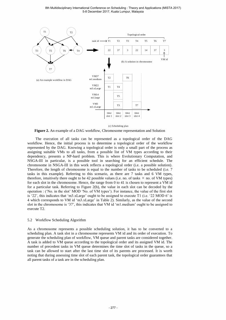
T1 T2

T3 T5 T6 T4

T7

22

T1

37

T2

3

T3

22

T4

14

T5

37 3

T7T6

T2VM37

m1.medium

VM22

m3.xLarge

VM14

m1.large

VM3

m1.xLarge

T4

T3

T5

T1

time

slot 1

T6

T7

(a) An example workflow in DAG

(b) A solution in chromosome

(c) Scheduling plan

task id

VM id

time

slot 2

time

slot 3

time

slot 4

Topological order

Figure 2. An example of a DAG workflow, Chromosome representation and Solution

The execution of all tasks can be represented as a topological order of the DAG

workflow. Hence, the initial process is to determine a topological order of the workflow

represented by the DAG. Knowing a topological order is only a small part of the process as

assigning suitable VMs to all tasks, from a possible list of VM types according to their

dependency, presents a NP-hard problem. This is where Evolutionary Computation, and

NSGA-III in particular, is a possible tool in searching for an efficient schedule. The

chromosome in NSGA-III in this work reflects a topological order (i.e. a possible solution).

Therefore, the length of chromosome is equal to the number of tasks to be scheduled (i.e. 7

tasks in this example). Referring to this scenario, as there are 7 tasks and 6 VM types,

therefore, intuitively there ought to be 42 possible values (i.e. no. of tasks no. of VM types)

for each slot in the chromosome. Hence, the range from 0 to 41 is chosen to represent a VM id

for a particular task. Referring to Figure 2(b), the value in each slot can be decoded by the

operation : (‘No. in the slot’ MOD ‘No. of VM types’). For instance, the value of the first slot

is ‘22’, this indicates that ‘m3.xLarge’ ought to be assigned to execute T1 (i.e. ‘22 MOD 6’ is

4 which corresponds to VM id ‘m3.xLarge’ in Table 2). Similarly, as the value of the second

slot in the chromosome is ‘37’, this indicates that VM id ‘m1.medium’ ought to be assigned to

execute T2.

5.2 Workflow Scheduling Algorithm

As a chromosome represents a possible scheduling solution, it has to be converted to a

scheduling plan. A task slot in a chromosome represents VM id and its order of execution. To

generate the scheduling plan of workflow, VM queue and parent tasks are considered together.

A task is added to VM queue according to the topological order and its assigned VM id. The

number of precedent tasks in VM queue determines the time slot of tasks in the queue, so a

task can be allowed to start after the last time slot of its parents are processed. It is worth

noting that during assessing time slot of each parent task, the topological order guarantees that

all parent tasks of a task are in the scheduling plan.


- 277 -

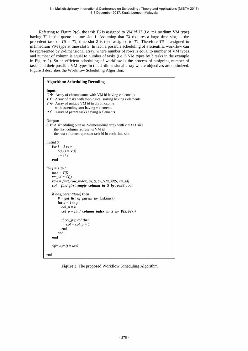
Referring to Figure 2(c), the task T6 is assigned to VM id 37 (i.e. m1.medium VM type)

having T2 in the queue at time slot 1. Assuming that T4 requires a large time slot, as the

precedent task of T6 is T4, time slot 2 is then assigned to T4. Therefore T6 is assigned to

m1.medium VM type at time slot 3. In fact, a possible scheduling of a scientific workflow can

be represented by 2-dimensional array, where number of rows is equal to number of VM types

and number of column is equal to number of tasks (i.e. 6 VM types by 7 tasks in the example

in Figure 2). So an efficient scheduling of workflow is the process of assigning number of

tasks and their possible VM types in this 2-dimensional array where objectives are optimized.

Figure 3 describes the Workflow Scheduling Algorithm.

Figure 3. The proposed Workflow Scheduling Algorithm

Algorithm: Scheduling Decoding

Input:

C Array of chromosome with VM id having c elements

T Array of tasks with topological sorting having t elements

V Array of unique VM id in chromosome

with ascending sort having v elements

P Array of parent tasks having p elements

Output:

S A scheduling plan as 2-dimensional array with v × t+1 size

the first column represents VM id

the rest columns represent task id in each time slot

initial S

for i = 1 to v

S(i,1) = V(i)

i = i+1

end

for j = 1 to t

task = T(j)

vm_id = C(j)

row = find_row_index_in_S_by_VM_id(S, vm_id)

col = find_first_empty_colunm_in_S_by row(S, row)

if has_parent(task) then

P = get_list_of_parent_by_task(task)

for k = 1 to p

col_p = 0

col_p = find_column_index_in_S_by_P(S, P(k))

if col_p ≥ col then

col = col_p + 1

end

end

end

S(row,col) = task

end


- 278 -

5.3 Fitness Functions

Once a possible schedule is generated, its efficiency must be evaluated, this is done by means

of assessing the fitness value of its chromosome. The fitness of a possible schedule comprises

three aspects, Cost, Makespan and VMutilization as stated in Section 2. Hence, fitness

functions are the equations 1, 2 and 6 stated in Sections 2.2. These fitness functions are used to

assess the scheduling model as stated in Section 2.3. Note that as the scheduling model is

multi-objective, hence a chromosome (i.e. a solution) with the best fitness values for all 3

objectives may not exist.

5.4 Selection, Crossover and Mutation

As in any Genetic Algorithm, in NSGA-III, a set of initial population is first generated. A

percentage of the initial population is selected for Crossover. Although Simulated Binary

Crossover (SBX) [26] was suggested for NSGA-III, this was intended for real number. One-

point Crossover is selected for this work and it was found more suitable and efficient for

integer values. Once the Crossover is completed, a percentage of the initial population is

selected for Mutation. In this work, Mutation adopts the Gaussian Mutation, where 2% of the

positions in the selected chromosomes are mutated, as used by the Yarpiz project [27]. The

whole population is then assessed for their fitness values as described in the previous Section,

this is followed by nondominated sorting. Elitism is used for the Selection to represent a new

generation of the population.

6 Scientific Workflows used

Four scientific workflows from different scientific fields were selected for this study, these are

of CyberShake, Epigenomics, LIGO, and Montage. These workflows are known applications

and have been used as test beds for scientific workflows. The number of tasks for all four

scientific workflows, used for this study, was set to be 100. Their brief descriptions are as

follows:

CyberShake

CyberShake is a seismology application that calculates probabilistic seismic hazard curves for

geographic sites in the Southern California region [1, 28]. It consists of five task types. Three

of them are multiple-task type including the root tasks. Figure 4(a) depicts the structure of

CyberShake workflow in DAG model.

Epigenomics

Epigenomics workflow created by the USC Epigenome Center and the Pegasus research team,

it is used to automate various operations in genome sequence processing [1, 29]. There are

eight task types in workflow. Four of them are singleton-task type. Figure 4(b) depicts the

structure of Epigenomics workflow in DAG model.

LIGO

Laser Interferometer Gravitational Wave Observatory (LIGO) workflow is used to search for

gravitational wave signatures in data collected by large-scale interferometers [1, 30]. It consists

of four task types and three of them are multiple-task type as shown in Figure 4(c).


- 279 -

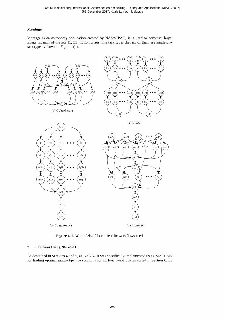
Montage

Montage is an astronomy application created by NASA/IPAC, it is used to construct large

image mosaics of the sky [1, 31]. It comprises nine task types that six of them are singleton-

task type as shown in Figure 4(d).

ES

SS SS SS SS

ES

SS SS SS SS

ZS

PC PC PC PC PC PC PC PC

ZP

fQS

fC fC fC fC

s2s s2s s2s s2s

fq2b fq2b fq2b fq2b

map map map map

mM

mI

pup

Tm

B

Tm

B

Tm

B

Ins Ins Ins

Tm

B

Tm

B

Tm

B

Ins Ins Ins

Thi Thi

TriB TriB TriB

Ins Ins Ins

TriB TriB TriB

Ins Ins Ins

Thi Thi

mPP mPP mPP mPP

mDF mDF mDF mDF mDFmDF

mCF

mB

M

mB mB mB mB

mIT

mA

mS

mJ

Figure 4. DAG models of four scientific workflows used

7 Solutions Using NSGA-III

As described in Sections 4 and 5, an NSGA-III was specifically implemented using MATLAB

for finding optimal multi-objective solutions for all four workflows as stated in Section 6. In


- 280 -

order to assess and evaluate the multi-objective solutions, optimal single objective solutions

were found first. Comparison and evaluation of the optimal multi-objective solutions can then

be assessed by comparing with the single objective solutions.

As three objectives in this work are, Cost, Makespan and VMutilization, optimal single

objective solution was generated by NSGA-III by means of simply using single fitness

function for each objective. This resulted in the single best solution that NSGA-III could

generate. In case of the multi-objective solutions, however, NSGA-III provides a set of Pareto-

optimal solutions as the best optimal solution for all three objectives may not exist.

The list of NSGA-III parameters is summarized in Table 3. Parameters used in this study

followed those proposed in DTLZ (3 to 15 multiple objectives were tested) [12] which reports

that 91 reference points are suitable for three objectives and population size has to be at least

as many as reference points and divisible by four. Hence, 92 were chosen as the number of

population in this study.

Table 3. Parameters of NSGA-III

Parameter Value

Scheduling objectives 3 (Cost, Makespan, VMutilization)

Length of chromosome

(No. of tasks)

100

(CyberShake, Epigenomics, LIGO, Montage)

Reference points 91

Population size 92

Crossover operation Single Point Crossover

- Random selection

- 50% of the parent population

Mutation operation Gaussian Mutation

- Random selection

- 2 out of 100 positions

- 50% of the parent population

Stopping criteria At least 500 iterations and No progress occurs

after 100 iterations onwards

7.1 Results

As the three multi-objective solutions generated a set of Pareto-optimal solutions, there are

numerous possible ways to present the results from NSGA-III for each scientific workflow. In

this Section, the results are presented in two parts including the Pareto-optimal solutions and

the comparison between single and multiple objectives of each workflow. For ease of

presentation in a graph, all values of Cost, Makespan and VMutilization are normalized such

that the lowest and highest values are 0 and 1 respectively. Note that the best value for Cost

and Makespan are 0 while this is 1 for VMutilization.

7.1.1 Pareto-optimal Solutions

As stated in the Section 4 NSGA-III offers nondominated solutions having the best value at

least one objective. To visualize the Pareto-optimal solutions of three objectives is capable and

informative in order to explore the Pareto plane. Figure 5 depicts the optimal solutions of each

workflow, each comprises 92 points. Note that different solutions yielded the same values for

all objectives (as shown Montage workflow where many among possible 92 solutions yielded

the same values). As in multi-objective optimization, the optimal solution where all criteria are

satisfied may not exist. The same happened in this work for all workflows. Hence, the best

solution has to be selected according to priorities of each requirement. Among the four


- 281 -

solutions, Montage is least distributed while Epigenomics is the most well distributed. In the

next section, Pareto-optimal solutions at the average value are compared to the best solution

from single objective.

(a) Cybershake (b) Epigenomics

(c) LIGO (d) Montage

Figure 5. Pareto-optimal solutions of the four scientific workflows

7.1.2 Single VS Multiple Objective Comparisons

As NSGA-III yielded solutions of all objectives where the best, average and worst value occur

at each objective for each workflow. Presenting them in all possible perspectives can

overwhelm the merit and the discussion. Therefore, for each scientific workflow, the best

solution from the single objective is depicted to compare with the Pareto-optimal solution at

the average value where that particular objective occurs. Figures 6, 7, 8 and 9 depict these

comparisons in terms of Cost, Makespan and VMutilization for CyberShake, Epigenomics,

LIGO, and Montage workflows respectively. For example Figure 6(a) depicts the best

solutions for each single optimal objective for CyberShake, where Figure 6(b) depicts

solutions for the three multiple-objective values where each objective is at average. The

rationale for comparing with the average solutions instead of the best in the three multiple-

objective solutions is that selecting the best solution at each objective implies that very

consideration/importance is given to the other two objectives.


- 282 -

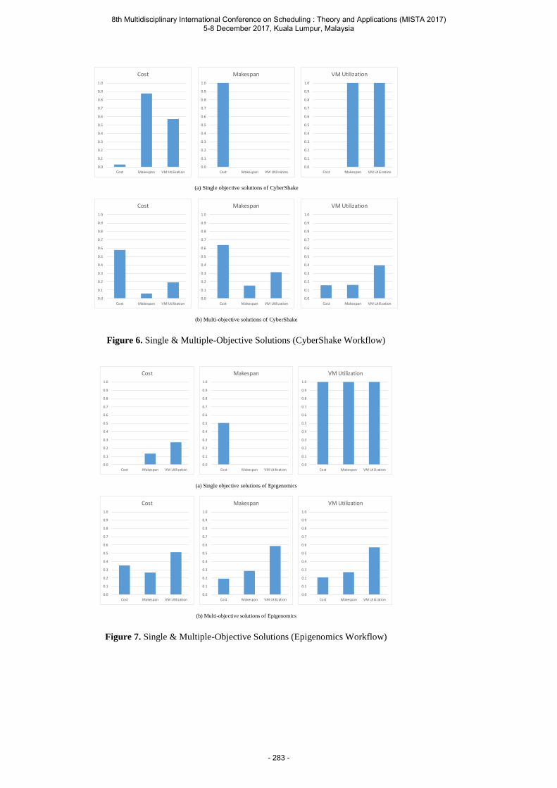
0.0

0.1

0.2

0.3

0.4

0.5

0.6

0.7

0.8

0.9

1.0

Cost Makespan VM Utilization

Cost

0.0

0.1

0.2

0.3

0.4

0.5

0.6

0.7

0.8

0.9

1.0


Makespan

0.0

0.1

0.2

0.3

0.4

0.5

0.6

0.7

0.8

0.9

1.0


VM Utilization

0.0

0.1

0.2

0.3

0.4

0.5

0.6

0.7

0.8

0.9

1.0


VM Utilization

0.0

0.1

0.2

0.3

0.4

0.5

0.6

0.7

0.8

0.9

1.0


Makespan

0.0

0.1

0.2

0.3

0.4

0.5

0.6

0.7

0.8

0.9

1.0


Cost

(a) Single objective solutions of CyberShake

(b) Multi-objective solutions of CyberShake

Figure 6. Single & Multiple-Objective Solutions (CyberShake Workflow)

0.0

0.1

0.2

0.3

0.4

0.5

0.6

0.7

0.8

0.9

1.0


Cost

0.0

0.1

0.2

0.3

0.4

0.5

0.6

0.7

0.8

0.9

1.0


Makespan

0.0

0.1

0.2

0.3

0.4

0.5

0.6

0.7

0.8

0.9

1.0


VM Utilization

0.0

0.1

0.2

0.3

0.4

0.5

0.6

0.7

0.8

0.9

1.0


Cost

0.0

0.1

0.2

0.3

0.4

0.5

0.6

0.7

0.8

0.9

1.0


Makespan

0.0

0.1

0.2

0.3

0.4

0.5

0.6

0.7

0.8

0.9

1.0


VM Utilization

(a) Single objective solutions of Epigenomics

(b) Multi-objective solutions of Epigenomics

Figure 7. Single & Multiple-Objective Solutions (Epigenomics Workflow)


- 283 -

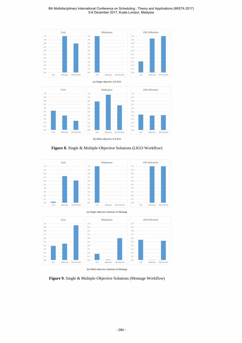
0.0

0.1

0.2

0.3

0.4

0.5

0.6

0.7

0.8

0.9

1.0


Cost

0.0

0.1

0.2

0.3

0.4

0.5

0.6

0.7

0.8

0.9

1.0


Makespan

0.0

0.1

0.2

0.3

0.4

0.5

0.6

0.7

0.8

0.9

1.0


VM Utilization

(a) Single objective of LIGO

(b) Multi-objective of LIGO

0.0

0.1

0.2

0.3

0.4

0.5

0.6

0.7

0.8

0.9

1.0


Cost

0.0

0.1

0.2

0.3

0.4

0.5

0.6

0.7

0.8

0.9

1.0


Makespan

0.0

0.1

0.2

0.3

0.4

0.5

0.6

0.7

0.8

0.9

1.0


VM Utilization

Figure 8. Single & Multiple-Objective Solutions (LIGO Workflow)

0.0

0.1

0.2

0.3

0.4

0.5

0.6

0.7

0.8

0.9

1.0


Cost

0.0

0.1

0.2

0.3

0.4

0.5

0.6

0.7

0.8

0.9

1.0


Makespan

0.0

0.1

0.2

0.3

0.4

0.5

0.6

0.7

0.8

0.9

1.0


VM Utilization

0.0

0.1

0.2

0.3

0.4

0.5

0.6

0.7

0.8

0.9

1.0


Cost

0.0

0.1

0.2

0.3

0.4

0.5

0.6

0.7

0.8

0.9

1.0


Makespan

0.0

0.1

0.2

0.3

0.4

0.5

0.6

0.7

0.8

0.9

1.0


VM Utilization

(a) Single objective solutions of Montage

(b) Multi-objective solutions of Montage

Figure 9. Single & Multiple-Objective Solutions (Montage Workflow)


- 284 -

7.2 Discussions

Referring to Figures 6 to 9, the solutions reaffirm the common belief that Cost and Makespan

are conflicting objectives as shown in cases of single objectives for all scientific workflows. It

also reveals that VMutilization and Makespan are also conflicting objectives. Contrast to

common suspicion that higher VMutilization implies lower Cost, this is not necessary true as

shown in Epigenomics workflow (i.e. best VMutilization in Figure 7(a)).

Multi-objective solutions from all scientific workflows also reaffirm the advantage of

considering multi-objective for such workflows. While no best solutions exist where all three

objectives are optimized, none of the multi-objective solutions leads to worst or considerably

high cost for any objective. Among the four scientific workflows, CyberShake configuration is

the hardest for finding compromising solutions among all three objectives as VMutilization are

considerably low for all three objectives. Previous work tends to concentrate on two multi-

objective optimizations (i.e. Cost and Makespan), the result of this study suggests that

inclusion of VMutilization in the multi-objective optimization is beneficial as optimizing

VMutilization has a tendency to balance the values both Cost and Makespan too (i.e. the

average solutions for VMutilization for all workflows do not show unsatisfactory values of

Cost and Makespan, even though the average of Cost in Montage workflow is relatively high).

The results of this study reveal that in multi-objective optimization of scientific

workflow, a trade-off between objectives must be considered and the configuration of the

workflow probably has the most significant impact to this multi-objective optimization

problem as no common factor can be concluded from the solutions in all four scientific

workflows used in this study.

8 Conclusions and Future Work

Scheduling in cloud computing where resources are efficiently utilized has become multi-

objective problem. Numerous studies of scientific workflow scheduling on cloud have been

carried out from different perspectives. This study is the first to attempt multi-objective

optimization of scheduling on cloud where Cost, Makespan and VMutilization are considered

from user perspective. The state of art NSGA-III was used as the tool in the multi-objective

optimization of four scientific workflows. The chromosome representation using the

topological order of tasks and a workflow scheduling algorithm are proposed.

Apart from reaffirming the two conflicting objectives of Cost and Makespan, the study

reveals that VMutilization ought not be overlooked as its inclusion does not lead to

unsatisfactory solutions from both Cost and Makespan perspectives, but can offer a more

balanced scheduling of scientific-workflows. Single objective scheduling ought to be avoided

as it may compromise other important aspects. Nevertheless, configuration and dependency in

a scientific workflow are the most crucial aspects in multi-objective optimization when

determining an efficient scheduling.

Further studies can be extended from several perspectives, this study considers

scheduling from user perspective. Similar attempts can be done from provider and broker

perspectives. This suggests inclusion of energy consumption, energy sources and CO2

Emissions in the multi-objectives. It is worth bearing in mind that the task can become very

complex when many objectives are considered together. From NSGA-III perspective, it can

also be applied to other areas of multi-objective optimization such as feature selection in data

mining. Another direction for future studies is the investigation of other EA techniques in

similar multi-objective optimization.

Acknowledgements The authors are grateful to School of Information Technology (SIT),

King Mongkut’s University of technology Thonburi (KMUTT) for the scholarship of Mr.

Peerasak Wangsom and the computing facilities throughout this research.


- 285 -

References

1. G. Juve, A. Chervenak, E. Deelman et al., Characterizing and profiling scientific

workflows, Future Generation Computer Systems, 29(3), 682-692 (2013)

2. E. Deelman, K. Vahi, G. Juve et al., Pegasus, a workflow management system for science

automation, Future Generation Computer Systems, 46, 17-35 (2015)

3. M. R. Garey, and D. S. Johnson, Computers and Intractability; A Guide to the Theory of

NP-Completeness: W. H. Freeman Co., (1990).

4. J. Blazewicz, K. H. Ecker, E. Pesch et al., Handbook on Scheduling: From Theory to

Applications: Springer Publishing Company, Incorporated, (2014).

5. M. A. Rodriguez, and R. Buyya, Deadline Based Resource Provisioningand Scheduling

Algorithm for Scientific Workflows on Clouds, IEEE Transactions on Cloud Computing,

2(2), 222-235 (2014)

6. M. Guzek, P. Bouvry, and E. G. Talbi, A Survey of Evolutionary Computation for

Resource Management of Processing in Cloud Computing [Review Article], IEEE

Computational Intelligence Magazine, 10(2), 53-67 (2015)

7. C. Szabo, and T. Kroeger, Evolving multi-objective strategies for task allocation of

scientific workflows on public clouds, in 2012 IEEE Congress on Evolutionary

Computation. 1-8 (2012)

8. F. Tao, Y. Feng, L. Zhang et al., CLPS-GA: A case library and Pareto solution-based

hybrid genetic algorithm for energy-aware cloud service scheduling, Applied Soft

Computing, 19, 264-279 (2014)

9. M. Guzek, J. E. Pecero, B. Dorronsoro et al., A Cellular Genetic Algorithm for

scheduling applications and energy-aware communication optimization, in 2010

International Conference on High Performance Computing & Simulation. 241-248 (2010)

10. M. Guzek, J. E. Pecero, B. Dorronsoro et al., Multi-objective evolutionary algorithms for

energy-aware scheduling on distributed computing systems, Applied Soft Computing, 24,

432-446 (2014)

11. K. Deb, A. Pratap, S. Agarwal et al., A fast and elitist multiobjective genetic algorithm:

NSGA-II, IEEE Transactions on Evolutionary Computation, 6(2), 182-197 (2002)

12. K. Deb, and H. Jain, An Evolutionary Many-Objective Optimization Algorithm Using

Reference-Point-Based Nondominated Sorting Approach, Part I: Solving Problems With

Box Constraints, IEEE Transactions on Evolutionary Computation, 18(4), 577-601

(2014)

13. E. L. Lawler, J. K. Lenstra, A. H. G. Rinnooy Kan et al., Chapter 9 Sequencing and

scheduling: Algorithms and complexity, Handbooks in Operations Research and

Management Science, 4, 445-522 (1993)

14. C. A. C. Coello, and G. B. Lamont, Applications of Multi-Objective Evolutionary

Algorithms: World Scientific Publishing Co Pte Ltd, (2004).

15. H. M. Fard, R. Prodan, and T. Fahringer, A Truthful Dynamic Workflow Scheduling

Mechanism for Commercial Multicloud Environments, IEEE Transactions on Parallel

and Distributed Systems, 24(6), 1203-1212 (2013)

16. B. P. Rimal, and M. Maier, Workflow Scheduling in Multi-Tenant Cloud Computing

Environments, IEEE Transactions on Parallel and Distributed Systems, 28(1), 290-304

(2017)

17. F. Zhang, J. Cao, K. Li et al., Multi-objective scheduling of many tasks in cloud

platforms, Future Generation Computer Systems, 37, 309-320 (2014)

18. M. A. Rodriguez, and R. Buyya, Budget-Driven Scheduling of Scientific Workflows in

IaaS Clouds with Fine-Grained Billing Periods, ACM Trans. Auton. Adapt. Syst., 12(2),

1-22 (2017)

19. J.-T. Tsai, J.-C. Fang, and J.-H. Chou, Optimized task scheduling and resource allocation

on cloud computing environment using improved differential evolution algorithm,

Computers & Operations Research, 40(12), 3045-3055 (2013)


- 286 -

20. Z. Wu, X. Liu, Z. Ni et al., A market-oriented hierarchical scheduling strategy in cloud

workflow systems, The Journal of Supercomputing, 63(1), 256-293 (2013)

21. E. Juhnke, T. Dornemann, D. Bock et al., Multi-objective Scheduling of BPEL

Workflows in Geographically Distributed Clouds, in 2011 IEEE 4th International

Conference on Cloud Computing. 412-419 (2011)

22. X. Wang, Y. Wang, and Y. Cui, A new multi-objective bi-level programming model for

energy and locality aware multi-job scheduling in cloud computing, Future Generation

Computer Systems, 36, 91-101 (2014)

23. M. A. Rodriguez, and R. Buyya, A Responsive Knapsack-Based Algorithm for Resource

Provisioning and Scheduling of Scientific Workflows in Clouds, in 2015 44th

International Conference on Parallel Processing. 839-848 (2015)

24. I. Das, and J. E. Dennis, Normal-Boundary Intersection: A New Method for Generating

the Pareto Surface in Nonlinear Multicriteria Optimization Problems, SIAM J. on

Optimization, 8(3), 631-657 (1998)

25. F. Akhavizadegan, R. Tavakkoli-Moghaddam, F. Jolai et al., Cross-training performance

of nurse scheduling with the learning effect, in Multidisciplinary International Scheduling

Conference (MISTA2015), Prague, Czech Republic (2015)

26. K. Deb, and R. B. Agrawal, Simulated Binary Crossover for Continuous Search Space,

Complex Systems, 9(2), 115-148 (1995)

27. The Yapiz Project, http://yarpiz.com/.

28. P. Maechling, E. Deelman, L. Zhao et al., SCEC CyberShake Workflows—Automating

Probabilistic Seismic Hazard Analysis Calculations, Workflows for e-Science: Scientific

Workflows for Grids, I. J. Taylor, E. Deelman, D. B. Gannon and M. Shields, eds., pp.

143-163, London: Springer London, (2007).

29. USC Molecular Genomics Core, http://epigenome.usc.edu/.

30. B. P. Abbott, R. Abbott, R. Adhikari et al., LIGO: the Laser Interferometer Gravitational-

Wave Observatory, Reports on Progress in Physics, 72(7), 076901 (2009)

31. G. B. Berriman, E. Deelman, J. C. Good et al., Montage: a grid-enabled engine for

delivering custom science-grade mosaics on demand, in SPIE Astronomical Telescopes +

Instrumentation (2004)


- 287 -

http://yarpiz.com/

http://epigenome.usc.edu/

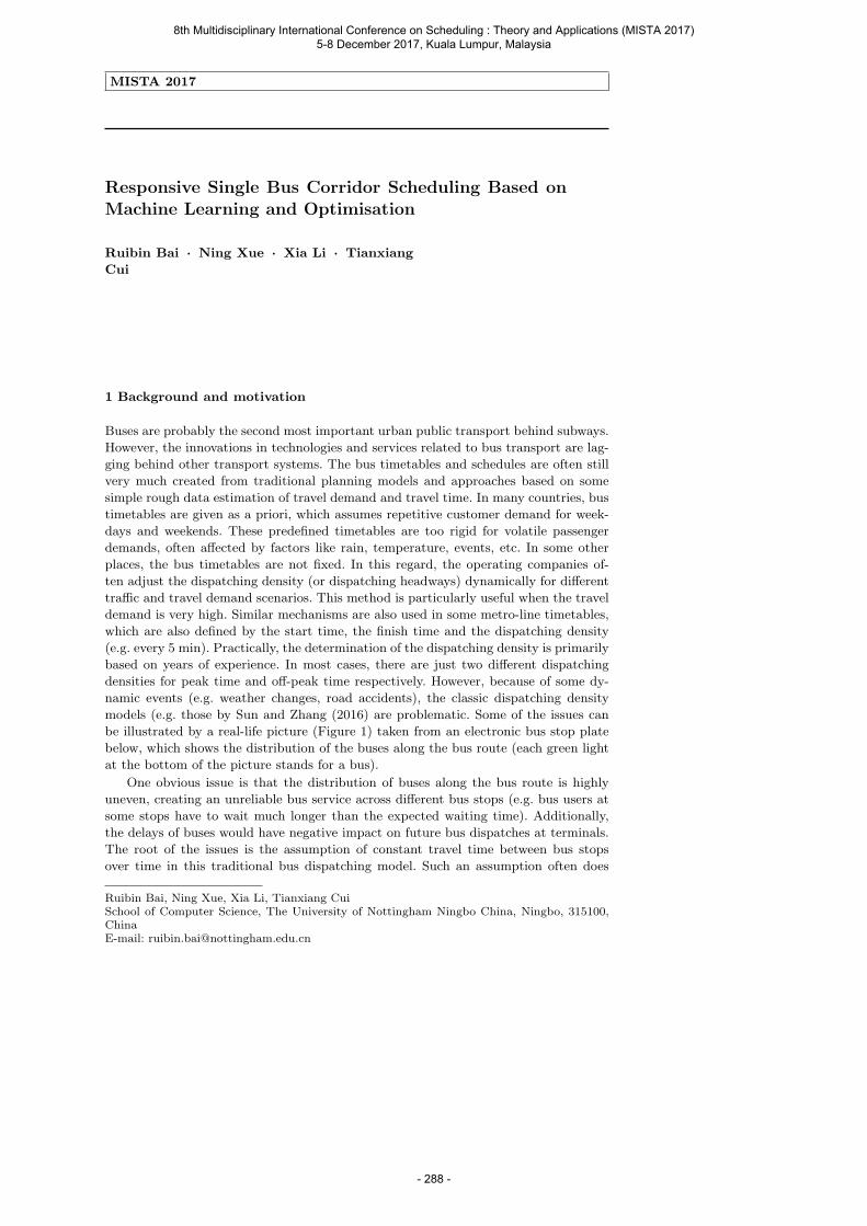
MISTA 2017

Responsive Single Bus Corridor Scheduling Based onMachine Learning and Optimisation

Ruibin Bai · Ning Xue · Xia Li · Tianxiang

Cui

1 Background and motivation

Buses are probably the second most important urban public transport behind subways.

However, the innovations in technologies and services related to bus transport are lag-

ging behind other transport systems. The bus timetables and schedules are often still

very much created from traditional planning models and approaches based on some

simple rough data estimation of travel demand and travel time. In many countries, bus

timetables are given as a priori, which assumes repetitive customer demand for week-

days and weekends. These predefined timetables are too rigid for volatile passenger

demands, often affected by factors like rain, temperature, events, etc. In some other

places, the bus timetables are not fixed. In this regard, the operating companies of-

ten adjust the dispatching density (or dispatching headways) dynamically for different

traffic and travel demand scenarios. This method is particularly useful when the travel

demand is very high. Similar mechanisms are also used in some metro-line timetables,

which are also defined by the start time, the finish time and the dispatching density

(e.g. every 5 min). Practically, the determination of the dispatching density is primarily

based on years of experience. In most cases, there are just two different dispatching

densities for peak time and off-peak time respectively. However, because of some dy-

namic events (e.g. weather changes, road accidents), the classic dispatching density

models (e.g. those by Sun and Zhang (2016) are problematic. Some of the issues can

be illustrated by a real-life picture (Figure 1) taken from an electronic bus stop plate

below, which shows the distribution of the buses along the bus route (each green light

at the bottom of the picture stands for a bus).

One obvious issue is that the distribution of buses along the bus route is highly

uneven, creating an unreliable bus service across different bus stops (e.g. bus users at

some stops have to wait much longer than the expected waiting time). Additionally,

the delays of buses would have negative impact on future bus dispatches at terminals.

The root of the issues is the assumption of constant travel time between bus stops

over time in this traditional bus dispatching model. Such an assumption often does

Ruibin Bai, Ning Xue, Xia Li, Tianxiang CuiSchool of Computer Science, The University of Nottingham Ningbo China, Ningbo, 315100,ChinaE-mail: [email protected]


- 288 -

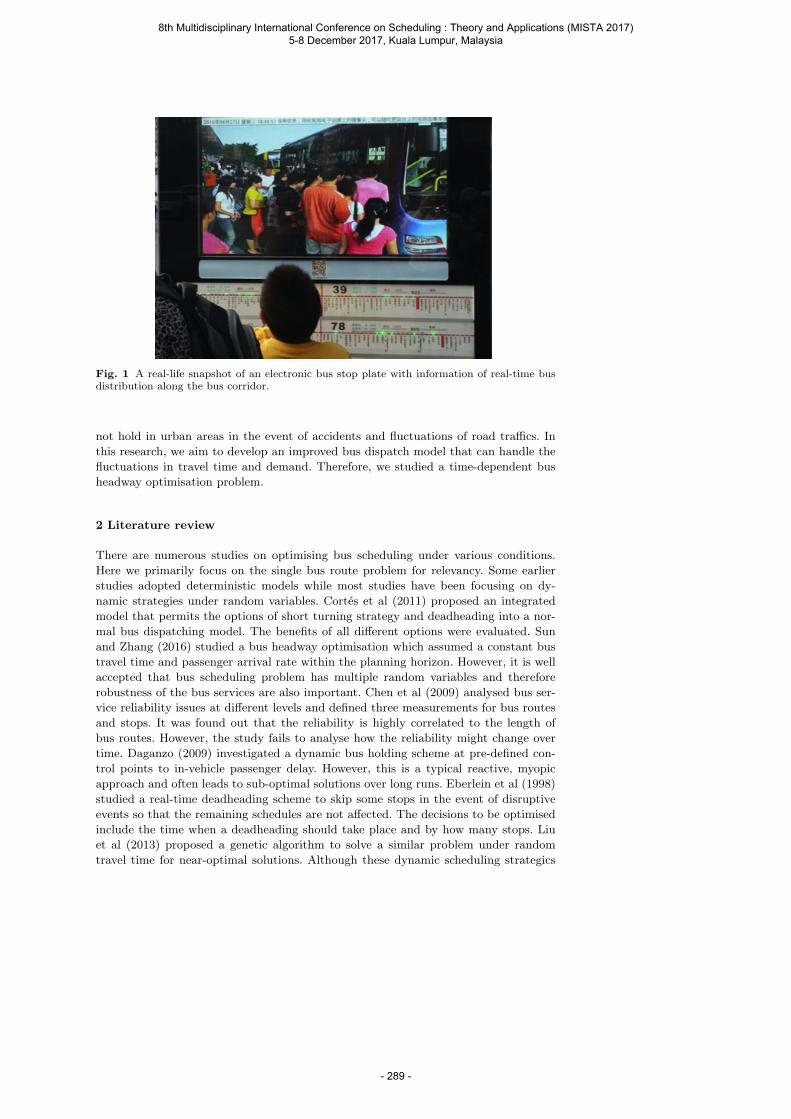
Fig. 1 A real-life snapshot of an electronic bus stop plate with information of real-time busdistribution along the bus corridor.

not hold in urban areas in the event of accidents and fluctuations of road traffics. In

this research, we aim to develop an improved bus dispatch model that can handle the

fluctuations in travel time and demand. Therefore, we studied a time-dependent bus

headway optimisation problem.

2 Literature review

There are numerous studies on optimising bus scheduling under various conditions.

Here we primarily focus on the single bus route problem for relevancy. Some earlier

studies adopted deterministic models while most studies have been focusing on dy-

namic strategies under random variables. Cortes et al (2011) proposed an integrated

model that permits the options of short turning strategy and deadheading into a nor-

mal bus dispatching model. The benefits of all different options were evaluated. Sun

and Zhang (2016) studied a bus headway optimisation which assumed a constant bus

travel time and passenger arrival rate within the planning horizon. However, it is well

accepted that bus scheduling problem has multiple random variables and therefore

robustness of the bus services are also important. Chen et al (2009) analysed bus ser-

vice reliability issues at different levels and defined three measurements for bus routes

and stops. It was found out that the reliability is highly correlated to the length of

bus routes. However, the study fails to analyse how the reliability might change over

time. Daganzo (2009) investigated a dynamic bus holding scheme at pre-defined con-

trol points to in-vehicle passenger delay. However, this is a typical reactive, myopic

approach and often leads to sub-optimal solutions over long runs. Eberlein et al (1998)

studied a real-time deadheading scheme to skip some stops in the event of disruptive

events so that the remaining schedules are not affected. The decisions to be optimised

include the time when a deadheading should take place and by how many stops. Liu

et al (2013) proposed a genetic algorithm to solve a similar problem under random

travel time for near-optimal solutions. Although these dynamic scheduling strategics


- 289 -

(e.g. short turning and deadheading) are useful to address some interruptive incidents

and improve bus service reliability, the solutions may be too myopic because the de-

cisions are primarily made by considering the real-time data. Repetitive patterns are

overlooked.

In this paper, we propose a new bus headway optimisation model that takes advan-

tage of both the dynamic events data as well as the historical data so that our solution

is more robust than the deterministic solution and less myopic than the aforementioned

dynamic schemes. This is achieved by developing a mathematical model integrated with

two machine learning modules to supply high quality forecasts for random variables

based on both the real-time and historical data.

3 Problem description and model formulation


The problem can be described as follows. Given a bus route with a dispatching terminal

and two directions (outbound or direction 1 and incoming or direction 2), let S and

K be the list of stops in direction 1 and direction 2 respectively. Denote V and W be

the list of bus trips to be made over the planning horizon for the two bus route direc-

tions respectively. At any moment of decision making, CT , we want to determine the

optimal dispatch headways (i.e. the gap between any two consecutive bus trips) at the

terminal for all the future outbound bus trips. The objectives include the minimisation

of the total passenger waiting time, minimisation of passenger total overload penalties

and minimisation of the total bus operation costs. The model contains three types of

parameters: user controlled parameters, real-time parameters and forecast parameters

by machine learning modules. They are listed below:

3.2 Parameters and notations

3.2.1 User controlled parameters

– BusRoute: including types (cyclic, or symmetric dual control for symmetric single

control), number of stops, total distance, travel time under normal conditions in

both directions (upstream and downstream).

– Ts: Planning horizon start time. By default this is set to the current time.

– Tf : finish time of the planning horizon. Target planning period is 2-3 hours.

– n: the total number of buses available.

– B: the list of buses available with properties including capacity, per trip running

cost, available time window (or unavailable time window), vehicle types (normal

bus or emergency back-ups). Broken-down vehicles should NOT be included in this

list.

– gmax: maximum bus dispatching gap permitted at different period p.

– gmin: minimum bus dispatching gap, if not given, default to 1 min.

– MinRestT ime: Minimum rest time for a bus at a terminal.

– w1, w2, w3: the weights for three penalty terms: total waiting time, overloading and

running cost. w1 + w2 + w3 = 1.


- 290 -

3.2.2 Parameters required from real-time monitor module

– The status of all buses defined in B, including their positions.

– The boarding and alighting data at each station in the most recent m trips. This

can be empty if no bus trips are made during that day.

– The GPS trajectory data of the most recent m bus trips.

3.2.3 Parameters estimated by machine learning modules

– r(p, k): Passenger arrival rate at time period p and stop k. unit: person/min.

– a(p, k): proportion of bus load alighting at stop k during time period p. 0 ≤ a(p, k) ≤1.

– RT (d0, i): the time for a given schedule bus trip i to reach final destination (i.e.

final terminal). d0 is the departure time of the bus trip i. If d0 < CT , the trip is

on-going. The time should be estimated based on a combination of the vehicle’s

current position and historical data.

– T (k, k + 1, p): trip time for a bus from stop k to k + 1.

– T1: the average total trip time in control direction 1. Time-independent.

– T2: the average total trip time in control direction 2. Time-independent.

3.2.4 Decision variables and auxiliary variables

The solution is represented by two bus trip queues, V and W , for control direction 1

and direction 2 respectively. Both V and W are sorted by the planned departure times.

The length of V and W should cover the entire planning horizon and can be estimated

based on the average departure headways and average travel time for each direction.

– gi: the dispatching headway for scheduled bus trip i ∈ V in control direction 1.

– hj : the dispatching headway for a scheduled bus trip j ∈ W in control direction 2.

– di: departure time of scheduled bus trip i ∈ V in control direction 1. Hence gi =

di − di−1.

– ej : departure time of bus trip j ∈ W in control direction 2, and hi = ei − ei−1.

– dki : departure time of bus trip i ∈ V from station/stop k.

– esj : departure time of trip j ∈ W from stop s ∈ S.

– gki : headway for trip i ∈ V at bus stop k ∈ K. gki = dki − dki−1.

– hsj : headway for trip j ∈ W at bus stop s ∈ S and hkj = ekj − ekj−1.

– Lki : passenger load for trip i ∈ V at stop k ∈ K for direction 1.

– Lsj : passenger load for trip j ∈ W at stop s ∈ S for direction 2.

3.2.5 Other notations

– CT : current time.

– K:The set of successive stops in control direction 1, including start and finish

terminals, indexed by k.

– S:The set of successive tops in control direction 2, including start and finish termi-

nals, indexed by s.

– P : a set of continuous time periods of identical length τ , indexed by p.

– Ci, Cj : the capacity of vehicles used for trips i and j respectively.

– Fi, Fj : the fixed operation cost for running trips i and j respectively.


- 291 -

3.3 Objective function

The scheduling can be activated by a returning vehicle or a number of returning vehicles

with a rolling planning horizon. Assume a current rescheduling point/time t0 and a

planning horizon consisting of P successive identical time periods, indexed by p.

The objective function consists of three penalty components, the total passenger

waiting time O1, the total passenger overloads O2 and the bus service operation cost

O3. The total waiting time at all stations can be calculated as follows.

O1 =∑i∈V

∑k∈K

r(p, k)× (gki )2/2 +

∑j∈W

∑s∈S

r(p, s)× (gsj )2/2 (1)

The first term is for the control direction 1 and the second term for the direction

2. Period p can be estimated as p = (dki−1 + dki )/(2 × τ) for direction 1 and p =

(esj−1 + dsj)/(2× τ) for direction 2.

The passenger overload penalty can be computed as follows.

O2 =∑

i∈V

∑k∈K [T (k, k + 1, p)×max0, r(p, k)gki + (1− a(p, k))Lk

i − Ci]+∑

j∈W

∑s∈S [T (s, s+ 1, p)×max0, r(p, s)gsj + (1− a(p, s))Lk

j − Cj]

where p can be estimated similarly to the previous equation.

The total operation cost can be estimated by.

O3 =∑i∈V

Fi +∑j∈W

Fj (2)

Naturally one could model this as a multi-criteria or multi-objective optimisation

problem. Unfortunately for real-life applications, bus planning practitioners generally

cannot tolerate long computational time that may be required by a multi-objective op-

timisation approach. Moving O1 and O2 into the constraints is another good option but

cautions should be made for a potential problem without feasible solution due to a lack

of sufficient buses. The main focus of this paper is modeling the optimisation problem

with (part of ) the parameters coming from machine learning modules. We adopted a

simple objective function which is a weighted sum of the above three components.

OBJ = mingi,hj

(w1O1 + w2O2 + w3O3) (3)

Auxiliary variables can be calculated through the following recursive functions

gki = dki−1 − dki ∀i ∈ V, k ∈ K (4)

dki = dk−1i + T (k − 1, k, p) ∀i ∈ V, k ∈ K (5)

g0i = gi ∀i ∈ V (6)

d0i = di ∀i ∈ V (7)

hsj = hsj−1 − hsj ∀j ∈ W, s ∈ S (8)

hkj = hs−1j + T (s− 1, s, p) ∀j ∈ W, s ∈ S (9)

h0j = hj ∀j ∈ W (10)

h0j = hj ∀j ∈ W (11)


- 292 -

For most applications, we can approximate T (k−1, k, p) by T (k−1, k). If this does not

meet practical real-life requirements, T (k − 1, k, p) should also be estimated through

machine learning modules where p = (dki−1 + dki )/(2 × τ) for direction 1 and p =

(esj−1 + dsj)/(2× τ) for direction 2.

3.4 Constraints

The following constraints should be satisfied.

gmin ≤ gi ≤ gmax∀i ∈ V (12)

gmin ≤ hj ≤ gmax∀j ∈ W (13)

di +RT (d0, i)− di ≥ MinRestT ime ∀i ∈ V (14)

ej +RT (d0, j)− dj ≥ MinRestT ime ∀j ∈ W (15)∑i∈V

gi ≥ Tf − Ts (16)

Constraints (12) and (13) ensure that the headways for each bus trips in both directions

are between a pre-specified minimum and maximum. Constraints (14) and (15) make

sure that drivers have a minimum rest time before their next trips start. Constraint

(16) guarantees the full coverage of planning horizon in any feasible list of bus trips

V . The constraint of the maximum number of vehicles used should be automatically

satisfied while creating trip lists V and W .

4 Solution methods

The model developed in the previous section is highly non-linear and can be in large-

scale if the granularity of periods P is significantly smaller than the planning horizon.

Therefore heuristic approaches are proposed as the solution method for the problem.

As illustrated in Section 3.2.4, the primary decision variables are the headways (gi, hj)

for bus route directions 1 and 2. Other variables can be computed through these two

set of decision variables. In this research, memetic algorithm was chosen as the solution

method for this problem. The reasons are: first, although the problem is formulated as a

single objective optimisation problem, naturally it has three conflicting objectives and

one would need minimal efforts to extend the proposed method to a multi-objective

version. Second, a natural solution encoding scheme will be a vector concatenating giand hj . Because the problem is not tightly bound, the combination operators in GA

could be very efficient in finding high quality regions and solutions. Finally, local search

procedure in memetic algorithm will make sure the resulting solution is at least a local

optimum.

One of the main contributions of this paper is the introduction of machine learning

methods into a traditional optimisation problem. Through machine learning modules,

much high quality parameters are estimated by utilising both the real-time traffic data

and historical data at a much finer time granularity (defined by the size of the period p).

The parameters estimated by the machine learning modules include passenger demand

data (r(p, k), a(p, k) and travel time data (RT (d0, i), DT (k, k + 1, p), and DT (p, k)).


- 293 -

In this research, we use a popular SVR (supporting vector regression) method from

the LIBSVM library (Chang, 2016) for the estimation of both the passenger demand

data and travel time data.

5 Discussions and future research

Although the coding of the algorithm is completed already and some initial results

with some toy instances are available, the full experimental results are not available

yet. It is expected that complete computational results will be presented during the

conference presentation.

References

Chang CC (2016) LIBSVM: A library for support vector machines. URL

http://www.csie.ntu.edu.tw/ cjlin/libsvm/

Chen X, Yu L, Zhang Y, Guo J (2009) Analyzing urban bus service reliability at the

stop, route, and network levels. Transportation research part A: policy and practice

43(8):722–734

Cortes CE, Jara-Dıaz S, Tirachini A (2011) Integrating short turning and deadheading

in the optimization of transit services. Transportation Research Part A: Policy and

Practice 45(5):419–434

Daganzo CF (2009) A headway-based approach to eliminate bus bunching: System-

atic analysis and comparisons. Transportation Research Part B: Methodological

43(10):913–921

Eberlein XJ, Wilson NH, Barnhart C, Bernstein D (1998) The real-time deadheading

problem in transit operations control. Transportation Research Part B: Methodolog-

ical 32(2):77–100

Liu Z, Yan Y, Qu X, Zhang Y (2013) Bus stop-skipping scheme with random travel

time. Transportation Research Part C: Emerging Technologies 35:46–56

Sun Q, Zhang X (2016) Optimization model and algorithm design of bus lines non-fixed

headways problem based on passenger arrival rates. Open Journal of Transportation

Technologies 5(1):7–16


- 294 -

MISTA 2017

Benders Decomposition in SMT for Reschedulingof Hierarchical Workflows

Marek Vlk · Roman Bartak ·Emmanuel Hebrard

Abstract Real-life scheduling has to face many difficulties such as dynamic manufac-

turing environments with failing resources and urgent orders arriving during the sched-

ule execution. Complete rescheduling, considering only the original objective function,

in response to unexpected events occurring on the shop floor may yield schedules that

are prohibitively different from the original schedule, which may lead to extra costs due

to impacts on other planned activities. Our novel approach in the area of predictive-

reactive scheduling is to allow for substitution of jobs which cannot be executed with

a set of alternative jobs. Hence, this paper describes the model of hierarchical work-

flows suitable for dealing with unforeseen events using the possibility of alternative

processes and proposes a new approach, based on the Satisfiability Modulo Theories

(SMT) formalism, to recover an ongoing schedule from a resource failure. The experi-

mental results show that the SMT approach using Benders decomposition is orders of

magnitude faster than a Constraint Programming approach.

1 Introduction

Scheduling aims at allocating scarce resources to jobs in order to optimize certain ob-

jectives. There has been extensive research on this area in the past decades. Developing

a detailed schedule in manufacturing environment helps maintain efficiency and control

of operations.

In the real world, however, manufacturing systems face uncertainty owing to un-

foreseen events occurring on the shop floor. Machines break down, operations take

longer than anticipated, personnel do not perform as expected, urgent orders arrive,

others are canceled, etc. These disturbances may bring inconsistencies into the ongoing

schedule. If the ongoing schedule becomes infeasible, the simple approach is to collect

Marek Vlk, Roman BartakCharles University, Faculty of Mathematics and PhysicsMalostranske nam. 25, 118 00 Praha 1, Czech RepublicE-mail: vlk, [email protected]

Emmanuel HebrardLaboratoire d’Analyse et d’Architecture des Systemes7 Avenue du Colonel Roche, 31077 Toulouse cedex 4, FranceE-mail: [email protected]


- 295 -

the data from the shop floor when the disruption occurs and to generate a new schedule

from scratch. Because most scheduling problems are NP-hard, complete rescheduling is

usually prohibitively time-consuming and generates a new schedule that is too deviated

from the original schedule.

To avoid the problems of rescheduling from scratch, the continuous correction of

precomputed predictive schedules (so-called reactive scheduling) is becoming more and

more important. Reactive scheduling differs from predictive scheduling mainly by its

on-line nature and associated real-time execution requirements. The schedule update

must be accomplished before the running schedule becomes invalid, and this time

window may be very short in some areas.

In this paper, we describe the model with the hierarchical structure of tasks that

is suitable also for the field of predictive-reactive scheduling. Further, we model the

rescheduling problem in the formalism called Satisfiability Modulo Theories (SMT)

[14]. The goal of the model is to recover a schedule from a resource failure, exploiting

the possibility of alternative processes. Also, we suggest how to leverage the Benders

decomposition [6] by dividing the problem into a master problem and a subproblem

where the subproblem passes the reason for inconsistency to the master problem. We

experimentally compare these two models to each other, as well as against a Constraint

Programming (CP) model.

We first contextualize this paper in terms of the related works. Section 3 then

describes the scheduling model and the resource failure recovery problem tackled in

this paper and the suggested approaches are described in Sect. 4. The experimental

results are given in Sect. 5, and the final part points out possible future work.

2 Related Work

The approaches how to tackle dynamics of the scheduling environment can be divided

basically into two branches according to whether or not the predictive schedule is

computed before the execution starts [24]. If the predictive schedule is not computed

beforehand and individual jobs are assigned to resources pursuant to some so-called

dispatching rules during the execution, we talk about completely reactive scheduling or

on-line scheduling. This strategy is suitable for very dynamic environments, where it

is not known in advance which jobs it will be necessary to process. On the other hand,

it is obvious that this approach seldom leads to an optimal or near-optimal schedule.

If the schedule is crafted beforehand and then updated during its execution, it is

referred to as predictive-reactive scheduling. When correcting the ongoing schedule in

response to changes within the environment, the aim is usually to minimize the schedule

modification. The motivation for minimizing the modification of the schedule is that

every deviation may lead to deterioration in the performance of the manufacturing

system because of impacts on other planned activities based upon the original schedule.

There is an extensive literature on rescheduling [2,17,26], giving various generic

approaches as well as ad-hoc procedures to particular cases. However, to the best of

our knowledge, there is only scarce research carried out aiming at the possibility of

re-planning in the field of predictive-reactive scheduling.

On the other hand, if a certain level of minor disruptions is anticipated, it can

be taken into account when generating a baseline schedule, such as in [15], where the

static schedules account for unforeseen prolongation of processing times of tasks. This

area is usually referred to as proactive scheduling.


- 296 -

The scheduling model described further is based on the notion of workflows. Work-

flow, in general, may be understood as a scheme of performing some complex process,

itemized into simpler processes and relationships among them. There exist many formal

models to describe workflows [23] that include decision points and loops to describe

repetition of operations, but in real-life applications, many workflows are obtained

by decomposition of tasks, which is the motivation for the hierarchical structure of

workflows. In this paper, we consider workflows that have a very similar structure to

Temporal Planning Networks [19] but are enhanced by extra constraints and resources.

The logical constraints in a workflow indicate the connection with the first order

logic and the problem of Boolean Satisfiability (SAT) [22]. Most SAT-solvers today are

still based on variations of the DPLL procedure [9]. However, significant advances in

SAT solving techniques were made in the last decades thanks to better implementa-

tion techniques such as the two-watched literal approach for unit propagation [13] and

conceptual improvements such as conflict-driven clause learning and restarts [20,5].

This progress made SAT-solvers applicable also to solving Constraint Satisfaction

Problems (CSP) [18] in general. In the lazy clause generation approach [16], a Boolean

formula corresponding to a finite domain CSP is lazily created during the computation.

On the other hand, motivation of gaining the advantages of techniques used both in

SAT-solvers and CSP-solvers lead to another hybrid approach, where some domain

specific reasoning is implemented within a SAT-solver: SAT Modulo Theories (SMT)

[14].

The temporal constraints in our scheduling model are linear inequalities so that

it is suitable for SMT, using the linear integer arithmetic as the background theory.

SMT solvers have already been used for solving combinatorial optimization problems

[8], including some scheduling problems [1], and exhibited promising performance.

The problem we tackle has already been targeted by [4], where an ad-hoc heuristic-

based algorithm is proposed which quickly finds near-optimal solutions, but supports

temporal constraints only between primitive tasks, which limits its applicability. Also in

[25], a very similar problem is addressed, with the main difference that the optimization

objective is to minimize the work processed in vain, and a detailed experimental analysis

is presented.

3 Scheduling Model

In this work, we use the model of workflows that match up the structure of Nested

Temporal Networks with Alternatives [3], where the nodes of a network correspond

to the tasks of a workflow. The tasks decompose into other tasks, referred to as their

subtasks. There are two types of decomposition: parallel and alternative. The tasks

that do not decompose further (i.e., leaves) are called primitive tasks. The primitive

tasks correspond to executable operations and are associated with some additional

parameters such as duration and resource.

The workflows as described define a number of feasible processes. A process is a

subset of tasks selected to be processed. While a parallel task requires all its children

to be processed, an alternative task requires exactly one of its children to be processed.

If an arbitrary task is not in the process, none of its subtasks is in the process either.

Hence, to ensure that an instance of a workflow is actually processed, its root task has

to be in the selected process. An example of a workflow and a process (Fig. 1) [21]

contains eight primitive tasks, three parallel tasks, and two alternative tasks.


- 297 -

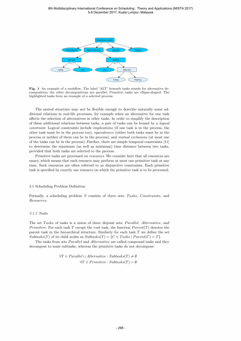
Fig. 1 An example of a workflow. The label ’ALT’ beneath tasks stands for alternative de-composition; the other decompositions are parallel. Primitive tasks are ellipse-shaped. Thehighlighted tasks form an example of a selected process.

The nested structure may not be flexible enough to describe naturally some ad-

ditional relations in real-life processes, for example when an alternative for one task

affects the selection of alternatives in other tasks. In order to simplify the description

of these additional relations between tasks, a pair of tasks can be bound by a logical

constraint. Logical constraints include implications (if one task is in the process, the

other task must be in the process too), equivalences (either both tasks must be in the

process or neither of them can be in the process), and mutual exclusions (at most one

of the tasks can be in the process). Further, there are simple temporal constraints [11]

to determine the maximum (as well as minimum) time distance between two tasks,

provided that both tasks are selected to the process.

Primitive tasks are processed on resources. We consider here that all resources are

unary, which means that each resource may perform at most one primitive task at any

time. Such resources are often referred to as disjunctive constraints. Each primitive

task is specified by exactly one resource on which the primitive task is to be processed.

3.1 Scheduling Problem Definition

Formally, a scheduling problem S consists of three sets: Tasks, Constraints, and

Resources.

3.1.1 Tasks

The set Tasks of tasks is a union of three disjoint sets: Parallel, Alternative, and

Primitive. For each task T except the root task, the function Parent(T ) denotes the

parent task in the hierarchical structure. Similarly for each task T we define the set

Subtasks(T ) of its child nodes as Subtasks(T ) = C ∈ Tasks | Parent(C) = T.The tasks from sets Parallel and Alternative are called compound tasks and they

decompose to some subtasks, whereas the primitive tasks do not decompose:

∀T ∈ Parallel ∪Alternative : Subtasks(T ) 6= ∅∀T ∈ Primitive : Subtasks(T ) = ∅


- 298 -

Let process P ⊆ Tasks be the set of tasks selected to be processed. To make the

process feasible, it is necessary to satisfy the following constraints:

∀T ∈ P ∩ Parallel : Subtasks(T ) ⊆ P (1)

∀T ∈ P ∩Alternative : |Subtasks(T ) ∩ P | = 1 (2)

∀T /∈ P : Subtasks(T ) ∩ P = ∅ (3)

root ∈ P (4)

Note that without constraint (4), an empty set would be a feasible process.

Let Si and Ei denote the start time and end time, respectively, of task Ti. We

consider only non-interruptible tasks, and each primitive task Ti is specified by the

duration Di. The times for compound tasks are computed from the times of their

subtasks. Thus we obtain the following constraints:

∀Ti ∈ P ∩ Primitive : Ei = Si + Di (5)

∀Ti ∈ P \ Primitive : Si = minSj | Tj ∈ Subtasks(Ti) ∩ P (6)

∀Ti ∈ P \ Primitive : Ei = maxEj | Tj ∈ Subtasks(Ti) ∩ P (7)

3.1.2 Extra constraints

There are basically two types of constraints: logical and temporal. Logical constraints

are of three types: implications, equivalences, and mutexes. The semantics of the con-

straints is as follows:

∀(i⇒ j) : Ti ∈ P ⇒ Tj ∈ P (8)

∀(i⇔ j) : Ti ∈ P ⇔ Tj ∈ P (9)

∀(i mutex j) : Ti /∈ P ∨ Tj /∈ P (10)

The time distance between two distinct tasks may be restricted by a simple temporal

constraint. This constraint can be written as a triplet (Xi, Xj , wij), where wij ∈ Z, Xi

is either Si or Ei, and Xj is either Sj or Ej . The semantics is as follows:

∀(Xi, Xj , wij) : Ti ∈ P ∧ Tj ∈ P ⇒ Xj −Xi ≤ wij (11)

Notice that temporal constraints may be between compound tasks, that is why the

time variables Si and Ei are needed for all tasks in the model.

3.1.3 Resources

Each primitive task is associated with exactly one resource where it can be processed.

Let Ti ∈ Primitive, then the resource that can process the primitive task Ti is denoted

Ri.

All resources in a schedule are unary, which means that they cannot execute several

tasks simultaneously. Therefore, in a feasible schedule, the following holds:

∀Ti, Tj ∈ Primitive ∩ P, Ti 6= Tj : Ri = Rj ⇒ Ei ≤ Sj ∨ Ej ≤ Si (12)

Note that the fact that each primitive task is associated with exactly one resource

does not make the model less expressive than considering alternative resources for

a primitive task as this may be modeled using alternative tasks. Similarly, more re-

sources for a primitive task can be modeled via parallel decomposition to temporally

synchronized primitive tasks.


- 299 -

3.2 Schedule

A schedule S (sometimes referred to as a resulting schedule or a solution) is acquired

by determining the set P , and allocating the tasks from P in time, that is, assigning

particular values to the variables Si and Ei for each Ti ∈ P .

To make a schedule feasible, the process selection and the allocation must be con-

ducted in such a way that all the constraints (1)–(12) in the problem are satisfied.

3.3 Rescheduling Problem

The problem we deal with is that we are given a particular instance of the scheduling

problem along with a feasible schedule, and also with a disturbance arising from the

shop floor. The aim is to find another schedule that is feasible with respect to the

disturbance. The feasible schedule we are given is referred to as an original schedule

or an ongoing schedule.

In what follows we restrict our attention to a disruption called a resource failure,

which is often referred to as a machine breakdown. The resource failure may happen

in a manufacturing system at any point in time, say tf , and means that a particular

resource cannot be used anymore, i.e., for all t ≥ tf there is no task allocated to that

resource.

Formally, let Sch0 be the original schedule, with P0 being the selected process in

Sch0, Si(Sch0) and Ei(Sch0) the start times and end times in Sch0; and R be the

resource that failed at some time tf : tf ∈ Z, tf ≥ 0. Next, let us define Pinned as

the set of primitive tasks that are from P0 and, whose execution has finished if they

were allocated to R or whose execution has at least started if they were allocated to

an available resource, that is, Ti ∈ Pinned if and only if:

Ti ∈ Primitive ∩ P0 ∧((Ei(Sch0) ≤ tf ∧Ri = R) ∨ (Si(Sch0) < tf ∧Ri 6= R)

)Finally, the aim is to find a new feasible (recovered) schedule Sch1, with P1 being

the selected process in Sch1, Si(Sch1) and Ei(Sch1) the start times and end times in

Sch1, subject to the following constraints:

∀Ti ∈ Pinned : Ti ∈ P1 ∧ Si(Sch1) = Si(Sch0) (13)

∀Ti ∈ Primitive \ Pinned,Ri = R : Ti /∈ P1 (14)

∀Ti ∈ Primitive \ Pinned,Ri 6= R : Ti ∈ P1 ⇒ Si(Sch1) ≥ tf (15)

The constraint (13) ensures that the primitive tasks defined above as Pinned are

also in the new process and are not shifted in time. The constraint (14) ensures that

each primitive task that is not in Pinned and is associated with the failed resource is

not in the new process P1, and for the remaining primitive tasks, the constraint (15)

ensures that no primitive task will be scheduled in the past.

The aim is to find the new schedule Sch1 as similar to Sch0 as possible. For this

purpose, we minimize the objective function defined as the number of primitive tasks

that were removed from the original schedule plus the number of primitive tasks that

were added to the recovered schedule:

f = |T ∈ P0 ∩ Primitive \ P1|+ |T ∈ P1 ∩ Primitive \ P0| (16)


- 300 -

Note that the constraint (3) states that non-membership of a task implies non-

membership of its subtasks. Hence, there cannot be any unneeded task in the process.

This is coherent with the needs of real-life applications.

4 Resource Failure Recovery as Satisfiability Modulo Theories

In this section, we describe how we model the resource failure recovery problem in

the SMT formalism. Recall that the task of an SMT solver is to find a satisfying

assignment of a formula ϕ or report unsatisfiability. Such formula is usually represented

in a Conjunctive Normal Form (CNF), i.e., as the conjunction of clauses, where clauses

are disjunctions of literals corresponding to expression in a particular theory, in our

case difference logic. To ease the description, we list the clauses in the form given by

their semantics. Such clauses can be transformed to a CNF.

We use the application interface of the Z3 solver [10]. This solver provides two

objects: Solver, which can determine the unsatisfiable core, and Optimizer, which allows

the addition of weighted soft clauses to the formula, and then minimizes the sum of

weights of soft clauses that are not satisfied by the assignment.

4.1 Global Model

For each task Ti ∈ Tasks, let us introduce propositional variables Vi that will be

true if and only if Ti ∈ P1, and numeric (non-negative integer) variables Si and Ei

determining the start time and end time of task Ti. Now we describe how the SMT

formula ϕ to be satisfied is constructed.

For each compound task Ti, let us denote Subtasks(Ti) = Ti1 , ..., Tik. If Ti ∈Parallel, then for each j = i1, ..., ik the following unit clause is added to the formula

ϕ:

(Vi = Vj) (17)

If Ti ∈ Alternative, the following clause is added:(ite(Vi; 1; 0) =

ik∑j=i1

ite(Vj ; 1; 0)

)(18)

The expression ite(Vi; 1; 0) is evaluated as 1 if Vi is true, otherwise 0. It is straight-

forward to verify that satisfying the clauses (17) and (18) enforces the satisfaction of

constraints (1)–(3). Note that we also tried modeling the constraint (2) in a purely log-

ical way, i.e., using disjunction and at-most-one clauses instead of clause (18), but this

did not lead to any measurable difference in run times. To satisfy also the constraint

(4), we simply add the unit clause:

(Vroot) (19)

As to the time allocations for primitive tasks, that is, satisfying the constraint (5),

it is enough to add the following clauses:

(Ei = Si + Di) (20)


- 301 -

The time allocations for compound tasks is not that straightforward as the functions

min and max are not in the formal specification of SMT. Hence for a parallel task we

need clauses ensuring that the start time of the task is always less than or equal to its

subtasks, and that it equals one of its subtasks. A similar construction is used for the

end times. Formally, for each Ti ∈ Parallel:

(Vi ⇒ik∨

j=i1

Si = Sj) (21)

(Vi ⇒ik∨

j=i1

Ei = Ej) (22)

And for each j = i1, ..., ik:

(Vi ⇒ Si ≤ Sj) (23)

(Vi ⇒ Ei ≥ Ej) (24)

Since alternative tasks have at most one subtask in the process, it suffices to add,

for each Ti ∈ Alternative, and for each j = i1, ..., ik:

(Vj ⇒ Si = Sj) (25)

(Vj ⇒ Ei = Ej) (26)

It is easy to see that the satisfaction of clauses (21)–(26) ensures satisfying the

constraints (6) and (7).

The logical constraints (8)–(10) in the format of (i→ j), (i↔ j), and (i mutex j)

are handled by adding the following clauses, respectively:

(Vi ⇒ Vj) (27)

(Vi ⇔ Vj) (28)

(¬Vi ∨ ¬Vj) (29)

Next, for each simple temporal constraint (11) (Xi, Xj , wij), where wij ∈ Z, Xi is

either Si or Ei, and Xj is either Sj or Ej , we add:

((Vi ∧ Vj)⇒ Xj −Xi ≤ wij) (30)

The disjunctive constraints (12) are handled by adding the following clauses, for

each Ti, Tj ∈ Primitive, Ti 6= Tj , Ri = Rj :

((Vi ∧ Vj)⇒ (Ei ≤ Sj ∨ Ej ≤ Si)) (31)

To ensure that the primitive tasks from the set Pinned are also in the new process

and are not shifted in time, that is, to satisfy the constraint (13), add for each Ti ∈Pinned:

(Vi) (32)

(Si = Si(Sch0)) (33)

To satisfy the constraint (14), add for each Ti ∈ Primitive \ Pinned,Ri = R:

(¬Vi) (34)


- 302 -

And to satisfy the constraint (15), add for each Ti ∈ Primitive \ Pinned,Ri 6= R:

(Si ≥ tf ) (35)

Note that the clauses (20) and (35) do not need the implication form (Vi ⇒ expr),

because in case Vi = false, the values of the time points Si and Ei do not affect other

variables and thus may be assigned arbitrary values (satisfying the clauses) by an SMT

solver, which turned out to be slightly faster than the implication form.

Finally, the distance function f is optimized by adding soft clauses of weight 1. For

each Ti ∈ Primitive ∩ P0, the following soft clause is added:

(Vi) (36)

Oppositely, for each Ti ∈ Primitive \ P0, the following soft clause is added:

(¬Vi) (37)

Notice that instead of all weights being equal to one, we could set the weights

according to the additional cost if the corresponding primitive task is processed. Thus,

instead of robust rescheduling, we could directly use the same model for cost-minimizing

scheduling.

4.2 Benders Decomposition

The SMT model can be decomposed in two phases: first, compute the process P1, that

is, assign truth values to the variables Vi, and second, schedule the process, that is,

assign time points to the variables Si and Ei for each Ti ∈ P1. If the second phase

corresponds to an unsatisfiable problem, get the reason for inconsistency (unsatisfiable

core) and go back to the first phase to find another process. Iterate until a feasible

schedule is found or there is no other process to try.

4.2.1 Master Problem

Formally, we first build a formula ϕp consisting exactly of the clauses that do not involve

time variables, i.e., the clauses (17)–(19), (27)–(29), (32), (34), (36), and (37). Then

the SMT solver is run. If it reports ’infeasible’, there is no solution to the problem. If it

finds a satisfying assignment V, we now build a formula ϕs exploiting the knowledge

of V.

4.2.2 Subproblem

The formula ϕs is build from the clauses involving the time variables. However, as we

already know the values of all Vi, we add only the clauses that are not trivially valid.

The clauses (21)–(26), and (35) of the form (Vi ⇒ expr), such that Vi is true, are

added to the formula ϕs in the form (expr). Similarly, the clauses (30) and (31) of the

form ((Vi ∧ Vj)⇒ expr), such that both Vi and Vj are true, are added to the formula

ϕs in the form (expr). Finally, the clauses (20), (33), and (35), such that Vi is true,

are added without modification.

After the SMT solver is run on the formula ϕs, there are two possible results. If

it finds a satisfying assignment, that is, a schedule, it is clearly the optimal solution


- 303 -

as the objective function concerns only the process selection. Otherwise, if it reports

unsatisfiable, i.e., the process is not schedulable, we will obtain an unsatisfiable core,

which is a set of clauses that cannot be satisfied together. Note that there may be

many reasons for inconsistency (hence many unsatisfiable subsets of clauses) but from

Z3 we will obtain just one unsatisfiable core. From the unsatisfiable core obtained, we

will get a set of tasks that cannot be in a feasible process together, hence removing at

least one such task from the process P1 may lead to finding a schedulable process.

4.2.3 Unsatisfiable Cores

In order to get a set of tasks that cannot be in a feasible process together, we associate

each clause in the formula ϕs with one or two tasks.

The clauses in the formula ϕs originating from the form (Vi ⇒ expr) are associated

with the task Ti. The reason for association with the task Ti is that if the clause in

question is in the unsatisfiable core, then removing task Ti from the process P1 may

lead to finding another process that is schedulable. Note that in the case of clauses for

alternative tasks (25) and (26) of the form (Vj ⇒ expr), we indeed need to associate

it with Tj , because in the case of alternative tasks it may be enough to replace the

subtask in the process. The clauses (20) and (35) are also associated with task Ti.

Similarly, the clauses of the form ((Vi∧Vj)⇒ expr) are associated with both tasks

Ti and Tj . Finally, the clauses (33) for pinned tasks are not associated with any task,

that is, these clauses are not tracked, because the primitive task Ti from the set Pinned

cannot be removed from the process. Note that for the set Pinned the clauses (20) are

not tracked either.

After obtaining an unsatisfiable core of the formula ϕs, we construct a new clause

to be added to ϕp. Assuming the union of tasks that are associated with clauses from

the unsatisfiable core is Tk, ..., Tl, the clause (¬Tk ∨ . . . ∨ ¬Tl) is added to the formula

ϕp. Then the SMT solver is run again to solve the updated formula ϕp, i.e., the master

problem.

It is not obvious whether the decomposition approach with passing the unsatisfi-

able core from the one subproblem to the other should lead to improvement in terms

of solving efficiency because learning nogood clauses is done internally by the DPLL

procedure that an SMT solver uses. The clauses learned by the global model are poten-

tially more powerful because they may use variables from both planning and scheduling

aspects, but the Benders decomposition helps focus quickly on the most relevant ex-

planations. We can observe in the experimental evaluation that indeed, the Benders

decomposition finds solutions much faster, which is very important given the real-time

aspect of the problem, but on the long run, the global model may sometimes be the

best.


In this section, we experimentally evaluate the global and the decomposed SMT model

using the Z3 solver. The Z3 solver allows us to set several parameters including the

engine. As to the Optimizer, the best engine for maximal satisfiability turned out to

be the one set by parameter wmax, which is described in [7]. As to the Solver used

for the formula ϕs, the best arithmetic solver turned out to be the one based on the

Bellman-Ford algorithm.


- 304 -

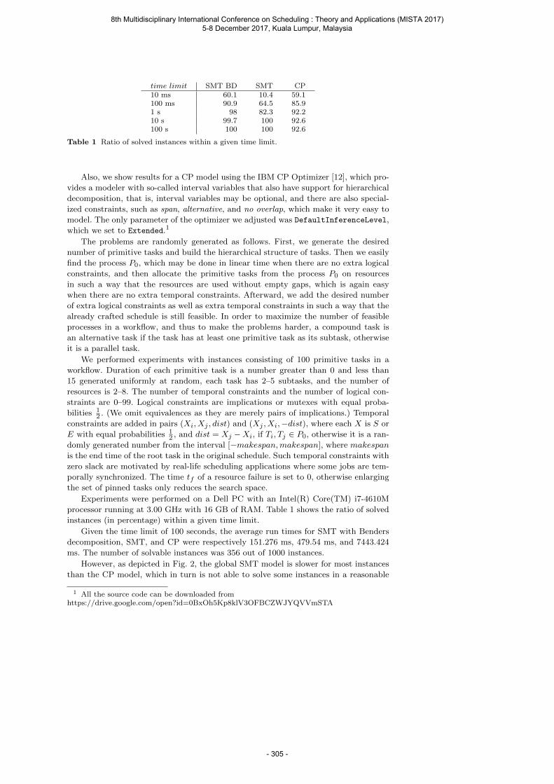
time limit SMT BD SMT CP10 ms 60.1 10.4 59.1100 ms 90.9 64.5 85.91 s 98 82.3 92.210 s 99.7 100 92.6100 s 100 100 92.6

Table 1 Ratio of solved instances within a given time limit.

Also, we show results for a CP model using the IBM CP Optimizer [12], which pro-

vides a modeler with so-called interval variables that also have support for hierarchical

decomposition, that is, interval variables may be optional, and there are also special-

ized constraints, such as span, alternative, and no overlap, which make it very easy to

model. The only parameter of the optimizer we adjusted was DefaultInferenceLevel,

which we set to Extended.1

The problems are randomly generated as follows. First, we generate the desired

number of primitive tasks and build the hierarchical structure of tasks. Then we easily

find the process P0, which may be done in linear time when there are no extra logical

constraints, and then allocate the primitive tasks from the process P0 on resources

in such a way that the resources are used without empty gaps, which is again easy

when there are no extra temporal constraints. Afterward, we add the desired number

of extra logical constraints as well as extra temporal constraints in such a way that the

already crafted schedule is still feasible. In order to maximize the number of feasible

processes in a workflow, and thus to make the problems harder, a compound task is

an alternative task if the task has at least one primitive task as its subtask, otherwise

it is a parallel task.

We performed experiments with instances consisting of 100 primitive tasks in a

workflow. Duration of each primitive task is a number greater than 0 and less than

15 generated uniformly at random, each task has 2–5 subtasks, and the number of

resources is 2–8. The number of temporal constraints and the number of logical con-

straints are 0–99. Logical constraints are implications or mutexes with equal proba-

bilities 12 . (We omit equivalences as they are merely pairs of implications.) Temporal

constraints are added in pairs (Xi, Xj , dist) and (Xj , Xi,−dist), where each X is S or

E with equal probabilities 12 , and dist = Xj −Xi, if Ti, Tj ∈ P0, otherwise it is a ran-

domly generated number from the interval [−makespan,makespan], where makespan

is the end time of the root task in the original schedule. Such temporal constraints with

zero slack are motivated by real-life scheduling applications where some jobs are tem-

porally synchronized. The time tf of a resource failure is set to 0, otherwise enlarging

the set of pinned tasks only reduces the search space.

Experiments were performed on a Dell PC with an Intel(R) Core(TM) i7-4610M

processor running at 3.00 GHz with 16 GB of RAM. Table 1 shows the ratio of solved

instances (in percentage) within a given time limit.

Given the time limit of 100 seconds, the average run times for SMT with Benders

decomposition, SMT, and CP were respectively 151.276 ms, 479.54 ms, and 7443.424

ms. The number of solvable instances was 356 out of 1000 instances.

However, as depicted in Fig. 2, the global SMT model is slower for most instances

than the CP model, which in turn is not able to solve some instances in a reasonable

1 All the source code can be downloaded fromhttps://drive.google.com/open?id=0BxOh5Kp8klV3OFBCZWJYQVVmSTA


- 305 -

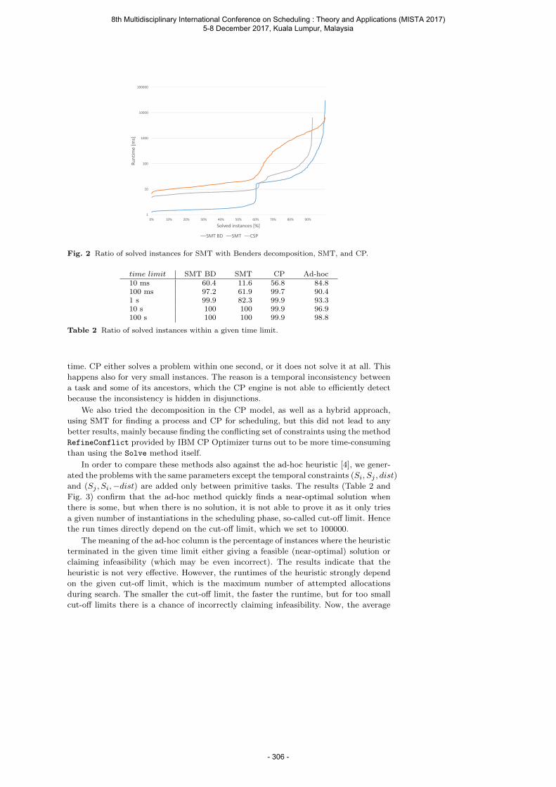
1

10

100

1000

10000

100000

0% 10% 20% 30% 40% 50% 60% 70% 80% 90%

Runt

ime

[ms]

Solved instances [%]

SMT BD SMT CSP

Fig. 2 Ratio of solved instances for SMT with Benders decomposition, SMT, and CP.

time limit SMT BD SMT CP Ad-hoc10 ms 60.4 11.6 56.8 84.8100 ms 97.2 61.9 99.7 90.41 s 99.9 82.3 99.9 93.310 s 100 100 99.9 96.9100 s 100 100 99.9 98.8

Table 2 Ratio of solved instances within a given time limit.

time. CP either solves a problem within one second, or it does not solve it at all. This

happens also for very small instances. The reason is a temporal inconsistency between

a task and some of its ancestors, which the CP engine is not able to efficiently detect

because the inconsistency is hidden in disjunctions.

We also tried the decomposition in the CP model, as well as a hybrid approach,

using SMT for finding a process and CP for scheduling, but this did not lead to any

better results, mainly because finding the conflicting set of constraints using the method

RefineConflict provided by IBM CP Optimizer turns out to be more time-consuming

than using the Solve method itself.

In order to compare these methods also against the ad-hoc heuristic [4], we gener-

ated the problems with the same parameters except the temporal constraints (Si, Sj , dist)

and (Sj , Si,−dist) are added only between primitive tasks. The results (Table 2 and

Fig. 3) confirm that the ad-hoc method quickly finds a near-optimal solution when

there is some, but when there is no solution, it is not able to prove it as it only tries

a given number of instantiations in the scheduling phase, so-called cut-off limit. Hence

the run times directly depend on the cut-off limit, which we set to 100000.

The meaning of the ad-hoc column is the percentage of instances where the heuristic

terminated in the given time limit either giving a feasible (near-optimal) solution or

claiming infeasibility (which may be even incorrect). The results indicate that the

heuristic is not very effective. However, the runtimes of the heuristic strongly depend

on the given cut-off limit, which is the maximum number of attempted allocations

during search. The smaller the cut-off limit, the faster the runtime, but for too small

cut-off limits there is a chance of incorrectly claiming infeasibility. Now, the average


- 306 -

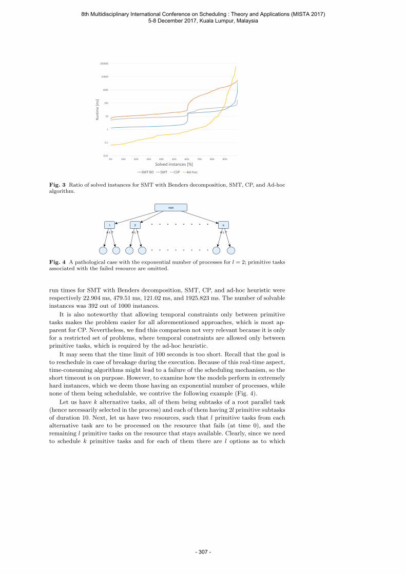
0,01

0,1

1

10

100

1000

10000

100000

0% 10% 20% 30% 40% 50% 60% 70% 80% 90%

Runt

ime

[ms]

Solved instances [%]

SMT BD SMT CSP Ad-hoc

Fig. 3 Ratio of solved instances for SMT with Benders decomposition, SMT, CP, and Ad-hocalgorithm.

Fig. 4 A pathological case with the exponential number of processes for l = 2; primitive tasksassociated with the failed resource are omitted.

run times for SMT with Benders decomposition, SMT, CP, and ad-hoc heuristic were

respectively 22.904 ms, 479.51 ms, 121.02 ms, and 1925.823 ms. The number of solvable

instances was 392 out of 1000 instances.

It is also noteworthy that allowing temporal constraints only between primitive

tasks makes the problem easier for all aforementioned approaches, which is most ap-

parent for CP. Nevertheless, we find this comparison not very relevant because it is only

for a restricted set of problems, where temporal constraints are allowed only between

primitive tasks, which is required by the ad-hoc heuristic.

It may seem that the time limit of 100 seconds is too short. Recall that the goal is

to reschedule in case of breakage during the execution. Because of this real-time aspect,

time-consuming algorithms might lead to a failure of the scheduling mechanism, so the

short timeout is on purpose. However, to examine how the models perform in extremely

hard instances, which we deem those having an exponential number of processes, while

none of them being schedulable, we contrive the following example (Fig. 4).

Let us have k alternative tasks, all of them being subtasks of a root parallel task

(hence necessarily selected in the process) and each of them having 2l primitive subtasks

of duration 10. Next, let us have two resources, such that l primitive tasks from each

alternative task are to be processed on the resource that fails (at time 0), and the

remaining l primitive tasks on the resource that stays available. Clearly, since we need

to schedule k primitive tasks and for each of them there are l options as to which


- 307 -

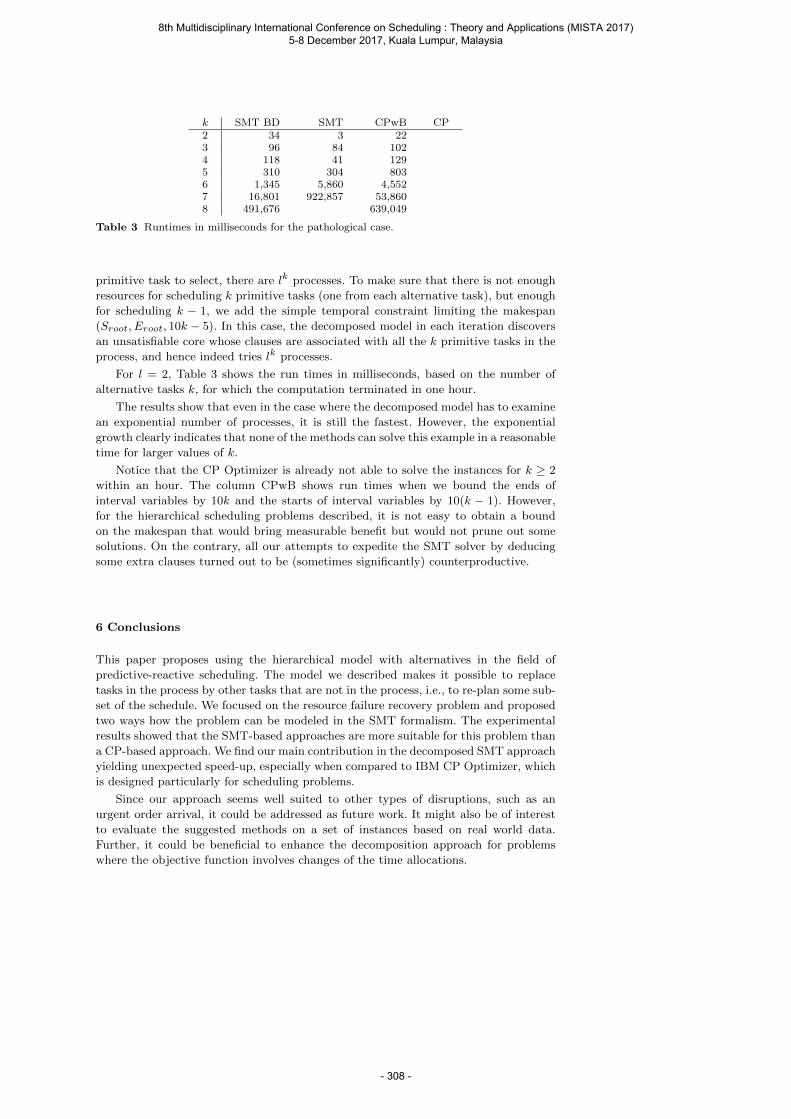
k SMT BD SMT CPwB CP2 34 3 223 96 84 1024 118 41 1295 310 304 8036 1,345 5,860 4,5527 16,801 922,857 53,8608 491,676 639,049

Table 3 Runtimes in milliseconds for the pathological case.

primitive task to select, there are lk processes. To make sure that there is not enough

resources for scheduling k primitive tasks (one from each alternative task), but enough

for scheduling k − 1, we add the simple temporal constraint limiting the makespan

(Sroot, Eroot, 10k − 5). In this case, the decomposed model in each iteration discovers

an unsatisfiable core whose clauses are associated with all the k primitive tasks in the

process, and hence indeed tries lk processes.

For l = 2, Table 3 shows the run times in milliseconds, based on the number of

alternative tasks k, for which the computation terminated in one hour.

The results show that even in the case where the decomposed model has to examine

an exponential number of processes, it is still the fastest. However, the exponential

growth clearly indicates that none of the methods can solve this example in a reasonable

time for larger values of k.

Notice that the CP Optimizer is already not able to solve the instances for k ≥ 2

within an hour. The column CPwB shows run times when we bound the ends of

interval variables by 10k and the starts of interval variables by 10(k − 1). However,

for the hierarchical scheduling problems described, it is not easy to obtain a bound

on the makespan that would bring measurable benefit but would not prune out some

solutions. On the contrary, all our attempts to expedite the SMT solver by deducing

some extra clauses turned out to be (sometimes significantly) counterproductive.

6 Conclusions

This paper proposes using the hierarchical model with alternatives in the field of

predictive-reactive scheduling. The model we described makes it possible to replace

tasks in the process by other tasks that are not in the process, i.e., to re-plan some sub-

set of the schedule. We focused on the resource failure recovery problem and proposed

two ways how the problem can be modeled in the SMT formalism. The experimental

results showed that the SMT-based approaches are more suitable for this problem than

a CP-based approach. We find our main contribution in the decomposed SMT approach

yielding unexpected speed-up, especially when compared to IBM CP Optimizer, which

is designed particularly for scheduling problems.

Since our approach seems well suited to other types of disruptions, such as an

urgent order arrival, it could be addressed as future work. It might also be of interest

to evaluate the suggested methods on a set of instances based on real world data.

Further, it could be beneficial to enhance the decomposition approach for problems

where the objective function involves changes of the time allocations.


- 308 -

Acknowledgements This research is partially supported by the Charles University, projectGA UK No. 158216, by SVV project number 260 453, and by the Czech Science Foundationunder the project P103-15-19877S.

References

1. Ansotegui, C., Bofill, M., Palahı, M., Suy, J., Villaret, M.: Satisfiability modulo theories:An efficient approach for the resource-constrained project scheduling problem. In: Pro-ceedings of the 9th Symposium on Abstraction, Reformulation and Approximation (SARA2011), pp. 2–9 (2011)

2. Aytug, H., Lawley, M.A., McKay, K., Mohan, S., Uzsoy, R.: Executing production sched-ules in the face of uncertainties: A review and some future directions. European Journalof Operational Research 161(1), 86–110 (2005)

3. Bartak, R., Rovensky, V.: On verification of nested workflows with extra constraints: Fromtheory to practice. Expert Systems with Applications 41(3), 904–918 (2014)

4. Bartak, R., Vlk, M.: Hierarchical task model for resource failure recovery in productionscheduling. In: Mexican International Conference on Artificial Intelligence, pp. 362–378.Springer (2016)

5. Bayardo Jr, R.J., Schrag, R.: Using csp look-back techniques to solve real-world sat in-stances. In: AAAI/IAAI, pp. 203–208 (1997)

6. Benders, J.F.: Partitioning procedures for solving mixed-variables programming problems.Numerische mathematik 4(1), 238–252 (1962)

7. Bjørner, N., Phan, A.D.: νz-maximal satisfaction with z3. In: SCSS, pp. 1–9 (2014)8. Bofill, M., Suy, J., Villaret, M.: A system for solving constraint satisfaction problems with

smt. In: International Conference on Theory and Applications of Satisfiability Testing,pp. 300–305. Springer (2010)

9. Davis, M., Logemann, G., Loveland, D.: A machine program for theorem-proving. Com-munications of the ACM 5(7), 394–397 (1962)

10. De Moura, L., Bjørner, N.: Z3: An efficient smt solver. In: International conference onTools and Algorithms for the Construction and Analysis of Systems, pp. 337–340. Springer(2008)

11. Dechter, R., Meiri, I., Pearl, J.: Temporal constraint networks. Artificial intelligence 49(1),61–95 (1991)

12. Laborie, P., Rogerie, J., Shaw, P., Vilim, P., Wagner, F.: Ilog cp optimizer: detailed schedul-ing model and opl formulation. Tech. rep., Technical Report 08-002, ILOG (2008)

13. Moskewicz, M.W., Madigan, C.F., Zhao, Y., Zhang, L., Malik, S.: Chaff: Engineering anefficient sat solver. In: Proceedings of the 38th annual Design Automation Conference, pp.530–535. ACM (2001)

14. Nieuwenhuis, R., Oliveras, A., Tinelli, C.: Solving sat and sat modulo theories: From anabstract davis–putnam–logemann–loveland procedure to dpll (t). Journal of the ACM(JACM) 53(6), 937–977 (2006)

15. Novak, A., Sucha, P., Hanzalek, Z.: Efficient algorithm for jitter minimization in time-triggered periodic mixed-criticality message scheduling problem. In: Proceedings of the24th International Conference on Real-Time Networks and Systems, pp. 23–31. ACM(2016)

16. Ohrimenko, O., Stuckey, P.J., Codish, M.: Propagation via lazy clause generation. Con-straints 14(3), 357–391 (2009)

17. Ouelhadj, D., Petrovic, S.: A survey of dynamic scheduling in manufacturing systems.Journal of scheduling 12(4), 417–431 (2009)

18. Petke, J.: Bridging Constraint Satisfaction and Boolean Satisfiability. Springer (2015)19. Shu, I.h., Effinger, R.T., Williams, B.C.: Enabling fast flexible planning through incre-

mental temporal reasoning with conflict extraction. In: ICAPS, pp. 252–261 (2005)20. Silva, J.P.M., Sakallah, K.A.: Graspa new search algorithm for satisfiability. In: Pro-

ceedings of the 1996 IEEE/ACM international conference on Computer-aided design, pp.220–227. IEEE Computer Society (1997)

21. Skalicky, T.: Interactive scheduling and visualisation. Master’s thesis, Masters thesis,Charles University in Prague (2011)

22. Tovey, C.A.: A simplified np-complete satisfiability problem. Discrete Applied Mathemat-ics 8(1), 85–89 (1984)


- 309 -

23. Van Der Aalst, W.M., Ter Hofstede, A.H.: Yawl: yet another workflow language. Informa-tion systems 30(4), 245–275 (2005)

24. Vieira, G.E., Herrmann, J.W., Lin, E.: Rescheduling manufacturing systems: a frameworkof strategies, policies, and methods. Journal of scheduling 6(1), 39–62 (2003)

25. Vlk, M., Bartak, R., Hanzalek, Z.: Minimization of useless work in resource failure recoveryof workflow schedules. In: Emerging Technologies & Factory Automation, 2017. ETFA2017. IEEE Conference on, p. to appear. IEEE (2017)

26. Wojakowski, P., Warzo lek, D.: The classification of scheduling problems under productionuncertainty. Research in Logistics & Production 4 (2014)


- 310 -

Abstracts


- 311 -

MISTA 2017

Optimal solutions for minimum-cost sequential systemtesting

Roel Leus · Salim Rostami · Stefan Creemers

1 Introduction

We consider a multi-component complex machine (subsequently referred to as a “sys-

tem”) that undergoes periodic functionality checkups. We examine in which order the

components of the system should be tested so as to diagnose the functionality of the

system and its potential malfunctioning components with minimum cost and/or time.

With these challenges in mind for preventive and corrective maintenance, the impor-

tance of the sequential testing problem was highlighted in the U.S. Air Force more than

sixty years ago [1]. The goal of sequential system testing is to discover the state of a

system, which is either up (working) or down (not working), by testing its components

one by one. The testing continues until the system state is identified. The objective is to

find a sequence of tests that minimizes the total expected cost of the sequential diagno-

sis. As equipment becomes more complex and expensive, the number of required tests

and the inspection costs increase, and consequently, the sequential diagnosis becomes

more expensive.

Depending on the type of the system under investigation, test failures may have

different consequences. A k:n system (or k-out-of-n) is up if at least k out of the n

components are functioning, and is down if (n− k + 1) components or more are down.

Minimum-cost test sequencing for k:n systems with general precedence constraints

between the tests is studied by Wei et al. [2]. An n-out-of-n (or serial) system is up if

all the n components are functioning. Hence, its testing terminates if a single failure

is encountered. In a 1:n (or parallel) system, on the other hand, a single working

component suffices to guarantee the functionality of the whole system. Consequently,

the diagnosis ends at the first success. Sequencing problems for serial and parallel

systems are equivalent: an optimal solution to a 1:n system with success probabilities p

is also optimal for an n:n system with success probabilites 1− p. In this work we focus

on test sequencing for n:n systems under general precedence constraints.

Roel LeusORSTAT, Faculty of Economics and Business, KU Leuven, BelgiumE-mail: [email protected]

Salim Rostami and Stefan CreemersIESEG School of Management, Lille, FranceE-mail: [email protected] ; [email protected]


- 312 -

The n:n case with general precedence constraints is known to be strongly NP-

hard [3]. To the best of our knowledge, no research has been specifically devoted to

developing exact algorithms for this problem. Simon and Kandane [4] describe condi-

tions for a diagnostic strategy to be optimal for series or parallel systems with general

precedence constraints, but they do not develop algorithms to find such a strategy. The

scientific work to date on sequential testing has mainly focused on identifying special

cases that are polynomially solvable; see for instance Monma and Sidney [5]. For an

extensive review of the literature we refer to Unluyurt [6]. We will benchmark our

computational results against the performance of the procedures in [2], where a more

general problem is solved.

2 Problem statement

We consider a set N = 1, . . . , n that contains n tasks, each of which corresponds

to an inspection or a test (the two terms can be used interchangeably) with a non-

negative testing cost ci and a success probability pi ∈ [0; 1]; the test outcomes are

independent. The tests are subject to technological precedence constraints represented

by a set E ⊂ N ×N , which is a partial order relation, such that (i, j) ∈ E implies that

test i should be executed before test j. A solution is then a sequence s = (s1, s2, . . . , sn)

of the tests that minimizes the total expected cost of the diagnosis∑n

j=1(∏j−1

i=1 psi)csj ,

where the cost csj of the activity sj in the j-th position is incurred only if all the

preceding activities succeed, which is the case with probability∏j−1

i=1 psi . Obviously, a

sequence is feasible if and only if it extends E.

A compact formulation for this sequencing problem uses binary “linear ordering”

variables xij (in line with Potts [7]), where xij = 1 if job i precedes job j in the

corresponding sequence, and xij = 0 otherwise. The problem can then be stated as

follows:

(CF) min

n∑j=1

cj

n∏i=1

[(pi − 1)xij + 1] (1)

subject to

xij + xji = 1 ∀i, j ⊂ N (2)

xij + xjk − xik ≤ 1 ∀i, j, k ⊂ N (3)

xij = 1 ∀(i, j) ∈ E (4)

xij ∈ 0, 1 ∀i, j ⊂ N (5)

Constraints (2) enforce the asymmetry property for every pair of activities, and Con-

straints (3) demand that the ordering be transitive (which also eliminates cycles). The

precedence constraints in E are imposed via Constraint set (4).

3 Solution methods

Although correct, the formulation (CF) is not very practical due to its non-linear

character. We examine two different ways to work around this issue. The first method

ensues from applying Dantzig-Wolfe decomposition to formulation (CF), where we


- 313 -

construct the set of all integer solutions xmj = (xm1j , xm2j , . . . , x

mnj) to the constraints (4)-

(5), ∀j ∈ N and m ∈ Mj . More specifically, we have xj =∑

m∈Mjzmj xmj , with∑

m∈Mjzmj = 1 and zmi ∈ 0, 1. This substitution leads to a linear formulation with

a large number of columns, which can be solved by means of column generation. The

corresponding pricing problem has a non-linear objective, but can be solved using

dynamic programming (DP). The search for integral x can then be embedded within

a branch-and-price (B&P) framework.

The second solution approach that is tested, is to apply a DP-recursion directly to

the original sequencing problem. In detail, each state Y ⊆ N of the recursion represents

a smaller-size sequencing instance, where the first n−|Y | positions of the sequence are

already filled and the remaining positions are still undecided. The state space contains

all the feasible states that can be visited during the diagnosis procedure, where a state Y

is feasible if it respects the precedence constraints, that is, ∀(i, j) ∈ E : i ∈ Y ⇒ j ∈ Y .

Similar recursions have been tested earlier for other scheduling problems [8,9], where

it was shown that a careful memory management is crucial in the implementation.

4 Main findings

We have performed experiments on benchmark datasets, the results of which will be

presented during the conference. As it stands, the DP-recursion with judiciously im-

plemented memory management is the clear winner of the two tested algorithms. The

B&P-algorithm does not deliver competitive performance, mainly due to the rather

weak LP-bounds. Despite this unfavorable comparison for the linear formulation, the

application of similar decompositions for other scheduling problems with a non-linear

objective in a compact intuitive formulation, e.g. for project scheduling for maximum

net present value [10], has not been attempted yet and might lead to viable procedures

(partly also because there are less alternative solution methods available).

References

1. S.M. Johnson. Optimal sequential testing. Rand Corporation, working paper, 1956.2. W. Wei, K. Coolen and R. Leus. Sequential testing policies for complex systems under

precedence constraints. Expert Systems with Applications, 40(2):611–620, 2013.3. F.P. Kelly. A remark on search and sequencing problems. Mathematics of Operations Re-

search, 7(1):154–157, 1982.4. H.A. Simon and J.B. Kadane. Optimal problem-solving search: All-or-none solutions. Ar-

tificial Intelligence, 6(3):235–247, 1975.5. C.L. Monma and J.B. Sidney. Sequencing with series-parallel precedence constraints. Math-

ematics of Operations Research, 4(3):215–224, 1979.

6. T. Unluyurt. Sequential testing of complex system: A review. Discrete Applied Mathematics,142:189–205, 2004.

7. C.N. Potts. An algorithm for the single machine sequencing problem with precedence con-straints. In V.J. Rayward-Smith (ed.). Combinatorial Optimization II, pages 78–87, Springer,1980.

8. V.G. Kulkarni and V.G. Adlakha. Markov and Markov-regenerative PERT networks. Op-erations Research, 34(5):769–781, 1986.

9. S. Creemers, R. Leus and M. Lambrecht. Scheduling Markovian PERT networks to maxi-mize the net present value. Operations Research Letters, 38(1), 51–56, 2010.

10. W.S. Herroelen, P. Van Dommelen and E.L. Demeulemeester. Project network modelswith discounted cash flows – A guided tour through recent developments. European Journalof Operational Research 100(1), 97–121, 1997.


- 314 -

MISTA 2017

Symmetry breaking in a special case of the RCPSP/max

Steven Edwards · Davaatseren Baatar ·Simon Bowly · Kate Smith-Miles

1 Introduction

This contribution was motivated by a practical problem arising in scheduling liquid han-

dling systems that automate laboratory procedures. The problem can be modelled quite

naturally as a special case of the well-studied Resource Constrained Project Schedul-

ing Problem with Generalized Precedence Relations (RCPSP/max)[1]. We prove the

existence of a symmetry in the problem and show how the default search of IBM’s

CP Optimizer 12.6 [7, 8] benefits from the removal of this symmetry. The approach is

tested on 177 real world test instances obtained from our industry partner.

2 Motivation

The liquid handling system is designed to process multiple laboratory tests in parallel

with the objective of processing all the tests in the least possible time, i.e. minimis-

ing makespan. In order to process a test, a protocol must be followed. This protocol

details the set of activities, that must be completed in order to successfully process

the test as well as the timings between these activities. Due to the sensitivities of the

chemical reactions involved in the tests, these timings specify both a minimum and a

maximum amount of time, commonly referred to as minimum and maximum time-lags

or generalized precedence constraints.

Scheduling the resources of automated systems, e.g. robots, vacuums, heating/cooling

instruments, to process multiple tests in parallel in the least amount of time can be

modelled as a special case of the RCPSP/max. In practice schedules must be generated

quickly so that systems do not stay idle while a solution is being determined.


We are given a set of jobs (tests) J which must be completed according to a set of

protocols P. A job j ∈ J must be processed according to its protocol, p(j) ∈ P. This

Steven Edwards, Davaatseren Baatar, Simon Bowly, Kate Smith-MilesSchool of Mathematical Sciences, Monash University, Victoria 3800, AustraliaE-mail: steven.edwards, davaatseren.baatar, simon.bowly, [email protected]


- 315 -

protocol defines both the set of activities, Vj , that must be processed, and the set of

precedence relations between these activities, Aj . We denote the set of all activities

and precedence relations by V =⋃j∈J Vj and A =

⋃j∈J Aj respectively.

A schedule is an assignment of start times to each activity, S = Si,j |(i, j) ∈ V,where Si,j denotes the start time of activity i from job j. The time at which activity

(i, j) ∈ V is completed is called the completion time and is denoted by Ci,j . Each

activity, (i, j) ∈ V, has a fixed duration, di,j , and must be scheduled without pre-

emption,

Ci,j = Si,j + di,j , (i, j) ∈ V (1)

A generalized precedence relation, (i, j, i′, j′) ∈ A, states that between the start

time of activity i ∈ Vj and the start time of activity i′ ∈ Vj′ there exist minimum and

maximum timelags, denoted by δmini,j,i′,j′ and δmaxi,j,i′,j′ respectively,

δmini,j,i′,j′ ≤ Si′,j′ − Si,j ≤ δmaxi,j,i′,j′ , (i, j, i′, j′) ∈ A (2)

A schedule is time feasible if all of the duration and timelag constraints, i.e. (1)

and (2), are feasible.

To process the activities we are given a set of renewable resources R. Each resource

k ∈ R has a fixed capacity of Rk units. In order to be processed, activity (i, j) ∈ Vconsumes ri,j,k units at the beginning of the activity, Si,j , and then releases ri,j,k units

at it’s completion, Ci,j . A schedule S is said to be resource feasible if at each time t

over some time horizon T the demand for resource k ∈ R, denoted by rk(S, t), does

not exceed the capacity Rk, i.e.,

rk(S, t) =∑

(i,j)∈V:Si,j≤t<Ci,j

ri,j,k ≤ Rk, t ∈ T, k ∈ R (3)

A schedule S is called feasible if it is both time and resource feasible. The objective

is to find a feasible schedule with the minimum makespan.

Furthermore protocols are designed in such a way that if the set of jobs contains

a single job, J = j, then the activities in the protocol form a complete linear

ordering, i.e. there exists a schedule S such that S1,j ≤ S2,j ... ≤ Snj ,j . For a given

schedule, we will refer to jobs in which all activities are ordered by index, as having

a standard ordering. Additionally the earliest schedule associated with this complete

linear ordering is optimal, and can be found in polynomial time by, for example, a

modified label correcting algorithm [2].

4 Properties

For the RCPSP/max even finding a feasible solution in general is NP-Complete [1].

However in this special case it is possible to find a feasible solution in polynomial

time, albeit a very poor one, by completing each job in standard ordering, one at a

time. This is a similar property to that found in the job shop problem with time-lags

problem (JSTL) and is referred to as a canonical solution [3]. The problem of finding an

optimal solution however remains NP-Hard, as single-machine problems with minimal

and maximal timelags between activities are in general NP-Hard [9].

Removing symmetries is a technique used extensively when solving combinato-

rial optimization problems [4]. A symmetry is a function that maps each solution to


- 316 -

an equivalent solution. Symmetry breaking is the process of eliminating a number of

equivalent solutions, ideally all but one, in order to reduce the search space while

ensuring that an optimal solution still exists. Historically, the most used method of

symmetry breaking involves adding constraints to the basic model.

For project scheduling problems specifically, Kovacs and Vancza [5, 6] define the

notion of a progressive pair, which represents two well-defined sets of activities that

characterise repetitive patterns on a graph theoretical basis. They show that symme-

tries can be removed by inserting additional Start-Start precedence constraints between

equivalent activities of the two sets in the progressive pair. Our contribution can be seen

as an extension of their work when generalized precedence relations are also considered.

More explicitly, with respect to the problem being considered in this work, we prove

the following,

Theorem 1 Given a feasible schedule S and an arbitrary ordering of jobs O, there

exists a feasible permutation of the schedule Sπ, where for any two jobs, j, j′ ∈ J ,such that j ≺ j′ ∈ O and both jobs have the same protocol, p(j) = p(j′), all activitiesin j′ must start at the same time or after their corresponding activity in j, that is

Sπi,j ≤ Sπi,j′ for all i ∈ Vj

During the conference, a sketch of the proof to Theorem 1 will be provided. It is

possible to remove this symmetry by introducing an additional set of Start-Start prece-

dence constraints between corresponding activities. Activity-on-Node (AoN) networks

are arc-labelled and node-labelled directed graphs that are commonly used to visualise

project scheduling problems. Activities are represented by nodes and precedence rela-

tions by arcs. In Figures 1 and 2, we see the AoN for two jobs with the same protocol

with and without the additional symmetry breaking constraints.

Fig. 1: The AoN for two jobs with the

same protocol

Fig. 2: The AoN for two jobs with the

same protocol with the additional set

of precedence constraints to break sym-

metries

5 Computational Study

IBM’s CP Optimizer 12.6 was tested on real-world test instances with and without

the symmetry breaking constraints. It was found that the approach with the symme-

try breaking constraints outperforms the approach without them on 110 of the 177

instances and greatly minimised the standard deviation for the time taken to find an

initial feasible solution, 7.3s and 17.6s respectively.


- 317 -

Acknowledgements This work was completed as part of an Australian Research CouncilLinkage Grant LP140101063

References

1. Bartusch M, Mohring RH, Radermacher FJ (1988) Scheduling project networks with

resource constraints and time windows. Annals of Operations Research 16(1):199–

240, DOI 10.1007/BF02283745

2. Carlier J, Moukrim A, Xu H (2009) The project scheduling problem with pro-

duction and consumption of resources: A list-scheduling based algorithm. Discrete

Applied Mathematics 157(17):3631–3642, DOI 10.1016/j.dam.2009.02.012, URL

http://dx.doi.org/10.1016/j.dam.2009.02.012

3. Caumond A, Lacomme P, Tchernev N (2008) A memetic algorithm for the job-

shop with time-lags. Computers and Operations Research 35(7):2331–2356, DOI

10.1016/j.cor.2006.11.007

4. Gent IP, Petrie KE, Puget JF (2006) Symmetry in Constraint Programming. Hand-

book of Constraint Programming pp 329–376, DOI 10.1016/S1574-6526(06)80014-3

5. Kovacs A, Vancza J (2006) Progressive Solutions : A Simple but Efficient Dominance

Rule for Practical RCPSP. In Integration of AI and OR Techniques in Constraint

Programming for Combinatorial Optimization Problems pp 139–151

6. Kovacs A, Vancza J (2010) Exploiting Repetitive Patterns in Practical Scheduling

Problems. In: 43rd CIRP International Conference on Manufacturing Systems, pp

868–875

7. Laborie P, Godard D (2007) Self-adapting large neighborhood search: Applica-

tion to single-mode scheduling problems. Proceedings MISTA-07, Paris p 8, URL

http://citeseerx.ist.psu.edu/viewdoc/download?doi=10.1.1.107.4415&rep=rep1&type=pdf

8. Vilim P, Laborie P, Shaw P (2015) Failure-Directed Search for Constraint-

Based Scheduling. Integration of AI and OR Techniques in Constraint Pro-

gramming: 12th International Conference, CPAIOR 2015, Barcelona, Spain,

May 18-22, 2015, Proceedings pp 437–453, DOI 10.1007/978-3-642-38171-3, URL

http://link.springer.com/10.1007/978-3-642-38171-3, 9780201398298

9. Wikum ED, Llewellyn DC, Nemhauser GL (1994) One-machine generalized prece-

dence constrained scheduling problems. Operations Research Letters 16(2):87–99,

DOI 10.1016/0167-6377(94)90064-7


- 318 -

Nurul Farahin Jamaluddin

School of Informatics and Applied Mathematics, Universiti Malaysia Terengganu

E-mail: [email protected]

Nur Aidya Hanum Aizam



Nurul Liyana Abdul Aziz



MISTA 2017

Mathematical model for a high quality examination timetabling problem:

case study of a university in Malaysia

Nurul Farahin Jamaluddin • Nur Aidya Hanum Aizam • Nurul Liyana Abdul Aziz

Abstract This paper presents mathematical programming models for a real-world university

examination timetabling problem (UETP) related to a university in Malaysia. The aim of this

study is to produce an examination timetable that most closely conforms to the demands of the

communities. Hence, a new binary model is developed. The model will consider most of the

preferences from the timetabling communities, which complicates the current scheduling

system in the related university. We tested the model in two cases of different preferences on a

real-world examination timetabling dataset at the university, for verification purposes. Case 1

is tested with single value of preference for all exam assignments to room and timeslot. Case 2

is tested using preferences in the range between 1 (least preferred) and 5 (most preferred)

values of exam assignments to room and timeslot. Computational results are reported and

analysed directly using the AIMMS mathematical software with CPLEX 12.6.3 as the solver.

The results are then compared in term of computational time and the optimal value of objective

function achieved to the existing timetable. The study clearly shows that the model generated

performed well and the solutions are successfully optimized in which the exams are scheduled

in compliance to the student’s demand. This model therefore increases the quality level of the

examination timetabling.


- 319 -



Nurul Liyana Abdul Aziz

School of Informatics and Applied Mathematics,

University of Malaysia Terengganu


Nur Aidya Hanum Aizam

Marine Management Sciences Research Group,




Nurul Farahin Jamaluddin




MISTA 2017

Variation of Demands for a New Improvised University Course

Timetabling Problem Mathematical Model

Nurul Liyana Abdul Aziz • Nur Aidya Hanum Aizam • Nurul Farahin Jamaluddin

Abstract University course timetabling is a well-known management problem amongst

researchers, thus the rich body of literature. However, published articles are mainly on

improved solution approaches and ignored human preference. Most researchers present

different constraints and ignored human preference. This however, limits the model application

to other universities. In our study, we aim to bridge the gap by acknowledging these varieties

of demands. In the process of generating our mathematical model, we have gone through

meticulously researches that have been carried out in the past years to determine the demands

and level of preferences of individuals involved directly with the timetable. The varieties of

demands were clarified from a survey conducted. Hence an improvised UCTP model was

developed, which involves a super set of constraints. To verify the compatibility of our

mathematical model, we illustrate with real data from a Tunisian university. The paper divides

the timetabling problem into two parts: case study 1 and case study 2. Case study 1 considers

all the requirements of Faculty of Economics and Management Sciences of Sfax (FEMSS) and

the resulting timetables were compared qualitatively with those generated by the Timetabling

Heuristic Approach. In case study 2, several additional constraints listed are considered. The

experimental results confirm the applicability of our improvised model towards real problem.


- 320 -


MISTA 2017

Multi-commodity flow and station logistics resolution for train unit

scheduling

Raymond S K Kwan • Zhiyuan Lin • Pedro J Copado-Mendez • Li Lei

1 Introduction

In UK and many other countries, self-propelled train vehicle units with a fixed number of

carriages, e.g. 2-car and 4-car units, are commonly used. This is in contrast to locomotive

pulled formations with a variable number of carriages. Scheduling a wide-area rail network

with route and time-of-the-day dependent seat demands, optimizing the coupling and de-

coupling of train units is often a key feature. Train unit movements are quite restrictive

because the tracks they run on are shared. Therefore rather than to create a new empty running

journey to redistribute a unit to elsewhere, the unit may be scheduled to be attached to some

trains already in the timetable. Also, no additional drivers would be needed. However, a side

consequence is that some train trips will be overprovided with seats by such train units in

transit to serve the real high demand trips. Since seat demand data is often not easy to

determine, inference from schedules in the past is heavily relied upon and overprovision in the

current round of scheduling therefore may have long lasting effects on future schedules.

To achieve an optimized flow of train unit resources over the rail network during a

working day is complex and difficult. The problem is made more complex in ensuring all the

train movements are conflict free at individual train stations. Typical station layouts include

tracks that are blind-ended or through running. Some platforms may be short limiting how

many train units are allowed to be coupled. To achieve an operable blockage-free schedule

may involve reassigning some linkages, re-ordering how multiple units are coupled, shunting

units between platforms and sidings, etc. The detailed logistics at each train station obviously

could have some rippling effects across all other stations in the network.

A multi-stage approach is proposed for the train unit scheduling problem. In the first

stage, a multi-commodity flow problem is solved temporarily regarding each station as a single

point with no infrastructure details and without fixing how multi-units are ordered when they

are coupled to serve a train trip. The second stage resolves potential station conflicts in the first

stage solutions. The resolution process is performed on each individual train station. The

results of the second stage would include some alternative resolution plans so that the third


- 321 -



stage process can finalize compatible station plans across the whole network. It is anticipated

that because of the real world nature of the scheduling problem, a fourth stage would be

needed allowing the human planners to assess and fine tune the schedules interactively.

This paper presents an overall framework and the on-going research on its component

stages. The research has been carried out in collaboration with some UK train operating

companies and tested on ScotRail, Transpennine Express, Great Western Railway and some

past rail franchise bid datasets. Research progress status and relevant results will be presented

at the conference.

2 Multi-commodity flow

Given a (tentatively) fixed timetable of train trips for one working day, a directed acyclic

graph (DAG) is constructed where the train trips are represented by nodes. A source node and

a sink node represent the beginning and end of the working day. Arcs represent potential

linkages between a pair of nodes. Different train unit types are multi-commodities. The

problem is to select paths from source to sink in the graph such that all the train trips are

covered meeting the seat demands. Where the paths overlap, the corresponding train units are

coupled subject to compatibility constraints and some coupling bounds.

The multi-commodity flow model is formulated as an integer linear program (ILP) [1].

Apart from minimizing the number of train units used, other quality measures such as total

mileage are also incorporated in the objective function. The ILP is computationally very

challenging to solve. Therefore, a specialized solver has been derived based on branch-and-

price [2]. The main features of the solver include local convex hull techniques [3] for more

efficient computation regarding constraints on seat demands and unit coupling type

compatibility and bounds. Some specialized branching techniques have also been derived.

In practice, train operators often cannot specify seat demands precisely for each train trip.

Deviations from the norm may be caused by many different circumstances and factors.

Passenger count surveys are only snapshots that may not always yield accurate inferences. Seat

capacities provided in historic schedules may also be unreliable because the scheduling process

might have deviated from the seat demands originally specified. Hence, bi-level seat demands

are accommodated [4]. For each train trip, the lower minimum seat demand is a hard

constraint. A higher seat demand may also be specified such that they would be satisfied as

much as possible without using additional train units.

The above solver has demonstrated the ability to solve small to medium sized real-life

problem instances within practical time. For larger and harder instances, a hybridized

algorithm called SLIM [5] has been developed. SLIM is driven by an iterative improvement

heuristics, which aims at converging from a low quality initial reduction of the DAG to a

minimally sized DAG that is sufficient to yield a (near) optimal solution. In every iteration, the

size-reduced DAG is passed to the core ILP solver above to derive a solution. Because of the

aggressive reduction of the DAG, the ILP solver needs little computational time in each

iteration. SLIM also benefits from being well suited for parallelization.

On-going research on the ILP solver above includes coping with integer fixed charge

variables more efficiently and catering for a richer variety of real-life problem variations and

constraints, For SLIM, the focus is on maintaining a good balance between DAG size and

search intensification/diversification.

3 Station level logistics

The multi-commodity flow schedule yielded in section 2 has left two operational aspects

open to be determined before the solution can be fully operable. First is the unit coupling order

in a trip served by multi-units. Second is the precise activity plan required to implement a

linkage between an arrival and a departure. For example, suppose a unit arrives on route A and

is scheduled to departure on route B next. And suppose route B uses a different platform, the


- 322 -

re-platforming implies some movements of the unit within the station that must not be blocked

in any way.

The multi-commodity flow network level solution can be easily transformed into a

station-by-station view. At each station, the partial solution consists of a list of arrivals, a list

of departures, and a set of linkages connecting the two lists. A linkage also includes

information about the unit(s) and platforms assigned. The movements of a unit to implement a

linkage is called a “linkage shunting plan” and the collection of linkage shunting plans at a

station is called a “station shunting plan”. For example, the assignment of a unit on arrival to

serve a departure 20 minutes later is a linkage; and if the arrival and departure concerned take

place at different platforms, a linkage shunting plan would be needed to re-platform the unit –

feasibility of such an activity depends on the time gap available and whether the path of

movement is free. Within a station shunting plan, all its linkage shunting plans must be conflict

free, i.e. not blocking each other. Since each linkage can have many possible linkage shunting

plans, their possible combinations in forming a station shunting plan would be prohibitively

numerous to be fully enumerated. Hence, an estimation approach is proposed [6]. The linkages

are classified according to characteristics of unit coupling, platform, track type (blind-end or

through track) for both the arrival and the departure linked. Each classified linkage type has

some associated shunting rules and parameters for determining an estimated minimum

shunting time required. Those linkages having time gaps below their corresponding minimum

shunting times are deemed infeasible, but they would have been prevented when the DAG was

formed. On the other hand, time gaps well above minimum are deemed to pose no problem in

deriving a suitable linkage shunting plan. Precise linkage shunting plans are then sought for the

remaining linkages, during which relevant unit coupling orders will also be resolved. Finally,

any other undetermined unit coupling orders will be determined.

Station logistics requires comprehensive studies of real operations to abstract. Hence,

investigations and station site visits with collaborating operators have been carried out and

their analyses are on-going.

4 Optimized and operable network-wide train unit schedules

Many UK train operating companies are already using the interactive TRACS-RS [7]

system without an optimizer for train unit scheduling. Trials with some collaborating operators

have demonstrated that the optimized multi-commodity flow solutions this research produced

can be uploaded onto TRACS-RS and the station logistics can be resolved through its

interactive facilities. The research described in section 3 will lead to minimal need for

interactive station logistic resolution. On-going research is investigating a mathematical

approach for finally integrating the prospective individual station logistics. In this approach,

the original DAG is transformed into a multi-graph in which some nodes will be extended into

multiple nodes representing alternative coupling orders. The objective is to find an optimal

selection of alternative coupling order nodes and their associated arcs to be used across the

network.

Data statement Part of the data used for this research may be commercially sensitive. Where

possible, the data that can be made publicly available is deposited in

http://archive.researchdata.leeds.ac.uk/.

Acknowledgements This research is sponsored by the Engineering and Physical Sciences

Council (grant EP/M007243/1), First Rail Holdings and Tracsis Plc. We would also like to

thank all the train operating companies involved in this project.

References


- 323 -

1. Lin Z, Kwan RSK, A two-phase approach for real-world train unit scheduling. Public

Transport, vol. 6, pp.35-65. (2014)

2. Lin Z, Kwan RSK, A branch-and-price approach for solving the train unit scheduling

problem. Transportation Research Part B: Methodological, vol. 94, pp.97-120. (2016)

3. Lin Z, Kwan RSK, Local convex hulls for a special class of integer multicommodity flow

problems, Computational Optimization and Applications, vol. 64, pp.881-919. (2016)

4. Lin Z, Barrena E, Kwan RSK, Train unit scheduling guided by historic capacity

provisions and passenger count surveys, Public Transport, vol. 9, pp.137-154. (2017)

5. Copado-Mendez PJ, Lin Z, Kwan RSK, Size limited iterative method (SLIM) for train

unit scheduling in: Proceedings of the 12th Metaheuristics International Conference,

Barcelona, Spain. (2017)

6. Lei L, Kwan RSK, Lin Z, Copado-Mendez PJ, Station level refinement of train unit

network flow schedules, 8th International Conference on Computational Logistics,

Southampton, UK. (2017)

7. Tracsis Plc, TRACS-RS, https://tracsisops.com/software/operations-planning-

software/tracs-scheduling-software/ Accessed: 20 July 2017, (2017)


- 324 -

https://tracsisops.com/software/operations-planning-software/tracs-scheduling-software/

https://tracsisops.com/software/operations-planning-software/tracs-scheduling-software/

MISTA 2017

On the exact solution of a large class of parallel machinescheduling problems

Teobaldo Bulhoes · Ruslan Sadykov ·Eduardo Uchoa · Anand Subramanian

1 Introduction

We consider the problem of scheduling a set of jobs J (n = |J |) on a set of machines

of different types k ∈ M (m = |M |) without preemption. A job j is not allowed to

be processed before its release date rj , and its processing time on a machine of type

k ∈ M is denoted as pkj . Also, skij denotes the setup time required to process job j

immediately after job i on a machine of type k. Each job j is associated to a cost

function fj(Cj) defined over its completion time Cj . The objective function is to min-

imize∑j∈J fj(Cj). This function is very general and can model many criteria. For

example, suppose each job has an earliness Ej = maxdj − Cj , 0 and a tardiness

Tj = maxCj − dj , 0 that is computed based on its due date dj . A classical objective

is to minimize the total weighted earliness and tardiness given by∑j∈J (w′jEj+wjTj),

where w′j and wj are penalty coefficients associated with job j. Remark that cost func-

tions that include earliness penalties are not regular and may have optimal solutions

that include idle times between jobs. In this work we present a novel exact algorithm

that is capable of solving problem R|rj , skij |∑fj(Cj) and the large class of problems

that can be derived as particular cases from it. The proposed algorithm consists of a

branch-cut-and-price approach that combines several features such as non-robust cuts,

strong branching, reduced cost fixing and dual stabilization. To our knowledge, this is

the first exact algorithm for unrelated machines with earliness and/or tardiness that

can solve consistently instances with more than 20 jobs. We report improved bounds

for instances of problems R|rj , skij |∑w′jEj + wjTj and R||

∑w′jEj + wjTj with up

to 80 and 120 jobs, respectively.

Teobaldo Bulhoes, Eduardo UchoaUniversidade Federal Fluminense, Niteroi, BrazilE-mail: [email protected], [email protected]

Ruslan SadykovInria Bordeaux - Sud Ouest, FranceE-mail: [email protected]

Anand SubramanianDepartamento de Sistemas de Computacao, UFPB, Joao Pessoa, BrazilE-mail: [email protected]


- 325 -

2 Mathematical formulation

We start by defining some notation required to introduce the mathematical formulation.

Let T be an upper bound on the maximum completion time of a job in some optimal

solution. Let Nk = (Vk = Rk ∪ Ok, Ak = A1k ∪ A

2k ∪ A

3k ∪ A

4k) be the acyclic graph

associated with each machine type k ∈ M , where set Rk = (j, t, k) : j ∈ J, t =

rj +pj , . . . , T contains the vertices associated with the jobs. We adopt the convention

that idle times only occur after the job has been processed. We assume that job j has

been processed when arriving at vertex (j, t, k), but note that j did not necessarily

finished at time t because of the existence of idle times. Set Ok = (0, t, k) : t =

0, . . . , T contains the vertices associated with a dummy job 0. For brevity, we denote

arc ((i, t, k), (j, t + skij + pkj , k)) as (i, j, t, k). Set A1k = (i, j, t, k) = ((i, t, k), (j, t +

skij + pkj , k)) : (i, t, k) ∈ Rk, (j, t + skij + pkj , k) ∈ Rk, j ∈ J \ i contains the arcs

connecting the vertices of Rk. Set A2k = (0, j, t, k) = ((0, t, k), (j, t + sk0j + pkj , k)) :

(j, t+sk0j +pkj , k) ∈ Rk, j ∈ J contains all arcs connecting the vertices from Ok to Rk.

Set A3k = (j, 0, t, k) = ((j, t, k), (0, T, k)) : (j, t, k) ∈ Rk contains all arcs connecting

the vertices from Rk to Ok. Set A4k = (j, j, t, k) = ((j, t, k), (j, t + 1, k)) : (j, t, k) ∈

Rk ∪Ok, (j, t+ 1, k) ∈ Rk ∪Ok contains the arcs associated with idle times. Let fa be

the cost of an arc a = (i, j, t, k) ∈ A1k ∪A

2k , which is the cost incurred if job j finishes

to be processed at time t + skij + pkj . Note that fa = 0,∀a ∈ A3k ∪ A

4k. Moreover, let

set Rjk = (i, t, k) ∈ Rk : i = j denote the vertices associated with job j. Finally, for

each subset S ⊆ Vk, let δ−(S) and δ+(S) be the sets representing the arcs entering

and leaving S, respectively. The proposed arc-time-indexed formulation is as follows.

(F1) min∑k∈M

∑a∈Ak

faxa (1)

s.t.∑k∈M

∑a∈δ−(Rj

k)

xa = 1, ∀j ∈ J (2)

∑a∈A2

k

xa ≤ mk, ∀k ∈M (3)

∑a∈δ−(v)

xa −∑

a∈δ+(v)

xa = 0, ∀k ∈M,∀v ∈ Vk \ (0, 0, k), (0, T, k) (4)

x ≥ 0, x integer (5)

Objective function (1) minimizes the completion time dependent costs. Constraints

(2) state that each job j ∈ J must be processed exactly once. Constraints (3) impose

that at most mk machines of type k ∈ M can be used. Constraints (4) are related to

the flow conservation. Define Pk as the set of paths in graph Nk that start at vertex

(0, 0, k) and end at vertex (0, T, k). Let bap be the number of times path p traverses

a ∈ Ak and let λp be a binary variable that assumes value 1 if p is in the solution.

Formulation F1 can be rewritten in terms of variables λp by means of a Dantzig-Wolfe

decomposition as follows.

(DW-F1) min∑k∈M

∑p∈Pk

( ∑a∈Ak

bpafa

)λp (6)


- 326 -

s.t.∑k∈M

∑p∈Pk

( ∑a∈δ−(Rj

k)

bpa

)λp = 1, ∀j ∈ J (7)

∑p∈Pk

( ∑a∈A2

k

bpa

)λp ≤ mk, ∀k ∈M (8)

λ binary (9)

3 Branch-cut-and-price algorithm

This section briefly describes the proposed branch-cut-and-price (BCP) algorithm over

formulation DW-F1. The solution of every node has the following three steps. (i)

A lower bound for the problem is obtained by solving the linear relaxation of DW-

F1 (possibly with cuts and branching constraints) through column generation. The

pricing subproblem for a machine type k ∈M corresponds to finding a least-cost path

in graph Nk where arc costs are associated with reduced costs. In this step, the pricing

subproblem is solved by a labeling algorithm and a dual stabilization technique is

applied. (ii) A reduced cost fixing procedure is executed for every machine type k ∈Mto remove from graph Nk the arcs that can not be in a solution that improve the

current upper bound. (iii) Cuts are separated and added to the master problem. Steps

(i), (ii) and (iii) are repeated as long as a tailing off condition is not reached and

the pricing time is smaller than a predefined threshold, after which a strong branching

technique is applied. The cuts adopted are obtained by a Chvatal-Gomory rounding of

the n constraints (7). Such cuts are often referred to as non-robust, since each single

cut requires additional states in the dynamic programming algorithm used for solving

the pricing subproblem. Therefore, those cuts should be added in a limited fashion

to avoid combinatorial explosion. To mitigate the impact of the Rank-1 cuts on the

pricing subproblem, we have adopted the limited arc memory technique described in

[4].

4 Computational results

Table 1 reports preliminary results obtained by the proposed BCP over the

R|rj , skij |∑w′jEj + wjTj instances of [3] and the R||

∑w′jEj + wjTj instances of [1].

The former instances were derived from the instances of [1] by adding two types of

sequence-dependent setup times: small and large. All experiments were conducted on a

Intel Xeon E5-2680 v3, running at 2.5 GHz with a single thread and a time limit of 12

hours. In this table, Improv (%) denotes the average percentage improvement over

the best known solution (BKS) which were obtained by running the methods devised

in [1,2], and #New corresponds to the number of new improved solutions. Regarding

the R|rj , skij |∑w′jEj + wjTj instances, it can be observed that most of them were

solved to optimality and several new improved solutions were found. Also, it appears

that the instances with large setup times are harder to be solved. More precisely, we

can verify that the quality of the lower bound obtained by BCP as well as the upper

bound found by running the heuristic proposed in [2] are worse for such instances.

On the other hand, only 8 R||∑w′jEj + wjTj instances considered were not solved to

optimality. In contrast, 497 such instances were not solved by the method presented


- 327 -

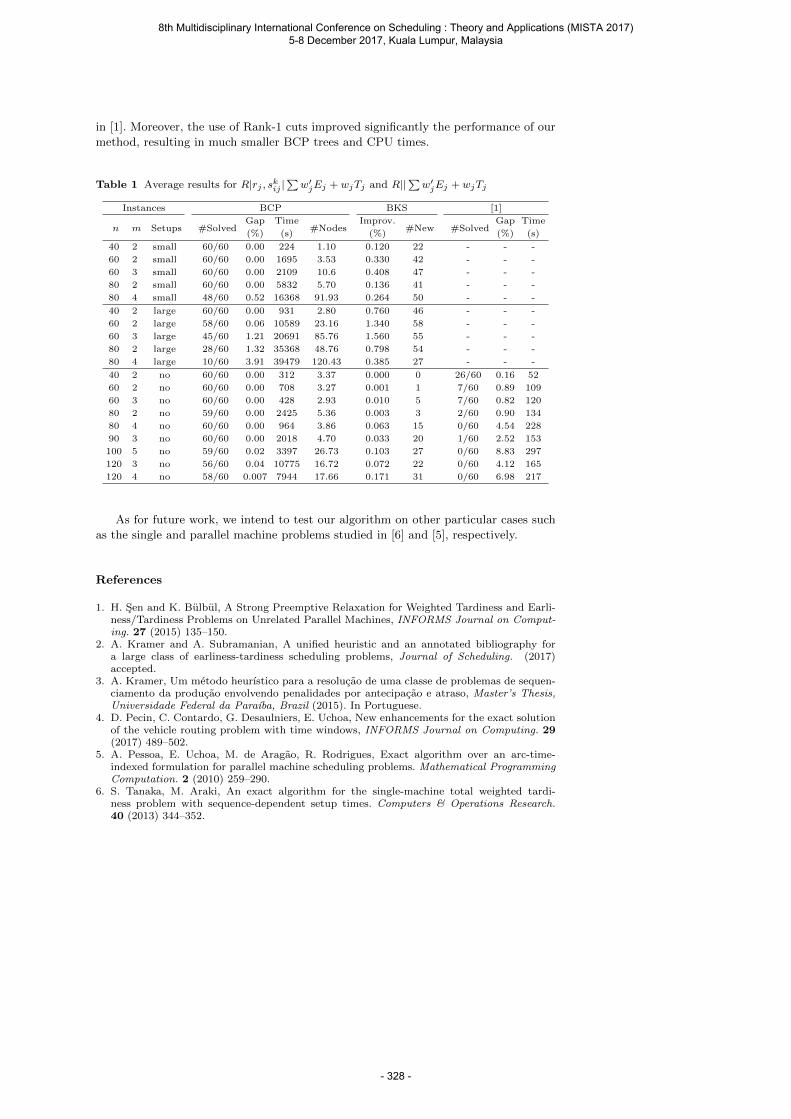
in [1]. Moreover, the use of Rank-1 cuts improved significantly the performance of our

method, resulting in much smaller BCP trees and CPU times.

Table 1 Average results for R|rj , skij |∑

w′jEj + wjTj and R||

∑w′

jEj + wjTj

Instances BCP BKS [1]

Gap Time Improv. Gap Timen m Setups #Solved

(%) (s)#Nodes

(%)#New #Solved

(%) (s)

40 2 small 60/60 0.00 224 1.10 0.120 22 - - -

60 2 small 60/60 0.00 1695 3.53 0.330 42 - - -

60 3 small 60/60 0.00 2109 10.6 0.408 47 - - -

80 2 small 60/60 0.00 5832 5.70 0.136 41 - - -

80 4 small 48/60 0.52 16368 91.93 0.264 50 - - -

40 2 large 60/60 0.00 931 2.80 0.760 46 - - -

60 2 large 58/60 0.06 10589 23.16 1.340 58 - - -

60 3 large 45/60 1.21 20691 85.76 1.560 55 - - -

80 2 large 28/60 1.32 35368 48.76 0.798 54 - - -

80 4 large 10/60 3.91 39479 120.43 0.385 27 - - -

40 2 no 60/60 0.00 312 3.37 0.000 0 26/60 0.16 52

60 2 no 60/60 0.00 708 3.27 0.001 1 7/60 0.89 109

60 3 no 60/60 0.00 428 2.93 0.010 5 7/60 0.82 120

80 2 no 59/60 0.00 2425 5.36 0.003 3 2/60 0.90 134

80 4 no 60/60 0.00 964 3.86 0.063 15 0/60 4.54 228

90 3 no 60/60 0.00 2018 4.70 0.033 20 1/60 2.52 153

100 5 no 59/60 0.02 3397 26.73 0.103 27 0/60 8.83 297

120 3 no 56/60 0.04 10775 16.72 0.072 22 0/60 4.12 165

120 4 no 58/60 0.007 7944 17.66 0.171 31 0/60 6.98 217

As for future work, we intend to test our algorithm on other particular cases such

as the single and parallel machine problems studied in [6] and [5], respectively.

References

1. H. Sen and K. Bulbul, A Strong Preemptive Relaxation for Weighted Tardiness and Earli-ness/Tardiness Problems on Unrelated Parallel Machines, INFORMS Journal on Comput-ing. 27 (2015) 135–150.

2. A. Kramer and A. Subramanian, A unified heuristic and an annotated bibliography fora large class of earliness-tardiness scheduling problems, Journal of Scheduling. (2017)accepted.

3. A. Kramer, Um metodo heurıstico para a resolucao de uma classe de problemas de sequen-ciamento da producao envolvendo penalidades por antecipacao e atraso, Master’s Thesis,Universidade Federal da Paraıba, Brazil (2015). In Portuguese.

4. D. Pecin, C. Contardo, G. Desaulniers, E. Uchoa, New enhancements for the exact solutionof the vehicle routing problem with time windows, INFORMS Journal on Computing. 29(2017) 489–502.

5. A. Pessoa, E. Uchoa, M. de Aragao, R. Rodrigues, Exact algorithm over an arc-time-indexed formulation for parallel machine scheduling problems. Mathematical ProgrammingComputation. 2 (2010) 259–290.

6. S. Tanaka, M. Araki, An exact algorithm for the single-machine total weighted tardi-ness problem with sequence-dependent setup times. Computers & Operations Research.40 (2013) 344–352.


- 328 -

MISTA 2017

Robotic Cell Scheduling Considering Energy Consumption of Robot

Moves

Hakan Gultekin • Sinan Gurel • Vahid Eghbal Akhlaghi

1 Introduction

We consider a robotic manufacturing cell consisting of serial machines that produce identical

parts. A material handling robot is responsible for loading/unloading the machines and

transferring the parts between the machines. Most of the studies in this literature consider the

problem of determining the sequence of robot moves that maximizes the throughput rate.

These studies assume that the robot moves are performed with its maximum speed, which

leads to higher energy consumption cost. However, reducing the speed of some moves may

lead the same production rate with a lower cost. In this study, we consider the problem of

determining both the optimal robot speeds and the optimal robot move sequence. The

objectives to be considered are the minimization of the total energy consumption and

maximization of the throughput rate. The energy consumption function is convex and

nonlinear with respect to the robot speed. We study the tradeoff between the throughput rate

and the energy consumption of the robot. We utilize the epsilon constraint approach for this bi-

criteria problem by writing the throughput objective as a constraint and formulate the problem

as a Mixed Integer Nonlinear Program for the general m-machine cells. We consider two-

machine cells in detail and develop analytical results by utilizing the KKT optimality

conditions. We develop a heuristic approximation algorithm to determine the optimal robot

speeds for each possible robot move cycle corresponding to a given throughput rate.

Acknowledgements

This study is supported by TUBİTAK under grant number 215M845.


- 329 -




MISTA 2017

Scheduling container transportation through conflict-freetrajectories in a warehouse layout: A local search approach

Emmanouil Thanos · Tony Wauters ·Greet Vanden Berghe

1 Introduction

Container storage and transportation procedures constitute a crucial element of ware-

house operations. Efficient transport scheduling significantly reduces serving time in

settings which involve large numbers of dynamic orders. Due to limited warehouse

space, container stacks frequently form highly-confined traffic networks for transfer-

ring vehicles. Pickup, relocation and dispatching operations are further constrained by

precedence and piling restrictions arising from containers’ physical properties and their

positions within the stacks. These factors impose great difficulties in terms of finding

globally optimal solutions for real-time applications.

A significant number of heuristic approaches have been developed for addressing

scheduling and routing of Autonomous Agents and Automated Guided Vehicles [7].

The two components are generally handled at distinct decision levels: vehicles are first

assigned to transportation requests and their routing is subsequently determined to

ensure good quality conflict-free paths for each request while also respecting deadlines

or priorities [2, 5, 8]. Less frequently conflict inspection precedes scheduling to com-

pletely eliminate overlapping routes [6], thus possibly excluding good-quality solutions

which could be resolved in a warehouse context by adding waiting times. Other notable

works focusing on conflict resolution utilize fixed itineraries, assuming vehicles’ assign-

ments are predetermined [1, 3, 4]. Concerning container relocations, extensive research

has revealed that there has been insufficient research towards integrated approaches

capable of simultaneously addressing relocation and routing objectives. An extended

literature review and research justification will be presented within the full paper.

Emmanouil ThanosKU Leuven, Department of Computer Science, CODeS & imecE-mail: [email protected]

Tony WautersKU Leuven, Department of Computer Science, CODeS & imecE-mail: [email protected]

Greet Vanden BergheKU Leuven, Department of Computer Science, CODeS & imecE-mail: [email protected]


- 330 -

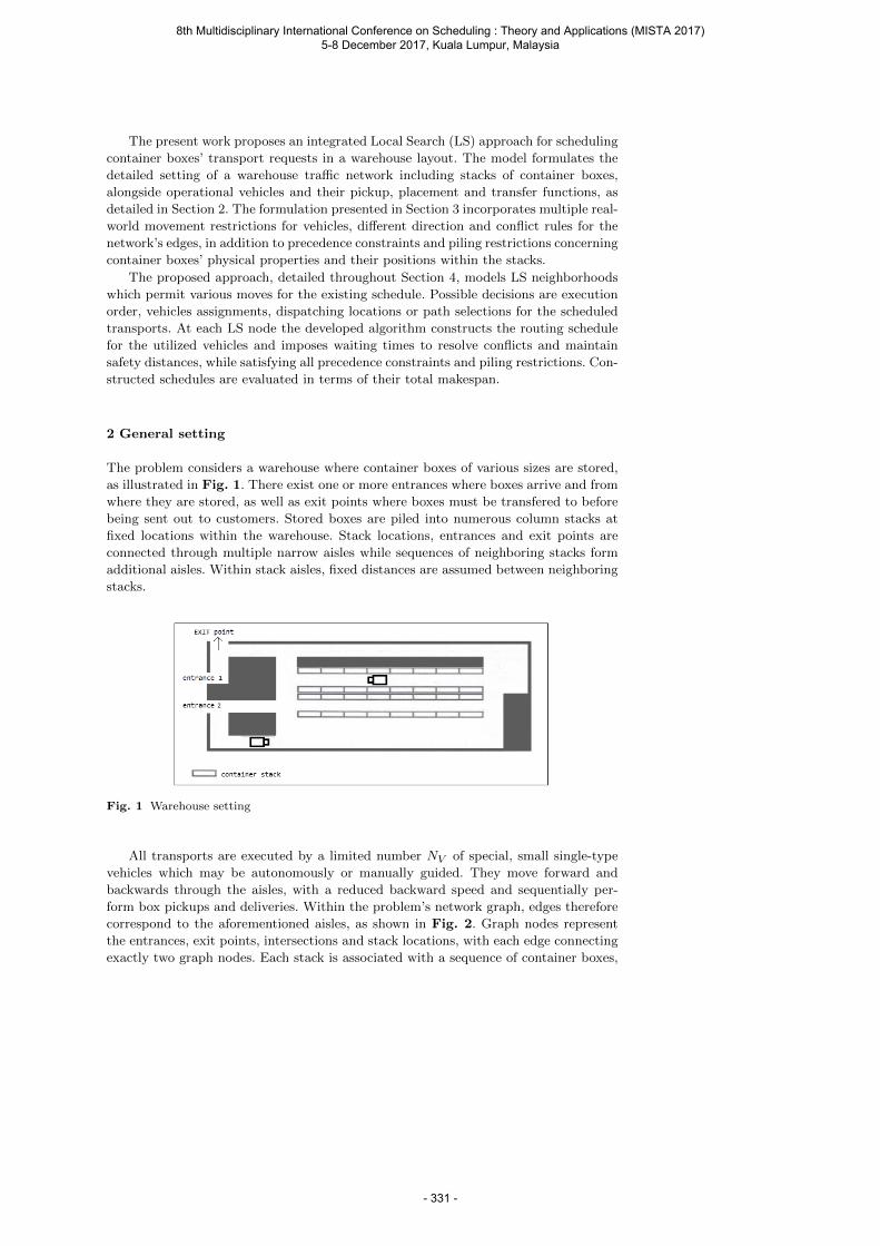
The present work proposes an integrated Local Search (LS) approach for scheduling

container boxes’ transport requests in a warehouse layout. The model formulates the

detailed setting of a warehouse traffic network including stacks of container boxes,

alongside operational vehicles and their pickup, placement and transfer functions, as

detailed in Section 2. The formulation presented in Section 3 incorporates multiple real-

world movement restrictions for vehicles, different direction and conflict rules for the

network’s edges, in addition to precedence constraints and piling restrictions concerning

container boxes’ physical properties and their positions within the stacks.

The proposed approach, detailed throughout Section 4, models LS neighborhoods

which permit various moves for the existing schedule. Possible decisions are execution

order, vehicles assignments, dispatching locations or path selections for the scheduled

transports. At each LS node the developed algorithm constructs the routing schedule

for the utilized vehicles and imposes waiting times to resolve conflicts and maintain

safety distances, while satisfying all precedence constraints and piling restrictions. Con-

structed schedules are evaluated in terms of their total makespan.

2 General setting

The problem considers a warehouse where container boxes of various sizes are stored,

as illustrated in Fig. 1. There exist one or more entrances where boxes arrive and from

where they are stored, as well as exit points where boxes must be transfered to before

being sent out to customers. Stored boxes are piled into numerous column stacks at

fixed locations within the warehouse. Stack locations, entrances and exit points are

connected through multiple narrow aisles while sequences of neighboring stacks form

additional aisles. Within stack aisles, fixed distances are assumed between neighboring

stacks.

Fig. 1 Warehouse setting

All transports are executed by a limited number NV of special, small single-type

vehicles which may be autonomously or manually guided. They move forward and

backwards through the aisles, with a reduced backward speed and sequentially per-

form box pickups and deliveries. Within the problem’s network graph, edges therefore

correspond to the aforementioned aisles, as shown in Fig. 2. Graph nodes represent

the entrances, exit points, intersections and stack locations, with each edge connecting

exactly two graph nodes. Each stack is associated with a sequence of container boxes,


- 331 -

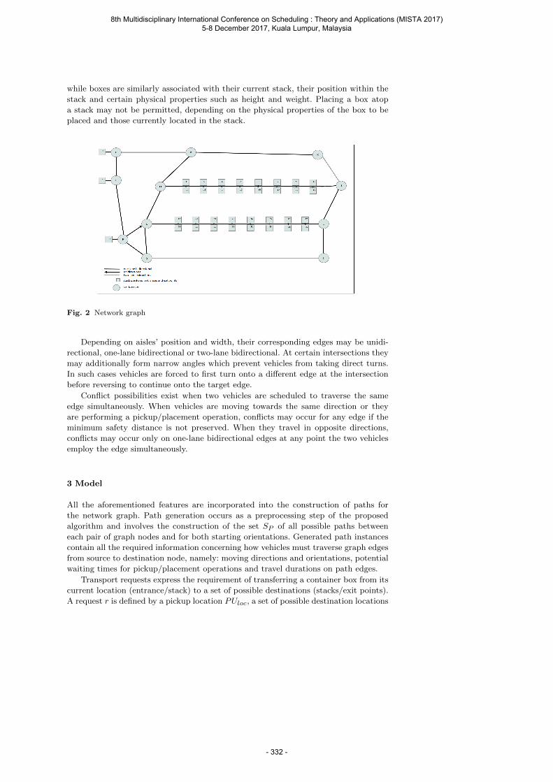
while boxes are similarly associated with their current stack, their position within the

stack and certain physical properties such as height and weight. Placing a box atop

a stack may not be permitted, depending on the physical properties of the box to be

placed and those currently located in the stack.

Fig. 2 Network graph

Depending on aisles’ position and width, their corresponding edges may be unidi-

rectional, one-lane bidirectional or two-lane bidirectional. At certain intersections they

may additionally form narrow angles which prevent vehicles from taking direct turns.

In such cases vehicles are forced to first turn onto a different edge at the intersection

before reversing to continue onto the target edge.

Conflict possibilities exist when two vehicles are scheduled to traverse the same

edge simultaneously. When vehicles are moving towards the same direction or they

are performing a pickup/placement operation, conflicts may occur for any edge if the

minimum safety distance is not preserved. When they travel in opposite directions,

conflicts may occur only on one-lane bidirectional edges at any point the two vehicles

employ the edge simultaneously.

3 Model

All the aforementioned features are incorporated into the construction of paths for

the network graph. Path generation occurs as a preprocessing step of the proposed

algorithm and involves the construction of the set SP of all possible paths between

each pair of graph nodes and for both starting orientations. Generated path instances

contain all the required information concerning how vehicles must traverse graph edges

from source to destination node, namely: moving directions and orientations, potential

waiting times for pickup/placement operations and travel durations on path edges.

Transport requests express the requirement of transferring a container box from its

current location (entrance/stack) to a set of possible destinations (stacks/exit points).

A request r is defined by a pickup location PUloc, a set of possible destination locations


- 332 -

SPL and a container box B. Each request must be assigned to exactly one vehicle

which must travel from its current location to PUloc, pick up B from the top of the

associated stack, travel from PUloc to a location PLloc ∈ SPL and finally unload B

atop the destination stack. Pickup and placement completion times Trpu and Trpl are

considered equal to the ending times of the corresponding operations.

A precedence constraint is a triple < op, r1, r2 >, where op is an operation (PU/PL)

and r1 and r2 are transport requests. It expresses the requirement that the defined

operation associated with r1 must be executed before r2’s. For the purposes of this

work, it is assumed that the set SR of transport requests to be processed and sched-

uled at each call of the LS algorithm includes all the auxiliary requests potentially

arisen due to relocation requirements, with the size of typical instances reaching up

to approximately 150. The set SC of precedence constraints possibly restricting their

execution order is generated upon SR and the requirement that all container boxes are

at the top of the right stack at their associated request’s pickup completion time.

A route is a path with waiting times possibly enforced in-between its pairs of con-

secutive edges. A routing schedule consists of an assignment of each transport request

r ∈ SR to a vehicle V , in addition to the pair of routes which must be followed to

execute r’s pickup and placement operations and a triple < TO, Trpu, T rpl > of times-

tamps defining take-off time, pickup and placement completion time, respectively. A

routing schedule is valid if (i) all precedence constraints are satisfied by the resulting

execution order, (ii) all placement operations are feasible at the time they occur and

(iii) all pairs of overlapping routes are conflict-free.

Given a warehouse network graph modeled with the aforementioned properties, the

set of paths SP , the set of transport requests SR, the set of precedence constraints SC

and the number of available vehicles NV , the problem consists of finding a valid routing

schedule which minimizes the total makespan. The total makespan M is equivalent to

the latest placement completion time of the schedule and calculated using Equation 1

as follows:

M = maxr∈SR

Trpl (1)

4 Local search framework

The general idea of the proposed LS algorithm is that an LS node indirectly defines a

routing schedule by gradually routing all available vehicles. An LS node is defined by:

– a vector Rins of all requests to be inserted into the schedule, defining the order in

which they will be processed

– for each r ∈ Rins, a quadruple < V , PLloc, PATHpu, PATHpl >,

where V is the vehicle assigned to r, PLloc ∈ SPL the selected destination for

placing box B, PATHpu the path V will follow to move from its current location

to PUloc and PATHpl the path V will follow to move from PUloc to PLloc

For the evaluation of a candidate node, all requests in Rins are sequentially inserted

into the initially empty schedule in the following manner: beginning from the ending

time of the latest route associated with V , every edge in PATHpu is iteratively checked

for conflicts with regard to the routes of every other vehicle. Whenever a conflict is

encountered, the problematic edge is shifted later into V ’s route imposing waiting times

for V on PATHpu’s graph nodes. If the conflict is not resolvable then a deadlock is


- 333 -

detected and the routing schedule is rendered invalid. The ending time of the last edge

of PATHpu, which contains the pickup operation, is stored as pickup completion time

Trpu of r. V is similarly routed through PATHpl to provide placement completion

time Trpl. After each operation the data concerning associated stacks and containers

is updated.The cost of a node is the total makespan of its resulting routing schedule,

calculated using Equation 1.

An LS node n is feasible if the resulting routing schedule is valid. The neighborhood

N(n) of n is the set of all feasible nodes obtainable from n by applying one of the

following operations:

– MOVE BACK(r) : move r one position back in Rins

– MOVE FORWARD(r) : move r one position forward in Rins

– CHANGE VEHICLE(r, V ′) : assign a different vehicle V ′ to r. PATHpu is assigned

default value.

– CHANGE PLloc(r, L′) : select a different placement location L′ ∈ SPL for r.

PATHpl is assigned default value.

– CHANGE PUpath(r, P ′) : select a different path P ′ connecting V ’s starting loca-

tion with PUloc

– CHANGE PLpath(r, P ′) : select a different path P ′ connecting PUloc with PLloc.

Beginning from an initial LS node with default values, the neighborhood of the

current node is explored at each iteration. During the search different variable selection

strategies are applied depending on the schedule’s current state. Simple value selection

strategies are utilized for each variable based on path lengths, location proximity,

vehicle availability and stack loads, properties which are also employed to provide

default values when required. The LS is incorporated within a meta-heuristic, the

details and performance of which will be presented at the conference. Nodes are selected

for expansion according to the evaluation function and the utilized meta-heuristic.

Concerning schedule construction, multiple techniques are employed to reduce re-

calculations and accelerate the conflict inspection procedure. For problems involving

small numbers of vehicles, the possibility of calculating time-difference windows for all

pairs of paths at the preprocessing step is also examined. All optimization techniques

will also be detailed during the presentation.

Acknowledgements Editorial consultation provided by Luke Connolly (KU Leuven).

References

1. Corman F, D’Ariano A, Pacciarelli D, Pranzo M (2012) Bi-objective conflict detec-

tion and resolution in railway traffic management. Transportation Research Part C:

Emerging Technologies 20(1):79–94

2. Correa AI, Langevin A, Rousseau LM (2007) Scheduling and routing of automated

guided vehicles: A hybrid approach. Computers & operations research 34(6):1688–

1707

3. Kim CW, Tanchoco JM (1991) Conflict-free shortest-time bidirectional agv routeing.

The International Journal of Production Research 29(12):2377–2391

4. Lange J, Werner F (2017) Approaches to modeling train scheduling problems as

job-shop problems with blocking constraints. Journal of Scheduling pp 1–17


- 334 -

5. Ma H, Li J, Kumar T, Koenig S (2017) Lifelong multi-agent path finding for online

pickup and delivery tasks. In: Proceedings of the 16th Conference on Autonomous

Agents and MultiAgent Systems, International Foundation for Autonomous Agents

and Multiagent Systems, pp 837–845

6. MacAlpine P, Price E, Stone P (2014) Scram: Scalable collision-avoiding role as-

signment with minimal-makespan for formational positioning. In: Proceedings of

the 2014 international conference on Autonomous agents and multi-agent systems,

International Foundation for Autonomous Agents and Multiagent Systems, pp 1463–

1464

7. Qiu L, Hsu WJ, Huang SY, Wang H (2002) Scheduling and routing algorithms for

agvs: a survey. International Journal of Production Research 40(3):745–760

8. Reveliotis SA (2000) Conflict resolution in AGV systems. IIE Transactions

32(7):647–659


- 335 -

MISTA 2017

An Integrated Optimization of Dynamic Product FamilyConfiguration and Supply Chain Configuration

Takuya Tsuboi · Tatsushi Nishi · Yoshitaka

Tanimizu · Toshiya Kaihara

Abstract In this paper, we consider an integrated optimization of dynamic product

family configuration and supply chain configuration. The problem is formulated as a

mixed integer linear programming model. Two types of methods: a sequential method

and a simultaneous method are applied to solve the problem. Computational experi-

ments are provided to show the effectiveness of the simultaneous method from practical

data.

1 Introduction

Mass customization is a strategy to meet customer’s needs while mass-producing prod-

ucts. One of the methods to achieve mass customization is a modular production. In

the method, a variety of final products are manufactured by assembling some modules.

Therefore, the optimal planning of Bill of Materials (BOM) is required. The number

of product types is limited due to the budget and common modules are available even

if different products are manufactured. The product family configuration determines

the selection of final products and their modules under the budget constraint. The

supply chain configuration is concerned with the selection of production facilities and

the production quantity of modules and products to be manufactured. Conventionally,

the product family configuration and the supply chain configuration decisions have

been regarded as separated problems. In many cases, a sequential method is adopted

Takuya TsuboiGraduate School of Engineering Science, Osaka UniversityE-mail: [email protected]

Tatsushi NishiGraduate School of Engineering Science, Osaka UniversityE-mail: [email protected]

Yoshitaka TanimizuDepartment of Mechanical Engineering, Osaka Prefecture UniversityE-mail: [email protected]

Toshiya KaiharaGraduate School of System Informatics, Kobe UniversityE-mail: [email protected]


- 336 -

to determine the supply chain decision after the product family configuration is de-

termined. However, it is expected that the profit becomes larger by simultaneously

optimizing the dynamic product family configuration and supply chain configuration

taking into account for production cost, transportation cost and inventory cost. Hence,

the integrated optimization of dynamic product family configuration and supply chain

configuration is required. Fujita et al. (2013) formulated a simultaneous decision prob-

lem of product family configuration and supply chain configuration as a mixed integer

nonlinear programing problem [1]. Bertrand et al. (2016) proposed a mixed integer

linear programing problem for the integrated optimization problem [2]. A Stackelberg

game model [3], a two-phase approach [4] were used to solve the integrated problems.

However, these studies considered the problem within a single period. In this paper,

we propose a multi-period model for simultaneous optimization of product family con-

figuration and supply chain configuration.

2 Mathematical model

Product family configuration is the selection of products to be manufactured and the

construction of the BOM for each product. The objective of product family configura-

tion problem is to maximize the profit by selecting the products to sell to customers

and reducing the costs related to the development and manufacturing of modules and

products. The module is a part of product and it has several functions. Each module

possesses a substitutability. Therefore, each product can be manufactured by assem-

bling some modules selected from candidate modules. Unit production cost of module

and unit assembly cost of product are incurred in the supply chain configuration. On

the other hand, the development and manufacturing costs are incurred for each type

of selected modules and products in the product family configuration. We need to se-

lect the best modules for final products to be manufactured from the combination of

modules. The supply chain configuration concerns with the operation of production

facilities, the production quantity of modules and products, product inventory, trans-

portation quantity of the modules and product sales. In the model, there are multiple

production facilities. The modules are produced at the supplier and the products are

manufactured at the production sites and they are directly solved to customers. There-

fore, transportation quantity of modules from a supplier to a production facility and

sales of products are also included in supply chain configuration. The total profit to be

maximized is the sales profit minus the total cost. The total cost is composed of produc-

tion cost, transportation cost, assembly cost, inventory cost, distribution cost, facility

maintenance cost, development and manufacturing cost. In the proposed model, the

product family configuration and supply chain configuration can be changed dynami-

cally according to the cost and the demand for each product. The proposed model has

two major characteristics. First, we can only change the product family configuration

in some specific periods because the product family configuration cannot be changed

frequently in practice. Therefore, the same product family is used until the next prod-

uct family determination period once the product family configuration is determined.

Second, since we assume a budget constraint for all time periods, interactions in dif-

ferent decision timing are considered. The constraints in the proposed model are listed

as follows:

1. All selected modules must be produced when manufacturing a product.

2. The modules and products can be produced within a finite capacity.


- 337 -

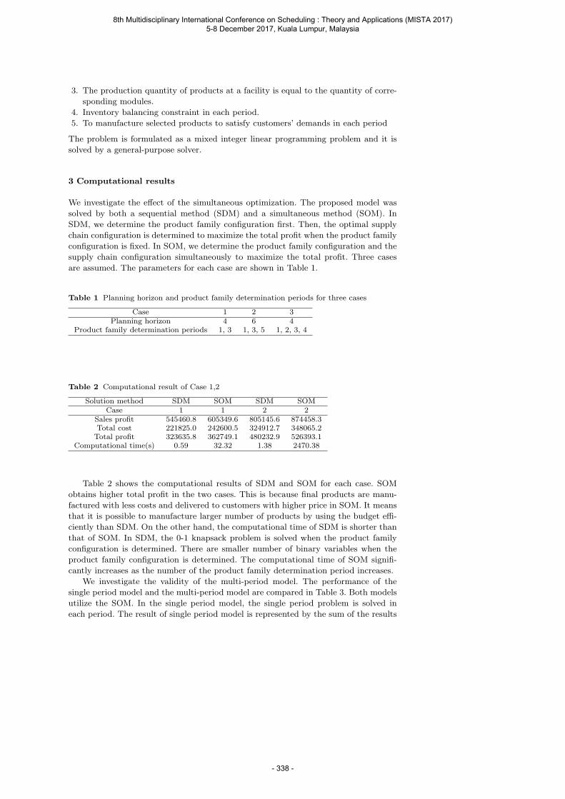
3. The production quantity of products at a facility is equal to the quantity of corre-

sponding modules.

4. Inventory balancing constraint in each period.

5. To manufacture selected products to satisfy customers’ demands in each period

The problem is formulated as a mixed integer linear programming problem and it is

solved by a general-purpose solver.


We investigate the effect of the simultaneous optimization. The proposed model was

solved by both a sequential method (SDM) and a simultaneous method (SOM). In

SDM, we determine the product family configuration first. Then, the optimal supply

chain configuration is determined to maximize the total profit when the product family

configuration is fixed. In SOM, we determine the product family configuration and the

supply chain configuration simultaneously to maximize the total profit. Three cases

are assumed. The parameters for each case are shown in Table 1.

Table 1 Planning horizon and product family determination periods for three cases

Case 1 2 3Planning horizon 4 6 4

Product family determination periods 1, 3 1, 3, 5 1, 2, 3, 4

Table 2 Computational result of Case 1,2

Solution method SDM SOM SDM SOMCase 1 1 2 2

Sales profit 545460.8 605349.6 805145.6 874458.3Total cost 221825.0 242600.5 324912.7 348065.2Total profit 323635.8 362749.1 480232.9 526393.1

Computational time(s) 0.59 32.32 1.38 2470.38

Table 2 shows the computational results of SDM and SOM for each case. SOM

obtains higher total profit in the two cases. This is because final products are manu-

factured with less costs and delivered to customers with higher price in SOM. It means

that it is possible to manufacture larger number of products by using the budget effi-

ciently than SDM. On the other hand, the computational time of SDM is shorter than

that of SOM. In SDM, the 0-1 knapsack problem is solved when the product family

configuration is determined. There are smaller number of binary variables when the

product family configuration is determined. The computational time of SOM signifi-

cantly increases as the number of the product family determination period increases.

We investigate the validity of the multi-period model. The performance of the

single period model and the multi-period model are compared in Table 3. Both models

utilize the SOM. In the single period model, the single period problem is solved in

each period. The result of single period model is represented by the sum of the results


- 338 -

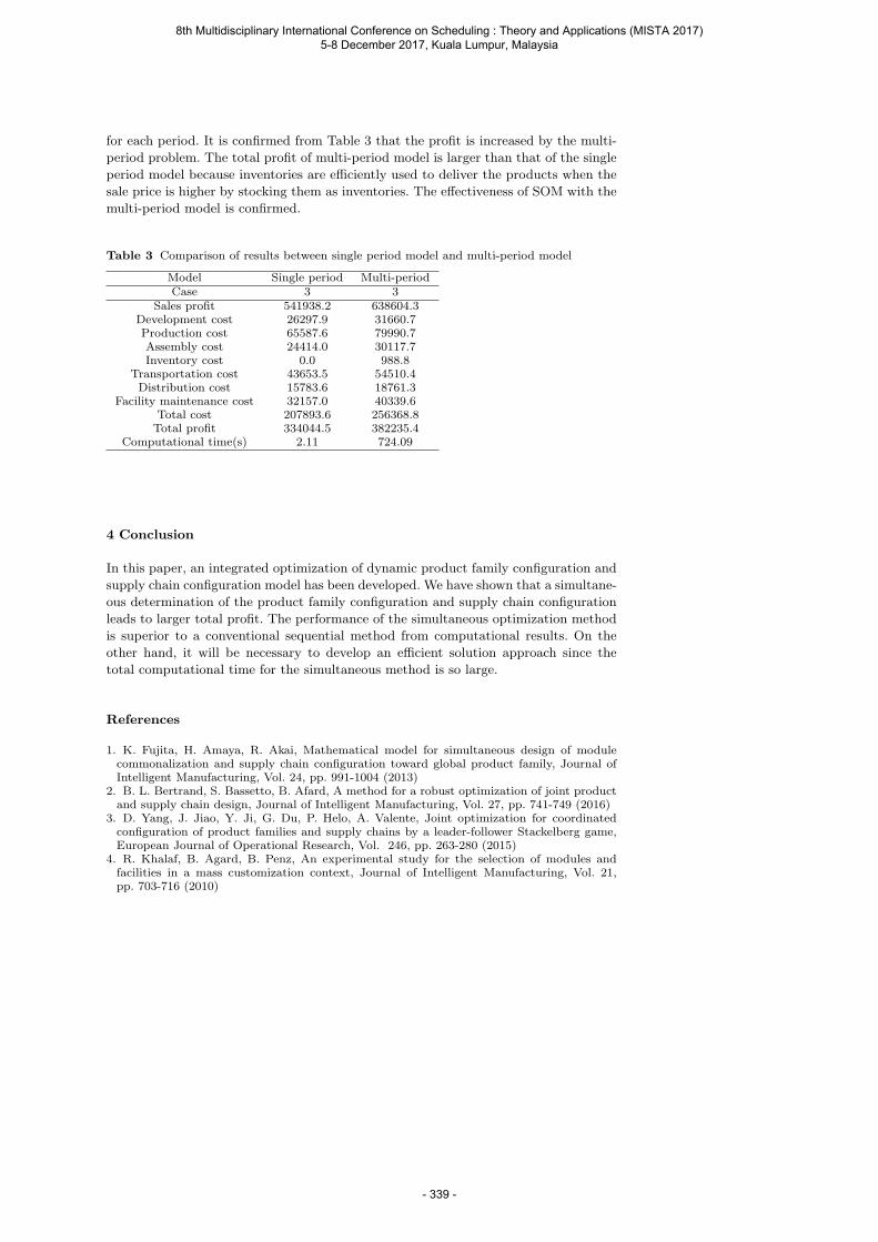
for each period. It is confirmed from Table 3 that the profit is increased by the multi-

period problem. The total profit of multi-period model is larger than that of the single

period model because inventories are efficiently used to deliver the products when the

sale price is higher by stocking them as inventories. The effectiveness of SOM with the

multi-period model is confirmed.

Table 3 Comparison of results between single period model and multi-period model

Model Single period Multi-periodCase 3 3

Sales profit 541938.2 638604.3Development cost 26297.9 31660.7Production cost 65587.6 79990.7Assembly cost 24414.0 30117.7Inventory cost 0.0 988.8

Transportation cost 43653.5 54510.4Distribution cost 15783.6 18761.3

Facility maintenance cost 32157.0 40339.6Total cost 207893.6 256368.8Total profit 334044.5 382235.4

Computational time(s) 2.11 724.09

4 Conclusion

In this paper, an integrated optimization of dynamic product family configuration and

supply chain configuration model has been developed. We have shown that a simultane-

ous determination of the product family configuration and supply chain configuration

leads to larger total profit. The performance of the simultaneous optimization method

is superior to a conventional sequential method from computational results. On the

other hand, it will be necessary to develop an efficient solution approach since the

total computational time for the simultaneous method is so large.

References

1. K. Fujita, H. Amaya, R. Akai, Mathematical model for simultaneous design of modulecommonalization and supply chain configuration toward global product family, Journal ofIntelligent Manufacturing, Vol. 24, pp. 991-1004 (2013)

2. B. L. Bertrand, S. Bassetto, B. Afard, A method for a robust optimization of joint productand supply chain design, Journal of Intelligent Manufacturing, Vol. 27, pp. 741-749 (2016)

3. D. Yang, J. Jiao, Y. Ji, G. Du, P. Helo, A. Valente, Joint optimization for coordinatedconfiguration of product families and supply chains by a leader-follower Stackelberg game,European Journal of Operational Research, Vol. 246, pp. 263-280 (2015)

4. R. Khalaf, B. Agard, B. Penz, An experimental study for the selection of modules andfacilities in a mass customization context, Journal of Intelligent Manufacturing, Vol. 21,pp. 703-716 (2010)


- 339 -

MISTA 2017

A Batch-oblivious Approach For Scheduling ComplexJob-Shops with Batching Machines: From Non-delay toActive Scheduling

Karim Tamssaouet · Stephane Dauzere-Peres ·Claude Yugma · Jacques Pinaton

1 Introduction and Problem Description

The production of microelectronic devices is a highly complicated and cost intensive

process, particularly in the front-end where the processing of wafers takes place. De-

pending on the product types and on the technology, a wafer goes through more than

600 process steps over a period of a few weeks. In this context, scheduling decisions

have a substantial impact on key performance indicators such as throughput and cycle

time, see Monch et al. (2011). Among the complex workshops in a wafer manufactur-

ing facility, the diffusion area is of critical importance. The processes in this area are

performed on two types of equipment: cleaning and furnace machines.These machines

can process several lots simultaneously. Moreover, the processing durations can be very

long compared to other operations in the fab. Due to the dynamic arrival of jobs, an

important decision is whether it makes sense to wait for the arrival of future jobs in

the case of incomplete batches, or to start non-full batches.

This work deals with a real-life complex scheduling problem arising in the diffusion

area, but can be applied in many other industrial contexts. We consider scheduling

a set of jobs that have different sizes, different priorities and arrive dynamically to

the work area. Each job is associated with a route that describes the sequence of

operations that the job should go through. Each operation can only be performed on a

set of qualified machines, and its processing duration depends on the selected machine.

A significant constraint to consider is p-batching, the machines can process multiple

operations in parallel. On a qualified batching machine, an operation can be batched

only with a subset of operations with the same batch family. Some of the machines

are subject to sequence-dependent setups, such that the amount of time required to

configure a machine to process a subsequent operation depends upon the machine’s

Karim Tamssaouet · Stephane Dauzere-Peres · Claude YugmaEcole des Mines de Saint-Etienne, CMP Georges CharpakDepartment of Manufacturing Sciences and LogisticsCNRS UMR 6158 LIMOS F-13541, Gardanne, FranceE-mail: karim.tamssaouet,dauzere-peres,[email protected]

Jacques PinatonSTMicroelectronics Rousset, ZI de RoussetAvenue Coq, F-13106 Rousset Cedex, FranceE-mail: [email protected]


- 340 -

configuration that was used by the precedent operation. We aim to optimize different

regular mono-objective functions from the literature.

Our proposition relies on the novel approach proposed by Knopp et al. (2017) for

complex job-shop problems with batching machines. In this approach, an adaptation

of the classical conjunctive graph, introduced by Roy and Sussmann (1964), is made

to represent batches through arc labels. Using this new representation, called batch-

oblivious graph, the schedules are constructed and improved during the graph traversal.

The obtained schedules are non-delay in the sense that no machine is kept idle while

an operation is waiting for processing. So instead of non-delay schedules, this work

proposes generating active schedules by inserting an idle time if it is relevant to increase

the batch size. This new way of constructing schedules aims at reaching quickly good

solutions within a heuristic.

2 Batch Oblivious Disjunctive Graph

Most existing solution approaches for Complex Job-Shop scheduling problems with

batching machines rely on the disjunctive graph representation of Ovacik and Uzsoy

(2012). This representation introduces dedicated nodes to represent explicitly batch-

ing decisions.A novel batch-oblivious modeling is presented by Knopp et al. (2017).

Like a classical conjunctive graph, the batch-oblivious conjunctive graph uses nodes to

uniquely represent operations and arcs to represent precedence constraints on routes

and resources. Instead of inserting additional nodes and arcs to model batches, they

are coded in the arc weights. This new representation has many advantages. It reduces

the structural complexity of the graph. It allows reusing ideas and techniques for a less

complex problem like the move proposed by Dauzere-Peres and Paulli (1997) for the

flexible job shop scheduling problem. Last but not least, it is possible to propose an

integrated algorithm that computes start dates and improves the solution during the

graph traversal by filling underutilized batches through a combined resequencing and

reassignment strategy. In this work, we adopt the same representation in the form of

a batch-oblivious modeling. We propose a new integrated algorithm that modifies the

solution differently during the graph traversal.

3 Towards Active Schedules

First, it is important to clarify the notion of active and non-delay schedules within this

work. The schedules that are provided by the construction algorithm of Knopp et al.

(2017) are qualified as non-delay schedules. When a node is visited during the graph

traversal, the construction algorithm gives this node the earliest start date. The last

condition only defines what is called semi-active schedules in the scheduling literature

(Pinedo (2016)). So, in addition to the earliest start date, when the algorithm searches

for potential operations that can complete a non-full batch, it advances only those that

can be integrated to the batch without delaying its start time.

Theoretically, it is always possible to construct an optimal solution using this con-

struction algorithm on the batch-oblivious conjunctive graph. However, it may take

a lot of moves before obtaining such a solution. A new construction algorithm that

outputs active schedules can constitute a useful shortcut that accelerates the search by

quickly constructing good solutions. The schedules are called active as we intentionally


- 341 -

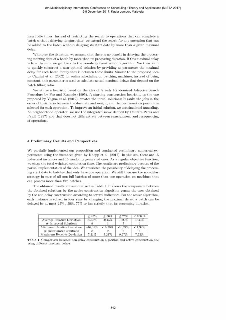
insert idle times. Instead of restricting the search to operations that can complete a

batch without delaying its start date, we extend the search for any operation that can

be added to the batch without delaying its start date by more than a given maximal

delay.

Whatever the situation, we assume that there is no benefit in delaying the process-

ing starting date of a batch by more than its processing duration. If this maximal delay

is fixed to zero, we get back to the non-delay construction algorithm. We then want

to quickly construct a near-optimal solution by providing as parameter the maximal

delay for each batch family that is between these limits. Similar to the proposed idea

by Cigolini et al. (2002) for online scheduling on batching machines, instead of being

constant, this parameter is used to calculate actual maximal delays that depend on the

batch filling ratio.

We utilize a heuristic based on the idea of Greedy Randomized Adaptive Search

Procedure by Feo and Resende (1995). A starting construction heuristic, as the one

proposed by Yugma et al. (2012), creates the initial solutions: It ranks the jobs in the

order of their ratio between the due date and weight, and the best insertion position is

selected for each operation . To improve an initial solution, we use simulated annealing.

As neighborhood operator, we use the integrated move defined by Dauzere-Peres and

Paulli (1997) and that does not differentiate between reassignment and resequencing

of operations.

4 Preliminary Results and Perspectives

We partially implemented our proposition and conducted preliminary numerical ex-

periments using the instances given by Knopp et al. (2017). In this set, there are 15

industrial instances and 15 randomly generated ones. As a regular objective function,

we chose the total weighted completion time. The results are preliminary because of the

partial implementation of the idea. We restricted the possibility of delaying the process-

ing start date to batches that only have one operation. We still then use the non-delay

strategy in case of all non-full batches of more than one operation on machines that

can process more than two batches.

The obtained results are summarized in Table 1. It shows the comparison between

the obtained solutions by the active construction algorithm versus the ones obtained

by the non-delay construction according to several indicators. For the active algorithm,

each instance is solved in four runs by changing the maximal delay: a batch can be

delayed by at most 25% , 50%, 75% or less strictly that its processing duration.

≤ 25% ≤ 50% ≤ 75% < 100 %Average Relative Deviation -0,55% -0,15% -0,20% -0,43%

# Improved Solutions 9 3 7 9Minimum Relative Deviation -16,31% -16,36% -16,24% -11,99%

# Deteriorated solutions 8 9 6 6Maximum Relative Deviation 7,21% 7,21% 9,57% 7,72%

Table 1 Comparison between non-delay construction algorithm and active construction oneusing different maximal delays


- 342 -

The relative deviation is computed as the (f(S) − f(Sref ))/f(Sref ), where S is

the active schedule, Sref is the non-delay solution and f() is the regular objective

function. In all cases, the average relative deviation shows the dominance of the active

construction algorithm. Depending on the accepted maximal delay, we can notice that

the results are quite different. If we take the case where the maximal delay is fixed

as the processing duration (< 100%), the active construction algorithm is better than

the non-delay one. 9 instances over 30 are improved while solutions of less quality

are obtained for only 6 instances with the worst relative deviation of 7.8%. The same

conclusion can be made about the case where the maximal delay is limited to the

quarter of the processing duration.

Although promising, these results are still preliminary. Definitive conclusions can

be made when the whole proposition is implemented. We intend to perform extensive

experiments to better analyze the benefit of going from non-delay to active schedules.

These experiments will also aim at studying how the allowed maximal delay impacts

the solution quality. Finally, as the non-delay construction algorithm is a particular

case of the active one, we have as objective to design an adaptive construction algo-

rithm that uses a suitable maximal delay depending on the solution space exploration.

While obtaining the advantage of accelerating the search through the construction of

active schedules, the ability to visit any solution is maintained through the non-delay

construction algorithm.

References

Cigolini, R., Perona, M., Portioli, A., and Zambelli, T. (2002). A new dynamic look-

ahead scheduling procedure for batching machines. Journal of scheduling, 5(2):185–

204.

Dauzere-Peres, S. and Paulli, J. (1997). An integrated approach for modeling and

solving the general multiprocessor job-shop scheduling problem using tabu search.

Annals of Operations Research, 70:281–306.

Feo, T. A. and Resende, M. G. (1995). Greedy randomized adaptive search procedures.

Journal of global optimization, 6(2):109–133.

Knopp, S., Dauzre-Prs, S., and Yugma, C. (2017). A batch-oblivious approach for

complex job-shop scheduling problems. European Journal of Operational Research,

263(1):50 – 61.

Monch, L., Fowler, J. W., Dauzere-Peres, S., Mason, S. J., and Rose, O. (2011). A

survey of problems, solution techniques, and future challenges in scheduling semi-

conductor manufacturing operations. Journal of Scheduling, 14(6):583–599.

Ovacik, I. M. and Uzsoy, R. (2012). Decomposition methods for complex factory schedul-

ing problems. Springer Science & Business Media.

Pinedo, M. (2016). Scheduling: Theory, Algorithms, and Systems. Springer Interna-

tional Publishing.

Roy, B. and Sussmann, B. (1964). Les problemes d’ordonnancement avec contraintes

disjonctives. Note ds, 9.

Yugma, C., Dauzere-Peres, S., Artigues, C., Derreumaux, A., and Sibille, O. (2012). A

batching and scheduling algorithm for the diffusion area in semiconductor manufac-

turing. International Journal of Production Research, 50(8):2118–2132.


- 343 -

MISTA 2017

Three upper bounds for the speed meeting problem

Benoit Cantais · Antoine Jouglet · David

Savourey

1 Introduction

In a speed meeting problem, people are gathered in a place where tables are disposed

to meet each other. The set of persons that each person wishes to meet is known.

At regular intervals, the persons are asked to get up and are redistributed among the

tables. A distribution of persons among the tables is called a round. Speed meetings

are getting popular in business networking. It allows, in a short period of time, a large

group of investors and businessmen to meet each other and find business opportunities.

We consider the problem with M tables of C seats, T meeting rounds and a set

a persons X = 1, . . . , N. G = (X,U ⊆ X2) is an oriented graph such as (i, j) ∈ U

means that person i wishes to meet person j (see example on Figure 1). A meeting

(i, j) ∈ U is considered as realized if persons i and j are seated at the same table during

at least one meeting round. At round t ∈ 1, . . . , T, each person i can be seated at

only one table and at most C persons can be seated at table m ∈ 1, . . . ,M. Given

the number of rounds T , the goal is to distribute the persons around the tables at every

round to maximise the total number of wished meetings realized. We use a reduction

from CLIQUE [3] to demonstrate that the problem is NP-Complete.

As far as we know, this problem has not been treated yet. Some well known prob-

lems can be seen as particular cases of the speed meeting problem. In the social golfer

problem, the persons do not want to meet more than once in a given number of rounds.

In the fully social golfer problem [4], every person has to meet every other person ex-

actly once. The Oberwolfach problem [2], the 36 officers problem [7], the Kirksman’s

schoolgirl problem [1] and the block design theory [6] are connected to the speed meet-

ing problem. In the speed dating problem [5], the special case where the capacity of

the tables is 2 is considered.

In this talk, we present three methods to find an upper bound for the speed meeting

problem.

Benoit Cantais, Antoine Jouglet, David SavoureySorbonne Universits, Universit de Technologie de CompigneHeudiasyc UMR CNRS 7253E-mail: benoit.cantais,antoine.jouglet,[email protected]


- 344 -

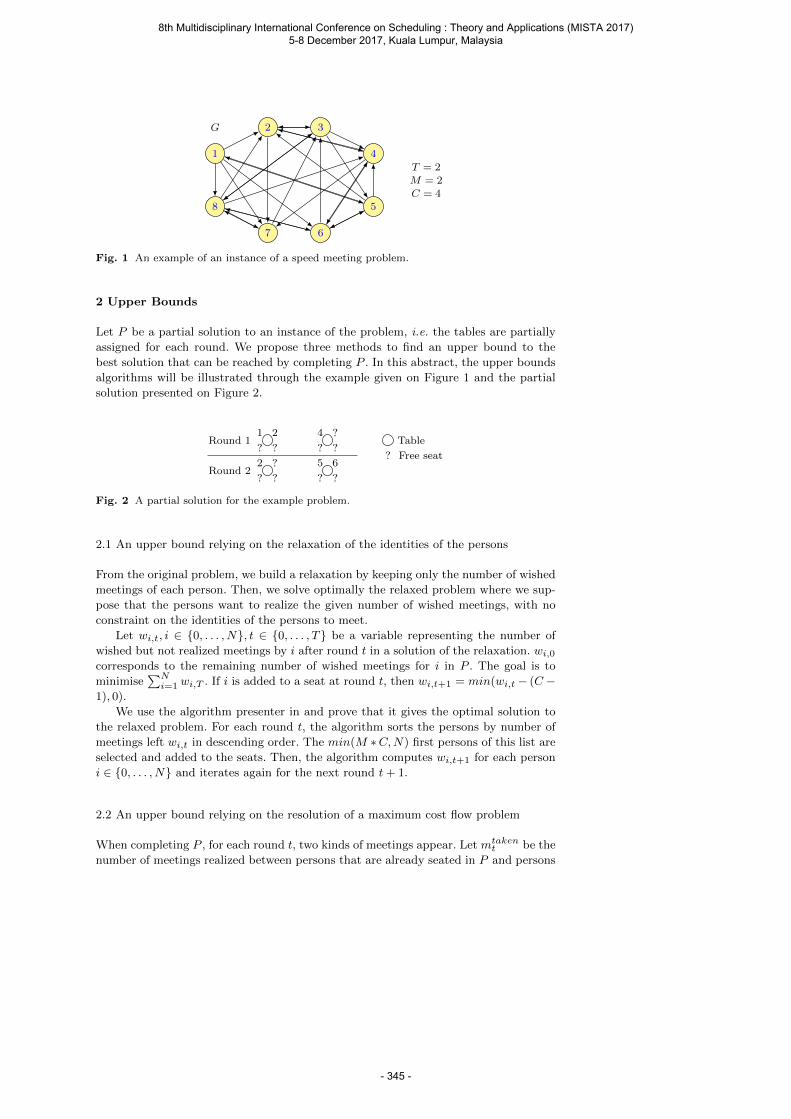
G

1

2 3

4

5

67

8

T = 2M = 2C = 4

Fig. 1 An example of an instance of a speed meeting problem.

2 Upper Bounds

Let P be a partial solution to an instance of the problem, i.e. the tables are partially

assigned for each round. We propose three methods to find an upper bound to the

best solution that can be reached by completing P . In this abstract, the upper bounds

algorithms will be illustrated through the example given on Figure 1 and the partial

solution presented on Figure 2.

Round 11 2

??

4 ?

??

Round 22 ?

??

5 6

??

Table

? Free seat

Fig. 2 A partial solution for the example problem.

2.1 An upper bound relying on the relaxation of the identities of the persons

From the original problem, we build a relaxation by keeping only the number of wished

meetings of each person. Then, we solve optimally the relaxed problem where we sup-

pose that the persons want to realize the given number of wished meetings, with no

constraint on the identities of the persons to meet.

Let wi,t, i ∈ 0, . . . , N, t ∈ 0, . . . , T be a variable representing the number of

wished but not realized meetings by i after round t in a solution of the relaxation. wi,0

corresponds to the remaining number of wished meetings for i in P . The goal is to

minimise∑N

i=1 wi,T . If i is added to a seat at round t, then wi,t+1 = min(wi,t− (C −1), 0).

We use the algorithm presenter in and prove that it gives the optimal solution to

the relaxed problem. For each round t, the algorithm sorts the persons by number of

meetings left wi,t in descending order. The min(M ∗C,N) first persons of this list are

selected and added to the seats. Then, the algorithm computes wi,t+1 for each person

i ∈ 0, . . . , N and iterates again for the next round t + 1.

2.2 An upper bound relying on the resolution of a maximum cost flow problem

When completing P , for each round t, two kinds of meetings appear. Let mtakent be the

number of meetings realized between persons that are already seated in P and persons


- 345 -

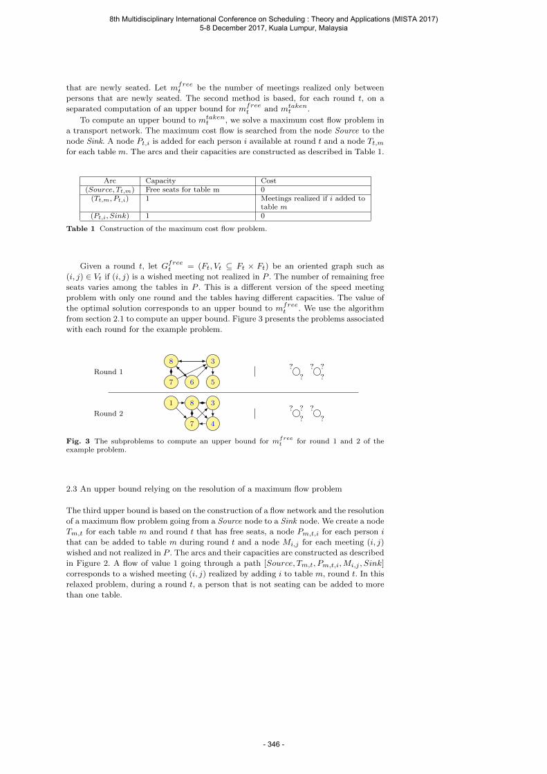
that are newly seated. Let mfreet be the number of meetings realized only between

persons that are newly seated. The second method is based, for each round t, on a

separated computation of an upper bound for mfreet and mtaken

t .

To compute an upper bound to mtakent , we solve a maximum cost flow problem in

a transport network. The maximum cost flow is searched from the node Source to the

node Sink. A node Pt,i is added for each person i available at round t and a node Tt,mfor each table m. The arcs and their capacities are constructed as described in Table 1.

Arc Capacity Cost(Source, Tt,m) Free seats for table m 0

(Tt,m, Pt,i) 1 Meetings realized if i added totable m

(Pt,i, Sink) 1 0

Table 1 Construction of the maximum cost flow problem.

Given a round t, let Gfreet = (Ft, Vt ⊆ Ft × Ft) be an oriented graph such as

(i, j) ∈ Vt if (i, j) is a wished meeting not realized in P . The number of remaining free

seats varies among the tables in P . This is a different version of the speed meeting

problem with only one round and the tables having different capacities. The value of

the optimal solution corresponds to an upper bound to mfreet . We use the algorithm

from section 2.1 to compute an upper bound. Figure 3 presents the problems associated

with each round for the example problem.

Round 1

3

567

8?

?

? ?

?

Round 2

1 3

47

8? ?

?

?

?

Fig. 3 The subproblems to compute an upper bound for mfreet for round 1 and 2 of the

example problem.

2.3 An upper bound relying on the resolution of a maximum flow problem

The third upper bound is based on the construction of a flow network and the resolution

of a maximum flow problem going from a Source node to a Sink node. We create a node

Tm,t for each table m and round t that has free seats, a node Pm,t,i for each person i

that can be added to table m during round t and a node Mi,j for each meeting (i, j)

wished and not realized in P . The arcs and their capacities are constructed as described

in Figure 2. A flow of value 1 going through a path [Source, Tm,t, Pm,t,i,Mi,j , Sink]

corresponds to a wished meeting (i, j) realized by adding i to table m, round t. In this

relaxed problem, during a round t, a person that is not seating can be added to more

than one table.


- 346 -

Arc Exists if Capacity(Source, Tm,t) ∅ Upper bound for number of meetings table m,

round t(Tm,t, Pm,t,i) ∅ Upper bound for number of meetings if i added

table m, round t(Pm,t,i,Mi,j) j seating table m, round t 1(Pm,t,i,Mj,i) j seating table m, round t 1(Pm,t,i,Mi,k) k free at round t 1(Mi,j , Sink) ∅ 1

Table 2 Arcs and their capacities for the construction of the flow network.

In this talk, we present preliminary results based on a set of crafted instances to

compare the efficiency of the differents upper bounds methods applied in a branch and

bound algorithm.

References

1. Nicolas Barnier and Pascal Brisset. Solving the kirkmans schoolgirl problem in a fewseconds. In Principles and Practice of Constraint Programming-CP 2002, pages 477–491.Springer, 2002.

2. Darryn Bryant and Victor Scharaschkin. Complete solutions to the oberwolfach problemfor an infinite set of orders. Journal of Combinatorial Theory, Series B, 99(6):904–918,2009.

3. MR Garey and DS Johnson. Computer and intractability: a guide to the theory of np-completeness, w. h. freeman & co., san francisco, ca. page 194, 1979.

4. Warwick Harvey. The fully social golfer problem. In SymCon, volume 3, pages 75–85, 2003.5. Agnes Le Roux. Ordonnancement de rendez-vous en tete a tete. PhD thesis, Ecole des

Mines de Nantes, 2014.6. ET Parker. Construction of some sets of mutually orthogonal latin squares. Proceedings of

the American Mathematical Society, 10(6):946–949, 1959.7. MG Tarry. Le probleme des 36 officiers. Association Francaise, 1900.


- 347 -

MISTA

2017

Modeling a Practical University Course Timetabling Problem with

Reward and Penalty Objective Function: Case Study FTSM-UKM

Xiao Fei Yang • Masri Ayob • Mohd Zakree Ahmad Nazri

1 Introduction

Generating a generally satisfied course timetable is a difficult task faces by most of educational

institutions in every semester. This is due to a large number of students, lecturers, and courses

which are inter-connected, and has objectives and constraints that need to be satisfied in order

to generate a feasible timetable[1]. The University Course Timetabling Problem (UCTP) is

defined as to schedule lectures (courses) that are conducted by lecturers within a given number

of timeslots and allocate these courses into available rooms satisfying certain constraints[2].

There are normally 5 basic components in the UCTP model[3], which are:

C - a set of courses to be scheduled;

T – a set of timeslots to allocate the courses in;

L - a set of lecturers conducting the courses;

S - a set of student groups taking the courses;

R - a set of class rooms to hold the courses.

There are two types of constraints needed to be considered when solving the UCTP

problem: the hard constraints and soft constraints. The hard constraints need to be satisfied to

ensure the feasibility of the generated timetable. Therefore, no hard constraint is allowed to be

violated in the solution. However, the soft constraints are allowed to be violated, as the soft

constraints are used to measure the general satisfaction of the generated timetable. Any violation

of the soft constraints will result in a reduction of the timetable’s satisfaction level. Therefore, a

good quality solution of the UCTP should violate no hard constraints and minimize the violations

of the soft constraints.

The UCTP is a Non-Polynomial-complete problem which cannot be solved in a polynomial

time[4]. In the other word, the UCTP is very difficult to solve for optimality. As an educational

timetabling problem, the UCTP has gathered great research interests in both operations research

and artificial intelligence fields since the 1950s[5]. In the early days, researchers are mainly


- 348 -




concentrating on developing models and solution approaches for a single institution[6][7][8]. A

survey regarding the early works in UCTP can be found in [9].

Since the approaches developed in the early days were tested on different specifically

designed UCTP models, researchers at that time were impossible to compare their solution

approaches with others. This issue caused the emergence of the first benchmark UCTP model,

which is published for the First International Timetabling Competition (ITC-2002)[10]. To the

current point of view, this benchmark model is a great reduction of real-world problems which

only involves the basic components collected from real-world problems[11]. This benchmark

model has greatly contributed the research field and provides a platform to compare different

solution approaches. The simplified model, i.e. ITC-2002 creates a gap between research and

practice. To bridge this gap, on the 2nd International Timetabling Competition, two new

benchmark models were published, which are post enrollment-based CTP (ITC-2007-track

2)[12] and curriculum-based CTP (ITC-2007-track 3)[13]. The major difference between these

two models is on how the conflictions between courses are defined. For the post-enrollment-

based problem, as an extension of previous benchmark problem, the conflictions is defined based

on the students’ enrollment information. However, the confliction for the curriculum based CTP

is based on the curriculum provided by the institution. Furthermore, lecturers are considered in

the curriculum-based CTP, whilst not in the post enrollment-based CTP. These two datasets have

significantly increased the problem complexity and make the problems closer to real-world

situations[14].

Although many research has been conducted on these benchmark datasets, these works

were rarely implemented on a real-world problem[11]. This might be due to the difference of

the constraints between benchmark UCTP model and practical problem model is different from

each other. Hence, an effectively modeling of a practical problem is important. [15] had stated

some factors that may result in the uniqueness of different UCTP models. Such as a high number

of elective courses. These elective courses are normally formed into groups which students need

to attend m out of n courses in each group. Another factor may influence the problem model is

the course sections, which represent for splitting a course into multiple sections. Furthermore,

course configuration is another factor may affect the problem model. Some courses may require

conducting different types of teaching events such as lectures, labs, and tutorials. These factors

may lead to a more complex model when dealing with real-world problems.

It is always important to consider human’s preference when designing a UCTP model[16].

When modeling a UCTP problem, the objective function should be carefully designed to reflect

the general satisfaction of a generated timetable. Traditionally, the objective functions are

designed based on measuring the violation of soft constraints. In both benchmark and practical

UTCP models, the objective function is designed only based on how many times a undesired

pattern appeared in solution. However, the user desired patterns in a timetable seem to be

ignored by the research society.

Our previous work in [17] has conducted an investigation of factors which may influence

the satisfaction on Fakulti Teknologi dan Sains Maklumat (FTSM), Universiti Kebangsaan

Malaysia (UKM). In [17], two questionnaires have been designed and distributed to the lecturers

and students in FTSM, UKM to collect their satisfaction information on every possible schedule

patterns. The result has identified the user’s undesired and desired patterns in a course timetable,

and how strong they like or dislike.

This work extends our previous work[17] and introduces a new practical course timetabling

problem at FTSM, UKM (FTSM-UCTP). The new practical problem contains more constraints

compared with benchmark problems. Additionally, we also introduced a new objective function

to measure the quality of the timetable by giving both penalty when undesired pattern appeared

and reward when the desired pattern appeared.

This paper is organized as follow: In Section 2, we present the description of the course

timetabling problem in FTSM, UKM. The formulation of the problem is presented in Section 3.

Section 4 proposed a new objection function with penalty and reward mechanism.

2 FTSM Course Timetabling Problem (FTSM-UCTP)


- 349 -

The dataset FTSM-UCTP SemII_16/17 presented in TABLE I is real data used in FTSM for

Semester II, year 2016/2017. In this dataset, the total number of courses is 74 exams with 21

students groups, required to be scheduled in 5 days (Mon-Fri) from 8:00 to 21:30. The features

of the datasets can be found in TABLE I.

TABLE I. FEATURES OF FTSM-UCTP SEMII_16/17

Feature Value Feature Value

number of undergraduate courses 42 number of student groups for undergraduate courses 21

number of postgraduate courses 25 number of available timeslots for post-graduate events 15

number of CITRA courses 7 number of available timeslots for undergraduate events 14

number of class events 75 number of available timeslots for CITRA events 5

number of tutorial events 34 number of available room for post-graduate class events 3

number of lab events 30 number of available room for undergraduate

class/tutorial events

7

number of lecturers 71 number of available room for undergraduate tutorial

events only

1

number of teachers 5 number of available lab room for undergraduate lab

events

11

In FTSM-UCTP, the faculty has three types of courses in each semester: undergraduate

courses, postgraduate courses, and CITRA courses. The CITRA courses can be enrolled by only

non-FTSM students. Therefore conflictions raised by students taking CITRA courses are out of

concern when scheduling the timetable. Furthermore, the post-graduate courses are only

registered by post-graduate students in FTSM and have already pre-scheduled in the timetable.

Neither the time nor classrooms can change. Hence, when generating the timetable, the

confliction between any courses and CITRA or postgraduate courses only comes from lecturers

availability. Furthermore, some undergraduate courses are elective courses. These courses are

formed by groups which a student can only take one from each group in this semester. One

thing needs to be noticed that each elective course requires only one class event to be scheduled.

Each course may require any number of events(sections) to be conducted weekly. There

are three types of events for the courses in FTSM-UCTP which are class events, tutorial events,

and lab events. The attendance required of an event depends on the type of the event. For class

events, all students taking this course should attend all the class event of this course. Whilst, for

lab and tutorial, if the course requires multiple events of lab or tutorial type, each student only

need to select one event from this type to attend. The duration of these events depends on the

type of the course they belonging to. The undergraduate and CITRA courses require all their

events to be scheduled in a two-hour timeslot. Whilst, for the post-graduate courses’ events, the

durations are three hours. For the elective courses, which students are only allowed to select one

from each group, all the class-type events in the same group should be scheduled at the same

time to avoid student takes more than one courses from the group.

All the events are required to be scheduled in 5 weekdays (Monday to Friday) every week,

from 08:00 to 21:30. As mentioned earlier, the duration of each type of courses is different, 2

hours for both undergraduate and CITRA courses, and 3 hours duration for postgraduate courses.

All the undergraduate courses can be scheduled into 3 timeslots: 08:00- 10:00, 10:00 - 12:00,

and 12:00 – 14:00, and for postgraduate courses, their activities should be scheduled into 3

timeslots: 09:00 to 12:00, 14:00-17:00 and 18:30 - 21:30. The CITRA courses’ activities can be

scheduled in 16:00-18:00 (Monday to Friday). Whilst, on Friday, there are only two timeslots

available for undergraduate courses’ activities which are: 08:00- 10:00 and 10:00 - 12:00. Due

to both students and lecturers need to pray every Friday, the timeslots from Monday to Thursday

is different with Friday. It should be noticed that if we failed to find a feasible arrangement in

the three timeslots for an undergraduate event, it is acceptable to schedule them in the timeslots

reserved for CITRA courses. In this case, a penalty should be applied to indicate a quality

decrease of the timetable.

There are two types of instructors in FTSM: lecturers, and teachers. Each course is

conducted by at least one lecturer. When scheduling a class event, the lecturers that were pre-


- 350 -

assigned to the course should be scheduled together. However, the lab or tutorial event require

occupying only one instructor (either lecturer or teacher). The teachers that were pre-assigned

to the course can only be assigned to handle lab and tutorial events, but not the class-type

activities. In the FTSM-CTP, the instructors (lecturers and teachers) have already been assigned

to each course, but not the event. The instructor(s) from a course should be assigned to this event

based on the event type and availability.

To schedule the undergraduate courses, we have 7 classrooms (for lectures), 1 tutorial room,

and 11 labs (this include 2 common labs for general courses and 9 specific labs for certain

courses such as the multimedia lab for multimedia courses, network lab for network courses).

These rooms and labs are with different facilities and capacities. The number of students

attending an activity should not exceed the capacity of the room holding it. Another issue needs

to be considered is each event may require different facilities. Therefore, the events should only

be held in one of the rooms that fulfilling the facility requirements.

3 Problem Formulation

The FTSM-UCTP can be stated as follows:

C = c1,c2,…,cn a set of courses that need to be scheduled;

E = e1,e2,…,en a set of events for courses requires to be scheduled, including classes, labs,

and tutorials;

E’ a set of events that have been scheduled ;

E* = E ∪ E’ a set of all events in the problem

𝑬𝒄 ⊂ 𝑬∗ a set of all events belongs to course c;

T= t1,t2,…,tn a set of timeslots to schedule the teaching activities in;

D =d1,d2,…,d5 a set of day from Monday to Friday;

R= r1,r2,…,rn a set of classrooms to locate the teaching activities;

S = s1,s2,…,sna set of students groups participating the teaching activities;

I = i1,i2,…,in a set of all instructors, including lecturers and teachers;

𝑳 ⊂ 𝑰 a set of lecturers conducting teaching activities;

𝑻𝒆𝒂𝒄𝒉𝒆𝒓 ⊂ 𝑰 a set of teachers that can only conduct tutorial and lab activities;

𝑪𝑬𝒍𝒆𝒄𝒕𝒊𝒗𝒆 ⊂ 𝑪 a set of elective courses in the same group, namely elective courses group;

𝑮 a set of all the elective courses groups; 𝑬𝒄𝒍𝒂𝒔𝒔 ⊂ 𝑬∗ a set of all class events;

te∈T the timeslots event e scheduled in;

re∈R the classroom event e allocation in;

𝒔𝒆 ⊂ 𝑺 the set of students attending event e;

𝑰𝒆 ⊂ 𝑰 the set of lecturers conducting event e;

𝒆𝑬𝒊 the ith event in event set E;

𝒅𝒕 ⊂ 𝑫 the day of timeslot t from;

𝑬𝒅𝒔 the set of events taken by student s in day d;

𝑻𝒄𝒂𝒏𝒅𝒊𝒅𝒂𝒕𝒆(𝒆) the candidates timeslots event e can schedule in;

𝑹𝒄𝒂𝒏𝒅𝒊𝒅𝒂𝒕𝒆(𝒆) the candidates room event e can allocate;

𝑬(𝑪) a set of all events requested by every courses in set C;

𝑪𝒆 the course event e blongs to;

CU ∈ C a set of undergraduate courses;

CP ⊂ C a set of post-graduate courses taken by post-graduate students.( Already

scheduled);

CCITRA ⊂ C a set of CITRA – courses taken by non-faculty students (partially scheduled);

Based on the information we gathered from the faculty management office, we are

introducing the hard constraints of the FTSM-UCTP model. These hard constrains are used to

define a generated timetable’s feasibility. The hard constraints of the FTSM-CTP are:


- 351 -

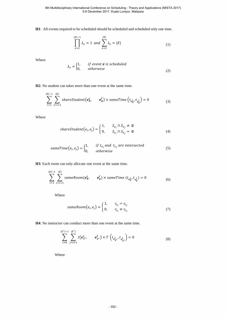
H1: All events required to be scheduled should be scheduled and scheduled only one time.

∏ 𝜆𝑒

|𝐸|−1

𝑒=1

= 1 𝑎𝑛𝑑 ∑ 𝜆𝑒

|𝐸|

𝑒=1

= |𝐸|

(1)

Where

𝜆𝑒 = 1, 𝑖𝑓 𝑒𝑣𝑒𝑛𝑡 𝒆 𝑖𝑠 𝑠𝑐ℎ𝑒𝑑𝑢𝑙𝑒𝑑 0, 𝑜𝑡ℎ𝑒𝑟𝑤𝑖𝑠𝑒

(2)

H2: No student can takes more than one event at the same time.

∑ ∑ 𝑠ℎ𝑎𝑟𝑒𝑆𝑡𝑢𝑑𝑒𝑛𝑡(𝒆𝑬𝒊 , 𝒆𝑬

𝒋) × 𝑠𝑎𝑚𝑒𝑇𝑖𝑚𝑒 (𝑡𝒆𝑬

𝒊 , 𝑡𝒆𝑬

𝒋 )

|𝐸|

𝑗=𝑖+1

|𝐸|−1

𝑖=1

= 0

(3)

Where

𝑠ℎ𝑎𝑟𝑒𝑆𝑡𝑢𝑑𝑒𝑛𝑡(𝑒𝑖 , 𝑒𝑗) = 1, 𝑆𝑒𝑖

∩ 𝑆𝑒𝑗≠ ∅

0, 𝑆𝑒𝑖∩ 𝑆𝑒𝑗

= ∅

(4)

𝑠𝑎𝑚𝑒𝑇𝑖𝑚𝑒(𝑒𝑖 , 𝑒𝑗) =

1, 𝑖𝑓 𝑡𝑒𝑖 𝑎𝑛𝑑 𝑡𝑒𝑗

𝑎𝑟𝑒 𝑖𝑛𝑡𝑒r𝑠𝑒𝑐𝑡𝑒𝑑

0, 𝑜𝑡ℎ𝑒𝑟𝑤𝑖𝑠𝑒 (5)

H3: Each room can only allocate one event at the same time.

∑ ∑ 𝑠𝑎𝑚𝑒𝑅𝑜𝑜𝑚(𝒆𝑬𝒊 , 𝒆𝑬

𝒋) × 𝑠𝑎𝑚𝑒𝑇𝑖𝑚𝑒 (𝑡𝒆𝑬

𝒊 , 𝑡𝒆𝑬

𝒋 )

|𝐸|

𝑗=𝑖+1

|𝐸|−1

𝑖=1

= 0

(6)

Where

𝑠𝑎𝑚𝑒𝑅𝑜𝑜𝑚(𝑒𝑖 , 𝑒𝑗) = 1, 𝑟𝑒𝑖

= 𝑟𝑒𝑗

0, 𝑟𝑒𝑖≠ 𝑟𝑒𝑗

(7)

H4: No instructor can conduct more than one event at the same time.

∑ ∑ 𝐼(𝒆𝐸∗𝒊 , 𝒆𝐸∗

𝒋) × 𝑇 (𝑡𝒆𝐸∗

𝒊 , 𝑡𝒆

𝐸∗𝒋 ) = 0

|𝐸∗|

𝑗=𝑖+1

|𝐸∗|−1

𝑖=0

(8)

Where


- 352 -

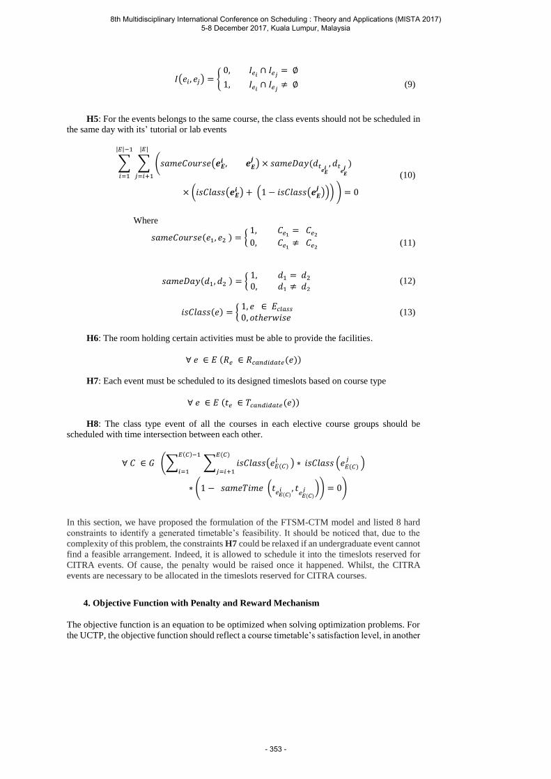
𝐼(𝑒𝑖, 𝑒𝑗) = 0, 𝐼𝑒𝑖

∩ 𝐼𝑒𝑗= ∅

1, 𝐼𝑒𝑖∩ 𝐼𝑒𝑗

≠ ∅

(9)

H5: For the events belongs to the same course, the class events should not be scheduled in

the same day with its’ tutorial or lab events

∑ ∑ (𝑠𝑎𝑚𝑒𝐶𝑜𝑢𝑟𝑠𝑒(𝒆𝑬𝒊 , 𝒆𝑬

𝒋) × 𝑠𝑎𝑚𝑒𝐷𝑎𝑦(𝑑𝑡

𝒆𝑬𝒊

, 𝑑𝑡𝒆𝑬

𝒋)

|𝐸|

𝑗=𝑖+1

|𝐸|−1

𝑖=1

× (𝑖𝑠𝐶𝑙𝑎𝑠𝑠(𝒆𝑬𝒊 ) + (1 − 𝑖𝑠𝐶𝑙𝑎𝑠𝑠(𝒆𝑬

𝒋))) ) = 0

(10)

Where

𝑠𝑎𝑚𝑒𝐶𝑜𝑢𝑟𝑠𝑒(𝑒1, 𝑒2 ) = 1, 𝐶𝑒1

= 𝐶𝑒2

0, 𝐶𝑒1≠ 𝐶𝑒2

(11)

𝑠𝑎𝑚𝑒𝐷𝑎𝑦(𝑑1, 𝑑2 ) =

1, 𝑑1 = 𝑑2 0, 𝑑1 ≠ 𝑑2

(12)

𝑖𝑠𝐶𝑙𝑎𝑠𝑠(𝑒) =

1, 𝑒 ∈ 𝐸𝑐𝑙𝑎𝑠𝑠

0, 𝑜𝑡ℎ𝑒𝑟𝑤𝑖𝑠𝑒 (13)

H6: The room holding certain activities must be able to provide the facilities.

∀ 𝑒 ∈ 𝐸 (𝑅𝑒 ∈ 𝑅𝑐𝑎𝑛𝑑𝑖𝑑𝑎𝑡𝑒(𝑒))

H7: Each event must be scheduled to its designed timeslots based on course type

∀ 𝑒 ∈ 𝐸 (𝑡𝑒 ∈ 𝑇𝑐𝑎𝑛𝑑𝑖𝑑𝑎𝑡𝑒(𝑒))

H8: The class type event of all the courses in each elective course groups should be

scheduled with time intersection between each other.

∀ 𝐶 ∈ 𝐺 (∑ ∑ 𝑖𝑠𝐶𝑙𝑎𝑠𝑠(𝑒𝐸(𝐶) 𝑖 ) ∗

𝐸(𝐶)

𝑗=𝑖+1𝑖𝑠𝐶𝑙𝑎𝑠𝑠 (𝑒𝐸(𝐶)

𝑗)

𝐸(𝐶)−1

𝑖=1

∗ (1 − 𝑠𝑎𝑚𝑒𝑇𝑖𝑚𝑒 (𝑡𝑒𝐸(𝐶)

𝑖 , 𝑡𝑒𝐸(𝐶)

𝑗 )) = 0)

In this section, we have proposed the formulation of the FTSM-CTM model and listed 8 hard

constraints to identify a generated timetable’s feasibility. It should be noticed that, due to the

complexity of this problem, the constraints H7 could be relaxed if an undergraduate event cannot

find a feasible arrangement. Indeed, it is allowed to schedule it into the timeslots reserved for

CITRA events. Of cause, the penalty would be raised once it happened. Whilst, the CITRA

events are necessary to be allocated in the timeslots reserved for CITRA courses.

4. Objective Function with Penalty and Reward Mechanism

The objective function is an equation to be optimized when solving optimization problems. For

the UCTP, the objective function should reflect a course timetable’s satisfaction level, in another


- 353 -

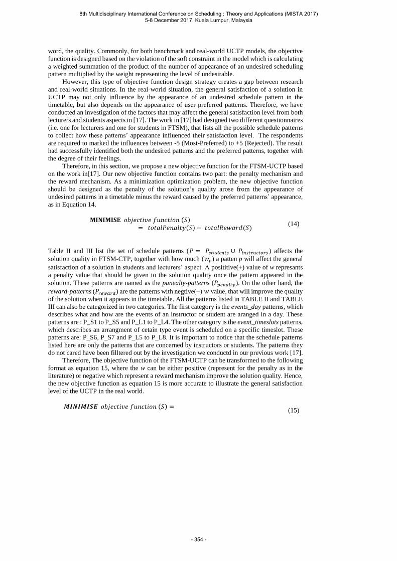
word, the quality. Commonly, for both benchmark and real-world UCTP models, the objective

function is designed based on the violation of the soft constraint in the model which is calculating

a weighted summation of the product of the number of appearance of an undesired scheduling

pattern multiplied by the weight representing the level of undesirable.

However, this type of objective function design strategy creates a gap between research

and real-world situations. In the real-world situation, the general satisfaction of a solution in

UCTP may not only influence by the appearance of an undesired schedule pattern in the

timetable, but also depends on the appearance of user preferred patterns. Therefore, we have

conducted an investigation of the factors that may affect the general satisfaction level from both

lecturers and students aspects in [17]. The work in [17] had designed two different questionnaires

(i.e. one for lecturers and one for students in FTSM), that lists all the possible schedule patterns

to collect how these patterns’ appearance influenced their satisfaction level. The respondents

are required to marked the influences between -5 (Most-Preferred) to +5 (Rejected). The result

had successfully identified both the undesired patterns and the preferred patterns, together with

the degree of their feelings.

Therefore, in this section, we propose a new objective function for the FTSM-UCTP based

on the work in[17]. Our new objective function contains two part: the penalty mechanism and

the reward mechanism. As a minimization optimization problem, the new objective function

should be designed as the penalty of the solution’s quality arose from the appearance of

undesired patterns in a timetable minus the reward caused by the preferred patterns’ appearance,

as in Equation 14.

𝐌𝐈𝐍𝐈𝐌𝐈𝐒𝐄 𝑜𝑏𝑗𝑒𝑐𝑡𝑖𝑣𝑒 𝑓𝑢𝑛𝑐𝑡𝑖𝑜𝑛 (𝑆)= 𝑡𝑜𝑡𝑎𝑙𝑃𝑒𝑛𝑎𝑙𝑡𝑦(𝑆) − 𝑡𝑜𝑡𝑎𝑙𝑅𝑒𝑤𝑎𝑟𝑑(𝑆)

(14)

Table II and III list the set of schedule patterns (𝑃 = 𝑃𝑠𝑡𝑢𝑑𝑒𝑛𝑡𝑠 ∪ 𝑃𝑖𝑛𝑠𝑡𝑟𝑢𝑐𝑡𝑜𝑟𝑠 ) affects the

solution quality in FTSM-CTP, together with how much (𝑤𝑝) a patten p will affect the general

satisfaction of a solution in students and lecturers’ aspect. A posititive(+) value of w represants

a penalty value that should be given to the solution quality once the pattern appeared in the

solution. These patterns are named as the panealty-patterns (𝑃𝑝𝑒𝑛𝑎𝑙𝑡𝑦). On the other hand, the

reward-patterns (𝑃𝑟𝑒𝑤𝑎𝑟𝑑) are the patterns with negtive(−) 𝑤 value, that will improve the quality

of the solution when it appears in the timetable. All the patterns listed in TABLE II and TABLE

III can also be categorized in two categories. The first category is the events_day patterns, which

describes what and how are the events of an instructor or student are aranged in a day. These

patterns are : P_S1 to P_S5 and P_L1 to P_L4. The other category is the event_timeslots patterns,

which describes an arrangment of cetain type event is scheduled on a specific timeslot. These

patterns are: P_S6, P_S7 and P_L5 to P_L8. It is important to notice that the schedule patterns

listed here are only the patterns that are concerned by instructors or students. The patterns they

do not cared have been filltered out by the investigation we conductd in our previous work [17].

Therefore, The objective function of the FTSM-UCTP can be transformed to the following

format as equation 15, where the w can be either positive (represent for the penalty as in the

literature) or negative which represent a reward mechanism improve the solution quality. Hence,

the new objective function as equation 15 is more accurate to illustrate the general satisfaction

level of the UCTP in the real world.

𝑴𝑰𝑵𝑰𝑴𝑰𝑺𝑬 𝑜𝑏𝑗𝑒𝑐𝑡𝑖𝑣𝑒 𝑓𝑢𝑛𝑐𝑡𝑖𝑜𝑛 (𝑆) =

(15)


- 354 -

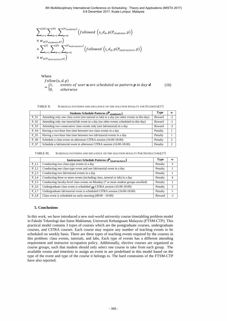
∑ ∑ ∑ (𝑓𝑜𝑙𝑙𝑜𝑤𝑒𝑑 (𝑠𝑠,𝑑𝑑 , 𝑝(𝑃𝑠𝑡𝑢𝑑𝑒𝑛𝑡𝑠 , 𝑝)) |𝑃𝑠𝑡𝑢𝑑𝑒𝑛𝑡𝑠|

𝑝=0

|𝐷|

𝑑=1

|𝑆𝐺|

𝑠=1

× 𝑤 𝑝(𝑃𝑠𝑡𝑢𝑑𝑒𝑛𝑡𝑠,𝑝))

+ ∑ ∑ ∑ (𝑓𝑜𝑙𝑙𝑜𝑤𝑒𝑑 (𝑖𝑖,𝑑𝑑, 𝑝(𝑃𝑖𝑛𝑠𝑡𝑟𝑢𝑐𝑡𝑜𝑟𝑠 , 𝑝)) |𝑃𝑖𝑛𝑠𝑡𝑟𝑢𝑐𝑡𝑜𝑟𝑠|

𝑝=0

|𝐷|

𝑑=1

|𝐼|

𝑖=1

× 𝑤 𝑝(𝑃𝑖𝑛𝑠𝑡𝑟𝑢𝑐𝑡𝑜𝑟𝑠,𝑝))

Where

𝑓𝑜𝑙𝑙𝑜𝑤(𝑢, 𝑑, 𝑝)

= 1, 𝑒𝑣𝑒𝑛𝑡𝑠 𝑜𝑓 𝑢𝑠𝑒𝑟 𝒖 𝑎𝑟𝑒 𝑠𝑐ℎ𝑒𝑑𝑢𝑙𝑒𝑑 𝑎𝑠 𝑝𝑎𝑡𝑡𝑒𝑟𝑛 𝒑 𝑖𝑛 𝑑𝑎𝑦 𝒅0, 𝑜𝑡ℎ𝑒𝑟𝑤𝑖𝑠𝑒

(16)

TABLE II. SCHEDULE PATTERNS AND INFLUENCE ON THE SOLUTION PENALTY FOR STUDENTS[17]

Students Schedule Patterns (𝑷𝒔𝒕𝒖𝒅𝒆𝒏𝒕𝒔) Type w

P_S1 Attending only one class event (not tutorial or lab) in a day (no other events in this day) Reward -2

P_S2 Attending only one tutorial/lab event in a day (no other events scheduled in this day) Reward -1

P_S3 Attending two consecutive class events only (not lab/tutorial) in a day Reward -3

P_S4 Having a two-hour free time between two class events in a day Penalty 1

P_S5 Having a two-hour free time between two lab/tutorial events in a day Penalty 1

P_S6 Schedule a class event on afternoon CITRA session (16:00-18:00) Penalty 2

P_S7 Schedule a lab/tutorial event in afternoon CITRA session (16:00-18:00) Penalty 2

TABLE III. SCHEDULE PATTERNS AND INFLUENCE ON THE SOLUTION PENALTY FOR INSTRUCTORS[17]

Instructors Schedule Patterns (𝑷𝒊𝒏𝒔𝒕𝒓𝒖𝒄𝒕𝒐𝒓𝒔) Type w

P_L1 Conducting two class-type events in a day Penalty 3

P_L2 Conducting one class-type event and one lab/tutorial event in a day Penalty 1

P_L3 Conducting two lab/tutorial events in a day Penalty 1

P_L4 Conducting three or more events (including class, tutorial or lab) in a day Penalty 4

P_L5 Conducting faculty-level class events on Monday (7 or more student groups enrolled) Penalty 1

P_L6 Undergraduate class event is scheduled on CITRA session (16:00-18:00) Penalty 3

P_L7 Undergraduate lab/tutorial event is scheduled CITRA session (16:00-18:00) Penalty 1

P_L8 Class event is scheduled on early morning (08:00 - 10:00) Reward -1

5. Conclusions

In this work, we have introduced a new real-world university course timetabling problem model

in Fakulti Teknologi dan Sains Maklumat, Universiti Kebangsaan Malaysia (FTSM-CTP). This

practical model contains 3 types of courses which are the postgraduate courses, undergraduate

courses, and CITRA courses. Each course may require any number of teaching events to be

scheduled on weekly basis. There are three types of teaching events required by the courses in

this problem: class events, tutorials, and labs. Each type of events has a different attending

requirement and instructor occupation policy. Additionally, elective courses are organized as

course groups, such that student should only select one course to take from each group. The

available rooms and timeslots to assign an event in are predefined in this model based on the

type of the event and type of the course it belongs to. The hard constraints of the FTSM-CTP

have also reported.


- 355 -

We have identified the limitation of the standard objective function that was designed based

on the appearance of user undesired schedule patterns. Therefore, in this work, we introduced a

new objective function that involved both penalty and reward mechanism to evaluate the quality

of a course timetable for the FTSM-UCTP. The new objective function bridged the gap between

research and real-world situations by evaluating the quality of the course timetable based on

users’ preferred and unpreferred schedule patterns in the evaluation process. The ongoing

research will focus on solving the FTSM-CTP by the graph-based constructive approach.

6 Acknowledgement

The authors wish to thank the Universiti Kebangsaan Malaysia for supporting this work

under grant Dana Impak Perdana (DIP-2014-039) and GP-K008009; and the Deputy Dean

(Undergraduate) and all program heads of Fakulti Teknologi dan Sains Maklumat.

References

[1] H. Alada, “A tabu search algorithm to solve a course timetabling problem,” J. Math.

Stat., vol. 36, no. 1, pp. 53–64, 2007.

[2] E. Burke, Y. Bykov, J. Newall, and S. Petrovic, “A time-predefined approach to course

timetabling,” Yugosl. J. Oper. Res., vol. 13, no. 2, pp. 139–151, 2003.

[3] R. A. Aziz, M. Ayob, and Z. Othman, “A Case Study of Practical Course Timetabling

Problems,” J. Comput. Sci., vol. 11, no. 10, pp. 152–155, 2011.

[4] S. Even, A. Itai, and A. Shamir, “On the complexity of time table and multi-

commodity flow problems,” 16th Annu. Symp. Found. Comput. Sci. (sfcs 1975), pp.

184–193, 1975.

[5] M. R. Malim, A. T. Khader, and Adli Mustafa, “University Course Timetabling: A

General Model,” The 2nd International Conference on Research and Education in

Mathematics (ICREM 2). pp. 834–853, 2005.

[6] W. Erben and J. Keppler, “A Genetic Algorithm Solving a Weekly Course-

Timetabling Problem,” 1995.

[7] S. Abdennadher and M. Marte, “University course timetabling using constraint

handling rules,” Appl. Artif. Intell., vol. 14, no. 4, pp. 311–325, 2000.

[8] A. Hertz, “Tabu search for large scale timetabling problems,” Eur. J. Oper. Res., vol.

54, no. 1, pp. 39–47, 1991.

[9] M. W. C. I and G. Laporte, “Recent Developments in Practical Course Timetabling,”

Pract. Theory Autom. Timetabling II, vol. 1408, pp. 3–19, 1998.

[10] Ben Paechter, “International Timetabling Competition,” 2001. [Online]. Available:

http://sferics.idsia.ch/Files/ttcomp2002/. [Accessed: 08-Jul-2017].

[11] B. McCollum, “University Timetabling: Bridging the Gap Between Research and

Practice,” Patat, no. May 2005, pp. 15–35, 2006.

[12] R. Lewis, B. Paechter, and B. McCollum, “Post enrolment based course timetabling: A

description of the problem model used for track two of the second international

timetabling competition,” vol. 44, no. July, pp. 1–9, 2007.

[13] L. di Gaspero, A. Schaerf, and B. McCollum, “The Second International Timetabling

Competition (ITC-2007): Curriculum-based Course Timetabling (Track 3),” Electr.

Eng., no. Track 3, pp. 1–21, 2007.

[14] B. McCollum, “A perspective on bridging the gap between theory and practice in

university timetabling,” Pract. Theory Autom. Timetabling VI, vol. 3867, pp. 3–23,

2007.

[15] T. Muller and H. Rudov??, “Real-life curriculum-based timetabling with elective

courses and course sections,” Ann. Oper. Res., vol. 239, no. 1, pp. 153–170, 2016.


- 356 -

[16] M. W. Carter, “A Comprehensive Course Timetabling and Student Scheduling System

at the University of Waterloo,” 3rd Int. Conf. Pract. Theory Autom. Timetabling

(PATAT 2000), vol. 2079, pp. 64–84, 2001.

[17] X. F. Yang, M. Ayob, and M. Z. A. Nazri, “An Investigation of Timetable Satisfaction

Factors For A Practical University Course Timetabling Problem,” in 6th International

Conference on Electrical Engineering and Informatics, 2017, accepted to be

published.


- 357 -

Jens Rocholl University of Hagen E-mail: [email protected] Lars Mönch University of Hagen E-mail: [email protected]

MISTA 2017 Hybrid Heuristics for Multiple Orders per Job Scheduling Problems with Parallel Machines and a Common Due Date

Jens Rocholl • Lars Mönch

1 Introduction, Problem Setting and Analysis

We consider an earliness-tardiness (E/T) scheduling problem for parallel identical machines that is motivated by process conditions found in semiconductor wafer fabrication facilities (wafer fabs). Front opening unified pods (FOUPs) transfer wafers, thin discs made from silicon in modern 300-mm wafer fabs. Each wafer might contain up to 1000 integrated circuits (chips). There exists only a limited number of FOUPs in each wafer fab to avoid a congested automated material handling system (AMHS) [6]. Recently, a smaller number of wafers is required to fill the chips of a customer due to a decreased line width and an increased area per wafer. Consequently, there is often a need to group orders of different customers into one FOUP. Such scheduling problems that include an integrated grouping problem are called multiple orders per job (MOJ) problems (see [5] for a more detailed discussion). The researched scheduling problem can be described as follows. There are F,,j 1 jobs available that can be processed on m identical parallel machines. Each job is associated with a FOUP and has a capacity K given in number of wafers. The set of all orders is denoted by O . Each order Oo has a size os given in wafers. It belongs to an order family L,,of 1 . Only orders of the same family can be processed together in a single job j at the same time. All orders of the same family l have identical processing times lP . Since all orders in a job are processed at the same time, the processing time of job j depends only on the family of the orders that belong to this job, i.e., we have lj Pp~ when the orders of the job belong to family l . This situation is called lot processing environment. A nonrestrictive common due date d for all the orders is assumed, i.e., we have dp

Oo o where op is the processing time of

order Oo . We have lnN orders in total where ln is the number of orders that belong

to family l . All orders are available at 0t , i.e., we have 0or for all Oo . The completion time of order o is oC . Using the three-field notation from scheduling theory, the scheduling problem considered in this paper can be represented as

T/E|dd,leincompatib,lotmoj|Pom , (1)

where mP indicates m identical parallel machines, lotmoj refers to the lot processing environment, odd to the nonrestrictive due date, incompatible to the different order

families, and T/E to the E/T measure that is given by

Oo

oo dCCdT/E

where we set 0max ,xx for abbreviation. We know from [10] that even the single-


- 358 -

machine version of problem (1) is NP-hard. Therefore, we have to look for efficient heuristics. Recently, MOJ scheduling problems have attracted a lot of interest from researchers (cf. [5] for a survey and [8], [10], [11] for specific MOJ scheduling problems). However, it seems that MOJ scheduling problems with a common due date are only rarely discussed so far in the literature. There are a few papers that deal with scheduling problems with a common due date on single and parallel batch processing machines (cf. [4], [7], [9]). Here, a batch is a group of jobs that are processed together at the same time on the same machine. Although these problems are somehow similar to problem (1) according to the grouping decisions, the major difference is that in problem (1) only a maximum number of jobs is allowed, while such a constraint does not exist for the number of batches in batch scheduling problems. The most pertinent reference for this research is [10] where the scheduling problem

T/E|dd,leincompatib,lotmoj|o1 is considered and two genetic algorithms (GAs) are

proposed. However, problem (1) deals with parallel machines which complicate the problem to a large extent.

It is possible to derive structural properties for certain classes of optimal schedules of problem (1) by using arguments similar to those in [3] for the problem T/Ew|dd|

jj1

where jw is the weight of job j . Note that the number of orders in a job plays the role of the weights considered in [3]. We denote the set of jobs on machine k that are not tardy by kA whereas the corresponding set of tardy jobs on this machine is abbreviated by kB . The number

of orders included in job j is denoted by jO . The most important of these properties are the following ones: Property 1: There exists an optimal schedule for each instance of problem (1) where a job completes its processing at time d on each nonempty machine. Property 2: The jobs in the set kA are sequenced in non-decreasing order of the ratio

jj p~O , while the jobs of the set kB are sequenced in non-increasing order of this ratio in each optimal schedule for an instance of problem (1).

Note that the jobs in kA are sorted according to the weighted longest processing time (WLPT) rule, whereas the jobs in kB are sorted according to the weighted shortest processing time (WSPT) rule. This leads to a V-shaped schedule. If the jobs are assigned and sequenced, the job formation problem is a generalized assignment problem (GAP) that can be solved as a binary program using a commercial solver. We abbreviate this procedure by MOJAP.

2 Decomposition Heuristics

In the course of solving problem (1) we have to make job formation, assignment, and sequencing decisions. These steps can be carried out by a simple list scheduling approach and by hybrids that combine biased random-key GAs (BRKGAs) [2] with the simple heuristics. For the simple heuristic, we start from a list of orders that are sorted in non-decreasing order of the order size os . Starting from the top of this list, a job will be filled with orders until this is possible for capacity reasons in a first fit (FF) manner. If there is capacity left, the last inserted order is removed and starting from the bottom of this list, the first order that fits will be inserted in a best fit (BF) manner. After this, this procedure is repeated using a new job. We obtain a set of formed jobs by using this procedure that is motivated by bin packing-type procedures [8]. Similar to [1], the jobs are sorted first according to a given rule. The next job then is assigned to the sets kA and kB in an alternating manner on the first or a last position,

respectively. The machine with the smallest value dC jj : is chosen to place job j .

Here, the completion time of job j is denoted by j

C . Based on property 1, we know the completion time of the first job to be placed on an empty machine. We use the abbreviation


- 359 -

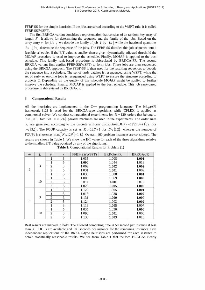
FFBF-SS for the simple heuristic. If the jobs are sorted according to the WSPT rule, it is called FFBF-SS(WSPT).

The first BRKGA variant considers a representation that consists of an random-key array of length F . It allows for determining the sequence and the family of the jobs. Based on the array entry for job j we decode the family of job j by Lv while the fractional quantities

LvLv determine the sequence of the jobs. The FFBF-SS decodes this job sequence into a feasible schedule. If the E/T value is smaller than a given dynamically adjusted threshold the MOJAP procedure is used to improve the schedule. Finally, MOJAP is applied to the best schedule. This family rank-based procedure is abbreviated by BRKGA-FR. The second BRKGA variant first applies FFBF-SS(WSPT) to form jobs. These jobs are then sequenced using the BRKGA approach. The FFBF-SS is then used for the resulting sequences to decode the sequence into a schedule. The set of tardy batches is resequenced using WSPT, while the set of early or on-time jobs is resequenced using WLPT to ensure the structure according to property 2. Depending on the quality of the schedule MOJAP might be applied to further improve the schedule. Finally, MOJAP is applied to the best schedule. This job rank-based procedure is abbreviated by BRKGA-JR.

3 Computational Results

All the heuristics are implemented in the C++ programming language. The brkgaAPI framework [12] is used for the BRKGA-type algorithms while CPLEX is applied as commercial solver. We conduct computational experiments for 120N orders that belong to

103,L families. 62,m parallel machines are used in the experiments. The order sizes

os are generated according to the discrete uniform distribution 21321 v,vDU for

53,v . The FOUP capacity is set as 112: K for 21, , whereas the number of FOUPs is chosen as L,Nv 112max . Overall, 160 problem instances are considered. The results are shown in Table 1. We show the E/T value for each of the three algorithms relative to the smallest E/T value obtained by any of the algorithms.

Table 1: Computational Results for Problem (1)

m L v FFBF-SS(WSPT) BRKGA-FR BRKGA-JR 1 3 1.035 1.008 1.0011 5 1.000 1.044 1.0182 3 1.062 1.002 1.0023

2 5 1.031 1.001 1.0091 3 1.036 1.008 1.0011 5 1.009 1.069 1.0002 3 1.051 1.000 1.001

2

10 2 5 1.029 1.005 1.005

1 3 1.120 1.005 1.0011 5 1.015 1.038 1.0022 3 1.131 1.000 1.0003

2 5 1.124 1.003 1.0021 3 1.119 1.005 1.0071 5 1.035 1.050 1.0002 3 1.098 1.001 1.006

6

10 2 5 1.130 1.003 1.015

Best results are marked in bold. The allowed computing time is 50 second per instance if less than 30 FOUPs are available and 180 seconds per instance for the remaining instances. Five independent replications of the BRKGA-type heuristics are performed for each instance to obtain statistically reasonable results. We see from Table 1 that the two BRKGAs clearly


- 360 -

outperform FFBF-SS(WSPT). In the case of six parallel machines and three families, the BRKGA-JR slightly outperforms the BRKGA-FR. We conclude that hybrids of metaheuristics and simple heuristics are able to determine high-quality solutions in a fairly short amount of computing time.

References

1. Emmons, H. Scheduling to a common due date on parallel uniform processors. Naval Research Logistics, 34(6), 803-810 (1987)

2. Gonçalves, J. F., Resende, M. G. C. Biased random-key genetic algorithms for combinatorial optimization. Journal of Heuristics, 17(5), 487–525 (2011)

3. Hall, N. G., Posner, M. E. Earliness-tardiness scheduling problems, I: weighted deviation of completion times about a common due date. Operations Research, 39(5), 836-846 (1991)

4. Li, X., Chen, H., Xu, R., Li, X. Earliness–tardiness minimization on scheduling a batch processing machine with non-identical job sizes. Computers & Industrial Engineering, 87, 590-599 (2015)

5. Mönch, L., Fowler, J. W., Dauzère-Pérès, S., Mason, S. J., Rose, O. Scheduling semiconductor manufacturing operations: problems, solution techniques, and future challenges. Journal of Scheduling, 14(6), 583-595 (2011)

6. Mönch, L., Fowler, J. W., Mason, S. J. Production planning and control for wafer fabrication facilities: Modeling, analysis, and systems. Springer, New York (2013)

7. Mönch, L., Unbehaun, R. Decomposition heuristics for minimizing earliness-tardiness on parallel burn-in ovens with a common due date. Computers & Operations Research, 34(11), 3380-3396 (2007)

8. Qu, P., Mason, S. J. Metaheuristic scheduling of 300 mm jobs containing multiple orders. IEEE Transactions on Semiconductor Manufacturing, 18(4), 633-643 (2005)

9. Parsa, N. R., Karimi, B., Moattar Husseini, S. M. Exact and heuristic algorithms for the just-in-time scheduling problem in a batch processing system. Computers & Operations Research, 80, 173-183 (2017)

10. Rocholl, J., Mönch, L. Hybrid Algorithms for the earliness-tardiness single-machine multiple orders per job scheduling problem with a common due date. Submitted for publication (2017)

11. Sobeyko, O., Mönch, L. Grouping genetic algorithms for solving single machine multiple orders per job scheduling problems. Annals of Operations Research, 235(1), 709-739 (2016)

12. Toso, R. F., Resende, M. G. C. A C++ application programming interface for biased random-key genetic algorithms. http://mauricio.resende.info/doc/brkgaAPI.pdf. Last accessed 2017-26-07.


- 361 -

MISTA 2017 The "Orchestrator" approach to multimodal continental trip planning.

Lukas Bach • Dag Kjenstad • Carlo Mannino

Abstract The orchestrator is a new, decentralized approach to trip planning in large multimodal networks. The solution technique, which resembles the overlay graphs approach [1], is based on an implicit and possibly recursive decomposition of the overall multi-modal network into a collection of multi- and mono-modal networks equipped with a specialized trip planner. Each subnetwork and associated solution algorithm can be created and maintained by different and independent organizations/developers and can be hosted by different platforms/servers. The orchestrator receives trip queries and, exploiting some pre-computed information, decomposes each trip query into a suitable sequence of queries to specific subnetworks in the available collection. The new approach, developed within the EU Horizon 2020 project BONVOYAGE is able to handle large collections of subnetworks significantly reducing response time.

1 Introduction

The orchestrator is a decomposition approach to solve the routing problem on a multimodal network N. It orchestrates a set of solution algorithms (solvers) acting on different multi- or single-mode subnetworks of the original network N. Depending on the specific query the orchestrator will pick up a suitable subset of solvers, run them, collect the partial solutions and compose them into a solution to the original query. For instance, if the request regards a trip from city A to city B, the orchestrator may invoke a solver in charge of city A, a solver in charge of city B, and a solver capable to find extra-urban path from the boundary of city A to the boundary of city B. Another example of such orchestrating approach regards the matching of two different trips in freight transportation scenarios, or the identification multimodal trips through successive and coordinated invocations to single-mode solvers.

The major features of the orchestrator approach are:

1. The decomposition allows for significant speed-ups in answering queries; 2. The different solvers operating on the subnetworks and made available may be designed and

implemented by different organizations;


- 362 -

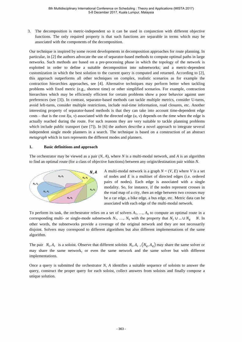
3. The decomposition is metric-independent so it can be used in conjunction with different objective functions. The only required property is that such functions are separable in terms which may be associated with the components of the decomposition.

Our technique is inspired by some recent developments in decomposition approaches for route planning. In particular, in [2] the authors advocate the use of separator-based methods to compute optimal paths in large networks. Such methods are based on a pre-processing phase in which the topology of the network is exploited in order to define a suitable decomposition into subnetworks; and a metric-dependent customization in which the best solution to the current query is computed and returned. According to [2], this approach outperforms all other techniques on complex, realistic scenarios as for example the contraction hierarchies approaches, see [4]. Alternative techniques may perform better when tackling problems with fixed metric (e.g., shortest time) or other simplified scenarios. For example, contraction hierarchies which may be efficiently efficient for certain problems show a poor behavior against user preferences (see [3]). In contrast, separator-based methods can tackle multiple metrics, consider U-turns, avoid left-turns, consider multiple restrictions, include real-time information, road closures, etc. Another interesting property of separator-based methods is that they can take into account time-dependent edge costs – that is the cost l(u, v) associated with the directed edge (u, v) depends on the time when the edge is actually reached during the route. For such reasons they are very suitable to tackle planning problems which include public transport (see [7]). In [6] the authors describe a novel approach to integrate several independent single mode planners in a search. The technique is based on a construction of an abstract metagraph which in turn represents the different modes and planners.

1. Basic definitions and approach

The orchestrator may be viewed as a pair (N, A), where N is a multi-modal network, and A is an algorithm to find an optimal route (for a class of objective functions) between any origin/destination pair within N.

A multi-modal network is a graph N = (V, E) where V is a set of nodes and E is a multiset of directed edges (i.e. ordered pairs of nodes). Each edge is associated with a single modality. So, for instance, if the nodes represent crosses in the road map of a city, then an edge between two crosses may be a car edge, a bike edge, a bus edge, etc. Metric data can be associated with each edge of the multi-modal network.

To perform its task, the orchestrator relies on a set of solvers A1, …, Aq to compute an optimal route in a corresponding multi- or single-mode subnetwork N1, …, Nq with the property that 𝑁𝑁1 ∪ …∪ 𝑁𝑁𝑞𝑞 = 𝑁𝑁. In other words, the subnetworks provide a coverage of the original network and they are not necessarily disjoint. Solvers may correspond to different algorithms but also different implementations of the same algorithm.

The pair (𝑁𝑁𝑖𝑖 ,𝐴𝐴𝑖𝑖) is a soloist. Observe that different soloists(𝑁𝑁𝑖𝑖 ,𝐴𝐴𝑖𝑖), 𝑁𝑁𝑞𝑞 ,𝐴𝐴𝑞𝑞 may share the same solver or may share the same network, or even the same network and the same solver but with different implementations.

Once a query is submitted the orchestrator N, A identifies a suitable sequence of soloists to answer the query, construct the proper query for each soloist, collect answers from soloists and finally compose a unique solution.


- 363 -

As mentioned, the orchestrator generalizes the ideas in the overlay graph decomposition approach to routing. The crucial differences are that

1. The reference graph N = (V, E) is a multi-modal network and may be partly unknown. 2. The elements in the decomposition are not simple cells identified by a set of nodes, but they are

(potentially multi-modal) subnetworks of N along with a solution algorithm, namely soloists (𝑁𝑁1,𝐴𝐴1), . . . , 𝑁𝑁𝑞𝑞 ,𝐴𝐴𝑞𝑞.

3. The concept of boundary nodes is replaced by that of connection nodes. Connection nodes represent entry and exit points of the subnetworks associated with soloist. They may and may not coincide with (a subset of) the boundary nodes of the subnetwork (defined as for overlay graphs). The may or may not be geographically localized. Observe that connection nodes may actually correspond to extended areas within the associated subnetworks. In general, connections nodes must be chosen carefully at the registration of a new soloist into the BONVOYAGE platform. Again, we denote by 𝑆𝑆𝑖𝑖 the set of connection nodes in subnetwork 𝑁𝑁𝑖𝑖.

4. The overlay graph is replaced by the orchestrator graph H = (S, F). The nodes of the graph are the connection nodes. Each set 𝑆𝑆𝑖𝑖 induces a clique in H, i.e. for every ordered pair of distinct nodes 𝑢𝑢, 𝑣𝑣 ∈ 𝑆𝑆𝑖𝑖 there is an edge (𝑢𝑢, 𝑣𝑣) ∈ 𝐹𝐹, called connection edge. With every connection edge (𝑢𝑢,𝑣𝑣) we also associate a distance 𝑙𝑙𝐻𝐻(𝑢𝑢, 𝑣𝑣) representing a lower bound on the minimum distance from u to v. in the subnetwork. Distances are evaluated according to one or more pre-defined metrics.

5. If nodes 𝑢𝑢,𝑣𝑣 ∈ 𝑆𝑆 belong to different subnetworks, there is an edge (u,v) in H only if it is possible to "transfer" from u to v. The length 𝑙𝑙𝐻𝐻(𝑢𝑢, 𝑣𝑣) is the distance between the connection nodes in terms of transfer time, and may also be 0 if the two nodes correspond to the same geographical location.

6. When a request for a route from A to B is received, the orchestrator looks for one or more shortest routes in

the orchestrator graph. Once the route(s) is (are) identified, the actual value is computed with the current lengths. Observe that since pre-computed distances are not necessarily exact – in general they are lower bounds – and in addition they are computed before they are actually used, the resulting solutions are not necessarily optimal. In the figure, we present a possible response of an orchestrator with several multimodal soloists, when asked to return a multimodal trip (car, train, airplane) from a location in Grenoble to a location in Bilbao.

N1

N6

N2

N4

N3

N5


- 364 -

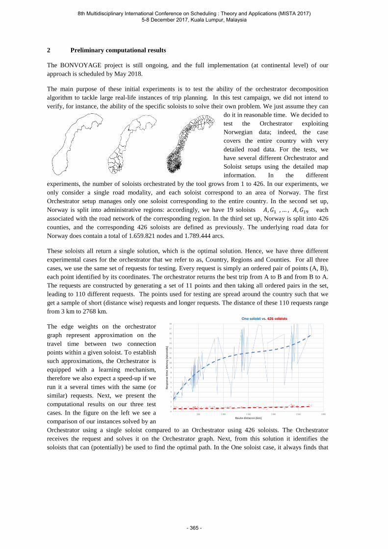
2 Preliminary computational results

The BONVOYAGE project is still ongoing, and the full implementation (at continental level) of our approach is scheduled by May 2018.

The main purpose of these initial experiments is to test the ability of the orchestrator decomposition algorithm to tackle large real-life instances of trip planning. In this test campaign, we did not intend to verify, for instance, the ability of the specific soloists to solve their own problem. We just assume they can

do it in reasonable time. We decided to test the Orchestrator exploiting Norwegian data; indeed, the case covers the entire country with very detailed road data. For the tests, we have several different Orchestrator and Soloist setups using the detailed map information. In the different

experiments, the number of soloists orchestrated by the tool grows from 1 to 426. In our experiments, we only consider a single road modality, and each soloist correspond to an area of Norway. The first Orchestrator setup manages only one soloist corresponding to the entire country. In the second set up, Norway is split into administrative regions: accordingly, we have 19 soloists (𝐴𝐴,𝐺𝐺1), … , (𝐴𝐴,𝐺𝐺19) each associated with the road network of the corresponding region. In the third set up, Norway is split into 426 counties, and the corresponding 426 soloists are defined as previously. The underlying road data for Norway does contain a total of 1.659.821 nodes and 1.789.444 arcs.

These soloists all return a single solution, which is the optimal solution. Hence, we have three different experimental cases for the orchestrator that we refer to as, Country, Regions and Counties. For all three cases, we use the same set of requests for testing. Every request is simply an ordered pair of points (A, B), each point identified by its coordinates. The orchestrator returns the best trip from A to B and from B to A. The requests are constructed by generating a set of 11 points and then taking all ordered pairs in the set, leading to 110 different requests. The points used for testing are spread around the country such that we get a sample of short (distance wise) requests and longer requests. The distance of these 110 requests range from 3 km to 2768 km.

The edge weights on the orchestrator graph represent approximation on the travel time between two connection points within a given soloist. To establish such approximations, the Orchestrator is equipped with a learning mechanism, therefore we also expect a speed-up if we run it a several times with the same (or similar) requests. Next, we present the computational results on our three test cases. In the figure on the left we see a comparison of our instances solved by an Orchestrator using a single soloist compared to an Orchestrator using 426 soloists. The Orchestrator receives the request and solves it on the Orchestrator graph. Next, from this solution it identifies the soloists that can (potentially) be used to find the optimal path. In the One soloist case, it always finds that


- 365 -

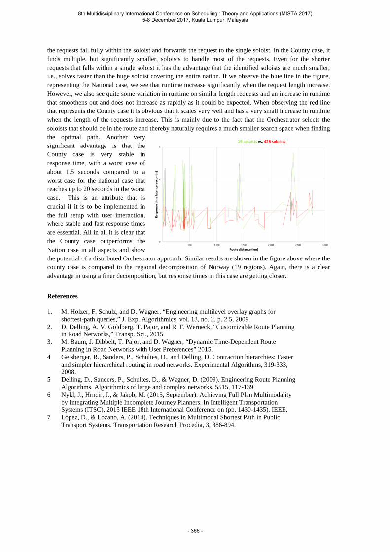
the requests fall fully within the soloist and forwards the request to the single soloist. In the County case, it finds multiple, but significantly smaller, soloists to handle most of the requests. Even for the shorter requests that falls within a single soloist it has the advantage that the identified soloists are much smaller, i.e., solves faster than the huge soloist covering the entire nation. If we observe the blue line in the figure, representing the National case, we see that runtime increase significantly when the request length increase. However, we also see quite some variation in runtime on similar length requests and an increase in runtime that smoothens out and does not increase as rapidly as it could be expected. When observing the red line that represents the County case it is obvious that it scales very well and has a very small increase in runtime when the length of the requests increase. This is mainly due to the fact that the Orchestrator selects the soloists that should be in the route and thereby naturally requires a much smaller search space when finding the optimal path. Another very significant advantage is that the County case is very stable in response time, with a worst case of about 1.5 seconds compared to a worst case for the national case that reaches up to 20 seconds in the worst case. This is an attribute that is crucial if it is to be implemented in the full setup with user interaction, where stable and fast response times are essential. All in all it is clear that the County case outperforms the Nation case in all aspects and show the potential of a distributed Orchestrator approach. Similar results are shown in the figure above where the county case is compared to the regional decomposition of Norway (19 regions). Again, there is a clear advantage in using a finer decomposition, but response times in this case are getting closer.

References

1. M. Holzer, F. Schulz, and D. Wagner, “Engineering multilevel overlay graphs for shortest-path queries,” J. Exp. Algorithmics, vol. 13, no. 2, p. 2.5, 2009.

2. D. Delling, A. V. Goldberg, T. Pajor, and R. F. Werneck, “Customizable Route Planning in Road Networks,” Transp. Sci., 2015.

3. M. Baum, J. Dibbelt, T. Pajor, and D. Wagner, “Dynamic Time-Dependent Route Planning in Road Networks with User Preferences” 2015.

4 Geisberger, R., Sanders, P., Schultes, D., and Delling, D. Contraction hierarchies: Faster and simpler hierarchical routing in road networks. Experimental Algorithms, 319-333, 2008.

5 Delling, D., Sanders, P., Schultes, D., & Wagner, D. (2009). Engineering Route Planning Algorithms. Algorithmics of large and complex networks, 5515, 117-139.

6 Nykl, J., Hrncir, J., & Jakob, M. (2015, September). Achieving Full Plan Multimodality by Integrating Multiple Incomplete Journey Planners. In Intelligent Transportation Systems (ITSC), 2015 IEEE 18th International Conference on (pp. 1430-1435). IEEE.

7 López, D., & Lozano, A. (2014). Techniques in Multimodal Shortest Path in Public Transport Systems. Transportation Research Procedia, 3, 886-894.


- 366 -

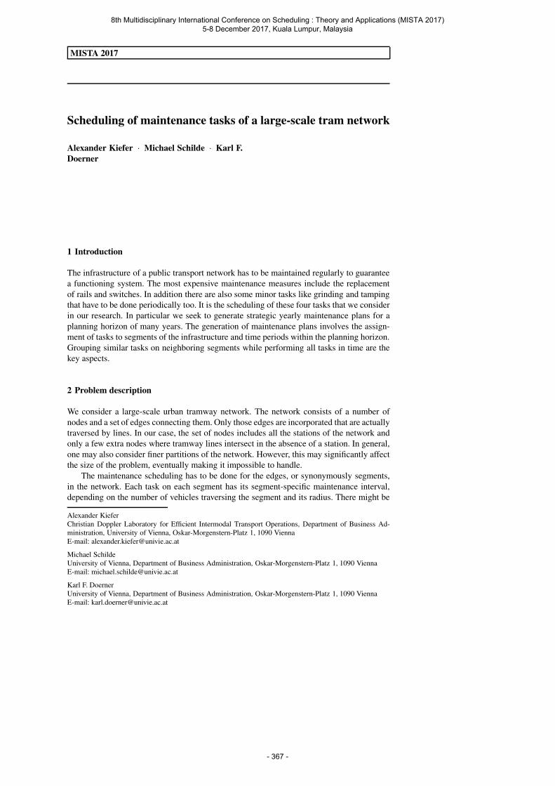
MISTA 2017

Scheduling of maintenance tasks of a large-scale tram network

Alexander Kiefer · Michael Schilde · Karl F.

Doerner

1 Introduction

The infrastructure of a public transport network has to be maintained regularly to guarantee

a functioning system. The most expensive maintenance measures include the replacement

of rails and switches. In addition there are also some minor tasks like grinding and tamping

that have to be done periodically too. It is the scheduling of these four tasks that we consider

in our research. In particular we seek to generate strategic yearly maintenance plans for a

planning horizon of many years. The generation of maintenance plans involves the assign-

ment of tasks to segments of the infrastructure and time periods within the planning horizon.

Grouping similar tasks on neighboring segments while performing all tasks in time are the

key aspects.

2 Problem description

We consider a large-scale urban tramway network. The network consists of a number of

nodes and a set of edges connecting them. Only those edges are incorporated that are actually

traversed by lines. In our case, the set of nodes includes all the stations of the network and

only a few extra nodes where tramway lines intersect in the absence of a station. In general,

one may also consider finer partitions of the network. However, this may significantly affect

the size of the problem, eventually making it impossible to handle.

The maintenance scheduling has to be done for the edges, or synonymously segments,

in the network. Each task on each segment has its segment-specific maintenance interval,

depending on the number of vehicles traversing the segment and its radius. There might be

Alexander Kiefer

Christian Doppler Laboratory for Efficient Intermodal Transport Operations, Department of Business Ad-

ministration, University of Vienna, Oskar-Morgenstern-Platz 1, 1090 Vienna


Michael Schilde

University of Vienna, Department of Business Administration, Oskar-Morgenstern-Platz 1, 1090 Vienna


Karl F. Doerner

University of Vienna, Department of Business Administration, Oskar-Morgenstern-Platz 1, 1090 Vienna



- 367 -

tasks that have to be scheduled multiple times on a segment. However, there could be rails

that do not have to be replaced within the planning horizon at all.

The infrastructure deteriorates constantly. Even before reaching the end of the mainte-

nance interval there is a point when vehicles cannot traverse an unmaintained segment with

the original speed. The reduced velocity causes the need of extra trains to keep the original

frequency of the lines. This in turn induces additional costs.

Scheduling the same or similar tasks on neighboring segments grants benefits as some

machines may have to be carried to the region only once and the site can be supervised more

efficiently. The tasks can be performed in different shifts, i.e. train-free night shifts and day

shifts. During the night there is a surcharge for the personnel. However, working during

the day requires to block the segment. As a consequence, trains have to turn early leading

to an effective blockade of lines on an even larger section. This requires the establishment

of costly replacement services with buses along the blocked sections. For now we simply

estimate the cost for extra buses on the basis of the originally provided capacity on the

segments. This aspect leaves room for more elaborate planning approaches in the future.

The public transport provider has a yearly budget for the maintenance tasks that must

not be exceeded. The objective is to minimize the overall costs, which includes maintenance

work, extra trains, costs for replacement services, and a penalty for the state of the network

at the end of the planning horizon.

3 Solution approach

We developed a MIP model for the problem that extends the one by Budai et al (2006). The

schedule is therein represented by four-indexed binary decision variables. These variables

indicate assignments for each segment, each task, each year, and each shift type. In total,

the model requires 7 groups of mostly binary decision variables and 11 types of constraints.

We implemented the model for solving it via CPLEX. Even for intermediate-sized instances

the model often cannot be solved to optimality within 1 day. However, in most cases good

lower bounds are provided.

Furthermore, we developed a large neighborhood search (LNS) algorithm to solve large

instances with a long planning horizon. LNS was invented by Shaw (1998) and is based on

repetitively destroying and subsequently repairing parts of the schedule. In every iteration a

destroy and a repair operator are randomly selected, as well as a number of assignments to

remove. The operators are then applied to the incumbent solution. Newly generated solutions

are accepted as new incumbent solution based on a simulated annealing acceptance scheme.

The algorithm incorporates one repair and three destroy operators. The greedy repair

operator schedules those tasks first that improve the schedule the most. The procedure con-

tinues as long as there are improving assignments that can be scheduled feasibly. The destroy

operators include the random destroy operator that removes assignments at random. Similar

to Shaw (1998) we make use of a related destroy operator that removes related assignments

with a higher probability. The relatedness measure between two assignments is larger if they

are scheduled in the same period and if they refer to the same or similar tasks on adjacent

segments. Finally, the operator interval destroy removes tasks randomly with a bias towards

those that are scheduled within a small interval to the previous and the next task of the same

type on the same segment relative to the maintenance interval.

The intermediate schedules generated by LNS are fragmented segment-wise and recom-

bined by a set covering (SC) model after the LNS phase. The SC model can be solved via

CPLEX in a few seconds and is able to improve the solution quality in almost every case.


- 368 -

4 Numerical tests

The nurmerical tests in this section are carried out on an Intel Xeon E5-2650v2 running

at 2.6 GHz. Intermediate-sized instances based on the regions of the Viennese tramway

network with a planning horizon of 20 years are solved by the MIP and the LNS approach.

The sizes of the instances are described in Table 1. The runtime of CPLEX is limited to 1

day, while LNS has a runtime of 15 minutes. The results corresponding to LNS are averages

over 10 runs. The optimality gaps of the solutions generated by CPLEX and the relative

differences of the solution qualities of LNS and CPLEX are shown in Table 2. CPLEX finds

good solutions with a small optimality gap for all instances, while LNS finds slightly worse

solutions. The limitations of CPLEX are revealed when extending the planning horizon

together with the size of the network. In particular, the complete network cannot be solved

for a planning horizon of 30 years within 1 day. Regarding the effectiveness of the SC phase

one has to mention that omitting this feature leads to a deterioration of 0.16% on average.

Instance Segments Lines

South 131 11

North 139 14

East 93 8

West 100 10

Table 1: Size of the instances

Instance CPLEX gap LNS vs CPLEX

South 0.17% 2.47%

North 0.10% 1.45%

East 0.00% 2.28%

West 0.07% 1.27%

Table 2: Comparison CPLEX vs LNS

The complete network is solved by the LNS approach with a runtime of 1 hour in a single

run. The share of the individual cost factors is presented in Table 3. Clearly, the costs for the

replacement services and extra trains play inferior roles. The effect of a 10% higher yearly

maintenance budget is shown in Table 4. Unsurprisingly, the total penalty can be reduced by

slightly relaxing the budget constraint. Increasing the budget leads to a significant decrease

of the costs for extra trams and also improves the state of the network at the end of the

planning horizon.

maintenance 63.74%

end of horizon 32.97%

extra trams 2.70%

replacement services 0.59%

Table 3: Shares of the cost factors

maintenance +0.77%

end of horizon -1.64%

extra trams -18.19%

replacement services -14.38%

total -0.63%

Table 4: Effect of an increased budget

Acknowledgements The financial support by the Austrian Federal Ministry of Science, Research and Econ-

omy and the National Foundation for Research, Technology and Development is gratefully acknowledged.

The computational results presented have been achieved using the Vienna Scientific Cluster (VSC).

References

Budai G, Huisman D, Dekker R (2006) Scheduling preventive railway maintenance activi-

ties. The Journal of the Operational Research Society 57(9):1035–1044

Shaw P (1998) Using constraint programming and local search methods to solve vehicle

routing problems. In: Maher M, Puget JF (eds) Principles and Practice of Constraint Pro-

gramming - CP98, Lecture Notes in Computer Science, vol 1520, Springer Berlin Heidel-

berg, pp 417–431


- 369 -

Helio Yochihiro Fuchigami

Federal University of Goias (UFG), Faculty of Sciences and Technology (FCT), Brazil


MISTA 2017

A parametric priority rule for just-in-time scheduling problem with

sequence-dependent setup times

Helio Yochihiro Fuchigami

1 Introduction

This work addresses the minimization of earliness and tardiness of jobs in a single

machine scheduling problem with sequence-dependent setup times and individual due dates.

This performance measure is directly related to the Just-in-time philosophy, which involves

broad concepts related to the elimination of waste and reductions in inventory items.

Just-in-time scheduling consists of obtaining solution that minimizes functions associated

with earliness and tardiness of the jobs. In practice, these performance measures are very

important because the increase of both leads to higher production costs. Anticipating the

completion of jobs increases inventory levels, material handling and product deterioration, and

delays in delivery may result in fines, cancellations of orders and even loss of customers. [7]

exemplifies some kind of manufacturing and service industries where quick and prompt

response to customers’ demand is the key to success: health care, nursing, operating theaters,

transportation, communication, delivery, apparel, glass, furniture and wood manufacturing.

In addition to its prevalence as a real-world situation, this problem arises as a relaxation

of scheduling problems with more complex manufacturing or with additional constraints as in

a flow shop and job shop. Yet, it is strongly NP-hard. It means that no efficient algorithm can

solve medium or large-sized instances [2]. Many different just-in-time problems can be seen in

[11] and [4].

The focused problem consists in scheduling a set of n jobs on a single machine with the

objective of minimizing their total earliness and tardiness and is represented in the known

three-field notation as 1|sij,dj|Ej+Tj. Each job has its processing time pj, due date dj and

sequence-dependent setup times sij, all deterministic, integer, known in advance and not

necessarily equal. The machine is ready at time zero.

Some previous work has addressed single machine problems similar to the one dealt in

this research, such as [5], [10], [13], [1] and [7]. Others applied variations of the ATCS rule

(apparent tardiness cost with setup) in different productive environments, such as [6], [9] and

[2] in parallel machines. However, no paper was found using this rule in the just-in-time

scheduling problem with sequence-dependent setup times. Generally, the ATCS rule was

applied in tardiness minimization, such as [14]. This is the motivation of the present research.

2 Proposed solution method


- 370 -

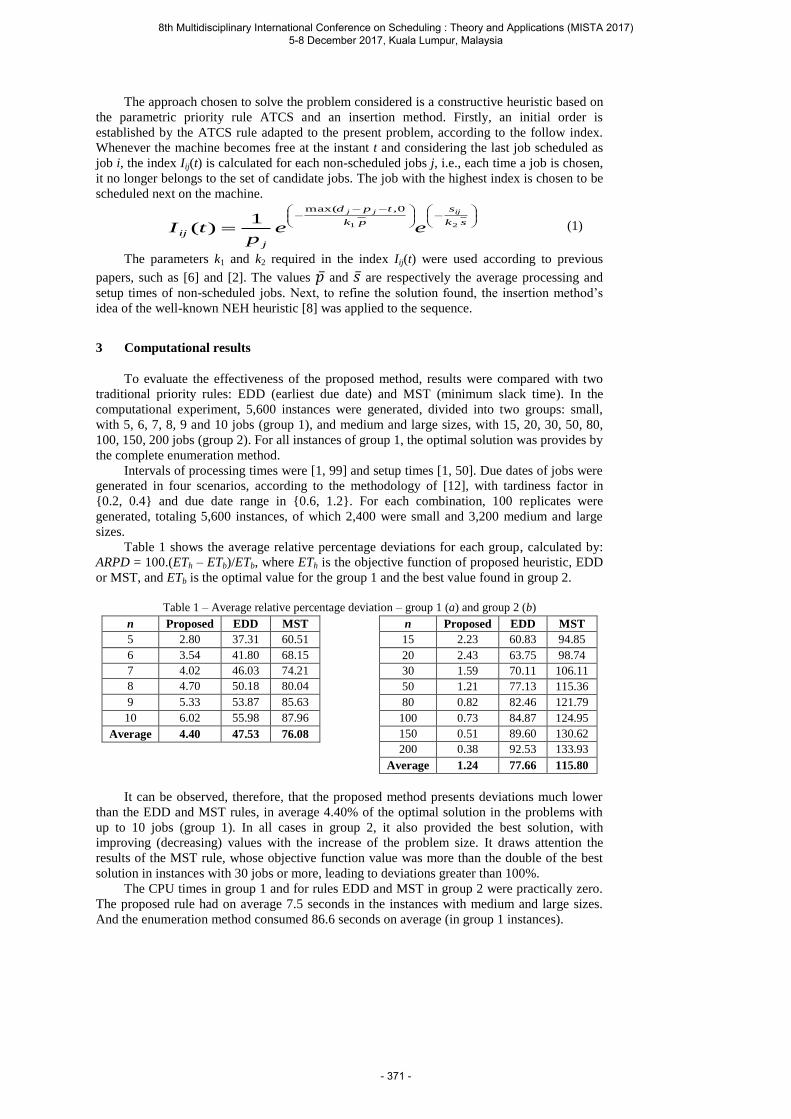
The approach chosen to solve the problem considered is a constructive heuristic based on

the parametric priority rule ATCS and an insertion method. Firstly, an initial order is

established by the ATCS rule adapted to the present problem, according to the follow index.

Whenever the machine becomes free at the instant t and considering the last job scheduled as

job i, the index Iij(t) is calculated for each non-scheduled jobs j, i.e., each time a job is chosen,

it no longer belongs to the set of candidate jobs. The job with the highest index is chosen to be

scheduled next on the machine.

sk

s

pk

tpd

j

ij

ijjj

eep

tI 21

0,max(

1)( (1)

The parameters k1 and k2 required in the index Iij(t) were used according to previous

papers, such as [6] and [2]. The values and are respectively the average processing and

setup times of non-scheduled jobs. Next, to refine the solution found, the insertion method’s

idea of the well-known NEH heuristic [8] was applied to the sequence.


To evaluate the effectiveness of the proposed method, results were compared with two

traditional priority rules: EDD (earliest due date) and MST (minimum slack time). In the

computational experiment, 5,600 instances were generated, divided into two groups: small,

with 5, 6, 7, 8, 9 and 10 jobs (group 1), and medium and large sizes, with 15, 20, 30, 50, 80,

100, 150, 200 jobs (group 2). For all instances of group 1, the optimal solution was provides by

the complete enumeration method.

Intervals of processing times were [1, 99] and setup times [1, 50]. Due dates of jobs were

generated in four scenarios, according to the methodology of [12], with tardiness factor in

0.2, 0.4 and due date range in 0.6, 1.2. For each combination, 100 replicates were

generated, totaling 5,600 instances, of which 2,400 were small and 3,200 medium and large

sizes.

Table 1 shows the average relative percentage deviations for each group, calculated by:

ARPD = 100.(ETh – ETb)/ETb, where ETh is the objective function of proposed heuristic, EDD

or MST, and ETb is the optimal value for the group 1 and the best value found in group 2.

Table 1 – Average relative percentage deviation – group 1 (a) and group 2 (b)

n Proposed EDD MST

5 2.80 37.31 60.51

6 3.54 41.80 68.15

7 4.02 46.03 74.21

8 4.70 50.18 80.04

9 5.33 53.87 85.63

10 6.02 55.98 87.96

Average 4.40 47.53 76.08

n Proposed EDD MST

15 2.23 60.83 94.85

20 2.43 63.75 98.74

30 1.59 70.11 106.11

50 1.21 77.13 115.36

80 0.82 82.46 121.79

100 0.73 84.87 124.95

150 0.51 89.60 130.62

200 0.38 92.53 133.93

Average 1.24 77.66 115.80

It can be observed, therefore, that the proposed method presents deviations much lower

than the EDD and MST rules, in average 4.40% of the optimal solution in the problems with

up to 10 jobs (group 1). In all cases in group 2, it also provided the best solution, with

improving (decreasing) values with the increase of the problem size. It draws attention the

results of the MST rule, whose objective function value was more than the double of the best

solution in instances with 30 jobs or more, leading to deviations greater than 100%.

The CPU times in group 1 and for rules EDD and MST in group 2 were practically zero.

The proposed rule had on average 7.5 seconds in the instances with medium and large sizes.

And the enumeration method consumed 86.6 seconds on average (in group 1 instances).


- 371 -

4 Conclusion

The analysis discussed proves the effectiveness in terms of solution quality, the

computational efficiency and the practical applicability of the proposed priority rule in the

addressed problem, which, as already mentioned, is quite frequent in real situations.

As a continuation of this research, it is possible to propose more elaborate solution

methods, such as mathematical models and metaheuristics and/or include different restrictions

on the problem, such as release dates, due windows etc.

Acknowledgements This work was supported by CAPES (Coordination for the Improvement

of Higher Education Personnel, Brazil), CNPq (National Council of Technological and

Scientific Development, Brazil) and FAPEG (Goias State Research Foundation, Brazil).

References

1. Arroyo, J.E.C., Ottoni, R.S., Santos, A., A multi-objective variable neighborhood search

algorithm for a just-in-time single machine scheduling problem, International Conference

on IEEE, p. 1116-1121 (2011).

2. Baker, K.R., Scudder, G.D., Sequencing with earliness and tardiness penalties: a review,

Operations Research, v. 38, p. 22-36 (1990).

3. Fuchigami, H.Y., Rangel, S., Métodos heurísticos para maximização do número de

tarefas Just-in-time em flow shop permutacional, Simpósio Brasileiro de Pesquisa

Operacional – SBPO (2015).

4. Józefowska, J. Just-in-time scheduling: models and algorithms for computer and

manufacturing systems. Springer Sciences, New York (2007).

5. Kanet, J., Minimizing the average deviation of job completion times about a common due

date, Naval Research Logistics, v. 28, n. 4, p. 643-651 (1981).

6. Lee, Y.H., Pinedo, M., Scheduling jobs on parallel machines with sequence-dependent

setup times, European Journal of Operational Research, v. 100, n. 3, p. 464-474 (1997).

7. M’Hallah, R., Alhajaraf, A., Ant colony systems for the single-machine total weighted

earliness tardiness scheduling problem, Journal of Scheduling, v. 19, n. 2, p. 191-205

(2015).

8. Nawaz, M., Enscore Jr., E. E., Ham, I., A heuristic algorithm for the m-machine, n-job

flow-shop sequencing problem, Omega, v. 11, n. 1, p. 91-95 (1983).

9. Pfund, M., Fowler, J.W., Gadkari, A., Chen, Y., Scheduling jobs on parallel machines

with setup times and ready times, Computers & Industrial Engineering, v.54 p.764-782

(2008).

10. Rabadi, G., Anagnostopoulos, G.C., Mollaghasemi, M., A heuristic algorithm for the just-

in-time single machine scheduling problem with setups: a comparison with simulated

annealing, The International Journal of Advanced Manufacturing Technology, v. 32, n. 3,

p. 326-335 (2007).

11. Ríos-Solís, Y.A., Ríos-Mercado, R.Z., Just-in-Time Systems. Springer Sciences, New

York (2012).

12. Ronconi, D.P., Birgin, E.G., Mixed-integer programming models for flow shop

scheduling problems minimizing the total earliness and tardiness. In: Ríos-Solís, Y.A.,

Ríos-Mercado, R.Z. (Eds.) Just-in-Time Systems. Springer Sciences, New York (2012).

13. Sourd, F., Dynasearch for the earliness–tardiness scheduling problem with release dates

and setup constraints, Operations Research Letters, v. 34, n. 5, p. 591-598 (2006).

14. Xi, Y., Jang, J. Minimizing total weighted tardiness on a single machine with sequence-

dependent setup and future ready time, The International Journal of Advanced

Manufacturing Technology, v. 67, p. 281-294 (2013).


- 372 -

MISTA 2017 Railway Rolling Stock Maintenance Scheduling

Lukas Bach • Daniel Palhazi Cuervo

1 Introduction

Recurring maintenance is necessary in many industries (e.g., power grids, buildings, ships and airplanes). In the railway domain, the vehicles (e.g. locomotives, freight cars and passenger cars) are taken out of their revenue-generating service (transporting goods or passengers) and moved to a maintenance depot. There, maintenance activities are performed before the vehicles are returned to service. Planned maintenance tasks have substantial fixed costs in terms of staff, equipment and vehicle transportation. Therefore, it is very important to perform as many of the maintenance tasks as possible when a vehicle is undergoing preventive maintenance. At the same time, the depot is required to have enough resources available to cover corrective urgent maintenance. Currently, maintenance planning in railways is predominantly done manually and involves solving the following connected planning problems: crew scheduling (assigning maintenance tasks to crew depending on skill sets) and job shop scheduling (assigning time slots for vehicles at certain depot workstations). Ideally, these activities should be synchronized with the vehicles’ revenue-generating activities (vehicle owners' commitment to transporting goods or passengers).

Individually, these planning problems are very complex due to the sheer number of tasks and resources involved. Because of this complexity, manually finding solutions is not only time-consuming but highly inefficient both for the maintenance companies and their customers. Due to the substantial fixed costs involved, inefficient solutions are very costly. Few tools exist that help to generate maintenance plans, and they normally focus on myopic parts of the overall problem (e.g. they exclude crew planning or have fewer parameters). Existing approaches try to solve the planning problems independently and then merge the plans, thereby losing the global perspective necessary to achieve the required efficiency. Individually, these planning problems have been studied at length in the scientific literature and in other industries where optimization-based planning tools are used frequently.


- 373 -

This work is performed in collaboration with a Norwegian railway rolling stock maintenance company, Mantena. Together with its customers, Mantena provide real-life data to build models that accurately describe the complexity of the problem. They will also assess and use the output solutions provided.

2 Problem description

All maintenance must be performed under capacity requirements (maintenance crew, depot capacity and the rolling stock being maintained must be at the depot). For each time rolling stock is undergoing maintenance, there is a set of tasks. Some of them are required, and some optional ones can be postponed to the next scheduled maintenance of the rolling stock. Some maintenance tasks are bundled together since they must, or because it is cost favorable to carry them out at the same time. As an example, assume that the preparation work to do task 1 is expensive. The same preparation work is needed for tasks 3 and 5. Therefore, one might want to do tasks 3 and 5 together with task 1. Then, one only needs to do the preparation work a single time. Even if some tasks are bundled, they cannot necessarily be treated as a single task as they might require different crew skill sets. Maintenance tasks require crew with a certain skill set. Crew are allocated to each set of maintenance tasks considering not only their skill set, but also other scheduling aspects (e.g., workload balance, union policies and labor laws). In addition, at the maintenance depot, there are limited equipment and working stations, so the inventory of spare parts must be considered. Also, nowadays, there is a lack of coordination of when locomotives, freight cars, passenger cars, maintenance cars, etc., are available for maintenance, what the crew planning at the depot is, and the possibility of performing optional maintenance tasks. So, it is necessary to plan and adjust the maintenance intervals of different tasks, by proactively performing maintenance tasks that are close to, but not yet on their due dates. This synchronization can postpone the next time equipment must undergo maintenance and generate a cost saving due to reduced setup costs related to performing the tasks.

2 Current practice

The integrated railway maintenance problem is a combination of several complex mathematical optimization problems. All of these problems are individually NP-hard combinatorial problems. For the individual problems, we refer to [1] for a recent review on the literature involving predictive maintenance. In the literature, predictive maintenance is often used to describe the use of sensors to predict maintenance. We refer to proactive maintenance, that has some similarities, but is mainly to perform maintenance before the due date to achieve future cost savings. Much of the focus within maintenance of railways is on infrastructure maintenance, see e.g. [2] for a recent study. In [3] a review of general railway optimization is given. The research is focused on single components of the overall problem. However there exists some work that seek to integrate parts of the process. In [4] a rolling stock rostering problem is designed to consider that the rolling stock is supposed to visit maintenance depots. A similar problem is addressed in [5]. In [6] a rolling stock timetable is designed while considering the crew rostering problem. In [7] the authors consider maintenance appointments in rolling stock rescheduling. Although there is much research on the individual problems, and some research – and interest – on integrating parts of the problems, there is to the best of our knowledge, no work that combines all these problems into a single integrated model. However, there is a clear trend in recent years towards a higher degree of integration. Therefore, this work will help expand the frontier of the current railway research. This field of railway planning has had the interest of researchers for many years, see [3] for an in-depth overview of the railway timetabling and planning research. When turning to the literature, there is a clear trend to integrate multiple problems into one. This has the clear advantage that less myopic decisions are made. Maintenance at Mantena can be described as a


- 374 -

Job Shop Scheduling Problem (JSSP), but it is necessary to extend the problem by considering optional tasks, task grouping and the additional constraints that arise when the problem is solved in reality. See [8] for a recent survey of the JSSP. Furthermore, there is a “Crew Scheduling Problem” and coordination with the customers, which own the rolling stock (locomotives, freight cars, passenger cars, maintenance cars, etc.), that need to be addressed, see [9]. The combination, coordination and synchronization of these problems will expand the research frontier – as the existing literature has a more myopic focus. It is the combination of these three main problems we refer to as the integrated maintenance problem.

3 Solution approach

Working with applied optimization pose some research challenges when it comes to modelling, scalability, data availability, etc. Problem specification and model development is essential to ensure that the produced mathematical model is fit to represent the maintenance problem – this is a very iterative process with challenges when it comes to represent constraints and objectives in an efficient and realistic way.

We seek to develop tailormade methods to solve the problem. The general approach will be as follows, first we will develop an exact solution method that at the very least, should be able to solve minor instances of the problem. This is essential as it will make it possible to benchmark the performance of heuristic methods. As it can be seen from the literature, e.g. [3, 6,7] mixed integer programming models that are either solved directly or handled by a column generation approach, are widely accepted for solving these type of problems (see [10] for more on column generation). A very important note here is that, by using a column generation approach, good quality feasible solutions can normally be reached earlier in the search phase.

The usage of the railway infrastructure and rolling stock is highly seasonal in the terms that, during the summer period, the demand for railway services fall significantly. Today, this seasonality is not considered when making maintenance plans. However, an approach where additional maintenance is carried out during this period could reduce the total need for rolling stock in the railway system. This could be the case if the maintenance is spread unevenly over the year such that the rolling stock taken out of circulation during their revenue-generating periods are reduced. In this way, the entire system can be serviced by less rolling stock. As a future research step, we seek to investigate to what extent it is possible to extend the models developed in such a way that the seasonal requirement for railway resources are taken into consideration.

4 Summary

The general research trend in railway planning and scheduling is towards more integrated research approaches. However, the integration has not yet reached a state where larger scale integration of maintenance planning can be handled. What we are going to do, is to combine the sub problems into one to ensure that we do not miss globally good solutions (e.g. one efficient solution might force subsequent problems to use very inefficient solutions). This becomes a much harder research challenge (develop models and algorithms that scale with the size of the problem, investigating efficient partition approaches) because solving them as one is scientifically known to be much harder. However, we believe that this goal can be achieved.


- 375 -

References

1. Alaswad, S., Xiang, Y., "A review on condition-based maintenance optimization models for stochastically deteriorating system", Reliability Engineering & System Safety, Volume 157, January 2017, Pages 54-63.

2. Lidén, T., "Railway Infrastructure Maintenance - A Survey of Planning Problems and

Conducted Research", Transportation Research Procedia, 2015, 10, 574-583. 3. Caprara, A., Kroon, L., Monaci, M., Peeters, M., Toth, P., "Chapter 3: Passenger Railway

Optimization", In: Cynthia Barnhart and Gilbert Laporte, Editor(s), Handbooks in Operations Research and Management Science, Elsevier, 2007, 14, 129-187.

4. Giacco, G. L., D’Ariano, A., Pacciarelli, D., "Rolling stock rostering optimization under

maintenance constraints". Journal of Intelligent Transportation Systems, 2014, 18(1), 95-105.

5. Andrés, J., Cadarso, L., Marín, A., "Maintenance Scheduling in Rolling Stock

Circulations in Rapid Transit Networks." Transportation Research Procedia, 2015, 524-533.

6. Bach, L., Dollevoet, T., Huisman, D., "Integrating Timetabling and Crew Scheduling at a

Freight Railway Operator", Transportation Science, 2016, 50(3), 878-891. 7. Wagenaar, J., Kroon, L., "Maintenance Appointments in Railway Rolling Stock

Rescheduling". ERIM Report Series Reference No. ERS-2015-002-LIS, 2015. 8. Pinedo, M., "Scheduling". Springer, 2015. 9. Abbink, E. J. W., Albino, L., Dollevoet, T., Huisman, D., Roussado, J., Saldanha, R. L.,

"Solving large scale crew scheduling problems in practice". Public Transport, 2015, 3(2), 149-164.

10. Desaulniers, G., Desrosiers, J., Solomon, M. M. (Eds.)., "Column generation" (Vol. 5).

Springer Science & Business Media, 2006.


- 376 -

MISTA 2017

Efficient algorithms for non-preemptive mixed-criticalitymatch-up scheduling problem

A. Novak · P. Sucha · Z. Hanzalek

1 Introduction and problem statement

This paper deals with a mixed-criticality scheduling problem. Each job Ji has a crit-

icality level Li ∈ N. The greater is Li the more critical is Ji. For each job, several

estimations of its processing time are considered, one for each level of criticality: each

job Ji has Li different processing time estimations. Optimistic estimations reflect the

average, more realistic, behavior of the jobs. Pessimistic (and thus safer) estimations

represent worst case executions. In order to achieve the tradeoff between safety guar-

antees and efficient resource usage, the jobs to execute are selected online depending

on the current criticality level of the system. Initially, the criticality level of the system

is 1. As soon as some job is executed for longer than its processing time estimation

corresponding to the current level of the system, the criticality of the system increases.

When the criticality level of the system is equal to some value l, the execution of all the

jobs with criticality level at least equal to l must be guaranteed, while jobs with a lower

criticality level can be rejected, in order to execute higher criticality jobs. In this paper

we propose algorithms for a model [2] that, following the idea of match-up schedul-

ing [1], allows switching back to a lower criticality level, to improve the efficiency of

resource usage.

We consider n jobs J1, . . . , Jn to be processed on a single machine. For i = 1, . . . , n,

job Ji has a release date ri ≥ 0 and a criticality level Li ∈ N∗: the greater is Li, the

more critical is Ji. Let L = maxi=1,...,n Li. Job Ji has Li possible processing times

0 < pi,1 < . . . < pi,Li, as well as a deadline di ≥ ri + pi,Li

. The actual processing

time of job Ji is uncertain (it takes one of the values pi,1, . . . , pi,Li) and is only known

at runtime: we denote it by pi. If pi = pi,j we say that j is the execution level of Ji,

j ∈ 1, . . . , Li.Notice that the criticality level of a job is known in advance, while its execution

level is only known at runtime. The execution level of a job is smaller than or equal to

its criticality level.

Antonin NovakFaculty of Electrical Engineering and Czech Institute of Informatics, Robotics and Cybernetics,Czech Technical University in PragueE-mail: [email protected]

Premysl SuchaCzech Institute of Informatics, Robotics and Cybernetics, Czech Technical University in PragueE-mail: [email protected]

Zdenek HanzalekCzech Institute of Informatics, Robotics and Cybernetics, Czech Technical University in PragueE-mail: [email protected]


- 377 -

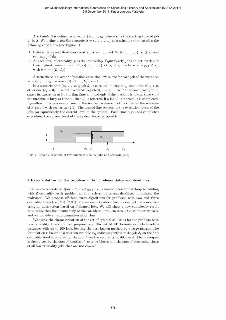
A schedule S is defined as a vector (s1, . . . , sn) where si is the starting time of job

Ji in S. We define a feasible schedule S = (s1, . . . , sn) as a schedule that satisfies the

following conditions (see Figure 1):

1. Release dates and deadlines constraints are fulfilled: ∀i ∈ 1, . . . , n: si ≥ ri and

si + pi,Li≤ di;

2. At each level of criticality, jobs do not overlap. Equivalently, jobs do not overlap at

their highest common level: ∀i, j ∈ 1, . . . , n s.t. si < sj , we have: si + pi,k ≤ sj ,

with k = min(Li, Lj).

A scenario sc is a vector of possible execution levels, one for each job of the instance:

sc = (e1, . . . , en), where ei ∈ 0, . . . , Li, i = 1, . . . , n.

In a scenario sc = (e1, . . . , en), job Ji is executed during pi,ei time units if ei > 0,

otherwise (ei = 0) Ji is not executed (rejected), i = 1, . . . , n. At runtime, each job Jistarts its execution at its starting time si if and only if the machine is idle at time si; if

the machine is busy at time si, then Ji is rejected. If a job Ji is started, it is completed,

regardless of its processing time in the realised scenario. Let us consider the schedule

of Figure 1 with scenarion (2,1). The dashed line represents the execution levels of the

jobs (or equivalently the current level of the system). Each time a job has completed

execution, the current level of the system becomes equal to 1.

J1

r2

J2

r1 d2d1s2

1

2

3

Fig. 1 Feasible schedule of two mixed-criticality jobs and scenario (2,1)

2 Exact solution for the problem without release dates and deadlines

First we concentrate on 1|mc = 2,mu|Cmax, i.e., a monoprocessor match-up scheduling

with L criticality levels problem without release dates and deadlines minimizing the

makespan. We propose efficient exact algorithms for problems with two and three

criticality levels (i.e., L ∈ 2, 3). The uncertainty about the processing time is modeled

using an abstraction based on F-shaped jobs. We will show a new complexity result

that establishes the membership of the considered problem into APX complexity class,

and we provide an approximation algorithm.

We study the characterization of the set of optimal solutions for the problem with

two criticality levels and we propose very efficient MILP formulation which solves

instances with up to 200 jobs, beating the best-known method by a large margin. The

formulation is based on a decision variable xij indicating whether the job Jj on the first

criticality level is covered by the job Ji on the second criticality level. The makespan

is then given by the sum of lengths of covering blocks and the sum of processing times

of all low criticality jobs that are not covered.


- 378 -

Furthermore, we propose efficient exact algorithm for problems with three criticality

levels, which solves instances with up to 60 jobs. The algorithm is based on the idea

of constructing the schedule in two stages. In the first stage, the relaxed problem

considering two levels is solved up to the optimality, which minimizes a lower bound

on the optimal makespan of the original problem. The second stage takes the relaxed

solution and constructs a locally optimal solution for the original problem. The first

stage of the algorithm solves restriction of the given problem instance which omits

the highest level; hence it is an instance of 1|mc = 2,mu|Cmax. In the second stage,

the algorithm defines a new problem instance of the problem 1|mc = 2,mu|Cmax

while grouping two lower levels into one and adding the highest level. In general, the

algorithm produces suboptimal solutions, however, there are cases when we can verify

if the produced schedule is optimal. When we fail to prove optimality, we go to the

MILP model for three criticality leves, while using the current solution as a lower

bound. The reason for executing heuristic algorithm before solving MILP model is

two-fold. First, we have observed the solver struggles to prove optimality when the

solution is clearly optimal regarding the critical path. The other observation is that if

the problem instance contains the majority of jobs with criticality one and two, then

solving its 1|mc = 2,mu|Cmax restriction frequently yields optimal solution since the

highest criticality levels are not likely to have impact on Cmax.

3 Heuristic solution for the problem with release dates and deadlines

The key idea of the heuristic algorithm is to split the solution of the problem into two

steps. The purpose of the stage separation is that the determination of the schedula-

bility of 1|ri, di,mc = L|Cmax problem is NP-hard in the strong sense. The MILP

from the previous section is not powerful enough to find any feasible solution even for

instances with larger tens of messages in a reasonable time. Therefore, we leverage the

finding an initial solution to a heuristic.

In the first stage of the algorithm, an initial feasible solution is obtained. The feasi-

bility stage is inspired by NEH heuristics [3] extended by our local search for reducing

infeasibility. In the second stage, the solution is iteratively reoptimized using Large

Neighborhood Search technique [4]. It is a local search method that iteratively explores

a local neighborhood by the MILP. The best solution over each neighborhood is taken

and adopted as a starting solution for another iteration. The choice of the neighborhood

is problem-dependent and utilizing the structure of the problem is crucial.

Acknowledgements This work was supported by the Grant Agency of the Czech Republicunder the Project FOREST GACR P103-16-23509S.

References

1. M. S. Akturk, E. Gorgulu, Match-up scheduling under a machine breakdown, Europeanjournal of operational research 112 (1) (1999) 81–97.

2. Z. Hanzalek, T. Tunys, P. Sucha, An analysis of the non-preemptive mixed-criticality match-up scheduling problem, Journal of Scheduling 19 (5) (2016) 601–607.

3. Pawel Jan Kalczynski and Jerzy Kamburowski. On the NEH heuristic for minimizing themakespan in permutation flow shops. Omega, 35(1):53 – 60, 2007.

4. David Pisinger and Stefan Ropke. Large neighborhood search. In Handbook of metaheuris-tics, pages 399–419. Springer, 2010.


- 379 -

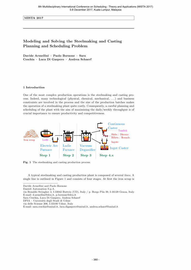
MISTA 2017

Modeling and Solving the Steelmaking and CastingPlanning and Scheduling Problem

Davide Armellini · Paolo Borzone · Sara

Ceschia · Luca Di Gaspero · Andrea Schaerf

1 Introduction

One of the most complex production operations is the steelmaking and casting pro-

cess. Indeed, many technological (physical, chemical, mechanical, . . . ) and business

constraints are involved in the process and the size of the production batches makes

the operation of a steelmaking plant quite costly. Consequently, a careful planning and

scheduling of the plant with the aim of maximizing the daily/weekly throughput is of

crucial importance to ensure productivity and competitiveness.

Electric ArcFurnace

LadleFurnace

VacuumDegassifier Ingot Caster

ContinuousCaster

Slabs / Blooms Billets / RoundsIngots

Step 1 Step 2 Step 3 Step 4.x

Iron scrap Ladle

Tundish

Fig. 1 The steelmaking and casting production process.

A typical steelmaking and casting production plant is composed of several lines. A

single line is outlined in Figure 1 and consists of four stages. At first the iron scrap is

Davide Armellini and Paolo BorzoneDanieli Automation S.p.A.via Bonaldo Stringher 4, I-33042 Buttrio (UD), Italy / p. Borgo Pila 39, I-16129 Genoa, ItalyE-mail: [email protected], [email protected] Ceschia, Luca Di Gaspero, Andrea SchaerfDPIA – Universita degli Studi di Udinevia delle Scienze 206, I-33100 Udine, ItalyE-mail: [email protected], [email protected], [email protected]


- 380 -

melted in an Electric Arc Furnace (EAF), then the liquid metal is poured into a ladle

that will be used to contain the steel in all the following processing steps. The next

step is performed in the Ladle Furnace (LF), where chemical additives are added to

the iron for obtaining the desired alloy. Afterwards, the gas content of the metal has

to be reduced in order to reduces hydrogen and nitrogen gases dissolved in the liquid

steel in a Vacuum Degasifier (VD) unit.

The last production step, called casting, might differ based on the type of semifin-

ished product required. Indeed, in the case of “long pieces” (i.e., slabs, rounds, blooms

or billets) the production is sent to a Continuous Casting (CC) machine, whereas “short

pieces” (e.g., ingots) are forged by an Ingot Casting (IC) machine. These semifinished

products, then, could be subject to further processing (e.g., hot rolling), which might

be planned and scheduled somehow independently from the casting one.

The main physical constraint of this initial part of the steelmaking process is the

practical impossibility to buffer jobs between different processing steps because of the

cooling of the liquid metal in case of waiting. As a consequence, the jobs should be

scheduled in a just-in-time fashion.

A similar version of the problem was presented by Fanti et al [2], who propose an

integrated system consisting of a database, an optimization engine, a simulation module

and an user interface for the pure scheduling problem. The optimization engine models

the scheduling as a hybrid flow shop using a MILP solver.

In our previous work [1], in order to better capture our real-world specification we

made the following modifications, with respect to [2]:

1. we considered the possibility that a job switches from one line to another at any

stage;

2. we considered the border data, coming from the previous scheduling stage (the plant

runs for 24h a day); in particular, for each machine, we register the time when it

is available, the section of last job and its steel grade; in addition, we consider the

status of the ladle with respect to pollutants;

3. we used the throughput as objective function, rather than the makespan, as we

schedule for a fixed horizon, but flexible number of jobs.

In this work, in order to obtain a model that captures the essential features of the

problem and can be shared with other researchers for comparison purposes, we decided

to make further modifications. In essence, on the one side, we simplify the problem

statement, so as to remove low level details specific for the situation at hand; on the

other side, we generalize the problem including features collected from the literature

that where not included in the models of [2] and [1].

In detail, the main differences with respect to our previous model in [1] are:

4. we consider possible standstills of single machines for limited times (e.g., for main-

tenance); as a consequence we have to resort heavily to the possibility that the

production is not executed by a single line, but goes through machines belonging

to different lines (at a price of longer moving times and possible bottlenecks);

5. we remove the detailed management of ingot wagons and stripping areas for the

ingot casting machines, as the number of ingot production is normally limited and

it does not have a strong impact on the overall performance;

6. the condition to perform a shorter setup (called fly-tundish) for CC machines has

been modified; the feasibility of this procedure technically involves the heating and

moving times of the tundish, which is an intermediate container that is needed to


- 381 -

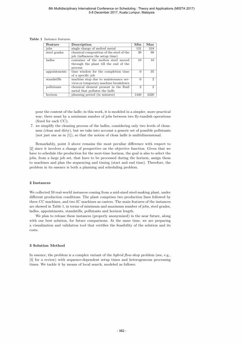
Table 1 Instance features.

Feature Description Min Maxjobs single charge of melted metal 131 318steel grades chemical composition of the steel of the

job (influences the setup time)39 98

ladles container of the molten steel movedthrough the plant till the end of theprocess

10 10

appointments time window for the completion timeof a specific job

0 35

standstills machine stop due to maintenance ser-vices or temporary machine breakdown

0 2

pollutants chemical element present in the fluidmetal that pollutes the ladle

2 2

horizon planning period (in minutes) 1440 4320

pour the content of the ladle; in this work, it is modeled in a simpler, more practical

way: there must by a minimum number of jobs between two fly-tundish operations

(fixed for each CC);

7. we simplify the cleaning process of the ladles, considering only two levels of clean-

ness (clean and dirty), but we take into account a generic set of possible pollutants

(not just one as in [1]), so that the notion of clean ladle is multidimensional.

Remarkably, point 3 above remains the most peculiar difference with respect to

[2] since it involves a change of perspective on the objective function. Given that we

have to schedule the production for the next-time horizon, the goal is also to select the

jobs, from a large job set, that have to be processed during the horizon, assign them

to machines and plan the sequencing and timing (start and end time). Therefore, the

problem in its essence is both a planning and scheduling problem.

2 Instances

We collected 59 real-world instances coming from a mid-sized steel-making plant, under

different production conditions. The plant comprises two production lines followed by

three CC machines, and two IC machines as casters. The main features of the instances

are showed in Table 1, in terms of minimum and maximum number of jobs, steel grades,

ladles, appointments, standstills, pollutants and horizon length.

We plan to release these instances (properly anonymized) in the near future, along

with our best solution, for future comparisons. At the same time, we are preparing

a visualization and validation tool that certifies the feasibility of the solution and its

costs.

3 Solution Method

In essence, the problem is a complex variant of the hybrid flow-shop problem (see, e.g.,

[3] for a review) with sequence-dependent setup times and heterogeneous processing

times. We tackle it by means of local search, modeled as follows:


- 382 -

– The search space is an indirect representation of the schedule by means of the

sequence (i.e., the permutation) of all the available jobs. Each job has also a set

of additional data stating on which machine it has been assigned for each specific

processing step. The mapping between the job sequence and the actual execution

times of each job is obtained by applying a chronological, right-justification greedy

algorithm. All the jobs whose execution time exceed the time-horizon are part of

the tail of the solution, which consists of the jobs considered as unscheduled. The

procedure decides also for the assignment of additional resources (i.e., the ladle and

the cooling place in case of ingots), introducing processing delays when no suitable

resource is available.

– The neighborhood relation is defined as the movement of a job to a new position in

the sequence. All jobs in the state within the current position of the candidate job

to be moved and its destination are shifted by one (either forward or backward).

In addition, the move includes a new machine for each step, which might also be

the same of the old ones. The neighborhood is refined by removing moves that are

clearly ineffective, such as for example moves that take a job in the tail of the state

and reinsert it in a different position still in the tail.

– The cost function takes into account the difference between the upper bound of

scheduled jobs and the number of jobs actually scheduled in the solution. In ad-

dition, it considers the violations of some hard constraints, as a ladle that is not

clean as required and a job that misses an appointment.

The experimental analysis with different metaheuristics (hill climbing, simulated

annealing, and tabu search) is still ongoing. We will report the results as soon as we

complete the tuning and the experimental comparison.

References

1. Davide Armellini, Paolo Borzone, Sara Ceschia, Luca Di Gaspero, and Andrea

Schaerf. A metaheuristic approach for scheduling steelmaking and casting plants. In

Proceedings of the 12th Metaheuristics International Conference (MIC-2017), pages

462–464, Barcelona, Spain, 2017.

2. Maria Pia Fanti, Giuliana Rotunno, Gabriella Stecco, Walter Ukovich, and Stefano

Mininel. An integrated system for production scheduling in steelmaking and casting

plants. IEEE Transactions on Automation Science and Engineering, 13(2):1112–

1128, April 2016.

3. Ruben Ruiz and Jose Antonio Vazquez-Rodrıguez. The hybrid flow shop scheduling

problem. European Journal of Operational Research, 205(1):1–18, 2010.


- 383 -

MISTA 2017

Solving Tourist Trip Design Problems Using a Virus Optimization

Algorithm

Yun-Chia Liang • Aldy Gunawan • Hui-Chih Chen • Josue Rodolfo Cuevas Juarez

1 Introduction

Tourist Trip Design Problems (TTDP) deal with the task to support tourists in creating a trip

consisting of a set or sequence of points-of-interests (POIs) or other items related to travel

(Gavalas et al., 2014). Among all POIs, the tourists arrange their trip based on their personal

preferences, the time and/or budget constraints. When considering the business hour of each

POI, the time window constraints have to be taken into consideration. If tourists arrive a

particular POI before its opening time, they will have to wait until it opens. Therefore, TTDP

can find its general form in the Orienteering Problem (OP) and its variations such as the Multi-

Objective Orienteering Problem with Time Windows (MOOPTW). Recent surveys of

orienteering problems can be found in Vansteenwegen et al. (2009) and Gunawan et al. (2016).

Due to its NP-Hard property, research on TTDP has paid lots of attention on

metaheuristics in the past decades. Virus Optimization Algorithm (VOA) is a newly developed

population-based algorithm and it has been successfully applied to different optimization

problems (Cuevas Juarez et al., 2009; Liang and Cuevas Juarez, 2013, 2014 & 2016; Liu et al.,

2017). Although the VOA was originally designed for continuous optimization problems, this

study focuses on converting the VOA to a structure able to solve combinatorial problems such

as the TTDP and also to fit in the “problem-independent” category as described in Sörensen

(2015). Different from other existing metaheuristics, the population size of the VOA varies

from iteration to iteration, and in order to avoid explosive growth of the viruses, an antivirus

mechanism is developed which also has a perfect matching metaphor in virology. Details of

the VOA will be discussed in the following sections.

2 Virus Optimization Algorithm

Virus Optimization Algorithm is inspired from the behavior of a virus attacking a host cell,

where each virus represents a candidate solution, and the strength of each virus is represented


- 384 -

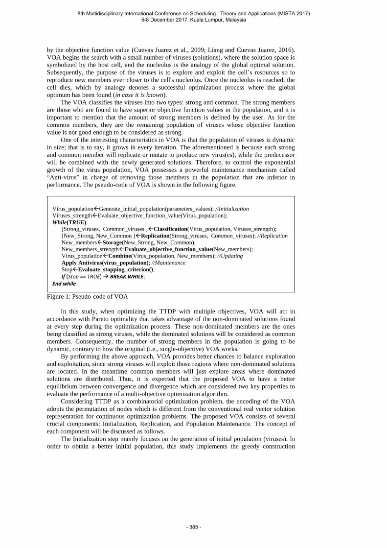
by the objective function value (Cuevas Juarez et al., 2009; Liang and Cuevas Juarez, 2016).

VOA begins the search with a small number of viruses (solutions), where the solution space is

symbolized by the host cell, and the nucleolus is the analogy of the global optimal solution.

Subsequently, the purpose of the viruses is to explore and exploit the cell’s resources so to

reproduce new members ever closer to the cell's nucleolus. Once the nucleolus is reached, the

cell dies, which by analogy denotes a successful optimization process where the global

optimum has been found (in case it is known).

The VOA classifies the viruses into two types: strong and common. The strong members

are those who are found to have superior objective function values in the population, and it is

important to mention that the amount of strong members is defined by the user. As for the

common members, they are the remaining population of viruses whose objective function

value is not good enough to be considered as strong.

One of the interesting characteristics in VOA is that the population of viruses is dynamic

in size; that is to say, it grows in every iteration. The aforementioned is because each strong

and common member will replicate or mutate to produce new virus(es), while the predecessor

will be combined with the newly generated solutions. Therefore, to control the exponential

growth of the virus population, VOA possesses a powerful maintenance mechanism called

“Anti-virus” in charge of removing those members in the population that are inferior in

performance. The pseudo-code of VOA is shown in the following figure.

Figure 1: Pseudo-code of VOA

In this study, when optimizing the TTDP with multiple objectives, VOA will act in

accordance with Pareto optimality that takes advantage of the non-dominated solutions found

at every step during the optimization process. These non-dominated members are the ones

being classified as strong viruses, while the dominated solutions will be considered as common

members. Consequently, the number of strong members in the population is going to be

dynamic, contrary to how the original (i.e., single-objective) VOA works.

By performing the above approach, VOA provides better chances to balance exploration

and exploitation, since strong viruses will exploit those regions where non-dominated solutions

are located. In the meantime common members will just explore areas where dominated

solutions are distributed. Thus, it is expected that the proposed VOA to have a better

equilibrium between convergence and divergence which are considered two key properties to

evaluate the performance of a multi-objective optimization algorithm.

Considering TTDP as a combinatorial optimization problem, the encoding of the VOA

adopts the permutation of nodes which is different from the conventional real vector solution

representation for continuous optimization problems. The proposed VOA consists of several

crucial components: Initialization, Replication, and Population Maintenance. The concept of

each component will be discussed as follows.

The Initialization step mainly focuses on the generation of initial population (viruses). In

order to obtain a better initial population, this study implements the greedy construction

Virus_populationGenerate_initial_population(parameters_values); //Initialization

Viruses_strengthEvaluate_objective_function_value(Virus_population);

While(TRUE)

[Strong_viruses, Common_viruses ]Classification(Virus_population, Viruses_strength);

[New_Strong, New_Common ]Replication(Strong_viruses, Common_viruses); //Replication

New_membersStorage(New_Strong, New_Common);

New_members_strengthEvaluate_objective_function_value(New_members);

Virus_populationCombine(Virus_population, New_members); //Updating

Apply Antivirus(virus_population); //Maintenance

StopEvaluate_stopping_criterion();

If (Stop == TRUE) BREAK WHILE; End while


- 385 -

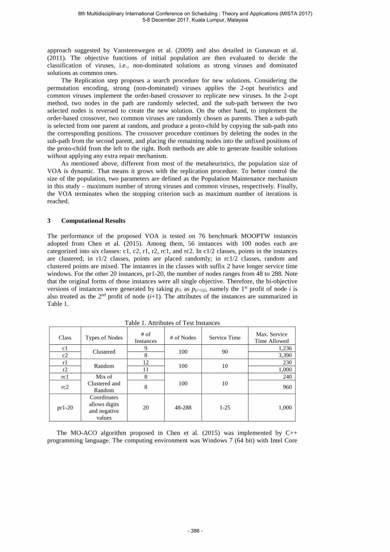
approach suggested by Vansteenwegen et al. (2009) and also detailed in Gunawan et al.

(2011). The objective functions of initial population are then evaluated to decide the

classification of viruses, i.e., non-dominated solutions as strong viruses and dominated

solutions as common ones.

The Replication step proposes a search procedure for new solutions. Considering the

permutation encoding, strong (non-dominated) viruses applies the 2-opt heuristics and

common viruses implement the order-based crossover to replicate new viruses. In the 2-opt

method, two nodes in the path are randomly selected, and the sub-path between the two

selected nodes is reversed to create the new solution. On the other hand, to implement the

order-based crossover, two common viruses are randomly chosen as parents. Then a sub-path

is selected from one parent at random, and produce a proto-child by copying the sub-path into

the corresponding positions. The crossover procedure continues by deleting the nodes in the

sub-path from the second parent, and placing the remaining nodes into the unfixed positions of

the proto-child from the left to the right. Both methods are able to generate feasible solutions

without applying any extra repair mechanism.

As mentioned above, different from most of the metaheuristics, the population size of

VOA is dynamic. That means it grows with the replication procedure. To better control the

size of the population, two parameters are defined as the Population Maintenance mechanism

in this study – maximum number of strong viruses and common viruses, respectively. Finally,

the VOA terminates when the stopping criterion such as maximum number of iterations is

reached.

3 Computational Results

The performance of the proposed VOA is tested on 76 benchmark MOOPTW instances

adopted from Chen et al. (2015). Among them, 56 instances with 100 nodes each are

categorized into six classes: c1, c2, r1, r2, rc1, and rc2. In c1/2 classes, points in the instances

are clustered; in r1/2 classes, points are placed randomly; in rc1/2 classes, random and

clustered points are mixed. The instances in the classes with suffix 2 have longer service time

windows. For the other 20 instances, pr1-20, the number of nodes ranges from 48 to 288. Note

that the original forms of those instances were all single objective. Therefore, the bi-objective

versions of instances were generated by taking pi1 as p(i+1)2, namely the 1st profit of node i is

also treated as the 2nd profit of node (i+1). The attributes of the instances are summarized in

Table 1.

Table 1. Attributes of Test Instances

Class Types of Nodes # of

Instances # of Nodes Service Time

Max. Service

Time Allowed

c1 Clustered

9 100 90

1,236

c2 8 3,390

r1 Random

12 100 10

230

r2 11 1,000

rc1 Mix of

Clustered and

Random

8

100 10

240

rc2 8 960

pr1-20

Coordinates

allows digits

and negative

values

20 48-288 1-25 1,000

The MO-ACO algorithm proposed in Chen et al. (2015) was implemented by C++

programming language. The computing environment was Windows 7 (64 bit) with Intel Core


- 386 -

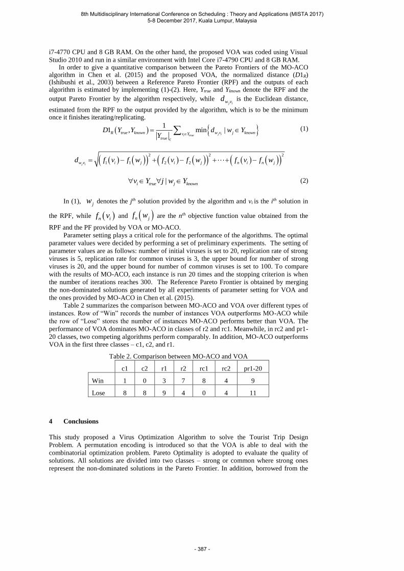
i7-4770 CPU and 8 GB RAM. On the other hand, the proposed VOA was coded using Visual

Studio 2010 and run in a similar environment with Intel Core i7-4790 CPU and 8 GB RAM. In order to give a quantitative comparison between the Pareto Frontiers of the MO-ACO

algorithm in Chen et al. (2015) and the proposed VOA, the normalized distance (D1R) (Ishibushi et al., 2003) between a Reference Pareto Frontier (RPF) and the outputs of each algorithm is estimated by implementing (1)-(2). Here, Ytrue and Yknown denote the RPF and the

output Pareto Frontier by the algorithm respectively, while j iw vd is the Euclidean distance,

estimated from the RPF to the output provided by the algorithm, which is to be the minimum once it finishes iterating/replicating.

11 , min |

j ii trueR true known w v j knownv Y

true c

D Y Y d w YY

(1)

2 2 2

1 1 2 2j iw v i j i j n i n jd f v f w f v f w f v f w

|i true j knownv Y j w Y (2)

In (1), jw denotes the jth solution provided by the algorithm and vi is the ith solution in

the RPF, while n if v and n jf w are the nth objective function value obtained from the

RPF and the PF provided by VOA or MO-ACO.

Parameter setting plays a critical role for the performance of the algorithms. The optimal

parameter values were decided by performing a set of preliminary experiments. The setting of

parameter values are as follows: number of initial viruses is set to 20, replication rate of strong

viruses is 5, replication rate for common viruses is 3, the upper bound for number of strong

viruses is 20, and the upper bound for number of common viruses is set to 100. To compare

with the results of MO-ACO, each instance is run 20 times and the stopping criterion is when

the number of iterations reaches 300. The Reference Pareto Frontier is obtained by merging

the non-dominated solutions generated by all experiments of parameter setting for VOA and

the ones provided by MO-ACO in Chen et al. (2015).

Table 2 summarizes the comparison between MO-ACO and VOA over different types of

instances. Row of “Win” records the number of instances VOA outperforms MO-ACO while

the row of “Lose” stores the number of instances MO-ACO performs better than VOA. The

performance of VOA dominates MO-ACO in classes of r2 and rc1. Meanwhile, in rc2 and pr1-

20 classes, two competing algorithms perform comparably. In addition, MO-ACO outperforms

VOA in the first three classes – c1, c2, and r1.

Table 2. Comparison between MO-ACO and VOA

c1 c2 r1 r2 rc1 rc2 pr1-20

Win 1 0 3 7 8 4 9

Lose 8 8 9 4 0 4 11

4 Conclusions

This study proposed a Virus Optimization Algorithm to solve the Tourist Trip Design

Problem. A permutation encoding is introduced so that the VOA is able to deal with the

combinatorial optimization problem. Pareto Optimality is adopted to evaluate the quality of

solutions. All solutions are divided into two classes – strong or common where strong ones

represent the non-dominated solutions in the Pareto Frontier. In addition, borrowed from the


- 387 -

Traveling Salesman Problem (TSP) and the Genetic Algorithm (GA), two popular methods –

2-opt and order-based crossover are implemented to replicate new solutions.

Computational results show that VOA can perform equally or better than MO-ACO in

instances with random data and longer service time (i.e., r2 class), the instances with mix

random and clustered data (rc1 and rc2 classes), and the ones with wider range on the number

of nodes (the pc class). For those instances VOA is inferior to MO-ACO, VOA can still find

good solutions particularly in the middle region of Pareto Frontier. However, VOA is unable to

find better solutions on two ends of Pareto Frontier. This observation may lead to future

research which focuses on improving diversity of Pareto Frontier.

Finally, note that this study is a preliminary but novel research to investigate the

possibilities and validity of applying VOA on network-type combinatorial optimization

problems. To further confirm the performance of the VOA, more comprehensive comparison

with different metaheuristics using more benchmark instances should be conducted in the

future.

References

1. Chen, Y.-H., Sun, W.-J., & Chiang, T.-C. Multiobjective Orienteering Problem with

Time Windows: An Ant Colony Optimization Algorithm. Proceedings of the 2015

Technologies and Applications of Artificial Intelligence (TAAI2015), 128-135 (2015).

2. Cuevas Juarez, J. R., Wang, H.-J., Lai, Y.-C., & Liang, Y.-C. Virus Optimization

Algorithm (VOA): A Novel Metaheuristic for Solving Continuous Optimization

Problems. Proceedings of the 10th Asia Pacific Industrial Engineering and Management

Systems Conference (APIEMS2009), 2166-2174 (2009).

3. Gavalas, D., Konstantopoulos, C., Mastakas, K. & Pantziou, G. A Survey on Algorithmic

Approaches for Solving Tourist Trip Design Problems. Journal of Heuristics, 20(3), 291-

328 (2014).

4. Gunawan, A., Lau, H. C., & Lu, K. An Iterated Local Search Algorithm for Solving the

Orienteering Problem with Time Windows. Proceedings of the 15th European Conference

on Evolutionary Computation in Combinatorial Optimization (EvoCOP 2015), 61-73

(2015).

5. Gunawan, A., Lau, H.C., & Vansteenwegen, P. Orienteering Problem: A Survey of

Recent Variants, Solution Approaches and Applications. European Journal of Operational

Research, 255, 315-332 (2016).

6. Ishibuchi, H., Yoshida, T., & Murata, T. Balance between Genetic Search and Local

Search in Memetic Algorithms for Multiobjective Permutation Flowshop Scheduling.

IEEE Transactions on Evolutionary Computation, 7, 204-223 (2003).

7. Liang, Y.-C., & Cuevas Juarez, J. R. An Automatic Multilevel Image Thresholding Using

Relative Entropy and Meta-Heuristic Algorithms. Entropy, 15(6), 2181-2209 (2013).

8. Liang, Y.-C., & Cuevas Juarez, J. R. A Normalization Method for Solving the Combined

Economic and Emission Dispatch Problem with Meta-Heuristic Algorithms. International

Journal of Electrical Power and Energy Systems, 54, 163-186 (2014).

9. Liang, Y.-C., & Cuevas Juarez, J. R. A Novel Metaheuristic for Continuous Optimization

Problems: Virus Optimization Algorithm. Engineering Optimization, 48(1), 73-93

(2016).

10. Lu, C., Li, X., Gao, L., Liao, W., & Yi, J. An Effective Multi-objective Discrete Virus

Optimization Algorithm for Flexible Job-shop Scheduling Problem with Controllable

Processing Times. Computers & Industrial Engineering, 104, 156-174 (2017).

11. Sörensen, K. Metaheuristics-The Metaphor Exposed. International Transactions in

Operational Research, 22, 3-18 (2015).

12. Vansteenwegen, P., Souffriau, W., Berghe, G. V., & Van Oudheusden, D. Iterated Local

Search for the Team Orienteering Problem with Time Windows. Computers &

Operations Research, 36(12), 3281-3290 (2009).


- 388 -

MISTA 2017

Integrated Scheduling of Machines, Vehicles, and Storage Tasks in

Flexible Manufacturing Systems

Seyed Mahdi Homayouni • Dalila B.M.M. Fontes

This work proposes an integrated scheduling approach for machines, vehicles, and storage

tasks in flexible manufacturing systems. Flexible manufacturing system (FMS) is a technology

that came into the theory of manufacturing and production systems in late 20th century. It

connects production, transportation, storage, and tooling in a way that various parts with

different specifications may be processed rapidly and precisely [1], [2]. FMS is important as it

allows to produce low volumes of a large variety of products while aiming for high productivity

and low costs, as in mass production systems. FMS technology leads to shorter product

development cycle, improved equipment utilization, reduced set up times, and lower work-in-

process inventories [2], [3]. FMS environments are composed of a set of computer numeric

control (CNC) machines connected by a set of automated guided vehicles (AGVs) under the

control of a computer system. An automated storage/retrieval system (AS/RS) is used to store

and retrieve raw parts, as well as products and/or components.The AS/RS comprises two racks

of storage locations, served using a storage/retrieval (S/R) machine. The parts are delivered to

the load/ unload (L/U) area by S/R machine, then they are picked up by the AGVs to go through

the manufacturing operations required. Once all such operations are completed parts are returned

to the L/U area. The S/R machine will then pick them up from the L/U area and transport them

back to the storage cell.

Production scheduling refers to sequencing and timing operations on the CNC machines;

vehicle scheduling refers to assigning the AGVs to the transportation of parts (or jobs) between

the CNC machines, as well as between the CNC machines and the L/U area. Storage and retrieval

transfer tasks are assigned to a single S/R machine, thus they need to be scheduled appropriately.

Since production scheduling in FMS is highly dependent on the material handling system, the

S/R machine and the production operations, as well as AGV scheduling need to be addressed

simultaneously. Scheduling in FMS environments is much more difficult than other

manufacturing systems due to the higher level of interrelations between various types of

equipment used in FMSs [4], [5]. Furthermore, the higher level of automation requires tighter

and reliable scheduling.

In FMS environments, a job comprises a set of predefined operations on a specific raw part.

The raw parts are stored in predetermined locations of the AS/RS, prior to their starting time of

production. A part is retrieved from the storage location to the L/U station by the S/R machine.

There, a vehicle picks up the part and move it to the machine performing its first operation. The

S/R machine is, usually, assumed to be at the L/U station at the beginning of the scheduling

horizon. For the following operations, parts are picked up by the vehicle from the machine where

the last operation was performed, waiting for its completion if necessary, and taken to the

corresponding machine to have the operation performed. Once the final operation is completed,

the part is moved to the L/U station, where the S/R machine picks it up and transfers it back to

the storage location (i.e., storage task). The job is then ready to be delivered to the final customer.


- 389 -



Note that when an AGV arrives at a machine, the part is delivered to the buffer area, and the

AGV can pursue its next assignment immediately. In such kind of FMS environments, the layout

of the machines and the AGV routes are known in advance.

To find solutions to this problem one needs to find the S/R machine schedule (both for

storage and retrieval tasks), the AGVs schedule, and the operations schedule. Among the

possible solutions, we are interested in one that minimizes the total time required to complete

all the jobs, i.e., the makespan.

Most of the reported work considers the simultaneous scheduling of either machines and

storage/retrieval tasks or machines and AGVs tasks (with the third equipment being considered

as an ever-available resource). The integrated scheduling of machines and AGVs has been

considered widely in the last 20 years [2], [3], [6], [7]. In this problem, the sequence of operations

on each machine is determined concurrently with the AGVs assignment to transport the parts

between the machines and between them and the L/U area. It is assumed that all the parts are

available at L/U area whenever an AGV reaches it. Bilge and Ulusoy [6] proposed the first

mathematical model, a nonlinear one, for the integrated scheduling of machines and AGVs.

Then, Zheng et al. [2] developed the first MILP (mixed-integer linear programming) model.

However, the former model was never solved and the latter was only used to solve very small

example. Ulusoy et al. [7], Abdelmaguid et al. [3], Gnanavel Babu et al [8], and Zheng et al. [2]

and many other researchers proposed (meta)heuristic algorithms to solve this problem within

reasonable CPU time. More recently, Fontes and Homayouni [9] and [10] have proposed a MILP

model and reported good performances solving the usually used benchmark problem instances,

first proposed by Bilge and Ulusoy [6]. In these works, the authors assumed that the jobs are in

the L/U station ready to be moved by an AGV. Some of the solution methods reported in the

literature have obtained “doubtful” results for the above mentioned instances. This fact has been

reported by several authors: Abdelmaguid et al. [3], Zheng et al. (2014), and Fontes and

Homayouni [10].

Other authors, recognizing that production scheduling in FMS environment is highly

dependent on the availability of the parts at L/U station addressed the simultaneous scheduling

of storage/retrieval tasks and production operations [11], [12]. Jawahar et al. [11] proposed

simultaneous scheduling of AS/RS storage and production in FMS. Later, the work is further

developed through developing an adaptive genetic algorithm by Jerald et al. [13], and a particle

swarm optimization algortihm by Asokan et al. [12]. In all these works it is assumed that

travelling time between the L/U area and the machines is negligible and that AGVs are available

to move the parts whenever needed.

To the best of our knowledge, Jerald et al. [14] and Gnanavel Babu et al. [15] are the only

reported works considering the integrated scheduling of machines, vehicles, and

storage/retrieval tasks in FMS. Both works aim at minimizing penalty cost, machine idle time,

and distance travelled by the S/R machine. Jerald et al. [14] proposed several metaheuristic

algorithms such as, genetic algorithm, particle swarm intelligence, and sheep flock heredity

algorithm; while Gnanavel Babu et al. [15] proposed an artificial immune system. However, no

optimal solution methods have ever been proposed for this problem. Here, a mixed integer linear

programming model is reported, with which optimal solutions can be found. This is important

as a mean to develop alternative heuristics and also to be able to provide a precise quality

measure for the solutions found by the (meta)heuristic, at least for small sized instances.

In FMS environments, a set of machines, a set of vehicles, and one S/R machine are in

service. There are J jobs, each requiring a set of operations to be done. Each operation is

characterized by a machine where it needs to be processed and a processing time. Routes

between the L/U area and the machines and between machines are predetermined.

The MILP model we develop extends the one proposed in Fontes and Homayouni [10] by

incorporating the AS/RS scheduling and its main novelty is the consideration of a set of chained

manufacturing tasks for the machines, a set of chained transportation tasks for the vehicles, and

a set of chained storage task for the S/R machine. These three sets of chains are connected

through the constraints regarding the completion time of the manufacturing tasks and traveling

task, both for vehicles and for the S/R machine. This, in turn results in a lower number of binary


- 390 -

variables, particularly for larger numbers (>2) of vehicles. In addition, our modeling approach

differs from current literature in the sense that we model the sequences of tasks for machines,

vehicles, and the S/R machine independently; while others, usually, assign machine tasks and

vehicles tasks simultaneously, i.e., in the same decision variable (see, e.g., Zheng et al. [2]).

For the evaluation purposes, we have used the set of frequently used benchmark instances,

first proposed by Bilge and Ulusoy [6]. This set contains 82 instances, considering four different

layouts, each of which having of one L/U station, four machines, and two vehicles. The instances

have been generated and consist of 10 job sets, each with 13 to 21 operations and 4 to 8 jobs.

We have adapted these instances to the problem being addressed by adding the specifications of

an AS/RS to the FMS layout, and storage cell for the jobs. The model was implemented in and

solved by Gurobi® software. The computational results obtained show that the proposed

modeling approach, in addition to being novel, is capable of finding optimal solutions efficiently.

Out of the 82 instances considered, 73 were optimally solved and in 47% of them CPU time is

under one minute.

The solutions obtained have also shown that the transportation associated the storage and

retrieval tasks should not be ignored, since it implies a much larger makespan. For example, for

the first instance, the makespan goes up from 96, when only machines and vehicles scheduling

is involved, (see, e.g., [2], [3], [7]) to 203 when the scheduling of machines, vehicles, and storage

is considered. Furthermore, it could be observed that in more than 95% of the makespan

duration, the S/R machine is working to retrieve/store parts, while machines and vehicles have

idle times in nearly half of this duration.

Acknowledgements We acknowledge the financial support of Projects \NORTE-01- 0145-

FEDER-000020", financed by the North Portugal Regional Operational Programme (NORTE

2020), under the PORTUGAL 2020 Partnership Agreement and PTDC/EEIAUT /2933/2014,

financed through the European Regional Development Fund (ERDF) and FEDER

/COMPETE2020- POCI/FCT.

References

[1] M. Zhao and M. Uzam, “A suboptimal deadlock control policy for designing non-blocking

supervisors in flexible manufacturing systems,” Inf. Sci. (Ny)., vol. 388, pp. 135–153, 2017.

[2] Y. Zheng, Y. Xiao, and Y. Seo, “A tabu search algorithm for simultaneous machine/AGV

scheduling problem,” Int. J. Prod. Res., vol. 52, no. October 2014, pp. 1–16, 2014.

[3] T. F. Abdelmaguid, A. O. Nassef, B. A. Kamal, and M. F. Hassan, “A hybrid GA/heuristic

approach to the simultaneous scheduling of machines and automated guided vehicles,” Int. J.

Prod. Res., vol. 42, no. 2, pp. 267–281, 2004.

[4] P. N. Pena, T. A. Costa, R. S. Silva, and R. H. C. Takahashi, “Control of Flexible Manufacturing

Systems under model uncertainty using Supervisory Control Theory and evolutionary

computation schedule synthesis,” Inf. Sci. (Ny)., vol. 329, pp. 491–502, 2016.

[5] H. E. Nouri, O. B. Driss, and K. Ghédira, “Simultaneous scheduling of machines and transport

robots in flexible job shop environment using hybrid metaheuristics based on clustered holonic

multiagent model,” Comput. Ind. Eng., vol. 102, pp. 488–501, 2016.

[6] Ü. Bilge and G. Ulusoy, “A time window approach to simultaneous scheduling of machines and

material handling system in an FMS,” Oper. Res., vol. 43, no. 6, pp. 1058–1070, 1995.

[7] G. Ulusoy, F. Sivrikaya-Serifoglu, and Ü. Bilge, “A genetic algorithm approach to the

simultaneous scheduling of machines and automated guided vehicles,” Comput. Oper. Res., vol.

24, no. 4, pp. 335–351, 1997.

[8] A. Gnanavel Babu, J. Jerald, A. Noorul Haq, V. Muthu Luxmi, and T. P. Vigneswaralu,

“Scheduling of machines and automated guided vehicles in FMS using differential evolution,”

Int. J. Prod. Res., vol. 48, no. 16, pp. 4683–4699, 2010.

[9] D. B. M. M. Fontes and S. M. Homayouni, “Joint Production & Transportation Scheduling in

Flexible Manufacturing Systems,” J. Glob. Optim., 2017.

[10] D. B. M. M. Fontes and S. M. Homayouni, “Joint Production & Transportation Scheduling in

Flexible Manufacturing Systems,” in Global Optimization Conference, 2017.

[11] N. Jawahar, P. Aravindan, and S. G. Ponnambalam, “Optimal random storage allocation for an


- 391 -

AS/RS in an FMS,” Int. J. Adv. Manuf. Technol., vol. 14, no. 2, pp. 116–132, 1998.

[12] P. Asokan, J. Jerald, S. Arunachalam, and T. Page, “Application of Adaptive Genetic Algorithm

and Particle Swarm Optimisation in scheduling of jobs and AS/RS in FMS,” Int. J. Manuf. Res.,

vol. 3, no. 4, pp. 393–405, 2008.

[13] J. Jerald, P. Asokan, R. Saravanan, and A. Rani, “Simultaneous scheduling of parts and

automated guided vehicles in an FMS environment using adaptive genetic algorithm,” Int. J.

Adv. Manuf. Technol., vol. 29, no. 5, pp. 584–589, 2006.

[14] J. Jerald, A. Gnanavelbabu, and A. N. Haq, “Multi-Objective Scheduling of Jobs, Automated

Guided Vehicles and Automated Storage/Retrieval System in Flexible Manufacturing System,”

J. Manuf. Sci. Prod., vol. 9, no. 1–2, pp. 61–80, 2008.

[15] A. Gnanavel Babu, J. Jerald, A. Noorul Haq, and P. Asokan, “Multi objective scheduling of

jobs, AGVs and AS/RS in FMS using artificial immune system,” Adv. Prod. Eng. Manag., vol.

4, no. 3, pp. 139–150, 2009.


- 392 -

MISTA 2017

Selection Hyper-heuristics for Solving the Wind FarmLayout Optimisation Problem

Ahmed Kheiri · Alaa Daffalla ·Yossra Noureldien · Ender Ozcan

1 Introduction

During the last two centuries, energy consumption from non-renewable sources has

reached its peak while demand for energy has increased. Therefore transitioning to

renewable energy sources is now recognised. Wind turbine technology is a promising

source of renewable energy, and hence efficient wind farm layout is needed so that each

turbine produces as much energy as possible. The placement of wind turbines directly

impacts the efficiency of the wind farm as turbines are close enough to influence each

other’s performance due to aerodynamic interactions (wakes) [7].

The wind farm layout optimisation problem is considered a highly complex NP-hard

problem, for which exact methods are unsuitable. There is a wide and varied literature

on the use of evolutionary algorithms for the optimisation of wind farm layouts [5,6].

These algorithms have proven to be very effective at finding near-optimal solutions to a

large number of problems in the energy industry. However, a new breed of optimisation

algorithms known as hyper-heuristics is beginning to be applied to these problems.

Hyper-heuristics are automated methodologies for selecting or generating heuristics

to solve multiple computationally difficult optimisation problems [1]. They combine

simple heuristics to create bespoke algorithms for specific problem domains, and have

proven successful on other optimisation problems (see for example [2,3]). This work

investigates the use of selection hyper-heuristics to wind farm layout optimisation that

could possibly outperform conventional evolutionary approaches in terms of solution

quality and run-time. There are two main components in a single-point-based search

selection hyper-heuristic: heuristic selection and move acceptance as identified in [4].

Alaa Daffalla and Yossra NoureldienUniversity of Khartoum, Department of Electrical and Electronic Engineering, SudanE-mail: [email protected], [email protected]

Ahmed KheiriLancaster University Management School, Lancaster LA1 4YX, UKE-mail: [email protected]

Ender OzcanUniversity of Nottingham, School of Computer Science, Nottingham NG8 1BB, UKE-mail: [email protected]


- 393 -

2 Solution Method

The wind farm layout optimisation problem involves finding the optimal positions of

wind turbines in a 2-dimensional plane, such that the cost of energy is minimised taking

into account several factors such as wind speed, site characteristics, turbines features,

wake effects and existence of obstacles.

Our approach discretises the site into a number of cells, and solutions to the problem

are represented as a vector of boolean to decide the absence or presence of turbines in

the cells of the grid. The simplest form of a selection hyper-heuristic is a stochastic local

search method which combines a simple random heuristic selection method (SR) with

an improve or equal acceptance method (IE). The proposed approach, denoted as SR-

IE, is implemented in this study using an open source software tool based on a generic

API, referred to as WindFLO1, designed for benchmarking purposes. This tool contains

problem domain specific details, such as, the evaluation function computing the cost

of energy. Moreover, a set of benchmark problem instances (terrain sizes, obstacles,

wind forces, layout shapes, . . . ) can be downloaded from the WindFLO website. The

evaluation function used in this study is as follows:

f =

(ct ∗ n + cs ∗ b nmc

)+ cOM ∗ n(

1− (1− r)−y)/r

∗ 1

8760 ∗ P +0.1

n(1)

where f is the cost of energy, ct = $750, 000 is the turbine cost, cs = $8, 000, 000 is the

price of a substation, m = 30 is the number of turbines per substation, r = 3% is the

interest rate, y = 20 years is the farm lifetime in years, cOM = $20, 000 per year is the

operation and maintenance costs, n is the number of turbines of the layout, P is the

layout’s energy output reported by the WindFLO API [5].

Selection hyper-heuristics operate by using a prefixed pool of low level heuristics by

which a randomly initialised solution is improved over the search time. The low level

heuristics used in this study are as follows:

– LLH1 replace a single cell at random.

– LLH2 swap two cells at random.

– LLH3 ruin 10% of cells and rebuild at random.

– LLH4 ruin 30% of cells and rebuild with all 0s or all 1s.

– LLH5 is a first improvement hill climbing that searches for the first best solution

between adjacent solutions.

– LLH6 select two rows in a grid and exchange with a crossover rate of 20%.

– LLH7 select two columns in a grid and exchange with a crossover rate of 20%.

Hence, SR chooses and applies a perturbative low level heuristic with a probability of

86%. Having LLH5 local search method as one of the low level heuristics creates an

iterated local search like overall approach [3].

3 Results

The WindFLO API provides an implementation of a genetic algorithm (GA) as a

baseline approach whose performance is compared to the proposed method, SR-IE.

Both algorithms are applied to three instances each for five trials, and the termination

1 https://github.com/d9w/WindFLO


- 394 -

https://github.com/d9w/WindFLO

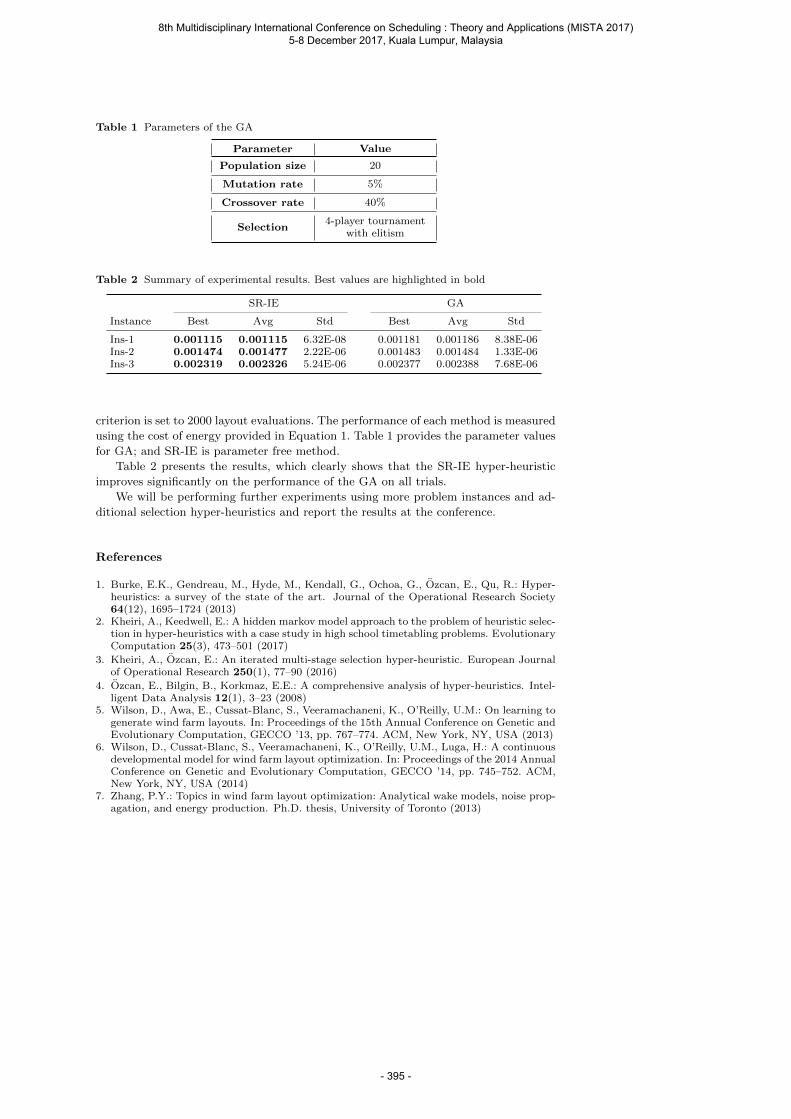
Table 1 Parameters of the GA

Parameter Value

Population size 20

Mutation rate 5%

Crossover rate 40%

Selection4-player tournament

with elitism

Table 2 Summary of experimental results. Best values are highlighted in bold

SR-IE GA

Instance Best Avg Std Best Avg Std

Ins-1 0.001115 0.001115 6.32E-08 0.001181 0.001186 8.38E-06Ins-2 0.001474 0.001477 2.22E-06 0.001483 0.001484 1.33E-06Ins-3 0.002319 0.002326 5.24E-06 0.002377 0.002388 7.68E-06

criterion is set to 2000 layout evaluations. The performance of each method is measured

using the cost of energy provided in Equation 1. Table 1 provides the parameter values

for GA; and SR-IE is parameter free method.

Table 2 presents the results, which clearly shows that the SR-IE hyper-heuristic

improves significantly on the performance of the GA on all trials.

We will be performing further experiments using more problem instances and ad-

ditional selection hyper-heuristics and report the results at the conference.

References

1. Burke, E.K., Gendreau, M., Hyde, M., Kendall, G., Ochoa, G., Ozcan, E., Qu, R.: Hyper-heuristics: a survey of the state of the art. Journal of the Operational Research Society64(12), 1695–1724 (2013)

2. Kheiri, A., Keedwell, E.: A hidden markov model approach to the problem of heuristic selec-tion in hyper-heuristics with a case study in high school timetabling problems. EvolutionaryComputation 25(3), 473–501 (2017)

3. Kheiri, A., Ozcan, E.: An iterated multi-stage selection hyper-heuristic. European Journalof Operational Research 250(1), 77–90 (2016)

4. Ozcan, E., Bilgin, B., Korkmaz, E.E.: A comprehensive analysis of hyper-heuristics. Intel-ligent Data Analysis 12(1), 3–23 (2008)

5. Wilson, D., Awa, E., Cussat-Blanc, S., Veeramachaneni, K., O’Reilly, U.M.: On learning togenerate wind farm layouts. In: Proceedings of the 15th Annual Conference on Genetic andEvolutionary Computation, GECCO ’13, pp. 767–774. ACM, New York, NY, USA (2013)

6. Wilson, D., Cussat-Blanc, S., Veeramachaneni, K., O’Reilly, U.M., Luga, H.: A continuousdevelopmental model for wind farm layout optimization. In: Proceedings of the 2014 AnnualConference on Genetic and Evolutionary Computation, GECCO ’14, pp. 745–752. ACM,New York, NY, USA (2014)

7. Zhang, P.Y.: Topics in wind farm layout optimization: Analytical wake models, noise prop-agation, and energy production. Ph.D. thesis, University of Toronto (2013)


- 395 -

Author Index Aizam N. A. H. .............................................................. 319, 320

Akhlaghi V. E. ....................................................................... 329

Alefragis P. .............................................................................. 30

Armellini D. ........................................................................... 380

Ayob M.................................................................................. 348

Aziz N. L. A. ................................................................. 319, 320

Baatar D. ................................................................................ 315

Bach L. .......................................................................... 362, 373

Bai R. ..................................................................................... 288

Barták R. ........................................................................ 189, 295

Berretta R. ............................................................................. 133

Blazewicz J. ............................................................................... 9

Borzone P. ............................................................................. 380

Bouvry P. ............................................................................... 269

Bowly S. ................................................................................ 315

Bulhoes T. ............................................................................. 325

Cantais B. .............................................................................. 344

Cao B. ...................................................................................... 93

Ceschia S. .............................................................................. 380

Chen H-C. .............................................................................. 384

Clement M. ............................................................................ 214

Copado-Mendez P. J. ............................................................. 321

Creemers S. ........................................................................... 312

Cuervo D. P. .......................................................................... 373

Cui T. ..................................................................................... 288

Daffalla A. ............................................................................. 393

Dauzère-Pérès S. ................................................................... 340

De Causmaecker P. .................................................................. 70

Demirovic E. ......................................................................... 214

Di Gaspero L. ........................................................................ 380


- 396 -

Doerner K. E. ......................................................................... 367

Dung P. Q. ............................................................................. 214

Edwards S. ............................................................................. 315

Emeretlis A. ............................................................................. 30

Fontes B. B. M. M. ................................................................ 389

Fuchigami H. Y. .................................................................... 370

Gomes F. R. A. ...................................................................... 201

Gonzalez M. A. ..................................................................... 158

Gort E. ................................................................................... 173

Gultekin H. ............................................................................ 329

Gunawan A. ........................................................... 229, 244, 384

Günther M. ............................................................................ 144

Gurel S. .................................................................................. 329

Han K. ................................................................................... 256

Hans E. .................................................................................. 173

Hanzalek Z. ........................................................................... 377

Hebrard E. ............................................................................. 295

Heydar M. .............................................................................. 133

Homayouni S. M. .................................................................. 389

Ilagan I. F. A .......................................................................... 103

Inoue K. ................................................................................. 214

Jamaluddin N. F. ........................................................... 319, 320

Jansen E. ................................................................................ 173

Jewpanya P. ........................................................................... 229

Jouglet A................................................................................ 344

Juarez J. R. C. ........................................................................ 384

Kaihara T. .............................................................................. 336

Kheiri A. ................................................................................ 393

Kiefer A. ................................................................................ 367

Kjenstad D. ............................................................................ 362

Kwan R. S. K. ........................................................................ 321

Lau H. C. ................................................................. 11, 229, 244

Lavangnananda K. ................................................................. 269


- 397 -

Lei L. ..................................................................................... 321

Leus R.................................................................................... 312

Li H. ........................................................................................ 13

Li X. ...................................................................................... 288

Liang Y-C. ............................................................................. 384

Lin Z. ..................................................................................... 321

Liu Y........................................................................................ 93

Lu K. ................................................................................ 93, 244

Mannino C. ............................................................................ 362

Martineau P. ............................................................................ 84

Mateus G. R. .......................................................................... 201

McMullan P. .......................................................................... 256

Mönch L. ............................................................................... 358

Moll M. .................................................................................... 59

Mosquera F. ........................................................................... 121

Nazri M. Z. A. ....................................................................... 348

Nezami F. G. ......................................................................... 133

Nishi T. .................................................................................. 336

Nissen V. ............................................................................... 144

Noureldien Y. ........................................................................ 393

Novak A. ............................................................................... 377

Oddi A. .................................................................................. 158

Ong W. E. ................................................................................ 43

Oude Vrielink R. ................................................................... 173

Pickl S...................................................................................... 59

Pinaton J. ............................................................................... 340

Raap M. ................................................................................... 59

Rahman A. ............................................................................... 43

Rasconi R. ............................................................................. 158

Redi A. A. N. P. ..................................................................... 229

Rocholl J. ............................................................................... 358

Rostami S. ............................................................................. 312

Sadykov R. ............................................................................ 325


- 398 -

Savourey D. ........................................................................... 344

Saw V. ..................................................................................... 43

Schaerf A. .............................................................................. 380

Schilde M. ............................................................................. 367

Schulte J. ............................................................................... 144

Smet P.................................................................................... 121

Smith-Miles K. ...................................................................... 315

Soukhal A. ............................................................................... 84

Srour A. ................................................................................... 70

Subramanian A. ..................................................................... 325

Sucha P. ................................................................................. 377

Švancara J. ............................................................................. 189

Sy C. L. .................................................................................. 103

Tamssaouet K. ....................................................................... 340

Tanimizu Y. ........................................................................... 336

Thanos E. ............................................................................... 330

Theodoridis G. ......................................................................... 30

Toffolo T. A. M. .................................................................... 121

Trung H. T. ............................................................................ 214

Tsuboi T. ............................................................................... 336

Uchoa E. ................................................................................ 325

van Hillegersberg J. ............................................................... 173

Vanden Berghe G. ......................................................... 121, 330

Vlk M. ........................................................................... 189, 295

Voros N. .................................................................................. 30

Wangsom P............................................................................ 269

Wauters T. ............................................................................. 330

Xu X. ....................................................................................... 13

Xue N. ................................................................................... 288

Yang X. F. ............................................................................. 348

Yu V. F. ................................................................................. 229

Yugma C................................................................................ 340

Zahout B. ................................................................................. 84


- 399 -

Zhao Y. .................................................................................... 13

Zsifkovits M. ........................................................................... 59


- 400 -

5–8 Dec 2017 | Kuala Lumpur, Malaysia ISSN: 2305-249X

Documents

Transcript of 5–8 Dec 2017 | Kuala Lumpur, Malaysia ISSN: 2305-249X