3rd BOLIVIAN INTERNATIONAL CONFERENCE ON DEEP ...
186
3 rd BOLIVIAN INTERNATIONAL CONFERENCE ON DEEP FOUNDATIONS PROCEEDINGS VOLUME 3 April 27 – 29, 2017 Santa Cruz de la Sierra, Bolivia
-
Upload
khangminh22 -
Category
Documents
-
view
0 -
download
0
Transcript of 3rd BOLIVIAN INTERNATIONAL CONFERENCE ON DEEP ...

3rd BOLIVIAN INTERNATIONAL CONFERENCE ON
DEEP FOUNDATIONS
PROCEEDINGS VOLUME 3
April 27 – 29, 2017Santa Cruz de la Sierra, Bolivia

PROCEEDINGS of the
3rd BOLIVIAN INTERNATIONAL CONFERENCE ON DEEP FOUNDATIONS
April 27 – 29, 2017 Santa Cruz de la Sierra, Bolivia
VOLUME 3
The Bolivian Experimental Site for Testing Piles (B.E.S.T.)
Predictions
Comments and Test Results
Submitted Papers
Edited by
Bengt H. Fellenius K. Rainer Massarsch
Alessandro Mandolini Mario Terceros Herrera

Design, execution, monitoring and interpretation of deep foundation methods
ORGANIZING COMMITTEE
Conference Chairman: Mario Terceros Herrera (Bolivia)
Conference Advisory Committee: Bengt H. Fellenius (Canada) Alessandro Mandolini (Italy) K. Rainer Massarsch (Sweden)
Chairman of B.E.S.T. Prediction Event: Bengt H. Fellenius (Canada)
© 2017, 3° C.F.P.B.
Copyright Information Manuscripts are published according to an exclusive publication agreement between the author and the conference organizer. Authors retain copyright to their works.
Printed by Omnipress, Madison, WI, USA

Table of Contents
Volume 3
Preface ........................................................................................................................ v
B.E.S.T Results and Interpretations
Information on the single pile, static loading tests at B.E.S.T. .................................................................... 1 Fellenius, B.H., Canada and Terceros H.M., Bolivia
Report on the B.E.S.T. prediction survey .................................................................................................... 7 Fellenius, B.H., Canada
Results of the integrity tests. ...................................................................................................................... 27 Amir, E.I. and Amir, J.M., Israel
Comments on the B.E.S.T. intentional defects and anomalies .................................................................. 39 Amir, J.M., Israel and Fellenius, B.H., Canada
Summary of dynamic loading test results obtained on four piles at Bolivian Experimental Site for Pile Testing .............................................................................................. 45 Rausche, F. and Moghaddam R., USA
B.E.S.T Prediction Hindsight Comments
Prediction of pile behavior under static and bi-directional tests and comparison with field results .......... 53 Abchir, Z., Burlon, S., Frank, R. and Reiffsteck, P., France
Not so B.E.S.T. Class A predictions of pile behaviour .............................................................................. 61 Basile, F., Italy
Approach to prediction of pile performances submitted to the 3rd Bolivian International Conference on Deep Foundations .............................................................................................................. 69 Buttling, S., Australia
Summary and comments on my prediction to the 3rd CFPB ...................................................................... 73 Fellenius, B.H., Canada
Calculations based on the pile on elastic supports model .......................................................................... 83 Kos, J., Czech Republic
CPT-based and numerical approaches to predict load-displacement and the bearing capacity of Bolivian piles .............................................................................................................. 91 Moshfeghi, S., Valikhah, F. and Eslami, A., Iran
iii3rd Bolivian International Conference on Deep Foundations—Volume 3

Summary and comments on predictions submitted to the 3rd Bolivian International Conference on Deep Foundations .............................................................................................................. 99 Murillo, T., Spain
Load-displacement curves for B.E.S.T. prediction using the FHWA and LCPC methods ...................... 105 Pinto, P.L., Ferreira, D.C. and Grazina, J.C.D., Portugal
Prediction of pile load movement response and assessment of pile capacity .......................................... 113 Raba, M. M. A., Colombia
Summary and comments on prediction submitted to the 3rd Bolivian International Conference on Deep Foundations ............................................................................................................ 125 Santos, A.L. and Bohn, C., France
Different in-situ tests as essential support to better justify and (maybe) approximate predictions of axial pile capacity ......................................................................................... 133 Togliani, G., Switzerland
Pile capacity prediction ............................................................................................................................ 141 Widjaja, B., Johan, A., Kristanto, F.S. and Wahyuningsih, S.R., Indonesia
General Paper
Cast-in-Place Piles Using Toe-Grouting Cell. Application in Bolivian Rivers ....................................... 149 Murillo, T., Spain
Reprint
Amir, J.M. and Fellenius, B.H., 2000. Pile testing competitions—a critical review. Proceedings of the 6th International Conference on Application of Stress-Wave Measurements to Piles, Sao Paulo, September 2000, 6 p. .................................................................................................... 167
Errata
Errata sheet - Volume 2 ........................................................................................................................... 173
iv 3rd Bolivian International Conference on Deep Foundations—Volume 3
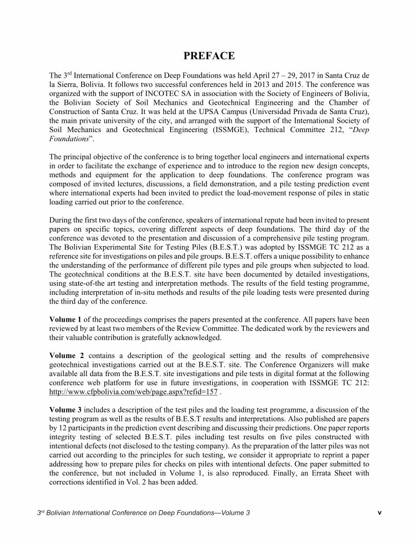
PREFACE The 3rd International Conference on Deep Foundations was held April 27 – 29, 2017 in Santa Cruz de la Sierra, Bolivia. It follows two successful conferences held in 2013 and 2015. The conference was organized with the support of INCOTEC SA in association with the Society of Engineers of Bolivia, the Bolivian Society of Soil Mechanics and Geotechnical Engineering and the Chamber of Construction of Santa Cruz. It was held at the UPSA Campus (Universidad Privada de Santa Cruz), the main private university of the city, and arranged with the support of the International Society of Soil Mechanics and Geotechnical Engineering (ISSMGE), Technical Committee 212, “Deep Foundations”. The principal objective of the conference is to bring together local engineers and international experts in order to facilitate the exchange of experience and to introduce to the region new design concepts, methods and equipment for the application to deep foundations. The conference program was composed of invited lectures, discussions, a field demonstration, and a pile testing prediction event where international experts had been invited to predict the load-movement response of piles in static loading carried out prior to the conference. During the first two days of the conference, speakers of international repute had been invited to present papers on specific topics, covering different aspects of deep foundations. The third day of the conference was devoted to the presentation and discussion of a comprehensive pile testing program. The Bolivian Experimental Site for Testing Piles (B.E.S.T.) was adopted by ISSMGE TC 212 as a reference site for investigations on piles and pile groups. B.E.S.T. offers a unique possibility to enhance the understanding of the performance of different pile types and pile groups when subjected to load. The geotechnical conditions at the B.E.S.T. site have been documented by detailed investigations, using state-of-the art testing and interpretation methods. The results of the field testing programme, including interpretation of in-situ methods and results of the pile loading tests were presented during the third day of the conference. Volume 1 of the proceedings comprises the papers presented at the conference. All papers have been reviewed by at least two members of the Review Committee. The dedicated work by the reviewers and their valuable contribution is gratefully acknowledged. Volume 2 contains a description of the geological setting and the results of comprehensive geotechnical investigations carried out at the B.E.S.T. site. The Conference Organizers will make available all data from the B.E.S.T. site investigations and pile tests in digital format at the following conference web platform for use in future investigations, in cooperation with ISSMGE TC 212: http://www.cfpbolivia.com/web/page.aspx?refid=157 . Volume 3 includes a description of the test piles and the loading test programme, a discussion of the testing program as well as the results of B.E.S.T results and interpretations. Also published are papers by 12 participants in the prediction event describing and discussing their predictions. One paper reports integrity testing of selected B.E.S.T. piles including test results on five piles constructed with intentional defects (not disclosed to the testing company). As the preparation of the latter piles was not carried out according to the principles for such testing, we consider it appropriate to reprint a paper addressing how to prepare piles for checks on piles with intentional defects. One paper submitted to the conference, but not included in Volume 1, is also reproduced. Finally, an Errata Sheet with corrections identified in Vol. 2 has been added.
v3rd Bolivian International Conference on Deep Foundations—Volume 3

vi 3rd Bolivian International Conference on Deep Foundations—Volume 3

Information on the single pile, static loading tests at B.E.S.T.
Fellenius, B.H.(1) and Terceros H.M.(2)
(1) Consulting Engineer, Sidney, BC, Canada, V8L 2B9 [email protected]
(2) Incotec S.A., Santa Cruz de la Sierra, Bolivia <[email protected]>
ABSTRACT. A brief background to the presentation of the results of the static loading tests on the single piles at the B.E.S.T. research site is presented. The test results are available in Excel files placed on the conference web site and reference is made herein to where in the Proceeding Volumes detailed information on the background is available. 1. INTRODUCTION
As a part of the 3rd Bolivian International Conference on Deep Foundations, a comprehensive pile testing programme was undertaken at the Bolivian Experimental Site for Testing Piles, B.E.S.T. The main objective of programme. was to compare the results of static loading tests on piles constructed using different methods at a site where the geotechnical conditions would be documented by detailed investigations, using state-of-the art testing and interpretation methods. The geotechnical conditions and the details on the piles and testing arrangement is presented in Proceedings Volume 2, Chapter 5. All field investigations records of the static loading tests are available for online downloading at http://www.cfpbolivia.com/web/page.aspx?refid=113. The downloading requires registration. 2. TEST PILES AND TEST METHODS
Three main types of piles were included in the testing programme as listed in Table 1. All test piles were installed to 9.5 m depth (bottom of reinforcement cage) below the ground surface. The bidirectional device (BD) consisted of a 200 mm high and 80 mm wide hydraulic jack and was installed centered in the "BD-piles" at 8.3 m depth (lower end of jack) in all TB and EBI (Expander Body with post-grouting) equipped piles, but for Piles F1 and F2, where the BD was installed at 6.5 m depth.
It is important to note that the reversal of shear force direction in the head-down test after a preceding bidirectional test affected the load-movement response of the test pile.
The test piles were strain-gage instrumented and the gages were installed in diametrically opposed pairs at 2.0 m, 5.0 m, and 7.5 m depths. Two parallel and separate systems of gages were used: one system employed electrical resistance gages and the other vibrating wire gages. Due to varying power supply and inability to record the data, but unrelated to the gage system itself, the vibrating wire gages never produced useful records.
The head-down test records of the electrical resistance gages showed that relatively large strains (maximum strains were within about 200 through 400 µõ). Therefore, where the head-down was applied as the first test (Piles A3, B2, C2), the strain records assisted in determining the load distributions. For the BD tests, however, the records of are not very useful because the strains imposed were too small and the expansion of the Expander Base units imposed residual strains in the pile and that adversely affected the evaluation of the load from the strain values.
13rd Bolivian International Conference on Deep Foundations—Volume 3

The reversal of shear force direction in the head-down test after a preceding BD test affected the load-movement response of the test pile, which made the evaluation of the measured strains during the subsequent head-down test, rather ambiguous.
TABLE 1. Primary information on the test piles.
ID Type Toe Test Methods Remark Augment Applied
Pile A1 620-mm bored pile EBI BD HD Pile A2 620-mm bored pile TB BD HD Pile A3 620-mm bored pile - - HD Pressure grouted Pile B1 450 mm CFA pile EBI BD HD Pressure grouted Pile B2 450 mm CFA pile - - HD Pressure grouted Pile C1 450 mm FDP pile EBI BD HD Pressure grouted Pile C2 450 mm FDP pile - - HD Pressure grouted Pile D1 150 mm bored pile EBI HD Pressure grouted Pile D2 150 mm bored pile - - HD Pressure grouted Pile E1 300 mm FDP pile EBI BD HD Pressure grouted Pile F1 450 mm bored pile EBI BD HD Pile F2 600 mm bored pile EBI BD HD Pile G1 helical pile EBI HD
EBI = Expander Base with post-grouting at pile toe, TB = Toe Box, BD = bidirectional test, HD = Head-down test.
Piles A3, B2, C2, and E3 were included in a Prediction Event reported separately in Volume 3. After completion of the 1st test on Pile A1 (Pile A1 BD), it was found that the data acquisition
equipment had not stored the records. The test was then repeated. The file called EB Expansion Records.xlsx reports the grouting volumes and pressures. The
expansion of the TB resulted in a 115-mm increase of height and the final grout pressure was 4.2 MPa. The BD unit of Pile A1 had 800 mm nominal diameter expanded to about 650 mm. All other EB-units (Piles B1, C1, D1, and E1) had 600 mm diameter and were expanded to widths of about 500, 500, 400, and 350 mm, respectively.
Test on expanding the EB in-air, i.e., unrestricted by pile tension and soil resistance, has shown to result in an about 200 mm shortening of the EB length. Such shortening of the EB in the soil could potentially result in softening of the soil below the EB and it is counteracted by post-grouting below the EB (EBI).
The BD piles were also instrumented with telltale rods to measure the movement of the upper and lower BD plates. Unfortunately, the expansion of the EB (and TB) invariably broke the connection of the telltale to the pile BD bottom and only the upper telltale gave useful records of movement. The usefulness is only approximate, however, because the telltales were deformed bars inside a pipe and side friction obviously affected the movement measurements.
2 3rd Bolivian International Conference on Deep Foundations—Volume 3
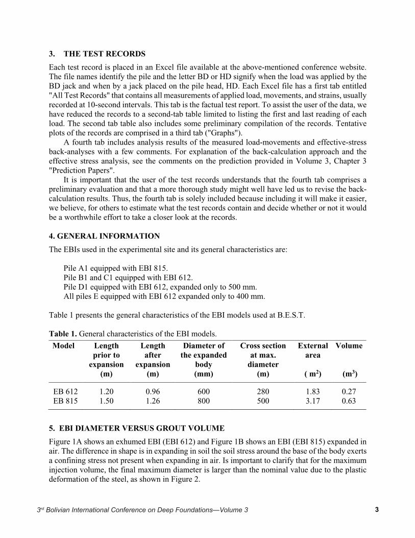
3. THE TEST RECORDS
Each test record is placed in an Excel file available at the above-mentioned conference website. The file names identify the pile and the letter BD or HD signify when the load was applied by the BD jack and when by a jack placed on the pile head, HD. Each Excel file has a first tab entitled "All Test Records" that contains all measurements of applied load, movements, and strains, usually recorded at 10-second intervals. This tab is the factual test report. To assist the user of the data, we have reduced the records to a second-tab table limited to listing the first and last reading of each load. The second tab table also includes some preliminary compilation of the records. Tentative plots of the records are comprised in a third tab ("Graphs").
A fourth tab includes analysis results of the measured load-movements and effective-stress back-analyses with a few comments. For explanation of the back-calculation approach and the effective stress analysis, see the comments on the prediction provided in Volume 3, Chapter 3 "Prediction Papers".
It is important that the user of the test records understands that the fourth tab comprises a preliminary evaluation and that a more thorough study might well have led us to revise the back-calculation results. Thus, the fourth tab is solely included because including it will make it easier, we believe, for others to estimate what the test records contain and decide whether or not it would be a worthwhile effort to take a closer look at the records. 4. GENERAL INFORMATION
The EBIs used in the experimental site and its general characteristics are:
Pile A1 equipped with EBI 815. Pile B1 and C1 equipped with EBI 612. Pile D1 equipped with EBI 612, expanded only to 500 mm. All piles E equipped with EBI 612 expanded only to 400 mm.
Table 1 presents the general characteristics of the EBI models used at B.E.S.T. Table 1. General characteristics of the EBI models.
Model Length prior to
expansion (m)
Length after
expansion (m)
Diameter of the expanded
body (mm)
Cross section at max.
diameter (m)
External area
( m2)
Volume
(m3)
EB 612 1.20 0.96 600 280 1.83 0.27 EB 815 1.50 1.26 800 500 3.17 0.63
5. EBI DIAMETER VERSUS GROUT VOLUME
Figure 1A shows an exhumed EBI (EBI 612) and Figure 1B shows an EBI (EBI 815) expanded in air. The difference in shape is in expanding in soil the soil stress around the base of the body exerts a confining stress not present when expanding in air. Is important to clarify that for the maximum injection volume, the final maximum diameter is larger than the nominal value due to the plastic deformation of the steel, as shown in Figure 2.
33rd Bolivian International Conference on Deep Foundations—Volume 3

Fig. 1. Exhumed EBI (EBI 612. Fig. 2. in-air expanded EBI (EBI 815).
Each model of EBI has a calibration curve representing the maximum diameter of the body versus volume of injected grout, cf. Figure 3. These curves are useful in the cases when the maximum volume is not reached, which could happen for reasons, such as like leakage, lack of pump capacity, etc.
5. EXPANDER BODIES USED IN THE B.E.S.T.
In the B.E.S.T. the actual EBIs had the following injected volumes and maximum diameters:
Pile A1 EBI 815 was injected with 266 liters, corresponding to 700-mm maximum diameter. Pile B1 EBI 612 was injected with 237 liters, corresponding to 675 mm maximum diameter. Pile C1 EBI 612 was injected with 210 liters, corresponding to 668 mm maximum diameter. Pile D1 EBI 612 was injected with 130 liters, corresponding to 489 mm maximum diameter. Pile E1 EBI 612 was injected with 110 liters, corresponding to 407 maximum diameter.
Acknowledgment
The detailed planning of the pile tests, instrumenting and constructing the piles, and performing the static loading tests were handled by Mario Terceros Arce and Bernado Vidal of Incotec S.A., Santa Cruz de la Sierra, Bolivia.
4 3rd Bolivian International Conference on Deep Foundations—Volume 3

Fig. 3. EBI calibration curves – expansion in air.
y = -0.0018x2 + 2.4509x + 174.24R² = 0.9942
0
100
200
300
400
500
600
700
800
900
0 100 200 300 400 500
DIA
MET
ER (
mm
)
VOLUME (L)
Regression Curve
EBI 815
y = -0.0191x2 + 8.792x - 312.19R² = 0.9906
0
100
200
300
400
500
600
700
800
900
0 50 100 150 200 250
DIA
MET
ER (
mm
)
VOLUME (L)
Regression Curve
EBI 612
53rd Bolivian International Conference on Deep Foundations—Volume 3

6 3rd Bolivian International Conference on Deep Foundations—Volume 3

Report on the B.E.S.T. prediction survey
Fellenius, B.H. (1)
(1) Consulting Engineer, Sidney, BC, Canada, V8L 2B9. <[email protected]> ABSTRACT. A prediction event organized in connection with the 3rd Bolivian International Conference on Deep Foundations attracted 72 contributions from all parts of the world predicting response to loading of four single piles, three tested in by head-down method and one by bidirectional method. The piles were constructed by different methods: one bored with slurry, one continuous flight auger, and two full displacement of the soils, one of which was the bidirectional pile. The predicted load-movement curves differed within a wide range. Most participants underestimated the actual pile response determined in subsequent static loading tests. The predictors were also asked to assess the capacities from the predicted load-movement response and the methods used and assessed values differed considerably. After all prediction had been submitted, static loading tests were performed on the piles. The participants were given the actual test results and asked to assess and submit capacities from the actual tests. The low and high of the assessed capacities ranged widely, making it clear the profession's concept of capacity deviates significantly between practitioners and not just between countries, but also within. 1. INTRODUCTION
In connection with the 3rd Bolivian International Conference on Deep Foundations, Santa Cruz de la Sierra, Bolivia April 27 - 29, 2017, site investigations were performed at the Bolivian Experimental Site for Testing Piles (B.E.S.T.) employing boreholes (SPT), cone penetrometer tests (SCPTU), pressuremeter tests (PMT), and dilatometer tests (DMT). The site investigation results have been reported in Volume 2 to the conference. The B.E.S.T. also included a total of 26 static and 4 dynamic tests constructed using different methods and employing different features for stiffening the pile response to load. The static tests of four single piles were selected for a prediction event. One pile (Pile A3) was drilled with slurry, one (Pile B2) was constructed with a continuous flight auger, and two (C2 and E1) were constructed by full displacement equipment. Piles A3, B2, and C2 were tested in head-down tests and Pile E1 by means of a bidirectional test. Pile E1 was supplied with an expanded base (EBI) with post-grouting at the pile toe. The others were straight-shaft piles.
Two months before the tests (January 2017), the profession was invited to submit predictions of the load-movements to be measured in the tests and to assess the capacity from these curves as well as predict the distribution of load in the piles at the so-assessed capacities. The invitees confirming interest in participation were supplied with the site and pile details. A few declined addressing the bidirectional test due to insufficient experience of this test method. Some submitted only the load-movement curves and no load distribution. All who submitted a load-movement prediction were then sent the results of the actual tests and asked to assess the tests as to pile capacity. The prediction of any group or individual are not disclosed to anyone.
A prediction event is a source of entertainment with a serious content. They usually attract considerable interest at many international and national conferences and this well beyond the conference attendees. I experienced recently a couple of such international geotechnical prediction events where the organizers, after receipt of predictions, requested payment from the participants
73rd Bolivian International Conference on Deep Foundations—Volume 3

and discarded received predictions when the predictor declined to pay. Moreover, the results were not disclosed to the participants, who had to wait for and purchase a summary publication of the results. I consider such events to be poorly and unprofessionally organized and hope they will not have followers.
A prediction event, such as the one reported here, must not be thought of as the same as a design effort. The main difference lies in the fact that a design involves liability while the only risk in submitting a prediction is for one's pride. Moreover, the effort that goes into a design of an actual piled foundation is that, in the latter, the engineer will have experience, or access to experience, of how other piles have responded at the site including construction methods and contractors' past performance, or no commitment will be made until results of suitable full-scale tests and other pertinent observations are available. The prediction presumes no such information.
It should be noted that the prediction pertained to the load-movement response of the test piles and that the part on the pile "capacity" was not a prediction, but an assessment. The following presents a compilation of the predictions and assessments. 2 SUBMITTED PREDICTIONS 2.1 Participants
A total of 72 separate predictions were submitted by 121 individuals from 30 different countries. Ten of the submissions were received from members of ISSMGE TC212. Appendix A lists the names, affiliation, and coordinates of all participants submitting predictions. A total of 94 of the 121 individual participants (54 of the 72 predictions) responded also to the second part of the survey and assessed the pile capacities as determined for the actual tests. While a couple of submissions were from students learning about analysis of pile response to load, most were submitted by practicing engineers and researchers knowledgeable in the field. Indeed, several of the participants are widely recognized for their expertise. I consider the results of the prediction survey to represent the current state-of-the-practice of analysis of pile response to load, i.e., what we know today and of what we typically accomplish in estimating expected pile response and how we assess the results of a static loading test. 2.2 Compiled Submissions
All submitted prediction results are presented in the graphs placed at the end of this paper. The diagrams have been separated on each pile type, Piles A3, B2, C2, and E1, respectively.
Figures 1, 6, and 11 compile all predicted pile-head load-movement curves. Figure 16 compiles the predicted upward and downward load-movement curves for Pile E1, the bidirectional test-pile. Each diagram is supplemented with the actual load-movement curve.
Figures 2, 7, and 12 show the assessed pile capacities of the three head-down tests and Figure 17 shows the submitted equivalent head-down tests constructed from the predicted Pile E1 tests. Each of the red dots in the graph indicates the capacity submitted as assessed from the curve by the submitting predictor.
Figures 3 and 4, 8 and 9, and 13 and 14 show the predicted distributions of load and shaft resistances for the head-down tests, as calculated for an applied load equal to the assessed capacity.
Figures 5, 10, and 15 show the plot of toe resistance (obtained from the load distribution data) versus the pile movement (pile shortening was negligible) for the load equal to the assessed capacity.
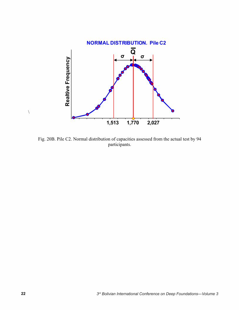
Figures 18A and 18B through 20A and 20B show a compilation of the predictors' assessment of pile capacity of the actual pile tests (54 participants). The A-part of the figure pairs shows the
8 3rd Bolivian International Conference on Deep Foundations—Volume 3

actual pile-head load-movement curve with the assessed capacities. The B-part shows the normal distribution of the capacity values and the corresponding standard variation (Ã). The double-arrow indicates the range of capacity between one standard deviation below and beyond the average value. The average is the intersection of the double-arrow and the test curve.
2.3 Comments
In predicting pile-head load-movement curves, the participants relied on different sets of the site investigation results. Some elected only to use the SPT N-indices. Others used mainly the CPTU records applying different correlations to the cone stress records. A few preferred to rely on the pressuremeter records. Only one reported having used the dilatometer records. A few, like me, used "engineering judgment" and records of past tests (results of the test performed in connection with the 1st and 2nd Conferences). Many included a list of references for background information to their predictions.
A variety of software was used for the calculations: Plaxis 2D and 3D, Flac 3d, Piglet, CPeT-IT, SHAFT 2012, UniPile5, Piver by ISTAR, Apile5, Repute, general finite element methods, company internal software, Mathlab, and personal Excel sheet templates. Effective stress analysis appears to have been used by most, though a couple reported using total stress analysis with reference to literature for sources of shaft and toe resistances.
The range between underestimated and overestimated stiffness responses of the predicted load-movement curves is wide. For Pile A3 (Figure 1), an eyeballed average prediction curve would not be too far off from the actual test curve, albeit slightly stiffer than the actual. For Piles B2, and C2 (Figures 6 and 11), the predictions generally underestimated the pile stiffness.
A CFA pile is generally expected to produce a somewhat larger shaft resistance as opposed to a bored pile. Both piles are considered to show small toe stiffness due to debris collected at the bottom of the shaft despite cleaning efforts. The fact that the concrete in the CFA-pile, Pile B2, was placed by pressure-grouting may have increased its shaft resistance, a fact that was not known to the predictors (nor to me), when submitting the prediction. The predictions were quite shy of the actual pile response also for Pile C2, the pile constructed by full-displacement method (FDP). This may again be because the predictors may not have sufficient experience of this full-displacement construction method and how much it enhances the pile shaft resistance.
The law of averages ensures that some of the predicted load-movement curves must be close to the actual and a couple are. I have not checked whether a predictor whose prediction was close to the actual results on one test, also produced predictions close to the other tests. The prediction event is not a competition and no "winner" will be announced. All predictors have received copies of the actual test results and can judge for themselves as to how close or distant their predictions were from the actual pile response. All test results are also available for downloading from the 3rd CFPB web site.
Each participant also submitted a pile capacity value as assessed from their predicted load-movement curves. Note, this capacity is not a prediction, but a value that anybody applying the same definition (and judgment) would determine from the prediction curve. Some of the participants defined capacity as the load that produced a movement equal to 5 % of the pile head diameter. Some choose to use 10 % of pile diameter—no doubt in the common and quite erroneous belief that this a definition proposed by Terzaghi (Likins et al. 2011). Terzaghi stated the opposite; that no one should define a capacity unless the pile toe had moved a distance equal to at least 10 % of the diameter, and, N.B., that the then determined capacity could be smaller or larger than the
93rd Bolivian International Conference on Deep Foundations—Volume 3
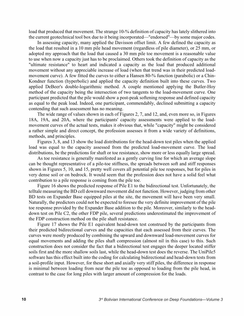
load that produced that movement. The strange 10-% definition of capacity has lately slithered into the current geotechnical tool box due to it being incorporated—"endorsed"—by some major codes.
In assessing capacity, many applied the Davisson offset limit. A few defined the capacity as the load that resulted in a 10 mm pile head movement (regardless of pile diameter), or 25 mm, or adopted my approach that the load that caused a 30 mm pile toe movement is a reasonable value to use when now a capacity just has to be proclaimed. Others took the definition of capacity as the "ultimate resistance" to heart and indicated a capacity as the load that produced additional movement without any appreciable increase of load (when that trend was in their predicted load-movement curve). A few fitted the curves to either a Hansen 80-% function (parabolic) or a Chin-Kondner function (hyperbolic) and applied the capacity definition built into these curves. Two applied DeBeer's double-logarithmic method. A couple mentioned applying the Butler-Hoy method of the capacity being the intersection of two tangents to the load-movement curve. One participant predicted that the pile would show a post-peak softening response and defined capacity as equal to the peak load. Indeed, one participant, commendably, declined submitting a capacity contending that such assessment has no meaning.
The wide range of values shown in each of Figures 2, 7, and 12, and, even more so, in Figures 18A, 19A, and 20A, where the participants' capacity assessments were applied to the load-movement curves of the actual tests, makes it obvious that, while "capacity" might be considered a rather simple and direct concept, the profession assesses it from a wide variety of definitions, methods, and principles.
Figures 3, 8, and 13 show the load distributions for the head-down test piles when the applied load was equal to the capacity assessed from the predicted load-movement curve. The load distributions, be the predictions for shaft or toe resistance, show more or less equally large spread.
As toe resistance is generally manifested as a gently curving line for which an average slope can be thought representative of a pile-toe stiffness, the spreads between soft and stiff responses shown in Figures 5, 10, and 15, pretty well covers all potential pile toe responses, but for piles in very dense soil or on bedrock. It would seem that the profession does not have a solid feel what contribution to a pile response is coming from the pile toe.
Figure 16 shows the predicted response of Pile E1 to the bidirectional test. Unfortunately, the telltale measuring the BD cell downward movement did not function. However, judging from other BD tests on Expander Base equipped piles at the site, the movement will have been very small. Naturally, the predictors could not be expected to foresee the very definite improvement of the pile toe response provided by the Expander Base addition to the pile. Moreover, similarly to the head-down test on Pile C2, the other FDP pile, several predictions underestimated the improvement of the FDP construction method on the pile shaft resistance.
Figure 17 shows the Pile E1 equivalent head-down test construed by the participants from their predicted bidirectional curves and the capacities that each assessed from their curves. The curves were mostly produced by combining the upward and downward load-movement curves for equal movements and adding the piles shaft compression (almost nil in this case) to this. Such construction does not consider the fact that a bidirectional test engages the deeper located stiffer soils first and the more shallow soils last, while the head-down test does the reverse. The UniPile5 software has this effect built into the coding for calculating bidirectional and head-down tests from a soil-profile input. However, for these short and axially very stiff piles, the difference in response is minimal between loading from near the pile toe as opposed to loading from the pile head, in contrast to the case for long piles with larger amount of compression for the loads.
10 3rd Bolivian International Conference on Deep Foundations—Volume 3

3. CONCLUSIONS
This said, the spread of the predicted pile-head load-movement responses certainly gives reason for reflection. The spread of the subject survey is not unique, but rather similar to many other prediction surveys. The spread pertains to both a limit value of load and to the movement required to mobilize this. No trend was discernible that could relate difference with regard to domicile of the predictor.
Most distressing is that the profession does not have a common understanding of the concept of capacity. Some may agree with me, as one predictor appeared to do, that "capacity" is a flawed and unnecessary concept that we would do well to abandon. However, the fact is that the prevailing design practice and most Codes and Standards do require a pile capacity value. Some such even define how to determine a capacity. For example, the EuroCode compels defining capacity as the load that gave a movement equal to 10-% of the pile diameter. However, I do not know of any structure that would care one whit about the diameter of the piles providing the support. Some definitions do make sense, e.g., letting the "capacity" to apply in the design effort be determined by a movement limit. A problem is that a "capacity" and its downgraded value after applying a safety factor or resistance factor correlate poorly to a limit of movement (settlement) for the piled foundation.
If fact, we do not need to base our designs on a "capacity". The response of the piles to load can easily be discussed—conservatively, of course—in terms of movement (settlement) for the actual foundation loads. Addressing the settlement for the sustained load on the foundation is certainly addressing the true issue of piled foundation design and a more rational approach than pursuing it in relation a load-value that will not ever be imposed by the structure or demanded from the soil.
Reference
Likins, G.E., Fellenius, B.H., and Holtz, R.D., 2011. Pile Driving Formulas—Past and Present. ASCE GeoInstitute Geo-Congress Oakland, March 25-29, 2012, Full-scale Testing in Foundation Design, State of the Art and Practice in Geotechnical Engineering, ASCE, Reston, VA, M.H. Hussein, K.R. Massarsch, G.E. Likins, and R.D. Holtz, eds., Geotechnical Special Publication, GSP 227, pp. 737-753.
113rd Bolivian International Conference on Deep Foundations—Volume 3

Fig. 1. Pile A3. Predicted and actual head-down tests pile-head load-movements. Pile A3 was constructed as a bored pile excavated using bentonite slurry. The nominal diameter of the pile is 620 mm. The as-used concrete volume corresponds to 670 mm average actual diameter, but this is a very approximate value. The as-is pile depth was the designed depth, 9.3 m. Construction and test dates were March 8 and March 20, respectively.
Fig. 2. Pile A3. Predicted pile-head load-movements and the respective assessed capacities.
0
500
1,000
1,500
2,000
2,500
0 25 50 75 100 125
LOAD
(kN
)
MOVEMENT (mm)
Pile A3
0
500
1,000
1,500
2,000
2,500
0 25 50 75 100 125
LOAD
(kN
)
MOVEMENT (mm)
Pile A3
12 3rd Bolivian International Conference on Deep Foundations—Volume 3

Fig. 3. Load-distribution at 'capacity'. Fig. 4. Shaft resistance distribution at 'capacity'.
Fig. 5. Pile A3. Toe force at 'capacity' plotted at predicted toe movement.
0
1
2
3
4
5
6
7
8
9
10
0 500 1,000 1,500 2,000 2,500 3,000
DEP
TH (
m)
LOAD (kN)
Pile A3
0
1
2
3
4
5
6
7
8
9
10
0 200 400 600 800 1,000 1,200
DEP
TH (
m)
SHAFT RESISTANCE (kN)
Pile A3
0
400
800
1,200
1,600
2,000
0 25 50 75 100 125
TOE
FOR
CE
(kN
)
MOVEMENT (mm)
Pile A3
133rd Bolivian International Conference on Deep Foundations—Volume 3

Fig. 6. Pile B2. Predicted pile-head load-movements and the respective assessed capacities. Pile B2 is a CFA-constructed pile. The concrete was placed by pressure-grouting as opposed to gravity flow. The nominal diameter of the pile is 450 mm. The as-used concrete volume corresponds to 445 mm average actual diameter, which is practically the same value. The as-is pile depth was the designed depth 9.3 m. Construction and test dates were March 11 and March 23, respectively.
Fig. 7. Pile B2. Predicted pile capacities with predicted pile-head load-movement curves.
0
500
1,000
1,500
2,000
2,500
0 25 50 75 100 125
LOAD
(kN
)
MOVEMENT (mm)
Pile B2
0
500
1,000
1,500
2,000
2,500
0 25 50 75 100 125
LOAD
(kN
)
MOVEMENT (mm)
Pile B2
14 3rd Bolivian International Conference on Deep Foundations—Volume 3
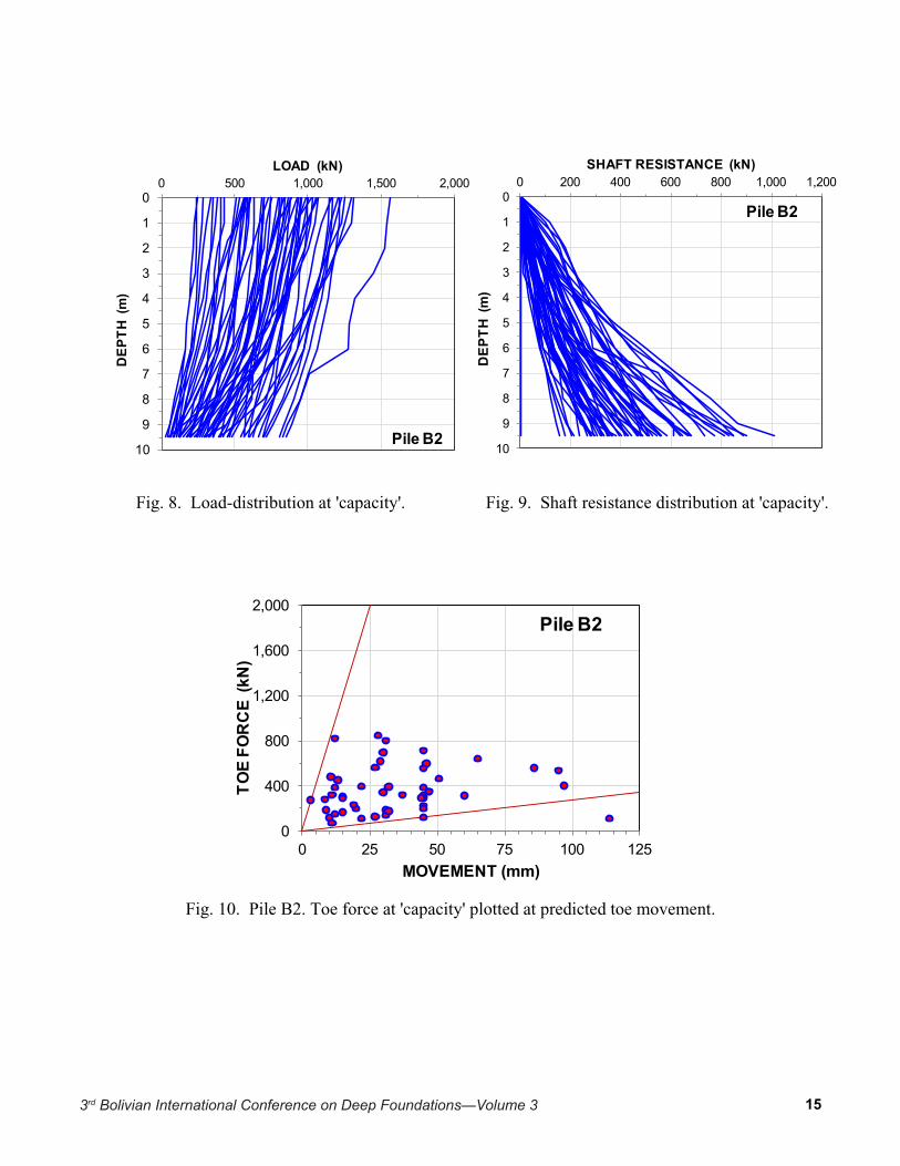
Fig. 8. Load-distribution at 'capacity'. Fig. 9. Shaft resistance distribution at 'capacity'.
Fig. 10. Pile B2. Toe force at 'capacity' plotted at predicted toe movement.
0
1
2
3
4
5
6
7
8
9
10
0 500 1,000 1,500 2,000
DEP
TH (
m)
LOAD (kN)
Pile B2
0
400
800
1,200
1,600
2,000
0 25 50 75 100 125
TOE
FOR
CE
(kN
)
MOVEMENT (mm)
Pile B2
0
1
2
3
4
5
6
7
8
9
10
0 200 400 600 800 1,000 1,200
DEP
TH (
m)
SHAFT RESISTANCE (kN)
Pile B2
153rd Bolivian International Conference on Deep Foundations—Volume 3

Fig. 11. Pile C2. Predicted pile-head load-movements and the respective assessed capacities. Pile C2 is a Full Displacement Pile (FDP)-constructed pile. The concrete was placed by pressure-grouting. The nominal diameter of the pile is 450 mm. The as-used concrete volume corresponds to 446 mm average actual diameter, which is practically the same value. The as-is pile depth was the designed depth, 9.3 m. Construction and test dates were March 7 and March 25, respectively. The pile was reloaded to have the pile-head movement (at least 75 mm and beyond) as was the movement for the other piles.
Fig. 12. Pile C2. Predicted pile capacities with predicted pile-head load-movement curves.
0
500
1,000
1,500
2,000
2,500
0 25 50 75 100 125
LOAD
(kN
)
MOVEMENT (mm)
Pile C2
0
500
1,000
1,500
2,000
2,500
0 25 50 75 100 125
LOAD
(kN
)
MOVEMENT (mm)
Pile C2
16 3rd Bolivian International Conference on Deep Foundations—Volume 3

Fig. 13. Load-distribution at 'capacity'. Fig. 14. Shaft resistance distribution at 'capacity'.
Fig. 15. Pile C2. Toe force at 'capacity' plotted at predicted toe movement.
0
1
2
3
4
5
6
7
8
9
10
0 500 1,000 1,500 2,000 2,500 3,000
DEP
TH (
m)
LOAD (kN)
Pile C2
0
1
2
3
4
5
6
7
8
9
10
0 200 400 600 800 1,000 1,200
DEP
TH (
m)
SHAFT RESISTANCE (kN)
Pile C2
0
400
800
1,200
1,600
2,000
0 25 50 75 100 125
TOE
FOR
CE
(kN
)
MOVEMENT (mm)
Pile C2
173rd Bolivian International Conference on Deep Foundations—Volume 3
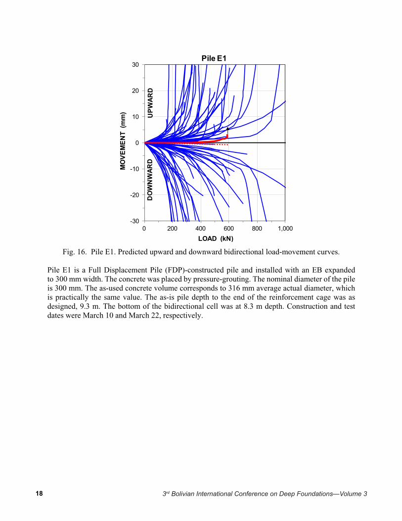
Fig. 16. Pile E1. Predicted upward and downward bidirectional load-movement curves. Pile E1 is a Full Displacement Pile (FDP)-constructed pile and installed with an EB expanded to 300 mm width. The concrete was placed by pressure-grouting. The nominal diameter of the pile is 300 mm. The as-used concrete volume corresponds to 316 mm average actual diameter, which is practically the same value. The as-is pile depth to the end of the reinforcement cage was as designed, 9.3 m. The bottom of the bidirectional cell was at 8.3 m depth. Construction and test dates were March 10 and March 22, respectively.
-30
-20
-10
0
10
20
30
0 200 400 600 800 1,000
MO
VEM
ENT
(mm
)
LOAD (kN)
UPW
ARD
Pile E1
DO
WN
WAR
D
18 3rd Bolivian International Conference on Deep Foundations—Volume 3

Fig. 17. Pile E1. Equivalent pile-head load-movement curves with assessed 'capacities'.
Fig. 18A. Pile A3. 54 'capacities' assessed from actual pile-head load-movement curve by 94 participants.
0
500
1,000
1,500
2,000
2,500
0 20 40 60 80 100
LOAD
(kN
)
MOVEMENT (mm)
Pile E1
0
200
400
600
800
1,000
1,200
1,400
0 10 20 30 40 50 60 70 80 90 100
LOA
D (
kN)
MOVEMENT (mm)
Pile A3Bored 620mm
1,750 kN
2 σ
Mean = 888 kNσ = 215 kN
193rd Bolivian International Conference on Deep Foundations—Volume 3
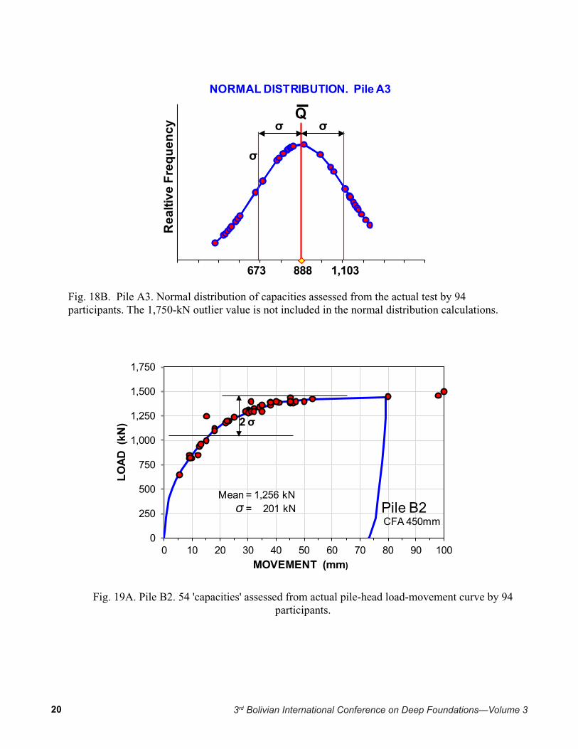
Fig. 18B. Pile A3. Normal distribution of capacities assessed from the actual test by 94 participants. The 1,750-kN outlier value is not included in the normal distribution calculations.
Fig. 19A. Pile B2. 54 'capacities' assessed from actual pile-head load-movement curve by 94 participants.
Rea
ltive
Fre
quen
cyσ
QNORMAL DISTRIBUTION. Pile A3
673 888 1,103
σσ
0
250
500
750
1,000
1,250
1,500
1,750
0 10 20 30 40 50 60 70 80 90 100
LOAD
(kN
)
MOVEMENT (mm)
Pile B2CFA 450mm
2 σ
Mean = 1,256 kNσ = 201 kN
20 3rd Bolivian International Conference on Deep Foundations—Volume 3

Fig. 19B. Pile B2. Normal distribution of capacities assessed from the actual test by 94 participants.
Fig. 20A. Pile C2. 54 'capacities' assessed from actual pile-head load-movement curve by 94 participants.
Rea
ltive
Fre
quen
cyσ
QNORMAL DISTRIBUTION. Pile B2
1,055 1,256 1,457
σσ
0
400
800
1,200
1,600
2,000
2,400
2,800
0 10 20 30 40 50 60 70 80 90 100
LOAD
(kN
)
MOVEMENT (mm)
Pile C2FDP 450mm
2 σ
Mean = 1,770 kNσ = 257 kN
213rd Bolivian International Conference on Deep Foundations—Volume 3
\
Fig. 20B. Pile C2. Normal distribution of capacities assessed from the actual test by 94 participants.
Rea
ltive
Fre
quen
cy
QNORMAL DISTRIBUTION. Pile C2
1,513 1,770 2,027
σσ
22 3rd Bolivian International Conference on Deep Foundations—Volume 3
Appendix A
Prediction Participants (participants shown in bold have submitted prediction papers which have been included in
Volume 3: B.E.S.T Predictions) Abchir, Zineb, University of Paris, Champs-sur-Marne, France Abrams, Tim, Terracon, Dallas, TX, USA Affi, Liiban, Foundation Engineering Consultants, Anaheim, CA, USA Akcakal, Önder, ZETAS Zemin Teknolojisi A.S., Istanbul, Turkey Albuquerque, Paulo, University of Campinas, Sao Paulo, Brazil Aljanabi, Hijran, Ferdowsi University of Mashhad, Mashhad, Iran Amorim, R. K., Egenharia Geotecnica, Brazil Bandeira, Neto L.A., Egenharia Geotecnica, Brazil Basile, Francesco, Geomarc Ltd., Messina, Italy Behroozian, Khalil, AUT, Tehran, Iran Bejancu, Ion, AATech, Ottawa, ON, Canada Bohn, Cecilia, Keller Holding, Frankfurt, Germany Burlon, Sebastien University of Paris, Champs-sur-Marne, France Buttling, Stephen, National Geotechnical Consulting, Yaltala, QLD, Australia Camacho, Boris, UMSS-Laboratorio de Geotecnia, Cochabamba, Bolivia Camacho, Marco Antonio, UMSS-Laboratorio de Geotecnia, Cochabamba, Bolivia Chan, Kim F., GHD Pty Ltd, Atarmon, Australia Chaudary, Sikander, Dente Engineering, New York, NY, USA Comodromos, Emilios, University of Thessaly, Greece Crawley, Charles, GeoEnvironmental Resources Inc, Virginia Beach, VA, USA Cunningham, John, Alder Geotechnical Services, Portland, OR, USA Dajani, Tareq, Vancouver, BC, Canada de Chaunac, Henri, UCL, Louvain-la-Neuve, Belgium Decourt, Luciano, Decourt Eng., Sao Paulo, Brazil Dei Svaldi, Andrea, University of Venice, Venice, Italy Edwards, Stuart, Michael Baker Int. Inc., Pittsburgh, PA, USA, Eriksson, Håkan, Geomind, Stockholm, Sweden Eslami, Abolfazl, AUT, Teheran, Iran Fakharian, Kazem, AUT, Tehran, Iran Fellenius, Bengt, BKFC, Sidney, BC, Canada Ferreira, Diogo, University of Coimbra, Coimbra, Portugal Fiorelli, Federico, Teleios srl, Castel Maggiore, Italy Franceschini, Marco, Teleios srl, Bologna, Italy Frank, Roger, University of Paris, Champs-sur-Marne, France Gao, Youi, China Gharsala, Haythem, UCL, Louvain-la-Neuve, Belgium Gidely, Iain, Thurber Engineering, Calgary, AB, Canada Grazina, José, University of Coimbra, Coimbra, Portugal Greaber, Steve, Terracon, Dallas, TX, USA Gunjan, Shimant, Fugro, Dubai, UAE
233rd Bolivian International Conference on Deep Foundations—Volume 3

Gwizdala, Kazimierz, Gdansk University, Gdansk, Poland Haghi, Iman, Cathie Associates, Nanterre, France Harris, Dean, CH2M, Sacramento, CA, USA Holeyman, Alain, University de Louvain, Louvain-la-Neuve, Belgium Hosseininia, Ehsan Seyedi, Ferdowsi University of Mashhad, Mashhad, Iran Iamato, K Y., Egenharia Geotecnica, Brazil Illingworth, Fernando, Tecnac Subterra, Guayquil, Ecuador Jeong, Sang Seom, Yonsei University, Seoul, Korea Jesswein, Markus, Ryerson University, Toronto, ON, Canada Jhalani, Mohit, NTPC Ltd., Noida, India Johan, Albert, Parahyangan Catholic University, Bandung, Indonesia Kim, Dohyun, Yonsei University, Seoul, Korea Kinnunen, Jussi, Valkeakoski, Finland Kos, Jan, Czech Technical University in Prague, Prague, Czech Republic Krasinski, Adam, Gdansk University, Gdansk, Poland Kristanto, Finna Setiani, Parahyangan Catholic University, Bandung, Indonesia Kumarasamy, Jitendra, NTPC Ltd., Noida, India Lavasan, Arash, Ruhr-University, Bochum, Germany Lee, John, CH2M, Santa Ana, CA, USA Liew, Shaw Shong, G&P Geotechnics Sdn Bhd, Kuala Lumpur, Malaysia Lopes dos Santos, Alexandre, University of Paris, Paris, France Lun, Martin, Thurber Engineering, Calgary, AB, Canada Macedo, A. D., Egenharia Geotecnica, Brazil Maiorano, Rosa Maria Stefania, University of Napoli, Napoli, Italy Makyama, E. S. V., Egenharia Geotecnica, Brazil Malek, Alain, BBRI, Brussles, Belgium Mandolini, Alessandro, Università degli Studi della Campania "Luigi Vanvitelli", Aversa, Italy Metaferia, Gohe, AATech, Ottawa, ON, Canada Moghaddam, Rozbeh, GRL, Cleveland, OH, USA Moshfeghi, S., AUT, Teheran, Iran Mousa Farkhani Mostafa, Ferdowsi University of Mashhad, Mashhad, Iran Mucolino, Elena, Teleios srl, Castel Maggiore, Italy Muller, Chris P., Hultgren-Tillis Engineers, Concord, CA, USA Murillo, Tomas, Uriel & Asociados, Pozuelo de Alarcón, Spain Nguyen, HongViet, Cathie Associates, Nanterre, France Nicolini, Emilio, Cathie Associates, Nanterre, France Nie, Rusong, Central South University, Changsha, China Noor, Mudasser, AATech, Ottawa, ON, Canada Oomen, Wieske, TU, Delft, Belgium Oztoprak, Sadik, Istanbul University, Istanbul, Turkey Pancaldi, Davide, Teleios srl, Castel Maggiore, Italy Penna, Antonio, S.D., Egenharia Geotecnica, Brazil Pereira, Mauricio Salinas, UMSS-Laboratorio de Geotecnia, Cochabamba, Bolivia Perera, Darshana, GHD Pty Ltd, Atarmon, Australia Pinto, Paulo, University of Coimbra, Coimbra, Portugal Poon, Bosco, GHD Pty Ltd, Atarmon, Australia
24 3rd Bolivian International Conference on Deep Foundations—Volume 3

Prieto, Rafael, Inteinsa, Medellin, Colombia Raba Moyano, Miguel Angel, Bogota, Colombia Rahardjo, Paulus, University Parahyanung, Bandung, Indonesia Ramos da Silva, Mikael, Fugro GeoConsulting, Brussels, Belgium Reiffsteck, Phillippe, University of Paris, Champs-sur-Marne, France Robertson, Peter, Gregg Drilling, Signal Hill, CA, USA Roca, Gabriel Rodriguez, UMSS-Laboratorio de Geotecnia, Cochabamba, Bolivia Rudianto, Sindhu, Geo-Optima Inc., Jakarta, Indonesia Russo, Gianpiero, University of Napoli, Napoli, Italy Santos, A.L., Navier Geotechnique, Université Paris Est, France Sargin, Sinan, Istanbul University, Istanbul, Turkey Schanz, Tom, Ruhr-University, Bochum, Germany Schmudderich, Christoph, Ruhr-University, Bochum, Germany Shah, D.L., Maharaja Sayajirao University of Baroda, Vadodara, India Shahrabi, M. Mahdi, UBC, Vancouver, BC, Canada Sharifi, Sohrab, Ferdowsi University of Mashhad, Mashhad, Iran Shkodrani, Neritan, Tirana, Albania Shukla, Jaykumar, L&T-Sargent & Lundy Ltd., Vadodara, India Shuntaro, Teramoto, Setsuan University, Osaka, Japan Siegel, Tim, Dan Brown and Associates, Knoxville TN, USA Sing, Anand Kumar, L&T-Sargent & Lundy Ltd., Vadodara, India Soliz, Wilsonn Heredia, UMSS-Laboratorio de Geotecnia, Cochabamba, Bolivia Stone, Rick, Savannah, GA, USA Taiebat, Mahdi, UBC, Vancouver, BC, Canada Tan, Harry, NUS, Singapore, Singapore Tarraf, Majd, Ferdowsi University of Mashhad, Mashhad, Iran Terceros A., Mario, Incotec, Santa Cruz, Bolivia Togliani, Gianni, Geologist, Massagno, Switzerland Tomaduci, F. B., Egenharia Geotecnica, Brazil Uyar, H. Kemal, Istanbul University, Istanbul, Turkey Vaidya, Ravikira, L&T-Sargent & Lundy Ltd., Vadodara, India Valikhah, F., AUT, Teheran, Iran Van Impe, William, AGE Bvga, Erpe-Mere, Belgium Wahyuningsih, Sri Ratna, Parahyangan Catholic University, Bandung, Indonesia Widjaja, Budijanto, Parahyangan Catholic University, Bandung, Indonesia
253rd Bolivian International Conference on Deep Foundations—Volume 3

26 3rd Bolivian International Conference on Deep Foundations—Volume 3

3rd Bolivian International Conference on Deep Foundations – Volume 3
Integrity test results of the 3rd Bolivian International Conference on Deep Foundations B.E.S.T. site
Amir, E.I.(1) and Amir, J.M.(2)
(1) President, Piletest.com, Israel <[email protected]> (2) Chairman, Piletest.com, Israel <[email protected]>
ABSTRACT. Integrity testing was performed on several piles at the "Bolivian Experimental Site for Testing" (B.E.S.T.): nine piles were tested with the Pulse-Echo method (ASTM D5882) using the PET (Pile Echo Tester) and five were tested by ultrasonic test methods (Cross-hole, 2D and 3D Tomography and single-hole) using the CHUM (Cross-Hole Ultrasonic Monitor) - Both systems were provided by Piletest.com. The results of the integrity tests are presented and several analysis techniques are demonstrated. 1. SOIL PROFILE
The soil profile underlying the site (Fellenius et al. 2017) typically consists of normally consolidated clays, silts, sands, in various combinations and thicknesses. The upper layer, about 5 to 6 m thick, consists of loose silt and sand below which lies a 6 to 7 m layer of compact silt and sand. At about 11 m depth lies an about 1 m thick layer of soft silty clay followed by an about 1 m thick layer of compact sand. Groundwater level is found between the ground surface and about 0.5 m depth. 2. SUMMARY OF RESULTS
TABLE 1. Summary of results. PILE CODE TYPE PILE Φ
(mm) Depth1) (m)
Stickup (m)
TESTS
A-5 Drilled with slurry 620.00 9.50 0.80 PET A-4 Drilled with slurry 620.00 9.50 0.58 PET A-3 Drilled with slurry 620.00 9.50 0.50 PET B-1 CFA 450.00 9.50 0.83 -- B-2 CFA 450.00 9.50 0.65 PET C-1 FDP 450.00 9.50 0.50 -- C-2 FDP 450.00 9.50 0.96 PET D-1 Self-boring Micropile 150.00 9.50 0.27 PET D-2 Self-boring Micropile 150.00 9.50 0.29 -- E-1 FDP 300.00 9.50 0.00 PET E-2 TO E-14 FDP 300.00 9.50 - -- F-1 Drilled with slurry 450.00 9.50 0.85 PET F-2 Drilled with slurry 600.00 9.50 0.57 PET G-1 Helical Pile 300.00 9.50 0.21 -- F-3 Drilled with slurry 1200.00 6.00 0.00 CHUM DC1200-1 Drilled with slurry 1200.00 2.50 (-0.85) CHUM DC620-1 Drilled with slurry 620.00 6.00 0 CHUM
273rd Bolivian International Conference on Deep Foundations—Volume 3

DC620-2 Drilled with slurry 620.00 6.00 0.00 CHUM DC620-3 Drilled with slurry 620.00 9.50 0.00 CHUM CFA450-1 CFA 450.00 9.50 0.00 CHUM CFA450-2 CFA 450.00 9.50 0.00 -- FDP450-1 FDP 450.00 9.50 - -- FDP360-1 FDP 360.00 9.50 0.00 --
1)"Depth" is depth below ground 3. DETAILED RESULTS
Abbreviations: TCL: Total Concrete Length (m) - calculated as the depth plus stickup (see Table 1). Note: all length measurements are from the pile head (includes the stickup above ground),
3.1 Pile A-2
Planned: TCL: 10.08 m, D: 620 mm, embedded jack above toe box.
Findings:
• Bulge at 4.7 m. • Uncertain length result: 11.5 m (matching cage length, 1.4 m
longer than planned TCL). • Very hard to see any toe reflection, even at double
amplification compared to A-1.
Analysis Techniques: visual inspection.
28 3rd Bolivian International Conference on Deep Foundations—Volume 3

3.2 Pile A-1
Planned: TCL: 10.30 m, D: 620 mm, embedded jack above Expander Base, grouted toe 1.2 m.
Findings:
• Necking at 1.3 m, also available at the FFT analysis.
• Clear toe reflection at 8.6 m - probably top of expander body.
Analysis Techniques: Visual inspection, FFT, signal matching.
293rd Bolivian International Conference on Deep Foundations—Volume 3

3.3 Pile A-3
Planned: TCL: 10.0 m, D: 620 mm, no jack, Expander Base, or Toe Box, reinforcement cage length = 11.50 m.
Findings:
• Very clear toe at 11.8 m: 1.8 m longer than planned TCL, but good match to cage length - could this be a typo in planned length?
Analysis Techniques: visual inspection, 2nd reflection very clear (high length certainty).
30 3rd Bolivian International Conference on Deep Foundations—Volume 3
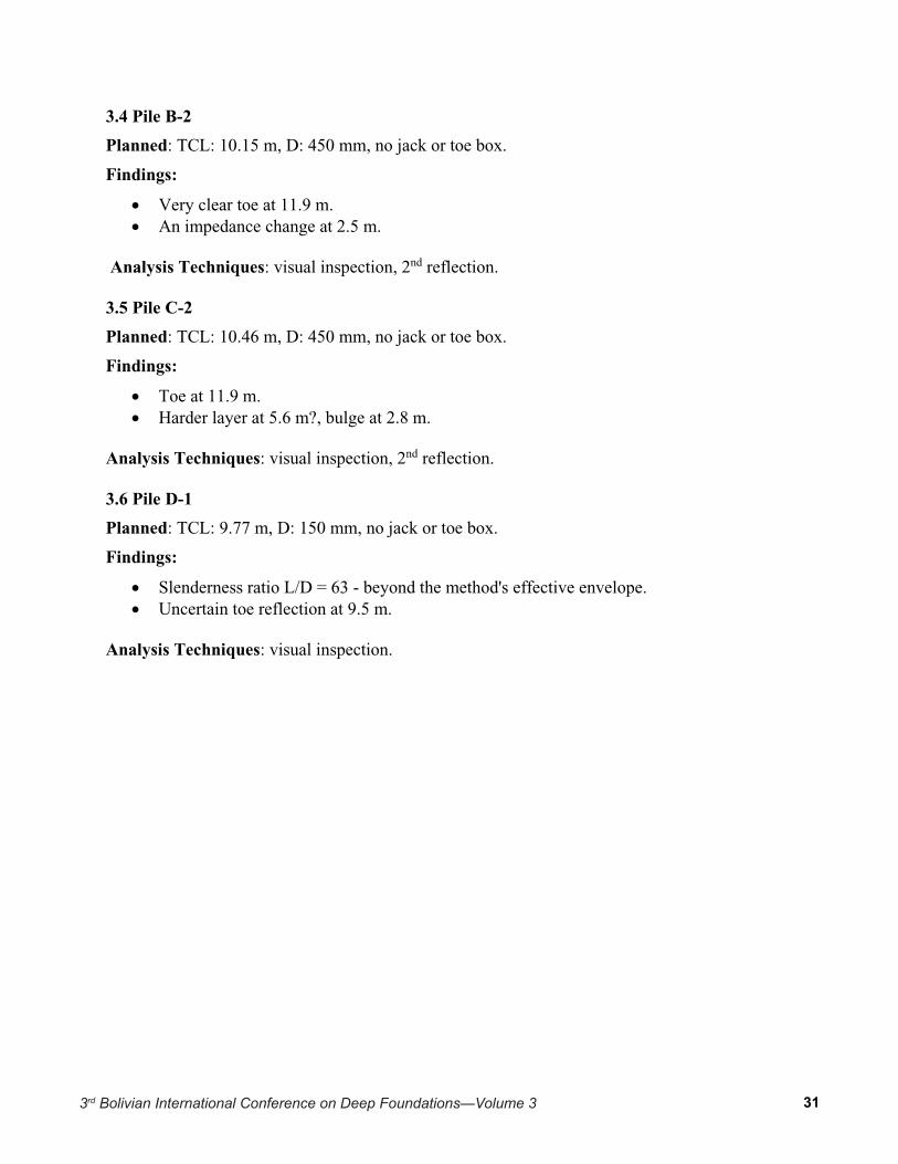
3.4 Pile B-2
Planned: TCL: 10.15 m, D: 450 mm, no jack or toe box.
Findings:
• Very clear toe at 11.9 m. • An impedance change at 2.5 m.
Analysis Techniques: visual inspection, 2nd reflection. 3.5 Pile C-2
Planned: TCL: 10.46 m, D: 450 mm, no jack or toe box.
Findings:
• Toe at 11.9 m. • Harder layer at 5.6 m?, bulge at 2.8 m.
Analysis Techniques: visual inspection, 2nd reflection. 3.6 Pile D-1
Planned: TCL: 9.77 m, D: 150 mm, no jack or toe box.
Findings:
• Slenderness ratio L/D = 63 - beyond the method's effective envelope. • Uncertain toe reflection at 9.5 m.
Analysis Techniques: visual inspection.
313rd Bolivian International Conference on Deep Foundations—Volume 3

3.7 Pile E-1
Planned: TCL: 9.5 m, D: 300 mm, Expander Base and bi-directional jack.
Findings:
• Slenderness ratio L/D = 32 - beyond the method's effective envelope. • Pile apparently broken at 1.2 m.
Analysis Techniques: FFT. Simulation available here.
32 3rd Bolivian International Conference on Deep Foundations—Volume 3

3.8 Pile F-1
Planned: TCL: 10.35 m, D: 450 mm, bi-directional jack 3 m above toe.
Findings:
• Clear toe reflection at 8.6 m (2nd and 3rd reflections also visible - high length certainty).
• Jack is visible at the expected location - but does not block the reflection from the toe.
Analysis Techniques: visual inspection. 3.9 Pile F-2
Planned: TCL: 10.07 m, D: 600 mm, bi-directional jack 3 m above toe.
Findings:
• Additional head as raised and cast above original head level. • Clear toe reflection at 9.5 m. • Strong reflector at 1.6 m - probably the above-ground extension.
Analysis Techniques: visual inspection.
333rd Bolivian International Conference on Deep Foundations—Volume 3
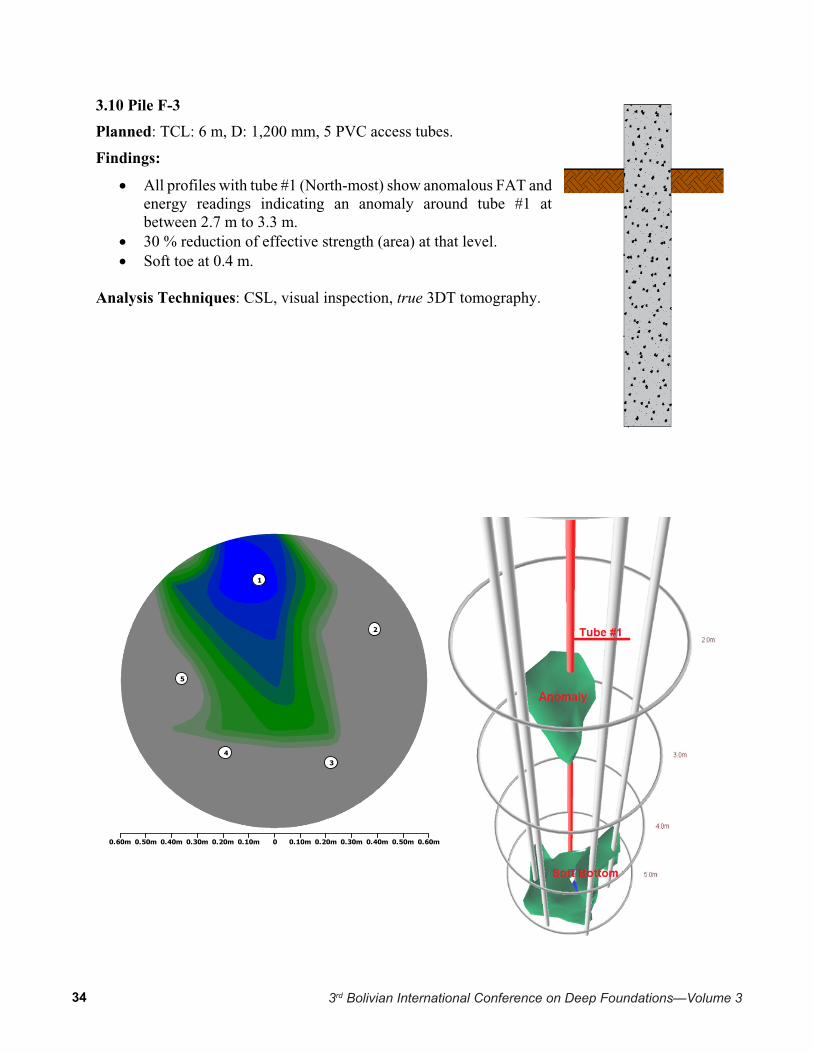
3.10 Pile F-3
Planned: TCL: 6 m, D: 1,200 mm, 5 PVC access tubes.
Findings:
• All profiles with tube #1 (North-most) show anomalous FAT and energy readings indicating an anomaly around tube #1 at between 2.7 m to 3.3 m.
• 30 % reduction of effective strength (area) at that level. • Soft toe at 0.4 m.
Analysis Techniques: CSL, visual inspection, true 3DT tomography.
1
2
34
5
0.60m 0.60m00.50m 0.40m 0.30m 0.20m 0.10m 0.10m 0.20m 0.30m 0.40m 0.50m
34 3rd Bolivian International Conference on Deep Foundations—Volume 3

3.11 Pile D! 1200-1
Planned: TCL: 1.65 m, D: 1,200 mm, 4 access tubes (not 5).
Findings:
• Unlike planned, pile head was at -0.85 m below ground level. Shaft was flooded.
• Cutoff clearly visible on CSL. • Severe anomaly 0.5 m above toe. • Pile was reported to be just 5 days old - marginally fit for
CSL testing.
Analysis Techniques: CSL, visual inspection.
353rd Bolivian International Conference on Deep Foundations—Volume 3

3.12 Pile D! 620-2
Planned: TCL 6 m, D: 620 mm, 3 access tubes.
Findings:
• Severe anomaly at the lower 2 m of the pile - all profiles. • Minor anomaly at ~1 m below pile head - close to north tube.
Analysis Techniques: CSL, visual inspection.
36 3rd Bolivian International Conference on Deep Foundations—Volume 3

3.13 Pile D! 620-3
Planned: TCL 9.5 m, D: 620 mm, 3 access tubes.
Findings:
• No anomalies found. • Access tubes not parallel.
Analysis Techniques: CSL, visual inspection.
3.14 Pile CFA 450-1
Planned: TCL 9.5 m, D: 450 mm, 1 PVC access tube.
Findings:
• No anomalies found.
Analysis Techniques: Single-Hole Ultrasonic Test (SHUT), visual inspection.
4. SUMMARY 4.1 Low-strain impact testing
a. Clear toe reflections were obtained from piles with a slenderness ratio (L/D) of 22, but not from those with a slenderness ratio above 60. b. An expanded base produces a clear toe reflection. An embedded jack may either reflect the waves or transmit them, depending on the specific configuration. c. The boundary between soil layers at 5 - 6 m depth was not noticeable in the results. 4.2. Ultrasonic testing
a. This test managed to discover soft toe conditions, although proximity to the toe prevented performing tomography. REFERENCES
Fellenius, B.H., Terceros H.M. and Massarsch. K.R. (2017). Bolivian Experimental Test Site - Presentation of Field Testing Programme. 3rd Bolivian Intl. Conf. on Deep Foundations. Santa Cruz de la Sierra. Volume 2, pp. 3 – 30.
373rd Bolivian International Conference on Deep Foundations—Volume 3

38 3rd Bolivian International Conference on Deep Foundations—Volume 3

Comments on the B.E.S.T. intentional defects and anomalies
Amir, J.M.(1) and Fellenius, B.H.(2)
(1) Chairman, Piletest.com, Israel <[email protected]
(2) Consulting Engineer, Sidney, BC, Canada <[email protected]>
ABSTRACT. The B.E.S.T. testing programme included an integrity testing demonstration, wherein the piles subjected to static loading tests and a total of eight additional piles constructed with intentional flaws that were kept unknown to the integrity tester. The value of the testing is very limited because only one company volunteered to participate by performing the integrity tests and, more disappointing, the preparation of the piles for intentional defects was botched due to inadequate communication between the organizers' office and field. The following are brief comments addressing what should have been addressed in the testing programme. 1. INTRODUCTION
In preparation of the 3rd Bolivian International Conference on Deep Foundations, an integrity demonstration was planned and executed with two main objectives in mind:
1. To demonstrate to participants up to date techniques for integrity testing of piles. 2. To invite manufacturers and testing firms to take part in an integrity testing
competition on piles constructed with intentional defects.
Unfortunately, the first objective could not be met due to weather conditions on the assigned date. The second objective suffered from the fact that only two firms appeared on site of which only one (Piletest.com Ltd.) submitted a report of the results. Thus, the affair could hardly be defined as a competition. Several aspects of this event are highlighted below for the benefit of similar events organized in the future. 2. PILE TESTING COMPETITIONS — OBJECTIVES AND PRINCIPLES
Pile testing competitions should be held with the following objectives in mind (Amir and Fellenius 2000 - this reference is reproduced for convenience in the Appendix to Volume 3 of the proceedings).
1. Kindling the competitive spirit between developers, manufacturers, and users of equipment in order to advance the state of the art.
2. Verifying capabilities and limitations of the testing methods. 3. Serving as milestones to monitor progress in both instrumentation and analysis
tools. 4. Providing an opportunity for potential clients to obtain reliable comparative data
regarding the performance of available commercial instruments.
393rd Bolivian International Conference on Deep Foundations—Volume 3

To meet the above objectives, a competition should try to simulate a realistic testing environment within the capabilities of existing instruments. The necessary conditions are, therefore:
1. The design of the competition should be based on firm theoretical grounds, meeting both stress-wave and statistical theories.
2. The tests should involve real piles, conventionally constructed, and constructed in real soil.
3. The piles should have various lengths and diameters. 4. At least some of the piles should include flaws (increased and decreased cross-
section). 5. For low-strain impact testing, only one flaw per pile shall be installed. 6. For cross-hole ultrasonic testing, piles may have several flaws with sufficient
vertical spacing between them. 7. Down the pile, the flaws should be of growing importance, from hardly discernible
to an almost complete discontinuity. 8. The data related to the flaws shall not be disclosed to the participants (type "A"
prediction). 9. The participants should get the same kind of data they expect in actual testing: Soil
profile, piling method, pile length (both design and as-made), and construction records.
10. The pile heads should be properly prepared, i.e. all poor quality concrete must be trimmed off, all loose concrete chunks removed and the surface made reasonably smooth and clean.
11. Access tubes must of the correct type (steel/plastic) and diameter and be free of obstructions.
12. The results should be reported in full for all piles, including the graphs and raw data.
3. SUGGESTED TESTING SCHEME
Based on the above principles, a testing setup, as summarized in Table 1, was prepared and submitted to the organizers of the B.E.S.T. ahead of time. Nine piles were prepared with intentional flaws: Piles F3, DC1200-1, DC620-1, DC620-2, DC620-3, CFA450-1, CFA450-2, FDP450-1, and FDP360-1. Unfortunately, instructions to the field staff on how to prepare the flawed piles was let to the field staff's own devices. They elected to produce the intentional flaws by tying multiple sand-filled bags with dimensions of about 200 x 100 mm—about 12 % of the pile cross section—to each reinforcing cage at different depths before inserting it into the hole or casing. This, obviously, is an impossible testing situation. The cross section of the "flaw-bags " is notably smaller than the accepted detection threshold of the integrity testing equipment (notwithstanding that the uppermost bag was clearly detected as a flaw by the single-hole ultrasonic method—the rest were invisible). For a series of flaws down a pile, the deeper-located flaws can only be assuredly detected if they are larger than those above—all bags were about equal size, however—and limited in number. The intentional flaws, as prepared, had neither relevance to the testing methods nor to being representative for flaws in actual piles.
Figure 1 shows the location of the "flaw-bags" as placed in Pile CFA450-1, a 450-mm diameter CFA pile.
40 3rd Bolivian International Conference on Deep Foundations—Volume 3

TABLE 1. Suggested test setup. Pile Construction Diameter Length Access Flaw Type Note Method (m) (m) Duct AI Cased pile 0.62 12 None None 1 AII Cased pile 0.62 2 None None 2 AIII Cased pile 0.62 12 3 x steel 30% @ 3 m AIV Cased pile 0.62 12 3 x PVC 50% @ 8 m BI Drilled w. slurry 0.45 12 1 x PVC Outside ring @ 4 m BII Drilled w. slurry 0.60 12 3 X PVC Outside ring @ 4 m and soft bottom CI Cased pile 1.20 6 5 x steel 0.12 m2 around 2 tubes at 2 m 400x400x400 box in the center @ 4 m DI1 Drilled w. slurry 1.20 6 5 x PVC Sand bag @ 4m outside cage next to two tubes, 0.4 m high, soft bottom EI CFA 0.45 12 None None EII CFA 0.45 2 None None 2 EIII CFA 0.45 8 1 X PVC Interrupted concrete flow at 4 m 3 HIV Helical None II FDP 0.36 12 None Interrupted concrete flow at 4 m 3 III FDP 0.45 12 None Interrupted concrete flow at 8 m 3 Note 1: Important to have a no-flaw reference. Note 2: Constructing a 2 m long pile adds very little to total costs, but increases variety and test options. Note 4: At the designated level, concrete flow should be stopped while raising the auger 0.3 to 0.5 m, then continued. Computerized records should be kept, when available.
Fig. 1. Installed defects in Pile CFA450-1.
413rd Bolivian International Conference on Deep Foundations—Volume 3

Pile F-3, a 1,200-mm diameter pile drilled with slurry, was equipped with five access ducts. The upper flaw was installed at a depth of 0.5 m (Figure 2) while two more flaws where crowded together at depths of 5.0 and 5.5, respectively. Due to the close spacing and proximity to the toe they could not be separated in the test. Interestingly, the ultrasonic test managed to discover an unplanned flaw at a depth of 3.0 m, proving the importance of closely-controlled construction on such test sites.
Fig. 2. Pile F3. Results of ultrasonic cross-hole tomography (left) and location of "bag flaws". 4. TESTS ON PILES WITHOUT INTENTIONAL DEFECTS
Eight of the B.E.S.T. test piles subjected to bidirectional and subsequent head-down static loading tests were tested for integrity after the completion of the static tests. Pile A1 was drilled with slurry and equipped with an Expander Base with post-grouting (EBI) and a bidirectional jack (BD) at about 8 m depth, Pile A2 was drilled with slurry and equipped with a toe box (TB) and a BD at about 8 m depth. Piles F1 and F2 which were drilled with slurry and equipped with a BD at about 6.5 m depth. Pile E1, a FDP pile equipped with an EBI and a BD at about 8 m depth. Pile E1 broke shortly below ground in the static loading test. Two test piles that had only been subjected to head-down tests (Pile A3, drilled with slurry and Pile B2, a CFA-pile that had neither an EBI, TB, or BD) were also tested. The results of the integrity assessments are reported separately in these proceedings.
42 3rd Bolivian International Conference on Deep Foundations—Volume 3

5. SUMMARY
From the point of view of integrity testing, the B.E.S.T. scheme was far below expectations. The main lesson we learned from this exercise is that future events should be led by a project manager able to produce the piles with the properly planned and executed flaws. This person should be versed in integrity testing techniques and at the same time be free from commercial involvement with either manufacturers or testing laboratories. A special effort should be made to bring in multiple testing firms and manufacturers with the widest variety of testing systems. Adopting the above suggestions will undoubtedly lead to more successful testing events in the future. References
Amir, J.M. and Fellenius, B.H., 2000. Pile testing competitions—a critical review. Proceedings of the 6th International Conference on Application of Stress-Wave Measurements to Piles, Sao Paulo, September 2000, 5 p.
433rd Bolivian International Conference on Deep Foundations—Volume 3

44 3rd Bolivian International Conference on Deep Foundations—Volume 3

Summary of dynamic loading test results obtained on four piles at Bolivian Experimental Site for Pile Testing
Rausche, F.,(1) and Moghaddam R.(2)
(1) Pile Dynamics, Inc., Cleveland, OH, USA <[email protected]> (2) GRL Engineers, Inc., Cleveland, OH, USA, <[email protected]>
ABSTRACT. The following is a brief summary of CAPWAP analysis results obtained by analyzing data that was collected during dynamic pile testing of four cast-in-situ piles at the Bolivian Experimental Site for Pile Testing (B.E.S.T.). The data had been collected, using a Pile Driving Analyzer. The testing and the dynamic loading were accomplished by personnel of Incotec, Santa Cruz, Bolivia, the main sponsor of the 3rd Bolivian International Conference on Deep Foundations (CBFP) and the B.E.S.T. demonstrations. 1. GENERAL REMARKS
Data from dynamic loading tests were submitted to GRL Engineers for analysis. These tests were conducted on May 3 through 5, 2007 at the Bolivian Experimental Site for Pile Testing (B.E.S.T.) on Piles A3, B2, C2 and F2. The four piles were constructed between March 7 and 11, 2017 and statically tested between March 20 and 25. For sensor attachment during dynamic testing, the piles were extended by typically 1 m for a total length of approximately 10.5 m (Figure 1). The pile penetrations and lengths below sensors were approximately 9.3 m and 9.5 m, respectively. During testing, a pile material (concrete) wave speed of 3,200 m/s had been initially assumed for all 4 test piles; after record inspection, a wave speed of 3,600 m/s was chosen for the CAPWAP® analyses.
As recommended, Incotec’s engineers performed the dynamic testing by measuring strain and acceleration near the pile head on two or four opposite pile sides. Strain and acceleration resulting from hammer impacts were measured by a Pile Driving Analyzer® system (PDA). For acceptable data quality, the sensors were installed at a sufficient distance, typically 2 diameters, from the ram impact location. For that reason, the pile heads had been extended as mentioned above.
The CAPWAP analyses were performed for all records collected. Impedance vs depth adjustments and radiation damping modeling were deemed appropriate and necessary to achieve acceptable signal matches. Static soil resistance and quake parameters, calculated by signal matching for each ram impact, were the basis of a CAPWAP calculated load displacement curve. These curves were then combined and replotted against the cumulative displacements induced by the dynamic tests. Considering that the static loading had been done more than a month prior to the dynamic testing, it is not clear whether or not the dynamic results should be compared with the initial or the reloading behavior of the static loading test.
Testing of all piles was done by dropping a mass having a weight of 5 tonnes with up to five different drop heights on the pile heads. The drop heights were 200, 400, 600, and 800 and, in addition, for two of the four piles (A3 and C2), 1,000 mm. The impacts were cushioned by plywood of 38 mm total thickness covering the whole pile top. A small circular steel plate centralized the impact and a larger, roughly 400 mm square steel plate distributed the impact force over the pile top.
453rd Bolivian International Conference on Deep Foundations—Volume 3

Soil conditions were described by Fellenius, 2017. The soil layers predominately consisted of sand with a cohesive layer close to grade. In such soils, a 5 tonnes drop weight is normally considered sufficient to activate up to 2,500 kN of static soil resistance.
Fig. 1. View of dynamic loading arrangement including PDA and 5 tonnes drop hammer.
2. RESULTS 2.1 Pile A3
This test pile was a 620 mm diameter drilled shaft, cast under bentonite slurry. It was impact loaded 5 times. Record quality was reasonably good, although bending at the pile head sensor location was relatively high. Drop heights and resulting permanent sets per blow as well as cumulative final sets are shown in Table 1 together with pertinent CAPWAP results which indicated for the second (400 mm drop) blow the highest soil resistance.
According to AASHTO (the American Association of Highway and Transportation Officials) criterion which is identical to the Davisson criterion for piles of 610 mm diameter or less and therefore practically applicable to all B.E.S.T. test piles, the cumulative load-displacement curve (Figure 2) indicates a capacity, called nominal resistance by AASHTO) of 885 kN. It may be theorized that a previously performed static loading test stiffened the pile and that the dynamic loading caused a reduction of resistance due to dynamic effects for the later higher energy blows. It may also be theorized that had the first and second blow been done with higher energies, higher resistances may have been activated.
The A3 data also included bottom strain and acceleration measurements of good quality; results from those measurements will not be included here.
2.2 Pile B2
The pile was constructed a 450 mm diameter Continuous Flight Auger (CFA) pile; it was impacted 4 times. Record quality was good. Drop heights and resulting permanent sets per blow as well as
46 3rd Bolivian International Conference on Deep Foundations—Volume 3

cumulative final sets are shown in Table 2 together with pertinent CAPWAP results which indicated for the last drop (800 mm) a highest soil resistance of 1,174 kN. According to AASHTO, the cumulative load-displacement curve (Figure 3) indicates a capacity of almost 800 kN.
The B2 data also included bottom strain measurements of good quality while acceleration signals were of poor quality; results from those measurements will not be included here. 2.3 Pile C2
This was a 450 mm diameter Full Displacement Pile (FDP); it was subjected to 5 ram drops. Drop heights and resulting permanent sets per blow as well as cumulative final sets are shown in Table 3 together with pertinent CAPWAP results which indicated for the 4th blow (800 mm drop) the highest soil resistance of 1,500 kN. According to AASHTO, the cumulative load-displacement curve (Figure 4) indicates a capacity of also 1,460 kN. The 5th blow caused very high bending at the pile head and, as a result, one of the strain sensors experienced a permanent deformation; the last dynamic loading cycle of Figure 3 is therefore not considered reliable and was included only for completeness sake. Also, for this last blow of C2, the measured set of 8 mm is not in agreement with the double integrated acceleration.
The C2 data also included bottom strain measurements of good quality while acceleration signals were of poor quality; results from those measurements will not be included here.
2.4 Pile F2
This 600 mm diameter slurry cast drilled shaft, was impacted 4 times. Record quality was good, however, the data indicated an early reflection which could be interpreted as a reduction in pile size or concrete quality a distance of roughly 2 m above the pile toe. Drop heights and resulting permanent sets per blow as well as cumulative final sets are shown in Table 4 together with pertinent CAPWAP results which indicated for the fourth (800 mm drop) blow the highest soil resistance of 820 kN. According to AASHTO, the cumulative load-displacement curve (Figure 5) indicates a capacity of 755 kN.
The F2 data also included bottom strain and acceleration measurements of good quality; results from those measurements will not be included here.
3. SUMMARY AND CONCLUSIONS
The dynamic loading test results presented herein were obtained by performing CAPWAP signal matching analyses. The data was collected under four or five impacts of a 5-tonne ram using a Pile Driving Analyzer.
The analyses indicated relatively low nominal static soil resistance values for the two 600 and 620 mm diameter drilled shafts (Piles A3 and F2). They were 885 and 755 kN, respectively, according to the AASHTO criterion. The 450 mm diameter CFA and FDP piles (Piles B2 and C3), in contrast, yielded 800 and 1,460 kN nominal resistances, respectively. The AASHTO criterion is normally used in the United States to compare static and dynamically determined bearing capacity values.
Maximum permanent displacements under the 800 mm drops were 5 and 5.5 mm for the two drilled shafts and 6.0 and 3.5 mm for the CFA and FDP piles, respectively. Obviously, the static resistance activated during the dynamic loadings cannot be compared with those obtained for much larger statically induced displacements. There was some indication that Piles A3 (620 mm DS) and C2 (450 mm FDP) lost some resistance due to the dynamic testing effects. However, in the
473rd Bolivian International Conference on Deep Foundations—Volume 3

case of the FDP pile, this may just be due to problems associated with one of the strain measurements (loosening of the strain transducer attachment). Additional measurements were taken during dynamic loading in the lower half of the piles. However, results from those measurements were not included in this brief report. 3. REFERENCES
AASHTO, 2014. LRFD Bridge Design Specifications, 7th Ed., Pub. Code LRFDUS-7, American Assoc. of State Highway and Transportation Officials, Washington DC, 20001.
Fellenius, B.H., 2017. Prediction of pile load-movement response and assessment of pile capacity at the ISSMGE TC212 Bolivian Experimental Site for Testing (B.E.S.T.).
48 3rd Bolivian International Conference on Deep Foundations—Volume 3

Table 2 - Summary of CAPWAP Results – Pile B2. Drop Weight 5 tonnes; Pile Type: CFA 450
Mobilized Capacity Soil Damping Soil Quake Blow No.
Measured Set/Blow
Cumul. Set
Drop Height Total Shaft Toe Skin Toe Skin Toe
mm mm mm kN kN kN s/m s/m mm m m
1 1.0 1.0 200 657 494 163 1.24 4.61 1.9 4.0 2 2.0 3.0 400 800 610 190 1.26 3.42 3.2 6.6 3 3.5 6.5 600 881 633 249 1.45 1.98 3.9 8.4 4 6.0 12.5 800 1174 718 457 0.84 0.74 1.1 9.0
Table 3 - Summary of CAPWAP Results – Pile C2. Drop Weight 5 tonnes; Pile Type: FDP 450
Mobilized Capacity Soil Damping Soil Quake Blow No.
Measured Set/Blow
Cumul. Set
Drop Height Total Shaft Toe Skin Toe Skin Toe
mm mm mm kN kN kN s/m s/m mm m m
1 0.5 0.50 200 1212 1165 47 1.88 1.31 1.0 1.0 2 0.5 1.00 400 1450 1350 100 1.40 2.00 1.5 1.0 3 1.0 2.00 600 1520 1370 150 1.70 1.45 1.9 5.0 4 3.5 5.50 800 1460 1380 80 1.54 1.43 2.1 1.8 5 8.0 12.5 1000 1307 1183 124 1.53 1.31 2.0 1.0
Table 1 - Summary of CAPWAP Results – Pile A3. Drop Weight 5 tonnes; Pile Type: DS 620
Mobilized Capacity Soil Damping Soil Quake Blow No.
Measured Set/Blow
Cumul. Set
Drop Height Total Shaft Toe Skin Toe Skin Toe
mm mm mm kN kN kN s/m s/m mm m m
1 1.5 1.50 200 725 485 240 1.31 0.99 2.7 4.0 2 2.5 4.00 400 885 545 340 1.31 0.33 2.5 5.5 3 3.5 7.50 600 783 481 302 1.31 1.31 4.8 6.6 4 5.5 13.00 800 758 420 338 1.31 1.31 4.3 9.3 5 7.0 20.00 1000 755 435 320 1.39 1.35 4.5 7.3
493rd Bolivian International Conference on Deep Foundations—Volume 3

Table 4 - Summary of CAPWAP Results – Pile F2. Drop Weight 5 tonnes; Pile Type: DS 600
Mobilized Capacity Soil Damping Soil Quake Blow No.
Measured Set/Blow
Cumul. Set
Drop Height Total Shaft Toe Skin Toe Skin Toe
mm mm mm kN kN kN s/m s/m mm m m
1 1.5 1.50 200 700 561 140 1.60 1.21 1.8 4.7 2 2.5 4.00 400 755 705 50 1.50 1.45 2.5 6.8 3 4.0 8.00 600 797 741 56 1.31 1.45 3.1 8.6 4 5.0 13.0 800 822 766 56 0.60 1.43 2.1 10.5
Fig. 2. Pile A3: Calculated load displacement curves for 5 consecutive ram drops.
Fig. 3. Pile B2: Calculated load displacement curves for 4 consecutive ram drops.
0
5
10
15
20
25
30
0 200 400 600 800 1000 1200
Dis
plac
emen
t -m
m
Resistance - kN
0
5
10
15
20
25
30
0 200 400 600 800 1000 1200
Dis
plac
emen
t -m
m
Resistance - kN
50 3rd Bolivian International Conference on Deep Foundations—Volume 3
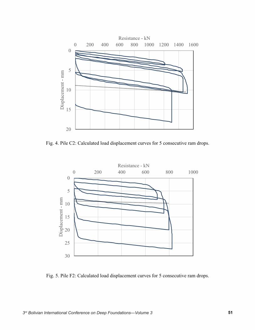
Fig. 4. Pile C2: Calculated load displacement curves for 5 consecutive ram drops.
Fig. 5. Pile F2: Calculated load displacement curves for 5 consecutive ram drops.
0
5
10
15
20
0 200 400 600 800 1000 1200 1400 1600
Dis
plac
emen
t -m
m
Resistance - kN
0
5
10
15
20
25
30
0 200 400 600 800 1000
Dis
plac
emen
t -m
m
Resistance - kN
513rd Bolivian International Conference on Deep Foundations—Volume 3

52 3rd Bolivian International Conference on Deep Foundations—Volume 3

Prediction of pile behavior under static and bi-directional tests and comparison with field results
Abchir, Z.(1), Burlon, S.(1), Frank, R.(2), and Reiffsteck, P. (1)
(1) Université Paris-Est, IFSTTAR, Champs-sur-Marne, France <[email protected]>
(2) Université Paris-Est, Navier Laboratory, CERMES, Champs-sur-Marne, France < [email protected]>
ABSTRACT. This paper includes a comparison between the measured data at the occasion of a campaign of full scale static pile load tests performed for the 3rd Bolivian International Conference on Deep Foundations and the values calculated by means of the software PIVER developed at IFSTTAR and using two kinds of t-z curves: The first one has been developed by Frank and Zhao (1982), and the second one is called AB1 (Abchir and al. 2016). These two kinds of t-z curves are defined by correlations from Ménard pressuremeter tests (PMT) data. The comparison between the measured and the calculated values enables to better estimate the bias and the uncertainty of the two t-z curves used and the method of the calculation of the bearing capacity. 1. INTRODUCTION
Pile design is generally based on the calculation of bearing capacity and application of safety factors. These factors aim to limit the load applied on the pile and ensure small displacements for the supported structures. Nevertheless, in some cases, the structures supported by piles may need high service requirements and pile settlement calculation becomes a major issue for the geotechnical engineer in charge of the design of these piles.
In this context, the comparison between measured and calculated values of pile settlement is very important to provide reliable methods. The understanding of axially loaded piles both in terms of displacements and bearing capacity has attracted important research efforts over the past decades (Poulos, 1989, Randolph, 2003) and many calculation models can be used. The two main approaches are the elastic continuum approach (Poulos and Davis, 1968) and the load transfer approach with t-z curves (Seed and Reese, 1957). This latter method is based on local interaction models between the ground and the pile where the ground is described by a series of independent non linear springs. These springs are distributed along the shaft (mobilisation of the shaft friction), and at the base, only one spring is considered (mobilisation of the base resistance). The shaft friction and the base resistance are progressively mobilised in function of the pile settlement.
This paper includes a comparison between the measured data at the occasion of a campaign of full scale static pile load tests performed for the 3rd Bolivian International Conference on Deep Foundations and the values calculated by means of the software PIVER developed at IFSTTAR and using two kinds of t-z curves: The first one has been developed by Frank and Zhao (1982), and the second one is called AB1 (Abchir and al. 2016). These two kinds of t-z curves are defined by correlations from Ménard pressuremeter tests (PMT) data.
2. SOIL CONDITIONS
The research site is located in Santa Cruz in Bolivia. Different in-situ and laboratory methods have been used in order to investigate the geotechnical conditions of the site. Boreholes with laboratory
533rd Bolivian International Conference on Deep Foundations—Volume 3
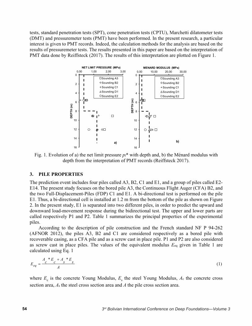
tests, standard penetration tests (SPT), cone penetration tests (CPTU), Marchetti dilatometer tests (DMT) and pressuremeter tests (PMT) have been performed. In the present research, a particular interest is given to PMT records. Indeed, the calculation methods for the analysis are based on the results of pressuremeter tests. The results presented in this paper are based on the interpretation of PMT data done by Reiffsteck (2017). The results of this interpretation are plotted on Figure 1.
Fig. 1. Evolution of a) the net limit pressure pl* with depth and, b) the Ménard modulus with depth from the interpretation of PMT records (Reiffsteck 2017).
3. PILE PROPERTIES
The prediction event includes four piles called A3, B2, C1 and E1, and a group of piles called E2-E14. The present study focuses on the bored pile A3, the Continuous Flight Auger (CFA) B2, and the two Full-Displacement-Piles (FDP) C1 and E1. A bi-directional test is performed on the pile E1. Thus, a bi-directional cell is installed at 1.2 m from the bottom of the pile as shown on Figure 2. In the present study, E1 is separated into two different piles, in order to predict the upward and downward load-movement response during the bidirectional test. The upper and lower parts are called respectively P1 and P2. Table 1 summarizes the principal properties of the experimental piles.
According to the description of pile construction and the French standard NF P 94-262 (AFNOR 2012), the piles A3, B2 and C1 are considered respectively as a bored pile with recoverable casing, as a CFA pile and as a screw cast in place pile. P1 and P2 are also considered as screw cast in place piles. The values of the equivalent modulus Eeq given in Table 1 are calculated using Eq. 1
As
Es
Ac
Ec
AEeq
** += (1)
where Ec is the concrete Young Modulus, Es the steel Young Modulus, Ac the concrete cross section area, As the steel cross section area and A the pile cross section area.
0
2
4
6
8
10
12
14
16
0,00 1,00 2,00 3,00DE
PTH
(m)
NET LIMIT PRESSURE (MPa)
Sounding A3Sounding B2Sounding C1Sounding D1Sounding E2
a)
0
2
4
6
8
10
12
14
16
0,00 10,00 20,00 30,00
DEPT
H (m
)
MENARD MODULUS (MPa)
Sounding A3Sounding B2Sounding C1Sounding D1Sounding E2
b)
54 3rd Bolivian International Conference on Deep Foundations—Volume 3
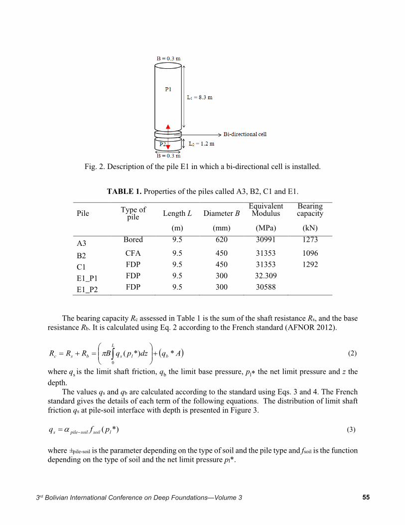
Fig. 2. Description of the pile E1 in which a bi-directional cell is installed.
TABLE 1. Properties of the piles called A3, B2, C1 and E1.
Pile Type of pile Length L Diameter B
Equivalent Modulus
Bearing capacity
(m) (mm) (MPa) (kN)
A3 Bored 9.5 620 30991 1273
B2 CFA 9.5 450 31353 1096
C1 FDP 9.5 450 31353 1292
E1_P1 FDP 9.5 300 32.309
E1_P2 FDP 9.5 300 30588
The bearing capacity Rc assessed in Table 1 is the sum of the shaft resistance Rs, and the base resistance Rb. It is calculated using Eq. 2 according to the French standard (AFNOR 2012).
( )AqdzpqBRRR b
L
lsbsc **)(0
+
=+= ∫π (2)
where qs is the limit shaft friction, qb the limit base pressure, pl* the net limit pressure and z the depth.
The values qs and qb are calculated according to the standard using Eqs. 3 and 4. The French standard gives the details of each term of the following equations. The distribution of limit shaft friction qs at pile-soil interface with depth is presented in Figure 3.
*)( lsoilsoilpiles pfq −=α (3)
where ±pile-soil is the parameter depending on the type of soil and the pile type and fsoil is the function depending on the type of soil and the net limit pressure pl*.
553rd Bolivian International Conference on Deep Foundations—Volume 3

*)(* Lepb pkq = (4)
where kp is the base factor and pLe* the equivalent net limit pressure.
Fig. 3. Distribution of limit shaft friction qs with depth along piles A3, B2, C1 and E1.
4. COMPUTATION METHOD
In order to predict the pile-head load movement curves of the piles presented above, a software called PIVER developed at IFSTTAR (France), based on the load transfer method, is used. The computation using this software requires the pile dimensions, the type of piles, the Young Modulus of the pile, the soil properties and the shape of the t-z curves at different depths. The present work proposes two predictions using two kinds of t-z curves. The first one has been developed by Frank and Zhao (1982), and the second one is called AB1 (Abchir and al. 2016). The software called PIVER gives the load-movement curves, the distribution of axial load versus depth and can be used to predict the behaviour of a pile submitted to a bi-directional test. 5. RESULTS
The following section presents the computed results using the software PIVER and its comparison with field data. A brief analysis and discussion is also presented below. 5.1 Load-movement curves
Figure 4 represents the load movement curves during the static loading tests applied to the piles A3, B2 and C2. The figure shows the computed results calculated using Frank and Zhao (1982) and the AB1 model (Abchir and al., 2016). The computed and experimental results present a clear
difference that still remains acceptable for a design. The ratio 𝑅𝑅𝑐𝑐,𝑐𝑐𝑐𝑐𝑐𝑐𝑅𝑅𝑐𝑐,𝑚𝑚𝑚𝑚𝑚𝑚
where Rc,cal is the computed
0
2
4
6
8
10
12
14
16
0 50 100 150
DEPT
H (m
)
LIMIT SHAFT FRICTION (kPa)
Pile A3
Pile B2
Pile C1
Pile E1
56 3rd Bolivian International Conference on Deep Foundations—Volume 3
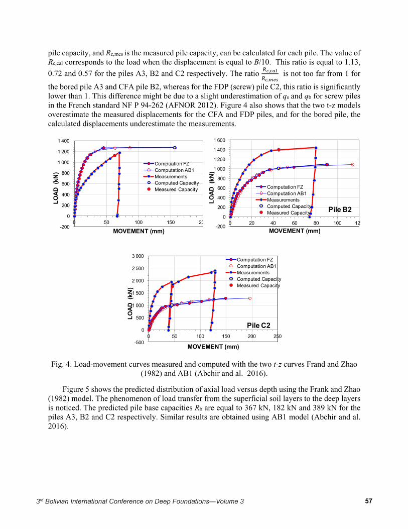
pile capacity, and Rc,mes is the measured pile capacity, can be calculated for each pile. The value of Rc,cal corresponds to the load when the displacement is equal to B/10. This ratio is equal to 1.13,
0.72 and 0.57 for the piles A3, B2 and C2 respectively. The ratio 𝑅𝑅𝑐𝑐,𝑐𝑐𝑐𝑐𝑐𝑐𝑅𝑅𝑐𝑐,𝑚𝑚𝑚𝑚𝑚𝑚
is not too far from 1 for
the bored pile A3 and CFA pile B2, whereas for the FDP (screw) pile C2, this ratio is significantly lower than 1. This difference might be due to a slight underestimation of qs and qb for screw piles in the French standard NF P 94-262 (AFNOR 2012). Figure 4 also shows that the two t-z models overestimate the measured displacements for the CFA and FDP piles, and for the bored pile, the calculated displacements underestimate the measurements.
Fig. 4. Load-movement curves measured and computed with the two t-z curves Frand and Zhao (1982) and AB1 (Abchir and al. 2016).
Figure 5 shows the predicted distribution of axial load versus depth using the Frank and Zhao (1982) model. The phenomenon of load transfer from the superficial soil layers to the deep layers is noticed. The predicted pile base capacities Rb are equal to 367 kN, 182 kN and 389 kN for the piles A3, B2 and C2 respectively. Similar results are obtained using AB1 model (Abchir and al. 2016).
-200
0
200
400
600
800
1 000
1 200
1 400
0 50 100 150 20
LOAD
(kN
)
MOVEMENT (mm)
Compuation FZComputation AB1MeasurementsComputed CapacityMeasured Capacity
-200
0
200
400
600
800
1 000
1 200
1 400
1 600
0 20 40 60 80 100 120
LOAD
(kN
)
MOVEMENT (mm)
Computation FZComputation AB1MeasurementsComputed CapacityMeasured Capacity Pile B2
-500
0
500
1 000
1 500
2 000
2 500
3 000
0 50 100 150 200 250
LOAD
(kN
)
MOVEMENT (mm)
Computation FZComputation AB1MeasurementsComputed CapacityMeasured Capacity
Pile C2
573rd Bolivian International Conference on Deep Foundations—Volume 3

Fig. 5. The predicted distributions of axial load versus depth for a pile head load equal Rc,cal
using Frank and Zhao (1982) t-z curve.
5.2 Results of bi-directional test
To predict the upward and downward load-movement response during the bidirectional static loading on pile E1, two calculations have been done: the first one on the upper part of E1, called P1, with a base resistance equal to 0, and the second one on the lower part of E1 that is considered as a second pile P2 (Figure 2).
The predicted upward and downward movements are plotted in Figure 6. The computations show that the lower part reaches the failure before the upper part. For the model developed by Frank and Zhao (1982), the calculated bearing capacities are equal to 481 kN and 231 kN for the upper and lower parts respectively. For the AB1 model (Abchir and al. 2016), the calculated bearing capacities are equal to 475 kN and 240 kN for respectively the upper and the lower parts. The comparison with field results shows that the prediction using the two t-z curves underestimates
slightly the bearing capacity of the upper part of E1. Indeed, the ratio 𝑅𝑅𝑐𝑐,𝑐𝑐𝑐𝑐𝑐𝑐𝑅𝑅𝑐𝑐,𝑚𝑚𝑚𝑚𝑚𝑚
of the upper part of
E1 is equal to 0.82 and 0.80 for Frank and Zhao (1982) and AB1 models respectively. 5.3 Equivalent head-down load movement
In order to predict the equivalent head-down load movement curve, two steps are required:
1. the estimate of the equivalent settlement at pile head called st; 2. the estimate of the equivalent load at pile head Qt.
In order to provide these two estimates, several methods have been developed. In the present
prediction work, a method called “elastic method” proposed by Lee and Park (2007) is used. The equivalent head-down load movement curve obtained using this method is plotted on Figure 7. The estimated pile bearing capacity Rc,cal is equal to 732 kN and 720 kN for respectively Frank and Zhao (1982) and AB1 (Abchir and al. 2016) models.
0
1
2
3
4
5
6
7
8
9
10
0 500 1 000 1 500DE
PTH
(m)
LOAD (kN)
Pile A3
0
1
2
3
4
5
6
7
8
9
10
0 500 1 000 1 500
DEPT
H (m
)
LOAD (kN)
Pile B2
0
1
2
3
4
5
6
7
8
9
10
0 500 1 000 1 500
DEPT
H (m
)
LOAD (kN)
Pile C2
58 3rd Bolivian International Conference on Deep Foundations—Volume 3

Fig. 6. The Upward and downward movements predicted using Frank and Zhao (1982) model and AB1 model (Abchir and al. 2016), compared to the measured
upward movement of the pile E1.
Fig. 7. Equivalent head-down load movement curve predicted for the pile E1 using a) Frank and Zhao (1982) model, and b) AB1 model (Abchir and al. 2016).
6. CONCLUSION
This paper presents a comparison between the measured data at the occasion of a campaign of full scale static pile load tests performed for the 3rd Bolivian International Conference on Deep Foundations and the values calculated by means of the software PIVER developed at IFSTTAR and using two kinds of t-z curves: The first one has been developed by Frank and Zhao (1982), and the second one is called AB1 (Abchir et al. 2016). These two kinds of t-z curves are defined by correlations from Ménard pressuremeter tests (PMT) data.
-100
-80
-60
-40
-20
0
20
40
60
0 200 400 600 8
MO
VEM
ENT
(mm
)
LOAD (kN)
Upward (Computation FZ)Downward (Computation FZ)Upward (Measurements)
-100
-80
-60
-40
-20
0
20
40
60
0 200 400 600 8
MO
VEM
ENT
(mm
)
LOAD (kN)
Upward (Computation AB1)Downward (Computation AB1)Upward (Measurements)
0
100
200
300
400
500
600
700
800
900
0 20 40 60 80 100
LOAD
(kN
)
MOVEMENT (mm)
Head
Capacity
a)
0
100
200
300
400
500
600
700
800
900
0 20 40 60 80 100
LOAD
(kN
)
MOVEMENT (mm)
Head Calculation 1
Capacity Calculation 1
b)
593rd Bolivian International Conference on Deep Foundations—Volume 3

The results allow to estimate the reliability of the two kinds of t-z curves used and the necessity to increase the number of comparisons between measured and calculated values in order to increase the precision of the calculation methods. This comparison underlines the need of high quality in terms of ground investigations since, in this case, both the bearing capacity of the piles and the t-z curves are derived from PMT data. 7. REFERENCES
Abchir, Z., Burlon, S., Frank, R., Habert, J., and Legrand, S., 2016. T-z curves for piles from pressuremeter test results. Géotechnique, 66(2), pp. 137-148.
AFNOR, 2012. Calcul des fondations profondes – NF P 94 282. French standard. Saint-Denis, France: AFNOR Groupe (in French).
Frank, R., and Zhao, S.R., 1982. Estimation par les paramètres pressiométriques de l’enfoncement sous charge axiale de pieux forés dans les sols fins. Bulletin de Liaison du Laboratoire des Ponts et Chaussées, 119 : 17-24 (in French).
Lee, J.S, and Park, Y.H., 2008. Equivalent Pile load-head settlement curve using a bi-directional pile load test. Computers and Geotechnics, 35(2), pp. 124-133.
Poulos, H.G, and Davis, E.H., 1968. The settlement behaviour of single axially loaded incompressible piles and piers. Géotechnique 18(3), pp. 351-371.
Poulos, H.G., 1989. Pile behaviour - Theory and application. Géotechnique, 39(3), 365-415. Randolph, M.F., 2003. Science and empiricism in pile foundation design. Géotechnique, 53(10),
pp. 847-875. Reiffsteck, P., 2017. Interpretation of PMT performed at Santa Cruz de la Sierra, Bolivia. Private
Communication. Seed, H.B., and Reese, L.C., 1957. The action of soft clay along friction piles. Transactions, ASCE,
Vol. 122, pp.731-754.
60 3rd Bolivian International Conference on Deep Foundations—Volume 3

Not so B.E.S.T. Class A predictions of pile behaviour
Basile, F.(1)
(1) Geomarc Ltd, Messina, Italy <[email protected]>
ABSTRACT. Class A predictions of axial response to loading of four single piles are presented. The Author's approach to develop his predictions is described, and an attempt is made to explain the success or otherwise of the prediction. 1. INTRODUCTION
In conjunction with the 3rd Bolivian International Conference on Deep Foundations, held in Santa Cruz in 2017, a pile prediction event was organized. This followed a comprehensive site investigation carried out at the “Bolivian Experimental Site for Testing” (B.E.S.T.). The prediction event included axial static tests of No. 4 single piles: one pile (Pile A3) was bored with slurry, one (Pile B2) was constructed with a continuous flight auger (CFA), and two (Piles C2 and E1) were constructed by full displacement equipment (FDP). In addition, Pile E1 was supplied with an expanded base (EB) at the pile toe, while the others were straight-shaft piles. Piles A3, B2, and C2 were tested in head-down tests while Pile E1 was tested by means of a bidirectional cell. A few months before the loading tests, geotechnical engineers throughout the world were invited to submit Class A predictions of the load-movement curves to be measured in the tests and to assess the pile capacity from these curves. The submission also included the profile of axial load along the piles at the so-assessed capacities. In this paper, the geotechnical assumptions and analysis method adopted by the Author to develop his predictions are described, and the comparison between predicted and measured response is discussed. 2. ANALYSIS METHOD
The load-movement response and axial load distribution of the piles have been analyzed using the commercial software Repute (Basile 2015, Bond and Basile 2017). Repute computes the response of single piles and pile groups under general loading conditions (i.e. vertical, horizontal, and moment) by means of a complete 3D boundary element (BEM) formulation (i.e. the reciprocal influence of all the pile elements within the group is considered). Soil nonlinearity is modelled by employing a hyperbolic continuum-based relationship which makes use of the initial value of soil Young's modulus (Es). In all the Class A predictions below, the initial value of Es has been derived from correlation with the shear wave velocity (Vs) measurements from SDMT. It is noted that the derivation of initial Es from shear wave velocity measurements is generally expected to provide upper bound values of the soil modulus derived from a pile loading test. However, the above choice has been made on the basis that, for the purpose of a pile prediction event, use of a 'best estimate' value of Es can be justifiable (rather than a more conservative, i.e. lower, 'design' value of Es). In addition, it has been assumed that the initial values of Es are unaffected by construction effects. This is based on the consideration that construction effects mainly influence pile capacity, while the initial pile stiffness depends primarily on the initial values of Es (e.g. Mandolini 2001). All pile-heads are assumed at ground level, and the pile Young's modulus is taken as 30 GPa.
613rd Bolivian International Conference on Deep Foundations—Volume 3
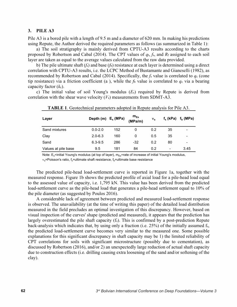
3. PILE A3
Pile A3 is a bored pile with a length of 9.5 m and a diameter of 620 mm. In making his predictions using Repute, the Author derived the required parameters as follows (as summarized in Table 1):
a) The soil stratigraphy is mainly derived from CPTU-A3 results according to the charts proposed by Robertson and Cabal (2014). The CPT values of qt, fs, and Rf assigned to each soil layer are taken as equal to the average values calculated from the raw data provided.
b) The pile ultimate shaft (fs) and base (fb) resistance at each layer is determined using a direct correlation with CPTU-A3 results, i.e. the LCPC Method of Bustamante and Gianeselli (1982), as recommended by Robertson and Cabal (2014). Specifically, the fs value is correlated to qc (cone tip resistance) via a friction coefficient (a ), while the fb value is correlated to qc via a bearing capacity factor (kc).
c) The initial value of soil Young's modulus (Es) required by Repute is derived from correlation with the shear wave velocity (Vs) measurements from SDMT-A3.
TABLE 1. Geotechnical parameters adopted in Repute analysis for Pile A3.
The predicted pile-head load-settlement curve is reported in Figure 1a, together with the measured response. Figure 1b shows the predicted profile of axial load for a pile-head load equal to the assessed value of capacity, i.e. 1,795 kN. This value has been derived from the predicted load-settlement curve as the pile-head load that generates a pile-head settlement equal to 10% of the pile diameter (as suggested by Poulos 2016). A considerable lack of agreement between predicted and measured load-settlement response is observed. The unavailability (at the time of writing this paper) of the detailed load distribution measured in the field precludes an optimal investigation of this discrepancy. However, based on visual inspection of the curves' shape (predicted and measured), it appears that the prediction has largely overestimated the pile shaft capacity (fs). This is confirmed by a post-prediction Repute back-analysis which indicates that, by using only a fraction (i.e. 25%) of the initially assumed fs, the predicted load-settlement curve becomes very similar to the measured one. Some possible explanations for this significant discrepancy in shaft capacity may be 1) the limited reliability of CPT correlations for soils with significant microstructure (possibly due to cementation), as discussed by Robertson (2016), and/or 2) an unexpectedly large reduction of actual shaft capacity due to construction effects (i.e. drilling causing extra loosening of the sand and/or softening of the clay).
Layer Depth (m) Es (MPa) mEs
(MPa/m)νs fs (kPa) fb (MPa)
Sand mixtures 0.0-2.0 152 0 0.2 35 -
Clay 2.0-6.3 160 0 0.5 35 -
Sand 6.3-9.5 286 -32 0.2 80 -
Values at pile base 9.5 181 84 0.2 - 3.45Note: Es=initial Young's modulus (at top of layer), mEs=rate of increase of initial Young's modulus, νs=Poisson's ratio, fs=ultimate shaft resistance, fb=ultimate base resistance
62 3rd Bolivian International Conference on Deep Foundations—Volume 3
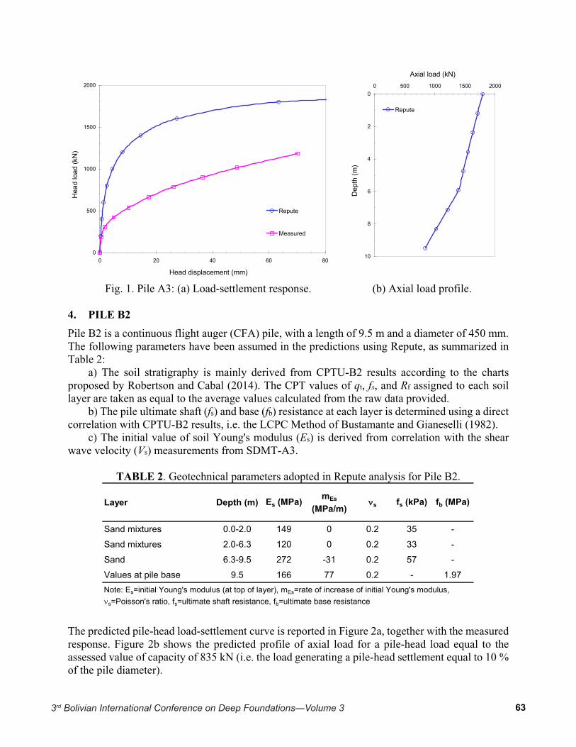
Fig. 1. Pile A3: (a) Load-settlement response. (b) Axial load profile.
4. PILE B2
Pile B2 is a continuous flight auger (CFA) pile, with a length of 9.5 m and a diameter of 450 mm. The following parameters have been assumed in the predictions using Repute, as summarized in Table 2:
a) The soil stratigraphy is mainly derived from CPTU-B2 results according to the charts proposed by Robertson and Cabal (2014). The CPT values of qt, fs, and Rf assigned to each soil layer are taken as equal to the average values calculated from the raw data provided.
b) The pile ultimate shaft (fs) and base (fb) resistance at each layer is determined using a direct correlation with CPTU-B2 results, i.e. the LCPC Method of Bustamante and Gianeselli (1982).
c) The initial value of soil Young's modulus (Es) is derived from correlation with the shear wave velocity (Vs) measurements from SDMT-A3.
TABLE 2. Geotechnical parameters adopted in Repute analysis for Pile B2.
The predicted pile-head load-settlement curve is reported in Figure 2a, together with the measured response. Figure 2b shows the predicted profile of axial load for a pile-head load equal to the assessed value of capacity of 835 kN (i.e. the load generating a pile-head settlement equal to 10 % of the pile diameter).
0
500
1000
1500
2000
0 20 40 60 80
Head displacement (mm)
Hea
d lo
ad (k
N)
Repute
Measured
0
2
4
6
8
10
0 500 1000 1500 2000
Axial load (kN)
Dep
th (m
)
Repute
Layer Depth (m) Es (MPa) mEs
(MPa/m)νs fs (kPa) fb (MPa)
Sand mixtures 0.0-2.0 149 0 0.2 35 -
Sand mixtures 2.0-6.3 120 0 0.2 33 -
Sand 6.3-9.5 272 -31 0.2 57 -
Values at pile base 9.5 166 77 0.2 - 1.97Note: Es=initial Young's modulus (at top of layer), mEs=rate of increase of initial Young's modulus, νs=Poisson's ratio, fs=ultimate shaft resistance, fb=ultimate base resistance
633rd Bolivian International Conference on Deep Foundations—Volume 3

A good agreement between the predicted and measured initial pile stiffness is observed, thus confirming the suitability of employing the initial soil modulus (Es) in Repute analyses. However, the actual pile capacity (herein intended as the load corresponding to the horizontal asymptote of the load-settlement curve) is underestimated by about 40%, thereby indicating that the empirical correlations with CPT results adopted by the Author were unable to fully capture the more complex mechanisms of behaviour (this may partially be due to the limited reliability of CPT correlations as discussed earlier). The larger actual resistance may also partially be attributed to pressure-grouting, a circumstance which was not known to the predictors when submitting the prediction.
Fig. 2. Pile B2: (a) Load-settlement response. (b) Axial load profile.
5. PILE C2
Pile C2 is a full-displacement pile (FDP), with a length of 9.5 m and a diameter of 450 mm. The following parameters have been adopted in Repute calculations, as summarized in Table 3:
a) The soil stratigraphy is mainly derived from CPTU-C1 results according to the charts proposed by Robertson and Cabal (2014). The CPT values of qt, fs, and Rf assigned to each soil layer are taken as equal to the average values calculated from the raw data provided.
b) The pile ultimate shaft (fs) and base (fb) resistance at each layer is determined using a direct correlation with CPTU-C1 results, specifically the method proposed by Bustamante and Gianeselli (1998) for screw piles.
c) The initial value of soil Young's modulus (Es) is derived from correlation with the shear wave velocity (Vs) measurements from SDMT-F1.
0
250
500
750
1000
1250
1500
0 20 40 60 80 100
Head displacement (mm)
Hea
d lo
ad (k
N)
Repute
Measured
0
2
4
6
8
10
0 500 1000
Axial load (kN)
Dep
th (m
)
Repute
64 3rd Bolivian International Conference on Deep Foundations—Volume 3

TABLE 3. Geotechnical parameters adopted in Repute analysis for Pile C2.
The predicted and measured pile-head load-settlement curves are shown in Figure 3a, while Figure 3b reports the predicted axial load profile for a pile-head load equal to the assessed value of capacity of 1,039 kN (i.e., the load generating a pile-head settlement equal to 10 % of the pile diameter).
Fig. 3. Pile C2: (a) Load-settlement response . (b) Axial load profile.
A fair agreement between the predicted and measured initial pile stiffness is observed, thereby
confirming the suitability of employing the initial soil modulus (Es) in calculations. However, the actual pile capacity (herein intended as the load corresponding to the horizontal asymptote of the load-settlement curve) is underestimated by about 45%. Such a significant discrepancy was also observed in the predictions submitted by most participants and confirms the general difficulty in estimating pile capacity, an issue which becomes even more prominent in the case of screw piles. Indeed, the installation of screw piles induces complex changes to the soil state (holding a major influence on pile capacity) which highly depend on the specific installation procedure and drilling tool employed. Nevertheless, presently available design methods are too general and further research is needed in order to develop design procedures which are more specific to the many different installation methods existing in industry (e.g. Atlas, De Waal, Fundex, Olivier, Omega, APGD, SVV, Franki VB, Bauer FDP piles, etc.). There is also a need for design methods to be more discriminating, going beyond just textbook soils (i.e. sand and clay).
Layer Depth (m) Es (MPa) mEs
(MPa/m)νs fs (kPa) fb (MPa)
Sand mixtures 0.0-6.3 130 0 0.2 13 -
Sand 6.3-9.5 305 -39 0.2 91 -
Values at pile base 9.5 175 81 0.2 - 4.11Note: Es=initial Young's modulus (at top of layer), mEs=rate of increase of initial Young's modulus, νs=Poisson's ratio, fs=ultimate shaft resistance, fb=ultimate base resistance
0
500
1000
1500
2000
2500
0 20 40 60 80 100
Head displacement (mm)
Hea
d lo
ad (k
N)
Repute
Measured
0
2
4
6
8
10
0 250 500 750 1000 1250
Axial load (kN)
Dep
th (m
)
Repute
653rd Bolivian International Conference on Deep Foundations—Volume 3

Indeed, currently available design methods (e.g. the method by Bustamante and Gianeselli 1998, the "Belgian" method described by Huybrechts et al. 2016, the method by NeSmith 2002) are mainly related to the specific installation method and to the site conditions for which they were developed. As a consequence, these methods imply a certain degree of conservativism to account for more general installation methods and soil conditions. For example, the method by Bustamante and Gianeselli (1998) adopted by the Author for his prediction of pile capacity (i.e. fs and fb) was mainly derived on the basis of 24 loading tests carried out in the 1980s on the pioneer Atlas piles which are short-displacement auger systems. However, the FDP pile at the B.E.S.T. site is a modern long-displacement auger system and is therefore expected to change the soil state differently, thereby leading to different pile capacities as compared to Atlas piles. A confirmation of the inherent conservatism of the method by Bustamante and Gianeselli (1998) can be derived from Table 4 which compares the pile shaft and base capacities computed by the Author using three different methods: 1) the LCPC Method by Bustamante and Gianeselli (1982) for bored piles, 2) the method by Bustamante and Gianeselli (1998) for screw piles, and 3) the Belgian method for screw piles. It is observed that the shaft capacity predicted by Method 1) (which is intended for standard bored piles) is actually greater than that computed using Method 2) which was specifically developed for screw piles. This appears to be an inconsistency given that FDP screw piles are expected to develop a greater shaft capacity than bored piles. As an indication, on the basis of several loading tests in soil conditions similar to the B.E.S.T. site, Terceros and Fellenius (2014) report that the FDP pile develops at least twice the shaft capacity of a standard bored pile. This feature confirms another important aspect of pile design, i.e. the issue of experience from prior similar work at a site and, in particular, past records of a contractor for the specific construction method.
TABLE 4. Comparison of capacities for Pile C2.
6. PILE E1
Pile E1 is a full-displacement pile (FDP) equipped with an Expander Body (EB), having a length of 9.5 m and a shaft diameter of 300 mm. The base diameter is also assumed to be equal to 300 mm (after inflation of the EB). The following parameters have been assumed in Repute calculations, as summarized in Table 5:
a) The soil stratigraphy is mainly derived from CPTU-E1 results according to the charts proposed by Robertson and Cabal (2014). The CPT values of qt, fs, and Rf assigned to each soil layer are taken as equal to the average values calculated from the raw data provided.
b) The pile ultimate resistance is determined using a direct correlation with CPTU-E1 results, specifically the ultimate shaft (fs) resistance from the method by Bustamante and Gianeselli (1998) for screw piles, and the ultimate base (fb) resistance from the method proposed by Massarsch and Wetterling (1993) for EB piles.
MethodShaft
capacity (kN)
Base capacity
(kN)
Total capacity
(kN)
(1) LCPC method by Bustamante and Gianeselli 1982 (bored piles) 581 418 999
(2) Bustamante and Gianeselli 1998 (screw piles) 527 653 1180
(3) Belgian method (screw piles) 585 733 1318
66 3rd Bolivian International Conference on Deep Foundations—Volume 3

c) The initial value of Es is derived from correlation with Vs measurements from SDMT-G1.
TABLE 5. Geotechnical parameters adopted in Repute analysis for Pile E1.
The predicted and measured load-movement curves are shown in Figure 4. As for Repute predictions, the (base) downward response of the bidirectional (BD) cell is simulated using the standard soil profile reported in Table 5. In order to compute the (shaft) upward load-movement response, the Repute analysis is performed using a 'mirror' soil profile (in order to account for the fact that the shaft upward response measured by the BD test engages the deeper located stiffer soils first and the more shallow weaker soils last), and assuming a negligible base diameter (in order to ignore the base contribution). In addition, the equivalent head-down load-movement response predicted by Repute is also reported in Figure 4. Unfortunately, during the test, the telltale measuring the downward movement of the bidirectional cell failed and therefore only the (shaft) upward movement was measured and can be compared with Repute predictions. The comparison shows a general overestimate of movements while a good agreement between predicted and measured shaft capacity is achieved.
Fig. 4. Load-movement response of Pile E1.
Layer Depth (m) Es (MPa) mEs
(MPa/m)νs fs (kPa) fb (MPa)
Sand mixtures 0.0-2.0 154 0 0.2 70 -
Silt mixtures 2.0-6.3 181 0 0.5 43 -
Sand 6.3-9.5 303 -39 0.2 92 -
Values at pile base 9.5 180 81 0.2 - 3.58Note: Es=initial Young's modulus (at top of layer), mEs=rate of increase of initial Young's modulus, νs=Poisson's ratio, fs=ultimate shaft resistance, fb=ultimate base resistance
0
200
400
600
800
1000
0 10 20 30 40 50
Displacement (mm)
Load
(kN
)
Repute - base downward
Repute - shaft upward
Repute - equivalent head-down
Measured - shaft upward
673rd Bolivian International Conference on Deep Foundations—Volume 3

7. CONCLUSIONS
The paper presents a comparison between Class A predictions and full-scale axial loading tests on four single piles constructed using different methods (i.e. bored, CFA, FDP, and FDP with Expander Body). The geotechnical assumptions and analysis method adopted by the Author to develop his predictions are described. It is found that, with the exception of Pile A3, all predictions are on the conservative side (from a design viewpoint). In particular, the predicted pile-head settlements generally show a reasonable agreement with the measured response within the usual serviceability range (say below 10mm); this agreement also attests the suitability of adopting the initial soil modulus (Es) in Repute calculations. However, some significant discrepancies in predicted and measured pile capacities are observed, thus confirming a critical (but often neglected) aspect of pile design, i.e. predicting pile capacity is usually more difficult and less reliable than predicting deformations. 8. REFERENCES
Basile, F., 2015. Non-linear analysis of vertically loaded piled rafts. Computers and Geotechnics 63, pp. 73–82. Bond, A.J. and Basile, F., 2017. Repute 2.5, Software for pile design and analysis. Reference Manual, Geocentrix Ltd, UK, 52 p. Bustamante, M. and Gianeselli, L., 1982. Pile Bearing Capacity Prediction by Means of Static Penetrometer. Proc. European Symposium on Penetration Testing, Vol. 2, Amsterdam, The Netherlands, pp. 493–500. Bustamante, M. and Gianeselli, L., 1998. Installation parameters and capacity of screwed piles. Proc. Int. Geotechnical Seminar on Deep Foundations on Bored and Auger Piles, BAP III, Balkema, Rotterdam, The Netherlands, pp. 95–108. Huybrechts, N., De Vos, M., Bottiau, M., and Maertens, L., 2016. Design of piles – Belgian practice. Proc. ISSMGE-ETC3 Int. Symp. on Design of Piles in Europe, Leuven, Belgium, pp. 7–44. Mandolini, A., 2001. Small-strain soil stiffness and settlement prediction for piled foundations. Proc. 2nd Int. Symp. on Pre-Failure Deformation Characteristics of Geomaterials (Eds: Jamiolkowski et al.), Torino, Italy, pp. 1397–1404. Massarsch, K.R. and Wetterling, S., 1993. Improvement of augercast pile performance by Expander Body system. Proc. Int. Geotechnical Seminar on Deep Foundations on Bored and Auger Piles, BAP II, Balkema, Rotterdam, The Netherlands, pp. 417–428. NeSmith, W.M., 2002. Static capacity analysis of augered, pressure-injected displacement piles. Proc. Int. Deep Foundations Congress 2002, ASCE Geotechnical Special Publication No. 116, Vol. 2, pp. 1174–1196. Poulos, H.G., 2016. Tall building foundations: design methods and applications. Innovative Infrastructure Solutions 1:10, Springer, pp. 1–51. Robertson, P.K., 2016. Cone penetration test (CPT)-based soil behaviour type (SBT) classification system – an update. Canadian Geotechnical Journal 53(12) 1910–1927. Robertson, P.K. and Cabal, K.L., 2014. Guide to Cone Penetration Testing for Geotechnical Engineering. Gregg Drilling & Testing, Inc., 140 p. Terceros, M.H. and Fellenius, B.H., 2014. Piling practice in the sedimentary granular soils of Santa Cruz, Bolivia. Proc. DFI-EFFC 11th Int. Conf. on Piling and Deep Foundations, Stockholm, Sweden, pp. 379–386.
68 3rd Bolivian International Conference on Deep Foundations—Volume 3

Approach to prediction of pile performances submitted to the 3rd Bolivian International Conference on Deep Foundations
Buttling, S.(1)
(1) National Geotechnical Consultants, Brisbane, Australia
<[email protected]> ABSTRACT. The approach to the prediction of pile performance is described. This was based on back analysis of the previous performance prediction events in 2013 and 2015, in order to try to compensate for a lack of local knowledge. Two methods of analysis were used, based on the Cemset and RATZ softwares. 1. BACKGROUND
The 1st International Conference and Seminar on Deep Foundations held in Santa Cruz, Bolivia in 2013, and the 2nd International Conference on Deep Foundations held again in Santa Cruz in 2015, both included pile performance prediction events. The first comprised four piles as follows:
TP1: a pile 400 mm in diameter, 17.5 m long, bored under bentonite TP2: a pile 360 mm in diameter, 11.6 m long, built as a FDP TP3: a pile 360 mm in diameter, 10.8 m long, built as a FDP but with an Expander Body EB600 at the toe TP4: a pile 400 mm in diameter, 17.5 m long, bored under bentonite but with an Expander
Body EB600 at the toe, and a bidirectional cell above the expander body. The soil data provided consisted of 3 boreholes with SPT N values to depths of 17 to 19 m, 3
CPT tests to depths of 9.2 to 9.6 m, seismic wave speed measurements to depths of 30 m, and data on grain size and moisture content.
It was found hard to make predictions for the performance of these piles, because not only were the soil conditions unfamiliar, but also the pile types and sizes, especially the Expander Body 600, were beyond our normal experience.
The second pile performance prediction event comprised a single pile, 600 mm in diameter and 16.4 m long, constructed as a dry bored pile with a temporary casing. As with TP4 in the first event a bi-directional cell was included, 14.8 m below ground level, along with relevant instrumentation.
The soil data provided consisted of 1 borehole with SPT N values, 1 CPTu with corrected cone resistance, sleeve friction, pore pressure and friction ratio.
Again, it was found hard to make a reliable prediction because of unfamiliarity with the soil type and the pile construction method. It is noted that empirical design rules, as are commonly used in pile design, rely heavily on actual experience of piling and load testing in the local soils.
693rd Bolivian International Conference on Deep Foundations—Volume 3

2. ANALYSIS METHODS 2.1 Methods to be used
It was intended to make use of a number of methods to predict the pile performance. These included:
• Cemset – based on the work of Fleming (1992) • RATZ – written by Randolph (2003)
The intention was to make use of the CPT data, using the method of Eslami and Fellenius (1997) which was based on 102 case histories where static load test results were available, although 90% of the cases were for driven piles. The method makes use of the geometric mean of effective cone resistance values in the zone 8 diameters above and 4 diameters below the pile toe to determine toe resistance, and the effective cone resistance at all depths to determine shaft friction. The toe resistance uses a toe correlation coefficient, Ct, which is suggested to be unity, and a shaft correlation coefficient, Cs, which varies with soil type and is selected based on a soil profiling chart.
2.2 Back analysis of previous events
In an attempt to improve the match between the predictions and the measured data, the results of the previous events were back analysed to try to make use of “local knowledge”. From the 2013 event the CPT data was not considered to be sufficient, since it only reached a depth of about half of the pile depth. For the bored pile the relationships between shaft friction and SPT N value (Ks = 2.8), and between end bearing and SPT N value (Kb = 25), based on the work of Chang and Broms (1991), Chen and Hiew (2006), Toh et al. (1991) and Phienwej et al (1994) were used. These gave an ultimate shaft friction of 1378 kN, and an ultimate end bearing of 1,108 kN. When applied in Cemset and compared with the measured data for TP1 the result was as shown in Figure 1.
Fig. 1. Comparison between measured data for Bolivia 2013 TP1 and Cemset analysis.
70 3rd Bolivian International Conference on Deep Foundations—Volume 3

Noting that the load test stopped well short of any reasonable definition of ultimate resistance, with a pile top settlement of only about 15 mm, this is considered to be excellent agreement.
From the 2015 test, there were both SPT and CPT data available. Both sets of data were therefore used. The SPT data using the same correlations as had been used for the 2013 tests, and the CPT data using the conversions of cone resistance to shaft friction and end-bearing as proposed by Eslami and Fellenius based on back analysis of 110 case histories, most of which were for driven piles. The correlation between the measured data and the SPT prediction was not very close, as seen in Figure 2, but that using the CPT prediction was much better.
Fig. 2. Comparison between measured data for Bolivia 2015 TP1 and Cemset analysis using SPT or CPT data.
2.3 Summary
These back analyses gave confidence that the estimates of shaft friction and end-bearing arising from use of the Eslami and Fellenius method with cone resistance data would compare favourably with those measured in actual pile load tests. In addition, since the Cemset method lumps all shaft resistance into one value, the RATZ program was used which considers a layered soil. 3. PREDICTIONS
For the predictions the CPT data was transferred to a spreadsheet based on the Eslami and Fellenius method which, at 9.5 m depth, gave estimates of the end-bearing resistance and cumulative shaft friction. These were transferred into the Cemset spreadsheet, with the other parameters selected based on the back-analysis of the earlier tests.
In addition the spreadsheet gave estimates of modulus based on the cone penetration test results, based on correlations provided in Lunne et al (1997). The individual shaft friction and modulus values were therefore plotted against depth, and used to determine layering. These data
713rd Bolivian International Conference on Deep Foundations—Volume 3

were then used in the RATZ program, which also produced a load/settlement curve. Both curves, Cemset and RATZ, were plotted together and a mean line drawn by eye between them. These were used as the basis of the predictions. 4. RESULTS
It has been noted that, although the agreement for pile A3 as acceptable, that for piles B2 and C2 was very poor, on the conservative side. Some back-analysis has suggested that the end-bearing resistance for A3 was about 5 MPa, and about 11 MPa for C2. Similarly, the shaft friction for B2 and C2 was underestimated by about 2.5 to 3 times. This appears to suggest that the design parameters determined from CPT tests using the Eslami and Fellenius method seriously underestimate the shaft friction, which could be a function of Cs being derived from driven pile tests and not from FDP pile tests which probably increases the available friction. The reasons for the very high end-bearing resistances, even in the bored pile, are less well understood. In addition, both the 2013 and 2015 tests on which the back analysis was based, did not approach failure which may have caused the shaft and end-bearing resistance values to have been underestimated. 5. REFERENCES Chang, M.F., and Broms, B.B. 1991. Design of bored piles in residual soils based on field-
performance data. Canadian Geotechnical Journal, 28, pp. 200-209. Chen, C.S., and Hiew, L.C. 2006. Performance of bored piles with different construction methods.
Proceedings of the Institution of Civil Engineers, Geotechnical Engineering, 159 GE3, pp. 227-232.
Fleming, W.G.K. 1992. A new method for single pile settlement prediction and analysis. Geotechnique, 42 (3), pp. 411-425.
Lunne, T., Robertson, P.K., and Powell, J.J.M. 1997. Cone penetration testing in geotechnical practice. Spon Press, London.
Phienwej, N., Balakrishnan, E.G. and Balasubramaniam, A.S. 1994. Performance of bored piles in weathered meta-sedimentary rocks in Kuala Lumpur, Malaysia. Proceedings of the Symposium on Geotextiles, Geomembranes and other Geosynthetics in Ground Improvement on Deep Foundations and Ground Improvement Schemes, Bangkok, A.A. Balkema Publishers Rotterdam, pp. 251-260.
Randolph, M.A. 2003. RATZ Version 4-2, Load transfer analysis of axially loaded piles. University of Western Australia, Perth.
Toh, C.T., Ooi, T.A., Chiu, H.K., Chee, S.K. and Ting, W.H. 1989. Design parameters for bored piles in a weathered sedimentary formation. Proceedings of the 12th International Conference on Soil Mechancis and Foundation Engineering, Rio de Janeiro, A.A. Balkema Publishers Rotterdam, 2 pp. 1073-1078.
72 3rd Bolivian International Conference on Deep Foundations—Volume 3
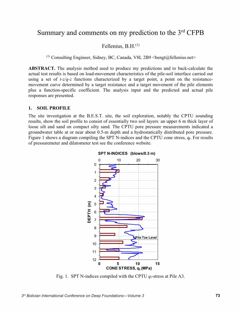
Summary and comments on my prediction to the 3rd CFPB
Fellenius, B.H.(1)
(1) Consulting Engineer, Sidney, BC, Canada, V8L 2B9 <[email protected]>
ABSTRACT. The analysis method used to produce my predictions and to back-calculate the actual test results is based on load-movement characteristics of the pile-soil interface carried out using a set of t-z/q-z functions characterized by a target point, a point on the resistance-movement curve determined by a target resistance and a target movement of the pile elements plus a function-specific coefficient. The analysis input and the predicted and actual pile responses are presented.
1. SOIL PROFILE
The site investigation at the B.E.S.T. site, the soil exploration, notably the CPTU sounding results, show the soil profile to consist of essentially two soil layers: an upper 6 m thick layer of loose silt and sand on compact silty sand. The CPTU pore pressure measurements indicated a groundwater table at or near about 0.5-m depth and a hydrostatically distributed pore pressure. Figure 1 shows a diagram compiling the SPT N-indices and the CPTU cone stress, qt. For results of pressuremeter and dilatometer test see the conference website.
Fig. 1. SPT N-indices compiled with the CPTU qt-stress at Pile A3.
SPT N-INDICES (blows/0.3 m)
0
1
2
3
4
5
6
7
8
9
10
11
12
0 10 20 30
DEP
TH (
m)
0 5 10 15 CONE STRESS, qt (MPa)
Pile Toe Level
733rd Bolivian International Conference on Deep Foundations—Volume 3

2. ANALYSIS PRINCIPLES
Several methods based on in-situ tests are available for calculating the response to load applied to a single pile. For example, based on the cone penetrometer test: the Dutch CPT-method (DeRuiter and Beringen 1976), the Schmertmann CPT-method (Schmertmann 1978), the LCPC CPT-method (Bustamante and Gianeselli 1982) and the Eslami-Fellenius CPTU-method (Eslami and Fellenius 1997). Based on the standard penetration test: the three most commonly referenced methods are Meyerhof (1976), Decourt (1999), and O'Neill and Reese (1999). There are also methods based on pressuremeter and dilatometer tests.
The aspects in common for all the methods based on results of in-situ tests are that they were originally referenced (calibrated) to a capacity assessed from the results of actual tests. No consideration appears to have been included about the movement of the pile head (or pile toe) at the so-assessed capacities, nor was anything reported about how that reference capacity was defined and the shape of the particular pile-head load-movement curves before and after the "capacity". Indeed, for many "calibrations", there was no distinction made for what portion of the resistance was from the shaft and what from the toe.
Figure 2A shows the distribution of axial load in test on Pile A3 calculated using the mentioned seven in-situ methods. The actually measured pile-head load and a back-calculated distribution (addressed below) are also shown along with the pile head load-movement curve (note, the movement is per the right side ordinate). Figure 2B shows the shaft resistance distribution for the same records.
Fig. 2A. Distributions of axial load. Fig. 2B. Distributions of shaft resistance.
0
1
2
3
4
5
6
7
8
9
10
0 500 1,000 1,500
DEPTH
LOAD (kN)
CPT Dutch
UniPile Simulation of the Test
CPTU E-F
CPT LCPC
CPT Schmertmann
Pile A3 HDShaft Resistance
(m)
SPT Meyerhof SPT
DecourtSPT O'Neill & Reese
0
20
40
60
80
100
120
140
160
180
200
0
1
2
3
4
5
6
7
8
9
10
0 500 1,000 1,500 2,000 2,500
MOVEMENTD
EPTH
LOAD (kN)
(m)
(mm)
Pile Head Movement
UniPile Simulation of the Test
Pile A3
CPT DutchCPT Schmertmann
CPT LCPC CPTU E-FSPT DecourtSPT
Meyerhof
SPT O'Neill & Reese
74 3rd Bolivian International Conference on Deep Foundations—Volume 3

The response of the soil to a load applied to a pile is first by shaft resistance along the pile and, then, as the load increases, by toe resistance. The shaft resistance along a specific pile element or toe resistance for a pile toe element are functions of the effective overburden stress and the relative movement between the pile and the soil at the element considered. The relations can take on different shapes and be continually increasing, reach a certain value and then stay constant or decrease—strain-hardening, plastic, or strain-softening—, as illustrated in Figure 3. The figure depicts six different curves of resistance versus movement, each following a distinct mathematical relation. Such curves are called t-z or q-z functions.
Fig. 3. Six resistance versus movement curves. Three of the curves shown in the figure, Hansen, Zhang, and Vijayvergiya, rise to a maximum value, a peak, and decay thereafter. One, Van der Veen, rises to a maximum and then stays constant—plastic behavior. Two curves, Gwizdala and Hyperbolic, continue to increase with increasing movement. The value of the maximum resistances—when reached—and the movements where they occur differ between the curves.
Both shaft and toe resistance are usually just referred to by a strength value, a certain proportionality coefficient, called beta (ß), times the effective stress acting at the element (or, more primitively, by a strength value directly, in total stress analysis). However, that value is not meaningful unless the movement at which it is mobilized is also noted. Figure 4 shows the six functions adjusted to pass through a common resistance-movement point, indicating that also the shape before and after this resistance-movement point on the curve differs between the curves.
For the Vijayvergiya, Hansen, and Van der Veen functions, it could seem logical to call the common point the "capacity" of the element. Not so, however, for the Zhang curve which has a peak resistance that is larger than that of the point and not for the Gwizdala and hyperbolic curves for which the point is no more characteristic than any other point on the curve. Therefore, the better terms to use are "target point", "target resistance", and "target movement". Any actual resistance-movement response of a pile element can be described by reference to the target point and coupled with the equation for the curve that best models the response—shape—before and
RES
ISTA
NC
E —
ß tim
es σ
' or t
oe s
tress
MOVEMENT, ´
Gwizdala
Hyperbolic
Van der Veen
Hansen
Zhang
Vijayvergiya
753rd Bolivian International Conference on Deep Foundations—Volume 3
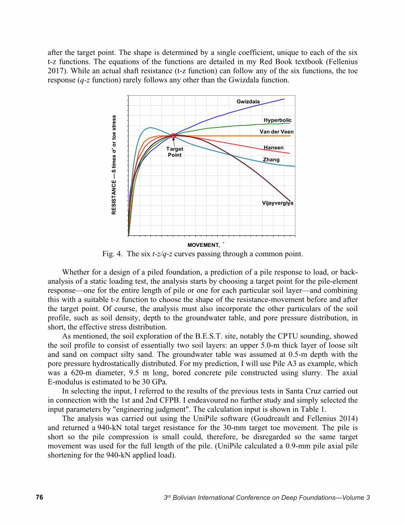
after the target point. The shape is determined by a single coefficient, unique to each of the six t-z functions. The equations of the functions are detailed in my Red Book textbook (Fellenius 2017). While an actual shaft resistance (t-z function) can follow any of the six functions, the toe response (q-z function) rarely follows any other than the Gwizdala function.
Fig. 4. The six t-z/q-z curves passing through a common point. Whether for a design of a piled foundation, a prediction of a pile response to load, or back-
analysis of a static loading test, the analysis starts by choosing a target point for the pile-element response—one for the entire length of pile or one for each particular soil layer—and combining this with a suitable t-z function to choose the shape of the resistance-movement before and after the target point. Of course, the analysis must also incorporate the other particulars of the soil profile, such as soil density, depth to the groundwater table, and pore pressure distribution, in short, the effective stress distribution.
As mentioned, the soil exploration of the B.E.S.T. site, notably the CPTU sounding, showed the soil profile to consist of essentially two soil layers: an upper 5.0-m thick layer of loose silt and sand on compact silty sand. The groundwater table was assumed at 0.5-m depth with the pore pressure hydrostatically distributed. For my prediction, I will use Pile A3 as example, which was a 620-m diameter, 9.5 m long, bored concrete pile constructed using slurry. The axial E-modulus is estimated to be 30 GPa.
In selecting the input, I referred to the results of the previous tests in Santa Cruz carried out in connection with the 1st and 2nd CFPB. I endeavoured no further study and simply selected the input parameters by "engineering judgment". The calculation input is shown in Table 1.
The analysis was carried out using the UniPile software (Goudreault and Fellenius 2014) and returned a 940-kN total target resistance for the 30-mm target toe movement. The pile is short so the pile compression is small could, therefore, be disregarded so the same target movement was used for the full length of the pile. (UniPile calculated a 0.9-mm pile axial pile shortening for the 940-kN applied load).
RES
ISTA
NC
E —
ß tim
es σ
' or t
oe s
tress
MOVEMENT, ´
Target Point
Hyperbolic
Van der Veen
Hansen
Zhang
Vijayvergiya
Gwizdala
76 3rd Bolivian International Conference on Deep Foundations—Volume 3

TABLE 1. Input parameters for static analysis.
Parameter Upper Layer Lower layer
Depth range (m) 0 to 6.0 6.0 to 10.0 Density (kg/m3) 2,000 2,100 Target ß-coefficient 0.3 0.4 Target toe stress (kPa) 1,500 Target movement (mm)*) 30 30 t-z function Van der Veen Gwizdala t-z coefficient 0.40 0.20 q-z function Gwizdala q-z coefficient 0.60
*) same target movement for all pile elements
Figure 5 presents the t-z and q-z curves for the prediction and to the curves used in UniPile's calculations of the load-movement curves for the back-calculation of the measured response of Pile A3. At each curve, the t-z/q-z curve 100 % ordinate value is the target unit shaft or toe resistances for the pile elements within the respective soil layers.
Table 2 compiles the input to UniPile in back-calculating the actual results showing only the parameters that needed adjustment. The best fit was obtained by input of slightly larger target beta-coefficients and smaller target toe resistance than those used for the prediction. The back-calculation target movement was the same as that used for the prediction. I could also have chosen to do the fit by keeping the original ß-coefficients, but using a smaller target movement.
TABLE 2. Input parameters adjusted in back-calculation.
Parameter Upper Layer Lower layer
Target ß-coefficient 0.4 0.6 Target toe stress (kPa) 1,100 t-z function Van der Veen Hyperbolic t-z coefficient 2.00 0.0070 q-z function Gwizdala q-z coefficient 0.70
Figure 6 shows the Pile A3 measured load-distribution (determined from the strain-gage
instrumentation) and the back-calculated load distribution for the target resistance. For comparison, the figure also includes the load distribution resulting from the prediction input.
The calculated load-movement curve predicting the pile response in the test is shown in Figure 7. The figure also shows the actual test curve and a back-calculation of the test carried out by computations varying the input until calculated load-movement curve fits the measured. The agreement between the predicted and actual curves is quite good. I can tell you that the agreement of my predictions for the other three piles is considerably less good. I considerably underestimated the stiffness improvement of the CFA- and FDP construction methods for both the shaft and toe responses.
773rd Bolivian International Conference on Deep Foundations—Volume 3

Fig. 5. Comparisons of t-z/q-z curves used in the prediction of Pile A3 load-movement response and as derived from a back-calculation of the actual test data.
rt = 1.1 MPa
ß = 0.60
ß = 0.40
Van der Veen,b = 2.00
HyperbolicC1 = 0.0070
Gwizdalaθ = 0.700
DERIVED IN BACK-CALCULATION
δ = 30 mm
δ = 30 mm
δ = 30 mm
USED IN PREDICTION
Van der Veen,b = 0.40
ß = 0.30
δ = 30 mm
ß = 0.40
Gwizdalaθ = 0.200
δ = 30 mm
rt = 1.5 MPa
Gwizdalaθ = 0.600
δ = 30 mm
78 3rd Bolivian International Conference on Deep Foundations—Volume 3

Fig. 6. Pile A3 measured and back-calculated load distribution.
Fig. 7. Predicted, measured, and back-calculated load-movement curves for Pile A3.
0
20
40
60
80
100
120
140
160
180
200
0
1
2
3
4
5
6
7
8
9
10
0 500 1,000 1,500
MOVEMENTD
EPTH
LOAD (kN)
(m)
(mm)
Pile Head Movement
UniPile Simulation for Target Resistance and Target Movement Pile A3 HD
0
200
400
600
800
1,000
1,200
1,400
1,600
0 10 20 30 40 50 60 70 80 90 100
LOA
D (
kN)
MOVEMENT (mm)
Actual Test
UniPile Fit
Prediction
Pile A3 HD
793rd Bolivian International Conference on Deep Foundations—Volume 3

The agreement between the predicted and actual curves is quite good. As Figure 8 makes clear, the agreement of my predictions of the other two head-down tests included in the prediction event (Pile B2 and C2) with the actual test curve, is considerably less good. I obviously underestimated the improvement of the pile stiffness for the CFA and FDP construction methods for both the shaft and toe responses. Nevertheless, the back-calculations fitting the UniPile analysis to the results of the tests show the power of the t-z/q-z computations in determining the load-movement response of pile.
Fig. 8. Predicted, measured, and back-calculated load-movement curves for Piles B2 and C2. Fitted curves are plotted as dashed lines.
The success of a design of a piled foundation ultimately rests with the foundation settlement
response to the applied load. What particular capacity definition and resistance factor that happened to be used for the design is rather moot. When the results of a static test do not show any particular point that could be assessed as a "capacity", I have found that the pile-head load that gave a 30-mm pile toe movement in the test is often suitable for putting the matter to at rest so the design effort could be directed to important issues, such as the settlement response of the foundation.
References
Bustamante, M. and Gianeselli, L., 1982. Pile bearing capacity predictions by means of static penetrometer CPT. Proc. of the Second European Symposium on Penetration Testing, ESOPT II, Amsterdam, May 24-27, A.A. Balkema, Vol. 2, pp. 493-500.
Chin, F.K., 1970. Estimation of the ultimate load of piles not carried to failure. Proc. of the 2nd Southeast Asian Conference on Soil Engineering, pp. 81-90.
Decourt, L., 1982. Prediction of bearing capacity of piles based exclusively on N-values of the SPT. Proc. ESOPT II, Amsterdam, May 24-27, pp. 19-34.
Decourt, L., 1999. Behavior of foundations under working load conditions. Proc. of 11th Pan-American Conference on Soil Mechanics and Geotechnical Engineering, Foz DoIguassu, Brazil, August 1999, Vol. 4, pp. 453 488.
DeRuiter, J. and Beringen F.L., 1979. Pile foundations for large North Sea structures. Marine Geotechnology, 3(3) 267 314.
0
500
1,000
1,500
2,000
2,500
0 20 40 60 80 100 120
LOA
D (
kN)
MOVEMENT (mm)
Pile C2 HD, FDP 450 mm
Pile B2 HD, CFA 450 mm
Piles B2 and C2 Predictions
C2
B2
80 3rd Bolivian International Conference on Deep Foundations—Volume 3

Eslami, A. and Fellenius, B.H., 1997. Pile capacity by direct CPT and CPTu methods applied to 102 case histories. Canadian Geotechnical Journal 34(6) 886–904.
Fellenius, B.H., 2017. Basics of foundation design–a textbook. Pile Buck International, Inc., Vero Beach, FL, Electronic Edition. www.Fellenius.net, 464 p.
Goudreault, P.A. and Fellenius, B.H., 2014. UniPile Version 5, User and Examples Manual. UniSoft Geotechnical Solutions Ltd. [www.UniSoftLtd.com]. 120 p.
Gwizdala, K., 1996. The analysis of pile settlement employing load-transfer functions (in Polish). Zeszyty Naukowe No. 532, Budownictwo Wodne No.41, Technical University of Gdansk, Poland, 192 p.
Hansen, J.B., 1963. Discussion on hyperbolic stress-strain response. Cohesive soils. ASCE Journal for Soil Mechanics and Foundation Engineering, 89(SM4) 241.
Meyerhof, G.G., 1976. Bearing capacity and settlement of pile foundations. The Eleventh Terzaghi Lecture, November 5, 1975. ASCE Journal of Geotechnical Engineering 102(GT3) 195 228.
O'Neill, M.W. and Reese, L.C., 1999. Drilled shafts. Construction procedures and design methods, Federal Highway Administration, Transportation Research Board, Washington, FHWA-IF99-025.
Van der Veen, C., 1953. The Bearing Capacity of a Pile. Proc. of the 3rd ICSMFE, Zürich, Switzerland, August 16-27, Vol. 2, pp. 84-90.
Schmertmann, J.H., 1978. Guidelines for cone penetration test, performance, and design. U.S. Federal Highway Administration, Washington, Report FHWA-TS-78-209, 145 p.
Vijayvergiya, V.N., 1977. Load-movement characteristics of piles. Proc. of Port '77 Conference, ASCE, Long beach, Ca, March 9 - 11, Vol. 2, pp. 269-284.
Zhang, Q.Q. and Zhang, Z.M., 2012. Simplified non-linear approach for single pile settlement analysis. Canadian Geotechnical Journal, 49(11) 1256-1266.
813rd Bolivian International Conference on Deep Foundations—Volume 3

82 3rd Bolivian International Conference on Deep Foundations—Volume 3
Calculations based on the pile on elastic supports model
Kos, J.(1)
(1) Czech Technical University in Prague, Prague, Czech Republic <[email protected]>
ABSTRACT. The computer program used for calculations, the input data for the program, and the results are briefly described. 1. INTRODUCTION
To predict behavior of piles tested at B.E.S.T. was not so easy for me. Large diameter piles bored with a casing or slurry are preferred in the Czech Republic. Use of CFA piles increased. Full displacement piles are practically not used. The site investigation is based on borehole results and laboratory testing of core samples. Penetrations are used especially for testing of subsoil heterogeneity. Due to this, most calculation methods and computer programs are based on classic soil parameters: φ, c, E, ½, stress-strain relationship, etc. I could use commercial computer programs (for example PLAXIS), or two my own: for finite element analysis (FEA), and “the pile on elastic springs”. Due to expected complications with evaluation of (classic) soil parameters at B.E.S.T., I decided to use the second of my programs. 2. COMPUTER PROGRAM
The computer program used for calculations of pile loading curves is based on an axially symmetric model of the perfectly elastic pile on non-linear elastic springs. The program is relatively old; the first presentation in English (more detailed, and describing the program for horizontally loaded piles too) is in Kos (1998). The program has been used to explain to students the principles of single and group pile behavior first of all. The main advantage is the computer time less than one second, and simple input data preparation.
The schema of the computer model is in Figure 1, where the left side is for a single pile, and the right side for a pile in a group. The elastic pile (divided on elements) rests on shear springs along its shaft (short cantilevers, horizontal layers of the soil cylinder surrounding the pile in reality), and on the Winkler spring under the toe. The gray area represents the soil at rest, i.e. with so small shear and vertical normal stress increments that deformations can be ignored. The group pile surroundings is limited, i.e. the settlement of a pile in a vertically compressed soil pier has to be calculated (the right schema). In the cross cut, the dotted circle is the pile, the white annulus represents shear springs, and the dotted surroundings the soil at rest. Stiffness of shear and the Winkler springs is calculated using the same principle: The contact stress increment Äol,c (Ãol,c) redistribution in the surrounding soil is calculated: Äol (Ãol). Stress increments are reduced using Äs (Ãs), so called “the structural strength of soil” (translation from Czech), i.e. the difference between the maximum normal (shear) stress at rest and the original stress. Thickness (t) of a soil layer disturbed by technology (without the structural strength) reduces maximum spring stiffness in the beginning of pile loading (contact stress increments are smaller than the structural strength). Deformations and stiffness of springs are calculated, and continually improved using the iterative process. Contact stress limits are continually checked and protected using zero spring stiffness (perfect plasticization).
833rd Bolivian International Conference on Deep Foundations—Volume 3

Fig. 1. Computer model for single (left) and group piles, and spring stiffness calculation.
The shear spring stiffness is calculated using Eq. (1):
( ) ∫∫
−
+=−=
aa L
scol
L
sol dxxr
r
Gdx
Gs
0
,
0
11 ττττ (1)
where s = settlement of the spring end connected to the pile shaft G = shear modulus (incorporating plastic deformations). Other symbols are in Figure 1.
The Winkler spring stiffness is calculated in the same manner. Shear stresses and the modulus
are changed by normal values (Ã, E), and the vertical stress distribution under the toe is calculated as under the circular foundation on the Boussinesq half-space:
( )∫ −=aL
sol dzE
s0
1 σσ (2)
84 3rd Bolivian International Conference on Deep Foundations—Volume 3

The “structural strength of soil” is calculated as the difference between the maximum normal (shear) stress at rest and the original stress (at rest). The partly mobilized angle of internal friction of the soil at rest (Æ0) is calculated from the peak value (Æ) using Eq. 3:
( ) ( )245tansin1 0
200 ϕσϕσσσ −°=−== zzaza K (3)
where K0a = minimum (active) Jáky’s coefficient of pressure at rest.
Resultant friction angle (and cohesion, Eq. 5) “at rest” is the extreme value. Smaller values can be obtained from the experimental stress-strain relationship of the soil. But it is better and more realistic to say a perfectly elastic soil with small strain than the soil “at rest“.
( )[ ]ϕϕϕ sin2sinarcsin0 −= (4)
ϕϕ tantan. 00 cc = (5)
Stresses “at rest” can be calculated using standard equations for active and passive pressures
with “partly mobilized” shear parameters. The shear resistance is calculated using Eq. 6. Peak, or partly mobilized shear parameters are
used as dependent on the situation (shear resistance, or shear stress “at rest”).
( )[ ] ( )2412
21
max cos.sin. xzxz c σσϕϕσστ −−++= (6)
The Coulomb Eq. 7 is used only if the shear resistance is reduced using the program input
coefficient < 1.0. Smaller from results of Eq. 6 and (reduced) Eq. 7 is then used.
ϕστ tan..0max zKc += (7)
Shear stresses calculated using Eqs. 6 – 7 for the soil with Æ = 32°, c = 14 kPa are in Figure 2. The vertical pressure Ãz = 100 kPa, the horizontal pressure Ãx varies between the Rankine active and passive stresses (Ã0p is the maximum /passive/ pressure “at rest”). The horizontal stress interval in stable walls of a borehole should be bigger than in a planar case solved by Eq. 6.
Fig. 2. Shear stresses calculated using Eqs. 6 – 7.
853rd Bolivian International Conference on Deep Foundations—Volume 3

Initial values of normal stresses on the pile surface-soil contact (radial on the pile shaft, vertical on the toe) are calculated as pressures of fresh concrete in the silo (like Janssen’s solution, but numeric). Using the fresh concrete parameters: Æ = 4-6°, c = 0 kPa, Æ0 = Æ/2, the stabilization of the radial stress can be reached at the depth less than 10-15 pile diameters as observed.
3. INPUT PARAMETERS
Soil characteristics necessary for the computer program was neither measured in B.E.S.T. nor entrained in publications for prediction of the B.E.S.T. piles behavior. Due to this, the soil characteristics were estimated using the description of soil layers, and static penetrations in B.E.S.T., and the soil characteristics typical for the territory of Czechoslovakia from CSN 73 1001: Ground under the spread foundations (translation from Czech). Stiffness of soil layers above the pile toe was reduced (the program overestimates stiffness of shear springs); the angle of internal friction of sandy soil under the toe was reduced to decrease the coefficient Nq, and the pile toe capacity. 4. CALCULATIONS
The input screens of the computer program, and pile load-settlement curves are in the next figures. Only the first screens with pile, and soil characteristics are presented. Second screens are not so important in this case. They contain present and original uniform load on terrain (zero was used), load increments (100 kN), maximum load for calculations (was changed during analyses), maximum settlement (sometimes limits the applied load), and the coefficient which can be used for reduction of the toe spring stiffness if the settlement is smaller than expected. 4.1 Piles A3, B2, and C2
Input characteristics of the bored Pile A3 and the soil layers are in the left on Figure 3. Practically all parameters have been introduced. “Disturbed soil thickness” is (t) in Figure 1. “Relative coefficient of pressure at rest” multiplies the minimum (active) pressure at rest if positive, or maximum (passive) pressure at rest if negative. The rest to 1.0 multiplies the “hydrostatic” pressure of soil. In the presented case, the initial pressure at rest is “hydrostatic” (K0 = 1.0). “PHIr/PHI rate” means Æ0/Æ for calculations of stresses at rest, and the � structural strength� . The unit weight of fresh concrete under GWL (defined by soil layers with “GAM” < 14 kNm-3) is reduced by water uplift. Input characteristics used for the recalculation after loading tests are in the right. The fresh concrete parameters (inside the white frame) were increased to enlarge the silo effect, and reduce the shaft resistance. The toe spring stiffness was reduced to reach the pile capacity at the settlement close to 10 % of the pile diameter (using the coefficient on the second screen of the program input).
86 3rd Bolivian International Conference on Deep Foundations—Volume 3

Fig. 3. Input characteristics for calculation (left) and recalculation of the Pile A3. The calculated, modified, measured and recalculated load-settlement curves of the Pile A3 are
in Figure 4. The curve was calculated using input characteristics in the left side of Figure 3. Due to small settlement, the calculated curve was modified applying the progressive plasticization of the soil under the toe. From the certain point, each load increment was connected with a double increment of the toe (pile) settlement than the preceding load increment. This “modified” curve was sent as the prediction. The “measured” curve is close to the result of the B.E.S.T. pile loading test; its points have been taken by fitting curves in Fellenius (2017). After obtaining the results of loading tests, the load-settlement curve has been recalculated with input characteristics in the right side of Figure 3.
Fig. 4. Pile load-settlement curves of the bored Pile A3.
873rd Bolivian International Conference on Deep Foundations—Volume 3

Fig. 5. Input characteristics for calculations of the Pile B2 (left), and Pile C2.
Input screens of the computer program for the CFA Pile B2 (left), and full displacement Pile C2 are on Figure 5. The program was modified (no uplift acts on fresh concrete under GWL), and input friction angles of fresh concrete were zero. The aim was to maximize contact pressure of fresh concrete. The effect of the full displacement body on the surrounding soil (Pile C2) was expressed by “Relative coefficient of pressure at rest” = -0.80, i.e. K0 = 0.80.K0p + 0.20×1.00.
For recalculations, unit weights of all soil layers have been increased to 20 kNm-3 (no ground water effect due to technology?), and the toe spring stiffness has been reduced (settlement round 10 % of a pile diameter for the calculated pile capacity).
Fig. 6. Pile load-settlement curves of the CFA Pile B2.
88 3rd Bolivian International Conference on Deep Foundations—Volume 3

Fig. 7. Pile load-settlement curves of the full displacement Pile C2.
References
Fellenius, B.H., 2017. B.E.S.T. results of static loading tests on Piles A3, B2, C2, and E1. MS Excel XLSX file sent by Internet, March 28, 38 kB.
Kos, J., 1998. Non-linear analyses of axially and laterally loaded bored piles. Proceedings of the 4th NUMGE, Udine, October 14-16, pp. 121-130.
893rd Bolivian International Conference on Deep Foundations—Volume 3

90 3rd Bolivian International Conference on Deep Foundations—Volume 3

CPT-based and numerical approaches to predict load-displacement and the bearing capacity of Bolivian piles
Moshfeghi, S.(1), Valikhah, F.(2), and Eslami, A.(3)
(1) Geotechnical Engineer, Sham-e Consulting Engineering Company, Tehran, Iran
<[email protected]> (2) PhD Candidate, Amirkabir University of Technology, Tehran, Iran <[email protected]>
(3) Professor, Amirkabir University of Technology, Tehran, Iran <[email protected]> ABSTRACT. This paper provides the procedure and the results of estimating the bearing capacity and load-displacement behaviour of three piles with reference to the 3rd Bolivian prediction event. In this regard, an initial bearing capacity has been estimated for each pile using CPT and CPTu-based methods. The results were then employed as an approximate load for the numerical analyses from which the load-movement diagrams have been derived. The methods as well as correlations used for estimating the capacity along with soil parameters via indirect approaches are introduced. Finally, the results are compared to the measurements and the possible reasons for the deviations from the measured values are discussed. 1. INTRODUCTION
In connection with the 3rd Bolivian prediction event, Santa Cruz de la Sierra, Bolivia, April 27 - 29, 2017, site investigations were performed at the Bolivian Experimental Site for Testing Piles (B.E.S.T.) comprising various in-situ tests. The B.E.S.T. also included several static and dynamic tests on single piles and group piles constructed using different methods and employing different features for stiffening the pile response to load. The static tests of four single piles were selected for a prediction event. One pile (Pile A3) was bored with slurry, one (Pile B2) was constructed with a continuous flight auger, and two (C2 and E1) were constructed by full displacement equipment. The piles characteristics are presented in Table 1. TABLE 1. Characteristics of the investigated piles.
Pile name Length (m) Diameter (mm) Construction type
A3 9.5 670 Bored B2 9.5 445 Continuous Flight Auger (CFA) C2 9.5 446 Full displacement
The Cone Penetration Test (CPT) has always been favored for several advantages, including
being fast, sufficiently accurate and providing continuous soil information in depth. Moreover, owing to its similarity to a pile in terms of shape and penetration mechanism, it has been widely used specifically in pile design. Therefore, in light of its applicability and promising performance, in this paper, CPT-based approaches were employed both directly and indirectly. In the direct approach the bearing capacity of piles was estimated with direct using of CPT results. And, in the indirect approach the soil parameters used as an input for the numerical model were estimated by CPT-based correlation.
913rd Bolivian International Conference on Deep Foundations—Volume 3

In this paper, the piles A3, B2, and C2 are studied which were straight-shaft piles and tested in head-down tests. The procedure and the methods used in this regard are introduced, the results are presented. Furthermore, the comparison is made with the actual values from field testing and the possible reasons for the differences in the estimated and the observed behavior are discussed. 2. DIRECT AND INDIRECT CPT-BASED METHODS
Indirect and direct methods are two main approaches to accomplish axial pile capacity analysis from CPT data. In indirect methods, the first step is providing an assessment of geoparameters such as strength parameters and bearing capacity coefficients (Nc and Nq). Then, in the second step, the shaft and toe resistances of a pile can be estimated using an appropriate analytical approach (Lee et al., 2003; Eslami et al., 2011, Niazi and Mayne, 2013).
Via direct CPT methods, the measured penetrometer readings are used to directly evaluate toe and shaft capacity of full-size piles by scaling algorithms. In fact, the unit toe resistance is evaluated from the cone tip resistance, and the shaft resistance from either the sleeve friction or the cone tip resistance profiles (Eslami and Fellenius, 1997; Eslami et al., 2011, Niazi and Mayne, 2013, Moshfeghi et al., 2015).
3.1 DIRECT APPROACH
In this part of the study, five well-known CPT and CPTu-based methods of determining the bearing capacity of which have previously shown compelling performance in literature (Moshfeghi and Eslami, 2016; Eslami and Fellenius, 1997; Abu-Farsakh and Titi, 2004) were selected. These methods in chronological order include Nottingham and Schmertmann (1978), LCPC (Bustamante and Gianeselli, 1982), UniCone (Eslami and Fellenius, 1997), Togliani (2008) and German method (Kempfert and Becker, 2010). Due to space limitations, the formulations of the methods are not provided in here. However, a brief description of each method and the corresponding references are presented in this section.
The Schmertmann method which is based on a summary of the work on model and full scale piles presented by Nottingham (1975) and Schmertmann (1978), considers the applicability of mechanical and electrical penetrometers as well as different soil type combinations.
The LCPC method by Bustamante and Gianeselli (1982) provides calculating the unit shaft and toe resistance by employing the cone tip resistance. Different soil type, pile type and installation procedures are considered by imposing different upper limits for the unit shaft resistance.
The Unicone method (Eslami and Fellenius, 1997) is based on a large database, including a large variety of piles installed in different soils. This method uses an effective stress approach for soil profiling and determining the pile capacity and employs all three CPTu readings (qc, fs, u2). In this method, the geometric mean is used to reduce the potential disproportionate influence of odd peaks and troughs.
Togliani (2008) is a simplified direct CPT-based method for displacement and non-displacement. In this method, the effect of the cone skin friction is considered in pile capacity estimation.
The German Method is based on the database of 1000 pile load tests of various pile types and presents upper and lower limits of the unit shaft and toe capacity from the cone tip resistance according to the proposed qc-rs and qc-rt charts (rt and rs are unit toe and shaft resistance of the pile, respectively.).
92 3rd Bolivian International Conference on Deep Foundations—Volume 3

The results of the pile bearing capacities obtained from these methods are presented in Table 2. It should be mentioned that the average capacity obtained from these methods were used in the analyses. TABLE 2. Bearing Capacity of piles estimated by different methods.
Methods A3 B2 C2
Rs
(kN) Rt
(kN) Ru
(kN) Rs
(kN) Rt
(kN) Ru
(kN) Rs
(kN) Rt
(kN) Ru
(kN) LCPC (1982) 763 1015 1778 554 525 1079 555 525 1080 Schmertmann (1978) 405 1306 1711 748 281 1029 281 748 1029 Eslami and Fellenius (1997) 574 809 1383 416 759 1175 416 759 1175 Togliani (2008) 611 481 1092 533 353 886 888 410 1298 German method (2010) 744 604 1349 540 318 859 710 545 1255
Average of all methods 619 843 1463 558 447 1006 570 597 1167
3.2 INDIRECT APPROACH
Indirect CPT-based approaches were used to estimate the required soil parameters for the numerical analysis, which will be discussed in the next section. Four soil parameters which consist of soil internal friction angle (ϕ), cohesion (c), Young elasticity modulus (Es) as well as Poisson’s ratio (Å) needed to be estimated for numerical analysis.
In order to estimate the soil internal friction angle, three correlations were used. The final friction angle value for each layer was considered as the average of the three values obtained from these correlations. The correlations are Bowles (1999), Robertson and Campanella (1988) and Mayne and Kulhawy (2003). Bowles (1999) correlates the internal friction angel with the square root of the cone tip resistance. According to Robertson and Campanella (1988) the internal friction angle in each depth can be estimated by the cone tip resistance as well as effective vertical stress in that depth. Quite similarly, Mayne and Kulhawy (2003) presented a correlation of determining the internal friction angle in terms of cone tip resistance and effective vertical stress.
The cohesion parameters in cohesive soils were estimated using the correlation presented in Mayne and Kulhawy (2003). According to this correlation, the cohesion can be obtained based on the values of cone tip resistance, total vertical stress as well as a coefficient varying between 10 and 15 for normally consolidated soils. It should be mentioned that for the non-cohesive layers, in order to avoid divergence in FE model, the value of 1 kPa was assumed for the cohesion.
The other two parameters, Young elasticity modulus and Poisson’s ratio, were determined according to the recommended values in Das (2006) based on soil types.
Soil layers were chosen based on the provided information about the site in addition to CPT classification charts (Eslami and Fellenius, 2004). The final soil layers considered for numerical analysis as well as the estimated soil parameters are presented in Table 3.
933rd Bolivian International Conference on Deep Foundations—Volume 3
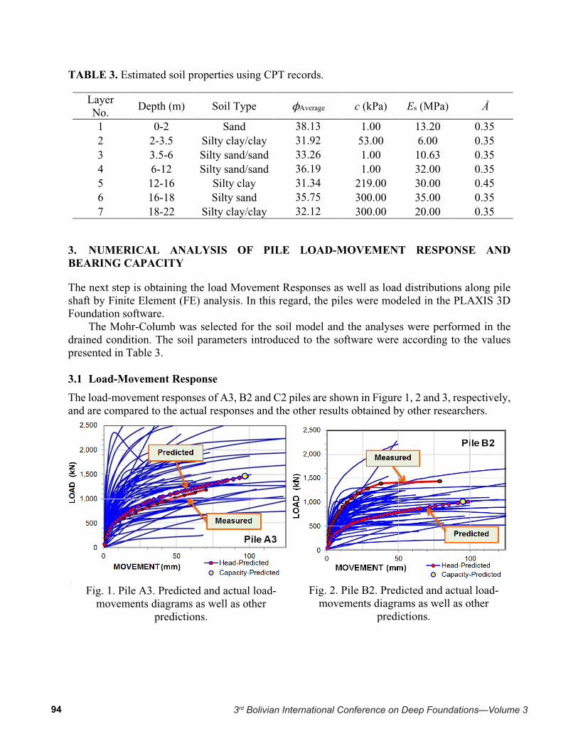
TABLE 3. Estimated soil properties using CPT records.
Layer No.
Depth (m) Soil Type ϕAverage c (kPa) Es (MPa) Å
1 0-2 Sand 38.13 1.00 13.20 0.35 2 2-3.5 Silty clay/clay 31.92 53.00 6.00 0.35 3 3.5-6 Silty sand/sand 33.26 1.00 10.63 0.35 4 6-12 Silty sand/sand 36.19 1.00 32.00 0.35 5 12-16 Silty clay 31.34 219.00 30.00 0.45 6 16-18 Silty sand 35.75 300.00 35.00 0.35 7 18-22 Silty clay/clay 32.12 300.00 20.00 0.35
3. NUMERICAL ANALYSIS OF PILE LOAD-MOVEMENT RESPONSE AND BEARING CAPACITY
The next step is obtaining the load Movement Responses as well as load distributions along pile shaft by Finite Element (FE) analysis. In this regard, the piles were modeled in the PLAXIS 3D Foundation software.
The Mohr-Columb was selected for the soil model and the analyses were performed in the drained condition. The soil parameters introduced to the software were according to the values presented in Table 3.
3.1 Load-Movement Response
The load-movement responses of A3, B2 and C2 piles are shown in Figure 1, 2 and 3, respectively, and are compared to the actual responses and the other results obtained by other researchers.
Fig. 1. Pile A3. Predicted and actual load-movements diagrams as well as other
predictions.
Fig. 2. Pile B2. Predicted and actual load-movements diagrams as well as other
predictions.
94 3rd Bolivian International Conference on Deep Foundations—Volume 3
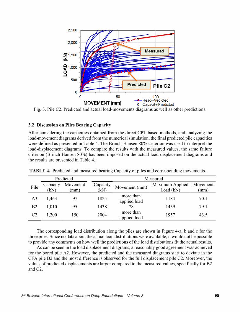
Fig. 3. Pile C2. Predicted and actual load-movements diagrams as well as other predictions.
3.2 Discussion on Piles Bearing Capacity
After considering the capacities obtained from the direct CPT-based methods, and analyzing the load-movement diagrams derived from the numerical simulation, the final predicted pile capacities were defined as presented in Table 4. The Brinch-Hansen 80% criterion was used to interpret the load-displacement diagrams. To compare the results with the measured values, the same failure criterion (Brinch Hansen 80%) has been imposed on the actual load-displacement diagrams and the results are presented in Table 4. TABLE 4. Predicted and measured bearing Capacity of piles and corresponding movements.
Predicted Measured
Pile Capacity
(kN) Movement
(mm) Capacity
(kN) Movement (mm)
Maximum Applied Load (kN)
Movement (mm)
A3 1,463 97
1825 more than
applied load 1184 70.1
B2 1,010 95 1438 78 1439 79.1
C2 1,200 150
2004 more than
applied load 1957 43.5
The corresponding load distribution along the piles are shown in Figure 4-a, b and c for the three piles. Since no data about the actual load distributions were available, it would not be possible to provide any comments on how well the predictions of the load distributions fit the actual results.
As can be seen in the load displacement diagrams, a reasonably good agreement was achieved for the bored pile A2. However, the predicted and the measured diagrams start to deviate in the CFA pile B2 and the most difference is observed for the full displacement pile C2. Moreover, the values of predicted displacements are larger compared to the measured values, specifically for B2 and C2.
953rd Bolivian International Conference on Deep Foundations—Volume 3
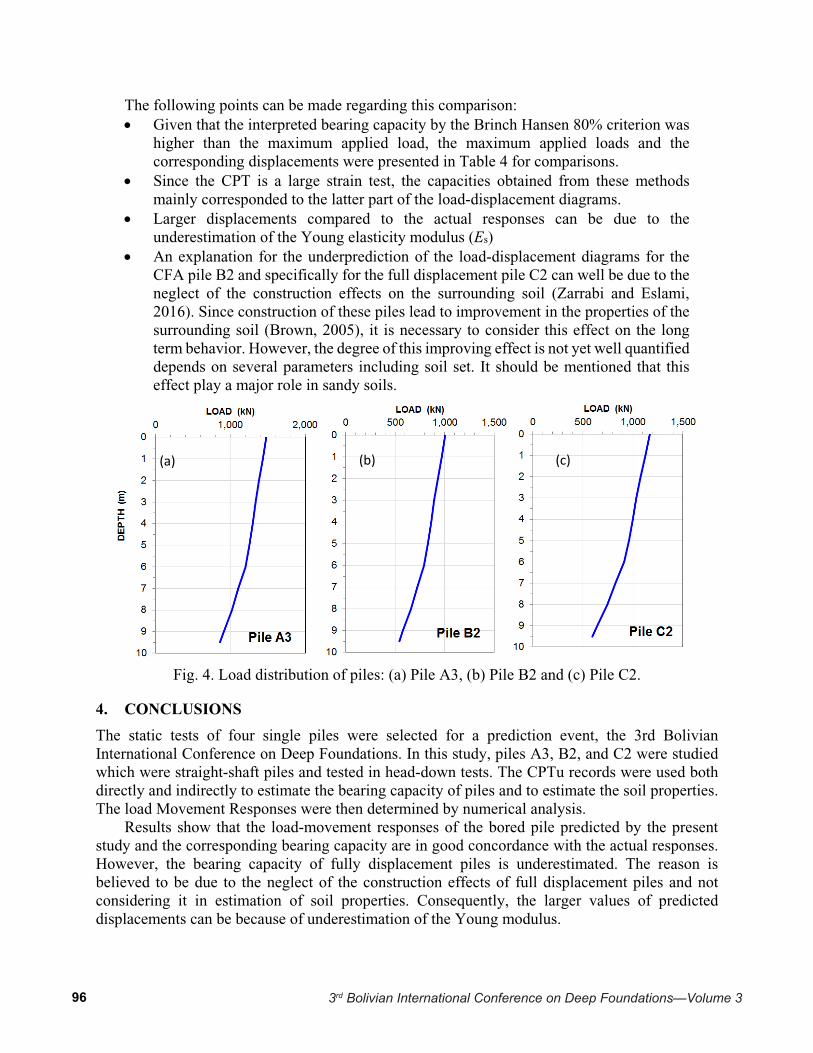
The following points can be made regarding this comparison: • Given that the interpreted bearing capacity by the Brinch Hansen 80% criterion was
higher than the maximum applied load, the maximum applied loads and the corresponding displacements were presented in Table 4 for comparisons.
• Since the CPT is a large strain test, the capacities obtained from these methods mainly corresponded to the latter part of the load-displacement diagrams.
• Larger displacements compared to the actual responses can be due to the underestimation of the Young elasticity modulus (Es)
• An explanation for the underprediction of the load-displacement diagrams for the CFA pile B2 and specifically for the full displacement pile C2 can well be due to the neglect of the construction effects on the surrounding soil (Zarrabi and Eslami, 2016). Since construction of these piles lead to improvement in the properties of the surrounding soil (Brown, 2005), it is necessary to consider this effect on the long term behavior. However, the degree of this improving effect is not yet well quantified depends on several parameters including soil set. It should be mentioned that this effect play a major role in sandy soils.
Fig. 4. Load distribution of piles: (a) Pile A3, (b) Pile B2 and (c) Pile C2.
4. CONCLUSIONS
The static tests of four single piles were selected for a prediction event, the 3rd Bolivian International Conference on Deep Foundations. In this study, piles A3, B2, and C2 were studied which were straight-shaft piles and tested in head-down tests. The CPTu records were used both directly and indirectly to estimate the bearing capacity of piles and to estimate the soil properties. The load Movement Responses were then determined by numerical analysis.
Results show that the load-movement responses of the bored pile predicted by the present study and the corresponding bearing capacity are in good concordance with the actual responses. However, the bearing capacity of fully displacement piles is underestimated. The reason is believed to be due to the neglect of the construction effects of full displacement piles and not considering it in estimation of soil properties. Consequently, the larger values of predicted displacements can be because of underestimation of the Young modulus.
(a) (b) (c)
96 3rd Bolivian International Conference on Deep Foundations—Volume 3
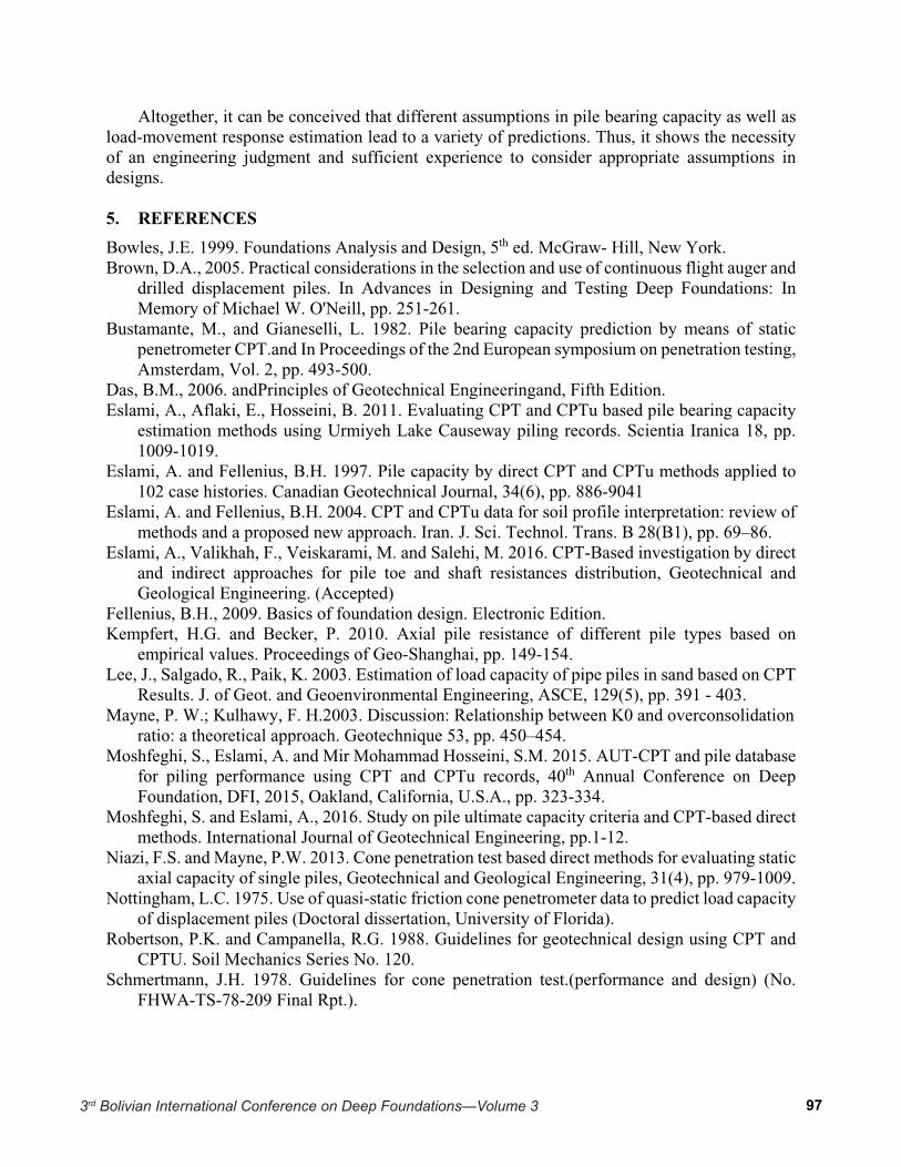
Altogether, it can be conceived that different assumptions in pile bearing capacity as well as load-movement response estimation lead to a variety of predictions. Thus, it shows the necessity of an engineering judgment and sufficient experience to consider appropriate assumptions in designs.
5. REFERENCES
Bowles, J.E. 1999. Foundations Analysis and Design, 5th ed. McGraw- Hill, New York. Brown, D.A., 2005. Practical considerations in the selection and use of continuous flight auger and
drilled displacement piles. In Advances in Designing and Testing Deep Foundations: In Memory of Michael W. O'Neill, pp. 251-261.
Bustamante, M., and Gianeselli, L. 1982. Pile bearing capacity prediction by means of static penetrometer CPT.and In Proceedings of the 2nd European symposium on penetration testing, Amsterdam, Vol. 2, pp. 493-500.
Das, B.M., 2006. andPrinciples of Geotechnical Engineeringand, Fifth Edition. Eslami, A., Aflaki, E., Hosseini, B. 2011. Evaluating CPT and CPTu based pile bearing capacity
estimation methods using Urmiyeh Lake Causeway piling records. Scientia Iranica 18, pp. 1009-1019.
Eslami, A. and Fellenius, B.H. 1997. Pile capacity by direct CPT and CPTu methods applied to 102 case histories. Canadian Geotechnical Journal, 34(6), pp. 886-9041
Eslami, A. and Fellenius, B.H. 2004. CPT and CPTu data for soil profile interpretation: review of methods and a proposed new approach. Iran. J. Sci. Technol. Trans. B 28(B1), pp. 69–86.
Eslami, A., Valikhah, F., Veiskarami, M. and Salehi, M. 2016. CPT-Based investigation by direct and indirect approaches for pile toe and shaft resistances distribution, Geotechnical and Geological Engineering. (Accepted)
Fellenius, B.H., 2009. Basics of foundation design. Electronic Edition. Kempfert, H.G. and Becker, P. 2010. Axial pile resistance of different pile types based on
empirical values. Proceedings of Geo-Shanghai, pp. 149-154. Lee, J., Salgado, R., Paik, K. 2003. Estimation of load capacity of pipe piles in sand based on CPT
Results. J. of Geot. and Geoenvironmental Engineering, ASCE, 129(5), pp. 391 - 403. Mayne, P. W.; Kulhawy, F. H.2003. Discussion: Relationship between K0 and overconsolidation
ratio: a theoretical approach. Geotechnique 53, pp. 450–454. Moshfeghi, S., Eslami, A. and Mir Mohammad Hosseini, S.M. 2015. AUT-CPT and pile database
for piling performance using CPT and CPTu records, 40th Annual Conference on Deep Foundation, DFI, 2015, Oakland, California, U.S.A., pp. 323-334.
Moshfeghi, S. and Eslami, A., 2016. Study on pile ultimate capacity criteria and CPT-based direct methods. International Journal of Geotechnical Engineering, pp.1-12.
Niazi, F.S. and Mayne, P.W. 2013. Cone penetration test based direct methods for evaluating static axial capacity of single piles, Geotechnical and Geological Engineering, 31(4), pp. 979-1009.
Nottingham, L.C. 1975. Use of quasi-static friction cone penetrometer data to predict load capacity of displacement piles (Doctoral dissertation, University of Florida).
Robertson, P.K. and Campanella, R.G. 1988. Guidelines for geotechnical design using CPT and CPTU. Soil Mechanics Series No. 120.
Schmertmann, J.H. 1978. Guidelines for cone penetration test.(performance and design) (No. FHWA-TS-78-209 Final Rpt.).
973rd Bolivian International Conference on Deep Foundations—Volume 3
Togliani, G. 2008. Pile capacity prediction for in-situ tests, Proceedings of Geotechnical and Geophysical Site Characterization, Taylor and Francis Group, London, pp. 1187-1192.
Zarrabi, M. and Eslami, A., 2016. Behavior of piles under different installation effects by physical modeling. International Journal of Geomechanics, 16(5) 04016014.
98 3rd Bolivian International Conference on Deep Foundations—Volume 3

Summary and comments on predictions submitted to the 3rd Bolivian International Conference on Deep Foundations
Murillo, T.(1)
(1) Uriel & Asociados, S.A., Pozuelo de Alarcón, Spain <[email protected]>
ABSTRACT. The text summarizes the procedure adopted for the prediction of the load-movement behavior of 4 piles at the Bolivian Experimental Site for Testing Piles (B.E.S.T.). 1. DESCRIPTION OF THE PILES
The characteristics of the piles are the following: TABLE 1. Characteristics of the piles.
Pile Construction method
Nominal Diameter (m)
Average estimated diameter
(m) Length
(m)
A3 Bored with slurry 0.62 0.67 9.5
B2 Continuous flight auger 0.45 0.45 9.5
C2 Full displacement 0.44 0.45 9.8
E1 Full displacement and expanded toe (expander body)
0.30 0.32 10.0
2. GEOTECHNICAL INVESTIGATIONS
CPTU and SPT tests have been used to define soil profile and its characteristics. In addition, percentage of fines and plasticity indices have helped to understand and classify the soil.
Although the pressuremeter is a useful test and serves as the basis for a great design method, it has been considered unreliable on these alluvial sands due to the very likely lack of stability and the disturbance of borehole walls.
To simplify calculations, the soil profile has been considered to have four layers with the same thickness for all the pile locations.
The following figure shows the CPTU qt-curves, and the SPT test results, for the four pile locations.
Table 2 shows a summary of the geotechnical profile considered for calculations.
993rd Bolivian International Conference on Deep Foundations—Volume 3

Fig. 1. a) CPTU qt-curve comparison; b) SPT N-index comparison.
TABLE 2. Soil layers.
Layer Top Bottom Thickness Soil classification N index qc
(m) (m) (m) (USCS) (Mpa)
1 0.0 1.5 1.5 SM 10 8.8
2 1.5 4.0 2.5 CL/SC 4 1.5
3 4.0 6.5 2.5 SM 3 2.9
4 6.5 12.0 5.5 SM 13 / 19 / 16 / 18 (*) 8.3
(*): Values for piles A3 / B2 / C1 / E1 3. CALCULATION METHODS 3.1 Selection of methods
The main ideas considered when choosing the calculation methods to give a prediction are the following:
1. - Empirical methods, based on in situ tests (CPT, SPT or pressuremeter), have been considered more realistic than analytical methods. Therefore, calculations for the prediction have been focused on these methods.
100 3rd Bolivian International Conference on Deep Foundations—Volume 3

2. – In addition, some empirical methods take into account the execution method of the piles, which is very relevant on daily works, and especially for this prediction, since every pile has been executed in a different way.
Two methods that satisfy the two points mentioned above are the Decourt and Quaresma method, based on SPT tests, and the French method by Gianelesi and Bustamante, based on pressuremeter tests. It is important to bear in mind that any method that includes coefficients to distinguish the shaft or toe resistance, depending on the construction method used for the pile, can be very useful to compare the capacities of different types of piles in the same soil. This is the case for the French method mentioned, which distinguishes 20 pile execution techniques that are classified into 8 types.
For the “basic” pile, i.e. the bored pile, several other methods have been used, including an analytical method, with the aim of comparing the variation of results through different approaches.
The methods finally considered for the prediction have been the following: - For pile A3, the capacity adopted has been an average of the Decourt and Quaresma and the
French CPT methods. - For piles B2, C2 and E1, the Decourt and Quaresma method has been adopted. For these
piles, the influence of the execution technique has been taken into account by mean of: a) Decourt and Quaresma alfa and beta coefficients; b) Pressuremeter method by Gianelesi and Bustamante. C) Decourt and Quaresma experience on Expander Boby.
Results from the calculations methods have been considered as the “capacity” of the pile. This capacity corresponds to a certain normalized settlement of the pile toe. A 10 % of normalized settlement has been assumed for all methods (although not all of them specify this value), except for the AASHTO SPT method (5 %), and for the analytical method (15 %).
Finally, it is worth pointing out that no corrections have been made on the raw N-index obtained in the field. This is obviously questionable. The main reason for proceeding this way is that it is not clear whether the SPT based methods, established a long time ago in many cases, were calibrated for SPT devices returning a 60 % of energy efficiency. Later on I learnt that Decourt and Quaresma take this concern very much into account, and they use a 60 % of energy efficiency for the SPT index.
3.2 Decourt and Quaresma method
This Decourt and Quaresma method is summarized in Figure 2. Notice that a recommended factor for the expander body has been added. It was obtained from a load test from the 1st Bolivian Congress on Deep Foundations (1er CFPB).
3.3 Considerations on the coefficients for each pile execution technique
I believe that the CFA pile develops higher side resistance than a conventional bored pile, so I adopted a β coefficient equivalent to the one for a driven pile. On the other hand, the toe behavior should be worse than the one for a driven pile and probably similar to the one for a bored pile. Therefore, I adopted the coefficients listed in the following table (in parenthesis, the Decourt and Quaresma proposal). For the Full Displacement Pile (FDP), I also made my own proposal, analyzing data from published load tests (Fellenius, B.H. and Terceros M., 2014.)
1013rd Bolivian International Conference on Deep Foundations—Volume 3
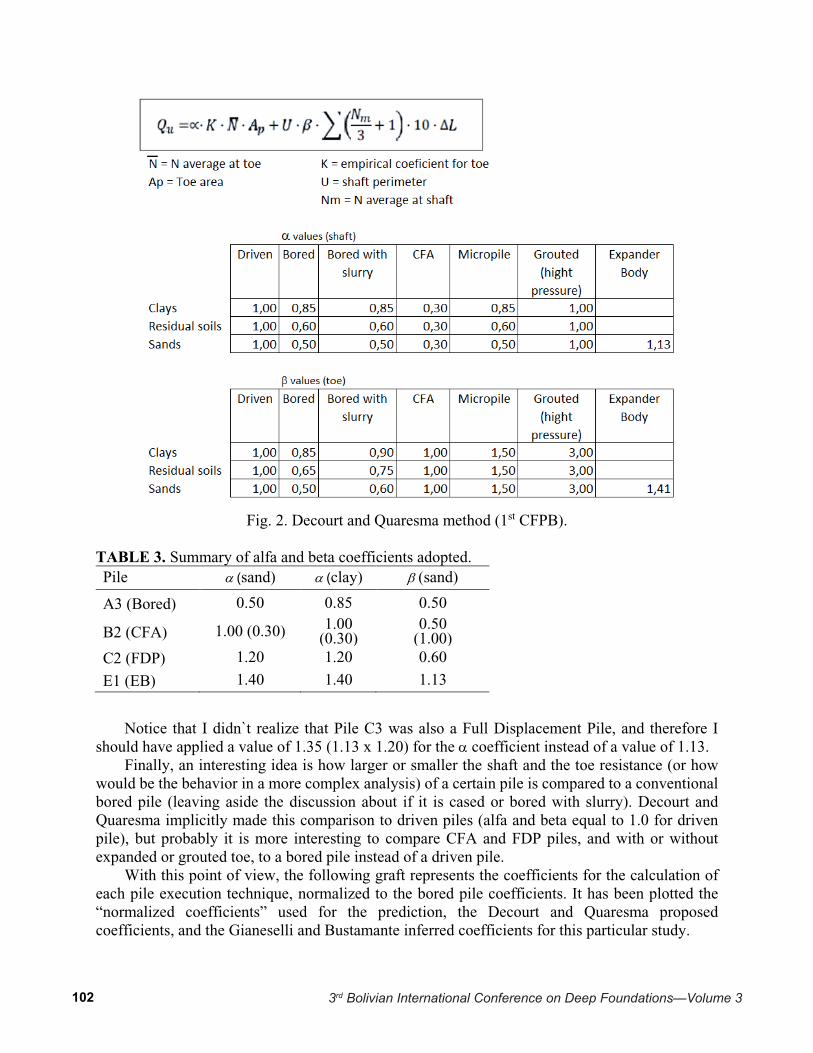
Fig. 2. Decourt and Quaresma method (1st CFPB).
TABLE 3. Summary of alfa and beta coefficients adopted. Pile α (sand) α (clay) β (sand)
A3 (Bored) 0.50 0.85 0.50
B2 (CFA) 1.00 (0.30) 1.00 (0.30)
0.50 (1.00)
C2 (FDP) 1.20 1.20 0.60
E1 (EB) 1.40 1.40 1.13
Notice that I didn`t realize that Pile C3 was also a Full Displacement Pile, and therefore I should have applied a value of 1.35 (1.13 x 1.20) for the α coefficient instead of a value of 1.13.
Finally, an interesting idea is how larger or smaller the shaft and the toe resistance (or how would be the behavior in a more complex analysis) of a certain pile is compared to a conventional bored pile (leaving aside the discussion about if it is cased or bored with slurry). Decourt and Quaresma implicitly made this comparison to driven piles (alfa and beta equal to 1.0 for driven pile), but probably it is more interesting to compare CFA and FDP piles, and with or without expanded or grouted toe, to a bored pile instead of a driven pile.
With this point of view, the following graft represents the coefficients for the calculation of each pile execution technique, normalized to the bored pile coefficients. It has been plotted the “normalized coefficients” used for the prediction, the Decourt and Quaresma proposed coefficients, and the Gianeselli and Bustamante inferred coefficients for this particular study.
102 3rd Bolivian International Conference on Deep Foundations—Volume 3

Fig. 3. Normalized coefficients for toe and shaft resistance.
4. CONSTRUCTING THE PILE RESPONSE CURVES
Once the resistance of the pile, corresponding to a settlement of 10 % of the diameter, is calculated, then its load-settlement curve considered is the sum of the shaft and toe curves proposed by O`Neill and Reese for bored piles on sands, included in FHWA (1999) and in AASHTO (2014). These curves are shown in the following figure.
Fig. 4. O`Neill and Reese pile behavior curves for bored piles on sands.
1033rd Bolivian International Conference on Deep Foundations—Volume 3

In particular, side mobilized resistance has been considered linear to 0.4 % of normalized settlement (s/D), fully mobilized at 0.7 %, and then as a constant value.
The elastic compression of the pile has been added, using a deformation modulus of 25 GPa for the pile and the theoretical cross section.
References
AASHTO, 2012. LRFD Bridge Design Specifications. Bustamante M., Gianeselli L., 2008. Reglas de cálculo de la resistencia de pilotes por el método
de los estados límites últimos. Método presiométrico. CEDEX. Madrid. Spain Decourt. L., 2013. Previsión de la capacidad de carga de pilotes de todos los tipos, en base al
ensayo SPT. 1er CFPB DTU 13.2, 1983. Fondations profondes pour le bâtiment, Chap 11: Calcul des fondations
profondes soumise à charge axiale: 1-8. Ministère de l´Équipement, des Transports et du Tourisme, 1993. Règles techniques de conception
et de calcul des fondations des ouvrages de génie civil.. France. FASCICULE N°62 -Titre V, Textes Officiels N° 93-3 T.O.: 182 pp.
Ministerio de Fomento, 2006. Código Técnico de la Edificación. Madrid.
104 3rd Bolivian International Conference on Deep Foundations—Volume 3

Load-displacement curves for B.E.S.T. prediction using the FHWA and LCPC methods
Pinto, P.L.(1), Ferreira, D.C.(2) and Grazina, J.C.D.(3)
(1) University of Coimbra, Coimbra, Portugal <[email protected]>
(2) University of Coimbra, Coimbra, Portugal <[email protected]> (3) University of Coimbra, Coimbra, Portugal <[email protected]>
ABSTRACT. This paper details the process followed to prepare the prediction of pile load-movement response and assessment of pile capacity for the piles being tested at the Bolivian Experimental Site for Testing (B.E.S.T.). The prediction of the pile capacity was performed according to the method proposed by Reese & O’Neil (1999) for pile A3 (Bored pile with retrievable casing) and by Bustamante, henceforward labelled LCPC, on its current version (AFNOR, 2012) for piles B2, C2 and E1. The load-movement response was computed using a finite element program with the t-z and Q-z approach, where t and Q are the mobilized shaft and toe resistances for a given displacement z. 1. INTRODUCTION
The Bolivian Experimental Site for Testing (B.E.S.T.) program consists on load tests conducted over 4 types of piles cast in situ using different drilling methods. The results of an exhaustive ground survey, as well as detailed information of the geometries, materials and construction processes were provided in order to elaborate the prediction of load-movement responses of piles. This paper presents the process followed to prepare the prediction of pile load-movement curves and assessment of pile capacity. The curves were computed using the finite element program with discretized springs FB-MultiPier (BSI, 2017) and the pile axial capacity was defined by the offset method. 2. PROPERTIES CONSIDERED IN THE ANALYSES 2.1. Main characteristics of the piles
To overcome the complex final geometry of the piles, simplified geometries were used on the numerical models, as presented in Table 1. The material used in the piles was a 30 MPa cylinder strength concrete mortar reinforced with 12 mm bars. Even though structural failure of the piles is not expected during the tests, thus making the concrete strength properties irrelevant for the load-movement response, appropriate strength of fc=20 MPa and deformability material properties of E=31 GPa and ν=0.2, corresponding to the concrete class, were used for piles modelling. 2.2. Soil profile and soil parameters
The definition of the soil profile and layers classification was conducted based on the results of CPTu tests. For this purpose the Soil Behaviour Type Index, SBT Ic (Eq. 1), was iteratively achieved and computed over depth according to the process described by Mayne (2014):
1053rd Bolivian International Conference on Deep Foundations—Volume 3
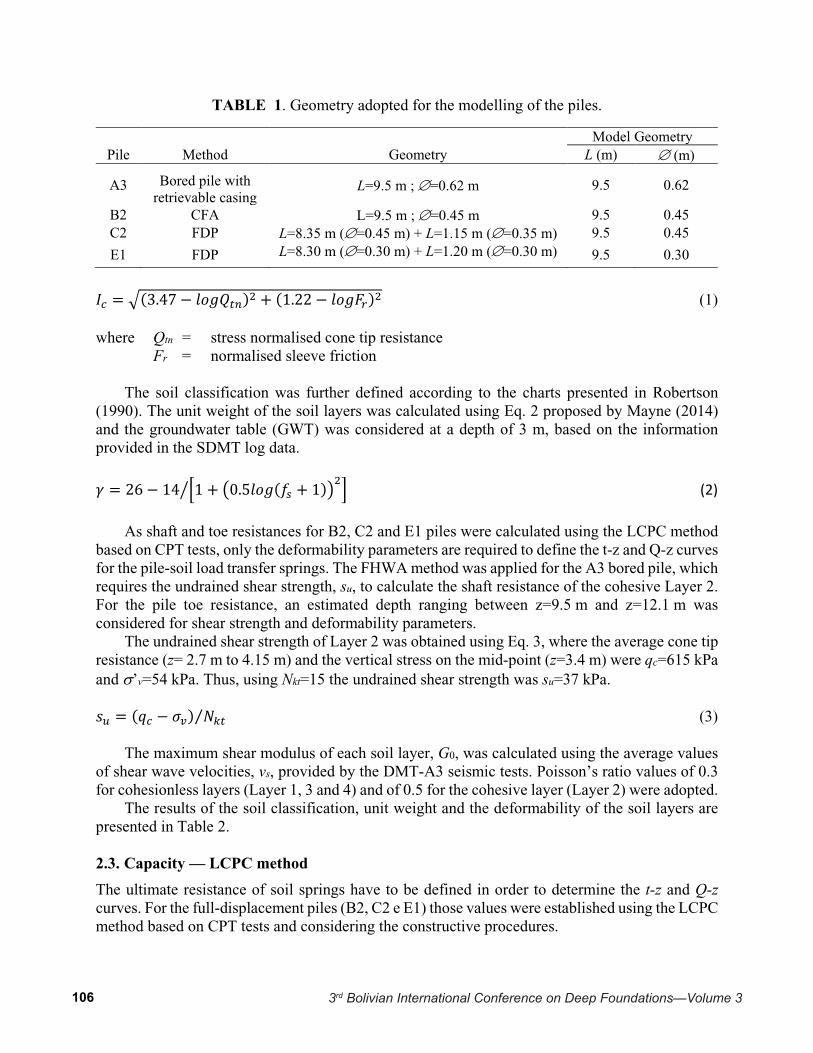
TABLE 1. Geometry adopted for the modelling of the piles.
Model Geometry Pile Method Geometry L (m) ∅ (m)
A3 Bored pile with retrievable casing
L=9.5 m ; ∅=0.62 m 9.5 0.62
B2 CFA L=9.5 m ; ∅=0.45 m 9.5 0.45 C2 FDP L=8.35 m (∅=0.45 m) + L=1.15 m (∅=0.35 m) 9.5 0.45
E1 FDP L=8.30 m (∅=0.30 m) + L=1.20 m (∅=0.30 m) 9.5 0.30
𝐼𝐼𝑐𝑐 = �(3.47 − 𝑙𝑙𝑙𝑙𝑙𝑙𝑄𝑄𝑡𝑡𝑡𝑡)2 + (1.22 − 𝑙𝑙𝑙𝑙𝑙𝑙𝐹𝐹𝑟𝑟)2 (1) where Qtn = stress normalised cone tip resistance Fr = normalised sleeve friction
The soil classification was further defined according to the charts presented in Robertson (1990). The unit weight of the soil layers was calculated using Eq. 2 proposed by Mayne (2014) and the groundwater table (GWT) was considered at a depth of 3 m, based on the information provided in the SDMT log data.
𝛾𝛾 = 26 − 14 �1 + �0.5𝑙𝑙𝑙𝑙𝑙𝑙(𝑓𝑓𝑠𝑠 + 1)�2�� (2)
As shaft and toe resistances for B2, C2 and E1 piles were calculated using the LCPC method based on CPT tests, only the deformability parameters are required to define the t-z and Q-z curves for the pile-soil load transfer springs. The FHWA method was applied for the A3 bored pile, which requires the undrained shear strength, su, to calculate the shaft resistance of the cohesive Layer 2. For the pile toe resistance, an estimated depth ranging between z=9.5 m and z=12.1 m was considered for shear strength and deformability parameters.
The undrained shear strength of Layer 2 was obtained using Eq. 3, where the average cone tip resistance (z= 2.7 m to 4.15 m) and the vertical stress on the mid-point (z=3.4 m) were qc=615 kPa and σ’v=54 kPa. Thus, using Nkt=15 the undrained shear strength was su=37 kPa. 𝑠𝑠𝑢𝑢 = (𝑞𝑞𝑐𝑐 − 𝜎𝜎𝑣𝑣) 𝑁𝑁𝑘𝑘𝑡𝑡⁄ (3)
The maximum shear modulus of each soil layer, G0, was calculated using the average values of shear wave velocities, vs, provided by the DMT-A3 seismic tests. Poisson’s ratio values of 0.3 for cohesionless layers (Layer 1, 3 and 4) and of 0.5 for the cohesive layer (Layer 2) were adopted.
The results of the soil classification, unit weight and the deformability of the soil layers are presented in Table 2. 2.3. Capacity — LCPC method
The ultimate resistance of soil springs have to be defined in order to determine the t-z and Q-z curves. For the full-displacement piles (B2, C2 e E1) those values were established using the LCPC method based on CPT tests and considering the constructive procedures.
106 3rd Bolivian International Conference on Deep Foundations—Volume 3
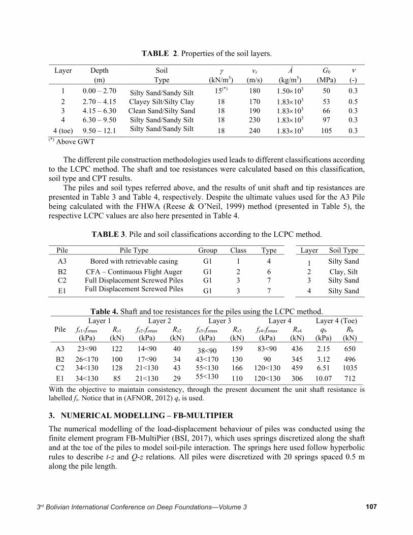
TABLE 2. Properties of the soil layers.
Layer Depth Soil γ vs Á G0 ν (m) Type (kN/m3) (m/s) (kg/m3) (MPa) (-)
1 0.00 – 2.70 Silty Sand/Sandy Silt 15(*) 180 1.50×10³ 50 0.3
2 2.70 – 4.15 Clayey Silt/Silty Clay 18 170 1.83×10³ 53 0.5 3 4.15 – 6.30 Clean Sand/Silty Sand 18 190 1.83×10³ 66 0.3 4 6.30 – 9.50 Silty Sand/Sandy Silt 18 230 1.83×10³ 97 0.3
4 (toe) 9.50 – 12.1 Silty Sand/Sandy Silt 18 240 1.83×10³ 105 0.3 (*) Above GWT
The different pile construction methodologies used leads to different classifications according to the LCPC method. The shaft and toe resistances were calculated based on this classification, soil type and CPT results.
The piles and soil types referred above, and the results of unit shaft and tip resistances are presented in Table 3 and Table 4, respectively. Despite the ultimate values used for the A3 Pile being calculated with the FHWA (Reese & O’Neil, 1999) method (presented in Table 5), the respective LCPC values are also here presented in Table 4.
TABLE 3. Pile and soil classifications according to the LCPC method.
Pile Pile Type Group Class Type Layer Soil Type
A3 Bored with retrievable casing G1 1 4 1 Silty Sand
B2 CFA – Continuous Flight Auger G1 2 6 2 Clay, Silt C2 Full Displacement Screwed Piles G1 3 7 3 Silty Sand
E1 Full Displacement Screwed Piles G1 3 7 4 Silty Sand
Table 4. Shaft and toe resistances for the piles using the LCPC method.
Layer 1 Layer 2 Layer 3 Layer 4 Layer 4 (Toe) Pile fs1<fsmax Rs1 fs2<fsmax Rs2 fs3<fsmax Rs3 fs4<fsmax Rs4 qb Rb
(kPa) (kN) (kPa) (kN) (kPa) (kN) (kPa) (kN) (kPa) (kN)
A3 23<90 122 14<90 40 38<90 159 83<90 436 2.15 650
B2 26<170 100 17<90 34 43<170 130 90 345 3.12 496 C2 34<130 128 21<130 43 55<130 166 120<130 459 6.51 1035
E1 34<130 85 21<130 29 55<130 110 120<130 306 10.07 712
With the objective to maintain consistency, through the present document the unit shaft resistance is labelled fs. Notice that in (AFNOR, 2012) qs is used. 3. NUMERICAL MODELLING – FB-MULTIPIER
The numerical modelling of the load-displacement behaviour of piles was conducted using the finite element program FB-MultiPier (BSI, 2017), which uses springs discretized along the shaft and at the toe of the piles to model soil-pile interaction. The springs here used follow hyperbolic rules to describe t-z and Q-z relations. All piles were discretized with 20 springs spaced 0.5 m along the pile length.
1073rd Bolivian International Conference on Deep Foundations—Volume 3
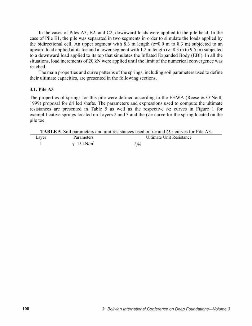
In the cases of Piles A3, B2, and C2, downward loads were applied to the pile head. In the case of Pile E1, the pile was separated in two segments in order to simulate the loads applied by the bidirectional cell. An upper segment with 8.3 m length (z=0.0 m to 8.3 m) subjected to an upward load applied at its toe and a lower segment with 1.2 m length (z=8.3 m to 9.5 m) subjected to a downward load applied to its top that simulates the Inflated Expanded Body (EBI). In all the situations, load increments of 20 kN were applied until the limit of the numerical convergence was reached.
The main properties and curve patterns of the springs, including soil parameters used to define their ultimate capacities, are presented in the following sections.
3.1. Pile A3
The properties of springs for this pile were defined according to the FHWA (Reese & O’Neill, 1999) proposal for drilled shafts. The parameters and expressions used to compute the ultimate resistances are presented in Table 5 as well as the respective t-z curves in Figure 1 for exemplificative springs located on Layers 2 and 3 and the Q-z curve for the spring located on the pile toe.
TABLE 5. Soil parameters and unit resistances used on t-z and Q-z curves for Pile A3. Layer Parameters Ultimate Unit Resistance
1 γ=15 kN/m3 iv@
108 3rd Bolivian International Conference on Deep Foundations—Volume 3

The parameters used to establish t-z curves and respective unit shaft resistance, fs, are presented in Table 6. Similarly, Table 7 presents the parameters and toe resistance, Rb, used to define Q-z curves. Exemplificative springs’ curves for the Pile C2 are also presented in Figure 2.
Table 6. Parameters for t-z curves for Piles B2, C2, and E1. Pile B2 Piles C2 and E1
Layer γ Gi ν fs fs (kN/m3) (MPa) (-) (kPa) (kPa)
1 15 3 0.3 26 34 2 18 3 0.5 17 21 3 18 8 0.3 43 55 4 18 21 0.3 90 120
Table 7. Parameters for Q-z curves for Piles B2, C2 and E1.
Pile Layer Gi ν Ultimate Toe Resistance - Rb (MPa) (-) (kN)
B2 4 (Toe) 42 0.3 495 C2 4 (Toe) 50 0.3 1035 E1 4 (Toe) 70 0.3 712
1093rd Bolivian International Conference on Deep Foundations—Volume 3

𝑠𝑠𝑓𝑓 = 𝑄𝑄𝑄𝑄 (𝐸𝐸𝐸𝐸)⁄ + 0.1𝑄𝑄𝑓𝑓 (4)
Fig. 3 Pile-head load-movement curves and axial load in depth for Pile A3, B2 and C2.
Fig. 4 Pile-head load-movement and upward and downward load-movement for Pile E1.
Table 8. Capacity and associated pile-head movement.
Pile Qf sf (kN) (mm)
A3 1302 63
B2 963 47 C2 1394 48
E1 425 32
5. CONCLUSION
A prediction exercise is an opportunity to access and validate design methods used for pile foundations. In this particular case, two of the most frequently used methods were adopted, together with the t-z and Q-z load transfer curves. The predicted capacities ranged from 425 to 1,394 kN.
Load
(kN
)
Movement (mm)
Dep
th (m
)
Load (kN)
Load
(kN
)
Movement (mm)
Mov
emen
t (m
m)
Load (kN)
110 3rd Bolivian International Conference on Deep Foundations—Volume 3
6. REFERENCES
AFNOR 2012. NF P 94-262 – Justification des ouvrages géotechniques – Normes d’application nationale de l’Eurocode 7 – Fondations profondes, AFNOR.
Reese, L.C. and O’Neill, M.W. (1999). Drilled Shafts: Construction Procedures and Design Methods, Report No. FHWA-IF-00-025, Federal Highway Administration.
BSI 2017. FB-Multipier, version 5.1, Bridge Software Institute, University of Florida. Mayne, P.W. 2014. KN2: Interpretation of geotechnical parameters from seismic piezocone tests.
Proceedings, 3rd International Symposium on Cone Penetration Testing (CPT'14, Las Vegas), ISSMGE Technical Committee TC 102, Edited by P.K. Robertson and K.I. Cabal: pp. 47-73.
Robertson, P.K. 1990. Soil classification using the cone penetration test. Canadian Geotechnical Journal, 27(1). pp. 151–158.
1113rd Bolivian International Conference on Deep Foundations—Volume 3

112 3rd Bolivian International Conference on Deep Foundations—Volume 3

Prediction of pile load movement response and assessment of pile capacity
Raba Moyano Miguel Angel(1)
(1) Ingeomar Sas., Bogotá, Colombia <[email protected]>
ABSTRACT. This paper presents a simple design proposal based on the method of charge transfer proposed by Coyle and Reese in 1966, which is based on a base resistance curve of the pile measured in field tests by instrumentation. The proposal consists in first establishing some adjustments and improvements of the method as such, including some basic tools and criteria to reconstruct and adjust these curves, from stress versus strain curves that can be obtained in the laboratory. 1. INTRODUCTION
The practice of Foundations Engineering generates in the daily work challenges to predict in a reliable way the behavior of foundations. There are very close traditional methods based on the elastic behavior of the soil, such as the method proposed by Poulos and Davis (1968) and Randolph and Wroth (1978), which are based on basic geometry of the pile as a cylindrical element embedded in an elastic and homogeneous system. These methods combined in non-coupled form with ideal plastic models allow an approximate reconstruction of the curve load versus displacement of a single pile and pile acting in a group.
On the other hand, perhaps other alternative methods of analysis, apparently more reliable based on complex methods of analysis have evolved from the years 80. It is now very commercial and easily accessible to reconstruct foundations models with the finite element technique, based on "advanced" models of soil behavior, which requires a high quality characterization program. These well-used methods undoubtedly constitute a most valuable tool, but in practice it also presents many limitations; Among others, the difficulty of obtaining reliable parameters of soil behavior that require laboratory tests and good quality samples and limitations of these models, which have proved, at least commercially, not to be reliable enough to evaluate complex phenomena Are difficult to model, such as softening effects by deformation and processes of consolidation and soil repair among other aspects.
Finally, practical experience has shown that a good tool for the prediction of pile behavior is based on in situ tests, among which we highlight the test of Dutch CPT and CPU, which represent a smaller scale and, in a faithful way, the pile driving process, leaving in evidence aspects that are extremely important in a prediction, such as the effects of anisotropy and loading speed.
It is clear that there are also other limitations that are not easy to evaluate, such as the effect of pile installation, which is undoubtedly uncertain and is decisive for predicting pile behavior. Although theoretical models are available, practical engineering indicates that semi-empirical and empirical models that are no longer used are still important in this kind of prediction.
1133rd Bolivian International Conference on Deep Foundations—Volume 3

2. THEORETICAL FRAMEWORK 2.1 Bearing Capacity
To determine the stress strain curve, the CPTU tests delivered were based on which the following criteria were adopted:
The subsoil was subdivided into ten (10) layers that coincide with the soil stratification, differentiating layers of sands and clays, as follows.
Resistance in the shaft, in sands: fs = fc/2 for pre-excavated piles "Bored Pile" fs = 0.75 fc for CFA and FDP piles fs = 1.00 fc In the cases of widening in the base and injection by system 'grouting' Resistance in the shaft, in clays: Undrained Shear resistance: Su = (Qt - σvo) / Nk Alpha Method. fs = α Su Toe capacity, in sands and clays: Based on the average resistance at the tip of the cone Qcp, where the bearing capacity is
determined as:
Qult = Qcp/2 for bored Piles Qult = 0.75Qcp for CFA and FDP piles without spreading. Qult = Qcp for FDP piles with widening at the base and injection by 'grouting'
In order to take into account the variation of the cone in depth, in the proximity of the base,
the weighted average value was taken, in a depth range, variable between 6 and 10 times the diameter, depending on the friction angle of the soil. A first calculation was made by taking the upper interval from the base level of the pile upwards and a second calculation was made by taking the lower interval from the base level of the pile down, using the following criterion (Meyerhof, 1976).
For the calculation of residual resistance in sands and clays, the theoretical criteria proposed by Vesic, Burland and others are taken in account, on the basis the angle of friction in the value of 28 degrees in sands and variable in clays.
2.2 Displacement
To determine the deformation stress curve, the soil shear modulus was determined as a function of the pile installation process:
K = 10 For pre-excavated piles "Bored Pile"
K = 15 For CFA and FDP piles without spreading.
K = 15 For FDP piles with widening at the base and injection by grouting system
114 3rd Bolivian International Conference on Deep Foundations—Volume 3

Fig. 1. Variation (D/d) with the angle of friction of the soil (Meyerhof 1976).
Fig. 2. Adaptation of the load vs. displacement curve, based on a hyperbolic model.
For the calculation of settlements, the Load Transfer Method, initially proposed by Seed &
Reese, 1957, was used, which is based on the construction of a synthetic curve of pile load versus soil displacement and starting from a condition of compatibility of deformations Along the pile starting from fixed displacement in the lower part, the curve of settlement of the pile in general is determined.
In parallel, a first approximation was made with the rigid linear-plastic elastic method proposed by Randolph, 1990.
The undersigned presents the application of an unpublished own procedure where he reconstructs in a simple and practical way the curve load of the pile versus displacement in function of the parameters of resistance and compressibility of the soil and considering a effect of softening by deformation. This adjustment is made with the help of a Duncan Hyperbolic Model, as shown in the Figure 2.
1153rd Bolivian International Conference on Deep Foundations—Volume 3

3. CALCULATION PROCEDURE 3.1 Modified Load Transfer Method
The proposed method of calculation is based on the Load Transfer Method proposed by Reese and Coyle (1960), for individual piles, with some modifications. This method considers the following steps:
1. The pile is subdivided into a number of segments; exercises performed allow us to recommend five to ten segments of different thickness, adjusting as closely as possible to the stratigraphy of the site soil.
2. At the base of the pile, a small displacement ρb is assumed, with a positive value if we want to evaluate a pile with axial compression and a negative value if we want to evaluate a pile with axial tension.
3. From the load-to-pile curve, which is explained later on how to obtain it, we determine the load Pb = f (ρb) that the pile takes as a function of the displacement ρb defined in the previous step. If the pile is subjected to axial tension, assume Pb = 0.
4. It is assumed as the first approximation ρn'= ρb, where ρn' is the displacement at the midpoint of the lower pile interval.
5. The charge at the base of the interval is taken as Qn-1 = Qn; if it is the lower interval, take Qn-1 = Pb.
6. The displacement in the middle of the interval n of the pile is calculated as ρn = ρn' + ∆ρn; in the first iteration logically ∆ρn = 0.
7. From the effort curve vs. displacement of the pile wall in the corresponding interval, we will explain how to obtain the load curve, we determine the average stress τn = g(ρn) that is generated in the interval n of the pile.
8. The accumulated load at the top of interval n is calculated as Qn = Qn-1 + ∆n1∆Ln1π1d, where ∆Ln is the height of the pile interval n and d the pile diameter.
9. The average load of the interval QMn is calculated as QMn = (Qn + Qn-1) / 2. 10. The elastic shortening at the midpoint of the interval n is calculated as: ∆ρn = (QMn + Qn-
1) / 2 * (∆Ln / 2) / (Ap1Ep); Where Ap is the area of the cross section of the pile and Ep is the modulus of elasticity of the pile.
11. Calculate again ρn = ρn'+ ∆ρn and compare with that obtained in step 6; The process is repeated until step 11, until convergence in the result.
12. Calculate the displacement at the upper point of the interval ρns = ρn + ∆ρn
13. With the interval n solved i.e. with Qn and ρns, the entire procedure is repeated from step 5
and the deformations in the pile are continued by solving the upper intervals n-1, n-2, ... until the level top of the pile, i.e. the interval 1.
14. The displacement is incremented repeatedly from step 2 and the whole procedure is solved until step 13 is reached.
3.2 Determination of load versus displacement curves in the pile
The functions Pb = f (ρb) y τn = g(ρn) are calculated in a synthetic way from ideal elasto-plastic models based on Randolph's rigidity and rigidity modulus for rigid piles and the adjustment to a Hyperbolic model taking the form of random reference curves of triaxial laboratory tests of their own geotechnical studies, as shown in Figure 2.
116 3rd Bolivian International Conference on Deep Foundations—Volume 3

In the shaft pile the equations 1, 2 and 3 represent such behavior:
Ks
CFif
Rfpeak
nKs
n peaknn
×≤
×+
=τρ
τ
ρ
ρτ ,
1 (1)
Ks
CFif
remRfpeak
nKs
n peaknn
×
−×+
= ≥τρ
ττ
ρ
ρτ ,
1 (2)
( ) Rfrespeak
Ks
CFpeakn
sK
Ks
CFpeakn
rem
×−
×−
+
×−
=
ττ
τρ
τρ
τ
'
1
(3)
where τpico = Peak shear stress
τres = Residual shear stress
τrem = Remainder shear stress CF = Failure constant
Rf = Failure relation Ks = Unit Rigid Constant in shaft pile. Ks’ = Inverse Unit Rigid Constant in shaft pile, in the remainder stress zone. Rf = Failure relation.
The Unit Rigid constant is calculated as:
d
GKs
××
=ζ2 (4)
The Inverse Unit Rigid Constant in shaft pile, in the remainder stress zone is calculated as:
τ
τ
peak
resKsKs =' (5)
where G = Shear modulus of soil in the shaft pile. d = Pile diameter in the shaft
ζ = Randolph geometrical constant
1173rd Bolivian International Conference on Deep Foundations—Volume 3
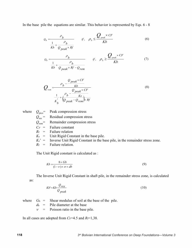
In the base pile the equations are similar. This behavior is represented by Eqs. 6 - 8
Kb
CFif
RfQ peak
bKb
bQ
peakbbQ
×≤
×+
= ρρ
ρ,
1 (6)
Kb
CFif
QremRfQ peak
bKb
bQ
peakbbQ
×
−×+
= ≥ρρ
ρ,
1 (7)
( ) RfQremQ peak
Ks
CFQ peakb
bK
Kb
CFQ peakbQ
rem
×−
×−
+
×−
=
ρ
ρ
'
1
(8)
where Qpico= Peak compression stress Qres = Residual compression stress
Qrem = Remainder compression stress CF = Failure constant
Rf = Failure relation Ks = Unit Rigid Constant in the base pile. Ks’ = Inverse Unit Rigid Constant in the base pile, in the remainder stress zone. Rf = Failure relation. The Unit Rigid constant is calculated as :
db
GbKb
××−×
=πν )1(
8 (9)
The Inverse Unit Rigid Constant in shaft pile, in the remainder stress zone, is calculated
as:
Q peak
QresKbKb =' (10)
where Gb = Shear modulus of soil at the base of the pile. db = Pile diameter at the base
ν = Poisson ratio in the base pile. In all cases are adopted from CF=4.5 and Rf=1,38.
118 3rd Bolivian International Conference on Deep Foundations—Volume 3
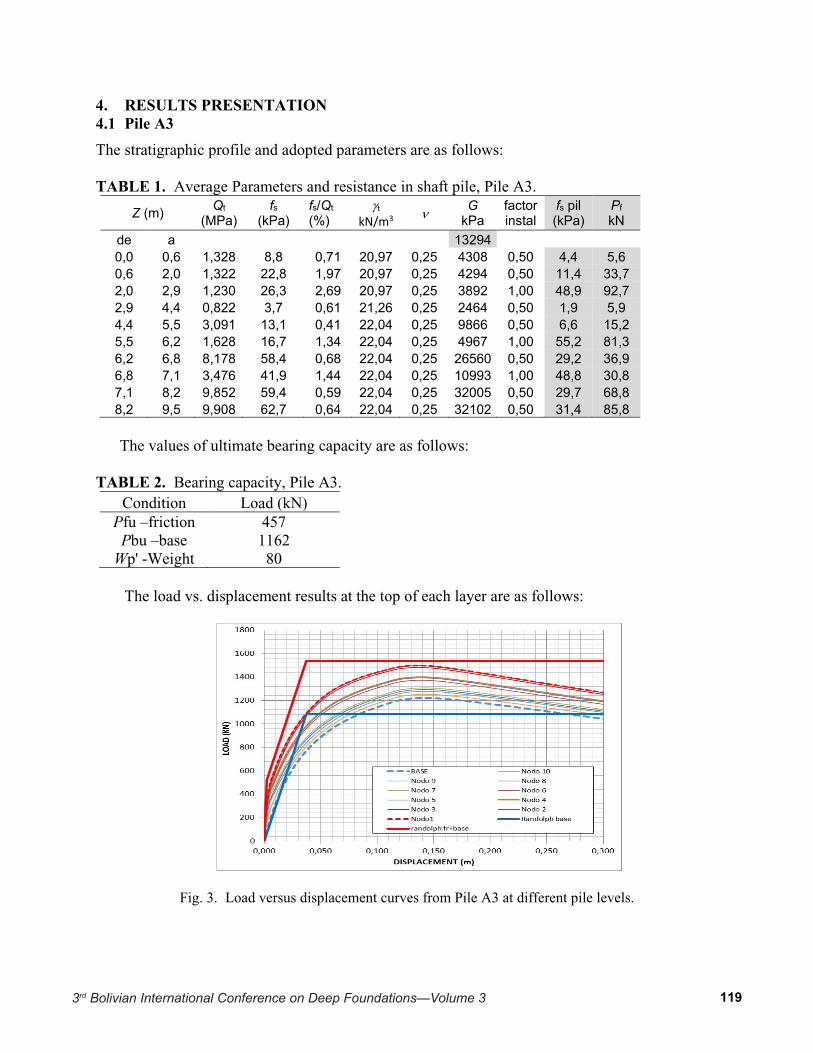
4. RESULTS PRESENTATION 4.1 Pile A3
The stratigraphic profile and adopted parameters are as follows: TABLE 1. Average Parameters and resistance in shaft pile, Pile A3.
Z (m) Qt (MPa)
fs (kPa)
fs/Qt (%)
γt kN/m3 ν G
kPa factor instal
fs pil (kPa)
Pf kN
de a 13294 0,0 0,6 1,328 8,8 0,71 20,97 0,25 4308 0,50 4,4 5,6 0,6 2,0 1,322 22,8 1,97 20,97 0,25 4294 0,50 11,4 33,7 2,0 2,9 1,230 26,3 2,69 20,97 0,25 3892 1,00 48,9 92,7 2,9 4,4 0,822 3,7 0,61 21,26 0,25 2464 0,50 1,9 5,9 4,4 5,5 3,091 13,1 0,41 22,04 0,25 9866 0,50 6,6 15,2 5,5 6,2 1,628 16,7 1,34 22,04 0,25 4967 1,00 55,2 81,3 6,2 6,8 8,178 58,4 0,68 22,04 0,25 26560 0,50 29,2 36,9 6,8 7,1 3,476 41,9 1,44 22,04 0,25 10993 1,00 48,8 30,8 7,1 8,2 9,852 59,4 0,59 22,04 0,25 32005 0,50 29,7 68,8 8,2 9,5 9,908 62,7 0,64 22,04 0,25 32102 0,50 31,4 85,8
The values of ultimate bearing capacity are as follows:
TABLE 2. Bearing capacity, Pile A3.
Condition Load (kN) Pfu –friction 457 Pbu –base 1162
Wp' -Weight 80 The load vs. displacement results at the top of each layer are as follows:
Fig. 3. Load versus displacement curves from Pile A3 at different pile levels.
1193rd Bolivian International Conference on Deep Foundations—Volume 3

4.2 Pile B2
The stratigraphic profile and adopted parameters are as follows: TABLE 3. Average Parameters and resistance in shaft pile, Pile B2.
Z (m) Qt (MPa)
fs (kPa)
fs/Qt (%)
γt kN/m3 ν G
kPa factor instal
fs pil (kPa)
Pf kN
de a 16466 0,0 1,0 3,466 7,3 0,25 20,97 0,25 17255 0,75 5,5 7,7 1,0 2,5 1,800 27,7 2,01 20,97 0,25 8680 1,00 50,5 105,9 2,5 3,2 0,815 11,6 1,72 20,97 0,25 3742 1,00 42,8 41,8 3,2 4,1 1,597 5,7 0,46 21,09 0,25 7534 0,75 4,3 5,4 4,1 5,6 2,958 8,1 0,29 22,04 0,25 14148 0,75 6,1 12,7 5,6 6,1 1,090 25,1 2,31 22,04 0,25 4782 1,00 55,2 38,6 6,1 6,6 7,410 32,2 0,48 22,04 0,25 36049 0,75 24,1 16,9 6,6 7,3 3,949 31,7 1,23 22,04 0,25 18832 1,00 49,9 48,8 7,3 8,4 6,729 29,0 0,47 22,04 0,25 32511 0,75 21,7 33,4 8,4 9,5 4,994 19,7 0,40 22,04 0,25 23790 0,75 14,8 22,8 The values of ultimate bearing capacity are as follows:
TABLE 4. Bearing capacity, Pile B2. Condition Load (kN)
Pfu –friction 334 Pbu –base 526
Wp' -Weight 35 The load vs. displacement results at the top of each layer are as follows:
Fig. 3. Load versus displacement curves from Pile B2 at different pile levels.
4.3 Pile C2
The stratigraphic profile and adopted parameters are as follows:
120 3rd Bolivian International Conference on Deep Foundations—Volume 3
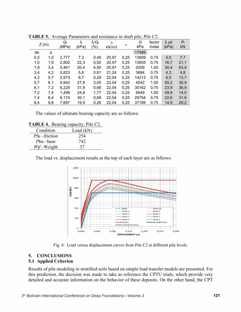
TABLE 5. Average Parameters and resistance in shaft pile, Pile C2.
Z (m) Qt (MPa)
fs (kPa)
fs/Qt (%)
γt kN/m3 ν G
kPa factor instal
fs pil (kPa)
Pf kN
de a 17489 0,0 1,0 2,777 7,3 0,48 20,97 0,25 13909 0,75 5,5 7,7 1,0 1,9 2,802 22,3 0,92 20,97 0,25 13655 0,75 16,7 21,1 1,9 3,4 0,461 20,4 4,50 20,97 0,25 2009 1,00 30,4 63,9 3,4 4,2 0,823 5,8 0,81 21,24 0,25 3684 0,75 4,3 4,8 4,2 5,7 2,973 8,7 0,29 22,04 0,25 14213 0,75 6,5 13,7 5,7 6,1 0,942 27,8 3,05 22,04 0,25 4042 1,00 55,2 30,9 6,1 7,2 6,229 31,9 0,68 22,04 0,25 30162 0,75 23,9 36,9 7,2 7,4 1,499 24,8 1,77 22,04 0,25 6649 1,00 49,9 14,0 7,4 8,4 6,174 30,1 0,69 22,04 0,25 29754 0,75 22,6 31,6 8,4 9,8 7,697 19,9 0,26 22,04 0,25 37169 0,75 14,9 29,2 The values of ultimate bearing capacity are as follows:
TABLE 4. Bearing capacity, Pile C2. Condition Load (kN)
Pfu –friction 254 Pbu –base 742
Wp' -Weight 37 The load vs. displacement results at the top of each layer are as follows:
Fig. 4. Load versus displacement curves from Pile C2 at different pile levels. 5. CONCLUSIONS 5.1 Applied Criterion
Results of pile modeling in stratified soils based on simple load transfer models are presented. For this prediction, the decision was made to take as reference the CPTU trials, which provide very detailed and accurate information on the behavior of these deposits. On the other hand, the CPT
1213rd Bolivian International Conference on Deep Foundations—Volume 3

test is considered useful since it can be considered a micro-scale test of the pile (cone size of 10 cm2); This test using it and interpreting it in a coherent and adequate way becomes a very valuable tool for the determination of the bearing capacity of piles.
In relation to the deformations, a typical laboratory curve of a triaxial test was used and parameterized applying the Hyperbolic Method including a process of softening by deformation. Based on the hypotheses used, a good relation of the load versus the resulting displacement curve was found with that obtained in the field instrumentation. This result indicates that this method, despite its simplicity, is quite useful for the prediction of pile behavior. In order to achieve a better fit, laboratory curves of the site can be parameterized to the stress levels presented on the pile.
Finally, it is important to indicate that the effect of densification or improvement of soils around CFA and FDP piles quantified by traditional methods are conservative and difficult to quantify. For a good prediction the adjustment of these formulas of work to the local geological conditions is required. The evaluation of the load versus displacement curves measured with those obtained in the field, for each case under study are presented below. 5.2 Pile A3
Figure 5 presents a comparison between the theoretical and the field curve. The results obtained from the applied model with the results of the load test indicate a fairly good fit, with a difference of 13% above the curve obtained in the load test. It is important to note that the calibration of the prototype curve used in our model for the prediction is arbitrarily taken from triaxial tests of other types of soils of Bogota, which has nothing to do with the soils of the test. Despite this the prediction is good.
Fig. 5. Comparison between load versus displacement curves from Pile A3. 5.3 Pile B2
Figure 6 presents a comparison between the theoretical and the field curve. The results obtained from the applied model with the results of the load test corresponds to values of 47% below the
122 3rd Bolivian International Conference on Deep Foundations—Volume 3

field curve; However, the shape of the load vs. displacement curve closely resembles the field curve. In principle, we believe that we underestimate the effect of densification on the resistance of the surrounding soil generated by a CFA pile where it is suggested that the actual resistance by stem and tip is on the order of 1.5 times the strength of the cone and not the adopted of 0.75. Despite the differences, we consider that the results obtained are not without interest.
Fig. 6. Comparison between load versus displacement curves from Pile B2.
5.4 Pile C2
Figure 7 presents a comparison between the theoretical and the field curve. Comparing the obtained results of the applied model with the results of the load test, it is found that the theoretical values are of the order of 44% below the field curve; And the shape of the load vs. displacement curve does not reflect the strain hardening effect generated by the field curve. In principle we believe that we underestimate the effect of densification on the resistance of the surrounding soil generated by a CFA pile in which it is suggested that the actual resistance by stem and tip is on the order of 2 times the strength of the cone and not the adopted of 1.0. On the other hand we believe that the effect of lateral compaction of the soil increases the effective stresses and reduces or eliminates the dilating effect of the sandy soil. Aspect that was not analyzed properly in our model, for that reason the differences are explained. Again, despite the differences, we consider that the results obtained are not without interest.
0
250
500
750
1,000
1,250
1,500
1,750
0 10 20 30 40 50 60 70 80 90 100
LOA
D (
kN)
MOVEMENT (mm)
1233rd Bolivian International Conference on Deep Foundations—Volume 3

Fig. 7. Comparison between load versus displacement curves from Pile C2.
6. REFERENCES Fellenius, B.H., 1990. Pile Foundation. Foundation Engineering Handbook, New York, Ch. 13,
pp. 511-536. Fellenius, B.H., 1990. Invitation Prediction of Pile Load Movement and Assessment of Pile
Capacity, Santa Cruz de la Sierra, Bolivia 1-10. Poulos, H.G. and Davis, E.H., 1980. Settlement Analysis of Single Piles. Pile Foundation Analysis
and Design, pp. 5 71-74. Kondner, R.L., 1963, Hyperbolic Stress strain response: Cohesive soils. J Soil Mech. Found. Div.,
ASCE, 89(SM1). pp. 115-143. Randolph, M.F., 1977. A theoretical study of performance of piles. PhD thesis, Cambridge
University, England. Randolph, M.F., 1979. Discussion in Proc. of Conf. on Recent Developments in the Design and
Construction of Piles, London: ICE, pp. 389-390. Randolph, M.F., 1983. Design of piled foundations. Cambridge Univ. Eng. Dept., Res. Rep. Soils
TR143. Randolph, M.F., and Wroth, C.P., 1978. Analysis of deformation of vertically loaded piles. ASCE,
104(GT12), pp. 1485-1488.
0
500
1,000
1,500
2,000
2,500
0 25 50 75 100 125 150
LOA
D (
kN)
MOVEMENT (mm)
124 3rd Bolivian International Conference on Deep Foundations—Volume 3

Summary and comments on prediction submitted to the 3rd Bolivian International Conference on Deep Foundations
Santos, A.L.(1) and Bohn, C.(2)
(1) Navier Géotechnique, Université Paris Est, France. <[email protected]>
(2) Keller Holding GmbH <[email protected]>
ABSTRACT. In the occasion of the third Bolivian International Conference on Deep Foundations, a series of static load pile tests were performed in the Bolivian Experimental Site for Testing Piles (BEST), which is situated 24 kilometers North-East of Santa Cruz de la Sierra, Bolivia. This paper presents the adopted approach based on CPT tests to estimate piles ultimate axial capacity. Axial load-settlement behavior was estimated by means of Load Transfer (“t-z”) Method. A brief comparison of the estimates to the actual static load test results is presented. 1. INTRODUCTION 1.1 Generalities on the site’s geology and the test piles
The Bolivian Experimental Site for Testing Piles (BEST) is situated 24 kilometers North-East of Santa Cruz de la Sierra. The soils in which the piles are embedded have its origins in a quaternary deposit, described mainly as silty sands and low plasticity clays. Site geotechnical investigation was mainly performed by in situ tests such as SPT, CPTU, PMT, SDMT, geophysical tests (SASW and REMI), and laboratory characterization. The four piles which are the scope of the prediction event, named A3, B2, C2, and E1, were all built measuring 9.5 meters with the following execution techniques: • Pile A3 is a bored pile constructed with a 620-mm casing which is retrieved on concreting it; • Pile B2 is a continuous flight auger pile with an outside diameter of 450 mm; • Pile C2 is a full displacement pile with a shaft outside diameter of 450 mm over 8.23 m and a
toe and near-toe diameter of 350 mm (1.27 m). • Pile E1 is a full displacement pile with its 1.2 m-near-toe diameter enhanced by an Expander
Body device. Its diameter was considered constant and equals 300 mm over its all length, but different pile-soil-interaction was estimated for the average shaft and the near-toe part.
Further details on the site geology, pile execution, testing procedures, in situ tests and instrumentation were given by the organizing committee and will not be presented in this work. 1.2 Selected in situ tests
Amongst all the in situ tests available, based on personal experience it was decided to use CPT, PMT and SPT to characterize the site’s geotechnical properties regarding the piles’ behavior. Final predictions relied only on CPT, but the three tests mentioned above were used for preliminary studies aiming to improve a “feeling” on what the real pile tests would be. It has been chosen to go ahead with CPT because its results had smaller dispersion between different tests. Furthermore, pile ultimate capacities estimates using CPT resulted in higher values than when
1253rd Bolivian International Conference on Deep Foundations—Volume 3

using PMT or SPT. Since the pile predictions are not to be used for an actual structure design, it was chosen to push calculations to try to obtain the most accurate values of pile ultimate capacity. This seemed to be a comfortable choice as soon as the piles were to be built under excellence engineering supervision and for an international prediction event directed to the foundation community. 2. ADOPTED APPROACH FOR ESTIMATING PILE ULTIMATE RESISTANCE
2.1 Using CPT to estimate the ultimate bearing capacity
The ultimate bearing capacity of the piles was estimated using the methods proposed in the French national application standard for the implementation of the Eurocode 7, NF P 94 262 (AFNOR, 2012), appendix G.
The average cone resistance profile adopted for the estimates is presented in Fig. 1. Adopted values of qc per soil layer are presented in Table 1.
Fig. 1. Average cone penetration resistances
and division in soil layers.
TABLE 1. Adopted average values of cone resistance per soil layer and soil type
according to AFNOR (2012). Depth Soil type qc
(m) (MPa)
0.0 to 2.0 Clay/silt 2.75
2.0 to 4.0 Clay/silt 0.91
4.0 to 6.0 Clay/silt 2.21
6.0 to 7.2 Sand/gravel 5.64
7.2 to 12.0 Sand/gravel 7.49
According to the method presented in the NF P 94 262, the ultimate shaft resistance, at a depth z, (𝑞𝑞𝑠𝑠(𝑧𝑧)) is a function of the pile type and soil type (expressed by means of the term 𝛼𝛼𝑝𝑝𝑝𝑝𝑝𝑝𝑝𝑝−𝑠𝑠𝑠𝑠𝑠𝑠) and the cone resistance (expressed by means of 𝑓𝑓𝑠𝑠𝑠𝑠𝑠𝑠[𝑞𝑞𝑐𝑐(𝑧𝑧)], which also depends on the soil type), being calculated by Eq. 1. The ultimate toe resistance, 𝑞𝑞𝑏𝑏, is a function of the bearing coefficient 𝑘𝑘𝑐𝑐, which depends on the pile class, the soil type and the toe embedment, and the equivalent CPT resistance near the pile toe, 𝑞𝑞𝑐𝑐𝑝𝑝, according to Eq. 2.
0
1
2
3
4
5
6
7
8
9
10
0 5 10 15
Dept
h (m
)
CPT qc (MPa)
Average of all CPTs
Average by soil layer
126 3rd Bolivian International Conference on Deep Foundations—Volume 3

𝑞𝑞𝑠𝑠(𝑧𝑧) = 𝛼𝛼𝑝𝑝𝑝𝑝𝑝𝑝𝑝𝑝−𝑠𝑠𝑠𝑠𝑠𝑠𝑓𝑓𝑠𝑠𝑠𝑠𝑠𝑠[𝑞𝑞𝑐𝑐(𝑧𝑧)] (1)
𝑞𝑞𝑏𝑏 = 𝑘𝑘𝑐𝑐𝑞𝑞𝑐𝑐𝑝𝑝 (2) Upper bound values for the shaft resistance and for the toe bearing capacity coefficient, as
well as mathematical expressions and tables for obtaining the needed parameters are given in the referenced document. Even though the standard describes precisely the existing pile types to which the method should be applied, engineering judgment is necessary for some execution techniques such as those employed for the toe of pile E1, which is not included in the standard. Engineering judgment is also needed for defining the final pile geometry in such a complex case, which also applies to C2 piles. The approach selected here to model pile-soil interaction is described in Table 2. TABLE 2. Piles classes and categories as defined by NF P 94 262 (AFNOR, 2013) and authors’ assumption. Pile Class Category Diameter (mm)
A3 1 4 620
B2 2 6 450
C2 3 7* 450 mm over 8,225 m length and 350 mm over 1,275 m near the toe
E1 3 7** 300 (but specific calculation for the 1.2 near-toe part) *Specific calculation procedure adopted differs from that proposed in NF P 94 262 (AFNOR, 2013). **The adopted standard does not provide a calculation method for piles with Expander Body.
Category 4 corresponds to bored piles with retrievable casing, category 6 corresponds to continuous flight auger and category 7 corresponds to screw displacement piles. According to the author’s experience, calculations performed using the above mentioned standard for screw displacement piles might result in conservative results. As a direct consequence of technological innovation regarding pile execution techniques, it is usual that contractors develop their own design procedures which might take into account execution improvement. It has been chosen to improve the estimate on pile C2 ultimate bearing capacity by using Keller specific rules for INSER piles (Keller, 2014). Although INSER execution tools are not exactly the same as those used to build the piles C2 and E1 in the prediction event, it was considered that this approach should be closer to reality than that proposed by the French standard. Regarding pile’s E1 near-toe part, none of the above mentioned calculation methods allowed to take the Expender Body effects into account. However, it has been considered here that this part of the pile would expect much higher shaft friction and toe resistance than those proposed by the standards and choice was made to model it as follows: for the 1.2 m near-toe shaft, it was considered as an injected micropile type IV (class 8, category 20 in the NF P 94 262); its toe was assumed to be similar to the one of a Franki pile. In injected micropiles, the soil near the shaft is subjected to expansion due to high pressure grout; in Franki piles, toe is subjected to expansion due to hammer blows in fresh concrete. Franki pile toe ultimate resistance was estimated using SPT and Aoki Velloso method (Monteiro 1997) considering average SPT values between 9 to 11 meters equals to 16 blows. For details regarding the calculation method, one should refer to the mentioned document.
1273rd Bolivian International Conference on Deep Foundations—Volume 3

Table 3 presents the estimated values for shaft and toe ultimate resistance per soil layer for each pile and Table 4 resumes the total ultimate capacities for the four piles. TABLE 3. Estimated ultimate shaft and toe resistance.
Layer depth (m) Pile A3 Pile B2 Pile C2 Pile E1 qs (kPa) qp (kPa) qs (kPa) qp (kPa) qs (kPa) qp (kPa) qs (kPa) qp (kPa)
0.0 2.0 45.5 52.5 80.0 66.5
2.0 4.0 20.2 23.3 29.5 29.5
4.0 6.0 39.7 45.8 70.0 58.0
6.0 7.2 61.0 76.2 88.4 88.4
7.2 8.2 73.6 91.9 106.6 106.6
8.2 9.5 73.6 1,498 91.9 1,872.5 106.6 3,745 194.9 4,500 TABLE 4. Estimated ultimate shaft and toe resistance. Pile Shaft (kN) Toe (kN) Total (kN)
A3 882 452 1,335
B2 772 298 1,070
C2 961 360 1,322
E1 482+239* 318 1,039 *upper 8.3 meter + 1.2 meter near toe 3. APPROACH FOR ESTIMATING PILE LOAD-SETTLEMENT BEHAVIOR
The axial load transfer or “t-z” method (LTM) has been selected to describe the pile shaft and pile toe local resistance mobilization as a function of the pile axial displacement. This represents a very straightforward and practical method for isolated piles and its concept is presented in Fig. 2. The stress mobilization is represented by springs which are in general non-linear and are made to replace the soil continuum around the pile and not only the interface behavior.
Cubic root load transfer curves developed based on a detailed investigation of pile load tests for a wide range of pile and soil types (Bohn et al., 2017) are used in this work to predict the load-settlement behavior of the proposed piles. More information about existing load transfer curves and literature on this subject are given in the above mentioned work. 3.1 Model description
For a pile with constant cross section and perimeter with depth, the infinitesimal pile segment equilibrium presented in Fig. 2 may be written as: 𝑑𝑑𝑑𝑑(ℎ) = −Ω 𝑞𝑞𝑠𝑠(𝑠𝑠𝑠𝑠)𝑑𝑑ℎ (3)
𝑑𝑑𝑠𝑠𝑠𝑠(ℎ) = −𝑑𝑑(ℎ)𝐸𝐸𝑏𝑏𝑆𝑆
𝑑𝑑ℎ (4)
128 3rd Bolivian International Conference on Deep Foundations—Volume 3

Replacing Eq. 4 in Eq. 3, the problem’s equation is obtained in Eq. 5 for each pile subdivision.
𝐸𝐸𝑏𝑏𝑆𝑆𝑑𝑑2𝑠𝑠𝑠𝑠𝑑𝑑ℎ2
− Ω 𝑞𝑞𝑠𝑠(𝑠𝑠𝑠𝑠) = 0 (5)
Fig. 2. Load transfer method for axially loaded single piles. where:
𝑑𝑑0 Load at the pile head 𝑑𝑑𝑏𝑏 Load at the pile tip 𝑑𝑑𝑠𝑠 Load at the pile shaft 𝑠𝑠𝑏𝑏 Relative settlement pile-soil at the pile tip 𝑠𝑠𝑠𝑠(h) Relative settlement pile-soil at the pile shaft 𝑞𝑞𝑠𝑠(𝑠𝑠𝑠𝑠) Stress at the pile shaft as a function of a relative settlement ℎ Depth Ω Pile perimeter 𝑆𝑆 Pile cross sectional area
The function 𝑞𝑞𝑠𝑠(𝑠𝑠𝑠𝑠) is the so-called skin friction mobilization function. The tip resistance
mobilization function is used as the limit condition for the pile tip reaction. Since both functions are known, equation 5 can be solved for each pile subdivision and thus for the whole pile system. The finite difference method can be used for the numerical solving.
The shaft friction load transfer curves are described by the cubic root equation as follows:
𝑞𝑞𝑠𝑠(𝑠𝑠𝑠𝑠) = min��𝑠𝑠𝑠𝑠
𝑠𝑠𝑠𝑠,𝑠𝑠𝑝𝑝𝑙𝑙�
13∙ 𝑞𝑞𝑠𝑠,𝑝𝑝𝑠𝑠𝑢𝑢 ; 𝑞𝑞𝑠𝑠,𝑝𝑝𝑠𝑠𝑢𝑢� (6)
1293rd Bolivian International Conference on Deep Foundations—Volume 3

The tip resistance mobilization function is described as follows:
𝑞𝑞𝑏𝑏(𝑠𝑠𝑏𝑏) = min��𝑠𝑠𝑏𝑏
𝑠𝑠𝑏𝑏,𝑠𝑠𝑝𝑝𝑙𝑙�
13∙ 𝑞𝑞𝑏𝑏,𝑝𝑝𝑠𝑠𝑢𝑢 ;𝑞𝑞𝑏𝑏,𝑝𝑝𝑠𝑠𝑢𝑢� (7)
where: 𝑞𝑞𝑏𝑏 Stress at the pile tip 𝑞𝑞𝑏𝑏,𝑝𝑝𝑠𝑠𝑢𝑢 Ultimate stress at the pile tip 𝑞𝑞𝑠𝑠 Stress at the pile shaft 𝑞𝑞𝑠𝑠,𝑝𝑝𝑠𝑠𝑢𝑢 Ultimate stress at the pile shaft 𝑠𝑠𝑏𝑏 The relative settlement pile-soil at the pile tip 𝑠𝑠𝑠𝑠 The relative settlement pile-soil at the pile shaft 𝑠𝑠𝑏𝑏,𝑠𝑠𝑝𝑝𝑙𝑙 Limit displacement for tip resistance full mobilization 𝑠𝑠𝑠𝑠,𝑠𝑠𝑝𝑝𝑙𝑙 Limit displacement for skin friction full mobilization
The curve stiffness is thus dependent on the ultimate skin friction and tip resistance, 𝑞𝑞𝑠𝑠,𝑝𝑝𝑠𝑠𝑢𝑢
and 𝑞𝑞𝑏𝑏,𝑝𝑝𝑠𝑠𝑢𝑢, respectively. Those parameters were determined as presented in paragraph 2.1. Pile stiffness was estimated considering the concrete Young’s modulus equals to 25,7 GPa and the pile circular cross-section according to the diameters previously described. 4. RESULTS AND COMPARISON TO LOAD TEST RESULTS
The following figures show a comparison between the predicted and the measured load-settlement curves. A conventional value for ultimate bearing capacity was adopted, defined as the load applied to the pile head that generates a head displacement corresponding to 10% of the pile diameter, according to French standard on pile static axial load tests (AFNOR, 1999). Toe diameter was considered in the case of pile C2. Comparison between the estimated and measured loads and settlements are presented in Table 3. Due to problems in the telltale measuring the downward movement of the lower part of E1 pile, only the upward movement of the upper shaft was obtained. It was not possible to draw an equivalent head-down load curve from the bi-directional load test of this pile. However, as informed by the organizing committee, near-toe part should not have settled more than one millimeter, thus indicating that its ultimate capacity was not mobilized.
As it can be noticed from Table 5, ultimate axial capacity was overestimated for pile A3 and underestimated for piles B2 and C2. It can be deduced that pile E1 near-toe ultimate capacity was also underestimated, since it was not fully mobilized at 600 kN. Regarding the relative error for the measured ultimate load (estimated capacity minus measured capacity divided by the measured capacity), we obtain 18% for pile A3, -24% for pile B2, -30% for pile C2 and -20% for the upper part of pile E1.
Pile A3 had a much softer response than expected. Even though its ultimate load was predicted with reasonably good accuracy, it was the only pile whose stiffness performance was underestimated. One of the possible reasons might be the steel casing retrieving process, in which the surrounding soil could have been disturbed, reducing shaft friction and thus leading the pile toe to be loaded in early stages of the load test. An investigation of the shaft instrumentation could confirm this explanation.
130 3rd Bolivian International Conference on Deep Foundations—Volume 3

TABLE 5. Comparison of predicted and measured values of ultimate load and settlement for the estimated service load.
Pile Estimated axial limit capacity
Measured load at 10%B
Estimated settlement at Qu,est/2
Measured settlement at Qu,est/2
Qu,est (kN) Qu,measured (kN) S0,est(Qu,est/2) (mm) S0,measured(Qu,est/2) (mm) A3 1332 1126 3.6 17.5 B2 1065 1397 3.4 3.4 C2 1314 1866 3.3 2.8 E1 482 + 557* - - -
*Upper shaft + toe and near-toe shaft
Fig. 3. Comparison of measured and estimated pile load-settlement curves.
Shape of B2 load-settlement curve is in great agreement with the prediction. Even though pile C2 ultimate capacity was underestimated the load settlement curve shape was in good agreement and the measured settlement corresponding to the predicted service load was well predicted by the LTM method. Pile E1 ultimate axial capacity was slightly underestimated despite the special considerations on shaft and toe resistance. Since near-toe downward movement measurement failed, it was not possible to compare predicted and measured settlement at the service load.
0
200
400
600
800
1,000
1,200
1,400
1,600
1,800
2,000
0 10 20 30 40 50 60 70 80 90
Load
(kN
)
Settlement (mm)
Test result
Prediction
Pile A3 - Bored - 620mm
0
200
400
600
800
1,000
1,200
1,400
1,600
1,800
2,000
0 10 20 30 40 50 60 70 80 90
Load
(kN
)
Settlement (mm)
Test result
Prediction
Pile B2 - CFA - 450mm
0200400600800
1,0001,2001,4001,6001,8002,000
0 10 20 30 40 50 60 70 80 90
Load
(kN
)
Settlement (mm)
Test result
Prediction
Pile C2 - FDP - 450 / 350mm
0200400600800
1,0001,2001,4001,6001,8002,000
0 10 20 30 40 50 60 70 80 90
Load
(kN
)
Upward movement (mm)
Test result
Prediction
Pile E1 - FDP + expander body - 300mm
Upward movement only(skin friction over the upper 8.3m length shaft)
1313rd Bolivian International Conference on Deep Foundations—Volume 3

5. SUMMARY AND CONCLUSIONS
This paper presented the methods adopted for predicting pile ultimate axial capacity and load-settlement response to static loading as submitted for the BEST Pile Prediction Event. Bearing capacity was estimated based on the French national application standard for Eurocode 7, NF P 94 262 (AFNOR, 2012), using CPT, as described in appendix G of this standard. Other available in situ tests, such as PMT and SPT, were of special importance so as to clarify soil properties and to allow for comparisons in terms of results. A choice was made to push calculations in order to obtain results as close to reality as possible (unlike practical pile design which may be conservative on purpose). The Load Transfer Method, as described by Bohn et al. (2017) has been used to predict the static loading behavior of the pile. Cubic root mobilization curves were employed to simulate stress mobilization as a function of the pile shaft and toe displacement. The ultimate axial capacity was adopted as the conventional pile head load to which the pile head settles 10% of its toe diameter (AFNOR, 1999). With this assumption, the error in the estimates ranged from 18% to 30%. In general, good agreement was obtained between predicted and measured load-settlement curve, with the exception of pile A3, which presented a much softer behavior. For this pile, displacement measured for a head load equivalent to the pile’s estimated service load was underestimated by 79%. For piles B2 and C2 the result was much better: exact displacement was predicted for pile B2 on its supposed service load, and an underestimation of 0.5 mm was obtained for pile C2. While further investigation might explain the unexpected behavior of pile A3, the results are considered good according to author’s experience. It is expected that more research and the execution of more instrumented load tests in piles equipped with expander body devices should allow to improve its design methods. 6. REFERENCES
AFNOR. 1999. Sols : Reconnaissance et essais. Essai statique de pieu isolé sous un effort axial. Partie 1 : en compression. NF P 94-150-1.
AFNOR. 2012. Justification des Ouvrages Géotechniques. Normes d’application de l’Eurocode 7. Fondations profondes. NF P 94-262.
Bohn, C., Lopes dos Santos, A., & Frank, R. 2017. Development of axial pile load transfer curves based on instrumented load tests. Journal of Geotechnical and Geoenvironmental Engineering, Vol. 143, Issue 1 (Published online July 25, 2016).
Keller, 2014. Pieux INSER. Procédé Keller Fondations Spéciales. Cahier de charges. Keller Fondations Spéciales.
Monteiro, P. F. 1997. Capacidade de carga de estacas–Método Aoki-Velloso. Relatório Interno de Estacas Franki Ltda, 1997.
132 3rd Bolivian International Conference on Deep Foundations—Volume 3

Different in-situ tests as essential support to better justify and (maybe) approximate predictions of axial pile capacity
Togliani, G.(1)
(1) Geologist Consultant., Massagno, Switzerland <[email protected]>
ABSTRACT. An extensive set of in-situ tests has been made available; although not always consistent and doubtful in some aspects, their processing has confirmed the lenticular structure of the alluvial deposits and also proved the (surprisingly) “structured” soils nature, significantly conditioning the requested predictions. In spite of the contrasting outcome, the comparison predictions/measures confirmed the presence of this “structure”, possibly due to aging /cementation phenomena. 1. GEOLOGY
In the B.E.S.T announcement we read that: “…the upper soils (about 15 to 18 m thick) consists of normally consolidated layers of clay, silt and sands, in various combination and thickness, thus resulting in a spatial variation even within short horizontal distances …”.
In the Author opinion, it is questionable whether the ones above mentioned are indeed NC soils, because judging their behaviour according to criteria recently proposed by Robertson (2015/2016), they are at least “micro-structured” (aging/cementation): the OC properties (dilative) consequently assumed appear evident by analysing the Figure 1 below.
Fig.1. CPTu A3 significant plots.
2. IN SITU TESTS: FACTS AND ANOMALIES
Whilst it is correct to state that the upper soils have “.. spatial variation even within short horizontal distances ..” it is not demonstrated that this is entirely due to their lenticular structure and not also
1333rd Bolivian International Conference on Deep Foundations—Volume 3

to a poor sensors calibration (especially fs) or, more simply, to a random intergranular bonds damage resulting from blade (DMT) or cone (CPTu) insertion. In fact it is difficult to justify that in the few meters separating CPTu A3 and CPTu B2, fs is reduced by more than two times; similarly, if it is true that the B2 area is the less performant according to CPTu and DMT tests, SPT tests there carried out give the opposite result, as illustrated in Table 1: about it has to be said that SPT measurements are much less frequent however, the difference remains meaningful. Table 1. CPTu, DMT and SPT: mean values comparison.
Pile qc (mean) fs (mean) p0 (mean) p1 (mean) N SPT (mean) (No., Type) (0.01-9.5m) (0.01-9.5m) (0.8-9.6m) (0.8-9.6m) (1-10m)
(MPa) (kPa) (kPa) (kPa) (Blows/0.3m) A3 (Bored/Slurry) 4.33 45 237 735 8 B2 (CFA) 3.41 19 172 513 13 C1 (FDP) 3.53 26 226 720 8 E1 (FDP+EBI) 3.81 27 273 773 10
Again, concerning DMT, it is to be noted that KD values, between 3m and 6m depth (but this is valid also for some other depth intervals), are curiously almost always < 1.5, usually associated to loose, soft or disturbed soils: nevertheless, by analysing the central graph in Figure 2, some of the points referring to sands (e.g. 4.6m, 5.6m, 6.0m), also retain microstructural traces being above the Cruz (2010) line, which marks the upper limit of sedimentary soils.
Fig.2. DMT A3 significant plots. These anomalous KD values imply a decrease to a variable extent of the axial shaft capacity evaluated with the design method based on DMT, the most evident example being Pile A3 (Figure 5); both tests there carried out could indeed have been affected by “accidents” during execution that have erased any trace of structure in the surrounding soil. The same is true for CPTu approaches, where fs values contribution is decisive.
134 3rd Bolivian International Conference on Deep Foundations—Volume 3

3. PILES CHARACTERISTICS
Table 2 summarizes the available information on piles; unfortunately, relevant (distribution of concrete volume) or potentially relevant details (days elapsed between pile execution and loading test), were provided after the delivery of predictions only. Table 2. Piles Data.
Pile Diameter Diameter Length Concrete Execution/ (No., Type) (nominal) (real-mean) (volume increase) Loading
(m) (m) (m) (%) (days) A3 (Bored/Slurry) 0.62 0.670 9.50 16.8 12 B2 (CFA) 0.45 0.445 9.50 -2.2 12 C1 (FDP) 0.45 0.446 9.50 -1.8 18 E1 (FDP+EBI) 0.30 0.316 8.45 11.0 12
A decrease of the actual concrete volume if compared to the theoretical one for piles B2 (CFA) and C2 (FDP) could confirm the overconsolidation of the supporting soils; even more so if considering the limited volume increase (11%) observed for pile E1 (FDP) equipped with a Bidirectional Cell and an Expander Body, to be compared with a current value of around 30%.
It is also to be stressed that, for A3, the concrete over-consumption is higher than usual but especially that it was originally proposed and therefore designed as “bored pile with retrievable casing”. The introduced adjustment is important because using a bentonite slurry the Author’s habit is to determine the pile capacity and the corresponding load–movement curve both with a upper bond (U.B), when the “cake” is completely eliminated through concreting and, if not, with a lower bond (L.B.) so that its Class A predictions has been updated in this way (Togliani, 2016).
As far as the time elapsed between pile execution and load test is concerned, the prediction could have been better focused, keeping into account the limited “set up” consistent with a 2÷3 weeks term and with the predominant granular nature of the surrounding soil (5%, with ≤15% for 100 days, according to Togliani et al., 2014-2015 criterion). 4. AXIAL CAPACITY DESIGN METHODS
Apart from the in-house methods, numerous well know approaches from literature have been applied, based on data from CPT/CPTu (LCPC, Eslami-Fellenius, KTRI) and SPT (Decourt et al., NeSmith et al.) or related to a “beta” coefficient (FHWA). While the results obtained with the most popular approaches have been submitted with the prediction, only the Author’s updated or new methods are described in the following because his final choices, highlighted in the subsequent figures, were solely dependent on them. 4.1 CPTu Based 4.11 Unit Friction (qs)
1. qc , Rf [(fs/qc)100] If Rf < 1 qs =qc
0.53[0.8+(1.1-Rf)/8]β (1) If 1<Rf< 1.5 qs =qc
0.51[ 0.8+(1-Rf)/8)]β (2) If Rf >1.5 qs =qc
0.52{1.1[0.4+ LN(Rf)]}β (3)
1353rd Bolivian International Conference on Deep Foundations—Volume 3

2. qc, fs, ∆u (u2-u0), OCR, pile length If ∆u<100 kPa qs=qc
0.48+α (4) where α=0.06LOG(OCR) (5) otherwise if fs <20 kPa qs =qc
0.4 (6)
otherwise qs =qc 0.5 (7)
qs,final =qsσ’v δ (8)
where: if LPile < 10m δ=0.020 otherwise δ=0.022LOG (LPile) (9)
3. qc , fs, Rf , OCR, K*G [G0/(qtn-σv)Qtn0.75], pile length
If fs <20 kPa qs=qc0.4 (10)
If Rf <1.5 qs=qc0.47+α (11)
where α=0.06LOG(OCR) (12) If K*G <300 qs=qc
0.57+α (13) otherwise qs=qc
0.5+α (14) qs,final =qsσ’v
δ (δ as above) (15) 4 Unit Base (qb - s/D=5%))-All Methods
qb=qc,base[λ+(0.005 Lpile/dbase)] (16) qc,base= + 8 dbase to -4 dbase
Table 3. β, λ (CPTu) and β (DMT) specific adopted values. Pile Type β λ Comments Precast Driven, Jacked (Reference) 1.00 0.30* *it doubles Drill Displacement (FDP) 0.90 0.25* with EB CFA , Bored-Cased or Bentonite Slurry (Upper Bond) 0.60 0.15* Bored-Bentonite Slurry (Lower Bond) 0.40 0.05*
4.2 DMT Based 4.21 Unit Friction (qs)
If ID>1.8 qs = βp00.68 KD
0.25ID0.2 (17)
0.6<ID<1.8 qs = βp00.66KD
0.2 (18) ID<0.6 qs = βp0
0.55KD0.1 ID
0.4 (19)
4.22 Unit Base (qb - s/D=5%)
Bored, CFA and SDP qb = ID0.3 p1base (20)
Driven, Jacked, FDP qb = 1.5*ID
0.3 p1base (21) ID base and p1base = + 8 dbase to -4 dbase
136 3rd Bolivian International Conference on Deep Foundations—Volume 3

5. DESIGN OF LOAD-DISPLACEMENT CURVES
The Class A predictions of the load-movement curves, based on processing CPTu and DMT axial capacity results, were undertaken making reference to the elastic continuum theory as presented by Randolph et al. (1978) and described by Mayne et al. (2001). The decay of the modulus associated with the increase of the strain was modelled adopting the Fahey & Carter (1993) equation (modified hyperbola).
Again, it is noteworthy that the operational values chosen for the soil “elastic” moduli vary depending on pile type: they are higher for full displacement piles (since the surrounding soil is densified) and lower for bored piles, following to decompression due to soil removal.
To determine the upward and downward displacement response of pile E1, Unipile was used (Goudreault and Fellenius 2014), gradually changing its reference parameters in order to match the capacity and the head-down curve obtained with the previously specified method.
Conversely, for Class C predictions, for B2 and C2, the curves were reproduced using the criterion proposed by Chen et al. (2002), but changing the load distribution in L2 (QSIDE 65% and QTIP 35%, against respectively 76% and 24%); for A3, Unipile was preferred (ratio function were used both for shaft and toe capacities).
It should finally be noted that the pile capacity was in all cases chosen as the value corresponding to 30 mm movement within the reference curve. 6. PREDICTION (CLASS A), MEASUREMENTS, PREDICTION (CLASS C): COMPARISONS
6.1 Pile E1
The upward movement applied by the Bidirectional Cell is important because it allows to precisely recognize the shaft capacity, therefore subsequently used as a reference; it is also to be noted that such capacity overlaps the one predicted, while the shape of the anticipated load-displacement curve is only slightly different and leads to a reasonable overestimate (12%).
Fig.3. E1: Axial Shaft Capacities and Load-Movement Curves.
1373rd Bolivian International Conference on Deep Foundations—Volume 3
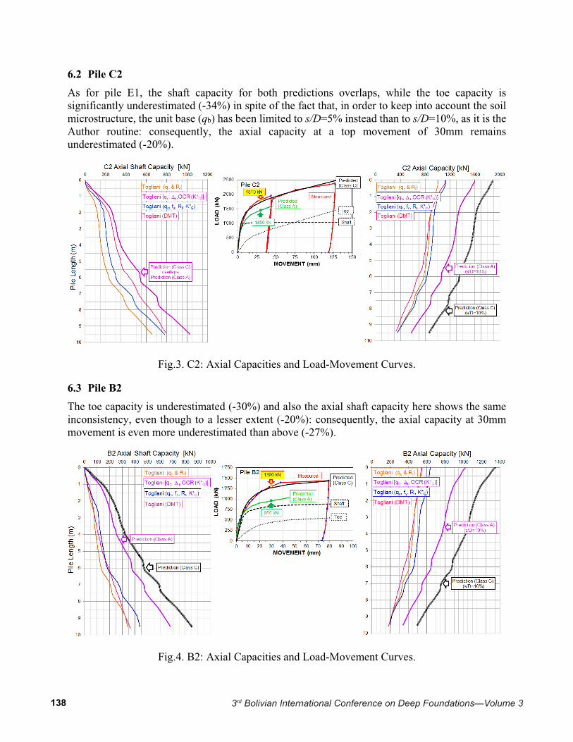
6.2 Pile C2
As for pile E1, the shaft capacity for both predictions overlaps, while the toe capacity is significantly underestimated (-34%) in spite of the fact that, in order to keep into account the soil microstructure, the unit base (qb) has been limited to s/D=5% instead than to s/D=10%, as it is the Author routine: consequently, the axial capacity at a top movement of 30mm remains underestimated (-20%).
Fig.3. C2: Axial Capacities and Load-Movement Curves. 6.3 Pile B2
The toe capacity is underestimated (-30%) and also the axial shaft capacity here shows the same inconsistency, even though to a lesser extent (-20%): consequently, the axial capacity at 30mm movement is even more underestimated than above (-27%).
Fig.4. B2: Axial Capacities and Load-Movement Curves.
138 3rd Bolivian International Conference on Deep Foundations—Volume 3

6.4 Pile A3
This prediction has been prepared on the assumption that even if with a less rigid response, the axial pile capacity was comparable, as upper bond, to the one of a CFA pile with same diameter, as frequently occurs.
The previous hypothesis is anything but optimistic, given that the Pile B2 load-displacement curve almost overlaps the predicted one, in spite of the much lesser pile diameter.
However, in the specific case, a lower bond prediction is surely the most suitable and thus, the corresponding load-movement curve better approximates the measured one.
As a comment, the axial shaft capacity has been overestimated (41% U.B. respectively 2% L.B.) as the U.B. toe capacity (9%) but the corresponding L.B. is underestimated (-28%), at 30mm displacement, the U.B. predicted capacity very largely exceeds the measured one (58%) while the L.B. capacity only slightly (7%).
Fig.5. A3: Axial Capacities and Load-Movement Curves. 7. CONCLUSIONS
Load-movement curves and corresponding axial pile capacities predictions always have been and still are a difficult and often frustrating exercise as the variables are many and in most cases unpredictable.
The logical consequence is that, as of today, no design method provides fully reliable predictions, if not in a random way: adding, in the specific case, the unexpected effects of the subsoil structure, inevitably appreciated only basing on a personal basis (no previous local experiences are available), one can understand why the Author has adopted its design methods which, at least, have allowed him to make mistakes with his own hands.
The predictions/measures comparison, basically summarized in the following Tables, highlights the sometimes out of the ordinary characteristics of the soil around the piles. For example, Table 4 highlights the anomalous value of predicted/reference ratio (Class C) of pile B2 (0.79 could be adequate for small displacement piles), contrary to what happens for all other types of pile. Similar considerations can be made for Table 5 comparisons (0.66, of B2, would be more appropriate for a driven pile and 0.82, of C2, is almost typical of a clay like soil rather than sand like, as in the reality of the site).
1393rd Bolivian International Conference on Deep Foundations—Volume 3

Table 4. Unit shaft comparison. Pile No. qs, reference (mean) qs, mean Predicted/ qs, mean Predicted/ (driven precast) Class A Reference Class C Reference (kPa) (kPa) (kPa) A3 (U.B.) 89 49 0.55 - - A3 (L.B.) 89 36 0.40 35 0.39 B2 80 51 0.63 63 0.79 C2 78 76 0.97 76 0.97 E1 77 75 0.97 75 0.97
Table 5. Unit Toe comparison Pile No. qc, base qb/qc, base qb/qc, base +8d, -4d
(MPa) Class A Class C
A3 (U.B) 6.8 0.29 - A3 (L.B.) 6.8 0.19 0.27 B2 4.7 0.47 0.66 C2 6.2 0.58 0.82
Finally, taking into account the very disappointing outcome of the predictions for all types of pile (excessive scattering), those of the Author, being in part sufficiently approximated, can be judged far more like an escaped debacle than a moderate success. 8. REFERENCES
Chen, Y.J. and Kulhawy, F.H. 2002. Evaluation of drained axial capacity for drilled shafts. Conference: International Deep Foundations Congress 2002.
Cruz, N. 2010. Modelling of geomechanics of residual soils with DMT tests. Ph D Thesis, Faculdade de Engenharia Universidade do Porto.
Fahey, M. and Carter, J. 1993. A finite element study of the pressuremeter using a nonlinear elastic plastic model. Canadian Geotechnical Journal 30(2) 348-362
Marchetti S. et al. 2008. In Situ Tests by Seismic Dilatometer (SDMT). GSP No. 270, 2008 Mayne, P.W. and Schneider, J.A. 2001. Evaluating axial drilled shaft response by seismic cone.
Foundation and Ground Improvement, GSP 113, ASCE, Reston/VA: 655-669 Monaco, P. and al. 2009. Interrelationship between small strain modulus G0 and operative
modulus. eds., Taylor & Francis Group, London, 1315–1323. Randolph, M.F. and Wroth C.P. 1978. Analysis of deformation of vertically loaded piles. Journal
of the Geotechnical Engineering Division ASCE. 104(GT12),1465-1488 Robertson, P.K. 2016. Cone penetration test (CPT)-based soil behaviour type (SBT) classification
system — an update. Canadian Geotechnical Journal Togliani, G. and Reuter, G.R. 2015. Piles capacity predictions (Class C): DMT vs CPTu.
Proceedings DMT’15. Rome, June 14-16, 2015. Togliani, G. 2016. Virtual DMT: An Opportunity for Pile Design? Proceedings International
Workshop on Metrology for Geotechnics. Benevento, Italy, March 17-18, 2016.
140 3rd Bolivian International Conference on Deep Foundations—Volume 3

Pile capacity prediction
Widjaja, B.(1), Johan, A.(1), Kristanto, F.S.(1), and Wahyuningsih, S.R.(1)
(1) Parahyangan Catholic University, Bandung, Indonesia <[email protected]>
ABSTRACT. Piles with different construction methods give dissimilar bearing capacity results. Compared to other piles, predictors conclude the bored pile has the smallest bearing capacity, followed by FDP and CFA pile. Conventional pile capacity analysis using t-z and q-z curve and PLAXIS software for FDP with expander body gives underestimated pile capacity compare to static loading test record. Furthermore, it is very important to do continuous research to get better and more accurate in predicting pile capacity in order to make perfect pile design. 1. INTRODUCTION
This paper describes brief design methods used for the 4 test piles. Test pile A3, which is a 620-mm diameter bored pile, is predicted with Reese and Wright (1977) method. Test Pile B2, which is a 450-mm diameter CFA pile, predicted with LCPC (1981) method. Test Pile C2, which is a 450-mm diameter FDP, is predicted with Eslami and Fellenius (1997) method. Test Pile E1, which is a 220-mm diameter FDP pile with an expander body, is also predicted with Eslami and Fellenius method. In the case of pile E1, the upward and downward load-movement response is predicted using PLAXIS software. 2. BACKGROUND
Pile capacity is used to be defined as the load which the pile movement exceeds a certain number, usually taken as 5% to 10% of the pile diameter. The definition is not considering the pile elastic shortening, which is very important for a long pile.
Pile capacity is also defined as the load at two lines intersection, approximating the initial point and the final point of pseudo-elastic load-movement curve. Fellenius (1975) gives nine definitions of pile capacity, two of them are used in this paper, they are the Mazurkiewicz method and the Chin Extrapolation.
3. PREDICTION INPUT 3.1 Soil Parameter
Determination of soil parameters for each pile is based on the SPT records. The soil unit weight (³ ) is determined with the recommendation from Cod to (2001), it gives a relationship between soil type and soil unit weight. Internal friction angle (Æ) is evaluated using a correlation with NSPT (Peck, 1974). Cohesion is evaluated using a correlation with NSPT (Terzaghi and Peck, 1967; Sowers, 1979). Table 1, Table 2, Table 3, and Table 4 show the soil parameters used in each pile. Table 5 shows the inputs for pile E1 in Plaxis software.
1413rd Bolivian International Conference on Deep Foundations—Volume 3
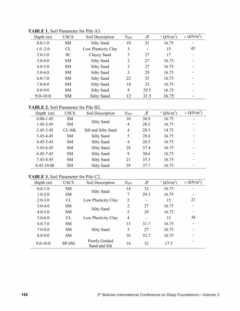
TABLE 1. Soil Parameter for Pile A3. Depth (m) USCS Soil Description NSPT Æ̊ ³ (kN/m3) c (kN/m2)
0.0-1.0 SM Silty Sand 10 31 16.75 -
1.0 -2.0 CL Low Plasticity Clay 5 - 15 45
2.0-3.0 SC Clayey Sand 3 27 17 -
3.0-4.0 SM Silty Sand 2 27 16.75 -
4.0-5.0 SM Silty Sand 2 27 16.75 -
5.0-6.0 SM Silty Sand 5 29 16.75 -
6.0-7.0 SM Silty Sand 22 35 16.75 -
7.0-8.0 SM Silty Sand 14 32 16.75 -
8.0-9.0 SM Silty Sand 8 29.5 16.75 -
9.0-10.0 SM Silty Sand 12 31.5 16.75 - TABLE 2. Soil Parameter for Pile B2.
Depth (m) USCS Soil Description NSPT Æ̊ ³ (kN/m3) c (kN/m2) 0.00-1.45 SM
Silty Sand 10 30.9 16.75 -
1.45-2.45 SM 4 28.5 16.75 -
2.45-3.45 CL-ML Silt and Silty Sand 4 28.5 14.75 -
3.45-4.45 SM Silty Sand 5 28.8 16.75 -
4.45-5.45 SM Silty Sand 4 28.5 16.75 -
5.45-6.45 SM Silty Sand 28 37.4 16.75 -
6.45-7.45 SM Silty Sand 9 30.6 16.75 -
7.45-8.45 SM Silty Sand 21 35.3 16.75 -
8.45-10.00 SM Silty Sand 29 37.7 16.75 -
TABLE 3. Soil Parameter for Pile C2.
Depth (m) USCS Soil Description NSPT Æ̊ ³ (kN/m3) c (kN/m2)
0.0-1.0 SM Silty Sand
14 32 16.75 -
1.0-2.0 SM 7 29.3 16.75 - 2.0-3.0 CL Low Plasticity Clay 2 - 15 21
3.0-4.0 SM Silty Sand
2 27 16.75 -
4.0-5.0 SM 5 29 16.75 -
5.0-6.0 CL Low Plasticity Clay 4 - 15 38
6.0-7.0 SM Silty Sand
13 31.7 16.75 -
7.0-8.0 SM 3 27 16.75 -
8.0-9.0 SM 16 32.7 16.75 -
9.0-10.0 SP-SM Poorly Graded Sand and Silt
14 32 17.5 -
142 3rd Bolivian International Conference on Deep Foundations—Volume 3

TABLE 4. Soil Parameter for Pile E1. Depth (m) USCS Soil Description NSPT Æ̊ ³ (kN/m3) c (kN/m2)
0.0-1.0 SM Silty Sand 10 31 16.75 -
1.0-2.0 CL Low Plasticity Clay 4 - 15 37
2.0-3.0 CL Low Plasticity Clay 2 - 15 19
3.0-4.0 SM Silty Sand 3 27 19.75 -
4.0-5.0 SM Silty Sand 3 27 19.75 -
5.0-6.0 CL Low Plasticity Clay 3 - 16 32
6.0-7.0 SM Silty Sand 7 29,3 19.75 -
7.0-8.0 SP-SM Poorly Graded Sand and Silt 18
34 20 -
8.0-9.0 SM Silty Sand 24 35,5 19.75 -
9.0-10.0 SM Silty Sand 22 35 19.75 -
TABLE 5. Inputs for Pile E1 in PLAXIS Software.
Material Description Modulus of Elastic (kN/m2)
Poisson’s Ratio
Internal Friction
Angle (o)
Soil Cohesion (kN/m2)
Explanation
CL Low Plasticity
Clay 5313 0.35 0.0 29.3
Average for CL soil layers
SM1 Silty Sand (NSPT 0-5)
4370 0.30 28.6 1.00
Plaxis requires not to fill zero as the cohesion
input
SM2 Silty Sand (NSPT 6-10)
10890 0.30 32.3 1.00
Plaxis requires not to fill zero as the cohesion
input
SM3 Silty Sand
(NSPT 11-25) 16340 0.30 35.0 1.00
Plaxis requires not to fill zero as the cohesion
input
SP-SM Poorly Graded Sand and Silt
13600 0.30 34.0 1.00
Plaxis requires not to fill zero as the cohesion
input
Pile E1 Pile E1
Concrete 2 x 10⁷ 0.15 - -
Non-porous material type
1433rd Bolivian International Conference on Deep Foundations—Volume 3
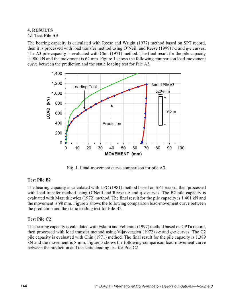
4. RESULTS 4.1 Test Pile A3
The bearing capacity is calculated with Reese and Wright (1977) method based on SPT record, then it is processed with load transfer method using O’Neill and Reese (1999) t-z and q-z curves. The A3 pile capacity is evaluated with Chin (1971) method. The final result for the pile capacity is 980 kN and the movement is 62 mm. Figure 1 shows the following comparison load-movement curve between the prediction and the static loading test for Pile A3.
Fig. 1. Load-movement curve comparison for pile A3.
Test Pile B2
The bearing capacity is calculated with LPC (1981) method based on SPT record, then processed with load transfer method using O’Neill and Reese t-z and q-z curves. The B2 pile capacity is evaluated with Mazurkiewicz (1972) method. The final result for the pile capacity is 1.461 kN and the movement is 98 mm. Figure 2 shows the following comparison load-movement curve between the prediction and the static loading test for Pile B2. Test Pile C2
The bearing capacity is calculated with Eslami and Fellenius (1997) method based on CPTu record, then processed with load transfer method using Vijayvergiya (1972) t-z and q-z curves. The C2 pile capacity is evaluated with Chin (1971) method. The final result for the pile capacity is 1.389 kN and the movement is 8 mm. Figure 3 shows the following comparison load-movement curve between the prediction and the static loading test for Pile C2.
0
200
400
600
800
1,000
1,200
1,400
0 10 20 30 40 50 60 70 80 90 100
LOA
D (
kN)
MOVEMENT (mm)
Loading Test
Prediction
620-mm
9.5 m
Bored Pile A3
144 3rd Bolivian International Conference on Deep Foundations—Volume 3

Fig. 2. Load-movement curve comparison for pile B2.
Fig. 3. Load-movement curve comparison for pile C2. Test Pile E1
The load-movement in bidirectional cell is predicted using model in PLAXIS 2D. Material model for all soil types is Mohr-Coulomb, while the pile uses Linear-elastic model. Groundwater level is applied at 3 m depth. Distributed load (load system A) is applied at the intersection between FDP pile and the expander body, then some different amount of loads are entered to have the pile movements. This relationship is plotted to make load-movement curve for upward and downward direction. Figure 4 shows the result prediction for load-movement in both upward and downward reaction.
0
250
500
750
1,000
1,250
1,500
1,750
0 10 20 30 40 50 60 70 80 90 100
LOA
D (
kN)
MOVEMENT (mm)
Loading Test
Prediction
450-mm
9.5 m
CFA B2
1453rd Bolivian International Conference on Deep Foundations—Volume 3

Fig. 4. Load-movement in bidirectional cell for pile E1.
5. COMMENT
All predicted piles give the underestimated pile capacity result, compared to the static loading test. It is because the predictors relied only a test record for each pile, whether it is SPT or CPTu record. The best calculation must be evaluated with all the records that available. Another reason is, the predictors also made some assumptions during the process, which are soil parameters (unit weight, cohesion, and internal friction angle), soil layer depth division, and some other factors such as: a factor and Cs value in Eslami and Fellenius method, and adhesion factor in Reese and Wright method. The assumptions may not equal to the actual condition. The predictors used many graphs and curves, which had to be evaluated visually. Therefore, the estimated numbers are not accurate perfectly. Prediction for Pile E1 bidirectional cell gives a different shape compare to the actual response, because the soil parameter, which is used by the predictors for the program input, may be not suit the pile and soil condition.
-2
-1
0
1
2
3
4
5
0 200 400 600 800 1,000
MO
VEM
ENT
(mm
)
LOAD IN BIDIRECTIONAL CELL (kN)
220-mm
9.5 m
FDP E1
300-mm
146 3rd Bolivian International Conference on Deep Foundations—Volume 3

6. REFERENCES Chin, F.K., 1970. Estimation of the Ultimate Load of Piles Not Carried to Failure. Proceedings of
the 2nd Southeast Asian Conference on Soil Engineering, pp. 81-90. Chin, F.K., 1971. Discussion on pile test. Arkansas River Project. ASCE, Journal for Soil
Mechanics and Foundation Engineering, 97(SM6), pp. 930-932. Coduto, D.P., 2001. Foundation Design Principles and Practices. Prentice Hall, 2nd ed. New
Jersey. pp. 50. Fellenius, B.H., 1975. Test Loading of Piles Methods, Interpretation, and New Proof Testing
Procedure. ASCE, 101(GT9), pp. 855-869. Fellenius, B.H., 2006. Basics of Foundation Design. Pile Buck International, Inc., Vero Beach,
FL, Electronic Edition. www.Fellenius.net, pp. 8-1 and 8-4. FHWA, NHI., 2016. Design and Construction of Driven Pile Foundations, Vol. 1. National
Highway Institute, pp. 260-261. Kulhawy, F.H., and Jackson, C.S., 1989. Some Observations on Undrained Side Resistance of
Drilled Shafts. Proceedings, Foundation Engineering: Current Principles and Practices, ASCE,Vol. 2, pp. 1011–1025.
Mazurkiewicz, B.K., 1972. Test Loading of Piles According to Polish Regulations. Preliminary Report No. 35. Commission on Pile Research, Royal Swedish Academy of Engineering Services. Stockholm.
O’Neill, M.W., Vipulanandan, C., Ata, A., and Tan, F., 1999. Axial Performance of Continuous Flight Auger Piles for Bearing. Center for Innovative Grouting Materials and Technology, University of Houston. Final Report to the Texas Department of Transportation, pp. 17-18, 20-25.
Peck, R.B., Hanson, W.E., and Thornburn, T.H., 1974. Foundation Engineering. John Wiley and Sons, Inc., 2nd ed. New York.
Rahardjo, P.P., 2005. Manual Pondasi Tiang. Edisi 3. Geotechnical Engineering Center. Bandung. Reese, L.C., and Wright, S.J., 1977. Drilled Shafts: Design and Construction, Guideline Manual.
Construction Procedures and Design for Axial Load. U.S. Department of Transportation, Federal Highway Administration, Vol. 1, 140 pp.
Sowers, G.F., 1974., Soil Mechanics and Foundations: Geotechnical Engineering. Macmillan Publishing Co., 4th ed. New York.
Terzaghi, K. And Peck, R.B., 1967. Soil Mechanics in Engineering Practice, 2nd ed. John Wiley and Sons, Inc. New York.
1473rd Bolivian International Conference on Deep Foundations—Volume 3

148 3rd Bolivian International Conference on Deep Foundations—Volume 3
Cast-in-Place Piles Using Toe-Grouting Cell. Application in Bolivian Rivers
Murillo, T.(1)
(1) Uriel & Asociados, S.A., Pozuelo de Alarcón, Spain <[email protected]>
ABSTRACT. The paper describes the design and construction of pile-toe, post-grouted drilled piles for bridge foundation, in sandy alluvial soils of rivers Piraí, Yapacaní, and Ichilo, in Bolivia. The grouting system is based on a grouting cell located at the pile toe, which allows distribution of the grout in a known zone underneath the pile toe. The cell’s behavior is similar to a hydraulic cell that stresses the ground downward and the pile itself upward. An advantage of this system is that it measures the force that is exerted on the toe (grouting pressure times cell area). The toe force is supported by the reaction developed along the pile shaft. Thus, the lower bound value of the shaft resistance is obtained. Additionally, if the upward and downward movements of the toe cell are monitored, the process is similar to that of a bi-directional loading test. 1. INTRODUCTION
The analysis of the response to a static load for cast-in-place piles is still a matter of a significant uncertainty. There are geotechnical intrinsic unknowns: geotechnical profile, material properties, and failure modes. Additionally, the ultimate load depends greatly on the construction method, as well as on the material the pile is made of. This is a complex problem of soil-construction-pile interaction.
Although this complex interaction scheme is well known beforehand, in standard practice this has been simplified by incorporating some parameters or making certain adjustments to the calculations, with the aim of approximating the results to the empirical observations. Even the more analytical calculation methods rely on empirical adjustments.
Consequently, when calculating the required length of a pile, it is common to obtain a wide array of results depending on the calculation method used and the version of the method recommended by the different standards.
As more results from static loading tests become available, standards will incorporate the effects of construction in a more efficient manner, leading to larger working loads applied to cast-in-place piles. 2. CAST-IN-PLACE PILES AND SANDS
In the case of cast-in-place piles, the following negative effects related with the response of a pile can appear:
1. Disturbance of the soil with excavation (stress relief, change of water content,…) 2. Debris accumulation at the bottom; the debris is usually more compressible than the
natural ground. 3. Incompatible movement (stiffness) of the pile shaft and pile toe to mobilize resistance.
The toe needs large movements to be mobilized, which will often exceed the maximum acceptable serviceability criterion for the supported structure.
1493rd Bolivian International Conference on Deep Foundations—Volume 3

These effects are more significant in sands, especially in sands with low fines content and below the water table, although they can also be present in other soils.
These limiting aspects are very present in US standards (AASHTO, FHWA), which are widely used worldwide. These standards propose reduced toe resistances for cast-in-place piles in sands. Another notable example can be seen in French standards, based on pressuremeter tests, which will be discussed later in this document.
A proper toe-grouting method can greatly mitigate, or even completely solve, these three negative effects: disturbance, debris accumulation, and low toe stiffness.
3. TOE-GROUTING SYSTEMS
3.1 Classification
Leaving aside the shaft-grouting methods, which constitute a separate issue, a classification of the different toe-grouting methods is presented below. A thorough overview of toe-grouting devices can be found in Mullins at al. (2001).
This classification has been devised from a practical point of view, depending on the installation of the systems and the possibilities that each one of them can provide. There are, logically, many options when manufacturing and installing a grouting system, but each one of them can be included into one of the following groups:
3.1.1 Systems drilled under the toe
This is the simplest method possible. The ground is drilled several meters below the pile toe, through one of the sonic test tubes or a pipe with a diameter larger than 76 mm. Subsequently, a tube is inserted and the grout is introduced through this tube. This tube can be an open ended tube (stem) or a tube with sleeve port valves.
The use of this system is not generally thought of as an improvement of ground conditions or on the bearing capacity of the pile, but rather as a control method and for occasional remediation in the case of small cavities or loosened sands at the toe that may have lead to poor construction or the loosening of these sands. The use can sometimes be systematic in a given location. In other locations, it is used on some of the piles and depending on the preliminary control tests (occasionally made of boreholes with SPT testing), it will be applied to the rest of the piles or not.
The system has several drawbacks. On the one hand, a hole has to be drilled through once the pile has been constructed. On the other, this technique is less efficient than the others presented here, unless sleeve ports are used.
3.1.2 Built-in circuits with sleeve ports
This system is based on the placement of an entry/exit circuit for the grout next to the rebar cage, with sleeve ports located at the toe of the drilled pile.
A steel plate is placed on top of the sleeve ports to separate them from the concreting process. Thus, the construction of the pile and the grouting phases are more independent. Otherwise, the grouting would have to be conducted before the concrete hardens, reducing its effectiveness. (Figure 1).
150 3rd Bolivian International Conference on Deep Foundations—Volume 3

Fig. 1. Examples of sleeve ports for toe grouting. a) from Mullins G., Winters D. (2004) b) from Brown (2012).
The first advantage is that no additional drillings are needed, as the whole system is installed
with the rebar cage. The other main advantage is the degree of control the grouting process provides, enabling
grouting in several phases.
3.1.3 Flat jack or toe-grouting cell
The underlying concept in these systems is the spreading of the cement grout under the pile toe and in contact with the concrete. This creates one unique grouting bulb that displaces the detritus and the loosen soil, densifying them. The grouting jack/cell’s behaviour is similar to a hydraulic cell that stresses the ground downward and the pile itself upward.
In fact, the pressured grouting bulb has a known horizontal cross-section, which is the cell’s or jack’s circular area, and which diameter is approximately equal to the diameter of the pile reinforcement cage, and slightly smaller than the pile’s diameter. In this way, it is possible to measure the force that is exerted on the toe (grouting pressure times cell area)
The toe force is supported by the reaction developed along the pile shaft and, consequently, the shaft mobilizes its shear resistance gradually as the grouting pressure increases, and a minor uplift of the pile occurs. The maximum grouting pressure is limited by the shaft’s ultimate resistance.
Monitoring the movement of the pile head during the grouting operation would be sufficient to serve as an approximate loading test for shaft resistance. If the downward movement of the grout cell is also monitored, the system serves as a bi-directional loading test for each pile. (In the event that the pile does not reach the uplifting point, a lower limit for the shaft resistance would have been obtained). An advantage of this is, therefore, that applicable standards’ provisions allow the use of lower resistance factors when loading tests are available.
1513rd Bolivian International Conference on Deep Foundations—Volume 3

Fig. 2. Construction and loading of the flat jack or grouting cell. Nowadays, these systems are usually built by using a flexible rubber membrane attached to
the edge of a steel plate that covers the entire pile toe (the diameter of this plate is the diameter of the rebar cage). The plate has orifices for the grouting. The grouting is done through tubes that reach these orifices. The grout is held by the membrane, as if it were a balloon inflated with it (see the figure below).
Fig. 3. Flat jack with membrane (taken from Mullins G., Winters D. 2004).
As a rule, this system is not designed for tube cleaning and re-grouting, but it could be feasible. In some variants, sleeve ports are used inside the membrane.
The system used in the bridges of rivers Piraí, Yapacaní and Ichilo, subject of this article, is a jack based on the concept of grouting cell or toe-box. It features two concentric steel cylinders that can shift around each other telescopically, enabling the expansion of the cell downwards as the grouting pressure increases. The cell is completed with 2 steel plates welded to the cylinders at the ends of the cell.
152 3rd Bolivian International Conference on Deep Foundations—Volume 3

Fig. 4. Grouting cell a) Before expansion b) Cylinders partially expanded.
Fig. 5. Grouting cell cross section a) Before expansion b) Maximum expansion (INCOTEC).
One or more rubber seals are placed between the cylinders to achieve better sealing during
the expansion of the cell. However, when a certain pressure is exceeded the grouting mix leaks from the cell, grouting the surrounding soil. In conclusion, the cell’s behaviour is initially similar to a hydraulic cell that stresses the ground downward and the pile itself upward, and then allows a conventional grouting of the soil.
The cell is also wrapped with a non-woven geotextile. This geotextile provides an additional isolation of the cell from the pile concrete, and also helps to create a grout bulb below the pile toe, minimizing hydro-fracture grout losses.
Fig. 6. Grouting cell fixed to the pile reinforcement cage. a) Bottom view. b) Top view.
1533rd Bolivian International Conference on Deep Foundations—Volume 3
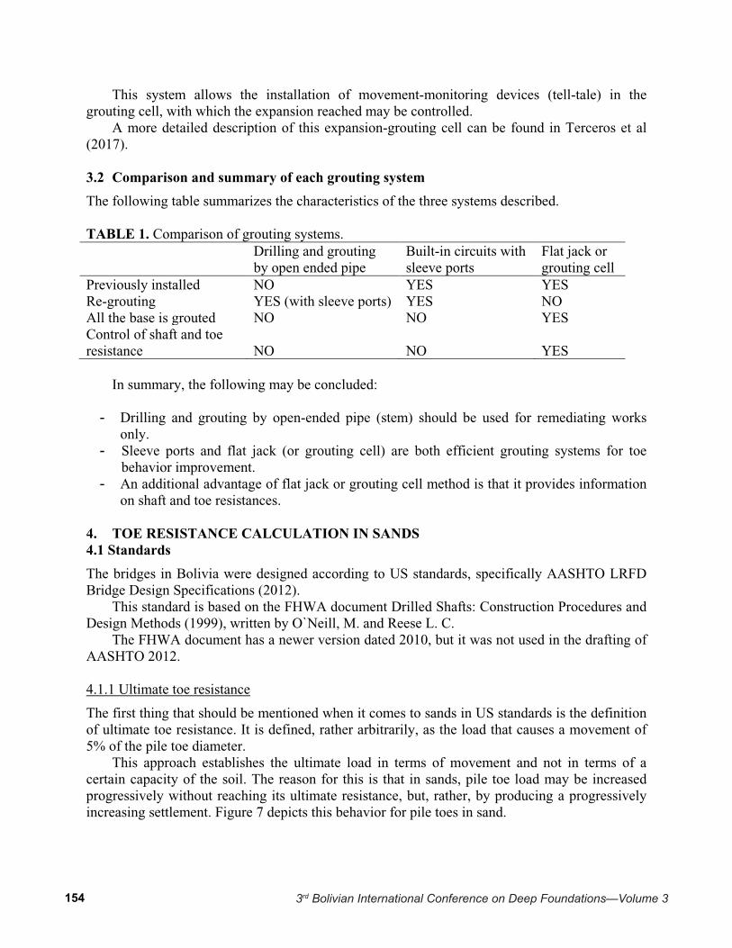
This system allows the installation of movement-monitoring devices (tell-tale) in the grouting cell, with which the expansion reached may be controlled.
A more detailed description of this expansion-grouting cell can be found in Terceros et al (2017). 3.2 Comparison and summary of each grouting system
The following table summarizes the characteristics of the three systems described. TABLE 1. Comparison of grouting systems.
Drilling and grouting by open ended pipe
Built-in circuits with sleeve ports
Flat jack or grouting cell
Previously installed NO YES YES Re-grouting YES (with sleeve ports) YES NO All the base is grouted NO NO YES Control of shaft and toe resistance
NO
NO
YES
In summary, the following may be concluded:
- Drilling and grouting by open-ended pipe (stem) should be used for remediating works
only. - Sleeve ports and flat jack (or grouting cell) are both efficient grouting systems for toe
behavior improvement. - An additional advantage of flat jack or grouting cell method is that it provides information
on shaft and toe resistances.
4. TOE RESISTANCE CALCULATION IN SANDS 4.1 Standards
The bridges in Bolivia were designed according to US standards, specifically AASHTO LRFD Bridge Design Specifications (2012).
This standard is based on the FHWA document Drilled Shafts: Construction Procedures and Design Methods (1999), written by O`Neill, M. and Reese L. C.
The FHWA document has a newer version dated 2010, but it was not used in the drafting of AASHTO 2012.
4.1.1 Ultimate toe resistance
The first thing that should be mentioned when it comes to sands in US standards is the definition of ultimate toe resistance. It is defined, rather arbitrarily, as the load that causes a movement of 5% of the pile toe diameter.
This approach establishes the ultimate load in terms of movement and not in terms of a certain capacity of the soil. The reason for this is that in sands, pile toe load may be increased progressively without reaching its ultimate resistance, but, rather, by producing a progressively increasing settlement. Figure 7 depicts this behavior for pile toes in sand.
154 3rd Bolivian International Conference on Deep Foundations—Volume 3

Fig. 7. Normalized toe resistance vs. settlement (AASHTO 2012). This concept is particularly relevant as:
- Loosening of sands and the presence of debris, due to construction techniques of cast-in-place piles, create a compressible layer of a certain thickness. This layer can cause a relevant settlement even for small loads. Therefore, the ultimate load is reduced when it is considered as being limited by a maximum allowable settlement.
- A construction method that increases the stiffness of the soils at the pile toe results in a smaller pile settlement than the original stiffness would have provided. Such increased stiffness is, for example, obtained by grouting at the soil below the pile toe.
Eurocode also introduces in some cases this concept of ultimate pile toe limitation, for example in the evaluation of the results of a static pile-loading test, by capping the toe load to the load that produced a movement equal to 10% of the pile diameter. 4.2 Calculation method
The FHWA’s document that discusses drilled piles mentions the disturbance of the sands at the pile toe as well as the accumulation of debris as sufficient reasons to justify the use of an empirical method, based on SPT results.
It mentions, in addition, that the analytic formulations used for obtaining the capacity would give the maximum resistances reachable, but the movement needed for the mobilization of those loads would be too high for the structure.
Consequently, AASHTO’s method for toe resistance in sand is limited to an SPT based method, using these equations:
𝑞𝑞𝑝𝑝 = 0.057 𝑁𝑁60 ; 𝑁𝑁60 ≤ 50 [𝑀𝑀𝑀𝑀𝑀𝑀] (1)
𝑞𝑞𝑝𝑝 = 0.0285 �𝑁𝑁60 �𝑝𝑝𝑎𝑎𝜎𝜎𝑣𝑣
, ��0.8𝜎𝜎𝑣𝑣
, ; 𝑁𝑁60 > 50 (2)
FHWA’s 2010 version now only accepts the first equation; the second one was included in
the 1999 version. AASHTO seems to still be based on the old FHWA document. The maximum toe resistances estimated when using this method, based on static loading
tests results, are 2.9 and 6.0 MPa for Equations 1 and 2, respectively.
1553rd Bolivian International Conference on Deep Foundations—Volume 3

4.3 Comparison with other methods
Results obtained according to the AASHTO method are low when compared with commonly used analytical methods, or even with other semi-empirical methods (at least with the ones used in Spain).
To illustrate the latter, the following graph has been prepared. It compares toe resistances obtained using the AASHTO method with other analytical methods (based on load factors, effective stresses, and internal effective angles of friction) as well as other semi-empirical methods used in Spain, based on SPT and pressuremeter test results.
Both the analytical and AASHTO methods have been applied to piles of 15, 20, and 25 meters in length. The total soil weight has been set at 20 kN/m3 (water table is assumed at ground level).
Peck’s correlation between the internal angle of friction and SPT-indices has been used for the analytical method. For pressuremeter values, the limit pressure (MPa) in sands is assumed to be 0.05 times the SPT index at the considered depth.
The result of the methods based on SPT results and assumed pressuremeter values represent a wide area due to the different proposals contemplated in the three Spanish standards of reference.
Fig. 8. Toe resistance in sand determined for three methods.
4.4 Calculations with toe-grouting
4.4.1 Mullins method (or FHWA method) Mullins et. al (2004) developed an investigation program sponsored by the Florida Department of Transportation, based on full scale testing.
The tests results led to a proposed calculation method for piles with grouted toe that was incorporated into the FHWA’s document on cast-in-place piles (2010).
156 3rd Bolivian International Conference on Deep Foundations—Volume 3

Without going into its applicability and related aspects that go beyond the scope of this paper,
the method considers that the improvement obtained depends on an index (GPI), equal to the grouting pressure (pi) divided by the ultimate toe resistance without grouting (qp):
𝐺𝐺𝑀𝑀𝐺𝐺 = 𝑃𝑃𝑃𝑃𝑞𝑞𝑝𝑝
(3)
The toe resistance, qp grouted, after grouting is expressed using a multiplier, TCM, of the toe
resistance (the ultimate capacity) 𝑞𝑞𝑝𝑝 𝑔𝑔𝑔𝑔𝑔𝑔𝑔𝑔𝑔𝑔𝑔𝑔𝑔𝑔 = (𝑇𝑇𝑇𝑇𝑀𝑀)(𝑞𝑞𝑞𝑞) (4)
The equation for this multiplier depends on the pile toe movement expressed in terms of a percentage of the pile diameter:
𝑇𝑇𝑇𝑇𝑀𝑀 = 0.713 (𝐺𝐺𝑀𝑀𝐺𝐺)(%𝐷𝐷0.364) + %𝐷𝐷0.4(%𝐷𝐷)+3.0
(5)
If we focus only on the ultimate load, defined as 5 % of the toe diameter, the relation between
TCM and the GPI-index (Eq. 3) is linear (TCM = 1+1.28GPI).
4.4.2 Expectations concerning the design pressures With the method discussed, as well as with any other based on grouting pressures, some concerns have to be taken into account and settled before construction. The following should be considered: - The available shaft resistance limits the maximum grouting pressure. At a certain point,
attempts to increase the grouting pressure on the toe will just result in pile uplift (when grouting with a grouting cell or a flat jack).
- The design grouting pressure will have to be achieved during the construction phase, something that is not guaranteed in the design phase, since it depends on many factors.
4.4.3 French method The pressuremeter test calculation method (based on limit pressure) is widely used in France for foundation design. It is an empirical method based on hundreds of pile loading tests.
In its first version (DTU 13.2 (1983)), this standard equated toe-grouted piles (high grouting pressures) with not-grouted, but driven piles. This was based on the idea that with proper toe grouting, the reduction of toe-resistance associated with the excavation of the bored piles could be eliminated (the toe resistance of the driven piles was twice that of the not-grouted cast-in-place piles).
In contrast, Mullins’ method seems to be a more precise method at first sight, but it is possible that results obtained under situations different to the ones tested by Mullins (different jacks, larger diameters, different types of sands…) would lead to further adjustments in the method.
In the particular case of piles grouted using a grouting cell such as the ones used in this project in Bolivia, cells allow a large downward movement and they also allow for grouting the ground with a significant volume. The increase in toe stiffness must be somehow related with the toe displacement and with the grouted volume. However, Mullins’ method does not take these variables into account.
1573rd Bolivian International Conference on Deep Foundations—Volume 3

5. PROJECT DESCRIPTION AND CONSTRUCTION 5.1 Introduction and purpose
The proposal and subsequent construction of the post-grouted-cast-in-place piles described in this article was due to the presence of several geotechnical factors, which could be summarized in:
a) The existence of very clean sands in the alluvial soils of the Piraí, Yapacaní, and Ichilo rivers.
b) The severe toe bearing limitation in sands, according to applicable standards (AASHTO) These technical circumstances, coupled with the search for the most economical foundation
possible (in terms of both, time and cost), gave Uriel and Asociados the chance to propose to Grupo Puentes, contractors and designers of three railroad bridges, the advantages of building toe-grouted cast-in-place piles using grouting cells. 5.2 Project description
The project is located in Bolivia, in the railway line between the petrochemical plant of Bulo Bulo and Montero, close to Santa Cruz de la Sierra, and part of the Bioceánico Railway.
The bridges, 331, 799 and 331 m in length, cross rivers Ichilo, Yapacaní, and Piraí, tributaries to the Amazon.
The spans were established at 39 meters and the designers were able to limit the foundations to 4 piles per bent.
Pile diameters were established at 1,200 and 1,500 mm. Drilling used temporary casing for the whole length of the pile and no slurry was used.
The diameter was chosen based more on compatibility with the available rigs than on the loads, as these were similar for all three bridges. Most of the piles had a factored vertical load between 7,000 and 7,700 kN (un-factored loads were between 4,900 and 5,400 kN). The corresponding working stresses were 4.7 and 3.0 MPa for the 1,200 and 1,500 mm piles. The maximum un-factored tension load was 2,600 kN.
Scour depth was defined as 5, 8, and 10 meters for each of the mentioned rivers, although it did not condition the length of the piles due to the reduced safety factors associated to this extreme event. The same can be said for seismic design. The tension loads exceeded the limit only in a few cases. 5.3 Soil profile
From a geological perspective, the bridges are located in the Chaco – Beniana plain (as it is called in Bolivia). This is part of the Amazonian plains, at an elevation of 275 above sea level. They are quaternary soils of alluvial and flood plain origin, with thicknesses that exceed 50 meters.
The geotechnical investigation works were carried out in two phases, consisting mainly on 29 boreholes with SPT tests for the 42 bents. In some cases, these borings were drilled on top of a pontoon. Laboratory tests carried out were sieve analysis and Atterberg limits.
The alluvial soil was predominantly fine sandy and clean. At a certain depth, sand was dense or very dense, which usually coincided with past scour depth.
158 3rd Bolivian International Conference on Deep Foundations—Volume 3

At varying depths, lenses of heterogenic clays and silts could be found, as well as sands with gravel (see next figure).
Fig. 9. Section of the geological profile in Yapacaní.
For the finer and looser sands, an angle of shearing resistance between 30º and 32º was
chosen. For the denser and coarser sands, the values reached 34º and 36º. In clays, angles of shearing resistance of 28º-29º were chosen for the low plasticity clays and of 26º for the high plasticity clays.
5.4 Design description
With the aim of searching for the most conventional calculation procedure possible, which also had to be accepted by local standards, Mullins’ method was used for estimating the grouting pressures required during construction.
It was assumed that grouting would cancel the effects of the disturbance of the sands and debris at the pile toe, as well as increase the stiffness of the soils at the pile toe.
The analytical method used for shaft and toe resistance calculations was based on effective stress distribution, internal angles of friction, and cohesion. An 11-MPa limit toe resistance was applied for each bent.
For the pile length of each cap, a required grouting pressure was calculated in order to obtain the toe resistance. For this, the non-grouted resistance was calculated according to the AASHTO formula, that is, 6 MPa for a sand with SPT N-indices indicating very dense conditions, instead of following the current FHWA formula. In order to reach the maximum 11 MPa toe resistance in sands, a TCM multiplier of 1.83 would be required, which could be obtained with a grouting pressure of 3.9-MPa, following the calculations presented herein.
The calculation process was completed by checking that, for each required grouting pressure, the estimated shaft resistance was sufficient for the pile not to move upwards.
The results for the bents are summarized in the following table:
1593rd Bolivian International Conference on Deep Foundations—Volume 3
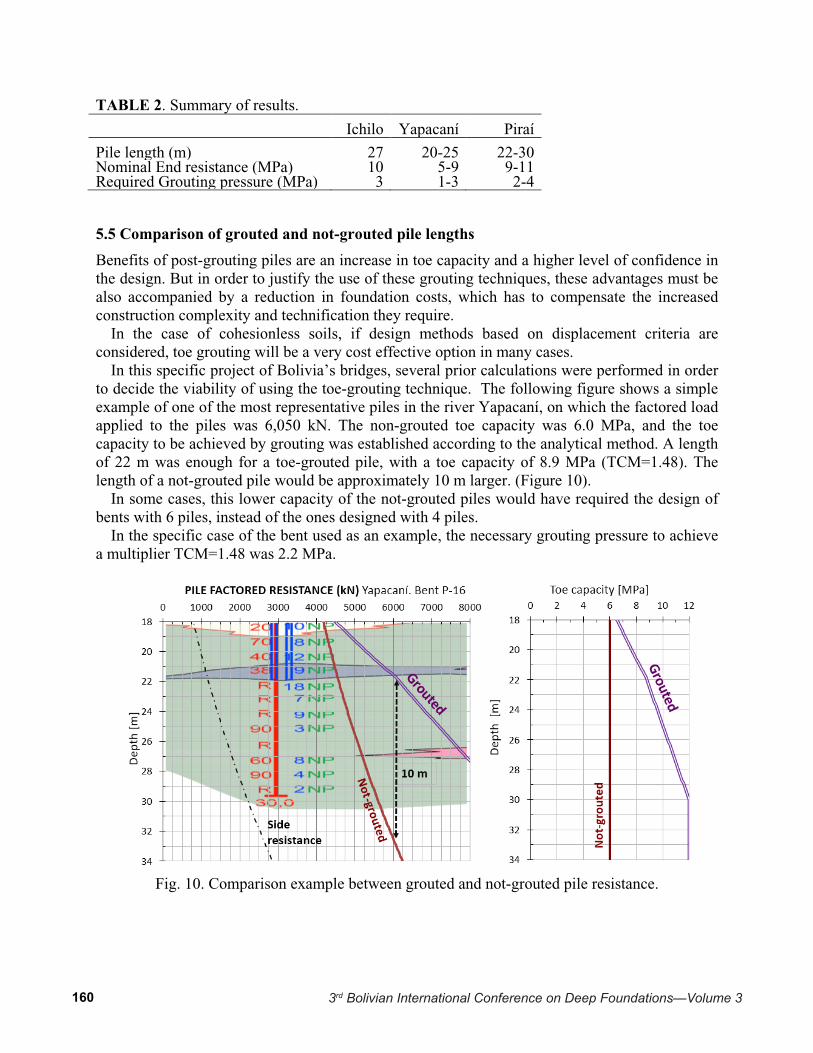
TABLE 2. Summary of results.
Ichilo Yapacaní Piraí
Pile length (m) 27 20-25 22-30 Nominal End resistance (MPa) 10 5-9 9-11 Required Grouting pressure (MPa) 3 1-3 2-4
5.5 Comparison of grouted and not-grouted pile lengths
Benefits of post-grouting piles are an increase in toe capacity and a higher level of confidence in the design. But in order to justify the use of these grouting techniques, these advantages must be also accompanied by a reduction in foundation costs, which has to compensate the increased construction complexity and technification they require.
In the case of cohesionless soils, if design methods based on displacement criteria are considered, toe grouting will be a very cost effective option in many cases.
In this specific project of Bolivia’s bridges, several prior calculations were performed in order to decide the viability of using the toe-grouting technique. The following figure shows a simple example of one of the most representative piles in the river Yapacaní, on which the factored load applied to the piles was 6,050 kN. The non-grouted toe capacity was 6.0 MPa, and the toe capacity to be achieved by grouting was established according to the analytical method. A length of 22 m was enough for a toe-grouted pile, with a toe capacity of 8.9 MPa (TCM=1.48). The length of a not-grouted pile would be approximately 10 m larger. (Figure 10).
In some cases, this lower capacity of the not-grouted piles would have required the design of bents with 6 piles, instead of the ones designed with 4 piles.
In the specific case of the bent used as an example, the necessary grouting pressure to achieve a multiplier TCM=1.48 was 2.2 MPa.
Fig. 10. Comparison example between grouted and not-grouted pile resistance.
160 3rd Bolivian International Conference on Deep Foundations—Volume 3

5.6 Grouting procedure
Grouting, carried out by INCOTEC, was taken to the maximum pressure possible. The limit was given either by the pile uplift or when a certain volume was reached.
The volume was increased to a maximum of 1,000 liters, after observing that the grout could leak out between the cylinders of the cell once a certain pressure was reached (the volume of the cell is 200 liters). Grouting pressure was released during the curing of the grout.
Pressure, volume, and flow controls were performed in real time using transducers. This enabled the evaluation of each grouting for validation purposes, together with the data measuring the pile uplift and pile toe movement. Movements were measured with tell-tales (free moving rods inside a tube that is resting on the base plate of the cell). These movements were measured manually, with the inconvenience that grouting is a dynamic process and the response measured at the pile head is not instantaneous.
Pile uplift was limited to 5 mm, allowing slightly higher values if the expected grout pressure was not obtained.
Fig. 11. Grouting pressure-volume log example.
Fig. 12. Measured movements example.
1613rd Bolivian International Conference on Deep Foundations—Volume 3

5.7 Analysis of toe load-movement
Figure 13 shows the pressures obtained with the cell and the movement obtained when grouting the 1,200 mm diameter piles. The heavy line at 60 mm indicates the limit value defined by FHWA and AASHTO (downward movement equal to 5 % of the diameter).
Fig. 13. Grouting pressures at toe vs. movement.
Grouting pressures reached are quite variable, mostly due to the fact that no maximum value was established. In general, pressures were greater than the required grouting pressure (Table 2), and show figures similar to the factored toe resistances.
With regards to the movements recorded, dispersion is due to several factors. On the one hand, it can be explained by the heterogeneity of the alluvial soils, as well as by the different results obtained in the construction of each pile (for example, the effort needed to control water inflow in each of the piles was very variable, depending on the unpredictable presence of artesian sand layers). On the other hand, the grouting cell used expands until the grout seeps through, and then the expansion rate decrease.
In general, movements recorded reveal the dubious behaviour of drilled-pile toes, especially if the piles have been drilled in sandy soils and are beneath the water table. If we assume that pile toe movement during grouting is, approximately, proportional to grouting pressure, this simplification would result in an average toe resistance of 5.2 MPa for a 60-mm movement before grouting. The standard deviation is high, 3.0 MPa.
A recommended improvement for future applications would be the use of tell-tales with LVDT sensors for data collection in real time. Thus, during the grouting process it would have been possible to record a fact observed on site, namely that induced toe movements are practically irreversible and that re-loading also causes a very stiff response. This is one of the mechanisms that enhances toe performance, and is stated in several references (Mullins G. et al (2006); CALTRANS (2016)). The following diagram illustrates this concept, through the use of a conceptual sketch from California’s Department of Transportation.
162 3rd Bolivian International Conference on Deep Foundations—Volume 3

Fig. 14. Effect of post-grouting on nominal toe resistance (adapted from CALTRANS).
5.8 Mobilized shaft resistance
The following graph depicts the mobilized shaft resistances, compared to calculated shaft resistance in the design phase, in piles that moved upwards during the grouting.
Fig. 15. Mobilized shaft resistance vs. nominal shaft resistance.
Mobilized shaft resistance was larger than nominal shaft resistance for 75 % of the piles. It is worth highlighting that mobilized shaft resistance is a lower bound of the actual shaft capacity of the pile, as the pile displacement was limited to avoid reaching the maximum shaft resistance. In addition, for many piles this limitation proved unnecessary, and the grouting process was fully performed without the upward movement limit pressure having been reached (volume was the limiting variable).
Average upward measured displacement of the piles was 4, 2 and 6 mm for rivers Piraí, Yapacaní and Ichilo, respectively, values that are clearly below those usually considered
1633rd Bolivian International Conference on Deep Foundations—Volume 3

necessary for fully developing ultimate shaft resistance in sandy soils (0.5 and 1.0 % of the diameter of the pile).
On average, mobilized shaft resistances were 40, 37 and 36 kPa in each river, respectively. For a group of 16 piles, the only ones with a 1200 mm diameter along the river Yapacaní, situated in 4 consecutive piles, uplifts reached significantly high figures, between 5 and 16 mm, and an average of 13 mm. On these piles, the mobilized force was between 1.2 and 1.6 times the calculated capacity, with the average multiplier being 1.8. The average mobilized resistance was 48 kPa.
As these figures became known during the piling works, they were taken into account when it came to re-evaluating the load capacity of some of the piles in which the design pressures had not been reached.
It can be concluded that the calculation method based on effective stresses has been conservative. This method is based on the beta parameter (β=Ko tan φ), which is not very sensitive to variations in the angle of shearing resistance. The conservative factor does not result from the representative parameters selected as much as from the method itself.
5.9 Load applied on piles
Finally, the following graph compares the total loads mobilized by grouting with the un-factored load in each pile.
Fig. 16. Mobilized load vs. un-factored load.
As it can be seen, most of the piles (76 %) were subjected to loads higher than the working loads.
Although data recorded for grouting parameters, as well as pile head and toe displacements, is not sufficient to be considered a comprehensive load test that fulfils standards, grouting is a bi-directional loading monitored process. Thus, this data contributes to increasing confidence in the design during construction, and constitutes a step forward in the execution, in comparison with not-grouted piles.
164 3rd Bolivian International Conference on Deep Foundations—Volume 3

6. CONCLUSIONS
Excavation and concreting of a pile in soils, especially in sandy soils under the water table, can significantly affect its capacity and, especially, the proper response of the pile toe. Toe-grouting technologies can mitigate the disturbance of the soil and debris accumulation, and increase pile toe stiffness.
In this specific project of Bolivia’s bridges, 1,200 and 1,500 mm diameter cast-in-place piles were post-grouted using toe-grouting cells. The calculated nominal resistances were twice what the AASHTO recommends for conventional cast-in-place piles in sands. Consequently, a substantial reduction in shaft lengths was achieved and, therefore, significant savings (both, in cost and time) on foundation works were made.
In addition, the use of toe-grouting cells, coupled with grouting parameters (pressure, volume, flow) being monitored and pile movements being controlled during grout loading, enhances the reliability of the pile’s design and construction. 7. ACKNOWLEDGEMENTS
The author would like to thank the Grupo Puentes team, led by their Project Manager, Ángel Eiras Sánchez, and their Head of Construction, José Antonio Rodríguez Quevedo, for their trust.
1653rd Bolivian International Conference on Deep Foundations—Volume 3
REFERENCES
AASHTO, 2012. LRFD Bridge Design Specifications. Brown, D. 2012. Recent Advances in the Selection and Use of Drilled Foundations.
Geotechnical Engineering State of the Art and Practice: Keynote Lectures from GeoCongress ASCE Oakland, California, pp. 519-548.
Bruce, D.A. 1986. “Enhancing the performance of large diameter piles by grouting, I and II, Ground Engineering, May and July
Bustamante M., Gianeselli L., 2008. Reglas de cálculo de la resistencia de pilotes por el método de los estados límites últimos. Método presiométrico. CEDEX. Madrid. Spain
CALTRANS, 2016. Memo to designers. 3-8 October. CEN, 1994. Eurocode 7: Geotechnical design - Part 1: General rules, Pre-standard ENV 1997-1.
European Committee for Standardization (CEN): Brussels. CEN, 2004. Eurocode 7: Geotechnical design - Part 1: General rules, EN 1997-1:2004 (E), (F)
and (G), November 2004, European Committee for Standardization (CEN): Brussels. CEN, 2007. Eurocode 7: Geotechnical design - Part 2: Ground investigation and testing. EN
1997-2:2007 (E), March 2007, European Committee for Standardization (CEN): Brussels. Daap S., Muchard M. and Brown, M. 2006. Experiences with base grouted drilled shafts in the
southeastern United States. DFI Conference. Amsterdam. DTU 13.2, 1983. Fondations profondes pour le bâtiment, Chap 11: Calcul des fondations
profondes soumise à charge axiale: 1-8. FHWA, 1999. Drilled Shafts: Construction Procedures and Design Methods. FHWA-NHI, 2010. Drilled Shafts: Construction Procedures and LRFD Design Methods. Dirección General de Carreteras. 2004. Guía de Cimentaciones de Obras de Carreteras.
Ministerio de Fomento. Madrid. Ministère de l´Équipement, des Transports et du Tourisme, 1993. Règles techniques de
conception et de calcul des fondations des ouvrages de génie civil.. France. FASCICULE N°62 -Titre V, Textes Officiels N° 93-3 T.O.: 182 pp.
Ministerio de Fomento, 2006. Código Técnico de la Edificación. Madrid. Mullins G., Winters D. 2001. Post-grouted drilled shafts Tips. Phase I. University of South
Florida. Mullins G., Winters D. 2004. Post-grouted drilled shafts Tips. Phase II. University of South
Florida. Mullins G., Winters D. and Dapp S. 2006. Predicting end-bearing capacity of post-grouted
drilled shafts in cohesionless soils. Journal of Geotechnical and Geoenvironmental Eng. ASCE.
Terceros M, Terceros M, 2017. Expander Body and Toe-Box: Expansion Devices for Deep Foundations Enhancement. 3rd B.F.P.B Santa Cruz de la Sierra. Bolivia.
166 3rd Bolivian International Conference on Deep Foundations—Volume 3

Pile testing competitions – a critical review J. M. Amir Foundation Control Institute Ltd., Herzlia, Israel B H. Fellenius University of Ottawa, Canada ABSTRACT: A number of pile testing competitions, using low-strain techniques, took place in different countries between 1987 and 1996 and they soon started heated debates by the professional community. Since the outcome of these competitions was obviously contentious, they do deserve a critical review. Such a review may serve as a basis for more productive competitions in the future. These, in turn, will highlight both capabilities and limitations of existing methods and contribute to the advancement of new techniques. The authors describe, for each competition held, the testing scope and program, piles tested, the nature of the defects installed, the participating parties, and the results obtained. They go on to analyze each competition, specifically stressing those items that if done differently could have significantly improved the outcome. Based on the lessons learned from these events, the authors propose ground rules for future pile-testing competitions. In addition, the importance of organizing competitions also in downhole testing applications is strongly recommended. 1. INTRODUCTION
In spite of the rapid progress in piling techniques (and maybe because of it), defective piles and drilled-shafts are still encountered at many construction sites. Among all the methods designed to test the integrity of bored piles, only two have proved to be of real practical value: The sonic (echo) and the ultrasonic (cross-hole) methods.
The sonic method was first applied a quarter of a century ago (Steinbach and Vey 1975). Since then, it has established itself as the leading method for testing the integrity of all kinds of piles. With the advent of handheld computing, sonic testing has become more reliable and at the same time more affordable.
The sonic method is based on pressing a sensor against the surface of the pile head while hitting the surface with a hammer. The hammer blow creates a low-strain wave that travels down the pile and is reflected from the pile toe, as well as from any abrupt change in the pile impedance. The hammer may be either plain or instrumented, and the results may be analyzed and presented in either time or frequency domain. An
extensive treatment of the sonic method is presented by Turner (1997). The popularity of the method has brought a proliferation of both instrumentation and testing laboratories. Consequently, it naturally became a subject for competition. 2. PILE TESTING COMPETITIONS 2.1 Objectives
In principle, pile-testing competitions should be held with the some or all of the following objectives in mind: 1. Kindling a competitive spirit amongst developers,
manufacturers, and users of equipment
2. Establishing the actual (as opposed to claimed) capabilities and limitations of the method
3. Indicating where advances in the state of the art are required.
4. Serving as milestones to monitor progress in both instrumentation and analysis tools
Paper reproduced from Amir, J.M. and Fellenius, B.H., 2000. Pile testing competitions—a critical review. Proceedings of the
6th International Conference on Application of Stress-Wave Measurements to Piles, Sao Paulo, September 2000, 6 p.
1673rd Bolivian International Conference on Deep Foundations—Volume 3

5. Providing an opportunity for potential clients to obtain reliable comparative data regarding the performance of available instruments
3. COMPETITION OVERVIEW
Following is a brief summary of five competitions, held in Ghent, Belgium (1987), California, USA (1990), Texas, USA (1990), Delft, The Netherlands (1992), and Texas, USA (1996). 3.1 Ghent 1987
The first known integrity testing competition was held in Ghent, Belgium in 1987 (De Jaeger et al. 1987). The Belgian Society for Soil Mechanics and Foundation Engineering organized this event. Altogether, twenty test piles were constructed by four different methods, five piles each: 1. Atlas helicoidal (sawtooth profile) piles, diameter
430/530 mm
2. De Waal square, precast concrete driven piles, diameter 320 mm
3. Socofonda CFA piles, diameter 460 mm
4. Fundex piles, bored with rotated casing and cast in situ, diameter 390 mm
The five testing firms that participated were given
the pile diameters, and told that the pile lengths ranged between 11 m and 16 m. No defects were knowingly produced, and the task in hand was to determine the correct length.
The best overall length agreements were obtained in the Socofonda and Fundex piles. The lengths obtained for the Socofonda piles were 93% and 100% of the correct lengths. For the Fundex piles, the spread was between 94% and 102%. Such results are perfectly acceptable.
On the other hand, poor results were reported for the precast piles (82% to 120%) and the Atlas piles (101% to 125% for three of the piles, with no results at all for the other two). The testing of the Atlas piles also produced poor results. Although the Atlas piles had the lowest L/D ratio (26 to 30), all testers reported lengths that were too high. The conclusions from this exercise were as follows:
1. The precast driven piles were difficult to test both due to higher shaft resistance and to high L/D ratio; 41 to 53, the highest.
2. The testers of the Atlas piles probably neglected the fact that a helicoidal pile exhibits a wave velocity that appears to be much lower
than that of a straight-shafted pile (Vyncke and van Nieuwenburg 1987).
3. The CFA piles and the Fundex piles were the easiest to test. This was probably due to their lower L/D ratios (32 to 37) as opposed to the precast piles.
3.2 California 1990
The California test program was carried out in the framework of a research project for the Federal Highway Administration (Baker et al. 1993). It took place on two sites: Cupertino, with dry gravelly and sandy soil and San Jose, with clayey soil below the groundwater table. The piles had a nominal diameter of 915 mm and lengths of between 7.6 m and 18.9 m.
There were five participants in the program, applying four testing methods: Sonic echo (time domain), transient dynamic response (frequency domain), cross-hole (ultrasonic) and radioactive (gamma-gamma). All participants were provided in advance with the lengths and shapes of the piles that they were to test. 3.3 Texas 1990
The Texas test program was a continuation of the California FHWA project (Baker et al. 1993). Altogether, nine bored piles were constructed, seven of which had known irregularities. All piles had a nominal diameter of 915 mm, with lengths varying between 11 and 24 m (L/D ratios between 12 and 26).
The irregularities were of different character and magnitude. Four of the piles had a single planned necking at a depth of between 3 and 18 m, the reduction in cross section being between 12 and 50 percent. Three other piles had both increased and decreased cross sections at various depths. In addition to the planned defects, some unplanned defects occurred and were recorded during construction.
Five testing firms took part in this competition. The testing firms received full information regarding the subsurface conditions, as well as the lengths of the two reference piles. No further data about the existence of defects was divulged.
The tests were conducted in two stages: In stage one, only surface (sonic) methods were used. In stage two, the contestants were allowed to lower testing equipment into access tubes which were prepared beforehand.
168 3rd Bolivian International Conference on Deep Foundations—Volume 3

The results of the Texas program may be summarized as follows: 1. At depths smaller than 7 m below the top of the pile
head, 80 percent or more of the testing firms managed to identify all important defects in the cross section.
2. The success rate dropped to 60 percent at a depth of 9 m.
3. All participants failed when the defect (necking) was located at a depth of 18 m.
4. Even at shallow depths, participants failed when the reduction in cross section area was merely 12 percent.
5. In general, an enlarged cross-section was more difficult to find than a reduced one.
6. The participants had difficulty in determining the length of the pile when there was a major necking at mid-length, or when a defect existed near the toe of a long pile.
7. As expected, no participant could identify a “soft bottom” condition.
3.4 Delft 1992
The Delft competition took place in conjunction with the Fourth International Conference on the Application of Stress-Wave Theory to Piles (1992). Twelve laboratories, employing six different types of instruments, participated in the event. The testing objects in this case were rather uncommon: All of the ten test piles were made from precast concrete and installed in the following way: First, closed-end steel tubes were driven to a predetermined depth. Then, a thin bed of sand was placed at the bottom of the tubes and the precast piles were lowered into the empty tubes and placed on the sand-bed. The space around the piles was then filled with a bentonite-cement mixture supposed to represent the local soil stiffness.
The test piles had a nominal cross-section 250-mm square. Two piles were straight shafted, with respective lengths of 17 m and 18 m. Of the rest, six piles were produced with the cross-section along a given length either enlarged to 300 mm-square, or reduced to 200 mm-square, or both. The two remaining piles had a sawed notch, 10 mm. thick and occupying one half of the cross section. Similar notches were also produced in two of the piles with enlarged section.
The testing circumstances were also noteworthy, in two important respects: First, the participants were not allowed to approach the piles, and the notary public’s clerk was mobilized to hit the piles with the hammer. Second, the participants were given beforehand the exact
shapes of all the piles, and their task was to decide which of these shapes best fitted each of the reflectograms they obtained.
All the participants managed to achieve was a correct fit for between three and seven piles, with a mean success rate of 44%. The scores for the individual piles varied between zero (straight shaft, L = V8L) to 100% (straight shaft, L = 17 m). 3.5 Texas 1996
This competition (Samman and O’Neill 1997) took place on the campus of the University of Houston, Texas. Altogether, twenty-two piles were tested. Eleven of the piles had a diameter of 460 mm and were bored to a depth of 4.6 m. The other eleven piles were 760 mm in diameter and 7 m long in the ground. Some of the piles were constructed with polymer slurry while the rest were cast in the dry. Six of the piles were regular piles, while sixteen piles had planned built-in defects. These defects were produced from 25 mm thick soft rubber mats, laid horizontally. The mats were placed at different depths, but not more than one per pile. Each occupied between 10 and 50 percent of the total cross section of the pile.
Eight laboratories took part: Two were from government agencies, five were commercial, and one academic. The contestants were asked to report for each pile whether it is sound or defective, and, in the latter case, specify the depth and severity of the defects. The participants were to submit two reports: A preliminary report on the same day, and a final report within five days.
The results, as can be expected, were far from satisfactory: In the piles intended to be sound, only 7% of the tests confirmed the integrity. In the anomalous piles, 82 % of the defects were found. These rates improved somewhat in the final reports, to 25% and 83%, respectively. The success rate for the defective piles may seem impressive, but a deeper look into the matter is far less encouraging: Of all the reported defects, only 36% managed to fit the depth of the defects within ±20 percent. Of these, only 37% provided the size of the defects within ±20 percentage points. Moreover, the participants reported on average 1.3 “phantom”, i.e., nonexistent, defects per pile. None of the contestants, or the testing instruments used, demonstrated a markedly outstanding performance. 4 EVALUATION 4.1 Ghent 1987
The organizers declared that the piles were between 11 m and 16 m long. Thus, a tester who would have reported a uniform length of 13.5 m (the mean of the above limits) for all the piles would be accurate to within ±10% in 90% of the piles.
1693rd Bolivian International Conference on Deep Foundations—Volume 3

While highlighting the influence of construction method on testability, the Ghent competition totally neglected the most important purpose of sonic testing—finding defects!
Publication of the test results was comprehensive, and included a special seminar where the results were presented and discussed. 4.2 California 1990
Since the organizers of the California testing program gave the participants full details regarding the planned defects, success rates have no meaning. It is therefore questionable whether the California test may qualify as a competition and therefore the case is not pertinent to the present paper. (The results are of course interesting in other contexts). 4.3 Texas 1990
While, in California, the participants were given information beyond that normally provided to testers, in Texas, they got too little. When a pile testing firm is invited to a construction site, it is customary and necessary to provide it with all relevant information, such as soil data, pile construction records, and piling logs with the as-made length and details of any irregular events that may have happened. Testing under the “Texas rules“, with no à-priori knowledge of the pile length, is therefore the exception and detracts from the representativeness of the results.
In other respects, the planning and execution of the Texas tests was very effective. The tasks were well graded from easy through difficult to impossible. Thus, the performance of contemporary systems was well defined. This competition proved convincingly that the sonic method is a viable technique for investigating pile integrity. It showed that sonic equipment is able to identify most important defects where they matter most, that is in the upper part of the pile. On the other hand, the competition event demonstrated that the sonic method is unable to distinguish features that are relatively small or located deep down the pile. 4.4 Delft 1992
As expected, the Delft 1992 event triggered a lengthy debate in Ground Engineering magazine (Stain 1993, 1993a, Ellway 1993). The main criticism was aimed at the following points: 1. Most routine sonic testing is done on cast in situ
piles, with an inherent variability of both concrete quality and shaft resistance soil friction and a rough top surface. Precast piles in an artificial “soil” with smooth upper surface do not represent real-world life conditions.
2. The unusually high L/D ratio (72) is generally considered to be beyond normal testing limits.
3. Most of the anomalies, and especially the saw cuts, were outside the theoretical performance envelope of the sonic method.
4. Actual testing was performed by inexperienced people, not familiar with fine points of the test.
In all important respects, the Delft competition did
little to advance the state of the art. It was, in fact, a large backward step from the Ghent event. With the whole setup being detached from the real testing world, it only reinforced the (erroneous) belief that sonic testing is not to be taken seriously, being based on little more than guesswork.
4.5 Texas 1996
In view of the poor results obtained in Houston, Texas, 1996, the organizers declared that sonic testing “may not be reliable enough to be regarded as a stand-alone measure of the assurance of drilled shafts”. Could it be that not the sonic method was to blame, but the organization of the competition? In principle, the Houston competition had the correct ingredients to simulate a realistic testing assignment. The main factor that detracted from the success of this competition lay in the nature of the “defects”: To be applicable, the sonic method utilizes a wavelength that is large in comparison with the pile diameter. A defect with a vertical dimension of 25 mm is therefore well beyond the capability of the sonic method unless it occupies all (or almost all) of the cross section of the pile. Since the defects in Houston occupied, at most, only one half of the total pile area, it took a lot of good luck to discover any of them. The fact that some defects were placed as close as 300 mm to the pile head only made things worse. Moreover, the rubber sheet that was intended to simulate cracks in the piles, has a low stiffness when unstressed. In contrast, when the rubber sheet is compressed and stressed by the weight of the concrete, it has a considerable stiffness that does not differ much, or enough, from the stiffness of the concrete in the pile. It would, therefore, have been very unlikely that a reflection occurred from the rubber sheet.
Since most competitors were keen to find defects, and the nature of the artificially created defects made them practically undetectable, the competitors found defects even in perfectly good piles (plain coin tossing would do markedly better!). 5. DOWNHOLE TESTING COMPETITIONS
Admittedly, the sonic method has a few basic flaws: First, the wavelength used is about 3 m, which provides rather poor resolution and second, both input (hammer
170 3rd Bolivian International Conference on Deep Foundations—Volume 3

blow) and output (accelerometer signal) are remote from potential defects. To overcome these drawbacks, the industry has developed instrumentation that is lowered into the pile through access tubes.
Historically, access tubes were first used for testing piles with radioactive isotopes. This method is now fast disappearing due to its limited range, environmental limitations, and regulatory requirements. It is largely replaced by ultrasonic instrumentation, using wave-lengths in the range of 50 through 100 mm. Modern ultrasonic equipment (Amir and Amir 1998) combines long wave lengths (~3 m) with high resolution. With a suitable setup, it can also perform tomographical imaging and produce two-dimensional vertical sections. Another technique, still experimental (Samman and O’Neill 1997), utilizes clear plastic tubes and a downhole video camera.
In view of their obvious advantages, downhole testing of piles has become the preferred method in certain sectors such as bridges and high rise buildings.
The time is ripe to organize suitably designed competitions which would greatly benefit the piling industry. 6. RULES FOR FUTURE COMPETITIONS
To be effective, competitions must satisfy certain minimum criteria. Based on the analysis of five such competitions. The following rules are therefore suggested: 1. The test programme should be based on sound
theoretical foundation—participants must not be asked to perform the impossible.
2. The tests should be carried out on real piles, conventionally constructed in real soil.
3. The piles should have different lengths and length-to-diameter ratios.
4. As a rule, organizers should create no more than one anomaly per pile.
5. Anomalies should be carefully designed and constructed to resemble, as far as possible, anomalies that are actually encountered in practice. This includes soil pockets and zones of weak, honeycombed concrete.
6. The anomalies should be of different magnitudes, with an importance ranging between minor irregularity through complete discontinuity.
7. Tests should be carried out by experienced personnel, familiar with the testing systems.
8. Participants should be provided with normal testing conditions.
9. Pile heads should consist of reasonably good-quality concrete. Testers who desire to improve the surface must be given an opportunity to do so.
10. Participants should be provided with sufficient soil data (borehole logs) and pile data in the manner and to the extent usually provided to testers on actual construction projects. This includes the as-made lengths and any special events observed during construction.
11. Participants should not get any data regarding the special features installed in the piles.
12. In addition to the piles specially prepared for testing, the competitors must be given an opportunity, where possible, to test “ordinary” control piles at the same site.
13. The integrity of the piles should be investigated also by conventional methods, such as coring and pile extraction, in order to provide reference to both the integrity of the piles and the success of the integrity testing competition.
14. The competitions setup and program should be reviewed and sanctioned by a reputable international body, such as APTLY, the Alliance of Pile Testing Laboratories.
7. SUMMARY
Pile testing competitions represent a major technical and financial effort for organizers and competitors alike. To profit from this investment, these competitions should be planned very carefully. The experience accumulated from pile testing competitions in the past can serve as a good basis for planning successful competitions in the future. Such competitions should be open to all available testing methods, both commercial and experimental. Such events should be coordinated with APTLY and published in full in a technical journal or conference that is readily accessible to the general piling community.
1713rd Bolivian International Conference on Deep Foundations—Volume 3

REFERENCES
Amir, E.I. and Amir J.M., 1998. Recent advances in ultrasonic pile testing, Proc. 3rd Intl. Geotechnical Seminar on Deep Foundation on Bored and Auger Piles, Ghent; 181-185.
Baker, C.N., Parikh, G., Briaud, J.L., Drumwright, E.E. and Mensah, F., 1993. Drilled Shafts for Bridge Foundations, FHWA, McLean, Virginia.
De Jaeger, J., Carpentier, R. and v.d. Broeck, M., 1987. Integrity Tests, Ch. IV in Seminar on Pile Dynamic Testing Integrity and Bearing Capacity, Brussels.
Ellway, K., 1993. Objectives of competition are unclear, Ground Engineering, June 8.
Samman, M.M. and O’Neill, M.W., 1997. An exercise in seismic testing of drilled shafts for structural defects, ADSC Foundation Drilling, Dec – Jan, 11-17.
Stain, R, 1993. Test’s integrity is questionable, Ground Engineering January/February, p. 7.
Stain, R, 1993a. Competition was not applicable, Ground Engineering, April 15.
Steinbach, J. and Vey, E. 1975: Caisson Valuation By Stress-Wave Propagation Method, J. Geotech. Div. ASCE, 101(GT4) 361-378.
Turner, M.J., 1993. Integrity test usefulness is not the issue, ability is. Ground Engineering, July/August pp. 27-28.
Turner, M.J., 1997. Integrity testing in piling practice, CIRIA Report 144, London.
Vyncke, J. and van Nieuwenburg, D., 1987. Ch. II, Theorie van de dynamische proeven: A. Integriteit, Seminar On Pile Dynamic Testing Integrity and Bearing Capacity, Brussels.
Samman, M.M. and McNeill, M.W., 1997: Fiber-optic inspection of drilled shafts, Foundation Drilling, Sept.-Oct; 16-19.
172 3rd Bolivian International Conference on Deep Foundations—Volume 3

Errata Sheet Volume 2 Volume 2 includes typing errors and changes made after the volume had been printed. The following presents the necessary corrections, where the error xxx is replaced by the corrected text yyy. Page 7 B. Two 450-mm diameter continuous flight auger (CFA), partial displacement piles, B1 and
B2. The central stem of the auger is 250 mm of O.D. Mortar Pressure grouting is used instead of concrete in order to allow the subsequent installing the reinforcement cage. Pile B-1 has a bidirectional cell (BD) and an Expander Body (EB800) placed below the BD. Pile B2 are is straight (have has no EB) and are is a part of the prediction event.
Page 9 Each BD-equipped pile will have two pairs of telltales placed diametrically opposed. One pair will measure the movement between the pile head and the bottom of upper BD plate and one will measure between the pile head and the upper BD plate. Page 10
300 EB (400)
1733rd Bolivian International Conference on Deep Foundations—Volume 3

Page 11 5.3 Pile Test Methods and Procedures The test procedure is according to the "quick method" consisting of a series of equal load increments applied at 15-minute 10-minute time intervals and held constant (electrically operating, automatic pressure-holding pump is required) during each interval until excessive movements have developed, whereupon the pile is unloaded in five or six about equal decrements, each maintained for 5 minutes. The pile group is made up of 13 Type E piles (Piles E2-E14) installed by as FDP piles at a c/c of c/c of 2.5b (0.6 m) 3.0b (0.9 m) and 4.3b (1.27 m) configured as shown in Figure 6. Page 12 7. PREDICTION EVENT
Single Piles, A3, B2, C2, and E1and group Piles E2 - E14 are part of a prediction event addressing the pile response in terms of load-movement. Page 16 9.2 9.3 Cone Penetrometer Soundings
The cone penetrometer soundings with pore water pressure measurements are presented in the following diagrams, Figures 16 - 30. For text files with the results of the cone penetrometer tests, see the conference web site www.cfpbolivia.com\documents\BEST\Field Investigations\DMT http://www.cfpbolivia.com/web/page.aspx?refid=157. Page 25 9.3 9.4 Dilatometer Tests
Figure 31 is a compilation of all DMT results. For graphic and text files with the results of the dilatometer tests, see the conference web site: http://www.cfpbolivia.com/web/page.aspx?refid=157. Page 30 9.5 Pressuremeter Figures 41 - xx show all PMT results. For graphic and text files with the results of the pressuremeter tests, see the conference web site: http://www.cfpbolivia.com/web/page.aspx?refid=157.
174 3rd Bolivian International Conference on Deep Foundations—Volume 3

Fig. 41. Borehole A3-PMT.
Fig. 42. Borehole B2-PMT.
1753rd Bolivian International Conference on Deep Foundations—Volume 3

Fig. 43. Borehole C1-PMT.
Fig. 44. Borehole D1-PMT.
176 3rd Bolivian International Conference on Deep Foundations—Volume 3

Fig. 45. Borehole E2-PMT.
Page 41 [email protected] [email protected] Section 9.4 Section 9.5 Thus, it seems that the size of the preborehole was optimal (only slightly larger than the size of the probe), ensuring good quality expansion tests. Indeed, the observation of the expansion curves (plotted in Section 9.4 Section 9.5 as pressure, p, vs. radial strain, r/r0) confirm the good quality of the tests. Page 42 Fig. 2. Expansion curve of Test No. 2 at location C1 of B.E.S.T. site – see Section 9.4 Section 9.5. Page 43 Fig. 3. Determination of the limit pressure pL by the “inverse volume method”. Test No. 2 at location C1 on B.E.S.T. site, PMT C1 – see Section 9.4 Section 9.5. This interpretation gives a picture which is overall consistent with the results given in Section 9.4 Section 9.5, but it leads to moduli EM usually lower and limit pressures pL usually larger than those presented in Section 9.4 Section 9.5.
1773rd Bolivian International Conference on Deep Foundations—Volume 3

178 3rd Bolivian International Conference on Deep Foundations—Volume 3