Mathematical Biosciences 233 (2011) 98–110

Contents lists available at ScienceDirect

Mathematical Biosciences

journal homepage: www.elsevier .com/locate /mbs

3D current–voltage–time surfaces unveil critical repolarization differencesunderlying similar cardiac action potentials: A model study

M. Zaniboni ⇑Dipartimento di Biologia Evolutiva e Funzionale – Sezione Fisiologia, Università degli Studi di Parma, V.le G.P. Usberti 11 A, 43124 Parma, Italy

a r t i c l e i n f o

Article history:Received 12 February 2011Received in revised form 18 June 2011Accepted 27 June 2011Available online 12 July 2011

Keywords:Cardiac action potentialVentricular repolarizationCardiac mathematical modelsElectrotonic interactionsModels parameter choice

0025-5564/$ - see front matter � 2011 Elsevier Inc. Adoi:10.1016/j.mbs.2011.06.008

⇑ Tel.: +39 0521 905623; fax: +39 0521 905673.E-mail address: massimiliano.zaniboni@unipr.it

a b s t r a c t

The number of mathematical models of cardiac cellular excitability is rapidly growing, and compactgraphical representations of their properties can make new acquisitions available for a broader rangeof scientists in cardiac field. Particularly, the intrinsic over-determination of the model equations systemswhen fitted only to action potential (AP) waveform and the fact that they are frequently tuned on datacovering only a relatively narrow range of dynamic conditions, often lead modellers to compare very sim-ilar AP profiles, which underlie though quite different excitable properties. In this study I discuss a novelcompact 3D representation of the cardiac cellular AP, where the third dimension represents the instan-taneous current–voltage profile of the membrane, measured as repolarization proceeds. Measurements ofthis type have been used previously for in vivo experiments, and are adopted here iteratively at a veryhigh time, voltage, current-resolution on (i) the same human ventricular model, endowed with two dif-ferent parameters sets which generate the same AP waveform, and on (ii) three different models of thesame human ventricular cell type. In these 3D representations, the AP waveforms lie at the intersectionbetween instantaneous time–voltage–current surfaces and the zero-current plane. Different surfaces canshare the same intersection and therefore the same AP; in these cases, the morphology of the current sur-face provides a compact view of important differences within corresponding repolarization dynamics.

Refractory period, supernormal excitability window, and extent of repolarization reserve can be visu-alized at once. Two pivotal dynamical properties can be precisely assessed, i.e. all-or-nothing repolariza-tion window and membrane resistance during recovery. I discuss differences in these properties amongthe membranes under study, and show relevant implications for cardiac cellular repolarization.

� 2011 Elsevier Inc. All rights reserved.

1. Introduction

Mathematical modelling of cardiac membrane excitability hasparalleled over the years, as modelling does in any other branchof modern science, our rational knowledge of the mechanisms gov-erning the phenomenon. The field has been originally establishedby Van der Pol and Van der Mark in 1920s [1], and later extendedby Fitzhugh to a simplified Hodgkin Huxley equations system [2].However, it has only been in 1960 that Noble based his mathemat-ical model of cardiac action potential (AP) on actual experimentaldata [3], and in 1977 that Beeler and Reuter were able to recon-struct a ventricular myocardial AP [4]. Since then, many key con-cepts, like threshold potential, refractoriness, and all-or-nothing-repolarization (AONR), have been clarified and carefully describedfor cardiac membrane excitability (e.g. [5,6]). Given the rathercomplex formalism involved and the rapidly growing number ofavailable models (e.g. [7–9]) though, not always physiologists,pharmacologists, or cardiologist, can easily take all these features

ll rights reserved.

into account in their studies, which often require screening onlyone or few parameters and discriminating between physiologicaland pathological states. An inherent problem with mathematicalmodelling is the generality of the model, i.e. how good the equa-tions system can predict different dynamical conditions of the ob-ject under study. This is always challenging, particularly when (1)the complexity of description increases, (2) the mathematical ap-proaches to modelling are not unique, and (3) models are tunedto fit only one or few experimental variables among the many thatare involved. A clear example of this can be found in the attempt ofmodelling the electrophysiology of a very specific cardiac cell type;at least three different models have been recently developed in or-der to reproduce the human ventricular epicardial AP: the Priebeand Beuckelmann model [10], the Ten Tusscher et al. model [11],and the Iyer et al. model [12]. Although these three models repro-duce rather similar AP waveforms and meet several in vivo ob-served dynamical properties, nevertheless they have alreadybeen shown to differ substantially, for example, in the role of in-wardly rectifying potassium currents to repolarization [13].Another example of this type has recently been described byCherry and Fenton in the case of dog canine ventricular AP [7],

M. Zaniboni / Mathematical Biosciences 233 (2011) 98–110 99

and others could be investigated only by looking into models col-lections in literature [9].

There is indeed a further complication in modelling the electro-physiology of a given cell type: not only different mathematicalmodels of the same cardiac preparation can show different proper-ties. Quite different parameters sets can be fed into the sameHodgkin–Huxley (HH)-type equation system and still generate ex-actly the same AP waveform, though endowed with differentdynamical properties. I have recently described this problem inthe case of a cardiac ventricular zero-dimensional (cellular) andone-dimensional (cable) membrane [14] by showing the relevantconsequences for the physiology and pathology of cardiac excita-tion and propagation. There is actually no guarantee that theparameters set which identifies a given AP form is unique, i.e.the system is over-determined, except that in highly specific cases[15,16]. This, in turn, leads modellers to increasingly seek forrobust parameters definition algorithms [17–19], and to testparameters sensitivity with newly developed techniques [20,21].

In this study I aim to show a novel and concise three-dimensional representation of the cardiac AP, which includes, inaddition to voltage and time, a third dimension representing, ateach time of repolarization, the instantaneous current–voltageprofile of the membrane [22], and is meant to compactly discrim-inate between different properties even among very similar oridentical AP trajectories.

The procedure to obtain these 3D plots consists in simulating anelectrically paced (current clamp) AP and, at progressively increas-ing repolarization times, in solving the membrane equation systemfor constant membrane potential values (voltage clamp), chosenwithin a physiological range. The protocol has been described inthe past for in vivo experiments [23,24], and only recently usedby my group on a more simplified mathematical model [14].

Through this representation, several properties can be viewed atonce, like voltage threshold for depolarization, voltage threshold forAONR, and effective refractory period. Of particular interest, the pos-sibility of univocally identifying a time window for AONR which,among other things, can be predictive of the membrane pronenessto trigger early after-depolarizations (EADs). The time-course ofmembrane resistance (Rm) during AP repolarization and diastole isperhaps the more important information that can be extracted fromthese 3D representations. I discuss the limits of using this parameterwhich, though already described by Weidmann in the 1950s [25],still needs to be fully understood, and has recently been object of arenewed interest [26,27] and of controversial considerations [28].

2. Methods

All simulations reported in this study have been performed bymeans of three mathematical models of human ventricular epicar-dial AP downloaded from the Internet: the Priebe and Beuckel-mann [10], the Ten Tusscher et al. [11] 2004, and the Iyer et al.[12]; they will be referred to in this manuscript as PB, TNNP, andIMW, respectively. All models were recompiled in their Matlab ver-sion by means of COR facility at http://www.cor.physiol.ox.ac.uk.The ‘ode15s’ solver built into the 7.0 version of Matlab (The Math-Wors, Inc., USA) was used to integrate the models equations for thesingle cell (zero-dimensional) and cell-pairs simulations. All simu-lations were run on a PC with Intel Core 2, 2.4 GHz CPU. Time forcalculating a single AP (1000 ms episode) took from 2.5 s for PBup to 6 s for IMW. High resolution current-to-voltage-clampprotocols, described below and used in order to measure mem-brane resistance (Rm) from 3D time–voltage–currents plots(DVm = 0.1 mV, Dt = 1 ms), took from about 24 h for PB, up to about6 days for IMW. Much longer integrating times for IMW models aredue to Markov chains adopted into its formalism.

The initial conditions for the three simulated APs were takenafter a conditioning train of 20 beats at 1 Hz, and with the param-eters reported in Table 1, starting from the steady-state conditionsprovided by the original papers. APs were elicited by modelling3 ms-long current injections with an amplitude 1.5 times the cur-rent threshold measured for this stimulation time in each model.The following protocols were used in order to compare dynamicproperties of repolarization in the three models.

2.1. 3D time–voltage–current plots

The one adopted here (Fig. 1) is the modified version of a proto-col that my co-workers and I have previously used in experimentaland modelling studies [24,14]. Briefly, during the repolarization ofa simulated electrically paced (current clamp) AP, and startingfrom different time delays (t1, t2, etc., in Fig. 1 A, step 1 ms), themembrane equations system (taken in the state occupied at timesteps t1 � 1, t2 � 1, etc. respectively) was integrated over time(10 ms – long) by assigning constant values to membrane potentialVm (analogous of voltage clamping), starting from �120 mV andreaching +80 mV (step 0.1 or 1.0 mV) (see representative examplesin Fig. 1A). The value of the membrane ionic current (Iion) densitygenerated by the equations systems during each voltage step(Fig. 1B) was measured at 1 ms after the onset of the step in orderto draw an instantaneous Iion–Vm curve (Fig. 1C) for any given timeof AP repolarization. The capacitive current density, flowing at eachtime during AP repolarization (IC = �Iion), was either calculated dif-ferentiating AP waveform respect to time as:

IC ¼ �dVðtÞ

dt

or simply saved from the model outputs as:

�Iion ¼Xn

i¼1

Ii

where Ii are the n ion currents included in the membrane equationsystem of each model. IC was then added to each Iion–Vm curve,leading to a collection of Im–Vm curves (Fig. 1D), where Im is themembrane current (Im = Ic + Iion) density. The collection of Im–Vm

plots generates a 3D surface where x is time, y is membrane po-tential and z is Im (Fig. 1E). Since Im = 0 for any (t, Vm) pointbelonging to AP waveform, and in general –0 elsewhere, the inter-section of such surface with the Im = 0 plane [14] coincides withthe AP profile.

2.2. Passive electrical properties

An iterative Matlab routine was used to simulate current clampprotocols in which 100 ms constant current injections of variableamplitude (from �0.5 to +3.0 pA/pF step 0.1 pA/pF) were appliedto the 3 models, resting at their diastolic potential (Vr). The plateauvalue of Vm(Vp) corresponding to each current injection was usedto calculate a diastolic Rm function of Vp–Vr, which provided the ac-tual diastolic Rd value, when extrapolated to Vp = Vr mV [29] (seevalues in Table 1). Membrane capacitance was chosen as Cm =150 pF, according to data reported in literature and to the originalIMW model (see Table 2 in [12]).

2.3. Strength–interval curves

The strength–interval curve for an excitable membrane, condi-tionally paced at a fixed frequency, represents the current thresh-old required to elicit an AP as a function of the time delay (of thestimulus) from the onset of the last conditioning beat; it is usuallytaken as a measure of membrane refractory period and of super-

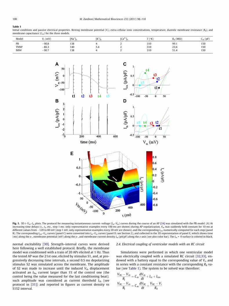
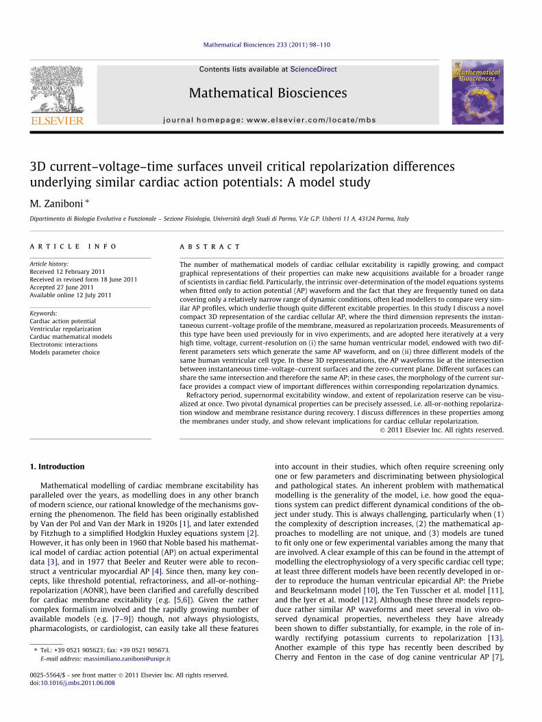
Table 1Initial conditions and passive electrical properties. Resting membrane potential (Vr), extra-cellular ionic concentrations, temperature, diastolic membrane resistance (Rd), andmembrane capacitance (Cm) for the three models.

Model Vr (mV) [Na+]o [K+]o [Ca2+]o T (�K) Rd (MX) Cm (pF)

PB �90.8 138 4 2 310 99.1 150TNNP �86.3 140 5.4 2 310 23.6 150IMW �90.7 138 4 2 310 51.4 150

Fig. 1. 3D t–Vm–Im plots. The protocol for measuring instantaneous current–voltage (Im–Vm) curves during the course of an AP [24] was simulated with the PB model. (A) Atincreasing time delays (t1, t2, etc., step 1 ms; only representative examples every 100 ms are shown) during AP repolarization, Vm was suddenly held constant for 10 ms atdifferent values from�120 to 80 mV (step 1 mV, only representative examples every 20 mV are shown), and the corresponding Iion numerically computed for each step (panelB). The corresponding Iion–Vm curves (panel C) were converted into Im–Vm curves (panel D, see Section 2), and collected in the 3D representation of panel E, which shows time(ms) along the x-, membrane potential (mV) along the y-, and membrane current density Im (pA/pF) along the z-axis (see also color bar). The Im = 0 surface is colored in black.

100 M. Zaniboni / Mathematical Biosciences 233 (2011) 98–110

normal excitability [30]. Strength–interval curves were derivedhere following a well established protocol. Briefly, the membranemodel was conditioned with a train of 20 APs elicited at 1 Hz. Thusthe tested AP was the 21st one, elicited by stimulus S1, and, at pro-gressively decreasing time intervals, a second 0.5 ms depolarizingstimulus S2 was simulated across the membrane. The amplitudeof S2 was made to increase until the induced Vm displacementactivated an INa current larger than 1% of the control one (thecontrol being the value measured for the last conditioning beat);such amplitude was considered as current threshold Ith (seeprotocol in [31]) and reported in figures as current density vsS1S2 interval.

2.4. Electrical coupling of ventricular models with an RC circuit

Simulations were performed in which one ventricular modelwas electrically coupled with a simulated RC circuit [32,33], en-dowed with a battery equal to the corresponding value of Vr, andin series with a constant resistance with the corresponding Rd va-lue (see Table 1). The system to be solved was therefore:

VRC � Vm

RJ¼ Cm

dVm

dtþ Ist þ Iion

VRC � Vm

RJ¼ Cm

dVRC

dtþ VRC � Vr

Rd

M. Zaniboni / Mathematical Biosciences 233 (2011) 98–110 101

with VRC the voltage drop across the RC circuit, Vm the membranepotential of the model cell, and Rj the gap junctional resistance be-tween the two.

Fig. 2. Membrane conductance during repolarization. (A) Colored contour plot ofFig. 1E is reported here, with z-axes normalized to 150 pF as current amplitude, andvertical dotted lines marking time = 150 ms (t1) and time = 350 ms (t2). The valuesof Vm occupied by the membrane at those times are marked with black and whitefilled circles respectively in all panels. Gray shaded area marks the time when APtrajectory proceeds on a negative (toward depolarization) sloping Im surface. (B)Vertical Im–Vm slices of the 3D surface, taken at t1 and t2, are reported on the left.The corresponding first derivative of Im with respect to Vm (slope conductance Gm)is reported on the right as a function of Vm.

3. Results

In this study I adopt three mathematical models of humanventricular AP. Since I show that one, at least, of the 3 is over-determined with respect to repolarization profile, i.e. the sameAP waveform can be obtained by introducing different sets ofparameters into the model equations [14], I consider indeed fourdifferent excitable membranes. My main goal is to show how tosynthetically characterize several differences in repolarizationproperties for different mathematical models of the same AP.In order to do this, I propose a compact representation of repolar-ization dynamics which adopts instantaneous current–voltage pro-files of the membrane, taken during the course of the AP. Withinthis representation, AP trajectory can be subdivided, for whatconcerns repolarization properties, in 3–4 different regions, whichcan be defined and usefully adopted to screen apparently similarmathematical models. I also measure and compare time courseof Rm in the four membranes and discuss the use of this parameter.

3.1. 3D time–voltage–current surfaces

The protocol adopted in order to obtain a 3D t–Vm–Im represen-tation of a cardiac excitable membrane is reported in Fig. 1 for thePB model (see Section 2 for initial conditions), and described in de-tail elsewhere for both in vivo and in silico conditions [24,14]. Thecollection of Im–Vm curves (panel D), derived from Iion–Vm curves(panel C) as described in Section 2, generates a 3D surface (panelE) where x is time, y is membrane potential and z is Im. For anon-propagated AP, the AP profile lies at the intersection betweensuch t–Vm–Im surface and the Im = 0 plane. AP trajectory, in thiscase, moves along a positive sloping (in Im–Vm planes) surface dur-ing early repolarization and most of the plateau phase (t1, t2, andt3 in panel D, green arrow in panel E), passes through a narrow re-gion where slope is negative during late repolarization (t4 in panelD, white arrow in panel E), and then again reaches diastole on a po-sitive sloping surface (t5 in panel D, red arrow in panel E). The con-tour plot of Fig. 2A shows the path of AP trajectory on theinstantaneous Im surface where the negative-sloping region isshaded in gray. I recall that a negative-sloping Im–Vm curve identi-fies, for an excitable membrane, a condition where any currentflowing across it tends to cause an auto-regenerative voltagedeflection [22,34,35,2], either in depolarizing direction, leading toan AP, or in repolarizing direction, leading to AONR. Panel B s howstwo very different Im–Vm time frames. Membrane current Im iszero, as expected, in both instances during repolarization; in t1(filled circle during plateau), Vm trajectory moves on a positivesloping quasi-linear Im–Vm curve (left panel), i.e. membrane is elec-trically stable, quasi-ohmic, and membrane conductance is quitehigh (right panel) and does not tend to change much when Vm

changes. On the contrary, in t2 (empty circle during late repolari-zation), Vm trajectory moves on a negative sloping highly non-lin-ear Im–Vm curve (left panel), membrane negative conductance isalmost zero (right panel) and increases dramatically and auto-regeneratively for any Vm deflection towards more polarizedpotentials: any polarization increases conductance to outward cur-rent which, in turn, promotes further polarization.

3.2. Over-determination of parameters for the PB model

HH type equations systems are known to be over-determined intheir solutions when only fitting repolarization trajectory, i.e. dif-

ferent parameters sets introduced in the same system can generatethe same AP waveform [14]. As an example of this phenomenon, Iuse in this study two identical AP waveforms simulated by meansof the Priebe and Beuckelmann human ventricular model [10]. Oneof the two waveforms is obtained from the model by adopting theparameters set reported in the original paper [10] (PB), the otherone, hereafter indicated as PB⁄, is obtained by choosing amaximum ICa conductance (gCamax) which is 30% lower than theoriginal, and adjusting other parameters by means of the minimi-zation procedure described in [14]. Of course, a trivial case of suchover-determination is when all parameters get modified by thesame factor, which is equivalent to a difference in cell size (mem-brane area). This, however, is not the case here, where the differention currents are very differently scaled (see Table 2).

3.3. Time-window for AONR

I applied the protocol described in Fig. 1 to both PB and PB⁄

membranes and obtained the 3D t–Vm–Im representations reportedin Fig. 3A and B. As my colleagues and I have shown in [14],solutions of HH type equations which are over-determined withrespect to AP trajectory correspond to different t–Vm–Im surfaceswhich intersect the Im = 0 plane (black surface in the 3D plots)along the same curve that coincides with the common APwaveform. This is particularly evident in panels C and D, where col-or-contour plots of the two surfaces are reported for a membranecurrent range from �0.3 pA/pF (dark blue) to +0.3 pA/pF (darkred), and where the three differently sloping Im–Vm time regions(from blue to red for positive sloping, vice versa for negative)described in Fig. 2 are now visible for PB and PB⁄ (panels C–F).Another negative sloping region can be seen on the depolarizationside of the outward Im ‘‘hill’’ which lies above the restingmembrane potential (Vr), starting from the end of the absoluterefractory period (vertical asymptote of strength-interval curvesin panels G and H). The Im = 0 level of such region above Vr

represents an instantaneous image of threshold for excitation in

Table 2Parameters set of the modified PB⁄ model. Percent changes in 12 parameters of the original PB model are reported in table. gK1, gNa, gCa, gTO, gKr, and gKs are maximumconductances of ion currents in their HH formulation; gbNa and gbCa are maximum conductances of linear background sodium and calcium currents, respectively (mS/lF), grel israte of spontaneous SR release (ms�1); Kleak is rate of calcium leak from the SR (ms�1), KNaCa and INaK are the current density scaling factors for INaCa and INaK, respectively (lA/lF).

gK1 gNa gCa gTO gKr gKs gbNa gbCa grel KNaCa Kleak INaK

0% 0% �30% �20% 0% �63% +3% 0% �34% �7% +24% 0%

Fig. 3. Comparison between PB and PB⁄. Three-dimensional t–Vm–Im plots like those described in Fig. 1 are shown in panels A and B for PB and PB⁄, respectively. A view fromthe top of these surfaces is also provided in the contour plots of panels C and D where the color scale for current density is the same as in 3D plots (see color bar). Black tracesmark �0.12, 0, and +0.12 pA/pF levels. Note that the zero-Im level is identical for the two surfaces, and coincides with corresponding AP waveforms, reported for comparisonin panels E and F. Panels G and H show strength–interval curves for PB and PB⁄ (see Sections 3 and 4). Shaded areas, spanning panels C through H, mark times where, duringAP trajectory, the Im–Vm slope of current surfaces becomes negative. Negative-sloping region goes from 340 to 405 ms for PB, and from 265 to 413 ms for PB⁄.

102 M. Zaniboni / Mathematical Biosciences 233 (2011) 98–110

the absence of any external current stimulus. The negative-slopingregions, colored in gray in Figs. 3 C–H, coincide with the time win-dows for AONR [35], i.e. the net positive Iion, flowing at this time, isauto-regenerative. Furthermore, the inspection of the Im-surfacesallows to appreciate that supernormal excitability [30], identifiedby strength-interval curves and delimited by vertical dotted lines,coincides with a region where zero-current contour level has adeflection towards more polarized potential and, simultaneously,INa already recovered from inactivation (blue contour above it).

3.4. Membrane resistance during repolarization

The 3D t–Vm–Im plots reported in Fig. 3 for PB and PB⁄ allow toeasily measure membrane resistance Rm during the course of theAP [14]. Briefly, the slope of the current surface is calculated athigh resolution along Im–Vm planes taken at different times ofthe AP (step 1 ms), for different clamped Vm values (step 0.1 mV),and around the Im = 0 pA/pF. Membrane specific conductance (pS/

pF) is then normalized to a common value of 150 pF for the Cm ofthis cell type (see Table 2 in [12]) and its reciprocal value, i.e. theelectrical resistance Rm in MX, reported in Fig. 4D for both APs.PB and PB⁄ waveforms are reported in figure (panel A) togetherwith simplified contour plots (like those in Fig. 3C and D) showingonly positivity and negativity of Im surface (panels B and C), wherethe duration of AONR regions can be easily determined (see verti-cal dotted lines, red for PB and blue for PB⁄).

As it appears, although both sets of parameters share the sameAP waveform and correspond to the same cell size, they are en-dowed with quite different time-varying Rm during AP trajectory,where PB⁄ resistance is higher that of PB for most of repolarization.In both cases of course membrane conductance becomes zero atthe border of the AONR region (about +50% longer in PB⁄ thanPB), where therefore membrane resistance tends to diverge. Onlythe non-diverging region of Rm is reported in Fig. 4D where itcan be seen also that, as it follows by definition, Rm is negativewithin the AONR region.

Fig. 4. Rmvalues of PB and PB⁄during AP repolarization. AP waveforms PB (red) andPB⁄ (blue) are reported in panel A. Simplified contour plots like those of Fig. 3C andD are reported in panels B and C for the two parameter sets, respectively; in green,regions where Im is positive (see Fig. 3A and B). Rm is calculated at each time duringAP repolarization (see Sections 3 and 4) as the reciprocal of the slope ofcorresponding Im–Vm plots, and reported in panel D for both waveforms. Verticalbroken lines and horizontal arrows delimit regions where membrane resistance/conductance is negative.

Fig. 5. Proneness to EAD formation. The same manoeuvre (reduction of GKr by 10%and 8 mV shift of ICaL activation curve towards negatively polarized potentials),operated on PB (red) and PB⁄ (blue) equations systems, leads to EAD formation inthe former, and only to APD prolongation in the latter. Dotted lines mark AONRwindow in both cases.

M. Zaniboni / Mathematical Biosciences 233 (2011) 98–110 103

3.5. Different propensity to EAD formation

As I have shown in a previous paper [14] on the Luo and Rudyphase 1 ventricular model [31], identical APs can present a quitedifferent propensity to EADs formation, when pharmacologicaldown-regulation is simulated on given repolarization currents.Similarly here, although PB and PB⁄ waveforms are identical incontrol conditions, when maximum conductance of IKr is reducedby 10% and the activation curve for ICaL shifted by 8 mV towardsnegatively polarized potentials, only PB develops an EAD, whereasPB⁄ only experiences a 25% increase in APD�80mV. Fig. 5 shows thetwo different responses. In the same figure the time window forAONR is reported for both waveforms in control conditions.

3.6. Different models of the same ventricular cell type

I have shown so far how different sets of parameters can gener-ate identical AP profiles when fed into the same mathematicalmodel, and also how differences in their repolarization propertiescan be highlighted in instantaneous t–Vm–Im surfaces. I providehere a further and perhaps more interesting case in which I studythree fairly similar ventricular epicardial AP waveforms generated

by three different mathematical models expressing different typesand densities of ion channels, different degree of complexity, andalso a different approach to the mathematical description of chan-nel kinetics: the already mentioned PB, TNNP, and IMW models[10–12]. Fig. 6 shows their waveforms (G–I) and the corresponding3D t–Vm–Im plots (A–C), together with the colored contour plots(D–F). Once again, despite the similarity between the three wave-forms, the differences between the current surfaces are quite strik-ing, particularly for what concerns the size of AONR window, theslope of current surface cutting the zero-current level, and the totalamount of current density displayed in the three cases.

As already seen in Fig. 3, during early repolarization and pla-teau, membrane potential is stable and Rm quasi-ohmic; the slopeof instantaneous t–Vm–Im curves becomes negative during AONRwindow (gray region), and then again positive during late repolar-ization and diastole, with a quasi-ohmic behaviour [29]. Verticaldotted lines mark the time windows for supernormal excitability,which is shown better in Fig. 7, where I report a more detailed viewof the last portion of the panels in Fig. 6D–F, which also include atime expanded view of strength-interval curves. Here we see again(panel A) the two conditions found during supernormal excitablewindow of PB in Fig. 3, i.e. (1) downward deflection of zero-currentcontour level (branches a and c) and (2) INa recovery from inactiva-tion (blue contour above it). Supernormal window is marked withred arrows. Condition (1) is not satisfied in the TNNP model, wherethe zero-current contour (‘d’) monotonically diverges towardsdepolarization and the outward barrier (saturated Im value > 2 -pA/pF) at the end of repolarization is much higher than that of fullyrecovered diastole. Both conditions are satisfied in IMW model atthe time indicated by the arrow in panel C. Accordingly, PB andIMW models show supernormal excitability, whereas TNNP doesnot, as can be seen in the strength–interval curves, also reportedin figure.

3.7. Membrane resistance in the three human ventricular models

As I have shown elsewhere for the Luo and Rudy phase 1 ven-tricular model [14] and earlier in this study for the PB model(Fig. 4), the 3D t–Vm–Im representations allow direct visualizationand calculation of Rm during repolarization, which I report for

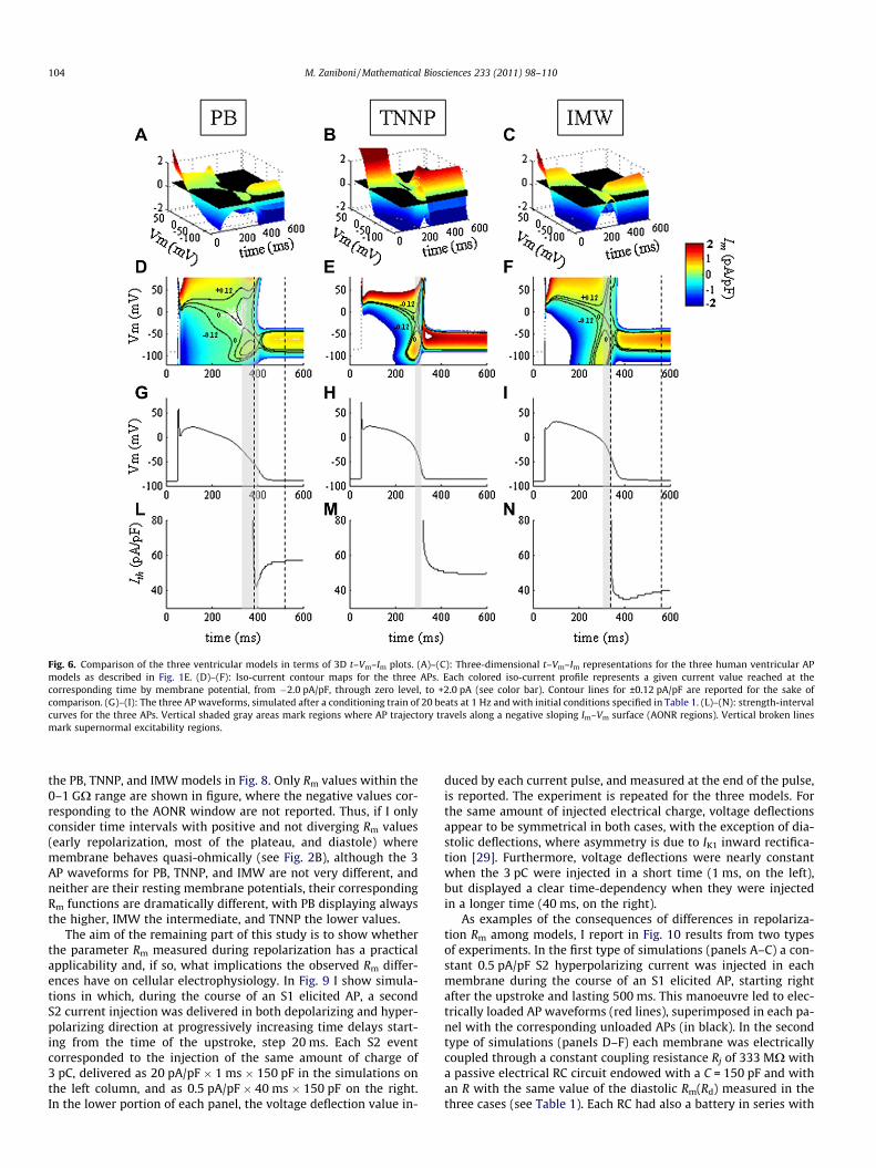
Fig. 6. Comparison of the three ventricular models in terms of 3D t–Vm–Im plots. (A)–(C): Three-dimensional t–Vm–Im representations for the three human ventricular APmodels as described in Fig. 1E. (D)–(F): Iso-current contour maps for the three APs. Each colored iso-current profile represents a given current value reached at thecorresponding time by membrane potential, from �2.0 pA/pF, through zero level, to +2.0 pA (see color bar). Contour lines for ±0.12 pA/pF are reported for the sake ofcomparison. (G)–(I): The three AP waveforms, simulated after a conditioning train of 20 beats at 1 Hz and with initial conditions specified in Table 1. (L)–(N): strength-intervalcurves for the three APs. Vertical shaded gray areas mark regions where AP trajectory travels along a negative sloping Im–Vm surface (AONR regions). Vertical broken linesmark supernormal excitability regions.

104 M. Zaniboni / Mathematical Biosciences 233 (2011) 98–110

the PB, TNNP, and IMW models in Fig. 8. Only Rm values within the0–1 GX range are shown in figure, where the negative values cor-responding to the AONR window are not reported. Thus, if I onlyconsider time intervals with positive and not diverging Rm values(early repolarization, most of the plateau, and diastole) wheremembrane behaves quasi-ohmically (see Fig. 2B), although the 3AP waveforms for PB, TNNP, and IMW are not very different, andneither are their resting membrane potentials, their correspondingRm functions are dramatically different, with PB displaying alwaysthe higher, IMW the intermediate, and TNNP the lower values.

The aim of the remaining part of this study is to show whetherthe parameter Rm measured during repolarization has a practicalapplicability and, if so, what implications the observed Rm differ-ences have on cellular electrophysiology. In Fig. 9 I show simula-tions in which, during the course of an S1 elicited AP, a secondS2 current injection was delivered in both depolarizing and hyper-polarizing direction at progressively increasing time delays start-ing from the time of the upstroke, step 20 ms. Each S2 eventcorresponded to the injection of the same amount of charge of3 pC, delivered as 20 pA/pF � 1 ms � 150 pF in the simulations onthe left column, and as 0.5 pA/pF � 40 ms � 150 pF on the right.In the lower portion of each panel, the voltage deflection value in-

duced by each current pulse, and measured at the end of the pulse,is reported. The experiment is repeated for the three models. Forthe same amount of injected electrical charge, voltage deflectionsappear to be symmetrical in both cases, with the exception of dia-stolic deflections, where asymmetry is due to IK1 inward rectifica-tion [29]. Furthermore, voltage deflections were nearly constantwhen the 3 pC were injected in a short time (1 ms, on the left),but displayed a clear time-dependency when they were injectedin a longer time (40 ms, on the right).

As examples of the consequences of differences in repolariza-tion Rm among models, I report in Fig. 10 results from two typesof experiments. In the first type of simulations (panels A–C) a con-stant 0.5 pA/pF S2 hyperpolarizing current was injected in eachmembrane during the course of an S1 elicited AP, starting rightafter the upstroke and lasting 500 ms. This manoeuvre led to elec-trically loaded AP waveforms (red lines), superimposed in each pa-nel with the corresponding unloaded APs (in black). In the secondtype of simulations (panels D–F) each membrane was electricallycoupled through a constant coupling resistance Rj of 333 MX witha passive electrical RC circuit endowed with a C = 150 pF and withan R with the same value of the diastolic Rm(Rd) measured in thethree cases (see Table 1). Each RC had also a battery in series with

Fig. 7. Supernormal excitability. The last temporal portions of contour plots reported in Fig. 6D–F are reported here for the three models. AP trajectory is marked with blackarrows which overlap with a portion of the zero-Im contour (black curves). Strength-interval curves, plotted with black dots, are superimposed to each panel (current scale onthe right). Red arrows on the AP trajectory mark regions where supernormal excitability occurs (see text for discussion).

M. Zaniboni / Mathematical Biosciences 233 (2011) 98–110 105

the resistance R, and with the same electromotive force of corre-sponding resting membrane (Vr values in Table 1). This type ofexperiments models what happens to an excitable cell when it iselectrically connected through gap junctions with a polarizedunexcitable cell, like in the case of ventricular-fibroblasts coupling[33]. APD shortenings induced by constant current injections andby electrical coupling with RCs are summarized in panels G andH, respectively, where it appears that PB membrane experiencedthe highest load on AP waveform in both instances, IMW the inter-mediate, and TNNP the lowest. Histogram in panel I shows, in thesame decreasing order, the percent change in resting membranepotential due to current injections of panels A–C. Rp representsRm values averaged, for each AP model, over the first 250 ms of pla-teau, and excluding therefore AONR region. Correlations between(i) Rp and APD shortening induced by current injection, (ii) Rp

and APD shortening induced by electrical coupling, and between(iii) Rd and electrical load of Vr during current injection are alsosummarized in panels L–N. It appears that the electrical load ofAPD and of Vr increases as Rp and Rd values do, respectively.

4. Discussion

The main focus of the present modelling study is to discuss anovel 3D representation of cardiac cellular AP repolarization which

contains and summarizes important dynamic properties of mem-brane electrophysiology. In doing so, I investigate the fact that verysimilar or even identical AP profiles can underlie quite different ionchannel properties, which, as I have shown recently [14], has rele-vant physiological and pathological implications. I illustrate this intwo different instances: when two nearly identical APs were gen-erated by the same mathematical model endowed with two differ-ent parameter sets, or when three different mathematical modelswere used in order to simulate the AP profile of the same cardiaccell type. Through the computational and graphical approach Iam presenting here, I show how to precisely define a time windowfor AONR, which can be usefully adopted to compare apparentlysimilar AP waveforms. I also show how the same approach allowsvisualization and calculation of Rm during AP repolarization. I final-ly demonstrate that this latter parameter, which has been observedsince early days of cardiac electrophysiology [25] but only margin-ally discussed before [14,24,26], and despite important concernsraised in very recent literature [28], is indeed appropriate forcharacterizing membrane electrotonic sensitivity during APrepolarization.

The 3D t–Vm–Im surfaces that I show give an instantaneous esti-mate of what current will flow on the membrane when this wouldbe made to deviate, either in depolarizing or polarizing direction,from AP Vm trajectory. It is an instantaneous estimate becauseany net current flowing across the membrane during the AP will

Fig. 8. Membrane resistance during repolarization. Rm during the AP waveforms ofthe three human ventricular models (top panel) is derived as explained in Resultsand reported in the lower panel. Only the 0–1 GX range is shown in order to betterappreciate differences. Negative resistance values are not shown.

106 M. Zaniboni / Mathematical Biosciences 233 (2011) 98–110

cause Vm(t) to deviate from the original trajectory, will changetherefore ion channels conductance, and finally modify the Im sur-face accordingly. Nevertheless, I demonstrate that this ‘current-surface-landscape’, seen by Vm during AP repolarization, providesmuch information on its dynamic properties.

4.1. Two parameter sets, one AP waveform

I adopt this graphical approach at first in the context of a knownproblem of differential equation systems used to model membraneexcitability, i.e. the over-determination of parameters with respectto one (or more) of the models solutions, which, in this case, is theAP waveform. By means of a previously published least squaresminimization method [14], which I apply here on the PB modelof human ventricular AP, I derive in fact two different sets ofparameters which give rise to the same AP waveform (Fig. 4Aand Table 2). An extensive numerical study on multivariable leastsquares regression has been recently published by Sobie and Sarkar[20,21] in order to highlight differences between models thatotherwise appear similar in one or more of their outputs.

I also note in passing that the procedure I described in [14] andapply here is very relevant with respect to AP scaling problems in-volved in the evolution of cardiac cellular electrophysiology, whichhave been elegantly described by Rosati et al. in a recent paper[36].

Despite the identical AP profiles reported in Fig. 4A, the 2 wave-forms show remarkable differences in the AONR window, which islonger and anticipated in PB⁄ respect to PB (see also Fig. 4B and C).Absolute refractory period and supernormal excitable region areonly slightly prolonged and shifted in PB⁄ (Fig. 3), whereas mem-brane resistance Rm, as considered in its positive values, was al-ways higher in PB⁄ than that in PB (Fig. 4D). I focus the first partof my discussion on defining, by means of 3D Im surfaces, the tem-poral region when AP repolarization becomes ‘all-or-nothing’, i.e.membrane conductance (resistance) is negative [34] and repolari-zation is auto-regenerative. At this time, Vm trajectory sits at the

Im = 0 level of negative-sloping Im–Vm curves, which means thatmembrane is at unstable equilibrium (no tendency to spontane-ously oscillate), and it is excitable [35,37], both to depolarizingand hyperpolarizing stimulations: any hyperpolarization leads toincreasing outward component of Im which, in turn, feeds back insustaining further hyperpolarization; same for depolarization[37]. This region is clearly shown in 3D plots of Fig. 3 (A and B)as a positive Im ‘hill’ (top of the hill is red, i.e. P1 A/pF) emergingfrom the black Im = 0 plane at the end of repolarization or, in thecontour plots (C and D), when AP trajectory travels on the top bor-der of the closed Im = 0 contour line centred at around 380 ms. Inthis region, the slope of the Im surface along the Im–Vm planeschanges sign and becomes negative, and membrane behaves as apolarizing current source: the beginning and the end of AONR win-dow are exactly defined by the time when the slope of Im–Vm

curves change sign. Other authors have recently provided a mea-sure of AONR window which, on the contrary, was based on thearbitrary choice of a threshold value for the outward repolarizingcurves [13].

The existence of regenerative repolarization and of AONR hasbeen reported already by Hoffman and Cranefield to be veryimportant for cardiac electrophysiology, since it implies the possi-bility of a propagated repolarization [38]. AONR and its conse-quences have than been extensively studied over the years[35,39–42]. The fact that threshold for AONR approaches AP trajec-tory as plateau phase proceeds, and moves into late repolarizationhas been noted in 1951 by Weidmann, who found that the applica-tion during late plateau of brief anodal pulses exceeding a givenamplitude could prevent membrane potential from resuming itstrajectory after the break of the pulse, and instead lead it to staynear its resting level; membrane at this time becomes a sourceand, as initial AP depolarization does, also AONR propagates witha time–dependent length constant (and therefore with a time-dependent velocity) [25–27]. Further observations on the same is-sue came in 1960 from Fitzhugh’s work on a modified (cardiac-like) HH equations system [2], and in 1969 from a study of Nobleand Tsien on cardiac Purkinje fibers [34]. In none of those cases,though, AP repolarization itself is documented to be auto-regener-ative, as I show here.

The shape of the 3D t–Vm–Im surfaces around this region makesindeed a lot of difference. The balance, for instance, between out-ward and inward repolarizing currents is identical in PB and PB⁄

over the entire AP and in particular during late repolarization,though the broader and higher outward current ‘hill’ in PB⁄ (Figs.3A and B and 4B and C) unmasks a larger repolarization reserve[13,43,44], which makes repolarization safer in PB⁄ than that inPB. A consequence of this is shown in the experiment of Fig. 5,where in fact the same manoeuvre on the same repolarizing cur-rents (10% partial block of IKr, 8 mV shift of ICa activation towardsnegative potentials), triggers an EAD in PB, whereas PB⁄ safelyrepolarizes.

4.2. Three different models of the same human ventricular AP type

When the three models of the human epicardial ventricular APare compared through their t–Vm–Im surfaces, despite the similar-ity between their waveforms (see Figs. 6G–I and 8A) and the factthat they are all designed to specifically simulate the same celltype, they show quite different electrophysiological properties,particularly: (1) AONR window, (2) refractory period, (3) supernor-mal excitability, (4) Rm during repolarization and correspondingproneness to be electrically loaded by external currents. Differ-ences between TNNP and IMW models, particularly concerningthe role of inwardly rectifying potassium currents in membranerepolarization, have been recently discussed [13]. Through the

Fig. 9. Current–induced voltage deflections during AP repolarization. Progressively delayed (step 20 ms) depolarizing and hyperpolarizing injections of the same electricalcharge (3 pC) were performed during the course of AP repolarization by means of two different parameter settings: ± 20 pA/pF � 1 ms in simulations reported on the leftcolumn, and ± 0.5 pA/pF � 40 ms in simulations reported on the right column. Each panel shows, on the top and for the sake of clarity, only one out of four superimposedvoltage deflections for each AP and, on the bottom, all the corresponding voltage deflection values as measured at the end of each pulse, and taken as difference respect to theVm value occupied by the membrane at that time in the un-injected AP.

M. Zaniboni / Mathematical Biosciences 233 (2011) 98–110 107

Physiome Project, actually, Fink and co-authors are carrying out abroader investigation on the relationship between the huge collec-tion of experimental data on cardiac cellular electrophysiology, iondynamics, mechanics, metabolism, and their parameterization intoa unique integrative computational framework [8]. The compari-son among the growing number of cardiac cellular models is in factraising in recent days the attention of cardiac scientific community

[45,46], and the graphical 3D representation I am discussing herecan represent a useful tool in this sense.

For example, it appears clear from Fig. 6 that, during plateauphase, membrane moves on positive-sloping, and nearly flat, Im–Vm curves (like in Fig. 2B), i.e. it is stable; any voltage displacementtends to be damped by the elicited ion current. On the contrary, atthe end of plateau the slope of Im–Vm curves becomes transiently

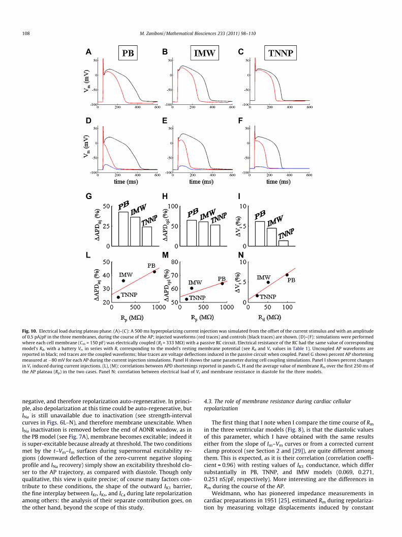
Fig. 10. Electrical load during plateau phase. (A)–(C): A 500 ms hyperpolarizing current injection was simulated from the offset of the current stimulus and with an amplitudeof 0.5 pA/pF in the three membranes, during the course of the AP; injected waveforms (red traces) and controls (black traces) are shown. (D)–(F): simulations were performedwhere each cell membrane (Cm = 150 pF) was electrically coupled (Rj = 333 MX) with a passive RC circuit. Electrical resistance of the RC had the same value of correspondingmodel’s Rd, with a battery Vr, in series with R, corresponding to the model’s resting membrane potential (see Rd and Vr values in Table 1). Uncoupled AP waveforms arereported in black; red traces are the coupled waveforms; blue traces are voltage deflections induced in the passive circuit when coupled. Panel G shows percent AP shorteningmeasured at �80 mV for each AP during the current injection simulations. Panel H shows the same parameter during cell coupling simulations. Panel I shows percent changesin Vr induced during current injections. (L), (M): correlations between APD shortenings reported in panels G, H and the average value of membrane Rm over the first 250 ms ofthe AP plateau (Rp) in the two cases. Panel N: correlation between electrical load of Vr and membrane resistance in diastole for the three models.

108 M. Zaniboni / Mathematical Biosciences 233 (2011) 98–110

negative, and therefore repolarization auto-regenerative. In princi-ple, also depolarization at this time could be auto-regenerative, butINa is still unavailable due to inactivation (see strength-intervalcurves in Figs. 6L–N), and therefore membrane unexcitable. WhenINa inactivation is removed before the end of AONR window, as inthe PB model (see Fig. 7A), membrane becomes excitable; indeed itis super-excitable because already at threshold. The two conditionsmet by the t–Vm–Im surfaces during supernormal excitability re-gions (downward deflection of the zero-current negative slopingprofile and INa recovery) simply show an excitability threshold clo-ser to the AP trajectory, as compared with diastole. Though onlyqualitative, this view is quite precise; of course many factors con-tribute to these conditions, the shape of the outward IK1 barrier,the fine interplay between IKr, IKs, and ICa during late repolarizationamong others: the analysis of their separate contribution goes, onthe other hand, beyond the scope of this study.

4.3. The role of membrane resistance during cardiac cellularrepolarization

The first thing that I note when I compare the time course of Rm

in the three ventricular models (Fig. 8), is that the diastolic valuesof this parameter, which I have obtained with the same resultseither from the slope of Im–Vm curves or from a corrected currentclamp protocol (see Section 2 and [29]), are quite different amongthem. This is expected, as it is their correlation (correlation coeffi-cient = 0.96) with resting values of IK1 conductance, which differsubstantially in PB, TNNP, and IMW models (0.069, 0.271,0.251 nS/pF, respectively). More interesting are the differences inRm during the course of the AP.

Weidmann, who has pioneered impedance measurements incardiac preparations in 1951 [25], estimated Rm during repolariza-tion by measuring voltage displacements induced by constant

M. Zaniboni / Mathematical Biosciences 233 (2011) 98–110 109

current injections. The attempt he made to provide a time course ofRm during cardiac AP [47] was not followed by further studies untilthe work of Goldmann and Morad [23] and that of my colleaguesand I in year 2000 [24].

A strong criticism has recently been raised by Zaza [28], who ar-gued that AP contour is uniquely determined by Iion and indepen-dent of Rm. I am showing here that, on the basis of the presentdiscussion, the opposite is true: not only Iion does not uniquelydetermine AP, several different (in their properties) APs can in factbe generated by exactly the same Iion (see Fig. 4 and [14]), but it isRm (the reciprocal of the slope, at every time, of the Im–Vm surface)which determines AP with its dynamical properties.

I note however that the very concept of Rm, as we relate it toOhm’s law (i.e. to the slope of Im–Vm curves), is straightforwardonly during diastole, early repolarization, and during most of theplateau phase, where Im–Vm curves are nearly linear around thepotential value occupied by the membrane (t1, t2 and t5 curves inFig. 1C and D; t1 curve in Fig. 2B; see also [29]). On the contrary,during AONR window, Im–Vm curves are highly non-linear aroundVm trajectory, and they are flattened on the zero current level, i.e.Rm is very high. It has been proposed by myself and others[8,24,48,49] that it is the increased Rm during the late repolariza-tion that makes it more electrically sensitive, during that phase,to even very small currents. This, however, only partially explainsthe results of Figs. 9 and 10; a further basic rule should be consid-ered. The final voltage displacement induced by injecting a fixedamount of charge across an RC circuit will be more sensitive to Rchanges if we measure it during longer injections, allowing C todischarge or, which is equivalent, for times much longer than thetime constant. On the other hand, the higher the resistance of anRC circuit, the longer is its time constant (s), and therefore the lessit will be possible to discriminate changes in R on the basis of volt-age displacements taken at times smaller than s itself. A mem-brane resistance of 500 MX combined with a C of 150 pF leads toa s of 75 ms and will cause a DVm of 15.5 mV when injected with75 pA for 40 ms. By doubling R to 1 GX, DVm will only further in-crease by 2.0 mV. If, instead, we consider an R of 10 MX (sameC), than s will be 1.5 ms, which means that, during 40 ms currentinjections, Vm reaches plateau, i.e. changes in DVm will linearly cor-relate with changes in R (DVm would go from 0.75 to 1.5 mV). Pro-vided we bear in mind this simple limitation, the parameter Rm

holds indeed a practical meaning, as it appears also in the experi-ments of Fig. 10, where APD changes induced both by constant cur-rent injections and by electrical coupling to an unexcitable cell, areshown to correlate with the average value of Rm measured duringthe plateau phase. It is PB, with its overall high Rm, that makes cor-relation poorer (panels L and M). Correlation is very good when Rvalues are all smaller than 200 MX (s < 30 ms), like in diastole(see panel N). For the same reason, voltage deflections during repo-larization (see Fig. 9) change dramatically (paralleling changes inRm) for the TNNP model, which has an Rp always lower than200 MX (Fig. 8B), somewhat less for IMW which has an Rp around200 MX, and at the lower extent for PB model where Rp goes ashigh as 1 GX.

In summary, the 3D graphical representation of cardiac cellularAP which I discuss in the present study, provides an easily imple-mentable tool which can be used to compare at once severaldynamical properties (i) of different mathematical models or (ii)of over-determined (in their parameters) AP solutions of the samemodel, within large simulation environments which are being con-structed in very recent times [45,8]. I provide instances, in partic-ular the measure of AONR window, where this approach is easierand more precise than those usually adopted. Also, 3D t–Vm–Im

surfaces allow precise visualization and calculation of membraneRmwhich, despite its pivotal role in the modulation and propaga-tion of repolarization, is still scarcely covered by cardiac electro-

physiology literature, and poorly understood in its physio-pathological implications.

5. Limitations of the study

This study has been carried out only on mathematical models ofsingle cells (zero-dimensional) and of cell pairs. A further study onthe use of t–Vm–Im representations in 1D or 2D simulations couldhave been done by considering that, apart from the case of thenon-propagated AP, electrotonic current should also be taken intoaccount in order for the AP trajectory to hold the property of lyingon the zero-current plane. Such an extension, which would havebeen particularly interesting for what concerns time-dependencyof length constant for propagation of repolarization [25,27], couldnot possibly fit into the present paper. Also, although I have ex-plored several important differences between identical AP solu-tions of the same mathematical models or between differentmodels of the same cell type, many others were not considered,in particular electrical restitution and rate-dependency which, onthe other hand, I have recently described in detail in a more simpli-fied model [14]. Finally, 3D t–Vm–Im plots in their printed versionmight be harder to read than 2D contour plots or Im–Vm slices ta-ken at fixed times; any graphical environment, though, would eas-ily handle such surfaces, which retain the advantage of makingavailable, at a glance, several key dynamical properties of cardiacmembrane repolarization.

Acknowledgements

This study was supported by local funding (FIL 2008 and FIL2009) from the University of Parma.

References

[1] B. Van der Pol, J. Van der Mark, The heartbeat considered as a relaxationoscillation, and an electrical model of the heart, Philos. Mag. (Suppl. 6) (1928)763.

[2] R. Fitzhugh, Thresholds and plateaus in the Hodgkin–Huxley nerve equations,J. Gen. Physiol. 43 (1960) 867.

[3] D. Noble, Cardiac action and pacemaker potentials based on the Hodgkin–Huxley equations, Nature 188 (1960) 495.

[4] G.W. Beeler, H. Reuter, Reconstruction of the action potential of ventricularmyocardial fibres, J. Physiol. 268 (1977) 177.

[5] S. Weidmann, Cardiac action potentials, membrane currents, and somepersonal reminiscences, Annu. Rev. Physiol. 55 (1993) 1.

[6] D. Noble, The surprising heart: a review of recent progress in cardiacelectrophysiology, J. Physiol. 353 (1984) 1.

[7] E.M. Cherry, F.H. Fenton, A tale of two dogs: analyzing two models of canineventricular electrophysiology, Am. J. Physiol. Heart Circ. Physiol. 292 (2007)H43.

[8] M. Fink, S.A. Niederer, E.M. Cherry, F.H. Fenton, J.T. Koivumäki, G. Seemann, T.Rüdiger, H. Zhang, F.B. Sachse, D. Beard, E.J. Crampin, N.P. Smith, Cardiac cellmodelling: observations from heart of the cardiac physiome project, Prog.Biophys. Mol. Biol. 104 (2011) 2.

[9] R.H. Clayton, O. Bernus, E.M. Cherry, H. Dierckx, F.H. Fenton, L. Mirabella, A.V.Panfilov, F.B. Sachse, G. Seemann, H. Zhang, Models of cardiac tissueelectrophysiology: progress, challenges and open questions, Prog. Biophys.Mol. Biol. 104 (2011) 22.

[10] L. Priebe, D.J. Beuckelmann, Simulation study of cellular electric properties inheart failure, Circ. Res. 82 (1998) 1206.

[11] K.H. Ten Tusscher, D. Noble, P.J. Noble, A.V. Panfilov, A model for humanventricular tissue, Am. J. Physiol. Heart Circ. Physiol. 286 (2004) H1573.

[12] V. Iyer, R. Mazhari, R.L. Winslow, A computational model of the human left-ventricular epicardial myocyte, Biophys. J. 87 (2004) 1507.

[13] M. Fink, W.R. Giles, D. Noble, Contributions of inwardly rectifying K+ currentsto repolarization assessed using mathematical models of human ventricularmyocytes, Philos. Trans. A Math. Phys. Eng. Sci. 364 (2006) 1207.

[14] M. Zaniboni, I. Riva, F. Cacciani, M. Groppi, How different two almost identicalaction potentials can be: a model study on cardiac repolarization, Math. Biosci.228 (2010) 56.

[15] S. Dokos, N.H. Lovell, Parameter estimation in cardiac ionic models, Prog.Biophys. Mol. Biol. 85 (2004) 407.

[16] S. Audoly, G. Bellu, L. D’Angiò, M.P. Saccomani, C. Cobelli, Global identifiabilityof nonlinear models of biological systems, IEEE Trans. Biomed. Eng. 48 (2001)55.

110 M. Zaniboni / Mathematical Biosciences 233 (2011) 98–110

[17] A.R. Willms, D.J. Baro, R.M. Harris-Warrick, J. Guckenheimer, An improvedparameter estimation method for Hodgkin–Huxley models, J. Comput.Neurosci. 6 (1999) 145.

[18] M.C. Vanier, J.M. Bower, A comparative survey of automated parameter-searchmethods for compartmental neural models, J. Comput. Neurosci. 7 (1999)149.

[19] Z. Syed, E. Vigmond, S. Nattel, L.J. Leon, Atrial cell action potentialparameter fitting using genetic algorithms, Med. Biol. Eng. Comput. 43(2005) 561.

[20] E.A. Sobie, Parameter sensitivity analysis in electrophysiological models usingmultivariable regression, Biophys. J. 96 (2009) 1264.

[21] A.X. Sarkar, E.A. Sobie, Regression analysis for constraining free parameters inelectrophysiological models of cardiac cells, PLoS Comput. Biol. 6 (2010)e1000914.

[22] J.J. Jack, D. Noble, R.W. Tsien, Nonlinear properties of excitable membranes, in:Electrical Current Flow in Excitable Cells, Oxford Science Publications,Clarendon Press, 1975, 250p.

[23] Y. Goldman, M. Morad, Ionic membrane conductance during the time course ofthe cardiac action potential, J. Physiol. 268 (1977) 655.

[24] M. Zaniboni, A.E. Pollard, L. Yang, K.W. Spitzer, Beat-to-beat repolarizationvariability in ventricular myocytes and its suppression by electrical coupling,Am. J. Physiol. Heart Circ. Physiol. 278 (2000) H677.

[25] S. Weidmann, Effect of current flow on the membrane potential of cardiacmuscle, J. Physiol. 115 (1951) 227.

[26] K.J. Sampson, C.S. Henriquez, Electrotonic influences on action potentialduration dispersion in small hearts: a simulation study, Am. J. Physiol. HeartCirc. Physiol. 289 (2005) H350.

[27] J. Wu, D.P. Zipes, Effects of spatial segmentation in the continuous model ofexcitation propagation in cardiac muscle, J. Cardiovasc. Electrophysiol. 10(1999) 965.

[28] A. Zaza, Control of the cardiac action potential: the role of repolarizationdynamics, J. Mol. Cell Cardiol. 48 (2010) 106.

[29] M. Zaniboni, F. Cacciani, M. Groppi, Effect of input resistance voltage-dependency on DC estimate of membrane capacitance in cardiac myocytes,Biophys. J. 89 (2005) 2170.

[30] J.F. Spear, E.N. Moore, Supernormal excitability and conduction in the His-Purkinje system of the dog, Circ. Res. 35 (1974) 782.

[31] C.H. Luo, Y. Rudy, A model of the ventricular cardiac action potential.Depolarization, repolarization, and their interaction, Circ. Res. 68 (1991) 1501.

[32] R. Wilders, R. Kumar, R.W. Joyner, H.J. Jongsma, E.E. Verheijck, D. Golod, A.C.G.Van Ginneken, W.N. Goolsby, Action potential conduction between aventricular cell model and an isolated ventricular cell, Biophys. J. 70 (1996)281.

[33] K.W. Spitzer, N. Sato, H. Tanaka, L. Firek, M. Zaniboni, W.R. Giles, Electrotonicmodulation of electrical activity in rabbit atrioventricular node myocytes, Am.J. Physiol. 273 (1997) H767.

[34] D. Noble, R.W. Tsien, Reconstruction of the repolarization process in cardiacPurkinje fibres based on voltage clamp measurements of membrane current, J.Physiol. 200 (1969) 233.

[35] D. Noble, A.E. Hall, The conditions for initiating all-or-nothing’’ repolarizationin cardiac muscle, Biophys. J. 3 (1963) 261.

[36] B. Rosati, M. Dong, L. Cheng, S.R. Liou, Q. Yan, J.Y. Park, E. Shiang, M.Sanguinetti, H.S. Wang, D. McKinnon, Evolution of ventricular myocyteelectrophysiology, Physiol. Genomics 35 (2008) 262.

[37] J.W. Woodbury, Cellular electrophysiology of the heart, in: Handbook ofPhysiology, Section 2, Circulation, vol. 1, 1962, 237p.

[38] B.F. Hoffman, P.F. Cranefield, Electrophysiology of the Heart, McGraw-HillBook Company, 1960. pp. 227–228.

[39] Y. Goldman, M. Morad, Regenerative repolarization of the frog ventricularaction potential: a time and voltage-dependent phenomenon, J. Physiol. 268(1977) 575.

[40] C. Larson, L. Dragnev, N. Trayanova, Analysis of electrically induced reentrantcircuits in a sheet of myocardium, Ann. Biomed. Eng. 31 (2003) 768.

[41] N. Sperelakis, L. Ramasamy, B. Kalloor, Propagated repolarization of simulatedaction potentials in cardiac muscle and smooth muscle, Theor. Biol. Med.Model 14 (2005) 2.

[42] M. Dong, P.J. Niklewski, H.S. Wang, Ionic mechanisms of cellular electrical andmechanical abnormalities in Brugada syndrome, Am. J. Physiol. Heart Circ.Physiol. 300 (2011) H279.

[43] Y. Wu, M.E. Anderson, Reduced repolarization reserve in ventricular myocytesfrom female mice, Cardiovasc. Res. 53 (2002) 763.

[44] O. Hauswirth, D. Noble, R.W. Tsien, The mechanism of oscillatory activity atlow membrane potentials in cardiac Purkinje fibres, J. Physiol. 200 (1969) 255.

[45] R.L. Winslow, S. Cortassa, B. O’Rourke, Y.L. Hashambhoy, J.J. Rice, J.L.Greenstein, Integrative modeling of the cardiac ventricular myocyte, WileyInterdiscip. Rev. Syst. Biol. Med. 3 (2011) 392.

[46] S.A. Niederer, M. Fink, D. Noble, N.P. Smith, A meta-analysis of cardiacelectrophysiology computational models, Exp. Physiol. 94 (2009) 486.

[47] S. Weidmann, Resting and action potentials of cardiac muscle, Ann. NY Acad.Sci. 65 (1957) 663.

[48] M. Zaniboni, F. Cacciani, N. Salvarani, Temporal variability of repolarization inrat ventricular myocytes paced with time-varying frequencies, Exp. Physiol. 92(2007) 859.

[49] K.W. Spitzer, A.E. Pollard, L. Yang, M. Zaniboni, J.M. Cordeiro, D.J. Huelsing,Cell-to-cell electrical interactions during early and late repolarization, J.Cardiovasc. Electrophysiol. 17 (Suppl 1) (2006) S8.