Wrona, T., Pan, I., Bell, R. E., Gawthorpe, R. L., Fossen, H., Brune, S. (2021): 3D seismic interpretation with deep learning: A brief introduction. - The Leading Edge, 40, 7, 524-532.

https://doi.org/10.1190/tle40070524.1

Institional Repository GFZpublic: https://gfzpublic.gfz-potsdam.de/

3-D seismic interpretation with deep learning: a briefintroductionThilo Wrona1,2*, Indranil Pan3,4, Rebecca E. Bell5, Robert L. Gawthorpe1, Haakon Fossen6

and Sascha Brune2,7

1Department of Earth Science, University of Bergen, Allégaten 41, N-5007 Bergen, Norway.2GFZ German Research Centre for Geosciences, Telegrafenberg, 14473 Potsdam, Germany.3Centre for Process Systems Engineering & Centre for Environmental Policy, Imperial College London, UK.4The Alan Turing Institute, British Library, London, UK.5Department of Earth Science and Engineering, Imperial College, Prince Consort Road, London, SW7 2BP, UK.6Museum of Natural History, University of Bergen, Allégaten 41, N-5007 Bergen, Norway.7Institute of Geosciences, University of Potsdam, Potsdam-Golm, Germany.

*wrona@gfz-potsdam.de

ABSTRACT

Understanding the internal structure of our planet is a fundamental goal of the Earth Sciences. As direct

observations are restricted to surface outcrops and borehole cores, we rely on geophysical data to study

the Earth’s interior. Especially, seismic reflection data showing acoustic images of the subsurface, provide

us with critical insights into sedimentary, tectonic and magmatic systems. The interpretation of these

large, 2-D grids or 3-D seismic volumes is however time-consuming even for a well-trained person or

team of people. Here, we demonstrate how to automate and accelerate the analysis of these increasingly

large seismic datasets with machine learning. We are able to perform typical seismic interpretation tasks,

such as the mapping of (1) tectonic faults, (2) salt bodies and (3) sedimentary horizons at high accuracy

using deep convolutional neural networks. We share our workflows and scripts, encouraging users to

apply our methods to similar problems. Our methodology is generic and flexible allowing an easy

adaptation without major changes. Once trained, these models can analyze large volumes of data within

seconds; opening a new exciting pathway to study the internal structure and processes shaping our planet.

2

1. INTRODUCTION

Deep learning is transforming the way we analyze large datasets in many scientific disciplines including

medicine (e.g. Esteva et al., 2017), chemistry (e.g. Butler et al., 2018), and physics (e.g. Carleo & Troyer,

2017). In Earth Science, we use large volumes of geophysical data to learn about the internal structure of

our planet. Seismic reflection data showing acoustic images of the subsurface are particularly important to

our understanding of sedimentary, tectonic and magmatic systems. The emergence of 3-D seismic

technology allows us to image geological structures in the subsurface over thousands of square kilometers

at a resolution of a few tens of meters (Cartwright & Huuse, 2005). While this technology provides

fascinating insights into the Earth’s interior, it does require increasing amounts of time, experience and

expertise to analyze these large datasets (e.g. Bond et al., 2012).

In recent years, machine learning has thus been applied to numerous problems in seismic

interpretation, such as: (1) salt detection (e.g., Guillen et al., 2015; Waldeland et al., 2018; Zhou et al,

2020) , (2) fault detection (e.g., Zhang et al., 2014; Araya-Polo et al., 2017; Wu and Fomel, 2018; Wu et

al., 2019; Mosser et al., 2020; Feng et al., 2021) , (3) horizon mapping (e.g., Peters et al., 2019;

Gramstad et al., 2020; Tschannen et al., 2020), and (4) seismic facies classification (e.g., Qian et al.,

2018; Wrona et al., 2018; Li et al., 2019; Liu et al., 2019; Zhao, 2019) . Most of these studies are built on

recent advances in machine learning of multi-layered neural networks (i.e. deep learning). Deep learning

describes a set of machine learning models that allow us to extract data representations (e.g. features,

patterns) from raw data (LeCun et al., 2015) . This allows us to learn where a particular geological feature

is in the data without requiring engineering of a specific set of features (seismic attributes). In addition,

we can use neural networks for unsupervised learning, where we do not pre-define the geological

structures, which we would like to detect (Coléou et al., 2003; de Matos et al., 2007) .

3

With a few exceptions (e.g. Waldeland et al., 2018, Wu et al., 2019), many studies exploring deep

learning in seismic interpretation do not publish their data, code or workflow. Given the complexity and

sensitivity of these models, this makes it extremely difficult to replicate, compare and evaluate different

approaches. Moreover, deep learning models are hardly used in practice, where seismic interpretations are

almost exclusively performed by experts. Here, we explain: (1) how these techniques work; (2) how to

apply them to your geophysical dataset; (3) which challenges can occur; and (4) which remedies are

available. Deep learning describes a set of machine learning models that allow us to extract data

representations (e.g. features, patterns) from the raw data (LeCun et al., 2015). Here, we train these

models to perform typical seismic interpretation tasks, such as: (1) mapping faults, (2) extracting

geobodies, and (3) tracing stratigraphic horizons in 3-D seismic reflection data. Our workflow, code and

tutorials are available at: https://github.com/thilowrona/seismic_deep_learning. Deep learning can

accelerate the analysis of geophysical datasets significantly, allowing us to study the structure and internal

processes of the Earth in great detail.

2. 3-D SEISMIC REFLECTION DATA

In this study, we exemplify our technique using 3-D seismic reflection data from the northern North

Sea, where continental crust experienced (at least) two episodes of extension in the late Permian–Early

Triassic and Middle Jurassic–Early Cretaceous (e.g., Bell et al., 2014). This led to the formation of the

northern North Sea rift; a complex system consisting of hundreds to thousands of normal faults, which we

can image using a newly-acquired volume of 3-D seismic reflection data. The dataset covers an area

35,410 km2, imaging the crust down to 20 km depth. This seismic cube was acquired with a G-Gun array

consisting of 3 subarrays with a source array depth of 6-9 m; a source length of 16-18 m; an SP interval of

18.75 m; source separation of 37.5 m; a volume of 4550 in3 and an air pressure of 2000 psi. The streamer

4

consisted of 12 up to 8 km long cables with 636 channels each; a cable separation of 75 m and group

spacing of 12.5 m; depths of 7-50 m covering offsets of 150-8100 m. The data was recorded with a 2 ms

sample interval; 9000 ms recording length; a low cut filter (2Hz-6db/oct) and high cut (200 Hz-370

db/oct) filter. The broadseis technology, used for recording, covers a wide range of frequencies (2.5-155

Hz) providing high resolution depth imaging. The data was binned at 12.5 × 18.75 m with a vertical

sample rate of 4 ms. The seismic data was processed in 90 steps including: divergence compensation; low

cut filter (1.5 Hz, 2.5 Hz); noise attenuation (e.g. swell, direct wave); spatial anti-aliasing filter (12.5 m

group interval); direct wave attenuation; source de-signature; de-spike; time-variant high cut filter;

receiver motion correction and de-ghosting; FK filter; cold water and tidal statics; multiple modelling

with adaptive subtraction; Tau-P mute; Radon de-multiple; far angle destriping; multiple attenuation;

binning (75 m interval, 107 offset planes); acquisition hole infill; 5-D regularization; 3-D true amplitude

pre-stack depth migration; residual move-out correction; Linear FL Radon; full offset stack with

time-variant inner and out mute; acquisition footprint removal; crossline K filter; residual de-striping and

dynamic Q-compensation. The seismic volume was zero-phase processed with SEG normal polarity; i.e.,

a positive reflection (white) corresponds to an acoustic impedance (density × velocity) increase with

depth.

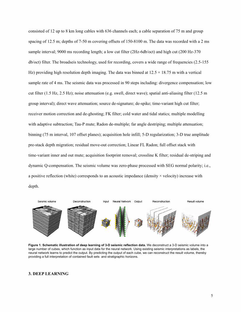
Figure 1. Schematic illustration of deep learning of 3-D seismic reflection data. We deconstruct a 3-D seismic volume into alarge number of cubes, which function as input data for the neural network. Using existing seismic interpretations as labels, theneural network learns to predict the output. By predicting the output of each cube, we can reconstruct the result volume, therebyproviding a full interpretation of contained fault sets and stratigraphic horizons.

3. DEEP LEARNING

5

Machine learning describes a set of algorithms and models, which learn to perform a specific task

on a given data set. While classic machine learning relies on features engineered for a specific task (e.g.

edges for fault detection), deep learning models derive features implicitly as part of the training. To learn

these features, deep neural networks typically require a large number of examples, either labelled for

supervised learning or unlabelled for unsupervised learning (e.g. LeCun et al., 2015). To generate these

examples, we employ supervised learning and interpret different geological structures (faults, salt bodies

and a horizon) in a subset of our data and subsequently divide this subset into a large number of patches,

i.e. squares in 2-D and cubes in 3-D (Fig. 1). Next, we split all of these examples into one set for training

and one for validation and one for testing. The training set is used to train the model to predict the labels.

The validation set is used for an evaluation of the trained model, which allows us to fine-tune

hyperparameters during training. The test set is used for an unbiased evaluation of the fine-tuned model.

Deep learning offers a variety of different types of models depending on the application. The basic

building blocks of convolutional neural networks are however often the same. They typically include: (1)

dense, (2) convolutional, (3) pooling, (4) batch normalisation and (5) dropout layers. A dense (or

fully-connected) layer is commonly used for classification, as it connects every input (e.g. features) to

every output (e.g. classes). A dense layer consists of artificial neurons, non-linear activation functions

(e.g. Rectified Linear Units or ReLu, which set values below a certain threshold to a lower bound (zero),

i.e. f(x)=max(0,x); for more details see Nair and Hinton, 2010). These values have previously been

multiplied by weights, which we fit during training. Based on the given features, this process allows dense

layers to learn which class to prioritize. A convolutional layer is typically used for feature extraction

converting images into activation maps highlighting where certain visual features (e.g. edges) occur in the

image. A convolutional layer consists of a set of trainable filters, which generate activation maps when

convolved with the input image. A key point is that these filters are flexible, as we train them to detect

visual features important to the task at hand. Another important point is that convolution preserves the

6

spatial structure of the image. A pooling layer is typically used for downsampling between convolutions.

This layer slides a filter across the image and passes the maximum (or another measure) within the filter

to the next layer. Downsampling allows us to process data at all scales irrespective of the size of the

convolutional layer. Batch normalization is a technique to normalize activations (zero-mean and unit

standard deviation) in intermediate layers of neural networks. Although the exact reason is still

investigated (e.g. Bjorck et al,. 2018, Santurkar et al., 2018), batch normalisation tends to accelerate

convergence during training. A dropout layer is used to prevent neural networks from overfitting the

training data and thus generalizing poorly. The basic idea is to randomly drop units from the network.

This prevents co-adaptation (different units of the network adapting similar weights) and provides

regularization (lower the generalization error) (Srivastava et al., 2014).

Using these building blocks, we construct two types of convolutional neural networks in this study.

The first type consists of several convolutional and max pooling layers, which downsample an image,

followed by a couple of dense layers, which classify it. These models are most commonly employed to

predict the label of an image, e.g. whether a certain object is in the image or not. The second type (U-Net)

consists of two paths: one for down and one for upsampling (e.g. Long et al., 2015, Ronneberger et al.,

2015). Each path typically consists of convolutional, max pooling, batch normalization and dropout layers

as well as so-called skip connections, i.e. extra connections between nodes in different layers of a network

that skip one or more layers (Orhan and Pitkov, 2018). In contrast to the first type, these models predict

the label of each pixel of an image, allowing a much faster pixel by pixel prediction of images. We apply

both of these types of models to compare their accuracy and speed as well as highlight advantages and

disadvantages during training and application.

We can think of the training of these models as an optimization, which aims to minimize the

difference between the predicted and the actual labels. This difference is calculated using a loss function

7

(e.g. mean squared error, cross-entropy). Optimizers (e.g. stochastic gradient descent, adaptive moment

estimation) allow us to minimize the loss function by adjusting the model weights via backpropagation

(Rumelhart et al., 1986). We can monitor the optimization by tracking several metrics (e.g. loss, accuracy)

during training. These learning curves are useful for hyperparameter tuning and to decide when training

has been completed. Once training is complete, we can determine the performance of the model on the

test set and if sufficient apply it to our entire data set.

On the technical side, we developed, trained and applied our models using a series of scripts

implemented in Python 3, which we based upon several existing packages such as Segyio, NumPy (Van

der Walt et al., 2011), Matplotlib (Hunter, 2007), Tensorflow (Abadi et al., 2016) and Keras (Chollet,

2015). Supervised machine learning workflows for seismic interpretation typically consist of six

components: (1) load data and labels, (2) prepare data, (3) set up model, (4) train model, (5) tune model,

and (6) apply model (e.g. Wrona et al, 2018). We describe these components in more detail before we

employ our approach to specific examples.

First, we load seismic sections or volumes into NumPy arrays using the package Segyio. We label

training data with a graphics editor (e.g. Inkscape or Adobe Illustrator) for the fault and salt interpretation

or with a seismic interpretation software (e.g. Petrel or Kingdom) for the horizon interpretation. We load

labelled sections saved as images using Matplotlib. Second, we standardize our seismic data (mean=0,

variance=1) using Scikit-learn. Then, we either store training and validation data in Numpy arrays or

stream the data using data generators from Keras. Third, we set up our models using Keras, a high-level

neural networks API built on top of Tensorflow. We use tensorflow-gpu to accelerate training. We

initialize model weights with Keras’ default settings (e.g. kernel initializer is glorot uniform). Fourth, we

train our models using one of these loss functions:

8

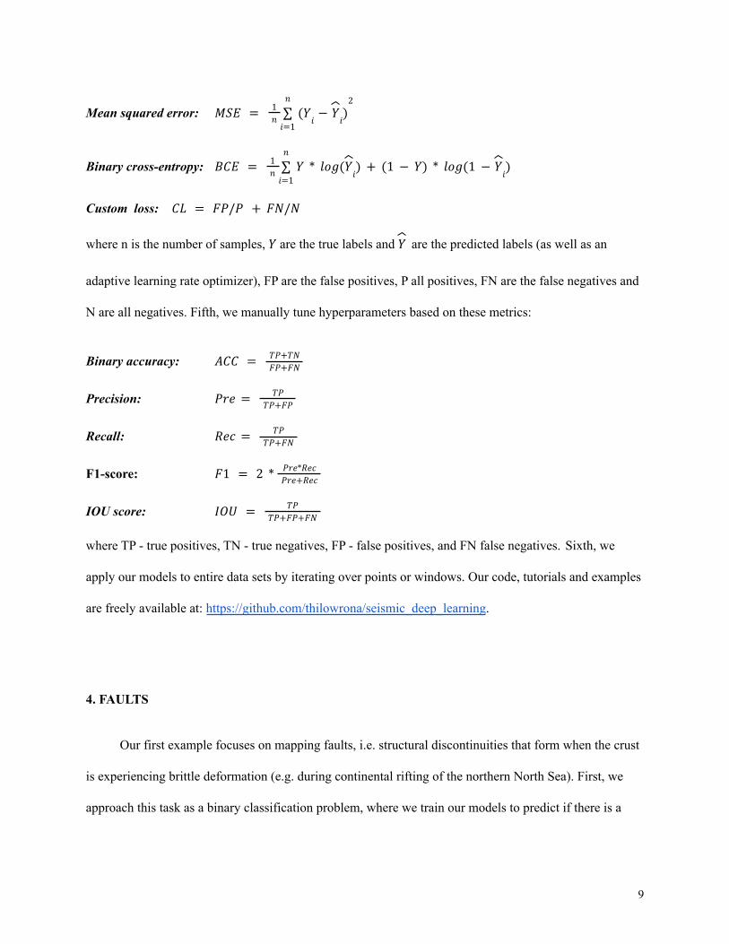
Mean squared error: 𝑀𝑆𝐸 = 1𝑛

𝑖=1

𝑛

∑ (𝑌𝑖

− 𝑌𝑖)

2

Binary cross-entropy: 𝐵𝐶𝐸 = 1𝑛

𝑖=1

𝑛

∑ 𝑌 * 𝑙𝑜𝑔(𝑌𝑖) + (1 − 𝑌) * 𝑙𝑜𝑔(1 − 𝑌

𝑖)

Custom loss: 𝐶𝐿 = 𝐹𝑃/𝑃 + 𝐹𝑁/𝑁

where n is the number of samples, are the true labels and are the predicted labels (as well as an𝑌 𝑌

adaptive learning rate optimizer), FP are the false positives, P all positives, FN are the false negatives and

N are all negatives. Fifth, we manually tune hyperparameters based on these metrics:

Binary accuracy: 𝐴𝐶𝐶 = 𝑇𝑃+𝑇𝑁𝐹𝑃+𝐹𝑁

Precision: 𝑃𝑟𝑒 = 𝑇𝑃𝑇𝑃+𝐹𝑃

Recall: 𝑅𝑒𝑐 = 𝑇𝑃𝑇𝑃+𝐹𝑁

F1-score: 𝐹1 = 2 * 𝑃𝑟𝑒*𝑅𝑒𝑐𝑃𝑟𝑒+𝑅𝑒𝑐

IOU score: 𝐼𝑂𝑈 = 𝑇𝑃𝑇𝑃+𝐹𝑃+𝐹𝑁

where TP - true positives, TN - true negatives, FP - false positives, and FN false negatives. Sixth, we

apply our models to entire data sets by iterating over points or windows. Our code, tutorials and examples

are freely available at: https://github.com/thilowrona/seismic_deep_learning.

4. FAULTS

Our first example focuses on mapping faults, i.e. structural discontinuities that form when the crust

is experiencing brittle deformation (e.g. during continental rifting of the northern North Sea). First, we

approach this task as a binary classification problem, where we train our models to predict if there is a

9

fault at each point of the section or not. We generate our training examples by manually labelling all faults

visible in ten 2-D seismic sections (2801×8096 samples, 180×20 km) of the northern North Sea (Fig. 2A,

B). Next, we extract squares (128×128 samples) from eight of these sections until we have 40,000

examples with a fault at the centre (label: 1) and 40,000 without (label: 0). Balancing these examples

across classes makes it easier to train models. Next, we extract 10,000 examples from each of the

remaining two seismic sections for validation (10%) and testing (10%). We use the training set to fit our

model; a 2-D convolutional neural network consisting of three 2-D convolutional layers followed by max

pooling and two dense layers. In total, the model has 8,413,442 trainable parameters. We train the model

over 10 epochs (one epoch refers one cycle through the entire training set) using 2500 batches consisting

of 32 labelled training examples each (one batch refers to one set of training examples to work through

before updating model weights). We use a binary cross-entropy loss function, an adaptive learning rate

optimizer and a softmax activation for two classes. The training takes 16 minutes on our desktop machine

with GPU support (see Appendix for specifications).

10

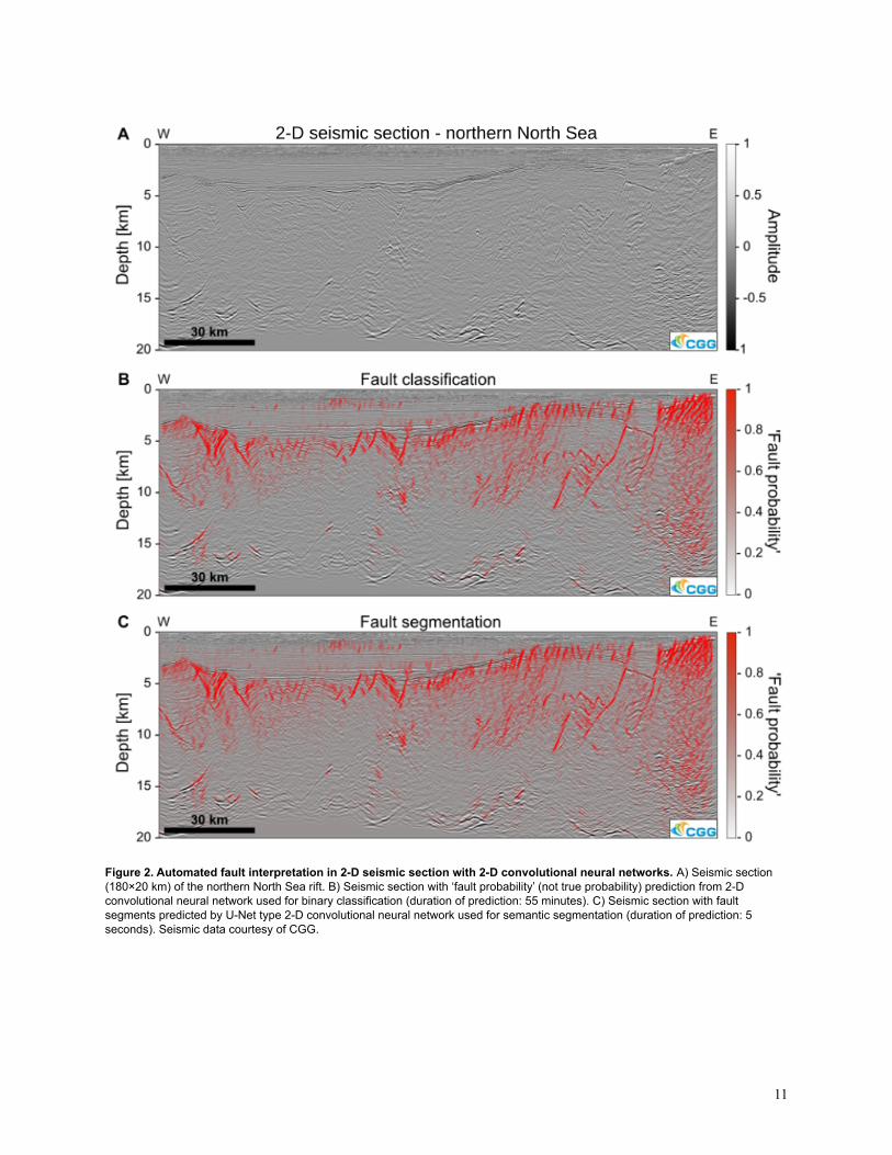
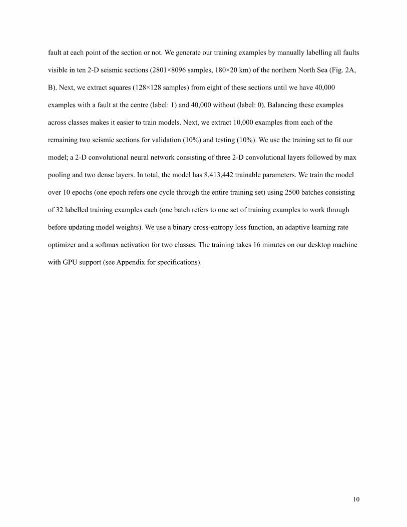
Figure 2. Automated fault interpretation in 2-D seismic section with 2-D convolutional neural networks. A) Seismic section(180×20 km) of the northern North Sea rift. B) Seismic section with ‘fault probability’ (not true probability) prediction from 2-Dconvolutional neural network used for binary classification (duration of prediction: 55 minutes). C) Seismic section with faultsegments predicted by U-Net type 2-D convolutional neural network used for semantic segmentation (duration of prediction: 5seconds). Seismic data courtesy of CGG.

11

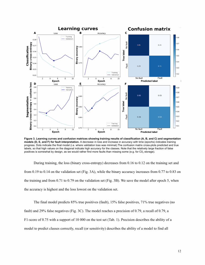
Figure 3. Learning curves and confusion matrices showing training results of classification (A, B, and C) and segmentationmodels (D, E, and F) for fault interpretation. A decrease in loss and increase in accuracy with time (epochs) indicates trainingprogress. Dots indicate the final model (i.e. where validation loss was minimal).The confusion matrix cross-plots predicted and truelabels, so that high values on the diagonal indicate high accuracy for the classes. Note that the relatively large fraction of falsepositives is somewhat by design, as we would rather find more faults than missing some (e.g. for C02 storage).

During training, the loss (binary cross-entropy) decreases from 0.16 to 0.12 on the training set and

from 0.19 to 0.14 on the validation set (Fig. 3A), while the binary accuracy increases from 0.77 to 0.83 on

the training and from 0.71 to 0.79 on the validation set (Fig. 3B). We save the model after epoch 5, when

the accuracy is highest and the loss lowest on the validation set.

The final model predicts 85% true positives (fault), 15% false positives, 71% true negatives (no

fault) and 29% false negatives (Fig. 3C). The model reaches a precision of 0.79, a recall of 0.79, a

F1-score of 0.75 with a support of 10 000 on the test set (Tab. 1). Precision describes the ability of a

model to predict classes correctly, recall (or sensitivity) describes the ability of a model to find all

12

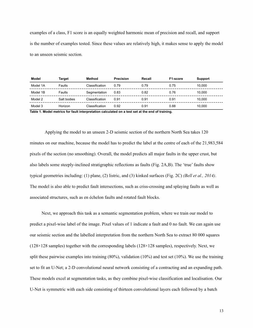
examples of a class, F1 score is an equally weighted harmonic mean of precision and recall, and support

is the number of examples tested. Since these values are relatively high, it makes sense to apply the model

to an unseen seismic section.

Model Target Method Precision Recall F1-score Support

Model 1A Faults Classification 0.79 0.79 0.75 10,000

Model 1B Faults Segmentation 0.83 0.82 0.76 10,000

Model 2 Salt bodies Classification 0.91 0.91 0.91 10,000

Model 3 Horizon Classification 0.92 0.91 0.88 10,000

Table 1. Model metrics for fault interpretation calculated on a test set at the end of training.

Applying the model to an unseen 2-D seismic section of the northern North Sea takes 120

minutes on our machine, because the model has to predict the label at the centre of each of the 21,983,584

pixels of the section (no smoothing). Overall, the model predicts all major faults in the upper crust, but

also labels some steeply-inclined stratigraphic reflections as faults (Fig. 2A,B). The ‘true’ faults show

typical geometries including: (1) plane, (2) listric, and (3) kinked surfaces (Fig. 2C) (Bell et al., 2014).

The model is also able to predict fault intersections, such as criss-crossing and splaying faults as well as

associated structures, such as en échelon faults and rotated fault blocks.

Next, we approach this task as a semantic segmentation problem, where we train our model to

predict a pixel-wise label of the image. Pixel values of 1 indicate a fault and 0 no fault. We can again use

our seismic section and the labelled interpretation from the northern North Sea to extract 80 000 squares

(128×128 samples) together with the corresponding labels (128×128 samples), respectively. Next, we

split these pairwise examples into training (80%), validation (10%) and test set (10%). We use the training

set to fit an U-Net; a 2-D convolutional neural network consisting of a contracting and an expanding path.

These models excel at segmentation tasks, as they combine pixel-wise classification and localisation. Our

U-Net is symmetric with each side consisting of thirteen convolutional layers each followed by a batch

13

normalisation, max pooling and dropout layer. In total, the model has 31,042,369 trainable parameters.

We train the model over 10 epochs using 2500 batches consisting of 32 labeled training examples each.

We use a binary cross-entropy combined with a custom loss function (normalized false positives +

normalized false negatives) and an adaptive learning rate optimizer. We chose this loss function, because

it minimizes both false negative and false positive predictions for imbalanced classes (e.g. fault vs no

fault). The training takes 2 hours 16 minutes on our desktop machine with GPU support (see Appendix

for specifications).

During training, the loss decreases from 0.35 to 0.29 on the training set and from 0.36 to 0.33 on

the validation set (Fig. 3D), while the binary accuracy increases from 0.82 to 0.84 on the training and

from 0.82 to 0.84 on the validation set (Fig. 3B). We save the model after epoch 3, when the loss is lowest

on the validation set.

The final model predicts 64% true positives (fault), 36% false positives, 95% true negatives (no

fault) and 5% false negatives (Fig. 3C). The model reaches a precision of 0.83, a recall of 0.82, a F1-score

of 0.76 with a support of 10,000 on the test set (Tab. 1). All these values are reasonably high, so it makes

sense to apply the model to the entire seismic section.

Applying the model to an unseen 2-D seismic section of the northern North Sea takes only 5

seconds on our machine, because the model simultaneously predicts 128×128 of the 21,983,584 pixels for

each batch of the section (no smoothing or overlap). The model is thus able to predict the faults just as

well as the previous model, but in a fraction of the time.

5. SALT BODIES

Our second example focuses on mapping salt bodies in three dimensions. Given that salt forms

complex bodies, which are difficult to label in 3-D as segmentation masks, we approach this task as a

14

binary classification, where we train a 3-D convolutional neural network using 3-D seismic reflection

data. We label salt on 5 seismic inlines and 5 crosslines to generate a total of 1,000,000 examples in the

form of small cubes (16×16×16 samples). These examples are already relatively balanced across the two

classes (salt, no salt) in this dataset. Next, we split these examples into exclusive training (8 lines, 80%),

validation (1 line, 10%) and test set (1 line, 10%). The training set is used to fit our model: a 3-D U-Net

consisting of 183-D convolutional, three 3-D max pooling and three upsampling layers . In total, the

model has 5,884,033 trainable parameters. We train the model over 10 epochs using 25,000 batches

consisting of 32 labelled training examples each. We use a binary cross entropy loss function and an

adaptive learning rate optimizer. The loss function is masked to allow training of a 3-D model with 2-D

labels (sensu Tschannen et al., 2020). The training took about 35 minutes on our desktop machine with

GPU support (see Appendix for specifications).

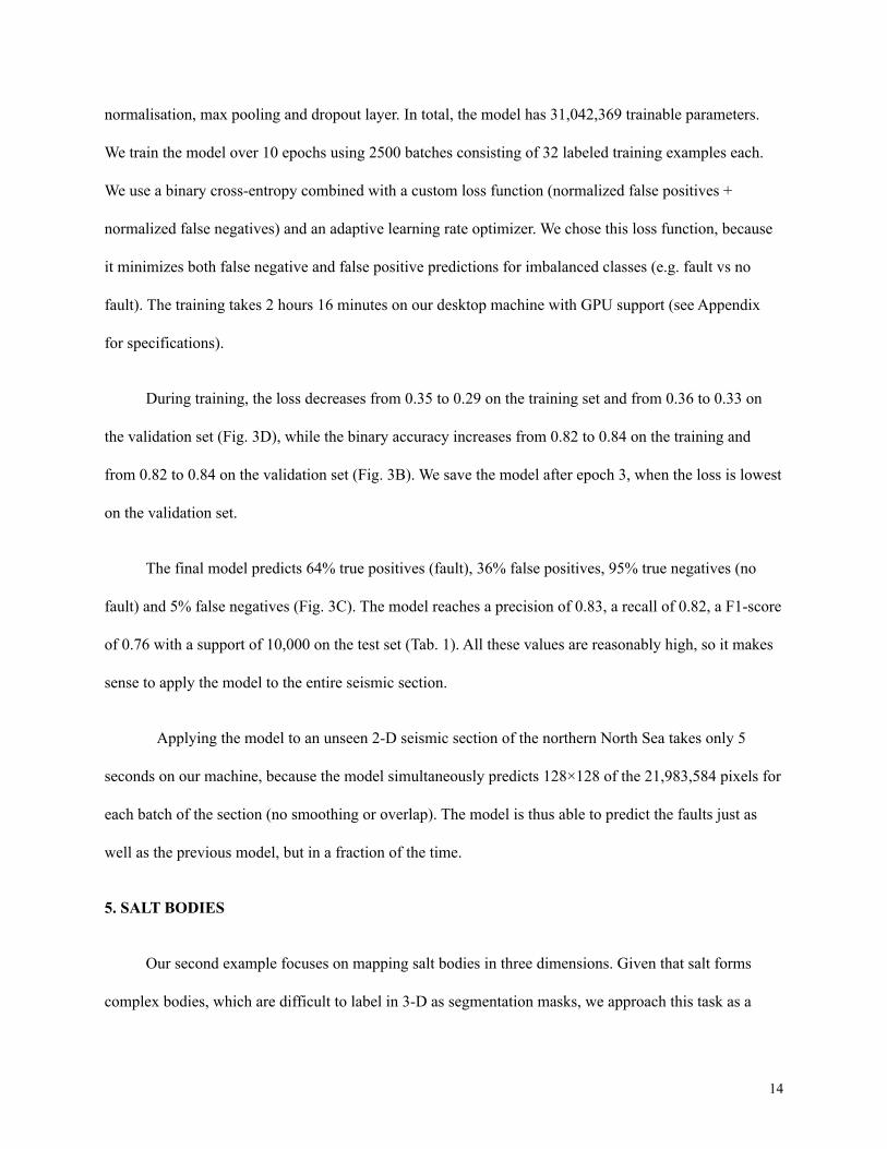
Figure 4. Learning curves and confusion matrices showing training results of classification model for salt interpretation. Adecrease in loss (A) and increase in accuracy (B) with time (epochs) indicates training progress. The final model is the one with thelowest validation loss (i.e. after 10 epochs).The confusion matrix cross-plots predicted and true labels, so that high values on thediagonal indicate high accuracy for the classes.

During training, the loss (binary cross entropy) decreases from 0.15 to 0.05 on the training set and

from 0.21 to 0.11 on the validation set, and the binary accuracy increases from 0.85 to 0.94 on the training

15

set and from 0.79 to 0.85 on the validation set (Fig. 4A,B). Constant losses and accuracies with time

indicate that training has been completed after 10 epochs.

The final model predicts 89% true positives (salt), 11% false positives, 92% true negatives (no salt)

and 8% false negatives (Fig. 4C). The model achieves a precision of 0.91, a recall of 0.91, a F1-score of

0.91 with a support of 10,000 on the test set (Tab. 1). These values give us confidence that we can apply

the model.

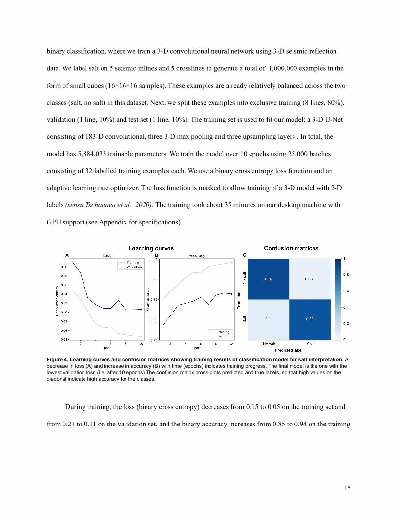
Figure 5: Salt diapirs mapped in 3-D seismic reflection data with a 3-D deep convolutional neural network. This volume hasan approximate size of 60×60×8 km.

Applying the model to the entire 3-D seismic volume takes 49 minutes on our machine. Overall,

the model is able to predict a number of typical 3-D structures, such as salt walls and diapirs (Fig. 5).

16

6. HORIZONS

Our third example focuses on mapping a seismic horizon in 3-D seismic reflection data from the

northern North Sea. We approach this problem as a binary segmentation, using a 3-D U-Net. To generate

examples, we map a horizon in one area of the dataset using a seismic interpretation software. This

provides us with 100,000 examples in the form of small cubes (32×32×32 samples). Next, we sort these

examples into exclusive sets: one for training (80%) and one for validation (10%) and one for testing

(10%). We use the training set to fit our model: a 3-D U-Net consisting of 183-D convolutional, batch

three 3-D max pooling and three upsampling layers. In total, the model has 5,884,033 trainable

parameters. We train our model over 10 epochs using 2500 batches consisting of 32 labelled training

examples each. We use a masked binary cross entropy loss function (sensu Tschannen et al., 2020) and an

adaptive learning rate optimizer. The training took about 38minutes on our desktop machine with GPU

support (see Appendix for specifications).

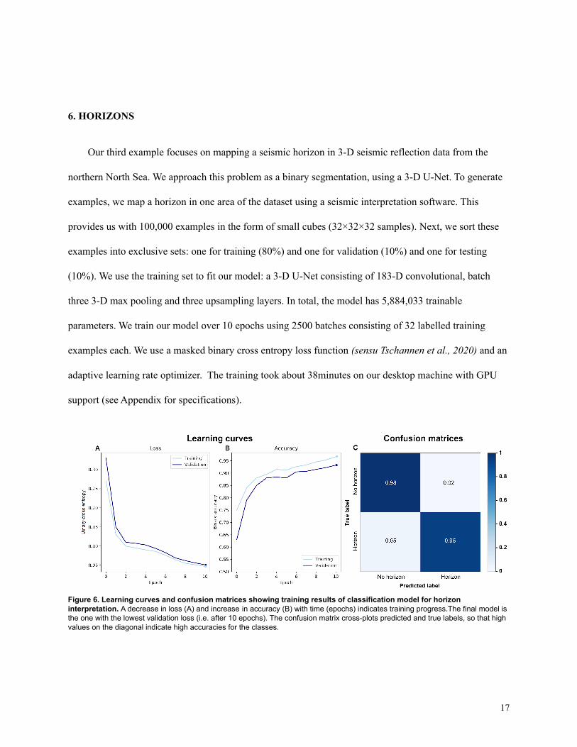
Figure 6. Learning curves and confusion matrices showing training results of classification model for horizoninterpretation. A decrease in loss (A) and increase in accuracy (B) with time (epochs) indicates training progress.The final model isthe one with the lowest validation loss (i.e. after 10 epochs). The confusion matrix cross-plots predicted and true labels, so that highvalues on the diagonal indicate high accuracies for the classes.

17

During training, the loss (binary cross-entropy) decreases from 0.27 to 0.047 on the training set and

from 0.33 to 0.051 on the validation set (Fig. 6A). At the same time, the binary accuracy increases from

0.75 to 0.966 on the training and from 0.63 to 0.932 on the validation set (Fig. 6B). Plateauing of loss and

accuracy with time suggests that training has been completed.

The final model predicts 95% true positives (horizon), 5% false positives, 98% true negatives (no

horizon) and 2% false negatives (Fig. 6C). The model reaches a precision of 0.92, a recall of 0.91, a

F1-score of 0.88 with a support of 10,00 on the test set (Tab. 1). Given that these values are sufficiently

high, we can apply the model to a neighbouring area.

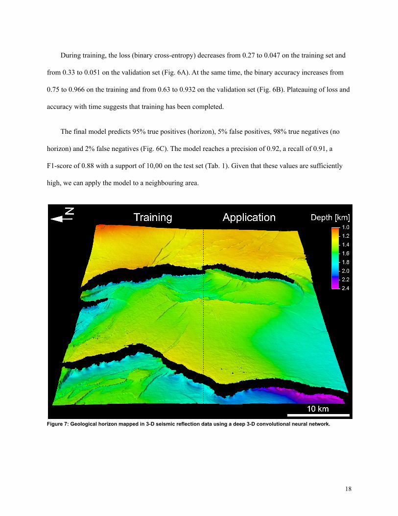
Figure 7: Geological horizon mapped in 3-D seismic reflection data using a deep 3-D convolutional neural network.

18

Applying the model to the right hand side of Figure 7 takes 1 hours 12minutes. A direct visual

comparison between the training data and the predictions shows that the model is able to map a

continuous horizon with the same geological structures (large and small normal faults) on unseen data.

7. DISCUSSION

Our models highlight that we can use deep learning for typical seismic interpretation tasks, such as

fault, salt and horizon mapping in two and three dimensions (Figs. 2, 5, 7). Using labelled training data,

we can train a set of 2-D and 3-D convolutional neural networks to perform these tasks in as little as 5

seconds. This allows us to map 2-D and 3-D geological structures (e.g. faults, geobodies and horizons) in

great detail, over vast areas, and at high accuracy. This has far-reaching implications. For instance, if we

are able to map entire rifts and rift systems in 3-D seismic reflection data, we could compare the

architecture of these systems to 3-D geodynamic models, which, in turn, helps us understand the rheology

of the lithosphere and the spatial evolution of fault rift systems. Mapping every stratigraphic horizon in

these systems would help us reconstruct their temporal evolution in much greater detail than previously

possible. While this example focuses on tectonic faults in continental rifts, a similar approach is feasible

in different disciplines working with 2-D and 3-D seismic reflection data, whether it concerns the study of

submarine channels, magmatic intrusions or salt tectonics.

In the following, we discuss: (1) the potential of deep learning in geophysics, (2) how generalisable

these methods are to other problems in geophysics, and (3) what are the challenges and few remedial

strategies. We think that there are three main reasons regarding the suitability of deep learning techniques

for analysis of 3-D geophysical data. First, geophysical datasets are large (GBs to TBs); a key

requirement for the implicit feature extraction of deep learning (Chen & Lin, 2014). Second, we already

have large volumes of historical training data labelled by experts and if necessary, we can label even more

19

training data. Third, the translation invariance of convolutional neural networks has made deep learning

very effective in analyzing images; a property we too can exploit in geophysics.

With deep learning transforming the way we analyze data, we can ask ourselves how transferable

these methods are to other problems in geophysics. First, it is worth noting that deep learning does not

require feature engineering and is thus not limited to a specific type of geophysical data. Appropriate

transformations (e.g. scaling) can however greatly improve model performance. Second, the models

presented here are still relatively simple in terms of architecture, so that users can easily tweak them to

adapt the workflow to their problem. Moreover, it is possible to optimize the hyperparameters of these

models to further increase accuracy and speed. To encourage these developments, we made our code

freely available on: https://github.com/thilowrona/seismic_deep_learning. Third, it is possible to apply

our workflow to map a variety of geological structures (e.g. volcanoes, channels or craters) in different

types of geophysical data (radar, magnetic, gravity). Finally, we can explore applications of deep learning

in other tasks in seismic interpretation. Uncertainty quantification, for example, is extremely difficult in

manual seismic interpretations. While our models only predict a proxy for the probability of detecting a

certain geological structure (e.g. Fig. 2B, C), we can envision incorporating uncertainty in the training

data and architecture of these models (e.g. Mosser et al., 2020; Feng et al., 2021). Accurate predictions of

subsurface rock properties with uncertainty are extremely important to risk evaluations of CO2 storage

sites and geothermal reservoirs. Bayesian techniques like Variational Inference for deep neural networks

can be used to approximate the posterior predictive distribution. These are optimisation based techniques

that are much faster and tractable than full Markov Chain Monte Carlo methods, although they are known

to under-estimate the uncertainty bounds (e.g. Blei et al., 2017).

While these techniques are very powerful, it is also worth highlighting some of the challenges (and

potential remedies) associated with deep learning. For example, pixel-wise predictions are more

20

time-consuming with classification instead of segmentation models (e.g. Zhao, 2018). Labelling training

data for segmentation models, in particular in 3-D, is challenging and time-consuming, too. A masked

loss function allows training with 3-D models and data using 1-D- and 2-D labels (see Tschannen et al.,

2020 for more details). This function restricts the loss calculation during training using a mask, which is

one where a label is available and zero where it is absent.

Another challenge is determining the optimal number of training examples. While we found that

around 100,000 examples provide a good trade-off between prediction accuracy and training time, this

point is worth investigating further. When labels are only available for a small subset, it is possible to

increase the size of the training set using data augmentation techniques. When there are no labels

available, we (as a user or community) have to spend time labelling data manually. Active learning, where

models can query users to label certain data points, is a promising approach worth exploring in seismic

interpretation. Moreover, we can explore unsupervised learning methods (e.g. autoencoders), which do

not require labels.

Another issue of deep learning is overfitting. Deep neural networks can provide accurate predictions

on the training set, but fail to generalize on new data (i.e. overfitting) (Domingos, 2012). To identify

overfitting, we can compare model predictions between the training and validation set. Moreover, it is

advisable to start with a simple model and successively increase complexity as necessary. Furthermore,

regularization techniques, such as dropout (Srivastava et al., 2014), can help us limit overfitting.

At last, it is worth mentioning that neural networks are still, to a large degree, a black box, offering

only sporadic insights into their inner workings. So while these models can perform many tasks at high

accuracy and speed, we are just beginning to understand which features these models use and how they

make decisions, so interpretability remains a key focus area of machine learning research (e.g. Ribeiro et

al., 2016; Lundberg and Lee, 2017; Molnar, 2018).

21

8. CONCLUSIONS

Here, we demonstrate how to use deep learning to analyse geophysical data sets at high accuracy and

limited time. We show that deep convolutional neural networks are able to perform key tasks, such as (1)

mapping tectonic faults, (2) extracting geobodies, and (3) tracing stratigraphic horizons. As such, this

study highlights new ways to efficiently analyze large volumes of geophysical data using freely available

methods. To summarize, this study shows that deep learning has the potential to drastically increase the

speed and accuracy of geophysical data analyses.

ACKNOWLEDGEMENTS

We would like to thank the journal editors (Yongyi Li, John T. Etgen and Erika Gasperikova) and the

reviewers (Rocky Roden, Xinming Wu, two anonymous) for their extremely constructive and helpful

comments, which significantly improved the manuscript. Furthermore, we thank The Norwegian

Academy of Science and Letters (VISTA), The University of Bergen and The Initiative and Networking

Fund of the Helmholtz Association through the project “Advanced Earth System Modelling Capacity

(ESM) and The Geo.X Network for supporting this work. S. Brune has been funded through the

Helmholtz Young Investigators Group CRYSTALS (VH-NG-1132). We are grateful to CGG, in particular

Stein Åsheim, for the permission to present this data and publish this work. We thank Schlumberger for

providing the software Petrel 2019© and Leo Zijerveld for IT support.

REFERENCES

Abadi, M., Barham, P., Chen, J., Chen, Z., Davis, A., Dean, J., et al. (2016). TensorFlow: A system forlarge-scale machine learning. In In12th Symposium on Operating Systems Design and Implementation(pp. 265–283). Retrieved from http://arxiv.org/abs/1605.08695

22

Araya-Polo, M., Dahlke, T., Frogner, C., Zhang, C., Poggio, T., & Hohl, D. (2017). Automated faultdetection without seismic processing. The Leading Edge, 36(3), 208–214.https://doi.org/10.1190/tle36030208.1

Bell, R. E., Jackson, C. A. L., Whipp, P. S., & Clements, B. (2014). Strain migration during multiphaseextension: Observations from the northern North Sea. Tectonics, 33(10), 1936–1963.https://doi.org/10.1002/2014tc003551

Bjorck, J., Gomes, C., Selman, B., & Weinberger, K. Q. (2018). Understanding batch normalization. InAdvances in Neural Information Processing Systems.

Blei, D. M., Kucukelbir, A., & McAuliffe, J. D. (2017). Variational Inference: A Review for Statisticians.Journal of the American Statistical Association. https://doi.org/10.1080/01621459.2017.1285773

Bond, C. E., Lunn, R. J., Shipton, Z. K., & Lunn, A. D. (2012). What makes an expert effective atinterpreting seismic images? Geology, 40(1), 75–78. https://doi.org/10.1130/g32375.1

Butler, K. T., Davies, D. W., Cartwright, H., Isayev, O., & Walsh, A. (2018). Machine learning formolecular and materials science. Nature. https://doi.org/10.1038/s41586-018-0337-2

Carleo, G., & Troyer, M. (2017). Solving the quantum many-body problem with artificial neuralnetworks. Science, 355(6325), 602–606. https://doi.org/10.1126/science.aag2302

Cartwright, J., & Huuse, M. (2005). 3D seismic technology: the geological ‘Hubble.’ Basin Research,17(1), 1–20. https://doi.org/10.1111/j.1365-2117.2005.00252.x

Chen, X. W., & Lin, X. (2014). Big data deep learning: Challenges and perspectives. IEEE Access.https://doi.org/10.1109/ACCESS.2014.2325029

Chollet, F. (2015). Keras: The Python Deep Learning library. Keras.Io.

Coléou, T., Poupon, M., & Azbel, K. (2003). Unsupervised seismic facies classification: A review andcomparison of techniques and implementation. The Leading Edge, 22(10), 942–953.https://doi.org/10.1190/1.1623635

Domingos, P. (2012). A few useful things to know about machine learning. Communications of the ACM.https://doi.org/10.1145/2347736.2347755

Esteva, A., Kuprel, B., Novoa, R. A., Ko, J., Swetter, S. M., Blau, H. M., & Thrun, S. (2017).Dermatologist-level classification of skin cancer with deep neural networks. Nature, 542(7639), 115.Retrieved from https://www.nature.com/articles/nature21056.pdf

Fent, R., Grana, D. and Bailing N. (2021). Uncertainty quantification in fault detection usingconvolutional neural networks. GEOPHYSICS 0: 1-45. https://doi.org/10.1190/geo2020-0424.1

Gramstad, O., Nickel, M., Goledowski, B., & Etchebes, M. (2020). Strategies in picking training data for3D convolutional neural networks in stratigraphic interpretation. SEG Technical Program ExpandedAbstracts : 1641-1645. https://doi.org/10.1190/segam2020-3427602.1

23

Guillen, P., Larrazabal*, G., González, G., Boumber, D., & Vilalta, R. (2015). Supervised learning todetect salt body. In SEG Technical Program Expanded Abstracts 2015 (pp. 1826–1829). Society ofExploration Geophysicists. https://doi.org/10.1190/segam2015-5931401.1

Hunter, J. D. (2007). Matplotlib: A 2D graphics environment. Computing in Science and Engineering.https://doi.org/10.1109/MCSE.2007.55

LeCun, Y., Bengio, Y., & Hinton, G. (2015). Deep learning. Nature, 521(7553), 436–444.https://doi.org/10.1038/nature14539

Li, W. (2018). Classifying geological structure elements from seismic images using deep learning. SEGTechnical Program Expanded Abstracts : 4643-4648. https://doi.org/10.1190/segam2018-2998036.1

Liu, Z., Cao, J., Lu, Y., Chen, S., & Liu, J. (2019). A seismic facies classification method based on theconvolutional neural network and the probabilistic framework for seismic attributes and spatialclassification. Interpretation. https://doi.org/10.1190/int-2018-0238.1

Long, J., Shelhamer, E., & Darrell, T. (2015). Fully convolutional networks for semantic segmentation. InProceedings of the IEEE Computer Society Conference on Computer Vision and Pattern Recognition.https://doi.org/10.1109/CVPR.2015.7298965

Lundberg, S. M., & Lee, S. I. (2017). A unified approach to interpreting model predictions. In Advancesin Neural Information Processing Systems.

de Matos, M. C., Osorio, P. L., & Johann, P. R. (2007). Unsupervised seismic facies analysis usingwavelet transform and self-organizing maps. Geophysics, 72(1), P9–P21.https://doi.org/10.1190/1.2392789

Molnar, C. (2018). Interpretable Machine Learning.Https://Christophm.Github.Io/Interpretable-Ml-Book/. https://doi.org/10.1007/978-1-4419-0790-5

Mosser, L., Purves S. and Naeini E.Z. (2020). Deep Bayesian Neural Networks for Fault Identificationand Uncertainty Quantification. Conference Proceedings, First EAGE Digitalization Conference andExhibition, Nov 2020, Volume 2020, p.1 - 5. https://doi.org/10.3997/2214-4609.202032036

Nair, V., & Hinton, G. E. (2010). Rectified linear units improve Restricted Boltzmann machines. In ICML2010 - Proceedings, 27th International Conference on Machine Learning.

Orhan, A. E., & Pitkow, X. (2018). Skip connections eliminate singularities. In 6th InternationalConference on Learning Representations, ICLR 2018 - Conference Track Proceedings.

Peters, B., Haber, E., & Granek, J. (2019). Neural networks for geophysicists and their application toseismic data interpretation. Leading Edge. https://doi.org/10.1190/tle38070534.1

Qian, F., Yin, M., Liu, X.-Y., Wang, Y.-J., Lu, C., & Hu, G.-M. (2018). Unsupervised seismic faciesanalysis via deep convolutional autoencoders. Geophysics, 83(3), A39–A43.https://doi.org/10.1190/geo2017-0524.1

24

Ribeiro, M. T., Singh, S., & Guestrin, C. (2016). “Why should i trust you?” Explaining the predictions ofany classifier. In Proceedings of the ACM SIGKDD International Conference on Knowledge Discoveryand Data Mining. https://doi.org/10.1145/2939672.2939778

Ronneberger, O., Fischer, P., & Brox, T. (2015). U-net: Convolutional networks for biomedical imagesegmentation. In Lecture Notes in Computer Science (including subseries Lecture Notes in ArtificialIntelligence and Lecture Notes in Bioinformatics). https://doi.org/10.1007/978-3-319-24574-4_28

Rumelhart, D. E., Hinton, G. E., & Williams, R. J. (1986). Learning representations by back-propagatingerrors. Nature. https://doi.org/10.1038/323533a0

Santurkar, S., Tsipras, D., Ilyas, A., & Madry, A. (2018). How does batch normalization helpoptimization? In Advances in Neural Information Processing Systems.

Srivastava, N., Hinton, G., Krizhevsky, A., Sutskever, I., & Salakhutdinov, R. (2014). Dropout: A simpleway to prevent neural networks from overfitting. Journal of Machine Learning Research.

Tschannen, V., Delescluse, M., Ettrich, N., & Keuper, J. (2020). Extracting horizon surfaces from 3Dseismic data using deep learning. GEOPHYSICS. https://doi.org/10.1190/geo2019-0569.1

Waldeland, A. U., Jensen, A. C., Gelius, L.-J., & Solberg, A. H. S. (2018). Convolutional neural networksfor automated seismic interpretation. The Leading Edge, 37(7), 529–537. Retrieved fromhttps://library.seg.org/doi/pdf/10.1190/tle37070529.1

Van Der Walt, S., Colbert, S. C., & Varoquaux, G. (2011). The NumPy array: A structure for efficientnumerical computation. Computing in Science and Engineering. https://doi.org/10.1109/MCSE.2011.37

Wrona, T., Pan, I., Gawthorpe, R. L., & Fossen, H. (2018). Seismic facies analysis using machinelearning. Geophysics, 83(5), O83–O95. https://doi.org/10.1190/Geo2017-0595.1

Wu, X. M., & Fomel, S. (2018). Automatic fault interpretation with optimal surface voting. Geophysics,83(5), O67–O82. https://doi.org/10.1190/Geo2018-0115.1

Wu, X., Yunzhi Shi, L.L. & Fomel, S. (2019), FaultSeg3D: Using synthetic data sets to train anend-to-end convolutional neural network for 3D seismic fault segmentation, GEOPHYSICS 84:IM35-IM45. https://doi.org/10.1190/geo2018-0646.1

Zhang, C., Frogner, C., Araya-Polo, M., & Hohl, D. (2014). Machine-learning Based Automated FaultDetection in Seismic Traces. In 76th EAGE Conference and Exhibition 2014.

Zhao, T. (2019). Seismic facies classification using different deep convolutional neural networks. 2018SEG International Exposition and Annual Meeting, SEG 2018, 2046–2050.https://doi.org/10.1190/segam2018-2997085.1

Zhou, H., Xu, S., Ionescu, G., Laomana, M., & Weber, N. (2020). Salt interpretation with U-SaltNet. SEGTechnical Program Expanded Abstracts : 1434-1438. https://doi.org/10.1190/segam2020-3423283.1

25

SUPPLEMENTARY MATERIAL

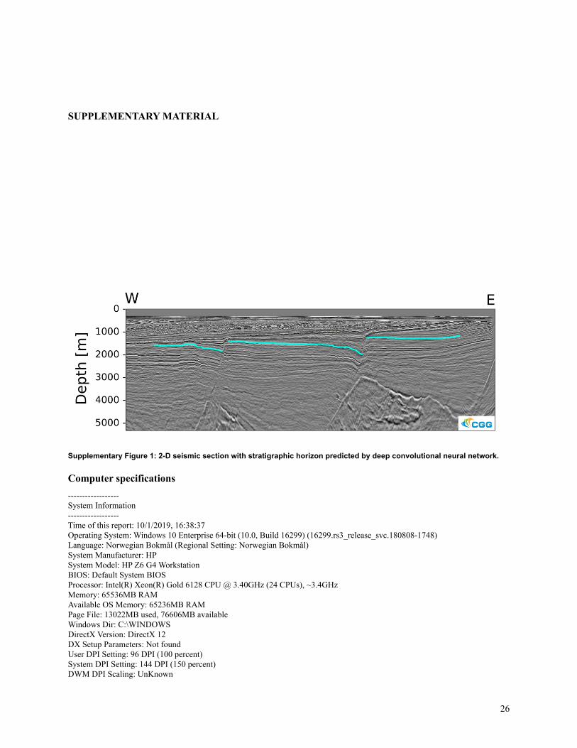
Supplementary Figure 1: 2-D seismic section with stratigraphic horizon predicted by deep convolutional neural network.

Computer specifications------------------System Information------------------Time of this report: 10/1/2019, 16:38:37Operating System: Windows 10 Enterprise 64-bit (10.0, Build 16299) (16299.rs3_release_svc.180808-1748)Language: Norwegian Bokmål (Regional Setting: Norwegian Bokmål)System Manufacturer: HPSystem Model: HP Z6 G4 WorkstationBIOS: Default System BIOSProcessor: Intel(R) Xeon(R) Gold 6128 CPU @ 3.40GHz (24 CPUs), ~3.4GHzMemory: 65536MB RAMAvailable OS Memory: 65236MB RAMPage File: 13022MB used, 76606MB availableWindows Dir: C:\WINDOWSDirectX Version: DirectX 12DX Setup Parameters: Not foundUser DPI Setting: 96 DPI (100 percent)System DPI Setting: 144 DPI (150 percent)DWM DPI Scaling: UnKnown

26

Miracast: Available, with HDCPMicrosoft Graphics Hybrid: Not SupportedDxDiag Version: 10.00.16299.0015 64bit Unicode

---------------Display Devices---------------Card name: NVIDIA GeForce GTX 1080 TiManufacturer: NVIDIAChip type: GeForce GTX 1080 TiAC type: Integrated RAMDACDevice Type: Full DeviceDevice Key: Enum\PCI\VEN_10DE&DEV_1B06&SUBSYS_85E51043&REV_A1Device Status: 0180200A[DN_DRIVER_LOADED|DN_STARTED|DN_DISABLEABLE|DN_NT_ENUMERATOR|DN_NT_DRIVER]Device Problem Code: No ProblemDriver Problem Code: UnknownDisplay Memory: 43744 MBDedicated Memory: 11127 MBShared Memory: 32617 MBCurrent Mode: 1920 x 1080 (32 bit) (32Hz)

27