2021, Md Masud Rana
123
New Models and Numerical Methods for Partial Differential Equations Applied to Spatial Stoichiometric Aquatic Ecosystems by Md Masud Rana A Dissertation In Mathematics and Statistics Submitted to the Graduate Faculty of Texas Tech University in Partial Fulfillment of the Requirements for the Degree of DOCTOR OF PHILOSOPHY Approved Katharine R. Long Chair of Committee Angela Peace Co-chair of Committee Victoria E. Howle Co-chair of Committee Linda J. S. Allen Chris J. Monico Mark A. Sheridan Dean of the Graduate School August, 2021
-
Upload
khangminh22 -
Category
Documents
-
view
1 -
download
0
Transcript of 2021, Md Masud Rana

New Models and Numerical Methods for Partial Differential Equations Applied toSpatial Stoichiometric Aquatic Ecosystems
by
Md Masud Rana
A Dissertation
In
Mathematics and Statistics
Submitted to the Graduate Facultyof Texas Tech University in
Partial Fulfillment ofthe Requirements for
the Degree of
DOCTOR OF PHILOSOPHY
Approved
Katharine R. LongChair of Committee
Angela PeaceCo-chair of Committee
Victoria E. HowleCo-chair of Committee
Linda J. S. Allen
Chris J. Monico
Mark A. SheridanDean of the Graduate School
August, 2021

©2021, Md Masud Rana

Texas Tech University, Md Masud Rana, August 2021
ACKNOWLEDGEMENTS
I wish to express my deepest appreciation to my advisors, Dr. Katharine Long,
Dr. Victoria Howle, and Dr. Angela Peace, for their invaluable advice, guidance,
encouragement, and continuous support throughout my PhD study. Without their
immense help, this dissertation would not have been possible. Their extensive knowl-
edge, profound belief in my abilities, and unparalleled support have taught me a great
deal about scientific research and life in general.
I would like to extend my sincere gratitude to the committee members, Dr. Linda
Allen and Dr. Chris Monico, for their insightful comments and suggestions. I would
also like to acknowledge Dr. Lourdes Juan with whom I have had the pleasure to
work in several projects.
I am grateful to all my friends who have helped me and supported me through-
out this journey. Many thanks to all my classmates at Texas Tech University and
Bangladeshi friends and families in Lubbock for making my graduate life enjoyable.
Finally, I would like to say a heartfelt thank you to my parents and my brothers
and sisters for always believing in me and encouraging me to follow my dream. Most
importantly, I wish to thank my loving and supportive wife, Mukta, and our son,
Aryaav, who provide unending inspiration.
ii

Texas Tech University, Md Masud Rana, August 2021
DEDICATION
To my mother who could not see this dissertation completed.
iii

Texas Tech University, Md Masud Rana, August 2021
TABLE OF CONTENTS
Acknowledgements . . . . . . . . . . . . . . . . . . . . . . . . . . . . . . . ii
Dedication . . . . . . . . . . . . . . . . . . . . . . . . . . . . . . . . . . . . iii
Abstract . . . . . . . . . . . . . . . . . . . . . . . . . . . . . . . . . . . . . viii
List of Tables . . . . . . . . . . . . . . . . . . . . . . . . . . . . . . . . . . ix
List of Figures . . . . . . . . . . . . . . . . . . . . . . . . . . . . . . . . . . xii
1. Introduction . . . . . . . . . . . . . . . . . . . . . . . . . . . . . . . . . 1
2. Space-Time Population Model . . . . . . . . . . . . . . . . . . . . . . . 6
2.1 Genotypic Selection Model . . . . . . . . . . . . . . . . . . . . 6
2.1.1 Introduction . . . . . . . . . . . . . . . . . . . . . . . . . . 6
2.1.2 Model development . . . . . . . . . . . . . . . . . . . . . . 8
2.1.2.1 Spatially heterogeneous model . . . . . . . . . . . . . 11
2.1.2.2 Light absorption . . . . . . . . . . . . . . . . . . . . 12
2.1.3 Numerical methods . . . . . . . . . . . . . . . . . . . . . . 15
2.1.4 Results . . . . . . . . . . . . . . . . . . . . . . . . . . . . . 17
2.1.4.1 Spatially homogeneous results . . . . . . . . . . . . . 17
2.1.4.2 Spatially heterogeneous results . . . . . . . . . . . . 21
2.1.5 Discussion . . . . . . . . . . . . . . . . . . . . . . . . . . . 23
2.2 Space-Time Mechanistic Model . . . . . . . . . . . . . . . . . . 27
2.2.1 Introduction . . . . . . . . . . . . . . . . . . . . . . . . . . 27
2.2.2 Model development . . . . . . . . . . . . . . . . . . . . . . 29
2.2.2.1 Light absorption . . . . . . . . . . . . . . . . . . . . 33
2.2.3 Numerical methods . . . . . . . . . . . . . . . . . . . . . . 35
iv

Texas Tech University, Md Masud Rana, August 2021
2.2.4 Results . . . . . . . . . . . . . . . . . . . . . . . . . . . . . 36
2.2.5 Discussion . . . . . . . . . . . . . . . . . . . . . . . . . . . 39
3. Reduced-Order Modeling . . . . . . . . . . . . . . . . . . . . . . . . . . 43
3.1 Introduction . . . . . . . . . . . . . . . . . . . . . . . . . . . . 43
3.2 Description of ROM . . . . . . . . . . . . . . . . . . . . . . . . 43
3.2.1 The ROM basis and reconstruction of results . . . . . . . . 44
3.2.1.1 An inner-product and norm appropriate to FEM . . 45
3.2.1.2 Finding a reduced-order basis . . . . . . . . . . . . . 46
3.2.1.3 Reduced-order reconstruction of existing results . . . 47
3.2.1.4 Error estimates . . . . . . . . . . . . . . . . . . . . . 48
3.2.2 From a PDE to a low-dimensional ODE system . . . . . . 49
3.2.3 An optimal basis for least squares approximation . . . . . 51
3.2.3.1 Which basis works best for all snapshots? . . . . . . 51
3.2.4 Beyond the simplest cases . . . . . . . . . . . . . . . . . . 54
3.2.4.1 Complex geometry in multiple spatial dimensions . . 54
3.2.4.2 Snapshots from runs with multiple parameters . . . . 54
3.2.5 Non-homogeneous boundary conditions . . . . . . . . . . . 55
3.2.5.1 BCs independent of time and parameters . . . . . . . 55
3.2.5.2 BCs dependent on parameters, independent of time . 55
3.2.5.3 BCs dependent on parameters and time . . . . . . . 56
3.2.6 Multiple unknowns . . . . . . . . . . . . . . . . . . . . . . 56
3.3 Mechanistic Model: ROM Approach . . . . . . . . . . . . . . . 57
3.3.1 ROM basis for mechanistic model . . . . . . . . . . . . . . 57
3.3.2 Results . . . . . . . . . . . . . . . . . . . . . . . . . . . . . 58
v

Texas Tech University, Md Masud Rana, August 2021
3.3.3 Discussion . . . . . . . . . . . . . . . . . . . . . . . . . . . 60
4. Preconditioning Implicit Runge–Kutta Methods for Parabolic PDEs . . 63
4.1 Overview . . . . . . . . . . . . . . . . . . . . . . . . . . . . . . 63
4.2 Appropriate Time-Integrator for Parabolic PDEs . . . . . . . . 64
4.2.1 Stability of time-integrator . . . . . . . . . . . . . . . . . . 65
4.2.2 CFL condition . . . . . . . . . . . . . . . . . . . . . . . . . 66
4.2.3 Second Dahlquist barrier . . . . . . . . . . . . . . . . . . . 67
4.3 Implicit Runge–Kutta Methods . . . . . . . . . . . . . . . . . 68
4.4 Choice of Solvers . . . . . . . . . . . . . . . . . . . . . . . . . 69
4.5 Preconditioning . . . . . . . . . . . . . . . . . . . . . . . . . . 70
4.6 IRK Methods Applied to Test PDEs . . . . . . . . . . . . . . . 72
4.6.1 Heat equation . . . . . . . . . . . . . . . . . . . . . . . . . 72
4.6.2 Double-Glazing advection-diffusion problem . . . . . . . . 74
4.7 Block Preconditioning IRK Methods for Parabolic PDEs . . . 75
4.7.1 LDU-based block triangular preconditioners . . . . . . . . 77
4.7.2 Application of the preconditioners . . . . . . . . . . . . . . 79
4.7.3 Analysis of the preconditioners . . . . . . . . . . . . . . . . 80
4.7.4 Comparison between PGSL with optimal coefficients and
PLD preconditioners . . . . . . . . . . . . . . . . . . . . . 82
4.8 Numerical Experiments . . . . . . . . . . . . . . . . . . . . . . 86
4.8.1 Heat Equation Results . . . . . . . . . . . . . . . . . . . . 89
4.8.1.1 Comparison results between PJ , PGSL, PDU , and PLD
preconditioners . . . . . . . . . . . . . . . . . . . . . 89
vi

Texas Tech University, Md Masud Rana, August 2021
4.8.1.2 Comparison results between PGSL with optimal coef-
ficients and PLD preconditioners . . . . . . . . . . . 92
4.8.2 Advection-Diffusion Equation Results . . . . . . . . . . . . 97
4.9 Discussion . . . . . . . . . . . . . . . . . . . . . . . . . . . . . 101
5. Conclusion . . . . . . . . . . . . . . . . . . . . . . . . . . . . . . . . . . 102
vii

Texas Tech University, Md Masud Rana, August 2021
ABSTRACT
Ecological stoichiometry is a framework to study population dynamics that incor-
porates energy flow in trophic levels as well as chemical imbalances. Spatial variation
in an ecological interaction also has effects on the population dynamics. We develop
and analyze numerically two stoichiometric producer-grazer models in a spatially het-
erogeneous environment: a model with two grazing genotypes to understand selection
processes and a mechanistic model that tracks explicitly the nutrient contents. Both
of our model equations are non-linear reaction-diffusion partial differential equations
(PDEs). Simulations of these models produce large data sets that are difficult to
analyze and interpret. We used a reduced-order modeling technique to interpret
the simulation data in terms of an underlying low-dimensional dynamical system.
The reaction-diffusion equations of our model can be viewed as a stiff system of
equations and require an A-stable time-stepping method. We implement high-order
Implicit Runge–Kutta (IRK) methods for our model PDEs. Although IRK methods
offer A-stability and high-order accuracy, these methods are not widely used in PDE
discretization due to the resulting complicated linear system. To solve these sys-
tems, we have developed a new preconditioner based on a block LDU factorization
with algebraic multigrid subsolves for scalability. We demonstrate the effectiveness
of our preconditioner on two test problems: a heat equation and a double-glazing
advection-diffusion problem, and find that the new preconditioner outperforms the
others currently in the literature.
viii

Texas Tech University, Md Masud Rana, August 2021
LIST OF TABLES
2.1 Model Parameters . . . . . . . . . . . . . . . . . . . . . . . . . . . . . 142.2 Equilibrium Q values for varying total phosphorus Pt and light levels
K0. The range of Q is given when the system exhibits a limit cycle.Values are in bold for Q > Q∗. . . . . . . . . . . . . . . . . . . . . . 20
2.3 Model Parameters . . . . . . . . . . . . . . . . . . . . . . . . . . . . . 354.1 Common IRK Methods . . . . . . . . . . . . . . . . . . . . . . . . . . 694.2 Condition numbers of right-preconditioned matrices with precondition-
ers P−1J , P−1
GSL, P−1DU , and P−1
LD applied to a 2D heat equation with
s-stage Radau IIA methods. Here, hx = 2−3 and ht = hp+12s−1x , where
p = 2 is the degree of the Lagrange polynomial basis functions in space.Preconditioners are constructed exactly. . . . . . . . . . . . . . . . . 80
4.3 Condition numbers of left-preconditioned and right-preconditioned ma-trices with preconditioners P−1
GSL and P−1LD applied to a 2D double-
glazing problem with ε = 0.005, and with s-stage Radau IIA meth-
ods. Here, hx = 2−4 and ht = hp+12s−1x , where p = 1 is the degree of
the Lagrange polynomial basis functions in space. Preconditioners areconstructed exactly. . . . . . . . . . . . . . . . . . . . . . . . . . . . . 81
4.4 Condition numbers of the left-preconditioned system with precondi-tioners PGSL (PGSL with optimal coefficients) and PLD for variousIRK methods applied to 1D and 2D heat problems. Here, hx = 2−3
and ht = hp+1q
x , where p = 2 is the degree of the Lagrange polynomialin space and q is the order of the corresponding IRK method (that is,q = 2s− 1 for Radau IIA and q = 2s− 2 for Lobatto IIIC). Precondi-tioners are constructed exactly. . . . . . . . . . . . . . . . . . . . . . 85
4.5 Iteration counts and elapsed time (times in seconds are shown in paren-theses) for right-preconditioned GMRES to converge with relative resid-ual tolerance 1.0 × 10⁻⁸ for a 2D heat problem with s-stage RadauIIA methods with preconditioners PJ , PGSL, PDU , and PLD. Here we
choose ht = hp+12s−1x , where p = 2 is the degree of the Lagrange poly-
nomial in space. Preconditioners are approximated using one AMGV-cycle for each subsolve. . . . . . . . . . . . . . . . . . . . . . . . . 91
ix

Texas Tech University, Md Masud Rana, August 2021
4.6 Iteration counts and elapsed time (times in seconds are shown in paren-theses) for right-preconditioned GMRES to converge with relative resid-ual tolerance 1.0 × 10⁻⁸ for a 2D heat problem with s-stage LobattoIIIC methods with preconditioners PJ , PGSL, PDU , and PLD. Here we
choose ht = hp+12s−2x , where p = 2 is the degree of the Lagrange poly-
nomial in space. Preconditioners are approximated using one AMGV-cycle for each subsolve. . . . . . . . . . . . . . . . . . . . . . . . . 92
4.7 Iteration counts and elapsed time (times in seconds are shown in paren-theses) for left-preconditioned and right-preconditioned GMRES toconverge with preconditioned relative residual tolerance 1.0× 10⁻⁸ fora 2D heat problem with s-stage Radau IIA methods with precondi-tioners PGSL and PLD. Here we keep h−1
x = 128 fixed and vary ht from0.05 to 5.0. Preconditioners are approximated using one AMG V-cyclefor each subsolve. . . . . . . . . . . . . . . . . . . . . . . . . . . . . . 93
4.8 Iteration counts and elapsed time (times in seconds are shown in paren-theses) for left-preconditioned GMRES to converge with preconditionedrelative residual tolerance 1.0 × 10⁻⁸ for a 2D heat problem with s-stage Radau IIA methods with preconditioners PJ , PGSL, PGSL, PDU ,
and PLD. Here we choose ht = hp+12s−1x , where p = 2 is the degree of
the Lagrange polynomial in space. Preconditioners are approximatedusing one AMG V-cycle for each subsolve. . . . . . . . . . . . . . . . 94
4.9 Iteration counts and elapsed time (times in seconds are shown in paren-theses) for left-preconditioned GMRES to converge with preconditionedrelative residual tolerance 1.0×10⁻⁸ for a 2D heat problem with s-stageLobatto IIIC methods with preconditioners PJ , PGSL, PGSL, PDU , and
PLD. Here we choose ht = hp+12s−2x , where p = 2 is the degree of the La-
grange polynomial in space. Preconditioners are approximated usingone AMG V-cycle for each subsolve. . . . . . . . . . . . . . . . . . . . 95
4.10 Relative error for left-preconditioned GMRES converging to a precon-ditioned relative residual tolerance of 1.0×10⁻⁸ for a 2D heat problemwith various IRK methods with preconditioners PJ , PGSL, PGSL, PDU ,
and PLD. Here, hx = 2−7 and ht = hp+1q
x , where p = 2 is the degree ofthe Lagrange polynomial in space and q is the order of the correspond-ing IRK method (that is, q = 2s − 1 for Radau IIA and q = 2s − 2for Lobatto IIIC). Preconditioners are approximated using one AMGV-cycle for each subsolve. . . . . . . . . . . . . . . . . . . . . . . . . 96
x

Texas Tech University, Md Masud Rana, August 2021
4.11 Relative error for right-preconditioned GMRES converging to a rela-tive residual tolerance of 1.0×10⁻⁸ for a 2D heat problem with variousIRK methods with preconditioners PJ , PGSL, PDU , and PLD. Here,
hx = 2−7 and ht = hp+1q
x , where p = 2 is the degree of the Lagrange poly-nomial in space and q is the order of the corresponding IRK method(that is, q = 2s − 1 for Radau IIA and q = 2s − 2 for Lobatto IIIC).Preconditioners are approximated using one AMG V-cycle for eachsubsolve. . . . . . . . . . . . . . . . . . . . . . . . . . . . . . . . . . . 97
4.12 Iteration counts and elapsed time (times in seconds are shown in paren-theses) for left-preconditioned GMRES to converge with preconditionedrelative residual tolerance 1.0 × 10⁻⁸ for the double-glazing problemwith s-stage Radau IIA methods with preconditioners PGSL and PLD.
Here we choose ht = hp+12s−1x , where p = 1 is the degree of the La-
grange polynomial in space. Preconditioners are approximated usingone AMG V-cycle for each subsolve. . . . . . . . . . . . . . . . . . . . 99
4.13 Iteration counts and elapsed time (times in seconds are shown in paren-theses) for left-preconditioned GMRES to converge with preconditionedrelative residual tolerance 1.0× 10⁻⁸ for a 2D double-glazing problemwith s-stage Radau IIA methods with preconditioners PGSL and PLD.Here we keep h−1
x = 128 fixed and vary ht from 0.05 to 5.0. Precondi-tioners are approximated using one AMG V-cycle for each subsolve. . 100
xi

Texas Tech University, Md Masud Rana, August 2021
LIST OF FIGURES
2.1 Numerical simulations of Model 2.1 for varying values of total phospho-rus Pt and light levels K0. Solid is algae density u(t), dotted is Daphniagenotype v1, and dashed is Daphnia genotype v2. Genotype v1 is se-lected for in simulations boxed in red and genotype v2 is selected for insimulations boxed in blue. Persistence of both genotypes is seen whenK0 = 1, Pt = 0.025 and K0 = 2, Pt = 0.04, boxed in green. Both geno-types die off in high light, low P conditions K0 = 3, Pt = 0.025, 0.03. 18
2.2 Fitness of the two Daphnia genotypes, equation (2.10) for various foodquantity (u) and quality (Q) conditions under spatially homogenousassumptions and fixed algae population density. . . . . . . . . . . . . 20
2.3 Comparing fitness of the two Daphnia genotypes for various food qual-ity conditions under spatially homogenous assumptions and fixed algaepopulation density. Q∗ = 0.01852 mgP/ mgC divides the space intotwo regions. When Q < Q∗ genotype v1 has a larger fitness than v2.When Q > Q∗, genotype v2 has a larger fitness. . . . . . . . . . . . . 21
2.4 Simulated algal P:C ratios for environmental conditions that resultsin Q (solid black) solutions of Model (2.1) oscillated around Q∗ (dot-ted red). Persistence of both genotypes is seen in cases (a) and (b).Genotype v2 is selected in case (c). . . . . . . . . . . . . . . . . . . . 22
2.5 Time snapshots of simulated population versus depth for four values oftotal phosphorous density Pt. Depth is on the horizontal axis. Algaedensity u is shown in black; densities of Daphnia genotypes v1 andv2 are shown in red and blue, respectively. Normalized food qualityQ/Q∗ is shown in green (Q∗ is defined in equation (2.11)). The scalefor Q/Q∗ is on the right-hand vertical axes. . . . . . . . . . . . . . . 23
2.6 Steady-state solution of simulation with K0 = 2, Pt = 0.025, andκ0 = 0.2. . . . . . . . . . . . . . . . . . . . . . . . . . . . . . . . . . . 24
2.7 Steady-state solution of simulation with K0 = 3, Pt = 0.03, and κ0 = 0.1. 242.8 Numerical simulations of the producer population density for Model
(2.13) for K0 = 0.5 mg C/L (a) and K0 = 1.0 mg C/L (b) and inter-mediate Pt = 0.6 mg P. . . . . . . . . . . . . . . . . . . . . . . . . . . 37
xii

Texas Tech University, Md Masud Rana, August 2021
2.9 Numerical simulation snap shots for a fixed time showing steady-statebehavior for Model (2.13) for intermediate Pt = 0.6 mgP (a),(c),(e) andhigh Pt = 1.0 mgP (b),(d),(f). The surface light levels is also varied:K0 = 0.5 mg C/L (a)-(b), K0 = 1.0 mg C/L (c)-(d), and K0 = 2.0mg C/L (e)-(f). The horizontal axis is depth in meters, so highestlight levels occur on the left at the surface. Regions where solutionsexhibit sustained oscillations are shaded in gray. Unshaded regionsdepict equilibrium solutions. . . . . . . . . . . . . . . . . . . . . . . 39
2.10 Numerical simulations snap shots for a fixed time showing steady-statebehavior for Model (2.12) (a) and Model (2.13) (b) for K0 = 1.5 mgC/L and P = 0.03 mg P/L. Regions where solutions exhibit sustainedoscillations are shaded in gray. Unshaded regions depict equilibriumsolutions. . . . . . . . . . . . . . . . . . . . . . . . . . . . . . . . . . 40
2.11 Numerical simulations snap shots for a fixed time showing steady-statebehavior for Model (2.12) (a) and Model (2.13) (b) for K0 = 2.5 mgC/L and P = 0.035 mg P/L. Regions where solutions exhibit sustainedoscillations are shaded in gray. Unshaded regions depict equilibriumsolutions. . . . . . . . . . . . . . . . . . . . . . . . . . . . . . . . . . 41
3.1 Singular values of the snapshot matrix W of Model 2.13. The x-axis represents the index ν of the singular value σν , and the y-axisis log (σν/σ1). . . . . . . . . . . . . . . . . . . . . . . . . . . . . . . . 58
3.2 First five left singular vectors of the snapshot matrix W . The x-axisrepresents the depth and the y-axis represents the population in arbi-trary units. . . . . . . . . . . . . . . . . . . . . . . . . . . . . . . . . 59
3.3 Projections of the simulations of model (2.13) onto the reduced basisfor K0 = 0.75 (a) and K0 = 1.5 (b). The x-axis represents time t (indays) and the y-axis represents the population in arbitrary units. . . 60
3.4 Phase Plane of the coefficients of the projections onto the reducedbasis (φ1(z) − φ3(z)) for K0 = 0.75 (a) and K0 = 1.5 (b). The x-axis represents the coefficients of the projections onto φ2(z), the y-axisrepresents the coefficients of the projections onto φ3(z), and the z-axisrepresents the coefficients of the projections onto φ1(z). . . . . . . . 60
3.5 Bifurcation diagram of the model (2.13) for surface irradiance thatcorresponds to surface carrying capacity K0 varying from 0.2 to 2.5.The x-axis represents K0 and the y-axis represents the coefficients ofthe projection onto φ1(z) (a), φ2(z) (b), and φ3(z) (c). . . . . . . . . 61
4.1 Solution plots of (4.2) with Trapezoidal method (a) and BackwardEuler method (b). Figure taken from [17]. . . . . . . . . . . . . . . . 67
xiii

Texas Tech University, Md Masud Rana, August 2021
4.2 Eigenvalues of the matrices A, AP−1J , AP−1
GSL, AP−1DU , and AP−1
LD for2D heat problem with Radau IIA s = 2 (a), s = 3 (b), s = 4 (c), ands = 5 (d). The x-axis is the real part and the y-axis is the imaginarypart of the eigenvalue. Preconditioners are constructed exactly. . . . . 83
4.3 Eigenvalues of the matrices A, P−1GSLA, and P−1
LDA for 2D double-glazing problem with ε = 0.005, and with Radau IIA s = 2 (a), s = 3(b), s = 4 (c), and s = 5 (d). The x-axis is the real part and they-axis is the imaginary part of the eigenvalue. Preconditioners areconstructed exactly. . . . . . . . . . . . . . . . . . . . . . . . . . . . . 84
4.4 Eigenvalues of the matrix A, AP−1GSL, and AP−1
LD for 2D heat problemwith Radau IIA s = 2 (a), s = 3 (b), s = 4 (c), and s = 5 (d).The x-axis is the real part and the y-axis is the imaginary part of theeigenvalue. Preconditioners are constructed exactly. . . . . . . . . . . 86
4.5 Eigenvalues of the matrix A, AP−1GSL, and AP−1
LD for 2D heat problemwith Lobatto IIIC stages s = 3 (a) and s = 4 (b). The x-axis isthe real part and the y-axis is the imaginary part of the eigenvalue.Preconditioners are constructed exactly. . . . . . . . . . . . . . . . . 87
xiv

Texas Tech University, Md Masud Rana, August 2021
CHAPTER 1
INTRODUCTION
Important progress in understanding ecological and evolutionary dynamics has
been made through the development of the theory of ecological stoichiometry [55].
This theory considers the balance of multiple chemical elements and how the relative
abundance of essential elements, such as carbon (C), nitrogen (N), and phosphorus
(P), in organisms affects ecological dynamics. Empirical efforts and models devel-
oped under this theory have advanced our understanding of ecological interactions
[3, 24]. The wide variety of stoichiometric food web models that have been proposed
and analyzed incorporate the effects of both food quantity and food quality into a
single framework that produces rich dynamics [2, 35, 20, 58, 59, 45, 44, 63]. Stoichio-
metric models allow one to investigate the effects of nutrient stressors on population
dynamics and track the trophic transfer of energy and nutrients [43].
Light availability plays an important role in the dynamics of an aquatic ecosys-
tem [26, 62, 27]. Irradiance is not uniform throughout a lake; it depends on depth.
Cantrell et al. [9] provides evidence that the spatial location effects population dy-
namics of an ecological interaction. Therefore, to describe the spatial variation of light
irradiance together with the changes of population densities with respect to spatial
location and time, we need a partial differential equation (PDE) model. Movement of
biological species is a random process which can be modeled by diffusion. Diffusion
describes mass transport from high to low concentration. Diffusion together with
a reaction term called a reaction-diffusion model provides a framework for studying
population dynamics of interacting species. A detailed formulation and analysis of
1

Texas Tech University, Md Masud Rana, August 2021
reaction-diffusion equations for spatial ecology can be found in [7]. In Chapter 2,
we develop producer-grazer ecosystem models that consider both stoichiometry and
spatial heterogeneity.
Abrams [1] noted that one of the current gaps in the theory of evolutionary
predator-prey interactions involves characterizing the general importance of spatial
heterogeneity on evolutionary dynamics. Cantrell et al. [9] identified the interplay
of spatial dynamics and evolutionary theory as an emerging challenge in spatial ecol-
ogy. While several advances have been made in understanding how spatial dynamics
influence evolutionary theory [22, 25, 8], the connections between genotypic selection
in spatially heterogeneous environments and stoichiometry is not fully understood.
In Section 2.1, we develop a spatially heterogeneous stoichiometric producer-grazer
model with two grazing genotypes to understand genotypic selection process.
In stoichiometric models of producer-grazer interactions, it is important to model
explicitly both food quantity and food quality since they determine the growth rate
of consumers as well as their odds of survival and extinction [58]. Known stoichiomet-
ric models to date of a two species producer-grazer ecosystem have either neglected
spatial dynamics or failed to track free phosphorus in the media. A spatially heteroge-
neous stoichiometric model of a two species producer-grazer ecosystem was developed
by Dissanayake 2016 [13]. This model tracks both, quantity and quality, of the pro-
ducer population in space, assessing quality through the phosphorus to carbon (P:C)
ratio of the producer. Like the LKE model developed by Loladze et al. 2000 [35]
that it extends, this model neglects the free phosphorus in the media through the
assumption that all phosphorus in the system is kept between the producer and the
grazer. Wang et al. 2008 [58] eliminate this assumption to extend the LKE to a model
2

Texas Tech University, Md Masud Rana, August 2021
that tracks phosphorus content in the producer and free phosphorus in the media,
but as the LKE, it neglects spatial dynamics. In Section 2.2 we extend the spatially
heterogeneous model of Dissanayake 2016, to track explicitly phosphorus content in
the producer and free phosphorus in the media.
Simulations of spatiotemporal behavior of biological systems produce large data
sets that can be difficult to analyze and interpret. Reduced-Order Modeling (ROM)
techniques can be used to interpret simulations of a stoichiometric producer-grazer
system in terms of an underlying low-dimensional dynamical system. A well-known
property of the Singular-Value Decomposition (SVD) is that it can produce optimal
low-rank approximations to a matrix [57]. This idea can be generalized to find low-
dimensional models that approximate the behavior of a dynamical system with many
degrees of freedom. This technique is known as reduced-order modeling. The purpose
of this approach is not to reduce the computational complexity of the system, but to
gain some biological insight of a large number of variables in space. In Chapter 3 we
discuss the ROM technique and its use to analyze the dynamics of the mechanistically
derived spatially heterogeneous producer-grazer model developed in Section 2.2. We
obtain and record a set of ‘snapshot’ results from the numerical simulations of our
model to produce a reduced-order basis. Then we project our current simulation into
this basis and use phase plane and bifurcation analysis to analyze the dynamics of
the system.
The reaction-diffusion PDE model of the spatio-temporal stoichiometric producer-
grazer system developed in Section 2.2 can be viewed as a stiff system of equations
and requires certain stability properties for time-stepping methods. Explicit time
integrators for parabolic PDEs are subject to the restrictive timestep limit ht . h2x,
3

Texas Tech University, Md Masud Rana, August 2021
so A-stable integrators are essential. It is well known that there are no A-stable ex-
plicit Runge-Kutta methods. According to the second Dahlquist barrier (discussed
in Section 4.2.3) there are no A-stable explicit linear multistep methods and implicit
multistep methods cannot be A-stable beyond order two. But there exist A-stable and
L-stable Implicit Runge–Kutta (IRK) methods at all orders [21, 60]. IRK methods
offer an appealing combination of stability and high order; however, these methods
are not widely used for PDEs because they lead to large, strongly coupled linear sys-
tems. An s-stage IRK system has s times as many degrees of freedom as the systems
resulting from backward Euler or implicit trapezoidal rule discretization applied to
the same equation set. Order-optimal preconditioners for such systems have been
investigated in a series of papers [39, 53]. In Chapter 4 we introduce a new block
preconditioner for IRK methods, based on an LDU factorization. Solves on individual
blocks are accomplished using a multigrid algorithm. We demonstrate the effective-
ness of this preconditioner on two test problems. The first is a simple heat equation,
and the second is a model advection-diffusion problem known as the double-glazing
problem. We find that our preconditioner is scalable (independent of mesh size) and
yields better timing results than other preconditioners currently in the literature.
This paper is organized as follows. In Chapter 2, we develop aquatic ecosystem
models that incorporate both spatial heterogeneity and ecological stoichiometry. In
Section 2.1, we develop a spatial stoichiometric producer-grazer model with two graz-
ing genotypes to get insight into the genotypic selection processes. A second spatial
stoichiometric producer-grazer model is developed in Section 2.2 that tracks explic-
itly the nutrient content both in the producer and in the environment. Chapter 3
starts with a description of the reduced-order modeling technique. In Section 3.3, we
4

Texas Tech University, Md Masud Rana, August 2021
discuss a reduced-order modeling approach in analyzing the dynamics of the spatial
stoichiometric producer-grazer model 2.13 developed in Section 2.2. Chapter 4 intro-
duces a new block preconditioning technique for implicit Runge–Kutta methods for
parabolic PDE problems.
5

Texas Tech University, Md Masud Rana, August 2021
CHAPTER 2
SPACE-TIME POPULATION MODEL
2.1 Genotypic Selection Model
2.1.1 Introduction
An understanding of evolutionary dynamics requires a good understanding of
genotypic selection. Natural selection can occur when a genotypic variation arises
that corresponds to a consistent variation in fitness. Environmental conditions, such
as varying light levels and nutrient loads, can exert selection pressures giving an
advantage to a particular genotype. However, these types of environmental conditions
often fluctuate. In an aquatic setting, the level of light changes with depth and is
altered by population densities along the water column. Ecological interactions and
population dynamics can significantly alter the amount of dissolved nutrients, such
as phosphorus, available for uptake. Correctly predicting genotypic selection and
species persistence depends on complex interactions of population dynamics, spatial
heterogeneity, and stoichiometric constraints.
Ecological Stoichiometry offers a conceptual framework to investigate the im-
pact of elemental imbalances on evolutionary predator-prey systems. It focuses on
key physiological structures and functions and their associated elemental demands
while considering evolutionary change primarily from the perspective of individual
fitness [32, 16]. Stoichiometric traits, such as organismal phosphorous to carbon
(P:C) ratios, govern ecological processes of nutrient recycling and therefore selection
of stoichiometric traits can have a major impact on the flows of energy and nutrients.
Furthermore, there is evidence that variations in these ratios are connected to evolved
6

Texas Tech University, Md Masud Rana, August 2021
differences in organismal growth rates due to the relationship between growth and
increased allocation to P-rich ribosomal RNA (rRNA)[16]. Weider et al. 2005 [61]
empirically investigate the interactions between two Daphnia genotypes under varying
environmental scenarios. They used two genetically distinct clones of Daphnia pulex
with different rRNA intergenic spacer (IGS) lengths. One clone had an rRNA IGS
with 3,800 base pairs and the second clone had an rRNA IGS with 3,300 base pairs.
This difference in IGS spacer length corresponded to variations in growth-rate related
life history parameters supporting the growth rate hypothesis (GRH) [55]. According
to this hypothesis, organisms with high growth rates have high demands for ribosomal
RNA production, and therefore higher P content. Using batch cultures, as well as
continuous flow microcosms, Wider et al. 2005 [61] observed that competition and se-
lection of these two different clones depends on stoichiometric constraints. The clone
with the longer ISG spacer out-competed the other under high algal P:C conditions,
however the second clone out-competed the first under low algal P:C conditions.
Yamamichi et al. 2015 [63] demonstrated that rapid evolution of a predator’s
stoichiometric trait can destabilize predator-prey dynamics through the development
and analysis of spatially homogeneous models. Their starting point is a one prey
and two competing predator model developed by [36]. Contrary to the commonly
assumed competitive exclusion principle (CPE), Loladge et al. 2004 [36] show that
mass balance laws and stoichiometric variability can explain the coexistence of mul-
tiple predators exploiting a single prey at equilibrium. The CPE states that no
equilibrium is possible when n species exploit fewer than n resources. Loladge et al.
2004 [36] point out that although the vast biodiversity that is observed in nature
clearly contradicts the CPE, this principle is found to be robust to a host of mod-
7

Texas Tech University, Md Masud Rana, August 2021
els hypothesizing that consumers and resources are in a predator-prey relationship.
Loladge et al. 2004 [36] construct what appears to be the simplest model needed to
address variable prey stoichiometry and competition among herbivores and show that
two predators exploiting a single prey can coexist at a stable equilibrium, which is
furthermore structurally stable in the sense that slight variations in the value of the
parameters do no destroy it.
Expanding the work done by Loladge et al. 2004 [36] and Yamamichi et al. 2015
[63], we develop a spatially heterogeneous model with two asexual genotypes preying
on a single prey subject to stoichiometric constraints. The two genotypes are charac-
terized by their P:C ratios and their maximum ingestion rates. We investigate how
diffusion processes, depth-dependent light levels, and varying food quality influence
population interactions and ultimately, selection for a single genotype or persistence
of both genotypes. This work has been published in [14].
2.1.2 Model development
We begin with the two grazer and single producer model by Loladge et al. 2004
[36], which was used by Yamamichi et al. 2015 [63] as an asexual genotype model.
Let u denote the biomass density of algae (the producer) and v1, v2 denote biomass
densities of the two genotypes of Daphnia grazers. Here, biomass density has units
8

Texas Tech University, Md Masud Rana, August 2021
mg C/l. The spatially homogenous model takes the following form:
du
dt= bu
1− u
minK0,
Pt−θ1v1−θ2v2q
− 2∑
i=1
fi(u)vi (2.1a)
dv1
dt= emin
1,Q
θ1
f1(u)v1 − dv1 (2.1b)
dv2
dt= emin
1,Q
θ2
f2(u)v2 − dv2 (2.1c)
where b is the algal maximum growth rate, K0 is the light level which defines the
algae carrying capacity in terms of carbon, Pt is the total amount of phosphorus in
the system, q is the minimum algal P:C ratio required for growth, θ1, θ2 are the con-
stant P:C ratios of the two Daphnia genotypes, e the Daphnia maximum conversion
efficiency, and d the Daphnia loss rate. The algal P:C ratio is denoted by Q and
defined as
Q =Pt − θ1v1 − θ2v2
u,
where the numerator represents the P available for the algae. We assume the algae
uptake dissolves P quickly enough to assume environmental P loads are negligible
and all available P is in the grazer or in the producer population. The Daphnia are
assumed to follow a Holling type II functional response:
fi(u) =ciu
a+ u, for i=1,2
where a is the half saturation constant for grazer ingestion and ci is the maximum
ingestion rate for the two genotypes, i = 1, 2.
We assume the producer follows stoichiometric logistic growth. The minimum
9

Texas Tech University, Md Masud Rana, August 2021
function in equation (2.1a) represents the stoichiometric carrying capacity for the
algae population. The use of the minimum function follows directly from Justin
Leibig’s law of the minimum, which states that an organism’s growth will be limited
by whichever single resource is in lowest supply relative to the organism’s needs [55].
The first input, K0 is the light level (mg C/l), assumed constant in the above model.
The minimum function takes this term when algal growth is limited by C. The second
input in this minimum function is the algal carrying capacity when growth is limited
by P. Below we expand K0 to a depth-dependent function.
The minimum functions in equations (2.1b, c) represent the grazers’ stoichio-
metric growth rates. The first input, 1, is used when grazer growth is limited by C.
The second input, Q/θi is used when grazer growth is limited by P. The two grazing
genotypes are characterized by the constant P:C ratio θi and maximum ingestion
rate ci, following Yamamichi et al. [63]. Here, we assume θ1 > θ2. The growth rate
hypothesis (GRH) predicts that organisms with higher maximum growth rates have
higher P:C ratios due to the increased demand for ribosomal RNA production needed
for growth [55]. Following the GRH, we assume that genotype v1, with a higher P:C
ratio (θ1 > θ2), has a higher growth rate and consider the maximum ingestion rate to
be higher, c1 > c2.
Model 2.1 takes similar assumptions as the base stoichiometric predator-prey
model developed by Loladge et al. [35], as well as an assumption following the GRH.
The major assumptions of the model are listed below:
A1: The total mass of phosphorus in the entire system is fixed, i.e., the system
is closed for phosphorus with a total of Pt (mgP/L).
A2: P:C ratio in the producer varies, but it never falls below a minimum q
10

Texas Tech University, Md Masud Rana, August 2021
(mgP/mgC); the grazers maintain constant P:C, θ1 and θ2 (mgP/mgC).
A3: All phosphorus in the system is divided into two pools: phosphorus in the
grazer and phosphorus in the producer.
A4: Following the GRH, higher growth rates correspond to higher P:C ratios;
θ1 > θ2 and c1 > c2.
2.1.2.1 Spatially heterogeneous model
Here, we spatially expand the two asexual grazer genotype model presented in
[63] and incorporate diffusion and depth-dependent light levels. A detailed model of
plankton motion would be extraordinarily complex. Even in still water they swim and
self-regulate buoyancy in response to environmental conditions. In realistic conditions
in a lake, they are carried with macroscopic flow caused by thermal gradients and
wind-driven circulation. Our transport model is greatly simplified. In the present
paper, we consider only vertical motion and ignore buoyancy effects. Swimming is
modeled as a random walk which contributes a diffusion term with coefficient Di for
species i = u, v. Turbulent convection is modeled phenomenologically by an effective
diffusion coefficient Dz [6, 28]. Rather than trying to include boundary layer effects,
we simply take Dz to be constant throughout the domain. Outside of a controlled
laboratory, the turbulent effective diffusivity Dz will normally be larger than the
particle diffusivities Di.
11

Texas Tech University, Md Masud Rana, August 2021
Our spatially heterogeneous two grazing genotype model is below:
∂u(x, t)
∂t− ∂
∂z
[(Dz +Du)
∂u
∂z
]= Ru(u, v1, v2, K) (2.2a)
∂v1(x, t)
∂t− ∂
∂z
[(Dz +Dv)
∂v1
∂z
]= Rv1(u, v1, v2) (2.2b)
∂v2(x, t)
∂t− ∂
∂z
[(Dz +Dv)
∂v2
∂z
]= Rv2(u, v1, v2) (2.2c)
where Ru, Rv1 , Rv2 are the ecological dynamics from the right hand side of Model 2.1
with a depth-dependent light level for K0, described below (Section 2.1.2.2). Param-
eter values are listed in Table 2.1.
In our one-dimensional model, the domain is [0, H] with the water’s surface at
z = 0. At both boundaries, no-flux conditions hold for all populations:
− (Dz +Du)∂u
∂z= 0 and − (Dz +Dvi)
∂vi∂z
= 0 (2.3)
for i=1,2.
Initial conditions are assumed constant in space:
u(x, 0) = u0(x), vi(x, 0) = vi0(x) for i = 1, 2. (2.4)
2.1.2.2 Light absorption
Light irradiance I in a one-dimensional absorbing medium obeys the equation of
radiative transfer [51, 34],
dI
dz= −κI (2.5)
12

Texas Tech University, Md Masud Rana, August 2021
with boundary condition at the surface
I(0) = I0, (2.6)
where κ is an absorption coefficient. In cases where κ is a constant, the familiar
Lambert-Beer exponential law I(z) = I0 exp(−κz) is recovered. In an aquatic ecosys-
tem, plankton themselves act as absorbers, so the absorption coefficient will depend
on plankton population as
κ(u, v1, v2) = κ0 + σuu+2∑i=1
σvvi, (2.7)
where κ0 is the absorption coefficient for plankton-free water, σu, σv are the absorption
cross sections per unit of carbon in species u and v, respectively. In this preliminary
study we regard the absorptivity κ as constant in space. Light availability is an
important factor for the producer’s carrying capacity, when producer growth is limited
by carbon. The LKE model assumes K0 is positively correlated with light irradiance.
Given a particular irradiance and ample nutrients, the producer density grows but
eventually stabilizes at K0 due to shelf-shading. In our extended model the irradiance
varies with depth following eq. (2.5). Here, we assume a linear relationship between
the irradiance and carbon-dependent producer carrying capacity K,
K(z) = αI(z), (2.8)
where α is a conversion coefficient correlating irradiance with the producer carrying
capacity, under environmental conditions where growth is limited by light-supplied
13

Texas Tech University, Md Masud Rana, August 2021
carbon. The largest carrying capacity will occur on the surface where light irradiance
is the largest I0. Non-spatial stoichiometric models typically assume algal carrying
capacity K0 ∈ (0, 3) mg C/L. In order to relate to these models and stay within
similar parameter space we assume the light irradiance at the surface, I0 corresponds
to K(0) = K0 and parameterize α accordingly. Given that global average irradiance
is 1,366 watts/m2 [5], We assume α=1.098 mg C/m/watts and consider values K0 ∈
(0, 3) mg C/L.
In principle, were the mean turbulent flow profile known we could estimate an
effective diffusion coefficient from mixing length theory [6]. Instead, we use emprical
values taken from a survey of the literature. These estimates have been inferred in-
directly from, for example, measurements of temperature profiles [38], measurements
of tracer species, and frequency spectra of buoyant oscillations.
Table 2.1. Model Parametersparameters description value
b algal maximum growth rate 1.2/dayq algal minimum P:C ratio 0.0038 mg P/mg Cθ1 P:C ratio of Daphnia genotype 1 0.03 mg P/mg Cθ2 P:C ratio of Daphnia genotype 2 0.015 mg P/mg Cc1 max ingestion rate of Daphnia genotype 1 0.81/dayc2 max ingestion rate of Daphnia genotype 2 0.5/daye Daphnia maximum conversion efficiency 0.8a half saturation constant of Daphnia ingestion 0.25 mc C/ld Daphnia loss rate 0.25/dayDz Effective diffusivity 0.1 m2/dayDu algal particle diffusivity 0.0001 m2/dayDv Daphnia particle diffusivity 0.01 m2/dayκ0 Constant absorption coefficient 0.1− 0.3m−1
K0 Carrying capacity at surface z = 0 0-3 mgC/lPt total phosphorus 0-0.4 mgP/l
14

Texas Tech University, Md Masud Rana, August 2021
2.1.3 Numerical methods
We conduct several numerical experiments of Models 2.1 and 2.2 in order to
investigate genotypic selection under various environmental conditions. We first ex-
plore the dynamics of the spatially homogenous Model 2.1 under a range of light
levels (K = 0.5− 3 mg C/l) and phosphorus loads (Pt = 0.025− 0.04 mg P/l). These
diverse environmental conditions yield a variety of population dynamics including
selection of genotype v1 over genotype v2, selection of genotype v2 over genotype v1,
persistence of both genotypes, and extinction of both. The results of these spatially
homogenous numerical experiments help guide the experiments of the spatially het-
erogenous model. We explore the dynamics Model 2.2 under similar ranges of light
levels and phosphorus loads. In particular, we examine environmental conditions that
yielded persistence of both genotypes in the spatially homogeneous case and vary the
absorption coefficient κ0.
The reaction-advection diffusion equation Model 2.2 together with equation eq.
(2.5) for radiative transport, form a system of nonlinear partial differential equations
which must be solved numerically. Our simulation methods are based on those de-
veloped by [13] for an algae-daphnia ecosystem with stoichiometry and diffusion. We
semidiscretize the equations in space using a Galerkin finite element method; this
method handles the no-flux boundary conditions eq. (2.3) very simply and is eas-
ily generalizable to problems in three dimensions with complex geometry. Galerkin
discretization of an advection-diffusion system is stable provided the element Peclet
number
Peh = maxi|ωi|h/ (Dz +Di)
for i = u, v is less than unity [19, 30]. Our element size h is chosen to respect this
15

Texas Tech University, Md Masud Rana, August 2021
condition.
We note that while the authors in [27] formulated the radiative transport com-
ponent of the model as an integral equation, we work directly with the equivalent
differential equation formulation given in eq. (2.5). There are two advantages to this
approach: first, it is simpler to program with standard PDE discretization software
tools such as Long et al. 2010 [37]; second, the equations remain entirely local, with
the effect that the matrices arising in the linear subproblems are sparse rather than
dense.
For time integration, the implicit trapezoidal rule (TR) is used. Since the TR is
implicit, a nonlinear solve is required at every timestep. Because no time derivative
appears in eq. (2.5), the complete system after discretization is actually a differential-
algebraic system [4], with eq. (2.5) acting as an algebraic constraint with respect to
time integration. The TR is suitable for differential-algebraic systems, and as an A-
stable method is not subject to a limiting timestep. With linear Lagrange elements
for spatial discretization and the TR for time integration, the method is second order
accurate in both time and space [13].
The stoichiometric reaction terms involve minimum functions, which are non-
differentiable. To avoid possible numerical difficulties during nonlinear solves, a
smoothed minimum function
smooth min(x, y) =xy
(xp + yp)1p
(2.9)
was used [13]. After experimentation we found that p ≈ 16−32 gave an approximate
minimum function sufficiently sharp to preserve the system’s correct dynamics yet
sufficiently smooth to avoid numerical difficulties.
16

Texas Tech University, Md Masud Rana, August 2021
Simulations were implemented using the Sundance PDE simulation toolkit [37],
a component of the Trilinos library for high-performance computation [23]. Sundance
has a built-in automatic differentiation capability for computation of the Jacobian op-
erators needed in nonlinear solves with a Newton-type method. Linear subproblems
were solved using the Amesos sparse direct solver library [50], and nonlinear equa-
tions were solved using a Newton-Armijo method [33]. Extensive validation tests of
the simulation software were carried out for a two-species stoichiometric model with
radiative transport in [13].
2.1.4 Results
The results of our numerical experiments varying environmental conditions of
Models 2.1 and 2.2 are presented below.
2.1.4.1 Spatially homogeneous results
First we consider the spatially homogenous dynamics of Model 2.1. Fig. 2.1
shows how different environmental conditions affect the selection process under spa-
tially homogenous assumptions. Here, simulations are boxed in red when genotype
v1 is selected, blue when genotype v2 is selected, and green when both genotypes
persists.
Under low light level K0 = 0.5 mg C/l (Fig. 2.1 top row) genotype v1 is selected
for and genotype u2 dies out regardless of the level of Pt. In this case there is a
stable boundary equilibrium E(1) =(u(1), v
(1)1 , 0
). These low light conditions result
in high food quality, Q, and genotype v1 has the advantage. As light levels increase
oscillations emerge as the system exhibits a Hopf bifurcation (Fig. 2.1 second row).
Environmental conditions K0 = 1 mg C/l and Pt = 0.025 mg P/l allow the persistence
17

Texas Tech University, Md Masud Rana, August 2021
Figure 2.1. Numerical simulations of Model 2.1 for varying values of total phosphorusPt and light levels K0. Solid is algae density u(t), dotted is Daphnia genotype v1, anddashed is Daphnia genotype v2. Genotype v1 is selected for in simulations boxed inred and genotype v2 is selected for in simulations boxed in blue. Persistence of bothgenotypes is seen when K0 = 1, Pt = 0.025 and K0 = 2, Pt = 0.04, boxed in green.Both genotypes die off in high light, low P conditions K0 = 3, Pt = 0.025, 0.03.
of both genotypes in a stable periodic solution or limit cycle (green box). For K0 = 1
mg C/l increasing Pt shortens the period of the limit cycle and causes genotype v1
to die out. As K continues to increase the cycles collapse (Fig. 2.1 rows 3, 4) and
another stable equilibrium emerges, E(2) =(u(2), 0, v
(1)2
). This change in selection
is due to the stoichiometric constraints incorporated into the model. High values of
K result in low Q, food quality. Under lower food quality conditions genotype v2
has the advantage and is selected for. Environmental conditions K0 = 2 mg C/l and
18

Texas Tech University, Md Masud Rana, August 2021
Pt = 0.04 mg P/l provide another scenario for persistence of both genotypes (green
box). Under very high light levels K0 = 3 mg C/l neither genotype can survive if P
levels are too low (Fig. 2.1 row 4). Here, food quality has become too low to support
the grazers. As P levels increase, food quality increases enough to allow persistence
of genotype v2.
Under spatially homogenous conditions, we investigate the fitness of the two
genotypes assuming algal population density is fixed at an equilibrium value. While
a good approximation of fitness is based on dominant Lyapunov exponents [41], in
an equilibrium environment, fitness can be measured by the per capita growth rate
of the clone [40]. Here, we approximate fitness at equilibria values. Let Fv1 and Fv2
denote the fitness of the two genotypes, where
Fv1 =dv1/dt
v1
= emin
1,Q
θ1
c1u
a+ u− d (2.10a)
Fv2 =dv2/dt
v2
= emin
1,Q
θ2
c2u
a+ u− d. (2.10b)
The fitness functions are plotted for varying values of food quantity, u and quality Q
in Fig. 2.2.
At equilibrium conditions, there exists a threshold algal P:C ratio where the
fitnesses of the two genotypes are equal. We denote this food quality threshold as Q∗
where
Q∗ =c2
c1
θ1 = 0.01852, (2.11)
given parameter values in Table 2.1. Genotype v1 has an advantage when Q > Q∗,
whereas genotype v2 has an advantage when Q < Q∗ (Fig. 2.2, 2.3). Table 2.2
shows a summary of Q values corresponding to the simulations presented in Fig.
19

Texas Tech University, Md Masud Rana, August 2021
Figure 2.2. Fitness of the two Daphnia genotypes, equation (2.10) for various foodquantity (u) and quality (Q) conditions under spatially homogenous assumptions andfixed algae population density.
2.1, where values are bold for Q > Q∗. Figure 2.4 shows Q for the cases where
Q oscillates around Q∗. Persistence of both genotype can occur when the systems
exhibits periodic solutions such that Q oscillations around Q∗ (Fig. 2.4ab). Although
Q oscillates around Q∗ when K0 = 2 mg C/l and Pt = 0.035 mg P/l persistence of
both genotypes does not occur (Fig. 2.4c). Here Q does not spend enough time above
Q∗ to allow co-persistence and genotype v1 is selected.
Table 2.2. Equilibrium Q values for varying total phosphorus Pt and light levels K0.The range of Q is given when the system exhibits a limit cycle. Values are in boldfor Q > Q∗.
Pt = 0.025 Pt = 0.03 Pt = 0.035 Pt = 0.04
K0 = 0.5 0.082 0.1120 0.1439 0.1757K0 = 1 0.0165-0.257 0.0205-1.54 0.025-7.94 0.0315-30K0 = 2 0.0106 0.0109 0.0114-8.3 0.0132-125K0 = 3 0.008 0.009 0.0102 0.0103
20

Texas Tech University, Md Masud Rana, August 2021
0.040 0.005 0.01 0.02 0.025 0.035
Q (mgC/mgP)θ2
Fv1 < Fv2 Fv1 > Fv2
θ1
Q*
Figure 2.3. Comparing fitness of the two Daphnia genotypes for various food qualityconditions under spatially homogenous assumptions and fixed algae population den-sity. Q∗ = 0.01852 mgP/ mgC divides the space into two regions. When Q < Q∗
genotype v1 has a larger fitness than v2. When Q > Q∗, genotype v2 has a largerfitness.
2.1.4.2 Spatially heterogeneous results
We conducted a series of numerical experiments of Model 2.2 in which phospho-
rous supply Pt was varied while K0 = 2 and κ0 = 0.1 were held constant. In most of
the spatial domain these solutions oscillate in time. In Figure 2.5 snapshots in time
of u, v1, v2 and Q/Q∗ versus depth are shown. The snapshot time t = 1000 days was
arbitrarily chosen. Though these snapshots cannot capture the oscillatory dynamics
of the system, they do represent well the behavior we wish to highlight here: the
selection of subpopulations v1 and v2 at different depths.
In Figures 2.5 (a), (b), and (c), corresponding to Pt = 0.025, 0.03, and 0.035,
we see co-persistence of v1 and v2 at shallow depths but disappearance of v2 from
deeper water where less light is available. In (a) and (b) v2 apparently outcompetes
v1 at shallow depths. In (c) v1 dominates throughout the spatial domain but does not
drive v2 to extinction; a small v2 population persists near the surface. In the higher
phosphorous level shown in (d), v2 cannot survive.
21

Texas Tech University, Md Masud Rana, August 2021
5000 100 200 300 400
0.01
10-1
time (days)
mg
P/ m
g C
Q*
100
101
102
(a) K0 = 1, Pt = 0.025
5000 100 200 300 400
time (days)
mg
P/ m
g C
10-2
10-1
Q*
100
101
102
(b) K0 = 2, Pt = 0.04
5000 100 200 300 400
time (days)
mg
P/ m
g C
10-2
10-1
Q*
100
101
102
(c) K0 = 2, Pt = 0.035
Figure 2.4. Simulated algal P:C ratios for environmental conditions that results in Q(solid black) solutions of Model (2.1) oscillated around Q∗ (dotted red). Persistenceof both genotypes is seen in cases (a) and (b). Genotype v2 is selected in case (c).
In Figures 2.5 (a) and (b) it is interesting to notice that the point where v1 = v2
is at very nearly the same depth at which Q/Q∗ = 1. As described in the argument
leading up to equation (2.11), this is where both genotypes are equally fit. However,
in (c) we see dominance of v1 even at those depths where Q < Q∗. Finally, in (d)
where Q Q∗ throughout the spatial domain, v2 has gone extinct.
All solutions shown in Figure 2.5 exhibited persistent oscillations in time; how-
ever, for other parameter values we did find solutions that reached a stable steady
state. In Figure 2.6 we show the steady state solution of a model with K0 = 2,
Pt = 0.025, and κ0 = 0.2. This experiment has the same phosphorous concentra-
tion and irradiance as the experiment shown in Figure 2.5(a), but absorptivity has
been increased from κ0 = 0.1 to 0.2. Unlike the spatially homogeneous model, here
we found co-persistence of both genotypes at equilibrium. Model 2.1 only exhibits
co-persistence during limit cycles (Figure 2.1).
An additional numerical experiment is shown in Figure 2.7 with very high light
level at the surface K0 = 3 mg C/l and Pt = 0.03 mg P/l. Here, we see selection
of genotype v2 near the surface, where food quality is low. Both genotypes persist
22

Texas Tech University, Md Masud Rana, August 2021
0 5 10 15 20
Depth (m)
0.0
0.5
1.0
1.5
2.0
Densi
ty (
mg C
/L)
=0.1 Pt =0.025 K0 =2.0
0.0
0.5
1.0
1.5
2.0
2.5
3.0
Q/Q∗
AlgaeDaphnia 1Daphnia 2
Q/Q ∗
(a) Pt = 0.025
0 5 10 15 20
Depth (m)
0.0
0.5
1.0
1.5
2.0
Densi
ty (
mg C
/L)
=0.1 Pt =0.03 K0 =2.0
0.0
0.5
1.0
1.5
2.0
2.5
3.0
Q/Q∗
AlgaeDaphnia 1Daphnia 2
Q/Q ∗
(b) Pt = 0.03
0 5 10 15 20
Depth (m)
0.0
0.5
1.0
1.5
2.0
Densi
ty (
mg C
/L)
=0.1 Pt =0.035 K0 =2.0
0.0
0.5
1.0
1.5
2.0
2.5
3.0
Q/Q∗
AlgaeDaphnia 1Daphnia 2
Q/Q ∗
(c) Pt = 0.035
0 5 10 15 20
Depth (m)
0.0
0.5
1.0
1.5
2.0
Densi
ty (
mg C
/L)
=0.1 Pt =0.04 K0 =2.0
0.0
0.5
1.0
1.5
2.0
2.5
3.0
Q/Q∗
AlgaeDaphnia 1Daphnia 2
Q/Q ∗
(d) Pt = 0.04
Figure 2.5. Time snapshots of simulated population versus depth for four valuesof total phosphorous density Pt. Depth is on the horizontal axis. Algae density uis shown in black; densities of Daphnia genotypes v1 and v2 are shown in red andblue, respectively. Normalized food quality Q/Q∗ is shown in green (Q∗ is defined inequation (2.11)). The scale for Q/Q∗ is on the right-hand vertical axes.
at intermediate depths and v1 is selected at low depths, where food quality remains
high.
2.1.5 Discussion
This study explores the interesting interplay between genotypic selection subject
to stoichiometric and spatial constraints. We conducted numerical experiments of
both spatially homogeneous and heterogeneous environments that investigate producer-
23

Texas Tech University, Md Masud Rana, August 2021
0 5 10 15 20
Depth (m)
0.0
0.5
1.0
1.5
2.0
Densi
ty (
mg C
/L)
=0.2 Pt =0.025 K0 =2.0
0.0
0.5
1.0
1.5
2.0
2.5
3.0
Q/Q
∗
AlgaeDaphnia 1Daphnia 2
Q/Q ∗
Figure 2.6. Steady-state solution of simulation with K0 = 2, Pt = 0.025, and κ0 = 0.2.
0 5 10 15 20
Depth (m)
0.0
0.5
1.0
1.5
2.0
Densi
ty (
mg C
/L)
=0.1 Pt =0.03 K0 =3.0
0.0
0.5
1.0
1.5
2.0
2.5
3.0
Q/Q
∗
AlgaeDaphnia 1Daphnia 2
Q/Q ∗
Figure 2.7. Steady-state solution of simulation with K0 = 3, Pt = 0.03, and κ0 = 0.1.
grazer population dynamics, as well as selection and co-persistence of grazer genotypes
for various environmental light and nutritional conditions. Simulations of the spa-
tially homogeneous model (2.1) show that diverse population dynamics are possible
including selection of a single genotype, persistence of both genotypes during oscilla-
tory solutions, and complete extinction of the grazer. Similar to empirical evidence
observed by Weider at al. [61], we identified environmental conditions for each of the
genotypic clones to out-compete the other, as well as clonal coexistence. Compar-
24

Texas Tech University, Md Masud Rana, August 2021
ing the fitness of the two genotypes revealed an important stoichiometric threshold
of food quality (Q∗), useful in predicting genotypic selection. Co-persistence is only
observed when solutions are on a limit cycle where food quality oscillates around this
threshold.
Numerical experiments of the spatially heterogeneous model (2.2) yield richer
dynamics. Incorporating diffusion and depth-dependent light levels allows selection
and persistence of both genotypes to vary across depth. We observed scenarios of
different genotypic selection for different depth. We also observed interesting cases
of co-persistence of both genotypes at the same depth at limit cycles, as well as at
equilibria.
In this study, we considered two grazer genotypes with different stoichiometric
ratios θ1, θ2 and maximum growth rates c1, c2 following the GRH. Similar to the asex-
ual clonal model approach in [63], our spatially homogeneous model is mathematically
identical to the stoichiometric model of one single producer and two competing graz-
ers developed in [36]. In addition we investigate fitness of the two genotypes assuming
that algal density is fixed at an equilibrium value. We observe that at equilibrium
conditions, there exists a threshold algal P:C ratio where the fitnesses of the two
genotypes are equal and we identify the escenarios where each genotype prevails as
well as persistence of both genotypes relative to this threshold. In our second model,
we spatially expand the two asexual grazer genotype model to include diffusion and
depth-dependent light levels. In future work it would be interesting to consider the
quantitative genetic approach presented in [63] and allow the adaptive trait to vary
according to the fitness gradient.
The above models assume that all phosphorus in the systems is located inside
25

Texas Tech University, Md Masud Rana, August 2021
the organisms and does not account for free nutrients in the environment. This
assumption is based on the fact that algae take up nutrient quickly and P only spends
a short time in the environment. However, when nutrient pools in the environment
are relevant to the dynamics, free nutrients must be tracked in the model. This
has been done, for example, in the extended models in [63, 46]. We will include
tracking of free phosphorus in future expansions of our model. Temperature is another
important aspect that may influence spatial ecological dynamics that is worth further
investigation. In fact, the authors in [42] empirically looked at different temperatures
and found evidence that suggests the GRH does not apply at different temperatures.
In this paper we have kept the particle transport and radiative transfer models
very simple so that we could concentrate on effects primarily due to stoichiometry.
Future enhancements to the transport model will include buoyancy. Future enhance-
ments to the radiation model will include concentration-dependent absorptivity and
also diurnal and seasonal variations in surface irradiance. Another avenue for ex-
ploration is the inclusion of variation of phosphorous concentration with space and
time.
Including buoyancy and concentration-dependent absorptivity with stoichiome-
try in an evolutionary context is interesting because plankton can self-regulate buoy-
ancy to seek food or light; this adds the issue of evolutionary strategy and will best
be simulated through adaptive dynamics.
The most challenging aspect of enriching our model will be drawing useful bio-
logical conclusions from spatiotemporally variable results in a large multidimensional
parameter space. In this paper, we have investigated the applicability of the Q∗ fit-
ness balance criterion – developed from a space-independent model – to a spatially
26

Texas Tech University, Md Masud Rana, August 2021
variable model, and we have found that it can often predict the spatial regions in
which different genotypes will predominate. However, as discussed above, the Q∗
criterion is not uniformly successful. Further investigation of why the Q∗ criterion
sometimes fails is necessary. We will explore dimension reduction techniques to seek
low-dimensional dynamics within this very complex system.
2.2 Space-Time Mechanistic Model
2.2.1 Introduction
In this section, we study the dynamics of a two species producer-grazer (algae-
Daphnia) ecosystem when the essential nutrient phosphorus is tracked in both the
producer and the media. Our main references are the LKE model developed by Lo-
ladze et al. 2000 [35], its spatial extension by Dissanayake 2016 [13] and an extension
by Wang et al. 2008 [58]. The LKE is a two dimensional stoichiometric model where
carbon is used to measure the biomass of the populations, and phosphorus is implicitly
tracked through the phosphorus to carbon (P:C) ratio. The main model assumptions
are:
A1: The total mass of phosphorus in the entire system is fixed, i.e., the system
is closed for phosphorus with a total of P (mgP/L).
A2: P:C ratio in the producer varies, but it never falls below a minimum q
(mgP/mgC); the grazers maintain constant P:C, θ (mgP/mgC).
A3: All phosphorus in the system is divided into two pools: phosphorus in the
grazer and phosphorus in the producer.
The incorporation of chemical heterogeneity and stoichiometric constraints in the
LKE model leads to complex dynamics with multiple equilibria, where bistability
27

Texas Tech University, Md Masud Rana, August 2021
and deterministic extinction of the grazer are possible. This model highlights the
important fact that energy enrichment of producer-grazer systems is dynamically
different than nutrient enrichment.
Dissanayake 2016 [13] extended the LKE model to include spatial dynamics. The
extended model still uses the three assumptions above and deals with the phosphorus
in the same way as the LKE, only tracking it implicitly through the (P:C) ratios of
the producer and consumer. The assumption A3 is also dropped in the spatially ho-
mogeneous model developed by Wang et al. [58], which extends the LKE to explicitly
track phosphorus in the producer and the media. Such considerations result in a 4-D
model which in their case leaves out consideration of spatial dynamics of the system.
With diffusivity not present in their model, the sole verification that the total amount
of phosphorus in the system is constant allows them to drop one equation and work
with a reduced 3-D model.
Our starting point is the spatial extension of the LKE model proposed by Dis-
sanayake 2016 [13]. Then, similarly to Wang et al [58], we arrive at a 4-D model
mechanistically formulated to explicitly track phosphorus in the producer and the
media. Since our model incorporates spatial dynamics, unlike [58], we do not reduce
it down to a 3-D model. To make that work in a spatially heterogeneous model,
we would need to add the rather unrealistic assumption that the diffusivities of all
variables in the system are equal. In reality, Daphnia diffusivity is higher than the
rest, and we choose to stay in the 4-D model.
Numerical simulations of our model reveal rich dynamics where the existence
and stability of equilibria and limit cycles depend on depth. For model comparisons,
we ran numerical simulations of a modified version of the model proposed by Dis-
28

Texas Tech University, Md Masud Rana, August 2021
sanayake 2016 [13]. This allowed us to compare a spatial model that uses the above
three assumptions with our model that drops assumption A3 and explicitly tracks
free P in space. Under the same parameter sets, we observed qualitative differences
between these two models, which highlight the importance of considering environ-
mental nutrients loads in stoichiometric models. This work has been published in
[46].
2.2.2 Model development
We begin with the spatially heterogeneous model developed in [13], where as-
sumptions A1-A3 from [35] are kept. Let u be the biomass density of producer
(algae) and v be the biomass density of grazer (Daphnia). The model is given by:
∂u(x, t)
∂t− ∂
∂z
[(Dz +Du)
∂u
∂z
]= bu
1− u
minK(z), Pt−θv
q
− f(u)v (2.12a)
∂v(x, t)
∂t− ∂
∂z
[(Dz +Dv)
∂v
∂z
]= e min
1,Q
θ
f(u)v − d v, (2.12b)
where Dz is the effective turbulent diffusivity; Du, the algal particle diffusivity; Dv,
the Daphnia particle diffusivity; b, the algal maximum growth rate; Pt, the fixed
total amount of phosphorus in the system; q, the minimum algal P:C ratio required for
growth; θ, the constant P:C ratio of the Daphnia; e, the Daphnia maximum conversion
efficiency and d, the Daphnia loss rate. The spatial coordinate is represented by
x = (x, y, z), although in our analysis below we assume a one dimensional model that
represents a water column with z as depth. The algal P:C ratio is denoted by Q and
is defined as
Q =Pt − θ v
u,
29

Texas Tech University, Md Masud Rana, August 2021
where the quantity Pt − θv represents the available phosphorus for the algae. Note
that this follows from assumption A3 above, as the P in the algae equals the total
amount in the system, Pt, minus the P in the grazer population, θv.
In this model, K(z) represents the algae carrying capacity in terms of carbon,
which is measured through the depth dependent irradiance discussed in Section 2.2.2.1
of this paper. The Daphnia biomass density is assumed to follow a Holling type II
functional response:
f(u) =c u
a+ u,
where a is the half saturation constant for grazer ingestion and c is the maximum
ingestion rate.
Following Wang et al. 2008 [58], where P is tracked in a spatially homogeneous
model, we drop assumption A3 and explicitly track the phosphorus in algae and free
phosphorus in the media. Here, we now assume that all P in the system is divided
into three pools: P in the grazer, P in the producer, and free P in the environment.
Let Pa be the density of phosphorus in algae and Pf be the density of free phosphorus
in the media. These P quantities depend on space and time. Our extended model
30

Texas Tech University, Md Masud Rana, August 2021
takes the following form:
∂u(x, t)
∂t− ∂
∂z
[(Dz +Du)
∂u
∂z
]= bu
1− u
minK(z), Pa
q
− f(u)v (2.13a)
∂v(x, t)
∂t− ∂
∂z
[(Dz +Dv)
∂v
∂z
]= e min
1,Q
θ
f(u)v − d v (2.13b)
∂Pa(x, t)
∂t− ∂
∂z
[(Dz +Du)
∂Pa∂z
]= g(Pf )u−
Pauf(u)v − d Pa (2.13c)
∂Pf (x, t)
∂t− ∂
∂z
[(Dz +Dp)
∂Pf∂z
]= −g(Pf )u+ d Pa + θ d v
+
(Pau− emin
θ,Pau
)f(u)v, (2.13d)
where Dp is the particle diffusivity of phosphorus and d the loss rate of phosphorus
for the producer. The algal P:C ratio Q in equation (2.13b) here takes the form
Q =Pau.
The phosphorus uptake rate of the producer is given by g(Pf ) and is also assumed to
follow a Holling type II functional response:
g(Pf ) =c Pfa+ Pf
.
Here a is the phosphorus half saturation constant, and c is the maximum phosphorus
uptake rate of the algae population. The remaining parameters in Model 2.13 mean
the same as in Model 2.12. The parameter values that we use in the numerical
simulations are given in Table 2.3.
Free phosphorous occurs in many forms in our system, including phosphorous
31

Texas Tech University, Md Masud Rana, August 2021
ions and phosphorous bound in dead organisms and macromolecular metabolic waste.
Typical diffusion coefficients for atoms, ions, and small molecules in water are on order
10−5 cm2 s−1 [10], which in our units is 8.64×10⁻⁵ m2 day−1. We adopt a nominal value
of 10−4 m2 day−1 for Dp; note that this is identical to our choice of algal diffusivity
Du.
The domain of our one-dimensional model is [0, H] with the water’s surface at
z = 0 and H is the total depth of the water column in meters. At both boundaries,
no-flux conditions hold for both populations and P quantities.
− (Dz +Du)∂u
∂z= 0, − (Dz +Dv)
∂v
∂z= 0,
− (Dz +Du)∂Pa∂z
= 0, and − (Dz +Dp)∂Pf∂z
= 0.
(2.14)
Initial conditions are assumed constant in space:
u(x, 0) = u0(x), v(x, 0) = v0(x), Pa(x, 0) = Pa0(x), Pf (x, 0) = Pf0(x). (2.15)
The total amount of phosphorus in the system Pt is the sum of the phosphorus in the
environment, phosphorus in the grazer, and phosphorus in the producer and thus is
given by
Pt (t) =
∫ H
0
(Pf + Pa + θ v) dz. (2.16)
32
Texas Tech University, Md Masud Rana, August 2021
Using the boundary condition (2.14), we have
dPtdt
=
∫ H
0
(∂Pf∂t
+∂Pa∂t
+ θ∂v
∂t
)dz
=
∫ H
0
[∂
∂z
(Dz +Dp)
∂Pf∂z
+
∂
∂z
(Dz +Du)
∂Pa∂z
+θ
∂
∂z
(Dz +Dv)
∂v
∂z
]dz
= 0.
Thus the total phosphorus in system (2.13) remains constant at all time. In the special
case where the four variables u, v, Pa and Pf have exactly the same diffusivity, the
global constraint (2.16) implies the local constraint Pt = Pf + Pa + θ v which can be
used to reduce the 4-D Model 2.13 to a 3-D model as in [58]. However, that is not
a realistic assumption since in the real world Daphnia diffusivity is higher than the
diffusivity of the other variables in the system. Here, we consider the 4-D Model 2.13
with the global constraint given by equation (2.16).
2.2.2.1 Light absorption
In a 1-dimensional medium, the irradiance I obeys the equation of radiative
transfer [34, 51],
dI
dz= −κ I (2.17)
with boundary condition at the surface
I(0) = I0, (2.18)
where κ denotes the absorption coefficient and I0 is the irradiance at the surface.
33

Texas Tech University, Md Masud Rana, August 2021
In cases where κ is a constant, the familiar Lambert-Beer’s exponential law I(z) =
I0 exp(−κz) is recovered. In an aquatic ecosystem, the light is absorbed by the water
molecules, dissolved organic matter, phytoplankton population and many other light
absorbing substances [27, 34]. Thus, we assume the absorption coefficient depends
on the density of the phytoplankton population as
κ(u) = κu u+ κbg, (2.19)
where κu is the specific light attenuation coefficient of algal biomass and κbg is the
total background turbidity due to nonphytoplankton components.
Irradiance is an important factor for the producer’s carrying capacity, when pro-
ducer growth is limited by carbon. The LKE model assumes K0 is positively corre-
lated with irradiance. Given a particular irradiance and ample nutrients, the producer
density grows but eventually stabilizes at K0 due to shelf-shading. In our extended
model the irradiance varies with depth following eq. (2.17). Here, we assume a linear
relationship between the irradiance and carbon-dependent producer carrying capacity
K,
K(z) = αI(z), (2.20)
where α is a conversion coefficient correlating irradiance with the producer carrying
capacity, under environmental conditions where growth is limited by light-supplied
carbon. The largest carrying capacity will occur on the surface where irradiance
is the largest I0. Non-spatial stoichiometric models typically assume algal carrying
capacity K0 ∈ (0, 3) mg C/L. In order to relate to these models and stay within
similar parameter space we assume the irradiance at the surface, I0 corresponds to
34

Texas Tech University, Md Masud Rana, August 2021
K(0) = K0 and parameterize α accordingly. Given that global average irradiance is
1,366 watts/m2 [34], We assume α=1.098 mg C/m/watts and consider values K0 ∈
(0, 3) mg C/L.
Table 2.3. Model Parameters
parameters description value
b algal maximum growth rate 1.2/dayq algal minimum P:C ratio 0.0038 mg P/mg Cθ P:C ratio of Daphnia 0.03 mg P/mg Cc max ingestion rate of Daphnia 0.81/dayc algal max phosphorus uptake rate 0.2 mg P/mg C/daye Daphnia max conversion efficiency 0.8a half saturation constant of Daphnia ingestion 0.25 mg C/la phosphorus half saturation constant of algae 0.008 mg P/ld Daphnia loss rate 0.25/day
d phosphorus loss rate of algae 0.05/dayDz Effective diffusivity 0.1 m2/dayDu algal particle diffusivity 0.0001 m2/dayDv Daphnia particle diffusivity 0.01 m2/dayDp phosphorus particle diffusivity 0.0001 m2/dayK0 carrying capacity at surface z = 0 0-3 mgC/lκu algal specific light attenuation coefficient 0.0004 m2/mg Cκbg background light attenuation coefficient 0.3− 0.9 m−1
H total depth 20 m
2.2.3 Numerical methods
We conduct series of numerical experiments of Model 2.12 and Model 2.13 in
order to understand the population dynamics under various environmental conditions.
The parameters values are summarized in Table 2.3.
The reaction-advection diffusion equation Model 2.12 and Model 2.13 together
with eq. (2.17) for radiative transport, form a system of nonlinear partial differential
equations which must be solved numerically. Our simulation methods are based
35

Texas Tech University, Md Masud Rana, August 2021
on those developed by Dissanayake 2016 [13] for an algae-Daphnia ecosystem with
stoichiometry and diffusion, which were then further extended in Dissanayake at al
2019 [14]. The reader is referred to [14] for a fuller description of the numerical
methods used.
2.2.4 Results
Numerical simulations of Model 2.13 are presented in Figures 2.8 and 2.9 for
varying levels of light K0 and two concentrations of total phosphorus Pt. The simu-
lations represent a one dimensional water column with a depth of 20 meters. Surface
plots for the algae producer population density for varying time and depth are shown
in Figure 2.8. Under low light conditions corresponding to a low surface algae car-
rying capacity K0 = 0.5 mg C/L the population exist at a stable equilibria which
decreases with depth (Figure 2.8(a)). Under higher light conditions corresponding
to a higher surface algae carrying capacity K0 = 1 mg C/L the population exhibits
oscillations near the surface, which dampen to stable equilibria as depth increases
(Figure 2.8(b)).
Figure 2.9 show snapshots of these dynamics for a single time point showing
steady state behaviors for varying depths. The curves represent stable equilibria
and stable limit cycles. The first column of figures considers intermediate values of
Pt = 0.6 mg P, which corresponds to 0.03 mg P/L. The second column of figures
considers high values of Pt = 1.0 mg P, which correspond to 0.05 mg P/L. The
unshaded regions in these figures depict the solutions of the model at equilibria and
the shaded regions depict regions with stable limit cycles.
Population dynamics depend on the level of light at the surface. For a low light
level at the surface corresponding with a low producer carrying capacity K0 = 0.5 mg
36

Texas Tech University, Md Masud Rana, August 2021
Time (day)
0 20 40 60 80 100Dep
th (m
)
0.02.55.07.510.012.515.017.520.0 Alga
e po
pula
tion
dens
ity (m
g C/
L)
0.050.100.150.200.250.300.350.40
Pt = 0.6, K0 = 0.5
0.050.100.150.200.250.300.350.40
(a)
Time (day)
0 20 40 60 80 100Dep
th (m
)
0.02.55.07.510.012.515.017.520.0 Alga
e po
pula
tion
dens
ity (m
g C/
L)
0.10.20.30.40.50.60.7
Pt = 0.6, K0 = 1.0
0.10.20.30.40.50.60.7
(b)
Figure 2.8. Numerical simulations of the producer population density for Model (2.13)for K0 = 0.5 mg C/L (a) and K0 = 1.0 mg C/L (b) and intermediate Pt = 0.6 mg P.
C/L the model predicts stable equilibria solutions throughout the entire water column
for both levels of P, see Figures 2.9a and b. The algae and Daphnia population coexist
near the surface. As depth increases, eventually the Daphnia population dies out, near
six meters for both P levels. The algal P:C ratio, Q is lowest near the surface, where
the level of light is highest. Comparing Figure 2.9a with Figure 2.9b, we see that Q
is higher under higher Pt, however the algae and Daphnia population dynamics are
similar. Here, both populations are limited by C, and growth is not limited by P. For
K0 = 0.5 mg C/L Daphnia is limited by food quantity.
For intermediate light levels at the surface corresponding with producer carrying
capacity K0 = 1 mg C/L the model exhibits sustained oscillatory dynamics near
the surface and stable equilibria solutions at low depths for both Pt conditions, see
Figures 2.9c and d. As depth increases, the stable limit cycles collapse between six
and seven meters. Here, the Daphnia are able to persist at deeper depth than the
low light predictions.
37

Texas Tech University, Md Masud Rana, August 2021
Under high light levels at the surface corresponding with producer carrying ca-
pacity K0 = 2 mg C/L the model exhibits stable equilibria throughout the entire
water column under intermediate Pt = 0.6 mg P conditions, see Figure 2.9e. The
equilibria observed near the surface consist of high algae densities but constrained
Daphnia densities. These constrained grazer densities are due to stoichiometric con-
straints, as the P:C ratio of algae near the surface is low. Algae near the surface are
exposed to high light levels and therefore make low quality food for the grazer. On
the other hand, stable equilibria observed at lower depths consist of lower algae den-
sities of higher quality, high Q. At these lower depths, despite the lower food quantity
the Daphnia population survives due to high food quality. At very low depths algal
densities become low enough, the Daphnia become limited by food quantity again.
As depth continues to increase, eventually the Daphnia population dies out, near 10
meters.
While the model predicts stable equilibria throughout the entire water column
under high light levels for intermediate P levels, under high light and high Pt = 1.0
mg P conditions, the model exhibits stable limit cycles near the surface, see Figure
2.9f. Near the surface, the Daphnia population obtains very high densities during
the oscillatory dynamics. The limit cycles have large amplitude. Throughout these
oscillations, it is likely that Daphnia experience both C and P limitations, as both food
quality and quantity oscillate. Comparing the region of oscillations (shaded regions
in Figures 2.9c, d, and f.), we can see that under high light levels the oscillations
persist to deeper depth.
38

Texas Tech University, Md Masud Rana, August 2021
0.0 2.5 5.0 7.5 10.0 12.5 15.0 17.5 20.0Depth (m)
0.0
0.2
0.4
0.6
0.8
1.0
Popu
lation
den
sity (
mgC
/L)
Pt = 0.6, K0 = 0.5
0.00
0.25
0.50
0.75
1.00
1.25
1.50
1.75
2.00
Carry
ing ca
pacit
y (m
gC/L)
AlgaeDaphniaQPf
K(z)
(a)
0.0 2.5 5.0 7.5 10.0 12.5 15.0 17.5 20.0Depth (m)
0.0
0.2
0.4
0.6
0.8
1.0
Popu
lation
den
sity (
mgC
/L)
Pt = 1.0, K0 = 0.5
0.00
0.25
0.50
0.75
1.00
1.25
1.50
1.75
2.00
Carry
ing ca
pacit
y (m
gC/L)
AlgaeDaphniaQPf
K(z)
(b)
0.0 2.5 5.0 7.5 10.0 12.5 15.0 17.5 20.0Depth (m)
0.0
0.2
0.4
0.6
0.8
1.0
Popu
lation
den
sity (
mgC
/L)
Pt = 0.6, K0 = 1.0
0.00
0.25
0.50
0.75
1.00
1.25
1.50
1.75
2.00
Carry
ing ca
pacit
y (m
gC/L)
AlgaeDaphniaQPf
K(z)
(c)
0.0 2.5 5.0 7.5 10.0 12.5 15.0 17.5 20.0Depth (m)
0.0
0.2
0.4
0.6
0.8
1.0
Popu
lation
den
sity (
mgC
/L)
Pt = 1.0, K0 = 1.0
0.00
0.25
0.50
0.75
1.00
1.25
1.50
1.75
2.00
Carry
ing ca
pacit
y (m
gC/L)
AlgaeDaphniaQPf
K(z)
(d)
0.0 2.5 5.0 7.5 10.0 12.5 15.0 17.5 20.0Depth (m)
0.0
0.2
0.4
0.6
0.8
1.0
Popu
lation
den
sity (
mgC
/L)
Pt = 0.6, K0 = 2.0
0.00
0.25
0.50
0.75
1.00
1.25
1.50
1.75
2.00
Carry
ing ca
pacit
y (m
gC/L)
AlgaeDaphniaQPf
K(z)
(e)
0.0 2.5 5.0 7.5 10.0 12.5 15.0 17.5 20.0Depth (m)
0.0
0.2
0.4
0.6
0.8
1.0
Popu
lation
den
sity (
mgC
/L)
Pt = 1.0, K0 = 2.0
0.00
0.25
0.50
0.75
1.00
1.25
1.50
1.75
2.00
Carry
ing ca
pacit
y (m
gC/L)
AlgaeDaphniaQPf
K(z)
(f)
Figure 2.9. Numerical simulation snap shots for a fixed time showing steady-statebehavior for Model (2.13) for intermediate Pt = 0.6 mgP (a),(c),(e) and high Pt = 1.0mgP (b),(d),(f). The surface light levels is also varied: K0 = 0.5 mg C/L (a)-(b),K0 = 1.0 mg C/L (c)-(d), and K0 = 2.0 mg C/L (e)-(f). The horizontal axis is depthin meters, so highest light levels occur on the left at the surface. Regions wheresolutions exhibit sustained oscillations are shaded in gray. Unshaded regions depictequilibrium solutions.
2.2.5 Discussion
We developed a stoichiometric producer-grazer model that explicitly tracks the
quantity and the nutritional quality of the producer in time and space. The model is39

Texas Tech University, Md Masud Rana, August 2021
formulated by mechanistically accounting for the content of two essential elements C
and P as they vary with depth. The developed model is an extension of the spatial
stoichiometric producer-grazer model by Dissanayake 2016 [13], which assumes algal
is extremely efficient at taking up nutrients. Here, we explicitly track free P in the
environment. Numerical simulations yield rich dynamics where the existence and
stability of equilibria and limit cycles depend on depth (Figures 2.8, 2.9).
0.0 2.5 5.0 7.5 10.0 12.5 15.0 17.5 20.0Depth (m)
0.0
0.2
0.4
0.6
0.8
1.0
Popu
latio
n de
nsity
(mgC
/L)
Pt = 0.03 mg P/L, K0 = 1.5 mg C/L
0.00
0.25
0.50
0.75
1.00
1.25
1.50
1.75
2.00
Carry
ing
capa
city
(mgC
/L)
AlgaeDaphniaQK(z)
(a)
0.0 2.5 5.0 7.5 10.0 12.5 15.0 17.5 20.0Depth (m)
0.0
0.2
0.4
0.6
0.8
1.0
Popu
latio
n de
nsity
(mgC
/L)
Pt = 0.03 mg P/L, K0 = 1.5 mg C/L
0.00
0.25
0.50
0.75
1.00
1.25
1.50
1.75
2.00
Carry
ing
capa
city
(mgC
/L)
AlgaeDaphniaQPf
K(z)
(b)
Figure 2.10. Numerical simulations snap shots for a fixed time showing steady-statebehavior for Model (2.12) (a) and Model (2.13) (b) for K0 = 1.5 mg C/L and P = 0.03mg P/L. Regions where solutions exhibit sustained oscillations are shaded in gray.Unshaded regions depict equilibrium solutions.
In order to investigate the impact of tracking free P we compare numerical sim-
ulations of two stoichiometric spatially heterogeneous models, Model 2.12 developed
by Dissanayake 2016 [13] with our modification of light absorption, and our extension
which explicitly tracks environmental P, Model 2.13. Figures 2.10 and 2.11 present a
comparison between Model 2.12 and Model 2.13. The parameter values for light and
P used in these simulations are examples where the two models predict qualitatively
different dynamics. Here, for Model 2.13 we set Pt to correspond with the same level
of total P used in Model 2.12. Under high light K0 = 1.5 mg C/L and intermediate
40

Texas Tech University, Md Masud Rana, August 2021
0.0 2.5 5.0 7.5 10.0 12.5 15.0 17.5 20.0Depth (m)
0.0
0.2
0.4
0.6
0.8
1.0
Popu
latio
n de
nsity
(mgC
/L)
Pt = 0.035 mg P/L, K0 = 2.5 mg C/L
0.00
0.25
0.50
0.75
1.00
1.25
1.50
1.75
2.00
Carry
ing
capa
city
(mgC
/L)
AlgaeDaphniaQK(z)
(a)
0.0 2.5 5.0 7.5 10.0 12.5 15.0 17.5 20.0Depth (m)
0.0
0.2
0.4
0.6
0.8
1.0
Popu
latio
n de
nsity
(mgC
/L)
Pt = 0.035 mg P/L, K0 = 2.5 mg C/L
0.00
0.25
0.50
0.75
1.00
1.25
1.50
1.75
2.00
Carry
ing
capa
city
(mgC
/L)
AlgaeDaphniaQPf
K(z)
(b)
Figure 2.11. Numerical simulations snap shots for a fixed time showing steady-statebehavior for Model (2.12) (a) and Model (2.13) (b) for K0 = 2.5 mg C/L and P =0.035 mg P/L. Regions where solutions exhibit sustained oscillations are shaded ingray. Unshaded regions depict equilibrium solutions.
levels of total P = 0.03 mg P/L Model 2.12 predicts stable equilibria throughout the
entire water column, however Model 2.13 exhibits stable limit cycles near the surface
and stable equilibria at lower depths, see Figure 2.10. Interestingly, under very high
light K0 = 2.5 mg C/L and slightly higher intermediate level of total P = 0.035 mg
P/L the behavior of the predicted population dynamics switches between the two
models, see Figure 2.11. Under these parameter conditions, Model 2.12 now exhibits
sustained oscillatory dynamics near the surface, whereas Model 2.13 has stable equi-
libria throughout the entire water column. Figures 2.10 and 2.11 are two example
regions in parameter space where our Model 2.13 has qualitatively different dynamics
than previous models that neglect to track environmental P loads.
The discrepancies between the predictions of these two models can have impor-
tant implications. Under certain environmental conditions the previous model that
incorporate spatial dynamics but neglect to track aquatic free P predict stable equi-
libria when our model predicts stable limit cycles near the surface. Here the grazer
41

Texas Tech University, Md Masud Rana, August 2021
Daphnia population densities can get to low values during the oscillations, where they
are in danger of stochastic extinction (Figure 2.10). During these oscillatory dynamics
the amplitudes of the oscillations become important to avoid possible extinction.
Interestingly, under very high light the previous spatial model that neglects to
track aquatic free P predicts limit cycles near the surface where our model predicts
the existence of stable equilibria (Figure 2.11). Further investigations into these
discrepancies should be conducted. We hypothesize that the dynamics are sensitive
to the resource limitation switch Daphnia experience, where they’re growth is either
nutrient or light limited.
These types of qualitative differences are also seen in the absence of spatial dy-
namics. Wang et al. 2008 [58] demonstrated that explicitly tracking free nutrients
in spatially homogeneous stoichiometric models can yield qualitatively different dy-
namics than spatially homogeneous models that don’t allow for the environmental
nutrient load. Peace et al 2014 [44] also investigated the effects of explicitly tracking
free nutrients in a model that considers the consequences of excess nutrients as well
nutrient limitations. Mechanistically formulated models that track free nutrients, like
Model 2.13 and the models presented in Wang et al. 2008 [58] and Peace et al 2014
[44] can be easily expanded to multiple producers and grazers while maintaining their
structure.
It is important to note that in this manuscript we considered simplified dynamics
for particle transport and focused our efforts on exploring the effects of stoichiometric
constraints on population dynamics over space and time. Future enhancements to
the model should include buoyancy, as plankton can self-regulate buoyancy to seek
nutrients or light.
42

Texas Tech University, Md Masud Rana, August 2021
CHAPTER 3
REDUCED-ORDER MODELING
3.1 Introduction
A well-known property of the Singular Value Decomposition (SVD) is that it can
produce optimal low-rank approximations to a matrix [57]. Reduced-Order Modeling
(ROM) is the generalization to this idea that can be use to interpret space-time
simulations in terms of an underlying low-dimensional dynamical system. The general
idea of this technique is that we obtain and record a set of ‘snapshot’ results from the
numerical simulations of a time-dependent PDE; we then use those results to produce
an empirical basis with which we can summarize and visualize full simulation results
in terms of a small set of physically meaningful variables and approximate the full
PDE by a small system of ODEs. The variables in the reduced-order model are the
coefficients in an expansion of the solution as a linear combination of the empirical
basis functions. While we will concentrate on the use of ROM to simplify PDE
simulations, the same idea can be used for many other purposes, for example, to find
the important combinations of variables in a complex reaction network or to model
the most significant fluctuations in a stochastic dynamical system. A brief survey of
the history of this approach to ROM and its connection to methods in statistics can
be found in [48].
3.2 Description of ROM
Consider an initial-boundary-value problem for a vector-valued function ω(x, t, a)
where x is a spatial variable, t is time, and a is a vector of parameters appearing in
the problem. We assume the boundary conditions are homogeneous; if not, a simple
43

Texas Tech University, Md Masud Rana, August 2021
change in variables is made to make them homogeneous [48].
For simplicity of presentation, we will restrict ω to be scalar-valued, ignore the
parameter a, and work in one spatial dimension on the interval [0, 1]. Relaxing these
restrictions introduces bookkeeping and notational complexity but does not change
the mathematical issues.
Suppose we have used a discretization method with Nx nodes in space and any
suitable time-stepping method in time to obtain and record ‘snapshots’ of ω at times
tj, j = 1 : Nt, where Nt is the number of timesteps. The snapshots don’t need to
start at the beginning of the simulation; we can, for instance, start recording only
after initial transients have died out. We will also assume the snapshots are evenly
spaced; this assumption is easily relaxed. The nodal values of ω at the jth snapshot
are recorded in a vector wj ∈ RNx ; the value at mesh node i is recorded in element
i of wj, which we’ll call wj,i. We pack the snapshots columnwise into a matrix
W ∈ RNx×Nt ,
W = [w1|w2| · · · |wNt ],
which we will call the snapshot matrix. We note here the slightly confusing, though
ultimately logical, notation: the element Wij is wj,i , not wi,j.
3.2.1 The ROM basis and reconstruction of results
The essential idea will be to find a low dimensional, orthonormal basis through
which we can well approximate (in a sense to be defined) any of the vectors wj. The
simplest way to do this is with the SVD: to find a basis of dimension R, we compute
the SVD W = UΣV ∗, then use the first R left singular vectors ur, r = 1 : R. Error
estimates in Euclidean or Frobenius norms then follow from the properties of the SVD
44

Texas Tech University, Md Masud Rana, August 2021
[57].
For a given vector wj, its projection onto the rth basis vector is then cr(tj) =
u∗rwj. The time evolution of the system is described well by the evolution of the
variables cr with time.
However, since our original problem was set in an infinite dimensional Hilbert
space, we need to state optimality conditions and error estimates with norms in that
space rather than in RNx . This will make the calculation of the ROM basis slightly
more complicated than simply taking an SVD.
3.2.1.1 An inner-product and norm appropriate to FEM
Now suppose we have a Finite Element (FE) discretization in space, with Nx
FE basis functions φi(x)Nx
i=1. At time tj , the function ω(x, tj) is approximated by
interpolation in space with the FE basis functions,
ω(x, tj) =Nx∑i=1
wj,iφi(x).
Let u and v be functions represented in this basis, with vectors of nodal values u and
v, respectively. Then the L2 inner product between u and v is
(u, v) =Nx∑m=1
Nx∑n=1
umvn
∫ 1
0
φmφn dx
or, (u, v) = uTSv,
where S ∈ RNx×Nx is the mass matrix: Smn =∫ 1
0φmφn dx. Here we note for later
reference that S is SPD. Hereafter, we will use this inner product and its associated
45

Texas Tech University, Md Masud Rana, August 2021
norm,
‖v‖ =√
vTSv.
3.2.1.2 Finding a reduced-order basis
So that we can go on to the use of the reduced-order basis, we present without
proof or derivation the procedure for finding a reduced-order basis. Proof that this
procedure yields an optimal basis will be presented in Section 3.2.3.
Pack the snapshot vectors wj into the columns of a snapshot matrix W . To
construct a reduced-order basis of dimension R, form the matrix B = SWW TS, and
find the R dominant eigenpairs of the generalized eigensystem BΨ = λSΨ. We will
call the set of appropriately normalized eigenvectors ΨrRr=1 the reduced-order basis.
Because B is symmetric (SPD, in fact) and S is SPD, the eigenvectors are orthogonal
in the inner product xTSy; thus the reduced order basis is orthonormal in that inner
product. The eigenvalues λr should be recorded as they will be useful in forming
error estimates.
Notice that when S is the identity, the R dominant eigenpairs of B are the R
leading singular vectors ur, r = 1 : R, and the squares of their associated singular
values σ2r . The naive ROM results from simplifying the inner product. In problems
where finite differences have been used for spatial discretization, there is no natural
inner product and the naive method might as well be used; with a finite element
simulation, an L2 or H1 inner product is appropriate.
The basis vector Ψr ∈ RNx is a vector of nodal values for a continuous function
46

Texas Tech University, Md Masud Rana, August 2021
interpolated in the FE basis,
ψr(x) =Nx∑i=1
Ψr,iφi(x).
By construction, the set ψr(x)Rr=1 is orthonormal in the L2 inner product defined
above.
3.2.1.3 Reduced-order reconstruction of existing results
We can use the reduced-order basis to approximate a known solution ω(x, tj) by
a reduced-order approximation
ωR(x, tj) =R∑i=1
cr(tj)ψr(x),
where the coefficients cr(tj) are computed by orthogonal projection,
cr(tj) = (ψr(x), ω(x, tj)) = ΨTr Swj.
Compare this to the naive result, where cr(tj) = u∗rwj; again, the only difference is
the modified inner product.
47

Texas Tech University, Md Masud Rana, August 2021
3.2.1.4 Error estimates
The time-integrated L2 error in this reconstruction is
ER2 =
Nt∑j=1
∥∥∥∥∥Nx∑
r=R+1
cr(tj)ψr(x)
∥∥∥∥∥2
=Nt∑j=1
Nx∑r=R+1
cr(tj)2
=Nx∑
r=R+1
Nt∑j=1
(ΨTr Swj
) (wTj SΨr
)=
Nx∑r=R+1
ΨTr SΨr
=Nx∑
r=R+1
λr.
The relative error is then
ERENx
=
√√√√∑Nx
r=R+1 λr∑Nx
r=1 λr.
The fraction of the energy captured by the dimension-R reconstruction is
fR =
∑Rr=1 λr∑Nx
r=1 λr.
Typically, a desired value for fR is chosen (say, 0.99) and then R is selected to meet
that condition. Similar error estimates for low-rank approximations via SVD can be
found in [57].
48

Texas Tech University, Md Masud Rana, August 2021
3.2.2 From a PDE to a low-dimensional ODE system
In Section 3.2.1 we saw how to represent existing solutions using a ROM basis.
Now we use the ROM basis to project a PDE onto a low-dimensional approximating
space, yielding a system of ODEs. Suppose our PDE is a reaction-diffusion system
with reaction term σ(u) and diffusivity D,
ut = Duxx + σ(u),
with some homogeneous boundary conditions. As our ROM basis functions ψr(x)
have been formed from computed solutions to this equation, they obey the boundary
conditions by construction.
Approximate the solution by
uR(x, t) =R∑r=1
cr(t)ψr(x),
where the cr(t) are to be determined. Substitute into the equation,
R∑r=1
c′r(t)ψr = DR∑r=1
cr(t)∂2ψr∂x2
+ σ(uR),
multiply by a test function ψq, and integrate
c′q(t) = DR∑r=1
cr(t)
∫ 1
0
ψqψ′′rdx +
∫ 1
0
ψqσ(uR)dx. (3.1)
In the first term on the RHS, integrate by parts and note that boundary terms will
49

Texas Tech University, Md Masud Rana, August 2021
vanish because of the homogeneous BCs,
∫ 1
0
ψqψ′′rdx = −
∫ 1
0
ψ′qψ′rdx.
In this expression, expand the ROM basis functions ψ in terms of the FE basis
functions φ, finding
∫ 1
0
ψ′qψ′rdx =
Nx∑m=1
Nx∑n=1
Ψq,mΨr,n
∫ 1
0
φ′mφ′n dx
= ΨTqKΨr,
where K is the usual stiffness matrix for the diffusion operator in the finite element
basis φ.
To put the new system of equations in compact form, we define the vector
c(t) = [c1(t), c2(t), · · · , cR(t)]T .
Create a matrix A ∈ RR×R with elements Aqr = DΨTqKΨr, and define the vector
valued function
b(c(t)) =
∫ 1
0
σ(uR(c))[ψ1(t), ψ2(t), · · · , ψR(t)]Tdx.
Then, equation (3.1) becomes
dc
dt= −Ac + b(c).
50

Texas Tech University, Md Masud Rana, August 2021
3.2.3 An optimal basis for least squares approximation
We stated above that a ROM basis of dimension R is obtained by finding the R
dominant eigenvectors of
SWW TSΨ = λSΨ.
In this section we show that this procedure yields a basis that is optimal in the sense
of minimizing the squared error
Nt∑j=1
‖ω(x, tj)− ωR(x, tj)‖2 .
3.2.3.1 Which basis works best for all snapshots?
In the previous subsection we saw how to approximate a single snapshot ω(x, tj)
given an approximating basis ψr . But we don’t want to approximate just one snap-
shot; we want to find good approximations to all snapshots. Therefore, we ask which
orthonormal basis set φrRr=1 will minimize the sum over snapshots of the squared
residuals,
J =Nt∑j=1
‖ω(x, tj)− ωR(x, tj)‖2
=Nt∑j=1
∥∥∥∥∥ω(x, tj)−R∑r=1
cr(tj)ψr(x)
∥∥∥∥∥2
.
Expand out this quantity, using the orthogonality of the ψr’s
J =Nt∑j=1
[(ω(x, tj), ω(x, tj))− 2
R∑r=1
cr(tj)(ω(x, tj), ψr(x)) +R∑r=1
cr(tj)2
],
51

Texas Tech University, Md Masud Rana, August 2021
and the values of the c’s obtained via projection,
J =Nt∑j=1
[(ω(x, tj), ω(x, tj))−
R∑r=1
(ω(x, tj), ψr(x))2
],
and then note that
(ω(x, tj), ω(x, tj)) = wTj Swj,
(ω(x, tj), ψr(x)) = ΨTr Swj,
to find that
J =Nt∑j=1
(wTj Swj −
R∑r=1
(ΨTr Swj
)2
).
In each term of the sum, the first term wTj Swj is independent of Ψr, so to minimize
J we must maximize the quantity
J =Nt∑j=1
R∑r=1
(ΨTr Swj
)2
=R∑r=1
Nt∑j=1
(ΨTr Swj
) (wTj SΨr
)=
R∑r=1
ΨTr SWW TSΨr,
subject to the orthonormality constraints
ΨTr SΨq = δrq.
52

Texas Tech University, Md Masud Rana, August 2021
We can solve this optimization problem using the method of Lagrange multipliers.
It will turn out that we need only enforce the normalization part of the orthonor-
mality constraints; orthogonality will follow naturally. The Lagrangian including the
normalization constraints is
L =R∑r=1
ΨTr SWW TSΨr −
R∑r=1
λr(ΨTr SΨr − 1
).
Then the adjoint equations are (after cancellation of a common factor of two),
0 =1
2
∂L
∂Ψr
= SWW TSΨr − λrSΨr,
and the state equations are
0 =∂L
∂λr= 1−ΨT
r SΨr.
We see that the optimal basis vectors are the normalized eigenvectors of the general-
ized eigenvalue problem (SWW TS
)Ψr = λrSΨr.
Since both S and SWW TS are SPD, the eigenvalues are real and positive, and the
eigenvectors are orthogonal. Since the goal was to maximize
J =R∑r=1
ΨTr SWW TSΨr =
R∑r=1
λr,
we take the R largest eigenvectors.
53

Texas Tech University, Md Masud Rana, August 2021
3.2.4 Beyond the simplest cases
Now we look at the complexities that arise when we break the simplifying as-
sumptions. None of these are show-stoppers, but they complicate the notation and
programming.
3.2.4.1 Complex geometry in multiple spatial dimensions
To adapt to a complex domain Ω ⊂ Rd, replace the elements of S and K by
Smn =
∫Ω
φm(x)ψn(x)dx,
and
Kmn =
∫Ω
∇φm · ∇ψndx.
In the calculation of b(c), do the integrals
bq(c) =
∫Ω
ψq(x)σ(c)dx.
3.2.4.2 Snapshots from runs with multiple parameters
Suppose we run the model with p different choices of parameter vector a :
a1, a2, · · · , ap. For the pth run, record the snapshot matrix Wp. Then form the
aggregate snapshot matrix by columnwise concatenation,
W = [W1 | W2 | · · · | Wp]
and use this matrix in constructing the ROM.
54

Texas Tech University, Md Masud Rana, August 2021
3.2.5 Non-homogeneous boundary conditions
As described in [18], for example, a problem with non-homogeneous boundary
conditions can be transformed to a homogeneous problem by writing the unknown
ω(x, t) as ω0(x, t)+ν(x, t) where ω0(x, t) is any sufficiently smooth function that obeys
the BCs and ν(x, t) is a new unknown.
3.2.5.1 BCs independent of time and parameters
In cases where the boundary values are independent of time and model param-
eters, a function ω0(x, t) can be constructed easily from snapshot values. Let wpj be
the jth snapshot vector from the run with parameter set ap. Compute the average
snapshot vector,
ω0 =1
NtP
P∑p=1
Nt∑j=1
wpj ,
and offset all snapshots by subtracting this vector. Then, when reconstructing a
reduced order function, add this vector back in:
ωR(x, t) =Nx∑i=1
w0,iφi(x) +R∑r=1
cr(t)ψr(x).
3.2.5.2 BCs dependent on parameters, independent of time
In this case, offset the columns in the pth parameter set’s snapshot matrix by the
time-averaged snapshot vector
wp0 =
1
Nt
Nt∑j=1
wpj .
Form the aggregate snapshot matrix by concatenation, and generate the ROM basis.
When reconstructing a reduced-order function for a ROM run with parameter set p,
55

Texas Tech University, Md Masud Rana, August 2021
add this vector back in:
ωR(x, t) =Nx∑i=1
wp0,iφi(x) +
R∑r=1
cr(t)ψr(x).
If doing a run with parameter values for which no snapshot exists, construct an
appropriate time-average vector by interpolation of the known wp0 vectors.
3.2.5.3 BCs dependent on parameters and time
In this case, every snapshot vector must be offset by a spatial discretization of the
function ω0(x, tj) used to satisfy the BCs. Call this vector wpj . When reconstructing
a reduced-order function for a ROM run with parameter set p, add this vector back
in:
ωR(x, tj) =Nx∑i=1
wpjφi(x) +
R∑r=1
cr(t)ψr(x),
or
ωR(x, t) = ω0(x, t) +R∑r=1
cr(t)ψr(x).
If doing a run with parameter values for which no snapshot exists, or at time t not in
the tabulated time values tj, construct an appropriate offset vector by interpolation
of the known w vectors.
3.2.6 Multiple unknowns
The simplest case is when all unknowns use the same finite element basis set.
Suppose we let the vector-valued unknown ω(x, t) ∈ Rn be
ω(x, t) =[ν1(x, t) ν2(x, t) · · · νn(x, t)
]T.
56

Texas Tech University, Md Masud Rana, August 2021
Then the jth snapshot vector is arranged as
wj =[ν1(x1, tj) ν2(x1, tj) · · · νn(x1, tj)| ν1(x2, tj) ν
2(x2, tj) · · · νn(x2, tj)| · · ·]T,
and the mass matrix S is replaced with a block mass matrix with an n × n identity
matrix times every entry in the original mass matrix.
We note that it is also possible to reverse the ordering of the variables, so that all
nodal values for ν1 are listed, then all nodal values for ν2, and so on. The mass matrix
then becomes diag
S, S, · · · , S︸ ︷︷ ︸n times
. This is easier to program, but is significantly
less efficient because it leads to more cache misses. Most finite element software will
use by default the variable-fastest rather than node-fastest ordering. With a mixed-
element discretization in which different variables have different finite element basis
functions, the notation becomes significantly more complicated but the basic idea is
the same.
3.3 Mechanistic Model: ROM Approach
Simulations of spatio-temporal behavior of biological systems produce large data
sets that can be difficult to analyze. To further analyze the dynamics of the spatial
stoichiometric mechanistic model developed in Chapter 2 we use reduced-order model-
ing to interpret the simulations in terms of an underlying low-dimensional dynamical
system. The purpose of this approach is to gain biological insight.
3.3.1 ROM basis for mechanistic model
We run simulations of the Mechanistic Model 2.13 for various environmental con-
ditions and build the snapshot matrix W . Figure 3.1(a) shows how fast the singular
57

Texas Tech University, Md Masud Rana, August 2021
values of W are dropping off, and Figure 3.1(b) shows that the first five singular
values of W are within 10% of the largest singular value (σ1), and capture the most
dominant behavior of the dynamics of our systems. We consider the first five left
singular vectors as our basis (Figure 3.2). We denote the set of the ROM basis as
φi(z)5i=1.
20 40 60 80 100
10 6
10 5
10 4
10 3
10 2
10 1
100
log(
/1)
Semilog plot of / 1 vs
(a)
2 4 6 8 10 12 14
10 2
10 1
100
log(
/1)
Semilog plot of / 1 vs
(b)
Figure 3.1. Singular values of the snapshot matrix W of Model 2.13. The x-axisrepresents the index ν of the singular value σν , and the y-axis is log (σν/σ1).
3.3.2 Results
To analyze the dynamics we project the current simulation of the Model 2.13 onto
the reduced-order basis. Figure 3.3a shows the projection for low surface irradiance
when K0 = 0.75 and Figure 3.3b shows the projection for intermediate surface irra-
diance when K0 = 1.5. We observe that the projection onto the first basis captures
the most dominant behavior of the dynamics. We also observe that the projection
onto φ4(z) and φ5(z) is negligible compared to the projection onto the first three
bases. Therefore, we conclude that the underlying dynamics of the model are three-
dimensional. We consider a 3D phase plane to analyze the dynamics. Figure 3.4
58

Texas Tech University, Md Masud Rana, August 2021
0.0 2.5 5.0 7.5 10.0 12.5 15.0 17.5 20.0Depth (m)
0.04
0.02
0.00
0.02
0.04Ar
bitra
ry u
nits
1(z)AlgaeDaphniaLightFree P
(a)
0.0 2.5 5.0 7.5 10.0 12.5 15.0 17.5 20.0Depth (m)
0.04
0.02
0.00
0.02
0.04
Arbi
trary
uni
ts
2(z)AlgaeDaphniaLightFree P
(b)
0.0 2.5 5.0 7.5 10.0 12.5 15.0 17.5 20.0Depth (m)
0.04
0.02
0.00
0.02
0.04
Arbi
trary
uni
ts
3(z)AlgaeDaphniaLightFree P
(c)
0.0 2.5 5.0 7.5 10.0 12.5 15.0 17.5 20.0Depth (m)
0.04
0.02
0.00
0.02
0.04
Arbi
trary
uni
ts
4(z)AlgaeDaphniaLightFree P
(d)
0.0 2.5 5.0 7.5 10.0 12.5 15.0 17.5 20.0Depth (m)
0.04
0.02
0.00
0.02
0.04
Arbi
trary
uni
ts
5(z)AlgaeDaphniaLightFree P
(e)
Figure 3.2. First five left singular vectors of the snapshot matrix W . The x-axisrepresents the depth and the y-axis represents the population in arbitrary units.
shows the phase plane of the coefficients of the projection onto φ2(z) vs. φ3(z) vs.
φ1(z). For low surface irradiance (Figure 3.4a) we find that the population approaches
a limit point, and for intermediate surface irradiance the population exhibits a limit
cycle (Figure 3.4b).
The bifurcation diagram (Figure 3.5) provides further insight into the effects
of the surface irradiance on population dynamics. We vary the surface irradiance
that corresponds to the surface carrying capacity K0 between 0.25 to 2.5. We take
the maximum and the minimum value of the coefficients of the projections onto the
reduced basis and expect them to be equal for limit points and the opposite of sign
for limit cycles. The bifurcation diagram on the first three bases (Figure 3.5(a-c))
shows qualitatively similar behavior. We find that the dynamics of the model exhibit
a stable limit point for K0 ≤ 0.93, for 0.93 < K0 ≤ 1.73 the dynamics exhibit a stable
59

Texas Tech University, Md Masud Rana, August 2021
0 50 100 150 200 250 300 350 400t (days)
10
5
0
5
10
15
Arbi
trary
uni
ts
K0 = 0.75
Projection onto 1(z)Projection onto 2(z)Projection onto 3(z)Projection onto 4(z)Projection onto 5(z)
(a)
0 50 100 150 200 250 300 350 400t (days)
10
5
0
5
10
15
Arbi
trary
uni
ts
K0 = 1.5
Projection onto 1(z)Projection onto 2(z)Projection onto 3(z)Projection onto 4(z)Projection onto 5(z)
(b)
Figure 3.3. Projections of the simulations of model (2.13) onto the reduced basis forK0 = 0.75 (a) and K0 = 1.5 (b). The x-axis represents time t (in days) and the y-axisrepresents the population in arbitrary units.
X
54
32
10
Y0.0
0.20.4
0.60.8
1.01.2
1.4
Z
1
0
1
2
3
4
K0 = 0.75
(a) K0 = 0.75
X
86
42
02
Y1.0
0.50.0
0.51.0
1.52.0
2.5
Z
2024
6
8
K0 = 1.5
(b) K0 = 1.5
Figure 3.4. Phase Plane of the coefficients of the projections onto the reduced basis(φ1(z) − φ3(z)) for K0 = 0.75 (a) and K0 = 1.5 (b). The x-axis represents thecoefficients of the projections onto φ2(z), the y-axis represents the coefficients of theprojections onto φ3(z), and the z-axis represents the coefficients of the projectionsonto φ1(z).
limit cycle, and this limit cycle collapses to a limit point for K0 > 1.73.
3.3.3 Discussion
We used the reduced-order modeling technique to further analyze and interpret
the simulations of the mechanistically derived space-time stoichiometric producer-
60

Texas Tech University, Md Masud Rana, August 2021
0.5 1.0 1.5 2.0 2.5K0
6
4
2
0
2
4
6
Coef
ficie
nts o
f the
pro
ject
ion
onto
1(
z) Max. value at last 1 yearMin. value at last 1 year
(a)
0.5 1.0 1.5 2.0 2.5K0
6
4
2
0
2
4
6
Coef
ficie
nts o
f the
pro
ject
ion
onto
2(
z) Max. value at last 1 yearMin. value at last 1 year
(b)
0.5 1.0 1.5 2.0 2.5K0
6
4
2
0
2
4
6
Coef
ficie
nts o
f the
pro
ject
ion
onto
3(
z) Max. value at last 1 yearMin. value at last 1 year
(c)
Figure 3.5. Bifurcation diagram of the model (2.13) for surface irradiance that corre-sponds to surface carrying capacity K0 varying from 0.2 to 2.5. The x-axis representsK0 and the y-axis represents the coefficients of the projection onto φ1(z) (a), φ2(z)(b), and φ3(z) (c).
grazer model (Model 2.13). We built a snapshot matrix from the simulations of the
model for various environmental conditions. The singular value decomposition of the
snapshot matrix reveals that the first five singular values are within 10% of the largest
singular value and capture the most dominant behavior of the dynamics. We consider
the first five left singular vectors as the reduced-order basis, which allows us to do
phase plane and bifurcation analysis for the model partial differential equations. We
find a Hopf bifurcation for the surface light irradiance that corresponds to the surface
61

Texas Tech University, Md Masud Rana, August 2021
carrying capacity K0. A similar type of Hopf bifurcation was also observed in the
spatially homogeneous model developed in [58].
62

Texas Tech University, Md Masud Rana, August 2021
CHAPTER 4
PRECONDITIONING IMPLICIT RUNGE–KUTTA METHODS FOR
PARABOLIC PDES
4.1 Overview
The reaction-diffusion equations of the spatio-temporal stoichiometric producer-
grazer system eq. (2.13) can be viewed as a stiff system of equations with decay
behavior and have specific stability needs, such as needing A-stable or L-stable time-
stepping methods. Also, generating bifurcation diagrams of the population interaction
Fig. 3.5 using the reduced-order basis require solving the PDE system eq. (2.13)
hundreds of times, which is time consuming. Therefore, higher-order time integrator
would be beneficial in this case.
Certain classes of implicit Runge-Kutta (IRK) methods, such as the Radau IA,
Radau IIA, and Lobatto IIIC methods, provide both L-stability and higher-order
accuracy. However, these methods are not commonly used in PDE discretization
because they lead to large, strongly coupled linear systems that need to be solved at
each time step. An s-stage IRK system has s times as many degrees of freedom as
the systems resulting from backward Euler or implicit trapezoidal rule discretization
applied to the same equation set. For example, if a PDE has been linearized and
then discretized with N degrees of freedom, using an s-stage IRK method leads to an
sN×sN linear system that must be solved at each time step. Iterative methods, such
as GMRES, can be used to solve such linear system; and preconditioning is essential
for their rapid convergence. In this chapter, we will investigate block preconditioning
techniques for the block linear system arising from IRK discretization of parabolic
63

Texas Tech University, Md Masud Rana, August 2021
PDEs. This work has recently been published in [47].
4.2 Appropriate Time-Integrator for Parabolic PDEs
In this section, we will discuss stability properties of time-stepping methods and
their importance to PDE discretization. Parabolic PDEs are often approximated by
a large system of stiff ODEs. The concept of a “stiff” system is difficult to define
precisely. A description, if not a rigorous definition, of a stiff system – following those
given by Iserles [29] and by Hairer and Wanner [60]– is
“An ODE system is stiff if its numerical solution by some methods requires a
substantially tiny timestep size to avoid instability”.
While the above concept helps to choose and implement numerical methods, it
does not provide a measure of stiffness by which a given system can be judged. One
such measure for system of ODEs is the stiffness ratio.
Definition 4.2.1. The stiffness ratio of an ODE system y′ = Ay is the ratio of
the magnitudes of the largest and the smallest eigenvalues of A. For a general system
y′ = Φ(t,y) its the ratio of the magnitudes of the largest and the smallest eigenvalues
of the Jacobian matrix ∂Φ∂y
.
In general, we say that if the ODE system has a large stiffness ratio then it is stiff.
However, for a non-linear system, large stiffness ratio may not necessarily indicate
that the system is actually stiff. For more detail on stiff problems and stability of
time-integrators, the reader is referred to [29, 60].
64

Texas Tech University, Md Masud Rana, August 2021
4.2.1 Stability of time-integrator
To define various notion of stability of a time-integrator, we consider the following
model initial value problem (IVP):
y′ = λy, Re(λ) < 0 (4.1a)
y(0) = 1. (4.1b)
Definition 4.2.2. The stability function of a time-integrator is the function R(z)
on the complex plane such that, when applied to the model IVP (4.1),
y(k+1) = [R(z)](k+1)y(0), whereλ ∈ C.
Definition 4.2.3. A method is called absolutely stable at htλ if, when applied to
the model IVP (4.1) with a given step-size ht and λ ∈ C, the sequence yn → 0 as
n→∞.
Definition 4.2.4. The Domain of Absolute Stability (DAS) is the set of htλ ∈ C
such that the method is absolutely stable.
Definition 4.2.5. A method is called A-stable if its domain of absolute stability
(DAS) includes the left half of C:
DAS ⊇ C−, where C− := z ∈ C : Re(z) < 0.
Definition 4.2.6. A method is called L-stable if it is A-stable and limz→∞|R(z)| = 0.
For a stiff differential equation with rapid transient, an L-stable method damps
out the transient after a few iterations and converges to the exact solution. On the
65

Texas Tech University, Md Masud Rana, August 2021
other hand, an A-stable method forces the numerical solution to honor the transient,
and as a result, oscillates around the exact solution for all timesteps. The following
is an illustration of this effect of a L-stable method presented in [60] and in Josh
Engwer’s thesis [17].
Consider the following stiff IVP, known as the Curtiss-Hirschfelder equation:
u′ + 50u = 50 cos t (4.2a)
u(0) = 0. (4.2b)
The exact solution is
u(t) = −2500
2501e−50t +
2500
2501cos t+
50
2501sin t, (4.3)
where the exponential term represents the rapid transient. Figure 4.1(a) shows that
the solution plots of (4.2) with Trapezoidal method oscillates about the exact solution
whereas Figure 4.1(b) shows Backward Euler method converges after one iteration.
4.2.2 CFL condition
The CFL condition, named after Richard Courant, Kurt Friedrichs, and Hans
Lewy, is a necessary condition for the convergence of a numerical approximation of a
PDE. For a detailed and thorough presentation of CFL condition we refer to [56].
Consider the heat equation
∂u
∂t− ∂2u
∂x2= 0, (4.4)
66

Texas Tech University, Md Masud Rana, August 2021
(a) (b)
Figure 4.1. Solution plots of (4.2) with Trapezoidal method (a) and Backward Eulermethod (b). Figure taken from [17].
where u(x, t) is the temperature. The CFL condition for (4.4) is given by
ht ≤1
2h2x.
A-stable methods are not restricted to the CFL condition, we can choose the step
size ht on accuracy considerations only [29]. It is well known that explicit methods
are not A-stable and therefore restricted to the CFL condition.
4.2.3 Second Dahlquist barrier
The following theorem, famously known as the second Dahlquist barrier,
presented in the classic paper by Dahlquist [11] gives an important bound for the
order of convergence of an A-stable linear multistep method.
Theorem 4.2.1. There are no A-stable explicit linear multistep methods. A-stable
implicit multistep methods are 2nd-order at best.
67

Texas Tech University, Md Masud Rana, August 2021
Since our goal is to use high-order A-stable or L-stable time-stepping methods for
the solution of parabolic PDEs, we must choose the implicit Runge–Kutta methods
as these methods offer both high-order and A-stability or L-stability.
4.3 Implicit Runge–Kutta Methods
IRK methods are described in detail in, for example, [60]. The general s-stage
IRK method for u′ = f(t, u) requires the solution of s simultaneous equations
Ki = f
(tn + ciht, un + ht
s∑j=1
aijKj
)for i = 1 to s
for the stage variables Ki, i = 1 to s. The stage variables are then used to update
the solution u,
un+1 = un + ht
s∑i=1
biKi.
The coefficients that define a given method are summarized in a Butcher table:
c1 a11 · · · a1s
......
. . ....
cs as1 · · · ass
b1 · · · bs
=
c A
bT .
We list some common IRK methods with their order and stability properties in
Table 4.1. As our goal is to use higher order L-stable methods, throughout this paper
we consider Radau IIA and Lobatto IIIC methods. Of the common L-stable methods,
these provide the highest order for a given number of stages, that is, for a given cost.
68

Texas Tech University, Md Masud Rana, August 2021
Table 4.1. Common IRK MethodsIRK Methods Order Stability
Gauss–Legendre (s) 2s A-stableRadau IA (s) 2s− 1 L-stableRadau IIA (s) 2s− 1 L-stableLobatto IIIA (s) 2s− 2 A-stableLobatto IIIC (s) 2s− 2 L-stableMiller DIRK (2) 2 L-stableMiller DIRK (3) 2 L-stableCrouzeix SDIRK(2) 2 L-stableCrouzeix SDIRK(3) 3 L-stable
4.4 Choice of Solvers
In this section, our focus is to discuss methods for solving a linear system
Ax = b, (4.5)
when A is large.
Although direct methods such as LU and Cholesky factorization gives exact so-
lution to (4.5) (neglecting rounding error), these methods are impractical to use for
large system due to the computational cost. Therefore, we will focus on iterative
methods. Krylov subspace methods, such as GMRES (Generalized Minimum Resid-
ual) and CG (Conjugate Gradient), are the most commonly used iterative methods
for (4.5) when A is large and sparse. CG is used when A is symmetric positive definite
(SPD) and GMRES is used when A is not SPD and AT not available [12]. For more
details on the iterative solvers for large-scale problems we refer to the classic book by
Yousef Saad [49].
69

Texas Tech University, Md Masud Rana, August 2021
4.5 Preconditioning
Preconditioning transforms a linear system into a mathematically equivalent sys-
tem with improved properties for solution by an iterative method. A good precondi-
tioner can improve both the efficiency and robustness of iterative methods [49], and
sometimes it is necessary for an iterative method to converge at all [12]. The first
step in preconditioning the linear system (4.5) is to find a preconditioning matrix P
that has the following minimum requirements:
1. the eigenvalues of P−1A are clustered together away from zero, and
2. Px = b is easy to solve.
Once a preconditioning matrix P is available there are three ways we can apply the
preconditioner to (4.5). We can apply the preconditioner to the left of (4.5), known
as left preconditioning, leading to the preconditioned system
P−1Ax = P−1b. (4.6)
Alternatively, we can apply the preconditioner to the right of (4.5), known as right
preconditioning:
AP−1y = b, x = P−1y. (4.7)
Finally, a split preconditioning is possible when we have P in a factored form:
P = PLPR; (4.8)
70

Texas Tech University, Md Masud Rana, August 2021
the preconditioned system is then given by
P−1L AP−1
R y = P−1L b, x = P−1
R y. (4.9)
This type of split preconditioning is used to preserve the symmetry of the linear
system being solved.
Commonly used preconditioning methods for block systems, such as those that
arise from IRK discretization of parabolic PDEs, are Jacobi preconditioning and the
Gauss-Seidel preconditioning. We discuss this block structure in section 4.6. The Ja-
cobi preconditioner, also known as the Diagonal preconditioner, is simply the diagonal
part of A: PJ = diag(A). Gauss-Seidel preconditioners are triangular precondition-
ers. For the Gauss-Seidel upper triangular preconditioner, the preconditioning matrix
is the upper triangular part of A: PGSU = triu(A). And for the Gauss-Seidel lower
triangular preconditioner, the preconditioning matrix is the lower triangular part of
A: PGSL = tril(A).
These two preconditioners can easily be defined for block systems. For example,
let A be a 2× 2 block system given by
A =
B C
D E
,where B,C,D,E ∈ RN×N . Then the block Jacobi preconditioner is given by the
block diagonal part of A:
PJ =
B 0
0 E
,
71

Texas Tech University, Md Masud Rana, August 2021
and the block Gauss-Seidel upper and lower triangular preconditioners are given by
the block upper and lower triangular parts of A respectively:
PGSU =
B C
0 E
,
PGSL =
B 0
D E
.4.6 IRK Methods Applied to Test PDEs
We consider two test problems. The first is a simple heat equation, and the
second is a double-glazing advection-diffusion problem.
4.6.1 Heat equation
As a first simple test problem, we consider the heat equation on some spatial
domain Ω over the time interval [0, T ] with Dirichlet boundary conditions:
ut = ∇2u in Ω× [0, T ]
u = 0 on ∂Ω
u(x, 0) = u0(x).
(4.10)
We first discretize in time using an IRK method. We write un for u(x, nh) and
introduce stage variables Ki = Ki(x) for i = 1 to s. In strong form, the stage
72

Texas Tech University, Md Masud Rana, August 2021
equations for an s-stage IRK method are:
Ki = ∇2un + ht
s∑j=1
aij∇2Kj in Ω
Ki = 0 on ∂Ω for i = 1 to s.
We discretize this system of time-independent PDEs using the finite element
method. Adopting test functions Ki ∈ H10 , we obtain a weak form as usual by
multiplying the i-th stage equation by the test function Ki, integrating, and applying
Green’s identity. This leads to the equations:
∫Ω
[KiKi +∇Ki · ∇un + ht
s∑j=1
aij∇Ki · ∇Kj
]dΩ−
∫∂Ω
Kin · ∇un dΓ
−hts∑j=1
aij
∫∂Ω
Kin · ∇Kj dΓ = 0,
which must hold for all Ki ∈ H10 . Note that the boundary terms vanish due to the
boundary restriction of Ki to H10 . Therefore we need to find Ki ∈ H1
0 such that
∫Ω
[KiKi +∇Ki · ∇un + ht
s∑j=1
aij∇Ki · ∇Kj
]dΩ = 0 ∀Ki ∈ H1
0 .
Converting to weak form and discretizing with finite element basis functions φj,
73
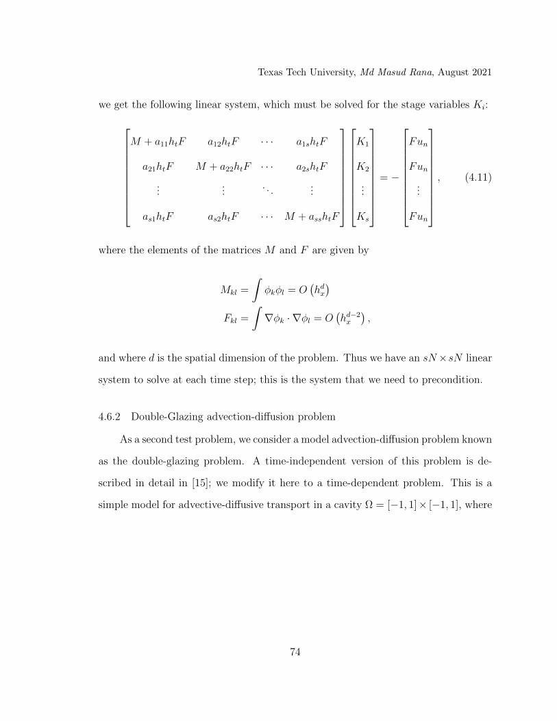
Texas Tech University, Md Masud Rana, August 2021
we get the following linear system, which must be solved for the stage variables Ki:
M + a11htF a12htF · · · a1shtF
a21htF M + a22htF · · · a2shtF
......
. . ....
as1htF as2htF · · · M + asshtF
K1
K2
...
Ks
= −
Fun
Fun
...
Fun
, (4.11)
where the elements of the matrices M and F are given by
Mkl =
∫φkφl = O
(hdx)
Fkl =
∫∇φk · ∇φl = O
(hd−2x
),
and where d is the spatial dimension of the problem. Thus we have an sN×sN linear
system to solve at each time step; this is the system that we need to precondition.
4.6.2 Double-Glazing advection-diffusion problem
As a second test problem, we consider a model advection-diffusion problem known
as the double-glazing problem. A time-independent version of this problem is de-
scribed in detail in [15]; we modify it here to a time-dependent problem. This is a
simple model for advective-diffusive transport in a cavity Ω = [−1, 1]× [−1, 1], where
74

Texas Tech University, Md Masud Rana, August 2021
one wall is hot. The equation and boundary conditions are
ut + (w · ∇)u− ε∇2u = 0 in Ω× [0, T ]
u = 0 on ∂ΩN ∪ ∂ΩW ∪ ∂ΩS
u = 1 on ∂ΩE
u(x, 0) = u0(x),
(4.12)
where ε > 0 and ∂ΩN , ∂ΩW , ∂ΩS and ∂ΩE are the North, West, South, and East
walls of Ω. For initial conditions we take u0(x) = 0 on Ω\∂ΩE; the solution evolves
towards the steady solution described in [15]. The transport is advection dominated
when ε 1 and diffusion dominated when ε & 1. For the wind w(x), we use the
circulating interior flow described in [15]. As before, we discretize in time using an
IRK method then convert the resulting time-independent PDEs to weak form and
discretize in space using stabilized finite elements. This results in a linear system for
the stage variables Ki of the same structural form as (4.11).
4.7 Block Preconditioning IRK Methods for Parabolic PDEs
In this section, we develop a block upper triangular preconditioner and a block
lower triangular preconditioner for systems of the form (4.11).
Let A be the s-stage IRK coefficient matrix, that is, the matrix comprising the
75

Texas Tech University, Md Masud Rana, August 2021
elements in the upper-right block of the Butcher table for the given IRK method:
A =
a11 a12 · · · a1s
a21 a22 · · · a2s
......
. . ....
as1 as2 · · · ass
.
Given an m × n matrix B and a matrix C, recall that their Kronecker product
B ⊗ C is given by
B ⊗ C =
b11C b12C · · · b1nC
b21C b22C · · · b2nC
......
. . ....
bm1C bm2C · · · bmnC
.
Using this notation, we can write the block matrix (4.11) arising from the FEM
discretization as
A = Is ⊗M + htA⊗ F,
where Is is the s× s identity matrix.
In this paper, we consider several block preconditioners P of the general form
P = Is ⊗M + htA⊗ F, (4.13)
where A is either a diagonal or triangular matrix referred as the preconditioner coef-
ficient matrix. We can, for example, define a block Jacobi preconditioner PJ and a
76

Texas Tech University, Md Masud Rana, August 2021
block Gauss–Seidel preconditioner PGSL using this notation as follows:
PJ = Is ⊗M + htAJ ⊗ F
PGSL = Is ⊗M + htAGSL ⊗ F,(4.14)
where AJ is the diagonal part of A and AGSL is the lower triangular part of A. These
preconditioners and their order optimality have been extensively studied in Mardal
et al. [39] and in G.A. Staff et al. [53]. We now introduce two new LDU -based block
triangular preconditioners for A.
4.7.1 LDU-based block triangular preconditioners
It has been shown in [53] that if all blocks of A are well preconditioned by a
preconditioner P of the form (4.13), then all of the eigenvalues of the preconditioned
system will be clustered, and the condition number of the preconditioned system can
be approximated by κ(P−1A) ≈ κ(A−1A
), where A is the preconditioner coefficient
matrix. In other words, if we make A an effective preconditioner for the Butcher
coefficient matrix A, then P can be expected to be an effective (left) preconditioner
for the system A. (In practice, we use the same motivation in developing left and
right preconditioners.) We begin, therefore, by preconditioning A.
For the development of our preconditioners, we assume that the IRK coefficient
matrix A is invertible and has nonsingular leading principal submatrices. It is proven
in [21] that the Butcher coefficient matrices for Gauss–Legendre, Radau IA, Radau
IIA, and Lobatto IIIC are nonsingular for all s. We have confirmed that the lead-
ing principal submatrices are all nonsingular for the coefficient matrices arising from
Gauss–Legendre, Lobatto IIIC, Radau IA, and Radau IIA IRK methods for all stages
77

Texas Tech University, Md Masud Rana, August 2021
that we use in this paper: s = 2 through s = 7. Given these conditions, A can be fac-
tored into A = LDU without pivoting. We compute formally the LDU factorization
A = LDU without pivoting
a11 a12 · · · a1s
a21 a22 · · · a2s
......
. . ....
as1 as2 · · · ass
=
1
l21 1
......
. . .
ls1 ls2 · · · 1
d11
d22
. . .
dss
1 u12 · · · u1s
1 · · · u2s
. . ....
1
and consider ADU = DU and ALD = LD as preconditioners for A. Since A = LDU ,
we have
A = LDU
A(DU)−1 = L
and
(LD)−1A = U.
The eigenvalues of U and L are all one, thus we expect ADU to be a good right
preconditioner and ALD to be a good left preconditioner for A. Since the eigenvalues
(though not the condition numbers) of the product of two matrices do not depend on
the order of the product, we consider both matrices as left and right preconditioners
in our numerical experiments.
Using the condition number motivation from [53], we now define block upper and
78

Texas Tech University, Md Masud Rana, August 2021
lower triangular preconditioners for A of the form:
PDU = Is ⊗M + htADU ⊗ F
PLD = Is ⊗M + htALD ⊗ F.(4.15)
4.7.2 Application of the preconditioners
Applying the block Jacobi preconditioner PJ to a vector v is straightforward,
and for an s-stage IRK scheme involves s subsolves. The subsolve for the jth block
has the form (M + htAjjF
)wj = vj.
In practice and for efficiency, we use a single algebraic multigrid (AMG) V-cycle for
each subsolve for the block wj.
Application of the block upper triangular preconditioner PDU is done via back
substitution and again involves s subsolves. The subsolve on the jth block in this
case is of the form
(M + htAjjF
)wj =
[vj −
s∑k=j+1
htAjkFwk
].
In practice, we again use a single AMG V-cycle for each subsolve.
Application of the block lower triangular preconditioners PGSL and PLD is done
via forward substitution and again involves s subsolves. The subsolves on the jth
block in this case are of the form
(M + htAjjF
)wj =
[vj −
j−1∑k=1
htAjkFwk
].
79

Texas Tech University, Md Masud Rana, August 2021
As with the previous preconditioners, we use a single AMG V-cycle for each subsolve.
4.7.3 Analysis of the preconditioners
The preconditioners have been chosen because of their intended effect on the
condition number of the preconditioned system. Although, as expected, the condition
number is not always a good indicator of performance for GMRES. In Table 4.2, we
examine the 2-norm condition number for the unpreconditioned system A and for A
preconditioned on the right by PJ , PGSL, PDU , and PLD. The system A is from a
2D heat equation using an s-stage Radau IIA IRK method for s ranging from 2 to
7. In all of these results, we have chosen hx = 2−3 and ht = hp+12s−1x , where p = 2 is
the degree of the Lagrange polynomial basis functions in space. The preconditioners
are constructed exactly. All of the preconditioners significantly reduce the condition
number, with PGSL and PLD giving the most improvement. PGSL gives the greatest
improvement on the condition number for the lower-order stages s = 2 and s = 3,
and PLD gives the greatest improvement for the higher-order stages s = 3 through
s = 7.
Table 4.2. Condition numbers of right-preconditioned matrices with preconditionersP−1J , P−1
GSL, P−1DU , and P−1
LD applied to a 2D heat equation with s-stage Radau IIA
methods. Here, hx = 2−3 and ht = hp+12s−1x , where p = 2 is the degree of the Lagrange
polynomial basis functions in space. Preconditioners are constructed exactly.
s κ(A) κ(AP−1J ) κ(AP−1
GSL) κ(AP−1DU) κ(AP−1
LD)
2 240.37 3.23 1.75 5.32 2.483 502.53 5.66 2.58 11.18 2.664 746.23 8.54 3.63 18.23 3.045 959.16 11.76 5.08 26.53 3.216 1137.24 15.23 7.13 35.97 3.507 1281.47 18.90 10.05 46.48 3.67
80

Texas Tech University, Md Masud Rana, August 2021
In Table 4.3, we examine the 2-norm condition number for the unpreconditioned
system A arising from the double-glazing problem, for A preconditioned on the left
by PGSL and PLD, and for A preconditioned on the right by PGSL and PLD. We have
set ε = 0.005, which corresponds to a weakly advection-dominated problem. We are
using an s-stage Radau IIA IRK method for s ranging from 2 to 7. In all of these
results, we have chosen hx = 2−4 and ht = hp+12s−1x , where p = 1 is the degree of the
Lagrange polynomial basis functions in space. The preconditioners are constructed
exactly. As with the heat problem, both of the preconditioners significantly reduce the
condition number. In this table, we omit results for the block Jacobi preconditioner
and our upper triangular preconditioner since, as in the heat test problem, these did
not perform as well as PGSL and PLD. The PLD preconditioner applied on the right
gives greater improvement than PGSL applied on the right for the higher-order stages
s = 4 through s = 7. PLD applied on the left gives the greatest improvement in
condition number for all stages.
Table 4.3. Condition numbers of left-preconditioned and right-preconditioned matri-ces with preconditioners P−1
GSL and P−1LD applied to a 2D double-glazing problem with
ε = 0.005, and with s-stage Radau IIA methods. Here, hx = 2−4 and ht = hp+12s−1x ,
where p = 1 is the degree of the Lagrange polynomial basis functions in space. Pre-conditioners are constructed exactly.
κ(P−1A) κ(AP−1)
s κ(A) κ(P−1GSLA) κ(P−1
LDA) κ(AP−1GSL) κ(AP−1
LD)
2 631.32 1.67 1.26 1.73 2.403 1237.60 2.67 1.53 2.51 2.574 1802.02 4.14 1.80 3.54 2.925 2310.65 6.47 2.05 4.92 3.076 2762.17 10.23 2.25 6.83 3.327 3155.26 16.30 2.44 9.55 3.46
81

Texas Tech University, Md Masud Rana, August 2021
With GMRES, the condition number does not always tell the whole story, and it
is also important to consider how well the preconditioner clusters the eigenvalues. In
Figures 4.2 and 4.3, we show eigenvalues plotted in the complex plane for the matrix
A and preconditioned systems. In Figure 4.2 the matrix A is from the 2D heat
problem and this system is right preconditioned with PJ , PGSL, PDU , and PLD. In
Figure 4.3, A is from the 2D double-glazing problem with ε = 0.005 and this system
is left preconditioned with PGSL and PLD. In both figures, we are using an s-stage
Radau IIA IRK method for s ranging from 2 to 5, and we have again chosen hx = 2−3
and ht = hp+12s−1x , where p is the degree of the Lagrange polynomial basis functions in
space; p = 2 for the heat problem and p = 1 for the double-glazing problem. The
preconditioners are constructed exactly. In both cases, the original matrix A has a
number of eigenvalues very near zero. All of the preconditioners succeed in clustering
the eigenvalues farther away from zero. In the heat problem with s = 2, PGSL and
PLD give the tightest clustering and have very similar eigenvalues. But as s increases,
PLD maintains tighter clustering than PGSL. This fact is reflected in our numerical
results presented in the next section. In the double-glazing problem, the original
matrix A also has a number of eigenvalues very near zero. In this problem, both
preconditioners cluster the eigenvalues farther from zero. Our PLD preconditioner
gives the tightest clustering for all stages s.
4.7.4 Comparison between PGSL with optimal coefficients and PLD preconditioners
In G.A. Staff et al. [53], the authors develop an optimal block lower triangular
Gauss–Seidel preconditioner. This block Gauss–Seidel preconditioner is derived such
that the preconditioner coefficients AGSL are computed from the following optimiza-
82

Texas Tech University, Md Masud Rana, August 2021
(a) (b)
(c) (d)
Figure 4.2. Eigenvalues of the matrices A, AP−1J , AP−1
GSL, AP−1DU , and AP−1
LD for2D heat problem with Radau IIA s = 2 (a), s = 3 (b), s = 4 (c), and s = 5 (d).The x-axis is the real part and the y-axis is the imaginary part of the eigenvalue.Preconditioners are constructed exactly.
tion problem
minAGSL
κ(A−1GSLA)
s.t. diag (AGSL) = diag (A).
(4.16)
That is, their optimal preconditioner, which we will refer to as PGSL, uses coefficients
that optimize the condition number of the (left) preconditioned system for a block
lower triangular matrix subject to the constraint that the diagonal entries are the
83

Texas Tech University, Md Masud Rana, August 2021
(a) (b)
(c) (d)
Figure 4.3. Eigenvalues of the matrices A, P−1GSLA, and P−1
LDA for 2D double-glazingproblem with ε = 0.005, and with Radau IIA s = 2 (a), s = 3 (b), s = 4 (c), ands = 5 (d). The x-axis is the real part and the y-axis is the imaginary part of theeigenvalue. Preconditioners are constructed exactly.
same as those in the Butcher matrix A.
In Table 4.4, we examine the 2-norm condition number for A left preconditioned
by PGSL and PLD for 1D and 2D heat problems. For PGSL, we use the optimized
AGSL coefficients given in [53]. We fix hx = 2−3 and ht = hp+1q
x , where p = 2 is the
degree of the Lagrange polynomial basis functions in space and q is the order of the
corresponding IRK method (that is, q = 2s − 1 for Radau IIA and q = 2s − 2 for
Lobatto IIIC). We use Radau IIA with s = 2 through s = 6 and Lobatto IIIC with s =
84

Texas Tech University, Md Masud Rana, August 2021
2 through s = 4. For the Lobatto IIIC problems, we see that PGSL consistently yields
a lower condition number than PLD for all stages s. For the Radau IIA problems,
however, the PLD preconditioner yields a lower condition number than the optimized
preconditioner PGSL for all stages s. In [53], the authors comment that they may not
obtain the global minimum to (4.16) with the optimization process they use. This may
indeed be true in some of their results, but is not the only issue. Their optimization
is subject to the constraint diag (AGSL) = diag (A). Thus they are not optimizing
over all lower triangular preconditioners, but rather over an affine subspace of the set
of all possible lower triangular preconditioners. The values used in PLD, which have
different diagonal elements, give a lower condition number in the Radau IIA case.
Table 4.4. Condition numbers of the left-preconditioned system with preconditionersPGSL (PGSL with optimal coefficients) and PLD for various IRK methods applied
to 1D and 2D heat problems. Here, hx = 2−3 and ht = hp+1q
x , where p = 2 is thedegree of the Lagrange polynomial in space and q is the order of the correspondingIRK method (that is, q = 2s − 1 for Radau IIA and q = 2s − 2 for Lobatto IIIC).Preconditioners are constructed exactly.
1D 2D
κ(P−1GSLA) κ(P−1
LDA) κ(P−1GSLA) κ(P−1
LDA)
R IIA 2 1.58 1.26 1.60 1.26R IIA 3 1.94 1.50 1.93 1.52R IIA 4 2.18 1.74 2.17 1.77R IIA 5 2.37 1.95 2.40 1.98R IIA 6 3.01 2.14 3.18 2.18
L IIIC 2 1.48 2.68 1.54 2.78L IIIC 3 3.20 6.68 3.32 6.94L IIIC 4 4.92 10.43 5.24 10.93
Again we note that for GMRES, a lower condition number does not always
indicate a superior preconditioner. In Figures 4.4 and 4.5 we see that PLD more
85

Texas Tech University, Md Masud Rana, August 2021
effectively clusters the eigenvalues for both Radau IIA and Lobatto IIIC for stages
s = 2, 3, 4 and 5.
(a) (b)
(c) (d)
Figure 4.4. Eigenvalues of the matrix A, AP−1GSL, and AP−1
LD for 2D heat problemwith Radau IIA s = 2 (a), s = 3 (b), s = 4 (c), and s = 5 (d). The x-axis is thereal part and the y-axis is the imaginary part of the eigenvalue. Preconditioners areconstructed exactly.
4.8 Numerical Experiments
To test the performance of our preconditioners we consider the two model prob-
lems described in Section 4.6: a 2D heat equation problem and the 2D advection-
diffusion double-glazing problem. For both we use s-stage Radau IIA or Lobatto
86

Texas Tech University, Md Masud Rana, August 2021
(a) (b)
Figure 4.5. Eigenvalues of the matrix A, AP−1GSL, and AP−1
LD for 2D heat problemwith Lobatto IIIC stages s = 3 (a) and s = 4 (b). The x-axis is the real part andthe y-axis is the imaginary part of the eigenvalue. Preconditioners are constructedexactly.
IIIC methods for time discretization. For the heat equation we discretize in space
using Galerkin finite elements with piecewise quadratic basis functions on triangular
meshes. For the double-glazing problem we use streamwise upwind Petrov-Galerkin
discretization [15] with piecewise linear basis functions, again on triangular meshes.
Dirichlet boundary conditions are imposed using Nitsche’s method [54, 31].
Production of the finite element matrices is carried out with the Sundance finite
element toolkit [37]. The method of manufactured solutions is used to produce an
exact solution to each linear subproblem so that we can check the error in addition
to the residual.
A common practice in analysis of methods for spatiotemporal problems is to
choose ht ∼ hx and increase the polynomial order of spatial discretization in lockstep
with the order of time discretization. Here, we use a different approach. We use
low-order elements (p = 1 or p = 2) throughout, and then for each hx we choose a
87

Texas Tech University, Md Masud Rana, August 2021
timestep ht such that the spatial discretization error and temporal global truncation
error are comparable. With a Radau s-stage method, we set hp+1x = h2s−1
t so that the
timestep is ht = hp+12s−1x , and with a Lobatto IIIC method, we set hp+1
x = h2s−2t so that
the timestep is ht = hp+12s−2x . By holding the spatial order p fixed, we are simulating
conditions in which a modeler uses a high order integrator to obtain results of a
specified accuracy with larger timestep and smaller computational cost.
We solve the linear system (4.11) using preconditioned GMRES. We construct
our preconditioners as described in Section 4.7 using one AMG V-cycle for each
subsolve. We use AMG from the IFISS software package [52]. When applied to the
advection-diffusion equation, multilevel algorithms and smoothers must be handled
with care [15]. In these experiments we use the strategy of ensuring that the SUPG
discretization is stabilized on the coarse mesh, and use the smoothed aggregation
smoother from IFISS. All results are computed in MATLAB on a machine with an
Intel Core i7 1.80 GHz (Turbo Boost up to 4.00 GHz) processor and 8.00 GB RAM.
In Section 4.7, we examined condition numbers and eigenvalue distributions for
the preconditioners PJ , PGSL, PGSL, PDU , and PLD applied to the 2D heat equation
(4.10) and the double-glazing advection-diffusion problem (4.12). In this section, we
investigate the convergence performance of our preconditioner compared to the others.
We start with the 2D heat equation (4.10) in Section 4.8.1 and compare iteration
counts and timing results for GMRES preconditioned on the right by PJ , PGSL,
PDU , and PLD for various problem sizes and varying orders of IRK methods. We
then examine the robustness of the PGSL and PLD preconditioners for a fixed spatial
resolution as we vary the time step size. We also compare our preconditioner with the
optimized preconditioner PGSL. We conclude the heat equation results by examining
88

Texas Tech University, Md Masud Rana, August 2021
the relative errors achieved with each of the preconditioners. In Section 4.8.2 we give
iteration count and timing results for the best performing of the preconditioners, PGSL
and PLD, applied to the double-glazing advection-diffusion problem (4.12). As with
the heat equation results, we first compare methods for varying spatial resolutions
and various order IRK methods. We then fix the spatial resolution and compare the
robustness the methods as we vary the time step size.
4.8.1 Heat Equation Results
We first test the performance of the preconditioners PJ , PGSL, PDU , and PLD,
on our 2D heat problem (4.10).
4.8.1.1 Comparison results between PJ , PGSL, PDU , and PLD preconditioners
In Table 4.5 we report iteration counts and timing results for right-preconditioned
GMRES to converge with relative tolerance 1.0× 10⁻⁸ for varying mesh sizes hx and
varying number of stages (varying order). Throughout, all of the triangular precondi-
tioners outperform the block Jacobi preconditioner PJ , as expected. The LDU -based
block upper triangular preconditioner PDU and the block Gauss–Seidel preconditioner
PGSL perform similarly, with PGSL performing slightly better, especially for the higher
stage methods. However, overall, the LDU -based block lower triangular precondi-
tioner PLD performs better than all of the other preconditioners in both iteration
count and timing. For 2-stage Radau IIA, PLD and PGSL have similar performance,
with PLD performing slightly better on the smaller problems and PGSL performing
slightly better on the larger problems. But as the number of stages increases (that
is, with increasing order), the performance of PLD improves over the other precondi-
tioners giving consistently lower iteration counts and timing. For a given number of
89

Texas Tech University, Md Masud Rana, August 2021
stages, all of the triangular preconditioners scale well with problem size, exhibiting
little to no growth in iteration count with increasing problem size. However the PLD
preconditioner has the least increase in cost as the number of stages increases.
We have also tested all four preconditioners for Lobatto IIIC methods. Table
4.6 shows iteration counts and timing results for right-preconditioned GMRES to
converge with a relative tolerance of 1.0× 10⁻⁸ for the 2D heat problem (4.10) using
Lobatto IIIC methods in time and quadratic finite elements in space. For the Lobatto
IIIC methods, the PLD preconditioner outperforms all of the other preconditioners
both in iteration count and timing, with more significant improvements for larger
problems and larger number of stages (higher order).
Because a common time-stepping solution method for (4.10) is an adaptive strat-
egy where the time step increases as the steady-state is approached, we also investigate
the effectiveness of our preconditioner for a fixed spatial resolution while varying the
time step size. In Table 4.7, we report iteration counts and timing results for left
and right-preconditioned GMRES to converge with a relative residual tolerance of
1.0 × 10⁻⁸ for the 2D heat problem with 2-stage and 7-stage Radau IIA methods.
In this table, we have fixed the spatial resolution at h−1x = 128 and we vary the
time step size ht between 0.05 and 5.0. Both the PGSL preconditioner and our PLD
preconditioner are quite robust with respect to varying time step size. Both precon-
ditioners perform very similarly (and robustly) for the lower-order s = 2 method;
for the higher-order s = 7 method, both preconditioners are robust with respect to
the varying time step size, but our PLD preconditioner outperforms PGSL as a left
preconditioner and as a right preconditioner for all values of the time step.
90

Texas Tech University, Md Masud Rana, August 2021
Table 4.5. Iteration counts and elapsed time (times in seconds are shown in paren-theses) for right-preconditioned GMRES to converge with relative residual tolerance1.0 × 10−8 for a 2D heat problem with s-stage Radau IIA methods with precondi-
tioners PJ , PGSL, PDU , and PLD. Here we choose ht = hp+12s−1x , where p = 2 is the
degree of the Lagrange polynomial in space. Preconditioners are approximated usingone AMG V-cycle for each subsolve.
stage h−1x DOF PJ PGSL PDU PLD
s=2
8 450 14 (0.03) 8 (0.01) 7 (0.01) 7 (0.01)16 1922 14 (0.05) 8 (0.02) 7 (0.02) 7 (0.02)32 7938 14 (0.10) 8 (0.06) 7 (0.06) 7 (0.05)64 32,258 14 (0.40) 7 (0.19) 7 (0.19) 7 (0.19)128 130,050 14 (1.48) 7 (0.80) 7 (0.83) 7 (0.82)
s=3
8 675 23 (0.06) 10 (0.05) 10 (0.03) 9 (0.03)16 2883 22 (0.06) 10 (0.03) 10 (0.03) 8 (0.02)32 11,907 21 (0.17) 10 (0.09) 10 (0.08) 8 (0.07)64 48,387 22 (0.67) 9 (0.29) 10 (0.32) 8 (0.26)128 195,075 21 (2.90) 8 (1.12) 9 (1.25) 8 (1.12)
s=4
8 900 32 (0.10) 13 (0.08) 13 (0.07) 10 (0.04)16 3844 31 (0.11) 12 (0.05) 13 (0.05) 10 (0.04)32 15,876 30 (0.31) 12 (0.13) 12 (0.13) 10 (0.12)64 64,516 29 (1.16) 11 (0.47) 12 (0.52) 9 (0.39)128 260,100 27 (5.24) 11 (2.10) 12 (2.29) 9 (1.73)
s=5
8 1125 42 (0.10) 15 (0.08) 16 (0.08) 11 (0.06)16 4805 40 (0.23) 15 (0.08) 16 (0.08) 11 (0.06)32 19,845 39 (0.50) 13 (0.18) 15 (0.20) 11 (0.17)64 80,645 35 (1.80) 13 (0.70) 15 (0.81) 11 (0.61)128 325,125 33 (8.44) 12 (2.98) 14 (3.49) 11 (2.75)
s=6
8 1350 53 (0.15) 18 (0.08) 19 (0.08) 12 (0.04)16 5766 50 (0.31) 17 (0.11) 18 (0.11) 12 (0.08)32 23,814 46 (0.73) 16 (0.27) 18 (0.29) 12 (0.19)64 96,774 42 (2.66) 15 (1.02) 17 (1.14) 12 (0.81)128 390,150 38 (12.13) 14 (4.27) 17 (5.41) 12 (3.56)
s=7
8 1575 62 (0.22) 21 (0.10) 23 (0.10) 13 (0.09)16 6727 57 (0.40) 20 (0.15) 22 (0.16) 13 (0.09)32 27,783 52 (0.98) 19 (0.37) 21 (0.40) 13 (0.26)64 112,903 48 (3.64) 18 (1.49) 20 (1.61) 12 (0.98)128 455,175 44 (17.06) 17 (6.29) 20 (7.24) 12 (4.42)
91

Texas Tech University, Md Masud Rana, August 2021
Table 4.6. Iteration counts and elapsed time (times in seconds are shown in paren-theses) for right-preconditioned GMRES to converge with relative residual tolerance1.0 × 10−8 for a 2D heat problem with s-stage Lobatto IIIC methods with precon-
ditioners PJ , PGSL, PDU , and PLD. Here we choose ht = hp+12s−2x , where p = 2 is the
degree of the Lagrange polynomial in space. Preconditioners are approximated usingone AMG V-cycle for each subsolve.
stage h−1x DOF PJ PGSL PDU PLD
s=2
8 450 17 (0.01) 10 (0.01) 7 (0.03) 7 (0.01)16 1922 18 (0.03) 10 (0.02) 7 (0.02) 8 (0.02)32 7938 19 (0.13) 10 (0.07) 8 (0.06) 8 (0.06)64 32,258 19 (0.47) 10 (0.26) 7 (0.19) 8 (0.22)128 130,050 18 (2.19) 10 (1.21) 7 (0.86) 8 (1.00)
s=3
8 675 27 (0.05) 12 (0.03) 11 (0.02) 10 (0.02)16 2883 29 (0.07) 12 (0.03) 11 (0.03) 10 (0.03)32 11,907 27 (0.22) 12 (0.10) 11 (0.10) 10 (0.08)64 48,387 29 (0.96) 11 (0.36) 11 (0.34) 10 (0.35)128 195,075 27 (3.89) 11 (1.54) 10 (1.41) 9 (1.27)
s=4
8 900 40 (0.07) 16 (0.05) 15 (0.05) 12 (0.05)16 3844 40 (0.14) 15 (0.06) 15 (0.06) 12 (0.05)32 15,876 39 (0.41) 14 (0.15) 14 (0.15) 12 (0.13)64 64,516 38 (1.58) 14 (0.60) 13 (0.57) 11 (0.47)128 260,100 37 (7.58) 13 (2.46) 13 (2.44) 11 (2.06)
s=5
8 1125 55 (0.08) 19 (0.03) 19 (0.03) 13 (0.02)16 4805 55 (0.26) 18 (0.09) 18 (0.08) 13 (0.07)32 19,845 51 (0.57) 17 (0.20) 17 (0.22) 13 (0.16)64 80,645 49 (2.61) 16 (0.85) 16 (0.84) 12 (0.64)128 325,125 45 (12.01) 15 (3.64) 15 (3.69) 12 (2.96)
4.8.1.2 Comparison results between PGSL with optimal coefficients and PLD
preconditioners
In this section we compare our LDU -based block lower triangular preconditioner
PLD with the optimal block lower triangular Gauss–Seidel preconditioner introduced
in [53]. PGSL was developed using coefficients optimized to reduce the condition
92

Texas Tech University, Md Masud Rana, August 2021
Table 4.7. Iteration counts and elapsed time (times in seconds are shown in parenthe-ses) for left-preconditioned and right-preconditioned GMRES to converge with pre-conditioned relative residual tolerance 1.0× 10⁻⁸ for a 2D heat problem with s-stageRadau IIA methods with preconditioners PGSL and PLD. Here we keep h−1
x = 128fixed and vary ht from 0.05 to 5.0. Preconditioners are approximated using one AMGV-cycle for each subsolve.
left prec. GMRES right prec. GMRES
stage ht PGSL PLD PGSL PLD
s = 2
0.05 8 (0.85) 7 (0.71) 7 (0.63) 7 (0.63)0.1 8 (0.78) 7 (0.73) 6 (0.55) 7 (0.63)0.5 7 (0.74) 7 (0.71) 6 (0.56) 7 (0.63)1.0 7 (0.70) 7 (0.70) 6 (0.56) 7 (0.64)5.0 7 (0.72) 8 (0.78) 7 (0.63) 7 (0.65)
s = 7
0.05 24 (7.38) 14 (4.24) 19 (5.43) 12 (3.49)0.1 24 (7.76) 14 (4.53) 18 (5.62) 12 (3.70)0.5 23 (7.42) 14 (4.49) 17 (5.34) 13 (4.05)1.0 23 (6.77) 14 (4.56) 17 (4.89) 13 (4.00)5.0 21 (6.74) 15 (4.93) 18 (5.64) 13 (4.17)
number of the left-preconditioned system P−1GSLA.
In Table 4.8, we present results similar to those in Table 4.5. The problem set
up is the same, but here we use left preconditioning for all of the preconditioners
since the coefficients of PGSL were optimized for left preconditioning, and we include
an additional column for PGSL. The first thing we note is that although the idea of
optimizing coefficients to reduce the condition number of the preconditioned system
is a perfectly sensible idea, for this problem the unoptimized PGSL performs better
than the optimized PGSL except on the smallest problems. For all numbers of stages,
PGSL performs better than PGSL for problems sizes h−1x = 32, 64, and 128. We
observe in this table that our PLD has the best performance overall. Although it
performs slightly worse as a left preconditioner than it did in Table 4.5 as a right
93

Texas Tech University, Md Masud Rana, August 2021
Table 4.8. Iteration counts and elapsed time (times in seconds are shown in parenthe-ses) for left-preconditioned GMRES to converge with preconditioned relative residualtolerance 1.0×10⁻⁸ for a 2D heat problem with s-stage Radau IIA methods with pre-
conditioners PJ , PGSL, PGSL, PDU , and PLD. Here we choose ht = hp+12s−1x , where p = 2
is the degree of the Lagrange polynomial in space. Preconditioners are approximatedusing one AMG V-cycle for each subsolve.
stage h−1x DOF PJ PGSL PGSL PDU PLD
s=2
8 450 14 (0.02) 9 (0.02) 9 (0.01) 7 (0.01) 7 (0.01)16 1922 16 (0.03) 9 (0.02) 10 (0.02) 8 (0.02) 7 (0.02)32 7938 16 (0.10) 9 (0.06) 10 (0.06) 8 (0.05) 7 (0.05)64 32,258 17 (0.38) 9 (0.24) 10 (0.27) 8 (0.23) 7 (0.21)128 130,050 18 (2.01) 9 (1.16) 10 (1.24) 8 (1.03) 7 (0.94)
s=3
8 675 23 (0.06) 11 (0.04) 13 (0.03) 10 (0.04) 9 (0.03)16 2883 25 (0.05) 12 (0.03) 13 (0.03) 11 (0.03) 9 (0.02)32 11,907 25 (0.20) 12 (0.09) 14 (0.10) 11 (0.08) 9 (0.07)64 48,387 27 (0.77) 12 (0.36) 14 (0.43) 11 (0.34) 9 (0.31)128 195,075 28 (3.65) 12 (1.65) 14 (1.91) 11 (1.56) 9 (1.32)
s=4
8 900 32 (0.07) 15 (0.06) 18 (0.05) 14 (0.06) 11 (0.04)16 3844 34 (0.13) 15 (0.06) 19 (0.07) 14 (0.06) 11 (0.05)32 15,876 36 (0.38) 15 (0.17) 19 (0.21) 14 (0.16) 11 (0.13)64 64,516 36 (1.52) 15 (0.70) 19 (0.84) 14 (0.64) 11 (0.51)128 260,100 36 (6.51) 15 (2.88) 19 (3.63) 14 (2.74) 11 (2.20)
s=5
8 1125 44 (0.11) 18 (0.08) 22 (0.06) 17 (0.07) 12 (0.06)16 4805 45 (0.21) 18 (0.08) 22 (0.10) 17 (0.08) 12 (0.06)32 19,845 46 (0.61) 18 (0.26) 22 (0.28) 17 (0.23) 12 (0.17)64 80,645 47 (2.21) 18 (0.90) 22 (1.18) 17 (0.93) 12 (0.74)128 325,125 47 (11.15) 18 (4.41) 22 (5.45) 17 (4.26) 12 (3.00)
s=6
8 1350 55 (0.14) 22 (0.08) 24 (0.07) 20 (0.07) 13 (0.04)16 5766 55 (0.32) 22 (0.14) 24 (0.16) 21 (0.14) 14 (0.09)32 23,814 56 (0.93) 22 (0.38) 24 (0.40) 20 (0.34) 14 (0.24)64 96,774 56 (3.77) 21 (1.49) 24 (1.69) 20 (1.42) 13 (0.94)128 390,150 56 (15.89) 21 (6.21) 23 (6.89) 20 (5.63) 13 (3.98)
preconditioner, it nonetheless achieves the lowest iteration count and lowest timing
of all of the preconditioners for all numbers of stages and all problem sizes.
94

Texas Tech University, Md Masud Rana, August 2021
In Table 4.9, we present results similar to those in Table 4.8 but using Lobatto
IIIC methods. The problem set up is again the same, using left preconditioning for all
of the preconditioners. The results are very similar to those in the previous table. The
unoptimized PGSL performs better than the optimized PGSL on all of these problems.
Our PLD preconditioner has the best performance overall.
Table 4.9. Iteration counts and elapsed time (times in seconds are shown in parenthe-ses) for left-preconditioned GMRES to converge with preconditioned relative residualtolerance 1.0× 10⁻⁸ for a 2D heat problem with s-stage Lobatto IIIC methods with
preconditioners PJ , PGSL, PGSL, PDU , and PLD. Here we choose ht = hp+12s−2x , where
p = 2 is the degree of the Lagrange polynomial in space. Preconditioners are approx-imated using one AMG V-cycle for each subsolve.
stage h−1x DOF PJ PGSL PGSL PDU PLD
s=2
8 450 18 (0.02) 11 (0.02) 18 (0.02) 7 (0.02) 8 (0.02)16 1922 20 (0.04) 12 (0.02) 20 (0.03) 8 (0.02) 8 (0.02)32 7938 21 (0.15) 12 (0.09) 21 (0.14) 8 (0.06) 8 (0.06)64 32,258 21 (0.56) 12 (0.34) 21 (0.56) 8 (0.24) 8 (0.23)128 130,050 21 (2.40) 12 (1.49) 21 (2.50) 8 (1.05) 8 (1.05)
s=3
8 675 27 (0.06) 14 (0.04) 25 (0.04) 11 (0.03) 11 (0.03)16 2883 32 (0.08) 14 (0.04) 27 (0.06) 12 (0.03) 11 (0.03)32 11,907 33 (0.23) 15 (0.11) 28 (0.20) 12 (0.09) 11 (0.09)64 48,387 35 (1.06) 15 (0.49) 30 (0.98) 12 (0.40) 11 (0.37)128 195,075 37 (3.89) 15 (1.87) 30 (3.76) 12 (1.67) 11 (1.58)
s=4
8 900 41 (0.09) 18 (0.06) 31 (0.07) 15 (0.06) 13 (0.05)16 3844 44 (0.13) 18 (0.06) 35 (0.11) 16 (0.06) 13 (0.05)32 15,876 46 (0.51) 18 (0.20) 35 (0.38) 16 (0.18) 13 (0.15)64 64,516 49 (2.14) 18 (0.80) 37 (1.66) 16 (0.74) 13 (0.60)128 260,100 49 (8.93) 18 (3.23) 36 (6.60) 16 (3.11) 13 (2.53)
It should be noted that since the results in Tables 4.8 and 4.9 are using left
preconditioning, the relative residuals are actually preconditioned relative residuals.
So the norms of the various preconditioners could be having an effect on the iteration
95

Texas Tech University, Md Masud Rana, August 2021
counts. Since all of our numerical tests were run using the method of manufactured
solutions, in Tables 4.10 and 4.11 we examine the relative errors for each method.
In Table 4.10 we report the relative errors for various numbers of stages for Radau
IIA and Lobatto IIIC with the five preconditioners PJ , PGSL, PGSL, PDU , and PLD
all used as left preconditioners. The problem size is fixed at h−1x = 128, which is the
largest of the problems we considered, and ht = hp+1q
x , where p = 2 is the degree of the
Lagrange polynomial in space and q is the order of the corresponding IRK method
(that is, q = 2s − 1 for Radau IIA and q = 2s − 2 for Lobatto IIIC). The stopping
criteria is the same as in all previous tables. With left preconditioning, problems with
Radau IIA and Lobatto IIIC methods and all numbers of stages yielded very similar
relative errors.
Table 4.10. Relative error for left-preconditioned GMRES converging to a precondi-tioned relative residual tolerance of 1.0 × 10⁻⁸ for a 2D heat problem with variousIRK methods with preconditioners PJ , PGSL, PGSL, PDU , and PLD. Here, hx = 2−7
and ht = hp+1q
x , where p = 2 is the degree of the Lagrange polynomial in space andq is the order of the corresponding IRK method (that is, q = 2s − 1 for Radau IIAand q = 2s− 2 for Lobatto IIIC). Preconditioners are approximated using one AMGV-cycle for each subsolve.
IRK method PJ PGSL PGSL PDU PLDR IIA 2 7.1× 10⁻⁹ 6.1× 10⁻⁹ 1.4× 10⁻⁹ 1.8× 10⁻⁹ 4.0× 10⁻⁹
R IIA 3 8.5× 10⁻⁹ 6.9× 10⁻⁹ 7.9× 10⁻⁹ 9.4× 10⁻⁹ 6.4× 10⁻⁹
R IIA 4 4.6× 10⁻⁸ 8.5× 10⁻⁹ 9.1× 10⁻⁹ 3.8× 10⁻⁸ 2.9× 10⁻⁹
R IIA 5 5.1× 10⁻⁸ 9.0× 10⁻⁹ 8.1× 10⁻⁹ 4.6× 10⁻⁸ 5.4× 10⁻⁹
R IIA 6 7.7× 10⁻⁸ 1.0× 10⁻⁸ 8.3× 10⁻⁹ 9.8× 10⁻⁸ 7.9× 10⁻⁹
L IIIC 2 8.0× 10⁻⁹ 1.8× 10⁻⁹ 8.0× 10⁻⁹ 3.9× 10⁻⁹ 6.6× 10⁻⁹
L IIIC 3 2.0× 10⁻⁸ 6.7× 10⁻⁹ 1.0× 10⁻⁸ 1.8× 10⁻⁸ 1.1× 10⁻⁸
L IIIC 4 5.7× 10⁻⁸ 1.2× 10⁻⁸ 7.9× 10⁻⁹ 2.3× 10⁻⁸ 8.9× 10⁻⁹
In Table 4.11 we report the relative errors for various numbers of stages for Radau
IIA and Lobatto IIIC with the four preconditioners PJ , PGSL, PDU , and PLD this
96
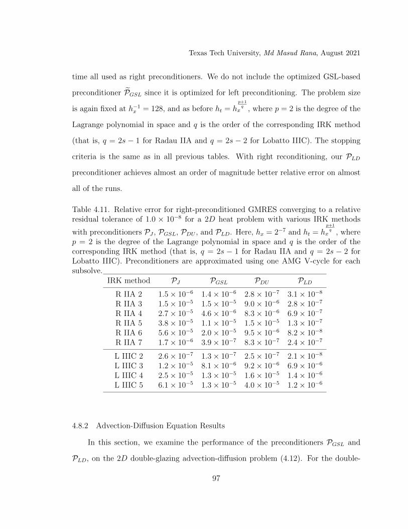
Texas Tech University, Md Masud Rana, August 2021
time all used as right preconditioners. We do not include the optimized GSL-based
preconditioner PGSL since it is optimized for left preconditioning. The problem size
is again fixed at h−1x = 128, and as before ht = h
p+1q
x , where p = 2 is the degree of the
Lagrange polynomial in space and q is the order of the corresponding IRK method
(that is, q = 2s − 1 for Radau IIA and q = 2s − 2 for Lobatto IIIC). The stopping
criteria is the same as in all previous tables. With right reconditioning, our PLD
preconditioner achieves almost an order of magnitude better relative error on almost
all of the runs.
Table 4.11. Relative error for right-preconditioned GMRES converging to a relativeresidual tolerance of 1.0 × 10⁻⁸ for a 2D heat problem with various IRK methods
with preconditioners PJ , PGSL, PDU , and PLD. Here, hx = 2−7 and ht = hp+1q
x , wherep = 2 is the degree of the Lagrange polynomial in space and q is the order of thecorresponding IRK method (that is, q = 2s − 1 for Radau IIA and q = 2s − 2 forLobatto IIIC). Preconditioners are approximated using one AMG V-cycle for eachsubsolve.
IRK method PJ PGSL PDU PLDR IIA 2 1.5× 10⁻⁶ 1.4× 10⁻⁶ 2.8× 10⁻⁷ 3.1× 10⁻⁸
R IIA 3 1.5× 10⁻⁵ 1.5× 10⁻⁵ 9.0× 10⁻⁶ 2.8× 10⁻⁷
R IIA 4 2.7× 10⁻⁵ 4.6× 10⁻⁶ 8.3× 10⁻⁶ 6.9× 10⁻⁷
R IIA 5 3.8× 10⁻⁵ 1.1× 10⁻⁵ 1.5× 10⁻⁵ 1.3× 10⁻⁷
R IIA 6 5.6× 10⁻⁵ 2.0× 10⁻⁵ 9.5× 10⁻⁶ 8.2× 10⁻⁸
R IIA 7 1.7× 10⁻⁶ 3.9× 10⁻⁷ 8.3× 10⁻⁷ 2.4× 10⁻⁷
L IIIC 2 2.6× 10⁻⁷ 1.3× 10⁻⁷ 2.5× 10⁻⁷ 2.1× 10⁻⁸
L IIIC 3 1.2× 10⁻⁵ 8.1× 10⁻⁶ 9.2× 10⁻⁶ 6.9× 10⁻⁶
L IIIC 4 2.5× 10⁻⁵ 1.3× 10⁻⁵ 1.6× 10⁻⁵ 1.4× 10⁻⁶
L IIIC 5 6.1× 10⁻⁵ 1.3× 10⁻⁵ 4.0× 10⁻⁵ 1.2× 10⁻⁶
4.8.2 Advection-Diffusion Equation Results
In this section, we examine the performance of the preconditioners PGSL and
PLD, on the 2D double-glazing advection-diffusion problem (4.12). For the double-
97

Texas Tech University, Md Masud Rana, August 2021
glazing problem, we only present results for the PGSL and PLD preconditioners since
in all of our previous experiments they performed best. We apply both as left precon-
ditioners in these results, but our results are similar when they are applied as right
preconditioners.
In Table 4.12, we report iteration counts and elapsed time for left-preconditioned
GMRES to converge with preconditioned relative residual tolerance 1.0×10⁻⁸ for the
double-glazing problem (4.12) with s-stage Radau IIA methods using the precondi-
tioners PGSL and PLD. We vary the number of stages from s = 2 to s = 7 for problems
with spatial resolution h−1x = 64 and 128. Here we choose ht = h
p+12s−1x , where p = 1
is the degree of the Lagrange polynomial in space. We present results for ε = 0.04,
which is diffusion dominated and ε = 0.005, which is weakly advection dominated.
Preconditioners are approximated using one AMG V-cycle for each subsolve.
For the lowest-order problems with s = 2, PGSL and our PLD preconditioner
perform similarly. For the diffusion dominated problem, ε = 0.04, PLD outperforms
PGSL for all of the higher-order problems, s = 3 through s = 7, with the improved
performance being more pronounced on the highest-order problems. For the weakly
advection-dominated problem, ε = 0.005, the results are more mixed. For the smaller
problems of each order, h−1x = 64, PLD takes fewer iterations in most cases, but takes
longer in compute time in a few cases. For the largest higher-order problems, s = 4
through s = 7 with h−1x = 128, PLD performs better than PGSL in both iteration
count and timing.
As we did for the heat equation, in Table 4.13, we investigate the robustness of the
preconditioners for a fixed spatial resolution while varying the time step size. In this
table, we present iteration counts and timing results for left-preconditioned GMRES
98

Texas Tech University, Md Masud Rana, August 2021
Table 4.12. Iteration counts and elapsed time (times in seconds are shown in parenthe-ses) for left-preconditioned GMRES to converge with preconditioned relative residualtolerance 1.0× 10⁻⁸ for the double-glazing problem with s-stage Radau IIA methods
with preconditioners PGSL and PLD. Here we choose ht = hp+12s−1x , where p = 1 is the
degree of the Lagrange polynomial in space. Preconditioners are approximated usingone AMG V-cycle for each subsolve.
ε = 0.04 ε = 0.005
stage h−1x ht DOF PGSL PLD PGSL PLD
s = 264 0.0625 33282 9 (0.50) 7 (0.43) 11 (0.89) 11 (0.83)128 0.0394 132098 9 (1.72) 7 (1.44) 10 (3.74) 10 (3.84)
s = 364 0.1895 49923 14 (1.13) 10 (0.84) 17 (1.92) 16 (1.83)128 0.1436 198147 14 (3.96) 9 (2.73) 15 (8.23) 14 (9.71)
s = 464 0.3048 66564 18 (1.95) 12 (1.28) 22 (3.22) 21 (3.04)128 0.25 264196 18 (6.47) 11 (4.44) 20 (16.83) 17 (15.17)
s = 564 0.3969 83205 22 (2.62) 13 (1.58) 26 (4.54) 25 (4.29)128 0.3402 330245 22 (10.38) 13 (6.45) 25 (22.75) 21 (22.33)
s = 664 0.4695 99846 25 (3.94) 14 (2.33) 31 (6.34) 28 (6.51)128 0.4139 396294 27 (15.84) 14 (10.59) 30 (34.10) 23 (33.38)
s = 764 0.5274 116487 30 (5.39) 16 (2.81) 36 (8.53) 30 (9.04)128 0.4740 462343 31 (20.89) 15 (10.34) 36 (55.84) 25 (36.33)
to converge with a preconditioned relative residual tolerance of 1.0× 10⁻⁸ for the 2D
double-glazing problem with s-stage Radau IIA methods using the preconditioners
PGSL and PLD. We present results for a lower-order method s = 2 and a higher-order
method s = 7 and for ε = 0.04, which is diffusion dominated, and ε = 0.005, which
is weakly advection dominated. In this table, we keep h−1x = 128 fixed and vary the
time step size ht from 0.05 to 5.0. Preconditioners are approximated using one AMG
V-cycle for each subsolve.
For the diffusion-dominated problem with the lower-order method, our PLD pre-
99

Texas Tech University, Md Masud Rana, August 2021
conditioner mildly outperforms PGSL for all time step sizes, and both preconditioners
are robust with respect to varying the time step size. For the higher-order method,
both preconditioners take more iterations and more time as the step size increases,
but PLD grows less dramatically than PGSL and takes fewer iterations and less time
for all time step sizes.
For the weakly advection-dominated problem, ε = 0.005, PLD performs very
similarly to PGSL on the lower-order problem, s = 2, and both preconditioners are
robust with respect to the varying time step size. For the higher-order method, both
preconditioners take more iterations and more time as the step size increases, but
PLD grows much less dramatically than PGSL and takes fewer iterations and less time
for all time step sizes.
Table 4.13. Iteration counts and elapsed time (times in seconds are shown in parenthe-ses) for left-preconditioned GMRES to converge with preconditioned relative residualtolerance 1.0× 10⁻⁸ for a 2D double-glazing problem with s-stage Radau IIA meth-ods with preconditioners PGSL and PLD. Here we keep h−1
x = 128 fixed and vary htfrom 0.05 to 5.0. Preconditioners are approximated using one AMG V-cycle for eachsubsolve.
ε = 0.04 ε = 0.005
stage ht PGSL PLD PGSL PLD
s = 2
0.05 9 (1.85) 7 (1.50) 11 (3.95) 10 (4.12)0.1 10 (1.96) 7 (1.43) 11 (4.24) 11 (5.01)0.5 11 (2.05) 8 (1.76) 12 (4.64) 11 (4.64)1.0 10 (2.08) 7 (1.47) 13 (4.76) 11 (4.72)5.0 10 (1.95) 8 (1.69) 12 (5.63) 12 (5.43)
s = 7
0.05 26 (18.39) 13 (9.78) 27 (41.80) 18 (28.56)0.1 27 (22.09) 14 (9.80) 28 (43.18) 21 (29.72)0.5 32 (24.97) 15 (12.29) 36 (53.60) 25 (40.76)1.0 37 (30.81) 17 (13.88) 45 (76.24) 26 (36.33)5.0 46 (35.33) 20 (16.14) 68 (109.26) 28 (36.66)
100

Texas Tech University, Md Masud Rana, August 2021
4.9 Discussion
In this chapter, we have introduced a new preconditioner for the large, struc-
tured systems appearing in implicit Runge–Kutta time integration of parabolic PDE
problems. Our preconditioner is based on a block LDU factorization, and for scala-
bility, we have used a single AMG V-cycle on all subsolves. We have compared our
preconditioner PLD in condition number and eigenvalue distribution to other pre-
conditioners, and have demonstrated its effectiveness on two test problems, the heat
equation and the double-glazing advection-diffusion problem. We have found that it
is scalable (hx-independent) and yields better timing results than other precondition-
ers currently in the literature: block Jacobi, block Gauss–Seidel, and the optimized
block Gauss–Seidel method of [53]. It is also robust with respect to varying time step
sizes for a fixed spatial resolution. We ran experiments with implicit Runge–Kutta
stages up to s = 7, and have found that the new preconditioner outperforms the
others, with the improvement becoming more pronounced as spatial discretization is
refined and as temporal order is increased.
101

Texas Tech University, Md Masud Rana, August 2021
CHAPTER 5
CONCLUSION
In this dissertation, we developed population models that include both spatial
heterogeneity and stoichiometry, explored a reduced-order modeling technique to an-
alyze and interpret the huge data sets produced from the simulations of the model,
and proposed preconditioners for high performance computation of the model with
implicit Runge-Kutta methods.
We discussed space-time population models incorporating ecological stoichiome-
try in chapter 2. In section 2.1, we developed a spatially heterogeneous stoichiomet-
ric producer-grazer (algae-Daphnia) model with two grazer genotypes to understand
genotypic selection. We conducted numerical experiments with the model to inves-
tigate selection processes and co-persistence of grazer genotypes under various envi-
ronmental conditions such as varying light level and nutrient availability. Numerical
simulations of our model yield rich dynamics where genotypic selection depends on
depth. We also observed cases where both Daphnia genotypes co-persist at the same
depth at limit cycles and at equilibria. This work has been published in [14].
In section 2.2, we developed a space-time stoichiometric algae-Daphnia model
that explicitly tracks the nutrient content (C and P). We again conducted several
numerical experiments varying light level and nutrient availability. We observed
qualitatively different dynamics than the space-time stoichiometric model that ne-
glects to track nutrient content explicitly. In particular, under certain environmental
conditions, our model predicts stable limit cycles whereas the model that neglects to
explicitly track nutrient content shows stable equilibria. This work has been published
102

Texas Tech University, Md Masud Rana, August 2021
in [46].
In chapter 3, we explored reduced-order modeling to analyze and interpret simu-
lations of the mechanistically derived space-time population model derived in section
2.2. We began this chapter with a description of the Reduced-Order modeling tech-
nique then applied it to the mechanistic model (2.13). We find that the most dominant
behavior of the model dynamics can be captured by five basis vectors. Reduced-order
modeling also allows us to investigate bifurcations of the PDE model for surface light
irradiance.
We began chapter 4 with a discussion on the choice of time-integrator for parabolic
PDEs, and choice of solver and preconditioning technique for the linear system arising
from discretization. We then developed block preconditioners for the block system
arising from implicit Runge-Kutta discretization of parabolic PDEs. Our block pre-
conditioners are based on an LDU−factorization of the IRK coefficient matrix. We
tested the effectiveness of our preconditioners on two test problem: the heat equation
and the advection-diffusion double-glazing problem. Numerical experiments showed
that our LDU -based block lower triangular preconditioner performs better than other
preconditioners currently in the literature. This work has been published in [47].
103

Texas Tech University, Md Masud Rana, August 2021
BIBLIOGRAPHY
[1] P. A. Abrams. The evolution of predator-prey interactions: theory and evidence.Annual Review of Ecology and Systematics, 31(1):79–105, 2000.
[2] T. Andersen. Pelagic nutrient cycles; herbivores as sources and sinks. Springer,Berlin, 1997.
[3] T. Andersen, J. J. Elser, and D. O. Hessen. Stoichiometry and population dy-namics. Ecology Letters, 7(9):884–900, 2004.
[4] U. M. Ascher and L. R. Petzold. Computer methods for ordinary differentialequations and differential-algebraic equations, volume 61. SIAM, 1998.
[5] R. G. Barry and R. J. Chorley. Atmosphere, weather and climate. Routledge,2009.
[6] R. B. Bird, W. E. Stewart, and E. N. Lightfoot. Transport phenomena. 2002.JohnWiley & Sons, New York, 2004.
[7] R. S. Cantrell and C. Cosner. Spatial ecology via reaction-diffusion equations.John Wiley & Sons, 2004.
[8] R. S. Cantrell, C. Cosner, and Y. Lou. Evolution of dispersal in heterogeneouslandscapes. Spatial ecology, pages 213–229, 2010.
[9] S. Cantrell, C. Cosner, and S. Ruan. Spatial ecology. CRC Press, 2010.
[10] E. L. Cussler. Diffusion: Mass Transfer in Fluid Systems. Cambridge UniversityPress, 1996.
[11] G. G. Dahlquist. A special stability problem for linear multistep methods. BITNumerical Mathematics, 3(1):27–43, 1963.
[12] J. W. Demmel. Applied numerical linear algebra. SIAM, 1997.
[13] C. Dissanayake. Finite element simulation of space/time behavior in a two speciesecological stoichiometric model. PhD thesis, Texas Tech University, 2016.
[14] C. Dissanayake, L. Juan, K. R. Long, A. Peace, and M. M. Rana. Genotypicselection in spatially heterogeneous producer-grazer systems subject to stoichio-metric constraints. Bulletin of mathematical biology, 81(11):4726–4742, 2019.
[15] H. Elman, D. Silvester, and A. Wathen. Finite Elements and Fast IterativeSolvers. Oxford University Press, 2005.
104

Texas Tech University, Md Masud Rana, August 2021
[16] J. Elser. Biological stoichiometry: a chemical bridge between ecosystem ecologyand evolutionary biology. The American Naturalist, 168(S6):S25–S35, 2006.
[17] J. Engwer. Partitioned implicit Runge-Kutta timesteppers for micromagneticswith eddy currents. PhD thesis, Texas Tech University, 2018.
[18] M. S. Gockenbach. Partial differential equations: analytical and numerical meth-ods, volume 122. SIAM, 2005.
[19] P. M. Gresho and R. L. Sani. Incompressible flow and the finite element method.Volume 1: Advection-diffusion and isothermal laminar flow. John Wiley andSons, Inc., New York, NY (United States), 1998.
[20] J. P. Grover. Predation, competition, and nutrient recycling: a stoichiometricapproach with multiple nutrients. Journal of theoretical biology, 229(1):31–43,2004.
[21] E. Hairer, S. P. Nørsett, and G. Wanner. Solving Ordinary Differential EquationsI, Nonstiff Problems. Springer Berlin Heidelberg, 1993.
[22] I. Hanski. Incorporating the spatial configuration of the habitat into ecology andevolutionary biology. Spatial Ecology, pages 167–188, 2010.
[23] M. A. Heroux, R. A. Bartlett, V. E. Howle, R. J. Hoekstra, J. J. Hu, T. G. Kolda,R. B. Lehoucq, K. R. Long, R. P. Pawlowski, E. T. Phipps, A. G. Salinger, H. K.Thornquist, R. S. Tuminaro, J. M. Willenbring, A. Williams, and K. S. Stanley.An overview of the trilinos project. ACM Trans. Math. Softw., 31(3):397–423,2005.
[24] D. O. Hessen, J. J. Elser, R. W. Sterner, and J. Urabe. Ecological stoichiometry:An elementary approach using basic principles. Limnol. Oceanogr, 58(6):2219–2236, 2013.
[25] R. D. Holt and M. Barfield. Metapopulation perspectives on the evolution ofspecies niches. Spatial Ecology, page 189, 2010.
[26] J. Huisman, R. R. Jonker, C. Zonneveld, and F. J. Weissing. Competition forlight between phytoplankton species: experimental tests of mechanistic theory.Ecology, 80(1):211–222, 1999.
[27] J. Huisman, J. Sharples, J. M. Stroom, P. M. Visser, W. E. A. Kardinaal, J. M.Verspagen, and B. Sommeijer. Changes in turbulent mixing shift competitionfor light between phytoplankton species. Ecology, 85(11):2960–2970, 2004.
105

Texas Tech University, Md Masud Rana, August 2021
[28] D. M. Imboden and A. Wuest. Mixing mechanisms in lakes. In Physics andchemistry of lakes, pages 83–138. Springer, 1995.
[29] A. Iserles. A first course in the numerical analysis of differential equations.Number 44. Cambridge University Press, 2009.
[30] C. Johnson. Numerical solution of partial differential equations by the finiteelement method. Courier Corporation, 2012.
[31] M. Juntunen and R. Stenberg. Nitsche’s method for general boundary conditions.Mathematics of computation, 78(267):1353–1374, 2009.
[32] A. D. Kay, I. W. Ashton, E. Gorokhova, A. J. Kerkhoff, A. Liess, and E. Litch-man. Toward a stoichiometric framework for evolutionary biology. Oikos,109(1):6–17, 2005.
[33] C. T. Kelley. Solving nonlinear equations with Newton’s method. SIAM, 2003.
[34] J. T. Kirk. Light and photosynthesis in aquatic ecosystems. Cambridge UniversityPress, 1994.
[35] I. Loladze, Y. Kuang, and J. J. Elser. Stoichiometry in producer–grazer sys-tems: linking energy flow with element cycling. Bulletin of Mathematical Biology,62(6):1137–1162, 2000.
[36] I. Loladze, Y. Kuang, J. J. Elser, and W. F. Fagan. Competition and stoichiom-etry: coexistence of two predators on one prey. Theoretical population biology,65(1):1–15, 2004.
[37] K. Long, R. Kirby, and B. van Bloemen Waanders. Unified embedded parallelfinite element computations via software-based Frechet differentiation. SIAMJournal on Scientific Computing, 32(6):3323–3351, 2010.
[38] A. Lorke. Investigation of turbulent mixing in shallow lakes using temperaturemicrostructure measurements. Aquatic Sciences-Research Across Boundaries,60(3):210–219, 1998.
[39] K.-A. Mardal, T. K. Nilssen, and G. A. Staff. Order-optimal preconditionersfor implicit Runge–Kutta schemes applied to parabolic PDEs. SIAM Journal onScientific Computing, 29(1):361–375, 2007.
[40] X. Meng and L. Zhang. Evolutionary dynamics in a lotka–volterra competitionmodel with impulsive periodic disturbance. Mathematical Methods in the AppliedSciences, 39(2):177–188, 2016.
106

Texas Tech University, Md Masud Rana, August 2021
[41] J. A. Metz, R. M. Nisbet, and S. A. Geritz. How should we define ‘fitness’ forgeneral ecological scenarios? Trends in ecology & evolution, 7(6):198–202, 1992.
[42] E. K. Moody, A. T. Rugenski, J. L. Sabo, B. L. Turner, and J. J. Elser. Does thegrowth rate hypothesis apply across temperatures? Variation in the growth rateand body phosphorus of Neotropical benthic grazers. Frontiers in EnvironmentalScience, 5:14, 2017.
[43] A. Peace. Effects of light, nutrients, and food chain length on trophic efficien-cies in simple stoichiometric aquatic food chain models. Ecological Modelling,312:125–135, 2015.
[44] A. Peace, H. Wang, and Y. Kuang. Dynamics of a producer–grazer model incor-porating the effects of excess food nutrient content on grazers growth. Bulletinof mathematical biology, 76(9):2175–2197, 2014.
[45] A. Peace, Y. Zhao, I. Loladze, J. J. Elser, and Y. Kuang. A stoichiometricproducer-grazer model incorporating the effects of excess food-nutrient contenton consumer dynamics. Mathematical biosciences, 2013.
[46] M. M. Rana, C. Dissanayake, L. Juan, K. R. Long, and A. Peace. Mechanisticallyderived spatially heterogeneous producer-grazer model subject to stoichiometricconstraints. Mathematical biosciences and engineering: MBE, 16(1):222–233,2018.
[47] M. M. Rana, V. E. Howle, K. Long, A. Meek, and W. Milestone. A new blockpreconditioner for implicit Runge-Kutta methods for parabolic PDE problems.SIAM Joirnal on Scientific Computing, 2021 (to appear). Preprint available atarXiv:2010.11377.
[48] S. A. Rush. Real-Time Simulation of Fluid Flow Based on Sensor Data UsingODE Constrained Optimization. PhD thesis, Texas Tech University, 2018.
[49] Y. Saad. Iterative methods for sparse linear systems. SIAM, 2003.
[50] M. Sala, K. Stanley, and M. Heroux. Amesos: A set of general interfaces tosparse direct solver libraries. In Proceedings of PARA’06 Conference, Umea,Sweden, 2006.
[51] F. H. Shu. The Physics of Astrophysics, Vol. 2: Radiation. Univ. Sci. Books,Mill Valley, CA, 1991.
[52] D. Silvester, H. Elman, and A. Ramage. Incompressible Flowand Iterative Solver Software (IFISS) version 3.5, September 2016.http://www.manchester.ac.uk/ifiss/.
107

Texas Tech University, Md Masud Rana, August 2021
[53] G. A. Staff, K.-A. Mardal, and T. K. Nilssen. Preconditioning of fully implicitRunge–Kutta schemes for parabolic PDEs. Modeling, Identification and Control,27(2):109–123, 2006.
[54] R. Stenberg. On some techniques for approximating boundary conditions inthe finite element method. Journal of Computational and applied Mathematics,63(1-3):139–148, 1995.
[55] R. W. Sterner and J. J. Elser. Ecological stoichiometry: the biology of elementsfrom molecules to the biosphere. Princeton University Press, 2002.
[56] L. N. Trefethen. Finite difference and spectral methods for ordinary and partialdifferential equations. 1996.
[57] L. N. Trefethen and D. Bau III. Numerical linear algebra. SIAM, 1997.
[58] H. Wang, Y. Kuang, and I. Loladze. Dynamics of a mechanistically derivedstoichiometric producer-grazer model. Journal of Biological Dynamics, 2(3):286–296, 2008.
[59] H. Wang, R. W. Sterner, and J. J. Elser. On the strict homeostasis assumptionin ecological stoichiometry. Ecological Modelling, 243:81–88, 2012.
[60] G. Wanner and E. Hairer. Solving ordinary differential equations II. SpringerBerlin Heidelberg, 1996.
[61] L. J. Weider, W. Makino, K. Acharya, K. L. Glenn, M. Kyle, J. Urabe, and J. J.Elser. Genotype × environment interactions, stoichiometric food quality effects,and clonal coexistence in daphnia pulex. Oecologia, 143(4):537–547, 2005.
[62] F. J. Weissing and J. Huisman. Growth and competition in a light gradient.Journal of theoretical biology, 168(3):323–336, 1994.
[63] M. Yamamichi, C. L. Meunier, A. Peace, C. Prater, and M. A. Rua. Rapidevolution of a consumer stoichiometric trait destabilizes consumer–producer dy-namics. Oikos, 124(7):960–969, 2015.
108