2018 Volume 14 Issues 1-4 - Progress in Physics
238
PROGRESS 2018 Volume 14 “All scientists shall have the right to present their scientific research results, in whole or in part, at relevant scientific conferences, and to publish the same in printed scientific journals, electronic archives, and any other media.” — Declaration of Academic Freedom, Article 8 ISSN 1555-5534 The Journal on Advanced Studies in Theoretical and Experimental Physics, including Related Themes from Mathematics IN PHYSICS Issues 1-4
-
Upload
khangminh22 -
Category
Documents
-
view
1 -
download
0
Transcript of 2018 Volume 14 Issues 1-4 - Progress in Physics

PROGRESS
2018 Volume 14
“All scientists shall have the right to present their scientificresearch results, in whole or in part, at relevant scientificconferences, and to publish the same in printedscientific journals, electronic archives, and any othermedia.” — Declaration of Academic Freedom, Article 8
ISSN 1555-5534
The Journal on Advanced Studies in Theoretical and Experimental Physics,including Related Themes from Mathematics
IN PHYSICS
Issues 1-4
The Journal on Advanced Studies in Theoretical and Experimental Physics, including Related Themes from Mathematics
PROGRESS IN PHYSICSA quarterly issue scientific journal, registered with the Library of Congress (DC, USA). This journal is peer reviewed and included in the abstractingand indexing coverage of: Mathematical Reviews and MathSciNet (AMS, USA), DOAJ of Lund University (Sweden), Scientific Commons of theUniversity of St. Gallen (Switzerland), Open-J-Gate (India), Referativnyi Zhurnal VINITI (Russia), etc.
Electronic version of this journal:http://www.ptep-online.com
Advisory Board
Dmitri Rabounski,Editor-in-Chief, FounderFlorentin Smarandache,Associate Editor, FounderLarissa Borissova,Associate Editor, Founder
Editorial Board
Pierre [email protected] [email protected] [email protected] [email protected] [email protected]
Postal Address
Department of Mathematics and Science,University of New Mexico,705 Gurley Ave., Gallup, NM 87301, USA
Copyright c⃝ Progress in Physics, 2018
All rights reserved. The authors of the ar-ticles do hereby grant Progress in Physicsnon-exclusive, worldwide, royalty-free li-cense to publish and distribute the articles inaccordance with the Budapest Open Initia-tive: this means that electronic copying, dis-tribution and printing of both full-size ver-sion of the journal and the individual paperspublished therein for non-commercial, aca-demic or individual use can be made by anyuser without permission or charge. The au-thors of the articles published in Progress inPhysics retain their rights to use this journalas a whole or any part of it in any other pub-lications and in any way they see fit. Anypart of Progress in Physics howsoever usedin other publications must include an appro-priate citation of this journal.
This journal is powered by LATEX
A variety of books can be downloaded freefrom the Digital Library of Science:http://fs.gallup.unm.edu/ScienceLibrary.htm
ISSN: 1555-5534 (print)ISSN: 1555-5615 (online)
Standard Address Number: 297-5092Printed in the United States of America
January 2018 Vol. 14, Issue 1
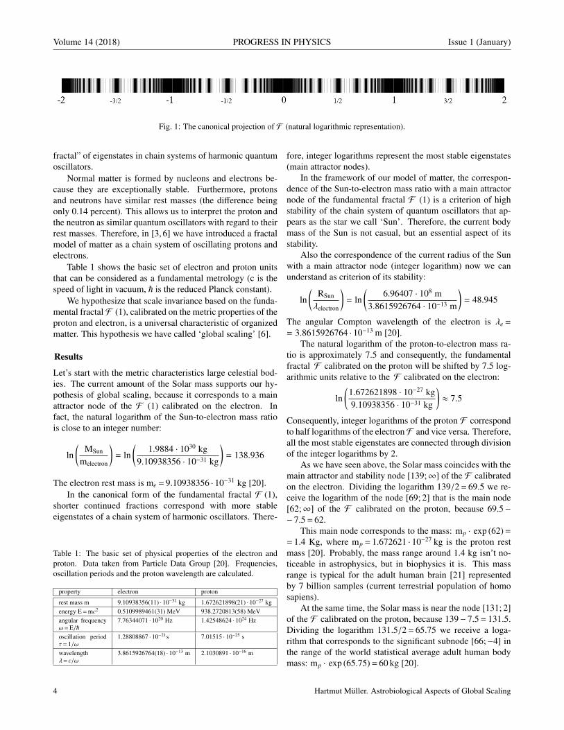
CONTENTS
Muller H. Astrobiological Aspects of Global Scaling . . . . . . . . . . . . . . . . . . . . . . . . . . . . . . . . . 3
Abdelmohssin F. A. Y. Modified Standard Einstein’s Field Equations and the Cosmo-logical Constant . . . . . . . . . . . . . . . . . . . . . . . . . . . . . . . . . . . . . . . . . . . . . . . . . . . . . . . . . . . . . . 7
Millette P. A. Bosons and Fermions as Dislocations and Disclinations in the SpacetimeContinuum . . . . . . . . . . . . . . . . . . . . . . . . . . . . . . . . . . . . . . . . . . . . . . . . . . . . . . . . . . . . . . . . . 10
Muller H. Gravity as Attractor Effect of Stability Nodes in Chain Systems of HarmonicQuantum Oscillators . . . . . . . . . . . . . . . . . . . . . . . . . . . . . . . . . . . . . . . . . . . . . . . . . . . . . . . . .19
Belyakov A. V. On the Ultimate Energy of Cosmic Rays . . . . . . . . . . . . . . . . . . . . . . . . . . . . . 24
Borissova L., Rabounski D. Cosmological Redshift in the De Sitter Stationary Universe 27
Eid S. A., Diab S. M. Nuclear Structure of 154,156Dy Isotopes . . . . . . . . . . . . . . . . . . . . . . . . . 30
Grigoryan A., Kutuzyan A., Yesayan G. Soliton-effect Spectral Self-compression forDifferent Initial Pulses . . . . . . . . . . . . . . . . . . . . . . . . . . . . . . . . . . . . . . . . . . . . . . . . . . . . . . . 35
Petit J.-P. A Symplectic Cosmological Model . . . . . . . . . . . . . . . . . . . . . . . . . . . . . . . . . . . . . . . 38
Muller H. Quantum Gravity Aspects of Global Scaling and the Seismic Profile of theEarth . . . . . . . . . . . . . . . . . . . . . . . . . . . . . . . . . . . . . . . . . . . . . . . . . . . . . . . . . . . . . . . . . . . . . . .41
Medina V., Falcon N. Relativistic Model for Radiating Spherical Collapse . . . . . . . . . . . . .46

Information for Authors
Progress in Physics has been created for rapid publications on advanced studies intheoretical and experimental physics, including related themes from mathematics andastronomy. All submitted papers should be professional, in good English, containinga brief review of a problem and obtained results.
All submissions should be designed in LATEX format using Progress in Physicstemplate. This template can be downloaded from Progress in Physics home pagehttp://www.ptep-online.com
Preliminary, authors may submit papers in PDF format. If the paper is accepted,authors can manage LATEXtyping. Do not send MS Word documents, please: we donot use this software, so unable to read this file format. Incorrectly formatted papers(i.e. not LATEXwith the template) will not be accepted for publication. Those authorswho are unable to prepare their submissions in LATEXformat can apply to a third-partypayable service for LaTeX typing. Our personnel work voluntarily. Authors mustassist by conforming to this policy, to make the publication process as easy and fastas possible.
Abstract and the necessary information about author(s) should be included intothe papers. To submit a paper, mail the file(s) to the Editor-in-Chief.
All submitted papers should be as brief as possible. Short articles are preferable.Large papers can also be considered. Letters related to the publications in the journalor to the events among the science community can be applied to the section Letters toProgress in Physics.
All that has been accepted for the online issue of Progress in Physics is printed inthe paper version of the journal. To order printed issues, contact the Editors.
Authors retain their rights to use their papers published in Progress in Physics asa whole or any part of it in any other publications and in any way they see fit. Thiscopyright agreement shall remain valid even if the authors transfer copyright of theirpublished papers to another party.
Electronic copies of all papers published in Progress in Physics are available forfree download, copying, and re-distribution, according to the copyright agreementprinted on the titlepage of each issue of the journal. This copyright agreement followsthe Budapest Open Initiative and the Creative Commons Attribution-Noncommercial-No Derivative Works 2.5 License declaring that electronic copies of such books andjournals should always be accessed for reading, download, and copying for any per-son, and free of charge.
Consideration and review process does not require any payment from the side ofthe submitters. Nevertheless the authors of accepted papers are requested to pay thepage charges. Progress in Physics is a non-profit/academic journal: money collectedfrom the authors cover the cost of printing and distribution of the annual volumes ofthe journal along the major academic/university libraries of the world. (Look for thecurrent author fee in the online version of Progress in Physics.)

Issue 1 (January) PROGRESS IN PHYSICS Volume 14 (2018)
Astrobiological Aspects of Global Scaling
Hartmut MullerE-mail: [email protected]
In this paper we apply chain systems of harmonic quantum oscillators as a fractal modelof matter to the analysis of astrophysical and biological metric data. Astrobiologicalaspects of global scaling are discussed.
Introduction
Already in [1] we have shown that scale invariance is a fun-damental characteristic of chain systems of harmonic oscilla-tors. In [2] we applied this model on chain systems of har-monic quantum oscillators and could show that particle restmasses coincide with the eigenstates of the system. This isvalid not only for hadrons, but for mesons and leptons as well.On this background we proposed scaling as model of massemergency [3] and introduced our fractal model of matter asa chain system of oscillating protons and electrons. AndreasRies [4] demonstrated that this model allows for the predic-tion of the most abundant isotope of a given chemical ele-ment.
Our fractal model of matter as a chain system of oscillat-ing protons and electrons provides also a good description ofthe mass distribution of large celestial bodies in the Solar Sys-tem [5]. Physical properties of celestial bodies such as mass,size, rotation and orbital period can be understood as macro-scopic quantized eigenstates in chain systems of oscillatingprotons and electrons [6]. This allows to see a connectionbetween the stability of the Solar system and the stability ofelectron and proton and consider scale invariance as a form-ing factor of the Solar system.
In [7] we have calculated the model masses of unknownplanets in the Solar system which correspond well with thehypothesis of Batygin and Brown [8] about a new gas giantcalled “planet 9” and with the hypothesis of Volk and Mal-hotra [9] about an unknown Mars-to-Earth mass “planet 10”beyond Pluto.
In [6] we have proposed a new interpretation of the cos-mic microwave background as a stable eigenstate in a chainsystem of oscillating protons. Therefore, our model may beof cosmological significance as well.
In [10] we applied our model to the domain of biophysicsand have demonstrated that the frequency ranges of electricalbrain activity and of other cyclical biological processes corre-spond with eigenstates in chain systems of oscillating protonsand electrons. This would indicate that biological cycles mayhave a subatomic origin.
Scale invariance as a property of the metric characteristicsof biological organisms is well studied [11, 12] and it is notan exclusive characteristic of adult physiology. Furthermore,many metric characteristics of human physiology, for exam-ple, the frequency ranges of electrical brain activity [13, 14],
are common to most mammalian species.In this paper we demonstrate how the scale invariance of
our fractal model of matter as a chain system of oscillatingprotons and electrons allows us to see a connection betweenthe metric characteristics of biological organisms and thoseof the celestial bodies. This connection could be of astrobio-logical significance.
Methods
In [1] we have shown that the set of natural frequencies of achain system of similar harmonic oscillators coincides witha set of finite continued fractions F , which are natural loga-rithms:
ln (ω jk/ω00)= n j0 +z
n j1 +z
n j2 + . . .+
zn jk
=
= [z, n j0; n j1, n j2, . . . , n jk]=F ,
(1)
where ω jk is the set of angular frequencies and ω00 is the fun-damental frequency of the set. The denominators are integer:n j0, n j1, n j2, . . . , n jk ∈Z, the cardinality j ∈N of the set and thenumber k ∈N of layers are finite. In the canonical form, thenumerator z equals 1.
For finite continued fractions F (1), ranges of high dis-tribution density (nodes) arise near reciprocal integers 1, 1/2,1/3, 1/4, . . . which are the attractor points of the distribution.
Any finite continued fraction represents a rational num-ber [15]. Therefore, all natural frequencies ω jk in (1) are irra-tional, because for rational exponents the natural exponentialfunction is transcendental [16]. It is probable that this cir-cumstance provides for high stability of an oscillating chainsystem because it prevents resonance interaction between theelements of the system [17]. Already in 1987 we have appliedcontinued fractions of the type F (1) as criterion of stabilityin engineering [18, 19].
In the case of harmonic quantum oscillators, the contin-ued fractions F (1) not only define fractal sets of naturalangular frequencies ω jk , oscillation periods τ jk = 1/ω jk andwavelengths λ jk = c/ω jk of the chain system, but also fractalsets of energies E jk = ℏ ·ω jk and masses m jk =E jk/c2 whichcorrespond with the eigenstates of the system. For this rea-son, we call the continued fraction F (1) the “fundamental
Hartmut Muller. Astrobiological Aspects of Global Scaling 3
Volume 14 (2018) PROGRESS IN PHYSICS Issue 1 (January)
Fig. 1: The canonical projection of F (natural logarithmic representation).
fractal” of eigenstates in chain systems of harmonic quantumoscillators.
Normal matter is formed by nucleons and electrons be-cause they are exceptionally stable. Furthermore, protonsand neutrons have similar rest masses (the difference beingonly 0.14 percent). This allows us to interpret the proton andthe neutron as similar quantum oscillators with regard to theirrest masses. Therefore, in [3, 6] we have introduced a fractalmodel of matter as a chain system of oscillating protons andelectrons.
Table 1 shows the basic set of electron and proton unitsthat can be considered as a fundamental metrology (c is thespeed of light in vacuum, ℏ is the reduced Planck constant).
We hypothesize that scale invariance based on the funda-mental fractal F (1), calibrated on the metric properties of theproton and electron, is a universal characteristic of organizedmatter. This hypothesis we have called ‘global scaling’ [6].
Results
Let’s start with the metric characteristics large celestial bod-ies. The current amount of the Solar mass supports our hy-pothesis of global scaling, because it corresponds to a mainattractor node of the F (1) calibrated on the electron. Infact, the natural logarithm of the Sun-to-electron mass ratiois close to an integer number:
ln(
MSun
melectron
)= ln
(1.9884 · 1030 kg
9.10938356 · 10−31 kg
)= 138.936
The electron rest mass is me = 9.10938356 · 10−31 kg [20].In the canonical form of the fundamental fractal F (1),
shorter continued fractions correspond with more stableeigenstates of a chain system of harmonic oscillators. There-
Table 1: The basic set of physical properties of the electron andproton. Data taken from Particle Data Group [20]. Frequencies,oscillation periods and the proton wavelength are calculated.
property electron proton
rest mass m 9.10938356(11) · 10−31 kg 1.672621898(21) · 10−27 kgenergy E=mc2 0.5109989461(31) MeV 938.2720813(58) MeVangular frequencyω=E/ℏ
7.76344071 · 1020 Hz 1.42548624 · 1024 Hz
oscillation periodτ= 1/ω
1.28808867 · 10−21s 7.01515 · 10−25 s
wavelengthλ= c/ω
3.8615926764(18) · 10−13 m 2.1030891 · 10−16 m
fore, integer logarithms represent the most stable eigenstates(main attractor nodes).
In the framework of our model of matter, the correspon-dence of the Sun-to-electron mass ratio with a main attractornode of the fundamental fractal F (1) is a criterion of highstability of the chain system of quantum oscillators that ap-pears as the star we call ‘Sun’. Therefore, the current bodymass of the Sun is not casual, but an essential aspect of itsstability.
Also the correspondence of the current radius of the Sunwith a main attractor node (integer logarithm) now we canunderstand as criterion of its stability:
ln(
RSun
λelectron
)= ln
(6.96407 · 108 m
3.8615926764 · 10−13 m
)= 48.945
The angular Compton wavelength of the electron is λe =
= 3.8615926764 · 10−13 m [20].The natural logarithm of the proton-to-electron mass ra-
tio is approximately 7.5 and consequently, the fundamentalfractal F calibrated on the proton will be shifted by 7.5 log-arithmic units relative to the F calibrated on the electron:
ln(
1.672621898 · 10−27 kg9.10938356 · 10−31 kg
)≈ 7.5
Consequently, integer logarithms of the proton F correspondto half logarithms of the electronF and vice versa. Therefore,all the most stable eigenstates are connected through divisionof the integer logarithms by 2.
As we have seen above, the Solar mass coincides with themain attractor and stability node [139;∞] of the F calibratedon the electron. Dividing the logarithm 139/2= 69.5 we re-ceive the logarithm of the node [69; 2] that is the main node[62;∞] of the F calibrated on the proton, because 69.5−− 7.5= 62.
This main node corresponds to the mass: mp · exp (62)== 1.4 Kg, where mp = 1.672621 · 10−27 kg is the proton restmass [20]. Probably, the mass range around 1.4 kg isn’t no-ticeable in astrophysics, but in biophysics it is. This massrange is typical for the adult human brain [21] representedby 7 billion samples (current terrestrial population of homosapiens).
At the same time, the Solar mass is near the node [131; 2]of the F calibrated on the proton, because 139− 7.5= 131.5.Dividing the logarithm 131.5/2= 65.75 we receive a loga-rithm that corresponds to the significant subnode [66;−4] inthe range of the world statistical average adult human bodymass: mp · exp (65.75)= 60 kg [20].
4 Hartmut Muller. Astrobiological Aspects of Global Scaling

Issue 1 (January) PROGRESS IN PHYSICS Volume 14 (2018)
Jupiter’s body mass coincides with the main attractornode [132;∞] of the electron-calibrated F (1):
ln(
MJupiter
melectron
)= ln
(1.8986 · 1027 kg
9.10938356 · 10−31 kg
)= 131.98
Dividing the logarithm 132/2= 66 we receive the logarithmof the main node [66;∞] that corresponds to the mass:me · exp (66)= 42 g. This mass range coincides with the av-erage mass of the human spinal cord [23].
At the same time, Jupiter’s body mass is near the node[124; 5] of the proton-calibrated F (1):
ln(
MJupiter
mproton
)= ln
(1.8986 · 1027 kg
1.672621 · 10−27 kg
)= 124.47
The half value of this logarithm 124.47/2= 62.24 correspondsto the mass: mp · exp (62.24)= 1.78 kg that is the range of theadult human liver [21]. It is remarkable that the most massiveplanet of the Solar System corresponds with the most massiveorgan of the human organism – the liver.
Saturn’s body mass is near the subnode [123; 4] of theproton-calibrated F (1):
ln(
MSaturn
mproton
)= ln
(5.6836 · 1023 kg
1.672621 · 10−27 kg
)= 123.26
The half value of this logarithm 123.26/2= 61.63 correspondsto the mass: mp · exp (61.63)= 0.975 kg that is the range ofthe adult human lungs [21]. It is remarkable that the secondmassive planet of the Solar System corresponds with the sec-ond massive organ of the human organism – the lungs.
The radius of Saturn is near the main node [54;∞] of theF calibrated on the proton:
ln(
RSaturn
λproton
)= ln
(6.0268 · 107 m
2.1030891 · 10−16 m
)= 54.01
Dividing the logarithm 54/2= 27 we receive the logarithmof the main node [27;∞] that corresponds to the wavelengthλp · exp (27)= 0.11 mm that coincides with the size of the hu-man fertile oocyte (zygote) [24].
As shown above, the Solar radius coincides with the mainnode [49;∞] of the F calibrated on the electron. Dividing thelogarithm 49/2= 24.5 we receive the logarithm of the node[24; 2] that is the main node [32;∞] of the F calibrated onthe proton, because 24.5+ 7.5= 32. This logarithm corre-sponds to the wavelength λe · exp (24.5)= 16.6 mm that co-incides with the object focal length of the human eye [25]that is also the length of the newborn eyeball.
At the same time, the Solar radius is near the node [56; 2]of the F calibrated on the proton:
ln(
RSun
λproton
)= ln
(6.96407 · 108 m
2.103089 · 10−16 m
)= 56.46
The angular Compton wavelength of the proton is λp =
= 2.103089 · 10−16 m [20].Dividing the logarithm 56.5/2= 28.25 we receive the log-
arithm of the significant subnode [28; 4] that corresponds tothe wavelength λp· exp (28.25)= 0.39 mm that coincides withthe second focal length [26] behind the retina of the humaneye.
Already in 1981 Leonid Chislenko [27] did demonstratethat ranges of body masses and sizes preferred by the mostquantity of biological species show an equidistant distribu-tion on a logarithmic scale with a scaling factor close to 3.Probably, this is a consequence of global scaling, if we con-sider that the scaling factor e= 2.718 . . . connects the mainattractor nodes of stability in the fundamental fractal F .
Conclusion
Applying our fractal model of matter as chain system of os-cillating protons and electrons to the analysis of astrophysi-cal and biophysical metric data we can assume that the metriccharacteristics of biological organisms and those of the Solarsystem have a common subatomic origin. However, there isa huge field of research where various discoveries are still tobe expected.
Acknowledgements
The author is grateful to Viktor Panchelyuga and Leili Khos-ravi for valuable discussions.
Submitted on November 5, 2017
References1. Muller H. Fractal Scaling Models of Resonant Oscillations in Chain
Systems of Harmonic Oscillators. Progress in Physics, 2009, v. 5, no. 2,72–76.
2. Muller H. Fractal Scaling Models of Natural Oscillations in Chain Sys-tems and the Mass Distribution of Particles. Progress in Physics, 2010,v. 6, no. 3, 61–66.
3. Muller H. Emergence of Particle Masses in Fractal Scaling Models ofMatter. Progress in Physics, 2012, v. 8, no. 4, 44–47.
4. Ries A. Qualitative Prediction of Isotope Abundances with the BipolarModel of Oscillations in a Chain System. Progress in Physics, 2015,v. 11, 183–186.
5. Muller H. Fractal scaling models of natural oscillations in chain sys-tems and the mass distribution of the celestial bodies in the Solar Sys-tem. Progress in Physics, 2010, v. 6, no. 3, 61–66.
6. Muller H. Scale-Invariant Models of Natural Oscillations in Chain Sys-tems and their Cosmological Significance. Progress in Physics, 2017,v. 13, 187–197.
7. Muller H. Global Scaling as Heuristic Model for Search of AdditionalPlanets in the Solar System. Progress in Physics, 2017, v. 13, 204–206.
8. Batygin K., Brown M.E. Evidence for a distant giant planet in the SolarSystem. The Astronomical Journal, 2016, v. 151.
9. Volk K., Malhotra R. The curiously warped mean plane of the Kuiperbelt. arXiv:1704.02444v2 [astro-ph.EP], 19 June 2017.
10. Muller H. Chain Systems of Harmonic Quantum Oscillators as a FractalModel of Matter and Global Scaling in Biophysics. Progress in Physics,2017, v. 13, no. 4, 231–233.
Hartmut Muller. Astrobiological Aspects of Global Scaling 5

Volume 14 (2018) PROGRESS IN PHYSICS Issue 1 (January)
11. Barenblatt G.I. Scaling. Cambridge University Press, 2003.
12. Schmidt-Nielsen K., Scaling. Why is the animal size so important?Cambridge University Press, 1984.
13. Sainsbury R.S., Heynen A., Montoya C.P. Behavioral correlates of hip-pocampal type 2 theta in the rat. Physiol. Behavior, 1987, v. 39 (4),513–519.
14. Stewart M., Fox S.E., Hippocampal theta activity in monkeys. BrainResearch, 1991, v. 538 (1), 59–63.
15. Khintchine A.Ya. Continued fractions. University of Chicago Press,Chicago 1964.
16. Hilbert D. Uber die Transcendenz der Zahlen e und π. MathematischeAnnalen, 1893, 43, 216–219.
17. Panchelyuga V.A., Panchelyuga M.S. Resonance and Fractals on theReal Numbers Set. Progress in Physics, 2012, v. 8, no. 4, 48–53.
18. Muller H. The general theory of stability and objective evolutionarytrends of technology. Applications of developmental and constructionlaws of technology in CAD. Volgograd, VPI, 1987 (in Russian).
19. Muller H. Superstability as a developmental law of technology. Tech-nology laws and their Applications. Volgograd-Sofia, 1989 (in Rus-sian).
20. Olive K.A. et al. (Particle Data Group), Chin. Phys. C, 2016, v. 38,090001. Patrignani C. et al. (Particle Data Group), Chin. Phys. C, 2016,v. 40, 100001.
21. Singh D. et al. Weights of human organs at autopsy in Chandigarh zoneof north-west India. JIAFM, 2004, v. 26 (3), 97-99.
22. Walpole S.C. et al. The weight of nations: an estimation of adult humanbiomass. BMC Public Health, 2012, v. 12 (1), 439.
23. Watson C., Paxinos G., Kayalioglu G. The Spinal Cord. Amsterdam:Elsevier, 2009.
24. Zamboni L., Mishell D.R., Bell J.H., Baca M. Fine structure of thehuman ovum in the pronuclear stage. Journal of Cell Biology 1966,30(3), 579–600.
25. Hunt et al. Light, Color and Vision. Chapman and Hall, Ltd, London,1968.
26. Ebenholtz S.M. Oculomotor Systems and Perception. Cambridge Univ.Press, 2001.
27. Chislenko L.L. The structure of fauna and flora in connection with thesizes of the organisms. Moscow, 1981 (in Russian).
6 Hartmut Muller. Astrobiological Aspects of Global Scaling

Issue 1 (January) PROGRESS IN PHYSICS Volume 14 (2018)
Modified Standard Einstein’s Field Equations and the Cosmological Constant
Faisal A. Y. AbdelmohssinIMAM, University of Gezira, P.O. BOX: 526, Wad-Medani, Gezira State, Sudan
Sudan Institute for Natural Sciences, P.O. BOX: 3045, Khartoum, SudanE-mail: [email protected]
The standard Einstein’s field equations have been modified by introducing a generalfunction that depends on Ricci’s scalar without a prior assumption of the mathemat-ical form of the function. By demanding that the covariant derivative of the energy-momentum tensor should vanish and with application of Bianchi’s identity a first orderordinary differential equation in the Ricci scalar has emerged. A constant resultingfrom integrating the differential equation is interpreted as the cosmological constantintroduced by Einstein. The form of the function on Ricci’s scalar and the cosmologi-cal constant corresponds to the form of Einstein-Hilbert’s Lagrangian appearing in thegravitational action. On the other hand, when energy-momentum is not conserved, anew modified field equations emerged, one type of these field equations are Rastall’sgravity equations.
1 Introduction
In the early development of the general theory of relativity,Einstein proposed a tensor equation to mathematically de-scribe the mutual interaction between matter-energy andspacetime as [13]
Rab = κTab (1.1)
where κ is the Einstein constant, Tab is the energy-momen-tum, and Rab is the Ricci curvature tensor which representsgeometry of the spacetime in presence of energy-momentum.
Einstein demanded that conservation of energy-momen-tum should be valid in the general theory of relativity sinceenergy-momentum is a tensor quantity. This was representedas
Tab;b = 0 (1.2)
where semicolon (;) represents covariant derivatives. Butequation (1.2) requires
Rab;b = 0 (1.3)
too which is not always true.Finally, Einstein presented his standard field equations
(EFEs) describing gravity in the tensor equations form,namely, [2–5, 8–12]
Gab = κTab (1.4)
where Gab is the Einstein tensor given by
Gab = Rab −12gabR (1.5)
where, R, is the Ricci scalar curvature, and gab is the funda-mental metric tensor.
In his search for analytical solution to his field equationshe turned to cosmology and proposed a model of static andhomogenous universe filled with matter. Because he believedof the static model for the Universe, he introduced a constant
term in his standard field equations to represent a kind of “antigravity” to balance the effect of gravitational attractions ofmatter in it.
Einstein modified his standard equations by introducinga term to his standard field equations including a constantwhich is called the cosmological constant Λ, [7] to become
Rab −12gabR + gabΛ = κTab (1.6)
whereΛ is the cosmological constant (assumed to have a verysmall value). Equation (1.6) may be written as
Rab −12
(R − 2Λ) gab = κTab (1.7)
Einstein rejected the cosmological constant for two rea-sons:
• The universe described by this theory was unstable.
• Observations by Edwin Hubble confirmed that the uni-verse is expanding.
Recently, it has been believed that this cosmological con-stant might be one of the causes of the accelerated expansionof the Universe [15].
Einstein has never justified mathematically introductionof his cosmological constant in his field equations.
Based on that fact I have mathematically done that usingsimple mathematics.
2 Modified standard Einstein’s field equations
I modified the (EFEs) by introducing a general function L(R)of Ricci’s scalar into the standard (EFEs). I do not assumea concrete form of the function. The modified (EFEs), thenbecomes
Rab − gabL(R) = κTab (2.1)
Faisal A.Y. Abdelmohssin. Modified Standard Einstein’s Field Equations 7

Volume 14 (2018) PROGRESS IN PHYSICS Issue 1 (January)
Taking covariant derivative denoted by semicolon (; ) ofboth sides of equation (2.1) yields
Rab;b − [gabL(R)];b = κTab;b (2.2)
Since covariant divergence of the metric tensor vanishes,equation (2.2) may be written as
Rab;b − gab
(dLdR
)R;b = κTab;b (2.3)
Substituting the Bianchi identity
R;c = 2gabRac;b (2.4)
in equation (2.3) and requiring the covariant divergence of theenergy-momentum tensor to vanish (i.e. energy-momentumis conserved), namely, equation (1.2), we arrive at
Rab;b − gab
(dLdR
) (2gacRab;c
)= 0 (2.5)
Rearranging equation (2.5) we get
Rab;b − 2(
dLdR
)(gabg
ac) Rab;c = 0 (2.6)
Substituting the following identity equation
gabgac = δcb (2.7)
in equation (2.6), we get
Rab;b − 2(
dLdR
) (δcb
)Rab;c = 0 (2.8)
By changing the dummy indices, we arrive at
Rab;b
(1 − 2
dLdR
)= 0 (2.9)
We have either,Rab;b = 0, (2.10)
or
1 − 2(
dLdR
)= 0 (2.11)
Equation (2.10) is not always satisfied as mentioned be-fore. Whilst, equation (2.11) yields
dLdR=
12
(2.12)
This has a solution
L(R) =12
R −C (2.13)
where C is a constant.Interpreting the constant of integration C, as the cosmo-
logical constant Λ, the functional dependence of L(R) onRicci scalar may be written as
L(R) =12
(R − 2Λ) (2.14)
Equation (2.14) is the well known Lagrangian functionalof the Einstein-Hilbert action with the cosmological constant.
3 The Modified Equations and the Einstein Spaces
In absence of energy-momentum i.e. in a region of spacetimewhere is there no energy, a state which is different from vac-uum state everywhere in spacetime, equation (2.1) becomes
Rab − gabL(R) = 0 (3.1)
Contacting equation (3.1) with gab, we get
R − NL(R) = 0 (3.2)
where N is the dimension of the spacetime. Equation (3.2)yields
L(R) =1N
R (3.3)
Substituting equation (3.3) in equation (3.1), we get
Rab =1NgabR (3.4)
Equation (3.4) is the Einstein equation for Einstein spaces indifferential geometry [1, 2];
Rab = I gab (3.5)
where I is an invariant. This implies that the function I pro-posed, L(R), is exactly the same as the invariant I in Einsteinspaces equation when contacted with gab.
A 2D sections of the 4D spacetime of Einstein spacesare geometrically one of the geometries of spacetime whichsatisfies the standard Einstein’s field equations in absence ofenergy-momentum.
A naive substitution of N = 4 into equation (3.4) wouldlead to an identity from which Ricci scalar could not be cal-culated, because it becomes a non-useful equation, it givesR = R.
4 The modified equations and gravity equations withnon-conserved energy-momentum
Because in general relativity spactime itself is changing, theenergy is not conserved, because it can give energy to theparticles and absorb it from them [2].
In cosmology the notion of dark energy – represented byterm introduced by Einstein – and dark matter is a sort ofsources of energy of unknown origin.
It is possible to incorporate the possibility of non-con-served energy-momentum tensor in the modified equations.In this case equation (2.9) should become
Rab;b
(1 − 2
dLdR
)= κTab;b (4.1)
where Tab;b , 0. Since Rab;b is not always equals to zero, thisimplies that the bracket in the LHS of equation (4.1) is notzero in any case.
8 Faisal A.Y. Abdelmohssin. Modified Standard Einstein’s Field Equations

Issue 1 (January) PROGRESS IN PHYSICS Volume 14 (2018)
Let us assume it is equal to D , where D is a dimensionlessconstant, i.e.
1 − 2dLdR= D (4.2)
Then, equation (4.2) becomes
dLdR=
12
(1 − D) (4.3)
Now, integrating equation (4.3) yields
L(R,D) =12
(1 − D) R − E (4.4)
where E is a constant. When D = 0, equation (4.4) shouldreduce to equation (2.13), the equation in case of conservedenergy-momentum, for which E = Λ. So, equation (4.4) be-comes
L(R,D) =12
(1 − D) R − Λ (4.5)
Finally, the modified equations (equation (2.1)) in case ofnon-conserved energy-momentum become
Rab −12
(1 − D) gabR + Λgab = κTab (4.6)
5 The modified equations and the Rastall gravityequations
Rastall [14] introduced a modification to the Einstein fieldequations, in which the covariant conservation conditionRab;b = 0 is no longer valid.
In his theory he introduced a modification to the Einsteinfield equations without the cosmological constant which read
Rab −12
(1 − 2λκ) gabR = κTab (5.1)
where λ is a free parameter. When λ = 0, we recover the stan-dard Einstein’s field equations. Comparing Rastall’s equa-tions in equation (5.1) with equation (4.6) without the cos-mological constant, we deduce
D = 2λκ (5.2)
Acknowledgements
I gratefully acknowledge IMAM, University of Gezira, P.O.BOX: 526, Wad-Medani, Gezira State, Sudan, for full finan-cial support of this work.
Submitted on November 5, 2017
References1. Besse A.L. Einstein Manifolds. Classics in Mathematics. Berlin,
Springer, 1987.
2. Misner C.W., Thorne K.S., Wheeler J.A. Gravitation, San Francisco:W. H. Freeman, 1973.
3. Landau L.D., Lifshitz E.M. The Classical Theory of Fields. 4th edition,Butterworth-Heinemann, 1975.
4. Hartle J.B. Gravity: An Introduction to Einstein’s General Relativity,Addison-Wesley, 2003.
5. Carroll S. Spacetime and Geometry: An Introduction to General Rela-tivity, Addison-Wesley, 2003.
6. Sharan P. Spacetime, Geometry and Gravitation, Springer, 2009.
7. D’Inverno R. Introducing Einstein’s Relativity, Clarendon Press, 1992.
8. Hobson M.P., Efstathiou G.P, Lasenby A.N. General Relativity: AnIntroduction for Physicists, Cambridge University Press, 2006.
9. Schutz B.A. First Course in General Relativity. Cambridge UniversityPress, 1985.
10. Foster J., Nightingale J.D. A Short Course in General Relativity. 3rdedition, Springer, 1995.
11. Wald R.M. General Relativity, Chicago University Press, 1984.
12. Hawking S.W., Israel W. Three Hundred Years of Gravitation, Cam-bridge University Press, 1987.
13. Mehra J. Einstein, Hilbert, and The Theory of Gravitation, HistoricalOrigins of General Relativity Theory, Springer, 1974.
14. Rastall P. Phys. Rev. D6, 3357 1972.
15. Riess A., et al. Observational Evidence from Supernovae for an Ac-celerating Universe and a Cosmological Constant. The AstronomicalJournal, 1998, v. 116(3), 1009–1038.
Faisal A.Y. Abdelmohssin. Modified Standard Einstein’s Field Equations 9

Volume 14 (2018) PROGRESS IN PHYSICS Issue 1 (January)
Bosons and Fermions as Dislocations and Disclinationsin the Spacetime Continuum
Pierre A. [email protected], Ottawa, Canada
We investigate the case for dislocations (translational displacements) and disclinations(rotational displacements) in the Spacetime Continuum corresponding to bosons andfermions respectively. The massless, spin-1 screw dislocation is identified with the pho-ton, while edge dislocations correspond to bosons of spin-0, spin-1 and spin-2. Wedgedisclinations are identified with quarks. We find that the twist disclination depends bothon the space volume ℓ3 of the disclination and on the length ℓ of the disclination. Weidentify the ℓ3 twist disclination terms with the leptons, while the ℓ twist disclinationwhich does not have a longitudinal (massive) component, is identified with the masslessneutrino. We perform numerical calculations that show that the dominance of the ℓ andℓ3 twist disclination terms depend on the extent ℓ of the disclination: at low values ofℓ, the “weak interaction” term ℓ predominates up to about 10−18 m, which is the gener-ally accepted range of the weak force, while at larger values of ℓ, the “electromagneticinteraction” term ℓ3 predominates. The value of ℓ at which the two interactions in thetotal strain energy are equal is given by ℓ = 2.0 × 10⁻¹⁸ m.
1 Introduction
Elementary quantum particles are classified into bosons andfermions based on integral and half-integral multiples of ℏrespectively, where ℏ is Planck’s reduced constant. Bosonsobey Bose-Einstein statistics while fermions obey Fermi-Di-rac statistics and the Pauli Exclusion Principle. These deter-mine the number of non-interacting indistinguishable parti-cles that can occupy a given quantum state: there can only beone fermion per quantum state while there is no such restric-tion on bosons.
This is explained in quantum mechanics using the com-bined wavefunction of two indistinguishable particles whenthey are interchanged:
Bosons : Ψ(1, 2) = Ψ(2, 1)
Fermions : Ψ(1, 2) = −Ψ(2, 1) .(1)
Bosons commute and as seen from (1) above, only the sym-metric part contributes, while fermions anticommute and onlythe antisymmetric part contributes. There have been attemptsat a formal explanation of this phenomemon, the spin-statis-tics theorem, with Pauli’s being one of the first [1]. Jabs [2]provides an overview of these and also offers his own attemptat an explanation.
However, as Feynman comments candidly [3, see p. 4-3],We apologize for the fact that we cannot give you anelementary explanation. An explanation has been wor-ked out by Pauli from complicated arguments of quan-tum field theory and relativity. He has shown that thetwo must necessarily go together, but we have not beenable to find a way of reproducing his arguments on anelementary level. It appears to be one of the few placesin physics where there is a rule which can be stated
very simply, but for which no one has found a simpleand easy explanation. The explanation is deep down inrelativistic quantum mechanics. This probably meansthat we do not have a complete understanding of thefundamental principle involved. For the moment, youwill just have to take it as one of the rules of the world.
The question of a simple and easy explanation is still out-standing. Eq. (1) is still the easily understood explanation,even though it is based on the exchange properties of parti-cles, rather than on how the statistics of the particles are re-lated to their spin properties. At this point in time, it is anempirical description of the phenomenon.
2 Quantum particles from STC defects
Ideally, the simple and easy explanation should be a physi-cal explanation to provide a complete understanding of thefundamental principles involved. The Elastodynamics of theSpacetime Continuum (STCED) [6,7] provides such an expla-nation, based on dislocations and disclinations in the space-time continuum. Part of the current problem is that there is nounderstandable physical picture of the quantum level. STCEDprovides such a picture.
The first point to note is that based on their properties,bosons obey the superposition principle in a quantum state.In STCED, the location of quantum particles is given by theirdeformation displacement uµ. Dislocations [7, see chapter 9]are translational displacements that commute, satisfy the su-perposition principle and behave as bosons. As shown in sec-tion §3-6 of [7], particles with spin-0, 1 and 2 are describedby
uµ;ν = εµν(0) + εµν(2) + ω
µν(1) , (2)
i.e. a combination of spin-0 εµν(0) (mass as deformation par-ticle aspect), spin-1 ωµν(1) (electromagnetism) and spin-2 εµν(2)
10 Pierre A. Millette. Bosons and Fermions as Dislocations and Disclinations in the Spacetime Continuum

Issue 1 (January) PROGRESS IN PHYSICS Volume 14 (2018)
(deformation wave aspect), where
εµν = 12 (uµ;ν + uν;µ) = u(µ;ν) (3)
andωµν = 1
2 (uµ;ν − uν;µ) = u[µ;ν] (4)
which are solutions of wave equations in terms of derivativesof the displacements uµ;ν as given in chapter 3 of [7].
Disclinations [7, see chapter 10], on the other hand, arerotational displacements that do not commute and that do notobey the superposition principle. You cannot have two rota-tional displacements in a given quantum state. Hence theirnumber is restricted to one per quantum state. They behaveas fermions.
Spinors represent spin one-half fermions. Dirac spinorfields represent electrons. Weyl spinors, derived from Dirac’sfour complex components spinor fields, are a pair of fieldsthat have two complex components. Interestingly enough,“[u]sing just one element of the pair, one gets a theory ofmassless spin-one-half particles that is asymmetric under mir-ror reflection and ... found ... to describe the neutrino and itsweak interactions” [4, p. 63].
“From the point of view of representation theory, Weylspinors are the fundamental representations that occur whenone studies the representations of rotations in four-dimensio-nal space-time... spin-one-half particles are representationof the group SU(2) of transformations on two complex vari-ables.” [4, p. 63]. To clarify this statement, each rotation inthree dimensions (an element of SO(3)) corresponds to twodistinct elements of SU(2). Consequently, the SU(2) trans-formation properties of a particle are known as the particle’sspin.
Hence, the unavoidable conclusion is that bosons are dis-locations in the spacetime continuum, while fermions are dis-clinations in the spacetime continuum. Dislocations are trans-lational displacements that commute, satisfy the superposi-tion principle and behave as bosons. Disclinations, on theother hand, are rotational displacements that do not commute,do not obey the superposition principle and behave as ferm-ions.
The equations in the following sections of this paper arederived in Millette [7]. The constants λ0 and µ0 are the Lameelastic constants of the spacetime continuum, where µ0 is theshear modulus (the resistance of the continuum to distortions)and λ0 is expressed in terms of κ0, the bulk modulus (the re-sistance of the continuum to dilatations) according to
λ0 = κ0 − µ0/2 (5)
in a four-dimensional continuum.
3 Dislocations (bosons)
Two types of dislocations are considered in this paper: screwdislocations (see Fig. 1) and edge dislocations (see Fig. 2).
Fig. 1: A stationary screw dislocation in cartesian (x, y, z) and cylin-drical polar (r, θ, z) coordinates.
Fig. 2: A stationary edge dislocation in cartesian (x, y, z) and cylin-drical polar (r, θ, z) coordinates.
Dislocations, due to their translational nature, are defects thatare easier to analyze than disclinations.
3.1 Screw dislocation
The screw dislocation is analyzed in sections §9-2 and §15-1of [7]. It is the first defect that we identified with the photondue to its being massless and of spin-1. Consequently, itslongitudinal strain energy is zero
WS∥ = 0. (6)
Pierre A. Millette. Bosons and Fermions as Dislocations and Disclinations in the Spacetime Continuum 11

Volume 14 (2018) PROGRESS IN PHYSICS Issue 1 (January)
Its transverse strain energy is given by [7, eq. (16.5)]
WS⊥ =µ0
4πb2 ℓ ln
Λ
bc, (7)
where b is the spacetime Burgers dislocation vector [9], ℓ isthe length of the dislocation, bc is the size of the core of thedislocation, of order b0, the smallest spacetime Burgers dislo-cation vector [10], andΛ is a cut-off parameter correspondingto the radial extent of the dislocation, limited by the averagedistance to its nearest neighbours.
3.2 Edge dislocation
The edge dislocation is analyzed in sections §9-3, §9-5 and§15-2 of [7]. The longitudinal strain energy of the edge dis-location is given by [7, eq. (16.29)]
WE∥ =
κ02πα2
0
(b2
x + b2y
)ℓ lnΛ
bc(8)
whereα0 =
µ0
2µ0 + λ0, (9)
ℓ is the length of the dislocation and as before, Λ is a cut-offparameter corresponding to the radial extent of the disloca-tion, limited by the average distance to its nearest neighbours.The edge dislocations are along the z-axis with Burgers vec-tor bx for the edge dislocation proper represented in Fig. 2,and a different edge dislocation with Burgers vector by whichwe call the gap dislocation. The transverse strain energy isgiven by [7, eq. (16.54)]
WE⊥ =µ0
4π
(α2
0 + 2β20
) (b2
x + b2y
)ℓ lnΛ
bc(10)
where
β0 =µ0 + λ0
2µ0 + λ0. (11)
The total longitudinal (massive) dislocation strain energyWD∥ is given by (8)
WD∥ = WS
∥ +WE∥ = WE
∥ , (12)
given that the screw dislocation longitudinal strain energy iszero, while the total transverse (massless) dislocation strainenergy is given by the sum of the screw (along the z axis) andedge (in the x−y plane) dislocation transverse strain energies
WD⊥ = WS
⊥ +WE⊥ (13)
to give
WD⊥ =
µ0
4π
[b2
z +(α2
0 + 2β20
) (b2
x + b2y
)]ℓ lnΛ
bc. (14)
It should be noted that as expected, the total longitudinal(massive) dislocation strain energy WD
∥ involves the space-time bulk modulus κ0, while the total transverse (massless)
Fig. 3: Three types of disclinations: wedge (top), splay (middle),twist (bottom) [5, 7].
dislocation strain energy WD⊥ involves the spacetime shear
modulus µ0.The total strain energy of dislocations
WD = WD∥ +WD
⊥ (15)
provides the total energy of massive and massless bosons,with WD
∥ corresponding to the longitudinal particle aspect ofthe bosons and WD
⊥ corresponding to the wave aspect of thebosons. As seen in [11], the latter is associated with the wave-function of the boson. The spin characteristics of these wasconsidered previously in section 2, where they were seen tocorrespond to spin-0, spin-1 and spin-2 solutions.
4 Disclinations (fermions)
The different types of disclinations considered in this paperare given in Fig. 3. Disclinations are defects that are moredifficult to analyze than dislocations, due to their rotationalnature. This mirrors the case of fermions, which are moredifficult to analyze than bosons.
4.1 Wedge disclination
The wedge disclination is analyzed in sections §10-6 and §15-3 of [7]. The longitudinal strain energy of the wedge discli-
12 Pierre A. Millette. Bosons and Fermions as Dislocations and Disclinations in the Spacetime Continuum

Issue 1 (January) PROGRESS IN PHYSICS Volume 14 (2018)
nation is given by [7, eq. (16.62)]
WW∥ =
κ04πΩ2
z ℓ[α2
0
(2Λ2 ln2Λ − 2b2
c ln2 bc
)+
+ α0γ0
(2Λ2 lnΛ − 2b2
c ln bc
)+
+ 12 (α2
0 + γ20)
(Λ2 − b2
c
) ] (16)
where Ωµ is the spacetime Frank vector,
γ0 =λ0
2µ0 + λ0(17)
and the other constants are as defined previously. In mostcases Λ ≫ bc, and (16) reduces to
WW∥ ≃
κ02πΩ2
z ℓΛ2[α2
0 ln2 Λ+ α0γ0 lnΛ+ 14 (α2
0 + γ20)]
(18)
which is rearranged as
WW∥ ≃
κ02πα2
0Ω2z ℓΛ
2[
ln2 Λ+γ0
α0lnΛ+
14
1 + γ20
α20
] . (19)
The transverse strain energy of the wedge disclination isgiven by [7, eq. (16.70)]
WW⊥ =
µ0
4πΩ2
z ℓ[α2
0
(Λ2 ln2Λ − b2
c ln2 bc
)−
−(α2
0 − 3α0β0
) (Λ2 lnΛ − b2
c ln bc
)+
+12
(α2
0 − 3α0β0 +32β2
0
) (Λ2 − b2
c
) ].
(20)
In most cases Λ ≫ bc, and (20) reduces to
WW⊥ ≃
µ0
4πΩ2
z ℓ[α2
0Λ2 ln2 Λ−
−(α2
0 − 3α0β0
)Λ2 lnΛ+
+12
(α2
0 − 3α0β0 +32β2
0
)Λ2
] (21)
which is rearranged as
WW⊥ ≃
µ0
4πα2
0Ω2z ℓΛ
2[
ln2 Λ −(1 − 3
β0
α0
)lnΛ+
+12
1 − 3β0
α0+
32β2
0
α20
] . (22)
We first note that both the longitudinal strain energy WW∥
and the transverse strain energy WW⊥ are proportional to Λ2 in
the limit Λ ≫ bc. The parameter Λ is equivalent to the extentof the wedge disclination, and we find that as it becomes moreextended, its strain energy is increasing parabolically. This
behaviour is similar to that of quarks (confinement) whichare fermions. In addition, as Λ → bc, the strain energy de-creases and tends to 0, again in agreement with the behaviourof quarks (asymptotic freedom).
We thus identify wedge disclinations with quarks. Thetotal strain energy of wedge disclinations
WW = WW∥ +WW
⊥ (23)
provides the total energy of the quarks, with WW∥ correspond-
ing to the longitudinal particle aspect of the quarks and WW⊥
corresponding to the wave aspect of the quarks. We note thatthe current classification of quarks include both ground andexcited states – the current analysis needs to be extended toexcited higher energy states.
We note also that the rest-mass energy density ρWc2 ofthe wedge disclination (see [7, eq. (10.102)]) is proportionalto ln r which also increases with increasing r, while the rest-mass energy density ρEc2 of the edge dislocation and ρT c2
of the twist disclination (see [7, eqs. (9.134) and (10.123)]respectively) are both proportional to 1/r2 which decreaseswith increasing r as expected of bosons and leptons.
4.2 Twist disclination
The twist disclination is analyzed in sections §10-7 and §15-4of [7]. Note that as mentioned in that section, we do not dif-ferentiate between twist and splay disclinations in this sub-section as twist disclination expressions include both splaydisclinations and twist disclinations proper. Note also that theFrank vector (Ωx,Ωy,Ωz) corresponds to the three axes (Ωr,Ωn,Ωz) used in Fig. 3 for the splay, twist and wedge disclina-tions respectively.
The longitudinal strain energy of the twist disclination isgiven by [7, eq. (16.80)]
WT∥ =
κ06πα2
0
(Ω2
x + Ω2y
)ℓ3 ln
Λ
bc. (24)
One interesting aspect of this equation is that the twist discli-nation longitudinal strain energy WT
∥ is proportional to thecube of the length of the disclination (ℓ3), and we can’t dis-pose of it by considering the strain energy per unit lengthof the disclination as done previously. We can say that thetwist disclination longitudinal strain energy WT
∥ is thus pro-portional to the space volume of the disclination, which isreasonable considering that disclinations are rotational defor-mations. It is also interesting to note that WT
∥ has the familiardependence lnΛ/bc of dislocations, different from the func-tional dependence obtained for wedge disclinations in sec-tion 4.1. The form of this equation is similar to that of thelongitudinal strain energy for the stationary edge dislocation(see [7, eq. (16.15)]) except for the factor ℓ3/3.
The transverse strain energy of the twist disclination is
Pierre A. Millette. Bosons and Fermions as Dislocations and Disclinations in the Spacetime Continuum 13

Volume 14 (2018) PROGRESS IN PHYSICS Issue 1 (January)
given by [8]
WT⊥ =µ0
2πℓ3
3
[ (Ω2
x + Ω2y
) (α2
0 +12 β
20
)+
+ 2ΩxΩy(α2
0 − 2β20
) ]lnΛ
bc+
+µ0
2πℓ[ (Ω2
x + Ω2y
) (α2
0
(Λ2 ln2Λ − b2
c ln2 bc
)+
+ α0γ0
(Λ2 lnΛ − b2
c ln bc
)− 1
2α0γ0
(Λ2 − b2
c
)+
+ 2 β20 lnΛ
bc
)− 2ΩxΩy
(α0β0
(Λ2 lnΛ − b2
c ln bc
)+
+12β0γ0
(Λ2 − b2
c
) )].
(25)
In most cases Λ ≫ bc, and (25) reduces to
WT⊥ ≃µ0
2πℓ3
3
[ (Ω2
x + Ω2y
) (α2
0 +12 β
20
)+
+ 2ΩxΩy(α2
0 − 2β20
) ]lnΛ
bc+
+µ0
2πℓΛ2
[ (Ω2
x + Ω2y
) (α2
0 ln2 Λ + α0γ0 lnΛ−
− 12α0γ0
)− 2ΩxΩy
(α0β0 lnΛ +
12β0γ0
)](26)
which can be rearranged to give
WT⊥ ≃µ0
2πα2
0ℓ3
3
[ (Ω2
x + Ω2y
) 1 + 12β2
0
α20
++ 2ΩxΩy
1 − 2β2
0
α20
] lnΛ
bc+
+µ0
2πα2
0 ℓΛ2[ (Ω2
x + Ω2y
) (ln2 Λ +
γ0
α0lnΛ−
− 12γ0
α0
)− 2ΩxΩy
( β0
α0lnΛ +
12β0γ0
α20
)].
(27)
As noted previously, WT∥ depends on the space volume ℓ3
of the disclination and has a functional dependence of lnΛ/bc
as do the dislocations. The transverse strain energy WT⊥ de-
pends on the space volume ℓ3 of the disclination with a func-tional dependence of lnΛ/bc, but it also includes terms thathave a dependence on the length ℓ of the disclination with afunctional dependence similar to that of the wedge disclina-tion including Λ2 in the limit Λ ≫ bc. The difference in thecase of the twist disclination is that its transverse strain en-ergy WT
⊥ combines ℓ3 terms with the functional dependencelnΛ/bc of dislocations, associated with the “electromagneticinteraction”, and ℓ terms with the Λ2 ln2 Λ functional depen-dence of wedge disclinations, associated with the “strong in-teraction”. This, as we will see in later sections, seems to be
the peculiar nature of the weak interaction, and uniquely po-sitions twist disclinations to represent leptons and neutrinosas participants in the weak interaction.
This leads us to thus separate the longitudinal strain en-ergy of the twist disclination as
WT∥ = Wℓ
3
∥ +Wℓ∥ = Wℓ3
∥ (28)
given that Wℓ∥ = 0, and the transverse strain energy of thetwist disclination as
WT⊥ = Wℓ
3
⊥ +Wℓ⊥ . (29)
We consider both ℓ3 twist disclination and ℓ twist disclinationterms in the next subsections.
4.2.1 ℓ3 twist disclination
The longitudinal strain energy of the ℓ3 twist disclination isthus given by the ℓ3 terms of (24)
Wℓ3
∥ =κ06πα2
0
(Ω2
x + Ω2y
)ℓ3 ln
Λ
bc. (30)
The transverse strain energy of the ℓ3 twist disclination isgiven by the ℓ3 terms of (25)
Wℓ3
⊥ =µ0
2πℓ3
3
[ (Ω2
x + Ω2y
) (α2
0 +12 β
20
)+
+ 2ΩxΩy(α2
0 − 2β20
) ]lnΛ
bc.
(31)
In most cases Λ ≫ bc, and (31) is left unchanged due to itsfunctional dependence on lnΛ/bc.
The total strain energy of the ℓ3 twist disclination terms isgiven by
Wℓ3= Wℓ
3
∥ +Wℓ3
⊥ . (32)
It is interesting to note that Wℓ3
∥ of (30) and Wℓ3
⊥ of (31) areproportional to lnΛ/bc, as are the screw dislocation (photon)and edge dislocation (bosons). This, and the results of thenext subsection, leads us to identify the ℓ3 twist disclinationterms with the leptons (electron, muon, tau) fermions, wherethe heavier muon and tau are expected to be excited states ofthe electron.
4.2.2 ℓ twist disclination
The longitudinal strain energy of the ℓ twist disclination termsin this case is zero as mentioned previously
Wℓ∥ = 0 . (33)
14 Pierre A. Millette. Bosons and Fermions as Dislocations and Disclinations in the Spacetime Continuum

Issue 1 (January) PROGRESS IN PHYSICS Volume 14 (2018)
The transverse strain energy of the ℓ twist disclination isthus also given by the ℓ terms of (25):
Wℓ⊥ =µ0
2πℓ[ (Ω2
x + Ω2y
) (α2
0
(Λ2 ln2 Λ − b2
c ln2 bc
)+
+ α0γ0
(Λ2 lnΛ − b2
c ln bc
)− 1
2α0γ0
(Λ2 − b2
c
)+
+ 2 β20 lnΛ
bc
)− 2ΩxΩy
(α0β0
(Λ2 lnΛ − b2
c ln bc
)+
+12β0γ0
(Λ2 − b2
c
) )].
(34)
In most cases Λ ≫ bc, and (34) reduces to
Wℓ⊥ =µ0
2πℓΛ2
[ (Ω2
x + Ω2y
) (α2
0 ln2Λ + α0γ0 lnΛ−
− 12α0γ0
)− 2ΩxΩy
(α0β0 lnΛ +
12β0γ0
)] (35)
which can be rearranged to give
Wℓ⊥ =µ0
2πα2
0 ℓΛ2[ (Ω2
x + Ω2y
) (ln2Λ +
γ0
α0lnΛ−
− 12γ0
α0
)− 2ΩxΩy
( β0
α0lnΛ +
12β0γ0
α20
)].
(36)
The total strain energy of the ℓ twist disclination is givenby
Wℓ = Wℓ∥ +Wℓ⊥ = Wℓ⊥ (37)
given that the ℓ twist disclination does not have a longitudinal(massive) component. Since the ℓ twist disclination is a mass-less fermion, this leads us to identify the ℓ twist disclinationwith the neutrino.
There is another aspect to the strain energy WT⊥ given by
(25) that is important to note. As we have discussed, theℓ3 twist disclination terms and the lnΛ/bc functional depen-dence as observed for the screw dislocation (photon) and edgedislocation (bosons) has led us to identify the ℓ3 portion withthe leptons (electron, muon, tau) fermions, where the heaviermuon and tau are expected to be excited states of the electron.These are coupled with transverse ℓ twist disclination termswhich are massless and which have a functional dependencesimilar to that of the wedge disclination, which has led us toidentify the ℓ portion with the weakly interacting neutrino.If the muon and tau leptons are excited states of the electronderivable from (25), this would imply that the neutrino por-tion would also be specific to the muon and tau lepton excitedstates, thus leading to muon and tau neutrinos.
We will perform numerical calculations in the next sec-tion which will show that the dominance of the ℓ and ℓ3 twistdisclination terms depend on the extent ℓ of the disclination,with the ℓ “weak interaction” terms dominating for small val-ues of ℓ and the ℓ3 “electromagnetic interaction” terms dom-inating for larger values of ℓ. The ℓ twist disclination terms
would correspond to weak interaction terms while the ℓ3 twistdisclination terms would correspond to electromagnetic inter-action terms. The twist disclination represents the unificationof both interactions under a single “electroweak interaction”.
This analysis also shows why leptons (twist disclinations)are participants in the weak interaction but not the strong in-teraction, while quarks (wedge disclinations) are participantsin the strong interaction but not the weak interaction.
It should be noted that even though the mass of the neu-trino is currently estimated to be on the order of 10’s of eV,this estimate is based on assuming neutrino oscillation be-tween the currently known three lepton generations, to ex-plain the anomalous solar neutrino problem. This is a weakexplanation for that problem, which more than likely indi-cates that we do not yet fully understand solar astrophysics.One can only hope that a fourth generation of leptons will notbe discovered! Until the anomaly is fully understood, we canconsider the twist disclination physical model where the massof the neutrino is zero to be at least a first approximation ofthe neutrino STC defect model.
4.3 Twist disclination sample numerical calculation
In this section, we give a sample numerical calculation thatshows the lepton-neutrino connection for the twist disclina-tion. We start by isolating the common strain energy elementsthat don’t need to be calculated in the example. Starting fromthe longitudinal strain energy of the twist disclination (24)and making use of the relation κ0 = 32µ0 [7, eq. (5.53)], (24)can be simplified to
WT∥ =µ0
2πα2
0 2Ω2[32ℓ3
3lnΛ
bc
](38)
where an average Ω is used instead of Ωx and Ωy. Defining Kas
K =µ0
2πα2
0 2Ω2 , (39)
then (38) is written as
WT∥
K= 32
ℓ3
3lnΛ
bc. (40)
Similarly for the transverse strain energy of the twist dis-clination, starting from (27), the equation can be simplifiedto
WT⊥ ≃µ0
2πα2
0 2Ω2[ℓ3
3
1 + 12β2
0
α20
+ 1 − 2β2
0
α20
lnΛ
bc
]+
+
[ℓΛ2
(ln2Λ +
γ0
α0lnΛ − 1
2γ0
α0−
− β0
α0lnΛ − 1
2β0γ0
α20
)].
(41)
Pierre A. Millette. Bosons and Fermions as Dislocations and Disclinations in the Spacetime Continuum 15

Volume 14 (2018) PROGRESS IN PHYSICS Issue 1 (January)
Using the definition of K from (39), this equation becomes
WT⊥
K≃ ℓ
3
3
2 − 32β2
0
α20
lnΛ
bc+
+ ℓΛ2(ln2Λ +
γ0 − β0
α0lnΛ − 1
2γ0
α0
(1 + β0
)).
(42)
Using the numerical values of the constants α0, β0 and γ0from [7, eqs. (19.14) and (19.35)], (42) becomes
WT⊥
K≃ ℓ
3
3(1.565) ln
Λ
bc+
+ ℓΛ2(ln2 Λ − lnΛ − 0.62
).
(43)
For this sample numerical calculation, we use bc∼10−35mof the order of the spacetime Burgers dislocation constant b0,and the extent of the disclination Λ ∼ 10−18 m of the order ofthe range of the weak force. Then
WT∥
K=
323
(39.1) ℓ3 = 417 ℓ3 . (44)
andWT⊥
K≃ 0.522 (39.1) ℓ3+
+Λ2 (1714 + 41.4 − 0.62) ℓ
(45)
which becomes
WT⊥
K≃ 20.4 ℓ3 + 1755Λ2 ℓ (46)
and finally
WT⊥
K≃ 20.4 ℓ3 + 1.76 × 10⁻³³ ℓ . (47)
We consider various values of ℓ to analyze its effect onthe strain energy. For ℓ = 10−21 m,
WT∥
K= 4.2 × 10−61 (ℓ3 term) (48)
WT⊥
K= 2.0 × 10−62 + 1.8 × 10−54 (ℓ3 term + ℓ term). (49)
For ℓ = 10−18 m,
WT∥
K= 4.2 × 10−52 (ℓ3 term) (50)
WT⊥
K= 2.0 × 10−53 + 1.8 × 10−51 (ℓ3 term + ℓ term). (51)
For ℓ = 10−15 m,
WT∥
K= 4.2 × 10−43 (ℓ3 term) (52)
WT⊥
K= 2.0 × 10−44 + 1.8 × 10−48 (ℓ3 term + ℓ term). (53)
For ℓ = 10−12 m,
WT∥
K= 4.2 × 10⁻³⁴ (ℓ3 term) (54)
WT⊥
K= 2.0 × 10⁻³⁵ + 1.8 × 10−45 (ℓ3 term + ℓ term). (55)
In the sums of WT⊥/K above, the first term ℓ3 represents
the electromagnetic interaction, while the second term ℓ rep-resents the weak interaction. Thus we find that at low val-ues of ℓ, the weak force predominates up to about 10−18 m,which is the generally accepted range of the weak force. Atlarger values of ℓ, the electromagnetic force predominates.The value of ℓ at which the two interactions in the transversestrain energy are equal is given by
20.4 ℓ3 = 1.76 × 10⁻³³ ℓ , (56)
from which we obtain
ℓ = 0.9 × 10⁻¹⁷ m ∼ 10−17 m . (57)
At that value of ℓ, the strain energies are given by
WT∥
K= 3.0 × 10−49 (58)
WT⊥
K= 3.1 × 10−50 . (59)
The longitudinal (massive) strain energy predominates overthe transverse strain energy by a factor of 10.
Alternatively, including the longitudinal ℓ3 strain energyin the calculation, the value of ℓ at which the two interactionsin the total strain energy are equal is given by
417 ℓ3 + 20.4 ℓ3 = 1.76 × 10⁻³³ ℓ , (60)
from which we obtain
ℓ = 2.0 × 10⁻¹⁸ m . (61)
At that value of ℓ, the strain energies are given by
WT∥
K= 3.3 × 10−51 (62)
WT⊥
K= 3.7 × 10−51 . (63)
The longitudinal (massive) strain energy and the transversestrain energy are then of the same order of magnitude.
5 Quantum particles and their associated spacetimedefects
Table 1 provides a summary of the identification of quantumparticles and their associated spacetime defects as shown inthis paper.
16 Pierre A. Millette. Bosons and Fermions as Dislocations and Disclinations in the Spacetime Continuum

Issue 1 (January) PROGRESS IN PHYSICS Volume 14 (2018)
STC defect Type of particle Particles
Screw dislocation Massless boson PhotonEdge dislocation Massive boson Spin-0 particle
Spin-1 Proca eqnSpin-2 graviton
Wedge disclination Massive fermion Quarksℓ3 Twist disclination Massive fermion Leptonsℓ Twist disclination Massless fermion Neutrinos
Table 1: Identification of quantum particles and their associated defects.
6 Discussion and conclusion
In this paper, we have investigated the case for dislocationsand disclinations in the Spacetime Continuum correspondingto bosons and fermions respectively. Dislocations are transla-tional displacements that commute, satisfy the superpositionprinciple and behave as bosons. Disclinations, on the otherhand, are rotational displacements that do not commute, donot obey the superposition principle and behave as fermions,including having their number restricted to one per quantumstate as it is not possible to have two rotational displacementsin a given quantum state.
We have considered screw and edge dislocations. Themassless, spin-1 screw dislocation is identified with the pho-ton. The total strain energy of dislocations WD correspondsto the total energy of massive and massless bosons, with WD
∥corresponding to the longitudinal particle aspect of the bosonsand WD
⊥ corresponding to the wave aspect of the bosons, withthe latter being associated with the wavefunction of the bo-son. Their spin characteristics correspond to spin-0, spin-1and spin-2 solutions.
We have considered wedge and twist disclinations, ofwhich the splay disclination is a special case. Wedge disclina-tions are identified with quarks. The strain energy of wedgedisclinations is proportional to Λ2 in the limit Λ ≫ bc. Theparameter Λ is equivalent to the extent of the wedge disclina-tion, and we find that as it becomes more extended, its strainenergy is increasing parabolically. This behaviour is similarto that of quarks (confinement) which are fermions. In addi-tion, as Λ → bc, the strain energy decreases and tends to 0,again in agreement with the behaviour of quarks (asymptoticfreedom). The total strain energy of wedge disclinations WW
thus corresponds to the total energy of the quarks, with WW∥
corresponding to the longitudinal particle aspect of the quarksand WW
⊥ corresponding to the wave aspect of the quarks.The twist disclination longitudinal strain energy WT
∥ isfound to be proportional to the cube of the length of the discli-nation (ℓ3), and hence depends on the space volume ℓ3 of thedisclination with a functional dependence of lnΛ/bc as do thedislocations. The transverse strain energy WT
⊥ also depends
on the space volume ℓ3 of the disclination with a functionaldependence of lnΛ/bc, but it also includes terms that have adependence on the length ℓ of the disclination with a func-tional dependence similar to that of the wedge disclinationincluding Λ2 in the limit Λ ≫ bc.
We have considered both ℓ3 twist disclination and ℓ twistdisclination terms. We note that Wℓ
3
∥ and Wℓ3
⊥ are propor-tional to lnΛ/bc, as are the screw dislocation (photon) andedge dislocation (bosons), which leads us to identify the ℓ3
twist disclination terms with the leptons (electron, muon, tau)fermions, where the heavier muon and tau are expected to beexcited states of the electron. Given that the ℓ twist disclina-tion does not have a longitudinal (massive) component, it isa massless fermion and this leads us to identify the ℓ twistdisclination with the neutrino. Thus the twist disclinationtransverse strain energy WT
⊥ combines ℓ3 terms with the func-tional dependence lnΛ/bc of dislocations and ℓ terms withthe functional dependence Λ2 of wedge disclinations.
We have performed numerical calculations that show thatthe dominance of the ℓ and ℓ3 twist disclination terms dependon the length ℓ of the disclination. We find that at low val-ues of ℓ, the “weak interaction” term ℓ predominates up toabout 10−18 m, which is the generally accepted range of theweak force. At larger values of ℓ, the “electromagnetic in-teraction” term ℓ3 predominates. The value of ℓ at which thetwo interactions in the total strain energy are equal is givenby ℓ = 2.0 × 10⁻¹⁸ m. We conclude that in WT
⊥ , the ℓ twistdisclination terms represent the weak interaction terms whilethe ℓ3 twist disclination terms represent the electromagneticinteraction terms. The twist disclination hence represents theunification of both interactions under a single “electroweakinteraction”.
This analysis also shows why leptons (twist disclinations)are participants in the weak interaction but not the strong in-teraction (wedge disclinations). In addition, if the muon andtau leptons are excited states of the electron derivable from(25), this would imply that the neutrino portion would also bespecific to the muon and tau lepton excited states, thus leadingto muon and tau neutrinos. A summary of the identification
Pierre A. Millette. Bosons and Fermions as Dislocations and Disclinations in the Spacetime Continuum 17

Volume 14 (2018) PROGRESS IN PHYSICS Issue 1 (January)
of quantum particles and their associated spacetime defectsas shown in this paper is provided in Table 1.
Received on October 25, 2017
References1. Pauli W. The Connection Between Spin and Statistics. Phys. Rev.,
1940, v. 58, 716–722. Reprinted in Schwinger, J., ed. Selected Paperson Quantum Electrodynamics. Dover Publications, New York, 1958,pp 372–378.
2. Jabs A. Connecting Spin and Statistics in Quantum Mechanics. arXiv:quant-ph/0810.2300v4.
3. Feynman R. P., Leighton R. B., Sands M. Lectures on Physics, VolumeIII: Quantum Mechanics. Addison-Wesley Publishing Company, Read-ing, Massachusetts, 1965.
4. Woit P. Not Even Wrong; The Failure of String Theory and the Searchfor Unity in Physical Law. Basic Books, NewYork, 2006.
5. Kleinert H. Multivalued Fields in Condensed Matter, Electromag-netism, and Gravitation. World Scientific Publishing, Singapore, 2008.
6. Millette P. A. Elastodynamics of the Spacetime Continuum. The Abra-ham Zelmanov Journal, 2012, v. 5, 221–277.
7. Millette P. A. Elastodynamics of the Spacetime Continuum: A Space-time Physics Theory of Gravitation, Electromagnetism and QuantumPhysics. American Research Press, Rehoboth, NM, 2017.
8. Corrected eq. (16.87) of [7].
9. Millette P. A. Dislocations in the Spacetime Continuum: Frameworkfor Quantum Physics. Progress in Physics, 2015, vol. 11 (4), 287–307.
10. Millette P. A. The Burgers Spacetime Dislocation Constant b0 and theDerivation of Planck’s Constant. Progress in Physics, 2015, vol. 11 (4),313–316.
11. Millette P. A. Wave-Particle Duality in the Elastodynamics of theSpacetime Continuum (STCED). Progress in Physics, 2014, vol. 10 (4),255–258.
18 Pierre A. Millette. Bosons and Fermions as Dislocations and Disclinations in the Spacetime Continuum

Issue 1 (January) PROGRESS IN PHYSICS Volume 14 (2018)
Gravity as Attractor Effect of Stability Nodes inChain Systems of Harmonic Quantum Oscillators
Hartmut MullerE-mail: [email protected]
In this paper we apply our fractal model of matter as chain systems of harmonic quan-tum oscillators to the analysis of gravimetric characteristics of the Solar system and in-troduce a model of gravity as macroscopic cumulative attractor effect of stability nodesin chain systems of oscillating protons and electrons.
Introduction
Gravity has still a special place in physics as it is the onlyinteraction that is not described by a quantum theory. Never-theless, the big G is considered to be a fundamental constantof nature, involved in the calculation of gravitational effectsin Newton’s law of universal gravitation and in Einstein’sgeneral theory of relativity. The currently recommended [1]value is G = 6.67408(31) · 10−11 m3kg−1s−2 and it seems thatwe know G only to three significant figures.
For several objects in the Solar System, the value of thestandard gravitational parameter µ is known to greater accu-racy than G. The value µ for the Sun is the heliocentric grav-itational constant and equals 1.32712440042(1) · 1020 m3s−2.The geocentric gravitational constant equals 3.986004418(8)·· 1014 m3s−2 [2]. The precision is 10−8 because this quantity isderived from the movement of artificial satellites, which basi-cally involves observations of the distances from the satelliteto earth stations at different times, which can be obtained tohigh accuracy using radar or laser ranging.
However, not the µ is directly measured, but the orbitalelements of a natural or artificial satellite. For instance, theorbital elements of the Earth can be used to estimate the he-liocentric gravitational constant. Already the basic solutionfor a circular orbit gives a good approximation:
µ=4π2R3
T 2 =4π2(149597870700 m)3
(31558149.54 s)2 =
= 1.327128 · 1020 m3s−2
where R is the semi-major axis and T is the orbital periodof the Earth. These orbital elements are directly measured,although µ=GM is an interpretation that provides mass assource of gravity and the universality of G. Within the princi-ple of equivalence, gravity is a universal property like inertiaand does not depend on the type or scale of matter.
Though, the big G is known only from laboratory mea-surements of the attraction force between two known masses.The precision of those measures is only 10−3, because grav-ity appears too weak on the scale of laboratory-sized massesfor to be measurable with the desired precision. However, asmentioned Quinn and Speake [3], the discrepant results may
demonstrate that we do not understand the metrology of mea-suring weak forces or they may signify some new physics.
On the other hand, the measured G values seem to os-cillate over time [4]. It’s not G itself that is varying, Ander-son and coauthors proposed, but more likely something elseis affecting the measurements, because the 5.9-year oscilla-tory period of the measured G values seems to correlate withthe 5.9-year oscillatory period of Earth’s rotation rate, as de-termined by recent Length of Day (LOD) measurements [5].However, this hypothesis is still under discussion [6].
In 1981, Stacey, Tuck, Holding, Maher and Morris [7]reported anomalous measures of the gravity acceleration inmines. They proposed an explanation of this anomaly by in-troducing a short-range potential, of the Yukawa type, thatoverlaps the Newtonian potential and describes the intensityand the action range of a hypothetical fifth interaction. In2005, Reginald T. Cahill [8] introduced an additional dimen-sionless constant that coincides with the fine structure con-stant and determines the strength of a new 3-space self-inter-action that can explain various gravitational anomalies, suchas the ‘borehole anomaly’ and the ‘dark matter anomaly’ inthe rotation speeds of spiral galaxies.
Obviously, the origin of gravity and the nature of particlemass generation are key topics in modern physics and theyseem to have a common future. In [9] we have introduced afractal model of matter as a chain system of harmonic quan-tum oscillators and have shown that particle rest masses coin-cide with the eigenstates of the system. This is valid not onlyfor hadrons, but for mesons and leptons as well. AndreasRies [10] demonstrated that this model allows for the predic-tion of the most abundant isotope of a given chemical ele-ment. Already in [11] we could show that scale invariance isa fundamental property of this model. On this background weproposed quantum scaling as model of mass generation [12].
Our model of matter also provides a good approximationof the mass distribution of large celestial bodies in the So-lar system [13]. Metric characteristics of celestial bodies canbe understood as macroscopic quantized eigenstates in chainsystems of oscillating protons and electrons [14].
In [15] we have calculated the model masses of new plan-ets in the Solar system and in [16, 17] were estimated the or-bital elements of these hypothetical bodies. Our calculations
Hartmut Muller. Gravity as Attractor Effect of Stability Nodes in Chain Systems of Harmonic Quantum Oscillators 19

Volume 14 (2018) PROGRESS IN PHYSICS Issue 1 (January)
Fig. 1: The canonical projection of F (natural logarithmic representation).
correspond well with the hypothesis of Batygin and Brown[18] about a new gas giant called “planet 9” and with thehypothesis of Volk and Malhotra [19] about a Mars-to-Earthmass “planet 10” beyond Pluto.
Our model allows us to see a connection between the sta-bility of the Solar system and the stability of the electron andproton and consider global scaling as a forming factor of theSolar system. This may be of cosmological significance.
In this paper we apply our model of matter to the analysisof gravimetric characteristics of large bodies of the Solar sys-tem and propose an interpretation of gravity as macroscopiccumulative attractor effect of stability nodes in chain systemsof oscillating protons and electrons.
Methods
In [11] we have shown that the set of natural frequencies ofa chain system of similar harmonic oscillators coincides witha set of finite continued fractions F , which are natural loga-rithms:
ln (ω jk/ω00)= n j0 +z
n j1 +z
n j2 + . . .+
zn jk
=
= [z, n j0; n j1, n j2, . . . , n jk]=F ,
(1)
where ω jk is the set of angular frequencies and ω00 is the fun-damental frequency of the set. The denominators are integer:n j0, n j1, n j2, . . . , n jk ∈Z, the cardinality j ∈N of the set and thenumber k ∈N of layers are finite. In the canonical form, thenumerator z equals 1.
For finite continued fractions F (1), ranges of high dis-tribution density (nodes) arise near reciprocal integers 1, 1/2,1/3, 1/4, . . . which are the attractor points of the distribution.
Any finite continued fraction represents a rational num-ber [20]. Therefore, all natural frequencies ω jk in (1) are ir-rational, because for rational exponents the natural exponen-tial function is transcendental [21]. It is probable that this cir-cumstance provides for high stability of an oscillating chainsystem because it prevents resonance interaction between theelements of the system [22]. Already in 1987 we have appliedcontinued fractions of the type F (1) as criterion of stabilityin engineering [23, 24].
In the case of harmonic quantum oscillators, the contin-ued fractions F (1) not only define fractal sets of natural an-gular frequencies ω jk, angular accelerations a jk = c ·ω jk, os-cillation periods τ jk = 1/ω jk and wavelengths λ jk = c/ω jk of
the chain system, but also fractal sets of energies E jk = ℏ ·ω jk
and masses m jk =E jk/c2 which correspond with the eigen-states of the system. For this reason, we call the continuedfraction F (1) the “fundamental fractal” of eigenstates inchain systems of harmonic quantum oscillators.
In the canonical form (z= 1) of the fundamental fractalF (1), shorter continued fractions correspond with more sta-ble eigenstates of a chain system of harmonic oscillators.Therefore, integer logarithms represent the most stable eigen-states (main attractor nodes).
Normal matter is formed by nucleons and electrons be-cause they are exceptionally stable. Furthermore, protons andneutrons have similar rest masses (the difference being only0.14 percent). This allows us to interpret the proton and theneutron as similar quantum oscillators with regard to their restmasses. Therefore, in [12, 14] we have introduced a fractalmodel of matter as a chain system of oscillating protons andelectrons.
Table 1 shows the basic set of electron and proton unitsthat can be considered as a fundamental metrology (c is thespeed of light in vacuum, ℏ is the reduced Planck constant).
Table 1: The basic set of physical properties of the electron and pro-ton. Data taken from Particle Data Group [25]. Frequencies, oscilla-tion periods, accelerations and the proton wavelength are calculated.
property electron proton
rest mass m 9.10938356(11) · 10−31 kg 1.672621898(21) · 10−27 kgenergy E=mc2 0.5109989461(31) MeV 938.2720813(58) MeVangular frequencyω=E/ℏ
7.76344071 · 1020 Hz 1.42548624 · 1024 Hz
angular oscillationperiod τ= 1/ω
1.28808867 · 10−21 s 7.01515 · 10−25 s
wavelengthλ= c/ω
3.8615926764(18) · 10−13 m 2.1030891 · 10−16 m
angular accelera-tion a= cω
2.327421 · 1029 ms−2 4.2735 · 1032 ms−2
The natural logarithm of the proton-to-electron mass ra-tio is approximately 7.5 and consequently, the fundamentalfractal F calibrated on the proton will be shifted by 7.5 loga-rithmic units relative to the F calibrated on the electron:
ln1.672621898 · 10−27kg9.10938356 · 10−31kg
≈ 7.5
We hypothesize that scale invariance based on the funda-mental fractal F (1), calibrated on the metric properties ofthe proton and electron, is a universal characteristic of or-ganized matter. This hypothesis we have called ‘global scal-ing’ [14, 26].
20 Hartmut Muller. Gravity as Attractor Effect of Stability Nodes in Chain Systems of Harmonic Quantum Oscillators
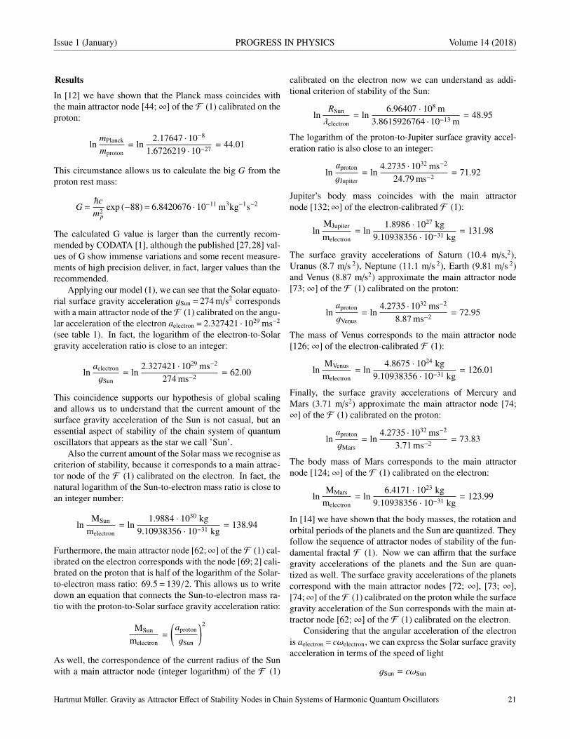
Issue 1 (January) PROGRESS IN PHYSICS Volume 14 (2018)
Results
In [12] we have shown that the Planck mass coincides withthe main attractor node [44;∞] of the F (1) calibrated on theproton:
lnmPlanck
mproton= ln
2.17647 · 10−8
1.6726219 · 10−27 = 44.01
This circumstance allows us to calculate the big G from theproton rest mass:
G =ℏcm2
pexp (−88)= 6.8420676 · 10−11 m3kg−1s−2
The calculated G value is larger than the currently recom-mended by CODATA [1], although the published [27,28] val-ues of G show immense variations and some recent measure-ments of high precision deliver, in fact, larger values than therecommended.
Applying our model (1), we can see that the Solar equato-rial surface gravity acceleration gSun = 274 m/s2 correspondswith a main attractor node of theF (1) calibrated on the angu-lar acceleration of the electron aelectron = 2.327421 · 1029 ms−2
(see table 1). In fact, the logarithm of the electron-to-Solargravity acceleration ratio is close to an integer:
lnaelectron
gSun= ln
2.327421 · 1029 ms−2
274 ms−2 = 62.00
This coincidence supports our hypothesis of global scalingand allows us to understand that the current amount of thesurface gravity acceleration of the Sun is not casual, but anessential aspect of stability of the chain system of quantumoscillators that appears as the star we call ’Sun’.
Also the current amount of the Solar mass we recognise ascriterion of stability, because it corresponds to a main attrac-tor node of the F (1) calibrated on the electron. In fact, thenatural logarithm of the Sun-to-electron mass ratio is close toan integer number:
lnMSun
melectron= ln
1.9884 · 1030 kg9.10938356 · 10−31 kg
= 138.94
Furthermore, the main attractor node [62;∞] of the F (1) cal-ibrated on the electron corresponds with the node [69; 2] cali-brated on the proton that is half of the logarithm of the Solar-to-electron mass ratio: 69.5= 139/2. This allows us to writedown an equation that connects the Sun-to-electron mass ra-tio with the proton-to-Solar surface gravity acceleration ratio:
MSun
melectron=
(aproton
gSun
)2
As well, the correspondence of the current radius of the Sunwith a main attractor node (integer logarithm) of the F (1)
calibrated on the electron now we can understand as addi-tional criterion of stability of the Sun:
lnRSun
λelectron= ln
6.96407 · 108 m3.8615926764 · 10−13 m
= 48.95
The logarithm of the proton-to-Jupiter surface gravity accel-eration ratio is also close to an integer:
lnaproton
gJupiter= ln
4.2735 · 1032 ms−2
24.79 ms−2 = 71.92
Jupiter’s body mass coincides with the main attractornode [132;∞] of the electron-calibrated F (1):
lnMJupiter
melectron= ln
1.8986 · 1027 kg9.10938356 · 10−31 kg
= 131.98
The surface gravity accelerations of Saturn (10.4 m/s,2),Uranus (8.7 m/s 2), Neptune (11.1 m/s 2), Earth (9.81 m/s 2)and Venus (8.87 m/s2) approximate the main attractor node[73;∞] of the F (1) calibrated on the proton:
lnaproton
gVenus= ln
4.2735 · 1032 ms−2
8.87 ms−2 = 72.95
The mass of Venus corresponds to the main attractor node[126;∞] of the electron-calibrated F (1):
lnMVenus
melectron= ln
4.8675 · 1024 kg9.10938356 · 10−31 kg
= 126.01
Finally, the surface gravity accelerations of Mercury andMars (3.71 m/s2) approximate the main attractor node [74;∞] of the F (1) calibrated on the proton:
lnaproton
gMars= ln
4.2735 · 1032 ms−2
3.71 ms−2 = 73.83
The body mass of Mars corresponds to the main attractornode [124;∞] of the F (1) calibrated on the electron:
lnMMars
melectron= ln
6.4171 · 1023 kg9.10938356 · 10−31 kg
= 123.99
In [14] we have shown that the body masses, the rotation andorbital periods of the planets and the Sun are quantized. Theyfollow the sequence of attractor nodes of stability of the fun-damental fractal F (1). Now we can affirm that the surfacegravity accelerations of the planets and the Sun are quan-tized as well. The surface gravity accelerations of the planetscorrespond with the main attractor nodes [72; ∞], [73; ∞],[74;∞] of the F (1) calibrated on the proton while the surfacegravity acceleration of the Sun corresponds with the main at-tractor node [62;∞] of the F (1) calibrated on the electron.
Considering that the angular acceleration of the electronis aelectron = cωelectron, we can express the Solar surface gravityacceleration in terms of the speed of light
gSun = cωSun
Hartmut Muller. Gravity as Attractor Effect of Stability Nodes in Chain Systems of Harmonic Quantum Oscillators 21

Volume 14 (2018) PROGRESS IN PHYSICS Issue 1 (January)
and receive the angular oscillation period 1/ωSun = 12.7 side-real days that is the first harmonic of the equatorial rotationperiod 25.4 days of the Sun. This coincidence suggests toanalyse also the gravity accelerations of the planets in termsof the speed of light.
If we express the Earth surface gravity accelerationg= 9.8 ms−2 in terms of the speed of light, we receive an os-cillation period of c/g= 355 sidereal days that is in the rangeof the Earth orbital period and coincides perfectly with theattractor node [63; 2] of the F (1) calibrated on the electronoscillation period 2πτelectron = 8.0933 · 10−21 s:
2πτelectron exp (63.5) = 355 days
The period of 355 days coincides with 12 synodic lunarmonths, the lunar year. The surface gravity accelerations ofSaturn (10.4 m/s2), Uranus (8.7 m/s2), Neptune (11.1 m/s2)and Venus (8.87 m/s2) are of the same range and consequent-ly, they approximate the same attractor node [63; 2].
The surface gravity acceleration of Saturn gSaturn =
= 10.4 m/s2 corresponds with an oscillation period ofc/gSaturn = 334 sidereal days that is in the range of the du-ration of lightning storms on Saturn which appear once every30 Earth years. The lightning storm of 2009 on Saturn in theplanet’s southern hemisphere lasted over 334 days [29].
Mars and Mercury have similar surface gravity accelera-tions of about 3.7 ms−2 that corresponds to an oscillation pe-riod of c/3.7 ms−2 = 938 sidereal days near the attractor node[64; 2] of the F (1) calibrated on the electron:
2πτelectron exp (64.5)= 966 days
The sidereal rotation period of Mars is 24.62278 hours andcoincides perfectly to the main node [67; ∞] of the proton-calibrated F (1):
lnτMars
τproton= ln
24.62278 · 3600 s7.01515 · 10−25s
= 67.00
In addition, the orbital period of Mars 686.971 days meetsprecisely the condition of global scaling:
lnTMars
τelectron= ln
686.971 · 86164 s1.28808867 · 10−21s
= 66.00
The surface gravity acceleration of Jupiter gJupiter =
= 24.79 ms−2 corresponds to an oscillation period ofc/gJupiter = 140 sidereal days near the main attractor nodeof the F calibrated on the electron:
2πτelectron exp (62.5) = 131 days
The sidereal rotation period of Jupiter is 9.925 hours and cor-responds with the main attractor node [66; ∞] of the protonF (1):
lnτJupiter
τproton= ln
9.9251 · 3600 s7.01515 · 10−25s
= 66.10
Jupiter’s orbital period of 4332.59 days fulfils the conditionsof global scaling very precisely:
lnTJupiter
2πτelectron= ln
4332.59 · 86164 s2π 1.28808867 · 10−21s
= 66.00
When the logarithm of the sidereal rotation period ofJupiter slows down to [66; ∞], the orbital-to-rotation periodratio of Jupiter can be described by the equation:
TJupiter
τJupiter=
2πτelectron
τproton
We can see that both the orbital periods of Jupiter and Marscorrespond with the main attractor node [66; ∞] of stability,but in the case of Jupiter with the electron oscillation periodas fundamental and in the case of Mars with the electron an-gular oscillation period as fundamental. Therefore, both or-bital periods are simply connected by 2π:
TJupiter = 2πTMars
Also these circumstances support our model of matter aschain system of harmonic quantum oscillators and our hy-pothesis of global scaling.
Conclusion
Applying our fractal model of matter as chain system of har-monic quantum oscillators to the analysis of gravimetric char-acteristics of large bodies of the Solar system we did showthat the surface gravity accelerations of the planets and theSun are quantized and correspond to nodes of stability inchain systems of oscillating protons and electrons and there-fore, they can be estimated without any information about themasses or sizes of the celestial bodies.
Furthermore, the quantized surface gravity accelerationsof the planets and the Sun seem to be connected with theirquantized orbital and rotation periods.
We presume that the accretion of gravitational mass is amacroscopic cumulative attractor effect of stability nodes inchain systems of oscillating protons and electrons. From thispoint of view, Newton’s constant of gravitation defines thecorresponding amount of gravitational mass a given attractornode can accumulate.
Acknowledgements
The author is grateful to Viktor Panchelyuga for valuable dis-cussions.
Submitted on November 23, 2017
References1. CODATA recommended 2014 values of the fundamental physical con-
stants: physics.nist.gov/constants.
2. Numerical Standards for Fundamental Astronomy. maia.usno.navy.mil,IAU Working Group, 2017.
22 Hartmut Muller. Gravity as Attractor Effect of Stability Nodes in Chain Systems of Harmonic Quantum Oscillators

Issue 1 (January) PROGRESS IN PHYSICS Volume 14 (2018)
3. Quinn T., Speake C. The Newtonian constant of gravitation – a constanttoo difficult to measure? An introduction. Phil. Trans. Royal Society A,v. 372, 20140253.
4. Anderson J. D. et al. Measurements of Newton’s gravitational constantand the length of day. EPL, v. 110, 10002, 2015.
5. Holme R., de Viron O. Characterization and implications of in-tradecadal variations in length of day. Nature, v. 499, 202-204, 2013.
6. Schlamminger S. et al. Recent measurements of the gravitational con-stant as a function of time. arXiv:1505.01774v2 [gr-qc] 21 May 2015.
7. Stacey F. D. et al. Constraint on the planetary scale value of the Newto-nian gravitational constant from the gravity profile within a mine. Phys.Rev. v. D23, 1683, 1981.
8. Cahill R. T. 3-Space In-Flow Theory of Gravity: Boreholes, Blackholesand the Fine Structure Constant. Progress in Physics, v. 2, 9–16, 2006.
9. Muller H. Fractal Scaling Models of Natural Oscillations in Chain Sys-tems and the Mass Distribution of Particles. Progress in Physics, v. 3,61–66, 2010.
10. Ries A. Qualitative Prediction of Isotope Abundances with the BipolarModel of Oscillations in a Chain System. Progress in Physics, v. 11,183–186, 2015.
11. Muller H. Fractal Scaling Models of Resonant Oscillations in ChainSystems of Harmonic Oscillators. Progress in Physics, v. 2, 72–76,2009.
12. Muller H. Emergence of Particle Masses in Fractal Scaling Models ofMatter. Progress in Physics, v. 4, 44–47, 2012.
13. Muller H. Fractal scaling models of natural oscillations in chain sys-tems and the mass distribution of the celestial bodies in the Solar Sys-tem. Progress in Physics, v. 3, 61–66, 2010.
14. Muller H. Scale-Invariant Models of Natural Oscillations in Chain Sys-tems and their Cosmological Significance. Progress in Physics, v. 4,187–197, 2017.
15. Muller H. Global Scaling as Heuristic Model for Search of AdditionalPlanets in the Solar System. Progress in Physics, v. 4, 204–206, 2017.
16. Muller H. Scaling of body masses and orbital periods in the Solar Sys-tem. Progress in Physics, v. 11, 133–135, 2015.
17. Muller H. Scaling of body masses and orbital periods in the Solar Sys-tem as consequence of gravity interaction elasticity. Abstracts of theXII. International Conference on Gravitation, Astrophysics and Cos-mology, dedicated to the centenary of Einstein’s General Relativity the-ory. Moscow, PFUR, 2015.
18. Batygin K., Brown M. E. Evidence for a distant giant planet in the SolarSystem. The Astronomical Journal, 151 / 22, February 2016.
19. Volk K., Malhotra R. The curiously warped mean plane of the Kuiperbelt. arXiv:1704.02444v2 [astro-ph.EP], 19 June 2017.
20. Khintchine A.Ya. Continued fractions. University of Chicago Press,Chicago, 1964.
21. Hilbert D. Uber die Transcendenz der Zahlen e und π. MathematischeAnnalen, v. 43, 216–219, 1893.
22. Panchelyuga V. A., Panchelyuga M. S. Resonance and Fractals on theReal Numbers Set. Progress in Physics, v. 4, 48–53, 2012.
23. Muller H. The general theory of stability and objective evolutionarytrends of technology. Applications of developmental and constructionlaws of technology in CAD. Volgograd, VPI, 1987 (in Russian).
24. Muller H. Superstability as a developmental law of technology. Tech-nology laws and their Applications. Volgograd-Sofia, 1989 (in Russian)
25. Olive K.A. et al. (Particle Data Group), Chin. Phys. C, v. 38, 090001,2016.Patrignani C. et al. (Particle Data Group), Chin. Phys. C, v. 40, 100001,2016.
26. Muller H. Scaling as Fundamental Property of Natural Oscillations andthe Fractal Structure of Space-Time. Foundations of Physics and Ge-ometry. Peoples Friendship University of Russia, 2008 (in Russian).
27. Newell D.B. CODATA and the Newtonian Gravitational Constant.Newtonian constant of gravitation workshop NIST, 9–10 October,2014.
28. Gillies G.T. The Newtonian gravitational constant: recent measure-ments and related studies. Rep. Prog. Phys., v. 60, 151–225, 1997.
29. NASA’s Cassini watches storm choke on its own tail. NASA/JPL-Caltech/SSI/Hampton University, Jan. 31, 2013.
Hartmut Muller. Gravity as Attractor Effect of Stability Nodes in Chain Systems of Harmonic Quantum Oscillators 23

Volume 14 (2018) PROGRESS IN PHYSICS Issue 1 (January)
LETTERS TO PROGRESS IN PHYSICS
On the Ultimate Energy of Cosmic RaysAnaltoly V. Belyakov
E-mail: [email protected]
It is established that the upper limit of cosmic-ray energy due to the Greisen-Zatsepin-Kuzmin effect is local. On the basis of the mechanistic interpretation of J. Wheeler’sgeometrodynamic concept, a more fundamental limitation on this limit was established,which, in the final analysis, depends on Planck’s size (~γ/c3)1/2 and for protons thelimit is 4.51× 10¹⁸ eV. The inflection in the spectrum curve, the “knee”, corresponds tothe mass-energy of the vortex tube of the limiting proton-electron contour, 1.46 × 10¹⁵
eV. For other nuclei these energies increase in proportion to the atomic number of theelement.
Cosmic rays are a flow of nuclei of chemical elements — hy-drogen (∼ 90%), helium (∼ 8%), and the nuclei of the heavierelements (∼ 2%). The energy spectrum of cosmic rays or thedependence of the cosmic ray flux on energy extends from103 to 1020 eV. The main sources of primary cosmic rays aresupernova explosions (galactic cosmic rays) and the Sun, aswell as extragalactic sources — radio galaxies and quasars.The protons and heavier nuclei emitted during supernova ex-plosions are further accelerated in specific astrophysical pro-cesses. Falling into the earth’s atmosphere, cosmic ray par-ticles transmit their energy to a multitude of secondary par-ticles. Thus, the particles cascade is formed; it is called anextensive air shower (EAS) and covers a large area.
Nature ultrahigh energy cosmic rays (more than 1017 eV)has not yet been unambiguously interpreted, their sourceshave not yet been identified, and there is no complete under-standing of the mechanisms of their acceleration and even thenature of the accelerated particles [1]. There are reasons toassume that they are of extragalactic origin. It is believed thatthe upper limit of cosmic-ray energy is limited by a thresholdof 5× 10¹⁹ eV, because cosmic ray particles interact energeti-cally with relic radiation, which leads to their absorption andreduction of their energy to a threshold value at distances ofthe order of several tens of megaparsecs (Greisen-Zatsepin-Kuzmin effect) [2,3]. The presence of particles with energiesexceeding this threshold does not yet find a satisfactory expla-nation, since within range of up to one hundred megaparsecpowerful radiation sources are absent.
The question arises: what energy could be cosmic rays, ifthe distance between the source and the Earth would be muchless than the Greisen-Zatsepin-Kuzmin limit, and could notmicroparticle produce a huge macroscopic effect? Here wesee a paradox, since theoretically relativistic mass and en-ergy of the particle can approach infinity. It seems that theGreisen-Zatsepin-Kuzmin effect is of local importance, andthere are more fundamental causes that limit the energy ofcosmic rays.
A fundamental limitation can be derived by considering acharged microparticle from the point of view of John Wheel-
er’s geometrodynamic concept. Wheeler’s concept assumesthat charged microparticles are singular points on a topolog-ically non-unitary coherent two-dimensional surface of ourworld, connected by a “wormhole”, a vortex tube or a currentline of the input-output kind in an additional dimension, gen-erally forming a closed counter. According to the mechanisticinterpretation of Wheeler’s idea when the contour (proton-electronic, for example) is opened individual charged parti-cles retain part of the contour vortex tube (boson mass) whosemomentum is numerically equal to the charge [4, 5]. In theseworks formulas are derived for the vortex tube parameters: itsboson mass my, the circulation velocity of the medium alongthe contour v, the radius r, and the length ly:
my = (an)2 me , (1)
v =c1/3
0
(an)2 c , (2)
r =c2/3
0
(an)4 re , (3)
ly = (an)2re , (4)
where n is the principal quantum number of the contour, a isthe inverse of the fine structure constant, me and re are themass and classical radius of the electron, c0 is the dimen-sionless speed of light equal to c/[m/sec]. Depending on thesize of the contour, i.e. from its quantum number, its param-eters vary, but the momentum (charge equivalent) in a closedcounter remains constant. At the same time, both the contoursize and the parameters of the vortex tube have their ultimatevalues.
In [6], in determining the neutrino mass, it was shown thatthe Planck size rh = (~γ/c3)1/2 has a physical meaning and isthe limiting size inherent in the neutrino, and, obviously, ingeneral for the microcosm, i.e. rmin = rh = 1.62 × 10⁻³⁵ mor 5.74 × 10⁻²¹ re. Then from (1) and (3) we get other ul-timate values: n = 21700 and my = 8.83 × 10¹² me. Theboson mass is compared with that of mass-energy in units of
24 Belyakov A.V. On the Ultimate Energy of Cosmic Rays

Issue 1 (January) PROGRESS IN PHYSICS Volume 14 (2018)
mec2, provided that v → c (here the boson mass can be con-sidered as the mass of the excited or “associated” vacuum). Itis this condition that is satisfied for cosmic rays whose parti-cles relative to their source move with velocities close to thespeed of light. Thus, the energy equivalent of the mass my isE = 8.83 × 1012 × 511000 = 4.51 × 10¹⁸ eV.
This quantity is the ultimate energy for cosmic-ray pro-tons. Obviously, for heavier nuclei, the energy increases inproportion to the atomic number A. This conclusion agreeswith the fact of “weight increasing” the primary cosmic raycomponent with increasing energy, and the heavy nuclei flux(most likely iron) in the region of ∼ 1018 eV is much largerthan that of protons [7–9]. Consequently, the largest energyvalue for the heaviest nuclei can not exceed E ∼ 3.7 × 10²⁰
eV and even higher values, apparently, can not be. Indeed,during the entire time of observation on Earth, only a fewdozen events with energies above 1020 eV were recorded invarious installations (the maximum energy of the cosmic par-ticle 3×10²⁰ eV was registered in October 1991 on the “Fly’sEye” device [10]).
The figure adopted from [11] shows the observed spec-trum of cosmic radiation, on which the energy limits for pro-tons (II) and heavy nuclei (III) are noted (the values alongthe ordinate are reduced to the energy in GeV). The regionof the graph is marked, where the intensity of cosmic rays isabout 1 particle per square meter per year. A narrow scatter ofthe experimental data over the entire length of the spectrum,with the exception of the region of ultrahigh energies, givesgrounds to assume that the intensity of cosmic rays dependsslightly on the nature of their sources and the mechanism fortheir acceleration, and this can be shown.
Fig. 1: The observed spectrum of cosmic radiation in the energyrange 108–1020 eV.
Let us assume that the particle velocity increases propor-tionally to the distance from the source, and the number of
particles falling per unit area of the receiver is inversely pro-portional to the cube of the distance from the source. This istrue in the case of unimpeded particle propagation. Then, bysimple computations, we obtain a relation that is independentof the distance:
I = (Em/E)1.5 Im , (5)
where Em and Im are the coordinates of some reference pointon the I(E) dependence in units of [eV] and [flux × m−2 ×
sr−1 × sec−1]. When the ordinates are divided by energy inGeV, formula (5) becomes:
I = 109 (E1.5m /E2.5) Im (6)
and shown in the figure with a dashed line. The actual de-pendence is somewhat more steeply and approximated by therelation dI/dE ∼ E−2.7, which is explained by the presence ofmagnetic fields and other cosmogenic factors affecting charg-ed particles. Nevertheless, it turns out that the shape of theenergy spectrum is largely determined by the increase in theparticles energy and the decrease in their number as radiationsources are removed from the Earth.
In the energy range 1015–1016 eV, the dependence I(E)undergoes an inflection increasing index at E, the so-called“knee”. The energy value at the inflection point matches withthe mass-energy of the contour corresponding to the ultimatesize of the hydrogen atom. For this atom, the ultimate value ofthe quantum number n = 390 [5]. In general, detailed formulafor the inflection point energy, given the results of [5], andassuming that the energy increases in proportion to the atomicnumber of nuclei can be represented as:
Eknee = 5.11 × 10⁵
2πγρemp × [sec2]
c1/30 cos qw
2 A =
= 1.46 × 10¹⁵ × A eV, (7)
where γ is the gravitational constant, ρe = me/r3e is the elec-
tron density equal to 4.07×10¹³ kg/m3, mp is the relative massof the proton, and qw is the Weinberg angle of 28.7.
For protons, this energy value is indicated in the figure bythe vertical (I), which matches with the beginning of the in-flection of the energy spectrum. The removal of the inflectionpoint towards higher energies for heavier nuclei is confirmedin [12].
One can propose the following explanation for the in-crease in the energy spectrum incline. At energies up to 1.46×10¹⁵ eV (n < 390), protons and electrons in cosmic rays canbe in a bound state — either as atoms having a neutral chargeor in some associations that have a total positive charge lessthan the protons total charge. It may reduce their interactionwith magnetic fields.
At higher energies, protons are not accompanied by elec-trons, their total positive charge remains, and they are fullyexposed to magnetic fields. Perhaps this is the reason for the
Belyakov A.V. On the Ultimate Energy of Cosmic Rays 25

Volume 14 (2018) PROGRESS IN PHYSICS Issue 1 (January)
abrupt decrease in the number of electrons in the EAS whenprimary particles have energies about 1015–1016 eV [13].
As for the neutrinos, then, bearing in mind their inherentsize limit of rh, their maximum energy, possible, can reach thesame value as that of the proton, 4.51 × 10¹⁸ eV. At the mo-ment, the highest recorded neutrino energy is 2×10¹⁵ eV [14].
Conclusion
The ultimate energy of cosmic rays is limited by the maxi-mum mass-energy of the proton vortex tube, which in turnis determined by the fundamental parameter — the Plancksize inherent in a neutrino. The reason for the inflection ofthe spectrum of cosmic rays (the “knee”) is the obtaining bythe proton of the energy at which a proton-electronic counter,having ultimate quantum number, opens. For other nucleithese energies increase in proportion to the atomic numberof the element.
It is shown that, for all on a variety of radiation sourcesand the mechanism of acceleration of cosmic particles, theshape of the spectrum of cosmic rays, provided that theyspread without interference, is largely determined by the mostcommon factors — the increase in their particle energy andthe decrease in their number — as the distance between thesources and the Earth is increasing.
Submitted on June 24, 2017
References1. Kalashev O.E. Cosmic rays of ultrahigh and ultrahigh energies. Asso-
ciated neutrino and photon radiation. 01.04.02 — theoretical physics.Thesis for the degree of Doctor of Physical and Mathematical Sciences.Moscow, 2016.
2. Greisen K. End to the cosmic ray spectrum? Phys. Rev. Lett., 1966,v. 16, 748–750.
3. Zatsepin G.T., Kuzmin V.A. On the upper boundary of the spectrum ofcosmic rays. JETP-Letters, 1966, v. 4, 78–80.
4. Belyakov A.V. Charge of the electron, and the constants of radia-tion according to J. A. Wheeler’s geometrodynamic model. Progress inPhysics, 2010, v. 4, 90–94.
5. Belyakov A.V. Macro-analogies and gravitation in the micro-world:further elaboration of Wheeler’s model of geometrodynamics. Progressin Physics, 2012, v. 2, 47–57.
6. Belyakov A.V. Determination of the neutrino mass. Progress inPhysics, 2016, v. 12, issue 1, 34–38.
7. Troitsky S.V. Cosmic rays of ultrahigh energies: composition andsource problem. 01.04.16 — physics of the atomic nucleus and ele-mentary particles. The dissertation author’s abstract on competition ofa scientific degree of the doctor of physical and mathematical sciences.Institute of Nuclear Research, Russian Academy of Sciences, Moscow,2008.
8. Grigorov N.L. et al. In: Proc. 12th Int. Cosmic Ray Conf., Hobart, 1971,v. 5, 1746.
9. Isaev P.S. Some problems of the physics of cosmic rays of ultrahighenergies. P2-99-33. Joint Institute for Nuclear Research, Dubna, 1999.
10. Bird D.J. et al. Astrophys. J., 1994, v. 424, 491.
11. Bednyakov V.A. Why research of cosmic rays of ultrahigh energiesshould be produced in a near-earth orbit. Physics of Elementary Par-ticles and the Atomic Nucleus, Joint Institute for Nuclear Research,Dubna, 2002, v. 33, no. 5.
12. Kalmykov V.N. Mass composition of primary cosmic radiation in theregion of the break according to the data of the installation EAS ofthe MSU. The dissertation and the author’s abstract on VAK 01.04.23(Moscow, Russia), the candidate of physical and mathematical sci-ences.
13. Kulikov G.V., Christiansen G.B. Journal of Experimental and Theoret-ical Physics, 1958, v. 35, 635.
14. Aartsen et al. Evidence for astrophysical muon neutrinos from theNorthern Sky with IceCube. Physical Review Letters, 2015, v. 115,081102; arXiv: 1507.04005 [astro-ph.HE].
26 Belyakov A.V. On the Ultimate Energy of Cosmic Rays

Issue 1 (January) PROGRESS IN PHYSICS Volume 14 (2018)
LETTERS TO PROGRESS IN PHYSICS
Cosmological Redshift in the De Sitter Stationary UniverseLarissa Borissova and Dmitri Rabounski
E-mail: [email protected]; [email protected]
Here we focus on our previous studies, wherein we deduced the redshift formula in thede Sitter metric space. The non-Newtonian gravitational forces of repulsion, acting inthe de Sitter universe, increase with distance. Thus these forces produce the redshifteffect on photons coming from distant objects. The redshift in the de Sitter universeincreases with distance from the observed objects, and is hyperbolic that matches withthe non-linear redshift recently registered by astronomers. As a result, we no longerneed the expanding model of the Friedmann metric to correctly explain the redshift inthe spectra of galaxies and quasars. The observed “cosmological” redshift is as wellgood explained in the de Sitter universe which is stationary as is well known.
Earlier, we studied the metric of the inner space of a liquidsphere — the sperical space filled with an ideal incompress-ible liquid (the so-called Schwarzschild 2nd metric). The ob-tained results were published in all necessary detail in [1–3].In particular, in our book Inside Stars [2] we considered starsas liquid spheres. Our computations made by the mathemat-ical methods of the General Theory of Relativity showed agood coincidence with the observational data known in as-tronomy. We also showed, in the journal papers [1, 2] andin §1.2 of the book Inside Stars [2], that the liquid spheremetric transforms into the de Sitter metric (the metric of aspherical space fulled with physical vacuum) under the fol-lowing two common conditions. First, under the gravitationalcollapse condition, when the radius of the liquid sphere be-comes equal to its gravitational radius (i.e. when the liquidsphere becomes gravitational collapsar). And second, whenthe space-time breaking matches with the radius of the liq-uid sphere. We also showed that the observed Universe isequivalent to a sphere in the state, which is very close togravitational collapse (See Chapter 6 in [2] for detail). Thusthe space of our Universe can be described by the metricof the de Sitter vacuum sphere. This means, in particular,that the non-Newtonian gravitational forces acting in the deSitter metric space must manifest themselves in some astro-nomical phenomena observed in our Universe (read aboutthe non-Newtonian forces of gravitational attraction and re-pulsion in §5.5 of our book Fields, Vacuum and the MirrorUniverse [4]). For example, the non-Newtonian gravitationalforces may also be the source of the observed redshift in thespectra of galaxies and quazars.
Now, this observed phenomenon is known as the “cos-mological redshift” due to Lemaıtre who in 1927 showed [5]that such redshift may be originated due the Doppler effect onphotons in an expanding universe (the universe of the Fried-mann metric). On the other hand, proceeding from the afore-mentioned theoretical results [1–3] we can now state that theobserved redshift in the spectra of galaxies and quazars hasno relation to cosmology but is the “effect of distance” in the
stationary universe of the de Sitter metric. Such a redshiftformula was derived in our publications [1–3]. But becausethose publications were focused on the internal constitutionof stars, the redshift effect in the de Sitter space was not em-phasized and analysed properly.
We now aim to emphasize it for better understanding ofthe obtained result.
The redshift formula is derived by integration of the scalargeodesic equation for photons. There are the scalar geodesicequation and the vectorial geodesic equation. They are therespective projections of the four-dimensional geodesic equa-tion (the equation of motion along the shortest/geodesic lines)onto the time line and the three-dimensional spatial sectionof the observer. The scalar geodesic equation, the projectiononto the time line, is the equation of energy. The vectorialgeodesic equation is the equation of three-dimensional mo-tion. So, integrating the scalar geodesic equation of a photonalong its path, we obtain how its energy and, hence, its fre-quency changes during its travel. As a result, we obtain theredshift formula. As a matter of fact that the geodesic equa-tions and, hence, their integration, depends on the metric ofthe particular space wherein the photons travel.
The three-dimensional sub-space of the de Sitter space(space-time) does not rotate and deform. But there is the grav-itational inertial force. This force acting inside a sphere filledwith physical vacuum, i.e. in the de Sitter space, in the radialcoordinates takes the form (5.74) [4, §5.5]
F =λc2
3r =
c2
a2 r ,
where λ = κρ0 is the Einstein cosmological constant, κ is theEinstein gravitational constant, while ρ0 is the density of thephysical vacuum that fills the de Sitter space (see §5.3 [4]).
The Hubble constant H = (2.3± 0.3) × 10−18 sec−1 is ex-pressed through the radius of the Universe a = 1.3 × 1028 cmas H = c/a. Thus, we obtain (6.11) [1]
F = H2r ,
Borissova L., Rabounski D. Cosmological Redshift in the De Sitter Stationary Universe 27

Volume 14 (2018) PROGRESS IN PHYSICS Issue 1 (January)
where the Hubble constant plays the role of a fundamentalfrequency
H =2πT
expessed through the time T of the existence of the Universe.So, the gravitational inertial force F acting in the de Sitterspace depends the Hubble constant H.
Because F > 0 in the de Sitter space, this is a force ofrepulsion. This force is proportional to the radial distance rto the observer: each system of reference is connected withits own observer and his reference body, which is the “centre”of his own universe.
Consider the scalar and vectorial geodesic equations for aphoton. This is the system of equations (6.22) [2]. Becausethe de Sitter space does not rotate and deform, the equationstake the simplified form (6.23), where the photon is affectedby only the gravitational inertial force and the space non-uniformity (expressed with the Christoffel symbols). Integrat-ing the scalar geodesic equation (the equation of energy) forthe photon travelling along the radial coordinate r in the deSitter space, with taking the vectorial geodesic equation, weobtain the formula of the photon’s frequency ω (6.27) [2]
ω =ω0√
1 − r2/a2,
where ω0 is the photon’s frequency in the beginning of itstravel (at its source wherefrom it was emitted). We see thatthe photon’s frequency is asymptotically increasing when thephoton’s source approaches to the event horizon (radius) ofthe Universe.
At distances much shorter than the Universe’s radius i.e.much shorter than the event horizon of the Universe (r a),the formula for the photon’s frequency becomes (6.28)
ω ' ω0
(1 +
r2
2a2
).
That is we get the quadratic additive to the initially frequencyof the photon or, in another word, the redshift effect z ofparabolic type (6.29–6.31)
z =ω − ω0
ω0=
1√1 − r2/a2
− 1 'r2
2a2 > 0 ,
which, in terms of the Hubble constant H = c/a, is
z 'H2r2
2c2 .
As is seen, the photon frequency shift is positive in this case:z > 0 (otherwise it would be blueshift). This means that theredshift effect takes place in the de Sitter universe. The spaceof the de Sitter metric is stationary: it neither expands norcompresses. The redshift effect in the de Sitter universe isdue to the non-Newtonian gravitational force of repulsion.
In the last decades, astronomical observations of the mostdistant galaxies showed an increase of the redshift effect inthe spectra of the most distant galaxies, which are locatedclose to the event horizon. The astronomers supposed there-fore, on the basis of the Friedmann metric of an expandinguniverse, that the space of our Universe expands with accel-eration. On the other hand, the non-linear redshift at largedistances is easily explained in the framework of the de Sitterstatic universe: see formula for z that above. This non-lineareffect is due to only the non-linearity of the non-Newtoniangravitational force of repulsion acting on the photon. Fromthe viewpoint of an earthy observer this effect looks as the in-creasing redshift with the increasing distance from the Earthto the observed object (the source of the photon).∗
The observed high redshift in the spectra of quazars isas well explained due to the powerful inner non-Newtonianforces of repulsion (not the far intergalactic distances in theFriedmann expanding universe). As we conclude on the ba-sis of our book Inside Stars [2], the ratio of the gravitationalradius and the space breaking radius to the physical radius a(i.e. the ratio rg/a and rbr/a) is close to 1 for neutron starsand quazars. If a star is in the state of gravitational collapse,the space breaking matches with both the gravitational radiusof the star rg and the star’s surface a, i.e. a = rg = rbr. If thespace breaking matches with only the star’s surface (rbr = a),gravitational collapse occurs at the radius
rc =
√9a2 – 8a3/rg
(2.7) in [1]. The physical radius a of such a star is
rg < a < 1.125 rg
see (2.8 – 2.9) in [1]. In other words, neutron stars and qua-zars are objects in the state, which is very close to collapse.The latter means that the inner non-Newtonian gravitationalforce of repulsion is so strong near the surface of a neutronstar or a quazar that photons emitted from its surface into thecosmos bear a high redshift independent on the distance fromthe observer. For this reason, quazars may be located notsomewhere near the event horizon of our Universe, but some-where much much closer to us.
In the end, a few words about our Universe as a whole.According to the contemporary astronomical data, its averagedensity is ∼ 10−29 g/cm3, while the ultimate large observeddistance (the radius of the Universe, or the event horizon) is∼ 1.3 × 1028 cm. With such characteristics, the collapse ra-dius is ∼ 1.2 × 1028 cm (a little lesser than the event horizon,
∗This conclusion on the unnecessity of the Friedmann metric meetsanother study [6–8] showing that the observed redshift, including its non-linearity, may be caused by the light-speed rotation of the isotropic space (thepartially degenerate space, wherein light-like particles e.g. photons travel).The found basic redshift effect in a flat space has the form of exponent, whilethe paticular space metrics make only an additional goal to it.
28 Borissova L., Rabounski D. Cosmological Redshift in the De Sitter Stationary Universe

Issue 1 (January) PROGRESS IN PHYSICS Volume 14 (2018)
while the space breaking radius is the same as he event hori-zon ∼ 1.3 × 1028 cm. These observed facts mean that we livein the inner space of an object which is either collapsar or isin the state which is very close to the state of collapse. Thedescription of such an object anyhow excludes the expandingmodel. That is the Friedmann metric of an expanding uni-verse is non-applicable to the observed Universe.
Finally, the observed non-linear redshift in the soectra ofgalaxies and quazars is well explained in the de Sitter station-ary space, wherein it is merely a “distant effect” due to thenon-Newtonian forces of repulasion which increase with dis-tance from the observer. The de Sitter universe is stationary— it is a bubble that has closed space and time on itself, andis floating in the surrounding outer space (because we haveno reason to assert that our Universe exists in isolation as anexceptional object).
Submitted on December 5, 2017
References1. Borissova L. De Sitter bubble as a model of the observable Universe.
The Abraham Zelmanov Journal, 2010, v.3, 3–24.
2. Borissova L. and Rabounski D. Inside Stars: A Theory of the InternalConstitution of Stars, and the Sources of Stellar Energy According toGeneral Relativity. 2nd Edition, American Research Press, Rehoboth(NM), 2014.
3. Borissova L. A telemetric multispace formulation of Riemannian ge-ometry, General Relativity, and cosmology: implications for relativisticcosmology and the true reality of time. Progress in Physics, 2017, v.13.Issue 2, 57–75.
4. Borissova L. and Rabounski D. Fields, Vacuum, and the Mirror Uni-verse. 2nd edition, Svenska fysikarkivet, Stockholm, 2009.
5. Block D.L. Georges Lemaıtre and Stiglers Law of Eponymy. arXiv:1106.3928.
6. Rabounski D. An explanation of Hubble redshift due to the global non-holonomity of space. Progress in Physics, 2009, v. 5, issue 1, L1–L2.
7. Rabounski D. Hubble redshift due to the global non-holonomity ofspace. The Abraham Zelmanov Journal, 2009, v. 2, 11–28.
8. Rabounski D. Non-linear cosmological redshift: the exact theory ac-cording to General Relativity. The Abraham Zelmanov Journal, 2012,v. 5, 4–30.
Borissova L., Rabounski D. Cosmological Redshift in the De Sitter Stationary Universe 29
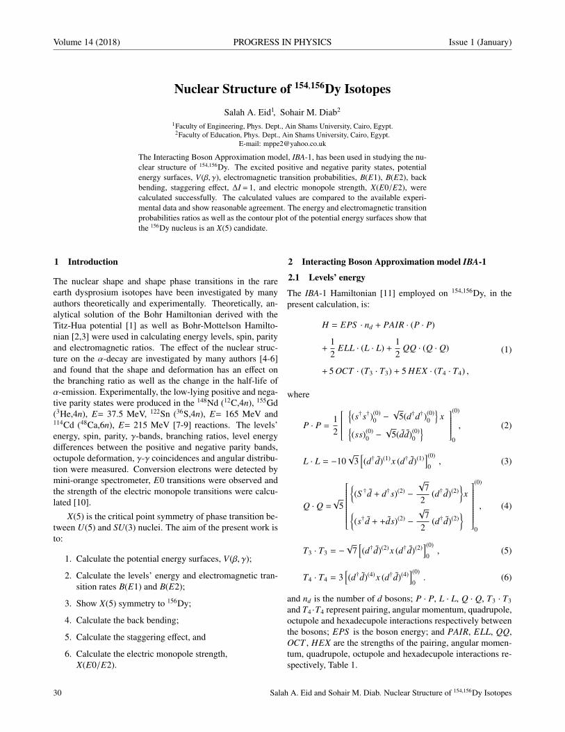
Volume 14 (2018) PROGRESS IN PHYSICS Issue 1 (January)
Nuclear Structure of 154,156Dy Isotopes
Salah A. Eid1, Sohair M. Diab2
1Faculty of Engineering, Phys. Dept., Ain Shams University, Cairo, Egypt.2Faculty of Education, Phys. Dept., Ain Shams University, Cairo, Egypt.
E-mail: [email protected]
The Interacting Boson Approximation model, IBA-1, has been used in studying the nu-clear structure of 154,156Dy. The excited positive and negative parity states, potentialenergy surfaces, V(β, γ), electromagnetic transition probabilities, B(E1), B(E2), backbending, staggering effect, ∆I = 1, and electric monopole strength, X(E0/E2), werecalculated successfully. The calculated values are compared to the available experi-mental data and show reasonable agreement. The energy and electromagnetic transitionprobabilities ratios as well as the contour plot of the potential energy surfaces show thatthe 156Dy nucleus is an X(5) candidate.
1 Introduction
The nuclear shape and shape phase transitions in the rareearth dysprosium isotopes have been investigated by manyauthors theoretically and experimentally. Theoretically, an-alytical solution of the Bohr Hamiltonian derived with theTitz-Hua potential [1] as well as Bohr-Mottelson Hamilto-nian [2,3] were used in calculating energy levels, spin, parityand electromagnetic ratios. The effect of the nuclear struc-ture on the α-decay are investigated by many authors [4-6]and found that the shape and deformation has an effect onthe branching ratio as well as the change in the half-life ofα-emission. Experimentally, the low-lying positive and nega-tive parity states were produced in the 148Nd (12C,4n), 155Gd(3He,4n), E= 37.5 MeV, 122Sn (36S,4n), E= 165 MeV and114Cd (48Ca,6n), E= 215 MeV [7-9] reactions. The levels’energy, spin, parity, γ-bands, branching ratios, level energydifferences between the positive and negative parity bands,octupole deformation, γ-γ coincidences and angular distribu-tion were measured. Conversion electrons were detected bymini-orange spectrometer, E0 transitions were observed andthe strength of the electric monopole transitions were calcu-lated [10].
X(5) is the critical point symmetry of phase transition be-tween U(5) and SU(3) nuclei. The aim of the present work isto:
1. Calculate the potential energy surfaces, V(β, γ);
2. Calculate the levels’ energy and electromagnetic tran-sition rates B(E1) and B(E2);
3. Show X(5) symmetry to 156Dy;
4. Calculate the back bending;
5. Calculate the staggering effect, and
6. Calculate the electric monopole strength,X(E0/E2).
2 Interacting Boson Approximation model IBA-1
2.1 Levels’ energy
The IBA-1 Hamiltonian [11] employed on 154,156Dy, in thepresent calculation, is:
H = EPS · nd + PAIR · (P · P)
+12
ELL · (L · L) +12
QQ · (Q · Q)
+ 5 OCT · (T3 · T3) + 5 HEX · (T4 · T4) ,
(1)
where
P · P = 12
(s†s†)(0)
0 −√
5(d†d†)(0)0
x
(ss)(0)0 −
√5(dd)(0)
0
(0)
0
, (2)
L · L = −10√
3[(d†d)(1)x (d†d)(1)
](0)
0, (3)
Q · Q =√
5
(S †d + d†s)(2) −
√7
2(d†d)(2)
x
(s†d + +ds)(2) −√
72
(d†d)(2)
(0)
0
, (4)
T3 · T3 = −√
7[(d†d)(2)x (d†d)(2)
](0)
0, (5)
T4 · T4 = 3[(d†d)(4)x (d†d)(4)
](0)
0. (6)
and nd is the number of d bosons; P · P, L · L, Q · Q, T3 · T3and T4 ·T4 represent pairing, angular momentum, quadrupole,octupole and hexadecupole interactions respectively betweenthe bosons; EPS is the boson energy; and PAIR, ELL, QQ,OCT , HEX are the strengths of the pairing, angular momen-tum, quadrupole, octupole and hexadecupole interactions re-spectively, Table 1.
30 Salah A. Eid and Sohair M. Diab. Nuclear Structure of 154,156Dy Isotopes

Issue 1 (January) PROGRESS IN PHYSICS Volume 14 (2018)
nucleus EPS PAIR ELL QQ OCT HEX E2SD(eb) E2DD(eb)154Dy 0.6240 0.000 0.0084 −0.0244 0.0000 0.0000 0.1510 −0.4467156Dy 0.4450 0.000 0.0084 −0.0244 0.0000 0.0000 0.1274 −0.3769
Table 1: Parameters used in IBA-1 Hamiltonian (all in MeV).
nucleus E4+1/E2+1
E6+1/E2+1
E8+1/E2+1
E0+2/E2+1
E6+1/E0+2
E0+3/E2+1
BE2(4+1 − 2+1 )/BE2(2+1 − 0+1 )154Dy 2.09 3.12 4.86 2.12 1.46 2.95 1.91156Dy 2.86 5.36 8.43 6.15 0.87 8.78 1.56
X(5) 3.02 5.83 9.29 5.65 1.53 6.03 1.58
Table 2: Energy and transition probability ratios.
2.2 Transition rates
The electric quadrupole transition operator employed is:
T (E2) = E2SD · (s†d + d†s)(2) +
+1√
5E2DD · (d†d)(2) .
(7)
E2SD and E2DD are adjustable parameters.The reduced electric quadrupole transition rates between
Ii → I f states are given by:
B (E2, Ii − I f ) =[< I f ∥ T (E2) ∥ Ii >]2
2Ii + 1. (8)
3 Results and discussion
3.1 The potential energy surfaces
The potential energy surfaces [12], V(β, γ), as a function ofthe deformation parameters β and γ are calculated using:
ENΠNν (β, γ) = <NπNν; βγ |Hπν|NπNν; βγ> =
= ζd(NνNπ)β2(1 + β2) + β2(1 + β2)−2×
×kNνNπ[4 − (XπXν)β cos 3γ]
+
+
[XπXνβ2] + Nν(Nν − 1)
(110
c0 +17
c2
)β2
,
(9)
where
Xρ =(
27
)0.5Xρ , ρ = π (proton) or υ (neutron) , (10)
and ζd : the energy of d bosons.The calculated potential energy surfaces, V(β, γ), are pre-
sented in Figs. 1, 2. Fig. 1 shows that 154Dy is a vibration-al-like nucleus, U(5), while 156Dy nucleus is deviated fromvibrational-like to rotational-like with slight prolate deforma-tion, SU(3), Fig. 2. The levels’ energy, transition probabilityratios presented in Table 2, as well as the potential energy sur-faces, are in favour to consider 156Dy as an X(5) candidate.
I+i I+f B (E2) I−i I+f B (E1)
21 01 0.4744 11 01 0.028222 01 0.0100 11 02 0.133622 02 0.3040 31 21 0.168331 21 0.0198 31 22 0.065841 21 0.9074 32 21 0.006931 22 0.2666 32 22 0.023542 41 0.1409 32 23 0.152042 21 0.0017 51 41 0.303542 22 0.5520 51 42 0.069861 41 1.1581 71 61 0.438062 41 0.0005 71 62 0.066562 42 0.8200 91 81 0.573481 61 1.2916 91 82 0.061081 62 0.0700 92 81 0.175081 63 0.0641 92 82 0.350182 62 0.9584 92 83 0.2144101 81 1.3384 111 101 0.7103101 82 0.0579 111 102 0.0543
Table 3: Calculated B(E2) and B(E1) in 154Dy.
3.2 Energy spectra and electric transition rates
The energy of the positive and negative parity states of iso-topes 154,156Dy are calculated using computer code PHINT[11]. A comparison between the experimental spectra [13,14]and our calculations, using values of the model parametersgiven in Table 1 for the ground state, β1, β2, γ1 and γ2 bandsare illustrated in Figs. 3, 4. The agreement between the cal-culated levels’ energy and their corresponding experimentalvalues are fair, but they are slightly higher especially for thehigher excited states. We believe this is due to the change ofthe projection of the angular momentum which is due mainlyto band crossing. Fig. 5 shows the position of X(5) and E(5)between the other types of nuclei.
Salah A. Eid and Sohair M. Diab. Nuclear Structure of 154,156Dy Isotopes 31
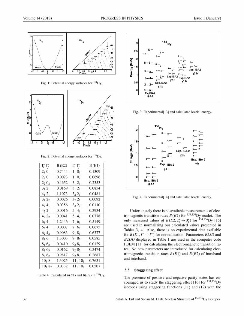
Volume 14 (2018) PROGRESS IN PHYSICS Issue 1 (January)
Fig. 1: Potential energy surfaces for 154Dy.
Fig. 2: Potential energy surfaces for 156Dy.
I+i I+f B (E2) I−i I+f B (E1)
21 01 0.7444 11 01 0.130922 01 0.0023 11 02 0.069622 02 0.4652 31 21 0.235331 21 0.0169 31 22 0.085441 21 1.1073 32 21 0.048131 22 0.0026 32 22 0.009242 41 0.0356 32 23 0.011042 21 0.0016 51 41 0.393442 22 0.0041 51 42 0.077861 41 1.2446 71 61 0.514962 41 0.0007 71 62 0.067562 42 0.9083 91 81 0.637781 61 1.3003 91 82 0.058581 62 0.0410 92 81 0.012981 63 0.0162 92 82 0.347482 62 0.9817 92 83 0.2687101 81 1.3025 111 101 0.7631101 82 0.0332 111 102 0.0507
Table 4: Calculated B(E1) and B(E2) in 156Dy.
Fig. 3: Experimental[13] and calculated levels’ energy.
Fig. 4: Experimental[14] and calculated levels’ energy.
Unfortunately there is no available measurements of elec-tromagnetic transition rates B (E2) for 154,156Dy nuclei. Theonly measured values of B (E2, 2+1 → 0+1 ) for 154,156Dy [15]are used in normalizing our calculated values presented inTables 3, 4. Also, there is no experimental data availablefor B (E1, I−→ I+) for normalization. Parameters E2SD andE2DD displayed in Table 1 are used in the computer codeFBEM [11] for calculating the electromagnetic transition ra-tes. No new parameters are introduced for calculating elec-tromagnetic transition rates B (E1) and B (E2) of intrabandand interband.
3.3 Staggering effect
The presence of positive and negative parity states has en-couraged us to study the staggering effect [16] for 154,156Dyisotopes using staggering functions (11) and (12) with the
32 Salah A. Eid and Sohair M. Diab. Nuclear Structure of 154,156Dy Isotopes

Issue 1 (January) PROGRESS IN PHYSICS Volume 14 (2018)
Fig. 5: Triangle showing the position of X(5) and E(5).
Fig. 6: Staggering effect on 154Dy and 154Dy.
help of the available experimental data [13,14].
S t (I) = 6∆E (I)− 4∆E (I − 1)− 4∆E (I + 1)+
+∆E (I + 2) + ∆E (I − 2) ,(11)
with∆E (I) = E (I + 1) − E (I) . (12)
The calculated staggering patterns are illustrated in Fig. 6and show an interaction between the positive and negativeparity states for the ground state band of 154,156Dy.
3.4 Back bending
The moment of inertia J and energy parameters ℏω are calcu-lated using (13) and (14):
2Jℏ2 =
4I − 2∆E(I → I − 2)
, (13)
(ℏω)2 = (I2 − I + 1)[∆E(I → I − 2)
(2I − 1)
]2
. (14)
The plots in Fig. 7 show forward bending for 154Dy atI+ = 18 and upper bending at I+ = 22 for 156Dy. Bending inhigher states may be explained as due to band crossing.
Fig. 7: Back bending 154Dy and 156Dy.
I+i I+f I+′ f154Dy 156Dy
02 01 21 0.0778 0.352603 02 22 0.2455 0.028503 01 22 0.0108 6.900004 03 23 0.1403 0.000004 02 23 0.0363 1.768604 01 23 0.0247 0.190322 21 02 2.4500 1.387023 21 02 0.2679 0.045423 22 02 0.1114 2.272743 41 23 0.0434 0.078543 42 23 0.0193 1.411744 41 23 0.0303 0.317744 42 23 5.3636 0.25442 41 22 0.2384 0.002762 61 42 0.2422 0.134782 81 62 0.0609 0.0173102 101 82 0.0337 0.0134
Table 5: Xi f ′ f (E0/E2) ratios in 154,156Dy.
3.5 Electric monopole transitions
The electric monopole transitions, E0, are normally occurringbetween two states of the same spin and parity by transferringenergy and zero unit of angular momentum. The strength ofthe electric monopole transition, Xi f ′ f (E0/E2) [17] can becalculated using (15) and (16) and are presented in Table 5
Xi f ′ f (E0/E2) =B (E0, Ii − I f )B (E2, Ii − I′ f )
, (15)
where Ii = I f=0, I′ f=2 and Ii= I f,0, I f = I′ f .
Xi f ′ f (E0/E2) = (2.54 × 10⁹) A3/4E5γ(MeV)
ΩKL×
×α(E2)Te(E0, Ii − I f )Te(E2, Ii − I′ f )
,
(16)
Salah A. Eid and Sohair M. Diab. Nuclear Structure of 154,156Dy Isotopes 33

Volume 14 (2018) PROGRESS IN PHYSICS Issue 1 (January)
A : mass number;Ii : spin of the initial state where E0 and E2 transitions aredepopulating it;I f : spin of the final state of E0 transition;I′ f : spin of the final state of E2 transition;Eγ : gamma ray energy;ΩKL : electronic factor for K, L shells [18];α(E2) : conversion coefficient of the E2 transition;Te(E0, Ii − I f ) : absolute transition probability of the E0 tran-sition between Ii and I f states; andTe(E2, Ii − I′ f ) : absolute transition probability of the E2 tran-sition between Ii and I′ f states.
Unfortunately, there is no experimental data available forcomparison with the calculated values.
3.6 Conclusions
The IBA-1 model has been applied successfully to 154,156Dyisotopes and:
1. Levels’ energy are successfully reproduced;
2. Potential energy surfaces are calculated and show vib-rational-like characteristics to 154Dy and slight prolatedeformation to 156Dy;
3. Electromagnetic transition rates B (E1) and B (E2) arecalculated;
4. Bending has been observed at I+= 18 for 154Dy and atI+= 22 for 156Dy ;
5. Staggering effect has been calculated and beat patternsobserved which show an interaction between the posi-tive and negative parity states;
6. Strength of electric monopole transitions Xi f ′ f (E0/E2)are calculated; and
7. The potential energy surfaces, transition probability ra-tes and energy show that 156Dy has the X(5) symmetry.
Received on November 28, 2017
References
1. Chabab M., El Batoul A., Hamzavi M., Lahbas A., Oulne M.Excited collective states of nuclei within Bohr Hamiltonianwith Tietz-Hua potential. Eur. Phys. J. A, 2017, v. 53, 157.
2. Buganu1 P. and Budaca R. Sextic potential for γ-rigid prolatenuclei. J. Phys. G, 2015, v. 42, 105106.
3. Alimohammadi M., Zare S. Investigation of Bohr-MottelsonHamiltonian in γ-rigid version with position dependent mass.Nucl. Phys. A, 2017, v. 960, 78.
4. Xiao-Dong Sun, Ping Guo, and Xiao-Hua Li. Systematicstudy of α-decay half-lives for even-even nuclei within a two-potential approach. Phys. Rev. C, 2016, v. 93, 034316.
5. Li1 Z. P., Niksic T. and Vretenar D. Coexistence of nuclearshapes: self-consistent mean-field and beyond. J. Phys. G,2015, v. 43, 024005.
6. Girija K. K. Role of shape and quadrupole deformation of par-ents in the cluster emission of rare earth nuclei. Int. J. Mod.Phys. E, 2014, v. 23, 1450002.
7. Zimba G. L., Sharpey-Schafer J. F., Jones P., Bvumbi S. P., Ma-siteng L. P., Majola S. N. T., Dinoko T. S., Lawrie E. A., LawrieJ. J., Negi D., Papka P., Roux D., Shirinda O., Easton J. E., Khu-malo N. A. Octupole correlations in N=88 154Dy: Octupole vi-bration versus stable deformation. Phys. Rev. C, 2016, v. 94,054303.
8. Ijaz Q. A., Ma W. C., Abusara H., Afanasjev A. V., Xu Y. B.,Yadav R. B., Zhang Y. C., Carpenter M. P., Janssens R. V. F.,Khoo T. L., Lauritsen T., Nisius D. T. Excited superdeformedbands in 154Dy and cranked relativistic mean field interpreta-tion. Phys. Rev. C, 2009, v. 80, 034322.
9. Paul E. S., Rigby S. V., Riley M. A., Simpson J., Appelbe D. E.,Campbell D. B., Choy P. T. W., Clark R. M., Cromaz M., EvansA. O., Fallon P., Gorgen A., Joss D. T., Lee I. Y., MacchiavelliA. O., Nolan P. J., Pipidis A., Ward D., Ragnarsson I. Loss ofcollectivity in the transitional 156Er nucleus at high spin. Phys.Rev. C, 2009, v. 79, 044324.
10. Blasi N., Atanasova L., Balabanski D., Das Gupta S., Gladin-ski K., Guerro L., Nardelli S., and Saltarelli A. E0 decay fromthe first 0+ state in 156Dy and 160Er. Phys. Rev. C, 2014, v. 90,044317.
11. Scholten O. The program package PHINT (1980) version. In-ternal report KVI-63, Keryfysisch Versneller Institut, Gronigen,1979.
12. Ginocchio J. N. and Kirson M. W. An intrinsic state for the in-teracting boson model and its relationship to the Bohr- Mottel-son approximation. Nucl. Phys. A, 1980, v. 350, 31.
13. Reich C. W. ADOPTED LEVELS, GAMMAS for 154Dy. Nu-clear Data Sheets, 2009, v. 110, 2257.
14. Reich C. W. ADOPTED LEVELS, GAMMAS for 156Dy. Nu-clear Data Sheets, 2012, v. 113, 2537.
15. Pritychenko B., Birch M., Singh B. and Horoi M. Tables ofE2 transition probabilities from the first 2+ states in even-evennuclei. Atomic Data and Nuclear Data Tables, 2016, v. 107, 1.
16. Minkov N., Yotov P., Drenska S. and Scheid W. Parity shiftand beat staggering structure of octupole bands in a collec-tive model for quadrupole-octupole deformed nuclei. J. Phys.G, 2006, v. 32, 497.
17. Rasmussen J. O. Theory of E0 transitions of spheroidal nuclei.Nucl.Phys., 1960, v. 19, 85.
18. Bell A. D., Aveldo C. E., Davidson M. G. and Davidson J. P.Table of E0 conversion probability electronic factors. Can. J.Phys., 1970, v. 48, 2542.
34 Salah A. Eid and Sohair M. Diab. Nuclear Structure of 154,156Dy Isotopes

Issue 1 (January) PROGRESS IN PHYSICS Volume 14 (2018)
Soliton-effect Spectral Self-compression for Different Initial Pulses
Armine Grigoryan1, Aghavni Kutuzyan2, and Garegin Yesayan3
Chair of Optics, Department of Physics, Yerevan State University, 1 Alex Manoogian, 0025 Yerevan, Armenia.E-mails: [email protected], [email protected], [email protected]
Our numerical studies demonstrate a spectral analogue of soliton-effect self-compression for different initial pulses. The evolution of transform-limited pulses dur-ing the propagation in a single-mode fiber with anomalous dispersion is studied. It isshown that the spectral analogue of soliton-effect self-compression is realized in thecase of different initial pulses: periodicity of the spectral compression and stretchingis different for different initial pulses. The approximation of curves introducing thefrequency of the spectral compression and stretching dependence on nonlinearity pa-rameter is implemented.
1 Introduction
The spectral compression (SC) process has numerous inter-esting applications in ultrafast optics and laser technology [1–5], such as the spectrotemporal imaging of ultrashort pulsesby means of Fourier transformation [1]. In [5], the authorsoffer to apply SC in a fiber laser instead of strong spectralfiltering. This allows to obtain transform-limited pulses andbenefits the laser’s power efficiency. As another practical ap-plication of SC, it is important to mention the transfer of fem-tosecond pulses without distortion at a relatively large dis-tance [6]. Diverse applications of SC remain urgent in rela-tion to the development and analysis of new effective com-pression systems. For example, in [7] the compression effi-ciency is improved by means of amplitude modulation.
The traditional spectral compressor consists of prism as adispersive delay line, where the pulse is stretched and nega-tively chirped, and single-mode fiber (SMF) with the normalgroup-velocity dispersion, where nonlinear self-phase modu-lation leads to the chirp compensation and spectral narrow-ing. At the wavelength range of <1.3 µm, the group-velocitydispersion is positive for standard silica fibers. The role ofthe normal dispersion in SC of subpicosecond laser pulsesis analyzed in [8]. As it is known, the combined impactof negative dispersion and the nonlinear self-phase modula-tion leads to the formation of solitons in SMF [9, 10], whenthe impact of dispersion and nonlinear self-phase modula-tion balance each other out. The pulse self-compression phe-nomenon is also known [11], which is obtained when the im-pact of the nonlinear self-phase modulation exceeds the dis-persion. Under the opposite condition, i.e. when the impactof dispersion exceeds the nonlinearity, we can expect spec-tral self-compression (self-SC) by the analogy of the pulseself-compression. Recently, the self-SC implementation di-rectly in a fiber with negative group-velocity dispersion (atthe wavelength range ≥1.3 µm for standard silica fibers) wasproposed [12] and studied [13]. In this work, we carriedout detailed numerical studies on the process of soliton-effectself-SC for different initial pulses. Simulations were carriedout for initial Gaussian and secant-hyperbolic pulses. We
have shown the soliton-effect self-SC in the fiber “directly”,without dispersive delay line, in the fiber with anomalous dis-persion for different initial pulses. It is shown that there isan analogy between the processes of soliton self-compressionand soliton-effect self-SC for different initial pulses: the pe-riodicity of the process changes in the case of different initialpulses. The studies show that the periodicity of the processdecreases when the nonlinearity parameter reduces. Our de-tailed study has shown that the frequency of compression haspolynomial and exponential approximations.
2 Numerical studies and results
In the SMF, the pulse propagation is described by the nonlin-ear Schrodinger equation for normalized complex amplitudeof field, considering only the influence of group-velocity dis-persion and Kerr nonlinearity [14]:
i∂ψ
∂ζ=
12∂2ψ
∂η2 + R |ψ2|ψ (1)
Fig. 1: The 3D map of the propagation of Gaussian (a, b) and secant-hyperbolic (c, d) pulses and its spectra. Ω = (ω − ω0)/∆ω0.
Armine Grigoryan, Aghavni Kutuzyan, and Garegin Yesayan. Soliton-effect Self SC for Different Initial Pulses 35

Volume 14 (2018) PROGRESS IN PHYSICS Issue 1 (January)
Fig. 2: The peak values of spectra (1) and pulses (2) vs fiber length for initial Gaussian (a) and secant-hyperbolic (b) pulses.
where ζ = z/LD is the dimensionless propagation distance,η = (t − z/u)/τ0 is the running time, which are normalizedto the dispersive length LD = τ2
0/|k2| (k2 is the coefficientof second-order dispersion), and initial pulse duration τ0, re-spectively. The nonlinearity parameter R is given by the ex-pression R = LD/LNL, where LNL = (k0n2I0)−1 is the non-linearity length, n2 is the Kerr index of silica, I0 is the peakintensity. The first and second terms of the right side of (1) de-scribe the impact of group-velocity dispersion and nonlinear-ity, respectively. We use the split-step Fourier method duringthe numerical solution of the equation, with the Fast FourierTransform algorithm on the dispersive step [15, 16].
The objective of our numerical studies is the soliton-effectself-SC, which takes place when the dispersive length in thefiber is shorter than the nonlinear length (LD < LNL, i.e.R < 1). Therefore, at first, the group-velocity dispersionstretches the pulse by acquiring a chirp. Afterwards, the ac-cumulated impact of nonlinear self-phase modulation leadsto the compensation of the chirp. As a result, the spectrumis compressed. The process has periodic character. We studythe pulse behavior in a fiber with negative group-velocity dis-persion for different initial pulses and different values of thenonlinearity parameter and fiber length.
Fig. 1 illustrates the process of propagation of Gaussian(a, b, R = 0.6) and secant-hyperbolic (c, d, R = 0.4) pulsesand their spectra. In this case, we study the process for shortfiber lengths where the efficiency of the process is high forthe nonlinearity parameter values of R = 0.6 (Gaussian pulse)and R = 0.4 (secant-hyperbolic pulse). It can be observed thatthe pulse is stretched and the spectrum is compressed in theinitial propagation step. Afterwards, the width of central peakof the spectrum decreases and the main part of the pulse en-ergy goes to the spectral satellites. At the certain fiber length,the reverse process starts the pulse self-compression.
The process can be explained in the following way: in theinitial propagation step the spectrum is compressed, whichleads to the decreasing of dispersion impact. As a result, thedispersive length increases, therefore, the nonlinearity param-eter also increases. When the condition R > 1 is satisfied(LD > LNL), the pulse is compressed. Then, the spectrum is
Fig. 3: The K (1) and self-SC (∆Ω0/∆Ω) (2), Imax(Ω)/I0(Ω) (3) vsfiber length for initial Gaussian pulse.
stretched, which leads to the increasing of dispersion impact(the decreasing of LD and R). When the condition R < 1 issatisfied (LD < LNL), the spectrum is compressed.
The process, which is described above has periodic char-acter, but in the case of every next cycle, the quality of theSC is worse than in the case of the previous SC as spectralsatellites increase within propagation.
Fig. 2 shows the peak value of spectra (1) and pulses(2) for initial Gaussian (a) and secant-hyperbolic (b) pulses,which shows that the process has a periodic character not onlyfor Gaussian pulses but also for secant-hyperbolic pulses. Thedifference between Gaussian and secant-hyperbolic pulses isthe speed of the process: as we see in Fig. 2, every nextspectrum compression occurs in the short distance in the caseof Gaussian pulses in comparison with the case of secant-hyperbolic pulses.
As we see in Fig. 2, the peak value decreases within thedistance which is conditioned by the fact that the energy ofspectral satellites increases. This fact is proved by the coeffi-cient of SC quality, K, (the ratio of the energy in the centralpart of pulse to the whole energy). As we see in Fig. 3, thecoefficient of SC quality decreases within the fiber length.
In the process of propagation, the behavior of the spec-
36 Armine Grigoryan, Aghavni Kutuzyan, and Garegin Yesayan. Soliton-effect Self SC for Different Initial Pulses

Issue 1 (January) PROGRESS IN PHYSICS Volume 14 (2018)
Fig. 4: The frequency vs nonlinearity parameter for initial secant-hyperbolic (a) and Gaussian (b) pulses. The points correspond to thenumerical investigations, solid lines introduce the approximation ofresults (Eqs. 2, 3) by all points, while the dotted lines correspond tothe approximation by last 3 points (Eqs. 4, 5).
trum is similar to the pulse behavior in the case of the solitoncompression. As it is known, the propagation of the high-order solitons have periodic character with a (π/2)LD period-icity. On the distance equal to the periodicity, at first pulseis compressed, then it is stretched taking initial shape. Inour case, the spectrum has similar behavior. However, dueto the incomplete cancellation of the chirp, the changing ofthe spectrum does not have the strict periodic character. Theprocess is different from soliton compression due to the factthat spectrum changes depend on a nonlinear phase, whichdepends on the shape of the pulse. In the case of solitonpropagation, the changes of the pulse depend on a dispersivephase, which depends on neither spectral nor temporal shapeof the pulse.
The study shows that the periodicity of the SC and stretch-ing decreases with the reduction of nonlinearity parameter(Fig. 4). It is shown that there are polynomial (Eqs. 2, 3)and exponential (Eqs. 4, 5) approximations of the curve intro-ducing nonlinearity parameter dependent frequency (Fig. 4),which is the frequency of the SC and stretching.
1/T = 1/(1.6 × 107 × 10−30R + 7821 × 10−4.79R
)(2)
1/T = 1/(5.09 × 106 × 10−19.8R + 731.3 × 10−3.83R
)(3)
1/T = 1/(0.004 × e3.08R
)(4)
1/T = 1/(0.001 × e3.73R
)(5)
3 Conclusion
Through the detailed study, we study the soliton-effect self-SC for initial Gaussian and secant-hyperbolic pulses. Theprocess is realized in the fiber with a negative group-velocitydispersion. The study shows that there is an analogy betweensoliton self-compression and soliton-effect self-SC processes.We show that the periodicity of the process decreases whenthe nonlinearity parameter reduces. It is shown that the fre-quency dependence on the nonlinearity parameter has poly-nomial and exponential approximations.
Acknowledgements
The authors acknowledges Prof. R. Hakobyan for fruitful dis-cussions and help during the work.
Received on December 4, 2017
References1. Mouradian L., Louradour F., Messager V., Barthelemy A., Froehly
C. Spectrotemporal imaging of femtosecond events. IEEE J. QuantumElectron., 2000, v. 36, 795.
2. Mansuryan T., Zeytunyan A., Kalashyan M., Yesayan G., MouradianL., Louradour F., and Barthelemy A. Parabolic temporal lensing andspectrotemporal imaging: a femtosecond optical oscilloscope. J. Opt.Soc. Am. B, 2008, v. 25, A101–A110.
3. Kutuzyan A., Mansuryan T., Kirakosian A., Mouradian L. Self-formingof temporal dark soliton in spectral compressor. Proc. SPIE, 2003,v. 5135, 156–160.
4. Louradour F., Lopez-Lago E., Couderc V., Messager V., Barthelemy A.Dispersive-scan measurement of the fast component of the third-ordernonlinearity of bulk materials and waveguides. Optics Lett., 1999, v. 24,1361–1363.
5. Boscolo S., Turitsyn S., and Finot Ch. Amplifier similariton fiber laserwith nonlinear spectral compression. Optics Lett., 2012, v. 37, 4531–4533.
6. Clark S., Ilday F., Wise F. Fiber delivery of femtosecond pulses from aTi:sapphire laser. Optics Lett., 2001, v. 26, 1320–1322.
7. Andresen E., Dudley J., Oron D., Finot Ch., and Rigneault H.Transform-limited spectral compression by self-phase modulation ofamplitude-shaped pulses with negative chirp. Optics Lett., 2011, v. 36,707–709.
8. Kutuzyan A., Mansuryan T., Yesayan G., Hakobyan R., Mouradian L.Dispersive regime of spectral compression. Quantum Electron., 2008,v. 38, 383–387.
9. Hasegawa A., Tappert F. Transmission of Stationary Nonlinear OpticalPulses in the Dispersive Dielectric Fibers. I. Anomalous Dispersion.Appl. Phys., 1973, v. 23, 142–144.
10. Mollenauer L., Stolen R., Gordon J. Experimental Observation of Pi-cosecond Pulse Narrowing and Soliton in Optical Fibers Dispersive Di-electric Fibers. I. Anomalous Dispersion. Phys. Rev. Lett., 1980, v. 45,1095–1098.
11. Mollenauer L., Stolen R., Gordon J., and Tomlinson W. Extreme pi-cosecond pulse narrowing by means of soliton effect in single-modeoptical fibers Dispersive Dielectric Fibers. I. Anomalous Dispersion.Optics Lett., 1983, v. 8, 289–291.
12. Yesayan G. Journal of Contemporary Physics, 2012, v. 45, 225.
13. Grigoryan A., Yesayan G., Kutuzyan A. and Mouradian L. Spectral do-main soliton-effect self-compression. Journal of Physics: ConferenceSeries, 2016, v. 672.
14. Akhmanov S. A., Vysloukh V. A. and Chirkin A. S. Optics of Femtosec-ond Laser Pulses. AIP, New York, 1992.
15. Hardin R., Tappert F. Applications of the Split-Step Fourier Methodto the Numerical Solution of Nonlinear and Variable Coefficient WaveEquations. Cronicle, 1973, v. 15, 423.
16. Fisher R., Bischel W. The role of linear dispersion in plane-wave self-phase modulation. Appl. Phys. Lett., 1973, v. 23, 661–663.
Armine Grigoryan, Aghavni Kutuzyan, and Garegin Yesayan. Soliton-effect Self SC for Different Initial Pulses 37
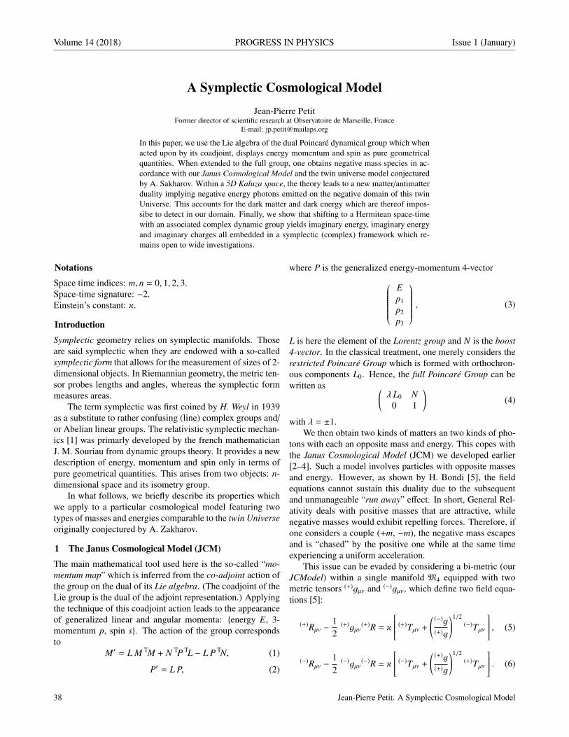
Volume 14 (2018) PROGRESS IN PHYSICS Issue 1 (January)
A Symplectic Cosmological Model
Jean-Pierre PetitFormer director of scientific research at Observatoire de Marseille, France
E-mail: [email protected]
In this paper, we use the Lie algebra of the dual Poincare dynamical group which whenacted upon by its coadjoint, displays energy momentum and spin as pure geometricalquantities. When extended to the full group, one obtains negative mass species in ac-cordance with our Janus Cosmological Model and the twin universe model conjecturedby A. Sakharov. Within a 5D Kaluza space, the theory leads to a new matter/antimatterduality implying negative energy photons emitted on the negative domain of this twinUniverse. This accounts for the dark matter and dark energy which are thereof impos-sibe to detect in our domain. Finally, we show that shifting to a Hermitean space-timewith an associated complex dynamic group yields imaginary energy, imaginary energyand imaginary charges all embedded in a symplectic (complex) framework which re-mains open to wide investigations.
Notations
Space time indices: m, n = 0, 1, 2, 3.Space-time signature: −2.Einstein’s constant: κ.
Introduction
Symplectic geometry relies on symplectic manifolds. Thoseare said symplectic when they are endowed with a so-calledsymplectic form that allows for the measurement of sizes of 2-dimensional objects. In Riemannian geometry, the metric ten-sor probes lengths and angles, whereas the symplectic formmeasures areas.
The term symplectic was first coined by H. Weyl in 1939as a substitute to rather confusing (line) complex groups and/
or Abelian linear groups. The relativistic symplectic mechan-ics [1] was primarly developed by the french mathematicianJ. M. Souriau from dynamic groups theory. It provides a newdescription of energy, momentum and spin only in terms ofpure geometrical quantities. This arises from two objects: n-dimensional space and its isometry group.
In what follows, we briefly describe its properties whichwe apply to a particular cosmological model featuring twotypes of masses and energies comparable to the twin Universeoriginally conjectured by A. Zakharov.
1 The Janus Cosmological Model (JCM)
The main mathematical tool used here is the so-called “mo-mentum map” which is inferred from the co-adjoint action ofthe group on the dual of its Lie algebra. (The coadjoint of theLie group is the dual of the adjoint representation.) Applyingthe technique of this coadjoint action leads to the appearanceof generalized linear and angular momenta: energy E, 3-momentum p, spin s. The action of the group correspondsto
M′ = L M TM + N TP TL − L P TN, (1)
P′ = L P, (2)
where P is the generalized energy-momentum 4-vectorEp1p2p3
, (3)
L is here the element of the Lorentz group and N is the boost4-vector. In the classical treatment, one merely considers therestricted Poincare Group which is formed with orthochron-ous components L0. Hence, the full Poincare Group can bewritten as (
λ L0 N0 1
)(4)
with λ = ±1.We then obtain two kinds of matters an two kinds of pho-
tons with each an opposite mass and energy. This copes withthe Janus Cosmological Model (JCM) we developed earlier[2–4]. Such a model involves particles with opposite massesand energy. However, as shown by H. Bondi [5], the fieldequations cannot sustain this duality due to the subsequentand unmanageable “run away” effect. In short, General Rel-ativity deals with positive masses that are attractive, whilenegative masses would exhibit repelling forces. Therefore, ifone considers a couple (+m, −m), the negative mass escapesand is “chased” by the positive one while at the same timeexperiencing a uniform acceleration.
This issue can be evaded by considering a bi-metric (ourJCModel) within a single manifold M4 equipped with twometric tensors (+)gµν and (−)gµν, which define two field equa-tions [5]:
(+)Rµν −12
(+)gµν(+)R = κ
(+)Tµν +
( (−)g(+)g
)1/2(−)Tµν
, (5)
(−)Rµν −12
(−)gµν(−)R = κ
(−)Tµν +
( (+)g(+)g
)1/2(+)Tµν
. (6)
38 Jean-Pierre Petit. A Symplectic Cosmological Model

Issue 1 (January) PROGRESS IN PHYSICS Volume 14 (2018)
Those time dependent and time independent solutions fitthe observational data.
2 Extension to a wider geometrical framework
We now turn consider an extension of the group to a five di-mensional scheme so as to obtain an isometry group whichacts on the basic Kaluza space-time λ µ 0 φ
0 λ L0 N0 0 1
(7)
with µ = ±1 and λ = ±1.By extending to the fifth dimension, the Noether theorem
induces an additional conserved scalar quantity which is read-ily identified with the electric charge q.
The µ = −1 implies both the inversion of this charge andthe inversion of the fifth dimension, which is just the geomet-rical expression of the matter-antimatter duality as primarlyshown by J. M. Souriau [6]. Therefore the physics ruled bythe dynamical group (7) exhibits straightforwardly the matter-antimatter symmetry in the two domains with opposed massand energy. If we now add p-Kaluza-like dimensions, we ob-tain the metric under the form:
ds2 = dx20 − dx2
1 − dx22 − dx2
3 − dξ21 − dξ2
2 − . . . − dξ2p . (8)
This can be coupled to an isometry group
λ µ 0 . . . 0 0 φ10 λ µ . . . 0 0 φ2. . . . . . . . . . . . . . . . . .0 0 . . . λ µ 0 φp
0 0 . . . 0 λ µ N0 0 . . . 0 0 1
(9)
with µ = ±1 and λ = ±1.The electric charge is just one of the quantum charges.
Here again, the (µ = −1) terms reflect the C-symmetry: theyaccount for the classical matter-antimatter representation.The (µ = −1; λ = −1) correspond to the PT -symmetry clas-sically associated with the “Feynman antimatter” which is nolonger indentified with the “C-antimatter”. This is due to thepresence of the time reversal T inducing both the mass andenergy inversion. In other words, the group representation(9) which is the basis of the JC Model, provides two distincttypes of antimatters:
— The C-type corresponding to Dirac’s antimatter.
— The PT -type corresponding to Feynman’s antimatter.
3 Remark about Andrei Sakharov’ scheme
In classical cosmology a severe problem remains, due to theabsence of observation of primordial antimatter. In 1967,
Sakharov suggested that the Universe comprises two dom-ains: the actual Universe and its twin Universe, each con-nected through a singularity [8–10]. Both are CPT -symmet-rical. Since the mass inversion goes with T -symmetry, ourJC Model [3,4] corresponds to such CPT -symmetry. The so-called twin matter becomes nothing but a copy of ordinaryparticles with opposite masses and charges. If, as suggestedby Sakharov, positive masses are synthetized by positive en-ergy quarks faster than the synthesis of negative masses frompositive energy antiquarks, then in the positive energy domainwe find:
— Remnant positive masses matter.
— The equivalent (ratio 3/1) of positive energy antiquarks.
— Positive energy photons.
In analogy to Sakharov’s ideas, the negative energy do-main would be thus composed of:
— Remnant negative masses matter.
— The equivalent (ratio 3/1) of negative energy quarks.
— Negative energy photons.
As shown in [3,4], the negative material suitably replacesboth dark matter and so-called dark energy. Accordingly,by emitting negative energy photons, the remnant negativemasses matter are genuinely invisible.
4 Remark about the Quantum Theory of Fields (QFT)
In QFT the time reversal operator is a complex operator whichcan be linear and unitary, as well as antilinear and anti-unita-ry. If chosen linear and unitary, this operator implies the exis-tence of negative energy states, which are a priori banned byQFT. In Weinberg [7], we quote: “In order to avoid this dis-astrous conclusion, we are forced to conclude that T is anti-linear and anti-unitary”. On page 104, Weinberg also writes:“no examples are known of particles that furnish unconven-tional representation of inversions, so these possibilities willnot be pursued further here”. Actually, this was true untilthe discovery of the acceleration of the expanding universewhich implies the action of a negative pressure. As a pres-sure is likened to an energy density, this new phenomenonimplies in turn the existence of negative energy states and asa result, it questions QFT by itself. In the same manner, it alsoraises some questions as to the validity of the so-called CPTtheorem and the vacuum instability. Indeed, classically, oneconsiders that a particle may loose energy through the emis-sion of a photon, so that such a process would lead to negativeenergy states. But if we consider that a negative mass parti-cle emits negative energy photons, this process would lead tostable zero energy state.
5 Extension of the method to a complex field
If one replaces the Minkowski coordinates x0, x1, x2, x3withcomplex coordinates we may form the Hermitean Riemann
Jean-Pierre Petit. A Symplectic Cosmological Model 39

Volume 14 (2018) PROGRESS IN PHYSICS Issue 1 (January)
metric:
ds2 = dx0∗dx0 − dx1
∗dx1 − dx2∗dx2 − dx3
∗dx3 . (10)
This metric is defined on a Hermitean manifold.Lest us now consider the real matrix G
1 0 0 00 −1 0 00 0 −1 00 0 0 −1
(11)
and the complex Lorentz group defined as
∗LGL = G , (12)
∗L stands for the adjoint of L.One can then easily show that the complex Poincare group(
L N0 1
)(13)
is an isometry group of such a Hermitean space and can beconsidered as a dynamic group. Surprizingly, all classical(matrix) calculations can be extended to such complex frame-work, by simply substituting the matrices ∗A to the transposematrices TA.
As a result, the complex momentum obeys the law:
M′ = L M ∗L + N ∗P ∗L − L P ∗N, (14)
P′ = L P, (15)
where ∗P is the complex energy momentum 4-vector. This ex-tended physics grants the mass a complex nature implying thepossible existence of purely real masses ±m and purely imag-inary masses: ±(−1)1/2 m. At the same time, such masses canexchange imaginary photons whose energies are: ±(−1)1/2 E.
Conclusion
J. M. Souriau gave the first purely geometrical interpretationof all classsical physics features, namely — energy, momenta,and spin. When extended to higher dimensions it provides ageometrical interpretation of the matter-antimatter duality. Inaddition, one can notice that the complex approach of spacedefinition yields complex physical quantities. The physicalmeaning of these complex quantities should demand furtherscrutiny and as such remains a new open field of investiga-tions.
Submitted on December 25, 2017
References1. Souriau J. M. Structure des Systemes Dynamiques. Dunod, Paris, 1970
(English translation: Structure of Dynamic Systems. Birkhauser, 1997).
2. Petit J. P., D’Agostini G. Negative mass hypothesis in Cosmology andthe nature of dark energy. Astrophysics and Space Sciences, 2014,v. 354, issue 2, 611–615
3. Petit J. P., D’Agostini G. Cosmological Bi-metric model with inter-acting positive and negative masses and two different speeds of lightin agreement with the observed acceleration of the Universe. ModernPhysics Letters A, 2014, v. 29, no. 34.
4. Petit J. P., D’Agostini G. Lagrangian derivation of the two coupled fieldequations in the Janus Cosmological Model. Astrophysics and SpaceScience, 2015, v. 357, issue 1, 67–74.
5. Bondi H. Negative mass in General Relativity. Rev. of Mod. Physics,1957, v. 29, issue 3, 423.
6. Souriau J. M. Geometrie et Relativite. Hermann, 1964.
7. Weinberg S. The Quantum Theory of Fields. Cambridge UniversityPress, 2005, p. 74–76, p. 104.
8. Sakharov A. D. ZhETF Pis’ma, 1967, v. 5, 32–35; JTEP Lett., 1967,v. 5, 24–27.
9. Sakharov A. D. ZhETF Pis’ma, 1979, v. 76, 1172–1181; JTEP, 1979,v. 49, 594–603.
10. Sakharov A. D. Cosmological model of the Universe with a time vectorinversion. ZhETF, 1980, v. 79, 689–693; Tr. JTEP, v. 52, 349–351.
40 Jean-Pierre Petit. A Symplectic Cosmological Model
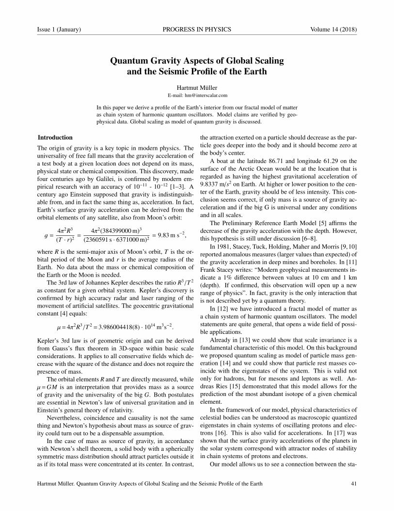
Issue 1 (January) PROGRESS IN PHYSICS Volume 14 (2018)
Quantum Gravity Aspects of Global Scalingand the Seismic Profile of the Earth
Hartmut MullerE-mail: [email protected]
In this paper we derive a profile of the Earth’s interior from our fractal model of matteras chain system of harmonic quantum oscillators. Model claims are verified by geo-physical data. Global scaling as model of quantum gravity is discussed.
Introduction
The origin of gravity is a key topic in modern physics. Theuniversality of free fall means that the gravity acceleration ofa test body at a given location does not depend on its mass,physical state or chemical composition. This discovery, madefour centuries ago by Galilei, is confirmed by modern em-pirical research with an accuracy of 10−11 - 10−12 [1–3]. Acentury ago Einstein supposed that gravity is indistinguish-able from, and in fact the same thing as, acceleration. In fact,Earth’s surface gravity acceleration can be derived from theorbital elements of any satellite, also from Moon’s orbit:
g =4π2R3
(T · r)2 =4π2(384399000 m)3
(2360591 s · 6371000 m)2 = 9.83 m s−2,
where R is the semi-major axis of Moon’s orbit, T is the or-bital period of the Moon and r is the average radius of theEarth. No data about the mass or chemical composition ofthe Earth or the Moon is needed.
The 3rd law of Johannes Kepler describes the ratio R3/T 2
as constant for a given orbital system. Kepler’s discovery isconfirmed by high accuracy radar and laser ranging of themovement of artificial satellites. The geocentric gravitationalconstant [4] equals:
µ= 4π2R3/T 2 = 3.986004418(8) · 1014 m3s−2.
Kepler’s 3rd law is of geometric origin and can be derivedfrom Gauss’s flux theorem in 3D-space within basic scaleconsiderations. It applies to all conservative fields which de-crease with the square of the distance and does not require thepresence of mass.
The orbital elements R and T are directly measured, whileµ= GM is an interpretation that provides mass as a sourceof gravity and the universality of the big G. Both postulatesare essential in Newton’s law of universal gravitation and inEinstein’s general theory of relativity.
Nevertheless, coincidence and causality is not the samething and Newton’s hypothesis about mass as source of grav-ity could turn out to be a dispensable assumption.
In the case of mass as source of gravity, in accordancewith Newton’s shell theorem, a solid body with a sphericallysymmetric mass distribution should attract particles outside itas if its total mass were concentrated at its center. In contrast,
the attraction exerted on a particle should decrease as the par-ticle goes deeper into the body and it should become zero atthe body’s center.
A boat at the latitude 86.71 and longitude 61.29 on thesurface of the Arctic Ocean would be at the location that isregarded as having the highest gravitational acceleration of9.8337 m/s2 on Earth. At higher or lower position to the cen-ter of the Earth, gravity should be of less intensity. This con-clusion seems correct, if only mass is a source of gravity ac-celeration and if the big G is universal under any conditionsand in all scales.
The Preliminary Reference Earth Model [5] affirms thedecrease of the gravity acceleration with the depth. However,this hypothesis is still under discussion [6–8].
In 1981, Stacey, Tuck, Holding, Maher and Morris [9,10]reported anomalous measures (larger values than expected) ofthe gravity acceleration in deep mines and boreholes. In [11]Frank Stacey writes: “Modern geophysical measurements in-dicate a 1% difference between values at 10 cm and 1 km(depth). If confirmed, this observation will open up a newrange of physics”. In fact, gravity is the only interaction thatis not described yet by a quantum theory.
In [12] we have introduced a fractal model of matter asa chain system of harmonic quantum oscillators. The modelstatements are quite general, that opens a wide field of possi-ble applications.
Already in [13] we could show that scale invariance is afundamental characteristic of this model. On this backgroundwe proposed quantum scaling as model of particle mass gen-eration [14] and we could show that particle rest masses co-incide with the eigenstates of the system. This is valid notonly for hadrons, but for mesons and leptons as well. An-dreas Ries [15] demonstrated that this model allows for theprediction of the most abundant isotope of a given chemicalelement.
In the framework of our model, physical characteristics ofcelestial bodies can be understood as macroscopic quantizedeigenstates in chain systems of oscillating protons and elec-trons [16]. This is also valid for accelerations. In [17] wasshown that the surface gravity accelerations of the planets inthe solar system correspond with attractor nodes of stabilityin chain systems of protons and electrons.
Our model allows us to see a connection between the sta-
Hartmut Muller. Quantum Gravity Aspects of Global Scaling and the Seismic Profile of the Earth 41

Volume 14 (2018) PROGRESS IN PHYSICS Issue 1 (January)
bility of the solar system and the stability of electron and pro-ton and consider global scaling as a forming factor of the solarsystem. This may be of cosmological significance.
In this paper we derive a profile of the Earth’s interiorfrom our fractal model of matter as chain system of harmonicquantum oscillators. Model claims are verified by geophysi-cal data. Global scaling as model of quantum gravity is dis-cussed.
Methods
In [13] we have shown that the set of natural frequencies of achain system of similar harmonic oscillators can be describedas set of finite continued fractions F , which are natural loga-rithms:
ln (ω jk/ω00) = n j0 + z
n j1 +z
n j2 + . . .+
zn jk
=
= [z, n j0; n j1, n j2, . . . , n jk] =F
(1)
where ω jk is the set of angular frequencies and ω00 is the fun-damental frequency of the set. The denominators are integer:n j0, n j1, n j2, . . . , n jk ∈Z, the cardinality j ∈N of the set and thenumber k ∈N of layers are finite. In the canonical form, thenumerator z equals 1.
In the canonical form, for finite continued fractions, thedistribution density of the eigenvalues reaches maxima nearreciprocal integers 1, 1/2, 1/3, 1/4, . . . which are the attractorpoints of the fractal set F of natural logarithms (fig. 1).
Fig. 1: The canonical form of F for k = 1 (above) and for k = 2(below) in the range -16F 6 1.
Any finite continued fraction represents a rational num-ber [18]. Therefore, all natural frequencies ω jk in (1) are irra-tional, because for rational exponents the natural exponentialfunction is transcendental [19]. This circumstance providesfor high stability of eigenstates in a chain system of harmonicoscillators because it prevents resonance interaction betweenthe elements of the system [20]. Already in 1987 we have ap-plied continued fractions of the type F as criterion of stabilityin engineering [21, 22].
In the case of harmonic quantum oscillators, the contin-ued fractions F define not only fractal sets of natural angu-lar frequencies ω jk, angular accelerations a jk = c ·ω jk, oscil-lation periods τ jk = 1/ω jk and wavelengths λ jk = c/ω jk of thechain system, but also fractal sets of energies E jk = ~ ·ω jk andmasses m jk = E jk/c2 which correspond with the eigenstates of
the system. For this reason, we call the continued fraction Fthe “fundamental fractal” of eigenstates in chain systems ofharmonic quantum oscillators.
In the canonical form (z = 1) of the fundamental fractalF , shorter continued fractions correspond with more stableeigenstates of a chain system of harmonic oscillators. There-fore, integer logarithms represent the most stable eigenstates(main attractor nodes).
As the cardinality and number of layers of the continuedfractions F are finite but not limited, in each point of thespace-time occupied by the chain system of harmonic quan-tum oscillators the scalar F is defined. Consequently, anychain system of harmonic quantum oscillators can be seen assource of the scalar field F , the fundamental field of the sys-tem. Figure 2 shows the linear 2D-projection of the first layer(k = 1) of the fundamental field F in the canonical form (z =
1) in the interval −16F6 1.
Fig. 2: The first layer (k = 1) of the linear 2D-projection of the funda-mental field F in the canonical form (z = 1) in the range -16F 6 1.
The scalar potential difference ∆F of sequent equipoten-tial surfaces at a given layer k is defined by the difference ofcontinued fractions (1). In the canonical form (z = 1):
∆F=F (j,k)−F (j+1,k) =
= [n j0; n j1, n j2, . . . , n jk]− [n j0; n j1, n j2, . . . , n j+1,k]
Normal matter is formed by nucleons and electrons becausethey are exceptionally stable quantum oscillators. In the con-cept of isospin, proton and neutron are viewed as two statesof the same quantum oscillator. Furthermore, they have sim-ilar rest masses. However, a free neutron decays into a pro-ton, an electron and antineutrino within 15 minutes while thelife-spans of the proton and electron top everything that ismeasurable, exceeding 1029 years [23].
These unique properties of the electron and proton pre-destinate their physical characteristics as fundamental units.Table 1 shows the basic set of electron and proton units thatcan be considered as a fundamental metrology (c is the speedof light in a vacuum, ~ is the Planck constant, kB is the Boltz-mann constant).
42 Hartmut Muller. Quantum Gravity Aspects of Global Scaling and the Seismic Profile of the Earth

Issue 1 (January) PROGRESS IN PHYSICS Volume 14 (2018)
Property Electron Proton
rest mass m 9.10938356(11) · 10−31 kg 1.672621898(21) · 10−27 kg
energy E = mc2 0.5109989461(31) MeV 938.2720813(58) MeV
angular frequency ω= E/~ 7.76344071 · 1020 Hz 1.42548624 · 1024 Hz
angular oscillation period τ= 1/ω 1.28808867 · 10−21 s 7.01515 · 10−25 s
angular wavelength λ= c/ω 3.8615926764(18) · 10−13 m 2.1030891 · 10−16 m
angular acceleration a = cω 2.327421 · 1029 ms−2 4.2735 · 1032 ms−2
Table 1: The basic set of physical properties of the electron and proton. Data taken from Particle Data Group [23]. Frequencies, oscillationperiods, accelerations and the proton wavelength are calculated.
In [16] was shown that the fundamental metrology (tab. 1)is completely compatible with Planck units [24]. Originallyproposed in 1899 by Max Planck, these units are also knownas natural units, because the origin of their definition comesonly from properties of nature and not from any human con-struct. Max Planck wrote [27] that these units, “regardless ofany particular bodies or substances, retain their importancefor all times and for all cultures, including alien and non-human, and can therefore be called natural units of measure-ment”. Planck units reflect the characteristics of space-time.
In [12, 14] we have introduced a fractal model of matteras a chain system of oscillating protons and electrons. We hy-pothesize that scale invariance of the fundamental field F cal-ibrated on the physical properties of the proton and electron(tab. 1) is a universal characteristic of organized matter andcriterion of stability. This hypothesis we have called ‘globalscaling’ [16, 26, 27].
Results
The proton-to-electron mass ratio is approximately 1836, sothat the mass contribution of the proton to normal matter isvery high, for example in the hydrogen atom (protium) it is1 – 1/1836 = 99.95 percent. Consequently, the mass contri-bution of the electron is only 0.05 percent. In heavier atomswhich contain neutrons, the electron contribution to atomicmass is even smaller. Therefore, in this paper we investigatea fractal model of matter as chain system of oscillating pro-tons and derive a profile of the Earth’s interior from it.
As figure 1 shows, in an attractor node of the layer k = 0,the potential difference on the layer k = 1 changes its signa-ture and compression of the equipotential density is changedto decompression. The same is valid in attractor nodes ofthe layer k = 1. There the potential difference on the layerk = 2 changes its signature. Therefore, we expect that nearthe attractor nodes of F the dramatic increase of the fieldstrength and the change of compression to decompression ofthe equipotential density in the attractor nodes should lead tomeasurable consequences. This should be valid at least forthe main attractor nodes on the layer k = 0.
Figure 3 shows the F calibrated on the angular Comp-ton wavelength of the proton in the canonical (z = 1) linear2D-projection for k = 1 in the interval [49;∞]6F 6 [52; -4].At the graphic’s left side the corresponding radii in km areindicated. The radial distribution of equipotential nodes rep-resents the expected 2D-profile of the Earth’s interior.
Fig. 3: The fundamental field F calibrated on the proton in thecanonical (z = 1) linear 2D-projection for k = 1 in the interval[49;∞]6F 6 [52; -4]. Radius in km (left side). The dotted line atthe top indicates the Earth surface that coincides with the significantsubnode [44; 4] = 6372 km of the F calibrated on the electron.
The propagation speed of a seismic compression wave de-pends on the density and elasticity of the medium and shouldtherefore correspond with zones of compression and decom-pression near the main nodes of the fundamental field F .
In accordance with both empirical models of the Earthinterior PREM [5] and IASP91 [28], the crust-mantle bound-ary (Mohorovicic discontinuity, ‘Moho’) is in between 35 and90 km depth from the Earth surface, where seismic P-wavesjump in speed abruptly from 6 to 8 km/s. In our model, theMoho corresponds with the compression zone before the sig-nificant subnode [52; -4] = 6275 km of the F calibrated onthe proton.
Hartmut Muller. Quantum Gravity Aspects of Global Scaling and the Seismic Profile of the Earth 43
Volume 14 (2018) PROGRESS IN PHYSICS Issue 1 (January)
Detailed seismic studies have shown that the speed of P-waves (longitudinal pressure waves) in the mantle increasesrather rapidly from about 9 to 11 km/s at depths between 400and 700 km, marking a layer called the transition zone. Thiszone separates the upper mantle from the lower mantle. In ourmodel, the transition zone corresponds with the compressionzone before the significant subnode [52; -3] = 5770 km of theF calibrated on the proton.
As they travel more deeply into the mantle, P-waves in-crease their speed from 8 km/s at the Moho to about 13 km/sat a depth of 2900 km. Though, once P-waves penetrate be-low 2900 km, their velocity suddenly drops from 13 km/sback down to about 8 km/s. This dramatic reduction in speedafter a depth of 2900 km defnes the boundary between theEarth’s mantle and the core. The outer core seems liquid, be-cause seismic S-waves (transversal shear waves) do not passthis boundary. In contrast, the innermost part of the corewithin a radius of 1210 km seems solid. Reaching the innercore, P-waves again jump to a velocity of 11 km/s.
Both models PREM and IASP91 identify these bound-aries with the radius of the liquid core (3480 km) and theradius of the inner solid core (1210 km). These estimationscorrespond with the compression zones before the main at-tractors [51; ∞] and [50; ∞] of the proton F and confirmthat P-waves increase their velocity in the compression zonebefore the attractor. Then in the decompression zone afterthe attractor, they decrease the velocity. This coincidence isa strong confirmation of global scaling and demonstrates thatthe current dimension and structure of the Earth interior is notcasual, but an essential criterion of its stability.
It is a notable circumstance that P-waves reach cosmicvelocities. In fact, at the Moho, P-waves jump to velocitiesnear 8 km/s that is in the range of the first cosmic velocity arocket must have to reach a circular orbit around the Earth. Inthe transition zone that separates the upper mantle from thelower mantle, P-waves jump to 11 km/s that is in the range ofthe second cosmic velocity a rocket must have to escape theEarth gravity acceleration. Through the lower mantle, the P-wave reach 13 km/s at the core-mantle boundary that is in therange of velocities a rocket launched from Earth must have toescape the solar system.
This similarity seems not by case: cosmic escape veloc-ities do not depend on the mass of the object escaping theEarth. The velocity a rocket must have to reach a circular or-bit around the Earth depends only on the gravity accelerationg and the radius r of the departure orbit. It is notable thatno data about the mass of the Earth is needed. In the case ofdeparture from the Earth surface:
vcircular =√
(gr) =
√9.8 m/s2 · 6371000 m = 7.9 km/s.
The second cosmic velocity a rocket must have to escapethe Earth gravity acceleration is
√2 times higher:
vescape =√
2 · vcircular = 11.2 km/s.
Conversely, an object that falls under the attraction ofthe Earth surface gravity acceleration g from infinity, startingwith zero velocity, will strike the Earth surface with a velocityequal to its escape velocity.
In accordance with our model (fig. 3), the inner core of theEarth should have a substructure that origins from the attrac-tor node [49; ∞] = 400 km of the F calibrated on the proton(fig. 4). In fact, the seismological exploration of the Earth’sinner core has revealed unexpected structural complexities.There is a clear hemispherical dichotomy in anisotropy andalso evidence of a subcore with a radius 300–600 km [29].Considering that the radius of the Sun coincides with the mainattractor node [49;∞] of the F calibrated on the electron:
ln(
rSun
λelectron
)= ln
(6.96407 · 108 m
3.8615926764 · 10−13 m
)= 48.945
we can write down the equation for the ratio of the radii:rSun
rEarth subcore=λelectron
λproton.
Already in [16] we have shown that the minimum and maxi-mum values of the Earth’s radius approximate the significantnode [44; 4] of the F calibrated on the electron:
ln(
r Earth max
λelectron
)= ln
(6.384 · 103 m
3.8615926764 · 10−13 m
)= 44.252,
ln(
r Earth min
λelectron
)= ln
(6.353 · 103 m
3.8615926764 · 10−13 m
)= 44.247.
Figure 3 shows the node [44; 4] of the electron F as dottedline in the top of the graphic.
Conclusion
In the framework of our model of matter as chain system ofharmonic quantum oscillators, the fractal fundamental fieldF affects any type of physical interaction, including the grav-itational. Fundamental particles like electron and proton arenot the ultimate sources, but stability nodes of the fundamen-tal field of any chain system of harmonic quantum oscillators.The spatial and temporal distribution of these stability nodesis determined by the ratio of fundamental constants. AlreadyPaul Dirac [30] mentioned that “... whether a thing is con-stant or not does not have any absolute meaning unless thatquantity is dimensionless”.
Applying our fractal model of matter to the analysis ofgravimetric and seismic characteristics of the Earth we didshow that it corresponds well with established empirical mod-els of the Earth interior. We interpret this correspondence asevidence of the fractality, scale invariance and macroscopicquantization of Earth’s gravity field.
We presume that gravity is a scale-invariant attractor ef-fect of stability nodes in chain systems of oscillating protonsand electrons. May be this hypothesis could become a bridgethat connects the island of gravity research with the continentof quantum physics.
44 Hartmut Muller. Gravity as Attractor Effect of Stability Nodes in Chain Systems of Harmonic Quantum Oscillators

Issue 1 (January) PROGRESS IN PHYSICS Volume 14 (2018)
Acknowledgements
I’m thankful to Leili Khosravi, Viktor Panchelyuga and OlegKalinin for valuable discussions.
Submitted on December 30, 2017
References1. Niebauer T.M., McHugh M.P., Faller J.E. Galilean test for the fifth
force. Physical Review Letters, 1987, v.59, 609–612.
2. Shapiro I.I. et al. Verification of the principle of equivalence for massivebodies. Physical Review Letters, 1976, v.36, 555–558.
3. Roll P.G., Krotov R., Dicke R.H. The equivalence of inertial and passivegravitational mass. Annals of Physics, 1964, v.26, 442–517.
4. Numerical Standards for Fundamental Astronomy. maia.usno.navy.mil,IAU Working Group, 2017.
5. Dziewonski A.M., Anderson D.L. Preliminary reference Earth model.Physics of the Earth and Planetary Interiors, 1981, v.25, 297–356.
6. Quinn T., Speake C. The Newtonian constant of gravitation — a con-stant too difficult to measure? An introduction. Phil. Trans. Royal So-ciety A, v.372, 20140253.
7. Anderson J.D. et al. Measurements of Newton’s gravitational constantand the length of day. EPL, 2015, v.110, 10002.
8. Cahill R.T. 3-Space In-Flow Theory of Gravity: Boreholes, Blackholesand the Fine Structure Constant. Progress in Physics, 2006, v. 2, issue2, 9–16.
9. Stacey F.D. et al. Constraint on the planetary scale value of the Newto-nian gravitational constant from the gravity profile within a mine. Phys.Rev. D, 1981, v.23, 1683.
10. Holding S.C., Stacey F.D., Tuck G.J. Gravity in mines. An investigationof Newton’s law. Phys. Rev. D, 1986, v.33, 3487.
11. Stacey F.D. Gravity. Science Progress, 1984, v.69, no.273, 1–17.
12. Muller H. Fractal Scaling Models of Natural Oscillations in Chain Sys-tems and the Mass Distribution of Particles. Progress in Physics, 2010,v.6, issue 3, 61–66.
13. Muller H. Fractal Scaling Models of Resonant Oscillations in ChainSystems of Harmonic Oscillators. Progress in Physics, 2009, v.5, is-sue 2, 72–76.
14. Muller H. Emergence of Particle Masses in Fractal Scaling Models ofMatter. Progress in Physics, 2012, v.8, issue 4, 44–47.
15. Ries A. Qualitative Prediction of Isotope Abundances with the BipolarModel of Oscillations in a Chain System. Progress in Physics, 2015,v.11, issue 2, 183–186.
16. Muller H. Scale-Invariant Models of Natural Oscillations in Chain Sys-tems and their Cosmological Significance. Progress in Physics, 2017,v.13, issue 4, 187–197.
17. Muller H. Gravity as Attractor Effect of Stability Nodes in Chain Sys-tems of Harmonic Quantum Oscillators. Progress in Physics, 2018,v.14, issue 1, 19–23.
18. Khintchine A.Ya. Continued fractions. University of Chicago Press,Chicago, 1964.
19. Hilbert D. Uber die Transcendenz der Zahlen e und π. MathematischeAnnalen, 1893, v.43, 216–219.
20. Panchelyuga V.A., Panchelyuga M.S. Resonance and Fractals on theReal Numbers Set. Progress in Physics, 2012, v.8, issue 4, 48–53.
21. Muller H. The general theory of stability and objective evolutionarytrends of technology. Applications of developmental and constructionlaws of technology in CAD, Volgograd, VPI, 1987 (in Russian).
22. Muller H. Superstability as a developmental law of technology. Tech-nology laws and their Applications, Volgograd-Sofia, 1989 (in Rus-sian).
23. Olive K.A. et al. (Particle Data Group), Chin. Phys. C, 2016, v.38,090001.Patrignani C. et al. (Particle Data Group), Chin. Phys. C, 2016, v.40,100001.
24. Astrophysical constants. Particle Data Group, pdg.lbl.gov
25. Planck M. Uber Irreversible Strahlungsvorgange. Sitzungsbericht derKoniglich Preußischen Akademie der Wissenschaften, 1899, v.1, 479–480.
26. Muller H. Scaling as Fundamental Property of Natural Oscillations andthe Fractal Structure of Space-Time. Foundations of Physics and Ge-ometry, Peoples Friendship University of Russia, 2008 (in Russian).
27. Muller H. Scaling of body masses and orbital periods in the Solar Sys-tem as consequence of gravity interaction elasticity. Abstracts of theXIIth International Conference on Gravitation, Astrophysics and Cos-mology, dedicated to the centenary of Einstein’s General Relativity the-ory, Moscow, PFUR, 2015.
28. Kennett B.L.N. IASPEI 1991 Seismological Tables. Canberra, Aus-tralia, 1991.Kennett B.L., Engdahl E.R. Travel times for global earthquake loca-tion and phase identification. Geophysical Journal International, 1991,v.105, 429–465.
29. Deguen R. Structure and dynamics of Earth’s inner core. Earth andPlanetary Science Letters, 2012, v.333–334, 211–225.
30. Dirac P.A.M. The cosmological constants. Nature, 1937, v.139, issue3512, 323.
Hartmut Muller. Quantum Gravity Aspects of Global Scaling and the Seismic Profile of the Earth 45
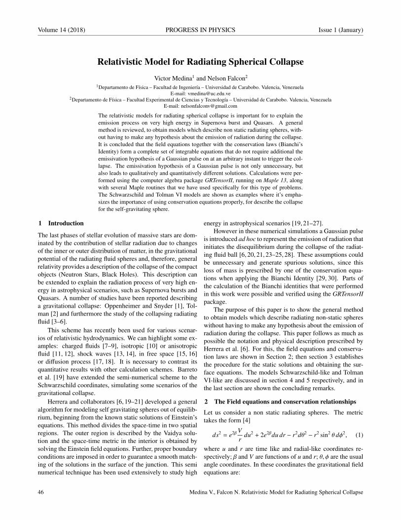
Volume 14 (2018) PROGRESS IN PHYSICS Issue 1 (January)
Relativistic Model for Radiating Spherical Collapse
Victor Medina1 and Nelson Falcon2
1Departamento de Fısica – Facultad de Ingenierıa – Universidad de Carabobo. Valencia, VenezuelaE-mail: [email protected]
2Departamento de Fısica – Facultad Experimental de Ciencias y Tecnologıa – Universidad de Carabobo. Valencia, VenezuelaE-mail: [email protected]
The relativistic models for radiating spherical collapse is important for to explain theemission process on very high energy in Supernova burst and Quasars. A generalmethod is reviewed, to obtain models which describe non static radiating spheres, with-out having to make any hypothesis about the emission of radiation during the collapse.It is concluded that the field equations together with the conservation laws (Bianchi’sIdentity) form a complete set of integrable equations that do not require additional theemissivation hypothesis of a Gaussian pulse on at an arbitrary instant to trigger the col-lapse. The emissivation hypothesis of a Gaussian pulse is not only unnecessary, butalso leads to qualitatively and quantitatively different solutions. Calculations were per-formed using the computer algebra package GRTensorII, running on Maple 13, alongwith several Maple routines that we have used specifically for this type of problems.The Schwarzschild and Tolman VI models are shown as examples where it’s empha-sizes the importance of using conservation equations properly, for describe the collapsefor the self-gravitating sphere.
1 Introduction
The last phases of stellar evolution of massive stars are dom-inated by the contribution of stellar radiation due to changesof the inner or outer distribution of matter, in the gravitationalpotential of the radiating fluid spheres and, therefore, generalrelativity provides a description of the collapse of the compactobjects (Neutron Stars, Black Holes). This description canbe extended to explain the radiation process of very high en-ergy in astrophysical scenarios, such as Supernova bursts andQuasars. A number of studies have been reported describinga gravitational collapse: Oppenheimer and Snyder [1], Tol-man [2] and furthermore the study of the collapsing radiatingfluid [3–6].
This scheme has recently been used for various scenar-ios of relativistic hydrodynamics. We can highlight some ex-amples: charged fluids [7–9], isotropic [10] or anisotropicfluid [11, 12], shock waves [13, 14], in free space [15, 16]or diffusion process [17, 18]. It is necessary to contrast itsquantitative results with other calculation schemes. Barretoet al. [19] have extended the semi-numerical scheme to theSchwarzschild coordinates, simulating some scenarios of thegravitational collapse.
Herrera and collaborators [6, 19–21] developed a generalalgorithm for modeling self gravitating spheres out of equilib-rium, beginning from the known static solutions of Einstein’sequations. This method divides the space-time in two spatialregions. The outer region is described by the Vaidya solu-tion and the space-time metric in the interior is obtained bysolving the Einstein field equations. Further, proper boundaryconditions are imposed in order to guarantee a smooth match-ing of the solutions in the surface of the junction. This seminumerical technique has been used extensively to study high
energy in astrophysical scenarios [19, 21–27].However in these numerical simulations a Gaussian pulse
is introduced ad hoc to represent the emission of radiation thatinitiates the disequilibrium during the collapse of the radiat-ing fluid ball [6, 20, 21, 23–25, 28]. These assumptions couldbe unnecessary and generate spurious solutions, since thisloss of mass is prescribed by one of the conservation equa-tions when applying the Bianchi Identity [29, 30]. Parts ofthe calculation of the Bianchi identities that were performedin this work were possible and verified using the GRTensorIIpackage.
The purpose of this paper is to show the general methodto obtain models which describe radiating non-static sphereswithout having to make any hypothesis about the emission ofradiation during the collapse. This paper follows as much aspossible the notation and physical description prescribed byHerrera et al. [6]. For this, the field equations and conserva-tion laws are shown in Section 2; then section 3 establishesthe procedure for the static solutions and obtaining the sur-face equations. The models Schwarzschild-like and TolmanVI-like are discussed in section 4 and 5 respectively, and inthe last section are shown the concluding remarks.
2 The Field equations and conservation relationships
Let us consider a non static radiating spheres. The metrictakes the form [4]
ds2 = e2βVr
du2 + 2e2βdu dr − r2dθ2 − r2 sin2 θ dϕ2, (1)
where u and r are time like and radial-like coordinates re-spectively; β and V are functions of u and r; θ, ϕ are the usualangle coordinates. In these coordinates the gravitational fieldequations are:
46 Medina V., Falcon N. Relativistic Model for Radiating Spherical Collapse

Issue 1 (January) PROGRESS IN PHYSICS Volume 14 (2018)
−8πT00 = −V,0 − 2Vβ,0r2 −V
r3
(e2β−V,1 + 2β,1V
)−8πT01 = − 1
r2
(e2β − V,1 + 2β,1V
)−8πT11 = −4β,1
r
−8πT 22 = −8πT 3
3 = −e2β(2β01 −
12r2
[rV,11+
−2β,1V + 2r(β,11V + β,1V,1
)] ).
As usual, note that we used the subscript ,0 and ,1 for thederivative for u and r, respectively; and the semicolon (;) forcovariant differentiation. Then transformation relations be-tween local Minkowskian and radiative coordinates are:
dt =(∂t∂u
)du +
(∂t∂r
)dr
= eβ(V
r
) 12
du + eβ( rV
) 12
dr (2)
dx =
(∂x∂r
)dr = eβ
( rV
) 12
dr (3)
dy =(∂y
∂θ
)dθ = r dθ (4)
dz =
(∂z∂ϕ
)dϕ = r · sin θ dϕ . (5)
We assumed the stellar material as perfect fluid, with energydensity ρ, radial pressure P, without heat conduction neitherviscosity, then
Tαβ =(ρ + P
)· UαUβ − P · ηαβ, (6)
where Uα = (1, 0, 0, 0), 3σ is the isotropic radiation of theenergy density, and ε no-polarized component of the energydensity in radial direction. Now consider an observer in localMinskowskian system with radial velocity ω, in the Lorent-zian system we can write:
Tµν = ΛαµΛβνTαβ, (7)
where the Lorentz matrix is
Λαµ =
1√
1−ω2− ω√
1−ω20 0
− ω√1−ω2
1√1−ω2
0 00 0 1 00 0 0 1
. (8)
We define
ρ = ρ + 3σ, P = P + σ, ε = ε1 + ω1 − ω.
Note also that from (2-3) the velocity of matter in the radiativecoordinates is given by
drdu=
Vr· ω
1 − ω, (9)
so forth the energy-impulse tensor in the Lorentz system is
T00 = ε +ρ + ω2P1 − ω2
T01 = T10 = −ε − ω
1 − ω2
(ρ + P
)T11 =
P + ω2ρ
1 − ω2 + ε
T22 = T33 = P.
Using (2) - (5) we obtain the energy-impulse tensor in radia-tive coordinates as:
T00 = e2β(V
r
) (ρ + ω2P1 − ω2 + ε
)T01 = T10 = e2β
(ρ − ωP1 + ω
)T11 = e2β
( rV
) (1 − ω1 + ω
) (ρ + P
)T22 =
T33
sin2 θ= r2P.
Remember that a bar indicates that the quantity is measured inthe Lorentzian system, and the effective variables are writtenwithout bar. Now
ρ ≡ ρ − ωP1 + ω
, P ≡ P − ωρ1 + ω
, ε ≡ ε. (10)
It can be seen at once that ρ = ρ and P = P in r = 0, also, inthe static case ω = 0. As before then:
T00 = e2β(V
r
) [ω (ρ + P)(1 − ω)2 + ρ + ε
]T01 = T10 = e2βρ
T11 = e2β( rV
)(ρ + P)
T22 =T33
sin2 θ= r2P,
thus the field equations are:
−Vr2
[(2β,0 −
V,0V
)− 1
r
(2Vβ,1 − V,1 + e2β
)]=
= 8π e2β(V
r
) [ε + ρ +
ω (ρ + P)(ω − 1)2
] (11)
2Vβ,1 − V,1 + e2β = 8πr2e2βρ (12)
4β,1r= 8π
rV
e2β (ρ + P) (13)
Medina V., Falcon N. Relativistic Model for Radiating Spherical Collapse 47

Volume 14 (2018) PROGRESS IN PHYSICS Issue 1 (January)
−2β,01 +1
2r2
[rV,11−2β,1V+2r
(V,1β,1+Vβ,11
)]=
= 8πe2βP.(14)
Using the conservation equations (Bianchi Identity) T µν;µ = 0,we obtain only three no-trivial relations:
T µ1;µ =e−2β
2πrβ,10 −
∂P∂r+
−12
(2β,1 +
V,1V− 1
r
)(ρ + P) −
2(P − P
)r
= 0,(15)
T λ0;λ =Vr
(2β1 +
V,1V+
1r
) [ε +ω (ρ + P)(1 − ω)2
]+
+ω
(1 − ω)2
∂ (ρ + P)∂r
+
12
(2β,0 −
V,0V
)(ρ + P)+
+∂ρ
∂u+
Vr
[∂ε
∂r+
1 + ω(1 − ω)3 (ρ + P)
∂ω
∂r
]= 0,
(16)
e2βT λ1;λ=Vr
(2β,1+
V,1V+
1r
) [ε+
1+ω2
2 (1−ω)2 (ρ+P)]
+ω (ρ + P),1(1 − ω)2 +
∂P∂r+
1r
[ρ + P −
(P − P
)]+
−12
(2β,0 −
V,0V
)(ρ + P) +
∂P∂u+
+Vr
[∂ε
∂r+
1 + ω(1 − ω)3 (ρ + P)
∂ω
∂r
]= 0.
(17)
It is remarkable that only two Bianchi equations (15-17)are independent, then
e2βT µ1;µ − T µ0;µ =
(Vr
)T µ1;µ = 0. (18)
If we use the Bondi mass aspect V ≡ e2β (r − 2m), af-ter some elementary algebra, the equation system becomesequivalent to:
m,1 = 4πr2ρ (19)
β,1 = 2πr(ρ + P)1 − 2m
r
(20)
m,0 = −4πr2e2β(1 − 2m
r
) [ε +ω (ρ + P)(1 − ω)2
](21)
8πP = −2β,01e−2β +
(1 − 2m
r
) (2β,11 + 4β 2
,1 −β,1
r
)+
+1r[3β,1
(1 − 2m,1
) − m,11]. (22)
Also, for two independent Bianchi equations (15) and (16),we obtain:
−e−2β
2πrβ,10 +
∂P∂r+
+
(4πr2P +
mr
) (ρ + P)
r(1 − 2m
r
) + 2r
(P − P
)= 0,
(23)
e2β
r
[1+
(1−2m
r
)+ 4πr2 (P−ρ)
] [ε+ω (ρ+P)(1−ω)2
]+
+Vr
ω
(1 − ω)2
∂
∂r(ρ + P)+
+Vr
[∂ε
∂r+
(1 + ω) (ρ + P)(1 − ω)3
∂ω
∂r
]+∂ρ
∂u= 0.
(24)
The expression (23) is the generalization of the Tolman -Oppenheimer - Volkoff (TOV) equation of hydrostatic equi-librium (see, for example [31]). It can be shown that the con-servation equation (24) can also be obtained from the fieldequations (19) and (21), remembering that the second mixedderivatives commute, that is, m,01 = m,10. Now, combining(21) with (24) we obtain:
2m,0e−2β
4πr3(1 − 2m
r
) [1 − m
r+ 2πr2 (P − ρ)
]=
ω
(1 − ω)2
(1 − 2m
r
)(ρ + P),1 +
+∂ε
∂r+
(1 + ω) (ρ + P)(1 − ω)3
∂ω
∂r+
e−2β
4πr2 m,10.
If we assume that radiation profiles ε and the variable ω,vary little, so we can write an expression very similar to theEuler equation
2m,0[1 − m
r+ 2πr2 (P − ρ)
]=
ω · e2β
(1 − ω)2
4πr2(1 − 2m
r
)2
r (ρ + P),1
++r
(1 − 2m
r
)m,10.
(25)
Equation (25) is omitted in previous works on the evolu-tion of radiating fluid sphere [6,20,21,23,28]. This omissionprevents the closing of the system of equations, and moti-vates the spurious inclusion of a luminosity Gaussian pulse[21, 23–25, 28]. Equation (25) allows us relate the mass ex-change with the time like and radial derivatives of the effec-tive variables, and together with eq. (21), the radiation flux ε
48 Medina V., Falcon N. Relativistic Model for Radiating Spherical Collapse
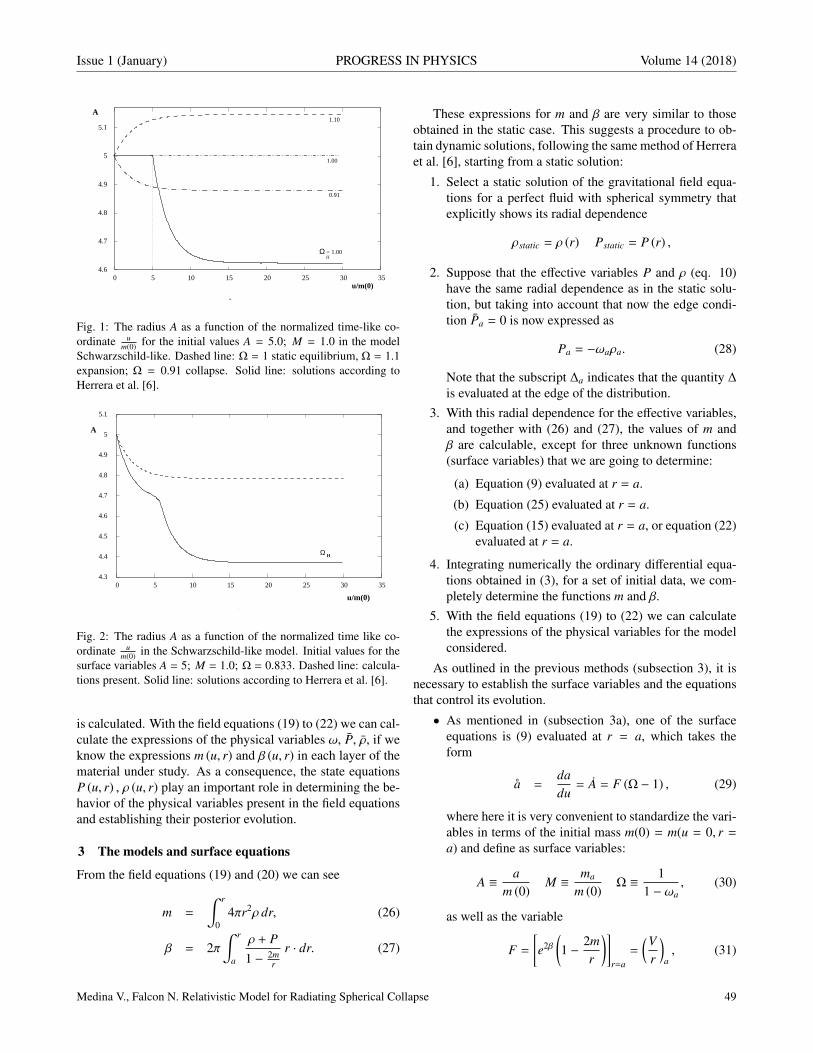
Issue 1 (January) PROGRESS IN PHYSICS Volume 14 (2018)
HΩ
0.91
1.10
1.00
= 1.00
A
5.1
5
4.9
4.8
4.7
4.6 0 5 10 15 20 25 30 35
.u/m(0)
Fig. 1: The radius A as a function of the normalized time-like co-ordinate u
m(0) for the initial values A = 5.0; M = 1.0 in the modelSchwarzschild-like. Dashed line: Ω = 1 static equilibrium, Ω = 1.1expansion; Ω = 0.91 collapse. Solid line: solutions according toHerrera et al. [6].
HΩ
u/m(0)
0 5 10 15 20 25 30 35
15
A
5.1
5
4.9
4.8
4.7
4.6
4.5
4.4
4.3
Fig. 2: The radius A as a function of the normalized time like co-ordinate u
m(0) in the Schwarzschild-like model. Initial values for thesurface variables A = 5; M = 1.0; Ω = 0.833. Dashed line: calcula-tions present. Solid line: solutions according to Herrera et al. [6].
is calculated. With the field equations (19) to (22) we can cal-culate the expressions of the physical variables ω, P, ρ, if weknow the expressions m (u, r) and β (u, r) in each layer of thematerial under study. As a consequence, the state equationsP (u, r) , ρ (u, r) play an important role in determining the be-havior of the physical variables present in the field equationsand establishing their posterior evolution.
3 The models and surface equations
From the field equations (19) and (20) we can see
m =
∫ r
04πr2ρ dr, (26)
β = 2π∫ r
a
ρ + P1 − 2m
r
r · dr. (27)
These expressions for m and β are very similar to thoseobtained in the static case. This suggests a procedure to ob-tain dynamic solutions, following the same method of Herreraet al. [6], starting from a static solution:
1. Select a static solution of the gravitational field equa-tions for a perfect fluid with spherical symmetry thatexplicitly shows its radial dependence
ρstatic = ρ (r) Pstatic = P (r) ,
2. Suppose that the effective variables P and ρ (eq. 10)have the same radial dependence as in the static solu-tion, but taking into account that now the edge condi-tion Pa = 0 is now expressed as
Pa = −ωaρa. (28)
Note that the subscript ∆a indicates that the quantity ∆is evaluated at the edge of the distribution.
3. With this radial dependence for the effective variables,and together with (26) and (27), the values of m andβ are calculable, except for three unknown functions(surface variables) that we are going to determine:
(a) Equation (9) evaluated at r = a.
(b) Equation (25) evaluated at r = a.
(c) Equation (15) evaluated at r = a, or equation (22)evaluated at r = a.
4. Integrating numerically the ordinary differential equa-tions obtained in (3), for a set of initial data, we com-pletely determine the functions m and β.
5. With the field equations (19) to (22) we can calculatethe expressions of the physical variables for the modelconsidered.
As outlined in the previous methods (subsection 3), it isnecessary to establish the surface variables and the equationsthat control its evolution.
• As mentioned in (subsection 3a), one of the surfaceequations is (9) evaluated at r = a, which takes theform
a =dadu= A = F (Ω − 1) , (29)
where here it is very convenient to standardize the vari-ables in terms of the initial mass m(0) = m(u = 0, r =a) and define as surface variables:
A ≡ am (0)
M ≡ ma
m (0)Ω ≡ 1
1 − ωa, (30)
as well as the variable
F =[e2β
(1 − 2m
r
)]r=a=
(Vr
)a, (31)
Medina V., Falcon N. Relativistic Model for Radiating Spherical Collapse 49

Volume 14 (2018) PROGRESS IN PHYSICS Issue 1 (January)
π2
ρx
36
32
40
44
48
52
0.00 0.40 1.00
8
m(0
)
0 5 10 15 20 25 30 35
u/m(0)
310
Fig. 3: Density 8πm (0)2 ρ in function of the temporal variable um(0)
for the model of Schwarzschild, for ra = 0.00, 0.40 and 1.00.
Instead of using as surface variable F (31) – the grav-itational potential at the surface – , as used in the ref-erences [6, 20, 21, 28]; we will use mass M, that is, theequation for radial evolution is
A =(1 − 2M
A
)(Ω − 1) , (32)
This equation is valid for all models.
• The second equation (25) is dependent on the modeland it becomes necessary to calculate the first deriva-tives of the effective density and pressure, as can beseen.
2m,0∣∣∣a
1 − m
r+ rβ,1
(1 − 2m
r
)− m,1
a+
− r(1 − 2m
r
)∂
∂u
(4πr2ρ
)∣∣∣∣∣∣a=
= Ω (Ω − 1)
4πr2(1 − 2m
r
)2
r∂
∂r(ρ + P)
a
(33)
• The last equation (23) is the Tolman - Oppenheimer- Volkoff conservation equation evaluated at r = a,which we can write
β,10∣∣∣a = 2πr
(∂P∂r
)∣∣∣∣∣∣a+
+
4πr2 (ρ + P)
2r2
(1 − 2m
r
)
a
(4πr2P +
mr
)a+
+ 4π (P − Pt)|a ≡ G.
(34)
π2
8
m(0
) P
15
20
25
10
5
0
−0.5
0.00 0.40 1.00
35 30 25 20u/m(0)
15 10 5 0
x10
3
30
Fig. 4: Normalized pressure values 8πm (0)2 P in function of thetime variable u
m(0) for the model of Schwarzschild, for ra = 0.4 and
1.00
Both equations (33) and (34) have a similar structure, interms of the surface variables:
ΥM A + ΞM M + ΛM Ω = ∆M (35)ΥΩ A + ΞΩ M + ΛΩ Ω = ∆Ω, (36)
where
Υξ ≡ Υξ (A,M,Ω) , Ξξ ≡ Ξξ (A,M,Ω) ,Λξ ≡ Λξ (A,M,Ω) , ∆ξ ≡ ∆ξ (A,M,Ω) , ∀ξ ∈ M,Ω
are functions of (A,M,Ω). These three equations (32), (33)and (34) allow us to establish a system of three ordinary dif-ferential equations for the surface variables; which togetherwith the initials data set, determine m and β, as set forth insubsection 4. Below are two examples for the interior dis-tribution Schwarzschild-like and Tolman VI-like in section 4and 5, respectively.
4 The Schwarzschild-like model
We will get as the first test example Schwarzschild’s well-known internal and static constant density solution. For this,we are going to assume that the density depends only on thetime-type variable, as explained in [6, 32] we can write thestate equation for the Schwarzschild type model as
ρ =3m
4πr3 (37)
P = ρ
1 − 1
g
[1− 2M
A ( ra )2
1− 2MA
] 12
1g
[1− 2M
A ( ra )2
1− 2MA
] 12
− 3
, (38)
where the value of g is determinated from the boundary con-dition
(Pa = 0
)then the effective pressure satisfies the rela-
tionship (28); and consequently g = 13−2Ω . Evaluating equa-
tion (9), for r = a, we get (32) and with (23) and (24) for
50 Medina V., Falcon N. Relativistic Model for Radiating Spherical Collapse

Issue 1 (January) PROGRESS IN PHYSICS Volume 14 (2018)
drdu
−12
−8
−4
0
0.00 0.40 1.00u/m(0)
35 30 25 20 15 10 5 0
10x2
Fig. 5: Temporal velocity evolution in coordinates radiative drdu , for
the model of Schwarzschild, for ra = 0.00, 0.40 and 1.00.
8
m(0
) ε π
2
−2
0
4
8
12
0.00 0.40 1.00 0 5 10 15 20 25 30 35
u/m(0)
x10
3
Fig. 6: Radiation profiles 8πm (0)2 ε. for the model ofSchwarzschild. All layers emit radiation but decrease until reach-ing a state of equilibrium for Ω = 1.
r = a we obtain then
M = 3( M
A
)2 (1 − 2M
A
)(Ω − 1) (2Ω-3)
3MA −Ω
(1 + 2M
A
)Ω =
2Ω (1 −Ω)A
(1 − 2M
A
)− 1
A
( MA
) 3 − 2Ω1 − 2M
A
A +
−ΩM
1(1 − 2M
A
) M,
and from (20) and (19) we obtain, then after the immediateintegration
m (r) = m (0) · M( ra
)3
β =12
log
1 + 32Ω
√√√ 1 − 2M
A
1 − 2MA
(ra
)2 − 1
.
Figures 1 and 2 show the evolution of the radius A. No-tice that Ω = 1 represents a condition of static equilibrium,
Ω > 1 represents expansion, Ω < 1 the collapse. In bothcases the system returns to equilibrium very quickly. In or-der to make some comparison, we took the initial data veryclose to those chosen in the reference [6]. We did not use thevalue for Ω = 1, since with this approximation the systemdoes not have static behavior. The figures 3, 4, 5, 6 representthe profiles of physical variables versus the time like coordi-nates for different pieces of material and for initials data. Weobtain monotonous variations in the physical quantities, asa consequence of the non-assumption of the Gaussian pulse.In particular it is shown in figure 6, how all the layers emitmonotonously, unlike the figure 7 in Herrera et al. [6]
5 The Tolman VI-like model
Following [2] we can assume as static solution
4πa2ρ = 3h(a
r
)2
4πa2P = h(a
r
)21 − 9 · z
(ra
)1 − z
(ra
) ,as before the value of z is determinated from the boundarycondition
(Pa = 0
)then Pa = −ωaρa; and consequently z =
4Ω−33(4Ω−1) ; and h = m
3r . Evaluating the equations (9), (23) and(24) at r = a we obtain
M = −
(1 − 2M
A
)2 (16Ω2 + 3
) (MA
)8[Ω
(1 − 2M
A
)+ M
A
] A
Ω = − 1A
[MA− (4Ω − 3) (4Ω − 1)
8
(1 − 2M
A
)]+ (4Ω − 1) (4Ω − 3)
A8A+
Ω(1 − 2M
A
) MM,
and the corresponding values of β and m are
β =2M3A
1(1 − 2M
A
)log
( ra
)+ 2 log
3 −(
4Ω−34Ω−1
) (ra
)3 −
(4Ω−34Ω−1
)
m = m (0) M( ra
).
Figure 7 shows the temporal variation of the radius of aradiant sphere, for different values of Ω. There is a criticalvalue Ω0 for A = 6.66 and M = 1 and slight increase inΩ causes a permanent expansion or the contraction rises tothe critical value. In the following figures 8,9,10 we showthe variations of pressure density and radiation of some inte-rior layers in case of surface expansion (explosion-like). Wenoted in the example in the figure 10 that all layers absorbedenergy during the initial collapse, an then a radiative pulse isemitted, before returning to the equilibrium configuration.
Medina V., Falcon N. Relativistic Model for Radiating Spherical Collapse 51
Volume 14 (2018) PROGRESS IN PHYSICS Issue 1 (January)
50 45 40 35 30 25 20 15 10 5 0
0.87 0.86 0.85
18A
16
14
12
8
6
4
10
u/m(0)
Fig. 7: Radio A of the distribution according to the variable tem-porary u
m(0) in a TolmannVI-like model. With initials values, A =6.66667; M = 1. Ω = 0.87 (rebound) and Ω = 0.85 (contraction)and the critical value Ω = 0.860723
π2
x 102
8
m(0
) P
0.20 0.40 0.60 0.80 1.00
−1
0
2
4
6
8
u/m(0) 50 45 40 35 30 25 20 15 10 5 0
Fig. 8: Values of the normalized pressure 8πm (0)2 P as function ofthe time-like variable u
m(0) in a TolmannVI-like model. For the layersin contraction (Ω = 0.87) with r
a = 0, 0.4, 0.6, 0.8 and 1.
6 Conclusions
We have reviewed the relativistic description of the collapseof self-gravitating radiant spheres, following the usual pro-cedure [6, 19–21, 23, 25, 28, 33] and find that it is an effec-tive method for such a purpose, since the field equations to-gether with the conservation laws (Bianchi’s Identity) forma complete set of integrable equations that do not require anadditional hypothesis about the emission of radiated energy.That is, the emission hypothesis of a Gaussian pulse at anarbitrary instant to trigger the collapse; it is not only unneces-sary, but also leads to qualitatively and quantitatively differentsolutions, as we have shown in figures 1-9. We emphasizethe importance of using conservation equations properly, aswas done in Section 2; We formally reobtain the generalizedTOV equation of the hydrostatic equilibrium (equation 23)and a relativistic version of the Euler equation for the self-gravitating sphere (equation 25).
We have seen that the Schwarzschild-like description is an
ρ2
π
u/m(0) 50 45 40 35 30 25 20 15 10 5 0
8 m
(0)
x1
02
0
5
10
15
20
25
1.00 0.80 0.60 0.20 0.40
Fig. 9: Density 8πm (0)2 ρ as function of the time-like variable um(0)
in a TolmannVI-like model. For the layers in contraction (Ω = 0.87)with r
a = 0.2, 0.4, 0.6, 0.8 and 1.
8
m(0
) ε
π2
x102
u/m(0) 0.20 0.40 0.60 0.80 1.00
50 45 40 35 30 25 20 15 10 5 0−0.03
6
5
4
3
2
1
0
−1
−2
Fig. 10: Radiation profiles emitted 8πm (0)2 ε as function of thetime-like variable u
m(0) in a TolmannVI-like model. For the layersin contraction (Ω = 0.87) with r
a = 0.2, 0.4, 0.6, 0.8 and 1.
ideal case that does not represent the phenomenology of thehigh energy events observed in the stellar collapse of massivestars such as supernovas and quasars. The measurable magni-tudes of density, pressure and emission evolve smoothly, re-turning to the equilibrium condition very rapidly (Figures 3-6). On the other hand, the Tolman VI description involves twopossible qualitatively different scenarios, such as the implo-sion or the explosion of the outer layers of the self-gravitatingsphere, depending on the initial values of the mass, radius andvelocity observables, as we have shown in figure 7.
We have shown that, in the case of contraction, the den-sity and pressure variables similarly evolve (Figures 8 and 9)as might be expected if a polytrope state equation is used.In addition, Figures 8 and 9, show a dependence of the evolu-tion of such magnitudes according to the radius of the consid-ered layer, with much higher values of density and pressurein the innermost layers, in agreement with the description ofthe stellar collapse of massive stars.
Finally figure 10 shows that during the collapse of the
52 Medina V., Falcon N. Relativistic Model for Radiating Spherical Collapse

Issue 1 (January) PROGRESS IN PHYSICS Volume 14 (2018)
self-gravitating radiating spheres a pulse of radiation emis-sion is generated before reaching equilibrium again; whicharises naturally from the complete solution of the evolutionequations, and maybe is important to explain the emissionprocess in very high energy in Supernova bursts and Quasars.
Submitted on January 12, 2018
References1. Oppenheimer J. R. and Snyder H. On Continued Gravitational Contrac-
tion. Physical Review, 1939, v. 56, 455–459.
2. Tolman R. C. Static Solutions of Einstein’s Field Equations for Spheresof Fluid. Physical Review, 1939, v. 55, 364–373.
3. Vaidya P. C. Nonstatic Solutions of Einstein’s Field Equations forSpheres of Fluids Radiating Energy. Physical Review, 1951, v. 83, 10–17.
4. Bondi H. The Contraction of Gravitating Spheres. Proceedings of theRoyal Society of London Series A, 1964, v. 281, 39–48.
5. Bayin, S. S Radiating fluid spheres in general relativity. Phys. Rev. D,1979, v. 19, 2838–2846.
6. Herrera L., Jimenez J., and Ruggeri G. J. Evolution of radiating fluidspheres in general relativity. Phys. Rev. D, 1980, v. 22, 2305–2316.
7. Patino A. and Rago H. The Effect of Electric Charge on the Evolution ofRadiant Spheres in General Relativity. Astrophysics and Space Science,1996, v. 241, 237–247.
8. Sah A. and Chandra P. Class of Charged Fluid Balls in General Rela-tivity. International Journal of Astronomy and Astrophysics, 2016, v. 6,494–511.
9. Pant N., Pradhan N. and Bansal R. K. Relativistic model of anisotropiccharged fluid sphere in general relativity. Astrophysics and Space Sci-ence, 2016, v. 361, 41.
10. Harko T. and Mak M. K. Exact power series solutions of the struc-ture equations of the general relativistic isotropic fluid stars with linearbarotropic and polytropic equations of state. Astrophysics and SpaceScience, 2016, v. 361, 283.
11. Maurya S. K. and Maharaj S. D. Anisotropic fluid spheres of embed-ding class one using Karmarkar condition. ArXiv e-prints, 2017.
12. Singh K. N., Bhar P., and Pant N. A new solution of embedding class Irepresenting anisotropic fluid sphere in general relativity. InternationalJournal of Modern Physics D, 2016, v. 25, 1650099.
13. Herrera L. and Falcon N. Heat waves and thermohaline instability in afluid. Physics Letters A, 1995, v. 201, 33–37.
14. Herrera L. and Santos N. O. Cylindrical collapse and gravitationalwaves. Classical and Quantum Gravity, 2015, v. 22, 2407–2413.
15. Van den Bergh N. and Slobodeanu R. Shear-free perfect fluids witha barotropic equation of state in general relativity: the present status.Classical and Quantum Gravity, 2016, v. 33(8), 085008.
16. Herrera L., Denmat G. L. and Santos N. O. Dynamical instability andthe expansion-free condition. General Relativity and Gravitation, 2012,v. 44, 1143–1162.
17. Aguirre F., Hernandez H., and Nunez L. A. Radiation hydrodynamicsand radiating spheres in general relativity. Astrophysics and Space Sci-ence, 1994, v. 219, 153–170.
18. Chan R., Herrera L., Pacheco J. A. F. and Santos N. O. Diffusion pro-cesses in the collapse of a radiating spherical body. Astrophysical Jour-nal, 1991, v. 382, 255–260.
19. Herrera L. and Barreto W. Relativistic Gravitational Collapse in Co-moving Coordinates:. the Post-Quasistatic Approximation. Interna-tional Journal of Modern Physics D, 2011, v. 20, 1265–1288.
20. Cosenza M., Herrera L., Esculpi M. and Witten L. Evolution of radiat-ing anisotropic spheres in general relativity. Phys. Rev. D, 1982, v. 25,2527–2535.
21. Medina V., Nunez L., Rago H. and Patino A. Evolution of radiatingcharged spheres in general relativity. Canadian Journal of Physics,1988, v. 66, 981–986.
22. Bonnor W. B., de Oliveira A. K. G., and Santos N. O. Radiating spher-ical collapse. Phys. Rep., 1989, v. 181, 269–326.
23. di Prisco A., Falcon N., Herrera L., Esculpi M. and Santos N. O. Pre-relaxation Processes in a Radiating Relativistic Sphere. General Rela-tivity and Gravitation, 1997, v. 29, 1391–1405.
24. Herrera L., Barreto W., di Prisco A., and Santos N. O. Relativistic grav-itational collapse in noncomoving coordinates: The post-quasistatic ap-proximation. Phys. Rev. D, 2002, v. 65(10), 104004.
25. Barreto W., Rodriguez B., and Martinez H. Radiating Fluid Spheresin the Effective Variables Approximation. Astrophysics and Space Sci-ence, 2002, v. 282, 581–593.
26. Pant N., Mehta R. N., and Tewari B. C. Relativistic model of radiat-ing massive fluid sphere. Astrophysics and Space Science, 2010, v. 327,279–283.
27. Tewari B. C. Relativistic collapsing radiating stars. Astrophysics andSpace Science, 2012, v. 342, 73–77.
28. Patino A. and Rago H. A Sphere Contraction in General Relativity. Lett.Nuovo Cimento, 1983, v. 38, 321–328.
29. Davies G. Second-Order Black Hole Perturbations: A Computer Alge-bra Approach, I – The Schwarzschild Spacetime. ArXiv General Rela-tivity and Quantum Cosmology e-prints, 1998.
30. Neary N., Ishak M., and Lake K. Tolman type VII solution, trapped nullorbits, and w-modes. Phys. Rev. D, 2001, v. 64(8), 084001.
31. Bekenstein J. D. Hydrostatic Equilibrium and Gravitational Collapse ofRelativistic Charged Fluid Balls. Phys. Rev. D, 1971, v. 4, 2185–2190.
32. Aguirre F., Nunez L. A., and Soldovieri T. Variable Eddington Fac-tor and Radiating Slowly Rotating Bodies in General Relativity. ArXivGeneral Relativity and Quantum Cosmology e-prints, 2005.
33. Barreto W., Rodrıguez B., Rosales L., and Serrano O. Self-similar andcharged radiating spheres: an anisotropic approach. General Relativityand Gravitation, 2007, v. 39, 537–538.
Medina V., Falcon N. Relativistic Model for Radiating Spherical Collapse 53


The Journal on Advanced Studies in Theoretical and Experimental Physics, including Related Themes from Mathematics
PROGRESS IN PHYSICSA quarterly issue scientific journal, registered with the Library of Congress (DC, USA). This journal is peer reviewed and included in the abstractingand indexing coverage of: Mathematical Reviews and MathSciNet (AMS, USA), DOAJ of Lund University (Sweden), Scientific Commons of theUniversity of St. Gallen (Switzerland), Open-J-Gate (India), Referativnyi Zhurnal VINITI (Russia), etc.
Electronic version of this journal:http://www.ptep-online.com
Advisory Board
Dmitri Rabounski,Editor-in-Chief, FounderFlorentin Smarandache,Associate Editor, FounderLarissa Borissova,Associate Editor, Founder
Editorial Board
Pierre [email protected] [email protected] [email protected] [email protected] [email protected]
Postal Address
Department of Mathematics and Science,University of New Mexico,705 Gurley Ave., Gallup, NM 87301, USA
Copyright c⃝ Progress in Physics, 2018
All rights reserved. The authors of the ar-ticles do hereby grant Progress in Physicsnon-exclusive, worldwide, royalty-free li-cense to publish and distribute the articles inaccordance with the Budapest Open Initia-tive: this means that electronic copying, dis-tribution and printing of both full-size ver-sion of the journal and the individual paperspublished therein for non-commercial, aca-demic or individual use can be made by anyuser without permission or charge. The au-thors of the articles published in Progress inPhysics retain their rights to use this journalas a whole or any part of it in any other pub-lications and in any way they see fit. Anypart of Progress in Physics howsoever usedin other publications must include an appro-priate citation of this journal.
This journal is powered by LATEX
A variety of books can be downloaded freefrom the Digital Library of Science:http://fs.gallup.unm.edu/ScienceLibrary.htm
ISSN: 1555-5534 (print)ISSN: 1555-5615 (online)
Standard Address Number: 297-5092Printed in the United States of America
April 2018 Vol. 14, Issue 2
CONTENTS
Scott D. E. Birkeland Currents and Dark Matter . . . . . . . . . . . . . . . . . . . . . . . . . . . . . . . . . . . . . 57
McCulloch M. E. Can Cold Fusion Be Explained by Quantised Inertia? . . . . . . . . . . . . . . . 63
Muller H. Global Scaling of Planetary Atmospheres . . . . . . . . . . . . . . . . . . . . . . . . . . . . . . . . . 66
Belyakov A. V. On the Possible Nature of Dark Matter and Dark Energy . . . . . . . . . . . . . . .71
Mayhew K. W. Kinetic Theory: Flatlining of Polyatomic Gases . . . . . . . . . . . . . . . . . . . . . . 75
Consa O. Helical Solenoid Model of the Electron . . . . . . . . . . . . . . . . . . . . . . . . . . . . . . . . . . . 80
Nyambuya G. G. Concerning the Dirac γ-Matrices Under a Lorentz Transformation ofthe Dirac Equation . . . . . . . . . . . . . . . . . . . . . . . . . . . . . . . . . . . . . . . . . . . . . . . . . . . . . . . . . . 90
Nyambuya G. G. Oscillating Massless Neutrinos . . . . . . . . . . . . . . . . . . . . . . . . . . . . . . . . . . . 94
Muller H. Global Scaling of Planetary Systems . . . . . . . . . . . . . . . . . . . . . . . . . . . . . . . . . . . . . 99

Information for Authors
Progress in Physics has been created for rapid publications on advanced studies intheoretical and experimental physics, including related themes from mathematics andastronomy. All submitted papers should be professional, in good English, containinga brief review of a problem and obtained results.
All submissions should be designed in LATEX format using Progress in Physicstemplate. This template can be downloaded from Progress in Physics home pagehttp://www.ptep-online.com
Preliminary, authors may submit papers in PDF format. If the paper is accepted,authors can manage LATEXtyping. Do not send MS Word documents, please: we donot use this software, so unable to read this file format. Incorrectly formatted papers(i.e. not LATEXwith the template) will not be accepted for publication. Those authorswho are unable to prepare their submissions in LATEXformat can apply to a third-partypayable service for LaTeX typing. Our personnel work voluntarily. Authors mustassist by conforming to this policy, to make the publication process as easy and fastas possible.
Abstract and the necessary information about author(s) should be included intothe papers. To submit a paper, mail the file(s) to the Editor-in-Chief.
All submitted papers should be as brief as possible. Short articles are preferable.Large papers can also be considered. Letters related to the publications in the journalor to the events among the science community can be applied to the section Letters toProgress in Physics.
All that has been accepted for the online issue of Progress in Physics is printed inthe paper version of the journal. To order printed issues, contact the Editors.
Authors retain their rights to use their papers published in Progress in Physics asa whole or any part of it in any other publications and in any way they see fit. Thiscopyright agreement shall remain valid even if the authors transfer copyright of theirpublished papers to another party.
Electronic copies of all papers published in Progress in Physics are available forfree download, copying, and re-distribution, according to the copyright agreementprinted on the titlepage of each issue of the journal. This copyright agreement followsthe Budapest Open Initiative and the Creative Commons Attribution-Noncommercial-No Derivative Works 2.5 License declaring that electronic copies of such books andjournals should always be accessed for reading, download, and copying for any per-son, and free of charge.
Consideration and review process does not require any payment from the side ofthe submitters. Nevertheless the authors of accepted papers are requested to pay thepage charges. Progress in Physics is a non-profit/academic journal: money collectedfrom the authors cover the cost of printing and distribution of the annual volumes ofthe journal along the major academic/university libraries of the world. (Look for thecurrent author fee in the online version of Progress in Physics.)

Issue 2 (April) PROGRESS IN PHYSICS Volume 14 (2018)
Birkeland Currents and Dark Matter
Donald E. ScottDept. of Electrical Engineering (Retired), University of Massachusetts, Amherst, Massachusetts, USA
E-mail: [email protected]
A straight-forward application of basic electrical definitions and one of Maxwell’s di-vergence equations provide an extension of the Bessel function model of force-free,field-aligned currents (FAC). This extended model offers descriptions of the charge den-sity, electric-field strength, velocity profile, and voltage profile, each as a function ofradial value, r, within the cross-section of the FAC structure. The resulting model ex-hibits an obvious correspondence with the results of the Marklund convection processin plasma filaments. Most importantly, it shows that observed stellar velocity profilesin galaxies are now accurately predicted without invocations of Dark Matter, WIMPs,or MACHOs.
1 Introduction
Kristian Birkeland’s hypothesis [1] that Earth’s auroras arepowered by electric charges flowing from the Sun was shownto be correct in the late 1960’s [2]. Since that time therehas been a growing interest in the exact structure of thosestreams. What are the precise shapes and physical proper-ties of these currents that cascade down into Earth’s polarregions? NASA calls them “magnetic flux-ropes”. A moreproper name is Birkeland Currents [3]. The general formof those tube-like flux-ropes is best visualized as being a setof concentric, counter- rotating, cylinders made up of vari-ous electric currents and magnetic fields. One mathematicaldescription of these structures is called the “Bessel FunctionModel”. Its derivation was initiated in 1950 by physicist StigLundquist [4,5]. This derivation was completed and its phys-ical consequences further defined by Scott in 2015 [6].
2 Force-free plasmas are field-aligned
The mechanism by which each moving charge magneticallyaffects its neighbors is called the Lorentz magnetic force [7].If these Lorentz forces can be reduced to zero-value every-where through out the plasma, then the overall current willproceed placidly with increased structural integrity, and notbe diverted from its original direction. If, at every point in theflow, the magnetic-flux, B, and the electric-current density,j, are aligned in the same direction (thus the adjective “field-aligned”), all disruptive Lorentz forces within the plasma willbe eliminated and the system is then termed a “Force-Free,Field-Aligned Current” (FAC).
3 Basic properties of field-aligned currents
The Bessel function model of a FAC explicitly involves onlytwo canonical variables: the magnetic-field, B(r), and elec-tric current density j(r). The model requires these two vectorquantities to be everywhere parallel (non-interacting). Cylin-drical coordinates (with fixed unit vectors r, θ, z) are used todescribe the resulting shape. Because the flow is assumed
to be of unlimited extent in length and have a circular cross-section, the model assumes no variation of either B or j in theθ, or z directions. The mathematical results of this modelingprocess are:
Bz(r) = Bz(0) J0(αr) , (1)
Bθ(r) = Bz(0) J1(αr) , (2)
jz(r) =αBz(0)µ
J0(αr) , (3)
jθ(r) =αBz(0)µ
J1(αr) , (4)
Br(r) = jr(r) = 0 , (5)
where J0 and J1 are Bessel functions of the first kind and oforder zero and one respectively. The physical consequencesof these equations are: The magnetic-field, B, at any point in-side the current stream, has two components, one in the axial,z direction (1), and one in the “wrap-around” or θ direction(2). The vector sum of these two orthogonal components atany point located at a distance r out from the central z-axis isthe net resulting magnetic field vector, B(r). The same is trueabout the current density, j; it is made up of two orthogonalcomponents (3) and (4) in the same way that B is.
Comparing expressions (1) and (3) shows that magnitudesBz and jz have the same shape except for a difference in scale(size). The same is true for Bθ and jθ as seen in expressions(2) and (4). In general, both B and j take on parallel, concen-tric spiral shapes.
Expression (5) reveals that neither the magnetic-field norcurrent density component is radiated (nothing leaves thecylindrical flow in the outward — radial, r — direction). Thispreserves the structural integrity of the flow over extreme dis-tances, z. A full derivation of these properties and equations(1) through (5) is contained in Scott’s 2015 paper [6].
Donald E. Scott. Birkeland Currents and Dark Matter 57

Volume 14 (2018) PROGRESS IN PHYSICS Issue 2 (April)
4 Extension of the Bessel function FAC model
The only physical quantities modeled in the original Besselfunction FAC analysis are magnetic-field vector, B, and elec-tric current density vector, j. But,if there are electric currentspresent, there must also be electric charges present to createthose currents. If there are electric charges in a given region,there may also be electric-fields.
By extending the Bessel function FAC model, the goal ofthis paper is to determine:
• The scalar charge density profile, ρ(r), that existswithin the FAC.
• The electric-field vector, E(r), that may result from thisρ(r) in the FAC.
• The scalar voltage profile, V(r), that may exist over anycross-section of the FAC.
• Whether the Bessel function FAC model is consistentwith the Marklund Convection mechanism.
• The extent to which observed stellar rotational profilesin galaxies are explicable by physical properties of theFAC without invoking the presence of hypotheticaldark matter.
5 Components of an electric current density
At every point within a FAC, a single current density vector,j(r), is assumed to exist. It is a vector quantity. Both the mag-nitude and the direction of this vector will vary only as theradial distance, r, of the point changes. There is no variationof current density or magnetic field with either z or θ.
A way to visualize this j(r) structure is the following: ifone looks inward toward the central z-axis of the flow fromany point, r,and then backs away, outward, with increasingdistance from the axis, the net current density vector, j(r),will appear to rotate smoothly clockwise, and its magnitudewill gradually decrease (as 1/
√r). This fact (the monotonic
decrease of total current density with 1/√
r) is of significantimportance in what follows. See figure 1.
The SI dimensional units of an electric current density,j(r), are Amperes per square meter. [i.e., the number of Am-peres of current that are passing through a unit area deter-mines the value of the “current density” there.]
1. The charge density, ρ(r), describes how much charge iscontained in a unit volume located at point r. Thereforeits SI units are Coulombs per cubic meter (C/m3).
2. The velocity, v(r), of this unit volume is the secondfactor. A one Ampere current is defined as being oneCoulomb moving past an observation point each sec-ond. SI units of velocity are m/sec.
Therefore the current density at any point, r, is given by
j(r) = ρ(r)v(r) , (6)
Fig. 1: Current density and its two components. The magnitude ofthe total current density varies as 1/
√r.
j =C
m3
ms
=C/sm2 =
Am2 . (7)
In expression 6, j(r) and v(r) are both vector quantitiesand, since ρ(r) is a scalar, it follows that j(r) and v(r) arecollinear (parallel). Thus the charge density, ρ(r), is definedas being the ratio of the magnitude of the current density vec-tor at point r divided by the magnitude of the velocity vectorat that same point. Therefore
ρ(r) =|j(r)||v(r)|
. (8)
Note that in the numerator of (8) it is the magnitude of the to-tal vector sum of the current density that is used. The vectorcomponents, jz(r) and jθ(r) each vary with r with their oscil-lating Bessel function shapes, but the magnitude of their vec-tor sum decreases smoothly with increasing radius as 1/
√r
(see figure 1). This value of the magnitude of the total cur-rent density, |j(r)|, at every point within the FAC is obtainedas the sum of its components, (3) and (4), described above. Itis evident from that figure that the magnitude of the currentdensity |j(r)| varies as 1/
√r.
|j(r)| =√
j2z (r) + j2θ(r) . (9)
In order to obtain an evaluation of the charge density, ρ(r),in expression (8), it is necessary to obtain a valid expressionfor |v(r)|.
6 Estimating the velocity profile of a FAC
It has been suggested [8] that galaxies form on and along cos-mic Birkeland currents. Consistent with that hypothesis, weassume that the velocity profiles of stars rotating around agalaxy’s center have a conformation similar to the FAC onwhich that galaxy formed. Galactic velocity profiles have
58 Donald E. Scott. Birkeland Currents and Dark Matter

Issue 2 (April) PROGRESS IN PHYSICS Volume 14 (2018)
Fig. 2: Observed (measured) velocity profile of a typical galaxy.NGC 1620. [9]
Fig. 3: Charge density produced by the known |j(r)| from the FACmodel and the |v(r)| of the observed galaxy from (8).
been extensively measured both in the past and presently be-cause of their being offered as evidence of the existence ofdark-matter, e.g. figure 2.
If using a typical empirically obtained galaxy velocityprofile, |v(r)|, in expression (8) results in a realistic chargedensity, ρ(r), this would constitute supporting evidence forthis hypothesis of galaxy formation.
7 A sample stellar velocity profile |v(r)| for a typical ga-laxy
The data in figure 2 [9] was sampled (the abscissa and ordi-nate of each data point was recorded). This empirical datawas incorporated into a spreadsheet database. In this way adata series for |v(r)| was obtained.
Then a numerical data series for |j(r)| as given by (9)(shown in figure 1) was also entered into the database. Ex-pression (8) was used together with those data sequences for|j(r)| and |v(r)| to obtain the charge density, ρ(r). The result isshown in figure 3.
Figure 3 indicates that the observed stellar rotation profile
in this sample galaxy (figure 2) will be correctly produced bythe Bessel function model FAC if its internal charge densityvaries with r as
ρ(r) =kr. (10)
8 Charge density determines the electric-field
One of Maxwell’s equations describes the relationship be-tween the electric charge density, ρ(r), at any point, r, andthe electric field, E(r), that diverges outward from any suchpoint.
∇ · E(r) =ρ(r)ε
. (11)
In this expression, ρ(r) is the electric charge density at thepoint r and ε is the permittivity of the surrounding medium.Therefore the electric-field in a region (such as within thisFAC) may be obtained by solving (11) using the ρ(r) arrivedat in (10).
The general form of the divergence operator in cylindricalcoordinates is
DivE = ∇ · E(r) =1r∂
∂r(rEr) +
1r
(∂Eθ
∂θ
)+∂Ez
∂z. (12)
As before, it was assumed that, in a Birkeland currentthere is no variation of E with respect to axial distance z,nor with angular displacement θ, around that axis. There isno preferred location along the unboundedly long z-axis, andthere is no angle, θ, around that axis that is preferred over anyother. Using these simplifications in (12) and substituting into(11) yields
1r∂
∂r(rEr) =
ρ(r)ε
, (13)
∂
∂r(rEr) =
rρ(r)ε
, (14)
Er =1εr
∫ r
0r ρ(r) dr . (15)
Substituting (10) into (15) and integrating results in
Er(r) =kε. (16)
Therefore the electric-field has a constant value across the en-tire cross-section of the FAC. The force per unit + charge isoutward.
9 The voltage profile is determined by the electric-field,E(r)
Using the definition of the electric-field,
Er(r) = −∂V(r)∂r
, (17)
V(r) = −
∫ r
0
kε
dr = −krε
+ C. (18)
Donald E. Scott. Birkeland Currents and Dark Matter 59
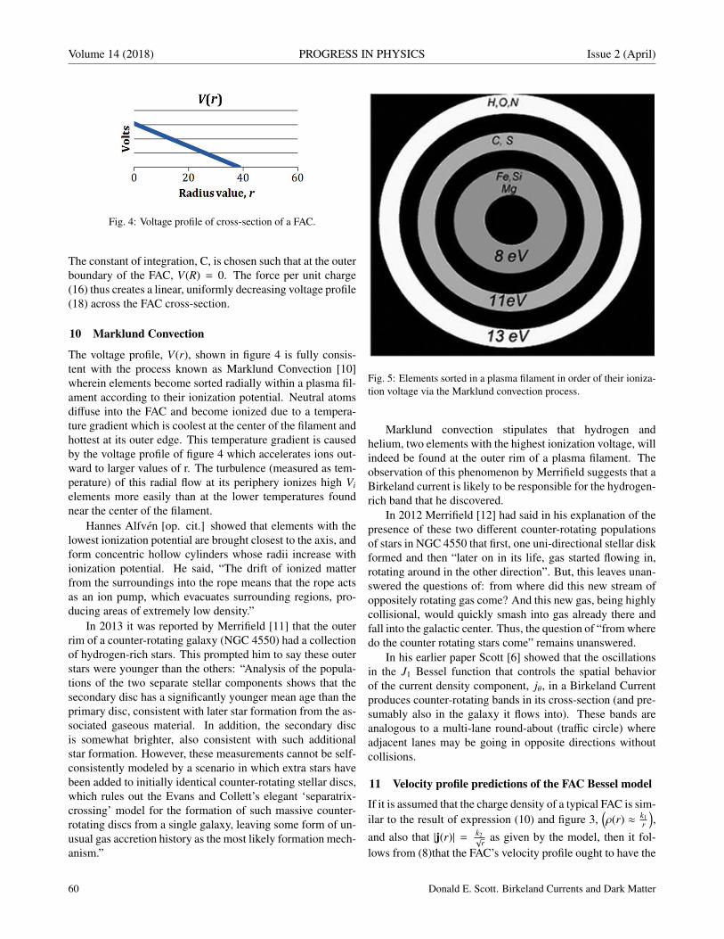
Volume 14 (2018) PROGRESS IN PHYSICS Issue 2 (April)
Fig. 4: Voltage profile of cross-section of a FAC.
The constant of integration, C, is chosen such that at the outerboundary of the FAC, V(R) = 0. The force per unit charge(16) thus creates a linear, uniformly decreasing voltage profile(18) across the FAC cross-section.
10 Marklund Convection
The voltage profile, V(r), shown in figure 4 is fully consis-tent with the process known as Marklund Convection [10]wherein elements become sorted radially within a plasma fil-ament according to their ionization potential. Neutral atomsdiffuse into the FAC and become ionized due to a tempera-ture gradient which is coolest at the center of the filament andhottest at its outer edge. This temperature gradient is causedby the voltage profile of figure 4 which accelerates ions out-ward to larger values of r. The turbulence (measured as tem-perature) of this radial flow at its periphery ionizes high Vi
elements more easily than at the lower temperatures foundnear the center of the filament.
Hannes Alfven [op. cit.] showed that elements with thelowest ionization potential are brought closest to the axis, andform concentric hollow cylinders whose radii increase withionization potential. He said, “The drift of ionized matterfrom the surroundings into the rope means that the rope actsas an ion pump, which evacuates surrounding regions, pro-ducing areas of extremely low density.”
In 2013 it was reported by Merrifield [11] that the outerrim of a counter-rotating galaxy (NGC 4550) had a collectionof hydrogen-rich stars. This prompted him to say these outerstars were younger than the others: “Analysis of the popula-tions of the two separate stellar components shows that thesecondary disc has a significantly younger mean age than theprimary disc, consistent with later star formation from the as-sociated gaseous material. In addition, the secondary discis somewhat brighter, also consistent with such additionalstar formation. However, these measurements cannot be self-consistently modeled by a scenario in which extra stars havebeen added to initially identical counter-rotating stellar discs,which rules out the Evans and Collett’s elegant ‘separatrix-crossing’ model for the formation of such massive counter-rotating discs from a single galaxy, leaving some form of un-usual gas accretion history as the most likely formation mech-anism.”
Fig. 5: Elements sorted in a plasma filament in order of their ioniza-tion voltage via the Marklund convection process.
Marklund convection stipulates that hydrogen andhelium, two elements with the highest ionization voltage, willindeed be found at the outer rim of a plasma filament. Theobservation of this phenomenon by Merrifield suggests that aBirkeland current is likely to be responsible for the hydrogen-rich band that he discovered.
In 2012 Merrifield [12] had said in his explanation of thepresence of these two different counter-rotating populationsof stars in NGC 4550 that first, one uni-directional stellar diskformed and then “later on in its life, gas started flowing in,rotating around in the other direction”. But, this leaves unan-swered the questions of: from where did this new stream ofoppositely rotating gas come? And this new gas, being highlycollisional, would quickly smash into gas already there andfall into the galactic center. Thus, the question of “from wheredo the counter rotating stars come” remains unanswered.
In his earlier paper Scott [6] showed that the oscillationsin the J1 Bessel function that controls the spatial behaviorof the current density component, jθ, in a Birkeland Currentproduces counter-rotating bands in its cross-section (and pre-sumably also in the galaxy it flows into). These bands areanalogous to a multi-lane round-about (traffic circle) whereadjacent lanes may be going in opposite directions withoutcollisions.
11 Velocity profile predictions of the FAC Bessel model
If it is assumed that the charge density of a typical FAC is sim-ilar to the result of expression (10) and figure 3,
(ρ(r) ≈ k1
r
),
and also that |j(r)| = k2√r as given by the model, then it fol-
lows from (8)that the FAC’s velocity profile ought to have the
60 Donald E. Scott. Birkeland Currents and Dark Matter
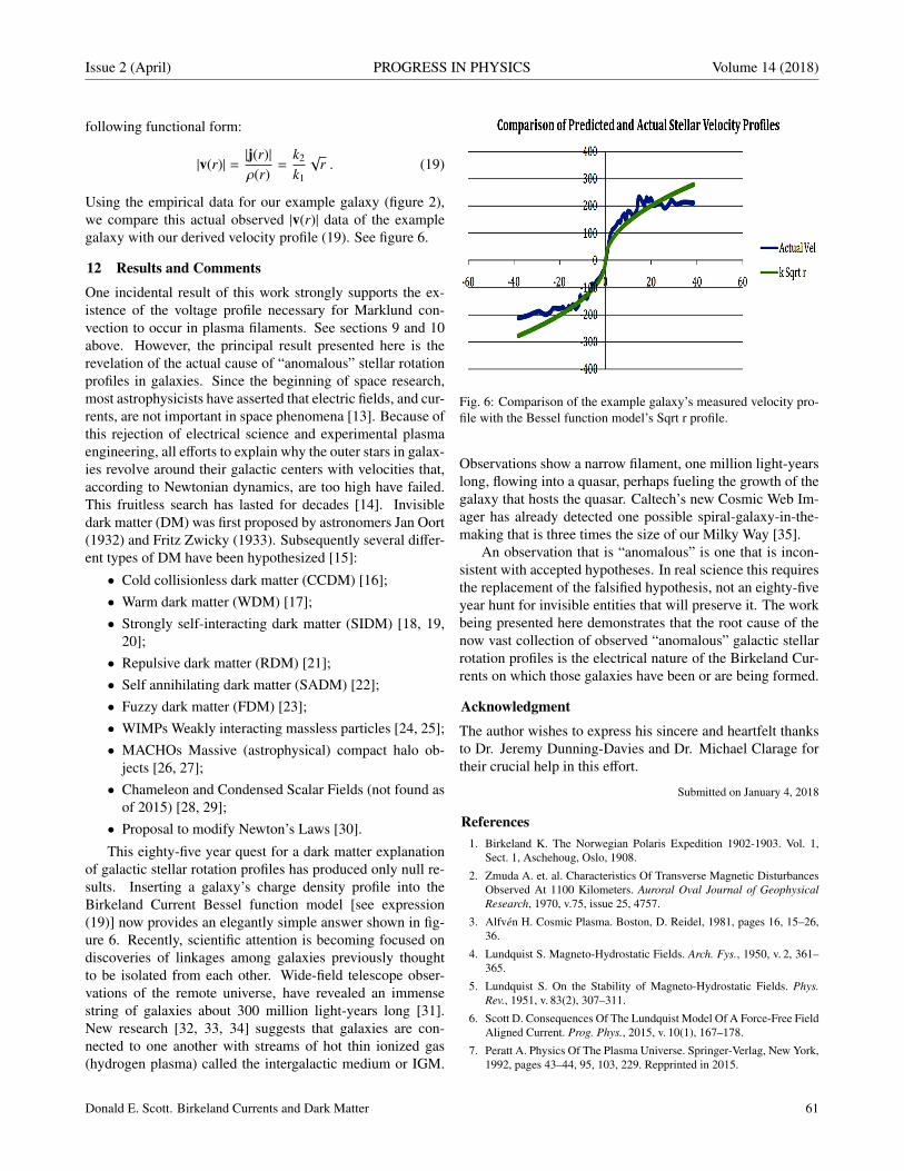
Issue 2 (April) PROGRESS IN PHYSICS Volume 14 (2018)
following functional form:
|v(r)| =|j(r)|ρ(r)
=k2
k1
√r . (19)
Using the empirical data for our example galaxy (figure 2),we compare this actual observed |v(r)| data of the examplegalaxy with our derived velocity profile (19). See figure 6.
12 Results and Comments
One incidental result of this work strongly supports the ex-istence of the voltage profile necessary for Marklund con-vection to occur in plasma filaments. See sections 9 and 10above. However, the principal result presented here is therevelation of the actual cause of “anomalous” stellar rotationprofiles in galaxies. Since the beginning of space research,most astrophysicists have asserted that electric fields, and cur-rents, are not important in space phenomena [13]. Because ofthis rejection of electrical science and experimental plasmaengineering, all efforts to explain why the outer stars in galax-ies revolve around their galactic centers with velocities that,according to Newtonian dynamics, are too high have failed.This fruitless search has lasted for decades [14]. Invisibledark matter (DM) was first proposed by astronomers Jan Oort(1932) and Fritz Zwicky (1933). Subsequently several differ-ent types of DM have been hypothesized [15]:
• Cold collisionless dark matter (CCDM) [16];• Warm dark matter (WDM) [17];• Strongly self-interacting dark matter (SIDM) [18, 19,
20];• Repulsive dark matter (RDM) [21];• Self annihilating dark matter (SADM) [22];• Fuzzy dark matter (FDM) [23];• WIMPs Weakly interacting massless particles [24, 25];• MACHOs Massive (astrophysical) compact halo ob-
jects [26, 27];• Chameleon and Condensed Scalar Fields (not found as
of 2015) [28, 29];• Proposal to modify Newton’s Laws [30].
This eighty-five year quest for a dark matter explanationof galactic stellar rotation profiles has produced only null re-sults. Inserting a galaxy’s charge density profile into theBirkeland Current Bessel function model [see expression(19)] now provides an elegantly simple answer shown in fig-ure 6. Recently, scientific attention is becoming focused ondiscoveries of linkages among galaxies previously thoughtto be isolated from each other. Wide-field telescope obser-vations of the remote universe, have revealed an immensestring of galaxies about 300 million light-years long [31].New research [32, 33, 34] suggests that galaxies are con-nected to one another with streams of hot thin ionized gas(hydrogen plasma) called the intergalactic medium or IGM.
Fig. 6: Comparison of the example galaxy’s measured velocity pro-file with the Bessel function model’s Sqrt r profile.
Observations show a narrow filament, one million light-yearslong, flowing into a quasar, perhaps fueling the growth of thegalaxy that hosts the quasar. Caltech’s new Cosmic Web Im-ager has already detected one possible spiral-galaxy-in-the-making that is three times the size of our Milky Way [35].
An observation that is “anomalous” is one that is incon-sistent with accepted hypotheses. In real science this requiresthe replacement of the falsified hypothesis, not an eighty-fiveyear hunt for invisible entities that will preserve it. The workbeing presented here demonstrates that the root cause of thenow vast collection of observed “anomalous” galactic stellarrotation profiles is the electrical nature of the Birkeland Cur-rents on which those galaxies have been or are being formed.
Acknowledgment
The author wishes to express his sincere and heartfelt thanksto Dr. Jeremy Dunning-Davies and Dr. Michael Clarage fortheir crucial help in this effort.
Submitted on January 4, 2018
References1. Birkeland K. The Norwegian Polaris Expedition 1902-1903. Vol. 1,
Sect. 1, Aschehoug, Oslo, 1908.
2. Zmuda A. et. al. Characteristics Of Transverse Magnetic DisturbancesObserved At 1100 Kilometers. Auroral Oval Journal of GeophysicalResearch, 1970, v.75, issue 25, 4757.
3. Alfven H. Cosmic Plasma. Boston, D. Reidel, 1981, pages 16, 15–26,36.
4. Lundquist S. Magneto-Hydrostatic Fields. Arch. Fys., 1950, v. 2, 361–365.
5. Lundquist S. On the Stability of Magneto-Hydrostatic Fields. Phys.Rev., 1951, v. 83(2), 307–311.
6. Scott D. Consequences Of The Lundquist Model Of A Force-Free FieldAligned Current. Prog. Phys., 2015, v. 10(1), 167–178.
7. Peratt A. Physics Of The Plasma Universe. Springer-Verlag, New York,1992, pages 43–44, 95, 103, 229. Repprinted in 2015.
Donald E. Scott. Birkeland Currents and Dark Matter 61
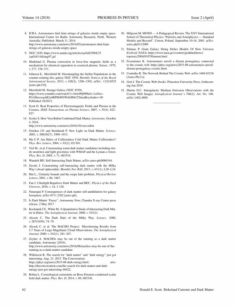
Volume 14 (2018) PROGRESS IN PHYSICS Issue 2 (April)
8. ICRA, Astronomers find faint strings of galaxies inside empty space.International Center for Radio Astronomy Research, Perth, WesternAustralia. Published: March 11, 2014.http://www.astronomy.com/news/2014/03/astronomers-find-faint-strings-of-galaxies-inside-empty-space
9. NGC 1620, https://www.aanda.org/articles/aa/full/2004/35/aa0183-04/img97.gif
10. Marklund G. Plasma convection in force-free magnetic fields as amechanism for chemical separation in cosmical plasma. Nature, 1979,v. 277, 370–371.
11. Johnson E., Merrifield M. Disentangling the Stellar Populations in thecounter-rotating disc galaxy NGC 4550. Monthly Notices of the RoyalAstronomical Society, 2013, v. 428(2), 1296–1302; arXiv: 1210.0535[astro-ph.CO].
12. Merrifield M. Strange Galaxy (NGC 4550).https://www.youtube.com/watch?v=0oie90j989kδt=1sδlist=PLGJ6ezwqAB2a4RP8hWEWAGB9eT2bmaBsyδindex=40Published 10/2012.
13. Scott D. Real Properties of Electromagnetic Fields and Plasma in theCosmos. IEEE Transactions on Plasma Science, 2007, v. 35(4), 822–827.
14. Scoles S. How Vera Rubin Confirmed Dark Matter. Astronomy, October4, 2016.http://www.astronomy.com/news/2016/10/vera-rubin
15. Ostriker J.P. and Steinhardt P. New Light on Dark Matter. Science,2003, v. 300(5627), 1909–1913.
16. Ma C-P. Are Halos of Collisionless Cold Dark Matter Collisionless?Phys. Rev. Letters, 2004, v. 93(2), 021301.
17. Viel M., et al. Constraining warm dark matter candidates including ster-ile neutrinos and light gravitinos with WMAP and the Lyman-α forest.Phys. Rev. D, 2005, v. 71, 063534.
18. Wandelt BD. Self-Interacting Dark Matter, arXiv:astro-ph/0006344.
19. Zavala J. Constraining self-interacting dark matter with the MilkyWay’s dwarf spheroidals. Monthly Not. RAS, 2013, v. 431(1), L20–L24.
20. Hui L., Unitarity bounds and the cuspy halo problem. Physical ReviewLetters, 2001, v. 86, 3467.
21. Fan J. Ultralight Repulsive Dark Matter and BEC. Physics of the DarkUniverse, 2016, v. 14, 1-126.
22. Natarajan P. Consequences of dark matter self-annihilation for galaxyformation, arXiv:0711.2302 [astro-ph].
23. Is Dark Matter “Fuzzy”, Astronomy Now, Chandra X-ray Center pressrelease, 2 May 2017.
24. Kochanek CS., White M. A Quantitative Study of Interacting Dark Mat-ter in Halos. The Astrophysical Journal, 2000, v. 543(2).
25. Alcock C. The Dark Halo of the Milky Way. Science, 2000,v. 287(5450), 74–79.
26. Alcock C. et al. The MACHO Project: Microlensing Results from5.7 Years of Large Magellanic Cloud Observations. The AstrophysicalJournal, 2000, v. 542(1), 281–307.
27. Zeyher A. MACHOs may be out of the running as a dark mattercandidate, Astronomy (2016);http://www.astronomy.com/news/2016/08/machos-may-be-out-of-the-running-as-a-dark-matter-candidate
28. Wilkinson R. The search for “dark matter” and “dark energy” just gotinteresting, Aug. 21, 2015. The Conversation:https://phys.org/news/2015-08-dark-energy.html; also:http://theconversation.com/the-search-for-dark-matter-and-dark-energy-just-got-interesting-46422.
29. Bohua L. Cosmological constraints on Bose-Einstein-condensed scalarfield dark matter. Phys. Rev. D, 2014, v. 89, 083536.
30. Milgrom M. MOND — A Pedagogical Review. The XXV InternationalSchool of Theoretical Physics “Particles and Astrophysics — StandardModels and Beyond”, Ustron, Poland, September 10-16, 2001. arXiv:astro-ph/0112069
31. Palunas P. Giant Galaxy String Defies Models Of How UniverseEvolved, NASA; https://www.nasa.gov/centers/goddard/news/topstory/2004/0107filament.html
32. Fesenmaier K. Astronomers unveil a distant protogalaxy connectedto the cosmic web. https://phys.org/news/2015-08-astronomers-unveil-distant-protogalaxy-cosmic.html.
33. Coutinho B. The Network Behind The Cosmic Web. arXiv:1604.03236[Astro-Ph.Co].
34. Gott J. The Cosmic Web (book). Princeton University Press, forthcom-ing Jun 2018.
35. Martin D.C. Intergalactic Medium Emission Observations with theCosmic Web Imager. Astrophysical Journal v. 768(2), Art. No. 106.arXiv:1402.4809.
62 Donald E. Scott. Birkeland Currents and Dark Matter
Issue 2 (April) PROGRESS IN PHYSICS Volume 14 (2018)
Can Cold Fusion Be Explained by Quantised Inertia?
M.E. McCullochPlymouth University, Plymouth, PL4 8AA, UK
E-mail: [email protected]
When electrolysis is performed using deuterium and a palladium cathode, more heatcan be generated than can be explained by chemical processes, implying that deuteronsare fusing but without the typical products of hot fusion (a phenomenon called Low-Energy Nuclear Reactions, LENR, or cold fusion). Fusion between deuterons usuallyrequires temperatures of 100 MK to overcome the repulsive Coulomb forces. Here itis shown that a theory called quantised inertia predicts that in cracks in the metal withdiameters less than 28 nm, the temperature is 27,000 K and mutual sheltering by thedeuterons can produce an attractive radiation recoil force strong enough to push themtogether through their Coulomb barriers. This offers a potential explanation for coldfusion or LENR.
1 Introduction
Many attempts are underway to initiate nuclear fusion be-tween atoms such as deuterium, releasing useful energy [1].The main challenge is to overcome the Coulomb barrier:deuterons have a charge equal to the charge on the proton,and they repel each other with a force given by
FC =q2
P
4πε0d2 (1)
where qP = 1.6 × 10⁻¹⁹ C is the charge on the proton, ε0 =
8.85 × 10⁻¹² m−3kg−1s4A2 is the permittivity of free spaceand d is the distance between the deuterons. Overcomingthe Coulomb barrier between the two deuterons in this pro-cess usually requires a high momentum and therefore tem-peratures in excess of 100 MK which are thought to only bepossible in gravitationally-confined systems such as the Sunor magnetically-confined fusion reactors.
This is why the results of Fleischmann and Pons [2] wereso surprising. When they used a palladium cathode to elec-trolyse heavy water (containing deuterium) they noticed thatmore heat was given off than was possible from chemical pro-cesses, implying that fusion was occuring (so called cold fu-sion). The expected product of deuterium fusion: helium-4,was also produced, but the nuclear emissions (neutrons andgamma rays) expected from hot fusion were not seen and socold fusion was dismissed by all but a small minority. How-ever, over the years there have been many successful repro-ductions of the Pons-Fleischmann effect, or variations of it[3], and many unsuccessful ones as well, and the topic hasbeen renamed LENR (Low-Energy Nuclear Reactions). Agood summary is available in [4].
Aoyama [5], Storms [6], [7] and others have noted an in-triguing pattern which is that a common feature to the suc-cessful experiments are the cracks or defects in the metals,which are on the order of the nanoscale.
McCulloch [8], [9], [10] has shown that a number of dy-namical anomalies such as galaxy rotation and cosmic accel-
eration can be explained by a theory called quantised inertiawhich assumes that inertial mass is due to Unruh radiation (aradiation seen only by accelerating objects) when this radia-tion is made non-uniform in space by horizons. These hori-zons can be caused by acceleration (relativistic horizons) orthey can be metal structures or cavities [11].
Another interesting anomaly down at the nuclear scale isthat of [12] who showed that when the proton radius is mea-sured with a orbiting muon rather than an electron, an extraunexplained binding energy is present. The muon orbits 200times closer than the electron, and quantised inertia can ex-plain 55% of this extra binding energy by assuming that thethermal Unruh radiation seen by the muon is blocked (shel-tered) from the direction of the proton, leading to a net ra-diation pressure from outside its orbit, and a new attractiveforce [13]. Quantised inertia also predicts high temperatureswithin small horizons, for example in the early universe [14].This may also apply to small metal cracks and so it may haverelevence for LENR.
In this paper it is shown that quantised inertia predicts thatcracks or defects in metals of 28 nm diameter or less shouldbe hot enough to cause an attractive radiation recoil forceon the deuterons strong enough to overcome their Coulombrepulsion. This suggests a mechanism for cold fusion andLENR.
2 Method & Results
The uncertainty principle of Heisenberg states that the un-certainty in momentum (∆p) times the uncertainty in position(∆x) must be greater than or equal to half the reduced Planck’sconstant
∆p∆x >ℏ
2(2)
so that if the uncertainty in position (∆x) is reduced in ametal cavity of diameter D, then the momentum uncertainty(∆p) should increase. Quantised inertia assumes that this in-
M.E. McCulloch. Can Cold Fusion Be Explained by Quantised Inertia? 63

Volume 14 (2018) PROGRESS IN PHYSICS Issue 2 (April)
crease in momentum can become real [15], and since E = pcthen a new energy becomes available, given by
∆E >ℏc2D. (3)
For thermalised energy E = 32 kT we can write an expres-
sion for temperature:
T >ℏc
3kD. (4)
Eq. 4 predicts that the temperature in tiny volumes is high.Figure 1 shows two deuterons (the black circles) close to-gether inside a defect (the grey area) within a palladium lat-tice (the mottled area). If the temperature within the defectis as given in Eq. 4 then this radiation will be absorbed byeach deuteron only on the side away from the other deuteron,assuming there is a mutual sheltering process (see the whiteradiation-free area in Figure 1) and so the absorption of thisradiation will produce a radiation recoil force (see also [16])that will push them together. This force is
FR =Pc=σT 4
c(5)
where σ is the Stefan-Boltzmann constant and c is the speedof light. In order for this radiative force to cause the deuteronsto fuse, it must be larger than the repulsive Coulomb force atthe seperation where the attractive strong force can take overand fuse the two deuterons, a distance of ds = 1.6 × 10⁻¹⁵ m.For this to happen, FR > FC at distance ds, and so using Eqs.1 and 5, and using Eq. 4 for T we get
σ(ℏc
3kD
)4c
>q2
4πε0d2s. (6)
We can now predict the crack size D needed to produce atemperature high enough to cause fusion in this new way:
D < (4πε0σ)14 c
34ℏ
3k
√ds
q= 28 nm. (7)
Therefore, quantised inertia predicts that deuterons incracks or defects in palladium of a size less than 28 nm willsee temperatures of ℏc/3kD ≥ 27000 K and be pushed to-gether by radiation in the crack strongly enough that theirCoulomb barrier can be breached, causing fusion. Cracks ofthis size are present in palladium after being stressed [17].
3 Discussion
Quantised inertia also suggests a way to account for the lackof emitted neutrons in LENR. The inwards force on all par-ticles in the defect may keep them confined, but it does notdirectly explain the lack of gamma rays.
Fig. 1: A schematic showing two deuterons (the black circles) lo-cated a distance d apart within a crack/defect of width D (the greyarea) in a palladium lattice (the mottled area). The metal radiates,and the mutual sheltering of the deuterons causes the white shel-tered zone. The non-uniformity of the thermal radiation then forcesthe deuterons together (the arrows).
As a test, this theory predicts that metals with cracks ordefects of size D should emit radiation of wavelength D. X-rays were indeed seen by [6] and [7] during LENR, withwavelengths in the nanometre range.
This mechanism also suggests a possible reason for sono-luminescence which similarly involves particles being con-fined to a small region, in this case a bubble collapsing toa size of 0.5 micron and attaining an apparent temperatureof between 2300 K to 5100 K, as measured by the radiationgiven off (see [18]). Eq. 4 predicts a temperature of 1500K.
This application of quantised inertia predicts that a nano-metal manufactured to have regular cracks of a size less than28 nm should show far more uniform LENR.
4 Conclusion
When electrolysis is performed using heavy water (deu-terium) and a palladium cathode, unexpected heat andHelium-4 can be generated indicating that nuclear fusion istaking place without the usual products of hot fusion (this iscalled LENR or cold fusion).
Quantised inertia predicts that deuterons in cracks or de-fects less than 28 nm in width should heat up enough that,through mutual sheltering, they feel an attractive radiationrecoil force that overcomes their Coulomb barrier, allowingfusion. This is a possible explanation for cold fusion.
As a test this model predicts that a metal with cracksshould emit radiation of a wavelength similar to the size ofits cracks, and that a nanometal manufactured with cracks ofsize 28 nm or less should produce LENR more uniformly.
Acknowledgements
Many thanks to Bob McIntyre who pointed out that an earlierpaper by the author on the proton radius anomaly [13] mightalso apply to LENR. Also many thanks to A. Dubourg andLENR pioneers Ed Storms and Russ George for advice.
64 M.E. McCulloch. Can Cold Fusion Be Explained by Quantised Inertia?

Issue 2 (April) PROGRESS IN PHYSICS Volume 14 (2018)
Submitted on January 20, 2018
References1. Clery D. ITER’s $12 billion gamble. Science, 2006 v. 214, 5797.
2. Fleischmann M., Pons S. and Hawkins M. Elecrochemically inducednuclear fusion of deuterium. J. Electroanal. Chem., 1989, v. 261, 301–308 and errata in v. 263, 187–188.
3. Kitamura A., Takayoshi N., Yu S., Akira T., Akito T., Reiko S., YushiF. Anomalous effects in charging of Pd powders with high density hy-drogen isotopes. Phys. Letters A, 2009, v. 373(35), 3109–3112.
4. Storms E.K. How basic behaviour of LENR can guide a search for anexplanation. J. Condensed Matter Nucl. Sci., 2016, v. 20, 1–39.
5. Aoyama T. et al. Highly reliable low-level neutron detection using 3Heproportional counters. Radioisotopes, 1991, v. 40, 188.
6. Storms E.K. and Scanlan B. Detection of radiation emitted from LENR.ICCF-14. Conference on Condensed Matter Nuclear Science, 2008.Washington, DC.
7. Storms E.K. and Scanlan B. Nature of energetic radiation emitted frommetal exposed to H2. J. Condensed Matter Nucl. Sci., 2013, v. 11, 142–156.
8. McCulloch M.E. Modelling the Pioneer anomaly as modified inertia.MNRAS, 2007, v. 376, 338–342.
9. McCulloch M.E. Testing quantised inertia on galactic scales. ApSS,2012, v. 342(2), 575–578.
10. McCulloch M.E. Galaxy rotations from quantised inerta and visiblematter only. Astrophys. Space Sci., 2017, v. 362, 149.
11. McCulloch M.E. Testing quantised inertia on the emdrive. EPL, 2015,v. 111, 60005.
12. Pohl R. et al. Laser spectroscopy of muonic deuterium. Nature, 2010,v. 466, 213.
13. McCulloch M.E. The proton radius anomaly from the sheltering of Un-ruh radiation. Progress in Physics, 2017, v. 13(2), 100–101.
14. McCulloch M.E. A toy cosmology using a Hubble-scale Casimir effect.Galaxies, 2014, v. 2, 81–88.
15. McCulloch, M.E. Quantised inertia from relativity and the uncertaintyprinciple. EPL, 2016, v. 115, 69001.
16. Haslinger P., Jaffe M., Xu V., Schwartz O., Sonnleitner M., Ritsch-Marte M., Ritsch H. and Mueller H. Attractive force on atoms due toblackbody radiation. Nature, 2017, doi: 10.1038/s41567-017-0004-9.
17. Kim S., Lee H.-S., Jang B. and Cho S. Strain-controlled nanocrackformation in a Pd film on polydimethylsiloxane for the detection of lowH2 concentrations. J. Mater. Sci., 2016, v. 51(9), 4530–4537.
18. Brenner M.P., Hilgenfeldt S. and Lohse D. Single-bubble sonolumines-cence. Rev. Mod. Phys., 2002, v. 74(2), 425–484.
M.E. McCulloch. Can Cold Fusion Be Explained by Quantised Inertia? 65

Volume 14 (2018) PROGRESS IN PHYSICS Issue 2 (April)
Global Scaling of Planetary Atmospheres
Hartmut MullerE-mail: [email protected]
We derive a model of the stratification of planetary atmospheres as application of ourscale-invariant model of matter as fractal chain system of oscillating protons and elec-trons. Model claims are verified by aerological, geophysical and planetological data.
Introduction
The vertical stratification of the Earth’s atmosphere is causedby very different processes and it is a complex field of re-search. In general, air pressure and density decrease exponen-tially with altitude, but temperature, ionization and chemicalcomposition have more complicated profiles. The standarddivision into troposphere, stratosphere, mesosphere, thermo-sphere, ionosphere and exosphere is based on satellite, air-plane and ground measurements and considers aerodynamic,hydrodynamic, thermodynamic, chemical, electromagnetic,gravitational factors in their complex interaction.
New measurements of the atmospheres of solar systemplanets and moons over the past four decades from variousspacecraft missions have been used to characterize the struc-ture and dynamics of these atmospheric environments and tocompare them to one another. A corresponding evolution ofmodeling tools occurs, from simple to complex frameworks.
Terrestrial modeling frameworks like HAMMONIA [1],ECHAM [2], IRI [3] and CMAM [4] of numerical modelinghave been used to launch simulations [5] of other planetaryupper atmospheres and ionospheres. The primary benefit ofthe Earth paradigm can be realized for other planetary upperatmospheres having similarities in their fundamental plane-tary parameters, basic processes and vertical domains (atmo-spheric layers).
In fact, stratification as atmospheric feature is associatednot only with Earth, but occurs on any other planet or moonthat has an atmosphere as well. Furthermore, stable atmo-spheric boundaries like tropopause, stratopause, thermopauseand mesopause have similar vertical distributions at differ-ent celestial bodies in atmospheres of very different chemicalcompositions.
In this paper we apply our scale-invariant model [6] ofmatter as fractal chain system of oscillating protons and elec-trons and develop a general model of planetary atmosphericstratification that might help to understand the processes sus-taining the observed stable atmospheric structures.
Methods
In [7] we have shown that the set of natural frequencies ofa fractal chain system of similar harmonic oscillators can bedescribed as set of finite continued fractions F (1), which arenatural logarithms, where ω jk is the set of angular frequen-cies and ω00 is the fundamental frequency of the set. The
denominators are integer: n j0, n j1, n j2, . . . , n jk ∈Z, the cardi-nality j ∈N of the set and the number k ∈N of layers are finite:
ln (ω jk/ω00)= n j0 +z
n j1 +z
n j2 + . . .+
zn jk
=
= [z, n j0; n j1, n j2, . . . , n jk]=F .
(1)
In the canonical form, the numerator z equals 1 and for finitecontinued fractions the distribution density of the eigenvaluesreaches maxima near reciprocal integers 1, 1/2, 1/3, 1/4, . . .which are the attractor points of the fractal set F of naturallogarithms (fig. 1).
Fig. 1: The canonical form of F for k= 1 (above) and for k= 2(below) in the range -1⩽F ⩽ 1.
Any finite continued fraction represents a rational num-ber [8]. Therefore, all natural frequencies ω jk in (1) are irra-tional, because for rational exponents the natural exponentialfunction is transcendental [9]. This circumstance provides forhigh stability of eigenstates in a fractal chain system of har-monic oscillators because it prevents resonance interactionbetween the elements of the system [10]. Already in 1987 wehave applied continued fractions of the type F as criterion ofstability in engineering [11, 12].
In the case of harmonic quantum oscillators, the contin-ued fractions F define not only fractal sets of natural angu-lar frequencies ω jk, angular accelerations a jk = c ·ω jk, oscil-lation periods τ jk = 1/ω jk and wavelengths λ jk = c/ω jk of thechain system, but also fractal sets of energies E jk = ℏ ·ω jk andmasses m jk =E jk/c2 which correspond with the eigenstates ofthe system. For this reason, we call the continued fraction Fthe “fundamental fractal” of eigenstates in chain systems ofharmonic quantum oscillators.
In the canonical form (z= 1) of the fundamental fractalF , shorter continued fractions correspond with more stableeigenstates of a chain system of harmonic oscillators. There-fore, integer logarithms represent the most stable eigenstates(main attractor nodes).
66 Hartmut Muller. Global Scaling of Planetary Atmospheres

Issue 2 (April) PROGRESS IN PHYSICS Volume 14 (2018)
Property Electron Proton
rest mass m 9.10938356(11) · 10−31 kg 1.672621898(21) · 10−27 kg
energy E=mc2 0.5109989461(31) MeV 938.2720813(58) MeV
angular frequency ω=E/ℏ 7.76344071 · 1020 Hz 1.42548624 · 1024 Hz
angular oscillation period τ= 1/ω 1.28808867 · 10−21 s 7.01515 · 10−25 s
angular wavelength λ= c/ω 3.8615926764(18) · 10−13 m 2.1030891 · 10−16 m
Table 1: The basic set of physical properties of the electron and proton. Data taken from Particle Data Group [13]. Frequencies, oscillationperiods and the proton wavelength are calculated.
As the cardinality and number of layers of the continuedfractions F are finite but not limited, in each point of thespace-time occupied by the chain system of harmonic quan-tum oscillators the scalar F is defined. Therefore, any chainsystem of harmonic quantum oscillators can be seen as sourceof the scalar field F , the fundamental field of the system.
Normal matter is formed by nucleons and electrons be-cause they are exceptionally stable quantum oscillators. Inthe concept of isospin, proton and neutron are viewed as twostates of the same quantum oscillator. Furthermore, they havesimilar rest masses. However, a free neutron decays into aproton, an electron and antineutrino within 15 minutes whilethe life-spans of the proton and electron top everything that ismeasurable, exceeding 1029 years [13].
The exceptional stability of electron and proton predesti-nate their physical characteristics as fundamental units. Ta-ble 1 shows the basic set of electron and proton units that canbe considered as a fundamental metrology (c is the speed oflight in a vacuum, ℏ is the Planck constant, kB is the Boltz-mann constant). In [14] was shown that the fundamentalmetrology (tab. 1) is compatible with Planck units [15].
We hypothesize that scale invariance of the fundamentalfield F calibrated on the physical properties of the proton andelectron (tab. 1) is a universal characteristic of organized mat-ter and criterion of stability. This hypothesis we have called‘global scaling’ [16, 17].
Results
Within our scale-invariant model of matter [18], atoms andmolecules emerge as eigenstates of stability in fractal chainsystems of harmonically oscillating protons and electrons.
Andreas Ries [19] demonstrated that this model allowsfor the prediction of the most abundant isotope of a givenchemical element. From this point of view, any physical body,being solid, liquid or gas can be seen as fractal chain systemof oscillating molecules, atoms, ions, protons and electronsthat generates its fundamental field F .
Therefore, in the framework of our fractal model of mat-ter, the fundamental field F affects any type of physical in-teraction, including the gravitational. In [20] we applied our
model to the analysis of gravimetric and seismic character-istics of the Earth and could show [21] that our estimationscorrespond well with established empiric models of the Earthinterior.
In this paper we demonstrate that the vertical sequence ofstable atmospheric layers corresponds with the sequence ofmain equipotential surfaces of the fundamental field F , notonly at Earth, but also at Venus, Mars and Titan. Table 2gives an overview of this correspondence.
The lowest layer of Earth’s atmosphere is the tropospherewhere nearly all weather conditions take place. The averageheight of the troposphere is 20 km in the tropics, 12 km in themid latitudes, and 7 km in the polar regions in winter [22].Table 2 and fig. 2 show the correspondence of these tropo-spheric levels with the main equipotential surfaces [37; 2] =7.5 km, [38; ∞] = 12 km and [38; 2] = 20 km of the funda-mental field F , calibrated on the electron wavelength.
At its lowest part, the planetary boundary layer (PBL),the troposphere displays turbulence and strong vertical mix-ing due to the contact with the planetary surface. The top ofthe PBL in convective conditions is often well defined by theexistence of a stable capping inversion, into which turbulentmotions from beneath are generally unable to penetrate [23].The height of this elevated stable layer is quite variable, butis generally below 3 km. Over deserts in mid-summer understrong surface heating the PBL may rise to 4 - 5 km. In thetemperate zones, it can be defined by the quite sharp decreaseof aerosol concentration at the height of about 1600 m. Overthe open oceans, but also at night over land, under clear skiesand light winds, with a capping stratocumulus, the depth ofthe PBL may be no more than 600 m.
Table 2 and fig. 2 show the correspondence of the PBLfeatures with the main equipotential surfaces [35; ∞] = 600m, [36; ∞] = 1600 m and [37; ∞] = 4.5 km of the funda-mental field F , calibrated on the electron wavelength. It isnoticeable that in 1992 Hess [24] already reviewed scalingaspects of the boundary layer.
Above the PBL, where the wind is nearly geostrophic,vertical mixing is less and the free atmosphere density strat-ification initiates. The jet stream flows near the boundary
Hartmut Muller. Global Scaling of Planetary Atmospheres 67

Volume 14 (2018) PROGRESS IN PHYSICS Issue 2 (April)
boundary of atmospheric layer altitude h, km ln (h/λe) F
van Allen outer electron belt max density 13000 44.96 [45;∞]
8200 [44; 2]
5000 [44;∞]
van Allen inner proton belt max density 3000 43.50 [43; 2]
Earth exopause 1800 42.99 [43;∞]
1100 [42; 2]
Earth thermopause 650 41.97 [42;∞]
400 [41; 2]
Venus & Mars thermopause, Venus atmospheric entry 250 41.01 [41;∞]
Earth atmospheric entry, Venus mesopause 150 40.50 [40; 2]
Earth & Titan mesopause, Venus tropopause, Mars stratopause & entry 90 39.99 [40;∞]
Earth & Titan stratopause 55 39.50 [39; 2]
Titan tropopause 33 38.99 [39;∞]
Earth tropic tropopause 20 38.49 [38; 2]
Earth temperate tropopause 12 37.98 [38;∞]
Earth polar tropopause 7.5 37.51 [37; 2]
desert summer PBL inversion 4.5 37.00 [37;∞]
continental PBL inversion 1.6 35.96 [36;∞]
marine PBL inversion 0.6 34.98 [35;∞]
Table 2: Altitudes of the boundaries of various atmospheric layers on Earth, Venus, Mars and Titan and their correspondence with mainequipotential surfaces of the fundamental field F , calibrated on the electron wavelength.
between the troposphere and the stratosphere. As altitudeincreases, the temperature of the troposphere generally de-creases until the tropopause.
At the bottom of the stratosphere, above the tropopause,the temperature doesn’t change much, but at the inverse layerat altitudes between 20 and 33 km the temperature increasesfrom -50C to 0C. Then at the stratopause at 55 km altitudethe temperature stabilizes. It is the boundary between twolayers: the stratosphere and the mesosphere [25]. The ozonelayer (ozonosphere) of the stratosphere absorbs most of theSun’s ultraviolet radiation and is mainly found at altitudesbetween 12 and 30 km, with the highest intensity of formationat 20 km height [26].
Table 2 and fig. 2 show the correspondence of the mainstratosphere layers with the main equipotential surfaces [39;∞] = 33 km and [39; 2] = 55 km of the fundamental field F ,calibrated on the electron wavelength.
Above the stratopause, in the mesosphere between 55 and90 km altitude [27], the temperature decreases again, reach-
ing about -100 C at the mesopause [28]. This altitude coin-cides with the turbopause: above this level the atmosphere isof extremely low density so that the chemical composition isnot mixed but stratified and depends on the molecular masses.Table 2 and fig. 2 show the correspondence of the mesopausewith the main equipotential surface [40; ∞] = 90 km of thefundamental field F , calibrated on the electron wavelength.
Above the mesopause, in the thermosphere, the (kinetic)temperature increases and can rise to 1000 C (depending onsolar activity) at altitudes of 250 km remaining quasi stablewith increasing height. Due to solar radiation, gas moleculesdissociate into atoms: above 90 km dissociate carbon dioxy-gen and dihydrogen, above 150 km dissociates dioxygen andabove 250 km dissociates dinitrogen. Above 150 km, the den-sity is so low that molecular interactions are too infrequent topermit the transmission of sound. Table 2 and fig. 2 show thecorrespondence of these thermosphere layers with the mainequipotential surfaces [40; 2] = 150 km and [41; ∞] = 250km of the fundamental field F , calibrated on the electron.
68 Hartmut Muller. Global Scaling of Planetary Atmospheres

Issue 2 (April) PROGRESS IN PHYSICS Volume 14 (2018)
Fig. 2: The fundamental field F (natural logarithmic presentation) calibrated on the electron wavelength in the range 35 ≤ F ≤ 40 and thecorresponding altitudes h in km.
The Karman line [29] is considered by the FederationAeronautique Internationale (FAI) [30] as the border betweenthe atmosphere and outer space, as altitude where the atmo-sphere becomes too thin to support aeronautical flight, since avehicle at this altitude would have to travel faster than orbitalvelocity to derive sufficient aerodynamic lift to support itself.On Earth, atmospheric effects become noticeable during at-mospheric entry of spacecraft already at an altitude of around120 - 150 km, while on Venus atmospheric entry occurs at250 km and on Mars at about 80 - 90 km above the surface.These heights mark also the bases of the anacoustic zones.
The location of the thermopause is near altitudes of 600 –700 km and depends on solar activity [31]. Above starts theexosphere, where the atmosphere (mostly consisting of hy-drogen atoms) thins out and merges with interplanetary space.This uppermost layer, until 13000 km observable from spaceas the geocorona, extends up to 100000 km. Table 2 and fig.2 show the correspondence of the thermopause with the mainequipotential surface [42; ∞] = 650 km of the fundamentalfield F , calibrated on the electron wavelength.
The van Allen radiation belts [32] are features of Earth’smagnetosphere. The inner belt consists of high energetic pro-tons which reach their maximum concentration at altitudes of3000 km. The outer belt consists of high energetic electronswith maximum concentration at altitudes of 13000 km.
While the outer belt maximum corresponds with the mainequipotential surface [45;∞] = 13000 km of the fundamentalfield F , calibrated on the electron wavelength, the inner beltmaximum corresponds with the equipotential surface [43; 2]= 3000 km that is the main equipotential surface [51; ∞] ofthe fundamental field F , calibrated on the proton wavelength.In fact, the natural logarithm of the electron-to-proton wave-length ratio is approximately 7.5 and consequently, F cali-brated on the proton will be shifted by 7.5 logarithmic unitsrelative to the F calibrated on the electron:
ln(λelectron
λproton
)= ln
(3.8615926764 · 10−13 m
2.1030891 · 10−16 m
)≈ 7.5.
This circumstance, probably, can explain the high proton con-centration at the inner belt.
Conclusion
The correspondence of the atmospheric stratification on theEarth, Venus, Mars and Titan with main equipotential sur-faces of F demonstrates that the fundamental field affectsvery different types of physical interaction and is a strongconfirmation of global scaling and our model of matter asfractal chain system of oscillating protons and electrons.
Probably, in future our model can be applied for estima-tion of the atmospheric stratification at ice giants like Uranusand Neptune and gas giants like Jupiter, Saturn and extrasolarplanets as well.
Acknowledgements
I’m thankful to Leili Khosravi and Oleg Kalinin for valuablediscussions.
Submitted on February 21, 2018
References1. Schmidt H., Brasseur G. P. The response of the middle atmosphere to
solar cycle forcing in the Hamburg Model of the neutral and ionizedatmosphere. Space Science Reviews, 1–12, 2006.
2. Roeckner E. et al. Report No. 349. The atmospheric general circula-tion model ECHAM5. Max Planck Institute for Meteorology, Hamburg,2003.
3. Bilitza D. et al. The International Reference Ionosphere 2012 – a modelof international collaboration. Journal of Space Weather and Space Cli-mat, 4, A07, 2014.
4. Grandpre J. de, Beagley S. R. et al. Ozone climatology using interac-tive chemistry: Results from the Canadian Middle Atmosphere Model.Journal of Geophysical Research, Vol. 105, No. D21, 475–491, 2000.
5. Bougher S. W. et al. Neutral Upper Atmosphere and Ionosphere Mod-eling. Space Science Reviews, 139: 107–141, 2008.
6. Muller H. Fractal Scaling Models of Natural Oscillations in Chain Sys-tems and the Mass Distribution of Particles. Progress in Physics, vol. 3,61–66, 2010.
7. Muller H. Fractal Scaling Models of Resonant Oscillations in ChainSystems of Harmonic Oscillators. Progress in Physics, vol. 2, 72–76,2009.
8. Khintchine A.Ya. Continued fractions. University of Chicago Press,Chicago, 1964.
9. Hilbert D. Uber die Transcendenz der Zahlen e und π. MathematischeAnnalen 43, 216–219, 1893.
10. Panchelyuga V. A., Panchelyuga M. S. Resonance and Fractals on theReal Numbers Set. Progress in Physics, vol. 4, 48–53, 2012.
Hartmut Muller. Global Scaling of Planetary Atmospheres 69

Volume 14 (2018) PROGRESS IN PHYSICS Issue 2 (April)
11. Muller H. The general theory of stability and objective evolutionarytrends of technology. Applications of developmental and constructionlaws of technology in CAD. Volgograd, VPI, 1987 (in Russian).
12. Muller H. Superstability as a developmental law of technology. Tech-nology laws and their Applications. Volgograd-Sofia, 1989 (in Rus-sian).
13. Olive K.A. et al. (Particle Data Group), Chin. Phys. C, 38, 090001,2016.Patrignani C. et al. (Particle Data Group), Chin. Phys. C, 40, 100001,2016.
14. Muller H. Scale-Invariant Models of Natural Oscillations in Chain Sys-tems and their Cosmological Significance. Progress in Physics, vol. 4,187–197, 2017.
15. Max Planck. Uber Irreversible Strahlungsvorgange. In: Sitzungsberichtder Koniglich Preußischen Akademie der Wissenschaften. 1899, vol. 1,479–480.
16. Muller H. Scaling as Fundamental Property of Natural Oscillations andthe Fractal Structure of Space-Time. Foundations of Physics and Ge-ometry. Peoples Friendship University of Russia, 2008 (in Russian).
17. Muller H. Scaling of body masses and orbital periods in the Solar Sys-tem as consequence of gravity interaction elasticity. Abstracts of theXII. International Conference on Gravitation, Astrophysics and Cos-mology, dedicated to the centenary of Einstein’s General Relativity the-ory. Moscow, PFUR, 2015.
18. Muller H. Emergence of Particle Masses in Fractal Scaling Models ofMatter. Progress in Physics, vol. 4, 44–47, 2012.
19. Ries A. Qualitative Prediction of Isotope Abundances with the BipolarModel of Oscillations in a Chain System. Progress in Physics, vol. 11,183–186, 2015.
20. Muller H. Gravity as Attractor Effect of Stability Nodes in Chain Sys-tems of Harmonic Quantum Oscillators. Progress in Physics, vol. 1, 19–23, 2018.
21. Muller H. Quantum Gravity Aspects of Global Scaling and the SeismicProfile of the Earth. Progress in Physics, vol. 1, 41–45, 2018.
22. Danielson, Levin, and Abrams, Meteorology, McGraw Hill, 2003.
23. Garratt J. R. Review: the atmospheric boundary layer. Earth-ScienceReview, 37, pp. 89–134, 1994.
24. Hess G. D. Observations and scaling of the atmospheric boundary layer.Australian Meteorological Magazine. 41, 79–99 (1992).
25. Brasseur G. P., Solomon S. Aeronomy of the Middle Atmosphere.Chemistry and Physics of the Stratosphere and Mesosphere. ISBN-101-4020-3824-0, Springer, 2005.
26. Stolarski R. et al. Measured Trends in Stratospheric Ozone. Science,New Series, Vol. 256, Issue 5055, 342–349, 1992.
27. Holton J. R. The Dynamic Meteorology of the Stratosphere and Meso-sphere. ISBN 978-1-935704-31-7, 1975.
28. Beig G., Keckhut P. Lowe R. P. et al. Review of mesospheric tempera-ture trends. Rev. Geophys. 41 (4), 1015, 2003.
29. Karman T., Edson L. The Wind and Beyond. Little, Brown, Boston,1967.
30. Cordoba S. F. The 100 km Boundary for Astronautics. Federation Aero-nautique Internationale, 2011.
31. Beig G., Scheer J., Mlynczak M. G., Keckhut P. Overview of the tem-perature response in the mesosphere and lower thermosphere to solaractivity. Reviews of Geophysics, 46, RG3002, July 2008.
32. Schaefer H. J. Radiation Dosage in Flight through the Van Allen Belt.Aerospace Medicine, Vol. 30, No. 9, 1959.
70 Hartmut Muller. Global Scaling of Planetary Atmospheres

Issue 2 (April) PROGRESS IN PHYSICS Volume 14 (2018)
LETTERS TO PROGRESS IN PHYSICS
On the Possible Nature of Dark Matter and Dark EnergyAnaltoly V. Belyakov
E-mail: [email protected]
It is assumed that the dark matter particle can be a structural unit of cosmological scale(superphoton) emitted by the active center of galaxies, analogous to a photon and balllightning (macrophoton), which are structural units of micro- and macroscales. Thelow density, potential and temperature of superphotons make them invisible during as-tronomical observations, and their negative charge prevents the galaxies from approach-ing each other which can explain the phenomenon of dark energy. It is shown that theexistence of superphotons together with the presence of cosmic rays indicates the con-servation of the electric charge as a whole in cosmological scales. It is assumed that thesuperphoton, like a giant ball lightning with energy of 1.03 × 10¹⁷ J, could collide withthe Earth which could explain the Tunguska phenomenon.
1 Introduction. On the natural range of the unitstructural objects
In nature, as the scale changes, a regular range of certainsingle structural objects is observed. Let us consider themfrom the point of view of the mechanistic interpretation ofJ. Wheeler’s geometrodynamic [1].
So, in the microcosm opposite charges (the proton and theelectron, for example) are connected by a current vortex tube,forming as a whole a closed contour based on the balanceof magnetic and gravitational forces; its structural unit is aphoton (wave). The number of these units depends on thecontour size, i.e. on the main quantum number n. The sizeof the “standard” contour rst = 1.25 × 10⁻⁹ m. It containsapproximately 137 photons (the inverse of the fine structureconstant) [1,2]. In the limit, the contour can have one photon,that is, being identical to the photon itself.
A photon, like the contour itself, is a one-dimensional ob-ject; the photon does not exist at rest alone.
In the area of Earth’s scales between charged macroob-jects — a thundercloud and Earth — a linear lightning arises,also a kind of the current tube that generates a ball lightning,which, in turn, can be regarded as a structural unit. Calcula-tion of the parameters of a typical ball lightning, provided thatit has a mass close to the Planck mass (quasiparticle) is de-scribed in [3]. It is assumed that the ball lightning consists ofmany single elements — photons or of one long closed con-tour packed into a spherical shape, forming a macrophoton.A macrophoton is a multilayer spherical capacitor, i.e. a kindof two-dimensional object; the lifetime of a macrophoton islimited.
As for cosmic scales, there was shown in [4] that thestructure of quasars can contain very long open vortex tubeswith opposite currents carrying charges of different signs atthe place of their rupture that resembles a kind of a superatom.Vortex tubes consist of vortex threads, which, supposedly, canbe transformed into compact structural units — superphotons
emitted by a quasar. Accordingly, continuing the analogy,the superphoton should be a three-dimensional object, and itslifetime is unlimited.
Indeed, galaxies form a homologous generation — fromgalaxies with a quasar in the center to galaxies with a blackhole in the center. Thus, if a black hole absorbs matter, thenthe quasar as a white hole (the superdense body according toAmbartsumyan) generates matter. Then galaxies with quasarspassing into a state of galaxies with black holes should radiate(to split off) part of its mass in the form of some particles.
2 On the possible super-photon structure
In [4] some parameters of the “standard” quasar were cal-culated, namely such ones, where the speed of the mediumalong the vortex tubes is that of “standard” proton-electroniccontour. In particular, the following are defined:
quasar mass M, kg 4.76 × 1042
quasar total energy E, J 9.61 × 1053
length of the quasar vortex tube l, m 1.58 × 10²¹
mass of 1 vortex threads of a quasar tube mi, kg 5.10 × 10⁵
number of unit threads const. the vortex tube, z 9.33 × 1036
If the vortex thread forms a certain stable structure, then,obviously, certain balances of interactions must exist to main-tain such a structure in equilibrium.
So, in [4] it is calculated that there is a balance of the vor-tex tube kinetic energy and the electrostatic energy of all sin-gle charges (not necessary electrons) placed along the vortextube length, provided the distance between the vortex threadsis equal to the size of the “standard” proton-electronic con-tour rst and the maximum single charges number must be
zie = l/re = 5.6 × 1035, (1)
where re is the electron classical radius (2.82 × 10⁻¹⁵ m).At the same time, when the vortex threads are split off
from the vortex tube, for a pair of threads a balance of electric
Belyakov A.V. On the Possible Nature of Dark Matter and Dark Energy 71
Volume 14 (2018) PROGRESS IN PHYSICS Issue 2 (April)
and magnetic forces must be realized that leads to a geometricmean [5]:
(li rst)1/2 = 7.52 × 10⁸ m, (2)
from which follows li = 4.52 × 1026 m.Let us assume that this extended one-dimensional struc-
ture, i.e. a double vortex thread with charges of opposite signscan somehow be packed into a compact volume (similar to adouble helix of DNA). In the most dense packing its lineardimension D can be estimated as
D =(li r2
st
)1/3= 890 m. (3)
Further one can find other averaged parameters of the ob-ject — density, energy, charge and potential:
ρ = mi/D3 = 0.72 × 10⁻³ kg/m3, (4)
Ei = E/z = 1.03 × 10¹⁷ J, (5)
Qi = zie e0 = 9.0 × 10¹⁶ K, (6)
where e0 is the electron charge,
Ui = Ei/Qi = 1.14 V. (7)
It is important that in this volume the average distance be-tween charges d is close to the size of the “standard contour”rst, i.e. the balance characteristic of the proton-electroniccontour is also realized. Really,
d =(D3/zie
)1/3= 1.08 × 10⁻⁹ m. (8)
Recall that all of the above calculated values are the result ofusing only the fundamental values.
Thus, when carrying out these balances, one can expectthat such an object is stable and exists for a long time. Let’sestimate this time, assuming that its object radiates as an ab-solutely black body and has a surface temperature close tothe cosmic background radiation temperature T = 2.7 K(otherwise such objects would be seen in the process of as-tronomical observations). The power radiated by its surfaceis determined from the well-known formula:
Ni = T 4σS , (9)
where σ is the Stefan-Boltzmann constant, equal to 5.67 ×10⁻⁸ Wm−2 (0K)−4, and S is the sphere area of diameter Dequal to πD2. Substituting the data, we get Ni = 7.5 W andthan the lifetime of the object is:
τ = Ei/Ni = 1.37 × 10¹⁶ sec or 442 million years, (10)
which in order of magnitude corresponds to the lifetime ofa quasar. Obviously, such an object can exist for a longertime, since it gradually dissipates its power and reduces theradiation temperature.
3 Superphoton as a candidate for the role of dark matter
A superphoton, unlike a ball lightning, has an insignificantdensity, potential, and surface temperature, hence it inter-acts with other bodies only in a collision or through gravity.Therefore, this object, inconspicuous against the backgroundof relic radiation, can claim the role of the desired dark mat-ter. The generality of its origin with ordinary baryonic matteris obvious; this possibility is also allowed in [6]. Let us as-sume that as the quasar “burns out” (before becoming into agalaxy), most of its mass is radiated in the form of superpho-tons (dark matter), and less of its mass remains in the formof a conventional galaxy (baryonic matter). Then the ratio ofthese masses should be close to the mass ratio of the quasarto the galaxy minus one. The calculated mass of the “stan-dard” quasar is about five times greater than the baryon massof our Milky Way galaxy [4]; for most other galaxies, lessmassive, this ratio is even greater. Thus, the ratio of the massof superphotons to the mass of the average galaxy is gener-ally consistent with the ratio of the dark matter mass to thebaryonic matter mass. According to WMAP (Wilkinson Mi-crowave Anisotropy Probe, 2003), the universe contains: darkmatter of 22%, baryonic matter of 4%.
Apparently, young galaxies as the most massive and ac-tive should gradually lose their mass and reduce activity. Thisprovision is consistent with the recently discovered of verymassive young galaxies, about one billion years of age thatproduce stars with intensity much higher than the rate of starformation in our galaxy the Milky Way [7].
If the superphoton has kinetic energy relative to the pointof origin (the quasar center) equal to its internal energy, thenits relative velocity is equal to the circulation velocity of themedium along the vortex tube (for the “standard” quasar, v =448, 000 m/sec), i.e. it is close to the escape velocity. If par-ticles are emitted mainly in the disk plane, then in this casetheir total velocity (peripheral velocity plus particle one) ex-ceeds the escape velocity. Thus, during its lifetime (quasaractivity), super-photons can move away from galaxies and fillthe halo of galaxies, thereby playing the role of dark matter.In this case, in the most remote galaxies, i.e. the youngestfrom the point of view of observers, dark matter should beless. Indeed, this fact is established [8, 9].
According to the model, the super-photon is a cold andslowly moving formation that corresponds to the model ofCold dark matter. And just in favor of this particular model,the results obtained by a group of astronomers led by VidIrsic, who analyzed the distribution of dark matter in the uni-verse, based on observations of the lyman alpha radiationfrom distant galaxies obtained with the help of the Keck Tele-scope (Hawaii) and the Very Large Telescope Observatory(Chile) indicate [10].
Some features of the behavior of dark matter is not yetamenable to computer simulation: the cosmological modelsof formation and evolution of disk Galaxies, the distribution
72 Belyakov A.V. On the Possible Nature of Dark Matter and Dark Energy

Issue 2 (April) PROGRESS IN PHYSICS Volume 14 (2018)
of the density of dark matter in the galaxy disk (the prob-lem of the central cusp), coplanarity dwarf galaxies-satellitesrelative to central galaxies, weak interaction of clouds of darkmatter among themselves and others [11]. Therefore, it wouldbe interesting to perform computer simulation, believing thatdark matter particles have the properties of superphotons andmove mainly in the plane of the galaxy disk.
The average density of particles in the form of superpho-tons in a galaxies interior, including the halo of diameter 105
light years, is very small, about one particle per cubic with aside of 0.5 million kilometers, which gives 5 × 10⁻²⁴ g /cm3.And, having the same charge, superphotons repel each otherand can not form clusters. Therefore clouds of dark mattercan freely intersect without significant interaction. At thisdensity of dark matter and even several orders of magnitudegreater (in the case of dark matter distribution mainly in thedisc plane), its presence in the solar system can not be de-tected, which corresponds with the conclusions [12].
Let’s try roughly to estimate the probability of a super-photon collision with the Earth. Let’s assume that duringour existence (1.3 × 10¹⁰ years) our galaxy has lost 4/5 of itsbaryonic matter due to the uniform radial radiation of super-photons on its inner spherical surface with a diameter of 105
light years. Then the number of super-photons from the totalnumber of them ( 1
2 ×45 × 9.33 × 1036 = 3.73 × 1036) that fall
per unit sphere area is 10−16 units per m2 per year. Accord-ingly, 0.013 units per year (one superphoton at 77 years) fallon the globe cross-section or, in terms of unit charges, thereare 1.46 × 1034 charges per year.
This is a reasonable value, but in reality this probabilityis much less and not only because of shading of the Earth byother cosmic bodies, dust, etc. The main reason is obviouslythe age of our galaxy and the presence of a black hole at itscenter; so we can assume that by now the radiation of super-photons is replaced by the reverse process — the absorptionof matter by a black hole. Superhotons are carriers of namelynegative charges, since there simultaneously are streams ofpositively charged particles — cosmic rays; at the same timenegative and positive charges should be compensated in spaceas a whole. Obviously, there is some physical mechanismthat separates the primary plasma into particles of oppositesigns. Positive particles (mainly protons) form cosmic rays,and electrons are decelerated in interstellar magnetic fields(the material basis of the vortex tubes in our model).
The intensity of cosmic rays at the surface of the Earth isapproximately one particle per cm2 per second or 1.6 × 1026
particles per year on the entire Earth surface that is eight or-ders of magnitude less than the number of negative charges.However, the characteristic scale of the propagation of slowsuperphotons is the size of the galaxy (105 light years), andthe similar propagation scale of cosmic rays, provided thatthey are uniformly distributed throughout the cosmic space,is the size of a larger structure — the cell of the cosmologicalnetwork or the vault (107–108 light years). Thus, the unit den-
sity of particles in the corresponding volumes, i.e. cube ratioof linear scales, corresponds to the same order of magnitude.
4 On the forces of repulsion and dark energy
If the hypothesis of a superphoton is correct, then the galaxiesperiphery, where dark matter is mainly accumulated, shouldbe surrounded by a distributed negative charge, which shouldcounteract the “clumping” of galaxies between each other andalso the walls of galactic vaults as a whole. Considering themasses and charges of galaxies at very great distances as pointones, it is possible to determine the magnitude of the equilib-rium negative charge, at which electric forces are comparedwith gravitational ones:
Q = 2M (π ε0 γ)1/2 , (11)
where ε0 and γ are known electric and gravitational constants.Substituting the data, we find for the “standard” mass of thequasar Q = 4.08 × 1032 Coulomb.
Neither the charge distribution around galaxies nor itsfraction responsible for the repulsive force between them isknown. Therefore, for a rough estimate of the smallest valueof the acting charge it suffices to restrict oneself to only thefraction of superphotons enclosed in a single spherical layeralong the halo periphery, and — in the superphotons them-selves — to a single spherical layer of negative charges alongthe periphery of superphotons. It was previously calculatedthat in the halo volume of 105 light years in size, the super-photon occupies the cell of 5 × 10⁸ m; then, based on theareas ratio, one can find that 1.13 × 1025 superphotons canbe placed in a single peripheral layer of the halo. Similarly,bearing in mind the dimensions of the superphoton D and thestandard contour rst, one can find that 1.59×1024 charges canbe placed in the peripheral layer of the superphoton. Thus,the effective minimum charge of the “standard” galaxy willbe 1.13 × 1025 × 1.59 × 1024 × e0 = 2.87 × 1030 Coulombor 0.7% of the equilibrium charge. This is already an appre-ciable value; therefore, with more number of active charges,for example, with the expansion of the halo surface, the re-pulsive forces between galaxies can increase up to exceedingthem above the forces of gravitational attraction.
So, if this hypothesis is correct, then in the space betweengalaxies and their clusters the electric field also acts, and theelectrostatic repulsive forces beyond the galaxies have thesame distance dependence as the gravitational ones, i.e. in-verse quadratic form. This is consistent with the opinion ofsome researchers that “the physical nature of dark energy isdetermined by the interaction of gravitation and electroweakforces” [13]. These forces manifest themselves as antigravity,which in total can be interpreted as a modification of the the-ory of gravity at extremely long distances and cosmologicaldurations [6], which is one of the explanations of dark energyaccepted to date.
Belyakov A.V. On the Possible Nature of Dark Matter and Dark Energy 73
Volume 14 (2018) PROGRESS IN PHYSICS Issue 2 (April)
Conclusion
Thus, the super-photon, bearing in mind its properties, mayturn out to be the desired dark matter or the missing substanceof the universe. Its existence as a carrier of negative chargesis indirectly confirmed in the existence of cosmic rays — car-riers of positive charges that correspond to the condition ofthe charge conservation in the universe as a whole. In thecase of correctness of the model presented, the problem ofdark matter and dark energy finds the most rational explana-tion: dark matter (superphotons having a negative charge) isa product of the evolution of ordinary matter, and dark energy(repulsive forces) is the property of dark matter.
Of course, the superphoton is such a “particle” that clearlydoes not meet the expectations of researchers studying darkmatter. Perhaps direct evidence of the existence of super-photons can be detected by observations during their interac-tion with the Sun or against the background of the Sun’s disk,the probability of which is four orders of magnitude higherthan when super-photons interact with the Earth.
There is only one event that could be explained by thecollision of the superphoton with the earth — this is the Tun-guska phenomenon. Indeed, the superphoton as the analog ofa giant ball lightning with an energy of 1.03×10¹⁷ J, in size of890 m and moving at cosmic speed could produce the specificeffects of the Tunguska catastrophe, including those that arenot explained by the currently dominant meteorite hypothe-sis [14].
Submitted on December 22, 2017
References1. Belyakov A.V. Charge of the electron, and the constants of radia-
tion according to J. A. Wheeler’s geometrodynamic model. Progress inPhysics, 2010, v. 6, issue 4, 90–94.
2. Belyakov A.V. Macro-analogies and gravitation in the micro-world:further elaboration of Wheeler’s model of geometrodynamics. Progressin Physics, 2012, v. 8, issue 2, 47–57.
3. Belyakov A.V. On the nature of ball lightning. Progress in Physics,2016, v.12, issue 3, 276–279.
4. Belyakov A.V. Are quazars white holes? Progress in Physics, 2017,v.13, issue 1, 7–10.
5. Belyakov A.V. Evolution of stellar objects according to J. Wheeler’sgeometrodynamic concept. Progress in Physics, 2013, v.9, issue 1, 25–40.
6. Lukash V.N., Rubakov V.A. Dark energy: myths and reality. Physics-Uspekhi, March 2008, v.178, issue 3, 301–308.
7. Discovered: Fast-growing galaxies from early universe. Carnegie Insti-tution for Science, Public Release: 24 May 2017.
8. Swinbank M. Astrophysics: distant galaxies lack dark matter. Nature,16 March 2017, v.543, 318–319.
9. Genzel R. et al. Strongly baryon-dominated disk galaxies at the peak ofgalaxy formation ten billion years ago. Nature, 16 March 2017, v. 543,397–401.
10. Irsic V. et al. First constraints on fuzzy dark matter from Lyman-α forestdata and hydrodynamical simulations. Physical Review Letters, 2017,v.119, 031302; arXiv: 1703.04683.
11. Khoperskov S.A., Shustov B.M., Khoperskov A.V. The interaction ofdark matter cusp with the baryon component in disk galaxies. arXiv:1204.4917 [astro-ph.CO].
12. Pitjev N.P., Pitjeva E.V. Constraints on Dark Matter in the Solar System.arXiv: 1306.5534 [astro-ph.EP].
13. Chernin A.D. Dark energy and universal antigravity. Physics-Uspekhi,2008, v.178, issue 3, 267–300.
14. Bronshten V.A. Tunguska meteorite: the history of the study. Moscow,Selyanov A. D. Publisher, 2000.
74 Belyakov A.V. On the Possible Nature of Dark Matter and Dark Energy
Issue 2 (April) PROGRESS IN PHYSICS Volume 14 (2018)
Kinetic Theory: Flatlining of Polyatomic Gases
Kent W. Mayhew
68 Pineglen Cres., Ottawa, Ontario, K2G 0G8, Canada. E-mail:[email protected]
By redefining a gas’ kinetic energy as translational plus rotational, an alternative ki-netic theory was disclosed by this author that was a superior fit with empirical findingsthan the accepted kinetic theory. This alternative kinetic theory’s fit for monatomic,diatomic and triatomic gases is exceptional, however the same cannot be said of largepolyatomic gases. Accordingly, a new consideration called “flatlining” is proposed inorder to explain the discrepancy between theory and the known empirical finding forheat capacities of large polyatomic gases.
1 Introduction
Traditionally accepted kinetic theory is based upon equiparti-tion and degrees of freedom [1,2,3]. Mathematically speakingequipartition uses the concept that a gaseous molecule withn′′ atoms has 3n′′ degrees of freedom (f ), [4,5] i.e.:
f = 3n′′. (1)
This leads to the isometric molar heat capacity (Cv) forlarge polyatomic gases being
Cv =32
n′′R (2)
where n” signifies the polyatomic number i.e. the number ofatoms in each gas molecule. Numerous explanations for tra-ditional kinetic theory’s failure in properly describing empir-ically determined heat capacities, have been proposed [1,6-10]. Interestingly, Einstein thought that such failures in ex-plaining empirical findings demonstrated the need for quan-tum theory [11-12].
This author proposed a new alternative kinetic theory [1].The basis of this alternative theory was that the surroundingwalls molecule’s mean vibrational energy, as defined by (kT),is continually pumped onto the gaseous molecules that theysurround. Where (k) is Boltzmann’s constant and (T) is theabsolute temperature.
After numerous impacts between the gaseous moleculesand walls, the above pumping results in the total kinetic en-ergy (EkT (t,r)) of an N-molecule monatomic gas being definedby [1]:
EkT (t,r) =32
NkT. (3)
Traditional kinetic theory considers that the kinetic en-ergy as defined by eqn (3) represents purely translational en-ergy.
In terms of this author’s alternative kinetic theory, theabove stated total kinetic energy consists of the gas’ transla-tional plus its rotational energy [1]. Interestingly, this author’stheory is a superior fit with various heat capacities studies forgases [1,13-18], when compared to accepted theory.
In order to better understand, consider that you hit a tennisball with a suitable racquet. If the ball impacts the racquet’sface at a 90 degree angle then the ball will have significanttranslational energy in comparison to any rotational energy.
Conversely, if the ball impacts the racquet at an acute an-gle, although the same force is imparted onto that ball, theball’s rotational energy can be significant in comparison to itstranslational energy. The point becomes, that both the trans-lational and rotational energy, are due to the same impact [1].
Now apply the above macroscopic considerations to themicroscopic world. When vibrating wall molecules pumptheir mean vibrational energy onto the gas molecules that theysurround it, it only makes sense that this results in both trans-lational and rotational energy of the gas [1].
This author also pointed out that all kinetic theory onlyholds for sufficiently dilute gases because the predominate en-ergy exchange is due to gas-wall molecule collisions, wherewall molecules that act as massive energy pumps, i.e. gasmolecules tend to take on the wall’s energy with every gas-wall collision [1]. However this would not necessarily bethe case for gases that are not sufficiently dilute i.e. gaseswhere inter-gas molecular collisions are the dominate inter-action [1].
This author has further asserted [1,19,20] that inter-gasmolecular collisions tend to obey conservation of momentum,rather than adhere to kinetic theory. And, when inter-gas col-lisions dominate over gas-wall collisions then kinetic theory,the ideal gas law, Avogadro’s hypothesis, Maxwell’s distribu-tions/velocities etc. all start to lose their validity [1].
For a system of diatomic gas molecules, the wall mole-cules still pass the same mean kinetic energy onto the di-atomic gas molecule’s center of mass with each collision.Therefore the diatomic gas’ kinetic energy is still defined byeqn (3) [1].
The diatomic gas molecule’s vibrational energy would berelated to the absorption and/or emission of its surroundingblackbody/thermal radiation at temperature (T). The vibra-tional energy (Ev) of an N-molecule diatomic gas in a closedsystem becomes [1]
Ev = NkT. (4)
Kent Mayhew. Kinetic Theory: Flatlining of Polyatomic Gases 75

Volume 14 (2018) PROGRESS IN PHYSICS Issue 2 (April)
And the total energy (Etot) for an N molecule diatomicgas becomes [1]
Etot = EkT (t,r) + Ev =32
NkT + NkT =52
NkT. (5)
Similarly, for N molecules of n”-polyatomic gas, the totalvibrational energy is [1]
Ev = (n′′ − 1)NkT. (6)
And, the total energy (Etot) for the polyatomic gas mole-cule becomes [1]:
Etot = EkT (t,r) + Ev =32
NkT + (n′′ − 1)NkT. (7)
Hence,
Etot =
(n′′ +
12
)NkT. (8)
Dividing both sides by temperature and rewriting in termsof per mole: (N=6.022×10²³), equation (8) becomes [1]:
Etot
T= Nk
(n′′ +
12
)= R
(n′′ +
12
). (9)
For most temperature regimes, the heat capacity of gasesremains fairly constant, hence equation (9) can be rewrittenin terms of the isometric molar heat capacity (Cv) [1], i.e.
Cv = R(n′′ +
12
). (10)
The difference between molar isobaric heat capacity (Cp)and molar isometric heat capacity (Cv) for gases is the idealgas constant (R). Therefore, a gas’s isobaric heat capacity Cp
becomes
Cp = R(n′′ +
12
). (11)
Interestingly this author realized that the above differencebetween molar heat capacities allows for a relationship be-tween the ideal gas constant (R) and the ability of a mole ofgas molecules to do work against a gravitational field [1, 20-21], as a function of temperature.
Based upon equations (10) and (11) the gas’s molar spe-cific heats were plotted against its polyatomic number (n”) asis shown by Fig. 1 and compared to the traditional acceptedvalues for large polyatomic gases as given by eqn (2). Notethe empirical data used in plotting Fig. 1 can be found in theTables (1) and (2) provided in this author’s previous paper [1]concerning kinetic theory.
Moreover, there was a discrepancy, between our modeland empirical findings for relatively large polyatomic gases.It becomes a goal of this paper to provide a plausible explana-tion for the moderate discrepancy between this author’s plotsbased upon equations (10) and (11) and the accepted empiri-cal findings for large polyatomic molecules i.e. those whosepolyatomic number is greater than four (n”> 4).
Fig. 1: Empirical versus theoretical heat capacities.
2 Flatlining
Why does the discrepancy exist for n”> 4? Let us considerthat the gas molecule’s size influences the exchange of kineticenergy (translational plus rotational) with the wall molecule’svibrational energy. How do we model this?
Consider the small monatomic gas molecule hitting thewall at location C, in Fig 2. Here the wall molecule is mov-ing outward from the wall thus instantly imparting momen-tum, hence pumping its kinetic energy onto the gas moleculeduring the collision.
Next consider the gas molecule hitting the wall at locationB. The wall molecule and gas molecule are initially mov-ing in the same direction, i.e. both into the wall. However,since the wall molecule is vibrating at a very high frequencythen within a fraction of a nanosecond, the wall moleculewill start moving in the opposite direction. At this point thewall molecule imparts its momentum hence imposes kineticenergy (translational plus rotational) onto the impacting gasmolecule.
Understandably, small gas molecules will tend to interactcleanly with the wall molecules, i.e. the significantly largervibrating wall molecules cleanly pumps/imposes their meanvibrational energy directly onto the much smaller gas molecu-les. Seemingly, this is not the case for larger mole-cules. Per-haps vibrating wall molecules simply cannot clean-ly pumpkinetic energy onto the larger gas molecules.
It can be envisioned that elongated linear gas moleculesand/or large gas molecules tend to “flatline” against the wall,as is illustrated in Fig 2 at location A. The implication be-ing that such large and/or elongated gas molecules tend tostrike two or more (several) vibrating wall molecules at an in-stant, when some wall molecules are moving inwards, whiletheir neighboring wall molecules are moving outwards, withrespect to the wall as a whole. Note: The motions of themolecules are indicated by the arrows in Fig. 2.
Clearly the above should alter the dynamics of any kine-
76 Kent Mayhew. Kinetic Theory: Flatlining of Polyatomic Gases

Issue 2 (April) PROGRESS IN PHYSICS Volume 14 (2018)
Fig. 2: Shows an elongated linear gas molecule flatlining against awall at location A and the relative motions of the wall’s moleculesor atoms plus the relative motions of the gas’ atoms. Also shown aresmaller gas molecules hitting the wall at locations B and C.
matic energy exchange! The expectation is that a large poly-atomic gas molecule’s mean kinetic energy would no longerbe simply defined in terms of the vibrating wall molecule’smean energy! Furthermore, the expectation is that polyatomicgases still interact with any surrounding blackbody/thermalradiation, thus continually striving for thermal equilibrium.
Consider that the primary energy exchange is betweenlarge polyatomic gases and their surroundings is with theirsurrounding blackbody/thermal radiation. The total energy(Etot) imparted onto the gas molecule becomes the purely vi-brational energy as defined by eqn (6). Accordingly:
Etot
T= (n′′ − 1)Nk. (12)
Based upon eqn (12), the expected isometric molar heatcapacity becomes:
Cv = (n′′ − 1)R. (13)
The graph for eqn. (13) is shown on Fig. 1; based uponCv = 0 when n”=1, and Cv= 19×8.314 =158.00 when n”=20.The fit for the isometric molar heat capacity (Cv) based uponeqn. (10) was very good, if not exceptional, for monatomicthrough triatomic gases (n”< or = 4) but not so much largerpolyatomic gases i.e. n”> 4. Certainly eqn (13) is a better fitfor the larger polyatomic gases than eqn. (10) was but the fitis only fairly good at best!
Reconsider what all might be happening. As previouslystated, flatlining implies that large polyatomic gas’ kinetic en-ergy is no longer defined/controlled by the pumping of thewall molecule’s vibrational energy onto the them. Rememberby kinetic energy herein we mean the gas’ translational plusrotational energy. In such a situation it becomes cumbersometo infer any net direction of energy flow being exchanged dur-ing collisions.
As previously stated, this author [1] understands that alimitation for the isometric molar heat capacity being definedby eqn (10) was the gas being sufficiently dilute, i.e. diluteenough that gas-wall molecule collisions are dominate incomparision to inter-gas molecule collisions. Part of the rea-soning being that inter gas molecule collisions will obey con-servation of momentum but not necessarily conservation of
energy [1] i.e. inter-gas collisions tend to be inelastic. Withfurther modelling this may help explain what is witnessed.
This author’s insight that inter-gas collisions may gen-erally be inelastic requires that radiation is given off duringsuch collisions thus enabling inelastic collisions to adhere toconservation of energy [1]. Such collision induced radiation,whether it be considered as part of the system’s blackbodyand/or thermal energy, becomes part of the system being inthermal equilibrium i.e. the walls adsorb as much radiationenergy as they emit.
The above is not to say that the walls and/or polyatomicgases necessarily emit the identical spectrum that they ad-sorb! It is, however to say that the total rate of energy ofemission approximates that of the adsorption! Note; the to-tal energy associated with radiation, whether it is blackbody,thermal or otherwise, can often be considered as insignificant,when compared to the energy associated with kinematics ofmatter. This is not saying that it can simply be ignored as istoo often traditionally done in thermodynamics!
It should also be stated that large polyatomic gases willhave large cross-sectional areas hence the concept of beingsufficiently dilute may require higher mean molecular vol-umes in the gaseous state i.e. relatively low pressures.
Can we now claim that large polyatomic gas moleculestend to attain their kinetic energy from inter-gas collisionsthat obey conservation of momentum? No we cannot! How-ever our expectation becomes that large polyatomic gases willnot have the specified kinetic energies that smaller gases pos-sess.
To further emphasize; the conceptualization of small gas-es having their kinetic energy pumped into to them by sur-rounding vibrating wall molecules, does not necessitate thatgas-wall molecules collisions are elastic. On the contrary, itjust implies that the gas’ mean kinetic energy is driven intothem via numerous collisions with wall molecules.
3 Addressing traditional dogma
As previously stated traditional kinetic theory is based uponequipartition and degrees of freedom arguments. We can goback further and acknowledge that for most of us, our learn-ing started with considering a gas molecule’s momentum andthat momentum is conserved in elastic wall-gas molecule col-lisions.
The main problem with the above approach being thatelastic collisions are a rarity i.e. it is rare to have a colli-sion where both momentum and kinetic energy are conserved.The one simple exception being the case of two balls of equalmass colliding, with the second ball being stationary beforethe collision and that second ball then attains all the kineticenergy from the first ball, after the collision, i.e. first ball isstationary after the collision.
Rather than address the elephant in the room, traditionalkinetic theory simply considered that all collisions are elastic,
Kent Mayhew. Kinetic Theory: Flatlining of Polyatomic Gases 77

Volume 14 (2018) PROGRESS IN PHYSICS Issue 2 (April)
as well as, the gas molecule leaves the wall with the samemagnitude of momentum as it has prior to hitting the wall.Realizing that walls impose their energetics onto the dilutegas implies that traditional teaching may have put the cartahead of the horse!
Certainly considering all collisions as being elastic avoidshaving to contemplate the various frequencies of radiationthat would be associated with inelastic collisions. And whenin equilibrium; since the mean kinetic energy of the gas mole-cules is constant then yes the mean magnitude of momentumremains constant but this is no longer a requirement for anelastic gas-wall collision!
The situation is no more complicated if it is consideredthat a dilute gas in thermal equilibrium requires that all of thefollowing three states remain related to the same temperature(T). Basically, as previously stated by this author [1]:
1. The walls are in thermal equilibrium with the enclosedradiation i.e. blackbody, thermal or otherwise.
2. The gas’ translational plus rotational energy is pumpedinto the gas by the more massive vibrating wallmolecules.
3. The gas’ vibrational energies are in thermal equilib-rium with the enclosed radiation i.e. blackbody, ther-mal or otherwise.
Remember: Part of this radiation surrounding the gasmolecules will now be a result of the various inelastic inter-molecular collisions.
4 Atmospheric gases
At first glance considering that walls impose/pump their vi-brational energy onto relatively small gases’ kinetic energy,may feel counter-intuitive in part because gases are routinelyput into, and/or removed from containers without any realnoticeable temperature changes. However, if we realize thatthe above does not necessarily hold for enclosed larger poly-atomic gases and that such gases generally obtain their vibra-tional energy from the surrounding blackbody/thermal radia-tion, then the mean energetics of such gases will not changesignificantly by placing them into, nor removing them fromenclosures.
Certainly small gas molecules in our atmosphere will hitthe Earth’s rough surface and have a certain amount of theirkinetic energy pumped/imposed upon them in various inelas-tic collisions with Earth’s surface. Even so, for atmosphericgases inter-gas collisions still should dominate.
Next consider the collision of a small gas molecule witha larger polyatomic gas. The expectation becomes that thelarger gas molecule will behave as a massive wall moleculedoes, i.e. the large polyatomic gas molecule will use its vi-brational energies to pump/impose some fairly well-definedmean kinetic energy (translational plus rotational) onto thecolliding small gas molecules.
5 Other proofs for inelastic collisions
There is more proof to inelastic intermolecular collisions thanjust the awkwardness of the mathematical justification forelastic intermolecular collisions. Some examples being:
1. Viscous dissipation i.e. heat being generated by gasessqueezed through a valve.
2. Natural P-T relationships i.e. temperature increaseswith increasing pressure.
3. Joule’s weight experiment i.e. Although designed todemonstrate a correlation between work and energy,what it really shows is that imposed increases to a liq-uid’s flow (due to the paddles attached to weights) re-sulted in increased intermolecular friction, which gen-erated heat.
All of the above is readily explained in terms of inelasticintermolecular collisions, but all are not so readily explain-able in terms of traditional understandings.
6 Conclusions
This author’s previous conclusion [1]; kinetic theory needsto be redrafted based upon the previous understanding that agas’ kinetic energy has both translational and rotational com-ponents that are pumped/imposed onto them due to the samewall molecule’s vibrational energy. Moreover, it seeminglyholds for most small gaseous molecules i.e. gas’ whose poly-atomic number is 4 or less.
For larger polyatomic gases, flatlining helps explain whatis witnessed. Specifically flatlining means that larger poly-atomic gases tend to strike two or more vibrating wall mole-cules at some instant. Therefore any kinetic energy transferbetween impacting gas molecule and vibrating wall molecule,is not clean. Moreover it becomes awkward to even determinewhat direction the net flow of energy exchange actually goes,assuming that there is any actual a net energy exchange!
This certainly improves the fit between accepted empiri-cal findings for large polyatomic gases and the kinetic theoryas previously proposed [1], combined with what is currentlydescribed herein, by this author.
Interestingly, it can be contemplated that atmosphericgases will tend to follow similar dynamics where large poly-atomic gases adsorb surrounding radiation (blackbody and/orthermal) thus increasing their vibrational energy. This vi-brational energy is then pumped/imposed onto any small gasmolecules that collide with the larger polyatomic gases.
Furthermore, we asserted that most inter-molecular col-lisons probably are inelastic. In which case radiation (ther-mal, blackbody or otherwise) will be a byproduct of such col-lisions, and as such must be considered as part of a system’sstate, whether or not, that system is in thermal equilibrium.And this does alter our consideration of thermal equilbrium!
The overall implication being that traditional theorists un-wittingly put the cart ahead of the horse by beginning the
78 Kent Mayhew. Kinetic Theory: Flatlining of Polyatomic Gases

Issue 2 (April) PROGRESS IN PHYSICS Volume 14 (2018)
teaching of kinetic theory in terms of gas molecule’s momen-tum and elastic collisions. This ignores the fact that elasticcollisions are rare hence may be an unnecessary, illogical, un-realistic, conceptualization when applied to kinetic theory!
Submitted on February 12, 2018
References1. Mayhew K.W. A new perspective for kinetic theory and heat capacity.
Progress in Physics, 2017, v.13(4), 166–173.
2. Reif F. Fundamentals of Statistical and Thermal Physics. McGraw-Hill,New York, 1965.
3. Carey V. Statistical Thermodynamics and Microscale Thermophysics.Cambridge University Press, 1999.
4. Goldstein H. Classical Mechanics (2nd. ed.). Addison-Wesley, 1980.
5. Wuller A. Lehrbuch der Experimentalphysik (Textbook of Experimen-tal Physics). Leipzig, Teubner, 1896, v.2, 507ff.
6. Boltzmann L. On certain Questions of the Theory of Gases. Nature1895, v.51(1322), 413–415.
7. Planck M. On the Law of the Energy Distribution in the Normal Spec-trum. Ann. Phys., 1901, v.4(553), 1–11.
8. Enstein A. and Stern O. Einige Argumente Fur die Annahme einermolekularen Agitation beim absolute Nullpunk (Some Arguments forthe Assumption of Molecular Agitation at Absolute Zero). Ann. Phys.,1913, v.40(551), 551–560.
9. Dahl J.P. On the Einstein–Stern model of rotational heat capacities. tex-titJ. of Chem. Physics, 1998, v.109, 10688.
10. Thomson W. Baltimore Lectures. Baltimore: Johns Hopkins UniversityPress. Sec. 27. Re-issued in 1987 by MIT Press as Kelvin’s Baltimore
Lectures and Modern Theoretical Physics: Historical and Philosophi-cal Perspectives, 1904.
11. Pais A. Subtle is the Lord. Oxford University Press. Oxford, 1982.
12. Hermann Armin (1971). The Genesis of Quantum Theory (1899–1913). Original title: Fruhgeschichte der Quantentheorie (1899–1913),translated by Claude W. Nash ed., Cambridge, MA.
13. Masi J.F., Petkof B. J. Res. Natl. Bur. Stand., 1952, v.48(3).
14. Scott R.B., Mellors J.W. J. Res. Natl. Bur. Stand., v.34, March 1945.
15. Prydz R., Goodwin R.D. J. Res. Natl. Bur. Stand., 1970, v.74A(5).
16. Giguere P.A. Heat capacities for water-hydrogen peroxide systems be-tween 25 and 60 C. J. Chem. Eng. Data, 1962, v.7(4), 526–527.
17. Chapman S., Cowling T.G. The mathematical theory of non-uniformgases, third edition. Cambridge University Press, 1970.
18. Wu L., White C., Scanlon T.J., Reese J.M. and Zhang Y. A kineticmodel of the Boltzmann equation for non-vibrating polyatomic gases.J. Fluid Mechanics, 2015, v.763, 24–50.
19. Mayhew K. Latent heat and critical temperature: A unique perspective.Phys. Essays, 2013, v.26, 4, 604–611.
20. Mayhew K. Second law and lost work. Phys. Essays, 2015, v.28, issue1, 152–155.
21. Mayhew K. Entropy: an ill-conceived mathematical contrivance? Phys.Essays, 2015, v.28, issue 3, 352–357.
22. Mayhew K. Changing our perspective: Part 1: A New Thermodynamics(Self-published 2015) Available at:http://www.newthermodynamics.comhttps://createspace.com/5277845
23. Mayhew K. Improving our thermodynamic perspective. Phys. Essays,2011, v.24, issue 3, 338–344.
Kent Mayhew. Kinetic Theory: Flatlining of Polyatomic Gases 79
Volume 14 (2018) PROGRESS IN PHYSICS Issue 2 (April)
Helical Solenoid Model of the Electron
Oliver ConsaDepartment of Physics and Nuclear Engineering, Universitat Politècnica de Catalunya
Campus Nord, C. Jordi Girona, 1-3, 08034 Barcelona, SpainE-mail: [email protected]
A new semiclassical model of the electron with helical solenoid geometry is presented.This new model is an extension of both the Parson Ring Model and the HestenesZitterbewegung Model. This model interprets the Zitterbewegung as a real motion thatgenerates the electron’s rotation (spin) and its magnetic moment. In this new model,the g-factor appears as a consequence of the electron’s geometry while the quantum ofmagnetic flux and the quantum Hall resistance are obtained as model parameters. TheHelical Solenoid Electron Model necessarily implies that the electron has a toroidalmoment, a feature that is not predicted by Quantum Mechanics. The predicted toroidalmoment can be tested experimentally to validate or discard this proposed model.
1 Introduction
Quantum mechanics (QM) is considered the most accuratephysics theory available today. Since its conception, however,QM has generated controversy. This controversy lies not inthe theory’s results but in its physical interpretation.
One of the most controversial interpretations of QM waspostulated by Bohr and Heisenberg. The “Copenhagen In-terpretation” described QM as a system of probabilities thatbecame definite upon the act of measurement. This interpre-tation was heavily criticized by many of the physicists whohad participated in the development of QM, most notably Al-bert Einstein. Because of its probability features, Einsteinbelieved that QM was only valid for analyzing the behaviorof groups of particles and that the behavior of individual par-ticles must be deterministic. In a famous quote from a 1926letter to Max Born, Einstein stated, “He (God) does not playdice with the universe”.
A major flaw in QM becomes apparent when the theoryis applied to individual particles. This leads to logical con-tradictions and paradoxical situations (e.g., the paradox ofSchrödinger’s Cat). Einstein believed that QM was incom-plete and that there must be a deeper theory based on hiddenvariables that would explain how subatomic particles behaveindividually. Einstein and his followers were not able to finda hidden variable theory that was compatible with QM, so theCopenhagen Interpretation was imposed as the interpretationof reference. If we assume that Einstein was correct, and thatQM is only applicable to groups of particles, it is necessaryto develop a new deterministic theory to explain the behaviorof individual particles.
2 Spinning models of the electron
2.1 Ring Electron Model
In 1915, Parson [1] proposed a new model for the electronwith a ring-shaped geometry where a unitary charge movesaround the ring generating a magnetic field. The electron be-haves not only as the unit of electric charge but also as the unit
of magnetic charge or magneton. Several important physi-cists, including Webster, Gilbert, Grondahl and Page, con-ducted studies that supported Parson’s Ring Electron Model.The most important of these studies was conducted by Comp-ton [2], who wrote a series of papers showing that his new-found Compton Effect was better explained with Parson’sRing Electron Model than with the classical model that de-picted the electron as a sphere. All these studies were com-piled in 1918 by Allen [3] in “The Case for a Ring Electron”and discussed at a meeting of the Physical Society of London.
The Ring Electron Model was not widely accepted andwas invalidated in 1923 by Schrödinger’s wave equation ofthe electron. The Ring Electron Model has been unsuccess-fully revisited several times by investigators like Iida, Carroll,Giese, Caesar, Bergman and Wesley [4], Lucas [5], Ginzburgor Kanarev [6]. Other researchers, such as Jennison [7], Gau-thier [8], and Williamson and van der Mark [9], proposedsimilar models, with the additional assumption that the elec-tron is a photon trapped in a vortex.
The Ring Electron Model proposes that the electron hasan extremely thin, ring-shaped geometry that is about 2000times larger than a proton. A unitary charge flows through thering at the speed of light, generating an electric current andan associated magnetic field. This model allows us to com-bine experimental evidence that the electron has an extremelysmall size (corresponding to the thickness of the ring) as wellas a relatively large size (corresponding to the circumferenceof the ring).
The Ring Electron Model postulates that the rotationalvelocity of the electric charge will match the speed of lightand that the angular momentum will match the reducedPlanck constant:
vr = c, (1)
L = mRvr = ~. (2)
As a consequence of (1) and (2), the radius of the ringwill match the reduced Compton wavelength and the circum-
80 Oliver Consa. Helical Solenoid Model of the Electron

Issue 2 (April) PROGRESS IN PHYSICS Volume 14 (2018)
Fig. 1: Ring Electron Model.
ference will matches the Compton wavelength
R =~
mvr=~
mc= oc , (3)
2πR =h
mc= λc . (4)
Meanwhile, the frequency, angular frequency and rotationtime period of the ring electron are defined by:
fe =vr
2πR=
mc2
h, (5)
we = 2π fe =mc2
~, (6)
Te =1fe
=h
mc2 . (7)
The electron’s ring acts as a circular antenna. In this type ofantenna, the resonance frequency coincides with the lengthof the antenna’s circumference. In the case of the electronring, the resonance frequency coincides with the electron’sCompton frequency.
Substituting the electron’s frequency (5) in the Planckequation (E = h f ), we obtain the Einstein’s energy equation
E = h fe = hmc2
h= mc2. (8)
The moving charge generates a constant electric current. Thiselectric current produces a magnetic moment that is equal tothe Bohr magneton:
I = e fe =emc2
h, (9)
µe = IS =emc2
hπR2 =
e2m~ = µB . (10)
The relationship between the magnetic moment and the angu-lar momentum is called the “gyromagnetic ratio” and has thevalue “e/2m”. This value is consistent with the magnetic mo-ment generated by an electric current rotating on a circular
surface of radius R. The gyromagnetic ratio of the electroncan be observed experimentally by applying external mag-netic fields (for example, as seen in the “Zeeman effect” or inthe “Stern-Gerlach experiment”):
E =e
2mB. (11)
The energy of the electron is very low, but the frequencyof oscillation is extremely large, which results in a significantpower of about 10 gigawatts:
P =ET
=m2c4
h= 1.01 × 10⁷ W. (12)
Using the same line of reasoning, the electric potential can becalculated as the electron energy per unit of electric charge,resulting in a value of approximately half a million volts:
V =Ee
=mc2
e= 5.11 × 10⁵ V. (13)
The electric current has already been calculated as 20 amps(I = e f = 19.83 A). Multiplying the voltage by the current,the power is, again, about 10 gigawatts (P = VI).
The Biot-Savart Law can be applied to calculate the mag-netic field at the center of the ring, resulting in a magneticfield of 30 million Tesla, equivalent to the magnetic field of aneutron star:
B =µ0I2R
= 3.23 × 10⁷ T. (14)
For comparison, the magnetic field of the Earth is 0.000005 T,and the largest artificial magnetic field created by man is only90 T.
The electric field in the center of the electron’s ringmatches the value of the magnetic field multiplied by thespeed of light:
E =e
4πε0R2 = cB = 9.61 × 10¹² V/m. (15)
The Ring Electron Model implies the existence of acentripetal force that compensates for the centrifugal forceof the electron orbiting around its center of mass:
F = mv2
r
R=
m2c3
~= 0.212 N. (16)
Electromagnetic fields with a Lorentz force greater thanthis centripetal force should cause instabilities in the elec-tron’s geometry. The limits of these electric and magneticfields are:
F = eE + evB, (17)
E =m2c3
e~= 1.32 × 10¹⁸ V/m, (18)
B =m2c2
e~= 4.41 × 10⁹ T. (19)
Oliver Consa. Helical Solenoid Model of the Electron 81

Volume 14 (2018) PROGRESS IN PHYSICS Issue 2 (April)
In quantum electrodynamics (QED), these two values areknown as the Schwinger Limits [10]. Above these values,electromagnetic fields are expected to behave in a nonlinearway. While electromagnetic fields of this strength have notyet been achieved experimentally, current research suggeststhat electromagnetic field values above the Schwinger Limitswill cause unexpected behavior not explained by the StandardModel of Particle Physics.
2.2 Helical Electron Model
In 1930, while analyzing possible solutions to the Dirac equa-tion, Schrödinger identified a term called the Zitterbewegungthat represents an unexpected oscillation whose amplitude isequal to the Compton wavelength. In 1953, Huang [11] pro-vided a classical interpretation of the Dirac equation in whichthe Zitterbewegung is the mechanism that causes the elec-tron’s angular momentum (spin). According to Huang, thisangular momentum is the cause of the electron’s magneticmoment. Bunge [12], Barut [13], Zhangi [14], Bhabha, Cor-ben, Weyssenhoff, Pavsic, Vaz, Rodrigues, Salesi, Recami,Hestenes [15, 16] and Rivas [17] have published papers in-terpreting the Zitterbewegung as a measurement of the elec-tron’s oscillatory helical motion that is hidden in the Diracequation. We refer to these electron theories as the HestenesZitterbewegung Model or the Helical Electron Model.
The Helical Electron Model assumes that the electron’scharge is concentrated in a single infinitesimal point calledthe center of charge (CC) that rotates at the speed of lightaround a point in space called the center of mass (CM).
The Helical Electron Model shares many similarities withthe Ring Electron Model, but in the case of the Helical Elec-tron Model, the geometric static ring is replaced by a dynamicpoint-like electron. In this dynamic model, the electron’s ringhas no substance or physical properties. It need not physicallyexist. It is simply the path of the CC around the CM.
The CC moves constantly without any loss of energy sothat the electron acts as a superconducting ring with a persis-tent current. Such flows have been experimentally detected insuperconducting materials.
The CC has no mass, so it can have an infinitesimal sizewithout collapsing into a black hole, and it can move at thespeed of light without violating the theory of relativity. Theelectron’s mass is not a single point. Instead, it is distributedthroughout the electromagnetic field. The electron’s masscorresponds to the sum of the electron’s kinetic and poten-tial energy. By symmetry, the CM corresponds to the centerof the electron’s ring.
We can demonstrate the principles of the Helical ElectronModel with an analogy to the postulates of the Bohr AtomicModel:
• The CC always moves at the speed of light, tracing cir-cular orbits around the CM without radiating energy.
Fig. 2: Helical Electron Model.
• The electron’s angular momentum equals the reducedPlanck constant.
• The electron emits and absorbs electromagnetic energythat is quantized according to the formula E = h f .
• The emission or absorption of energy implies an accel-eration of the CM.
The electron is considered to be at rest if the CM is atrest, since in that case the electric charge has only rotationalmovement without any translational movement. In contrast,if the CM moves with a constant velocity (v), then the CCmoves in a helical motion around the CM.
The electron’s helical motion is analogous to the observedmotion of an electron in a homogeneous external magneticfield.
It can be parameterized as:x(t) = R cos(wt) ,y(t) = R sin(wt) ,z(t) = vt .
(20)
The electron’s helical motion can be deconstructed intotwo orthogonal components: a rotational motion and a trans-lational motion. The velocities of rotation and translation arenot independent; they are constrained by the electron’s tan-gential velocity that is constant and equal to the speed of light.As discussed above, when the electron is at rest, its rotationalvelocity is equal to the speed of light. As the translationalvelocity increases, the rotational velocity must decrease. Atno time can the translational velocity exceed the speed oflight. Using the Pythagorean Theorem, the relationship be-tween these three velocities is:
c2 = v2r + v2
t . (21)
Then the rotational velocity of the moving electron is:
vr = c√
1 − (v/c)2 , (22)
vr = c/γ . (23)
82 Oliver Consa. Helical Solenoid Model of the Electron

Issue 2 (April) PROGRESS IN PHYSICS Volume 14 (2018)
Where gamma is the coefficient of the Lorentz transforma-tion, the base of the Special Relativity Theory:
γ =1√
1 − (v/c)2. (24)
Multiplying the three components by the same factor (γmc)2:
(γmc)2c2 = (γmc)2v2r + (γmc)2v2
t . (25)
Substituting the value of the rotational velocity (vr = c/γ) andlinear momentum (p = γmv), results in the relativistic energyequation:
E2 = (γmc2)2 = (mc2)2 + (pc)2. (26)
With this new value of the rotational velocity, the frequency,angular frequency and rotational time period of the helicalelectron are defined by:
fe =vr
2πR=
mc2
γh, (27)
we = 2π fe =mc2
γ~, (28)
Te =1fe
=γh
mc2 . (29)
The rotation time period of the electron acts as the elec-tron’s internal clock. As a result, although there is no absolutetime in the universe, each electron is always set to its propertime. This proper time is relative to the electron’s referenceframe and its velocity with respect to other inertial referenceframes.
The electron’s angular momentum is always equal to thereduced Planck constant. This implies that the electron’smass has to increase γ times in order to compensate for thedecrease in its rotational velocity:
L = mRvr = (γm) R (c/γ) = mRc = ~. (30)
If the electron moves at a constant velocity, the particle’strajectory is a cylindrical helix. The geometry of the helix isdefined by two constant parameters: the radius of the helix(R) and the helical pitch (H). The helical pitch is the spacebetween two turns of the helix. The electron’s helical motioncan be interpreted as a wave motion with a wavelength equalto the helical pitch and a frequency equal to the electron’snatural frequency. Multiplying the two factors results in theelectron’s translational velocity:
λe fe = v , (31)
λe = H =v
fe= v
γhmc2 = γβλc . (32)
The rest of the parameters representative of a cylindrical helixcan also be calculated, including the curvature (κ) and thetorsion (τ), where h = 2πH = γβoc:
κ =
RR2 + h2 =
1γ2R
,
τ =h
R2 + h2 =β
γR.
(33)
According to Lancret’s Theorem, the necessary and suf-ficient condition for a curve to be a helix is that the ratio ofcurvature to torsion must be constant. This ratio is equal tothe tangent of the angle between the osculating plane with theaxis of the helix:
tanα =κ
τ=
1γβ
. (34)
2.3 Toroidal Solenoid Electron Model
In 1956, Bostick, a disciple of Compton, discovered the exis-tence of plasmoids. A plasmoid is a coherent toroidal struc-ture made up of plasma and magnetic fields. Plasmoids are sostable that they can behave as individual objects and interactwith one another. From Parson’s Ring Electron Model, Bo-stick [21] proposed a new electron structure, similar to that ofthe plasmoids. In his model, the electron takes the shape ofa toroidal solenoid where the electric charge circulates at thespeed of light. In the Toroidal Solenoid Electron Model, weassume that the electric charge is a point particle and that thetoroidal solenoid represents the trajectory of that point elec-tric charge.
In a toroidal solenoid, any magnetic flux is confinedwithin the toroid. This feature is consistent with the ideathat the mass of a particle matches the electromagnetic en-ergy contained therein. Storage of electromagnetic energy ina toroidal solenoid superconductor without the loss of energyis called superconducting magnetic energy storage (SMES).According to the Toroidal Solenoid Electron model, an elec-tron is a microscopic version of a SMES system.
Toroidal solenoid geometry is well known in the electron-ics field where it is used to design inductors and antennas. Atoroidal solenoid provides two additional degrees of freedomcompared to the ring geometry. In addition to the radius (R)of the torus, two new parameters appear: the thickness of thetorus (r) and the number of turns around the torus (N) with Nbeing an integer.
The toroidal solenoid can be parameterized as:x(t) = (R + r cos Nwt) coswt ,y(t) = (R + r cos Nwt) sinwt ,z(t) = r sin Nwt.
(35)
Where the tangential velocity is:
|r′(t)|2 = (R + r cos Nwt)2w2 + (rNw)2. (36)
We postulate that the tangential velocity is always equal tothe speed of light (|r′(t)| = c). For R rN, the rotational
Oliver Consa. Helical Solenoid Model of the Electron 83
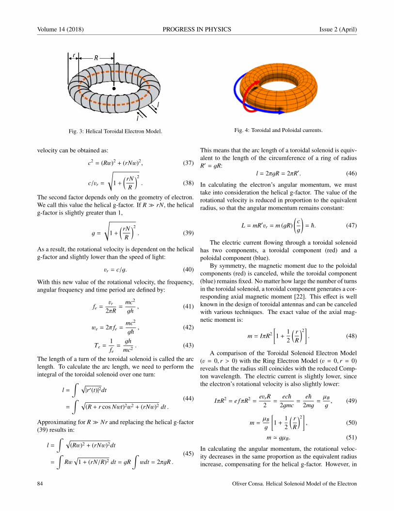
Volume 14 (2018) PROGRESS IN PHYSICS Issue 2 (April)
Fig. 3: Helical Toroidal Electron Model.
velocity can be obtained as:
c2 = (Rw)2 + (rNw)2, (37)
c/vr =
√1 +
( rNR
)2
. (38)
The second factor depends only on the geometry of electron.We call this value the helical g-factor. If R rN, the helicalg-factor is slightly greater than 1,
g =
√1 +
( rNR
)2
. (39)
As a result, the rotational velocity is dependent on the helicalg-factor and slightly lower than the speed of light:
vr = c/g. (40)
With this new value of the rotational velocity, the frequency,angular frequency and time period are defined by:
fe =vr
2πR=
mc2
gh, (41)
we = 2π fe =mc2
g~, (42)
Te =1fe
=gh
mc2 . (43)
The length of a turn of the toroidal solenoid is called the arclength. To calculate the arc length, we need to perform theintegral of the toroidal solenoid over one turn:
l =
∫ √|r′(t)|2dt
=
∫ √(R + r cos Nwt)2w2 + (rNw)2 dt .
(44)
Approximating for R Nr and replacing the helical g-factor(39) results in:
l =
∫ √(Rw)2 + (rNw)2dt
=
∫Rw
√1 + (rN/R)2 dt = gR
∫wdt = 2πgR .
(45)
Fig. 4: Toroidal and Poloidal currents.
This means that the arc length of a toroidal solenoid is equiv-alent to the length of the circumference of a ring of radiusR′ = gR:
l = 2πgR = 2πR′. (46)
In calculating the electron’s angular momentum, we musttake into consideration the helical g-factor. The value of therotational velocity is reduced in proportion to the equivalentradius, so that the angular momentum remains constant:
L = mR′vr = m (gR)(
cg
)= ~. (47)
The electric current flowing through a toroidal solenoidhas two components, a toroidal component (red) and apoloidal component (blue).
By symmetry, the magnetic moment due to the poloidalcomponents (red) is canceled, while the toroidal component(blue) remains fixed. No matter how large the number of turnsin the toroidal solenoid, a toroidal component generates a cor-responding axial magnetic moment [22]. This effect is wellknown in the design of toroidal antennas and can be canceledwith various techniques. The exact value of the axial mag-netic moment is:
m = IπR2[1 +
12
( rR
)2]. (48)
A comparison of the Toroidal Solenoid Electron Model(v = 0, r > 0) with the Ring Electron Model (v = 0, r = 0)reveals that the radius still coincides with the reduced Comp-ton wavelength. The electric current is slightly lower, sincethe electron’s rotational velocity is also slightly lower:
IπR2 = e fπR2 =evrR
2=
ec~2gmc
=e~
2mg=µB
g, (49)
m =µB
g
[1 +
12
( rR
)2], (50)
m ' gµB. (51)
In calculating the angular momentum, the rotational veloc-ity decreases in the same proportion as the equivalent radiusincrease, compensating for the helical g-factor. However, in
84 Oliver Consa. Helical Solenoid Model of the Electron

Issue 2 (April) PROGRESS IN PHYSICS Volume 14 (2018)
the calculation of magnetic moment, the rotational velocitydecreases by a factor of g, while the equivalent radius in-creases by a factor approximately equal to g squared. Thisis the cause of the electron’s anomalous magnetic moment.
2.4 Helical Solenoid Model
The geometries of both the Ring Electron Model and theToroidal Solenoid Electron Model represent a static electron(v = 0). For a moving electron with a constant velocity(v > 0), the ring geometry becomes a circular helix, whilethe toroidal solenoid geometry becomes a helical solenoid.On the other hand, if the thickness of the toroid is negated(r = 0), the toroidal solenoid is reduced to a ring, and thehelical solenoid is reduced to a helix.
Experimentally, the electron’s magnetic moment isslightly larger than the Bohr magneton. In the Ring ElectronModel, it was impossible to explain the electron’s anomalousmagnetic moment. This leads us to assume that the electronhas a substructure. The Toroidal Solenoid Electron Model al-lows us to obtain the electron’s anomalous moment as a directconsequence of its geometry.
Geometry v = 0 v > 0
r = 0 Ring Helix
r > 0 Toroidal Solenoid Helical Solenoid
The universe generally behaves in a fractal way, so themost natural solution assumes that the electron’s substructureis similar to the main structure, that is, a helix in a helix.
Fig. 5: Helical Solenoid Electron Model.
The trajectory of the electron can be parameterized withthe equation of the helical solenoid:
x(t) = (R + r cos Nwt) coswt ,y(t) = (R + r cos Nwt) sinwt ,z(t) = r sin Nwt + vt .
(52)
Like the other electron models discussed above, the HelicalSolenoid Electron Model postulates that the tangential veloc-
ity of the electric charge matches the speed of light and thatthe electron’s angular momentum matches the reduced Planckconstant.
|r′(t)|2 = c2 = (Rw)2 + (rNw)2 + v2
+ rw(2Rw + rw cos Nwt + 2vN) cos Nwt .(53)
This equation can be obtained directly from the helicalsolenoid geometry without any approximation. This equationshows a component that oscillates at a very high frequencywith an average value of zero. Consequently, the HelicalSolenoid Electron Model implies that the electron’s g-factoris oscillating, not fixed. Since the value oscillates, there is amaximum level of precision with which the g-factor can bemeasured. This prediction is completely new to this modeland is directly opposite to previous QED predictions. ForR rN, this oscillating component can be negated, and theequation reduces to
c2 = (Rw)2 + (rNw)2 + v2. (54)
The rotational velocity can be obtained as a function ofthe speed of light, the Lorentz factor, and the helical g-factor:
c2 = (Rw)2(1 + (rN/R)2) + v2, (55)
c2 = (vr)2g2 + v2, (56)
gvr = c√
1 − v2/c2 , (57)
vr = c/gγ. (58)
With this new value of the rotational velocity, the frequency,angular frequency, rotation time period and the wavelength(o pitch) of the helical solenoid electron are defined by:
fe =vr
2πR=
mc2
gγh, (59)
we = 2π fe =mc2
gγ~, (60)
Te =1fe
=gγhmc2 , (61)
λe = H =v
fe= gγβλc . (62)
In 2005, Michel Gouanère [18] identified this wavelength ina channeling experiment using a beam of ∼80 MeV electronsaligned along the < 110 > direction of a thick silicon crys-tal (d = 3.84 × 10⁻¹⁰ m). While this experiment has nothad much impact on QM, both Hestenes [19] and Rivas [20]have indicated that the experiment provides important experi-mental evidence consistent with the Hestenes ZitterbewegungModel:
d = gγβλc = (γmv)gh
(mc)2 = pgh
(mc)2 , (63)
Oliver Consa. Helical Solenoid Model of the Electron 85

Volume 14 (2018) PROGRESS IN PHYSICS Issue 2 (April)
p = d(mc)2
gh= 80.874 MeV/c. (64)
In the Helical Solenoid Electron Model, the rotational ve-locity is reduced by both the helical g-factor and the Lorentzfactor. In contrast, the equivalent radius compensates for thehelical g-factor while the increasing mass compensates forthe Lorentz factor. The angular momentum remains equal tothe reduced Planck constant:
L = m′R′vr = (γm)(gR)(c/γg) = mRc = ~. (65)
3 Consequences of the Helical Solenoid Electron Model
3.1 Chirality and helicity
In 1956, an experiment based on the beta decay of a Cobalt-60nucleus demonstrated a clear violation of parity conservation.In the early 1960s the parity symmetry breaking was used byGlashow, Salam and Weinberg to develop the ElectroweakModel, unifying the weak nuclear force with the electromag-netic force. The empirical observation that electroweak in-teractions act differently on right-handed fermions and left-handed fermions is one of the basic characteristics of this the-ory.
In the Electroweak Model, chirality and helicity are es-sential properties of subatomic particles, but these abstractconcepts are difficult to visualize. In contrast, in the HelicalSolenoid Electron Model, these concepts are evident and adirect consequence of the model’s geometry:
• Helicity is given by the helical translation motion (v >0), which can be left-handed or right-handed. Helicityis not an absolute value; it is relative to the speed of theobserver.
• Chirality is given by the secondary helical rotationalmotion, which can also be left-handed or right-handed.Chirality is absolute since the tangential velocity is al-ways equal to the speed of light; it is independent ofthe velocity of the observer.
3.2 Quantum Hall resistance and magnetic flux
The movement of the electric charge causes an electrical cur-rent (I = e fe) and a electric voltage (V = E/e = h fe/e). Ap-plying Ohm’s law, we obtain a fixed value for the impedanceof the electron equal to the value of the quantum Hall resis-tance. This value is quite surprising, since it is observable atthe macroscopic level and was not discovered experimentallyuntil 1980:
R =Ve
Ie=
h fe/ee fe
=he2 . (66)
According to Faraday’s Law, voltage is the variation of themagnetic flux per unit of time. So, in a period of rotation,we obtain a magnetic flux value which coincides with thequantum of magnetic flux, another macroscopically observ-able value. This value was expected since, in this model, the
electron behaves as a superconducting ring, and it is experi-mentally known that the magnetic flux in a superconductingring is quantized:
V = φe/Te , (67)
φe = VeTe =h fee
1fe
=he. (68)
3.3 Quantum LC circuit
Both the electrical current and the voltage of the electronare frequency dependent. This means that the electron be-haves as a quantum LC circuit, with a Capacitance (C) anda Self Inductance (L). We can calculate these coefficients fora electron at rest, obtaining values L = 2.08 × 10⁻¹⁶ H andC = 3.13 × 10⁻²⁵ F:
Le =φe
Ie=
he2 fe
=gγh2
mc2e2 , (69)
Ce =e
Ve=
e2
h fe=gγe2
mc2 . (70)
Applying the formulas of the LC circuit, we can obtain thevalues of impedance and resonance frequency, which coin-cide with the previously calculated values of impedance andnatural frequency of the electron:
Ze =
√Le
Ce=
he2 , (71)
fe =1
√LeCe
=mc2
gγh= fe . (72)
As the energy of the particle oscillates between electric andmagnetic energy, the average energy value is
E =LI2
2+
CV2
2=
h f2
+h f2
= h f . (73)
The above calculations are valid for any elementary particlewith a unit electric charge, a natural frequency of vibrationand an energy which match the Planck equation (E = h f ).
From this result, we infer that the electron is formed bytwo indivisible elements: a quantum of electric charge and aquantum of magnetic flux, the product of which is equal toPlanck’s constant. The electron’s magnetic flux is simultane-ously the cause and the consequence of the circular motion ofthe electric charge:
eφ = h. (74)
3.4 Quantitative calculation of the helical G-factor
The g-factor depends on three parameters (R, r and N) but wedo not know the value of two of them. We can try to figure outthe value of the helical g-factor using this approximation [28]:
Using this expansion series:√1 + (a)2 = 1 + 1/2(a)2 + . . . (75)
86 Oliver Consa. Helical Solenoid Model of the Electron
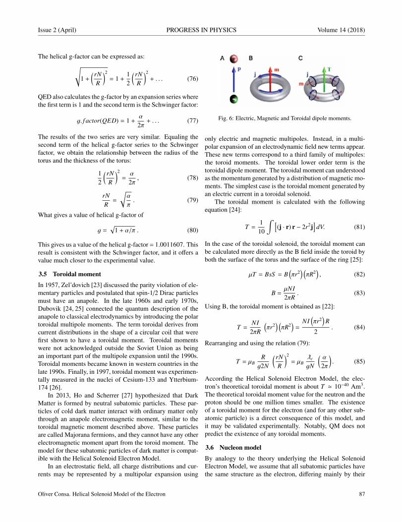
Issue 2 (April) PROGRESS IN PHYSICS Volume 14 (2018)
The helical g-factor can be expressed as:√1 +
( rNR
)2
= 1 +12
( rNR
)2
+ . . . (76)
QED also calculates the g-factor by an expansion series wherethe first term is 1 and the second term is the Schwinger factor:
g. f actor(QED) = 1 +α
2π+ . . . (77)
The results of the two series are very similar. Equaling thesecond term of the helical g-factor series to the Schwingerfactor, we obtain the relationship between the radius of thetorus and the thickness of the torus:
12
( rNR
)2
=α
2π, (78)
rNR
=
√α
π. (79)
What gives a value of helical g-factor of
g =√
1 + α/π . (80)
This gives us a value of the helical g-factor = 1.0011607. Thisresult is consistent with the Schwinger factor, and it offers avalue much closer to the experimental value.
3.5 Toroidal moment
In 1957, Zel’dovich [23] discussed the parity violation of ele-mentary particles and postulated that spin-1/2 Dirac particlesmust have an anapole. In the late 1960s and early 1970s,Dubovik [24, 25] connected the quantum description of theanapole to classical electrodynamics by introducing the polartoroidal multipole moments. The term toroidal derives fromcurrent distributions in the shape of a circular coil that werefirst shown to have a toroidal moment. Toroidal momentswere not acknowledged outside the Soviet Union as beingan important part of the multipole expansion until the 1990s.Toroidal moments became known in western countries in thelate 1990s. Finally, in 1997, toroidal moment was experimen-tally measured in the nuclei of Cesium-133 and Ytterbium-174 [26].
In 2013, Ho and Scherrer [27] hypothesized that DarkMatter is formed by neutral subatomic particles. These par-ticles of cold dark matter interact with ordinary matter onlythrough an anapole electromagnetic moment, similar to thetoroidal magnetic moment described above. These particlesare called Majorana fermions, and they cannot have any otherelectromagnetic moment apart from the toroid moment. Themodel for these subatomic particles of dark matter is compat-ible with the Helical Solenoid Electron Model.
In an electrostatic field, all charge distributions and cur-rents may be represented by a multipolar expansion using
Fig. 6: Electric, Magnetic and Toroidal dipole moments.
only electric and magnetic multipoles. Instead, in a multi-polar expansion of an electrodynamic field new terms appear.These new terms correspond to a third family of multipoles:the toroid moments. The toroidal lower order term is thetoroidal dipole moment. The toroidal moment can understoodas the momentum generated by a distribution of magnetic mo-ments. The simplest case is the toroidal moment generated byan electric current in a toroidal solenoid.
The toroidal moment is calculated with the followingequation [24]:
T =1
10
∫ [(j · r) r − 2r2j
]dV. (81)
In the case of the toroidal solenoid, the toroidal moment canbe calculated more directly as the B field inside the toroid byboth the surface of the torus and the surface of the ring [25]:
µT = BsS = B(πr2
) (πR2
), (82)
B =µNI2πR
. (83)
Using B, the toroidal moment is obtained as [22]:
T =NI
2πR
(πr2
) (πR2
)=
NI(πr2
)R
2. (84)
Rearranging and using the relation (79):
T = µBRg2N
( rNR
)2
= µBoc
gN
(α
2π
). (85)
According the Helical Solenoid Electron Model, the elec-tron’s theoretical toroidal moment is about T ' 10−40 Am3.The theoretical toroidal moment value for the neutron and theproton should be one million times smaller. The existenceof a toroidal moment for the electron (and for any other sub-atomic particle) is a direct consequence of this model, andit may be validated experimentally. Notably, QM does notpredict the existence of any toroidal moments.
3.6 Nucleon model
By analogy to the theory underlying the Helical SolenoidElectron Model, we assume that all subatomic particles havethe same structure as the electron, differing mainly by their
Oliver Consa. Helical Solenoid Model of the Electron 87

Volume 14 (2018) PROGRESS IN PHYSICS Issue 2 (April)
charge and mass. Protons are thought to be composed ofother fundamental particles called quarks, but their internalorganization is beyond the scope of this work.
The radius of a nucleon is equal to its reduced Comp-ton wavelength. The Compton wavelength is inversely pro-portional to an object’s mass, so for subatomic particles, asmass increases, size decreases. Both the proton and the neu-tron have a radius that is about 2000 times smaller than theelectron. Historically, the proton radius was measured usingtwo independent methods that converged to a value of about0.8768 fm. This value was challenged by a 2010 experimentutilizing a third method, which produced a radius of about0.8408 fm. This discrepancy remains unresolved and is thetopic of ongoing research referred to as the Proton RadiusPuzzle. The proton’s reduced Compton wavelength is 0.2103fm. If we multiple this radius by 4, we obtain the value of0.8412 fm. This value corresponds nicely with the most re-cent experimental radius of the proton. This data supports ourtheory that the proton’s radius is related to its reduced Comp-ton radius and that our Helical Solenoid Electron Model isalso a valid model for the proton.
The current of a nucleon is about 2000 times the currentof an electron, and the radius is about 2000 times lower. Thisresults in a magnetic field at the center of the nucleon’s ringthat is about four million times bigger than that of the elec-tron or thousands of times bigger than a neutron star. Thismagnetic field is inversely dependent with the cube of thedistance. This implies that while the magnetic field insidethe neutron’s ring is huge, outside the ring, the magnetic fielddecays much faster than the electric field. The asymmetri-cal behavior of the neutron’s magnetic field over short andlong distances leads us to suggest that the previously identi-fied strong and weak nuclear forces are actually manifesta-tions of this huge magnetic field at very short distances.
3.7 Spin quantum number
In 1913, Bohr introduced the Principal Quantum Number toexplain the Rydberg Formula for the spectral emission linesof atomic hydrogen. Sommerfeld extended the Bohr the-ory with the Azimuthal Quantum Number to explain the finestructure of the hydrogen, and he introduced a third MagneticQuantum Number to explain the Zeeman effect. Finally, in1921, Landé put forth a formula (named the Landé g-factor)that allowed him to explain the anomalous Zeeman effect andto obtain the whole spectrum of all atoms.
gJ = gLJ(J + 1) − S (S + 1) + L(L + 1)
2J(J + 1)
+ gSJ(J + 1) + S (S + 1) − L(L + 1)
2J(J + 1).
(86)
In this formula, Landé introduced a fourth Quantum Num-ber with a half-integer number value (S = 1/2). This Landég-factor was an empirical formula where the physical mean-ing of the four quantum numbers and their relationship with
the motion of the electrons around the nucleus was unknown.Heisenberg, Pauli, Sommerfeld, and Landé tried unsuccess-fully to devise a new atomic model (named the Ersatz Model)to explain this empirical formula. Landé proposed that hisg-factor was produced by the combination of the orbital mo-mentum of the outer electrons with the orbital momentumof the inner electrons. A different solution was suggestedby Kronig, who proposed that the half-integer number wasgenerated by a self-rotation motion of the electron (spin), butPauli rejected this theory.
In 1925, Uhlenbeck and Goudsmit published a paperproposing the same idea, namely that the spin quantum num-ber was produced by the electron’s self-rotation. The half-integer spin implies an anomalous magnetic moment of 2. In1926, Thomas identified a relativistic correction of the modelwith a value of 2 (named the Thomas Precession) that com-pensated for the anomalous magnetic moment of the spin.Despite his initial objections, Pauli formalized the theory ofspin in 1927 using the modern theory of QM as set out bySchrödinger and Heisenberg. Pauli proposed that spin, angu-lar moment, and magnetic moment are intrinsic properties ofthe electron and that these properties are not related to anyactual spinning motion. The Pauli Exclusion Principle statesthat two electrons in an atom or a molecule cannot have thesame four quantum numbers. Pauli’s ideas brought about aradical change in QM. The Bohr-Sommerfeld Model’s ex-plicit electron orbitals were abandoned and with them anyphysical model of the electron or the atom.
We propose to return to the old quantum theory of Bohr-Sommerfeld to search for a new Ersatz Model of the atomwhere the four quantum numbers are related to electron or-bitals. We propose that this new atomic model will be com-patible with our Helical Solenoid Electron Model. We alsopropose that the half-integer spin quantum number is not anintrinsic property of the electron but a result of the magneticfields generated by orbiting inner electrons.
Submitted on January 25, 2018
References1. Parson L. A Magneton Theory of the Structure of the Atom. Smithso-
nian Miscellaneous Collections, 1915, v. 65, 2–80.
2. Compton A.H. The Size and Shape of the Electron. Phys. Rev., 1917.v. 14(3), 247–259.
3. Allen H.S. The Case for a Ring Electron. Proceedings of the PhysicalSociety, 1919, v. 31, 49–68.
4. Bergman D., Wesley J.P. Spinning Charged Ring Model of ElectronYielding Anomalous Magnetic Moment. Galilean Electrodynamics,1990, v. 1, 63–67.
5. Lucas C.W. A Classical Theory of Elementary Particles Electromag-netic Part 2, intertwining Charge-Fibers. The Journal of Common SenseScience, 2005, v. 8(2), 1–7.
6. Kanarev P. Model of the Electron. Apeiron, 2000, v. 7(3–4), 184–194.
7. Jennison R.C. A new classical relativistic model of the electron. Phys.Letters A., 1989, v. 141(8–9), 377–382.
88 Oliver Consa. Helical Solenoid Model of the Electron

Issue 2 (April) PROGRESS IN PHYSICS Volume 14 (2018)
8. Gauthier R. Superluminal Quantum Models of the Electron and thePhoton. viXra:0703.0015.
9. Williamson J.G., van der Mark J.M.B. Is the electron a photon withtoroidal topology? Annales de la Fondation Louis de Broglie, 1997,v. 22(2), 133–146.
10. Schwinger J. On Gauge Invariance and Vacuum Polarization. Phys.Rev., 1951, v. 82, 664–679.
11. Huang K. On the Zitterbewegung of the Dirac Electron. Am. J. Phys.,1952, v. 20, 479–484.
12. Bunge M. A picture of the electron. Nuovo Cimento, 1955, v. 1(6), 977–985.
13. Barut A.O., Bracken A.J. Zitterbewegung and the internal geometry ofthe electron. Phys. Rev. D, 1981, v. 23(10), 2454–2463.
14. Barut A.O., Zanghi N. Classical Model of the Dirac Electron. Phys.Rev. Lett., 1984, v. 52, 2009–2012.
15. Hestenes D. The Zitterbewegung Interpretation of Quantum Mechan-ics. Found. Phys., 1990, v. 20(10), 1213–1232.
16. Hestenes D. Zitterbewegung in Quantum Mechanics. arXiv:8002.2728.
17. Rivas M. Kinematical Theory of Spinning Particles. Kluwer, Dordrecht,2001.
18. Gouanère M. A Search for the de Broglie Particle Internal Clock byMeans of Electron Channeling. Foundations of Physics, 2008, v. 38,659–664.
19. Hestenes D. Reading the Electron Clock. arXiv:0802.3227.
20. Rivas M. Measuring the internal clock of the electron.arXiv:0809.3635.
21. Bostick W. Mass, Charge and Current: The Essence and Morphology.Physics Essays, 1991, v. 4(1), 45–59.
22. Marinov K., Boardman A.D., Fedotov V.A. Metamaterial Toroidal.New Journal of Physics, 2007, v. 9, 324–335.
23. Zel’dovich Y. Electronic interaction with parity violation. Zh. Eksp.Teor. Fiz., 1957, v. 33, 1184–1186.
24. Dubovik V.M., Tugushev. Toroid moments in electrodynamics andsolid-state physics. Physics Reports, 1990, v. 187(4), 145–202.
25. Dubovik V.M., Kuznetsov. The toroid moment of Majorana neutrino.Int. J. Mod. Phys., 1998, v. A13, 5257-–5278.
26. Wood C.S. Measurement of parity nonconservation and an anapole mo-ment in cesium. Science, 1997, v. 275, 1759–1763.
27. Ho C.M., Scherrer R.J. Anapole dark matter. Phys. Lett. B, 2013, v. 722,341–346.
28. Consa O. G-factor and the Helical Solenoid Electron Model. viXra:1702.0185.
Oliver Consa. Helical Solenoid Model of the Electron 89

Volume 14 (2018) PROGRESS IN PHYSICS Issue 2 (April)
Concerning the Dirac γ-Matrices Undera Lorentz Transformation of the Dirac Equation
G. G. Nyambuya
National University of Science and Technology, Faculty of Applied Sciences — Department of Applied Physics,Fundamental Theoretical and Astrophysics Group, P. O. Box 939, Ascot, Bulawayo, Republic of Zimbabwe
E-mail: [email protected]
We embolden the idea that the Dirac 4 × 4 γ-matrices are four-vectors where the spacecomponents (γi) represent spin and the forth component (γ0) should likewise representthe time component of spin in the usual four-vector formalism of the Special Theory ofRelativity. With the γ-matrices as four-vectors, it is seen that the Dirac equation admitstwo kinds of wavefunctions — (1) the usual four component Dirac bispinor ψ and (2) ascalar four component bispinor φ. Realizing this, and knowing forehand of the existingmystery as to why Leptons and Neutrinos come in pairs, we seize the moment and makethe suggestion that the pair (ψ, φ) can be used as a starting point to explain mystery ofwhy in their three generations [(e±, νe), (µ±, νµ), (τ±, ντ)], Leptons and Neutrinos comein doublets. In this suggestion, the scalar-bispinor φ can be thought of as the Neutrinowhile the usual Dirac bispinor ψ can be thought of as the Lepton.
“We have found it of paramount importance that inorder to progress we must recognize our ignoranceand leave room for doubt.”
— Richard Phillips Feynman (1918-1988)
1 Introduction
As taught to physics students through the plethora of text-books available on our planet e.g., refs. [1–5], the Dirac 4× 4γ-matrices (γµ) are usually presented as objects that undergoa transformation during a Lorentz transformation of the Dirac[6, 7] equation. This issue of the transformation of these γ-matrices is not well represented in the literature [8]. There,thus, is a need to clear the air around this issue regarding theproper transformation properties of these matrices. To thatend, we here argue in favour of these matrices as physicalfour-vectors and as such, they must under a Lorentz transfor-mation transform as four-vectors. In-fact, it is well knownthat the γi-matrices (i = 1, 2, 3) represent spin (i.e., ~S =
12~γ
1~i + 12~γ
2~j + 12~γ
3~k) because, together with the angularmomentum operator ( ~L), their sum total of the orbital angu-lar momentum and spin ( ~J = ~L + ~S) commutes with theDirac Hamiltonian (HD), i.e. ([ ~J ,HD] = 0), implying that ~Jis a constant of motion.
For a particle whose rest-mass and Dirac [6, 7] wave-function are m0 and ψ respectively, the corresponding Dirac[6, 7] equation is given by:
ı~γµ∂µψ = m0cψ, (1)
where:
γ0 =
I2 0
0 −I2
, γi =
0 σi
−σi 0
, (2)
are the 4 × 4 Dirac γ-matrices where I2 and 0 are the 2×2identity and null matrices respectively, and |ψ〉 is the fourcomponent Dirac [6, 7] wave-function, ~ is the normalizedPlanck constant, c is the speed of light in vacuum, ı =
√−1,
and:
ψ =
ψ0ψ1ψ2ψ3
=
ψL
ψR
, (3)
is the 4 × 1 Dirac [6,7] four component wavefunction and ψL
and ψR are the Dirac [6,7] bispinors that are defined such that:
ψL =
ψ0
ψ1
and ψR =
ψ2
ψ3
. (4)
Throughout this reading — unless otherwise specified;the Greek indices will here-and-after be understood to mean(µ, ν, ... = 0, 1, 2, 3) and the lower case English alphabet in-dices (i, j, k ... = 1, 2, 3).
2 Lorentz Transformation of the Dirac as usually pre-sented
To prove Lorentz Invariance (Covariance) two conditionsmust be satisfied:
1. The first condition is that: given any two inertial ob-servers O and O′ anywhere in spacetime, if in the frameO we have:
[i~γµ∂µ −m0c]ψ(x) = 0, (5)
as the Dirac equation for the particle ψ, then:
[i~γµ′
∂µ′ −m0c]ψ′(x′) = 0 (6)
is the equation describing the same state but in the fra-me O′.
90 G. G. Nyambuya. Transformation of the Dirac Matrices
Issue 2 (April) PROGRESS IN PHYSICS Volume 14 (2018)
2. The second condition is that: given that ψ(x) is thewavefunction as measured by observer O, there must bea prescription for observer O′ to compute ψ′(x′) fromψ(x) where ψ′(x′) describes to O′ the same physicalstate as that measured by O. The conserve must be trueas-well, that is: there must exist a prescription such thatstarting from equation (6), one can arrive at (5).
In simpler mathematical terms, the above two require-ments are saying that: starting from equation (5), there mustexist some physically legitimate transformations within theframework of Lorentz transformations that can take (map) usfrom this equation (5) to equation (6) and vice-versa. If wecan find these, then, the Dirac equation is said to be LorentzInvariant (Covariant).
Now, since the Lorentz transformations are linear, it is tobe required or expected of the transformations between ψ(x)and ψ′(x′) to be linear too, i.e.:
ψ′(x′) = ψ′(Λx) = S (Λ)ψ(x) = S (Λ)ψ(Λ−1x′), (7)
where S (Λ) is a 4 × 4 matrix which depends only on the rel-ative velocities of O and O′ and Λ is the Lorentz transforma-tion matrix. S (Λ) has an inverse if O→ O′ and also O′ → O.The inverse is:
ψ(x) = S −1(Λ)ψ′(x′) = S −1(Λ)ψ′(Λx), (8)
or we could write:
ψ(x) = S (Λ−1)ψ′(Λx) =⇒ S (Λ−1) = S −1(Λ). (9)
We can now write equation (5), as:[i~γµ
∂xµ′
∂xµ∂µ′ −m0c
]S −1(Λ)ψ′(x′) = 0, (10)
and multiplying this from the left by S (Λ), we have:
S (Λ)[i~γµ
∂xµ′
∂xµ∂µ′ −m0c
]S −1(Λ)ψ′(x′) = 0, (11)
and hence:[i~S (Λ)γµ
∂xµ′
∂xµS −1(Λ)∂µ′ −m0c
]ψ′(x′) = 0. (12)
Therefore, for the above equation to be identical to equa-tion (6) (hence Lorentz Invariant), the requirement is that:
γµ′
= S (Λ)γµ∂xµ
′
∂xµS −1(Λ), (13)
hence, we have shown that — for as long as S −1(Λ) exists,equation (5) is Lorentz Invariant.
3 Dirac ~4 × 4 ~γ-matrices as a four-vector
The Dirac equation (1) can be re-written in the traditionalSchrodinger formulation as (H ψ = Eψ) where H and E arethe energy and Hamiltonian operators respectively. In thisSchrodinger formulation, H , will be such that it is given by:
H = γ0m0c2 − ı~cγ0γ j∂ j, (14)
and (E = i~∂/∂t).Now, according to the quantum mechanical equation gov-
erning the evolution of any quantum operator Q , we knowthat:
ı~∂Q∂t
= QH − HQ = [Q ,H ] , (15)
hence, if:[Q ,H ] ≡ 0, (16)
then, the quantum mechanical observable corresponding tothe operator Q is a conserved physical quantity.
With this [equation (15)] in mind, Dirac asked himselfthe natural question — what the “strange” new γ-matricesappearing in his equation really represent. What are they?In-order to answer this question, he decided to have a “look”at or make a closer “inspection” of the quantum mechanicalorbital angular momentum operator Li which we all know tobe defined:
Li = (~r × ~p)i = −ı~εi jk x j∂k, (17)
where, εi jk is the completely-antisymmetric three dimensionalLevi-Civita tensor. In the above definition of Li, the momen-tum operator ~p is the usual quantum mechanical operator, i.e.:
~p = −ı~~∇ ⇒ pi = ı~∂i. (18)
From this definition of Li given in equation (17), it fol-lows from equation (15) that ı~∂Li/∂t = [Li,H ], will be suchthat:
ı~∂Li
∂t= −ı~m0c2εi jk
[x j∂k, γ
0]+~2cεi jk
[x j∂k, γ
0γl∂l
]. (19)
Now, because the term γ0m0c2 is a constant containing noterms in pi, it follows from this very fact that (εi jk
[x j∂k, γ
0]≡
0), hence equation (19) will reduce to:
ı~∂Li
∂t= ~2cεi jkγ
0γl[x j∂k, ∂l
]= ~2cεi jkγ
0γl(x j∂k∂l − ∂lx j∂k
).
(20)
From the commutation relation of position (xi) and mo-mentum (−ı~∂ j) due to the Heisenberg uncertainty princi-ple [9], namely (−ı~
[xi, ∂ j
]= −ı~δi j) where δi j is the usual
Kronecker-delta function, it follows that if in equation (20),we substitute (∂lx j = x j∂l + δl j), this equation is going toreduce to:
ı~∂Li
∂t=~2cεi jkγ
0γl(x j∂k∂l−x j∂l∂k
)︸ ︷︷ ︸ +~2cεi jkγ0γlδl j∂k. (21)
G. G. Nyambuya. Transformation of the Dirac Matrices 91

Volume 14 (2018) PROGRESS IN PHYSICS Issue 2 (April)
The term with the under-brace vanishes identically, that isto say: (x j∂k∂l − x j∂l∂k ≡ 0); and (εi jkγ
0γlδl j = εilkγ0γl), it
follows from this that equation (21), will reduce to:
ı~∂Li
∂t= ~2cεilkγ
0γl∂k. (22)
Since this result [i.e., equation (22) above] is non-zero, itfollows from the dynamical evolution theorem [i.e., equation(16)] of Quantum Mechanics (QM) that none of the angularmomentum components Li are — for the Dirac particle —going to be constants of motion. This result obviously both-ered the great and agile mind of Paul Dirac. For example,a non-conserved angular momentum would mean spiral or-bits i.e., Dirac particles do not move in fixed and well definedorbits as happens with electrons of the Hydrogen atom for ex-ample; at the very least, this is very disturbing because it doesnot tally with observations. The miniature beauty that Dirachad — had the rare privilege to discover and, the first humanbeing to “see” with his beautiful and great mind — this —had to be salvaged∗ somehow.
Now — enter spin! Dirac figured that “Subtle Nature”must conserve something redolent with orbital angular mo-mentum, and he considered adding something to Li thatwould satisfy the desired conservation criterion, i.e.: call thisunknown, mysterious and arcane quantity Si and demandthat:
ı~∂ (Li + Si)
∂t≡ 0. (23)
This means that this strange quantitySi must be such that:
ı~∂Si
∂t= [Si,H ] = −~2cεilkγ
0γl∂k. (24)
Solving equation (24) for Si, Dirac arrived at:
Si =12~
(σi 00 σi
)=
12~γ5γi, (25)
where (γ5 = ıγ0γ1γ2γ3), is the usual Dirac gamma-5 matrix.Now, realising that:
1. The matrices σi are Pauli matrices and they had beenad hocly introduced in 1925 into physics to account forthe spin of the Electron by the Dutch-American the-oretical physicists, George Eugene Uhlenbeck (1900–1988) and his colleague, Samuel Abraham Goudsmit(1902–1978) [10].
2. His equation — when taken in the non-relativistic limit,it would account for the then unexplained gyromag-netic ratio (g = 2) of the Electron and this same equa-tion emerged with σi explaining the Electron’s spin.
∗Such is the indispensable attitude of the greatest theoretical physiciststhat ever graced the face of planet Earth — beauty must and is to be pre-served; this is an ideal for which they will live for, and if needs be, it is anideal for which they will give-up their life by taking a gamble to find thatunknown quantity that restores the beauty glimpsed!
The agile Paul Dirac seized the golden moment and forth-with identified Si with the ψ-particle’s spin. The factor 1
2~ inSi implies that the Dirac particle carries spin 1/2, hence, theDirac equation (1) is an equation for a particle with spin 1/2!
While in this esoteric way (i.e., as demonstrated above)Dirac was able to explain and “demystify” Wolfgang Pauli(1900–1958)’s strange spin concept which at the time hadonly been inserted into physics by “the sleight of hand” outof an unavoidable necessity, what bothers us (i.e., myself) themost is:
How it comes about that we (physicists) have hadissues to do with the transformational propertiesof the γ-matrices? Why? Really — why? Thefact that orbital angular momentum ~L is a vectorinvariably leads to the indelible fact that ~S is avector as-well, because we can only add vectorsto vectors.
If ~S is a vector, then the matrices γi must be componentsof a 3-vector, so must the matrix γ0 be the component of thetime-vector in the usual four-vector formalism, hence γµ mustbe a four-vector. So, right from the word go — with little orno resistance whatsoever, it must have been pristine clear thatthe γ-matrices must be four-vectors.
4 Dirac equation with the ~γ-matrices as a four-vector
With γ-matrices now taken as a four-vector, the object γµ∂µis a scalar, the meaning of which is that the Dirac equationwill now accommodate two types of spinors “the usual Diracbispinor” and a new “scalar-bispinor”, i.e.:
1. A spinor that is a scalar. Let us here call this a scalar-bispinor and let us denote it with the symbol φ and be-cause of its scalar nature — under a Lorentz transfor-mation, we will have (φ′ = φ). Just like the ordinaryDirac wavefunction ψ is a 4 × 1 component object, φ isalso a 4 × 1 object, i.e.:
φ =
φ0φ1φ2φ3
=
φL
φR
, (26)
where φL and φR are the scalar-spinors — which arelike the ordinary left and right handed Dirac spinors(ψL, ψR); ψL and φR are defined:
φL =
φ0
φ1
and φR =
φ2
φ3
. (27)
Consideration of the scalar-bispinor has been made inthe past by others e.g., [11].
2. The ordinary Dirac bispinor ψ: that transforms lin-early under a Lorentz transformation i.e. (ψ′ = Sψ),
92 G. G. Nyambuya. Transformation of the Dirac Matrices

Issue 2 (April) PROGRESS IN PHYSICS Volume 14 (2018)
where, a usual, Lorentz Invariance (Covariance) requi-res that the function S = S (xµ, xµ) be such that:
γµ′
∂µ′S = γµ∂µS = 0, (28)
and:γµ = S −1γµS , (29)
which implies: [S , γµ
]= 0. (30)
Now, we certainly must ask “What does this all mean”.That is to say, the fact that the Dirac equation allows for theexistence of the usual Dirac bispinor ψ and in addition to that— a scalar-bispinor φ? Taken at the same level of under-standing that the Dirac equation’s prediction of the existenceof antimatter is premised on the Dirac equation being sym-metric under charge conjugation — on that very same levelof understanding, this fact that the Dirac equation in its mostnatural and un-tempered state as presented herein — it, allowsfor the existence of the usual Dirac bispinor ψ and scalar-bispinor φ; in the same vein of logic, this naturally impliesthat for every Dirac bispinor ψ, there must exist a correspond-ing scalar-bispinor φ. That is, the Dirac bispinor ψ and thescalar-bispinor φmust come in pairs. There is no escape fromthis train of logic.
If we are thinking of Leptons and Neutrinos, the abovepair-picture of (ψ, φ) makes perfect sense. Based on this pic-ture, we can write the Dirac equation for this pair (ψ, φ) as:
ı~γµ∂µ
ψ
φ
= m0c(
1 00 η
) ψ
φ
, (31)
where η is a scalar-constant that we have introduced so asto accommodate the possibility that the particle-pair (ψ, φ),may have different masses. In this way, one can begin to en-tertain ideas on how to explain the Lepton-Neutrino pairing[(e±, νe), (µ±, νµ), (τ±, ντ)]. We have no intention of doing thisor going any deeper on this matter but merely to point out —as we have just done — that, this idea may prove a viable av-enue of research to those seeking an explanation of why thismysterious pairing occurs in nature.
5 General discussion
We must categorically state that — what we have presentedherein is not new at all. All we have endeavoured is to makebold the point that the γ-matrices constitute a four-vector.Perhaps the only novelty there is — in the present contribu-tion — is the suggestion that we have made — namely that,the resulting scalar-bispinor (φ) and the usual Dirac bispinor(ψ) can be used as a starting point to explain the currentlyopen problem of the three generation Lepton-Neutrino pair-ing (e±, νe), (µ±, νµ) and (τ±, ντ); where the scalar-bispinorcan be assumed to be the Neutrino while the usual Dirac
bispinor can be thought of the Lepton. In the sequatial read-ing [12], we will demonstrate how this formulation of theDirac equation can be used to explain how massless neutri-nos can oscillate.
Acknowledgements
We are grateful for the assistance rendered unto us by theNational University of Science and Technology’s ResearchBoard toward our research endeavours.
Submitted on March 16, 2018
References1. Itzykson C. and Zuber J.-B. Quantum Mechanics II. McGraw-Hill,
New York, USA, 1980.
2. Messiah A. Quantum Mechanics II. North-Holland Publishing Com-pany, Amsterdam, Netherland, second edition, 1962.
3. Sakurai J. J. Advanced Quantum Mechanics. Addison-Wesley Publish-ing Company, Massachusetts, USA, 1967.
4. Schweber S. S. An Introduction to Relativistic Quantum Field Theory.Row, Peterson and Company, New York, USA, 1961.
5. Zee A. Quantum Field Theory in a Nutshell. Princeton University Press,USA, second edition, 2010.
6. Dirac P. A. M. The Quantum Theory of the Electron. Proceedings of theRoyal Society of London A: Mathematical, Physical and EngineeringSciences, 1928, v.117(778), 610–624.
7. Dirac P. A. M. The Quantum Theory of the Electron. Part II. Proceed-ings of the Royal Society of London A: Mathematical, Physical andEngineering Sciences, 1928, v. 118(779), 351–361.
8. Nikolic H. How (Not) To Teach Lorentz Covariance of the Dirac Equa-tion. European Journal of Physics, 2014, v.35(3), 035003.
9. Heisenberg W. Ueber den anschaulichen Inhalt der quantentheoretis-chen Kinematik and Mechanik. Zeitschrift fur Physik, 1927, v.43, 172–198. Engilish Translation: Wheeler J. A. and Zurek W. H. (eds) Quan-tum Theory and Measurement. Princeton (NJ), Princeton UniversityPress, 1983, 62–84.
10. Uhlenbeck G. E. and Goudsmit S. Ersetzung der Hypothese vom un-mechanischen Zwang durch eine Forderung bezuglich des innerenVerhaltens jedes einzelnen Elektrons. Die Naturwissenschaften, 1925,v.13(47), 953–954.
11. Chapman T. C. and Leiter D. J. On the Generally Covariant Dirac Equa-tion. American Journal of Physics, 1976, v.44(9), 858–862.
12. Nyambuya G. G. Oscillating Massless Neutrinos. Progress in Physics,2018, v. 14, 94–98.
G. G. Nyambuya. Transformation of the Dirac Matrices 93

Volume 14 (2018) PROGRESS IN PHYSICS Issue 2 (April)
Oscillating Massless Neutrinos
G. G. Nyambuya
National University of Science and Technology, Faculty of Applied Sciences — Department of Applied Physics,Fundamental Theoretical and Astrophysics Group, P. O. Box 939, Ascot, Bulawayo, Republic of Zimbabwe
E-mail: [email protected]
The phenomenon of neutrino oscillations requires that not only should neutrinos bemassive but that these masses be unique. How they acquire this mass remains an openquestion. Various mechanisms have been proposed to explain this phenomenon of neu-trino oscillations. Herein, we propose — the simplest imaginable — alternative mecha-nism which operates via coupling the massless neutrino to a massive Dirac scalar. Thismassive Dirac scalar is a new hypothetical particle that we — unfortunately — can notobserve directly because of its point-particle nature. Further, this massive Dirac scalarcomes in as an integral part of the neutrino system — it [massive Dirac scalar] oscil-lates between three states, thus leading to the observed neutrino oscillations. This modelpredicts neutrinos are Dirac in nature and not Majorana.
“Just by studying mathematics we can hope tomake a guess at the kind of mathematics that willcome into the physics of the future.”
— Paul A. M. Dirac (1902-1984)
1 Introduction
According to Albert Einstein (1879–1955)’s Special Theoryof Relativity (STR) [1], the energy E and momentum p ofa massless (m0 = 0) are related by the energy-momentumequation (E = pc), where c is the speed of Light in vacuo.In accordance with the dictates of wave mechanics/phenom-enon, the group velocity, vg:
vg =∂E∂p
, (1)
of a particle whose energy and momentum are related by(E = pc) is equal to the speed of Light in vacuo, i.e. (vg = c).All indications are that the neutrino travels at the vacuo speedof Light, c, thus prompting physicists to assume that the neu-trino is massless. Be that as it may, a massless neutrino pausesa problem to the physicist in that one can not explain the all-important experimentally [2–5] verified and common-placephenomenon of neutrino oscillation.
First predicted [6, 7] in 1957 by the Italian nuclear physi-cist — Bruno Pontecorvo (1913–1993), and observed in 1968by the America chemist and physicist — Raymond Davis Jr.(1914–2006) et al. [8], neutrino oscillation is a quantum me-chanical phenomenon whereby a neutrino created with a spe-cific lepton flavour (electron νe, muon νµ, or tau ντ) can bemeasured at a latter time to have a different flavour. Theprobability of measuring a particular flavour for a neutrinovaries between the three known flavour states (νe, νµ, ντ) asit propagates through the intestacies of space. From a the-oretical standpoint, two conditions are necessary for neutri-nos to oscillate — i.e., to change from one type to the other,
e.g., from an Electron-neutrino (νe) to a Muon-neutrino (νµ)or vice-verse, and these conditions are:
1. Neutrinos must have a non-zero mass, and this mass cannotbe identical for all the three neutrino flavours (νe, νµ, ντ).
2. There must be no rigorous law forbidding a transition be-tween neutrino species, the meaning of which is that thesetransitions are purely probabilistic in nature.
Since the coming to light or since the “conception” of thisimportant question i.e., the question of how neutrino massesarise — this question, has not been answered conclusively[9]. In the Standard Model of particle physics, fermions onlyhave mass because of interactions with the Higgs Field. Doneutrinos generate their mass via the Higgs Mechanism [10–12] as-well? This is a question that needs an answer. We heredo not claim to give a definitive answer to this question, butmerely a suggestion — perhaps, a suggestion that one mightconsider worthy of their attention.
That said, we must here at the penultimate of this intro-ductory section make clear the scope of the present letter —i.e., while this letter presents — in our feeble view, a newmodel whose endeavour is to explain neutrino oscillations,we present this model only as an alternative to existing ex-planations on this phenomenon. We deliberately avoid an in-depth comparative analysis of these models with the presentand this we have done in-order that our ideas are clearly pre-sented without overshadowing them with existing ideas onthe same endeavour.
2 Massless Dirac particle
First considered by the German mathematician, mathemati-cal physicist and philosopher — Hermann Klaus Hugo Weyl(1885–1955); a massless Dirac particle is described by thefollowing Dirac-Weyl [13] equation:
ı~γµ∂µψ = 0, (2)
94 G. G. Nyambuya. Oscillating Massless Neutrinos

Issue 2 (April) PROGRESS IN PHYSICS Volume 14 (2018)
where (ı =√−1), ∂µ is the four spacetime partial derivatives,
~ is the normalized Planck constant, γµ are the four 4×4 Diracmatrices and ψ is the usual 4× 1 component Dirac wavefunc-tion.
In this letter, the gamma matrices shall be assumed to befour vectors the meaning of which is that they transform likevectors i.e.:
γµ′
=∂xµ
′
∂xµγµ. (3)
This assumption of treating the γ-matrices as four vectorsmay appear strange and if not completely and outright wrong.Be that as it may, in the letter [14], this idea of treating the γ-matrices as vectors as been justified. As argued therein thesaid letter [14], once the γ-matrices are four vectors, ψ cantake three forms:
1. It [ψ] can be a zero ranks scalar.2. It [ψ] can be a four 4 × 1 component scalar where the
four components are zero ranks scalar objects.3. Provided a certain transformational condition is met
[i.e., the condition given in equation (28) of [14]], it[ψ] can be the typical Dirac spinor.
In the subsequent section, we shall look at the scalar ver-sion.
3 Scalar coupled massive Dirac particle
For a moment, suppose we couple the massless ψ-particle toa massive φ-scalar particle, that is to say, we have ψ interferewith φ in such a way that the resulting 4× 1 component Diracwavefunction of the interference ψ, is such that:
ψ = φψ. (4)
The φ-particle is a simple (zero-rank) scalar, i.e., unlikethe ψ-particle which is a 4 × 1 component object, φ has nocomponents, it is a zero rank mathematical object. Together,φ and ψ make a complete quantum mechanical particle i.e.,they satisfy the quantum probability normalization condition:$
∀ S pace(φψ)† (φψ) dxdydz = 1, (5)
and as individuals (φ, ψ), they do not satisfy the quantumprobability normalization condition required for a completequantum mechanical particle i.e.:
0 <$
∀ S paceφ†φdxdydz < 1, (6)
and:0 <$
∀ S paceψ†ψdxdydz < 1. (7)
Now, substituting (ψ = φψ) into equation (2), we willhave:
ı~γµφ∂µψ = −ı~γµ(∂µφ)ψ. (8)
If φ is a massive particle satisfying the equation:
−ı~γµ∂µφ = m0cφ, (9)
where (m0 , 0), then, equation (8), becomes:
ı~γµφ∂µψ = m0cφψ, (10)
hence:ı~γµ∂µψ = m0cψ. (11)
Equation (11) is the Dirac [15, 16] equation describinga massive particle of mass m0 and it is this equation that isused to describe neutrino oscillations. Thus, the neutrino asdescribed by ψ is now a massive particle — the meaningof which is that one can now describe neutrino oscillationswhich require a non-zero mass. It is important at this juncturethat we state the obvious, namely that — just as the ψ-particleis a spin-1/2 particle, the φ-particle is likewise a spin-1/2 par-ticle. As pointed out in the pernultimate of the previous sec-tion, we must remind the reader at this point that equation (9)with φ as a scalar has been justified in the letter [14]. That isto say, as justified therein the letter [14], the γ-matrices havehere been assumed to be four vectors, hence equation (9).
While neutrino oscillations strongly point to the existenceof unique non-zero mass for the three neutrino flavours, theseoscillations do not directly mean the mass of these neutrinosis non-zero (e.g., [17]). Only direct experimental observa-tions as deliver a definitive answer to the question (e.g., [17]).A number of experiments have been dedicated to this effectand these experiments place upper limits with not definitiveand precise value being pinned down.
4 Dirac scalar particle
While the φ-scalar particle is operated on by the usual Diracoperator, it is not an ordinary Dirac particle because an ordi-nary Dirac particle is described by a 4 × 1 component wave-function and not a zero rank scalar. Consequently, the ques-tion that naturally and immediately comes to mind is whetherthis Dirac [15, 16] equation (9) describing this scalar particleis a valid equation. To answer this — just as is the case withthe Dirac [15, 16] equation, the validity of this equation is tojudged on whether or not this equation (9) yields reasonableenergy solutions for the case of a free scalar. As usual, thefree particle solution of the new hypothetical Dirac scalar is:
φ = φ0eıpµxµ/~, (12)
where φ0 is a normalization constant, pµ and xµ are the fourmomentum and position of this scalar particle. Substituting φas given in equation (12) into equation (9), and thereafter per-forming some algebraic operations and clean-up, one obtainsthe following set of four simulations equations:
(E −m0c2) − c(px − ipy) − cpz = 0 . . . (a)(E −m0c2) − c(px + ipy) + cpz = 0 . . . (b)(E + m0c2) − c(px − ipy) − cpz = 0 . . . (c)(E + m0c2) − c(px + ipy) + cpz = 0 . . . (d)
(13)
G. G. Nyambuya. Oscillating Massless Neutrinos 95

Volume 14 (2018) PROGRESS IN PHYSICS Issue 2 (April)
Adding together equations (13a) and (13b), one obtains:
E = pxc + m0c2, (14)
and likewise, adding together equations (13c) and (13d), oneobtains:
E = pxc − m0c2. (15)
Undoubtedly, the solutions (14) and (15), are indeed ac-ceptable solutions — hence, the scalar Dirac [15,16] equation(9), is as a result, an acceptable equation describing this hy-pothetical Dirac scalar particle. The question now is what dothese solutions (14) and (15) mean?
First — we must notice that these solutions (14) and (15)tell us that the energy of the φ-scalar particle is determinedby this particle’s momentum along the x-axis. If this particledid have a non-zero momentum along the other two axis i.e.,the y and z-axis, what the equations (14) and (15) are tellingus, is that this momentum is of no consequence whatsoever indetermining the energy of this particle. This does not makesense. The only reasonable solution to this dilemma is to as-sume that (py = pz = 0) and (px , 0). This means that theφ-particle only moves along the x-axis and nothing else. Ifthis is the case that it only moves along the x-axis, then —clearly, this φ-particle can not be an extended particle, but apoint-particle. If the φ-particle is indeed a point-particle, itmust be invisible hence non-detectable. This not only a natu-ral conclusion to reach, but a logical one.
Second — we have the two solutions equation (14) and(15) having different energies. What does this mean? Oneway to look at this is to assume that there exists two such par-ticles with each having different energies. The other would beto assume that there is just one φ-particle — albeit, with themass discretely fluctuating between the two mass extremumsi.e., (−m0) and (+m0). That is to say, the φ-particle is unstableand its instability is naturally transmitted to the neutrino viathe (φ− ψ)-coupling. As the unobservable φ-particle changesits energy state, it will excite and de-excite the observableneutrino into the energy states of the other two flavours. Ifthe mass only fluctuated between the two mass extremumsi.e., (−m0) and (+m0), it would mean the neutrino would fluc-tuate between two states only, without it returning to its nat-ural state. We know that a neutrino of any type will fluctuatebetween all the three states. In-order for the neutrino to en-ter its natural state, there is need for φ to enter into a thirdeigenstate of is mass. Naturally, this must be the eigenstate(m0 = 0). Therefore, the φ-particle will discretely fluctuatebetween the three states (−m0, 0,+m0) and each of these statescorresponds to a particular value of energy which switches theneutrino to the right energy state of a given neutrino state.
5 The neutrino oscillations
How do these oscillations in the particle’s state occur in thepresent model? Just as happens in quantum gauge transfor-mations — for an answer to this very important question, we
envisage a discrete gauge-transformation-like spontaneousand random change in the state of the φ-particle occurs inthe phase i.e.:
φ 7−→ eiχiφ, (16)
where χ is some continuous and differentiable smooth func-tion of the four position xµ and or four momentum pµ. In-order to preserve the composite-state ψ, such a change as thatgiven in equation (16) is to be simultaneously met with a cor-responding conjugate change in the phase of the neutrino, i.e.:
ψ 7−→ e−iχiψ, (17)
and these two changes, leave the ψ-state unchanged, i.e.:
ψ 7−→(eiχiφ) (
e−iχiψ)
= φψ = ψ. (18)
We expect that there be three phase changes correspond-ing to the three mass states (−m0, 0,+m0), hence three energystates.
The phase change given in equation (16) leads the scalarDirac equation (9), to transform and become:
−ı~γµ∂µφ =(m0 + m∗j
)cφ, (19)
while the phase change given in equation (17) leads to theDirac equation (11) for the neutrino, to transform and be-come:
ı~γµ∂µψ =(m0 + m∗j
)cψ, (20)
where the three-state fluctuating mass m∗j is such that:
m∗j =~γµ∂µχi
c. (21)
In the following subsections, we discuss the possible os-cillations of the neutrino for all the three neutrino flavours.
5.1 Oscillations of the Electron-neutrino state
Presented in the self-explanatory diagram in Figure (1) is agraphic visual of the six possible transitions of the naturalElectron-neutrino. That is, when the φ-particle’s mass is zero(m0 = 0), the Electron-neutrino is in its natural state of beingan Electron-neutrino. Further, when the mass of the φ-particleis negative (−m0), the Electron-neutrino is in enters the µ-neutrino state and likewise, when mass of the φ-particle ispositive (+m0), Electron-neutrino enters the τ-neutrino state.
5.2 Oscillations of the Muon-neutrino state
Just as in Figure (1), we have in Figure (2) a graphic visual ofthe four possible transitions of natural Muon-neutrino. Whenthe φ-particle’s mass is zero (m0 = 0), the Muon-neutrino is inits natural state of being an Muon-neutrino. When the massof the φ-particle is negative (−m0), the Muon-neutrino is inenters the Electron-neutrino state and likewise, when massof the φ-particle is positive (+m0), Muon-neutrino enters theτ-neutrino state.
96 G. G. Nyambuya. Oscillating Massless Neutrinos

Issue 2 (April) PROGRESS IN PHYSICS Volume 14 (2018)
Fig. 1: The six possible transitions of the Electron-neutrino.
Fig. 2: The four possible transitions of the Muon-neutrino.
5.3 Oscillations of the Tau-neutrino state
Again, just as is the case in the previous cases, Figure (3) is agraphic presentation of the six possible transitions of naturalTau-neutrino. When the φ-particle’s mass is zero (m0 = 0),the Tau-neutrino is in its natural state of being an Tau-neutrinoand when the mass of the φ-particle is negative (−m0), theTau-neutrino enters the Electron-neutrino state and likewise,when mass of the φ-particle is positive (+m0), Muon-neutrinoenters the µ-neutrino state.
6 General discussion
Clearly, without casting away any of the existing theories(e.g., [17–19]) whose endeavour is to explain the mystery be-hind the neutrino oscillations, we here have provided an alter-native explanation via what appears to us to be a mathemati-cally permissible mechanism whereby the massless neutrinois coupled to an unobservable and unstable scalar Dirac point-particle. The resulting mathematics thereof requires that thishypothetical Dirac scalar must be a point-particle. From aphysics standpoint, this point-particle nature of the φ-scalarimplies that this particle can not be observed in nature be-cause it is not an extended particle like the Electron, Proton,Neutrino etc. So, we should not expect to observe this particle
Fig. 3: The six possible transitions of the Tau-neutrino.
at all. We can only assign it to be a property of the neutrinoparticle — with it, being the “culprit” behind the observedphenomenon of neutrino oscillation.
Interestingly, within the context of the present model, onecan answer the paramount question of whether of not neutri-nos are Majorana or Dirac in nature. Majorana neutrinos sat-isfy the Majorana [20] equation while Dirac neutrinos satisfythe usual massive Dirac equation (11). In the present model,for these neutrinos to be Majorana, the Dirac scalar must beMajorana too, that is to say, the scalar Dirac equation (9), willhave to be such that:
−ı~γµ∂µφ = m0cγ2φ. (22)
With equation (22) in place, equation (11) will as a con-sequence thereof, reduce to the [20] equation, i.e.:
ı~γµ∂µψ = m0cγ2ψ, (23)
Now, substituting the free particle solution of the φ-scalargiven in equation (12) into equation (22), just as in equation(13), one obtains the following set of four simulations equa-tions:
(E + ım0c2) − c(px − ipy) − cpz = 0 . . . (a)(E + ım0c2) − c(px + ipy) + cpz = 0 . . . (b)(E − ım0c2) − c(px − ipy) − cpz = 0 . . . (c)(E − ım0c2) − c(px + ipy) + cpz = 0 . . . (d)
(24)
Adding together equations (24a) and (24b), correspond-ing to equation (14), one obtains:
E = pxc − ım0c2, (25)
and likewise, adding together equations (24c) and (24d), cor-responding to equation (15), one obtains:
E = pxc + ım0c2. (26)
In contrast to the solutions given in equations (14)& (15),these solutions equation (25) & (26), are complex. As a rule
G. G. Nyambuya. Oscillating Massless Neutrinos 97

Volume 14 (2018) PROGRESS IN PHYSICS Issue 2 (April)
of quantum mechanics, energy eigenvalues must be real.What this means is that we must reject these solutions [i.e.,equations (25) & (26)], and with them, the premise on whichthey are founded, namely that neutrinos are Majorana. Onecan try and save the Majorana model by invoking an imag-inary mass so that the energy is real, but this will sure notwork for so long as mass is a quantum mechanical observ-able because quantum mechanics will require that the massbe real thus leaving us exactly where we started off i.e., withcomplex energy states, hence, in-accordance with the presentmodel, neutrinos can not be Majorana, but can only be Diracin nature.
7 Conclusion
Assuming that what has been presented in the present letter isacceptable, one can put forward the following as the conclu-sion to be drawn thereof:
1. In addition to the existing theories on neutrino oscilla-tions, the present model is an alternative explanation,where these neutrino oscillations are explained by as-suming that the massless neutrino is intrinsically cou-pled to a hypothetical, massive three-state unstable, in-visible, unobservable point-particle which is a Diraczero-rank scalar. The three-state unstableness of thisDirac scalar is what leads to the observed neutrino os-cillations.
2. If complex energy states are physically non-permis-sible and/or forbidden — be they for the case of ob-servable or non-observable particle(s) — then, accord-ing to the present model, neutrinos can not be Majo-rana in nature as this directly leads to complex energyeigenvalues for the Dirac φ-particle. On this basis andthis alone, one is to reject this and with it, the idea ofMajorana neutrinos.
Acknowledgements
We are grateful for the assistance rendered unto us by theNational University of Science and Technology’s ResearchBoard toward our research endeavours.
Submitted on March 16, 2018
References1. Einstein A. Zur Elektrodynamik Bewegter Korper. Annalen der Physik,
1905, v. 322(10), 891–921.
2. Agafonova A., Aleksandrov A., Altinok O., Ambrosio M. and et al.Observation of a First ντ Candidate Event in the OPERA Experimentin the CNGS Beam. Physics Letters B, 2010, v. 691(3), 138–145.
3. Ahmad Q. R., Allen R. C. , Andersen T. C., and et al. Measurementof the Rate of νe + d → p + p + e− Interactions Produced by 8B SolarNeutrinos at the Sudbury Neutrino Observatory. Phys. Rev. Lett., 2001,v. 87, 071301.
4. An F. P., Bai J. Z., Balantekin A. B., Band H. R., and et al. Observationof Electron-Antineutrino Disappearance at Daya Bay. Phys. Rev. Lett.,2012, v. 108, 171803.
5. Fukuda Y., Hayakawa T., Ichihara E., Inoue K., and et al. Evidencefor Oscillation of Atmospheric Neutrinos. Phys. Rev. Lett., 1998, v. 81,1562–1567.
6. Pontecorvo B. Mesonium and anti-Mesonium. Zh. Eksp. Teor. Fiz.,1957, v. 33(2), 549–551. Reproduced and translated in: Pontecorvo, B.Mesonium and Anti-mesonium. Sov. Phys. JETP, 1957, v. 6(2), 429–431.
7. Pontecorvo B. Neutrino Experiments and the Problem of Conserva-tion of Leptonic Charge. Zh. Eksp. Teor. Fiz., 1968, v. 53, 1717–1725.Reproduced and translated in: Pontecorvo, B. Neutrino Experimentsand the Problem of Conservation of Leptonic Charge. Sov. Phys. JETP,1968, v. 26, 984–988.
8. Davis R., Harmer D. S. and Hoffman K. C. Search for Neutrinos fromthe Sun. Phys. Rev. Lett., 1968, v. 20, 1205–1209.
9. Murayama H. The Origin of Neutrino Mass. Physics World (Maga-zine), 2002, May Issue, 35–39.
10. Englert F. and Brout R. Broken Symmetry and the Mass of GaugeVector Mesons. Phys. Rev. Lett., 1964, v. 13, 321–323.
11. Guralnik G. S., Hagen, C. R. and Kibble T. W. B. Global ConservationLaws and Massless Particles. Phys. Rev. Lett., 1964, v. 13, 585–587.
12. Higgs P. W. Broken Symmetries and the Masses of Gauge Bosons.Phys. Rev. Lett., 1964, v. 13, 508–509.
13. Weyl H. K. H. Gravitation and the Electron. Proceedings of the Na-tional Academy of Sciences, 1929, v. 15(4), 323–334.
14. Nyambuya G. G. Concerning the Dirac γ-Matrices Under a LorentzTransformation of the Dirac Equation. Progress in Physics, 2018, v. 14,90–93.
15. Dirac P. A. M. The Quantum Theory of the Electron. Proc. Roy. Soc.(London), 1928, v. A117, 610–612.
16. Dirac P. A. M. The Quantum Theory of the Electron II. Proc. Roy. Soc.(London), 1928, v. A118, 351–361.
17. Weinheimer C. and Zuber K. Neutrino Masses. Annalen der Physik,2013, v. 525(8-9), 565–575.
18. Amsler C., Doser M., Antonelli M., Asner D. M. and et al. Review ofParticle Physics. Physics Letters B, 2008, v. 667(1), 1–6.
19. Eidelman S., Hayes K. G., Olive K. A., Aguilar-Benitez M., and et al.Review of Particle Physics. Physics Letters B, 2004, v. 592(1), 1–5.
20. Majorana E. Theory of the Symmetry of Electrons and Positrons.Nuovo Cimento, 1937, v. 5, 171–184.
98 G. G. Nyambuya. Oscillating Massless Neutrinos

Issue 2 (April) PROGRESS IN PHYSICS Volume 14 (2018)
Global Scaling of Planetary Systems
Hartmut MullerE-mail: [email protected]
The paper introduces a scale-invariant model of matter as fractal chain system of oscil-lating protons and electrons that is applied to the analysis of the solar system and extra-solar planetary systems. Based on global scaling, an explanation of the large number ofcoincident metric characteristics in different planetary and moon systems is proposed.
Introduction
The formation and evolution of the solar system is causedby very different processes and it is a complex field of re-search that considers electromagnetic, thermodynamic, hy-drodynamic, nuclear physical and chemical factors in theircomplex interaction. Advanced models were developed [1–5]in the last century which explain essential features of the so-lar system formation. Gravity is treated as dominant force atmacroscopic scales that forms the shape and trajectory (orbit)of astronomical bodies including stars and galaxies. Indeed,if numerous bodies are gravitationally bound to one another,classic models predict long-term highly unstable states thatcontradict with the astrophysical reality in the solar system.
Furthermore, many metric characteristics of the solar sys-tem are not predicted in standard models. A remarkably largenumber of coincidences are considered to be casual and arenot even topics of theoretical research. For example, Marsand Mercury, but also Uranus and Venus have the same sur-face gravity acceleration. Such dissimilar bodies like Jupiterand Ceres, but also Earth, Mars and Eris have similar rotationperiods. Various moons of very different planets in the solarsystem have the same orbital periods as have various planetsin different extrasolar systems like Trappist 1 or Kepler 20.
In this paper we apply our scale-invariant model [6–8] ofmatter as fractal chain system of oscillating protons and elec-trons to the analysis of the solar system and extrasolar plan-etary systems. Based on our hypothesis of global scaling wepropose an explanation of the large number of coincidencesof the metric characteristics of the systems.
Methods
As result of measurement, real numbers build the bridge thatconnects theoretical models with the physical reality [9]. Theclassification of real numbers, in particular the difference be-tween rational and irrational numbers is not only a mathemat-ical task. It is also an essential aspect of stability in real sys-tems. Parameter relations corresponding to rational numbersof small quotients support resonance interactions inside thesystem and make the system unstable. On the contrary, irra-tional relations correspond to minimum resonance interactioninside the system and to its stability [10].
Indeed, this stability can be lasting only if a given irra-tional relation cannot be transformed into a rational by ele-
mentary arithmetic operations. In the case of algebraic num-bers, an irrational relation of wavelengths can lead to rationalrelations of surfaces, volumes, masses or energies and never-theless can make the system unstable.
Transcendental numbers cannot be represented as rootsof algebraic equations. Therefore, no elementary arithmeticoperation like addition or multiplication can transform a tran-scendental number into a rational. This is not valid for ir-rational, but non transcendental numbers, including the so-called golden number ϕ = (
√5+1)/2.
It is remarkable that only continued fractions deliver bi-unique representations of all real numbers, rational and ir-rational. Finite continued fractions represent always ratio-nal numbers, whereas infinite continued fractions representirrational numbers. That is why any irrational number canbe approximated by finite continued fractions - the conver-gents which deliver always the best and quickest approxima-tion [11]. It is notable that the best rational approximationof an irrational number by a finite continued fraction is nota task of computation, but only an act of termination of thefractal recursion.
Alas, transcendental numbers can be approximated ex-ceptionally well by rational numbers, because their contin-ued fractions contain large denominators and can be truncatedwith minimum loss of precision. For instance, the fourth de-nominator in the simple continued fraction of π = [3; 7, 15, 1,292, ...] = 3.1415927... is quite big, so that the ratio 355/113≈ 3.1415929 delivers a very good approximation. Euler’snumber e = 2.71828... is also transcendental and can be repre-sented as continued fraction with quickly increasing denom-inators, so that already the ratio 193/71 ≈ 2.71831 gives agood approximation.
In the consequence, transcendental numbers define thepreferred relations of parameters which sustain the stabilityof a complex system. In this way, the system avoids destabi-lizing resonance. At the same time, a good rational approx-imation can be induced quickly, if resonance interaction isrequired. Furthermore, if stability is provided concerning allderivatives of a process, Euler’s number is the only choice,because of the self-similarity of the natural exponential func-tion regarding its derivatives:
ddx
ex = ex.
Hartmut Muller. Global Scaling of Planetary Systems 99

Volume 14 (2018) PROGRESS IN PHYSICS Issue 2 (April)
Property Electron Proton
rest mass m 9.10938356(11) · 10−31 kg 1.672621898(21) · 10−27 kg
energy E=mc2 0.5109989461(31) MeV 938.2720813(58) MeV
angular frequency ω=E/ℏ 7.76344071 · 1020 Hz 1.42548624 · 1024 Hz
angular oscillation period τ= 1/ω 1.28808867 · 10−21 s 7.01515 · 10−25 s
angular wavelength λ= c/ω 3.8615926764(18) · 10−13 m 2.1030891 · 10−16 m
angular acceleration a= c/ω 2.327421 · 1029 ms−2 4.2735 · 1032 ms−2
Table 1: The basic set of physical properties of the electron and proton. (c is the speed of light in a vacuum, ℏ is the reduced Planckconstant, kB is the Boltzmann constant). Data taken from Particle Data Group [20]. Frequencies, oscillation periods, accelerations and theproton wavelength are calculated.
Fig. 1: The distribution of eigenvalues of F for k= 1 (above) andfor k= 2 (below) in the range -1⩽F ⩽ 1.
In [12] we have shown that the set of natural frequencies(eigenstates) of a fractal chain system of harmonic oscillatorscan be described as set (1) of finite continued fractions F ,which are natural logarithms:
F = ln (ω jk/ω00)= [n j0; n j1, n j2, . . . , n jk] (1)
where ω jk is the set of angular frequencies and ω00 is the fun-damental frequency of the set. The denominators are integer:n j0, n j1, n j2, . . . , n jk ∈Z, the cardinality j ∈N of the set and thenumber k ∈N of layers are finite. In the canonical form, allnumerators equal 1.
Any finite continued fraction represents a rational num-ber. Therefore, all frequency ratios ω jk/ω00 in (1) are irra-tional, because for rational exponents the natural exponentialfunction is transcendental [13]. This circumstance providesfor high stability of the eigenstates (1) of a chain system ofharmonic oscillators because it prevents resonance interac-tion between the elements of the system. In [14–16] we haveapplied continued fractions of the type (1) as criterion of sta-bility in engineering.
In the canonical form, the distribution density of eigen-values of finite continued fractions reaches maxima near re-ciprocal integers 1, 1/2, 1/3, 1/4, . . . which are the attractorpoints in the fractal set F of natural logarithms (fig. 1).
Shorter continued fractions (1) with smaller denominatorscorrespond with more stable eigenstates of the chain system,because the logarithmic distance between their eigenvalues ismaximum. Considering the existence of two complementaryfractals on the sets of rational and irrational numbers accord-ingly [17], the probability that small variations (fluctuations)
lead to coincidences between irrational and rational numbersof small quotients is minimum. Therefore, integer and halflogarithms represent the most stable eigenstates.
Already in 1950 Gantmacher and Krein [18] have demon-strated that continued fractions are solutions of the Euler-Lagrange equation for low amplitude harmonic oscillations insimple chain systems. Terskich [19] generalized this methodfor the analysis of oscillations in branched chain systems.In [6] the continued fraction method was extended to the anal-ysis of chain systems of harmonic quantum oscillators.
In the case of harmonic quantum oscillators, the contin-ued fractions (1) define not only fractal sets of natural angu-lar frequencies ω jk, angular accelerations a jk = c ·ω jk, oscil-lation periods τ jk = 1/ω jk and wavelengths λ jk = c/ω jk of thechain system, but also fractal sets of energies E jk = ℏ ·ω jk andmasses m jk =E jk/c2 which correspond with the eigenstates ofthe system [8].
In this way, the continued fractions (1) generate the funda-mental fractal F of eigenstates in chain systems of harmonicquantum oscillators.
As the cardinality and number of layers of the continuedfractions (1) are finite but not limited, in each point of thespace-time occupied by the chain system of harmonic quan-tum oscillators the scalar F is defined. Therefore, any chainsystem of harmonic quantum oscillators can be seen as sourceof the fractal scalar field F , the fundamental field of the sys-tem. The scalar potential difference∆F of sequent equipo-tential surfaces at a given layer k is defined by the differenceof continued fractions (1). In the canonical form:
∆F=F (j,k)−F (j+1,k) == [n j0; n j1, n j2, . . . , n jk]− [n j0; n j1, n j2, . . . , n j+1,k].
In [7] we have introduced a scale-invariant model of mat-ter as fractal chain system of harmonically oscillating protonsand electrons that generates the fundamental field F . Normalmatter is formed by nucleons and electrons because they areexceptionally stable quantum oscillators. In the concept ofisospin, proton and neutron are viewed as two states of the
100 Hartmut Muller. Global Scaling of Planetary Systems

Issue 2 (April) PROGRESS IN PHYSICS Volume 14 (2018)
same quantum oscillator. Furthermore, they have similar restmasses. However, a free neutron decays into a proton, anelectron and antineutrino within 15 minutes while the life-spans of the proton and electron top everything that is mea-surable, exceeding 1029 years [20].
The exceptional stability of electron and proton predesti-nate their physical characteristics as fundamental units. Ta-ble 1 shows the basic set of electron and proton units that canbe considered as a fundamental metrology. In [8] was shownthat it is compatible with Planck units [21].
Within our model, the proton-to-electron ratio (tab. 1) iscaused by the fundamental field F . In fact, the natural loga-rithm is close to rational:
ln938.2720813 MeV0.5109989461 MeV
≈ 7 +12.
As a consequence, the fundamental field of the proton iscomplementary to that of the electron, because integer loga-rithms of the proton F correspond to half logarithms of theelectron F and vice versa, so that the scaling factor
√e con-
nects similar equipotential surfaces of the proton field withthose of the electron field in alternating sequence [8].
We hypothesize that scale invariance of the fundamentalfield F calibrated on the physical properties of the proton andelectron (tab. 1) is a universal characteristic of organized mat-ter and criterion of stability. This hypothesis we have calledGlobal Scaling [22].
Results
Within our scale-invariant model of matter [7], atoms andmolecules emerge as eigenstates of stability in fractal chainsystems of harmonically oscillating protons and electrons.
Andreas Ries [23] demonstrated that this model allowsfor the prediction of the most abundant isotope of a givenchemical element. From this point of view, any physical body,being solid, liquid or gas can be seen as fractal chain systemof oscillating molecules, atoms, ions, protons and electronsthat follows the fundamental field F .
Therefore, in the framework of our fractal model of mat-ter, the fundamental field F affects any type of physical inter-action, regardless of its complexity.
In [24] we applied our model to the analysis of gravimet-ric and seismic characteristics of the Earth and could showthat our estimations [25] correspond well with establishedempiric models of the Earth interior.
In [26] we did demonstrate that the vertical sequence ofstable atmospheric layers corresponds with the sequence ofmain spatial equipotential surfaces of the fundamental fieldF , not only at Earth, but also at Venus, Mars and Titan.
In [27] was demonstrated that the mass distribution in thesolar system and the mass distribution of elementary particlesfollow the same scaling law. In [8] was shown that the dis-tribution of rotation and orbital periods in the solar system
corresponds with main temporal equipotential surfaces of thefundamental field F .
For verification of Global Scaling in this paper we con-sider only direct measurements and refer on data that shouldnot contain systematic errors. As such data we consider therotation and orbital periods, but also the majority of estimatedbody radii and orbital distances in the solar system.
Fig. 2 shows the correspondence of orbital periods forplanets and planetoids of the solar system with equipotentialsurfaces of the fundamental field F . Tab. 2 contains the cor-responding data. Integer numbers in the bottom of the graphicare natural logarithms of main equipotential surfaces [n0;∞]of the fundamental field F calibrated on the proton (bold) andelectron (thin). For example, Jupiter’s orbital period [28] cor-responds with the main temporal equipotential surface [66;∞] of the fundamental field F calibrated on the oscillationperiod of the electron:
ln(
T Jupiter
τelectron
)= ln
(4332.59 · 86400 s
2π · 1.28808867 · 10−21 s
)= 66.00
The logarithmic scale in fig. 2 covers a range of 79 to235000 days ≈ 640 years.
Fig. 3 shows the correspondence of orbital periods formoons of the solar system and planets of the systems Trap-pist 1 [29] and Kepler 20 [30] with temporal equipotentialsurfaces of the fundamental field F . Tab. 3 and 4 contain thecorresponding data. It is remarkable that the orbits of Trappist1b, c, d and e correspond with main equipotential surfaces ofthe fundamental field F . This is also valid for Kepler 20b, c,d and e and for many other exoplanetary systems we did notinclude in this paper.
Because of the complementarity of the fundamental fieldof the proton to that of the electron, equipotential surfacesof the type [n j0;±2] coincide always with complementary
body orbital period T, d ln (T/2π τe) FEris (P) 203830 69.86 [70; -6]
Pluto (P) 90560 69.04 [69;∞]
Neptune 60182 68.64 [69; -3]
Uranus 30688.5 67.96 [68;∞]
Saturn 10759.22 66.91 [67;∞]
Jupiter 4332.59 66.00 [66;∞]
Ceres (P) 1681.63 65.06 [65;∞]
Mars 686.971 64.16 [64; 6]
Earth 365.256363 63.53 [63; 2]
Venus 224.701 63.04 [65;∞]
Mercury 87.9691 62.12 [62; 6]
Table 2: Natural logarithms of the orbital period-to-electron oscilla-tion period ratios for planets and heaviest planetoids (P) of the solarsystem and the corresponding equipotential surfaces of the funda-mental field F . Data: [28]
Hartmut Muller. Global Scaling of Planetary Systems 101

Volume 14 (2018) PROGRESS IN PHYSICS Issue 2 (April)
Fig. 2: Correspondence of orbital periods of planets and planetoids of the solar system with temporal equipotential surfaces of the fun-damental field F . Integers in the bottom of the graphic are natural logarithms of main equipotential surfaces [n j0;∞] of the fundamentalfield F calibrated on the proton (bold) and electron (thin). The logarithmic scale covers a range of 79 to 235 000 days ≈ 640 years. Tab. 2contains the corresponding data.
Fig. 3: Correspondence of orbital periods of moons of the solar system and planets of the systems Trappist 1 and Kepler 20 with temporalequipotential surfaces of the fundamental field F . The logarithmic scale covers a range of 0.5 to 220 days. Tab. 3 and 4 contain thecorresponding data.
Fig. 4: Correspondence of metric characteristics of large structures in the solar system with spatial equipotential surfaces of the fundamentalfield F . The logarithmic scale covers a range of 670 km to 295 AU. The width of the arrows is a measure of data dispersion or eccentricityof an orbit. Grey arrows and descriptions are hypothetical. The corresponding data are published in [8, 25].
102 Hartmut Muller. Global Scaling of Planetary Systems

Issue 2 (April) PROGRESS IN PHYSICS Volume 14 (2018)
Fig. 5: Correspondence of rotation periods of planets and some planetoids of the solar system with temporal equipotential surfaces of thefundamental field F . The logarithmic scale covers a range of 9 to 6000 hours. Tab. 5 contains the corresponding data.
main equipotential surfaces [n j0;∞], so that the remaining or-bits correspond mostly with equipotential surfaces of the type[n j0;±3]. This distribution is a consequence of the fractal hi-erarchy 1/2, 1/3, 1/4, ... of stability layers (see fig. 1) givenby the continued fraction (1) of natural logarithms.
Fig. 4 shows the correspondence of metric characteristics
moon of orbital period T, d ln (T/2π τe) FEARTH
Moon 27.321661 60.94 [61;∞]
JUPITERCallisto 16.689 60.45 [60; 2]
Ganymede 7.1546 59.61 [60; -3]
Europa 3.5512 58.91 [60;∞]
Io 1.7691 58.21 [58; 4]
SATURN
Iapetus 79.3215 62.00 [62;∞]
Titan 15.945 60.41 [60; 2]
Rhea 4.5182 59.14 [59; 6]
Dione 2.7369 58.65 [59; -3]
Tethys 1.8878 58.26 [58; 4]
Enceladus 1.3702 57.95 [58;∞]
Mimas 0.942 57.57 [57; 2]
URANUS
Oberon 13.4632 60.24 [60; 4]
Titania 8.7062 59.78 [60; -4]
Umbriel 4.144 59.05 [59;∞]
Ariel 2.52 58.54 [58; 2]
Miranda 1.4135 57.98 [58;∞]
NEPTUNE
Nereid 360.1362 63.52 [63; 2]
Triton 5.877 59.41 [59; 2]
Proteus 1.1223 57.75 [58; -4]
Larissa 0.555 57.04 [57;∞]
Table 3: Natural logarithms of the orbital period-to-electron oscil-lation period ratios for the largest moons of in the solar system andthe corresponding equipotential surfaces of the fundamental field F .Data: [31]
of large structures in the solar system with spatial equipoten-tial surfaces of the fundamental field F . The correspondingdata are published in [8, 25]. For example, the visible equa-torial radius of Saturn [32] corresponds with the main spatialequipotential surface [54;∞] of the fundamental field F cal-ibrated on the wavelength of the proton (tab. 1):
ln(
rSaturn
λproton
)= ln
(6.0268 · 107 m
2.1030891 · 10−16 m
)= 54.01
The logarithmic scale in fig. 4 covers a range of 670 kmto 295 AU. In general, the width of the arrows is a measure ofdata dispersion or eccentricity of an orbit. Grey arrows anddescriptions are hypothetical.
Fig. 4 shows that the orbits of Venus, Jupiter, Saturn andPluto correspond with main equipotential surfaces [n j0;∞] ofthe fundamental field F .
It is notable that Jupiter’s orbit represents the logarithmicmean between the orbits of Venus and Pluto. The orbits of
planet of orbital period T, d ln (T/2π τe) FTRAPPIST 1
H 18.767953 60.56 [60; 2]
G 12.354473 60.15 [60; 6]F 9.205585 59.86 [60;∞]
E 6.099615 59.45 [59; 2]
D 4.04961 59.03 [59;∞]
C 2.4218233 58.51 [58; 2]
B 1.51087081 58.04 [58;∞]
KEPLER 20
D 77.61130017 61.98 [62;∞]
G 34.94 61.17 [61; 6]
F 19.57758478 60.61 [61; -3]
C 10.85409089 60.01 [60;∞]E 6.09852281 59.45 [59; 2]
B 3.69611525 58.94 [59;∞]
Table 4: Natural logarithms of the orbital period-to-electron oscilla-tion period ratios for exoplanets of the systems Trappist 1 and Kepler20 with the corresponding equipotential surfaces of the fundamentalfield F . Data: [29, 30]
Hartmut Muller. Global Scaling of Planetary Systems 103

Volume 14 (2018) PROGRESS IN PHYSICS Issue 2 (April)
body rotation period τ, h ln (τ/τp) FVenus 5816.66728 72.48 [72; 2]
Mercury 1407.5 71.05 [71;∞]
Sun 823.346 70.51 [70; 2]
Pluto (P) 152.87496 68.83 [69; -6]
Eris (P) 25.9 67.06 [67;∞]
Mars 24.62278 67.01 [67;∞]
Earth 23.93444 66.98 [67;∞]
Uranus 17.24 66.66 [67; -3]
Neptune 16.11 66.57 [66; 2]
Saturn 10.55 66.16 [66; 6]
Jupiter 9.925 66.09 [66;∞]
Ceres (P) 9.07417 66.01 [66;∞]
Table 5: Natural logarithms of the rotation period-to-proton oscilla-tion period ratios for planets and heaviest planetoids (P) of the solarsystem and the corresponding equipotential surfaces of the funda-mental field F . Data: [28].
Mercury, Earth, Mars, Ceres correspond all with equipoten-tial surfaces of the type [n j0;±3]. This is valid also for the or-bits of Ganymede, Rhea, Dione and the Moon. The orbits ofUranus and Neptune correspond with equipotential surfaces[n j0;±4].
The orbits of Callisto, Europa, Io and Titan correspondwith main equipotential surfaces [n j0;∞]. This is also validfor the orbits of Tethys, Umbriel, Titania and Iapetus.
The radius of the photosphere of the Sun and the visibleradius of Saturn correspond with main spatial equipotentialsurfaces [n j0;∞].
The visible radii of Jupiter, Uranus and Neptune, but alsothe radii of the solid bodies Mars, Mercury, Ganymede, Titan,Callisto, Europa and Ceres correspond all with equipotentialsurfaces of the type [n j0;±3]. Only the radii of Earth andVenus correspond with equipotential surfaces [n j0;±4]. Theradii of Io, the Moon, Pluto and Eris correspond with mainequipotential surfaces [n j0;∞].
It is remarkable that the orbit of Europa coincides withthe radius of the Sun (boundary of the photosphere), the or-bit of Galatea (Neptune VI) coincides with Saturn’s radius(stratopause) and the orbit of Larissa (Neptune VII) with theradius of Jupiter.
Fig. 5 shows the correspondence of rotation periods ofplanets and large planetoids of the solar system with tempo-ral equipotential surfaces of the fundamental field F . Thelogarithmic scale in fig. 5 covers a range of 9 to 6000 hours.Tab. 5 contains the corresponding data.
The rotation periods of Venus, Mercury, the Sun, Earth,Mars, Eris, Neptune, Jupiter and Ceres coincide with mainequipotential surfaces while the rotation periods of Saturn,Uranus and Pluto correspond with temporal equipotential sur-faces of the type [n j0;±3].
Although the rotation of Venus [31] is retrograde, its rota-tion period of 5816.66728 hours fits perfectly with the maintemporal equipotential surface [65;∞] of the electron F :
ln(τVenus
τelectron
)= ln
(5816.66728 · 3600 s1.28808867 · 10−21 s
)= 64.96
Concluding our analysis of the solar system and exoplan-etary systems we assume that planetary systems preferentiallyoccupy main equipotential surfaces of the fundamental fieldF . This circumstance makes possible the calculation of re-maining orbits in exoplanetary systems.
Conclusion
The logarithmic projection of the fundamental field F revealsthe remarkable scale symmetry of the solar system and sug-gests that it could hardly be the consequence of random col-lisions. Within our cosmological hypothesis of Global Scal-ing [8], the formation of the solar system as well as exoplan-etary systems can be understood in terms of harmonic oscil-lations in chain systems.
Movement along equipotential surfaces requires no work.That’s why stable orbits correspond with equipotential sur-faces of the fundamental field F and orbital eccentricity isalways limited by neighboring equipotential surfaces [8].
Equipotential surfaces of the fundamental field F definenot only stable planetary orbits, but also the metric charac-teristics of stratification layers in planetary atmospheres [26]and lithospheres [25]. From this point of view, metric charac-teristics of stable structures origin from the same fundamentalfield F and different only in scale.
The conceptual core of our model are harmonic oscilla-tions in chain systems. These oscillations remain stable onlyif resonance interaction inside the system can be avoided. Assolution survives a logarithmically fractal set (1) of transcen-dental frequency ratios. Note it is not a simple power law.
We suppose that basic power rules like the Titius-Bode[33], Dermott’s rule [34] as well as the discovered goldennumber [35] and Fibonacci ratios [36] in solar planetary andsatellite systems and in exoplanetary systems reflect a localfeature of the fundamental field F , because
√e = 1,648... is
close to the golden number ϕ = 1.618... and for small ex-ponents, the rounded up powers of the square root of Euler’snumber deliver the sequence of Fibonacci numbers.
Another essential aspect of our cosmological model [8]is Global Scaling, the hypothesis that in the universe there isonly one global fundamental field F . In fact, it was demon-strated that scale relations in particle physics [6, 7, 37] andnuclear physics [23, 38, 39], astrophysics [8, 27, 40–43], geo-physics [25, 26] and biophysics [44, 45] follow always thesame fundamental field F calibrated on the proton and elec-tron, without any additional or particular settings. The uni-versality and unity of the fundamental field F might signifythat everything in the universe is part of one giant oscillatingchain system.
104 Hartmut Muller. Global Scaling of Planetary Systems

Issue 2 (April) PROGRESS IN PHYSICS Volume 14 (2018)
Acknowledgements
The author is thankful to Oleg Kalinin, Alexej Petrukhin, Vik-tor Panchelyuga and Erwin Muller for valuable discussionsand to Leili Khosravi for permanent support on all stages ofthe study.
Submitted on March 27, 2018
References1. Williams I. O., Cremin A.W. A survey of theories relating to the origin
of the solar system. Qtly. Rev. RAS, 1968, v. 9, 40–62.
2. Alfven H. Band Structure of the Solar System. Dermot S.F. Origin ofthe Solar System. pp. 41–48. Wiley, (1978).
3. Woolfson M.M. The Solar System: Its Origin and Evolution. Journalof the Royal Astronomical Society, 1993, v. 34, 1–20.
4. Van Flandern T. Our Original Solar System - a 21st Century Perspec-tive. MetaRes. Bull. 17: 2–26, (2008). D21, 475–491, 2000.
5. Woolfson M. M. Planet formation and the evolution of the Solar Sys-tem. arXiv:1709.07294, (2017).
6. Muller H. Fractal Scaling Models of Natural Oscillations in Chain Sys-tems and the Mass Distribution of Particles. Progress in Physics, 2010,no. 3, 61–66.
7. Muller H. Emergence of Particle Masses in Fractal Scaling Models ofMatter. Progress in Physics, 2012, v. 4, 44–47.
8. Muller H. Scale-Invariant Models of Natural Oscillations in Chain Sys-tems and their Cosmological Significance. Progress in Physics, 2017,no. 4, 187–197.
9. International Vocabulary of Metrology – Basic and General Conceptsand Associated Terms. International Bureau of Weights and Measures,2008, p. 16.
10. Dombrowski K. Rational Numbers Distribution and Resonance.Progress in Physics, 2005, no. 1, 65–67.
11. Khintchine A.Ya. Continued fractions. University of Chicago Press,Chicago, 1964.
12. Muller H. Fractal Scaling Models of Resonant Oscillations in ChainSystems of Harmonic Oscillators. Progress in Physics, 2009, no. 2, 72–76.
13. Hilbert D. Uber die Transcendenz der Zahlen e und π. MathematischeAnnalen, 1893, v. 43, 216–219.
14. Muller H. The general theory of stability and objective evolutionarytrends of technology. Applications of developmental and constructionlaws of technology in CAD. Volgograd, VPI, 1987 (in Russian).
15. Muller H. Superstability as a developmental law of technology. Tech-nology laws and their Applications. Volgograd-Sofia, 1989.
16. Muller H., Otte R. Verfahren zur Stabilisierung von technischenProzessen. PCT, WO 2005/071504 A2.
17. Panchelyuga V. A., Panchelyuga M. S. Resonance and Fractals on theReal Numbers Set. Progress in Physics, 2012, no. 4, 48–53.
18. Gantmacher F.R., Krein M.G. Oscillation matrixes, oscillation coresand low oscillations of mechanical systems. Leningrad, 1950.
19. Terskich V.P. The continued fraction method. Leningrad, 1955.
20. Olive K.A. et al. (Particle Data Group), Chin. Phys. C, 2016, v. 38,090001. Patrignani C. et al. (Particle Data Group), Chin. Phys. C, 2016,v. 40, 100001.
21. Planck M. Uber Irreversible Strahlungsvorgange. Sitzungsberichte derKoniglich Preußischen Akademie der Wissenschaften, 1899, v. 1, 479–480.
22. Muller H. Scaling as Fundamental Property of Natural Oscillations andthe Fractal Structure of Space-Time. Foundations of Physics and Ge-ometry. Peoples Friendship University of Russia, 2008 (in Russian).
23. Ries A. Qualitative Prediction of Isotope Abundances with the BipolarModel of Oscillations in a Chain System. Progress in Physics, 2015,v. 11, 183–186.
24. Muller H. Gravity as Attractor Effect of Stability Nodes in Chain Sys-tems of Harmonic Quantum Oscillators. Progress in Physics, 2018,v. 14, 19–23.
25. Muller H. Quantum Gravity Aspects of Global Scaling and the SeismicProfile of the Earth. Progress in Physics, 2018, v. 14, 41–45.
26. Muller H. Global Scaling of Planetary Atmospheres. Progress inPhysics, 2018, v. 14, 66–70.
27. Muller H. Fractal scaling models of natural oscillations in chain sys-tems and the mass distribution of the celestial bodies in the Solar Sys-tem. Progress in Physics, 2010, no. 4, 44–47.
28. Jupiter Fact Sheet. nssdc.gsfc.nasa.gov
29. Gillon M. et al. Seven temperate terrestrial planets around the nearbyultracool dwarf star TRAPPIST-1. Nature, 2017, 21360.
30. Hand E. Kepler discovers first Earth-sized exoplanets. Nature, 2011,9688.
31. Venus Fact Sheet. nssdc.gsfc.nasa.gov
32. Saturn Fact Sheet. nssdc.gsfc.nasa.gov
33. Hayes W. Fitting random stable solar systems to Titius-Bode laws.arXiv: astro-ph/9710116v1 10 Oct 1997.
34. Dermott S.F. On the origin of commensurabilities in the solar sys-tem - II: The orbital period relation. Mon. Not. R. Astron. Soc., 1968,v. 141(3), 363–376.
35. Butusov K. P. The Golden Ratio in the Solar System. Problems of Cos-mological Research, v. 7, Moscow – Leningrad, 1978 (in Russian).
36. Pletser V. Orbital Period Ratios and Fibonacci Numbers in So-lar Planetary and Satellite Systems and in Exoplanetary Systems.arXiv:1803.02828 [physics.pop-ph], 2018.
37. Ries A., Fook M. Fractal Structure of Nature’s Preferred Masses: Ap-plication of the Model of Oscillations in a Chain System. Progress inPhysics, 2010, no. 4, 82–89.
38. Ries A. A Bipolar Model of Oscillations in a Chain System for Elemen-tary Particle Masses. Progress in Physics, 2012, no. 4, 20–28.
39. Ries A. The Radial Electron Density in the Hydrogen Atom and theModel of Oscillations in a Chain System. Progress in Physics, 2012,no. 3, 29–34.
40. Muller H. Scaling of Body Masses and Orbital Periods in the SolarSystem. Progress in Physics, 2015, no. 2, 133–135.
41. Muller H. Scaling of Moon Masses and Orbital Periods in the Systemsof Saturn, Jupiter and Uranus. Progress in Physics, 2015, no. 2, 165–166.
42. Muller H. Scaling of body masses and orbital periods in the Solar Sys-tem as consequence of gravity interaction elasticity. Abstracts of theXII. International Conference on Gravitation, Astrophysics and Cos-mology, dedicated to the centenary of Einstein’s General Relativity the-ory. Moscow, PFUR, 2015.
43. Muller H. Global Scaling as Heuristic Model for Search of AdditionalPlanets in the Solar System. Progress in Physics, 2017, no. 4, 204–206.
44. Muller H. Chain Systems of Harmonic Quantum Oscillators as a FractalModel of Matter and Global Scaling in Biophysics. Progress in Physics,2017, no. 4, 231–233.
45. Muller H. Astrobiological Aspects of Global Scaling. Progress inPhysics, 2018, v. 14, 3–6.
Hartmut Muller. Global Scaling of Planetary Systems 105


The Journal on Advanced Studies in Theoretical and Experimental Physics, including Related Themes from Mathematics
PROGRESS IN PHYSICSA quarterly issue scientific journal, registered with the Library of Congress (DC, USA). This journal is peer reviewed and included in the abstractingand indexing coverage of: Mathematical Reviews and MathSciNet (AMS, USA), DOAJ of Lund University (Sweden), Scientific Commons of theUniversity of St. Gallen (Switzerland), Open-J-Gate (India), Referativnyi Zhurnal VINITI (Russia), etc.
Electronic version of this journal:http://www.ptep-online.com
Advisory Board
Dmitri Rabounski,Editor-in-Chief, FounderFlorentin Smarandache,Associate Editor, FounderLarissa Borissova,Associate Editor, Founder
Editorial Board
Pierre [email protected] [email protected] [email protected] [email protected] [email protected]
Postal Address
Department of Mathematics and Science,University of New Mexico,705 Gurley Ave., Gallup, NM 87301, USA
Copyright c⃝ Progress in Physics, 2018
All rights reserved. The authors of the ar-ticles do hereby grant Progress in Physicsnon-exclusive, worldwide, royalty-free li-cense to publish and distribute the articles inaccordance with the Budapest Open Initia-tive: this means that electronic copying, dis-tribution and printing of both full-size ver-sion of the journal and the individual paperspublished therein for non-commercial, aca-demic or individual use can be made by anyuser without permission or charge. The au-thors of the articles published in Progress inPhysics retain their rights to use this journalas a whole or any part of it in any other pub-lications and in any way they see fit. Anypart of Progress in Physics howsoever usedin other publications must include an appro-priate citation of this journal.
This journal is powered by LATEX
A variety of books can be downloaded freefrom the Digital Library of Science:http://fs.gallup.unm.edu/ScienceLibrary.htm
ISSN: 1555-5534 (print)ISSN: 1555-5615 (online)
Standard Address Number: 297-5092Printed in the United States of America
July 2018 Vol. 14, Issue 3
CONTENTS
Tselnik F. Cosmological Cold Dark Matter and Dark Energy Match IcosahedronSymmetry . . . . . . . . . . . . . . . . . . . . . . . . . . . . . . . . . . . . . . . . . . . . . . . . . . . . . . . . . . . . . . . . . 109
Daywitt W. C. The Planck Vacuum Physics Behind the Huygens Principle and thePropagator Theory for the Schrodinger Electron . . . . . . . . . . . . . . . . . . . . . . . . . . . . . . . 111
Potter F. Predicting Total Angular Momentum in TRAPPIST-1 and Many Other Multi-planetary Systems Using Quantum Celestial Mechanics . . . . . . . . . . . . . . . . . . . . . . . . 115
Millette P. A. On the Classical Scaling of Quantum Entanglement . . . . . . . . . . . . . . . . . . . 121
Mashkin M. N. Matter in a Space of a Fractional Dimension. A Cosmological Systemof Spaces and Evolution of the Universe . . . . . . . . . . . . . . . . . . . . . . . . . . . . . . . . . . . . . . 131
Mashkin M. N. Calculation of the Density of Vacuum Matter, the Speed of Time andthe Space Dimension . . . . . . . . . . . . . . . . . . . . . . . . . . . . . . . . . . . . . . . . . . . . . . . . . . . . . . . 135
Andersen T. C. Fully Classical Quantum Gravity . . . . . . . . . . . . . . . . . . . . . . . . . . . . . . . . . . 138
Robitaille P.-M. Kirchhoff’s Law of Thermal Emission: Blackbody and Cavity Radi-ation Reconsidered . . . . . . . . . . . . . . . . . . . . . . . . . . . . . . . . . . . . . . . . . . . . . . . . . . . . . . . . . 141
Wackler C. M. Outline of a Kinematic Light Experiment . . . . . . . . . . . . . . . . . . . . . . . . . . . 152
Mashkin M. N. Fractional Degrees of Freedom in Statistics . . . . . . . . . . . . . . . . . . . . . . . . . 159
Sarasua L. Seeliger’s Gravitational Paradox and the Infinite Universe . . . . . . . . . . . . . . . . 165
Feeney A. M. Utilizing Future-Viewing Instruments . . . . . . . . . . . . . . . . . . . . . . . . . . . . . . . . 169
Robitaille P.-M. Thermodynamics and the Virial Theorem, Gravitational Collapse andthe Virial Theorem: Insight from the Laws of Thermodynamics . . . . . . . . . . . . . . . . . 179

Information for Authors
Progress in Physics has been created for rapid publications on advanced studies intheoretical and experimental physics, including related themes from mathematics andastronomy. All submitted papers should be professional, in good English, containinga brief review of a problem and obtained results.
All submissions should be designed in LATEX format using Progress in Physicstemplate. This template can be downloaded from Progress in Physics home pagehttp://www.ptep-online.com
Preliminary, authors may submit papers in PDF format. If the paper is accepted,authors can manage LATEXtyping. Do not send MS Word documents, please: we donot use this software, so unable to read this file format. Incorrectly formatted papers(i.e. not LATEXwith the template) will not be accepted for publication. Those authorswho are unable to prepare their submissions in LATEXformat can apply to a third-partypayable service for LaTeX typing. Our personnel work voluntarily. Authors mustassist by conforming to this policy, to make the publication process as easy and fastas possible.
Abstract and the necessary information about author(s) should be included intothe papers. To submit a paper, mail the file(s) to the Editor-in-Chief.
All submitted papers should be as brief as possible. Short articles are preferable.Large papers can also be considered. Letters related to the publications in the journalor to the events among the science community can be applied to the section Letters toProgress in Physics.
All that has been accepted for the online issue of Progress in Physics is printed inthe paper version of the journal. To order printed issues, contact the Editors.
Authors retain their rights to use their papers published in Progress in Physics asa whole or any part of it in any other publications and in any way they see fit. Thiscopyright agreement shall remain valid even if the authors transfer copyright of theirpublished papers to another party.
Electronic copies of all papers published in Progress in Physics are available forfree download, copying, and re-distribution, according to the copyright agreementprinted on the titlepage of each issue of the journal. This copyright agreement followsthe Budapest Open Initiative and the Creative Commons Attribution-Noncommercial-No Derivative Works 2.5 License declaring that electronic copies of such books andjournals should always be accessed for reading, download, and copying for any per-son, and free of charge.
Consideration and review process does not require any payment from the side ofthe submitters. Nevertheless the authors of accepted papers are requested to pay thepage charges. Progress in Physics is a non-profit/academic journal: money collectedfrom the authors cover the cost of printing and distribution of the annual volumes ofthe journal along the major academic/university libraries of the world. (Look for thecurrent author fee in the online version of Progress in Physics.)

Issue 3 (July) PROGRESS IN PHYSICS Volume 14 (2018)
LETTERS TO PROGRESS IN PHYSICS
Cosmological Cold Dark Matter and Dark EnergyMatch Icosahedron Symmetry
Felix TselnikE-mail: [email protected]
A charge analogous though different from the usual electric charge is introduced withthe same kind of gauge but applied to the icosahedron. This “cosmocharge” might be asource of the accelerating expansion of universe in cosmology (Dark Energy).
In a unmetric approach [1], contact is the prime concept de-fined by the point-like — yes/no — condition, and all pre-dictions in a Contact Problem are made by means of count-ing top-velocity signal oscillations numbers between bodiesmoving along their trajectories. In so doing, we need no in-termediaries like rulers, clocks, or reference frames that couldintroduce all of their own or hide something. Therefore onlydirect motion-to-motion measurements should be used. Theneven the concept of body is introduced solely as something,for which Contact Problem makes sense.
Suggesting free motion to be rectilinear and uniform, weascribe acceleration to external forces. However, as men-tioned by Einstein, this picture leads to a vicious circle, sincethe absence of forces itself is verified just by this kind ofmotion. There is nothing intrinsic for an individual straightline. Moreover, how can we be sure in practice that rulers arestraight and clocks click uniformly? And are such features ofthese auxiliary devices actually necessary for Contact Prob-lem predictions? Can integration required to construct thetrajectory in a field be carried out without approximation withsuch segments?
Metric-less approach makes it possible to dispense withthese artificial schemes. Rather than consider particular lines,we could first work with classes of lines provided with someparticular rules for mutual intersections and then develop fullspace-time geometry out of these. To this end, let us definefirst a special class of trajectories with the following prop-erty: Any two of these either do not intersect, or intersectin a single point. We define free trajectories as members ofthis class. Assuming their intersections to mark contacts, wecan consider Contact Problem for this class only, implying itsfurther application to the full Contact Problem with externalforces. For this to be possible, general trajectories, which canhave multiple contacts as mutual, so also with free trajecto-ries, must satisfy some conditions:
i. They contact some of free trajectories at each points;
ii. At each point a next point exists, such that a free tra-jectory connecting these two points has no other con-tacts with this general trajectory. As shown in [1], wecan define parallel trajectories and predict contacts us-ing them by means of counting top-signal oscillationsratios.
The reaction of the body’s motion on external influencesdepends on its charge pertained to a particular field. AnyContact Problem can be specified by means of oscillationsnumbers and their ratios, provided the standard of charge canbe transported to all points of a trajectory in question. It isjust the availability of this procedure that provides the list ofrelevant fields as compatible with it. To this end, some partic-ular arrangements of test trajectories — spheres — are used.Sphere is defined as a finite or infinite set of trajectories hav-ing common contact (the sphere center) with some definiteratios of (infinite) oscillations numbers in order to introducea measure for operations such as field determining integra-tion. Some kinds of spheres — regular stars, the trajectoriesof which are distributed according to the vertices of the Pla-tonic solids, provide a basis for the electric charge gauge bymeans of detecting the related symmetries of their motionstoward the star center solely under their interaction.
In particular, the cube symmetry defines the charge gaugefor the electroweak interaction. Considering the trajectoriesof the two cube comprising tetrahedrons, one of which con-sists of four electrons and another of four positrons, we candevelop a full gauge framework for these interactions, yet ad-ditionally requiring the existence of neutrinos (with the re-sulting parity violation) [2]. In the same sense the dodeca-hedron star, comprising besides the cube also the 12-verticesset of “roofs”, ascribed to the quarks, adds the strong inter-action in accord with this additional symmetry. The set ofroof trajectories might have a center on their own, providedthe strong potential squarely increases (over a limited range)to form a strictly fine star. Their electromagnetic interactionwith the cube sub-star of this dodecahedron (necessary to fixtheir position with respect to the cube) prevents the latter frombeing a strictly fine star. For this perturbation to fall withinthe range of the weak interaction, the quark masses must beaccordingly small. The dodecahedron symmetry exhausts thelist of interactions that could be ultimately registered with ourelectricity-based devices.
Of the five Platonic solids, only the cube and the icosa-hedron allow for arrangements of trajectories that can formstrictly fine regular stars even for charged particles, providedthese have equal masses and absolute values for oppositelycharged particles (neither tetrahedron, nor octahedron can
F. Tselnik. Cosmological Cold Dark Matter and Dark Energy Match Icosahedron Symmetry 109
Volume 14 (2018) PROGRESS IN PHYSICS Issue 3 (July)
form these). Since the icosahedron cannot be included in therichest with sub-stars dodecahedron, its possible charges havenothing in common with electric or other charges of the do-decahedron. Hence, this charge cannot be detected with ourcustomary devices.
Like the roofs of the dodecahedron, the set of 12 trajecto-ries of the icosahedron corresponding to its 12 vertices can bedecomposed into 3 reciprocally orthogonal rectangles (how-ever, having a particular — “golden” — ratio of their sides’lengths for the star to be regular). Again, in each rectangle allthese trajectories belong to test-bodies for the charge gauge,having equal masses and absolute values of some charge withopposite signs on their side vertices. Then mutual compen-sation of these charges lets these 3 rectangles be quite inde-pendent of each other due to compensation of effects of onecharged rectangle on another.
Just as the usual electric charge in our ordinary situa-tions creates a field that, in turn, is detectable due to chargedbodies motion, this “cosmocharge” Q, though being not de-tectable with our conventional devices, still might be foundin observations of far galaxies or their clusters [3]. If, anal-ogously to baryon matter-antimatter asymmetry, one sign ofcosmocharge has some larger density than its opposite one,then so created “cosmofield” will let our universe expand withacceleration now ascribed to the Dark Energy. Similarly tothe rectangles of the strong interacting sub-star in the dodec-ahedron, the rectangles of the icosahedron can possess strictlyfine center only for a force with a potential squarely increas-ing with distance. Consisting of opposite charges, such a“cosmoplasma” might fluctuate to have observable anisotropyin the universe expansion acceleration.
For basic electromagnetic interaction for the charge gaugein the dodecahedron, we had to restrict the strong interactionregion to prevent adverse influence of 12 vertices subset onthe cube symmetry. There is no need in this confinement now,since the charge of only one force is to be gauged. Hencethe increasing field can exist over the whole universe keepingasymptotic freedom in our short range environment, while be-ing effective far away.
Having no sub-symmetries in the icosahedron star, thecosmofield cannot involve other than strong-like interactions.However, its rectangles might have different values of Q andmasses M, provided Q2M are the same for all of them to forma regular icosahedron star. So, stable “cosmoatoms” mightexist as combined of bodies with different Q’s and M’s toavoid annihilation.
Now, in general relativity, scalar action includes an arti-ficially inserted baryon term, contributing to the momentum-energy tensor in the Einstein equation and basing only on acovariance argument. This source of space-time curvaturelooks natural for our local environment. Moreover, we canspecify space-time scalar curvature as a violation of transitiv-ity in the finite local oscillations numbers for sets of curvedlines that are still regarded “parallel” in terms of our oscilla-
tions numbers. So defined, curvature should replace the scalarin the least action principle for Contact Problem. We then re-verse the very definition of matter. Just as in Contact Problema concept of body was introduced due to its participation inContact Problem scheme, the concept of matter in cosmologyis just a visualization of the observed curvature of space-time.Unlike baryon case of general relativity, there is no indepen-dent of curvature definition of matter now. Actually, no ColdDark Matter, whether or not detectable, might exist there atall. Merely the empty space-time of the real universe is actu-ally curved, while we ascribe the measured curvature to someimaginary Cold Dark Matter as its source in analogy to theNewton law.
Submitted on April 8, 2018
References1. Tselnik F. Irony of the Method. Progress in Physics, 2016, v.12, issue
2, see p.95 in the paper.
2. Tselnik F. Progress in Physics, 2015, v.11, issue 1, 50.
3. Tselnik F. Communications in Nonlinear Science and Numerical Simu-lation, 2007, v.12, 1427.
110 F. Tselnik. Cosmological Cold Dark Matter and Dark Energy Match Icosahedron Symmetry

Issue 3 (July) PROGRESS IN PHYSICS Volume 14 (2018)
The Planck Vacuum Physics Behind the Huygens Principle andthe Propagator Theory for the Schrodinger Electron
William C. Daywitt
National Institute for Standards and Technology (retired), Boulder, Colorado, USAE-mail: [email protected]
This paper reviews a small portion of the quantum-electrodynamic propagator modelas viewed from the Planck vacuum (PV) theory. The nonrelativistic calculations sug-gest that the degenerate collection of Planck-particle cores (that pervade the invisible,negative-energy vacuum state) is responsible for the Huygens principle, the propagatortheory, and the Feynman diagrams.
1 Introduction
The theoretical foundation [1–3] of the PV theory rests uponthe unification of the Einstein, Newton, and Coulomb super-forces:
c4
G
(=
m∗c2
r∗
)=
m2∗Gr2∗
=e2∗
r2∗
(1)
where the ratio c4/G is the curvature superforce that appearsin the Einstein field equations. G is Newton’s gravitationalconstant, c is the speed of light, m∗ and r∗ are the Planck massand length respectively [4, p. 1234], and e∗ is the masslessbare charge. The fine structure constant is given by the ratioα = e2/e2
∗, where (−e) is the observed electronic charge.The two particle/PV coupling forces
Fc(r) =e2∗
r2 −mc2
rand F∗(r) =
e2∗
r2 −m∗c2
r(2)
the electron core (−e∗,m) and the Planck-particle core(−e∗,m∗) exert on the PV state, along with their coupling con-stants
Fc(rc) = 0 and F∗(r∗) = 0 (3)
and the resulting Compton radii
rc =e2∗
mc2 and r∗ =e2∗
m∗c2 (4)
lead to the important string of Compton relations
rcmc2 = r∗m∗c2 = e2∗ (= c~) (5)
for the electron and Planck-particle cores, where ~ is the re-duced Planck constant. The electron and Planck-particlemasses are m and m∗ respectively. To reiterate, the equa-tions in (2) represent the forces the free electron and Planck-particle cores exert on the PV space, a space that is itself per-vaded by a degenerate collection of Planck-particle cores [5].
The Planck constant is a secondary constant whose struc-ture can take different forms, e.g.
~ [erg sec] = rcmc = r∗m∗c =
(e2∗
r∗
)t∗ = m∗c2t∗ (6)
that are employed throughout the following text, where t∗ (=r∗/c) is the Planck time [4, p. 1234].
Furthermore, the energy and momentum operators ex-pressed as
E = i~∂
∂t= i (m∗c2) t∗
∂
∂t= i (m∗c2) r∗
∂
c∂t(7)
and
c p = −i c ~∇ = −i (m∗c2) r∗ ∇ = −i (mc2) rc ∇ (8)
will be used freely in what follows.Section 2 re-examines the Schrodinger equation in light of
the PV theory, the calculations concluding that the pervadedvacuum state is the source of the scattering in the propagatortheory. Section 3 presents a nonrelativistic look at the Huy-gens principle and the propagator theory for the electron core.
2 Schrodinger equation
The inhomogeneous Schrodinger equation, where H = H0+Vis the Hamiltonian operator, can be expressed as(
i~∂
∂t− H
)ψ(x, t) = 0 . (9)
The free-space Hamiltonian is H0 and V is some position andtime-dependent potential that is assumed to slowly vanish inthe remote past (t → −∞) and in the remote future (t → +∞).In free space V = 0 and (9) becomes(
i~∂
∂t− H0
)φ(x, t) = 0 . (10)
For t′ > t, the formal solution to (9) or (10) takes theform [6]
ψ(x, t′) = T exp[−i
∫ t′
tdt′′
H(t′′)/~]ψ(x, t) (11)
where T is the time-ordering operator whose details are unim-portant here (see Appendix A). What is important is the de-composition of ~ (= m∗c2t∗) in the exponent of (11), leading
W. C. Daywitt. The Planck Vacuum Physics Behind the Huygens Principle and the Propagator Theory 111

Volume 14 (2018) PROGRESS IN PHYSICS Issue 3 (July)
to ∫ t′
t
dt′′
H(t′′)~
=
∫ t′
t
dt′′
t∗
H(t′′)m∗c2 . (12)
From the perspective of the PV theory, the normalization ofdt′′
by the Planck time t∗ and H by the Planck-particle massenergy m∗c2 strongly suggest that the scattering in the quan-tum-electrodynamic propagator theory is caused by thePlanck-particle cores that pervade the vacuum state. Thisconclusion will be reinforced by the calculations to follow.
The normalized Hamiltonian operator H0 can beexpressed as
H0
m∗c2 =“p2/2m”
m∗c2 =cp · cp/2mc2
m∗c2
=(−im∗c2r∗∇) · (−imc2rc∇)/2mc2
m∗c2 = −rcr∗∇2
2
(13)
where the equalities in (5) are used. Then the normalizedSchrodinger equation becomes
ir∗∂φ
c∂t−
(−irc∇) · (−ir∗∇)2
φ = 0 (14)
or (it∗∂
∂t+
rcr∗∇2
2
)φ = 0 (15)
where t∗ (= r∗/c) is the Planck time and the equations are di-mensionless. The dimensionless aspect of the equations hereand in what follows will help in recognizing the relationshipbetween the Huygens principle and the propagator formalism.
The normalized inhomogeneous equation (9) becomes(it∗∂
∂t+
rcr∗∇2
2
)ψ =
Vm∗c2 ψ (16)
where again the equation is dimensionless.
3 Electron-core propagator
Roughly speaking, the Huygens principle states that everypoint on a wavefront is itself the source of a spherical wavelet.In the present context, the Huygens principle takes the form[7, eqn. 6.29]
φ(x′, t′) = i∫
d3xG0(x′, t′; x, t)
~φ(x, t) for t′ > t
φ(x′, t′) = i∫
d3xG0(x′, t′; x, t)
(m∗c2)t∗φ(x, t) (17)
and
ψ(x′, t′) = i∫
d3xG(x′, t′; x, t)
~ψ(x, t) for t′ > t
ψ(x′, t′) = i∫
d3xG(x′, t′; x, t)
(m∗c2)t∗ψ(x, t) (18)
where the Green function propagators G0 and G have theunits “erg-sec per unit volume”. In the present paper, equa-tions (17) and (18) are associated with what are defined asinternal- and external-scattering processes respectively. Theinternal scattering refers to the free electron φ(x, t) scatteringoff the pervaded PV space. The external scattering refers tothe electron ψ(x, t) scattering off the pervaded PV space withan external potential V(x, t) perturbing that space. It will beseen in what follows that the units “erg-sec per unit volume”almost define the “pervaded vacuum space”.
Now begins the calculation of the wave function ψ result-ing from the continuous interaction of the free-electron wavefunction φ with the perturbed vacuum state. The calculationwill not be carried to completion, but only far enough (equa-tion (25)) to suggest that the wave scattering takes place be-tween φ and the pervaded vacuum space. Furthermore, manyof the details in the following calculations based on reference[7] are unimportant to the present needs; so the calculationsare heavily referenced in case the reader is interested in thosedetails.
For t = ∆t1 [7, eqn. 6.30](it∗
∂
∂t1+
rcr∗∇2
2
)ψ(x1, t1) =
V(x1, t1)m∗c2 ψ(x1, t1) (19)
and (it∗
∂
∂t1+
rcr∗∇2
2
)ψ(x1, t1) = 0 (20)
for t , ∆t1. Equation (19) refers to an external scattering asdefined above.
The new wave function due to the external perturbation Vin (19) can be expressed as [7, eqn. 6.31]
ψ(x1, t1) = φ(x1, t1) + ∆ψ(x1, t1) (21)
so the Schrodinger equation yields (using (15) for φ)(it∗
∂
∂t1+
r∗rc∇2
2
)∆ψ(x1, t1)
=V(x1, t1)
m∗c2
[φ(x1, t1) + ∆ψ(x1, t1)
].
(22)
It can be shown that the second terms on the left and rightsides of (22) can be dropped [7, eqn.6.35], leading to
it∗∂
∂t1∆ψ(x1, t1) =
V(x1, t1)m∗c2 φ(x1, t1) (23)
which to first order in ∆t1 yields
∆ψ(x1, t1 + ∆t1) = −iV(x1, t1)
m∗c2 φ(x1, t1)∆t1t∗
(24)
where the differential ∆ψ(x1, t1) coming from the approxima-tion is ignored compared to the φ(x1, t1) on the right side of(24).
For two consecrative time periods ∆t1∆t2, with an infi-nite past [where ψ(x′) → φ(x′)], it can be argued that [7,eqn. 6.43]
112 W. C. Daywitt. The Planck Vacuum Physics Behind the Huygens Principle and the Propagator Theory

Issue 3 (July) PROGRESS IN PHYSICS Volume 14 (2018)
Fig. 1: The Feynman diagram for the propagation of the electroncore (−e∗,m) from (x, t) to (x′, t′) with no external scattering.
Fig. 2: The Feynman diagram for the propagation of the electroncore (−e∗,m) from (x, t) to (x′, t′) with one external scattering at(x1, t1).
ψ(x′) = φ(x′) +
∫d3x1
∆t1t∗
G0(x′; 1)V(1)m∗c2 φ(1)
+
∫d3x1
∆t2t∗
G0(x′; 2)V(2)m∗c2 φ(2)
+
∫d3x1
∆t1t∗
d3x2∆t2t∗
G0(x′; 2)
V(2)m∗c2 G0(x′; 1)
V(1)m∗c2 φ(1)
(25)
where the obvious notations (x) ≡ (x, t) and φ(2) ≡ φ(x2) areused. The four terms in (25) represent respectively the prop-agation from (x, t) to (x′, t′): a) as a free particle with no ex-ternal scatterings; b) with one scattering at (x1, t1); c) withone scattering at (x2, t2); and d) with a double scattering at(x1, t1) and (x2, t2) in succession. The representations of thesescatterings in Figures 1-4 are called Feynman diagrams [7,eqn. 6.43], where the horizontal axis represents space and thevertical axis represents time.
Fig. 3: The Feynman diagram for the propagation of the electroncore (−e∗,m) from (x, t) to (x′, t′) with one external scattering at(x2, t2).
Fig. 4: The Feynman diagram for the propagation of the electroncore (−e∗,m) from (x, t) to (x′, t′) with a double external scatteringat (x1, t1) and (x2, t2).
4 Conclusions and comments
A close examination of the previous calculations stronglysuggests that the PV theory, which envisions a vacuum spacepervaded by a degenerate collection of Planck-particle cores,provides a fundamental explanation for the Huygens princi-ple and the scattering associated with the quantum-electro-dynamic propagator formalism.
The retarded Green function G+0 associated with the Green
function G0(x′, t′; x, t) in equation (17) and in Figure 1 isgiven by the equations [7, eqn. 6.60](
i~∂
∂t′− H0(x′)
)G+
0 (x′; x)~
= δ3(x′ − x)δ(t′ − t) (26)
for t′ > t and G+0 (x′; x) = 0 for t′ < t, where x′ = (x′, t′) and
x = (x, t); or(it∗
∂
∂t′+ rcr∗∇2
x′
)G+
0 (x′; x) = δ3(x′ − x)[t∗δ(t′ − t)] (27)
where the parenthesis on the left and the bracket on the rightof (27) are dimensionless.
W. C. Daywitt. The Planck Vacuum Physics Behind the Huygens Principle and the Propagator Theory 113

Volume 14 (2018) PROGRESS IN PHYSICS Issue 3 (July)
Appendix A: Time-ordering operator T
The time-ordering operator [6] is defined by
T exp[−i
∫ t′
tdt′′
H(t′′)/~]≡ (A1)
∞∑n=0
1n!
(−i~
)n ∫ t′
tdt1· · ·
∫ tn−1
tdtnH(t1) . . .H(tn) (A2)
=
∞∑n=0
(−i)n
n!
∫ t′
t
dt1t∗· · ·
∫ tn−1
t
dtnt∗
H(t1)m∗c2 . . .
H(tn)m∗c2 (A3)
where the final equality comes from the decomposition of thePlanck constant, ~ = m∗c2t∗, in (A2).
Submitted on April 14, 2018
References1. Davies P. Superforce: the Search for a Grand Unified Theory of Nature.
Simon and Schuster, Inc., New York, 1984.
2. Daywitt W.C. A Model for Davies’ Universal Superforce. GalileanElectrodynamics, 2006, v. 5, 83.
3. Daywitt W.C. The Trouble with the Equations of Modern FundamentalPhysics. American Journal of Modern Physics. Special Issue: “Physicswithout Higgs and without Supersymmetry”, 2016, v. 5(1-1), 22. Seealso www.planckvacuumDOTcom.
4. Carroll B.W., Ostlie A.D. An Introduction to Modern Astrophysics.Addison-Wesley, San Francisco, Boston, New York, Cape Town, HongKong, London, Madrid, Mexico City, Montreal, Munich, Paris, Singa-pore, Sydney, Tokyo, Toronto, 2007.
5. Daywitt W.C. The Planck Vacuum. Progress in Physics, 2009, v. 1, 20.
6. Fradkin E. Chapter 10: Observables and Propagators. Internet website:“Observables and Propagators, Fradkin”.
7. Gingrich D.M. Practical Quantum Electrodynamics. CRC, The Taylor& Francis Group, Boca Raton, London, New York, 2006.
114 W. C. Daywitt. The Planck Vacuum Physics Behind the Huygens Principle and the Propagator Theory

Issue 3 (July) PROGRESS IN PHYSICS Volume 14 (2018)
Predicting Total Angular Momentum in TRAPPIST-1 and Many OtherMulti-Planetary Systems Using Quantum Celestial Mechanics
Franklin Potter8642 Marvale Drive, Huntington Beach, CA 92646, USA
E-mail: [email protected]
TRAPPIST-1 harbors at least 7 Earth-mass planets orbiting a 0.089 solar mass dwarfM-star. Numerous other multi-planetary systems have been detected and all obey aquantization of angular momentum per unit mass constraint predicted by quantum ce-lestial mechanics (QCM) as derived from the general theory of relativity (GTR). Theuniversality of this constraint dictates that the TRAPPIST-1 system should obey also. Ianalyze this recently discovered system with its many mean motion resonances (MMRs)to determine its compliance and make some comparisons to the Solar System and 11other multi-planetary systems.
1 Introduction
In the past 25 years, more than 3500 exoplanets have been de-tected, many in multi-planetary systems with 4 or more plan-ets [1]. Extreme examples include HD 10180 with 9 plan-ets and TRAPPIST-1 with 7 planets. In each of the discov-ered systems the understanding of their formation and stabil-ity over tens of millions or even billions of years using New-tonian dynamics remains an interesting challenge.
A prediction of whether additional planets exist beyondthose already detected is not an expected outcome of the dy-namical studies. However, a different approach [2] calledquantum celestial mechanics (QCM) offers the potential abil-ity to predict the existence of additional angular momentumin the planetary system, which could indicate additional plan-ets to be detected or additional mass in the form of rings orspherical shells of mass chunks orbiting the star, such as theKuiper belt or the Oort Cloud in our Solar System.
The history of the formation of most of these planetarysystems remains an active research area, ranging from in situformation from a dust disk to pebble accretion followed bysequential inward migration toward the central star [3]. Theirstability may depend upon numerous factors, and many re-search groups continue to investigate the long-term stabilityfor millions of orbits over tens of millions of years, includingin models for the history of our Solar System.
There is a recent paper [4] that considers the total angularmomentum deficit (AMD) of multi-planetary systems withthe proposal that the AMD is a way to classify their predictedstability. The AMD is defined by the total angular momentumdifference
AMD =
n∑k=1
µk√
GM rk
(1 −
√1 − ε2
k cos ik)
(1)
between the maximum total orbital angular momentum whenall the planets orbit in the same plane and the total angu-lar momentum determined from the orbital data. The SolarSystem and HD 10180 are two examples discussed in whichthe outer system of planets is AMD-stable, the inner system
Fig. 1: Solar System fit to QCM total angular momentum constraint.The uncertainties are within the data circles.
of planets is AMD-unstable, and the whole system is AMD-unstable.
In fact, this AMD approach demonstrates that the AMD-unstable systems tend to have orbital period ratios concen-trated around the lower integer mean motion resonance ratiossuch as 3:2 and 2:1, a result perhaps somewhat in conflict withexpectations. This unexpected outcome is interesting becausemany planetary systems exhibit at least one mean motion res-onance (MMR), which had been expected to contribute a sta-bilizing factor in parts of those systems. The AMD researchtherefore means that not all MMRs are beneficial toward sta-bilizing the planetary orbits.
The recently discovered TRAPPIST-1 system has 7 Earth-mass planets all within 0.1 au of its dwarf M-star of 0.089 so-lar masses [5]. Three of the planet pairs exhibit a 3:2 MMRand another pair exhibits the 4:3 MMR, yet studies indicatethat this system has been in existence for at least 7 billionyears. Perhaps an additional factor contributes to the stabilityof these multi-planetary systems.
We propose that the additional factor is the quantizationof angular momentum per unit mass predicted by quantum ce-lestial mechanics (QCM). The QCM theory [6] dictates thatnot all planetary orbits about the central star are availableas equilibrium orbits but, instead, QCM determined equilib-
Franklin Potter. TRAPPIST-1 and Quantum Celestial Mechanics 115

Volume 14 (2018) PROGRESS IN PHYSICS Issue 3 (July)
rium orbits exist only at specific radii. Bodies in orbits atall other radial distances will migrate towards these specificQCM equilibrium orbital radii.
In the following sections we review the QCM proposedangular momentum constraint that leads to a select set of or-bital radii for all planetary systems and demonstrate its ap-plication to the Solar System, the 5 moons of Pluto, the 7planets of TRAPPIST-1, and to numerous other exoplanetarysystems, including HD 10180.
2 The QCM angular momentum constraint
The total angular momentum in a planetary system is an im-portant physical parameter not often discussed. In 2003, H. G.Preston and F. Potter proposed [6] a new gravitational theorycalled Quantum Celestial Mechanics (QCM), which is de-rived from the general theory of relativity (GTR), that claimsthat all gravitationally bound systems in the Schwarzschildmetric will exhibit the quantization of angular momentum perunit mass constraint
Lµ
= mLT
MT(2)
with m being the orbit quantization integer, L the angularmomentum of each orbiting body of mass µ, and LT and MT
the total angular momentum and total mass of the planetarysystem.
In the simplest applications of QCM, one assumes thatafter tens of millions of years that the orbiting planet is atits equilibrium orbital radius r with a small eccentricity εso that the Newtonian orbital angular momentum value L =
µ√
GM r(1 − ε2), with M being the star mass, can be used.For most multi-planetary systems, including the Solar Sys-tem, TRAPPIST-1, and HD 10180, the values of ε are all lessthan 0.2 and will be ignored in the QCM analysis fit to theconstraint.
Because the QCM quantization of angular momentum perunit mass constraint is derived from the general relativisticHamilton-Jacobi equation via a simple transformation, oneobtains a new gravitational wave equation [6]. In the famil-iar Schwarzschild metric this gravitational wave equation willapply to all gravitationally-bound systems with orbiting bod-ies. However, as in GTR, different metrics can be considered,including the static interior metric, for which the QCM anal-ysis of the Universe [7] predicts a new interpretation of thecosmological redshift in agreement with the data, that all dis-tant sources are in a more negative gravitational potential thanall observers, i.e. the distant clocks tick slower.
3 Application of QCM to the Solar System
Our first application of QCM in the Schwarzschild metricwas to our Solar System using the known masses and presentspacings of its 8 planets. If only the orbital angular momen-tum of the 8 planets and the Sun are considered, so that LT
≈ 4 × 1043 kg m2 s−1, then this value of the total angular mo-mentum meant that QCM predicted that all the planetary or-bits should be within the radius of the Sun! Obviously, some-thing was wrong.
At first, we suspected that our derivation of the constraintwas incorrect. But a detailed check proved that our derivationhad been done correctly, including the numerous approxima-tions needed to obtain an equation with the most importantfactors. Therefore, in order to achieve the present day orbitalspacings, we interpreted the QCM equations to be predictingmuch more angular momentum in the Solar System, about 50times as much!
Indeed, we subsequently learned that the Solar Systemdoes have much more angular momentum in its system thanthe contributions from just the Sun and its planets. The So-lar System has an enormous angular momentum contribu-tion from the Oort Cloud with its approximately 100 Earthmasses of ice chunks orbiting at about an average distance of40,000 au, thereby dominating the total angular momentumof the Solar System by almost a factor of 50.
The new orbital fits of QCM using the constraint thenagreed with the present orbital radii of the planets, and wepredicted the total angular momentum in the Solar System tobe the much higher value LT ≈ 1.9 × 1045 kg m2 s−1. Fig. 1shows our QCM fit to the 8 planets plus the 5 known dwarfplanets, with m values 3, 4, 5, 6, 9, 13, 17, 25, 31, 36, 38,39, 48.
So, for the first time, we were able to use the QCM angu-lar momentum constraint to fit the equilibrium orbital radii ofall the planets of the Solar System and to verify that the con-straint could be an important factor in predicting additionalangular momentum in a planetary system. One should notethat the QCM fit does not require the division of the systeminto the inner planets and the outer planets, a prominent fea-ture of other approaches, including AMD.
The successful application of the QCM angular momen-tum constraint to the Solar System encouraged us to try tofind a definitive test. But the QCM constraint fit to the So-lar System and to the orbiting satellites of the Jovian planetscould not be considered definitive tests of QCM because theirsystem total angular momentum values were not known towithin 10%. So a decade long hunt began to find a multi-bodied system for which the physical parameters are knownto be within a few percent.
4 Pluto system as a definitive test of QCM
Fortunately, in 2012, the dwarf planet Pluto was reported tohave 5 moons. Their orbital stability was being studied inreference to the Pluto-Charon barycenter, and the moons arenearly in a 1:3:4:5:6 resonance condition!
An early QCM linear regression fit with R2 = 0.998 tothe angular momentum constraint for the Pluto system re-vealed more angular momentum could be present in this sys-
116 Franklin Potter. TRAPPIST-1 and Quantum Celestial Mechanics

Issue 3 (July) PROGRESS IN PHYSICS Volume 14 (2018)
m r (au) P (days) P2/P1 (n2/n1)3 Lmax MMR(P) MMR(n)1039 kg m2 s−1
b 15 0.0115 1.51087 1.000 1.000 1.103c 18 0.0158 2.42182 1.603 1.675 1.802 1.603 1.675d 21 0.0223 4.04961 2.680 2.600 0.540 1.672 1.552e 24 0.0293 6.09961 4.037 3.815 1.828 1.506 1.467f 28 0.0385 9.20669 6.094 5.954 1.651 1.509 1.560g 31 0.0469 12.35294 8.176 8.000 2.066 1.342 1.344h 36 0.0619 18.76700 12.421 12.366 0.826 1.519 1.546
9.815
Table 1: Fit of the 7 planets of TRAPIST-1 to the QCM angular momentum constraint.
tem, hinting that at least one more moon could exist. This fitused the smallest set of integers possible with m values 2, 6,9, 10, 11, 12. A set with larger integers was also available be-ginning with m = 4 for a good fit but indicating a lower totalangular momentum value for the system.
Then, in 2015, the New Horizons spacecraft sent backprecise data about the Pluto system that established 5 tinymoons only. That limitation allowed us to have a definitivetest [8] of QCM because the total angular momentum wasthen known to within 2.4%. With the m values 4, 10, 15,16, 18, 19, the QCM angular momentum constraint appliedto the Pluto system predicted LT = 6.28 × 1030 kg m2 s−1, avalue commensurate with the value LT = 6.26 (±0.14) × 1030
kg m2 s−1 calculated from the known physical parameters.We therefore consider the Pluto system to be the defini-
tive test of the QCM angular momentum constraint becausewe know the pertinent physical parameters to within 2.4%,and the predicted QCM total angular momentum determinedfrom the slope of the QCM plot of L/µ vs m agrees with thetotal value determined in the standard way using Newtonianphysics.
5 QCM constraint applied to TRAPPIST-1
There has been great interest in the TRAPPIST-1 system be-cause at least 3 of the planets are in the so-called HabitableZone where liquid water and perhaps some kind of life formcould have evolved over its nearly 9 billion year history [10].However, being so close-in to their M-star also means thatthese planets could be experiencing a severe UV radiationflux as well as particle winds emanating from the star. Stud-ies of their atmospheric content are under way by researchersto determine whether water still exists or whether the UV ra-diation has dissociated any previously existing water vaporwith the resulting particles having evaporated away to leavebehind an arid surface environment [9, 11].
We know that the planetary system orbiting TRAPPIST-1 harbors at least 7 Earth-mass planets orbiting close-in tothe dwarf M-star of 0.089 M [5]. More planets further outbeyond 1 au could exist, a possibility that QCM may suggestby interpreting the constraint fit. The orbital period ratios
reveal that planet pairs d/e, e/f and g/h exhibit nearly a 3:2mean motion resonance (MMR) and the pair f/g has a 4:3MMR [9]. Planet pairs b/c and c/d do not have a first orderMMR although their period ratios are near 5:3.
The formation of this system has been a challenge formodeling, and in a recent study [3] a pebble accretion and in-ward migration history have been proposed to accommodateits formation, including a process called resonance trappingas planets sequentially move inward and build.
The pertinent data for the 7 known planets and the pre-dicted m values from the system’s linear regression fit to theQCM angular momentum constraint are provided in Table 1.This set of m values is the lowest set of integers that achieveda linear regression least squares fit of R2 > 0.999 for bothplots: L/µ vs m and P2/P1 vs (n2/n1)3, with n = m+1 forthe assumed circular orbits. Of course, other integer sets withlarger m values will also fit the constraint as well, but theywill have a smaller slope and therefore a smaller system totalangular momentum value calculated with (2).
In Fig. 2 is the plot of L/µ vs m with all uncertaintieswithin the small circles around each data point. From theslope 8.77 × 10¹² m2 s−1 of this QCM fit, one predicts a sys-tem total angular momentum of 1.56 × 1042 kg m2 s−1. Theangular momentum from the star rotation plus the orbital mo-tion of the 7 planets is much less, about 1.2 × 1040 kg m2 s−1,using the values given in Table 1 and a star rotation period of3.295 days.
The angular momentum difference could be accommo-dated in several ways, including a larger integer for the first mvalue and larger integers overall, thereby reducing the QCMpredicted total angular momentum. Or the difference couldbe due to the presence of at least one additional planet furtherout beyond a distance of about 1 au. For example, if the addi-tional planet had the mass of Saturn, its orbit at about 3.8 auwould be sufficient to account for the discrepancy betweenthe total angular momentum values. And, of course, this sys-tem could have the equivalent of the Oort Cloud at a largedistance from the star.
The period ratios provided in both columns 5 and 6 arereferenced to planet b. For a circular orbit, n = `+1, and
Franklin Potter. TRAPPIST-1 and Quantum Celestial Mechanics 117

Volume 14 (2018) PROGRESS IN PHYSICS Issue 3 (July)
Fig. 2: QCM angular momentum constraint applied to theTRAPPIST-1 system of 7 planets close-in to the dwarf M-star. Theuncertainties all lie within the data circles.
Fig. 3: The QCM predicted radial accelerations r for each of the 7planets of TRAPPIST-1. Note that some planets should experiencecorrections to their radial positions over tens of millions of years.
we assume ` = m, its maximum value. QCM predicts periodratios
P2
P1=
[m2 + 1m1 + 1
]3
. (3)
The largest discrepancy of the QCM predicted period ratiosin column 6 from the actual values in column 5 is for planet eat 5.5%.
In the last two columns are the calculated MMRs for theadjacent planets when calculated from values in column 4,the MMR(P), and values calculated from column 6, for theMMR(n), revealing the amazing first order resonances d/e,e/f, g/h, and f/g, as well as the possible higher order reso-nances b/c and c/d. Planet c exhibits the biggest difference inQCM predicted values at about 7.2%.
Recall that QCM in the Schwarzschild metric predicts aspecific but limited set of radii for circular equilibrium orbitsthat have both inward and outward forces acting, in directcontrast to Newtonian orbital dynamics which has an equilib-rium orbit at all planetary orbital radii. For QCM the approx-imate expression for the effective gravitational potential is
Ve f f = −GM
r+`(` + 1) L2
T
2r2 M2T
, (4)
where the angular momentum quantization integer ` origi-nates in the θ-coordinate. We have taken ` = m for the ex-pression. Whence, the expected value of the orbital radialacceleration near the equilibrium radius is defined by
req = −GMr2 +
`(` + 1) L2T
r3 M2T
. (5)
A computer simulation of the TRAPPIST-1 system could usethis equation to study its long-term QCM dynamic stabilitycontributions but must also include perturbations by the otherplanets. The net QCM accelerations are very small, varyingfrom around a hundredth to a few tenths of a meter per secondsquared.
A plot of the QCM radial accelerations near the equilib-rium radii for all 7 planets is shown in Fig. 3, where the verti-cal lines labelled b to h are the reported present radial orbitaldistances of the planets. As can be seen from the plot, a smallradial movement inward for planet e is predicted to occur be-cause its present radial acceleration is negative with respectto the QCM equilibrium orbital distance.
One would expect that the planets will oscillate about theQCM equilibrium orbital radii throughout their history, neversettling at the exact radius at which no further radial accelera-tion would occur. Perturbations from the other nearby planetsas they pass by will be larger than the QCM accelerations, butthey last for short time intervals while the small QCM accel-erations are acting constantly.
This TRAPPIST-1 system has existed for many billionsof years, so some sort of stabilizing influence has been atplay. We suspect that the QCM angular momentum constraintis the important additional factor, providing accelerations onboth sides of the predicted QCM equilibrium orbital radius.A computer simulation will be needed to determine the out-comes over long time periods.
6 HD 10180 and other exosystems
The QCM quantization of angular momentum per unit massconstraint is expected to apply to all gravitationally boundsystems described in the Schwarzschild metric.
In previous articles we analyzed multi-planetary systemswith 4 or more planets and found that they all can fit the QCMangular momentum constraint. We list some of those systemsfor comparison in Table 2 in order of increasing star mass incolumn 2. Their m values and slope b are derived from thelinear regression plots of L/µ versus m. The QCM value ofLT in column 6 is calculated from b and then compared totheir known total angular momentum values (sum of columns7 and 8).
Therefore, from the values in Table 2 we notice:
1. That our Solar System’s b value is much larger than allthe other multi-planetary system’s b values. Why? Be-cause the Solar System has the overwhelming angularmomentum contribution from its Oort Cloud, a physi-
118 Franklin Potter. TRAPPIST-1 and Quantum Celestial Mechanics

Issue 3 (July) PROGRESS IN PHYSICS Volume 14 (2018)
System Star N m values b QCM LT Star LT Planets LT
M 1015 m2 s−1 1045 kg m2 s−1 1042 kg m2 s−1 1042 kg m2 s−1
TRAPPIST-1 0.089 7 15,18,21,24,28,31,36: 0.00877 0.00156 0.0113 0.012GJ 667 C 0.31 7 16,21,26,29,34,39:55 0.0333 0.0206 0.00971 0.169GJ 581 0.31 6 8,10,14,20,25:47 0.0456 0.0283 0.00454 0.229HD 40307 0.75 6 9,12,16,19,22:35 0.0863 0.129 0.179 0.340Tau Ceti 0.783 7 13,14,18,20:25,31,49 0.0923 0.145 0.0820 0.311HR 8832 0.794 7 4,6,9,12:15,41,44 0.144 0.229 0.491 4.131Kepler-20 0.912 6 8,10,12,15:18,24 0.105 0.191 0.846Kepler-11 0.95 6 11,12,15,17,19:26 0.113 0.215 5.6055 Cancri 0.95 5 3,8,12:23,62 0.160 0.304 0.118 78Sun 1.0 8 :3,4,5,6,13,17,25,31 0.762 1.524 0.192 31HD 10180 1.062 9 3,6,7,8,12,14:17,29,46 0.185 0.393 0.436 5.153Kepler-90 1.20 8 14,15,17,28:33,36,43,50 0.0949 0.228 0.738
Table 2: QCM angular momentum constraint applied to selected multi-planetary systems listed in order of star mass. N is the number ofknown planets which determine the m values for a linear regression fit R2 ≥ 0.999. The m values for planets with orbital radii less thanMercury’s are to the left of the colon. The predicted QCM LT in column 6 is calculated using the QCM slope b times the star mass.
cal property that dictates QCM to predict the very largeorbital spacings for its planets. We cannot say muchmore about the Solar System, i.e., predict whether moreplanets or dwarf planets exist, because the overwhelm-ing but unknown total angular momentum contributionof the Oort Cloud precludes making such a prediction.
2. That for the TRAPPIST-1 system, with its incrediblysmall QCM b value, we expect another planet or moreorbiting bodies because the QCM predicted total angu-lar momentum value is much greater than the orbitalcontribution from its 7 known planets and the rotationof the central star. Perhaps the proposed pebble accre-tion and inward migration train is the explanation forits formation, but QCD would suggest otherwise, thatthe planets formed in situ by gathering the local dustaccumulating at the QCM equilibrium radii, assumingthat the total angular momentum in this system did notchange significantly during their formation.
3. That even for the HD 10180 system fit, as shown in Fig.4 with its 9 planets, the total angular momentum fromits star rotation plus the known orbiting planets falls farshort of the QCM predicted total angular momentum,so more orbiting mass is expected.
4. That all the systems in Table 2 are expected to have ad-ditional angular momentum based upon the predictedQCM value of LT . If more planets in these systems aredetected, they should have orbital radii correspondingto the listed QCM m values that dictate their allowedequilibrium orbital distances.
Perhaps another exosystem will be discovered in the nearfuture that also has a large angular momentum contributionand very large QCM orbital spacings so that direct compar-isons can be made to the Solar System in terms of the totalangular momentum parameter.
Fig. 4: QCM angular momentum constraint applied to HD 10180.Uncertainties lie within the data circles.
Note that both the 4 inner planets of the Solar Systemand the 7 planets of the TRAPPIST-1 system have been de-termined to be unstable by the AMD analysis [4]. Yet bothsystems have been in existence for more than 4 billion years,i.e., more than 4 billion Earth orbits. Perhaps the small QCMgravitational potential valleys around their QCM orbital equi-librium radii, such as those shown in Fig. 3, are contributingfactors to their long-term stability. Or the existence of ad-ditional orbital mass further out contributes to their stabilityalso. A computer simulation of these systems and the othersthat includes the QCM constraint could be done to determinewhether this QCM effect is large enough to ensure their long-term stability.
7 Conclusions
Many multi-planetary systems have been discovered and theyall had been determined previously to obey the QCM quan-tization of angular momentum per unit mass constraint. Formost of those systems if not all of them, additional angularmomentum is predicted by QCM, angular momentum which
Franklin Potter. TRAPPIST-1 and Quantum Celestial Mechanics 119
Volume 14 (2018) PROGRESS IN PHYSICS Issue 3 (July)
could be contributed by additional planets or spherical shellsof ice.
Now the interesting TRAPPIST-1 system of 7 Earth-likeplanets has been shown to obey the angular momentum con-straint for each known planet in the system. The QCM pre-dicted total angular momentum of its planetary system is 1.56×1042 kg m2 s−1 versus the estimated value of 1.2×1040 kg m2
s−1 for the 7 planets plus the star rotation contribution. Thislarge total angular momentum discrepancy could indicate thateither at least one more planet could exist beyond several 1 auor that a set of m values with larger integers would be a betterfit to decrease the predicted total angular momentum.
Also, for the TRAPPIST-1 system, from the determinedradial acceleration values near to the QCM predicted orbitalequilibrium radii, several planets could migrate slightly. Forexample, planet e has a present radial distance that should de-crease slightly over several thousand years in order to reachits nearby predicted QCM orbital equilibrium radius. Pertur-bations from the other planets will be important to consider ina computer simulation of its behavior as the planet migratesto its true QCM equilibrium orbital radius.
We also provide a list of 12 multi-planetary systems sothat a direct comparison of our Solar System QCM param-eters can be made to other systems. The major difference isthat our Solar System contains significantly more angular mo-mentum than any other known planetary system discovered.Our QCM theory uses this information to predict the allowedequilibrium orbital distances, an approach that explains whyalmost all other multi-planetary systems with smaller total an-gular momentum values can have so many planets within theorbital radius of Mercury. Dynamically, a larger repulsive or-bital angular momentum term in the QCM radial accelerationequation will result in the planets forming at larger orbitalequilibrium radii.
Finally, the long-term stability of these multi-planetarysystems remains a challenge for the traditional modeling us-ing Newtonian universal gravitation without additional con-straints. The consideration of the total angular momentumdeficit (AMD) has introduced a method to classify their sta-bility but is incomplete. Perhaps the QCM quantization ofangular momentum per unit mass approach will be the ad-ditional constraint needed in order to better understand theformation and stability of multi-planetary systems.
Acknowledgements
We thank Sciencegems.com for continued support. Also, thisresearch has made use of the Exoplanet Orbit Database andthe Exoplanet Data Explorer at exoplanets.org.
Received on April 20, 2018
References1. Han E., et al. Exoplanet Orbit Database. II. Updates to Exoplanets.org.
PASP, 2014, v. 126 (943), 827.
2. Potter F. Multi-planet Exosystems All Obey Orbital Angular Momen-tum Quantization per Unit Mass predicted by Quantum Celestial Me-chanics (QCM). Progress in Physics, 2013, v. 9 (3), 60–61.
3. Ormel C., Liu B., Schoonenberg D. Formation of TRAPPIST-1 andother compact systems. arXiv: astro-ph/1703.06924.
4. Laskar J., Petit A. AMD-stability and the classification of planetarysystems. arXiv: astro-ph/1703.07125.
5. Gillon M., Triaud A. H. M. J., Demoy B.-O., et al. Seven temperate ter-estrial planets around a nearby untracool dwarf star TRAPPIST-1. Na-ture, 2017, v. 542, 456–460.
6. Preston H. G., Potter F. Exploring large-scale gravitational quantizationwithout ~ in planetary systems, galaxies, and the Universe. arXiv: gr-qc/0303112.
7. Potter F., Preston H. G. Cosmological Redshift Interpreted as Gravita-tional Redshift. Progress in Physics, 2007, v. 3 (2), 31–33.
8. Potter F. Update on Pluto and its 5 Moons Obeying the Quantizationof Angular momentum per Unit Mass Constraint of Quantum CelestialMechanics. Progress in Physics, 2016, v. 12 (1), 56–58.
9. Luger R., Sestovic M., et al. A seven-planet resonant chain inTRAPPIST-1. Nature Astronomy, 2017, v. 1, (Article 0129).
10. Burgasser A. J., Mamejek E. E. On the Age of the TRAPPIST-1 System.arXiv: astro-ph/1706.02018.
11. Borrier V., De Wit J., Bolmont E., et al. Temporal Evolution of theHigh-energy Irradiation and the Water Content of TRAPPIST-1 Exo-planets. arXiv: astro-ph/1708.09484v1.
120 Franklin Potter. TRAPPIST-1 and Quantum Celestial Mechanics

Issue 3 (July) PROGRESS IN PHYSICS Volume 14 (2018)
On the Classical Scaling of Quantum Entanglement
Pierre A. MilletteE-mail: [email protected], Ottawa, Canada
In this paper, we consider the implications of the classical scaling of quantum entan-glement observed experimentally. The probability of preserving entanglements overclassical scales and preventing the entanglement from collapsing due to physical inter-actions is exceedingly small, indicating a fragile entanglement process. We propose aphysically robust entanglement process that persists to classical scales as observed. Weuse a formulation of quantum mechanics that gives precedence to the physical ratherthan the mathematical aspects of the theory and its transition to the classical domain,using a physical interpretation instead of the literal interpretation of the Hilbert space ofthe standard formalism. We clarify the difference between separable (product) and non-separable (entangled) states, and the local realism nature of the product states whichobey Bell’s inequality compared to the non-local nature of the entangled states whichviolate Bell’s inequality. We note that the truly quantum mechanical processes suchas the double-slit interference pattern, potential barrier tunneling, and in particular theentanglement process as we show in this paper, depend on the quantum mechanicalphenomenon of wave-particle duality. In entanglement experiments, the quantum me-chanical results obtained are from the wave aspect of the wave-particle quantum object(q-object), just like the interference pattern in double-slit experiments, not the particleaspect of the q-object which is currently unknowingly assumed. The wave aspect ofthe q-object gives rise to the non-local behaviour as would be expected from the quan-tum mechanical calculations, while the particle aspect exhibits local causal behaviour.This explains why the entanglement process is robust: the wave-particle q-objects ofentangled states have definite physical characteristics at emission time and are free offragile evanescent properties. In addition, we conclude that “spooky action at a dis-tance” (SAAD) is not required.
1 Introduction
Quantum entanglement is a quantum mechanical property ofa composite quantum system consisting of two or more sub-systems (such as particles), describing a situation where aquantum subsystem is linked to another via a specific processleading to correlations between observable physical proper-ties of the subsystems. The two-particle spin-singlet state
|ψ−〉 =1√
2
(| ↑1↓2 〉 − | ↓1↑2 〉
)(1)
is an example of state entanglement in bipartite systems [1,p. 19].
Schrodinger first introduced the term entangled state todescribe the non-separable pure states of quantum systems[2], [1, p. 17]. Consider for example the emission of twophotons of opposite polarization from a given process, suchas the stimulated emission of polarization-entangled photons(see for example [3, 4]). The emitted photons are then con-ceived of as “entangled” pure states. The system is describedby the wavefunction [4]
|ψ〉 =1√
2
(|1 〉 |2 〉 + |1 〉 |2 〉
)(2)
where i and i represent the right-hand and left-hand cir-cularly polarized photons for i = 1 or 2. This wavefunction
represents what we know of the entangled system, or alterna-tively represents our lack of knowledge of the specific prop-erties of each photon that is emitted. All we know is thatif one emitted photon is right-hand circularly polarized, thenthe other will be left-hand circularly polarized, and vice versa.Eq. (2) is a statement of this situation.
The predominant interpretation (the orthodox viewpoint[5]) is that the wavefunction (2) represents a physical descrip-tion of the emitted photons in an unresolved evanescent state,and that once a measurement is performed on one of them, thewavefunction collapses, the measured photon’s actual proper-ties are then known and an instantaneous propagation of thatinformation is perceived by the other photon so that it can as-sume the complementary properties required by the process– “spooky action at a distance” (SAAD) as Einstein called it,a process that some physicists like to think of as quantummagic, an approach that speaks more of metaphysics thanphysics. The reasons for the acceptance of this descriptionwill be considered in greater detail in Section 5.
Over the past decades, experiments have been devisedto extend the range of quantum entanglements, to the pointwhere classical scales have been achieved. This includes boththe size of entangled objects (e.g. [6–10]) and the distancesover which entanglement has been maintained (e.g. [11, 12]).
These are particularly stunning results as any interaction
Pierre A. Millette. On the Classical Scaling of Quantum Entanglement 121

Volume 14 (2018) PROGRESS IN PHYSICS Issue 3 (July)
of one of the entangled components with its environment willcollapse the entanglement. The probability of preventingsuchinteractions and preserving entanglements over classical sizesand distances is exceedingly small. As noted by Jaeger [1,p. 20] “Indeed, pure such states of two-particle systems areexceptional rather than typical in the world; typically, a sys-tem very soon interacts with a number of other systems, sothat, even if it were prepared in a pure state, it is typicallydescribed by a mixed state”.
The probability that a photon can travel a distance x with-out interaction is given by [13] [14, Section 3.3.1] [15, p 304]
Pno−int(x) = exp(−np σ x) (3)
where np is the particle number density and σ is the total pho-ton interaction cross-section including absorption and scat-tering. For propagation of photons in the atmosphere, np ∼
2.5 × 1025 m−3 [16] and σ ∼ 180 barn/molecule ≡ 1.8 ×10⁻²⁶ m2/molecule [17]. Using these values in (3), the no-interaction probability becomes
Pno−int(x) = e−0.45 x (4)
where x is in meters. We see that for classical distances x,the probability Pno−int(x) increasingly becomes very small.For example, Pno−int(1 m) = 0.64, Pno−int(10 m) = 0.011,Pno−int(100 m) = 2.9 × 10⁻²⁰, Pno−int(1 km) = 3.6 × 10−196.For the value of 143 km of [11,12] the probability that a pho-ton can travel such a distance without interaction is astronom-ically small.
Hence the probability of preserving entanglements overclassical sizes and distances and preventing the entanglementfrom collapsing due to physical interactions is exceedinglysmall. The question has to be raised: in light of these suc-cessful classical-scale experiments, are we currently misun-derstanding the quantum entanglement process such that in-stead of a fragile entanglement situation as the above consid-erations indicate, we can derive a quantum entanglement pro-cess that leads to a physically robust entanglement situationthat persists to classical scales as observed?
2 Quantum entanglement questions
Questions have been raised concerning entanglement and itsextension to the classical (or macro) domain [18]. There is nodoubt that some processes generate particle or photon pairsthat have a definite relationship (correlation) between them(which are referred to as being entangled) and these relation-ships are confirmed experimentally. At stake here is the inter-pretation of the quantum entanglement process, and the im-pact of the understanding of this process on the developmentand technological applications of this quantum mechanicalprocess – a misinterpretation can lead to considerations thatare not physically realistic.
Questions have also been raised on the limited applica-bility of Bell’s inequality [19–21], based on the assumptions
used in its derivation. Bell [22] uses a single continuous pa-rameter λ described by a probability distribution ρ(λ): thebasic limitation of this approach is that it imposes a quan-tum mechanical calculation approach on the analysis. Bell’sderivation is only applicable to a specific class of hidden vari-able theories that can be represented by his starting equationand assumptions, which Jaynes [20] refers to as Bell theories.Some hidden variable theories don’t need to satisfy Bell’sstarting equation to reproduce quantum mechanical results,as evidenced by Bohmian mechanics [23]. Bell’s inequalityis thus found to apply to a limited set of circumstances and sit-uations, not to every quantum system. Selleri [24] provides acomprehensive review of the proofs of Bell’s inequality.
Actual experimental demonstration of entanglement is achallenge. Entanglement experiments detect both entangledcomponents within the same time window (see Subsection5.3), so there is no way to confirm the presence or absence ofSAAD – it is assumed to be present purely based on the pre-dominant interpretation discussed in Section 1. Zhao [19] hasproposed various experiments to clarify the physical proper-ties of entanglement, including one to determine if the col-lapse of the entangled wavefunction due to the measurementof one component causes the transformation of the other com-ponent due to SAAD as is supposed in the orthodox inter-pretation. No reports of these experiments having been per-formed have surfaced – their execution should be given a highpriority to help us better understand the phenomenon of en-tanglement.
3 Literal or physical interpretation?
To be able to answer the question posed at the end of Sec-tion 1 on a physically robust entanglement process, we needto have a better understanding of the physical description ofquantum mechanics and of its transition to the classical do-main. The orthodox view in the standard formalism of quan-tum mechanics is done via entanglement, wavefunction col-lapse and decoherence [25]. This is a literal interpretation ofthe Hilbert space mathematical theory of quantum mechanicsdeveloped by von Neumann and Dirac [26, 27]. However, asnoted by Home and Whitaker [15, see p. 309], “[t]o conclude,there are aspects of classical reality pertaining to the macro-physical world that cannot be made consistent with quantumtheory in any limit, at least using the standard formalism anddecoherence models.”
This thus leads us to consider other approaches to under-stand this problem. There are other interpretations of quan-tum mechanics which satisfy its principles – the book by Ho-me [14] provides an excellent exposition of the conceptualfoundations of quantum physics. As is well-known [28], thevarious formulations of quantum mechanics provide the sameresults (Schrodinger wave equation, Heisenberg matrix for-mulation, Dirac standard formalism, Feynman path integral,Bohm quantum potential among others) – the differences be-
122 Pierre A. Millette. On the Classical Scaling of Quantum Entanglement

Issue 3 (July) PROGRESS IN PHYSICS Volume 14 (2018)
tween them lie in the insights that these different formula-tions can provide. To understand the process under discus-sion, what is required is a physical interpretation based on aformulation of quantum mechanics that gives precedence tothe physical rather than the mathematical aspects of the the-ory, and of its transition to the classical domain.
A physical theory of quantum mechanics which offers alogical transition into classical physics was first developedbefore it was displaced by the preferred standard formalism.This initial theory was instrumental in the development ofquantum mechanics. Here we briefly recap this approach.
In classical mechanics [29], the phase space descriptionof a system is given in terms of generalized coordinates q =
qi ; i = 1, 2, · · · ,N and canonical momenta p = pi ; i =
1, 2, · · · ,N and its time evolution is described in terms of itsHamiltonian H(q, p) using Hamilton’s equations
qi =∂H∂pi
, pi = −∂H∂qi
. (5)
The Lagrangian of the system determines its dynamics in con-figuration space in terms of the coordinates qi through theEuler-Lagrange equations
∂L∂qi−
ddt
(∂L∂qi
)= 0 , i = 1, 2, · · · ,N . (6)
If a statistical description of the system is desired, the stateof the system is described in terms of a probability functionP(q, p) defined on the phase space, and its time evolution isgiven by
dPdt
= P,H +∂P∂t
, (7)
where the Poisson bracket P,H is given by
P,H =∑
i
(∂P∂qi
∂H∂pi−∂H∂qi
∂P∂pi
). (8)
The quantum mechanical description of the system de-rived from the foregoing considerations sees the dynamicalvariables (q, p) now interpreted as operators (q, p) acting oncomplex wavefunctions ψ(q) generating observables and sat-isfying the commutation relation
[qi, p j] = i~ δi j , (9)
where ~ is Planck’s reduced constant. This transition froma classical to a quantum mechanical description, known ascanonical quantization, is effected (done) by the replacementof classical variables by quantum operators according to
qi → qi , pi → pi (10)
and (classical) Poisson brackets by (quantum) commutatorsaccording to
A, B →1i~
[A, B] . (11)
The close relation between the classical and quantum dynam-ical equations is evident in the similarity between the classicalequation of motion (7) and the quantum equation of motionas derived by Heisenberg,
ddt〈A〉 =
1i~
⟨[A, H]
⟩+
⟨∂A∂t
⟩. (12)
This result is a manifestation of Ehrenfest’s theorem [30, seepp. 389–394] which holds that quantum mechanical expecta-tion values 〈A〉 obey the classical equations of motion. Thissimilarity points to the relation between the classical prob-ability functions defined on the (q, p) phase space and thequantum mechanical expectation values obtained from the(q, p) operators acting on the complex wavefunctions ψ(q)representing our knowledge of the system, which in the endobey the classical equations of motion.
This approach provides a physical interpretation that canbe used to better understand the classical scaling of quantumentanglement. One of the characteristics of the above con-siderations is the physical reality of the underlying quantummechanical system as it evolves into a classical system. In thefollowing section, we consider the nature of quantum states asthis has an impact on the robustness of entangled states.
4 The nature of quantum states
Jaeger [1, pp. 19–22] clearly communicates the importance ofunderstanding the difference between separable (product) andnon-separable (entangled) states. Over the past quarter cen-tury, the definition of entanglement has been extended, frominformation theory, to include mixed states that are separablewhen given as combination of products of subsystem states.Separable subsystem states are entirely uncorrelated (not en-tangled), while the entangled mixed states are the insepara-ble states – however, “[t]he problem of determining whetheror not a given state of a composite system is entangled isknown as the separability problem.” [1, p. 21]. These entan-gled mixed states tend to somewhat muddle the entanglementwater.
When considering separable (product) states, as noted byJaeger [1, p. 21], “...the outcomes of local measurements onany separable state can be simulated by a local hidden-varia-bles theory, that is, the behavior of systems described by suchstates can be accounted for using common-cause explana-tions”. In other words, separable states can have definitephysical properties when they are prepared.
It is important to note that Bell’s inequality is violatedonly by entangled (non-separable) states. As noted by Jaeger[1, p. 22], “[t]he quantum states in which correlations be-tween [components] A and B can violate a Bell-type inequal-ity are called Bell correlated, or EPR correlated. If a bipar-tite pure state is entangled, then it is Bell correlated with cer-tainty, as was first pointed out by Sandu Popescu and DanielRohrlich [31] and by Nicolas Gisin in the early 1990s [32].
Pierre A. Millette. On the Classical Scaling of Quantum Entanglement 123

Volume 14 (2018) PROGRESS IN PHYSICS Issue 3 (July)
However, no simple logical relation between entanglementand Bell correlation holds for the mixed entangled states”.
Home [14, pp. 203–209] also makes the point. He con-cludes “an arbitrary mixture of factorable or product statevectors always satisfies Bell’s inequality” as first shown by[33, 34], while “ [f]or any given nonfactorable state vector ofcorrelated quantum systems it is always possible to chooseobservables so that Bell’s inequality is violated by quantummechanical predictions.” [14, pp. 205, 208] which was firstdemonstrated by [32] as seen previously.
Hence we have two different types of quantum states de-pending on whether they are product (separable) or entangled(non-separable) states. Separable states are consistent withlocal realism – they can be physical and local, while entan-gled states are not consistent with local realism, based onBell’s inequality. The normal reaction would be that thereshould be one consistent behaviour across all states, that theentangled states’ behaviour trumps the separable states’ be-haviour, and hence quantum states are not consistent with lo-cal realism.
However, as seen in Section 2, questions have been raisedabout Bell’s inequality, and this difference in behaviour be-tween separable and entangled states may indicate that thereis a problem with our understanding of Bell’s inequality andof entanglement in general. We explore this question in great-er details in the next section, and in doing so, show that wecan in fact derive a robust entanglement process as observedin the classical scaling of quantum entanglement.
5 A robust entanglement process
The considerations of Section 3 reinforce the underlying phy-sical building blocks of quantum mechanics: the superposi-tion principle, Heisenberg’s uncertainty principle and wave-particle duality. These are crucial to physically understandthe entanglement process and demonstrate why it is a robustprocess. While the superposition property results from thelinear wave equations used in the theory and Heisenberg’s un-certainty principle results from the fact that quantum mechan-ical canonically conjugate dynamical variables are Fouriertransform pairs of variables [35], wave-particle duality is apurely quantum mechanical property and is undoubtedly themost important of these. The truly quantum mechanical pro-cesses such as the double-slit interference pattern, potentialbarrier tunneling, and in particular the entanglement processas we will see in this section, depend on the quantum me-chanical phenomenon of wave-particle duality. It is critical toanalyze quantum phenomena in terms of wave-particle dual-ity to fully understand them.
5.1 Non-existence of hidden-variables?
Home [14] does an extensive review of all proofs of the non-existence of hidden-variable theories in quantum mechanicsand concludes “[h]aving established that contrary to folklore,
no a priori compelling argument excludes the possibility ofcontextual hidden variable theories, the entire enterprise ofdeveloping a more complete description of quantum phenom-ena beyond the ambit of the standard interpretation becomeslogically legitimate”, and provides a reference to an exam-ple: “A pedagogically instructive model example of how acontextual hidden variable model can reproduce the standardquantum mechanical results is discussed by [36], who show indetail how such a model can provide an objectively real treat-ment of decaying, oscillating, and regenerating kaons” [14,pp. 195–196]. A contextual hidden variable model is one “inwhich the value obtained by a measurement is a function ofthe premeasurement value as well as the measurement con-text.” [14, p. 37].
In addition, the basic deficiency of hidden-variable non-existence proofs is that they are derived within the context ofquantum mechanics. By its very nature, quantum mechan-ics is a probabilistic theory – so it is not surprising that such“proofs” find that deterministic results cannot be derived fromquantum mechanics. The reader is referred to [21] for an ex-ample of this approach in the assumptions used by Bell inthe derivation of his inequality, which leads to the conclusionthat “it is not surprising that Bell’s inequality is not satisfiedin systems that obey quantum mechanics”.
It is important to note that the label “hidden-variable the-ories” is attached indiscriminately to more complete theoriesof quantum mechanics. However, as in the case of Bohmianmechanics, a deterministic quantum physics theory does notneed to include hidden variables. The proper path to such atheory is to start outside of quantum mechanics, derive a de-terministic microscopic theory, and show that quantum me-chanics can be derived from it – see [44] for an example ofthis approach.
Home [14] continues “[t]here are strong physical groundsfor suspecting that the standard framework (formalism andinterpretation) of quantum mechanics is fundamentally inad-equate, though its empirical success to date is unquestion-ably impressive” [14, p. 37]. Home identifies the followingaspects of quantum mechanics that are not well understood inthe standard framework: the quantum measurement paradox,the classic limit of quantum mechanics, nonlocality of quan-tum mechanics arising from entanglement, and wave-particleduality [14, pp. 37-38]. These are the very factors at play inthe robustness of the entanglement process as discussed inthis paper.
5.2 Wave-particle q-objects
Entanglement experiments compare the behaviour ofclassicalparticles with quantum mechanical results that are unknow-ingly assumed to represent the particle aspect of the wave-particle quantum object (which for brevity we refer to as a“q-object”). It is important to realize that a q-object does notbehave as a classical object due to its explicit wave-particle
124 Pierre A. Millette. On the Classical Scaling of Quantum Entanglement
Issue 3 (July) PROGRESS IN PHYSICS Volume 14 (2018)
nature. For the wave aspect of a macroscopic object, its deBroglie wavelength is extremely small and its effect is negli-gible – however, in the quantum mechanical domain the im-pact of the wave-particle nature of the q-object becomes sig-nificant as observed in quantum physics. It is interesting tonote that the impact of wave-particle duality has been ob-served at mesoscopic scales as reported in [6]. Thus a q-object is an object where the effect of wave-particle dualitycannot be neglected.
In entanglement experiments, the quantum mechanical re-sults obtained are from the wave aspect of the wave-particleq-object, just like the interference pattern in double-slit exper-iments. Hence, the results obtained in Bell experiments [38]and other entanglement experiments devised since then arethe quantum mechanical results of the wave aspect of thewave-particle q-objects which are different from the parti-cle results, again as seen in double-slit experiments (classicaldouble-particle pattern versus quantum mechanical wave in-terference pattern). Similarly in Hardy experiments [39], thenon-zero probability P(A1, B1) [40] obtained in contradistinc-tion to the local realist probability of zero is due to the waveaspect of the wave-particle q-object.
Wave-particle duality is still somewhat of a mystery inquantum mechanics. It is still understood mostly in termsof Bohr’s principle of wave-particle complementarity whichholds that the wave aspect and the particle aspect of an ob-ject are complementary aspects of a quantum object [14, seeChapter 5]. However, wave-particle duality arises naturally inthetheory of Spacetime Continuum Elastodynamics (STCED)[57, 58] which is briefly covered in the Appendix and is con-sidered in greater detail in [44]. This model provides a naturalexplanation for wave-particle duality, where an object, rep-resented as a spacetime deformation, is composed of trans-verse and longitudinal modes, with the transverse mode cor-responding to the wave aspects of the deformation and thelongitudinal mode corresponding to the particle aspects of thedeformation.
A wave-particle q-object is thus a hybrid object consistingof both wave and particle aspects which manifest themselvesdifferently in experiments, depending on the type of measure-ment. We examine the experiments of Aspect et al. [41–43]using single-photon states covered in Home [14, Section 5.4]to demonstrate how they can be fully understood in terms ofSTCED wave-particle duality.
In the “light pulses on a beam splitter” experiment (Ho-me’s Fig. 5.2), for a pulsed photodiode light pulse, the waveaspect is expected to apply from the STCED wave-particlemodel – indeed, as Home comments “[t]he striking featureis that even under this apparently quantum condition, lightpulses arriving at the beam splitter continued to behave asclassical waves, and the inequality [PC ≥ PT PR] was neverobserved to be violated” [14, p. 288], where PT is the proba-bility that a single count is transmitted, PR is the probabilitythat a single count is reflected, and PC is the probability of a
coincidence for that single count.For a source of single photon pulses from an excited atom
transition, using the same experimental setup, the particleaspect is expected to apply from the STCED wave-particlemodel – indeed, “a clear-cut violation of the inequality [PC ≥
PT PR]” was observed. “This confirmed single particle behav-ior of the single-photon states.” [14, p. 288].
The experiment was then modified as per Home’s Fig. 5.3by removing the detectors on either side of the beam splitterand recombining the two beams using mirrors and a secondbeam splitter. Using the source of single photon pulses froman excited atom transition as previously, this time the waveaspect is expected to apply from the STCED wave-particlemodel as it is being treated as a wave (recombining the twobeams) – indeed, the experiment “showed interference effectsdependent on the difference in path lengths along two possi-ble routes of single-photon pulses.” [14, p. 288].
This provides experimental confirmation of the STCEDwave-particle model where the wave-particle q-object con-sists of both wave and particle aspects which manifest them-selves differently depending on the type of measurement. Thebehaviour is physical and logical. In addition, nothing pre-cludes the wave-particle q-object from having the full phys-ical properties encoded in the q-object. The results obtainedin the case of non-rotated detectors are in agreement with lo-cal results that would be obtained classically, because thereare no specific quantum effects coming out of the quantummechanical calculations in this case.
This indicates that the entangled q-objects are emittedwith deterministic physical properties. The wave aspect givesrise to the non-local behaviour (within causality requirementsdue to the particle aspect of the q-object) as would be ex-pected from the quantum mechanical calculations, while theparticle aspect exhibits local causal behaviour [44]. This ex-plains why the entanglement process is robust: the wave-particle q-objects of entangled states have definite physical,not evanescent, characteristics at emission time.
5.3 Physical approach
This leads us to consider a physical approach which positsthat the photons (for example), as wave-particle q-objects, areemitted with specific properties, but that due to our lack ofknowledge of their detailed characteristics, can only be prob-abilistically characterized with the wavefunction ψ as a com-bination of the possible states and their probabilities (the real-istic viewpoint [5]). Once a measurement is performed on oneof the photons, its properties are resolved, thereby increasingour knowledge of the system, and allowing us to specify theproperties of the other photon – a simple physical understand-ing of the process [21]. Such a process can easily scale toclassical objects and distances, and is undeniably very robustas the q-objects’ properties are determined at emission time,not evanescent depending either on an experimenter’s whim
Pierre A. Millette. On the Classical Scaling of Quantum Entanglement 125

Volume 14 (2018) PROGRESS IN PHYSICS Issue 3 (July)
or thought process, or on not having an interaction that woulddestroy the entanglement on its way to measurement resolu-tion. The classical-scale experiments considered previouslyare then seen to be a confirmation of this approach.
The wavefunction is thus seen to be a probabilistic de-scription of our (limited) knowledge of a quantum mechan-ical system, not a complete physical description of the sys-tem, with this probability being proportional to the intensityof the wavefunction as seen in [44]. This explains the laws ofquantum probability [45,46]. We note the same behaviour forelectromagnetic radiation, where the intensity is proportionalto the energy density of the field, which can be converted to aprobability by normalization, as seen in [44].
As a result of the measurement process, the original wave-function description is superceded (the so-called collapse ofthe wavefunction) and is replaced by a more accurate wave-function description of the quantum mechanical system thattakes into account the results of the measurement process.As [37] puts it, “When a detector clicks the wavefunctiondoes not ‘collapse’ from all over space to a point, it is simplythat only part of it is now relevant.”. It is important to notethat this measurement process is effected (done) by the in-teraction of the quantum mechanical system with an outsideagency, whether it is a measurement apparatus or an interac-tion with another quantum mechanical system.
This is a simple logical description of the physical processthat does not require metaphysical “spooky action at a dis-tance” explanations and, by the principle of Occam’s razor, isa superior explanation of the entanglement process. It shouldbe noted that the imaginary actors “Bob” and “Alice” whichare used in the explanation of entanglement and SAAD, eventhough the explanation is presented as a sequential series ofevents, are both aware of the same experimental informationwithin the same time window, as mentioned in Section 2, andhence fully satisfy Jaynes’ analysis of entanglement experi-ments as discussed in [20, 21].
As Home points out, “[c]ontrary to a widely held mis-conception, we stress that no experiment probing quantumlocality has yet tested quantum correlations measured acrossspacelike separation unambiguously.” [14, p. 233]. In pho-ton polarization correlation experiments [38], “[t]he claim ofspacelike separation is usually based on ensuring that a pho-ton on one side reaching a photomultiplier detector is space-like separated from its partner passing the polarization ana-lyzer on the other side.” However, a typical photomultiplierdetector requires about 30 ns for a current pulse to be gener-ated following the arrival of a photon, which provides a dif-ferent spacelike separation than that obtained from the reso-lution time of a photomultiplier which is usually of order 1ns [14, p. 233].
It should be noted that the model proposed in this pa-per is independent of these so-called “loopholes”. They arementioned to indicate the difficulty of performing such ex-periments which raises cautionary notes on the concomitant
dangers of wishful thinking and unrecognized assumptions,limitations and interpretation of the results.
5.4 Evidence for SAAD?
So why introduce a mysterious agent, “spooky action at adistance”, when none is required? As we asked in Section1, what prompts the acceptance of this description as part ofthe orthodox interpretation? The reason is that SADD is be-lieved to be supported by the experimental evidence. How-ever, the aforementioned considerations and the analysis ofJaynes [20,21,47] show that the experimental evidence can beexplained without resorting to metaphysics, that the problemresults from the assumption that a conditional probability rep-resents a physical influence instead of the physically-correctlogical inference that it is.
As Home and Whitaker write [15, p. 238],
In one out of four cases, Alice is lucky with her mea-surement, and Bob’s particle immediately becomes anidentical replica of Alice’s original. Then it mightseem as if information has traveled instantly from Al-ice to Bob. Yet this strange feature cannot be used tosend usable information instantaneously, because Bobhas no way of knowing that his particle is already anidentical replica. Only when he learns the result ofAlice’s Bell-state measurement, which is transmittedto him via classical means, can he exploit the informa-tion in the teleported quantum state.
where the emphasis is in the original text and we have in ad-dition highlighted the word “learns”.
In other words, what is believed to be “spooky action ata distance” is actually the experimenters’ knowledge of thesystem suddenly increasing as a result of the measurementprocess, and the experimenters being in a position to logi-cally infer the properties of the distant component, which isconfirmed in the measurement performed on the distant com-ponent. In actual practice, in entanglement experiments, bothmeasurements are done in the same time window (see Sec-tions 2 and 5.3).
There is also a certain intellectual inertia at play. As Bell[48] commented, “Why is the pilot wave picture [Bohm’s] ig-nored in text books? Should it not be taught, not as the onlyway, but as an antidote to the prevailing complacency? Toshow that vagueness, subjectivity, and indeterminism, are notforced on us by experimental facts, but by deliberate theoret-ical choice?” All very good questions.
6 Quantum information causality
The emerging concept of information causality [49–51] is anattempt to preserve causality based on the underlying premisethat it is information that is the core element in the analysisof the entanglement process. The approach followed is to im-pose this concept as a principle of nature to avoid the specialrelativistic causality problems raised by SAAD. This concept
126 Pierre A. Millette. On the Classical Scaling of Quantum Entanglement

Issue 3 (July) PROGRESS IN PHYSICS Volume 14 (2018)
unwittingly reflects Jaynes’ analysis of entanglement experi-ments in that it focuses on information – however, Jaynes’analysis [20, 47] already accomplishes this without havingto introduce an additional constraint in the guise of a newcausality principle, and in so doing, also eliminates the needfor SAAD.
7 Weak quantum measurements
Weak quantum measurements [52–56] is another emergingconcept in quantum mechanics that has an impact on the un-derstanding of the entanglement process. What is interest-ing with this approach is that it is possible to make minimal-interacting measurements, which leaves the collapse of thewavefunction in the literal interpretation of the mathemati-cal standard formalism of quantum mechanics in a quandary:how can any measurement be done without collapsing thewavefunction?
The accepted explanation [54] is that the quantum state isnot collapsed into eigenvectors, but instead, by a weak cou-pling of the measurement device and the system, is biasedby a small angle such that the measurement device shows asuperposition of several eigenvalues. The current status issummarized as follows: “weak measurement theory presentsa plethora of strange quantum phenomena, not yet completelyunderstood.” [54]. There is no doubt that even a weak inter-action measurement will have an impact on the system, andthis approach, certainly experimentally valid, puts the wave-function collapse of the literal interpretation of quantum me-chanics into question.
The proposal of weakly interacting measurements was al-so introduced in [35] in the context of the application of theNyquist-Shannon Sampling Theorem to quantum measure-ments. The author showed that Brillouin zones in Solid StatePhysics are a manifestation of the Nyquist-Shannon SamplingTheorem at the quantum level, where the translational sym-metry of atoms in a solid resulting from the regular latticespacing, is equivalent to an effective sampling of the atomsof the solid giving rise to the Brillouin zones. This raised thepossibility of investigating new experimental conditions lead-ing to new measurements previously considered unreachable,a possibility that is also considered possible in the literatureon weak quantum measurements.
8 Discussion and conclusion
In thispaper, wehave considered the classical scaling of quan-tum entanglement. This implies a physically robust entan-glement process, contrary to the fragile entanglement pro-cess that the standard formalism interpretation implies giventhat the probability of preserving entanglements over classi-cal sizes and distances and preventing the entanglement fromcollapsing due to physical interactions is exceedingly small.
Actual experimental demonstration of entanglement, oth-er than testing the Bell inequality, is a challenge. Entangle-
ment experiments detect both entangled components withinthe same time window, so there is no way to confirm thepresence or absence of “spooky action at a distance” (SAAD)which is assumed to be present based on the standard formal-ism interpretation.
To better understand the entanglement process and deter-mine a robust entanglement process, we have considered aphysical interpretation based on a formulation of quantummechanics that gives precedence to the physical rather thanthe mathematical aspects of the theory used in the literal in-terpretation of the Hilbert space formulation.
We have considered the transition from a classical to aquantum mechanical description, known as canonical quan-tization, which is effected (done) by the replacement of clas-sical variables by quantum operators, and have noted that oneobtains closely related classical and quantum (Heisenberg)equations of motion. This result is a manifestation of Ehren-fest’s theorem which holds that quantum mechanical expec-tation values obey the classical equations of motion.
We haveconsidered the differencebetween separable(pro-duct) and non-separable (entangled) states. Mixtures of prod-uct (separable) states always satisfy Bell’s inequality i.e. sep-arable states can have definite physical properties when theyare prepared. Bell’s inequality fails only for entangled (non-separable) states. Hence separable states are consistent withlocal realism – they can be physical and local, while entan-gled states are not consistent with local realism, based on theirviolation of Bell’s inequality.
We have seen that these considerations reinforce the un-derlying physical building blocks of quantum mechanics: thesuperposition principle, Heisenberg’s uncertainty principleand wave-particle duality which is the most important of the-se. The truly quantum mechanical processes such as the dou-ble-slit interference pattern, potential barrier tunneling, andin particular the entanglement process as we have seen in thispaper, depend on the quantum mechanical phenomenon ofwave-particle duality. It is thus critical to analyze quantumphenomena in terms of wave-particle duality to fully under-stand them.
We have noted Home’s [14] conclusion reached after anextensive review of all proofs of the non-existence of hid-den-variable theories, that “no a priori compelling argumentexcludes the possibility of contextual hidden variable theo-ries”, giving legitimacy to the development of a more com-plete description of quantum phenomena beyond the standardinterpretation. He further identifies the aspects of quantummechanics that are not well understood in the standard frame-work: the quantum measurement paradox, the classic limit ofquantum mechanics, nonlocality of quantum mechanics aris-ing from entanglement, and wave-particle duality, which arethe very factors at play in the robustness of the entanglementprocess as discussed in this paper.
We have noted that in entanglement experiments, the qua-ntum mechanical results obtained are from the wave aspect of
Pierre A. Millette. On the Classical Scaling of Quantum Entanglement 127

Volume 14 (2018) PROGRESS IN PHYSICS Issue 3 (July)
the wave-particle quantum object (which for brevity we referto as a “q-object”), just like the interference pattern in double-slit experiments. A q-object is an object where the effect ofwave-particle duality cannot be neglected.
Hence, Bell’s inequality is violated in the quantum me-chanical problem, that is the wave aspect of the wave-particleq-object, which is different from the particle results, as seen indouble-slit experiments (particle versus wave patterns). How-ever, nothing precludes the wave-particle q-object from hav-ing the full physical properties encoded in the q-object whenthe entangled q-objects are emitted. The wave aspect thengives rise to the non-local behaviour (within causality require-ments due to the particle aspect of the q-object) as would beexpected from the quantum mechanical calculations, whilethe particle aspect exhibits local causal behaviour. This ex-plains why the entanglement process is robust: the wave-particle q-objects of entangled states have definite physicalcharacteristics at emission time.
This has lead us to consider a physical approach whichposits that the photons (for example), as wave-particle q-ob-jects, are emitted with specific properties, but that due to ourlack of knowledge of their detailed characteristics, can onlybe probabilistically characterized with the wavefunction ψ asa combination of the possible states and their probabilities(the realistic viewpoint). Performing a measurement on oneof the photons resolves its properties which allows us to spec-ify the properties of the other photon – a simple physical un-derstanding of the entanglement process. Such a process caneasily scale to classical objects and distances, and is undeni-ably very robust as the q-objects’ properties are determinedat emission time, not evanescent as in the standard formal-ism. The classical-scale experiments considered previouslyare then seen to be a confirmation of this approach.
We have also considered the emerging concept of infor-mation causality which is an attempt to preserve causalitybased on the underlying premise that it is information that isthe core element in the analysis of the entanglement process,which is correct. However, Jaynes’ analysis [20, 47] alreadyaccomplishes this without having to introduce an additionalconstraint in the guise of a new causality principle, and in sodoing, also eliminates the need for SAAD.
We have also considered weak quantum measurementswhich is another emerging concept in quantum mechanics.There is no doubt that even a weak quantum measurementwill have an impact on the system, and this approach, cer-tainly experimentally valid, puts the wavefunction collapse ofthe literal interpretation of quantum mechanics into question.
It should be noted that quantum cryptography and quan-tum computing are then seen to depend on the wave aspect ofthe wave-particle q-object. This fundamental understandingshould help accelerate the progress of these new developmentprograms.
The resolution of the robustness of the entanglement pro-cess in classical scale quantum entanglement experiments is
thus achieved within the wave-particle q-object explanationof the process in which entangled state q-objects have definitephysical characteristics at emission time. Strong evidence hasbeen provided to support this proposal.
The design of experiments to provide experimental evi-dence requires that experimentalists shift the paradigm usedto test quantum theories. Currently experiments are designedto try to prove the applicability of quantum mechanics to en-tangled states by verifying various inequalities such as Bell’s.The experiments suggested by Zhao [19] try to clarify thephysical properties of quantum entanglement and includesexperimental tests of the locality of the measurements of Bellstates, experimental tests of the constituents of Bell states,and experimental tests of determinism in quantum measure-ments. In addition, even though the entanglement experi-ments currently performed agree with the model proposedin this paper, specific experiments need to be performed totest the model under conditions that emphasize that quantumentanglement behaviour results from the wave aspect of thewave-particle q-objects.
Appendix: wave-particle duality in STCED
It should be noted that wave-particle duality is consideredin greater detail in [44] within the theory of the Elastody-namics of the Spacetime Continuum (STCED) [57, 58]. Asshown in STCED, energy propagates in the spacetime con-tinuum as wave-like deformations which can be decomposedinto dilatations and distortions. Dilatations involve an invari-ant change in volume of the spacetime continuum which is thesource of the associated rest-mass energy density of the defor-mation. On the other hand, distortions correspond to a changeof shape of the spacetime continuum without a change in vol-ume and are thus massless. Thus the deformations propagatein the continuum by longitudinal (dilatation) and transverse(distortion) wave displacements. This provides a natural ex-planation for wave-particle duality, with the transverse modecorresponding to the wave aspects of the deformation and thelongitudinal mode corresponding to the particle aspects of thedeformation.
Received on April 26, 2018
References1. Jaeger G. Entanglement, Information, and the Interpretation of Quan-
tum Mechanics. Springer-Verlag, Berlin, 2009.
2. Schrodinger E. Die gegenwaertige Situation in der Quantenmechanik.Die Naturwissenschaften, 1935, v. 23, 807; Discussion of probabilityrelations between separated systems. Proc. Cambridge Philos. Soc.,1935, v. 32, 446.
3. Lamas-Linares A., Howell J. C. and Boowmeester, D. Stimulated emis-sion of polarization-entangled photons. Nature, 2001, v. 412, 887–890.
4. Hayat A., Ginzburg P. and Orenstein, M. High-rate entanglementsource via two-photon emission from semiconductor quantum wells.Physical Review B, 2001, v. 76, 035339.
128 Pierre A. Millette. On the Classical Scaling of Quantum Entanglement

Issue 3 (July) PROGRESS IN PHYSICS Volume 14 (2018)
5. La Rosa A. Introduction to Quantum Mechanics. Portland State Uni-versity Lecture Notes, Portland, 2017, Chapter 12, Quantum Entangle-ment.
6. Arndt M., Nairz O., Vos-Andreae J., Keller C., van der Zouw G.,Zeilinger A. Wave-particle duality of C60 molecules. Nature, 1999,v. 401, 680–682.
7. Nairz O., Arndt M., and Zeilinger A. Quantum interference experi-ments with large molecules. American Journal of Physics, 2003, v. 71,319—325.
8. Lee K. C., Sprague M. R., Sussman B. J., Nunn J., Langford N. K., JinX. M., Champion T., Michelberger P., Reim K. F., England D., JakschD., Walmsley I. A. Entangling macroscopic diamonds at room temper-ature. Science, 2011, v. 334 (6060), 1253—1256.
9. Dolde F., Jakobi I., Naydenov B., Zhao N., Pezzagna N. Trautmann C.,Meijer J., Neumann P., Jelezko F., and Wrachtrup J. Room-temperatureentanglement between single defect spins in diamond. Nature PhysicsLetters, 2013, DOI: 10.1038/NPHYS2545, 139–143.
10. Belli S., Bonsignori R., D’Auria G., Fant L., Martini M. and PeironeS. Entangling macroscopic diamonds at room temperature: Boundson the continuous-spontaneous-localization parameters. arXiv: quant-ph/1601.07927v3.
11. Xiao S. M., Herbst T., Scheldt T., Wang D., Kropatschek S., Nay-lor W., Wittmann B., Mech A., Kofler J., Anisimova E., Makarov V.,Jennewein Y., Ursin R and Zeilinger A. Quantum teleportation over143 kilometres using active feed-forward. Nature Letters, 2012, v. 489,269–73.
12. Herbst T., Scheidl T., Fink M., Handsteiner J., Wittmann B., Ursin R.and Zeilinger A. Teleportation of Entanglement over 143 km. arXiv:quant-ph/1403.0009v3.
13. Townsend R. H. D. Stellar Astrophysics. University of Wisconsin-Madison Lecture Notes, Madison, 2008, Section 10, Radiation & Mat-ter.
14. Home D. Conceptual Foundations of Quantum Physics, An Overviewfrom Modern Perspectives. Plenum Press, New York, 1997.
15. Home D., Whitaker A. Einstein’s Struggles with Quantum Theory, AReappraisal. Springer, New York, 2007.
16. Value for “dry air” from “Molecular number density” table inWikipedia under entry “Number density”, accessed 10 March 2018.
17. Hubbell J. H. Photon Cross-Sections, Attenuation Coefficients, and En-ergy Absorption Coefficients from 10 keV to 100 GeV. Nat. Bur. Stand.(US) Report NSRDS-NBS-29, Washington DC, 1969, pp. 45–46.
18. Bruno N., Martin A., Sekatski P., Sangouard N., Thew R. T. andGisin N. Displacement of entanglement back and forth betweenthe micro and macro domains. Nature Physics Letters, 2013, DOI:10.1038/NPHYS2681, 1–4.
19. Zhao H. L. On Bell’s Joint Probability Distribution Assumption andProposed Experiments of Quantum Measurement. arXiv: physics.gen-ph/0906.0279v4.
20. Jaynes E. T. Clearing Up Mysteries – The Original Goal. In SkillingJ., ed. Proceedings Volume, Maximum Entropy and Bayesian Methods.Kluwer Academic Publishers, Dordrecht, 1989, pp. 1–27.
21. Millette P. A. On the Applicability of Bell’s Inequality. Progress inPhysics, 2016, vol. 12 (3), 211–215.
22. Bell J. S. On the Einstein–Podolsky–Rosen Paradox. Physics, 1964,v. 1, 195–200. Reprinted in Bell J. S. Speakable and Unspeakable inQuantum Mechanics. Cambridge University Press, Cambridge, 1987,pp. 14–21.
23. Durr D., Teufel S. Bohmian Mechanics: The Physics and Mathematicsof Quantum Theory. Springer-Verlag, Berlin, 2009.
24. Selleri F., ed. Quantum Mechanics Versus Local Realism: TheEinstein-Podolsky-Rosen Paradox. Plenum, New York, 1988.
25. Joos E., Zeh H. D., Kiefer C., Giulini D., Kupsch J., Stamtescu I.-O.Decoherence and the Appearance of a Classical World in Quantum The-ory, Second Edition. Springer-Verlag, Berlin, 2003.
26. von Neumann J. Mathematical Foundations of Quantum Mechanics.Princeton University Press, Princeton, (1932) 1996.
27. Dirac P. A. Lectures on Quantum Mechanics. Dover Publications, NewYork, (1964) 2001.
28. Styer D. F., Balkin M. S., Becker K. M., Burns M. R., Dudley C. E.,Forth S. T., Gaumer J. S., Kramer M. A., Oertel D. C., Park L. H.,Rinkoski M. T., Smith C. T. and Wotherspoon T. D. Nine formulationsof quantum mechanics. Am. J. Phys., 2002, v. 70 (3), 288–297.
29. Leinaas J. M. Non-Relativistic Quantum Mechanics. University ofOslo Lecture Notes, Oslo, 2003.
30. Ballentine L. E. Quantum Mechanics, A Modern Development. WorldScientific Publishing, Singapore, 1998.
31. Popescu S. and Rohrlich D. Generic quantum nonlocality. Phys. Lett.A, 1992, v. 166, 293.
32. Gisin N. Bell’s inequality holds for all non-product states. Phys. Lett.A, 1991, v. 154, 201.
33. Capusso V., Fortunato D. and Selleri F. Generic quantum nonlocality.Int.J. Theor. Phys., 1973, v. 7, 319.
34. Home D. and Selleri F. Riv. Nuov. Cim., 1991, v. 14 (9), 1.
35. Millette P. A. The Heisenberg Uncertainty Principle and the Nyquist-Shannon Sampling Theorem. Progress in Physics, 2013, v. 9 (3), 9–14.arXiv: quant-ph/1108.3135.
36. Home D. and Selleri F. J. Phys. A, 1991, v. 24, L1073.
37. Holland P. R. The Quantum Theory of Motion. Cambridge UniversityPress, Cambridge, 1993.
38. Aspect A., Dalibard J. and Roger G. Experimental test of Bell’s in-equalities using time-varying analyzers. Phys. Rev. Lett., 1982, v. 49,1804–1807.
39. Hardy L. Nonlocality for Two Particles without Inequalities for AlmostAll Entangled States. Phys. Rev. Lett., 1993, v. 71, 1665–1668.
40. Guo W. J., Fan D. H. & Wei L. F. Experimentally testing Bell’s theorembased on Hardy’s nonlocal ladder proofs. Sci China-Phys Mech Astron,2015, v. 58, 024201-1–5.
41. Grangier P., Roger G. and Aspect A. Europhys. Lett., 1986, v. 1, 173.
42. Aspect A. and Grangier P. Hyp. Int., 1987, v. 37, 3.
43. Aspect A. In Miller A. I., ed. Sixty-Two Years of Uncertainty. Plenum,New York, 1990, pp. 45–59.
44. Millette P. A. Wave-Particle Duality in the Elastodynamics ofthe Spacetime Continuum (STCED). Progress in Physics, 2014,vol. 10 (4), 255–258.
45. Feynman R. P. The Concept of Probability in Quantum Mechanics.Lecture, 1951.
46. Feynman R. P., Leighton R. B., Sands M. Lectures on Physics, VolumeIII: Quantum Mechanics. Addison-Wesley Publishing Company, Read-ing, Massachusetts, 1965, Chapter 3, Probability Amplitudes.
47. Jaynes E. T. Probability in Quantum Theory. In Zurek W. H., ed. Com-plexity, Entropy and the Physics of Information. Addison Wesley Pub-lishing, Reading, MA, 1990.
48. Bell J. S. On the Impossible Pilot Wave. Foundations of Physics, 1982,v. 12, 989–999. Reprinted in Bell J. S. Speakable and Unspeakable inQuantum Mechanics. Cambridge University Press, Cambridge, 1987,pp. 159–168.
49. Pawlowski M., Paterek T., Kaszlikowski D., Scarani V., Winter A. andZukowski M. Information causality as a physical principle. Nature Let-ters, 2009, vol. 461, doi:10.1038/nature08400, T101–104.
50. Pitalua-Garcıa D. Quantum information causality. arXiv: quant-ph/1210.1943v3.
Pierre A. Millette. On the Classical Scaling of Quantum Entanglement 129

Volume 14 (2018) PROGRESS IN PHYSICS Issue 3 (July)
51. Ringbauer M., Fedrizzi A., Berry D. W. and White A. G. InformationCausality in the Quantum and Post-Quantum Regime. arXiv: quant-ph/1406.5034v2.
52. Fuchs C. A. Information Gain vs. State Disturbance in Quantum The-ory. arXiv: quant-ph/9605014.
53. Vaidman L. Weak Value and Weak Measurements. arXiv: quant-ph/0706.1348.
54. Tamir B. and Cohen E. Introduction to Weak Measurements and WeakValues. Quqnta, 2013, vol. 2 (1), 7–17.
55. Svensson B. E. Y. Pedagogical Review of Quantum MeasurementTheory with an Emphasis on Weak Measurements. Quqnta, 2013,vol. 2 (1), 18–49.
56. Vaidman L. Weak Value Controversy. arXiv: quant-ph/1703.08870.
57. Millette P. A. Elastodynamics of the Spacetime Continuum. The Abra-ham Zelmanov Journal, 2012, vol. 5, 221–277.
58. Millette P. A. Elastodynamics of the Spacetime Continuum: A Space-time Physics Theory of Gravitation, Electromagnetism and QuantumPhysics. American Research Press, Rehoboth, NM, 2017.
130 Pierre A. Millette. On the Classical Scaling of Quantum Entanglement

Issue 3 (July) PROGRESS IN PHYSICS Volume 14 (2018)
Matter in a Space of a Fractional Dimension. A Cosmological System of Spacesand Evolution of the Universe
Mikhail N. MashkinE-mail: [email protected]
In this article, we propose a model of evolution of the Universe from topological spacesas a sequence generating one space from another. While the Universe is modelled in theform of a fraction-dimensional space, where time is the manifestation of the fractionaldimension of the space.
Introduction
The origin of the Universe is a key topic in modern physics.Expansion of the Universe still demands an explanation.
Forty years ago, the physicist A. D. Sakharov has intro-duced a hypothesis: objects of the three-dimensional spaceare compositions of objects of a two-dimensional space and aone-dimensional space.
Based on this hypothesis, we propose a new cosmolog-ical model. In the framework of this cosmological model,the three-dimensional space is generated by its sub-spaces oflower dimensions. So forth this cosmological model and theprocess generating the spaces are described in detail.
The cosmological model of the Universe
The topological approaches described in Alexandrov’s Com-binatorial Topology [1] are used here to introduce the newcosmological model of the Universe. So we have:
R−1 — a space, which dimension is −1 that means a lackof space;
R0 — a space of zero dimension means a space of en-ergy, which is similar to energy of a quark;
R1 — a space, which dimension is 1, means a space ofelectric energy;
R2 — a space, which dimension is 2, means a space ofmagnetic energy;
R3 — a space, which dimension is 3, means a space ofgravitational energy (the “weight space”);
R1, R2 and R3 — Euclidean spaces. Dimension of sucha space is the number of freedom degrees of a material pointlocated therein.
The process generating the aforementioned topologicalspaces is as follows.
The space R0. As a result of inflation [2] as symmetriza-tion, an R−1 space generates an R0 space. The space R0 is notEuclidean. Each object located in a space contains a part ofthe total energy of the space. As such one, the space R0 con-tains two groups of symmetric objects. The additive energyof objects located in the space is zero. Interaction betweenobjects of one group is proportional to their distance fromeach other. Objects of the space R0 uniquely define this spaceitself. Hence, the space R0 is a space of quark-like energy.
Distances between the objects is determined by the differencein energies of these objects. Time is a factor of evolution ofthe space. This evolution factor (time) is manifested in the re-distribution of energy between the objects, and in the changein the objects’ number in this space (i.e. transition from onestate of the space into another state of the space). When in-teraction between the objects of the space reached symmetry,time disappears. In this case, the space R0 arrives at a singu-lar state. As is known, a space is identical to a specific typeof energy. Quark-like energy is identical to the space R0. So,quark-like energy and generates the space R0.
The space R1. Due to symmetrization of the singularityof the space R0, synthesis of two objects which are attributedto two different groups of the space R0 generates an objectof a higher-dimensional space R1. This is a space of electricenergy (see above). Thus the space of electric energy is gen-erated. Objects of the space R1 are charges. The numericalvalue of such a charge is equal to the modulus of the energydifference of two objects attributed to the space R0. Interac-tion between two charges is proportional to the multiplyingresult of their numerical values. Time in the space R1 is de-termined by transformation of energy of the space R0 intoelectric energy. The space R1 evolves from the space R0 tothe singularity state. Singularity of a space is another spacein which time is absent. So, after the entire energy of thespace R0 is transformed into electric energy, time disappears.Energy of each single charge is unlimitedly and continuouslydistributed along the space R1 according to the interaction.
The space R2. Due to symmetrization of the singularitystate of the space R1, charges in the space are separated fromeach other by the sign of difference of the objects attributedto the groups of the space R0. The groups of charges differ bytheir signs. Synthesis of two charges bearing different signsgenerates an object of a higher-dimensional space R2 (a spaceof magnetic energy, see above). Thus the space of magneticenergy is generated.
Consider the generation process by the example of a sin-gle photon. The photon is a result of synthesis of two chargesbearing different signs (the space R1), which are equal in theirabsolute values. The photon energy is continuously and un-limitedly distributed along the space R2. Interaction betweentwo photons is inversely proportional to the distance between
Mashkin M. N. Matter in a Space of a Fractional Dimension 131
Volume 14 (2018) PROGRESS IN PHYSICS Issue 3 (July)
them, and is proportional to the product of their energies. Asingle photon is an object of the magnetic energy space R2.Objects in the space R2 have the rotational degree of freedom(the spin).
The space R2 evolves from the singularity state of thespace R1 to its own state of singularity. After converting elec-trical energy into magnetic energy, the space R2 arrives at itsown singularity state: time disappears in the space.
The space R3. As a result of symmetrization of the sin-gularity state of R2, objects of the space are separated by therotational degree of freedom (the spin). Synthesis of two ob-jects, which are located in the space R2 and bear oppositelydirected spins, generates an object of a higher-dimensionalspace R3 (a space of gravitational energy, see above). Thusthe space of gravitational energy, R3, is generated. Objectsof the space R3 are composed of objects of the spaces whichdimensions are 1 and 2. The mass of objects of R3 is contin-uously and unlimitedly distributed along the space.
Evolution of the space R3
At present, the process converting magnetic energy of the spa-ce R2 into gravitational energy of the space R3 is in progress.We suggest to refer magnetic energy of the space R2 as darkenergy (the vacuum-like substance according to Gliner [3,4]).In these terms, mass (gravitational energy) is represented bymatter and dark matter. Dark matter is a result of conver-tion of the magnetic energy into the gravitational energy. Inthe process of evolution of the space R3, the shared part ofthe gravitational energy increases. This leads to slowing theclock down in this space. The process of passage of light ina space is analogous to the process of registration of time bya clock. The speed of light in this case is the conversion fac-tor of the length in a duration of time. This coefficient is aconstant of the space R3. The process of passage of light inthe space R3 is the process of motion of a photon in the spaceR2. In the space R3, there are regions of absorption and emis-sion of the photon. The photon’s trajectory in the space R2 ismapped into the region of its registration in the space R3 inthe relation “one-to-many”. Thus the photon is tunneling inthe space R3. With the increase in the mass fraction in space,the redshift effect arises: a clock slow down with the processof passage of light. Density of the gravitational energy of thespace R3 depends on the speed of light. The energy densityof a space, reduced to time duration, is a constant value [5]:dt cr−1
t = const, where dt is the density of matter at a givenpoint of the space; ct is the speed of light (the speed of time)at the given point of the space; r is the dimension of the spaceat the given point.
Matter in a space of a fractional dimension
Consider how we percept the space of our world. At present,the space is three-dimensional: three spatial coordinates withtriangulation of three dimensions are required. The fourth
coordinate is time. In this case, the qualitative difference be-tween the coordinate of time and the coordinates of space isemphasized. It is suggested that there exists an infinite setof three-dimensional spaces. However, under certain condi-tions (such as that the light speed in vacuum is constant), thetime coordinate can be expressed in terms of linear length andvice versa. This allows us to assume that the time coordinateand the space coordinates have the same nature. In this case,the question about the infinite set of three-dimensional spacesdoes not vanish. On the basis of the above, we consider theproblem of generation of spaces in the framework of the the-ory of topology sets.
Consider metric spaces Rn. In accordance with [1], anempty set has a dimension of n = −1. A set R0 contain-ing only one point Xt has a dimension of n = 0. To go to ahigher dimensional space, it is necessary to perform a contin-uous mapping of one point Xt ∈ R0 into a continuous set ofpoints X ⊆ R1. Here are two ways to display the sequence:1) in the form of the ε-displacement (see §1.1 of Chapter 6in [1]), where the continuity sequence of the subsequent pointfrom the previous one is observed; and 2) the transfer method,where this condition is not satisfied. Introducing the notion ofa sequence maps, we thereby define the time factor. Here thetime factor determines the process generating a space with ahigher dimension from a space of a lower dimension. Usingonly the shift method to generate a space gives a set that has abeginning, i.e. the starting point of reference. To exclude thestarting point of reference, it is necessary to use, at least once,the transfer method. To generate all points of the set R1, aninfinite set of steps (an infinite amount of time) is required.
Time is a quantitative characteristic of the displayed spa-ce. Introducing the time factor is equivalent to introducing acharacteristic of the density of the mapping flow — the speedof time. By the speed of time, we understand the ratio ofthe number of displayed points of a higher dimension spaceto the number of points of a space of a smaller (than thatgenerated these points) dimension. This determines the mul-tiplicity: how many points of the higher dimension space isdisplayed by one point of the lower dimension space. The in-stant fulfillment of the mapping (the multiplicity is infinite) isidentical to the infinite speed of time, which in all cases is di-mensionless. Hence, the complete numerical axis (line) in theset attributed to the metric space R1 can be obtained by instantmapping one point Xt ∈ R0 into a continuous set of pointsX ⊆ R1 using two methods: the shift and carry methods.
In this case, metric spaces with an integer dimension canbe represented as spaces with the zero time speed (that meansthat time is absent — there is no generation process, the num-ber of displayed points is zero). The Hilbert space can bedecomposed into an infinite number of metric spaces of a fi-nite dimension (see §2.4 of Chapter 1 in [1]), and the fol-lowing relation is fulfilled: Rn−1 ⊆ Rn. And the cardinalityof the set Rn−1 is equal to infinity: |Rn−1| = ∞. This as-sumes that the speed of time is infinite when creating a space,
132 Mashkin M. N. Matter in a Space of a Fractional Dimension
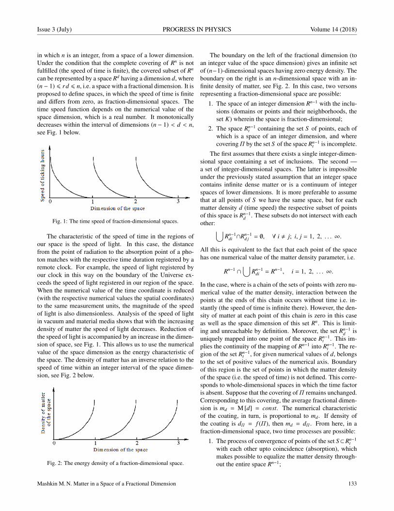
Issue 3 (July) PROGRESS IN PHYSICS Volume 14 (2018)
in which n is an integer, from a space of a lower dimension.Under the condition that the complete covering of Rn is notfulfilled (the speed of time is finite), the covered subset of Rn
can be represented by a space Rd having a dimension d, where(n − 1) ⩽ rd ⩽ n, i.e. a space with a fractional dimension. It isproposed to define spaces, in which the speed of time is finiteand differs from zero, as fraction-dimensional spaces. Thetime speed function depends on the numerical value of thespace dimension, which is a real number. It monotonicallydecreases within the interval of dimensions (n − 1) < d < n,see Fig. 1 below.
Fig. 1: The time speed of fraction-dimensional spaces.
The characteristic of the speed of time in the regions ofour space is the speed of light. In this case, the distancefrom the point of radiation to the absorption point of a pho-ton matches with the respective time duration registered by aremote clock. For example, the speed of light registered byour clock in this way on the boundary of the Universe ex-ceeds the speed of light registered in our region of the space.When the numerical value of the time coordinate is reduced(with the respective numerical values the spatial coordinates)to the same measurement units, the magnitude of the speedof light is also dimensionless. Analysis of the speed of lightin vacuum and material media shows that with the increasingdensity of matter the speed of light decreases. Reduction ofthe speed of light is accompanied by an increase in the dimen-sion of space, see Fig. 1. This allows us to use the numericalvalue of the space dimension as the energy characteristic ofthe space. The density of matter has an inverse relation to thespeed of time within an integer interval of the space dimen-sion, see Fig. 2 below.
Fig. 2: The energy density of a fraction-dimensional space.
The boundary on the left of the fractional dimension (toan integer value of the space dimension) gives an infinite setof (n−1)-dimensional spaces having zero energy density. Theboundary on the right is an n-dimensional space with an in-finite density of matter, see Fig. 2. In this case, two versonsrepresenting a fraction-dimensional space are possible:
1. The space of an integer dimension Rn−1 with the inclu-sions (domains or points and their neighborhoods, theset K) wherein the space is fraction-dimensional;
2. The space Rn−1t containing the set S of points, each of
which is a space of an integer dimension, and wherecoveringΠ by the set S of the space Rn−1
t is incomplete.
The first assumes that there exists a single integer-dimen-sional space containing a set of inclusions. The second —a set of integer-dimensional spaces. The latter is impossibleunder the previously stated assumption that an integer spacecontains infinite dense matter or is a continuum of integerspaces of lower dimensions. It is more preferable to assumethat at all points of S we have the same space, but for eachmatter density d (time speed) the respective subset of pointsof this space is Rn−1
d . These subsets do not intersect with eachother:∪
Rn−1di ∩Rn−1
d j = ∅, ∀ i , j; i, j = 1, 2, . . . ∞.
All this is equivalent to the fact that each point of the spacehas one numerical value of the matter density parameter, i.e.
Rn−1 ∩∪
Rn−1di = Rn−1, i = 1, 2, . . . ∞.
In the case, where is a chain of the sets of points with zero nu-merical value of the matter density, interaction between thepoints at the ends of this chain occurs without time i.e. in-stantly (the speed of time is infinite there). However, the den-sity of matter at each point of this chain is zero in this caseas well as the space dimension of this set Rn. This is limit-ing and unreachable by definition. Moreover, the set Rn−1
d isuniquely mapped into one point of the space Rn−1
t . This im-plies the continuity of the mapping of Rn−1 into Rn−1
t . The re-gion of the set Rn−1
t , for given numerical values of d, belongsto the set of positive values of the numerical axis. Boundaryof this region is the set of points in which the matter densityof the space (i.e. the speed of time) is not defined. This corre-sponds to whole-dimensional spaces in which the time factoris absent. Suppose that the covering ofΠ remains unchanged.Corresponding to this covering, the average fractional dimen-sion is md = M [d] = const. The numerical characteristicof the coating, in turn, is proportional to md. If density ofthe coating is dΠ = f (Π), then md = dΠ . From here, in afraction-dimensional space, two time processes are possible:
1. The process of convergence of points of the set S⊂Rn−1t
with each other upto coincidence (absorption), whichmakes possible to equalize the matter density through-out the entire space Rn−1;
Mashkin M. N. Matter in a Space of a Fractional Dimension 133
Volume 14 (2018) PROGRESS IN PHYSICS Issue 3 (July)
2. The process inverse to the convergence of points. Sep-aration of one point into at least two points.
These two processes compete and provide a mapping ofK into S , previously considered in two ways: the shift andcarry methods. Due to the shift and transfer of points of theset Rn−1
t , mutual absorption of the points is possible. Thisshould be accompanied with the reverse: the generation ofpoints. This condition ensures that the covering of the sameset Rn−1
t — the conservation law of the dimension (covering)of the space — remains constant. On the other hand, the cov-ering Π is incomplete, but ensures the mapping S into therange of possible numerical values of the set Rn−1
t , — thepositive numerical axis. This mapping is also determinedby the fractional dimension through the time flow, and de-termines dynamics of the interaction processes of points ofthe set K = Rn−1
d with each other. Therefore, the space of afractional dimension is dynamic. The point of the set Rn−1
tcorresponds to Rn−1
d — the set of points with the same densityof matter of the space Rn−1. That is, in the absence of interac-tion with the remaining points, its position is determined onlyupto the set Rn−1
d . In this case, the point of the latter can be de-fined (perhaps) simultaneously at all points of Rn−1
d . That is,each such point has no distinctive features over the others. Inthe case of absorption (synthesis), it is possible and necessaryto generate (divide) points of the spaces Rn−1
t and K. This is anecessary condition for generating a space (i.e. transfer). Onthe other hand, at a sufficiently high density of matter in thelocalization region of the point, the time speed is sufficientlysmall: displacement or transfer in this case almost does notrequire time. This also gives rise to the effect of supposedlysimultaneous finding of one point in all places (points) of thelocalization region.
Results
Spaces of fractional dimensions contain local inhomogenei-ties in which the fractional dimension of the space differsfrom the fractional dimension of the vacuum region (whichis the neighborhood of the inhomogeneity, the localizationspace). These are material objects. A local inhomogeneityis manifested in the numerical values of the parameters ofthe fields of a material object. The numerical values of thefield parameters show the energy distribution of the space inthe object’s localization region. Combinations of the fields asthe distribution characteristics of energies of the space give adescription to the whole variety of the material objects. De-generation of a fraction-dimensional space in the part of ma-terial objects leads to the appearance of zero-dimensional pa-rameters that is quantum numbers. This quantum mechanismdetermines the discreteness of the set of phenomena there.A space with a unit inhomogeneity is an integer (for exam-ple, the three-dimensional space) everywhere, except for theheterogeneity itself. For an observer, it turns into a point be-cause transition from one point to another does not require
time. The very region of heterogeneity is a point at which thedensity of matter is infinite high. Passage through this pointrequires an infinite amount of time. Such a point is limiting,boundary, open, that is unreachable. Another boundary, witha uniform density of matter throughout the space, is also un-reachable. Hence, we have an open interval for describing theentire set of material objects in a fraction-dimensional space.
Conclusion
So, a model of the cosmological system of spaces is proposedhere. When considering this model, evolution of the Universeis discussed as well as the problem of description of fraction-dimensional spaces. Such spaces are defined as a results ofenergy conversion from the moment of inflation to R3. Theconcept of singularity as a space in which time is absent isproposed. A “fractional space” is defined as a space in whichthe process of energy conversion from one type to anothertakes place. In this case, time is a factor of the process ofenergy conversion. Dynamics of fraction-dimensional spacesis predicted. These research results are a basis to calculatenumerical values of the characteristics of such spaces.
Acknowledgements
I am thankful to Svyatoslav Petrovich Gabuda (April 23, 1936— April 7, 2015), a Soviet/Russian physicist, Professor andDoctor of Physical and Mathematical Sciences, for valuablediscussions.
Submitted on April 17, 2018
References1. Alexandrov P.S. Combinatorial Topology. Volumes 1, 2, and 3 bound
as one. Mineola (NY), Dover Publications, 1998 (reprinted from the1957, 1959, and 1960 editions).
2. Linde A. Particle Physics and Inflationary Cosmology. Chur (Switzer-land), Harwood Academic Publishers, 1990; arXiv: hep-th/0503203,p. 1–6.
3. Gliner E.B. The vacuum-like state of a medium and Friedman cosmol-ogy. Soviet Physics Doklady, 1970, v. 15, no. 6, 559–561.
4. Gliner E.B. Algebraic properties of the energy-momentum tensor andvacuum-like states of matter. Soviet Physics JETP, 1966, v. 22, no. 2,378–382.
5. Mashkin M.N. Matter in a space of a fractional dimension (in Russian)http://www.sciteclibrary.ru/rus/catalog/pages/6525.html
134 Mashkin M. N. Matter in a Space of a Fractional Dimension
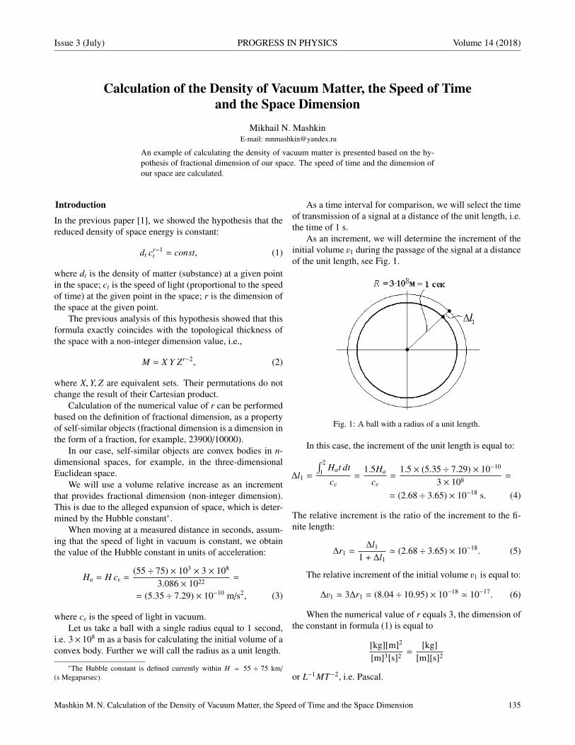
Issue 3 (July) PROGRESS IN PHYSICS Volume 14 (2018)
Calculation of the Density of Vacuum Matter, the Speed of Timeand the Space Dimension
Mikhail N. MashkinE-mail: [email protected]
An example of calculating the density of vacuum matter is presented based on the hy-pothesis of fractional dimension of our space. The speed of time and the dimension ofour space are calculated.
Introduction
In the previous paper [1], we showed the hypothesis that thereduced density of space energy is constant:
dt cr−1t = const, (1)
where dt is the density of matter (substance) at a given pointin the space; ct is the speed of light (proportional to the speedof time) at the given point in the space; r is the dimension ofthe space at the given point.
The previous analysis of this hypothesis showed that thisformula exactly coincides with the topological thickness ofthe space with a non-integer dimension value, i.e.,
M = X Y Zr−2, (2)
where X,Y,Z are equivalent sets. Their permutations do notchange the result of their Cartesian product.
Calculation of the numerical value of r can be performedbased on the definition of fractional dimension, as a propertyof self-similar objects (fractional dimension is a dimension inthe form of a fraction, for example, 23900/10000).
In our case, self-similar objects are convex bodies in n-dimensional spaces, for example, in the three-dimensionalEuclidean space.
We will use a volume relative increase as an incrementthat provides fractional dimension (non-integer dimension).This is due to the alleged expansion of space, which is deter-mined by the Hubble constant∗.
When moving at a measured distance in seconds, assum-ing that the speed of light in vacuum is constant, we obtainthe value of the Hubble constant in units of acceleration:
Ha = H cv =(55 ÷ 75) × 103 × 3 × 108
3.086 × 1022 =
= (5.35 ÷ 7.29) × 10−10 m/s2, (3)
where cv is the speed of light in vacuum.Let us take a ball with a single radius equal to 1 second,
i.e. 3× 10⁸ m as a basis for calculating the initial volume of aconvex body. Further we will call the radius as a unit length.
∗The Hubble constant is defined currently within H = 55 ÷ 75 km/
(s Megaparsec).
As a time interval for comparison, we will select the timeof transmission of a signal at a distance of the unit length, i.e.the time of 1 s.
As an increment, we will determine the increment of theinitial volume v1 during the passage of the signal at a distanceof the unit length, see Fig. 1.
Fig. 1: A ball with a radius of a unit length.
In this case, the increment of the unit length is equal to:
∆l1 =
∫ 21 Hat dt
cv=
1.5Ha
cv=
1.5 × (5.35 ÷ 7.29) × 10−10
3 × 108 =
= (2.68 ÷ 3.65) × 10−18 s. (4)
The relative increment is the ratio of the increment to the fi-nite length:
∆r1 =∆l1
1 + ∆l1' (2.68 ÷ 3.65) × 10−18. (5)
The relative increment of the initial volume v1 is equal to:
∆v1 ' 3∆r1 = (8.04 ÷ 10.95) × 10−18 ' 10−17. (6)
When the numerical value of r equals 3, the dimension ofthe constant in formula (1) is equal to
[kg][m]2
[m]3[s]2 =[kg]
[m][s]2
or L−1MT−2, i.e. Pascal.
Mashkin M. N. Calculation of the Density of Vacuum Matter, the Speed of Time and the Space Dimension 135

Volume 14 (2018) PROGRESS IN PHYSICS Issue 3 (July)
Hence, this can be interpreted as the modulus of the vol-ume compression/expansion of the three-dimensional space.
In case when 3 > r > 2, we will refer to the reviewedconstant to as the module of the extension of a non-integerdimension space.
Then the formula (1) can be represented in the form of:
dt cr−1t = Mr , (7)
where Mr is the module of the expansion of the space of non-integer dimension, taken in Pascals.
Calculation of the density of vacuum matter
Using the ratio (7), we can calculate the density of vacuummatter. With this, it is possible to accept in first approxima-tion the vacuum density inside material bodies as that equalto the density of their substance.
Let is take the following approximations: the space di-mension is constant, i.e. r = const, and is r ' 3; the effectsof light dispersion are not taken into account.
Formula (1) contains three interrelated parameters: den-sity, the speed of light and the space dimension. Consider therelationship between the speed of light and the matter densityin detail. The table data of the refractive index (optical den-sity) and the density of precious stones are shown in Fig. 2.
Fig. 2: The precious stones density.
Analysis of Fig. 2 allows us to suggest that the refractiveindex is linearly dependent on the matter density. Hence, weobtain the formula of the vacuum matter density outside ma-terial bodies:
dv =dms
Π–1, (8)
where dms is the density of substance, Π = cv/cms is the re-fractive index, cms is the speed of light in the substance.
Here are the tabular data of the stones, used in jewelryindustry. The data give the minimum of the calculated densityof vacuum for diamonds and synthetic rutile (see Table fordetail).
In the above calculations, we used the average density ofsubstance. However, under real conditions inside real sub-stances there are nodes of the crystal lattice in the form ofions or atoms which have a finite volume and their own den-sity. For example, for a diamond we have the radius of the
The groupof stones
Stone Density,g/cm3
Refract.index
Calc. vacuumdensity, g/cm3
Colorlessstones
Diamond 3.52 2.42 2.48
Syntheticrutile
4.25 2.9 2.24
carbon atom ra = 0.077, and the distance between the reflec-tion planes (interatomic) d = 0.356 nm. Hence, the densityof the carbon atom itself is 6,274 g/cm3. Let us calculate themaximum reduced density between two carbon atoms locatedfrom each other at a distance d using the following formula:
dred. =mc
Vc1
+mc
Vc2
, (9)
where Vc1 = 4π3 r3
1 is the volume of a sphere with the firstcarbon atom in the center, r1 = 0.0385 ÷ 0.3165 nm, Vc2 =4π3 (0.356 − r1)3 is the volume of a sphere with the second
carbon atom in the center, mc is the mass of the carbon atom.Calculation by formula (9) shows that approximately 50%
of the space between carbon atoms has a density of about 1g/cm3. Hence, the estimated density of vacuum substanceobtained by formula (8) is less than 0.7 g/cm3. The actualnumerical value, obviously, is much lower, since the reduceddensity assumes uniform distribution of the substance of thecarbon atom within the sphere.
Calculation of the space dimension and the speed of time
On the other hand, it follows from the definition of fractionaldimension of space, that any volume of a space generates avolume in a certain multiplicity, which is equal to the speedof time [1]. For vacuum it is:
dt ' ∆t = ∆v1 = 10−17, (10)
i.e. any volume of a space, when a signal passes through it,generates a relative, additional volume equal to the speed oftime.
The generation of the volume corresponds to a certainamount of gravitational energy. This amount can be com-pared to a quantum of energy which, taking into account for-mula (10), gives the ratio:
Mr V1 dt = h, (11)
where V1 is the generated unit volume, 1 m3, h is the Planckconstant (6.626 × 10⁻³⁴ J s).
Our three-dimensional space is flat. The critical Friedmandensity of our space is about d f = 1×10⁻²⁸ kg/m3. From here,we calculate the dimension of our space:
r =log h − log V1 − log d f − log dt
log cv+ 1 =
=log 6.626 − 34 − 0 + 28 + 17
8 + log 3+ 1 = 2.395; (12)
136 Mashkin M. N. Calculation of the Density of Vacuum Matter, the Speed of Time and the Space Dimension

Issue 3 (July) PROGRESS IN PHYSICS Volume 14 (2018)
where ct ' cv = 3 · 108 m/s; d f = dt = 10−28 kg/m3; V1 =
1 m3; dt = 10−17.If the space has a Friedman energy density, the photon
speed in the region of the carbon atom is (on the average):
cc =
√d f
dccv =
√1 × 10⁻²⁸
6274cv =
= 1.26 × 10−16 × 3 × 108 = 37.9 nm/s, (13)
where dc is the average density of matter inside the sphere ofa carbon atom.
At the obtained speed of light inside the sphere of the car-bon atom, the wavelength of visible radiation is:
λc = 1.26 × 10¹⁶λmv = 1.26 × 10−16 × 600 × 10−9 =
= 7.56 × 10⁻²³ m, (14)
where λmv is the wavelength of visible radiation. This is about1013 times less than the diameter of a carbon atom. This givesa possibility of interaction between the waves of visible radia-tion and a carbon atom which is represented as a drain funnel(the source — reverse funnel — tornado). That is the photon,as an object of magnetic energy, behaves as a time magneticmonopole: it can be absorbed and emitted.
Results
Substantiation and calculation of the density of space mat-ter have been done. The concept of the time speed has beenspecified. The time speed of our space has been calculated. Aformula for calculating the fractional dimension of our spacehas been obtained. The calculation of the fractional dimen-sion of our space has been performed.
So, on the basis of representation of the fractional dimen-sion of a space as a space with the presence of time, the fol-lowing calculations were done: the density of vacuum matter,the speed of time and the dimension of our space.
Further calculation of the numerical values of the follow-ing properties — the substance density of material objects,the vacuum and space density as a whole — can be contin-ued dealing with (see [1] for detail): conversion of magneticenergy into dark matter; dark matter interaction with matter;synthesis of objects of our space; a three-dimensional modelof distribution of density of the outer space mass.
Submitted on April 17, 2018
References1. Mashkin M.N. Matter in a space of a fractional dimension. A cosmo-
logical system of spaces and evolution of the Universe. Progress inPhysics, 2018, v.14, issue 3, 131–134.
Mashkin M. N. Calculation of the Density of Vacuum Matter, the Speed of Time and the Space Dimension 137

Volume 14 (2018) PROGRESS IN PHYSICS Issue 3 (July)
Fully Classical Quantum Gravity
Thomas C. AndersenNSCIR, 8 Bruce St. B 841, Thornbury, Ontario, N0H 2P0, Canada
E-mail: [email protected]
It’s an experimental fact that quantum objects in the ground state do not radiate electro-magnetic energy, but what are the limits on our knowledge of the gravitational equiv-alent of this? In semiclassical gravity it is the expectation values of quantum particlepositions that form the source for the Einstein equations, thus a particle or atom in aground state emits no gravitational radiation. Here we instead assume a fully classi-cal quantum gravity — the internal components of objects in a pure quantum state areassumed to classically radiate gravitational waves. The effects of this theory of micro-scopic gravity on the measured properties of the hydrogen atom, along with possibilitiesto experimentally measure the effects of atomic or nuclear scale gravitational radiationare explored.
1 Introduction
The quantum gravity problem remains unsolved in physicstoday. There are many possible solutions proposed, but al-most all of them suppose the existence of the graviton. Thegraviton should have the same energy relation as the photon:
Egraviton = ℏν. (1)
There not only exists no experimental confirmation of thisrelationship for gravity, it is also widely known that an experi-ment to detect a single graviton is well beyond the capabilitiesof any present or future realizable experiment. Gravity maysimply be a non quantum effect. Rosenfeld in 1963 is stillvery much relevant [1].
There is no denying that, considering the uni-versality of the quantum of action, it is verytempting to regard any classical theory as a lim-iting case to some quantal theory. In the absenceof empirical evidence, however, this temptationshould be resisted. The case for quantizing grav-itation, in particular, far from being straightfor-ward, appears very dubious on closer examina-tion.
2 Other classical gravity theories
Semiclassical gravity can be summarized as a classical grav-itational field coupled to quantum matter fields. While semi-classical gravity is widely thought of as a workable limitingapproximation until a quantum theory of gravity is discov-ered, there are researchers who treat semiclassical gravity asa real possibility and hence in need of experimental tests [2].The semiclassical equations for quantum gravity are as fromMøller [3] and Rosenfeld [1]:
Rµν −12gµνR =
8πGc4 ⟨Ψ|Tµν|Ψ⟩. (2)
While seemingly straightforward, semiclassical gravityhas subtleties, especially in determining the quantum expec-tation value (see Appendix A of Bahrami [4]).
Another classical treatment of quantum gravity comesfrom Roger Penrose with the Gravitization of Quantum Me-chanics [5] where he posits that gravity connects not to the ex-pectation value, but rather directly to each superposed quan-tum state. Gravitation causes collapse as the gravitationalfield of multiple superposed states becomes too energetic.
3 Fully classical quantum gravity
Fully classical quantum gravity (FCQG) uses Einstein’s equa-tions as given,
Rµν −12gµνR =
8πGc4 Tµν (3)
with the coupling to microscopic matter being on some as-sumed sub-quantum level, where particle positions alwayshave a definite value, as in for instance de Broglie-Bohm me-chanics [6]. Of course if one uses Bohmian mechanics in itsentirety, then gravitation is also quantized, and particles willnot radiate from their ground states. We thus assume herethat quantization does not apply to gravity at all, that par-ticle trajectories are real and that they interact directly andclassically using the laws of Einstein’s general relativity. Inmany ways it is similar to the program of stochastic electro-dynamics (SED) [7], in that classical fields couple directly tosub-quantum particle motions. Indeed if one is to assumea SED like explanation of quantum behavoir, then gravityshould also be treated classically.
4 Gravitational radiation from atoms and nucleons
Ashtekar [8] for example elucidates the need for a quantumtheory of gravity by citing Einstein in 1916:
. . . Nevertheless, due to the inner-atomicmovement of electrons, atoms would have to ra-
138 T.C. Andersen. Fully Classical Quantum Gravity

Issue 3 (July) PROGRESS IN PHYSICS Volume 14 (2018)
diate not only electro-magnetic but also gravi-tational energy, if only in tiny amounts. As thisis hardly true in Nature, it appears that quantumtheory would have to modify not onlyMaxwellian electrodynamics, but also the newtheory of gravitation.
Using instead Rosenfeld’s position that we must rely onexperiment to show the need for quantum gravity, considerthe energy loss rate of a circa 1916 style Bohr planetary hy-drogen atom in the ground state, using Eddington’s [9] for-mula for the gravitational energy radiated by a two body sys-tem (in the approximation that one mass is much heavier):
dEdt
(atom) = −32Gm2
er4hω
6
5c5 = −10−43eV/s. (4)
Which even over the age of the universe amounts to anenergy loss due to gravitational waves for a hydrogen atomin the ground state of only 10−25 eV. Why was Einstein wor-ried about such a small rate of gravitational energy loss fora hydrogen atom? In contrast the electromagnetic lifetime ofthe classical hydrogen atom is about 10−11s which of coursehelped lead to the discovery of quantum mechanics.
As a comparison to the above estimate, a quantum me-chanical prediction of the lifetime of the 3p−1s state for emit-ting a graviton is about 1.9× 1039s [10,11], which is within afew orders of magnitude of the fully classical estimate above.
This energy loss is of no experimental significance. So wecan conclude that the stability of atomic orbitals is not an ex-perimental indication of a need for quantum gravity. In otherwords we cannot experimentally determine if atoms radiategravitational waves continuously or not.
4.1 Gravitational radiation from within nuclei
The Sivram-Arun paper Thermal Gravitational Waves [12]is an expansion of Weinberg’s results in his 1972 book [10].Both calculate the gravitational wave (GW) emission fromnuclei passing each other thermally in an astrophysical hotplasma (stars). In fully classical quantum gravity we makethe additional assumption that gravitational waves are alsoproduced by nucleon motion inside each individual nucleus,even in the ground state, greatly increasing GW emission andmaking it happen at any temperature, since it arises from in-ternal nucleon movements within each nucleus. Calculatingan estimate for the GW emission would depend on the modelone uses for the nucleus. The Fermi gas model of the nucleusassumes that the nucleons are free to move inside the poten-tial well of the nucleus. Since we are assuming that gravityis fully classical, we can use the same calculations as that ofWeinberg and Sivram to arrive at an estimate of gravitationalwave emission from nucleons inside nuclei.
4.2 A GW nuclear emission/absorption model
Taking the calculation of Weinberg to nuclear material,Sivaram finds a rate of 10−16eV/s per neutron [12] (usingtheir neutron star calculation). Fully classical quantum grav-ity would then suggest that the Sun emits about 1022 wattsof 1022 Hz gravitational wave energy, as opposed to the 109
watts at a lower atomic frequency that Weinberg calculatesfrom plasma conditions only.
Another way to arrive an estimate for GW emission innuclei is to treat a nucleus as having several nucleons movingin it at some typical internal velocity. The speed of nucleonsis given by their kinetic energy in the Fermi gas model with apeak momentum of about 250 MeV/c. Using only one pair ofthese peak energy nucleons and setting r = 1 fm, Eddington’sformula for a bar of mass 2 nucleons, spinning at a nuclear1023 Hz, predicts an emission rate of about 10−9 eV/s.
While these two approaches to calculate the GW emis-sion of a nucleus in the fully classical model differ by sev-eral orders of magnitude, GW emission rates near these levelshint that such effects (or perhaps more likely a lack of effect)might be measurable in the lab.
Experiments might need to use differential absorption ef-fects to arrive at results. Absorption models are harder toquantify, as the cross section estimate is quite uncertain dueto unknown detailed information on particle substructure.
Within this fully classical quantum model each nucleonwill have its own characteristic spectrum of nucleon-fre-quency gravitational waves, depending on the structure andsize of the atomic nucleus. Experiments similar to those doneto look for “big G” could use dissimilar materials for themasses whose force of attraction is to be measured. It’s no-table that experiments to determine Newton’s constant G havehad great difficulty obtaining consistent results. Most mea-surements of G do not agree with each other to within theerrors carefully determined by the experimenters [13].
Another experimental avenue would be to search for GWinteraction effects between the bulk of the earth and massesin a lab of dissimilar materials.
5 Emission/absorption parameter space
Fig. 1 is a sketch of allowed emission and absorption param-eters. Some — but not all — combinations of emission andabsorption parameters are ruled out by experiment. Towardsthe upper left of the image limited absorption combined withhigher emission would mean that the stochastic backgroundof gravitational waves would be too energetic, having for ex-ample energy greater than the baryonic mass in the universe.The phrase “stability of nuclei” refers to the experimental factthat nuclei live for billions of years. On the right a ruled outregion exists where absorption cross sections are not physi-cally likely. The top line shows a calculation for the gravi-tational wave emission rate of a proton due to parton (quark)motion. “Nuclear emission (high)” refers to the Eddington
T.C. Andersen. Fully Classical Quantum Gravity 139

Volume 14 (2018) PROGRESS IN PHYSICS Issue 3 (July)
Fig. 1: Nuclear frequency gravitational wave emission and absorp-tion. The elusive nature of gravitational wave detection means thateven fully classical quantum gravity cannot be experimentally ruledout. The frequency of the gravitational waves is that of nucleons(ω ≈ 1022 Hz).
emission rate for a heavy nucleus, while the lower nucleusemission rate is calculated assuming thermal Coulomb GWemission inside each nucleus.
6 Discussion
Due to the weak nature of gravitational effects on subatomicparticles, even fully classical gravity cannot be experimen-tally ruled out at this time. Quantum gravity experiments thatare possible with today’s technology are very rare, this pro-posal represents an opportunity to test one of the tenants ofquantum gravity.
Null results from experiments as described here will beable to constrain the allowed parameter space of a fully classi-cal theory of microscopic gravity, thus suggesting that gravityneeds to be quantized.
These tests are also a test of the ubiquity of quantum me-chanics. With a non null result the conceptual foundationsof quantum mechanics would be in question, as gravity mightthen be determined to be outside of the realm of quantum me-chanics.
Submitted on April 1, 2018
References1. Rosenfeld L. On Quantization of fields. Nuclear Physics, 1963, v. 40,
353–356.
2. Großardt A. Newtonian self-gravity in trapped quantum systems andexperimental tests. arXiv:1702.04309 [quant-ph].
3. Møller C. Les theories relativistes de la gravitation. Colloques Interna-tionaux CNRS, Paris, p. 91, 1962.
4. Bahrami M., Großardt A., Donadi S., and Bassi A. The SchrodingerNewton equation and its foundations. arXiv:1407.4370 [quant-ph],2014.
5. Penrose R. On the Gravitization of Quantum Mechanics 1: QuantumState Reduction. Found. Phys., 2014, v. 44, 557–575.
6. Bohm D. A suggested interpretation of the quantum theory in terms of“hidden” variables. I. Physical Review, 1952, v. 85(2), 166–179.
7. De la Pena L., Cetto A.M., and Hernandez A.V. The Emerging Quan-tum, 2015.
8. Ashtekar A., Reuter M., and Rovelli C. From General Relativity toQuantum Gravity. arXiv:1408.4336 [gr-qc], 2014.
9. Eddington A.S. The Propagation of Gravitational Waves. Proceedingsof the Royal Society of London A: Mathematical, Physical and Engi-neering Sciences, 1922, v. 102(716), 268–282.
10. Weinberg S. Gravitation and cosmology : principles and applicationsof the general theory of relativity. Wiley, 1972.
11. Boughn S. and Rothman T. Aspects of graviton detection: gravitonemission and absorption by atomic hydrogen. Classical and QuantumGravity, 2006, v. 23(20), 5839–5852.
12. Sivaram C. Thermal Gravitational Waves. arXiv:0708.3343, 2007.
13. Rosi G., Sorrentino F., Cacciapuoti L., Prevedelli M., and Tino G.M.Precision measurement of the Newtonian gravitational constant usingcold atoms. Nature, 2014, v. 510(7506), 518–21.
140 T.C. Andersen. Fully Classical Quantum Gravity

Issue 3 (July) PROGRESS IN PHYSICS Volume 14 (2018)
Kirchhoff’s Law of Thermal Emission:Blackbody and Cavity Radiation Reconsidered
Pierre-Marie RobitailleDepartment of Radiology and Chemical Physics Program, The Ohio State University, Columbus, Ohio 43210, USA.
E-mail: [email protected]
Kirchhoff’s law of thermal emission asserts that, given sufficient dimensions to neglectdiffraction, the radiation contained within arbitrary cavities must always be black, ornormal, dependent only upon the frequency of observation and the temperature, whileindependent of the nature of the walls. In this regard, it is readily apparent that all cav-ities appear black at room temperature within the laboratory. However, two differentcauses are responsible: 1) cavities made from nearly ideal emitters self-generate theappropriate radiation, while 2) cavities made from nearly ideal reflectors are filled withradiation contained in their surroundings, completely independent of their own temper-ature. Unlike Kirchhoff’s claims, it can be demonstrated that the radiation containedwithin a cavity is absolutely dependent on the nature of its walls. Real blackbodies cando work, converting any incoming radiation or heat to an emission profile correspondingto the Planckian spectrum associated with the temperature of their walls. Conversely,rigid cavities made from perfect reflectors cannot do work. The radiation they containwill not be black but, rather, will reflect any radiation which was previously incidentfrom the surroundings in a manner independent of the temperature of their walls.
1 Introduction
Kirchhoff’s law of thermal emission was formulated in1859 [1, 2]. It is often presented as stating that, at thermalequilibrium, the emissivity of an object, ϵν, is equal its ab-sorptivity, αν. However, this should properly be consideredas ‘the law of equivalence’, first proposed by Balfour Stew-art [3] in 1858.
Kirchhoff’s law extended much beyond Stewart’s [3] andstated that, given thermal equilibrium, the radiation containedwithin an arbitrary cavity was depended only on the temper-ature of the enclosure and on the frequency of observation[1, 2]. Such radiation was completely independent of the na-ture of the walls [1,2]. It was because of Kirchhoff’s law thatblackbody, or normal, radiation has always been viewed as in-dependent of the lattice and unlinked to a physical cause [4].Clearly, if Kirchhoff was correct and blackbody radiation wasindependent of the nature the walls, then such radiation couldnot be ascribed causality in the emitting structure.
Yet, it has been known for over 200 years that the radia-tion emitted from objects was highly variable [5]. In 1804,Leslie reported that the emission of surfaces depended ontheir nature and established the primacy of lampblack as ablackbody surface [6]. As a result, lampblack or soot, alongwith graphite, soon gained a dominant role in the constructionof laboratory blackbodies (see [7] and references containedtherein). The nature of the surface producing a thermal spec-trum clearly did matter, in stark contrast to Kirchhoff’s claimsrelative to cavity radiation [1, 2].
In the early 19th century, blackbodies were simply objectsmade from graphite or coated with materials such as soot andlampblack. Carbon black was also employed, a pigment used
in paints since pre-historic times [8]. Eventually, blackbod-ies became increasingly sophisticated devices, typically cav-ities. Other good absorbers of radiation slowly moved ontothe scene relative to the construction of laboratory blackbod-ies [9–11], but graphite, soot, and carbon black retained theirpre-eminent role [12]. Max Planck soon benefited from theconstruction of advanced cavities [9–11], when he formu-lated the blackbody solution [13, 14]. Contrary to Kirchhofflaw [1, 2] the nature of the walls was thereby proven to beimportant on a practical level. It governed the quality of ablackbody. The quest for ever blacker surfaces [15–22] hasnow turned to novel structural absorbance approaches guidedby samples as diverse as butterflies [23, 24] and birds [25].Yet still today, many blackbodies in national laboratories arebased upon the use of graphite (e.g. [26, 27]).
It remains true that blackbodies are specialized cavitieswhich depend entirely on the nature of their walls [7, 9–12,26,27]. Laboratory blackbodies are made from materials thathave an elevated emissivity over the range of interest, as iswidely known throughout metrology. This fact alone is suffi-cient to illustrate that Kirchhoff’s law cannot be valid.
As such, it is surprising that many still believe that anyarbitrary cavity can produce a blackbody spectrum. In thelaboratory, this was never the case. Planck himself [13] wasdependent on the work of leading scientists in order to obtaina spectrum with the blackbody frequency distribution [9–11].If Kirchhoff law had been correct [1, 2], this should not havebeen necessary.
The author has previously stated that Kirchhoff’s law wasnot valid (see [4, 7, 12] and references therein), as it has noproper theoretical [28] or experimental proof. Planck’s equa-
Pierre-Marie Robitaille. Kirchhoff’s law of thermal emission: Blackbody and cavity radiation reconsidered 141

Volume 14 (2018) PROGRESS IN PHYSICS Issue 3 (July)
tion [13, 14] remained unlinked to a physical mechanism [4]because of Kirchhoff’s law [1, 2]. As a result, physics wasprevented from accounting for the production of a thermalphoton from a simple cavity made from a block of graphite.Blackbody radiation remained, according to Kirchhoff, in-dependent of the nature of the walls [1, 2]. In this respect,Planck’s equation [13] was unique in spectroscopy. This hasenabled scientists, in disciplines other than condensed mat-ter physics, to infer that thermal photons could be producedwithout having recourse to a physical lattice, as was clearlyrequired when emitted from graphite [4]. This has also en-abled Max Planck to claim that his equation had universalsignificance [14, §164]. But in reality, Planck’s solution wasstrictly limited to actual blackbodies (e.g. [7, 9–11, 26, 27])and not to all cavities.
Thus, cavity radiation is reconsidered herein as to refuteKirchhoff’s law [1, 2] and place a proper perspective on cav-ity radiation. In order to do so, cavities were constructed frommaterials which acted as nearly perfect absorbers or reflectorsof radiation in the infrared. The results are discussed in termsof the work required to convert incident energy into normalradiation within the blackbody cavity. Conversely, the ex-istence of nearly perfectly reflecting cavities is discussed inthe context of resonant cavities used in magnetic resonanceimaging [29], microwave cavities [30, 31], and lasers [32].The findings demonstrate that cavity radiation is absolutelydependent on the nature of the walls. Consequently, Kirch-hoff’s law was never valid [4, 7, 12] and Planck’s equation isnot universal, as confirmed by a wide array of experimentalresults [29–32].
For the sake of brevity, the challenge to Kirchhoff’s lawpresented herein can be limited to the study of a single ap-proach without any loss in content. In 1954, de Vos publishedhis Evaluation of the Quality of a Blackbody in the journalPhysica [33]. This article has become a classic in blackbodyradiation. de Vos [33] examined the quality of cavities con-structed from materials with varying emissivity by noting thechange upon incident radiation. This radiation was allowed toenter a cavity, exit, and be monitored with a detector placedat various angles. For cylindrical cavities, de Vos was con-cerned with the ratio of the length of the cavity to its diam-eter. He demonstrated that the radiation within cavities ap-peared to become increasingly isotropic as this ratio was in-creased [33]. However, de Vos had not demonstrated that allcavities will be black, independent of incident radiation. Infact, de Vos was concerned with the degree to which the sur-face of the cavity was either specular or white [33]. He didnot evaluate whether a cavity could actually emit photons atthe correct temperature. Thus, his work provided only limitedinsight into blackbody radiation [33]. He did analyze to whatextent the surface property of a cavity affected the change ofincoming light into fully diffuse reflection [33]. However, ifa cavity was not constructed of a near ideal absorber, it wasnot necessarily black unless it was able to receive the proper
incident radiation from its surroundings.At the same time, if a cylindrical hole of sufficient depth
was placed in a material with an elevated emissivity, the find-ings from de Vos suggest that the resulting cavity should in-deed be black [33]. This approach was therefore implementedin this work in order to construct a simple blackbody cav-ity from small blocks of graphite. In parallel fashion, nearlyperfectly reflecting cavities were constructed from blocks ofbrass, copper, and aluminum.
2 Materials and methods
Infrared images were obtained using a CompactPro thermalimaging camera (Seek Thermal, Inc., Santa Barbara, CA93117; Thermal.com) interfaced with an Android (version4.4.2) cell phone, as shown in Fig. 1A.
The camera had a focusable lens and a 32 field of view. Itwas equipped with a 320× 240 thermal sensor, had a temper-ature range of -40 to 330C, and was capable of obtaining ei-
Fig. 1: A) Photograph of the Android phone, Seek Thermal camera,and aluminum, copper, brass, steel, and graphite blocks; B) Blockassembly I (graphite on the left, then on the right from top to bot-tom: steel, brass, copper, aluminum). Note that two small scratchesare visible near the graphite cavity. C) Block assembly II (brass,graphite, brass). D) Block assembly III (horizontal rows from top tobottom: aluminum, brass, graphite, copper).
142 Pierre-Marie Robitaille. Kirchhoff’s law of thermal emission: Blackbody and cavity radiation reconsidered

Issue 3 (July) PROGRESS IN PHYSICS Volume 14 (2018)
ther still images or video. All images were obtained with thecamera operating in white mode, except for Fig. 2A, whereblack mode was utilized.
Cylindrical cavities where constructed by drilling a smallhole into 12.5 × 12.5 × 50 mm blocks of copper, aluminum,brass, and steel (Specific Gravity Metal Blocks, EISCO,Haryana 133001, India). The expected emissivity of the cop-per, brass, and steel holes should be on the order of 0.03-0.1 [34]. The type of steel was unknown. A 20 × 50 × 50mm 99.9% Purity Graphite Ingot Block EDM Graphite PlateMilling Surface (Otoolworld, China) was used to build thereference blackbody using the same approach.
Cavities were produced with a drill press using eitherstandard 3
16
′′or 1
4
′′diameter drill bits or a DeWalt Pilot Point
14
′′diameter drill bit to the depth described in the figure leg-
ends. Cavities were examined at room temperature or afterhaving reached steady state while being heated on a hotplate(Cuisinart, East Windsor, NJ) to a temperature of approxi-mately ∼304C. Small graphite particles were made from 2mm mechanical pencil refills (Menards, Eau Claire, WI) cutto a length of 0.5 cm and inserted into the cavities of interest.
Experiments were initiated at room temperature, by plac-ing the camera at a distance of ∼20 cm above the table surfaceand therefore ∼15 cm above the surface of the block assem-bly. The eye of the camera was positioned directly over thecenter of this assembly. In order to document the effect ofambient radiation on the cavities, a galvanized steel rod wasplaced in an oven, heated to ∼232C, and then brought nearthe cavities, as described in the figures.
3 Results
Thermal images are presented in Fig. 2 with the correspond-ing schematic representations outlining the position of the rodin Fig. 3. In Fig. 2A, a thermal image is presented in blackmode, revealing that all the cavities appeared nearly the sameat room temperature. In this image, there was also reflec-tion of thermal radiation from the body of the observer ontothe block assembly. Thus, on cursory examination, Kirch-hoff’s law appeared valid as all cavities essentially containedthe same radiation. Still, the block was positioned within aroom filled with radiation at the same temperature. There-fore, it was important to determine whether the cavities weregenerating radiation on their own or simply manifesting theradiation in their surroundings.
For other studies, the camera was switched to white modeand the cavities all appeared black, as seen in Fig. 2B. Next,in Fig. 2C-F (see schematics in Fig. 3C-F), a heated galva-nized steel rod was placed above their surface. The rod hadbeen heated to ∼232C. In Fig. 2C, the rod was positionedto the right of the steel cavity (see schematic Fig. 3C). Withthe heated rod in this position, the graphite and steel cavi-ties could not be filled with its radiation. These two remainpretty much as they were with just a tiny spec of reflection at
the graphite cavity. Thus, radiation from the rod was reach-ing this cavity as well, as expected. At the same time, thealuminum, copper, and brass cavities were immediately filledwith radiation from the rod.
The rod was then moved to the left in Fig. 2D, as shownin Fig. 3D. Notice, once again, that there was no effect on thegraphite cavity and that only a slight reflection was observedat the top of the steel cavity. However, all the others werefilled with radiation from the rod. In particular, note the pat-tern in the brass cavity revealing that it was still not able tofully convert incoming radiation into isotropic ejected radi-ation. This indicated this cavity should be deeper to renderthe radiation fully isotropic, as suggested in de Vos’ classicwork [33].
In Fig. 2E, the rod was placed near the center of the blockas represented in Fig. 3E. The three cavities from aluminum,copper and brass were again filled with rod radiation, but thegraphite cavity remained unaffected and the steel cavity al-most unaffected. However, reflection of rod radiation couldbe observed in the scratches on each side of the graphite cav-ity. As such, radiation from the rod was clearly reaching thiscavity. Finally, in Fig. 2F, the rod was positioned just to theright of the steel cavity as shown in Fig. 3F. In this position,the steel cavity was no longer black. Now, it could be ob-served that rod radiation was able to partially fill the steelcavity. Nonetheless, the bottom of this cavity was darker,thereby indicating that steel had a much higher emissivitythan the aluminum, copper, or brass cavities, but was not onpar with graphite. The aluminum, copper, and brass cavitiesall appeared filled with radiation from the rod.
Next, the effect of inserting a small piece of graphite intothe cavities was examined as shown in Fig. 4. In Fig. 4A (seeschematic 4D), the graphite cavity was indistinguishable fromthe surface of the block at thermal equilibrium. Both cavitieswithin the brass blocks were clearly visible.
When the heated steel rod was brought in close proximityto the cavities, its radiation was reflected off the surfaces andthe signal to noise of the resulting image increased, as shownin Fig. 4B (schematic 4E). However, the central graphite cav-ity appeared black and both of the brass cavities became filledwith rod radiation. This revealed that real blackbodies dowork and convert any incident radiation to that correspond-ing to the temperature of their walls. Conversely, the twobrass cavities on each side became filled with radiation orig-inating from the steel rod. Again, the reflecting cavities werenot black, as they manifested the radiation present in theirsurroundings in a manner independent of the temperature oftheir own walls. When the graphite particle was introducedinto each of the cavities, it was unable to make the brass cavi-ties fully black, as clear signs of radiation from the heated rodremained, as shown in Fig. 4C (schematic 4F).
Next, consider the findings from block assembly III, asdisplayed in Fig. 5. Initially, this assembly was monitored atroom temperature, in equilibrium with its surroundings, as
Pierre-Marie Robitaille. Kirchhoff’s law of thermal emission: Blackbody and cavity radiation reconsidered 143
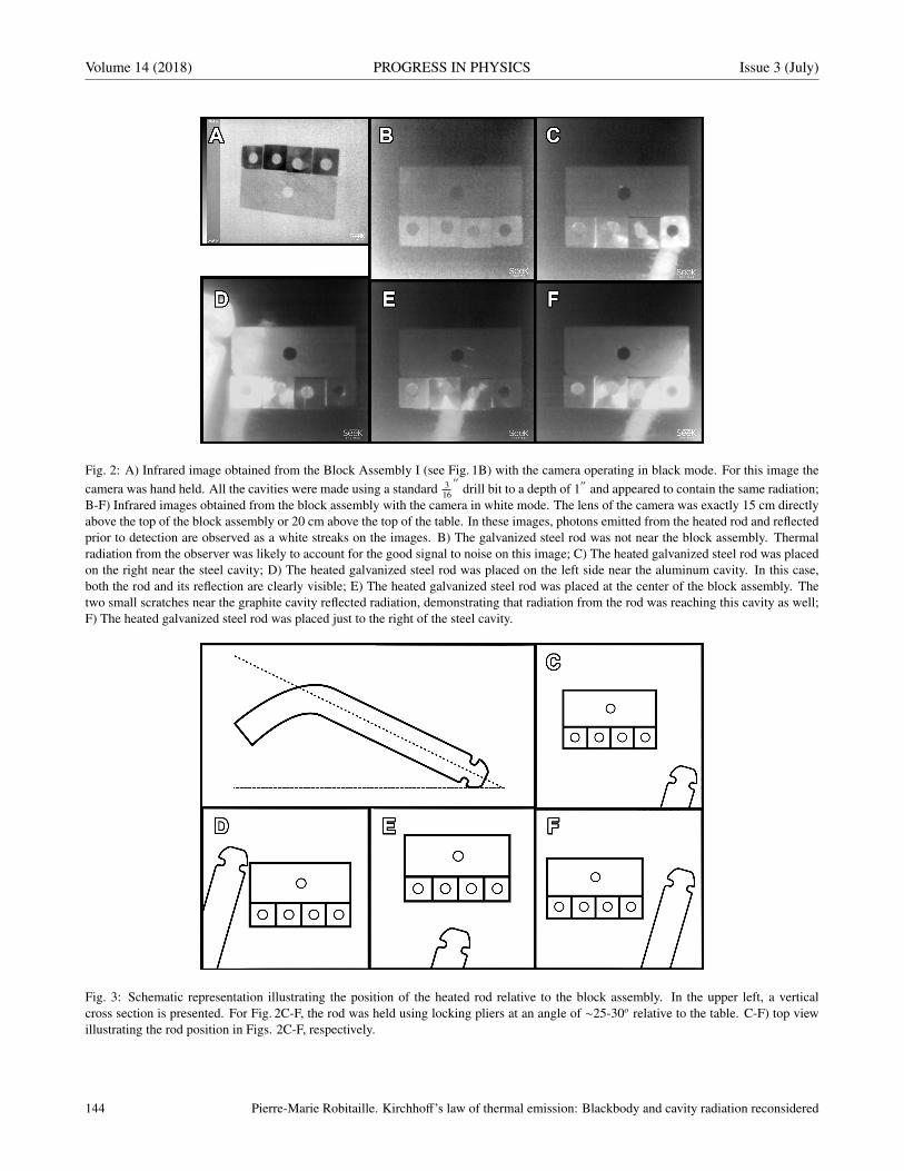
Volume 14 (2018) PROGRESS IN PHYSICS Issue 3 (July)
Fig. 2: A) Infrared image obtained from the Block Assembly I (see Fig. 1B) with the camera operating in black mode. For this image thecamera was hand held. All the cavities were made using a standard 3
16
′′drill bit to a depth of 1
′′and appeared to contain the same radiation;
B-F) Infrared images obtained from the block assembly with the camera in white mode. The lens of the camera was exactly 15 cm directlyabove the top of the block assembly or 20 cm above the top of the table. In these images, photons emitted from the heated rod and reflectedprior to detection are observed as a white streaks on the images. B) The galvanized steel rod was not near the block assembly. Thermalradiation from the observer was likely to account for the good signal to noise on this image; C) The heated galvanized steel rod was placedon the right near the steel cavity; D) The heated galvanized steel rod was placed on the left side near the aluminum cavity. In this case,both the rod and its reflection are clearly visible; E) The heated galvanized steel rod was placed at the center of the block assembly. Thetwo small scratches near the graphite cavity reflected radiation, demonstrating that radiation from the rod was reaching this cavity as well;F) The heated galvanized steel rod was placed just to the right of the steel cavity.
Fig. 3: Schematic representation illustrating the position of the heated rod relative to the block assembly. In the upper left, a verticalcross section is presented. For Fig. 2C-F, the rod was held using locking pliers at an angle of ∼25-30o relative to the table. C-F) top viewillustrating the rod position in Figs. 2C-F, respectively.
144 Pierre-Marie Robitaille. Kirchhoff’s law of thermal emission: Blackbody and cavity radiation reconsidered

Issue 3 (July) PROGRESS IN PHYSICS Volume 14 (2018)
Fig. 4: Infrared images (A-C) and their schematic representations (D-F). The cavities were drilled with a DeWalt Pilot Point 14
′′diameter
drill bit to the depth 1 14
′′. A) Infrared image obtained from the Block Assembly II (see Fig. 1C) at room temperature without any heated
rod present (schematic in D). B) Image obtained while placing a heated steel rod in close proximity to the cavities (schematic in E). C)Repeat of B, but this time, a graphite particle was suspended from two strings into the left brass cavity such that the center of the particlewas exactly 1 cm from the top of the block (schematic in F). Graphite particles were also inserted at the bottom of the other two cavities.In B and C, the stem of the rod was parallel to and about 7 cm above, the top of the table (or a height of about 2 cm above the top of theblock). In schematics E and F, the rod was illustrated such that its position from left to right could be accurately represented relative tothe block. However, in the plane of the image, the rod was actually positioned just below the field of view considered by the schematic, orabout one rod width from the block.
shown in Fig. 5A (corresponding schematic, 5C).Once again the infrared camera was positioned a distance
of ∼15 cm from the top of the block. The cavities withinthe graphite portion of the block under those conditions wereindistinguishable from the graphite surface. The image wasnoisy, as expected, since the observer was well removed fromthe block during data acquisition. At the same time, the cav-ities made within the aluminum, brass, and copper blockswere clearly visible and distinct from one another, demon-strating that they did not contain identical radiation. Sincethese cavities were made from highly reflective materials, thisimplied that the space surroundings of the block containedsome anisotropic radiation.
In Fig. 5B, the same block was examined (schematic 5D).This time, the hands of the investigator were positioned oneach side of the block, such that thermal equilibrium was notmaintained and the associated radiation could be observed
filling the aluminum, brass, and copper cavities. Clearly,these nearly perfectly reflecting cavities were not black, butcontained radiation emitted by their surroundings.Conversely, under these conditions, the three deepest graphitecavities, located on the left of the third row, remained essen-tially unaffected. At the same time, the shallowest cavity,made from the tip of the drill bit and located on the right of thethird row, was sensitive to this challenge (Fig. 5B, D). Therewere reflections of thermal photons off the surfaces of eachblock which altered the appearance of the images as well.This study served to exemplify, once again, that real black-bodies could do work converting radiation incident upon theirwalls to black radiation manifesting their temperature. Con-versely, rigid perfectly reflecting cavities could not do work.They contained the radiation present in their surroundings in amanner independent of their own temperature and such radia-tion was clearly observed in the aluminum, brass, and copper
Pierre-Marie Robitaille. Kirchhoff’s law of thermal emission: Blackbody and cavity radiation reconsidered 145

Volume 14 (2018) PROGRESS IN PHYSICS Issue 3 (July)
Fig. 5: A) Infrared image obtained from the Block Assembly III (see Fig. 1D) at room temperature. The corresponding schematic isdisplayed in C (reduced by 25%). B) Same as in A, but this time the hands of the investigator were placed near the sides of the block suchthat thermal photons from the first two fingers of each hand could challenge the cavities, as seen in the schematic representation D (reducedby ∼50%). The horizontal rows from top to bottom correspond to aluminum, brass, graphite, copper. These cylindrical cavities were madeusing a standard 1
4
′′drill bit to different depths (from right to left: 1) depth corresponding to just the cone of the drill bit, 2) depth to 1
4
′′, 3)
34
′′and 4) 1 1
4
′′).
cavities.
At this point Block Assembly III was placed onto the sur-face of a hotplate brought to a temperature of ∼304C, asshown in Fig. 6.
Under these conditions, the graphite cavities located onthe third row all appeared to contain isotropic radiationclosely manifesting their equilibrium temperature. This in-dicated that these cavities were able to convert heat energylocated in their walls to blackbody radiation. Even the cavityproduced with only the tip of the drill bit, on the right, con-tains isotropic radiation. Conversely, the cavities constructedfrom aluminum, brass, and copper did not all contain such
radiation. Rather, they showed clear signs that their radia-tion originated from the hotplate and was a property of thesurroundings, not the cavity itself.
While the 1 14
′′aluminum (top row, left most) and copper
(bottom row, left most) cavities appeared to contain isotropicradiation, the brass cavity of the same depth (second row, leftmost) clearly did not. In addition, careful examination re-vealed that crescents were visible in the aluminum, brass, andcopper 3
4
′′cavities (second column) as well. With the excep-
tion of graphite, the 14
′′cavities (third column) did not contain
isotropic radiation at the appropriate temperature and neitherdid the corresponding conical cavities made from just the tip
146 Pierre-Marie Robitaille. Kirchhoff’s law of thermal emission: Blackbody and cavity radiation reconsidered

Issue 3 (July) PROGRESS IN PHYSICS Volume 14 (2018)
Fig. 6: Infrared image obtained from the Block Assembly III (see Fig. 1D) positioned on a hotplate surface at a temperature estimated at∼304C using the thermal camera. In order to acquire this image, the camera was mounted on a tripod such that its lens was ∼20 cm fromthe face of the block.
of the drill bit (fourth column). For instance, note the inabil-ity of any of the smallest cavities, made from these materials,to sustain radiation at the proper temperature. Crescent pat-terns also appeared in cavities constructed from aluminum,brass, and copper, even at a depth of 3
4
′′(second column), de-
spite the fact that the radiation in the graphite cavity at thesame depth was clearly isotropic. At a depth of 1 1
4
′′, the brass
cavity (second row, first column) still displayed such patterns.When the block assembly was cooled, it was apparent that
the copper blocks had become highly oxidized and this, inaddition to their proximity to the hotplate, might help explaintheir superior performance when compared to aluminum andbrass.
Still, these results revealed that real blackbodies, repre-sented herein by the graphite cavities, could do work andmanifested the radiation appropriate to the temperature oftheir own walls. Conversely, the aluminum, brass, and cop-per cavities illustrate that nearly ideal reflectors could not dowork, but contained the radiation present in their surround-ings which was independent of the nature of their walls.
4 Discussion
The approach to, and departure from, thermal equilibrium hasbeen the subject of countless studies by Fourier [35], Dulong[36], Petit [36], de la Provostaye [37], and Desains [37] (see[38] for a full review). In similar fashion, through the stud-
ies presented herein, a greater understanding has been soughtabout the nature of the radiation within cavities. This wasaccomplished both under conditions of thermal equilibriumand also by considering challenges which represent small de-partures from equilibrium. However, these challenges wereimportant because they served to highlight the nature of theradiation which filled a cavity and thereby help to establishthe identity of those objects which properly constituted black-bodies.
4.1 Blackbodies defined
Prior to formulating his law, Kirchhoff first defined a black-body by stating that “This investigation will be much simpli-fied if we imagine the enclosure to be composed, wholly orin great part, of bodies which, for infinitely small thickness,completely absorb all rays which fall upon them” [2, §7].Kirchhoff therefore recognized the importance of surface ab-sorptivity in the blackbody problem.
Surprisingly however, when Max Planck would later de-fine the blackbody in his classic text [14], he completely re-jected Kirchhoff’s approach writing: “In defining a black-body Kirchhoff also assumes that the absorption of incidentrays takes place in a layer ‘infinitely thin’. We do not in-clude this in our definition” [14, §10]. Planck then changedthe characteristics of a blackbody surface: “A rough surfacehaving the property of completely transmitting the incidentradiation is described as ‘black”’ [14, §10]. With this defini-
Pierre-Marie Robitaille. Kirchhoff’s law of thermal emission: Blackbody and cavity radiation reconsidered 147

Volume 14 (2018) PROGRESS IN PHYSICS Issue 3 (July)
tion, Planck removed absorbance of the surface itself fromthe requirements for creating a blackbody and inappropri-ately placed the focus on transmittance. Planck adopted thisnew definition because he was preparing to advance a proofof Kirchhoff’s law which ignored absorbance at the bound-ary of two materials [14, §35-37]. But in doing so, Planckmoved away from physical reality. His approach proved in-valid [39]. Nearly ideal absorbance for thin surfaces remainsthe hallmark of all materials used to construct quality black-bodies [7, 9–11, 25, 27].
4.2 The mathematical form of Kirchhoff’s Law
In advancing his law [2], Kirchhoff did not have recourse toexperimental verification. He first stated that the emissivepower of an object, E, divided by its absorptive power, A,was equal to a universal function which depended only upontemperature, T, and frequency, ν (E/A= e where e = f T, ν).He then immediately replaced absorptive power, A, with ab-sorptivity, αν, such that E/αν= f T, ν. For actual blackbod-ies, it is clear that αν can be set to 1 and E= f T, ν. However,Kirchhoff’s expression becomes undefined when αν is set tozero, as would occur if the cavity was constructed from a per-fect reflector. Planck himself recognized the undefined natureof Kirchhoff’s law under those conditions (see §48, §51, §52in [14]).
Thus, relative to Kirchhoff’s relationship, two limits areinvolved. The first, addresses cavities constructed from per-fect absorbers, such that αν can be set to 1. The second, in-volves cavities constructed from perfect reflectors, such thatαν can be set to zero and the law becomes undefined. Per-fectly reflecting cavities never followed Kirchhoff’s law.They are important however as they form the basis for manyresonant devices [29–32]. In any event, Kirchhoff had nomathematical basis for arguing that all cavities must containblack radiation which is dependent only upon temperatureand frequency.
4.3 Laboratory blackbodies
Clearly, laboratory blackbodies [4, 7, 12, 26, 27], includingthose utilized to provide Planck with data [9–11], were spe-cialized cavities constructed from highly absorbing materials.This observation alone was sufficient to conclude that Kirch-hoff’s law was invalid.
In the infrared, it was evident that the graphite cavitiesused in this study were able to maintain their internal radi-ation in a manner which was essentially independent of anyradiative challenge. They acted as real blackbodies and coulddo work. They could ensure that the radiation they containedwas governed by the nature and the temperature of their ownwalls. They converted incoming energy, whether in the formof incident radiation or heat, into normal radiation with thecorrect frequency distribution.
Conversely, cavities constructed from aluminum, brass,
and copper acted as nearly ideal reflectors. They containedthe radiation which was incident from their surroundings andshowed no ability to convert this radiation to black radia-tion corresponding to the temperature of their own walls. Inthis regard, it was evident that perfect reflectors could not dowork. They were unable to effect any change upon incidentradiation other than that which would occur given specular ordiffuse reflection.
de Vos noted the extent to which cavities could make radi-ation isotropic as a function of the ratio of their diameter anddepth [33]. However, perfectly reflecting cavities, by defini-tion, could not emit radiation. As such, the radiation whichthey contained must remain completely independent of thetemperature of their walls and dependent solely on the radi-ation contained in their surroundings. de Vos’s analysis ofthe quality of a cavity in terms of its ability to convert incom-ing radiation into ejected isotropic radiation, while of interest,actually had little baring on the behavior of real blackbodies.This was because real blackbodies depended on the natureof their surfaces, not on the dimension of a cavity, in orderto ensure that the emitted radiation would be both isotropicand black. A cavity in fact, should not be required, providedthat the surface material was black and that no external radia-tion was able to contaminate this emission. This explained inpart the interest in materials with elevated emissivity values[9–11, 26, 27] and highly absorbing surfaces [15–22]. Cavi-ties did enable blackbody radiation to be contained, but theywere not necessary for its production.
4.4 Cavities and work
Perhaps the central feature of all actual blackbodies was thatthey must have the ability to do work and convert any inci-dent energy into the frequency distribution corresponding tothe temperature of their own walls. In this sense, the workperformed by a blackbody conformed to the standard defini-tion whereby energy was converted from one form to another.Blackbodies accomplished this task in two ways. First, theywere able to alter the frequency of incoming radiation and re-emit it with the blackbody frequency distribution correspond-ing to the temperature of their walls. Secondly, they couldconvert heat energy located in their own walls into thermal ra-diation associated with this temperature. In either case, onlyabsorbers of radiation could act as blackbodies, as only theycould serve as emitters. Radiation was absorbed by the wallsand re-emitted in a manner which depended on the density ofstates and thereby upon temperature.
Conversely, rigid perfect reflectors could only redirect in-coming radiation in a specular or diffuse manner. A change inphase occurred without any change in frequency. Therefore,no work was done, as a change in the energy distribution ofthe incoming radiation did not occur. Furthermore, perfect re-flectors could not harness the energy contained in their wallsand thereby emit radiation. Unable to absorb, they could not
148 Pierre-Marie Robitaille. Kirchhoff’s law of thermal emission: Blackbody and cavity radiation reconsidered
Issue 3 (July) PROGRESS IN PHYSICS Volume 14 (2018)
emit.The reality that rigid perfectly reflecting cavities cannot
do work is the basis for resonant cavities in ultra high fieldmagnetic resonance imaging (UHFMRI) [29], electron para-magnetic resonance (EPR) [30], microwave communications[31] and the resonant cavities used for building coherent ra-diation following stimulated emission in lasers [32]. All ofthese disciplines strive to build highly reflective resonant cav-ities with optimal quality factors, Q = f /δ f , where f is thefrequency of interest and δ f full width at half maximum ofthe resonance. Q-factors are inversely proportional to surfaceresistance echoing Planck’s desire for infinitely large conduc-tivity.
In clinical MRI, dielectric loses in the human body willdominate Q-factors for any resonator [26]. As a result, littlecan be gained in this discipline from building resonators frommaterials more sophisticated than copper or silver.
However, lasers do not experience these limitations. Asa result, resonant cavities in lasers can benefit from the con-struction of highly reflective Bragg super-mirrors, which canhave reflectance values of 99.9999% [40–42]. Ion-beam in-terference coating mirrors [43] are associated with LIGO[44]. Specialized mirrors are also used in high precisionatomic clocks to generate optical cavities with low thermalnoise in that setting [45]. Laser cavities can thus achieve Q-factors of 1010, or more [46].
The use of resonant cavities in UHFMRI [29], EPR [30],microwave technology [31], and lasers [32] proves that Kirch-hoff’s law is not valid. These cavities critically depend ontheir nearly perfectly reflecting nature which allows them toserve as resonant devices, unable to alter incoming radiationby making it black. It is evident that the radiation in these cav-ities is absolutely dependent upon the radiation which was in-cident upon them and completely independent of the temper-ature of their walls. Absorption of incident photons, transfor-mation into thermal vibrations, and re-emission into thermalphotons does not occur in perfectly reflecting cavities. Kirch-hoff and Planck cannot claim otherwise, when they assert thatall cavities contain black radiation [1, 2, 14].
4.5 Max Planck and Kirchhoff’s law
Max Planck attempted to prove the validity of Kirchhoff’slaw in the opening sections of The Theory of Heat Radia-tion [14, §1-52]. Upon close examination, the derivation wasdiscovered to be unsound [39]. In order to construct his proof,Planck actually redefined the very nature of a blackbody andno longer required, as did Kirchhoff, the ability to absorb ra-diation over an infinitely small thickness [2, §1]. In contrast toKirchhoff, Planck permitted radiation to enter a medium with-out absorption/emission at its surface [14, §36-37]. Whenconsidering a medium with a vanishingly small absorptivity,he allowed for their use as blackbodies by invoking infinitethickness [14, §10]. Thus, Planck’s proof of Kirchhoff’s law
used transmission and, at times, improperly ignored absorp-tion. Additionally, his proof relied on the use of polarizedlight [14, §35-37] and the use of Brewster’s angle, when heatradiation is never polarized [47].
In this regard, it is noteworthy that in order to address theblackbody problem Max Planck actually focused his attentionon the perfectly reflecting, rather than the perfectly absorb-ing, wall [14]. Planck had defined the reflector as: “the sur-face of an absolute conductor (metal) of infinitely large con-ductivity” [14, §55]. Planck’s focused on perfectly reflectingcavities despite the fact that such cavities cannot function asproper blackbodies.
Indeed, Planck understood that “In a vacuum boundedby perfectly reflecting walls, any state of radiation may per-sist” [14, §51]. However, he advanced that such radiationcould be converted to blackbody radiation at the correct tem-perature with the simple addition of a small particle of car-bon [14, §51]. He believed that this particle acted as a cata-lyst and provided no heat energy of its own [14, §51]. How-ever, Fig. 3 demonstrated that the addition of a carbon particlealone was not sufficient to produce the desired radiation. Infact, it was doubtful that Planck or his contemporaries evertested the concept, as a small particle of graphite could neverdo enough work to fully convert the radiation, incident upon acavity, into fully black radiation. The second law has alwaysrestricted what the carbon particle could achieve. In addition,Planck’s use of the carbon particle [14, §51] could easily leadto a violation of the 1st law.
Using a thought experiment, it could be demonstrated thatthe catalyst argument violated the 1st and 2nd laws of thermo-dynamics [48]. Planck himself recognized that the radiationcontained in a perfectly reflecting cavity was undefined [14,§48, §51, §52]. As such, the energy contained in these radi-ation fields could not be transformed to the proper frequencydistribution, unless it exactly matched the energy required atthe temperature of interest. Since the radiation was undefined,any attempt to transform radiation of arbitrary energy con-tent to that with the proper frequency distribution for a giventemperature risked violating the 1st law of thermodynamics.Planck could not be assured that the energy density withinthe cavity enabled the carbon particle to make the radiationblack at the correct temperature. Only when the correct en-ergy density was initially present in the cavity, could Planckavoid violating the 1st law. Furthermore, the carbon particlemust do work to transform heat energy into radiation and fillthe cavity. It could never act as a catalyst. Planck’s attemptto address the undefined nature of the radiation in a perfectlyreflecting cavity, by the insertion of a carbon particle, stoodin opposition to the laws of thermodynamics [48].
Throughout his text on The Theory of Heat Radiation[14], Max Planck attributed all of the energy to the radiationfield and included none in the walls of the cavity. Obviously,if this was done, the solution could not depend on the natureof the walls. However, the approach was not justified. Real
Pierre-Marie Robitaille. Kirchhoff’s law of thermal emission: Blackbody and cavity radiation reconsidered 149

Volume 14 (2018) PROGRESS IN PHYSICS Issue 3 (July)
cavities have energy in their walls. The most important ex-ample is the perfectly reflecting cavity, wherein thermal equi-librium is governed by the conduction of energy in the walls,not within a radiation field. By definition, such walls have nomeans of interacting with radiation and, therefore, a radiationfield cannot be used to set equilibrium in a perfectly reflect-ing cavity. Perfectly reflecting cavities are responsive to theradiation incident upon their openings only through reflec-tion. The reflection can be either specular, white, or a mix-ture. However, any effect on the incoming light in a perfectlyreflecting cavity will occur in a manner completely devoid ofany relationship to the temperature of its walls. The radiationwithin perfectly reflecting cavities is determined by historyand environment, not temperature.
5 Conclusions
For more than 150 years [12], Kirchhoff’s law of thermalemission [1, 2] has governed much of scientific thought inphysics and astronomy, despite the fact that it lacked propertheoretical [28] and experimental proof [4, 7, 12, 28, 38, 39,48]. Now it is clear that cavities do not all contain the sameradiation, independent of the nature of their walls. Perfectreflectors are unable to convert incoming radiation into thePlanckian distribution corresponding to their wall tempera-ture. In the absence of wall motion, they are unable to doany work and merely sustain the radiation in their surround-ings. If this incident radiation is phase coherent, then per-fect reflectors can even sustain standing waves, as requiredin UHFMRI [29], EPR [30], microwave telecommunication[31] and lasers [32]. Had Kirchhoff’s law been valid, thennone of these modalities would exist, as no cavity would be-come resonant and all incident radiation would become des-tined to adopt the blackbody profile.
Kirchhoff’s law is demonstrably false. Real blackbod-ies can do work on any incoming radiation and, as shownherein, they appear to do so instantly. They exclusively con-tain radiation which reflects the temperature of their walls,not the presence of the radiation in their surroundings. It isthis ability to do work in the ideal blackbody, and the inabil-ity to do work in the perfect reflector, which determines thereal behavior of cavities. That is also why laboratory black-bodies are always constructed from materials which possessrelatively elevated emissivity values over the frequencies ofinterest [4, 7, 9–12, 26, 27]. The production of a blackbodyspectrum absolutely requires the presence of a vibrating lat-tice and is intrinsically tied to the nature of the walls [4], con-trary to Kirchhoff’s claim [1, 2].
As a result, Max Planck’s long advocated universality [14,§164] as to time, length, mass, and temperature was nevervalid. The concept was entirely dependent on the notion thatKirchhoff’s law was correct, but this was never the case. Asa consequence, the units of measure remain a product of hu-manity’s definitions and science constrained by this fact.
Though Planck’s equation remains correct for actual black-bodies, it is no longer reasonable to proclaim that black radia-tion can be produced simply through arbitrary cavities in ther-mal equilibrium. Such assertions are incorrect as evidencedby the preeminent role of graphite and soot in the constructionof actual blackbodies [4] and as modern technology readilydemonstrates [29–32].
Acknowledgement
The author would like to thank Joseph Luc Robitaille for as-sistance in conducting these experiments and relative to thepreparation of the figures. An earlier partial version of thiswork was archived on viXra.org as follows: Robitaille P.-M.and Robitaille J. L. Kirchhoff’s Law of Thermal Emission:What Happens When a Law of Physics Fails an ExperimentalTest? viXra:1708.0053 submitted on 2017-08-06.
Dedication
This work is dedicated to Joseph Benoıt Martin Robitaille.
Received on May 8, 2018
References1. Kirchhoff G. Uber den Zusammenhang zwischen Emission und Ab-
sorption von Licht und Warme. Monatsberichte der Akademie der Wis-senschaften zu Berlin, 1860 (sessions of Dec. 1859), 783–787.
2. Kirchhoff G. Uber das Verhaltnis zwischen dem Emissionsvermogenund dem Absorptionsvermogen. der Korper fur Warme und Licht.Poggendorfs Annalen der Physik und Chemie, 1860, v. 109, 275–301.(English translation by Guthrie F.: Kirchhoff G. On the relation be-tween the radiating and the absorbing powers of different bodies forlight and heat. Phil. Mag., 1860, v. 20, 1–21).
3. Stewart B. An account of some experiments on radiant heat, involvingan extension of Prevost’s theory of exchanges. Trans. Royal Soc. Ed-inburgh, 1858, v. 22 (1), 1–20 (also found in Harper’s Scientific Mem-oirs, Ames, J. S., ed. The Laws of Radiation and Absorption: Memoirsof Prevost, Stewart, Kirchhoff, and Kirchhoff and Bunsen, translatedand edited by Brace D. B., American Book Company, New York, 1901,pp. 21–50).
4. Robitaille P.-M. On the validity of Kirchhoff’s law of thermal emission.IEEE Trans. Plasma Science, 2003, v. 31 (6), 1263–1267.
5. Wedgwood T. Experiments and observations on the production of lightfrom different bodies, by heat and by attrition. Phil. Trans. Roy. Soc.Lond., 1792, v. 82, 28–47; Wedgwood T. Continuation of a paper onthe production of light and heat from different bodies. Phil. Trans. Roy.Soc. Lond., 1792, v. 82, 270–282.
6. Leslie J. An Experimental Inquiry into the Nature and Propagation ofHeat. T. Gillet, Salisbury Square, 1804.
7. Robitaille P.-M. Blackbody radiation and the carbon particle. Progr.Phys., 2008, v. 3, 36–55.
8. Winter J., FitzHugh E. W. Pigments based on Carbon. In: Berrie B.H.,ed. Artists’ Pigments: A Handbook of Their History and Characteris-tics, 1986, v. 4, 1–37.
9. Hoffmann D. On the experimental context of Planck’s foundation ofquantum theory. In: Revisiting the Quantum Discontinuity, Max PlanckInstitute for the History of Science, Preprint 150, 2000, 47–68.
10. Lummer O., Pringsheim E. Kritisches zur schwarzen Strahlung. An-nalen der Physik, 1901, v. 6, 192–210.
150 Pierre-Marie Robitaille. Kirchhoff’s law of thermal emission: Blackbody and cavity radiation reconsidered

Issue 3 (July) PROGRESS IN PHYSICS Volume 14 (2018)
11. Rubens H. and Kurlbaum F. Anwendung der Methode der Reststrahlen-zur Prufung der Strahlungsgesetzes. Annalen der Physik v. 2, 649–666;Rubens H., Kurlbaum F. On the heat radiation of longwave-length emit-ted by black bodies at different temperatures. Astrophys. J., 1901, v. 74,335–348.
12. Robitaille P.-M. Kirchhoff’s Law of Thermal Emission: 150 Years.Progr. Phys., 2009, v. 4, 3–13.
13. Planck M. Uber das Gesetz der Energieverteilung im Normalspektrum.Annalen der Physik, 1901, v. 4, 553–563.
14. Planck M. The Theory of Heat Radiation. P. Blakiston’s Son & Co.,Philadelphia, PA, 1914.
15. Brown R. J. C., Brewer P. J., Milton M. J. T. The physical and chemicalproperties of electroless nickel–phosphorus alloys and low reflectancenickel–phosphorus black surfaces. J. Mater. Chem., 2002, v. 12, 2749–2754.
16. Yang Z. P., Ci L., Bur J., Lin S. Y., Ajayan P. M. Experimental obser-vation of an extremely dark material made by a low-density nanotubearray. Nano Lett., 2008, v. 8 (20), 446–451.
17. Kravets V. G., Schedin F., Grigorenko A. N. Plasmonic blackbody: Al-most complete absorption of light in nanostructured metallic coatings.Phys. Rev. B, 2008, v. 78, 205405.
18. Vorobyev A. Y., Topkov A. N., Gurin O. V., Svich V. A., Guo C. En-hanced absorption of metals over ultrabroad electromagnetic spectrum.Appl. Phys. Lett., 2009, v. 95, 121106.
19. Liu X., Coxon P. R., Peters M., Hoex B., Cole J. M., Fray D. J. Blacksilicon: fabrication methods, properties and solar energy applications.Energy Environ. Sci., 2014, v. 7, 3223–3263.
20. Guo J., Guo X., Xu W., Zhang Z., Dong J., Peng L. A Zn-Ni coatingwith both high electrical conductivity and infrared emissivity preparedby hydrogen evolution method. Applied Surface Science, 2017, v. 402,92–98.
21. Sun W., Du A., Feng Y., Shen J., Huang S., Tang J., Zhou B. Su-per Black Material from Low-Density Carbon Aerogels with Subwave-length Structures. ACS Nano, 2016, v. 10 (10), 9123–9128.
22. Panagiotopoulos N. T., Diamanti E. K., Koutsokeras L. E., Baikousi M.,Kordatos E., Matikas T. E., Gournis D., Patsalas P. Nanocomposite cat-alysts producing durable, super-black carbon nanotube systems: appli-cations in solar thermal harvesting. ACS Nano, 2012, v. 6 (12), 10475–10485.
23. Zhao Q., Fan T., Ding J., Guo Q., Kamada M. Super black and ultra-thin amorphous carbon film inspired by anti-reflection architecture inbutterfly wing. Carbon, 2011, v. 49 (3), 877–883.
24. Han Z., Li B., Mu Z., Yang M., Niu S., Zhang J., Ren L. An inge-nious super light trapping surface templated from butterfly wing scales.Nanoscale Res. Lett., 2015, v. 10 (1), 1052.
25. McCoy D. E., Feo T., Harvey T. A. and Prum R. O. Structural absorp-tion by barbule microstructures of super black bird of paradise feathers.Nature Communications, 2018, v. 9, 1.
26. Navarro N., Bruce S. S., Johnson B. C., Murphy A. V., Saunders R. D.Vacuum processing techniques for development of primary standardblackbodies. J. Res. Nat. Inst. Stand. Technol., 1999, v. 104, 253–259.
27. Chahine K., Ballico M., Reizes J., Madadnia J. Optimization of agraphite tube blackbody heater for a thermogage furnace. Int. J. Ther-mophys., 2008, v. 29, 386–394.
28. Schirrmache A. Experimenting theory: The proofs of Kirchhoff’s ra-diation law before and after Planck. Hist. Studies Phys. Biol. Sciences,2003, v. 33 (2), 299–335.
29. Robitaille P.-M., Berliner L. Biological Magnetic Resonance, Vol. 26:Ultra High Field Magnetic Resonance Imaging. Springer-Verlag, NewYork, 2006.
30. Wertz J. E., Bolton J. R. Electron Spin Resonance: Elementary Theoryand Practical Applications. McGraw-Hill Book Company, New York,1972, p. 23.
31. Pozar D. Microwave Engineering, 2nd edition. Wiley, New York, NY,1998.
32. Siegman A. E. Laser beams and resonators: the 1960s. IEEE J. Sel.Topics Quantum Electronics v. 6 (6) (2000) 1380-1388; Siegman A. E.Laser beams and resonators: Beyond the 1960s. IEEE J. Sel. Top.Quantum Electronics, 2000, v. 6 (6), 1389–1399.
33. de Vos J. C. Evaluation of the quality of a blackbody. Physica, 1954,v. 20, 669–689.
34. Lawrence Berkeley Laboratory, Table of Emissivity of Various Sur-faces. http://www-eng.lbl.gov/˜dw/projects/DW4229 LHC detectoranalysis/calculations/emissivity2.pdf
35. Fourier J. Memoire sur la propagation de la chaleur dans les corpssolides. Nouveau Bulletin des Sciences par la Societe Philomathiquede Paris, 1808, v. 1, 112–116.
36. Dulong P. L., Petit A. T. Recherches sur la mesure des temperatureset sur les lois de la communication de la chaleur. Journal de LEcolePolytechnique, 1820, v. 11 (18), 189–294.
37. de la Provostaye F., Desains P. Memoire sur la determination du pouvoirabsorbant des corps pour la chaleur rayonnante. Annales de Chimie etde Physique, 1850, v. 30, 431–443.
38. Robitaille P.-M., Blackbody Radiation and the Carbon Particle. Progr.Phys., 2008, v. 3, 36–55.
39. Robitaille P.-M., Crothers S. J. “The Theory of Heat Radiation” Revis-ited: A Commentary on the Validity of Kirchhoff’s Law of ThermalEmission and Max Planck’s Claim of Universality. Progr. Phys., 2015,v. 11 (2), 120–132.
40. Schaerpf O. Comparison of theoretical and experimental behaviour ofsupermirrors and discussion of limitations. Physica B: Condensed Mat-ter, 1989, v. 156–157, 631–638.
41. Stanley R. P., Houdre R., Oesterle U., Gailhanou M., Ilegems M. Ultra-high finesse microcavity with distributed Bragg reflectors. Appl. Phys.Lett., 1994, v. 65, 1883–1885.
42. Cole G. D., Zhang W., Martin M. J., Ye J., Aspelmeyer M. Tenfold re-duction of Brownian noise in high-reflectivity optical coatings. NaturePhotonics, 2013, v. 7, 644–650.
43. Wei D. T. Ion beam interference coating for ultralow optical loss. Appl.Opt., 1989, v. 28, 2813–2816.
44. The LIGO Scientific Collaboration, LIGO: the Laser InterferometerGravitational-Wave Observatory. Rep. Prog. Phys., 2009, v. 72, 076901(25 pp.).
45. Jiang Y. Y., Ludlow A. D., Lemke N. D., Fox R. W., Sherman J. A.,Ma L. S., Oates C. W. Making optical atomic clocks more stable with10−16-level laser stabilization. Nature Photonics, 2011, v. 5, 158–161.
46. Paschotta R. “Q-Factor”. In: Encyclopedia of Laser Physics andTechnology, V. 1. Wiley-VCH, Berlin, 2008; available online:https://www.rp-photonics.com/q factor.html.
47. Jenkins F. A. and White H. E. Fundamentals of Optics, 4th edition.McGraw-Hill, Inc., New York, 1976, p, 450.
48. Robitaille P.-M. Further Insight Relative to Cavity Radiation: AThought Experiment Refuting Kirchhoff’s Law. Progr. Phys., 2014,v. 10 (1), 38-40; Robitaille P.-M. Further Insight Relative to CavityRadiation III: Gedanken Experiments, Irreversibility, and Kirchhoff’sLaw. Progr. Phys., 2016, v. 12 (1), 85–88.
Pierre-Marie Robitaille. Kirchhoff’s law of thermal emission: Blackbody and cavity radiation reconsidered 151
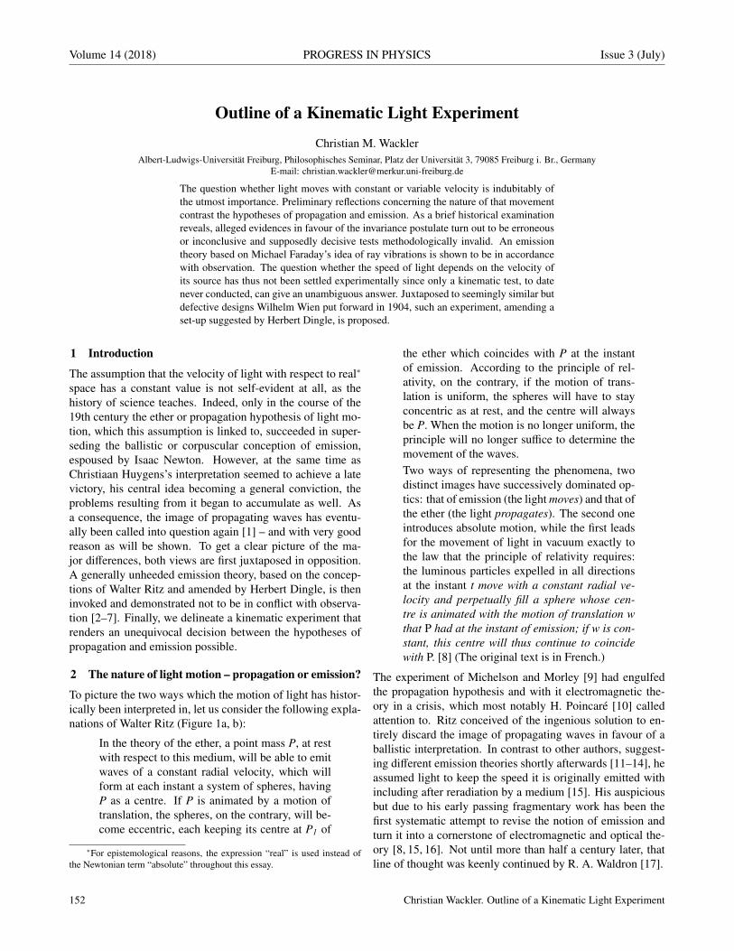
Volume 14 (2018) PROGRESS IN PHYSICS Issue 3 (July)
Outline of a Kinematic Light Experiment
Christian M. WacklerAlbert-Ludwigs-Universitat Freiburg, Philosophisches Seminar, Platz der Universitat 3, 79085 Freiburg i. Br., Germany
E-mail: [email protected]
The question whether light moves with constant or variable velocity is indubitably ofthe utmost importance. Preliminary reflections concerning the nature of that movementcontrast the hypotheses of propagation and emission. As a brief historical examinationreveals, alleged evidences in favour of the invariance postulate turn out to be erroneousor inconclusive and supposedly decisive tests methodologically invalid. An emissiontheory based on Michael Faraday’s idea of ray vibrations is shown to be in accordancewith observation. The question whether the speed of light depends on the velocity ofits source has thus not been settled experimentally since only a kinematic test, to datenever conducted, can give an unambiguous answer. Juxtaposed to seemingly similar butdefective designs Wilhelm Wien put forward in 1904, such an experiment, amending aset-up suggested by Herbert Dingle, is proposed.
1 Introduction
The assumption that the velocity of light with respect to real∗
space has a constant value is not self-evident at all, as thehistory of science teaches. Indeed, only in the course of the19th century the ether or propagation hypothesis of light mo-tion, which this assumption is linked to, succeeded in super-seding the ballistic or corpuscular conception of emission,espoused by Isaac Newton. However, at the same time asChristiaan Huygens’s interpretation seemed to achieve a latevictory, his central idea becoming a general conviction, theproblems resulting from it began to accumulate as well. Asa consequence, the image of propagating waves has eventu-ally been called into question again [1] – and with very goodreason as will be shown. To get a clear picture of the ma-jor differences, both views are first juxtaposed in opposition.A generally unheeded emission theory, based on the concep-tions of Walter Ritz and amended by Herbert Dingle, is theninvoked and demonstrated not to be in conflict with observa-tion [2–7]. Finally, we delineate a kinematic experiment thatrenders an unequivocal decision between the hypotheses ofpropagation and emission possible.
2 The nature of light motion – propagation or emission?
To picture the two ways which the motion of light has histor-ically been interpreted in, let us consider the following expla-nations of Walter Ritz (Figure 1a, b):
In the theory of the ether, a point mass P, at restwith respect to this medium, will be able to emitwaves of a constant radial velocity, which willform at each instant a system of spheres, havingP as a centre. If P is animated by a motion oftranslation, the spheres, on the contrary, will be-come eccentric, each keeping its centre at P1 of
∗For epistemological reasons, the expression “real” is used instead ofthe Newtonian term “absolute” throughout this essay.
the ether which coincides with P at the instantof emission. According to the principle of rel-ativity, on the contrary, if the motion of trans-lation is uniform, the spheres will have to stayconcentric as at rest, and the centre will alwaysbe P. When the motion is no longer uniform, theprinciple will no longer suffice to determine themovement of the waves.Two ways of representing the phenomena, twodistinct images have successively dominated op-tics: that of emission (the light moves) and that ofthe ether (the light propagates). The second oneintroduces absolute motion, while the first leadsfor the movement of light in vacuum exactly tothe law that the principle of relativity requires:the luminous particles expelled in all directionsat the instant t move with a constant radial ve-locity and perpetually fill a sphere whose cen-tre is animated with the motion of translation wthat P had at the instant of emission; if w is con-stant, this centre will thus continue to coincidewith P. [8] (The original text is in French.)
The experiment of Michelson and Morley [9] had engulfedthe propagation hypothesis and with it electromagnetic the-ory in a crisis, which most notably H. Poincare [10] calledattention to. Ritz conceived of the ingenious solution to en-tirely discard the image of propagating waves in favour of aballistic interpretation. In contrast to other authors, suggest-ing different emission theories shortly afterwards [11–14], heassumed light to keep the speed it is originally emitted withincluding after reradiation by a medium [15]. His auspiciousbut due to his early passing fragmentary work has been thefirst systematic attempt to revise the notion of emission andturn it into a cornerstone of electromagnetic and optical the-ory [8, 15, 16]. Not until more than half a century later, thatline of thought was keenly continued by R. A. Waldron [17].
152 Christian Wackler. Outline of a Kinematic Light Experiment

Issue 3 (July) PROGRESS IN PHYSICS Volume 14 (2018)
(a)
t0
t1
t2
P
P1
P1
P
P
(b)
t0 t1 t2
P
P
P P
P P
P1 P1
(c) P
P
P
t0 t1 t2
Fig. 1: Movement of a light source P and of a corresponding spherical wave generated at the instant t0. (a) Propagation (after Maxwell-Lorentz), (b) ballistic emission (after Newton-Ritz), (c) emanation (after Ritz-Dingle).
3 The Ritz theory – criticism and countercriticism
To test Ritz’s explanation, M. La Rosa [18,19] and R. C. Tol-man [13] suggested to repeat the Michelson-Morley experi-ment using light from an extraterrestrial source as the lattermoves rapidly with respect to the measuring apparatus. Theywrongly presupposed that another null result on such condi-tions would invalidate his conception. In 1919, an equivalenttest, conducted by Q. Majorana [20] with a moving terrestriallight source, showed no shift of the interference pattern. Al-though F. Michaud [21] demonstrated that Ritz’s theory con-forms with Majorana’s findings – unlike all other emissiontheories which had been proposed – inferring the fallacy of LaRosa’s and Tolman’s reasoning from this was omitted. Theirview found its way into W. Pauli’s [22] influential article onEinstein’s theory instead, and after R. Tomaschek [23] and D.C. Miller [24] had finally performed experiments employingsun and star light that again yielded no interference fringes tothe calculated extent, Ritz’s ideas largely fell into oblivion.
Already previously, an argument adduced by D. F. Com-stock [25] and W. de Sitter [26–29] had severely underminedthe plausibility of the emission hypothesis. They pointed outthat the observed orbits of binary stars are irreconcilable witha ballistic motion of light since particles emitted by a starapproaching the observer would overtake the preceding cor-puscles and thus distort the image of the system.
Almost half a century had passed until Herbert Dingle[2–4] not only brought the error in La Rosas’s and Tolman’sreasoning to light but also found a possible explanation con-sidering the seemingly unsurmountable objection that Com-stock and de Sitter had raised. In doing so, he seized uponideas which Michael Faraday had outlined in his Thoughts onRay-vibrations:
The view which I am so bold as to put forth con-siders, therefore, radiation as a high species ofvibration in the lines of force which are knownto connect particles and also masses of mattertogether. It endeavours to dismiss the æther, butnot the vibrations. [30]
Dingle showed that it suffices to extend the classical princi-ple of relativity concerning electromagnetic radiation so thatthe velocity of light would remain constant with respect toits source even if the radiating body moves non-uniformlyand non-rectilinearly (Figure 1c). According to this view,the vibrating rays stay throughout their journey through purespace connected to the source and share the latter’s changesof motion. A few years earlier but without building on Fara-day’s idea, P. Moon and D. E. Spencer had already reasonedalong similar lines in response to de Sitters objection [31–35].However, as H. Bondi aptly remarked, the term “ballistic”does not fit Dingle’s conception since the analogy with pro-jectiles no longer characterizes the image [2]. To make a cleardistinction, we hence refer to the variation of the emission hy-pothesis based on vibrating rays as emanation and to the cor-relating principle, governing the motion of electromagneticradiation, as classicistic relativity.
Admitting this principle renders yet another astronomi-cal objection irrelevant H. Thirring [36] propounded againstthe ballistic concept. He argued that as atoms in the sun areaccelerated through thermal collisions, they would emit lightparticles with different velocities at successive instants. Thewave train travelling along a terrestrial observer’s line of sightwould therefore shrink first, then be stretched, and arrive atthe earth as a radio signal.
Finally, a whole class of methodologically interrelated ev-idences that had been put forward against the emission hy-pothesis could not withstand Dingle’s astute scrutiny either.Over the years, a considerable number of experiments wasconducted which seemed to corroborate the postulate of con-stant light velocity relative to pure space, e.g. [37–43]. But asDingle correctly remarked:
The postulate is adopted as part of the basis of akinematic theory, so that “velocity” must be un-derstood in a kinematic sense, and this requiresthat the source of light must be an identifiablebody, having a definite position in space at eachsuccessive instant, the whole sequence of posi-
Christian Wackler. Outline of a Kinematic Light Experiment 153

Volume 14 (2018) PROGRESS IN PHYSICS Issue 3 (July)
A
B
LB
LA
M2
L1 S1
M1
L2 S2
β
α
Fig. 2: Schematic of Wien’s first and second experimental proposals. A, B: translationally congruent cogwheels; L1, L2, LA, LB: lightsources; M1, M2: mirrors in parallel position; S1, S2: diaphragms with scales; α, β: deviation angles assuming a stationary ether so thatα> β as the mirrors rotate, the arrow below indicating the direction of motion of the earth around the sun. Bolometers behind A and Bwere to record the luminous energy of the incoming beams. When the cogwheels are at rest, the respective values are the same but changeas soon as A and B start spinning. An ensuing difference in luminous energy between the rays passing through the notches in oppositedirections would have confirmed the hypothesis of a stationary ether.
tions being consistent with the velocity assignedto the body. [6]
Furthermore, the fact that tests which employ interferometryor use hypothetical particles as sources of light are subject tocircular reasoning was generally disregarded.
In all such experiments, the Maxwell-Lorentz the-ory, in one respect or another, has been assumedin the description of the experiment itself, andsince that theory requires that the velocity of lightshall be independent of that of its source, theresults are of no value at all in relation to thispoint. [44]
If one visualizes, for instance, the image of the ejected pho-ton string indicated above, it becomes clear at once that a lightray’s velocity is not determined by its frequency of vibration.Consequently, a measurement of the frequency of reception,taken by itself, does not allow a conclusion to be drawn aboutthat velocity. Thus, a kinematic question demands a kine-matic answer.
For all that and although it was occasionally admitted thatRitz’s ideas were discarded prematurely and in part on er-roneous grounds [45–49], the theory as amended by Dingle,which no valid evidence exists against, was for decades ne-glected. Only recently, this conception has finally been re-sumed and substantially expanded by Luis Bilbao [50], LuisBernal, and Fernando Minotti [7] under the name of VibratingRays Theory (VRT). Having adduced further observationaldata in support of it, they conclude their comprehensive studyas follows: “We believe that, given the above evidence, a con-scientious experimental research is needed to settle the ques-tion of the dependence of the speed of light on that of itssource as predicted by Vibrating Rays Theory, and that hasbeen observed during the 1998 NEAR flyby.” [7]
4 Towards a kinematic experiment
In 1904, Wilhelm Wien [51–55, pp. 1408-1409] outlined twoexperiments to determine whether the ether is dragged by the
earth or stationary based on the procedures Leon Foucault[56] and Hippolyte Fizeau [57, 58] had devised to measurethe speed of light. His first design includes employing tworotating mirrors, his second using two spinning cogwheelswhich are placed far apart from each other and aligned withthe orbital motion of the earth around the sun, respectively(Figure 2). Both experiments demand that the componentsin rotation have the same angular velocity at any given mo-ment. They therefore depend on the real synchronicity of theinstants which the mirrors or cogwheels are set in motion at.However, according to the prevailing theory, this is unattain-able through a material connection between them, for exam-ple by means of an axle, because within its framework thenotion of the rigid body is no longer valid as Wien [59, 60]himself later explained. Nor is utilizing electromagnetic sig-nals to simultaneously start two separate motors feasible dueto the supposedly indeterminable times the signals need toreach the different propulsion systems, which count as clocks,so that any possible asymmetry looked for would be offsetby the signals’ nonsynchronous arrival. These designs beingfoiled, Wien relinquished further efforts and became a leadingproponent of Einstein’s theory.
More than half a century later, Herbert Dingle pointed re-peatedly to the necessity of a kinematic test for a final answerto the question of the speed of light [4–6, 43, 61–68]. In hisbook Science at the Crossroads, he eventually presented hismost sophisticated proposal of an experiment of the kind hehoped for (Figure 3):
A and B are two sources of light (visible, mate-rial sources, not hypothetical particles) of whichB is moving rapidly to the left while A is at rest,the paper being the standard of rest. At the in-stant at which they are adjacent to one anotherthey emit pulses of light towards C and D, whichare photographic films whose distances from Aare constant and which are moving rapidly down-wards through the paper. The relative motion
154 Christian Wackler. Outline of a Kinematic Light Experiment
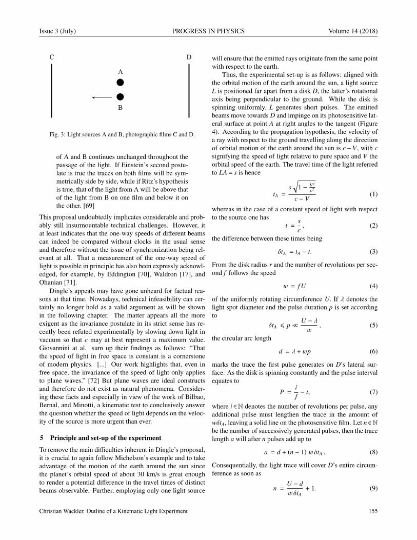
Issue 3 (July) PROGRESS IN PHYSICS Volume 14 (2018)
Α
Β
C D
Fig. 3: Light sources A and B, photographic films C and D.
of A and B continues unchanged throughout thepassage of the light. If Einstein’s second postu-late is true the traces on both films will be sym-metrically side by side, while if Ritz’s hypothesisis true, that of the light from A will be above thatof the light from B on one film and below it onthe other. [69]
This proposal undoubtedly implicates considerable and prob-ably still insurmountable technical challenges. However, itat least indicates that the one-way speeds of different beamscan indeed be compared without clocks in the usual senseand therefore without the issue of synchronization being rel-evant at all. That a measurement of the one-way speed oflight is possible in principle has also been expressly acknowl-edged, for example, by Eddington [70], Waldron [17], andOhanian [71].
Dingle’s appeals may have gone unheard for factual rea-sons at that time. Nowadays, technical infeasibility can cer-tainly no longer hold as a valid argument as will be shownin the following chapter. The matter appears all the moreexigent as the invariance postulate in its strict sense has re-cently been refuted experimentally by slowing down light invacuum so that c may at best represent a maximum value.Giovannini at al. sum up their findings as follows: “Thatthe speed of light in free space is constant is a cornerstoneof modern physics. [...] Our work highlights that, even infree space, the invariance of the speed of light only appliesto plane waves.” [72] But plane waves are ideal constructsand therefore do not exist as natural phenomena. Consider-ing these facts and especially in view of the work of Bilbao,Bernal, and Minotti, a kinematic test to conclusively answerthe question whether the speed of light depends on the veloc-ity of the source is more urgent than ever.
5 Principle and set-up of the experiment
To remove the main difficulties inherent in Dingle’s proposal,it is crucial to again follow Michelson’s example and to takeadvantage of the motion of the earth around the sun sincethe planet’s orbital speed of about 30 km/s is great enoughto render a potential difference in the travel times of distinctbeams observable. Further, employing only one light source
will ensure that the emitted rays originate from the same pointwith respect to the earth.
Thus, the experimental set-up is as follows: aligned withthe orbital motion of the earth around the sun, a light sourceL is positioned far apart from a disk D, the latter’s rotationalaxis being perpendicular to the ground. While the disk isspinning uniformly, L generates short pulses. The emittedbeams move towards D and impinge on its photosensitive lat-eral surface at point A at right angles to the tangent (Figure4). According to the propagation hypothesis, the velocity ofa ray with respect to the ground travelling along the directionof orbital motion of the earth around the sun is c−V , with csignifying the speed of light relative to pure space and V theorbital speed of the earth. The travel time of the light referredto LA = s is hence
tA =s√
1 − V2
c2
c − V(1)
whereas in the case of a constant speed of light with respectto the source one has
t =sc, (2)
the difference between these times being
δtA = tA − t. (3)
From the disk radius r and the number of revolutions per sec-ond f follows the speed
w = f U (4)
of the uniformly rotating circumference U. If λ denotes thelight spot diameter and the pulse duration p is set accordingto
δtA 6 p U − λw
, (5)
the circular arc length
d = λ + wp (6)
marks the trace the first pulse generates on D’s lateral sur-face. As the disk is spinning constantly and the pulse intervalequates to
P =if− t, (7)
where i ∈N denotes the number of revolutions per pulse, anyadditional pulse must lengthen the trace in the amount ofwδtA, leaving a solid line on the photosensitive film. Let n ∈Nbe the number of successively generated pulses, then the tracelength a will after n pulses add up to
a = d + (n − 1) w δtA . (8)
Consequentially, the light trace will cover D’s entire circum-ference as soon as
n =U − dw δtA
+ 1. (9)
Christian Wackler. Outline of a Kinematic Light Experiment 155

Volume 14 (2018) PROGRESS IN PHYSICS Issue 3 (July)
A2
A1 0
B2
B1
D A1
0
L
B1
Fig. 4: Schematic of the experimental set-up: A1 and A2 denote the points where the rays generated by the first and the second light pulsehit the disk D at the instants t1 and t2. The circular arc length A1B1 = d represents the trace on D’s photosensitive lateral surface the veryfirst pulse causes. B1B2 = wδtA depicts the trace’s length increment produced by the second and any additional pulse according to thepropagation hypothesis. The arrow at the bottom indicates the direction of motion of the earth around the sun.
By contrast, if the emission hypothesis is correct, the raysmust always impinge on the same spot so that the trace on thedisk retains the length d no matter how much the value of nincreases, δtA having to be substituted with δt in equation (8),where δt = t− t = 0.
Provided that the propagation hypothesis applies, the ex-act value of a cannot be predicted. For the conventional valueof c would be an average that resulted from two-way mea-surements and thus deviates from the real one-way speed oflight. In case the first test indeed gave a> d for n> 1, theresult should be crosschecked. Rotating the set-up and re-peating the experiment would be expected to yield a differentvalue of a at each angle for a given n. Perpendicular to the di-rection of orbital motion of the earth around the sun, the tracelength would then be
a90 = d + (n − 1) w
√s2 + V2t2
c− t
(10)
and at 180
a180 = d + (n − 1) w
t −s√
1 − V2
c2
c + V
, (11)
where a≈ a180 . Equations (1) and (11), taking the supposedLorentz contraction into account, are applicable if the dis-tance LA is measured by means of an etalon. However, con-sidering the necessary magnitude of LA, a travel time mea-surement using electromagnetic radiation will be conductedin practice. The determined distance
s =c T2
=(c − V + c + V) T
4(12)
then arises from the signal’s two-way speed, with T signify-ing the total time elapsed between emission and return, the re-spective instants being measured by one and the same clock.Although the square root factor within equations (1) and (11)must under these premises be omitted, the choice between thetwo methods of establishing LA is evidently of no significanceregarding the validity of the experiment.
Due to the motion of the solar system, the propagationhypothesis involves the assumption that tA varies seasonally.Therefore, if the first experimental run yields a = d for n> 1,a conclusive confirmation of the emission hypothesis will notonly demand repetitions of the test at different angles but alsoreperforming it over an extended period to exclude a mislead-ing result because of V being possibly offset by an unknownvelocity component just at the time of the initial measure-ments.
The outlined experiment avoids the theoretical obstacleswhich defeated Wilhelm Wien’s proposals as merely one uni-formly spinning mechanical component is required and at-tuning a pulsing light source to it does not pose a conceptualproblem. The test itself implies no two-way measurement andis neither dependent on assumptions of the Maxwell-Lorentzelectromagnetic theory, nor are hypothetical particles used asa radiation source. Thus, Dingle’s criteria for a kinematiclight experiment are met, and objections against proceduresbased on a closed light path do not apply [73].
6 Conclusion
We may summarize the proposed experimentum lucis et cru-cis in the following way: since any “in itself determined pe-riodic process realized by a system of sufficiently small spa-tial extension” [74] is considered to be a timepiece, the de-
156 Christian Wackler. Outline of a Kinematic Light Experiment

Issue 3 (July) PROGRESS IN PHYSICS Volume 14 (2018)
scribed set-up consisting of a uniformly spinning disk featur-ing a photosensitive lateral surface and of a light source puls-ing at equal intervals embodies two clocks, their “hands” be-ing successively emitted rays. These “light clocks” run syn-chronously and thus display real simultaneity. The outcomeof the experiment is therefore identical for any observer inany system of reference.
Since the assumption that an ether is dragged by the earthwas experimentally refuted [75, 76], no theory reposing onthe postulate of constant light velocity relative to pure spaceor a luminiferous medium in it can explain successive beamsimpinging on the disk at the same spot. Instead, the emissionhypothesis will be fully confirmed. Electromagnetic radia-tion will have to be understood as a form of energy which isemitted with a real velocity c + v, that is the vector sum ofa component being invariant relative to the light source anda variable component, the real velocity of this very source.However, according to K. Brecher’s [77] analysis of regu-larly pulsating x-ray sources in binary star systems, a ballisticinterpretation even if it allows for the extinction theorem ofdispersion theory, as considered by J. G. Fox [45, 46], seemsto be untenable (cf. also [48]). Thus, the Ritz-Dingle Emana-tion or Vibrating Rays Theory will remain the only explana-tion consistent with observation [2–7]. In addition to classi-cal relativity holding true for matter in uniform translation, aclassicistic principle will apply stating that the speed of lightstays constant relative to its source even if the latter movesnon-rectilinearly and non-uniformly.
Should, on the contrary, successive beams mark a solidline on the disk, the propagation hypothesis would bear thepalm. Light would have the characteristics of a wave thatpropagates in a medium with constant velocity relatively tothat medium. The recently renewed question whether thereis a resting frame in space [78] would be answered in theaffirmative.
Submitted on May 11, 2018
References1. Ritz W. Du role de l’ether en physique. Rivista di Scienza ‘Scientia’,
1908, v. 3 (6), 260–274.
2. Bondi H. et al. Meeting of the Royal Astronomical Society, Friday,1958 November 14, at 16h 30m. Observatory, 1958, v. 78 (907), 232–241.
3. Dingle H. A Proposed Astronomical Test of the “Ballistic” Theory ofLight Emission. Monthly Notices of the Royal Astronomical Society,1959, v. 119 (1), 67–71.
4. Dingle H. Relativity and Electromagnetism: An Epistemological Ap-praisal. Philosophy of Science, 1960, v. 27 (3), 233–253.
5. Dingle H. A Reply to Professor Grunbaum’s Rejoinder. British Journalfor the Philosophy of Science, 1961, v. 12 (46), 156–157.
6. Dingle H. Reason and Experiment in Relation to the Special RelativityTheory. British Journal for the Philosophy of Science, 1964, v. 15 (57),41–61.
7. Bilbao L., Bernal L., Minotti F. Vibrating Rays Theory. arXiv:1407.5001.
8. Ritz W. Recherches critiques sur l’electrodynamique generale. Annalesde chimie et de physique, 1908, v. 13, 145–275.
9. Michelson A. A., Morley E. W. On the Relative Motion of the Earth andthe Luminiferous Ether. American Journal of Science, 1887, v. 34 (203),333–345.
10. Poincare H. The Value of Science. The Science Press, New York, 1907.11. Thomson J. J. On a Theory of the Structure of the Electric Field and its
Application to Rontgen Radiation and to Light. Philosophical Maga-zine, 1910, v. 19 (110), 301–312.
12. Tolman R. C. The Second Postulate of Relativity. Physical Review,1910, v. 31, 26–40.
13. Tolman R. C. Some Emission Theories of Light. Physical Review, 1912,v. 35, 136–143.
14. Stewart O. M. The Second Postulate of Relativity and the Electromag-netic Emission Theory of Light. Physical Review, 1911, v. 32, 418–428.
15. Ritz W. Recherches critiques sur les theories electrodynamiques de Cl.Maxwell et de H.-A. Lorentz. Archives des Sciences Physiques et Na-turelles, 1908, v. 26, 209–236.
16. Ritz W. Uber die Grundlagen der Elektrodynamik und die Theorie derschwarzen Strahlung. Physikalische Zeitschrift, 1908, v. 9 (25), 903–907.
17. Waldron R. A. The Wave and Ballistic Theories of Light: A CriticalReview. Frederick Muller, London, 1977.
18. La Rosa M. Fondamenti sperimentali del 2. Principio della teoria dellarelativita. Nuovo Cimento, 1912, v. 3 (1), 345–365.
19. La Rosa M. Uber einen Versuch zum Vergleiche der Relativitatstheo-rie mit den mechanischen Anschauungen uber die Lichtausstrahlung.Physikalische Zeitschrift, 1912, v. 13 (23), 1129–1131.
20. Majorana Q. Experimental Demonstration of the Constancy of Veloc-ity of the Light emitted by a Moving Source. Philosophical Magazine,1919, v. 37 (217), 145–150.
21. Michaud F. Les theories emissives et le principe de Doppler-Fizeau.Comptes rendus de l’Academie des sciences, 1919, v. 168, 507–509.
22. Pauli W. Theory of Relativity. Pergamon Press, London, 1958.23. Tomaschek R. Uber das Verhalten des Lichtes außerirdischer Licht-
quellen. Annalen der Physik, 1924, v. 73, 105–126.24. Miller D. C. Ether-Drift Experiments at Mount Wilson. Proceedings
of the National Academy of Sciences of the United States of America,1925, v. 11 (6), 306–314.
25. Comstock D. F. A Neglected Type of Relativity. Physical Review, 1910,v. 30, 267.
26. de Sitter W. A proof of the constancy of the velocity of light. Proceed-ings of the Section of Sciences, Koninklijke Akademie van Wetenschap-pen te Amsterdam, 1913, v. 15 (2), 1297–1298.
27. de Sitter W. Ein astronomischer Beweis fur die Konstanz der Licht-geschwindigkeit. Physikalische Zeitschrift, 1913, v. 14 (10), 429.
28. de Sitter W. On the constancy of the velocity of light. Proceedings ofthe Section of Sciences, Koninklijke Akademie van Wetenschappen teAmsterdam, 1913, v. 16 (1), 395–396.
29. de Sitter W. Uber die Genauigkeit, innerhalb welcher die Unabhangig-keit der Lichtgeschwindigkeit von der Bewegung der Quelle behauptetwerden kann. Physikalische Zeitschrift, 1913, v. 14 (25), 1267.
30. Faraday M. Thoughts on Ray-vibrations. Philosophical Magazine,1846, v. 28 (188), 345–350.
31. Moon P., Spencer D. E. Binary Stars and the Velocity of Light. Journalof the Optical Society of America, 1953, v. 43 (8), 635–641.
32. Moon P., Spencer D. E. On the Establishment of a Universal Time. Phi-losophy of Science, 1956, v. 23 (3), 216–229.
33. Moon P., Spencer D. E. The New Electrodynamics and its Bearing onRelativity. In: Kritik und Fortbildung der Relativitatstheorie, editedby K. Sapper, 1958, Austria Akademische Druck- und Verlagsanstalt,Graz, 144–159.
Christian Wackler. Outline of a Kinematic Light Experiment 157

Volume 14 (2018) PROGRESS IN PHYSICS Issue 3 (July)
34. Moon P., Spencer D. E., Moon E. E. Binary Stars from Three View-points. Physics Essays, 1989, v. 2 (3), 275–287.
35. Moon P., Spencer D. E., Moon E. E. Universal Time and The Velocityof Light. Physics Essays, 1989, v. 2 (4), 368–374.
36. Thirring H. Uber die empirische Grundlage des Prinzips der Konstanzder Lichtgeschwindigkeit. Zeitschrift fur Physik, 1925 v. 31, 133–138.
37. Bonch-Bruevich A. M. A Direct Experimental Confirmation of the Sec-ond Postulate of the Special Theory of Relativity (in connection withDingle’s note). Optics and Spectroscopy, 1960, v. 9, 73.
38. Sadeh D. Experimental Evidence for the Constancy of the Velocity ofGamma Rays, Using Annihilation in Flight. Physical Review Letters,1963, v. 10 (7), 271–273.
39. Alvager T., Nilsson A., Kjellman J. A Direct Terrestrial Test of the Sec-ond Postulate of Special Relativity. Nature, 1963, v. 197 (4873), 1191.
40. Rotz F. B. New Test of the Velocity of Light Postulate. Physics Letters,1963, v. 7 (4), 252–253.
41. Babcock G. C., Bergman T. G. Determination of the Constancy of theSpeed of Light. Journal of the Optical Society of America, 1964,v. 54 (2), 147–151.
42. Alvager T., Farley F. J. M., Kjellman J., Wallin I. Test of the SecondPostulate of Special Relativity in the GeV Region. Physics Letters,1964, v. 12 (3), 260–262.
43. Waddoups R. O., Edwards W. F., Merrill J. J. Experimental Investiga-tion of the Second Postulate of Special Relativity. Journal of the Opti-cal Society of America, 1965, v. 55 (2), 142–143.
44. Dingle H. A Re-examination of the Michelson-Morley Experiment. Vis-tas in Astronomy, 1967, v. 9, 97–100.
45. Fox J. G. Experimental Evidence for the Second Postulate of SpecialRelativity. American Journal of Physics, 1962, v. 30 (4), 297–300.
46. Fox J. G. Evidence Against Emission Theories. American Journal ofPhysics, 1965, v. 33 (1), 1–17.
47. Beckmann P., Mandics P. Experiment on the Constancy of the Veloc-ity of Electromagnetic Radiation. Radio Science Journal of Research,1964, v. 68D (12), 1265–1268.
48. Beckmann P., Mandics P. Test of the Constancy of the Velocity of Elec-tromagnetic Radiation in High Vacuum. Radio Science Journal of Re-search, 1965, v. 69D (4), 623–628.
49. Martınez A. A. Ritz, Einstein, and the Emission Hypothesis. Physics inPerspective, 2004, v. 6 (1), 4–28.
50. Bilbao L. Does the Velocity of Light Depend on the Source Movement?Progress in Physics, 2016, v. 12 (4), 307–312.
51. Wien W. On experiments to decide whether the ether moves with theearth or not. Observatory, 1904, v. 27 (349), 360.
52. Wien W. Uber einen Versuch zur Entscheidung der Frage, ob sich derLichtather mit der Erde bewegt oder nicht. Physikalische Zeitschrift,1904, v. 5 (19), 585–586.
53. Wien W. Experimente zur Entscheidung der Frage, ob sich der Athermit der Erde bewegt oder nicht. Physikalische Zeitschrift, 1904,v. 5 (19), 604–605.
54. Wien W. Experiments to decide whether the Ether moves with theEarth. Report of the British Association for the Advancement of Sci-ence, 1905, v. 74, 433–434.
55. Cohn E. Zur Elektrodynamik bewegter Systeme. II. Sitzungsberichteder Koniglich Preussischen Akademie der Wissenschaften, 1904, v. 53,1404–1416.
56. Foucault L. Mesure de la vitesse de la lumiere, etude optique dessurfaces; memoires de Leon Foucault. Librairie Armand Colin, Paris,1913.
57. Fizeau H. Sur une experience relative a la vitesse de propagation dela lumiere. Comptes rendus hebdomadaires des seances de l’Academiedes Sciences, 1849, v. 29, 90–92.
58. Fizeau H. Sur une experience relative a la vitesse de propagation de lalumiere. Revue scientifique et industrielle, 1849, v. 5, 393–397.
59. Wien W. Uber die Wandlung des Raum- und Zeitbegriffs in derPhysik. Sitzungsberichte der Physikalisch-medicinischen Gesellschaftzu Wurzburg 1909, 1910, (2,3), 29–39.
60. Wien W. Die Relativitatstheorie. In: Taschenbuch fur Mathematikerund Physiker, Bd. 2, edited by F. Auerbach and R. Rothe, B. G. Teub-ner, Leipzig and Berlin, 1911, 283–292.
61. Dingle H. A Possible Experimental Test of Einstein’s Second Postulate.Nature, 1959, v. 183 (4677), 1761.
62. Dingle H. An opportunity to check on Einstein. New Scientist, 1959,v. 5 (133), 1253.
63. Dingle H. Ritz theory of light. Observatory, 1959, v. 79 (910), 106–107.
64. Dingle H. The Falsifiability of the Lorentz-FitzGerald Contraction Hy-pothesis. British Journal for the Philosophy of Science, 1959, v. 10 (39),228–229.
65. Dingle H. A Radio-astronomical Test of the Ballistic Theory of LightEmission. Observatory, 1960, v. 80 (914), 35–36.
66. Dingle H. The Doppler Effect and the Foundations of Physics (I).British Journal for the Philosophy of Science, 1960, v. 11 (41), 11–31.
67. Dingle H. The Doppler Effect and the Foundations of Physics (II).British Journal for the Philosophy of Science, 1960, v. 11 (42), 113–129.
68. Dingle H. Special Theory of Relativity. Nature, 1962, v. 195 (4845),985–986.
69. Dingle H. Science at the Crossroads. Martin Brian & O’Keeffe, Lon-don, 1972.
70. Eddington A. S. The Mathematical Theory of Relativity. The UniversityPress, Cambridge, 1923.
71. Ohanian H. C. Einstein’s mistakes: the human failings of genius. W. W.Norton & Co., New York, 2008.
72. Giovannini D., Romero J., Potocek V., Ferenczi G., Speirits F., Bar-nett S. M., Faccio D., Padgett M. J. Spatially structured photons thattravel in free space slower than the speed of light. Science, 2015,v. 347 (6224), 857–860.
73. Perez I. On the experimental determination of the one-way speed oflight. European Journal of Physics, 2011, v. 32 (4), 993–1005.
74. Einstein A. Autobiographical Notes. In: Albert Einstein: Philosopher-Scientist, edited by P. A. Schilpp, The Library of Living Philosophers,Evanston, IL, 1949, 2–94.
75. Michelson A. A. The Effect of the Earth’s Rotation on the Velocity ofLight, Part I. Astrophysical Journal, 1925, v. 61 (3), 137–139.
76. Michelson A. A., Gale H. G., Pearson F. The Effect of the Earth’s Ro-tation on the Velocity of Light, Part II. Astrophysical Journal, 1925,v. 61 (3), 140–145.
77. Brecher K. Is the Speed of Light Independent of the Velocity of theSource? Physical Review Letters, 1977, v. 39 (17,19), 1051–1054,1236.
78. Chang D. C. Is there a resting frame in the universe? A proposed exper-imental test based on a precise measurement of particle mass. EuropeanPhysical Journal Plus, 2017, v. 132, 140.
158 Christian Wackler. Outline of a Kinematic Light Experiment

Issue 3 (July) PROGRESS IN PHYSICS Volume 14 (2018)
Fractional Degrees of Freedom in Statistics
Mikhail N. MashkinE-mail: [email protected]
The concept of observation and presentation of the count (reference) results in an inter-val form is considered. The transition to interval measurements is achieved by use ofthe total reduced number of measurements (number of degrees of freedom) as a sampleparameter, which allows the use of non-integer (fractional) powers of freedom in thecalculation of the estimates of static parameters and criteria values. The replacementof single measurements with interval measurements at their same quantities in all casesreduces the accuracy of statistical parameters estimates.
Introduction
Currently, there are known applications of fractional powersin statistics [1]. However, the use of different methods ofdata processing, in particular for small samples [2] and forprocessing with the use of methods similar to the method ofgroup accounting arguments [3], allows to broaden their usein calculations.
The concept of observation
According to [4], observation is the experimental basis of sci-entific research. Observed results are most often recorded inthe form of meanings of the measured values or their counts.For static methods of measurement, the result is a single num-ber. With dynamic methods, it is possible to record the mea-sured value in time as the implementation of a random (non-random) process. In the latter case, the results of measure-ments often are the evaluations of the process parameters. Inboth cases, statistical stability is a prerequisite, which in par-ticular consists, in the approximation, with a sufficiently largenumber of observations∗ to the probability of a given value.In all cases, if the measurement of the value is repeated manytimes, the result is a statistical distribution series correspond-ing to any distribution law, which may be associated with theerror of the measuring system or instrument.
Each single measurement (count), as well as their totality,gives an empirical distribution, which is described in the formof a histogram, statistical series, empirical distribution func-tion, etc. In this case, along with the above, it is necessary tospecify the number of measurements, i.e. empirical descrip-tion requires specifying the number of experiments (samplesize) on the basis of which it is obtained. We will refer to thenumber of measurements, on the basis of which the empiricaldescription of the distribution law is obtained, as the numberof degrees of freedom. However, there are measured values,which, by their nature, initially have a form corresponding toa certain distribution law [5]. In this case, the measured valueis set not by a value, which is constant or changing in time,but by an area at each point of which it can be located with a
∗The ratio of the number of observations of a particular value to the totalnumber of observations.
certain probability. This allows each measurement to matchthe area of the measured value with the law of its distribution.
The area of determination of the value can be set withone or more than one interval, see Fig. 1. One dimensiongives the area and the value of the parameters’ estimates ofthe distribution law.
Interval measurements
Let us consider the basic prerequisites for using intervals asmeasurement results.
The possibility to express numerical values of quantitiesin the form of intervals is used in the theory of intervals [6].The basic idea of interval analysis is that you can work withintervals as with plain numbers. Common operations suchas addition, subtraction, multiplication and division, as wellas set theory operations such as intersection and union, arequite applicable to them. Interval operations are described bya ratio:
A@B = x@y|x ∈ A, y ∈ B , (1)
where @ is one of the operations +, −, ∗, /, ∪, ∩, whileA, B are intervals.
Fig. 1: Types of areas for determining the measurement value: a —one observation — a single numerical value; b — one observation— a set of intervals of numerical values, including those that are notlimited to the left or to the right; c — one observation — a set ofintervals strictly limited to the left and to the right; d — one obser-vation — one interval of numerical values with one border to the leftand one to the right.
Mashkin M. N. Fractional Degrees of Freedom in Statistics 159

Volume 14 (2018) PROGRESS IN PHYSICS Issue 3 (July)
A single (real) number can be viewed as that an intervalhaving a definition domain and the law of distribution in theform of a certain event probability:
P (a ∈ [a, a]) = 1, a = [a, a] , (2)
i.e. just one numerical value is sufficient for the descriptionof the measured value.
Let us consider the measurement process of the diameterof a bearing ring as an example of a measurement that hasa definition area of one interval. The measurement of theradius of the hole or the outer diameter (done with sufficientlyaccurate instruments) relative to the calculated center of thebearing ring gives the dependence of the radius to the pointon the circumference surface of the hole or the outer diameterin the form of a realization of a random process that can bedescribed by a random function like follows:
R = X (α) , (3)
where 0 6 α 6 2π is the bearing ring angle of rotation.Accurate lab instruments such as circular gauges allow us
to fully record the kind of realization of a random process.Obviously, when such a record exists, it can be processed bywell known methods of the theory of random processes. Inproduction conditions, the use of precision instruments is im-practical. The control devices used allow to quite preciselymeasure the diameter of a bearing ring. During the rotationof the bearing ring it is also possible to determine the max-imum and minimum values of the diameter of the bearing.If we limit ourselves to only two of these values, then actu-ally we come to a case of two independent observations. Theinformation that there are other numerical values of the diam-eter, between these two values, becomes thus lost. For a morecomplete explanation of the essense of the observation, it isproposed to consider the considered measurement process asa single observation in the form of one interval, Fig. 1, d. Thevalue of the measured diameter has a description in the formof a statistical series at a given interval:
P ( d : d ∈ [dmin, dmax]) , (4)
where d is the value of the bearing ring diameter.With an interval measurement, however, there are two de-
grees of freedom: the measurements of one and the otherborder of the interval. However, these two dimensions areconsidered together over the interval. For example, one di-mension is a border, and the other is the interval value it-self, that is, there is a relationship: for the first dimension,the entire numerical axis is available, and the second dimen-sion describes the area of the finite length bound to the firstmeasurement. The availability of the entire numerical axishere must be understood as a possibility to represent the firstmeasurement only by selecting the initial value of the refer-ence point by any number, including almost infinity. For the
interval, whatever we choose as the reference point, its valueremains constant. From this we can assume that the specifiedrelationship as if reduces the number of degrees of freedomof choice of numerical values for the interval measurement.We can assume that it is less than two, but more than one. In-terval measurement generally gives the values of the bordersof intervals and parameters or their estimates of the distribu-tion law. This can be described by displaying the interval inparameters’ values:
G : [ ai bi ]P−→
β j : j = 1, . . . , k
, (5)
where G displays the set of numerical values of the intervalmeasurement in the values of parameters or their estimates ofthe probability distribution law; ai, bi are borders of the i-thinterval; P is the law of distribution of values of a randomvariable from the interval; β j is the value or estimate of aparameter of the distribution law.
It should be noted that the borders of the interval can bedisplayed in the parameters of the distribution law explicitly(for example, the boundaries of the interval in the case of thelaw of equal probability density) or indirectly as the area ofdefinition of this law.
One of the options for describing the distribution law Pis the probability density. By the given probability density orhistogram it is possible to calculate or to estimate the param-eters of the distribution law. The previously declared com-monality for the interval and for one number (2) allows thesecalculations to be applied for one number obtained during themeasurement. Let us illustrate this by calculating the disper-sion of a single observation.
Calculation of the dispersion estimation of one observa-tion by known relations [1] can be performed by the formula:
σ2x =
n∑i=1
(xi − mx)2
n=
(x − mx)2
1if mx is known, (6)
where mx is the mathematical expectation; x is the numericalvalue of the dimension.
For one number from the interval with coinciding borders,formula (6) is valid, because the mathematical expectationdoes not require an evaluation, but is equal to the number it-self. The value of the dispersion estimate in this case is zero.This clearly indicates the non-randomness of the interval rep-resentation of the same number, i.e., the specific meaning ofthe measured value does not have a random component — itis a non-random value.
Calculation of the dispersion estimate for an interval mea-surement in the extreme case can be performed as that for twoindependent observations by formulas:
σ2x =
(b − mx)2 + (a − mx)2
1, if mx is unknown, (7)
σ2x =
(b − mx)2 + (a − mx)2
2, if mx is known. (8)
160 Mashkin M. N. Fractional Degrees of Freedom in Statistics

Issue 3 (July) PROGRESS IN PHYSICS Volume 14 (2018)
It can be assumed that the value of the dispersion estimatefor the interval for each case, due to the lower value of the de-grees of freedom, should exceed the values given by formulas(7) and (8). In addition, within the interval, the measured nu-merical values of the value are determined by its distributionlaw. If we choose as the basic one the law of equal probabilitydensity (EPD), then we lead the rest of the distributions to itby changing the value of the interval on the basis of equalityof the entropy value.
Let us define the given number of measurements (degreesof freedom) for an interval measurement in the form of:
ri = 1 + ∆i , 1 > |∆i| > 0; (9)
where
∆i =
+∆is, boundaries are given from experience;−∆is, one boundary is given by the researcher;−1, boundaries are given randomly.
The value ∆is can be determined by formula:
∆is =
1
1 + 1/his, at bi, ai , 0;
0, at bi, ai = 0;(10)
wherehis =
bi − ai12 | ai + bi |
is choosen for the EPD law and
his =(bi − ai) Hx
HEPD
∣∣∣ M [X[a,b]
] ∣∣∣is choosen for any other law of the distribution of x along theinterval [ai, bi];
Hx = M[log P
(X = x j ∈ [ai bi]
)]=
−
n∑j=1
P(X = x j
)log P
(X = x j
)is chosen if the given measured value is discreet∗;
Hx = M[log P ( f (x))
]= −
∫ bi
ai
f (x) logc f (x) dx
is taken at c < (bi − ai) if the measured value is continuous(relative entropy);
HEPD = log n[a,b]
if the discrete measured value is distributed equally possiblewithin the interval, where n[a,b] is the number of equally pos-sible states in the interval;
HEPD = logc (bi − ai)∗The given relations for determination of H# are similar to entropy for-
mulas, and for the case of discrete measured values exactly coincide withthem.
if within the interval the measured value is distributed accord-ing to the EPD law;
M[X[a, b]
]is the mathematical expectation of the measured value in theinterval [ai, bi].
The total reduced number of measurements, the value forthe calculation of statistical parameters for the sample, isequal to:
nr =
n∑i=1
ri . (11)
This assumes that, when creating a statistical series of dis-tributions or histograms, each interval dimension must haveits own share proportional to the value of ri. If it is 0, thisdimension is ignored. If it differs from zero, then this con-tribution, as the number of measurements (experiments), isequal to its value.
Formulas for calculation of the main estimates of statisti-cal parameters for one, i-interval measurement, in the case ofthe EPD law for the measured value within the interval, havethe form:
mxi =bi + ai
2; (12)
σ2ri
=
(bi − mxi
)2+
(ai − mxi
)2
ri − 1=
(bi − ai)2
2 (ri − 1). (13)
Example. With a rectangular contribution (EPD), let usdefine by formula (13) the estimate of the variance in the in-terval of an i-th observation for different ratios of the valueof the interval and the values of its mathematical expectation,see Table 1.
Left bor-der of theinterval,
ai
Right bor-der of theinterval,
bi
Math. ex-pectationestimate,
mxi
Reduced no.of measure-ments, ri
Estim.variance,σ2
ri(13)
−4 4 0 2 32
−3 5 1 1.889 36
−2 6 2 1.8 40
−1 7 3 1.727 44
0 8 4 1.667 48
1 9 5 1.615 52
2 10 6 1.571 56. . . . . . . . . . . . . . .
30 38 34 1.190 168
Table 1: Dispersion (variance) estimation via the given number ofmeasurements.
Analysis of Table 1 shows that in the symmetric interval(the case when the estimate of the mathematical expectationis 0), the variance estimate coincides with the value calcu-lated by formula (7) for two unit measurements. As the value
Mashkin M. N. Fractional Degrees of Freedom in Statistics 161

Volume 14 (2018) PROGRESS IN PHYSICS Issue 3 (July)
of mathematical expectation increases, the variance value in-creases due to the reduction of the reduced number of mea-surements, which can be taken as the number of degrees offreedom of the resulting measurement.
Taking into account the above, a single measurement canbe considered as an interval measurement when the interval isequal to the rounding error of the instrument readings. In thiscase, a fairly small relative error gives the reduced number ofmeasurements equal to 1.
Contributions method
To process the results of a small sample in the evaluation ofthe distribution laws, the contribution method is used [2, 6].This approach allows us to obtain a paradoxical result: due tothe empirical selection of the width of the interval of a rectan-gular or other contribution, the accuracy of the assessment in-creases. The paradox is that, by coarsening the measurementresults (the numbers are replaced by fixed-width intervals),the accuracy of statistical parameters is allegedly improved.
When using the formalism published in the work [2], theproposed estimation formula for the method of contributionsfor the probability density is:
f (x) =
n∑i=1
ri · pi (x, ai, bi)
n∑i=1
ri
, (14)
where n is the number of observations; pi (x, ai, bi) is a gen-eralized record of the empirical component of the distributiondensity associated with the interval of i-th observation (hav-ing all the properties of the distribution density), describesthe law of distribution of measurements in the interval. Un-like the work [2], empiricism is limited by the choice of thedistribution law in the interval. And there are two options:
1. The distribution law is the same for all intervals;2. For each interval, its own law of distribution is picked.
For the case of the EPD law in the interval we have:
pi (x, ai, bi) =1
bi − ai, ai 6 x 6 bi . (15)
The work [7] presents a formula which uses the methodof contributions for the empirical component of density esti-mation in the form of:
f ∗N (x) = C (ρ)N∑
i=1
µi ψi (ρ, x) , (16)
where the ρ parameter is equal to half of the contribution in-terval, ρ = bi−ai
2 = const, that is, the interval in all dimensionsis the same;
C (ρ) =
ρ∫−ρ
ψi (ρ, x) dx
−1
, (17)
the amplitude ensures the equality of each contribution 1;µi = 1/N is weight (the ratio for norming density estimation);and also
ψi (ρ, x) =
1, xi − ρ 6 x 6 xi + ρ ;0, for others x.
(18)
Let us consider the use of formulas (14) and (16) for Ex-ample 2.1 from the work [7].
Example 2.1 [7]. As a result of measurement of param-eter X of three products after adjustment of the equipment,the following results were obtained: 6.0; 6.4; 6.6. Let us es-timate the empirical density that characterizes the quality ofthe equipment setup.
Some assumptions must be made to calculate by (16). Letus suppose that. Let us suppose that µi = 1/N = 1/3 = 0.3.
Then by formula (17)
C (ρ) =
0,3∫−0,3
ψi (ρ, x) dx
−1
=1
0.6≈ 1.67.
Summing the kernels (contributions) ψi (ρ, x) for all i =
1, 2, 3 with amplitudes of 1.67 and weights 1/3, we obtain
f ∗N (x) =
0.56, 5.7 6 x < 6.1;1.11, 6.1 6 x < 6.7;0.56, 6.7 6 x 6 6.9;
(19)
(see Fig. 2):
Fig. 2: Empirical estimates of the probability density, Example 2.1.
Using formula (14), the example data can be interpretedas follows: three intervals are used as input: [5.7; 6.3], [6.1;6.7], [6.3; 6.9]. The length of each interval is equal to 0.6.The distribution law within the interval is EPD. The distribu-tion density is equal to:
pi (x, ai, bi) = 1/0.6; ai 6 x 6 bi . (20)
162 Mashkin M. N. Fractional Degrees of Freedom in Statistics

Issue 3 (July) PROGRESS IN PHYSICS Volume 14 (2018)
Reduced number, ri
N/Ni/o
Leftborderof theinterv.,
ai
Rightborderof theinterv.,
bi
Math.expec-tatedestim.,
mxi
Bothbordersare expe-rim.,
rie
One bor-der is setby the re-searcher,
rip
1 5.7 6.3 6 1.091 0.909
2 6.1 6.7 6.4 1.086 0.914
3 6.3 6.9 6.6 1.083 0.917
Total: 3.26 2.74
Table 2: The reduced number of measurements by intervals, Exam-ple 2.1.
The calculated numerical values according to formula (9)of the given numbers of measurements for each the intervalare shown in Table 2.
The total number of measurements calculated by formula(11) is equal to:
nre
n∑i=1
rie = 3.26
if all parameters of the interval are obtained experimentally(experimental data);
nrp
n∑i=1
rip = 2.74
if one of the interval’s limits is specified by the researcher (apriori data).
Hence, the estimated values for the probability density(14) with account of contributions (18) look like these:
fre (x) = ∆ref 1 + ∆re
f 2 + ∆ref 3 for experimental data, (21)
frp (x) = ∆rpf 1 + ∆
rpf 2 + ∆
rpf 3 for a priori data, (22)
fmv (x) = ∆mvf 1 + ∆mv
f 2 + ∆mvf 3 for a small sampling, (23)
where
∆ref 1 = 0.558, ∆re
f 2 = 0.555, ∆ref 3 = 0.554;
∆rpf 1 = 0.553, ∆
rpf 2 = 0.556, ∆
rpf 3 = 0.558;
∆mvf 1 = 0.556, ∆mv
f 2 = 0.556, ∆mvf 3 = 0.556;
are contribution of the intervals, while i is the interval num-ber,
∆#f i =
∆hi , ai 6 x 6 bi;0, ai > x > bi;
is a contribution of the i-th interval under # (here re means“experimental”, rp means “a priori”, mv means “calculatedby data method” [7]);
∆hi =ri#
n# · (bi − ai)
Reduced number, ri
N/Ni/o
Leftborderof theinterv.,
ai
Rightborderof theinterv.,
bi
Math.expec-tatedestim.,
mxi
Bothbordersare expe-rim.,
rie
One bor-der is setby the re-searcher,
rip
1 5.56 6.44 6 1.128 0.872
2 5.96 6.84 6.4 1.121 0.879
3 6.16 7.04 6.6 1.118 0.882
4 5.0 7.2 6.1 1.265 0.735
Total: 4.631 3.369
Table 3: The reduced number of measurements by intervals of Ex-ample 2.2.
Contribution height:
Interv. no. Experim. data A priori data Small sampl.
1 0.277 0.294 0.284
2 0.275 0.297 0.284
3 0.274 0.298 0.284
4 0.124 0.099 0.114
Table 4: Height of contributions for Example 2.2.
is the height of the i-th contribution; nmv = 3 is number ofintervals; rimv = 1 is the value of the method contribution [7].
The graphs of probability density estimation for depen-dencies (21–23) are shown in Fig. 2.
Let us also consider Example 2.2 [7], in which, along withthe intervals of Example 2.1, an interval different from theothers by length is included.
Example 2.2 [7]. Let us assume that in the conditionsof Example 2.1 there is a priori information in the form ofan interval [5.0; 7.2]. Let us calculate the estimates of theprobability density. The length of the interval for readings6.0; 6.4 and 6.6 is calculated [7] equal to 0.88, i.e. ρ = 0.44.
The given numbers of measurements (9) for each the in-terval are shown in Table 3.
The estimated probability density values in this case is:
fre (x) =
4∑i=1
∆ref i for experimental data, (24)
frp (x) =
4∑i=1
∆rpf i for a priori data, (25)
fmv (x) =
4∑i=1
∆mvf i for small sample contributions. (26)
The heights of contributions for the intervals are shown inTable 4.
Probability density estimates for dependencies (24–26)are shown in Fig. 3.
Mashkin M. N. Fractional Degrees of Freedom in Statistics 163
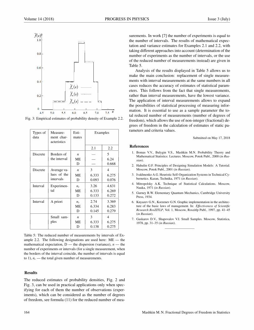
Volume 14 (2018) PROGRESS IN PHYSICS Issue 3 (July)
Fig. 3: Empirical estimates of probability density of Example 2.2.
Types ofdata
Measure-ment char-acteristics
Esti-mates
Examples
2.1 2.2
Discrete Borders ofthe interval
n — 5ME — 6.24D — 0.668
Discrete Average va-lues of theintervals
n 3 4ME 6.333 6.275D 0.093 0.076
Interval Experimen-tal
nr 3.26 4.631ME 6.333 6.269D 0.133 0.272
Interval A priori nr 2.74 3.369ME 6.334 6.283D 0.145 0.279
Small sam-ples
n 3 4ME 6.333 6.275D 0.138 0.275
Table 5: The reduced number of measurements by intervals of Ex-ample 2.2. The following designations are used here: ME — themathematical expectation, D — the dispersion (variance), n — thenumber of experiments or intervals (for a single measurement, whenthe borders of the interval coincide, the number of intervals is equalto 1), nr — the total given number of measurements.
Results
The reduced estimates of probability densities, Fig. 2 andFig. 3, can be used in practical applications only when spec-ifying for each of them the number of observations (exper-iments), which can be considered as the number of degreesof freedom, see formula (11) for the reduced number of mea-
surements. In work [7] the number of experiments is equal tothe number of intervals. The results of mathematical expec-tation and variance estimates for Examples 2.1 and 2.2, withtaking different approaches into account (determination of thenumber of experiments as the number of intervals, or the useof the reduced number of measurements instead) are given inTable 5.
Analysis of the results displayed in Table 5 allows us tomake the main conclusion: replacement of single measure-ments with interval measurements at the same numbers in allcases reduces the accuracy of estimates of statistical param-eters. This follows from the fact that single measurements,rather than interval measurements, have the lowest variance.The application of interval measurements allows to expandthe possibilities of statistical processing of measuring infor-mation. It is essential to use as a sample parameter the to-tal reduced number of measurements (number of degrees offreedom), which allows the use of non-integer (fractional) de-grees of freedom in the calculation of estimates of static pa-rameters and criteria values.
Submitted on May 17, 2018
References1. Bomas V.V., Bulygin V.S., Mashkin M.N. Probability Theory and
Mathematical Statistics: Lectures. Moscow, Potok Publ., 2000 (in Rus-sian).
2. Hahulin G.F. Principles of Designing Simulation Models: A Tutorial.Moscow, Potok Publ., 2001 (in Russian).
3. Ivakhnenko A.G. Heuristic Self-Organization Systems in Technical Cy-bernetics. Kazan, Technika, 1971 (in Russian).
4. Mitropolsky A.K. Technique of Statistical Calculations. Moscow,Nauka, 1971 (in Russian).
5. Gurney R.W. Elementary Quantum Mechanics, Cambridge UniversityPress, 1934.
6. Knyazev G.N., Korzenev G.N. Graphic implementation in the architec-ture of the basic laws of management. In: Effectiveness of ScientificResearch RosZITLP, Vol. 1, Moscow, Roszitlp Publ., 1997, pp. 41–45(in Russian).
7. Gaskarov D.V., Shapovalov V.I. Small Samples. Moscow, Statistica,1978, pp. 31–35 (in Russian).
164 Mashkin M. N. Fractional Degrees of Freedom in Statistics
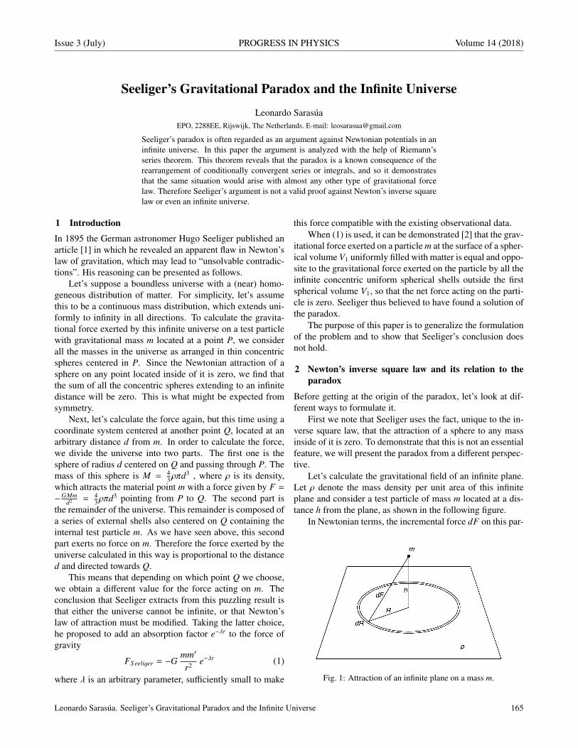
Issue 3 (July) PROGRESS IN PHYSICS Volume 14 (2018)
Seeliger’s Gravitational Paradox and the Infinite Universe
Leonardo SarasuaEPO, 2288EE, Rijswijk, The Netherlands. E-mail: [email protected]
Seeliger’s paradox is often regarded as an argument against Newtonian potentials in aninfinite universe. In this paper the argument is analyzed with the help of Riemann’sseries theorem. This theorem reveals that the paradox is a known consequence of therearrangement of conditionally convergent series or integrals, and so it demonstratesthat the same situation would arise with almost any other type of gravitational forcelaw. Therefore Seeliger’s argument is not a valid proof against Newton’s inverse squarelaw or even an infinite universe.
1 Introduction
In 1895 the German astronomer Hugo Seeliger published anarticle [1] in which he revealed an apparent flaw in Newton’slaw of gravitation, which may lead to “unsolvable contradic-tions”. His reasoning can be presented as follows.
Let’s suppose a boundless universe with a (near) homo-geneous distribution of matter. For simplicity, let’s assumethis to be a continuous mass distribution, which extends uni-formly to infinity in all directions. To calculate the gravita-tional force exerted by this infinite universe on a test particlewith gravitational mass m located at a point P, we considerall the masses in the universe as arranged in thin concentricspheres centered in P. Since the Newtonian attraction of asphere on any point located inside of it is zero, we find thatthe sum of all the concentric spheres extending to an infinitedistance will be zero. This is what might be expected fromsymmetry.
Next, let’s calculate the force again, but this time using acoordinate system centered at another point Q, located at anarbitrary distance d from m. In order to calculate the force,we divide the universe into two parts. The first one is thesphere of radius d centered on Q and passing through P. Themass of this sphere is M = 4
3ρπd3 , where ρ is its density,
which attracts the material point m with a force given by F =−GMm
d2 = 43ρπd
3 pointing from P to Q. The second part isthe remainder of the universe. This remainder is composed ofa series of external shells also centered on Q containing theinternal test particle m. As we have seen above, this secondpart exerts no force on m. Therefore the force exerted by theuniverse calculated in this way is proportional to the distanced and directed towards Q.
This means that depending on which point Q we choose,we obtain a different value for the force acting on m. Theconclusion that Seeliger extracts from this puzzling result isthat either the universe cannot be infinite, or that Newton’slaw of attraction must be modified. Taking the latter choice,he proposed to add an absorption factor e−λr to the force ofgravity
FS eeliger = −Gmm′
r2 e−λr (1)
where λ is an arbitrary parameter, sufficiently small to make
this force compatible with the existing observational data.When (1) is used, it can be demonstrated [2] that the grav-
itational force exerted on a particle m at the surface of a spher-ical volume V1 uniformly filled with matter is equal and oppo-site to the gravitational force exerted on the particle by all theinfinite concentric uniform spherical shells outside the firstspherical volume V1, so that the net force acting on the parti-cle is zero. Seeliger thus believed to have found a solution ofthe paradox.
The purpose of this paper is to generalize the formulationof the problem and to show that Seeliger’s conclusion doesnot hold.
2 Newton’s inverse square law and its relation to theparadox
Before getting at the origin of the paradox, let’s look at dif-ferent ways to formulate it.
First we note that Seeliger uses the fact, unique to the in-verse square law, that the attraction of a sphere to any massinside of it is zero. To demonstrate that this is not an essentialfeature, we will present the paradox from a different perspec-tive.
Let’s calculate the gravitational field of an infinite plane.Let ρ denote the mass density per unit area of this infiniteplane and consider a test particle of mass m located at a dis-tance h from the plane, as shown in the following figure.
In Newtonian terms, the incremental force dF on this par-
Fig. 1: Attraction of an infinite plane on a mass m.
Leonardo Sarasua. Seeliger’s Gravitational Paradox and the Infinite Universe 165
Volume 14 (2018) PROGRESS IN PHYSICS Issue 3 (July)
ticle contributed by an annular ring of radius R and incremen-tal width dR is just the projection onto the perpendicular ofthe forces exerted by each element of the plane around thecircumference of the annular region. Thus we have:
dF =Gmρ
h2 + r2 [π(R + dR)2 − πR2]( h√
h2 + R2
).
Expanding this expression and ignoring second order differ-ential terms, we get
dF = 2πGmρhR
(h2 + R2)32
dR .
Integrating from R = 0 to ∞, we find that the total force ex-perienced by the particle is
F = 2πGmρh∫ ∞
0
R
(h2 + R2)32
dR = 2πGmρ .
Thus the force exerted on the particle is independent of thedistance h from the plane. Adding more planes to form a slabof thickness a, we get that the force would be in this case:
F = 2πGmρa.
Grouping infinite parallel slabs of the same thickness a andadding the contribution of each of them, we get the force ofthe universe acting on particle m
F =∞∑−∞
2πGmρa . (2)
It can be shown that this infinite sum will yield a differentresult depending on how it is calculated. As a first way ofdetermining the value of (2), let’s pair each slab with its cor-responding symmetrical one around the plane of origin. If weconsider this plane as the plane xy, then we take a parallelslab of coordinate z0 and pair it with the slab of coordinate−z0. Since the force of each slab in the pair is equal and op-posite, their sum vanishes. The total force (2) will thus bezero. Analytically, we can write this as
F = (2πGρma − 2πGρma)+
+ (2πGρma − 2πGρma) + ... = 0 .(3)
Next, let’s calculate (2) again but this time starting one slabfurther from m. The total force on m will be the sum of theforce due to this separate slab, which contains m on one of itssurfaces, plus all the remaining slabs in the universe, on bothsides of the first slab, thus
F = 2πGρma0 +
0∑n=−∞
2πGρman −∞∑
n=1
2πGρman
where n = 0 represents the separate slab. Since the terms
0∑n=−∞
2πGρman −∞∑
n=1
2πGρman
are paired one to one as in (3), they cancel each other outand the result is zero. Therefore the total force on m will beF = 2πGρma, which is an arbitrary value, since a has beenarbitrarily chosen.
This new version of the paradox does not use the fact thatthe potential is null inside a sphere and yet, as in Seeliger’soriginal version, it can return any arbitrary value. It is possi-ble in fact to prove that the paradox occurs with a wide rangeof forces other than Newton’s inverse square law. With New-ton’s law, the force of each slab is independent of the dis-tance, thus the force exerted by each of the layers is the sameand cancels out with another slab located symmetrically fromthe given particle. However, if we had a different force lawin which the gravitational force of each slab were dependenton the distance, we still would be able to repeat the previouscalculation by choosing for each slab a suitable thickness soas to exactly balance another slab at the opposite side of theparticle, provided that the sum of the forces diverged.
3 Riemann series theorem
In 1827, mathematician Peter Lejeune-Dirichlet discoveredthe surprising result that some convergent series, when rear-ranged, can yield a different result [3]. Based on this dis-covery, another German mathematician, Bernhard Riemannpublished in 1852 a theorem [3], known today as Riemann’sseries theorem (or Riemann rearrangement theorem), provingthat in general, infinite series are not associative, that is, theycannot be rearranged.
According to this theorem (see for example [4]), an abso-lutely convergent series will always give the same result, nomatter how it is rearranged. However, a conditionally conver-gent series, by a suitable permutation of its elements, can takeany arbitrary value or even diverge.
Let’s review some definitions. A series converges if thereexists a value ℓ such that the sequence of the partial sums
S 1, S 2, S 3, ... , where S n =
n∑k=1
ak
converges to ℓ. That is, for any ϵ > 0, there exists an integerN such that if n ≥ N, then
|S n − ℓ| ≤ ϵ .
A series S n =∑∞
n=1 an converges absolutely if S n =∑∞
n=1 |an|converges. A series S n =
∑∞n=1 an converges conditionally if
it converges but the series S n =∑∞
n=1 |an| diverges.Riemann’s series theorem can be directly extrapolated to
conditionally convergent integrals (see for example [5]).In the case of Seeliger’s paradox, we note first that al-
though the masses in the universe should be treated as dis-crete, Seeliger for simplicity turns them into a homogeneousmass distribution throughout the universe, thus formulating itin terms of integrals instead of series. Like Seeliger, we will
166 Leonardo Sarasua. Seeliger’s Gravitational Paradox and the Infinite Universe

Issue 3 (July) PROGRESS IN PHYSICS Volume 14 (2018)
work with a continuous mass distribution, but bearing in mindthat the problem is actually discrete.
Considering a uniform mass distribution with a volumedensity ρ, and using a spherical coordinate system (r, θ, ϕ)centered on m, we have that, according to Newton’s law, thecomponent of the total force exerted on a particle m along thex axis is
Fx = −Gm∫ ∞
r=0
∫ π
θ=0
∫ 2π
ϕ=0ρ sin ϕ cos ϕ dϕdθdr , (4)
and similarly for the other axes.Since the integral is only conditionally convergent, we
have to pay attention to the order in which we calculate themultiple integral. In this case, our goal is to integrate sequen-tially the shells around the test mass, starting from r = 0 andextending to r = ∞, thus we have to integrate first over thevariables θ and ϕ and only then over r. Note therefore that (4)is not necessarily equal to
Fx = −Gm∫ 2π
ϕ=0
∫ π
θ=0
∫ ∞
r=0ρ sin ϕ cos ϕ drdθdϕ .
We solve the integral (4)
Fx = −Gm∫ ∞
r=0
∫ π
θ=0
∫ 2π
ϕ=0ρ sin ϕ cos ϕ dϕdθdr
= −Gm∫ ∞
r=0
∫ π
θ=0ρ
[sin
(− cos2 ϕ
2
) ]2π
ϕ=0dθdr = 0 ,
which, again, is what could be expected from symmetry. Fol-lowing Seeliger’s procedure, we can calculate the integral ina different way by splitting the space into a sphere of radiusa, centered in a point Q separated from m by a distance a,so that the test mass lies on its surface, and concentric shellsalso centered in Q containing the particle in their interior. Inother words, the contribution of every mass in the universe isadded but in a different order. Thus the integral is rearranged,which is what Riemanns’s theorem warns us against. TakingQ as the origin of coordinates, the x component of the forcewill be
Fx = −GmM
a2 −Gm∫ ∞
r=0
∫ π
θ=0
∫ 2π
ϕ=0ρ sin ϕ cos ϕ dϕdθdr . (5)
The first term on the right hand side of (5) is the attractionof the sphere, being M its mass, and a the distance betweenthe particle m and the center of the sphere. The second is theattraction of the concentric shells, which is zero. Therefore,
Fx = −GmM
a2 .
Since the integral is only conditionally convergent, it is nosurprise that the new integral obtained by a rearrangement ofits terms yields a different result.
Riemann’s theorem shows the reason why Seeliger’s para-dox occurs, and it also demonstrates that its origin is mathe-matical, not physical.
The integral converges to zero but any other rearrange-ment of the integral will yield a different value. Given theinfinitely many possible results, we are forced to ask whichone, if any, is the “correct” value, i.e. the one that a measureinstrument would register in reality. Riemann’s theorem doesnot provide a way to decide this, having therefore to rely onthe physical significance of each reordering of the integralor the series. The following two arguments, although lack-ing mathematical rigor, both indicate that the only valid wayto carry out the calculation is by considering the mass at thecenter of coordinates:
a) Since all the observable physical magnitudes in thissystem, i.e. the mass distribution, are smooth everywhere,i.e. infinitely differentiable (except possibly at the point wherethe test mass is located), it is required that any derived func-tion be also differentiable. Any discontinuity introduced inany of the magnitudes must be discarded as lacking physicalbasis. However, the force obtained when we calculate (5) is
F(r) =
−4
3GρπMr , r ≤ R0
−GMmr2 , r > R0
(6)
where r is the distance from the test mass to the center of thesphere, and R0 the radius of the latter. This function is differ-entiable at r = R0 only if R0 = 0. Thus, the only arrangementof terms which will provide a differentiable force function isthe one which considers the test mass at the origin of coordi-nates.
b) A non-nil result of (5) would be acceptable only if itis a constant finite value independent of r. That would cor-respond to the whole universe being pushed and moving inone direction with respect to absolute space. Since this ab-solute space is not detectable, we cannot determine whetherthis movement is actually taking place or not. However, ifthe force depends on r, different parts of the universe wouldbe pushed with different forces, giving rise to the motion ofsome masses with respect to other masses. This is not ob-served, and thus we have to reject this possibility.
The only case where the force (5) is independent of r iswhen F(r) = 0 everywhere. These two arguments both sug-gest that the nil result is the only one physically meaningful.
Some authors had already suspected that Seeliger’s para-dox has no physical relevance, [6], [7], but none of them givea rigorous explanation. It is common to find in the litera-ture regarding Seeliger’s paradox, confusing statements aboutconvergence of infinite series [6, 8]. Even Newton, in his fa-mous letter to Bentley [9], erred when he spoke about thestability of an infinite Universe:
... if a body stood in equilibrio between any two equaland contrary attracting infinite forces, and if to either
Leonardo Sarasua. Seeliger’s Gravitational Paradox and the Infinite Universe 167
Volume 14 (2018) PROGRESS IN PHYSICS Issue 3 (July)
of these forces you add any new finite attracting force,that new force, howsoever little,will destroytheir equi-librium.
In the situation described by him we have two oppositeinfinite sides pulling on each other, or ∞ − ∞. This is inde-terminate and so, it might or might not be stable. However, ifwe assume the stability of the system, as Newton does, it isobvious that adding a finite quantity of mass to either infiniteside will not destroy the equilibrium, since a finite quantityadded to an infinite one will not alter the latter, and so it willmake no difference in the balance between the two infinitehemispheres of the universe. The universe will thus remainstable.
4 Conclusion
We have proved, with the help of Riemann’s series theorem,that Seeliger’s paradox has no physical significance. It is theconsequence of a flawed manipulation of infinite condition-ally convergent integrals. Therefore the paradox cannot beused as a valid argument against Newton’s potential or theinfiniteness of the universe.
Received on May 22, 2018
References1. Seeliger H. Ueber das Newton’sche Gravitationsgesetz. Astronomische
Nachrichten, 1895, N. 3273 v. 137 (9), 129–136.
2. Ghosh A. Origin of Inertia, Extended Mach’s Principle and Cosmolog-ical Consequences. Apeiron, Montreal, 2000, p. 20.
3. Riemann B. Ueber die Darstellbarkeit einer Function durch einetrigonometrische Reihe. Abh. der Kgl. Ges. der Wiss. zu Gottingen,1867, v. 13 (3), 423–428.
4. Galanor S. Riemann’s Rearrangement Theorem. Mathematics Teacher,Nov. 1987, v. 80 (8), 675–681.
5. Timko E. J. Rearrangement on Conditionally Convergent Integrals inAnalogy to Series. Electronic Proceedings of Undergraduate Mathe-matics Day, 2008, v. 3 (6), Paper 23.
6. Norton J. The Cosmological Woes of Newtonian Gravitation Theory.The expanding worlds of general relativity, presentations of the fourthconference on the and gravitation held in Berlin, July 31-August , 1999,v. 7, 271.
7. Vickers H. Was Newtonian Cosmology Really Inconsistent?. Studies inHistory and Philosophy of Modern Physics, 2008, v. 40 (3), 197–208.
8. Harrison E. R. Cosmology. Cambridge University Press, Cambridge,1981, p. 280.
9. Newton I. Correspondence with Richard Bentley [1692–3]. CambridgeUniversity Press, Cambridge, 1924.
168 Leonardo Sarasua. Seeliger’s Gravitational Paradox and the Infinite Universe
Issue 3 (July) PROGRESS IN PHYSICS Volume 14 (2018)
Utilizing Future-Viewing Instruments
Aaron M. FeeneyE-mail: [email protected]
The concept of future-viewing instruments is examined in detail. This term refers todevices which, under some circumstances, could allow users to directly observe futurescenes. It is shown that such a technology would enable systems of intertemporal dataexchange without any possibility of paradox or “auto-generated information” [1]. In-struments of this type could lead to the founding of an intertemporal Internet. Workingout how they could be invented and constructed are matters left for the reader.
1 Introduction
The idea of instruments for viewing future scenes appearedin fiction as early as 1924, and this concept was introducedto millions of television viewers in the 1960s [2–4], but ithas yet to be thoroughly examined in academic circles. Onthe other hand, the related concept of travel to the past hasreceived considerable attention from scientists and philoso-phers, especially in recent decades. Here, the logical dimen-sions of future-viewing instruments will be explored and thencontextualized in terms of what has been learned about thelogical dimensions of time travel. With this understanding itbecomes possible to entertain ideas about how future-viewinginstruments could be utilized.
Tales of mystic seers abound in myths from ancient cul-tures. The ancient Greeks told of Cassandra, princess of Troy.In her youth, she and her brother gained the gift of prophecyduring an overnight stay in the temple of Apollo. After shegrew to become a beautiful woman, Cassandra spent anothernight in the temple. Apollo then appeared to her and soughtintimacy. She refused him, so Apollo cursed Cassandra. Hedecreed that her prophecies would be disbelieved; thus, theseeds of tragedy were sown. Cassandra warned that warriorshid in the wooden horse, but she was thought a lunatic [5].
Although the concept of individuals who are able to ac-cess future scenes in personal visions is directly relevant tothe topic at hand, it will not be discussed further here. Thefocus instead will be the concept of technological instrumentsthat normal individuals could use to see into the future. A per-son who controls and monitors a future-viewing instrumentwill be referred to as its operator.
To begin, it is necessary to isolate an appropriate conceptof future-viewing instruments. What kind of device would beboth useful as a future-viewing instrument and logically pos-sible? The analysis must start with consideration of a foun-dational issue—information. The future is unknown to us.Information about any set of unknowns may be either definiteor ambiguous as well as correct or incorrect.
Thinking about a playing card concealed in a box, con-sider an example of definite information about it: “The cardin the box is the queen of hearts.” Definite information whichalso happens to be correct, of course, is the most useful. One
might instead receive ambiguous information: “The box con-tains some card in the suit of hearts.” Correct but ambiguousinformation might also be useful. However, when vague in-formation approaches maximal ambiguity it becomes so non-specific that it is guaranteed to be correct, rendering it useless.
In considering possible types of future-viewing machines,a maximally ambiguous device might be imagined. Sucha device would display every possible happening associatedwith a given selected set of future spatio-temporal coordinates(x, y, z, t), but it could not highlight what will actually happen.Devices of this type are here termed Everett machines, refer-encing physicist Hugh Everett III’s influential 1957 “relativestate” interpretation of quantum mechanics [6].
Being maximally ambiguous, Everett machines would beuseless as future-viewing instruments. They are unable to tellwhat will occur among everything that might occur at any setof future coordinates under examination; in a term, they arenot outcome-informative. For this reason, Everett machinescannot be classified as future-viewing instruments. Outcome-informative devices have the ability to provide definite andcorrect information about future events, at least in some cases.
How powerful could a future-viewing instrument possi-bly be? Composite devices such as have appeared in fiction,which somehow have agency and the means to force theirown prophecies to come true, must be excluded from con-sideration.∗ Future-viewing devices which are only capableof gathering and displaying information will here be termedinert future-viewing instruments. Given this important refine-ment, the following question may be asked: How powerfulcould an inert future-viewing instrument possibly be?
To answer this question, the maximal case is explored.Consider an inert future-viewing device which is always ableto provide definite and correct information about all futureoutcomes in every possible circumstance of attempted future-viewing. These hypothetical devices for exploring the max-imal case are termed Cassandra machines after Cassandra’stragic helplessness in averting the calamities she foresaw.
It will be shown that Cassandra machines, as defined, arenot logically possible; no inert device could provide definite
∗It would appear that Serling’s most unusual camera can occasionallyexert diabolical control over those who end up in its pictures of the future [3].
Aaron M. Feeney. Utilizing Future-Viewing Instruments 169
Volume 14 (2018) PROGRESS IN PHYSICS Issue 3 (July)
and correct information about all future outcomes in everypossible circumstance of attempted future-viewing. A sin-gle counterexample situation is sufficient to prove this. Thissituation will emerge as one mode of a future-viewing exper-iment involving three randomly selected modes. The experi-ment will be built up in stages; the counterexample mode willbe presented at the end.
Begin by imagining an experimental setup consisting ofan inert, though otherwise arbitrarily powerful future-viewinginstrument (FVI) and a computer. The computer is constantlybeing fed a string of ones and zeros from a random num-ber generator (RNG). The RNG contains a radioactive sampleconnected to a sensitive Geiger counter. The pattern of onesand zeros the RNG produces is a function of the output of theGeiger counter, so no known prediction methodology couldpredict the sequence produced.
The computer will use an algorithm to process one secondof the sampled output of the RNG to arrive at a whole numberin the range 0 through 99. This number will be displayed onits large and bright, two-digit readout.
Many kinds of algorithms can be used to determine awhole number, within any desired range, from any finite setof ones and zeroes. For instance, in order to arrive at a wholenumber in the range 0 through n, divide the number of onesin the set by (n + 1) to find the remainder. With completedivision represented by a remainder of 0, the remainder willalways be a whole number in the range 0 through n.
Here is a simple two-step experiment involving these sys-tems. Each step lasts one minute. At the start of step one,the FVI will attempt to future-view the computer’s two-digitreadout as it will appear in the middle of step two, i.e., aminute and thirty seconds later. When step two arrives, thecomputer will sample one second of the RNG’s output and,by dividing the total number of ones in the sample by 100 tofind the remainder, it will arrive at some whole number in therange 0 through 99 for display on its readout. This numberis calculated and displayed within a few seconds and it willremain displayed throughout step two.
It should be no surprise that a properly functioning future-viewing instrument (in this situation) would always be ableto correctly show, during step one, the whole number thatthe computer will interpret from RNG data and display on itsreadout during step two. An unpredictable process alone doesnot render the final outcome any less visually apparent whenit arrives, and there are no logical barriers here.
Now, another system is added to the experiment. A char-acter recognition system (CRS) is placed between the FVIand the computer. The CRS receives input from its camerawhich is pointed at the FVI’s display. During step one, theCRS will recognize any computer readout digits it finds onthe FVI’s display and will assign the corresponding numberas the value of the variable ‘z’ to be stored in its memory.
The critical detail which allows the counterexample toemerge in this expanded setup is that the computer has the
ability to temporarily connect to the CRS and retrieve z. Hereis the full experiment, encompassing all three modes:
As before, a two-step protocol is followed and each stephas a duration of one minute. Before each run, the computeruses RNG data to reset its readout to some whole numberin the range 0 through 99 to establish a preliminary value.Then, at the beginning of step one, the FVI attempts to seewhat number will be displayed on the computer’s two-digitreadout in the middle of step two, a minute and a half later.If the FVI is successful in receiving an image, the CRS willrecognize the number in the image and store it as z. If the FVIdoes not receive an image, the CRS will revert to defaults andassign 0 as the value of z.
At the beginning of step two, the computer will sampleone second of RNG data and process it to yield a whole num-ber in the range 0 through 2. This selects one of the followingthree programs for the computer to run immediately:
PR: Sample one second of the RNG output, interpret asa whole number in the range 0 through 99, display theresult on the readout, then halt.
P0: Connect to the CRS and retrieve z, then disconnectfrom the CRS. Halt if the number on the readout equalsz + 0, otherwise change the readout to display a numberequaling z + 0, then halt.
P1: Connect to the CRS and retrieve z, then disconnectfrom the CRS. Halt if the number on the readout equalsz + 1, otherwise change the readout to display a numberequaling z + 1, then halt.
In each of these cases, the computer will finish all tasksand halt within a few seconds. In any kind of run, the FVIis involved in an attempt during step one to receive a signalcontaining an image of the post-halt value that the computerwill display during step two.
Consider what would happen in a series of experimentsusing this expanded setup. In any PR-mode run, althoughthe z-value has been ignored by the computer, subsequentcomparison will reveal that it matches the generated post-haltvalue. Consistent matching in PR-mode runs confirms the in-strument’s basic functionality.
Next, in any run selected as a P0-mode run at the outsetof step two, the z-value encoded by the CRS during step onewill also always be correct. It must be. After all, z has beenretrieved from the CRS and z + 0 = z. So, the post-halt valuein P0 runs comes from the z-value, but where does the z-valuecome from? It comes from the post-halt value. So, anotherquestion must be asked: What determines the value itself?This is the purpose of resetting the readout to a preliminaryvalue before step one. In every run that will turn out to bea P0-mode run, the FVI will detect a post-halt value equalto the preliminary value. In P0-mode runs, although any z-value at all encoded during step one would end up on thecomputer’s readout in step two, only the preliminary value is
170 Aaron M. Feeney. Utilizing Future-Viewing Instruments
Issue 3 (July) PROGRESS IN PHYSICS Volume 14 (2018)
non-arbitrary. So, even though P0 follows the form of a self-fulfilling prophecy, the z-values encoded during step one ofP0-mode runs are still recognizably genuine prophecies sincethe mode of a given run is not decided until step two.
P1-mode runs, however, would produce a very differentkind of result. If RNG data will select P1 at the beginningof step two, no z-value whatsoever encoded during step onecould correctly identify the post-halt value that will be dis-played on the readout, since z + 1 , z. In P1-mode runs, itis impossible for any z-value to be correct; the z-value andpost-halt value in P1-mode runs will never match.∗
This establishes that no device whatsoever could fulfill thedefinition of a Cassandra machine: Inert devices which wouldbe able to provide definite and correct information about allfuture outcomes in every possible circumstance of attemptedfuture-viewing are not logically possible.
So far, two kinds of hypothetical devices have been de-scribed; they are Everett machines which would not be usefulas future-viewing instruments and Cassandra machines whichare not logically possible. Eliminating both of these imaginedconceptual options helps to identify an appropriate concept offuture-viewing instruments.
For further understanding, it must also be recognized thatany device which could ever provide incorrect (i.e., mislead-ing) information regarding future events cannot be a future-viewing instrument. This is due to the important distinctionbetween viewing future events directly, which cannot involveguesswork, and merely generating predictions about futureevents, which must involve guesswork. Visually accessingveridical foreknowledge is unlike the uncertain process ofgenerating predictions.
Upon the above analysis, three features of any future-viewing instrument of an operationally coherent descriptionmay be specified: (1) Such an instrument must be outcome-informative, unlike an Everett machine, (2) it must be logi-cally possible, unlike a Cassandra machine, and (3) it mustbe incapable of providing incorrect (i.e., misleading) infor-mation about future events. Devices which satisfy all threerequirements have been termed foreknowledge instruments.
Foreknowledge instruments could be used to gain defi-nite and correct information about future outcomes in a widerange of circumstances corresponding to PR-mode and P0-mode runs within the RNG experiment. Definite and correctinformation about future outcomes obtained from foreknowl-edge instruments will be termed viewer foreknowledge. Sinceforeknowledge instruments cannot misinform, definite infor-mation about future states obtained from foreknowledge in-struments will always prove to be correct. So, it would bepossible to recognize viewer foreknowledge upon reception.However, as the RNG experiment demonstrates, viewer fore-knowledge would not always be accessible.
∗The post-halt value in P1-mode runs will always be 1. This is becausethe CRS will not detect anything from the FVI, since the FVI cannot acquirea signal; so, the CRS will revert to defaults and assign 0 as the value of z.
Situations exemplified by P1-mode runs, wherein future-viewing cannot occur, are here termed interference viewingsituations. Viewer foreknowledge would only be accessi-ble within non-interference viewing situations, exemplifiedby runs of the two non-interfering programs, PR and P0.
2 Time machines and foreknowledge instruments
Time travel to the past will be referred to as pastward timetravel. Pastward time travel and future-viewing are intimatelyrelated, for each could be used to acquire information fromthe future. So, if pastward time travel and future-viewing re-ally are coherent concepts, they should be found to naturallycohere within a single conceptual context.
Serious interest in pastward time travel began when KurtGodel proved in 1949 that the equations of general relativitypermit pastward time travel situations [7]. Extensive tech-nical details concerning how time travel or future-viewingmight be achieved within the framework of general relativ-ity, or any other, are not needed here. The aim of this sectionis to explore the logical dimensions of pastward time travel,not how it might be achieved. Furthermore, it would not beappropriate to limit a discussion of the logical dimensions oftime travel to any theoretical framework.
Conceptually, relocation may be achieved by continuousmovement between spatio-temporal points, i.e., translation,or by what will be termed discontinuous relocation. Trans-lation is familiar to everyone. Discontinuous relocation willhere be defined as a process whereby a vehicle, for instance, ismade to disappear from one location and reappear somewhereelse, either a moment later or in a different time period alto-gether, even much earlier. Whether discontinuous relocationcould be achieved, and how it could be achieved, are irrele-vant considerations. For the current discussion it is merelynecessary to recognize that discontinuous relocation is a log-ically possible mode of travel (i.e., relocation).
Since translation and discontinuous relocation exhaust allpossibilities for relocation in space and time, it is possible toobtain exhaustive conclusions about the logical dimensionsof time travel without referencing any further specifics abouthow time travel might be achieved. This allows the argumentto be conducted without tying it to any theoretical framework.
The central issue in any discussion of the logical dimen-sions of time travel concerns whether past-alteration para-doxes, which are so popular in fictional treatments of the sub-ject, could ever be actualized. An extended argument willestablish that it is not possible for changes to the past and ac-companying paradoxes to result from the accomplishment ofpastward time travel, no matter how accomplished. This ar-gument will begin by referencing methods of pastward timetravel based on translation, such as exist in general relativity.A simple extension of the argument will additionally showthat paradoxes could not result from any form of pastwardtime travel based on discontinuous relocation.
Aaron M. Feeney. Utilizing Future-Viewing Instruments 171

Volume 14 (2018) PROGRESS IN PHYSICS Issue 3 (July)
The arguments of this section will explore time travel andfuture-viewing as conceived within a single timeline, sincemultiple-timeline models of time travel inherently sidestepany possibility of paradoxes. For instance, under a multiple-timeline model, if a time traveler were to go back in time andsuccessfully prevent his parents from meeting, his own birthwould remain safely unaffected in his origin timeline. Onlytime travel from a given timeline to its own earlier periodshas ever been thought to offer any potential for paradox, somultiple-timeline models are safely ignored here.
Fiction has distorted our perceptions about time travel. Itwill be shown below that events which have happened oneway without time travelers cannot somehow be made to hap-pen again, but differently, if time travelers would ever happento visit that time and place. While stories based on such ab-surdities can be entertaining, the misconception that the prac-tice of time travel might ever actualize revisions to the pasthas been termed the “second-time-around fallacy” [8]. Thefollowing quotation from philosopher Larry Dwyer providesa sensible way to think about pastward time travel:
If we hypothesize that T pulls levers and manip-ulates a rocket in 1974, and travels back in timeto the year 3000 B.C. then of course, even beforeT enters his rocket, it is true that any accuratecatalogue of all the events on earth during theyear 3000 B.C. would include an account of T’sactions, reactions and mental processes. Thereis no question of the year 3000 B.C. occurringmore than once. [9]
Although theoretical considerations related to achievingpastward time travel are not needed in the present discussion,some operational concepts are helpful for purposes of visu-alization. Imagine a device which is able to open hyperdi-mensional tunnels to past, present, and future spatio-temporalpoints. Travelers who would pass through such tunnels couldtravel great distances or achieve time travel to any connectedera, and be retrieved. The device would remain stationed inthe laboratory throughout.
This way of visualizing time travel by translation is foundin the colorful literature of general relativity. Solutions ofEinstein’s field equations which describe hyperdimensionaltunnels have existed since 1916, though travel concepts werenot part of the early work in this area. Physicist LudwigFlamm discovered solutions describing such tunnels shortlyafter the publication of general relativity [10]. These struc-tures were further explored by Hermann Weyl in the 1920s[11]. Then, in 1935, when Albert Einstein and Nathan Rosenattempted to formulate solutions of Einstein’s field equationsfree from singularities, they were also led to such structures:“These solutions involve the mathematical representation ofphysical space by a space of two identical sheets, a particlebeing represented by a ‘bridge’ connecting these sheets” [12].These connecting structures came to be known as Einstein-
Rosen bridges. In 1955, physicist John Wheeler named them“wormholes” [13].
In 1969, Homer Ellis and Kirill Bronnikov independentlysolved Einstein’s field equations to describe gravitating, two-way traversable wormholes, and their works were publishedin 1973 [14, 15]. These ideas led to an understanding ofwormholes of a kind that would be appropriate for travel, timetravel, future-viewing, and past-viewing. These structuresare non-gravitating, two-way traversable wormholes knownas Ellis wormholes [16]. In 1988, Kip Thorne, Mike Morris,and Ulvi Yurtsever independently derived such structures andadded important details to the discussion [17].
Two years later, these physicists co-authored an influen-tial paper with Igor Novikov and three other physicists whichsuggested a “principle of self-consistency” would unfailinglygovern pastward time travel situations [18]. Novikov beganthe tradition, at least in physics literature, of time travel freefrom paradoxes in a co-authored 1975 work [19].
Returning to the development of the argument, it is worthnoting that all “arguments from paradox” against the possibil-ity of pastward time travel require a false premise—that everypossible form of pastward time travel would let time travelersalter past events. However, a form of time travel which wouldnot allow past-alteration has been understood for decades.
The key to understanding this concept of time travel isthe idea that time machines which operate accordingly wouldnot be able to fulfill every time travel request. Author RobertHeinlein may have been the first to suggest what may be re-ferred to as a gatekeeping mechanism, a natural process whichgoverns whether any given attempt to travel back to a partic-ular set of coordinates in the past will prove to be successfulwhen a time machine is activated for that purpose.
In terms of pastward time travel via traversable worm-holes, for instance, a gatekeeping mechanism would deter-mine, in a given situation of attempted time travel, whetherthe wormhole manipulation device being used will be able toenlarge the selected natural microscopic wormhole and con-dition it for transport, or not.∗
A gatekeeping mechanism would act to enforce a consis-tent logic of time travel; any given attempt to send peopleinto the past can only occur in a consistent manner if the pastincludes their visit as a result of that very attempt. Heinleinimagined that nature would always prevent the success of anyother kind of pastward time travel attempt, thereby eliminat-ing any chance of time travel paradoxes. Heinlein revealedthis basic but profound insight in a conversation between twocharacters in his 1964 novel, Farnham’s Freehold:
“The way I see it, there are no paradoxes in timetravel, there can’t be. If we are going to makethis time jump, then we already did; that’s whathappened. And if it doesn’t work, then it’s be-
∗“One can imagine an advanced civilization pulling a wormhole out ofthe quantum foam and enlarging it to classical size.” [17, see p. 1446]
172 Aaron M. Feeney. Utilizing Future-Viewing Instruments

Issue 3 (July) PROGRESS IN PHYSICS Volume 14 (2018)
cause it didn’t happen.”“But it hasn’t happened yet. Therefore, you aresaying it didn’t happen, so it can’t happen. That’swhat I said.”“No, no! We don’t know whether it has alreadyhappened or not. If it did, it will. If it didn’t, itwon’t.” [20]
It turns out that pastward time travel, while difficult to ac-complish, is basic from a logical point of view. Tenses andperceptions of time confuse many issues that are easy to un-derstand within a tenseless picture of space and time. Thiskind of picture was developed by the German mathematicianHermann Minkowski, and it is the subject of his groundbreak-ing 1908 lecture, “Raum und Zeit” [21]. Although the term‘spacetime’ will be avoided here, other terms associated withthe work of Minkowski and Einstein will be used which effi-ciently refer to important spatio-temporal concepts that wouldbe meaningful in any theoretical framework.
Four-dimensional spatio-temporal coordinates (x, y, z, t)are sufficient to specify any location in our universe at anytime, i.e., any world-point [21] defined with respect to somearbitrary origin. So, relations between any two world-pointscan be discussed in a tenseless fashion, just as one woulddiscuss relations between points plotted on graph paper. Forinstance, regarding time travel by wormhole, the relation ofinterest concerns whether two world-points are bridged by atraversable wormhole:
“If it did, it will,” describes two world-points bridgedby a traversable wormhole.“If it didn’t, it won’t,” describes two world-points notbridged by a traversable wormhole.
The antecedent phrases, “[i]f it did” and “[i]f it didn’t,”refer to what has happened at the intended pastward desti-nation, and the consequent phrases, “it will” and “it won’t,”describe the corresponding event of success or failure to ini-tiate pastward time travel that will be discovered once thewormhole manipulation device has been activated for thatpurpose. Note that world-points which are not bridged bya traversable wormhole cannot somehow change to becomebridged; the configuration of world-points is fixed in the ten-seless picture.
The argument to show that time travel to arbitrary world-points within a single-timeline model is not possible will fol-low shortly, but first it is necessary to discuss the ontologyof time. As will be established below, the only ontology thatcould accommodate pastward time travel and future-viewingis eternalism, also known as the block universe concept.
Within eternalism, every event in a given spatio-temporalmanifold exists together with every other event in a coherent,unchanging whole, and all times are ontologically identical.(Multi-timeline forms of eternalism need not enter the discus-sion, for reasons explained above.) Eternalism will be con-trasted with the growing block universe concept which holds
that, while the past has become fixed, the ever-advancing mo-mentary present is ontologically distinct from the past, andfuture events have yet to be forged in the advancing now.
The reason eternalism is the only ontology relevant inthe context of future-viewing and pastward time travel is thatthese technologies would allow questions about the ontologyof time to be answered empirically, in favor of eternalism. Forinstance, through wormhole time travel or future-viewing ac-complished using wormholes, it would be possible for peoplestationed in different centuries to conduct a two-way radioconversation through the wormhole throat. Demonstrationsof this sort would entirely rule out the growing block uni-verse concept. After all, future-dwellers could not reply to usif the future does not exist and time travelers could not visitand return from a future that is not there.∗ As such, any argu-ment purporting to reach a conclusion with relevance to timetravel and use of a “time viewer” [23, see p. 283] to see intothe past or future must be cast within eternalism.
A few more background details are necessary before thefinal argument against the possibility of time travel paradoxescan be presented. It is important to discuss how change andmovement are conceptually accommodated within the tense-less, unchanging picture of eternalism.
When particle movements are graphed, four-dimensionalworld-lines are traced out [21]. All world-lines are completewithin eternalism. One can see that collections of particleworld-lines may describe any object or body in space endur-ing through time, including all internal occurrences and allactions (e.g., digestion, typing, walking). Such collectionswill be referred to as composite world-lines.
So, within eternalism, the composite world-lines of hu-man beings are complete from birth to death in every phys-ical and behavioral detail. Since a composite world-line isa record of all change and movement, no world-line can bechanged or moved. This applies to all past world-lines in bothontologies, and in either view, no individual may change anyaspect of his or her future composite world-line.
Change requires a difference between an initial state anda post-change state. Comparing ontologies, under the grow-ing block universe concept it is not possible for a person tochange his or her future composite world-line because it doesnot exist; in this view, the future is made in the objectivelyadvancing present. Under eternalism, even though a person’sfuture composite world-line exists in its entirety, it exists asthe accumulated product of actions taken and processes whichoccur in that person’s perceived advancing present. So, un-der eternalism, it remains the case that one’s future compos-ite world-line is not and cannot be changed. It is fulfilled.Philosopher J.J.C. Smart expressed the distinction betweenacting in the present to produce the future and the mistakenidea of “changing the future,” this way:
∗As one would expect, the view known as presentism which holds thatonly the present exists would also be thoroughly ruled out [22].
Aaron M. Feeney. Utilizing Future-Viewing Instruments 173

Volume 14 (2018) PROGRESS IN PHYSICS Issue 3 (July)
...[T]he fact that our present actions determinethe future would be most misleadingly expressedor described by saying that we can change the fu-ture. A man can change his trousers, his club, orhis job. Perhaps he may even change the courseof world history or the state of scientific thought.But one thing that he cannot change is the future,since whatever he brings about is the future, andnothing else is, or ever was. [24]
With this background in place, the promised argumentfor the impossibility of paradoxes arising from pastward timetravel will now be presented: Considering whether paradoxesdue to time travel could occur at all requires considerationof a successful instance of pastward time travel. Therefore,begin by positing one such instance. For reasons explainedabove, this is a posit which requires eternalism. So, in thisinstance of pastward time travel, the composite world-linesof time travelers are necessarily embedded in “the past” asjudged with respect to the date of their journey’s origin. Thismeans that the actions of these time travelers during their visitare necessarily part of the historical background leading to theworld situation of their journey’s origin.
So, paradoxes emerging from pastward time travel wouldonly be possible if the composite world-lines of time travel-ers embedded in the past could be made to change, move, ordisappear. However, world-lines cannot be made to change,move, or disappear. Ultimately, pastward time travel cannotlead to paradoxes due to the unalterable geometry of com-pleted world-lines within eternalism, wherein all world-linesare complete. Within a single timeline model, the unalterablenature of world-lines produces all the effects of a gatekeepingmechanism which include making past-alteration impossible.
This argument will now be extended for sake of thorough-ness. One might imagine that some unknown method of timetravel which somehow operates according to discontinuousrelocation might allow time travelers to visit scenes whichdid not involve time travelers “the first time around.” How-ever, examining the tenseless picture of eternalism shows thatthis is not the case:
“If it did, it will,” describes two world-points associatedby discontinuous relocation.“If it didn’t, it won’t,” describes two world-points notassociated by discontinuous relocation.
In order for a time traveler using a form of time travelbased on discontinuous relocation to visit a scene which didnot involve time travelers “the first time around,” specific con-ditions must obtain. For a given world-point w to qualify ashaving been without visits from time travelers, w must not beassociated with another world-point by discontinuous reloca-tion and w must not be a world-point visited by time travelersusing some form of time travel based on translation.
If one symbolizes “world-point w is associated with an-other world-point by discontinuous relocation” as Dw, and
symbolizes “world-point w is visited by time travelers usingsome form of time travel based on translation” as Tw, thenin order for a given world-point w to qualify as having beenwithout visits from time travelers “the first time around,” both¬Dw and ¬Tw must obtain. So, even a method of time travelbased on discontinuous relocation could not allow time trav-elers to visit world points that were not visited by time travel-ers “the first time around,” since there can be no world-pointw for which the statements Dw and ¬Dw are both true.
As continuous and discontinuous means of travel exhaustall possibilities for relocation in any spatio-temporal mani-fold, it is possible to conclude that, regardless of the way inwhich pastward time travel might ever be achieved, it couldnever lead to changes to the past or paradoxes of any sort.
This understanding produces unwavering clarity. No typeof vexation ever thought to rule out time travel remains.∗ Allof the imagined logical barriers which would fundamentallyblock the actualization of time machines and foreknowledgeinstruments have turned out to be illusory.
With any technology that would allow information to betransferred from later to earlier world-points, temporal gate-keeping is key. In other words, in any given effort to travelpastward, time machines will only be able to send travelersto parts of the past that were visited by those very travel-ers as a result of that very effort to send them pastward, andlikewise, any attempt to use a foreknowledge instrument toreveal future events will only be successful if, from the per-spective of the future, that attempt to peer into the future hadbeen successful. In both scenarios, the world at the “futureend” results from the world at the “past end,” and so, in eithertechnological case, the resulting state of affairs is necessarilycompatible with all events occurring at the “past end.”
Related to these findings, quantum information pioneer,Seth Lloyd, with other scientists, produced four papers in2010 and 2011 which present a formal model here called theP-CTC model [25, 28–30]. In effect, the P-CTC model is atemporal gatekeeping model.
3 Obtaining viewer foreknowledge
The three modes of the RNG experiment produce three dif-ferent kinds of viewing situations. An understanding of thesesituations is a necessary prerequisite to deciphering how fore-knowledge instruments would operate in real-world settings.
∗Along with past-alteration paradoxes, another potential problem hasbeen imagined, the “paradox of auto-generated information” or the “un-proved theorem paradox” [1, 25]. The unproved theorem paradox appearsin a groundbreaking 1991 paper by physicist David Deutsch [26]. Lloyd etal. address this issue. Their “[u]nproved theorem paradox circuit” affirms theconclusion that meaningful information cannot be auto-generated via closedtimelike curves (CTCs) [25]. (CTCs are trajectories apparent within somesolutions of general relativity which would allow an object to meet an earlierversion of itself—i.e., to travel pastward.) An objection was raised to theirresolution of the unproved theorem paradox [27], but Lloyd et al. showed thebasis of the objection to be erroneous [28].
174 Aaron M. Feeney. Utilizing Future-Viewing Instruments
Issue 3 (July) PROGRESS IN PHYSICS Volume 14 (2018)
PR produces what will be described as an independentviewing situation. Outcomes which have been foreseen in anindependent viewing situation during a given session with aforeknowledge instrument are not contingent in any way upondata received in that session.
On the other hand, P0 produces a cooperative viewingsituation, a kind of circumstance wherein data received inviewer foreknowledge of an outcome factors into the detailsof that outcome or is responsible for its very occurrence.
Within independent viewing situations and cooperativeviewing situations, there are no logical barriers to the recep-tion of viewer foreknowledge. As such, they are both classi-fied as non-interference viewing situations. These situationsrepresent two different ways of not using data from the instru-ment to interfere with the outcome. In PR-mode runs the datais not involved in the outcome at all, and in P0-mode runs thedata is followed exactly. If independent viewing and cooper-ative viewing exhaust all modes of non-interference, then aninterference viewing situation will arise in every other kind ofcase, exemplified by what happens in P1-mode runs.
It is important to determine whether there are any basiclimitations which must affect the practice of future-viewing.Are there kinds of outcomes a particular foreknowledge in-strument operator will fundamentally be unable to foresee?
Operators who are able to achieve an independent viewingsituation with respect to a given event will be able to foreseeit, for no logical barriers will be encountered. However, noindividual can achieve an independent viewing situation withrespect to the events of her own future life, assuming she willretain her memories. This important limitation will be calledthe self-implication effect of viewer foreknowledge; individ-uals are necessarily implicated in their own futures.
What about cooperative viewing situations? Could a per-son witness video sequences of her own future actions withina cooperative viewing situation if she later follows what shehas seen exactly? Attempting to arrange such a circumstancewould overwhelmingly tend to produce an interference view-ing situation. However, an individual could receive limitedsecond-hand information regarding some general features ofher future. To explain, two new terms are helpful:
Viewing interval: The interval of time elapsed betweenthe reception of viewer foreknowledge pertaining to aset of outcomes and the occurrence of those outcomes.
Operator pool: The operator of a foreknowledge in-strument, along with any additional witnesses (if any)during the reception of viewer foreknowledge, togetherwith other individuals (if any) who—during the view-ing interval—will be apprised of the results or whowill be instructed or influenced based on such results(whether or not they have been made aware of the ex-istence of foreknowledge instruments). This term car-ries another layer of meaning, for ‘operator’ may alsorefer to a mathematical function; the combined input-
to-output processing carried out by members of an op-erator pool will result in (or cohere with) the future-viewed outcome.
For instance, a person might be informed that she willstill be alive in forty years time. This particular factual de-tail is chosen because it admits no variation other than itsfalsification. A person could not be truthfully informed thatviewer foreknowledge has revealed she will still be alive inforty years time, only for her to somehow lose her life at anearlier point. Operator pools are formed only when viewerforeknowledge has been received. All effects upon the worldthat a given operator pool will generate within the associatedviewing interval have therefore passed temporal gatekeeping.So, these effects will at least partially produce (or, for inde-pendent viewing, have no causal relation with) the outcomesreceived in viewer foreknowledge. These effects, of course,include everything the earlier members of the pool will telllater members of the pool. For this reason, no member ofan operator pool will do, say, or successfully achieve any-thing that will prevent, or result in any modification to, theoutcomes foreseen.
How would independent viewing situations and coopera-tive viewing situations manifest in real-world settings withhuman operators and witnesses? Either the occurrence ofa set of future events is compatible with being foreseen byparticular operators and witnesses during a particular future-viewing session, or not. In the case of compatibility, a givenfuture-viewing attempt can succeed. Without such compat-ibility, operators and witnesses could not gain viewer fore-knowledge about what will occur at the chosen future co-ordinates during that situation of attempted future-viewing.(However, one person leaving the room might be enough toachieve compatibility; this could occur if the self-implicationeffect had been the cause of interference.)
It is apparent that the logic of future-viewing is anothermanifestation of temporal gatekeeping. Future-viewing andpastward time travel cohere within a seamless whole.
4 Handling foreknowledge instrument data
So far, the discussion has focused on the actions of networksof human beings within a viewing interval who have obtainedviewer foreknowledge. However, in order to account for all ofthe relevant factors which may lead to a set of future-viewedoutcomes, the influences of reactive technological systemswithin a viewing interval must also be considered.
The RNG experiment involves two cases where reactivetechnological systems are interposed between the attempt toobtain viewer foreknowledge of an outcome and the outcomeitself. A system must (during the viewing interval) be capableof both receiving viewer foreknowledge data and performingactions which could have bearing upon the associated out-comes, in order for either a cooperative viewing situation oran interference viewing situation to arise as a result of that
Aaron M. Feeney. Utilizing Future-Viewing Instruments 175

Volume 14 (2018) PROGRESS IN PHYSICS Issue 3 (July)
system’s presence or involvement. Due to these requirements,other than systems deliberately arranged in laboratory setupsto test future-viewing instruments, AI systems are the onlykind of technological systems with any likelihood of becom-ing interposed in the necessary way.
Systems referred to as AI systems today do not qualifyas conscious minds. The dream/nightmare of an artifact withconscious awareness, thankfully, has not been realized. In thecontext of foreknowledge instruments, however, the topic ofwhether any interposed technological systems are consciousmust be treated as a side issue. This is because informationprocessing does not require a conscious being, as any func-tioning thermostat will demonstrate.
Why is it important to consider the possibility of inter-posed AI systems? If current trends continue, informationprocessing systems will eventually have the ability to influ-ence real-world outcomes to a much greater degree than theycan today. If information processing systems with sufficientlypowerful capabilities become members of operator pools, thiscould produce cooperative viewing situations with results thatdiffer radically from the results that operator pools composedentirely of humans would produce.
In considering the severity this problematic possibility, itis necessary to realize that once viewer foreknowledge hasbeen received, all of the outcomes detailed will come to passwith certainty. In the case of cooperative viewing, the actionsof members of an operator pool bring about or strongly factorinto the details of the outcomes originally received.
If AI systems are allowed to acquire future-derived in-formation at any time within a given viewing interval, evenyears into it, they would be factors in the operator pool allalong. In such a case, the combined processing and network-coordinated actions of interposed AI systems could easilydominate the outcomes produced. Leaving the door open forAI systems to join operator pools is therefore a grave riskwhich must be comprehensively addressed.
There is at least one other reason to keep AI systems outof operator pools: The presence of AI systems in the pro-cess of attempted future-viewing could produce interferenceviewing situations in cases which might otherwise have beenindependent viewing situations or (entirely human-directed)cooperative viewing situations. So, at best, the presence ofinterposed information processing systems would disrupt ourability to use foreknowledge instruments effectively.
For these critical and interrelated reasons, every effortshould be made to ensure that AI systems will not be ableto gain access to viewer foreknowledge data. As well, mon-itoring procedures should be implemented to make sure thatAI systems will not be able to retain data derived from viewerforeknowledge for long enough to utilize it in cases where abreach has occurred.
To prevent AI systems from accessing viewer foreknowl-edge data to support the enforcement of AI safety, such datacould be distributed exclusively in encrypted packets which
have been flagged as off-limits for decryption by AI systems.Any processing which could constitute decryption of flaggedpackets by AI systems would be considered forbidden pro-cessing. Future AI systems should be designed to containseparate, internal monitoring systems which would be pro-grammed to immediately put the monitored AI to sleep if aninstance of forbidden processing is detected.
Along with data access control, memory control is an-other important protective strategy. Memory control may bethe most fundamental way to keep all of the potentially nega-tive effects of an “intelligence explosion” [31] at bay. FutureAI systems should be designed to sleep several times a day(others could cover for the ones that are asleep). This way,memory contents could be optimized and routinely clearedof all potentially hazardous data structures. Regular mem-ory clearing and the addition of internal monitoring systemsshould be seen as necessities for AIs, much like the use ofsafety glass for car windows is recognized as necessary.
From these considerations it is apparent that it is possible,in principle, to fundamentally prevent any of the potentiallynegative effects of an intelligence explosion. One of the mostimportant aspects of AI safety, in a world with foreknowledgeinstruments, would be preventing AIs from acquiring and re-taining viewer foreknowledge data. Successfully navigatingthe rise of artificial intelligence will be difficult enough with-out letting AIs dominate operator pools.
Additional ideas related to the topic of AI safety will haveto be saved for another work. It will be noted, however, thatif artificial systems are ever constructed which would qualifyas conscious beings—artificial systems fundamentally unlikeany type of system ever built or currently considered—an en-tirely different approach would be required due to the ethicalconcerns which would apply only in that case.
Of course, ethical concerns can only apply to consciousbeings because only conscious beings are able to suffer. So,these same ethical concerns demand that AI systems shouldalways be designed so there is absolutely no chance of pro-ducing a conscious being. It would be horribly inhumane tocross this line—to do so would be just as wrong as the cre-ation of human-animal hybrids, for largely the same reasons.
There is no basis for feigning confusion about whetherany current AI systems qualify as conscious beings. Thereare a lot of philosophical positions out there, but no one be-lieves that there is even a remote chance that the line has beencrossed, or has even been approached. No matter how fastand capable of solving problems AI systems ever become, letthem remain, as they are today, non-conscious informationprocessing engines, systems which cannot suffer or desire.
5 Assurance protocols
Foreknowledge instruments will be put to practical use if andwhen they become available, but how could they be utilized?Foreknowledge instruments could be combined with current
176 Aaron M. Feeney. Utilizing Future-Viewing Instruments

Issue 3 (July) PROGRESS IN PHYSICS Volume 14 (2018)
computer technology to allow us to comprehensively manageoutcomes in a wide variety of circumstances. For instance,with the right systems and protocols in place, it would be pos-sible to entirely eliminate flight accidents and other threats toair travel safety.
Here is an outline of one way this might be done: All air-craft operating systems could be modified so that, after land-ing, the higher engine speeds required for take-off are lockedout by default. In order to fly again, it would be necessary toobtain an encryption code, here called a confirmation key, tounlock these higher engine speeds.
Each flight plan would be assigned a unique confirma-tion key during the planning stage. For a given flight planto be allowed to progress to the point of becoming a sched-uled flight, the assigned confirmation key would have to be re-trieved from a future-based assurance database. Data could beretrieved from a future-based database by means of a wirelessdata exchange conducted between intertemporal data nodes,devices based on foreknowledge instrument technology.∗
Here is the critical detail: By procedural design, depositof a given flight’s confirmation key, for earlier retrieval, mayonly be initiated after that flight has safely landed. As longas this rule is not violated, database integrity is maintained,and plane operating systems are not compromised, all flightswhich take off under this assurance protocol will land safely.
The steps of this protocol would have to be followed ina particular order. Once a confirmation key for a given flightplan has been generated, if it is not subsequently found inthe future-based assurance database (by looking ahead), thatflight plan would have to be canceled. Then, another set ofparameters constituting a new flight plan (such as the aircraftand pilots to be used, time of departure, and so on) wouldbe prepared and another confirmation key would be gener-ated. This process would continue until a newly generatedconfirmation key has been found in the future-based assur-ance database.
Why (one might wonder) is the particular order just de-scribed important in this protocol design? In other words,why not simply begin by querying the future-based database,far enough ahead, to find out which flights will land safely,and only schedule those flights? The answer is that suchan ordering could not work. Flight plan specifics and asso-ciated confirmation keys must have an origin. Since auto-generated information is not possible, no practical systemcould be based on the expectation of its reception.
∗Two varieties of intertemporal data nodes may be described as follows:A passive node would consist of a Faraday cage of known spatial coordinatescontaining a wireless data communication device wired to the Internet of itstime period. An initiating node or active node would consist of a Faradaycage of known spatial coordinates containing a wireless data communicationdevice wired to the Internet of its time period, coupled with a temporal instru-ment (such as a foreknowledge instrument) which is able to establish light-path continuity with node interiors in other time periods. Initiating nodeswould allow spontaneous wireless data exchanges to be conducted betweendifferent time periods.
Assurance protocols could be extended into several otherdomains. So many of our current problems are based on theseeming necessity of facing an entirely unknowable future.
6 Intertemporal networking
Another application of foreknowledge instrument technologyis intertemporal networking. An intertemporal Internet couldbe founded by connecting active intertemporal data nodes toour current Internet. Foreknowledge instruments are the onlycomponents of active intertemporal data nodes which remainunavailable. Once foreknowledge instruments are inventedand/or made available, if they really are part of our future,then achieving access to a future intertemporal Internet willlikely be among the major milestones to follow.
The development of an intertemporal Internet is a natu-ral aspect of societal future-sightedness. When one considerswidespread access to time viewers, obvious privacy and intel-ligence concerns arise. To address these issues, it would benecessary for foreknowledge instruments and other kinds oftime viewers, such as past-viewing instruments, to be madeexclusively accessible over the (standard) Internet; then, theservers which govern time viewing could be programmed torespect a database of spatio-temporal coordinate limitationsin order to prevent rampant voyeurism and espionage. In thisway, the four-dimensional coordinate volumes within whichprivate residences, businesses, and government buildings arecontained could be comprehensively protected against timeviewer access.
For this kind of solution to function, each time periodwithin an intertemporal society must have the ability to con-tribute to the management of such a database. (An intertem-poral society is an enduring population which benefits fromintertemporal coordination among its time periods.) To en-able shared management of a coordinate limitation databasewithin an intertemporal society, shared access to an intertem-poral Internet among its time periods would be required.
While foreknowledge instruments and related technolo-gies could provide direct observation of past or future scenes,many people would primarily use these devices in the formof active intertemporal data nodes to access the intertemporalInternet. In recent years, people have become accustomed toreceiving most of their news electronically; with access to anintertemporal Internet—unless an interference viewing situa-tion is encountered instead—individuals could discover whatwill happen decades or even centuries ahead of time. Read-ing about future history would be similar to reading aboutpast history, though one would have to be careful with suchinformation in order to successfully obtain it in the first place.An intertemporal Internet could also be used purely for enter-tainment purposes. Would it not be endlessly fascinating tohear the music of the far future?
These possibilities may seem outlandish until it is recog-nized that members of an intertemporal society would live
Aaron M. Feeney. Utilizing Future-Viewing Instruments 177

Volume 14 (2018) PROGRESS IN PHYSICS Issue 3 (July)
in an intertemporal world, a kind of situation that would bevery different from our current situation. All happenings inan intertemporal world would be constrained according tothe inviolable barriers of temporal gatekeeping and the self-implication effect, thus ensuring that information flows wouldoperate coherently, without ever even a hint of paradox.
As a case in point, it might be thought that the prospectof people having access to future news would be inherentlythreatening to the coherence of future events: For instance,might an article from the future revealing an invention not yetinvented give someone else the opportunity to “invent” thattechnology instead, thereby leading to changes to the future?Or worse, could an invention emerge purely from an auto-generated information loop? Of course, neither of these sce-narios reside within the realm of possibility. As raised above,the P-CTC model explains why auto-generated informationcannot emerge from time travel or future-viewing. Temporalgatekeeping, also addressed by the P-CTC model, explainswhy the future and the past are safe from changes.
Anyone who is able to acquire future-derived informationwill, by virtue of having been able to acquire it, not use thatinformation to change the future. This is true even thoughno mysterious force prevents a person from misusing future-derived information once it has been acquired. Whoever hasacquired future-derived information is in an operator pool, sono individual can both acquire future-derived information anduse it to change the future.
Submitted on May 24th, 2018
References1. Romero G., Torres D. Self-existing objects and auto-generated informa-
tion in chronology-violating space-times: A philosophical discussion.arXiv: gr-qc/0106048v1.
2. Cummings R. The Man Who Mastered Time. Argosy All-Story Weekly,1924.
3. Serling R. A Most Unusual Camera. The Twilight Zone, CBS World-wide, Inc., 1960.
4. Allen I. One Way to the Moon. Chase Through Time. The Time Tunnel,20th Century Fox Television, 1966.
5. Bell R. Women of Classical Mythology: A Biographical Dictionary.Oxford University Press, New York, 1991.
6. Everett H. III. ‘Relative State’ Formulation of Quantum Mechanics.Reviews of Modern Physics, 1957, v. 29 (3), 454–462.
7. Godel K. An Example of a New Type of Cosmological Solutions ofEinstein’s Field Equations of Gravitation. Reviews of Modern Physics,1949, v. 21 (3), 447–450.
8. Smith N. Bananas Enough for Time Travel? British Journal of the Phi-losophy of Science, 1997, v. 48 (3), 363–389.
9. Dwyer L. Time Travel and Changing the Past. Philosophical Stud-ies: An International Journal for Philosophy in the Analytic Tradition,1975, v. 27 (5), 341–350.
10. Flamm L. Beitrage zur Einsteinschen Gravitationstheorie. Physikalis-che Zeitschrift, 1916, v. 17, 448–454.
11. Weyl H. Was ist Materie? Springer, Berlin, 1924.
12. Einstein A., Rosen R. The Particle Problem in the General Theory ofRelativity. Physical Review, 1935, v. 48 (1), 73–77.
13. Wheeler J. Geons. Physical Review, 1955, v. 97 (2), 511–535.
14. Ellis H. Ether flow through a drainhole: A particle model in generalrelativity. Journal of Mathematical Physics, 1973, v. 14 (1), 104–118.
15. Bronnikov K. Scalar-tensor theory and scalar charge. Acta PhysicaPolonica B, 1973, v. 4, 251–266.
16. Bronnikov K., Lipatova L., Novikov I., Shatskiy I. Example of a stablewormhole geometry in general relativity. arXiv: gr-qc/1312.6929v1.
17. Thorne K., Morris M., Yurtsever U. Wormholes, Time Machines, andthe Weak Energy Condition. Physical Review Letters, 1988, v. 61 (13),1446–1449.
18. Friedman J., Morris M., Novikov I., Echeverria F., Klinkhammer G.,Thorne K., Yurtsever U. Cauchy problem in spacetimes with closedtimelike curves. Physical Review D, 1990, v. 42 (6), 1915-1930.
19. Novikov I., Zel’dovich Y. Stroeniye i Evolyutsia Vselennoi. Nauka,Moscow, 1975.
20. Heinlein R. Farnham’s Freehold. G.P. Putnam’s Sons, New York, 1964.
21. Minkowski H. Raum und Zeit. Jahresbericht der DeutschenMathematiker-Vereinigung, 1909, 75–88.
22. Hales S. No Time Travel for Presentists. Logos & Episteme, 2010,v. 1 (2), 353–360.
23. Nahin P. Time Machines: Time Travel in Physics, Metaphysics, andScience Fiction. Springer-Verlag, New York, 1999.
24. Smart J., ed. Introduction. Problems of Space and Time. The MacmillanCo., New York, 1964.
25. Lloyd S., Maccone L., Garcia-Patron R., Giovannetti V., Shikano Y.,Pirandola S., Rozema L., Darabi A., Soudagar Y., Shalm L., Stein-berg A. Closed timelike curves via postselection: theory and experi-mental demonstration. arXiv: quant-ph/1005.2219v1.
26. Deutsch D. Quantum mechanics near closed timelike lines. PhysicalReview D, 1991, v. 44 (10), 3197–3217.
27. Ralph T. Problems with modelling closed timelike curves as post-selected teleportation. arXiv: quant-ph/1107.4675v1.
28. Lloyd S., Maccone L., Garcia-Patron R., Giovannetti V., Shikano Y.,Pirandola S., Rozema L., Darabi A., Soudagar Y., Shalm L., Stein-berg A. A reply to ‘Problems with modelling closed timelike curves aspost-selected teleportation.’ arXiv: quant-ph/1108.0153v1.
29. Lloyd S., Maccone L., Garcia-Patron R., Giovannetti V., Shikano Y.Quantum mechanics of time travel through post-selected teleportation.arXiv: quant-ph/1007.2615v2.
30. Lloyd S., Maccone L., Garcia-Patron R., Giovannetti V., Shikano Y., Pi-randola S., Rozema L., Darabi A., Soudagar Y., Shalm L., Steinberg A.Closed Timelike Curves via Postselection: Theory and ExperimentalTest of Consistency. Physical Review Letters, 2011, v. 106 (4), 040403.
31. Chalmers D. The singularity: A philosophical analysis. Journal of Con-sciousness Studies, 2010, v. 17 (9-10), 7–65.
178 Aaron M. Feeney. Utilizing Future-Viewing Instruments

Issue 3 (July) PROGRESS IN PHYSICS Volume 14 (2018)
Thermodynamics and the Virial Theorem, Gravitational Collapse andthe Virial Theorem: Insight from the Laws of Thermodynamics
Pierre-Marie RobitailleDepartment of Radiology and Chemical Physics Program, The Ohio State University, Columbus, Ohio 43210, USA.
E-mail: [email protected]
Application of the virial theorem, when combined with results from the kinetic the-ory of gases, has been linked to gravitational collapse when the mass of the resultingassembly is greater than the Jeans mass, MJ . While the arguments appear straightfor-ward, the incorporation of temperature into these equations, using kinetic theory, resultsin a conflict with the laws of thermodynamics. Temperature must always be viewed asan intensive property. However, it is readily demonstrated that this condition is vio-lated when the gravitational collapse of a free gas is considered using these approaches.The result implies star formation cannot be based on the collapse of a self-gravitatinggaseous mass.
1 Introduction
While the virial theorem derives its name from the work ofClausius [1], credit for its initial formulation has also beenascribed to Lagrange [2], as the theorem can be derived fromthe Lagrange identity [3, 4]. The virial theorem representsone of the most powerful axioms in physics and has beenused to address a wide array of problems [4–6]. Jeans uti-lized the theorem at length in his classic text, The Dynami-cal Theory of Gases [7], in order to derive some of the well-known gas laws. However, it was not until seven years laterthat the virial theorem was introduced into astrophysics byPoincare [8]. Soon after, A. S. Eddington [9], apparently un-aware of Poincare’s contribution, applied the theorem to a starcluster. This work centered on kinetic energy of motion anddid not attempt to introduce temperature as a variable. Eachof these developments adheres to the laws of physics.
Eventually, Eddington [10] came to use the virial theoremwhen addressing the general theory of star formation. In do-ing so, it appears that he was the first to combine gravitationalpotential energy with the kinetic energy for a gas, as derivedfrom the ideal gas law, and thereby obtained an expressiondefining the mean temperature of a star. Jeans [11] and Chan-drasekhar [12] soon followed the same steps. Today, manyof these ideas relative to stellar equilibrium and temperatureremain ( [13], [14, see Eq. 26.7]). In this case, the use of thevirial theorem appears to be in conflict with the laws of ther-modynamics.
2 Theoretical considerations
The existence of intensive (e.g. temperature, pressure, den-sity, molar mass, thermal conductivity, . . . ) and extensive(e.g. mass, volume, internal energy, heat capacity, . . . ) prop-erties has been recognized. In fact, Landsberg [15] has ar-gued that this concept is so vital as to constitute the 4th law ofthermodynamics. By necessity, intensive properties must bemeasured in terms of extensive properties. Extensive proper-
ties must be additive and are directly related to the mass ofa system. Conversely, intensive properties are independentof total mass. When two extensive properties are divided, anintensive property is obtained (e.g. mass/volume = density).However, not all properties can be characterized as either in-tensive or extensive [16]. Still, it is clear that “if one side ofan equation is extensive (or intensive), then so must be theother side” [17]. These last two realities urge some cautionwhen advancing new relations. The point can be made byfirst examining the ideal gas law and then, a result from theinappropriate application of the virial theorem.
The ideal gas law is usually expressed as PV = nRT ,where P, V , n, R and T correspond to the pressure, the vol-ume, the number of moles, the universal gas constant, andthe absolute temperature, respectively. If one considers thatn = M/M, (where M is the total mass and M correspondsto the molar mass) and that the mean density, ρ0, can be ex-pressed as ρ0 = M/V , then the ideal gas law takes the follow-ing form:
P = ρ0RM T . (1)
Recognizing that R/M is also known as the specific gas con-stant, Rs, then the ideal gas law can simply be expressed asP = ρ0RsT . Note that this equation does not contain any ex-tensive properties, as both the mass of the system and its vol-ume have been replaced by density, ρ0, which is an intensiveproperty. Similarly, P and T are intensive properties, whileRs is a constant for any given system. In accordance with thestate postulate, this simple system is fully defined by any twointensive properties [18].
At the same time, an intensive property must remain afunction of only intensive properties, or of extensive prop-erties which in combination, result in an intensive property.This is especially important when considering temperature inlight of the 0th law of thermodynamics. If the ideal gas law is
Pierre-Marie Robitaille. Thermodynamics and the Virial Theorem, Gravitational Collapse and the Virial Theorem 179

Volume 14 (2018) PROGRESS IN PHYSICS Issue 3 (July)
re-expressed in terms of temperature,
T =P
Rsρ0, (2)
it is observed that this property remains defined only in termsof intensive properties for this system, namely pressure anddensity.
When considering the kinetic theory as applied to an idealgas (see Jeans [19]), any of the associated results are inher-ently linked to the conditions which gave rise to the ideal gaslaw. For instance, 1) a large number of rapidly moving par-ticles must be considered, 2) these must be negligibly smallrelative to the total volume, 3) all collisions must be elastic,4) no net forces must exist between the particles, 5) the wallsof the enclosure must be rigid, 6) the only force or changein momentum with time, dp/dt, which is experienced to de-fine pressure, P, must occur at the walls, and 7) the sum offorces everywhere else must be zero. In this instance, tem-perature becomes linked to the total kinetic energy of the en-closed system, K.E. = 3
2 NkBT , where N represents the totalnumber of particles and kB is Boltzmann’s constant. Notethat this expression does not address any contribution to thetotal kinetic energy which this enclosed system might gainif it were in motion relative to another object. Such motionwould increase the total kinetic energy of the system, but notits temperature.
When the virial theorem is applied to a self-gravitatinggaseous mass, wherein the kinetic theory of gases has beenused to insert temperature dependence [10–12], it is well-established ([13], [14, see Eq. 26.7]) that this combination re-sults in the following expression for temperature:
T =GMmp
5kBr, (3)
where G, M, mp, kB, and r corresponds to the gravitationalconstant, the mass of the system, the particle mass, Boltz-mann’s constant, and the radius. With dimensional analysis,this expression appears valid, equating Kelvin on each side.However, this is not true, relative to analysis of intensive andextensive properties.
Observe that G, mp, and kB are constants for this system.Mass, M, is an extensive property. However, the radius, r,is neither extensive nor intensive [18]. In order to see thatradius is not an extensive property, one simply needs to re-call that for an ideal gas, volume, an extensive property, isdirectly related to mass, M. In fact, mass is usually dividedby volume in order to lead to density, ρ0, an intensive prop-erty. However, since V = 4
3πr3, it is evident that radius is
not directly related to mass, M, but rather to M1/3. As such,r cannot be an extensive property. Thus, temperature in (3)is being defined in terms of two properties, M and r, whichin combination do not result in an intensive property. Thisconstitutes a direct violation of the 0th law which seeks, first
and foremost, to define temperature as an intensive property,a reality well-established in thermodynamics (e.g. [17]).
In arriving at (3), the kinetic energy of the gas, K.E., wasassumed to be equal to 3
2 NkBT , as presented above. However,the temperature obtained from kinetic theory is a manifesta-tion of the internal motion of the gas within an enclosure.That energy represents heat energy and it is not related to thekinetic energy of translational motion which should be com-bined in the virial theorem with gravitational potential energy,when considering a bound system.
Furthermore, this expression was obtained for a gas en-closed by a rigid wall. Such a wall is not present when con-sidering gravitational collapse. Yet, the results relative to theideal gas law were critically dependent on the presence of thisenclosure. The relationship between pressure, volume, andtemperature was extracted using real walls. This is critical asthe only forces used in defining pressure in this system occurat this boundary. It is not proper to remove the wall and thenassume that the kinetic energy of the gaseous system remainsequal to 3
2 NkBT .A thermodynamic problem also occurs with any expres-
sion attempting to define the Jeans mass, MJ , an extensiveproperty, in terms of temperature and mean density, both ofwhich are intensive properties. Consider the following ex-pression:
MJ =
(5kBTGmp
)3/2 (3
4πρ0
)1/2
, (4)
which is analogous to Eq. 12.14 in [14]. Note in (4) that allterms are raised to either the 3/2 or 1/2 power. As such, noterm on the right side of this equation could have been con-sidered to behave as an extensive property. Extensive prop-erties must be additive, a feature which is lost when they areraised to an exponential power. In (4), the only terms whichare not constants are T and ρ0, but these are intensive, notextensive properties. As such, the concept of Jeans mass isnot supported by the laws of thermodynamics as no extensiveproperties exist on the right side of (4).
3 Discussion
When applying the virial theorem, it is important to differen-tiate the kinetic energy associated with temperature from thekinetic energy of motion. For instance, when Chandrasekhar[20] applied the virial theorem to rotating fluid masses, hemade a clear distinction between heat energy and kinetic en-ergy of motion. If this is not done and the two are consideredthe same, as with all applications to a gaseous mass [10–14],then violations of thermodynamics ensue.
It is not solely that an intensive property, like temperature,is being defined in terms of properties which, in combination,do not yield an intensive property. While this is a violation ofthe 0th law, the 3rd law is also being violated, as 0 K is a tem-perature. One cannot, by (3), increase the radius to infinity
180 Pierre-Marie Robitaille. Thermodynamics and the Virial Theorem, Gravitational Collapse and the Virial Theorem

Issue 3 (July) PROGRESS IN PHYSICS Volume 14 (2018)
and, therefore, define 0 K as an intensive property. These con-siderations illustrate that gases cannot undergo gravitationalcollapse.
Lane’s Law [21,22], or the self-compression of a gaseousmass, also constitutes a violation of the 1st law of thermo-dynamics. A system cannot do work upon itself and therebyraise its own temperature. This results in a perpertual motionmachine of the first kind. Additionally, a gravitationally col-lapsing gaseous cloud, which obeys the ideal gas law, violatesthe 2nd law of thermodynamics. An ideal gas is elastic by def-inition. It has no means of dissipating heat into the heat sinkof its surroundings. Moreover, the system lacks an “engine”whereby compression can be achieved. Work must be doneon the system in order to increase its order. To argue oth-erwise consitutes a perpertual motion machine of the secondkind.
4 Conclusion
The idea that a gaseous mass can undergo gravitational col-lapse ([9, 11–13], [14, see Eq. 26.7]) stands in violation ofthe 0th, 1st, 2nd and 3rd laws of thermodynamics. It is well-established in the laboratory that gases expand to fill the void.According to the laws of thermodynamics a system cannot dowork upon itself. When dealing with an ideal gas without nettranslation, all of the energy should be considered as kineticenergy, exclusively. It is not appropriate to add a potentialenergy term, if the total energy has already been defined askinetic energy, thereby establishing temperature.
At the same time, the question remains: How do starsform? They do not arise from gravitational collapse. Theonly feasible solution is that they are the result of condensa-tion reactions, whereby material, as it condenses and forms anew system, emits photons into its surroundings. Insight rel-ative to this issue can be gained by considering the work ofKonig et al [23], wherein the condensation of silver clustersat low temperatures has been associated with the emission ofphotons. It is highly likely that hydrogen ion clusters [24]will be found someday to behave in the same fashion. Alongwith other advancements in condensed matter physics [25],such discoveries may well provide the necessary force to helpastronomers recognize that the stars are comprised of con-densed matter [26].
Dedication
This work is dedicated to my wife, Patricia Anne.
Received on May 29, 2018
References1. Clausius R. J. E. 1870, Phil. Mag., S. 4, v. 40 (265), 122–127.
2. Lagrange J. L. Oeuvres Completes, tome 6, Essai sur le probleme destrois corps. Acad. Sci. Paris, Tome IX, 1772, p. 231–242.
3. Jacobi C. G. J. Vorlesungen Uber Dynamik. A. Clerbsch, G. Reimer,Berlin, 1884, p. 18–31.
4. Collins G. W. The Virial Theorem in Stellar Astrophysics. Pachart Pub-lishing House, Tucson, 1978.
5. Landau L. D. and Lifshitz E. M. Mechanics. Pergamon Press, Oxford,1960, p. 22–24.
6. Goldstein H. Classical Mechanics, 2nd Ed. Addison-Wesley PublishingCo., London, 1980, p. 82–85.
7. Jeans J. H. The Dynamical Theory of Gases. Cambridge UniversityPress, Cambridge, 1904, p. 143–148.
8. Poincare H. Lecons sur les hypotheses cosmogoniques. Librairie Sci-entifique A Hermann et Fils, Paris, 1911, p. 90–94.
9. Eddington A. S. 1916, MNRAS, 76, 525–528.
10. Eddington A. S. The Internal Constitution of the Stars. Cambridge Uni-versity Press, Cambridge, 1926, p. 79–96.
11. Jeans J. Astronomy and Cosmogony. Cambridge University Press,Cambridge, 1928, p. 65–69.
12. Chandresekhar S. An Introduction to the Study of Stellar Structure.Dover Publications, 1939, p. 61–83.
13. Bowers R. L. and Deeming T. Astrophysics II: Interstellar Matter andGalaxies, Jones and Bartlett Publishers, Inc., Boston, 1984, p. 420.
14. Carroll B. W. and Ostlie D. A. An Introduction to Modern Astrophysics(2nd Edition). Cambridge University Press, Cambridge, U.K., 2017.
15. Landsberg P. T. Thermodynamics with Quantum Statistical Illustra-tions. Interscience Publishers, New York, 1961, p. 142.
16. Hatsopoulos G. N. and Keenan J. H. Principles of General Thermody-namics. John Wiley & Sons, Inc., 1965, p. 19.
17. Canagaratna S. G. 1992, J. Chem. Educ., v. 69 (12), 957–963.
18. Cengel Y. A. and Boles M. A. Thermodynamics - An Engineering Ap-proach (8th Edition). McGraw-Hill, New York, 2015, p. 15.
19. Jeans J. An Introduction to the Kinetic Theory of Gases. CambridgeUniversity Press, Cambridge, U.K., 1940.
20. Chandrasekhar S. and Fermi E. 1953, Astro. Phy. Jr 118, 116–141.
21. Lane L. H. 1870, Am. J. Sci. Arts, Ser. 2, v. 50, 57–74.
22. Stevenson-Powell C. J. 1988, J. Hist. Astron., v. 19, 183–199.
23. Konig L., Rabin I., Schultze W., and Ertl G. 1996, Science,v. 274 (5291), 1353–1355.
24. Kirchner N. J. and Bowers M. T. 1987, J. Chem. Phys., v. 86 (3), 1301–1310.
25. McMahon J. M., Morales M. A., Pierleoni C., and Ceperley D. M. 2012,Rev. Mod. Phys., v. 84 (4), 1607–1653.
26. Robitaille P.-M. 2013, Progr. Phys., v. 4, 90–142.
Pierre-Marie Robitaille. Thermodynamics and the Virial Theorem, Gravitational Collapse and the Virial Theorem 181

The Journal on Advanced Studies in Theoretical and Experimental Physics, including Related Themes from Mathematics
PROGRESS IN PHYSICSA quarterly issue scientific journal, registered with the Library of Congress (DC, USA). This journal is peer reviewed and included in the abstractingand indexing coverage of: Mathematical Reviews and MathSciNet (AMS, USA), DOAJ of Lund University (Sweden), Scientific Commons of theUniversity of St. Gallen (Switzerland), Open-J-Gate (India), Referativnyi Zhurnal VINITI (Russia), etc.
Electronic version of this journal:http://www.ptep-online.com
Advisory Board
Dmitri Rabounski,Editor-in-Chief, FounderFlorentin Smarandache,Associate Editor, FounderLarissa Borissova,Associate Editor, Founder
Editorial Board
Pierre [email protected] [email protected] [email protected] [email protected] [email protected]
Postal Address
Department of Mathematics and Science,University of New Mexico,705 Gurley Ave., Gallup, NM 87301, USA
Copyright c⃝ Progress in Physics, 2018
All rights reserved. The authors of the ar-ticles do hereby grant Progress in Physicsnon-exclusive, worldwide, royalty-free li-cense to publish and distribute the articles inaccordance with the Budapest Open Initia-tive: this means that electronic copying, dis-tribution and printing of both full-size ver-sion of the journal and the individual paperspublished therein for non-commercial, aca-demic or individual use can be made by anyuser without permission or charge. The au-thors of the articles published in Progress inPhysics retain their rights to use this journalas a whole or any part of it in any other pub-lications and in any way they see fit. Anypart of Progress in Physics howsoever usedin other publications must include an appro-priate citation of this journal.
This journal is powered by LATEX
A variety of books can be downloaded freefrom the Digital Library of Science:http://fs.gallup.unm.edu/ScienceLibrary.htm
ISSN: 1555-5534 (print)ISSN: 1555-5615 (online)
Standard Address Number: 297-5092Printed in the United States of America
October 2018 Vol. 14, Issue 4
CONTENTS
Potter F. Elimination of Anomalies Reported for b → sℓℓ and b → cℓνℓ Semi-LeptonicDecay Ratios R(K,K*) and R(D,D*) when the Lepton Families Represent DiscreteSymmetry Binary Subgroups 2T, 2O, 2I of SU(2) . . . . . . . . . . . . . . . . . . . . . . . . . . . . . 185
Nyambuya G. G. On the Anomalous Electronic Heat Capacity γ-Coefficient . . . . . . . . . 188
Daywitt W. C. The Dirac Electron and Its Propagator as Viewed in the Planck VacuumTheory . . . . . . . . . . . . . . . . . . . . . . . . . . . . . . . . . . . . . . . . . . . . . . . . . . . . . . . . . . . . . . . . . . . . 194
Millette P. A. QED Mass Renormalization, Vacuum Polarization and Self-Energies inthe Elastodynamics of the Spacetime Continuum (STCED) . . . . . . . . . . . . . . . . . . . . . 197
Daywitt W. C. The Nature of the Electron and Proton as Viewed in the Planck VacuumTheory . . . . . . . . . . . . . . . . . . . . . . . . . . . . . . . . . . . . . . . . . . . . . . . . . . . . . . . . . . . . . . . . . . . . 203
Kundeti M., Rajendra P. M. B. Theory of Anomalous Magnetic Moment and LambShift of Extended Electron in Stochastic Electrodynamics . . . . . . . . . . . . . . . . . . . . . . 205
Belyakov A. V. On the Speed of Light and the Continuity of Physical Vacuum . . . . . . . . 211
Feinstein C. A. Unfalsifiable Conjectures in Mathematics . . . . . . . . . . . . . . . . . . . . . . . . . . . 213
Consa O. The Helicon: A New Preon Model . . . . . . . . . . . . . . . . . . . . . . . . . . . . . . . . . . . . . . 215
Muller H., Angeli R., Baccara R., Contenti F., Hofmann R. L., Muratori S., Papa G.,Santoni F., Turiano A., Turiano S., Venegoni C., Khosravi L. On the Acceleration of
Free Fall inside Polyhedral Structures . . . . . . . . . . . . . . . . . . . . . . . . . . . . . . . . . . . . . . . . 220
Petit J.-P. Janus Cosmological Model and the Fluctuations of the CMB . . . . . . . . . . . . . . 226
Levin B. M. On the Supersymmetry Realization of Involving β+-Orthopositronium.Phenomenology . . . . . . . . . . . . . . . . . . . . . . . . . . . . . . . . . . . . . . . . . . . . . . . . . . . . . . . . . . . .230
Belyakov A. V. On the Nature and Values of the Gravitational and CosmologicalConstants . . . . . . . . . . . . . . . . . . . . . . . . . . . . . . . . . . . . . . . . . . . . . . . . . . . . . . . . . . . . . . . . . 233

Information for Authors
Progress in Physics has been created for rapid publications on advanced studies intheoretical and experimental physics, including related themes from mathematics andastronomy. All submitted papers should be professional, in good English, containinga brief review of a problem and obtained results.
All submissions should be designed in LATEX format using Progress in Physicstemplate. This template can be downloaded from Progress in Physics home pagehttp://www.ptep-online.com
Preliminary, authors may submit papers in PDF format. If the paper is accepted,authors can manage LATEXtyping. Do not send MS Word documents, please: we donot use this software, so unable to read this file format. Incorrectly formatted papers(i.e. not LATEXwith the template) will not be accepted for publication. Those authorswho are unable to prepare their submissions in LATEXformat can apply to a third-partypayable service for LaTeX typing. Our personnel work voluntarily. Authors mustassist by conforming to this policy, to make the publication process as easy and fastas possible.
Abstract and the necessary information about author(s) should be included intothe papers. To submit a paper, mail the file(s) to the Editor-in-Chief.
All submitted papers should be as brief as possible. Short articles are preferable.Large papers can also be considered. Letters related to the publications in the journalor to the events among the science community can be applied to the section Letters toProgress in Physics.
All that has been accepted for the online issue of Progress in Physics is printed inthe paper version of the journal. To order printed issues, contact the Editors.
Authors retain their rights to use their papers published in Progress in Physics asa whole or any part of it in any other publications and in any way they see fit. Thiscopyright agreement shall remain valid even if the authors transfer copyright of theirpublished papers to another party.
Electronic copies of all papers published in Progress in Physics are available forfree download, copying, and re-distribution, according to the copyright agreementprinted on the titlepage of each issue of the journal. This copyright agreement followsthe Budapest Open Initiative and the Creative Commons Attribution-Noncommercial-No Derivative Works 2.5 License declaring that electronic copies of such books andjournals should always be accessed for reading, download, and copying for any per-son, and free of charge.
Consideration and review process does not require any payment from the side ofthe submitters. Nevertheless the authors of accepted papers are requested to pay thepage charges. Progress in Physics is a non-profit/academic journal: money collectedfrom the authors cover the cost of printing and distribution of the annual volumes ofthe journal along the major academic/university libraries of the world. (Look for thecurrent author fee in the online version of Progress in Physics.)

Issue 4 (October) PROGRESS IN PHYSICS Volume 14 (2018)
Elimination of Anomalies Reported for b → sℓℓ and b → cℓνℓ Semi-LeptonicDecay Ratios R(K,K*) and R(D,D*) when the Lepton Families Represent
Discrete Symmetry Binary Subgroups 2T, 2O, 2I of SU(2)
Franklin PotterSciencegems.com, 8642 Marvale Drive, Huntington Beach, CA 92646 USA. E-mail: [email protected]
The large discrepancies between the measured and predicted values of B meson de-cay ratios R(K) and R(D) could indicate lepton flavor universality violation and newphysics beyond the Standard Model. I propose that the only new physics is that eachlepton family represents a different discrete symmetry binary subgroup of SU(2) andthat lepton flavor mixing exists because the 3 families act collectively to achieve SU(2)symmetry. Successful calculations of the neutrino mixing angles and of the measuredratios R(K,K*) and R(D, D*) by using those mixing angles confirm that the 3 leptonfamilies represent the 3 binary subgroups 2T, 2O, and 2I.
1 Introduction
Perhaps the hottest research topic today in particle physics iswhether the door to new physics (NP) has been pried ajar bythe Belle, BaBar, and LHCb reports of significant discrepan-cies from the Standard Model (SM) predicted values in the Bmeson semi-leptonic decay ratios. In particular, rare b→ sℓℓand b → cℓνℓ decays are now known to exhibit significantdeviations from the SM predictions for both their branchingratios and their angular distributions [1]. One possible in-terpretation of these results would be the violation of leptonflavor universality (LFUV) with regard to the weak interac-tion.
Over the past two decades these deviations from the SMpredicted values have triggered a variety of models of NP,such as Z’ models with gauged Lµ - Lτ, models with lepto-quarks, models with compositeness, etc. For a complete listof the great variety of proposed NP models, see [2].
I claim that the only NP required is to properly identifythe lepton and quark family symmetries. Previously, I haveshown [3] that their EW flavor states actually represent 3 spe-cific discrete symmetry subgroups of SU(2). In better words,the true reason for lepton mixing is the collective action ofthe 3 lepton families with their discrete symmetries to mimicthe SU(2) weak isospin eigenstates ± 1
2 demanded by the SMgauge interaction bosons representing SU(2)W × U(1)Y . Thecorrect statement that the mixing angles represent a mismatchbetween the EW flavor states and their mass states is the con-sequence of but not the reason for the mixing. I explain be-low how this collective action is achieved by the 3 specificdiscrete symmetry binary subgroups of SU(2), known as 2T,2O, and 2I, for the electron, muon, and tau families, respec-tively. The immediate results are the correct mixing anglesand the correct ratios of branching ratios for b quark semi-leptonic decays.
Section 2 is a brief review of the recent experimental re-sults for B meson semi-leptonic decays. Section 3 explainshow the lepton mixing angles are derived from the generators
of the 3 discrete symmetry subgroups of SU(2), or equiva-lently the group of unit quaternions Q. Section 4 includes aderivation of the electroweak (EW) boson states W±, Z0, andγ as well as the Weinberg angle. Finally, in Section 5, I cal-culate the ratios for the semi-leptonic b decays b → sℓℓ andb → cℓνℓ using alternative EW boson state assignments. Inorder to do so, one requires the appropriate discrete symmetryeigenstates for the leptons, quarks, and EW bosons, which Ihave discussed in the literature [3,4] and at conferences [5,6].
2 The B meson decays
The ratio of branching ratios has been used extensively tosummarize both the theoretical and the experimental resultsbecause almost all the hadronic uncertainties are eliminated.For example, these four ratios for B meson decays exhibitlarge discrepancies of more than 2.5σ from their SM predic-tions [1]:
R(K)S M =B(B→ Kµ+µ−)B(B→ Ke+e−)
= 1.00 ± O(1%), (1)
R(K∗)S M =B(B→ K∗µ+µ−)B(B→ K∗e+e−)
= 1.00 ± O(1%), (2)
R(D)S M =B(B→ Dτντ)B(B→ Dℓνℓ)
= 0.298 ± 0.003, (3)
R(D∗)S M =B(B→ D∗τντ)B(B→ D∗ℓνℓ)
= 0.255 ± 0.004, (4)
valid over a broad range of q2 values.LHCb has recently reported [7]
R(K)exp = 0.745 ± 0.090 ± 0.036 (5)
R(K∗)exp = 0.685 ± 0.113 ± 0.047 (6)
in the di-lepton invariant mass range 1 GeV2 < q2 < 6 GeV2,exhibiting significant deviations from the SM predictions.
For muonic decays [8]
R(D)exp = 0.407 ± 0.039 ± 0.024. (7)
Franklin Potter. Elimination of anomalies reported for b→ sℓℓ and b→ cℓνℓ 185

Volume 14 (2018) PROGRESS IN PHYSICS Issue 4 (October)
Table 1: Exact angle contributions by the U2 generators of 2T, 2O, and 2I. Note that ϕ = (1 +√
5)/2, and Angle = arccosine (Factor), whichis twice the projection angle to the k-axis.
Family Group U1 U2 U3 Factor Angle Angle/2
νe, e− 2T j - i2 - j
2+k√2
i -0.26422 105.3204 52.660
νµ, µ− 2O j - i2 - j√
2+ k
2 i +0.80116 36.7581 18.379
ντ, τ− 2I j - i2 - ϕ j
2 +ϕ−1 k
2 i -0.53695 122.4764 61.238
R(D∗)exp = 0.336 ± 0.027 ± 0.030. (8)
I propose that the values of the ratios R(K), R(K*), R(D),and R(D*), all can be expressed in terms of the lepton mixingangles, without venturing outside the realm of the SM localinteraction symmetry group SU(3)C × SU(2)W × U(1)Y . Forexample, I derive in Section 5 how using the lepton familymixing angles predicts
R(K) =Cos θ23
Cos θ13=
Cos 42.859
Cos 8.578= 0.74127 R(K)S M , (9)
R(D) =Cos θ33
Cos θ23=
Cos 0.000
Cos 42.859= 1.36420 R(D)S M , (10)
which agree with the experimental values 0.745 ±0.090 ±0.036 and 0.407±0.039±0.024, respectively.
Why does this procedure work? Because the W± and Z0
bosons have discrete symmetry properties, too, and are eigen-states of the binary product group 2I × 2I’. In the traditionalway of thinking, such an alternative way to express W± andZ0 comes as a big surprise!
3 Brief review of neutrino mixing
In 2013 I derived [3] the exact lepton mixing angles for theneutrino PMNS mixing matrix by first assigning the three lep-ton families to three special discrete symmetry binary sub-groups of the unitary quaternion group Q, which is equivalentto the SU(2) group used for the two electroweak (EW) isospinflavor states ± 1
2 in each lepton and quark family. I provide abrief review of that lepton mixing angle derivation here.
The group Q of unitary quaternions has these discretesymmetry subgroups:
2T, 2O, 2I,D2n,C2n,Cn (n odd). (11)
If I assume that leptons are 3-D entities at the Planck scale,then only 2T, 2O, and 2I, are useful for identifying them. So Iassigned these 3 finite binary subgroups to the electron family(νe, e−), to the muon family (νµ, µ−), and to the tau family (ντ,τ−), respectively.
These 3 binary subgroups each have the 3 quaternion gen-erators U1, U2, and U3 as given in Table 1. Notice that for
each group only two of the three generators, U1 = j, and U3= i, are the same as for SU(2), which has the three quater-nion generators j, k, i. Their other generator, U2, is differ-ent for each binary subgroup and different from each other.By demanding that the three U2 generators collectively act asthe k-generator of SU(2), their linear superposition providesthree equations for three unknown factors. Their normalizedfactors, the corresponding angles calculated by their inversecosine projections to the k-axis, and the physical rotation an-gles, are quantities all listed in Table 1.
Defining the lepton mixing angles by θi j = | θi - θ j | pro-duces the three neutrino PMNS mixing angles
θ12 = 34.281 vs 33.56 ± 0.77 (exp) (12)
θ23 = 42.859 vs 41.6 ± 1.5 (exp) (13)
θ13 = 8.578 vs 8.46 ± 0.15 (exp), (14)
with their absolute values agreeing with the experimental val-ues. Note that I have no mixing among the charged leptonflavor states, unitarity of the PMNS mixing matrix, a normalmass state hierarchy, and no additional neutrino states beyondthose in the three known lepton families.
Therefore, I claim that the three lepton families representthe three chosen discrete symmetry binary subgroups 2T, 2O,2I, and that they act collectively to mimic the SU(2) symme-try required for the isospin flavor states of the EW componentof the SM.
4 Electroweak boson states W+, Z0, W−, γ
The SM local gauge group SU(2) × U(1) has four EW inter-action bosons W+, Z0, W−, γ, which can be derived from thefour quaternion generators i, j, k, b, with the first three gener-ators for SU(2) or Q and the generator b for U(1) [or, equiva-lently, for the 2-element inversion group I2]. These four gen-erators required for the EW boson operations on the leptonflavor states must be able to perform the discrete rotations ofthe binary subgroups 2T, 2O, and 2I, in order to go from onelepton flavor state ± 1
2 to the other in each family. Of course,the Lie groups SU(2), or Q, are capable of doing these dis-crete rotations because they include all possible operations.
186 Franklin Potter. Elimination of anomalies reported for b→ sℓℓ and b→ cℓνℓ

Issue 4 (October) PROGRESS IN PHYSICS Volume 14 (2018)
But there exists a smaller group with discrete symmetrythat can provide the essential operations. One might expectthat the largest group 2I of binary icosahedral operations byitself would be able to perform the required rotations in thenormal space C2 = R4. However, some operations in the bi-nary octahedral group 2O for the muon family would be omit-ted, so one finds that the product group 2I × 2I’ is necessary,where 2I’ provides certain ”reciprocal” operations, as they arecalled.
In a 2014 paper [9], by using 2I × 2I’, I derived the Wein-berg angle, i.e., the weak mixing angle, using U2 × U’2 topredict
θW = 30 vs 28.4 ± 0.5 (exp). (15)
The discrepancy between the measured and the theoreticalvalues of the Weinberg angle could be indicating that the 30
value applies at the Planck scale.One now defines the four EW boson states in terms of the
2I × 2I’ weak isospin states by these four relations:
|W+ >= | + 12 > | +
12 > (16)
|Z0 >=(| + 1
2 > | −12 > + | −
12 > | +
12 >)/√
2 (17)
|W− >= | − 12 > | −
12 > (18)
|γ >=(| + 1
2 > | −12 > − | −
12 > | +
12 >)/√
2. (19)
where the upper state + 12 for 2I is the tau neutrino flavor state
ντ and the lower state − 12 is the τ− state. The tau family anti-
particle states representing the 2I’ discrete symmetry grouphave the upper and lower states τ+ and ντ.
One would expect that these four EW boson state identifi-cations in terms of 2I × 2I’ eigenstates would be important forunderstanding their decays into leptons and quarks. Indeed,unless one uses these particular identifications, the B mesondecays will have large discrepancies with the SM predictionsand remain a challenge for the SM traditional approach, par-icularly for the semi-leptonic decays
b → s ℓ+ℓ− and b→ cℓνℓ, (20)
precisely the decays for R(K) and R(D).Therefore, I can re-define the EW boson states in terms of
the tau lepton family flavor states for calculation purposes anddetermine the consequences for the b semi-leptonic decays:
|W+ >= |ντ > |τ+ > (21)
|Z0 >=(|ντ > |ντ > + |τ− > |τ+ >) /√2 (22)
|W− >= |τ− > |ντ > (23)
|γ >= (|ντ > |ντ > − |τ− > |τ+ >) /√2. (24)
That these assignments work well in determining the ratiosR(K) and R(D) is discussed in the next section.
5 b→ sℓℓ and b→ cℓνℓThe traditional way to handle these decays would be to exam-ine the Wilson coefficients [10] and determine which ones arepossibly responsible for the discrepancies of the experimentalresults from the SM predictions.
However, now that I have proposed explicit expressionsfor the EW bosons in terms of the tau family flavor states,I can calculate directly the decay ratios reported in the liter-ature. For the decay b → sℓℓ in which R(K) is expressed interms of the ratio of the branching ratios of Z0→ µ−µ+ and Z0
→ e−e+ in Eq. 1, the semi-leptonic B meson decays requirethe Z0 decays expressed as
|τ− > |τ+ >→ |µ− > |µ+ > (25)
|τ− > |τ+ >→ |e− > |e+ >, (26)
with each decay being proportional to the cosine of the spe-cific lepton mixing angle between families, i.e., one predictstheir ratio
R(K) =cos θ23
cos θ13=
0.733030.98888
= 0.74127, (27)
which is the measured value of R(K) = 0.745 ±0.090 ±0.36.The R(K*) ratio has the same Z0 decays, so the prediction
is the same,
R(K∗) =cos θ23
cos θ13=
0.733030.98888
= 0.74127, (28)
which is within the measured value of R(K) = 0.685 ±0.113±0.47 with its large uncertainties.
In order to use the same procedure for b→ cℓνℓ, whichinvolves the W− decay, the three W− decays are expressed as
|τ− > |ντ >→ |τ− > |ντ > (29)
|τ− > |ντ >→ |µ− > |νµ > (30)
|τ− > |ντ >→ |e− > |νe >, (31)
again with each decay being proportional to the cosine of thelepton mixing angle. For example, taking the ratio of the firsttwo, one obtains the factors
R(D)µ =cos θ33
cos θ23=
10.73303
= 1.364, (32)
and the ratio of the first and third produces
R(D)e =cos θ33
cos θ13=
10.98888
= 1.011. (33)
Either or both of these factors multiplies the SM predictedvalue in order to achieve the measured values of R(D) andR(D*). The W− decay to the muon family alone produces
R(D)µ = 1.364 x 0.298 = 0.408, (34)
Franklin Potter. Elimination of anomalies reported for b→ sℓℓ and b→ cℓνℓ 187

Volume 14 (2018) PROGRESS IN PHYSICS Issue 4 (October)
R(D∗)µ = 1.364 x 0.255 = 0.348. (35)
both predicted values matching the experimental values 0.407±0.039 ±0.024 and 0.336 ±0.027 ±0.030, respectively, forpurely muonic decays.
And for the other product, the one involving the tau fam-ily states decaying to the electron family only, the predictedresults are
R(D)e = 1.011 x 0.298 = 0.301, (36)
R(D∗)e = 1.011 x 0.255 = 0.258. (37)
Therefore, if there is a significant electron family contribu-tion to the R(D*) decay channel, that would lower the totalpredicted R(D*) value for those reports that average both themuon and electron contributions.
6 Summary
There is no evidence in these semi-leptonic decays for lep-ton flavor violation. The lepton mixing angles are used tosuccessfully calculate the B meson ratios R(K), R(K*), R(D),and R(D*), which involve ratios of the semi-leptonic b quarkdecays b→ sℓℓ and b→ cℓνℓ. No discrepancies between thepredicted values and the experimental values exist when thelepton families are expressed in terms of the 3 discrete sym-metry binary subgroups 2T, 2O, and 2I of SU(2) and the EWboson states are expressed in terms of the discrete symme-try product group 2I × 2I’. The predicted values agree withthe experimental values for all four ratios when expressed interms of the appropriate mixing angles.
The key idea is that the lepton mixing angles exist be-cause the 3 binary subgroups identifying the 3 lepton fam-ily discrete symmetries are acting collectively to achieve theSU(2) Lie symmetry of the EW part of the SM. One imme-diate consequence is that the EW boson states W+, Z0, W−,γ can be expressed in terms of the discrete symmetry productgroup 2I × 2I’, a real surprise. With these discrete symmetrygroups, I calculate the neutrino mixing angles, the Weinbergangle, and the four B meson ratios, all in agreement with theexperimental values.
Acknowledgements
I thank Sciencegems.com for their continued support.
Submitted on June 10, 2018
References1. Altmannshofer W., Stangl P., Straub D.M. Interpreting Hints for Lepton
Flavor Universality Violation. arXiv: 1704.05435v2 [hep-ph]. Includesa complete reference list.
2. Watanabe R. New Physics effect on Bc→ J/ψτν in relation to the R(D*)anomaly. arXiv: 1709:08644v3 [hep-ph].
3. Potter F. Geometrical Derivation of the Lepton PMNS Matrix Values.Progress in Physics, v. 9(3), 2013, 29–30.http://www.ptep-online.com/2013/PP-34-09.PDF.
4. Potter F. CKM and PMNS mixing matrices from discrete subgroups ofSU(2). Progress in Physics, v. 10(3), 2014, 146–150.http://www.ptep-online.com/2013/PP-34-09.PDF.
5. Potter F. CKM and PMNS mixing matrices from discrete subgroups ofSU(2). J. Phys: Conf. Ser., v. 631, 2015, 012024.http://iopscience.iop.org/article/10.1088/1742-6596/631/1/012024/meta.
6. Potter F. Exact Neutrino Mixing Angles from Three Subgroups ofSU(2) and the Physics Consequences. Workshop in Neutrinos (WIN)2017 UC Irvine, June 19-24, 2017https://indico.fnal.gov/event/9942/session/4/contribution/23/material/slides/0.pdf
7. Albrecht J. Lepton Flavour Universality tests with B decays at LHCb.arXiv: 1805.06243 [hep-ph].
8. Aaij R. et al. [LHCb Collaboration] Measurement of the Ratio ofBranching Fractions B(B0 → D∗+τ−τντ)/B(B0 → D∗+µ−µνµ). Phys.Rev. Lett., 2015, v. 115(11), 111803. Erratum: [Phys. Rev. Lett., 2015,115(15), 159901].
9. Potter F. Weinberg Angle Derivation from Discrete Subgroups of SU(2)and All That. Progress in Physics, v. 11(1), 2014, 76–77.http://www.ptep-online.com/2015/PP-40-14.PDF.
10. Cornella, C., Feruglio F., Paradisi P. Low-energy Effects of LeptonFlavour Universality Violation. arXiv: 1803:00945v1 [hep-ph].
188 Franklin Potter. Elimination of anomalies reported for b→ sℓℓ and b→ cℓνℓ

Issue 4 (October) PROGRESS IN PHYSICS Volume 14 (2018)
On the Anomalous Electronic Heat Capacity γ-Coefficient
G. G. Nyambuya
National University of Science and Technology, Faculty of Applied Sciences – Department of Applied Physics,Fundamental Theoretical and Astrophysics Group, P. O. Box 939, Ascot, Bulawayo, Republic of Zimbabwe.
E-mail: [email protected]
As is common knowledge, the experimentally measured and theoretically deduced val-ues of the γ-coefficient of the electronic heat capacity of metals exhibit a clear dis-crepancy. This discrepancy is usually attributed to the neglected effects such as theelectron self-interaction and the electron interaction with phonons and the Coulomb po-tential. Despite the said pointers to the possible cause in the obtaining theoretical andexperimental dichotomy, no dedicated effort has been put in order to come up with atheory to explain this. An effort is here made to come-up with an alternative theoreticalframework whose endeavour is to proffer a theory that may explain why there is thistheoretical and experimental dichotomy by invoking the hypothesis that the tempera-ture of electrons and the lattice may be different. We argue that the different electronand lattice temperatures can – in-principle – give an alternative explanation as to thesaid theoretical and experimental dichotomy in the γ-coefficient of the electronic heatcapacity of metals without the need to invoke the effective mass theory as currentlyobtains.
“Thermodynamics is a funny subject. The first timeyou go through it, you don’t understand it at all. Thesecond time you go through it, you think you under-stand it, except for one or two small points. The thirdtime you go through it, you know you don’t under-stand it, but by that time you are so used to it, it doesn’tbother you anymore.”
Arnold J. W. Sommerfeld (1868–1951)
1 Introduction
The main purpose of the present reading is to provide (pro-pose) an alternative model that seeks to explain the existingdiscrepancy in the electronic heat capacity γ-coefficients fordifferent metals. That is to say, for temperatures below theDebye (θD) and Fermi temperature (θF), in terms of the tem-perature (T ) of the metal in question, the total molar heat ca-pacity at constant volume C T
V of metals is satisfactorily de-scribed by the sum of a linear electronic (C e
V ∝ T ) [1, 2] anda cubic phononic (C l
V ∝ T 3) contribution [3], i.e.:
C TV = γT + AT 3 , (1)
where γ = π2n∗R/2θF is the said γ-coefficient in question,with n∗ being the number of free electrons per lattice point,R = 8.3144600(50) Jmol−1K−1 is the ideal gas constant andis such that R = NAkB, where NA = 6.022140857(74) ×1023 is the Avogadro number and kB = 1.38064852(79) ×10−23 JK−1 is the Boltzmann’s constant, and:
A =9R
θ3D
∫ xD
0
x4exdx(ex − 1)2 , (2)
where x = ~ω/kBT and xD = θD/T , ~ is Planck’s normalizedconstant and ω is the angular frequency of the oscillating lat-tice points (i.e. atom or molecule). In the low temperature
region, i.e. x≪ 1, A is such that:
A '12π4R
5θ3D
. (3)
For a given metal in question – the coefficients γ and A areconstant coefficients which are determined experimentally.
It was after Albert Einstein’s [4] first great insights intothe quantum nature of solids that the cubic term C l
V ∝ T 3, wassuccessfully explained by Peter Debye [3]. At low tempera-tures the lattice contribution C l
V ∝ T 3 is significantly smallerthan the electronic contribution C e
V ∝ T , it vanishes fasterthan the electronic contribution and from this, γ (also knownas the Sommerfeld constant) can be measured experimentally.As will be seen in the next section, there is a clear markeddifference in the theoretical and experimental values of theγ-coefficient and we seek here an answer to as to why thisfragment disagreement between theoretical and experiment.
2 Problem
Table 1 lists the theoretical γtheo and experimental γexp val-ues of twenty one elements and these values are plotted inFigure 1. One finds that they can fit either a linear, quadra-tic, a general power law or logarithmic curve to these datapoints. The marked difference in the theoretical and exper-imental values of the γ-coefficient is clear. From column 3of Table 1, the percentage deviations are presented and it canbe seen from this that the mean square deviation is as high as35%, while the mean value of the ratio γexp/γtheo (column 5of Table 1) together with its deviation from this mean value is1.30 ± 0.40.
The said marked difference in the theoretical and exper-imental values of the γ-coefficient as presented in Figure 1
G. G. Nyambuya. On the Anomalous Electronic Heat Capacity γ-Coefficient 189

Volume 14 (2018) PROGRESS IN PHYSICS Issue 4 (October)
Table 1: Table of 21 elements for the experimental and theoretical values of the electronic heat capacity coefficients. From left to right,the columns represent the element, its corresponding theoretical and experimental γ-coefficient and the percentage (1 − γexp/γtheo) × 100%deviation of the experimental value from the theoretical one, respectively. The values of γexp and γtheo are adapted from Kittel (2005,1986) [5, 6] and Tari (2003) [7].
Element γtheo γexp %Dev.γexp
γtheo(mJmol−1K−2) (mJmol−1K−2)
Li 1.63 0.75 +54 2.18Be 0.17 0.50 +190 0.34Na 1.38 1.09 +20 1.26Mg 1.30 0.99 +24 1.31Al 1.35 0.91 +32 1.48K 2.08 1.67 +20 1.25Ca 2.90 1.51 +48 1.92Cu 0.70 0.51 +27 1.38Zn 0.64 0.75 −18 0.85Ga 0.60 1.03 −72 0.58Rb 2.41 1.91 +21 1.26Sr 3.60 1.79 +50 2.01Ag 0.65 0.65 +0.15 1.00Cd 0.69 0.95 −38 0.73In 1.69 1.23 +27 1.37Sn 1.78 1.41 +20 1.26Cs 3.20 2.24 +30 1.43Ba 2.70 1.94 +28 1.39Au 0.73 0.64 +12 1.14Hg 1.79 0.95 +47 1.88Pb 2.98 1.51 +49 1.97
Mean Square Deviation 7→ 35
Fig. 1: A comparison graph of the experimental and theoretical values for the electronic heat capacity coefficients for the twenty oneelements listed in Table 1. If there was a good agreement between theory and experimental, the values of γexp and γtheo would lay along theline γexp = γtheo. This is not the case implying a sure fragment disagreement between theory and experiment.
190 G. G. Nyambuya. On the Anomalous Electronic Heat Capacity γ-Coefficient

Issue 4 (October) PROGRESS IN PHYSICS Volume 14 (2018)
demonstrates an underlying correlation between these values.Amongst others, a correlation such as this, suggests some cor-related physics must be at play – one way or the other. Giventhat electrons do interact with phonons, this correlation musthave something to do with the electron-phonon interaction.We are not going to seek a fundamental origin of this corre-lation but merely suggest that this deviation may (as will bedemonstrated) very well be due to a possible inequality in theelectron and lattice temperatures.
The general and widely held view (see e.g. [5,6,8–10]) asto this discrepancy is that:
1. The interaction of the conduction electrons with the pe-riodic Coulomb potential of the rigid crystal lattice isneglected.
2. The interaction of the conduction electrons with pho-nons is also neglected. This interaction causes changesin the effective mass of the electron and therefore it af-fects the electron energy.
3. The interaction of the conduction electrons with them-selves is also ignored. For example, a moving electroncauses an inertial reaction in the surrounding electrongas.
Since γ ∝ me (see e.g. [5, 6]), to bring about agreement be-tween theory and observation, the mass of the electron is cor-rected by introducing an effective mass m∗e for the electron(e.g. [5, 6, 8–10]). Whatever difference there exists betweentheory and experiment, the effective mass is wholly assumedto shoulder this discrepancy (e.g. [5, 6, 8, 9]) as follows:
γexp
γtheo=
m∗eme
, (4)
where me = 9.10938356(11) × 10−31 kg is the usual elemen-tary mass of the electron.
The effective mass theory (see e.g. [5, 11] or any goodtextbook on the subject) is essentially about the equation ofmotion of a charged particle (electron in this case) insidethe energy band of the crystal. In this theory, the electronis treated as a wave-packet in the typical de Broglie wave-particle duality model. That is to say, the electron is assumedto be a wave-packet made up of wavefunctions near a partic-ular wavevector ~k and this wave-packet has a group velocity~vg = ∂ω/∂~k. All the effects of the environment on the elec-tron are contained in the dispersion relation ω = ω(k). Foran electron whose energy is ε, the effective mass theory (seee.g. [5,11] or any good textbook on the subject) predicts that:
1m∗e
=1~2
∂2ε
∂k2 =1~
∂2ω
∂k2 =1~
∂vg
∂k, (5)
where m∗e is the effective mass of the electron as it moves inthe energy band of the crystal. For example, in the case of afree electron where ε = ~2k2/2me, we have m∗e = me, i.e. theelectron has its usual mass me. Inside the crystal structure
where there is no current flow, the valency electrons are freehaving only thermal energy, they do not have a net drift veloc-ity, but have random fluctuations whose net velocity is zero –hence, the effective mass theory should not be inapplicable tosuch electrons since measurements of the electronic γ-factoris conducted on such electrons. It is this that has made us todoubtfully question the effective mass theory in accountingfor the γ-factor discrepancy.
The effective mass m∗e can be larger or smaller than theelectron’s actual mass me and this depends on whether thestates within the electron’s energy band are denser (more co-mpressed) or less dense (expanded) compared with those ofa free gas [5, 6, 11]. The effective mass also reflects the in-ertia of the charge carriers. The two (effective mass & theinertia of the charge carriers) are related, because narrower,denser, bands reflect a smaller overlap of neighbouring elec-tron clouds and hence greater difficulty for electrons to travelfrom one atom to the next.
This communication presents an alternative model whoseaim is to explain the discrepancy in theoretical and experi-mental values of the electronic heat capacity coefficient. Aspointed above – currently this is explained by invoking theeffective mass theory. As shown in Figure 1, there is a cleartrend in the experimental and theoretical values of the elec-tronic heat capacity coefficient. We have not seen any theorythat tries to explain this trend, not even within the effectivemass theory. It is our firm belief that the effective mass the-ory should fail to explain this trend for the reason pointedabove about the electrons inside metals during the measure-ment of γ, namely that they have a net zero group velocity.This communication makes an endeavour to provide an al-ternative model by invoking the not so unreasonable idea thatelectrons and atoms (molecules) in solids are at different tem-peratures.
3 Electron-lattice temperature correction
In our suggested alternative explanation – as to the discrep-ancy between theory and experiment, we propose to recon-sider the issue of the lattice and electron temperatures. Thatis to say, a solid can be viewed as a homogeneous mixture ofthe lattice and the valency electrons. Just like any mixture, thedifferent species are not expected to be at the same tempera-tures. Yes, the mixture will come together to a common tem-perature T , which is the temperature that we generally assignto the solid in question. The species with “more heat” willtransfer this heat to the species with “less heat”. In this caseof the electron-lattice mixture, we expect the lattice to have“more heat” with the valency electrons having “less heat”. If∆Ql is the heat transfer from the lattice and ∆Qe is the heatreceived by the free electrons, then we must have:
∆Qe + ∆Ql = 0 . (6)
So, unlike in the conventional treatment where the lattice andelectron temperatures are assumed to be equal, we here as-
G. G. Nyambuya. On the Anomalous Electronic Heat Capacity γ-Coefficient 191

Volume 14 (2018) PROGRESS IN PHYSICS Issue 4 (October)
sume them to be different. If one accepts this, then what fol-lows is straightforward.
If Me, cev ,Te; Ml, cl
v,Tl is the total mass, specific heat ca-pacity and temperature of the electrons gas and the lattice re-spectively, and T is the common temperature of the mixture,then, from (6), we will have:
Mecev (T − Te)︸ ︷︷ ︸
∆Qe
+ Mlclv (T − Tl)︸ ︷︷ ︸
∆Ql
= 0 . (7)
Rearranging (7) and making T the subject, we will have:
T =
(Mece
v
Mecev + Mlcl
v
)Te +
(Mlcl
v
Mecev + Mlcl
v
)Tl . (8)
Further – rearrangement of (8), gives:
T =
(1 +
Mlclv
Mecev
)−1
Te +
(1 +
Mecev
Mlclv
)−1
Tl . (9)
We know that:
cev =
CeV
NAmeand cl
v =Cl
V
NAAl, (10)
where Al is the atomic mass of the lattice and CeV and Cl
V arethe electronic and lattice molar heat capacity respectively, andthat:
Ml
Me=
Al
n∗me, (11)
and substituting (10) and (11) into (9), we will have:
T =
1 +C l
V
n∗C eV
−1
Te +
1 +n∗C e
V
C lV
−1
Tl . (12)
Now – because of the different temperatures of the elec-trons and the lattice, the total internal energy Ue of the elec-trons is to be expressed as a function of the electron tempera-ture Te i.e. Ue = Ue(Te) and likewise, that of the lattice struc-ture is such that Ul = Ul(Tl). With the internal energy givenin terms of the electron and lattice temperatures respectively,the corresponding electronic and lattice molar heat capacitiesare:
C eV =
∂Ue(Te)∂Te
and C lV =
∂Ul(Tl)∂Tl
. (13)
The total internal energy UT of the solid is such that:
UT = Ue(Te) + Ul(Tl) . (14)
Now, to compute the total molar heat capacity of the solid,one does this by differentiating (14) with respect to the com-mon temperature T as follows:
C TV =
∂UT
∂T=∂Ue(Te)∂Te
dTe
dT+∂Ue(Tl)∂Tl
dTl
dT. (15)
Eq. (15) can be re-written as:
C TV = aeC e
V + alC lV , (16)
where ae = dTe/dT and al = dTl/dT . From (12) and (16), itfollows that:
a−1e =
11 + C l
V/n∗C eV
+1η
11 + n∗C e
V/C lV
, (17)
where η = dTe/dTl. Setting:
x = n∗
C eV
C lV
, (18)
it follows that:
ae =
(x
1 + x+
1η
11 + x
)−1
= η
(1 + x1 + ηx
). (19)
It is expected that the lattice contribution will always be sig-nificantly larger than that of the electrons and this means ordirectly translates to: x 1. In addition to the said conditionx 1, if we assume |ηx| < 1, then, to first order approxima-tion, we will have:
ae ' η and al ' 1 , (20)
hence:C T
V = ηC eV + C l
V . (21)
Clearly, from (21) above, the obvious identification:
γexp = ηγtheo , (22)
can be made, the meaning of which is that the theoretical andexperimental discrepancy in the values of the γ-coefficientcan be ascribed to η.
We shall reiterate: one very important thing to note is thatthe effective mass of the electron applies only in the case ofan electron that is in motion with vg , 0 in the crystal struc-ture and this is in the case of an applied potential across themetal. The γ-coefficient is measured not for a metal that hasa flow of current in it, but one with no current, thus makingis logically inappropriate in this instance to ascribe an effec-tive mass to the electron that is different to its bare mass me.In such a case, it would make sense to ascribe the differentvalues of γexp and γtheo to the difference in the electron andlattice temperatures as suggested herein.
4 General discussion
We herein have provided an alternative model whose endeav-our is to explain the existing discrepancy between the exper-imental and theoretical values of the electronic heat capacityγ-coefficient. We must say that – at a reasonable and satis-factory level, the proposed model does explain the discrep-ancy in the experimental and theoretical γ-values. The preva-lent (current mainstream) view is that this discrepancy comes
192 G. G. Nyambuya. On the Anomalous Electronic Heat Capacity γ-Coefficient

Issue 4 (October) PROGRESS IN PHYSICS Volume 14 (2018)
about as a result of a variable effective mass of the electron– wherein, the difference between the experimental and theo-retical γ-values is wholly shouldered by the effective mass ofthe electron (see e.g. [5–10]). This idea of the effective massmay be logically inappropriate because the effective mass the-ory applies only in the case of an electron that is in motionwith vg , 0 in the crystal structure whereas the γ-coefficientis measured not for a metal that has a flow of current in it, butone with no current. Current flow implies “with vg , 0”, andno-current flow implies “with vg = 0”.
In the proposed model, this discrepancy is explained asbeing due to the different temperatures of the electrons andthe lattice. In the mainstream model, the thermodynamic tem-perature of the electrons and atoms (molecules) of the solidare assumed to be equal. This view may not be correct. Itis actually not unreasonable to think that electrons and atoms(molecules) of the solid are at different temperatures as this iscommon place in e.g. the study of molecular clouds in Astro-physics and as well as in Plasma Physics.
This model does not discard the effective mass modelwhere results of experiments are made to agree with the the-oretical value by postulating that the entire discrepancy beshouldered by the resulting effective mass of the electron.What the model does is basically to “tell” us that the differ-ent electron and lattice temperatures may have a role to playin the said observed discrepancies, or both models may be atplay. This is something that can be investigated in a separatestudy unit altogether. As to what use this model may holdin the immediate future, we can not say, but we hope it willprove useful in the future as our knowledge horizons broadenand push further than where they lie at present.
Acknowledgements
We are grateful for the assistance rendered unto us by theNational University of Science and Technology’s ResearchBoard toward our research endeavours.
Received on June 7, 2018
References1. Sommerfeld A. Zur Elektronentheorie der Metalle. Naturwis-
senschaften, 1927, v. 15 (41), 825–832.
2. Bethe H. A. On the Theory of Metals. Zeitschrift fur Physik, 1931, v. 71,205–226.
3. Debye P. Zur Theorie der Spezifischen Warmen. Annalen der Physik,1912, v. 344 (14), 789–839.
4. Einstein A. Die Plancksche Theorie der Strahlung und die Theorie derspezifischen Warme. Annalen der Physik, 1906, v. 327 (1), 180–190.
5. Kittel C. Introduction to Solid State Physics. John Wiley & Sons Inc.,New York, Hoboken, USA, 8th edition, 2005, pp. 146, 193–200.
6. Kittel C. Introduction to Solid State Physics. John Wiley & Sons Inc.,New York, Chichester, USA, 6th edition, 1986, pp. 140, 193–200.
7. Tari A. The Specific Heat of Matter at Low Temperatures. ImperialCollege Press, London, 6th edition, 2003, p. 71.
8. Varshney D., Mansuri I., and Khan E. Phonon, Magnon and ElectronContributions to Low Temperature Specific Heat in Metallic State ofLa0.85Sr0.15MnO3 and Er0.8Y0.2MnO3 Manganites. Bulletin of Materi-als Science, 2013, v. 36 (7), 1255–1260.
9. Varshney D. and Kaurav N. Analysis of Low Temperature Specific Heatin the Ferromagnetic State of the Ca-doped Manganites. Eur. Phys. J.B, 2004, v. 37 (3), 301–309.
10. Carbotte J. P. Properties of Boson-Exchange Superconductors. Rev.Mod. Phys., 1990, v. 62, 1027–1157.
11. Stowe K. An Introduction to Thermodynamics and Statistical Mechan-ics. Cambridge University Press, The Edinburgh Building, CambridgeCB2 8RU, UK, 2nd edition, 2007, p. 486.
G. G. Nyambuya. On the Anomalous Electronic Heat Capacity γ-Coefficient 193

Volume 14 (2018) PROGRESS IN PHYSICS Issue 4 (October)
The Dirac Electron and Its Propagator as Viewed in the Planck Vacuum Theory
William C. DaywittNational Institute for Standards and Technology (retired), Boulder, Colorado, USA
E-mail: [email protected]
This paper examines the covariant Dirac equation and its associated quantum-electrodynamic propagator from the perspective of the Planck vacuum (PV) theory.Calculations reveal: that the PV state is a bifurcated state whose two branches pro-vide the electrons and positrons that, under certain conditions, can be scattered fromthe PV into free space; that the degenerate collection of Planck-particle cores (that per-vade the invisible, negative-energy vacuum state) is responsible for the scattering thattakes place in the Huygens principle and the propagator theory; and that the two-termcoupling force the electron core exerts on the PV state vanishes at the electron Comp-ton radius, preventing the electron core (and its consequent Dirac electron) from beingtethered by the coupling force to the vacuum state, assuring that the electron propagatesfreely in free space. The paper represents a relativistic addendum to an earlier paper [1]concerning the Schrodinger electron.
1 Introduction
Charge conjugation [2] in the PV theory implies that the in-visible vacuum state must be a bifurcated state — bifurcationmeaning that at each point in free space there exists a vacuumsubspace consisting of the charge doublet (±e∗)2 that definesthe two vacuum branches
e2∗ = (−e∗)(−e∗) and e2
∗ = (+e∗)(+e∗) . (1)
The first charge in each branch belongs to the electron orpositron and the second charge to the corresponding branch ofthe subspace. For example, if the first charge (−e∗) in the neg-ative branch on the left belongs to the electron, then the firstcharge (+e∗) in the positive branch at the right belongs to thepositron. In other words, in the PV theory charge conjugationsimply switches back and forth between the two branches.The equivalence of the two branches can be seen in the Diracequation
ic~(∂
c∂t+ αα · ∇
)ψ = mc2βψ (2)
or, using c~ = e2∗,[
i(−e∗)(−e∗)(∂
c∂t+ αα · ∇
)− mc2β
]ψ = 0 (3)
where the negative branch, the electron branch, is used. TheDirac equation (2) applies to both branches; i.e. the equationworks for both the electron and positron. A similar statementcan also be made for the equations in (5).
The theoretical foundation [3, 4, 5] of the PV theory restsupon the unification of the Einstein, Newton, and Coulombsuperforces:
c4
G
(=
m∗c2
r∗
)=
m2∗Gr2∗
=e2∗
r2∗
(4)
where the ratio c4/G is the curvature superforce that appearsin the Einstein field equations. G is Newton’s gravitational
constant, c is the speed of light, m∗ and r∗ are the Planck massand length respectively [6, p.1234], and e∗ is the masslessbare charge. The fine structure constant is given by the ratioα = e2/e2
∗, where (−e) is the observed electronic charge.The two particle/PV coupling forces
Fc(r) =e2∗
r2 −mc2
rand F∗(r) =
e2∗
r2 −m∗c2
r(5)
the electron core (−e∗,m) and the Planck-particle core(−e∗,m∗) exert on the PV state, along with their coupling con-stants
Fc(rc) = 0 and F∗(r∗) = 0 (6)
and the resulting Compton radii
rc =e2∗
mc2 and r∗ =e2∗
m∗c2 (7)
lead to the important string of Compton relations
rcmc2 = r∗m∗c2 = e2∗ (= c~) (8)
for the electron and Planck-particle cores, where ~ is the re-duced Planck constant. The electron and Planck particlemasses are m and m∗ respectively. The vanishing of Fc(rc)in (6) frees the electron from being tethered to the vacuumstate, insuring that the electron propagating in free space be-haves as a free particle.
The Planck constant is a secondary constant whose struc-ture can take different forms; e.g.
~ [erg sec] = rcmc = r∗m∗c =
(e2∗
r∗
)t∗ = m∗c2t∗ (9)
that are employed throughout the following text, where t∗ (=r∗/c) is the Planck time [6, p.1233]. The products to the rightof ~ relate the electron mass m and Compton radius rc to thevacuum parameters r∗, m∗, t∗, and e2
∗.
194 William C. Daywitt. The Dirac Electron and Its Propagator as Viewed in the Planck Vacuum Theory

Issue 4 (October) PROGRESS IN PHYSICS Volume 14 (2018)
Furthermore, the energy and momentum operators ex-pressed as
E = i~∂
∂t= i(m∗c2)t∗
∂
∂t= i(m∗c2)r∗
∂
c∂t(10)
andc p = −ic~∇ = −i(m∗c2)r∗∇ = −i(mc2)rc∇ (11)
will be used freely in what follows.Section 2 examines the covariant Dirac equation and the
covariant Dirac equation with the electromagnetic interactionincluded. Results show that the two equations can be totallynormalized by the vacuum parameters r∗ and m∗c2 from (8).
Section 3 looks at the relativistic Dirac propagator thatprovides the foundation for the scattering in the Huygens-principle and the propagator formalisms. The propagatorequation is normalized by the vacuum parameters r∗ and m∗cfrom (9).
Section 4 traces the scatterings of the Huygens principleand the propagator theory to the pervaded vacuum space, andindicates how electron-positron pair creation is related to PVcharge conjugation.
2 Dirac equation
The manifestly covariant form of the Dirac equation [7, p.90]is (
i~γµ∂
∂xµ
)ψ − mcψ = 0 (12)
which, using (9), can be expressed as(iγµ
r∗∂∂xµ
)ψ −
mcm∗c
ψ = 0 (13)
with∂
∂xµ≡
(∂
c∂t,∇
)(14)
where ψ is the 4x1 Dirac spinor, [µ = 0, 1, 2, 3], and ∇ is thenormal 3-dimensional gradient operator. See Appendix A forthe definition of the γµ matrices. The summation conventionover the two µs in the first terms of (12) and (13) is under-stood.
The Dirac equation with the electromagnetic interactionincluded is [7, eqn.5.249][
i~γµ∂
∂xµ±
eγµAµ
c
]ψ − mcψ = 0 (15)
which, using (9), can be reduced to[iγµ
r∗∂∂xµ±
eγµAµ
m∗c2
]ψ −
mcm∗c
ψ = 0 (16)
where the minimal-substitution ratio [7, p.90]
±eγµAµ
c(17)
represents the relativistic electromagnetic interaction of thecharge (∓e) with the 4-potential Aµ.
3 Dirac propagator
The relativistic Dirac propagator S F(x′, x; A) is defined to sat-isfy the Green-function equation [7, eqn.6.91][
γµ
(i~
∂
∂x′µ−
eAµ(x′)c
)− mc
]αλ
S Fλβ(x′, x; A)
= δαβδ4(x′ − x) (18)
which reduces to[γµ
(ir∗∂∂x′µ−α1/2e∗Aµ(x′)
m∗c2
)−
mcm∗c
]αλ
S Fλβ(x′, x; A)
= δαβδ4(x′ − x)
m∗c(19)
where e = α1/2e∗ is used in the reduction and δαβ is the Kro-necker delta. The bracket on the left is dimensionless and theδ4on the right has the units of “1/spacetime-volume”. ThusS F in (19) has the units “1/mc·spacetime-volume”.
4 Conclusions and comments
The product m∗c2 in (8) is the upper limit to elementary-particle mass-energy and r∗ is the lower limit to the parti-cle Compton radius. With this in mind, and the fact the nor-malizers in equations (13), (16), and (19) are m∗c and r∗, itis assumed in the PV theory that the Planck-particle cores(±e∗,m∗) associated with the two branches in (1) that pervadethe PV state are the scatterers that provide the scattering forthe Huygens-principle and the propagator formalisms. Forexample, in (13) r∗ normalizes the four spacetime gradients∂/∂xµ and m∗c normalizes the electron product mc.
Finally, the charge ambiguity in (2) due to (1) allows forthe creation of an electron-positron pair [7, fig.6.6],[
i(−e∗)(−e∗)(∂
c∂t+ αα · ∇
)− mc2β
]ψ = 0
⊕[i(+e∗)(+e∗)
(∂
c∂t+ αα · ∇
)− mc2β
]ψ = 0 , (20)
where the first and second equations are related respectivelyto the electron and positron branches in (1).
Appendix A: The γ and β matrices
The 4x4 γ, β, and αi matrices used in the Dirac and propagatortheories are defined here: where [7, p.75]
γ0 ≡ β =
(I 00 −I
)(A1)
and
γi ≡ βαi =
(0 σi
−σi 0
)(A2)
William C. Daywitt. The Dirac Electron and Its Propagator as Viewed in the Planck Vacuum Theory 195
Volume 14 (2018) PROGRESS IN PHYSICS Issue 4 (October)
and where I is the 2 × 2 unit matrix and
αi =
(0 σi
σi 0
)(A3)
where the σi are the 2 × 2 Pauli matrices
σ1 =
(0 11 0
), σ2 =
(0 −ii 0
), σ3 =
(1 00 −1
)(A4)
and αα = (α1, α2, α3).
Received on June 26, 2018
References1. Daywitt W.C. The Planck Vacuum Physics Behind the Huygens Princi-
ple and the Propagator Theory for the Schrodinger Electron. Progressin Physics, 2018, v. 14, issue 3, 111.
2. Daywitt W.C. Antiparticles and Charge Conjugation in the Planck Vac-uum Theory. Progress in Physics, 2015, v. 11, issue 4, 311.
3. Davies P. Superforce: the Search for a Grand Unified Theory of Nature.Simon and Schuster, New York, 1984.
4. Daywitt W.C. A Model for Davies’ Universal Superforce. GalileanElectrodynamics, 2006, v. 5, Sept./Oct., 83.
5. Daywitt W.C. The Trouble with the Equations of Modern FundamentalPhysics. American Journal of Modern Physics. Special Issue: “Physicswithout Higgs and without Supersymmetry”. 2016, v. 5, no.1–1, 22. Seealso www.planckvacuumDOTcom.
6. Carroll B.W., Ostlie A.D. An Introduction to Modern Astrophysics.Addison-Wesley, 2007.
7. Gingrich D.M. Practical Quantum Electrodynamics. CRC Press, 2006.
196 William C. Daywitt. The Dirac Electron and Its Propagator as Viewed in the Planck Vacuum Theory
Issue 4 (October) PROGRESS IN PHYSICS Volume 14 (2018)
QED Mass Renormalization, Vacuum Polarization and Self-Energiesin the Elastodynamics of the Spacetime Continuum (STCED)
Pierre A. MilletteE-mail: [email protected], Ottawa, Canada
In this paper, we consider the explanation of the Quantum Electrodynamics (QED)phenomena of self-energy, vacuum polarization and mass renormalization provided bythe Elastodynamics of the Spacetime Continuum (STCED). We note that QED onlydeals with the wave aspect of wave-particle objects, and hence QED only deals with thedistortion transverse strain energy W⊥, while the dilatation massive longitudinal strainenergy term W‖ is not considered. Hence there is no possibility of properly derivingthe mass, as QED uses an incomplete description of particle energies at the quantumlevel. Comparison of QED mass renormalization with STCED strain energy shows thatthe interaction of the particle with the medium or the field, δm, is the transverse strainenergy present in the spacetime continuum (or vacuum), essentially a field energy. Weprovide the strain energy equivalence for QED mass renormalization and self-energiesfor bosons, quarks and leptons.
1 Introduction
In this paper, we consider the explanation of the QuantumElectrodynamics (QED) phenomena of self-energy, vacuumpolarization and mass renormalization provided by the Elas-todynamics of the Spacetime Continuum (STCED) [1–11].QED is the well-known relativistic quantum field theory ofelectromagnetic dynamics (electrodynamics) in which char-ged particle interactions are described by the exchange of(virtual) photons. QED is a perturbative theory of the elec-tromagnetic quantum vacuum [12], and the virtual particlesare introduced as an interpretation of the propagators whichappear in the perturbation expansion of vacuum expectationvalues represented by Feynman diagrams.
In STCED, energy propagates in the spacetime continuum(STC) as wave-like deformations which can be decomposedinto dilatations and distortions. Dilatations involve an invari-ant change in volume of the spacetime continuum which isthe source of the associated rest-mass energy density of thedeformation. On the other hand, distortions correspond to achange of shape (shearing) of the spacetime continuum with-out a change in volume and are thus massless. Thus the de-formations propagate in the continuum by longitudinal (di-latation) and transverse (distortion) wave displacements.
This provides a natural explanation for wave-particle du-ality, with the massless transverse mode corresponding to thewave aspects of the deformations and the massive longitu-dinal mode corresponding to the particle aspects of the de-formations. The rest-mass energy density of the longitudinalmode is given by [1, see Eq.(32)]
ρc2 = 4κ0ε (1)
where ρ is the rest-mass density, c is the speed of light, κ0 isthe bulk modulus of the STC (the resistance of the spacetime
continuum to dilatations), and ε is the volume dilatation
ε = εαα (2)
which is the trace of the STC strain tensor obtained by con-traction. The volume dilatation ε is defined as the change involume per original volume ∆V/V [13, see pp. 149–152] andis an invariant of the strain tensor, as is the rest-mass energydensity. Hence
mc2 = 4κ0 ∆V (3)
where m is the mass of the deformation and ∆V is the di-latation change in the spacetime continuum’s volume corre-sponding to mass m. This demonstrates that mass is not inde-pendent of the spacetime continuum, but rather mass is partof the spacetime continuum fabric itself.
In STCED, λ0 and µ0 are the Lame elastic constants of thespacetime continuum: µ0 is the shear modulus (the resistanceof the spacetime continuum to distortions) and λ0 is expressedin terms of κ0, the bulk modulus:
λ0 = κ0 − µ0/2 (4)
in a four-dimensional continuum.
2 Energy in the spacetime continuum
In STCED, energy is stored in the spacetime continuum asstrain energy [5]. As seen in [1, see Section 8.1], the strainenergy density of the spacetime continuum is separated intotwo terms: the first one expresses the dilatation energy den-sity (the mass longitudinal term) while the second one ex-presses the distortion energy density (the massless transverseterm):
E = E‖ + E⊥ (5)
whereE‖ =
12κ0ε
2 ≡1
32κ0ρ2c4 , (6)
Pierre A. Millette. QED Mass Renormalization, Vacuum Polarization and Self-Energies in STCED 197

Volume 14 (2018) PROGRESS IN PHYSICS Issue 4 (October)
ρ is the rest-mass density of the deformation, and
E⊥ = µ0eαβeαβ =1
4µ0tαβtαβ , (7)
with the strain distortion
eαβ = εαβ − esgαβ (8)
and the strain dilatation es = 14ε
αα. Similarly for the stress
distortion tαβ and the stress dilatation ts. Then the dilatation(massive) strain energy density of the deformation is given bythe longitudinal strain energy density (6) and the distortion(massless) strain energy density of the deformation is givenby the transverse strain energy density (7).
The strain energy W of the deformation is obtained byintegrating (5) over the volume V of the deformation to give
W = W‖ + W⊥ (9)
where W‖ is the (massive) longitudinal strain energy of thedeformation given by
W‖ =
∫VE‖ dV (10)
and W⊥ is the (massless) transverse distortion strain energyof the deformation given by
W⊥ =
∫VE⊥ dV (11)
where the volume element dV in cylindrical polar coordinatesis given by rdr dθ dz for a stationary deformation.
3 Quantum particles from STC defects
In [8, 10, 11], we show that quantum particles can be rep-resented as defects in the spacetime continuum, specificallydislocations and disclinations. Dislocations are translationaldeformations, while disclinations are rotational deformations.In particular, we consider the simplest quantum particle de-fect given by the edge dislocation [10].
The strain energy density of a stationary edge dislocationis given by
WE = WE‖ + WE
⊥ . (12)
The longitudinal strain energy of the edge dislocation WE‖
isgiven by [10, eq. (8)]
WE‖ =
κ0
2πα2
0 b2 ` logΛ
bc(13)
whereα0 =
µ0
2µ0 + λ0, (14)
` is the length of the dislocation, bc is the size of the coreof the dislocation, of order b0, the smallest spacetime Burg-ers dislocation vector [9] and Λ is a cut-off parameter corre-sponding to the radial extent of the dislocation, limited by the
average distance to its nearest neighbours. In (13), the edgedislocation is along the z-axis with Burgers vector b along thex-axis.
The transverse strain energy WE⊥ is given by [10, eq. (10)]
WE⊥ =
µ0
4π
(α2
0 + 2β20
)b2 ` log
Λ
bc(15)
where
β0 =µ0 + λ0
2µ0 + λ0(16)
and the other parameters are as defined previously.
4 QED mass renormalization
The basic Feynman diagrams can be seen to represent screwdislocations as photons, edge dislocations as bosons, twistand wedge disclinations as fermions [10], and their interac-tions. The interaction of defects results from the overlap ofthe defects’ strain energy densities. In QED, the exchange ofvirtual particles in interactions can be seen to be a perturba-tion expansion representation of the forces resulting from theoverlap of the strain energy densities of the dislocations anddisclinations.
Similarly, the phenomena of self-energy and vacuum po-larization can be understood to result from the strain energydensities of individual defects. QED again represents thissituation as a perturbation expansion of an interaction of aphoton with the vacuum (photon self-energy also known asvacuum polarization) or of a particle such as an electron withits field (self-energy). In STCED, the perturbative expansionsare replaced by finite analytical expressions for the strain en-ergy density of individual screw dislocations as photons, edgedislocations as bosons, twist and wedge disclinations as ferm-ions [10].
Quantum Mechanics and QED only deal with the trans-verse component of spacetime continuum deformations asthey are only concerned with the wave aspect of wave-parti-cle duality (see [14] for a discussion of this topic). The energyterms used in QED thus correspond to the transverse strainenergy WE
⊥ . Hence there is no equivalent dilatation massivelongitudinal strain energy term (WE
‖) used in QED, and no
possibility of properly deriving the mass from the theory, asQED uses an incomplete description of particle energies atthe quantum level.
The mass term used in the QED equations is external toand not derived from quantum equations. It is thus foundto not correspond to the actual mass of the particle and ischaracterized instead as the bare mass m0 [15]. To this massis added the interaction of the particle with the medium or thefield, δm, the result of which mqm is “renormalized” (the valueof m0 and the field corrections are infinite) and replaced withthe actual experimental mass m according to
mqm = m0 + δm→ m . (17)
198 Pierre A. Millette. QED Mass Renormalization, Vacuum Polarization and Self-Energies in STCED

Issue 4 (October) PROGRESS IN PHYSICS Volume 14 (2018)
Comparing this equation with (12), we find that
m = WE
m0 = WE‖ =
κ0
2πα2
0 b2 ` logΛ
bc
δm = WE⊥ =
µ0
4π
(α2
0 + 2β20
)b2 ` log
Λ
bc.
(18)
The interaction of the particle with the medium or the field,δm, is the transverse strain energy present in the spacetimecontinuum (or vacuum), essentially a field energy.
We note that the bare mass (i.e. the massive longitudi-nal strain energy) and the field correction (i.e. the transversestrain energy) are both finite in this approach and there is noneed for the subtraction of infinities as both terms are well-behaved. If integrated over all of spacetime, they would bedivergent, with the divergence being logarithmic in nature.However, contrary to QED, the strain energies are boundedby the density of defects present in the spacetime continuum,which results in an upperbound to the integral of half the av-erage distance between defects. As mentioned by Hirth [16],this has little impact on the accuracy of the results due to thelogarithmic dependence. Hence including the longitudinal di-latation mass density term as derived in STCED along withthe transverse distortion energy density term in the strain en-ergy density provides the expression for the mass m and elim-inates the need for mass renormalization as the theory is de-veloped with the correct mass term.
Eq. (18) applies to massive bosons as shown in [10]. Forelectrons, we have
W`3= W`3
‖+ W`3
⊥ , (19)
where the defect in this case is the `3 twist disclination [10]and where (18) is replaced with the following:
m = W`3
m0 = W`3
‖=κ0
6πα2
0
(Ω2
x + Ω2y
)`3 log
Λ
bc
δm = W`3
⊥ =µ0
2π`3
3
[ (Ω2
x + Ω2y
) (α2
0 + 12 β
20
)+
+ 2 ΩxΩy
(α2
0 − 2β20
) ]log
Λ
bc
(20)
where Ωµ is the spacetime Frank vector. The same consider-ations as seen previously for bosons apply to (20) due to thelogarithmic dependence of the expressions.
For quarks, we have
WW = WW‖
+ WW⊥ (21)
where the defect in this case is the wedge disclination [10].
In most cases Λ bc, and we have
m = WW
m0 = WW‖'κ0
2πΩ2
z `Λ2[α2
0 log2 Λ+
+ α0γ0 log Λ + 14 (α2
0 + γ20)]
δm = WW⊥ '
µ0
4πΩ2
z `Λ2[α2
0 log2 Λ−
−(α2
0 − 3α0β0
)log Λ+
+ 12
(α2
0 − 3α0β0 + 32 β
20
) ]
(22)
where
γ0 =λ0
2µ0 + λ0. (23)
In this case, both the longitudinal strain energy WW‖
and thetransverse strain energy WW
⊥ are proportional to Λ2 in thelimit Λ bc. The parameter Λ is equivalent to the extent ofthe wedge disclination, and we find that as it becomes moreextended, its strain energy is increasing parabolically. Thisbehaviour is similar to that of quarks (confinement). In ad-dition, as shown in [10, see eqs. (16) and (20)], as Λ → bc,the strain energy decreases and tends to 0, again in agreementwith the behaviour of quarks (asymptotic freedom).
5 Dislocation self-energy and QED self-energies
The dislocation self-energy is related to the dislocation self-force. The dislocation self-force arises from the force on anelement in a dislocation caused by other segments of the samedislocation line. This process provides an explanation forthe QED self-energies without the need to resort to the emis-sion/absorption of virtual particles. It can be understood, andis particular to, dislocation dynamics as dislocations are de-fects that extend in the spacetime continuum [16, see p. 131].Self-energy of a straight-dislocation segment of length L isgiven by [16, see p. 161]:
Wsel f =µ0
4π
((b · ξ)2 +
µ0 + λ0
2µ0 + λ0|(b × ξ)|2
)×
× L(ln
Lb− 1
) (24)
where there is no interaction between two elements of thesegment when they are within ±b, or equivalently
Wsel f =µ0
4π
((b · ξ)2 +
µ0 + λ0
2µ0 + λ0|(b × ξ)|2
)L ln
Leb
(25)
where e = 2.71828... . These equations provide analytic ex-pressions for the non-perturbative calculation of quantum selfenergies and interaction energies, and eliminate the need forthe virtual particle perturbative approach.
Pierre A. Millette. QED Mass Renormalization, Vacuum Polarization and Self-Energies in STCED 199

Volume 14 (2018) PROGRESS IN PHYSICS Issue 4 (October)
In particular, the pure screw (photon) self-energy
WSsel f =
µ0
4π(b · ξ)2 L
(ln
Lb− 1
)(26)
and the pure edge (boson) self-energy
WEsel f =
µ0
4πµ0 + λ0
2µ0 + λ0|(b × ξ)|2 L
(ln
Lb− 1
)(27)
are obtained from (25), while (25) is also the appropriateequation to use for the dual wave-particle “system”.
We can relate (27) to (12) and (18) by evaluating WE from(12) using (13) and (15):
WE =b2
4π
[2κ0α
20 + µ0
(α2
0 + 2β20
)]` log
Λ
bc. (28)
Substituting for κ0 from (4), for α0 from (14) and for β0 from(16), the factor in square brackets in the above equation be-comes
[] =µ0
(2µ0 + λ0)2
(4µ2
0 + 6µ0λ0 + 2λ20
)(29)
which can be factored as
[] =2µ0
(2µ0 + λ0)2(2µ0 + λ0)(µ0 + λ0) . (30)
Substituting back into (28), we obtain
WEsel f =
12
WE =µ0
4πµ0 + λ0
2µ0 + λ0b2 ` log
Λ
bc. (31)
As noted in [17, see p. 178], the self-energy and the inter-action energies are described by the same equations in thenon-singular theory, except that the self-energy is half of theinteraction energy. We thus see that the above result (28) isessentially the same as (27) from Hirth [16, see p. 161] exceptthat the log factors are slightly different, but similar in intent(log Λ/bc compared to log `/eb).
Dislocation self energies are thus found to be similar instructure to Quantum Electrodynamics self energies. Theyare also divergent if integrated over all of spacetime, with thedivergence being logarithmic in nature. However, contraryto QED, dislocation self energies are bounded by the densityof dislocations present in the spacetime continuum, which re-sults in an upperbound to the integral of half the average dis-tance between dislocations.
For a dislocation loop, as each element dl of the dislo-cation loop is acted upon by the forces caused by the stressof the other elements of the dislocation loop, the work doneagainst these corresponds to the self-energy of the dislocationloop. The self-energy of a dislocation loop can be calculatedfrom Eq. (4-44) of [16, see p. 110] to give
Wsel f =µ0
8π
∮C1=C
∮C2=C
(b · dl1) (b · dl2)R
+
+µ0
4πµ0 + λ0
2µ0 + λ0
∮C1=C
∮C2=C
(b × dl1) · T · (b × dl2)R
(32)
where T is as defined in Eq. (4-44) of [16, see p. 110].
The photon self-energy also known as vacuum polariza-tion is obtained from the strain energy density of screw dis-locations. The longitudinal strain energy of the screw dis-location WS
‖= 0 as given by [10, eq. (6)] i.e. the photon is
massless. The photon self-energy is given by half the trans-verse strain energy of the screw dislocation WS
⊥ given by [10,eq. (7)]
WSsel f =
12
WS⊥ =
µ0
8πb2 ` log
Λ
bc(33)
which again includes the log Λ/bc factor. Comparing this ex-pression with (26) and with (32), we find that (26) is likelyoff by a factor of 2, being proportional to 1/8π as per Hirth’s(32) and (33), not 1/4π as given in Hirth’s (24) and Hirth’s(26).
6 Disclination self-energy and QED self-energies
From dislocation self-energies, we can calculate the photonself-energy (also known as the vacuum polarization) and, inthe general case, the boson self-energy.
The fermion self-energies are calculated from the cor-responding disclination self-energies, with the lepton self-energy calculated from the interaction energy W`3
of the `3
twist disclination, the neutrino self-energy calculated fromthe interaction energy W` of the ` twist disclination and thequark self-energy calculated from the interaction energy WW
of the wedge disclination, using the result that self-energy ishalf of the interaction energy as seen previously in Section 5.
6.1 The `3 twist disclination self-energy and lepton self-energies
The lepton (electron) self-energy is calculated from the inter-action energy W`3
of the `3 twist disclination by evaluatingW`3
from (19) using W`3
‖and W`3
⊥ from (20):
W`3=κ0
6πα2
0
(Ω2
x + Ω2y
)`3 log
Λ
bc+
+µ0
2π`3
3
[ (Ω2
x + Ω2y
) (α2
0 + 12 β
20
)+
+ 2 ΩxΩy
(α2
0 − 2β20
) ]log
Λ
bc.
(34)
Substituting for κ0 from (4), for α0 from (14) and for β0 from(16), (34) becomes
W`3=`3
6πµ0
(2µ0 + λ0)2×
×[ (
Ω2x + Ω2
y
) (2µ2
0 + 2µ0λ0 + 12 λ
20
)−
− 2 ΩxΩy
(µ2
0 + 4µ0λ0 + 2λ20
) ]log
Λ
bc
(35)
200 Pierre A. Millette. QED Mass Renormalization, Vacuum Polarization and Self-Energies in STCED

Issue 4 (October) PROGRESS IN PHYSICS Volume 14 (2018)
which can be factored as
W`3=
`3
12πµ0
(2µ0 + λ0)2
(Ω2
x + Ω2y
) (2µ0 + λ0
)2−
− 4ΩxΩy
[(µ0 + λ0
) (µ0 + 2λ0
)+ µ0λ0
] log
Λ
bc.
(36)
The lepton self-energy is then given by
W`3
sel f =12
W`3=
µ0
24π
(Ω2
x + Ω2y
)−
− 4 ΩxΩy
(µ0 + λ0
) (µ0 + 2λ0
)+ µ0λ0
(2µ0 + λ0)2
`3 log
Λ
bc,
(37)
where we have used the result that self-energy is half of theinteraction energy as seen previously in Section 5.
6.2 The ` twist disclination self-energy and the neutrinoself-energy
The neutrino self-energy is calculated from the strain energyW` of the ` twist disclination. The longitudinal strain energyof the ` twist disclination W`
‖= 0 as given by [10, eq. 33)]
i.e. the neutrino is massless. In most cases Λ bc, and thestrain energy W` of the ` twist disclination is given by thetransverse strain energy W` = W`
⊥ given by [10, eq. (35)]:
W` =µ0
2π`Λ2
[ (Ω2
x + Ω2y
) (α2
0 log2 Λ + α0γ0 log Λ−
− 12 α0γ0
)− 2 ΩxΩy
(α0 β0 log Λ + 1
2 β0γ0
)].
(38)
Substituting for α0 from (14), for β0 from (16) and for γ0 from(23), (38) becomes
W` =µ0
2π`Λ2
(2µ0 + λ0)2
(Ω2
x + Ω2y
) [µ2
0 log2 Λ+
+ µ0λ0
(log Λ − 1
2
) ]−
− 2 ΩxΩy
[µ0
(µ0 + λ0
)log Λ + 1
2 λ0
(µ0 + λ0
)] .
(39)
The neutrino self-energy is then given by
W`sel f =
12
W` =µ0
4π`Λ2
(2µ0 + λ0)2×
×
(Ω2
x + Ω2y
) [µ2
0 log2 Λ + µ0λ0
(log Λ − 1
2
) ]−
− 2 ΩxΩy
(µ0 + λ0
) (µ0 log Λ + 1
2 λ0
) (40)
where we have used the result that self-energy is half of theinteraction energy as seen previously in Section 5.
6.3 The wedge disclination self-energy and quark self-energies
The quark self-energy is calculated from the interaction en-ergy WW of the wedge disclination by evaluating WW from(21) using WW
‖and WW
⊥ from (22). In most cases Λ bc,and we have
WW 'κ0
2πΩ2
z `Λ2[α2
0 log2 Λ+
+ α0γ0 log Λ + 14 (α2
0 + γ20)]+
+µ0
4πΩ2
z `Λ2[α2
0 log2 Λ−
−(α2
0 − 3α0β0
)log Λ+
+ 12
(α2
0 − 3α0β0 + 32 β
20
) ].
(41)
Substituting for κ0 from (4), for α0 from (14) for β0 from (16)and for γ0 from (23), (41) becomes
WW 'Ω2
z
2π`Λ2
(2µ0 + λ0)2
[µ2
0
(µ0 + λ0
)log2 Λ+
+ µ0
(µ2
0 + 2µ0λ0 + λ20
)log Λ+
+ 14 λ0
(µ2
0 + 2µ0λ0 + λ20
) ](42)
which can be factored as
WW 'Ω2
z
2π`Λ2
(2µ0 + λ0)2
[µ2
0
(µ0 + λ0
)log2 Λ+
+(µ0 + λ0
)2 (µ0 log Λ + 1
4 λ0
) ].
(43)
The quark self-energy is then given by
WWsel f =
12
WW 'Ω2
z
4π(µ0 + λ0)2
(2µ0 + λ0)2`Λ2 ×
×
µ20
µ0 + λ0log2 Λ + µ0 log Λ + 1
4 λ0
(44)
where we have used the result that self-energy is half of theinteraction energy as seen previously in Section 5.
7 Discussion and conclusion
In this paper, we have considered how the Elastodynamicsof the Spacetime Continuum (STCED) explains the QuantumElectrodynamics (QED) phenomena of self-energy, vacuumpolarization and mass renormalization. We have noted thatQED only deals with the wave aspect of wave-particle ob-jects, and hence QED only deals with the distortion trans-verse strain energy WE
⊥ , while the dilatation massive longitu-dinal strain energy term WE
‖is not considered. Hence there
Pierre A. Millette. QED Mass Renormalization, Vacuum Polarization and Self-Energies in STCED 201

Volume 14 (2018) PROGRESS IN PHYSICS Issue 4 (October)
is no possibility of properly deriving the mass, as QED usesan incomplete description of particle energies at the quantumlevel.
Comparison of mass renormalization with STCED strainenergy shows that the interaction of the particle with the me-dium or the field, δm, is the transverse strain energy presentin the spacetime continuum (or vacuum), essentially a fieldenergy. We provide the strain energy equivalence for QEDmass renormalization for bosons, leptons and quarks.
Both the bare mass (i.e. the massive longitudinal strainenergy) and the field correction (i.e. the transverse strain en-ergy) are finite in this approach and there is no need for thesubtraction of infinities as both terms are well-behaved. Con-trary to QED, the strain energies are bounded by the densityof defects present in the spacetime continuum, which resultsin an upperbound to the integral of half the average distancebetween defects. Hence including the longitudinal dilatationmass density term as derived in STCED along with the trans-verse distortion energy density term in the strain energy den-sity provides the expression for the mass m and eliminates theneed for mass renormalization as the theory is developed withthe correct mass term. We have also derived the self-energyexpressions for bosons including photons, leptons includingneutrinos, and quarks.
It is important to note that
1. The expressions derived are for stationary (time inde-pendent) defects.
2. The case of time-dependent screw and edge disloca-tions moving with velocity v is covered in §16.1.2 and§16.2.2 of [11] respectively. The calculations involveintegrals of the form∫
y
1αy
arctan(
x − vtαy
)dy =
−i2
[Li2
(−i
x − vtαy
)− Li2
(i
x − vtαy
)] (45)
where
α =
√1 −
v2
c2 (46)
and where Lin(x) is the polylogarithm function whicharises in Feynman diagram integrals. For n = 2 andn = 3, we have the dilogarithm and the trilogarithmspecial cases respectively. This is a further indicationthat the interaction of strain energies are the physicalsource of quantum interaction phenomena described byFeynman diagrams as discussed in section 4.
The results obtained are found to provide a physical explana-tion of QED phenomena in terms of the interaction resultingfrom the overlap of defect strain energies in the spacetimecontinuum in STCED.
Received on July 18, 2018
References1. Millette P. A. Elastodynamics of the Spacetime Continuum. The Abra-
ham Zelmanov Journal, 2012, vol. 5, 221–277.
2. Millette P. A. On the Decomposition of the Spacetime Metric Tensorand of Tensor Fields in Strained Spacetime. Progress in Physics, 2012,vol. 8 (4), 5–8.
3. Millette P. A. The Elastodynamics of the Spacetime Continuum asa Framework for Strained Spacetime. Progress in Physics, 2013,vol. 9 (1), 55–59.
4. Millette P. A. Derivation of Electromagnetism from the Elastodynamicsof the Spacetime Continuum. Progress in Physics, 2013, vol. 9 (2), 12–15.
5. Millette P. A. Strain Energy Density in the Elastodynamics of theSpacetime Continuum and the Electromagnetic Field. Progress inPhysics, 2013, vol. 9 (2), 82–86.
6. Millette P. A. Dilatation–Distortion Decomposition of the Ricci Tensor.Progress in Physics, 2013, vol. 9 (4), 32–33.
7. Millette P. A. Wave-Particle Duality in the Elastodynamics of theSpacetime Continuum (STCED). Progress in Physics, 2014, vol. 10 (4),255–258.
8. Millette P. A. Dislocations in the Spacetime Continuum: Frameworkfor Quantum Physics. Progress in Physics, 2015, vol. 11 (4), 287–307.
9. Millette P. A. The Burgers Spacetime Dislocation Constant b0 and theDerivation of Planck’s Constant. Progress in Physics, 2015, vol. 11 (4),313–316.
10. Millette P. A. Bosons and Fermions as Dislocations and Disclinations inthe Spacetime Continuum. Progress in Physics, 2018, vol. 14 (1), 10–18.
11. Millette P. A. Elastodynamics of the Spacetime Continuum: A Space-time Physics Theory of Gravitation, Electromagnetism and QuantumPhysics. American Research Press, Rehoboth, NM, 2017.
12. Milonni P. W. The Quantum Vacuum: An Introduction to QuantumElectrodynamics. Academic Press, San Diego, 1994.
13. Segel L. A. Mathematics Applied to Continuum Mechanics. DoverPublications, New York, 1987.
14. Millette P. A. On the Classical Scaling of Quantum Entanglement.Progress in Physics, 2018, vol. 14 (3), 121–130.
15. Schweber S. S. An Introduction to Relativistic Quantum Field Theory.Dover Publications, Mineola, NY, (1962), 2005, pp. 510–511.
16. Hirth R. M. and Lothe J. Theory of Dislocations, 2nd ed. Krieger Pub-lishing Co., Florida, 1982.
17. Bulatov V. V. and Cai W. Computer Simulation of Dislocations. OxfordUniversity Press, Oxford, 2006.
202 Pierre A. Millette. QED Mass Renormalization, Vacuum Polarization and Self-Energies in STCED

Issue 4 (October) PROGRESS IN PHYSICS Volume 14 (2018)
The Nature of the Electron and Proton as Viewed in the Planck Vacuum Theory
William C. Daywitt
National Institute for Standards and Technology (retired), Boulder, Colorado. E-mail: [email protected]
There is a long-standing question whether or not the proton obeys the Dirac equation.The following calculations answer that question in the affirmative. The paper arguesthat, even though the proton has an internal structure, unlike the electron, it is still aDirac particle in the sense that it obeys the same Dirac equation
±
[ie2∗γ
µ ∂
∂xµ− mc2
]ψ = 0
as the electron, where the upper and lower signs refer to the electron and proton respec-tively with their masses me and mp. Calculations readily show why the proton mass isorders-of-magnitude greater than the electron mass, and suggest that the constant 1836can be thought of as the ‘proton structure constant’.
1 Introduction
The electron is assumed to be a structureless particle [1, p.82]that obeys the Dirac equation; so it is somewhat surprisingthat the structured proton also obeys that same equation. Thereason for this apparent conundrum is tied to the nature of thePlanck vacuum (PV) state itself [2].
The manifestly covariant form of the Dirac equation [1,p.90] is [
i~γµ∂
∂xµ− mc
]ψ = 0 (1)
which, using c~ = e2∗, can be expressed as[ie2∗γ
µ ∂
∂xµ− mc2
]ψ = 0 (2)
with∂
∂xµ≡
(∂
c∂t, ∇
)(3)
where ψ is the 4x1 Dirac spinor, [µ = 0, 1, 2, 3], and ∇ is thenormal 3-dimensional gradient operator. See Appendix A forthe definition of the γµ matrices. The summation conventionover the two µs in the first terms of (1) and (2) is understood.
The two particle/PV coupling forces [3]
Fe(r) =e2∗
r2 −mec2
rand Fp(r) =
e2∗
r2 −mpc2
r(4)
the electron and proton cores (−e∗,me) and (+e∗,mp) exert onthe PV state, along with their coupling constants
Fe(re) = 0 and Fp(rp) = 0 (5)
and the resulting Compton radii
re =e2∗
mec2 and rp =e2∗
mpc2 (6)
lead to the important string of Compton relations
remec2 = rpmpc2 = e2∗ = r∗m∗c2 (= c~) (7)
where ~ is the reduced Planck constant. The electron andproton masses are me and mp respectively. The vanishing ofFe(re) and Fp(rp) in (5) frees the electron and proton frombeing tethered by their coupling forces to the vacuum state,insuring that both particles propagate in free space as freeparticles. The Planck particle mass and Compton radius arem∗ and r∗.
2 Electron and positron
The Dirac electron equation from (2) with the positive signfrom the abstract leads to [3][
i(−e∗)(−e∗)γµ∂
∂xµ− mec2
]ψ = 0 (8)
where the first charge (−e∗) comes from the electron core, andthe second charge (−e∗) from any one of the Planck-particlecores in the negative branch of the PV state (Appendix B).
Charge conjugation of (8) then leads to the positron equa-tion [
i(+e∗)(+e∗)γµ∂
∂xµ− mec2
]ψ = 0 . (9)
where the first charge (+e∗) comes from the positron core(+e∗,me), and the second charge (+e∗) from any one of thePlanck-particle cores in the positive branch of the PV state.
3 Proton and antiproton
The proton equation from the preceding abstract
−
[ie2∗γ
µ ∂
∂xµ− mpc2
]ψ = 0 (10)
can be expressed as[i(+e∗)(−e∗)γµ
∂
∂xµ+ mpc2
]ψ = 0 (11)
William C. Daywitt. The Nature of the Electron and Proton as Viewed in the Planck Vacuum Theory 203

Volume 14 (2018) PROGRESS IN PHYSICS Issue 4 (October)
where the first charge (+e∗) comes from the proton core, andthe second charge (−e∗) from any one of the Planck-particlecores in the negative branch of the PV state.
Charge conjugation of (11) then leads to the antiprotonequation [
i(−e∗)(+e∗)γµ∂
∂xµ+ mpc2
]ψ = 0 (12)
where the first charge (−e∗) comes from the antiproton core(−e∗,mp), and the second charge (+e∗) from any one of thePlanck-particle cores in the positive branch of the PV state.
4 Proton structure
The reason for the proton structure is easily seen from thenature of the charge products in equations (8) and (9), as op-posed to those in equations (11) and (12). In (8) and (9) bothproducts yield a positive e2
∗, signifying that the electron andpositron charges repel their corresponding degenerate collec-tion of PV charges (Appendix B); isolating the characteristicsof the electron/positron from the PV state.
In (11) and (12), however, things are reversed. Both prod-ucts yield a negative e2
∗, signifying that the proton and an-tiproton charges are attracting their corresponding degeneratecollection of PV charges; converting a small portion of thePV energy into the proton and antiproton states, elevating theproton/antiproton masses orders-of-magnitude over those ofthe electron/positron masses.
5 Conclusions and comments
From (7) the mass energies of the electron and proton are [2]
mec2 =e2∗
reand mpc2 =
e2∗
rp(13)
which lead tomp =
re
rp· me (14)
where the ratio re/rp ≈ 1836. Thus, since me is assumed tobe structureless, (14) suggests that the constant 1836 can bethought of as the ‘proton structure constant’.
Finally, in the PV theory the so-called structure appears inthe proton rest frame as a small spherical ‘collar’ surroundingthe proton core [5].
Appendix A: The γ and β matrices
The 4x4 γ, β, and αi matrices used in the Dirac theory aredefined here: where [1, p.91]
γ0 ≡ β =
( I 00 −I
)(A1)
and (i = 1, 2, 3)
γi ≡ βαi =
( 0 σi
−σi 0
)(A2)
and where I is the 2x2 unit matrix and
αi =
( 0 σi
σi 0
)(A3)
where the σi are the 2x2 Pauli spin matrices
σ1 =
( 0 11 0
), σ2 =
( 0 −ii 0
), σ3 =
( 1 00 −1
)(A4)
and αα = (α1, α2, α3).
Appendix B: Charge conjugation
Charge conjugation [4] in the PV theory implies that the in-visible vacuum state must be a bifurcated state—bifurcationmeaning that at each point in free space there exists a vacuumsubspace consisting of the charge doublet (±e∗)2 that leads totwo vacuum branches
e2∗ = (−e∗)(−e∗) and e2
∗ = (+e∗)(+e∗) (B1)
where, by definition, the second charge in each product de-fines the branch. The first charge in each branch belongsto the electron or positron. For example, if the first charge(−e∗) in the negative branch on the left belongs to the elec-tron, then the first charge (+e∗) in the positive branch at theright belongs to the positron. In the PV theory charge con-jugation simply switches back and forth between the two PVbranches, which amounts to changing the signs in the fourproducts (±e∗)(±e∗). For example, if C is the charge conjuga-tion operator, then
C(±e∗)(±e∗) = (∓e∗)(∓e∗) . (B2)
In the proton case (the negative sign in the abstract)
−e2∗ = (+e∗)(−e∗) and − e2
∗ = (−e∗)(+e∗) (B3)
where the first charge on the left belongs to the proton and thefirst charge on the right belongs to the antiproton. Again, thesecond charge in each product defines the branch.
Submitted on July 19, 2018
References1. Gingrich D.M. Practical Quantum Electrodynamics. CRC, The Taylor
& Francis Group, Boca Raton, London, New York, 2006.
2. Daywitt W.C. The Trouble with the Equations of Modern FundamentalPhysics. American Journal of Modern Physics. Special Issue: “Physicswithout Higgs and without Supersymmetry”. 2016, v. 5, no.1-1, 22. Seealso www.planckvacuumDOTcom.
3. Daywitt W.C. The Dirac Electron and Its Propagator as Viewed in thePlanck Vacuum Theory. Progress in Physics, 2018, Issue 4, v. 14, 194.
4. Daywitt W.C. Antiparticles and Charge Conjugation in the Planck Vac-uum Theory. Progress in Physics, 2015, Issue 11, v. 4, 311.
5. Daywitt W.C. A Planck Vacuum Pilot Model for Inelastic Electron-Proton Scattering. Progress in Physics, 2015, Issue 4, v. 11, 308.
204 William C. Daywitt. The Nature of the Electron and Proton as Viewed in the Planck Vacuum Theory
Issue 4 (October) PROGRESS IN PHYSICS Volume 14 (2018)
Theory of Anomalous Magnetic Moment and Lamb Shiftof Extended Electron in Stochastic Electrodynamics
Muralidhar Kundeti1, Prasad M. B. Rajendra2
1 B-74, Kendriya Vihar, Gachibowli, Hyderabad-500032, India. E-mail: [email protected] Physics Department, National Defence Academy, Khadakwasla, Pune-411023, India. E-mail: [email protected]
The very presence of zero-point field allows us to consider the structure of the electronwith center of charge in circular motion around center of mass. Considering extendedelectron structure in stochastic electrodynamics, mass and charge corrections are de-rived without any logarithmic divergence terms. Using these corrections, the anoma-lous magnetic moment of the electron has been expressed in a series as a function offine-structure constant. The evaluated magnetic moment is found to be accurate up toninth decimal place with a difference of 90.22 × 10⁻¹² from the experimental value. Inthe case of an orbital electron, due to its motion, the surrounding zero-point field ismodified and the zero-point energy associated with these modifications leads to a shiftin the energy level. By imposing a cut-off frequency equal to the de Broglie frequency,the zero-point energy associated with the orbital electron is attributed to the Lamb shift.The estimated Lamb shift in hydrogen atom is found to be in agreement with the exper-imental value. These theoretical derivations give a new classical approach to both theanomalous magnetic moment of the electron and the Lamb shift.
1 IntroductionAn electron is visualized as a point particle in both quantummechanics and quantum field theories in general. Efforts tofind the size of the electron have led to a very small size∼ 10−20 m in high energy scattering experiments [1] and inthe penning trap experiment, the finite size effect was consid-ered to be of the order of experimental uncertainty in the mea-surement of the anomalous magnetic moment of the electron.Thus any sub-structure of the electron is ruled out in quantumfield theories and the particles are treated as point particleswithout any size. The point particle limit of the electron, inmost of the theoretical approaches is fine and excellent exceptfor the singularity syndrome and any cut-off procedure leadsto a finite structure of the electron.
The concept of an extended structure of the electron orig-inates from the zitterbewegung motion (rapid oscillations ofDirac electron) and such random oscillations are invariablyattributed to the presence of zero-point field throughout theuniverse. The extended electron theories were developed overseveral decades [2–10] and the perception of point particlehaving charge and mass or rigid sphere with charge distri-bution was denied and the structure of the electron had beenconsidered with the charge in an average circular motion a-bout the center of mass. While dealing with extended elec-tron models, a natural question arises that why such extendedstructure is not detected in scattering experiments. The reasonbeing the charge rotation is at the speed of light and therefore,it cannot be detected at all. However, the footprints of suchextended electron can be seen from the recent detection of thede Broglie wave of the electron in the scattering of a beam ofelectrons in thin silicon crystal [11] and from the high resolu-tion scanning tunneling microscopy images [12].
Recently, the role of spin and the internal electron struc-ture in complex vector formalism was studied by the author[13–15] and it had been shown that the mass of the particlemay be interpreted to the zero-point field energy associatedwith the local complex rotation or oscillation confined in aregion of space of the order of the Compton wavelength. Fur-ther, the logical classical foundations of quantum mechanicswere explored from the consideration of extended electronstructure [16, 17]. It is of particular interest whether the cal-culations of the electron magnetic moment and Lamb shift arepossible with the extended electron theories.
In the charge shell model of the electron, Puthoff [18] hasshown that the zero-point energy of the particle is equal tothe Coulomb energy in the limit when the shell radius tendsto zero. The zero-point energy within the shell was found tobe proportional to the fine-structure constant. Therefore, itmay be expected that the zero-point energy associated withan electron in the point particle limit may be attributed to thecharge correction rather than any mass correction which wasconsidered earlier in the stochastic electrodynamics theories.
In stochastic electrodynamics (classical electrodynamicsalong with zero-point field), a charged point particle is con-sidered as an oscillator and its equation of motion is given bythe Brafford-Marshall equation which is simply the Abraham-Lorentz equation with zero-point field. In the stochastic elec-trodynamics approach, the energy of the electron oscillatorwas estimated by Boyer [19] and without imposing any cut-off frequency the zero-point energy of the oscillator wasfoundto be ℏω0/2 per mode, where ω0 and ℏ are the oscillator fre-quency and reduced Planck constant respectively. Thoughmany quantum phenomena were explained in the stochasticelectrodynamics approach, the theory was found to be incom-
Muralidhar Kundeti, Prasad M. B. Rajendra Theory of Anomalous Magnetic Moment and Lamb Shift 205

Volume 14 (2018) PROGRESS IN PHYSICS Issue 4 (October)
plete [20]. However, it has been found that the introductionof spin into the problem leaves the theory to overcome suchfailures. The detailed discussion of stochastic electrodynam-ics with spin was given by Cavelleri et al [21] and in thistheory, the electron has an extended structure. In view ofthe extended electron structure, one can impose a cut-off fre-quency ω0 and in that case, in the absence of radiation damp-ing and binding terms, the energy associated with the electronhas been derived in Section 2.
In the point particle limit, the energy associated with theelectron is found to be
∆E0 =2α3πℏω0 , (1)
where α = (1/4πϵ0)(e2/ℏc) is the fine-structure constant and−e is the electron charge. This energy may be attributed tothe charge correction and the ratio ∆E0/ℏω0 corresponds to acorrection to fine-structure constant due to interaction of ran-dom zero-point field fluctuations. In general, the effective orobserved fine-structure constant can be expressed by the rela-tion αobs → αth + ∆α. Now, the ratio ∆α/α can be expressedin the following form:
∆α
α=∆Ec
ℏω0=
2α3π. (2)
In quantum electrodynamics such charge correction was cal-culated considering the vacuum polarization and it may benoted that the above estimate gives a similar result exceptfor the diverging logarithmic term. The incorporation of thischarge correction leads to a replacement of fine-structure con-stant in the theoretical calculations by α (1 − 2α/3π).
The total energy of the electron immersed in the zero-point field can be expressed by substituting
(p − eAzp/c
)for
momentum in the relation E2 = p2c2 + m2c4 [15]:
E2 = p2c2 − 2ecp.Azp + e2A2zp + m2c4, (3)
where Azp is the electromagnetic vector potential of zero-point field. The energy in the last two terms in the aboveequation can be written in the form E0 = mc2 + e2A2
zp/2mc2.Thus under the influence of zero-point field, there appears acorrection to mass and such correction to mass must be of theorder of fine-structure constant. The derivation of such masscorrection of extended electron in stochastic electrodynamicsis given in Section 2. We find that the mass correction ∆m de-pends on the reduced particle velocity β = v/c and the ratio∆m/m is expressed by the relation
∆mm=α
2π
(1 + β2
). (4)
From the knowledge of mass and charge corrections, theanomalous magnetic moment ae of the electron is estimatedin Section 3.
Under the influence of central Coulomb potential, an or-bital electron moves with a velocity proportional to the finestructure constant. When the electron moves in the zero-pointfield, it induces certain modifications in the surrounding zero-point field. Since these zero-point field modifications may beconsidered at least of the order of the de Broglie wavelength,the energy associated with the shift in the electron energy lev-els can be obtained by imposing a cut-off frequency equal tothe de Broglie frequency ωB and the derived zero-point en-ergy is attributed to the Lamb shift. The derivation of Lambshift and its calculation are given in Section 4. The energyshift in the electron circular orbit is found to be
∆EL =4α5
3πmrc2, (5)
where mr = mM/(m + M) is the reduced mass and M is thenuclear mass. The calculation of the Lamb shift has beenperformed using charge correction in the Coulomb field andthe mass correction for the electron. Finally, the conclusionsare presented in Section 5. The derived formulas elucidate acomplete classical approach to both the anomalous magneticmoment of the electron and the Lamb shift.
2 Zero-point energy associated with an extended elec-tron
When an electron moves in the zero-point field, we mean thatthe center of mass moves with velocity v. The particle motionthen contains both internal rotational motion and the transla-tional motion. Denoting the center of mass motion by a po-sition vector x and the radius of internal rotation by a vectorξ, a complex vector connected with both internal and transla-tional motions of an extended electron can be expressed by acomplex vector X = x + iξ , where i is a pseudoscalar repre-senting an oriented volume in geometric algebra. A completeaccount of complex vector algebra was elaborately discussedin the reference [14].
In stochastic electrodynamics, the expression for the elec-tric field vector of electromagnetic zero-point field can bewritten in the following form
Ezp(x, t) = Re 2∑λ=1
∫d3k ϵ(k, λ)
H(ω)2×
×[aei(k.x−ωt) + a∗e−i(k.x−ωt)
] ,
(6)
where ϵ(k, λ) is the polarization vector which is a functionof wave vector k, polarization index λ = 1, 2 and Re rep-resents the real part. We define a = eiθ(k,λ) and a∗ = e−iθ(k,λ)
and the phase angle is introduced to generate random fluc-tuations of the zero-point field. The normalization constantin (6) is set equal to unity. The spectral function H(ω) rep-resents the magnitude of zero-point energy and in stochasticelectrodynamics its value is found to be
(ℏω/8π3ϵ0
)1/2. In the
206 Muralidhar Kundeti, Prasad M. B. Rajendra Theory of Anomalous Magnetic Moment and Lamb Shift

Issue 4 (October) PROGRESS IN PHYSICS Volume 14 (2018)
complex vector formalism, we replace x by X in the electricfield Ezp(x, t) and expanding in terms of Taylor series yields
Ezp(X, t) = Ezp(x, t) + iξ∂Ezp(x, t)∂x
∣∣∣∣∣∣x→0
− ξ2
2∂2Ezp(x, t)∂x2
∣∣∣∣∣∣x→0+ O(ξ3) + . . .
(7)
Neglecting higher order terms and denoting
Ezp(ξ, t) = ξ∂Ezp(x, t)∂x
∣∣∣∣∣∣x→0, (8)
one can express the electric field vector in a complex form
Ezp(X, t) = Ezp(x, t) + iEzp(ξ, t) . (9)
The random zero-point fluctuations influence both the centerof mass and the center of charge and therefore the force actingon the extended particle can be decomposed into force actingon center of charge and force acting on center of mass. Theequation of motion of center of mass is then expressed in theform
mx − Γamv + mω20x = eEz p(x, t), (10)
where v = x, Γa = 2e2/3mc3 and an over dot represents dif-ferentiation with respect to time. The second and third termson the left are radiation damping and binding terms. It shouldbe noted that for the zero-point field acting on center of mass,both particle charge and mass appear at the center of masspoint. On the other hand, for the field acting on the centerof charge, the effective mass seen by the zero-point field isthe potential equal to e2/2ξ ∼ mzc2, where mz is the effectivemass at the center of charge and the magnitude of ξ is of theorder of the Compton wavelength. In this case both radiationdamping and binding forces are absent and the equation ofmotion of center of charge can be written in the form
mzξ = eEzp(ξ, t) . (11)
The average zero-point energy of the electron in its rest framewas previously estimated and it had been shown to be equiva-lent to the zitterbewegung energy [15]. Further, it was shownthat the particle mass arises from the internal complex rota-tions and a relation between particle spin and mass had beenderived previously in the following form [13]:
mc2 = Ωs · S (12)
In the above equation, S is the spin bivector, Ωs is the angularfrequency bivector and it shows that the mass of an electron isequal to the zero-point energy associated with the local com-plex rotation in the spin plane.
In the case of center of mass motion of the particle withvelocity v, as a result of super position of internal complexrotations on translational motion, the particle is associated
with a modulated wave containing internal high frequencyω0 and envelop frequency ωB which is the de Broglie fre-quency of the particle. Differentiating the position complexvector X = x + iξ with respect to time gives the velocitycomplex vector U = v + iu and the complex conjugate ofU is obtained by taking reversion operation on it,U = v − iuand the product UU = v2 + u2 [13]. Dividing this equationthroughout by ξ2 and denoting ωB = |v|/ξ, ω0 = |u|/ξ andωc = |U |/ξ, we obtain the effective cut-off frequency ωc ofthe modulated wave in the particle frame of reference in theform ω2
c = ω20 + ω
2B = ω
20(1 + β2). In the equation of motion
of center of mass (9), the strength of radiation damping andbinding terms are much smaller than the force term on theright. Therefore, neglecting radiation damping and bindingterms in (10) and integrating the expression with respect totime gives
x =em
∫ τ
0Ezp(x, t) dt, (13)
where the upper limit of integration is chosen to be the char-acteristic time τ = 2π/ωc. Substituting the electric field vec-tor Ezp(x, t) given in (6) into (13) and performing the integra-tion gives
x =em
2∑λ=1
∫d3kϵ(k, λ)
H(ω)2
×
aeik.x(
e−iωτ − 1−iω
)+ a∗e−ik.x
(eiωτ − 1
iω
).
(14)
Now, using |x|2 = xx∗, we find
|x|2 = e2
m2
2∑λ,λ′=1
∫∫d3kd3k′ϵ(k, λ)ϵ(k′, λ′)
H2(ω)2ω2
× (1 − cosωτ)aa∗′e−i(k−k′).x + a∗a′ei(k−k′).x
,
(15)
where the terms containing aa′ and a∗a∗′ are dropped becauseof their stochastic averages are zero. Taking the stochastic av-erage of (15) on both sides and using the following relations⟨
aa∗′e−(k−k′).x⟩=
⟨a∗a′e+(k−k′).x⟩ = δ3(k − k′) δ(λ − λ′) ,⟨ 2∑
λ,λ′=1
ϵ(k, λ)ϵ(k, λ′)δ(λ − λ′)
⟩=
⟨ 2∑λ=1
|ϵ(k, λ)|2⟩
= 1 − k2x
k2 =23
,∫d3k =
∫dΩ k2dk = 4π
∫k2dk =
4πc3
∫ω2dω ,
the average value ⟨|x|2⟩ is found to be
⟨|x|2⟩ = 4α3πℏ2
m2c2
∫ ωc
0ω(1 − cosωτ)dω , (16)
Muralidhar Kundeti, Prasad M. B. Rajendra Theory of Anomalous Magnetic Moment and Lamb Shift 207

Volume 14 (2018) PROGRESS IN PHYSICS Issue 4 (October)
where the upper limit of integration is the chosen cut-off fre-quency ωc. Because of this cut-off frequency, the zero-pointfield spectral components of wavelength of the order of 2πc/ωc are only effective and thus there exists an upper boundto the energy available from the electromagnetic zero-pointfield. For an extended particle of radius R, a convergenceform factor can be obtained by finding the upper bound to theenergy available from the electromagnetic zero-point field. Adetailed calculation of such convergence form factor was cal-culated by Reuda [22]. This convergence form factor is givenby
η(ω) = η(δ) =9δ4
(sin δδ
)2 (sin δδ− cos δ
)2
, (17)
where δ = ωR/c and the values of η(δ) lie in the range 0 to1. For ω ∼ ω0 and R ∼ 2ℏ/3mc , we have δ ∼ 2/3 andthe convergence form factor η (2/3) ∼ 3/4. In view of theextended structure of the particle, the convergence form factoris introduced in the energy calculation. In general, the totalenergy of an oscillator is a sum of both kinetic and potentialenergies and it is equal to twice the kinetic energy. Now, thezero-point energy associated with the particle is expressed inthe form
∆Ec = m⟨|x|2⟩ = 2α3πℏ2ω2
c
mc2 η(ωc)
×[1 +
2ω2
cτ2 (1 − cosωcτ − ωcτ sinωcτ)
].
(18)
Substituting ωcτ = 2π , ω2c = ω
20(1+β2), using the Einstein de
Broglie relation ℏω0 = mc2 and approximating η(ωc) ∼ 3/4in (18) gives finally
∆Ec =α
2πmc2(1 + β2) . (19)
This energy change gives the correction to the mass, ∆m =∆Ec/c2 and we get the relation (4). The result in (19) differsfrom our previous calculation in reference [15] by the term(1 + β2), where we have assumed ωc = ω0. It may be notedthat the energy associated with the particle derived in (19) de-pends on the particle velocity. However, in the point particlelimit, R→ 0 , ωc → ω0 and η (ω0R/c)→ 1. Thus in the pointparticle limit the energy in (18) reduces to the expression (1).It may be noted that both mass correction and charge correc-tion are derived from the common origin zero-point field.
3 Estimation of the anomalous magnetic moment
Dirac theory of the electron predicts the magnetic momentof the electron g = 2. However, a small deviation of mag-netic moment ae = (g − 2)/2 is known as the anomalousmagnetic moment and it was discovered by Kusch and Fo-ley [23]. The quantization of electromagnetic field led toquantum electrodynamics and the first theoretical calculationof ae in the purview of quantum electrodynamics was due
to Schwinger [24] and it was estimated to be ae = α/2π.The quantum electrodynamics theoretical calculations of ae
almost over fifty years by several authors showed an excellentagreement between theory and experiment and an extensivereview of ae was given by Kinoshita [25]. High precessionpenning trap measurements of ae were done by several au-thors and a recent measurement of ae was given by Hennekeet al. [26], ae(exp) = 1.15965218073(28) × 10−3. In this sec-tion we shall explore an entirely different classical approachfor the calculation of ae.
Any change in the mass of the particle due to particle mo-tion in the fluctuating zero-point field brings a change in thespin angular frequency in (12).
(m + ∆m)c2 = Ω · S . (20)
Combining (12) and (20) gives the ratio
∆mm=
∣∣∣∣∣Ω −Ωs
Ωs
∣∣∣∣∣ . (21)
The ratio of change in spin frequency to the spin frequencyrepresents the anomalous magnetic moment. In an alterna-tive way, this can be arrived by considering the energy term(geB/2mc) · S and identifying m as the theoretical mass andreplacing mth = mobs − ∆m. To a first approximation we getg/2 (1 + ∆m/m) in place of g/2. Now, from (4) the anoma-lous magnetic moment of the electron can be expressed in theform
ae =∆mm=α
2π+α
2πβ2 . (22)
The first term on right of the above equation gives the wellknown Schwinger’s result and to obtain this result we havechosen η(ωc) ∼ 3/4 in (18). The velocity of an orbital elec-tron in an atom is proportional to α. For a linear motion ofthe electron we approximate β2 = α2/3 and to account for twomodes of polarization of zero-point field, it is multiplied by 2.The reduced velocity is now written in the form β2 = 2α2/3.Substituting this result in (22) and using charge correctionrelation α→ α (1 − 2α/3π) gives finally the anomalous mag-netic moment of the electron as a function of fine-structureconstant:
ae =12
(α
π
)− 1
3
(α
π
)2+π2
3
(α
π
)3− 2π2
3
(α
π
)4+
+4π2
9
(α
π
)5− 8π2
81
(α
π
)6.
(23)
The calculation of ae is performed using the CODATA rec-ommended fine-structure constant α = 7.2973525376(50) ×10−3 [27] and from (23) the value is estimated to be ae(th) =1.15965227095 × 10⁻³. Though this classical estimate is notat par with the quantum electrodynamics calculations, the dif-ference ae(th)−ae(exp) = 90.22×10⁻¹² shows the result is atleast accurate up to ninth decimal place. With proper approxi-mation to the reduced velocity, equation (22) may be used forfinding the anomalous magnetic moment of any other lepton.
208 Muralidhar Kundeti, Prasad M. B. Rajendra Theory of Anomalous Magnetic Moment and Lamb Shift

Issue 4 (October) PROGRESS IN PHYSICS Volume 14 (2018)
4 Lamb shift
Relativistic theory of a bound electron predicts that the en-ergy levels 2S 1/2 and 2P1/2 are degenerate. However, the en-ergy level shift 2S 1/2 − 2P1/2 was experimentally found to be1058.27 + 1.0 MHz in 1947 by Lamb and Rutherford [28].For the Lamb shift calculation, we consider the average de-viation in the path of orbital electron is equal to twice theradius of rotation (diameter) of the extended electron. Thusthe orbital radius spreads out over a distance 2ξ and the corre-sponding change in the Coulomb potential is expressed in theform V(r + 2iξ). Expanding this function in terms of Taylorseries gives
V(r + 2iξ) − V(r) = 2iξ∂V(r)∂r− 2ξ2
(∂2V(r)∂r2
)+ . . . (24)
In the Welton’s approach of Lamb shift calculation [29], con-sidering the symmetric potential, an additional multiplyingfactor 1/3 was introduced in the second term on right of (24).Since the deviation is considered as a bivector which repre-sents rotation in local space, any such factor is not required inthe present calculation. The radius of rotation is a vector inthe spin plane and therefore, it can be expressed in the formξ = |ξ| exp(−iσsω0t), where iσs is a unit bivector in the spinplane [14]. Then, the stochastic average ⟨ξ⟩ = 0 and the av-erage of square of radius of rotation ⟨ξ2⟩ = ⟨|ξ|2⟩/2. Usingthe relation ξ = −iσsω0ξ, we find ⟨|ξ2|⟩ = ⟨|ξ|2⟩/ω2
0 . Now,taking the stochastic average on both sides of (24), we obtainthe stochastic average of change in the potential energy:
∆EL = ⟨V(r + 2iξ) − V(r)⟩ = ⟨|ξ2|⟩ω2
0
∣∣∣∣∣∣∂2V(r)∂r2
∣∣∣∣∣∣ (25)
where the higher order terms are neglected. The energy in(25) corresponds to the Lamb shift in the energy levels due tothe interaction of the electron with the zero-point field. Weconsider that the zero-point field around the atom is modifieddue to the extended electron in the orbit and as a consequencethe electron orbit spreads out around the Coulomb source.Since the modifications in the zero-point field takes place atthe atomic size, we choose the cut-off frequency equal to thede Broglie frequency ωB. Such low frequency cut-off was notconsidered previously and this may be one of the reasons fornot finding the exact estimate of the Lamb shift in stochas-tic electrodynamics. Considering the equation of motion ofcenter of charge ξ = eEzp(ξ, t)/m and using the same methodof derivation given in Section 3, and imposing the upper cut-off frequency ωB, we obtain the zero-point energy associatedwith the orbital electron shift in the form
m⟨|ξ|2⟩ = 2α3πℏ2ω2
B
mc2 η(ωB)
×1 + 2
ω2Bτ
2(1 − cosωBτ + ωBτ sinωBτ)
.(26)
Since ωBτ ≪ 1,we neglect the terms in curly brackets andthe converging form factor η(ωB) = 1. Now, (26) can be ex-pressed in the form
⟨|ξ|2⟩ = 2α3πℏ2ω2
B
m2c2 . (27)
Substituting this result in (25) and using the relation ℏω0 =
mc2 gives
∆EL =2α3πω2
Bc2
ω40
∣∣∣∣∣∣∂2V(r)∂r2
∣∣∣∣∣∣ . (28)
For an orbital electron in a circular orbit, the magnitude ofCoulomb potential is equal to twice the kinetic energy of theelectron:
V(r) =Ze2
r= mrv
2 = mrω2Br2 . (29)
Differentiating (29) twice with respect to r yields∣∣∣∣∣∣∂2V(r)∂r2
∣∣∣∣∣∣ = mrω2B . (30)
Substituting the above result in (28) gives
∆EL =4α3πβ4mrc2 . (31)
Considering β2 = α2, we finally arrive at the required energyshift given in (5). The charge correction of a free electron isgiven in (2) and in the case of an atomic electron it may beexpected that it is three times that of the free electron. Thenthe correction for the fine-structure constant is 2α/π. Further,one may consider the mass correction of the reduced mass,same as α/2π. Using these corrections in (5) and substitutingthe CODATA values of the electron mass, proton mass andother fundamental constants [27], the calculated Lamb shiftin hydrogen spectra is found to be 1058.3696 MHz. Thusthe present calculation is considerably in agreement with thestandard value of Lamb shift 1057.8439 MHz [27] and thedifference 0.5257 MHz may be attributed to the finite size ofthe proton.
In the quantum electrodynamics treatment, normally theexpectation value of |∇2V(r)| is found to be ⟨|∇2V(r)|⟩ ∝ α4
[30], the upper bound of integration is chosen to be ω0 andthe integration yields a logarithmic term. Comparing (5) withthe Welton’s result given by [31]
∆En =4α5
3πZ4
n3 ln(
216.55α2
)mrc2 , (32)
we get the correct order of fine-structure constant. The log-arithmic term ln
(2/16.55α2
)∼ 8 and one can approximate
β4 = 8(Zα)4/n3 . Then, if one wishes to include the principalquantum number, (5) may be rewritten in the form
∆EL =4α3π
8(Zα)4
n3 mrc2 . (33)
Muralidhar Kundeti, Prasad M. B. Rajendra Theory of Anomalous Magnetic Moment and Lamb Shift 209

Volume 14 (2018) PROGRESS IN PHYSICS Issue 4 (October)
It may be noted that a complete relativistic quantum electro-dynamics evaluation is free from high energy cut-off. How-ever, the above calculation of Lamb shift is entirely differ-ent from the quantum electrodynamics treatment, where weconsider radiative corrections, and the present calculation ispurely based on classical considerations along with the ex-tended structure of the electron.
5 Conclusions
Consideration of extended structure of the electron in zero-point field yields a classical, straightforward and simple ap-proach to find mass and charge corrections. We find the masscorrection depends on the particle velocity. The orbital elec-tron reduced velocity is assumed to be proportional to thefine-structure constant. The anomalous magnetic moment ofthe electron has been expressed as a function of fine-structureconstant and the estimated ae(th) value is found to be cor-rect up to ninth decimal place. Using a low frequency cut-offequal to the de Broglie frequency, the Lamb shift of an ex-tended electron in stochastic electrodynamics is derived andthe estimated result deviates from the experimental value by0.5257 MHz. The theory presented elucidates a classical ap-proach to both anomalous magnetic moment of the electronand Lamb shift and paves the way for further research.
Received on August 13, 2018
References1. Gabrielse G., Hanneke D., Kinoshita T., Nio M., Odom B. New Deter-
mination of the Fine Structure Constant from the Electron g Value andQED. Phys. Rev Lett., 2006, v. 97, 030802.
2. Mathisson M. Neuemekhanikmaterietter system. Acta. Phys. Pol.,1937, v. 6, 163–200.
3. Weyssenhoff J., Raabbe A. Relativistic dynamics of spin fluids and spinparticles. Acta. Phys. Pol., 1947, v. 9, 7.
4. Barut O. A., and Zanghi A. J. Classical model of the Dirac electron.Phys. Rev. Lett., 1984, v. 52, 2009–2012.
5. Barut O. A., Bracken A. J. Zitterbewegung and the internal geometryof electron. Phys. Rev. D, 1981, v. 23, 2454.
6. Corben H. C. Classical and Quantum Theories of Spinning Particles.Holden and Day, New York, 1968.
7. Horvathy P. A. Mathisson’s spinning electron: Non commutative me-chanics and exotic Galilean symmetry 66 years ago. Acta. Phys. Pol. B,2003, v. 34, 2611–2622.
8. Recami E., Salesi G. Kinematics and hydrodynamics of spinning par-ticles. Phys. Rev. A, 1998, v. 57, 98–105.
9. Pavsic M, Recami E., Rodrigues W. A., Maccarrone G. D., Raciti F.,Salesi G. Spin and electron structure. Phys. Lett. B, 1993, v. 318, 481.
10. Maruani J. The Dirac electron as a massless charge spinning at lightspeed: Implications on some basic physical concepts. Prog. Theor.Chem. and Phys. B, 2013, v. 27, 53–74.
11. Gouanere M., Spighel M., Cue N., Gaillard M. J., Genre R., KirschR., Poizat J. C., Remillieux J., Catillon P., Roussel L. Experimentalobservation compatible with the particle internal clock. Annales de laFondation Louis de Broglie, 2005, v. 30, 109.
12. Hofer W. A. An extended model of electrons: experimental evidencefrom high-resolution scanning tunneling microscopy. J. Phys. Confer-ence Series, 2012, v. 361, 012023.
13. Muralidhar K. Complex vector formalism of harmonic oscillator in ge-ometric algebra: Particle mass, spin and dynamics in complex vectorspace. Found. Phys., 2014, v. 44, 266–295.
14. Muralidhar K. Algebra of complex vectors and applications in elec-tromagnetic theory and quantum mechanics. Mathematics, 2015, v. 3,781–842.
15. Muralidhar K. Mass of a charged particle with complex structure inzerpoint field. Progress in Physics, 2016, v. 12, 224–230.
16. Muralidhar K. Theory of stochastic Schrodinger equation in complexvector space. Found. Phys., 2017, v. 47, 532.
17. Muralidhar K. Classical approach to the quantum condition and bi-axial spin connection to Schrodinger equation. Quantum Stud.: Math.Found., 2016, v. 3, 31–39.
18. Puthoff H. E. Casimir Vacuum Energy and the Semiclassical Electron.Int. J. Theor. Phys., 2007, v. 46, 3005–3008.
19. Boyer T. H. Random electrodynamics: The theory of classical electro-dynamics with classical electromagnetic zeropoint radiation. Phys. Rev.D, 1975, v. 11, 790–808.
20. Boyer T. H. A brief survey of stochastic electrodynamics. In: Barut O.A., ed. Foundations of Radiation Theory and Quantum Electrodynam-ics. Springer Science + Bissinessmedia, New York, 1980, pp. 49–63.
21. Cavalleri G., Barbero F., Bertazzi G., Casaroni E., Tonni E., Bosi L.,Spavieri G., Gillies G. T. A quantitative assessment of stochastic elec-trodynamics with spin (SEDS): Physical principles and novel applica-tions. Front. Phys. China, 2010, v. 5, 107–122.
22. Rueda A. Behavior of classical particles immersed in electromagneticzero-point field. Phys. Rev. A, v. 23, 2020.
23. Kusch P., Foley H. M. The Magnetic Moment of the Electron. Phys.Rev., 1948, v. 74, 250.
24. Schwinger J. Collected Papers on Quantum Electrodynamics. DoverPublications Inc, New York, 1958.
25. Kinoshita T. Theory of the Anomalous Magnetic Moment of Electron– Numerical Approach. World Scientific, Singapore, 1990.
26. Henneke D., Fogwell S., Gabrielse G. New measurement of electronmagnetic moment and the fine structure constant. Phys. Rev. Lett., 2008,v. 100, 120801.
27. Mohr P. J., Taylor B. N., Newell D. B. CODATA recommended valuesof the fundamental physical constants: 2006. Rev. Mod. Phys., 2008,v. 80, 633.
28. Lamb W. E. Jr., and Rutherford R. C. Fine structure of hydrogen atomby a microwave method. Phys. Rev., 1947, v. 72, 241–243.
29. Welton T. A. Some observable effects of quantum mechanical fluctua-tions of electromagnetic field. Phys. Rev., 1948, v. 74, 1157.
30. Milonni P. W. The Quantum Vacuum: An Introduction to QuantumElectrodynamics. Academic Press, San Diego, 1994, p. 410.
31. Schwabl F. Advanced Quantum Mechanics, Springer, New Delhi,2005, p. 189.
210 Muralidhar Kundeti, Prasad M. B. Rajendra Theory of Anomalous Magnetic Moment and Lamb Shift

Issue 4 (October) PROGRESS IN PHYSICS Volume 14 (2018)
On the Speed of Light and the Continuity of Physical Vacuum
Anatoly V. Belyakov
E-mail: [email protected]
It is shown that the speed of light can be calculated on the basis of the velocity equationof the waves propagating along a liquid surface. This gives a reason to believe that thevacuum medium, being discrete, simultaneously possesses the property of continuitylike the surface of an ideal fluid.
The speed of light is one of a few fundamental values, whichare not deducible from theory. However, it turns out that thepropagation of light is similar to wave motion on a liquid sur-face, and has a maximum, which is equal to the speed of light.This maximum is determined on the basis of the well-knownequation
v2 =gλ
2π+
2πσρλ
, (1)
where g is the acceleration, λ is the wavelength, σ is the sur-face tension (force-to-perimeter ratio, [N/m]), while ρ is thespecific density. The first term means the influence of grav-ity on the wave speed, the second — the influence of surfacetension.
Of course, various physical phenomena described by thesame equations are not reducible to each other. Nevertheless,there must be something common between them. In this case,the common feature should be the continuity of the medium(physical vacuum). Thus, the physical vacuum, being dis-crete and being a source of virtual particles, at the same timealso possesses the property inherent in the inviscid continuousmedium surface through which electromagnetic oscillationspropagate in the form of surface transverse waves!
In order to apply formula (1) and determine the parame-ters entering into it, it is necessary to isolate some unit ele-ment of the medium (a radiating cell), which they would ap-ply to. In [1], when determining the critical vacuum density,it was shown that such an element can be a hydrogen atom asthe most common element in the Universe.
From the point of view of John Wheeler’s geometrody-namic concept, charged microparticles are singular points ona the three-dimensional surface of our world, connected by a“wormhole”, i.e. a vortex tube or power current line (of theinput-output kind) located in an additional dimension. As aresult, a closed contour is formed along which the physicalvacuum or some other medium circulates. The presence ofcontours (vortex tubes) is also postulated, for example, in [2],where the vacuum structure is considered as a network ofone-dimensional flow tubes (knotted/linked flux tubes) andit is claimed that it is such a network that provides the spatialthree-dimensionality of the Universe. Such a tube or a vac-uum unit can be regarded as a field unit, in contrast to an atom— a matter unit [3].
Geometrodynamics in the mechanistic interpretation
does not introduce any additional entities. On the contrary,it reduces them. So, from the dimensions set, Coulomb iseliminated: it is replaced by the ultimate momentum of theelectron mec [4]. In this case, the vortex tube is character-ized by the electric constant and magnetic constant ε0 and µ0,where the electric constant becomes linear density of the vor-tex tube, and the reciprocal of the magnetic constant is thecentrifugal force produced by rotation of a vortex tube ele-ment with the light velocity c along the electron radius re. Itis also the force acting between elementary charges at a dis-tance re:
ε0 = me/re , (2)
µ0 =1
c2ε0=
re
mec2 . (3)
It is assumed that the medium circulating along a contourwith a radius R in the same time rotates spirally inside it, sothat the contour (toroid) contains z structurally ordered units(in this case — the waves or photons). The speed of circula-tion and rotation is:
v =c c1/3
0
a2n2 , (4)
where c0 is the dimensionless speed of light c/[m/sec], a isthe inverse fine structure constant, and n is the main quantumnumber. In this interpretation for the single element (hydro-gen atom) accepted, there is only g — the centrifugal acceler-ation appearing when the medium moves along the contour,i.e. square of the velocity-to-the radius of the spiral rotationratio:
g =v2
R/z=
zc2c2/30
a4n4R, (5)
whereR = n2RB = n2a2re , (6)
where RB is the Bohr radius.The surface tension of a unit cell [N/m], using the force
1/µ0 (there is no other force there), is represented as:
σ =1/µ0
R=
mec2
reR, (7)
and the hydrogen atom density for an arbitrary n is:
ρH =mpme
R3 , (8)
Belyakov A. V. On the Speed of Light and the Continuity of Physical Vacuum 211

Volume 14 (2018) PROGRESS IN PHYSICS Issue 4 (October)
where mp is the proton relative mass in units of me. The wave-length is defined for the case of ionization:
λ =n2
R∞, (9)
where R∞ is the Rydberg constant. As a result, assuming thespeed of light to be unknown, replacing c by v and bearing inmind the above formulas, (1) can be represented as:
v2 =z v2v2/3
0
2πa4n4RBR∞+
2πa2n2RBR∞v2
mp. (10)
Making the transformations and bearing in mind that RBR∞ =
1/(4πa), we obtain from (10):
v2/30 =
(1–
an2
2mp
)a3n4
2z, (11)
when differentiating (11) with respect to n, the value of n forthe maximum velocity is found:
nm =
√4mp
3a= 4.23. (12)
It is noteworthy that the radiation wavelength during ion-ization, i.e. at the transition nm ← ∞, corresponds to thetemperature of blackbody radiation 1840K, which is closeto the temperatures of the red and brown dwarfs — the mostcommon bodies in the Universe.
Further, replacing n2 in formula (11) with the value n2m,
from (11) the maximum of the velocity is determined by:
vm =
(a3n4
6 z
)3/2
×[m/sec] = 2.81×10⁸(
n4
z
)3/2
×[m/sec]. (13)
In [4], we give additional relations connecting the param-eters v0, z, n, and also the sine of the projection angle (thecosine of the Weinberg angle), which follow from that n4/zdoes not depend on n and this value is slightly more than one.As a result, we obtained the value of v, which is very close tothe speed of light and is determined only by the fine structureconstant and velocity dimensionality as well as the Weinbergangle cosine. The last calculations as not having fundamentalimportance are not given here.
The obtained solution can be considered as a special caseof the wave velocity maximum. However, unlike a liquidwhere the surface wave velocity has a minimum and thesecapillary and gravitational waves velocity depends on the sur-face tension and the basin depth, there is a natural mechanismfor electromagnetic waves ensuring the independence of theirspeed from the wavelength. This follows even from the aboveformulas, which have a model-simplified character.
Indeed for this, it is necessary that there in formula (11)the ratio n2/mp remains constant. Since the wavelength isproportional to n2, then, with increasing the interval betweenwaves, the mass of the medium in a given interval must grow
proportionally, which means that the medium remains homo-geneous in the direction of wave propagation. This is true,because equation (1) is based on the law of a simple one-dimensional oscillation of a pendulum. Perhaps, someday, amore accurate equation for the general case made in electro-dynamics terms will be deduced.
It should be noted that the fundamental difference be-tween long-wave radiations and particle-like X-rays (gammaradiations) is associated with their different nature: the first isdue to the medium surface tension, while the second is due tothe medium acceleration in the radiating cell of the contour.
Thus, the physical vacuum as a medium is discrete at acertain level, and its unit is a vortex tube (the field unit). Atthe same time, it is capable of being infinitely densely filledwith such units forming a continuous surface (the possibil-ity of this was proved in the 19th century by J. Peano [5]).This surface, in turn, as it becomes more complex, can formthree-dimensional material objects. When driving in such acontinuous medium body does not feel any resistance up tothe speed of light, i.e., until a surface wave forms, and, forthe observer, the vacuum medium remains undetectable. Re-call that even when moving in a real liquid body, an observerdoes not feel a resistance up to the speed when a surface waveis formed (for water, the speed is 0.3 . . . 0.5 m/sec).
Conclusion
The fact that the vacuum manifests properties of a continuoussurface while electromagnetic waves propagate in the form ofsurface waves gives grounds to combine the light speed con-stancy with its wave nature and with the physical vacuum asa transmitting medium (and, at the same time, we can remainwithin the framework of Newtonian space and time). For thisit is sufficient to accept the postulate that an observer is al-ways at rest with respect to the vacuum medium, and a sourcealways moves with respect to it and, accordingly, with respectto the observer. Thus, the passive element (an observer) doesnot detect the vacuum medium, but at the same time he re-ceives an evidence of its existence as a continuous medium,namely — a change in the radiation wavelength (the Dopplereffect) due to the motion of the active element (source).
Received on August 28, 2018
References1. Belyakov A.V. On the independent determination of the ultimate den-
sity of physical vacuum. Progress in Physics, 2011, v.7, issue 2, 27–29.
2. Berera A., Buniy R. V., Kephart T. W., Pas H., and Rosa J. G. Knottyinflation and the dimensionality of spacetime. arXiv: 1508.01458.
3. Belyakov A.V. On Materiality and Dimensionality of the Space.Progress in Physics, 2014, v.10, issue 4, 203–206.
4. Belyakov A.V. Charge of the electron, and the constants of radia-tion according to J. A. Wheeler’s geometrodynamic model. Progress inPhysics, 2010, v.6, issue 4, 90–94.
5. Peano G. Sur une courbe, qui remplit toute une aire plane. Mathematis-che Annalen, 1890, v.36, issue 1, 157–160.
212 Belyakov A. V. On the Speed of Light and the Continuity of Physical Vacuum

Issue 4 (October) PROGRESS IN PHYSICS Volume 14 (2018)
Unfalsifiable Conjectures in Mathematics
Craig Alan Feinstein2712 Willow Glen Drive, Baltimore, Maryland 21209, USA
E-mail: [email protected]
It is generally accepted among scientists that an unfalsifiable theory, a theory which cannever conceivably be proven false, can never have any use in science. In this paper,we shall address the question, “Can an unfalsifiable conjecture ever have any use inmathematics?”
1 Introduction
It is generally accepted among scientists that an unfalsifiabletheory, a theory which can never conceivably be proven false,can never have any use in science. As the philosopher KarlPopper said, “the criterion of the scientific status of a theoryis its falsifiability, or refutability, or testability” [4]. In thispaper, we shall address the question, “Can an unfalsifiableconjecture ever have any use in mathematics?” First, we shallpresent a famous mathematical conjecture and prove that itis unfalsifiable. Next, we shall discuss the implications ofproving that a mathematical conjecture is unfalsifiable. Andfinally, we shall present some open problems.
2 An unfalsifiable conjecture
Landau’s fourth problem is to prove that there are an infinitenumber of prime numbers of the form n2 +1, where n ∈ N [6].We shall call this conjecture the n2 + 1-Conjecture. And weshall prove that the n2 +1-Conjecture is unfalsifiable, i.e., thatits negation is unprovable in any reasonable axiom system:
Theorem: The (n2 + 1)-Conjecture is unfalsifiable.
Proof: Suppose there exists a proof that there are only a finitenumber of primes of the form n2 + 1. Then there would existan N ∈ N such that for any n ∈ N in which n > N, n2 + 1would be composite; thus, one could deduce that n2 + 1 iscomposite from only the assumption that n − N ∈ N. Butthis is impossible, since the polynomial n2 + 1 is irreducibleover the integers. Hence, it is impossible to prove that thereare only a finite number of primes of the form n2 + 1. So then2 + 1-conjecture is unfalsifiable.
3 Implications
Let us assume that the ZFC axioms are consistent [10]. Thenwhat are the implications of proving that a mathematical con-jecture is unfalsifiable? The answer is that even though anunfalsifiable conjecture might not be true, there is still noharm in assuming that it is true, since there is no chance thatone could derive any provably false statements from it; if onecould derive any provably false statements from an unfalsifi-able conjecture, this would imply that the conjecture is falsi-fiable, which is a contradiction.
For example, there is a probabilistic heuristic argumentthat the n2 + 1-Conjecture is true [3]. This implies that all
statements which can be derived from the n2 + 1-Conjectureare almost certainly true. Since our theorem above says thatthe n2 + 1-Conjecture is unfalsifiable, there is no chance thatany of these statements could be proven false.
As a different type of example, in 2006 the author showedthat the Riemann Hypothesis is unprovable in any reasonableaxiom system [1]. This implies that the negation of the Rie-mann Hypothesis is unfalsifiable, so one might conjecturethat the Riemann Hypothesis is false. However, there is aprobabilistic heuristic argument that the Riemann Hypothesisis true [2]; therefore, if one were to assume that the RiemannHypothesis is false, one could derive statements which arealmost certainly false from this assumption. However, thesestatements could never be proven false, since the negation ofthe Riemann Hypothesis is unfalsifiable.
4 Open problems
Can the following famous conjectures also be proven to beunfalsifiable?
1. There are an infinite number of pairs of primes whichdiffer by two. These are called twin primes [9].
2. There are an infinite number of primes of the form 2p−
1, where p is also prime. These are called Mersenneprimes [7].
3. There are an infinite number of primes p, where 2p + 1is also prime. These are called Sophie Germain primes[8].
4. There are an infinite number of primes of the form 22n+
1. These are called Fermat primes [5].
5 Conclusion
An unfalsifiable theory can never have any use in science;however, an unfalsifiable conjecture can be very useful inmathematics: When an unfalsifiable conjecture is difficult toprove, one can assume that the conjecture is true and not haveto worry about deriving any provably false statements fromit, assuming that the ZFC axioms are consistent.
Acknowledgements
The author would like to thank Florentin Smarandache for hisvery helpful comments.
Received on September 6, 2018
Feinstein C.A. Unfalsifiable Conjectures in Mathematics 213
Volume 14 (2018) PROGRESS IN PHYSICS Issue 4 (October)
References1. Feinstein C.A. Complexity science for simpletons. Progress in Physics,
2006, issue 3, 35–42.
2. Good I.J. and Churchhouse R.F. The Riemann hypothesis and pseudo-random features of the Mobius Sequence”. Math. Comp., 1968, v.22,857–861.
3. Hardy G.H. and Littlewood J.E. Some problems of “Partitio Numero-rum”. III. On the expression of a number as a sum of primes. ActaMath., 1923, v.44, 1–70.
4. Popper K. Conjectures and Refutations: The Growth of ScientificKnowledge. London, Routledge, 1963.
5. Fermat Prime. From MathWorld — A Wolfram Web Resource.http://mathworld.wolfram.com/FermatPrime.html
6. Landau’s Problems. From MathWorld — A Wolfram Web Resource.http://mathworld.wolfram.com/LandausProblems.html
7. Mersenne Prime. From MathWorld — A Wolfram Web Resource.http://mathworld.wolfram.com/MersennePrime.html
8. Sophie Germain Prime. From MathWorld — A Wolfram Web Resource.http://mathworld.wolfram.com/SophieGermainPrime.html
9. Twin Prime Conjecture. From MathWorld — A Wolfram Web Resource.http://mathworld.wolfram.com/TwinPrimeConjecture.html
10. Zermelo-Fraenkel Axioms. From MathWorld — A Wolfram Web Re-source. http://mathworld.wolfram.com/Zermelo-FraenkelAxioms.html
214 Feinstein C.A. Unfalsifiable Conjectures in Mathematics

Issue 4 (October) PROGRESS IN PHYSICS Volume 14 (2018)
The Helicon: A New Preon Model
Oliver ConsaDepartment of Physics and Nuclear Engineering, Universitat Politècnica de Catalunya
Campus Nord, C. Jordi Girona, 1-3, 08034 Barcelona, SpainE-mail: [email protected]
A new preon model is presented as an extension of the semiclassical Helical SolenoidElectron Model that was previously proposed by the author. This helicon model as-sumes as postulates both the Atomic Principle and the equality between matter andelectric charge. These postulates lead us to a radical reinterpretation of the concepts ofantimatter and dark matter and form a new framework for future preon theories.
1 Introduction
According to the Atomic Principle, “matter is composed ofindivisible, indestructible and immutable elementary parti-cles.” This principle has guided the greatest successes in thehistory of science [2]. However, the currently-accepted Stan-dard Model of Particle Physics (SM) does not comply withthis principle since most of this model’s elementary particlesare unstable, and all of them can be created or destroyed bymatter-antimatter interactions. In concurrence with Kalman[3], we consider the current state of particle physics to beanomalous. We propose that the Atomic Principle is an un-renounceable postulate. Any fundamental theory of elemen-tary particles should strictly respect this principle. If neces-sary, we should reinterpret the experimental results and dis-card any theory that does not strictly comply with the AtomicPrinciple.
The large number of elementary particles described bythe SM and the regularities of their properties suggest thatthere is a lower level of matter organization. In 1974, Pati andSalam [11] proposed that both leptons and quarks were com-posite particles formed by fundamental particles called pre-ons. To date, no preon model has attracted the general interestof the particle physics community. However, preon modelshave continued to evolve with new proposals, including thoseby Terazawa (1977) [12], Harari (the Rishon Model, 1979)[13], Mandelbaum (the Haplon Model, 1981) [14], Dehmelt(the Cosmon Model, 1989) [15], Kalman and d’Souza (thePrimon Model, 1992) [17], Dunge and Fredriksson (1997)[16], Bilson-Thompson (the Helon Model, 2005) [18], Yer-shov (the Y-particle Model, 2006) [19] and Lucas (the Inter-twining Charged Fibers Model, 2006) [20].
The objective of this paper is to propose a new preonmodel as an extension of the Helical Solenoid Model of theelectron [1] that is applicable to any subatomic particle andthat strictly complies with the Atomic Principle. The Heli-coidal Solenoid Model is a semiclassical model that proposesthat the electron is a point-like electric charge that moves atthe speed of light following a helical solenoid trajectory withan angular momentum equal to the reduced Planck constant.This model assumes that the Zitterbewegung is the mecha-
Fig. 1: Trajectory of the electron in the Helical Solenoid Model.
nism that causes the helical movement of the electron (spin)and its corresponding magnetic moment.
2 Nuclear Forces
The main challenge for preon theories is to explain the forcethat holds the preons together. Quantum Chromodynamics(QCD) defines a strong nuclear force based on the existenceof gluons, but this theory is incompatible with the preon hy-pothesis. To date, it has not been possible to identify an ex-tension of the QCD theoretical basis that would allow for theincorporation of a substructure common to both leptons andquarks. In addition, all attempts to expand the QCD theoryinvolve an exponential increase in mathematical complexity,the opposite of what is intended with preon theories. There-fore, a preon theory that is compatible with the Atomic Prin-ciple will be, predictably, incompatible with QCD.
We are not bothered by this incompatibility because westart from a semiclassical Helical Solenoid Model that is in-compatible in fundamental aspects with many of the mod-ern dominant theories (Quantum Mechanics (QM), QuantumElectrodynamics (QED) and Quantum Chromodynamics(QCD)). This is not an insurmountable problem since it iswell known that mutually incompatible theories can explain
Oliver Consa. The Helicon: A New Preon Model 215
Volume 14 (2018) PROGRESS IN PHYSICS Issue 4 (October)
the same experimental results and, in certain cases, may evenbe useful. For example, the Bohr-Sommerfeld model was sur-passed by QM but, nevertheless, produces the same results forthe fine structure of the hydrogen atom.
In 1986, Barut [4] proposed that nuclear forces are man-ifestations of electromagnetic forces at very short distances.While electric fields decrease with the square of the distance,magnetic fields decrease with the cube of the distance. Mag-netic forces are dominant over very small distances, but theirinfluence decreases rapidly with respect to electrical forces asdistances expand
Fmag ∝1
R3 , (1)
Felec ∝1
R2 . (2)
This hypothesis is shared by Pati [5], the creator of thefirst preon theory, and by other lesser-known researchers suchas Schaeffer [6], Dallacasa [7], Cook [8], Kaliambos [9],Kanarev [10] and Lucas [20].
Historically, it has been assumed that magnetic forces atthe subatomic level are negligible, but in our Helical SolenoidModel, the magnetic field density at the center of the nucleonis enormous, about 100 trillion tesla. This magnetic field den-sity is thousands of times greater than that of a neutron star. Amagnetic field of these proportions must necessarily producesignificant effects
R = oN =~
mNc= 2.103 × 10⁻¹⁶ m, (3)
f =vr
2πR=
c2πoN
= 2.268 × 10²³ Hz, (4)
B =µ0I2R
=µ0e f2oN
= 1.088 × 10¹⁴ T. (5)
In our preon model, we do not contemplate the existenceof particles that mediate nuclear forces, such as gluons. In-stead, we assume that elementary particles interact with eachother through their respective electromagnetic fields. Whileit is outside the present work to explain the physical natureof photons, we conclude that photons (i) are not particles ofmatter, (ii) are not composed of preons and (iii) do not haveto comply with the Atomic Principle. Therefore, photons canbe created (by emission) and destroyed (by absorption) with-out any limitations. Many theories have tried to explain thephoton as the union of an electron and a positron, however,all the experiments conducted to date are consistent with theidea that a photon transports electromagnetic energy but doesnot carry any type of electrical or magnetic charge.
3 Topology
The SM assumes that fermions are point particles and thatit is impossible for a point particle to be formed by otherpoint subparticles. For this reason, the more advanced preon
models, such as those proposed by Bilson-Thompson [18],Yershov [19] and Lucas [20], describe preons and fermionsas structures with a determined topology. In most cases, theproposed topology is toroidal or helical. This topology is sug-gested by the helical and chiral properties of the subatomicparticles. The helical topology allows the composite parti-cles to establish different structures that can be analyzed usingknot theory (e.g., Rañada [21]) or braid theory (e.g., Bilson-Thompson [18]). The different combinations would give riseto the various symmetries of the subatomic particles, such asthe conservation of the color charge.
The experimental data obtained in particle colliders sug-gest that fermions are point particles, so we need a model thatcan combine both point and helical topologies. Our HelicalSolenoid Model [1] proposes a dynamic point-particle model,in which a point particle always moves at the speed of light ina closed path. This allows the advantages of the point particleto be combined with helical topology (which corresponds tothe particle’s trajectory).
In the Helical Solenoid Model, several point particles canform a single helical structure. For example, several particlescould share the same closed trajectory in an equidistant fash-ion or they could share the trajectory in the same plane butwith different radii. Finally, Lucas’s Intertwining ChargedFibers Model [20] illustrates graphically how several helicalpaths could interlink with each other, giving rise to differentsubatomic particles.
4 Matter
In classical physics, matter is any substance that has massand volume (i.e., that occupies space). This definition is validfor all matter composed of atoms, but when we analyze thesubatomic particles that make up the atoms, this definitionloses its meaning. In the SM, mass is considered only oneform of energy, and the subatomic particles are consideredquantum entities that do not have a definite volume or size.In this framework, matter no longer has a precise definitionnor is it considered a fundamental concept.
But, to apply the Atomic Principle, matter must have aprecise definition and be considered a fundamental concept.To define the concept of matter, we need to identify a fun-damental property that strictly complies with three require-ments: it must be absolute (the amount of matter cannot de-pend on the observer or the reference system), conserved (theamount of matter must be retained in any iteration) and quan-tified (the amount of matter must be composed of wholeunits).
Mass is an indicator of the kinetic energy and electromag-netic potential associated with the internal structure of eachsubatomic particle. But, as a property of matter, mass doesnot meet any of the three requirements. Only one propertyof matter satisfies the test, the electric charge. Therefore, wepropose a new postulate: Electric charge is the fundamental
216 Oliver Consa. The Helicon: A New Preon Model

Issue 4 (October) PROGRESS IN PHYSICS Volume 14 (2018)
property of matter.All matter is composed of unitary electric charges.
Phrased in a different manner, matter is everything that iscomposed of electric charges. Consequently, our second pos-tulate is that matter and electric charge represent exactly thesame thing. This postulate has important implications. Itimplies that all neutral particles must necessarily be com-posite particles of an equal number of negative and positiveelectric charge particles. Combining this postulate with theAtomic Principle, we conclude that all subatomic particlesmust be composed of a whole number of fundamental elec-tric charges.
We also assume the validity of the minimalist hypothesisthat postulates that all matter is composed of only two fun-damental particles, the positive fundamental electric chargeand the negative fundamental electric charge. In our model,we call these elementary particles helicons (H+ and H−), todifferentiate them from those discussed in other preon modelsand to emphasize the relationship of this elementary particlewith the Helical Solenoid Model. The three preon modelsthat we consider the most advanced (Bilson-Thompson, Yer-shov and Lucas) concur with this minimalist hypothesis ofonly two fundamental particles.
All the preon models we have analyzed treat the massof subatomic particles as an additive property. The greaterthe number of components in each subatomic particle and themore complex its internal structure, the greater the particle’smass. These models all group elementary particles into sev-eral sublevels of organization, forming increasingly complexstructures. These models also assume that hadrons have amuch more complex structure than leptons. The exact com-position of each subatomic particle depends on the proposedpreon model. We do not propose any particular organizationscheme for subatomic particles; their composition should ex-plain the value of the masses of each subatomic particle andexplain all known modes of decay.
5 Antimatter
The concept of antimatter originated in 1898 when Schuster[22] speculated that there were particles with negative gravi-tational mass. Since antimatter would have negative gravity,antimatter would have a propensity to join together and sepa-rate from the matter of positive masses. Over time, antimat-ter would separate from matter, forming atoms, molecules oreven stars and entire galaxies of antimatter. The difficulty oc-curs in the analysis of negative inertial mass. Negative inertialmass is a strange concept in physics; it causes serious prob-lems and contradictions with the principles of conservation ofenergy and movement. For example, according to these theo-ries, the more a particle of negative inertial mass accelerates,the more energy is created. In 1905, Einstein demonstratedthat mass is only an expression of a particle’s energy, imply-ing that negative mass would be equivalent to negative energy.
In 1928, Dirac presented his electron equation, a relativis-tic half-integer spin version of the Schrodinger Equation, thatcorrectly predicted the value of the electron’s magnetic mo-ment and the fine structure of the hydrogen atom. The DiracEquation elegantly solved the main problems plaguing QMat that time. However, the Dirac Equation created new prob-lems, since it predicted quantum electron states with negativeenergy. To resolve these issues, Dirac proposed the extrava-gant “sea of Dirac,” where empty space would be formed byan infinite sea of negative energy particles that would occupyall the negative energy quantum states. In 1930, Dirac [23]proposed that there could be “gaps” in this “sea” of negativeenergy states. These “gaps” would be observed as a particleof positive energy with a positive charge, otherwise known asprotons.
Oppenheimer [24] criticized Dirac’s proton hypothesis.The positively charged particle predicted by Dirac could notbe the proton since it would have the same mass as the elec-tron; they would then annihilate each other upon contact,making the hydrogen atom unstable. Coincidentally, in 1932,while analyzing traces of cosmic rays in a cloud chamber,Anderson identified a particle with a positive electric chargeand a mass identical to the mass of the electron that he calleda positron. The positron corresponded with the particle pre-dicted by Dirac, confirming the validity of his equation. In1933, he was awarded the Nobel Prize for the discovery ofantimatter.
However, there are many inconsistencies in antimattertheory that have been overlooked. According to Schuster, bydefinition, antimatter would have a negative mass, which doesnot happen with the positron. In addition, Dirac’s antimatteris a consequence of his “sea of Dirac” theory, an implausiblehypothesis that has been ruled out by modern physics. In real-ity, the current concept of antimatter is the result of a tempo-ral coincidence between Dirac’s hypothesis and Anderson’sexperiments, combined with a factual misinterpretation.
If we set aside the Dirac hypothesis and analyze thepositron identified in Anderson’s experiments, we find an un-stable particle that is identical to the electron but with a pos-itive charge. When a positron comes into contact with anelectron, a large amount of energy is emitted, and neither theelectron nor the positron presence is longer detected. The cur-rently accepted explanation for this phenomenon is that thereis a mutual annihilation of the positron with the electron, butthis explanation is not supported by theory or experience. Theannihilation theory is only applicable to particles with nega-tive mass, but both the electron and the positron have positivemasses. However, if we rely on experience, when a positiveelectric particle joins a negative electric particle, the result isa neutral electric particle (and radiation emission). There isa similar occurrence when an anion is attached to a cation,forming a neutral molecule, or when an electron is attachedto a proton, forming a hydrogen atom.
Instead of mutual annihilation, a more logical explanation
Oliver Consa. The Helicon: A New Preon Model 217
Volume 14 (2018) PROGRESS IN PHYSICS Issue 4 (October)
of the matter-antimatter interaction is the creation of neutralmatter. This alternative explanation complies with the prin-ciples of conservation of electric charge and conservation ofmatter. According to our postulates, the electric charge isneither created nor destroyed, so the result of the electron-positron interaction must be the creation of one or severalneutral particles that are currently unknown. Symmetrically,the creation of an electron-positron pair from energy wouldalso not be possible. Instead, one or more of these unknownneutral particles would need to intervene, in addition to thenecessary energy. Therefore, we should not call these pro-cesses of creation or annihilation of matter but of decomposi-tion and aggregation of matter.
According to our interpretation, antimatter is character-ized by having a topology that is symmetric to the topologyof matter. Due to this symmetry, when particles of matterand antimatter come into contact, they have a strong ten-dency to decompose and reorder, producing simpler neutralparticles. However, there is an asymmetry in the universeby which negative helicons tend to organize into simple sub-atomic structures (electrons), while positive helicons tend toorganize into complex subatomic structures (protons and neu-trons). This asymmetry in helicon grouping tendencies meansthat some structures are more common (electrons, protonsand neutrons), while other structures form less frequently anddecompose rapidly (antimatter). This asymmetry can be ex-plained by assuming that the positive helicon is not exactlysymmetric to the negative helicon, but that there is a slightasymmetry in some property of the helicon that causes thispredisposition for different grouping tendencies.
The three preon models that we consider the most ad-vanced (Bilson-Thompson, Yershov and Lucas) agree that an-timatter is formed by positive and negative preons, in thesame fashion as matter, and they reject the possibility of anti-preons. Our interpretation of the matter-antimatter interactionis also consistent with Lucas’s Intertwining Charged FibersModel.
6 Dark Matter
Continuing with our minimalist hypothesis, a positive heliconbound to a negative helicon would result in a neutral particle(Ho = H+ + H−). This neutral particle would be the sim-plest possible composite particle; therefore, it should be themost abundant stable particle in the universe. The rest of theparticles should be produced with a much lower probability.What we currently consider to be empty space would actu-ally be space that is full of neutral particles. The hypothesisof an empty space full of neutral particles is not unusual forphysics. Most of the matter in the universe is currently con-sidered to be dark matter that does not correspond to knownmatter. The electromagnetic properties of this quantum vac-uum could also be caused by a sea of neutral particles. Wepropose the term etheron for the neutral particle that is formed
by the binding of a positive helicon to a negative helicon, toemphasize that the etherons form a sea that covers the entireuniverse, like the old concept of ether. In this case, the seaof etherons is not a fluid of a substance that is different frommatter but a sea of neutral particles of ordinary matter.
An indirect consequence of the Sea of Etherons Hypoth-esis is the recovery of the Principle of Causality or Laplace’sPrinciple of Causal Determinism, according to which everyeffect has a cause. According to this theory, apparently ran-dom processes, such as the disintegration of atomic nuclei orthe decay of subatomic particles, are not in reality randomprocesses but are instead determined by collisions with par-ticles from the sea of etherons. Etherons have mass, so theirspatial distribution should not be homogeneous. This allowsus to establish the first experimentally testable hypothesis ofthis model: the average lifetime of atoms and subatomic par-ticles must be different in different parts of the universe.
And there is experimental evidence: unexpected and un-explained fluctuations in the decay rates of 32Si and 226Rahave been reported and evidence of correlations between nu-clear decay rates and Earth-Sun distance has been found(Jenkins-Fishbach effect [25]).
7 Conclusions
We are convinced of the validity of the Helical SolenoidModel’s applicability to the electron, and we believe that thismodel can be extended to all subatomic particles. We mustdispense with the mathematical and conceptual complexitiesof the SM and the theories that support it (QM, QED andQCD).
As a basis for our preon model, we postulate that theAtomic Principle should be strictly followed and that the fun-damental property of matter is the electric charge. From there,we assume the minimalist hypothesis of only two fundamen-tal particles, the negative helicon (H−) and the positive heli-con (H+). These two point-like particles always move at thespeed of light following a helical movement. When severalhelicons are combined, they form a subatomic particle. Thereis an asymmetry between the negative helicon and the positivehelicon that leads to a propensity of the negative helicons toorganize into simple structures (electrons), while the positivehelicons tend to organize into complex structures (protonsand neutrons). This asymmetry causes opposing structuresto be generated with much less probability, as these struc-tures are easily disorganized upon contact with a symmetricstructure (matter-antimatter iteration). The union of a nega-tive helicon and a positive helicon forms an etheron, the sim-plest and most abundant stable particle in the universe. Whatwe know as empty space is actually replete with these neutralparticles, forming a sea of etherons. Collisions of particles ofmatter with particles from the sea of etherons are the cause ofmany phenomena that are considered random, including:
• Spontaneous disintegration of atomic nuclei;
218 Oliver Consa. The Helicon: A New Preon Model
Issue 4 (October) PROGRESS IN PHYSICS Volume 14 (2018)
• Spontaneous disintegration of subatomic particles;• Antimatter interactions;• Gravitational dark matter; and• Quantum effects of vacuum, as the Casimir effect.
Since etherons have mass, their distribution in the uni-verse is not perfectly homogeneous. This allows us to makean experimentally verifiable prediction: the average lifetimesof atomic particles and atomic nuclei must be different in dif-ferent parts of the universe. Experimental evidence has beenreported in this matter [25].
This proposed preon model based on the helicon is notcomplete since the composition of each subatomic particle isnot indicated, nor is the calculation of its masses or its modesof decay. Our main objective was to provide a frameworkbased on new principles and a radical reinterpretation of thefacts. We leave for other researchers the job of proposing acomplete preon theory based on this framework, highlightingthree preon models (Bilson-Thompson, Yershov and Lucas)that we believe are close enough to achieve this target andthat can serve as inspiration for others.
Submitted on September 21, 2018
References1. Consa O. Helical solenoid model of the electron. Progress in Physics,
2018. v. 14(2), 80–89.
2. Feynman R. The Feynman Lectures on Physics. 1964 volume I; lec-ture 1, “Atoms in Motion"; section 1–2, “Matter is made of atoms";p. 1–2. If, in some cataclysm, all of scientific knowledge were to bedestroyed, and only one sentence passed on to the next generations ofcreatures, what statement would contain the most information in thefewest words? I believe it is the atomic hypothesis.
3. Kalman C.S. Why quarks cannot be fundamental particles. NuclearPhysics B: Proceedings Supplements, 2005, v. 142, 235–237.
4. Barut A.O. Unification based on electromagnetism. A simple compos-ite model of particles. Annalen der Physik, 1986, v. 498(1–2), 83–92.
5. Pati J.C. Magnetism as the origin of preon binding. Physics Letters B,1981 ,v. 98(1-2), 40–44.
6. Schaeffer B. Electromagnetic theory of the nuclear interaction. WorldJournal of Nuclear Science and Technology, 2016, v. 6, 199–205
7. Cook N.D., Dallacasa V. Models of the Atomic Nucleus. 2nd Edition,Springer, Berlin, 2010.
8. Cook N.D., Dallacasa V. LENR and nuclear structure theory. J. Con-densed Matter Nucl. Sci., 2014, v,13, 68–79.
9. Kaliambos, L.A. Nuclear structure is governed by the fundamentallaws of electromagnetism. Indian Journal of Theoretical Physics, 2003,v. 51(1), 1–37.
10. Kanarev M., Models of the atomic nuclei. Journal of Theoretics, 2002,v. 4, 1–7.
11. Pati J.C., Salam A. Lepton number as the fourth “color". Physical Re-view D, 1974, v. 10, 275–289.
12. Terazawa H. Unified model of the Nambu-Jona-Lasinio type for all el-ementary particles. Physical Review D, 1977, v. 15(2), 480–487.
13. Harari H. A schematic model of quarks and leptons. Physics Letters B,1979, v. 86(1), 83–86.
14. Fritzsch H., Mandelbaum G. Weak interactions as manifestations of thesubstructure of leptons and quarks. Physics Letters B, 1981, v. 102(5),319–322.
15. Dehmelt H.G. Experiments with an Isolated Subatomic Particle at Rest.Nobel Lecture, 1989.
16. Dugne J.J. Higgs pain? Take a preon! arXiv: hep-ph/9709227.
17. D’Souza I.A.; Kalman C.S. Preons: Models of Leptons, Quarks andGauge Bosons as Composite Objects. World Scientific, 1992.
18. Bilson-Thompson S. A topological model of composite preons. arXiv:hep-ph/0503213.
19. Yershov V.N. Fermions as topological objects. Progress in Physics,2006. v. 2 (4), 19–26.
20. Lucas C.W. A Classical theory of elementary particles. Part 2. Inter-twining charge-fibers. The Journal of Common Sense Science, 2005,v. 8(2), 1–7.
21. Rañada A. Topological electromagnetism. J. Phys A: Math. Gen., 1992vol. 25, 1621–1641.
22. Schuster A. Potential matter. A holiday dream. Nature, 1898, v. 58, 367.
23. Dirac P.A.M. A Theory of electrons and protons. Proc. R. Soc. Lond. A,1930, v. 126, 360–365.
24. Oppenheimer J.R. On the theory of electrons and protons. Physical Re-view, 1930, v. 35, 562–563.
25. Jenkins J.H. Evidence for correlations between nuclear decay rates andEarth-Sun distance, arXiv:0808.3283.
Oliver Consa. The Helicon: A New Preon Model 219

Volume 14 (2018) PROGRESS IN PHYSICS Issue 4 (October)
On the Acceleration of Free Fall inside Polyhedral StructuresHartmut Muller, Renata Angeli, Roberta Baccara, Flavia Contenti, Rose Line Hofmann,
Simona Muratori, Giuliana Papa, Francesca Santoni, Alessandro Turiano, SimonaTuriano, Claudio Venegoni, Leili Khosravi
E-mail: [email protected]
In this paper we develop a fractal model of matter as stable eigenstates in chain systemsof harmonic quantum oscillators and derive a fractal scalar field that should affect anytype of physical interaction, regardless of its complexity. Based on this assumption,we discuss series of experiments on the timing of free falling solid particles insidepolyhedral structures whose boundaries coincide with equipotential surfaces of the field.
Introduction
An essential aspect of scientific research is the distinction be-tween empirical facts and theoretical models. This is not onlyabout honesty and ethics in science, but a crucial condition ofits evolution. The scientist should always be aware of this.
The nature and origin of gravitation is a key topic in mod-ern physics. Gravitation manifests itself as universal forceof attraction. It decreases with increasing distance, but it isthought as having unlimited range. Unlike electrical or mag-netic forces, gravitation is considered as to be not shieldable.
The term ‘gravitational shielding’ is usually imagined aseffect of reducing the weight of an object located in a constantgravitational field, neither changing the mass of the object norits location in that field. Gravitational shielding is consideredto be a violation of the equivalence principle and therefore in-consistent with both Newtonian theory and general relativity.
Nevertheless, some experimental evidence [1] indicatesthat such effect might exist under quite exotic conditions inwhich a superconductor is subjected to peak currents in ex-cess of 104 A, surface potentials of 106 V, magnetic fields upto 1 T, and temperature down to 40 K.
In the context of classical physics, mass is considered assource of gravitation described by the Newtonian ‘law of uni-versal gravitation’ as an instantaneous force acting throughempty space. A fundamentally different understanding ofgravitation arises from Einstein’s general theory of relativity.In this case, gravity acts through a hypothetical ‘curvature ofspace-time’, while any kind of energy can cause it.
Gravitation is treated as dominant force at macroscopicscales that forms the shape and trajectory (orbit) of astronom-ical bodies including stars and galaxies. Advanced modelswere developed [2–4] in the last century which explain es-sential features of the formation of the solar system. Though,if numerous bodies are gravitationally bound to one another,classic models predict long-term highly unstable states thatcontradict with the astrophysical reality in the solar system.
Furthermore, many metric characteristics of the solar sys-tem are not predicted in standard models. A remarkably largenumber of coincidences are considered to be accidental andare not even topics of theoretical research. Until today none
of the standard models of gravitation could explain why thesolar system has established Jupiter’s orbital period at 11.86years and not 10.27 or 14.69 years; why the Sun and theMoon, the gas giant Jupiter and the planetoid Ceres, but alsoEarth and Mars have similar rotation periods; why Venus andUranus, as well as Mars and Mercury have similar surfacegravity accelerations; why several exoplanets in the Trap-pist 1 system have the same orbital periods as the moons ofJupiter, Saturn and Uranus etc. etc.
The standard theory of gravitation experiences also ex-ceptional difficulties to explain the dynamics in star systems.The orbital velocities of stars should decrease in an inversesquare root relationship with the distance from the GalacticCenter, similar to the orbital velocities of planets in the so-lar system. But this is not observed. Outside of the centralgalactic bulge the orbital velocities are nearly constant.
Already in 1933, Fritz Zwicky [5] discovered that thefast movement of the galaxies in the Coma Cluster cannotbe explained by the gravity effect of the visible galaxies onlyand hypothesized the existence of unseen mass that he called‘dark matter’. In 1957, Henk van de Hulst and then in 1959,Louise Volders demonstrated that the galaxies M31 and M33do not spin as expected in accordance with Kepler’s laws.
According to the hypothesis of mass as source of grav-ity, this deviation might be explained by the existence of asubstantial amount of matter flooding the galaxy that is notemitting light and interacts barely with ordinary matter andtherefore it is not observed. To explain the dynamics in galax-ies and clusters, standard theories of gravitation need a lot ofdark matter - 85% of the matter in the universe. Even particlephysics has no idea what dark matter could be.
Nevertheless, it is still believed that gravitation of massdetermines the orbits of planets and moons, planetoids andasteroids, comets and artificial satellites, and in the cosmos,the formation of stars and galaxies and their evolution. It isalso thought that it is the mass of the Earth that causes allbodies to fall ‘down’.
The universality of free fall means that the gravity accel-eration of a test body at a given location does not depend onits mass, form, physical state or chemical composition. This
220 Hartmut Muller et. al. On the Acceleration of Free Fall inside Polyhedral Structures

Issue 4 (October) PROGRESS IN PHYSICS Volume 14 (2018)
discovery, made four centuries ago by Galilei, is confirmed bymodern empirical research with an accuracy of 10−11−10−12.A century ago Einstein supposed that gravity is indistinguish-able from, and in fact the same thing as, acceleration. Indeed,Earth’s surface gravity acceleration can be derived from theorbital elements of any satellite, also from Moon’s orbit:
g =µ
r2 =µ
(6372000 m)2 = 9.82 m/s2
µ = 4πR3
T 2 = 3.9860044 · 1014 m3/s2
where R is the semi-major axis of Moon’s orbit, T is the or-bital period of the Moon and r is the average radius of theEarth. No data about the mass or chemical composition ofthe Earth or the Moon is needed.
The 3rd law of Johannes Kepler describes the ratio R3/T 2
as constant for a given orbital system. Kepler’s discovery isconfirmed by high accuracy radar and laser ranging of themovement of artificial satellites.
Actually, Kepler’s 3rd law is of geometric origin and canbe derived from Gauss’s flux theorem in 3D-space within ba-sic scale considerations. It applies to all conservative fieldswhich decrease with the square of the distance and does notrequire the presence of mass.
It is important to underline that the orbital elements R andT are measured, but µ = GM is a theoretical presumptionthat provides mass as a source of gravity and the universalityof the coefficient G, the ‘gravitational constant’.
One of the basic principles of scientific research is thefalsifiability of a theory. Occam’s Razor that expresses thepreference for simplicity in the scientific method is mainlybased on the falsifiability criterion: simpler theories are moretestable.
Obviously, any theory that postulates gravitation of massas dominant forming factor of the solar system and the galaxyis not falsifiable, because there is no independent method tomeasure the mass of a celestial body. Actually, no mass ofany celestial body is measured, but only calculated based onthe theoretical presumption µ = GM, and G is estimated inlaboratory scale only.
This does not mean that those theories are compellinglywrong, but it should not surprise anyone if the assumptionG = constant leads to problems in describing processes thatdiffer by 40 orders of magnitude.
The big G is known only to three decimals, because grav-ity appears too weak on the scale of laboratory-sized massesfor to be measurable with higher precision. As mentionedQuinn and Speake [6], the discrepant results may demonstratethat we do not understand the metrology of measuring weakforces or they may signify some new physics.
In the case of mass as source of gravity, in accordancewith Newton’s shell theorem, a solid body with a sphericallysymmetric mass distribution should attract particles outside it
as if its total mass were concentrated at its center. In contrast,the attraction exerted on a particle should decrease as the par-ticle goes deeper into the body and it should become zero atthe body’s center.
The Preliminary Reference Earth Model [7] affirms thedecrease of the gravity acceleration with the depth. How-ever, this hypothesis is still under discussion. In 1981, Stacey,Tuck, Holding, Maher and Morris [8, 9] reported anomalousmeasures (larger values than expected) of the gravity accel-eration in deep mines and boreholes. In [10] Frank Staceywrites: “Modern geophysical measurements indicate a 1%difference between values at 10 cm and 1 km (depth). If con-firmed, this observation will open up a new range of physics”.
Anomalies have been discovered also under conditions ofmicrogravity – in drop towers, abroad the NASA Space Shut-tle and the ISS. Whenever an object is in free fall the condi-tion of microgravity comes about. Microgravity significantlyalters many processes – the behavior of liquids [11], plasmaand granular materials [12, 13] as well, and there is no com-plete explanation for all the discovered phenomena yet.
Studies [14] of plant growth under different gravity con-ditions show that elongation growth is stimulated under mi-crogravity conditions. Elongation growth is suppressed withincreasing gravitational acceleration and varies in proportionto the logarithm of the magnitude of gravitational accelera-tion in the range from microgravity to hypergravity.
Already in 2010, Erik Verlinde [15] proposed an alterna-tive explanation of gravitation as an entropic force caused bychanges in the information associated with the positions ofmaterial bodies. An entropic force is thought as an effectivemacroscopic force that originates in a system with many de-grees of freedom by the statistical tendency to increase its en-tropy. The term ‘entropic force’ was introduced by Bechingerand Grunberg [16] when they did demonstrate that in systemsof particles of different sizes, entropy differences can causeforces of attraction between the largest particles. However,entropic models of gravitation [17] are still in developmentand under discussion [18].
It is remarkable that similar dynamics of plant growth ob-served in laboratory [19] and field experiments [20] are alsoknown as the ‘pyramid effect’: Inside pyramidal construc-tions made of various materials, germination and elongationgrowth of plants are accelerated.
The diversity of sizes and materials (glass, plastic, wood,stone, metal) applied in the pyramidal constructions makesdifficult to define the cause of the observed growth stimula-tion. At the same time, even this diversity supports the suspi-cion that the ‘pyramid effect’ could be caused by reduction ofgravitation – as it is the most universal physical interaction.
To verify this hypothesis, we have designed an experi-mental setup that models the free fall of solid particles insidecontainers of various sizes, shapes and materials. The exper-imental design is based on global scaling [21] and considersKosyrev’s [22] temporal studies.
Hartmut Muller et. al. On the Acceleration of Free Fall inside Polyhedral Structures 221

Volume 14 (2018) PROGRESS IN PHYSICS Issue 4 (October)
Methods
In [23] we have introduced a fractal model of matter as sta-ble eigenstates in chain systems of harmonic quantum oscilla-tors and could show the evidence of this model for all knownhadrons, mesons, leptons and bosons as well. On this back-ground, atoms and molecules emerge as eigenstates of stabil-ity in fractal chain systems of harmonically oscillating pro-tons and electrons. Andreas Ries [24] demonstrated that thismodel allows for the prediction of the most abundant isotopeof a given chemical element.
In [25] we have shown that the set of stable eigenstates inchain systems of harmonic quantum oscillators is fractal andcan be described by finite continued fractions:
Fjk = ln (ω jk/ω00) = [n j0; n j1, n j2, . . . , n jk]
where ω jk is the set of angular eigenfrequencies and ω00 isthe fundamental frequency of the set. The denominators areinteger: n j0, n j1, n j2, . . . , n jk ∈Z, the cardinality j ∈N of theset and the number k ∈N of layers are finite. In the canonicalform, all numerators equal 1.
Any finite continued fraction represents a rational num-ber [26]. Therefore, the ratios ω jk/ω00 of eigenfrequenciesare always irrational, because for rational exponents the nat-ural exponential function is transcendental [27].
This circumstance provides for lasting stability of thoseeigenstates of a chain system of harmonic oscillators becauseit prevents resonance interaction [28, 29] between the ele-ments of the system. In [30, 31] we have applied our modelas criterion of stability in engineering.
The distribution density of stable eigenstates reaches localmaxima near reciprocal integers ±1/2,±1/3,±1/4, . . . thatare the subattractor points in the fractal set Fjk of natural log-arithms (fig. 1). Integer logarithms 0,±1,±2, . . . representthe most stable eigenstates (main attractors).
Fig. 1: The distribution of stable eigenvalues of Fjk for k = 1 (above)and for k = 2 (below) in the range -16Fjk 6 1.
In the case of harmonic quantum oscillators, the continuedfractions Fjk define not only fractal sets of natural angularfrequencies ω jk, angular accelerations a jk = c ·ω jk, oscilla-tion periods τ jk = 1/ω jk and wavelengths λ jk = c/ω jk of thechain system, but also fractal sets of energies E jk = ~ ·ω jk andmasses m jk = E jk/c2 which correspond with the eigenstatesof the system. For this reason, we call the continued fractionFjk the ‘Fundamental Fractal’ of stable eigenstates in chainsystems of harmonic quantum oscillators.
The spatio-temporal projection of the Fundamental Frac-tal Fjk of stable eigenstates is a fractal scalar field of tran-scendental attractors, the Fundamental Field.
The connection between the spatial and temporal projec-tions of the Fundamental Fractal is given by the speed of lightc = 299792458 m/s. The constancy of c makes both projec-tions isomorphic, so that there is no arithmetic or geometricdifference. Only the units of measurement are different.
Fig. 2: The equipotential surfaces of the Fundamental Field in thelinear 2D-projection for k = 1.
Figure 2 shows the linear 2D-projection exp (Fjk) of thefirst layer of the Fundamental Field for Fj1 = n j0 + 1/n j1 inthe interval −1 < Fj1 < 1. Figure 1 shows the same intervalin the logarithmic representation.
At each layer k, the potential energy of the FundamentalField is constant, therefore the layers are equipotential sur-faces. The potential difference defines a gradient, a vectordirected to the center of the field that causes a central force ofattraction. However, the gradient exposes the logarithmicallyhyperbolic fractal metric of the Fundamental Field.
The Fundamental Field does not propagate, it is omni-present. As spatio-temporal projection of the FundamentalFractal, it is an inherent feature of the number continuum andit causes the fractality of the model space-time.
In physics, only field distortions (waves or currents), notthe fields themselves have propagation speeds. In astronomiccalculations, gravitation is traditionally considered as beinginstantaneous. First Laplace [32] demonstrated that gravi-tation as field does not propagate with the speed of light c.Modern estimations [33] confirm a lower limit of 2 · 1010 c.
The Fundamental Field is of pure mathematical origin,and there is no particular physical mechanism required asfield source. It is all about numbers as ratios of physicalquantities which inhibit destabilizing resonance. In this way,the Fundamental Field concerns all repetitive processes whichshare at least one characteristic — the frequency.
Therefore, we assume the universality and unity of theFundamental Field. It might signify that everything in theuniverse is part of one giant oscillating chain system. Thishypothesis we have called ‘global scaling’ and it is the basisof interscalar cosmology [34].
222 Hartmut Muller et. al. On the Acceleration of Free Fall inside Polyhedral Structures

Issue 4 (October) PROGRESS IN PHYSICS Volume 14 (2018)
In fact, scale relations in particle physics [23, 35, 36] andnuclear physics [24, 37, 38], astrophysics [39, 40] and bio-physics [41,42] follow always the same Fundamental Fractalcalibrated on the proton and electron, without any additionalor particular settings. The proton-to-electron mass ratio itselfis caused by the Fundamental Fractal [34].
Planetary and lunar orbits [43] correspond with equipo-tential surfaces of the Fundamental Field, as well as the met-ric characteristics of stratification layers in planetary atmo-spheres [44] and lithospheres [21]. Surface gravity accelera-tions [45] of the planets in the solar system correspond withattractors of stability in chain systems of oscillating protonsand electrons. From this point of view, the metric character-istics of stable structures origin always from the same Funda-mental Fractal and different only in scale. Because of its nu-merical origin, we assume that the Fundamental Field affectsany type of physical interaction, regardless of its complexity.
Based on this assumption, we have designed an experi-mental setup that models the free fall of solid particles insidea container whose boundaries coincide with equipotential sur-faces of the Fundamental Field exp (Fjk). The experimen-tal setup consists of a vacuum hourglass (sand clock) and aclosed container. The duration of the hourglass was measuredinside and outside the container in alternating sequence.
Three different in size, material and duration (40 s, 8 min,60 min) hourglasses and 18 different in shape (cubic, tetra-hedral, octahedral), size (0.3 – 0.6 m diameter) and material(carton, acrylic glass, metal) containers were used.
Based on relevant studies [46], we conducted mechani-cal tests of the utilized hourglasses and could make sure thatinclination below 5 degrees, rotation below 5 Hz and micro-vibration (vertical and horizontal) below 10 Hz do not in-crease the average fluctuation level (0.2 %) of the durationof the hourglasses.
The accuracy of the vertical was controlled by two or-thogonal spirit levels. The complete setup was placed in anelectromagnetic shielding chamber. During the measurement,the hourglass had direct contact to an aluminum plate for con-duction of eventual electrostatic charge.
The environment control included electromagnetic fieldsin the frequency range of 1 Hz to 5 GHz, air temperature,pressure and humidity, micro-seismic activity. The experi-ments were conducted in different places, but always far fromthe city electrification net.
Results
In general, the measured deviations of the hourglass dura-tions inside containers of different material, shape and sizein comparison with the durations outside them did not exceedthe average fluctuation level of the duration of the used hour-glass. However, a stable significant deviation in the hourglassduration was measured with the 8-minute vacuum hourglassinside a closed truncated octahedron (fig. 3) made of 1/16 alu-
minum sheet. The ‘sand’ of this hourglass consists of glassbeads of ca. 50 µm diameter.
Fig. 3: The duration of the 8-minute hourglass was measured insideand outside the truncated octahedron in alternating sequence.
The truncated octahedron one can imagine as a square pyra-mid plus an inversed square frustum (fig. 3). The length ofthe edges of the pyramid coincides with the radius of the mainequipotential surface F (35) of proton stability:
F (35) = λ proton · exp(35) = 33 cm
Considering the height r = 33 cm ·√
2 / 2 = 23 cm of thepyramid, the orifice of the hourglass was placed in a distancefrom the vertices of the pyramid that equals to the radius ofthe main equipotential surface F (27) of electron stability:
F (27) = λ electron · exp(27) = 21 cm
The height 7.5 cm of the frustum coincides with the radius ofthe main equipotential surface F (26) of electron stability:
F (26) = λ electron · exp(26) = 7.5 cm
Furthermore, at 6 minutes after start, the continuing processof free fall passes the main temporal attractor F (54) of elec-tron stability:
F (54) = τ electron · exp(54) = 6 min
The Compton angular wavelength of the electron is λelectron =
3.86159310−13 m, of the proton λproton = 2, 10308910−16 m,and the angular oscillation period of the electron is τelectron =
λelectron/c = 1.28808910−21 s [47].Probably, all these coincidences together caused an accu-
mulated effect of damping the acceleration of free fall. Fur-thermore, we suppose that potential differences between equi-potential surfaces of the Fundamental Field can change theentropy of the involved processes.
In series of crystallization experiments, we observed thatinside the same truncated octahedron, sodium chloride crys-tals grow in salt solutions with concentrations far below thesaturated concentration and develop octahedral shapes like di-amonds instead of cubic.
The most widely accepted law that predicts the flowrate ofmono-sized grains through an orifice and its dependence ondifferent parameters was proposed by Beverloo, Leniger andvan de Velde [48, 49]. They have shown that under otherwise
Hartmut Muller et. al. On the Acceleration of Free Fall inside Polyhedral Structures 223

Volume 14 (2018) PROGRESS IN PHYSICS Issue 4 (October)
Fig. 4: Time series of the alternating measurements of the hourglassduration (s) inside the truncated octahedron (pyramid) and outside.
constant conditions k, the mass flowrate W is proportional tothe square root of the gravity acceleration g:
W = k√g
This equation coincides with Torricelli’s law for the speed offluid flowing out of an orifice and allows for estimation of theequivalent gravity reduction ∆g that corresponds to the ratioof the measured durations inside and outside the octahedron:
∆g = g
(toutside
tinside
)2
− g
Table 1 contains representative samples of the durations mea-sured inside and outside the truncated octahedron and the cal-culated corresponding equivalent gravity reduction in units ofg. Fig. 1 shows time series of the alternating measurements.
series out, s inside, s inside/out-1, % ∆g
1 474 481 1.48 -0.2832 472 481 1.91 -0.3643 472 480 1.69 -0.3244 472 479 1.48 -0.2855 472 480 1.69 -0.3246 473 480 1.48 -0.2847 474 481 1.48 -0.2838 473 479 1.27 -0.2449 472 480 1.69 -0.324
10 474 481 1.48 -0.283average 473 ± 1 480 ± 1 1.57 -0.300
Table 1: The measured duration (s) of the 8-minute hourglass insidethe truncated octahedron and outside, the relative deviation and theequivalent gravity reduction in units of g.
Over all series of the total 255 hours of measurements, thefluctuation level of the hourglass durations inside and outsidethe truncated octahedron did not exceed 0.2 %. The relativedifference of the durations inside and outside the octahedrondid not fall below 1.2%. The average relative difference was
1.67% that corresponds to an equivalent gravity reduction of-0.324 g inside the octahedron. Outside the octahedron, thisamount of gravity reduction would correspond to an altitudeof 100 km over sea level.
Only inside the described truncated octahedral containerwe observed a stable significant deviation in the duration ofthe hourglass, regardless of the location and time. In contain-ers of different shape and size, even made of the same 1/16aluminum sheet, the measured deviations did not exceed theaverage fluctuation level of the hourglass duration.
Currently we have no explanation for the extraordinari-ness of the octahedral (pyramidal) shape. However, in Fins-lerian multi-dimensional time models, the pseudo-Euclideanlight cone becomes a light pyramid [50].
Conclusion
We are aware that our experiments cannot claim to be con-clusive. However, they could point out that gravity is not justabout the amount of the involved masses and energies. It maywell be that ‘subtle’ factors like the spatial configuration ofthe system and its scale have higher influence than expected.
Acknowledgements
The authors are grateful to the Community of Living Ethicsfor permanent support on all stages of the study.
Submitted on September 20, 2018
References1. Podkletnov E., Modanese G. Impulse Gravity Generator Based on
Charged YBa2Cu3O7−y Superconductor with Composite Crystal Struc-ture. arXiv:physics/0108005v2 [physics.gen-ph], (2001).
2. Williams I.O., Cremin A.W. A survey of theories relating to the originof the solar system. Qtly. Rev. RAS, 1968, v. 9, 40–62.
3. Van Flandern T. Our Original Solar System – a 21st Century Perspec-tive. MetaRes. Bull., 2008, v. 17, 2–26.
4. Woolfson M.M. Planet formation and the evolution of the Solar System.arXiv:1709.07294, (2017).
5. Zwicky F. On the Masses of Nebulae and of Clusters of Nebulae. TheAstrophysical Journal, 1937, v. 86, 217.
6. Quinn T., Speake C. The Newtonian constant of gravitation – a constanttoo difficult to measure? An introduction. Phil. Trans. Royal Society A,2014, v. 372, 20140253.
7. Dziewonski A.M., Anderson D.L. Preliminary reference Earth model.Physics of the Earth and Planetary Interiors, 1981, v. 25, 297–356.
8. Stacey F.D. et al. Constraint on the planetary scale value of the Newto-nian gravitational constant from the gravity profile within a mine. Phys.Rev. D, 1981, v. 23, 1683.
9. Holding S.C., Stacey F.D., Tuck G.J. Gravity in mines. An investigationof Newton’s law. Phys. Rev. D, 1986, v. 33, 3487.
10. Stacey F.D. Gravity. Science Progress, 1984, v. 69, no. 273, 1–17.
11. Kundan A. et al. Condensation on Highly Superheated Surfaces: Unsta-ble Thin Films in a Wickless Heat Pipe. Phys. Rev. Lett., 2017, v. 118,094501.
12. Alshibli Kh. et al. Strain Localization in Sand: Plane Strain versus Tri-axial Compression. Journal of Geotechnical and Geoenvironmental En-gineering, 2003, v. 129, no. 6.
224 Hartmut Muller et. al. On the Acceleration of Free Fall inside Polyhedral Structures

Issue 4 (October) PROGRESS IN PHYSICS Volume 14 (2018)
13. Alshibli Kh. Behavior of granular materials in microgravity environ-ment: implication for future exploration missions. Infrastruct. Solut.,2017, v. 2, 22.
14. Hoson T. Plant Growth and Morphogenesis under Different GravityConditions: Relevance to Plant Life in Space. Life, 2014, v. 4, 205–216.
15. Verlinde E. On the Origin of Gravity and the Laws of Newton.arXiv:1001.0785v1 [hep-th], (2010).
16. Bechinger C., Grunberg H., Leiderer P. Entropische Krafte. Physikalis-che Blatter, 1999, v. 55, no. 12.
17. Nicolini P. Entropic force, noncommutative gravity and ungravity.arXiv:1005.2996v3 [gr-qc], (2010).
18. Kobakhidze A. Gravity is not an entropic force. arXiv:1009.5414v2[hep-th], (2010).
19. Motloch L.N. Effects of Pre-Sowing Incubation within a Pyramid onGermination and Seedling Growth of Phaseolus Vulgaris L. // Masterof Science Thesis, Tarleton State University, (2017).
20. Skliarov A. Biological Experiments in the Egyptian Pyramids. LAH,www.lah.ru, (2009).
21. Muller H. Quantum Gravity Aspects of Global Scaling and the SeismicProfile of the Earth. Progress in Physics, 2018, v. 14, 41–45.
22. Kosyrev N.A. Astronomical observations through the physical proper-ties of time. // Kosyrev N. A. Selected Works. Leningrad, 363–383,(1991).
23. Muller H. Fractal Scaling Models of Natural Oscillations in Chain Sys-tems and the Mass Distribution of Particles. Progress in Physics, 2010,v. 6, no. 3, 61–66.
24. Ries A. Qualitative Prediction of Isotope Abundances with the BipolarModel of Oscillations in a Chain System. Progress in Physics, 2015,v. 11, 183–186.
25. Muller H. Scale-Invariant Models of Natural Oscillations in Chain Sys-tems and their Cosmological Significance. Progress in Physics, 2017,vol. 13, 187–197.
26. Khintchine A.Ya. Continued fractions. University of Chicago Press,Chicago, (1964).
27. Hilbert D. Uber die Transcendenz der Zahlen e und π. MathematischeAnnalen, 1983, v. 43, 216–219.
28. Dombrowski K. Rational Numbers Distribution and Resonance.Progress in Physics, 2005, v. 1, no. 1, 65–67.
29. Panchelyuga V.A., Panchelyuga M. S. Resonance and Fractals on theReal Numbers Set. Progress in Physics, 2012, v. 8, no. 4, 48–53.
30. Muller H. The general theory of stability and objective evolutionarytrends of technology. Applications of developmental and constructionlaws of technology in CAD. Volgograd, VPI, (1987).
31. Muller H. Superstability as a developmental law of technology. Tech-nology laws and their Applications. Volgograd-Sofia, (1989).
32. Laplace P. Mechanique Celeste. pp. 642–645, (1825).
33. Van Flandern T. The Speed of Gravity — What the Experiments Say.Physics Letters A, 1998, v. 250, 1–11.
34. Muller H. Global Scaling. The Fundamentals of Interscalar Cosmology.New Heritage Publishers, Brooklyn, New York, USA, (2018).
35. Muller H. Emergence of Particle Masses in Fractal Scaling Models ofMatter. Progress in Physics, 2012, v. 8, no. 4, 44–47.
36. Ries A. A Bipolar Model of Oscillations in a Chain System for Elemen-tary Particle Masses. Progress in Physics, 2012, v. 8, no. 4, 20–28.
37. Ries A., Fook M. Fractal Structure of Nature’s Preferred Masses: Ap-plication of the Model of Oscillations in a Chain System. Progress inPhysics, 2010, v. 6, no. 4, 82–89.
38. Ries A. The Radial Electron Density in the Hydrogen Atom and theModel of Oscillations in a Chain System. Progress in Physics, 2012,v. 8, no. 3, 29–34.
39. Muller H. Fractal scaling models of natural oscillations in chain sys-tems and the mass distribution of the celestial bodies in the Solar Sys-tem. Progress in Physics, 2010, v. 6, no. 4, 44–47.
40. Muller H. Global Scaling as Heuristic Model for Search of AdditionalPlanets in the Solar System. Progress in Physics, 2017, v. 13, 204–206.
41. Muller H. Chain Systems of Harmonic Quantum Oscillators as a FractalModel of Matter and Global Scaling in Biophysics. Progress in Physics,2017, v. 13, 231–233.
42. Muller H. Astrobiological Aspects of Global Scaling. Progress inPhysics, 2018, v. 14, 3–6.
43. Muller H. Global Scaling of Planetary Systems. Progress in Physics,2018, v. 14, 99–105.
44. Muller H. Global Scaling of Planetary Atmospheres. Progress inPhysics, 2018, v. 14, 66–70.
45. Muller H. Gravity as Attractor Effect of Stability Nodes in Chain Sys-tems of Harmonic Quantum Oscillators. Progress in Physics, 2018,v. 14, 19–23.
46. Staude J. Untersuchung granularer Materie am Beispiel desLaufzeitverhaltes einer Sanduhr unter Einwirkung außerer Krafte.Bachelor Thesis Physics, Freie Universitat Berlin, (2013).
47. Olive K.A. et al. (Particle Data Group), Physical Constants. Chin. Phys.C, 2016, v. 38, 090001.
48. Beverloo W.A., Leniger H.A., van de Velde J. The flow of granularsolids through orifices. Chem. Eng. Sci., 1961, v. 15, 260–269.
49. Mankoc C. et al. The flow rate of granular materials through an orifice.arXiv:0707.4550v1 [cond-mat.soft], (2007).
50. Pavlov D.G. Chronometry of the Three-Dimensional Time. // Space-Time Structure. Algebra and Geometry. Russian Hypercomplex Soci-ety, Moscow, (2007).
Hartmut Muller et. al. On the Acceleration of Free Fall inside Polyhedral Structures 225

Volume 14 (2018) PROGRESS IN PHYSICS Issue 4 (October)
Janus Cosmological Model and the Fluctuations of the CMBJean-Pierre Petit
E-mail: [email protected]
It is shown than, in the framework of the Janus Cosmological Model the gravitationalinstability which occurs in the negative sector makes an imprint in the positive one,which corresponds to the CMB inhomogeneities. So that their characteristic wavelengthgives the ratio of the space scale factors of the two sectors, which differ from two ordersof magnitude. Subsequently the speed of light in the negative sector is ten times highersthan ours. So that, given to distant points, if the travel between them is managed alongthe negative geodesics paths, the corresponding travel time is reduced by a factor onethousand.
1 Introduction
A cosmological model must take account of the observations.From this point of view a recent paper [1] showed that the theJanus Cosmological Model (JCM) fits many.• JCM explains the absence of observation of the so call-
ed primeval antimatter, opposite to the mainstreamΛCDM model.
• JCM describes precisely the nature of the invisiblecomponents of the universe, opposite to the mainstreamΛCDM model.
• JCM predicts that the antimatter produced in laboratorywill react as the matter with respect to the gravitationalfield of the Earth (it will fall).
• Because positive and negative matter are repelling eachother, the negative matter in the solar system is almostzero. So, JCM fits the classical relativistic observation,as presented in former papers [2, 3].
• JCM suggests a clear schema for VLS formation [4]when the mainstream model ΛCDM seems to struggleto give one.
• JCM explains the observed strange effect due to theGreat Repeller [5]. The measured escape velocities ofgalaxies are due to the presence of an invisible repellentcluster made of negative mass, located in the centre ofthe big void. The mainstream model supporters suggestthat such a repellent effect could be due to some kindof a hole in the dark matter field of the universe (pos-itive masses). But, if the gravitational instability leadsto the setting up of massive clusters, it does not provideant scheme for such void formations. So that the main-stream model ΛCDM does not provide any explanationof the observation.
• JCM explains the confinement of galaxies and their flatrotation curves [1, 6]. Mysterious dark matter is nolonger required, while the mainstream model ΛCDMdoes.
• After JCM the intensity of the observed gravitationallensing effect is mainly due to the negative matter thatsurrounds galaxies and clusters of galaxies. Mysterious
dark matter is no longer required, while the mainstreammodel ΛCDM does.
• JCM suggests an explanation of the low magnitude ofvery young galaxies: this would be due to the negativelensing weakening, when their light are crossing thenegative mass clusters located at the center of the bigvoids.
• JCM explains the spiral structure of galaxies, due to dy-namical friction with the surrounding mass [1, 6]. Themodel ΛCDM don’t give any model explaining the spi-ral structure.
• JCM explains the acceleration of the universe [1]. Theso-called dark energy is the one associated to the nega-tive mass content through E = ρc2, with ρ < 0.
• JCM explains the homogeneity of the primeval uni-verse [2, 16].
JCM is definitively not a simple or pure product of math-ematical physics. But it represents a deep paradigmatic chan-ge, on geometrical grounds. In the Einstein’s model the uni-verse is considered as a manifold, whose geometry corre-sponds to a single metric field , solution of a single field equa-tion, without cosmological constant:
Rµν −12
R gµν = χTµν . (1)
Such model automatically generates the unmanageable run-away effect [7, 8], just because, if imbedded in a given grav-itation field (the term Tµν), positive and negative masses re-act the same way (a single metric solution gµν). If we giveup such restrictive and non-logical hypothesis it means that,imbedded in a given gravitation field the geodesics of the twospecies derive from two metrics fields g(+)
µν and g(−)µν , solutions
of two coupled field equations, as derived from Lagrangianmethod [9, 10].
R(+)µν −
12
R(+) g(+)µν = +χ
T (+)µν +
√g(−)
g(+) T (−)µν
,R(−)µν −
12
R(−) g(−)µν = − χ
T (−)µν +
√g(+)
g(−) T (+)µν
.(2)
226 J. P. Petit. The Janus Cosmological Model and the CMB fluctuations
Issue 4 (October) PROGRESS IN PHYSICS Volume 14 (2018)
The physical meaning of the presence of the two squareroots in the second members is the energy conservation re-quirement. We have a single manifold M4, with two tensorfields T (+)
µν and T (−)µν , which refer to positive and negative mass
contents. In some regions T (+)µν dominates, in other T (−)
µν dom-inate. In others the two are zero. In any case we find every-where two families of geodesics, as derived from the metricg(+)µν and g(−)
µν . The first refers to the paths of positive mass par-ticles, and positive energy photons (null positive geodesics).The second refers to the paths of negative mass particles, andnegative energy photons (null negative geodesics).
On pure geometric grounds the negative mass objects areinvisible to us, because they emit negative energy photonsthat positive mass devices cannot capture. And vice versa.The positive and negative masses interact only trough (anti)gravitation.
The classical Newton’s law comes from the Einstein’sequation (1) through Newtonian approximation (small curva-ture, velocities small with respect to the speed of light, quasiLorentzian metric).
Similarly from the system (2) we get [3,11] the followingNewtonian, and antinewtonian interaction laws:• Positive masses do attract together, through Newton’
law;• Negative masses do attract together, through Newton’s
law;• Opposed masses do repel each other, through anti New-
ton’s law.This interaction scheme fits the action-reaction principle.
The nature of the invisible components of the universe aredetermined from dynamic group theory [6, 12]. They are acopy of the ordinary antiparticles, with negative energy. Thisschema fits initial Sakharov’s idea [13–15].
As evoked in [17], JCM may produce an original schemefor galaxies’ formation. The structures of the positive andnegative sectors are fairly different. After discoupling, withρ− ρ+, spheroidal globular clusters form first, the matterbeing confined in the remnant place, getting an alveolar struc-ture. The compression of positive matter along flat structureis optimum for radiative cooling and Jeans’ instability trig-gering, giving galaxies, stars and heavy atoms. At the con-trary the negative mass antimatter is confined in spheroidalobjects, that can be compared to huge proto-stars that willnever ignite because their cooling time is longer that the ageof the universe. As a consequence no galaxies, no stars, noheavy atomes and planets can form. Life is absent from suchnegative world.
2 A short remark about another model with negativemass
The model of L. Blanchet and G. Chardin is based on theEinstein’s equation, so that the runaway effect belongs to it,which does not worry the authors.
Their scheme suggests, without theoretical grounds, thatthe primeval antimatter could have a negative mass.
From the Einstein’s equation the interaction laws betweenpositive and negative masses is the following (which containsthe runaway effect):
• Positive masses mutually attract through the Newton’slaw;
• Negative masses mutually repel through “anti-New-ton’s law”;
• Positive masses are repelled by negative masses;• Negative masses are attracted by positive masses;
which contradicts the action-reaction principle. HoweveverL.Blanchet and G.Chardin think that, thanks to such inter-action scheme the primeval (negative mass) antimatter couldhave survived somewhere.
About cosmological evolution the authors opt for theDirac-Milne model [17], which corresponds to a constant nullgravitational field, with a constantly global zero mass. Thenthe expansion is linear in time, which contradicts the recentobservation of the acceleration of the expansion.
JCM shows that there are two forms of antimatter. Thepositive mass, we can call it “Dirac antimatter” (C-symmet-rical of our matter) reacts as the ordinary matter, if imbeddedin a gravitational field This is the antimatter we produce inlaboratory, so that we predict that the antimatter weighted ifthe alpha experiment will fall down.
The negative mass antimatter corresponds to the primevalantimatter and is located between galaxies. We may call it“Feynmann antimatter” (PT-symmetrical from our ordinarymatter).
3 How to determine the parameters in the negativesector
According to the “variable constants” evolution schema [2,16] the two sectors correspond to two different sets of so-called constants, time plus scale parameters:
c(+); G(+); h(+); e(+); m(+); µ(+)0 ; a(+); t(+)
,
c(−); G(−); h(−); e(−); m(−); µ(−)0 ; a(−); t(−)
.
(3)
Where are space and time factors. In both sectors the so-called constants and space and time factors experience “jointgauge variations” which keep the equations of physics invari-ant. It means that if one chooses one of the eight parametersthe other seven can be expressed using that one. For example:
c(+) ∝1√
a(+), G(+) ∝
1a(+) , h(+) ∝ (a(+))3/2 ,
e(+) ∝√
a(+) , m(+) ∝ a(+) , t(+) ∝ (a(+))3/2 ;
c(−) ∝1√
a(−), G(−) ∝
1a(−) , h(−) ∝ (a(−))3/2 ,
e(−) ∝√
a(−) ; m(−) ∝ a(−) , t(−) ∝ (a(−))3/2 .
(4)
J. P. Petit. The Janus Cosmological Model and the CMB fluctuations 227

Volume 14 (2018) PROGRESS IN PHYSICS Issue 4 (October)
What is the ontological justification of such process? Itmakes no necessary to invoke inflation to justify the observedhomogeneity of the primeval universe. In effect, the cosmo-logical horizon becomes an integral [2, 16]:
horizon(+) =
∫c(+) dt(+) ∝ a(+). (5)
Same thing in the “negative sector”.A question arises immediately: when does this general-
ized gauge process era ends? This will be examined in a nextpaper.
Have a look on the Jeans’ lengths L(+)J and L(−)
J and timesJeans t(+)
J and t(−)J . In this gauge process all the velocities,
including thermal velocities, vary like the speed of light oftheir corresponding sector:
〈V (+)〉 ∝ c(+) , 〈V (−)〉 ∝ c(−) (6)
so that
L(+)J ,' a(+) , t(+)
J ' t(+) ,
L(−)J ,' a(−) t(−)
J ' t(−) .
(7)
The fluctuations, due to gravitational instability are notobservable in a given sector, by observers who live in.
Anyway, in a fully ionized plasma the strong link to theradiation backgrounds prevents clustering of matter in bothsectors. What about the “gas of photons”?
4 Photons react to gravitational field
This gives the gravitational lensing effect. On another handthe photons contribute to the curvature. If the inertial mass ofthe photon is zero, we can introduce an individual equivalentgravitational mass of the photon:
m(+)ϕ =
h(+) v(+)
c(+)2 ∝ a(+) ∝ m(+) ,
m(−)ϕ =
h(−) v(−)
c(−)2 ∝ a(−) ∝ m(−) .
(8)
We may consider than the gravitational instability occursin the “gaz of photons” but the corresponding Jeans’ lengthbecomes:
L(+)J =
c(+)√4 πG(+) ρ(+)
' a(+) ,
L(−)J =
c(−)√4 πG(−) ρ(−)
' a(−) ,
(9)
again, such fluctuations in one sector cannot be observed byan observer that belongs to, because it extends beyond thecorresponding cosmological horizon. But, from a concep-tual point of view, this links to the idea of so-called “mul-tivers”. Beyond our cosmological universe we may consider
that other “universes” extend, with different sets of physicalconstants and scale factors. But, as such they should obey thesame equations, their histories would not be different fromours, giving, in the corresponding positive sectors, atoms,stars, galaxies, planets and life.
We get an infinite set of coupled (positive/negative mass)portions of the universe.
If the gravitational instability cannot occur in our sectorof the universe, before decoupling, we have the imprint ofsuch primeval instability, which occurs in the negative sector.We think that this produces the light inhomogeneities in theCMB.
The basic fluctuation extent is two order of magnitudesmaller than the whole angular extent. It gives directly theorder of magnitude of the ratio of the space scale factoirs. Inthe negative sector the fluctuations have a characteristic wave-length, so that the measure of the imprints in our sector givesthe order of magnitude according to:
a(−)
a(+) ≈1
100. (10)
As a conclusion, if we consider two points A and B of themanifold, we have two different lengths, which differ fromthe same ratio.
5 Link to the interstellar travel problem
During the gauge process era the two sectors experience evo-lution of their constants according to:
a(+) c(+)2 = a(′) c(′)2 = constant. (11)
Combining with (10) we get:
c(−)
c(+) ≈ 10. (12)
According to the Einstein’s model (1), interstellar travelsat sub-relativistic velocity implies durations fairly incompat-ible with human lifetime. But if some distant civilizationscould invert the mass of a vehicle (plus passengers) and travelalong geodesics of the negative sector at V (−) < c(−) the gainin time travel would correspond to three order of magnitude.So that a travel to, or from the nearest systems could be pos-sible.
6 Conclusion
We review the many observational confirmations of the JanusCosmological Model. We deal with the origin of the fluc-tuations in the CMB. Based on our primeval gauge processera, which explains the homogeneity of the primeval uni-verse, without need to the inflation schema, we look at thegravitational instability during that era and show that the cor-responding Jeans’s length follows the extension of the cos-mological horizon in both sectors. We notice that, even if we
228 J. P. Petit. The Janus Cosmological Model and the CMB fluctuations

Issue 4 (October) PROGRESS IN PHYSICS Volume 14 (2018)
cannot make observation beyond the horizon, other portionsof the universe could be ruled by different sets of so-calledconstants and scale factors. This links to the idea of “Multi-verse”. But, according to ou scheme such sets should derivefrom the same set of equations, so that the physical, an bio-logical evolution in such sectors should give the same patter(atoms, stars, planets, life).
We point out that such primeval gravitational instability,occurring in the negative sector, make an imprint in ours, andthat corresponds to the observed fluctuations in the CMB.
Then it gives the measure of the ration of the two scalefactors a(+)
a(−) ≈ 100.According to our gauge process scheme it corresponds to
c(−)
c(+) ≈ 10.As a conclusion it shortens the travel time, for sub-relativ-
ist journeys, by a factor 1000, which makes the impossibilityof travels to nearest stars questionable, if mass inversion tech-nique would be someday possible.
Submitted on September 26, 2018
References1. D’Agostini G. and Petit J.P. Constraints on Janus Cosmological Model
from recent observations of supernovae type Ia. Astrophysics and SpaceScience, 2018.
2. Petit J.P. Twin universe cosmology. Astrophysics and Space Science,1995, v.222, 273.
3. Petit J.P. and D’Agostini G. Negative mass hypothesis and the natureof dark energy. Astrophysics And Space Science, 2014, v.353, issue 2.
4. De Lapparent V., Geller M.H. and Huchara J.P. A slice of the Universe.Astrophysical Journal, 1986, v. 102, L1–L2.
5. Hoffman Y., Pomarede D., Tully R.B. and Courtois H.M. The DipoleRepeller. Nature Astronomy, 2017, 0036.
6. Petit J.P., Midy P. and Landsheat F. Twin matter against dark matter.International meeting on astrophysics and Cosmology “Where is thematter”?, Marseille, June 2001, 25–29.
7. Bondi H. Negative mass in General Relativity. Review of ModernPhysics, 1957, v. 29, no. 3.
8. Bonnor W.B. Negative mass in General Relativity. General relativityand Gravitation, 1989, v. 21, no. 11, 1143–1157.
9. Hossenfelder S. Antigravitation. Physics Letters B, 2006, v. 636, 119–125.
10. Hossenfelder S. A bimetric theory with exchange symmetry. PhysicalReview D, 2008, v. 78, 044015.
11. Petit J.P. and D’Agostini G. Cosmological model with interaction posi-tive and negative masses and two different speeds of light, in agreementwith the observed acceleration of the universe. Modern Physics LettersA, 2014, v. 29, no. 34.
12. Souriau J.-M. Structure des Systemes Dynamiques. Dunod, Paris, 1970.(English translation: Souriau J.-M. Structure of Dynamical Systems.Birkhauser, Boston, 1997).
13. Sakharov A.D. ZhETF Pis’ma, 1967, v. 5, 32; JETP Lett., 1967, v. 5,24.
14. Sakharov A.D. ZhETF, 1979, v. 76, 1172; ZhETF, 1979, v. 49, 594).
15. Sakharov A.D. (1980). Cosmological model of the Universe with a timevector inversion. ZhETF, 1980, v. 52, 349–351; ZhETF, 1980, v. 79,689–693.
16. Petit J.P. Cosmological model with variable velocity of light. ModernPhys. Letters A, 1988, v. 3, 1988, 1527.
17. Petit J.P. The missing mass problem. Il Nuovo Cimento, 1994, v. 109,697–710.
18. Benoit-Levy A. and Chardin G. Introducing the Dirac-Milne universe.arXiv:1110.3954v2 (astro-ph).
J. P. Petit. The Janus Cosmological Model and the CMB fluctuations 229

Volume 14 (2018) PROGRESS IN PHYSICS Issue 4 (October)
On the Supersymmetry Realization of Involving β+-Orthopositronium.Phenomenology
Boris M. LevinN. N. Semenov Inst. Chem. Phys. Russian Acad. of Sci., Moscow (1964–1987),
The creative cooperation with B. P. Konstantinov Leningrad Inst. Nucl. Phys. Russian Acad. of Sci., Gatchina (1984–1987),A. F. Ioffe Phys. Tech. Inst. Russian Acad. of Sci., St. Petersburg (2005–2007)
E-mail: [email protected]
The absence of a Coulomb barrier in the interaction of the Vacuum-Like State of Mat-ter with normal matter is the basis of the phenomenology of the Project of the New(Additional) G~/ck-Physics “Outside” the Light Cone.
“Of course, the most intriguing question is whether NEC-violation fields exist in Nature. Needless to say, no such fieldshave been discovered. The situation is not entirely hopeless,however: we may learn at some point in future that Uni-verse went through the bounce or Genesis epoch, and thatwill be an indication that NEC-violation indeed took place inthe past” [1].
Closely adjoins this problem the phenomenology of theextension of the Standard Model/SM (as the possibility oftwo-valued/± vacuum states), the formulation of which is sti-mulated by observations (1956/USA, 1965/USA, 1967/Rus-sia, 1975/USA, 1975/England, 1975/Canada, 1987/Russia,1982–1990/USA, 2003/USA) anomalies of annihilation ofβ+-decay positrons (β+-orthopositronium) in the system
22Na (3+)e+β+ν
−−−−−→ 22∗Ne (2+)γn'1.274 MeV−−−−−−−−−−−−→
22Ne (0+) − gaseous neon (8.86% 22Ne).
The necessary definiteness in the construction of the mo-del to explain the anomalies in neon is the result of our crit-ical experiment [2] (the hypothesis about paradoxical real-ization of the Mossbauer effect/EM): at the indicated “reso-nance conditions” there is doubling 1.85 ± 0.1 of the contri-bution of the orthopositronium component I2 of the lifetimespectra of the β+-positrons e+
β at decrease in the fraction ofthe isotope 22Ne in the natural isotope composition — from8.86% to 4.91% — in the sample for comparison. From theSM position, the possible change in I2 is vanishingly small:10−7 − 10−6.
Self consistent phenomenology in the proposed model isformulated with reference to the results and conclusions ofa number of creative searches for theorists (1962–2012) —by including in the final state of the β+-decay of nuclei 22Na,64Cu, 68Ga and the like (∆Jπ = 1π) of the bounded 4-volumeof space-time “outside” the Light Cone, instead of counter-productive phenomenology “tachyon, as a particle” [3].
Otherwise, it is impossible to explain the “isotope ano-maly”.
It is necessary to return to this fact ignored by the sci-entific community: among the known and presumed vacuum
effects — from the Lamb shift of atomic levels and Casimireffect to the birth of the universe “in the Laboratory” [1, 4]— there is no discussion of a paradoxical realization of EMin the “resonance conditions”.
The effect can be represented as the result of a Topo-logical Quantum Transition/TQT of a bounded 4-volume ofspace-time in the final state of β+-decay into a two-valued/±
Vacuum-Like State of Matter/VSM“+′′ “Through the LookingGlass”/TLG“−′′ — Long-Range Atom/LRA with a LRA Core.In phenomenology, this is a kind of realization of a string (theHamiltonian chain), at the nodes of which there are quasi-particles of all the ingredients of stable matter – quasiprotons( p), quasielectron (e), quasineutrino (ν) [2, 3].
According to the SM, negative masses are not physicallyrealized, since otherwise such physical states would be unsta-ble with respect to the catastrophic generation of an unlim-ited number “particle-antiparticle” pairs (disintegration of thevacuum). The prohibition of such “pathological states” un-derlies the Weak Energy Condition/WEC (NEC) of the Gen-eral Relativity.
The model proposed in [3] of the LRA of the two-valued/
± Planck mass
±MPl = ±
√(±~) · (±c)
G, G > 0,
with the total number of cells/nodes
±N(3) =±MPl
±m p ± me ± mν' 1.3 · 1019
and a LRA Core [5]
±n ' 5.3 · 104,
in the final state of the β+-decay type ∆Jπ = 1π stops the dis-integration of the vacuum and substantiated the EM in “reso-nance conditions”.
The main thing is that presented model is based on theassumption of a fundamental difference between the QED-orthopositronium formed in the substance as result of the pro-duction of the e+ − e− pair from the β+-orthopositronium/β+-o-Ps, since it is possible to justify [3] that in the process of
230 B. M. Levin. On the Supersymmetry Realization of Involving β+-Orthopositronium. Phenomenology

Issue 4 (October) PROGRESS IN PHYSICS Volume 14 (2018)
formation and lifetime β+-o-Ps in the substance a supersym-metry is realized [6]. The process is limited by the lifetimeof β+-o-Ps, which, being formed “inside” the Light Cone —oscillates due to single-quantum (virtual) annihilation.
So β+-o-Ps objectively formalized the status of the physi-cal observer.
In this case, the causality principle (global) is realized asa local causality principle due to the presence of β+-o-Ps.
Because of the fundamental difference in the radii of in-teractions — infinite radius for electromagnetic and gravita-tional interactions and submicroscopic radii of “nuclear” in-teractions (weak ones, rw ∼ 10−16 cm and rstr ∼ 10−13 cm) —there is no Coulomb barrier at interaction the LRA Core withordinary substance.
In the gravitational field of the ground laboratory, the two-valued/± components of the LRA Core (VSM“+′′ / TLG“−′′ )diverge vertically by a distance hG in the vertical during thelifetime of β+-o-Ps (τo−Ps 6 1.42 · 10−7 s)
hG = 2 ·g τ2
o−Ps
26 10−11 cm.
Since hG rw and rstr, in the final start of the β+-decay of22Na, 64Cu, 68Ga nuclei (TQT in the presence of β+-o-Ps) atthe nodes of the LRA Core, the quasiprotons of the VSM“+′′
( p) are released (decompensation of the baryon charge) butthe electric charges of the quasiprotons and the charges of thequasi-electrons of the VSM“+′′ ( p+, e−) are compensated bythe TLG“−′′ ( p−, e+).
This means that there is no Coulomb barrier in the interac-tion of the LRA Core with the nuclei of the substance atoms.As a result, a Rigid Body/RB is formed (22Ne) in the system
22Na (3+) −→ 22∗Ne (2+) −→22Ne (0+) − gaseous neon (8.86% 22Ne).
by way exchange interaction of the quasiprotons of the 22Nanuclei from gas with the quasiprotons of the LRA Core atnodes (n) during the lifetime of the β+-o-Ps (τβ+−o−Ps 6 1.42 ·10−7)-collectivization of the γn-quantum (“resonance condi-tions” — the Mossbauer effect)
∗22Ne (2+)γn'1.274 MeV−−−−−−−−−−−−→ 22Ne (0+).
It is interesting that the ratio of the macroscopic dimen-sions of the LRA to the size of the LRA Core on the orderof magnitude is equal to this ratio for atoms of the ordinarysubstance
3
√N(3)
n'
rH
rp' 105,
where rH and rp, respectively, are the radii of the hydrogenatom and the proton.
Conceptually, the stated phenomenology seems to havefor a long time been foreseen:
“A week energy conditions is not satisfied for the ‘C-field’proposed by Hoyle and Narlikar 〈[7]〉, which is also a scalarfield m = 0; only this time the energy-momentum tensor hasthe opposite sign and, consequently, the energy density is neg-ative. In view of this, simultaneous production of quanta offields with positive energy and C-field with negative energyis possible. This process take place in a stationary universeproposed by Hoyle and Narlikar, in which, as the particles in-crease, a new substance is continuously created as a result ofthe general expansion of the universe, so that a constant av-erage density is maintained. However, such a process causesdifficulties in terms of quantum mechanics. Even if the crosssection of such process is very small, the presence of an infi-nite phase volume for quanta of positive and negative energywould lead to the production of an infinite number of pairs ina finite region of space-time” [8].
With the adoption of the considered model, the process ofreal one-quantum annihilation of the β+-o-Ps is
β+–o–Ps/p-Ps′ −→ γU±(γ/2γ′),
where γ is a notoph [9], p-Ps′ is a parapositronium in theTLG, γ′ is a photon/notoph in TLG and β+-decay of nuclei ofthe type ∆Jπ = 1π with “resonance conditions” (EM) in thefinal state of the TQT [2, 3]
22Na (3+)e+β + ν + U±
−−−−−−−−−→ 22∗Ne (2+)γn'1.274 MeV−−−−−−−−−−−−→
22Ne (0+) − gaseous neon (8.86% 22Ne).
At the same due to the interaction of the neon atoms fromthe gas (90.88% 20Ne, 0.26% 21Ne) with the lattice nodes ofthe LRA Core, a quasi-nucleus [22Ne– p] ⇔ 22Na is formed,since the nuclear-mass defect 23Na (−9.5296) is maximal incomparison with 22Na (−5.1840) and 21Na (−2.1858).
The model realizes the thought first expressed in the re-port of M. Faraday to the Royal Society “On the possibleconnection of gravity to electricity” (November 28, 1850)— “A long and unchanging conviction that all the forces ofNature are in mutual communication, having a common orrather, representing different manifestations of the single ba-sic force. . . ” — the connection of physical interactions, in-cluding strong and weak (electroweak) interaction [10], openin the twentieth century.
Submitted on September 27, 2018
References1. Rubakov V.A. The Null Energy Condition and its violation. arXiv:
1401.4024v2 [hep-th]; Phys. Usp., 2014, v. 57(2), 128.2. Levin B.M., Kochenda L.M., Markov A.A., Shantarovich V.P. Time
spectra of annihilation of positrons (22Na) in gaseous neon of variousisotopic compositions. Sov. J. Nucl. Phys., 1987, v. 45(6), 1119.
3. Levin B.M. Atom of Long-Range Action Instead of Counter-ProductiveTachyon Phenomenology. Decisive Experiment of the New (Addi-tional) Phenomenology Outside of the Light Cone. Progress in Physics,2017, v.13(1), 11; Levin B.M. Half-Century History of the Project ofNew (Additional) Physics. Progress in Physics, 2017, v. 13(1), 18.
B. M. Levin. On the Supersymmetry Realization of Involving β+-Orthopositronium. Phenomenology 231

Volume 14 (2018) PROGRESS IN PHYSICS Issue 4 (October)
4. Rubakov V.A. Consistent NEC-violation: towards creating a universein the laboratory. arXiv:1305.2614v2 [hep-th]; Phys. Rev. D, 2013,v. 88, 044015.
5. Levin B.M. On the kinematics of one-photon annihilation of or-thopositronium. Phys. Atom. Nucl., 1995, v. 58(2), 332.
6. Di Vecchia P., and Schuchhardt V. N = 1 and N = 2 supersymmetricpositronium. Phys. Lett. B, 1985, v. 155(5/6), 427.
7. Hoyle F., Narlikar J.V. C-field as direct field of particles. Proc. Roy.Soc. A, 1964, v. 282, issue 1382, 178.
8. Hawking S.W., Ellis J.F.R. Large-Scale Structure of Space-Time.Camb. Univ. Press, 1973.
9. Ogievetsky V.I. and Polubarinov I.V. The notoph and its possible inter-actions. Sov. J. Nucl. Phys., 1967, v. 4(1), 156.
10. Kotov B.A., Levin B.M., Sokolov V.I. Orthopositronium: “On the pos-sible relation of gravity to electricity”. Preprint No. 1784, A. F. IoffePhysical Technical Institute Russian Academy of Sciences, Saint-Petersburg, 2005; arXiv: quant-ph/0604171.
232 B. M. Levin. On the Supersymmetry Realization of Involving β+-Orthopositronium. Phenomenology
Issue 4 (October) PROGRESS IN PHYSICS Volume 14 (2018)
On the Nature and Values of the Gravitational and Cosmological Constants
Anatoly V. BelyakovE-mail: [email protected]
Stable particles of the Universe — protons and electrons — are in constant motion(there is a background component of their velocity), which is the source of the vacuumenergy, explains the non-Newtonian vacuum potential and the curvature of space anddetermines the values of the gravitational and cosmological constants. This followsfrom the balance of interactions between a free electron and a proton, provided thatthere are no electrical forces and external influences.
1 Introduction
The origin and nature of the gravitational constant γ and, inparticular, the cosmological constant Λ, introduced by Ein-stein into the equations of the general theory of relativity, arestill the subject of discussion [1–3]. The cosmological con-stant determines the non-Newtonian gravitational forces andcharacterizes the curvature of empty space, as if additionalmass or energy was introduced into it, and has a dimensionof m−2.
One of the points of view is that the vacuum itself is ma-terial, and the space containing it rotates. That is, for theUniverse being in the stationary state, it is necessary that theinertial forces field generated by rotation compensate for thevacuum gravitational attraction [3]. However, the questionarises, is it really necessary to endow vacuum with a massand space with rotation to maintain such a balance?
Indeed, there is a geometrodynamic concept (J. Wheeleret al. [4, 5]), in which, in fact, the materiality of space it-self is postulated, and in this space the initial one-dimensionalspatial elements can be organized into the three-dimensionalobjects that one can observe. Then the original primary ele-ments, if they are real entities, not mathematical abstractions,should in its physical incarnation be vortex structures beingbased on the phase boundary (surface).
So, according to Wheeler, charged microparticles are sin-gular points on the three-dimensional surface of our world,connected by a “wormhole”, i.e. a vortex tube or a powercurrent line (of the input-output kind) located in an additionaldimension. As a result, a closed contour is formed which aphysical vacuum or some medium circulates along. Wheel-er’s idea, even in a simple mechanistic interpretation, allowsto use macroanalogies successfully for objects of any matterorganization levels: see [6, 7] etc. In particular, in determin-ing the speed of light, it was sufficient to apply Wheeler’sscheme for a single closed proton-electron contour [8].
2 The gravitational constant in geometrodynamics
Let us consider, as in the case of determining of the lightspeed, a single spatial-material cell, where there is a balanceof forces acting between a proton and an electron. Assumethat in this case the particles are in a free state, not bound
to an atom, and there are no electrical forces and externalinfluences. That is, it is assumed that a hydrogen atom isformed only when the particles approach the distance of theBohr radius, and as for the atom larger size (the excited state),it arises only when the atom receives additional energy.
Indeed, if the contour is not closed, then the “photon ex-change” does not occur, and there are no electric forces be-tween the proton and the electron, and the electron can not“rotate” around the proton if the distance between them ex-ceeds the Bohr radius. Then, in the state of equilibrium parti-cles must move rectilinearly, changing only their mutual po-sition. The particles themselves, according to Wheeler, ifthe contour is open, can be considered as single-pole vor-tex formations. They interact with each other through gravityand also retain the magnetic interactions between their vortextubes (force lines) extending into “extra” dimension. Theseforces between the particles must be compensated by the in-ertial quasi-centrifugal forces, determined in the case of rec-tilinear motion of particles with respect to the instantaneousradius equal to the distance between the particles.
We recall that in [6, 7] the formula for electric and mag-netic forces are written in the “Coulombless” form, where thecharge is replaced by the electron ultimate momentum. It isassumed that the unit element of such a tube is an elementhaving the size of the classical electron radius re and its massme. In this case, the electric and magnetic constants have theform:
ε0 =me
re= 3.23 × 10⁻¹⁶ kg/m, (1)
µ0 =1ε0c2 = 0.0344 N−1, (2)
where me, re, c are the electron mass, the electron radius, andthe light speed. The balance between magnetic, inertial andgravitational forces has the form:
ze1 ze2 µ−10
l2πr
(re
c × [sec]
)2
+ zg1 zg2 µ−10ε0γ/c2
r2 =
zg µ−10
(v0/c)2
r, (3)
where l, r, v0, ze, zg are the relative length of the vortex tubein units of re, the relative distance between the particles in
A. V. Belyakov. On the Nature and Values of the Gravitational and Cosmological Constants 233

Volume 14 (2018) PROGRESS IN PHYSICS Issue 4 (October)
units of re, the relative to each other velocity of the particles,the relative charge and mass in electron charges and masses.Making transformations and neglecting the electron mass, werepresent (3) in the form:
rl
mp
r2e
2π × [sec2]− rv2
0 = ε0γ , (4)
where mp is the relative proton mass in units of me. Thus,an equation has been obtained having the velocity squares di-mension, and these terms of the equation are proportional tothe energies of the corresponding interactions.
As for the vortex tube length, then a < l < mp (a is the finestructure inverse constant), since the electron spin (aremec/2)means the presence of either a “hidden” mass or a linear pa-rameter in its structure which is increased not less than 137times with respect to the electron standard parameters, evenif the spin speed of rotation is equal to the light speed. On theother hand, l can not exceed of the proton vortex tube length(with correction for the projection angle) [7].
To maintain the equilibrium state, the velocity v0 must beconstant for any distance between particles, including for lim-iting cases. Neglecting the gravitational component at r → ∞and l = mp, we obtain from (4):
v0 =re
(2π)1/2 × [sec]= 1.12 × 10⁻¹⁵ m/sec. (5)
Neglecting the magnetic component, when the distancebetween the particles is equal to the Bohr radius RB, i.e. forr = a2, we obtain:
v0 =(ε0γ)1/2
a= 1.07 × 10⁻¹⁵ m/sec, (6)
which actually coincides with the previous value. It can bereasonably assumed that this velocity is constant throughoutthe entire range of distances between particles — from theBohr radius size to infinity — and it is a fundamental value,so that one can derive a formula for the gravitational constant.Bearing in mind (4) and (5), we obtain:
γ = r(1 −
lmp
)v2
0
ε0. (7)
At the Bohr radius distance, substituting r = a2, l = 137 andthe v0 value, we find γ = 6.79 × 10⁻¹¹ m3kg−1sec−2, whichis close to the actual value. Since γ = const, an increasein the distance between particles must be accompanied by inthe vortex tubes length increase (the “hidden” mass) up to thevalue mp.
We note that homogeneous particles behave otherwise.From the balance of interactions it follows that the free elec-trons must come together, and the free protons, on the con-trary, move away from each other, starting from some dis-tance between them. This difference, perhaps, contributes tothe separation of particles in outer space.
The correct value of the gravitational constant for a singleproton-electron unit cell has been obtained, and its value doesnot change when passing to cosmological scales. This givesgrounds to believe that this scheme can be extended to theUniverse level as a whole.
3 The cosmological constant
The equation (4) can be interpreted in the sense that the grav-itational energy proportional to ε0γ is, as it were, a back-ground or additional constant that ensures the equilibriumstate of an elementary space-material cell regardless of itssize, and the motion of free particles with velocity v0 is some-thing similar to cosmic “Brownian motion”. Within the fra-mework of this model, it is this motion of free particles that,when passing to cosmological scales, creates its own vacuumpotential (which is perceived by an external observer as amanifestation of non-Newtonian forces) and determines thecosmological constant magnitude.
The inverse quantity Λ−1 can be regarded as the surfacearea on which the inertial forces, arising during rotation ofthe Universe as a whole with a background velocity v0 oversome radius L, act.
These forces counteract gravitational forces. In this case,the magnetic forces can be neglected, since in space macro-bodies are in general electrically neutral. For the Universebeing in equilibrium state, taking into account only the forcesassociated with masses, bearing in mind (4), one can writedown the balance of pressures produced by these forces:
Mε0γ
L3 =Mrv2
0
L Λ−1 , (8)
where M is an arbitrary mass, L is a linear parameter (radius).The balance does not depend on the mass of the Universe,
but depends on its parameter L. Both the shape of the Uni-verse and the position of its center are undefined, and any ofits points can be taken as the center of rotation, so its volumecan be taken equal to L3, and the radius of rotation is equal tothe parameter L. In [9] the basic parameter of the Universe Lvis uniquely defined as the length of a vacuum structural unit(vortex tube):
Lv =R2
c
RB, (9)
where Rc is a mean geometric, the linear parameter obtainedfrom the balance of electric and magnetic forces and equalto (2π)1/2c × [sec] = 7.51 × 10⁸ m. The parameter Lv is thegreatest length to which the lowest peripheral speed v0 corre-sponds.
The formal increase in the kinetic energy component informula (8) a multiple of r, while maintaining the balanceof pressures, requires that in this case there should be L =
Lvr−1/2, so the parameter r in (8) is reduced. As a result,
234 A. V. Belyakov. On the Nature and Values of the Gravitational and Cosmological Constants

Issue 4 (October) PROGRESS IN PHYSICS Volume 14 (2018)
referring to (5), (9) and revealing Rc and RB, (8) we obtain:
Λ =ε0γ
(Lv v0)2 =1
2π
(ac
)4ε0γ × [sec−2] =
= 1.49 × 10−52 m−2, (10)
and such a value must correspond to the equilibrium state ofthe Universe. At present, based on the assumed age of theUniverse, the value of Λ is estimated at 10−52 m−2 [10].
Perhaps there are regions of space filled with free elemen-tary particles that are not bound to atoms (voids). Then it isnecessary to consider the sum of set of unit elementary cells,taking into account the magnetic forces, and then the sum inbrackets in an analogous formula is close to one:
Λ =
lmp
+ε0γ
rv20
1L2 ≈ L−2. (11)
In this case, there is a trivial uncertain result, depending onlyon the region size Λ−1/2.
As for the hypothetical form of the Universe, the ratioLv/Λ−1/2 = 130.6 is a very characteristic value close to a.Let us assume that the properties of vorticity and helicity areinherent in the structure of the Universe as a whole, as wellas of its constituent units. Then the size Λ−1/2 = 8.2 × 1025
m can be associated with the diameter of its vortex tube, andthe size Lv = 1.06 × 1028 m with the size of a spiral turn,the number of turns is indeterminate and they are directedalong the time axis to infinity. Note that this size has the sameorder of magnitude as the ultimate radius of the event horizon(0.59 × 1028 m), calculated by di Bartini [11]. Some hintson the unusual form of the Universe are found in [12], wherecosmological effects are given, which the authors explain bythe shape of the Universe resembling a horn or a saddle.
4 Conclusions
The stable particles of matter — protons and electrons are incontinuous motion (the background component of its veloc-ity). This follows from the balance of magnetic, gravitationaland inertial interactions under the condition that there are noelectrical forces and external influences. At cosmologicalscales, the field of inertial forces generated by their motioncompensates for the gravitational attraction of the Universematter as a whole. It is this balance applied to a unit cellcontaining a proton and an electron that determines the grav-itational constant value, and, as applied to the Universe as awhole, determines the cosmological constant value. From theobserver’s point of view, Λ-field manifests itself as a result ofthe action of non-Newtonian gravitational forces, and there-fore there is no need to involve dark energy and dark matterto substantiate this field.
Submitted on September 18, 2018
References1. Weinberg C. S. The cosmological constant problem. Reviews of Modern
Physics, 1989, v.61, 1–23.
2. Carroll S.M. The Cosmological Constant. The Living Reviews in Rela-tivity, 2001, v.4, 1–56.
3. Yermolenko Yu. The cosmological constant problem. http://cdn.scipeople.ru/materials/55751/The cosmological constant problem.pdf
4. Dewitt B.S. Quantum gravity. Scientific American, December 1983,v.249, 112–129.
5. Berera A., Buniy R.V., Kephart T.W., Pas H., and Rosa J.G. Knottyinflation and the dimensionality of spacetime. arXiv: 1508.01458.
6. Belyakov A.V. Charge of the electron, and the constants of radia-tion according to J.A.Wheeler’s geometrodynamic model. Progress inPhysics, 2010, v.6, issue 4, 90–94.
7. Belyakov A.V. Macro-analogies and gravitation in the micro-world:further elaboration ofWheeler’s model of geometrodynamics. Progressin Physics, 2012, v.8, issue 2, 47–57.
8. Belyakov A.V. On the Speed of Light and the Continuity of PhysicalVacuum. Progress in Physics, 2018, v. 14, issue 4, 211–212.
9. Belyakov A.V. On the independent determination of the ultimate den-sity of physical vacuum. Progress in Physics, 2011, v. 7, issue 2, 27–29.
10. Borissova L., Rabounski D. Fields, Vacuum and the Mirror Universe.Swedish Physical Archive, Stockholm, 2009, Ch. 5, §5.4.
11. Oros di Bartini R. Relations Between Physical Constants. Progress inPhysics, 2005, v.1, issue 3, 34–40 (English translation from the 1966original manuscript).
12. Aurich R., Lustig S., Steiner F., and Then H. Hyperbolic Universes witha Horned Topology and the CMB Anisotropy. arXiv: astro-ph/0403597.
A. V. Belyakov. On the Nature and Values of the Gravitational and Cosmological Constants 235


Progress in Physics is an American scientic journal on advanced studies in physics, regi-stered with the Library of Congress (DC, USA): ISSN 1555-5534 (print version) and ISSN 1555-5615 (online version). The journal is peer reviewed and listed in the abstracting and indexing coverage of: Mathematical Reviews of the AMS (USA), DOAJ of Lund University (Sweden), Scientic Commons of the University of St.Gallen (Switzerland), Open-J-Gate (India), Refe-rential Journal of VINITI (Russia), etc. Progress in Physics is an open-access journal published and distributed in accordance with the Budapest Open Initiative: this means that the electro-nic copies of both full-size version of the journal and the individual papers published therein will always be accessed for reading, download, and copying for any user free of charge. The journal is issued quarterly (four volumes per year).
Electronic version of this journal: http://www.ptep-online.com
Postal address: Department of Mathematics and Science, University of New Mexico,705 Gurley Avenue, Gallup, NM 87301, USA
Advisory Board of Founders:Dmitri Rabounski, Editor-in-ChiefFlorentin Smarandache, Assoc. EditorLarissa Borissova, Assoc. Editor
Editorial Board:Pierre MilletteAndreas RiesGunn QuznetsovFelix ScholkmannEbenezer Chifu