Technical Report No 2/2012 ASCD-ME, Aligarh India

Corrections/IIPR1:

”Accounting for uncertainty in the analysis of overlap layer meanvelocity models [Phys. Fluids 24, 075108 (2012)]

by Oliver, T.A. and Moser, R.D.”

Noor Afzal2

Aero-Space Consultancy Division, Golden Apartment, Sahab Bagh, Aligarh 202002, India

(22 December 2012)

This work firstly deals with the necessary corrections that have been causing an interference

in intelactual property rights of research work of Afzal et al. (1973, 1976, 1985) in a paper by

Oliver and Moser (2012). The corrections by Afzal (2012) were unduly declined form publica-

tion by John Kim Editor Physics of Fluids where as several analogous Erratum/corrections;

say, Molla, David & Kuhn (2013), published in same journal, by same Editor. Secondly an

analysis for transitional rough surface in terms of log law and power law is also presented.

Thirdly. implications of the Prandtl (1941) transport theorem are also considered for seeking

the effect of the shift of origin of normal co-ordinate (y to y + a) on the velocity distribution.

———————————

1. Corrections to work of Oliver and Moser 2012

In a recent paper by Oliver and Moser (2012), the citations for extended forms of the

logarithmic law for the overlap layer in turbulent wall-bounded flow have been found to be

incomplete. The classical log law is

u+ =1

κln(y+) + C (1)

The models of Afzal (0), Afzal (1) and Squire in question in overlap region are:

u+ =1

κln(y+) + C +

E

y+(2)

u+ =1

κln(y+) + C +

E

y++

1

δ+

(

1

κ1

ln(y+) + C1 + B1y+ +

E1

y+

)

(3)

u+ =1

κln(y+ + a+) + C (4)

1IIPR: Interference in intelactual property rights of Afzal et al. 1973, 1976, 19852email: noor.afzal@yahoo.com

1

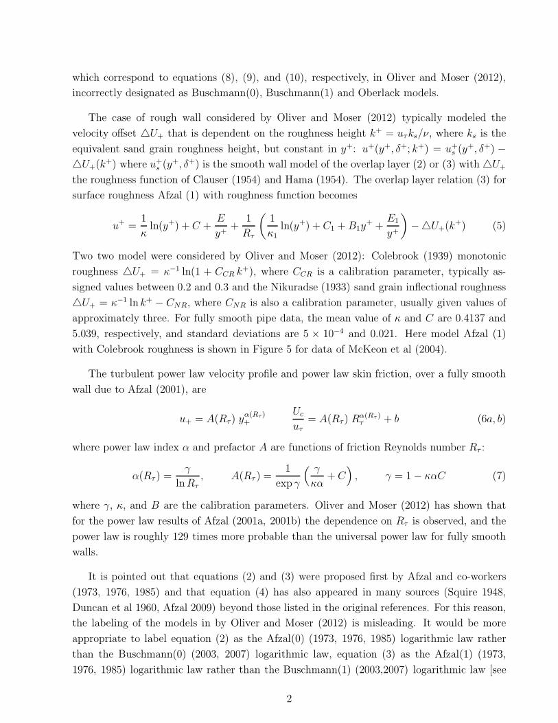
which correspond to equations (8), (9), and (10), respectively, in Oliver and Moser (2012),

incorrectly designated as Buschmann(0), Buschmann(1) and Oberlack models.

The case of rough wall considered by Oliver and Moser (2012) typically modeled the

velocity offset 4U+ that is dependent on the roughness height k+ = uτks/ν, where ks is the

equivalent sand grain roughness height, but constant in y+: u+(y+, δ+; k+) = u+s (y+, δ+) −

4U+(k+) where u+s (y+, δ+) is the smooth wall model of the overlap layer (2) or (3) with 4U+

the roughness function of Clauser (1954) and Hama (1954). The overlap layer relation (3) for

surface roughness Afzal (1) with roughness function becomes

u+ =1

κln(y+) + C +

E

y++

1

Rτ

(

1

κ1ln(y+) + C1 + B1y

+ +E1

y+

)

−4U+(k+) (5)

Two two model were considered by Oliver and Moser (2012): Colebrook (1939) monotonic

roughness 4U+ = κ−1 ln(1 + CCR k+), where CCR is a calibration parameter, typically as-

signed values between 0.2 and 0.3 and the Nikuradse (1933) sand grain inflectional roughness

4U+ = κ−1 ln k+ − CNR, where CNR is also a calibration parameter, usually given values of

approximately three. For fully smooth pipe data, the mean value of κ and C are 0.4137 and

5.039, respectively, and standard deviations are 5 × 10−4 and 0.021. Here model Afzal (1)

with Colebrook roughness is shown in Figure 5 for data of McKeon et al (2004).

The turbulent power law velocity profile and power law skin friction, over a fully smooth

wall due to Afzal (2001), are

u+ = A(Rτ) yα(Rτ)+

Uc

uτ= A(Rτ) Rα(Rτ )

τ + b (6a, b)

where power law index α and prefactor A are functions of friction Reynolds number Rτ :

α(Rτ ) =γ

lnRτ, A(Rτ ) =

1

exp γ

( γ

κα+ C

)

, γ = 1 − καC (7)

where γ, κ, and B are the calibration parameters. Oliver and Moser (2012) has shown that

for the power law results of Afzal (2001a, 2001b) the dependence on Rτ is observed, and the

power law is roughly 129 times more probable than the universal power law for fully smooth

walls.

It is pointed out that equations (2) and (3) were proposed first by Afzal and co-workers

(1973, 1976, 1985) and that equation (4) has also appeared in many sources (Squire 1948,

Duncan et al 1960, Afzal 2009) beyond those listed in the original references. For this reason,

the labeling of the models in by Oliver and Moser (2012) is misleading. It would be more

appropriate to label equation (2) as the Afzal(0) (1973, 1976, 1985) logarithmic law rather

than the Buschmann(0) (2003, 2007) logarithmic law, equation (3) as the Afzal(1) (1973,

1976, 1985) logarithmic law rather than the Buschmann(1) (2003,2007) logarithmic law [see

2

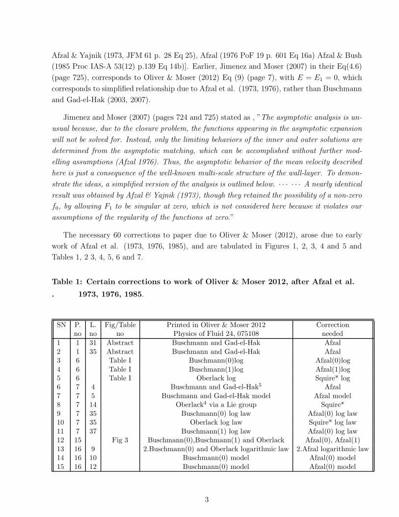
Afzal & Yajnik (1973, JFM 61 p. 28 Eq 25), Afzal (1976 PoF 19 p. 601 Eq 16a) Afzal & Bush

(1985 Proc IAS-A 53(12) p.139 Eq 14b)]. Earlier, Jimenez and Moser (2007) in their Eq(4.6)

(page 725), corresponds to Oliver & Moser (2012) Eq (9) (page 7), with E = E1 = 0, which

corresponds to simplified relationship due to Afzal et al. (1973, 1976), rather than Buschmann

and Gad-el-Hak (2003, 2007).

Jimenez and Moser (2007) (pages 724 and 725) stated as , ”The asymptotic analysis is un-

usual because, due to the closure problem, the functions appearing in the asymptotic expansion

will not be solved for. Instead, only the limiting behaviors of the inner and outer solutions are

determined from the asymptotic matching, which can be accomplished without further mod-

elling assumptions (Afzal 1976). Thus, the asymptotic behavior of the mean velocity described

here is just a consequence of the well-known multi-scale structure of the wall-layer. To demon-

strate the ideas, a simplified version of the analysis is outlined below. · · · · · · A nearly identical

result was obtained by Afzal & Yajnik (1973), though they retained the possibility of a non-zero

f0, by allowing F1 to be singular at zero, which is not considered here because it violates our

assumptions of the regularity of the functions at zero.”

The necessary 60 corrections to paper due to Oliver & Moser (2012), arose due to early

work of Afzal et al. (1973, 1976, 1985), and are tabulated in Figures 1, 2, 3, 4 and 5 and

Tables 1, 2 3, 4, 5, 6 and 7.

Table 1: Certain corrections to work of Oliver & Moser 2012, after Afzal et al.

. 1973, 1976, 1985.

SN P. L. Fig/Table Printed in Oliver & Moser 2012 Correctionno no no Physics of Fluid 24, 075108 needed

1 1 31 Abstract Buschmann and Gad-el-Hak Afzal

2 1 35 Abstract Buschmann and Gad-el-Hak Afzal3 6 Table I Buschmann(0)log Afzal(0)log

4 6 Table I Buschmann(1)log Afzal(1)log5 6 Table I Oberlack log Squire* log6 7 4 Buschmann and Gad-el-Hak5 Afzal

7 7 5 Buschmann and Gad-el-Hak model Afzal model8 7 14 Oberlack4 via a Lie group Squire*

9 7 35 Buschmann(0) log law Afzal(0) log law10 7 35 Oberlack log law Squire* log law

11 7 37 Buschmann(1) log law Afzal(0) log law12 15 Fig 3 Buschmann(0),Buschmann(1) and Oberlack Afzal(0), Afzal(1)

13 16 9 2.Buschmann(0) and Oberlack logarithmic law 2.Afzal logarithmic law14 16 10 Buschmann(0) model Afzal(0) model

15 16 12 Buschmann(0) model Afzal(0) model

3

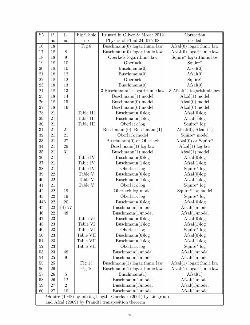
SN P. L. Fig/Table Printed in Oliver & Moser 2012 Correction

no no no Physics of Fluid 24, 075108 needed

16 18 Fig 8 Buschmann(0) logarithmic law Afzal(0) logarithmic law17 18 8 Buschmann(0) logarithmic law Afzal(0) logarithmic law

18 18 9 Oberlack logarithmic law Squire* logarithmic law19 18 10 Oberlack Squire*

20 18 10 Buschmann(0) Afzal(0)21 18 12 Buschmann(0) Afzal(0)

22 18 12 Oberlack Squire*23 18 13 Buschmann(0) Afzal(0)

24 18 13 3.Buschmann(1) logarithmic law 3.Afzal(1) logarithmic law25 18 14 Buschmann(1) model Afzal(1) model26 18 15 Buschmann(0) model Afzal(0) model

27 18 16 Buschmann(0) model Afzal(0) model28 21 Table III Buschmann(0)log Afzal(0)log

29 21 Table III Buschmann(1)log Afzal(1)log30 21 Table III Oberlack log Squire* log

31 21 21 Buschmann(0), Buschmann(1) Afzal(0), Afzal (1)32 21 21 Oberlack model Squire* model

33 21 27 Buschmann(0) or Oberlack Afzal(0) or Squire*34 21 29 Buschmann(1) log law Afzal(1) log law

35 21 31 Buschmann(1) model Afzal(1) model36 21 Table IV Buschmann(0)log Afzal(0)log37 21 Table IV Buschmann(1)log Afzal(1)log

38 21 Table IV Oberlack log Squire* log39 22 Table V Buschmann(0)log Afzal(0)log

40 22 Table V Buschmann(1)log Afzal(1)log41 21 Table V Oberlack log Squire* log

42 22 19 Oberlack log model Squire* log model43 22 19 Oberlack log Squire* log

443 22 20 Buschmann(0)log Afzal(0)log45 22 (4) 27 Buschmann(1)model Afzal(1)model

46 22 48 Buschmann(1)model Afzal(1)model47 23 Table VI Buschmann(0)log Afzal(0)log48 23 Table VI Buschmann(1)log Afzal(1)log

49 23 Table VI Oberlack log Squire* log50 23 Table VII Buschmann(0)log Afzal(0)log

51 23 Table VII Buschmann(1)log Afzal(1)log52 23 Table VII Oberlack log Squire* log

53 23 48 Buschmann(1)model Afzal(1)model54 25 9 Buschmann(1)model Afzal(1)model

55 25 Fig 15 Buschmann(1) logarithmic law Afzal(1) logarithmic law56 26 Fig 16 Buschmann(1) logarithmic law Afzal(1) logarithmic law

57 26 5 Buschmann(1) Afzal(1)58 26 12 Buschmann(1)model Afzal(1)model59 27 2 Buschmann(1)model Afzal(1)model

60 27 10 Buschmann(1)model Afzal(1)model

*Squire (1948) by mixing length, Oberlack (2001) by Lie groupand Afzal (2009) by Prandtl transposition theorem

4

.

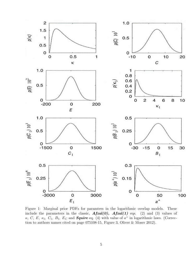
Figure 1: Marginal prior PDFs for paramters in the logarithmic overlap models. Theseinclude the parameters in the classic, Afzal(0), Afzal(1) eqs. (2) and (3) values ofκ, C, E, κ1, C1, B1, E1; and Squire eq. (4) with value of a+ in logarithmic laws. (Correc-tion to authors names cited on page 075108-15, Figure 3, Oliver & Moser 2012).

5

.

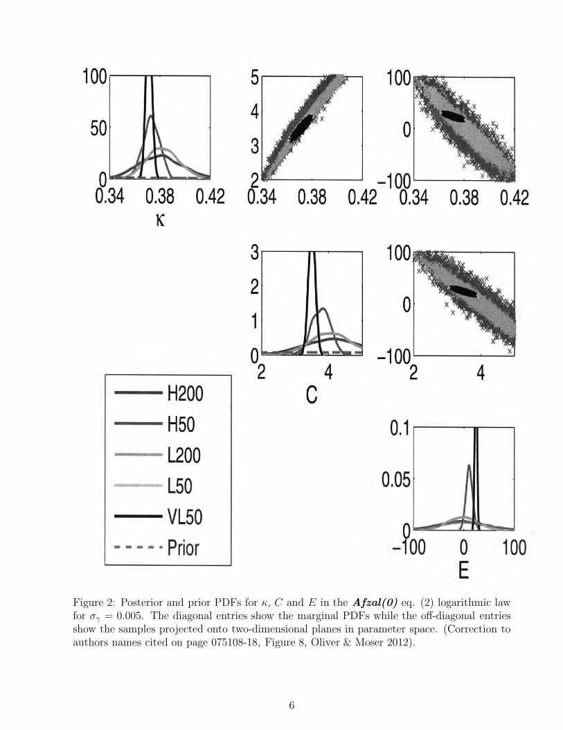
Figure 2: Posterior and prior PDFs for κ, C and E in the Afzal(0) eq. (2) logarithmic lawfor σγ = 0.005. The diagonal entries show the marginal PDFs while the off-diagonal entriesshow the samples projected onto two-dimensional planes in parameter space. (Correction toauthors names cited on page 075108-18, Figure 8, Oliver & Moser 2012).

6

.

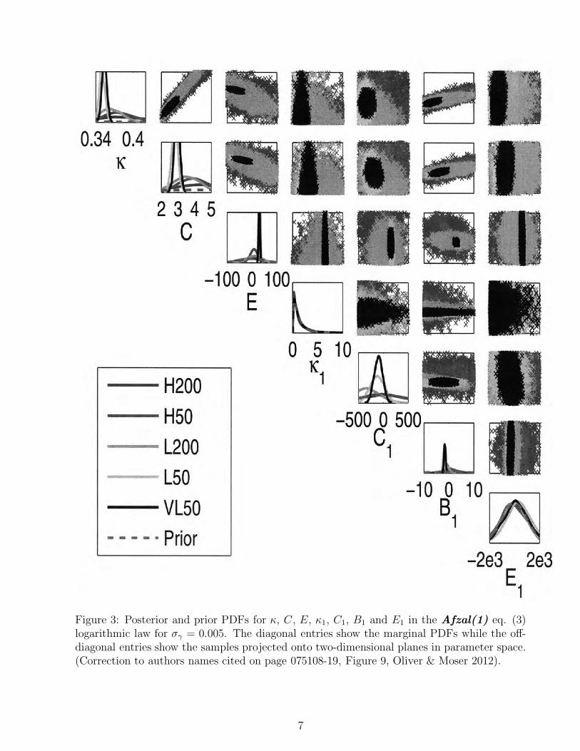
Figure 3: Posterior and prior PDFs for κ, C , E, κ1, C1, B1 and E1 in the Afzal(1) eq. (3)logarithmic law for σγ = 0.005. The diagonal entries show the marginal PDFs while the off-diagonal entries show the samples projected onto two-dimensional planes in parameter space.(Correction to authors names cited on page 075108-19, Figure 9, Oliver & Moser 2012).

7

.

Figure 4: Posterior and prior PDFs for κ, C , E, κ1, C1, B1 and E1 in the Afzal(1) eq.(3) logarithmic law obtained using McKeons Superpipe data. The diagonal entries show themarginal PDFs while the off-diagonal entries show the samples projected onto two-dimensionalplanes in parameter space. (Correction to authors names cited on page 075108-25, Figure 15,Oliver & Moser 2012).

8

.

Figure 5: Posterior and prior PDFs for κ, C , E, κ1, C1, B1, E1, and CCR in the Afzal(1)eq. (5) logarithmic law with Colebrook roughness obtained using McKeons Superpipe data.The diagonal entries show the marginal PDFs while the off-diagonal entries show the samplesprojected onto two-dimensional planes in parameter space. (Correction to authors names citedon page 075108-26, Figure 16, Oliver & Moser 2012).

9

.

Figure 6: Marginal prior PDFs for parameters in the universal and Afzal power laws. (Ref.page 075108-16, Figure 4, Oliver & Moser 2012; and on page 075108-7 in the eq (14) replaceB by C ; and read eqs. (12), (13), (14) as u+ = A(Rτ) (y+)α(Rτ ), where α = γ/ ln Rτ ,A = e−γ[γ(κα)−1 + C ], and γ = 1 − καC.

10

.

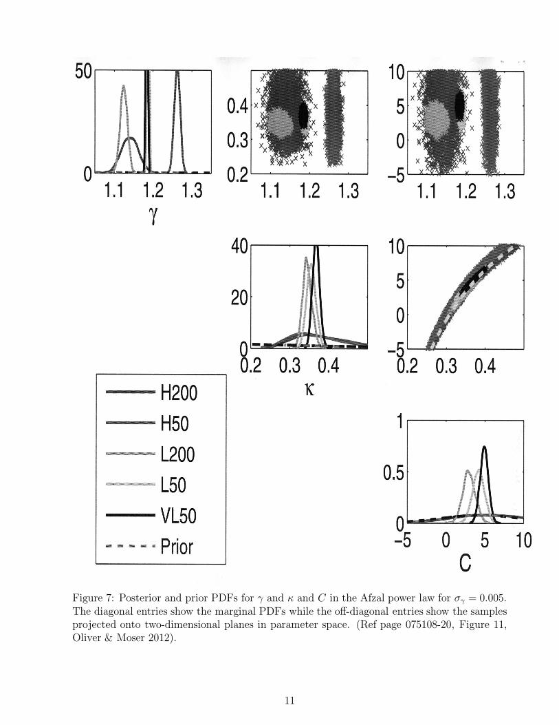
Figure 7: Posterior and prior PDFs for γ and κ and C in the Afzal power law for σγ = 0.005.The diagonal entries show the marginal PDFs while the off-diagonal entries show the samplesprojected onto two-dimensional planes in parameter space. (Ref page 075108-20, Figure 11,Oliver & Moser 2012).

11

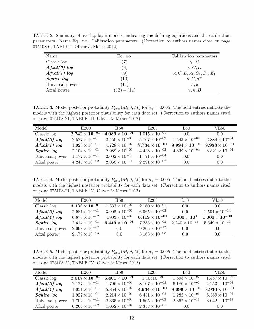
TABLE 2. Summary of overlap layer models, indicating the defining equations and the calibrationparameters. Name Eq. no. Calibration parameters. (Correction to authors names cited on page

075108-6, TABLE I, Oliver & Moser 2012).

Name Eq. no. Calibration parameters

Classic log (7) γ, CAfzal(0) log (8) κ, C, E

Afzal(1) log (9) κ, C, E, κ1, C1, B1, E1

Squire log (10) κ, C, a+

Universal power (11) A, aAfzal power (12)− (14) γ, κ, B

TABLE 3. Model posterior probability Ppost(Mi|d, M) for σγ = 0.005. The bold entries indicate the

models with the highest posterior plausibility for each data set. (Correction to authors names citedon page 075108-21, TABLE III, Oliver & Moser 2012).

Model H200 H50 L200 L50 VL50

Classic log 2.742× 10−01 4.089× 10−01 1.015× 10−01 0.0 0.0

Afzal(0) log 2.527× 10−01 2.450× 10−01 5.767× 10−02 1.543× 10−04 2.884× 10−04

Afzal(1) log 1.026× 10−01 4.728× 10−02 7.734 × 10−01 9.994× 10−01 9.988× 10−01

Squire log 2.104× 10−01 2.989× 10−01 4.438× 10−02 4.839× 10−04 8.821× 10−04

Universal power 1.177× 10−01 2.002× 10−14 1.771× 10−04 0.0 0.0

Afzal power 4.245× 10−02 2.068× 10−14 2.291× 10−02 0.0 0.0

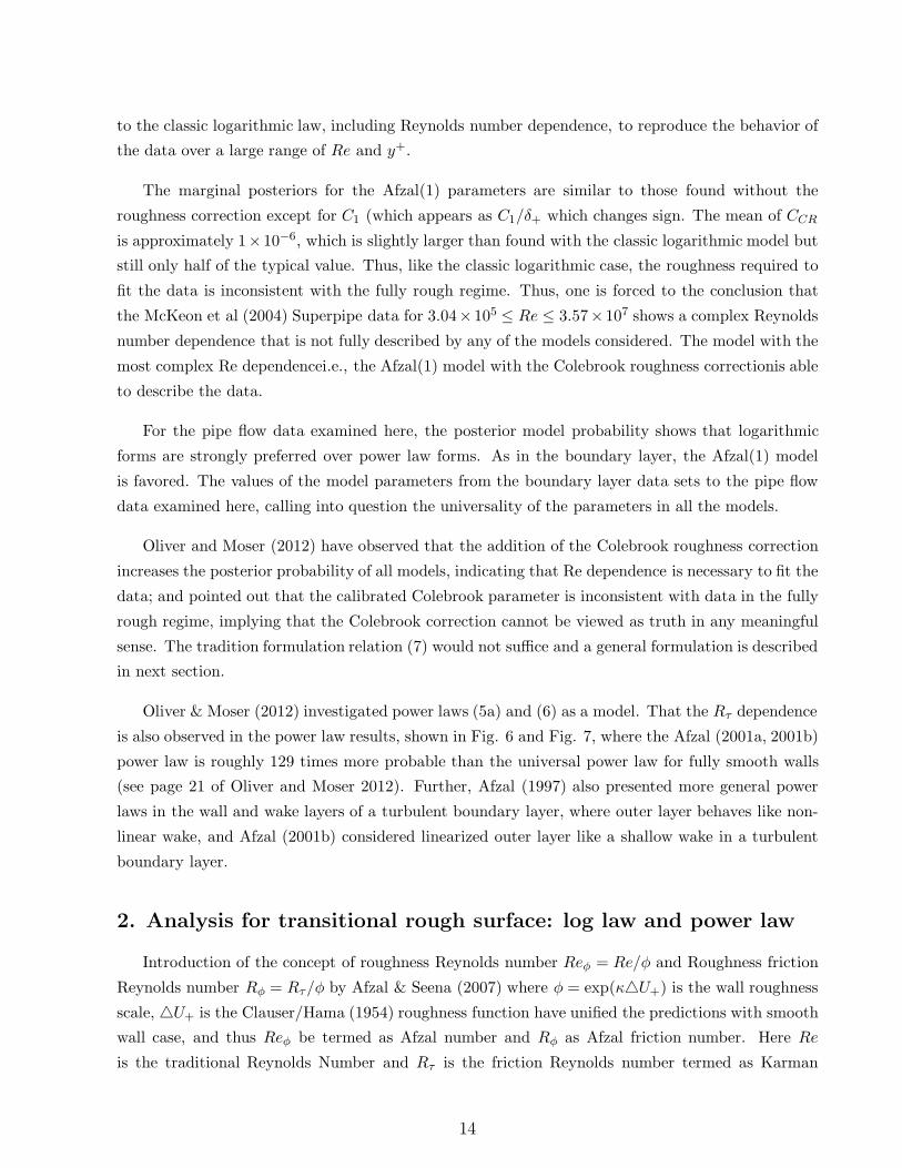
TABLE 4. Model posterior probability Ppost(Mi|d, M) for σγ = 0.005. The bold entries indicate the

models with the highest posterior probability for each data set. (Correction to authors names citedon page 075108-21, TABLE IV, Oliver & Moser 2012).

Model H200 H50 L200 L50 VL50

Classic log 3.433× 10−01 1.533× 10−02 2.160× 10−01 0.0 0.0

Afzal(0) log 2.981× 10−01 3.905× 10−01 6.965× 10−02 0.0 1.594× 10−14

Afzal(1) log 6.675× 10−02 4.903× 10−02 6.419 × 10−01 1.000× 101 1.000× 10−00

Squire log 2.614× 10−01 5.449× 10−01 7.235× 10−02 2.240× 10−15 5.549× 10−13

Universal power 2.098× 10−02 0.0 9.205× 10−12 0.0 0.0Afzal power 9.479× 10−03 0.0 3.163× 10−08 0.0 0.0

TABLE 5. Model posterior probability Ppost(Mi|d, M) for σγ = 0.005. The bold entries indicate themodels with the highest posterior probability for each data set. (Correction to authors names cited

on page 075108-22, TABLE IV, Oliver & Moser 2012).

Model H200 H50 L200 L50 VL50

Classic log 2.517× 10−01 5.401× 10−01 1.10810−01 1.698× 10−07 1.457× 10−08

Afzal(0) log 2.177× 10−01 1.796× 10−01 8.107× 10−02 6.180× 10−02 4.253× 10−02

Afzal(1) log 1.051× 10−01 5.854× 10−02 4.934 × 10−01 8.099× 10−01 8.936× 10−01

Squire log 1.927× 10−01 2.214× 10−01 6.431× 10−02 1.282× 10−01 6.389× 10−02

Universal power 1.702× 10−01 2.365× 10−04 1.505× 10−02 2.367× 10−11 3.042× 10−12

Afzal power 6.266× 10−02 1.062× 10−04 2.353× 10−01 0.0 0.0

12

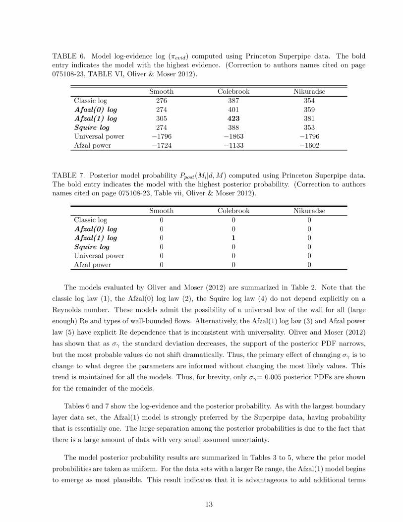
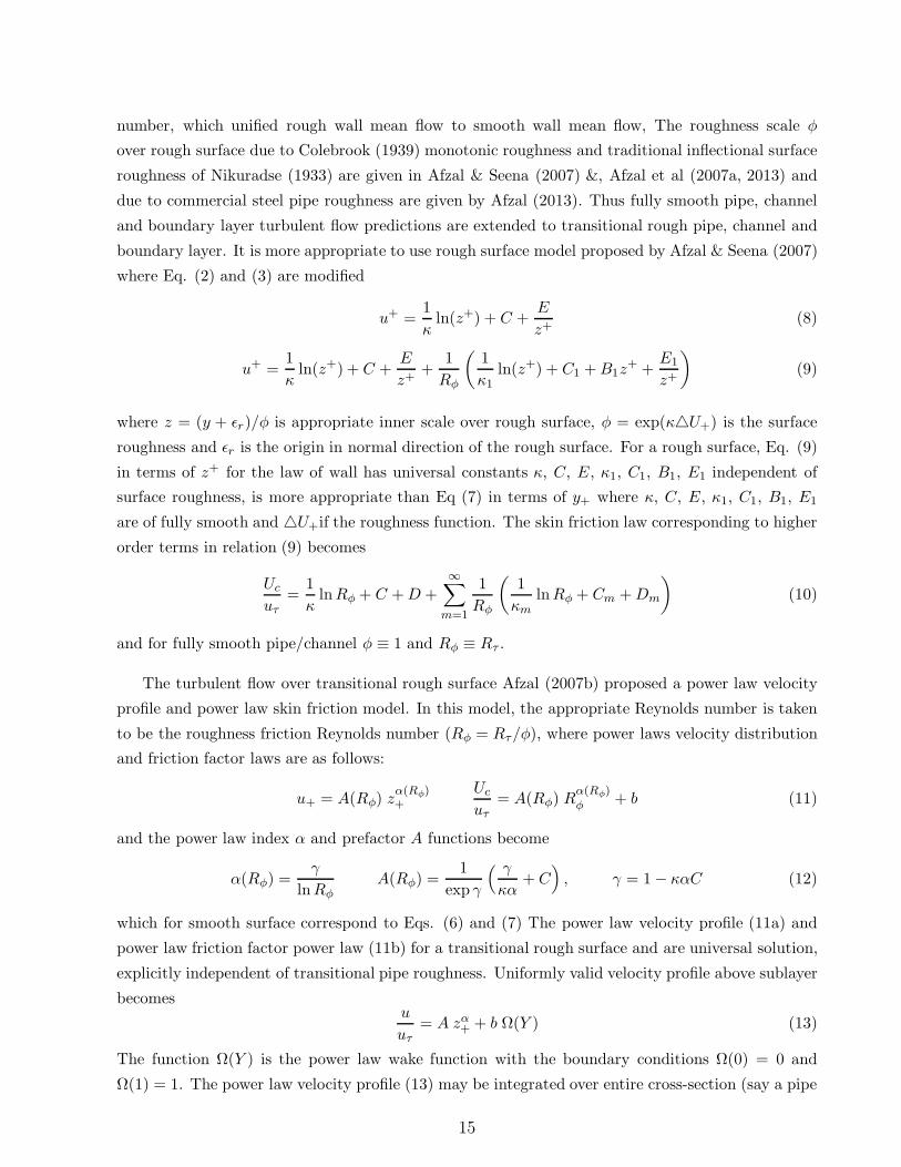
TABLE 6. Model log-evidence log (πevid) computed using Princeton Superpipe data. The boldentry indicates the model with the highest evidence. (Correction to authors names cited on page

075108-23, TABLE VI, Oliver & Moser 2012).

Smooth Colebrook Nikuradse

Classic log 276 387 354

Afazl(0) log 274 401 359Afzal(1) log 305 423 381

Squire log 274 388 353Universal power −1796 −1863 −1796

Afzal power −1724 −1133 −1602

TABLE 7. Posterior model probability Ppost(Mi|d, M) computed using Princeton Superpipe data.The bold entry indicates the model with the highest posterior probability. (Correction to authorsnames cited on page 075108-23, Table vii, Oliver & Moser 2012).

Smooth Colebrook Nikuradse

Classic log 0 0 0

Afzal(0) log 0 0 0Afzal(1) log 0 1 0

Squire log 0 0 0Universal power 0 0 0

Afzal power 0 0 0

The models evaluated by Oliver and Moser (2012) are summarized in Table 2. Note that the

classic log law (1), the Afzal(0) log law (2), the Squire log law (4) do not depend explicitly on a

Reynolds number. These models admit the possibility of a universal law of the wall for all (large

enough) Re and types of wall-bounded flows. Alternatively, the Afzal(1) log law (3) and Afzal power

law (5) have explicit Re dependence that is inconsistent with universality. Oliver and Moser (2012)

has shown that as σγ the standard deviation decreases, the support of the posterior PDF narrows,

but the most probable values do not shift dramatically. Thus, the primary effect of changing σγ is to

change to what degree the parameters are informed without changing the most likely values. This

trend is maintained for all the models. Thus, for brevity, only σγ= 0.005 posterior PDFs are shown

for the remainder of the models.

Tables 6 and 7 show the log-evidence and the posterior probability. As with the largest boundary

layer data set, the Afzal(1) model is strongly preferred by the Superpipe data, having probability

that is essentially one. The large separation among the posterior probabilities is due to the fact that

there is a large amount of data with very small assumed uncertainty.

The model posterior probability results are summarized in Tables 3 to 5, where the prior model

probabilities are taken as uniform. For the data sets with a larger Re range, the Afzal(1) model begins

to emerge as most plausible. This result indicates that it is advantageous to add additional terms

13

to the classic logarithmic law, including Reynolds number dependence, to reproduce the behavior of

the data over a large range of Re and y+.

The marginal posteriors for the Afzal(1) parameters are similar to those found without the

roughness correction except for C1 (which appears as C1/δ+ which changes sign. The mean of CCR

is approximately 1×10−6, which is slightly larger than found with the classic logarithmic model but

still only half of the typical value. Thus, like the classic logarithmic case, the roughness required to

fit the data is inconsistent with the fully rough regime. Thus, one is forced to the conclusion that

the McKeon et al (2004) Superpipe data for 3.04×105 ≤ Re ≤ 3.57×107 shows a complex Reynolds

number dependence that is not fully described by any of the models considered. The model with the

most complex Re dependencei.e., the Afzal(1) model with the Colebrook roughness correctionis able

to describe the data.

For the pipe flow data examined here, the posterior model probability shows that logarithmic

forms are strongly preferred over power law forms. As in the boundary layer, the Afzal(1) model

is favored. The values of the model parameters from the boundary layer data sets to the pipe flow

data examined here, calling into question the universality of the parameters in all the models.

Oliver and Moser (2012) have observed that the addition of the Colebrook roughness correction

increases the posterior probability of all models, indicating that Re dependence is necessary to fit the

data; and pointed out that the calibrated Colebrook parameter is inconsistent with data in the fully

rough regime, implying that the Colebrook correction cannot be viewed as truth in any meaningful

sense. The tradition formulation relation (7) would not suffice and a general formulation is described

in next section.

Oliver & Moser (2012) investigated power laws (5a) and (6) as a model. That the Rτ dependence

is also observed in the power law results, shown in Fig. 6 and Fig. 7, where the Afzal (2001a, 2001b)

power law is roughly 129 times more probable than the universal power law for fully smooth walls

(see page 21 of Oliver and Moser 2012). Further, Afzal (1997) also presented more general power

laws in the wall and wake layers of a turbulent boundary layer, where outer layer behaves like non-

linear wake, and Afzal (2001b) considered linearized outer layer like a shallow wake in a turbulent

boundary layer.

2. Analysis for transitional rough surface: log law and power law

Introduction of the concept of roughness Reynolds number Reφ = Re/φ and Roughness friction

Reynolds number Rφ = Rτ/φ by Afzal & Seena (2007) where φ = exp(κ4U+) is the wall roughness

scale, 4U+ is the Clauser/Hama (1954) roughness function have unified the predictions with smooth

wall case, and thus Reφ be termed as Afzal number and Rφ as Afzal friction number. Here Re

is the traditional Reynolds Number and Rτ is the friction Reynolds number termed as Karman

14

number, which unified rough wall mean flow to smooth wall mean flow, The roughness scale φ

over rough surface due to Colebrook (1939) monotonic roughness and traditional inflectional surface

roughness of Nikuradse (1933) are given in Afzal & Seena (2007) &, Afzal et al (2007a, 2013) and

due to commercial steel pipe roughness are given by Afzal (2013). Thus fully smooth pipe, channel

and boundary layer turbulent flow predictions are extended to transitional rough pipe, channel and

boundary layer. It is more appropriate to use rough surface model proposed by Afzal & Seena (2007)

where Eq. (2) and (3) are modified

u+ =1

κln(z+) + C +

E

z+(8)

u+ =1

κln(z+) + C +

E

z++

1

Rφ

(

1

κ1ln(z+) + C1 + B1z

+ +E1

z+

)

(9)

where z = (y + εr)/φ is appropriate inner scale over rough surface, φ = exp(κ4U+) is the surface

roughness and εr is the origin in normal direction of the rough surface. For a rough surface, Eq. (9)

in terms of z+ for the law of wall has universal constants κ, C, E, κ1, C1, B1, E1 independent of

surface roughness, is more appropriate than Eq (7) in terms of y+ where κ, C, E, κ1, C1, B1, E1

are of fully smooth and 4U+if the roughness function. The skin friction law corresponding to higher

order terms in relation (9) becomes

Uc

uτ=

1

κln Rφ + C + D +

∞∑

m=1

1

Rφ

(

1

κmln Rφ + Cm + Dm

)

(10)

and for fully smooth pipe/channel φ ≡ 1 and Rφ ≡ Rτ .

The turbulent flow over transitional rough surface Afzal (2007b) proposed a power law velocity

profile and power law skin friction model. In this model, the appropriate Reynolds number is taken

to be the roughness friction Reynolds number (Rφ = Rτ/φ), where power laws velocity distribution

and friction factor laws are as follows:

u+ = A(Rφ) zα(Rφ)+

Uc

uτ= A(Rφ) R

α(Rφ)φ + b (11)

and the power law index α and prefactor A functions become

α(Rφ) =γ

ln RφA(Rφ) =

1

exp γ

( γ

κα+ C

)

, γ = 1 − καC (12)

which for smooth surface correspond to Eqs. (6) and (7) The power law velocity profile (11a) and

power law friction factor power law (11b) for a transitional rough surface and are universal solution,

explicitly independent of transitional pipe roughness. Uniformly valid velocity profile above sublayer

becomesu

uτ= A zα

+ + b Ω(Y ) (13)

The function Ω(Y ) is the power law wake function with the boundary conditions Ω(0) = 0 and

Ω(1) = 1. The power law velocity profile (13) may be integrated over entire cross-section (say a pipe

15

of radius δ) to obtain the bulk averaged velocity

Ub

uτ= 2

∫ δ

0(1− Y ) u+ dY = Rα

φ

2A

(1 + α)(2 + α)+ bb (14)

where bb = 2b∫ 10 (1−Y )Ω(Y )dY . The friction factor power law from Eq. (14) may also be expressed

as

λ = 8

(

2A

(1 + α)(2 + α)Rα

φ + bb

)

−2

(15)

In fully developed turbulent pipe flow, the outer wake is weak (bb ≈ 0) and the expression (15) is

simplified as

λ = 8

(

2α−1

A(1 + α)(2 + α)

)2/(1+α)

Re−2α/(1+α)φ (16)

where n = 2α/(1 + α) is the roughness friction Reynolds number index of friction factor power law.

For fully smooth pipe φ = 1 and Rφ = Rτ and fully rough flows φ = χk+ and Rφ = δ/(χk), and in

transitional pipes roughness Rτ ≤ Rφ ≤ δ/(χk). Further, for specific value α = 1/7 or n = 1/4 the

power law friction factor (16) for transitional rough pipes become

λ = 0.3164 Re−1/4φ = 0.3164

(

Re

φ

)

−1/4

(17)

in a domain 3 × 103 < Reφ < 2 × 105. Here the numerical constant 0.3194 is universal for all types

of roughness; first proposed by Blasius (1908) for fully smooth pipe (φ = 1).

The power law velocity profile (13) may be integrated over entire cross-section of a channel of

semi depth δ, to obtain the bulk averaged velocity

Ub

uτ= 2

∫ δ

0u+ dY = Rα

φ

2A

(1 + α)+ bb (18)

where bb = 2b∫ 10 Ω(Y )dY . The friction factor power law may also be expressed as

λ = 8

(

2A

(1 + α)Rα

φ + bb

)

−2

(19)

In fully developed turbulent pipe flow, the outer wake is weak (bb ≈ 0) and the expression (19) is

simplified as

λ = 8

(

2αA

(1 + α)

)2/(1+α)

Re−2α/(1+α)φ (20)

For fully smooth channel φ = 1 and Reφ = Re and fully rough channel φ = χk+ (where χ =

exp[κ(B − BF )] is Colebrook type constant), and Rφ = δ/(χk), and in transitional rough channel

Rτ ≤ Rφ ≤ δ/(χk). Further, for specific value α = 1/7 or n = 1/4 the power law friction factor (20)

for transitional rough pipes become

λ = 0.292 Re−1/4φ = 0.292

(

Re

φ

)

−1/4

(21)

16

valid in a domain 6 × 103 < Reφ < 6 × 105. Here numerical constant 0.292 is adopted from Dean

(1956) for 1/4-power law for fully smooth channel (φ = 1).

3. The Prandtl (1938) transposition (PT) theorem:

If [u(x, y, t), v(x, y, t)] is a solution of the boundary-layer equations then [U(x, z, t), V(x, z, t)]

is also a solution, where z = y + a(x, t), U(x, z, t) = u(x, y, t) and V (x, z, t) = v(x, y, t)− ∂a/∂t −

u(x, y, t)∂a(x, t)/∂x for arbitrary a = a(x, t).

The Prandtl transport theorem implies that if normal ordinate y is shifted to y + a by shift of

origin by distance ’a’, then velocity u(y) under transformation yields the velocity U(y +a) at shifted

location. Afzal (2009) considered geostrophic Ekman layer and proposed his equations (31a,b) for

velocity distribution due to shift of origin.

In the power law velocity, Prandtl transport theorem, in the overlap region, for the law of wall

and velocity defect law yieldU

uτ= Ci(z

+ + aφ)α (22)

U

uτ= Co(Y + aδ)

α, Co = Ci Rαφ (23)

and skin friction law remains same as Uc/uτ = A(δ+/φ)α + B. Here z+ = (y+ + ε+r )/φ, aφ = a+/φ,

a+ = auτ/ν, Y = (y + εr)/δ and aδ = a/δ.

In the present case of log laws, Prandtl transport theorem, in the overlap region, for the law of

wall and velocity defect law yield

U

uτ=

1

κln(z+ + aφ) + C (24)

U − Uc

uτ=

1

κln(Y + aδ) − D (25)

and the skin friction law remains same as Uc/uτ = κ−1 ln(δ+/φ) + C + D. The next order term

region, for the law of wall and velocity defect law yield

U

uτ=

1

κln(z+ + aφ) + C +

E

z+ + aφ(26)

U − Uc

uτ=

1

κln(Y + aδ)− D + (Y + aδ)F (27)

The linearizing (26) for large z+ yields

U

uτ=

1

κln z+ + C +

E + κ−1a+

z+(28)

The above equations for fully smooth surface φ = 1, z+ = y+ and εr = 0 and the equation E = 0

yield relation proposed by Square (1948) (also described in Duncan et al. 1960) and Oberlack (2001)

viz Lie group analysis, was adopted by Oliver and Moser (2012).

17

4. Conclusions

1. That Oliver and Moser (2012) equation number (2,OM(8)) be termed as Afzal(0) & Squire

logarithmic law instead of Buschmann(0) & Oberlack logarithmic law; and their equation number

(3,OM(9)) be also termed as Afzal(1) logarithmic law instead of Buschmann(1) logarithmic law.

2. That Afzal(1) model emerges as most plausible. This also result indicates that it is advanta-

geous to add additional terms to the classic logarithmic law, including Reynolds number dependence,

to reproduce the behavior of the data over a large range of Re and y+ . Not only do these terms

improve the fit between the model and the data some improvement is inevitablethe improvement is

enough to make the model more probable according to Bayes theorem.

3. That model of Afzal(1) found good for largest boundary layer data set, ia also is strongly

preferred by the Superpipe data, having probability that is essentially one. Thus for the boundary

layer and pipe flow data the posterior model probability shows that Afzal(1) logarithmic forms are

strongly preferred.

4. The model with the most complex Re dependence i.e., the Afzal(1) model with the Colebrook

roughness correctionis able to best describe the data.

5. In the power law results of Afzal (2001a, 2001b) dependence on Rτ is observed. and the power

law is roughly 129 times more probable than the universal power law for fully smooth walls.

6. That the corrections by Afzal (2012) was unduly declined form publication by John Kim

Editor Physics of Fluids where as several analogous Erratum; say, Molla, David & Kuhn (2013),

published in same journal, by same Editor Physics of Fluids.

Acknowledgment: Dr Todd Oliver is thanked for his message by email dated November 9, 2012

9:08 PM: ”Dear Prof. Afzal, Thank you for your interest in our work, and thank you for including

your earlier references. Things are very hectic for me right now, so it may take a bit of time to

resolve things, but I am consulting with Dr. Moser and the journal editor to decide how to proceed.

Best, Todd Oliver.”

18

References

Afzal, N. 1976 Millikan’s argument at moderately large Reynolds numbers. Physics of Fluids, 19,

600-602.

Afzal, N. 1997 Power laws in the wall and wake layers of a turbulent boundary layer. pp 805 - 808

in Proc 7 Asian Congress of Fluid Mechanics at Chennai. Allied Publisher New Delhi. Online

https://sites.google.com/site/noorafzal/publications.

Afzal, N. 2001 Power law and log law velocity profiles in turbulent boundary-layer flow: Equivalent

relations at large Reynolds number. Acta Mechanica, 151, 195-216.

Afzal, N. 2001 Power and log laws velocity profiles in fully developed turbulent pipe flows: Equiv-

alent relations at large Reynolds numbers. Acta Mechanica, 151, 171-183.

Afzal, N. 2007a Friction factor directly from transitional rough pipes. ASME J. Fluid Engineering,

129 (10), 1255-1267.

Afzal, N. 2007b Power law velocity profile in turbulent boundary layers on transitional rough wall.

ASME J. Fluid Engineering, 129(8), 1083-1100.

Afzal, N. 2009 Neutrally stratified turbulent Ekman boundary layer: universal similarity for tran-

sitional rough surface. Boundary Layer Meteorology, 132, 241-259.

Afzal, N. 2012 Comments on ”Accounting for uncertainty in the analysis of overlap layer mean

velocity models’ (Manuscript PF#12-1526-C, November 28, 2012. Declined publication in

Physics of Fluids by John Kim Editor Physics of Fluids).

Afzal, N. 2013 Roughness effects of commercial steel pipe in turbulent flow: Universal scaling.

Canadian J. Civil Engineering, 40(2), 188-193.

Afzal, N. and Bush, W.B. 1985 A three layer asymptotic analysis of turbulent channel. Indian

Academy of Sciences: Series A, 53(12), 640-642.

Afzal, N. and Yajnik, K. 1973 Analysis of turbulent pipe and channel flows at moderately large

Reynolds number. J. Fluid Mechanics, 61, 23-31.

Afzal, N. and Seena, A. 2007 Alternate scales for turbulent flow in transitional rough pipes: Uni-

versal log laws. ASME J. Fluid Engineering, 129 (1), 80-90.

Afzal, N., Seena, A. and Bushra, A. 2013 Effects of machined surface roughness on high Reynolds

number turbulent pipe flow: Universal scaling. Journal of Hydro-environment Research, IAHR

7, pp. 81-90.

Buschmann, M.H. and Gad-el-Hak, M. 2003 Generalized logarithmic law and its consequences.

AIAA Journal 41 (1), 40-48.

Buschmann, M.H. and Gad-el-Hak, M. 2007 Recent developments in scaling of wall-bounded flows.

Progress in Aerospace Sciences, 42, 419-467.

Clauser, F.H. 1954 Turbulent boundary layers in adverse pressure gradients. J. Aeronautical Sci-

ences, 21, 91-105.

19

Colebrook, C. F. 1939 Turbulent flow in pipes, with particular reference to the transitional region

between smooth and rough wall laws. J. Institution of Civil Engineers, 11, 133-156.

Dean, R. B. 1978 Reynolds number dependence of skin friction and other bulk flow variables in

two-dimensional rectangular duct flows. J. Fluids Eng.*, 100, 215223.

Duncan, W.J., Thom, A.and Young, A. 1960 Mechanics of Fluids. Edward Arnold UK.

Hama, F R. 1954 Boundary-layer characteristics for smooth and rough surfaces. Trans SNAME,

62, 333-358.

Jimenez, J. and Moser, R.D. 2007 What are we learning from simulating wall turbulence?. Phil.

Trans. Royal Soc. A 365, 715−732.

Molla, M.M., Wang, B. and David C. S. Kuhn, D.C.M. 2013 Erratum: Numerical study of pulsatile

channel flows undergoing transition triggered by a modelled stenosis [Phys. Fluids 24, 121901

(2012)],Physics of Fluids, 25, 049901.

McKeon, B.J., J. Li, Jiang, W., Morrison, J.F. and Smits, A.J. 2004 Further observations on the

mean velocity distribution in fully developed pipe flow, J. Fluid Mech. 501, 135147.

Nikuradse, J. 1933 Laws of flow in rough pipe. VI, Forchungsheft N-361 (NACA TM 1292, 1950).

Oberlack, M. 2001 A unified approach for symmetries in plane parallel turbulent shear flows. J.

Fluid Mech., 427, 299 - 328

Oliver, T.A. and Moser, R.D. 2012 Accounting for uncertainty in the analysis of overlap layer mean

velocity models. Physics of Fluids, 24, 075108.

Prandtl, L. 1938 Aur Berechung der Grenzchichten, ZAMM, 18, p. 77; also in: Laminar Boundary

Layers, L. Rosenhead, ed., Clarendon Press, Oxford, 1963, p. 211.

Squire, H.B. 1948 Reconsideration of the theory of free turbulence. Philosophical Magazine, 39(288),

16-19.

20