2 Atmospheric C02, global carbon fluxes and the biosphere

J. Goudriaan

2.1 Introduction

In the atmosphere carbon occurs mainly as C02, in the biosphere mainly as organic compounds, and in the sea mainly as bicarbonate and carbonate ions. The amount of atmospheric carbon is relatively small compared with the amounts of carbon in the biosphere and in the ocean, and therefore the level of atmospheric C02 can be expected to be sensitive to changes in the global carbon fluxes. This paper describes a simulation model for the global carbon cycle that was developed to investigate interaction between the carbon pools in the ocean, the biosphere and the atmosphere, particularly how the interaction affects atmospheric C02.

The most obvious reason for the rise of atmospheric C02 is the burning of fossil fuel, but deforestation is also generally considered to be a significant source of C02. However, this source is partly compensated for by regrowth. This paper aims at estimating not only the gross but also the net release of carbon from the biosphere to the atmosphere.

The terrestrial biosphere, and especially the soil, contains a significant amount of carbon. The quantity of carbon stored depends on a dynamic equilibrium between processes of decomposition and photosynthetic carbon fixation. When atmospheric C02 rises, it stimulates leaf photosynthesis, and consequently the dynamic equilibrium can be expected to be shifted towards a larger carbon storage. An important question is to what extent emission of C02 to the at­mosphere is buffered by biospheric fixation of carbon. Since this storage occurs in reservoirs with vastly different time coefficients, the time pattern of storage is a complex phenomenon.

The carbon pool in the ocean is much larger than the carbon pools in the atmosphere and biosphere combined. Chemical buffering in the ocean stores about 40% of the C02 emission, but a much larger percentage could be stored if the emission rate were lower, permitting more time for mixing towards the deep sea.

Although the mechanism for storage of carbon in the ocean is mainly by chemical buffering, there is an important role for the functioning of the marine biosphere. Algae have a short lifetime and so carbon storage in algae themselves is negligible. However, a small portion of their remains sinks to the waters of the deep sea, where it decomposes, causing a considerable carbon flux from the surface waters to the deep sea. As a result of this process, water from the deep sea has a much higher C02 pressure than surface water. Algal growth is mostly limited by phosphate, and so eutrophication of the sea can reduce atmospheric C02 by increasing the deep sea storage of carbon.

17

The deep waters of the Atlantic Ocean have lower nutrient and carbonate levels than the deep waters of the Pacific and Indian Oceans. The mixing currents in the Atlantic Ocean are much stronger, and prevent high levels from building up. Ocean currents also have a large effect on atmospheric C02, and this may help explain the sudden end of the glacial periods.

The ratios of I3C and I4C to I2C are different in the atmosphere, in ocean water, in fossil carbon and in biomass. These differences and their time patterns are used here for validating the model presented.

2.2 Carbon reservoirs and fluxes

Three major reservoirs of carbon, the atmosphere (700 Gt C), the oceans (39000GtC) and the terrestrial biosphere (2000 GtC) exchange carbon in the form of C02 (Figure 4) (Bolin et al., 1979; Clark, 1982). The photosynthetic activity of the biosphere acts as a powerful driving force for these exchange fluxes.

With industrialization, increasing amounts of carbon from fossil fuels are emitted as C02 into the atmosphere, at present at a rate of over 5 Gt C yr" \ At the current rates, about 60% remains in the atmosphere and 40% is absorbed by the oceans, but this partitioning is dependent on the rate of emission itself. A lower rate of emission gives more time for absorption in the ocean. The chemical buffering capacity of the oceans is large enough for about 85% of each unit of C02

600->700 Gt C atmosphere I ' M

60 Gt yr -1

7!

^ML

K 60 GtC yr

39000 Gt C %

ocean

6000 Gt c

fossil

Figure 4. Major compartments in the global carbon cycle and the exchange fluxes between them. The accumulated effect of the fluxes of fossil fuel burning and biomass removal over the last 200 years is indicated by the hatched rectangles.

18

emitted into the atmosphere to be absorbed eventually, leaving only 15% in the atmosphere. However, mixing in the deep sea is so slow, that hundreds of years will be needed for this absorption capacity to be utilized. Biospheric uptake is not yet included in this calculation.

The surface waters of the oceans are almost in equilibrium with atmospheric C02, but the deep waters have a much higher C02 pressure (above lOOOpmol mol-1) and a correspondingly higher carbonate and bicarbonate content. This high level is maintained by the sinking of carbon contained in the remains of dead plankton. In the upper layer of the sea photosynthetic activity extracts carbon from the water, and strongly reduces the levels of nutrients such as phosphate. Local up welling of deep water returns these nutrients and some of the accumula­ted carbon to the surface layers. The intensity of this circulation flux is estimated to be about 2 to 6 Gt C yr" ! (Baes et al., 1985).

The chemical equilibration of ocean water with atmospheric C02 is the most important sink of C02 released into the atmosphere, either from fossil fuel or from the biosphere. The slope of the graph of carbon in atmospheric C02 versus carbon emitted from fossil fuels (Figure 5) can be considered as the fraction remaining in the atmosphere, and it is therefore called the 'airborne fraction'. Because of the chemical nature of buffering of C02 in the ocean, this fraction is expected to be fairly stable. Over the period 1960-1980 it had an observed value of 0.576 (Bolin, 1986).

Although the net uptake of carbon by the terrestrial biosphere is modest when

atmospheric carbon (Gt)

800 r-

750

700

650

600

5^.-'"

. - • "

^ - -

550 J I I 50 100 150 200 250

fossil carbon emitted (Gt )

Figure 5. Simulated (every 5 years until 1995, (•)) and measured (annually 1958-1988, (o)) atmospheric carbon versus cumulative emission of carbon from fossil fuels. The simulated results were obtained with ( ) and without ( ) biospheric exchange.

19

compared with the ocean, an undisturbed biosphere is potentially able to seques­ter large amounts of carbon. On the other hand, significant amounts of carbon (mainly in the form of C02) can be released from the biosphere when it is disturbed. Reclamation of land for agriculture and for other types of human utilization can cause oxidation of carbon compounds in the soil and of long-lived biomass such as wood. These processes took place on a large scale in the past century. They are still continuing, and are accelerating in the tropics, but at the same time a global stimulus of growth caused by increased atmospheric C02 itself is increasingly restoring the terrestrial carbon balance (this study). Regrowth on abandoned land partially compensates for losses of carbon elsewhere. In this study the effect of these processes on the rate at which the level of atmospheric C02 is rising, is quantitatively analysed.

The stimulation of net photosynthesis by C02 causes an additional buffering of atmospheric C02 into the biosphere. The eventual partitioning of carbon over the three reservoirs atmosphere, ocean and terrestrial biosphere will be 0.11:0.71:0.18, respectively (result of this study), in contrast to the 0.15:0.85:0.0 mentioned earlier for the situation when the biosphere was igno­red.

Over the 200 years until 1980, it is estimated that about 159 Gt C were released by burning of fossil fuel. About 108 Gt C remained in the atmosphere raising the atmospheric partial pressure of C02 from 285 to 337|imol mol"1 (Goudriaan & Ketner, 1984). However, the biosphere also released carbon as a result of defor­estation and decomposition of organic matter in cultivated soils. Estimates vary from more than lOOGtC in total (Houghton et al., 1985) to about 39GtC (this study). Obviously, to balance the global carbon budget, estimates for ocean uptake over the same period should vary between more than 150 Gt C to 89 Gt C in this study. Whereas the high estimates are hard to reconcile with oceanographic data (Bolin, 1986), my own low estimate is in much better agreement with these observations.

2.3 The terrestrial biosphere

2.3.1 Model components in time and space

Model components in time In this study the biosphere was modelled in the same way as presented in a previous paper by Goudriaan & Ketner (1984). A one-box model is unable to represent the complex dynamic response of the whole system, or to describe the different effects of human disturbance on wood, leaves and soil carbon. Therefore, a cascade of carbon pools (Figure 6), consisting of short-lived (leaves) and long-lived (wood, humus) components was used. Each individual component was treated as a simple first-order box, characterized by its own residence time. The carbon flow to living biomass was driven by net primary productivity (NPP), subdivided into flows to leaves, branches, stemwood and roots. The outflows cascade down to litter, humus, and resistant soil carbon. In

20

transition from biomass to humus a considerable fraction of carbon is lost by respiratory processes, and also in transition from humus to resistant soil carbon. In Table 2 the residence time and the fraction of carbon flowing to the next pool are given for each pool of carbon. The complement of this fraction returns to the atmosphere as respiratory C02.

For humus and resistant carbon this type of structure can be derived from the work of Kortleven (1963) and of Olsen (1963), who both showed that the response of humus level to litter input is of a first-order character. Schlesinger (1986) reviewed several data sources supporting the contention that the dynamics of humus are first order. He mentioned that considerable losses in soil carbon occurred when virgin land was reclaimed (from an equilibrium of 20 kg Cm" , to a new equilibrium of 15 kg Cm"2, to be reached after several decades).

These losses can be well simulated by using a shorter residence time of humus in agricultural soil (20 yr) than in grassland or in forest (50 yr). Resistant carbon (residence time 500 years) which amounts to about 10 kg Cm"2 is included in total soil carbon, and is much less affected by these land use changes.

Model components in space In an earlier model (Goudriaan & Ketner, 1984) only 6 major types of vegetation ('ecosystems') were distinguished, to represent the major features of the geographical distribution of biotic terrestrial carbon.

NPP

allocation

leaves

±. branch

\L

stem

_&.

roots

^

litter

humus

y

K-

longevity

resistant carbon

Figure 6. Generalized model structure for an ecosystem. Each box itself is described by first order decay. NPP, its allocation, longevities and transitional losses from one box to the next are characteristic ecosystem properties.

21

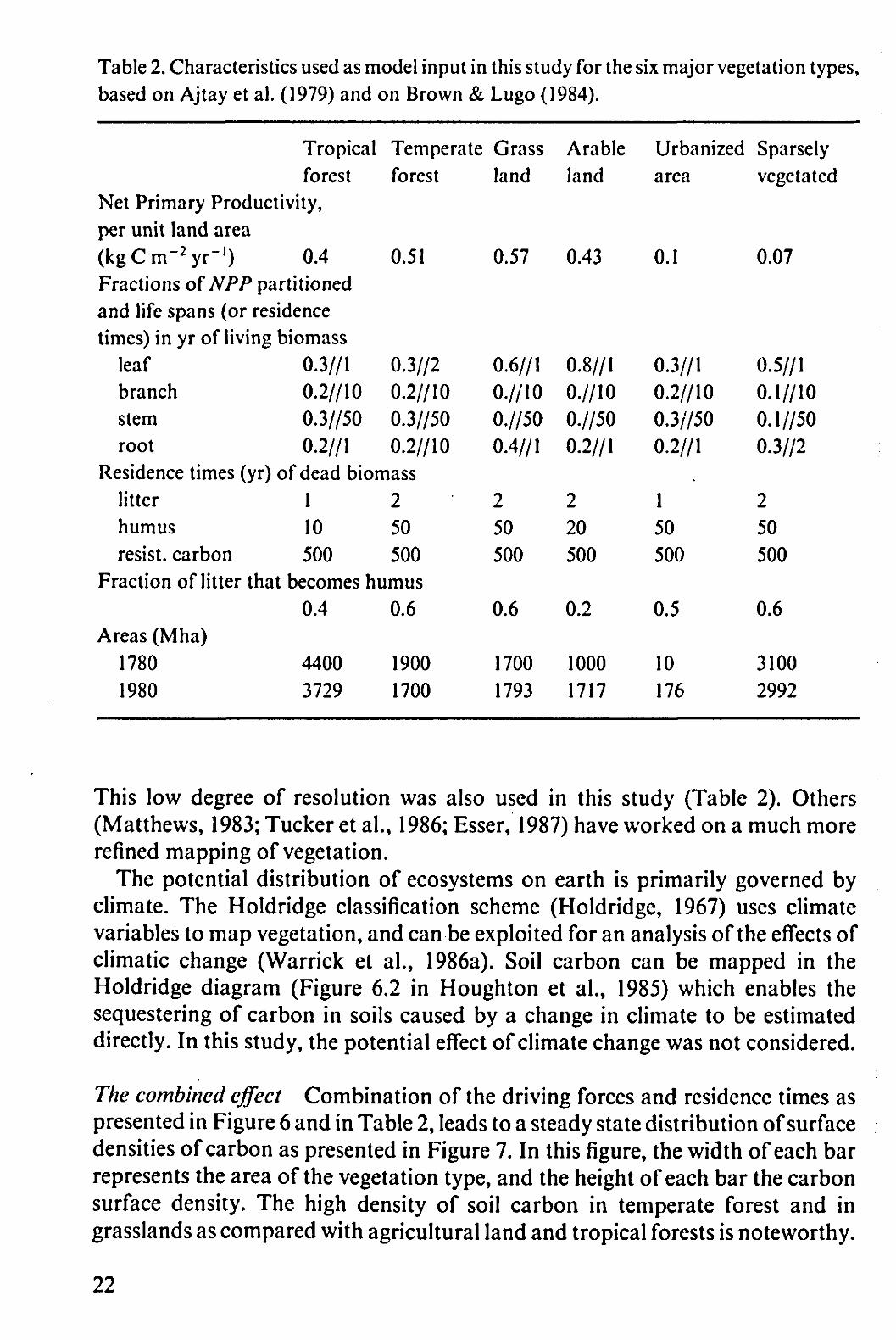
Table 2. Characteristics used as model input in this study for the six major vegetation types, based on Ajtay et al. (1979) and on Brown & Lugo (1984).

Tropical forest

Net Primary Productivity, per unit land area (kgCm- 2yr' ) 0.4 Fractions of NPP partitioned and life spans (or residence times) in yr of living biomass

leaf 0.3//1 branch 0.2//10 stem 0.3//50 root 0.2//1

Temperate forest

0.51

0.3//2 0.2//10 0.3//50 0.2//10

Residence times (yr) of dead biomass litter 1 humus 10 resist, carbon 500

2 50 500

Fraction of litter that becomes humus 0.4

Areas (Mha) 1780 4400 1980 3729

0.6

1900 1700

Grass land

0.57

0.6//1 0.//10 0.//50 0.4//1

2 50 500

0.6

1700 1793

Arable land

0.43

0.8//1 0.//10 0.//50 0.2//1

2 20 500

0.2

1000 1717

Urbanized area

0.1

0.3//1 0.2//10 0.3//50 0.2//1

.

1 50 500

0.5

10 176

Sparsely vegetated

0.07

0.5//1 0.1//10 0.1//50 0.3//2

2 50 500

0.6

3100 2992

This low degree of resolution was also used in this study (Table 2). Others (Matthews, 1983; Tucker et al., 1986; Esser, 1987) have worked on a much more refined mapping of vegetation.

The potential distribution of ecosystems on earth is primarily governed by climate. The Holdridge classification scheme (Holdridge, 1967) uses climate variables to map vegetation, and can be exploited for an analysis of the effects of climatic change (Warrick et al., 1986a). Soil carbon can be mapped in the Holdridge diagram (Figure 6.2 in Houghton et al., 1985) which enables the sequestering of carbon in soils caused by a change in climate to be estimated directly. In this study, the potential effect of climate change was not considered.

The combined effect Combination of the driving forces and residence times as presented in Figure 6 and in Table 2, leads to a steady state distribution of surface densities of carbon as presented in Figure 7. In this figure, the width of each bar represents the area of the vegetation type, and the height of each bar the carbon surface density. The high density of soil carbon in temperate forest and in grasslands as compared with agricultural land and tropical forests is noteworthy.

22

tropical forest

t e m P e * arass rate flrass

forest land agric. land

urban area

s • • • • • • i i 1111

M » » I I M U H * * * * * * * V * * * * * * * * * * * * * * * • * * * * * * * * * * * * * * * 4 * * * * * * * * * * * * * * * *

fc* * * * * * * * * * * * * * * 4

A* * * * * * * * * * * * * * * * * * * * * * * * * * * * * * * * * * * * * * * * * * * * * * * * * * * * * * * * * * * * * * * * * * * * * * * * * * * * * * * * ! * * * * * * * * * * „ * * * * '

desert, tundra

leaf

n n 1 A * i A i * i wood

ft>\ftfr\?9 PiJiyifum i f t i w i B litter

mmmmnninnn] mmmn

i 1kgC

m"

b=zzd

root

humus

resistant carbon

1000 Mha

Figure 7. Simulated equilibrium distribution of carbon surface densities (heights of the columns) on the areas of each vegetation type (widths of the columns).

Although leaves in forests receive 30% of the NPP, they make up less than 5% of the forest biomass. The density of roots in forests is much higher than in herbaceous ecosystems, because forest roots have a longer residence time.

2.3.2 Human disturbance of vegetation

Houghton (1986) gave a detailed review of the subject of ecosystem disturban­ce, in which he highlighted the uncertainties of estimates of current carbon contents and of the timing of past carbon releases.

Human activities such as agriculture, logging, pollution and urbanization have strongly altered vegetation and will continue to do so. They are locally clearly visible and tend to obscure the physiological and climatic effects of rising at­mospheric C02 on vegetation.

A clear distinction must be made between the two reasons for logging. One is to permanently reclaim agricultural land; the other is to remove wood, perhaps with the intention of a temporary agricultural utilization. Both types of disruption can be modelled by a triangular transition matrix that represents the annual area to be transferred from one vegetation type to another.

23

Disturbance without change of land use For this situation, the local effect of such a disturbance was modelled as a release of most of the aboveground carbon to the atmosphere (burning and decomposition). A small fraction of the biomass, however, becomes longlasting charcoal (5% of leaves, 10% of branches and 20% of stems), and hence is excluded from atmospheric circulation for a long time. This effect reflects the twofold consequence of burning: it not only immediately releases C02 into the atmosphere, but it also fixes a small fraction of the carbon of burnt material into the highly inert charcoal pool (Seiler & Crutzen, 1980). Therefore, the repeated burning of forests, agricultural land and savannahs increases the carbon content of soils at the expense of the atmospheric and oceanic reservoirs. In the model, the charcoal was included in the pool of resistant carbon (residence time 500 yr). Simulation showed that without this type of charcoal formation, atmospheric C02 would currently be at a level of about 5|imol mol'1 higher and increase 5% faster.

On the time scale of a year, carbon fixation is not greatly reduced after the removal of biomass, because pioneer vegetation will take over. As far as the modelling of carbon is concerned, it does not matter what type of vegetation takes up the carbon from the atmosphere. Several decades are needed, however, to restore carbon pools with long residence times, such as stemwood. Net ecosystem production (NEP) after deforestation is typically temporarily positive. After several decades the losses of slowly decaying biomass increase in reservoirs with long residence times (stems in particular) and finally consume almost all produc­tion.

An assumed rate of annual burning (800 Mha yr"1) of biomass (mainly litter) on grassland and agricultural land may seem large, since it causes about 5 Gt C per year to be released, the same rate as fossil fuel burning. However, this litter would have decomposed anyway, and for the carbon cycle it matters little whether it is burnt now, or decomposed one year later. So, it is not surprising that the simulated atmospheric C02 concentration in 1980 was scarcely affected (6pmol mol"1 lower) when this litter burning was set at zero. Shifting cultivation in tropical forests (15 Mha yr"1) did not have a large effect either: if it did not occur, the simulated atmospheric C02 concentration in 1980 was only 1 ^mol mol-1

lower.

Land reclamation When land use is changed as well, the contents of the soil carbon reservoirs are transferred to the corresponding reservoirs of the new vegetation type, usually agricultural land. The residence time of humus in agricul­tural land is shorter than in forest soil, resulting in a considerable loss of soil carbon during the subsequent years. For instance, in soils of tropical forests the simulated mean areal density of carbon was 14 kg m"2 in contrast with only 8kgm"2 in agricultural land. A rate of transfer of 12 Mha yr"1 therefore means that about 0.7 Gt C will eventually be released for each year that this deforesta­tion occurs. This release is not instantaneous but delayed in time. A dynamic

24

simulation model takes such a delay into account, in contrast with simple statistical calculations that assume immediate release.

The rate of land reclamation around the turn of this century was assumed to be faster than in Goudriaan & Ketner (1984), and the current rate was assumed to be lower. This larger emphasis on early reclamation better represents the colonial expansion in that period. The net effect of these land use changes was that during the last 200 years the area of agricultural land rose from 1000 to 1800 Mha (100 Mha = 10I2m2), mainly at the expense of tropical forests. Temperate forests were also reduced (by 100 Mha), but grassland area increased (by 140 Mha). The assumed present rate of deforestation is about 6 Mha yr ~' to agricultural land and another 6 Mha yr"1 to grassland.

A straightforward method of estimating biospheric releases is to use the rate of annual land transfer from virgin land to agricultural soil, and to multiply it by the difference between soil carbon content typical for both types of land use. Similar­ly, the rate of removal of aboveground biomass can also be included. Added to 'calculated soil carbon loss' this rate gives the 'calculated total reclamation losses' in Figure 8. The strong increase in recent times is caused by accelerated deforesta­tion in the tropics.

However, this type of calculation neglects other important components of the global fluxes between atmosphere and biosphere, which can change the net balance considerably. First, deforested land is not only taken into use as arable land but also as grassland, and grassland has a much higher soil carbon content than arable land. Second, the soil carbon is not released instantaneously, but is gradually decomposed over decades. Third, partial humification and charcoal formation reduce the carbon losses by 10 to 20%. Fourth, in other parts of the world land is also reclaimed by irrigation. In such locations soil carbon is increased, not decreased. Fifth, and most important, a global stimulus ofNPP is likely to occur as a result of the rising level of atmospheric C02. This phenomenon will be examined more closely below.

2.3.3 Terrestrial photosynthesis as affected by C02

The weight fraction of carbon in dry weight of plant material only varies between 40 and 50%, which shows that there must be a close connection between C02 assimilation and dry weight gain. Research has shown the importance of environmental factors such as radiation, temperature, water and nutrient supply for primary production (de Wit et al., 1979). Aerial C02 itself has been proven to be important as well (Lemon, 1984; Warrick et al., 1986b; Kimball, 1983).

In general, the normal partial pressure of ambient CO, of about 300-330 jimol mol"1 is suboptimal (Strain & Cure, 1985) for C3 plants, which form 95% of the biomass. Seasonal dry weight gain is stimulated by increasing ambient C02 up to about 1000 jimol mol"1 partial pressure. Over a large range of C02 (200-1000 jimol mol-1) the response of dry weight gain to C02 can be described by a logarithmic response function

25

net rate of carbon release (Gt y r - 1 ) 2.0 r-

1800 1850 1900 1950 2000 time ( y r )

Figure 8. Reclamation losses of carbon from the biosphere to the atmosphere, according to simple statistics, assuming immediate transition to carbon content in the new vegetation type ( ). Only those transitions to lower carbon contents are considered. Reclamation losses of carbon from the biosphere to the atmosphere, but including delayed release, charcoal formation, and transitions to vegetation types with higher carbon contents ( • ) • The simulated effect of stimulation by increased C02 is also presented ( • ) .

NPP = NPP0 (1 4- p\og(CO2/CO20)) Equation 16

where NPP is the net annual primary production (kg m "2 yr ~!), and NPP0 is NPP in the reference situation at 300u:mol mol"1. C02 stands for the C02 con­centration in the atmosphere expressed in |imol mol-1.

The value of the response factor /? is about 0.7 under good conditions for growth (Goudriaan et al., 1985), but declines with increasing nutrient shortage (Goudriaan & de Ruiter, 1983). Under water shortage (Gifford, 1979; Rosenberg, 1981) the growth-stimulating effect of atmospheric C02 is not reduced, but may even be enhanced. This interaction with water shortage is caused by partial stomatal closure under increased C02. In this situation C4 plants benefit from increased C02 just as much as C3 plants.

Ideally, the value of fi should be determined separately for each type of vegetation, but so far a single value has been used in modelling the global carbon cycle, usually between 0.2 and 0.5. Esser's (1987) equation implies a value of/? as

26

high as just above 1. Goudriaan & Ketner (1984) whose model will be used here, adopted 0.5. This relatively high value was chosen to allow for eutrophication as well.

Because of natural heterogeneity, the resulting stimulus of net primary produc­tivity is not directly measurable or visible in terms of biospheric carbon content, but its actual existence can be inferred from what is known from plant physiology. Its global presence makes its effect significant in terms of global carbon flux, as illustrated in Figure 8.

2.3.4 Terrestrial photosynthesis as affected by biomass

The logarithm of the growth rate of a free-standing individual plant is often linearly related to the logarithm of plant size itself: an allometric relationship. This relationship has been used in a number of models as reviewed by Bolin (1986). However, this relationship cannot be used on the scale of a field, let alone on that of an ecosystem. Because of competition between plants, the effect of biomass on growth can therefore better be described in terms of fraction of radiation absorbed by green leaf area (de Wit, 1965; Milthorpe & Moorby, 1979). As a result of the mutual shading of leaves, the fraction of absorbed radiation is soon saturated as leaf area increases. Above a leaf area index (LAI) of 3 m2 (leaf area) m~2 (land area), which corresponds to a leaf dry weight of 150gm"2 (land area) no further increase of NPP can be expected with increasing leaf biomass. Once the soil is covered, positive feedback of biomass on NPP is further weake­ned by increased partitioning of growth to non-photosynthesizing organs such as stems and branches. Therefore, models that use an allometric relationship be­tween NPP and biomass on a global scale tend to overestimate the positive feedback of biomass.

Expansion of vegetation onto previously bare land should be explicitly model­led as area growth of vegetation coverage. Such processes were not considered in this study, but it is clear that they might occur as an effect of increasing C02.

2.4 The ocean

2.4.1 Layer structure, and two ocean types

Reviews of some of the existing models for carbon exchange between ocean and atmosphere can be found in Bjorkstrom (1986), Sarmiento (1986), Broecker & Peng (1982), Baes et al. (1985). As Bjorkstrom (1986) pointed out, some of these models have been compartmentalized to such an extent that they need as many as 600 parameters.

The work presented here aims at striking a balance between the needs for high resolution on one hand and for simplicity on the other. As in the model presented by Goudriaan & Ketner (1984), the ocean was compartmentalized into 10 strata, and the top one was further split into three zones: a high latitude zone (after

27

HE T T

T7T" 1b

I L L

IF

10

ic

JZ:

T

IT

mass flow VMMAb.

I I '//.•

I

Figure 9. Modelled stratification of the ocean.

Viecelli et al., 1981) and a low latitude zone consisting of two strata (Figure 9). Exchange between adjacent strata was described by a diffusion type equation, with a 'diffusion' coefficient derived from tracer studies (K = 4000 m2 yr"'). There was a mass flow (Gordon flow), sinking from the high latitude surface zone, and re-entering the deep sea at a depth between 2000 and 3000 m. This mass flow forced an upwelling into the low latitude surface zone. The circulation was closed by a mass flow from the low to the high latitude surface zone.

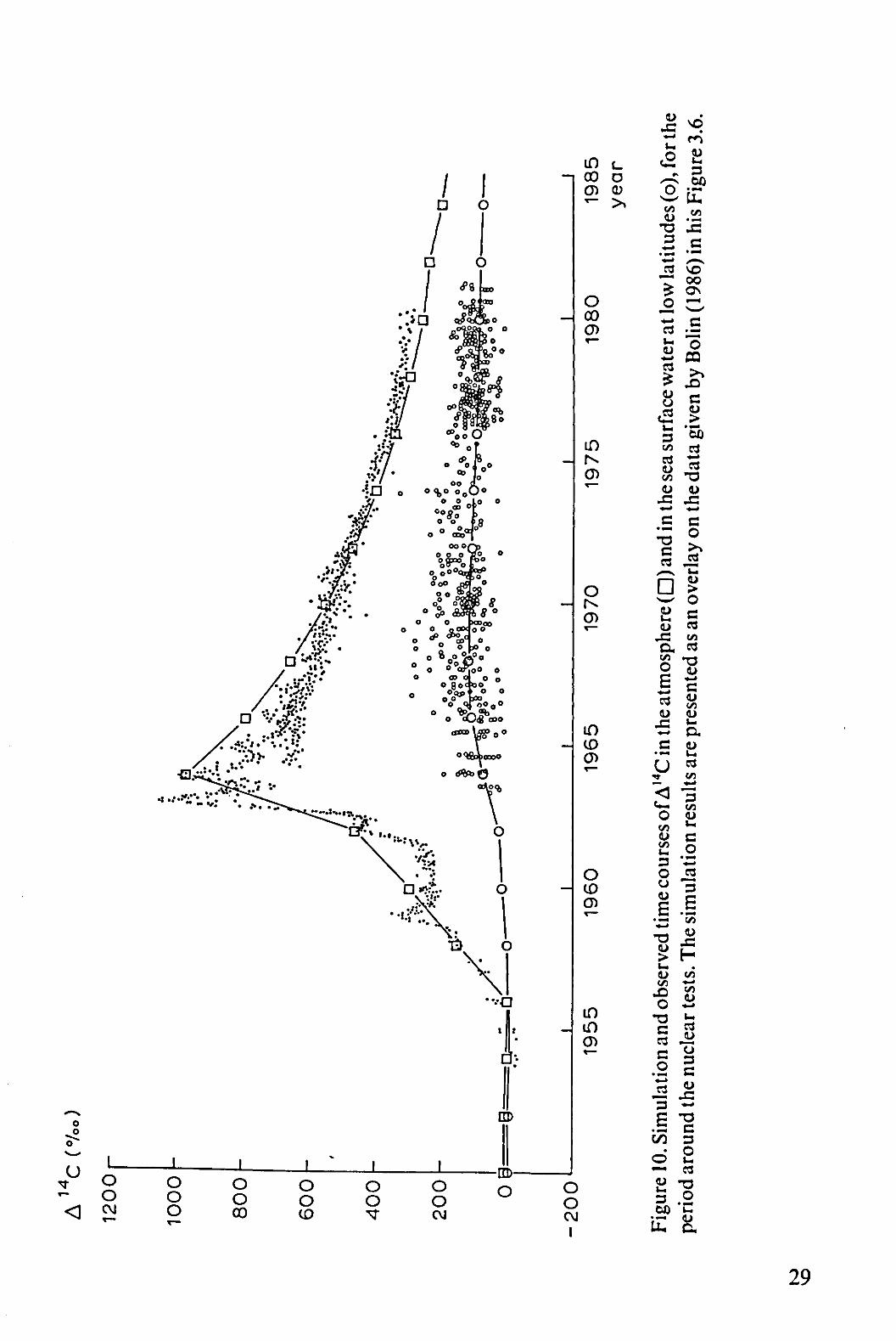
In modification of the Goudriaan & Ketner (1984) model, the surface zones of the oceans were considered to be internally well-mixed (£ infinite), but a surface conductance of 4myr"1 was modelled for exchange with the atmosphere. The value of this conductance was found by calibration with the rate of decline of the ,4C peak after the nuclear tests in the early 1960s (Figure 10). The carbon content of these 4 m of sea water is annually exchanged with the atmosphere, which is equivalent to an exchange rate of about 9 mol Cm"2 yr-1 (39 Gt C yr"1 globally). However, since the amount of carbon that is needed for chemical equilibration is about 10 times (Revelle factor) less, this same exchange flux involves a 10 times greater depth for chemical equilibration.

In the 1984 model, marine photosynthesis was defined as a fixed driving force. The decomposition of precipitated organic material could account for observed features such as high partial pressure of C02 in deep sea water, C02 release in the upwelling zone and uptake C02 in the high latitude downwelling zone.

In view of large observed differences between the Atlantic Ocean on one hand and the Pacific and Indian Oceans on the other (Baes et al., 1985), the two ocean systems were modelled separately by using the same ocean submodel with adap­ted characteristics. In the modified model, the two ocean systems differed mainly by their rate of internal turning over of deep and surface water (Gordon flow), which is much higher in the Atlantic than in the Pacific and Indian Oceans (2 1015

m3 yr"1 versus 0.2 1015 m3 yr"1) (Baes et al., 1985). In glacial periods these oceans may have been more similar (Broecker & Peng, 1982); this was modelled by a reduction of the Atlantic deep mass flow.

28

o o

o

00 o O) <D

C D - T

* 3

S .2 3 c

. _ • •<-< • ^ / — ^

•r oo £ OS o

00 0 )

in r G)

c3

CD

d £ CD

£ U* 3 C/3

cj CD C/3

c

"o CO

c CD

> • ^ 60 et*

c c o

C

B £ w o E c CD S3

JZ c/3 a a

IS <u CD

U CD

C/3

< -3

C/3

3

CD C/3 U , 3 O CD CD

E • ^ - -» T 3 CD > u, CD C/3

O T3 C

c o 'ZZ j « 3

6 35 CD

H • C/3

• ^ C/3 CD

u c3

c3 -25 C 3

.2 c 3 * -B "

. 3 C in D ^ ° O u, 3 .2 ;r «

29

Apart from their obvious connection via atmospheric C02, the two ocean systems were connected via a strong circumpolar flow of surface water in the Antarctic Sea, exchanging phosphate, oxygen and total carbon. Some exchange of deep sea water may occur as well, but was not included in the model. At the 45.2%o isopycnal many characteristics have a steep gradient (GEOSECS data in Broecker & Peng, 1982), which means that there is little exchange between the deep waters of the Antarctic Sea and the oceans.

This modelled connection of both oceans enabled the Pacific Ocean to extract nutrients from the Atlantic Ocean, by a process of skimming the surface water. This combination of primary productivity and exchange of surface water could generate the observed large differences in chemical compositions in both ocean systems. The precipitation of organic material originating from marine photosyn­thesis was found to be essential in maintaining this difference.

2 A.2 Marine photosynthesis

Since nutrients strongly affect marine photosynthesis, it was necessary to include nutrient transport in the model. Phosphate was treated as the main factor limiting primary productivity. The total amount of ocean phosphate was initiali­zed as an input parameter (92 Gt P, on the basis of Baes et al., 1985), but the distribution of phosphate was established by simulation. The ratio between precipitation of organic material (C) in gm"2 yr"1 and phosphate concentration (P) of the upper layer in gm"3, which had a value of 278 gCg"1 Pm yr"1, is an important model parameter. This parameterization led to a global downward flux of approximately 3GtC yr"1, sinking below 400 m depth. The phosphorus content of organic material, and its oxygen demand upon decomposition were derived from the Redfield equation (Baes et al., 1985), and were 0.024 g P g"1 C and 3.47g Og"'C, respectively.

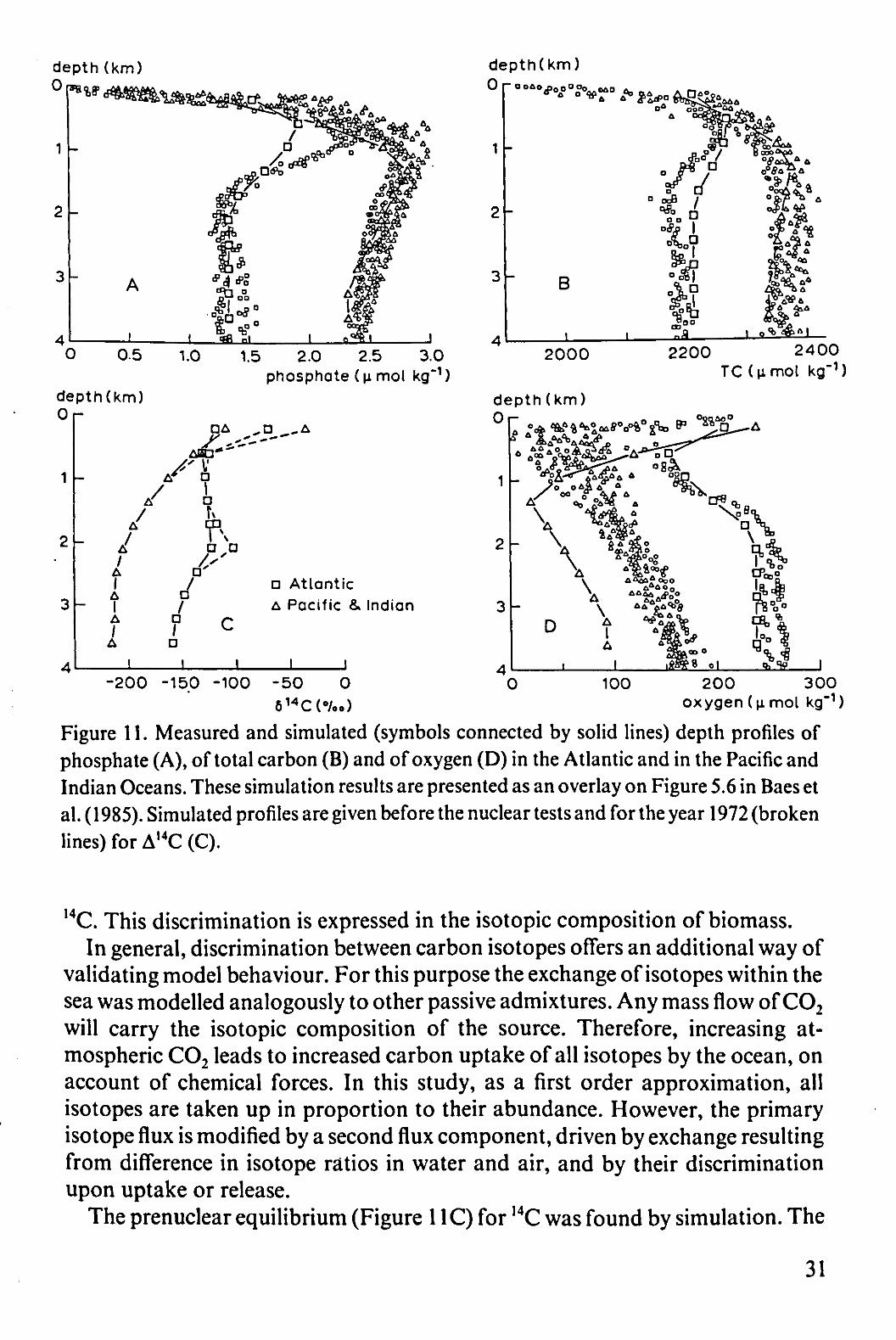
Surface layers received phosphate from the deeper layers by upwelling and by diffusion. The precipitating organic material was allowed to decompose between 400 and 1500 m depth, thereby boosting the levels of phosphate and carbonate and reducing that of oxygen (Figure 11). The profiles generated in this way are similar to observed profiles (Baes et al., 1985). The biological parameters of primary productivity were identical in the two major ocean systems, showing that the difference between these systems is caused by the different characteristics of physical flow.

2.5 The carbon isotopes

The radioactive carbon isotope 14C is absent in fossil fuel, and so the use of fossil fuel leads to a dilution of the ,4C concentration in atmosphere, biosphere and ocean. On the other hand, much 14C was produced during the nuclear tests in the 1960s. In the process of photosynthetic carbon uptake there is a slight discrimination in favour of the lighter carbon isotopes in the series ,2C, ,3C and

30

depth (km) 0 p8> m&&^{b£%^^ *&

1.5 2.0 2.5 3.0 phosphate (\i mol kg"1)

depth(km) O r

DA

y /

A m " " ' " '

D

/

/ A I

A I

A /

A

D D

A'

/ a /

D

n Atlantic A Pacific & Indian

_L ±

depth(km) O r B " ° ^ C

0 V D * 2%p?

1 -

B

2 0 0 0

depth (km)

2200 2 4 0 0 TC(i imot kg"1)

^ i ^ n ^ 0 ^ 0 ^ * 3 °&>*g

D \ A I A q

J - 2 0 0 -150 -100 100 200 3 0 0

oxygen (\i mol kg"1) - 5 0 0 0 614C (%,<»)

Figure 11. Measured and simulated (symbols connected by solid lines) depth profiles of phosphate (A), of total carbon (B) and of oxygen (D) in the Atlantic and in the Pacific and Indian Oceans. These simulation results are presented as an overlay on Figure 5.6 in Baes et al. (1985). Simulated profiles are given before the nuclear tests and for the year 1972 (broken lines) for A,4C (C).

14C. This discrimination is expressed in the isotopic composition of biomass. In general, discrimination between carbon isotopes offers an additional way of

validating model behaviour. For this purpose the exchange of isotopes within the sea was modelled analogously to other passive admixtures. Any mass flow of C02

will carry the isotopic composition of the source. Therefore, increasing at­mospheric C02 leads to increased carbon uptake of all isotopes by the ocean, on account of chemical forces. In this study, as a first order approximation, all isotopes are taken up in proportion to their abundance. However, the primary isotope flux is modified by a second flux component, driven by exchange resulting from difference in isotope ratios in water and air, and by their discrimination upon uptake or release.

The prenuclear equilibrium (Figure 11C) for 14C was found by simulation. The

31

long residence time of water in the deep Pacific shows up in low values of the concentration of ,4C. This concentration is expressed by the symbol A,4C, which stands for 1000 times the relative difference of the ratio 14C/Ctotal, compared with a standard ratio. In Figure 11C an effect of the nuclear testing period in the 1960s is also visible: a tongue of downwelled water can be seen in the Atlantic Ocean at a depth of about 2000 m.

The assumed discrimination of 13C in photosynthesis (Mook, 1986) caused a correlation between A,3C and phosphate practically identical to the observed relationship (see Figure 6-12 in Broecker & Peng, 1982).

The A,3C was assumed to be — 25%o for carbon in fossil fuels and — 19%o in photosynthesis, and so the simulated level of atmospheric A13C decreased by 1.47%o between 1860 and 1980, with a continuing annual rate of decrease of 0.03 in 1980. These figures practically coincide with the data recorded by Freyer (1986) (Figure 12A), but they show a faster rate of decrease than Stuiver (1986) found. For atmospheric A,4C a similar, but much stronger decrease (the Suess effect) was simulated, from — 23.5%o in 1860 down to — 46%o in 1950. These model simula­tions fall in line with the data as given in Stuiver & Quay (1981) and Bolin (1986) (Figure 12B). Using these methods, the accumulated net loss of biospheric carbon between 1860 and 1980, was simulated to be no more than 30GtC.

On the basis of direct calculations and of isotope ratios, other researchers have come up with much higher estimates, even exceeding 100 GtC in total (Bolin, 1986; Houghton et al., 1985). The difficulty with the direct estimates was discussed above (Sections 2.2 and 2.3). The uncertainty range of the isotope-based estimates is also large, because these estimates are based on the difference between the ,3C and ,4C records. Actual ,3C variability in sampled wood is often as large as the signal itself. These high estimates of releases have caused some problem in connection with the actual rate of increase of atmospheric CO:. The simulation results presented here do not suffer from this problem of'missing carbon'.

2.6 The importance of model factors

2.6.1 Terrestrial biosphere

Because of the large size of the ocean in comparison with the terrestrial biosphere, the ocean was included when the effect of biospheric parameters was studied. On the other hand the biosphere could have been omitted when studying the first order effects of changes in ocean parameters, but for completeness the ocean was then also included. Unless explicitly mentioned all affects apply to the response of the combined atmosphere-ocean-biosphere system.

Change in vegetated area As a theoretical exercise the effect of the vegetated area increasing by 1000Mha (10 1012m2) from bare land to grassland and forest was studied. It is hard to see how such an increase would be possible under steady climatic conditions, but a changing climate could perhaps induce such an in-

32

A13 C (•/.,)

-1.0 -

- 1 . 5 -

-2.0 -

1800 1900 2000 t ime (y r )

- 10

-20

. • •• ••% > -

I I J I L

B

1850

••.-V .•

J I I ' ' • I

1900 1950 t ime (y r )

Figure 12. Simulated and measured time courses of carbon isotope ratios. The simulation results are presented as overlays. A: For A,3C on the data given by Freyer (1986) in his Figure 7.5. B: For A,4C on the data given by Stuiver & Quay (1981). The 'MODEL PREDICTION1 of Broecker & Peng (1982) in their Figure 10-23 for the same data and my simulated results practically coincide (solid line).

crease. This increase in vegetated area would cause a carbon sequestering of some 230 Gt C (23 kg C m"2) in the long run. Although such a large amount of carbon is equivalent to about 110|xmol mol"1 if extracted instantaneously from the at­mosphere, the slowness of growth of stemwood and of accumulation of soil carbon permitted the oceans to gradually release C02 in response to the decreased partial pressure of C02 in the atmosphere. As a result, atmospheric C02 never dropped to more than 25^mol mol"1 below the starting level. It reached an equilibrium after one thousand years, which was only 15 |imol mol"1 lower than the initial level.

33

Change in longevity of soil carbon The longevity of soil carbon (humus and charcoal) is of great importance. When its value was instantaneously doubled, atmospheric C02 dropped from 285 to around 220|imol mol"1 within a few decades, and remained at that level. About 1000 Gt C was sequestered in the soil, of which 840 Gt C was extracted from the sea, and 140 Gt C from the atmosphere.

Wetness of climate has a large effect on the amount of soil carbon. Doubling the precipitation/evaporation ratio also practically doubles the soil carbon (Figure 6.2 in Houghton et al., 1985). General Circulation Model (GCM) studies indicate that the hydrological cycle is increased up to 15% when atmospheric C02 is doubled, but it is not clear what this means in terms of the precipitation/ evaporation ratio in vegetated regions.

Change in C02 stimulus of NPP In the control run, fi was set at 0.5. In this situation, C02, when emitted into the atmosphere, will eventually be redistributed between ocean, biosphere and atmosphere in a ratio of 0.71:0.18:0.11. If, on the other hand, any effect of atmospheric C02 on net primary productivity was assumed to be absent, C02 emitted into the atmosphere was redistributed be­tween ocean and atmosphere only in a ratio of 0.85:0.15. This redistribution process will take hundreds of years, because of the slowness of mixing in the oceans. On such long time scales the effect of the ocean reservoir is so large that the importance of photosynthetic stimulus by atmospheric C02 is only slight.

On a time scale of decades, however, and at the present rate of fossil fuel consumption, a value of 0.5 or of 0.0 for JS makes a difference of about 10 years in the rising curve of atmospheric C02. This global photosynthetic stimulus slows down the greenhouse effect by about 10 years.

2.6.2 Ocean

Changes in marine photosynthesis In the model, marine primary productivity was linearly linked to phosphate concentration in the surface waters. As a result, two model characteristics dominated the precipitation rate of dead organic matter. First, the phosphate content of organic material (Redfield ratio), since it governs the rate of extraction from surface water, and second, the proportionality factor between precipitation rate and phosphate concentration. When this pro­portionality factor was doubled, precipitation doubled instantaneously too. However, phosphate was then withdrawn at a doubled rate, and the phosphate concentration in the water dropped. This negative feedback mechanism consider­ably reduced the eventual effects of the precipitation/phosphate ratio: atmos­pheric C02 dropped by 35 nmol mol"1. A similar mechanism operated when the Redfield ratio was halved: decreased withdrawal of phosphate caused some accumulation of phosphate in the surface layers, thereby stimulating photosyn­thesis and carbon precipitation to the deep sea: a drop by about 30 imol mol"1. Only when the Redfield ratio was halved and the precipitation/phosphate ratio was simultaneously doubled, did the phosphate content of the water remain

34

unchanged and a strong change in rate of carbon precipitation could be maintain­ed, resulting in a considerable change of atmospheric C02: a drop of 85 jimol mol"1.

Of course, a direct change in the total amount of phosphate in the ocean also had a large effect: about 1 jimol mol"1 decline of atmospheric C02 for every per cent increase of total ocean phosphate.

Changes in ocean currents Atmospheric C02was remarkably insensitive to the circumpolar flow that connects both ocean systems. If it was decreased from 2 1015

m3 yr"1 to 0.1 10,5m3 yr-1, the difference between the ocean systems was largely maintained, and atmospheric C02 remained about the same.

A much stronger effect resulted from changes in the mass flow within each ocean system. If the Gordon flow in the Atlantic was reduced from 2 to 1 1015 m3

yr-1, atmospheric C02 dropped from 285 to 273|imol mol"1 and a further reduction to 0.2 1015 m3 yr-1 resulted in an atmospheric C02 of 260^mol mol"1.

This effect can be explained by decreased upwelling, a lowering of the phos­phate concentration in the surface layer of the Atlantic and increase of both phosphate and total carbon in the deep Atlantic. In the Pacific very little changed.

Similarly, if the mass flow in the Pacific was increased from 0.2 1015 m3 yr"1 in the control run to 2 1015 m3 yr-1, the atmospheric concentration of C02 was increased from 285 up to 334 nmol mol"' in 500 years time. The relaxation time of these changes was about 200 years.

Changing the depth at which the downwelling water of the Atlantic enters the deep sea from 1500 to 3500 m reduced the residence time of the deep water (as indicated by A,4C) but with little effect for other factors. This lack of importance of the re-entry depth is connected with the completeness of decomposition of precipitated organic material in the upper 1500 m. Below this depth almost no gradient remained.

2.7 Conclusion and discussion

About 60% of the C02 currently emitted from the burning of fossil fuel remains in the atmosphere and 40% is absorbed by the oceans. The distribution pattern is strongly dependent on the rate of emission. A lower rate of emission gives more time for absorption in the ocean.

When it is taken into account that net photosynthesis is stimulated by C02, the partitioning of carbon over atmosphere, ocean and terrestrial biosphere is shifted from the ratios 0.15:0.85:0.0 to 0.11:0.71:0.18, respectively.

Significant amounts of carbon can be released from the biosphere when it is disturbed. Reclamation of land for agriculture and for other types of human utilization can cause oxidation of soil carbon and of long-lived biomass such as wood. In the past century such processes were responsible for the release of large amounts of carbon. At present they tend to be increasingly balanced by a global stimulus of growth resulting from increased atmospheric C02 itself. Regrowth on abandoned land also gives a partial compensation.

35

The role of the biosphere made it difficult to define the airborne fraction of C02. If atmospheric increase is related to emission from fossil fuel only, C02 uptake by the biosphere is included in the net effect. Since the biosphere does not follow the rules of chemical equilibration, the airborne fraction will be less stable and will also be dependent on human disturbance of the biosphere. For this reason Bolin (1986) introduced the term 'total airborne fraction' which was defined as at­mospheric increase divided by the sum of biospheric and fossil fuel emissions. Of course, net biospheric emission of C02 should then be used and not the gross emission. When Bolin (1986) criticized the model of Goudriaan & Ketner (1984) for having too low an airborne fraction (0.3), he found this figure by using gross biospheric emission. In fact, when the net result of biomass removal and subse­quent regrowth is used, the airborne fraction for the year 1980 in their model was 0.58 and not 0.3.

In this study felling forest for land reclamation for permanent human use was found to be significant, releasing C02 at a rate of about 0.5 to 1 Gt C yr~'. On the other hand, this rate of release is more than compensated for by global stimula­tion of growth by atmospheric C02. Model calculations showed that the growth stimulus has caused an additional uptake of about 64 Gt C by the biosphere, reducing atmospheric C02 by about 36 Gt C. This increased carbon sequestering is equivalent to 10 years of emission from fossil fuels. However, this additional storage of carbon induced by increased C02 is extremely difficult to detect directly by sampling methods in the field, because of the large natural heterogeneity.

The results presented for the time patterns of carbon isotopes give no reason to believe that the net accumulated carbon release from the biosphere during the last century has been more than about 30GtC. Both the isotopic data and the C02

data themselves are consistent with this limited net release of biotic carbon. Even a slight imbalance in the growth of terrestrial ecosystems on a global scale is sufficient to absorb the carbon released by deforestation (Lugo & Brown, 1986). Such an imbalance may result from increasing atmospheric C02, as assumed here, but other environmental factors may be involved as well.

A further conclusion along this line is that the terrestrial biosphere, and especially the soil, can store significant amounts of carbon. A 3% increase in carbon content (relative to carbon, not to soil weight) means a carbon sequester­ing of 50 GtC.

The ocean is extremely important for the level of atmospheric C02. If the rate of upwelling of deep water is increased, more C02 will be released and atmospheric C02 will rise. This effect is only partly compensated for by a simultaneous increase of marine photosynthesis by the nutrients that are brought to the surface.

During the glacial periods atmospheric C02 was much lower than during interglacials, and the vegetated area was presumably much smaller. Although soil carbon may have been higher in the tropics than at present, it seems unlikely that it could have stored the loss of terrestrial carbon in the high latitudes. Climatic wetness stimulates accumulation of soil carbon, but during the glacials climate was probably drier, not wetter. From a physiological point of view the dryness

36

was accentuated by low atmospheric C02 which stimulates stomatal opening and transpiration. Dry and C02-poor conditions definitely favoured C4 species, and probably stimulated their evolution. In view of these considerations it is most likely that the terrestrial carbon pool was much smaller during the glacials than between them. The increase of terrestrial biomass at the end of the glacial periods must have created a large sink for C02. In addition to going the wrong way, it is hard to see how the terrestrial biosphere could have caused the rapidity of the changes of atmospheric C02.

Marine photosynthesis itself can probably not be altered much in its response to the limiting nutrient phosphate. However, it is the precipitated fraction that matters for carbon accumulation in the deep sea. Also, the depth at which decomposition occurs is important. These factors are probably biology-linked and controlled by species composition. One other factor: if release of phosphate upon decomposition of precipitating organic material is accelerated with respect to that of carbon, the remaining material is depleted in phosphate. Such a shift would cause a further decline in atmospheric C02.

Ocean circulation, however, must have been the dominant factor. Changes in ocean circulation have a very large and quick effect. The question remains what has initiated the required changes in pattern or magnitude of the circulating flows. The temperature feedback on solubility of C02 in sea surface water was found to amplify an externally caused change in atmospheric C02 by a factor of 1.5.

According to the ocean part of the model presented here, the differences in nutrient content between the major ocean systems can be sufficiently explained by their vastly different rates of internal water circulation, even if deep sea currents from the Atlantic to the Pacific (Broecker & Peng, 1982) are not considered. These currents will enhance the nutrient-enriched character of the deep Pacific as compared with the waters of the Atlantic.

2.8 Acknowledgments

The author would like to thank Dr P.A. Leffelaar, Dr P. de Willigen and Dr R. Jenne (NCAR, U.S.A.) for their valuable criticism and comments.

2.9 References

Ajtay, G.L., P. Ketner & P. Duvigneaud, 1979. Terrestrial primary production and phytomass. In: B. Bolin et al. (Eds): The global carbon cycle. SCOPE 13: 129-181.

Baes, C.F., A. Bjorkstrom & P.J. Mulholland, 1985. Uptake of carbon dioxide by the oceans. In: J.R. Trabalka (Ed.): Atmospheric carbon dioxide and the global carbon cycle. United States Department of Energy, Office of Energy Research, Washington, D.C. DOE/ER-0239:81-111.

Bjorkstrom, A., 1986. One-dimensional and two-dimensional ocean models for predicting the distribution of CO: between the ocean and the atmosphere. In: J.T. Trabalka & D.E.

37

Reichle (Eds): The changing carbon cycle, a global analysis. Springer Verlag, New York, pp. 258-278.

Bolin, B., E.T. Degens, S. Kempe & P. Ketner (Eds), 1979. The global carbon cycle. Scientific Committee on Problems of the Environment, SCOPE 13, Wiley & Sons, Chichester, 491 pp.

Bolin, B., B.R. Doos, J. Jiiger & R.A. Warrick (Eds), 1986. The greenhouse effect, climatic change and ecosystems. Scientific Committee on Problems of the Environment, SCOPE 29. Wiley & Sons, Chichester, 541 pp.

Bolin, B., 1986. How much C02 will remain in the atmosphere? In: B. Bolin, B.R. Doos, J. Jiiger & R.A. Warrick (Eds.): The greenhouse effect, climatic change and ecosystems. SCOPE 29: 93-155.

Broecker, W.S. & T.H. Peng, 1982. Tracers in the sea. Lamont-Doherty Geological Observatory, Columbia University, Palisades, New York, 690 pp.

Brown, S. & A.E. Lugo, 1984. Biomass of tropical forests: a new estimate based on forest volumes. Science 223: 1290-1293.

Clark, W.C. (Ed.), 1982. Carbon dioxide review: 1982. Oxford University Press, Oxford, 469 pp.

Esser, G., 1987. Sensitivity of global carbon pools and fluxes to human and potential climatic impacts. Tellus 39B: 245-260.

Freyer, H.D., 1986. Interpretation of the northern hemisphere record of l3C/,2C trends of atmospheric C02 in tree rings. In: J.R. Trabalka & D.E. Reichle (Eds): The changing carbon cycle, a global analysis. Springer Verlag, New York, pp. 125-150.

Gifford, R.M., 1979. Growth and yield of C02-enriched wheat under water-limited condi­tions. Australian Journal of Plant Physiology 6: 367-378.

Goudriaan, J. & H.E. de Ruiter, 1983. Plant growth in response to C02 enrichment, at two levels of nitrogen and phosphorus supply. Netherlands Journal of Agricultural Science 31: 157-169.

Goudriaan, J. & P. Ketner, 1984. A simulation study for the global carbon cycle, including man's impact on the biosphere. Climatic Change 6: 167-192.

Goudriaan, J., H.H. van Laar, H. van Keulen & W. Louwerse, 1985. Photosynthesis, C02

and plant production. In: W. Day & R.K. Atkin (Eds): Wheat growth and modeling. NATO ASI Series, Series A: Life Sciences Vol. 86. Plenum Press, New York, pp. 107-122.

Goudriaan, J., 1986. Simulation of ecosystem response to rising C02, with special attention to interfacing with the atmosphere. In: C. Rosenzweig & R. Dickinson (Eds): Climate-Vegetation interactions. NASA Conference Publication 2440, Greenbelt Md. pp. 68-75.

Holdridge, R., 1967. Life Zone Ecology. Tropical Science Center. San Jose, Ca., 206 pp. Houghton, R.A., 1986. Estimating changes in the carbon content of terrestrial ecosystems

from historical data. In: J.R. Trabalka & D.E. Reichle (Eds): Springer Verlag, New York, pp. 175-193.

Houghton, R.A., W.H. Schlesinger, S. Brown & J.F. Richards, 1985. Carbon dioxide exchange between the atmosphere and terrestrial ecosystems. In: J.R. Trabalka (Ed.): Atmospheric carbon dioxide and the global cycle. United States Department of Energy, Office of Energy Research. DOE/ER-0239: 113-140.

38

Kimball, B.A., 1983. Carbon dioxide and agricultural yield: an assemblage and analysis of 430 prior observations. Agronomy Journal 75: 779-788.

Kortleven, J., 1963. Kwantitatieve aspecten van humusopbouw en humusafbraak. Agricul­tural Research Reports 69.1. Pudoc, Wageningen. 109 pp.

Lemon, E.R. (Ed.), 1984. C02 and plants. Westview Press, Colorado, 280 pp. Lugo, A.E. & S. Brown, 1986. Steady state terrestrial ecosystems and the global carbon

cycle. Vegetatio 68: 83-90. Matthews, E., 1983. Global vegetation and land use: new high resolution data bases for

climate studies. Journal of Climate and applied Meteorology 22: 474-487. Milthorpe, F.L. & J. Moorby, 1979. An introduction to crop physiology. Cambridge

University Press, Cambridge, 244 pp. Mook, W., 1986. ,3C in atmospheric C02. Netherlands Journal of Sea Research 20:

211-223. Olson, J.S., 1963. Energy storage and the balance of producers and decomposers in

ecological systems. Ecology 44: 322-331. Rosenberg, N.J., 1981. The increasing C02 concentration in the atmosphere and its

implication for agricultural productivity. Climatic Change 3: 265-279. Sarmiento, J.L., 1986. Three-dimensional ocean models for predicting the distribution of

C02 between the ocean and atmosphere. In: J.R. Trabalka & D.E. Reichle (Eds): Springer Verlag, New York, pp. 279-294.

Schlesinger, W.H., 1986. Changes in soil carbon storage and associated properties with disturbance and recovery. In: J.R. Trabalka & D.E. Reichle (Eds): Springer Verlag, New York, pp. 194-220.

Seiler, W. & P.J. Crutzen, 1980. Estimates of gross and net fluxes of carbon between the biosphere and the atmosphere from biomass burning. Climatic Change 2: 207-247.

Strain, B.R. & J.D. Cure (Eds), 1985. Direct effects of increasing carbon dioxide on vegetation. United States Department of Energy, Office of Energy Research, Washing­ton D.C., DOE/ER-0238, 286 pp.

Stuiver, M. & P.D. Quay, 1981. Atmospheric ,4C changes resulting from fossil fuel C02

release and cosmic ray flux variability. Earth and Planetary Science Letters 53: 349-362. Stuiver, M., 1986. Ancient carbon cycle changes derived from tree-ring ,3C and ,4C. In: J.R.

Trabalka & D.E. Reichle (Eds): The changing carbon cycle, a global analysis. Springer Verlag, New York, pp. 109-124.

Tucker, C.J., I.Y. Fung, CD. Keeling & R.H. Gammon, 1986. Relationship between atmospheric C02 variations and a satellite-derived vegetation index. Nature 319: 195-199.

Viecelli, J.A., H.W. Ellsaesser & J.E. Burt, 1981. A carbon cycle model with latitude dependence. Climatic Change 3: 281-302.

Warrick, R.A., H.H. Shugart, M.Ja. Antonovsky, with J.R. Tarrant & C.J. Tucker, 1986a. The effects of increased C02 and climatic change on terrestrial ecosystems. In: B. Bolin, B.R. Doos, J. Jager & R.A. Warrick (Eds): The greenhouse effect, climatic change and ecosystems. SCOPE 29: 363-392.

39

Warrick, R.A. & R.M. GifTord, with M.L. Parry, 1986b. C02, climatic change and agriclture. In: B. Bolin, B.R. Doos, J. Jager & R.A. Warrick (Eds): The greenhouse effect, climatic change and ecosystems. SCOPE 29: 393-473.

Wit, C.T. de, 1965. Photosynthesis of leaf canopies. Agricultural Research Reports 66.3, Pudoc, Wageningen, 57 pp.

Wit, C.T. de, H.H. van Laar & H. van Keulen, 1979. Physiological potential of crop production. In: J. Sneep & A.J.T. Hendriksen (Eds): Plant breeding perspectives. Pudoc, Wageningen, pp. 47-82.

40