�13C and �18O Isotopic Composition of CaCO3 Measured by Continuous

Flow Isotope Ratio Mass Spectrometry: Statistical Evaluation and Verification by Application to Devils Hole Core DH-11 Calcite.

Kinga M. Révész and Jurate M. Landwehr

U. S. Geological Survey, 431 National Center, Reston, VA 20192 FAX: 703-648-5274; e-mail: krevesz@usgs.gov; jmlandwe@usgs.gov Abstract

A new method was developed to analyze the stable carbon and oxygen isotope ratios of small samples (400±20 µg) of calcium carbonate. This new method streamlines the classical phosphoric acid – calcium carbonate (H3PO4 – CaCO3) reaction method by making use of a recently available Thermoquest-Finnigan GasBench II* preparation device and a Delta Plus XL continuous flow isotope ratio mass spectrometer. Conditions for which the H3PO4 – CaCO3 reaction produced reproducible and accurate results with minimal error had to be determined. When the acid-carbonate reaction temperature was kept at 26ºC and the reaction time was between 24 and 54 hours, the precision of the carbon and oxygen isotope ratios for pooled samples from 3 reference standard materials was •0.1 and •0.2 per mill or ‰, respectively, although later analysis showed that materials from one specific standard required reaction time between 34 and 54 hours for �

18O to achieve this level of precision. Aliquot screening methods were shown to further minimize the total error. The accuracy and precision of the new method were analyzed and confirmed by statistical analysis.

The utility of the method was verified by analyzing calcite from Devils Hole, Nevada, for which isotope-ratio values previously had been obtained by the classical method. Devils Hole core DH-11 recently had been re-cut and re-sampled, and isotope-ratio values were obtained using the new method. The results were comparable to those obtained by the classical method with correlation = +0.96 for both isotope ratios. The consistency of the isotopic results is such that an alignment offset could be identified in the re-sampled core material, and two cutting errors that occurred during re-sampling then were confirmed independently. This result indicates that the new method is a viable alternative to the classical reaction method. In particular, the new method requires less sample material permitting finer resolution and allows automation of some processes resulting in considerable time savings. Introduction

Calcium carbonate or calcite (CaCO3) can be analyzed for the stable isotopes of carbon-13 and oxygen-18 to determine the ratios of the rare (usually the heavy) to the more common (usually the light) isotopes. The classical method used to obtain carbon and oxygen isotope ratios in calcite1 is labor intensive and requires relatively large sample sizes (10-20 mg). Samples are loaded in a y-shaped vessel with 100 % phosphoric acid * Use of the brand, firm, or trade names in this report is for identification purposes only and does not constitute endorsement by the U.S. Geological Survey. 1 McCrea, J.M., J. Chem. Phys. 1950;18: 849-857.

1

(2 ml) in one branch and the carbonate sample in the other. The vessel is evacuated on a vacuum line and placed in a constant temperature bath (25 ± 0.1ºC). When the temperature stabilizes, each vessel is oriented in such a way as to have the acid flow and react with the carbonate sample following the equation

CaCO3 (s) + H3PO4 (l) • CaHPO4 (s) + H2O (l, g) + CO2 (g). (1) The reaction of acid with calcite produces solid calcium hydrogen phosphate,

liquid water, and two gases, water vapor, and carbon dioxide. First, both gases are frozen in liquid nitrogen. The frozen gases then are exposed to a dry ice slush, and the carbon dioxide sublimates while the water stays frozen. After two iterations of melting and then freezing of the gases, it is possible to remove the water vapor from the carbon dioxide. At this point, the carbon dioxide can be analyzed with a dual-inlet isotope ratio mass spectrometer (DI-IRMS).

A mass spectrometer is used to determine the ratio (R) of the heavy isotope to the light isotope in a sample. The value or proportional difference from a standard is used for reporting stable isotope abundances and variations. Carbon and oxygen isotope data are reported as differences in parts per thousand (per mill or ‰) from their respective reference materials. The value is defined as

310 ���

����

� ��

std

stdxx R

RR� , (2)

where Rx=(C13/C12)x or (O18/O16)x for the sample X, and Rstd is the corresponding stable isotope ratio in the reference standard2. The � values for the carbon isotope ratio or �13C are reported relative to Vienna Peedee belemnite [VPDB] is defined by �13CNBS19/VPDB = +1.95 ‰3. The � values for the oxygen isotope ratio or �18O are reported relative to Vienna Standard Mean Ocean Water [VSMOW; �18OVSMOW=0‰] on a normalized scale using Standard Light Antarctic Precipitation [SLAP, �18OSLAP/VSMOW = -55.5 ‰4].

The classical preparation was streamlined to make use of robotic technologies and a more sensitive detection method referred to as continuous flow isotope ratio mass spectrometry (CF-IRMS). This new method uses 400 µg of calcite or 2 - 4 % of the sample required in the classical method and only 10 % of the acid previously required. To be viable, this new method should provide results that are similar in accuracy and precision to those of the classical method. The purpose of this report is to describe the development and application of this new method.

Methodology and Equipment

The new method makes use of a continuous flow isotope ratio mass spectrometer (CF-IRMS), the Thermoquest-Finnigan Delta Plus XL. Attached to this mass spectrometer is a preparation device (Thermoquest GasBench II) with a robotic sampling arm (CTC Combi-PAL) by which the sample is ultimately sent to the mass spectrometer. The calcium carbonate samples must first be properly prepared. The sample initially was

2 Friedman, I., and O’Neil, J.R., U.S. Geological Survey Professional Paper 440-KK. U.S. Government Printing Office, Washington

D.C., Sixth Edition, edited by M. Fleischer. 1977; 12 p. plus illustrations.

3 Hut, G., Consultants’ Group Meeting on Stable Isotope Reference Samples for Geochemical and Hydrological Investigations,

Vienna, 16 to 18 September 1985. Report to Director General, International Atomic Energy Agency. 1987; 42 p. 4 Coplen, T.B., Chemical Geology. 1988, 72: 293.

2

dried in an oven at 90ºC overnight to prevent any moisture from reacting with carbon dioxide and exchanging an oxygen atom. This drying needed to be done only once, providing that the dried sample was kept in a tightly sealed container when not in use. The sample vessels, 12.5 x 100 mm borosilicate glass (produced by Wheaton), also were dried in a 90�C oven for at least 24 hours. Once the vessels were removed from the oven, they were capped immediately to keep out the moisture. The glass vessels were washed before reuse. Each set of vessels was rinsed eight times with tap water and once with de-ionized (DI) water. An ultrasonic bath was filled with DI water and all of the vessels were submerged. The vessels were cleaned in the ultrasonic bath for 30 minutes, during which time the water was changed three times, and than removed, emptied and dried as described above.

Each dried sample was weighed on a microbalance in an aluminum boat with a target weight of 400 ± 20 µg. Each sample was transferred quantitatively to a clean and dried sample vessel and capped with a rubber septum (Labco Limited, Pierceable Rubber Wad, order code VC309)*. The rubber septum retains an airtight seal after being punctured with a needle. A sample set, consisting of up to 94 vessels containing calcium carbonate, was loaded into the GasBench II auto sampler. Each field sample was analyzed at least twice. Vessels containing one of three isotopically different reference materials were interspersed among the samples. No less than one set of reference materials for every eight unknowns was analyzed with weights in the same range as that of the samples.

After the set of samples and reference materials were assembled, vessels were loaded into the GasBench II tray. The Finnigan Isotope Data acquisition software (ISODAT 7.2) controls the GasBench II preparation device including the CF-IRMS. Vessels containing acid were also added to the tray. While carbonate and acid were in the GasBench II, the tray was kept at a constant 26.0 ± 0.1 �C. In this way the acid temperature was identical to that of the sample before it was added. The GasBench II then automatically and individually flushed the samples with helium using a needle to inject, displace and replace the air contained above the samples. Helium is the carrier gas for the CF-IRMS; it is inert and reacts with neither the sample nor the mass spectrometer. Helium has a common mass (4), which substantially is different than that of CO2 (44).

After the flushing process was complete, acid was added to the calcium carbonate. To prevent any water oxygen atoms from exchanging with the carbon dioxide, only 100 % phosphoric acid (1.906 g/cc) was used. A gastight syringe was used to manually transfer 0.1 ml of acid into each sample vessel. Care was taken to keep the septum acid free. The samples were left to react with the acid for 24 hours and the resulting gases were analyzed automatically within 54 hours of the initial acid injection. The "method" in ISODAT was defined such that each individual sample had a sampling set of seven gas aliquots bracketed at both ends by three reference gas injections pulses (Figure 1). Subsequently, the data was exported from ISODAT to a laboratory information management system (LIMS)5, where the final sample values were computed. For each sample, LIMS computed the �X value relative to a working standard, (�13C or �18O relative to reference gas working standard, equation 2), by defining the Rstd as the average of the six independently computed reference gas ratios that bracketed each sample set. A correction was applied to �X to normalize the data relative to VPDB (�13C) and relative to

5 Coplen, T.B., U.S. Geological Survey Open-File Report 00-345. 2000; 121p.

3

VSMOW (�18O). This was computed as the linear fit between the analytic results for the three reference standard materials and their known reference values relative to VPDB and VSMOW, respectively. If the standard deviation among the seven computed � values of an analysis was larger than the accepted limit (0.1 and 0.2 ‰ for �13C and �18O, respectively), the analysis was rejected. Similarly, if the difference between the averaged values computed for the two samples aliquots was not within the accepted limits, then the sample was re-analyzed. When sample results were in the correct range, the isotopic ratio was computed on the basis of the 14 gas aliquot results, and the average ratio will have a standard deviation of less than 0.03 and 0.06 ‰, for �13C and �18O, respectively.

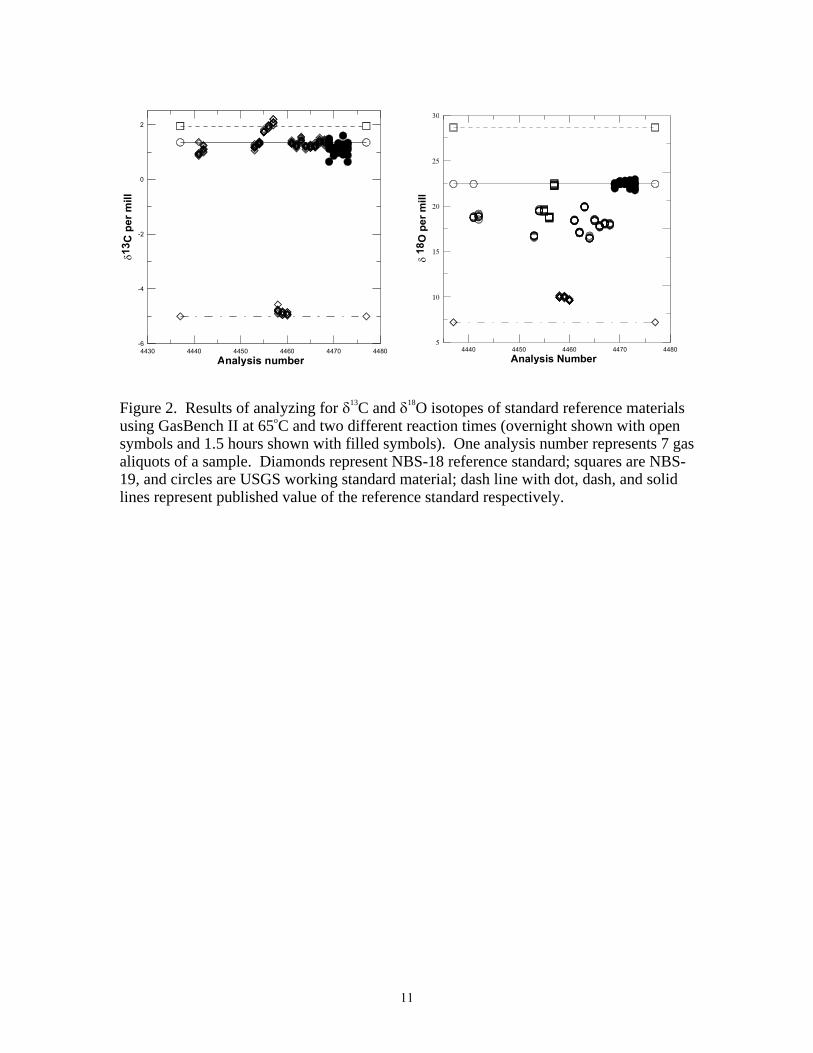
The reaction conditions ultimately chosen after a series of experiments were to maintain the acid reaction at a constant temperature of 26ºC and for a minimum duration of 24 hours but the maximum duration less than 54 hours. Originally, the samples were reacted at 65ºC, approximately the temperature suggested by the equipment manufacturer. At that temperature, reacted overnight, the carbon isotope ratios for the reference materials were reproducible and accurate, but the oxygen isotope ratios were neither accurate (approximate difference of +3 ‰; -8 ‰; -4 ‰ from reference value of NBS-18; NBS-19 and USGS Working Standard, respectively) nor reproducible (standard deviation was 1.88 ‰ among sample runs) (Figure 2).

The question is whether hot acid reaction for a shorter time would produce acceptable values. The equipment available did not allow this set-up to be automatically configured; therefore, the acid injection procedure was done manually in the proper timely manner. Shortening the reaction time to 1.5 hours improved the reproducibility and accuracy of the oxygen isotope ratios obtained for the working standard material (Figure 2), but the standard deviation of the 7 gas aliquots within an analysis for both isotopes were only marginally acceptable (0.21 and 0.27‰ for �13C and �18O, respectively). This combination of time and temperature has potential if proper equipment is available (e.g. 2 arm robot system) and the difficulty of handling high temperature water vapor (e.g. clogging capillary tubes) can be overcome.

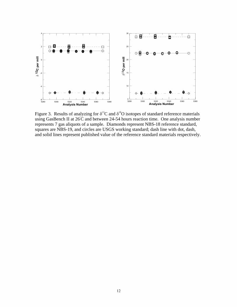
Using a lower reaction temperature (R.Yam, private communication, 2000) and a minimum 24-hour reaction time, allowed reproducible isotope standards within acceptable range for both, carbon and oxygen (Figure 3). Because the reaction time affected the oxygen isotope ratios, but not the carbon isotope ratios, it suggests that an exchange reaction for the oxygen isotope occurs during the overnight acid reaction period. Since the shortened reaction time of 1.5 hours at 65 °C gave acceptable, albeit imprecise results, suggests that this secondary reaction must have a kinetic component. Therefore, lowering the reaction temperature should inhibit or slow down this secondary reaction. It is important to note that all samples were analyzed within 54 hours of acid injection. (Indeed, all but four were analyzed within 47 hours). Because of the kinetic component of the reaction, the method presented in this work should be considered to have an upper bound of 54 hours allowed for reaction time. Analysis of Reference Standards

The three reference standard samples were interspersed among field samples that were analyzed over a five-month period under the identified experimental conditions of 26°C temperature and overnight (•24 hours) reaction time with acid before analysis. All results of the reference standards were collected into a single dataset, for further analysis, in order to determine the capability of the new method to provide long term accurate and precise results. The three reference standards used in this work -- NBS-18, USGS Working Standard and NBS-19 -- have different isotopic signatures; ordered by

4

increasing values of �13C and �18O. NBS-18 with �13CVPDB = -5‰ and �18OVSMOW = 7.2‰, the USGS Working Standard with �13CVPDB = 1.35 ‰ and �18OVSMOW = 22.43‰, and NBS-19 with �13CVPDB = 1.95‰ and �18OVSMOW = 28.65‰. Results were inspected graphically (using Grapher version 3 and KaleidaGraph version 3.5 software), and subjected to formal statistical analysis (using Minitab version 10xtra software as well as simple statistics from KaleidaGraph version 3.5 software) to assess bias, precision, total error, effect of sample amount, homogeneity of samples, as well as the effect of the duration of the reaction time from the time the acid was added to a sample up to the time when the sample was analyzed in the mass spectrometer.

A total of 88 samples were analyzed for the three standards: 23 of NBS-18, 39 of the USGS Working Standard and 26 of NBS-19. Samples amounts were weighed carefully to be ~0.40 mg; the average of the 88 samples was 0.42 ±0.02 mg, ranging from 0.37 to 0.48 mg. The reaction time was calculated from lab records and noted along with the sample results. Since the analytical procedure for each sample includes seven gas aliquots to the IRMS, a total of 616 = (7x88) analyses were made for the three reference standards, with 161 for NBS-18, 276 for the USGS Working Standard, and 182 for NBS-19.

The IRMS produces voltage-time (Volts-seconds) peaks for each gas aliquot, where the integrated peak area at the first sample injection is a function of the amount of sample material. The cumulative peak areas produced by the subsequent six other injections diminish in size (Figures 1 and 4). However, the area of the first injection peak is not simply a linear function of the amount of sample material: the linear correlation coefficient between the amount of sample and the first peak was only 0.22, suggesting that some factor in addition to any error in weighing confounded this relation. The estimates of �13C and �18O for each of the seven injections of all 88 analyses by the three reference standards plotted as a function of the cumulative spectrometric peak area for the injection, in volts-seconds (Vs) units is shown in Figure 4. The area ranges predominantly from ~20 to ~5 Vs (maximum/minimum ratio = 4) which indicates that the linearity of the mass spectrometer was acceptable and the experimental conditions (ISODAT method, Process File, He flow rate, needle size6) were set correctly. In addition, regardless of the initial peak area value, and that of the six subsequent peaks, their minimum value was constrained, suggesting that even a potentially broad range in the sample amount (0.1 –0.4 mg) could produce accurate and reproducible results. Figure 4 demonstrates that the results for the USGS Working Standard (Figure 4c) were more variable and negatively biased than for either NBS-18 or NBS-19 (Figures 4a and 4b respectively), even though the isotopic signature of this material is bracketed by the other two. This may reflect the differing mineral composition or grain size of the material.

In order to permit comparisons between reference standards, analytic results were expressed in terms of bias, that is, the difference between the analytic isotopic estimate and the known isotopic reference standard value. Table 1 provides a statistical summary of results for the 88 samples, with results for �13C summarized in Table 1a, and for �18O in Table 1b. The average bias, the standard deviation of the averaged bias which is called the standard error of the bias and the standard deviation of the bias values are shown when results from all three-reference standards are treated as one set. Results are also summarized for each reference standard set separately, because an analysis of variance rejected (p•0.001) the hypothesis of equal average bias among analyses categorized by

6 K.Revesz, J.M. Landwehr and J. Kebly. USGS Open File Report N:01-257. 2001.

5

reference standard. Also, individual analyses were pooled by their sample sets of seven injections, and a bias and standard deviation for these respective sets computed. In addition to the average bias, the average standard deviation for the pooled samples is shown because it is the standard deviation of the pooled set that determines whether or not an aliquot is accepted. Finally, it was seen that the correlation between the amount of sample material and the area of the first injection peak increased from 0.22 to ~0.50 in the case of analyses run with a reaction time between 34-54 hours, suggesting some stabilizing factor with longer reaction time. Consequently, the pooled sets were separated into categories by reaction time, from 24 to 34 hours and from 34 to 54 hours, to determine what, if any, effect is obtained with longer reaction times.

It can be seen that the estimate of �13C appeared to be unbiased (confirmed by t-test, with p<0.05) over the set of all analyses and all pooled analyses, but the results differed when examined by reference standard (Table 1a). The results for NBS-18 are unbiased, the results for the USGS Working Standard negatively biased and the results for NBS-19 positively biased, but the absolute value of the average bias is < 0.1‰. The difference in bias between samples with reaction times of 24-34 hours and those with reaction time 34-54 hours was neither large nor significant (confirmed by F-test using p•0.05), except for NBS-18 for which the average bias went from a small positive value to a small negative value but one that was indistinguishable from 0. As expected, pooling reduced the standard deviation of the set, although the standard error of the bias remains at 0.01 ‰. The standard deviation of the bias is •0.1‰ for each reference category. Thus, for �13C, the analyses precisely and accurately reproduce the reference standard values within the desired tolerance (•0.1‰).

The results for �18O analyses are summarized in Table 1b. It is seen that the average bias was not zero (rejected by t-test, at p<0.05 level) for either the set of all analyses or the set of pooled analyses. This is because, although the results for both NBS-18 and NBS-19 are unbiased, those for the USGS Working Standard indicate a negative bias that was larger than the desired tolerance of 0.2‰. However, when samples were categorized by reaction time, those run with a reaction time 24-34 hours were significantly negatively biased but those with reaction time 34-54 hours were unbiased. The standard error and the standard deviation were larger for the �18O analyses than for �13C. Furthermore, for both NBS-19 and the USGS Working Standard, the standard deviations were greater than the desired tolerance of 0.2‰ when considered overall samples, but diminished to less than 0.2‰ for samples with reaction time between 34-54 hours.

Results for all available analyses, without application of the additional screening rules applied to field sample aliquots described above are summarized in Table 1. We now consider how these results would change when the more rigorous screening rules that are used to determine aliquot acceptability are applied. In examining the data, in one analysis set (1% of 88) it was found that the integrated peak area of aliquot-7 was larger than aliquot-1 for the sample gas, possibly indicating incorrect sample preparation; consequently, that sample was discarded. According to the rules for examining aliquots stated above, if the standard deviation among the 7 injection results was >0.1 ‰ for �13C or >0.2 ‰ for �18O, the sample was not used. It was found that 14 (16%) of the remaining 87 samples failed with respect to this rule of which 3 (3%) failed just with respect to �13C, 10 (11%) failed just with respect �18O, and 1 (1%) failed with respect to both isotopes. In addition, two pooled samples (2%) were found to have an average �18O estimate differing from any other analysis for their respective standards by ~ 1.5‰ and

6

~0.7‰, respectively, which violates the • 0.2‰ screening rule for aliquots stated above. These samples were also removed from further consideration. All pooled samples had an average �13C value within • 0.1‰ and thus satisfied the screening rule adapted for aliquots as described above. Of the 17 discarded samples, 3 (13% of the initial 23) were for reference standard NBS-18, 9 (23% of 39) for the USGS Working Standard and 5 (19% of 26) for reference standard NBS-19. It was noted that all 17 samples that failed the screening rules had a reaction time between 24 and 34 hours.

Of the original 88 samples, 71 (>80%) satisfied the aliquot screening rules. A statistical summary of results for the 71 acceptable samples is provided in Table 2, which follows the format of Table 1. The results for �13C are summarized in Table 2a and are completely consistent with those in Table 1a, although with smaller average pooled standard deviation. The results for �18O are summarized in Table 2b. The results are unbiased (confirmed by t-test, with p<0.05) for all cases, except for samples from the USGS Working Standard, but even for this category the bias is within the desired tolerance of 0.2‰. Both the standard error and the standard deviation were larger among the �18O analyses than for �13C, but the standard deviation was also within the desired tolerance of 0.2‰ for NBS-18 and NBS-19 samples, although larger (0.31‰) for the USGS Working Standard samples. Samples were separated by reaction time • 34 hours and > 34 hours. Results between the sets of shorter and longer reaction time differed more for samples from the USGS Working Standard, than for either NBS-18 or NBS-19. Samples run with the shorter reaction time were negatively biased at ~ 0.2‰ with a standard deviation of ~0.4‰, whereas those with reaction time >34 hours were unbiased (confirmed with t-test) with standard deviation 0.13‰. (Note: we could not reject the hypothesis of equal means for the average bias for the USGS Working Standard, but this is a function of the large standard deviation associated with the shorter time samples.) Furthermore, an analysis of variance test among the samples analyzed at >34 hours could not reject the hypothesis of equality of average bias among reference standards, although it did so among those of •34 hour reaction time and for the entire pooled set. Thus, for �

18O, when the screening rules are applied, samples from all three-reference standards produced unbiased results with minimum standard deviation (<0.2‰), although it appears that the USGS Working Standard needs more reaction time for the method to perform correctly. However, given the kinetic nature of the reaction, these results cannot be extrapolated beyond 54 hours, the maximum analysis time of these experiments.

Table 3 shows the average root mean square error among all of the pooled samples, and when they were separated by reaction time. This statistic is a metric of the total error in an analysis and is defined as the square root of the sum of the squared bias and the estimated variance; effectively, it is the radius of a circle whose center is the true value of a reference where one coordinate axis is the bias, and the other is the standard deviation. The total error in the �18O is about twice as large in absolute value as that in �

13C, and no significant reduction in error accrues from a longer reaction time in the case of �13C, but there is a reduction for �18O, especially in the case of the USGS Working Standard (Table 3). This metric cannot be used in the case of assessing an unknown sample, but is useful for screening results in the case of known reference standards, or for inter-laboratory comparisons. Testing of Method by Application to Devils Hole Calcite

Calcite from Devils Hole, Nevada was used to test this new method. Devils Hole is a tectonic cave formed in the discharge zone of a regional carbonate-rock aquifer in south-central Nevada (36oN, 116oW). Dense vein calcite has precipitated from the ground

7

water onto the walls of this sub aqueous cavern7. Devils Hole Core DH-11 is a 36-cm long core taken from the wall of the cave at about 30 meters below the water table; it contains an approximately 500,000-year-old continuous record of the paleoclimate 8. The core originally was sampled along its length at approximately 1.27 - mm intervals by milling and analyzed for stable isotopic composition by the classical method; it was uranium-series dated using thermal ionization mass spectrometry (TIMS)9. In 1998, a new slab was cut from DH-11 for trace-element determination. We analyzed the C and O stable isotope ratios in the new slab samples taken again in 1.27- mm intervals at distances from 165.7 mm to 266.0 mm from the free (outer) face of the specimen. The �

13C and �18O analyses of the 1998 sample were intended to be used for dating the isotopic time series of the new slab by matching it with the time series from the original slab (analyzed by the classical method) of DH-11.

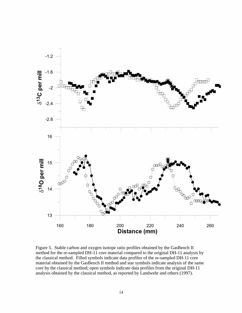
Calcite re-sampled from core DH-11 was analyzed by the new method. The analytical results, compiled into a data table organized by the reported re-sampling depth of each sample, are given in appendix A. The stable isotope data plotted with the re-sampled depth is shown in Figure 5. An inverse relation results between the oxygen and carbon isotope ratio data, consistent with the pattern reported by Coplen and others (1994)10.

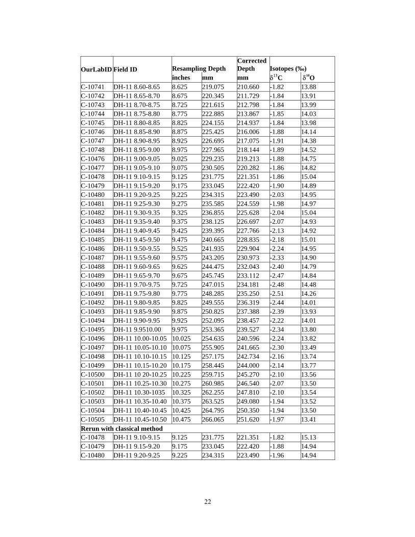
For a check of method consistency, three samples of the re-sampled material (at approximately 232, 233, and 234 mm) also were analyzed using the classical method. These data are shown in Figure 5 as stars and listed at the bottom of the Table in appendix A. All results differ by less than 0.1 ‰ and this corroborates the consistency of the two methods.

When the series from the resampled material (filled symbols in Figure 5) was compared with the original data (open symbols), two locations from which offsets increased non linearly with depth were identified (Figure 5). This observation was confirmed to correspond with periodic re-positioning of the new slab during milling when it was observed to be slipping in the vise (I.J.Winograd, private communication, 2001). A mathematical correction to the recorded cutting depths was applied to accommodate these re-sampling conditions (Figure 6).

When the results of the new method, with corrected sampling depths, are compared to the classical method (Figure 6), it can be seen that the new method reproduced the isotopic trace produced by the classical method. This is demonstrated by a linear correlation between isotope values of approximately 0.96 for both isotopes, after correcting for an alignment offset. Hence, the new method can be used as an alternative to the classical method. In the case of the DH-11 sample, both methods allow one to stratigrafically align cores by matching stable isotope patterns, a useful capability in paleoclimate studies; however, because the new method requires less sample material, it

7 Winograd, I.J., Landwehr, J.M., Ludwig, K.R., Coplen, T.B., Riggs, A.C., Szabo, B.J., Kolesar, P.T. and Revesz, K.M. Science.

1992; 258: 255-260.

8 Landwehr, J.M, Coplen, T.B., Ludwig, K.R., Winograd, I.J., and Riggs, A.C. U.S. Geological Survey Open-File Report 97-792.

1997; 8 p.

9 Ludwig, K.R.; Simmons, K.R.; Szabo, B.J.; Winograd, I.J.; Landwehr, J.M.; Riggs, A.C.; Hoffman, R.J. Science. 1992;.258: 284-

287.

10 Coplen, T.B., Winograd, I.J., Landwehr, J.M. and Riggs, A.C. Science. 1994; 263: 361-365.

8

permits finer resolution over the length of the core, thus finer temporal resolution of the material.

In addition, this work demonstrates the method’s utility for making stratigraphic connections between cores by matching stable isotope patterns, e.g. allowing one to age-date new core material by reference to previously dated material. Conclusion

A new method was developed to analyze small samples (approximately 400 µg) of calcium carbonate (calcite) for the stable isotope ratios of carbon and oxygen. The new method streamlines the classical H3PO4 – CaCO3 reaction method by making use of a Thermoquest-Finnigan GasBench II preparation device and Delta Plus XL continuous flow, isotope ratio mass spectrometer. Results from analysis of three different reference materials were evaluated statistically; the method was seen to produce unbiased and precise estimates of �13C when the acid reaction time was between 24 and 54 hours, and of �18O when the reaction time between 24 and 54 hours. Aliquot screening methods were shown to further minimize the total error. The method was tested by analyzing calcite from Devils Hole, Nevada, core DH-11, and its utility is confirmed by its capability to reproduce results, thereby allowing one to stratigrafically align cores by matching stable isotope patterns.

Care must be taken to check the precision of the standards, because reruns might be necessary. These additional analyses require time, but overall the automation of the GasBench II method results in considerable time savings. An additional advantage of the new method is that it requires less sample materials; hence, allowing analysis when sample amount is limited or when finer sampling resolution is needed. These advantages make this method a viable alternative to the classical method. Acknowledgments

We thank Tyler B. Coplen for his support in all aspects of the project, Isaac J. Winograd for his help in ascertaining the 1998 re-sampling procedure and for many useful discussions, and Jerry Keybl for assistance in this project.

9

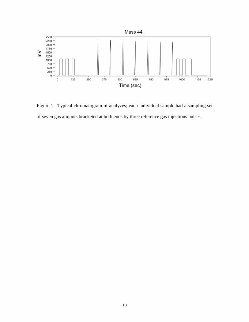
Figure 1. Typical chromatogram of analyzes; each individual sample had a sampling set

of seven gas aliquots bracketed at both ends by three reference gas injections pulses.

10

4430 4440 4450 4460 4470 4480Analysis number

-6

-4

-2

0

2�13

C p

er m

ill

4440 4450 4460 4470 4480

Analysis Number�

��

��

��

��

��

� 1

8 O p

er m

ill

Figure 2. Results of analyzing for �13C and �18O isotopes of standard reference materials using GasBench II at 65oC and two different reaction times (overnight shown with open symbols and 1.5 hours shown with filled symbols). One analysis number represents 7 gas aliquots of a sample. Diamonds represent NBS-18 reference standard; squares are NBS-19, and circles are USGS working standard material; dash line with dot, dash, and solid lines represent published value of the reference standard respectively.

11

5280 5300 5320 5340 5360 5380Analysis Number

-6

-4

-2

0

2

4

� 1

3 C p

er m

ill

5280 5300 5320 5340 5360 5380Analysis Number

5

10

15

20

25

30

���O

per

mill

Figure 3. Results of analyzing for �13C and �18O isotopes of standard reference materials using GasBench II at 26ºC and between 24-54 hours reaction time. One analysis number represents 7 gas aliquots of a sample. Diamonds represent NBS-18 reference standard, squares are NBS-19, and circles are USGS working standard; dash line with dot, dash, and solid lines represent published value of the reference standard materials respectively.

12

6.2

7.2

8.2

0 5 10 15 20

-6

-5

-4

�13

C p

er m

ill

� 18O per m

illArea (Vs)

4a. NBS-18

-3.05

-2.05

-1.05

-0.05

0.95

1.95

2.95

25.65

26.65

27.65

28.65

29.65

30.65

31.65

0 5 10 15 20

4b. NBS19

�13

C p

er m

ill

�18O

per mill

Area (Vs)

0.35

1.35

2.35

19.43

20.43

21.43

22.43

23.43

0 5 10 15 20

4c. USGS Working Standard

�13

C p

er m

ill

�18O

per mill

Area (Vs)

Figure 4. Isotope values for �13C and for �

18O versus area Volt-seconds for all seven analyses for each sample analyzed from the three reference standards (a=NBS-18;b=NBS-19, c=USGS working standard), totaling 88 samples. Symbols �,�,�,�,�,�,�, represent injection peak #1,#2,#3,#4,#5,#6,#7 respectively

13

160 180 200 220 240 260Distance (mm)

13

14

15

16

�18

O p

er m

ill

-2.8

-2.4

-2

-1.6

-1.2

�13

C p

er m

ill

Figure 5. Stable carbon and oxygen isotope ratio profiles obtained by the GasBench II method for the re-sampled DH-11 core material compared to the original DH-11 analysis by the classical method. Filled symbols indicate data profiles of the re-sampled DH-11 core material obtained by the GasBench II method and star symbols indicate analysis of the same core by the classical method; open symbols indicate data profiles from the original DH-11 analysis obtained by the classical method, as reported by Landwehr and others (1997).

14

160 180 200 220 240 260Distance (mm)

13

14

15

16

�18

O p

er m

ill

-2.8

-2.4

-2

-1.6

-1.2�

13C

per

mill

Figure 6. Stable carbon and oxygen isotope ratio profiles obtained by the GasBench II method for the re-sampled DH-11 core material, with appropriate sampling depth correction applied, compared to the original DH-11 analysis by the classical method. Filled symbols indicate data profiles of the re-sampled DH-11 core material obtained by the GasBench II method and star symbols indicate analysis of the same core by the classical method; open symbols indicate data profiles from the original DH-11 analysis obtained by the classical method, as reported by Landwehr and others (1997). The linear correlation between the isotope values generated by the classical and the new method is > 0.96 for both isotopes.

15

Table 1a. For �13C analysis, for all 88 samples from three-reference standards run concurrently with field samples, statistics pertaining to bias and pooled standard deviation, among all and pooled analyses and analyses separated by reaction time, and the number of analyses in each category. All units are in ‰. Reference Category All analyses Pooled

analyses Samples analyzed 24-34 hours after acid injection

Samples analyzed 34-54 hours after acid injection

Average bias All Samples -0.01 * -0.01 * -0.01 * -0.005 * # NBS-18 +0.01 * +0.01 * +0.03 R -0.03 * r USGS Working Standard -0.08 R -0.08 R -0.10 R -0.05 R # NBS-19 +0.08 R +0.08 R +0.07 R +0.09 R # Standard Error of Bias All Samples 0.01 0.01 0.01 0.02 NBS-18 0.01 0.01 0.01 0.02 USGS Working Standard 0.01 0.01 0.02 0.02 NBS-19 0.01 0.01 0.02 0.03 Standard Deviation of Bias All Samples 0.15 0.10 0.11 0.09 NBS-18 0.09 0.05 0.05 0.04 USGS Working Standard 0.16 0.09 0.09 0.08 NBS-19 0.11 0.07 0.07 0.09 Average pooled standard deviation All Samples --- 0.09 0.09 0.08 NBS-18 --- 0.08 0.08 0.08 USGS Working Standard --- 0.10 0.12 0.07 NBS-19 --- 0.08 0.08 0.10 Number of analyses All Samples n=616 n=88 n=61 n=27 NBS-18 161 23 17 6 USGS Working Standard 273 39 26 13 NBS-19 182 26 18 8

R Reject the null hypothesis Ho: average bias = 0 (t-test), at p ≤0.05 level. * Cannot reject null hypothesis that average bias is 0. r: Reject the null hypothesis Ho: average bias (samples with time ≤34 hours) = average bias (samples with time between >34 hours), at p ≤0.05.level. #: Cannot reject null hypothesis of equality of average bias.

16

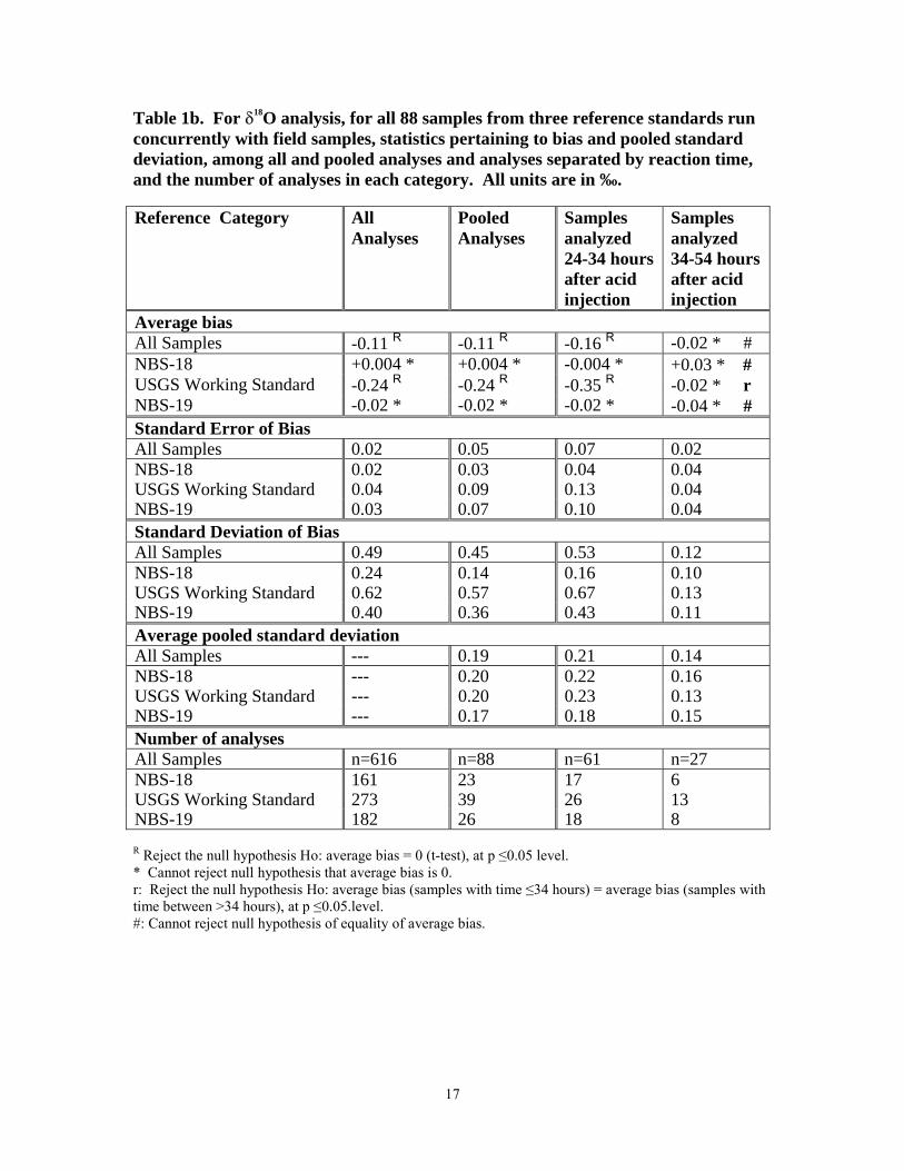
Table 1b. For �18O analysis, for all 88 samples from three reference standards run concurrently with field samples, statistics pertaining to bias and pooled standard deviation, among all and pooled analyses and analyses separated by reaction time, and the number of analyses in each category. All units are in ‰. Reference Category All

Analyses Pooled Analyses

Samples analyzed 24-34 hours after acid injection

Samples analyzed 34-54 hours after acid injection

Average bias All Samples -0.11 R -0.11 R -0.16 R -0.02 * # NBS-18 +0.004 * +0.004 * -0.004 * +0.03 * # USGS Working Standard -0.24 R -0.24 R -0.35 R -0.02 * r NBS-19 -0.02 * -0.02 * -0.02 * -0.04 * # Standard Error of Bias All Samples 0.02 0.05 0.07 0.02 NBS-18 0.02 0.03 0.04 0.04 USGS Working Standard 0.04 0.09 0.13 0.04 NBS-19 0.03 0.07 0.10 0.04 Standard Deviation of Bias All Samples 0.49 0.45 0.53 0.12 NBS-18 0.24 0.14 0.16 0.10 USGS Working Standard 0.62 0.57 0.67 0.13 NBS-19 0.40 0.36 0.43 0.11 Average pooled standard deviation All Samples --- 0.19 0.21 0.14 NBS-18 --- 0.20 0.22 0.16 USGS Working Standard --- 0.20 0.23 0.13 NBS-19 --- 0.17 0.18 0.15

Number of analyses All Samples n=616 n=88 n=61 n=27 NBS-18 161 23 17 6 USGS Working Standard 273 39 26 13 NBS-19 182 26 18 8

R Reject the null hypothesis Ho: average bias = 0 (t-test), at p ≤0.05 level. * Cannot reject null hypothesis that average bias is 0. r: Reject the null hypothesis Ho: average bias (samples with time ≤34 hours) = average bias (samples with time between >34 hours), at p ≤0.05.level. #: Cannot reject null hypothesis of equality of average bias.

17

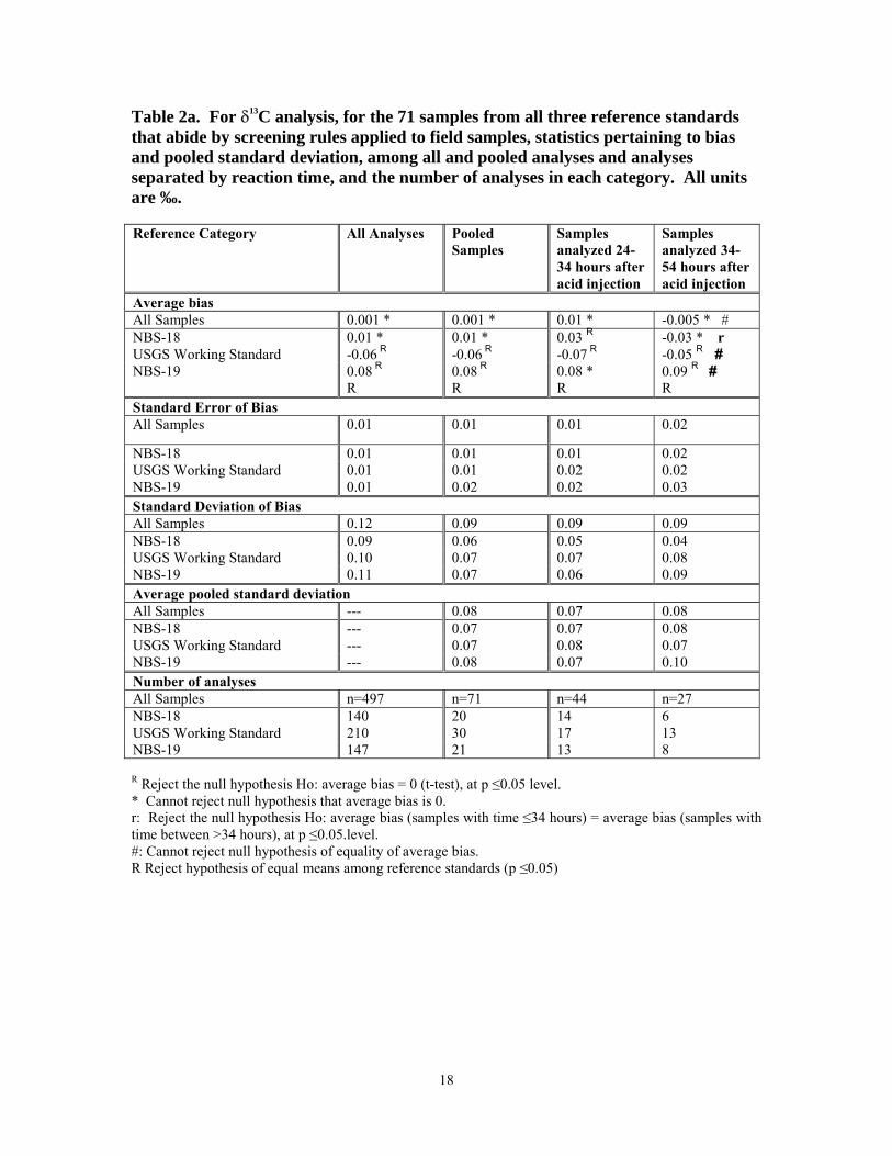
Table 2a. For �13C analysis, for the 71 samples from all three reference standards that abide by screening rules applied to field samples, statistics pertaining to bias and pooled standard deviation, among all and pooled analyses and analyses separated by reaction time, and the number of analyses in each category. All units are ‰. Reference Category All Analyses Pooled

Samples Samples analyzed 24-34 hours after acid injection

Samples analyzed 34-54 hours after acid injection

Average bias All Samples 0.001 * 0.001 * 0.01 * -0.005 * # NBS-18 0.01 * 0.01 * 0.03 R -0.03 * r USGS Working Standard -0.06 R -0.06 R -0.07 R -0.05 R # NBS-19 0.08 R

R 0.08 R R

0.08 * R

0.09 R # R

Standard Error of Bias All Samples 0.01 0.01 0.01 0.02

NBS-18 0.01 0.01 0.01 0.02 USGS Working Standard 0.01 0.01 0.02 0.02 NBS-19 0.01 0.02 0.02 0.03 Standard Deviation of Bias All Samples 0.12 0.09 0.09 0.09 NBS-18 0.09 0.06 0.05 0.04 USGS Working Standard 0.10 0.07 0.07 0.08 NBS-19 0.11 0.07 0.06 0.09 Average pooled standard deviation All Samples --- 0.08 0.07 0.08 NBS-18 --- 0.07 0.07 0.08 USGS Working Standard --- 0.07 0.08 0.07 NBS-19 --- 0.08 0.07 0.10 Number of analyses All Samples n=497 n=71 n=44 n=27 NBS-18 140 20 14 6 USGS Working Standard 210 30 17 13 NBS-19 147 21 13 8

R Reject the null hypothesis Ho: average bias = 0 (t-test), at p ≤0.05 level. * Cannot reject null hypothesis that average bias is 0. r: Reject the null hypothesis Ho: average bias (samples with time ≤34 hours) = average bias (samples with time between >34 hours), at p ≤0.05.level. #: Cannot reject null hypothesis of equality of average bias. R Reject hypothesis of equal means among reference standards (p ≤0.05)

18

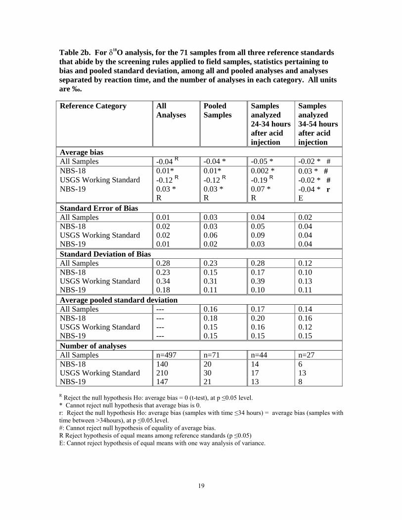
Table 2b. For �18O analysis, for the 71 samples from all three reference standards that abide by the screening rules applied to field samples, statistics pertaining to bias and pooled standard deviation, among all and pooled analyses and analyses separated by reaction time, and the number of analyses in each category. All units are ‰. Reference Category All

Analyses Pooled Samples

Samples analyzed 24-34 hours after acid injection

Samples analyzed 34-54 hours after acid injection

Average bias All Samples -0.04 R -0.04 * -0.05 * -0.02 * # NBS-18 0.01* 0.01* 0.002 * 0.03 * # USGS Working Standard -0.12 R -0.12 R -0.19 R -0.02 * # NBS-19 0.03 *

R 0.03 * R

0.07 * R

-0.04 * r E

Standard Error of Bias All Samples 0.01 0.03 0.04 0.02 NBS-18 0.02 0.03 0.05 0.04 USGS Working Standard 0.02 0.06 0.09 0.04 NBS-19 0.01 0.02 0.03 0.04 Standard Deviation of Bias All Samples 0.28 0.23 0.28 0.12 NBS-18 0.23 0.15 0.17 0.10 USGS Working Standard 0.34 0.31 0.39 0.13 NBS-19 0.18 0.11 0.10 0.11 Average pooled standard deviation All Samples --- 0.16 0.17 0.14 NBS-18 --- 0.18 0.20 0.16 USGS Working Standard --- 0.15 0.16 0.12 NBS-19 --- 0.15 0.15 0.15

Number of analyses All Samples n=497 n=71 n=44 n=27 NBS-18 140 20 14 6 USGS Working Standard 210 30 17 13 NBS-19 147 21 13 8

R Reject the null hypothesis Ho: average bias = 0 (t-test), at p ≤0.05 level. * Cannot reject null hypothesis that average bias is 0. r: Reject the null hypothesis Ho: average bias (samples with time ≤34 hours) = average bias (samples with time between >34hours), at p ≤0.05.level. #: Cannot reject null hypothesis of equality of average bias. R Reject hypothesis of equal means among reference standards (p ≤0.05) E: Cannot reject hypothesis of equal means with one way analysis of variance.

19

Table 3. Average Root Mean Square Error ( ‰) among pooled samples, for all samples and for samples categorized by reference standard and by reaction time, for samples from all three reference standards, for both �13C and �18O analysis, and the number of samples in each category. Reference Category All Samples Samples

analyzed 24-34 hours after acid injection

Samples analyzed 34-54 hours after acid injection

�13C

All Samples 0.11 0.11 0.11 NBS-18 0.09 0.09 0.09 USGS Working Standard 0.11 0.11 0.11 NBS-19 0.13 0.11 0.15 �

18O All Samples 0.21 0.24 0.17 NBS-18 0.21 0.23 0.17 USGS Working Standard 0.24 0.30 0.16 NBS-19 0.18 0.18 0.17 Number of samples All Samples n=71 n=44 n=27 NBS-18 20 14 6 USGS Working Standard 30 17 13 NBS-19 21 13 8

20

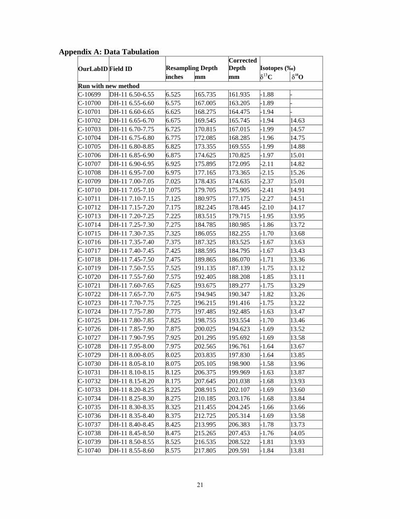
Appendix A: Data Tabulation

Resampling Depth Corrected Depth Isotopes (‰) OurLabID Field ID

inches mm mm ���C� �18O

Run with new method �

C-10699 DH-11 6.50-6.55 6.525 165.735 161.935 -1.88 - C-10700 DH-11 6.55-6.60 6.575 167.005 163.205 -1.89 - C-10701 DH-11 6.60-6.65 6.625 168.275 164.475 -1.94 - C-10702 DH-11 6.65-6.70 6.675 169.545 165.745 -1.94 14.63 C-10703 DH-11 6.70-7.75 6.725 170.815 167.015 -1.99 14.57 C-10704 DH-11 6.75-6.80 6.775 172.085 168.285 -1.96 14.75 C-10705 DH-11 6.80-8.85 6.825 173.355 169.555 -1.99 14.88 C-10706 DH-11 6.85-6.90 6.875 174.625 170.825 -1.97 15.01 C-10707 DH-11 6.90-6.95 6.925 175.895 172.095 -2.11 14.82 C-10708 DH-11 6.95-7.00 6.975 177.165 173.365 -2.15 15.26 C-10709 DH-11 7.00-7.05 7.025 178.435 174.635 -2.37 15.01 C-10710 DH-11 7.05-7.10 7.075 179.705 175.905 -2.41 14.91 C-10711 DH-11 7.10-7.15 7.125 180.975 177.175 -2.27 14.51 C-10712 DH-11 7.15-7.20 7.175 182.245 178.445 -2.10 14.17 C-10713 DH-11 7.20-7.25 7.225 183.515 179.715 -1.95 13.95 C-10714 DH-11 7.25-7.30 7.275 184.785 180.985 -1.86 13.72 C-10715 DH-11 7.30-7.35 7.325 186.055 182.255 -1.70 13.68 C-10716 DH-11 7.35-7.40 7.375 187.325 183.525 -1.67 13.63 C-10717 DH-11 7.40-7.45 7.425 188.595 184.795 -1.67 13.43 C-10718 DH-11 7.45-7.50 7.475 189.865 186.070 -1.71 13.36 C-10719 DH-11 7.50-7.55 7.525 191.135 187.139 -1.75 13.12 C-10720 DH-11 7.55-7.60 7.575 192.405 188.208 -1.85 13.11 C-10721 DH-11 7.60-7.65 7.625 193.675 189.277 -1.75 13.29 C-10722 DH-11 7.65-7.70 7.675 194.945 190.347 -1.82 13.26 C-10723 DH-11 7.70-7.75 7.725 196.215 191.416 -1.75 13.22 C-10724 DH-11 7.75-7.80 7.775 197.485 192.485 -1.63 13.47 C-10725 DH-11 7.80-7.85 7.825 198.755 193.554 -1.70 13.46 C-10726 DH-11 7.85-7.90 7.875 200.025 194.623 -1.69 13.52 C-10727 DH-11 7.90-7.95 7.925 201.295 195.692 -1.69 13.58 C-10728 DH-11 7.95-8.00 7.975 202.565 196.761 -1.64 13.67 C-10729 DH-11 8.00-8.05 8.025 203.835 197.830 -1.64 13.85 C-10730 DH-11 8.05-8.10 8.075 205.105 198.900 -1.58 13.96 C-10731 DH-11 8.10-8.15 8.125 206.375 199.969 -1.63 13.87 C-10732 DH-11 8.15-8.20 8.175 207.645 201.038 -1.68 13.93 C-10733 DH-11 8.20-8.25 8.225 208.915 202.107 -1.69 13.60 C-10734 DH-11 8.25-8.30 8.275 210.185 203.176 -1.68 13.84 C-10735 DH-11 8.30-8.35 8.325 211.455 204.245 -1.66 13.66 C-10736 DH-11 8.35-8.40 8.375 212.725 205.314 -1.69 13.58 C-10737 DH-11 8.40-8.45 8.425 213.995 206.383 -1.78 13.73 C-10738 DH-11 8.45-8.50 8.475 215.265 207.453 -1.76 14.05 C-10739 DH-11 8.50-8.55 8.525 216.535 208.522 -1.81 13.93 C-10740 DH-11 8.55-8.60 8.575 217.805 209.591 -1.84 13.81

21

22

Resampling Depth Corrected Depth Isotopes (‰) OurLabID Field ID

inches mm mm ���C� �18O

C-10741 DH-11 8.60-8.65 8.625 219.075 210.660 -1.82 13.88 C-10742 DH-11 8.65-8.70 8.675 220.345 211.729 -1.84 13.91 C-10743 DH-11 8.70-8.75 8.725 221.615 212.798 -1.84 13.99 C-10744 DH-11 8.75-8.80 8.775 222.885 213.867 -1.85 14.03 C-10745 DH-11 8.80-8.85 8.825 224.155 214.937 -1.84 13.98 C-10746 DH-11 8.85-8.90 8.875 225.425 216.006 -1.88 14.14 C-10747 DH-11 8.90-8.95 8.925 226.695 217.075 -1.91 14.38 C-10748 DH-11 8.95-9.00 8.975 227.965 218.144 -1.89 14.52 C-10476 DH-11 9.00-9.05 9.025 229.235 219.213 -1.88 14.75 C-10477 DH-11 9.05-9.10 9.075 230.505 220.282 -1.86 14.82 C-10478 DH-11 9.10-9.15 9.125 231.775 221.351 -1.86 15.04 C-10479 DH-11 9.15-9.20 9.175 233.045 222.420 -1.90 14.89 C-10480 DH-11 9.20-9.25 9.225 234.315 223.490 -2.03 14.95 C-10481 DH-11 9.25-9.30 9.275 235.585 224.559 -1.98 14.97 C-10482 DH-11 9.30-9.35 9.325 236.855 225.628 -2.04 15.04 C-10483 DH-11 9.35-9.40 9.375 238.125 226.697 -2.07 14.93 C-10484 DH-11 9.40-9.45 9.425 239.395 227.766 -2.13 14.92 C-10485 DH-11 9.45-9.50 9.475 240.665 228.835 -2.18 15.01 C-10486 DH-11 9.50-9.55 9.525 241.935 229.904 -2.24 14.95 C-10487 DH-11 9.55-9.60 9.575 243.205 230.973 -2.33 14.90 C-10488 DH-11 9.60-9.65 9.625 244.475 232.043 -2.40 14.79 C-10489 DH-11 9.65-9.70 9.675 245.745 233.112 -2.47 14.84 C-10490 DH-11 9.70-9.75 9.725 247.015 234.181 -2.48 14.48 C-10491 DH-11 9.75-9.80 9.775 248.285 235.250 -2.51 14.26 C-10492 DH-11 9.80-9.85 9.825 249.555 236.319 -2.44 14.01 C-10493 DH-11 9.85-9.90 9.875 250.825 237.388 -2.39 13.93 C-10494 DH-11 9.90-9.95 9.925 252.095 238.457 -2.22 14.01 C-10495 DH-11 9.9510.00 9.975 253.365 239.527 -2.34 13.80 C-10496 DH-11 10.00-10.05 10.025 254.635 240.596 -2.24 13.82 C-10497 DH-11 10.05-10.10 10.075 255.905 241.665 -2.30 13.49 C-10498 DH-11 10.10-10.15 10.125 257.175 242.734 -2.16 13.74 C-10499 DH-11 10.15-10.20 10.175 258.445 244.000 -2.14 13.77 C-10500 DH-11 10 20-10.25 10.225 259.715 245.270 -2.10 13.56 C-10501 DH-11 10.25-10.30 10.275 260.985 246.540 -2.07 13.50 C-10502 DH-11 10.30-1035 10.325 262.255 247.810 -2.10 13.54 C-10503 DH-11 10.35-10.40 10.375 263.525 249.080 -1.94 13.52 C-10504 DH-11 10.40-10.45 10.425 264.795 250.350 -1.94 13.50 C-10505 DH-11 10.45-10.50 10.475 266.065 251.620 -1.97 13.41 Rerun with classical method C-10478 DH-11 9.10-9.15 9.125 231.775 221.351 -1.82 15.13 C-10479 DH-11 9.15-9.20 9.175 233.045 222.420 -1.88 14.94 C-10480 DH-11 9.20-9.25 9.225 234.315 223.490 -1.96 14.94