
1~1~U~!iii~11111111~11 - Fermilab | Technical Publications
311
a 1160 008b038 1 A COMPARISON OF HIGH TRANSVERSE MOMENTUM DIRECT PHOTON AND NEUTRAL PION EVENTS IN NEGATIVE PION AND PROTON-NUCLEUS COLLISIONS Nr 31.5 GeV CENTER OF MASS ENERGY By David Shaw Brown A THESIS Submitted to Michig&'-1 State: UDiversity · in partial fulfillment of the requirements for the degree of DOCTOR OF PfilLOSOPHY Department of Physics 1992
-
Upload
khangminh22 -
Category
Documents
-
view
1 -
download
0
Transcript of 1~1~U~!iii~11111111~11 - Fermilab | Technical Publications

1~1~~1~1~U~!iii~11111111~11 a 1160 008b038 1
A COMPARISON OF HIGH TRANSVERSE MOMENTUM DIRECT PHOTON AND NEUTRAL PION EVENTS
IN NEGATIVE PION AND PROTON-NUCLEUS COLLISIONS Nr 31.5 GeV CENTER OF MASS ENERGY
By
David Shaw Brown
A THESIS
Submitted to Michig&'-1 State: U Diversity ·
in partial fulfillment of the requirements for the degree of
DOCTOR OF PfilLOSOPHY
Department of Physics
1992


-
ABSTRACT
A COMPARISON OF HIGH TRANSVERSE MOMENTUM DIRECT PHOTON AND NEUTRAL PION EVENTS
IN NEGATIVE PION AND PROTON-NUCLEUS COLLISIONS AT 31.5GeV CENTER OF MASS ENERGY
By
David Shaw Brown
In 1988 experiment E706 at Fermilab wrote approximately 6 million triggered
events to tape. The purpose of this was to measure the cross sections for high p ..L 1r0
and single photon production. In addition, the cross sections were to be measured
for proton and 'Ir- beams on a variety of nuclear targets. To achieve these goals the
experiment had been furnished with a large liquid argon calorimeter. A magnetic
spectrometer for studying the associated production of charged particles had been
built as well.
The purpose of this analysis is to compare the associated charged particle structure
of high P.L 1ro and direct photon events to see if they are indeed different. The current
theory of hadron-hadron interactions, quantum chromodynamics, makes a number of
predictions indicating that they are. The charged particles recoiling from a high p ..L '1
or 1ro trigger will be used to reconstruct the 1ro +jet and '1 +jet angular and invariant
mass distributions for this study. Finally, the invariant mass distributions will be
employed to study the gluon structure. functions of hadrons.
FERMI LAB LIBRARY

---
--
-
...

ACKNOWLEDGEMENTS
First, I would like to extend my gratitude to all of those involved in making E706
an operational, and successful experiment. A number of these i~dividuals are non
physicists who didn't share in the excitement and glory of doing any physics. They
worked hard within the narrow window of their specialty, often providing expert
advice and getting us cocky graduate students out of numerous jams during the
construction of the calorimeters.
I want to express my appreciation for the efforts of all first run graduate students
and post-docs. I know our relationship has been rough at times, but I am truly
grateful. The validity, importance and relevance of my analysis rests on the mon
umental efforts of the photon group, and those who got the tracking code up and
running. Many thanks to Marek Zielinski, Joey Huston, Phil Gutierrez, Takahiro Ya
suda, George Fanourakis, Clark Chandlee, John Mansour, Dane Skow, Eric Prebys,
Armando Lanaro, Bill Desoi, Chris Lirakis, Alex Sinanidis, Carlos Yosef, loanis Kour
banis, Dhammika Weerasundra, Richard Benson, Brajeesh Choudhary, Casey Hart
man, Sajan Easo, and Guiseppe Ballochi. Oh and thanks for the grapa, Guiseppe.
Maybe again sometime ...
There are three individuals I want to single out as being instrumental in directing
me along the path I took for my analysis. First, there is my advisor, Carl Bromberg.
Carl has made many important contributions to the experiment, including a first rate
MWPC system. He has endured ~any frustrations as well. I must admit I have been
the cause more than once. His willingness to endure and overcome my hardheadedness
has saved me much embarassment. Carl's understanding of and experience in hadron
hadron collisions at high P.l provided the subject matter for my analysis. However, I

-
-
-
could not.have completed my studies without his guidance and many helpful insights
along the way. I thank him for his continual support through the years. I must also
thank Sudhindra Mani for enduring so many long discussions about where to go ~ith
the charged tracking analysis. We have had many arguments, but they clarified a
number of issues for me. The same goes for the noble/notorious George Ginther.
He has made many extraordinary efforts, including the data summary work. Besides
"canning" the data for us students, he got "canned" plenty in our sundry discussions,
which more than once turned into acrimonious debate. Thank you George for your
patience and help in making me an experimentalist. At least I usually look before I
leap now.
The collaboration's senior members played very pivotal roles. They conceived
this experiment, and used their expertise in seeing it become a reality. Thanks to the
Rochester members for providing invaluable help and effort in designing the electro
magnetic calorimeter. They also kept the experiment alive at Fermilab during the
many years prior ·to data taking. The Pennsylvania State Univeristy, University of
Pittsburg and Michigan State University people were instrumental in furnishing the
tracking system upon whose data my analysis depends heavily.
My parents deserve special credit in providing much needed emotional support
during this long ardorous venture. I have not been able to see them very much
these past ten years, but thanks to AT&T and the U.S. mail system the lines of
communication have remained open! I also want to express appreciation for their
lovingkindness during my childhood years. It was they who encouraged and initially.
nurtured my interest in science from an early age. Last but not least I am deeply
indebted to the American taxpayers, who have shelled out the better part of a million·
bucks so that I could get a Ph.D. in high energy physics. I hope I am worth the
investment.

TABLE OF CONTENTS
1 Motivation
1.1 Current View of Hadron-Hadron Collisions
1.1.1 The Factorization Scheme ....
1.1.2 Hard-Scatter Kinematics . . . . . .
1.1.3 The Meaning of dtr/dt ...... .
1.2 Direct Photons and QCD ..... .
1.3 Experimental Considerations . . . .
1.4 · Thesis Goals ....... .
1.4.1 Biases in cos e• 1.4.2 Biases in M
1.5 Thesis Outline . . .
2 Experimental Setup
2.1 Beamline . . . . . . . . . . . . .
2.1.1 The Cerenkov Detector . . .
2.1.2 The Hadron Shield and Veto Wall .
2.2 Liquid Argon Calorimeters ...
2.2.1 EMLAC Design . . . ..
2.2.2 EMLAC Construction
2.2.3 The Hadron Calorimeter
2.2.4 LAC Electronics
. . . . . . . . . . . . . 1
4
4
6
10
11
18
20
22
23
26
29
29
30
33
36
39
47
55
59

2. 3 The E706 Trigger System . . . . . . . . . . . . . . . . . .
2.3.1 EMLAC P.L System . . . . . ..
2.3.2 Beam and Interaction Definition . .
2.3.3 Vetoing Elements . . . . . . . . . .
2.3.4 High Level Trigger Operation
2.4 Charged Tracking System ...
2.4.1 SSD System . .
2.4.2 MWPC System
2.4.3 MWPC Gas System
2.4.4 Tracking System Electronics
2.4.5 MWPC Commissioning . .
2.5 The Forward Calorimeter.
3 Data Reconstruction
3.1 EMLAC Reconstruction
3.1.1 EMREC Unpacking ...
3.1.2
3.1.3
Shower Reconstruction .
TVC Reconstruction . .
3.2 Tracking Reconstruction ........... .
3.2.1 MWPC Space Track Reconstruction
3.2.2 SSD Track Reconstruction
3.2.3 Linking . . . . . . . . . . .
3.2.4 Event Vertex Reconstruction . .
3.2.5 Relinking ........... .
3.2.6 Track Momentum Reconstruction .
3.3 Track Quality Studies . . . . . . . . . . . .
3.3.1 Alignment and Plane1s Efficiencies
ii
65
68
73
76
78
79
80
84
105
108
111
113
119
119
120
121
126
128
128
130
131
132
135
135
137
137
-
---...
-
...
-

-
3.3.2 Quality of Tra_ck Reconstruction . .
3.3.3 Track Quality Cuts . . . . . . . .
3.3.4 Comparison of Data and Monte Carlo .
3.4 Discrete Logic Reconstruction
4 Event Selection
4.1 Whole Event Cuts
4.2 Muon and Hadron Backgrounds
4.3 ?r0 Reconstruction ...... .
4.4 Single Photon Reconstruction
4.5 Systematics . . . . . . . . . . .
4.6 7ro Background Calculation .
5 Event Features
5.1 Differences Between 7s and ?r0s
5.2 Rapidity Correlations .
6 Jet Reconstruction
6.1 Jet Algorithms .
6.1.1 Cone Algorithm ..
6.1.2 WA70 Algorithm
6.2 The Jet Monte Carlo ...
6.2.1 Implementation of ISAJET
6.2.2 Detector Simulation
6.3 Jet Algorithm Performance.
6.3.1 Jet Axis Resolution .
6.3.2 Jet Finding Efficiency
6.3.3 Parton Variables . . . .
m
..
142
144
146
153
155
155
156
168
172
172
174
.177
177
180
195
195
196
197
198
198
199
201
202
207
208

-6.4 Measurement of cos 8*and M . . 215
6.4.1 cos 8* .......... 216 -6.4.2 Cross Sections in M 216
-7 Final Results 225
7.1 11"0 Background Subtraction 227 -7.2 Results for cos 8* ...... 232
7.3 11"0 +jet and '7 + jet M Distributions 240 -7.4 Errors· .......... . . . . . . . . 254
8 Summary and Conclusion 259
A Corrections to the "Kick" Approximation 261
B Fake Tracks 265
c Track Reconstruction Efficiency 271
D Trigger Particle Corrections 277
D.1 Corrections for Cuts . . . . 277
D.2 Corrections for Inefficiencies . . . . . 278
D.3 Photon Energy Corrections . 281
--iv

·-
-
LIST OF FIGURES
1.1 A hadron-hadron collision according to the factorization scheme; two
partons undergo a hard scatter. . . . . . . . . . . . . . . . . . . . . . 7
1.2 All possible parton-parton scatters in first order QCD~ The Mandel-
stam variables are for the constituent processes. A common factor of
1ro.!/ 82 has been left out. . . . . . . . . . . . . 12
1.3 1st order direct photon subprocesses in QCD. 14
1.4 Bremstrahlung contribution to direct photon production. 16
1.5. Theoretical di-r0 and single photon cos 8* distributions from Owens.
The calculations for prompt photons are presented with and without
the Bremsstrahlung contribution. The recoil jet is defined as the lead-
ing hadron away from the trigger in </>. • . • • . . • • . . • • . . . • . 17
1.6 Scatter plot of cos 8* vs r. The region between the two horizontal lines,
and to the right of the vertical line is unbiased from the trigger over
the measured interval of cos 8*. . . . . . . . . . . . . . . . . . . . . . 24
1.7 An illustration of the bias in cos 8* as a result of the detector's accep-
tance being < 41r. 25
2.1 E706 Plan View . 31
2.2 A schematic of the MWEST secondary beam.line. All devices are rep-
resented in terms of their optical equivalents. . . . . . . . . . . . . . . 32
2.3 Examples of C pressure curves for both beam polarities. The peaks for
each type of beam particle are labeled accordingly. . . . . . . . . . . . 34
v

2.4 Isometric drawing of the hadron shield, showing the central vertical.
slab through which the beam passes. This piece was removed during
LAC calibration. . ........................... .
2.5 Sketch of the Veto Wall planes. The arrows represent the beam's pas-
sage through the counters. Each square represents one scintillation
35
counter. . . . . . . . . . . . . . . . . . . . . . . . . . . . . . . . . . . 37
2.6 Layout of the calorimeters on the gantry support structure. Also shown
are the filler vessel, the beam tube, and the Faraday room ...... .
2. 7 Isometric and Cross-sectional views of an EMLAC sampling cell, show
ing the r-</> geometry of the charge collection layers. . . . . . .
2.8 Cut-view drawing of the EMLAC illustrating r-strip focusing.
2.9 Longitudinal segmentation as an aid to r 0 reconstruction. Showers
have narrower profiles in the EMLAC's front section, allowing both
decay photons to be resolved. . . . . . . . . . . . . . . . . . . . . . .
40
42
43
48
2.10 Isometric drawing of the EMLAC with an exploded view of one quadrant. 49
2.11 Drawing of the Physical Boundaries for the sensitive area of an EMLAC
Quadrant. . . . . . . . . . . . . . . . . . . . . . . . . . . . . . . . .. . 5.1
2.12 Typical layout of rand</> strips on the readout boards for the EMLAC. 52
2.13 Signal summing scheme in the EMLAC. Signals in a quadrant are
summed in the front and back sections separately. These sums are
grouped into outer r, inner r, outer </J , and inner </J views. . . . . . . . 53
2.14 Cross-sectional view of an EMLAC cell at the outer edge oj the elec-
tromagnetic calorimeter. . . . . . . . . . . . . . . . . . . . . . . . . . 54
2.15 Cross-sectional drawing of a quadrant support assembly for the EMLAC 56
2.16 Front and side views of the hadron calorimeter. Steel "Zorba Plates"
are the absorber media. The hole, shown in the center of the front
view, allows passage of beam and halo particles. 58
V1
-
-
-
-
-
-

-
-
2.17 Exploded portion of a HADLAC charge collection cell or "cookie". . 59
2.18 Schematic of a LAC amplifier channel showing the Sample-and-Hold,
TVC, and Fast Out circuits. . . . . . . . . . . . . . . . . . . . . . . . 62
2.19 An example of an Event Timing Sequence initiated by the BAT mod
ules. An event fires the master TVC, but fails to produce a PRE
TRIGGER signal. A short time later, an event fires the slave TVC,
generating a PRETRIGGER and BEFORE pulses as well. 66
2.20 A simplified diagram for a TVC unit. . . . . . . . . . . . . 67
2.21 Octant r-channel summing scheme employed by the local PJ. modules.
These modules produced summed signals for groups of 8 and 32 strips. 70
2.22 Front-back summing scheme employed by the local discriminator mod-
ules. . . . . . . . . . . . . . . . . . . . . . . . . . . . . . . . . . . 71
2.23 Schematic of the EMLAC charge collection tjrcuit (one channel).. 73
2.24 The effect of image charge on the global trigger input signal. . . . 74
2.25 The configuration of scintillation· counters used the the beam and in-
teraction definitions. . . . . . . . . . . . . . . . . . . . . . . . . • . . 75
2.26 Schematic diagram of the interaction pile-up filter, and live interaction
definition circuits ....................... . . 77
2.27 Schematic of the segmented target/SSD system of E706. A typical
multiple event is superimposed on the planes. . . . . . . . . . . . . . 82
2.28 Readout electronics schematic used to determine operating character-
istics of SSD system. . . . . . . . . . . . . . . . . . . .
2.29 Arrangement of sense planes in each MWPC module.
2.30 Electric field equipotential and field lines in a multiwire proportional
chamber. The effect on the field due a small displacement of one wire
is also shown. . . . . . . . . .
vii
83
86
87

2.31 Principl~ of construction and definition of parameters in a multiwire
proportional chamber. A set of parallel anode wires is mounted sym
metrically between two cathode foils. . . . . . . . . . . . . . . . . . .
2.32 Equilibrium configuration of anode wires in a large proportional cham
ber under the influence of the device's electric field.
2.33 MWPC test system used to determine latch delays.
2.34 A high voltage plateau curve for MWPC module 3.
2.35 Perspective drawing of the Forward Calorimeter with an exploded view
91
95
112
114
of one of the modules. . . . . . . . . . . . . . . . . . . . . . . . . . . 116
3.1 The z coordinate distribution for matched vertices within the target
volume. The different target elements are clearly resolved. . .
3.2 The x2 distributions for 16, 15, 14, and 13 hit physics tracks
3.3 Y distribution of tracks . . . . . . . . . . . . . .
3.4 Y-view impact parameter distribution of tracks
3.5 Y distributions for all tracks, and tracks passing the track quality cuts.
136
140
147
148
The monte carlo result has been superimposed ~ a smooth curve. . . 150
3.6 Multiplicity distributions for all tracks, and tracks passing the track
quality cuts. The monte carlo result has been superimposed as a
smooth curve. . . . . . . . . . . . . . . . . . . . . . . . . . . . . . . . 151
3. 7 Momentum distributions for all tracks, and tracks passing the track
quality cuts. The monte carlo result has been superimposed as a
smooth curve. . . . . . . . . . . . . . . . . . . . . . . . . .
4.1 IDustration of photon directionality and related quantities. A shower
ing muon from the beam halo will have a larger directionality than a
photon emanating from the target.
viii
152
159
----
---
---
--

-
-
-
4.2 Photon P.L vs directionality for events in which the veto wall quadrant
shadowing the trigger quadrant had a hit in either wall (left), and had
no hit (right). . . . . . . . . . . . . . . . . . . . . . . . . . . . . . 160
4.3 TVC distributions for non-µ, (left) andµ, induced (right) events. 162
4.4 5r vs TVC time for events with a veto wall hit (top) and without a veto
wall hit (bottom). The data in the region outside the vertical. lines and
above the horizontal line is excluded by the directionality and timing
cuts. . . . . . . . . . . . . . . . . . . . . . . . . . . . . . . . . . . . . 163
4.5 6.r between showers and nearest tracks (left); 6.r between high P.L
photons and nearest tracks (right) . . . . . . . . . . . . . . . . . . . . 165
4.6 Etront/Etotal for Hadron Showers (top) and Electron Showers (bottom). 166
4.7 Erront/Etotal for High P.L Photon Showers (top) andµ, Showers (bottom).167
4.8 77 Mass Spectrum . . . . . . . . . . . . . . . . . . . . . . . . . . . . 170
4.9 Asymmetry distributions for 7r0s without sidebands subtracte~ (top)
and with sidebands subtracted (bottom). . . . . . . . . . . . . . . . . 171
5.1 <P density distributions for charged particles in high p .L 7r0 and single
photon events with 5.0 ::; P.L < 5.5 GeV /c. . . . . . . . . . . . . . . . 181
5.2 <P density distributions for charged particles in high P.L 7r0 and single
photon events with P.L 2! 5.5 GeV /c. . . . . . . . . . . . . . . . . . . . 182
5.3 q.L weighted <P distributions for charged particles in high P.L 1r0 and
single photon events with 5.0 ::; P.L < 5.5 GeV /c . . . . . . . . . . . . 183
5.4 q.L weighted <P distribution~ for charged particles in high P.L 7ro and
single photon events with P.L 2! 5.5 GeV /c. . . . . . . . . . . . . . . . 184
5.5 P.L weighted <P distributions for charged particles in high P.L 7r0 and
single photon events with 5.0 < P.L «5.5 GeV /c ..
1X
185
--------------- -- ·-··--~·--------

5.6 P.l. weighted cp distributions for charged particles in high P.l. ?r0 and
single photon events with P.l. 2: 5.5 GeV /c. . . . . . . . . . . . . . . . 186
5. 7 6.y distributions for 1st and 2nd highest P.l. recoil tracks (left), and
1st, 3rd, 4th, ... highest P.l. tracks (right). . . . . . . . . . . . 190
5.8 6.y between highest P.l. recoil track and the trigger particle.
5.9 6.y distribution of highest P.l. recoil charged pair for ISAJET generated
data (left), and phase-space monte carlo data (right). The uncorrelated
6.y distributions appear as smooth curves ............... .
191
192
5.10 6.y between the highest P.l. recoil charged pair in data with the corre
sponding ISAJET result superimposed as a smooth curve. . . . . . . 193
6.1 The p J.. imbalance between the two hard scatter jets in ISAJET with
(kJ..} = 0.95 GeV /c. . . . . . . . . . . . . . . . . . . . . . . . . . . . . 200
6.2 Scatter plots of jet resolution over the acceptance for Cone (Top) and
WA70 (Bottom) algorithms. . . . . . . . . . . . . . . . . . . . . . . . 204
6.3 6 cos 8 distributions for Cone (Left) and WA70 (Right) algorithms in
tegrated over the acceptance. . . . . . . . . . . . . . . . . . . . . . . 205
6.4 Scatter plots of 6 cos 8 between WA 70 and Cone algorithms over the
acceptance for data (Top) and monte carlo (Bottom)... . . . . . . . . 206
6.5 The jet finding efficiency for Cone and WA 70 algorithms as a function
of the trigger's PJ..· Monte carlo is superimposed on the data. . . . . . 210
6.6 Resolution plots of the reconstructed jet momentum. for ?r0 triggers
integrated over the acceptance. . . . . . . . . . . . . . . . . . . . . . 211
6. 7 Resolution plots of the ·reconstructed jet momentum for 'Y triggers in
tegrated over the acceptance. . . . . . . . . . . . . . . . . . . . . . . 212
6:8 6z / z resolution plots for parton momenta in high p .l. ?r0 events, inte-
grated over the acceptance. 213
x
-
--
--
--
...

-
-
6.9 5z/z resolution plots for parton momenta in high Pl. single photon
events, integrated over the acceptance. . . . . . . . . . . . . . . . . . 214
6.10 Effects of M and 1/B cuts which unbias the reconstructed cos IJ• distri-
bution ............................. . 217
6.11 1/B for high Pl. ?r0s produced via proton-nucleus collisions .. 218
6.12 Reconstructed and parton level cos 8* distributions for high P.L ?ro.
events. The parton level distribution is shown as a smooth curve. 219
. 6.13 Reconstructed and parton level cos IJ* distributions for high p .L single
photon events. The parton level distribution is shown as a smooth curve. 220
6.14 Reconstructed and parton level M distributions for high P.L ?r0 events.
The parton level distribution is shown as a smooth curve. . . . . . . . 223
6.15 Reconstructed and parton level M distributions for high PJ. direct pho-
ton events. The parton level distribution is shown as a smooth curve. 224
7.1 Inclusive-, /?r0 ratio for 11"--nucleus collisions ..
7.2 Inclusive-, /?r0 ratio for proton-nucleus collisions
7 .3 Scatter plots of cos 8* and M versus p J. for ?r0 events
7.4 ·Absolute cos 8* plots for -,sand 11"0s i.n 11"- data ...
230
231
233
236
7.5 Absolute cos IJ* plots for -,sand ?r0s in proton data 237
7.6 -, to 1r'o ratio in cos 8* for 11"- data {top) and proton data (bottom) 238
7.7 Absolute cos 8* plots for -,s and ?r0s in ?r- data . . . 241
7.8 Absolute cos 8* plots for -,sand ?r0s in proton data 242
7.9 -, to ?ro ratios in cos (J* for ?r- data (top) and proton data (bottom) . 243
7.10 Absolute cos 8* plots for 7s and 1r0s in 11"- data with no 11"0 background
subtraction for the -,s . . . . . . . . . . . . . . . . . . . . . . . . . . . 244
7.11 -, to ?ro ratio in cos (J* for ?r- data without ?r0 background subtraction 245
7 .12 1r'o + jet cross section in M for 1r'- beam
. X1
248
7.13 ; +jet cross section in M for 11"- beam .... 249
7 .14 1ro +jet cross section in M for proton beam 250
7.15 ; +jet cross section in M for proton beam . . 251
7.16 1ro +jet and ;+jet cross sections in M for 11"- beam. The; distribution
is unsubtracted. . . . . . . . . . . . . . . . . . . . . . . . . . . . . . . 252
7 .17 Ratio of absolute 1ro +jet cross sections between 11"- and proton beams.
There is no cos 8* cut. . . . . . . . . . . . . . . . . . . . . . . . . . . 255
7 .18 Ratio of absolute ; +jet cross sections between 1r- and proton beams.
There is no cos 8* cut. . . . . . . . . . . . . . . . . . . . . . . . . . . 256
A.1 Top: A track,s orientation in the bend plane as it passes through the
analyzing magnet's field. Bottom: The angles involved in magnetic
field corrections. . . . . . . . . . . . . . . . . . . . . . . . 262
B .1 Scatter plot of ~X vs ~ Y for tracks and nearest showers . . . . . . . 266
B.2 EMLAC efficiency in P for high quality 16-hit tracks (top) and all high
quality tracks (bottom). . . . . . . . . . . . . . . . . . . . . . . . . . 267
B.3 b11 distribution for physics tracks that are linked in the x-view to an
SSD track, assigned to the primary vertex. . . . . . . . . . . . . . . . 269
C.1 A typical relative hit multiplicity distribution for the physics tracks 274
C.2 Relative hit multiplicity distributions .of physics tracks for the four
separate data. sets. The monte carlo prediction appears as the dotted
bars. . . . . . . . -;. . . . . . . . . . . . . . . . . . . . . . . . . . . . . 275
C.3 Relative hit multiplicity distributions for positive data (Left) and neg
ative data (Right). These plots are for tracks that do not project out
side the MWPC acceptance. Also shown is the binomial distribution
for {E} = 0.92; the binomial distribution is plotted as dotted bars. . . 276
xii
---
---
-
--
....

-
LIST OF TABLES
1.1 The additive quantum numbers for the six flavors of quarks.
1.2 The constituent quark content of some common hadrons . .
2
2
2.1 Fractions of the various particle species in the 500 GeV /c secondary
beam. . . . . . . . . . . . . . . . . . . . . 33
2.2 Trigger threshold settings by run number. 72
2.3 Relevant geometrical parameters for MWPC anodes (MKS units). 90
2.4 Electrostatic parameters for· all MWPC anodes. . . 92
2.5 Sizes of the various cathode regions in each module. 102
2.6 Orientation and positions of the garlands in each plane. . . 102
3.1 List of MWPC Plane Efficiencies ..... . 141
4.1 E706 data divided by beam and target type. . . . . . . . . . . 156
4.2 Corrections for whole event cuts, and cuts for single photons. . 17 4
4.3 False '7 fractions in PJ. for proton and 7r- beams. . . . . . . . 176
7 .1 Monte carlo data sets by collision and trigger particle type. . . 228
7.2 Summary of differences between 1s and 7r0s in cos 8* . 240
B.1 List of fake track fractions ................... . . 270
xiii

--
--
--
-
----
--.....

Chapter 1
Motivation
Over the past twenty years or so a fundamental picture of hadronic structure and
collision processes has emerged. This pidure is fundamental for two reasons. First,
it describes hadrons as being composed of structureless or pointlike objects called
partons. Second, it views a high energy collision involving hadrons as an interaction
between partons. If the collision is sufficiently violent, a simple picture of the parton
level interaction emerges, which leads to predictions for absolute cross sections.
There are two distinct classes of partons based on the spin quantum number.
Spin-1/2 or fermionic partons are c~ed quarks. Quarks carry electric charge such
that eq = ±llel or eq = ±~lel where eq is the quark charge and lel is the absolute
value 9f the electron's charge. Quarks possess two other discrete quantum numbers
known as :flavor and color. Six different :flavor states and three different color states
are possible. Flavor is important in the weak interactions involving quarks, whereas
color plays a role in the strong interaction. While it is true that some quarks are
known to be massive, a quark's mass appears to be completely correlated with its
flavor quantum number. Table 1.1 gives the additive quantum numbers for the six
different :flavors of quarks. Note that the top quark has not yet been discovered.
Nucleons and pions are composed of just two kinds kinds of quarks, up ( u) and down
(d). The quark content of the more common hadrons is shown in Table 1.2.
The other major group of partons consists of spin-1 objects called gluons. Gluons
are massless and carry no :flavor or electric charge. However, they do exist in eight
different superpositions of a color and anticolor state. They are thought to play a
role in confining quarks within the volume of a hadron ("' 1 fm.3 ), hence the name.
1

-2 -
-Table 1.1: The additive quantum numbers for the six ft.avors of quarks.
II Quark Flavors -Quantum Number d u 8 c b t
Q-electric charge 1 +! 1 +! 1 +! -3 3 -3 3 -3 3 -1.-isospin 1 +! 0 0 0 0 -2 2
S-strangeness 0 0 -1 0 0 0 -C-charm 0 0 0 +1 0 0 -B-bottomness 0 o· 0 0 -1 0
T-topness 0 0 0 0 0 +1 -Table 1.2: The constituen~ quark content of some common hadrons ....
Hadron Quark Contents
-p uud
n udd -r+ ud
11"0 uii, dd -11"- iid
K+ ui
K- us -Ko di
i{O ls ---,,

-
3
Sometimes a violent collision involving a quark produces a photon with a large
component of its momentum transverse to the coµision axis. Such photons are called
direct or prompt photons. The processes responsible for their production are anal
ogous to electron bremsstrahlung in the nuclear coulomb field, electron-positron an
nihilation into gamma rays, and the Compton scattering of electrons by high energy
X-rays. The study of direct photons is interesting for several reasons:
• Prompt photons emanate from the hard scatter with no further scattering
among constituents. They are thus a direct probe of the parton-parton in
teraction, and allow the kinematics to be more clearly understood.
• Only a few subprocesses prod'1ce them so the overall interaction is easier to
interpret.
• A direct measurement of the gluon content of hadrons is possible.
• It is possible to ascertain at least qualitatively the differences between quarks
iloild gluons. Such differences, if they exist, can be compared to those expected
from theory. In particular, it can be determined whether or not quark and gluon
final states produce different hadronic spectra.
Unfortunately, direct photon events are quite rare, representing less than .1 % of
the total proton cross section. One reason is that the fraction of events containing
particles whose transverse momenta are a significant portion of the .c.m. energy is very
small. Even if the experiment selects only high p .L events online the prompt photon
sample will be sparse for two reasons. First, direct photon production relative to
high P.L parton production goes as ~ aan/a.. aem and a, are the coupling constants
for the electromagnetic and strong interactions respectively. Naively, a, ~ 1 so the
cross section is already down two orders of magnitude. Second, there are considerably
more types of processes available for producing generic hard scatters as opposed to the

4
limite4 number c~pable of generating direct photons. It is a great technical challenge
indeed to collect a statistically significant and normalizable sample of these events.
1.1 CURRENT VIEW OF HADB.ON-HADB.ON COLLISIONS
Before delving into the 1988 data analysis an elaboratio.n of the high momentum
transfer, Q2 , scattering process is in order. This discussion will clarify the terminology
used in the analysis procedure, and provide a description of the kinematics governing
such reactions. As far as labelling is concerned, all hadron names and dynamical
variables will be denoted by uppercase letters. Parton names and variables will appear
in lowercase.
1.1.1 The Factorization Scheme
Figure 1.1 provides a schematic illustration of a typical high P.L collision between
two hadrons, A and B. The hadrons are viewed as clouds of partons passing ·through
one another such that a parton from A and a parton from B experience a violent
scattering. Partons c and d then emerge from this collision with large components of
their momenta transverse to the collision axis. Q2 refers to the momentum exchanged
between a and b. While Q2 cannot, generally speaking, be expressed in terms of
experimental quantities, it is certainly true that Q2 ex Pi. This is because p .L is
invariant under Lorentz boosts along the collision axis.
The interaction of hadrons A and B is believed to occur in three stages:
• At some instant as the hadrons A and B pass through one another partons ·a
and b have momenta Pa. = z,,.P A, 0 < Za. < 1 and p,, = z,,Ps, 0 < z,, < 1
respectively. The probability density for parton a's momentUm. distribution is
denoted by GA(z0 , Q2) and similarly for b inside B.
• Partons a and b interact on a time scale much shorter than the lifetime of the
--
--
--
--
---

-
--
-
5
initial parton states. d<J' /di denotes the constituent interaction's cross section.
• The final state partons, c and d, radiate additional partons, creating a cascade
that results in two clusters of outgoing hadrons know~ colloquially as jets. This
process is cal.led fragmentation; it is assumed that c and d don't begin radiating
until they are far from the hard scatter region. The probability that hadron
C is produced by parton c with a fraction, zc, of e's momentum is given by
Dc(zc, Q2). One can also construct fragmentation functions as the number of
hadrons per unit z from parton i, and then sum over flavors.
This 3-step process is known as the factorization scheme. The implication is that
quantum mechanical interference effects between different sets of initial and final
states can be ignored since they are distinguishable. Only interference effects among
the processes contributing to d<J' /di need be taken into account. The reaction has the
following shorthand notation
A + B -+ jetl + jet2 + X {1.1)
where X represents all the hadrons associated with the non-interacting partons. These
non-interacting partons are referred to as spectators. The hadron fragments of these
constituents emerge in very narrow forward and backward cones parallel to the colli- ·
sion axis. These forward and backward clusters of fragments are called the beam and
target jets respectively.
The reader may wonder why it is assumed that partons radiate in such a way
that only hadrons appear in the final state. Simply stated, no free quarks have been
observed. It seems that, whatever force acts between partons, it must be strongly
attractive over macroscopic distances. The current view is that hadrons represent
singlet states of the field responsible for the parlon-parton interaction.
Mathematically factorization leads to a general expression for the hadron-hadron
cross section at high Q2; it is written as a product of structure functions, and d<1'f dt

6
as follows:
(1.2)
This form for the cross section trivially generalizes to other processes such as deep
inelastic lepton-nucleon scattering, and Drell-Yan production of high mass dilepton
pa.trs.
1.1.2 Hard-Scatter Kinematics
Equipped with this view of the collision process, the reader is now given a descrip
tion of .the kinematics relevant to the analysis. At the parton level the collision is a
simple 2-2 scatter with well defined initial and final states. A complete kinematical
description of such a process is provided by the Mandelstam invariants a, t, and u [1].
The Mandelstam. variables corresponding to the interacting partons are denoted by
8, t, and u. They are defined in terms of the incoming and outgoing parton 4-momenta
as follows:
(1.3)
These special scalars obey the following sum rule;
s+i+u = l:m: (1.4) i
where mi is the mass of the ith particle either entering or exiting the interaction. For
massless quarks and gluons the rule becomes
(1.5)
-
-
-----
-
---...

-
--
7
A
8
Figure 1.1: A hadron-hadron -collision according to the factorization scheme; two partons undergo a hard scatter.

8
The reader should be aware that while .s applies to the collision at the hadron level t
and u do not because the overall collision is not a simple 2·hody scatter.
It is important to relate experiment.al quantities to the underlying parton hard
scatter. The hard scatter can be specified by 8 and cos 8*; 6* is the angle between an
outgoing parton's 3-momentum and the beam direction in the colliding partons' c.m.
frame. If one assumes an observed jet's direction is also the direction of the parton
which produced it, then cos 8* is the orientation of the dijet system in a frame where
the jets are back-to-back. Furthermore, .i is just the dijet system's invariant mass
squared, M 2 •
The initial state can be specified by the variables z 1 and z2. These variables
represent the fractional momenta of the beam. and target partons, respectively, in the
hadrons' rest frame. M, ::c1 , ::c2, s, and .i are all related to one another by the fvllowing
(1.6)
.i - M2 - (~.u + ~.u)2
~eu and ~etJ are the 4-vectors of the hard-scatter jets. In principle, at least, they
are measurable. If it is further assumed that the dijet system possesses no net P.L
and the jets are massless, the variable M can be expressed as follows:
M = 2p.L sin8•
(1.7)
where p .L is the measured transverse momentum of one of the jets. In the context of
E706 this would be the transverse momentum of a high p .L ?r0 or direct photon. The
p .L balancing assumption is inexact. on general grounds. A simple application of the
Heisenberg Uncertainty Relation between position and momentum for distances on
the order of ,.. .. 1 fm. results in momenta. on the order of 300 Mc V / c.
The variable cos 8* can be calculated from the corresponding pseudorapidity, 1(.
,,,. in turn can be obtained by solving the following set of equations, where it has been
-
-
---
--
-
--

-
-
9
assumed that the jet and corresponding parton pseudorapidities are the same .
... ... 17jetl + T/B 11,,1 - T/jetl -
... ... ... T/jet2+11B {1.8) 11,,2 - 1ljet2 - -17jetl -
... ... 1ljetl - 1ljet2 11111 - -11112 - 2
Clearly, the Lorentz boost to the parton-parton rest frame, 11B, is nonzero whenever
z1 - z2 = 6.z =/: 0. This method for determining cos(}"' assumes that the c.m. of the
colliding hadrons is related to the rest frame of the interacting partons by a boost
along the hadrons' collisio.n axis. In other words, intrinsic transverse momentum
effects i.e. k.L, are ignored.
The invariant cross section, expressed by equation 1.3, can also be written in terms
of the parton variables.
do- ZaZb8 ~ ( 2 ( 2)do-( ) dz d d 8* = -2- ~Ga/A Za, Q )Gb/B z,,, Q d" ab-+ 12
a Zb COS ab t {1.9)
Instead of 8 or M the dimensionless variable r = 8 / s can be used to represent the
energy of the hard scatter. In terms of z 1 and z 2
O<r<l (1.10)
r is generally used in the analysis of Drell-Yan data. In fact, ado-/ di is Lorentz
invariant [2]. The cross section can also be written in terms of r or M, cos 6*, and
6.z by a simple Jacobian transformation. These variables are related to z1· and z2 as
follows:
6.z + . .J ~!z + 4r Z1 - 2
-6.z+J~2z+4r (1.11) Z2 - 2
sdo- do- 8 do-- -
d~zdrd cos 8• d~z2kfdMdcos8• (z1 + z2) dz0 dz,,dcos 8•
Because of the manner in which the data will be binned, Mis the variable of choice
together with cos 8*.

10
One piece of nomenclature still needs to be clarified. All high p ..L events will be
divided into two hemispheres of azimuth. The events that will be analyzed contain
either a high p ..L single photon or 1t'o, responsible for triggering the detector in the
first place. The set of all points closer than </> = 1t' /2 to this trigger particle will be
defined as the trigger hemisphere. The complimentary set of points comprises the
recoil hemisphere. All variables expressing quantities in the trigger hemisphere will
be subscripted by trig, and all corresponding variables in the recoil hemisphere by
recoil.
1.1.3 The Meaning of d<r/di
The calculation of d<r /di for purely hadronic collisions requires a field theory
for the strong interaction. Quantum Chromodynamics or QCD for short is the best
candidate for such a theory. This theory assigns a dynamical role to the color quantum
number which is analogous to the role of electric charge in QED.
However, there is one very important conceptual difference between Quantum
Electrodynamics and Quantum Chromodynamics. Gluons carry color so they can
interact with one another. When radiative corrections are applied to the Bom terms in
a perturbation series, an effective strong coupling constant emerges with the following
Q2 dependence [3]:
12~ 12~
a.= {lln - 2f)ln(Q2/A) = 25ln(Q2/A) (1.12)
where n is the n~ber of colOr degrees of freedom n = 3 and f is the number of
flavor states within the accessible phase space. f = 5 for this experiment. A is a free
par~eter to be determined by experiment. It is an artifact from summing only a
finite portion of the perturbation expansion; an exact result would not contain this
parameter. Obviously as Q2 -+ oo, a. -+ 0. Thus, in the high Q2 limit the partons
behave like free particles within the volume of a hadron. This property is called
-
-
-
-
...
-
-
-

-
-
-
11
asymptotic freedom. Since high p .L implies high Q2 , high p .L hadron interactions may
serve as an application for perturbative QCD.
Gluon-gluon collisions take place also at the Born level. As a result, a large
number of subprocesses can contribute to the hard·scatter cross section at lowest
order. Figure 1.2 lists the various mechanisms contributing to generic parton scatters.
Referring back to Figure 1.1, both the G and D functions have a dependence on
Q2• In the high Q2 regime the partons behave like free particles so the structure
and fragmentation functions should cease to depend on the momentum transfer i.e.
they should sea.le. All of the p .L dependence in the cross section would then reside in
dtr /di, and QCD predicts that all subprocesses fall as l/p1. Unfortunately, the data is
observed to fall as 1/p1 or faster in E706's kinematic regime [4]. Clearly G and D have
a dependence on Q2 there. This ambiguity is not as bad as might be supposed. While
G and D cannot be calculated at the present time, their Q2 variation is completely
predicted by the Alteralli-Parisi Equations [5]. Measuring G and/or D at some Q2
and using these equations allows one to know the behavior of these functions at any
other momentum transfer where perturbation theory is applicable.
1.2 DIRECT PHOTONS AND QCD
Although QCD may provide a theoretical framework that leads to predictions
for absolute cross sections, the picture is nonetheless very complicated. There is
little if any sensitivity in discriminating between quark and gluon effects. Worst of
all is the fact that jets are fuzzy objects from an experimental standpoint. It is
not straightforward to determine which jet each particle belongs to. In addition,
the distinction between hard-scatter and minimum bias events isn't always clear,
especially at E706 energies.
The technical difficulties peculiar to studying generic jet production can be over
come by studying only those events containing a high P.L hadron i.e., a 11"0 • However,

12
S1Abproccss Crou section
qq'-qq' .il!:t£. 9 ,1
'If-ff • [ 1l+ui +.!.!.±.!! ]-..!....!!. i -r u' 21111
4 1a+ 11 i qf-t'f' 9-;r
'If-ff " [ !!.±!! + .!!±!: ]-.!. JI! 9 1i 11 27 u
If-If ~!I • ]+£±£ -- -+- I 9 II I l
ff-u 32(1 u] I~ 27 ;~7 -r ,a
11-qf l l r u l 3 rZ+uz 6 ;+7 -.-,-i-a-a 9[ Ill IV Ill - 3----r--r 2 1 1 I II
lf-Yf _!l. {.!.+J. J · 3 I II
ff-YI J.,a l .!. + .!. j 9 f I II
ff-rt 1.,• [.!.+.!.I 3 f II I
,._.,., !.;. .: I':! It II ''O'i'''"' 1-t 1·2';' +t II' • I¥ ... I-! J+2. ;·"'I-! JI'+·~·· 1....; ... J •2, ;· .. -; J'I .
I [£±.!!ir[-LJ+2'-'1a l-L]+¥ir[-.1.·J+2•-•a., 1-.!.] Xi 11 1 I • I I . 11 I U
+ ''S"I [1a1J.+ . .aj+21-11 ... J. I I U . I II
Figure 1.2: All possible parton-parton scatters in first order QCD. The Mandelstam variables are for the constituent processes~ A comm.on factor of 1l"a! / 82 has been left out.
--,...
-
-
-
---
-
...

-
-
·--
13
contributing subprocesses involve a mixture of quarks and gluons in the initial and
final states. So, the ability to separate the effects of gluons and quarks is compro
mised.
Direct photon events stand in sharp contrast to this rather murky situation. In
lowest orde~ only two subprocesses contribute to their production. These are illus
trated in Figure 1.3. The process involving the collision of a quark and gluon is
referred to as the Compton process by analogy with the scattering of electrons by
high energy photons. The other Feynman graphs describe the annihilation of a quark
and anti-quark into a photon and gluon. This process is similar to e+e- aimjbjlation
into photons. The QCD formulas for the two production mechanisms are also shown,
being expressed in terms of the Mandelstam variables.
The Compton process is expected to dominate direct photon production in proton
nu~leus collisi~ns because to first order there are no anti-qu.3.?la in the nucleon. B~.ng
able to measure this cross section in terms of the photon and outgoing quark 4-vectors
yields a direct measurement of the gluon structure function for nucleons. Only a quark
appears in the final state a.long with the photon. Thus, direct photon production
in proton-nucleus collisions should yield information on quark fragmentation. The
overall dependence of dtr /di on the quark charges results in an effect known as ~u
quark dominance". It simply means that direct photon events are more likely to be
produced by u-quark interactions. For the Compton subprocess, there will be an
enhancement of u-quark jets in the data. In fact, one expects an 8-fold enhancement
of u-quark jets over d-quark jets for pp interactions, an extra factor of two a.rising from
there being twice as many u as d-quarka in the proton. The effect is dilut~d somewhat
in this experiment because nuclear targets have been used. No such enhancement is
expected for high p .l. 1ro production since the s:4;rong interaction is charge independent
and 7r0s contain equal numbers of u and d-quarks.

-14
..
-
-Comptcn Diagrams •
di __ 2_QQ • •
- - ,.. '1" J) ~; l.'l ~~-:0-":"'
&w, .... .. u.
-
-
Annihilation Diagrams •
Figure 1.3: l_st order direct photon subproci-.sses in QCD. -

-
-
-
-
15
The annihilation process is expected to be responsible for most of the cross section
at high P.l in 1t'--nucleus collisions. This follows from the form for d<r /di and the
gluon structure function is believed to fall faster than the valence quark distributions
at high x. In this regime the recoil jet is being produced by a gluon. Thus, it would
be interesting to compare the hadronic spectra between proton induced direct photon
events, which -contain a quark generated recoil jet, and 1t'- induced events.
Generally speaking, the QCD production mechanisms for direct phot9ns result in
the photon being isolated. In other words the photon always comprises a one particle
jet so there should be no enhancement of charged particles near it in phase space.
This is in contrast to high p .l 1t'0 events. There the high p .l particle is only one
of several products of a final state parton's fragmentation. A study of the overall
charged structure of high p .l 1t'o and single photon events should be sensitive to such
a dllference between the two event types.
Going back to the expressions for the production mechanisms in Fipre 1.3, if one
substitutes the ingoing and outgoing 4-momenta in place of th~ variables .;, £,and u
they will obtain formulas with 1/(1±cos6*) terms in them. This is a general result
for elementary processes containing only fermionic propagators. Among the more
general subprocesses responsible for high P.l 1t'o production are some that contain
gluon propagators. Since gluons are bosons, it follows from general considerations
that dtr/tli will have 1/(1±cos6*)2 terms. As a result, the cos6* distributions for
1l"0 +jet events should rise more sharply than for 7+jet events as I cos 8*1approaches1.
Unfortunately, the picture is not quite as simple as this. Single 7s can be produced
via a bremsstrahlung type mechanism illustrated in Figure 1.4. Although higher order
in a., a. ~ .1 yields ~ 10% contribution. This subprocess 1s thought to lie impm·
tant at E706 energies for PJ. ~ 4.0 GeV /c, so there may be some ambiguity in the
interpretation of the data. However, calculations by Owens [6] predict that the direct

16
q q
I '
c q c
•(q....q)
-• q 6
Figure 1.4: Bremstrahlung contribution to direct photon pro-· duction.
q
'
q
-Cl
....
II' .. --
---
.....
--

-
-
-
-
--
17 11
pp•Y+h++ X -10 ./f • 40 GeV Q
M • 10 GeV • 9 . --No bremsstrahlung GI»
8 8 ...•••.•• pp - ~· ". + x
-• GI»
en 8 l:? 0 ~
s: . GI»
§ l:? 0 ~
7
6
5
4 : .. 3 . .
. 2 . .. .. .. .. 0 ._.....__L..--.....L...----1-....L----1-....L-----I
0.0 1.0 0.2 0.3 0.4 0.5 0.6 0.7 0.8 cos e •
Figure 1.5: Theoretical di-r0 and single photon cos s• distributions from Owens. The calculations for prompt photons are presented with and without the Bremsstrahlung contribution. The recoil jet is defined as the leading hadron away from the trigger in </>.
photons should still be distinguishable from r 0s as Figure 1.5 shows. The reader
should be aware that Owen's calculations involve high p.i. r 0 pair production rather
than generic 11"0 +jet production, and there may be a larger contribution by subpro
cesses with gluon propagators in the former than the latter.
The cross sections in M for high Pl. direct photon and ?r0 events should be different.
The photon cross section should fall more slowly with M since there is no attenuation
due to a fragmentation function in lowest order. It would be interesting to see if
the two rates cross over within the accessible kinematic range. At higher energies
direct photon production would increasingly dominate! The "hardness" of the gluon
distribution can be studied by examinjng the ratio of 'Y +jet cross sections in ?r- -
nucleus collisions to proton-nucleus collisions as a function of M. In particular, it

18 .
can be seen how quickly this ratio rises with increasing energy. Taking the ratio
cancels out a number of systemati~ effects, including k.L and massive jets. These
effects introduce large uncertainties in a study of the cross section for proton-nucleus
collisions a.lone because it is steeply falling in M.
The physics behind this is very simple. In l<?west order only the Compton sub
process is active in proton-nucleus collisions. This mechanism results in an overall
dependence of the rate on a ( 1 - z )'1a :£actor. The cross section thus dies out at large
z. In 7r- - nucleus interactions there is the additional contribution of quark-antiquark
annihilation so the overall rate should not decrease a.s quickly in this case. Therefore,
the larger the value of 1/G the faster the 1"-/proton ratio of-,+ jet cross sections rises
with M.
1.3 EXPERIMENTAL CONSIDERATIONS
A number of experiments have been performed which attempted to determine if direct
photons exist and estimate the cross section. Some of them also looked for unique
features in the event structure of prompt photons. An excellent review of these first
generation experiments is given in the article by Ferbel and Molzon [7].
Experiment E706 is one of several second generation experiments, designed t~
obtain a. quantitative measure of the direct photon cross section. In addition, E706
hopes to measure the gluon structure functions for protons and pions with unprece
dented precision. The rather large acceptance of the spectrometer ( ~ 653 of the
solid angle) gives it a greater sensitivity to differences in the overall event structure
between single -rs and high p .L single hadrons as well as between various types of
direct photon events. The experiment is capable of obtaining single -, events in the
P.L range of 4.0 GeV /c to 10.0 GeV /c.
-
-
-

-
--
-
-
-
-
19
The rarity of prompt photon events requires a detector much more efficient at
selecting them than in selecting the more common hard-scatter events. There are
two major steps in solving this problem. High energy photons interact with dense
forms of matter, producing showers of minimum ionizing electrons. A detector is
needed that is capable of measuring the electron shower energy while being i~sensitive
to the passage of high energy hadrons. Such devices are known as electromagnetic
calorimeters. The second step involves implementing a special electronic circuit to
sense the presence of a high p .l electromagnetic shower in the detector, and to send
a signal to the data acquisition system that the event information should be latched.
This circuit is known as the trigger. The trigger must be capable of generating latch
signals on the same time scale as the interaction rate in the target, which is 1 MHz
for E706.
Even for data taken using these techniques, there is still a large background to
the direct photon signal. The background is produced from ?r0 and 'I'/ decays, and it is
at least as large as the prompt photon signal over most of the kinematic region. ?r0s
decay into two photons with a 99.93 branching fraction; f'/S decay similarly 403 of
the time. However, the 11 production rate is only 403 of ?r0 production rate. By re
constructing the 4-vectors of these particles from their decay products, a quantitative
measurement of the photon cross section is possible. However, the electromagnetic
calorimeter must have a fine enough spatial granularity so that both decay photons
can be reconstructed. Unfortunately, electromagnetic showers have a natural width
associated with them, making it very difficult to separate showers closer than ,_ 1 cm
at energies typically found in the data. This difficulty can be circumvented by moving
the detector farther downstream of the target, but a price is paid in acceptance. A
65 3 solid angle coverage was chosen so that the two decay photons from a 100 Ge V / c
?ro could be separated. Such a coverage lies between ±1.0 unit of rapidity and 21" in

20
azimuth.
Because the acceptance is less than 41r, and the detector itself has an energy
threshold ( "'J 5 Ge V), not all neutral mesons will be reconstructed. By measuring the
1ro and 11 cross sections, the contribution of 1r0 and 11 decays to the observed single
photon spectrum can be calculated. This false direct photon spectrum can then be
subtracted from the reconstructed single photon spectrum, resulting in the true P.i.
spectrum for prompt photons.
An experiment sensitive to the event structure associated with direct photons
must have some ability to determine the 4-vectors of the recoiling hadrons. For
this reason a magnetic spectrometer was used to measure the 4-vectors of charged
hadrons. Although the experiment's ability to reconstruct the neutral component of
jets has been compromised, the information gained from the charged tracking system
suffices for this analysis. The magnetic spectrometer provides excellent solid angle
coverage, allowing containment of the recoil jet within the apparatus. This has been
accomplished by using a set of silicon microstrip detectors to reconstruct the event
vertex, which allows the production target to be placed right up next to the analyzing
magnet's aperture.
1.4 THESIS GOALS
The major goal of this thesis is to compare direct photon and 1ro events. The asso
ciated charged particle structure of these events will be used in making comparisons.
The events will be studied to see how isolated the single photons are. The angular
and invariant mass spectra will also b"e compared between the two event types. In
addition, they will be checked to see how well they conform to QCD expectations.
Being able to observe all the expected differences between direct photons and 1l"0s
has a twoedged advantage. First, it means the experiment .is capable of resolving
---...
-
-... ....
-
-
-

-.
--
-.-...
-
-
-
<7
21
the direct photon signal from a substantial background due to neutral meson decays.
Second, it further validates the QCD interpretation of hadron-hadron collisions. At
tempts will be made to see if differences between ;s and 1r0s can be found without ---~~~~~~~~~~~~~~~~~~~~~~~~~~~-
a background subtraction. Such a finding would greatly bolster the direct photon
results with a background subtraction. The conformity to QCD will be checked by
comparing data distributions with those generated by a physics monte carlo. All cuts
applied to the data will be applied to the monte carlo along with the p .i. balancing
and mas~less jet assumptions. In so doing, the systematics affecting both types of {
data can be equalized. ___J
In addition to looking for differences between 7s and 7r0s, the ratio of absolute
M cross sections between proton and 7r- beam data will be studied to see how hard
the gluon distribution is. ~y "hardness" or "softness" is meant whether the value of
1/G is small or large respectively. The data ratio is to be compared with monte carlo
predictions, using two different sets of structure functions; the sets are distinguished
by their value for 1/G· As a check on this method's validity, the corresponding M ratio
for high P.i. 1r0s will be examined and compared with monte carlo predictions.
The calculation of M and cos 8* is straightforward as shown in section 1.1. How-. .
ever, the Mand especially the angular distributions for the E706 data sample possess
large systematic biases. These biases are due primarily to the P.i. cuts imposed on the
trigger particle. The P.i. cut is necessitated by the trigger apparatus' PJ. threshold.
In addition, the calorimeter's limited acceptance in rapidity causes variable losses
in cos 8* over the measured range. While these biases could be compensated for by
applying corrections based on a physics monte carlo, such a procedure introduces a
~ model dependence. Instead, cuts will be applied so that the true shapes of. these ~
distributions- can be observed, albeit over a restricted range. A cut in M and 1/B are
- required to remove the bias in the angular distributions, but cuts in Mand cos fJ* are
needed for the cross sections.

22
1.4.1 Biases in cos 9*
The uncut cos 8* distributions contain two sources of bias. One, triggering on
events according to P.L introduces a large artificial enhancement of events around
cos 8* = 0. Second, the detector's geometric acceptance is considerably less than 41r.
These acceptance edges result in an enhancement of events around cos 8* = 0 relative
to those near cos 9* = ±1.
The Pl. trigger bias can be removed by applying a cut in either 8 or r. Figure 1.6
shows how this cut works. In this plot cos 8* is plotted against r. The absolute
kinematic boundaries are defined by cos 8* = ±1 and r = 0, r = 1. However, the
plotted points do not cover the whole region of phase space, but are constrained to
lie within a region determined by the trigger threshold. The equation for this region's
boundary curve is given by
. 9* 2p.l. 1 sm = Vs · ;, (1.13)
Note that for Pl.th = 0 this boundary merges with the absolute one. Clearly the
density of points is not uniform, but increases rapidly as r decreases towards the
minimum dictated by the trigger threshold. This behavior stems from the fact that
the cross section is a steeply falling function of 8. At cos 8* = O, 0 ~ 2p.L but away
from cos 8* = 0, 0 > 2P.L· Events with the same P.L· may have different values of
8 depending on their orientation in cos 9*. So, selecting events according to pl. will
enhance those with low~r values of" 8 over those with larger values. Because the cro!s_
section is so steeply falling, this artificial enhancement will completely wash out the
shape of the true distribution, renc!.~ring any _comparisons meaningless. ----- ·--· ~~-------- ----- ----- '---- ----=--- .......______.-·-·------ --
Consider dividing the data in Figure 1.6 by the liner= Tcut· This line intersects
two points on the curve defined by Equation 1.13. The line cos 8* = ± cos 8:Ut passing
through these intersection points defines a region to the right of r = r cut unaffected ..

--
-
-
---
-
-
23
by the trigger bias because no points in this region lie on the boundary curve. It
follows that for the data in this region each bin of cos 8* has the same s spectrum.
Therefore, the true dependence of the cross section on cos 8* may be observed there.
The cut in r only allows for an unbiased measurement of cos 8* within the region
cos 8* = ± cos 8:Ut· Increasing the r cut allows greater coverage of cos 8*, but with a
substantial loss in statistics. This analysis of the 1988 E706 data will employ r cuts
yielding an unbiased cos 8* distribution out to cos 8* = ±0.5.
The acceptance bias is purely geometrical and easily understood in terms of
71trig, 71*, 11B and 1/LAC where 1/LAC represents the edge of the electromagnetic calorime
ter's acceptance in pseudorapidity
*-1/ - 1/B = 1/trig {1.14)
It is easy to show that 11B - pn(z2/z1) .. Since z1, z2, and cos e· are physically
mdependent, the .,,,B distribution is the same for all ~·. The detector's acceptance,
however, causes the boost distribution to be diiferent for 11• near 1/LAC from 11* ~
0. This is shown in Figure 1. 7. There are pieces of each 11B distribution that are
una.:ffected by acceptance, namely l11s I < IT/LAC -11maxl· If a cut in 11B is imposed such
that the inequality is satisfied, then there is uniform acceptance in cos (J*. The true
shape of the angular distribution will then be observed.
1.4.2 Biases in M
Refering again to Figure 1.6, the T distribution inside the rectangle is unbiased
with respect to the trigger. Including regions outside the rectangle would bias the
absolute cross section in such a way that if the cross section were flat with respect
to T, the trigger would produce a cross section increasing in r. This bias is not a
problem when comparing two distributions having identical trigger thresholds and
acceptances. In the case of the 1988 run of E706 though, the data can be divided into

a.a
a.6
a.4
a.2
-0.2
-0.4
-0.6
-a.a
-1
24
0.06 o.oa a.1 a.12 0.14 0.16 o.1a 0.2 0.22
Figure 1.6: Scatter plot of cos 8* vs r. The region between the two horizontal lines, and to the right of the vertical line is unbiased from the trigger over the measured interval. of eos 8*.
-
-0.24
-

-
---
-
-
-
25
,,,.
-1
Figure 1. 7: An illustration of the bias in cos 8* as a result of the detector's acceptance being < 4r.
,,,.

26
three distinct sets according to trigger threshold. Comparing a pa.it of cross sections in
M from different threshold sets could be misleading. In addition, there are problems
combining data from different threshold sets into the same distribution. For this
reason, only data within the unbiased region will be used. In order to ga.in statistics
the mass cut will be smaller than the one employed for the cos 6• plots. However, this
means that the cos 6* limits in the M distributions are also correspondingly tighter.
1.5 THESIS OUTLINE
A very brief outline of this thesis is now presented. The reader interested only in
the data analysis is advised to skip the next three chapters and start with the chapter
on event features. It may be wise to skim the fourth chapter in order to understand
how the single photon and 11"0 data samples were initially determined.
The next chapter describes at considerable length the major design features of the
calorimeter and its associated electronics. These features are discussed in terms of
how they maximize this device's sensitivity to direct photon events while making it as
insensitive as possible to the very large background. The tracking system is dealt with
also because the ensuing analysis relies heavily on the magnetic spectrometer's ability
to detect the particles recoiling from a high p .L electromagnetic trigger. Following the
chapter on detector hardware is a chapter about the reconstruction software, which
converts the signals recorded from the detectors into photon and charged particle
4-vectors. Next comes a discussion of how events containing a high P.L 11"0 or single
photon are selected from the reconstructor output. There is a discussion of how the
muon and 11"0 backgrounds are eliminated from the single photon data set. Finally,
there is a presentation of the various corrections applied to the trigger particles in
order to obtain absolute cross sections. Some of these corrections are also required in
obta.inlng the proper cos s• and M distributions.
-
-
-·

-
27
This data analysis really begins in the chapter on event features. The charged
particle structure associated with the --y and ?r0 samples .is examined. This study has
two major goals. First, it will be shown th~t a difference exists between single photon
and 11"0 events at high P.l. without a background subtraction. Second, it must be shown
that the tracking system is capable of "seeing" the recoil jet structure.. Correlations
in rapidity will be used to demonstrate this is so. The recoil jet reconstruction is
studied in chapter 6. Much of this work depends on the output of a physics monte
carlo. The aim here is to determine how correctly and efficiently the recoil jet direction
is calculated over the acceptance. It will be shown that the reconstruction of cos 8*
and Mis meaningful within the conceptual framework of QCD.
The reconstructed cos 8* and M ·distributions are presented in the last chapter.
The cuts and corrections used will be elaborated upon further. A generalized method
of computing the ?r0 component of an unsubtracted single photon distribution is given,
and the effects of ?ro background in the direct photon sample will be studied. Again,
the emphasis is on comparing direct photons and ?r0s in data and monte carlo.

-
--
-
-...

-
·-- --
·-
-
Chapter 2 ·
Experimental Setup
The design, operation and performance of the various detector systems is now dis
cussed. The main hardware components are the beam.line, the liquid argon calorime
ters, the online trigger system, the charged tracking spectrometer, and the forward
calorimeter. The online trigger system consists of a set of scintillation counters, and
a special high speed electronics system that analyzes signals coming from the liquid
argon calorimeters in real time. The scintillation counter data can also be employed
ofBine in whole event selection. The analysis to be presented in the following chap
ters centers around the electromagnetic liquid argon calorimeter (EMLAC), and the
charged tracking system. Consequently, only these detector components will be dealt
with in great detail. Figure 2.1 shows a plan view of the apparatus.
2.1 BEAMLINE
The MWEST beam.line is designed to produce and transport a 500 GeV /c hadron
beam. This hadron beam can be either positive or negatively charged, but different
charges have to be transported at different times. The secondary beam originated in
a 3/4 interaction length piece of aluminum, whenever 800 GeV /c protons from the
Tevatron impinged upon it. One accelerator cycle occurs every 57 s. For 23 out of
those 57 seconds, primary beam is available for producing the 500 GeV /c secondary
beam. The period for which the primary beam is available each cycle is termed· a
spill.
The primary beam was rotated l.9mrad relative to the secondary beam during
positive running. This was done to prevent primary beam from entering the exper
imental hall. The two beams had no relative angle during the negative beam run-
29

30
rung. The intensities for positive and negative beam were about 6.5 x 10⁷ /spill and
2 x 10⁷ /spill respectively. The primary intensity delivered to the MWEST beamline
was 2 x 10¹² /spill.
A string of dipole and quadrupole magnets directed and focused the secondary
beam unto a nuclear target in the experimental hall. The string of magnets also
contained special toroids, called spoilers, which swept the halo particles out of the
E706 detector's acceptance. A set of collimators selected the beam's momentum and
regulated its intensity. The momentum spread was !:J.P/ P = 6%. The collimators
responsible for regulating the beam's intensity were left wide open during negative
running, but had to be closed down for positive beam so that the interaction rate
would be ~ 1 MHz.
Figlire 2.2 shows a schematic of the beam.line. All bending and focusing elements
are represented by their optical equivalents. A D or Q in the device name indicates
. a dipole or q-µ.adrupole respectively. An S stands for a spoiler while C designates
a collimator. Hor Vindicates whether the device affects the beam horizontally or
vertically. The primary target is designated as MW6TGT.
2.1.1 The Cerenkov Detector
The positive beam contained a mixture of proton, r+, and K+ particles while
the negative beam was composed of 'Ir-, K-, and p particles. To identify which type
of particle produced a particular event, a differential C counter was installed in the
beam.line. The beam was tuned so that dispersion was minimized as it traversed this
piece of apparatus. The C detector is 42m long and filled with helium gas, which
functions as the radiator.
The helium pressure varied from 4 - 6 PSI over the course of the 1987-88 run.
The counter's Cerenkov angle is 5 mrad. So, by varying the pressure different beam
particle species could be detected and pressure curves constru~ted (see Figure 2.3 ).
-~
._.
,
-
-

,_
Hadron Shleld
Veto Wall Ar.oly.Ae Ma9net
SSQ· a net
Ta~et
lnteraotlon Counte.-.
a 200
31
PWC.
eoo
Figure 2.1: E706 Pla.n View
800
UQuid A~on Colorimeter
Hoaronlo
1ooa· cm

0
100
400
g ::o
~ :.;J
~ 400
3 :l
~
z ~~o
~ '-' ~
~ a~o 6
7CO
f aoo
1000
1100
Q
32 HORIZONTAL PosmoN (FEET)
10 lO
..... --uwti""-r i.-----UWIVI
\A•~---U'llf7Q+
~~----------UW7QS
..------UW7S•l
~----- U'W7\lt''%-1.%
-------- UW7$-+
Y-•"IQ2 ------ U'M'7S-a IJW'IQ.l DG.------ WIQ4
,.._ ______ uwrHi-J
""""'!!:----uwav1 ,...... _____ uwawci
MWaev---~ UWIWc::t
ilNICH ~ lil#IQ5 --~--~ wao-----1.lWaQ•-----..... ::=.;)(""'~
\l'NIQ7---....,-.,.
UWIQl-----------.:::::::r;.o ~'WIQl---------""'1.
wav:----= WWIH------
Figure 2.2: A schematic of the MWEST secondary beamline . • ..\ 11 devi~~s are rPpTesentPrl in t~!"TTI~ nf thPtt' n!'tical equivalents.
40
-
-
...

-,.._
""'-
33
The relative fractions of particle species were determined by comparing the peak
amplitudes in these graphs. In addition, the efficiency was measured by sitting at
a particular peak pressure and comparing the C counter rate to the corresponding
prescaled beam rate. The C pressure was set to tag 7r,.. during positive running and
K- during negative running. Table 2.1 lists the fraction of each particle type in the
secondary beam. The C tagging efficiency in negative beam was 423 and 873 for
positive beam [8].
Table 2.1: Fractions of the various particle species in the 500 GeV /c secondary beam.
i I Negative beam Positive beam I
I 11"- 97.03 p 91.33 '
K- 2.93 11"+ 7.23 I
I p 0.23 K+ 1.53
2.1.2. The Hadron Shield and Veto Wall
A 5 m long stack of steel slabs blocks the entrance of the beam enclosure into the
MWEST hall. This stack is known as the hadron shield. Its purpose is to stop all
halo hadrons from entering the detector. Such high energy particles can produce
tracks, showers and possibly triggers which would obscure the true event structure.
The beam pipe passes through the center of a special vertical slab that divides the
hadron shield in half. Figure 2.'4 contains a drawing of it.
Immediately downstream. of the hadron shield lies an array of scintillation count~rs
called the veto wall. While the hadron shield stops the hadronic halo, it is transparent
to high. energy muons. Muons are copiously produced in the primary target and the
spoiler magnets cannot sweep the entire flux out of the electromagnetic calorimeter's
acceptance. A large number of muons will penetrate the EMLAC during data taking;

-w.c 4 Coto
·5~0CeY
04Y2IAR COINC.
34
•I
10 .. -..c
0JV28AR C~INC.
I.
I I I
I
,;·~'--~----~----~----~~--~-=---s.o !iO '60 '70 SIO (, .... .._. .1001
10 "--,-'0....---~,~IO....---~,~IO~~--~IOO~----~u~o-
(llltlA .... ..,..- • tOOJ
Figure 2.3: Examples of C pressure curves for both beam polarities. The peaks for each type of beam particle are labeled accordingly.
-...,
-
-..

-
••••••••••••
35
~=~~·.. . ...
Hadron Shield
Calibration B c:.;un (Blado Removed)
········ ···········~
Incident Be4m
' Romovablo "BlAdo"
Figure 2.4: Isometric drawing of the hadron shield, showing the central vertical slab through wich the beam passes. This piece was removed during LAC calibration.

36
some fraction of them will produce electromagnetic showers with apparent high p J...
Dependin~ on the true single photon rate, these showering muons could compietely
overwhelm. the direct photon signal. To help prevent this possibility, the veto wall
detects the passage of charged halo particles exiting the downstream face of the hadron
shield, a.nd disables the trigger system if a certain configuration of counters fires. See
the section on the E706 trigger system for more details.
As Figure 2.5 illustrates, the veto wall is actually two separate walls, containing
32 counters a.piece. Each wall is subdivided into 4 quadrants. The individual counters
are each 50 x 50 cm2 in a.rea. The quadrants within a particular wall overlap each other
by 10 cm vertically and horizontally on shared. sides. This creates a 10 x 10 cm2 hole
in the middle to allow passage of beam particles without introducing gaps between
active regions. An event was vetoed online if both walls registered a hit. Oftiine,
events were cut from the data sample if the quadrant shadowing the EMLAC octattt
with the highest p .1. had a hit in either wall. A discussion of the offtine cut is given
in chapter 4.
2.2 LIQUID ARGON CALORIMETERS
There a.re two liquid argon calorimeters in the experiment. They reside in the same
cryostat and sit one behind the other along the beam direction. The electromagnetic
calorimeter (EMLAC) is positioned in front of the hadron calorimeter (HADLAC).
The cryostat was ma.de from 5 / 8 in stainless steel, covered with thermal insulating
material. Between the EMLAC and the front wall of the dewar is a filler vessel.
This vessel is ma.de from stainless steel sheet metal and is filled with Roha.cell, a. low
density compound. The fill,.rr v~~RP.l's purpos" is tn rerluce as much as possible the
nw:iber of radiation lengths of material in front of the calorimeters. Passing through
the central region of the calorimeters along the beam a.xis is a hollow stainless steel
tube with a diameter of 40 cm. This vessel is pressurized with helium; its purpose is
-
...
--

--
-.
-
-
31 -
W(IV©> Wt!\O.ll. ~
SS !4 42 4 D.
~! s~ !' 4! 44
~HS ! $) 40 4~ 41
<6 3
VETO W6\lL 1 ~q)
n. 2 11 q) g !7
3 I . -O s ll 3 D. 2 ll ll
~ ' a ll QS D. 5 ll 4
3 JI. 3 (0
II 27
25
Figure 2.5: Sketch of the Veto Wall planes. The arrows represent the beam's passage through the counters. Each square represents one scintillation counter.
~~
~ :5
<6 2
St

. 38
to minimize the number of interaction and radiation lengths between the target and
the forward calorimeter. Finally, the cryostat was sealed at the top by a soft steel
structure known as the top-hat. The argon was kept below its boiling point by
circulating liqliid nitrogen through copper cooling coils situated immediately beneath
the top-hat. A layer of insulating plastic between the top-hat a.nd these coils kept
the top hat at room temperature.
The calorimeters are suspended from threaded rods which a.re attached to a. steel
gantry structure. The cryostat can be moved vertically by another set of threaded rods
that a.re also fixed to the gantry structure. The gantry itself rest on Hillman rollers
which allow movement transverse to the beam direction. Such movement is used for
calibration purposes a.nd to move the calorimeters over to the service area should
This cage ia actually a room lined with sheet metal. The calorimeter electronics a.nd
high·level trigger system reside in a Faraday room since they are very sensitive to
radio.frequency noise. In addition the room is air·conditioned in order to maintain a
temperature at which the solid state circuitry can operate properly. Figure 2.6 shows
the arrangement of all these modules on the gantry siructure.
The EMLAC measured the energies and positions of incident photons a.nd elec
trons; thia device also provided the high level online trigger signal for selecting events
with high P.L photons. As the name implies, a. liquid argon calorimeter measures the
energy ~f wddent particles by measuring the amount of ionization they generate in
liquid ar;on. The EMLAC is a sampling calorimeter, containing 66 ionization cells.
Each cell contains, in addition to liquid argon, a 0.3 radiation length lead absorber
plate and ~ copper-clad printed circuit boa.rd to collect the ionization eiectrons. The
EMLAC is more than 27 radiation lengths thick longitudinally thereby insuring com·
plete containment of all electromagnetic showers. This device employs a strip readout
-
-
-·
-

.......
-,._
-
39
scheme for recording the energy deposited by individual showers, and measuring their
positions. Such a scheme is very cost-effective, and greatly simplifies the formation of
a high level trigger.
2.2.1 EMLAC Design
The electromagnetic calorimeter is the heart of the experiment. The data gathered
from this device is used to reconstruct the high p .L '1, 7ro, or 11 that triggered the
events, and ultimately to measure the direct photon signal. To achieve this goal this
detector had to be able to operate in a high rate environment, allow for efficient 7r0
reconstruction, and contribute small_ systematic uncertainties to the r 0 cross section.
These qualities necessitated the following design criteria:
• The detector must operate reliably with a 1-2 MHz interaction ra.te.
• The device should have the ability to distinguish electromagnetic showen from
those produced by hadrons.
• The detector should have as large an acceptance as possible.
• The energy resolution and response linearity, i.e.pulse height to energy relation,
must be good enough for r 0s and 11s to be reliably reconstructed.
• The lateral segmentation of the calorimeter should be fine enough so that pho-
tons emanating from r 0 or T/ decays can be resolved.
• The lateral segmentation should be designed so that a trigger based on electro
magnetic pl. can be easily formed.
• The large number of channels needed to achieve the desired lateral segmentation
requires the channel electronics to be stable over time, since frequent calibration
would introduce unacceptable down time.

Faraday room
gantry
.-gmman HAI.AC rollers
40
To storngc ______ _, dewars .._..
Figure 2.6: Layout of the calorimeters on the gantry support structure. Also sbown are the filler vessel, th,.. beam tube, a.nd the Fara.day room.
-
-
-
..
-

-
-
41
In order to have good 7r0 reconstruction efficiency, reliable triggering capability
and keep costs down, a sampling calorimeter design with~ strip .a.eadout scheme was
chosen. Liquid argon waa selected for the s~pling medium because of its homogene·
ity, high density, and stability in a high radiation environment. The major drawback
in using liquid argon is that a large cryogenics support system must be furnished, and
the other materials used in constructing the device, as well as the mechanical design
itseH, must remain sound during and a.fter cooldown to liquid argon temperature. The
absorber material was lead. Lead is a high Z material with a radiation length of .56
cm and an interaction length of 17 .1 cm, allowing good longitudinal discrimination
between photons &nd hadrons. 27. 76. radiation lengths of lead have been used in order
to longitudinally contain the highest energy electromagnetic showers (:::::: 250 Ge V).
To facilitate the formation of a high Pl. trigger an r·<P geometry ·was chosen for
the readout scheme. Figure 2. 7 illustrates this scheme. The calorimeter consists of
alternating layers of r and <P strips, sandwiched between lead absorber plates. In
between each lead plate and a neighboring charge collection .or signal layer is a gap
filled with liquid argon. Only the r-view pulse heights a.re used to form. the trigger.
The strips in each r layer are arranged in concentric a.nnuli. Each layer is focused·
on the target 9 m away. As shown in Figure 2.8, a piece of solid angle subtending a
strip in the first r layer will subtend one and only one strip in every succeeding layer.
In other words, a particle trajectory emanating from the target at an angle a with
respect to the beam axis will pass through a unique set of r strips .. Hence, a simple
sin 8 weighted energy summing scheme over groups of r strips can be used to trigger
on electromagnetic pl..
The q, layers comprise sectors of a circle. There are two sets of </> strips in each <P
layer. The inner-4' set divides the sector into 7r /192 subsectors while the outer <P set
divides the sector into 7r /384 pieces. The inner-outer <P boundary occurs at .,. = 40 cm

..
Exploded View of EMLACCcll
(beam '*ection)
42
Cross-sectional View . of EMLAC Cell
Figure 2. 7: Isometric a.nd Cross-sectional views oi an EMLAC sCl.Inpli:lg cell, showing the '?-!/J ;~m~try of the charge collection layers.
...
...
--
-
...

-
43
a_s determines the strip width on au of the r-boards
All strips on an ~·
r·boatd have 1.!.6-~.,.. the same width
EMLAC
Target -------9.0m ------- First A-Board
Figure 2.8: Cut-view drawing of the EMLAC illustrating r~trip focusing.

44
in the first layer, and is focused in succeeding layers. Such a. division corresponds to
~ 90° in the nucleon-nucleon cm frame. The EMLAC has a central hole cf ndius
20 cm. This hole allows the passage of beam particles and accompanying ha.lo. The
detector cannot reliably operate in this region of the acceptance where particle· rates
exceed 10 MHz.
The ability to function in a high rate environment, i.e. 1 MHz is primarily a
function of the ·argon gap width [9], since this determines the rise-time of the device.
A rise time of~ 1 µ.sis required for operation at a 1 MHz rate. To see how this comes
about consider the following formula:
d t < -
Vfl (2.1)
where Q( t) is the charge collected in a time t off of the signal strips, Vfl is the electron
drift velocity, d is the gap width, and N. is the total charge deposited in the gap
which can be collected by a particular group of strips. According to this formula, the
maximum amount of charge that can be collected is Ne/2. If the rise-time is defined
as time required to collect 903 of the charge, then
d tn.. = 0.63-
Vfl (2.~)
Argon cannot sustain electric fields much above 10 kV/ cm so this places an upper
limit on the drift velocity such that Vfl = 4.5 x 105 cm/ s. Therefore, a gap no larger
than 1 mm can be used if the detector is to function properly with a 1 MHz interaction
rate.
However, a small gap wirlth d,.r,.,.,.,ses the ~i811a.1-t0-!'otc;~ ratio because the chan-
nel capacitance increases as more sampling cells are added. This assumes ·the total
number of radiation lengths in the detector remains fixed. Choosing a particular gap
width involves a compromise between energy resolution and rate limitations.
-
..
-
..
....
..
....
-

-
45
The lower limit on the gap width is determined by the intrinsic energy resolution.
The energy resolution of a sampling calorimeter is limited by the fluctuations in the
number of charged tracks, N, traversing the sampling gap. If the track crossings are
independent, and the particles are minimum ionizing then
(cr(E)/ E)sampling = 1/VIf (2.3)
There are variations in the measured energy due to path length fluctuations of
showering parti~les, and fluctuations in the energy deposition processes themselves.
The energy deposition processes for electromagnetic showers are pair production,
bremsstrahlung, and multiple coulomb scattering in the absorber medium. The cor
responding fluctuations are known as Landau fluctuations and are parametrized as
follows
{ci(E)/E)Landau ~ 1/VIf{Z/ln{104 z)) (2.4)
where x is in g/ cm2• Therefore, the total energy resolution can be expressed in the
following form:
( cr(E)) = (cr(E)) (i + [ Z 4
]2) ! E . E .Sampling ln{lO z)
(2.5)
To minimize ionization losses in the absorber medium the thickness per absorber
layer should be minimized. The availability of lead sheets from industry starts at
~ 2.0 mm in thickness so this is what was used. Thus, the argon gap determines the
energy resolution. The energy resolution was found not to vary significantly from
2.0 - 7.0 mm gap thickn_ess. Gaps below 2.0 mm encounter HV breakdown problems
-because the necessary mechanical tolerances for flatness and smoothness cannot be
maintained. Therefore, an argon gap of 2.5 mm was chosen.
The lateral segmentation, i.e. the r and <P strip widths, of the calorimeter is impor
tant for reconstructing 11"0s and 'TJS. The segmentation must be fine enough so that the
individual decay photons can be accurately and efficiently reconstructed ofBine. This

46
reduces the direct photon background, making the corresponding cross section less
dependent on monte carlo technique. However, very high energy 1r0s, decaying with
low asymmetry will be not be reconstructed as such because the natural or Moliere
width of the showers causes them to coalesce. Consequently, there is a practical limit
to the strip width, which is dictated by the natural shower width. The 1r0s lost due
to coalescence are a very small fraction of the total. A monte carlo study was done,
using a simulation of the EMLAC that included the intrinsic energy resolution and
the noise due to channel capacitance. The strip width was a free parameter. The re
sponse to high energy 1ro decays was simulated and the showers reconstructed. It was
found that the probability of 1ro and single 'Y having the same width was minimized
for a strip width of 6 mm. Hence, the .,. strips_ were designed to be 5 mm wide in the
first layer, increasing in successive layers to accommodate the focusing. The lateral
segmentation ~f the q, layers was done so that the average <P width was 6 mm.
· The electromagnetic calorimeter was longitudinally divided into front and back
sections. This was done to enhance 1ro reconstruction efficiency since showers spread
laterally with depth in the detector. Showers that may coalesce in the back sec
tic:>n may appear as two photons in the front section as illustrated in Figure 2.9. . .
Also, dividing the EMLAC in this fashion provides for photon-hadron discrimination.
Hadrons have a longitudinal profile considerably different from photons because the
shower maxima are typically in different places due to the interaction and radiation
lengths of lead being different. A monte carlo study determined that the EMLAC
could resolve photons from 1ro decays wit_h optimum efficiency with a front to back
ratio of 15/51 layers (10]. Due to considerations of channel capacitance noise in the
back section, a ratio of 11/22 layers was selected separately for the rand q, views [11].
...
-
...
....
-

47
2.2.2 EMLAC Construction
The electromagnetic calorimeter was built in 4 mechanically independent units, called
quadrants, because each cell represents 1/ 4 of the detector's azimuthal acceptance.
Each quadrant contains 66 sampling cells with 33 r signal layers interleaved with 33
</> layers. Between each r and </> pair there is a lead plate. An aluminum plate was
place in front of the first layer to reduce the systematic energy loss. The lead plates
~e quadrant sized, but the r and </> layers octant sized. Special G-10 spacers placed
around perimeter of each cell maintain the cell thickness. Figure 2.10 shows the entire
detector in its assembled configuration. Also shown is an exploded view of one of the
quadrants. The details regarding the various components shown in this tigure are
discussed in the following text.
The.,. and </>layers are composed of copper clad G-lQ boards 1.59 mm thick. The
boards are clad on both sides, and the appropriate strip p~tterns were routed out,
using a specially designed computer controlled tool [12]. Each layer is composed
of two boards fitted together at the quadrant bisection by special two-headed G-10
buttons having a yo-yo shape. There are 31 single.headed buttons placed in the active
region of each board. Half of these buttons have heads on one side of the board, and
half of them on the opposite side. These buttons are uniformly distributed on each
board, and are randomly displaced between layers. Their purpose is to maintain the
proper argon gap width. A strip ~ 1 cm on the readout edge of each-board was
tinned to provide a good low contact potential junction with the readout connector.
The charge collec-t1on bo~rds have holes drilled out on the sides corresponding to
a quadrant perimeter. Special stainless steel rods with graphite epoxy coating for
insulation are inserted through these holes. Figure 2.11 shows the dimensions and

48
t I x
• •••• ••• I •• " I ••••••
• •• • •• I .• ••• • •• • •• I •• • •••
• • ••• • •• •
I •• •• •····· ;:·· ·····~ . ~
\
;·· ··., n
Figure 2.9: Longitudinal segmentation as an aid to 11"0 reconstruction. Showers have narrower profiles in the EMLAC's front section, allowing both decay photons to be resolved.
-
-
...
-
-
-
...
...

Vertical Tapere~ Plate Sections
Sp~cers
Front G-10 plate
49
4'"-til'l+-Capacitor Bank ~~~~11
Slotted Spring plate
Figure 2.10: Isometric drawing of the EMLAC with an exploded view of one quadrant.

50
divisions of an EMLAC quadrant's active a.rea.
At the front and back of a. quadrant stack a.re two 3.6 cm thi~k G-10 plates.
The threaded rods hold the stack together laterally during assembly. The rods a.re
then bolted to the thick G-10 support plates at the -end of assembly, and the entire
quadrant stack is . held together under compression. Between the active stack and
each G-10 support plate lie three layers of readout boards. The front set of readout
boards read out the front section of the EMLAC, and the other set read out the
back. Unlike the signal boards, the readout boards were scored only on one side; the
other side's cladding served a.s a ground flash, which was removed a.round the edges.
Thick G-10 buttons separated the various re~out layers from each other. One layer
in each set contains the summed inner-outer ti> channels. Another fans in the summed
inner r channels, while the third contains the longitudinal sum of outer r cha.Iinels.
Figure 2.12 illustrates the layout of channel strips on r and ti> readout boards. The
summed signals are fanned into a series of connectors on the azimuthal perimeter of
each board. Cables a.re attached to these connectors that lead up to ~he feed-thru
connectors for the calorimeter electronics crates attached to the dewar top hat.
The longitudinal summing of signals is done using specially designed connector
cables. Each cable is composed of a l/32iil copper. braided wire to which special
clamps have been attached. The clamp~ are stamped from bronze spring metal.
There a.re eight classes of these connector strings, corresponding to the four views in
each longitudinal section of the EMLAC. The spacing of the clamps on a connector
string corresponds to the r or ti> cell spacing. In addition, the clamp that attaches to
the readout boa.rd ha.s to be positioned according to the placement of the particular
readout boa.rd in the quadrant stack. The connector strings lay in channels along
the various sides of a quadrant, J.:id the cl~ps fit through zpecfa.l. slot:> in the C- !O
spacers of each cell, grabbing the appropriate signal or readout strip. All connector
cables were tinned to provide good electrical connections and minimize contact poten-
-
-
-
-
--
...
...

-
-
7.o •900.0 SW • 0.545598 sap•0.8572 r1. 21.59 rio •40.17' DDIX • 159~791 mlin•21.59 diltlncea m in c:cndmercrs an1les an in radians
51
y $ 7~.0HO,_x • l 76.H15 --'ld~I
011• •• 111ip bo1mdaria r (l ·1) / 314 $ ...,_._.. ,__
• $ a- (i)/ 384
r- scrip boundlries (rl +sw • (i • 3)) •Cl +(j • l) • 1ap/7.o)
$r$ (rl + IW * (i • 2)) * (1 +(f • l) * pp/7.o)
rma
(Viaw 1) •
(View4)
imm/our.er • division r•no • u +u • 11•1ap/Zo)
lnmr• • suip boundaries
x 21.27
y $ -5.029 • x + 823.98 n• (i ·l) / 192 $ ..,_..,...._
tlplnd plara inlllr ecl1• • $2'9 (i) / 192
y 2 0.013319 • x +2.355 r • 71.33(1+ • (j-i) • l•P /Z,J:J) Y. 2 1.27
•·View 2 same u view 1 but COYen ... whaa view 3 and4 ue
-1- S1rip numblr; 1 • laysnmnblr
Figure 2.11: Drawing of the Physical Boundaries for the sensitive area of an EMLAC Quadrant.

52
r- readout
Figure 2.12: Typical layout of.,. and </J strips on the readout boards for the EMLAC.
tials. A schematic illustration of the summing of the various signal strips is given in
Figure 2.13.
Figure 2.14 shows a typical EMLAC pair of.,. and </J cells with spacer and connec
tor. A special plunger appears in the figure too. In fact, there is a set of plungers
along the outer edges of each lead plate in the bottom quadrants. The other two edges
are used for the high voltage hookup to the ballast capacitors for each absorber plate.
The plungers are spring loaded, and their purpose is to provide a force on the lead
plates during and after cooldown to liquid argon temperature. Such a compression
force is needed because the lead contracts laterally more than the rest of the quad-
rant stack. Since the absorber plates are not mechanically fastened to the stack, they -·- ---
could pull free from the inner part of the detector, compromising the acceptance._
Going back to Figure 2.10 the reader can see how the four quadrants are assembled
together to form one functioning unit. The vertical quadrant boundaries are fastened
together via tapered steel plates that run along. them. Thin stainless steel plates are
-
-
-,,.
-
-
...

_ .. _
-
Phi Signal Swmning
53
'· ·· ..... . ··.
R Signal Swnming
Connector Scrin1s
····· ... ··.
Figure 2.13: Signal summing scheme in the EMLAC. Signals-in a quadrant are summed in the front and back sections separately. These sums are grouped into outer r, inner r, outer <P , and inner ,<p views.
back OULCt•phi sisnaJs

2.0 mm Lc:ld Plates
Teflon Runner
0·10 Support
0-10 Sp:cc:
CoMec~or
Stri.'lg
54
r ·Board
Z.5 mm Arson Oaps
Spring Plunger
Figure 2.14: Cross-sectional view of an EMLAC cell at the outer edge of the electromagnetic calorimeter.
are fastened to all individual horizontal boundaries. There is no mechanical connec-
tion along the horizontal boundary between quadrants. Slotted stainless steel plates
are positioned around those sides of the quadrants that contain the spring loaded
plungers. They are bolted to the thick G-10 support plates. These plates help· main
tain the lateral sta.ck alignment, but more importantly they connect the EMLAC
quadrants to the main support rings via the support bars. The threaded rods are
bolted to the G-10 plates using Bellville compression washers as are the slotted plates
to the support bars. The washers insure that compression is adequately and evenly
distributed during the differential contraction associated with cooldown. Finally, the
support bars are bolted to the support rings, and the rings are joined together via::-_
patch plates. Figure 2.15 shows the cross-sectional view of the quadrant support
assembly. The assembled detector was then suspended from the gantry by four four
clevises attached to the loops on the top support rings. A full discussion of the con
struction procedure for this detector as well as the properties of the materials used to·
-
-
-
..
....

-
55
fabricate it is found in Bill DeSoi's thesis [13].
2.2.3 The Hadron Calorimeter
The hadron calorimeter or HADLAC was positioned directly behind the electro
magnetic calorimeter, and it shared the same cryostat and gantry structure. This
calorimeter operated in the same fashion as the EMLAC, but it was designed to mea
sure the energy of hadronic rather than electromagnetic showers. For this reason a
sampling design with steel absorber media and a pad type charge collection scheme
was selected. Figure 2.16 shows the assembled device as it resides inside the cryostat.
The hadron calorimeter consists of 53 steel plates each 2.5 cm thick, interleaved
with sampling cells called "cookies". An exploded view of one of these "cookies"
appears in Fi..:ure 2.17. As the reader can see, the charge collection layer consisted
of two large circuit boards facing back-to-back between a pair of high voltage planes.
Both the signal and high voltage boards were made from copper clad G-10. The signal
boards were tessellated with horizontal rows of equilateral triangular pads. Signals
from these pads were brought to the edge of the. boards via signal traces, running
between rows of pads. Each pair of signal boards was relatively aligned such that a
row of pads on one plane corresponded to a row of signal traces on the other ~lane.
The signal planes a.re separated from the high voltage planes within a cell by
a 3 mm gap filled with liquid argon. Hence, the rise times of both liquid argon
calorimeters are similar. The HADLAC also has a central hole focused on the target.
The gap width is maintained by G-10 spacers that run horizontally between the high
voltage and signal planes. The spacers are positioned· so that they cover the readout
lines on the signal boards. Trjs prevents charge from being collected on the signal
lines, reducing the channel-to-channel variation in response to a shower of a given
energy.
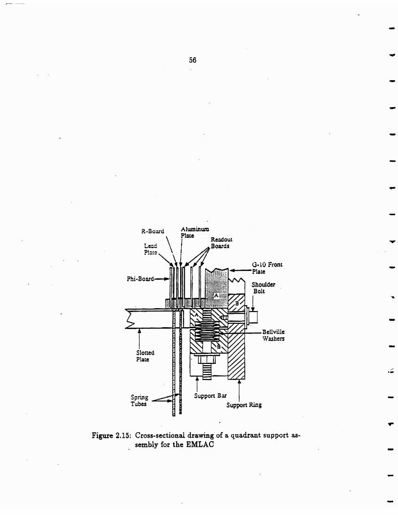
56
R-Bo:ird Aluminwu
\ /
Plate Rwout Le::d Boards
Pi~tz~ i Phi-Boa.rd__.
Stoned Plate
G·lO Front ----Plate
~~~~--Bellville Washers
Support B:ir
Support Ring
Figure 2.15: Cross-sectional drawing of a quadrant support assembly for the EMLAC
-----
-
--
/ ·--
---

-
·-
57
The. HADLAC's signal pads were designed such that corresponding pads in suc
cessive cookies subtend the same solid angle as the pad in the front cookie. The
pad height in the front was 10 cm and it increased to 14 cm in the last cookie. The
calorimeter was longit~clinally divided into a front section with 14 sampling cells and
a back section with 39 sampling cells. The cookies in each section had all longitudinal
sets of focused pads electrically connected together into a tower. The summed signal
from every tower was hooked up to an amplifier channel in the Faraday Room.
The high voltage planes are clad on both sides with copper. The side facing the
signal plane is held at negative high voltage while the other side is grounded. There
is enough capacitance between high voltage and ground that ballast capacitors are
not required for this detector.
The energy resolution of this device was determined by using 11"- beams of 50 and
200 Ge V in energy. The resolution was parametrized in the following form
CT(E) = 0.04 + 1.83 E f<E)
(2.6)
One cause for the rather poor performance of this device was that the sampling was
not fine .enough. Also a substantial fraction of the ionization occurred in a region
outside the drift field so it could not be collected. .Another factor that degraded the
HADLAC's energy resolution was the rather large channel capacitance due the pad
sizes being too large. This capacitance decreased the signal-to-noise ratio. Finally, the
neutron energy fraction was never seen. Neutrons are co~iously produced in hadronic
showers, but they leave no ionization in liqwd argon because they are electrically
neutral. Plastic scintillator, on the other hand, does respond to neutrons. Plastic
materials generally contain a large number of hydrogen nuclei. Neutrons traversing
the material will knock these nuclei out of the molecular sttucture a significant fraction
of the time. The hydrogen nuclei will recombine generating UV light which can be
detected by a phototube.

Frame Rail
•••• •••
58
Sway Bar
r_
-
~-~ \ - - )
..._ ~
~
'·'
z.otba Plates
~ Suppon I-Beams Super Plates
Figure 2:16: Front and side views of the hadron calorimeter. Steel "Zorba Plates" are the absorber media. The hole, shown in the center of the front view, allows passage of beam and halo particles.
--
-
I
-
-

- .
59
Card Edge Comector
Figure 2.17: Exploded portion of a HADLAC charge collection cell or "cookie".
2.2.4 LAC Electronics
The RABBIT system was used to readout the liquid argon calorimeters. Thia elec
tronics system was developed at Fermilab; RABBIT is the acronym for Redundant
Analog Bus Based Information Transfer. The Rabbit system is based on a special bus
capable of transmitting analog signals. Digital information in the form of address and
control signals can also be transmitted over a set of differential ECL and TTL signal
lines. The RABBIT bus is contained in the backplane of every RABBIT crate. The
backplane is actually divided into two separate busses: a. top bus and a bottom bus.
This feature allows the RABBIT system to function in a. low access environment such
as a high energy collider. In principle a. detector channel can have two completely
independent and redundant data transfer paths to the data acquisition computer.
This allows full hardwarP. function to he rna.inta.ined in the event of an electronics
failure along one of these paths.

60
Each slot within a RABBIT crate is assigned an address, and so every module is
referenced according to the slot in which it resides. Individual channels within a mod
ule are referenced by a subaddress. There are 64 analog and 64 digital subaddresses
per slot. A crate contains two controller modules called EWE's. One EWE controls
the top bus while the other controls the flow of information in the bottom bus. Each
EWE is capable of controlling either bus in accordanc~ with the redundancy feature.
Because the Faraday room was accessible under run~~ conditions, the redundancy
feature was not exploited so that the number of crates could be kept to a minimum.
This helped reduce costs along the entire data. transfe1· path.
Thre_e other modules were employed in the-experiment. The BAT module (before
and after timer) was used to terminate the end of. the backplane opposite the .EWE
mcdules. The :nodule monito:ed the various voltage levels in a c~tc, the a.mount
of current being consumed, and the crate temperature. However, its most important
function waa, as its name implies, to provide timing pulses for the sample-and-hold
and TVC circuits of the LACAMP modules. The LACAMP modules each contained
16 channels for amplification and readout of the signals coming from the calorimeters.
The amplliier modules were also capable of providing a fast output signal. The fast
output signals generated from the electromagnetic calorimeter pulses were used to
form the high level electromagnetic trigger. In order to have a reliable and efficient
triggering capability special summing modules known as P.J.. -ADDER cards were used
to sum the individual fast output pulses for each octant separately. The details of
their operation is described in the section discussing the trigger apparatus.
The EWE module is designed to receive the analog data coming from the LA
CAMP modules, digitize it, and buffer 1t for transfer to the next element of the data
acquisition system. Each controller possess a 16-bit analog-to-digital converter that
is used to digitize the analog signals coming from the amplifier modules. Having only
-
-
-

-
--
-
61
one ADC per bus simplifies the design and calibration procedures 1 and it keeps costs
down as well. The main drawback to this approach is that it .takes more time to read
out the amplifier channels, each digitization cycle taking about 17 µs to complete.
Two steps were ta.ken to overcome this problem. First, the simultaneous readout of
two channels is possible if the redundancy option is not utilized. Second, a zero sup
pression window was set whereby a channel was not digitized if its analog level failed
to exceed a predetermined value. The zero suppression procedure ta.lees about 1/6 as
much time as digitization. The EWEs are readout by processor-buffer units known
as MXs. The crate controllers also receive sets of instructions for executing different
procedures from the MX units. Each MX can control up to 4 RABBIT crates with
separate cabling for top and bottom busses.
The 16 channels in each LAC AMP module are clustered into four groups of nearest
neighbors. All channels in a group of four are tied to the same reference voltages.
Such a clustering is natural because the summed output form every group of four is
fed into a time-to-voltage converter circuit (TVC). Figure 2.18 shows the four basic
components of an amplifier channel together with the summing scheme used for the
TVC inputs. The four major circuits in a LACAMP channel are:
• A charge integrating amplifier
• A sample-and-hold circuit to measure energy deposition
• A TVC circuit to measure the time at which energy was deposited relative to a
particular interaction
• A fast output circuit to provide trigger signals
The charge integrating amplifier had a capacitor in the feedback loop for an opera
tional amplifier. The charge collected from a longitudinal sum of calorimeter sampling
cells was proportional to the charge, and hence the voltage, on the feedback capacitor.
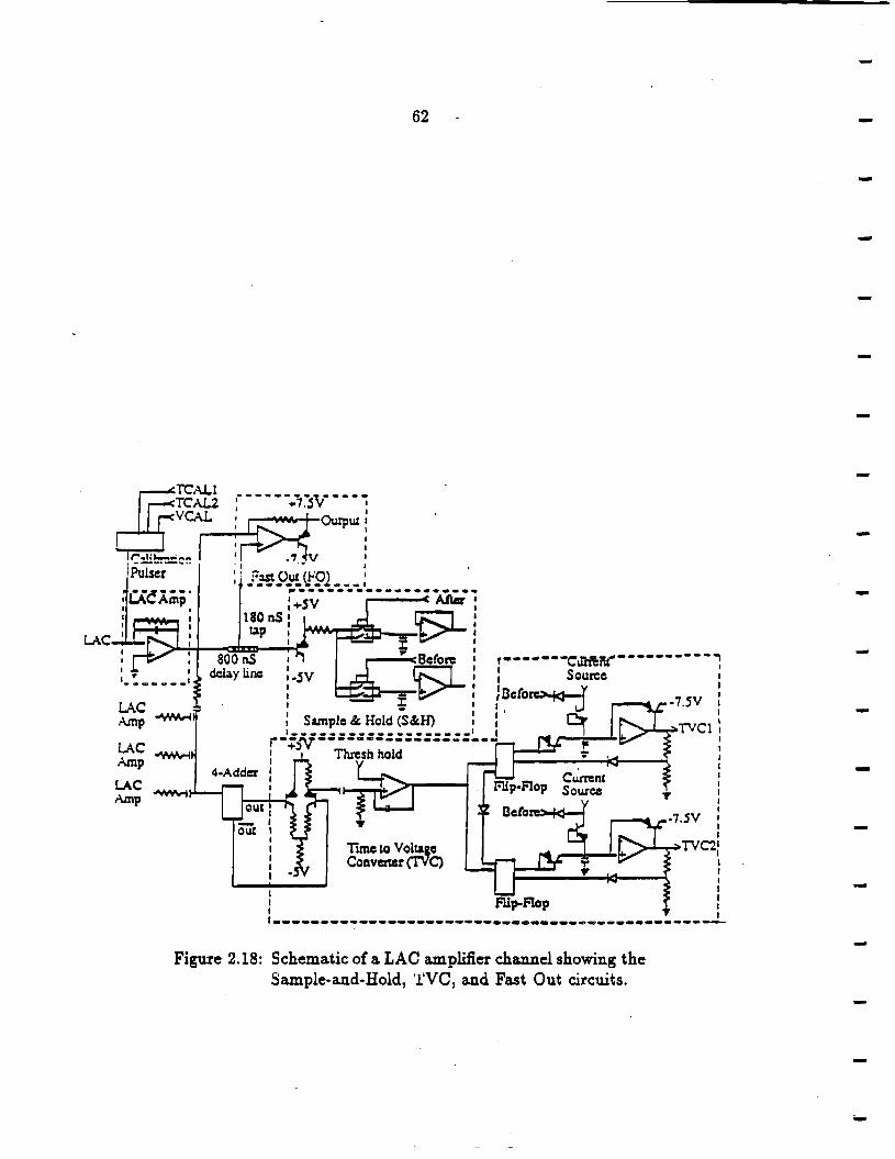
TCALl TCAL2 YCAL
l-. .. " .. I
62
l?uu;~--··
LAC A.mp
U\C Amp
LAC Amp
Tune 10 Vo~~ Convener (fVC)
Figure 2.18: Schematic of a LAC amplifier channel showing the Sample-and-Hold, '!'VC, a.nd Fast Out circuits.
--
-
--

/_
- .
63
Therefore, a linear relations~p exists between the energy deposited in a channel and
the voltage or pulse height appearing on the capacitor. A resistor was hooked up in
parallel with the capacitor so that the circuit would return to its ambient state over
a time interval much longer than the rise-time of a LAC pulse. The decay-time of
the resistor capacitor loop was :::::::: 150 µs as opposed to a rise-time of :::::::: 350 ns for
the calorimeters. The design of this circuit was governed by four criteria. First, the
amplifier had to have a low input impedance to match the rather low impedance of
the inpu~ cable, which was around 10 to 20 0. Otherwise, there would a several large.
reilections during the signal rise-time that would distort the actual signal from the
calorimeter. Second, the amplifier must have a high gain. The charge collected per
channel in the calorimeter is on the order of pico Coulombs while the range of the
ADC in a EWE module is 2.5 volts. Considerable amplification of the LAC signals
is required if the full 16 bit precision of the ADC is to be utilized. The smallness
of the calorimeter signals also dictates that the amplifier must have low input noise.
Finally, the devices must be stable over time since that large number of channels
makes frequent calibration infeasible. An amplifier design, composed of low noise
FET network, was chosen with the following characteristics: a feedback capacitance
of 20 pF, a gain bandwidth of _700 MHz, and· an open-loop or zero. frequency gain of
80 dB [14]. Examination of Figure 2.18 reveals that the charge integrating amplifier's
output was divided three ways. One output goes into an 800 ns delay line , another
is input to a fast output unit (EMLAC only), and the third output is fanned into a
TVC circuit.
The fast-out unit used the difference between the current amplifier output, and
the value it hacJ, 180 ns earlier to make a short negative pulse. ·This was accomplished
by tapping the delay line at an intermediate point. A pulse was produced only
if the difference was above a specified threshold. The generated pulse height was
proportional to the integrated signal, so it provided useful information to the trigger

64
logic, described in a following section. The fact that the shape of the integrated signal
is the same for all pulse heights insures the validity of this method, because the signal
value at 180 ns is always the same fraction of the full pulse height. The trigger logic
used the fast-out signals to determine whether or not enough PJ.. had been deposited
in the EMLAC to make an event a high p J.. '1, 11"0 , or 1J candidate. ff ~ 1. 7 Ge V / c of p J..
was deposited in an EMLAC octant, a PRETRIGGER signal was generated by the
trigger electronics. The PRETRIGGER signal resulted in an EVENT signal being
sent to the BAT modules. Upon receiving this signal, the BAT's initiated an event
timing sequence, illustrated in Figure 2.19. Two logic signals known as BEFORE and
AFTER were sent to all LACAMP channels in each crate.
The sample-and-hold circuits consisted of two precision capacitors which looked at
the delayed output of the amplifiers. Between each capacitor and the delayed output
was an electronic switch. Under ambien~ conditions the switches were closed, and the
outputs were sampled. Upon receiving a BEFORE or AFTER pulse the switches were
opened and the corresponding voltages were held on the capacitors, hence the name
sample-and-hold. The BEFORE signal was issued so that one capacitor measured the
level just before the amplifier pulse arrived. The AFTER puls~, generated ~ 640 ns
later, caused the peak level of the output to be retained. Upon command by the EWE
module these levels were read for each channel and subtracted before digitizatio~.
This reduced the effects of low frequency line noise as well as pile-up, which involves
the amplifier signals from a second event arriving before the circuit returned to its
ambient state.
Events that deposited energy within a few hundred nanoseconds of one another
could not be distinguished by the sample-and-hold circuitry. TVC circuits were em- -
ployed to solve this pile-up problem. Each TVC unit is composed of two circuits in a
master slave arrangement. Figure 2.20 shows a simplified schematic diagram of the cir-

-
65
cuit. The differentiated output, of a group of four amplifiers is fanned into a given
TVC input. Each sum is compared to a. crate-wide threshold set by the BAT. All sums
that exceed the threshold fire their respective discriminators which in turn clock the
filp-ftops of the corresponding master TVCs. Ordinarily, all current from the source
drains through the flip-flop, but when the fl.ip-iiop unit is clocked the resulting change
in the volta.ge level prevents this. As a. result, the ca.pacitor is charged at a. constant
rate. The slave TVC flip-flop is ena.bled whenever the master TVC is docked. If a
second input signal arrives before a global reset or a BEFORE signal, then the slave
TVC is docked, causing its capacitor to charge up. The BEFORE signal breaks the
path between the current source and ·the capacitor, thereby holding the capacitor's
voltage level.
If no BEFORE signal arrives within 150 ns of a TVC's firing, then the unit is au
tomatically reset. The BEFORE signal was timed to always a.rrive ~ 800 na after the
triggering event, and the TVC circuit wu designed to read half of full scale under this
condition. The event timing sequence of Figure 2.19 shows the usefulness of the slave
circuit. Here, an event fires the master TVC, but doesn't produce a PRETRlGGER
signal so no BEFORE pulse is generated. Later, a second event arrives that does
generate a PRETRIGGER pulse, and its time relative to the interaction responsible
for it is recorded by the slave TVC.
2.3 THE E706 TRIGGER SYSTEM
If one examines an unbiased sample of hadronic interactions, the occurrence of a high
p .l. 7ro or single photon event will be very rare. To enrich the E706 data with these
types of events a special electronics system was devised to select only those events,
containing a. significant amount of electromagnetic P.l. (- 3.0 GeV /c), for writing out
to tape. This selection mechanism, known as the trigger, is composed of very fast

66 -
1ccaad •ipal
rnclip&l (&aka)
(noc&Maa) / / output of integrator
"Cast-out" v v / / output of delay chip
BEFORE signal
AFTER signal 111111'!'
owpur of BEFORE -sample· and-hold
/ / output of AFI"ER. sample-and-hold
MASTERTVC ----\ SLAVETVC -------------tUnc:(approxiaiaie)
-1 µsc:o 0 J.l.$00 1 µsec 2 IJ.Sec
Figure 2.19: An example of an Event Timing Sequence initi-a.ted by the BAT modules. An event fires the master TVC, but fails to produce a PRETRIG-GER signal. A short time later, an event fires the slave TVC, ePne!"a.t.~ng a. PRETRIGGF.R. anci BEFORE pulses as well.
-
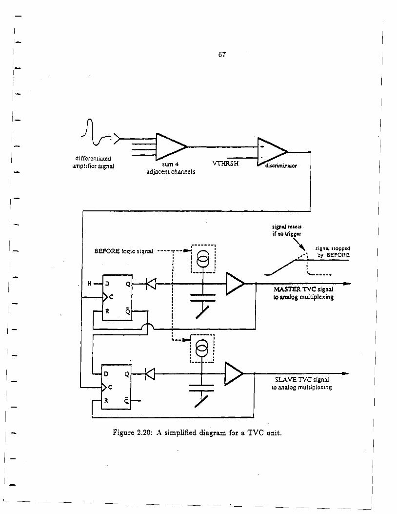
,_
67
d iff crcmiatcd amptdier aigmu swn4
adjacent channels VTHRSH
H D Q
s ignaJ reseu . i (no triggc:r
~ .. t
,• I
I I I
signal scoppcd by BEFORI!
'------MASTER TVC signal
C to analog multiplexing
R Q
D Q SLAVE TVC signal
C LO analog multiplexing
R Q
Figure 2.20: A simplified diagram for a TVC unit.

68
circuits. There are three major portions of the trigger system. First, there are the
electronics associated with the EMLAC which estimate the amount of p .J.. deposited in
the detector. Another part of the circuit provides the beam and interaction definition.
Finally, there are several counters and modules that generate vetoing signals. These
vetoes halt the trigger's operation for up to 30 µs.
2.3.1 EMLAC p.J. System
The EMLAC was used to detect local depositions of large amounts of P.L· The P.L
deposited is obtained from the deposited energy by the following
P.J.=Esin6 (2.7)
The detector's fo~used r - </J geometry ma.de the formation of the trigger straightfor-
{2.8)
P.J. is the amount of transve?'~.; momentum in a particular r-region of a.n octant. The
sum is over the strips in the front a.nd back sections within the region. ei is the energy
dep'JSited in the ith readout strip in a. summed region, and 8, is the production angle
corresponding to the ith readout strip.
Figure 2.21 shows how the r-strips of each EMLAC octant are grouped together
to form the various P.J. sums. The analog summing begins by taking the sum of
adjacent fast-outputs from the LACAMPs, and putting the signals into 8-bit linear
attenuators. The attenuators provide the sin 6 weighting of the pulse heights. The
attenuator outputs are then summed in groups of 8; front and back sections a.re
summed separatP.ly at this stage. Adjacent gT'onps nf 8 at'P. suhsPcp1ently summed into
non-overlapping groups of 32 channels. The groups of 8 provided the input to the
local discriminator modules, while the sums of 32 were used to form the global trigger
signals.
-
-
-
-
-

-69
The local discriminator modules are shown schematically in Figure 2.22. At this
stage the sums of corresponding front and back groups of 8 are summed together
on input. Furthermore, adjacent groups of 8 are summed together into groups of 16
channels, overlapping one another by 8 channels. If any sum of 16 exceeds a specified
threshold, then a single-signal (SLOC) trigger signal is generated. There were two
local discriminator modules per octant for the 1987-1988 data taking period. They
produced logic signals referred to as LOCAL_PT_HI and LOCAL_PT_LO, indicating
the relative magnitudes of the thresholds.
The sums of 32 are discriminated in a similar fashio.n by a set of devices called
the global P.L modules. However, the groups of 32 are summed in a different manner.
There is a sum of the 3 innermost groups of 32 channels, a sum of the next 4 groups
of 32, and a sum over all groups of 32 in each octant. Thus, each octant had three
different global P.L_ sums assigned to it, and there were two global P.L thresholds per
octant. The three global slims are expressed mathematically as follows:
91
glpt13 - LP.Li i:sO
233 glpt47 - E P.Li (2.9)
•=• 233
glpt17 - LP.Li isO
P.Li oc Ei sin 9,
Besides forming a global P.L logic signal, the global P.L sums glpt13 and glpt47 were
used to generate octant PRETRIGGER signals. The generation and purpose of the
PRETRIGGER signal as well as the high level interrupt signal are given in a following
subsection. Table 2.2 lists_ the nominal thresholds for both the local and global P.l
trigger modules. Notice that several of them were changed from time to time during
the data taking period.

70
Figure 2.21:. Octant r-cha.nnel summing scheme employed by the local Pl. modules. These modules produced summed signals for groups of 8 and 32 strips.
SUUl·Of·32
-
-
-

-
rrcm pT modwe sum-of ·8 ourpuLS
~ 0-7 rronc
0-7 b:ick
8·15 front
8·15b:ick
~6·23 (ronc
:5-23 b:ick
:.;.31 Crone
:.;.31 back
248-255 front
2.;s.2ss b:ick
8-bic DAC 0-2.SV
S·bic OAC 0·2.SV
S·bit OAC 0-2.SV
71
!C. Ourpucs ,.-. .,
Glob3.l OR (NIM& TIL)
Figure 2.22: Front-back summing scheme employed by the local descriminator modules.

72
Table 2.2: Trigger threshold settings by run number.
...----------------·--------------...... ,\ ·I
I Logic Signal i Threshold (Ge V / c)
runs . runs \ runs ! runs
1811-2292 ~ 2293-2310 12311-290412905-3036 i
LOCAL_PT_LO I 1.2
LOCAL_PT_HI I 4.2 !
i 3.6 I 3.0 I
GLOBAL_PT_LO I 2.5
GLOBAL_PT_HI I 4.0 3.6 I
At this point a brief discussion of the image charge effect is in order. The effect
of image charge can be understood by examining Figure 2.23. As the ionization
electrons drift towards the a.node under the influence of the electric field between
the lead plate and the grounded readout board, a current is induced. This current
was originally intended to flow out through the amplifier signal cables and retum to
the lead plates via the high voltage ballast capacitors. However, when the EMLAC
was put into operation, it was found that due to impedances in the ground path
between the ballast capacitors and the amplifiers th~ retum current flowed through
the amplifiers adjacent to the ones sensing the actual ionization during the first 200 ns
or so of pulse formation. The result was a signal of opposite sign and nearly equal
magnitude on the channels surrounding a high energy electromagnetic shower during
the time of trigger pulse formation.
When s11mming a. group of 16 channels for the local trigger, the image charge
contribution is small since the typical shower width is a.bout 16 strips. However,
-the global sums result in a. serious loss of signal, greatly compromising the 0!cb~
trigger's efficiency a.s Figure 2.24 illustrates. What's even worse is that the image
charge contribution grows with radius due to the r-strips' increasing capacitance, and
----
--
-

-
Elcccron·lon P"'1
iiV Ca:.hooc
' ..
73
, 1
I , ,
I
············•······
I I I I
~--················
Si;n~
Figure 2.23: Schematic of the EMLAC charge collection circuit (one channel).
the increase in the sin 9 weighting. To alleviate the image charge problem cut off
diodes were installed on the inputs to the modules performing the sums of 32. These
diodes shunt the "wrong sign" image charge current to ground. In addition, The
outermost 32 channels were not utilized in forming a trigger. Because diodes have a
characteristic turn on voltage, not all of the image current was shunted to ground,
and so the global trigger's performance was indeed compromised.
2.3.2 Beam and Interaction Definition
A trigger logic signal from the EMLAC should be "in time" with a particular inter-
action in the target if it corresponds to an event of interest. The interaction itself
should be in coincidence with the passage of a beam particle through the apparatus.
To avoid pile-up effects. in the calorimeter and constrain the event kinematics the
interaction responsible for a high level trigger should not be accompanied by another
interaction within a time window of 150 ns. Finally, it is useful to know whether

74 Signai
I
P U=gc Ch:arge (Summed over Rcm:Wicicr of Oct.l.'lt)
~----
·summed Sign~ for Entire Ocu.nt
--------------~----·
I
100 :oo I
300 I
~oo
I
500 600 time (ns)
Figure 2.24: The effect of image charge on the global trigger input signal.
or not the beam particle associated with a given interaction was part of the beam
ha.lo since it was possible for halo particles to generate interaction signals a.nd/ or
electromagnetic showers.
The layout of the scintillation counters used in the beam a.nd interaction definitions
is shown in Figure 2.25. The presence of a beam particle was signalled by counters
BA, BB, and BH. BH was a counter with a 1.0 cm hole to allow true beam particles
to pass through it. A signal from BH indicated a ha.lo particle's passage. In addition,
the signals from the beam counters were put in coincidence with the RF clock and
beam gate provided by the accelerator control room. The RF clock provides pulses
with a period of 19.4ns, which matches the beam's bucket structure. The beam gate
is activated when the extraction magnets are energized. The beam signal for the
1987-1988 data taking period is given by the following logical expression,
BM = BA· BB · BH · BMGATE ·RF _CLOCK (2.10)
Beam signals were generated once every 19.4ns.
-
-
--
-
-
-
-

-
Be:im
75
Figure 2.25: The configuration of scintillation counters used the the beam and interaction definitions.
The interaction signal was formed from the coincidence of any one of the inter
action counters, SWl, SW2, SEl, or SE2 with the BM signal. Each interaction
counter had a semicircular hole in it, allowing passage of the beam.. Otherwise there
would be an "interaction" every 20 111 and the pile-up filter would veto every event
selected by the EMLAC trigger electronics. The interaction pile-up filter circuit is
shown schematically in Figure 2.26. The signal from each interaction is delayed 16
times in successive 20ns intervals. The ninth delay port was defined to bet= 0, and
put in coincidence with the logic signals coming from the calorimeter and vetoing el
ements. A clean interaction signal was produced if a signal exiting port nine was not
in coincidence with any signals from the three a~jacent ports on either side. Thus, a
triggerable interaction was isolated in time from other interactions by ±60 ns. A live
interaction was defined as the coincidence of a clean interaction, the BM signal and a
computer-ready gate. The computer-ready was required since the DA system had to
be capable of reading out the detectors should a trigger occur; this was the guiescent

76
state of the DA system. It was the live interaction signal that was actually put in
coincidence with the high level trigger from the EMLAC.
2.3.3 Vetoing Elements
There are three online veto requirements. All of them have to be satisfied at the
PRET~GGER level. The first requirement is that no PRETRIGGER has occurre~
within the previous 300ns of the current PRETRIGGER. The PRETRIGGER sig-
nals are delayed in a manner similar to the interaction signals so that a coinc~dence
backward in time can be made. This veto is known as the early P..L kill. Its purpose is
to prevent two low P..L events, separated in time by less than the LAC risetime, from
satisfying the high-pl. trigger.
· Another vetc i: p:ovided by the ... •eto . wall described earlier. The hadron shield
is very effective at stopping the d.iffiue beam halo. However, the muon Hux is so
high during data taking that many halo muons penetrate the shield, and shower
in the EMLAC. Enough high Pl. showers could be generated this way to seriously
contaminate the single photon sample. Therefore if both veto w~ register at least
one hit in time with an EMLAC trigger, then a signal is produced that disables the
trigger for - 150 ns.
Finally, there was an SCR kill which disabled the trigger for 30 µs. The SCR spikes
are detected by a set of HADLAC channels, discriminated and then sent as a veto to
ports on the trigger electronics modules responsible for the PRETRIGGER signal.
SCR noise spikes are generated by the 400 Hz RABBIT power supplies inside the
Faraday room. Such noise spikes induced LACAMP oscillations capable of producing -
false triggers. These oscillations are damped out within 30 µ.s.
---------
-
-

-
INT
-
BM
INT
CL(AN.l.AT(
CLCAN.CARLY
r:ICl.AY I I
tCLAT I ' CICLAY I 1
CICC.AT I ' CCL.U I ' CCL.·" I u:
DCL.U I II
CCI.AT z ll
OC~AT J 17
NCSCA4.CI
~SCA4.C•
77
) )
PRCLN
COMP.ROY
SM
BH
Cl.tAN.l.ATC
CLCAH.CARl.Y
PRCLN
Figure 2.26: Schematic diagram of the interaction pile-up filter, and live interaction definition circuits.
LINT!

78
2.3.4 High Level Trigger Operation
The operation of all the high level triggers is essentially the same. If the sum glptl 7
for any octant has more than 1.7GeV /c of P..:. then an octant pretrigger signal is
generated. Provided that a live interaction signal is in coincidence with the octant
pretrigger and there are is no trigger veto then a LAC pretrigger is generated. The
use of zero-crossing discrimina.tors allows a. given pretrigger to be put in coincidence
with the proper interaction. At this point a "load" and "event" signal are sent to the
tracking system's latches and the BAT modules respectively. In addition, the pre
trigger ·circuit is disabled from generating another pretrigger pulse. This guarantees
that there is only one "load" signal given per high level trigger, which must be the
c~~ ii tile traciu11g system's electronic reaciout system is to iunction correctly.
If the high level trigger logic generates a signal, then the DA sends out a busy
signal, suspending all further data taking. All latched information is then read by the
DA and transferred to the proper PDP-11 memory. When all PDP-Us have finished
reading out the detectors, the computer-ready gate is enabled, and data taking may
resume. A master clear signal is also generated which resets all the electronics. The
master clear prevents trigger operation for 5 µ.s so that the trigger electronics may
settle into a quiescent state. If no high level trigger is formed within 300 ns of a
given pretrigger, then a clear signal is sent to the tracking system electronics and the
pretrigger circuit is enabled once more.
Four distinct types of high level triggers were implemented during the first da.ia.
taking period of E706. They were constructed from the logic signals listed in Table 2.2.
• Local-Global-Hi, the trigger generated by a logical AND of the GLOBAL_PT_HI
and LOCAL_PT_LO logic signals. This trigger indicated that a large amount
of p .L had been deposited within an octant with a significant fraction localized
---
---
-
-
---

- 79
in a small region. Its purpose was to provide efficient detection of high p .L 1/
.particles.
• Single-Local, defined only by the LOCAL_PT_HI signal, signified a large local
deposition of P.L within some octant (;<: 3.0 GeV /c). This trigger was very
efficient at selecting single photon and high p .L ?ro events.
• Local-Global-Lo, was similar to the Local-Global-Hi trigger except that the
GLOBAL_PT_LO signal was used instead of the high threshold global signal.
Its purpose was to study the Local-Global-Hi's performance. This trigger was
prescaled by a factor of 10 so it wouldn't dominate the trigger rate.
• Two-Gamma, defined by the logical AND of the LOCAL_PT_LO signal from
one octant with the same signal from any of the three opposing octants. This
trigger selected events containing massive ?r0 ~d single photon pairs at high
P.l·
Triggers based on only the beam and interaction definitions were also implemented for
diagnostic purposes and various detector studies. ~hey were prescaled by tremendous
factors so as not to dominate the trigger rate. The E672 experiment also supplied a
high level dimuon-muon trigger which was or'd with the E706 trigger. However, these
triggers are not pertinent to this analysis.
2.4 CHARGED TRACKING SYSTEM
The charged tracking system consisted of 14 planes of silicon microstrip detectors
(SSDs ), a dipole analyzing magnet, and 16 planes of multiwir.e proportional chambers
(MWPCs). The SSDs are positioned upstream of the analyzing magnet. They have
been used to reconstruct the primary event vertex and the beam track responsible
for the interaction. The MWPCs are placed downstream of the magnet. Only the

80
MWPCs possess stereo capabilities and can therefore reconstruct tracks in space.
As its name implies, the magnet was used for momentum analysis of tracks and to
determine the sign of their respective electric charges.
2.4.1 SSD System
The-14 planes of SSD are grouped into modules by pairs. Each pair of planes
consists of an X-Plane (strips vertical) and a Y-Plane (strips horizontal). Four of
these X-Y modules are positioned downstream of the target and have been used to
reconstruct the primary vertex. Three of the X-Y modules are positioned upstream
of the target. Their purpose was to reconstruct the tracks of the beam particles
appearing within the primary interaction's vertex. The SSD modules are composed
of an aluminum plate which has the PC boards containing the SSD wafers attached
to it. The plates lay in precision milled slots on a one-piece cradle. The cradle sits
on an optical table which. is mounted at three points to the SSD cart. The cart is a
. steel structure that sits on rails rigidly attached to the floor of the experimental. hall.
The cart has the ability to move horizontally transverse to the beamliile.
Figure 2.27 gives a schematic layout of the SSD system in the X and Y-Views.
The three X-Y modules upstream. of the target and the first X-Y module downstream.
of the target contain 3 x 3 cm2 wafers. The other three modules have 5 x 5 cm2 wafers
installed in them. Each wafer is 250 - 300 µ.m thick. After the wafers are mounted
onto their respective PC boards two holes are drilled in the board. The holes are on
either side of the wafer 6 inches apart, centered on and parallel to the central strip.
These holes mate with precision located pins in the aluminum module plates. The
module plates are seated in precision milled slots on the SSD cradle. Thus, each SSD
strip's location can be known in a surveyor's coordinate system thereby permitting
an alignment of the full SSD. system. A complete description of how the wafers are
mounted into the modules and connected electrically strip by strip with the outside
---
---
----
-
-

-
-
-
81
world is given in a NIM article (15].
There are a total of 7120 active strips in the SSD system. Each strip is 50 µ.m
wide and is essentially a p-i-n diode. A minimum ionizing particle that traverses one
of these strips deposits (2.0- 2.4) x 104 electron-hole pairs. The charge is collected in
~ 20 ns. This charge is picked up by a Rel-Lab 10-323-C charge sensitive preamplifier.
The preamplifier output is input for the NANO METRIC digitization system which
is described in a subsequent section.
The apparatus shown in Figure 2.28 was used to measure the operating charac
teristics of the SSDs. A 108Ru /3-source with an endpoint of 3.4 Me V was used as
the source of min;mum ionizing radiation. 51 and S2 were scintillation counters put
in coincidence to form a trigger for genera.ting load signals. The load signala were
sent to the latches for the SSD plane being tested. For pulse height measurements, a
post-amplifier designed to imitate the N - 2770 was used to drive a LeCroy 2249A
ADC. The pulse height measurements yielded a minimum ionizing peak at 71KeV
above an ADC pedestal peak. The pedeatal peak had a HWHM of 3.4KeV, which
yielded a ratio of 21. A threshold study using the N - 277C amplifier yielded a plateau
region between 1.5 and 2.5 volts. When normalized to the number of source electrons
traversing the detector, the plateau region corresponds to an efficiency of - 1003.
The small amount of charge produced per strip and ·the corresponding high gain of
the amplifier stages makes the SSD system vulnerable to stray electromagnetic radia
tions coupling into the amplifier stages and dominating the signal. The SSD modules
and the preamplifier stages were enclosed in an aluminum housing which formed a.
Fara.day cage. The cables leading from the preamplifiers to the NANOMETRIC am
plifiers passed through shielded conduits; the same is true for the cables going from
the discriminated outputs of the N -277Cs to the latch modules. The power supplying
the preamplifiers was passed through XENTEC isolation transformers. All amplifiers
were grounded in parallel to the SSD table which was connected to the MWEST hall

82
M1crostr1p Detector X-Y Modules XY
/ \ / .,.,, .,,, XY XY XY XY ,-
.,,,,,,, .,,, ,., .,,,,,.,
Proton Beam 800
GeV/c \
I \ O.t Interaction \ Length of Be
\ ' ' \ Photon PT = 8.2 2 GeV/c \
\ \
___ _,,. Direct Photon
Jet } Charqed Particle -spectatori Trocks
2mmI
Figure 2.27: Schematic of the segmented target/SSD system of E706. A typical multiple event is superimposed on the planes.
....... .......
....... t cm
--
x '(
,, -
---
......
'
--
-

--
83
I I I I I
I I p __ _... ________ __
I N
. . . - 50 ft I I I I
f .. s, Thrtshold
...,._! ________ s I 2
Tri 99tr Co1nc:1 d ence ,___.;,_m.._.,._
.-----~ ·--1 I.RS 2323 '-OGd I 0 I Gate Generator.__ .. ______ ...., ___ ,.. a>
I Read Laich ~ .! - - - - - - -NANO N-281 Z ~
•I Inter foce ~~~iiiiliili!=§i!i. ~ g I 4U
RS·422 Bus I z I ~ __ Ct>:__MAC Crat.:_ J
~~C~y-3~~ J Figure 2.28: Readout electronics schematic used to determine
operating characteristics of SSD system.
I I I I

84
ground via a thick braided cable.
2.4.2 MWPC System
The 16 planes of MWPC ~e grouped into 4 views (X, Y, U, and V). Each view
contains 4 planes. The views are grouped into pairs with the members of each pair
being mutually orthogonal. The pa.irs are X-Y and U-V; the U-V system is rotated
about the Z-axis with respect to the X-Y system such that the intersections of X, Y,
and U lines form 3-4-5 triangles, i.e. the two systems are related by the following
transformation:
4 3 U - -X+-Y
5 5
V - _!x+!Y 5 5
(2.11)
In terms of hardware the MWPCs are grouped into 4 modules. Each module
contains 4 an~de planes, one for each view. The sense planes have independent facing
cathodes for a total of twelve layers. In addition, there is a spacer layer at either end
of the stack to provide clearance for the high voltage leads of the end cathodes. The
sandwich is held together in compression by two massive frames. The alignment of
the planes is accomplished by 12 precision steel pins which fit through bushings on
each plane and precision located braaa bushings in the frames. Figure 2.29 shows the
manner in which the sense planes are stacked in each MWPC module.
The operation of these chambers is fairly simple. Charged particles traversing
the chambers ionize argon atoms in the gap between the anode and cathode layers.
The cathodes are held at around -2900 V while the anodes are grounded. Asa:-
result, the ionization electrons drift towards the anodes. An illustration of the electric
field lines in a multiwire proportional chamber is given in Figure 2.30 [16]. The
electrons drift along the field lines towards one of the anode wires. The anode planes
typically consist of 800 20 µ.m gold plated tungsten wires positioned precisely parallel
---
--
...
--
-
-
...

-
85
to and coplanar with one another~ The spacing between neighboring wires in the
E706 MWPC chambers is maintained at 2.5 mm. As drifting electrons. get within
close proximity of a wire, they acquire enough kinetic energy per mean free path to
ionize other argon atoms due to the ""' 1/r behaviour of the electric field near a long
filamentary conductor. These liberated electrons are in turn able to ionize additional
atoms, and so an exponentially increasing amount of ionization occurs as the ions
drift towards a given wire. This phenomenon is called a.n avalanche.
An avalanche generally yields a gain of 106 in the amount of ionization collected
on a given anode wire over the amount originally deposited in the gap. If the wire is
terminated with a resistor, then a current on the order of several µ.A will ilow through
it during the first 100 ns of signal formation. The resulting voltage is detectable
by a high bandwidth amplifier. The amplifier outputs were discriminated in this
experiment so the .:>ruy informa.tiun. a.vailable was whether or not a. given wi:c had
registered the nearby passage of a charged particle. By determining which wires had
experienced an avalanche in an event, and knowing their positions it was possible to
recomtruct the trajectories of the charged particles which passed through the system
during the event. The spatial resolution of t~ese chamben is only a function of the
wire spacing. In fa.ct, it is given simply by tr = s / Ji2 where s is the wire spacing.
The avalanche process is the basis of operation for all proportional type counters.
It is fairly simple to quantify it. If a-1 and n are the mean free path and number of
electrons at position z, then after travelling a distance 6z the increase in electrons,
6n is given by
(2.12)
This proportionality between the incremental increase in ionization and the total
amount of ionization is what gives proportional counters their name. A simple inte-

Oif fractive Region Beam Region.
86
Figure 2.29: Arrangement of sense planes in each MWPC module.
-
-
---
---
-

-
-
--.
111 ! I~ I I
'ii l, '
' : ii
~: 11 i I 1 . I' . ,:J: !I I I
• , II I I
• I t I m • t
. I ~ ~1111 t ~
i
JI I I I I
87
II IJ I I
I I
. . II
. -.. . ---
~--· ~-lJ··~ ·~ h J I . . •I . I
I, 11 .. ,. I I
' !1
I II I II I II
OJ.
0.5
0.7
OJO o.as Q.90
Figure 2.30: Electric field equipotential and field lines in a multiwire proportional chamber. The effect on the field due a small displacement of one wire is also
shown.

88
gration leads to an expression for the multiplication factor M.
M = 2::. = exp [1•2
a( z )dz] no al
(2.13)
It is possible to determine the form of a(z) exactly for a proportional tube counter.
Such a detector is composed of a hollow conductive cylinder with a fine wire running
along its a.xis, which is held at positive high voltage. The voltage at a distance r
from the anode inside the tube and the capacitance per unit length are given by the
following equations,
V(r) - CVo 1n :_ 2rEo a
(2~14)
2reo O = ln(6/a)
where a and bare the coun~er's inner and outer radii respectively and v(,is the applied
voltage. Generally speaking a has the form a = lcpE where p is the number density of
molecules in t~e ionizing medium, Eis the ionization electrons' average kinetic energy
and le is a constant of proportioDality. Given that an electron acquires on average
a kinetic energy E from the applied electric field between collisions, it follows that a
has the following form:
a(r) = lcpCVo 1 2rEQ r
(2.15)
If the applied voltage is much greater than the ionization potential, then the mul-
tiplication factor has the following simple form where K is another constant with
dimension of charge-1 •
M = exp(K(CVo)) (2:16)
The ~1~ctric field configuration in multiwire proportional. chambers 1$ T'tluch more
complex than in cylindrically symm~tric proportional tube counters. However, the
same simple description of the ava.la.nche process does apply as will now be demon-
strated. For a description of the pa.rameters and coordinates used to describe the
.. -
--
---
-

-
89
field in an MWPC the reader is referred to Figure 2.31. The field, potential and
capacitance per unit length have been found to be of the following form [17],
E(z,z) - CVo(l + tan2 ~tanh2 ~)1/2 (tan2 ~ + tanh2 ~)-1/2 2Eo8 8 S S 8
V( .. , z) CVo [21rl In ( ( . 2 ?rZ • 2 1r'Z )] .... - - -- 4 sm -+s1nh -) (2.17) 41r'Eo s 8 s
21r'Eo c -1rl/s -In(21ra/s)
These expressions are valid for the boundary conditions V(a) = Vo, V(l) = O. Note
that a is the nominal radius of the anode wires, s is the wire spacing, and l is the
distance between anode and cathode planes. Now, for the region very close to a given
wire i.e. z < s and z < s the electric field expression reduces to the following
CVo 1 E(z,z) ~ -
2 --,
1r'Eo r (2.18)
This is identical to the field for a simple proportional tube counter and so the de
scription of the aval.~che phenomenon is identical in both cases! Table 2.3 lists the
relevant geometric parameters for each anode plane in the MWPC system; Table 2.4
sumniarizes the electrostatic parameters of the anode planes. Note that the operating
voltage is actually applied to the cathodes and the anode wires a.re held at ground.
There a.re two fundamental design considerations in building proportional cham
bers of the size used in E706. First, there is the variation in gain due to variations
in the geometrical parameters a, s, and 1. Second, the high electric fields required
to operate such devices create considerable forces which tend to pull the anode wires
out of plane and attract. neighboring cathode and anode planes together. Such me
chanical deformations will, at the least produce variations in gain and at the worst
the electrical breakdown of the chamber due to broken wires and/ or the cathode and
anode planes coming into actual contact with· one another.
The gain variations can be estimated by taking the differential of 2.16,
6.M =lnM6.Q M Q' Q =CVo (2.19)

90
Table 2.3: Relevant geometrical parameters for MWPC anodes (MKS units).
Plane Module View Aperture (in m2 ) Z (in m) Channels
1 1 x 1.6256 x 1.2192 3.4790 640
2 1 y 1.6256 x 1.2192 3.4965 480
3 1 u 1.6256 x 1.2192 3.5140 704
4 1 v 1.6256 x 1.2192 3.5315 672
5 2 x 2.0320 x 2.0320 4.5458 800
6 2 y 2.0320 x 2.0320 4.5633 800
7 2 u 2.0320 x 2.0320 4.5808 896
8 2 v 2.0320 x 2.0320 4.5983 896
9 3 x 2.0320 x 2.0320 5.6126 ·800
10 3 y 2.0320 x 2.0320 5.6301 800
11 3 u 2.0320 x 2.0320 5.6476 896
12 3 v 2.0320 x 2.0320 5.6651 896
13 4 x 2.4384 x 2.4384 6.6794 960
14 4 y 2.4384 x 2.4384 6.6969 960
15 4 u 2.4384 x 2.4384 6.7144 1120
16 4 v 2.4384 x 2.4384 6. 7319 1120
--
--
-
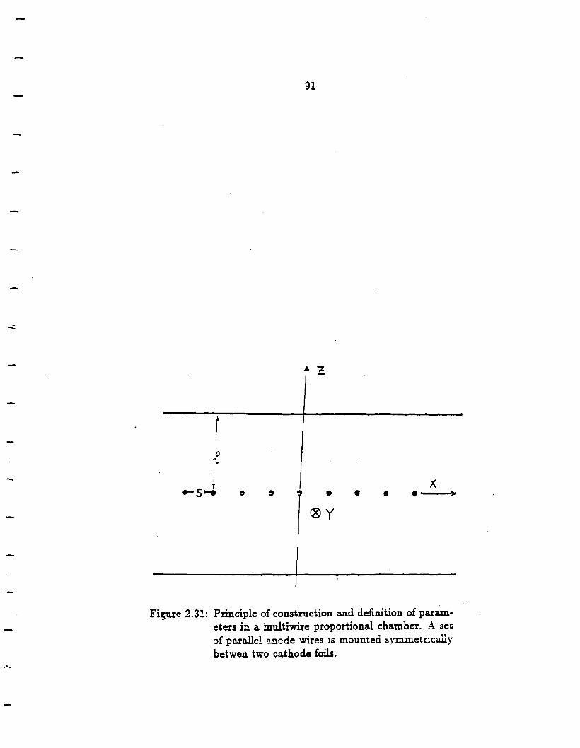
-
r
,e !
' ~s .... e
91
• ®Y
x • • . ~
Figure 2.31: Principle of construction and definition of para.meters in a multiwire proportional chamber. A set of parallel anode wires is mounted symmetrically betwen two cathode foils.

92
Table 2.4: Electrostatic parameters for all MWPC a.nodes.
MWPC Electrostatic
Parameters (MKS units)
Parameter Value
c 5.15 x io-12 Fm-1
Vo 2900V
1 0.0574m
s 0.0254m
a. 2.0 x 10-e m
Using the formula for the capacitance per unit length, one can derive the following
relationships between l:l.M/M, a, a, and l:
M l!::.M
(2.20)
For gains of - 108, and using the parameters for the largest module one obtains,
l:l.M 4.3 x l:l.a M -
CJ
6.M 6.l (2.21)
M - 9.7 x -l
6.M 9.7 x (; + 1)~.; M -
The gain variations are not critical for the experiment since only the discriminated
outputs of the amplifiers are -used in data processing. However, to keep the gain
variations ~ 50% requires 6.l ~ 0.1 mm, and ~a ~ 50 µ.m. !::::.a/ a is known to
vary by about 1 % a.nd the gain variation is weakest in this parameter anyway. The
wirespacing was the most difficult tolerance to ·maintain. The wire laying procedure
-
-
-
-
-
-

-
-
93
relied on· using printed circuit boards with a precision spacing between the pads on
which the wires were laid. As will be described later, these printed circuit boards
were mounted on the anode frames to 1 mil precision.
Once laid, the wires are tensioned in order to compensate for the electrostatic
forces that pull them out of plane with one another. This technique works so long as
the tension component normal to the plane of wires becomes large enough before an
undesirable amount of distortion occurs. Care must be taken that the applied tension
does not exceed the elastic limit of the wire.
It is possible to be more quantitative about this issue. Trippe [18] has shown that
for chambers of the aperture used in this experiment a stable equilibrium arises when
the tensioned wires are altemately displaced up and down as shown in Figure 2.32.
H the following expression, valid in the approximation of tangents to· arcs, is used for
the force between two anode wires,
F = (CVo)2 ~ 21r'Eo r
(2.22)
then the force per unit length on a given wire in the direction normal to the wire
plane is given by,
{2.23)
where 5( z) is the wire's displacement along its length. This formula describes the
force at a point on a given wire as a sum of forces between pairs of linear charges.
These linear charges are in the direction of the tangents to the wires at a distance x
along the given wire. This formula is valid in the limit of small displacements. Now,
if T is the applied tension on the wire, then the restoring force perpendicular to the
anode plane per unit length is expressed as
R = Td25 dz2
(2.24)

94
One thus obtains a second order differential equation of the form,
d25 + (CVo)2 5 = O ck2 T41rEo s2
(2.25)
with 5(0) = 6(L) =Oas the boundary conditions._ Lis wire's length. The solution of
this diff'erential equation consistent with the boundary conditions is
.· (CVo fI:_ ) 5(z) = 50 sm 2;'V ;;fz (2.26)
The boundary condition 5(L) = 0 implies that if T exceeds the critical tension, Tc,
given by
T >Tc= _1_(CVoL)2 411"Eo 8
(2.27)
then the anode wires will remain coplanar. Substituting the parameters of Table 2.4
into this equation yields a critical tension of 175 g, which ex~eeds the elastic limit of a
20 p.m tungsten filament. The applied tension should be kept below the elastic limit
by about a factor of two in order to allow variations in wire diameter and applied
tension during wire laying. For this reason a nominal tension of 40 g was selected. The
critical length, Le, beyond which the wires will move out of plane to the equilibrium
configuration of Figure 2.32 is 1.2 m. Therefore, some form of mechanical spacer
between anodes and cathodes is required in order to maintain the desired planar
arrangement of anode wires.
The mechanical spacers between neighboring anode and cathode surfaces are also
needed just to keep the planes from coming into contact with one another due to
unstable electrostatic attraction. The cathode planes are composed of 1 mil MYLAR
sheet held under tension to which a conducting graphite film has been applied. The
amount of tension necessary to maintain the proper a.node.cathode spacing, l, ca.n be
found from the following equation
pH2 ~l=-T 8
(2.28)
-..
---
-
-...
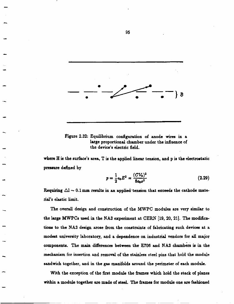
-
-
-
-
-
95
• •
Figure 2.32: Equilibrium configuration of anode wires in a large proportional chamber under the influence of the device's electric field.
where His the surface's area, Tis the applied linear tension, and pis the electrostatic
presaure defined by
= !eoE2 = (CVo)2 P 2 8eo42
(2.29)
Requiring ~I - O.lmm results in an a.pplied·temion that exceeds the cathode.mate-
rial's elastic limit.
The overall design and construction of the MWPC modules are very similar to
the large MWPCs used in the N A3 experiment at CERN (19, 20, 21]. The modifica-
tiona to the N A3 design arose from the constraints of fabricating such devices at a
modest university laboratory, and a dependence on industrial vendors for all major
components. The main dliferences between the E706 and NA3 chambers is in the
mechanism for insertion and removal of the stainless steel pins .that hold the module
sandwich together, and in the .gas manifolds around the perimeter of each module.
With the exception of the first module the frames which hold the stack of planes
within a module together are made of steel. The frames for module one are fashioned

96
out of aluminum to prevent a.ny coupling with the spectrometer magnet's field. The
twelve stainless steel pins, responsible for the planes' alignment, are arran~ed around
the frames three per side. The pins are spherically convex at one end to facilitate
passage through the stack during insertion and removal when a chamber is opened
and closed respectively. The .other end of each pin is spherically concave to allow
mating with an identical pin which is used to push the pin already in place through
the stack. These pins are hollow along their axes in order that threaded rods may be
inserted through them. Stack compression is achieved by placing flat washers over
the bushings in the frames, and nuts with lockwashers onto the threaded rods. The
nuts are then tightened with a torque wrench to 7 kg m.
The chamber frames are constructed of 6 in x 1 in pieces of steel or aluminum plate
that are fastened together at the corners by blocks and bolts. C-channel has been
welded along the outer faces to provide additional strength and rigidity. In the case
of module four this channel was bolted onto the outer face. The frames were designed
to be square within 5 mil. The inner faces have been ground flat in order to apply
e!'en pressure on the chamber stack and keep it properly aligned. Holes were tapped
around the outside edges of each frame so the gas manifolds could be attached after
stack assembly.
Because the frames were made square, the brass bushings for the steel pins could
be precision located, and bored out on the frames. Each bushing has a circular notch
machined around the inside of it. An 0-ring is seated inside the notch, providing a
gas seal between the pins and the bushing.
Al11minized MYLAR sheets 3 mil in thickness were glued to the inner face of each
frame with EPON epoxy. These sheets formed windows which sealed the chambers,
allowed them to be pressurized, and prevented water vapor from diifusing in. An ad
ditional. very important {unction of these windows is to provide a radio-frequency ra
diation shield for the anode planes. When the gas manifolds are attached, the MWPC
-
-
-
-
--

-
--
97
planes are enclosed in an excellent Faraday cage.
Modules one and two were put together at Pennsylvania State U nivers~ty while
chambers three and four were assembled at Michigan State University. Each institu
tion employed different construction techniques. The work done by the MSU team
will be presented below. A good discussion of the PSU group's effort can be found in
another thesis [22].
Both anode and cathode planes are constructed from square frames of G-10 fiber
glass pieces that have been glued together at the corners. An anode plane then has
a special printed circuit boards glued onto two opposing sides of a frame. The anode
wires are then laid onto tiny pads located on the printed circuit boards and attached
mechanically by glue and electrically with solder. A cathode plane is made by gluing
a MYLAR sheet, which is held under tension, to the inside edge of a frame. The
assembly of these G-10 frames as well as the construction and finishing of the anode
and cathode elements, required two special tools.
First, a set of so called transfer frames had to be made for each module. The
transfer frames kept individual planes flat and rigid during fabrication and stack
assembly. Two frames were made for each module. Those for module three are
constructed out of aluminum C-channel, which has been welded together. The frames
for the fourth module are made out of a composite honeycomb-celled material, covered
with aluminum sheet metal. These transfer frames have concave spherical bushings
that mate with the steel pins, and keep the attached plane in proper orientation for
transfer to the chamber stack.
The other important tool was an assembly jig for putting the frames together.
This jig was just a simpl~ wooden box-frame structure with inner and outer sides. A
steel frame could be seated inside of it with the inside face up. The steel pins would
then be inserted into the bushings. It was then a simple matter to put the anode and

98
cathode frames together such that they would eventually fit onto the actual chamber
stack without any difficulty. The assembly jig possessed a set of clamps around the
top inner and outer edges. Once a frame had been glued together in the jig, steel
plates were laid over it, the clamps were brought to be bear on them, and they were
locked in place. This provided an even pressure that held the frame pieces flat and
in place until the glue set.
The frames had one pair of opposing sides thinner than the other pair. The thin
pair of sides possessed a series of wide channels, which had been milled out of them.
For the cathode planes, an additional thin piece of G-10 was laid down on top of the
thin frame pieces. The anode frames had the printed circuit boards laid on top instead.
The milled channels thus became slots that allowed the chamber gas to seep into all
parts of a module, displacing the air. The G-10 material used to make the frames had
been sanded flat to within 1 mil. The frame piece~ were glued· together with 3M 2216
epoxy. There are four basic pieces in a frame each forming a side. These pieces
have holes cu~ out for the steel pins to go through. However, they are considerably
larger in diameter than the pins, but when a frame was being assembled, special brass
bushings were slipped over the steel pins. The frame pieces were then laid down with
the holes fitting around these bushings. 2216 epoxy was used to bind the frame pieces
to the bushings.
Greater care was required in fabricating an anode frame since the alignment of
the readout pads for the individual wires is critical. Five printed circuit boards laid
end to end made up one readout side of an anode plane. The central board had a
precision milled hole located with respect to the readout pads. The other boards
possessed precision milled semicircular notches. These notches formed a circular hole
when the boards were joined at the outer pins on a side. The steel pins had one tum
of scotch tape around them during assembly so there would be no slop in the readout
-
--
....
---
.....
-

--
-
99
boards about the steel pins. The inner comers of the thick G-10 pieces had been milled
square so the printed circuit boards could be aligned straight, having no rotations
about the steel pins. In order to have the inner edges of the t~ck G-10 pieces at the
proper positions along the axis containing the center of the pins, the anode frames
required brass bushings with tolerances better than 1 mil. To keep costs down only
those bushings needed to make the eight anode planes for both modules had such fine
tolerances. The U and V anodes had the readout boards laid along a portion of the
thick G-10 sides as well. Of course, those portions had been milled thin.
Once a cathode frame had been assembled, it was attached to a transfer frame
using cable ties. The cable ties were placed through the gas slots. The transfer frame
was then placed beneath a special box-channel frame supported by four screw jacks.
T~s jacked up frame was used to stretch the 1.0mil MYLAR sheet that formed the
cathode surface. After the MYLAR sheet was attached to the frame and held un
der tension, a bead of EPON was applied around the cathode frame's inside edge.
The stretcher frame was lowered until the MYLAR sheet pressed against the epoxy.
Wooden blocks were then placed over the glued MYLAR to eliminate any gaps.
When the glue had cured, the excess plastic was cut away. The three active regions
of the cathode were masked out with 1/8 in wide scotch tape. The outer boundary of
the main cathode region, including the transfer frame, was masked off with tape and
brown paper. A 1/8in hole was cut out at one comer of each active cathode region,
using a special hand held punch. A short strip of al11minized MYLAR was then glued
with conductive epoxy over each hole on the cathode's back side.
The front or anode facing side of the cathode was then sprayed with a colloidal
suspension of graphite in isopropryl alcohol and epoxy binder. After the paint dried a
number of small bumps and ridges remained behind. These were successfully removed
by buffing the graphite coated surface with a lens tissue. The :finished surfaces have

100
a resistance of 10-20 kO/sq. Such resistances will not affect operation in an environ
ment where the particle flux from the target is - 101 s-1• The alum.inized MYLAR
terminals were attached to TEFLON insulated high voltage leads, .running along the
back sides of the cathodes. The leads are held under mechanical tension by DELRIN
buttons attached to the thin G-10 pieces covering the gas slots. These leads connect
in turn to high voltage bus lines running along the outer frame edge against the thin
G-10 piece to a DELRIN connector. This connector mates to a connector attached
to a feed-thru cable on a gas manifold.
The mechanical spacers needed to keep the anode wires in plane, and maintain the
nominal anode-cathode spacing were fastened to the finished cathode planes. These
spacers are called garlands. They are made from KAPTON strips; these strips were
first folded in a zig-zag pattern similar to that of corrugated sheet metal. A hole was
punched through each folded stack of plastic. An elastic thread was then run through
this hole and the plastic ·strip allowed to· unfold. Metal clips were attached at either
end of the thread and they were in tum fastened to DELRIN buttons like the ones
used to attach the high voltage leads. The ends of the KAPTON strips were fastened
to the buttons also.
Because of KAPTON's dielectric properties, the garlands will reduce the electric
field in their vicinity around the anode wires. The chamber efficiency will thus be
reduced near the garlands. To compensate for this effect a PVC insulated wire is
strung across the edge of each garland that faces the anode. The wires are attached
to the garlands at several points with NYLON fishing line, and they are fastened at
both ends to the buttons holding the garlands under tension. These wires were held
at lOOOV potential during the 1987-1988 data taking period.
The number of garlands strung on each cathode depends on which cathode they
are for. The orientation depends on which type of anode they correspond to. The X
...
. ..,,
--
-

I -
101
and U view~ have their garlands strung horizontally while those for the Y and V
views are strung vertically. Table 2.5 lists the the active areas' dimensions for each
cathode; Table 2.6 lists the orientations and positions of the garlands relative to the
center of each plane i.e. the nominal intersection with the beam axis.
The finished cathode planes were stored on a wall mounted structure at MSU. A
protective dust cover was furnished for the mounting so the cathodes could be kept
as clean as possible during storage. Once all the cathode frames were finished, it
was time to make the anode plane&. The sense wires were laid down on the readout
pads using a winding machine at FNAL. Two frames were wound on each trip to
the laboratory since only two free transfer frames were available at any given time.
The finished anode planes were shipped back to MSU where they and their respective
cathodes were assembled into a portion of the chamber stack.
. As mentioned previo~sly, the individual anode wires consisted of 20 µ.m gold plated
tungsten filaments~ The tungsten provided tensile strength while the gold served as
a conduetor of avalanche electrons to the amplifier inputs. Besides being a good·
conductor, there are two additional reasons for choosing gold as the plating metal.
First, it makes it easy to solder the wires to the pads on the readout boards. Second,
gold is chemically inert so it won't react with the chamber gas. In addition, the gold
protects the tungsten from corrosion and subsequent mechanical failure.
The anode frames were mounted onto transfer frames, again by running cable
ties through the gas slots, while still in the assembly jig. They were then carted off
to Fermilab. The transfer frames were mounted on the winder platen such that the
inner edges of the readout boards were parallel to the threaded rod that drove the
wire laying carriage. Aluminum bars were laid along the edges ~f the platen, and
strips of double-stick tape were applied along the bars. As the platen revolved, the
tensioned wires would be held in place by the tape. Of course, the first wire had to

102
Table 2.5: Sizes of the various cathode regions in each module. ... Aperature (X x Y cm2)
Module Beam Diffractive Main
1 2.54 x 2.54 15.24 x 15.24 162.56 x 191.52
2, 3 3.81 x 3.81 20.32 x 20.32 203.20 x 203.20
4 5.08 x 5.08 30.48 x 30.48 243.84 x 243.84 -
Table 2.6: Orientation and positions of the garlands in each plane.
Garlands
Module View Orientation Position
1 X,U Horizontal ±2.54, ~38.1, ·±43.2cm -1 Y,V Vertical ±17.8, ±22.9, ±58.4, ±63.5 cm
-2, 3 x,u Horizontal ±12.7, ±17.8, ±43.2, ±48.3; ±73.7, ±78.7cm
2, 3 Y,V Vertical ±12.7, ±17.8, ±43.2, ±48.3, ±73.7, ±78.7 cm
4 x,u Horizontal ±15.2, ±20.3, ±50.8, ±55.9, ±86.4, ±91.4 cm
4 Y,V Vertical ±15.2, ±20.3, ±50.8, ±55.9, ±86.4, ±91.4 cm
--

',
;_
-
103
be laid manually. The wires were laid with 40 g of tension via a tensioning arm on
the winder c~age. Barring any breaks in the wire filament, it took around 12 hr to
wind a single anode plane.
Once a wind had been completed, a rounded bead of EPON was placed between
the readout pads and the inner edge of the readout boards. This was done to provide
strain relief ·for the solder joints. After the glue cured the wires were taped down
along the outer edge of the readout boards. All excess wire was then cut away. The
transfer frame was then removed from the platen, and placed on a flat table. All the
anode wires were then soldered at either end to the readout pads. The reader should
be aware that the anode wires are read out at only on end. Adjacent groups of sixteen
channels in the X and Y views are read out on opposite sides of the chambers. For
the U and V views the channels are grouped into sets of 32. The portion of each wire
between the solder joint and the tape was cut at the solder joint. The tape along
with the excess wire was then easily removed. A check was made for sharp edges on
the solder beads. H any were found, they were filed smooth.
No wire was laid on the last three channels at each end of an X or Y-view anode
plane. Instead 1.0, 1.2, and 5.0 mil diameter wires were laid by hand at each end,
and tensioned to 40 g. The increasing diameter of these so called guard wires reduced
the large fringe fields at the planes' edges. Otherwise, these fields might have caused
electrical breakdown in the chambers.
Because 40 g of tension is near the tungsten filaments' elastic limit, it is important
that variations about this nominal value-be kept to. a minimum. Reducing the varia
tions in tension also guarantees that the wires will remain coplanar during chamber
operation. The winding machine shpuld in principle maintain a sufficiently constant
tension on the MWPC wire as it is being laid down. However, after the first wind it
was decided that variations in the wire tension should be checked. An elegant method

104
was used to perform this task. The natural or first harmonic frequency, wo, of a taut
wire is related to the tension by the following formula:
Wo = 2 f2T YML (2.30)
where T is the tension L is the wire's length, and Mis its mass. This formula is valid , .
whenever the changes in tension over one perio~ of oscillation are small compared to
the static tension, i.e. in the limit of small oscillations. A bar magnet was placed
under the midpoint of each Wire in succession. At the same time a small sinusoidal
electric current was put through the wires, and the frequency varied until a resonance
was observed. The current was kept low enough that the resonance was sufficiently
damped. From this study it was determined that the winding technique had sufficient
tolerances. In fact, none of the wires were found to be stretched beyond the elastic
limit.
Nevertheless, wire breakage was a serious problem at the beginning. The origin of
it appears to have been due to the presence of tiny kinks in the wire on the spools. The
wire was examined and it was found that there were enough good spools to finish the
chambers. The bad spools were subsequently discarded. The breakage rate dropped
dramatically, but there was still some breakage over time periods of several weeks
when the chambers were first put into operation. These breaks have been attributed
to mechanical flaws in the manufacturing process. The wires could be fixed while a
particular anode was on the chamber stack, so repairs were not a major problem. As
the :flaws were eliminated the breakage rate dec~eased even more until it is currently
on the order of one data taking period i.e. 1000 hr.
The gas manifolds are box structures made from aluminum sheet metal. Each
manifold extends along the entire outside edge of a module; there are four manifolds
per module. The mci.nifolds have gaskets running along both underside edges. These
gaskets form a gas tight seal when the gas boxes are bolted in place on the chambers.
--
--
--

._ ..
-
105
The chambers are sealed at the comers with 3.0mil sheets of aluminized MYLAR· all ,
ga.ps are filled with RTV compound. Each manifold has a series of ha.flies in it which
insure the chamber gas is dispersed evenly to all parts of the device, displacing all of
the initial air or nitrogen.
A series of 16-pin connectors runs along the top side of each gas manifold. These
connectors are designed to hold the 16-cha.nnel amplifier/discriminator cards, de
scribed in a. following section. Ribbon cables run from the feed-thru connectors to
another set of connectors that mate with tabs on the printed circuit boards. These
connectors are either 20-pin (16 signal a.nd 4 ground lines), or 36-pin {32 signal a.nd
4 ground lines). The 36-pin connectors are used only on the U a.nd V planes. The
16-pin connectors were bolted in place with feed-thru ca.hies attached. A layer of RTV
compound was then poured onto the inside fa.ce of each manifold's top pla.te, thereby
providing a. gas seal. The gas boxes also contain power buses for the amplifiers. In
addition, there are trays for the signal ca.hies. Finally, there are lines for the discrim
inator threshold voltages a.nd for test pulses to be broadcast to the ampli:fi.ers.
2.4.3 MWPC Gas System
A standard gas mixture was chosen for use in the proportional chambers. By
mass this mixture consists of 80.4% argon, 18% isobuta.ne, 0.1% FREON, and 1.53
isopropryl alcohol vapor. The functions of these various components is discussed
qualitatively below. A comprehensive survey a.nd description of gas mixtures for wire
chambers, including the one utilized by this experiment, is found in the article by
Sauli [23].
The role of argon is to provide a.n ionizing medium for charged particles traversing
the chamber system. Atoms of argon are ionized about the charged particle trajecto
ries in the gaps between anode a.nd cathode planes. These electrons drift toward the
a.node wires, produce avalanches, a.nd so generate signals. Noble gases are desirable

106
for use as ionizing media because th-ey are chemically inert and their ions will only
recombine with electrons to produce other noble atoms. Generally, the higher an
atom's nuclear charge the lower is its first ionization potential. Since the operating
voltage of a proportional counter varies directly with the ionization potential, it is
best to use as heavy a noble gas as possible. Argon represents a compromise between
cost and running at the lowest possible operating voltage.
The isobutane and FREON act as quenching agents, spurious avalanches. Argon
atoms emit ultraviolet radiation during recombination that can ionize other atoms
in distant parts of the chamber. In addition, the avalanche process also produces
photons with energies greater than the ionization potential of carbon (11.6 eV); ion
ization electrons can thus be produced off the cathodes, inducing false signals. Isobu
tane absorbs UV light in a range overlapping the emission spectrum of argon. The
molecule has a highly non-spherical shape, giving it many rotational and vibrational
modes. These excited states are reached from the ground state by absorption of UV
photons with no subsequent emission of ionizing radiation. FREON is an electroneg
ative molecule with a high affinity for photo-ionization electrons, emanating from
the cathodes. While large amounts of any electronegative gas are undesirable, trace
quantities at the 0.1% level improve the signal-to-noise ratio. Negative FREON ions
do not produce avalanches at the anode wires because they are so massive.
The avalanche process generates enough heat to polymerize the isobutane mole
cules and bind them to the anode wires. Over time a non-conductive layer can
accumulate and literally cause the chamber to turn off. To prevent the binding of
these polymers isopropryl alcohol is added to the gas mixture at the 1.03 level.
Alcohols have considerable dipole moments, i.e. they are polar and miscible in water.
So, the isopropryl molecules tend to concentrate only near the anode and cathode
surfaces. ·This is why such small amounts are required. The chamber gas is flowed
through these detectors to keep the concentrations of these polymers to a minimum.
...
-
...

-
107
The gas delivery system consists of two basic modules: a mixing station and a
distribution rack. The distribution rack fanned out the mixed gases to each MWPC
module. The gas flow to each module was controlled separately. The typical flow
requirement was 1.51/min or 2.5 SCFH for each module. The flow was under au
tomatic control such that the press:are in each chamber was somewhere between
.02- .08inH20. Each module was f~shed with a flow meter and a pressure gauge.
Lim.it switches on the pressure gauge allowed solenoidal valves at the input and out
put gas ports to be shut in the event of a high pressure or low pressure condition,
respectively .. The expended gas was piped out to a blower which vented to the at
mosphere. It is possible to switch the flow to each module from the standard gas
mixture to a nitrogen purge line. The chambers are purged at the beginning and end
of each data taking period. After purging at the end of data taking they are sealed.
A mixing station is necessary because the required gas mixture is unavailable
commercially. The scheme is to mix argon gas venting off a storage dewar with a 4 %
argon-FREON mixture. A resulting mixture of 99.883 argon and .12% FREON is
then bubbled through isopropryl alcohol at 283 K. The alcohol has a vapor pressure
of .026 atm at this temperature. So, by keeping the bubbler vessel pressure around
6.0 PSIG the alcohol fraction is 1.83. The isobutane is mixed in after the bubbler
because it liquifi.es above 283 K around STP conditions. The desired mix is achieved
after the addition of isobutane. The chamber gas was then transported to the distri
bution rack after passing through a blender to insure homogeneity.
While the alcohol fraction is adjusted by varying the bubbler vessel's pressure at
constant temperature, a more sophisticated device is needed to control the mixture
of the other gases. Three DATAMETRICS model 825 mass flow controllers are used
in conjunction with a model 1511 control unit. The mixing apparatus was configured
to operate in a ii.ow-on-demand mode which means that whatever ii.ow is required at

108
the distribution station proper gas mixture will be maintained. To achieve this the
control unit monitors the :8.ow of argon, the majority gas, and adjusts the rate through
the other slave controllers accordingly. The majority gas controller is left wide open;
a check valve at the bubbler vessel's input porl shuts off the gas flow whenever the
pressure inside the vessel exceeds 6.5 PSIG. A second check valve before the blender
closes whenever the bubbler pressure goes below 5.5 PSIG.
A digital display on the DATAMETRICS controller unit monitors the relative
:8.ow rates of the premixed argon-FREON and isobutane. The individual :8.ow rates
for all the bottled gases are monitored by precision mechanical flow meters as well. A
mechanical ft.ow meter also measures the ft.ow of mixed gases as they enter the bubbler
vessel.
2.4.4 Tracking System Electronics
After the pre~plifier stage of the SSD system the MWPC and SSD electronic
readout systems were identical and operated in a parallel fashion up to the input
of the PDP-11 data acquisition {DA) computer. This common readout system was
furnished by a commercial vendor, Nanometrics Systems, Inc. It consisted of four
distinct types of modules. Only a brief sketch of this system's operation is given here.
The reader interested in a more detailed description, including the CAMAC protocol,
should consult the Nanometric Systems document [24].
At the front end are 16-channel N - 277 amplifier-discriminator cards, which are
mounted in the connectors potted into the MWPC gas manifolds. Each channel
has a 330 n input impedance, making it sensitive to currents as small as 1/2 µA.
The discriminator produces an ECL pulse in a time-over-threshold configuration.
However, very long inputs are limited to 45 ns output pulses by a simple differentiator
circuit between the amplifier and discriminator units. The discriminator thresholds
-
... i
-
...

-
-
-',
109
are set by an external voltage applied to a special pin on the service tab of each card.
The conversion factor is 1 V = 1 µ,A over a range of 0 - 20 µA. The typical threshold
voltage for the MWPC's was~ 1.2V. Each N-277 card requires +5.0V at 0.4A and
-5.2 V at 0.68 A. Module 4 with its 4160 channels has the largest current requirement
with 104 A and 177 A at 5.0 V and -5.2 V respectively. The service tab on each card
also has a special pin for TTL test pulses, allowing for diagnostic testing of the entire
readout system.
The ECL outputs ~om the amplifier cards pass through twisted pair cables ap
proximately 50 ft in length on their way to the N - 278 data latch modules. The
latch units can receive up to 32 input signals, which are first delayed by a cascade of
one-shot units, and then loaded into a 32-bit buffer register. The data in the buffer
is latched whenever the leading edges of the input pulses are in coincidence with 1
100 ns "load" pulse, generated by the pretrigger under standard running conditions.
The delay time for each individual latch channel is programmable in a range from
300-650ns for fully reliable operation. While the delays could be set up to~ 700ns,
the reliability was less than optimum in this region. Nevertheless, the time required
to form a pretrigger signal and transport it to the N - 278 units forces the delays to
be on the order of 700ns, causing some detector inefficiencies.
These latch modules reside in CAMAC crates whose buses are controlled by Nano
metric N - 280 crate controller units. When a LAC pretrigger is followed by an as
sociated high level trigger, the PDP-11 computers generate interrupt signals. One of
these signals provides a "read" pulse to the N -280 crate controller units, which then
process the data residing in the latch units' buffers. Otherwise, the buffers are reset
by a clear signal, provided by the trigger logic. This is necessary because the latched
data is cumulative over successive loads. The processing of the N - 278 data involves
reading only the non-zero words in the buffers and assigning to each non-zero bit
within a word a wire address. The wire address is a 15-bit word, allowing the system

110
to handle up to 32,768 channels. The wire addresses are assigned by a wire map
stored in a RAM memory under. computer control. The addresses corresponding to
actual hits are stored sequentially in the controller unit.
The N - 280 modules for the MWPC and SSD systems are serially connected to
separate N - 281 CAMAC Interface units. The DA program running in the PDP-11
reads the data currently in each unit, and then transfers the data in each controller
unit into a new stack within the Interface unit. It is therefore possible to have three
events worth of tracking system data in the readout system simultaneously: while one
event resides in the two CAMAC Interface modules, the next event in time resides in
the N - 280 memories, while the most recently triggered event gets latched into the
buffers of the N - 278 modules. Each PDP-11 interrupt only pushes each event into
the next level of buffers, greatly reducing the DA system's dead time.
The determination and loading of delays as well as the loading of the wire map is
all under computer control. A program called N ANEX [25] performs these tasks. It
is run on the PDP-11 which reads the CAMAC Interface units. In addition, it is used
to diagnose problems in any channel along the dataway. Faulty modules can thus be
identified and replaced. NANEX cannot run concurrently with ·the DA, but. can be
exercised between runs. In order for this program to perform its tasks the amplifier
discriminator cards must be pulsed. A special load signal must also be generated
and delayed by the appropriate amount from the pulse going to the amplifiers. This
delay should be equal to the time interval between the generation of amplifier signals
and the arrival of the pretrigger signal at the latches, centered around 100 ns. All
this is accomplished by ~~ing a programmable pulse delay generator accessed over a
serial CAMAC highway by N ANEX. Figure 2.33 gives a schematic of the MWPC test
system run by N ANEX.
-
--...
-

-
--
111
2.4.5 MWPC Commissioning
Once the chamben were mounted on their support frames in the experimental hall,
several operatiom were required to ready them f~r data ta.king. First, the gaa man
ifolds had to be attached and the chamben sealed. Second, the amplifiers had to
be mounted and the signal cables neatly installed. The signal cables had to be bun
dled and routed to the latch units, which reside in CAMAC crates inside a special
air-conditioned room. In addition, the amplifiers had to be hooked up to the power
distribution system, the threshold lines and the test pulse lines. Each module is
equipped with its with a pair of FASTBUS switching supplies, providing the neces
sary power at the right voltage to operate all the amplifiers. Third, the electronics
read-out system had to be prepared for data taking. This procedure haa been de
sCribed in the preceeding paragraphs. Finally, the modules had to be filled with
chamber gaa and "plateaued".
The "plateauing" procedure involved finding at what voltage each module oper
ated in the middle of the proportional region. There were two ways in which this
voltage waa determined. One method is to use a 1"Ru source and two scintillator
paddles. One paddle is positioned near the upstream face of the chamber while the
other resides immediately doW111tream. The two counters are put in coincid~ce and
the ratio of MWPC hits in the overlapping region to scintillatoi firings is taken. This
ratio is plotted as a function of voltage for each plane. An example of this so called
plateau curve appears in Figure 2.34. An operating voltage of 2900 V was found ad
equate for each chamber. A second approach is to use low intensity beam and take
the ratio of MWPC hits to the beam count. This procedure also yielded an operating
voltage of 2900 V.

112
-.--------HOCIU
'--'ICll ou.n WWPC LO.AO
CHAW BU ,.ouu CJ.MAC ureas on.n
SYSTEM OEL.&Yt:O.,. PULS!
UHO WIR£ PROW PT PULSE OPll •I
'
Figure 2.33: MWPC test system used to determine latch delays.
-
...
--...
-
-

113
The high voltage distribution system is such that each chamber has its own inde
pendent supply. All cathode regions within a module are kept at the same voltage.
A separate supply for ea.ch module held the garlands at 1000 V. However, each beam
region had a 10 Mn resistor between it and the supply.· By using a large resistor
a voltage drop of several hundred volts occurs during the beam's passage. Such a
voltage drop insures that the beam region falls below the voltage required for propor-
tional operation. The a.node. wires passing through the beam region are thus sensitive
to avalanches outside of it; the information outside the beam cathode region is more
interesting and important from a physics point of view. In addition, the chambers
ca.nnot operate properly in regions where the rate exceeds - 10 7 • The reason is that
the total drift time across the gap is - 100 ns. So, at rates higher than 107 s-1 ion-
ization from earlier events will create avalanches within the time window of the load
-
-
signal. This is true even when shorter gate widths are used. Furthermore, radiation ..
damage can occur in the beam region, and the organic components in the chamber gas
gas can breakdown, causing polymerization in distant regions.
In order to maximize the planes' efficiencies the discriminator thresholds should
be kept as low as possible. However, they ca.nnot be so low that the discriminators
continually fire on ambient noise. By studying the ambient rate and the efficiency
as a function of threshold at the 2900 V operating point, a threshold of 1.2 V was
deemed optimal.
2.5 THE FORWARD CALORIMETER
It is expected that a high p J.. interaction will produce a significant amount of energy
within the hollowed uut region .of the LAC. This energy is in the form ~fpa.riicles
which are either fragments from the spectator partons or the ensuing nuclear breakup.
In order to measure the amount of that energy and its direction of flow a special
-
-
....

-'""""
"'· ~ ....._,, :>-. (J
c: u ·u ·-... ... ~
--
110 r 100
90
80
70
+
114
-+ + + +
. I
S02~C 2800 2700 2800 2900 3000
PWC 3 C&thode Voltage
Figure 2.34: A hip:h voltage plateau curve for MWPC module 3.

115
calorimeter wu constructed. It is known appropriately as the forward calorimeter or
FCAL.
Figure 2.35 shows an expanded view of this device in perspective. It consists of
three separate modules. Each module is 3.17 interaction lengths thick for a total of
9.5 interaction lengths. Within each module a.re 28 circular steel absorber plates 114
cm in diameter a.nd spaced 6.9 mm apart. 29 plex:ipop scintillator sheets are sand
wiched between the plates and positioned at either end of a module. The scintillator
sheets a.re 4.6 mm thick. A set of i6 holes, drilled on an 11.5 cm grid, exists in each
scintillator sheet and absorber plate. 76 wave-shifter rods 1.0 cm in diameter a.re
inserted longitudinally through the aligned holes. The wave-shifter material ia an
acrylic doped with BBQ which shifts the ultra violet li~t, produced by the scintilla
tor, into the green wavelengths so that it can be detected by phototubes. In addition,
the doping absorbs UV light produced by particles traversing the length of the rods
that would otherwise produce an anomalous signal.
A phototube is attached at one end of each wave-shifter rod. The extinction length
of the rods wu short enough to make the d~tector1 s response was very sensitive to the . .
longitudinal shower profile, which hu la.rge iluctuatiom for hadronic showers anyway.
To m;nimize the sensitivity half the rods had phototubes attached to the upstream
end, and half had their phototubes attached to the downstream ends. The energy
resolution could then be maximized by making corrections to the total energy based
on the front-to-back ratio. The details concerning the construction and performance
of this device can be found elsewhere (26]
The signal from each phototube was digitized by a ilash ADC clocked info a 256 x 4
bit memory at 100 MHz. The reference voltage to the ADC obeys the relation
VN£ = Vo + A x Vmput (2.31)
Thia aJlows the ADC's to have a dynamic range of 8 bits for A = 3/4, but the

116
Steel Absorber
Figure 2.35: Perspective drawing of the Forward Calorimeter with an ~x'!pnrtPd view of one oi the modules.
-
..
.....
-
-
-
-
-

,_
/ -
117
resolution of pulses near the top of the range is compromised. A 2.56 µs history of
each phototube about the trigger time can be readout.
The energy resolution of the FCAL was parametrized using a monte carlo. The
energy scale was determined from data taken with a 530 Ge V pion beam. U nfortu-
nately, the energy resolution was dominated by systematic losses in the wave-shifter
rods; the resolution has a quoted value of 161%v'E. The position resolution of single
showers was estimated by monte carlo· to be 0. 75 mm. For the actual data only the
centroid of the energy flow could be determined. The reason is that several showers
typically deposited energy within the device in a single event, and their energy was
shared globally among the various phototubes.

-
-
-
-
-
-
....

~-
Chapter 3
Data Reconstruction
The data for each event is collected from the detectors and written onto magnetic
tape. This stored data must be subsequently processed to obtain the following quan
tities for every event: 1} the number, trajectories and momenta of charged particles
traversing the tracking system, 2} the number, transverse positions, and energies of
showers in the EMLAC, and 3) the status of the various scintillation counters, the
trigger logic, and the scaler counts. The information in the HADLAC and FCAL was
also processed, but the details are not pertinent here. A good discussion of how the
data from these devices is analyzed can be found elsewhere [27, 28].
Each major piece of the apparatus has its own reconstruction program. The recon
~tructors for the tracking system, the electromagnet~c calorimeter, and the discrete
logic are known as PLREC, EMREC, and DLREC respectively. All of the reconstruc
tors are embedded in a la.tger program called MAGIC. MAGIC controls the program
flow, handles I/O operations, and provides memory management via the ZEBRA
package [29]. The entire data reconstruction package was written in ANSI standard
FORTRAN77.
3.1 EMLAC RECONSTRUCTION
During data taking the pulse heights from individual amplifier and TVC channels
were written out to tape. These pulse heights have to be converted into energies
and time values which are then input to a reconstruction program. This translation
procedure is known generally as unpacking. The reconstructor uses the channel en
ergies to compute the energies and centroids of the electromagnetic showers. It also
determines the time of arrival for the reconstructed showers relative to the interaction
119

120
responsible for the trigger. A complete description of EMREC is found in the thesis
of J.P. Mansour (30]. Only the basic steps in the algorithm are given in the following
discussion.
3.1.1 EMREC Unpacking
The amplifier channel pulse heights are given in ADC counts. These ADC values
are converted to channel energies by the formula
{3.1)
where e, is the energy deposited in channel i, and N, is the raw number of ADC
counts. A.cm is the conversion of ADC counts to energy and represents a global
energy scale factor. This factor was determined from the electron beam calibration
studies; it was found to have the value of 3.1 MeV /count. The global energy scale
for each octant was later modified slightly in order to reproduce the nominal 11"0 mass
using 2-photon combinations. G, and~ represent the individual channel gains and
pedestals respectively. The pedestals were obtained by reading out the calorimeter
with pulser triggers. The gains were computed by pulsing each amplifier channel with
a precision charge injection capacitor and analyzing the pulse height distribution.
A correction for dead channels was made during the unpacking procedure. Some
channels were known to contain strips which either had shorts or bad connections,
making them unusable. Also, the amplifiers themselves occasionally developed prob
lems as revealed by the calibration tasks. Under such circumstances a channel was
labelled "dead" and assigned an energy value that was the mean of the two adjacent
cha.11D.els.
The unpacking program al.so performed a sum of energies for corresponding chan
nels in the front and back sections of the EMLAC. The set of summed channels was
known as the summed section. The pattern recognition routines in EMREC used the
-
-
.. -
-

-
-
--
121
summed ·and front sections' channels of unpacked energies to reconstruct the showers.
The TVC data was unpacked in a manner similar to the amplifier channels. Recall
that four amplifier channels were used to generate one channel of raw TVC data. The
conversion of raw pulse height to time-of-arrival is given by the following expression:
(3.2)
ti is the arrival time with respect to the triggering interaction, and Ti is the raw pulse
height. Ti0 is the channel pedestal, which represents the average time-of-arrival for in
time pulses. It was determined by a special calibration task described in the thesis
of E.J. Prebys (31]. Nominally, Ti0 was half of the full scale value for a single TVC
channel. The C(Ei) term represents a correction stemming from the fact that smaller
pulses i. e.lower ~nergy showers, tended to trigger the TV C's later than larger ones.
3.1.2 Shower Reconstruction
The purpose of the shower reconstruction algorithm is to ascertain the energies,
positions and arrival times of all photons and electrons incident on the EMLAC.
EMREC reconstructs showers on a quadrant by quadrant basis. Each quadrant is
divided into four views. The r channels are subdivided into 'rJ.eft and 'rright views; the ·
<P channels are divided into </J-mner and <Pouter views at the inner-outer <P boundary of the
readout boards. The same pattern recognition procedures are performed on the views
in the summed and front sections. This is done in order to estimate Efront/Etotal for a
shower in a particular view, and to aid in splitting showers which may have merged
into a single shower in the back section, and appearing as such in the summed section.
The basic program flow of EMREC goes as follows. First, individual channels are
gathered into groups in each view and section. The number of peaks in each group is
then computed. Each peak represents a shower whose energy, position and time-of
arriva.1. is to be reconstructed. Second, showers are reconstructed in each view about

122
the peaks found earlier. These view showers are called "gammas". The reconstructed
"gammas" in <P and rare then correlated by energy to obtain reconstructed photons.
The arrival times are then assigned to these photons. The energy resolution function
used for all weighting and decision making criteria is given by
rr, = Jco.1)2 + (0.14)2e, (3.3)
where rr1 is the resolution of a particular amplifier channel. The 0.1 term is the
incoherent noise contribution to an individual channel. The other term is the intrinsic
energy resolution due to sampling fluctuations; e, is the measured channel energy.
Four requirements must be met before a set of strips can be classified as a group.
• For f"left, 1"rigbt, and cPin there must be at least three consecutive strips above
threshold. Only two channels are required for <Pout because the readout strip
widths are larger.
• The summed channel energies must be greater than 700 Me V.
• The average energy per strip must be greater than 150 Me V.
• The highest energy channel must contain more than 300 Me V of energy. ·
The peak finding procedure is straightforward. Starting at one edge of a group, the
energy of each channel is examined. When a channel is found to have less energy than
the preceed.ing one, the preceed.ing channel is termed a "peak". When a channel's
energy is greater than the preceed.ing channel's or the edge of a group has been reached
then the previous channel is termed a "valley". If the energy of a peak is more than
2.5rr( Epeak) from either valley, then the peak is flagged for reconstruction as a gamma.
The gamma reconstruction algorithm is split into two parts. One set of routines
· is used on groups containing a single peak channel. Another set of routines is initially
used on groups possessing multiple peaks. To begin with the single peak case will be
-
....
-

--
123
described. First, the position of the shower in the view is determined. The median
position of the peak channel is taken and shifted by an amount depending on the
relative amounts of energy in the adjacent channels. Calling this position X, two
other trial positions at X ± 0.2 cm are successively chosen as the shower centroid and
input to a shower shape-fitting routine. This routine compares a parametrized shower
shape to the actual shape of the group energy distribution and calculates a x2 [32].
The trial centroid position corresponding to the lowest x2 is taken as the true shower
centroid. Furthermore, the relative fraction of energy per channel, z1, is computed
from the fit to the shower shape.
The estimated channel energy fractions relative to the full shower energy are then
used to statistically determine the shower's energy by minimization of the following
likelihood function: Ns 1
X2 = E 2(e1 - Ez,)2
i=l tr, H this x2
:::; 5.0, then the shower energy is co~puted to be
Otherwise,
Ns
Eahowv = Etail + E, Etail = E(l - E z1}
Ns
Eahowv = 2: e, i=l
i=l
(3.4)
(3.5)
(3.6)
Two caveats are in order. Etail is an estimate of tl~e energy in the shower tails.
The tail energy cannot actually be measured because of zero suppression (nominally
150 MeV), and because Ns may be less than the number of channels in the group. Ns
is the number of channels about the peak for which the energy measurements are not
dominated by fluctuations i.e.the energy estimate is better than 50%. Ns was deter
mined from monte carlo studies, using the beforementioned shower parametrization
function and· measured energy resolution of the detector.
For multiple peak groups the each shower's contribution to the energy in a partic
ular channel has to be estimated. To do this the fraction of each shower's energy in a

124
particular channel of the group was calculated by applying the shower shape-fitting
routine used in the single peak group algorithm to each peak. The shower centroids
corresponding to each peak were also measured. The number of channels N s used for
each peak was less than or equal to the number of channels between the two valleys
surrounding the peak. The energy of each shower was obtained by minimizing the
following likelihood function:
(3.7)
Here, N is the total number of channels in the group, E1c is the total energy of the
kth shower, and /1 is the fraction of the kth shower's energy in the ith channel. ei
and <Ti are the ith channel's energy and resolution respectively.
From E,. and fi. the channel energies corresponding to each shower were separately
computed. Each calculated distribution was then input to the algorithm implemented
for the single-peak groups. The final ene~gy and shower centroid estimates for each
gamma were then obtained.
Ha group in the front section contained two reconstructed gammas while the
c9rresponding summed section had only one gamma, the summed section gamma
was split into two. The positions of the split gammas were taken to be the positions
of the front section gammas. The split gamma energies were determined from the
following condition:
Ei split + E2 split -
Ei split
E2 split
{3.8)
Finally, all gammas reconstructed in the r view had their centroids for the back
section as well as the front section calculated and assigned to them on output from
the gamma reconstruct or. This was done so that front and back coordinates could
be assigned to the fully reconstructed photons.
...
-
..
-......

-
-
,_
125
The reconstructed gammas in the two r views are then correlated with those re
constructed in the <P views. The gammas are correlated on the basis of their energies
and front-to-total energy ratios. The interleaving of r and <P readout layers in the
electromagnetic calorimeter results, on average, in equal amounts of energy being
deposited in both views. At the simplest level a gamma from the r view can be cor--
related with a <P view gamma by finding the one which has an energy and Erront/Etotal
closest to its own. If these quantities match within the expected resolution, then a
fully reconstructed photon can be formed. This simplest of correlations is called a
1-1 correlation.
However, there are a number of complications which introduce ambiguities and
inefficiencies into the pattern recognition for gamma correlation. One complication is
the splitting of a shower in a particular view, resulting in two reconstructed gammas.
Another is the loss of a gamma in a particular view, and the subsequent mismatching
of the corresponding gamma in the orthogonal view. Still another problem is the
presence of two showers with nearly equal energies in a single quadrant. The cor
relation routine's performance can be optimized using monte carlo events, but there
is a physics bias due to the reconstruction efficiency's dependence on· quadrant and
octant multiplicities.
The basic philosophy of the correlation procedure is to divide all gammas into
three groups. One group involves <P view gammas at the inner-outer <P boundary and
the octant boundary. The second group consists of r view gammas at the octant
boundary. The third group is composed of all gammas which are away from the
boundaries and are not likely to suffer problems with shower splitting.
The correlation algorithm first tries to match 1'l.eft and rright gammas at the octant
boundary with those from the <P views near the boundary. The routine first checks if
an 1'l.eft, rright pair can be matched with a <P pair based on energy sums of each pair. A

126
single photon i~ reconstructed if a match is found; the r and <P positions are determined
from energy weighted sums. Such a correlation is termed a 2-2 correlation. After these
2-2 correlations have been found the algorithm then matches the remaining rien, Tright
gamma pairs with single gammas from the <P views. Whenever a match is found ,
a single photon is formed. This type of correlation is termed 2-1. The routine then
attempts to match </>-m., <Pout gamma pairs near the inner-outer <P boundary with single
r view gammas. Again, if a match is found for a pair, a single photon is reconstructed.
Finally, r and <P gammas away from boundaries are correlated. The algorithm first
looks for 2-1 type correlations. Whenever such a match is found, the single gamma
is split into a pair whose energies have the following relationship,
Ei split + E2 split - Ecamma (3.9)
Ei split E1 -E21plit. E2
The positions of the reconstructed photons in the split view are both equal to the
position of the unsplit gamma. This change in philosophy is due to the fact that away
from boundaries such 2-1 correlations are more likely to arise from 1ro and 1/ decays.
All 1-1 correlations are found at the end, and the energies, positions, and :Emmt/Etotal
of all photons are written to output.
After each correlation is found the <P position of the reconstructed photon is re
calculated based on its r position. This is because the width of the 4' strips increases
with increasing r. So, a better estimate of the 4' coordinate can be achieved using
the improved <P strip width.
3.1.3 TVC Reconstruction
The reconstruction of the TVC data takes place at the group level. No TVC
criterion is used at any stage of the shower reconstruction. Within each group of
amplifier channels used to reconstruct gammas, corresponding TVC channels are
-· -
-
•

127
clustered together. The clustering involves taking each TVC channel in a group and
forming a set of TVC values containing the given TVC and a.11 other TVCs within
±45 ns of the given TVC's time value. Hence, there is a one-to-one correspondence
between a.11 TVC channels belonging to an EMREC group, and the TVC time clusters
associated with that group.
A time value is computed for each cluster based on the energy weighted sum,
T = EstsEs Es Es
(3.10)
where Ei is the energy in the ith channel and ti is the TVC time value for the channel.
The clusters are then ranked in a hierarchal order according to three criteria. They
are listed on the following page.
• The number of TV Cs in a cluster.
• Clusters not ordered by the above are ordered according to the cluster energy.
• Clusters still not ordered are ranked according to how close their times were to
the time of the interaction which triggered the event.
The two highest ranked times from the above set are assigned to a.11 gammas recon-
structed from the EMREC group.
TVC times for reconstructed photons are obtained by ordering a.11 clusters, as
signed to the gammas from which the photon is formed, by the same ordering criteria
presented above. The photon has the two highest ranked TVC values assigned to it.
H less than two TVC values get assigned to a photon, then the photon is assumed
to be in time with the triggering interaction. Besides being assigned time values, a
photon is also given a TVC quality value. This quality value is defined as follows,
TVCquality = 103 x (#of TVCs used)+ (summed energy of TVC channels) (3.11)
Clearly, a photon's TVC values have meaning only if the quality value is greater than
2000.

128
3.2 TRACKING RECONSTRUCTION
The reconstruction of tracks from raw hits is now described. The MWPC and SSD
planes provide two coordinates for every track. The data is stored ·as a wire address,
which is transformed into a real coordinate value by an unpacker program. The
program responsible for reconstructing the tracking system data is called PLREC.
The basic program flow is as follows. The four views in the MWPC system enable
the reconstruction of tracks in space._ Tracks in the SSD system are only reconstructed
in the X-Z and Y-Z projections. The SSD tracks are used to reconstruct the vertex
of the interaction responsible for the high p .L trigger. Space tracks are assigned X and
Y view SSD tracks, taking into account changes in trajectory due to the analyzing
magnet's field. Each space track is assigned a value ?f momentum, and the sign of
the charge which corresponds to that of the particle responsible for the space. track.
All charges are assumed to be either ±1. The details of the PLREC functions are
given in the following subsections.
3.2.1 MWPC Space Track Reconstruction
The reconstruction begins with the formation of tracks in the X, Y, U, and
V projections. Reconstruction in the various projections proceeds in the following
manner for each view. First, a pair of hits is chosen form modules 1 and 4. Second,
a line is constructed from the pair. Third, the points on this line that intersect
planes in modules 2 and 3 are computed; the closest h:its in these searched modules
within 1.5 wire spacings are used to reconstruct a view track. Fourth, the program
calculates the view track's parameters ~a a least-squares fitting routine. The fitting
procedure yields a x2; if this x2 is less than a cut value, reflecting 953 confidence,
then the track parameters are retained for further processing. Otherwise, if the track
contains four hits, then the hit with the largest residual is dropped and a 3-hit track
-
....
--

-
-
129
is reconstructed. Any 3-hit track that fails the x2 cut is dropped. PLREC performs
this procedure for every pair of hits in modules 1 and 4. All 4-hit combinations for
which a track was reconstructed are fiagged. After all combinations in modules 1 and
4 have been checked the view track algorithm takes hit pairs in modules 2 and 3 as
seeds for view track reconstruction. The purpose of this is to pick up 3-hit tracks
missed during the first iteration. In fact, no 4-hit combinations from the first pass,
which resulted in a reconstructed track, were reused in the second pass.
Once the view tracks have been reconstructed, a cleanup procedure removes du-
plicate tracks. All 4-hit tracks are grouped into sets such that each track in a set
shares 3 or more hits with some other track in the set. These sets are known as global
clusters. If a global cluster contains only two tracks, then the one with lowest x2 is
retained. Otherwise, the two tracks with lowest x2s are saved for further processing.
The same procedure culls all the 3-hit tracks as well, except that the hit sharing
requirement is reduced to 2 or more hits. Finally, 3-hit view tracks that share 2 or
more hits with a 4-hit view track are dropped from the ZEBRA structure.
The tracking reconstructor takes the cleaned view tracks and forms tracks in space.
The algorithm starts by taking all pa.irs of X and Y view tracks and computing the
corresponding U and V projections. The intersections of these U and V projections
are determined for each U and V plane. The closest U and V hits within 1.5 wire-
spacings are then used to construct a space track, provided that each view contains 2
or more hits and there are 13 or more hits in all. A space track is defined in terms of
its X and Y projections, which are obtained from the following likelihood function:
x2 - (3.12)
where b., a.., by, and av are the space track's parameters in the x and y projections
respectively. N denotes the total number of hits. cos a1a and sin a,. project the space

130
track's parameters into the proper view for each plane. If the ith MWPC plane has no
hit for a particular track candidate then the corresponding term in the sum is skipped
in the calculation. After the X and Y view track combinations have been exhausted
the program goes through all U and V combinations, searching for matching hits in
the X and Y views. This step recovers all those tracks which contain only two hits in
either the X or the Y view, and would therefore have been missed in the first iteration.
Clearly, a space track is typically reconstructed twice by this procedure. So,
another routine removes all the duplicate space tracks by the following method:
• Any space track possessing 9 or more unique hits is always retained for output.
• Ha pair of tracks share 6 or more hits between them, the procedure eliminates
the track with fewer hits. In the event that both tracks contain the same number
of hits, the selection is made according to smallest x2 •
• H a pair of space tracks had 7 or more shared or adjacent hits, the algorithm
executes the above procedure for shared hits.
3.2.2 SSD Track Reconstruction
The SSD system consists of two distinct parts with separate functions. The
beam SSD system is located upstream of the target and contains three modules.
The information provided by this group of planes is used to reconstruct the track of
the beam particle that produced a particular event. The vertex SSD system resides
immediately downstream of the target. As its name implies, this set of planes enabled
a triggered event's vertex to be reconstructed.
Before any SSD track reconstruction is performed all adjacent hits in each plane
are clustered. A cluster's position is simply the mean position of the strips comprising
it; this position is the "hit" coordinate input to the reconstruction software. The
hits have to be clustered for two reasons. One, the ratio of strip width to plane
....
..
...
-

-
-
... _
131
thickness is typically 1:5 for the SSD's. Thus, a 30 mrad track has ~ 25% chance
of firing the discriminators of two adjacent strips. Second, the cross talk between
adjacent preamplifier channels enhances the double hit count for wide angle tracks,
and degrades the pair resolution for low angle tracks.
The reconstruction scheme for the vertex SSD's is identical to the MWPC. view
reconstruction. For the beam SSD's, the view track reconstruction procedure is used
first to find all 3-hit tracks in the beam SSD system. Afterwards 2-hit tracks are made
from the unused 2-hit combinations. The XY combination of view tracks with the
smallest impact parameter about the vertex becomes the beam track for the event.
3.2.3 Linking
Once the SSD and MWPC track reconstruction has been performed, an attempt is
made to match each MWPC space track with an X-view and Y-view upstream track
from the vertex SSD system. This requires that the effects of the analyzing magnet's
field be accounted for. Ideally, the analyzing magnet produces a uniform field parallel
to the y-axis in the experiment's coordinate system. This field is produced between
Zc ± L/2. where Zc is the magnet's geometric center, and Lis the length of the pole
pieces. In addition, the momentum kick "'W 450 Me V / c is very small compared to·
typical track momenta "'W 10 Ge V / c. Under these circumstances charged particles
with p1 < Ps travel through the magnet unaffected in the YZ plane and undergo
uniform circular motion in the XZ plane. Because ~ p / p < 1 for most tracks, the
X-view SSD tracks intersect the X-projections of the corresponding space tracks at
the magnet's center.
Howevet, in reality the analyzing magnet's field is asymmetric in z due to the up
stream and downstream. apertures being considerably different in size. A measurable
B. component exists also, which is non-negligible at the entranc~ and exit planes of
the magnet. The B. component introduces PxBs and p,.B. couplings that produce a

132
helical motion about the beam direction. This twisting effect prevents upstream and
downstream tracks from intersecting at the center of the magnet. Also, many tracks
possess a non-negligible py component so they make a non-zero angle with respect to
the bend plane. In this case there is a change in the y-view slope of a track due to the
change in p., which occurs in the bend plane. Finally, for low momentum tracks the
kick approximation breaks down i.e.6..p/p,...., 1, so the x-view tracks are not expected
to meet at the middle of the magnet.
The field asymmetry, produced by the di:fference in upstream and downstream
apertures, is easily accounted for. The geometric center and length are replaced by
an effective center and length. These quantities were obtained from the field map.
The corrections for the other effects involve a rather detailed analysis of the field.
They have been worked out, and are summarized in an appendix [33].
The x-view SSD tracks that projected to within ±0. 7 cm of a particular down
stream track are arranged in ascending order of the projection difference. The five
upstream tracks with the smallest difference are retained for further processing. The
y-view linking procedure imposes a cut in the slope di:fference between upstream and
downstream tracks of ±2.5 mrad. Ally-view SSD tracks that match to a downstream
track within this window are assigned a x2• This x2 is a weighted sum of the slope
and projection dilf'erences. The linked upstream tracks are put in ascending order
of the x2 parameter' and the five tracks with the lowest x2 are kept in the ZEBRA
structure.
3.2.4 Event Vertex Reconstruction
The event or primary vertex is formed from the vertex SSD tracks. The efficiency
of the vertex algorithm is critical since the high p J. event selection involves a vertex
cut. To study the nuclear A dependence of the 11"0 and direct photon cross sections
one must know which part of the target a given interaction occurred in. This implies
-
-
-

,_
133
that the vertex finder's z resolution has to be better than 1 mm.
The algorithm first reconstructs a vertex in the X and Y views. If view vertices
are found, then the program attempts to match the vertices based on the difference
in their z positions. When a match is found, a matched vertex is computed whose z
coordinate is the weighted average of the view vertices' z coordinates.
The view vertex reconstruction algorithm first culls the SSD view tracks and takes
a subset of them to construct the vertex. This procedure has three possible outcomes,
• The subset of vertex SSD tracks consists of all linked 4-hit tracks.
• If there are less than three linked 4-hit tracks in a view, then the set of all 4-hit
tracks formed.
• H there are less than three 4-hit tracks, the procedure uses the set of all 3-hit
linked tracks as input to the next stage of vertex reconstruction.
• In the event that all of the above sets contained less than three tracks, no view
vertex was reconstructed.
A special likelihood function is used to calculate the position of ea.ch view vertex,
(Xo, Zo). This function expresses a track's x2 as a Taylor series of the x2 with the
vertex constraint, a.k = Xo - bkZo. This function therefore possesses the following
form,
(3.13)
The x 2 minimization condition forces the first order terms to vanish. By imposing
the vertex constraint, and the additional condition that b,. ~ b~ within the detector's

134
resolution, one obtains the following 2nd order expression:
Summing over all tracks in the input set gives,
l:lx2 = ~)ar. -(Xo -b1aZ0))2iro• la
Minimizing this likelihood function yields Xo and Z0 •
(3.14)
{3.15)
Once the vertex coordinates are calculated for a particular view, the algorithm
checks whether or not the average impact parameter of the input tracks is greater than
20 µ.m, or the highest impact parameter is larger than 50 um. Should this situation
arise, the track with the highest impact parameter is dropped from the input set,
and the resulting set of tracks is used to refit the vertex. The program repeats the
refitting procedure until the impact parameter cuts are satisfied, or only two tracks
remain in the input set.
H vertices are reconstructed in both views, then a routine is called to find a
matched vertex. To start with the routine takes the diiference in the z coordinates
.of the view vertices. If this difference is less than 3.0 mm, then construction of the
matched vertex takes place immediately. Otherwise, all X-view tracks, used to re-
construct the view vertex, within ±1.0 cm of the Y-view vertex's z position are used
to recalculate the X-view vertex's coordinates. This assumes, of course, that two or
more X-view tracks exist which satisfy the foregoing criterion. The Y-view vertex is
recalculated in the sa.m.e fashion. When the program fails to find a matched vertex,
it assigns a nominal vertex position to the event. This nominal position is just the
target's geometric center.
The vertex reconstructor was determined to be 95% efficient. It possesses a z
resolution of 600 µ.m; this is sufficient to resolve the target elements as Figure 3.1
demonstrates. The quoted resolution comes from the ~z distribution of X and Y
view vertices. The z resolution calculated from the likelihood function is 300 µ.m.
-
-
-
-

-
135
This discrepancy arises from the clustering of hits in individual planes, decay vertex
tracks being assigned to the primary vertex, and secondary interactions. The vertex
resolution in X and Y, estimated from the track residual distributions, is 20 µm.
3.2.5 Relinking
Any time PLREC finds a primary vertex, it reorders each space track's X and
Y links. The program places all links belonging to the primary vertex at the top of
each list. Furthermore, each list of links associated with the event vertex is put in
ascending order of a x2 parameter. The parameter is the weighted sum of a link's
impact parameter and the projection difference at the center of the magnet. The
calculation of the track momenta employs those links with the lowest value of this
x2 • In the event that a space track has no links in a particular view, the upstream
trajectory is· estimated by constructing a line between the vertex and the projection
point at Zc. The nominal vertex position is used if a.n event contains no matched
vertex.
3.2.6 Track Momentum Reconstruction
The space track momenta are determined using the square :field and PJ.kick ap-
proximations with an effective length, L0 , for the magnet. The momentum calculation
proceeds by solving the following three equations,
VP!+~ PJ. kick
PJ. kick eBoLo - I sin a - sin.Bl' -
Pa tan17 (3.16) -
P:. s1na P11 tan17 -P:& cos a
tan a and tan /3 are the upstream and downstream slopes, respectively in the x-view.
In addition, the sign of the particle's charge is given by,
q =sign( a - /3)sign(Bo) (3.17)

136
1000 .... ...
.. I-
.. 800 -.. .. ..
.. J .I
600 - J .. "'" .. .... J ... .J I-
400 -.. .. ..
.. 200 .... .. ..
..
.. ..
0 ... IL.), I ••.• I' •• ' 1. I I I 1. I I I 1. I I I I'''. I'. I I I I :i....
-13 '-12 -11 -10 -9 -8 -7 -6 -5
Vz (cm)
Figure 3.1: The z coordinate distribution for matched vertices within the target volume. The different target elements are clearly resolved.
l
-4
-

-
137
It should be noted that tan 11 / sin a and tan 11 / cos a a.re just the x and y view slopes
of the upstream links. respectively. The magnet's momentum kick was originally
estimated to be 450 Me V / c. A subsequent analysis of the J / 'r/J and Ks masses indicate
that the kick is 449 Me V / c instead; this data analysis will employ this p J. Icicle value.
3.3 TRACK QUALITY STUDIES
Because the ensuing analysis relies heavily on the tracking system's data, it is
important to understand its quality. The analysis uses the physics tracks, obtained
from the MWPC data, to study the charged particle structure of high p J. 7ro and '1
events. Therefore, the following discussion will focus almost entirely on the quality of
the physics tracks. The SSD data is relevant only in so far as linking is concerned, and
with the associated systematic effects on the track momentum calculation. Several
issues must be dealt with in obtaining a quantitative understanding of track quality.
First, it must be determined what· fraction of the physics tracks is false. By false it
is meant that the reconstructed track does not correspond to an actual charged par
ticle's trajectory in an event. Second, the reconstruction efficiency for true physics
tracks needs to be ascertained. Third, how reliable is the momentum calculation?
Fourth, can those charged hadrons emanating from the primary vertex be so iden
tified? Finally, how well do the multiplicity, rapidity, and momentum spectra of he
physics tracks compare with the monte carlo simulation used in comparing data with
theory?
3.3.1 Alignment and Plane's Efficiencies
To guarantee the highest quality tracks possible the various modules in th~ track
ing system had to be aligned relative to one another, and to a universal coordinate
system. Aligning things to a precision better than· the spatial resolution of the track
ing system insures that the reconstruction program is limited in principle only by the

138
device's inherent resolution. The alignment procedure consists of two steps. To begin
with a survey is performed. The survey establishes a universal coordinate system
for the entire experiment, including the beamline, with respect to a U.S. Geological
Survey marker. The survey had a precision of < 1 mm.
The universal coordinates of a point on the SSD cart was established by the
survey. A transit, whose-position was known relative to this point,· was then used
to locate the transverse positions of all SSD modules. The modules' positions along
the beam direction are known from the SSD cart's dimensions. The MWPC modules
were leveled square with the beam direction i.e.the z-axis, and plumbed vertical. The
transverse y-position was determined by measuring the bottom center pins' height
above the iloor, which was assumed to be fiat. The transverse orientation in x was
found by centering a plumb bob about a survey line on the fioor parallel to the z-ax:is.
The plumb line hung from a rod which passed through the top center pin on each
chamber. Another vertical plumb line was dropped which passed across the face of
the top and bottom center bushings. A tape measure was then placed between the
survey plug {z = 0), and the plumb bob, yielding each chamber's z-position. From
the known positions of each anode plane within a module stack, the position of every
anode wire was determined in the universal coordinate system.
A computer program was used to reduce the uncertainties in the transverse align
ments to a negligible level. It systematically centered all residuals between track
projections and hits about 0. In addition, a relative alignment between SSD and
MWPC systems was performed so that the linking procedure could be optimized.
The SSD system was moved relative to the MWPC system, and then each sense
plane in the tracking system was transformed back to the universal coo~dinates as
established by the point on the SSD cart. Both non-interacting beam
-
-

139
and minim.um bias events were processed by the alignment program. The data was
taken at low intensity with the analyzing magnet's field off. The algorithm found
no rotations about the z-axis, but small shifts in z were detected. However, these
shifts were so small that their effect on the reconstruction was negligible. Besides
residual distributions, the x2 distributions provide some information on alignment
quality. Figure 3.2 shows x2 distributions for 16, 15, 14, and 13- hit tracks. The
16-hit distribution provides the best indication since it involves all planes. The 13-
hit distribution looks rather poor, but thls is because PLREC did not utilize the
narrowest window cuts possible. This was so that the reconstruction efficiency would
be maximized.
The measurement of individual MWPC sense plane efficiencies is important in
understanding the reconstruction efficiency. Even if the reconstruction program gen
erated no losses, the reconstruction efficiency is ultiJ:11.ately limited by the efficiencies
of the various planes. The method used to determine the planes' efficiencies was as
follows. The hit information for a given plane was not used to reconstruct tracks, and
only 15-hit tracks were reconstructed. The fraction of times there was a hit within a
one wirespacing window of a projected track's intersection with the given plane was
computed; this fraction is the given plane's detection efficiency. This method takes
into account all equipment effects, including the readout electronics. Efficiencies have
been determined for the three separate cathode regions, using low intensity minimum
bias data. The reader should be aware that under standard running conditions the
beam region is essentially oif. Table 3.1 provides a complete list of all MWPC plane
efficiencies [34].

140
--
0.05 0.045
0.04
0.04 0.035
O.OJ 0.03
0.025
0.02 0.02
0.015
0.01 0.01
0.005
a 0 0 2 .3 4 a 2 3
t 16-hit t 15-hit -0.06
0.04
0.035 0.05
0.03 0.04
0.025
0.02 0.03
0.015 0.02 .... 0.01
0.01 0.005
0 0 0 2 3 4
t 14-hit t 13-hit
Figure 3.2: The x2 distributions for 16, 15, 14, and 13 hit physics tracks
-

141 .
Table 3.1: List of MWPC Plane Effidencies
Plane Efficiency
Diffraction Main
1 0.8862 0.9365
2 0.9463 0.9565
3 0.8751 0.9450
4 0.9233 0.9488
5 ' 0.9488 0.9455
6 0.9168 0.9338
7 0.9395 0.9488
8 0.9134 0.9263
9 0.9483 0.9603
10 0.9822 0.9594
11 0.9726 0.9463
12 0.9799 0.9470
13 0.8405 0.9008
14 0.9535 0.9327
15 0.9127 0.8998
16 0.9340 0.9167

142
3.3.2 Quality of Track Reconstruction
The fraction of fake tracks in the data summary output has been estimated using
the data itself. Various distributions have been studied which are sensitive to misre
constructions. From these studies two techniques have been developed for measuring
the fraction of fake tracks. These two techniques involve different cuts and track
selection criteria, although there is a significant amount of overlap between the two
sets. A common assumption for both techniques is that all high quality 16-hit tracks
are real. The definition of high quality implies that a given track has a x2 :5 1, a
y-view impact parameter ,I b11 I, of :5 1 cm, and is linked in the x-view to an SSD
track, belonging to the primary vertex.
The first technique is known as the LAC method because it considers the matching
of tracks (or the lack thereof) to showers in the electromagnetic calorimeter. The
high quality 16-hit tracks are used to estimate the device's efficiency for detecting
charged particles impinging upon it as a function of their momenta. The number
of generic tracks, which failed to match with a shower, can then be corrected for
those real tracks that failed to match because of inefficiency. The second method
utilized the y-view impact parameter distributions for physics tracks that linked in
the x-view to a matched vertex. It is known as the b71 technique. The basic idea
here is that such physics tracks with high impact parameters are suspect because
the linking information indicates they are associated with the primary vertex; a high
y-view impact parameter indicates otherwise. Of course, there may be some real
tracks in the tails of the b71 distribution due to improper linking. The fraction of such
tracks has been estimated by studying the corresponding distribution for the high
quality 16-hit tracks, and the tails of the generic b11 distribution have been corrected
accordingly. The LAC method used only those tracks with I y 1:5 0.7 while the b11
--
--
-

143
technique used tracks between ±1.5 units of rapidity. The reader interested in the
exact details of the two methods, and all the selection criteria for the tracks should
consult the appendices.
Both techniques have been found to yield consistent results. The LAC method
gives a higher estimate for fake tracks than the b,, one, but the variation is also
considerably larger and overlaps with the results of the impact parameter study. It
appears that the fraction of fake tracks is ~ 1 % for I b11
I~ 1 cm and ~ 2% for all
impact parameters.
The reconstruction efficiency can be estimated from a study of the relative 16,
15, 14, and 13-hit multiplicity distribution. If the reconstruction program results in
miniscule losses, then the shape of such a distribution is govemed by the individual
planes' efficiencies and the geometric acceptance. A monte carlo study has been done
using the output from ISAJET. The charged particles generated by the ISAJET monte
carlo are projected through a simulation ~f the analyzing magnet's field. The altered
trajectories are subsequently projected through the MWPC acceptance to determine
the number of intersections with ·active regions of the sense planes. In addition, an
intersection with a particular active region is considered to be a "hit" only a certain
fraction of the time; this fraction or probability is just the measured efficiency for
that active region. The monte carlo result yields a relative multiplicity distribution
corresponding to a higher reconstruction efficiency than the data. However, data and
monte carlo are close. An effective planes' efficiency has been determined for each
data distribution. This efficiency corresponds to a reconstruction efficiency of 96% or
better for the data; the monte carlo distribution yields an efficiency of 98%. Again,
the reader interested in the details of this analysis, and the exact means by which
these two numbers were arrived at should consult the appendices.

144
3.3.3 Track Quality Cuts
These results indicate that the quality of the track reconstruction is very high.
The physics tracks almost always represent an actual charged particle's trajectory in
the MWPC system, and only a few trajectories are missed. It can be inferred that
the reconstruction program, PLREC, introduces a very small inefficiency and that the
pattem recognition is almost always reliable. However, the momentum calculation
does rely on the linking of upstream and downstream tracks. In the event that a
space track is improperly linked a spurious momentum may be assigned to it. This
systematic effect can be overcome by recalculating the track momentum, using only
the vertex position and the space track parameters. What one does is project the
space track to the magnet's center in the x-view. One then calculates the slope of
the segment between the vertex point and the projected point. The difference in
slope between this segment and the space track is used to calculate the momentum
in the manner dictated by equation 3.17. The expected statistical variation between
recalculated and PLREC momenta, 5P, is given by the following expression,
52 P = (.002Pit,c.if' + (.001PtLREc)2 {3.18)
H the two momenta differ by more than 35 P, the recalculated value is used. Note that
the above expression ignores a constant multiple scattering term. Such a contribution
is negligible above 5 GeV /c.
This technique has two underlying assumptions. First, the event contains a re
constructed primary vertex, and second, the space track corresponds to a particle
produced af the main vertex. All of the data used in this analysis is required to have
a primary vertex. The second assumption can be satisfied by applying a selection
criterion. Such a cut is indeed necessary for this analysis since only charged hadrons
emanating from the primary vertex are of interest.
-
-
-

145
A set of track quality cuts has been developed for preferentially selecting those
MWPC tracks produced by hadrons coming from the vertex, and rejecting those which
do not. An additional cut in Pl. of 300 MeV /c selects out the jet candidate tracks,
used by the jet reconstruction algorithm. The first cut requires I y I 5 1.5. This cut
can be better understood by examining the rapidity distributions of tracks shown in
Figure 3.3. This distribution is asymmetric due to the effect of the magnet and the
MWPC acceptance. Such an asymmet·ry will produce a systematic uncertainty in the
pseudorapidity, 11 1 distribution o~ reconstructed jets. A cut of I y 15 1.5 prevents this.
Furthermore, the quality of reconstruction beyond rapidities of 1.5 is compromised
by the beam region's inefficiency, and there is a degradation in ~omentum resolution
due to a constant wire spacing.
Because no change in trajectory occurs in the YZ-plane as a particle passes through
the analyzing magnet's field, a cut in the y-view impact parameter of the physics
tracks will select only those coming from the primary vertex. The b11 distribution of
all tracks is shown in Figure 3.4. There is a dominant peak between ±1.0 cm on top
of a fairly fiat tail. Therefore, a quality cut of I b11 15 1.0 cm is imposed on all charged
tracks." The fiat tails of the b11 plot contain tracks from strange decays {K0s and As),
muon halo and fake tracks. All such tracks would not have a correct momentum
assigned to them by either method employed by this analysis. The impact parameter
cut guarantees that the momentum recalculation is valid within its resolution, and so
all tracks satisfying the track quality cuts will have the recalculated momentum as
signed to them, if it differs significantly from the value assigned by the reconstruction
program.
Finally, the foregoing cuts do not _discriminate between electrons and hadrons.
Electrons can arise from photon conversions in the target, and by certain heavy quark
decays. The decay electrons are effectively removed by the impact parameter cut, but
the vast majority arise from photon conversions. A detailed study concerning electron

146
identification has been carried out [35]. This study resulted in an electron identify
ing algorithm, which was implemented during the reconstruction pass through the
data. Those tracks so identified as being electrons will be removed from the sample
satisfying the track quality criteria.
3.3.4 Comparison of Data and Monte Carlo
The data and monte carlo will be compared by studying the rapidity, multiplicity,
and momentum distributions of tracks. Separate data distributions have been con
structed. for all tracks, and those satisfying the track quality cuts. The monte carlo
results are superimposed on the data as smooth curves. Since it is the shapes of these
distributions that are of interest, all plots have been area-normalized.
The ~tudies of fake tracks and reconstruction inefficiencie~, presented earlier, in
dicate that the track reconstruction code for the MWPC's does not introduce any
major systematic effects. Such a result allows for a great simplification to the detec
to~ portion of the monte carlo with a great saving in computer time. The monte carlo
used for this study takes the ISAJET output for high p ..L 1t'o and single photon events
and projects the charged particles through a simulation of the analyzing magnet and
MWPC system only.
The magnet is assumed to be a simple dipole, and the p ..L "kick" approximation
is used. The slight change of slope in they-view is accounted for also as well as the
acceptance at the entry and exit apertures. Tracks that project into the iron yoke
are dropped from further consideration. A track is considered to have produced a
"hit" in a given MWPC sense pla.ii.e in the same manner as it was in the study of
track reconstruction efficiency. Only the main and d.iffractive cathode regions are
considered active. Those tracks that produce 13 or more "hits" are used to generate
the various monte carlo distributions. The reader should be a.ware that in addition to
--
-
-
-
-

0.05
0.04
0.03
0.02
0.01
0 -3 -2 -1
147
0
YTNoa Plrec
Figure 3.3: Y distribution of tracks
---------------
2 3

-1 10
-2 10
-3 10
-4 10
-25 -20 -15 -10 -5
148
0 5 10 15
Figure 3.4: Y-view impact parameter distribution of tracks
--
--
. -
-
...
-
20 25
-
-

149
ignoring PLREC effects this monte carlo does not account for secondary interactions
and nuclear rescattering effects.
The rapidity, multiplicity, and momentum distributions are displayed in Fig
ures 3.5 through 3. 7 respectively. The rapidity distributions agree very well although
the backward acceptance seems to have been underestimated in the monte carlo.
Overall, the data possesses highe~ multiplicity than the monte carlo, and an excess
of low momentum tracks. These discrepancies are reduced in the sample of tracks
that meet the track quality criteria. Such behavior is expected, indicating the cuts
are doing their job. The discrepancy in the rapidity distributions may in fact be due
to an excess of low momentum tracks in the data.
A similar study has been carried out for thejet candidate tracks (P.L > 0.3 GeV /c)
with the same trends and discrepancies present. The discrepancies are reduced only
slightly over those in the set for which the track quality cuts have been applied.
While the observed differences in multiplicity and momentum may be due secondary
interactions, n~clear rescattering, and/ or prompt strange decays, the fact that they
appea:r in the jet candidate sample with its substantial p .L cut indicates that the
monte carlo fragmentation may be too stiff. Additional evidence is provided by the
jet reconstruction efficiency as a function of p .L, which is presented in Chapter 6. The
efficiency is about 10% higher in the monte carlo than real data.
While there are systematic discrepancies between data and monte carlo, they are
only at the 10% level. They are not due to PLREC effects. Therefore, the simple
monte carlo should suffice for the more sophisticated comparisons and distributions
studied in Chapters 5, and 7. In particular, the '1-7r0 comparison should not be
compromised. The r 0 +jet and '1 +jet cross sections can be affected, but their
ratios should be insensitive to the observed discrepancies. These systematic effects
are negligible compared to the statistical uncertaintie~ as shall be seen.

0.06
0.05
0.04
0.03
0.02
0.01
0
150
0.06
:· ·:
All Tracks 0.05 f: ~l : :.: TkQual Cuts
·1 • ..
0.04
0.03
0.02
0.01
-2 0 2 0
-2 0
y y
Figure 3.5: Y distributions for all tracks, and tracks passing the track quality cuts. The monte carlo result has been superimposed as a smooth curve.
2
--
--

-
0.2
0.18
0.16
0.14
0.12
0.1
0.08
0.06
0.04
0.02
0
151
0.2
All Tracks 0.18 TkQual Cuts
O.t6
0.14
0.12
0.1
0.08
0.06
0.04
0.02
0 10 20 30 10 20
Multiplicity Multiplicity
Figure 3.6: Multiplicity distributions for all tracks, and tracks passing the track quality cuts. The monte carlo result has been superim.pos~d as a smooth curve.
30
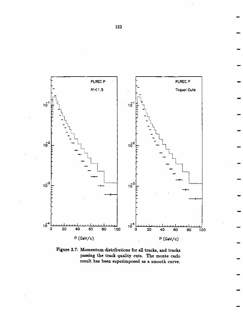
-1 10
-2 10
-3 10
0
:···~
··: ..J••
... -~\
... -_ ~·11
····: - : ... \ •• 1 - : ... ]
... -~
PLREC P
IYl<1.5
152
-1 10
-2 10
"\, - ··1 - ··:
···: - .. : ... ··1 ... ,_ __ ;
- L.l ~--~
···1 ···1
PLREC P
Tkqual Cuts
···~·····L..l .......... .. -3
10
~~-.... 1 ...... L ...... .. --+-
20 40 60 80 100 o 20 40 60
P (GeV/c) P (GeV/c)
Figure 3. 7: Momentum distributions for all tracks, and tracks passing the track quality cuts. The monte carlo result has been superimposed as a smooth curve.
-+-
80 100
-
--
-
-
-

153
3.4 DISCRETE LOGIC RECONSTRUCTION
The latching of various logic levels took place during the 1987-1988 data taking
period. These latched outputs are represented as specific bit patterns in a portion
of each event word known as the event header. The offi.ine analysis of these bit
patterns has two major purposes. One is to accumulate and interpret the information
from those detectors which provided only discrete logic output. The other purpose
is to ascertain the types of high level triggers associated with a given event, and
to determine whether or not any inconsistencies in the outputs of modules, used
to construct the high level trigger, occurred. The following detectors yielded only
discrete logic data:
• The veto wall
• The beam.line Cerenkov (C) counter
• The beam and interaction counters. The accumulated information from these
counters provides absolute normalization of cross sections, and live-time esti-
mates.
The interaction counter data included a bit which was set if the clean interaction
definition had been satisfied.
All of these counters had their information stored in the Minnesota latch modules.
These modules latched data at a clocked rate. Each latched word gets stacked into
a buffer, capable of storing up to 255 consecutive words. If a buffer overflowed,
only the most recent words with respect to a given pretrigger remained. The clock
stopped whenever a trigger signal arrived from the Faraday room, and the buffers
were read out. Only the information latched on the 15 clock pulses centered about
the interaction time are available to the offtine analysis.

154
The C counter's data allows one to know what type of beam particle interacted in
the target by determining which differential and anticoincidence counters had fired.
The counter configuration is represented by dNM where N and M are the minimum
and maximum number of anticoincidence and differential counters, respectively, that
fired. For data taken with positive beam the combination d23 indicates a 7r+ produced
a particular event. Otherwise, one should assu~e a proton has interacted in the target.
The veto wall data is checked to see if either wall contains a hit. If a hit exists,
then the veto wall quadrant possessing the hit is determined. A bit is set whenever a
veto wall quadrant, containing a hit, shadows an EMLAC quadrant that produced a
trigger. For reasons discussed in the next chapter, all events having this bit set, are
cut from the DST level analysis.
An examination of the beam and interaction counter data shows one if the beam
and clean interaction definitions used in the online trigger have actually been satisfied.
A.set of scalers accumulated the beam and interaction signals during each spill. The
total beam count, corrected for the fraction of time the detector was incapable of
taking data, is used to normalize all cross sections. Scalers also counted how many
times the C detector satisfied the online d23 requirement.
The EMLAC's trigger logic formed a tree structure with a LeCroy 4508 pro
grammable logic unit (PLU) at each branch point. The 4508 units can latch the
input signal configuration upon being strobed. All 4508 units at the pretrigger and
higher levels had this feature enabled. Every time an interrupt occurred, these units
were read out. The trigger logic can then be analyzed offline to see whether or not
the 4508s' logic states were consistent with the logic state corresponding to the high
level trigger signal. Besides this diagnostic role, the 4508 data also tells one which
octants triggered and what type of trigger they contained.
-·
-
-
-
-
-
-

Chapter 4
Event Selection
The reconstruction of high P.L '1, 11"0
, or 1/ events from the compressed data sum
mary tapes is the subject of this chapter. The selection of events containing high
P.L triggers, and the filtering out of muon induced triggers will be described. A
discussion of the cuts pertaining to the direct photon sample, and their systematic
effects is presented. The 11"0 background to the direct photon signal is also dealt with.
However, the analysis of the recoil features and the problem of jet reconstruction are
discussed in the next two chapters. The major subsamples of the data used are given
in Table 4.1.
4.1 WHOLE EVENT CUTS
Each reconst.ructed event was subjected to a series of general cuts in order to
obtain a sample of enhanced high PJ. events containing a non-muon induced electro
magnetic trigger. These cuts are listed below:
• There was no hit in either veto wall corresponding to a trigger quadrant.
• There was a single-local trigger.
• The event contained a matched vertex
• The event contained physics tracks, and reconstructed photons.
The veto wall cut provided an excellent filter for removing muon induced events
from the sample. The performance o~ this device is the subject of the next section.
The vertex cut insures that an interaction in the target is associated with the event.
This helps cover for inefficiency in the veto wall, and the possibility of upstream
155

156
Table 4.1: E706 data divided by beam and target type.
Set Beam Polarity Target Run Interval Triggers
A Negative Cu+Be 2852-3036 786K
B Positive Cu+Be 2588-2670 440K
c Positive Cu+Be 2387-2586 1225K -
D Negative Be 2062-2382 1247K
E Positive Be 1728-2007 1508K
F Positive c 2588-2670 161K
and downstream interactions contributing to the sample. The latter possibili~y could
result in a compromise of the raw data reconstruction.
The single local trigger requirement was necessary for two reasons. Firs~, the
events of interest are those containing a high p .L -, , r 0, or 11 so a high threshold
trigger from the LAC is necessary. Second, the single-local trigger is the only high
level trigger for which reliable corrections exist. The global triggers experienced
problems in their turn on characteristics due to image charging effects, and these
effects are still not completely understood. Hence, no corrections exist.
4.2 MUON AND HADRON BACKGROUNDS
The veto wall is sensitive to beam halo particles which penetrate the hadron
shield. Clearly, the only particles capable of traversing the shield and forming high
P.L showers in the electromagnetic c&lorimeter are muons. In this section the efficiency
of the veto wall in rejecting muon background is explored. There are actually two
veto wall requirements. The online veto wall requirement was part of the trigger.
If the same quadrant in both walls had a hit in coincidence with a LAC pretrigger,
the event was vetoed. The offi.ine requirement is just the veto wall cut described
-
-
...
------
-

-
157
above. The oftline requirement is necessary because of i~efficiency, gaps in the two
wall cointjdence, and the fact that the online veto signal window was not centered in
time about the pretrigger signal as shall be seen.
Besides the veto wall there are two other ways of identifying muon events. The
first one involves studying the directionality of a high Pl. shower in the LAC. The
directionality of a shower is defined as follows
(4.1)
Rr and Rb are the r coordinates of the shower at the beginning of the front and back
sections of the LAC respectively. The quantities
Zrrom - 900 cm (4.2)
zback - 918.5 cm
are the positions of front and back. sections of the LAC along the beam direction
relative to the target center. Particles which travel parallel the beamline, i.e. muons,
will tend to have larger values of 5,. than those which emanate from the target. In
fact, particles coming from the target are expected to have directionalities distributed
about zero. This effect is illustrated in Figure 4.1.
In the left half of Figure 4.2 the pl. distribution of the highest pl. photon is plotted
against its directionality for all events containing a hit in either veto wall quadrant
that shadows the trigger quadrant. Two bands of directionality are easily distin
guished. The high directionality band doin.inates the high pl. spectrum indicating a
large muon background. The band of low directionality is centered about 5,. = 0 as
is expected for photons originating from interactions in the target. A similar plot
appears in the right half of Figure 4.2, but with the requirement that neither veto
wall contains a hit in the quadrant corresponding to the LAC trigger quadrant. Very
little is left of the high directionality band, while the band corresponding to photons

158
origin~ting in the target is intact. In fact, the remaining distribution is quite sym
metric about 5,. = 0 except at very high P.1.· Thus, the online veto wall requirement
in the trigger should predominately reject muon induced triggers. Imposing an offtine
veto wall or requirement is necessary in direct photon candidate events because of
the high muon background. The loss of true direct photons due to the oftline cut can
be investigated with high p J. 11"0 events.
The other quantity of interest is the time at which a shower's energy was deposited
in the LAC relative to the time the interaction for a particular event occurred. Muons
are expected to have a time distribution that is considerably broader than for show
ers truly associated with a particular interaction. This is because there is no a priori
correlation between the muon shower and the interaction which was detected in co
incidence with it by the trigger logic. In reality the muon showers are peaked before
the interaction due to the online veto wall requirement being shifted such that an
event having a LAC pretrigger was vetoed if there was a hit in both walls from
"' -20ns to 120ns about the interaction time.
The timing information was provided by the TVC circuits described in chapter 2.
There were two· factors which, unfortunately, hindered the performance of these de
vices. One, the TVC's were susceptible to firing by high frequency noise, which
blocked real signals from being timed. Evidence for this effect occurs in the TVC
efficiency curve as a function of energy; the efficiency :flattens out at about 903. The
other problem is that the TVC efficiency was lower in earlier runs due to malfunction
ing units and threshold problems. A complete description of TVC calibration, and
reconstruction of TVC data is given in a thesis [36]. The time distributions for the
highest p J. photon in each event with and without the offtine veto wall hit requirement
are shown in Figure 4.3. When there is no hit in the veto wall, a distribution sharply
peaked at zero emerges with only a slight forward skew. On the other hand, the time
-
-
--
-
-
-
-

159
- Muon -------~--------....-
6, > 0
Photon · --------------- 6, = 0
Beam
z,_. - 900.0 cm z._. • 918.5 cm
Figure 4.1: illustration of photon directionality and related quantities. A showering muon from the beam halo will have a larger directionality than a photon em~ anating from the target.

10
9
8
7
6
s
-2 -1 0
Pr vs 6,
160
2
<511 (cm)
10
9
8
7
6
5
...
. .. . -~: .
.. . . ·:: .: . ·.·· .
. · .... . :· .. : .. ·
-2 -1 0
Pr vs c5,
Figure 4.2: Photon P.i. vs directionality for events in which the veto wall quadrant shadowing the trigger quadrant· had a hit in either wall (left), and had no hit (right).
2
c5" (cm)
-
----
-
-
....

--
161
distribution without the oflline veto require~ent is broadly peaked at ".J -40ns. There
is also a large fiat tail extending forward in time, which reflects the inefficiency in
the online veto requirement. One expects the oflline veto to be more efficient and the
evidence for this is the much smaller tail in the non-µ, induced distribution.
At the top o~ Figure 4.4 the photon directionality is plotted against the TVC time
for events containing a veto wall hit. Two distinct regions of clustering exist. In-time
photons strongly populate the low directionality region, while those that are early
cluster in the high directionality region. The fiat tail of the time distribution, having
only the online veto requirement, also has high directionality, indicating the presence
of muons missed by the online requirement. The lower plot in Figure 4.4 results when
there is no hit in the veto wa.ll. The highly clustered region of in-time photons with
good directionality remains with small uncorrelated tails extending vertically and
horizontally. The in-time tail extending towards negative directionality is assumed to
be entirely due to single photons. The other tails are a mixture of single photons and
muons, resulting from TVC inefficiency and ambiguity in directionality on the inner
part of the EMLAC. A discussion of the systematic effect of TVC and directionality
cuts on the single photon distribution is given in a following section.
The muon cuts are very effective. However, charged and neutral hadrons as well
as electrons can also contribute to the direct photon signal. It is imperative to at
least ascertain the magnitude of their effect. Two quantities enable discrimination
against hadrons. One is the front to total energy ratio of EMLAC showers. The other
quantity is the distance of a charged track to a shower as seen by the MWPC system.
A proximity distribution for showers and nearest tracks appears in Figure 4.5 for
the hemisphere opposite a high P.l trigger. There is a very sharp peak for ~r < 2.0 cm,
demonstrating a clear signal for showers produced by charged particles. Figure 4.5 also
contains the corresponding distribution for high p .L photons where directionality and
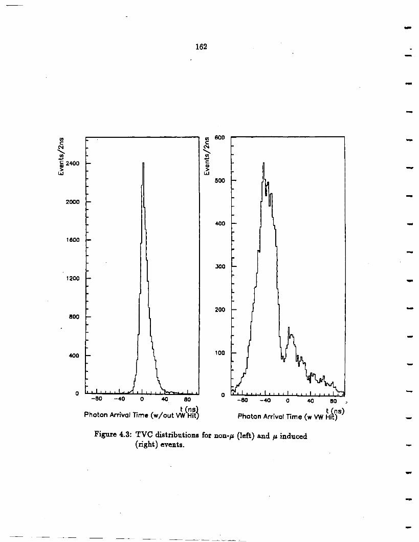
en c:
N
' (11 -i 2400 > w
2000
1600
1200
800
400
0
162
-80 -40 0 40. 80
t (ns) Photon Arrival Time (w/out VW Hit)
0 c
N
' en ~
c Cl)
> w
600
500
400
300
200
100
0 -80 -40 0 40 80
t (ns) Photon Arrival TI me ( w VW Hil)
Figure 4.3: TVC distributions for non-µ. (left) and µ induced (right) events.
-
-....
-
-....
-
-
--

[
,,_ 2 E
1.6 u ........ • 1.2 I()
0.8
0.4
0
-0.4
-0.8
-1.2
-1.6
-2 -- -100
- 2 ·E
1.6 u -• 1.2 I()
0.8
0:4
- 0
-0.4
-0.8
-1.2
-1.6 - -2 -100
-
163
-80 -60 -40 -20 0 20 40 60
c5, vs TVC Time
I·.· ::~.A~:~~;~-~ : . · ... .·.
. . .. .. :· ... : . :
-ao -60 -40 -20 0 . 20 40 60
d, vs TVC Time
Figure 4".4: Or vs TVC time for events with a veto wall hit (top) and without a veto wall hit (bottom). The data in the region outside the vertical lines and above the horizontal line is excluded by the directionality and timing cuts.
80 100
t (ns)
80 100
t (ns)

164
timing cuts have been imposed as outlined in Figure 4.4. Again there is a sharp peak
at small 6.r, but it is narrower than for showers that don't possess a high trigge~ bias.
In addition, we expect direct photons to be more isolated because they can be pro
duced without accompanying hadron fragments. To eliminate the charged hadron
background an isolation cut will be imposed on all direct photon candidates.
Generally speaking, showers in the EMLAC ca.n be hadronic or electromagnetic
in origin. The electromagnetic showers associated with charged tracks are due to
electrons (positrons), generated from 11"0 decay photons that have converted in the
target. Detailed studies of conversion pairs have been performed, and a method
exists for identifying them, using only the charged tracking system. This method
relies on the fact that the mass spectrum of conversion pairs peaks sharply at zero
since the photon has no rest mass. For this reason a pair of conversion electrons is
referred to as a zero-mass-pair or ZMP for short. The reader who is interested in the
details of this procedure should consult the thesis by Hartman [37]. The EMLAC's
response to el~ctromagnetic energy can be studied quite well with these reconstructed
ZMPs.
The front-to-tot~ ratios for showering electrons from conversion pairs are plotted
in Figure 4.6. The Etront/Etotal distribution for hadron showers is also shown. For the
conversion pairs a large peak at high Errout/Etotal dominates, and only a small tail
extends to 0. The non-conversion plot contains a dominant Efront/Etotal peak below
about 0.2 with a tail extending to 1.0. Clearly electromagnetic and hadronic showers
have very clift'erent longitudinal characteristics in the EMLAC. The Etront/Etotal plot
for photons that are in time and have low directionality appears U:i Figure 4. 7. This
distribution is similar to the one for the electrons, possessing only a slight hump at
Erront/Etotal ~ 0. The plot for the muon showers, selected by requiring a veto wall
hit, and an out-of-time shower with large directionality, is completely different. The
--
-
-
--

9000
8000
7000
6000
5000
4000
.3000
2000
1000
0 0
165
1000
800
600
400
200
0 20 40 60 80 100 0 20 40 60 80
Ar for Showers {cm) Ar for -y Events (cm)
Figure 4.5: 6.r between showers and nearest tracks (left); 6.r between high p J. photons and nearest tracks (right)
100

-166 -
-......
1600
1400
1200 -1000
800 -600
400 ... 200
0 0 0.1 0.2 O.J 0.4 0.5 0.6 0.7 0.8 0.9
E,/Em for Hadrons
70
60
50
40
JO
20
10
0 0 0.1 0.2 0.3 0.4 0.5 0.6 0.7 0.8 0.9
E,/ETOT for Electrons ... Figure 4.6: Em,m/Etotal for Hadron Showers (top) and Elec-
tron Showers (bottom).
-

- 167
2•00
·- 2000
1600
1200
800
400
0 0 0.1 0.2 0.3 0.4 0.5 0.6 0.7 0.8 0.9
E,/Emr for 1 Events
4~0
400
350
- 300
250
200
150
100
50
0 0 0.1 0.2 O.J 0.4 0.5 0.6 0.7 0.8 0.9
E,/ETUr for µ, Events
-~ Figure 4.7: Etront/Etotal for High PJ. Photon Showers (top) and µ.Showers (bottom).

168
:flatness is expected, however, because muons can penetrate considerably into the
EMLAC before emitting a hard bremsstrahlung photon. In order to eliminate neutral
hadrons and compensate for inefficiencies in the tracking reconstruction, a cut on the
Etront/Etotal ratio will be imposed on all direct photon candidate events.
4.3 1t'o RECONSTRUCTION
For the highest P.L trigger octant all 2-photon mass combinations were used to ob
tain a mass distribution. This distribution is shown in Figure 4.8 for all asymmetries
and for asymmetries less than 0. 75. Asymmetry is defined as
(4.3)
where E1 and E2 are the energies of each photon. The 11'0 and 1/ peaks at ~ 135 Me V
and "' 550 Me V respectively are dearly visible above the combinatorial background.
The uncut distribution has a considerably larger low mass region below 110 Me V than
the plot with the 0.75 asymmetry cut. In fact, the cut plot has a pretty.symmetric
background around the 1t'0 peak. The low mass pa.ir~ have been studied extensively
[38]. The majority of them are produced from single high energy showers that hap-
pen to fluctuate into two showers. The systematic loss of 1l"0s due shower energy
fluctuations is very small.
The mass region from 110 - 160 Me V has been designated as the 7ro mass band.
An event is labelled a 7ro event if it satisfies the following criteria:
• All whole-event cuts are satisfied
• An octant has a diphoton pair with 110 Me V < Mp.a- < 160 Me V
• The diphoton pair has A < 0. 75
---
--
...
---
-
•

-
169
Similarly, if the di photon pair has a mass between 500-620 Me V, the event is labelled
an 1/ event. Otherwise, the event ~s considered a direct photon candidate.
The r0
sideband regions have been designated as 75-100 Me V and 170-195 Me V.
These regions are used to estimate the combinatorial background underneath the r 0
peak. Any r0 distribution __ ~~~~- A, Mass, E, is made for the peak and sidebands
---~-·----------~-·--
separat_:~!· The sideband distribution is .~hen subtracted from the peak distributions.
The r 0 mass has been studied as a function of radius and azimuth in the octants. The
sundry distributions show a number of dips in the mass, indicative of energy losses.
These losses occur near the various boundaries. Such losses can result from only
part of the shower being contained in an active region. They can also arise from the
reconstruction program incorrectly splitting showers in multiple peak groups, and/or
failing to properly correlate showers between views. For this reason, a set of fiducial
cuts have been imposed on all photons used to reconstruct a high P.L 1, r 0 , or 11:
• A photon must have its r coordinate in the interval 24 cm ~ R., ~ 138 cm.
• A photon must lie more than 2.0 cm away from any radial boundary of an
octant.
The asymmetry distributions for r 0s with and without sideband subtraction are
displayed in Figure 4.9. There is no asymmetry cut so that the roll-off at high asym
metry can be observed. Ideally, one expects a fiat asymmetry distribution because
the r 0 is a spin 0 particle undergoing a two-body decay to photons. In the rest frame
of the ?ro the photons emerge back-to-back isotropically. Consequently, the A distri
bution should be flat in any frame for which the motion of the r 0 is very relativistic.
However, the plots of Figure 4.9 are fairly flat out to . 75 after which significant losses
of r 0s occur with increasing A. Such behaviour is due to the increasing inefficiency of
the LAC for photon energies below 10 Ge V. This is the reason for the . 75 A cut on
reconstructed r 0s. All 21 masses above . 75 A are classified as direct photon candi-

~ ::& I() .........
(IJ -c: Q) > w
-1 10
0
r :JU
/':)
/
..
0.1
·-~ :·
..
170
:.·.
1;;~ .. f ··r;''""ir"t ""· ';:-~~,~ ,.; ij
0.2 0.3 0.4 0.5 0.6
TY Mass
Figure 4.8: 11 Mass Spectrum
P, > 3.5 GeV/c
0.7
A< 1.0
A< 0.75
0.8 0.9 1 Mass (GeV)
-
--
-
--

171
Figure 4.9: Asymmetry distributions for 1r0s without sidebands subtracted (top) and with sidebands subtracted (bottom).

172
dates if the highest P.J. photon passes all oth~r direct photon criterion. It is these 1t'0s
with A> 0.75 that are the source of direct photon background after cuts.
4.4 SINGLE PHOTON RECONSTRUCTION
An event is classified as a direct photon event if it meets the following conditions:
• All whole event cuts were satisfied.
• No di photon pair formed a mass in the 1t'o or 11 mass bands
• .The highest P.J. photon had Dr < 0.4cm
• H timing information was available, then -15ns < TVCiime > 40ns
•·There was no charged track within 1.0 cm of the high~st P.J. shower
• Etrom/Eiotal > 0.2
The octant multiplicity distribution for the single photon sample shows that about
30% of the events have more than one photon in the octant, containing the recon~
structed single photon. This indicates that r 0s, which decayed asymmetrically, are
present. However, even the events with only one photon contain r 0 background from
decays in which a photon was lost due to acceptance or inefficiency.
4.5 SYSTEMATICS
Both the whole event cuts and the single photon cuts resulted in losses of recon ..
structed 1, r 0, or 11 that must be accounted for. The 7r
0s are affected only by the
whole event cuts. The direct photon candidates also have to be corrected for timing,
directionality, track isolation, and Etront/Etotal losses. Furthe~ore, the direct photon
... -
-
--
-

-
173
events must in principle be corrected for residual muon background. However, stud
ies indicate that this background is consistent with zero, given the available statistics
[39]. Table 4.2 summarizes the corrections for the whole event and muon cuts.
Besides correcting for cuts, corrections must also be applied to compensate for
trigger inefficiency, reconstruction losses, and conversions of high P.1. photons in the
target material. The correction for reconstruction inefficiency is different for 1r0s
and single photons because ?r0s are also a.ff'ected by geometric acceptance losses as
well. Studies have been done to determine these corrections, and routines exist in
the library of data summary programs to compute them on an event-by-event basis.
The analysis presented in the following chapters utilizes these standard routines in
making the various corrections as they are currently available.
There is still one very important correction, which is critical in obtaining absolute
cross sections. This is the correction to individual photon energies that takes into
account the electromagnetic cal.orimeter1 s response (energy scale), and the energy loss
due to the three radiation lengths of material in front of the detector. This energy
correction is critical because the cross sections fall steeply with p .1.. This systematic
uncertainty must be known to better than 13 if the cross sections are to be known
to better than 10%. The localization .of shower energies in liquid argon sampling
ca19rimeters, and the ionization mechanism's stability makes these device capable of
such precision. It is thus imperative to understand the energy loss in the material
between the vertex and the calorimeter. Studies have been done using the ZMP's
reconstructed from the tracking system to determine the photon energy correction.
The correction is also available in the data summary library, and has been used in the
following analysis. H the reader is interested in the details of how all the corrections
were obtained, he will find a summary of them in an appendix.

174
Table 4.2: Corrections for whole event cuts, a.nd cuts for single photons.
Cut Correction
Negative Beam Positive Beam
Veto Wall 1.111 ± .033 1.099 ± .006
Vertex €vert;ex = 1.0019 - 0.0079 X V z
Track lsol. 1.043 ± .002
Timing 1.034 ± .004
Directionality 1.005 ± .001
Etrom /Etotal 1.015 ± .001
(JTcvt• (total correction) 1.230 ± .007 1.216 ± .009
4.6 w0 BACKGROUND CALCULATION
After muons the major source of direct photon background is the decay products
of highly asymmetric w0s. Because of the asymmetry cut of 0.75 on reconstructed
r 0s, 253 of all triggering w0s could contribute. The P.1. distribution of fake direct
photons has to be calculated, and for this task a monte carlo program was developed.
The monte carlo used events from the DST stream as input. The input set con
sisted of all events with a high p J. diphoton pair in the mass range 0 - 175 Me V. The
diphoton pair must have sufficient P.1. so that a reliable trigger correction exists, and
each member of the pair must r~side in the same octant. However, no asymmetry cut
is applied to the pair of photons. All of the extra photons in the octant containing
the high p J. pair_ are also included. Relaxing the mass and asymmetry cuts on the ?ro
candidates allows the simulated energy fluctuations to reproduce the actual 2-y mass
spectrum obtained from the data. This provides yet another check on the monte
carlo.
-
-
-
-...
-

.... _
-
175
Each ·event is processed through a GEANT simulation of the detector a total of 5
times. On each successive generation the entire event is rotated by 7r / 4 into a neigh
boring octant. Since the 7r0 decay is uncorrelated with the underlying event topology,
the 7ro is redecayed with a new asymmetry and rotation of the decay photons about
the direction of motion on each generation. The simulated raw data is then processed
by EMREC and a binary DST output file is written. The monte carlo DST is then
processed by the high level reconstructor and the P.L distributions of 7r0s and fake
direct photons are generated. Each entry in these distributions is corrected by the
event weight of the corresponding input event and the acceptance, reconstruction,
and conversion weights corresponding to the generated event. The quotient distri
bution yields a set of numbers in P.L which are used to correct the direct photon
PJ. distribution. The bin contents of the quotient distribution are the so called /..,
numbers in PJ.· These numbers have been computed separately for the proton and
r- data sets. Although the /., numbers from both sets are statistically consistent,
the ensuing analysis will use the set of/., numbers that corresponds to the beam type
used to generate a specific data set. Table 4.3 gives the fake gamma,/.,, numbers for
both types of beam together with their uncertainties.
While the background from asymmetric r 0 decays is dominant, there are measur-.
able contributions from 11, 11', and w decays into two photons. The calculation of these
contributions to the direct photon background was performed in the same manner as
for ?r0s. The same input data was used in each case, but the 11, 11', or w mass was
assigned to the diphoton pair instead before redecaying it. In addition, these events
had an additional. weight factor assigned to them, which accounts for their respective
production rate and branching ratio relative to ?r0s. The relative production rate for
71s was obtained from the world data. The world data is consistent with an 11/'71'0 ratio
of 0.45. Based on results for the relative rate of high P.L K to 7r production [40], the
other relative production rates were assumed to be the same as for the 11·

-176
..
Table 4.3: False 7 fractions in P.i. for proton and 1t'- beams. -P.i. (GeV /c) fgam Numbers -Proton Beam ?r- Beam
4.375 .169 ± .006 .192 ± .006
4.625 .162 ± .006 .185 ± .006
4.875 .156 ± .006 .178 ± .006
5.250 .146 ± .006 .166 ± .007 -5.750 .133 ± .008 .152 ± .008
6.500 .113 ± .011 .129 ± .010 ... 7.500 . 087 ± .016 .099 ± .013
9.000 .048 ± .023 .055 ± .018
-

·-
-
Chapter 5
Event Features
Attention is now turned to the charged particle structure of high P.L 7ro and single
· "'( events. The distributions of charged particles in both the recoil and same-side
hemispheres will be examined. One purpose of this study is to determine if there
are any differences between high P.L single 'Y candidates and 7ro events. Another
purpose is to demonstrate the existence of jet structure in the recoil hemisphere. The
results presented in this chapter are qualitative in nature. Nevertheless, it will be
shown that a direct photon signal exists in the data without the application of a 7r0
background subtraction, but employing all of the selection criteria described in the
previous chapter. The existence of dynamical correlations among the recoil charged
particles will also be investigated.
5.1 DIFFERENCES BETWEEN "'(S AND ?roS
The azimuthal distributions of charged particles with respect to the trigger a.xis
have been used to find differences in the overall features of ?r0 and single "'( events.
Sets of distributions have been made for different trigger p .L intervals. These intervals
are 5.0 ~ P.L < 5.5 GeV /c, and P.L ~ 5.5 GeV /c. The only cuts made on the charged
particles, besides the general track quality cuts discussed in chapter 3, were P.L cuts.
a.nd a rapidity cut of I y I< 0. 7. The rapidity cut was intended to cut down on the
background from spectator jet fragments. The spectator fragments emerge in narrow
cones about the beam a.xis, the particle density having an exp-8PJ. dependence. This
cut should not compromise the comparison of 'Y and ?r0 events.
Sets of plots were made for each of the following P.L intervals: P.L(tracks) >
0.05 GeV /c, P.t(tracks) > 0.3 GeV /c, P.L(tracks) > 0.5 GeV /c, and P.t(tracks) > . 177

178
0.75 GeV /c. This was done in order to minimize the spectator jet·background. The
particles emanating from the hard scatter should be enhanced in P..L while those
produced by the othe~ "soft" part of the interaction should be strongly suppressed
with respect to this variable. More importantly, however, was to check the stability
of any observed trend in the</> distributions as a function of PJ..· The plots presented
here correspond to the 0.3 GeV /c PJ.. cut. The features appearing in this data set are
present in all of the others as well.
The azimuthal plots have been constructed over the interval 0 ~ </> ~ 7r. H the
6.</> value computed for a track fell outside this interval, it was transformed into the
corresponding value lying within the interval. All plots have been normalized to the
corresponding number of 7ro or single 'Y triggers. The corresponding plots for proton
and r- beam appear in the same figure. The 'Y and r 0 distributions for the same
data set and cuts appear superimposed in the same plot to facilitate the comparison.
Three difrerent types of azimuthal distributions have been constructed. First,
there are the simple number density distribution of charged particles about the trigger .
a.xis. These are shown in Figures 5.1 and 5.2. The 11"- beam data gives reveals an
unambiguous dift'erence between single photons and r 0s for PJ.. ~ 5.5 GeV /c. Here
the photons appear more isolated within the trigger hemisphere than do the 1l"0s.
Such an effect is expected since direct photons are produced iD: lowest order with no
accompanying hadrons whereas high Pl. r 0s are just one of several hadrons resulting
from the hadronization of the hard-scattered parton in the trigger hemisphere. The
proton data shows a similar trend in both P.J.. intervals, but it isn't as significant.
Another type of </> distribution is one in which each entry is weighted by the p J.. of
the corresponding track. Such a weighting has a sensitivity to jet structure in so far
as jet particles tend to have more P.J.. than non-jet particles. The P.L weighted plots
appear in Figures 5.3 and 5.4. Again the 11"- data shows the "YS as being definitely
more isolated th.'an the 1l"0s for P.J.. ~ 5.5 GeV /c. In addition, the same trend appears
-
-
-

--
... _
-
179
for the lower PJ.. interval although it is confined to the bin closest to the trigger
particle. The proton data follows a trend consistent with the direct photons being
isolated but again it is not very significant statistically.
A third type of distribution arises by weighting the entries by the quantity qJ..
defined as follows,
PJ..(track) · PJ..(trigger)
Pl (trigger)
PJ.(track) A A.
( • ) COS U'fJ
PJ.. tngger
(5.1)
This quantity is similar to a PJ.. weighting, but it also takes into account the expected
spatial orientation of the jet in azimuth. Such a weighting is useful in conjunction
with a PJ.. weighting since systematic effects due to misreconstruction of track mo-
menta enter differently. Consistency with the p J.. weighted plots indicates that this
systematic effect is not determining the observed features. The qJ.. weighted plots
are shown in Figures 5.5 and 5.6. They display the same trends observed in the PJ..
weighted distributions.
In summary all of the r- distributions show a clear and consistent difference
between 7s and r 0s above 5.5 Ge V / c in p J... The p J.. and qJ. weighted plots show the
isolation of direct photons at lower PJ. but the <P density distributions do not. The
trends in the proton data are consistent with this observed difference, but have little
statistical significance. This could be due to a greater relative amount of background
from r 0 and 1/ decays in the reconstructed photon sample than is present in the
negative data. Such an effect is expected from naive QCD considerations. There are
two direct photon production mechanisms in r- data, but only one in proton. While
the a.nnihiJation process can contribute to high PJ.. r 0 production in the negative data
as well, it makes a much smaller relative contribution because· the overall number of
contributing subprocesses is much larger than for direct photons. Finally, a set of <P

180
distributions was.made for 4.5 ~ p.i < 5.0 GeV /c. No differences between ')'Sand 7r0s
were observed.
Besides finding a difference between reconstructed photon and 7ro events in at
least some portion of the data, all of the azimuthal distributions show a dominant
peak opposite the trigger. This peak begins near 21r /3 away from the trigger particle
and has its maximum at 7r. Furthermore, these t/> plots possess only two peaks; a
dominant peak at 7r and a small bump about the trigger particle's direction. Such
behavior is consistent with a 2-body hard scattering among pointlike constituents,
i.e.partons. This recoil feature will be utilized in the following chapters to ascertain
the direction of the jet recoiling from either a high p .i 11"0 or single photon. Similar
analyses of charged particles associated with single high P.i particle production have
been done at the ISR [41].
5.2 RAPIDITY COB.RELATIONS
The azimuthal distributions showed a very strong clustering of particles opposite
the trigger iD. the plane transverse to the beam. If jets indeed exist, then correlations
should also exist in the plane defined by the beam a.xis and the transverse axis of
the hard scatter. Orientation in this plane can be measured as a function of cos 8
where 8 is the polar angle. However, a more desirable quantity is the rapidity, y.
A particle's rapidity has very simple Lorentz transformation properties along the z
axis. In addition, differences in the rapidities of a pair of particles are invariant under
Lorentz boosts parallel to the beam direction. ~y distributions are the same whether
they are constructed in the lab frame, the beam-target cm frame, or the rest frame
of the colliding partons.
The difference in rapidity between recoiling charged particles will be used to see
whether or not they are dynamically correlated. If this experiment is sensitive to jet
structure, then one would expect the highest p .i charged particles to cluster together
....
...
--...
---
-

181
-.. 6 6 Proton Beam n· eeam
O')'s O')'S
en°s en°s
5 5.0' P, < 5.5 GeV/c 5 5.0' P, < 5.5 GeV/c
Track PT !l 0.3 GeV / c Track P, !l 0.3 GeV / c
4 4
- t -t
i i ~
t ~
0 0 ~ \,, - -- -&. .3
~ &. .3 '1J '1J
' ' '·
c c '1J '1J - -z z
' t
' -2 2
~ ~ - +
+ • ; d i + ;
+ ~ • * ~ $ + ~ • t ~
a a 0 2 3 a 2
~(rad) 6<p (rad)
Figure 5.1: <P density distributions for charged particles in high P.L 11"0 and single photon events with 5.0 :5 P.L < 5.5 GeV /c.

182
6 6 Proton Beam w· eeam
Oys O')'S
en's en's 5.5' P, GeV/c 5.5' P, CeV/c
.... 5 5
Track P1 ~ 0.3 GeV/c
l Track P, !& 0.3 GeV/c
4 4 --j
-i i -0 -0 a a .. .. - - -- -
~ Q.
3 Q.
3 .,, .,, ' ' c c "C .,, - -z z -' ' -
2
t j 2
+ t t! f t ~ i t ' + i t ++ ;
+ + t
0 0 a 2 3 a 2 3
llt/J (rad) ~(rad)
Figure 5.2: </J density distributions for charged particles in high p .L ?r
0 and single photon events with p .L ~
5.5GeV /c.
-·

-
-
1.4
1.2
i -g 0.8 "" --s.
"O ., 6 ~0.6
' 0.4
0.2
0
• 0
183
Proton Beam n· Beam
07s L4 O')'S
en's en's 5.0' P, < 5.5 GeV/c 5.0 !i P, < 5.5 GeV/c
Track P, ~ 0.3 GeV/c , .2 Track P, ill 0.3 GeV/c
-u
~ u e,, i
f '8 0.8 ... --
f s.
"O ~ r::r ~0.6 z ........
t -0.4
+ + 0.2
• • + ~ t 0 •
• • • • • e 0 • • • 0 2 3 0 2
6.r{J (rod) ~rp (rod)
Figure 5.3: q..L weighted <P distributions for charged particles in high P..L 11"0 and single photon events with 5.0 :5 P..L < 5.5 GeV /c
------------ ---------------··-
t
;
•

... 184
Proton Beam n- Beam ·-1.4 07s 1.4 0-ys
en's en's -5.5 i P, GeV/c 5.5' P, GeV/c
1.2 Track P1 ~ 0.3 GeV / c , .2 Track P, ~ 0.3 GeV / c
- I - -<J <J
~ ~
t u u
(.!) <.:> i i -g 0.8 -g 0.8 ~ ~ - -- -s. s.
"'O "'O ~ ~ -r:::r r:::r ~0.6
t ~0.6
....... ....... -0.4 0.4 .. 0.2 t 0.2 ;
t ---
' t $ + • • • • • 0 0 I • • 0 • 0
0 2 3 0 2 3
61/J (rad) ~(rad) ....
Figure 5.4: qJ. weighted <P distributions for charged particles in high p .L ?r
0 and single photon events with p .L 2:: 5.5GeV /c.
--

185
8 8 Proton Beam w- Beam
019 O')'S
7 en's 7 en's
5.0 S P, < 5.5 GeV/c 5.0' P, < 5.5 GeV/c
Track P, ~ 0.3 GeV/c Track P, 5: 0.3 GeV/c
6 6
- -0 5
u 5 ;;:- ~ u u
~ ~
i i -0 "O e
f e - 4 - 4 - - t a. a. -0
f "O
~ ~ -0 "O - -z 3 z 3 .......
t ....... - f
+ ,,. 2 2
f ; + t • • • t + ' • *
+ +
s + 0 •• • • ~ ' a
0
0 0 0 2 3 0 2 3
6qJ (rod) 6qJ {rad)
Figure 5.5: PJ. weighted <P distributions for charged particles in high PJ. 1ro and single photon events with 5.0 $ PJ. < 5.5 GeV /c.

8
7
6
-CJ 5 j;-
G (,!)
i ,, e - 4 -&. ,, ~ ,, -z J ........ -
2
0 0
186
8 Proton Beam n- Beam
01s 019
en•s 7 en°s
5.5 ai P, GeV/c 5.5 ai P, GeV/c
Track P, ~ O.J GeV/c Track P, ~ 0 . .3 GeV/c
I 6
-u 5 j;-
G (,!)
i ,, e - 4 -
j &. ,, ) ,, -z J ........ -
2
t ti • tt * +
~ ~ + • ' + • e • 3 • 0 0
2 3 0
0 2
6qJ (rod) ~<P (rad)
Figure 5.6: p .i. weighted </> distributions for charged particles in high p .i. 11"
0 and single photon events with p .i. ~ 5.5GeV /c.
-
t
-
~
...
-

187
in rapidity producing a peak in the 6.y distribution about 0. Of course, some of
the clustering around zero can be due to accidental. coincidence. Even perfectly flat
rapidity distributions will produce a 6.y distribution peaked at 0. It is important
therefore, to compare any observed correlation in rapidity against that which is at
tributable to random coincidence. The degree of random coincidence is governed by
the shape of the particles' rapidity distributions; these are in tum governed by the
physics of the hadron-hadron collisions as well as the acceptance and overall efficiency
for finding tracks.
The 6.y plots appearing in the following figures have the uncorrelated background
superimposed as a smooth curve. The uncorrelated 6.y distributions are constructed
by choosing values from the rapidity distributions of those particles used in mak
ing the corresponding data plots. The values are chosen such that if plotted the
shape of the parent distribution is preserved. As with the azimuthal. distributions,
a set of selection criteria have been applied to the tracks used in this study. These
criteria are essentially the same as for the <P distributions except that the rapidity
cut was extended to ±1.5 in the beam-target center of mass, and only PJ.. cuts of
0.3 and 0.5 GeV /c were applied. The results from the two sets in track PJ.. are the
same, and so only the study employing the lGw PJ.. cut will be discussed. Finally, the
plots have been folded into the interval from 0 to 3.0 units of rapidity, the data for
different trigger particle's and beam types have been combined, and all plots are area
normalized.
Figure 5.7 shows the rapidity differences between the two highest P.L tracks in the
recoil hemisphere, and between the highest p .L track and all other tracks besides the
second highest which pass the selection criteria. Both plots show a definite correla
tion above the level of accidentals. The correlation is strongest between the highest
PJ.. tracks. This is probably due to a larger fraction of non-jet tracks in the other
distribution. Such a correlation has al.so been reported by the AFS collaboration [42].
188
Before the observed correlations can be interpreted as dynamical in origin it has to
be demonstrated that they are not an artifact of phase space. In particular, it could
be argued that the enhancement around 6.y = 0 is due to longitudinal momentum,
p., conservation and/or energy conservation.
H p. · conservation is responsible for the correlation, then the highest p .J. recoil
particle should be correlated in rapidity with the trigger particle. FigUre 5.8 clearly
shows this not to be the case; all correlation is merely accidental. Such a result
is consistent with a hard-scattering of nucleon constituents in relative motion. The
colliding partons' rest frame does not generally coincide with the rest frame of the
colliding hadrons.
To understand the effect of energy conservation on the correlation one must resort
to a phase space monte carlo. Such a monte carlo produces a spectrum of particles,
governed only by the constraint of energy-momentum conservation. The phase space
monte carlo GENBOD was chosen for this study. It exists in the CERN library
of FORTRAN callable routines. Events were generated in which all particles were
assumed to be pions with equal numbers of 1r+ ,1r-, and ?r0s present; the conservation
of electric charge and isospin was thus automatically insured. The data presented here
was generated with 30 particles per event. Parallel studies in which the multiplicity
varies from 20 to 50 tracks have yielded the same result. A generated event was
selected for output, provided it contained a high P.J.. 1ro with P.J.. ~ 4.0 GeV /c and
I y I< 0.7. The 6.y histograms were filled in accordance with the same selection
criteria as used on the charged tracks in the data. The effect of the analyzing magnet's
field together with the MWPC's geometric acceptance, and the effect of the planes'
efficiencies have also been accounted for.
Figure 5.9 shows the phase space result for the two highest P.J. tracks recoiling
from a ?r0• No correlation above the accidental background is observed! Also shown is
-~
-
-
----

.. _
189
a plot from the ISAJET monte carlo where each event contains a high PJ.1t'0 • The
ISAJET result is very similar to the real data. In fact, Figure 5.10 shows the data
~y distribution with the ISAJET prediction superimposed. Although this physics
monte carlo differs from the data in the tails, there is good agreement near ~y = 0 .
The ISAJET data has been subjected to the same cuts, track selection criteria, and
detector effects as the GENBOD gene~ated set.
It appears that the observed correlations in the data are artifacts of the underlying
collision dynamics. They are consistent with those observed in the ISAJET generated
distributions. If one interprets the ~y and <P correlations in the recoil hemisphere as
arising from the presence of jets in the high pl. data, then these correlations can be
utilized on an event by event basis to ascertain the direction of a recoiling jet in the
apparatus. This is the subject of the following chapter.

-1 10
>. "O ........ c -2
Jl.. 10 z ........ --
-3 10
-4
• • •
• •
190
P,>4.~ C.V/c
Track P, ii O.J GeV/c
• • • • • • + +
+ +
-1 10
>. "O ........ c -2
Jl.. 10 z ........ --
-3 10
P,>4.5 GeV/c
Track P, ii O.J GeV/c
• • •
, 0 _____ ......,.....__..._ ________ .._. -4 10 ~ ......................... ...i...1 ........ i-i.....i...i... ................. ...i...1 ........ i-i...~
0 0.4 0.8 1.2 1.6 2 a 0.4 0.8 1.2
16Yl12 16YI 13,4,5 ...
Figure 5.7: ~y distributions for 1st and 2nd highest PJ. recoil tracks (left), and 1st, 3rd, 4th, ... highest PJ. tracks (right).
1.6 2
--.,
-
-
-

--
~ "'C
'
-1 10
c -2 ;g 10 z
' -........
-3 10
-4
191
P,>4.5 GeV/c Track P, ~_0.3 GeV/c
10 ....-..-... ........ -..----.-... ........ ----................................ _._ ................................ _._ .................................. _._ ........................ 0 0.2 0.4 0.6 0.8 1.2 1.4 1.6
IY T11C1:E111-nw:icl
Figure 5.8: 6y between highest P.L recoil track and the trigger particle.
1.8 2

>..
~
-1 10
c -2 ..:2. 10 z ......... -·-
-3 10
0 0.4 0.8
192
P,>4.~ GeV/c
Track P, ~ 0.3 GeV/c
ISAJET
+ +
1.2 1.6 2
IAY112
>..
~
-1 10
c -2 ..:2. 10
~ --
-3 10
P,>4.5 GeV/c
Track P, ~ 0.3 GeV/c
GEN BOD
IAYl12
Figure 5.9: ~y distribution of highest PJ. recoil charged pair for ISAJET generated data (left}, and phase-space monte carlo data (right). The uncorrelated ~y distributions appear as smooth curves.
-.....
_,
--
-

~ "'O .........
-1 10
c -2 ~ 10 z
. ::::-.......,
-3 10
-4
193
···,;······················;····················· ..........
·······t •
P,>4.5 GeV/c Track P, ~ O.J GeV / c
............ ISAJET
··········..... ' . ·········-~··············-~·-..... ! ....... ~ ....... ~ ....... ~ ....... ~ ....... t
·· ...
10 _________________ ...._ __________________________ ....... __ ...._ ______ __
. 0.2 0 0.4 0.6 0.8 1.2 1.4 1.6
l~Yl12
Figure 5.10: 6.y between the highest PJ. recoil charged pair in data with the corresponding ISAJET result superimposed as a smooth curve.
1.8 2
-
,,..
-

Chapter 6
· Jet Reconstruction
The previous chapter contained a study of the correlations associated with jet
structure. The study revealed that the recoil jet is contained within the tracking -
system's acceptance a fair fraction of the time. This chapter focuses on the recon-
struction of the recoil jet's 4-vector. The goal is to show that cos (J* and M TVS are
measurable quantities within the realm of a physics monte carlo. ff the corresponding
distributions in the data are similar, then one might be inclined to believe the data
distributions are meaningful as well.
Achieving this goal requires several intermediate steps. First, the jet axis must
be reconstructed with some reasonable efficiency, and the resolution estimated. This
task is accomplished by implementing a jet reconstruction algorithm. Second, the
recoil jet's mom~tum must be computed, and values of z1 and z 2 obtained. The
sources of systematic uncertainty in these variables have to be understood, and their
magnitudes estimated. Understanding the origin of these effeCts allows one to decide
if meaningful cos (J* and M distributions can be constructed.
6.1 JET ALGORITHMS
Two jet algorithms will be studied and compared against one another. A cone
type algorithm, familiar to collider experiments, has been chosen since it is directly
sensitive to the jet correlations described in the previous chapter. The other algorithm
has been used by the WA70 [43] collaboration in their study of jets recoiling from
high PJ. single photons and 1l"0s. Use of the WA70 procedure allows the results from
this analysis to be compared directly with those of another experiment in a similar
kinematic regime.
195

196
. Both algorithms only make use of the charged tracking data. They utilize the
same initial set of jet candidate tracks, and employ the leading charged particle as
the initial or "seed" jet direction. The input set of tracks is define~ by the following
criteria:
• All tracks must be more than 1r /2 radians away from the trigger particle (Hemi·
sphere Cut).
• All tracks must have PJ. ~ 0.3 GeV /c.
• All tracks must have 11 ~ 1.5.
The last cut is intended to provide a symmetric acceptance, but it also removes tracks
belonging to the forward spectator jet. Such tracks can have considerable momentum· • •
and as a result, bias the jet reconstruction. In addition to these criteria, two addi~ional
constraints are imposed on the lea~g charged particle. One, the leading charged
track must have PJ. ~ 0.5 GeV /c, and two, this track must be more than 2?r/3 radians
from the trigger particle in azimuth.
6.1.1 Cone Algorithm
The cone algorithm selects tracks from the input set based on the value of 6.R
associated with them. This quantity is defined as follows:
(6.1)
where 6.11 and 6.<P are the differences in pseudorapidity and azimuth, respectively,
between the candidate jet track's orientation and the jet axis's direction. Of course,
on the first iteration the jet axis is just the direction of the leading charged track. -
The 6.<P and 6.y plots, presented in the last chapter, indicate that strong correlations
exist between particles in the recoil hemisphere for 6.<P ~ 1r /3 and 6.y ~ 1.0. For
this reason a cut value of 1.0 has been chosen for 6.R. While not all jet tracks will
-
-
•
-

-
197
be included by this procedure, it is expected that the fastest jet tracks will be and
that most spectator tracks will be excluded.
After making a selection based on ~R the momentum vectors of the tracks as
signed to thejet are summed, and thejet axis's direction computed. The new estimate
for the jet direction is used to make another ~R selection on the initial input set of
tracks. Another jet axis is calculated from the second set of jet candidate tracks. This
process is repeated until a maximum number of tracks are assigned to the recoil jet,
or the algorithm oscillates between a solution containing N tracks and one possessing
N + 1 tracks. In the latter case the solution with N + 1 tracks is chosen.
A final check is made on the jet axis calculation. First, a reconstructed jet must
havp-o or more tracks assigned to it. Second, the reconstructed jet axis must be
more than·211"/3 radians from the trigger in </>. These cuts on the reconstructed jet
reduce the number of jets biased by spectator fragments and insure that the events
represent true 2-2 hard scatters rather than multi-jet events, which are difficult to
interpret.
6.1.2 WA70 Algorithm
The algorithm developed by the WA70' group is based on an e+e- sphericity
algorithm. The routine has been modified for use in a hadro-production environment
by including a means of discriminating between particles belonging to the recoil jet
and those belonging to the spectator jets. Furthermore, the sphericity tensor is not
actually used in calculating the jet axis because the trigger and recoil jet axes are not
generally back-to-back in the rest frame of the colliding hadrons.
The WA70 routine is the same as the cone algorithm except that instead of making
ajet track selection based on ~R, a selection based on the probability, P, that a track
belongs to the recoil jet as opposed to the spectator jet is performed. Pis calculated

198
from weights w1 and w2 • These weights are formulated mathematically as
W1 - PllJET exp( -3.0pl.JET) p
W2 - P!!BEAM exp(-3.0p.lBEAM) (6.2) p
p Wt P > 0.5 (cut criterion) - (w1 + w2)'
The subscript, JET, refers to the momentum component parallel or transverse to
the current estimate of the jet direction. The subscript, BEAM, has an analogous
meaning for a track's momentum components with respect to the beam direction,
taken as the z-axis in the experiment's coordinate system. In addition, the same pair
of cuts a.re applied to the final estimate of the jet axis.
6.2 THE JET MONTE CARLO
The monte carlo used to study jet reconstruction and resolution has two distinct
parts: an event generator that produces simulated events according to the current
understanding of hadronic interaction, and another program which simulates the de
tector's response to the passage of high energy particles. The ISAJET monte carlo
was chosen as the event generator. Version 6.36 has been used since it allows for effi
cient generation of high p .l r 0 events. All events were generated on the VAX family
of computers, possessing 32 bits of precision.
6.2.1 Implementation of ISAJET
The physics monte carlo employs the independent fragmentation model, and the
factorization scheme outlined in the introduction. The results from perturbative
QCD are used to simulate the high Q2 parton-parton scatter. It should be noted that
the event generator for direct photons contains only the Compton and annihilation
subprocesses; there is no bremsstrahlung component in the direct photon monte carlo
...
!fl
....
....

. -
---
·-
--
-
199
data. Unless otherwise stated, the events were generated with the default set of
para.meters. This implies a 6 GeV Jc radiative cutoff and a (k.L) of 0.95 GeV /c.
As described in the chapters on the experimental apparatus and event selection,
the type of trigger utilized in detecting high P.L 1r0s and single photons relied on
only one large deposition of p .L in the electromagnetic calorimeter. There is then the
possibility of a net P.L for the trigger+recoil-jet system in the direction of the trigger
particle due to fluctuations in the trans'\Terse momenta of the colliding partons. Recent
results from _the WA70 group indicate a rather substantial (k.L) of 0.95 GeV /c [44].
This explains the value currently implemented in ISAJET.
In order to take into account the effects of the single-local trigger, the P.L thresholds
for jets 1and2, produced by the monte carlo, were set at different levels. Jet 1 was re
quired to have P.L ~ 4.0 GeV /c. while jet 2 was only required to have P.L ~ 3.0 GeV /c.
The plot in Figure 6.1 reveals a significant spread in ~P.L with a mean of"' 1.0 GeV /c.
As a matter of fact, there is evidence in the E706 data sample for such a P.L imbal
ance in the direction of the trigger particle. This imbalance represents the minimum
imbalance in the acceptance for tracks and showers outside the beam halo region of
the LAC (45].
6.2.2 Detector Simulation
Ideally the ISAJET generated data would be input to a f1.!11 detector simulation
program. The simulation used by the E706 collaboration is an implementation of the
GEANT monte carlo_ package. The output from GEANT would be run through the
same chain of reconstructor code used on the real data. Finally, a compressed DST
is made from the reconstructor output, and the monte carlo DST's are subsequently
processed by the high level DST reconstruction code. The advantage of this method
is that the systematics associated with data reconstruction, e.g. "bugs" in the code,
are duplicated in the monte carlo.

0.09
0.08
0.07
0.06
0.05
0.04
0.03
0.02
0.01
0 -5
200
-4 -3 -2 -1 a 2 3
Figure 6.1: The P.L imbalance between the two hard scatter jets in ISAJET with (k.!.) = 0.95 GeV /c.
-----
-· 4 5
--
-

201
Unfortunately, such a thorough procedure represents a huge investment of com
puter time. A more expedient solution was used in tliis analysis. A simplified detec
tor si~ulator w~ written which takes into account the acceptance of the magnet and
MWPC system, the efficiencies of the individual chamber planes, and the effects of
the analyzing magnet's field on charged tracks that traverse it. The field is modeled
as a simple dipole with an effective length as measured from the data. This same
magnetic field model, incidentally, is used by the GEANT monte ca.rlo as well. All
charged ISAJET particles within the fiducial volume of the detector a.re projected
through the magnet into the MWPC system. A detailed description of this simple
monte carlo for the tracking system is found in chapter 3. In addition, the interested
reader will find a comparison of this monte carlo with data.
Except for the trigger particle, no neutral particles from the monte carlo were
analyzed by the DST level reconstruction routines. No simulation of the calorimeter's
response to the high P.L trigger particle was implemented here. Such a response was
modeled, however, for the 11"0 background calculation to the direct photon signal; the
details of this monte carlo procedure are given in the next chapter. The acceptance
cuts in rapidity that were applied to the real data have also been imposed on the high
P.L single photons and ?r0s generated by ISAJET.
6.3 JET ALGORITHM PERFORMANCE
The performance of the Cone and WA70 algorithms is summarized in this sec
tion. There are three basic performance characteristics relevant for later studies.
First, there is the question of how well each algorithm can determine the recoil jet's
direction. Second, does the jet reconstruction algorithm find the recoil jet a substan
tial fraction of the time. While the results for cos 8* and M do n«:>t depend critically
on the reconstruction efficiency, a low efficiency means a loss of statistics. The third
issue concerns the precision and accuracy with which z1 and z 2 are calculated. Of

202·
immediate concern is the issue of jet axis resolution since this determines if cos 8*and
kl_ are measurable. In addition, it can provide. a measure of how often the jet is
misreconstructed. All subsequent studies of reconstructed jets will involve a pseudo
rapidity cut of 1111 ~ 1.0. Such a cut is necessary because of the pseudorapidity cut
on individual tracks (1111 ~ 1.5).
6.3.1 Jet Axis Resolution
The previous work with the <P distributions indicates that things are alright trans
verse to the collision axis. The particles clearly recoil from the trigger. The events
are not expected to always be planar, but the <P variable plays no role in determin
ing :c1 or z 2 • What is of great interest is how well a jet's longitudinal direction is
ascertained. A number of variables can be used to express the longitudinal direction.
cos 8 a.nd 1/ in ·the rest frame of the colliding hadrons are the most relevant for this
· study; all results will be expressed in terms of them. Figure 6.2 plots the difference,
5 cos 8, between the reconatructed and generated directions in cos 8 as a function of
the sum cos 8 ALG + cos 8aEN for each algorithm. This particular choice of variables
allows for a symmetric distribution of points centered about 5 cos 8 = 0 over the
entire acceptance. Such a plot has absolute boundaries formed by the intersection
of lines through the points {-2, 0), (0, 2), (2, 0), and (0, -2). The allowed region of
scatter is therefore a square. However, the plots in Figure 6.2 appear bounded by a
parallelogram with the extrema in 5 cos fJ shifted away from cos fJ ALG + cos 8Mc = 0.
This effect is due solely to the pseudorapidity cut on the reconstructed jet axis.
By inspection one can see that both algorithms yield very siinilar results. There is
a dense band of points, centered about 5 cos fJ = O, extending across each plot with an
absolute width of about 0.3. In addition, there is a sparse uniform scatter of points
away from the band in each plot. The dark band represents the resolution of each
jet algorithm, while the diffuse scatter indicates the frequency at which the jet is
-
--

203
misreconstructed. Fortunately, the fraction of misreconstructed jets is rather small.
A projection of ~ach plot into 5 cos (J appears in Figure 6.3. The HWHM indicates a
uniform resolution in cos 8 of 0.1 for both algorithms.
An estimate of the misreconstruction frequency can be obtained by measuring the
fraction of each distribution in Figure 6.3 comprised by the tails. Out to 15 cos 61 = 0.3
the jets should be deemed properly reconstructed. Outside this interval there is a
mixture of correctly and incorrectly reconstructed jet axes with the relative fraction
of misreconstructed axes increasing with increasing 15 cos 6j. By deeming all jets
for which 15 cos 81 > 0.5 as improperly formed, and using this fraction to determine
the "wrong" jet contribution between 0.3 and 0.5 in 5 cos 8, the misreconstruction
frequency has been found to be about 73 for the Cone and WA 70 algorithms.
It is also interesting to know how well the jet reconstructors track each other
event-by-event. An advantage in studying the diff'erence in cos 8 between the two
. algorithms versus cos 8coNE +cos Bwuo is that the monte carlo can be compared with
the data! Such a study appears in Figure 6.4. It is easy to see that the data and monte.
carlo are similar and that the algorithms track each other very well. The dense band
about 5 cos 8 = 9 is much narrower than in Figure 6.2, implying the reconstructors
do not cllifer significantly in their estimates of the jet's longitudinal orientation. Such
a systematic correlation between the two algorithms is expected because they both
rely on the same input track set.
The diffuse spread of points in the Figure 6.4 represents the frequency for either
one or both algorithms to misreconstruct the recoil jet direction. However, the central
band contains those events for which both routines either correctly or incorrectly de
termined the recoil jet axis. The fraction of those events for which the "wrong" jet was
reconstructed represents the frequency for which the input track set contains insuffi
cient information. A study has been done in which the difference between both jet al
gorithms is plotted against the difference between each algorithm and the monte carlo
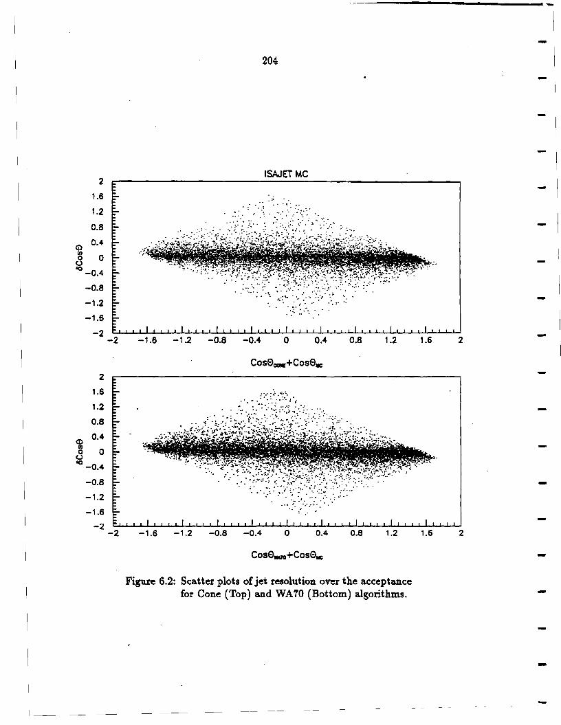
2
1.6
1.2
0.8
© 0.4
(I) 0 0
(.) 'O
-0.4
-0.8
-1.2
-1.6
-2 -2
2
1.6
1.2
0.8
<D 0.4
OJ 0 0
(.J 'O
-0.4
-a.a -1.2
-1.6
-2 -2
204
ISAJET MC
.> ... ,.
~ .... ' ....
···.: ." .. ·.:. :· ..
.. ,. . ;: .. ··= ... ·:. .·.·.
-:: .'\,··.·· ~
. · . .. .·.:· .. ..
-1.6 -1.2 -0.8 -0.4 o 0.4 0.8 1.2
CosE>ca.+CosE>..:
: :·: :·~.-;;:::· ! ..
.. . . ....
.. .:. . . .. :·····
-1.6 -1.2 -0.8 -0.4 0 0.4 0.8 1.2
Cos0.,.;+Cos0..:
Figure 6.2: Scatter plots of jet resolution over the acceptance for Cone (Top) and WA70 (Bottom) algorithms.
-
-
-1.6 2 -
-
1.6 2
----

0.2
0.18
0.16
o. 14
0.12
0.1
0.08
0.06
0.04
0.02
0 -2
205
CONE Algorithm
_, 0 2
c5Cose
0.2
0.18
0.16
0.14
0.12
0.1
o.oa
0.06
0.04
0.02
0 -2
WA70 Algorithm
_, 0
dCos0
Figure 6.3: 5 cos fJ distributions for Cone (Left) and WA70 (Right) algorithms integrated over the acceptance.
2

2
1.6
1.2
0.8
CD 0.4
~ 0 (.)
'O -0.4
CD
-a.a -1.2
-1.6
-2
2
1.6
1.2
0.8
0.4
~ 0 (.)
I() -0.4
-0.8
-1.2
-1.6
-2
-2
-2
206
Monte Corio
..
. ~;~:iii'f t~\,t~y:;::}si::~~;H\;f :t\i;;+~M{~:t:i::~·~-.
-1.6 -1.2 -0.8 -0.4 0 0.4 0.8 1.2
Cosemc+Cose.,.,
...
-1.6 -1.2 -0.8 -0.4 0 0.4 0.8 1.2
Cosec:oc+Cose.,.,
Figure 6.4: Scatter plots of 6 cos 8 between WA 70 and Cone algorithms over the acceptance for data (Top) and monte carlo (Bottom).
1.6
1.6
2
-
-
2
-
-

207
The abscissa in each plot is projected out for lcS' cos 61 < 0.2. Again, the technique
of measuring misreconstruction by examining the tails of these distributions is used
to determine the fraction of "wrong" jets beyond I cos 6ALG - cos BMcl = 0.3. This
fraction is 5%. Clearly, it is the input track set which is responsible for most of the
jet misreconstruction.
Comparing one reconstruction technique against another also allows one to study
the variation in resolution as a.n algorithm's parameters are varied. Such a study has
been done where l:J.R was allowed to vary between 1.0 and 2.0, while the factor in
the exponential terms for w1 a.nd w2 was varied between 2.0 and 5.0. No significant
changes in resolution were observed for either jet reconstructor. This indicates that
the systematics associated with jet a.xis reconstruction are not critically dependent
on the reconstruction technique.
6.3.2 Jet Finding Efficiency
There are a number of viewpoints concerning the jet finding efficiency. In the
previous discussion, inefficiency was viewed in terms of how often the recoil jet axis is
formed. incorrectly. There is also the questio11 of how frequently a jet is found given
that an event contains a high p .l. 1ro or single photon. One expects that within the
hard-scatter picture any event possessing such a high PJ. object will have a recoil jet.
However, the limited acceptance of the experiment's spectrometer, the P.t cuts on
the jet candidate tracks, the leading charged particle cuts, a.nd the selection criteria
of the jet algorithms all conspire to produce a jet finding efficiency substantially less
than one.
The jet finding efficiency can be estimated by taking the trigger's p J. spectrum for
those events with a reconstructed jet, and dividing it by the inclusive PJ. spectrum.
This method has the advantage of being able to compare the monte carlo with data.

208
The jet finding efficiencies for both jet algorithms are plotted in Figure 6.5; the data
is plotted with error bars and the monte carlo is superimposed as a dashed line.
All plots show an increase in efficiency with P.l.· This is due to kinematics, which
favors the trigger and recoil jet to be at 90 degrees in the nucleon-nucleon rest frame
at high P.l., and the scaling of the fragmentation functions. The WA70 algorithm
appears to be more efficient than the Cone algorithm, implying the !:::,.R cut is a
bit more selective. The greatest source of inefficiency are the leading particle cuts,
which represent a 203 loss. Overall the monte carlo data is 103 more efficient at low
p .l. with the data and monte carlo coming into agreement above 5 Ge V / c p J.. This
effect is not due to hardware or PLREC systematics since they should possess no PJ.
dependence. Rather, this difference stems from the fragmentation functions being
steeper, and/or the structure functions peaking at lower x values in the data than
the monte carlo.
6.3.3 Parton Variables
Before z1 and z 2 can be calculated the recoil jet's momentum must be determined.
This analysis makes an estimate based on the assumption that p J. is balanced between
the trigger particle and the recoil jet. It is important to see how well this premise
works when intrinsic kJ.and fragmentation effects are present. Figure 6.6 illustrates
the difference between generated and reconstructed jet momenta as a fraction of the
reconstructed momentum. Both algorithms give consistent results. The peaks are
centered a.bout zero with HWHM's of 253. From the expression for the momentum
of the recoil jet, .·
PJET = P.l. /sin tJJET (6.3)
and the· estimated resolution for the reconstructed jet axis one can easily calculate the
contribution to the smearing of PJET over the acceptance. This contribution alone
-
-
-

209
represents~ 803 of the total observed smearing in the peak of 5P/ P! In Figure 6.7
the corresponding plots for single photon events are shown. By inspection the reader
can see they yield slightly better estimates of the jet momentum resolution.
All of these plots have an asymmetric tail extending towards increasing 5 P / P.
This tail is a combination of events with misreconstructed jets, and those containing
a large k..L enhancement in the direction of the trigger. No correlation between the
frequency of jet misreconstruction and large 5P/ P values has been found. So, the
right hand tails of the 5P/ P plots indicate the magnitude of the effect intrinsic k.l.has
on the misreconstruction of jet momenta. By subtracting the left portion of each
histogram from the right half one determines the fraction of incorrect momenta to
be 153. Although the contribution of jet axis m.isreconstruction to the tails of the
5P/ P distributions is quite small, it does bring into consideration the application of
general kinematical cuts, i.e. PJET < '18 /2, and z1, z2 < 1.
The resolution for z 1 and z 2 is estimated from the monte carlo by computing fiz/z.
Recall that in addition to the P.l. balancing assumption, the trigger and recoil jets a.re
assumed to be massless in calculating z 1 and z 2• Figure 6.8 and Figure 6.9 display
the parton z resolution functions for r 0 and s~gle p~oton events, respectively. Once,
again both jet reconstruction algorithms yield consistent results. The asymmetric tails
in the momentum resolution plots do not, however, carry over into these distributions.
The fiz/z distributions for "Y events a.re centered near 0 with a HWHM o~ 10%.
Unfortunately the r 0 plots a.re smeared about twice as much and are systematically
shifted below 0 ~ 103. This systematic shift arises because 1r0 s are usually only one
of the trigger jet's fragments. This difference between single photons and 11'0s implies
that the kinematic regions for both classes of events, used to construct the cos 8* and
M distributions do not coincide exactly.
In summary, both jet algorithms have yielded consistent results as far as the
resolution of various quantities is concerned. It is expected that the same behaviour

0.9
0.8
0.7
0.6
t 0.5
0.4
0.3
0.2
0.1
0 4
210
CONE Algorithm WA 70 Algorithm
0.9
0.8
+r ------- ----------- ------- 0.7
1 ··:;++ft+
.
0.6
t 0.5
0.4
0.3
0.2
0.,
0 5 6 7 8 4 5 6
Pr (GeV) Pr (GeV)
Figure 6.5: The jet finding efficiency for Cone and WA 70 algorithms as a function of the trigger's p .L. Monte carlo is superimposed on the data.
-
-
--
-
-7 8
--

0.1
0.09
0.08
0.07
0.06
0.05
0.04
O.OJ
0.02
0.01
0
211
High Pr 1T0 Events
....-------------------------. 0.1 ----------------------------.
0.09
0.08
0.07
0.06
0.05
0.04
0.03
0.02
0.01
0 -1 0 -1 0
6P /P for Cone 6P /P for WA70
Figure 6.6: Resolution plots of the reconstructed jet momentum for ?ro triggers integrated over the acceptance.

0.1
0.09
0.08
0.07
0.06
o.os
0.04
0.03
0.02
0.01
0
212
High Pr")' Events ----------------------------- 0.1 .-----------------------------,
0.09
0.08
0.07
0.06
o.os
0.04
0.03
0.02
0.01
0 _, 0 _,
0
c5P /P for Cone c5P /P for WA70
Figure 6.7: Resolution plots of the reconstructed jet momentum for '1 triggers integrated over the acceptance.
-
-
--
-

0.25
0.225
0.2
0.175
0.15
0.125
0.1
0.075
0.05
0.025
0
213
High Pr n° Events ,-------------- 0.25 .--------------...
0.225
0.2
0.175
0.15
0.125
0.1
0.075
0.05
0.025
0 -o.a -o.4 0 0.4 0.8 -0.8 -0.4 0 0.4
6x/x
Figure 6.8: 5z/z resolution plots for parton momenta in high p J. 1r'o events, integrated over the acceptance.
0.8

0.25
0.225
0.2
0.175
0.15
0.125
0.1
0.075
0.05
0.025
0
214-
0.2
0.175
0.15
0.125
0.1
-0.8 -0.4 0 0.4 0.8 -0.8 -0.4 0 0.4
dx/x 6x/x
Figure 6.9: 6z/z resolution plots for pa.rton momenta in high p .L single photon events, integrated over the acceptance.
-
-
---
-0.8
-

215
will be observed in cos 8* and M _as well. From the lack of sensitivity to a particular
jet algorithm., even under a reasonable variation of its parameters, it can be concluded
that the information required for this analysis is contained in the leading jet particles.
This property is an artifact of the independent fragmentation scheme, but it appears
to adequately represent the data for the task at hand.
6.4 MEASUREMENT OF cos 6* AND M
For the studies of cos 6* and M only the Cone algorithm will be utilized. There
is still the issue of what it means to measure these quantities. By measuring the
cos fJ* and M distributions for the 7 +jet and ,..o +jet systems it is hoped that one is
essentially reconstructing the same distributions for the final state partons. To check
whether or not this is indeed the case the angular and invariant mass distributions
at the parton level will be compared to those reconstructed from the complete event
generation. The. parton level distributions will be constructed from ISAJET data
generated without any evolution (k.L smearing, underlying event) or hadronization
processes activated.
There are several general kinematical cuts that will be applied to the monte carlo
data in performing this study, and in subsequent studies with the real data. Because
the possibility exists for misreconstructing the recoil jet's direction, unphysical values
for the jet's momentum and/or the parton momentum fractions may occur. By defi
nition z1 and z2 can never be negative, but they can exceed 1. Such misreconstructed
events will be eliminated from ·consideration by imposing the following kinematical
constraints
PJET ~ ..;; 2
Zt ~ 1 {6.4)
Z2 < 1

216
6.4.1 . cos 8*
Figure 6.10 illustrates the effects of applying those cuts in succession that provide
uniform acceptance in cos 6*. Clearly the edges of the reconstructed distribution rise
relative to the central region in accordance with the discussion presented in the first
chapter. The smearing observed in the reconstructed parton momentum fractions
is also present in M. In addition, this smearing is different for 7s and 7r0s. This
doesn't compromise the M cut's effectiveness, however. Mis proportional to the Pl.
of the trigger particle, and it is the Pl. cut on the data which introduces the bias in
cos 8*. So, if M is cut on accordingly, the bias is removed. Figure 6.11 shows the 11B
distribution generated by ISAJET, and the interval of 118 for which there is uniform
acceptance in cos 8*. Any smearing in this variable will tend to "feed" down from
bins of smaller 118 to bins of larger "lB· Hence, the smearing may produce a net loss
of events, but it will not affect the reconstructed distribution's shape provided the
smearing is uniform over the acceptance used in constructing cos 8*.
The absolute cos 8* distributions for r 0s and direct photons are shown iii Fig
ures 6.12 and 6.13 respectively. The cos 8* distribution for 7r0s agrees ·vary well with
the one corresponding to just 2-2 parton scatters. The parton distribution is plotted
in Figure 6.14 as a smooth curve. All of the parton level distributions are referred to
as the generated distributions. The parton level distribution for direct photon events,
however, appears to rise faster than the reconstructed distribution. The effect is not
very large, and the ability to discriminate between the two types of events in cos 8*
is not compromised. The reconstructed monte carlo cos 8* distributions will be used
in comparing these results with the actual data.
6.4.2 Cross Sections in M
Reconstructed invariant mass cross sections for high pl. 1ro and direct photon
events are displayed in Figures 6.14 and 6.15 respectively. Again the corresponding
-
---
--
----
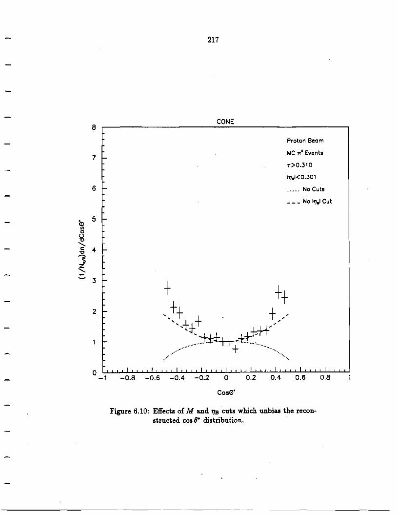
Co fl> 0 u "C
' c: "C -; ' -........
-
8
7
6
5
4
3
2
a -1
217
CONE
Proton Beam
MC n° Events
-r>0.310
1.,,,1<0.301
........ No Cuts
___ No i.,,11 Cut
\ ++ ',,+ + . +/ ',+t., ~-
..... ±+t_u_.~+ ...... :. ... I""!+ ... .... ··············· ················· ...
-0.8 -0.6 -0.4 -0.2 0 0.2 0.4 0.6 0.8
Cose·
Figure 6.10: Effects of Mand 1/B cuts which unbias tJ:ie recon-structed cos 8* distribution. ·

0.07
0.06
0.05
0.04
0.03
0.02
0.01
0 -1
218
-0.8 -0.6 -0.4 -0.2 0 0.2 0.4 0.6
'1]1
Figure 6.11: 1JB for high P.L 1r0s produced via prpton-nucleus collisions.
--
---
-
0.8
--
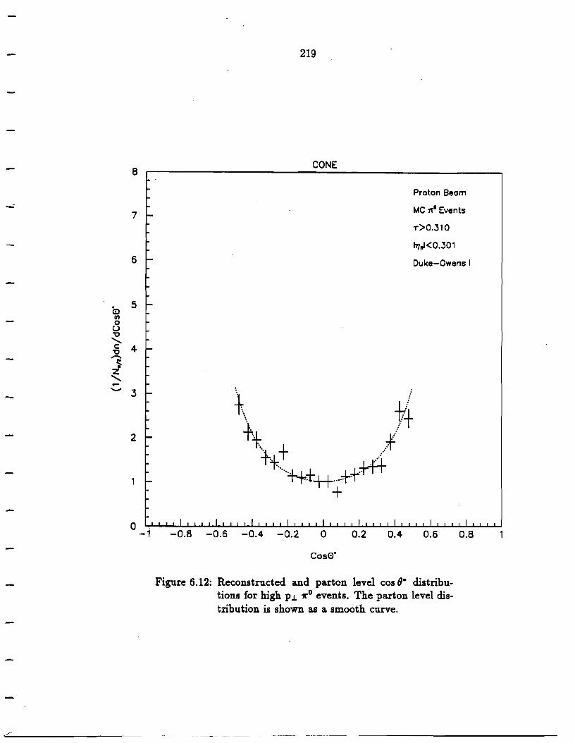
(!) rn 0
(.) "O .......... c:
"O ,-.,,
~ z ·' -.......,,
5
4
3
2
219
\ t+ ++. +
t+~.. +++ +++++····++
+ o __ ............. _._.. ......... __ ....... ....., ....... ..i....i __ ......... ...._-'-"...,,_. __ '-'-...._-'-"..i....l_,_ ......... .i....i....i....i.......i_,_ ......... ....., _,
-0.8 -0.6 -0.4 -0.2 a 0.2 0.4 0.6
Cose·
Figure 6.12: Reconstructed and parton level cos 8* distributions for high p J. 1ro events. The parton level distribution is shown as a smooth curve.
0.8
----------- -- - ----- -------

Co rn 0 u "C
' c: "C -~ • z
' -.......
B
7
6
5
4
3
2
0 -1
220
CONE
Proton Beam
MC 1 Events
T>0 . .310
171,l<0.301
Duke-Owens I
-0.8 -0.6 -0.4 -0.2 0 0.2 0.4 0.6 0.8
Cose·
Figure 6.13: Reconstructed and parton level cos IJ* distributions for high PJ. single photon events. The parton level distribution is shown as a smooth curve.
---
---
--
-

221
parton level (generated) distributions are superimposed as smooth curves. These
cross sections have been normalized according to the convention of ISAJET version
6.36. They are unbiased with respect to the trigger threshold, having a cut in cos 8*
of ±0.4 applied to them along with a corresponding cut in M( r ). The 1/B cut is
unnecessary in obtaining uniform acceptance in M because the geometric losses are
the same·for all bins in M allowed by the cos 8* and M cuts.
The reconstructed M distribution for direct photon events, shown in Figure 6.15,
is shifted above the corresponding distribution for pure parton scatters. The PJ.
balancing and massless jet assumptions used in the reconstruction procedure tend to
cancel one another in the calculation of M. However, it appears that the effect of PJ.
balancing is dominant. What is happening is that hard scatters are generated below
the p J. of the 7, but are evolved upwards in p J. by the k.J. mechanism. Some of these
events get reconstructed and pass all of the analysis cuts. Because the cross section
falls steeply with M, these events produce a net enhancement of the reconstructed
cross section across the measured spectrum.
Besides the effect of k.J. smearing, the 1ro cross section shown in Figure 6.14 has an
additional smearing from ignoring the 1r0 's fragmentation function, i.e. z is assumed
to be 1. This effect results in a change of slope for the reconstructed distribution
compared to the parton level distribution because a fraction of higher mass events
are reconstructed as lower mass events.
While one can always compare reconstructed monte carlo .distributions with data,
there is still the question of whether the smearing is the same in both cases. However,
these effects should not change in the 7r- data so a good method of comparison is to
plot the ratios of cross sections for 1r- to proton beams. The ratios must be taken
betwee1.1 spectra of the same trigger particle type. Otherwise, the systematics will
not divide out, and the monte carlo comparisons will be more ambiguous. As was
pointed out in Chapter 1, it is the ratio for direct photon events which is of primary

222
interest. The corresponding ratio for r 0s can serve as a benchmark in judging the
agreement between data and monte carlo.
...
-
--
--
-
-
-
-

-
223
-6 CONE Algorithm 10 i:--------------------------------------------------------
-7 10
~ u -8 ~ 10 E --:& ,, :2
-N ........ .s -9 110 ........
-10 10
-11
.. -··· ... ; ....
··· ... ~ · .. ~
"·."':"+"-•,
.... ~
··~
~. ·· .. · .. ;·· .....
•,
·· ......... . " "· ··· ...
·· ..
MC 1t0 Events
Proton Beam
Duke-Owens I
1Cos01<0.4
+·· ......... .
·· .. ·· ...
t 10 ____ .._ __ -'-__ _... __ _.. __ ___,.__ ______ ....._ __ -"-__ _,_ __ ___,.__ __ "--__ _._ __ ~
8 10 12 14 16 18
M (GeV)
Figure 6.14: Reconstructed and parton level M distributions for high p J. 1ro events. The parton level distribution is shown as a smooth curve.
20
--'---------------~- ·--····· --

224
-7 CONE Algorithm 10 ---------------------------------------------------------.
-8 10
~ ., -9 ~ 10 ..a E -,...., 2 "C 2 N ....... .ij -10 - 10 z . .......
-11 10
···~ ..... ··.-···· .. -:-+-
···· .. .-..... ········.-+-
·········::;:--····~ ··· ...
MC 1 Events
Proton Beam
Duke-Owens I
1Cos01<0.4
··~ .. ··•··•· ... ~
········~
·······+ ··············.l·· ..
·········· .. ,, ·· .. ·· ...
-12 ~ 10 .__ __ ......._ __________ __.. ____ ...._ __ ...._ ______ _.._ __ _.._ ____ ...._ __ ...._ __ """"""" __ ~
8 10 12 14 16 18
M (GeV)
Figure 6.15: Reconstructed and parlon level M distributions for high P.l. direct photon events. The parton level distribution is shown as a smooth curve.
20
----
-
--
-

Chapter 7.
Final Results
The last chapter demonstrated the feasibility of studying 7 +jet and 1ro +jet
systems within the kinematic regime accessible by the experiment. The jet. recon
struction techniques that have been developed will be used in reconstructing the M
and cos fJ• distributions from the real data. ·Here, the emphasis is on comparing 7
and 1r0 distributions. Attempts will be made to show just how different correspond
ing distributions are. However, comparisons with ISAJET will also be performed.
In particular, the data will be examined to see whether or not the Duke-Owens I or
Duke-Owens II [46] structure functions are preferred.
Because of its simplicity and explicit use of correlations among recoil charged
particles, indicative of jet structure, the cone algorithm is used exclusively in the
following analysis. A complete description of this algorithm is found in the previous
chapter. Only jets reconstructed between ±.85 in pseudorapidity are used in obtaining
the mass and angular distributions of 7 +jet and ?r0 +jet systems.
There are a number of corrections applied to high P..L 11"0 and 7 events. They
include corrections for trigger inefficiency, reconstruction efficiency, acceptance ( rele
wkt for 11"0s which decay into two photons), for photons. converting into e+e- pairs in
the target, a correction to individual reconstructed photon energies, and corrections
for whole event cuts. Th~se corrections are applied on an event-by-event basis to all
data distributions presented in the following figures. They are important in obtaining
the correct shape of the cos fJ• distributions, especially for 11"0s, and the absolute nor
malization of cross sections. The reader interested in the details of these corrections
should consult Chapter 4, which discusses the selection of high p ..L ?r0 and 7 events.
The ISAJET comparison involves generating monte carlo events with V6.36, and
passing charged particles through a simple simulation of the tracking system. This . 225

226
simulation takes into account the MWPC acceptance, the efficiencies of individual
planes, and the effect of the analyzing magnet's field. A description of this simulator
program is found in Chapter 3. The simulator's output is subsequently used in jet
reconstruction. The mass and angular distributions are then constructed from the
monte carlo data, using the same cuts in M, cos 8*, ,,,, and 11B as applied on the
real data. The monte ca.rlo distributions have been generated in the same kinematic
range as the real data. Sets corresponding to different trigger thresholds were not
generated, however. Both 'Y and ?r0 monte ca.rlo data sets have a trigger particle
P..L cut of 4.0 GeV /c. All monte carlo distributions have been fitted with sundry
functional. forms; these fits are superimposed on the data as smooth curves.
Separate sets of monte carlo data have been produced with proton and ?r- beam
particles. Within each set are equal numbers of proton and neutron target hadrons.
This is done in order to simulate the approximate isoscal.ar character of the target
material.. All coherent nuclear effects are ignored by this procedure as well as nuclear
rescattering effects.
The standard ISAJET package is not equipped to simulate hadron collisions in
volving mesons. A member of the E706 collaboration, S. Mani, has· provided an
implementation for r- and r+ beams into the standard ISAJET program, as well as
making the Duke-Owens set I (DOI) and Duke-Owens set II (DOii) structure func
tions available (47]. The point in studying these two sets is that they represent the
limits of gluon "hardness" and "softness" via the value of 11G each one incorporates.
The 11G parameter appears as an exponent iD. the following form both sets use for the
gluon momentum distribution,
zG(z, Q~) = AG(l + 'YGz)(l - z)"G (7.1)
Direct photon production is directly sensitive to the gluon distribution within hadrons,
and should therefore be able to discriminate among the various choices for 11G partic-
....
------
----

227.
ularly at high x values.
The hard scattering in ISAJET is a next to "leading log calculation for 7ro pro
duction, but direct photons are generated at the Bom level only. Furthermore, there
is no· Bremsstrahlung mechanism present for direct photon generation. It should be
noted that a consistent generation of events with the DOI and DOii sets involves
using different values of Aqcn. For DOI Aqcn must be set to 0.2 GeV /c, while for
DOii a value of 0.4 GeV /c is required.· All the monte carlo data has been generated -
with the following Q2 definition,
(7.2)
The QCD radiative cutoff has been set at 6 GeV for final state radiation, and, as men
tioned earlier, an intrinsic kJ. value of 0.95 GeV /c has been employed. The scattered
quarks and gluons are fragmented into hadrons using the independent fragmentation
ansatz of Field and Feynman. This physics monte carlo provides for absolute normal
ization via a weighting function whose value is obtained event-by-event, and can be
loaded as a weight for a particular histogram. Table 7 .1 shows the number of events
generated for each type of collision, trigger particle, and structure function set.
7.1 7ro BACKGROUND SUBTRACTION
A general technique of constructing the 1ro background component "of a given
reconstructed photon distribution will now be discussed. This method is an extension
of the one used for the inclusive photon PJ. spectra. A description of the monte carlo
used in obtaining the false direct photon PJ. spectrum appears -in Chapter 4.
The ratio of the false photon and monte carlo 1ro PJ. spectra is taken bin-by-bin
in order to produce a set of so called fga.m numbers. Each PJ. ~in of the 7r0 spectrum,
reconstructed from the actual data, is then weighted by the appropriate f 11a.m number;
the resulting distribution represents the 1t'0 background present in the reconstructed
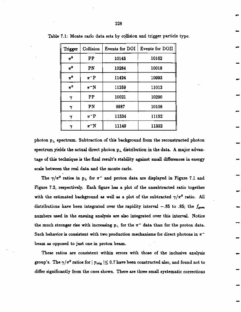
228
Table 7.1: Monte carlo data sets by collision and trigger particle type.
Trigger Collision Events for DOI Events for DOii
1ro pp 10143 10162
ro PN 10284 10018
1ro r-P 11424 10993
1ro r-N 11259 11013
'Y pp 10021 10290
'Y PN 9987 10108
'Y r-P 11334 11152·
'Y r-N 11149 11352
photon p J. spectrum. Subtraction of this background from the reconstructed photon
spectl'UD1 yields the actu&:l direct photon PJ. distribution in the data. A major advan
tage of this technique is the final result's stability against small differences in energy
scale between the real data and the monte carlo.
The 7 / r 0 ratios in p J. for r- and proton data are displayed in Figure 7 .1 and
Figure 7 .2, respectively. Each figure has a plot of the unsubtracted ratio together
with the estimated background as well as a plot of the subtracted 7 / r 0 ratio. All
distributions have been integrated over the rapidity interval - .85 to .85; the f gam
numbers used in the ensuing analysis are also integrated over this interval. Notice
the much stronger rise with increasing PJ. for the 1r- data than for the proton data.
Such behavior is consistent with two production mechanisms·for direct photons in 1r
beam as opposed to just one in proton beam.
These ratios are consistent within errors with those of the inclusive analysis
group's. The 7/r0 ratios. for I Ytrig I~ 0.7 have been constructed also, and found not to
differ significantly from the ones shown. There are three small systematic corrections
-
.. -
---
...
----

-
229
applied to the inclusive analysis group's data that are currently unavailable in the
DST library. It is assumed they are responsible for the observed differences. All of
the following analysis ignores a rapidity dependence for the f 11a.m numbers. Such a
consideration is beyond the available statistics.
The set off ga.m numbers used on the inclusive spectra can also be used to construct
the background distributions in cos 8* and M. First, scatter plots of cos 8*, M, or
any other two-body variable for that matter versus p .L are constructed using events
containing a high P.L 11"0
• Second, a given scatter plot is unpacked and each slice
in p .L is weighted by the appropriate f 11a.m number. Finally, the two dimensional
distribution is integrated in P.L, resulting in the 11"0 background distribution for a
particular two-body variable. This background distribution is then subtracted from
the corresponding reconstructed photon distribution to obtain the estimated true
direct ·photon spectrum in that variable.
This background subtraction procedure ignores a possible rapidity dependence for
the /ga.m numbers. However, because of the fJB distribution's width a particular value
of cos 8* or M is integrated over a large part of the acceptance in rapidity. Thus,
one does not expect a significant dependence of the background in cos 8* or M on
rapidity. This hypothesis has been checked by employing the tracking information in
the data-driven monte carlo, which was used to calculate the f 11a.m numbers. The fake
; angular and invariant mass distributions were constructed, and the ratios of these
distributions to those for the reconstructed monte carlo 11"0 events were then taken.
The ratios are just the spectra of f ga.m numbers in cos 8* and M. These f 11a.m numbers
were then used to construct the 11"0 background distributions in cos 8* and M for the
real data in the same manner as is done in p .L. The two methods of background
subtraction yield the same 11"0 background spectra well within the uncertainties. The
first method has been chosen because of its superior precision since the calculation of

230
-
-0.7
0.6
0.5
0
~ 0.4 -+- -.......... ...
ca--. 0.3
0.2 :············'\ ..... . : ···················································
0.1
0 -l ~-······················1 ............................................... . j '
4 5 6 7 8 9 10
P, (GeV/c)
0.7
0.6
0.5
0
~ 0.4 ..........
ca--. 0.3
-0.2
0.1 -! -+---+--t---t-
0 4 5 6 7 8 9 10
P, (GeV/c) -Figure 7.1: Inclusive 7 /7r0 ratio for 7r--nucleus collisions
--
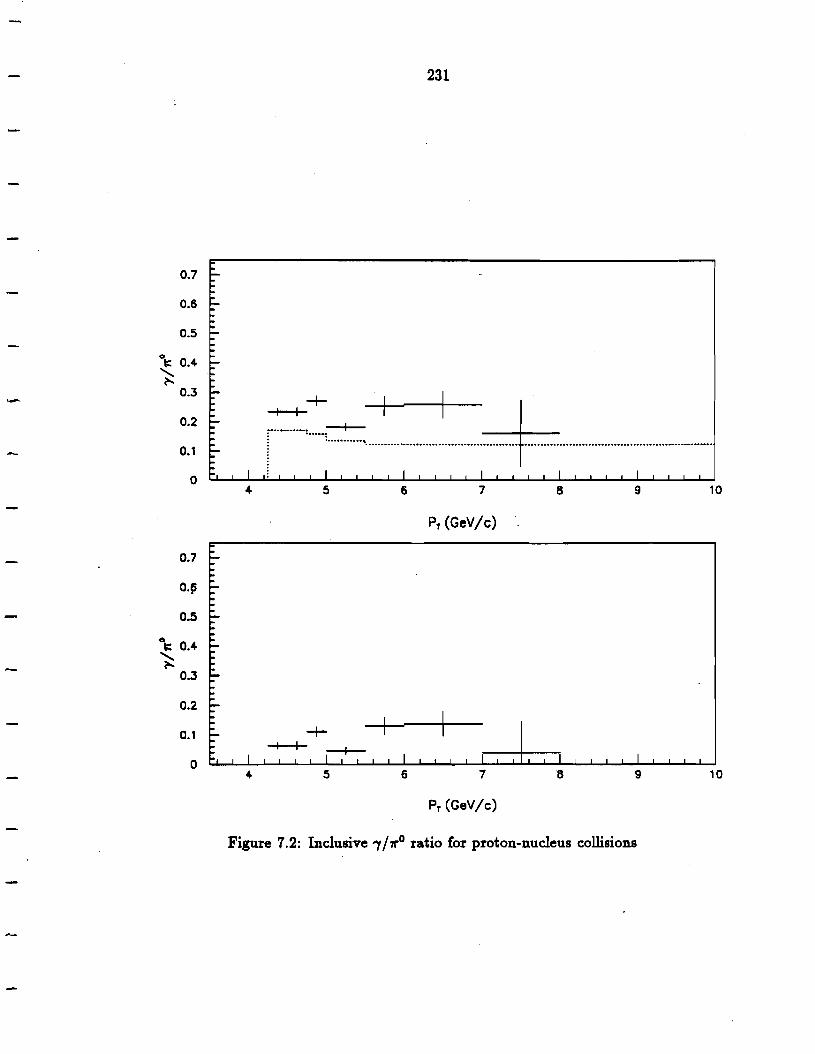
231
0.7
0.6
0.5
0
~ 0.4 '?::
0.3
0.2
0.1
0
-+-+--+- I I =+-==. ............. -+-: ······-: i ············'··········-··································· ···················································-····-
4 5 6 7 8 9 10
PT (GeV/c)
0.7
o.~
0.5
0
~ 0.4 '?::
0.3
0.2
0.1 -+--+-+- :---+--
0 4 5 6 7 8 9 10
PT (GeV/c)
Figure 7.2: Inclusive 7 /1r0 ratio for proton-nucleus collisions

232
the f ga.m numbers does not depend on the jet reconstruction efficiency.
To facilitate the analysis the normalization of cos 8* and M distributions always
occurs after subtraction. Also, the background histograms are. fitted to sundry func
tional forms, discussed below, and it is the fitted results which are subtracted off of
the reconstructed photon. distributions. Such a procedure reduces the uncertainty in
the subtraction, reducing the error bars of the true direct photon distribution. Fig
ure 7.3 shows actual scatter plots of cos 8* and M versus P.L for high P.L ?r0 events.
7.2 RESULTS FOR cos 8*
The cos 8* distributions obtain the data will now be presented along with
JET results for comparison. Plots for ?r0 and '1 triggers in proton and ?r
beams are shown in the following figures. In addition, separate histogram sets have
been generated for the standard p .L cut of 4.25 Ge V / c (large background), and for a
cut of 5.0GeV/c (small background)t.. Since no significa.nt forw~ard asym
metries have been absented a11 results are folded into the interval 0 < cos 8* < 1. ~ '
The emphasis here is on the difference in shape' between '1 +jet and ?ro +jet
angular distributions. As pointed out at some length in the Introduction, QCD
predicts a difference between "'fS and ?r0s in this variable. Direct photon subprocesses
contain only quark ( fermionic) propagators at the Bom level while 7r0 events possess a
number of subprocesses with gluon (bosonic) propagators in lowest order. Fermionic
propagators result in at most a 1/(1 ± cos 8*) dependence. Bosonic propagators, on
the other hand, yield 1 / ( 1 ± cos 8* )2 terms in their respective angular distributions.
A further refinement to the general background technique· has been added for
the cos 8* analysis. All fake '1 distributions have been fitted with the following 1-
parameter function,
-
-
...
--
-
--
-
--

10
9
8
,..... 7 u ~
Q)
" ......... ~ 6
5
4
3
-
233
10
9
8
,..... 7 u ~ .. Q)
: " ......... . . ·=· .... · · ..
.. ... a. 6 . . ...
~·.·· ... ~~; .. :
·~/t: t_.r. ...
5 ~ .. l~·:· ff· ... • . ~,.
t!"i$f:. ·:. ~: j,1: .. ~··
4
3 8 12 16 20 0 0.2 0.4 0.6
M (GeV) Cose·
Figure 7.3: Scatter plots of cos 8* and M versus Pl. for ?r0
events
----------
0.8

234
__ (N_j) [ 1 +--1--] cl.cos 6* fgcr.m - 2 (1+cos6•)a (1 - cos 6•)a '
cl.n a.ER (7.3)
a. is taken as real since there is no a priori reason for it to be integer. The smearing in
the reconstructed recoil jet's direction together with variations in the 11"0 background
across the LAC's acceptance mitigate against such an assumption. This functional - . '
form has yielded an excellent x2(~ 1) on-all calculated backgrounds. The uncertainty
in a, 5a, obtained from the fitting procedure was used to compute 5dn/ cl. cos 6* ltgcr.m
point-by-point. A histogram. was filled for each fit; the contents and errors for each
bin were computed from the mean values of the ·integrals of dn/dcos 6* ltgcr.m and
52dn/dcos 6* ltgcam over each bin. What this procedure does is make the backgrounds'
contributions to the uncertainty in the corresponding subtracted photon distributions
negligible.
Finally, a word needs to be said about normalization. Because only the shapes
of the angular distributions are of interest, and in keeping with standard practice,
all cos 6* distributions are normalized to 1 at cos 6* = 0, ( 6* = goo). The angular
distributions are :8.at near cos 6* = 0 so the two central bins are averaged; this average
is used to scale all other bins. The bin closest to 6* =goo is set to 1.
The absolute angular distributions ( M and 11B cuts) for the standard p J. cut are
displayed in Figure 7.4 and Figure 7.5. In Figure 7.6 one finds the correspondinu.....,.../-r_0 __
ratios. The ratios are formed from distributions without 11B cuts. As far as geometry ~
is conceme.d, the systematic losses are the same for 7s and 11"0s so they should divide
out in the ratio anyway. Furthermore, these losses do not drastically affect the data;
they represent ~ 50% e:ffects. This allows the 7/11"0 ratios to have greater statistical
significance without being compromised by systematic e:ffects.
One obvious feature in the absolute cos 8* plots is. the size of the direct photon
distributions' error bars. The backgrounds are large at low P..L as manifested in the
inclusive 7/11"0 ratios shown earlier. This together with a steeply falling cross section in
-
-
------

-·
235
P..L causes a sharp increase in the relative uncertainties on the subtracted distributions
over those in the unsubtracted ones. For this reason, the single photon histograms
ave been rebinned to half as many bins as those for the 7r0 events.
The plots in the foregoing figures show the expected trends and differences for
the 71"- data only. The 7 /7r0 ratio is clearly different from 1, which is the result if no
shape difference is present. There appears to be no statistically significant difference
between 7s and 71"0s in the proton data. The size of the direct photon distribution's
error bars indicate a very large background given the available statistics. Even if
one were to conjecture that the background had been underestimated in this case,
and that this was the cause for the shapes being so similar, the errors would increase
still further destroying any significance of the result with an improved background
estimate.
As far as the ISAJET comparison is concemed, the 7r0 +jet distributions show a
dramatic agreement with the QCD prediction! The monte carlo data have also been
fitted with the form given by equation 7.1. Such a procedure has been recommended
by Owens [ 6}. However, a is allowed to take on real values in order to accommodate
the smearing in the reconstructed jet's direction. The results from the fitting proce
dure have been superimposed on. the real dat'a. Each plot has two curves associated
with it. One curve corresponds to the DOI set of structure functions, and the other
to the DOii set. Both sets agree with the data there being no significant preference
of one over the other. This is consistent with naive expectations. While the parton
momentum distributions are different for the two sets, ~specially for the gluons, they
do not result in monte carlo data being generated in dramatically different regions of
phase space. Of course, the large uncertainties on the direct photon plots don't allow
for much discrimination anyWay.

-236
5 Single n Events 5
Single 7 Events
(subtracted)
4.5 .,,.· aeam 4.5 n· eeam
M > 9.82 GeV M > 9.82 GeV -...•..• DOI ....... DOI
4 ___ 0011 4 -- .DOii
I
3.5 I .3.5 I
(D 3 ~ Cr> 3 en en 0 . 0
(.)
tf (.)
"'tJ "'tJ ......... ! ......... z 2.5 z 2.5 "'C· "'tJ - . -i . i -z z ......... I : ........ - 2 I i - 2 ........ ........
+++/ ....
1.5 1.5
0.5 0.5
0 0 0 0.2 0.4 0.6 0.8 0 0.2 0.4 0.6 0.8
Cose· Cose·
Figure 7.4: Absolute cos 8* plots for --ys and r 0s in r- data

237
5 Single n Events 5 Single -y Events
(subtracted)
4.5 Proton Beam 4.5 Proton Beam
M > 9.82 GeV M > 9.82 GeV
....... DOI ....... DOI 4
- _.DOii 4
-- .DOii
I
3.5
t J.5
. 3 a, J co en en
0 I: 0 (,)
I f u "O "O
' ,f ' z 2.5 z 2.5 "O -0 - -~ ~ z z ' ' - 2 - 2 - ,f -
I: ,,... 1.5
J+tft 1.5
0.5 0.5
0 0 0 0.2 0.4 0.6 0.8 0 0.2 0.4 0.6 o.a
Cose·
Figure 7.5: Absolute cos 8* plots for 1s and ?r0s in proton data

2
1.8
~ 1.6 en 0
1.4 (J "'O ........ • 1.2 z ,, -........ -C:D 0.8 en 0 (J -0 0.6 ~ "'O 0.4 -
0.2
0
2
1.8 -Co 1.6 ., 0
1.4 (J
~ 1.2 "'O -' r CD a.a ., 0 (J "'C 0.6 ~ -0 0.4 -
0.2
0
238
n· Beam
M > 9.82 GeV
=F·································································-···························································
+++ 0 0.1 0.2 0.3 o.• 0.5 0.6 0.7 0.8 0.9
Cose·
Proton Beam
M > 9.82 GeV
.._ ....... _ ....................................................................................................................................... .
0 0.1 0.2 0.3 0.4 0.5 0.8 0.7 o.a
Figure 7.6: '1 to r 0 ratio in cos 8* for.,...- data (top) and proton data (bottom)
0.9
-
-
--

239
Figures 7.7 through 7.9 display another set of cos e· plots for Pl. 2:: 5.0 GeV /c. The
?r-data shows the same trends as the low PJ. sample albeit with greater significance.
The proton data is quite different. though. At high pl. it has the same behaviour
as the negative data! These trends are expected from QCD as well. Of course, the
observed change is due entirely to a change in the shape of the direct photons' angular
distribution. An explanation for this change is that there is less ?r0 background at high
p .L. The difference between "'(S and ?r0s in the high p .L proton data is not as significant
as it is for the 1r- sample, but the"'( /1r0 ratio doesn't rise as fast for protons either.
The high P.L sample exhibits a direct photon signal without background subtrac
tion as Figure 7.10 and Figure 7.11 reveal. Only the ?r-data shows such an effect.
This behavior is consistent with that observed in the l::l.</> distributions, presented in
Chapter 5.
What appear to be definite differences between the '1 +jet and r 0 + jet systems
by visual inspection are quantified below. A simple way to do this is to compute the
x2 diiference between corresponding angular distributions as follows,
2 1 ' ( (cos s.;. - cos s:,,)2 )
XPDI' - 4 ~ 62 cos 6*. + 62 cos 9* · ~1 ~ ~-
(7.4)
The x2 is for four degrees of freedom because the central bins have no information
content. Note that the ?r0 distributions have been rebinned for this operation. The
observed differences in the angular distributions are summarized in Table 7.2. The
meaning of 3 confidence in the table's last column is the percent chance that the
computed difference (x2) is not due to a statistical fluctuation.
A simple linear fit has been applied to the various 7 / ?r0 ratios. Except for the
low p J. proton data, the results are consistent with a 1 - cos IJ* dependence at > 3CT
significance. The ratio plots are inconsistent with a constant value of 1, which is
expected in the case of no difference between 'YS and r 0s. Indeed, the 7 / ?r0 ratio for
the proton data with a P.L cut of 4.25 GeV /c is consistent with 1 across the whole

.240
Table 7.2: Summary of differences between ;sand 7r0s in cos 9*
Beam PJ. Cut (GeV /c) 2 XPDF 3 Confidence
Proton 4.25 0.583 > 32.4
Proton 5.0 2.93 > 98.0
Proton 5.0 (Unsubtracted) 1.31 > 73.2
7r- 4.25 2.45 > 95.4
7r- 5.0 5.15 > 99.9
"Ir- 5.0 (Unsubtracted) 2.83 > 97.5
accessible range of cos 8* (see Figure 7.6).
7 .3 7ro +jet AND i +jct }4 DISTRIBUTIONS
The invariant mass distributions are presented as absolute cross sections, and as
ratios of absolute cross sections. The 7r0 +jet and 7 +jet cross sections arc given by,
1 dtr NB"NIJ11 c (7.5) - .
2M dM d cos 8* d</> Nseam. 21r~M2M ~cos 8•
NsWm&. - the number of reconstructed events
Nseam - the number of incident beam particles
~M - the bin size in M
~cos8* - interval of cos (J* integrated over
c - the trigger particle corrections
1/{21r~M2M ~cos 8*) - normalization to an element ef phase space
The calculation of Nseam is essentially just the total beam particle count, corrected
for the time the apparatus could not take data. There a.re additional corrections
for inefficiencies in the discrete logic a.a well as beam absorption in the target. The
details involved in calculating the live-triggerable-beam (LTB) a.re found in Chris
-
-
-
-
------

241
5 Single n Events 5 Single "'f Events
(subtracted)
4.5 1Te Beam 4.5 n· Beam
M > 11.5 GeV M > 11.5 GeV
....... 001 ....... 001 4
- _.DOii 4 ___ 0011
.3.5 J.5
Co .3 .
J I j co (I) en 0 I i 0
(.) If (.) "O "O
' 'j ' z 2.5 z 2.5 "O "O - -i ; z
' ' - 2 - 2 .._ .._
,,~~
1.5 I
1.5 , .· , .. · , .. ··
t· ,,..~·~ ....
0.5 0.5
0 0 0 0.2 0.4 0.6 0.8 0 0.2 0.4 0.6 0.8
Cose· Cose·
Figure 7.7: Absolute cos 9* plots for 7s and 1r0s in 1r- data

242
-
5 Single n Events s
Single '1 Events
(subtracted)
4.5 Proton Beam 4.5 Proton Beam
M > 11.5 GeV M > 11.5 GeV
..•.••• DOI .....•. DOI
- __ 0011 4 __ .0011
I
3.5 I J.5 I I -
(I) 3 I j <D J CIJ CIJ 0 I i 0 -(.)
'/ (.)
1::J 1::J
' ' z 2.5 z 2.5 1::J 1::J - -~ I i i z I : z
' ........ - . 2 - 2 ....... I/
....... I
I:'
. tt·'ft I
1.5 1.5 ~ •· .. ·· -
t t -0.5 0.5
-0 0 0 0.2 0.4 0.6 0.8 0 0.2 0.4 0.6 o.a
Cose· Cose·
Figure 7.8: Absolute cos 8* plots for ;sand ?r0s in proton data -
--

2
1.8 -Co 1.6 en 0
1.4 (.) .,, ......... . 1.2 z ,, -......... ~ 0.8 fl> 0 u ,, 0.6 ) ,, 0.4 -
0.2
0
2
1.8 -Co 1.6 .,. 0
1.4 u
~ 1.2 ,, -......... ~ o.a ., 0
(.) "'O 0.6 ~ z
0.4 ,, -0.2
0
243
n- Beam
M > 11.5 GeV
=t=························································-·········-··················································· .. ····
++ ~
0 0.1 0.2 0 . .3 0.4 0.5 0.6 0.7 0.8 0.9
Cose·
Proton Beam
M > 11.5 GeV
.....,_....,__ .................... ···················································•·······•··········•·•············································
0 0.1 0.2 0.3 0.4 0.5 0.6 0.7 0.8
Cose·
Figure 7.9: -y to 11"0 ratios in cos 6* for 11"- data (top) and proton data (bottom)
0.9

244
-5 5 Single n Events Single "I Events
( unsubtracted)
4.5 w· Beam 4.5 ".Beam
M > 11.5 GeV M > 11.5 GeV
4 4
3.5 J.5
<n J Co .3 en en 0 0
(.) (.)
~ ,, ........ z 2.5 z 2.5
~ ~ - -~ .j z
t -........ ........ - 2 - 2 - -
1.5 1.5
++ 0.5 0.5
0 a 0 0.2 0.4 0.6 0.8 0 0.2 0.4 0.6 0.8
Cose· Cose· -Figure 7.10: Absolute cos 9* plots for 7s and 7r
0s in "'- data with no ?r
0 background subtracticin for the 7s -
-
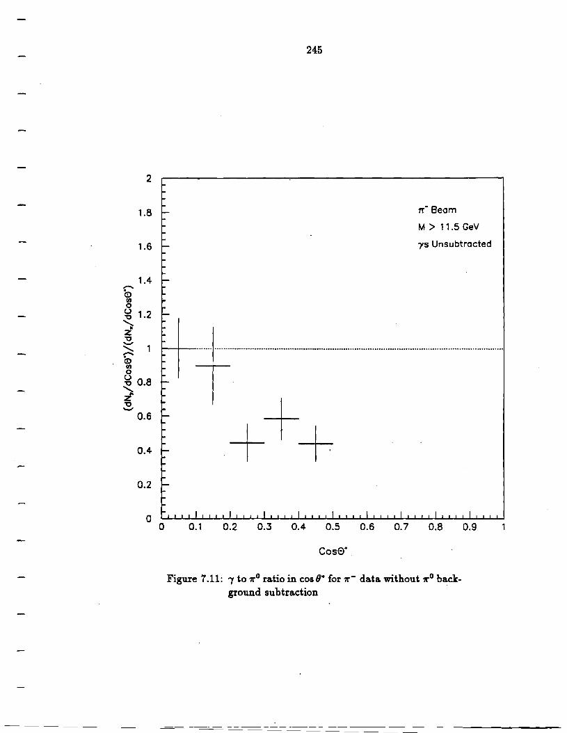
"'"" © UJ 0
2
1.8
1.6
, .4
~ 1.2 '-.. z ,, ' 1 "'"" (o
UJ 0 (.) ,, 0.8 ~ z ,, '-"
0.6
0.4
0.2
0
245
1T- Beam
M > 11.5 GeV
ys Unsubtrccted
~~-·········································································································································
0 0.1 0.2 0.3 0.4 0.5 0.6 0.7 0.8
Cose·
Figure 7.11: "Y to 11"0 ratio in cos 8* for 11"- data without 11"0 background subtraction
0.9

246
Lirakis' thesis [48]. Absorbed into NEvent1 , is the number of target nucleons per unit
area. The conversion factor from events to nucleons per unit area is given by,
NoALpc MW (7.6)
No - Avogadro's number
A - the atomic mass number
L - the target length
p - the ~arget's density
MW - the atomic weight in g/mol
c - conversion from cm-2 tomb
All cross sections in M a.re given in units of mb /Ge V2 • The target was composed
of copper and beryllium. elements; the configuration did. change to just beryllium for
certain data sets. NEvart• has been computed for the whole target in accordance with
· the actual copper-beryllium configuration on a run-by-run basis.
A cut in cos 6* is necessary for the absolute M distributions because different
trigger threshold sets are to be combined. A cut in 11B is not required as long as
the monte carlo data is processed in like fashion. The reason is that the geometric
acceptance in f'/B is the same for all M.
The results of the ISAJET analysis are superimposed on the data as parametrized
fits. The absolute M cross sections for r 0 events have been parametrized as ex
ponentiated linear fits. Those for direct photon events have been parametrized as
exponentiated quadratic fits. The results from both t~e DOI and DOil structure
function sets will be presented.
Figures 7 .12 through 7 .15 show the absolute M cross sections for r 0 + jet and
'1 +jet events. It is clear from inspecting all four plots that the data is tracked by the
DOI and DOII monte carlo sets. There does not seem to be a great deal of preference
for one set of structure functions over the other, particularly in _the direct photon data.
-
-
-
-
-
-

247
More statistics are required. However, the 7 +jet cross section for 7r- data definitely
has a shallower slope than the corresponding ?ro + jet distribution. It appears that
the two mass distributions cross over, i.e. 7 /7r0 ~ 1 at 18 GeV. This corresponds to
a p.1.of 9 GeV at 90°. The shape difference is also present iii. the unsubtracted 7 +jet
cross section as Figure 7.16 clearly shows. Note how the unsubtracted distribution
turns up at low M indicative of a substantial 1ro background there (low Pl.)·
Unfortunately, the 7 - 7ro difference is not very significant in the proton data.
This is mainly due to a lack of statistics as is evident from the size of the error bars.
Part of the problem may also be that the low M region rises too steeply because of
residual 7r0 background. Such behavior is consistent with earlier results in ~<P and
cos 8* at low pl..
The absolute M cross sections are plagued by a number of large systematic effects.
· Most notable is the smearing that results from the assumptions of massless jets, and
P.L balancing between the trigger particle and recoil jet. There is the uncertainty in
the electromagnetic calorimeter's energy scale too ( "J 13); this effects the trigger par
ticle's reconstructed four-vector. These effects are very substantial because the cross
sections are so steeply falling. In fact, there is already a 25% systematic uncertainty
on the inclusive cross sections alone! Besides these experimental uncertainties there
are theoretical ones as well. They are the value of AQcD, the definition of Q2 and
the amount of primordial kJ.. High P.1. 1r0s suffer an additional uncertainty due to an
incomplete knowledge of the z-distribution or fragmentation function. All of thes~
problems can be minimized, even cancelled, by studying the ratio of corresponding
cross sections for 1r- and proton data. The variation of these ratios in M is dependent
on the hadrons' internal structure, if any, and the behavior of 7s and 1r0s should be
different.
For direct photon events, the ratio is particularly sensitive to the ·value of T/G· In
principle it should be able to discriminate between the DOI and DOii sets. The physics

248
-6 10 ~--------------------------------------------------------_..,
~··· ...
~ (.!)
' .Q
E -
-7 10
-8 10
- -9 ~ 10 ~ N
' b ,, ~ ......... -10
10
-11 10
. -12
'·· .. ......,._ ' · .. ' ··. ' ·· .. ', .. + ' ··. ' ..
,~·,· ....... ', ·· ..... '~ ', ·· ...
' ··. ' .... ' ... ' ·· .. ' ·· ..
n° Events
n- Beam
tCosei<0.4
DOii
DOI
' .. ',, ......... . ' ' ' '
10 .__ __ ...._ __ _._ ________ ...._ __ ...._ __ __.. ____ ..._ _____________ ...._ __ ...i.-__ ....... __ __
8 10 12 14 16 18 20
M (GeV)
Figure 7.12: 71"0 +jet cross section in M for 71"- beam
-
-
-
-
-
-

249
-6 10 -------------------------------------------------------------...
-7 10
-8 - 10
~ ' .a E ........
- -9 ~ 10 ~ .
N
' b -a
~ -10 10
-11 10
-12
~·~·~·~·tt·· .:.:· .. ,·.·~1 .....
'~·· .. . ~ ....... .
··. , ... , .. , .. ~l·
~·· .. ......
1 Events
Subtracted
1f- Beam
ICosftJ<0.4
DOii
DOI
, .. , ... ,·::: ... , ... -·· ~ ..
,.:;, ... ....... '
10 ----------------'----------------------------------------------......... ----.1 8 10 12 14 16 18 20
M (GeV)
Figure 7.13: 7 +jet cross section in M for 'Ir- beam

~ (.!) ......... ~
E --:I "C :I N ......... t)
"C
250
-6 10 ----------------------------------------------------------
-7 10
-8 10
-9 10
··. ·· ... ' ·· ... ' ·· ..
', ····· ... ', ·· ..
' ·· .. ,~ .. ', ··· ...
' · .. ~ ', ·· ...
' ·· .. ' · .. ~ ..
' '' ~·····,··· ... ', '· ... 'f ..
n° Events
Proton Beam
DOI
~ - -10 10
-11 10
-12
', ······· ... ' .. ' '· ' ' ',
10 '----~--....... ----1.-.-------'------------------------"----....... --......a... __ ___ 8 10 12 14 16 18 20
M (GeV)
Figure 7.14: 7r0 +jet cross section in M for proton beam
-
-
-
-
--
-

~ ~ E --:I . "'C :I
~ b
"'O
~ -
251
-6 10 ,_.-----------------------------------------------------------
-7 10
-8 10
-9 10
-.10 10
-11 10
· . .. • . ... ·· ... ', ··· ...
'<"~ .. ~ .. : ··. ~-.
I~,>· ...
-y Events
Subtracted
Proton Beam
ICosei<0.4
DOii
DOI
'' ·· ... .
t ... ,· ....... l
', .. ·~ ' · .. ', ···· ...
' ··. ', ···· ... ' · .. ' · .. ', ······ ...
', ··· ... .. .. ' ··· ... ', ', ··•·············· ...
' .. '' ·· .. ' ' ' ' ' ' -12 10 ________ _.. _____________ __. ____ .._ __ _,_ __ __. ______________ ..._ ______ __,
8 10 12 14 16 18 20
M (GeV)
Figure 7.15: ~+jet cross section in M for proton beam
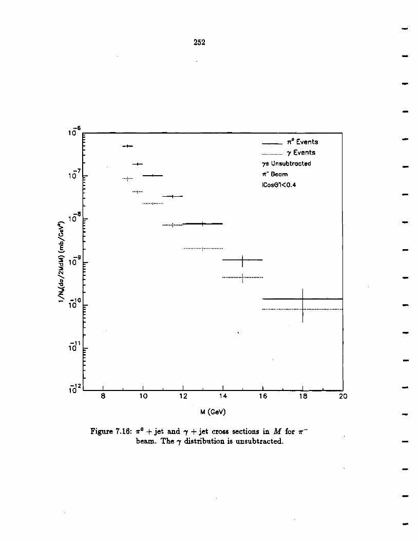
252
-6 10 ~--------------------------------------------------------.
-7 10
-8 - 10 ~ C) .......... .c E -- -9 ~ 10 :I N
.......... b ~
~ ...- -10 10
-11 10
-12
n° Events
-y Events
1s Unsubtracted
1t'- Beam
1Cos01<0.4
10 __________________ ..._ ____________________________________ __,
8 10 12 14 16 18
M {GeV)
Figure 7.16: 11"0 +jet and 'Y +jet cross sections in M for 11"
beam.. The 'Y distribution is unsubtracted.
20
-------
-
-
--
-

253
behind this is very simple, and is described in chapter 1. Since the DOI and DOU
sets of structure functions are distinguished by their values for T/G, it is expected that
they will yield rather different predictions for this ratio.
Studying the ratios of cross sections has yet another advantage. No cut in cos 8* is
required, allowing the full sample of data to be used, and thereby reducing the error
bars. The systematic effect due to the trigger threshold can be divided out as follows.
The absolute cross sections are calculated separately for each threshold set. They are
then averaged together and the ratio is taken. The averaging procedure insures that
the trigger-turn-on effect appears equally in the 7r- and proton data. This method
works because the p J. cuts for 7r- and proton data have the same values.
The 1r-/proton ratio of 1r0 +jet cross sections appears in Figure 7.17. The ISAJET
predictions are again superimposed as smooth curves. The actual monte carlo his-
tograms were fit with the following form.,
. dO"(r-N-+ 'lro +jet+ X) (b M) ------------- = a. + exp + c · dO"(pN-+ r 0 +jet+ X)
(7.7)
The bin-by-bin uncertainties in the fit are insignificant compared to those in the data.
One can see by inspection that the ratio is greater than 1, being centered around 1.5.
Such a trend is expected since the pion contains half as many partons on average as ·
the proton, and the beam energies were the same. Thus, the value of z is typically
larger for a pion than for a proton, and M is the proportional to the geometric mean
of z1 and z 2• It is fair to say that the DOI and DOii sets merely bracket this sample.
The ratio for 7 +jet events appears in Figure 7.18. The general trend here is
for a larger ratio at high M than for 1r0s. Although the error bars are quite large,
· such an effect is consistent with an additional enhancement over parton counting due
to a larger relative contribution of the annihilation mechanism in 7r- data for direct
· photons as opposed to r 0s. Most dramatic of all is the difference between the DOI
and DOii predictions with the data clearly favoring DOii. H the low point at small

254
M is ignored, a x2 difference between the monte carlo curves and the data shows the .
DOI prediction to be inconsistent.
Some qualifications are in order. The major contribution to the x2 occurs in the
last bin and the statistics are pretty low. While tantalizing to say the least, this
result can only be of a preliminary nature. Five events from the r- data and two
events from the proton data contribute. to the last point. The error bars have been
calculated using the assumption of Gaussian statistics. The proton data events are
all above 7 GeV /c in PJ.., while those from the r- data are all ab.ove 6 GeV /c. The
trigger particle rapidities are all within y = ±0. 7, which is the range used in the
inclusive analysis. The acceptance and reconstruction efficiency corrections are well
understood within this region. Finally, the ISAJET rapidity distributions for high
PJ.. single photons are in agreement with the subtracted data distributions, especially
for PJ.. ~ 5.0 GeV /c. There is therefore no apparent systematic bias in the last data
point. However, the issue of just what the value of 1'/G is needs to be resolved with a
higher statistics sample, whose systematics are better understood than at present.
7.4 ERRORS
A few comments about errors are in order. The error bars on the data distribu
tions are the statistical errors multiplied by the systematic corrections to the trigger
particle. All corrections currently available in the data summary library of E706 anal
ysis code have been applied. The shape of the cos (J* distributions could in principle
be driven by the corrections. However, studies of cos (J* versus the various corrections
have been done and it has been determined that they are not responsible for the
observed shape differences between the two types of events.
As mentioned earlier, the absolute cross sections possess large systematic uncer
tainties. ·The uncertainty from the inclusive analysis is 25 %. This number was arrived
at from a careful study of the data and varying the input parameters to the data driven
-
--
---
--

10
9
8
-x + 7 -Q) .., + 0
l:::
t 6 z 0. -b ~
' 5 -x + -Q) ..,. + 4 ol:::
t z I l::: 3 -b ~
2
0
255
---
n° Events
A<0.75
No Cose·, ,.,, Cuts
DOii
DOI
--- ---------------~~~-+-~~~~
---"' .. , .. + .... i .... "1" ." ...... ~-~........................................................ . ..................... . :........................................................... .
8 10 12 14 16 18
M (GeV)
Figure 7 .17: Ratio of absolute r 0 + jet cross sections between r- and proton beams. There is no cos 6* cut.
20

10
9
8
-x + 7 -Cl) .., + ci-.
t 6 z Q. -b "t1 ........ 5 -x +· -Q) ""l + 4 ci-.
t z I
&::: 3 -b "t1
2
0
256
I
I I
I I
I
1 Events
Subtracted
No Cose·. 1')1 Cuts
I DOii
/ DOI ..... /
,/ .................. ·
I /
1' .. ········· I
,',/ ...• ········•···•······•·· ....
I ..• .-· I •• , .. • , .. ·
/ /,, .. ···········-····_···_· .....,... __ .. ···
+ "" .... ·······
,""' ··········· .,,. .: ...... ···
.... - ... ········
+ 8 10 12 14 16 18
M (GeV)
Figure 7.18: Ratio of absolute 7 +jet cross sections between r- and proton beams. There is no cos 8* cut.
20
-
-
-

257
background monte carlo over known limits [49]. Unfortunately, the systematic error.
arising from the jet reconstruction technique cannot be determined in any absolute
sense, but is inherently model dependent. No physics monte carlo corrections have
been applied to any of the results presented in this chapter~ Rather, cuts have been
applied to unbias the data as much as possible, and the monte carlo data has been
subjected to the same jet reconstruction procedure and cuts. Finally, the 7 / ?r0 ratio
in cos (}* and the ratios of cross sections in M minimize the effects of smearing on the
result since numerator and denominator are similarly effected.

---
---
-

Chapter 8
Summary and Conclusion
This analysis represents a logical extension of the inclusive r 0 and direct photon
analysis. After selecting a high Pl. sample of r 0 and single 7 candidate events atten
tion turned towards the associated event structure. In particular, the charged particle
structure has been used to establish the existence of jets in these events. The pres
ence of jets is manifested in the correlations found in the l:l.<P and l:l.y distributions
presented in chapter 5. These correlations are consistent with a 2-2 hard scattering
mechanism, acting among hadron constituents. Furthermore, these correlations have
been utilized by a jet-finding algorithm to reconstruct the recoil jet's spatial orien
tation event-by-event. The recoil jet's direction together with the trigger particle's
four-vector have subsequently been used to reconstruct the cos IJ* and M distributions
of the r 0 +jet and 7 +jet systems in their rest frames.
The principle thrust of these studies has been to determine if 7 and r 0 events are
different from one another as QCD predicts they are. The r- data has proven very
fruitful in this regard. The shapes of the /:l.</J, cos IJ* and. M distributions for single
photons are a.11 significantly di:fferent from those for high pl. r 0s. In addition, the
r- data above 5.0 GeV /c in Pl. reveals these differences without any r 0 background
subtraction, and at a high degree of significance. Unfortunately the proton beam
data's results are not very convincing. No direct photon signal was found below
5.0 GeV /c in Pl. even with a background subtraction. Above 5.0 GeV /c however, the
angular distributions do show the expected difference. The differences observed in
cos (J* have also been seen by the high energy collider experiments CD F and U A2
[50, 51]. The M distributions reveal only a slight difference in slope. Finally, the
ratios of 7 +jet and r 0 +jet cross sections in r- and proton beams are different, but
the error bars are large. Nevertheless, there is a definite trend for the ·7 +jet ratio of
259

260
cross sections in r- a.nd proton beams to be larger than the corresponding ratio of
r 0 +jet cross sections as M increases.
The ISAJET generated data possesses similar jet correlations to the real data. The
agreement between data and monte carlo is very good for the a.ngula.r distributions.
The DOI and DOil sets of structure functions allow ISAJET to bracket the data's
M cross sections. The ratios of these cross sections in r- and proton beam also track
well, especially for the direct photons.
Indeed, the 1988 data supports a "low" value of T/G, implying a "ha.rd" gluon
distribution for hadrons. The DOii prediction is consistent with the r- to proton
beam ratio of direct photon cross sections in M while that for DOI is not. However,
the statistics a.re rather poor, and all the errors have been assumed to be Gaussian.
One can look towards the new higher statistics data sample, and an improved tracking
system simulation to ascertain the value of 'l/G with better confidence. HopefUlly, a
direct photon signal before background subtraction will emerge for P.L values above
6.0 Ge V / c in the new proton beam data.
--
-
-
-
--

APPENDICES

-
--
-
-
----
-
-

-
-
Appendix A
.Corrections to the "Kick" Approximation
The following is a summary of the various corrections to the P.L "kick" approximation.
These corrections are important in obtaining the correct matching of upstream and
downstream tracks. Consequently, the momentum calculation becomes more reliable.
The corrections described below take into account the non-negligible z-component of
the analyzing magnet's field, the change in they-view slope of a track as it traverses
the magnetic field, and the momentum dependence of the intersection point in z of
corresponding upstream and dowmtream tracks.
All of the field corrections can be expressed in terms of the angles of tracks, a a.nd
/3 at the entrance and exit pla.nes of the magnet, the a.ngle of the track with respect to
the bend plane, 71, and the effective length, Lo. The reader is referred to Figure A.1
for a.n illustration of these quantities.
The effect for a::/: /3 and ~p/p "'tJ ~1 in the x-view is given by
6x1 = - Lo(a + /j)(a -/3)2
8
The shift due to the p,.B. coupling is
~ Lo ( . . r.1) . 2 0X2 = -- sma - SlDl-J S1Df1
2
(A.1)
(A.2)
There are three shifts in they-view. First, there is the effect of the PxB• coupling
5y1 = - t8;'" (sin a - sin,B)[Ao(tana + tan,8) +Lo tan,8] __ . (A.3)
where Ao is the distance from the vertex to the· entrance plane of the magnet. The
correction for p. changing in the bend plane is split into two pieces. The track inside
the magnet follows a spiral path while the Icicle approximation assumes straight lines.
Hence, the real downstream track is to~ high by
261
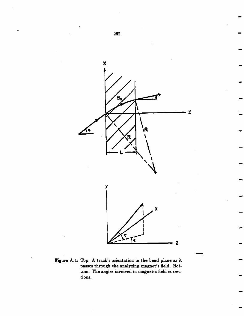
262
x
\R \
\ ' \
""\ y
x
I I I
.-_.J « z
Figure A.1: Top: A track's orientation in the bend plane as it passes through the analyzing magnet 1 s :field. Bottom: The angl~s involved in magnetic :field corrections.
-
-
...
z
-
-
-
-
-

263
5y2 - tan17[R(a - /3)- Lo]
= Lo tan 1J [ • a - ~ - 1] sin a - s1nf3
{A.4)
- ~o(a2 + a,8 + ,a2)tan71 (A.5)
where R is the track's radius of curvature in the bend plane. The change in the
x-view slope produces an offset at Zc because the apparent slopes, tan 11/ cos a and
tan 11 /cos {3, rather than the actual slope_ out of the bending plane. Thus,
5y3 = tan((1- _1_) Lo+ (1- _1_) Lo] cos a 2 cos f3 2
(A.6)
The linking procedure is different for the X and Y projections of the space tracks.
However, both methods project the upstream view tracks to the center of the magnet
and attempt to match them with the proper space track projection via separate
selection procedures. All of the above corrections are applied --before matching is
attempted.

-----
-
---
-
-
-

-
-
Appendix B
Fake Tracks
The following is description of the two methods used in estimating the fraction
of fake tracks in the data. Both methods assume that the high quality 16-hit tracks
are all real. Recall that a high quality track is one with x2 ~ 1, lb!ll ~ 1 cm, and is
linked in the x-view to an SSD track belonging to the primary vertex.
The first technique is known as the LAC method. As its name implies, it utilizes
the data produced by the electromagnetic calorimeter. Scatter plots of the differences
in X {.6X) and Y (.6 Y) between each track and the nearest electromagnetic shower
was constructed. The tracks used in making the plots had to have momenta greater
than 5 GeV /c, the LAC's " turn on" point, and IYI 5 0.7, the LAC's acceptance.
Two scatter plots were used. One was for all tracks satisfying the momentum and
rapidity cuts, and the other was for those tracks that, in addition" had lb!ll ~ 1 cm.
The absolute limits of each plot are 0 to 10 cm. Those tracks with .6X, .6 Y 5 2.0 cm
were deemed to have been "seen" by the LAC. Figure B.1 displays one of these scatter
plots.
In order to correct for the LAC's inefficiency the detection efficiency for all high
quality 16-hit tracks as a function of their momenta was measured. The detection
efficiency for all high quality tracks was measured also. Plots of these efficiencies
appear in Figure B.2. Those scatter plot entries for which .6X, .6 Y 5 2.0 cm were
then corrected by the appropriate e(P) for high quality 16-hit tracks. A second
study performed the correction using the e(P)s coming from all high quality tracks.
The ratio of weighted contents in the region .6X, .6 Y ~ 2.0 cm to the total contents
(weighted and unweighted) yields the true track fraction. The fake track percentage
is just this number subtracted from 1.
265

10
9
8
7
6
"""' E u
5 """
~
4
.J
2
0 0
266
1 2 3 4 5 6 7 8
AX (cm)
Figure B.1: Scatter plot of 6.X vs 6. Y for tracks and nearest showers
-
-
....
-
-
---
9 10
-
--

- 267
1.4
1.2
++~+++++++++ +t t 0.8
0.6
0.4
0.2 :-
0 0 20 40 60 80 100
P (GeV/c)
1.4 -1.2
0.8 1+++++ ~+++++ 0.6 -+--+-
:-+- -+-0.4 -+-
- 0.2
0 0 20 40 60 80 100
P (GeV/c)
- Figure B.2: EMLAC efficiency in P for high quality 16-hit tracks (top) and all high quality tracks (bottom).
268
The second method employs the y-view impact parameter distributions for physics
tracks that are linked in the x-projection to an SSD track belonging to a primary
vertex. It is known as the bv method. Such an impact parameter distribution is
shown in Figure B.3. Clearly, tracks that are linked in x to an SSD track associated
with a reconstructed vertex should have small lb11 1; those which do not are suspicious.
Those tracks for which lbvl ~ 2.0 cm have been deemed fake; a fiat contribution under
the peak in the bv distribution has been assumed. To account for improper linking of
real tracks in the tails a similar b11 distribution was made for the high quality 16-hit
tracks. The ratio of entries for lb11I 2: 2.0 cm to those inside lbvl ~ 1.0 cm was used
to subtract off a portion of the tail in the distribution for all tracks. The fraction of
fake tracks, including the· contribution under the peak was then estimated from the
subtracted distribution.
. The results of these studies are summarized in Table B.1 for all b11 and for lbvl ~
1.0 cm. LACl and LAC2 refer to the separate studies using efficiency corrections for
16-hit high quality tracks and all high quality tracks respectively. Notice that the
impact parameter method yields very small fractions while those measured via the
LAC technique are considerable. However, the results of the LAC method, using the
efficiency corrections for all high quality tracks appear consistent with the b11 method
based on their variation. In addition, the error bars on the plots of Figure B.2 indicate
that both sets of efficiency corrections yield consistent estimates for the percentage
of fake tracks. From these studies it appears that the tracking data contains fake
MWPC tracks at the~ 1% level for lbvl < 1.0cm and~ 2% overall.
-
-
---
-
...
----

-
-
269
-25 -20 -15 -10 -5 0 5 10 15
b., linked
Figure B.3: b11 distribution for physics tracks that are linked in the x-view to an SSD track, assigned to the primary vertex.
20 25

-270 -
-
Table B.1: List of fake track fractions. -Beam Method lbvl ~ 1.0 cm(%.) all b!I (%)
+ LA Cl 2.97 9.39
+ . LAC2 -.946 1.82 -+ b!I .0592 1.39
- LA Cl 2.92 9.41 -- LAC2 .208 3.32
- bv .0586 1.41
-
...
---

-
--
Appendix C
Track Reconstruction Efficiency
The issue of track reconstruction efficiency will now be addressed. This efficiency
can be estimated by studying the relative multiplicities of 13, 14, 15, and 16-hit
tracks. Such a distribution appears in Figure C.1 along with the MC prediction.
The monte carlo prediction uses the ISAJET monte carlo's output, and projects the
charged particles through a simulation of the magnet and MWPC system. Such a
simulation takes into account the effects of the analyzing magnet's field, the geometric
acceptance of the wire chambers, and most importantly, the planes' efficiencies on the
relative multiplicity of 13, 14, 15, and 16-hit tracks. However, it completely ignores
the effects of noise and the reconstruction program.
Figure C.2 shows four plots of relative hit multiplicities. Each plot is for one of
the separate sets of data used in the analysis. The sets a.re distinguished by the time
at which they were accumulated, and by the sign of the beam used to generate them.
The sets are time ordered with set E being the earliest, and set A the latest. Sets A
and D were generated with negative beam; sets C and E were generated with positive
beam. Each of the plots has the monte ca.rlo result superimposed on it. It is clear by
inspection that the shape of the distribution has a tim~ dependence. It also looks as
. though PLREC might be reconstructing 14-hit tracks in favor of 15-hit tracks because
the 13-hit and 16-hit fractions are closer to the monte carlo result. This effect should
not degrade the reconstruction efficiency though. Overall the monte carlo distribution
does have a greater efficiency for seeing tracks than the data, except possibly for set E.
Nevertheless, all tli.e distributions are quite similar, implying that the reconstruction
efficiency for the data is close to that predicted by the monte carlo.
The monte carlo reconstruction efficiency can be calculated explicitly from the
plane's efficiencies. The result is 98%. One can average the efficiencies and use the . 271
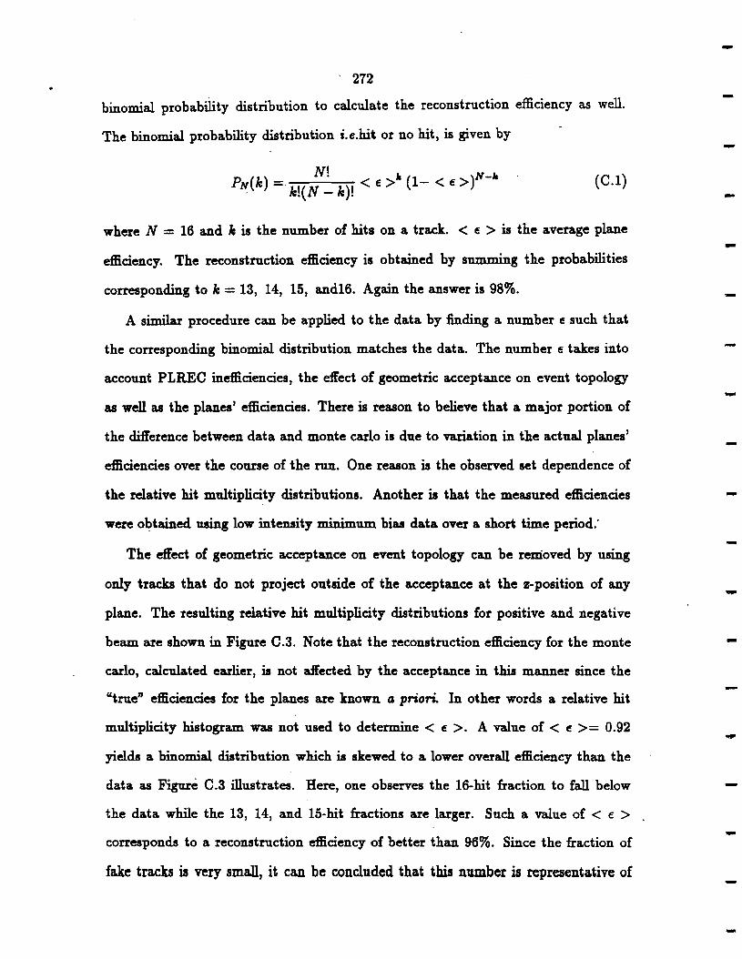
. 272
binomial probability distribution to calculate the reconstruction efficiency as well.
The binomial probability distribution i. e.hit or no hit, is given by
N! la ( )N-la P~(k) =·k!(N-k)! < E > 1- < E > (C.l)
where N = 16 and le is the number of hits on a track. < e > is the average plane
efficiency. The reconstruction efficiency is obtained by summing the probabilities
corresponding to k = 13, 14, 15, and16. Again the answer is 983.
A similar procedure can be applied to the data by finding a number e such that
the corresponding binomial distribution matches the data. The number e takes into
account PLREC inefficiencies, the effect of geometric acceptance on event topology
as well as the planes' efficiencies. There is reason to believe that a major portion of
the difference between data and monte carlo is due to variation in the actual planes'
efficiencies over the course of the run. One reason is the observed set dependence of
the relative hit multiplicity distributions. Another is that the measured efficiencies
were o~tained using low intensity minimum bias data over a short time period:
The effect of geometric acceptance on event topology can be removed by using
only tracks that do not project outside of the acceptance at the z-position of any
plane. The resulting relative hit multiplicity distributions for positive and negative
beam are shown in Figure C.3. Note that the reconstruction efficiency for the monte
carlo, calculated earlier, is not affected by the acceptance in this manner since the
"true" efficiencies for the planes are known a priori. In other words a relative hit
multiplicity histogram. was not used to determine < e >. A value of< e >= 0.92
yields a binomial distribution which is skewed to a lower overall efficiency than the
data as Figure C.3 illustrates. Here, one observes the 16-hit fraction to fall below
the data while the 13, 14, and 15-hit fractions are larger. Such a value of < e >
corresponds to a reconstruction efficiency of better than 963. Since the fraction of
fake tracks is very small, it can be concluded that this number is representative of
-
----
--
-
-

273
the real tracks. It is clear from this discussion that the reconstruction program has a
very small adverse affect indeed!
-

0.36
0.32
0.28
0.24
0.2
0.16
0.12
0.08
0.04
0
274
12.4 12.8 13.2 13.6 14 14.4 14.8 15.2 15.6
Hits
Figure C.l: A typical relative hit multiplicity distribution for the physics tracks
--
-
-
--
-16
-
-
-

275
-0.5 0.5
O.-i-5 SETA O.-i-5 SETO
OA 0.-i-........ 0.35 -----: 0.35
0.3 0.3 -- 0.25 0.25
0.2 0.2
0.15 0.15
0.1 0.,
- 0.05 0.05
0 0 13 14 15 16 13 14 15 16
Hits Hits
0.5 0.5
0.45 SETC 0.45 SETE
0.4 0.4
0.35 r······1
0.35 r·······1 H 0.3 l l 0.3
: : 0.25 . i 0.25
- 0.2 ........ 0.2
0.15 0.15
0.1 0.1
0.05 0.05
0 0 13 14 15 16 13 14 15 16
Hits Hits
- Figure C.2: Relative hit multiplicity distributions of physics tracks for the four separate data sets. The monte carlo prediction appears as the dotted bars.

0.5
0.45
0.4
0 . .35
0.3
0.25
0.2
0.15
0.1
0.05
0
276
0.5
0.45
0.4 ..........
f ·······1 ! :
~ ~ 0.35 ~
0.3
' i 0.25 ·········· . .
0.2 I : 0.15
- 0.1
0.05
13 14 15 16 o
13 14 15
Hits in Acceptance Hits in Acceptance
Figure C.3: Relative hit multiplicity distributions for positive data (Left) and negative data (Right). These plots are for tracks that do not project outside the MWPC acceptance. Also shown is the binomial distribution for (e) = 0.92; the binomial distribution is plotted as dotted bars.
-
-
,,..
--
~·······
-
-16
-
--

-
..._
Appendix D
Trigger Particle Corrections
The following is a brief summary of the methods employed in determining the
various corrections to high Pl.,..,, ?r0
, or T/ events. These corrections involve those asso
ciated with the whole event and muon cuts described in Chapter 4, those for trigger
and reconstruction inefficiencies, and the energy correction for individual photons.
This last correction is both an energy scale correction, and an energy loss correction
that takes into account all the material in front of the electromagnetic calorimeter.
D.l CORRECTIONS FOR CUTS
The correction for vertex finding efficiency has been parametrized as a function of the
z position in the target. It has the following form [52]:
£vertex = 1.0019 - 0.0079 X V z (D.1)
This correction was obtained by studying the behaviour of the vertex finding algo
rithm on a sample of events which had been visually examined via computer graphics
to see if they should have satisfied the vertex criterion. This correction is applied to
each reconstructed event individually.
The 5,. correction was obtained by assuming that the true directionality distri
bution of photons emanating from the target was symmetric about 0. The fraction,
/a .. <-o.4 of photon events with Dr< -0.4cm relative to the total number passing the
directionality cut was computed. The correction is then expressed as follows.
ea, = 1 + ~r<-0.4 (D.2)
All the other cut corrections are obtained by studying the ?r0 mass distribution
with sidebands subtracted. For the offtine veto wall and track isolation cuts all that is
277

278
necessary to do is see how many good 11"0s remain after each cut is applied individually.
The correction is just the ratio of good 11"0s without the cut to good 11"0s remaining
after the cut is applied. The timing and Ef.rom/Etotal corrections are obtained by ex
amining the tails of these distributions. The timing and ~11,/Etotal distributions for
11"0s in the mass band and the sidebands are constructed. The sideband distributions
are subtracted from the mass band distribution. The ratio of the total entries in each
distribution to the number satisfying the cut divided by 2 constitutes the correction.
Note that the track isolation correction for 11"0s is twice that for direct photon candi
dates. The corrections for all cuts that are applied to the reconstructed direct photon
sample are summarized in Table 4.2, along with a total correction.
D.2 CORRECTIONS FOR INEFFICIENCIES
There are additional corrections to the data. First, the trigger inefficiency has to be
taken into account. Second, there are the acceptance and reconstruction efficiency
corrections for 11"0s and photons. Third, the loss of photons and 11"0s through photon
conversion in the target material has to be accounted for. All these corrections, along
with the vertex correction, are applied to each event individually while it is being
reconstructed from the DST stream.
The trigger efficiency consists of two parts. There is the efficiency of the high
threshold SLOC relative to the TWOGAM trigger, and there is the pretrigger effi
ciency. The overall efficiency is just the product of the individual efficiencies. This
breakdown of the trigger analysis is due to the fact that there are two independent
hardware mechanisms responsible for producing a high P.Ltrigger. To simulate the
hardware response to P.Ldeposited in the EMLAC, the actual energy' of a triggering
event is reconstructed by EMREC. The energy deposited in the individual r-view
strips. is then. estimated from the reconstructed showers, and the simulation of the
hardware s11mming schemes is performed. Thus the actual P.L~ seen by the hardware
-
--
-
-
--
-
-
--

-
-
-
279
can be determined. Pedestal shifts, gain variations and discriminator thresholds can
be taken into account with this method. However, no reliable model of image charge
effects exists at this time.
The turn on curve for the SLOC was done using the TWOGAM trigger, which
was known to be fully efficient at a P.J.Of 1.8 GeV /c. Recall that the TWOGAM
trigger is a special coincidence of low threshold ·sLOC triggers. The ratio SLOC •
TWOGAM/TWOGAM is plotted as a function of P.J.· The calculation of P.J.is done
by using the reconstructed energy to estimate the energy in the r strips. The summing
of overlapping groups of 16 strips is simulated and the value of p.J.determined. The
efficiency curve was fitted to a function of the following form:
N l+oo P(r, P.J.) = y'21r ( ) dx8{p.J. + x - T(r)) exp(-x2 /2cr2{r)) 2?rcr r -oo (D.3)
where P(r, P.J.) is the probability a trigger was satisfied which deposited transverse
momentum.· p .J. at the position r. The integral is a convolution of a step function
and a gaussian which represents an ideal discriminator affected by gaussian noise.
The parameters.,. and er are the threshold and smearing respectively. Each octant is
divided into five regions on the basis of statistics. The r dependence o~ the t~gger is
determined by taking the eight strips with the highest p .J. and assigning that as the ·
triggering p .J..
The pretrigger tum-on curve was made using events with SLOC triggers, and
examining the octant opposite the trigger octant. The energy of the octant was
reconstructed using EMREC and the strip energies estimated. The global summing
scheme was simulated and a value of triggering P.J.assigned. A P.Ldistribution for
events with a pretrigger and an unbiased p .L distribution were made. The quotient
distribution is the pretrigger tum-on curve. To accommodate the summing scheme
each octant was divided into two regions, corresponding to inner and outer r. A fit
was done to the tum-on curve for each octant, using equation D.3, although the r

280
dependence was simply averaged over each region. Due to a lack of statistics the
outer regions' results were averaged over all octants.
There is an additional trigger correction of a purely geometrical nature. The cor
rection is for dead octants and dead regions of octants. It is computed by dividing
the number of octants by the number of active octant regions corresponding to the
region that triggered the event. This correction is necessary for calculating the abso
lute cross sections, but can be ignored when making relative distributions i.e. 1-to-11'0
ratios.
To find the acceptance and reconstruction efficiency for 1t'0s a monte carlo genera
tion of events with a single 11'0 was performed. The 1t'0s were generated uniformly in a
grid from 3.0 - 10.0 Gev / c in P.L with 0.5 Ge V / c bins and -0.85 - 0.85 in Y with 0.2
bins. 1000 events were generated per unit mesh in the grid. The 1r0s were required
to have asymmetry less than 0.75 on input to a GEANT simulation of the LAC.
EMREC was run on the ·GEANT. output and the number of 1t'0s reconstructed per
unit mesh was determined, yielding the correction £acc(Y,P.L)· The acceptance and
reconstruction· efficiency for direct photons was determined in a similar fashion. The
inefficiencies for photons occur at the inner-outer <P boundary and near the edges of
fiducial regions.
A 11'0 can be lost if one of its decay photons converts in the target material. The
conversion probability is a function of the vertex z position in the target. A photon
can be assigned a probability that it did not convert in the target material. The
conversion correction for 1t'0s is the square of the reciprocal of this probability, :-vhile
for direct photons it is just the reciprocal
-
-
-
-
--
--

281
D.3 PHOTON ENERGY CORRECTIONS
Photons impinging on the front face of the EMLAC typically lose energy in the
material between the event vertex and the calorimeter. In fact, there are nearly three
radiation lengths of material between the outside surface of the dewar vessel and the
upstream face of the electromagnetic calorimeter alone! One would therefore expect a
net energy loss as a function of photon energy, which manifests itself in a systematic
shift in the calorimeter's energy scale. By studying the energy scale one can determine
a single function of energy which will compensate for this systematic effect on the
measured photon energies.
There are other systematic effects on the energy scale, namely ambiguities in the
amplifier ga.fus, the ADC pedestals, and energy losses near the fiducial boundaries.
In order to simplify the monte carlo simulation of.the detector, used in this study, the
pedestal shifts and gain variations were determined using the calibration procedures
available during data taking. In addition, the energy losses around fiducial boundaries
were compensated for by ~djusting the energies of photons used in reconstructing r 0s.
This was accomplished by fixing the reconstru'cted r 0 mass at its nominal value. Only
photon pairs with a separation greater than 5.0 cm wer~ used for this procedure. By
using separated photons one is guaranteed that no systematic correlations due to
reconstructed energy _sharing between the two photons occurs. The absolute energy
scale was then set with the electron calibration beam data as will be described shortly.
The corrections for these effects are applied to the DST data so that the energy loss
corrections are independent of them.
The solution .to the energy loss problem has required many months of work on
the part of several individuals [53]. Only the highlights will be presented here. To
start with conversion electron pairs were reconstructed from the tracking system data.

282
Those conversion. or zero mass pair (ZMP) tracks that matched to EMLAC showers
within the fiducial region of the detector were used to compute the ratio shower energy
to tracking momentum. These E/P ratios were then plotted as a f~nction of shower
energy. The point at 100 GeV was determined from the calibration data, which used
a 100 Ge V electron beam. This was done because the track momentum resolution
begins to suffer systematic uncertainties greater than 13 at momenta "' 100 Ge V / c.
The E/P ratio was set to one for the calibration data point, thereby establishing the
absolute energy scale for the EMLAC. This calibration factor was then applied to
the E/P ratios for the ZMP data. An E/P ratio was constructed for each octant.
The values of E /P thus determine an energy loss correction for electron showers as a
function of their measured energy.
The corresponding correction for photons was obtained by running a monte carlo
simulatfon of the calorimeter apparatus, including the inactive material between the
target and photon detector. The mean energy loss per unit solid angle in the interval
E --.. E + 6.E was used to estimate the actual energy loss of photons and electrons in
the inactive material. This mean energy 1011 is obtained from well bown formulas
governing the behaviour of minimum ionizing radiation [54]. The altemative to this
approach is to implement a full showering scheme in the monte carlo; such a scenario
was unrealistic for the computing power then available to the collaboration. The
photon and electron shower energies were reconstructed by EMREC and the ratio
of photon to electron energies computed as a function of the rec.onstructed photon
energy. This ratio can then be used together with the E/P ratio obtained for showering
electrons to determine the EMLAC energy scale for photons as a function of their
reconstructed energy.
This method for ascertaining the reconstructed photons' energy scale was checked
by calculating the 1e+e- mass spectrum, using the reconstructed electron track mo
menta. By utilizing the tracking information the width and position of the ?r0 mass
---
...
--
--
-
-
..
-

-~
-
283
peak would be determined solely from the photon energy resolution and energy scale
uncertainty. The peak revealed that the energy scale uncertainty is within the re
quired tolerance and the width is consistent with an energy resolution of 183/ v'E.
Furthermore, the two photon mass spectrum for ?r0s and 11s in which the two photons
are separated by more than 5.0 cm were also found to be consistent with an energy
scale uncertainty on the order of 13 ~d the above quoted energy resolution.
The photon energy corrections for the data vary according to energy, octant and
run set. The corresponding set of corrections for the monte carlo, which is_ used to
compute the ?ro background, vary only according to energy. The monte carlo energy
scale corrections were determined from the two photon mass spectrum for separated
'1r0s. Again, the use of separated ?r0s uncouples the energy scale correction from the
effects of systematic energy sharing between two reconstructed photons that are in
close spatial proximity to one another.

-
-
-
-
-
-
-

BIBLIOGRAPHY
[1] R. Hagedorn. Relativistic Kinematics, pages 67-79. Benjamin/Cummings Pub
lishing Co., Inc., 1978.
[2] F. E. Close. An Introduction to Quarles and Partons, pages 320-322. Academic
Press, 1982.
[3] Chris Quigg. Gauge Theories of the Strong Weak and Electromagnetic Interac
tions, page 223. Benjamin/Cummings Publishing Co., Inc., 1983.
[4] F. E. Close. op. cit. pp. 312-325.
[5] G. Alteralli and G. Parisi. Asymptotic freedom in parton language. Nuclear
Physics B, 126:298-318, 1977.
[6] J. F. Owens. Large-momentum-transfer production of direct photons, jets, and
particles. Reviews of Modern Physics, 59(2):494, 495, 1987.
[7] T. Ferbel and W.R. Molzon. Direct photon production in high-energy collisions.
Reviews of Modern Physics, 56(2):181, 1984.
[8] Armando Lanaro. 11"0 Production with Hadron Beams at 530 GeV /c. PhD thesis,
University of Rochester, 1989. pp. 120-127.
[9] V. Radeka. and W.J. Willis. Liquid-argon ionization chambers as total absorption
detectors. Nuclear lnstnimen"ts and Methods, 120:221-226, 1974.
285

286
[10] D. Dunlap. How front/back separations affect the shower shape. Internal Note
075, E-706, 1982.
[11] T. Ferbel. Comment on front/back separation for EMLAC. Internal Note 049,
E-706, 1982.
[12] William E. Desoi. Constroction and Performance of a Liquid-Argon Calorimeter
for Use in Ezperiment E-706 at the Fermi National Accelerator Laboratory. PhD
thesis, University of Rochester, 1990. pp. 57-61.
[13] William E. Desoi. op. cit. pp. 55--68.
[14] Dana D. Skow. A Study of High 7ransverse Momentum 1J Meson Production.
PhD thesis, University of Rochester, 1990. pp. 63-71.
[15] E. Engels. Silicon position sensitive detectors for the helios (NA 34) experiment.
Nuclear Inst"'ments and Methods, 253:523-529, 1987.
[16] F. Sauli. Principles of operation of multi wire proportional and drift chambers.
Publication, CERN, 1977.
[17] P. Morse and H. Feshbach. Methods of Theoretical Physics. Mcgraw Hill, 1953.
[18] T. Trippe. Minim.um. tension requirements for charpak chambers' wires. Internal
Report 69-18, CERN, 1969.
[19] R. Hammerstrom et al. Large multiwire proportional chambers for experiment
NA3 at the CERN SPS. In Wire Chamber Conference, Vienna, 1980.
[20] S. Ferroni et al. Development of large planar proportional chambers. Nuclear
Instruments and Methods, 178:77-83, 1980.
(21] G. Bergun et al. Very large multiwire proportional chambers for the NA3 exper
iment. Technical Report 79-13, SACLAY-DPHPE, 1979.
-
...
-
---
-
-

--
287
(22] Keith W. Hartman. Hadronic Production of Pizero Pairs and Associated Event
Structure at 530 GeV. PhD thesis, Pennsylvania State University, 1990. pp.
39-51.
[23] F. Sauli. op. cit.
[24] Nanometric Systems, Inc., Oak Park, IL. Multi Wire Proportional Chamber
Readout System.
[25] Robert Miller. Private Communication.
[26] Richard S. Benson. Characteristics of Forward Energy Production in Proton
Nucleus and Pion-Nucleus Collisions at VS= 31.5 GeV. PhD thesis, University
of Minnesota, 1989.
,[27] Richard S. B_enson. op. cit. pp. 4o-41.
[28] Alexandros P. Sinanidis. Particlea Produced in Association with High 7ra.ns
verse Momentum Single Photons and 1r0 s in Hadronic Collisions. PhD thesis,
Northeastern University, 1989. pp. 182-196.
[29] R. Brun. ZEBRA Data Management System. CERN, Geneva, Switzerland, 1~87.
[30] John P. Mansour. High 7ransverse Momentum 11"0 Production from 11"- and P
Beams at 530 GeV /c on Be and Cu. PhD thesis, University of Rochester, 1989.
pp. 39-59.
[31] Eric J._ Prebys. A Study of High 7ransverse Momentum Direct Photon Production
from Beryllium and Copper Targets with 530 Ge V / c Incident 11"- and Proton
Bea~. PhD thesis, :University of Rochester, 1990. pp. 55-59.
(32] John P. Mansour. op. cit. p. 49.

288
(33] F. Lobkowicz. How front /back separations affect the shower shape. Internal
Note 199, E-706, 1988.
(34] Volodia Sirotenko. Private Communication.
(35] Keith W. Hartman. op. cit. pp. 106-132.
[36] Eric J. Prebys. op. cit. pp. 58-69, 78-80.
[37] Keith W. Hartman. op. cit. pp. 107-115.
[38] John P. Mansour. Private Communication.
[39] Eric J. Prebys. op. cit. pp. 114-120.
[40] W.M. Geist. Hadronic production of particles at large transverse momentum:
Its relevance to hadron structure, parton fragmentation and scattering. Physics
Reports, 197:306-307, 1990.
[41] T. Ferbel and W. R. Molzon. op. cit. pp. 206-208.
[42] T. Akesson et al. A comparison of particles recoiµ.ng from high P.L direct. photons
and 1r0s at the !SR. Physica Scripta, 34:106-110, 1986.
(43] M. Bonesini et al. The structure of events triggered by direct photons in 1r-p,
1r+p, and pp collisions at 280gev/c. Zeitschrift /Ur Physilc, 44:71-78, 1989.
[44] E".. Bonvin. Intrinsic transverse momentum in the 11"- p --to 'Y'YX reaction at
280 Ge V / c. Physics Letters B, 236:523-527, 1989.
(45] Alexandros P. Sinanidis. op. cit. pp. 247-250.
[46] D. W. Duke and J. F. Owens. Q2-dependent parametrizations of parton distri
bution functions. Physical Review D, 30(1):49-54, 1984.
[47] Sudhindra Mani. Private Communication.
...
--
-
--
-

-.
-
~-
289
(48] Christopher B. Lirakis. A Study of High Tra~sverse Momentum 1/ production in
530 GeV /c Hadronic Interactions. PhD thesis, Northeastern University, 1990.
pp. 110-112.
(49] G. Alverson et al. Production of direct photons and neutral mesons at large
transverse momenta from 7r- and p beams at 500 Ge V / c. Physical Review D,
~992. Unpublished as of January 23, 1993.
(50] Robert M. Harris. Isolated single and double direct photon production at cdf.
In The Vancouver Meeting, pages 719-726. American Physical Society, Division
of Particles and Fields, 1991.
[51] T. Ferbel. Ten years of direct-photon physics. In Physics in Collision, page 8,
1988.
(52] Dhammika Weerasundra. Private Communication.
[53] Marek Zielinski. Pri11ate Communication.
[54] Richard Femow. Introduction to Ezperimental Particle ·Physics, pages 29-75.
Cambridge University Press, 1990.