1. Prof. S. R. Satish Kumar Department of Civil E
553
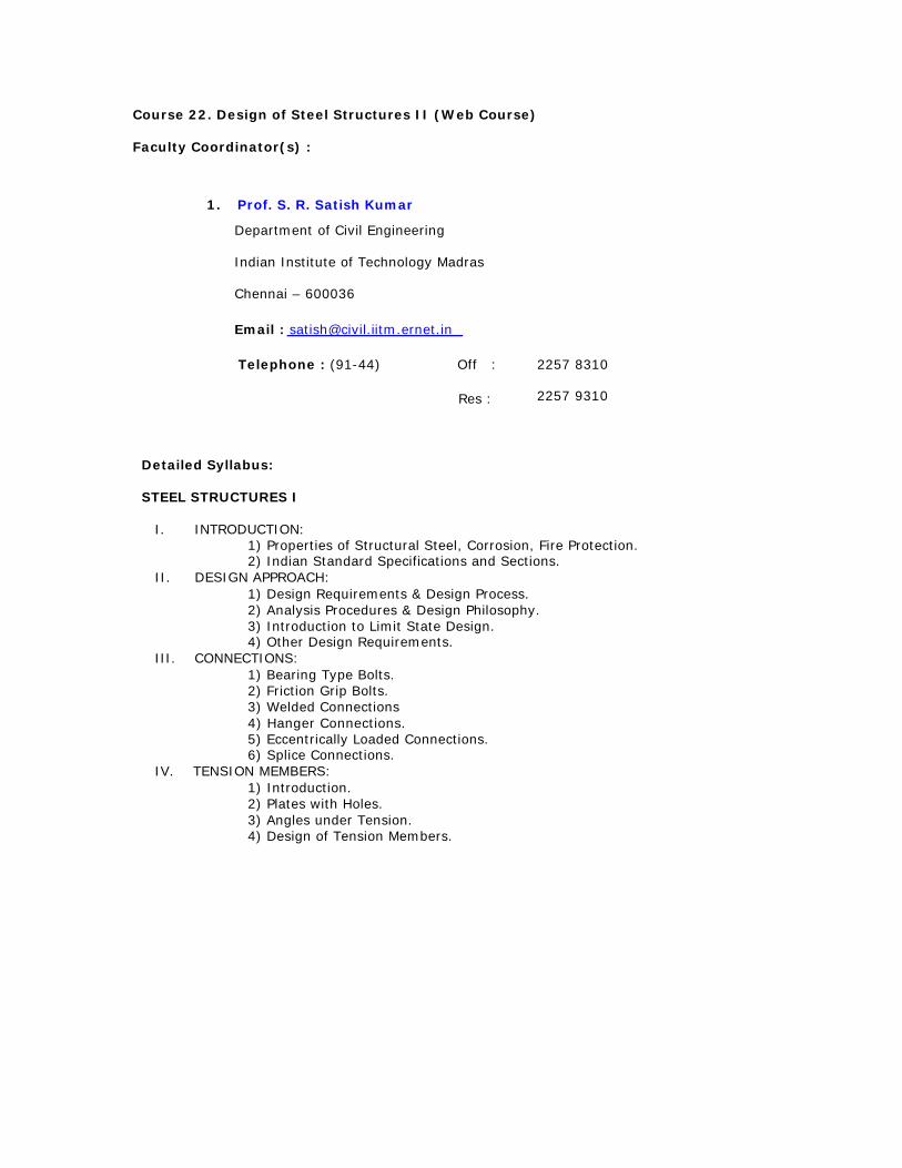
Course 22. Design of Steel Structures II (Web Course) Faculty Coordinator(s) : 1. Prof. S. R. Satish Kumar Department of Civil Engineering Indian Institute of Technology Madras Chennai – 600036 Email : [email protected] Telephone : (91-44) Off : 2257 8310 Res : 2257 9310 Detailed Syllabus: STEEL STRUCTURES I I. INTRODUCTION: 1) Properties of Structural Steel, Corrosion, Fire Protection. 2) Indian Standard Specifications and Sections. II. DESIGN APPROACH: 1) Design Requirements & Design Process. 2) Analysis Procedures & Design Philosophy. 3) Introduction to Limit State Design. 4) Other Design Requirements. III. CONNECTIONS: 1) Bearing Type Bolts. 2) Friction Grip Bolts. 3) Welded Connections 4) Hanger Connections. 5) Eccentrically Loaded Connections. 6) Splice Connections. IV. TENSION MEMBERS: 1) Introduction. 2) Plates with Holes. 3) Angles under Tension. 4) Design of Tension Members.
-
Upload
khangminh22 -
Category
Documents
-
view
3 -
download
0
Transcript of 1. Prof. S. R. Satish Kumar Department of Civil E
Course 22. Design of Steel Structures II (Web Course) Faculty Coordinator(s) :
1. Prof. S. R. Satish Kumar
Department of Civil Engineering
Indian Institute of Technology Madras
Chennai – 600036
Email : [email protected]
Telephone : (91-44) Off : 2257 8310
Res : 2257 9310
Detailed Syllabus:
STEEL STRUCTURES I
I. INTRODUCTION:
1) Properties of Structural Steel, Corrosion, Fire Protection. 2) Indian Standard Specifications and Sections.
II. DESIGN APPROACH: 1) Design Requirements & Design Process. 2) Analysis Procedures & Design Philosophy. 3) Introduction to Limit State Design. 4) Other Design Requirements.
III. CONNECTIONS: 1) Bearing Type Bolts. 2) Friction Grip Bolts. 3) Welded Connections 4) Hanger Connections. 5) Eccentrically Loaded Connections. 6) Splice Connections.
IV. TENSION MEMBERS: 1) Introduction. 2) Plates with Holes. 3) Angles under Tension. 4) Design of Tension Members.
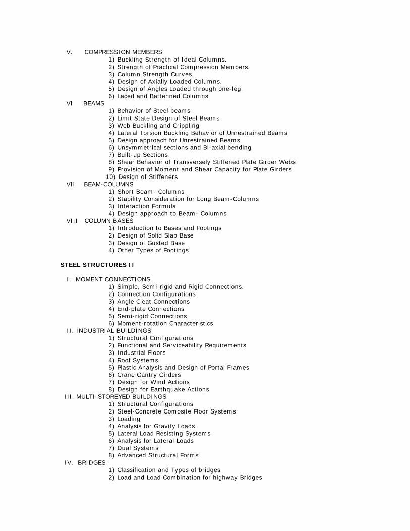
V. COMPRESSION MEMBERS 1) Buckling Strength of Ideal Columns. 2) Strength of Practical Compression Members. 3) Column Strength Curves. 4) Design of Axially Loaded Columns. 5) Design of Angles Loaded through one-leg. 6) Laced and Battenned Columns.
VI BEAMS
1) Behavior of Steel beams 2) Limit State Design of Steel Beams 3) Web Buckling and Crippling 4) Lateral Torsion Buckling Behavior of Unrestrained Beams 5) Design approach for Unrestrained Beams 6) Unsymmetrical sections and Bi-axial bending 7) Built-up Sections 8) Shear Behavior of Transversely Stiffened Plate Girder Webs 9) Provision of Moment and Shear Capacity for Plate Girders
10) Design of Stiffeners VII BEAM-COLUMNS
1) Short Beam- Columns 2) Stability Consideration for Long Beam-Columns 3) Interaction Formula 4) Design approach to Beam- Columns
VIII COLUMN BASES 1) Introduction to Bases and Footings 2) Design of Solid Slab Base 3) Design of Gusted Base 4) Other Types of Footings
STEEL STRUCTURES II
I. MOMENT CONNECTIONS
1) Simple, Semi-rigid and Rigid Connections. 2) Connection Configurations 3) Angle Cleat Connections 4) End-plate Connections 5) Semi-rigid Connections 6) Moment-rotation Characteristics
II. INDUSTRIAL BUILDINGS 1) Structural Configurations
2) Functional and Serviceability Requirements 3) Industrial Floors
4) Roof Systems 5) Plastic Analysis and Design of Portal Frames 6) Crane Gantry Girders 7) Design for Wind Actions 8) Design for Earthquake Actions
III. MULTI-STOREYED BUILDINGS 1) Structural Configurations 2) Steel-Concrete Comosite Floor Systems 3) Loading 4) Analysis for Gravity Loads 5) Lateral Load Resisting Systems 6) Analysis for Lateral Loads
7) Dual Systems 8) Advanced Structural Forms
IV. BRIDGES
1) Classification and Types of bridges 2) Load and Load Combination for highway Bridges
V. TANKS
VI. TOWERS
3) Load and Load Combination for Railway Bridges 4) Wind and Earthquake Effects 5) Design of a Typical Truss Bridge 6) Bearings and Supporting Elements 1) Introduction- Types of Tanks 2) Load and Load Combination 3) Design Aspects of Cylindrical Tanks 4) Design Aspects of Rectangular Tanks 5) Wind and Earthquake effects 6) Staging Design 1) Classification of Types of Towers 2) Loads and Load Combinations 3) Wind Effects on Towers 4) Methods of Analysis 5) Design Approaches 6) Economy and Optimisation
Design of Steel Structures Prof. S.R.Satish Kumar and Prof. A.R.Santha Kumar
Indian Institute of Technology Madras
1. BEAM – COLUMN CONNECTIONS 1.1 Introduction:
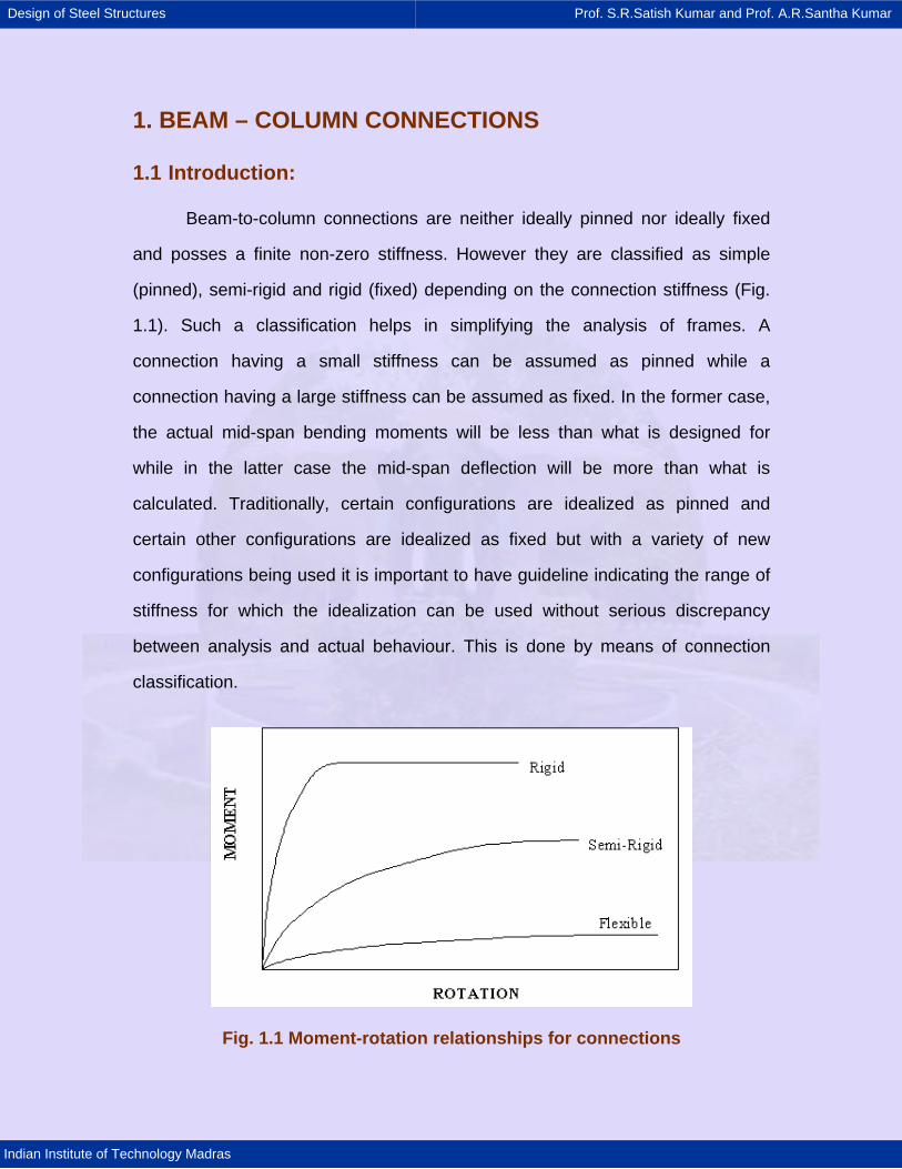
Beam-to-column connections are neither ideally pinned nor ideally fixed
and posses a finite non-zero stiffness. However they are classified as simple
(pinned), semi-rigid and rigid (fixed) depending on the connection stiffness (Fig.
1.1). Such a classification helps in simplifying the analysis of frames. A
connection having a small stiffness can be assumed as pinned while a
connection having a large stiffness can be assumed as fixed. In the former case,
the actual mid-span bending moments will be less than what is designed for
while in the latter case the mid-span deflection will be more than what is
calculated. Traditionally, certain configurations are idealized as pinned and
certain other configurations are idealized as fixed but with a variety of new
configurations being used it is important to have guideline indicating the range of
stiffness for which the idealization can be used without serious discrepancy
between analysis and actual behaviour. This is done by means of connection
classification.
Fig. 1.1 Moment-rotation relationships for connections
Design of Steel Structures Prof. S.R.Satish Kumar and Prof. A.R.Santha Kumar
Indian Institute of Technology Madras
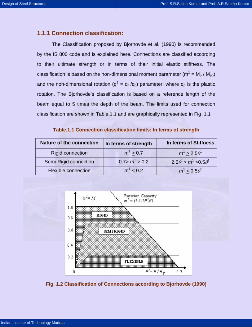
1.1.1 Connection classification:
The Classification proposed by Bjorhovde et al. (1990) is recommended
by the IS 800 code and is explained here. Connections are classified according
to their ultimate strength or in terms of their initial elastic stiffness. The
classification is based on the non-dimensional moment parameter (m1 = Mu / Mpb)
and the non-dimensional rotation (q1 = qr /qp) parameter, where qp is the plastic
rotation. The Bjorhovde’s classification is based on a reference length of the
beam equal to 5 times the depth of the beam. The limits used for connection
classification are shown in Table.1.1 and are graphically represented in Fig .1.1
Table.1.1 Connection classification limits: In terms of strength
Nature of the connection In terms of strength In terms of Stiffness
Rigid connection m1 > 0.7 m1 > 2.5θ1
Semi-Rigid connection 0.7> m1 > 0.2 2.5θ1 > m1 >0.5θ1
Flexible connection m1 < 0.2 m1 < 0.5θ1
Fig. 1.2 Classification of Connections according to Bjorhovde (1990)
Design of Steel Structures Prof. S.R.Satish Kumar and Prof. A.R.Santha Kumar
Indian Institute of Technology Madras
1.2 Connection configurations:
1.2.1 Simple connections:
Simple connections are assumed to transfer shear only shear at some nominal
eccentricity. Therefore such connections can be used only in non-sway frames where
the lateral loads are resisted by some alternative arrangement such as bracings or
shear walls. Simple connections are typically used in frames up to about five storey in
height, where strength rather than stiffness govern the design. Some typical details
adopted for simple connections are shown in Fig. 1.3.
The clip and seating angle connection [Fig.1.3 (a)] is economical when automatic
saw and drill lines are available. An important point in design is to check end bearing for
possible adverse combination of tolerances. In the case of unstiffened seating angles,
the bolts connecting it to the column may be designed for shear only assuming the
seating angle to be relatively flexible. If the angle is stiff or if it is stiffened in some way
then the bolted connection should be designed for the moment arising due to the
eccentricity between the centre of the bearing length and the column face in addition to
shear. The clip angle does not contribute to the shear resistance because it is flexible
and opens out but it is required to stabilise the beam against torsional instability by
providing lateral support to compression flange.
The connection using a pair of web cleats, referred to as framing angles, [Fig.1.3
(b)] is also commonly employed to transfer shear from the beam to the column. Here
again, if the depth of the web cleat is less than about 0.6 times that of the beam web,
then the bolts need to be designed only for the shear force. Otherwise by assuming
pure shear transfer at the column face, the bolts connecting the cleats to the beam web
should be designed for the moment due to eccentricity.
The end plate connection [Fig. 1.3(c)] eliminates the need to drill holes in the
beam. A deep end plate would prevent beam end rotation and thereby end up
Design of Steel Structures Prof. S.R.Satish Kumar and Prof. A.R.Santha Kumar
Indian Institute of Technology Madras
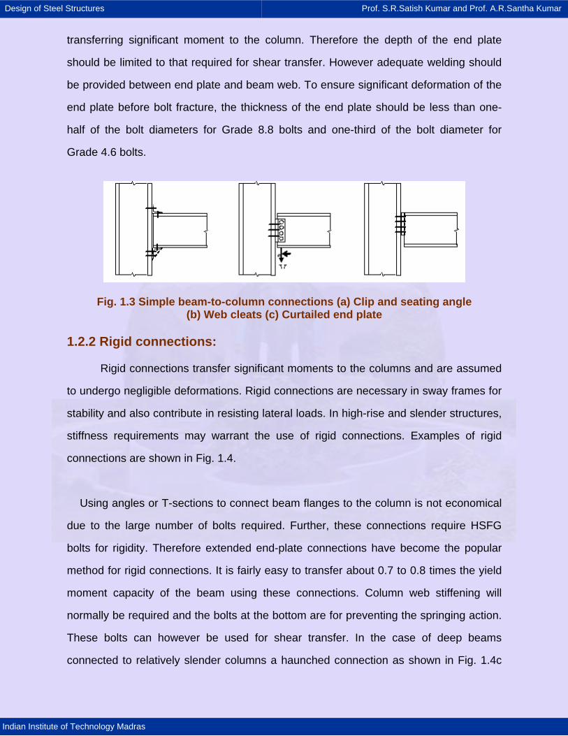
transferring significant moment to the column. Therefore the depth of the end plate
should be limited to that required for shear transfer. However adequate welding should
be provided between end plate and beam web. To ensure significant deformation of the
end plate before bolt fracture, the thickness of the end plate should be less than one-
half of the bolt diameters for Grade 8.8 bolts and one-third of the bolt diameter for
Grade 4.6 bolts.
Fig. 1.3 Simple beam-to-column connections (a) Clip and seating angle (b) Web cleats (c) Curtailed end plate
1.2.2 Rigid connections:
Rigid connections transfer significant moments to the columns and are assumed
to undergo negligible deformations. Rigid connections are necessary in sway frames for
stability and also contribute in resisting lateral loads. In high-rise and slender structures,
stiffness requirements may warrant the use of rigid connections. Examples of rigid
connections are shown in Fig. 1.4.
Using angles or T-sections to connect beam flanges to the column is not economical
due to the large number of bolts required. Further, these connections require HSFG
bolts for rigidity. Therefore extended end-plate connections have become the popular
method for rigid connections. It is fairly easy to transfer about 0.7 to 0.8 times the yield
moment capacity of the beam using these connections. Column web stiffening will
normally be required and the bolts at the bottom are for preventing the springing action.
These bolts can however be used for shear transfer. In the case of deep beams
connected to relatively slender columns a haunched connection as shown in Fig. 1.4c
Design of Steel Structures Prof. S.R.Satish Kumar and Prof. A.R.Santha Kumar
Indian Institute of Technology Madras
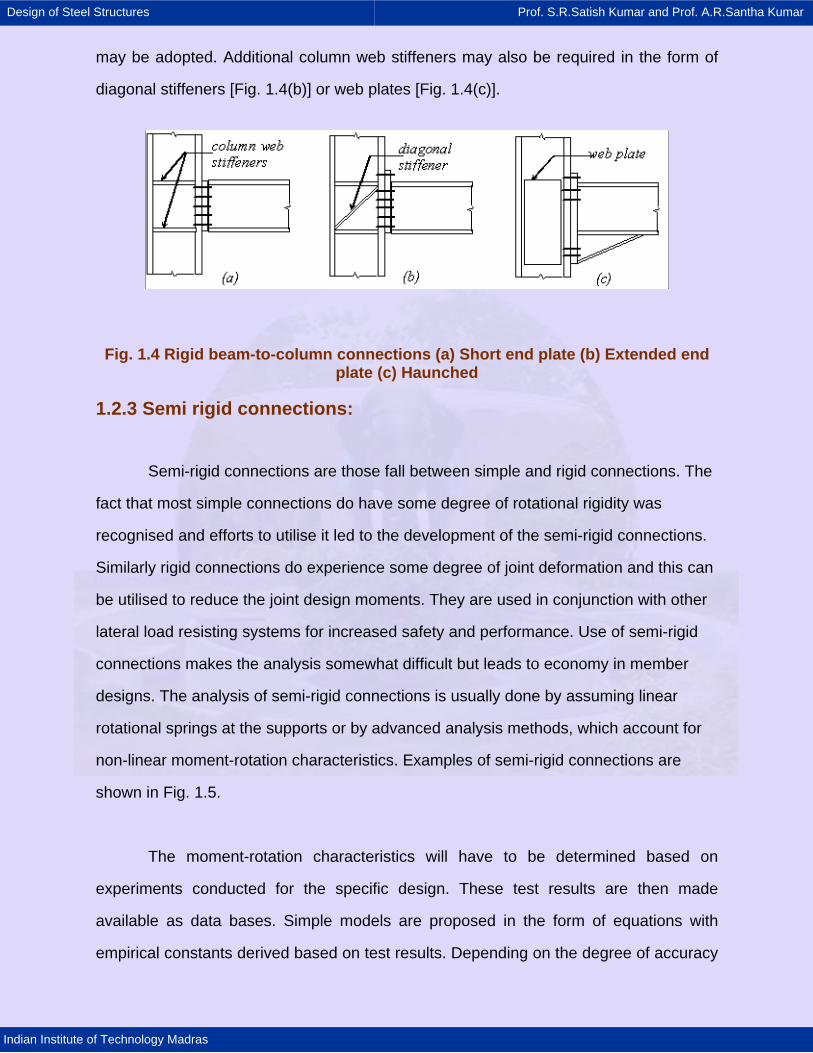
may be adopted. Additional column web stiffeners may also be required in the form of
diagonal stiffeners [Fig. 1.4(b)] or web plates [Fig. 1.4(c)].
Fig. 1.4 Rigid beam-to-column connections (a) Short end plate (b) Extended end plate (c) Haunched
1.2.3 Semi rigid connections:
Semi-rigid connections are those fall between simple and rigid connections. The
fact that most simple connections do have some degree of rotational rigidity was
recognised and efforts to utilise it led to the development of the semi-rigid connections.
Similarly rigid connections do experience some degree of joint deformation and this can
be utilised to reduce the joint design moments. They are used in conjunction with other
lateral load resisting systems for increased safety and performance. Use of semi-rigid
connections makes the analysis somewhat difficult but leads to economy in member
designs. The analysis of semi-rigid connections is usually done by assuming linear
rotational springs at the supports or by advanced analysis methods, which account for
non-linear moment-rotation characteristics. Examples of semi-rigid connections are
shown in Fig. 1.5.
The moment-rotation characteristics will have to be determined based on
experiments conducted for the specific design. These test results are then made
available as data bases. Simple models are proposed in the form of equations with
empirical constants derived based on test results. Depending on the degree of accuracy
Design of Steel Structures Prof. S.R.Satish Kumar and Prof. A.R.Santha Kumar
Indian Institute of Technology Madras
required, the moment-rotation characteristics may be idealized as linear, bilinear or non-
linear curves.
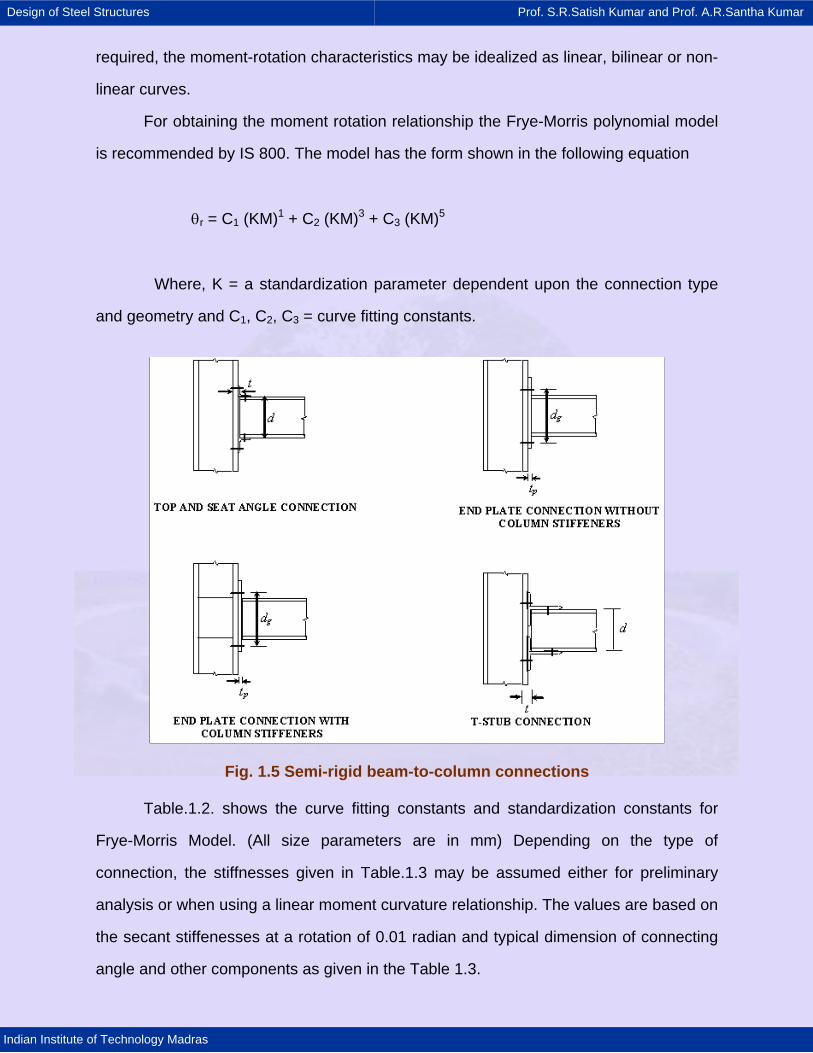
For obtaining the moment rotation relationship the Frye-Morris polynomial model
is recommended by IS 800. The model has the form shown in the following equation
θr = C1 (KM)1 + C2 (KM)3 + C3 (KM)5
Where, K = a standardization parameter dependent upon the connection type
and geometry and C1, C2, C3 = curve fitting constants.
Fig. 1.5 Semi-rigid beam-to-column connections
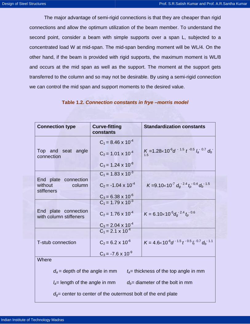
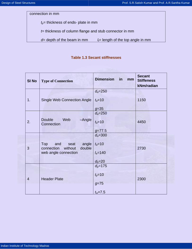
Table.1.2. shows the curve fitting constants and standardization constants for
Frye-Morris Model. (All size parameters are in mm) Depending on the type of
connection, the stiffnesses given in Table.1.3 may be assumed either for preliminary
analysis or when using a linear moment curvature relationship. The values are based on
the secant stiffenesses at a rotation of 0.01 radian and typical dimension of connecting
angle and other components as given in the Table 1.3.
Design of Steel Structures Prof. S.R.Satish Kumar and Prof. A.R.Santha Kumar
Indian Institute of Technology Madras
The major advantage of semi-rigid connections is that they are cheaper than rigid
connections and allow the optimum utilization of the beam member. To understand the
second point, consider a beam with simple supports over a span L, subjected to a
concentrated load W at mid-span. The mid-span bending moment will be WL/4. On the
other hand, if the beam is provided with rigid supports, the maximum moment is WL/8
and occurs at the mid span as well as the support. The moment at the support gets
transferred to the column and so may not be desirable. By using a semi-rigid connection
we can control the mid span and support moments to the desired value.
Table 1.2. Connection constants in frye –morris model
Connection type Curve-fitting constants
Standardization constants
Top and seat angle connection
C1 = 8.46 x 10⁻⁴
C2 = 1.01 x 10⁻⁴
C3 = 1.24 x 10⁻⁸
K =1.28×10⁻⁶d - 1.5 t -0.5 la- 0.7 db-
1.5
End plate connection without column stiffeners
C1 = 1.83 x 10⁻³
C2 = -1.04 x 10⁻⁴
C3 = 6.38 x 10⁻⁶
K =9.10×10⁻⁷ dg- 2.4 tp- 0.4 db
- 1.5
End plate connection with column stiffeners
C1 = 1.79 x 10⁻³
C2 = 1.76 x 10⁻⁴
C3 = 2.04 x 10⁻⁴
K = 6.10×10⁻⁵dg- 2.4 tp- 0.6
T-stub connection
C1 = 2.1 x 10⁻⁴
C2 = 6.2 x 10⁻⁶
C3 = -7.6 x 10⁻⁹
K = 4.6×10⁻⁶d - 1.5 t - 0.5 lt- 0.7 db- 1.1
Where
da = depth of the angle in mm ta= thickness of the top angle in mm
la= length of the angle in mm db= diameter of the bolt in mm
dg= center to center of the outermost bolt of the end plate
Design of Steel Structures Prof. S.R.Satish Kumar and Prof. A.R.Santha Kumar
Indian Institute of Technology Madras
connection in mm
tp= thickness of ends- plate in mm
t= thickness of column flange and stub connector in mm
d= depth of the beam in mm lt= length of the top angle in mm
Table 1.3 Secant stiffnesses
SI No Type of Connection Dimension in mm
Secant Stiffeness kNm/radian
1. Single Web Connection Angle
da=250
ta=10
g=35
1150
2. Double Web –Angle Connection
da=250
ta=10
g=77.5
4450
3 Top and seat angle connection without double web angle connection
da=300
ta=10
la=140
db=20
2730
4 Header Plate
dp=175
tp=10
g=75
tw=7.5
2300

Design of Steel Structures Prof. S.R.Satish Kumar and Prof. A.R.Santha Kumar
Indian Institute of Technology Madras
1.3 Summary
The types of connections between beam and column were described. The
connection configurations were illustrated and the advantages of semi-rigid
connections were outlined. The method of modeling the non linear moment
rotation relationships was illustrated.
Design of Steel Structures Prof. S.R.Satish Kumar and Prof. A.R.Santha Kumar
Indian Institute of Technology Madras
1.4 References
1) IS: 800 (Daft 2005) Code of Practice for Use of Structural Steel in General
Building Construction, Bureau of Indian Standards. New Delhi.
2) Chen, W.F. and Toma. S. Advanced analysis of steel frames. . Boca Raton
(FL): CRC Press, 1994
3) Mazzolani, F.M. and Piluso, V (1996) Theory and Design of Seismic
Resistant Steel Frames, E & F Spon Press, UK.
4) Owens G W and Cheal B D (1988) Structural Steelwork Connections,
Butterworths, London.
Design of Steel Structures Prof. S.R.Satish Kumar and Prof. A.R.Santha Kumar
Indian Institute of Technology Madras
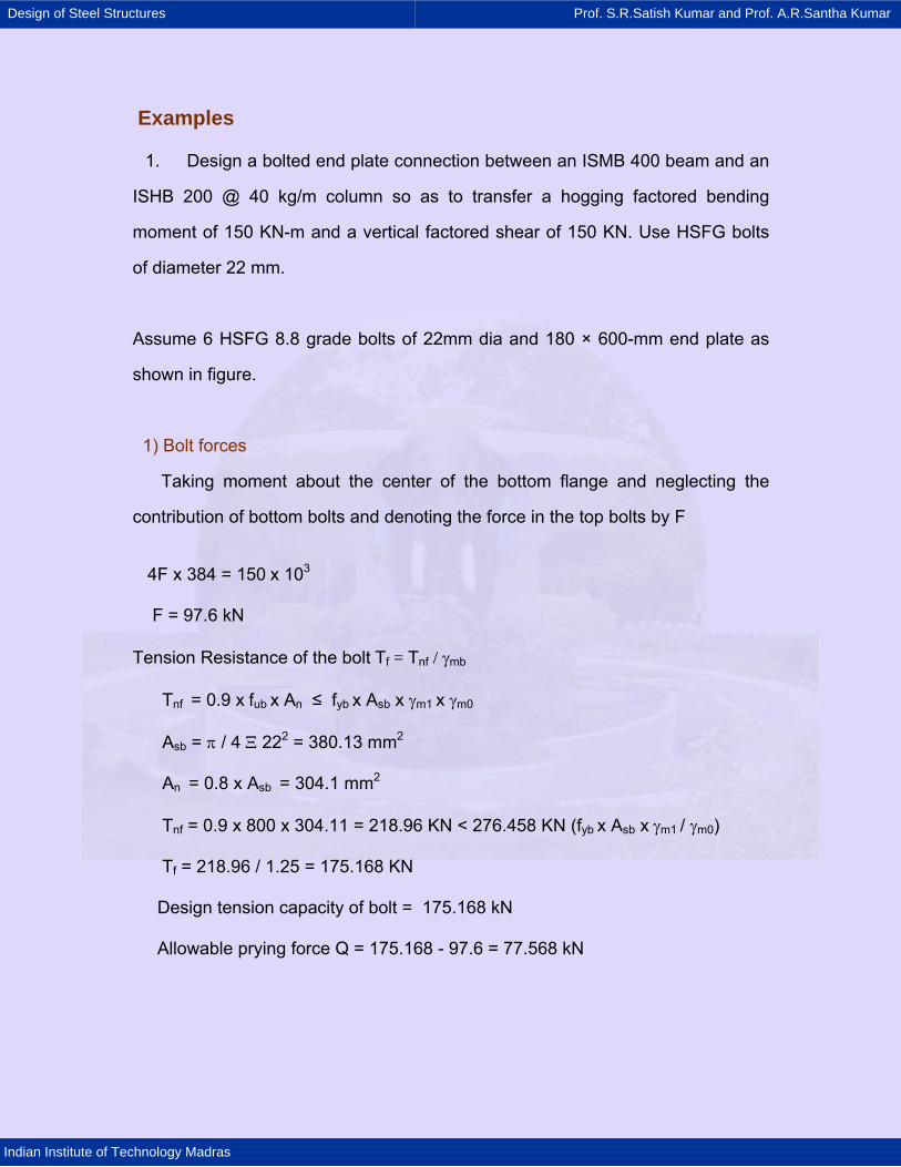
Examples
1. Design a bolted end plate connection between an ISMB 400 beam and an
ISHB 200 @ 40 kg/m column so as to transfer a hogging factored bending
moment of 150 KN-m and a vertical factored shear of 150 KN. Use HSFG bolts
of diameter 22 mm.
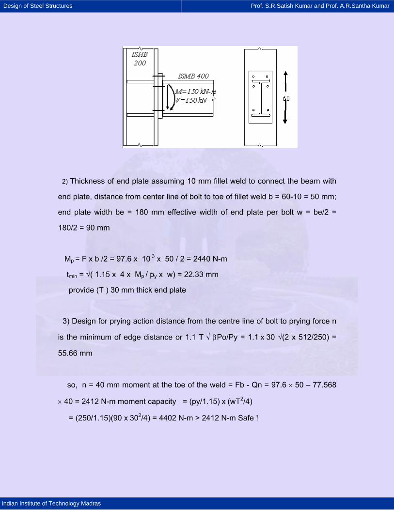
Assume 6 HSFG 8.8 grade bolts of 22mm dia and 180 × 600-mm end plate as
shown in figure.
1) Bolt forces
Taking moment about the center of the bottom flange and neglecting the
contribution of bottom bolts and denoting the force in the top bolts by F
4F x 384 = 150 x 103
F = 97.6 kN
Tension Resistance of the bolt Tf = Tnf / γmb
Tnf = 0.9 x fub x An ≤ fyb x Asb x γm1 x γm0
Asb = π / 4 Ξ 222 = 380.13 mm2
An = 0.8 x Asb = 304.1 mm2
Tnf = 0.9 x 800 x 304.11 = 218.96 KN < 276.458 KN (fyb x Asb x γm1 / γm0)
Tf = 218.96 / 1.25 = 175.168 KN
Design tension capacity of bolt = 175.168 kN
Allowable prying force Q = 175.168 - 97.6 = 77.568 kN
Design of Steel Structures Prof. S.R.Satish Kumar and Prof. A.R.Santha Kumar
Indian Institute of Technology Madras
2) Thickness of end plate assuming 10 mm fillet weld to connect the beam with
end plate, distance from center line of bolt to toe of fillet weld b = 60-10 = 50 mm;
end plate width be = 180 mm effective width of end plate per bolt w = be/2 =
180/2 = 90 mm
Mp = F x b /2 = 97.6 x 10 3 x 50 / 2 = 2440 N-m
tmin = √( 1.15 x 4 x Mp / py x w) = 22.33 mm
provide (T ) 30 mm thick end plate
3) Design for prying action distance from the centre line of bolt to prying force n
is the minimum of edge distance or 1.1 T √ βPo/Py = 1.1 x 30 √(2 x 512/250) =
55.66 mm
so, n = 40 mm moment at the toe of the weld = Fb - Qn = 97.6 × 50 – 77.568
× 40 = 2412 N-m moment capacity = (py/1.15) x (wT2/4)
= (250/1.15)(90 x 302/4) = 4402 N-m > 2412 N-m Safe !
Design of Steel Structures Prof. S.R.Satish Kumar and Prof. A.R.Santha Kumar
Indian Institute of Technology Madras
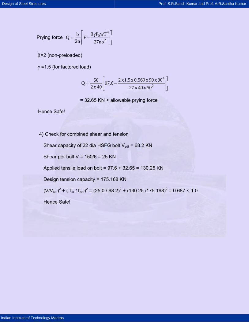
Prying force 4
02
P wTbQ F2n 27nb
⎡ ⎤βγ= −⎢ ⎥
⎢ ⎥⎣ ⎦
β=2 (non-preloaded)
γ =1.5 (for factored load)
4
22 x1.5x 0.560 x 90 x 3050Q 97.6
2 x 40 27 x 40 x 50
⎡ ⎤= −⎢ ⎥
⎢ ⎥⎣ ⎦
= 32.65 KN < allowable prying force
Hence Safe!
4) Check for combined shear and tension
Shear capacity of 22 dia HSFG bolt Vsdf = 68.2 KN
Shear per bolt V = 150/6 = 25 KN
Applied tensile load on bolt = 97.6 + 32.65 = 130.25 KN
Design tension capacity = 175.168 KN
(V/Vsdf)2 + ( Te /Tndf)2 = (25.0 / 68.2)2 + (130.25 /175.168)2 = 0.687 < 1.0
Hence Safe!
Design of Steel Structures Prof. S.R.Satish Kumar and Prof. A.R.Santha Kumar
Indian Institute of Technology Madras
2 INDUSTRIAL BUILDINGS
2.1 Introduction
Any building structure used by the industry to store raw materials or for
manufacturing products of the industry is known as an industrial building.
Industrial buildings may be categorized as Normal type industrial buildings and
Special type industrial buildings. Normal types of industrial building are shed type
buildings with simple roof structures on open frames. These buildings are used
for workshop, warehouses etc. These building require large and clear areas
unobstructed by the columns. The large floor area provides sufficient flexibility
and facility for later change in the production layout without major building
alterations. The industrial buildings are constructed with adequate headroom for
the use of an overhead traveling crane. Special types of industrial buildings are
steel mill buildings used for manufacture of heavy machines, production of power
etc. The function of the industrial building dictates the degree of sophistication.
2.1.1 Building configuration
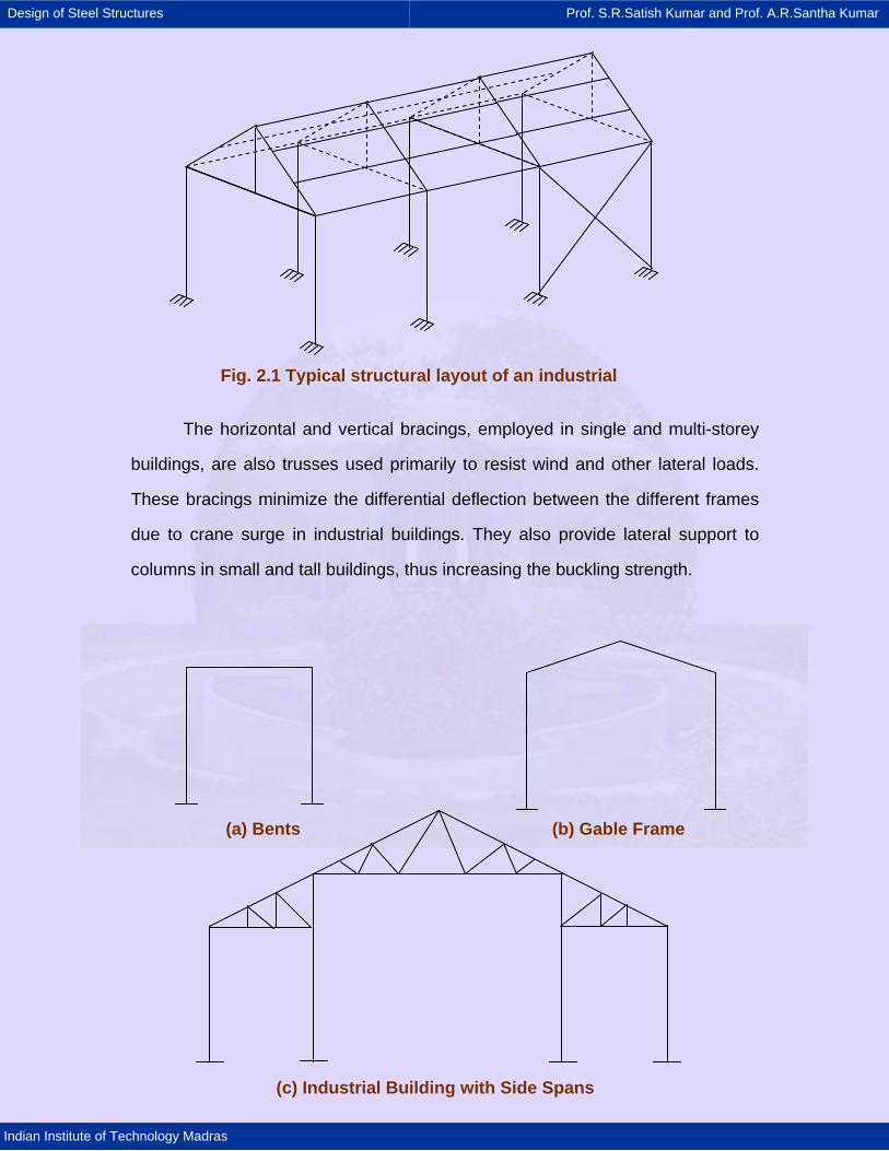
Typically the bays in industrial buildings have frames spanning the width
direction. Several such frames are arranged at suitable spacing to get the
required length (Fig. 2.1). Depending upon the requirement, several bays may be
constructed adjoining each other. The choice of structural configuration depends
upon the span between the rows of columns, the head room or clearance
required the nature of roofing material and type of lighting. If span is less, portal
frames such as steel bents (Fig. 2.2a) or gable frames (Fig. 2.2b) can be used
but if span is large then buildings with trusses (Fig. 2.2 c & d) are used.
Design of Steel Structures Prof. S.R.Satish Kumar and Prof. A.R.Santha Kumar
Indian Institute of Technology Madras
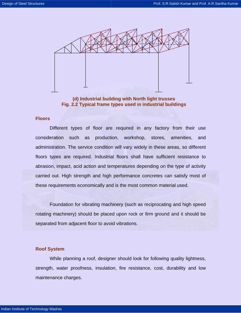
The horizontal and vertical bracings, employed in single and multi-storey
buildings, are also trusses used primarily to resist wind and other lateral loads.
These bracings minimize the differential deflection between the different frames
due to crane surge in industrial buildings. They also provide lateral support to
columns in small and tall buildings, thus increasing the buckling strength.
(a) Bents (b) Gable Frame
(c) Industrial Building with Side Spans
Fig. 2.1 Typical structural layout of an industrial
Design of Steel Structures Prof. S.R.Satish Kumar and Prof. A.R.Santha Kumar
Indian Institute of Technology Madras
Floors
Different types of floor are required in any factory from their use
consideration such as production, workshop, stores, amenities, and
administration. The service condition will vary widely in these areas, so different
floors types are required. Industrial floors shall have sufficient resistance to
abrasion, impact, acid action and temperatures depending on the type of activity
carried out. High strength and high performance concretes can satisfy most of
these requirements economically and is the most common material used.
Foundation for vibrating machinery (such as reciprocating and high speed
rotating machinery) should be placed upon rock or firm ground and it should be
separated from adjacent floor to avoid vibrations.
Roof System
While planning a roof, designer should look for following quality lightness,
strength, water proofness, insulation, fire resistance, cost, durability and low
maintenance charges.
(d) Industrial building with North light trusses Fig. 2.2 Typical frame types used in industrial buildings
Design of Steel Structures Prof. S.R.Satish Kumar and Prof. A.R.Santha Kumar
Indian Institute of Technology Madras
Sheeting, purlin and supporting roof trusses supported on column provide
common structural roof system for industrial buildings. The type of roof covering,
its insulating value, acoustical properties, the appearance from inner side, the
weight and the maintenance are the various factors, which are given
consideration while designing the roof system. Brittle sheeting such as asbestos,
corrugated and trafford cement sheets or ductile sheeting such as galvanized
iron corrugated or profiled sheets are used as the roof covering material. The
deflection limits for purlins and truss depend on the type of sheeting. For brittle
sheeting small deflection values are prescribed in the code.
Lighting
Industrial operations can be carried on most efficiently when adequate
illumination is provided. The requirements of good lighting are its intensity and
uniformity. Since natural light is free, it is economical and wise to use daylight
most satisfactory for illumination in industrial plants whenever practicable.
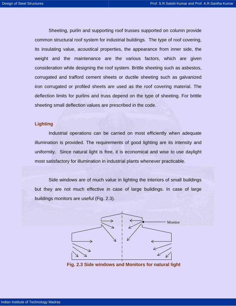
Side windows are of much value in lighting the interiors of small buildings
but they are not much effective in case of large buildings. In case of large
buildings monitors are useful (Fig. 2.3).
Monitor
Fig. 2.3 Side windows and Monitors for natural light

Design of Steel Structures Prof. S.R.Satish Kumar and Prof. A.R.Santha Kumar
Indian Institute of Technology Madras
Ventilation
Ventilation of industrial buildings is also important. Ventilation will be used
for removal of heat, elimination of dust, used air and its replacement by clean
fresh air. It can be done by means of natural forces such as aeration or by
mechanical equipment such as fans. The large height of the roof may be used
advantageously by providing low level inlets and high level outlets for air.
Design of Steel Structures Prof. S.R.Satish Kumar and Prof. A.R.Santha Kumar
Indian Institute of Technology Madras
2.2 Loads Dead load
Dead load on the roof trusses in single storey industrial buildings consists
of dead load of claddings and dead load of purlins, self weight of the trusses in
addition to the weight of bracings etc. Further, additional special dead loads
such as truss supported hoist dead loads; special ducting and ventilator weight
etc. could contribute to roof truss dead loads. As the clear span length (column
free span length) increases, the self weight of the moment resisting gable frames
(Fig. 2.2b) increases drastically. In such cases roof trusses are more economical.
Dead loads of floor slabs can be considerably reduced by adopting composite
slabs with profiled steel sheets as described later in this chapter.
Live load
The live load on roof trusses consist of the gravitational load due to
erection and servicing as well as dust load etc. and the intensity is taken as per
IS:875-1975. Additional special live loads such as snow loads in very cold
climates, crane live loads in trusses supporting monorails may have to be
considered.
Wind load
Wind load on the roof trusses, unless the roof slope is too high, would be
usually uplift force perpendicular to the roof, due to suction effect of the wind
blowing over the roof. Hence the wind load on roof truss usually acts opposite to
the gravity load, and its magnitude can be larger than gravity loads, causing
reversal of forces in truss members. The calculation of wind load and its effect on
roof trusses is explained later in this chapter.
Design of Steel Structures Prof. S.R.Satish Kumar and Prof. A.R.Santha Kumar
Indian Institute of Technology Madras
Earthquake load
Since earthquake load on a building depends on the mass of the building,
earthquake loads usually do not govern the design of light industrial steel
buildings. Wind loads usually govern. However, in the case of industrial buildings
with a large mass located at the roof or upper floors, the earthquake load may
govern the design. These loads are calculated as per IS: 1893-2002. The
calculation of earthquake load and its effect on roof trusses is explained later in
this chapter.
Design of Steel Structures Prof. S.R.Satish Kumar and Prof. A.R.Santha Kumar
Indian Institute of Technology Madras
2.3 Industrial floors The industrial buildings are usually one-story structures but some
industrial building may consist of two or more storey. Reinforced concrete or
steel-concrete composites slabs are used as a floor system. The rolled steel
joists or trusses or plate girders support these slabs. The design of reinforced
concrete slabs shall be done as per IS 456-2000. Steel-concrete composite slabs
are explained in more detail below.
2.3.1 Steel-concrete composite floors
The principal merit of steel-concrete composite construction lies in the
utilisation of the compressive strength of concrete in conjunction with steel
sheets or beams, in order to enhance the strength and stiffness.
Composite floors with profiled decking consist of the following structural
elements in addition to in-situ concrete and steel beams:
• Profiled decking
• Shear connectors
• Reinforcement for shrinkage and temperature stresses
Composite floors using profiled sheet decking have are particularly
competitive where the concrete floor has to be completed quickly and where
medium level of fire protection to steel work is sufficient. However, composite
slabs with profiled decking are unsuitable when there is heavy concentrated
loading or dynamic loading in structures such as bridges. The alternative
composite floor in such cases consists of reinforced or pre-stressed slab over
steel beams connected together using shear connectors to act monolithically
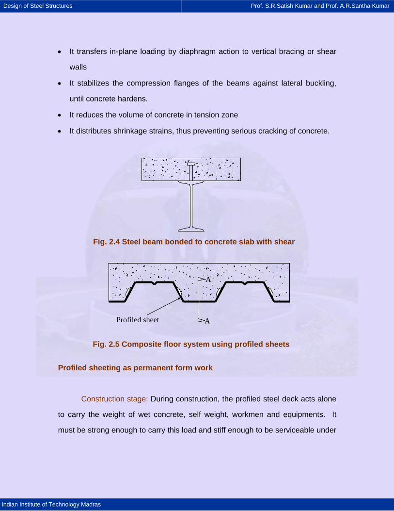
(Fig. 2.4).
Design of Steel Structures Prof. S.R.Satish Kumar and Prof. A.R.Santha Kumar
Indian Institute of Technology Madras
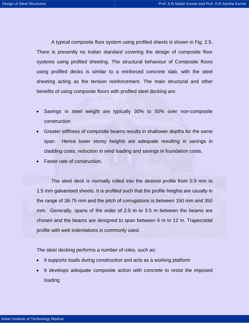
A typical composite floor system using profiled sheets is shown in Fig. 2.5.
There is presently no Indian standard covering the design of composite floor
systems using profiled sheeting. The structural behaviour of Composite floors
using profiled decks is similar to a reinforced concrete slab, with the steel
sheeting acting as the tension reinforcement. The main structural and other
benefits of using composite floors with profiled steel decking are:
• Savings in steel weight are typically 30% to 50% over non-composite
construction
• Greater stiffness of composite beams results in shallower depths for the same
span. Hence lower storey heights are adequate resulting in savings in
cladding costs, reduction in wind loading and savings in foundation costs.
• Faster rate of construction.
The steel deck is normally rolled into the desired profile from 0.9 mm to
1.5 mm galvanised sheets. It is profiled such that the profile heights are usually in
the range of 38-75 mm and the pitch of corrugations is between 150 mm and 350
mm. Generally, spans of the order of 2.5 m to 3.5 m between the beams are
chosen and the beams are designed to span between 6 m to 12 m. Trapezoidal
profile with web indentations is commonly used.
The steel decking performs a number of roles, such as:
• It supports loads during construction and acts as a working platform
• It develops adequate composite action with concrete to resist the imposed
loading
Design of Steel Structures Prof. S.R.Satish Kumar and Prof. A.R.Santha Kumar
Indian Institute of Technology Madras
• It transfers in-plane loading by diaphragm action to vertical bracing or shear
walls
• It stabilizes the compression flanges of the beams against lateral buckling,
until concrete hardens.
• It reduces the volume of concrete in tension zone
• It distributes shrinkage strains, thus preventing serious cracking of concrete.
Profiled sheeting as permanent form work
Construction stage: During construction, the profiled steel deck acts alone
to carry the weight of wet concrete, self weight, workmen and equipments. It
must be strong enough to carry this load and stiff enough to be serviceable under
Fig. 2.4 Steel beam bonded to concrete slab with shear
Fig. 2.5 Composite floor system using profiled sheets
A
A
Profiled sheet
Design of Steel Structures Prof. S.R.Satish Kumar and Prof. A.R.Santha Kumar
Indian Institute of Technology Madras
the weight of wet concrete only. In addition to structural adequacy, the finished
slab must be capable of satisfying the requirements of fire resistance.
Design should make appropriate allowances for construction loads, which
include the weight of operatives, concreting plant and any impact or vibration that
may occur during construction. These loads should be arranged in such a way
that they cause maximum bending moment and shear. In any area of 3 m by 3 m
(or the span length, if less), in addition to weight of wet concrete, construction
loads and weight of surplus concrete should be provided for by assuming a load
of 1.5 kN/m2. Over the remaining area a load of 0.75 kN/m2 should be added to
the weight of wet concrete.
Composite Beam Stage: The composite beam formed by employing the
profiled steel sheeting is different from the one with a normal solid slab, as the
profiling would influence its strength and stiffness. This is termed ‘composite
beam stage’. In this case, the profiled deck, which is fixed transverse to the
beam, results in voids within the depth of the associated slab. Thus, the area of
concrete used in calculating the section properties can only be that depth of slab
above the top flange of the profile. In addition, any stud connector welded
through the sheeting must lie within the area of concrete in the trough of the
profiling. Consequently, if the trough is narrow, a reduction in strength must be
made because of the reduction in area of constraining concrete. In current
design methods, the steel sheeting is ignored when calculating shear resistance;
this is probably too conservative.
Composite Slab Stage: The structural behaviour of the composite slab is
similar to that of a reinforced concrete beam with no shear reinforcement. The
Design of Steel Structures Prof. S.R.Satish Kumar and Prof. A.R.Santha Kumar
Indian Institute of Technology Madras
steel sheeting provides adequate tensile capacity in order to act with the
concrete in bending. However, the shear between the steel and concrete must
be carried by friction and bond between the two materials. The mechanical
keying action of the indents is important. This is especially so in open
trapezoidal profiles, where the indents must also provide resistance to vertical
separation. The predominant failure mode is one of shear bond rupture that
results in slip between the concrete and steel.
Design method
As there is no Indian standard covering profiled decking, we refer to
Eurocode 4 (EC4) for guidance. The design method defined in EC4 requires that
the slab be checked first for bending capacity, assuming full bond between
concrete and steel, then for shear bond capacity and, finally, for vertical shear.
The analysis of the bending capacity of the slab may be carried out as though the
slab was of reinforced concrete with the steel deck acting as reinforcement.
However, no satisfactory analytical method has been developed so far for
estimating the value of shear bond capacity. The loads at the construction stage
often govern the allowable span rather than at the composite slab stage.
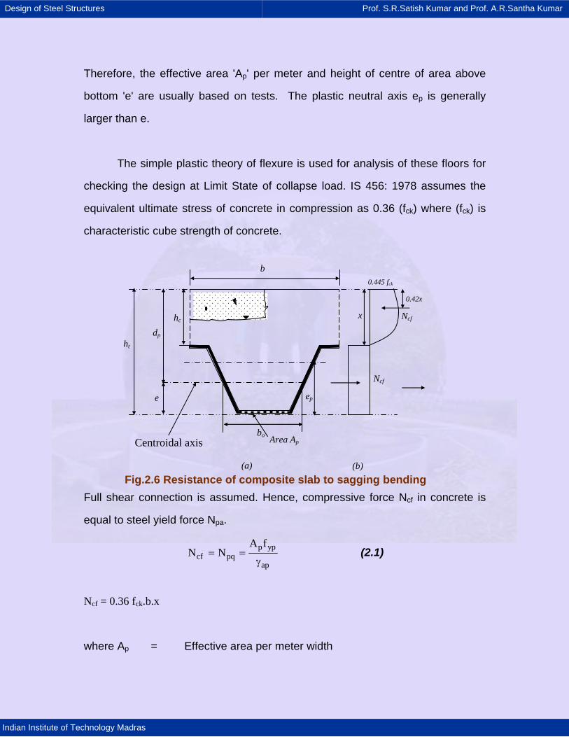
The width of the slab ‘b’ shown in Fig. 2.6(a) is one typical wavelength of
profiled sheeting. But, for calculation purpose the width considered is 1.0 m. The
overall thickness is ht and the depth of concrete above main flat surface hc.
Normally, ht is not less than 80 mm and hc is not less than 40 mm from sound
and fire insulation considerations.
The neutral axis normally lies in the concrete in case of full shear
connection. For sheeting in tension, the width of indents should be neglected.
Design of Steel Structures Prof. S.R.Satish Kumar and Prof. A.R.Santha Kumar
Indian Institute of Technology Madras
Therefore, the effective area 'Ap' per meter and height of centre of area above
bottom 'e' are usually based on tests. The plastic neutral axis ep is generally
larger than e.
The simple plastic theory of flexure is used for analysis of these floors for
checking the design at Limit State of collapse load. IS 456: 1978 assumes the
equivalent ultimate stress of concrete in compression as 0.36 (fck) where (fck) is
characteristic cube strength of concrete.
Full shear connection is assumed. Hence, compressive force Ncf in concrete is
equal to steel yield force Npa.
p ypcf pq
ap
A fN N= =
γ (2.1)
Ncf = 0.36 fck.b.x
where Ap = Effective area per meter width
Fig.2.6 Resistance of composite slab to sagging bending (b)
ht
dp
e
hc
ep
bo Centroidal axis Area Ap
(a)
Ncf
0.42x
0.445 fck
x
b
Ncf
Design of Steel Structures Prof. S.R.Satish Kumar and Prof. A.R.Santha Kumar
Indian Institute of Technology Madras
fyp = Yield strength of steel
γap = Partial safety factor (1.15)
The neutral axis depth x is given by
( )cf
ck
Nx
b 0.36f= (2.2)
This is valid when x ≤ hc, i.e. when the neutral axis lies above steel
decking.
Mp.Rd is the design resistance to sagging bending moment and is given by:
p.Rd = Ncf (dp - 0.42 x) (2.3)
Note that centroid of concrete force lies at 0.42 x from free concrete surface.
The shear resistance of composite slab largely depends on connection
between profiled deck and concrete. The following three types of mechanisms
are mobilised:
(i) Natural bond between concrete and steel due to adhesion
(ii) Mechanical interlock provided by dimples on sheet and shear connectors
(iii) Provision of end anchorage by shot fired pins or by welding studs (Fig.
2.7) when sheeting is made to rest on steel beams.
Natural bond is difficult to quantify and unreliable, unless separation at the
interface between the sheeting and concrete is prevented. Dimples or ribs are
incorporated in the sheets to ensure satisfactory mechanical interlock. These are
effective only if the embossments are sufficiently deep. Very strict control during
manufacture is needed to ensure that the depths of embossments are
Design of Steel Structures Prof. S.R.Satish Kumar and Prof. A.R.Santha Kumar
Indian Institute of Technology Madras
consistently maintained at an acceptable level. End anchorage is provided by
means of shot-fired pins, when the ends of a sheet rest on a steel beam, or by
welding studs through the sheeting to the steel flange.
Quite obviously the longitudinal shear resistance is provided by the
combined effect of frictional interlock, mechanical interlock and end anchorage.
No mathematical model could be employed to evaluate these and the
effectiveness of the shear connection is studied by means of load tests on simply
supported composite slabs as described in the next section.
Serviceability criteria
The composite slab is checked for the following serviceability criteria:
Cracking, Deflection and Fire endurance. The crack width is calculated for the
top surface in the negative moment region using standard methods prescribed
for reinforced concrete. The method is detailed in the next chapter. Normally
crack width should not exceed 3 mm. IS 456: 2000 gives a formula to calculate
the width of crack. Provision of 0.4 % steel will normally avoid cracking problems
in propped construction and provision 0.2 % of steel is normally sufficient in un-
propped construction. If environment is corrosive it is advisable to design the slab
as continuous and take advantage of steel provided for negative bending
moment for resisting cracking during service loads.
The IS 456: 2000 gives a stringent deflection limitation of /350 which may
be un- realistic for un-propped construction. The Euro code gives limitations of
/180 or 20 mm which ever is less. It may be worth while to limit span to depth
ratio in the range of 25 to 35 for the composite condition, the former being
Design of Steel Structures Prof. S.R.Satish Kumar and Prof. A.R.Santha Kumar
Indian Institute of Technology Madras
adopted for simply supported slabs and the later for continuous slabs. The
deflection of the composite slabs is influenced by the slip-taking place between
sheeting and concrete. Tests seem to be the best method to estimate the actual
deflection for the conditions adopted.
The fire endurance is assumed based on the following two criteria:
• Thermal insulation criterion concerned with limiting the transmission of heat
by conduction
• Integrity criterion concerned with preventing the flames and hot gases to
nearby compartments.
It is met by specifying adequate thickness of insulation to protect
combustible materials. R (time in minutes) denotes the fire resistance class of a
member or component. For instance, R60 means that failure time is more than
60 minutes. It is generally assumed that fire rating is R60 for normal buildings.
2.3.2 Vibration
Floor with longer spans of lighter construction and less inherent damping
are vulnerable to vibrations under normal human activity. Natural frequency of
the floor system corresponding to the lowest mode of vibration and damping
characteristics are important characteristics in floor vibration. Open web steel
joists (trusses) or steel beams on the concrete deck may experience walking
vibration problem.
Generally, human response to vibration is taken as the yardstick to limit
the amplitude and frequency of a vibrating floor. The present discussion is mainly
aimed at design of a floor against vibration perceived by humans. To design a
floor structure, only the source of vibration near or on the floor need be
Design of Steel Structures Prof. S.R.Satish Kumar and Prof. A.R.Santha Kumar
Indian Institute of Technology Madras
considered. Other sources such as machines, lift or cranes should be isolated
from the building. In most buildings, following two cases are considered-
i) People walking across a floor with a pace frequency between 1.4 Hz and
2.5 Hz.
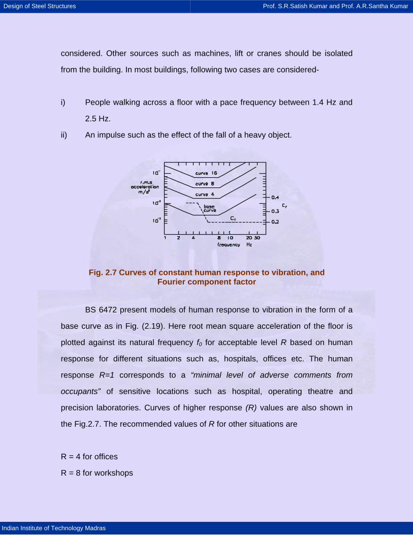
ii) An impulse such as the effect of the fall of a heavy object.
Fig. 2.7 Curves of constant human response to vibration, and Fourier component factor
BS 6472 present models of human response to vibration in the form of a
base curve as in Fig. (2.19). Here root mean square acceleration of the floor is
plotted against its natural frequency f0 for acceptable level R based on human
response for different situations such as, hospitals, offices etc. The human
response R=1 corresponds to a “minimal level of adverse comments from
occupants” of sensitive locations such as hospital, operating theatre and
precision laboratories. Curves of higher response (R) values are also shown in
the Fig.2.7. The recommended values of R for other situations are
R = 4 for offices
R = 8 for workshops
Design of Steel Structures Prof. S.R.Satish Kumar and Prof. A.R.Santha Kumar
Indian Institute of Technology Madras
These values correspond to continuous vibration and some relaxation is
allowed in case the vibration is intermittent.
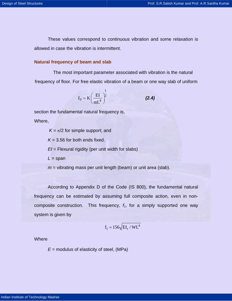
Natural frequency of beam and slab
The most important parameter associated with vibration is the natural
frequency of floor. For free elastic vibration of a beam or one way slab of uniform
12
0 4EIf K
mL⎛ ⎞= ⎜ ⎟⎝ ⎠
(2.4)
section the fundamental natural frequency is,
Where,
K = π/2 for simple support; and
K = 3.56 for both ends fixed.
EI = Flexural rigidity (per unit width for slabs)
L = span
m = vibrating mass per unit length (beam) or unit area (slab).
According to Appendix D of the Code (IS 800), the fundamental natural
frequency can be estimated by assuming full composite action, even in non-
composite construction. This frequency, f1, for a simply supported one way
system is given by
41 rf 156 EI / WL=
Where
E = modulus of elasticity of steel, (MPa)
Design of Steel Structures Prof. S.R.Satish Kumar and Prof. A.R.Santha Kumar
Indian Institute of Technology Madras
IT = transformed moment of inertia of the one way system (in term of
equivalent steel) assuming the concrete flange of width equal to the
spacing of the beam to be effective (mm4)
L = span length (mm)
W = dead load of the one way joist (N/mm)
The effect of damping, being negligible has been ignored.
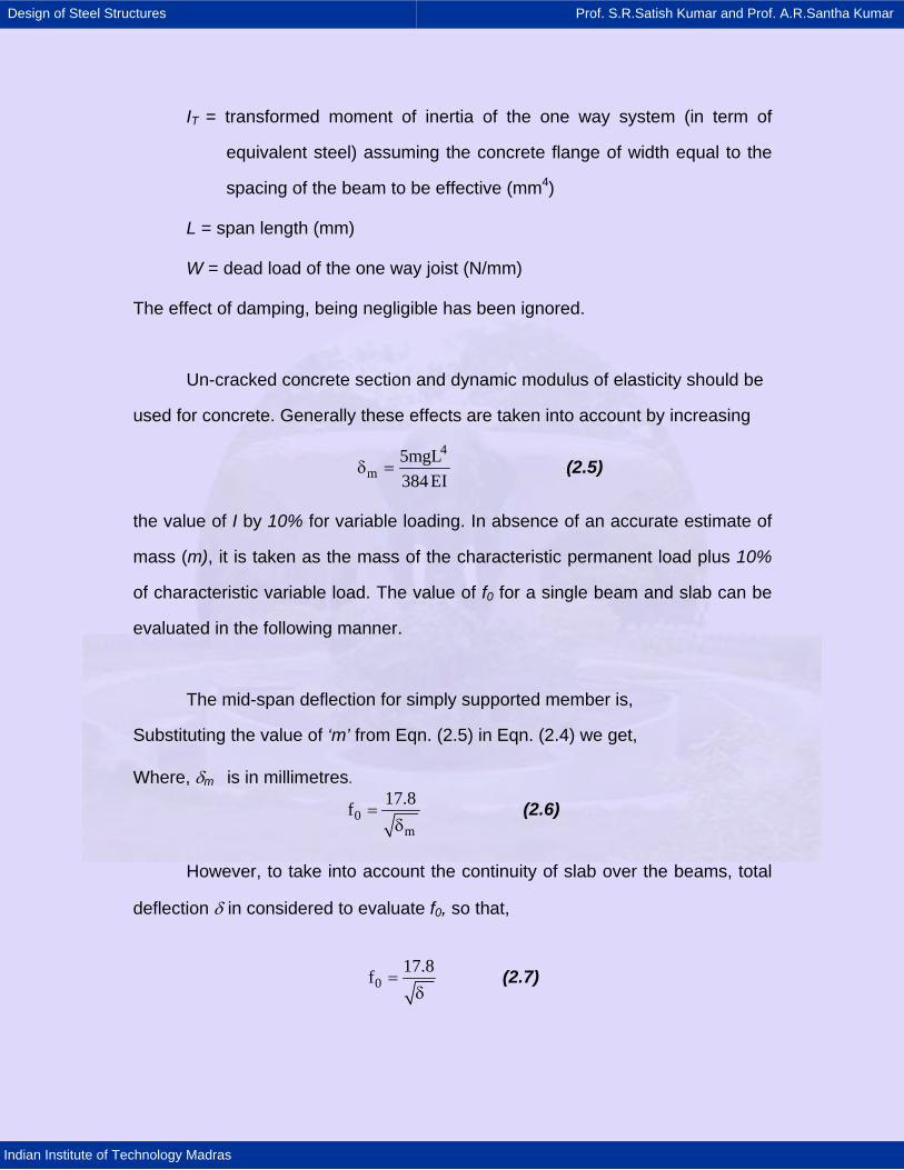
Un-cracked concrete section and dynamic modulus of elasticity should be
used for concrete. Generally these effects are taken into account by increasing
4
m5mgL384EI
δ = (2.5)
the value of I by 10% for variable loading. In absence of an accurate estimate of
mass (m), it is taken as the mass of the characteristic permanent load plus 10%
of characteristic variable load. The value of f0 for a single beam and slab can be
evaluated in the following manner.
The mid-span deflection for simply supported member is,
Substituting the value of ‘m’ from Eqn. (2.5) in Eqn. (2.4) we get, Where, δm is in millimetres.
0m
17.8f =δ
(2.6)
However, to take into account the continuity of slab over the beams, total
deflection δ in considered to evaluate f0, so that,
017.8f =δ
(2.7)
Design of Steel Structures Prof. S.R.Satish Kumar and Prof. A.R.Santha Kumar
Indian Institute of Technology Madras
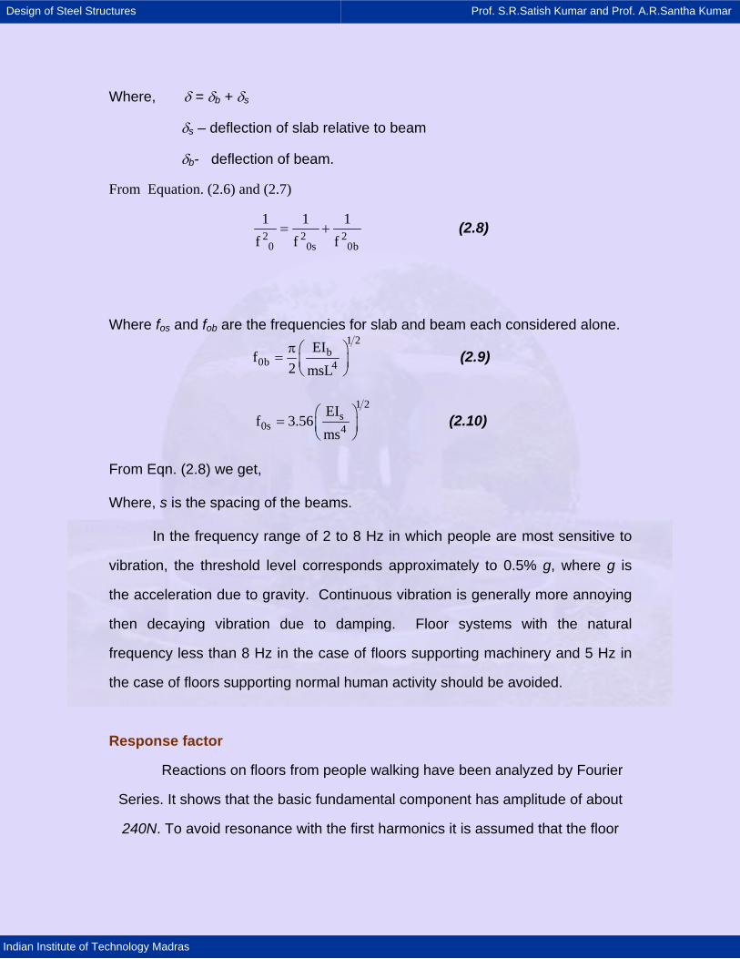
Where, δ = δb + δs
δs – deflection of slab relative to beam
δb- deflection of beam.
From Equation. (2.6) and (2.7)
2 2 20 0s 0b
1 1 1f f f
= + (2.8)
Where fos and fob are the frequencies for slab and beam each considered alone.
1 2b
0b 4EI
f2 msLπ ⎛ ⎞= ⎜ ⎟⎝ ⎠
(2.9)
1 2
s0s 4
EIf 3.56
ms⎛ ⎞= ⎜ ⎟⎝ ⎠
(2.10)
From Eqn. (2.8) we get, Where, s is the spacing of the beams.
In the frequency range of 2 to 8 Hz in which people are most sensitive to
vibration, the threshold level corresponds approximately to 0.5% g, where g is
the acceleration due to gravity. Continuous vibration is generally more annoying
then decaying vibration due to damping. Floor systems with the natural
frequency less than 8 Hz in the case of floors supporting machinery and 5 Hz in
the case of floors supporting normal human activity should be avoided.
Response factor
Reactions on floors from people walking have been analyzed by Fourier
Series. It shows that the basic fundamental component has amplitude of about
240N. To avoid resonance with the first harmonics it is assumed that the floor
Design of Steel Structures Prof. S.R.Satish Kumar and Prof. A.R.Santha Kumar
Indian Institute of Technology Madras
has natural frequency f0> 3, whereas the excitation force due to a person walking
fF 240C= (2.11)
has a frequency 1.4 Hz to 2 Hz. The effective force amplitude is,
where Cf is the Fourier component factor. It takes into account the
differences between the frequency of the pedestrians’ paces and the natural
frequency of the floor. This is given in the form of a function of f0 in Fig. (2.19).
0e
Fy sin 2 f t2k S
= π (2.12)
The vertical displacement y for steady state vibration of the floor is given
approximately by,
e
0
FWhere Staticdeflection floork1 magnification factor at resonance2
0.03 for open plan offices with composite floorf steady state vibration frequency of the floor
=
=ζ=
=
RMS value of acceleration
The effective stiffness ke depends on the vibrating area of floor, L×S. The
width S is computed in terms of the relevant flexural rigidities per unit width of
floor which are Is for slab and Ib /s for beam.
2 2rm.s 0
e
Fa 4 f2 2k
= πζ
(2.13)
14
s2
0
EIS 4.5
mf
⎛ ⎞= ⎜ ⎟⎜ ⎟
⎝ ⎠ (2.14)
As f0b is much greater than f0s, the value of f0b can be approximated as f0.
So, replacing mf02 from Eqn. (2.9) in Eqn. (2.12), we get,
Design of Steel Structures Prof. S.R.Satish Kumar and Prof. A.R.Santha Kumar
Indian Institute of Technology Madras
14
s
0
I SS 3.6L I
⎛ ⎞= ⎜ ⎟
⎝ ⎠ (2.15)
Eqn. (2.15) shows that the ratio of equivalent width to span increases with
increase in ratio of the stiffness of the slab and the beam.
The fundamental frequency of a spring-mass system,
12
e0
e
k1f2 M
⎛ ⎞= ⎜ ⎟π ⎝ ⎠
(2.16)
Where, Me is the effective mass = mSL/4 (approximately) From Eqn. (2.18),
2 2e 0k f mSL= π (2.17)
Substituting the value of ke from Eqn. (50) and F from Eqn. (2.11) into Eqn. (2.13)
frms
Ca 340
msL=
ζ (2.18)
From definition, Response factor, Therefore, from Equation (52),
3 2rmsa 5x10 R m / s−= (2.19)
To check the susceptibility of the floor to vibration the value of R should be
compared with the target response curve as in Fig. (2.19).
fCR 68000 in MKS units
msL=
ζ (2.20)
Design of Steel Structures Prof. S.R.Satish Kumar and Prof. A.R.Santha Kumar
Indian Institute of Technology Madras
2.4 Roof systems
Trusses are triangular frame works, consisting of essentially axially loaded
members which are more efficient in resisting external loads since the cross
section is nearly uniformly stressed. They are extensively used, especially to
span large gaps. Trusses are used in roofs of single storey industrial buildings,
long span floors and roofs of multistory buildings, to resist gravity loads. Trusses
are also used in walls and horizontal planes of industrial buildings to resist lateral
loads and give lateral stability.
2.4.1 Analysis of trusses
Generally truss members are assumed to be joined together so as to
transfer only the axial forces and not moments and shears from one member to
the adjacent members (they are regarded as being pinned joints). The loads are
assumed to be acting only at the nodes of the trusses. The trusses may be
provided over a single span, simply supported over the two end supports, in
which case they are usually statically determinate. Such trusses can be
analysed manually by the method of joints or by the method of sections.
Computer programs are also available for the analysis of trusses.
From the analysis based on pinned joint assumption, one obtains only the
axial forces in the different members of the trusses. However, in actual design,
the members of the trusses are joined together by more than one bolt or by
welding, either directly or through larger size end gussets. Further, some of the
members, particularly chord members, may be continuous over many nodes.
Generally such joints enforce not only compatibility of translation but also
compatibility of rotation of members meeting at the joint. As a result, the
Design of Steel Structures Prof. S.R.Satish Kumar and Prof. A.R.Santha Kumar
Indian Institute of Technology Madras
members of the trusses experience bending moment in addition to axial force.
This may not be negligible, particularly at the eaves points of pitched roof
trusses, where the depth is small and in trusses with members having a smaller
slenderness ratio (i.e. stocky members). Further, the loads may be applied in
between the nodes of the trusses, causing bending of the members. Such
stresses are referred to as secondary stresses. The secondary bending stresses
can be caused also by the eccentric connection of members at the joints. The
analysis of trusses for the secondary moments and hence the secondary
stresses can be carried out by an indeterminate structural analysis, usually using
computer software.
The magnitude of the secondary stresses due to joint rigidity depends
upon the stiffness of the joint and the stiffness of the members meeting at the
joint. Normally the secondary stresses in roof trusses may be disregarded, if the
slenderness ratio of the chord members is greater than 50 and that of the web
members is greater than 100. The secondary stresses cannot be neglected
when they are induced due to application of loads on members in between nodes
and when the members are joined eccentrically. Further the secondary stresses
due to the rigidity of the joints cannot be disregarded in the case of bridge
trusses due to the higher stiffness of the members and the effect of secondary
stresses on fatigue strength of members. In bridge trusses, often misfit is
designed into the fabrication of the joints to create prestress during fabrication
opposite in nature to the secondary stresses and thus help improve the fatigue
performance of the truss members at their joints.
Design of Steel Structures Prof. S.R.Satish Kumar and Prof. A.R.Santha Kumar
Indian Institute of Technology Madras
(a) Pratt Truss (b) Howe Truss
(c) Fink Truss (d) Fan Truss
(e) Fink Fan Truss (f) Mansard Truss
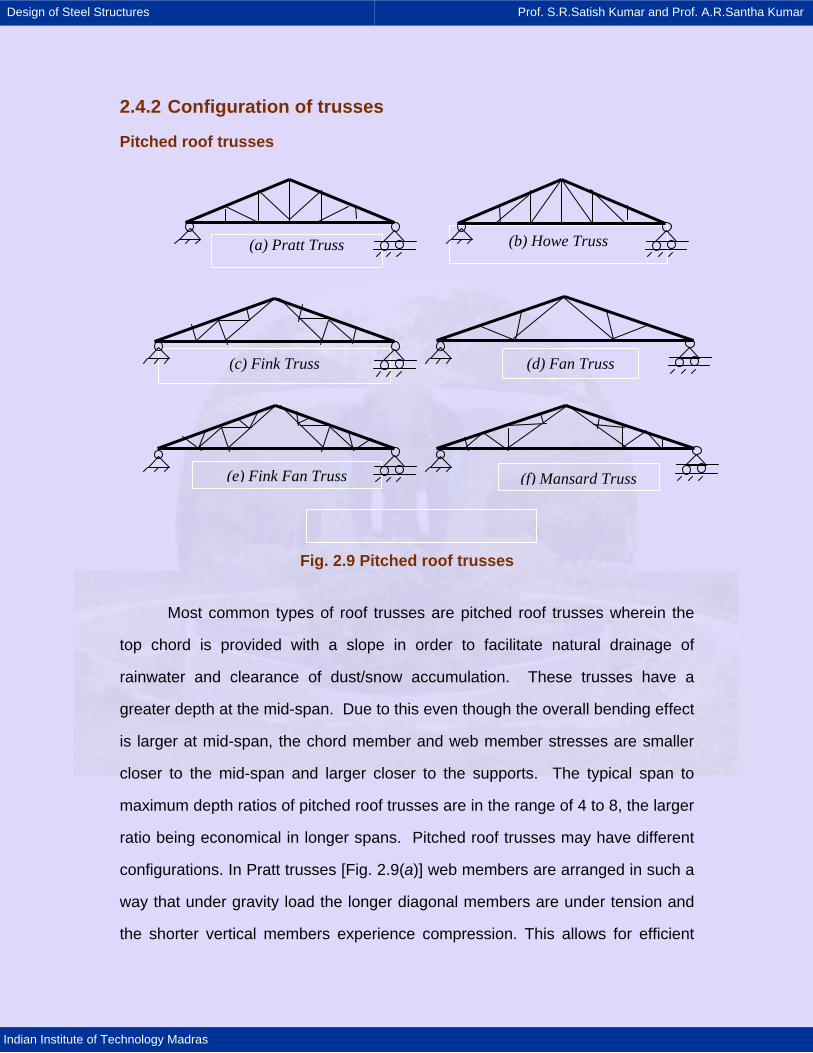
2.4.2 Configuration of trusses Pitched roof trusses
Fig. 2.9 Pitched roof trusses
Most common types of roof trusses are pitched roof trusses wherein the
top chord is provided with a slope in order to facilitate natural drainage of
rainwater and clearance of dust/snow accumulation. These trusses have a
greater depth at the mid-span. Due to this even though the overall bending effect
is larger at mid-span, the chord member and web member stresses are smaller
closer to the mid-span and larger closer to the supports. The typical span to
maximum depth ratios of pitched roof trusses are in the range of 4 to 8, the larger
ratio being economical in longer spans. Pitched roof trusses may have different
configurations. In Pratt trusses [Fig. 2.9(a)] web members are arranged in such a
way that under gravity load the longer diagonal members are under tension and
the shorter vertical members experience compression. This allows for efficient
Design of Steel Structures Prof. S.R.Satish Kumar and Prof. A.R.Santha Kumar
Indian Institute of Technology Madras
design, since the short members are under compression. However, the wind
uplift may cause reversal of stresses in these members and nullify this benefit.
The converse of the Pratt is the Howe truss [Fig. 2.9(b)]. This is commonly used
in light roofing so that the longer diagonals experience tension under reversal of
stresses due to wind load.
Fink trusses [Fig. 2.9(c)] are used for longer spans having high pitch roof,
since the web members in such truss are sub-divided to obtain shorter members.
Fan trusses [Fig. 2.9(d)] are used when the rafter members of the roof
trusses have to be sub-divided into odd number of panels. A combination of fink
and fan [Fig. 2.9(e)] can also be used to some advantage in some specific
situations requiring appropriate number of panels.
Mansard trusses [Fig. 2.9(f)] are variation of fink trusses, which have
shorter leading diagonals even in very long span trusses, unlike the fink and fan
type trusses.
The economical span lengths of the pitched roof trusses, excluding the
Mansard trusses, range from 6 m to 12 m. The Mansard trusses can be used in
the span ranges of 12 m to 30 m.
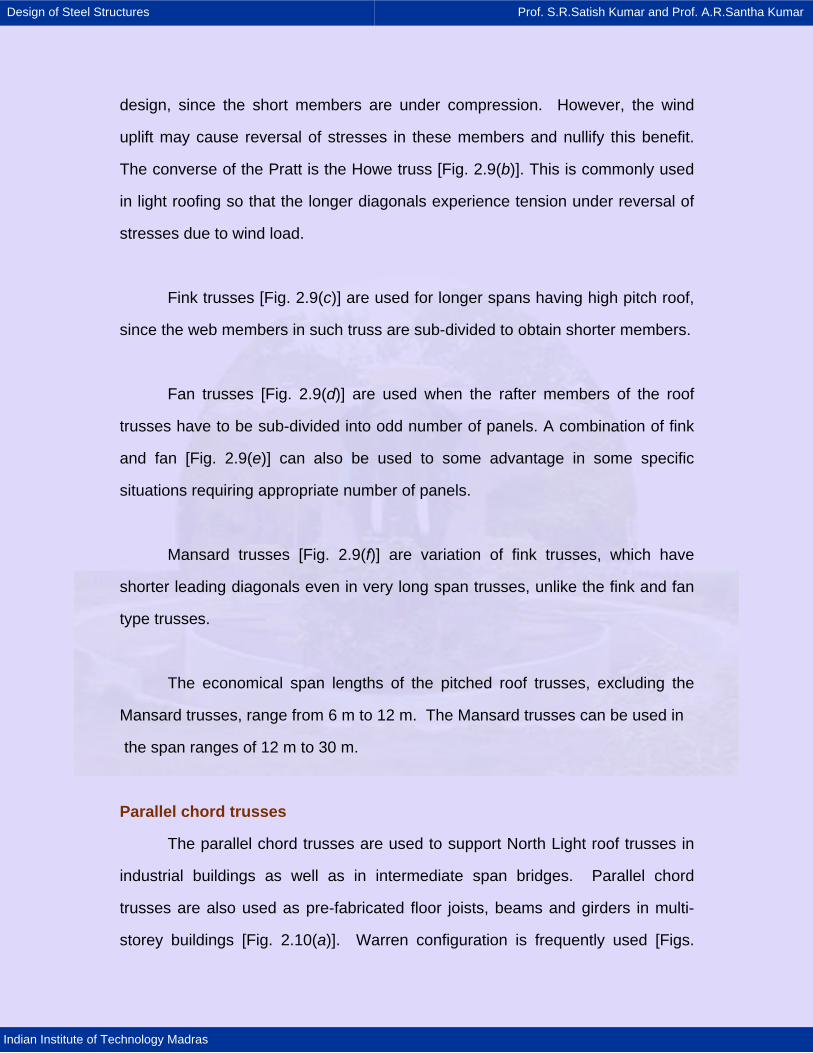
Parallel chord trusses
The parallel chord trusses are used to support North Light roof trusses in
industrial buildings as well as in intermediate span bridges. Parallel chord
trusses are also used as pre-fabricated floor joists, beams and girders in multi-
storey buildings [Fig. 2.10(a)]. Warren configuration is frequently used [Figs.
Design of Steel Structures Prof. S.R.Satish Kumar and Prof. A.R.Santha Kumar
Indian Institute of Technology Madras
Fig. 2.10 Parallel chord trusses
(a) Floor Girder (b) Warren Truss
(d) K type Web
(c) Lattice Girder
(e) Diamond Type Web
2.10(b)] in the case of parallel chord trusses. The advantage of parallel chord
trusses is that they use webs of the same lengths and thus reduce fabrication
costs for very long spans. Modified Warren is used with additional verticals,
introduced in order to reduce the unsupported length of compression chord
members. The saw tooth north light roofing systems use parallel chord lattice
girders [Fig. 2.10(c)] to support the north light trusses and transfer the load to the
end columns.
The economical span to depth ratio of the parallel chord trusses is in the
range of 12 to 24. The total span is subdivided into a number of panels such that
the individual panel lengths are appropriate (6m to 9 m) for the stringer beams,
transferring the carriage way load to the nodes of the trusses and the inclination
of the web members are around 45 degrees. In the case of very deep and very
shallow trusses it may become necessary to use K and diamond patterns for web
members to achieve appropriate inclination of the web members. [Figs. 2.10(d),
2.10(e)]
Design of Steel Structures Prof. S.R.Satish Kumar and Prof. A.R.Santha Kumar
Indian Institute of Technology Madras
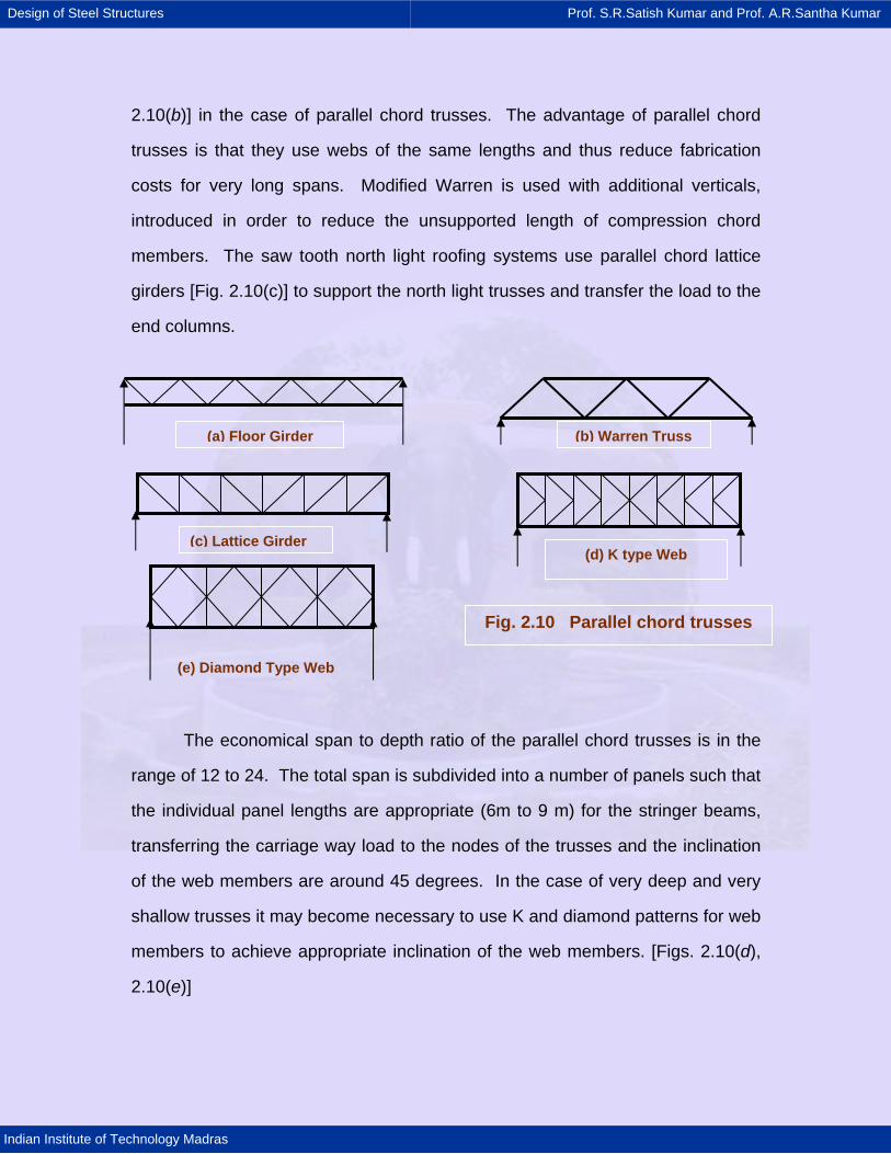
Fig 2.11 Trapezoidal trusses (a)
(b)
Trapezoidal trusses
In case of very long span length pitched roof, trusses having trapezoidal
configuration, with depth at the ends are used [Fig. 2.11(a)]. This configuration
reduces the axial forces in the chord members adjacent to the supports. The
secondary bending effects in these members are also reduced. The trapezoidal
configurations [Fig. 2.11(b)] having the sloping bottom chord can be economical
in very long span trusses (spans > 30 m), since they tend to reduce the web
member length and the chord members tend to have nearly constant forces over
the span length. It has been found that bottom chord slope equal to nearly half
as much as the rafter slope tends to give close to optimum design.
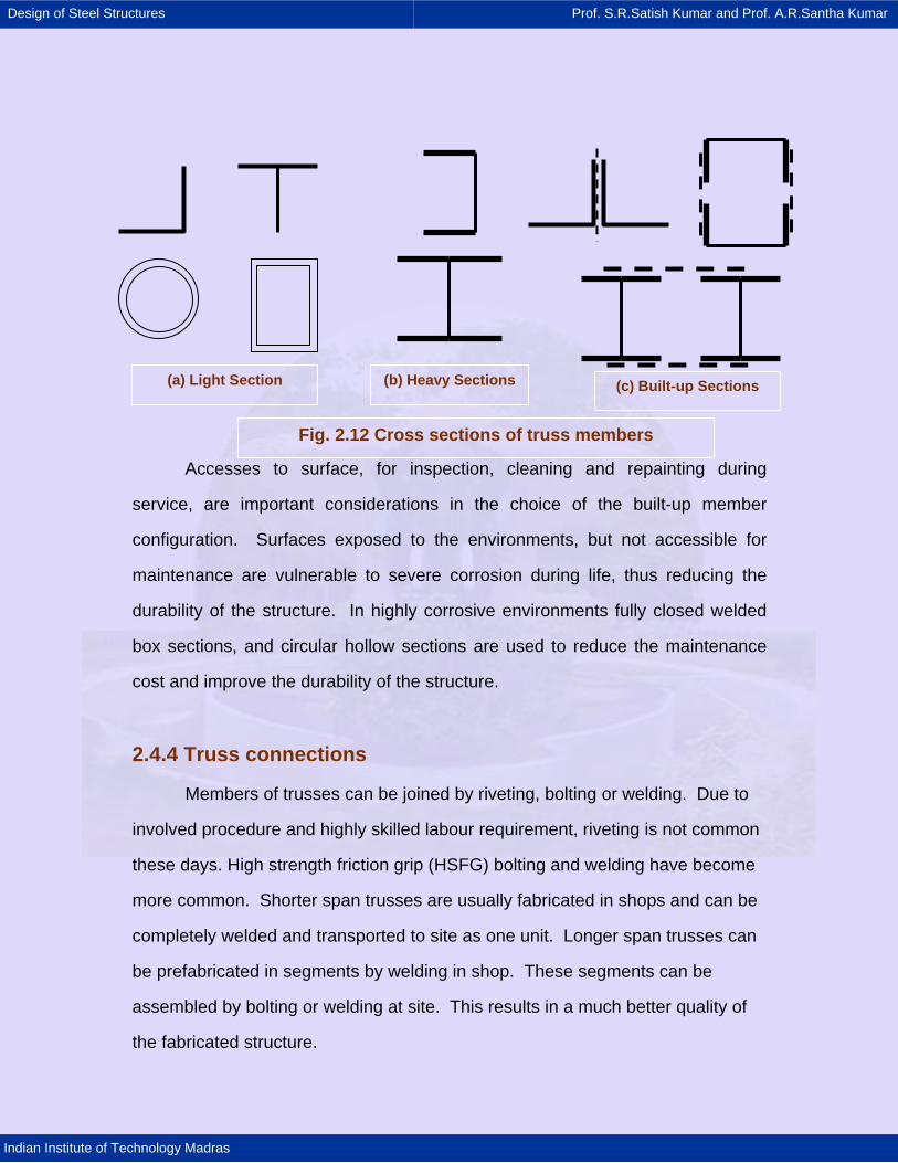
2.4.3 Truss members
The members of trusses are made of either rolled steel sections or built-up
sections depending upon the span length, intensity of loading, etc. Rolled steel
angles, tee sections, hollow circular and rectangular structural tubes are used in
the case of roof trusses in industrial buildings [Fig. 2.12(a)]. In long span roof
trusses and short span bridges heavier rolled steel sections, such as channels, I
sections are used [Fig. 2.12(b)]. Members built-up using I sections, channels,
angles and plates are used in the case of long span bridge trusses [Fig. 2.12(c)]
Design of Steel Structures Prof. S.R.Satish Kumar and Prof. A.R.Santha Kumar
Indian Institute of Technology Madras
Accesses to surface, for inspection, cleaning and repainting during
service, are important considerations in the choice of the built-up member
configuration. Surfaces exposed to the environments, but not accessible for
maintenance are vulnerable to severe corrosion during life, thus reducing the
durability of the structure. In highly corrosive environments fully closed welded
box sections, and circular hollow sections are used to reduce the maintenance
cost and improve the durability of the structure.
2.4.4 Truss connections
Members of trusses can be joined by riveting, bolting or welding. Due to
involved procedure and highly skilled labour requirement, riveting is not common
these days. High strength friction grip (HSFG) bolting and welding have become
more common. Shorter span trusses are usually fabricated in shops and can be
completely welded and transported to site as one unit. Longer span trusses can
be prefabricated in segments by welding in shop. These segments can be
assembled by bolting or welding at site. This results in a much better quality of
the fabricated structure.
(a) Light Section (b) Heavy Sections
Fig. 2.12 Cross sections of truss members
(c) Built-up Sections
Design of Steel Structures Prof. S.R.Satish Kumar and Prof. A.R.Santha Kumar
Indian Institute of Technology Madras
Truss connections form a high proportion of the total truss cost. Therefore
it may not always be economical to select member sections, which are efficient
but cannot be connected economically. Trusses may be single plane trusses in
which the members are connected on the same side of the gusset plates or
double plane trusses in which the members are connected on both sides of the
gusset plates.
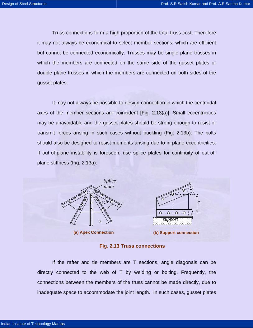
It may not always be possible to design connection in which the centroidal
axes of the member sections are coincident [Fig. 2.13(a)]. Small eccentricities
may be unavoidable and the gusset plates should be strong enough to resist or
transmit forces arising in such cases without buckling (Fig. 2.13b). The bolts
should also be designed to resist moments arising due to in-plane eccentricities.
If out-of-plane instability is foreseen, use splice plates for continuity of out-of-
plane stiffness (Fig. 2.13a).
If the rafter and tie members are T sections, angle diagonals can be
directly connected to the web of T by welding or bolting. Frequently, the
connections between the members of the truss cannot be made directly, due to
inadequate space to accommodate the joint length. In such cases, gusset plates
GP
(a) Apex Connection
Splice plate
Fig. 2.13 Truss connections
support
e
(b) Support connection
Design of Steel Structures Prof. S.R.Satish Kumar and Prof. A.R.Santha Kumar
Indian Institute of Technology Madras
are used to accomplish such connections. The size, shape and the thickness of
the gusset plate depend upon the size of the member being joined, number and
size of bolt or length of weld required, and the force to be transmitted. The
thickness of the gusset is in the range of 8 mm to 12 mm in the case of roof
trusses and it can be as high as 22 mm in the case of bridge trusses. The design
of gussets is usually by rule of thumb. In short span (8 – 12 m) roof trusses, the
member forces are smaller, hence the thickness of gussets are lesser (6 or 8
mm) and for longer span lengths (> 30 m) the thickness of gussets are larger (12
mm). The designs of gusset connections are discussed in a chapter on
connections.
2.4.5 Design of trusses
Factors that affect the design of members and the connections in trusses
are discussed in this section.
Instability considerations
While trusses are stiff in their plane they are very weak out of plane. In
order to stabilize the trusses against out- of- plane buckling and to carry any
accidental out of plane load, as well as lateral loads such as wind/earthquake
loads, the trusses are to be properly braced out -of -plane. The instability of
compression members, such as compression chord, which have a long
unsupported length out- of-plane of the truss, may also require lateral bracing.
Compression members of the trusses have to be checked for their
buckling strength about the critical axis of the member. This buckling may be in
plane or out-of-plane of the truss or about an oblique axis as in the case of single
angle sections. All the members of a roof truss usually do not reach their limit
Design of Steel Structures Prof. S.R.Satish Kumar and Prof. A.R.Santha Kumar
Indian Institute of Technology Madras
states of collapse simultaneously. Further, the connections between the
members usually have certain rigidity. Depending on the restraint to the
members under compression by the adjacent members and the rigidity of the
joint, the effective length of the member for calculating the buckling strength may
be less than the centre-to-centre length of the joints. The design codes suggest
an effective length factor between 0.7 and 1.0 for the in-plane buckling of the
member depending upon this restraint and 1.0 for the out of plane buckling.
In the case of roof trusses, a member normally under tension due to
gravity loads (dead and live loads) may experience stress reversal into
compression due to dead load and wind load combination. Similarly the web
members of the bridge truss may undergo stress reversal during the passage of
the moving loads on the deck. Such stress reversals and the instability due to
the stress reversal should be considered in design. The design standard (IS:
800) imposes restrictions on the maximum slenderness ratio, ( /r).
2.4.6 Economy of trusses
As already discussed trusses consume a lot less material compared to
beams to span the same length and transfer moderate to heavy loads. However,
the labour requirement for fabrication and erection of trusses is higher and hence
the relative economy is dictated by different factors. In India these
considerations are likely to favour the trusses even more because of the lower
labour cost. In order to fully utilize the economy of the trusses the designers
should ascertain the following:
• Method of fabrication and erection to be followed, facility for shop
fabrication available, transportation restrictions, field assembly facilities.
Design of Steel Structures Prof. S.R.Satish Kumar and Prof. A.R.Santha Kumar
Indian Institute of Technology Madras
• Preferred practices and past experience.
• Availability of materials and sections to be used in fabrication.
• Erection technique to be followed and erection stresses.
• Method of connection preferred by the contractor and client (bolting,
welding or riveting).
• Choice of as rolled or fabricated sections.
• Simple design with maximum repetition and minimum inventory of material.
Design of Steel Structures Prof. S.R.Satish Kumar and Prof. A.R.Santha Kumar
Indian Institute of Technology Madras
2.5 Plastic analysis
In plastic analysis and design of a structure, the ultimate load of the
structure as a whole is regarded as the design criterion. The term plastic has
occurred due to the fact that the ultimate load is found from the strength of steel
in the plastic range. This method is rapid and provides a rational approach for the
analysis of the structure. It also provides striking economy as regards the weight
of steel since the sections required by this method are smaller in size than those
required by the method of elastic analysis. Plastic analysis and design has its
main application in the analysis and design of statically indeterminate framed
structures.
2.5.1 Basics of plastic analysis
Plastic analysis is based on the idealization of the stress-strain curve as
elastic-perfectly-plastic. It is further assumed that the width-thickness ratio of
plate elements is small so that local buckling does not occur- in other words the
sections will classify as plastic. With these assumptions, it can be said that the
section will reach its plastic moment capacity and then undergo considerable
rotation at this moment. With these assumptions, we will now look at the
behaviour of a beam up to collapse.
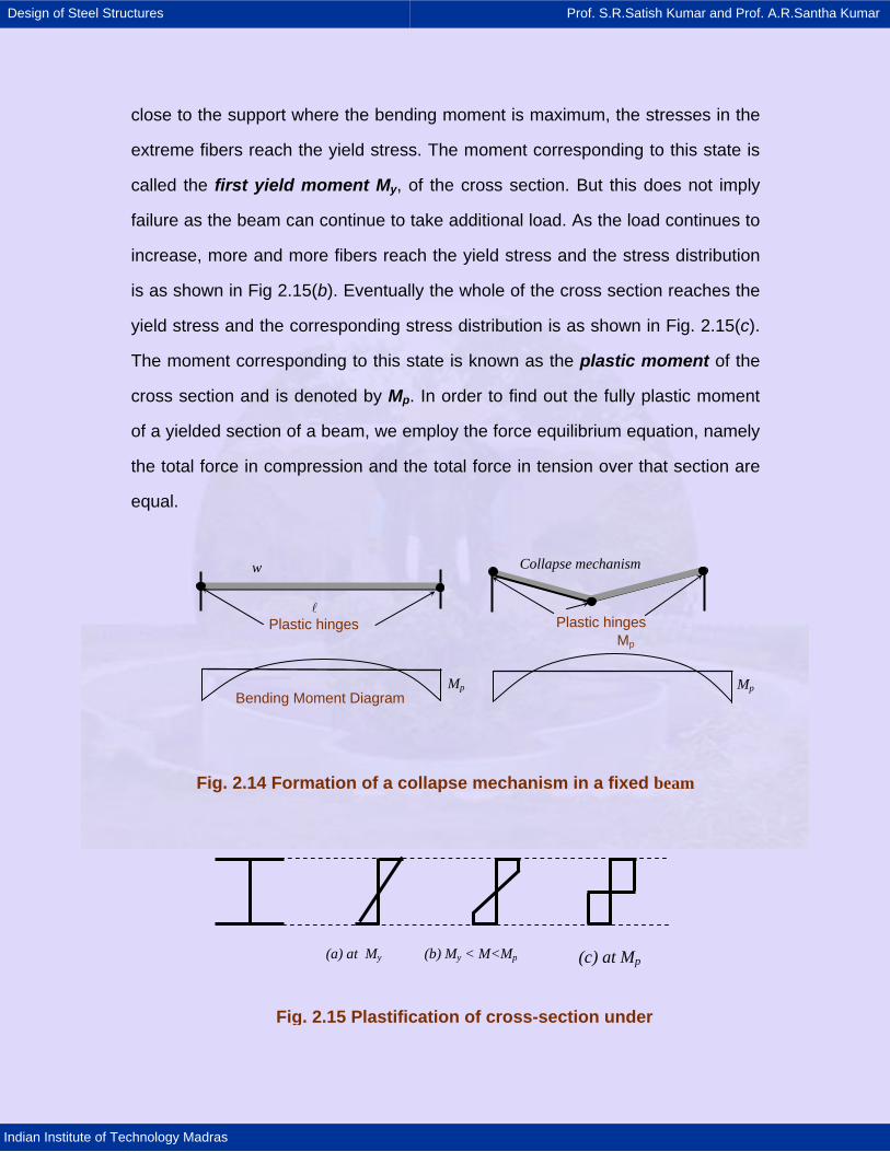
Consider a simply supported beam subjected to a point load W at mid-
span. as shown in Fig. 2.14(a). The elastic bending moment at the ends is w 2/12
and at mid-span is w 2/24, where is the span. The stress distribution across any
cross section is linear [Fig. 2.15(a)]. As W is increased gradually, the bending
moment at every section increases and the stresses also increase. At a section
Design of Steel Structures Prof. S.R.Satish Kumar and Prof. A.R.Santha Kumar
Indian Institute of Technology Madras
close to the support where the bending moment is maximum, the stresses in the
extreme fibers reach the yield stress. The moment corresponding to this state is
called the first yield moment My, of the cross section. But this does not imply
failure as the beam can continue to take additional load. As the load continues to
increase, more and more fibers reach the yield stress and the stress distribution
is as shown in Fig 2.15(b). Eventually the whole of the cross section reaches the
yield stress and the corresponding stress distribution is as shown in Fig. 2.15(c).
The moment corresponding to this state is known as the plastic moment of the
cross section and is denoted by Mp. In order to find out the fully plastic moment
of a yielded section of a beam, we employ the force equilibrium equation, namely
the total force in compression and the total force in tension over that section are
equal.
Fig. 2.14 Formation of a collapse mechanism in a fixed beam
Bending Moment Diagram
Plastic hinges
Mp
Collapse mechanism
Plastic hinges Mp
w
Mp
(a) at My (b) My < M<Mp (c) at Mp
Fig. 2.15 Plastification of cross-section under
Design of Steel Structures Prof. S.R.Satish Kumar and Prof. A.R.Santha Kumar
Indian Institute of Technology Madras
The ratio of the plastic moment to the yield moment is known as the
shape factor since it depends on the shape of the cross section. The cross
section is not capable of resisting any additional moment but may maintain this
moment for some amount of rotation in which case it acts like a plastic hinge. If
this is so, then for further loading, the beam, acts as if it is simply supported with
two additional moments Mp on either side, and continues to carry additional loads
until a third plastic hinge forms at mid-span when the bending moment at that
section reaches Mp. The beam is then said to have developed a collapse
mechanism and will collapse as shown in Fig 2.14(b). If the section is thin-
walled, due to local buckling, it may not be able to sustain the moment for
additional rotations and may collapse either before or soon after attaining the
plastic moment. It may be noted that formation of a single plastic hinge gives a
collapse mechanism for a simply supported beam. The ratio of the ultimate
rotation to the yield rotation is called the rotation capacity of the section. The
yield and the plastic moments together with the rotation capacity of the cross-
section are used to classify the sections.
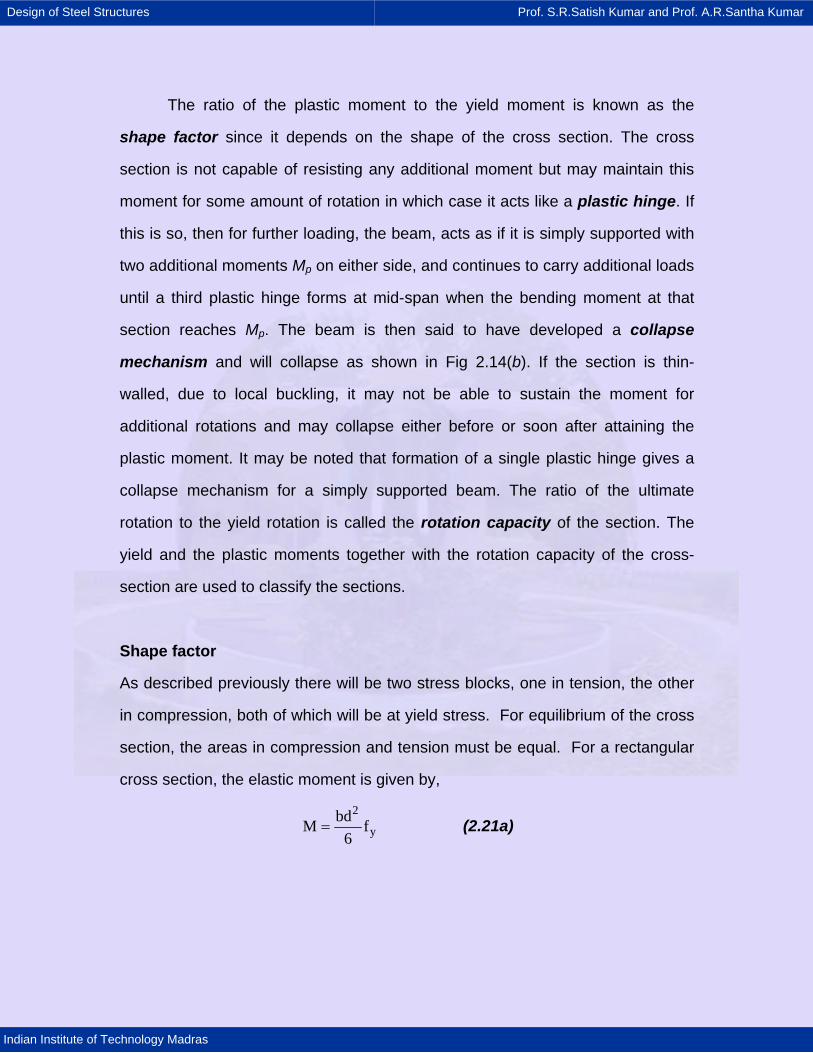
Shape factor
As described previously there will be two stress blocks, one in tension, the other
in compression, both of which will be at yield stress. For equilibrium of the cross
section, the areas in compression and tension must be equal. For a rectangular
cross section, the elastic moment is given by,
2
ybdM f
6= (2.21a)
Design of Steel Structures Prof. S.R.Satish Kumar and Prof. A.R.Santha Kumar
Indian Institute of Technology Madras
The plastic moment is obtained from,
2
p y yd d bdM 2.b. . .f f2 4 4
= = (2.21b)
Thus, for a rectangular section the plastic moment Mp is about 1.5 times
greater than the elastic moment capacity. For an I-section the value of shape
factor is about 1.12.
Theoretically, the plastic hinges are assumed to form at points at which
plastic rotations occur. Thus the length of a plastic hinge is considered as zero.
However, the values of moment, at the adjacent section of the yield zone are
more than the yield moment upto a certain length ∆L, of the structural member.
This length ∆L, is known as the hinged length. The hinged length depends upon
the type of loading and the geometry of the cross-section of the structural
member. The region of hinged length is known as region of yield or plasticity.
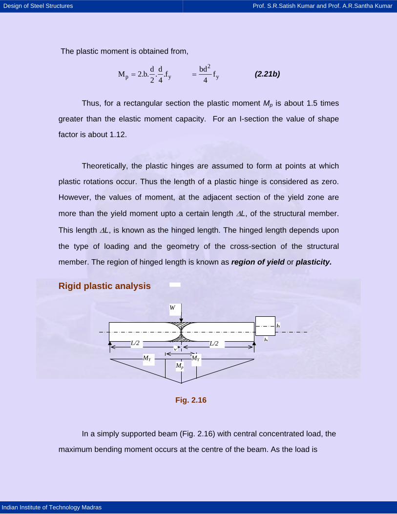
Rigid plastic analysis
Fig. 2.16
In a simply supported beam (Fig. 2.16) with central concentrated load, the
maximum bending moment occurs at the centre of the beam. As the load is
L/2 L/2
MY MYMp
W
xb
h
Design of Steel Structures Prof. S.R.Satish Kumar and Prof. A.R.Santha Kumar
Indian Institute of Technology Madras
increased gradually, this moment reaches the fully plastic moment of the section
Mp and a plastic hinge is formed at the centre.
Let x (= ∆L) be the length of plasticity zone.
From the bending moment diagram shown in Fig. 2.16
(L-x)Mp=LMy
x=L/3 (2.22)
Therefore the hinged length of the plasticity zone is equal to one-third of
the span in this case.
p
2 2
y p
2 2
y y y
y p
WlM4
bh bhf . Z4 4
bh bh 2M f . f .6 4 3
2M M3
=
⎛ ⎞= =⎜ ⎟⎜ ⎟
⎝ ⎠⎛ ⎞
= =⎜ ⎟⎜ ⎟⎝ ⎠
=
∵
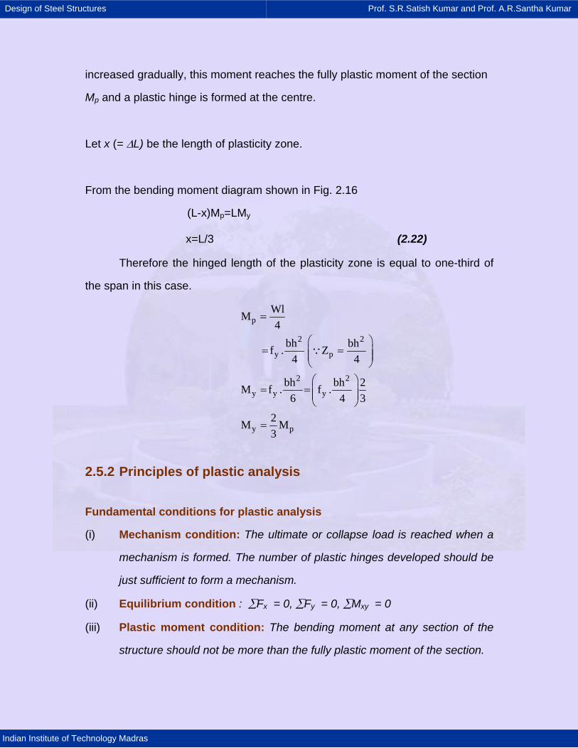
2.5.2 Principles of plastic analysis Fundamental conditions for plastic analysis
(i) Mechanism condition: The ultimate or collapse load is reached when a
mechanism is formed. The number of plastic hinges developed should be
just sufficient to form a mechanism.
(ii) Equilibrium condition : ∑Fx = 0, ∑Fy = 0, ∑Mxy = 0
(iii) Plastic moment condition: The bending moment at any section of the
structure should not be more than the fully plastic moment of the section.
Design of Steel Structures Prof. S.R.Satish Kumar and Prof. A.R.Santha Kumar
Indian Institute of Technology Madras
Collapse mechanisms
When a system of loads is applied to an elastic body, it will deform and will
show a resistance against deformation. Such a body is known as a structure. On
the other hand if no resistance is set up against deformation in the body, then it is
known as a mechanism.
Various types of independent mechanisms are identified to enable
prediction of possible failure modes of a structure.
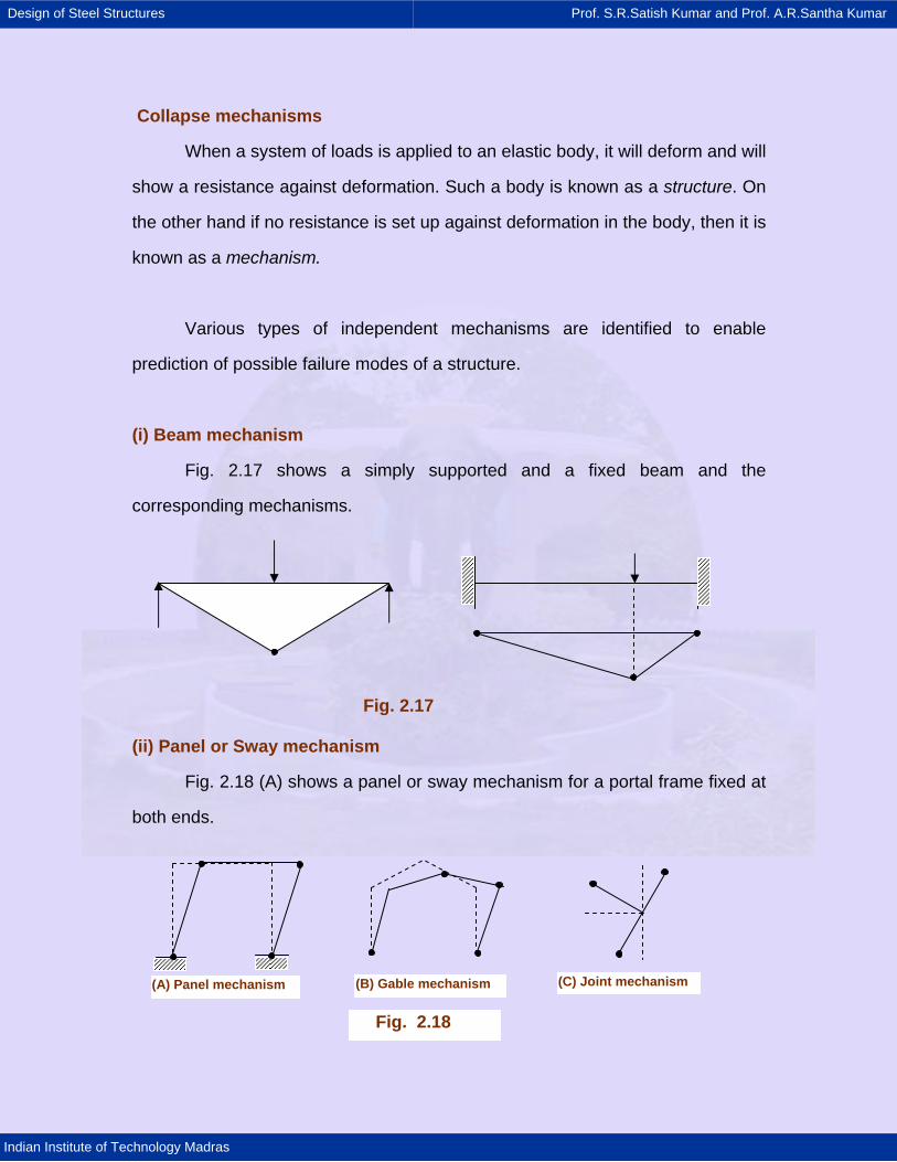
(i) Beam mechanism
Fig. 2.17 shows a simply supported and a fixed beam and the
corresponding mechanisms.
Fig. 2.17
(ii) Panel or Sway mechanism
Fig. 2.18 (A) shows a panel or sway mechanism for a portal frame fixed at
both ends.
(A) Panel mechanism (B) Gable mechanism (C) Joint mechanism
Fig. 2.18
Design of Steel Structures Prof. S.R.Satish Kumar and Prof. A.R.Santha Kumar
Indian Institute of Technology Madras
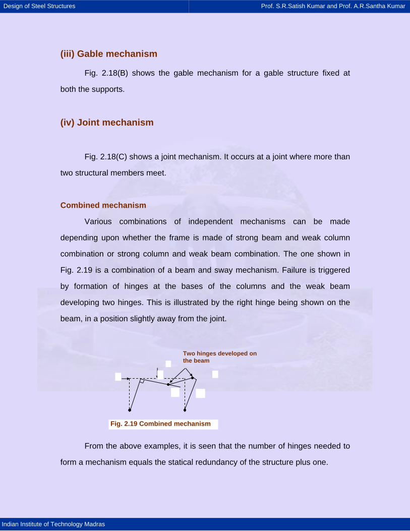
Fig. 2.19 Combined mechanism
Two hinges developed on the beam
(iii) Gable mechanism
Fig. 2.18(B) shows the gable mechanism for a gable structure fixed at
both the supports.
(iv) Joint mechanism
Fig. 2.18(C) shows a joint mechanism. It occurs at a joint where more than
two structural members meet.
Combined mechanism
Various combinations of independent mechanisms can be made
depending upon whether the frame is made of strong beam and weak column
combination or strong column and weak beam combination. The one shown in
Fig. 2.19 is a combination of a beam and sway mechanism. Failure is triggered
by formation of hinges at the bases of the columns and the weak beam
developing two hinges. This is illustrated by the right hinge being shown on the
beam, in a position slightly away from the joint.
From the above examples, it is seen that the number of hinges needed to
form a mechanism equals the statical redundancy of the structure plus one.
Design of Steel Structures Prof. S.R.Satish Kumar and Prof. A.R.Santha Kumar
Indian Institute of Technology Madras
Plastic load factor and theorems of plastic collapse
The plastic load factor at rigid plastic collapse (λp) is defined as the lowest
multiple of the design loads which will cause the whole structure, or any part of it
to become a mechanism.
In a limit state approach, the designer is seeking to ensure that at the
appropriate factored loads the structure will not fail. Thus the rigid plastic load
factor λp must not be less than unity.
The number of independent mechanisms (n) is related to the number of
possible plastic hinge locations (h) and the number of degree of redundancy (r)
of the frame by the equation.
n = h – r (2.23)
The three theorems of plastic collapse are given below.
Lower bound or Static theorem
A load factor (λs ) computed on the basis of an arbitrarily assumed
bending moment diagram which is in equilibrium with the applied loads and
where the fully plastic moment of resistance is nowhere exceeded will always be
less than or at best equal to the load factor at rigid plastic collapse, (λp). In other
words, λp is the highest value of λs which can be found.
Upper bound or Kinematic theorem
A load factor (λk) computed on the basis of an arbitrarily assumed
mechanism will always be greater than, or at best equal to the load factor at rigid
Design of Steel Structures Prof. S.R.Satish Kumar and Prof. A.R.Santha Kumar
Indian Institute of Technology Madras
plastic collapse (λp ). In other words, λp is the lowest value of λk which can be
found.
Uniqueness theorem
If both the above criteria are satisfied, then the resulting load factor
corresponds to its value at rigid plastic collapse (λp).
Mechanism method
In the mechanism or kinematics method of plastic analysis, various plastic
failure mechanisms are evaluated. The plastic collapse loads corresponding to
various failure mechanisms are obtained by equating the internal work at the
plastic hinges to the external work by loads during the virtual displacement. This
requires evaluation of displacements and plastic hinge rotations.
As the plastic deformations at collapse are considerably larger than elastic
ones, it is assumed that the frame remains rigid between supports and hinge
positions i.e. all plastic rotation occurs at the plastic hinges.
Considering a simply supported beam subjected to a point load at
midspan, the maximum strain will take place at the centre of the span where a
plastic hinge will be formed at yield of full section. The remainder of the beam
will remain straight, thus the entire energy will be absorbed by the rotation of the
plastic hinge.
Considering a centrally loaded simply supported beam at the instant of
plastic collapse (see Fig. 2.17)
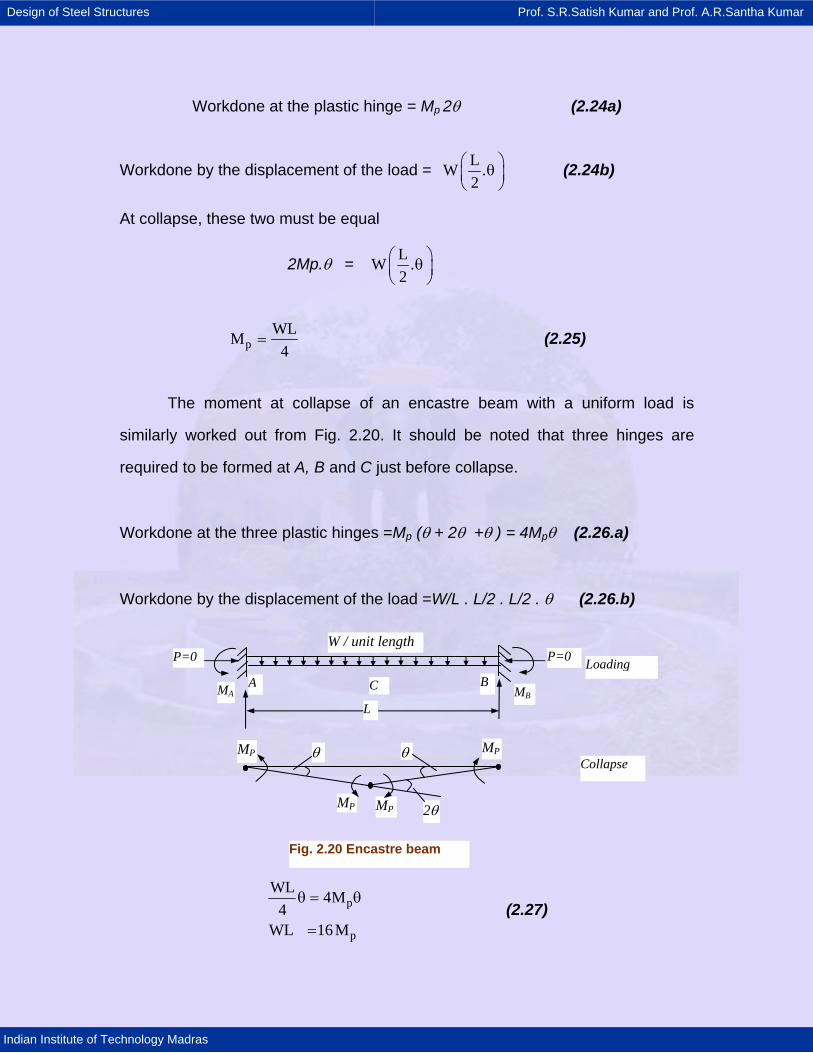
Design of Steel Structures Prof. S.R.Satish Kumar and Prof. A.R.Santha Kumar
Indian Institute of Technology Madras
Workdone at the plastic hinge = Mp 2θ (2.24a)
Workdone by the displacement of the load = LW .2
⎛ ⎞θ⎜ ⎟⎝ ⎠
(2.24b)
At collapse, these two must be equal
2Mp.θ = LW .2
⎛ ⎞θ⎜ ⎟⎝ ⎠
pWLM
4= (2.25)
The moment at collapse of an encastre beam with a uniform load is
similarly worked out from Fig. 2.20. It should be noted that three hinges are
required to be formed at A, B and C just before collapse.
Workdone at the three plastic hinges =Mp (θ + 2θ +θ ) = 4Mpθ (2.26.a)
Workdone by the displacement of the load =W/L . L/2 . L/2 . θ (2.26.b)
p
p
WL 4M4
WL 16M
θ = θ
= (2.27)
P=0 P=0
MBA BC
W / unit length
L
Loading
MPMP
MP MP
θθ
2θ
Collapse
Fig. 2.20 Encastre beam
MA
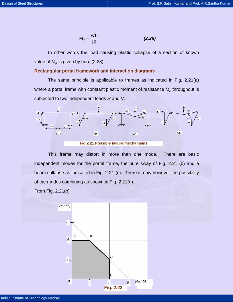
Design of Steel Structures Prof. S.R.Satish Kumar and Prof. A.R.Santha Kumar
Indian Institute of Technology Madras
pWLM16
= (2.28)
In other words the load causing plastic collapse of a section of known
value of Mp is given by eqn. (2.28).
Rectangular portal framework and interaction diagrams
The same principle is applicable to frames as indicated in Fig. 2.21(a)
where a portal frame with constant plastic moment of resistance Mp throughout is
subjected to two independent loads H and V.
This frame may distort in more than one mode. There are basic
independent modes for the portal frame, the pure sway of Fig. 2.21 (b) and a
beam collapse as indicated in Fig. 2.21 (c). There is now however the possibility
of the modes combining as shown in Fig. 2.21(d).
From Fig. 2.21(b)
Fig. 2.22 0 2 4 6
2
4
6
Va / Mp
H a / M p
A B
C
D
Ha / Mp
H
a a
a
V
(a)
H
θθ θ
θ
V
(b
HV
(c)
θ θ2θ
Fig.2.21 Possible failure mechanisms
(d)
H
θ
θ
θθ
V
2θ

Design of Steel Structures Prof. S.R.Satish Kumar and Prof. A.R.Santha Kumar
Indian Institute of Technology Madras
Work done in hinges = 4 Mpθ
Work done by loads = Haθ
At incipient collapse Ha /Mp= 4 (2.29)
From Fig. 2.21 (c)
Work done in hinges = 4 Mpθ
Work done by loads = Vaθ
At incipient collapse = Va / Mp = 4 (2.30)
From Fig. 2.21(d)
Work done in hinges = 6 Mpθ
Work done by loads = Haθ + Vaθ
At incipient collapse Ha / Mp + Va / Mp = 6 (2.31)
The resulting equations, which represent the collapse criteria, are plotted
on the interaction diagram of Fig. 2.22. Since any line radiating from the origin
represents proportional loading, the first mechanism line intersected represents
failure. The failure condition is therefore the line ABCD and any load condition
within the area OABCD is therefore safe.
Stability
For plastically designed frames three stability criteria have to be considered
for ensuring the safety of the frame. These are
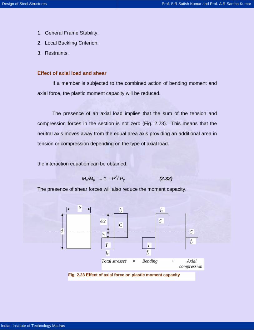
Design of Steel Structures Prof. S.R.Satish Kumar and Prof. A.R.Santha Kumar
Indian Institute of Technology Madras
1. General Frame Stability.
2. Local Buckling Criterion.
3. Restraints.
Effect of axial load and shear
If a member is subjected to the combined action of bending moment and
axial force, the plastic moment capacity will be reduced.
The presence of an axial load implies that the sum of the tension and
compression forces in the section is not zero (Fig. 2.23). This means that the
neutral axis moves away from the equal area axis providing an additional area in
tension or compression depending on the type of axial load.
the interaction equation can be obtained:
Mx/Mp = 1 – P2/ Py (2.32)
The presence of shear forces will also reduce the moment capacity.
Fig. 2.23 Effect of axial force on plastic moment capacity
C
C
Tfy
fy
fy
Total stresses = Bending + Axial compression
b
d C
T fy
fy
d/2
y1
Design of Steel Structures Prof. S.R.Satish Kumar and Prof. A.R.Santha Kumar
Indian Institute of Technology Madras
Plastic analysis for more than one condition of loading
When more than one condition of loading can be applied to a beam or
structure, it may not always be obvious which is critical. It is necessary then to
perform separate calculations, one for each loading condition, the section being
determined by the solution requiring the largest plastic moment.
Unlike the elastic method of design in which moments produced by
different loading systems can be added together, plastic moments obtained by
different loading systems cannot be combined, i.e. the plastic moment calculated
for a given set of loads is only valid for that loading condition. This is because the
'Principle of Superposition' becomes invalid when parts of the structure have
yielded.
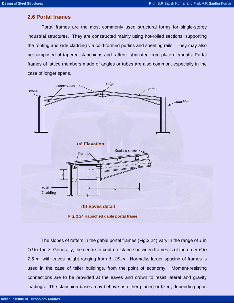
Design of Steel Structures Prof. S.R.Satish Kumar and Prof. A.R.Santha Kumar
Indian Institute of Technology Madras
2.6 Portal frames
Portal frames are the most commonly used structural forms for single-storey
industrial structures. They are constructed mainly using hot-rolled sections, supporting
the roofing and side cladding via cold-formed purlins and sheeting rails. They may also
be composed of tapered stanchions and rafters fabricated from plate elements. Portal
frames of lattice members made of angles or tubes are also common, especially in the
case of longer spans.
The slopes of rafters in the gable portal frames (Fig.2.24) vary in the range of 1 in
10 to 1 in 3. Generally, the centre-to-centre distance between frames is of the order 6 to
7.5 m, with eaves height ranging from 6 -15 m. Normally, larger spacing of frames is
used in the case of taller buildings, from the point of economy. Moment-resisting
connections are to be provided at the eaves and crown to resist lateral and gravity
loadings. The stanchion bases may behave as either pinned or fixed, depending upon
Fig. 2.24 Haunched gable portal frame
a
b
(b) Eaves detail
connections
(a) Elevation
ridge
eaves rafter
stanchion
PurlinsRoofing sheets
Wall Cladding
Design of Steel Structures Prof. S.R.Satish Kumar and Prof. A.R.Santha Kumar
Indian Institute of Technology Madras
rotational restraint provided by the foundation and the connection detail between the
stanchion and foundations. The foundation restraint depends on the type of foundation
and modulus of the sub-grade. Frames with pinned bases are heavier than those
having fixity at the bases. However, frames with fixed base may require a more
expensive foundation.
For the design of portal frames, plastic methods of analysis are mainly used,
which allows the engineer to analyse frames easily and design it economically. The
basis of the plastic analysis method is the need to determine the load that can be
applied to the frame so that the failure of the frame occurs as a mechanism by the
formation of a number of plastic hinges within the frame. The various methods of plastic
analysis are discussed later.
The most common form of portal frame used in the construction industry is the
pinned-base frame with different rafter and column member size and with haunches at
both the eaves and apex connections (Fig.2.24).
Due to transportation requirements, field joints are introduced at suitable
positions. As a result, connections are usually located at positions of high moment, i.e.
at the interface of the column and rafter members (at the eaves) and also between the
rafter members at the apex (ridge) (See Fig.2.24). It is very difficult to develop sufficient
moment capacity at these connections by providing 'tension' bolts located solely within
the small depth of the rafter section. Therefore the lever arm of the bolt group is usually
increased by haunching the rafter members at the joints. This addition increases the
section strength.

Design of Steel Structures Prof. S.R.Satish Kumar and Prof. A.R.Santha Kumar
Indian Institute of Technology Madras
2.6.1 General design procedure
The steps in the plastic design of portals, according to SP: 6(6) – 1972, are given
below:
a) Determine possible loading conditions.
b) Compute the factored design load combination(s).
c) Estimate the plastic moment ratios of frame members.
d) Analyse the frame for each loading condition and calculate the maximum required
plastic moment capacity, Mp
e) Select the section, and
f) Check the design for other secondary modes of failure (IS: 800-1984).
The design commences with determination of possible loading conditions, in which
decisions such as, whether to treat the distributed loads as such or to consider them as
equivalent concentrated loads, are to be made. It is often convenient to deal with
equivalent concentrated loads in computer aided and plastic analysis methods.
In step (b), the loads determined in (a) are multiplied by the appropriate load factors
to assure the needed margin of safety. This load factor is selected in such a way that
the real factor of safety for any structure is at least as great as that decided upon by the
designer. The load factors to be used for various load combinations are presented in an
earlier chapter on Limit states method.
The step (c) is to make an assumption regarding the ratio of the plastic moment
capacities of the column and rafter, the frame members. Optimum plastic design
methods present a direct way of arriving at these ratios, so as to obtain an optimum
value of this ratio. The following simpler procedure may be adopted for arriving at the
ratio.
Design of Steel Structures Prof. S.R.Satish Kumar and Prof. A.R.Santha Kumar
Indian Institute of Technology Madras
(i) Determine the absolute plastic moment value for separate loading conditions.
(Assume that all joints are fixed against rotation, but the frame is free to sway).
For beams, solve the beam mechanism equation and for columns, solve the panel
(sway) mechanism equation. These are done for all loading combinations. The
moments thus obtained are the absolute minimum plastic moment values. The actual
section moment will be greater than or at least equal to these values.
(ii) Now select plastic moment ratios using the following guidelines.
• At joints establish equilibrium.
• For beams use the ratio determined in step (i)
• For columns use the corner connection moments Mp (Col) = Mp (beam)
In the step (d) each loading condition is analysed by a plastic analysis method for
arriving at the minimum required Mp. Based on this moment, select the appropriate
sections in step (e). The step (f) is to check the design according to secondary design
considerations discussed in the following sections (IS: 800-1984).
2.6.2 Secondary design considerations
The 'simple plastic theory' neglects the effects of axial force, shear and buckling on
the member strength. So checks must be carried out for the following factors.
a) Reductions in the plastic moment due to the effect of axial force and shear force.
b) Instability due to local buckling, lateral buckling and column buckling.
c) Brittle fracture.
d) Deflection at service loads.
In addition, proper design of connections is needed in order that the plastic moments
can be developed at the plastic hinge locations.
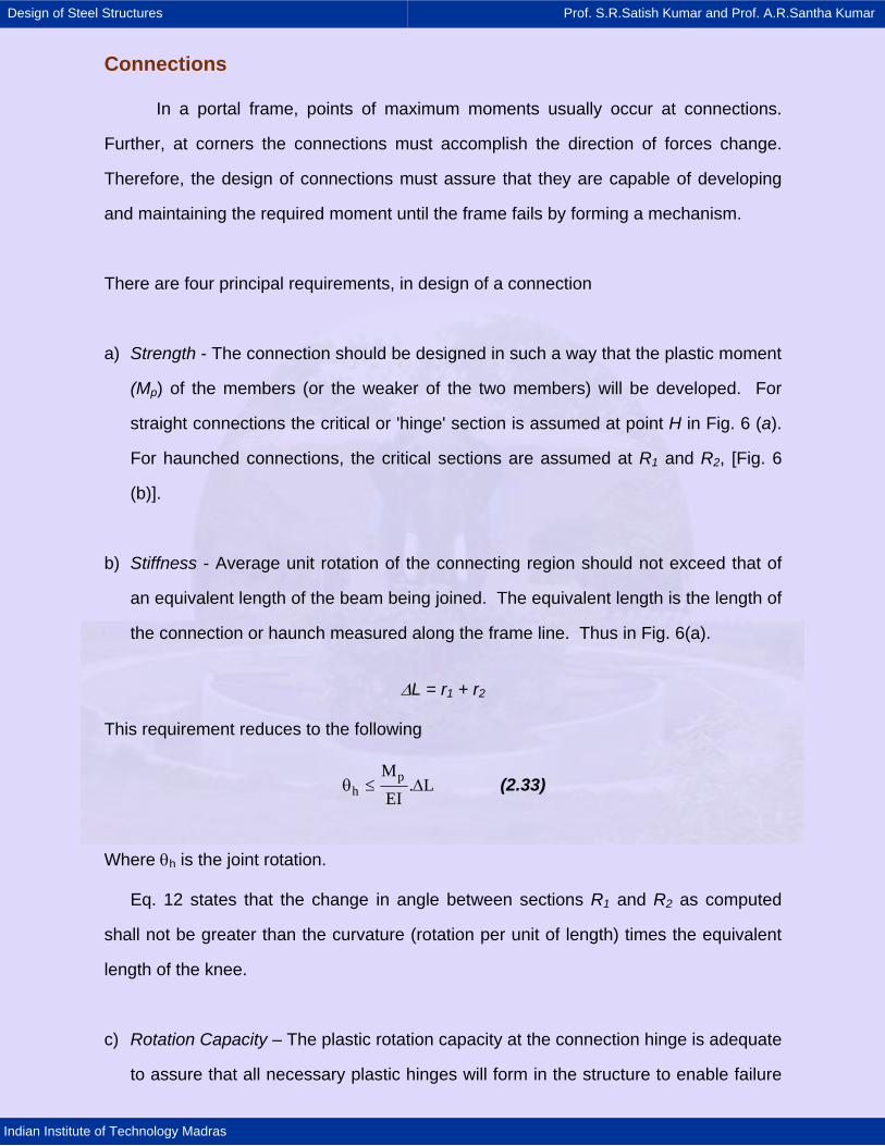
Design of Steel Structures Prof. S.R.Satish Kumar and Prof. A.R.Santha Kumar
Indian Institute of Technology Madras
Connections
In a portal frame, points of maximum moments usually occur at connections.
Further, at corners the connections must accomplish the direction of forces change.
Therefore, the design of connections must assure that they are capable of developing
and maintaining the required moment until the frame fails by forming a mechanism.
There are four principal requirements, in design of a connection
a) Strength - The connection should be designed in such a way that the plastic moment
(Mp) of the members (or the weaker of the two members) will be developed. For
straight connections the critical or 'hinge' section is assumed at point H in Fig. 6 (a).
For haunched connections, the critical sections are assumed at R1 and R2, [Fig. 6
(b)].
b) Stiffness - Average unit rotation of the connecting region should not exceed that of
an equivalent length of the beam being joined. The equivalent length is the length of
the connection or haunch measured along the frame line. Thus in Fig. 6(a).
∆L = r1 + r2
This requirement reduces to the following
ph
M. L
EIθ ≤ ∆ (2.33)
Where θh is the joint rotation.
Eq. 12 states that the change in angle between sections R1 and R2 as computed
shall not be greater than the curvature (rotation per unit of length) times the equivalent
length of the knee.
c) Rotation Capacity – The plastic rotation capacity at the connection hinge is adequate
to assure that all necessary plastic hinges will form in the structure to enable failure
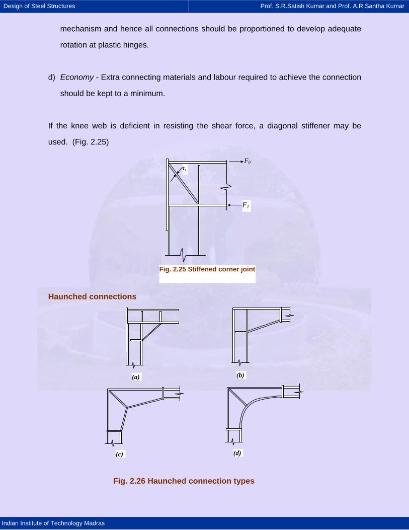
Design of Steel Structures Prof. S.R.Satish Kumar and Prof. A.R.Santha Kumar
Indian Institute of Technology Madras
mechanism and hence all connections should be proportioned to develop adequate
rotation at plastic hinges.
d) Economy - Extra connecting materials and labour required to achieve the connection
should be kept to a minimum.
If the knee web is deficient in resisting the shear force, a diagonal stiffener may be
used. (Fig. 2.25)
Haunched connections
F0ts
F1
Fig. 2.25 Stiffened corner joint
(a) (b)
(c) (d)
Fig. 2.26 Haunched connection types

Design of Steel Structures Prof. S.R.Satish Kumar and Prof. A.R.Santha Kumar
Indian Institute of Technology Madras
Some of the typical haunched connections are shown in Fig. 2.26. Haunched
connections are to be proportioned to develop plastic moment at the junction between
the rolled steel section and the haunch. In order to force formation of hinge at the end
of a tapered haunch (Fig. 2.26), make the flange thickness in the haunch, to be 50
percent greater than that of section joined. Check the shear resistance of the web to
ensure Mp governs the strength.
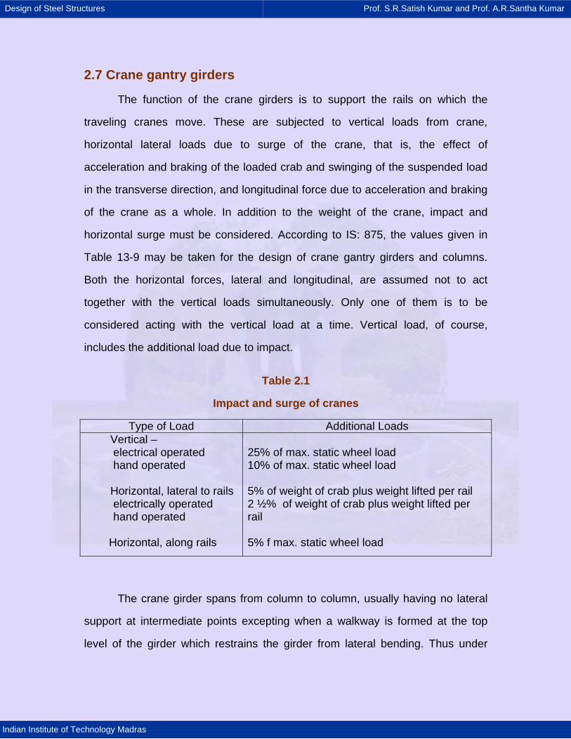
Design of Steel Structures Prof. S.R.Satish Kumar and Prof. A.R.Santha Kumar
Indian Institute of Technology Madras
2.7 Crane gantry girders
The function of the crane girders is to support the rails on which the
traveling cranes move. These are subjected to vertical loads from crane,
horizontal lateral loads due to surge of the crane, that is, the effect of
acceleration and braking of the loaded crab and swinging of the suspended load
in the transverse direction, and longitudinal force due to acceleration and braking
of the crane as a whole. In addition to the weight of the crane, impact and
horizontal surge must be considered. According to IS: 875, the values given in
Table 13-9 may be taken for the design of crane gantry girders and columns.
Both the horizontal forces, lateral and longitudinal, are assumed not to act
together with the vertical loads simultaneously. Only one of them is to be
considered acting with the vertical load at a time. Vertical load, of course,
includes the additional load due to impact.
Table 2.1
Impact and surge of cranes
Type of Load Additional Loads Vertical –
electrical operated hand operated
Horizontal, lateral to rails electrically operated hand operated
Horizontal, along rails
25% of max. static wheel load 10% of max. static wheel load 5% of weight of crab plus weight lifted per rail 2 ½% of weight of crab plus weight lifted per rail 5% f max. static wheel load
The crane girder spans from column to column, usually having no lateral
support at intermediate points excepting when a walkway is formed at the top
level of the girder which restrains the girder from lateral bending. Thus under
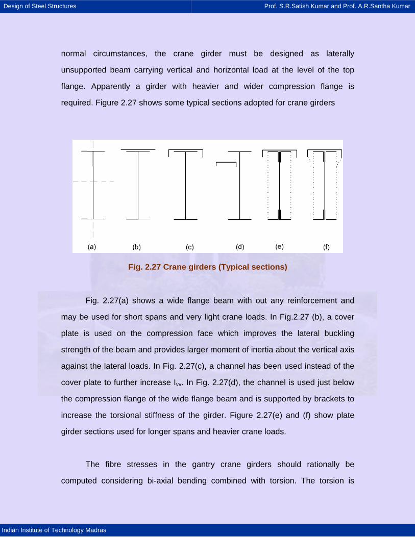
Design of Steel Structures Prof. S.R.Satish Kumar and Prof. A.R.Santha Kumar
Indian Institute of Technology Madras
normal circumstances, the crane girder must be designed as laterally
unsupported beam carrying vertical and horizontal load at the level of the top
flange. Apparently a girder with heavier and wider compression flange is
required. Figure 2.27 shows some typical sections adopted for crane girders
Fig. 2.27 Crane girders (Typical sections)
Fig. 2.27(a) shows a wide flange beam with out any reinforcement and
may be used for short spans and very light crane loads. In Fig.2.27 (b), a cover
plate is used on the compression face which improves the lateral buckling
strength of the beam and provides larger moment of inertia about the vertical axis
against the lateral loads. In Fig. 2.27(c), a channel has been used instead of the
cover plate to further increase Ivv. In Fig. 2.27(d), the channel is used just below
the compression flange of the wide flange beam and is supported by brackets to
increase the torsional stiffness of the girder. Figure 2.27(e) and (f) show plate
girder sections used for longer spans and heavier crane loads.
The fibre stresses in the gantry crane girders should rationally be
computed considering bi-axial bending combined with torsion. The torsion is
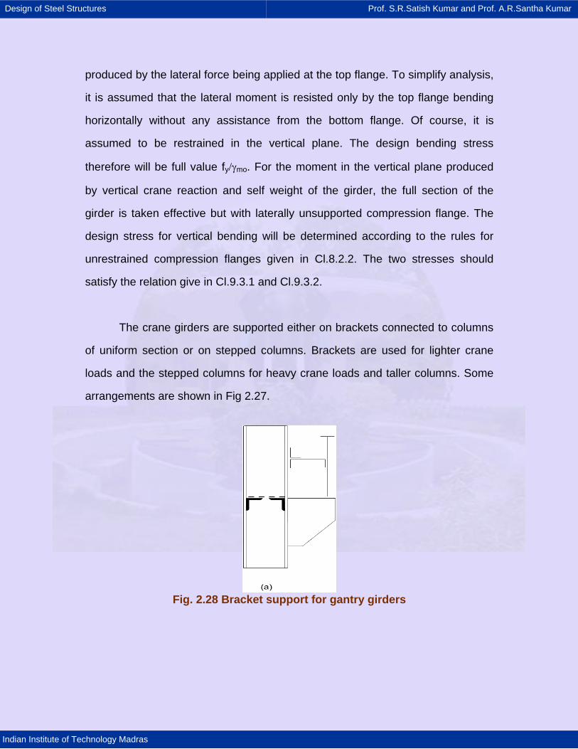
Design of Steel Structures Prof. S.R.Satish Kumar and Prof. A.R.Santha Kumar
Indian Institute of Technology Madras
produced by the lateral force being applied at the top flange. To simplify analysis,
it is assumed that the lateral moment is resisted only by the top flange bending
horizontally without any assistance from the bottom flange. Of course, it is
assumed to be restrained in the vertical plane. The design bending stress
therefore will be full value fy/γmo. For the moment in the vertical plane produced
by vertical crane reaction and self weight of the girder, the full section of the
girder is taken effective but with laterally unsupported compression flange. The
design stress for vertical bending will be determined according to the rules for
unrestrained compression flanges given in Cl.8.2.2. The two stresses should
satisfy the relation give in Cl.9.3.1 and Cl.9.3.2.
The crane girders are supported either on brackets connected to columns
of uniform section or on stepped columns. Brackets are used for lighter crane
loads and the stepped columns for heavy crane loads and taller columns. Some
arrangements are shown in Fig 2.27.
Fig. 2.28 Bracket support for gantry girders
Design of Steel Structures Prof. S.R.Satish Kumar and Prof. A.R.Santha Kumar
Indian Institute of Technology Madras
The girder is supported on a suitably formed seat and it is also connected
to the column near the top flange in each case in order to restrain it from lateral
bending and twisting at the support point. In Fig. 2.28(a), a channel has been
used for this purpose. To permit longitudinal movement, due to temperature and
deflection, slotted holes are used to connect the channel with the column. In Fig.
2.28 (b) and (c) vertical plates have been employed for providing the restraint.
Since such plates are flexible for horizontal bending no slotted holes are
necessary. Where roof leg and crane leg are provided separately in a built-up
column as shown at (c), the two legs are properly braced together to act as one
piece. The bracing is designed to take 2 ½% of column load plus shear due to
bending under crane loan and wind. The load of roof leg and crane are eccentric
to the combined column axis and should be considered as such.
The crane columns must be properly braced in the longitudinal direction of
the crane girders to be able to take the longitudinal forces due to crane. Such
brancing may be provided every fourth or fifth bay. In other bays, struts must be
used to transmit the longitudinal force to the bracing frame.
Design of Steel Structures Prof. S.R.Satish Kumar and Prof. A.R.Santha Kumar
Indian Institute of Technology Madras
2.8 Design for wind action
The wind pressure on a structure depends on the location of the structure,
height of structure above the ground level and also on the shape of the structure.
The code gives the basic wind pressure for the structures in various parts of the
country. Both the wind pressures viz. including wind of short duration and
excluding wind of short duration, have been given. All structures should be
designed for the short duration wind.
For buildings upto 10m in height, the intensity of wind pressure, as
specified in the code, may be reduced by 25% for stability calculations and for
the design of framework as well as cladding. For buildings over 10m and upto 30
m height, this reduction can be made for stability calculations and for design of
columns only.
The total pressure on the walls or roof of an industrial building will depend
on the external wind pressure and also on internal wind pressure. The internal
wind pressure depends on the permeability of the buildings. For buildings having
a small degree of permeability, the internal air pressure may be neglected. In the
case of buildings with normal permeability the internal pressure can be ± 0.2p.
Here ‘+’ indicates pressure and ‘-‘ suction, ‘p’ is the basic wind pressure. If a
building has openings larger than 20% of the wind pressure. If a building has
openings larger than 20% of the wall area, the internal air pressure will be ±0.5 p.
(a) Wind pressure on walls The wind pressure per unit area ‘p’ on the wall is taken as 0.5p pressure on
windward surface and 0.5p suction on leeward surface. When the walls form an
enclosure, the windward wall will be subjected to a pressure of 0.5p and leeward
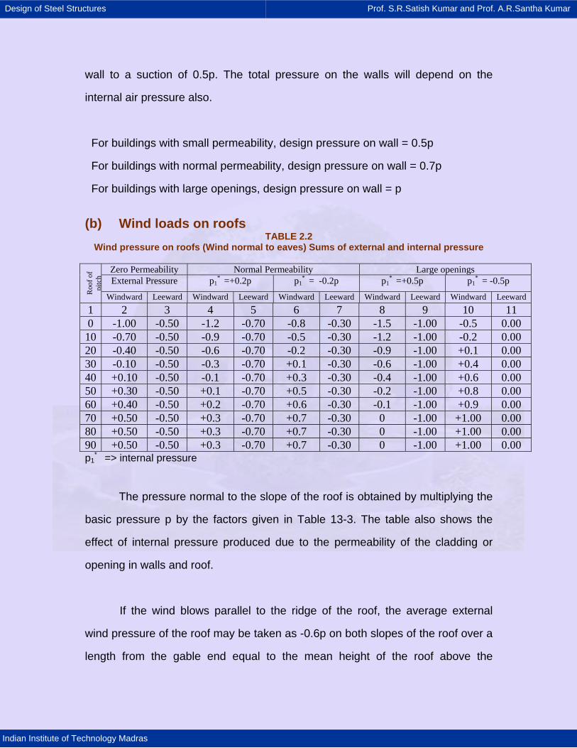
Design of Steel Structures Prof. S.R.Satish Kumar and Prof. A.R.Santha Kumar
Indian Institute of Technology Madras
wall to a suction of 0.5p. The total pressure on the walls will depend on the
internal air pressure also.
For buildings with small permeability, design pressure on wall = 0.5p
For buildings with normal permeability, design pressure on wall = 0.7p
For buildings with large openings, design pressure on wall = p
(b) Wind loads on roofs
TABLE 2.2 Wind pressure on roofs (Wind normal to eaves) Sums of external and internal pressure
Zero Permeability Normal Permeability Large openings External Pressure p1
* =+0.2p p1* = -0.2p p1
* =+0.5p p1* = -0.5p
Roo
f of
pitc
h
Windward Leeward Windward Leeward Windward Leeward Windward Leeward Windward Leeward
1 2 3 4 5 6 7 8 9 10 11 0 -1.00 -0.50 -1.2 -0.70 -0.8 -0.30 -1.5 -1.00 -0.5 0.00 10 -0.70 -0.50 -0.9 -0.70 -0.5 -0.30 -1.2 -1.00 -0.2 0.00 20 -0.40 -0.50 -0.6 -0.70 -0.2 -0.30 -0.9 -1.00 +0.1 0.00 30 -0.10 -0.50 -0.3 -0.70 +0.1 -0.30 -0.6 -1.00 +0.4 0.00 40 +0.10 -0.50 -0.1 -0.70 +0.3 -0.30 -0.4 -1.00 +0.6 0.00 50 +0.30 -0.50 +0.1 -0.70 +0.5 -0.30 -0.2 -1.00 +0.8 0.00 60 +0.40 -0.50 +0.2 -0.70 +0.6 -0.30 -0.1 -1.00 +0.9 0.00 70 +0.50 -0.50 +0.3 -0.70 +0.7 -0.30 0 -1.00 +1.00 0.00 80 +0.50 -0.50 +0.3 -0.70 +0.7 -0.30 0 -1.00 +1.00 0.00 90 +0.50 -0.50 +0.3 -0.70 +0.7 -0.30 0 -1.00 +1.00 0.00 p1
* => internal pressure
The pressure normal to the slope of the roof is obtained by multiplying the
basic pressure p by the factors given in Table 13-3. The table also shows the
effect of internal pressure produced due to the permeability of the cladding or
opening in walls and roof.
If the wind blows parallel to the ridge of the roof, the average external
wind pressure of the roof may be taken as -0.6p on both slopes of the roof over a
length from the gable end equal to the mean height of the roof above the
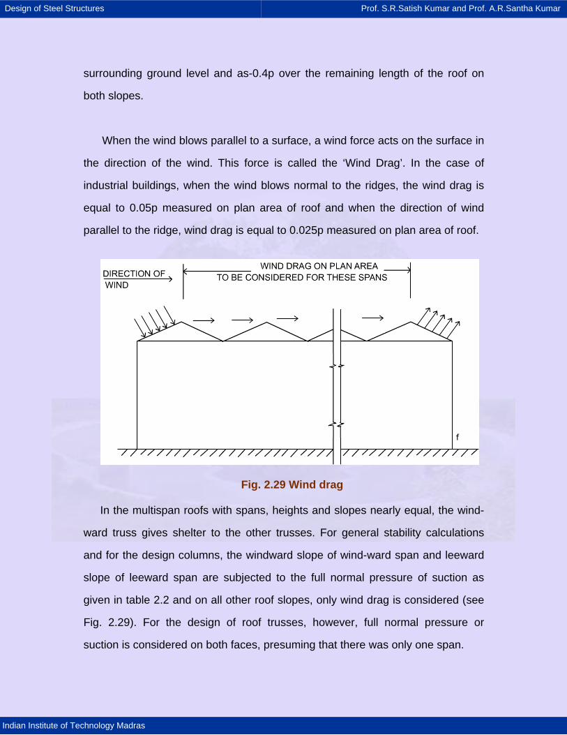
Design of Steel Structures Prof. S.R.Satish Kumar and Prof. A.R.Santha Kumar
Indian Institute of Technology Madras
surrounding ground level and as-0.4p over the remaining length of the roof on
both slopes.
When the wind blows parallel to a surface, a wind force acts on the surface in
the direction of the wind. This force is called the ‘Wind Drag’. In the case of
industrial buildings, when the wind blows normal to the ridges, the wind drag is
equal to 0.05p measured on plan area of roof and when the direction of wind
parallel to the ridge, wind drag is equal to 0.025p measured on plan area of roof.
Fig. 2.29 Wind drag
In the multispan roofs with spans, heights and slopes nearly equal, the wind-
ward truss gives shelter to the other trusses. For general stability calculations
and for the design columns, the windward slope of wind-ward span and leeward
slope of leeward span are subjected to the full normal pressure of suction as
given in table 2.2 and on all other roof slopes, only wind drag is considered (see
Fig. 2.29). For the design of roof trusses, however, full normal pressure or
suction is considered on both faces, presuming that there was only one span.
Design of Steel Structures Prof. S.R.Satish Kumar and Prof. A.R.Santha Kumar
Indian Institute of Technology Madras
The wind pressures given above are the average pressures on a roof slope.
For designing the roof sheeting or the fastenings of roof sheeting, we may take a
larger wind pressure because these pressures may considerably exceed the
average value on small areas. For designing roof sheeting and its fastenings, the
values given in Table 2.2 may be increased numerically by 0.3p. In a distance
equal to 15% of the length of the roof from the gable ends, fastenings should be
capable of resisting a section of 2.0p on the area of the roof sheeting them
support.
Design of Steel Structures Prof. S.R.Satish Kumar and Prof. A.R.Santha Kumar
Indian Institute of Technology Madras
2.9 Design for earthquake action
Single storey industrial buildings are usually governed by wind loads rather than
earthquake loads. This is because their roofs and walls are light in weight and often
pitched or sloping and also because the buildings are permeable to wind which results
in uplift of the roof. However, it is always safe to check any building for both wind and
earthquakes.
Earthquake loading is different from wind loading in several respects and so
earthquake design is also quite different from design for wind and other gravity loads.
Severe earthquakes impose very high loads and so the usual practice is to ensure
elastic behaviour under moderate earthquake and provide ductility to cater for severe
earthquakes. Steel is inherently ductile and so only the calculation of loads due to
moderate earthquake is considered. This can be done as per the IS 1893 code.
According to this code, a horizontal seismic coefficient times the weight of the structure
should be applied as equivalent static earthquake load and the structure should be
checked for safety under this load in combination with other loads as specified in IS
800. The combinations are as follows:
1. 1.5 (DL + IL)
2. 1.2 (DL + IL + EL)
3. 1.5 (DL + EL)
4. 0.9 DL + 1.5 EL
The horizontal seismic coefficient Ah takes into account the location of the structure
by means of a zone factor Z, the importance of the structure by means of a factor I and
the ductility by means of a factor R. It also considers the flexibility of the structure-
foundation system by means of an acceleration ratio Sa/g , which is a function of the
natural time period T. This last ratio is given in the form of a graph known as the
response spectrum. The horizontal seismic coefficient Ah is given by
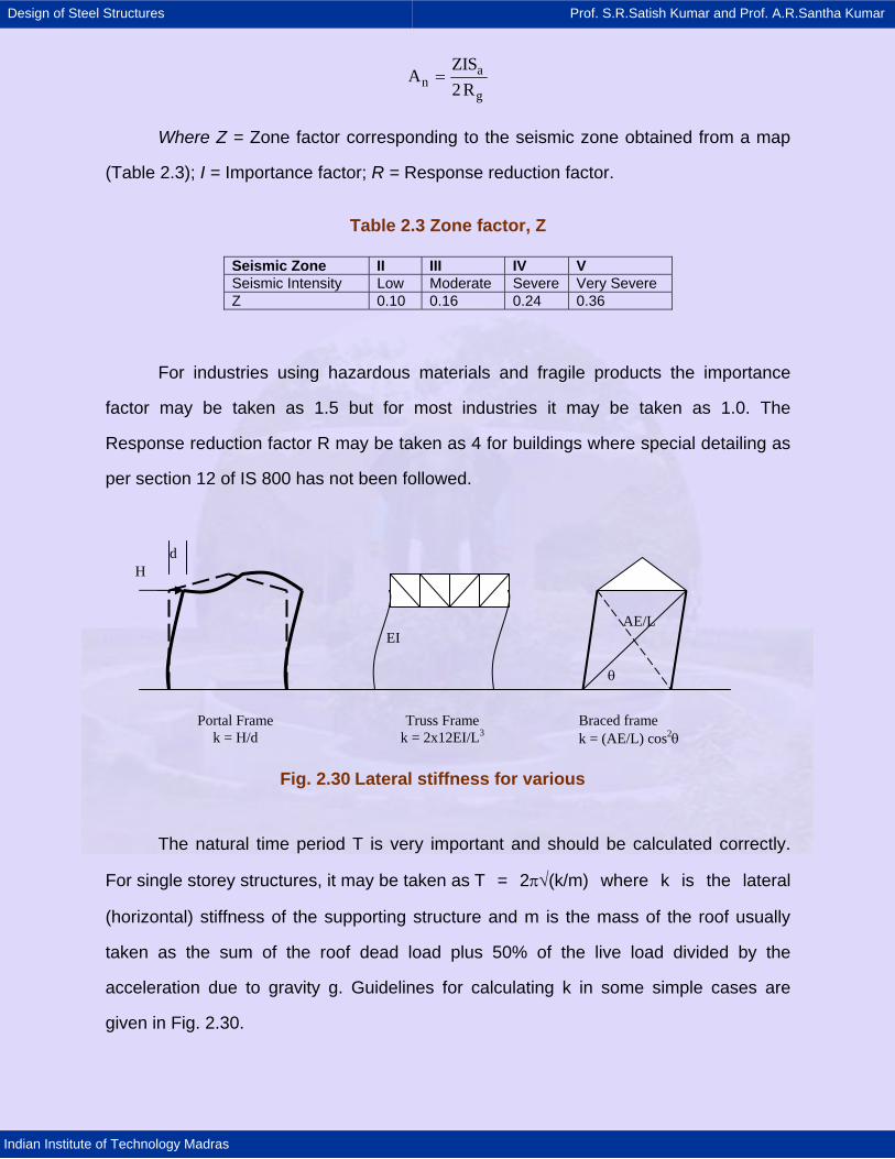
Design of Steel Structures Prof. S.R.Satish Kumar and Prof. A.R.Santha Kumar
Indian Institute of Technology Madras
an
g
ZISA
2 R=
Where Z = Zone factor corresponding to the seismic zone obtained from a map
(Table 2.3); I = Importance factor; R = Response reduction factor.
Table 2.3 Zone factor, Z
Seismic Zone II III IV V Seismic Intensity Low Moderate Severe Very Severe Z 0.10 0.16 0.24 0.36
For industries using hazardous materials and fragile products the importance
factor may be taken as 1.5 but for most industries it may be taken as 1.0. The
Response reduction factor R may be taken as 4 for buildings where special detailing as
per section 12 of IS 800 has not been followed.
The natural time period T is very important and should be calculated correctly.
For single storey structures, it may be taken as T = 2π√(k/m) where k is the lateral
(horizontal) stiffness of the supporting structure and m is the mass of the roof usually
taken as the sum of the roof dead load plus 50% of the live load divided by the
acceleration due to gravity g. Guidelines for calculating k in some simple cases are
given in Fig. 2.30.
H d
Portal Frame k = H/d
Truss Frame k = 2x12EI/L3
EI AE/L
θ
Braced frame k = (AE/L) cos2θ
Fig. 2.30 Lateral stiffness for various
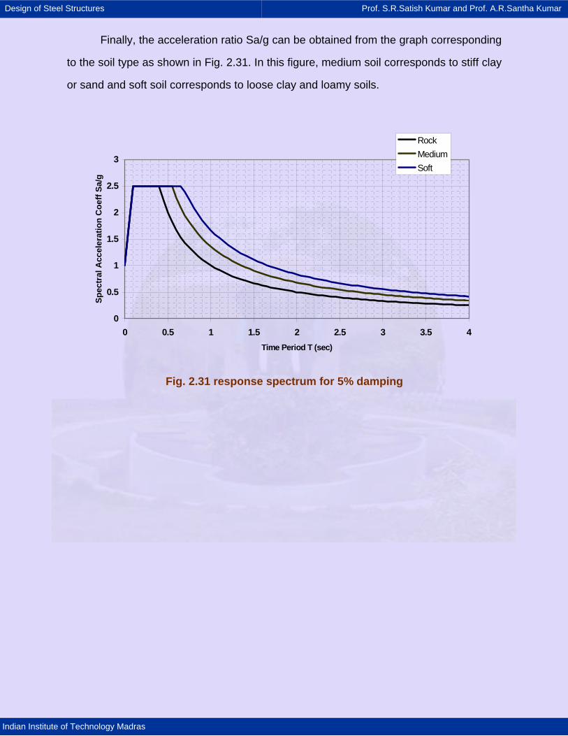
Design of Steel Structures Prof. S.R.Satish Kumar and Prof. A.R.Santha Kumar
Indian Institute of Technology Madras
Finally, the acceleration ratio Sa/g can be obtained from the graph corresponding
to the soil type as shown in Fig. 2.31. In this figure, medium soil corresponds to stiff clay
or sand and soft soil corresponds to loose clay and loamy soils.
0
0.5
1
1.5
2
2.5
3
0 0.5 1 1.5 2 2.5 3 3.5 4Time Period T (sec)
Spec
tral
Acc
eler
atio
n C
oeff
Sa/g
RockMediumSoft
Fig. 2.31 response spectrum for 5% damping
Design of Steel Structures Prof. S.R.Satish Kumar and Prof. A.R.Santha Kumar
Indian Institute of Technology Madras
2.10 Summary
In this chapter, initially the structural and functional requirements of
industrial buildings were described. The loads to be considered were mentioned
and then the floor and roof systems were explained. In particular, the steel-
concrete composite slab using profiled deck sheets was explained along with the
design methods. The topic of roof trusses was covered in detail.
The basic concepts of Plastic Analysis were discussed and the methods of
computation of ultimate load causing plastic collapse were outlined. Theorems of
plastic collapse and alternative patterns of hinge formation triggering plastic
collapse have been discussed. The use of plastic analysis and design of steel
portal frames for single storey industrial buildings was discussed.
The calculation of wind and earthquake loads was also described.
Design of Steel Structures Prof. S.R.Satish Kumar and Prof. A.R.Santha Kumar
Indian Institute of Technology Madras
2.11 References Teaching resources for structural Steel Design (Volume 1 to 3), INSDAG
publication, Calcutta 2000.
R.P. Johnson “Composite Structures of Steel and Concrete” Volume 1,
Blackwell Scientific Publications, UK, 1994.
R.M. Lawson, D.L Mullett and FPD Ward “Good practice in Composite
floor Construction”. The Steel Construction Institute, 1990.
Mark Lawson and Peter Wickens “Composite Deck Slab”, Steel Designers
Manual (Fifth edition), The Steel Construction Institute, UK, 1992.
Anon “Constructional Steel Design: An International Guide”, Elsevier,
London, 1993.
Vallenilla, C.R., and Bjorhovde, R., “Effective Width Criteria for Composite
Beams”, Engineering Journal, AISC, Fourth Quarter, 1985, pp. 169-175.
Clarke, A. B. and Coverman, S. H. Structural Steelwork, Limit state
design, Chapman and Hall Ltd, London, 1987.
Horne, M. R. Plastic Theory of Structures, Pergamon Press Ltd, Oxford,
1979.
Introduction to Steelwork Design to BS 5950: Part 1, The Steel
Construction Institute, 1988.
Design of Steel Structures Prof. S.R.Satish Kumar and Prof. A.R.Santha Kumar
Indian Institute of Technology Madras
Owens G.W., Knowles P.R: "Steel Designers Manual", The Steel
Construction Institute, Ascot, England, 1994.
IS: 800 (Daft 2005) Code of Practice for Use of Structural Steel in General
Building Construction, BIS New Delhi.
SP:6 (6) – 1972, “Handbook for Structural Engineers – Application of
Plastic Theory in Design of Steel Structures”, BIS New Delhi.
IS: 875 - 1987 (Parts - I to V), Indian Code of Practice for evaluating loads
excepting earthquake load, BIS New Delhi.
IS: 1893 - 2002, Criteria for the seismic design of structures subjected to
earthquake loads. BIS New Delhi.
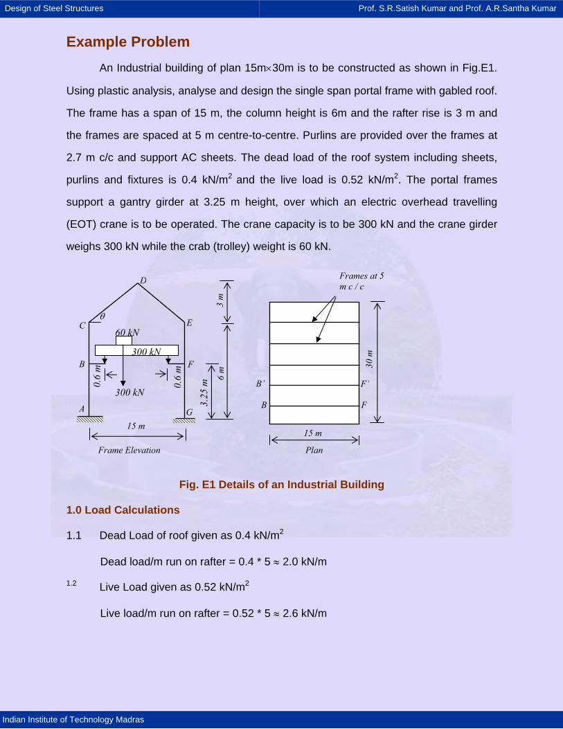
Design of Steel Structures Prof. S.R.Satish Kumar and Prof. A.R.Santha Kumar
Indian Institute of Technology Madras
Example Problem
An Industrial building of plan 15m×30m is to be constructed as shown in Fig.E1.
Using plastic analysis, analyse and design the single span portal frame with gabled roof.
The frame has a span of 15 m, the column height is 6m and the rafter rise is 3 m and
the frames are spaced at 5 m centre-to-centre. Purlins are provided over the frames at
2.7 m c/c and support AC sheets. The dead load of the roof system including sheets,
purlins and fixtures is 0.4 kN/m2 and the live load is 0.52 kN/m2. The portal frames
support a gantry girder at 3.25 m height, over which an electric overhead travelling
(EOT) crane is to be operated. The crane capacity is to be 300 kN and the crane girder
weighs 300 kN while the crab (trolley) weight is 60 kN.
Fig. E1 Details of an Industrial Building 1.0 Load Calculations 1.1 Dead Load of roof given as 0.4 kN/m2 Dead load/m run on rafter = 0.4 * 5 ≈ 2.0 kN/m 1.2 Live Load given as 0.52 kN/m2
Live load/m run on rafter = 0.52 * 5 ≈ 2.6 kN/m
15 m
30 m
Frames at 5 m c / c
3 m
6
m
3.25
m
15 m
0.6
m
0.6
m
A
B
C
D
E
F
G
θ
300 kN
300 kN
60 kN
B
B’
F
F’
Frame Elevation Plan
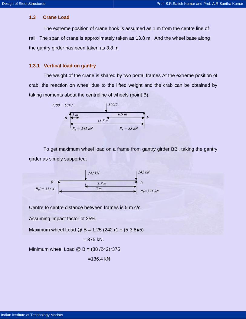
Design of Steel Structures Prof. S.R.Satish Kumar and Prof. A.R.Santha Kumar
Indian Institute of Technology Madras
1.3 Crane Load
The extreme position of crane hook is assumed as 1 m from the centre line of
rail. The span of crane is approximately taken as 13.8 m. And the wheel base along
the gantry girder has been taken as 3.8 m
1.3.1 Vertical load on gantry
The weight of the crane is shared by two portal frames At the extreme position of
crab, the reaction on wheel due to the lifted weight and the crab can be obtained by
taking moments about the centreline of wheels (point B).
To get maximum wheel load on a frame from gantry girder BB', taking the gantry
girder as simply supported.
Centre to centre distance between frames is 5 m c/c. Assuming impact factor of 25% Maximum wheel Load @ B = 1.25 (242 (1 + (5-3.8)/5)
= 375 kN.
Minimum wheel Load @ B = (88 /242)*375
=136.4 kN
13.8 m 1 m
(300 + 60)/2 300/2
B F 6.9 m
RB = 242 kN RF = 88 kN
242 kN 242 kN
3.8 m 5 m
B' B RB
1 = 136.4 RB=375 kN
Design of Steel Structures Prof. S.R.Satish Kumar and Prof. A.R.Santha Kumar
Indian Institute of Technology Madras
1.3.2 Transverse Load (Surge): Lateral load per wheel = 5% (300 + 60)/2 = 9 kN (i.e. Lateral load is assumed as 5% of the lifted load and the weight of the crab acting
on each rail).
Lateral load on each column *3752429
= = 13.9 kN
(By proportion) 1.4 Wind Load Design wind speed, Vz = k1 k2 k3 Vb From Table 1; IS: 875 (part 3) – 1987 k1 = 1.0 (risk coefficient assuming 50 years of design life) From Table 2; IS: 875 (part 3) – 1987 k2 = 0.8 (assuming terrain category 4) k3 = 1.0 (topography factor) Assuming the building is situated in Chennai, the basic wind speed is 50 m
/sec
Design wind speed, Vz = k1 k2 k3 Vb
Vz = 1 * 0.8 *1 * 50
Vz = 40 m/sec
Design wind pressure, Pd = 0.6*Vz2
= 0.6 * (40)2
= 0.96 kN/m2
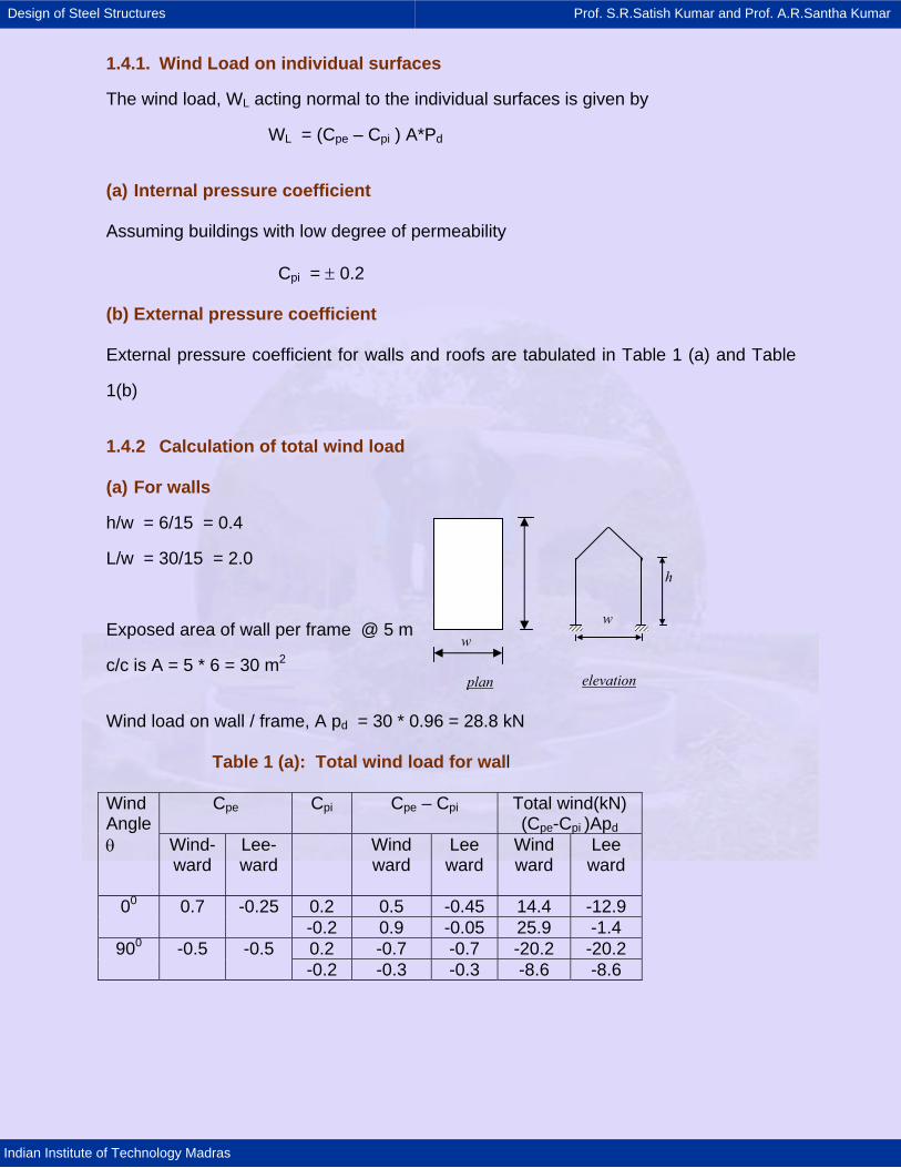
Design of Steel Structures Prof. S.R.Satish Kumar and Prof. A.R.Santha Kumar
Indian Institute of Technology Madras
h
ww
plan elevation
1.4.1. Wind Load on individual surfaces
The wind load, WL acting normal to the individual surfaces is given by
WL = (Cpe – Cpi ) A*Pd
(a) Internal pressure coefficient
Assuming buildings with low degree of permeability Cpi = ± 0.2 (b) External pressure coefficient External pressure coefficient for walls and roofs are tabulated in Table 1 (a) and Table
1(b)
1.4.2 Calculation of total wind load (a) For walls
h/w = 6/15 = 0.4
L/w = 30/15 = 2.0
Exposed area of wall per frame @ 5 m
c/c is A = 5 * 6 = 30 m2
Wind load on wall / frame, A pd = 30 * 0.96 = 28.8 kN
Table 1 (a): Total wind load for wall
Cpe Cpi Cpe – Cpi Total wind(kN) (Cpe-Cpi )Apd
Wind Angle θ Wind-
ward Lee-ward
Wind ward
Lee ward
Wind ward
Lee ward
0.2 0.5 -0.45 14.4 -12.9 00 0.7 -0.25 -0.2 0.9 -0.05 25.9 -1.4 0.2 -0.7 -0.7 -20.2 -20.2 900 -0.5 -0.5 -0.2 -0.3 -0.3 -8.6 -8.6
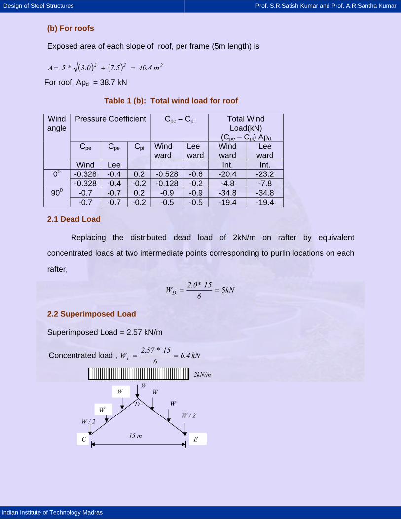
Design of Steel Structures Prof. S.R.Satish Kumar and Prof. A.R.Santha Kumar
Indian Institute of Technology Madras
15 m
(b) For roofs Exposed area of each slope of roof, per frame (5m length) is
For roof, Apd = 38.7 kN Table 1 (b): Total wind load for roof
Pressure Coefficient Cpe – Cpi Total Wind Load(kN)
(Cpe – Cpi) Apd Cpe Cpe Wind
ward Lee ward
Wind ward
Lee ward
Wind angle
Wind Lee
Cpi
Int. Int. -0.328 -0.4 0.2 -0.528 -0.6 -20.4 -23.2 00 -0.328 -0.4 -0.2 -0.128 -0.2 -4.8 -7.8 -0.7 -0.7 0.2 -0.9 -0.9 -34.8 -34.8 900 -0.7 -0.7 -0.2 -0.5 -0.5 -19.4 -19.4
2.1 Dead Load
Replacing the distributed dead load of 2kN/m on rafter by equivalent
concentrated loads at two intermediate points corresponding to purlin locations on each
rafter,
kN6
15*2.0WD 5==
2.2 Superimposed Load Superimposed Load = 2.57 kN/m
Concentrated load , kN6.46
15*2.57WL ==
( ) ( ) 222 m40.47.53.0*5A =+=
2kN/m
C E
W
W W
W
W
W / 2W / 2
D
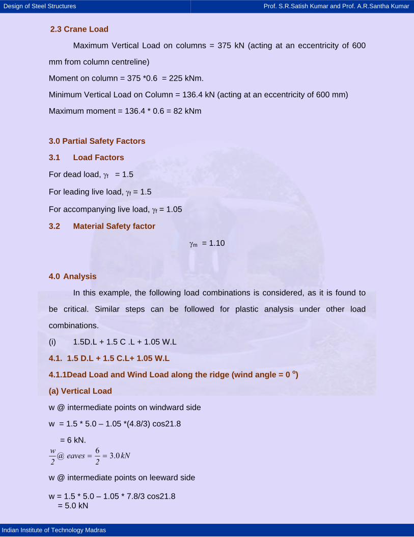
Design of Steel Structures Prof. S.R.Satish Kumar and Prof. A.R.Santha Kumar
Indian Institute of Technology Madras
kN2
eaves@2w 0.36
==
2.3 Crane Load
Maximum Vertical Load on columns = 375 kN (acting at an eccentricity of 600
mm from column centreline)
Moment on column = 375 *0.6 = 225 kNm.
Minimum Vertical Load on Column = 136.4 kN (acting at an eccentricity of 600 mm)
Maximum moment = 136.4 * 0.6 = 82 kNm
3.0 Partial Safety Factors
3.1 Load Factors
For dead load, γf = 1.5
For leading live load, γf = 1.5
For accompanying live load, γf = 1.05
3.2 Material Safety factor
γm = 1.10
4.0 Analysis
In this example, the following load combinations is considered, as it is found to
be critical. Similar steps can be followed for plastic analysis under other load
combinations.
(i) 1.5D.L + 1.5 C .L + 1.05 W.L
4.1. 1.5 D.L + 1.5 C.L+ 1.05 W.L
4.1.1Dead Load and Wind Load along the ridge (wind angle = 0 o)
(a) Vertical Load
w @ intermediate points on windward side
w = 1.5 * 5.0 – 1.05 *(4.8/3) cos21.8
= 6 kN.
w @ intermediate points on leeward side w = 1.5 * 5.0 – 1.05 * 7.8/3 cos21.8 = 5.0 kN
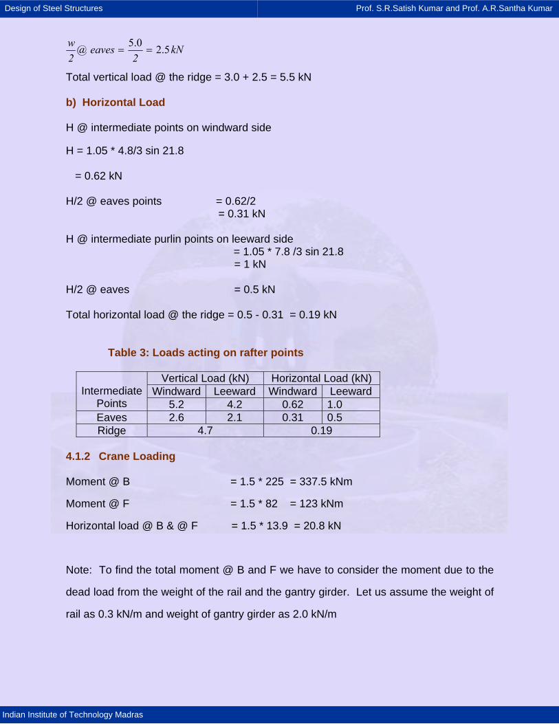
Design of Steel Structures Prof. S.R.Satish Kumar and Prof. A.R.Santha Kumar
Indian Institute of Technology Madras
kN2
eaves@2w 5.20.5
==
Total vertical load @ the ridge = 3.0 + 2.5 = 5.5 kN b) Horizontal Load H @ intermediate points on windward side H = 1.05 * 4.8/3 sin 21.8 = 0.62 kN H/2 @ eaves points = 0.62/2 = 0.31 kN
H @ intermediate purlin points on leeward side = 1.05 * 7.8 /3 sin 21.8 = 1 kN H/2 @ eaves = 0.5 kN Total horizontal load @ the ridge = 0.5 - 0.31 = 0.19 kN
Table 3: Loads acting on rafter points
Vertical Load (kN) Horizontal Load (kN) Windward Leeward Windward Leeward
Intermediate
Points 5.2 4.2 0.62 1.0 Eaves 2.6 2.1 0.31 0.5 Ridge 4.7 0.19
4.1.2 Crane Loading Moment @ B = 1.5 * 225 = 337.5 kNm
Moment @ F = 1.5 * 82 = 123 kNm
Horizontal load @ B & @ F = 1.5 * 13.9 = 20.8 kN
Note: To find the total moment @ B and F we have to consider the moment due to the
dead load from the weight of the rail and the gantry girder. Let us assume the weight of
rail as 0.3 kN/m and weight of gantry girder as 2.0 kN/m
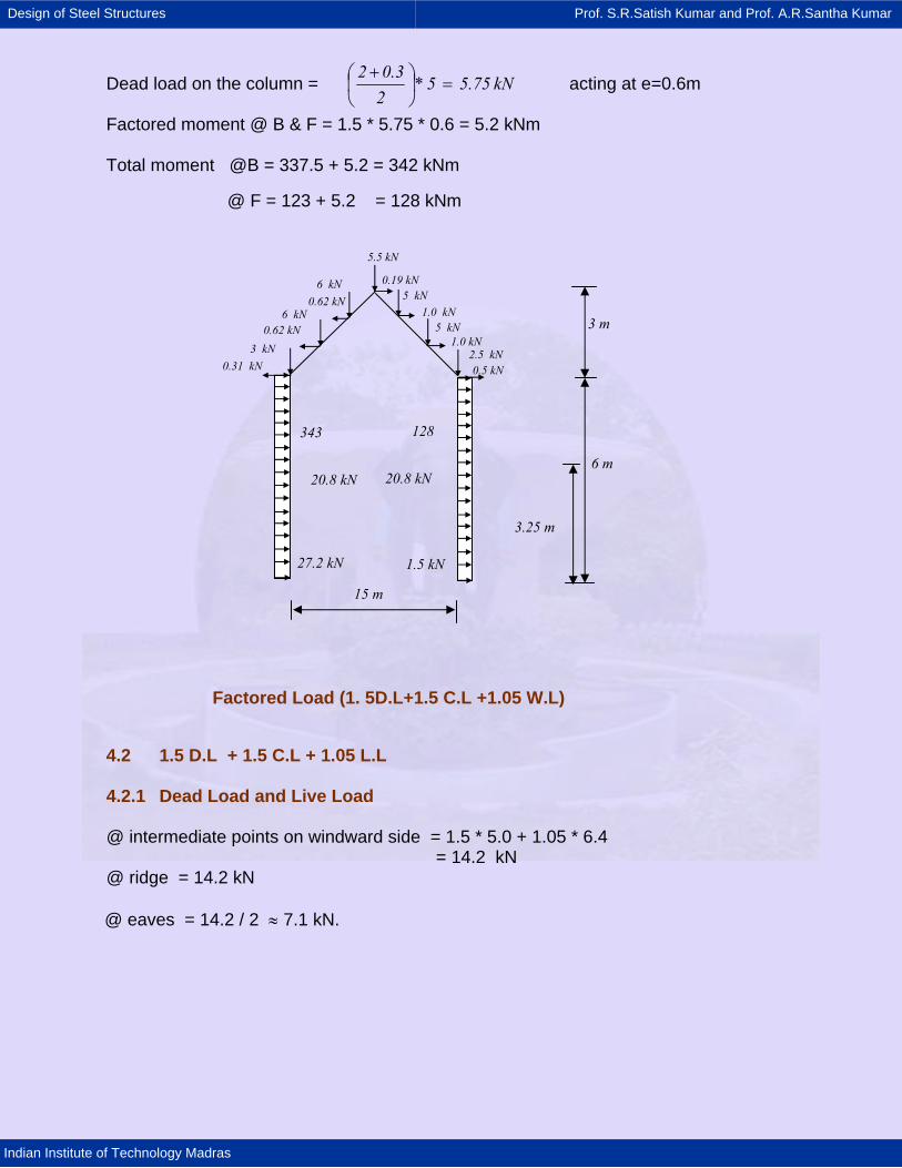
Design of Steel Structures Prof. S.R.Satish Kumar and Prof. A.R.Santha Kumar
Indian Institute of Technology Madras
Dead load on the column = acting at e=0.6m Factored moment @ B & F = 1.5 * 5.75 * 0.6 = 5.2 kNm Total moment @B = 337.5 + 5.2 = 342 kNm
@ F = 123 + 5.2 = 128 kNm
Factored Load (1. 5D.L+1.5 C.L +1.05 W.L) 4.2 1.5 D.L + 1.5 C.L + 1.05 L.L 4.2.1 Dead Load and Live Load @ intermediate points on windward side = 1.5 * 5.0 + 1.05 * 6.4 = 14.2 kN @ ridge = 14.2 kN
@ eaves = 14.2 / 2 ≈ 7.1 kN.
kN5.755*20.32
=⎟⎠
⎞⎜⎝
⎛ +
15 m
3 m
6 m
3.25 m
20.8 kN 20.8 kN
343 128
27.2 kN 1.5 kN
1.0 kN
1.0 kN
0.5 kN
0.19 kN
5.5 kN
5 kN
5 kN
2.5 kN
0.62 kN
0.62 kN 6 kN
6 kN
3 kN 0.31 kN
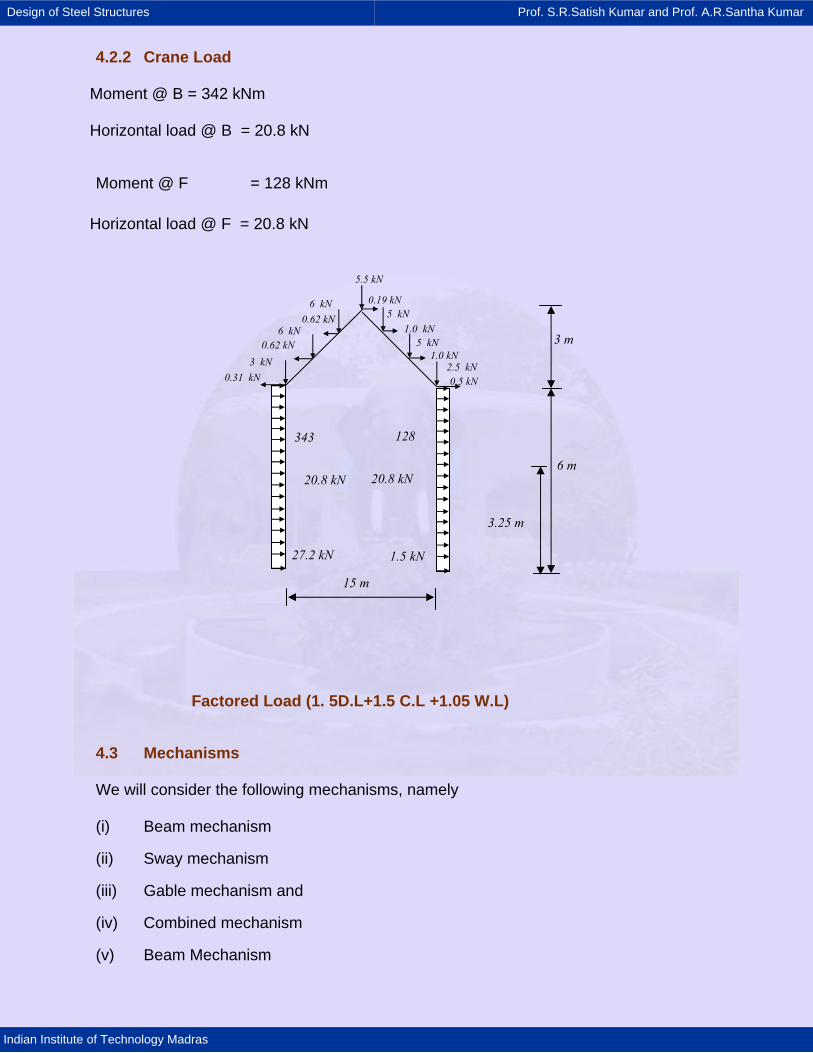
Design of Steel Structures Prof. S.R.Satish Kumar and Prof. A.R.Santha Kumar
Indian Institute of Technology Madras
4.2.2 Crane Load
Moment @ B = 342 kNm Horizontal load @ B = 20.8 kN
Moment @ F = 128 kNm
Horizontal load @ F = 20.8 kN
Factored Load (1. 5D.L+1.5 C.L +1.05 W.L) 4.3 Mechanisms We will consider the following mechanisms, namely (i) Beam mechanism
(ii) Sway mechanism
(iii) Gable mechanism and
(iv) Combined mechanism
(v) Beam Mechanism
15 m
3 m
6 m
3.25 m
20.8 kN 20.8 kN
343 128
27.2 kN 1.5 kN
1.0 kN
1.0 kN
0.5 kN
0.19 kN
5.5 kN
5 kN
5 kN
2.5 kN
0.62 kN
0.62 kN 6 kN
6 kN
3 kN 0.31 kN
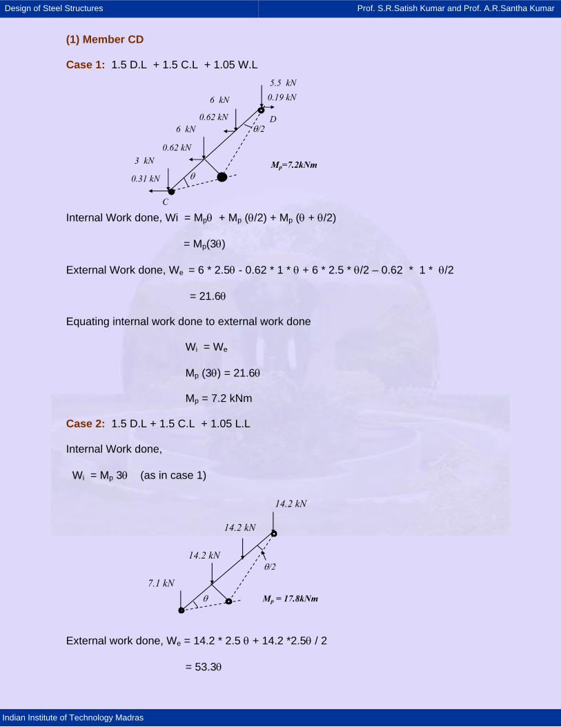
Design of Steel Structures Prof. S.R.Satish Kumar and Prof. A.R.Santha Kumar
Indian Institute of Technology Madras
(1) Member CD Case 1: 1.5 D.L + 1.5 C.L + 1.05 W.L Internal Work done, Wi = Mpθ + Mp (θ/2) + Mp (θ + θ/2) = Mp(3θ) External Work done, We = 6 * 2.5θ - 0.62 * 1 * θ + 6 * 2.5 * θ/2 – 0.62 * 1 * θ/2 = 21.6θ Equating internal work done to external work done Wi = We Mp (3θ) = 21.6θ Mp = 7.2 kNm Case 2: 1.5 D.L + 1.5 C.L + 1.05 L.L Internal Work done, Wi = Mp 3θ (as in case 1)
External work done, We = 14.2 * 2.5 θ + 14.2 *2.5θ / 2 = 53.3θ
D
C
5.5 kN
0.62 kN
6 kN
0.62 kN
0.31 kN
6 kN
0.19 kN
3 kN
θ/2
θ Mp=7.2kNm
θ
14.2 kN
14.2 kN
14.2 kN
7.1 kN
θ/2
Mp = 17.8kNm
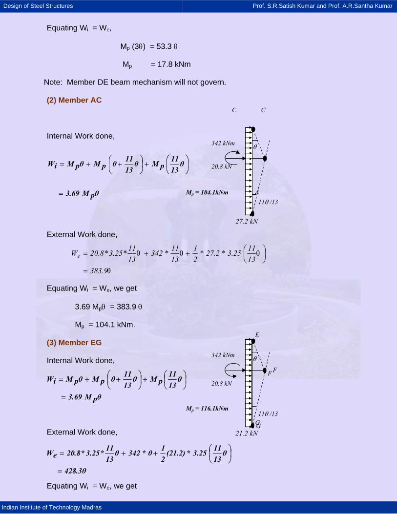
Design of Steel Structures Prof. S.R.Satish Kumar and Prof. A.R.Santha Kumar
Indian Institute of Technology Madras
Equating Wi = We, Mp (3θ) = 53.3 θ Mp = 17.8 kNm
Note: Member DE beam mechanism will not govern. (2) Member AC Internal Work done, External Work done, Equating Wi = We, we get 3.69 Mpθ = 383.9 θ Mp = 104.1 kNm. (3) Member EG Internal Work done, External Work done, Equating Wi = We, we get
θpM3.69
θ1311
pMθ1311θpMθpMiW
=
⎟⎠⎞
⎜⎝⎛+⎟
⎠⎞
⎜⎝⎛ ++=
C C
A
θpM3.69
θ1311
pMθ1311θpMθpMiW
=
⎟⎠⎞
⎜⎝⎛+⎟
⎠⎞
⎜⎝⎛ ++=
θ
θ**θ*θ**
383.913113.2527.2
21
1311342
13113.2520.8We
=
⎟⎠⎞
⎜⎝⎛++=
428.3θ
θ13113.25*(21.2)
21θ*342θ
1311*3.25*20.8eW
=
⎟⎠⎞
⎜⎝⎛++=
E
F
G
20.8 kN
342 kNm
27.2 kN
θ
11θ /13 Mp = 104.1kNm
20.8 kN
342 kNm
21.2 kN
θ
11θ /13
F
G
Mp = 116.1kNm
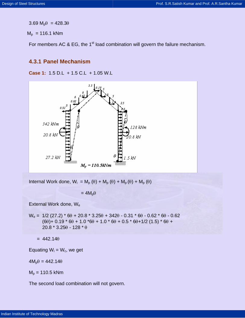
Design of Steel Structures Prof. S.R.Satish Kumar and Prof. A.R.Santha Kumar
Indian Institute of Technology Madras
3.69 Mpθ = 428.3θ
Mp = 116.1 kNm For members AC & EG, the 1st load combination will govern the failure mechanism. 4.3.1 Panel Mechanism Case 1: 1.5 D.L + 1.5 C.L + 1.05 W.L
Internal Work done, Wi = Mp (θ) + Mp (θ) + Mp (θ) + Mp (θ) = 4Mpθ External Work done, We We = 1/2 (27.2) * 6θ + 20.8 * 3.25θ + 342θ - 0.31 * 6θ - 0.62 * 6θ - 0.62 (6θ)+ 0.19 * 6θ + 1.0 *6θ + 1.0 * 6θ + 0.5 * 6θ+1/2 (1.5) * 6θ + 20.8 * 3.25θ - 128 * θ = 442.14θ Equating Wi = Wc, we get 4Mpθ = 442.14θ Mp = 110.5 kNm The second load combination will not govern.
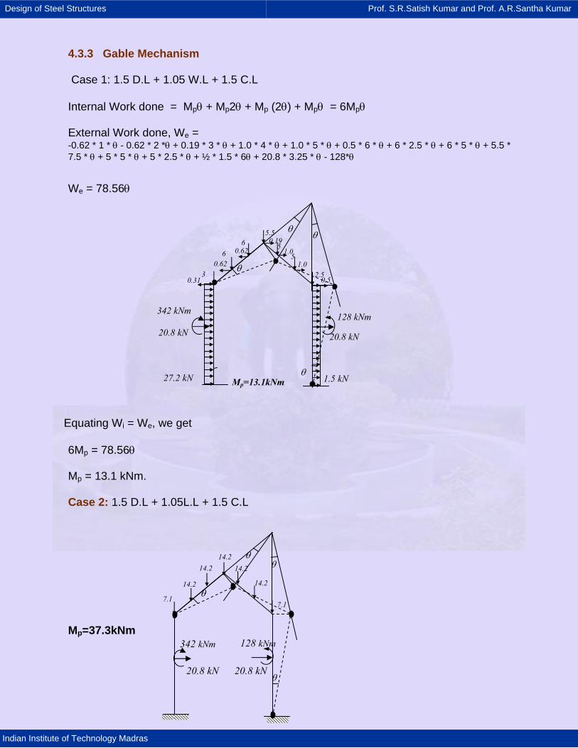
Design of Steel Structures Prof. S.R.Satish Kumar and Prof. A.R.Santha Kumar
Indian Institute of Technology Madras
14.2 14.2
14.2
14.2
7.1
14.2
20.8 kN20.8 kN
342 kNm 128 kNm
θ
θ
θ
θ
7.1
4.3.3 Gable Mechanism Case 1: 1.5 D.L + 1.05 W.L + 1.5 C.L
Internal Work done = Mpθ + Mp2θ + Mp (2θ) + Mpθ = 6Mpθ External Work done, We = -0.62 * 1 * θ - 0.62 * 2 *θ + 0.19 * 3 * θ + 1.0 * 4 * θ + 1.0 * 5 * θ + 0.5 * 6 * θ + 6 * 2.5 * θ + 6 * 5 * θ + 5.5 * 7.5 * θ + 5 * 5 * θ + 5 * 2.5 * θ + ½ * 1.5 * 6θ + 20.8 * 3.25 * θ - 128*θ
We = 78.56θ
Equating Wi = We, we get 6Mp = 78.56θ Mp = 13.1 kNm.
Case 2: 1.5 D.L + 1.05L.L + 1.5 C.L
Mp=37.3kNm
θ
1.0
1.0
0.5
0.19 5.5
5 5
2.5
0.62
0.62 6
6
3 0.31
θ
θ
θ
20.8 kN
342 kNm
20.8 kN
128 kNm
27.2 kN 1.5 kN Mp=13.1kNm
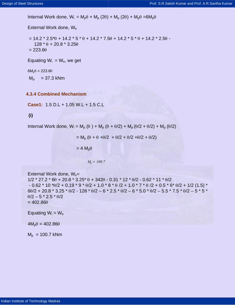
Design of Steel Structures Prof. S.R.Satish Kumar and Prof. A.R.Santha Kumar
Indian Institute of Technology Madras
Internal Work done, Wi = Mpθ + Mp (2θ) + Mp (2θ) + Mpθ =6Mpθ External Work done, We = 14.2 * 2.5*θ + 14.2 * 5 * θ + 14.2 * 7.5θ + 14.2 * 5 * θ + 14.2 * 2.5θ - 128 * θ + 20.8 * 3.25θ = 223.6θ
Equating Wi = We, we get 6Mpθ = 223.6θ
Mp = 37.3 kNm
4.3.4 Combined Mechanism Case1: 1.5 D.L + 1.05 W.L + 1.5 C.L
(i) Internal Work done, Wi = Mp (θ ) + Mp (θ + θ/2) + Mp (θ/2 + θ/2) + Mp (θ/2) = Mp (θ + θ +θ/2 + θ/2 + θ/2 +θ/2 + θ/2) = 4 Mpθ External Work done, We= 1/2 * 27.2 * 6θ + 20.8 * 3.25* θ + 342θ - 0.31 * 12 * θ/2 - 0.62 * 11 * θ/2 - 0.62 * 10 *θ/2 + 0.19 * 9 * θ/2 + 1.0 * 8 * θ /2 + 1.0 * 7 * θ /2 + 0.5 * 6* θ/2 + 1/2 (1.5) * 6θ/2 + 20.8 * 3.25 * θ/2 - 128 * θ/2 – 6 * 2.5 * θ/2 – 6 * 5.0 * θ/2 – 5.5 * 7.5 * θ/2 – 5 * 5 * θ/2 – 5 * 2.5 * θ/2 = 402.86θ Equating Wi = We 4Mpθ = 402.86θ Mp = 100.7 kNm
Mp = 100.7
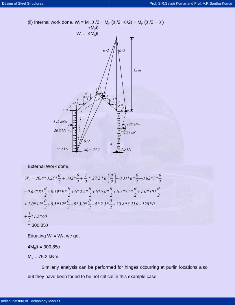
Design of Steel Structures Prof. S.R.Satish Kumar and Prof. A.R.Santha Kumar
Indian Institute of Technology Madras
6θ1.521
θ128θ3.2520.82θ2.5
2θ5.0
2θ120.5
2θ111.0
2θ101.0
2θ7.5
2θ5.0
2θ2.5
2θ90.19
2θ80.62
2θ70.62
2θ60.31
2θ627.2
21
2θ342
2θ3.2520.8We
**
****5**5****
****5.5**6**6****
*********
+
−+++++
+++++−
−−⎟⎠⎞
⎜⎝⎛++=
(ii) Internal work done, Wi = Mp θ /2 + Mp (θ /2 +θ/2) + Mp (θ /2 + θ ) +Mpθ Wi = 4Mpθ
External Work done,
= 300.85θ Equating Wi = We, we get 4Mpθ = 300.85θ Mp = 75.2 kNm
Similarly analysis can be performed for hinges occurring at purlin locations also
but they have been found to be not critical in this example case
θ /2
θ /2 θ /2
θ
20.8 kN
342 kNm
20.8 kN
128 kNm
27.2 kN 1.5 kN
1.0
1.0
0.5
0.19 5.5
5
4.2
2.1
0.62
0.62 6
6
3 0.31
12 m
Mp = 75.2
Design of Steel Structures Prof. S.R.Satish Kumar and Prof. A.R.Santha Kumar
Indian Institute of Technology Madras
From all the above analysis, the largest value of Mp required was for member EG
under
1.5 DL + 1.5 CL + 1.05 WL Therefore the Design Plastic Moment = 116.1 kNm.
5.0 DESIGN
For the design it is assumed that the frame is adequately laterally braced so
that it fails by forming mechanism. Both the column and rafter are analysed assuming
equal plastic moment capacity. Other ratios may be adopted to arrive at an optimum
design solution.
5.1 Selection of section Plastic Moment capacity required= 116 kNm Required section modulus, Zp = Mp/ fyd ISMB 300 @ 0.46 kN/ m provides Zp = 683 * 10-3 mm3
b = 140 mm
Ti = 13.1 mm
A = 5.87 * 10 3 mm2
tw =7.7 mm
rxx =124 mm
ryy =28.6 mm
( )
3310*4.5100
mm1.1
250116*106
=
=
Design of Steel Structures Prof. S.R.Satish Kumar and Prof. A.R.Santha Kumar
Indian Institute of Technology Madras
y1
f
f136
Tb
=
8.65.3413.170
Tb
1
f <==
kN
x5.87*101.1250 3
13340
=
=
5.2 Secondary Design Considerations 5.2.1 Check for Local buckling of flanges and webs
Flanges
bf = 140/2 = 70 mm T1 = 13.1 mm t = 7.7 mm
Web
5.2.2 Effect of axial force
Maximum axial force in column, P = 40.5 kN
Axial load causing yielding, Py = fyd * A
Therefore the effect of axial force can be neglected.
⎥⎥⎦
⎤
⎢⎢⎣
⎡
⎟⎟⎠
⎞⎜⎜⎝
⎛−≤
yyy
1
PP
f1600
f1120
td
( )
KO.Hence68,38.9
0.27250
1600250
11207.7300
yy
≤
⎥⎥⎦
⎤
⎢⎢⎣
⎡−≤
0.150.03140.5
PP
y
<==334
Design of Steel Structures Prof. S.R.Satish Kumar and Prof. A.R.Santha Kumar
Indian Institute of Technology Madras
5.2.3 Check for the effect of shear force Shear force at the end of the girder = P- w/2 = 40.5 -6.8 kN
= 33.7 kN
Maximum shear capacity Vym, of a beam under shear and moment is given by Vym = 0.55 Aw* fyd / 1.10 = 0.55 * 300* 7.7* 250/1.10 =289 kN>> 33.7 kN Hence O.K.
Design of Steel Structures Prof. S.R.Satish Kumar and Prof. A.R.Santha Kumar
Indian Institute of Technology Madras
3. MULTI – STOREY BUILDINGS 3.1 Introduction
In developed countries a very large percentage of multi-storeyed buildings are
built with steel where as steel is not so commonly used in construction of multi-storeyed
frames in India even though it is a better material than reinforced concrete. The use of
steel in multi-storey building construction results in many advantages for the builder and
the user. The advantages of using steel frames in the construction of multi-storey
buildings are listed below:
• Steel, by virtue of its high strength to weight ratio enables large spans and light
weight construction.
• Steel structures can have a variety of structural forms like braced frames and
moment resistant frames suitable to meet the specific requirements.
• Steel frames are faster to erect compared with reinforced concrete frames resulting
in economy.
• The elements of framework are usually prefabricated in the factory under effective
quality control thus enabling a better product.
• Subsequent alterations or strengthening of floors are relatively easy in steel frames
compared with concrete frames.
• The steel frame construction is more suitable to withstand lateral loads caused by
wind or earthquake.
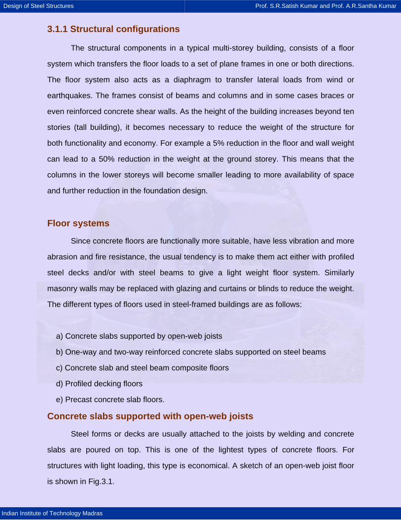
Design of Steel Structures Prof. S.R.Satish Kumar and Prof. A.R.Santha Kumar
Indian Institute of Technology Madras
3.1.1 Structural configurations
The structural components in a typical multi-storey building, consists of a floor
system which transfers the floor loads to a set of plane frames in one or both directions.
The floor system also acts as a diaphragm to transfer lateral loads from wind or
earthquakes. The frames consist of beams and columns and in some cases braces or
even reinforced concrete shear walls. As the height of the building increases beyond ten
stories (tall building), it becomes necessary to reduce the weight of the structure for
both functionality and economy. For example a 5% reduction in the floor and wall weight
can lead to a 50% reduction in the weight at the ground storey. This means that the
columns in the lower storeys will become smaller leading to more availability of space
and further reduction in the foundation design.
Floor systems
Since concrete floors are functionally more suitable, have less vibration and more
abrasion and fire resistance, the usual tendency is to make them act either with profiled
steel decks and/or with steel beams to give a light weight floor system. Similarly
masonry walls may be replaced with glazing and curtains or blinds to reduce the weight.
The different types of floors used in steel-framed buildings are as follows:
a) Concrete slabs supported by open-web joists
b) One-way and two-way reinforced concrete slabs supported on steel beams
c) Concrete slab and steel beam composite floors
d) Profiled decking floors
e) Precast concrete slab floors.
Concrete slabs supported with open-web joists
Steel forms or decks are usually attached to the joists by welding and concrete
slabs are poured on top. This is one of the lightest types of concrete floors. For
structures with light loading, this type is economical. A sketch of an open-web joist floor
is shown in Fig.3.1.
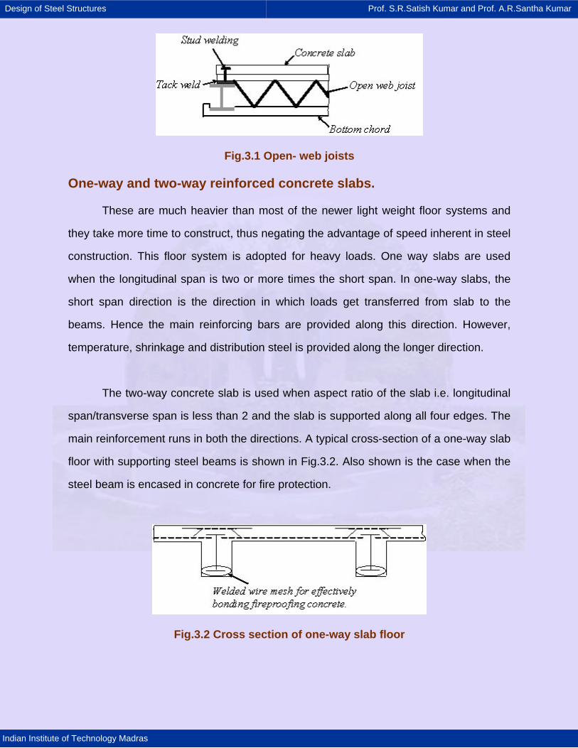
Design of Steel Structures Prof. S.R.Satish Kumar and Prof. A.R.Santha Kumar
Indian Institute of Technology Madras
Fig.3.1 Open- web joists
One-way and two-way reinforced concrete slabs.
These are much heavier than most of the newer light weight floor systems and
they take more time to construct, thus negating the advantage of speed inherent in steel
construction. This floor system is adopted for heavy loads. One way slabs are used
when the longitudinal span is two or more times the short span. In one-way slabs, the
short span direction is the direction in which loads get transferred from slab to the
beams. Hence the main reinforcing bars are provided along this direction. However,
temperature, shrinkage and distribution steel is provided along the longer direction.
The two-way concrete slab is used when aspect ratio of the slab i.e. longitudinal
span/transverse span is less than 2 and the slab is supported along all four edges. The
main reinforcement runs in both the directions. A typical cross-section of a one-way slab
floor with supporting steel beams is shown in Fig.3.2. Also shown is the case when the
steel beam is encased in concrete for fire protection.
Fig.3.2 Cross section of one-way slab floor
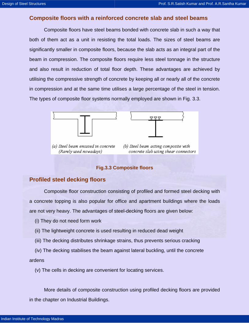
Design of Steel Structures Prof. S.R.Satish Kumar and Prof. A.R.Santha Kumar
Indian Institute of Technology Madras
Composite floors with a reinforced concrete slab and steel beams
Composite floors have steel beams bonded with concrete slab in such a way that
both of them act as a unit in resisting the total loads. The sizes of steel beams are
significantly smaller in composite floors, because the slab acts as an integral part of the
beam in compression. The composite floors require less steel tonnage in the structure
and also result in reduction of total floor depth. These advantages are achieved by
utilising the compressive strength of concrete by keeping all or nearly all of the concrete
in compression and at the same time utilises a large percentage of the steel in tension.
The types of composite floor systems normally employed are shown in Fig. 3.3.
Fig.3.3 Composite floors
Profiled steel decking floors
Composite floor construction consisting of profiled and formed steel decking with
a concrete topping is also popular for office and apartment buildings where the loads
are not very heavy. The advantages of steel-decking floors are given below:
(i) They do not need form work
(ii) The lightweight concrete is used resulting in reduced dead weight
(iii) The decking distributes shrinkage strains, thus prevents serious cracking
(iv) The decking stabilises the beam against lateral buckling, until the concrete
ardens
(v) The cells in decking are convenient for locating services.
More details of composite construction using profiled decking floors are provided
in the chapter on Industrial Buildings.
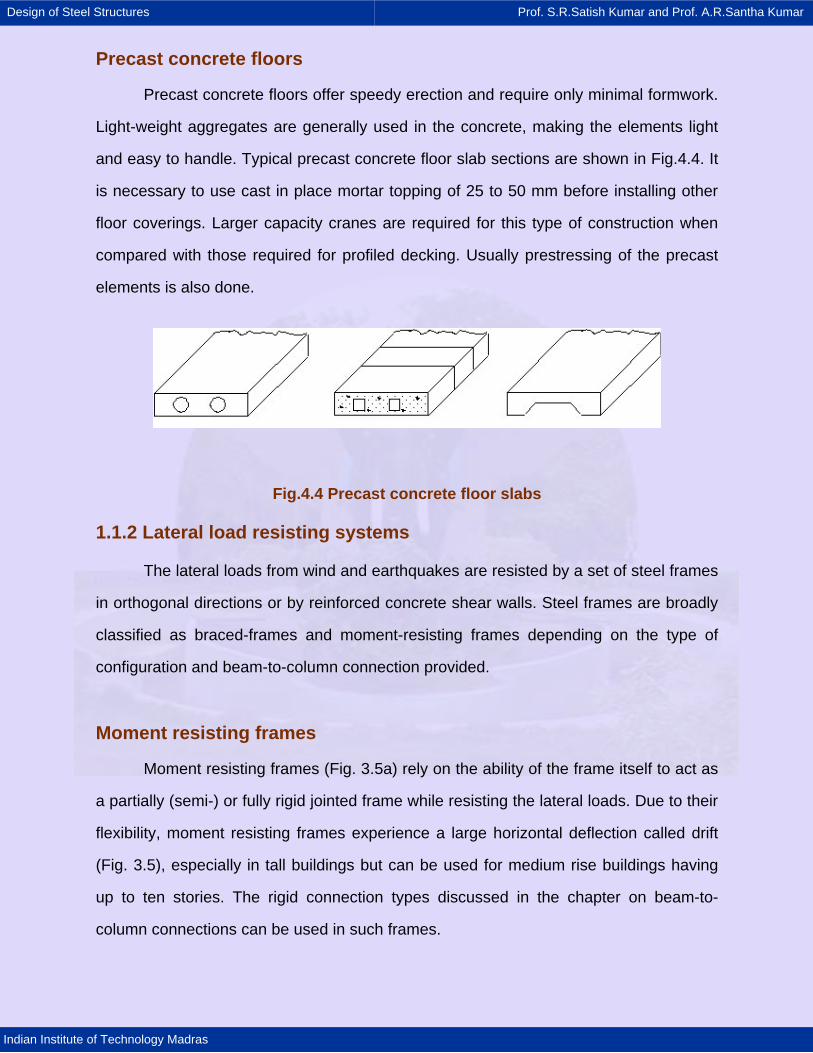
Design of Steel Structures Prof. S.R.Satish Kumar and Prof. A.R.Santha Kumar
Indian Institute of Technology Madras
Precast concrete floors
Precast concrete floors offer speedy erection and require only minimal formwork.
Light-weight aggregates are generally used in the concrete, making the elements light
and easy to handle. Typical precast concrete floor slab sections are shown in Fig.4.4. It
is necessary to use cast in place mortar topping of 25 to 50 mm before installing other
floor coverings. Larger capacity cranes are required for this type of construction when
compared with those required for profiled decking. Usually prestressing of the precast
elements is also done.
Fig.4.4 Precast concrete floor slabs
1.1.2 Lateral load resisting systems
The lateral loads from wind and earthquakes are resisted by a set of steel frames
in orthogonal directions or by reinforced concrete shear walls. Steel frames are broadly
classified as braced-frames and moment-resisting frames depending on the type of
configuration and beam-to-column connection provided.
Moment resisting frames
Moment resisting frames (Fig. 3.5a) rely on the ability of the frame itself to act as
a partially (semi-) or fully rigid jointed frame while resisting the lateral loads. Due to their
flexibility, moment resisting frames experience a large horizontal deflection called drift
(Fig. 3.5), especially in tall buildings but can be used for medium rise buildings having
up to ten stories. The rigid connection types discussed in the chapter on beam-to-
column connections can be used in such frames.
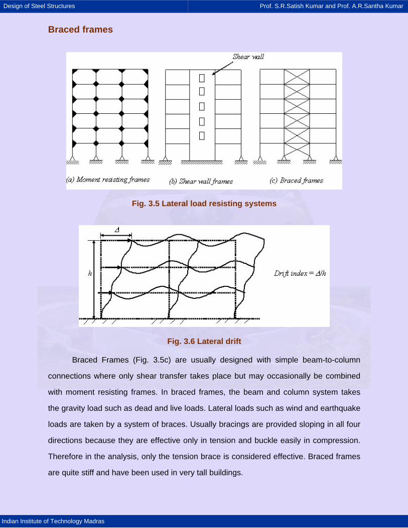
Design of Steel Structures Prof. S.R.Satish Kumar and Prof. A.R.Santha Kumar
Indian Institute of Technology Madras
Braced frames
Fig. 3.5 Lateral load resisting systems
Fig. 3.6 Lateral drift
Braced Frames (Fig. 3.5c) are usually designed with simple beam-to-column
connections where only shear transfer takes place but may occasionally be combined
with moment resisting frames. In braced frames, the beam and column system takes
the gravity load such as dead and live loads. Lateral loads such as wind and earthquake
loads are taken by a system of braces. Usually bracings are provided sloping in all four
directions because they are effective only in tension and buckle easily in compression.
Therefore in the analysis, only the tension brace is considered effective. Braced frames
are quite stiff and have been used in very tall buildings.
Design of Steel Structures Prof. S.R.Satish Kumar and Prof. A.R.Santha Kumar
Indian Institute of Technology Madras
3.2 Loading
Loading on tall buildings is different from low-rise buildings in many ways
such as large accumulation of gravity loads on the floors from top to bottom,
increased significance of wind loading and greater importance of dynamic
effects. Thus, multi-storeyed structures need correct assessment of loads for
safe and economical design. Except dead loads, the assessment of loads can
not be done accurately. Live loads can be anticipated approximately from a
combination of experience and the previous field observations. Wind and
earthquake loads are random in nature and it is difficult to predict them. They are
estimated based on a probabilistic approach. The following discussion describes
some of the most common kinds of loads on multi-storeyed structures.
3.2.1 Gravity loads
Dead loads due the weight of every element within the structure as well as
live loads that are acting on the structure when in service constitute gravity loads.
The dead loads are calculated from the member sizes and estimated material
densities. Live loads prescribed by codes are empirical and conservative based
on experience and accepted practice. The equivalent minimum loads for office
and residential buildings as per IS 875 are as specified in Table -3.1
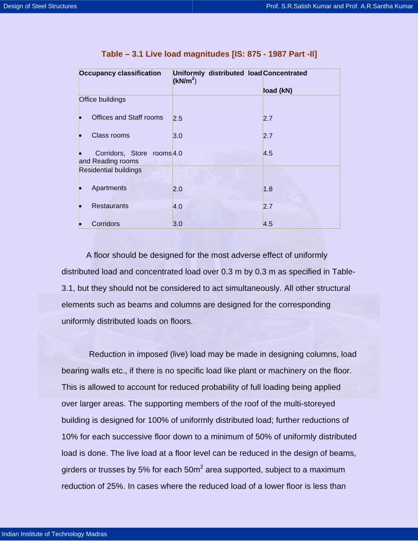
Design of Steel Structures Prof. S.R.Satish Kumar and Prof. A.R.Santha Kumar
Indian Institute of Technology Madras
Table – 3.1 Live load magnitudes [IS: 875 - 1987 Part -II]
Occupancy classification Uniformly distributed load (kN/m2)
Concentrated
load (kN) Office buildings
• Offices and Staff rooms
• Class rooms
• Corridors, Store rooms and Reading rooms
2.5
3.0
4.0
2.7
2.7
4.5
Residential buildings
• Apartments
• Restaurants
• Corridors
2.0
4.0
3.0
1.8
2.7
4.5
A floor should be designed for the most adverse effect of uniformly
distributed load and concentrated load over 0.3 m by 0.3 m as specified in Table-
3.1, but they should not be considered to act simultaneously. All other structural
elements such as beams and columns are designed for the corresponding
uniformly distributed loads on floors.
Reduction in imposed (live) load may be made in designing columns, load
bearing walls etc., if there is no specific load like plant or machinery on the floor.
This is allowed to account for reduced probability of full loading being applied
over larger areas. The supporting members of the roof of the multi-storeyed
building is designed for 100% of uniformly distributed load; further reductions of
10% for each successive floor down to a minimum of 50% of uniformly distributed
load is done. The live load at a floor level can be reduced in the design of beams,
girders or trusses by 5% for each 50m2 area supported, subject to a maximum
reduction of 25%. In cases where the reduced load of a lower floor is less than
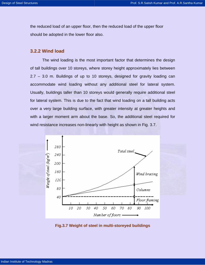
Design of Steel Structures Prof. S.R.Satish Kumar and Prof. A.R.Santha Kumar
Indian Institute of Technology Madras
the reduced load of an upper floor, then the reduced load of the upper floor
should be adopted in the lower floor also.
3.2.2 Wind load
The wind loading is the most important factor that determines the design
of tall buildings over 10 storeys, where storey height approximately lies between
2.7 – 3.0 m. Buildings of up to 10 storeys, designed for gravity loading can
accommodate wind loading without any additional steel for lateral system.
Usually, buildings taller than 10 storeys would generally require additional steel
for lateral system. This is due to the fact that wind loading on a tall building acts
over a very large building surface, with greater intensity at greater heights and
with a larger moment arm about the base. So, the additional steel required for
wind resistance increases non-linearly with height as shown in Fig. 3.7.
Fig.3.7 Weight of steel in multi-storeyed buildings
Design of Steel Structures Prof. S.R.Satish Kumar and Prof. A.R.Santha Kumar
Indian Institute of Technology Madras
As shown in Fig.3.7 the lateral stiffness of the building is a more important
consideration than its strength for tall multi-storeyed structures. Wind has
become a major load for the designer of multi-storeyed buildings. Prediction of
wind loading in precise scientific terms may not be possible, as it is influenced by
many factors such as the form of terrain, the shape, slenderness, the solidity
ratio of building and the arrangement of adjacent buildings. The appropriate
design wind loads are estimated based on two approaches. Static approach is
one, which assumes the building to be a fixed rigid body in the wind. This method
is suitable for buildings of normal height, slenderness, or susceptible to vibration
in the wind. The other approach is the dynamic approach. This is adopted for
exceptionally tall, slender, or vibration prone buildings. Sometimes wind sensitive
tall buildings will have to be designed for interference effects caused by the
environment in which the building stands. The loading due to these interference
effects is best ascertained using wind tunnel modeled structures in the
laboratory.
However, in the Indian context, where the tallest multi-storeyed building is
only about 35 storeys high, multi-storeyed buildings do not suffer wind-induced
oscillation and generally do not require to be examined for the dynamic effects.
For detailed information on evaluating wind load, the reader is referred to IS:
875-1987 (Part-III).
Design of Steel Structures Prof. S.R.Satish Kumar and Prof. A.R.Santha Kumar
Indian Institute of Technology Madras
3.2.3 Earthquake load
Seismic motion consists of horizontal and vertical ground motions, with the
vertical motion usually having a much smaller magnitude. Further, factor of safety
provided against gravity loads usually can accommodate additional forces due to
vertical acceleration due to earthquakes. So, the horizontal motion of the ground
causes the most significant effect on the structure by shaking the foundation
back and forth. The mass of building resists this motion by setting up inertia
forces throughout the structure.
The magnitude of the horizontal shear force F depends on the mass of the
building M, the acceleration of the ground a, and the nature of the structure. If a
building and the foundation were rigid, it would have the same acceleration as
the ground as given by Newton’s second law of motion, i.e. F = Ma. However, in
practice all buildings are flexible to some degree. For a structure that deforms
slightly, thereby absorbing some energy, the force will be less than the product of
mass and acceleration. But, a very flexible structure will be subject to a much
larger force under repetitive ground motion. This shows the magnitude of the
lateral force on a building is not only dependent on acceleration of the ground but
it will also depend on the type of the structure. As an inertia problem, the
dynamic response of the building plays a large part in influencing and in
estimating the effective loading on the structure. The earthquake load is
estimated by Seismic co-efficient method or Response spectrum method. The
later takes account of dynamic characteristics of structure along with ground
motion. For detailed information on evaluating earthquake load, reader is referred
to IS: 1893 - 2002 and the chapter on Industrial Buildings.
Design of Steel Structures Prof. S.R.Satish Kumar and Prof. A.R.Santha Kumar
Indian Institute of Technology Madras
3.3 Analysis for gravity loads
Simple framing
If a simple framing is used, the analysis is quite simple because they can
be considered as simply supported. In such cases, shears and moments can be
determined by statics. The gravity loads applied to the columns are relatively
easy to estimate, but the column moments may be a little more difficult to find
out. The column moments occur due to uneven distribution and unequal
magnitude of live load. If the beam reactions are equal on each side of interior
column, then there will be no column moment. If the reactions are unequal, the
moment produced in the column will be equal to the difference between reactions
multiplied by eccentricity of the beam reaction with respect to column centre line.
Semi rigid framing
The analysis of semi-rigid building frames is complex. The semi-rigid
frames are analysed and designed by using special techniques developed based
on experimental evidence on the behaviour of the connections. For more details
the reference quoted in the chapter on beam-to-column connections may be
consulted.
Rigid framing
Rigid frame buildings are analysed by one of the approximate methods to
make an estimate of member sizes before going to exact methods such as slope-
deflection or moment-distribution method. If the ends of each girder are assumed
to be completely fixed, the bending moments due to uniform loads are as shown
in full lines of Fig. 3.8(a). If the ends of beam are connected by simple
connection, then the moment diagram for uniformly distributed load is shown in
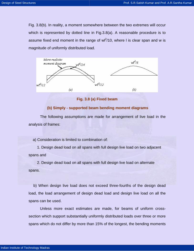
Design of Steel Structures Prof. S.R.Satish Kumar and Prof. A.R.Santha Kumar
Indian Institute of Technology Madras
Fig. 3.8(b). In reality, a moment somewhere between the two extremes will occur
which is represented by dotted line in Fig.3.8(a). A reasonable procedure is to
assume fixed end moment in the range of wl2/10, where l is clear span and w is
magnitude of uniformly distributed load.
Fig. 3.8 (a) Fixed beam
(b) Simply - supported beam bending moment diagrams
The following assumptions are made for arrangement of live load in the
analysis of frames:
a) Consideration is limited to combination of:
1. Design dead load on all spans with full design live load on two adjacent
spans and
2. Design dead load on all spans with full design live load on alternate
spans.
b) When design live load does not exceed three-fourths of the design dead
load, the load arrangement of design dead load and design live load on all the
spans can be used.
Unless more exact estimates are made, for beams of uniform cross-
section which support substantially uniformly distributed loads over three or more
spans which do not differ by more than 15% of the longest, the bending moments
Design of Steel Structures Prof. S.R.Satish Kumar and Prof. A.R.Santha Kumar
Indian Institute of Technology Madras
and shear forces used for design is obtained using the coefficients given in Table
3.2 and Table 3.3 respectively. For moments at supports where two unequal
spans meet or in cases where the spans are not equally loaded, the average of
the two values for the hogging moment at the support may be used for design.
Where coefficients given in Table 3.2 are used for calculation of bending
moments, redistribution of moments is not permitted.
Substitute frame method
Rigid frame high-rise buildings are highly redundant structures. The
analysis of such frames by conventional methods such as moment distribution
method or Kane’s method is very lengthy and time consuming. Thus,
approximate methods (such as two cycled moment distribution method) are
adopted for the analysis of rigid frames under gravity loading, one of such
methods is Substitute Frame Method.
Substitute frame method is a short version of moment distribution method.
Only two cycles are carried out in the analysis and also only a part of frame is
considered for analysing the moments and shears in the beams and columns.
The assumptions for this method are given below:
1) Moments transferred from one floor to another floor are small. Hence, the
moments for each floor are separately calculated.
2) Each floor will be taken as connected to columns above and below with
their far ends fixed.
If the columns are very stiff, no rotation will occur at both ends of a beam
and the point of contraflexure will be at about 0.2 l. The actual beam can be
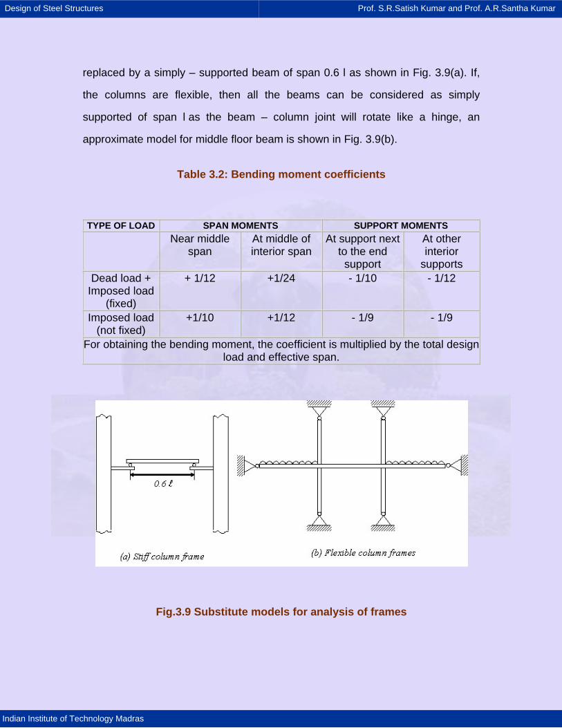
Design of Steel Structures Prof. S.R.Satish Kumar and Prof. A.R.Santha Kumar
Indian Institute of Technology Madras
replaced by a simply – supported beam of span 0.6 l as shown in Fig. 3.9(a). If,
the columns are flexible, then all the beams can be considered as simply
supported of span l as the beam – column joint will rotate like a hinge, an
approximate model for middle floor beam is shown in Fig. 3.9(b).
Table 3.2: Bending moment coefficients
TYPE OF LOAD SPAN MOMENTS SUPPORT MOMENTS Near middle
span At middle of interior span
At support next to the end support
At other interior
supports Dead load +
Imposed load (fixed)
+ 1/12 +1/24 - 1/10 - 1/12
Imposed load (not fixed)
+1/10 +1/12 - 1/9 - 1/9
For obtaining the bending moment, the coefficient is multiplied by the total design load and effective span.
Fig.3.9 Substitute models for analysis of frames
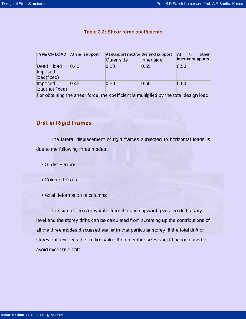
Design of Steel Structures Prof. S.R.Satish Kumar and Prof. A.R.Santha Kumar
Indian Institute of Technology Madras
Table 3.3: Shear force coefficients
At support next to the end support TYPE OF LOAD At end support Outer side Inner side
At all other interior supports
Dead load + Imposed load(fixed)
0.40 0.60 0.55 0.50
Imposed load(not fixed)
0.45 0.60 0.60 0.60
For obtaining the shear force, the coefficient is multiplied by the total design load
Drift in Rigid Frames
The lateral displacement of rigid frames subjected to horizontal loads is
due to the following three modes:
• Girder Flexure
• Column Flexure
• Axial deformation of columns
The sum of the storey drifts from the base upward gives the drift at any
level and the storey drifts can be calculated from summing up the contributions of
all the three modes discussed earlier in that particular storey. If the total drift or
storey drift exceeds the limiting value then member sizes should be increased to
avoid excessive drift.
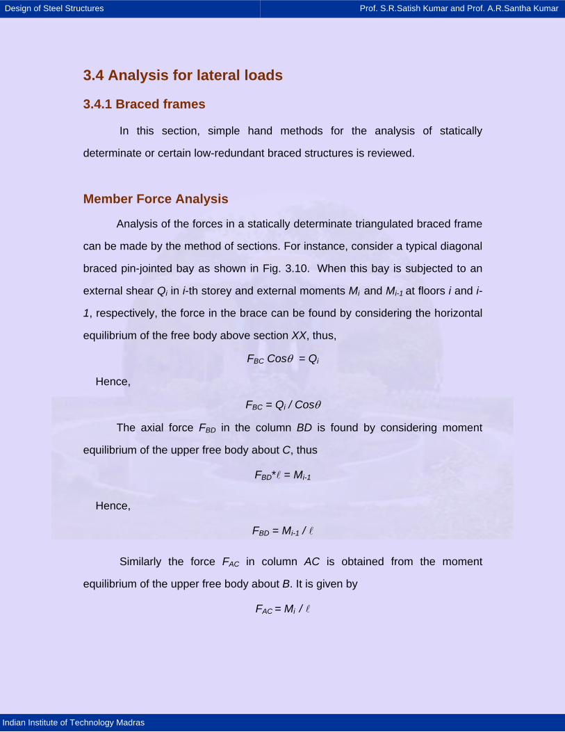
Design of Steel Structures Prof. S.R.Satish Kumar and Prof. A.R.Santha Kumar
Indian Institute of Technology Madras
3.4 Analysis for lateral loads
3.4.1 Braced frames
In this section, simple hand methods for the analysis of statically
determinate or certain low-redundant braced structures is reviewed.
Member Force Analysis
Analysis of the forces in a statically determinate triangulated braced frame
can be made by the method of sections. For instance, consider a typical diagonal
braced pin-jointed bay as shown in Fig. 3.10. When this bay is subjected to an
external shear Qi in i-th storey and external moments Mi and Mi-1 at floors i and i-
1, respectively, the force in the brace can be found by considering the horizontal
equilibrium of the free body above section XX, thus,
FBC Cosθ = Qi
Hence,
FBC = Qi / Cosθ
The axial force FBD in the column BD is found by considering moment
equilibrium of the upper free body about C, thus
FBD* = Mi-1
Hence,
FBD = Mi-1 /
Similarly the force FAC in column AC is obtained from the moment
equilibrium of the upper free body about B. It is given by
FAC = Mi /
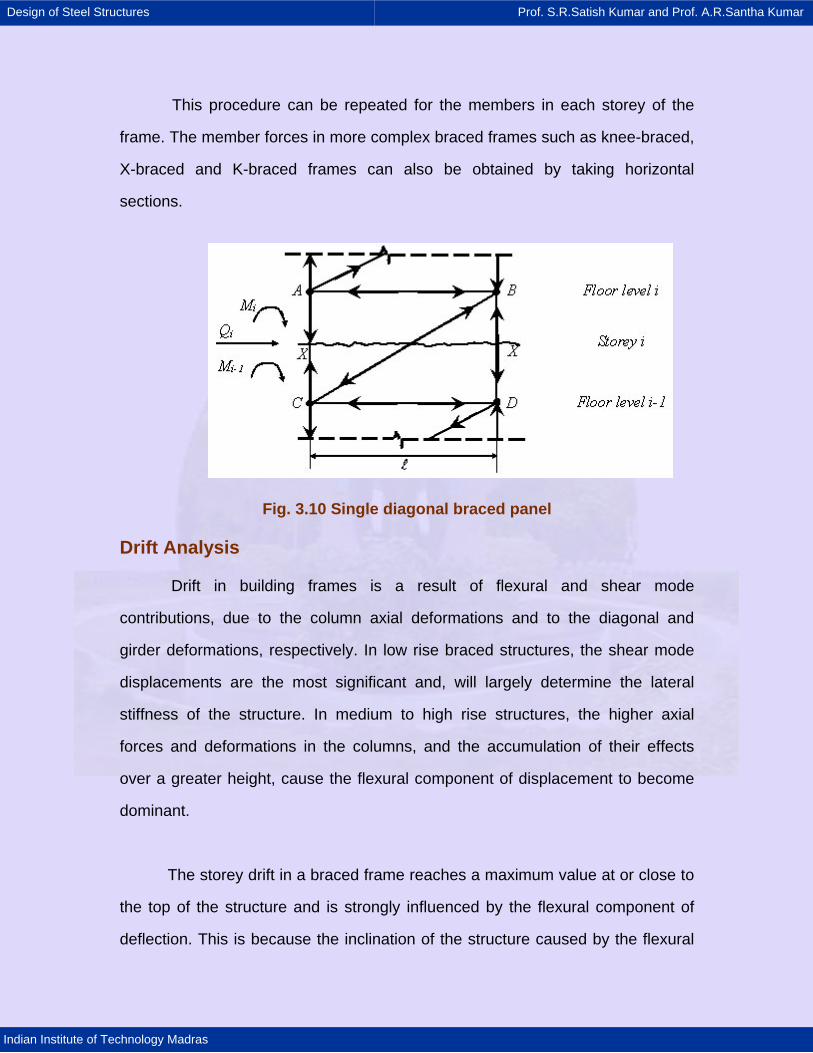
Design of Steel Structures Prof. S.R.Satish Kumar and Prof. A.R.Santha Kumar
Indian Institute of Technology Madras
This procedure can be repeated for the members in each storey of the
frame. The member forces in more complex braced frames such as knee-braced,
X-braced and K-braced frames can also be obtained by taking horizontal
sections.
Fig. 3.10 Single diagonal braced panel
Drift Analysis
Drift in building frames is a result of flexural and shear mode
contributions, due to the column axial deformations and to the diagonal and
girder deformations, respectively. In low rise braced structures, the shear mode
displacements are the most significant and, will largely determine the lateral
stiffness of the structure. In medium to high rise structures, the higher axial
forces and deformations in the columns, and the accumulation of their effects
over a greater height, cause the flexural component of displacement to become
dominant.
The storey drift in a braced frame reaches a maximum value at or close to
the top of the structure and is strongly influenced by the flexural component of
deflection. This is because the inclination of the structure caused by the flexural
Design of Steel Structures Prof. S.R.Satish Kumar and Prof. A.R.Santha Kumar
Indian Institute of Technology Madras
component accumulates up the structure, while the storey shear component
diminishes toward the top.
Hand analysis for drift allows the drift contributions of the individual frame
members to be seen, thereby providing guidance as to which members should
be increased in size to effectively reduce an excessive total drift or storey drift.
The following section explains a method for hand evaluation of drift.
3.4.2 Moment-resisting frames
Multi-storey building frames subjected to lateral loads are statically
indeterminate and exact analysis by hand calculation takes much time and effort.
Using simplifying assumptions, approximate analyses of these frames yield good
estimate of member forces in the frame, which can be used for checking the
member sizes. The following methods can be employed for lateral load analysis
of rigidly jointed frames.
• The Portal method.
• The Cantilever method
• The Factor method
The portal method and the cantilever method yield good results only when
the height of a building is approximately more than five times its least lateral
dimension. Either classical techniques such as slope deflection or moment
distribution methods or computer methods using stiffness or flexibility matrices
can be used if a more exact result is desired.
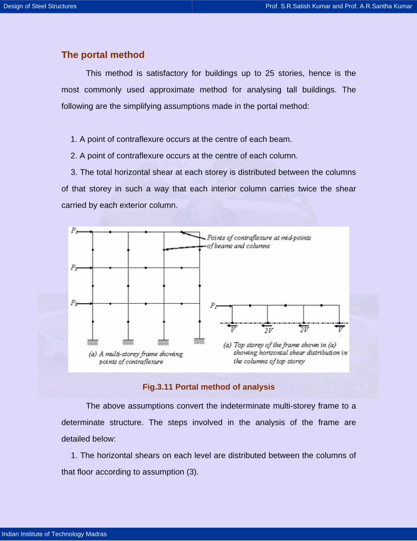
Design of Steel Structures Prof. S.R.Satish Kumar and Prof. A.R.Santha Kumar
Indian Institute of Technology Madras
The portal method
This method is satisfactory for buildings up to 25 stories, hence is the
most commonly used approximate method for analysing tall buildings. The
following are the simplifying assumptions made in the portal method:
1. A point of contraflexure occurs at the centre of each beam.
2. A point of contraflexure occurs at the centre of each column.
3. The total horizontal shear at each storey is distributed between the columns
of that storey in such a way that each interior column carries twice the shear
carried by each exterior column.
Fig.3.11 Portal method of analysis
The above assumptions convert the indeterminate multi-storey frame to a
determinate structure. The steps involved in the analysis of the frame are
detailed below:
1. The horizontal shears on each level are distributed between the columns of
that floor according to assumption (3).
Design of Steel Structures Prof. S.R.Satish Kumar and Prof. A.R.Santha Kumar
Indian Institute of Technology Madras
2. The moment in each column is equal to the column shear multiplied by half
the column height according to assumption (2).
3. The girder moments are determined by applying moment equilibrium
equation to the joints: by noting that the sum of the girder moments at any joint
equals the sum of the column moments at that joint. These calculations are
easily made by starting at the upper left joint and working joint by joint across to
the right end.
4. The shear in each girder is equal to its moment divided by half the girder
length. This is according to assumption (1).
5. Finally, the column axial forces are determined by summing up the beam
shears and other axial forces at each joint. These calculations again are easily
made by working from left to right and from the top floor down.
Assumptions of the Portal method of analysis are diagrammatically shown in
Fig.3.11.
The cantilever method
This method gives good results for high-narrow buildings compared to
those from the Portal method and it may be used satisfactorily for buildings of 25
to 35 storeys tall. It is not as popular as the portal method.
The simplifying assumptions made in the cantilever method are:
1. A point of contraflexure occurs at the centre of each beam
2. A point of contraflexure occurs at the centre of each column.
3. The axial force in each column of a storey is proportional to the horizontal
distance of the column from the centre of gravity of all the columns of the storey
under consideration.
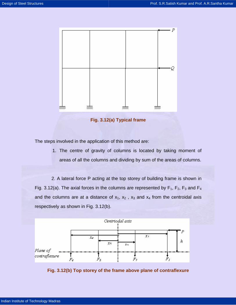
Design of Steel Structures Prof. S.R.Satish Kumar and Prof. A.R.Santha Kumar
Indian Institute of Technology Madras
Fig. 3.12(a) Typical frame
The steps involved in the application of this method are:
1. The centre of gravity of columns is located by taking moment of
areas of all the columns and dividing by sum of the areas of columns.
2. A lateral force P acting at the top storey of building frame is shown in
Fig. 3.12(a). The axial forces in the columns are represented by F1, F2, F3 and F4
and the columns are at a distance of x1, x2 , x3 and x4 from the centroidal axis
respectively as shown in Fig. 3.12(b).
Fig. 3.12(b) Top storey of the frame above plane of contraflexure
Design of Steel Structures Prof. S.R.Satish Kumar and Prof. A.R.Santha Kumar
Indian Institute of Technology Madras
By taking the moments about the centre of gravity of columns of the storey,
P h - F1x1 - F2x2 - F3x3 - F4x4 = 0
The axial force in one column may be assumed as F and the axial forces of
remaining columns can be expressed in terms of F using assumption (3).
3. The beam shears are determined joint by joint from the column axial forces.
4. The beam moments are determined by multiplying the shear in the beam by
half the span of beam according to assumption (1).
5. The column moments are found joint by joint from the beam moments.
The column shears are obtained by dividing the column moments by the half-
column heights using assumption (2)
The factor method
The factor method is more accurate than either the portal method or the
cantilever method. The portal method and cantilever method depend on
assumed location of hinges and column shears whereas the factor method is
based on assumptions regarding the elastic action of the structure. For the
application of Factor method, the relative stiffness (k = I/l), for each beam and
column should be known or assumed, where, I is the moment of inertia of cross
section and l is the length of the member.
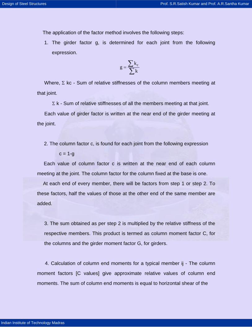
Design of Steel Structures Prof. S.R.Satish Kumar and Prof. A.R.Santha Kumar
Indian Institute of Technology Madras
The application of the factor method involves the following steps:
1. The girder factor g, is determined for each joint from the following
expression.
ckg
k= ∑∑
Where, Σ kc - Sum of relative stiffnesses of the column members meeting at
that joint.
Σ k - Sum of relative stiffnesses of all the members meeting at that joint.
Each value of girder factor is written at the near end of the girder meeting at
the joint.
2. The column factor c, is found for each joint from the following expression
c = 1-g
Each value of column factor c is written at the near end of each column
meeting at the joint. The column factor for the column fixed at the base is one.
At each end of every member, there will be factors from step 1 or step 2. To
these factors, half the values of those at the other end of the same member are
added.
3. The sum obtained as per step 2 is multiplied by the relative stiffness of the
respective members. This product is termed as column moment factor C, for
the columns and the girder moment factor G, for girders.
4. Calculation of column end moments for a typical member ij - The column
moment factors [C values] give approximate relative values of column end
moments. The sum of column end moments is equal to horizontal shear of the
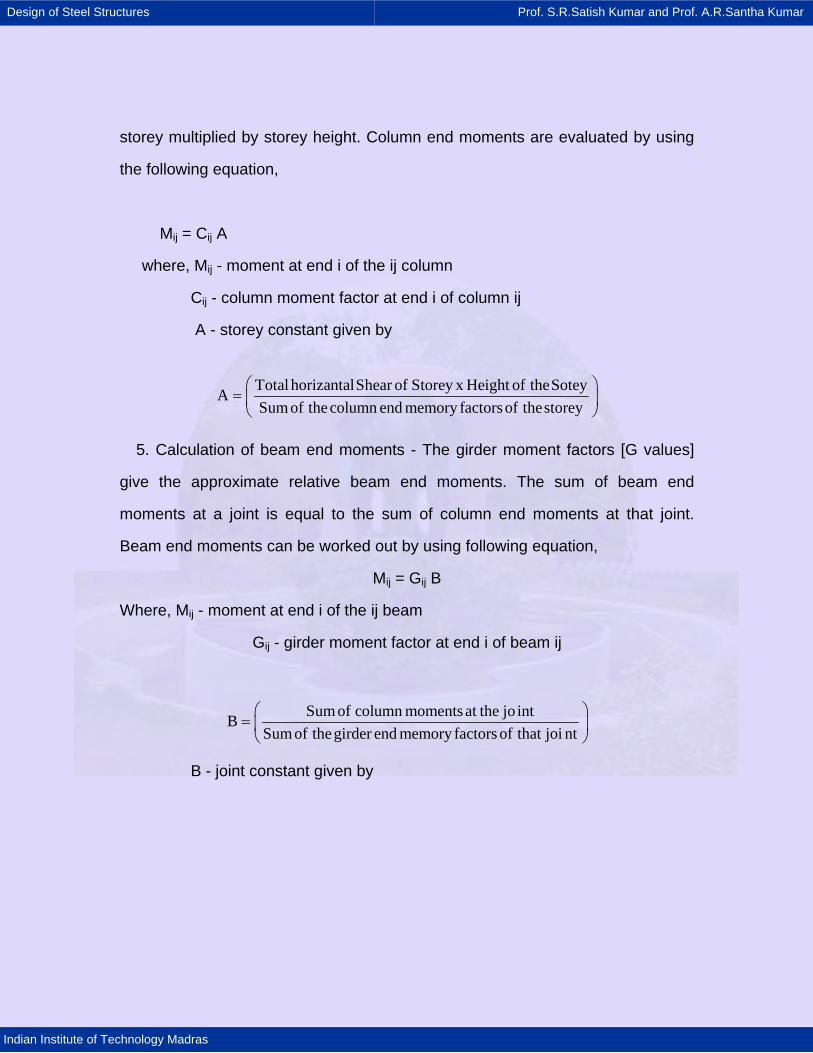
Design of Steel Structures Prof. S.R.Satish Kumar and Prof. A.R.Santha Kumar
Indian Institute of Technology Madras
storey multiplied by storey height. Column end moments are evaluated by using
the following equation,
Mij = Cij A
where, Mij - moment at end i of the ij column
Cij - column moment factor at end i of column ij
A - storey constant given by
Total horizantalShear of Storey x Height of theSoteyASum of thecolumn end memory factors of thestorey
⎛ ⎞= ⎜ ⎟⎝ ⎠
5. Calculation of beam end moments - The girder moment factors [G values]
give the approximate relative beam end moments. The sum of beam end
moments at a joint is equal to the sum of column end moments at that joint.
Beam end moments can be worked out by using following equation,
Mij = Gij B
Where, Mij - moment at end i of the ij beam
Gij - girder moment factor at end i of beam ij
Sum of column moments at the jo intBSum of thegirder end memory factors of that joi nt
⎛ ⎞= ⎜ ⎟⎝ ⎠
B - joint constant given by
Design of Steel Structures Prof. S.R.Satish Kumar and Prof. A.R.Santha Kumar
Indian Institute of Technology Madras
Illustration of calculation of G values:
Consider the joints B and C in the frame shown in Fig. 3.13.
Joint B: gB = k1 /( k1 + k2 + k3)
cB = 1 - gB
Joint C: gC = k4 /( k2 + k4 + k5)
cC = 1 - gC
As shown in Fig. 3.13, we should obtain values like x and y at each end of
the beam and column. Thereafter we multiply them with respective k values to
get the column or girder moment factors. Here, GBC = x k2 and GCB = y k2.
Similarly we calculate all other moment factors.
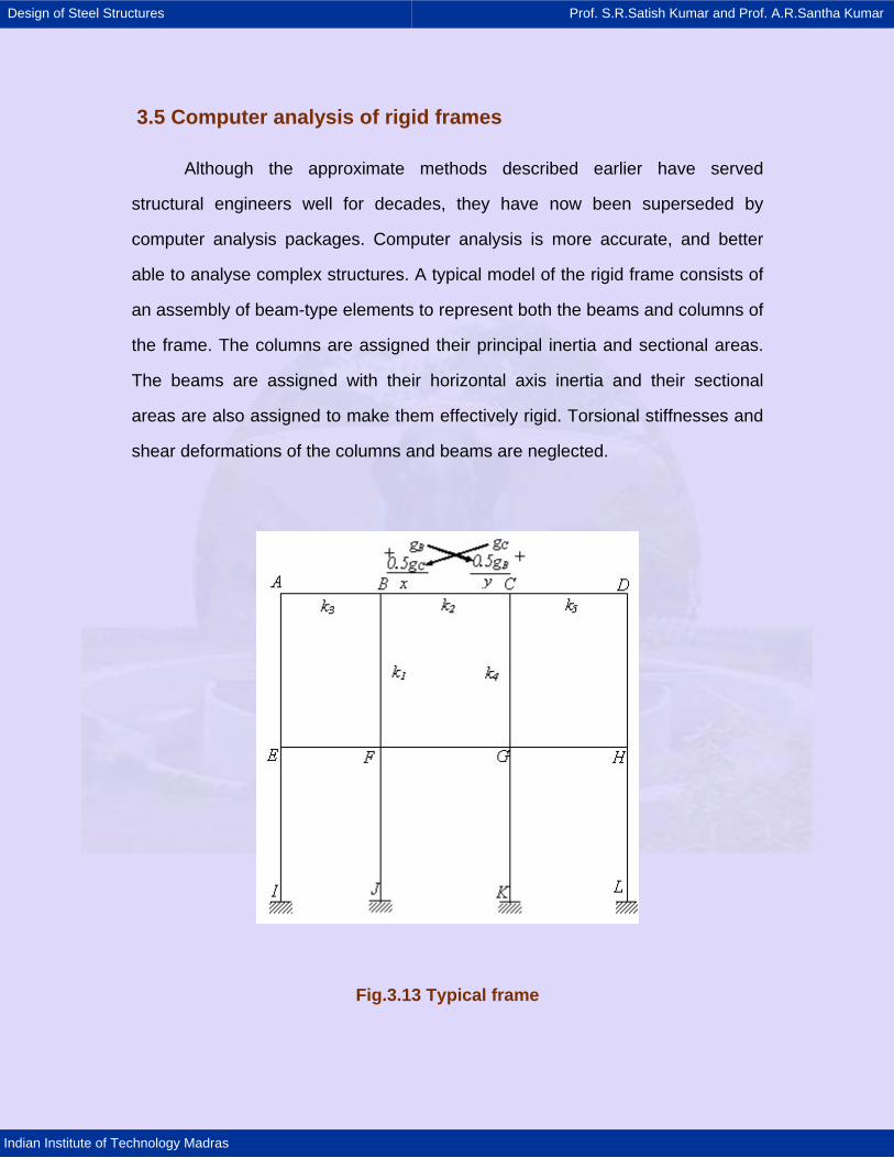
Design of Steel Structures Prof. S.R.Satish Kumar and Prof. A.R.Santha Kumar
Indian Institute of Technology Madras
3.5 Computer analysis of rigid frames
Although the approximate methods described earlier have served
structural engineers well for decades, they have now been superseded by
computer analysis packages. Computer analysis is more accurate, and better
able to analyse complex structures. A typical model of the rigid frame consists of
an assembly of beam-type elements to represent both the beams and columns of
the frame. The columns are assigned their principal inertia and sectional areas.
The beams are assigned with their horizontal axis inertia and their sectional
areas are also assigned to make them effectively rigid. Torsional stiffnesses and
shear deformations of the columns and beams are neglected.
Fig.3.13 Typical frame
Design of Steel Structures Prof. S.R.Satish Kumar and Prof. A.R.Santha Kumar
Indian Institute of Technology Madras
Some analysis programs include the option of considering the slab to be
rigid in plane, and some have the option of including P-Delta effects. If a rigid
slab option is not available, the effect can be simulated by interconnecting all
vertical elements by a horizontal frame at each floor, adding fictitious beams
where necessary, assuming the beams to be effectively rigid axially and in
flexure in the horizontal plane.
Modern design offices are generally equipped with a wide variety of
structural analysis software programs, invariably based on the stiffness matrix
method. These Finite Element Analysis packages such as MSC/NASTRAN, SAP
- 90, STAAD etc., give more accurate results compared with approximate
methods, but they involve significant computational effort and therefore cost.
They are generally preferred for complex structures. The importance of
approximate hand methods for the analysis of forces and deflections in multi-
storeyed frames can not be ignored; they have served the Structural Engineer
well for many decades and are still useful for preliminary analysis and checking.
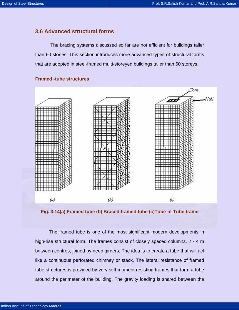
Design of Steel Structures Prof. S.R.Satish Kumar and Prof. A.R.Santha Kumar
Indian Institute of Technology Madras
3.6 Advanced structural forms
The bracing systems discussed so far are not efficient for buildings taller
than 60 stories. This section introduces more advanced types of structural forms
that are adopted in steel-framed multi-storeyed buildings taller than 60 storeys.
Framed -tube structures
Fig. 3.14(a) Framed tube (b) Braced framed tube (c)Tube-in-Tube frame
The framed tube is one of the most significant modern developments in
high-rise structural form. The frames consist of closely spaced columns, 2 - 4 m
between centres, joined by deep girders. The idea is to create a tube that will act
like a continuous perforated chimney or stack. The lateral resistance of framed
tube structures is provided by very stiff moment resisting frames that form a tube
around the perimeter of the building. The gravity loading is shared between the
Design of Steel Structures Prof. S.R.Satish Kumar and Prof. A.R.Santha Kumar
Indian Institute of Technology Madras
tube and interior columns. This structural form offers an efficient, easily
constructed structure appropriate for buildings having 40 to100 storeys.
When lateral loads act, the perimeter frames aligned in the direction of
loads act as the webs of the massive tube cantilever and those normal to the
direction of the loading act as the flanges. Even though framed tube is a
structurally efficient form, flange frames tend to suffer from shear lag. This results
in the mid face flange columns being less stressed than the corner columns and
therefore not contributing to their full potential lateral strength. Aesthetically, the
tube looks like the grid-like façade as small windowed and is repetitious and
hence use of prefabrication in steel makes the construction faster. A typical
framed tube is shown in Fig.3.14 (a).
Braced tube structures
Further improvements of the tubular system can be made by cross bracing
the frame with X-bracing over many stories, as illustrated in Fig. 3.14(b). This
arrangement was first used in Chicago's John Hancock Building in 1969.
As the diagonals of a braced tube are connected to the columns at each
intersection, they virtually eliminate the effects of shear lag in both the flange and
web frames. As a result the structure behaves under lateral loads more like a
braced frame reducing bending in the members of the frames. Hence, the
spacing of the columns can be increased and the depth of the girders will be
less, thereby allowing large size windows than in the conventional framed tube
structures.
Design of Steel Structures Prof. S.R.Satish Kumar and Prof. A.R.Santha Kumar
Indian Institute of Technology Madras
In the braced tube structure, the braces transfer axial load from the more
highly stressed columns to the less highly stressed columns and eliminates
differences between load stresses in the columns.
Tube-in-Tube structures
This is a type of framed tube consisting of an outer-framed tube together
with an internal elevator and service core. The inner tube may consist of braced
frames. The outer and inner tubes act jointly in resisting both gravity and lateral
loading in steel-framed buildings. However, the outer tube usually plays a
dominant role because of its much greater structural depth. This type of
structures is also called as Hull (Outer tube) and Core (Inner tube) structures. A
typical Tube-in-Tube structure is shown in Fig. 3.14c.
Bundled tube
The bundled tube system can be visualised as an assemblage of
individual tubes resulting in multiple cell tube. The increase in stiffness is
apparent. The system allows for the greatest height and the most floor area. This
structural form was used in the Sears Tower in Chicago. In this system,
introduction of the internal webs greatly reduces the shear lag in the flanges.
Hence, their columns are more evenly stressed than in the single tube structure
and their contribution to the lateral stiffness is greater.

Design of Steel Structures Prof. S.R.Satish Kumar and Prof. A.R.Santha Kumar
Indian Institute of Technology Madras
3.7 Summary
Approximate analyses of simple braced frame as well as for frames with
moment resisting joints are described. Simplified analyses of building frames with
gravity loads as well as frames with lateral loads have been discussed. More
accurate methods making use of flexibility or stiffness matrices are generally
incorporated in sophisticated software in many design offices. Advanced
structural forms used in tall buildings were also described.
Design of Steel Structures Prof. S.R.Satish Kumar and Prof. A.R.Santha Kumar
Indian Institute of Technology Madras
3.8 References
1. Teaching resources for structural Steel Design (Volume 1 to 3), INSDAG
publication, Calcutta 2000.
2. McCormac. C. J., (1994): "Structural Steel Design", Harper Collins College
Publishers.
3. Owens. G. W. and Knowles. P., (1994) "Steel Designers Manual", The
Steel Construction Institute, ELBS Blackwell Scientific Publishers, London.
4. Taranath. S. B., (1984): "Structural analysis and design of tall buildings",
McGraw-Hill Book Company
5. Schuller. W., (1976): "High-rise building structures", John Wiley & Sons
6. Smith. B. S., and Coull. A., (1991): "Tall building structures: Analysis and
Design", John Wiley & Sons.
7. IS: 875 - 1987 (Parts - I to V), Indian Code of Practice for evaluating loads
excepting earthquake load, BIS New Delhi.
8. IS: 1893 - 2002, Criteria for the seismic design of structures subjected to
earthquake loads. BIS New Delhi.
Design of Steel Structures Prof. S.R.Satish Kumar and Prof. A.R.Santha Kumar
Indian Institute of Technology Madras
4. SPACE FRAMES
4.1 Introduction
4.1.1. General
Tensile structures are economical and efficient solution for large span
structures. Although such structures are very common in all the developed
countries, they are yet to make great strides in India.
The structural and material science engineers are already addressing
themselves to the task of development of new construction material, and
techniques and computer based tools for analysis and design to meet the
challenge of providing long span structures.
Currently INDIA is poised for a major initiative in infrastructure.
Development of tensile structures should naturally play their rightful role in
this initiative. In view of the tremendous oppurtunity for their use. There is need
to increase the general level of the competence in the analysis and design of
tensile structure in India.
Development of new techniques is space structures to reduce the
deflection and the effective use of materials like steel are the great advantages in
ensuring cost effectiveness.
Design of Steel Structures Prof. S.R.Satish Kumar and Prof. A.R.Santha Kumar
Indian Institute of Technology Madras
In the space structures and the tensile structure systems steel is widely
used for effective construction and to establish the use of steel in our country, we
need a new technique like prestressing of steel and effective use of steel
members by reducing the compression force.
4.1.2. Introduction to space frames
A space frames is structural system with three dimensional assembly of
linear elements, so arranged that the loads are transferred in a three dimensional
manner. These structures are commonly used for large span structures, which
are more advantageous and economical for providing roofs for large span
building.
Design of Steel Structures Prof. S.R.Satish Kumar and Prof. A.R.Santha Kumar
Indian Institute of Technology Madras
4.2. Types of space frames
They are classified broadly in three categories
i. Skeleton (braced) frame work
e.g. domes, barrel vaults, double and multiplier grids, braced plates. They
are more popular. They are innumerable combinations and variation possible and
follow regular geometric forms.
ii. Stressed skin systems
e.g. Stressed skin folded plates, stressed skin domes and barrel vaults,
pneumatic structures.
iii. Suspended (cable or membrane) structures
e.g. Cable roofs.
Design of Steel Structures Prof. S.R.Satish Kumar and Prof. A.R.Santha Kumar
Indian Institute of Technology Madras
4.3. Space truss
Skeleton, three dimensional frame works consisting of pin connected bars
are called space trusses. They are characterised by hinged joints with no
moments or torsional resistance. All members carry only axial compression or
tension.
4.3.1 Space grids
A grid may be defined as two or more sets of parallel beams intersecting
each other at any angle and loaded by an external loading normal to the plane.
They are characterised as two way or three way depending upon whether the
members intersecting at a node run in two or three directions.
4.3.2. Double layer grid
A space truss can be formed by two or three layers of grids. A double
layer grid consist of two plane grids forming the top and bottom layers, parallel to
each other and interconnected by vertical and diagonal members. A space truss
is a combination of prefabricated tetrahedral, octahedral or skeleton pyramids or
inverted pyramids having triangular, square or hexagonal basis with top and
bottom members normally not lying in the same vertical plane.
Double layer flat grid truss, having greater rigidity allow greater flexibility in
layout and permit changes in the positioning of columns. Its high rigidity ensures
that the deflections of the structures are within limits. They are usually built from
simple prefabricated units of standard shape. Due to its high indeterminacy,
buckling of any member under any concentrated load may not lead to the
collapse of the entire structure.
Design of Steel Structures Prof. S.R.Satish Kumar and Prof. A.R.Santha Kumar
Indian Institute of Technology Madras
Various types of double layer grids are shown in fig 4.1. They can be
developed by varying the direction of top and bottom layers with respect to each
other, by different positioning of the top layer nodal points and also by changing
the size of the top layer grid with respect to bottom layer grid. Some examples of
double layer flat grid truss constructed in India and abroad are given in Table 4.1.
Table 4.1: Some examples of Double layer grids
SI.No Name and location Types of frame work Year
1 Al Wahda sports hall at Abudhabi
Square over diagonal grid (set orthogonally) covering an area of 54 x 43.4m tuball spherical connectors
1989
2 Tennis court at Deira city center, UAE
Square on square offset set diagonally 50.4 x 58.8m Depth:2.1m plate connectors.
1995
3
Indian Oil Corporation Ltd., LPG Bottling Plant, Cuddapah India.
Diagonal (size 2.8m) over square topology, consists of several largest having a size of 47.6 x 39.6m Depth:2m for larger shed 1.4m smaller shed, schkul spherical node.
1998
4
Indian Oil Corporation Ltd., LPG Bottling Plant, Ennore, Chennai
Similar configuration (vide fig) 1999
4.3.3. Advantages of space truss
1. They are light, structurally efficient and use materials optimally. It can be
designed in such a way that the total weight comes between 15 to 20kg/m2
2. It can be built up from simple, prefabricated units of standard size and
shape. Hence they can be mass-produced in the factory, can be easily and
rapidly assembled at site using semi-skilled labour.
Design of Steel Structures Prof. S.R.Satish Kumar and Prof. A.R.Santha Kumar
Indian Institute of Technology Madras
3. The small size components simplify the handling, transportation and
erection.
4. They are an elegant and economical means of covering large column free
spaces.
5. They allow great flexibility in designing layout and positioning of end
supports.
6. Services such as lighting, air conditioning etc., can be integrated with space
structures.
7. The use of complicated and expensive temporary supports during erection
are eliminated.
8. They posses great rigidity and stiffness for a given span/depth ratio and
hence are able to resist large concentrated and unsymmetrical loading. Local
overloading can be taken care by built-in reserve strength. They do not collapse
locally.
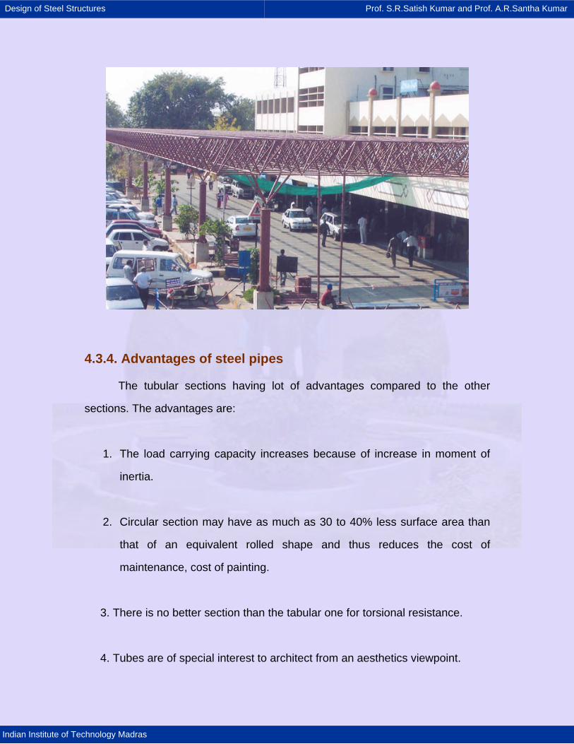
Design of Steel Structures Prof. S.R.Satish Kumar and Prof. A.R.Santha Kumar
Indian Institute of Technology Madras
4.3.4. Advantages of steel pipes
The tubular sections having lot of advantages compared to the other
sections. The advantages are:
1. The load carrying capacity increases because of increase in moment of
inertia.
2. Circular section may have as much as 30 to 40% less surface area than
that of an equivalent rolled shape and thus reduces the cost of
maintenance, cost of painting.
3. There is no better section than the tabular one for torsional resistance.
4. Tubes are of special interest to architect from an aesthetics viewpoint.
Design of Steel Structures Prof. S.R.Satish Kumar and Prof. A.R.Santha Kumar
Indian Institute of Technology Madras
5. The external surface of the tube does not permit the collection of moisture
and dust thus reducing the possibility of corrosion.
6. Under dynamic loading the tube has a higher frequency of vibration than
any other cross section including a solid round bar.
4.3.5. Components of space truss
1. Axial members which are preferably tubes.
2. Connectors which join the members together
3. Bolts connecting members with nodes.
Depending upon the connecting system space truss systems are classified
as Nodular and Modular systems.
Nodular systems
They consist of members and nodes.
Mero connector
It is an abbreviation for Dr. Merigenhausen, a German, inventor of the
connector. With his invention in 1942, he commercialized the space frames
successfully due to factory mass production of standard components and easy
field assembly. It can accept as many as 18 members (Fig 4.2 shows a K-K
system mero).
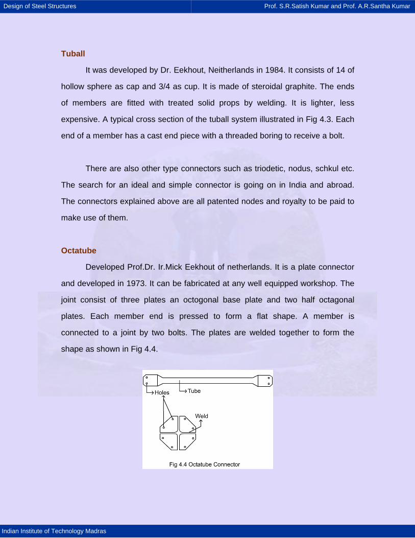
Design of Steel Structures Prof. S.R.Satish Kumar and Prof. A.R.Santha Kumar
Indian Institute of Technology Madras
Tuball
It was developed by Dr. Eekhout, Neitherlands in 1984. It consists of 14 of
hollow sphere as cap and 3/4 as cup. It is made of steroidal graphite. The ends
of members are fitted with treated solid props by welding. It is lighter, less
expensive. A typical cross section of the tuball system illustrated in Fig 4.3. Each
end of a member has a cast end piece with a threaded boring to receive a bolt.
There are also other type connectors such as triodetic, nodus, schkul etc.
The search for an ideal and simple connector is going on in India and abroad.
The connectors explained above are all patented nodes and royalty to be paid to
make use of them.
Octatube
Developed Prof.Dr. Ir.Mick Eekhout of netherlands. It is a plate connector
and developed in 1973. It can be fabricated at any well equipped workshop. The
joint consist of three plates an octogonal base plate and two half octagonal
plates. Each member end is pressed to form a flat shape. A member is
connected to a joint by two bolts. The plates are welded together to form the
shape as shown in Fig 4.4.
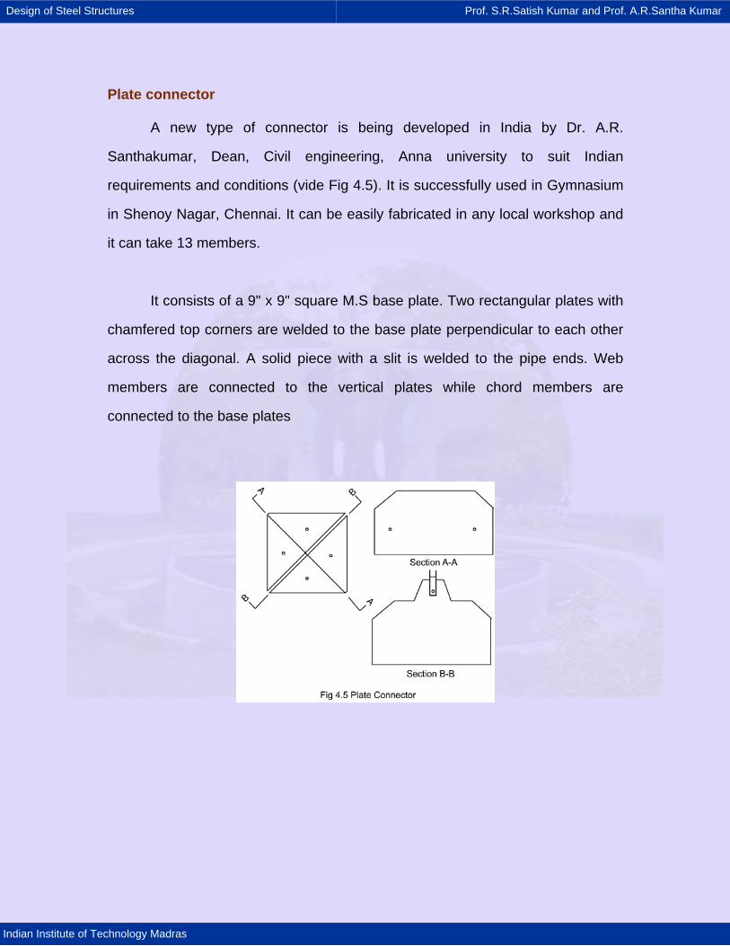
Design of Steel Structures Prof. S.R.Satish Kumar and Prof. A.R.Santha Kumar
Indian Institute of Technology Madras
Plate connector
A new type of connector is being developed in India by Dr. A.R.
Santhakumar, Dean, Civil engineering, Anna university to suit Indian
requirements and conditions (vide Fig 4.5). It is successfully used in Gymnasium
in Shenoy Nagar, Chennai. It can be easily fabricated in any local workshop and
it can take 13 members.
It consists of a 9" x 9" square M.S base plate. Two rectangular plates with
chamfered top corners are welded to the base plate perpendicular to each other
across the diagonal. A solid piece with a slit is welded to the pipe ends. Web
members are connected to the vertical plates while chord members are
connected to the base plates
Design of Steel Structures Prof. S.R.Satish Kumar and Prof. A.R.Santha Kumar
Indian Institute of Technology Madras
4.4. Optimisation
Many design are possible to satisfy the functional requirements and a trial
and error procedure may be employed to choose the optimal design. Selection of
the best geometry of a structure or the member sizes are examples of optimal
design procedures. The computer is best suited for finding the optimal solutions.
Optimisation then becomes an automated design procedure, providing the
optimal values for certain design quantities while considering the design criteria
and constraints.
Computer-aided design involving user machine interaction and automated
optimal design, characterised by pre-programmed logical decisions, based upon
internally stored information, are not mutually exclusive, but complement each
other. As the techniques of interactive computer-aided design develop, the need
to employ standard routines for automated design of structural subsystems will
become increasingly relevant.
The numerical methods of structural optimisation, with application of
computers automatically generate a near optimal design in an interactive
manner. A finite number of variables has to be established, together with the
constraints relating to these variables. An initial guess-solution is used as the
starting point for a systematic search for better designs and the process of
search is terminated when certain criteria are satisfied.
Those quantities defining a structural system that are fixed during the
automated design are called pre-assigned parameters or simply parameters and
those quantities that are not pre-assigned are called design variables. The
design variables cover the material properties, the topology of the structure, its
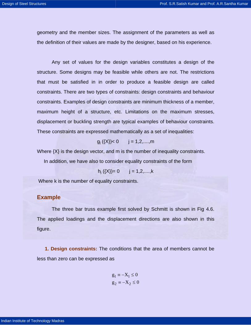
Design of Steel Structures Prof. S.R.Satish Kumar and Prof. A.R.Santha Kumar
Indian Institute of Technology Madras
geometry and the member sizes. The assignment of the parameters as well as
the definition of their values are made by the designer, based on his experience.
Any set of values for the design variables constitutes a design of the
structure. Some designs may be feasible while others are not. The restrictions
that must be satisfied in in order to produce a feasible design are called
constraints. There are two types of constraints: design constraints and behaviour
constraints. Examples of design constraints are minimum thickness of a member,
maximum height of a structure, etc. Limitations on the maximum stresses,
displacement or buckling strength are typical examples of behaviour constraints.
These constraints are expressed mathematically as a set of inequalities:
gj ({X})< 0 j = 1,2,....,m
Where {X} is the design vector, and m is the number of inequality constraints.
In addition, we have also to consider equality constraints of the form
hj ({X})= 0 j = 1,2,....,k
Where k is the number of equality constraints.
Example
The three bar truss example first solved by Schmitt is shown in Fig 4.6.
The applied loadings and the displacement directions are also shown in this
figure.
1. Design constraints: The conditions that the area of members cannot be
less than zero can be expressed as
1 1
2 2
g X 0g X 0
≡ − ≤≡ − ≤
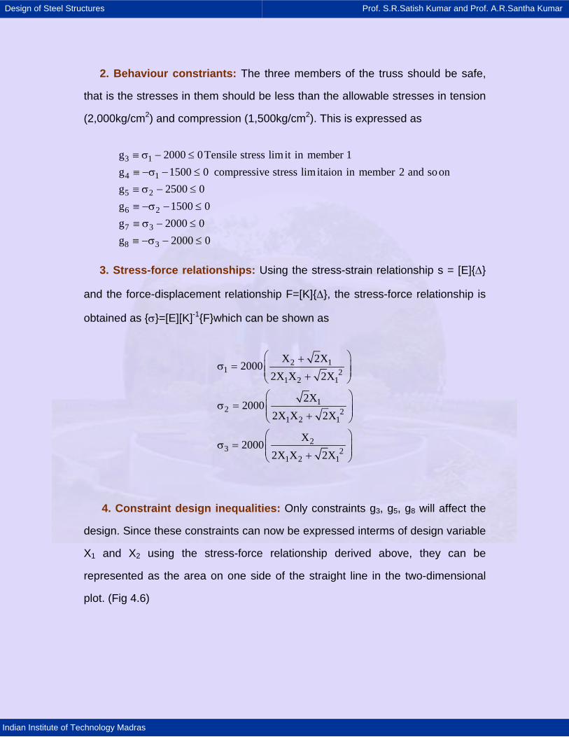
Design of Steel Structures Prof. S.R.Satish Kumar and Prof. A.R.Santha Kumar
Indian Institute of Technology Madras
2. Behaviour constriants: The three members of the truss should be safe,
that is the stresses in them should be less than the allowable stresses in tension
(2,000kg/cm2) and compression (1,500kg/cm2). This is expressed as
3 1
4 1
5 2
6 2
7 3
8 3
g 2000 0Tensile stress limit in member 1g 1500 0 compressive stress limitaion in member 2 and soong 2500 0g 1500 0g 2000 0g 2000 0
≡ σ − ≤
≡ −σ − ≤≡ σ − ≤
≡ −σ − ≤
≡ σ − ≤
≡ −σ − ≤
3. Stress-force relationships: Using the stress-strain relationship s = [E]{∆}
and the force-displacement relationship F=[K]{∆}, the stress-force relationship is
obtained as {σ}=[E][K]-1{F}which can be shown as
2 11 2
1 2 1
12 2
1 2 1
23 2
1 2 1
X 2X2000
2X X 2X
2X2000
2X X 2X
X2000
2X X 2X
⎛ ⎞+σ = ⎜ ⎟⎜ ⎟+⎝ ⎠
⎛ ⎞σ = ⎜ ⎟⎜ ⎟+⎝ ⎠
⎛ ⎞σ = ⎜ ⎟⎜ ⎟+⎝ ⎠
4. Constraint design inequalities: Only constraints g3, g5, g8 will affect the
design. Since these constraints can now be expressed interms of design variable
X1 and X2 using the stress-force relationship derived above, they can be
represented as the area on one side of the straight line in the two-dimensional
plot. (Fig 4.6)
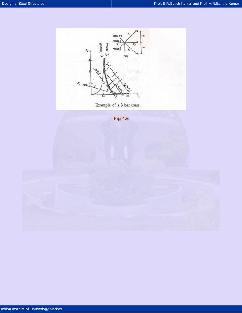
Design of Steel Structures Prof. S.R.Satish Kumar and Prof. A.R.Santha Kumar
Indian Institute of Technology Madras
Fig 4.6
Design of Steel Structures Prof. S.R.Satish Kumar and Prof. A.R.Santha Kumar
Indian Institute of Technology Madras
4.5. Design space
Each design variable X1, X2 ...is viewed as one dimension in a design
space a particular set of variable as a point in this space. In the general case of n
variable, we have an n-dimensioned space. In the example where we have only
two variables, the space reduces to a plane figure shown in (Fig 4.6(b)). The
arrows indicate the inequality representation and the shaded zone shows the
feasible region. A design falling in the feasible region is an unconstrained design
and the one falling on boundary is a constrained design.
An infinite number of feasible design is possible. In order to find the best
one, it es necessary of form a function of the variables to use for comparision of
feasible design alternatives. The objective (merit) function is a function whose
least value is sought in an optimisation procedure. In other words, the
optimisation problem consists in the determination of the vector of variables X
that will minimise a certain given objective functions.
Z = F({X})
In the example chosen, assuming the volume of material as the objective
function, we get
Z = 2(141 X1) + 100 X2
Design of Steel Structures Prof. S.R.Satish Kumar and Prof. A.R.Santha Kumar
Indian Institute of Technology Madras
The locus of all points satisfying F ({X}) = constant, form a straight line in a
two -dimensional space. (In this general case of n-dimensional space, it will form
a surface). For each value of constraint, a different straight line is obtained. Fig
4.6(b) shows the objective function contours. Every design on a particular
contour has the same volume or weight. It can be seen that the minimum value
of F ({X}) in the feasible region occurs at point A.
There are different approaches to this problem which constitute the
various methods of optimization. The traditional approach searches the solution
by pre-selecting a set of critical constraints and reducing the problem to a set of
equations in fewer variables. Successive reanalysis of the structure for improved
sets of constraints will tend towards the solution. Different re-analysis methods
can be used, the iterative methods being the most attractive in the case of space
structures.
Design of Steel Structures Prof. S.R.Satish Kumar and Prof. A.R.Santha Kumar
Indian Institute of Technology Madras
4.6. Optimality criteria
An interesting approach in optimization is a process known as optimality
criteria. The approach to the optimum is based on the assumption that some
characteristic will be attained at such optimum. The well-known example is the
fully stressed design where it is assumed that, in an optimal structure, each
member is subjected to its limiting stress under at least one loading condition.
The optimality criteria procedures are useful for space structures because
they constitute an adequate compromise to obtain practical and efficient
solutions. In many studies, it has been found that the shape of the objective
function around the optimum is flat, which means that an experienced designer
can reach solutions which are close to the theoretical optimum.
Design of Steel Structures Prof. S.R.Satish Kumar and Prof. A.R.Santha Kumar
Indian Institute of Technology Madras
4.7. Mathematical programming
It is difficult to anticipate which of the constraints will be critical at the
optimum. Therefore, the use of inequality constraints is essential for a proper
formulation of the optimal design problem.
The mathematical programming (MP) methods are included to solve the
general optimisation problem by numerical search algorithms while being general
regarding the objective function and constraints. On the other hand,
approximations are often required tube efficient on large practical problems such
as space structures.
Optimal design processes involves the minimization of weight subject to
certain constraints. Mathematical programming methods and structural theorems
are available to achieve such a design goal.
Of the various mathematical programming methods available for
optimisation, the linear programming methods is widely adopted in structural
engineering practice because of its simplicity. The objective function, which is the
minimisation of weight, is linear and a set of constraints, which can be expressed
by linear equations involving the unknowns (area, moment of inertia, etc., of the
members), are used for solving the problems. This can be mathematically
expressed as follows:
Suppose it is required to find a specified number of design variables x1,
x2...xn such that the objective function.
Z = C1x1 + C2x2 +....Cnxn
is minimised, satisfying the constraints.
Design of Steel Structures Prof. S.R.Satish Kumar and Prof. A.R.Santha Kumar
Indian Institute of Technology Madras
11 1 12 2 1n n 1
21 1 22 2 2n n 2
m1 1 m2 2 mn n m
a x a x ......a x ba x a x ......a x b..a x a x ......a x b
= + ≤= + ≤
= + ≤
The simplex algorithm is a versatile procedure for solving linear
programming (LP) problems with a large number of variables and constraints.
The simplex algorithm is now available in the form of standard computer
software package which uses the matrix representation of the variables and
constraints, especially when their number is very large.
The above set of equations is expressed in the matrix form as follows:
Find
1
2
n
xx
X ..x
⎡ ⎤⎢ ⎥⎢ ⎥⎢ ⎥=⎢ ⎥⎢ ⎥⎢ ⎥⎣ ⎦
Which minimised
The objective function ( )n
i in 1
f x C x−
= ∑
subject to the constraints
n
jk k jk 1
i
a x b , j 1, 2,....m
and x 0, i 1, 2,...n−
≤ =
≥ =
∑
Where Ci, ajk and bj are constants
The stiffness method of analysis is adopted and the optimisation is
achieved by mathematical programming
Design of Steel Structures Prof. S.R.Satish Kumar and Prof. A.R.Santha Kumar
Indian Institute of Technology Madras
The structure is divided into a number of groups and the analysis is
carried out groupwise. Then the member forces are determined. The critical
members are found out from each group. From the initial design, the objective
function and the constraints are framed. Then, by adopting the fully stressed
design (optimality criteria) method, the linear programming problem is solved and
the optimal solution found out. In each group every member is designed for the
fully stressed condition and the maximum size required is assigned for all the
members in that group. After completion of the design, one more analysis and
design routine for the structure as a whole is completed for alternative cross-
section.
Design of Steel Structures Prof. S.R.Satish Kumar and Prof. A.R.Santha Kumar
Indian Institute of Technology Madras
4.8. Geometry as variable
In method 1, only the member sizes were treated as variables whereas
the geometry was assumed as fixed. Method 2 treats the geometry also as a
variable and gets the most preferred geometry. The geometry developed by the
computer results in the minimum weight of space frame for any practically
acceptable configuration. For solutions, since a iterative procedure is adopted for
the optimum structural design, it is obvious that the use of a computer is
essential.
The algorithm used for optimum structural design is similar to that given by
Samuel L. Lipson which presumes that an initial feasible configuration is
available for the structure. The structure is divided into a number of groups and
the externally applied loadings are obtained. For the given configuration, the
upper limits and the lower limits on the design variables, namely the joint
coordinates are fixed. Then (k-1) new configurations are generated randomly as
Xij = 1i + rij (ui - 1i)
i = 1,2,...n
j = 1,2,...k
where k is the total number of configurations in the complex, usually larger
than (n+1) where n is the number of design variables and rij is the random
number for the ith coordinates of the jth points, the random numbers having a
uniform distribution over the interval 10 to 1 ui is the upper limit and 1i is the lower
limit of the ith independent variable.
Thus, the complex containing k number of feasible solutions is generated
and all these configurations will satisfy the explicit constraints, namely, the upper
and lower bounds on the design variables. Next, for all these k configurations,
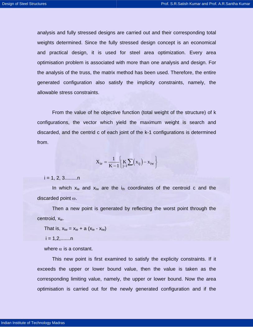
Design of Steel Structures Prof. S.R.Satish Kumar and Prof. A.R.Santha Kumar
Indian Institute of Technology Madras
analysis and fully stressed designs are carried out and their corresponding total
weights determined. Since the fully stressed design concept is an economical
and practical design, it is used for steel area optimization. Every area
optimisation problem is associated with more than one analysis and design. For
the analysis of the truss, the matrix method has been used. Therefore, the entire
generated configuration also satisfy the implicity constraints, namely, the
allowable stress constraints.
From the value of he objective function (total weight of the structure) of k
configurations, the vector which yield the maximum weight is search and
discarded, and the centrid c of each joint of the k-1 configurations is determined
from.
( )ie ij iwj 1
1X K x xK 1 −
⎧ ⎫= −⎨ ⎬− ⎩ ⎭∑
i = 1, 2, 3.........n
In which xie and xiw are the ith coordinates of the centroid c and the
discarded point ω.
Then a new point is generated by reflecting the worst point through the
centroid, xie.
That is, xiw = xie + a (xie - xiw)
i = 1,2,.......n
where α is a constant.
This new point is first examined to satisfy the explicity constraints. If it
exceeds the upper or lower bound value, then the value is taken as the
corresponding limiting value, namely, the upper or lower bound. Now the area
optimisation is carried out for the newly generated configuration and if the
Design of Steel Structures Prof. S.R.Satish Kumar and Prof. A.R.Santha Kumar
Indian Institute of Technology Madras
functional value is better than the second worst, the point is accepted as an
improvement and the process of developing the new configuration is repeated as
mentioned earlier. Otherwise, the newly generated point is moved halfway
toward the centroid of the remaining points and the area optimisation is repeated
for the new configuration,. This process is repeated over a fixed number of
iterations and the end of every iteration, the weight and the corresponding
configuration are printed out, which will shown the minimum weight achievable
within the limits (ui and 1i) of the configuration.
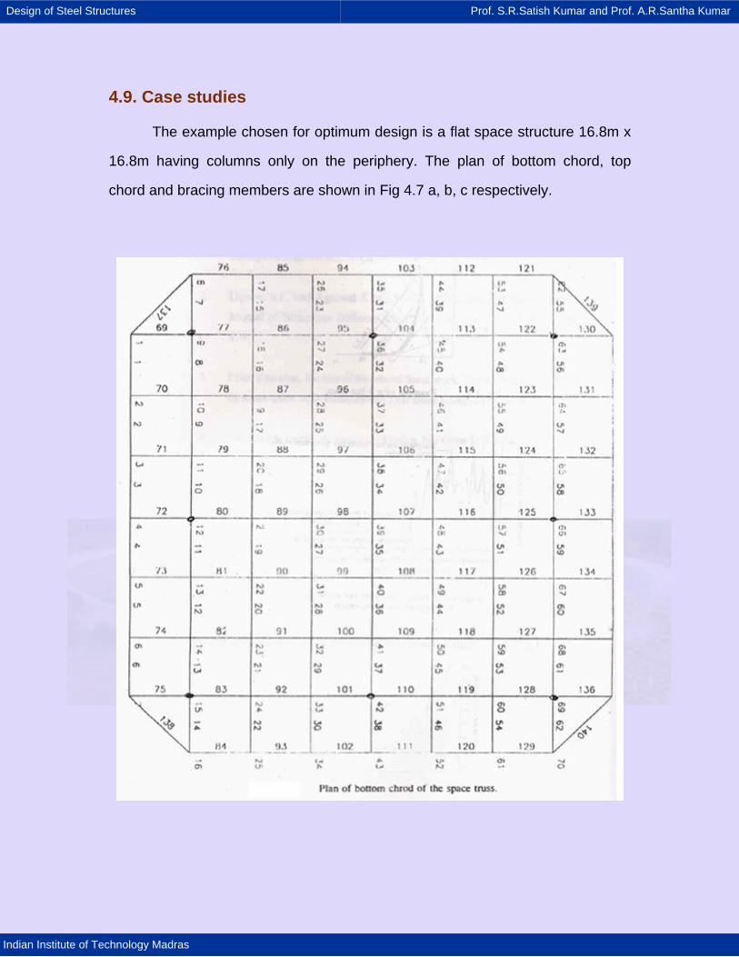
Design of Steel Structures Prof. S.R.Satish Kumar and Prof. A.R.Santha Kumar
Indian Institute of Technology Madras
4.9. Case studies
The example chosen for optimum design is a flat space structure 16.8m x
16.8m having columns only on the periphery. The plan of bottom chord, top
chord and bracing members are shown in Fig 4.7 a, b, c respectively.
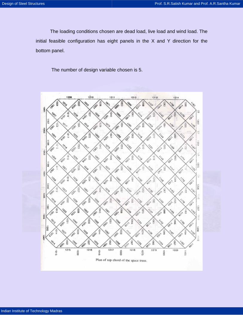
Design of Steel Structures Prof. S.R.Satish Kumar and Prof. A.R.Santha Kumar
Indian Institute of Technology Madras
The loading conditions chosen are dead load, live load and wind load. The
initial feasible configuration has eight panels in the X and Y direction for the
bottom panel.
The number of design variable chosen is 5.
Design of Steel Structures Prof. S.R.Satish Kumar and Prof. A.R.Santha Kumar
Indian Institute of Technology Madras
In the initial complex 27 configuration are generated, including the initial
feasible configuration. Random numbers required for generation of these
configurations are fed into the computer as input. The variables involved one
type of arrangement, height of the truss, number of panels is x direction, number
of panels in y direction and location of columns. The number of iterations for
development during optimisation procedure is pictorially represented in Fig 4.8.
The final configuration selected is based in the least weight of 15 Kg/Sq mt for
the initial feasible of weight with respect to height of space frame.
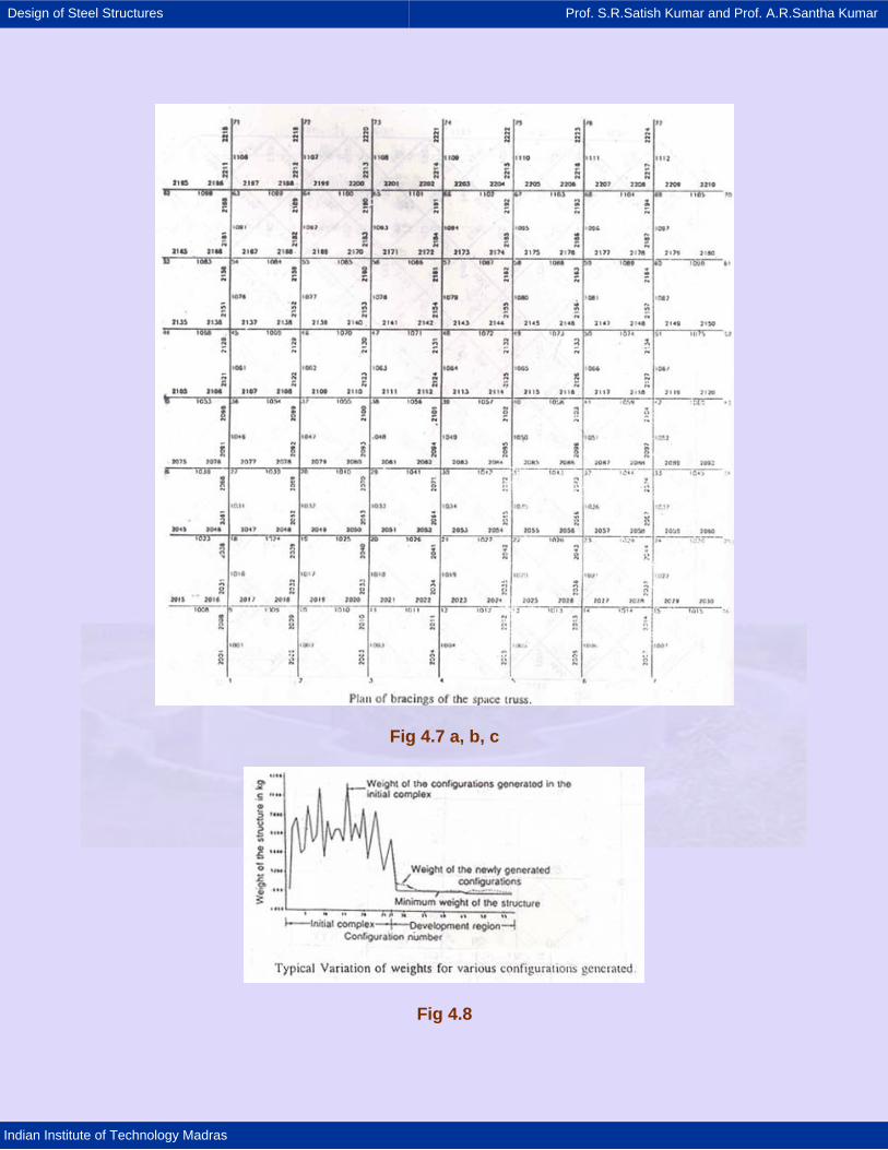
Design of Steel Structures Prof. S.R.Satish Kumar and Prof. A.R.Santha Kumar
Indian Institute of Technology Madras
Fig 4.7 a, b, c
Fig 4.8
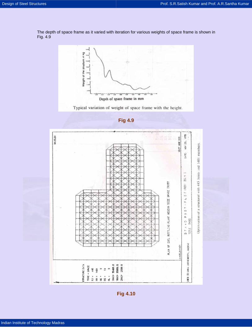
Design of Steel Structures Prof. S.R.Satish Kumar and Prof. A.R.Santha Kumar
Indian Institute of Technology Madras
The depth of space frame as it varied with iteration for various weights of space frame is shown in Fig. 4.9
Fig 4.9
Fig 4.10
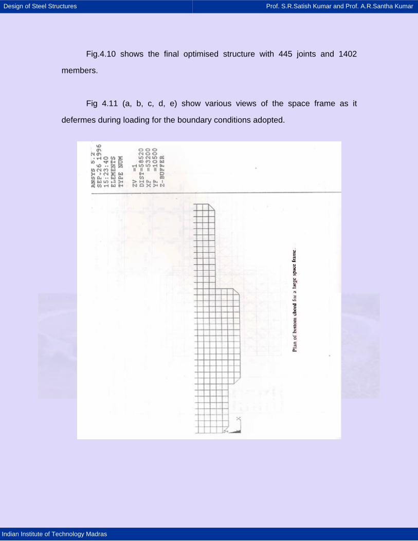
Design of Steel Structures Prof. S.R.Satish Kumar and Prof. A.R.Santha Kumar
Indian Institute of Technology Madras
Fig.4.10 shows the final optimised structure with 445 joints and 1402
members.
Fig 4.11 (a, b, c, d, e) show various views of the space frame as it
defermes during loading for the boundary conditions adopted.
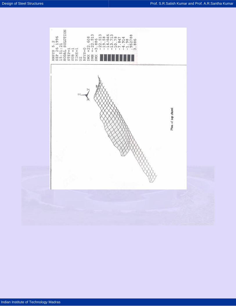
Design of Steel Structures Prof. S.R.Satish Kumar and Prof. A.R.Santha Kumar
Indian Institute of Technology Madras
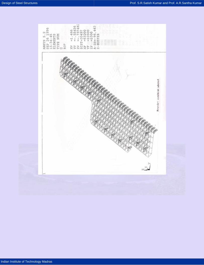
Design of Steel Structures Prof. S.R.Satish Kumar and Prof. A.R.Santha Kumar
Indian Institute of Technology Madras
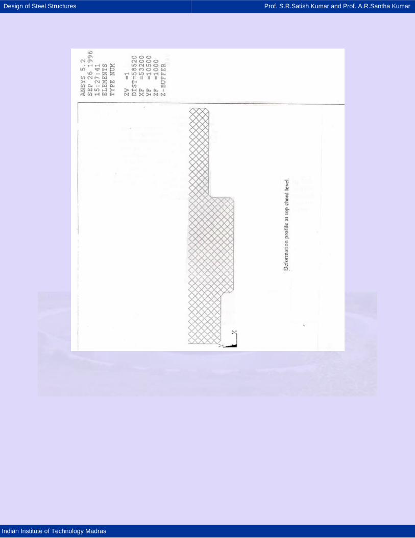
Design of Steel Structures Prof. S.R.Satish Kumar and Prof. A.R.Santha Kumar
Indian Institute of Technology Madras
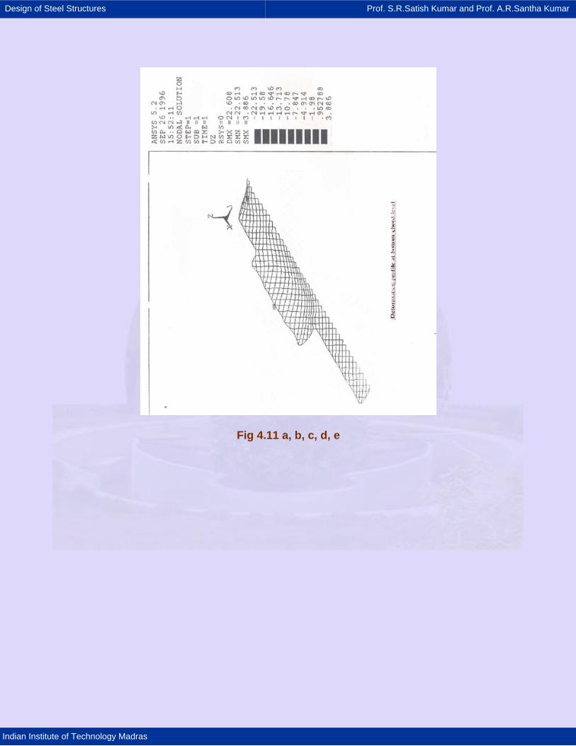
Design of Steel Structures Prof. S.R.Satish Kumar and Prof. A.R.Santha Kumar
Indian Institute of Technology Madras
Fig 4.11 a, b, c, d, e
Design of Steel Structures Prof. S.R.Satish Kumar and Prof. A.R.Santha Kumar
Indian Institute of Technology Madras
4.10 Conclusion
The case study shows the behaviour of an actual space frame constructed
for a typical industrial structure. Such frames can be provided for factories, sports
complexes and airports.
Design of Steel Structures Prof. S.R.Satish Kumar and Prof. A.R.Santha Kumar
Indian Institute of Technology Madras
4.11. References
1. Kumar. R. Configuration of Truss M.E thesis, Structures division, College of
Engineering, Anna University, Madras 1981.
2. Lipson. S.L. and Agrawal K.M., Weight optimisation of Plane Trusses,
Journal of Structures Division ASCE Vol.100, No. 575, 1974, pp 865-879.
3. Peter Knowles, Design of Structural Steel worl, Survey University Press in
Association with International Text Book Company, UK 1977.
4. Uni Kirsch, Optimum structural Design, Mc Graw Hill, 1981.
Design of Steel Structures Prof. S.R.Satish Kumar and Prof. A.R.Santha Kumar
Indian Institute of Technology Madras
5. COLD FORM STEEL 5.1 Introduction
Thin sheet steel products are extensively used in building industry, and range
from purlins to roof sheeting and floor decking. Generally these are available for use as
basic building elements for assembly at site or as prefabricated frames or panels. These
thin steel sections are cold-formed, i.e. their manufacturing process involves forming
steel sections in a cold state (i.e. without application of heat) from steel sheets of
uniform thickness. These are given the generic title Cold Formed Steel Sections.
Sometimes they are also called Light Gauge Steel Sections or Cold Rolled Steel
Sections. The thickness of steel sheet used in cold formed construction is usually 1 to 3
mm. Much thicker material up to 8 mm can be formed if pre-galvanised material is not
required for the particular application. The method of manufacturing is important as it
differentiates these products from hot rolled steel sections. Normally, the yield strength
of steel sheets used in cold-formed sections is at least 280 N/mm2, although there is a
trend to use steels of higher strengths, and sometimes as low as 230 N/mm2.
Manufacturers of cold formed steel sections purchase steel coils of 1.0 to 1.25 m
width, slit them longitudinally to the correct width appropriate to the section required and
then feed them into a series of roll forms. These rolls, containing male and female dies,
are arranged in pairs, moving in opposite direction so that as the sheet is fed through
them its shape is gradually altered to the required profile. The number of pairs of rolls
(called stages) depends on the complexity of the cross sectional shape and varies from
5 to 15. At the end of the rolling stage a flying shearing machine cuts the member into
the desired lengths.
An alternative method of forming is by press - braking which is limited to short lengths
of around 6 m and for relatively simple shapes. In this process short lengths of strip are
pressed between a male and a female die to fabricate one fold at a time and obtain the
final required shape of the section. Cold rolling is used when large volume of long
Design of Steel Structures Prof. S.R.Satish Kumar and Prof. A.R.Santha Kumar
Indian Institute of Technology Madras
products is required and press breaking is used when small volumes of short length
products are produced.
Galvanizing (or zinc coating) of the preformed coil provides very satisfactory
protection against corrosion in internal environments. A coating of 275 g/m2 (total for
both faces) is the usual standard for internal environments. This corresponds to zinc
coating of 0.04 mm. Thicker coatings are essential when moisture is present for long
periods of time. Other than galvanising, different methods of pre-rolling and post-rolling
corrosion protection measures are also used.
Although the cold rolled products were developed during the First World War,
their extensive use worldwide has grown only during the last 20 years because of their
versatility and suitability for a range of lighter load bearing applications. Thus the wide
range of available products has extended their use to primary beams, floor units, roof
trusses and building frames. Indeed it is difficult to think of any industry in which Cold
Rolled Steel products do not exist in one form or the other. Besides building industry,
they are employed in motor vehicles, railways, aircrafts, ships, agricultural machinery,
electrical equipment, storage racks, house hold appliances and so on. In recent years,
with the evolution of attractive coatings and the distinctive profiles that can be
manufactured, cold formed steel construction has been used for highly pleasing designs
in practically every sector of building construction.
In this chapter, the background theory governing the design of cold formed steel
elements is presented in a summary form. Designs of cold formed steel sections are
dealt with in IS: 801-1975 which is currently due under revision. In the absence of a
suitable Limit State Code in India, the Code of Practice for Cold Formed Sections in use
in the U.K. (BS 5950, Part 5) is employed for illustrating the concepts with suitable
modifications appropriate to Indian conditions.
Design of Steel Structures Prof. S.R.Satish Kumar and Prof. A.R.Santha Kumar
Indian Institute of Technology Madras
In the last chapter, the special features and attractions of cold formed steel
sections for many industrial applications were presented and discussed. In view of the
use of very thin steel sheet sections, (generally in the 1 mm - 3 mm range), particular
attention has to be paid to buckling of these elements. Stiffened and unstiffened
elements were compared and the concept of effective width to deal with the rapid
design of compression elements together with suitable design simplifications, outlined.
Finally, the methods adopted for the design of laterally restrained beams and
unrestrained beams were discussed. The techniques of eliminating lateral buckling in
practice, by providing lateral braces or by attachment to floors etc were described so
that the compression flanges would not buckle laterally.
In this chapter the design of columns for axial compression, compression
combined with bending as well as for torsional-flexural buckling will be discussed. The
diversity of cold formed steel shapes and the multiplicity of purposes to which they are
put to, makes it a difficult task to provide general solution procedures covering all
potential uses. Some design aspects are nevertheless included to provide a general
appreciation of this versatile product. It is not unusual to design some cold formed steel
sections on the basis of prototype tests or by employing empirical rules. These are also
discussed in a summary form herein.
Design of Steel Structures Prof. S.R.Satish Kumar and Prof. A.R.Santha Kumar
Indian Institute of Technology Madras
5.2 Advantages of cold formed sections
Cold forming has the effect of increasing the yield strength of steel, the
increase being the consequence of cold working well into the strain-hardening
range. These increases are predominant in zones where the metal is bent by
folding. The effect of cold working is thus to enhance the mean yield stress by
15% - 30%. For purposes of design, the yield stress may be regarded as having
been enhanced by a minimum of 15%.
Some of the main advantages of cold rolled sections, as compared with
their hot-rolled counterparts are as follows:
• Cross sectional shapes are formed to close tolerances and these can be
consistently repeated for as long as required.
• Cold rolling can be employed to produce almost any desired shape to any
desired length.
• Pre-galvanised or pre-coated metals can be formed, so that high resistance to
corrosion, besides an attractive surface finish, can be achieved.
• All conventional jointing methods, (i.e. riveting, bolting, welding and
adhesives) can be employed.
• High strength to weight ratio is achieved in cold-rolled products.
• They are usually light making it easy to transport and erect.
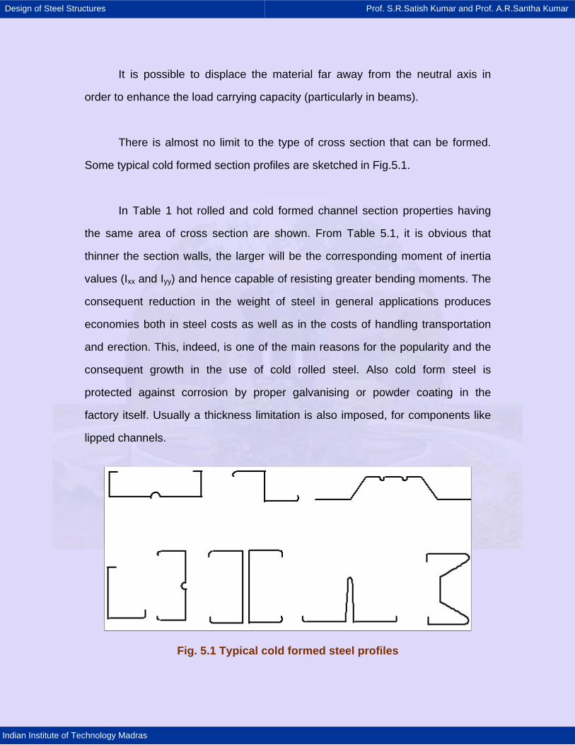
Design of Steel Structures Prof. S.R.Satish Kumar and Prof. A.R.Santha Kumar
Indian Institute of Technology Madras
It is possible to displace the material far away from the neutral axis in
order to enhance the load carrying capacity (particularly in beams).
There is almost no limit to the type of cross section that can be formed.
Some typical cold formed section profiles are sketched in Fig.5.1.
In Table 1 hot rolled and cold formed channel section properties having
the same area of cross section are shown. From Table 5.1, it is obvious that
thinner the section walls, the larger will be the corresponding moment of inertia
values (Ixx and Iyy) and hence capable of resisting greater bending moments. The
consequent reduction in the weight of steel in general applications produces
economies both in steel costs as well as in the costs of handling transportation
and erection. This, indeed, is one of the main reasons for the popularity and the
consequent growth in the use of cold rolled steel. Also cold form steel is
protected against corrosion by proper galvanising or powder coating in the
factory itself. Usually a thickness limitation is also imposed, for components like
lipped channels.
Fig. 5.1 Typical cold formed steel profiles
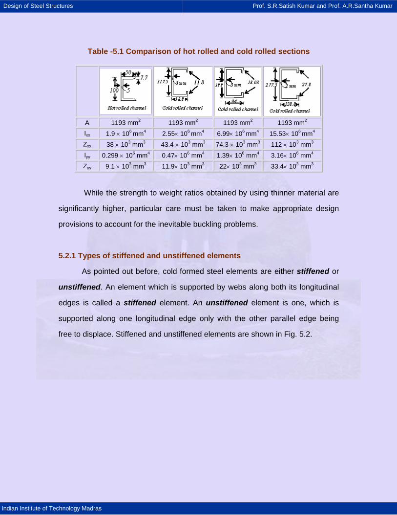
Design of Steel Structures Prof. S.R.Satish Kumar and Prof. A.R.Santha Kumar
Indian Institute of Technology Madras
Table -5.1 Comparison of hot rolled and cold rolled sections
A 1193 mm2 1193 mm2 1193 mm2 1193 mm2 Ixx 1.9 × 106 mm4 2.55× 106 mm4 6.99× 106 mm4 15.53× 106 mm4 Zxx 38 × 103 mm3 43.4 × 103 mm3 74.3 × 103 mm3 112 × 103 mm3 Iyy 0.299 × 106 mm4 0.47× 106 mm4 1.39× 106 mm4 3.16× 106 mm4 Zyy 9.1 × 103 mm3 11.9× 103 mm3 22× 103 mm3 33.4× 103 mm3
While the strength to weight ratios obtained by using thinner material are
significantly higher, particular care must be taken to make appropriate design
provisions to account for the inevitable buckling problems.
5.2.1 Types of stiffened and unstiffened elements
As pointed out before, cold formed steel elements are either stiffened or
unstiffened. An element which is supported by webs along both its longitudinal
edges is called a stiffened element. An unstiffened element is one, which is
supported along one longitudinal edge only with the other parallel edge being
free to displace. Stiffened and unstiffened elements are shown in Fig. 5.2.
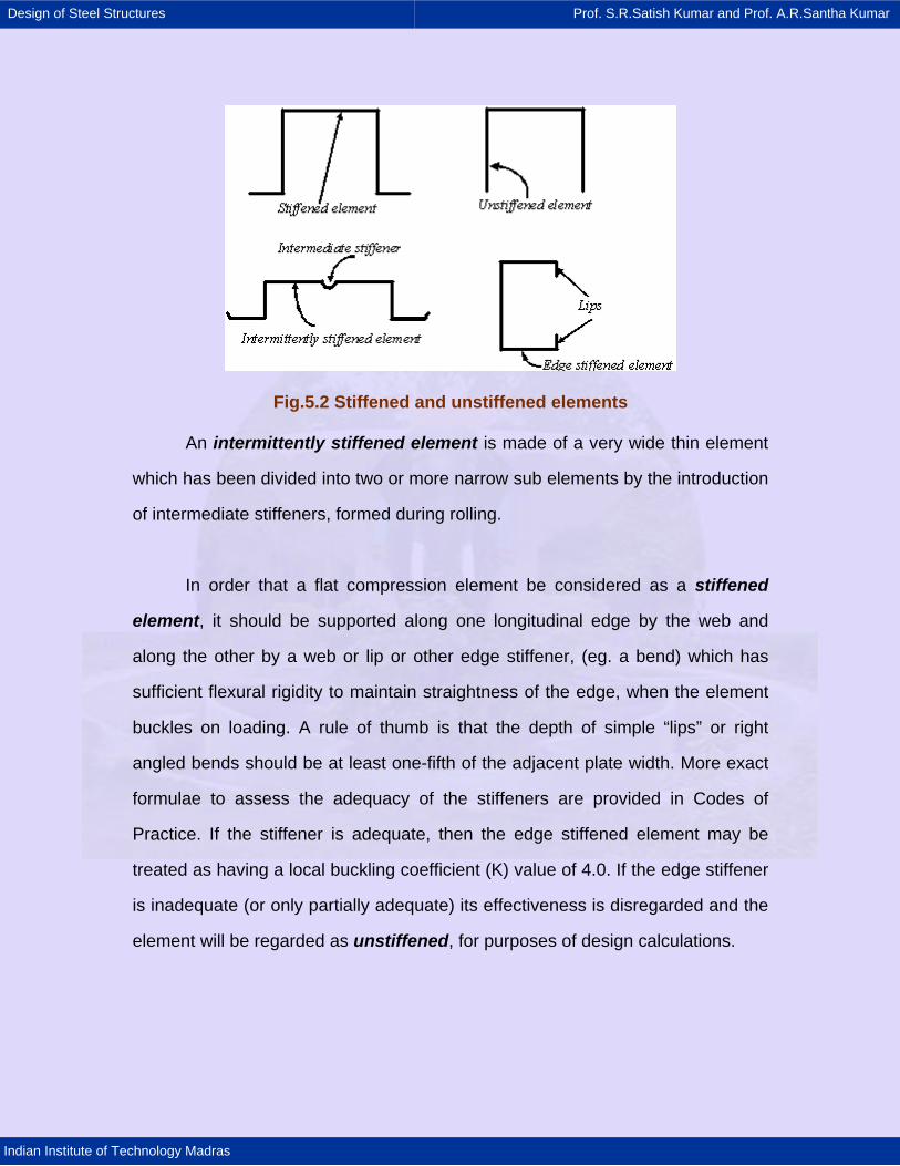
Design of Steel Structures Prof. S.R.Satish Kumar and Prof. A.R.Santha Kumar
Indian Institute of Technology Madras
Fig.5.2 Stiffened and unstiffened elements
An intermittently stiffened element is made of a very wide thin element
which has been divided into two or more narrow sub elements by the introduction
of intermediate stiffeners, formed during rolling.
In order that a flat compression element be considered as a stiffened
element, it should be supported along one longitudinal edge by the web and
along the other by a web or lip or other edge stiffener, (eg. a bend) which has
sufficient flexural rigidity to maintain straightness of the edge, when the element
buckles on loading. A rule of thumb is that the depth of simple “lips” or right
angled bends should be at least one-fifth of the adjacent plate width. More exact
formulae to assess the adequacy of the stiffeners are provided in Codes of
Practice. If the stiffener is adequate, then the edge stiffened element may be
treated as having a local buckling coefficient (K) value of 4.0. If the edge stiffener
is inadequate (or only partially adequate) its effectiveness is disregarded and the
element will be regarded as unstiffened, for purposes of design calculations.
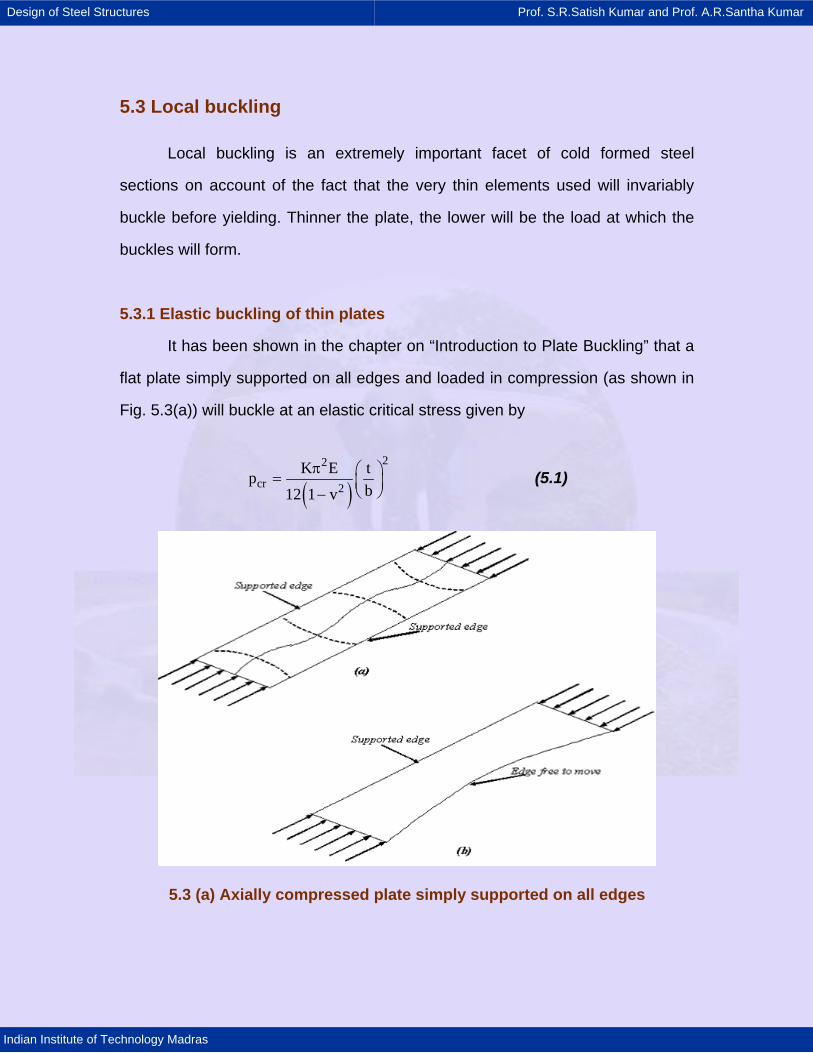
Design of Steel Structures Prof. S.R.Satish Kumar and Prof. A.R.Santha Kumar
Indian Institute of Technology Madras
5.3 Local buckling
Local buckling is an extremely important facet of cold formed steel
sections on account of the fact that the very thin elements used will invariably
buckle before yielding. Thinner the plate, the lower will be the load at which the
buckles will form.
5.3.1 Elastic buckling of thin plates
It has been shown in the chapter on “Introduction to Plate Buckling” that a
flat plate simply supported on all edges and loaded in compression (as shown in
Fig. 5.3(a)) will buckle at an elastic critical stress given by
( )22
cr 2K E tp
b12 1 v
π ⎛ ⎞= ⎜ ⎟⎝ ⎠−
(5.1)
5.3 (a) Axially compressed plate simply supported on all edges
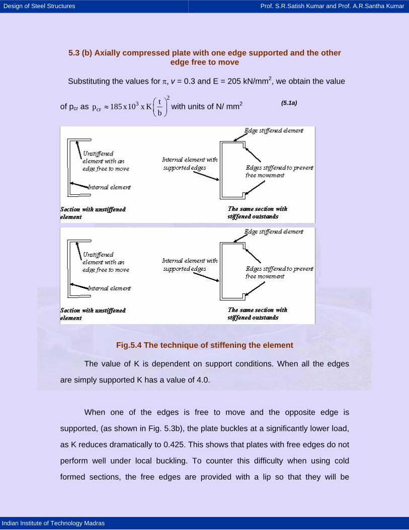
Design of Steel Structures Prof. S.R.Satish Kumar and Prof. A.R.Santha Kumar
Indian Institute of Technology Madras
5.3 (b) Axially compressed plate with one edge supported and the other edge free to move
Substituting the values for π, v = 0.3 and E = 205 kN/mm2, we obtain the value
of pcr as 2
3cr
tp 185 x10 x Kb
⎛ ⎞≈ ⎜ ⎟⎝ ⎠
with units of N/ mm2 (5.1a)
Fig.5.4 The technique of stiffening the element
The value of K is dependent on support conditions. When all the edges
are simply supported K has a value of 4.0.
When one of the edges is free to move and the opposite edge is
supported, (as shown in Fig. 5.3b), the plate buckles at a significantly lower load,
as K reduces dramatically to 0.425. This shows that plates with free edges do not
perform well under local buckling. To counter this difficulty when using cold
formed sections, the free edges are provided with a lip so that they will be
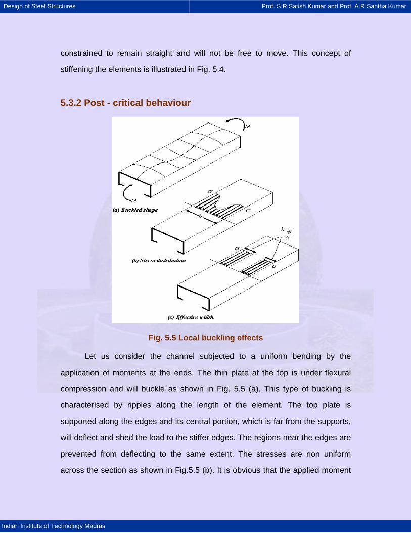
Design of Steel Structures Prof. S.R.Satish Kumar and Prof. A.R.Santha Kumar
Indian Institute of Technology Madras
constrained to remain straight and will not be free to move. This concept of
stiffening the elements is illustrated in Fig. 5.4.
5.3.2 Post - critical behaviour
Fig. 5.5 Local buckling effects
Let us consider the channel subjected to a uniform bending by the
application of moments at the ends. The thin plate at the top is under flexural
compression and will buckle as shown in Fig. 5.5 (a). This type of buckling is
characterised by ripples along the length of the element. The top plate is
supported along the edges and its central portion, which is far from the supports,
will deflect and shed the load to the stiffer edges. The regions near the edges are
prevented from deflecting to the same extent. The stresses are non uniform
across the section as shown in Fig.5.5 (b). It is obvious that the applied moment
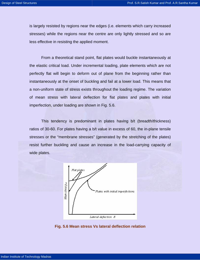
Design of Steel Structures Prof. S.R.Satish Kumar and Prof. A.R.Santha Kumar
Indian Institute of Technology Madras
is largely resisted by regions near the edges (i.e. elements which carry increased
stresses) while the regions near the centre are only lightly stressed and so are
less effective in resisting the applied moment.
From a theoretical stand point, flat plates would buckle instantaneously at
the elastic critical load. Under incremental loading, plate elements which are not
perfectly flat will begin to deform out of plane from the beginning rather than
instantaneously at the onset of buckling and fail at a lower load. This means that
a non-uniform state of stress exists throughout the loading regime. The variation
of mean stress with lateral deflection for flat plates and plates with initial
imperfection, under loading are shown in Fig. 5.6.
This tendency is predominant in plates having b/t (breadth/thickness)
ratios of 30-60. For plates having a b/t value in excess of 60, the in-plane tensile
stresses or the “membrane stresses” (generated by the stretching of the plates)
resist further buckling and cause an increase in the load-carrying capacity of
wide plates.
Fig. 5.6 Mean stress Vs lateral deflection relation
Design of Steel Structures Prof. S.R.Satish Kumar and Prof. A.R.Santha Kumar
Indian Institute of Technology Madras
5.3.3 Effective width concept
The effects of local buckling can be evaluated by using the concept of
effective width. Lightly stressed regions at centre are ignored, as these are least
effective in resisting the applied stresses. Regions near the supports are far more
effective and are taken to be fully effective. The section behaviour is modeled on
the basis of the effective width (beff) sketched in Fig. 5.5(c).
The effective width, (beff) multiplied by the edge stress (σ) is the same as
the mean stress across the section multiplied by the total width (b) of the
compression member.
The effective width of an element under compression is dependent on
the magnitude of the applied stress fc, the width/thickness ratio of the element
and the edge support conditions.
5.3.4 Code provisions on “Local buckling of compressed plates”
The effective width concept is usually modified to take into account the
effects of yielding and imperfection. For example, BS5950: Part 5 provides a
semi-empirical formula for basic effective width, beff, to conform to extensive
experimental data.
When fc > 0.123 pcr, then
0.240.5eff c
cr
b f1 14 0.35
b p
−⎡ ⎤⎧ ⎫⎡ ⎤⎪ ⎪⎢ ⎥= + −⎨ ⎬⎢ ⎥⎢ ⎥⎣ ⎦⎪ ⎪⎩ ⎭⎢ ⎥⎣ ⎦
(5.2a)
When fc < 0.123 pcr, then beff = b (5.2b)
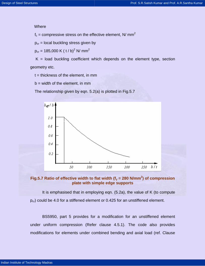
Design of Steel Structures Prof. S.R.Satish Kumar and Prof. A.R.Santha Kumar
Indian Institute of Technology Madras
Where
fc = compressive stress on the effective element, N/ mm2
pcr = local buckling stress given by
pcr = 185,000 K ( t / b)2 N/ mm2
K = load buckling coefficient which depends on the element type, section
geometry etc.
t = thickness of the element, in mm
b = width of the element, in mm
The relationship given by eqn. 5.2(a) is plotted in Fig.5.7
Fig.5.7 Ratio of effective width to flat width (fy = 280 N/mm2) of compression plate with simple edge supports
It is emphasised that in employing eqn. (5.2a), the value of K (to compute
pcr) could be 4.0 for a stiffened element or 0.425 for an unstiffened element.
BS5950, part 5 provides for a modification for an unstiffened element
under uniform compression (Refer clause 4.5.1). The code also provides
modifications for elements under combined bending and axial load (ref. Clause
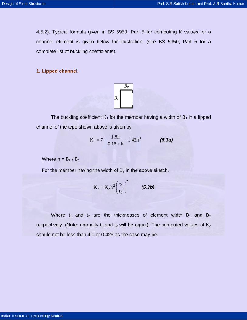
Design of Steel Structures Prof. S.R.Satish Kumar and Prof. A.R.Santha Kumar
Indian Institute of Technology Madras
4.5.2). Typical formula given in BS 5950, Part 5 for computing K values for a
channel element is given below for illustration. (see BS 5950, Part 5 for a
complete list of buckling coefficients).
1. Lipped channel.
The buckling coefficient K1 for the member having a width of B1 in a lipped
channel of the type shown above is given by
31
1.8hK 7 1.43h0.15 h
= − −+
(5.3a)
Where h = B2 / B1
For the member having the width of B2 in the above sketch.
22 1
2 22
tK K h
t⎛ ⎞
= ⎜ ⎟⎝ ⎠
(5.3b)
Where t1 and t2 are the thicknesses of element width B1 and B2
respectively. (Note: normally t1 and t2 will be equal). The computed values of K2
should not be less than 4.0 or 0.425 as the case may be.
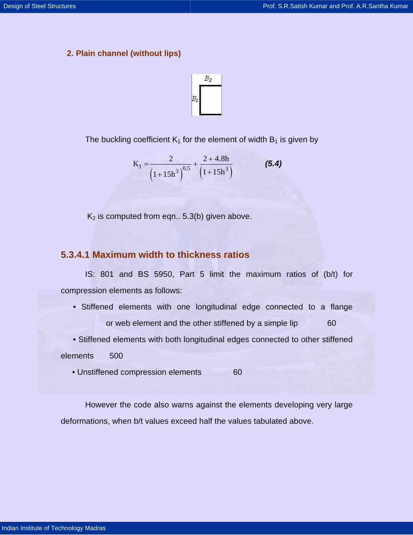
Design of Steel Structures Prof. S.R.Satish Kumar and Prof. A.R.Santha Kumar
Indian Institute of Technology Madras
2. Plain channel (without lips)
The buckling coefficient K1 for the element of width B1 is given by
( ) ( )1 0.5 33
2 2 4.8hK1 15h1 15h
+= +
++ (5.4)
K2 is computed from eqn.. 5.3(b) given above.
5.3.4.1 Maximum width to thickness ratios
IS: 801 and BS 5950, Part 5 limit the maximum ratios of (b/t) for
compression elements as follows:
• Stiffened elements with one longitudinal edge connected to a flange
or web element and the other stiffened by a simple lip 60
• Stiffened elements with both longitudinal edges connected to other stiffened
elements 500
• Unstiffened compression elements 60
However the code also warns against the elements developing very large
deformations, when b/t values exceed half the values tabulated above.
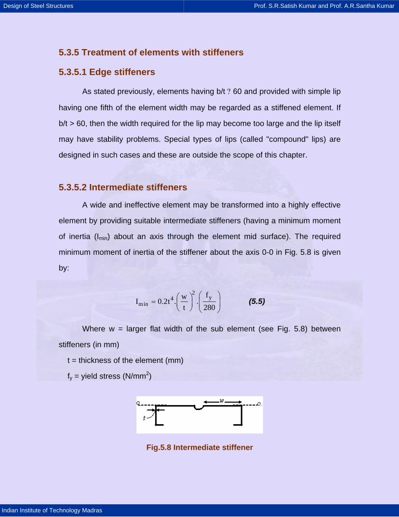
Design of Steel Structures Prof. S.R.Satish Kumar and Prof. A.R.Santha Kumar
Indian Institute of Technology Madras
5.3.5 Treatment of elements with stiffeners
5.3.5.1 Edge stiffeners
As stated previously, elements having b/t ? 60 and provided with simple lip
having one fifth of the element width may be regarded as a stiffened element. If
b/t > 60, then the width required for the lip may become too large and the lip itself
may have stability problems. Special types of lips (called "compound" lips) are
designed in such cases and these are outside the scope of this chapter.
5.3.5.2 Intermediate stiffeners
A wide and ineffective element may be transformed into a highly effective
element by providing suitable intermediate stiffeners (having a minimum moment
of inertia (Imin) about an axis through the element mid surface). The required
minimum moment of inertia of the stiffener about the axis 0-0 in Fig. 5.8 is given
by:
2y4
minfwI 0.2t . .
t 280⎛ ⎞⎛ ⎞= ⎜ ⎟⎜ ⎟
⎝ ⎠ ⎝ ⎠ (5.5)
Where w = larger flat width of the sub element (see Fig. 5.8) between
stiffeners (in mm)
t = thickness of the element (mm)
fy = yield stress (N/mm2)
Fig.5.8 Intermediate stiffener
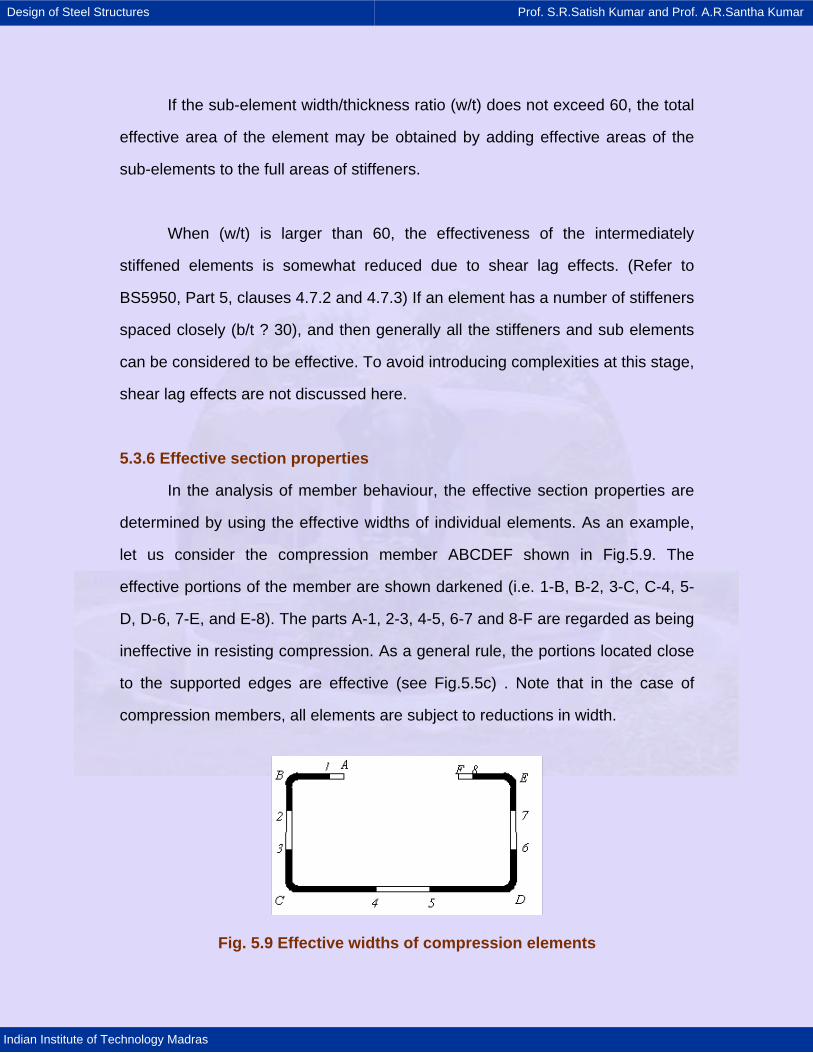
Design of Steel Structures Prof. S.R.Satish Kumar and Prof. A.R.Santha Kumar
Indian Institute of Technology Madras
If the sub-element width/thickness ratio (w/t) does not exceed 60, the total
effective area of the element may be obtained by adding effective areas of the
sub-elements to the full areas of stiffeners.
When (w/t) is larger than 60, the effectiveness of the intermediately
stiffened elements is somewhat reduced due to shear lag effects. (Refer to
BS5950, Part 5, clauses 4.7.2 and 4.7.3) If an element has a number of stiffeners
spaced closely (b/t ? 30), and then generally all the stiffeners and sub elements
can be considered to be effective. To avoid introducing complexities at this stage,
shear lag effects are not discussed here.
5.3.6 Effective section properties
In the analysis of member behaviour, the effective section properties are
determined by using the effective widths of individual elements. As an example,
let us consider the compression member ABCDEF shown in Fig.5.9. The
effective portions of the member are shown darkened (i.e. 1-B, B-2, 3-C, C-4, 5-
D, D-6, 7-E, and E-8). The parts A-1, 2-3, 4-5, 6-7 and 8-F are regarded as being
ineffective in resisting compression. As a general rule, the portions located close
to the supported edges are effective (see Fig.5.5c) . Note that in the case of
compression members, all elements are subject to reductions in width.
Fig. 5.9 Effective widths of compression elements
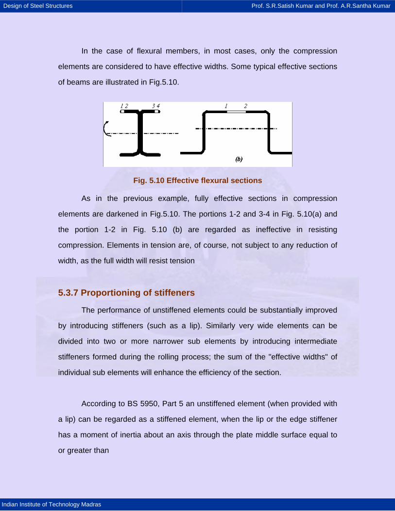
Design of Steel Structures Prof. S.R.Satish Kumar and Prof. A.R.Santha Kumar
Indian Institute of Technology Madras
In the case of flexural members, in most cases, only the compression
elements are considered to have effective widths. Some typical effective sections
of beams are illustrated in Fig.5.10.
Fig. 5.10 Effective flexural sections
As in the previous example, fully effective sections in compression
elements are darkened in Fig.5.10. The portions 1-2 and 3-4 in Fig. 5.10(a) and
the portion 1-2 in Fig. 5.10 (b) are regarded as ineffective in resisting
compression. Elements in tension are, of course, not subject to any reduction of
width, as the full width will resist tension
5.3.7 Proportioning of stiffeners
The performance of unstiffened elements could be substantially improved
by introducing stiffeners (such as a lip). Similarly very wide elements can be
divided into two or more narrower sub elements by introducing intermediate
stiffeners formed during the rolling process; the sum of the "effective widths" of
individual sub elements will enhance the efficiency of the section.
According to BS 5950, Part 5 an unstiffened element (when provided with
a lip) can be regarded as a stiffened element, when the lip or the edge stiffener
has a moment of inertia about an axis through the plate middle surface equal to
or greater than
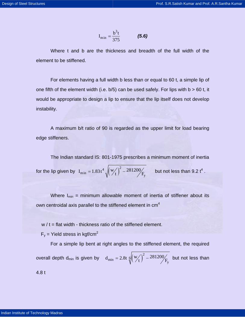
Design of Steel Structures Prof. S.R.Satish Kumar and Prof. A.R.Santha Kumar
Indian Institute of Technology Madras
3
minb tI375
= (5.6)
Where t and b are the thickness and breadth of the full width of the
element to be stiffened.
For elements having a full width b less than or equal to 60 t, a simple lip of
one fifth of the element width (i.e. b/5) can be used safely. For lips with b > 60 t, it
would be appropriate to design a lip to ensure that the lip itself does not develop
instability.
A maximum b/t ratio of 90 is regarded as the upper limit for load bearing
edge stiffeners.
The Indian standard IS: 801-1975 prescribes a minimum moment of inertia
for the lip given by ( )24min
yw 281200I 1.83t t F= − but not less than 9.2 t4 .
Where Imin = minimum allowable moment of inertia of stiffener about its
own centroidal axis parallel to the stiffened element in cm4
w / t = flat width - thickness ratio of the stiffened element.
Fy = Yield stress in kgf/cm2
For a simple lip bent at right angles to the stiffened element, the required
overall depth dmin is given by ( )26miny
w 281200d 2.8t t F= − but not less than
4.8 t
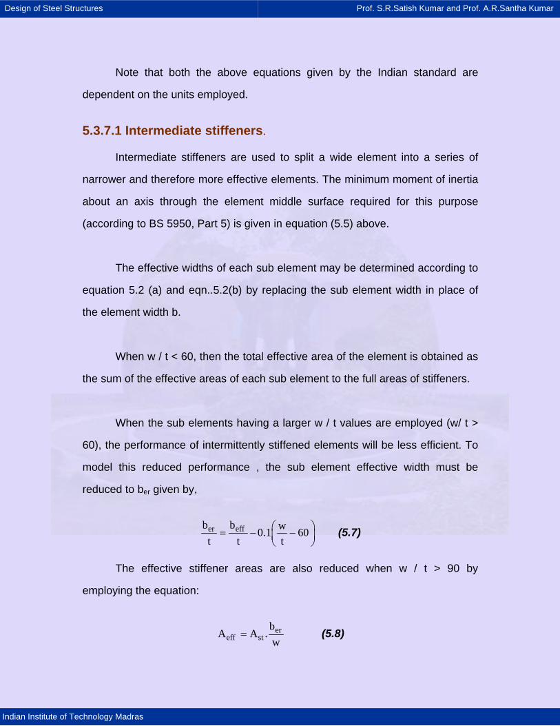
Design of Steel Structures Prof. S.R.Satish Kumar and Prof. A.R.Santha Kumar
Indian Institute of Technology Madras
Note that both the above equations given by the Indian standard are
dependent on the units employed.
5.3.7.1 Intermediate stiffeners.
Intermediate stiffeners are used to split a wide element into a series of
narrower and therefore more effective elements. The minimum moment of inertia
about an axis through the element middle surface required for this purpose
(according to BS 5950, Part 5) is given in equation (5.5) above.
The effective widths of each sub element may be determined according to
equation 5.2 (a) and eqn..5.2(b) by replacing the sub element width in place of
the element width b.
When w / t < 60, then the total effective area of the element is obtained as
the sum of the effective areas of each sub element to the full areas of stiffeners.
When the sub elements having a larger w / t values are employed (w/ t >
60), the performance of intermittently stiffened elements will be less efficient. To
model this reduced performance , the sub element effective width must be
reduced to ber given by,
er effb b w0.1 60t t t
⎛ ⎞= − −⎜ ⎟⎝ ⎠
(5.7)
The effective stiffener areas are also reduced when w / t > 90 by
employing the equation:
ereff st
bA A .
w= (5.8)
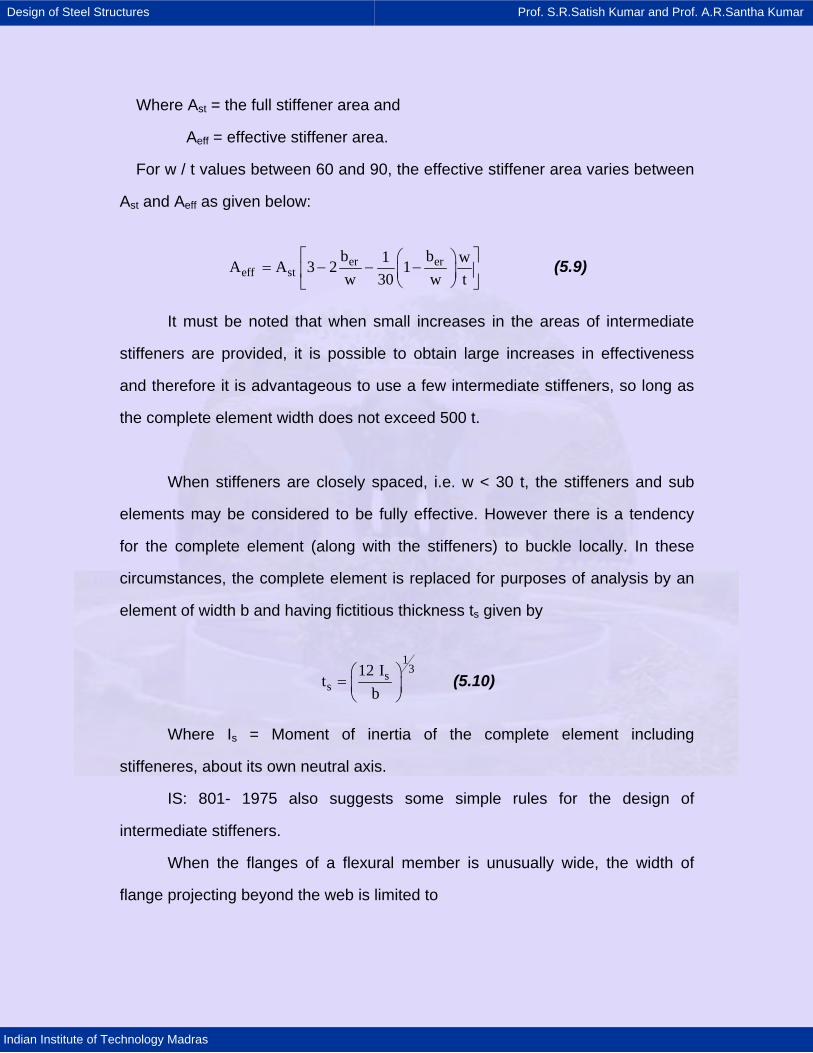
Design of Steel Structures Prof. S.R.Satish Kumar and Prof. A.R.Santha Kumar
Indian Institute of Technology Madras
Where Ast = the full stiffener area and
Aeff = effective stiffener area.
For w / t values between 60 and 90, the effective stiffener area varies between
Ast and Aeff as given below:
er ereff st
b b1 wA A 3 2 1w 30 w t
⎡ ⎤⎛ ⎞= − − −⎢ ⎥⎜ ⎟⎝ ⎠⎣ ⎦
(5.9)
It must be noted that when small increases in the areas of intermediate
stiffeners are provided, it is possible to obtain large increases in effectiveness
and therefore it is advantageous to use a few intermediate stiffeners, so long as
the complete element width does not exceed 500 t.
When stiffeners are closely spaced, i.e. w < 30 t, the stiffeners and sub
elements may be considered to be fully effective. However there is a tendency
for the complete element (along with the stiffeners) to buckle locally. In these
circumstances, the complete element is replaced for purposes of analysis by an
element of width b and having fictitious thickness ts given by
13s
s12 I
tb
⎛ ⎞= ⎜ ⎟⎝ ⎠
(5.10)
Where Is = Moment of inertia of the complete element including
stiffeneres, about its own neutral axis.
IS: 801- 1975 also suggests some simple rules for the design of
intermediate stiffeners.
When the flanges of a flexural member is unusually wide, the width of
flange projecting beyond the web is limited to
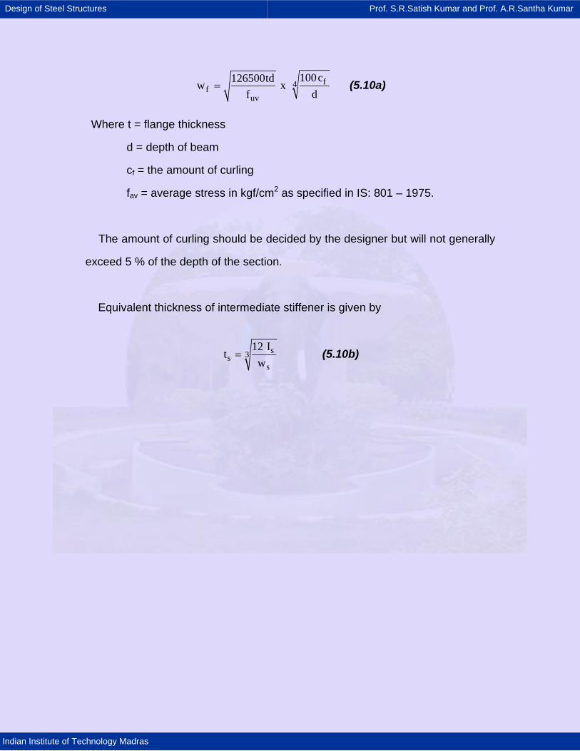
Design of Steel Structures Prof. S.R.Satish Kumar and Prof. A.R.Santha Kumar
Indian Institute of Technology Madras
f4fuv
100c126500tdw xf d
= (5.10a)
Where t = flange thickness
d = depth of beam
cf = the amount of curling
fav = average stress in kgf/cm2 as specified in IS: 801 – 1975.
The amount of curling should be decided by the designer but will not generally
exceed 5 % of the depth of the section.
Equivalent thickness of intermediate stiffener is given by
s3ss
12 It
w= (5.10b)
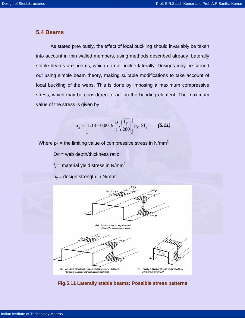
Design of Steel Structures Prof. S.R.Satish Kumar and Prof. A.R.Santha Kumar
Indian Institute of Technology Madras
5.4 Beams
As stated previously, the effect of local buckling should invariably be taken
into account in thin walled members, using methods described already. Laterally
stable beams are beams, which do not buckle laterally. Designs may be carried
out using simple beam theory, making suitable modifications to take account of
local buckling of the webs. This is done by imposing a maximum compressive
stress, which may be considered to act on the bending element. The maximum
value of the stress is given by
0
yy y
fDp 1.13 0.0019 p ft 280
⎡ ⎤⎢ ⎥= − ≥/⎢ ⎥⎣ ⎦
(5.11)
Where po = the limiting value of compressive stress in N/mm2
D/t = web depth/thickness ratio
fy = material yield stress in N/mm2.
py = design strength in N/mm2
Fig.5.11 Laterally stable beams: Possible stress patterns
Design of Steel Structures Prof. S.R.Satish Kumar and Prof. A.R.Santha Kumar
Indian Institute of Technology Madras
For steel with fy = 280 N/mm2, p0 = fy when (D/t) ? 68.
For greater web slenderness values, local web buckling has a detrimental
effect. The moment capacity of the cross section is determined by limiting the
maximum stress on the web to p0. The effective width of the compression
element is evaluated using this stress and the effective section properties are
evaluated. The ultimate moment capacity (Mult) is given by
Mult = Zc.p0 (5.11a)
Where Zc = effective compression section modulus
This is subject to the condition that the maximum tensile stress in the
section does not exceed fy (see Fig.5.11a).
If the neutral axis is such that the tensile stresses reach yield first, then the
moment capacity is to be evaluated on the basis of elasto-plastic stress
distribution (see Fig.5.11b). In elements having low (width/thickness) ratios,
compressive stress at collapse can equal yield stress (see Fig. 5.11c). In order to
ensure yielding before local buckling, the maximum (width/thickness) ratio of
stiffened elements is y
28025f
≤ and for unstiffened elements, it is y
2808f
≤
5.4.1 Other beam failure criteria
5.4.1.1 Web crushing
This may occur under concentrated loads or at support point when deep
slender webs are employed. A widely used method of overcoming web crushing
problems is to use web cleats at support points (See Fig.5.12).
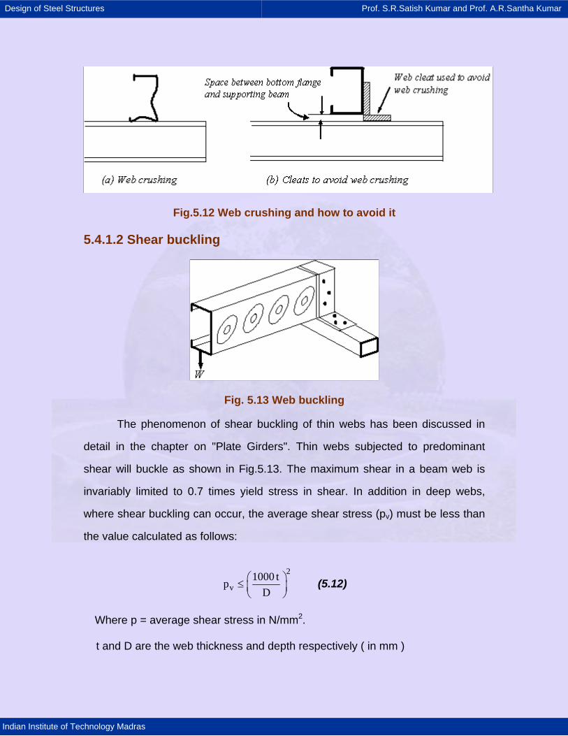
Design of Steel Structures Prof. S.R.Satish Kumar and Prof. A.R.Santha Kumar
Indian Institute of Technology Madras
Fig.5.12 Web crushing and how to avoid it
5.4.1.2 Shear buckling
Fig. 5.13 Web buckling
The phenomenon of shear buckling of thin webs has been discussed in
detail in the chapter on "Plate Girders". Thin webs subjected to predominant
shear will buckle as shown in Fig.5.13. The maximum shear in a beam web is
invariably limited to 0.7 times yield stress in shear. In addition in deep webs,
where shear buckling can occur, the average shear stress (pv) must be less than
the value calculated as follows:
2
v1000 tp
D⎛ ⎞≤ ⎜ ⎟⎝ ⎠
(5.12)
Where p = average shear stress in N/mm2.
t and D are the web thickness and depth respectively ( in mm )
Design of Steel Structures Prof. S.R.Satish Kumar and Prof. A.R.Santha Kumar
Indian Institute of Technology Madras
5.4.2 Lateral buckling
The great majority of cold formed beams are (by design) restrained
against lateral deflections. This is achieved by connecting them to adjacent
elements, roof sheeting or to bracing members. However, there are
circumstances where this is not the case and the possibility of lateral buckling
has to be considered.
Lateral buckling will not occur if the beam under loading bends only about
the minor axis. If the beam is provided with lateral restraints, capable of resisting
a lateral force of 3% of the maximum force in the compression flange, the beam
may be regarded as restrained and no lateral buckling will occur.
As described in the chapter on "Unrestrained Beams'", lateral buckling
occurs only in "long" beams and is characterised by the beam moving laterally
and twisting when a transverse load is applied. This type of buckling is of
importance for long beams with low lateral stiffness and low torsional stiffness
(See Fig.5.14); such beams under loading will bend about the major axis.
The design approach is based on the "effective length" of the beam for
lateral buckling, which is dependent on support and loading conditions. The
effective length of beams with both ends supported and having restraints against
twisting is taken as 0.9 times the length, provided the load is applied at bottom
flange level. If a load is applied to the top flange which is unrestrained laterally,
the effective length is increased by 20%. This is considered to be a "destabilising
load", i.e. a load that encourages lateral instability.
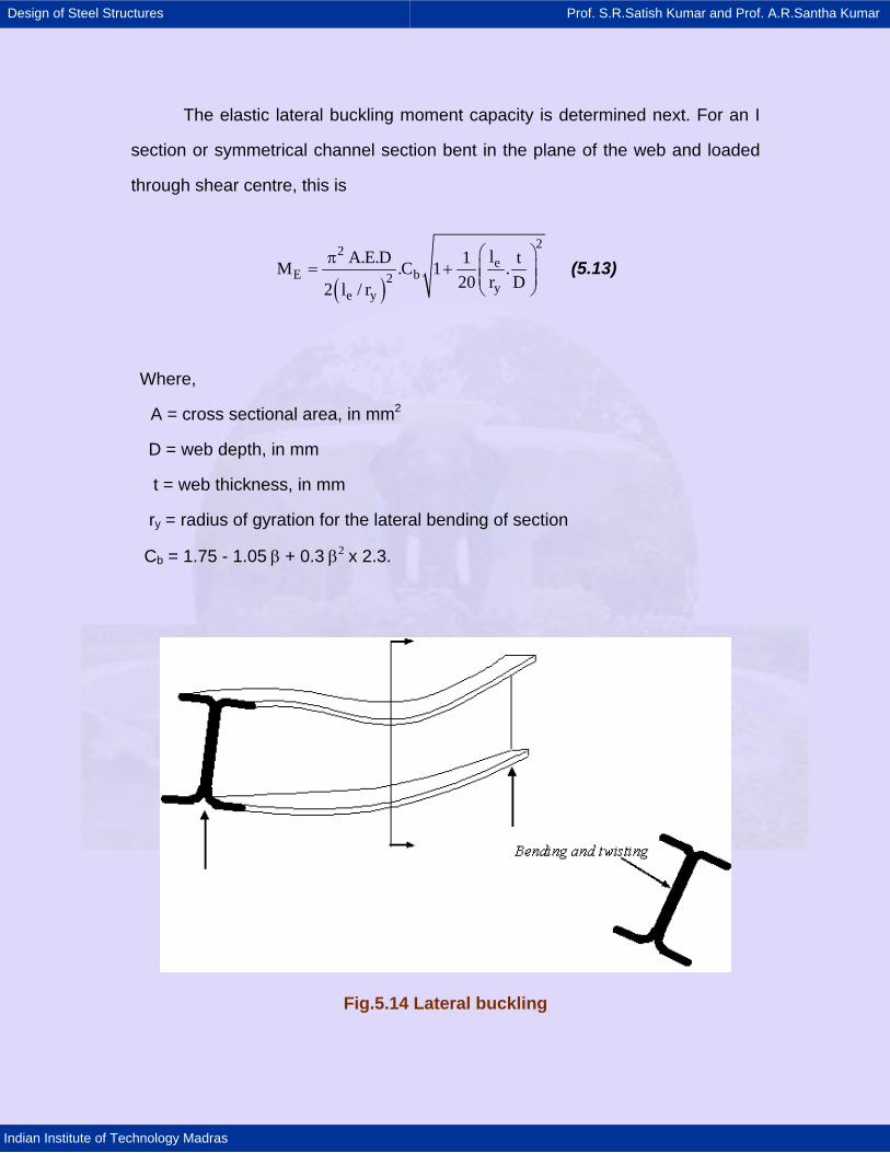
Design of Steel Structures Prof. S.R.Satish Kumar and Prof. A.R.Santha Kumar
Indian Institute of Technology Madras
The elastic lateral buckling moment capacity is determined next. For an I
section or symmetrical channel section bent in the plane of the web and loaded
through shear centre, this is
( )
22e
E b2ye y
lA.E.D 1 tM .C 1 .20 r D2 l / r
⎛ ⎞π= + ⎜ ⎟⎜ ⎟
⎝ ⎠ (5.13)
Where,
A = cross sectional area, in mm2
D = web depth, in mm
t = web thickness, in mm
ry = radius of gyration for the lateral bending of section
Cb = 1.75 - 1.05 β + 0.3 β2 x 2.3.
Fig.5.14 Lateral buckling
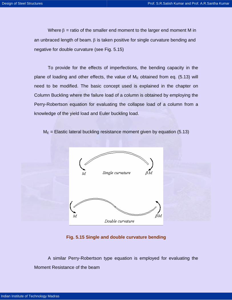
Design of Steel Structures Prof. S.R.Satish Kumar and Prof. A.R.Santha Kumar
Indian Institute of Technology Madras
Where β = ratio of the smaller end moment to the larger end moment M in
an unbraced length of beam. β is taken positive for single curvature bending and
negative for double curvature (see Fig. 5.15)
To provide for the effects of imperfections, the bending capacity in the
plane of loading and other effects, the value of ME obtained from eq. (5.13) will
need to be modified. The basic concept used is explained in the chapter on
Column Buckling where the failure load of a column is obtained by employing the
Perry-Robertson equation for evaluating the collapse load of a column from a
knowledge of the yield load and Euler buckling load.
ME = Elastic lateral buckling resistance moment given by equation (5.13)
Fig. 5.15 Single and double curvature bending
A similar Perry-Robertson type equation is employed for evaluating the
Moment Resistance of the beam
Design of Steel Structures Prof. S.R.Satish Kumar and Prof. A.R.Santha Kumar
Indian Institute of Technology Madras
( ){ } ( ) 2b y E y E y E
1M M 1 M M 1 M 4M .M2
⎡ ⎤⎡ ⎤= + + η − + + η −⎢ ⎥⎣ ⎦⎣ ⎦ (5.14)
My = First yield moment given by the product of yield stress (fy) and the
Elastic Modulus (Zc) of the gross section.
η = Perry coefficient, given by
eb
y
e eb b
y y
lWhen 40C , 0.
r
l lWhen 40C , 0.002 40C
r r
< η=
⎛ ⎞< η= −⎜ ⎟⎜ ⎟
⎝ ⎠
le = effective length
ry = radius of gyration of the section about the y - axis.
When the calculated value of Mb exceed Mult calculated by using equation
(5.11.a), then Mb is limited to Mult. This will happen when the beams are "short".
Design of Steel Structures Prof. S.R.Satish Kumar and Prof. A.R.Santha Kumar
Indian Institute of Technology Madras
5.5 Axially compressed column
As pointed out in the last chapter, local buckling under compressive
loading is an extremely important feature of thin walled sections. It has been
shown that a compressed plate element with an edge free to deflect does not
perform as satisfactorily when compared with a similar element supported along
the two opposite edges. Methods of evaluating the effective widths for both edge
support conditions were presented and discussed.
In analysing column behaviour, the first step is to determine the effective
area (Aeff) of the cross section by summing up the total values of effective areas
for all the individual elements.
The ultimate load (or squash load) of a short strut is obtained from
Pcs = Aeff . fyd = Q. A. fyd (5.15)
Where
Pcs = ultimate load of a short strut
Aeff = sum of the effective areas of all the individual plate elements
Q = the ratio of the effective area to the total area of cross section at yield
stress
In a long column with doubly - symmetric cross section, the failure load
(Pc) is dependent on Euler buckling resistance (PEY) and the imperfections
present. The method of analysis presented here follows the Perry-Robertson
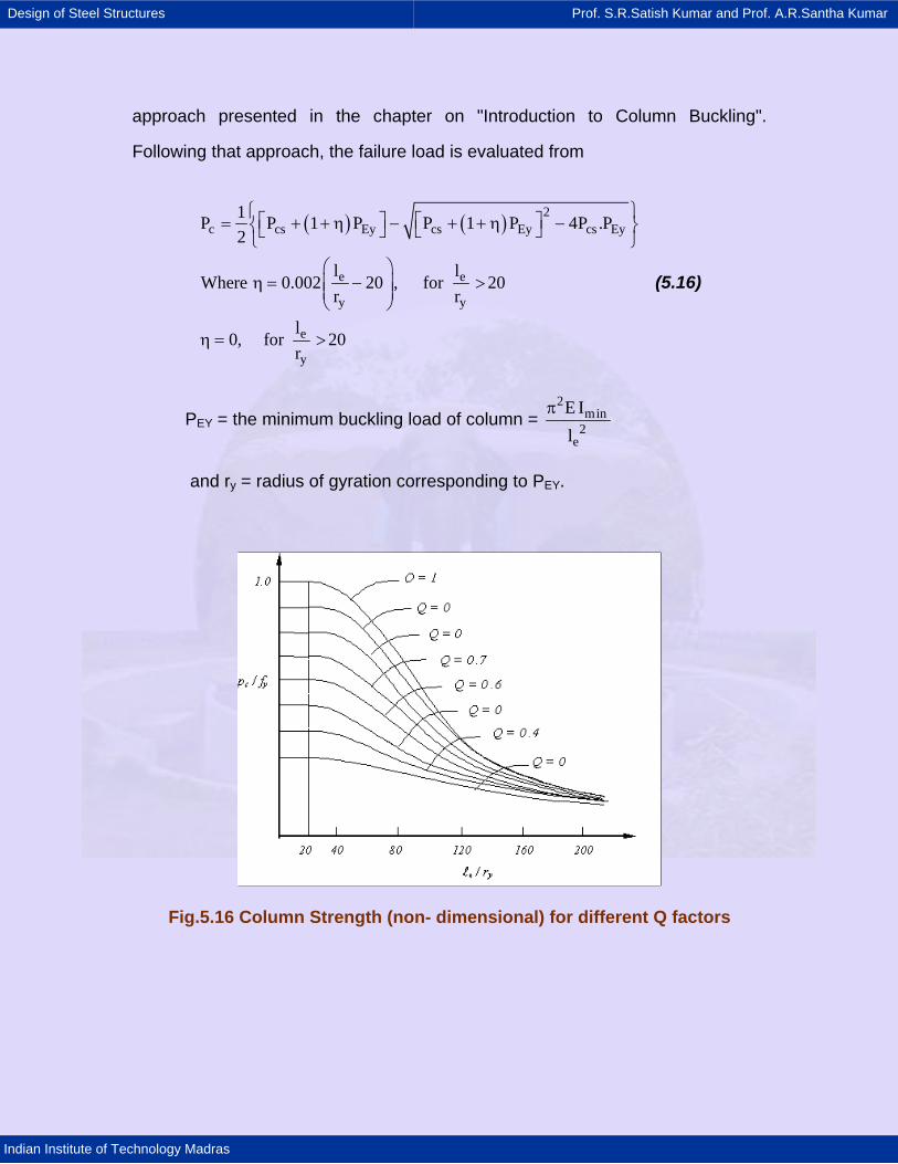
Design of Steel Structures Prof. S.R.Satish Kumar and Prof. A.R.Santha Kumar
Indian Institute of Technology Madras
approach presented in the chapter on "Introduction to Column Buckling".
Following that approach, the failure load is evaluated from
( ) ( ) 2c cs Ey cs Ey cs Ey
e e
y y
e
y
1P P 1 P P 1 P 4P .P2
l lWhere 0.002 20 , for 20
r r
l0, for 20
r
⎧ ⎫⎡ ⎤ ⎡ ⎤= + + η − + + η −⎨ ⎬⎣ ⎦ ⎣ ⎦⎩ ⎭⎛ ⎞
η = − >⎜ ⎟⎜ ⎟⎝ ⎠
η = >
(5.16)
PEY = the minimum buckling load of column = 2
min2
e
E Il
π
and ry = radius of gyration corresponding to PEY.
Fig.5.16 Column Strength (non- dimensional) for different Q factors
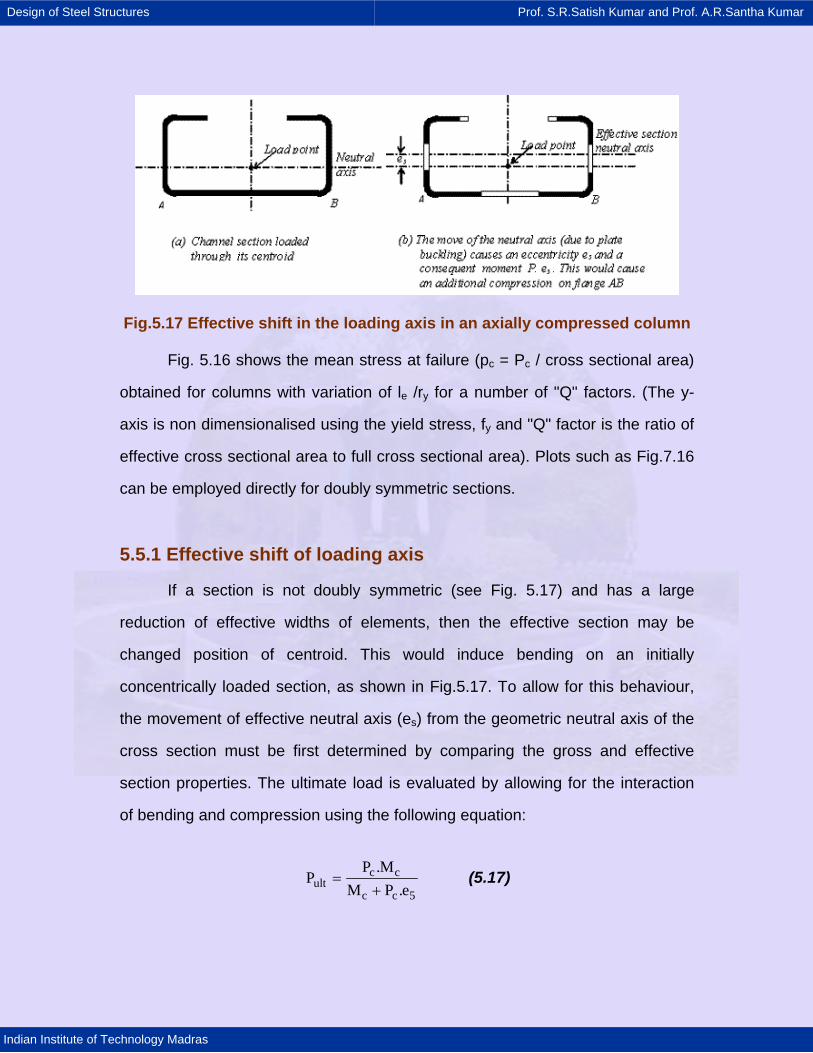
Design of Steel Structures Prof. S.R.Satish Kumar and Prof. A.R.Santha Kumar
Indian Institute of Technology Madras
Fig.5.17 Effective shift in the loading axis in an axially compressed column
Fig. 5.16 shows the mean stress at failure (pc = Pc / cross sectional area)
obtained for columns with variation of le /ry for a number of "Q" factors. (The y-
axis is non dimensionalised using the yield stress, fy and "Q" factor is the ratio of
effective cross sectional area to full cross sectional area). Plots such as Fig.7.16
can be employed directly for doubly symmetric sections.
5.5.1 Effective shift of loading axis
If a section is not doubly symmetric (see Fig. 5.17) and has a large
reduction of effective widths of elements, then the effective section may be
changed position of centroid. This would induce bending on an initially
concentrically loaded section, as shown in Fig.5.17. To allow for this behaviour,
the movement of effective neutral axis (es) from the geometric neutral axis of the
cross section must be first determined by comparing the gross and effective
section properties. The ultimate load is evaluated by allowing for the interaction
of bending and compression using the following equation:
c cult
c c 5
P .MP
M P .e=
+ (5.17)
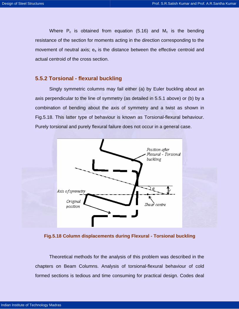
Design of Steel Structures Prof. S.R.Satish Kumar and Prof. A.R.Santha Kumar
Indian Institute of Technology Madras
Where Pc is obtained from equation (5.16) and Mc is the bending
resistance of the section for moments acting in the direction corresponding to the
movement of neutral axis; es is the distance between the effective centroid and
actual centroid of the cross section.
5.5.2 Torsional - flexural buckling
Singly symmetric columns may fail either (a) by Euler buckling about an
axis perpendicular to the line of symmetry (as detailed in 5.5.1 above) or (b) by a
combination of bending about the axis of symmetry and a twist as shown in
Fig.5.18. This latter type of behaviour is known as Torsional-flexural behaviour.
Purely torsional and purely flexural failure does not occur in a general case.
Fig.5.18 Column displacements during Flexural - Torsional buckling
Theoretical methods for the analysis of this problem was described in the
chapters on Beam Columns. Analysis of torsional-flexural behaviour of cold
formed sections is tedious and time consuming for practical design. Codes deal
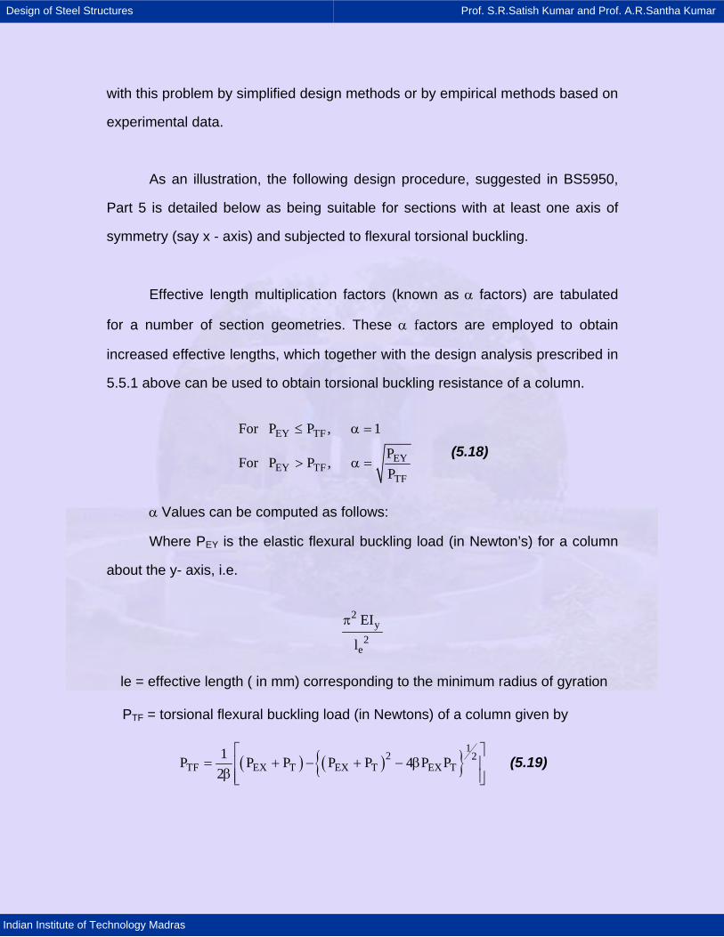
Design of Steel Structures Prof. S.R.Satish Kumar and Prof. A.R.Santha Kumar
Indian Institute of Technology Madras
with this problem by simplified design methods or by empirical methods based on
experimental data.
As an illustration, the following design procedure, suggested in BS5950,
Part 5 is detailed below as being suitable for sections with at least one axis of
symmetry (say x - axis) and subjected to flexural torsional buckling.
Effective length multiplication factors (known as α factors) are tabulated
for a number of section geometries. These α factors are employed to obtain
increased effective lengths, which together with the design analysis prescribed in
5.5.1 above can be used to obtain torsional buckling resistance of a column.
EY TF
EYEY TF
TF
For P P , 1
PFor P P ,
P
≤ α =
> α = (5.18)
α Values can be computed as follows:
Where PEY is the elastic flexural buckling load (in Newton’s) for a column
about the y- axis, i.e.
2y
2e
EI
l
π
le = effective length ( in mm) corresponding to the minimum radius of gyration
PTF = torsional flexural buckling load (in Newtons) of a column given by
( ) ( ){ }1
2 2TF EX T EX T EX T
1P P P P P 4 P P2
⎡ ⎤= + − + − β⎢ ⎥
β ⎢ ⎥⎣ ⎦ (5.19)
Design of Steel Structures Prof. S.R.Satish Kumar and Prof. A.R.Santha Kumar
Indian Institute of Technology Madras
where PEX = Elastic flexural buckling load of the column (in Newton’s) about
the x- axis given by
2y
2e
EI
l
π
PT = Torsional buckling load of a column (In Newton’s) given by
2
T 2 20 e
2 .E T1P GJr l
⎛ ⎞π= +⎜ ⎟⎜ ⎟
⎝ ⎠ (5.20)
β is a constant given by 0
0
x1
r⎛ ⎞
β = − ⎜ ⎟⎝ ⎠
(5.21)
In these equations,
ro = polar radius of gyration about the shear centre (in mm) given by
( )1
2 2 2 20 x y 0r r r x= + + (5.22)
Where
rx, ry are the radii of gyration (in mm) about the x and y- axis
G is the shear modulus (N/mm2)
x0 is the distance from shear centre to the centroid measured along the x axis
(mm)
J St Venants' Torsion constant (mm4) which may be taken as 3bt
3∑
summed up for all elements,
Where b = flat width of the element and t = thickness (both of them measure in
mm)
Design of Steel Structures Prof. S.R.Satish Kumar and Prof. A.R.Santha Kumar
Indian Institute of Technology Madras
Ix the moment of inertia about the x axis (mm4)
Γ Warping constant for all section.
5.5.3 Torsion behaviour
Cold formed sections are mainly formed with "open" sections and do not
have high resistance to torsion. Hence the application of load which would cause
torsion should be avoided where possible. Generally speaking, by adjusting the
method of load application, it is possible to restrain twisting so that torsion does
not occur to any significant extent.
In general, when examining torsional behaviour of thin walled sections, the
total torsion may be regarded as being made up of two effects:
• St. Venant's Torsion or Pure Torsion
• Warping torsion.
St.Venant's torsion produces shear stresses, which vary linearly through
the material thickness. Warping torsion produces in-plane bending of the
elements of a cross section, thus inducing direct (i.e. normal) stresses and the
angle of twist increases linearly.
Since cold formed sections are thin walled, they have very little resistance
to St. Venant's Torsion and will twist substantially. The extent of warping torsion
in a thin walled beam is very much dependent on the warping restraint afforded
by the supports as well as the loading conditions and the type of section.
Design of Steel Structures Prof. S.R.Satish Kumar and Prof. A.R.Santha Kumar
Indian Institute of Technology Madras
If the beam ends are restrained from warping, then short beams exhibit
high resistance to warping torsion and the total torque acting on such a beam will
be almost completely devoted to overcoming warping resistance, the St Venant's
Torsion being negligible. Conversely, the resistance to warping torsion becomes
low for long beams and warping stresses and degrees of twist become very
large.
A detailed theoretical treatment of beams subject to bending and torsion is
given in another chapter. As stated previously, particular care and attention
should be paid to the detailing of the connections and the method of load
application so that the design for torsion does not pose a serious problem.
Design of Steel Structures Prof. S.R.Satish Kumar and Prof. A.R.Santha Kumar
Indian Institute of Technology Madras
5.6 Combined bending and compression
Compression members which are also subject to bending will have to be
designed to take into account the effects of interaction. The following checks are
suggested for members which have at least one axis of symmetry: (i) the local
capacity at points of greatest bending moment and axial load and (ii) an overall
buckling check.
5.6.1 Local Capacity Check
The local capacity check is ascertained by satisfying the following at the points
of greatest bending moment and axial load:
yc x
cs cx cy
MF Ml
P M M+ + ≤ (5.23)
Fc = applied axial load
Pcs = short strut capacity defined by Aeff.Pyd (eqn.7.15)
Mx, My = applied bending moments about x and y axis
Mcx = Moment resistance of the beam about x axis in the absence of Fc and My
Mcy = Moment resistance of the beam about y axis in the absence of Fc and Mx.
5.6.2 Overall buckling check
For members not subject to lateral buckling, the following relationship
should be satisfied:
yc x
c c cbx cx by cy
EX EY
MF M1
P F FC .M 1 C .M 1
P P
+ + ≤⎛ ⎞ ⎛ ⎞− −⎜ ⎟ ⎜ ⎟
⎝ ⎠ ⎝ ⎠
(5.24)
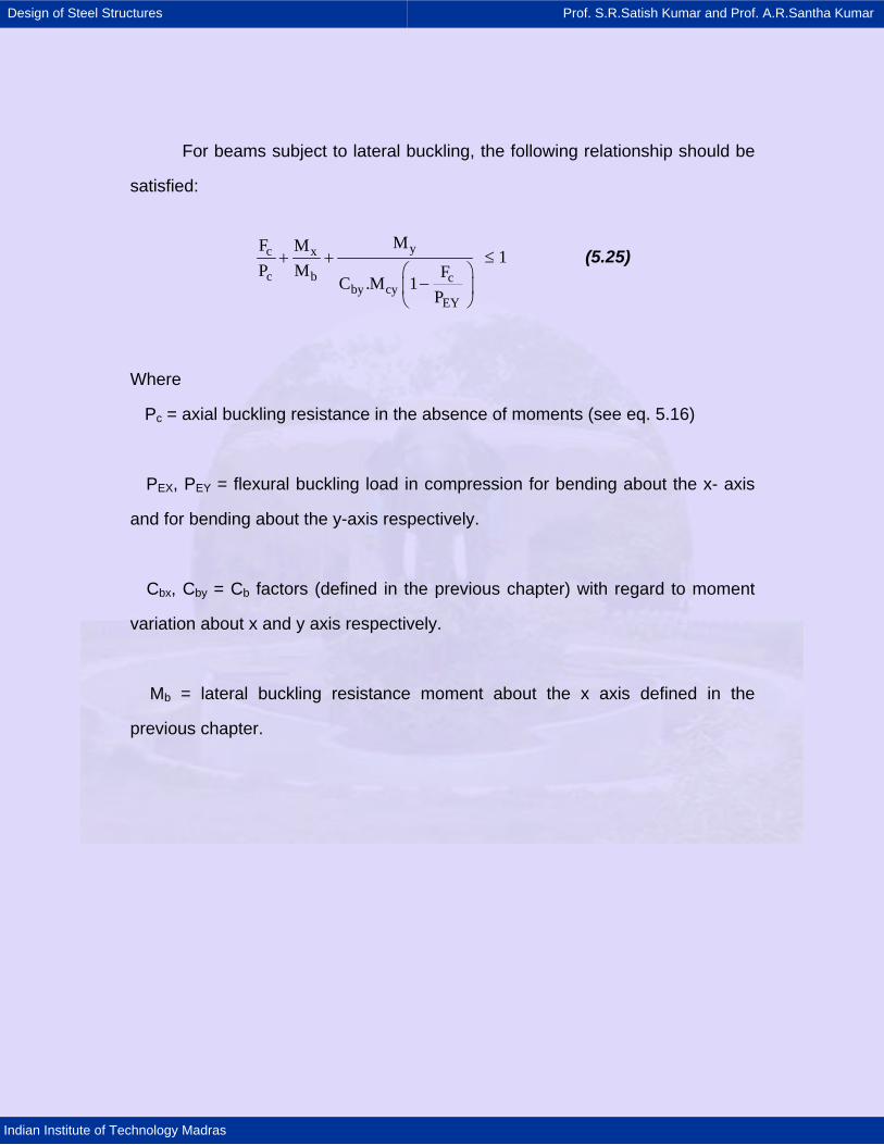
Design of Steel Structures Prof. S.R.Satish Kumar and Prof. A.R.Santha Kumar
Indian Institute of Technology Madras
For beams subject to lateral buckling, the following relationship should be
satisfied:
yc x
c b cby cy
EY
MF M1
P M FC .M 1
P
+ + ≤⎛ ⎞−⎜ ⎟
⎝ ⎠
(5.25)
Where
Pc = axial buckling resistance in the absence of moments (see eq. 5.16)
PEX, PEY = flexural buckling load in compression for bending about the x- axis
and for bending about the y-axis respectively.
Cbx, Cby = Cb factors (defined in the previous chapter) with regard to moment
variation about x and y axis respectively.
Mb = lateral buckling resistance moment about the x axis defined in the
previous chapter.
Design of Steel Structures Prof. S.R.Satish Kumar and Prof. A.R.Santha Kumar
Indian Institute of Technology Madras
5.7 Tension members
If a member is connected in such a way as to eliminate any moments due
to connection eccentricity, the member may be designed as a simple tension
member. Where a member is connected eccentrically to its axis, then the
resulting moment has to be allowed for.
The tensile capacity of a member (Pt) may be evaluated from
Pt = Ae . Py (5.26)
Where
Ae is the effective area of the section making due allowance for the type of
member (angle, plain channel, Tee section etc) and the type of connection (eg.
connected through one leg only or through the flange or web of a T- section).
py is design strength (N/mm2)
Guidance on calculation of Ae is provided in Codes of Practice (eg. BS
5950, Part 5). The area of the tension member should invariably be calculated as
its gross area less deductions for holes or openings. (The area to be deducted
from the gross sectional area of a member should be the maximum sum of the
sectional areas of the holes in any cross section at right angles to the direction of
applied stress).
Reference is also made to the chapter on "Tension Members" where
provision for enhancement of strength due to strain hardening has been
incorporated for hot rolled steel sections. The Indian code IS: 801-1975 is in the
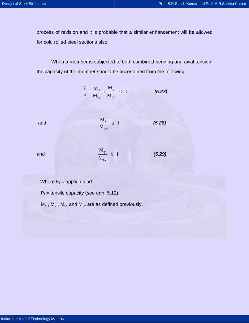
Design of Steel Structures Prof. S.R.Satish Kumar and Prof. A.R.Santha Kumar
Indian Institute of Technology Madras
process of revision and it is probable that a similar enhancement will be allowed
for cold rolled steel sections also.
When a member is subjected to both combined bending and axial tension,
the capacity of the member should be ascertained from the following:
yt x
t cx cy
MF Ml
P M M+ + ≤ (5.27)
and x
cx
Ml
M≤ (5.28)
and y
cy
Ml
M≤ (5.29)
Where Ft = applied load
Pt = tensile capacity (see eqn. 5.12)
Mx , My , Mcx and Mcy are as defined previously.
Design of Steel Structures Prof. S.R.Satish Kumar and Prof. A.R.Santha Kumar
Indian Institute of Technology Madras
5.8 Design on the basis of testing
While it is possible to design many cold formed steel members on the
basis of analysis, the very large variety of shapes that can be formed and the
complex interactions that occur make it frequently uneconomical to design
members and systems completely on theoretical basis. The behaviour of a
component or system can often be ascertained economically by a test and
suitable modifications incorporated, where necessary.
Particular care should be taken while testing components, that the tests
model the actual loading conditions as closely as possible. For example, while
these tests may be used successfully to assess the material work hardening
much caution will be needed when examining the effects of local buckling. There
is a possibility of these tests giving misleading information or even no information
regarding neutral axis movement. The specimen lengths may be too short to pick
up certain types of buckling behaviour.
Testing is probably the only realistic method of assessing the strength and
characteristics of connections. Evaluating connection behaviour is important as
connections play a crucial role in the strength and stiffness of a structure.
In testing complete structures or assemblies, it is vital to ensure that the test
set up reflects the in-service conditions as accurately as possible. The method of
load application, the type of supports, the restraints from adjacent structures and
the flexibility of connections are all factors to be considered carefully and
modeled accurately.
Design of Steel Structures Prof. S.R.Satish Kumar and Prof. A.R.Santha Kumar
Indian Institute of Technology Madras
Testing by an independent agency (such as Universities) is widely used by
manufacturers of mass produced components to ensure consistency of quality.
The manufacturers also provide load/span tables for their products, which can be
employed by structural designers and architects who do not have detailed
knowledge of design procedures. An advantage to the manufacturers in
designing on the basis of proof testing is that the load/span tables obtained are
generally more advantageous than those obtained by analytical methods; they
also reassure the customers about the validity of their load/span tables.
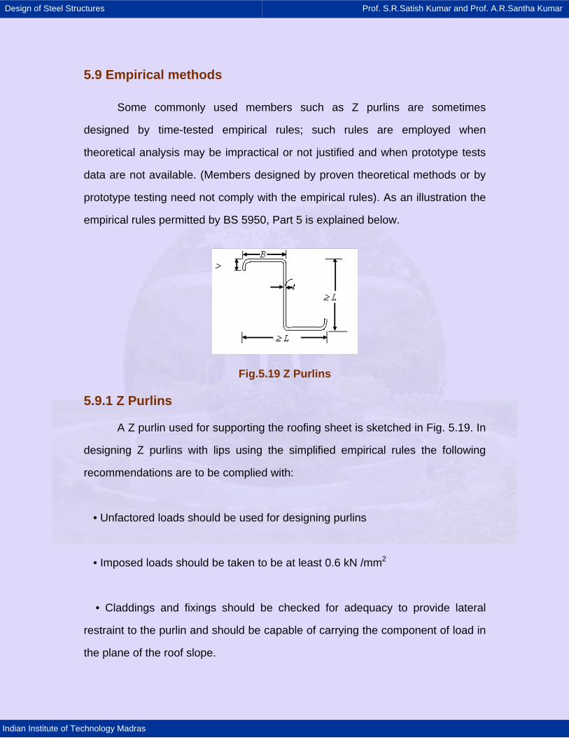
Design of Steel Structures Prof. S.R.Satish Kumar and Prof. A.R.Santha Kumar
Indian Institute of Technology Madras
5.9 Empirical methods
Some commonly used members such as Z purlins are sometimes
designed by time-tested empirical rules; such rules are employed when
theoretical analysis may be impractical or not justified and when prototype tests
data are not available. (Members designed by proven theoretical methods or by
prototype testing need not comply with the empirical rules). As an illustration the
empirical rules permitted by BS 5950, Part 5 is explained below.
Fig.5.19 Z Purlins
5.9.1 Z Purlins
A Z purlin used for supporting the roofing sheet is sketched in Fig. 5.19. In
designing Z purlins with lips using the simplified empirical rules the following
recommendations are to be complied with:
• Unfactored loads should be used for designing purlins
• Imposed loads should be taken to be at least 0.6 kN /mm2
• Claddings and fixings should be checked for adequacy to provide lateral
restraint to the purlin and should be capable of carrying the component of load in
the plane of the roof slope.
Design of Steel Structures Prof. S.R.Satish Kumar and Prof. A.R.Santha Kumar
Indian Institute of Technology Madras
• The purlin should be considered to carry the load normal to roof slope (and a
nominal axial load due to wind or restraint forces)
• These rules apply to purlins up to 8 m span in roof slopes up to 122 2
• Antisag bars should be provided to ensure that laterally unsupported length of
the purlin does not exceed 3.8 m. These should be anchored to rigid apex
support or their forces should be transferred diagonally to main frames.
• Purlin cleats should provide adequate torsional restraint.
5.9.2 Design rules
The following design rules apply with reference to Fig. 5.19
• The overall depth should be greater than 100 t and not less than L /45.
• Overall width of compression flange / thickness ratio should be less than 35.
• Lip width should be greater than B /5
• Section Modulus 3WL cm1400
≥ for simply supported purlins and 3WL cm1400
≥
for continuous or semi rigidly jointed purlins.
Design of Steel Structures Prof. S.R.Satish Kumar and Prof. A.R.Santha Kumar
Indian Institute of Technology Madras
In the above,
L = span of the purlin (in mm)
W = Normal component of unfactored (distributed dead load + imposed load)
in kN
B = Width of the compression flange in mm
T = thickness of the purlin in mm.
• The net allowable wind uplift in a direction normal to roof when purlins are
restrained is taken as 50% of the (dead + imposed) load.
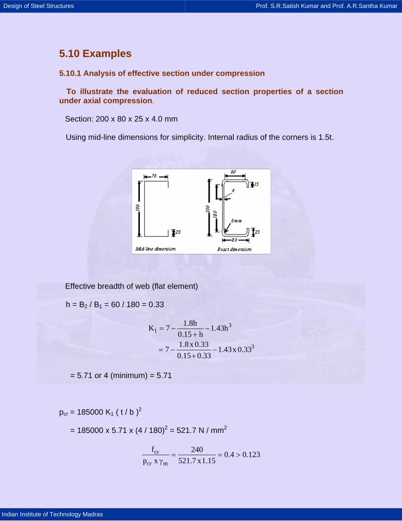
Design of Steel Structures Prof. S.R.Satish Kumar and Prof. A.R.Santha Kumar
Indian Institute of Technology Madras
5.10 Examples
5.10.1 Analysis of effective section under compression
To illustrate the evaluation of reduced section properties of a section under axial compression.
Section: 200 x 80 x 25 x 4.0 mm
Using mid-line dimensions for simplicity. Internal radius of the corners is 1.5t.
Effective breadth of web (flat element)
h = B2 / B1 = 60 / 180 = 0.33
31
3
1.8hK 7 1.43h0.15 h1.8x 0.337 1.43x 0.330.15 0.33
= − −+
= − −+
= 5.71 or 4 (minimum) = 5.71
pcr = 185000 K1 ( t / b )2
= 185000 x 5.71 x (4 / 180)2 = 521.7 N / mm2
cr
cr m
f 240 0.4 0.123p x 521.7 x1.15
= = >γ
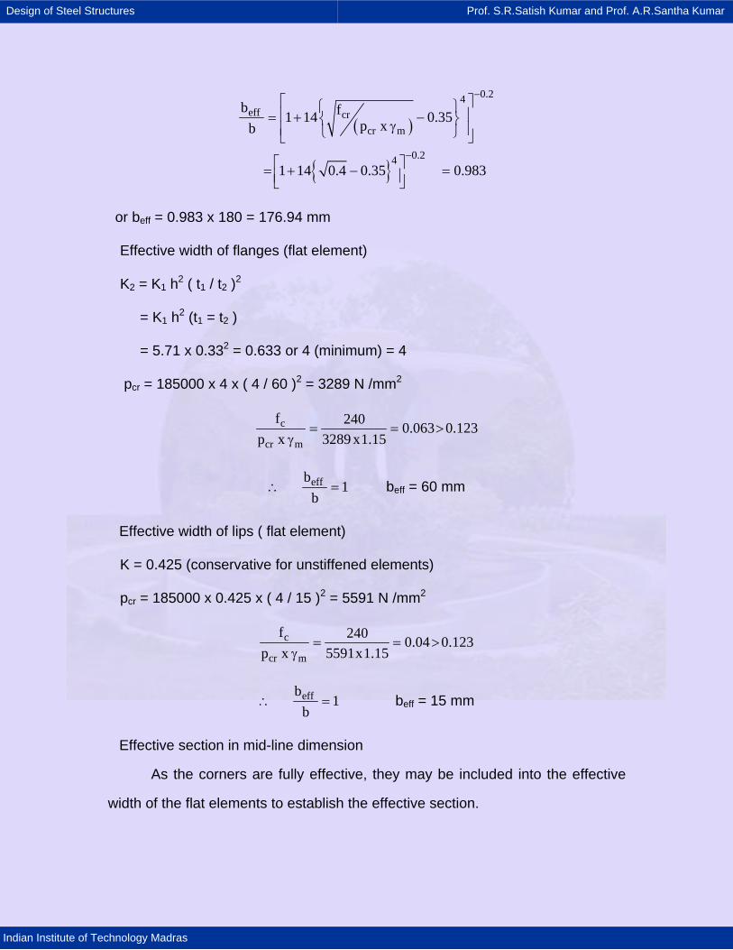
Design of Steel Structures Prof. S.R.Satish Kumar and Prof. A.R.Santha Kumar
Indian Institute of Technology Madras
( )
{ }
0.24eff cr
cr m
0.24
b f1 14 0.35p xb
1 14 0.4 0.35 0.983
−
−
⎡ ⎤⎧ ⎫⎢ ⎥= + −⎨ ⎬γ⎢ ⎥⎩ ⎭⎣ ⎦
⎡ ⎤= + − =⎢ ⎥⎣ ⎦
or beff = 0.983 x 180 = 176.94 mm
Effective width of flanges (flat element)
K2 = K1 h2 ( t1 / t2 )2
= K1 h2 (t1 = t2 )
= 5.71 x 0.332 = 0.633 or 4 (minimum) = 4
pcr = 185000 x 4 x ( 4 / 60 )2 = 3289 N /mm2
c
cr m
f 240 0.063 0.123p x 3289 x1.15
= = >γ
effb1
b∴ = beff = 60 mm
Effective width of lips ( flat element)
K = 0.425 (conservative for unstiffened elements)
pcr = 185000 x 0.425 x ( 4 / 15 )2 = 5591 N /mm2
c
cr m
f 240 0.04 0.123p x 5591x1.15
= = >γ
effb1
b∴ = beff = 15 mm
Effective section in mid-line dimension
As the corners are fully effective, they may be included into the effective
width of the flat elements to establish the effective section.
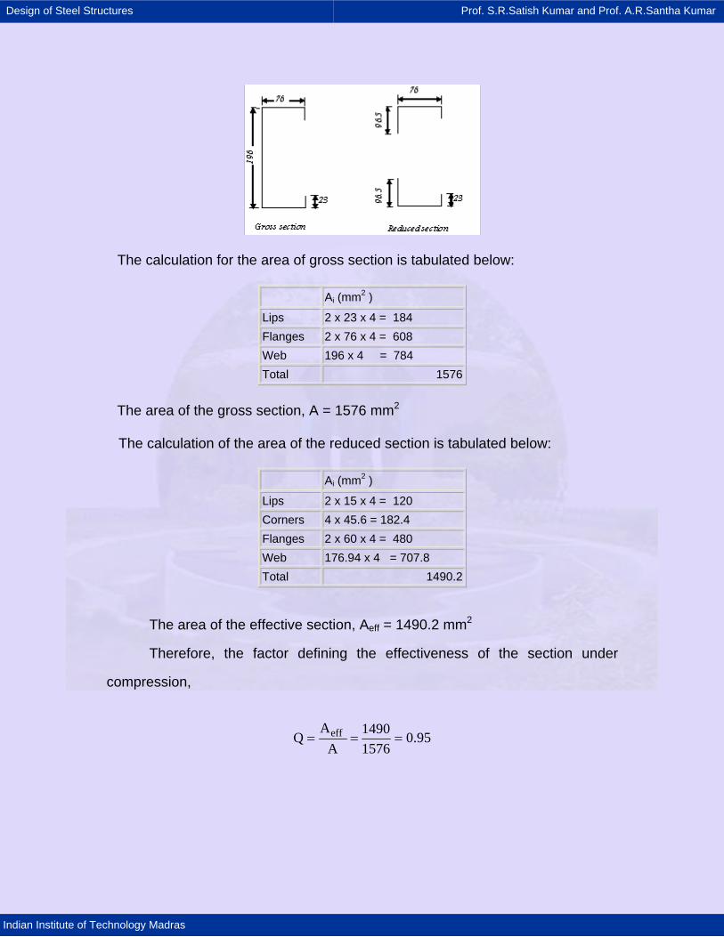
Design of Steel Structures Prof. S.R.Satish Kumar and Prof. A.R.Santha Kumar
Indian Institute of Technology Madras
The calculation for the area of gross section is tabulated below:
Ai (mm2 ) Lips 2 x 23 x 4 = 184 Flanges 2 x 76 x 4 = 608 Web 196 x 4 = 784 Total 1576
The area of the gross section, A = 1576 mm2
The calculation of the area of the reduced section is tabulated below:
Ai (mm2 ) Lips 2 x 15 x 4 = 120 Corners 4 x 45.6 = 182.4 Flanges 2 x 60 x 4 = 480 Web 176.94 x 4 = 707.8 Total 1490.2
The area of the effective section, Aeff = 1490.2 mm2
Therefore, the factor defining the effectiveness of the section under
compression,
effA 1490Q 0.95A 1576
= = =
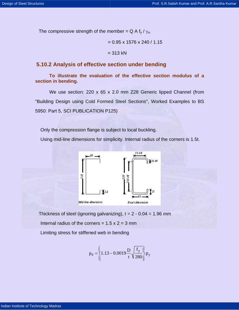
Design of Steel Structures Prof. S.R.Satish Kumar and Prof. A.R.Santha Kumar
Indian Institute of Technology Madras
The compressive strength of the member = Q A fy / γm
= 0.95 x 1576 x 240 / 1.15
= 313 kN
5.10.2 Analysis of effective section under bending
To illustrate the evaluation of the effective section modulus of a section in bending.
We use section: 220 x 65 x 2.0 mm Z28 Generic lipped Channel (from
"Building Design using Cold Formed Steel Sections", Worked Examples to BS
5950: Part 5, SCI PUBLICATION P125)
Only the compression flange is subject to local buckling.
Using mid-line dimensions for simplicity. Internal radius of the corners is 1.5t.
Thickness of steel (ignoring galvanizing), t = 2 - 0.04 = 1.96 mm
Internal radius of the corners = 1.5 x 2 = 3 mm
Limiting stress for stiffened web in bending
y0 y
fDp 1.13 0.0019 pt 280
⎧ ⎫⎪ ⎪= −⎨ ⎬⎪ ⎪⎩ ⎭
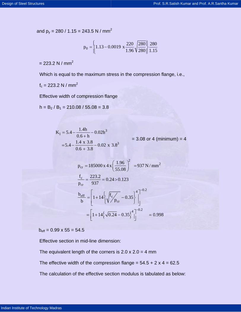
Design of Steel Structures Prof. S.R.Satish Kumar and Prof. A.R.Santha Kumar
Indian Institute of Technology Madras
and py = 280 / 1.15 = 243.5 N / mm2
0220 280 280p 1.13 0.0019 x1.96 280 1.15
⎧ ⎫⎪ ⎪= −⎨ ⎬⎪ ⎪⎩ ⎭
= 223.2 N / mm2
Which is equal to the maximum stress in the compression flange, i.e.,
fc = 223.2 N / mm2
Effective width of compression flange
h = B2 / B1 = 210.08 / 55.08 = 3.8
31
3
1.4hK 5.4 0.02h0.6 h
1.4 x 3.85.4 0.02 x 3.80.6 3.8
= − −+
= − −+
= 3.08 or 4 (minimum) = 4
{ }
22
cr
c
cr0.24
eff ccr
0.24
1.96p 185000 x 4 x 937 N / mm55.08
f 223.2 0.24 0.123p 937
b f1 14 0.35pb
1 14 0.24 0.35 0.998
−
−
⎛ ⎞= =⎜ ⎟⎝ ⎠
= = >
⎡ ⎤⎧ ⎫⎢ ⎥= + −⎨ ⎬⎢ ⎥⎩ ⎭⎣ ⎦
⎡ ⎤= + − =⎢ ⎥⎣ ⎦
beff = 0.99 x 55 = 54.5
Effective section in mid-line dimension:
The equivalent length of the corners is 2.0 x 2.0 = 4 mm
The effective width of the compression flange = 54.5 + 2 x 4 = 62.5
The calculation of the effective section modulus is tabulated as below:
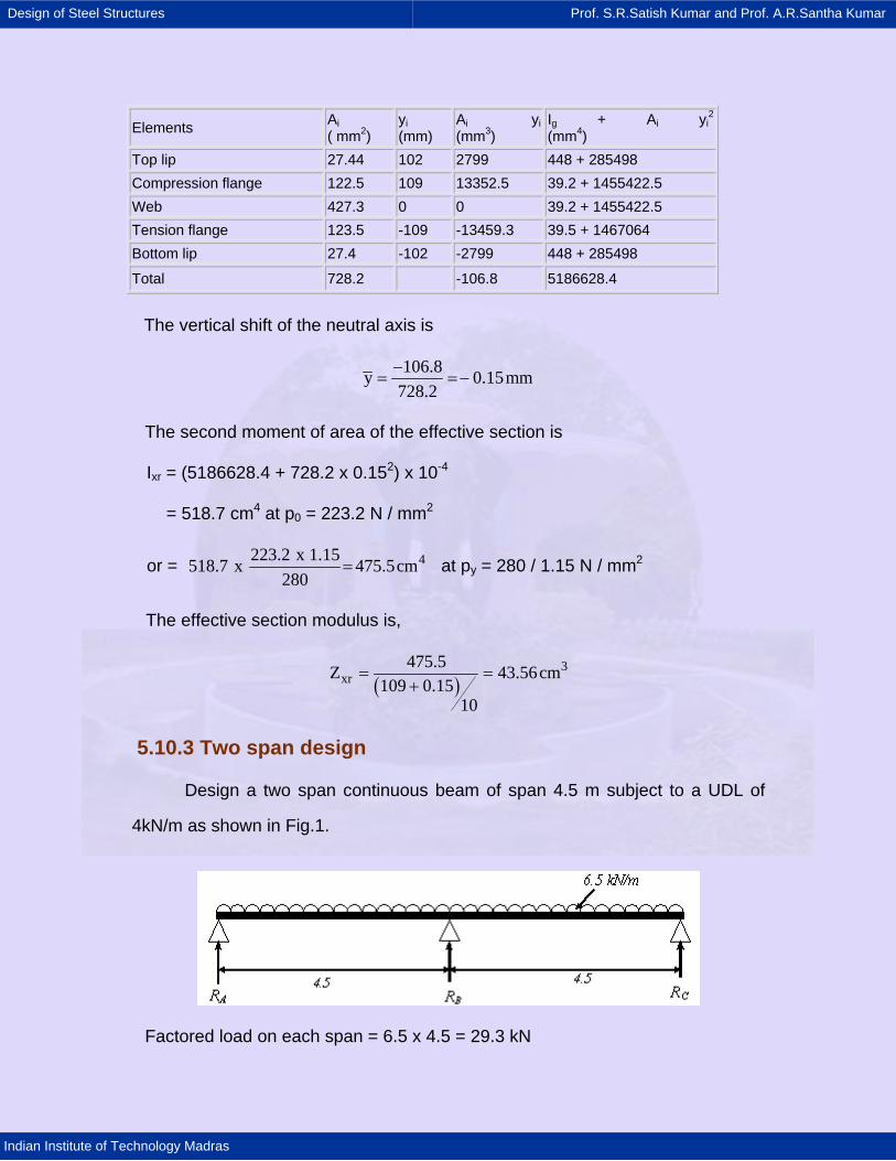
Design of Steel Structures Prof. S.R.Satish Kumar and Prof. A.R.Santha Kumar
Indian Institute of Technology Madras
Elements Ai ( mm2)
yi (mm)
Ai yi(mm3)
Ig + Ai yi2
(mm4) Top lip 27.44 102 2799 448 + 285498 Compression flange 122.5 109 13352.5 39.2 + 1455422.5 Web 427.3 0 0 39.2 + 1455422.5 Tension flange 123.5 -109 -13459.3 39.5 + 1467064 Bottom lip 27.4 -102 -2799 448 + 285498 Total 728.2 -106.8 5186628.4
The vertical shift of the neutral axis is
106.8y 0.15mm728.2−
= =−
The second moment of area of the effective section is
Ixr = (5186628.4 + 728.2 x 0.152) x 10-4
= 518.7 cm4 at p0 = 223.2 N / mm2
or = 4223.2 x 1.15518.7 x 475.5cm280
= at py = 280 / 1.15 N / mm2
The effective section modulus is,
( )3
xr475.5Z 43.56cm
109 0.1510
= =+
5.10.3 Two span design
Design a two span continuous beam of span 4.5 m subject to a UDL of
4kN/m as shown in Fig.1.
Factored load on each span = 6.5 x 4.5 = 29.3 kN
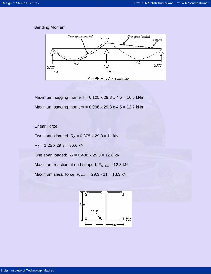
Design of Steel Structures Prof. S.R.Satish Kumar and Prof. A.R.Santha Kumar
Indian Institute of Technology Madras
Bending Moment
Maximum hogging moment = 0.125 x 29.3 x 4.5 = 16.5 kNm
Maximum sagging moment = 0.096 x 29.3 x 4.5 = 12.7 kNm
Shear Force
Two spans loaded: RA = 0.375 x 29.3 = 11 kN
RB = 1.25 x 29.3 = 36.6 kN
One span loaded: RA = 0.438 x 29.3 = 12.8 kN
Maximum reaction at end support, Fw,max = 12.8 kN
Maximum shear force, Fv,max = 29.3 - 11 = 18.3 kN
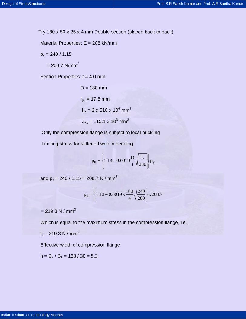
Design of Steel Structures Prof. S.R.Satish Kumar and Prof. A.R.Santha Kumar
Indian Institute of Technology Madras
Try 180 x 50 x 25 x 4 mm Double section (placed back to back)
Material Properties: E = 205 kN/mm
py = 240 / 1.15
= 208.7 N/mm2
Section Properties: t = 4.0 mm
D = 180 mm
ryy = 17.8 mm
Ixx = 2 x 518 x 104 mm4
Zxx = 115.1 x 103 mm3 Only the compression flange is subject to local buckling
Limiting stress for stiffened web in bending
y0 y
fDp 1.13 0.0019 pt 280
⎧ ⎫⎪ ⎪= −⎨ ⎬⎪ ⎪⎩ ⎭
and py = 240 / 1.15 = 208.7 N / mm2
0180 240p 1.13 0.0019 x x208.7
4 280⎧ ⎫⎪ ⎪= −⎨ ⎬⎪ ⎪⎩ ⎭
= 219.3 N / mm2
Which is equal to the maximum stress in the compression flange, i.e.,
fc = 219.3 N / mm2
Effective width of compression flange
h = B2 / B1 = 160 / 30 = 5.3
Design of Steel Structures Prof. S.R.Satish Kumar and Prof. A.R.Santha Kumar
Indian Institute of Technology Madras
31
3
1.4hK 5.4 0.02h0.6 h
1.4 x 3.85.4 0.02 x 5.30.6 3.8
= − −+
= − −+
= 1.1 or 4 (minimum) = 4
22
cr
c
cr
eff
4p 185000 x 4 x 13155 N / mm30
f 219.3 0.017 0.123p 13155b
1b
⎛ ⎞= =⎜ ⎟⎝ ⎠
= = >
=
beff = 30 mm
i.e. the full section is effective in bending.
Ixr = 2 x 518 x 104 mm4
Zxr = 115.1 x 103 mm3
Moment Resistance
The compression flange is fully restrained over the sagging moment
region but it is unrestrained over the hogging moment region, that is, over the
internal support.
However unrestrained length is very short and lateral torsional buckling is
not critical.
The moment resistance of the restrained beam is:
Mcx = Zxr py
Design of Steel Structures Prof. S.R.Satish Kumar and Prof. A.R.Santha Kumar
Indian Institute of Technology Madras
= 115.1 x 103 x (240 / 1.15) 10-6 = 24 kNm > 16.5 kNm
O.K
Shear Resistance
Shear yield strength,
pv = 0.6 py = 0.6 x 240 /1.15 = 125.2 N/mm2
Shear buckling strength, qcr = 22 1000 x 41000t
D 180⎛ ⎞⎛ ⎞ =⎜ ⎟ ⎜ ⎟
⎝ ⎠ ⎝ ⎠ = 493.8 N/mm2
Maximum shear force, Fv,max = 18.3 kN
Shear area = 180 x 4 = 720 mm2
Average shear stress fv = 3
218.3x10 25.4 N / mm720
= < qcr
O.K
Web crushing at end supports
Check the limits of the formulae.
D 180 45 200 O.Kt 4r 6 1.5 6 O.Kt 4
= = ≤ ∴
= = ≤ ∴
At the end supports, the bearing length, N is 50 mm (taking conservatively
as the flange width of a single section)
For c=0, N/ t = 50 / 4 = 12.5 and restrained section.
C is the distance from the end of the beam to the load or reaction.
Use
Design of Steel Structures Prof. S.R.Satish Kumar and Prof. A.R.Santha Kumar
Indian Institute of Technology Madras
{ }
{ }
y2w r
m
r
2 3w
f NP 2 x t C 8.8 1.11 t
DtC 1
750451 1.06
750240P 2 x 4 x1.06 x 8.8 1.11 12.5 101.15
−
= +γ
= +
= + =
= +
Web Crushing at internal support
t the internal support, the bearing length, N, is 100mm (taken as the flange
width of a double section)
For c > 1.5D, N / t = 100 / 4 = 25 and restrained section.
{ }y2w 5 6
m
y
m
f NP t C C 13.2 1.63 t
f 240k 0.9228 x 1.15 x 228
= +γ
= = =γ
C5 = (1.49 - 0.53 k) = 1.49 - 0.53 x 0.92 = 1.0 > 0.6
C6 = (0.88 - 0.12 m)
m = t / 1.9 = 4 / 1.9 = 2.1
C6 = 0.88 - 0.12 x 2.1 = 0.63
{ }2 3w
240P 2 x 4 x1x 0.63x 13.2 1.63 25 101.15
−∴ = +
= 89.8 kN > RB (= 36 kN)
Deflection Check
A coefficient of 3384
is used to take in account of unequal loading on a double
span. Total unfactored imposed load is used for deflection calculation.
Design of Steel Structures Prof. S.R.Satish Kumar and Prof. A.R.Santha Kumar
Indian Institute of Technology Madras
3
maxav
xx xy 4 4av
W L3384 E I
I I 1036 1036I 1036 x10 mm2 2
δ =
+ += = =
W = 29.3 / 1.5 = 19.5 kN
3 3
max 3 419.5 x10 x 45003 6.53mm
384 205 x10 x1036 x10δ = =
Deflection limit = L / 360 for imposed load
= 4500 / 360 = 12.5 mm > 6.53 mm O.K
In the double span construction: Use double section 180 x 50 x 25 x 4.0
mm lipped channel placed back to back.
5.10.4 Column design
Design a column of length 2.7 m for an axial load of 550 kN.
Axial load P = 550 kN
Length of the column, L = 2.7 m
Effective length, le = 0.85L = 0.85 x 2.7 = 2.3 m
Try 200 x 80 x 25 x 4.0 mm Lipped Channel section
Material Properties: E = 205 kN/mm2
fy = 240 N/ mm2
py = 240 / 1.15 = 208.7 N/mm2
Section Properties: A = 2 x 1576 = 3152 mm2
Ixx = 2 x 903 x 104 mm4
Iyy = 2 [124 x 104 + 1576 x 24.82]
= 442 x 104 mm4
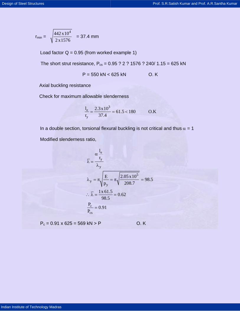
Design of Steel Structures Prof. S.R.Satish Kumar and Prof. A.R.Santha Kumar
Indian Institute of Technology Madras
rmin = 4442 x10
2 x1576 = 37.4 mm
Load factor Q = 0.95 (from worked example 1)
The short strut resistance, Pcs = 0.95 ? 2 ? 1576 ? 240/ 1.15 = 625 kN
P = 550 kN < 625 kN O. K
Axial buckling resistance
Check for maximum allowable slenderness
3e
y
l 2.3x10 61.5 180r 37.4
= = < O.K
In a double section, torsional flexural buckling is not critical and thus α = 1
Modified slenderness ratio,
e
y
y
5
yy
c
cs
lr
2.05x10E 98.5p 208.7
1x 61.5 0.6298.5
P0.91
P
α
λ =λ
λ = π = π =
∴λ = =
=
Pc = 0.91 x 625 = 569 kN > P O. K
Design of Steel Structures Prof. S.R.Satish Kumar and Prof. A.R.Santha Kumar
Indian Institute of Technology Madras
5.11 Concluding remarks
In this chapter the difference between cold rolled steel and hot rolled steel
has been discussed and the merits of the former are outlined. The concepts of
"effective width" and "effective section" employed in the analysis and design of
cold rolled section have been explained. The difference between "stiffened" and
"unstiffened" elements has been explained. Considerations in the design of cold
rolled beams have been explained and formulae employed for the limit state
design of beams made of cold rolled sections have been provided.
In the two preceeding chapters on cold rolled steel, a detailed discussion
of design of elements made from it has been provided, the major differences
between the hot rolled steel products and cold rolled steel products outlined and
the principal advantages of using the latter in construction summarized. Design
methods, including methods based on prototype testing and empirical design
procedures have been discussed in detail.
Thin steel products are extensively used in building industry in the western
world and this range from purlins and lintels to roof sheeting and decking. Light
steel frame construction is often employed in house building and is based on
industrialized manufacture of standardized components, which ensure a high
quality of materials of construction. The most striking benefit of all forms of light
steel framing is their speed of construction, ease of handling and savings in site
supervision and elimination of wastage in site, all of which contribute to overall
economy.

Design of Steel Structures Prof. S.R.Satish Kumar and Prof. A.R.Santha Kumar
Indian Institute of Technology Madras
In the Indian context, industrialized methods of production and delivery of
cold rolled steel products to site have the potential to build substantially more
houses than is otherwise possible, with the same cash flow, thus freeing capital
and financial resources for other projects. Other advantages include elimination
of shrinkage and movement cracks, greater environmental acceptability and less
weather dependency. Properly constructed light steel frames are adaptable to
future requirements and will provide high acoustic performance and a high
degree of thermal insulation. Provided the sheets are pre-galvanised, the
members provide adequate corrosion protection when used close to the
boundaries of the building envelope. The design life of these products exceeds
60 years.
Design of Steel Structures Prof. S.R.Satish Kumar and Prof. A.R.Santha Kumar
Indian Institute of Technology Madras
5.12 References
1. BS5950, Part 5: Structural Use of Steelwork in Building, British Standards
Institution, London 1987.
2. J. Rhodes and R.M. Lawson "Design of Structures using Cold Formed
Steel Sections, SCI Publication 089, The Steel Construction Institute, U.K.
1992.
3. Rhodes, J. and Lawson, R. M., Design of Structures using Cold Formed
Steel Sections, The Steel Construction Institute, Ascot, 1992.
4. Chung, K. F Worked examples to BS 5950, Part 5, 1987, The Steel
Construction Institute, Ascot, 1993.
5. Wei-Wen Yu , Cold Formed Steel Structures by, Mc Graw Hill Book
Company, 1973.
Design of Steel Structures Prof. S.R.Satish Kumar and Prof. A.R.Santha Kumar
Indian Institute of Technology Madras
6. MICROWAVE TOWERS
6.1 Introduction
In the present era the technology in communications has developed to a
very large extent. The faster growth demands advances in the design and
implementation of the communication towers. There are different types of
communication towers present now-a-days in the cellular business. The present
paper covers the issues related to the types of towers, codal provisions for the
communication towers, foundation design of the green field and roof top towers
and optimization of the towers through expert ware.
Cold-formed sections are used in many industries and are often specially
shaped to suit the particular application. In building uses, the most common
sections are the C and the Z shapes. There are, however, a whole range of
variants of these basic shapes, including those with edge lips, internal stiffeners
and bends in the webs.
Other section shapes are the "top-hat" section and the modified I section.
The common range of cold-formed sections that are marketed is illustrated in
Figure. The sections can also be joined together to form compound members.
The reason for the additional lips and stiffeners is because unstiffened
wide thin plates are not able to resist significant compression and consequently
the use of steel in the section becomes inefficient. However, a highly stiffened
section is less easy to form and is often less practicable from the point of view of
its connections. Therefore, a compromise between section efficiency and
practicability is often necessary.
Design of Steel Structures Prof. S.R.Satish Kumar and Prof. A.R.Santha Kumar
Indian Institute of Technology Madras
High strength for a given section depth
Ability to provide long spans (up to 10 m)
Dimensional accuracy
Long term durability (if galvanized) in internal environments
Freedom from creep and shrinkage
Can be formed to a particular shape or application
Lightness, particularly important in poor ground conditions
Dry envelope
Delivered to site cut to length and with pre-punched holes, requiring no further fabrication
Ability to be prefabricated into panels etc.
Robust and sufficiently light for site handling
Examples of the structural use of cold-formed sections which utilize these features are as follows:
Roof and wall members
Traditionally, a major use of cold-formed steel in the UK has been as
purlins and side rails to support the cladding in industrial type buildings. These
are generally based on the Z section (and its variants) which facilitates
incorporation of sleeves and overlaps to improve the efficiency of the members in
multi-span applications. Special shapes are made for eaves members etc.
Steel framing
An increasing market for cold-formed steel sections is in site-assembled
frames and panels for walls and roofs, and stand-alone buildings. This approach
has been used in light industrial and commercial buildings and in mezzanine
floors of existing buildings.
Design of Steel Structures Prof. S.R.Satish Kumar and Prof. A.R.Santha Kumar
Indian Institute of Technology Madras
Wall partitions
A special application is for very light sections used in conjunction with
plaster board panels in stud wall partitioning to form a thin robust wall.
Large panels for housing
Storey-high panels can be factory-built and assembled into housing units
on site. This is an extension of the approach used for timber framing.
Lintels
A significant market for specially formed cold formed sections is as lintels
over doors and windows in low rise masonry walls (Figure 6). These products are
often powder coated for extra corrosion protection.
Floor joists
Cold formed sections may be used as an alternative to timber joists in
floors of modest span in domestic and small commercial buildings.
Modular frames for commercial buildings.
A prefabricated modular framing system panel system using cold formed
channels and lattice joists has been developed for use in buildings up to 4
storeys height (Figure 7). Although primarily developed for commercial building
this modular system has broad application in such as educational and apartment
buildings.
Trusses
There are a number of manufacturers of lattice girder and truss systems
using cold formed steel sections.
Design of Steel Structures Prof. S.R.Satish Kumar and Prof. A.R.Santha Kumar
Indian Institute of Technology Madras
Space frames
A space frame (a three-dimensional truss) using cold formed steel
sections has recently been marketed in the UK.
Curtain walling
A modem application is in cladding framing to multi-storey mullions and
transoms in standard glazing systems, steel buildings, and as mullions and
transoms in standard glazing systems.
Prefabricated buildings
The transportable prefabricated building unit (such as the ubiquitous site
hut) is a common application of the use of cold-formed steel. Other applications
are as prefabricated "toilet pod" units in multi-storey buildings.
Frameless steel buildings
Steel folded plates, barrel vaults and truncated pyramid roofs are
examples of systems that have been developed as so-called frameless buildings
(i.e. those without beams and which rely partly on ‘stressed skin" action).
Storage racking
Storage racking systems for use in warehouses and industrial buildings
are made from cold formed steel sections. Most have special clip attachments, or
bolted joints for easy assembly.
Design of Steel Structures Prof. S.R.Satish Kumar and Prof. A.R.Santha Kumar
Indian Institute of Technology Madras
Applications in general civil engineering include:
Lighting and transmission towers
These are often made from thin tubular or angle sections.
Motorway crash barriers
These thin steel members are primarily designed for strength but also
have properties of energy absorbtion by permitting gross deformation.
Silos for agricultural use
Silo walls are often stiffened and supported by cold-formed steel sections.
The main structural use of cold-formed steel not listed above is that of
floor decking which is usually sold as a galvanised product. In particular,
‘composite" decking is designed to act in conjunction with in situ concrete
floors in steel framed buildings to form composite slabs. Composite decking is
usually designed to be unpropped during construction and typical spans are 3.0m
to 3.6m.
Other major non-structural applications of cold formed steel in building
include such diverse uses as garage doors, and ducting for heating and
ventilating systems.
Design of Steel Structures Prof. S.R.Satish Kumar and Prof. A.R.Santha Kumar
Indian Institute of Technology Madras
6.2 Types of communication towers
The different types of communication towers are based upon their
structural action, their cross-section, the type of sections used and on the
placement of tower.
A brief description is as given below:
6.2.1 Based on structural action.
Towers are classified into three major groups based on the structural
action. They are:
• Self supporting towers
• Guyed towers
• Monopole.
6.2.1.1. Self supporting towers.
The towers that are supported on ground or on buildings are called as
self-supporting towers. Though the weight of these towers is more they require
less base area and are suitable in many situations. Most of the TV, MW, Power
transmission, and flood light towers are self-supporting towers.
6.2.1.2. Guyed towers.
Guyed towers provide height at a much lower material cost than self-
supporting towers due to the efficient use of high-strength steel in the guys.
Guyed towers are normally guyed in three directions over an anchor radius of
typically 2/3 of the tower height and have a triangular lattice section for the
central mast. Tubular masts are also used, especially where icing is very heavy
and lattice sections would ice up fully. These towers are much lighter than self-
Design of Steel Structures Prof. S.R.Satish Kumar and Prof. A.R.Santha Kumar
Indian Institute of Technology Madras
supporting type but require a large free space to anchor guy wires. Whenever
large open space is available, guyed towers can be provided. There are other
restrictions to mount dish antennae on these towers and require large anchor
blocks to hold the ropes.
6.2.1.3 Monopole.
It is single self-supporting pole, and is generally placed over roofs of high
raised buildings, when number of antennae required is less or height of tower
required is less than 9m.
6.2.2. Based on cross section of tower.
Towers can be classified, based on their cross section, into square,
rectangular, triangular, delta, hexagonal and polygonal towers.
Open steel lattice towers make the most efficient use of material and
enables the construction of extremely light-weight and stiff structures by offering
less exposed area to wind loads. Most of the power transmission,
telecommunication and broadcasting towers are lattice towers.
Triangular Lattice Towers have less weight but offer less stiffness in
torsion. With the increase in number of faces, it is observed that weight of tower
increases. The increase is 10% and 20% for square and hexagonal cross
sections respectively. If the supporting action of adjacent beams is considered,
the expenditure incurred for hexagonal towers is somewhat less.
Design of Steel Structures Prof. S.R.Satish Kumar and Prof. A.R.Santha Kumar
Indian Institute of Technology Madras
6.2.3 Based on the type of material sections.
Based on the sections used for fabrication, towers are classified into
angular and hybrid towers (with tubular and angle bracings).
Lattice towers are usually made of bolted angles. Tubular legs and
bracings can be economic, especially when the stresses are low enough to allow
relatively simple connections. Towers with tubular members may be less than
half the weight of angle towers because of the reduced wind load on circular
sections. However the extra cost of the tube and the more complicated
connection details can exceed the saving of steel weight and foundations.
6.2.4 Based on the placement of tower.
Based on this placement, Communication towers are classified as follows:
Green Field Tower Roof Top Tower Erection Erected on natural ground with
suitable foundation. Erected on existing building with raised columns and tie beams.
Height 30 – 200 m 9 – 30 m Usual Location Rural Areas Urban Areas Economy Less More
6.2.5 Based on the number of segments.
The towers are classified based on the number of segments as Three
slope tower; Two slope tower; Single slope tower; Straight tower.
Design of Steel Structures Prof. S.R.Satish Kumar and Prof. A.R.Santha Kumar
Indian Institute of Technology Madras
6.3 Ladders and platforms
6.3.1 Ladder
In communication towers the climbing facility can be provided by two
ways.
a) by providing climbing ladder with or without safety ring and
b) by providing step bolts confirming to IS 10238:1982.
Generally for communication towers it is usual practice to provide climbing
ladder with safety cage. The exposed area of ladder shall be considered while
calculating the wind load on tower. The position of ladder will have impact on
weight of tower. If ladder is provided internally its effect will be less and if it is
provided externally it will have more effect. Protection ring is a safety requirement
and may be replaced by fall arrest safety system.
Cable ladder is provided to support the cable wave-guide running from
antenna to the equipment shelter. The cable ladder is provided inside and along
the slope of the tower.
Step bolts are provided only for specific cases of narrow based towers of
smaller heights as per user’s requirements. The step bolts should be capable of
withstanding a vertical load of not less than 1.5 kN.
6.3.2 Platforms
The platforms shall be provided at different levels as rest platforms or
working platforms. The rest platforms are provided with chequered plate or
Design of Steel Structures Prof. S.R.Satish Kumar and Prof. A.R.Santha Kumar
Indian Institute of Technology Madras
welded wire mesh along with suitable railing inside the tower and are provided for
every 10m height, for all towers of height exceeding 20m.
The working platforms may be internal or external and these are provided
with railings of 1000mm with toe, knee and hand rail protection.
Design of Steel Structures Prof. S.R.Satish Kumar and Prof. A.R.Santha Kumar
Indian Institute of Technology Madras
6.4 Codal provisions in design of communication towers
The following are the steps involved in design of communication tower.
a. Selection of configuration of tower
b. Computation of loads acting on tower
c. Analysis of tower for above loads
d. Design of tower members according to codes of practices.
Selection of configuration of a tower involves fixing of top width, bottom
width, number of panels and their heights, type of bracing system and slope of
tower.
6.4.1 Wind load on tower
The wind load on tower can be calculated using the Indian standards IS:
875(Part 3)-1987[3] and BS: 8100 (Part 1)-1996[4].
The designer should select the basic wind speed depending on the
location of tower. The design wind speed is modified to induce the effect of risk
factor (k1), terrain coefficient (k2) and local topography (k3) to get the design wind
speed Vz. (Vz = k1k2k3Vb).
The design wind pressure Pz at any height above mean ground level is
0.6Vz2.
The coefficient 0.6 in the above formula depends on a number of factors
and mainly on the atmospheric pressure and air temperatures.
Design of Steel Structures Prof. S.R.Satish Kumar and Prof. A.R.Santha Kumar
Indian Institute of Technology Madras
Solidity ratio is defined as the ratio of effective area (projected area of all
the individual elements) of a frame normal to the wind direction divided by the
area enclosed by the boundary of the frame normal to the wind direction.
Force coefficient for lattice towers of square or equilateral triangle section
with flat sided members for wind blowing against any face shall be as given in
Table 30 of IS:875(Part-3)-1987.
Force coefficients for lattice towers of square section with circular
members and equilateral triangle section with circular members are as given in
tables 31 and 32 of IS: 875(Part-3)-1987 respectively.
Table 2 of IS:875(Part-3)-1987 gives the factors to obtain design wind
speed variation with height in different terrains for different classes of structures
such as class A, class B, class C.
The wind load acting on a tower can be computed as F= CdtAePzk2.
For circular sections the force coefficient depends upon the way in which
the wind flows around it and is dependent upon the velocity and kinematic
viscosity of the wind and diameter of the section. The force coefficient is usually
quoted against a non-dimensional parameter, called the Reynolds number, which
takes account of the velocity and viscosity of the medium and the member
diameter.
Design of Steel Structures Prof. S.R.Satish Kumar and Prof. A.R.Santha Kumar
Indian Institute of Technology Madras
6.4.2 Wind load on antennae
Wind load on antennae shall be considered from Andrew’s catalogue. In
the Andrew’s catalogue the wind loads on antennas are given for 200kmph wind
speed. The designer has to calculate the antenna loads corresponding to design
wind speed.
6.4.3 Design of tower members
According to the clause 5.1 of IS-802(Part-1/sec2)[5] the estimated tensile
stresses on the net effective sectional areas in various members shall not exceed
minimum guaranteed yield stress of the material. However in case the angle
section is connected by one leg only, the estimated tensile stress on the net
effective sectional area shall not exceed Fy, where Fy is the minimum guaranteed
yield stress of the material. For structural steels confirming to IS-226[6] and IS-
2062[7] the yield strength is 250 MPa. Generally yst25 grade tubes confirming
IS-1161[8] are used for tower members.
As per IS-802 part1/sec2 estimated compressive stresses in various
members shall not exceed the values given by the formulae in clause 5.2.2. of
IS-802 code.
6.4.4 Limiting slenderness ratios
a. As per clause 6.3 of IS-802(Part1/sec2)-1992 the limiting values KL / r
shall be as follows:
Leg members 120
Redundant members and those carrying nominal stresses 250
Other members carrying computed stresses 200
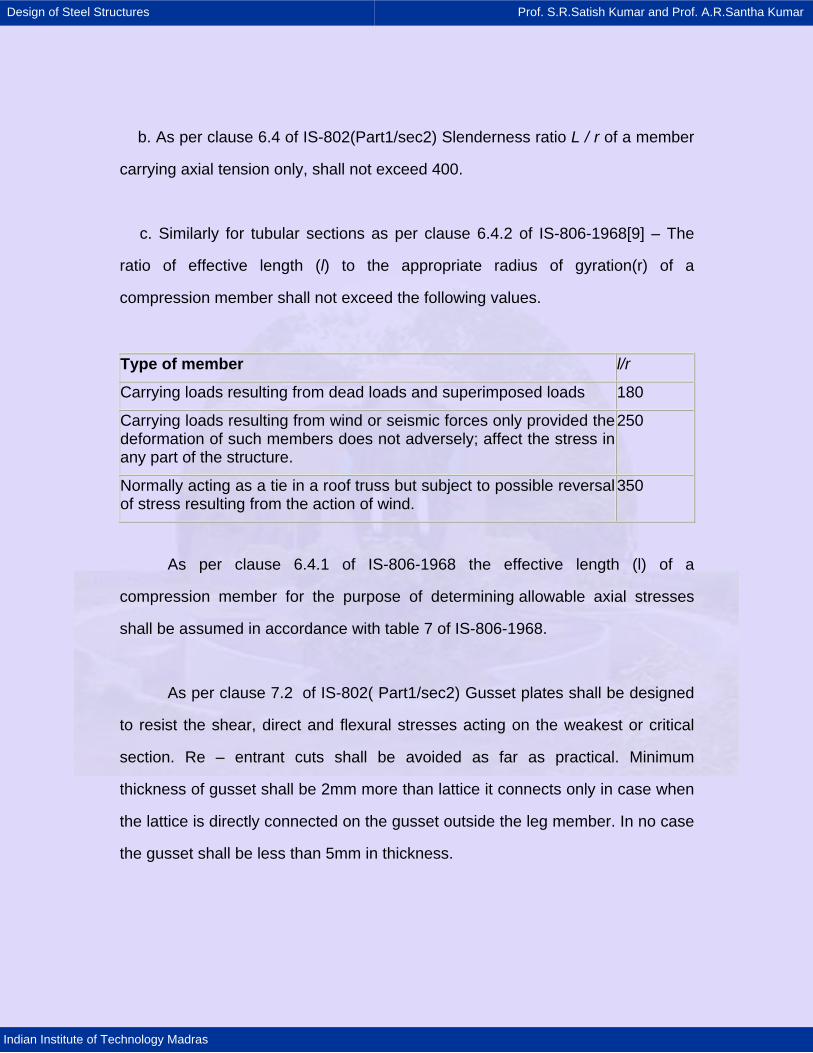
Design of Steel Structures Prof. S.R.Satish Kumar and Prof. A.R.Santha Kumar
Indian Institute of Technology Madras
b. As per clause 6.4 of IS-802(Part1/sec2) Slenderness ratio L / r of a member
carrying axial tension only, shall not exceed 400.
c. Similarly for tubular sections as per clause 6.4.2 of IS-806-1968[9] – The
ratio of effective length (l) to the appropriate radius of gyration(r) of a
compression member shall not exceed the following values.
Type of member l/r
Carrying loads resulting from dead loads and superimposed loads 180
Carrying loads resulting from wind or seismic forces only provided the deformation of such members does not adversely; affect the stress in any part of the structure.
250
Normally acting as a tie in a roof truss but subject to possible reversal of stress resulting from the action of wind.
350
As per clause 6.4.1 of IS-806-1968 the effective length (l) of a
compression member for the purpose of determining allowable axial stresses
shall be assumed in accordance with table 7 of IS-806-1968.
As per clause 7.2 of IS-802( Part1/sec2) Gusset plates shall be designed
to resist the shear, direct and flexural stresses acting on the weakest or critical
section. Re – entrant cuts shall be avoided as far as practical. Minimum
thickness of gusset shall be 2mm more than lattice it connects only in case when
the lattice is directly connected on the gusset outside the leg member. In no case
the gusset shall be less than 5mm in thickness.
Design of Steel Structures Prof. S.R.Satish Kumar and Prof. A.R.Santha Kumar
Indian Institute of Technology Madras
6.5 References:
[1]. G.A. Savitskii “Calculation of Antenna Installations, Physical Principles”
[2]. A.R. Santhakumar, S.S. Murthy “Transmission Line Structures” McGraw-
Hill Book Co. 1990.
[3]. IS: 875(Part-3):1987 “Code of practice for design loads (other than
earthquake) for buildings and structures”.
[4]. BS: 8100 (Part-1)-1996 “Lattice towers and Masts”.
[5]. IS: 802(Part-1)-1977 “Code of practice for use of structural steel in
overhead transmission line towers”.
[6]. IS: 226-1975 “Structural Steel (Standard Quality)”.
[7]. IS: 2062 – 1992 “Steel for general structural purposes”.
[8]. IS: 1161 – 1998 “Steel tubes for structural purposes”.
[9]. IS: 806 – 1968 “Code of practice for use of steel tubes in general building
construction”.
Design of Steel Structures Prof. S.R.Satish Kumar and Prof. A.R.Santha Kumar
Indian Institute of Technology Madras
Examples
Example1 Basic wind pressure - calculation
A Power house building 25m high is to be designed in Darbhanga
city. Compute the basic wind pressure.
Basic wind speed in Darbhanga (from appendix A)
P. 53 Code Vb = 55m/sec
An industrial building can be grouped under all general buildings and
structures so should be designed for 50 years of design life
Risk coefficient from table 1. P. 11 code
k1 = 1
Assuming the terrain is in city industrial area with numerous closely
spaced obstructions. It can be grouped under category 3. P.8 code. Since the
height of the building is 25m this falls under class B P.11 code. The terrain factor
k2 can be got from table 2 P.12 code. For category 3, class B interpolating
between 20m and 30m
k2 = 1.005
The ground is assumed to be plain so the topography factor k3 is 1 + cs P.
56 code
where c = Z / L
Since the terrain assumed is plain. Read clause 5.3.3.1 P.12 code
k3 = 1
Design wind speed (Vz) = Vb k1 k2 k3
= 55 (1) (1.005) (1)
= 55.275 m/sec
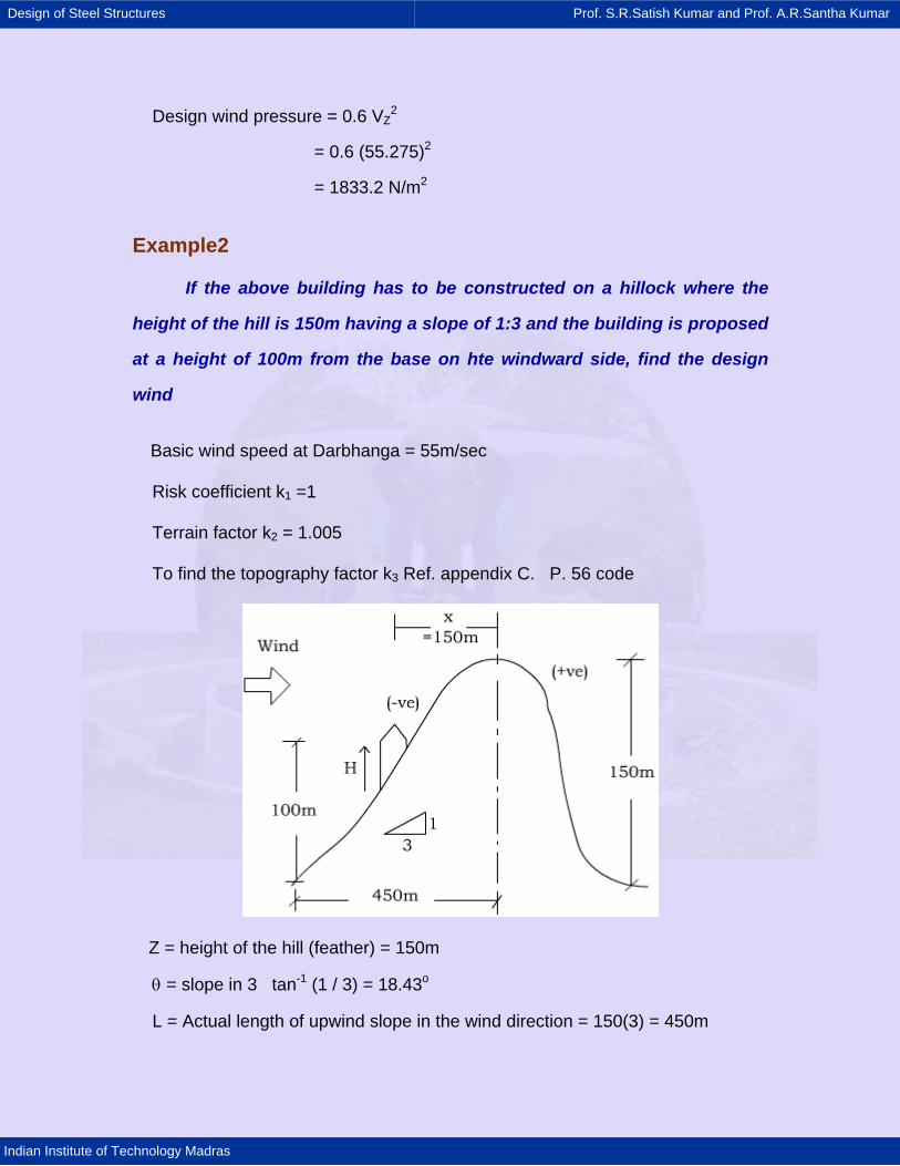
Design of Steel Structures Prof. S.R.Satish Kumar and Prof. A.R.Santha Kumar
Indian Institute of Technology Madras
Design wind pressure = 0.6 VZ2
= 0.6 (55.275)2
= 1833.2 N/m2
Example2
If the above building has to be constructed on a hillock where the
height of the hill is 150m having a slope of 1:3 and the building is proposed
at a height of 100m from the base on hte windward side, find the design
wind
Basic wind speed at Darbhanga = 55m/sec
Risk coefficient k1 =1
Terrain factor k2 = 1.005
To find the topography factor k3 Ref. appendix C. P. 56 code
Z = height of the hill (feather) = 150m
θ = slope in 3 tan-1 (1 / 3) = 18.43o
L = Actual length of upwind slope in the wind direction = 150(3) = 450m
Design of Steel Structures Prof. S.R.Satish Kumar and Prof. A.R.Santha Kumar
Indian Institute of Technology Madras
Le = Effective horizontal length of the hill for θ > 17o Le = Z / 0.3 = 150 / 0.3 =
500m
Values of C for θ = 18.43o (i.e.) > 17o
C = 0.36
Height of the building = 25m
To find x (i.e) the horizontal distance of the building from the crest
measured +ve towards the leeward side and -ve towards the windward side.
k3 = 1 + cs
To get s Fig 14 and 15 are used
x = -150m
x / Le = -150 / 500 = -0.3 H / Le = 25 / 500 = 0.05
Referring to figure 15 hill and ridge for x / Le = -0.3 and H / Le = 0.05 on
the upwind direction
s = 0.58
k3 = 1 + (0.36) (0.58)
k3 = 1.21
Design wind speed Vz = Vb k1 k2 k3
= 55 (1) (1.005) (1.21)
= 66.9 m/sec
Design wind pressure PZ = 0.6 VZ2
= 0.6 (66.9)2
= 2685.4 N/m2
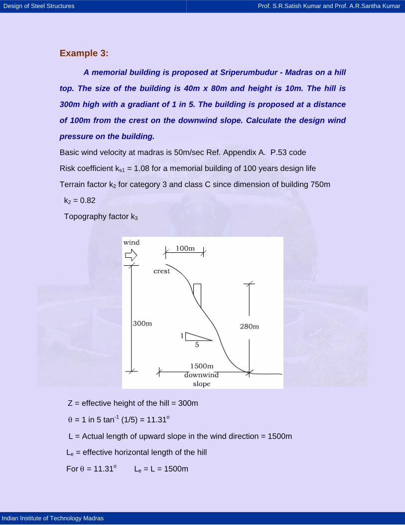
Design of Steel Structures Prof. S.R.Satish Kumar and Prof. A.R.Santha Kumar
Indian Institute of Technology Madras
Example 3:
A memorial building is proposed at Sriperumbudur - Madras on a hill
top. The size of the building is 40m x 80m and height is 10m. The hill is
300m high with a gradiant of 1 in 5. The building is proposed at a distance
of 100m from the crest on the downwind slope. Calculate the design wind
pressure on the building.
Basic wind velocity at madras is 50m/sec Ref. Appendix A. P.53 code
Risk coefficient ks1 = 1.08 for a memorial building of 100 years design life
Terrain factor k2 for category 3 and class C since dimension of building 750m
k2 = 0.82
Topography factor k3
Z = effective height of the hill = 300m
θ = 1 in 5 tan-1 (1/5) = 11.31o
L = Actual length of upward slope in the wind direction = 1500m
Le = effective horizontal length of the hill
For θ = 11.31o Le = L = 1500m
Design of Steel Structures Prof. S.R.Satish Kumar and Prof. A.R.Santha Kumar
Indian Institute of Technology Madras
Topography factor k3 = 1 +cs
where c = 1.2 (Z/L) since θ = 11.31o 3o < θ < 17o
c = 1.2 (300/1500) = 0.24
x is the distance of the building from the crest + on downwind side
- on upward side x = +100m
The non dimensional factors are
x / Le = 100 / 1500 = 0.067; H / Le = 10 / 1500 = 0.0067
s = 1 from fig 15. P.57
k3 = 1 + (0.24) (1);
k3 = 1.24
Design wind speed Vz = Vb k1 k2 k3
= 50 (1.08) (0.82) (1.24)
= 54.91 m/sec
Design wind pressure PZ = 0.6 VZ2
= 0.6 (54.91)2
=1809.1 N/m2
Example 4: Wind pressure on tower on a hill
A microwave tower of 50m height is proposed over a hill top. The
height of the hill is 50m with a gradiant of 1 in 4. The terrain category is 3.
The tower is proposed at coimbatore. Compute the design wind pressure:
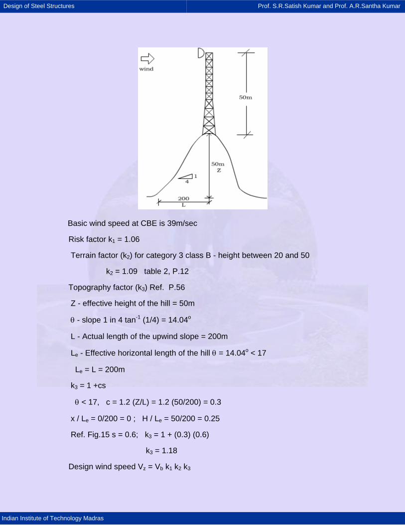
Design of Steel Structures Prof. S.R.Satish Kumar and Prof. A.R.Santha Kumar
Indian Institute of Technology Madras
Basic wind speed at CBE is 39m/sec
Risk factor k1 = 1.06
Terrain factor (k2) for category 3 class B - height between 20 and 50
k2 = 1.09 table 2, P.12
Topography factor (k3) Ref. P.56
Z - effective height of the hill = 50m
θ - slope 1 in 4 tan-1 (1/4) = 14.04o
L - Actual length of the upwind slope = 200m
Le - Effective horizontal length of the hill θ = 14.04o < 17
Le = L = 200m
k3 = 1 +cs
θ < 17, c = 1.2 (Z/L) = 1.2 (50/200) = 0.3
x / Le = 0/200 = 0 ; H / Le = 50/200 = 0.25
Ref. Fig.15 s = 0.6; k3 = 1 + (0.3) (0.6)
k3 = 1.18
Design wind speed Vz = Vb k1 k2 k3
Design of Steel Structures Prof. S.R.Satish Kumar and Prof. A.R.Santha Kumar
Indian Institute of Technology Madras
= 39 (1.06) (1.09) (1.18)
= 53.17 m/sec
Design wind pressure PZ = 0.6 VZ2
= 0.6 (53.17)2
=1696.23 N/m2
Example 5:
If the 50m tower given in previous example is mounted with a hollow
hemispherical dome of 2m diameter weighing 10kN. Compute the forces
and stresses in members of various panels. The elevation of the tower is as
shown below
Data given: Height of the tower = 50m
Base width = 6m
Top width = 2m
No. of panels = 20
Disk size = 2m diameter
Step 1: Wind force - From the previous example
Basic wind speed = 39m/sec
Risk coefficient (k1) = 1.06
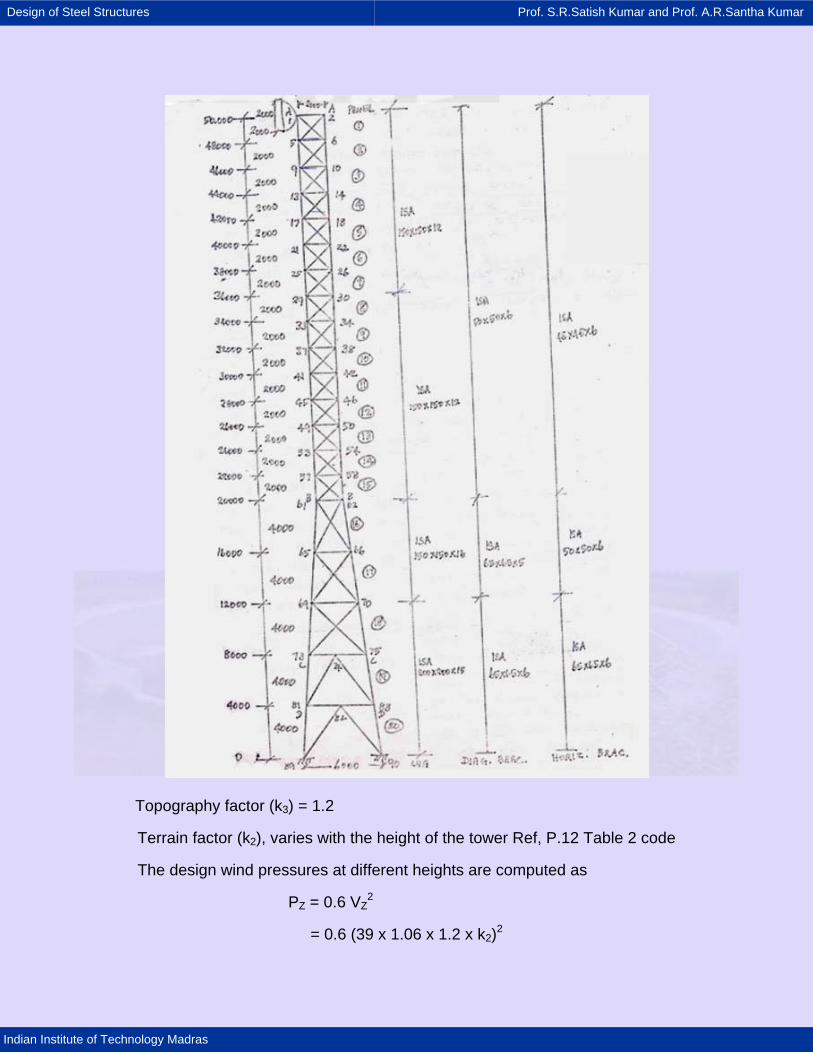
Design of Steel Structures Prof. S.R.Satish Kumar and Prof. A.R.Santha Kumar
Indian Institute of Technology Madras
Topography factor (k3) = 1.2
Terrain factor (k2), varies with the height of the tower Ref, P.12 Table 2 code
The design wind pressures at different heights are computed as
PZ = 0.6 VZ2
= 0.6 (39 x 1.06 x 1.2 x k2)2
Design of Steel Structures Prof. S.R.Satish Kumar and Prof. A.R.Santha Kumar
Indian Institute of Technology Madras
=1476.6 k22 N/m2
The values of k2 at different height is chosen from Table 2
Step2: Basic assumptions:
1. Self weight of the members are equally distributed to the two joints
connected by the members
2. No load is applied at the middle of the k-braced joint but allocated to column
joint
3 Dead and wind loads are increased by 15% for each joints to account for
Gussets, bolts and nuts
4. Secondary members are assumed to be provided in the panel where batter
starts (below the waist level in our case panels 16 to 20. So an additional load of
10% is accounted for in the case of provision of secondary members
5. The wind loads on the members are equally distributed to the connecting
joints.
Step3: Calculation of solidity ratios: Ref P.7 code
Solidity ratio for different panels are calculated
( ) Pr ojected area of all theindividualelementsSolidity ratioArea enclosed by the boundaryof theframe normal to the wind direction
φ =
Solidity ratios of panel 1 to 15 are calculated once as panels 1 to 15 are
similar
Design of Steel Structures Prof. S.R.Satish Kumar and Prof. A.R.Santha Kumar
Indian Institute of Technology Madras
( ) ( )1 15
1 15 16
1 16
16
17
17
18
15x 2 2 x 0.15 15x 2 2 x 2 x 0.05 16 x 2 x 0.045
30 x 20.245 Similarly for
2 x 4.04 x 0.15 2 x 4.68x 0.065 2.8x 0.052 2.8 x 4
20.204
2 x 4.04 x 0.15 2 x 5.14 x 0.065 1x 3.6 x 0.0652 3.6 x 4
20.165
2
−
−
−
+ +φ =
φ = φ
+ +φ =
+⎛ ⎞⎜ ⎟⎝ ⎠
φ =
+ +φ =
+⎛ ⎞⎜ ⎟⎝ ⎠
φ =
φ =
18
x 4.04 x 0.2 2 x 5.67 x 0.065 1x 4.4 x 0.0653.6 4.4 x 4
20.165
+ ++⎛ ⎞
⎜ ⎟⎝ ⎠
φ =
19
19
20
20
2 x 4.04 x 0.2 2 x 4.79 x 0.065 1x 5.2 x 0.0654.4 5.2 x 4
20.134
2 x 4.04 x 0.2 2 x5.016 x 0.0655.2 6 x 4
20.101
+ +φ =
+⎛ ⎞⎜ ⎟⎝ ⎠
φ =
+φ =
+⎛ ⎞⎜ ⎟⎝ ⎠
φ =
Step4 : Calculation of bowl wind pressure
Ref. Fig6 P.44 code. Bowl wind coeffs. are
cf = 1.4 for wind from front
cf = 0.4 for wind from rear
wind pressure at 50m above GL
Design wind pressure PZ =1476.6 (1.09)2
= 1.754 kN/m2
Wind loads on dish are on front face FDISH 1 = cf.Ae.pd
Ref. P.36 clause 6.3 code

Design of Steel Structures Prof. S.R.Satish Kumar and Prof. A.R.Santha Kumar
Indian Institute of Technology Madras
FDISH 1 = 1.4 x π/4 x 22 x 1.754
= 7.71 kN
On rear face
FDISH 2 = 0.4 x π/4 x 22 x 1.754
= 2.20 kN
Step5:
The terrain factor (k2), the solidity ratio and the design wind pressures at
various heights are tabulated as shown - category 3 class B
Panel from top
Height in 'm' from top
Terrain size,HT. coeff. k2
Design wind pressure PZ=1476.6 (k2
2) N/m2
Solidity ratio
Overall force coeff. cfTable30 P.47
PZ . cf N/m2
1 to 5 10 1.09 = 1.075 1.06
1706.4 0.245 3.075 5247.2
6 to 10 20 1.06 = 1.045 1.03
1612.5 0.245 3.075 4958.4
11 to 15 30
1.03 = 1.005 0.98
1491.4 0.245 3.075 4586.1
16 34 0.98 = 0.964 0.948
1372.2 0.204 3.28 4500.8
17 38 0.948 = 0.926 0.904
1266.1 0.165 3.475 4399.7
18 42 0.904 = 0.88 0.856
1143.5 0.165 3.475 3975.7
19 46 0.856 = 0.832 0.808
1022.1 0.134 3.630 3710.2
20 50 0.808 964.0 0.101 3.795 3658.4
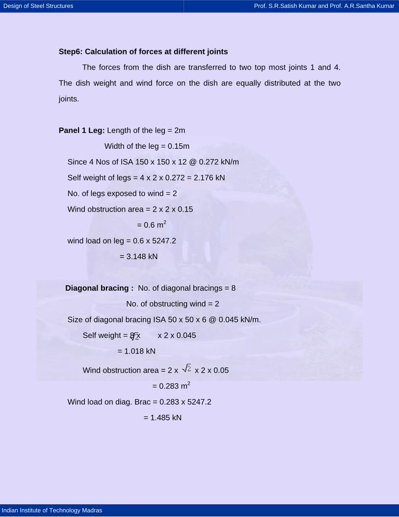
Design of Steel Structures Prof. S.R.Satish Kumar and Prof. A.R.Santha Kumar
Indian Institute of Technology Madras
Step6: Calculation of forces at different joints
The forces from the dish are transferred to two top most joints 1 and 4.
The dish weight and wind force on the dish are equally distributed at the two
joints.
Panel 1 Leg: Length of the leg = 2m
Width of the leg = 0.15m
Since 4 Nos of ISA 150 x 150 x 12 @ 0.272 kN/m
Self weight of legs = 4 x 2 x 0.272 = 2.176 kN
No. of legs exposed to wind = 2
Wind obstruction area = 2 x 2 x 0.15
= 0.6 m2
wind load on leg = 0.6 x 5247.2
= 3.148 kN
Diagonal bracing : No. of diagonal bracings = 8
No. of obstructing wind = 2
Size of diagonal bracing ISA 50 x 50 x 6 @ 0.045 kN/m.
Self weight = 8 x x 2 x 0.045
= 1.018 kN
Wind obstruction area = 2 x x 2 x 0.05
= 0.283 m2
Wind load on diag. Brac = 0.283 x 5247.2
= 1.485 kN
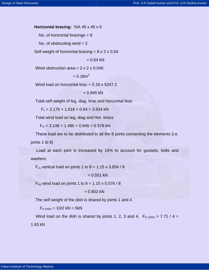
Design of Steel Structures Prof. S.R.Satish Kumar and Prof. A.R.Santha Kumar
Indian Institute of Technology Madras
Horizontal bracing: ISA 45 x 45 x 6
No. of horizontal bracings = 8
No. of obstructing wind = 2
Self weight of horizontal bracing = 8 x 2 x 0.04
= 0.64 kN
Wind obstruction area = 2 x 2 x 0.045
= 0.18m2
Wind load on horizontal brac = 0.18 x 5247.2
= 0.945 kN
Total self weight of leg, diag. brac and horizontal brac
Fv = 2.176 + 1.018 + 0.64 = 3.834 kN
Total wind load on leg, diag and Hor. bracs
FH = 3.148 + 1.485 + 0.945 = 5.578 kN
These load are to be distributed to all the 8 joints connecting the elements (i.e.
joints 1 to 8)
Load at each joint is increased by 15% to account for gussets, bolts and
washers
Fv1 vertical load on joints 1 to 8 = 1.15 x 3.834 / 8
= 0.551 kN
FH1 wind load on joints 1 to 8 = 1.15 x 5.576 / 8
= 0.802 kN
The self weight of the dish is shared by joints 1 and 4
FV DISH = 10/2 kN = 5kN
Wind load on the dish is shared by joints 1, 2, 3 and 4, FH DISH = 7.71 / 4 =
1.93 kN
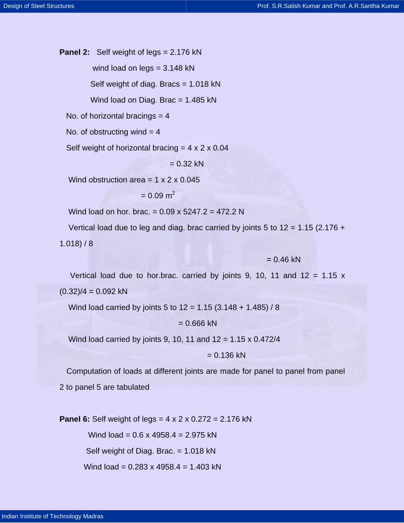
Design of Steel Structures Prof. S.R.Satish Kumar and Prof. A.R.Santha Kumar
Indian Institute of Technology Madras
Panel 2: Self weight of legs = 2.176 kN
wind load on legs = 3.148 kN
Self weight of diag. Bracs = 1.018 kN
Wind load on Diag. Brac = 1.485 kN
No. of horizontal bracings = 4
No. of obstructing wind = 4
Self weight of horizontal bracing = 4 x 2 x 0.04
= 0.32 kN
Wind obstruction area = 1 x 2 x 0.045
= 0.09 m2
Wind load on hor. brac. = 0.09 x 5247.2 = 472.2 N
Vertical load due to leg and diag. brac carried by joints 5 to 12 = 1.15 (2.176 +
1.018) / 8
= 0.46 kN
Vertical load due to hor.brac. carried by joints 9, 10, 11 and 12 = 1.15 x
(0.32)/4 = 0.092 kN
Wind load carried by joints 5 to 12 = 1.15 (3.148 + 1.485) / 8
= 0.666 kN
Wind load carried by joints 9, 10, 11 and 12 = 1.15 x 0.472/4
= 0.136 kN
Computation of loads at different joints are made for panel to panel from panel
2 to panel 5 are tabulated
Panel 6: Self weight of legs = 4 x 2 x 0.272 = 2.176 kN
Wind load = 0.6 x 4958.4 = 2.975 kN
Self weight of Diag. Brac. = 1.018 kN
Wind load = 0.283 x 4958.4 = 1.403 kN
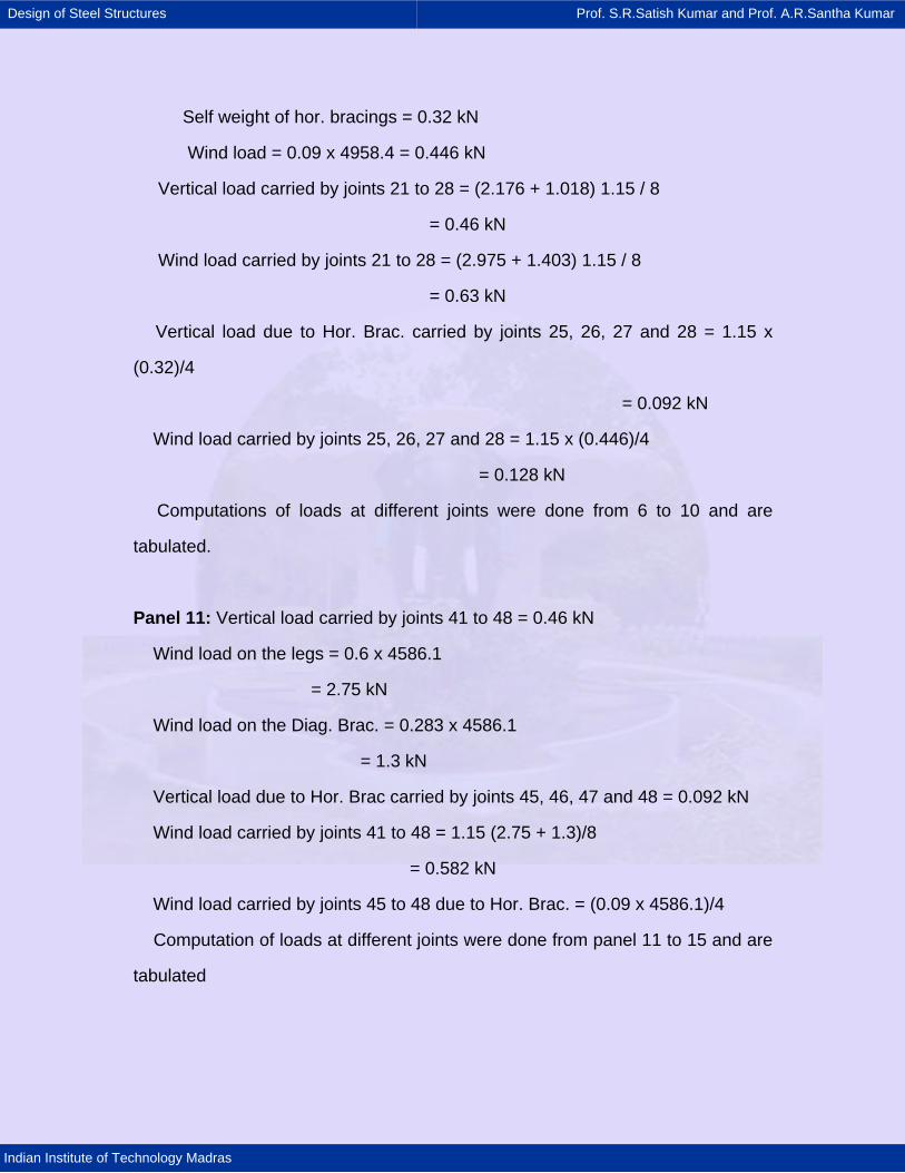
Design of Steel Structures Prof. S.R.Satish Kumar and Prof. A.R.Santha Kumar
Indian Institute of Technology Madras
Self weight of hor. bracings = 0.32 kN
Wind load = 0.09 x 4958.4 = 0.446 kN
Vertical load carried by joints 21 to 28 = (2.176 + 1.018) 1.15 / 8
= 0.46 kN
Wind load carried by joints 21 to 28 = (2.975 + 1.403) 1.15 / 8
= 0.63 kN
Vertical load due to Hor. Brac. carried by joints 25, 26, 27 and 28 = 1.15 x
(0.32)/4
= 0.092 kN
Wind load carried by joints 25, 26, 27 and 28 = 1.15 x (0.446)/4
= 0.128 kN
Computations of loads at different joints were done from 6 to 10 and are
tabulated.
Panel 11: Vertical load carried by joints 41 to 48 = 0.46 kN
Wind load on the legs = 0.6 x 4586.1
= 2.75 kN
Wind load on the Diag. Brac. = 0.283 x 4586.1
= 1.3 kN
Vertical load due to Hor. Brac carried by joints 45, 46, 47 and 48 = 0.092 kN
Wind load carried by joints 41 to 48 = 1.15 (2.75 + 1.3)/8
= 0.582 kN
Wind load carried by joints 45 to 48 due to Hor. Brac. = (0.09 x 4586.1)/4
Computation of loads at different joints were done from panel 11 to 15 and are
tabulated
Design of Steel Structures Prof. S.R.Satish Kumar and Prof. A.R.Santha Kumar
Indian Institute of Technology Madras
Panel 16: Leg: ISA 150 x 150 x 15 @ 0.336 kN/m
Length of the leg (L) = 4.04m
Width of the leg (B) = 0.15m
Self weight of legs = 4 x 4.04 x 0.336
= 5.43 kN
No. of legs exposed to wind = 2
Wind obstruction area = 2 x 4.04 x 0.15
= 1.212 m2
Wind load on leg = 1.212 x 4500.8
= 5.454 kN
Diag. Brac: ISA 65 x 65 x 5 @ 0.049 kN/m
No. of bracing = 8
No. of obstructing wind = 2
Self weight of diagonal brac. = 8 x 4.68 x 0.049
= 1.835 kN
Wind obstruction area = 2 x 4.68 x 0.065
= 0.6084 m2
Wind load on Diag. Brac = 0.6084 x 4500.8
= 2.74 kN
Horizontal Brac: ISA 65 x 65 x 5 @ 0.045 kN/m
No. of bracing = 4
No. of obstructing wind = 1
Self weight of Hor. brac. = 4 x 2.8 x 0.045
= 0.504 kN
Wind obstruction area = 1 x 2.8 x 0.050
Design of Steel Structures Prof. S.R.Satish Kumar and Prof. A.R.Santha Kumar
Indian Institute of Technology Madras
= 0.14 kN
Wind load on Hor. Brac = 0.14 x 4500.8
= 0.63 kN
Secondary bracings are accounted for so DL and WL is increased by 10%
Vertical load carried by joints 61 to 68 = (1.25 / 5.43 + 1.835)/8
= 1.135 kN
Vertical load carried by joints 65 to 68 due to Hor. Brac. = 1.25 (0.504)/4
= 0.158 kN
Wind load carried by joints 61 to 68 = 1.25 (5.454 + 2.74)/8
= 1.28 kN
Wind load carried by joints 65 to 68 due to Hor. Brac = 1.25 (0.63) / 4
= 0.197 kN
Panel 17: Leg: ISA 150 x 150 x 16 @ 0.336 kN/m
Self weight of legs = 4 x 4.04 x 0.336
= 5.43 kN
Wind obstruction area = 2 x 4.04 x 0.15
= 1.212 m2
Wind load on leg = 1.212 x 4399.7
= 5.332 kN
Diag. Brac: ISA 65 x 65 x 5 @ 0.049 kN/m
Self weight of diagonal brac. = 8 x 5.14 x 0.049
= 2.015 kN
Wind obstruction area = 2 x 5.14 x 0.065
= 0.6682 m2
Wind load on Diag. Brac = 0.6682 x 4399.7
Design of Steel Structures Prof. S.R.Satish Kumar and Prof. A.R.Santha Kumar
Indian Institute of Technology Madras
= 2.94 kN
Horizontal Brac: ISA 65 x 65 x 6 @ 0.058 kN/m
Self weight of Hor. brac. = 4 x 3.6 x 0.058
= 0.835 kN
Wind obstruction area = 1 x 3.6 x 0.065
= 0.234 m2
Wind load on Hor. Brac = 0.234 x 4399.7
= 1.03 kN
Secondary bracings should be accounted for in this panel
Vertical load carried by joints 69 to 72 = 1.25 (5.43 + 2.015)/8
= 1.163 kN
Vertical load carried by (Due to horizontal brac.) joints 69 to 72 = 1.25
(0.835)/4
= 0.261 kN
Wind load carried by joints 65 to 72 = 1.25 (5.332 + 2.94)/8
= 1.29 kN
Wind load carried by joints 69 to 72 due to Hor. Brac = 1.25 (1.03) / 4
= 0.332 kN
Panel 18 : Leg: ISA 200 x 200 x 15 @ 0.454 kN/m
Self weight of legs = 4 x 4.04 x 0.454
= 7.34 kN
Wind obstruction area = 2 x 4.04 x 0.2
= 1.616 m2
Wind load on leg = 1.616 x 3973.7
= 6.42 kN
Design of Steel Structures Prof. S.R.Satish Kumar and Prof. A.R.Santha Kumar
Indian Institute of Technology Madras
Diag. Brac: ISA 65 x 65 x 6 @ 0.058 kN/m
Self weight of diagonal brac. = 8 x 5.67 x 0.058
= 2.63 kN
Wind load on Diag. Brac = 2 x 5.67 x 0.065 x 3973.7
= 2.93 kN
Horizontal Brac: ISA 65 x 65 x 6 @ 0.058 kN/m
Self weight of Hor. brac. = 4 x 4.4 x 0.058
= 1.02 kN
Wind load on Hor. Brac = 1 x 4.4 x 0.065 x 3973.7
= 1.14 kN
Vertical load carried by joints 69 to 79 except 74, 76, 78, 80 = 1.25 (7.34 +
2.68)/8
= 1.56 kN
Vertical load carried by joints 73, 75, 77, 79 (Due to horizontal brac.) = 1.25
(1.02)/4
= 0.32 kN
Wind load carried by joints 65 to 79 except 74, 76, 78, 80 = 1.25 (6.42 +
2.93)/8
= 1.46 kN
Wind load carried by joints 73, 75, 77, 79 due to Hor. Brac = 1.25 (1.14) / 4
= 0.356 kN
Panel 19: Leg: ISA 200 x 200 x 15 @ 0.454 kN/m
Self weight of legs = 4 x 4.04 x 0.454
= 7.34 kN
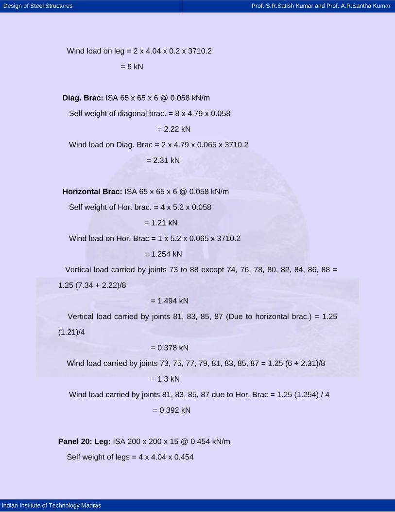
Design of Steel Structures Prof. S.R.Satish Kumar and Prof. A.R.Santha Kumar
Indian Institute of Technology Madras
Wind load on leg = 2 x 4.04 x 0.2 x 3710.2
= 6 kN
Diag. Brac: ISA 65 x 65 x 6 @ 0.058 kN/m
Self weight of diagonal brac. = 8 x 4.79 x 0.058
= 2.22 kN
Wind load on Diag. Brac = 2 x 4.79 x 0.065 x 3710.2
= 2.31 kN
Horizontal Brac: ISA 65 x 65 x 6 @ 0.058 kN/m
Self weight of Hor. brac. = 4 x 5.2 x 0.058
= 1.21 kN
Wind load on Hor. Brac = 1 x 5.2 x 0.065 x 3710.2
= 1.254 kN
Vertical load carried by joints 73 to 88 except 74, 76, 78, 80, 82, 84, 86, 88 =
1.25 (7.34 + 2.22)/8
= 1.494 kN
Vertical load carried by joints 81, 83, 85, 87 (Due to horizontal brac.) = 1.25
(1.21)/4
= 0.378 kN
Wind load carried by joints 73, 75, 77, 79, 81, 83, 85, 87 = 1.25 (6 + 2.31)/8
= 1.3 kN
Wind load carried by joints 81, 83, 85, 87 due to Hor. Brac = 1.25 (1.254) / 4
= 0.392 kN
Panel 20: Leg: ISA 200 x 200 x 15 @ 0.454 kN/m
Self weight of legs = 4 x 4.04 x 0.454
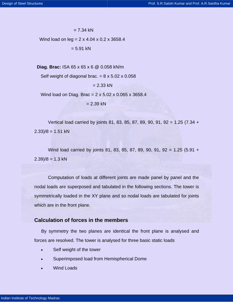
Design of Steel Structures Prof. S.R.Satish Kumar and Prof. A.R.Santha Kumar
Indian Institute of Technology Madras
= 7.34 kN
Wind load on leg = 2 x 4.04 x 0.2 x 3658.4
= 5.91 kN
Diag. Brac: ISA 65 x 65 x 6 @ 0.058 kN/m
Self weight of diagonal brac. = 8 x 5.02 x 0.058
= 2.33 kN
Wind load on Diag. Brac = 2 x 5.02 x 0.065 x 3658.4
= 2.39 kN
Vertical load carried by joints 81, 83, 85, 87, 89, 90, 91, 92 = 1.25 (7.34 +
2.33)/8 = 1.51 kN
Wind load carried by joints 81, 83, 85, 87, 89, 90, 91, 92 = 1.25 (5.91 +
2.39)/8 = 1.3 kN
Computation of loads at different joints are made panel by panel and the
nodal loads are superposed and tabulated in the following sections. The tower is
symmetrically loaded in the XY plane and so nodal loads are tabulated for joints
which are in the front plane.
Calculation of forces in the members
By symmetry the two planes are identical the front plane is analysed and
forces are resolved. The tower is analysed for three basic static loads
• Self weight of the tower
• Superimposed load from Hemispherical Dome
• Wind Loads
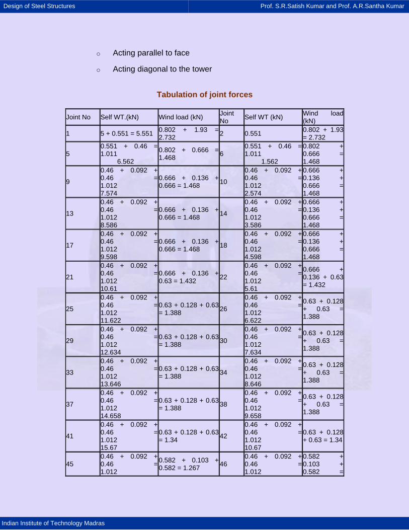
Design of Steel Structures Prof. S.R.Satish Kumar and Prof. A.R.Santha Kumar
Indian Institute of Technology Madras
o Acting parallel to face
o Acting diagonal to the tower
Tabulation of joint forces
Joint No Self WT.(kN) Wind load (kN) Joint No Self WT (kN) Wind load
(kN) 1 5 + 0.551 = 5.551 0.802 + 1.93 =
2.732 2 0.551 0.802 + 1.93 = 2.732
5 0.551 + 0.46 = 1.011 6.562
0.802 + 0.666 = 1.468 6
0.551 + 0.46 = 1.011 1.562
0.802 + 0.666 = 1.468
9 0.46 + 0.092 + 0.46 = 1.012 7.574
0.666 + 0.136 + 0.666 = 1.468 10
0.46 + 0.092 + 0.46 = 1.012 2.574
0.666 + 0.136 +0.666 = 1.468
13 0.46 + 0.092 + 0.46 = 1.012 8.586
0.666 + 0.136 + 0.666 = 1.468 14
0.46 + 0.092 + 0.46 = 1.012 3.586
0.666 + 0.136 + 0.666 = 1.468
17 0.46 + 0.092 + 0.46 = 1.012 9.598
0.666 + 0.136 + 0.666 = 1.468 18
0.46 + 0.092 + 0.46 = 1.012 4.598
0.666 + 0.136 + 0.666 = 1.468
21 0.46 + 0.092 + 0.46 = 1.012 10.61
0.666 + 0.136 + 0.63 = 1.432 22
0.46 + 0.092 + 0.46 = 1.012 5.61
0.666 + 0.136 + 0.63 = 1.432
25 0.46 + 0.092 + 0.46 = 1.012 11.622
0.63 + 0.128 + 0.63 = 1.388 26
0.46 + 0.092 + 0.46 = 1.012 6.622
0.63 + 0.128 + 0.63 = 1.388
29 0.46 + 0.092 + 0.46 = 1.012 12.634
0.63 + 0.128 + 0.63 = 1.388 30
0.46 + 0.092 + 0.46 = 1.012 7.634
0.63 + 0.128 + 0.63 = 1.388
33 0.46 + 0.092 + 0.46 = 1.012 13.646
0.63 + 0.128 + 0.63 = 1.388 34
0.46 + 0.092 + 0.46 = 1.012 8.646
0.63 + 0.128 + 0.63 = 1.388
37 0.46 + 0.092 + 0.46 = 1.012 14.658
0.63 + 0.128 + 0.63 = 1.388 38
0.46 + 0.092 + 0.46 = 1.012 9.658
0.63 + 0.128 + 0.63 = 1.388
41 0.46 + 0.092 + 0.46 = 1.012 15.67
0.63 + 0.128 + 0.63 = 1.34 42
0.46 + 0.092 + 0.46 = 1.012 10.67
0.63 + 0.128 + 0.63 = 1.34
45 0.46 + 0.092 + 0.46 = 1.012
0.582 + 0.103 + 0.582 = 1.267 46
0.46 + 0.092 + 0.46 = 1.012
0.582 + 0.103 + 0.582 =
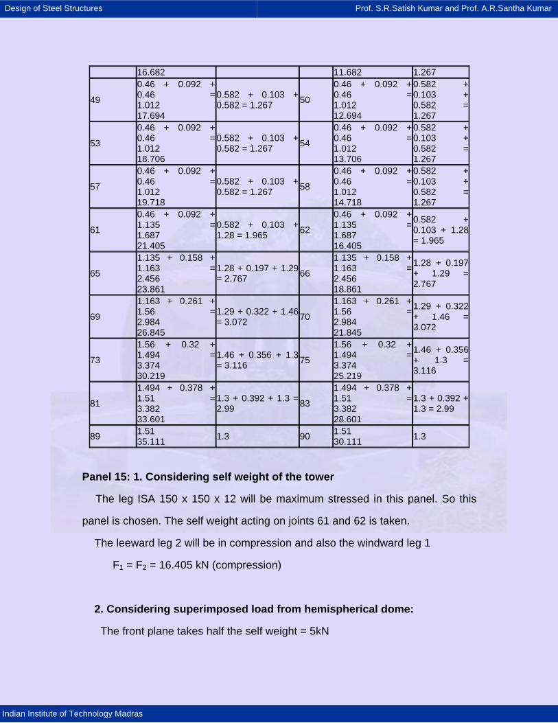
Design of Steel Structures Prof. S.R.Satish Kumar and Prof. A.R.Santha Kumar
Indian Institute of Technology Madras
16.682 11.682 1.267
49 0.46 + 0.092 + 0.46 = 1.012 17.694
0.582 + 0.103 + 0.582 = 1.267 50
0.46 + 0.092 + 0.46 = 1.012 12.694
0.582 + 0.103 + 0.582 = 1.267
53 0.46 + 0.092 + 0.46 = 1.012 18.706
0.582 + 0.103 + 0.582 = 1.267 54
0.46 + 0.092 + 0.46 = 1.012 13.706
0.582 + 0.103 + 0.582 = 1.267
57 0.46 + 0.092 + 0.46 = 1.012 19.718
0.582 + 0.103 + 0.582 = 1.267 58
0.46 + 0.092 + 0.46 = 1.012 14.718
0.582 + 0.103 + 0.582 = 1.267
61 0.46 + 0.092 + 1.135 = 1.687 21.405
0.582 + 0.103 + 1.28 = 1.965 62
0.46 + 0.092 + 1.135 = 1.687 16.405
0.582 + 0.103 + 1.28 = 1.965
65 1.135 + 0.158 + 1.163 = 2.456 23.861
1.28 + 0.197 + 1.29 = 2.767 66
1.135 + 0.158 + 1.163 = 2.456 18.861
1.28 + 0.197 + 1.29 = 2.767
69 1.163 + 0.261 + 1.56 = 2.984 26.845
1.29 + 0.322 + 1.46 = 3.072 70
1.163 + 0.261 + 1.56 = 2.984 21.845
1.29 + 0.322 + 1.46 = 3.072
73 1.56 + 0.32 + 1.494 = 3.374 30.219
1.46 + 0.356 + 1.3 = 3.116 75
1.56 + 0.32 + 1.494 = 3.374 25.219
1.46 + 0.356 + 1.3 = 3.116
81 1.494 + 0.378 + 1.51 = 3.382 33.601
1.3 + 0.392 + 1.3 = 2.99 83
1.494 + 0.378 + 1.51 = 3.382 28.601
1.3 + 0.392 + 1.3 = 2.99
89 1.51 35.111 1.3 90 1.51
30.111 1.3
Panel 15: 1. Considering self weight of the tower
The leg ISA 150 x 150 x 12 will be maximum stressed in this panel. So this
panel is chosen. The self weight acting on joints 61 and 62 is taken.
The leeward leg 2 will be in compression and also the windward leg 1
F1 = F2 = 16.405 kN (compression)
2. Considering superimposed load from hemispherical dome:
The front plane takes half the self weight = 5kN
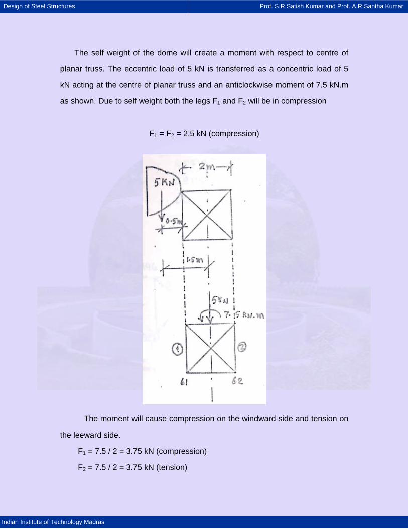
Design of Steel Structures Prof. S.R.Satish Kumar and Prof. A.R.Santha Kumar
Indian Institute of Technology Madras
The self weight of the dome will create a moment with respect to centre of
planar truss. The eccentric load of 5 kN is transferred as a concentric load of 5
kN acting at the centre of planar truss and an anticlockwise moment of 7.5 kN.m
as shown. Due to self weight both the legs F1 and F2 will be in compression
F1 = F2 = 2.5 kN (compression)
The moment will cause compression on the windward side and tension on
the leeward side.
F1 = 7.5 / 2 = 3.75 kN (compression)
F2 = 7.5 / 2 = 3.75 kN (tension)
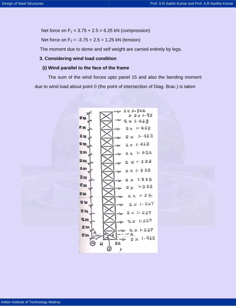
Design of Steel Structures Prof. S.R.Satish Kumar and Prof. A.R.Santha Kumar
Indian Institute of Technology Madras
Net force on F1 = 3.75 + 2.5 = 6.25 kN (compression)
Net force on F2 = -3.75 + 2.5 = 1.25 kN (tension)
The moment due to dome and self weight are carried entirely by legs.
3. Considering wind load condition
(i) Wind parallel to the face of the frame
The sum of the wind forces upto panel 15 and also the bending moment
due to wind load about point 0 (the point of intersection of Diag. Brac.) is taken
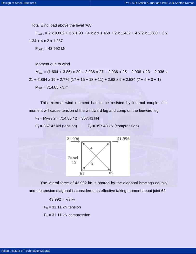
Design of Steel Structures Prof. S.R.Satish Kumar and Prof. A.R.Santha Kumar
Indian Institute of Technology Madras
Total wind load above the level 'AA'
FLAT1 = 2 x 0.802 + 2 x 1.93 + 4 x 2 x 1.468 + 2 x 1.432 + 4 x 2 x 1.388 + 2 x
1.34 + 4 x 2 x 1.267
FLAT1 = 43.992 kN
Moment due to wind
MW1 = (1.604 + 3.86) x 29 + 2.936 x 27 + 2.936 x 25 + 2.936 x 23 + 2.936 x
21 + 2.864 x 19 + 2.776 (17 + 15 + 13 + 11) + 2.68 x 9 + 2.534 (7 + 5 + 3 + 1)
MW1 = 714.85 kN.m
This external wind moment has to be resisted by internal couple. this
moment will cause tension of the windward leg and comp on the leeward leg
F1 = MW1 / 2 = 714.85 / 2 = 357.43 kN
F1 = 357.43 kN (tension) F2 = 357.43 kN (compression)
The lateral force of 43.992 kn is shared by the diagonal bracings equally
and the tension diagonal is considered as effective taking moment about joint 62
43.992 = 2 F3
F3 = 31.11 kN tension
F4 = 31.11 kN compression
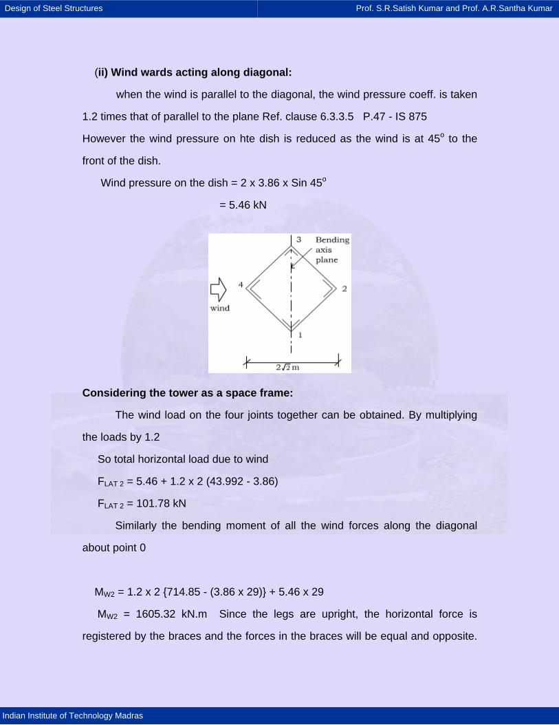
Design of Steel Structures Prof. S.R.Satish Kumar and Prof. A.R.Santha Kumar
Indian Institute of Technology Madras
(ii) Wind wards acting along diagonal:
when the wind is parallel to the diagonal, the wind pressure coeff. is taken
1.2 times that of parallel to the plane Ref. clause 6.3.3.5 P.47 - IS 875
However the wind pressure on hte dish is reduced as the wind is at 45o to the
front of the dish.
Wind pressure on the dish = 2 x 3.86 x Sin 45o
= 5.46 kN
Considering the tower as a space frame:
The wind load on the four joints together can be obtained. By multiplying
the loads by 1.2
So total horizontal load due to wind
FLAT 2 = 5.46 + 1.2 x 2 (43.992 - 3.86)
FLAT 2 = 101.78 kN
Similarly the bending moment of all the wind forces along the diagonal
about point 0
MW2 = 1.2 x 2 {714.85 - (3.86 x 29)} + 5.46 x 29
MW2 = 1605.32 kN.m Since the legs are upright, the horizontal force is
registered by the braces and the forces in the braces will be equal and opposite.
Design of Steel Structures Prof. S.R.Satish Kumar and Prof. A.R.Santha Kumar
Indian Institute of Technology Madras
The forces have to be resolved in the horizontal plane and then parallel to the
diagonal.
Let FD = force in each brace (tension or compression)
The total force from braces in the horizontal plane along the tower
diagonal is
= 8 FD cos45o. sin45o
= 4 FD
Equilibrium in the horizontal direction gives
4 FD = 101.78 kN
FD = 25.45 kN
This value is less than that of case 1. Therefore the forces in braces are
controlled by the load condition wind parallel to the frame. The bending moment
is resisted by the pair of extreme legs 2 and 4. Forces in legs 3 and 1 will be zero
as they lie in the bending axis Ref. Fig.
F1 = F3 = 0
F2 = MW2 /2 2 = 1605.32 / 2 2
F2 = 567.57 kN (compression)
F4 = 567.57 kN (tension)
Maximum compressive force on the leg = 567.57 + 16.405 - 1.25
= 582.73 kN
Leg ISA 150 x 150 x 12 @ 0.272 kN / m
A = 3459 mm2; rmin = 29.3 mm
Leff = 0.85 x 2000 = 1700mm; Leff / ry = 1700 / 29.3 = 58.02
Design of Steel Structures Prof. S.R.Satish Kumar and Prof. A.R.Santha Kumar
Indian Institute of Technology Madras
σac from table 5.1 = 124 N/mm2 can be raised by 25%. Since wind is
considered: σac = 1.25 x 124 = 155 N/mm2
Actual stress σc = (582.73 x 10³) / 3459 = 168.5 N/mm2
Diag. Brac: The tension member is considered effective.
Force in the bracing = 31.11 kN
Size ISA 50 x 50 x 6 mm A = 568 mm2
Check the adequacy of the section as a tension member
Panel 20: Leg: ISA 200 x 200 x 15 @ 0.454 kn/m
1. Self weight acting at the bottom most panels
F1 = F2 = 30.111 kn (compression)
The leg is checked at the mid height as buckling will occur midway between
the nodes
2. Considering superimposed load from hemispherical dome
Due to moment F1 = 7.5 / 5.6 = 1.34 kn (compression)
F2 = 1.34 kN (tension)
Due to self weight F1 = 2.5 kN (compression)
F2 = 2.5 kN (compression)
Net forces F1 = 1.34 + 2.5 = 3.84 kN (compression)
F2 = -1.34 + 2.5 = 1.16 kN (compression)
3. Considering wind load condition:
(a) Wind parallel to the face of the frame:
Total wind load above level 'BB'
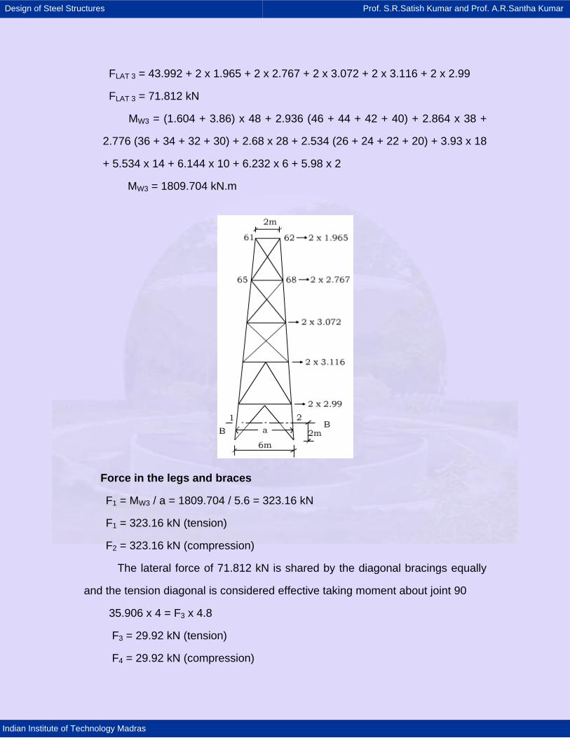
Design of Steel Structures Prof. S.R.Satish Kumar and Prof. A.R.Santha Kumar
Indian Institute of Technology Madras
FLAT 3 = 43.992 + 2 x 1.965 + 2 x 2.767 + 2 x 3.072 + 2 x 3.116 + 2 x 2.99
FLAT 3 = 71.812 kN
MW3 = (1.604 + 3.86) x 48 + 2.936 (46 + 44 + 42 + 40) + 2.864 x 38 +
2.776 (36 + 34 + 32 + 30) + 2.68 x 28 + 2.534 (26 + 24 + 22 + 20) + 3.93 x 18
+ 5.534 x 14 + 6.144 x 10 + 6.232 x 6 + 5.98 x 2
MW3 = 1809.704 kN.m
Force in the legs and braces
F1 = MW3 / a = 1809.704 / 5.6 = 323.16 kN
F1 = 323.16 kN (tension)
F2 = 323.16 kN (compression)
The lateral force of 71.812 kN is shared by the diagonal bracings equally
and the tension diagonal is considered effective taking moment about joint 90
35.906 x 4 = F3 x 4.8
F3 = 29.92 kN (tension)
F4 = 29.92 kN (compression)
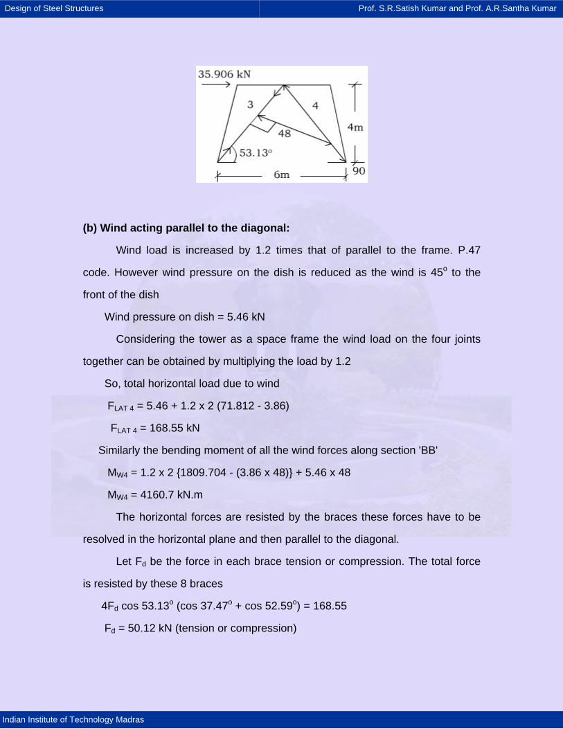
Design of Steel Structures Prof. S.R.Satish Kumar and Prof. A.R.Santha Kumar
Indian Institute of Technology Madras
(b) Wind acting parallel to the diagonal:
Wind load is increased by 1.2 times that of parallel to the frame. P.47
code. However wind pressure on the dish is reduced as the wind is 45o to the
front of the dish
Wind pressure on dish = 5.46 kN
Considering the tower as a space frame the wind load on the four joints
together can be obtained by multiplying the load by 1.2
So, total horizontal load due to wind
FLAT 4 = 5.46 + 1.2 x 2 (71.812 - 3.86)
FLAT 4 = 168.55 kN
Similarly the bending moment of all the wind forces along section 'BB'
MW4 = 1.2 x 2 {1809.704 - (3.86 x 48)} + 5.46 x 48
MW4 = 4160.7 kN.m
The horizontal forces are resisted by the braces these forces have to be
resolved in the horizontal plane and then parallel to the diagonal.
Let Fd be the force in each brace tension or compression. The total force
is resisted by these 8 braces
4Fd cos 53.13o (cos 37.47o + cos 52.59o) = 168.55
Fd = 50.12 kN (tension or compression)
Design of Steel Structures Prof. S.R.Satish Kumar and Prof. A.R.Santha Kumar
Indian Institute of Technology Madras
This is more than the value with wind parallel to the frame. The bending
moment MW4 is resisted by the pair of extreme legs which does not lie on the
bending axis
F1 = F3 = 0
F2 = MW4 / a 2 = 4160.7 / 5.6 2 = 525.4 kN
F2 = 525.4 kN (compression)
F4 = 525.4 kN (tension)
Maximum compressive force will be on leg 2
= 30.111 + 1.16 + 525.4
F2 = 556.67 kN (compression)
Leg ISA 200 x 200 x 15 @ 0.454 kN/m
A = 5780 mm2; ry = 39.1 mm
Lef = 0.85 x 4040 = 3434mm
Lef / ry = 3434 / 39.1 = 87.83 Refer Table 5.1
σac = 86 N / mm2
Since wind is considered allowable stresses are raised by 25%. So σac = 1.25 x 86 = 107.5 N / mm2
Actual stress σc = 556.67 / 5780 = 96.31 N / mm2
σac and σc Safe
Design of Steel Structures Prof. S.R.Satish Kumar and Prof. A.R.Santha Kumar
Indian Institute of Technology Madras
7. TRANSMISSION TOWERS
7.1 Introduction
In every country, developed and developing, the elastic power
consumption has continued to rise, the rate of growth being greater in the
developing countries on account of the comparatively low base. This in turn had
led to the increase in the number of power stations and their capacities and
consequent increase in power transmission lines from the generating stations to
the load centres. Interconnections between systems are also increasing to
enhance reliability and economy. The transmission voltage, while dependent on
th quantum of power transmitted, should fit in with the long-term system
requirement as well as provide flexibility in system operation. It should also
conform to the national and international standard voltage levels.
In the planning and design of a transmission line, a number of
requirements have to be met. From the electrical point of view, the most
important requirement is insulation and safe clearances to earthed parts. These,
together with the cross-section of conductors, the spacing between conductors,
and the relative location of ground wires with respect to the conductors, influence
the design of towers and foundations. The conductors, ground wires, insulation,
towers and foundations constitute the major components of a transmission line.
Design of Steel Structures Prof. S.R.Satish Kumar and Prof. A.R.Santha Kumar
Indian Institute of Technology Madras
7.2 Material properties, clearances and tower configurations
7.2.1 Material properties
Classification of steel
The general practice with reference to the quality of steel is to specify the
use of steel for tower members, although some authorities have instead specified
the use of steel manufactured by either the open hearth or electric furnace
process for tower members, although some athorities have instead specified the
use of steel manufactured by either the open hearth or electric furnace process.
The usual standards specified are ASTM A-7, BSS 15, and German Steel
Standard St 37. IS: 226-1975, Specification for structural Steel (Revised), is
currently adopted in India.
In so far as standard structural steel is concerned, reference to IS: 226-
1975 shows that
Steel manufactured by the open-hearth, electric, basic oxygen or a
combination of the processes is acceptable for structural use and that in case
any other process is employed, prior approval of the purchaser should be
obtained.
In addition to standard structural steel (symbol A), high tensile steel
conforming to IS: 226-1975 may be used for transmission line towers for greater
economy. The chemical composition and mechanical properties of steel covered
by IS: 226-1975 for structural steel and IS: 961-1975 for high tensile steel are
shown in Tables 7.1 to 7.4.
Design of Steel Structures Prof. S.R.Satish Kumar and Prof. A.R.Santha Kumar
Indian Institute of Technology Madras
Suitability for welding
The standard structural mild steel is suitable for welding, provided the
thickness of the material does not exceed 20mm. When the thickness exceeds
20mm, special precautions such as double Vee shaping and cover plates may
be required.
St 58-HT is intended for use in structures where fabrication is done by
methods other than welding. St 55-HTw is used where welding is employed for
fabrication.
In the past, transmission line structures in India were supplied by firms like
Blaw Knox, British Insulated Callender Cables (BICC), etc. from the United
Kingdom. Later, towers from SAE, Italy, were employed for some of the
transmission lines under the Damodar Valley Corporation. In recent times, steel
from the USSR and some other East European countries were partly used in the
transmission line industry. Currently, steel conforming g to IS: 961 and IS: 226
and manufactured in the country are almost exclusively use for towers.
A comparison of mechanical properties of standard and high tensile steels
conforming to national standards of the countries mentioned above is given in
Table 7.5.
Properties of structural steel
A typical stress-strain curve of mild steel is shown in Figure 7.1. Steels for
structural use are classified as: Standard quality, high strength low carbon steel
and alloy steel. The various properties of steel will now be briefly discussed.
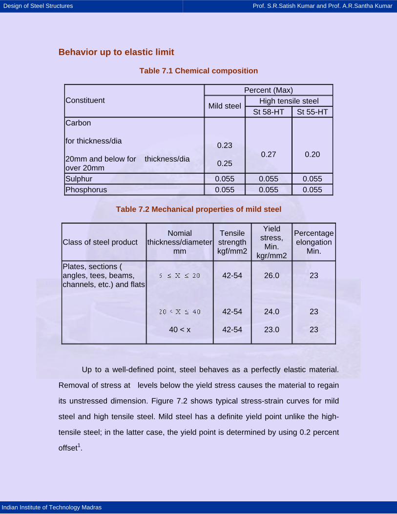
Design of Steel Structures Prof. S.R.Satish Kumar and Prof. A.R.Santha Kumar
Indian Institute of Technology Madras
Behavior up to elastic limit
Table 7.1 Chemical composition
Percent (Max) High tensile steel Constituent
Mild steel St 58-HT St 55-HT
Carbon
for thickness/dia
20mm and below for thickness/dia over 20mm
0.23
0.25
0.27
0.20
Sulphur 0.055 0.055 0.055 Phosphorus 0.055 0.055 0.055
Table 7.2 Mechanical properties of mild steel
Class of steel product Nomial
thickness/diameter mm
Tensile strength kgf/mm2
Yield stress, Min.
kgr/mm2
Percentage elongation
Min.
Plates, sections ( angles, tees, beams, channels, etc.) and flats
40 < x
42-54
42-54
42-54
26.0
24.0
23.0
23
23
23
Up to a well-defined point, steel behaves as a perfectly elastic material.
Removal of stress at levels below the yield stress causes the material to regain
its unstressed dimension. Figure 7.2 shows typical stress-strain curves for mild
steel and high tensile steel. Mild steel has a definite yield point unlike the high-
tensile steel; in the latter case, the yield point is determined by using 0.2 percent
offset1.
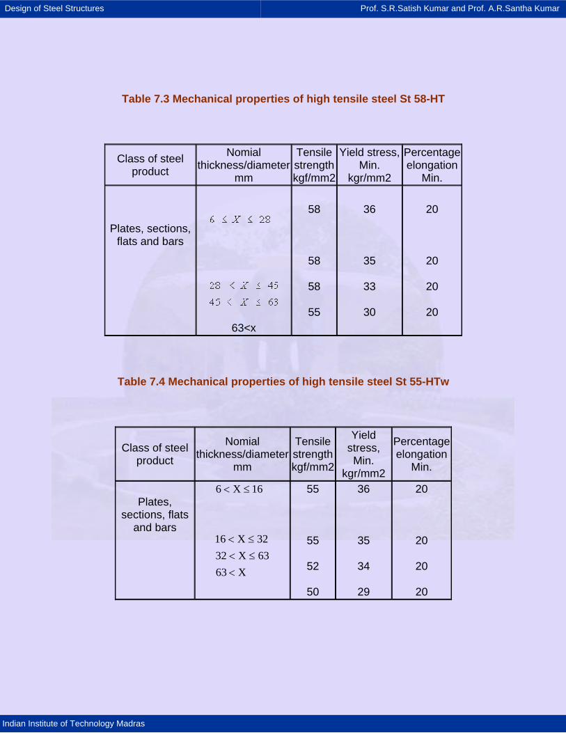
Design of Steel Structures Prof. S.R.Satish Kumar and Prof. A.R.Santha Kumar
Indian Institute of Technology Madras
Table 7.3 Mechanical properties of high tensile steel St 58-HT
Class of steel product
Nomial thickness/diameter
mm
Tensile strength kgf/mm2
Yield stress, Min.
kgr/mm2
Percentage elongation
Min.
Plates, sections, flats and bars
63<x
58
58
58
55
36
35
33
30
20
20
20
20
Table 7.4 Mechanical properties of high tensile steel St 55-HTw
Class of steel product
Nomial thickness/diameter
mm
Tensile strength kgf/mm2
Yield stress, Min.
kgr/mm2
Percentage elongation
Min.
Plates, sections, flats
and bars
6 X 16
16 X 3232 X 6363 X
< ≤
< ≤< ≤<
55
55
52
50
36
35
34
29
20
20
20
20
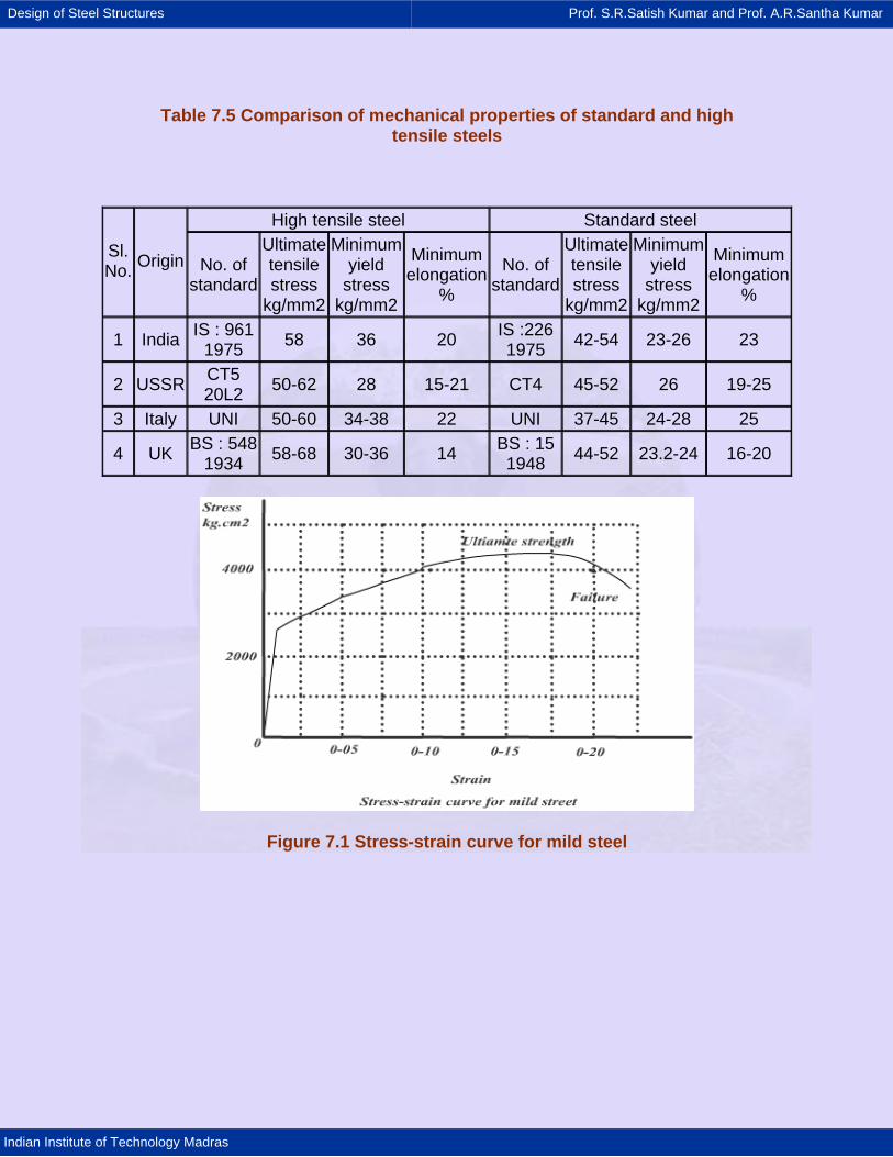
Design of Steel Structures Prof. S.R.Satish Kumar and Prof. A.R.Santha Kumar
Indian Institute of Technology Madras
Table 7.5 Comparison of mechanical properties of standard and high tensile steels
High tensile steel Standard steel
Sl. No. Origin No. of
standard
Ultimate tensile stress
kg/mm2
Minimum yield
stress kg/mm2
Minimum elongation
%
No. of standard
Ultimate tensile stress
kg/mm2
Minimum yield
stress kg/mm2
Minimum elongation
%
1 India IS : 961 1975 58 36 20 IS :226
1975 42-54 23-26 23
2 USSR CT5 20L2 50-62 28 15-21 CT4 45-52 26 19-25
3 Italy UNI 50-60 34-38 22 UNI 37-45 24-28 25
4 UK BS : 548 1934 58-68 30-36 14 BS : 15
1948 44-52 23.2-24 16-20
Figure 7.1 Stress-strain curve for mild steel
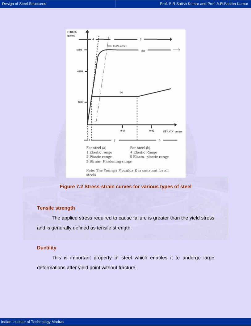
Design of Steel Structures Prof. S.R.Satish Kumar and Prof. A.R.Santha Kumar
Indian Institute of Technology Madras
Figure 7.2 Stress-strain curves for various types of steel
Tensile strength
The applied stress required to cause failure is greater than the yield stress
and is generally defined as tensile strength.
Ductility
This is important property of steel which enables it to undergo large
deformations after yield point without fracture.
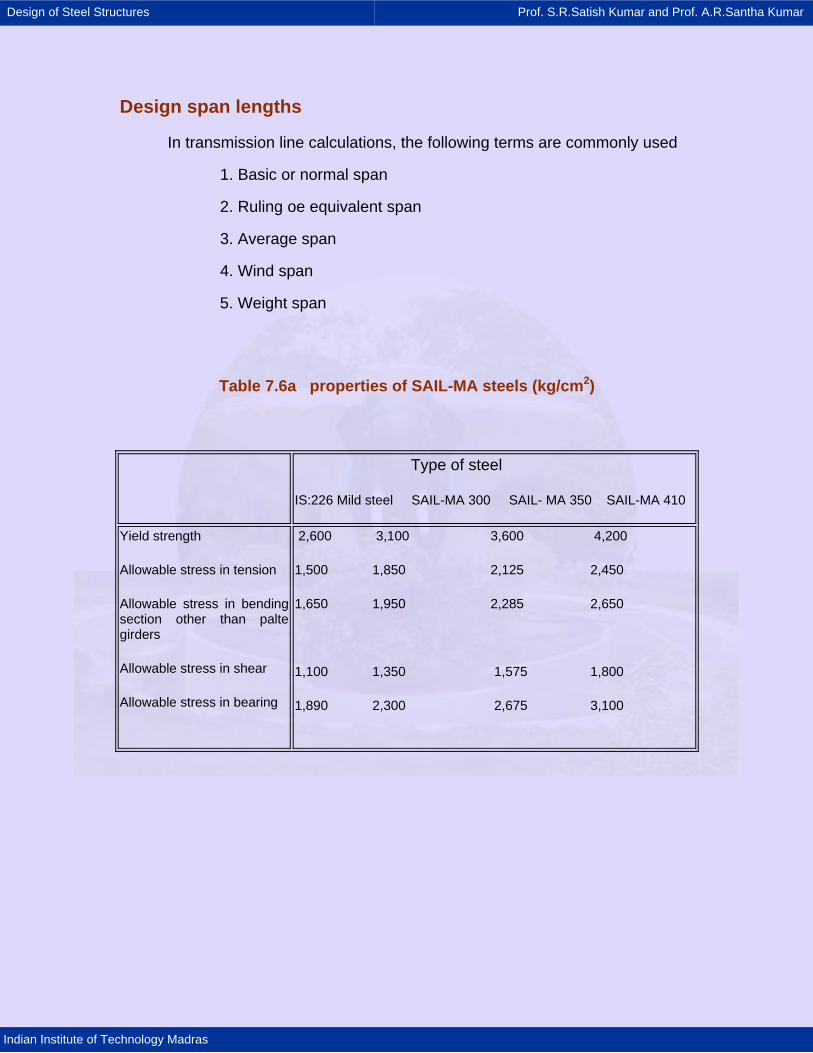
Design of Steel Structures Prof. S.R.Satish Kumar and Prof. A.R.Santha Kumar
Indian Institute of Technology Madras
Design span lengths
In transmission line calculations, the following terms are commonly used
1. Basic or normal span
2. Ruling oe equivalent span
3. Average span
4. Wind span
5. Weight span
Table 7.6a properties of SAIL-MA steels (kg/cm2)
Type of steel
IS:226 Mild steel SAIL-MA 300 SAIL- MA 350 SAIL-MA 410
Yield strength
Allowable stress in tension
Allowable stress in bending section other than palte girders
Allowable stress in shear
Allowable stress in bearing
2,600 3,100 3,600 4,200
1,500 1,850 2,125 2,450
1,650 1,950 2,285 2,650
1,100 1,350 1,575 1,800
1,890 2,300 2,675 3,100
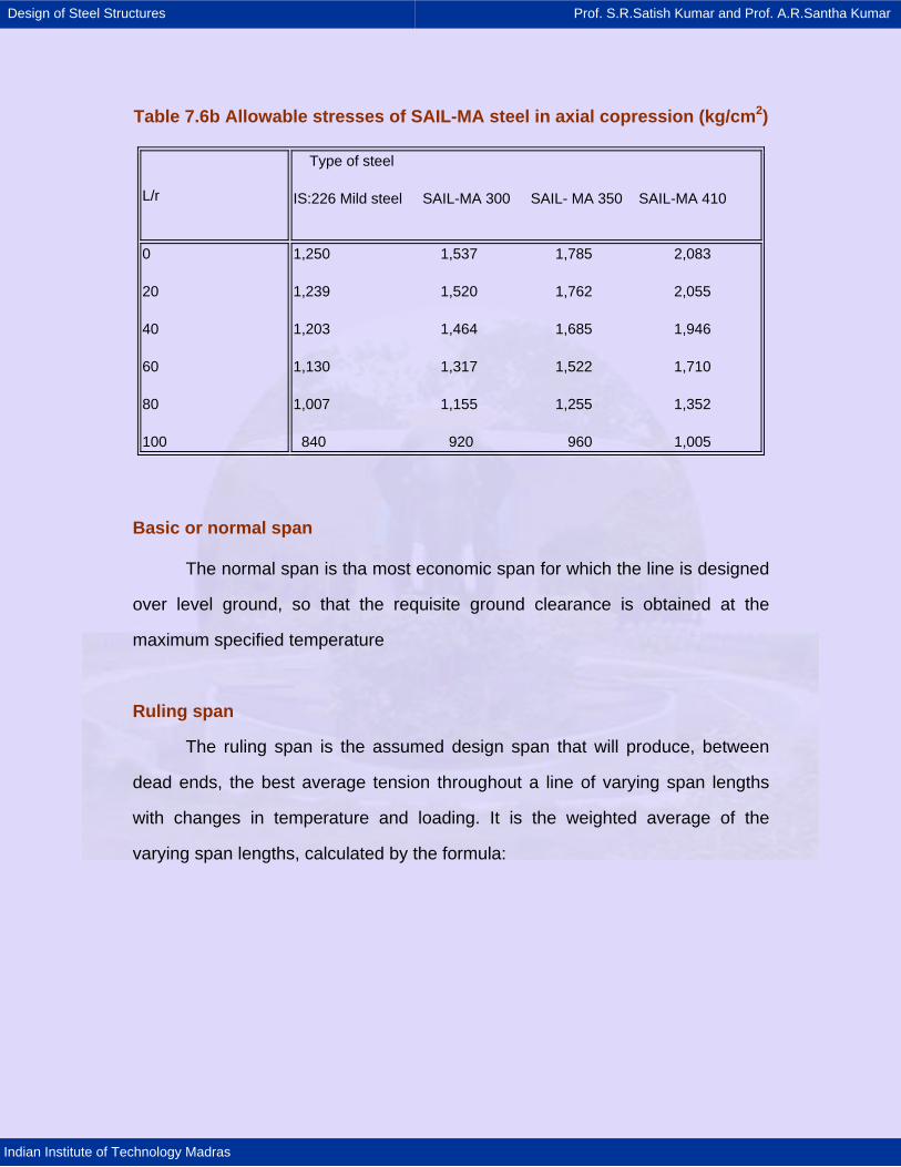
Design of Steel Structures Prof. S.R.Satish Kumar and Prof. A.R.Santha Kumar
Indian Institute of Technology Madras
Table 7.6b Allowable stresses of SAIL-MA steel in axial copression (kg/cm2)
L/r
Type of steel
IS:226 Mild steel SAIL-MA 300 SAIL- MA 350 SAIL-MA 410
0
20
40
60
80
100
1,250 1,537 1,785 2,083
1,239 1,520 1,762 2,055
1,203 1,464 1,685 1,946
1,130 1,317 1,522 1,710
1,007 1,155 1,255 1,352
840 920 960 1,005
Basic or normal span
The normal span is tha most economic span for which the line is designed
over level ground, so that the requisite ground clearance is obtained at the
maximum specified temperature
Ruling span
The ruling span is the assumed design span that will produce, between
dead ends, the best average tension throughout a line of varying span lengths
with changes in temperature and loading. It is the weighted average of the
varying span lengths, calculated by the formula:
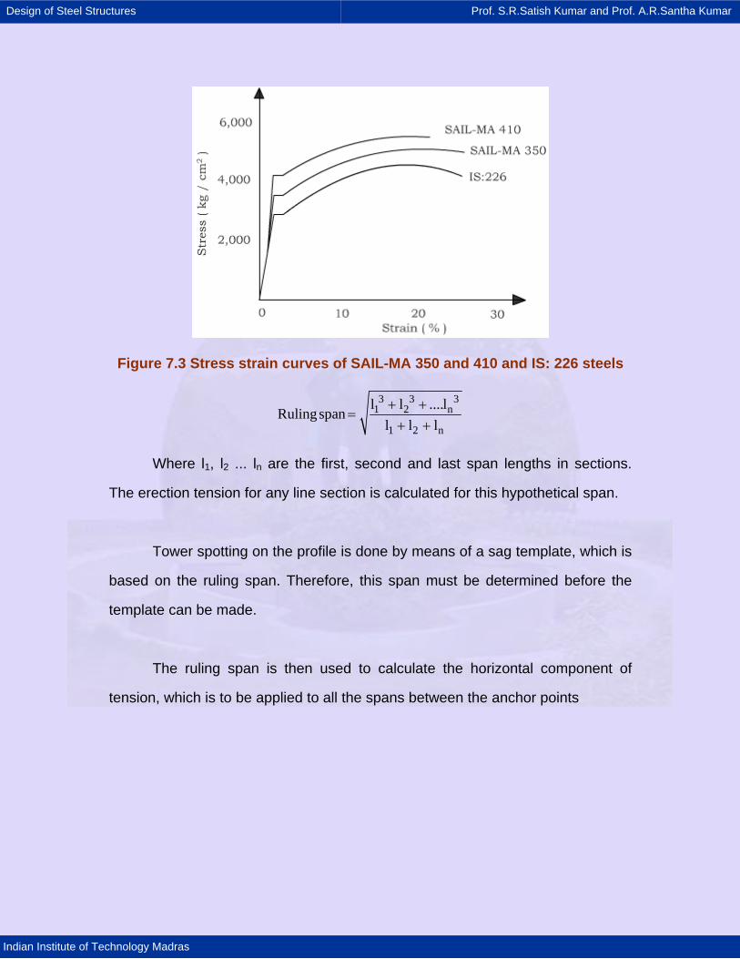
Design of Steel Structures Prof. S.R.Satish Kumar and Prof. A.R.Santha Kumar
Indian Institute of Technology Madras
Figure 7.3 Stress strain curves of SAIL-MA 350 and 410 and IS: 226 steels
3 3 31 2 n
1 2 n
l l ....lRuling span
l l l+ +
=+ +
Where l1, l2 ... ln are the first, second and last span lengths in sections.
The erection tension for any line section is calculated for this hypothetical span.
Tower spotting on the profile is done by means of a sag template, which is
based on the ruling span. Therefore, this span must be determined before the
template can be made.
The ruling span is then used to calculate the horizontal component of
tension, which is to be applied to all the spans between the anchor points
Design of Steel Structures Prof. S.R.Satish Kumar and Prof. A.R.Santha Kumar
Indian Institute of Technology Madras
Average span
The average span is the mean span length between dead ends. It is
assumed that the conductor is freely suspended such that each individual span
reacts to changes in tension as a single average span. All sag and tension
calculations are carried out for the average span, on this assumption.
Wind span
The wind span is that on which the wind is assumed to act transversely on
the conductors and is taken as half the sum of the two spans, adjacent to the
support ( Figure 7.4 ). In order to take full advantage of towers located on
elevated ground, it is usual to allow a wind span of 10 to 15 percent in excess of
the normal span. This additional strength can be used in taking a samll angle of
deviation on an intermediate tower, where the actual wind span is less than the
design wind span. The angle of deviation to be taken in such cases is
approximately given by:
wl x180T
θ =π
Where w = total ind load per unit run of span length of all conductor
carried by the tower,
l = difference between the wind span used for design and the actual
wind span, and
T = the total maximum working tension of all conductors carried by the
tower.
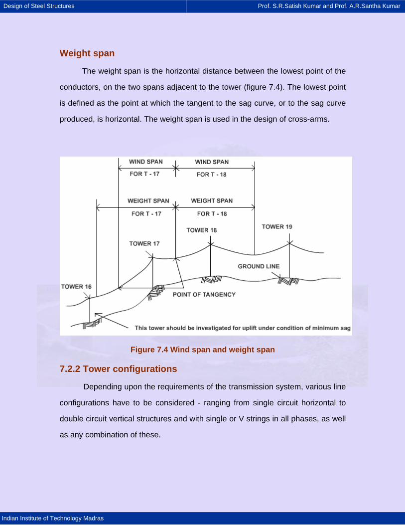
Design of Steel Structures Prof. S.R.Satish Kumar and Prof. A.R.Santha Kumar
Indian Institute of Technology Madras
Weight span
The weight span is the horizontal distance between the lowest point of the
conductors, on the two spans adjacent to the tower (figure 7.4). The lowest point
is defined as the point at which the tangent to the sag curve, or to the sag curve
produced, is horizontal. The weight span is used in the design of cross-arms.
Figure 7.4 Wind span and weight span
7.2.2 Tower configurations
Depending upon the requirements of the transmission system, various line
configurations have to be considered - ranging from single circuit horizontal to
double circuit vertical structures and with single or V strings in all phases, as well
as any combination of these.
Design of Steel Structures Prof. S.R.Satish Kumar and Prof. A.R.Santha Kumar
Indian Institute of Technology Madras
The configuration of a transmission line tower depends on:
1. the length of the insulator assembly
2. the minimum clearances to be maintained between conductors, and
between conductors and tower
3. the location of ground wire or wires with respect to the outermost
conductor
4. the mid-span clearance required from considerations of the dynamic
behaviour of conductors and lightning protection of the line
5. the minimum clearance of the lowest conductor above ground level.
The tower outline is determined essentially by three factors: tower height,
base width, and top hamper width.
Determination of tower weight
The factors governing the height of the tower are:
1. Minimum permissible ground clearance (h1)
2. Maximum sag (h2)
3. Vertical spacing between conductors (h3)
4. Vertical clearance between ground wire and top conductor (h4)
Thus the total height of the tower is given by
H = h1 + h2 + h3 + h4
in the case of double circuit tower with vertical configuration of conductors
(figure 7.5 )
Design of Steel Structures Prof. S.R.Satish Kumar and Prof. A.R.Santha Kumar
Indian Institute of Technology Madras
The calculation of sags (h2) is covered later. The principles and practices
in regard to the determination of ground clearance and spacings between
conductors and between the ground wire and top conductor will now be outlined.
Minimum permissible ground clearance
For safety considerations, power conductors along the route of the
transmission line should maintain requite clearance to ground in open country,
national highways, rivers, railways tracks, telecommunication lines, other power
lines, etc.., as laid down in the Indian Electricity Rules, or Standards or codes of
practice in vogue.
Rule 77(4) of the Indian Electricity Rules, 1956, stipulates the following
clearances above ground of the lowest point of the conductor:
For extra- high voltage lines, the clearance above ground shall not be less
than 5.182 metres plus 0.305 metres for every 33,000 volts or part there of by
which the voltage of the line exceeds 33,000 volts.
Accordingly, the values for the various voltages, 66kV to 400 kV, are:
66kV - 5.49m
132kV - 6.10m
220kV - 7.01m
400kV - 8.84m
The above clearances are applicable to transmission lines running in open
country.
Design of Steel Structures Prof. S.R.Satish Kumar and Prof. A.R.Santha Kumar
Indian Institute of Technology Madras
Power line crossings
In crossings over rivers, telecommunication lines, railway tracks, etc.., the
following clearances are maintained:
1. Crossing over rivers
a. Over rivers which are not navigable. The minimum clearance of
conductor is specified as 3.05 over maximum flood level.
b. Over navigable rivers: Clearances are fixed in relation to the tallest
mast, in consultation with the concerned navigation authorities.
2. Crossing over telecommunication lines. The minimum clearances between
the conductors of a power line and telecommunication wires are
66 kV - 2,440mm
132 kV - 2,740mm
220 kV - 3,050mm
400 kV - 4,880mm
3. Crossing over railway tracks: The minimum height over the rail level, of
the lowest portion of any conductor under conditions of maximum sag, as
stipulated in the regulations for Electrical Crossings of Railway Tracks, 1963, is
given in Table 7.7.
4. Between power lines
a. Between power lines L.T up to 66 kV - and 66 kV line 2.44m
b. Between power lines L.T up to 132 kV - and 132kV line 2.75m
c. Between power lines L.T up to 220kV - and 220kV line 4.55m
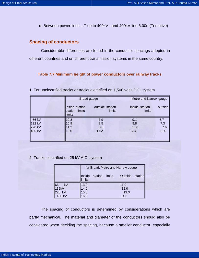
Design of Steel Structures Prof. S.R.Satish Kumar and Prof. A.R.Santha Kumar
Indian Institute of Technology Madras
d. Between power lines L.T up to 400kV - and 400kV line 6.00m(Tentative)
Spacing of conductors
Considerable differences are found in the conductor spacings adopted in
different countries and on different transmission systems in the same country.
Table 7.7 Minimum height of power conductors over railway tracks
1. For unelectrified tracks or tracks electrified on 1,500 volts D.C. system
Broad gauge Metre and Narrow gauge
inside station outside station inside station outside station limits limits limits limits
66 kV 132 kV 220 kV 400 kV
10.3 7.9 9.1 6.7 10.9 8.5 9.8 7.3 11.2 8.8 10.0 7.6 13.6 11.2 12.4 10.0
2. Tracks electrified on 25 kV A.C. system
for Broad, Metre and Narrow gauge
Inside station limits Outside station limits
66 kV 132kV 220 kV 400 kV
13.0 11.0 14.0 12.0 15.3 13.3 16.3 14.3
The spacing of conductors is determined by considerations which are
partly mechanical. The material and diameter of the conductors should also be
considered when deciding the spacing, because a smaller conductor, especially
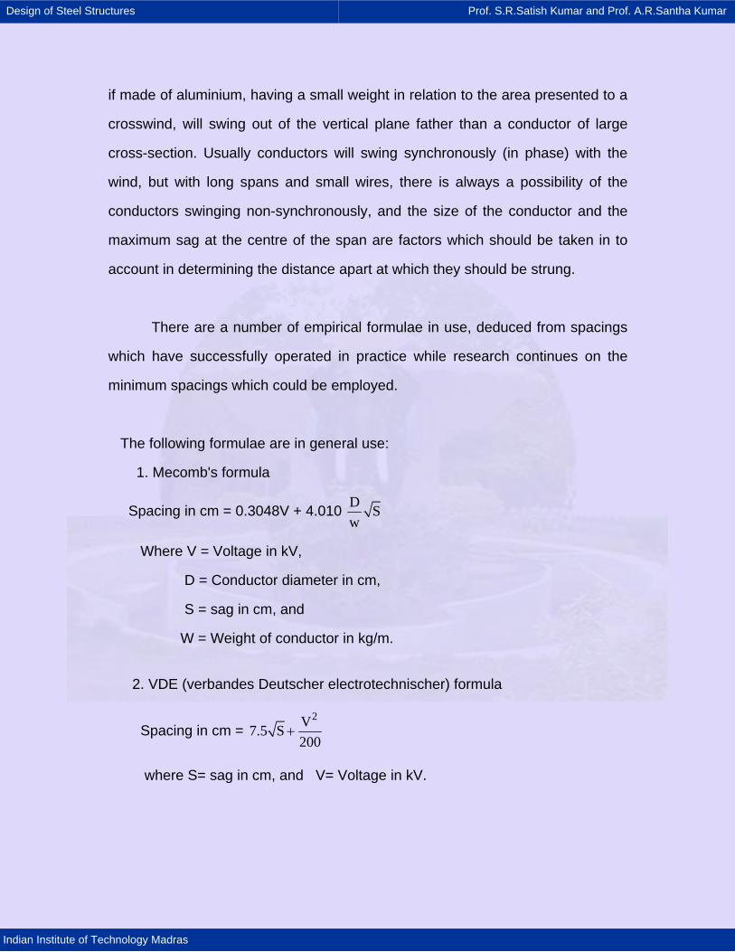
Design of Steel Structures Prof. S.R.Satish Kumar and Prof. A.R.Santha Kumar
Indian Institute of Technology Madras
if made of aluminium, having a small weight in relation to the area presented to a
crosswind, will swing out of the vertical plane father than a conductor of large
cross-section. Usually conductors will swing synchronously (in phase) with the
wind, but with long spans and small wires, there is always a possibility of the
conductors swinging non-synchronously, and the size of the conductor and the
maximum sag at the centre of the span are factors which should be taken in to
account in determining the distance apart at which they should be strung.
There are a number of empirical formulae in use, deduced from spacings
which have successfully operated in practice while research continues on the
minimum spacings which could be employed.
The following formulae are in general use:
1. Mecomb's formula
Spacing in cm = 0.3048V + 4.010 D Sw
Where V = Voltage in kV,
D = Conductor diameter in cm,
S = sag in cm, and
W = Weight of conductor in kg/m.
2. VDE (verbandes Deutscher electrotechnischer) formula
Spacing in cm = 2V7.5 S
200+
where S= sag in cm, and V= Voltage in kV.

Design of Steel Structures Prof. S.R.Satish Kumar and Prof. A.R.Santha Kumar
Indian Institute of Technology Madras
3. Still's formula
Distance between conductors (cm)
2l50.8 1.8.14 V
27.8⎡ ⎤= + + ⎢ ⎥⎣ ⎦
Where l = average span length in metres ,and V = line voltage between
conductors in kV.
The formula may be used as a guide in arriving at a suitable value for the
horizontal spacing for any line voltage and for the value spans between 60 and
335 meters
4. NESC, USA formula
Horizontal spacing in cm
LA 3.681 S2
= + +
Where A= 0.762 cm per kV line voltage S = Sag in cm, and
L = Length of insulator string in cm
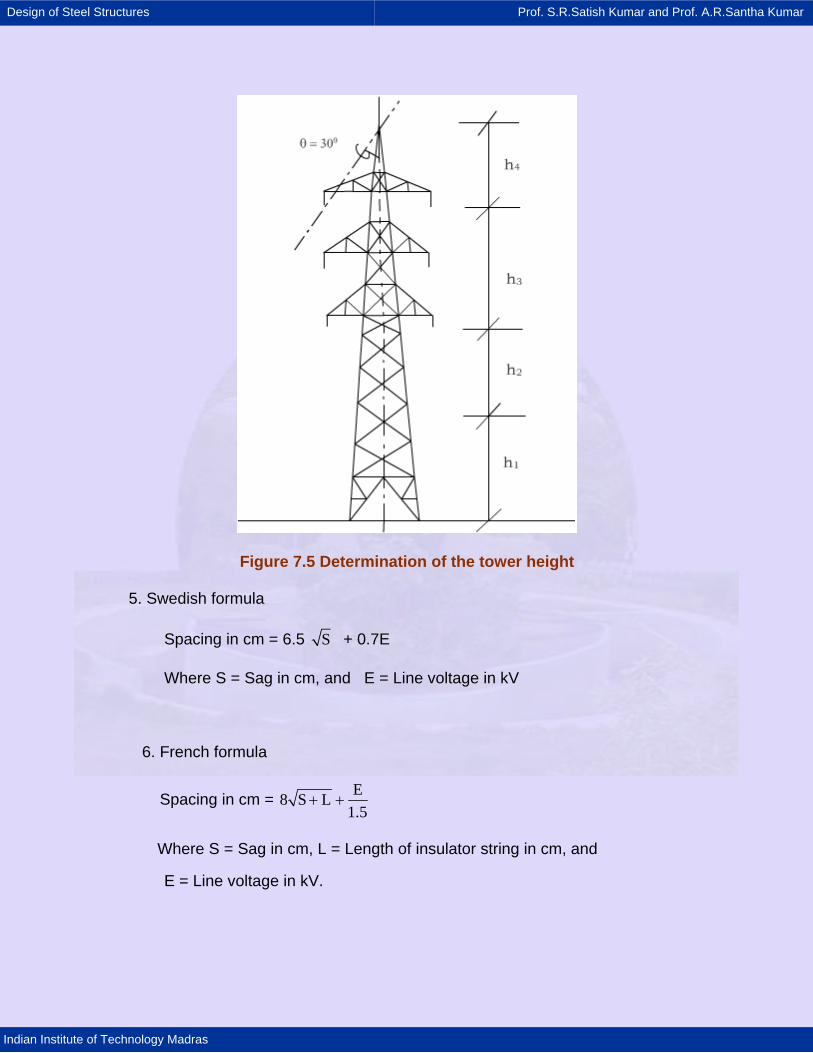
Design of Steel Structures Prof. S.R.Satish Kumar and Prof. A.R.Santha Kumar
Indian Institute of Technology Madras
Figure 7.5 Determination of the tower height
5. Swedish formula
Spacing in cm = 6.5 S + 0.7E
Where S = Sag in cm, and E = Line voltage in kV
6. French formula
Spacing in cm = E8 S L1.5
+ +
Where S = Sag in cm, L = Length of insulator string in cm, and
E = Line voltage in kV.
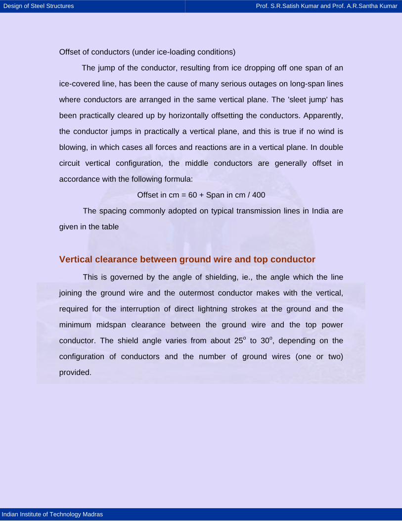
Design of Steel Structures Prof. S.R.Satish Kumar and Prof. A.R.Santha Kumar
Indian Institute of Technology Madras
Offset of conductors (under ice-loading conditions)
The jump of the conductor, resulting from ice dropping off one span of an
ice-covered line, has been the cause of many serious outages on long-span lines
where conductors are arranged in the same vertical plane. The 'sleet jump' has
been practically cleared up by horizontally offsetting the conductors. Apparently,
the conductor jumps in practically a vertical plane, and this is true if no wind is
blowing, in which cases all forces and reactions are in a vertical plane. In double
circuit vertical configuration, the middle conductors are generally offset in
accordance with the following formula:
Offset in cm = 60 + Span in cm / 400
The spacing commonly adopted on typical transmission lines in India are
given in the table
Vertical clearance between ground wire and top conductor
This is governed by the angle of shielding, ie., the angle which the line
joining the ground wire and the outermost conductor makes with the vertical,
required for the interruption of direct lightning strokes at the ground and the
minimum midspan clearance between the ground wire and the top power
conductor. The shield angle varies from about 25o to 30o, depending on the
configuration of conductors and the number of ground wires (one or two)
provided.
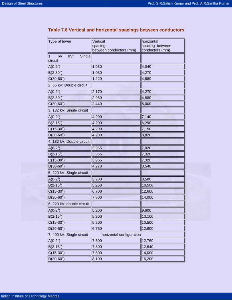
Design of Steel Structures Prof. S.R.Satish Kumar and Prof. A.R.Santha Kumar
Indian Institute of Technology Madras
Table 7.8 Vertical and horizontal spacings between conductors
Type of tower Vertical spacing between conductors (mm)
horizontal spacing between conductors (mm)
1. 66 kV: Single circuit
A(0-2o) 1,030 4,040 B(2-30o) 1,030 4,270 C(30-60o) 1,220 4,880 2. 66 kV: Double circuit A(0-2o) 2,170 4,270 B(2-30o) 2,060 4,880 C(30-60o) 2,440 6,000 3. 132 kV: Single circuit A(0-2o) 4,200 7,140 B(2-15o) 4,200 6,290 C(15-30o) 4,200 7,150 D(30-60o) 4,200 8,820 4. 132 kV: Double circuit A(0-2o) 3,965 7,020 B(2-15o) 3,965 7,320 C(15-30o) 3,965 7,320 D(30-60o) 4,270 8,540 5. 220 kV: Single circuit A(0-2o) 5,200 8,500 B(2-15o) 5,250 10,500 C(15-30o) 6,700 12,600 D(30-60o) 7,800 14,000 6. 220 kV: double circuit A(0-2o) 5,200 9,900 B(2-15o) 5,200 10,100 C(15-30o) 5,200 10,500 D(30-60o) 6,750 12,600 7. 400 kV: Single circuit horizontal configuration A(0-2o) 7,800 12,760 B(2-15o) 7,800 12,640 C(15-30o) 7,800 14,000 D(30-60o) 8,100 16,200
Design of Steel Structures Prof. S.R.Satish Kumar and Prof. A.R.Santha Kumar
Indian Institute of Technology Madras
Determination of base width
The base width at the concrete level is the distance between the centre of
gravity at one corner leg and the centre of gravity of the adjacent corner leg.
There is a particular base width which gives the minimum total cost of the tower
and foundations
Ryle has given the following formula for a preliminary determination of the
economic base width:
B 0.42 M or 0.013 m=
Where B = Base width in meters,
M = Overturning moment about the ground level in tonne-meters, and
M= Overturning moment about the ground level in kg.meters.
The ratio of base width to total tower height for most towers is generally
about one-fifth to one-tenth from large-angle towers to tangent towers.
The following equations have been suggested9,based on the best fit
straight line relationship between the base width B and M
B 0.0782 M 1.0
B 0.0691 M 0.7
= +
= +
Equations are for suspension and angle towers respectively.
It should be noted that Ryle’s formula is intended for use with actual
external loads acting on the tower whereas the formulae in Equations take into
account a factor of safety of 2.0.
Design of Steel Structures Prof. S.R.Satish Kumar and Prof. A.R.Santha Kumar
Indian Institute of Technology Madras
Narrow-base towers are commonly used in Western Europe, especially
Germany, mainly from way-leave considerations. British and American practices
generally favor the wide base type of design, for which the total cost, of tower
and foundations is a minimum. In the USA, a continuous wide strip of land called
the ‘right of way’ has usually to be acquired along the line route. In Great Britain,
the payments made for individual tower way-leaves are generally reasonably
small and not greatly affected by tower base dimensions. Therefore, it has been
possible to adopt a truly economical base width in both the United States and
Great Britain.
A wider taper in the tower base reduces the foundation loading and costs
but increases the cost of the tower and site. A minimum cost which occurs with a
tower width, is greater with bad soil than with good soil. A considerable saving in
foundation costs results from the use of towers with only three legs, the tower
being of triangular section throughout its height. This form of construction entails
tubular legs or special angle sections. The three-footing anchorage has further
advantages, e.g., greater accessibility of the soil underneath the tower when the
land is cultivated.
Determination of top hamper width
The width at top hamper is the width of the tower at the level of the lower
cross-arm in the case of barrel type of towers (in double circuit towers it may be
at the middle level) and waist line in the case of towers with horizontal
configuration of conductors.
The following parameters are considered while determining the width of
the tower at the top bend line:
Design of Steel Structures Prof. S.R.Satish Kumar and Prof. A.R.Santha Kumar
Indian Institute of Technology Madras
1. Horizontal spacing between conductors based on the midspan flashover
between the power conductor under the severest wind and galloping conditions
and the electrical clearance of the line conductor to tower steel work.
2. The sloe of the legs should be such that the corner members intersect as
near the center of gravity (CG) of the loads as possible. Then the braces will be
least loaded. Three cases are possible depending upon the relative position of
the CG of the loads and intersection of the tower legs as shown in Figure 7.6.
In Case (1) the entire shear is taken up by the legs and the bracings do not
carry any stress. Case (2) shows a condition in which the resultant of all loads O’
is below the inter-section of tower legs O. The shear here is shared between legs
and bracings which is a desirable requirement for an economical tower design. In
Case (3), the legs have to withstand greater forces than in cases (1) and (2)
because the legs intersect below the center of gravity of the loads acting on the
tower. This outline is uneconomical.
The top hamper width is generally found to be about one-third of the base
width for tangent and light angle towers and about 1.35 of the base width for
medium and heavy angle towers. For horizontal configurations, the width at the
waistline is, however, found to vary from 1/1.5 to ½.5 of the base width.
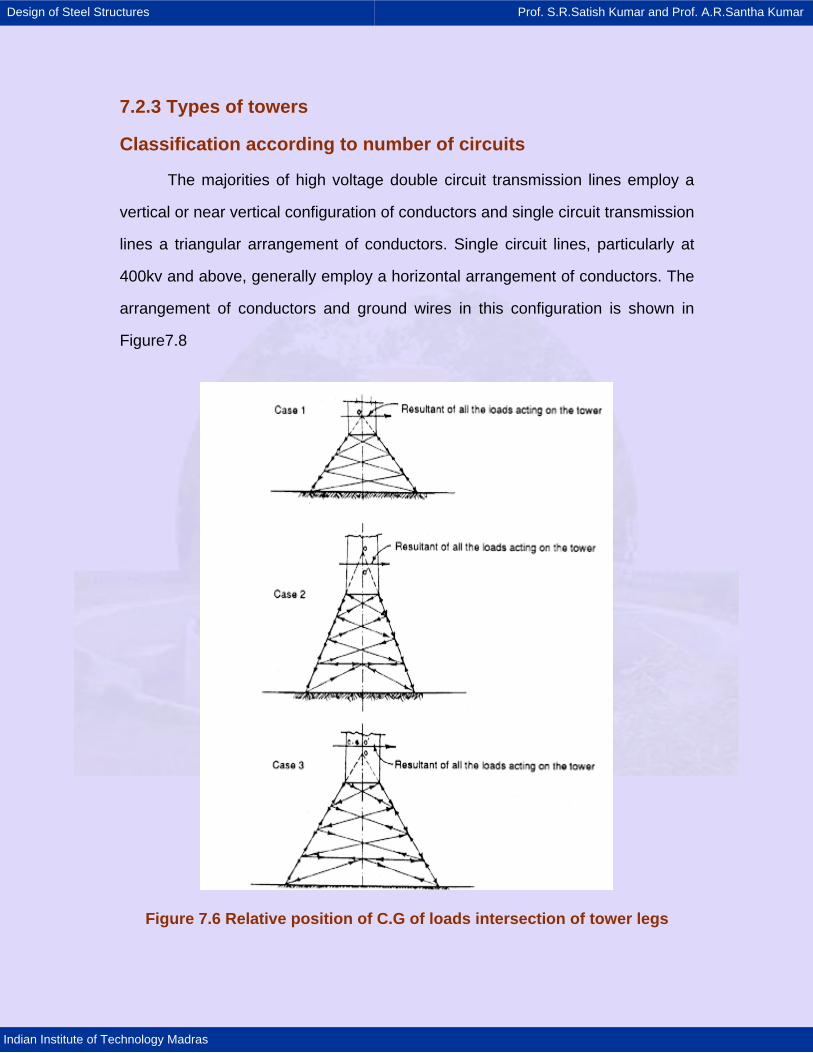
Design of Steel Structures Prof. S.R.Satish Kumar and Prof. A.R.Santha Kumar
Indian Institute of Technology Madras
7.2.3 Types of towers
Classification according to number of circuits
The majorities of high voltage double circuit transmission lines employ a
vertical or near vertical configuration of conductors and single circuit transmission
lines a triangular arrangement of conductors. Single circuit lines, particularly at
400kv and above, generally employ a horizontal arrangement of conductors. The
arrangement of conductors and ground wires in this configuration is shown in
Figure7.8
Figure 7.6 Relative position of C.G of loads intersection of tower legs
Design of Steel Structures Prof. S.R.Satish Kumar and Prof. A.R.Santha Kumar
Indian Institute of Technology Madras
The number of ground wires used on the line depends on the isoceraunic
level (number of thunderstorm days/hours per year) of the area, importance of
the line, and the angle of coverage desired. Single circuit line using horizontal
configuration generally employ tow ground wires, due to the comparative width of
the configuration; whereas lines using vertical and offset arrangements more
often utilize one ground wire except on higher voltage lines of 400 kv and above,
where it is usually found advantageous to string tow ground wires, as the phase
to phase spacing of conductors would require an excessively high positioning of
ground wire to give adequate coverage.
Classification according to use
Towers are classified according to their use independent of the number of
conductors they support.
A tower has to withstand the loadings ranging from straight runs up to
varying angles and dead ends. To simplify the designs and ensure an overall
economy in first cost and maintenance, tower designs are generally confined to a
few standard types as follows.
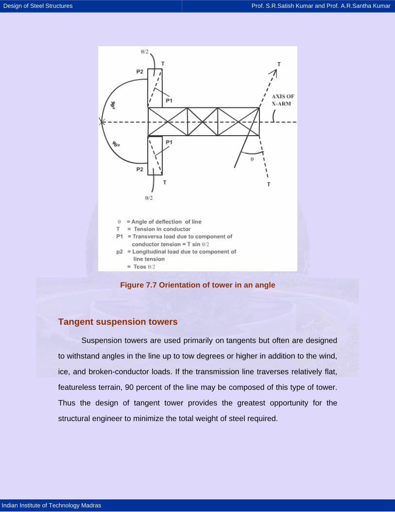
Design of Steel Structures Prof. S.R.Satish Kumar and Prof. A.R.Santha Kumar
Indian Institute of Technology Madras
Figure 7.7 Orientation of tower in an angle
Tangent suspension towers
Suspension towers are used primarily on tangents but often are designed
to withstand angles in the line up to tow degrees or higher in addition to the wind,
ice, and broken-conductor loads. If the transmission line traverses relatively flat,
featureless terrain, 90 percent of the line may be composed of this type of tower.
Thus the design of tangent tower provides the greatest opportunity for the
structural engineer to minimize the total weight of steel required.
Design of Steel Structures Prof. S.R.Satish Kumar and Prof. A.R.Santha Kumar
Indian Institute of Technology Madras
Angle towers
Angle towers, sometimes called semi-anchor towers, are used where the
line makes a horizontal angle greater than two degrees (Figure). As they must
resist a transverse load from the components of the line tension induced by this
angle, in addition to the usual wind, ice and broken conductor loads, they are
necessarily heavier than suspension towers. Unless restricted by site conditions,
or influenced by conductor tensions, angle towers should be located so that the
axis of the cross-arms bisects, the angle formed by the conductors.
Theoretically, different line angles require different towers, but for
economy there are a limiting number of different towers which should be used.
This number is a function of all the factors which make up the total erected cost
of a tower line. However, experience has shown that the following angle
towers are generally suitable for most of the lines:
1. Light angle - 2 to 15o line deviation
2. Medium angle - 15 to 30o line deviation
3. Heavy angle - 30 to 60o line deviation
(And dead end)
While the angles of line deviation are for the normal span, the span may
be increased up to an optimum limit by reducing the angle of line deviation and
vice versa. IS: 802(Part I)-1977 also recommends the above classification.
The loadings on a tower in the case of a 600 angle condition and dead-end
condition are almost the same. As the numbers of locations at which 600 angle
towers and dead-end towers are required are comparatively few, it is economical
Design of Steel Structures Prof. S.R.Satish Kumar and Prof. A.R.Santha Kumar
Indian Institute of Technology Madras
to design the heavy angle towers both for the 600 angle condition and dead-end
condition, whichever is more stringent for each individual structural member.
For each type of tower, the upper limit of the angle range is designed for
the same basic span as the tangent tower, so that a decreased angle can be
accommodated with an increased span or vice versa.
In India, then angle towers are generally provided with tension insulator
strings.
Appreciable economies can be affected by having the light angle towers (2
to 150) with suspension insulators, as this will result in lighter tower designs due
to reduced longitudinal loads to which the tower would be subjected under
broken-wire conditions because of the swing of the insulator string towards the
broken span. It would be uneconomical to use 300 angle tower in locations where
angle higher than 20 and smaller than 300 are encountered. There are limitations
to the use of 20 angle towers at higher angles with reduced spans and the use of
300 angle towers with smaller angles and increased spans. The introduction of a
150 tower would bring about sizeable economies.
It might appear that the use of suspension insulators at angle locations
would result in longer cross-arms so as to satisfy the clearance requirements
under increased insulator swings because of the large line deviation on the
tower. In such a case, it is the usual practice to counteract the excessive swing of
insulator string by the use of counter weights ( in some countries counter weights
up to 250kg have been used) and thus keep the cross-arm lengths within the
economic limits. It is the practice in Norway and Sweden to use suspension
Design of Steel Structures Prof. S.R.Satish Kumar and Prof. A.R.Santha Kumar
Indian Institute of Technology Madras
insulators on towers up to 200 angles and in France up to as much as 400. The
possibilities of conductor breakdown in modern transmission lines equipped with
reliable clamps, anti-vibration devices, etc., are indeed rare, and should the
contingency of a breakdown arise, the problems do not present any more
difficulties than those encountered in the case of plain terrain involving tangent
towers over long stretches.
Calculation of counterweights
The calculation for the counterweights (Figure 7.8) to be added to limit the
sing of the insulator string is quite simple and is illustrated below:
Let θ1 = Swing of insulator string with-out counterweight.
θ2 = Desired swing of insulator string (with suitable counterweight).
H = Total transverse load due to wind on one span of conductor and
line deviation.
W1 and W2 = Weight of one span of the conductor, insulators, etc.,
corresponding to insulator swings θ1and θ2 respectively
Now, tanθ1 = H / W1
and tanθ2 = H / W2
Therefore, the magnitude of the counterweight required to reduce the
insulator swing from θ1 to θ2 = W2-W1.
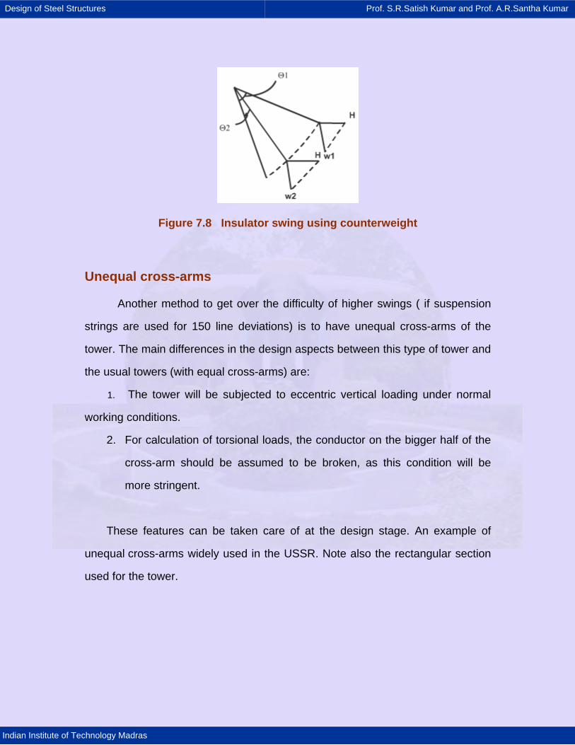
Design of Steel Structures Prof. S.R.Satish Kumar and Prof. A.R.Santha Kumar
Indian Institute of Technology Madras
Figure 7.8 Insulator swing using counterweight
Unequal cross-arms
Another method to get over the difficulty of higher swings ( if suspension
strings are used for 150 line deviations) is to have unequal cross-arms of the
tower. The main differences in the design aspects between this type of tower and
the usual towers (with equal cross-arms) are:
1. The tower will be subjected to eccentric vertical loading under normal
working conditions.
2. For calculation of torsional loads, the conductor on the bigger half of the
cross-arm should be assumed to be broken, as this condition will be
more stringent.
These features can be taken care of at the design stage. An example of
unequal cross-arms widely used in the USSR. Note also the rectangular section
used for the tower.
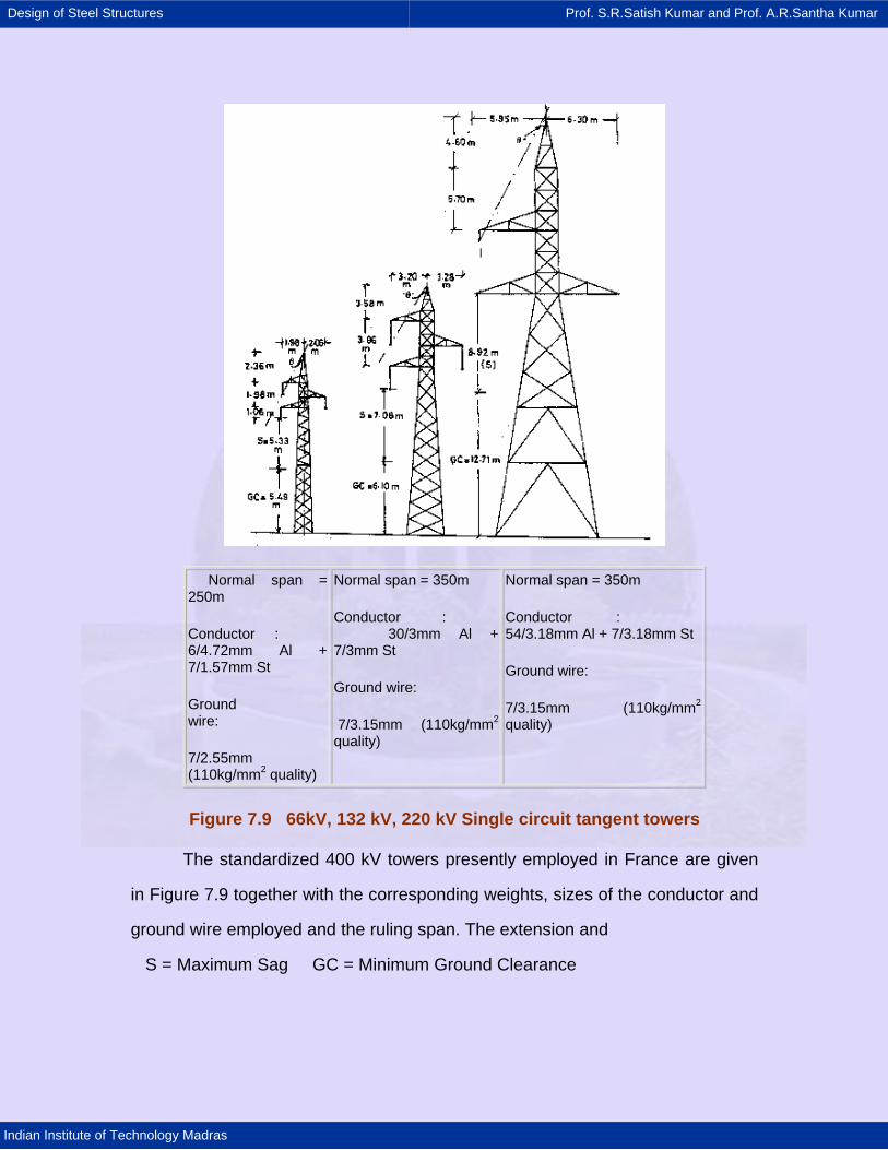
Design of Steel Structures Prof. S.R.Satish Kumar and Prof. A.R.Santha Kumar
Indian Institute of Technology Madras
Normal span = 250m
Conductor : 6/4.72mm Al + 7/1.57mm St
Ground wire:
7/2.55mm (110kg/mm2 quality)
Normal span = 350m
Conductor : 30/3mm Al + 7/3mm St
Ground wire:
7/3.15mm (110kg/mm2
quality)
Normal span = 350m
Conductor : 54/3.18mm Al + 7/3.18mm St
Ground wire:
7/3.15mm (110kg/mm2 quality)
Figure 7.9 66kV, 132 kV, 220 kV Single circuit tangent towers
The standardized 400 kV towers presently employed in France are given
in Figure 7.9 together with the corresponding weights, sizes of the conductor and
ground wire employed and the ruling span. The extension and
S = Maximum Sag GC = Minimum Ground Clearance
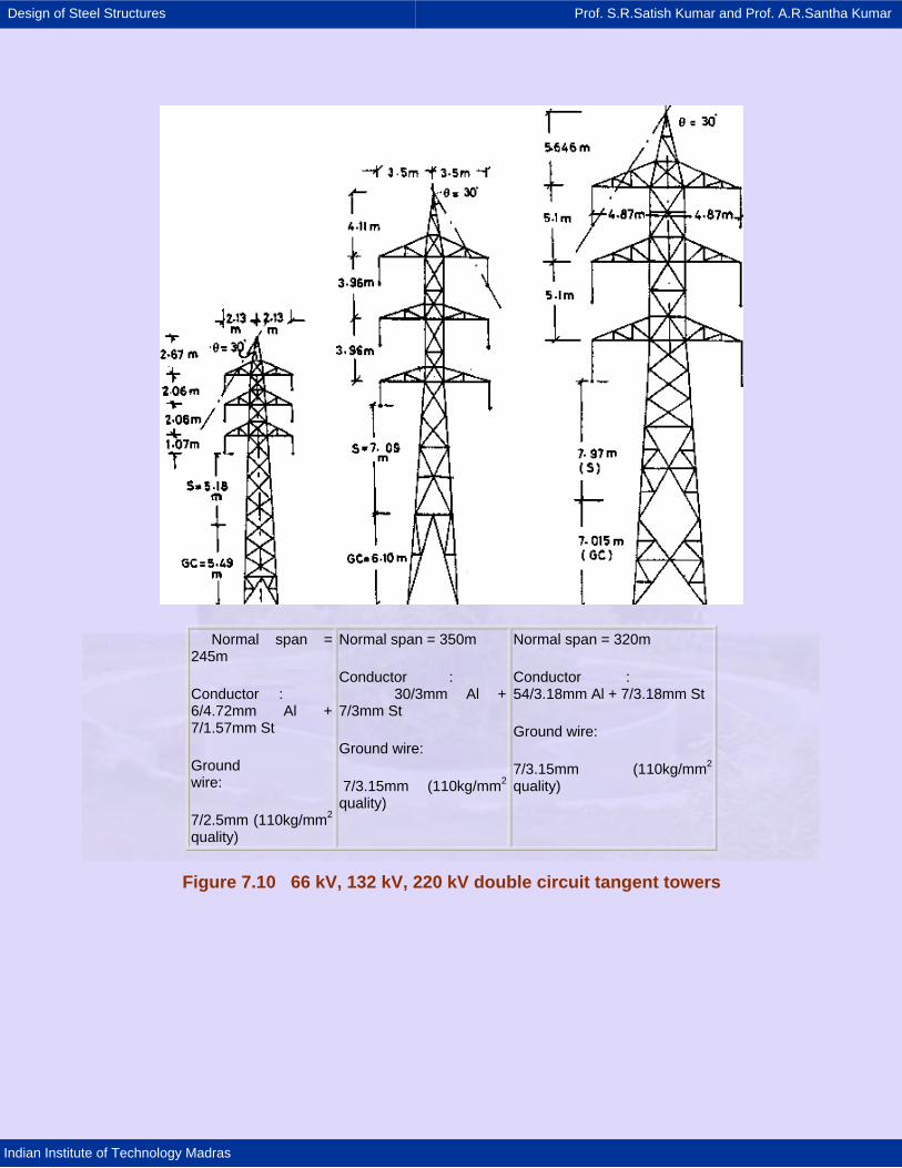
Design of Steel Structures Prof. S.R.Satish Kumar and Prof. A.R.Santha Kumar
Indian Institute of Technology Madras
Normal span = 245m
Conductor : 6/4.72mm Al + 7/1.57mm St
Ground wire:
7/2.5mm (110kg/mm2 quality)
Normal span = 350m
Conductor : 30/3mm Al + 7/3mm St
Ground wire:
7/3.15mm (110kg/mm2
quality)
Normal span = 320m
Conductor : 54/3.18mm Al + 7/3.18mm St
Ground wire:
7/3.15mm (110kg/mm2 quality)
Figure 7.10 66 kV, 132 kV, 220 kV double circuit tangent towers
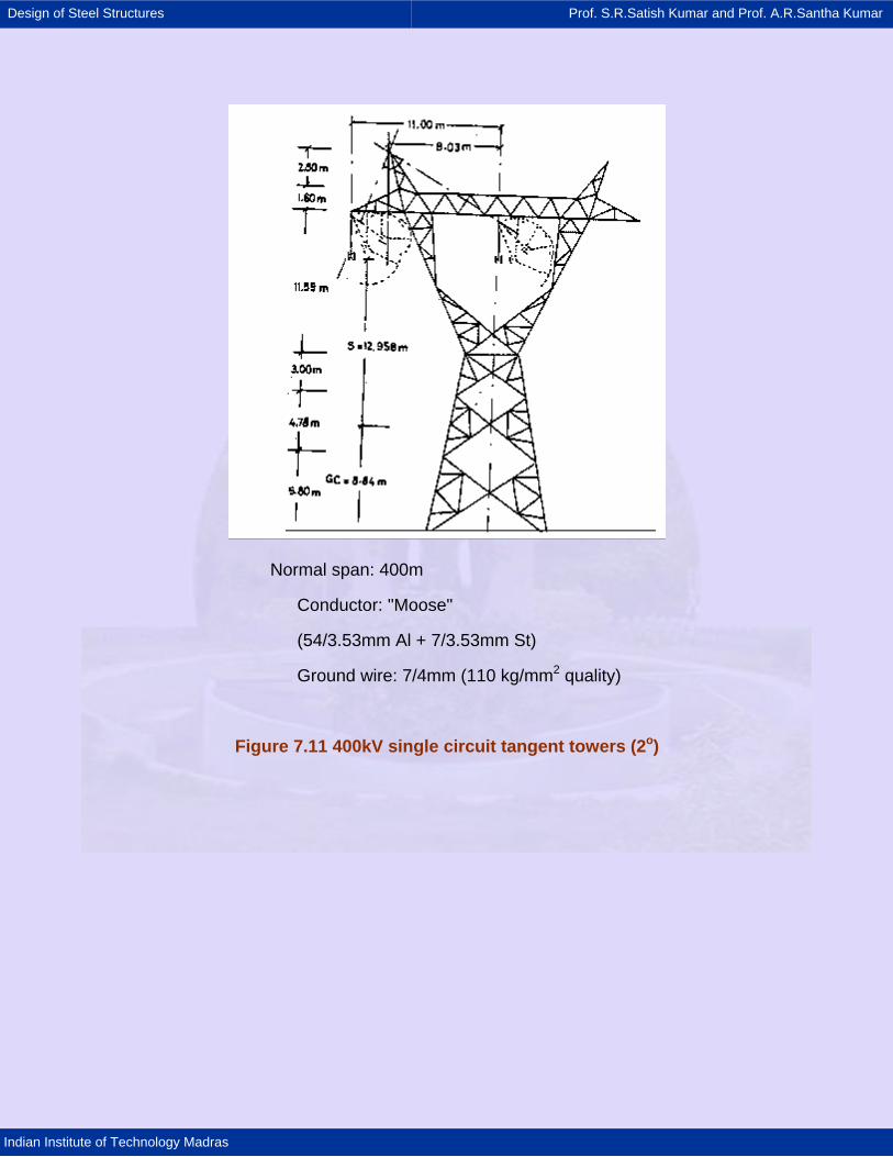
Design of Steel Structures Prof. S.R.Satish Kumar and Prof. A.R.Santha Kumar
Indian Institute of Technology Madras
Normal span: 400m
Conductor: "Moose"
(54/3.53mm Al + 7/3.53mm St)
Ground wire: 7/4mm (110 kg/mm2 quality)
Figure 7.11 400kV single circuit tangent towers (2o)
Design of Steel Structures Prof. S.R.Satish Kumar and Prof. A.R.Santha Kumar
Indian Institute of Technology Madras
7.3 Factors of safety and load
7.3.1 Factors of safety and Permissible deflections
Factors of safety of conductors and ground wires
The factor of safety ( f.o.s ) of a conductor ( or ground wire ) is the ratio of
the ultimate strength of the conductor ( or ground wire ) to the load imposed
under assumed loading condition. Rule 76 (1)(c) of the Indian Electricity Rules,
1956, stipulates as follows:
The minimum factor of safety for conductors shall be two, based on their
ultimate tensile strength. In addition, the conductor tension at 32oC without
external load shall not exceed the following percentages of the ultimate tensile
strength of the conductor:
Intial unloaded tension 35 percent
Final unloaded tension 25 percent
The rule does not specify the loading conditions to which the minimum
factor of safety should correspond. Generally, these loading conditions are taken
as the minimum temperature and the maximum wind in the area concerned.
However, meteorological data show that minimum temperature occurs during the
winter when, in general, weather is not disturbed and gales and storms are rare.
It therefore appears that the probability of the occurrence of maximum wind
pressures, which are associated with gales and stromy winds and prevail for
appreciable periods of hours at a time, simultaneously with the time of
occurrence of the lowest minimum temperatures is small, with the result that the
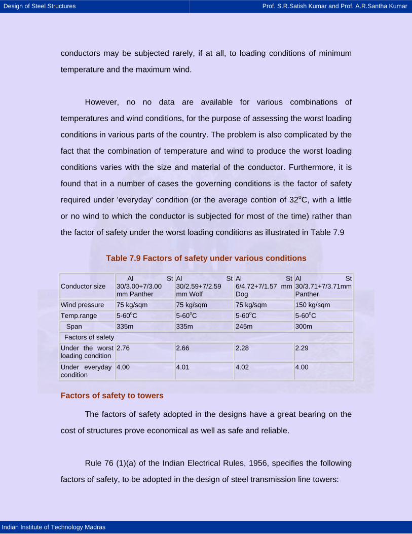
Design of Steel Structures Prof. S.R.Satish Kumar and Prof. A.R.Santha Kumar
Indian Institute of Technology Madras
conductors may be subjected rarely, if at all, to loading conditions of minimum
temperature and the maximum wind.
However, no no data are available for various combinations of
temperatures and wind conditions, for the purpose of assessing the worst loading
conditions in various parts of the country. The problem is also complicated by the
fact that the combination of temperature and wind to produce the worst loading
conditions varies with the size and material of the conductor. Furthermore, it is
found that in a number of cases the governing conditions is the factor of safety
required under 'everyday' condition (or the average contion of 32oC, with a little
or no wind to which the conductor is subjected for most of the time) rather than
the factor of safety under the worst loading conditions as illustrated in Table 7.9
Table 7.9 Factors of safety under various conditions
Conductor size Al St 30/3.00+7/3.00 mm Panther
Al St 30/2.59+7/2.59 mm Wolf
Al St 6/4.72+7/1.57 mm Dog
Al St 30/3.71+7/3.71mm Panther
Wind pressure 75 kg/sqm 75 kg/sqm 75 kg/sqm 150 kg/sqm Temp.range 5-60oC 5-60oC 5-60oC 5-60oC Span 335m 335m 245m 300m Factors of safety Under the worst loading condition
2.76 2.66 2.28 2.29
Under everyday condition
4.00 4.01 4.02 4.00
Factors of safety to towers
The factors of safety adopted in the designs have a great bearing on the
cost of structures prove economical as well as safe and reliable.
Rule 76 (1)(a) of the Indian Electrical Rules, 1956, specifies the following
factors of safety, to be adopted in the design of steel transmission line towers:
Design of Steel Structures Prof. S.R.Satish Kumar and Prof. A.R.Santha Kumar
Indian Institute of Technology Madras
1. under normal conditions 2.0
2. under broken-wire conditions 1.5
It is interesting to compare this practice with that followed in the USSR. In
the USSR, while for normal conditions the f.o.s. is 1.5, that for the broken-wire
condition is 1.2 for suspension tower, and 1.33 for anchor towers. In the case of
transmission lines at 500kV and above, in addition of these factors of safety, an
impact condition is also imposed. When the conductor breaks, there is a sudden
impact on the tower occuring for 0.4 to 0.6 second. The impact factor is assumed
as 1.3 in the case of suspension tower with rigid clamps and 1.2 in the case of
anchor tower, and the loads acting on the tower are increased correspondingly.
Thus, the final force in the case of suspension towers is increased by a factor 1.3
x 1.1 and in the case of anchor towers by 1.2 x 1.2. The corresponding factor of
safety assumed under the impact conditions is 1.1 and 1.2.
Permissible deflections
Sufficient data are not available with regard to the permissible limits of
deflection of towers, as specified by the various authorities. However, one
practice given below is followed in the USSR:
Assuming that there is no shifting of the foundation, the deflection of the
top of the support in the longitudinal direction from the vertical should not exceed
the following limits:
For dead-end heavy-angle structure (1/120) H
For small angle and straight line structures with strain insulators (1/100) H
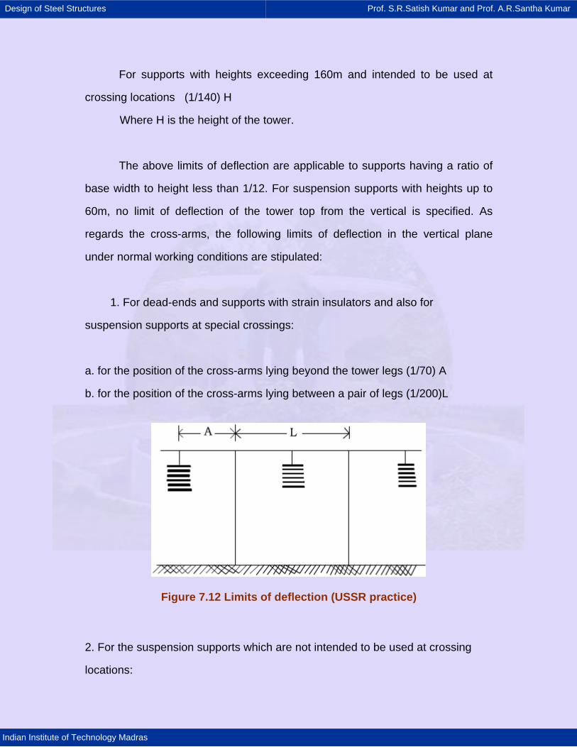
Design of Steel Structures Prof. S.R.Satish Kumar and Prof. A.R.Santha Kumar
Indian Institute of Technology Madras
For supports with heights exceeding 160m and intended to be used at
crossing locations (1/140) H
Where H is the height of the tower.
The above limits of deflection are applicable to supports having a ratio of
base width to height less than 1/12. For suspension supports with heights up to
60m, no limit of deflection of the tower top from the vertical is specified. As
regards the cross-arms, the following limits of deflection in the vertical plane
under normal working conditions are stipulated:
1. For dead-ends and supports with strain insulators and also for
suspension supports at special crossings:
a. for the position of the cross-arms lying beyond the tower legs (1/70) A
b. for the position of the cross-arms lying between a pair of legs (1/200)L
Figure 7.12 Limits of deflection (USSR practice)
2. For the suspension supports which are not intended to be used at crossing
locations:
Design of Steel Structures Prof. S.R.Satish Kumar and Prof. A.R.Santha Kumar
Indian Institute of Technology Madras
a. for the position of the cross-arms lying beyond the tower legs (1/50)A
b. for the position of the cross-arms lying between a pair of tower legs (1/150)L
Where A = length of the cross-arm lying beyond the tower leg, and
L = length of the cross-arm lying between the two tower legs (Figure 7.12)
7.3.2 Loads
The various factors such as wind pressures, temperature variations and
broken-wire conditions, on the basis of which the tower loadings are determined,
are discussed in this section.
A new approach
During the past two decades, extensive live load surveys have been
carried out in a number of countries with a view to arriving at realistic live loads,
based on actual determination of loadings in different occupancies. Also
developments in the field of wind engineering have been significant.
A correct estimation of wind force on towers is important, as the stresses
created due to this force decide the member sizes. The standardization of wind
load on structure is a difficult task and generally involves three stages:
1. analysis of meteorological data
2. simulation of wind effects in wind tunnels
3. synthesis of meteorological and wind tunnel test results.
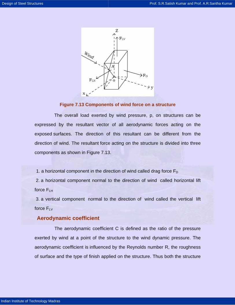
Design of Steel Structures Prof. S.R.Satish Kumar and Prof. A.R.Santha Kumar
Indian Institute of Technology Madras
Figure 7.13 Components of wind force on a structure
The overall load exerted by wind pressure, p, on structures can be
expressed by the resultant vector of all aerodynamic forces acting on the
exposed surfaces. The direction of this resultant can be different from the
direction of wind. The resultant force acting on the structure is divided into three
components as shown in Figure 7.13.
1. a horizontal component in the direction of wind called drag force FD
2. a horizontal component normal to the direction of wind called horizontal lift
force FLH
3. a vertical component normal to the direction of wind called the vertical lift
force FLV
Aerodynamic coefficient
The aerodynamic coefficient C is defined as the ratio of the pressure
exerted by wind at a point of the structure to the wind dynamic pressure. The
aerodynamic coefficient is influenced by the Reynolds number R, the roughness
of surface and the type of finish applied on the structure. Thus both the structure
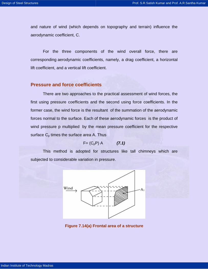
Design of Steel Structures Prof. S.R.Satish Kumar and Prof. A.R.Santha Kumar
Indian Institute of Technology Madras
and nature of wind (which depends on topography and terrain) influence the
aerodynamic coefficient, C.
For the three components of the wind overall force, there are
corresponding aerodynamic coefficients, namely, a drag coefficient, a horizontal
lift coefficient, and a vertical lift coefficient.
Pressure and force coefficients
There are two approaches to the practical assessment of wind forces, the
first using pressure coefficients and the second using force coefficients. In the
former case, the wind force is the resultant of the summation of the aerodynamic
forces normal to the surface. Each of these aerodynamic forces is the product of
wind pressure p multiplied by the mean pressure coefficient for the respective
surface Cp times the surface area A. Thus
F= (CpP) A (7.1)
This method is adopted for structures like tall chimneys which are
subjected to considerable variation in pressure.
Figure 7.14(a) Frontal area of a structure
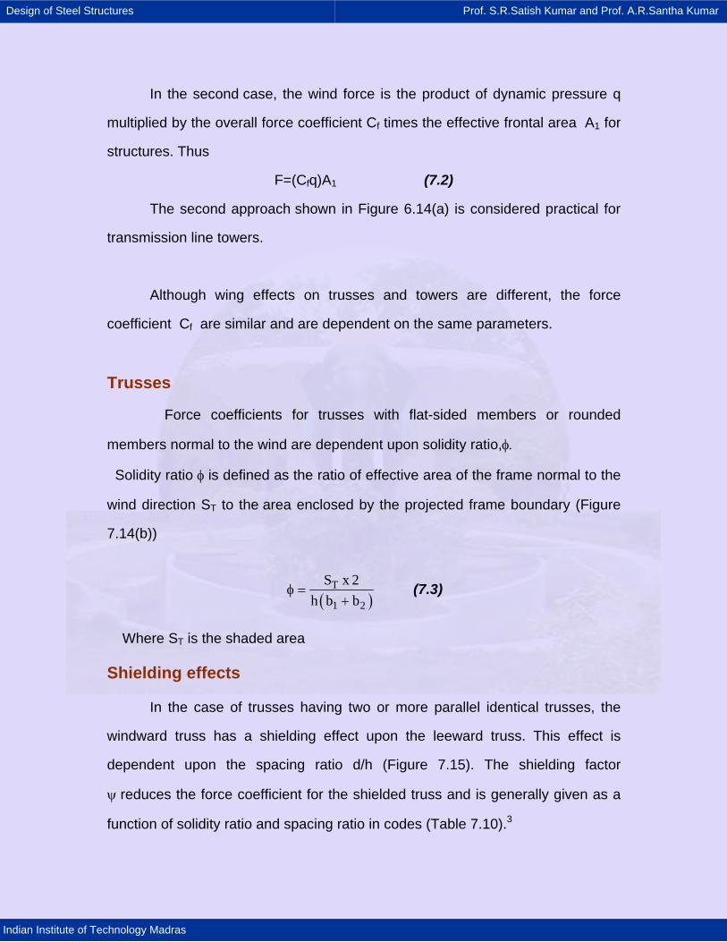
Design of Steel Structures Prof. S.R.Satish Kumar and Prof. A.R.Santha Kumar
Indian Institute of Technology Madras
In the second case, the wind force is the product of dynamic pressure q
multiplied by the overall force coefficient Cf times the effective frontal area A1 for
structures. Thus
F=(Cfq)A1 (7.2)
The second approach shown in Figure 6.14(a) is considered practical for
transmission line towers.
Although wing effects on trusses and towers are different, the force
coefficient Cf are similar and are dependent on the same parameters.
Trusses
Force coefficients for trusses with flat-sided members or rounded
members normal to the wind are dependent upon solidity ratio,φ.
Solidity ratio φ is defined as the ratio of effective area of the frame normal to the
wind direction ST to the area enclosed by the projected frame boundary (Figure
7.14(b))
( )T
1 2
S x 2h b b
φ =+
(7.3)
Where ST is the shaded area
Shielding effects
In the case of trusses having two or more parallel identical trusses, the
windward truss has a shielding effect upon the leeward truss. This effect is
dependent upon the spacing ratio d/h (Figure 7.15). The shielding factor
ψ reduces the force coefficient for the shielded truss and is generally given as a
function of solidity ratio and spacing ratio in codes (Table 7.10).3
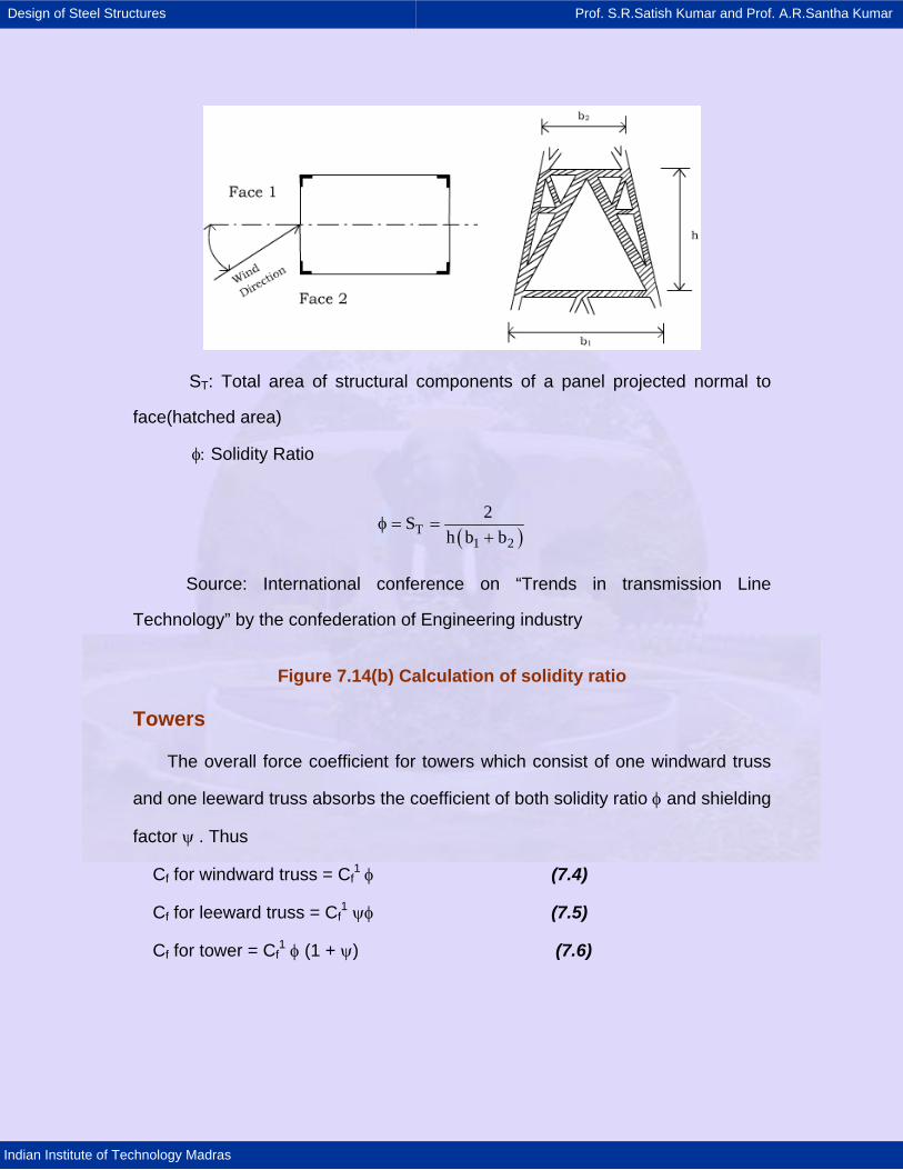
Design of Steel Structures Prof. S.R.Satish Kumar and Prof. A.R.Santha Kumar
Indian Institute of Technology Madras
ST: Total area of structural components of a panel projected normal to
face(hatched area)
φ: Solidity Ratio
( )T1 2
2Sh b b
φ = =+
Source: International conference on “Trends in transmission Line
Technology” by the confederation of Engineering industry
Figure 7.14(b) Calculation of solidity ratio
Towers
The overall force coefficient for towers which consist of one windward truss
and one leeward truss absorbs the coefficient of both solidity ratio φ and shielding
factor ψ . Thus
Cf for windward truss = Cf1 φ (7.4)
Cf for leeward truss = Cf1 ψφ (7.5)
Cf for tower = Cf1 φ (1 + ψ) (7.6)
Design of Steel Structures Prof. S.R.Satish Kumar and Prof. A.R.Santha Kumar
Indian Institute of Technology Madras
Where Cf1 is the force coefficient for individual truss and Cf is the force
coefficient for the overall tower.
Table 7.11 gives the overall force coefficients for square sections
towers recommended in the French and the British codes.3
Figure 7.15 Spacing ratio for leeward truss
The wind force F on latticed towers is given by
F= CfPAe (7.7)
Where Cf is the overall force coefficient,
P dynamic wind pressure, and
Ae the surface area in m2 on which wind impinges.
Wires and cables
Table 7.12 gives the force coefficient as a function of diameter d, dynamic
pressure and roughness for wires and cables for infinite length (1/d>100)
according to the French and the British Practices.
Based on the considerations discussed above, the practice followed in the
USSR in regard to wind load calculations for transmission line towers is
summarized below.
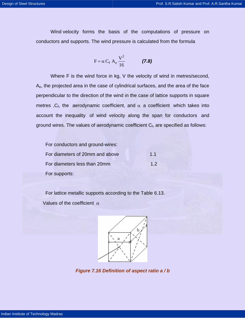
Design of Steel Structures Prof. S.R.Satish Kumar and Prof. A.R.Santha Kumar
Indian Institute of Technology Madras
Wind velocity forms the basis of the computations of pressure on
conductors and supports. The wind pressure is calculated from the formula
2
f eVF C A16
= α (7.8)
Where F is the wind force in kg, V the velocity of wind in metres/second,
Ae, the projected area in the case of cylindrical surfaces, and the area of the face
perpendicular to the direction of the wind in the case of lattice supports in square
metres ,Cf, the aerodynamic coefficient, and α a coefficient which takes into
account the inequality of wind velocity along the span for conductors and
ground wires. The values of aerodynamic coefficient Cf, are specified as follows:
For conductors and ground-wires:
For diameters of 20mm and above 1.1
For diameters less than 20mm 1.2
For supports:
For lattice metallic supports according to the Table 6.13.
Values of the coefficient α
Figure 7.16 Definition of aspect ratio a / b

Design of Steel Structures Prof. S.R.Satish Kumar and Prof. A.R.Santha Kumar
Indian Institute of Technology Madras
The values of α are assumed as given in Table 7.14. Wind velocity charts
have been prepared according to 5-year bases. That is, the five-year chart gives
the maximum wind velocities which have occurred every five years, the 10-year
chart gives the maximum velocities which have occurred every ten years and so
on. The five-year chart forms the basis of designs for lines up to 35 kV, the 10-
year chart for 110kV and 220 kV lines and the 15-year chart for lines at 400 kV
and above. In other words, the more important the line, the greater is the return
period taken into account for determining the maximum wind velocity to be
assumed in the designs. Although there are regions with maximum wind
velocities less than 25m/sec. In all the three charts, e.g., the 10-year chart shows
the regions of 17,20,24,28,32,36 and greater than 40m/sec., the minimum
velocity assumed in the designs is 25m/sec. For lines up to and including 220 kV,
and 27m/sec. For 330kV and 500 kV lines.
The new approach applicable to transmission line tower designs in India is
now discussed.
The India Meteorological Department has recently brought out a wind map
giving the basic maximum wind speed in km/h replacing the earlier wind pressure
maps. The map is applicable to 10m height above mean ground level.
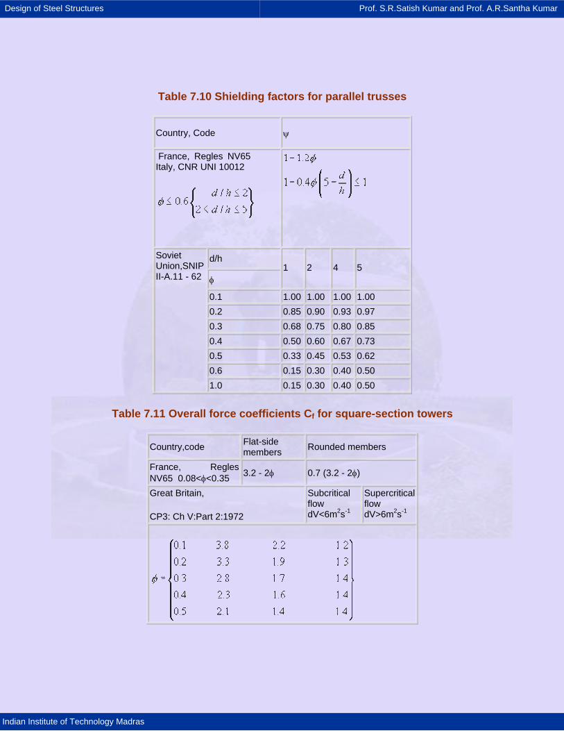
Design of Steel Structures Prof. S.R.Satish Kumar and Prof. A.R.Santha Kumar
Indian Institute of Technology Madras
Table 7.10 Shielding factors for parallel trusses
Country, Code ψ
France, Regles NV65 Italy, CNR UNI 10012
d/h
φ 1 2 4 5
0.1 1.00 1.00 1.00 1.00 0.2 0.85 0.90 0.93 0.97 0.3 0.68 0.75 0.80 0.85 0.4 0.50 0.60 0.67 0.73 0.5 0.33 0.45 0.53 0.62 0.6 0.15 0.30 0.40 0.50
Soviet Union,SNIP II-A.11 - 62
1.0 0.15 0.30 0.40 0.50
Table 7.11 Overall force coefficients Cf for square-section towers
Country,code Flat-side members Rounded members
France, Regles NV65 0.08<φ<0.35 3.2 - 2φ 0.7 (3.2 - 2φ)
Great Britain,
CP3: Ch V:Part 2:1972
Subcritical flow dV<6m2s-1
Supercritical flow dV>6m2s-1
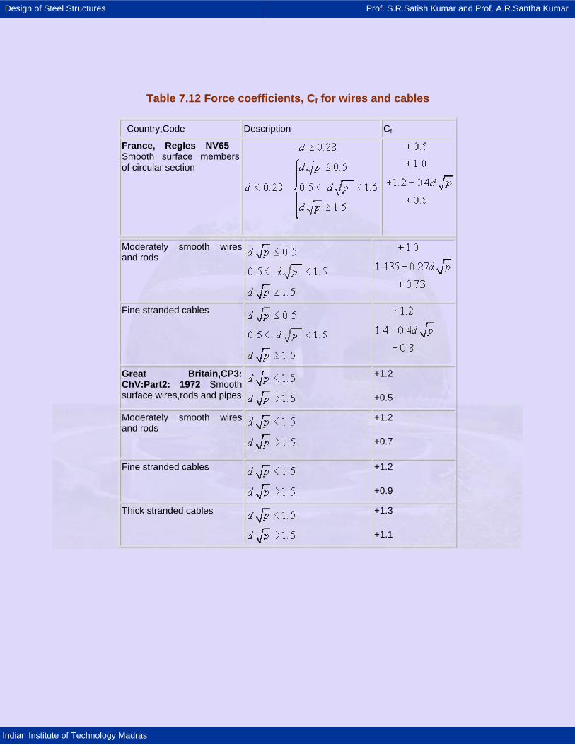
Design of Steel Structures Prof. S.R.Satish Kumar and Prof. A.R.Santha Kumar
Indian Institute of Technology Madras
Table 7.12 Force coefficients, Cf for wires and cables
Country,Code Description Cf France, Regles NV65 Smooth surface members of circular section
Moderately smooth wires and rods
Fine stranded cables
Great Britain,CP3: ChV:Part2: 1972 Smooth surface wires,rods and pipes
+1.2
+0.5
Moderately smooth wires and rods
+1.2
+0.7
Fine stranded cables
+1.2
+0.9
Thick stranded cables
+1.3
+1.1
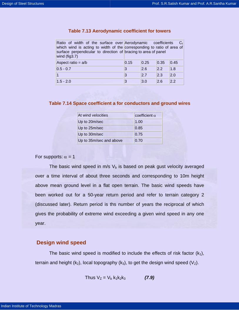
Design of Steel Structures Prof. S.R.Satish Kumar and Prof. A.R.Santha Kumar
Indian Institute of Technology Madras
Table 7.13 Aerodynamic coefficient for towers
Ratio of width of the surface over which wind is acting to width of the surface perpendicular to direction of wind (fig3.7)
Aerodynamic coefficients Cf corresponding to ratio of area of bracing to area of panel
Aspect ratio = a/b 0.15 0.25 0.35 0.45 0.5 - 0.7 3 2.6 2.2 1.8 1 3 2.7 2.3 2.0 1.5 - 2.0 3 3.0 2.6 2.2
Table 7.14 Space coefficient a for conductors and ground wires
At wind velocities coefficient α Up to 20m/sec 1.00 Up to 25m/sec 0.85 Up to 30m/sec 0.75 Up to 35m/sec and above 0.70
For supports: α = 1
The basic wind speed in m/s Vb is based on peak gust velocity averaged
over a time interval of about three seconds and corresponding to 10m height
above mean ground level in a flat open terrain. The basic wind speeds have
been worked out for a 50-year return period and refer to terrain category 2
(discussed later). Return period is ths number of years the reciprocal of which
gives the probability of extreme wind exceeding a given wind speed in any one
year.
Design wind speed
The basic wind speed is modified to include the effects of risk factor (k1),
terrain and height (k2), local topography (k3), to get the design wind speed (VZ).
Thus VZ = Vb k1k2k3 (7.9)
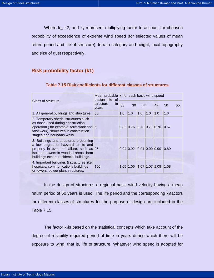
Design of Steel Structures Prof. S.R.Satish Kumar and Prof. A.R.Santha Kumar
Indian Institute of Technology Madras
Where k1, k2, and k3 represent multiplying factor to account for choosen
probobility of exceedence of extreme wind speed (for selected values of mean
return period and life of structure), terrain category and height, local topography
and size of gust respectively.
Risk probobility factor (k1)
Table 7.15 Risk coefficients for different classes of structures
k1 for each basic wind speed Class of structure
Mean probable design life of structure in years 33 39 44 47 50 55
1. All general buildings and structures 50 1.0 1.0 1.0 1.0 1.0 1.0 2. Temporary sheds, structures such as those used during construction operation ( for example, form-work and falsework), structures in construction stages and boundary walls
5 0.82 0.76 0.73 0.71 0.70 0.67
3. Buildings and structures presenting a low degree of hazzard to life and property in event of failure, such as isolated towers in wooded areas, farm buildings except residential buildings
25 0.94 0.92 0.91 0.90 0.90 0.89
4. Important buildings & structures like hospitals, communications buildings or towers, power plant structures.
100 1.05 1.06 1.07 1.07 1.08 1.08
In the design of structures a regional basic wind velocity having a mean
return period of 50 years is used. The life period and the corresponding k1factors
for different classes of structures for the purpose of design are included in the
Table 7.15.
The factor k1is based on the statistical concepts which take account of the
degree of reliability required period of time in years during which there will be
exposure to wind, that is, life of structure. Whatever wind speed is adopted for
Design of Steel Structures Prof. S.R.Satish Kumar and Prof. A.R.Santha Kumar
Indian Institute of Technology Madras
design purposes, there is always a probability (however small) that may be
exceeded in a storm of exceptional violence; the greater the period of years over
which there will be exposure to the wind, the greater is this probability. Higher
return periods ranging from 100 years to 1,000 years in association with greater
periods of exposure may have to be selected for exceptionally important
structures such as natural draft cooling towers, very tall chimneys, television
transmission towers, atomic reactors, etc.
Terrain categories (k2 factors)
Selection of terrain categories is made with due regards to the effect of
obstructions which constitute the ground surface roughness. Four categories are
recognised as given in Table 7.16
Variation of basic wind speed with height in different terrains
The variation of wind speed with height of different sizes of structures
depends on the terrain category as well as the type of structure. For this purpose
three classes of structures given in the note under Table 7.17 are recognised by
the code.
Table 7.17 gives the multiplying factor by which the reference wind speed
should be multiplied to obtain the wind speed at different heights, in each terrain
category for different classes of structures.
The multiplying factors in Table 7.17 for heights well above the heights of
the obstructions producing the surface roughness, but less than the gradient
height, are based on the variation of gust velocities with height determined by the
following formula based on the well known power formula explained earlier:
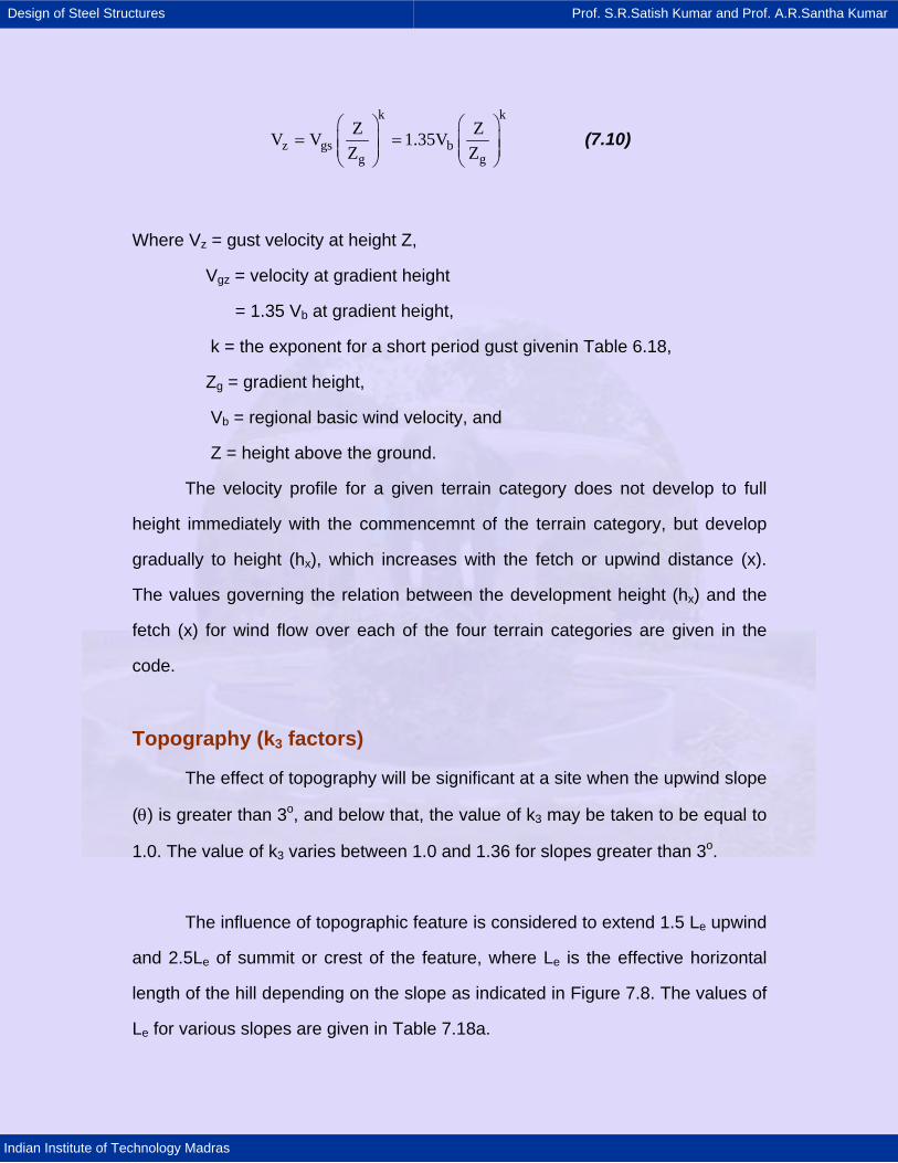
Design of Steel Structures Prof. S.R.Satish Kumar and Prof. A.R.Santha Kumar
Indian Institute of Technology Madras
k k
z gs bg g
Z ZV V 1.35VZ Z
⎛ ⎞ ⎛ ⎞= =⎜ ⎟ ⎜ ⎟⎜ ⎟ ⎜ ⎟
⎝ ⎠ ⎝ ⎠ (7.10)
Where Vz = gust velocity at height Z,
Vgz = velocity at gradient height
= 1.35 Vb at gradient height,
k = the exponent for a short period gust givenin Table 6.18,
Zg = gradient height,
Vb = regional basic wind velocity, and
Z = height above the ground.
The velocity profile for a given terrain category does not develop to full
height immediately with the commencemnt of the terrain category, but develop
gradually to height (hx), which increases with the fetch or upwind distance (x).
The values governing the relation between the development height (hx) and the
fetch (x) for wind flow over each of the four terrain categories are given in the
code.
Topography (k3 factors)
The effect of topography will be significant at a site when the upwind slope
(θ) is greater than 3o, and below that, the value of k3 may be taken to be equal to
1.0. The value of k3 varies between 1.0 and 1.36 for slopes greater than 3o.
The influence of topographic feature is considered to extend 1.5 Le upwind
and 2.5Le of summit or crest of the feature, where Le is the effective horizontal
length of the hill depending on the slope as indicated in Figure 7.8. The values of
Le for various slopes are given in Table 7.18a.
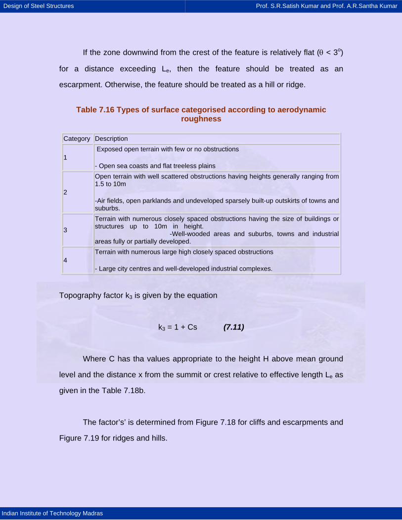
Design of Steel Structures Prof. S.R.Satish Kumar and Prof. A.R.Santha Kumar
Indian Institute of Technology Madras
If the zone downwind from the crest of the feature is relatively flat (θ < 3o)
for a distance exceeding Le, then the feature should be treated as an
escarpment. Otherwise, the feature should be treated as a hill or ridge.
Table 7.16 Types of surface categorised according to aerodynamic roughness
Category Description
1 Exposed open terrain with few or no obstructions
- Open sea coasts and flat treeless plains
2
Open terrain with well scattered obstructions having heights generally ranging from 1.5 to 10m
-Air fields, open parklands and undeveloped sparsely built-up outskirts of towns and suburbs.
3 Terrain with numerous closely spaced obstructions having the size of buildings or structures up to 10m in height. -Well-wooded areas and suburbs, towns and industrial areas fully or partially developed.
4 Terrain with numerous large high closely spaced obstructions
- Large city centres and well-developed industrial complexes.
Topography factor k3 is given by the equation
k3 = 1 + Cs (7.11)
Where C has tha values appropriate to the height H above mean ground
level and the distance x from the summit or crest relative to effective length Le as
given in the Table 7.18b.
The factor’s’ is determined from Figure 7.18 for cliffs and escarpments and
Figure 7.19 for ridges and hills.
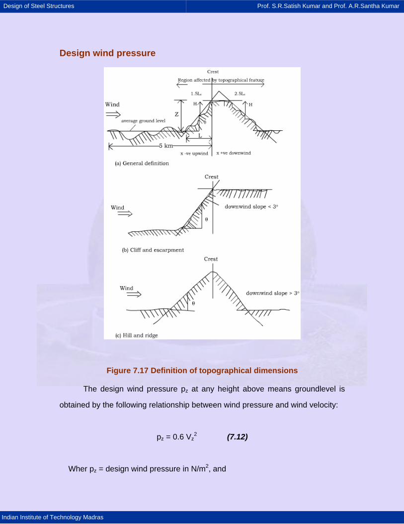
Design of Steel Structures Prof. S.R.Satish Kumar and Prof. A.R.Santha Kumar
Indian Institute of Technology Madras
Design wind pressure
Figure 7.17 Definition of topographical dimensions
The design wind pressure pz at any height above means groundlevel is
obtained by the following relationship between wind pressure and wind velocity:
pz = 0.6 Vz2
(7.12)
Wher pz = design wind pressure in N/m2, and
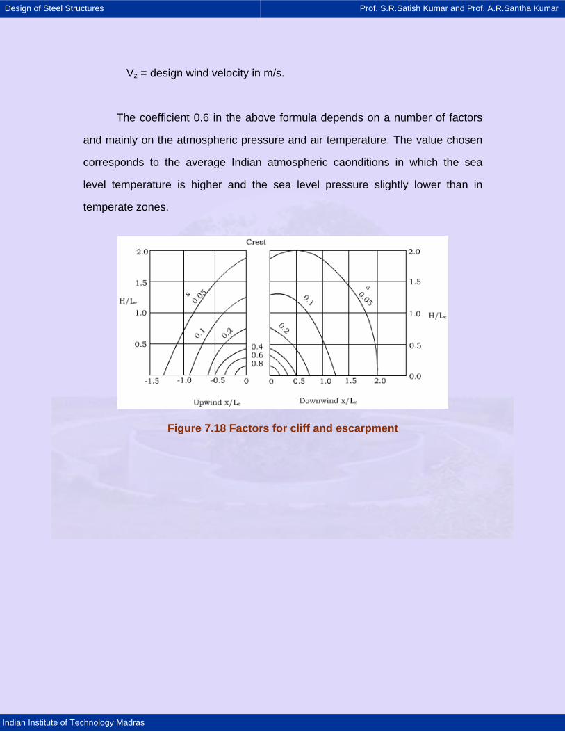
Design of Steel Structures Prof. S.R.Satish Kumar and Prof. A.R.Santha Kumar
Indian Institute of Technology Madras
Vz = design wind velocity in m/s.
The coefficient 0.6 in the above formula depends on a number of factors
and mainly on the atmospheric pressure and air temperature. The value chosen
corresponds to the average Indian atmospheric caonditions in which the sea
level temperature is higher and the sea level pressure slightly lower than in
temperate zones.
Figure 7.18 Factors for cliff and escarpment
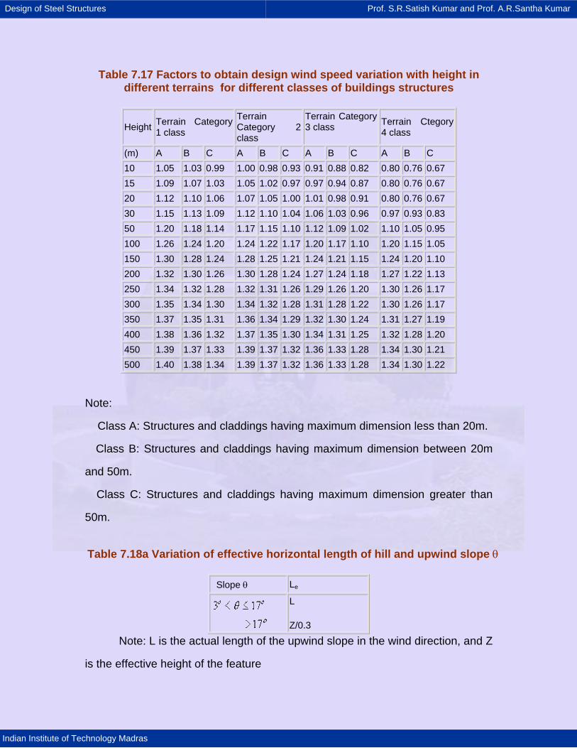
Design of Steel Structures Prof. S.R.Satish Kumar and Prof. A.R.Santha Kumar
Indian Institute of Technology Madras
Table 7.17 Factors to obtain design wind speed variation with height in different terrains for different classes of buildings structures
Height Terrain Category 1 class
Terrain Category 2 class
Terrain Category 3 class Terrain Ctegory
4 class
(m) A B C A B C A B C A B C 10 1.05 1.03 0.99 1.00 0.98 0.93 0.91 0.88 0.82 0.80 0.76 0.67 15 1.09 1.07 1.03 1.05 1.02 0.97 0.97 0.94 0.87 0.80 0.76 0.67 20 1.12 1.10 1.06 1.07 1.05 1.00 1.01 0.98 0.91 0.80 0.76 0.67 30 1.15 1.13 1.09 1.12 1.10 1.04 1.06 1.03 0.96 0.97 0.93 0.83 50 1.20 1.18 1.14 1.17 1.15 1.10 1.12 1.09 1.02 1.10 1.05 0.95 100 1.26 1.24 1.20 1.24 1.22 1.17 1.20 1.17 1.10 1.20 1.15 1.05 150 1.30 1.28 1.24 1.28 1.25 1.21 1.24 1.21 1.15 1.24 1.20 1.10 200 1.32 1.30 1.26 1.30 1.28 1.24 1.27 1.24 1.18 1.27 1.22 1.13 250 1.34 1.32 1.28 1.32 1.31 1.26 1.29 1.26 1.20 1.30 1.26 1.17 300 1.35 1.34 1.30 1.34 1.32 1.28 1.31 1.28 1.22 1.30 1.26 1.17 350 1.37 1.35 1.31 1.36 1.34 1.29 1.32 1.30 1.24 1.31 1.27 1.19 400 1.38 1.36 1.32 1.37 1.35 1.30 1.34 1.31 1.25 1.32 1.28 1.20 450 1.39 1.37 1.33 1.39 1.37 1.32 1.36 1.33 1.28 1.34 1.30 1.21 500 1.40 1.38 1.34 1.39 1.37 1.32 1.36 1.33 1.28 1.34 1.30 1.22
Note:
Class A: Structures and claddings having maximum dimension less than 20m.
Class B: Structures and claddings having maximum dimension between 20m
and 50m.
Class C: Structures and claddings having maximum dimension greater than
50m.
Table 7.18a Variation of effective horizontal length of hill and upwind slope θ
Slope θ Le
L
Z/0.3 Note: L is the actual length of the upwind slope in the wind direction, and Z
is the effective height of the feature
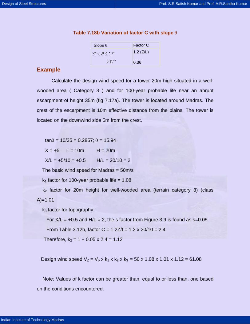
Design of Steel Structures Prof. S.R.Satish Kumar and Prof. A.R.Santha Kumar
Indian Institute of Technology Madras
Table 7.18b Variation of factor C with slope θ
Slope θ Factor C
1.2 (Z/L)
0.36 Example
Calculate the design wind speed for a tower 20m high situated in a well-
wooded area ( Category 3 ) and for 100-year probable life near an abrupt
escarpment of height 35m (fig 7.17a). The tower is located around Madras. The
crest of the escarpment is 10m effective distance from the plains. The tower is
located on the downwind side 5m from the crest.
tanθ = 10/35 = 0.2857; θ = 15.94
X = +5 L = 10m H = 20m
X/L = +5/10 = +0.5 H/L = 20/10 = 2
The basic wind speed for Madras = 50m/s
k1 factor for 100-year probable life = 1.08
k2 factor for 20m height for well-wooded area (terrain category 3) (class
A)=1.01
k3 factor for topography:
For X/L = +0.5 and H/L = 2, the s factor from Figure 3.9 is found as s=0.05
From Table 3.12b, factor C = 1.2Z/L= 1.2 x 20/10 = 2.4
Therefore, k3 = 1 + 0.05 x 2.4 = 1.12
Design wind speed VZ = Vb x k1 x k2 x k3 = 50 x 1.08 x 1.01 x 1.12 = 61.08
Note: Values of k factor can be greater than, equal to or less than, one based
on the conditions encountered.
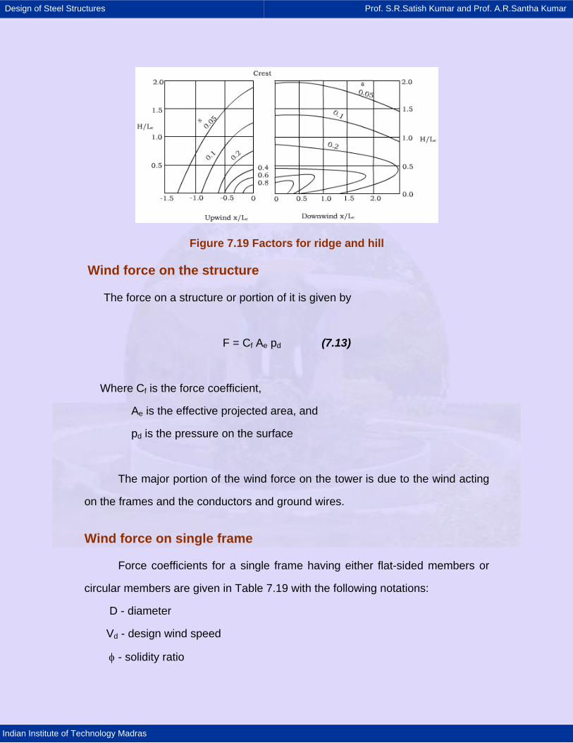
Design of Steel Structures Prof. S.R.Satish Kumar and Prof. A.R.Santha Kumar
Indian Institute of Technology Madras
Figure 7.19 Factors for ridge and hill
Wind force on the structure
The force on a structure or portion of it is given by
F = Cf Ae pd (7.13)
Where Cf is the force coefficient,
Ae is the effective projected area, and
pd is the pressure on the surface
The major portion of the wind force on the tower is due to the wind acting
on the frames and the conductors and ground wires.
Wind force on single frame
Force coefficients for a single frame having either flat-sided members or
circular members are given in Table 7.19 with the following notations:
D - diameter
Vd - design wind speed
φ - solidity ratio
Design of Steel Structures Prof. S.R.Satish Kumar and Prof. A.R.Santha Kumar
Indian Institute of Technology Madras
Wind force on multiple frames
The wind force on the winddard frame and any unshielded parts of the
other frame is calculated using the coefficients given in Table 7.19. The wind
load on parts of the sheltered frame is multiplied by a shielding factor ψ, which is
dependent upon the solidity ratio of windward frame, the types of members and
tha spacing ratio. The values of shielding factors are given in Table 7.20.
The spacing ratio d/h (same as aspect ratio a/b for towers) has already
been defined in Figure 7.16.
While using Table 7.20 for different types of members, the aerodynamic
solidity ratio β to be adopted is as follows:
Aerodynamic solidity ratio β = solidity ratio φ for flat-sided members. (7.14)
Wind force on lattice towers
Force coefficients for lattice towers of square or equilateral triangle
sections with flat-sided members for wind direction against any face are given in
Table 7.21.
Force coefficients for lattice towers of square sections with with circular
members are given in the Table 7.22.
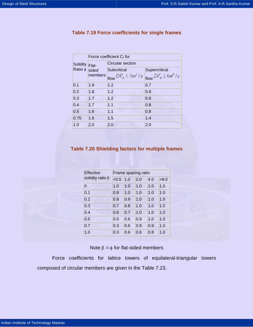
Design of Steel Structures Prof. S.R.Satish Kumar and Prof. A.R.Santha Kumar
Indian Institute of Technology Madras
Table 7.19 Force coefficients for single frames
Force coefficient Cf for Circular section Solidity
Ratio φ Flat-sided members
Subcritical
flow
Supercritical
flow 0.1 1.9 1.2 0.7 0.2 1.8 1.2 0.8 0.3 1.7 1.2 0.8 0.4 1.7 1.1 0.8 0.5 1.6 1.1 0.8 0.75 1.6 1.5 1.4 1.0 2.0 2.0 2.0
Table 7.20 Shielding factors for multiple frames
Frame spacing ratio Effective solidity ratio β <0.5 1.0 2.0 4.0 >8.00 1.0 1.0 1.0 1.0 1.0 0.1 0.9 1.0 1.0 1.0 1.0 0.2 0.8 0.9 1.0 1.0 1.0 0.3 0.7 0.8 1.0 1.0 1.0 0.4 0.6 0.7 1.0 1.0 1.0 0.5 0.5 0.6 0.9 1.0 1.0 0.7 0.3 0.6 0.8 0.9 1.0 1.0 0.3 0.6 0.6 0.8 1.0
Note β = φ for flat-sided members
Force coefficients for lattice towers of equilateral-triangular towers
composed of circular members are given in the Table 7.23.

Design of Steel Structures Prof. S.R.Satish Kumar and Prof. A.R.Santha Kumar
Indian Institute of Technology Madras
The wind load on a square tower can either be calculated using the overall
force coefficient for the tower as a whole given in Tables 7.21 to 7.23, using the
equation F = Cf Ae pd, or calculated using the cumulative effect of windward and
leeward trusses from the equation
F = Cf ( 1 + ψ )Ae pd (7.15)
Tables 7.19 and 7.20 give the values of Cf and y respectively.
In the case of rectangular towers, the wind force can be calculated base
on the cumulative effect of windward and leeward trusses using the equation F
= Cf (1 + ψ)Ae pd, the value of Cf and ψ being adopted from 7.19 and 7.20
respectively.
While calculating the surface area of tower face, an increase of 10 percent
is made to account for the gusset plates, etc.
Wind force on conductors and ground wires
Table 7.21 Overall force coefficients for towers composed of flat-sided members
Force coefficient for Solidity Ratio φ Square towers Equilateral
triangular towers0.1 3.8 3.1 0.2 3.3 2.7 0.3 2.8 2.3 0.4 2.3 1.9 0.5 2.1 1.5
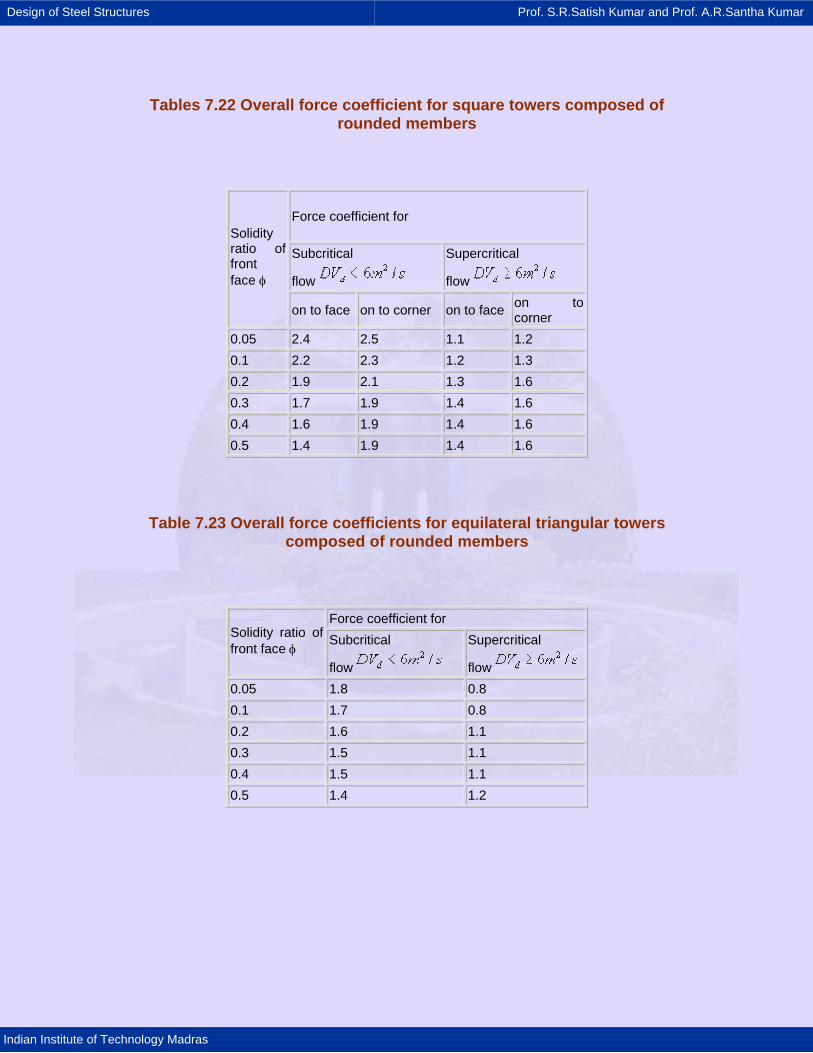
Design of Steel Structures Prof. S.R.Satish Kumar and Prof. A.R.Santha Kumar
Indian Institute of Technology Madras
Tables 7.22 Overall force coefficient for square towers composed of rounded members
Force coefficient for
Subcritical
flow
Supercritical
flow
Solidity ratio of front face φ
on to face on to corner on to face on to corner
0.05 2.4 2.5 1.1 1.2 0.1 2.2 2.3 1.2 1.3 0.2 1.9 2.1 1.3 1.6 0.3 1.7 1.9 1.4 1.6 0.4 1.6 1.9 1.4 1.6 0.5 1.4 1.9 1.4 1.6
Table 7.23 Overall force coefficients for equilateral triangular towers composed of rounded members
Force coefficient for Solidity ratio of front face φ Subcritical
flow
Supercritical
flow 0.05 1.8 0.8 0.1 1.7 0.8 0.2 1.6 1.1 0.3 1.5 1.1 0.4 1.5 1.1 0.5 1.4 1.2
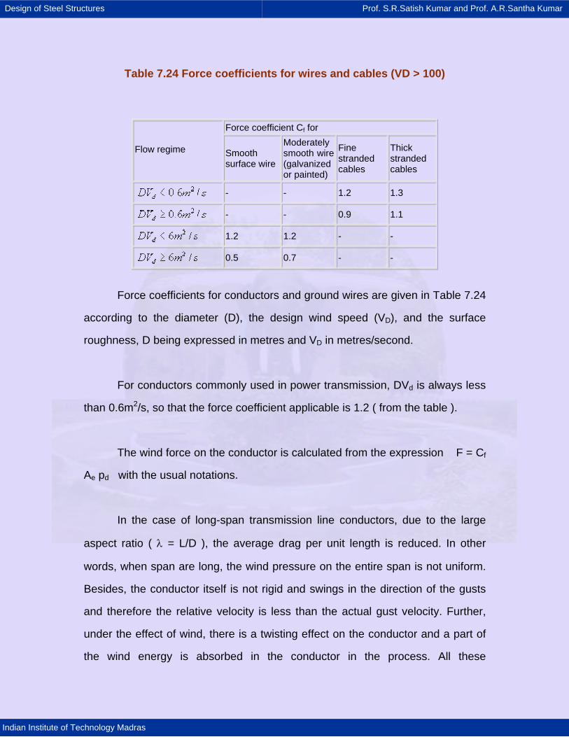
Design of Steel Structures Prof. S.R.Satish Kumar and Prof. A.R.Santha Kumar
Indian Institute of Technology Madras
Table 7.24 Force coefficients for wires and cables (VD > 100)
Force coefficient Cf for
Flow regime Smooth surface wire
Moderately smooth wire (galvanized or painted)
Fine stranded cables
Thick stranded cables
- - 1.2 1.3
- - 0.9 1.1
1.2 1.2 - -
0.5 0.7 - -
Force coefficients for conductors and ground wires are given in Table 7.24
according to the diameter (D), the design wind speed (VD), and the surface
roughness, D being expressed in metres and VD in metres/second.
For conductors commonly used in power transmission, DVd is always less
than 0.6m2/s, so that the force coefficient applicable is 1.2 ( from the table ).
The wind force on the conductor is calculated from the expression F = Cf
Ae pd with the usual notations.
In the case of long-span transmission line conductors, due to the large
aspect ratio ( λ = L/D ), the average drag per unit length is reduced. In other
words, when span are long, the wind pressure on the entire span is not uniform.
Besides, the conductor itself is not rigid and swings in the direction of the gusts
and therefore the relative velocity is less than the actual gust velocity. Further,
under the effect of wind, there is a twisting effect on the conductor and a part of
the wind energy is absorbed in the conductor in the process. All these
Design of Steel Structures Prof. S.R.Satish Kumar and Prof. A.R.Santha Kumar
Indian Institute of Technology Madras
considerations can be accounted for in a singlr factor called tha 'space factor',
which varies from 0.7 to 0.85; this factor decreases with increase in wind velocity
and span length.
The wind force F on the conductor may not be calculated from the
following expressions:
F = α Cf Ae pd
Where α is the space factor (0.7 to 0.85) and Cf ,Ae and pd have the usual
notations.
Maximum and minimum temperature charts
Knowledge of the maximum and the minimum temperatures of the area
traversed by a transmission line is necessary for calculating sags and tensions of
conductors and ground wires under different loading conditions. The maximum
and the minimum temperatures normally vary for different localities under
different diurnal and seasonal conditions.
IS: 802 (Part 1)-1977 (Second Revision) gives the absolute maximum and
minimum temperatures that are expected to prevail in different areas in the
country. The maximum temperature isopleths range from 37.5° to 50.0°C in steps
of 2.5° and the minimum temperature isopleths from -7.5° to 17.5° in steps of
2.5°.
The absolute maximum temperature values are increased by 17°C to
allow for the sun's radiation, heating effect of current, etc., in the conductor. In
Design of Steel Structures Prof. S.R.Satish Kumar and Prof. A.R.Santha Kumar
Indian Institute of Technology Madras
case the temperature-rise curves of conductors are readily available, the actual
rise in temperature in the conductor due to the heating effect of current for a
given line capacity is read from the curves and added to the absolute maximum-
temperature values. To the values thus arrived at, is added the rise in
temperature due to sun's radiation which is normally taken as 6° to 7°C for
conductors at temperatures below 40°C and 2° to 3°C for conductors at higher
temperatures.
Seismic effects
The force attracted by a structure during a seismic disturbance is a
function of the ground acceleration and the properties of the structure. The
seismic disturbance is essentially a dynamic phenomenon, and therefore
assuming an equivalent lateral static seismic force to simulate the earth- quake
effects is an oversimplification of the problem. However, allover the world, in
regions affected by earthquakes, the structures designed based on the
equivalent static approach have withstood the earthquake shocks satisfactorily,
which justifies the use of this method. The equivalent static method can be
derived from first principles from Newton's second law of motion thus:
Seismic lateral force P = Ma (7.16) a
= (W/g) a = W (a/g) (7.16) b
Where M = mass of the structure,
W = weight of the structure,
a = acceleration experienced by the structure due to earthquake, and
g = acceleration due to gravity.
Design of Steel Structures Prof. S.R.Satish Kumar and Prof. A.R.Santha Kumar
Indian Institute of Technology Madras
This force is dependent on a number of factors, the more important among
them being
. stiffness of the structure
. damping characteristics of the structure
. probability of a particular earthquake occurring at a particular site where
the structure is located
. Importance of the structure based on the consequences of failure
. foundation characteristics.
Incorporating the above variables in the form of coefficients, IS:1893-1975
gives the following formula for the calculation of horizontal equivalent seismic
force:
P = αHW in which αH = βlFo (Sa/g) (7.16c)
= βlαo (7.16d)
Where β = a coefficient depending on the soil- foundation system (Table of
the Code),
I = coefficient depending on the importance of structure (for transmission
towers this may be taken as 1.0),
Fo = seismic zone factor,
(Sa/g) = average acceleration coefficient which takes into account the
period of vibration of the structure and damping characteristics to be read from
Figure 7.20,
αH = Seismic coefficient, and
Design of Steel Structures Prof. S.R.Satish Kumar and Prof. A.R.Santha Kumar
Indian Institute of Technology Madras
αo = ad hoc basic seismic coefficient.
Seismic coefficients specified in IS: 1893-1975 are based on a number of
simplifying assumptions with regard to the degree of desired safety and the cost
of providing adequate earthquake resistance in structures. A maximum value of
αo = 0.08 has been adopted in the Code arbitrarily because the practice in
Assam before the code was introduced was to design structures for this value,
again fixed somewhat arbitrarily. The structures constructed with this seismic
coefficient have performed well and withstood the 1950 Assam earthquake (
Richter's Scale Magnitude 8.3).
For transmission line towers, the weight Wof the structure is low in
comparison with buildings. The natural period is such that the (Sa/g) value is
quite low (See Figure 7.20). Because the mass of the tower is low and the (Sa/g)
value is also low, the resultant earthquake force will be quite small compared to
the wind force normally considered for Indian conditions. Thus, earthquake
seldom becomes a governing design criterion.
Full-scale dynamic tests have been conducted by the Central Research
Institute of Electric Power Industry, Tokyo, on a transmission test line.6 In this
study, the natural frequency, mode shape and damping coefficient were obtained
separately for the foundation, the tower, and the tower-conductor coupled
system. Detailed response calculation of the test line when subjected to a
simulated EI Centro N-S Wave (a typical earthquake) showed that the tower
members could withstand severe earthquakes with instantaneous maximum
stress below yield point.
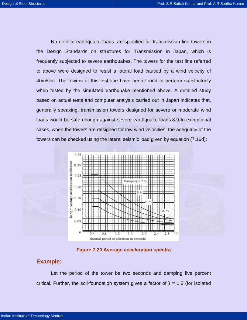
Design of Steel Structures Prof. S.R.Satish Kumar and Prof. A.R.Santha Kumar
Indian Institute of Technology Madras
No definite earthquake loads are specified for transmission line towers in
the Design Standards on structures for Transmission in Japan, which is
frequently subjected to severe earthquakes. The towers for the test line referred
to above were designed to resist a lateral load caused by a wind velocity of
40m/sec. The towers of this test line have been found to perform satisfactorily
when tested by the simulated earthquake mentioned above. A detailed study
based on actual tests and computer analysis carried out in Japan indicates that,
generally speaking, transmission towers designed for severe or moderate wind
loads would be safe enough against severe earthquake loads.8.9 In exceptional
cases, when the towers are designed for low wind velocities, the adequacy of the
towers can be checked using the lateral seismic load given by equation (7.16d):
Figure 7.20 Average acceleration spectra
Example:
Let the period of the tower be two seconds and damping five percent
critical. Further, the soil-foundation system gives a factor of β = 1.2 (for isolated
Design of Steel Structures Prof. S.R.Satish Kumar and Prof. A.R.Santha Kumar
Indian Institute of Technology Madras
footing) from Table 3 of 18:1893-1975. The importance factor for transmission
tower I = 1.00 (as per the Japanese method).
Referring to Figure 7.20, the spectral acceleration coefficient (Sa/g) =
0.06. Assuming that the tower is located in Assam (Zone V -from Figure 1 of
18:1893-1975 -8eismic Zones of India), the horizontal seismic coefficient
αH = βlFo (Sa/g)
= 1.2 x 1 x 0.4 x 0.06
= 0.0288
Therefore, the horizontal seismic force for a tower weighing 5,000kg is
P = αHW
= 0.0288 x 5,000
= 144 kg (quite small)
Broken-wire conditions
It is obvious that the greater the number of broken wires for which a
particular tower is designed, the more robust and heavier the tower is going to
be. On the other hand, the tower designed for less stringent broken-wire
conditions will be lighter and consequently more economical. It is clear therefore
that a judicious choice of the broken-wire conditions should be made so as to
achieve economy consistent with reliability.
The following broken-wire conditions are generally assumed in the design
of towers in accordance with 18:802 (Part 1)-1977:
Design of Steel Structures Prof. S.R.Satish Kumar and Prof. A.R.Santha Kumar
Indian Institute of Technology Madras
For voltage. up to 220 kV
Single:.circuit towers
It is assumed that either anyone power conductor is broken or one ground
wire is broken, whichever constitutes the more stringent condition for a particular
member.
Double-circuit towers
1. Tangent tower with suspension strings (0° to 2°):
It is assumed that either anyone power conductor is broken or one ground
wire is broken, whichever constitutes the more stringent condition for a particular
member.
2. Small angle towers with tension strings (2° to 15°) and medium angle
tower with tension strings (15°to30°):
It is assumed that either any two of the power conductors are broken on
the same side and on the same span or anyone of the power conductors and
anyone ground wire are broken on the same span, whichever combination is
more stringent for a particular member.
3. Large angle (30" to 60") and dead-end towers with tension strings:
It is assumed that either three power conductors are broken on the same
side and on the same span or that any two of the power conductors and anyone
ground wire are broken on the same span, whichever combination constitutes the
most stringent condition for a particular member.
Design of Steel Structures Prof. S.R.Satish Kumar and Prof. A.R.Santha Kumar
Indian Institute of Technology Madras
Cross-arms
In all types of towers, the power conductor sup- ports and ground wire
supports are designed for the broken-wire conditions.
For 400 k V line.
Single circuit towers (with two sub-conductors per phase)
1. Tangent towers with suspension strings (0° to 2°):
It is assumed that any ground wire or one sub-conductor from any bundle
conductor is broken, whichever is more stringent for a particular member.
The unbalanced pull due to the sub-conductor being broken may be
assumed as equa1 to 25 percent of the maximum working tension of all the sub-
conductors in one bundle.
2. Small angle tension towers (2° to 15°):
3. Medium angle tension towers (15° to 30°):
4. Large angle tension (30° to 60°) and dead-end towers:
It is assumed that any ground wire is broken or all sub-conductors in the
bundle are broken, whichever is more stringent for a particular member.
Double-circuit towers (with two sub-conductors per phase)
1. Tangent towers with suspension strings (0° to 2°):
It is assumed that all sub-conductors in the bundle are broken or any
ground wire is broken, whichever is more stringent for a particular member.
Design of Steel Structures Prof. S.R.Satish Kumar and Prof. A.R.Santha Kumar
Indian Institute of Technology Madras
2. Small-angle tension towers (2° to 15°):
3. Medium-angle tension towers (15° to 30°):
It is assumed that either two phase conductors (each phase comprising
two conductors) are broken on the same side and on the same s pan, or anyone
phase and anyone ground wire is broken on the same span, whichever
combination is more stringent for a particular member.
4. Large-angle tension (30° to 60°) and Dead-end towers:
It is assumed that either all the three phases on the same side and on the
same span are bro- ken, or two phases and anyone ground wire on the same
span is broken, whichever combination is more stringent for a particular member.
500 k V HVDC bipole
During the seventh plan period (1985-90), a 500 kV HVDC bipole line
with four subconductors has been planned for construction from Rihand to Delhi
(910km). The following bro- ken-wire conditions have been specified for this line:
1. Tangent towers (0°):
This could take up to 2° with span reduction. It is assumed that either one
pole or one ground wire is broken, whichever is more stringent for a particular
member.
Design of Steel Structures Prof. S.R.Satish Kumar and Prof. A.R.Santha Kumar
Indian Institute of Technology Madras
2. Small-angle towers (0° to 15°):
It is assumed that either there is breakage of all the subconductors of the
bundle in one pole or one ground wire, whichever is more stringent.
When used as an anti-cascading tower (tension tower for uplift forces)
with suspension insulators, all conductors and ground wires are assumed to be
broken in one span.
3. Medium-angle towers (15° to 30°):
It is assumed that either one phase or one ground wire is broken,
whichever is more stringent.
4. Large-angle towers 30° to 60° and dead-end towers:
It is assumed that all conductors and ground wires are broken on one
side.
It would be useful to review briefly the practices regarding the broken-wire
conditions assumed in the USSR, where extensive transmission net- works at
various voltages, both A.C.and D.C., have been developed and considerable
experience in the design, construction and operation of networks in widely
varying climatic conditions has been acquired.
For suspension supports, under the conductor broken conditions, the
conductors of one phase are assumed to be broken, irrespective of the number
of conductors on the support, producing the maxi- mum stresses on the support;
and under the ground wire broken condition, one ground wire is assumed to be
broken, which produces the maximum stresses with the phase conductors intact.
Design of Steel Structures Prof. S.R.Satish Kumar and Prof. A.R.Santha Kumar
Indian Institute of Technology Madras
For anchor supports, any two phase conductors are assumed to be
broken (ground wire remaining intact) which produce the maximum stresses on
the support, and the ground wire bro- ken conditions (with the conductors intact)
are the same as in the case of suspension supports.
The broken-wire conditions specified for a tower also take into account the
type of conductor clamps used on the tower. For example, if 'slip' type clamps
are used on the line, the towers are not designed for broken-wire conditions,
even for 220 kV, 330 kV and 500 kV lines.
The designs of anchor supports are also checked for the erection
condition corresponding to only' one circuit being strung in one span, irrespective
of the number of circuits on the support, the ground wires being not strung, as
well as for the erection condition corresponding to the ground wires being strung
in one span of the support, the conductors being not strung. In checking the
designs for erection conditions, the temporary strengthening of individual
sections of supports and the installation of temporary guys are also taken into
account.
In the case of cross-arms, in addition to the weight of man and tackle, the
designs are checked up for the loadings corresponding to the method of erection
and the additional loadings due to erection devices.
7.3.3 Loadings and load combinations
The loads on a transmission line tower consist of three mutually
perpendicular systems of loads acting vertical, normal to the direction of the line,
and parallel to the direction of the line.
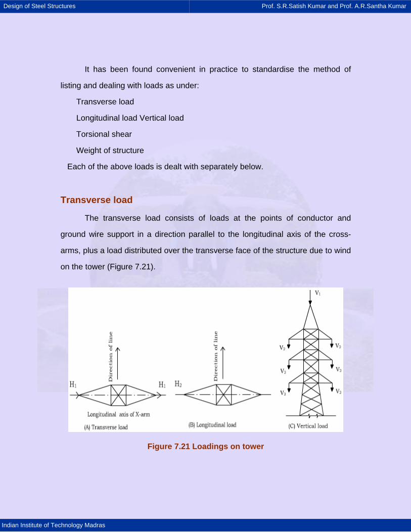
Design of Steel Structures Prof. S.R.Satish Kumar and Prof. A.R.Santha Kumar
Indian Institute of Technology Madras
It has been found convenient in practice to standardise the method of
listing and dealing with loads as under:
Transverse load
Longitudinal load Vertical load
Torsional shear
Weight of structure
Each of the above loads is dealt with separately below.
Transverse load
The transverse load consists of loads at the points of conductor and
ground wire support in a direction parallel to the longitudinal axis of the cross-
arms, plus a load distributed over the transverse face of the structure due to wind
on the tower (Figure 7.21).
Figure 7.21 Loadings on tower
Design of Steel Structures Prof. S.R.Satish Kumar and Prof. A.R.Santha Kumar
Indian Institute of Technology Madras
Transverse load due to wind on conductors and ground wire
The conductor and ground wire support point loads are made up of the
following components:
1. Wind on the bare (or ice-covered) conductor/ground wire over the wind
span and wind on insulator string.
2. Angular component of line tension due to an angle in the line (Figure 7.22).
The wind span is the sum of the two half spans adjacent to the support
under consideration. The governing direction of wind on conductors for an angle
condition is assumed to be parallel to the longitudinal axis of the cross-arms
(Figure 7.23). Since the wind is blowing on reduced front, it could be argued that
this reduced span should be used for the wind span. In practice, however, since
the reduction in load would be relatively small, it is usual to employ the full span.
In so far as twin-conductor bundle in horizontal position (used for lines at
400 k V) is concerned, it has been found that the first sub-conductor in each
phase does not provide any shielding to the second sub-conductor. Accordingly,
the total wind load for bundled conductors is assumed as the sum total of wind
load on each sub-conductor in the bundle.
Under broken-wire conditions, 50 percent of the nonnal span and 10
percent of the broken span is assumed as wind span.
Design of Steel Structures Prof. S.R.Satish Kumar and Prof. A.R.Santha Kumar
Indian Institute of Technology Madras
Wind load on conductor
Wind load on conductors and ground wire along with their own weight
produces a resultant force, which is calculated as follows. The calculation covers
the general case of an ice-coated conductor:
Let d be the diameter of conductor in mm and t the thickness of ice coating
in mm (Figure 7.24).
Then, weight of ice coating on I-metre length of conductor,
( )2 21 6
1W d 2t d x x 900kg4 10π ⎡ ⎤= + −
⎣ ⎦ (7.17a)
(Ice is assumed to weigh 900 kg/m3)
Weight per metre length of ice-coated conductor
W = w +w1
Where w = weight of bare conductor per metre length, and
w1 = weight of ice coating per metre length.
Horizontal wind load on ice-coated conductor per metre length,
( )d 2t2P x p kg3 1000
+= (7.17b)
Where p = wind pressure in kg/m2 on two-thirds the projected area of
conductor.
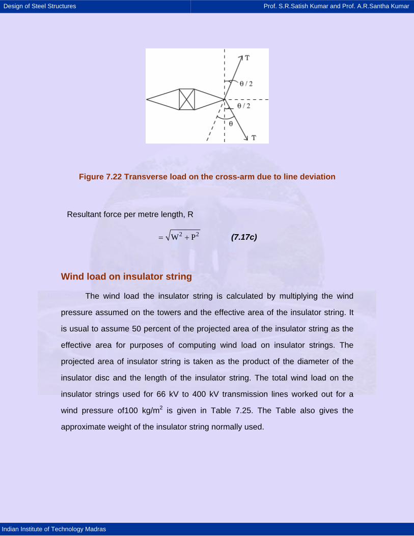
Design of Steel Structures Prof. S.R.Satish Kumar and Prof. A.R.Santha Kumar
Indian Institute of Technology Madras
Figure 7.22 Transverse load on the cross-arm due to line deviation
Resultant force per metre length, R
2 2W P= + (7.17c)
Wind load on insulator string
The wind load the insulator string is calculated by multiplying the wind
pressure assumed on the towers and the effective area of the insulator string. It
is usual to assume 50 percent of the projected area of the insulator string as the
effective area for purposes of computing wind load on insulator strings. The
projected area of insulator string is taken as the product of the diameter of the
insulator disc and the length of the insulator string. The total wind load on the
insulator strings used for 66 kV to 400 kV transmission lines worked out for a
wind pressure of100 kg/m2 is given in Table 7.25. The Table also gives the
approximate weight of the insulator string normally used.
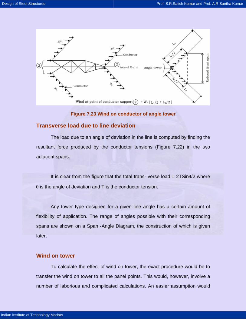
Design of Steel Structures Prof. S.R.Satish Kumar and Prof. A.R.Santha Kumar
Indian Institute of Technology Madras
Figure 7.23 Wind on conductor of angle tower
Transverse load due to line deviation
The load due to an angle of deviation in the line is computed by finding the
resultant force produced by the conductor tensions (Figure 7.22) in the two
adjacent spans.
It is clear from the figure that the total trans- verse load = 2TSinθ/2 where
θ is the angle of deviation and T is the conductor tension.
Any tower type designed for a given line angle has a certain amount of
flexibility of application. The range of angles possible with their corresponding
spans are shown on a Span -Angle Diagram, the construction of which is given
later.
Wind on tower
To calculate the effect of wind on tower, the exact procedure would be to
transfer the wind on tower to all the panel points. This would, however, involve a
number of laborious and complicated calculations. An easier assumption would
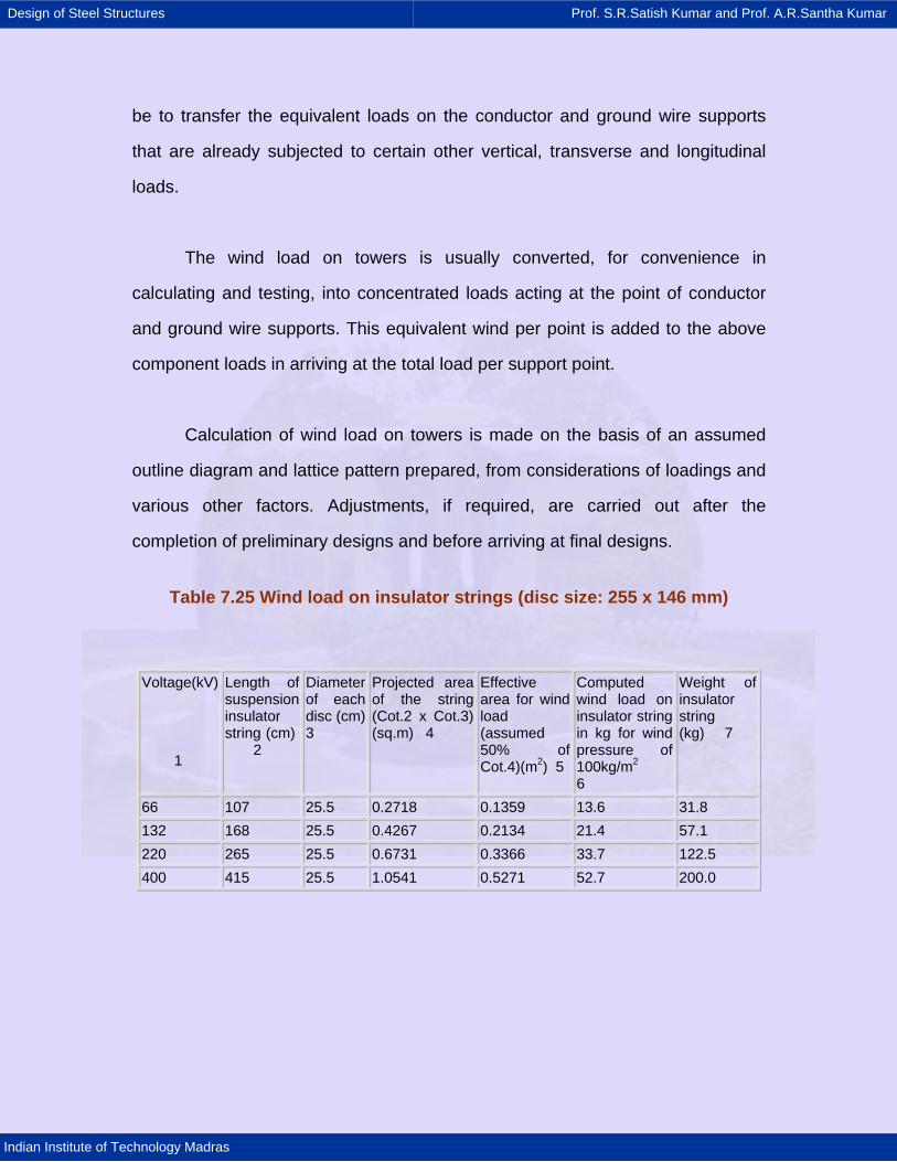
Design of Steel Structures Prof. S.R.Satish Kumar and Prof. A.R.Santha Kumar
Indian Institute of Technology Madras
be to transfer the equivalent loads on the conductor and ground wire supports
that are already subjected to certain other vertical, transverse and longitudinal
loads.
The wind load on towers is usually converted, for convenience in
calculating and testing, into concentrated loads acting at the point of conductor
and ground wire supports. This equivalent wind per point is added to the above
component loads in arriving at the total load per support point.
Calculation of wind load on towers is made on the basis of an assumed
outline diagram and lattice pattern prepared, from considerations of loadings and
various other factors. Adjustments, if required, are carried out after the
completion of preliminary designs and before arriving at final designs.
Table 7.25 Wind load on insulator strings (disc size: 255 x 146 mm)
Voltage(kV)
1
Length of suspension insulator string (cm) 2
Diameter of each disc (cm) 3
Projected area of the string (Cot.2 x Cot.3) (sq.m) 4
Effective area for wind load (assumed 50% of Cot.4)(m2) 5
Computed wind load on insulator string in kg for wind pressure of 100kg/m2
6
Weight of insulator string (kg) 7
66 107 25.5 0.2718 0.1359 13.6 31.8 132 168 25.5 0.4267 0.2134 21.4 57.1 220 265 25.5 0.6731 0.3366 33.7 122.5 400 415 25.5 1.0541 0.5271 52.7 200.0
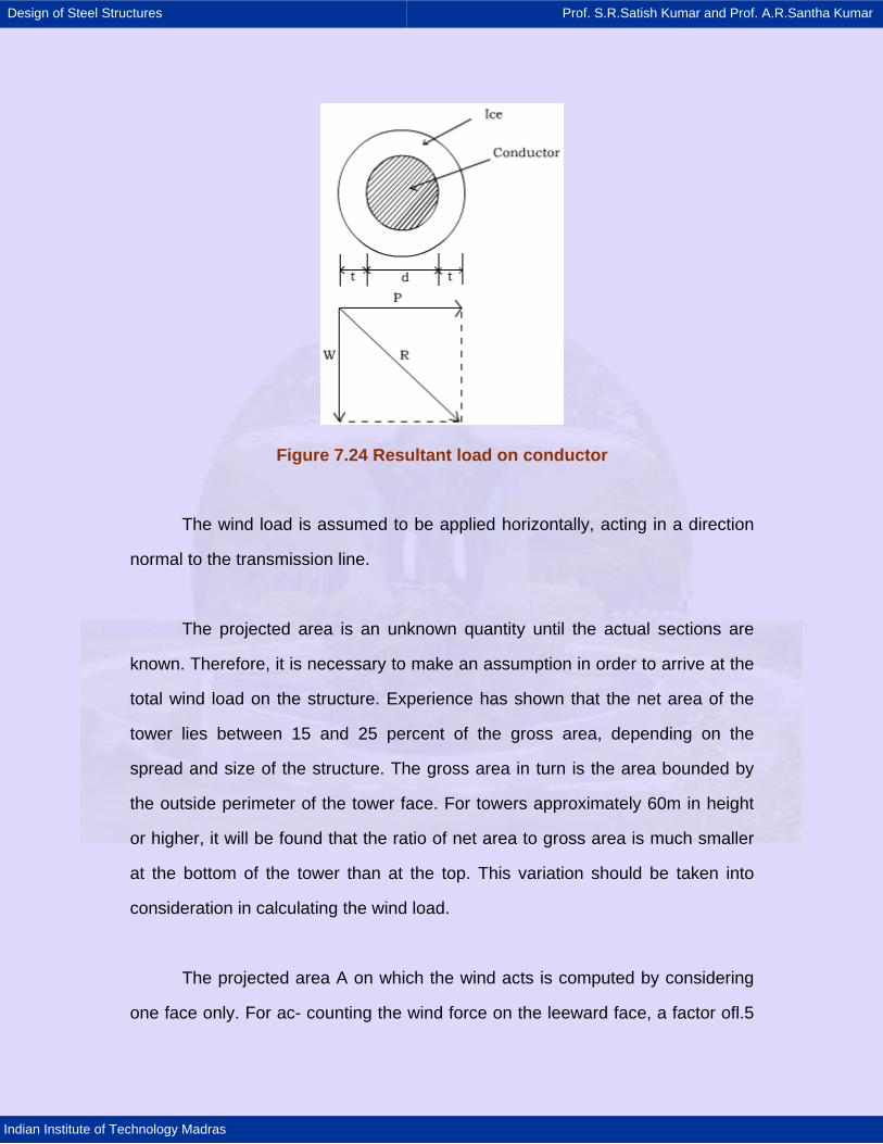
Design of Steel Structures Prof. S.R.Satish Kumar and Prof. A.R.Santha Kumar
Indian Institute of Technology Madras
Figure 7.24 Resultant load on conductor
The wind load is assumed to be applied horizontally, acting in a direction
normal to the transmission line.
The projected area is an unknown quantity until the actual sections are
known. Therefore, it is necessary to make an assumption in order to arrive at the
total wind load on the structure. Experience has shown that the net area of the
tower lies between 15 and 25 percent of the gross area, depending on the
spread and size of the structure. The gross area in turn is the area bounded by
the outside perimeter of the tower face. For towers approximately 60m in height
or higher, it will be found that the ratio of net area to gross area is much smaller
at the bottom of the tower than at the top. This variation should be taken into
consideration in calculating the wind load.
The projected area A on which the wind acts is computed by considering
one face only. For ac- counting the wind force on the leeward face, a factor ofl.5
Design of Steel Structures Prof. S.R.Satish Kumar and Prof. A.R.Santha Kumar
Indian Institute of Technology Madras
is used in accordance with the relevant provision of the Indian Electricity Rules,
1956. The wind load on the tower, for the purpose of analysis, is assumed to act
at selected points, generally at the cross-arm and also at the waist in the case of
corset type towers. One of the following methods is adopted to determine the
magnitude of loads applicable at the aforesaid selected points. Figure 7.25 gives
the framework of a tower with reference to which the methods are explained.
Method 1
The wind loads are first calculated for various members or parts of the
tower. Thereafter, the moments of all these loads taken about the tower base are
added together. The total load moment so obtained is replaced by an equivalent
moment assuming that equal loads are applied at the selected points.
Method 2
The loads applied on the bottom cross-arms are increased with
corresponding reduction in the loads applied on the upper cross-arms.
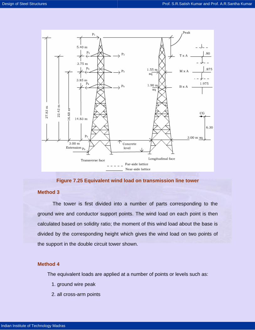
Design of Steel Structures Prof. S.R.Satish Kumar and Prof. A.R.Santha Kumar
Indian Institute of Technology Madras
Figure 7.25 Equivalent wind load on transmission line tower
Method 3
The tower is first divided into a number of parts corresponding to the
ground wire and conductor support points. The wind load on each point is then
calculated based on solidity ratio; the moment of this wind load about the base is
divided by the corresponding height which gives the wind load on two points of
the support in the double circuit tower shown.
Method 4
The equivalent loads are applied at a number of points or levels such as:
1. ground wire peak
2. all cross-arm points
Design of Steel Structures Prof. S.R.Satish Kumar and Prof. A.R.Santha Kumar
Indian Institute of Technology Madras
3. waist level (also portal base level if desired) in the case of corset type
towers.
The wind loads on different parts of the tower are determined by choosing
an appropriate solidity ratio. Out of the load on each part, an equivalent part (that
is, a part load which produces an equal moment at the base of that part) is
transferred to the upper loading point and the remaining part to the base. This
process is repeated for the various parts of the tower from the top downwards.
It can be seen that the load distribution in Method 4 is based on a logical
approach in which importance is given not only to moment equivalence but also
to shear equivalence at the base. Thus Method 4 is considered to be superior to
others. A typical wind load calculation based on this method is given in Figure
7.26. Table 7.26 compares the wind loads arrived at by the four methods.
Although the design wind load based on method 4 is higher than that in the
other-three methods, it is still lower than the actual load (2,940kg).
A realistic approach is to apply the wind load at each node of the tower.
This is practically impossible when calculations are done manually. How- ever,
while this could be handled quite satisfactorily in a computer analysis, the
representation of wind load in prototype tower tests poses problems. Therefore,
the current practice is to adopt Method 4 in computer analysis and design, which
are also being validated by prototype tests. Further research is needed for
satisfactory representation of forces due to wind on tower during tests if the
actual wind load which can be accounted for in computer analysis is to be
simulated.
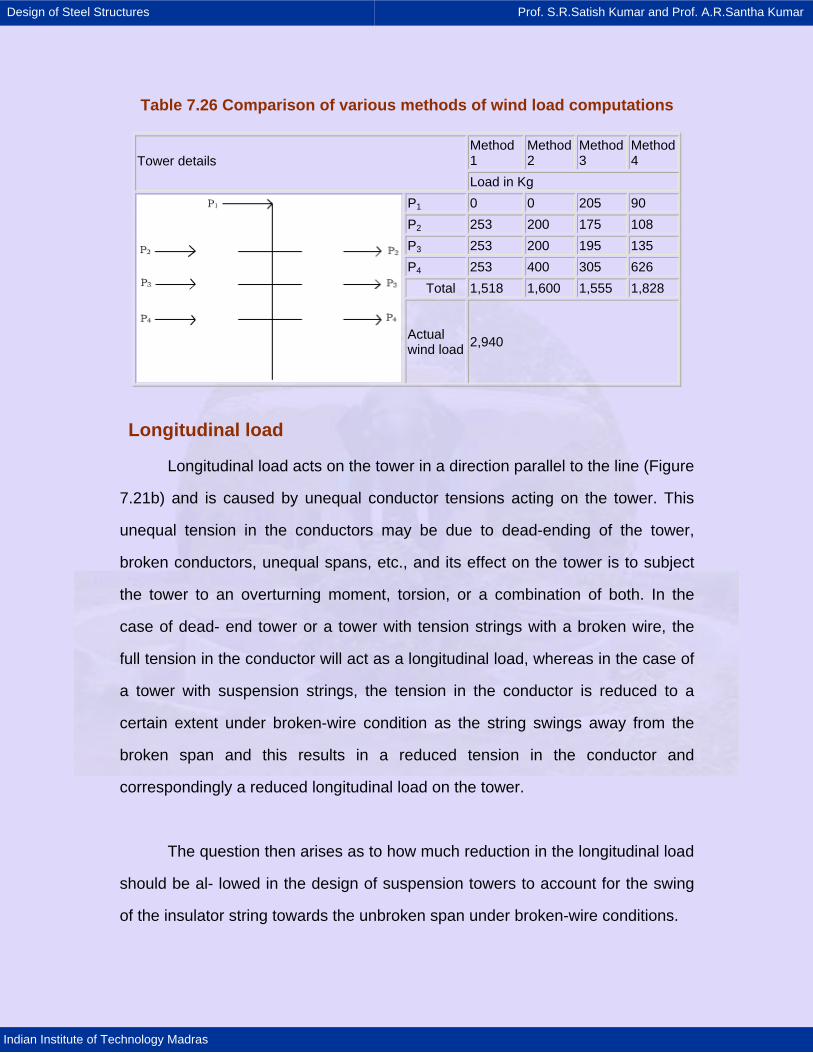
Design of Steel Structures Prof. S.R.Satish Kumar and Prof. A.R.Santha Kumar
Indian Institute of Technology Madras
Table 7.26 Comparison of various methods of wind load computations
Method 1
Method 2
Method 3
Method 4 Tower details
Load in Kg P1 0 0 205 90 P2 253 200 175 108 P3 253 200 195 135 P4 253 400 305 626 Total 1,518 1,600 1,555 1,828
Actual wind load 2,940
Longitudinal load
Longitudinal load acts on the tower in a direction parallel to the line (Figure
7.21b) and is caused by unequal conductor tensions acting on the tower. This
unequal tension in the conductors may be due to dead-ending of the tower,
broken conductors, unequal spans, etc., and its effect on the tower is to subject
the tower to an overturning moment, torsion, or a combination of both. In the
case of dead- end tower or a tower with tension strings with a broken wire, the
full tension in the conductor will act as a longitudinal load, whereas in the case of
a tower with suspension strings, the tension in the conductor is reduced to a
certain extent under broken-wire condition as the string swings away from the
broken span and this results in a reduced tension in the conductor and
correspondingly a reduced longitudinal load on the tower.
The question then arises as to how much reduction in the longitudinal load
should be al- lowed in the design of suspension towers to account for the swing
of the insulator string towards the unbroken span under broken-wire conditions.
Design of Steel Structures Prof. S.R.Satish Kumar and Prof. A.R.Santha Kumar
Indian Institute of Technology Madras
The general practice followed in India is to assume the unbalanced pull
due to a broken conductor as equal to 50 percent of the maximum working
tension of the conductor.
In this practice, as in the practices of other countries, the longitudinal load
is somewhat arbitrarily fixed in the tower design. However, it is now possible
through computer programs to calculate the actual longitudinal loads during the
construction of the line, taking into account the effective span lengths of the
section (between angle towers), the positioning of insulator strings, and the
resulting deformations of supports, thus enabling a check on the proper choice of
supports.
For the ground wire broken condition, 100 percent of the maximum
working tension is considered for design purposes.
The unbalanced pull due to a broken conductor/ground wire in the case of
tension strings is assumed equal to the component of the maximum working
tension of the conductor or the ground wire, as the case may be, in the
longitudinal direction along with its components in the transverse direction. This
is taken for the maximum as well as the minimum angle of deviation for which the
tower is designed and the condition, which is most stringent for a member, is
adopted. The forces due to impact, which arises due to breaking, are assumed to
be covered by the factor of safety allowed in the designs.
When there is a possibility of the tower being used with a longer span by
reducing the angle of line deviation, the tower member should also be checked
Design of Steel Structures Prof. S.R.Satish Kumar and Prof. A.R.Santha Kumar
Indian Institute of Technology Madras
for longitudinal and transverse components arising out of the reduced angle .of
line deviation.
Vertical load
Vertical load is applied to the ends of the cross- arms and on the ground
wire peak (Figure 7.21c) and consists of the following vertical downward
components:
1. Weight of bare or ice-covered conductor, as specified, over the governing
weight span.
2. Weight of insulators, hardware, etc., covered with ice, if applicable.
3. Arbitrary load to provide for the weight of a man with tools.
In addition to the above downward loads, any tower, which will be
subjected to uplift, must have an upward load applied to the conductor support
points. While the first two components can be evaluated quite accurately, a
provision of 150 kg is generally made for the weight of a lineman with tools (80
kg for the weight of man and 70 kg for tools).
Another uncertain factor that arises is the extra load to be allowed in the
design over and above the normal vertical load, to enable the tower to be used
with weight spans larger than the normal spans for which it is designed (in other
words, the choice of a suitable weight span for which the tower is to be
designed). It is not possible for the designer to make an assumption regarding
the weight span unless he has a fairly accurate knowledge of the terrain over
which the line has to pass; and therefore the economic weight span will be
different for different types of terrain.
Design of Steel Structures Prof. S.R.Satish Kumar and Prof. A.R.Santha Kumar
Indian Institute of Technology Madras
An allowance of 50 percent over the normal vertical load is considered to
be quite adequate to cover the eventuality of some of the towers being used with
spans larger than the normal spans. This slight increase in the design vertical
load will not affect the line economy to an appreciable extent, as the contribution
of vertical loads towards the total load on the tower members is small. However,
where the lines have to run through hilly and rugged terrain, a higher provision is
made, depending on the nature of the terrain. The Canadian practice usually
makes an allowance of 100 percent over the normal vertical load; this large
allowance is probably due to the rugged and hilly terrain encountered in the
country. It should be noted that, for the design of uplift foundations and
calculation of tensile stress in corner legs and also in some members of the
structure, the worst condition for the design is that corresponding to the minimum
weight span.
Weight of structure
The weight of the structure, like the wind on the structure, is an unknown
quantity until the actual design is complete. However, in the design of towers, an
assumption has to be made regarding the dead weight of towers. The weight will
no doubt depend on the bracing arrangement to be adopted, the strut formula to
be used and the quality or qualities of steel used, whether the design is a
composite one comprising both mild steel and high tensile steel or makes use of
mild steel only. However, as a rough approximation, it is possible to estimate the
probable tower weight from knowledge of the positions of conductors and ground
wire above ground level and the overturning moments. Ryle has evolved an
empirical formula giving the approximate weight of any tower in terms of its
height and maximum working over- turning moment at the base. The tower
weight is represented by
Design of Steel Structures Prof. S.R.Satish Kumar and Prof. A.R.Santha Kumar
Indian Institute of Technology Madras
W = KH M (7.18)
Where W = weight of tower above ground level in kg,
H = overall height of the tower above ground level in metres,
M = overturning moment at ground level, in kg m (working loads), and
K = a constant which varies within a range of 0.3970 to 0.8223.
The towers investigated covered ranges of about 16 to 1 in height, 3,000
to 1 in overturning moment, and 1,200 to 1 in tower weight.
A reliable average figure for tower weight may be taken as 0.4535 H M kg,
for nearly all the towers studied have weights between 0.3970 H M and 0.5103
H M tonnes. Ryle points out that any ordinary transmission line tower (with
vertical or triangular configuration of conductors) giving a weight of less than,
say, 0.3686 H M may be considered inadequate in design and that any tower
weighing more than, say, 0.567 H M must be of uneconomic design.
In the case of towers with horizontal configuration of conductors, the
coefficient K lies in the range of 0.5103 to 0.6748. Ryle recommends that the
average weight of such towers may be represented by 0.6238H M kg.
Values of K for heavy angle towers tend to be less than for straight-line
towers. This is due to the fact that on a tower with a wider base-angle it is easier
to direct the leg lines towards the load centre of gravity. Values of K tend to be
higher the larger the proportion of the tower represented by cross-arms or 'top
hamper'.
The weight of a river-crossing suspension tower with normal cross-arms
lies between 0.4820 H M for towers of about 35 metres in height, and 0.7088
Design of Steel Structures Prof. S.R.Satish Kumar and Prof. A.R.Santha Kumar
Indian Institute of Technology Madras
H M for very tall towers of height 145 metres. Towers with special 'top-hamper'
or long-span terminal-type towers may be 10-20 percent heavier.
The tower weights given by these formulae are sufficiently accurate for
preliminary estimates. The formulae are also found to be extremely useful in
determining the economic span length and general line estimates including
supply, transport and erection of the tower.
It is obvious that, when the height of the upper ground wire is raised, the
conductors being kept at the same height, the weight of the tower does not
increase in proportion to the height of the ground wire alone. Taking this factor
into consideration, Ailleret has proposed the presentation of Ryle's fonnula in the
form PH . While this is more logical, Ryle's formula is simpler, and for general
estimating purposes, sufficiently accurate.
In Ryle's formula, safe external loads acting on a tower are used as
against ultimate loads generally adopted for design as per IS:802(Part 1)- 1977.
Since the factor of safety applied for normal conditions is 2.0, the Ryle's equation
is not directly applicable if the tower weight is calculated based on loads
determined as per the above Code. In this case the following formulae are
applicable.
For suspension towers,
W = 0.1993 H M + 495 (7.19)
For angle towers
W = 0.2083 H M + 400 (7.20)
Design of Steel Structures Prof. S.R.Satish Kumar and Prof. A.R.Santha Kumar
Indian Institute of Technology Madras
Since there is no appreciable difference in the above two equations, the
common equation given below may be used for both the tower types:
W = 0.205 H M + 450 (7.21)
A more detailed evaluation of tower weight due to Walter BIlckner is
presented below. This is based on the principle of summing up the minimum
weight of struts panel by panel.
The minimum weight of a single strut is given by
K
Pw Al l= γ = γσ
(7.22)
Where A is the cross-section of strut,
l is the unsupported length,
γ is the density, and
P is the compression load on strut
For a given compression load P and unsupported length l, the lightest
angle section is that which permits the highest crippling stress σK. For
geometrically similar sections
( )K C P / lσ = (7.23)
Where C is a constant
Taking the factor ( )P / l as a reference, the crippling stresses of all
geometrically similar sections for any compression loadings and strut lengths can
be plotted as curves, which enable the characteristics of the various sections to
be clearly visualised.
Design of Steel Structures Prof. S.R.Satish Kumar and Prof. A.R.Santha Kumar
Indian Institute of Technology Madras
At the higher values of ( )P / l , high-tensile steels (for example, St 52) are
economical. This applies especially with staggered strutting, in which the
maximum moment of inertia is utilised.
The theoretical minimum weight of the complete tower wm is given by the
sum of the weights of the members according to equation (7.22). The weight gm
per metre of tower height for one panel is
m zE K
lPg glγ
= +σ∑ (7.24)
Where n = number of members,
P = truss force,
gz = additional weight of bolts, etc. per. metre of tower height, and
lE = equivalent height of panel.
If this expression is integrated from x = 0 to x = h, we get the weight of the
tower body GT with leg members of St 52 roughly in kilograms without cross-
arms, etc:
( )2
3 23 2TT m 0
0 b b
Mh QG Q 4.4 b b2b
⎛ ⎞= + + −⎜ ⎟⎜ ⎟∆ ∆⎝ ⎠
(7.25)
Where h = height of tower from the top crossarm to ground level in metres,
Q = Mbmax / h; Mb= maximum normal mo- ment at ground level (x = h) in
tonne- metres,
bo = tower width at the top cross-arm (x = 0) in metres,
bm = tower width at ground level (x = h) in metres,
∆b= taper in metres/metre, and
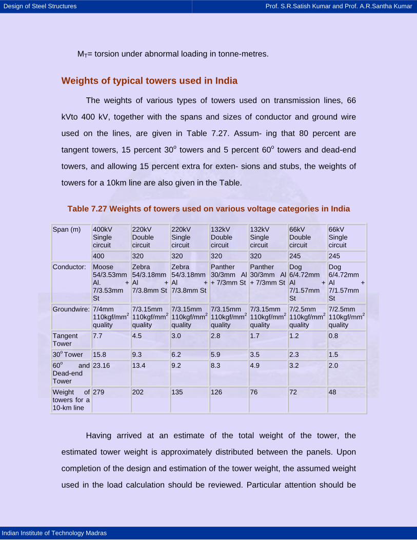
Design of Steel Structures Prof. S.R.Satish Kumar and Prof. A.R.Santha Kumar
Indian Institute of Technology Madras
MT= torsion under abnormal loading in tonne-metres.
Weights of typical towers used in India
The weights of various types of towers used on transmission lines, 66
kVto 400 kV, together with the spans and sizes of conductor and ground wire
used on the lines, are given in Table 7.27. Assum- ing that 80 percent are
tangent towers, 15 percent 30o towers and 5 percent 60o towers and dead-end
towers, and allowing 15 percent extra for exten- sions and stubs, the weights of
towers for a 10km line are also given in the Table.
Table 7.27 Weights of towers used on various voltage categories in India
400kV Single circuit
220kV Double circuit
220kV Single circuit
132kV Double circuit
132kV Single circuit
66kV Double circuit
66kV Single circuit
Span (m)
400 320 320 320 320 245 245 Conductor: Moose
54/3.53mm Al. + 7/3.53mm St
Zebra 54/3.18mm Al + 7/3.8mm St
Zebra 54/3.18mm Al + 7/3.8mm St
Panther 30/3mm Al + 7/3mm St
Panther 30/3mm Al + 7/3mm St
Dog 6/4.72mm Al + 7/1.57mm St
Dog 6/4.72mm Al + 7/1.57mm St
Groundwire: 7/4mm 110kgf/mm2 quality
7/3.15mm 110kgf/mm2
quality
7/3.15mm 110kgf/mm2
quality
7/3.15mm 110kgf/mm2
quality
7/3.15mm 110kgf/mm2
quality
7/2.5mm 110kgf/mm2 quality
7/2.5mm 110kgf/mm2
quality Tangent Tower
7.7 4.5 3.0 2.8 1.7 1.2 0.8
30o Tower 15.8 9.3 6.2 5.9 3.5 2.3 1.5 60o and Dead-end Tower
23.16 13.4 9.2 8.3 4.9 3.2 2.0
Weight of towers for a 10-km line
279 202 135 126 76 72 48
Having arrived at an estimate of the total weight of the tower, the
estimated tower weight is approximately distributed between the panels. Upon
completion of the design and estimation of the tower weight, the assumed weight
used in the load calculation should be reviewed. Particular attention should be
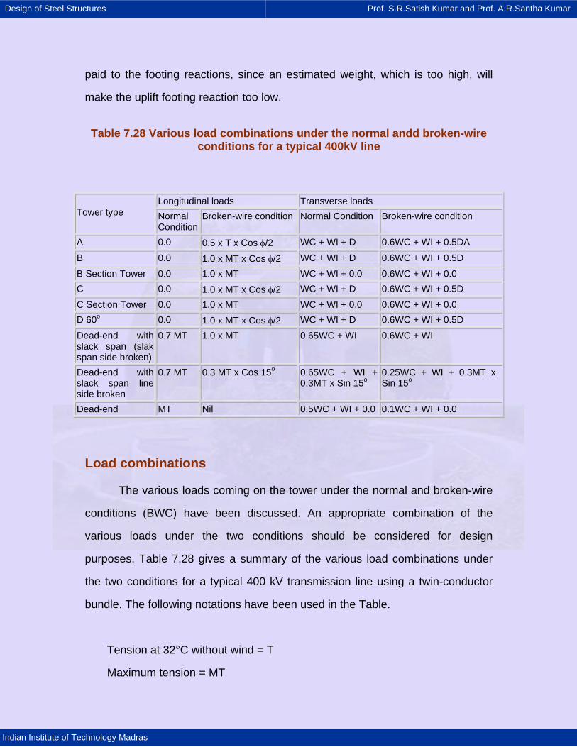
Design of Steel Structures Prof. S.R.Satish Kumar and Prof. A.R.Santha Kumar
Indian Institute of Technology Madras
paid to the footing reactions, since an estimated weight, which is too high, will
make the uplift footing reaction too low.
Table 7.28 Various load combinations under the normal andd broken-wire conditions for a typical 400kV line
Longitudinal loads Transverse loads Tower type Normal
Condition Broken-wire condition Normal Condition Broken-wire condition
A 0.0 0.5 x T x Cos φ/2 WC + WI + D 0.6WC + WI + 0.5DA B 0.0 1.0 x MT x Cos φ/2 WC + WI + D 0.6WC + WI + 0.5D B Section Tower 0.0 1.0 x MT WC + WI + 0.0 0.6WC + WI + 0.0 C 0.0 1.0 x MT x Cos φ/2 WC + WI + D 0.6WC + WI + 0.5D C Section Tower 0.0 1.0 x MT WC + WI + 0.0 0.6WC + WI + 0.0 D 60o 0.0 1.0 x MT x Cos φ/2 WC + WI + D 0.6WC + WI + 0.5D Dead-end with slack span (slak span side broken)
0.7 MT 1.0 x MT 0.65WC + WI 0.6WC + WI
Dead-end with slack span line side broken
0.7 MT 0.3 MT x Cos 15o 0.65WC + WI + 0.3MT x Sin 15o
0.25WC + WI + 0.3MT x Sin 15o
Dead-end MT Nil 0.5WC + WI + 0.0 0.1WC + WI + 0.0
Load combinations
The various loads coming on the tower under the normal and broken-wire
conditions (BWC) have been discussed. An appropriate combination of the
various loads under the two conditions should be considered for design
purposes. Table 7.28 gives a summary of the various load combinations under
the two conditions for a typical 400 kV transmission line using a twin-conductor
bundle. The following notations have been used in the Table.
Tension at 32°C without wind = T
Maximum tension = MT
Design of Steel Structures Prof. S.R.Satish Kumar and Prof. A.R.Santha Kumar
Indian Institute of Technology Madras
Wind on conductor = WC
Wind on insulator = WI
Angle of deviation = φ
Load due to deviation of 'A' type tower under BWC = DA = 2 x T x Sin (φ / 2)
Load due to deviation for others = D = 2 x MT x Sin (φ / 2)
The vertical loads due to conductors and ground wire are based on the
appropriate weight spans; these are in addition to the dead weight of the
structure, insulators and fittings.
Example:
Calculation of tower loading for a typical 132 kV double circuit line.
Basic data
1. Type of tower: Tangent tower with 2 degrees line deviation
2. Nonnal span: 335 m
2. Wind pressure
a. Tower (on 11/2 times the exposed area of one face): 200 kg/m2
b. Conductors and ground wire (on fully projected area): 45 kg/m2
Characteristics of conductor
1. Size conforming to : 30/3.00mmAl+7/3.00mm
IS:398-1961 St ACSR
Design of Steel Structures Prof. S.R.Satish Kumar and Prof. A.R.Santha Kumar
Indian Institute of Technology Madras
2. Overall diameter
of the conductor : 21 mm
3. Area of the complete
conductor : 26.2 mm2
4. Ultimate tensile
strength : 9,127 kg
5. Weight : 976 kg/m
6. Maximum working
tension : 3,800 kg (say)
Characteristics of ground wire
1. Size conforming to : 7/3.15 mm galvanised
IS: 2141-1968
Stranded steel wire of 110 kgf/mm2 quality
2. Diameter : 9.45 mm
3. Area of complete : 54.5 mm2
ground wire
4. Ultimate tensile : 5,710 kg
strength
Design of Steel Structures Prof. S.R.Satish Kumar and Prof. A.R.Santha Kumar
Indian Institute of Technology Madras
5. Weight : 428 kg/km
6. Maximum working
tension : 2,500 kg (say)
Tower loadings:
1. Transverse load
For the purpose of calculating the wind load on conductor and ground
wire, the wind span has been assumed as normal span.
a. Wind load on conductor (Normal condition) = 335 x45 x 21 / 1,000
= 317 kg
Wind load on conductor (broken-wire condition) = 0.6x317= 190 kg
b. Wind load on ground wire (Normal condition) = 335 x 9.45 x45 / 1,000
= 142 kg
Wind load on ground wire (Broken-wire condition) = 0.6 x 142 = 85 kg
c. Wind load on tower
The details in regard to the method of calculating the equivalent wind load
on tower (We) are given in Figure 6.26.
d. Wind load on insulator string.
Diameter of the insulator skirt = 254 mm
Length of the insulator string with arcing horns = 2,000 mm
Design of Steel Structures Prof. S.R.Satish Kumar and Prof. A.R.Santha Kumar
Indian Institute of Technology Madras
Projected area of the cylinder with diameter equal to that of the nsulator skirt
= 2,000 x 254 sq. mm
= 0.508 sq. m.
Net effective projected area of the insulator string exposed to wind = 50
percent of 0.508 sq.m.
= 0.254 sq.m.
Wind load on insulator string = 200 x 0.254
= 50.8 kg
Say 50 kg
e. Transverse component of the maximum working tension (deviation load)
(1) For power conductor = 2 x sin 10 x 3,800 kg
= 133 kg
(2) For ground wire = 2 x sin 10 x 2,500 kg
= 87 kg
f. Deviation loads under the broken-wire condition
(1) Conductor point = 3,800 x sin 1o x 0.5
= 33 kg
(2) Ground wire point = 2,500 x sin 1o
= 44 kg
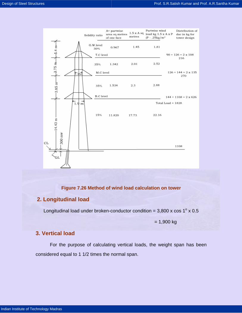
Design of Steel Structures Prof. S.R.Satish Kumar and Prof. A.R.Santha Kumar
Indian Institute of Technology Madras
Figure 7.26 Method of wind load calculation on tower
2. Longitudinal load
Longitudinal load under broken-conductor condition = 3,800 x cos 1o x 0.5
= 1,900 kg
3. Vertical load
For the purpose of calculating vertical loads, the weight span has been
considered equal to 1 1/2 times the normal span.
Design of Steel Structures Prof. S.R.Satish Kumar and Prof. A.R.Santha Kumar
Indian Institute of Technology Madras
At conductor point
Weight of conductor per weight span = 335 x 1.5 x 0.976 = 490 kg
Weight of insulator string including hardware = 60 kg
Weight of a lineman with tools = 150 kg
Total vertical load at one conductor point = 490 + 60 + 150 = 700 kg
At ground wire point
Weight of ground wire per weight span = 335 x 1.5 x 0.428 = 215 kg
Weight of ground wire attachment = 20 kg
Weight of a lineman with tools = 150 kg
Total vertical load at ground wire point = 215 + 20 + 150
= 385 kg
Say 390 kg
Vertical loads under broken-wire conditions
Vertical load under conductor-broken condition = (0.6 x 490) + 60 + 150
= 504 kg
Say 500 kg
Vertical load under ground wire broken condition = (0.6 x 215) + 20 + 150
= 299 kg
4. Torsional shear
Torsional shear per face at the top conductor position = 1,900 x 3.5 / 2 x
1.75 =1,900kg where 3.5m is the distance between the conductor point of
suspension and the centre line of the structure and 1.75 m is the width of the
tower at top conductor level.
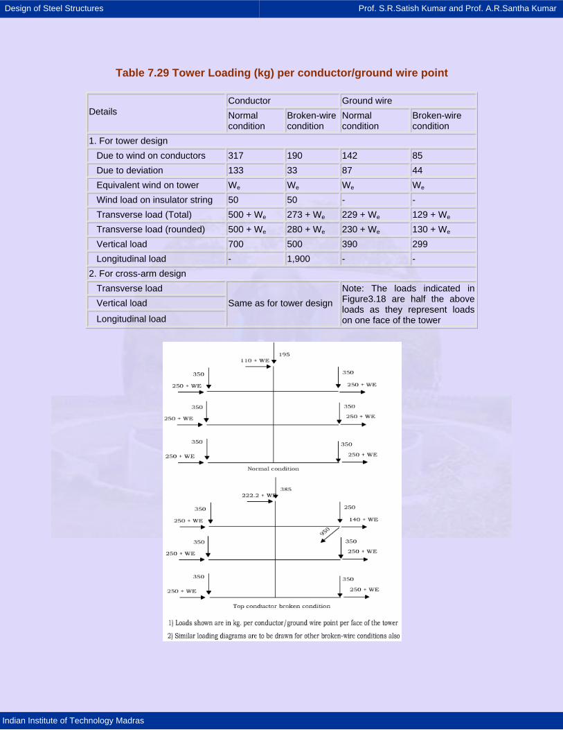
Design of Steel Structures Prof. S.R.Satish Kumar and Prof. A.R.Santha Kumar
Indian Institute of Technology Madras
Table 7.29 Tower Loading (kg) per conductor/ground wire point
Conductor Ground wire Details Normal
condition Broken-wire condition
Normal condition
Broken-wire condition
1. For tower design Due to wind on conductors 317 190 142 85 Due to deviation 133 33 87 44 Equivalent wind on tower We We We We Wind load on insulator string 50 50 - - Transverse load (Total) 500 + We 273 + We 229 + We 129 + We Transverse load (rounded) 500 + We 280 + We 230 + We 130 + We Vertical load 700 500 390 299 Longitudinal load - 1,900 - - 2. For cross-arm design Transverse load Vertical load Longitudinal load
Same as for tower design Note: The loads indicated in Figure3.18 are half the above loads as they represent loads on one face of the tower
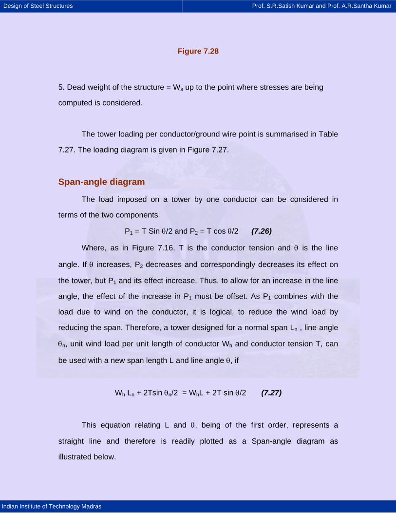
Design of Steel Structures Prof. S.R.Satish Kumar and Prof. A.R.Santha Kumar
Indian Institute of Technology Madras
Figure 7.28
5. Dead weight of the structure = Ws up to the point where stresses are being
computed is considered.
The tower loading per conductor/ground wire point is summarised in Table
7.27. The loading diagram is given in Figure 7.27.
Span-angle diagram
The load imposed on a tower by one conductor can be considered in
terms of the two components
P1 = T Sin θ/2 and P2 = T cos θ/2 (7.26)
Where, as in Figure 7.16, T is the conductor tension and θ is the line
angle. If θ increases, P2 decreases and correspondingly decreases its effect on
the tower, but P1 and its effect increase. Thus, to allow for an increase in the line
angle, the effect of the increase in P1 must be offset. As P1 combines with the
load due to wind on the conductor, it is logical, to reduce the wind load by
reducing the span. Therefore, a tower designed for a normal span Ln , line angle
θn, unit wind load per unit length of conductor Wh and conductor tension T, can
be used with a new span length L and line angle θ, if
Wh Ln + 2Tsin θn/2 = WhL + 2T sin θ/2 (7.27)
This equation relating L and θ, being of the first order, represents a
straight line and therefore is readily plotted as a Span-angle diagram as
illustrated below.
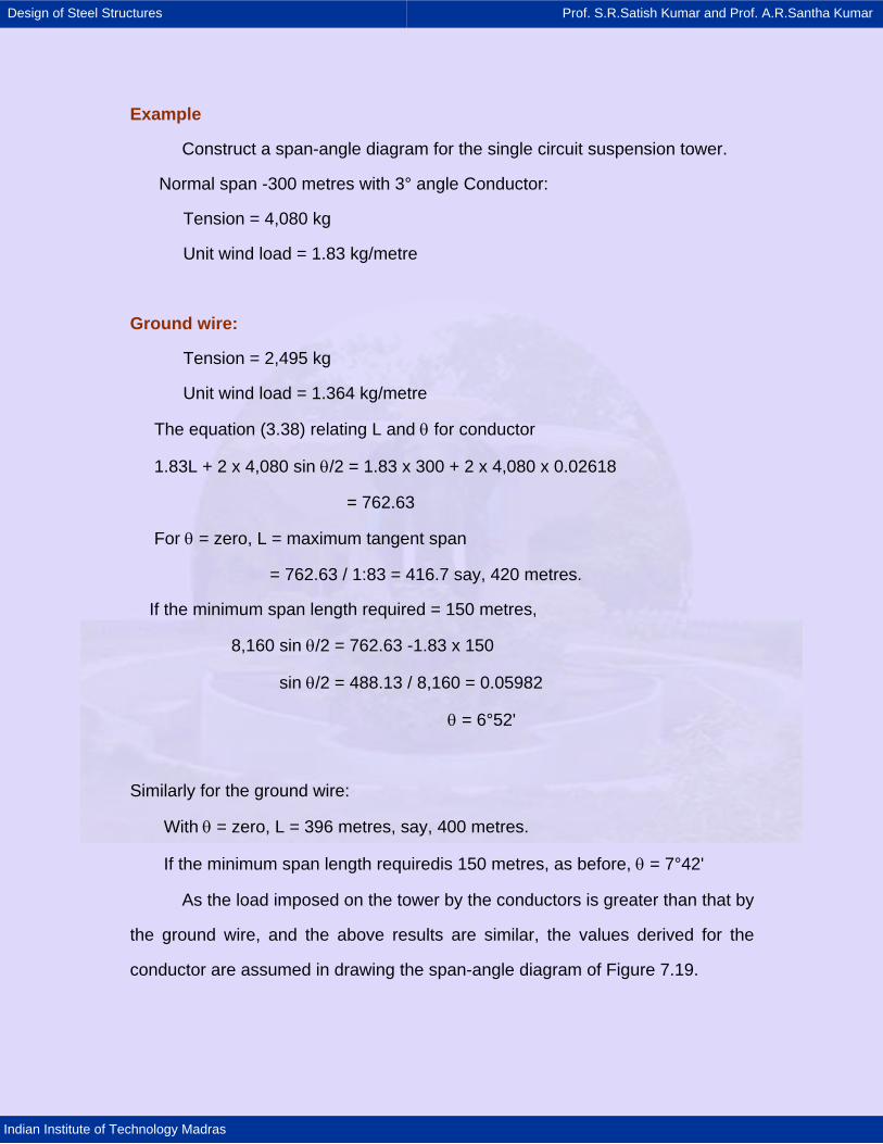
Design of Steel Structures Prof. S.R.Satish Kumar and Prof. A.R.Santha Kumar
Indian Institute of Technology Madras
Example
Construct a span-angle diagram for the single circuit suspension tower.
Normal span -300 metres with 3° angle Conductor:
Tension = 4,080 kg
Unit wind load = 1.83 kg/metre
Ground wire:
Tension = 2,495 kg
Unit wind load = 1.364 kg/metre
The equation (3.38) relating L and θ for conductor
1.83L + 2 x 4,080 sin θ/2 = 1.83 x 300 + 2 x 4,080 x 0.02618
= 762.63
For θ = zero, L = maximum tangent span
= 762.63 / 1:83 = 416.7 say, 420 metres.
If the minimum span length required = 150 metres,
8,160 sin θ/2 = 762.63 -1.83 x 150
sin θ/2 = 488.13 / 8,160 = 0.05982
θ = 6°52'
Similarly for the ground wire:
With θ = zero, L = 396 metres, say, 400 metres.
If the minimum span length requiredis 150 metres, as before, θ = 7°42'
As the load imposed on the tower by the conductors is greater than that by
the ground wire, and the above results are similar, the values derived for the
conductor are assumed in drawing the span-angle diagram of Figure 7.19.
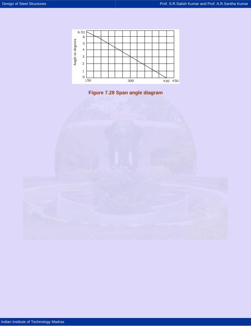
Design of Steel Structures Prof. S.R.Satish Kumar and Prof. A.R.Santha Kumar
Indian Institute of Technology Madras
Figure 7.28 Span angle diagram
Design of Steel Structures Prof. S.R.Satish Kumar and Prof. A.R.Santha Kumar
Indian Institute of Technology Madras
7.4 Tower Design
Once the external loads acting on the tower are determined, one proceeds
with an analysis of the forces in various members with a view to fixing up their
sizes. Since axial force is the only force for a truss element, the member has to
be designed for either compression or tension. When there are multiple load
conditions, certain members may be subjected to both compressive and tensile
forces under different loading conditions. Reversal of loads may also induce
alternate nature of forces; hence these members are to be designed for both
compression and tension. The total force acting on any individual member under
the normal condition and also under the broken- wire condition is multiplied by
the corresponding factor of safety, and it is ensured that the values are within the
permissible ultimate strength of the particular steel used.
Bracing systems
Once the width of the tower at the top and also the level at which the
batter should start are determined, the next step is to select the system of
bracings. The following bracing systems are usually adopted for transmission line
towers.
Single web system (Figure 7.29a)
It comprises either diagonals and struts or all diagonals. This system is
particularly used for narrow-based towers, in cross-arm girders and for portal
type of towers. Except for 66 kV single circuit towers, this system has little
application for wide-based towers at higher voltages.
Design of Steel Structures Prof. S.R.Satish Kumar and Prof. A.R.Santha Kumar
Indian Institute of Technology Madras
Double web or Warren system (Figure 7.29b)
This system is made up of diagonal cross bracings. Shear is equally
distributed between the two diagonals, one in compression and the other in
tension. Both the diagonals are designed for compression and tension in order to
permit reversal of externally applied shear. The diagonal braces are connected at
their cross points. Since the shear perface is carried by two members and critical
length is approximately half that of a corresponding single web system. This
system is used for both large and small towers and can be economically adopted
throughout the shaft except in the lower one or two panels, where diamond or
portal system of bracings is more suitable.
Pratt system (Figure 7.29c)
This system also contains diagonal cross bracings and, in addition, it has
horizontal struts. These struts are subjected to compression and the shear is
taken entirely by one diagonal in tension, the other diagonal acting like a
redundant member.
It is often economical to use the Pratt bracings for the bottom two or three
panels and Warren bracings for the rest of the tower.
Portal system (Figure 7.29d)
The diagonals are necessarily designed for both tension and compression
and, therefore, this arrangement provides more stiffness than the Pratt system.
The advantage of this system is that the horizontal struts are supported at mid
length by the diagonals.
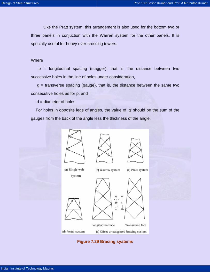
Design of Steel Structures Prof. S.R.Satish Kumar and Prof. A.R.Santha Kumar
Indian Institute of Technology Madras
Like the Pratt system, this arrangement is also used for the bottom two or
three panels in conjuction with the Warren system for the other panels. It is
specially useful for heavy river-crossing towers.
Where
p = longitudinal spacing (stagger), that is, the distance between two
successive holes in the line of holes under consideration,
g = transverse spacing (gauge), that is, the distance between the same two
consecutive holes as for p, and
d = diameter of holes.
For holes in opposite legs of angles, the value of 'g' should be the sum of the
gauges from the back of the angle less the thickness of the angle.
Figure 7.29 Bracing syatems
Design of Steel Structures Prof. S.R.Satish Kumar and Prof. A.R.Santha Kumar
Indian Institute of Technology Madras
Net effective area for angle sections in tension
In the case of single angles in tension connected by one leg only, the net
effective section of the angle is taken as
Aeff = A + Bk (7.28)
Where
A = net sectional area of the connected leg,
B = area of the outstanding leg = (l -t)t,
l = length of the outstanding leg,
t = thickness of the leg, and
1kB1 0.35A
=+
In the case of a pair of angles back to back in tension connected by only
one leg of each angle to the same side of the gusset,
1kB1 0.2A
=+
The slenderness ratio of a member carrying axial tension is limited to 375.
7.4.1 Compression members
While in tension members, the strains and displacements of stressed
material are small, in members subjected to compression, there may develop
relatively large deformations perpendicular to the centre line, under certain
criticallol1ding conditions.
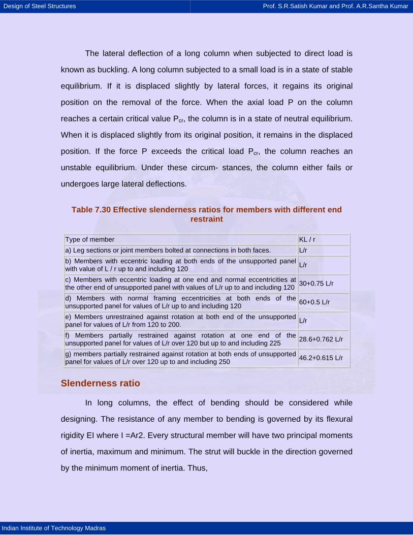
Design of Steel Structures Prof. S.R.Satish Kumar and Prof. A.R.Santha Kumar
Indian Institute of Technology Madras
The lateral deflection of a long column when subjected to direct load is
known as buckling. A long column subjected to a small load is in a state of stable
equilibrium. If it is displaced slightly by lateral forces, it regains its original
position on the removal of the force. When the axial load P on the column
reaches a certain critical value Pcr, the column is in a state of neutral equilibrium.
When it is displaced slightly from its original position, it remains in the displaced
position. If the force P exceeds the critical load Pcr, the column reaches an
unstable equilibrium. Under these circum- stances, the column either fails or
undergoes large lateral deflections.
Table 7.30 Effective slenderness ratios for members with different end restraint
Type of member KL / r a) Leg sections or joint members bolted at connections in both faces. L/r b) Members with eccentric loading at both ends of the unsupported panel with value of L / r up to and including 120 L/r
c) Members with eccentric loading at one end and normal eccentricities at the other end of unsupported panel with values of L/r up to and including 120 30+0.75 L/r
d) Members with normal framing eccentricities at both ends of the unsupported panel for values of L/r up to and including 120 60+0.5 L/r
e) Members unrestrained against rotation at both end of the unsupported panel for values of L/r from 120 to 200. L/r
f) Members partially restrained against rotation at one end of the unsupported panel for values of L/r over 120 but up to and including 225 28.6+0.762 L/r
g) members partially restrained against rotation at both ends of unsupported panel for values of L/r over 120 up to and including 250 46.2+0.615 L/r
Slenderness ratio
In long columns, the effect of bending should be considered while
designing. The resistance of any member to bending is governed by its flexural
rigidity EI where I =Ar2. Every structural member will have two principal moments
of inertia, maximum and minimum. The strut will buckle in the direction governed
by the minimum moment of inertia. Thus,
Design of Steel Structures Prof. S.R.Satish Kumar and Prof. A.R.Santha Kumar
Indian Institute of Technology Madras
Imin = Armin2 (7.29)
Where rmin is the least radius of gyration. The ratio of effective length of
member to the appropriate radius of gyration is known as the slenderness ratio.
Normally, in the design procedure, the slenderness ratios for the truss elements
are limited to a maximum value.
IS: 802 (Part 1)-1977 specifies the following limiting values of the
slenderness ratio for the design of transmission towers:
Leg members and main members in the cross-arm in compression 150
Members carrying computed stresses 200
Redundant members and those carrying nominal stresses 250
Tension members 350
Effective length
The effective length of the member is governed by the fixity condition at
the two ends.
The effective length is defined as 'KL' where L is the length from centre to
centre of intersection at each end of the member, with reference to given axis,
and K is a non-dimensional factor which accounts for different fixity conditions at
the ends, and hence may be called the restraint factor. The effective slenderness
ratio KL/r of any unbraced segment of the member of length L is given in Table
7.30, which is in accordance with 18:802 (Part 1)-1977.
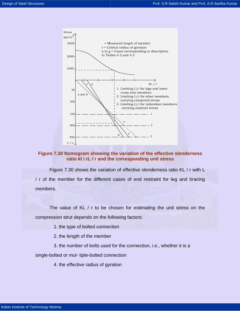
Design of Steel Structures Prof. S.R.Satish Kumar and Prof. A.R.Santha Kumar
Indian Institute of Technology Madras
Figure 7.30 Nomogram showing the variation of the effective slenderness ratio kl / rL / r and the corresponding unit stress
Figure 7.30 shows the variation of effective slenderness ratio KL / r with L
/ r of the member for the different cases of end restraint for leg and bracing
members.
The value of KL / r to be chosen for estimating the unit stress on the
compression strut depends on the following factors:
1. the type of bolted connection
2. the length of the member
3. the number of bolts used for the connection, i.e., whether it is a
single-bolted or mul- tiple-bolted connection
4. the effective radius of gyration
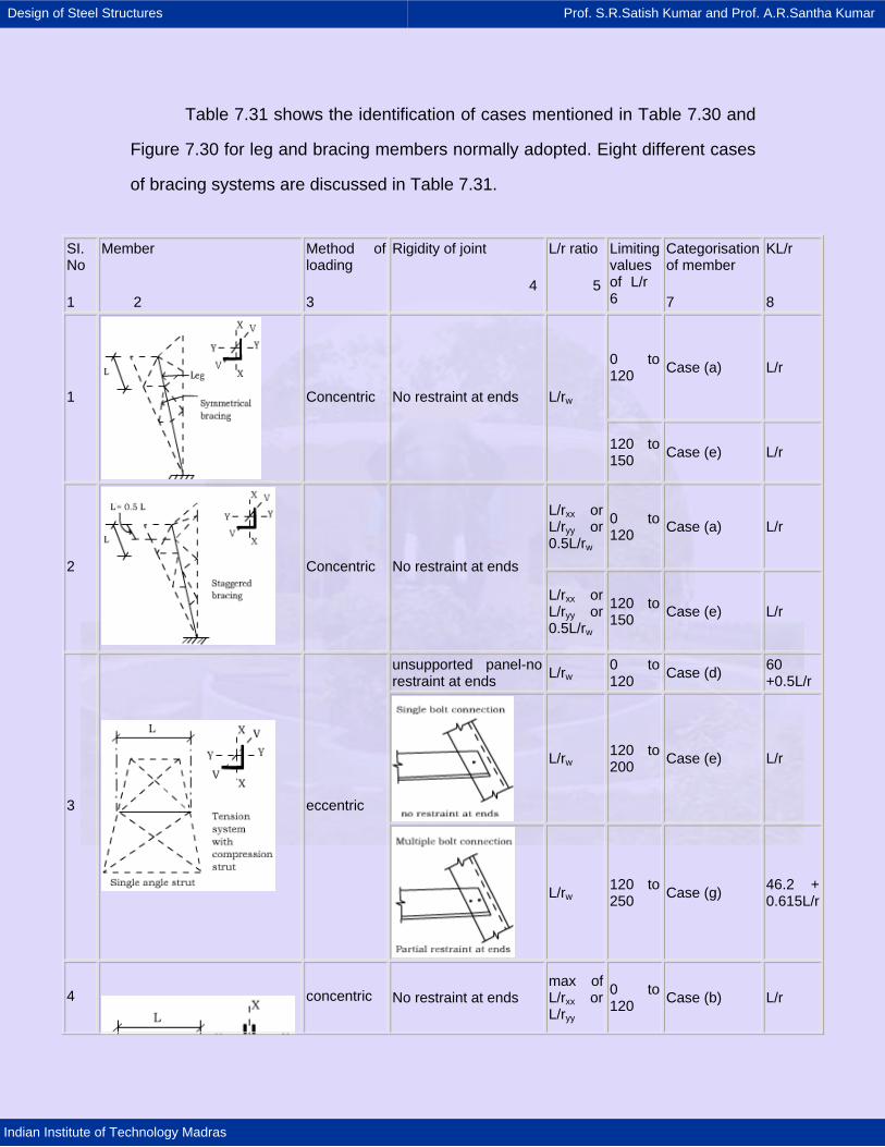
Design of Steel Structures Prof. S.R.Satish Kumar and Prof. A.R.Santha Kumar
Indian Institute of Technology Madras
Table 7.31 shows the identification of cases mentioned in Table 7.30 and
Figure 7.30 for leg and bracing members normally adopted. Eight different cases
of bracing systems are discussed in Table 7.31.
SI. No
1
Member
2
Method of loading
3
Rigidity of joint
4
L/r ratio
5
Limiting values of L/r 6
Categorisation of member
7
KL/r
8
0 to 120 Case (a) L/r
1
Concentric No restraint at ends L/rw
120 to 150 Case (e) L/r
L/rxx or L/ryy or 0.5L/rw
0 to 120 Case (a) L/r
2
Concentric No restraint at ends L/rxx or L/ryy or 0.5L/rw
120 to 150 Case (e) L/r
unsupported panel-no restraint at ends L/rw 0 to
120 Case (d) 60 +0.5L/r
L/rw 120 to 200 Case (e) L/r
3
eccentric
L/rw 120 to 250 Case (g) 46.2 +
0.615L/r
4 concentric No restraint at ends max of L/rxx or L/ryy
0 to 120 Case (b) L/r
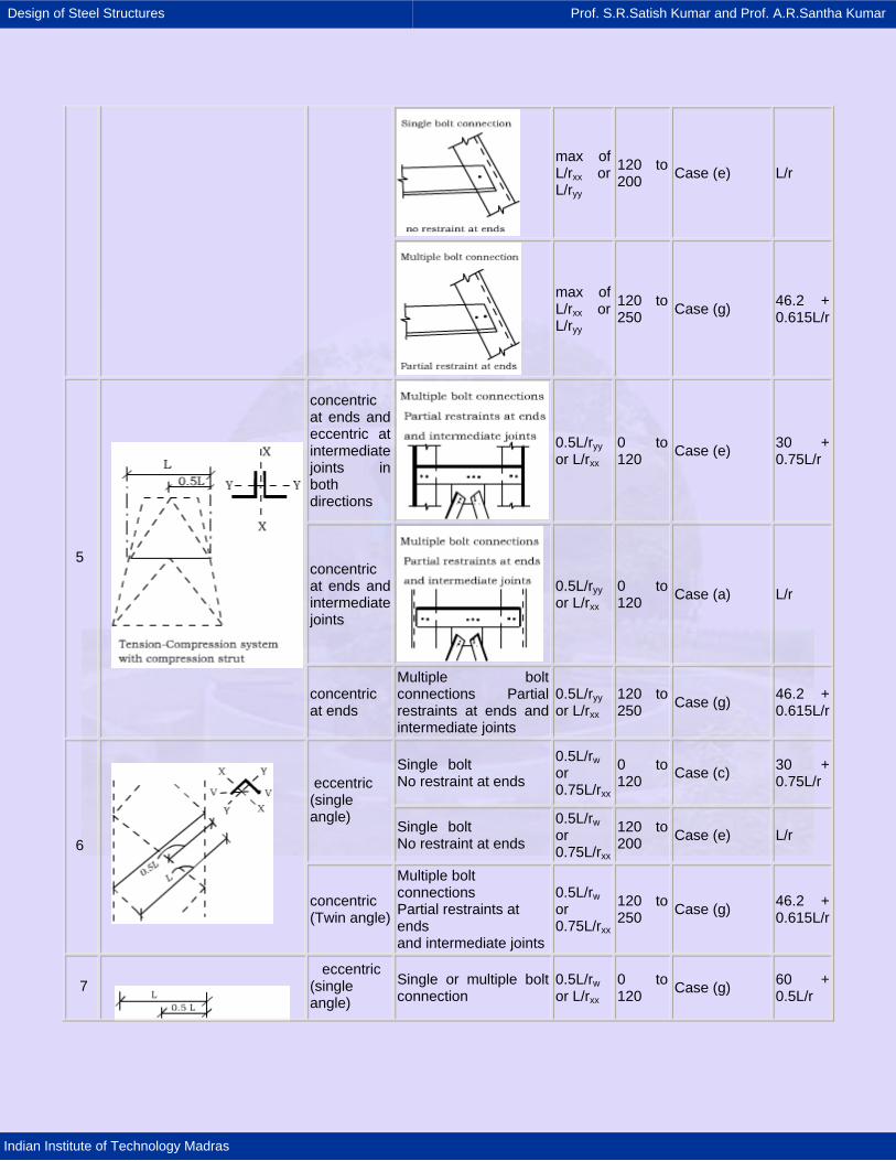
Design of Steel Structures Prof. S.R.Satish Kumar and Prof. A.R.Santha Kumar
Indian Institute of Technology Madras
max of L/rxx or L/ryy
120 to 200 Case (e) L/r
max of L/rxx or L/ryy
120 to 250 Case (g) 46.2 +
0.615L/r
concentric at ends and eccentric at intermediate joints in both directions
0.5L/ryy or L/rxx
0 to 120 Case (e) 30 +
0.75L/r
concentric at ends and intermediate joints
0.5L/ryy or L/rxx
0 to 120 Case (a) L/r
5
concentric at ends
Multiple bolt connections Partial restraints at ends and intermediate joints
0.5L/ryy or L/rxx
120 to 250 Case (g) 46.2 +
0.615L/r
Single bolt No restraint at ends
0.5L/rw or 0.75L/rxx
0 to 120 Case (c) 30 +
0.75L/r eccentric (single angle)
Single bolt No restraint at ends
0.5L/rw or 0.75L/rxx
120 to 200 Case (e) L/r
6
concentric (Twin angle)
Multiple bolt connections Partial restraints at ends and intermediate joints
0.5L/rw or 0.75L/rxx
120 to 250 Case (g) 46.2 +
0.615L/r
7 eccentric (single angle)
Single or multiple bolt connection
0.5L/rw or L/rxx
0 to 120 Case (g) 60 +
0.5L/r
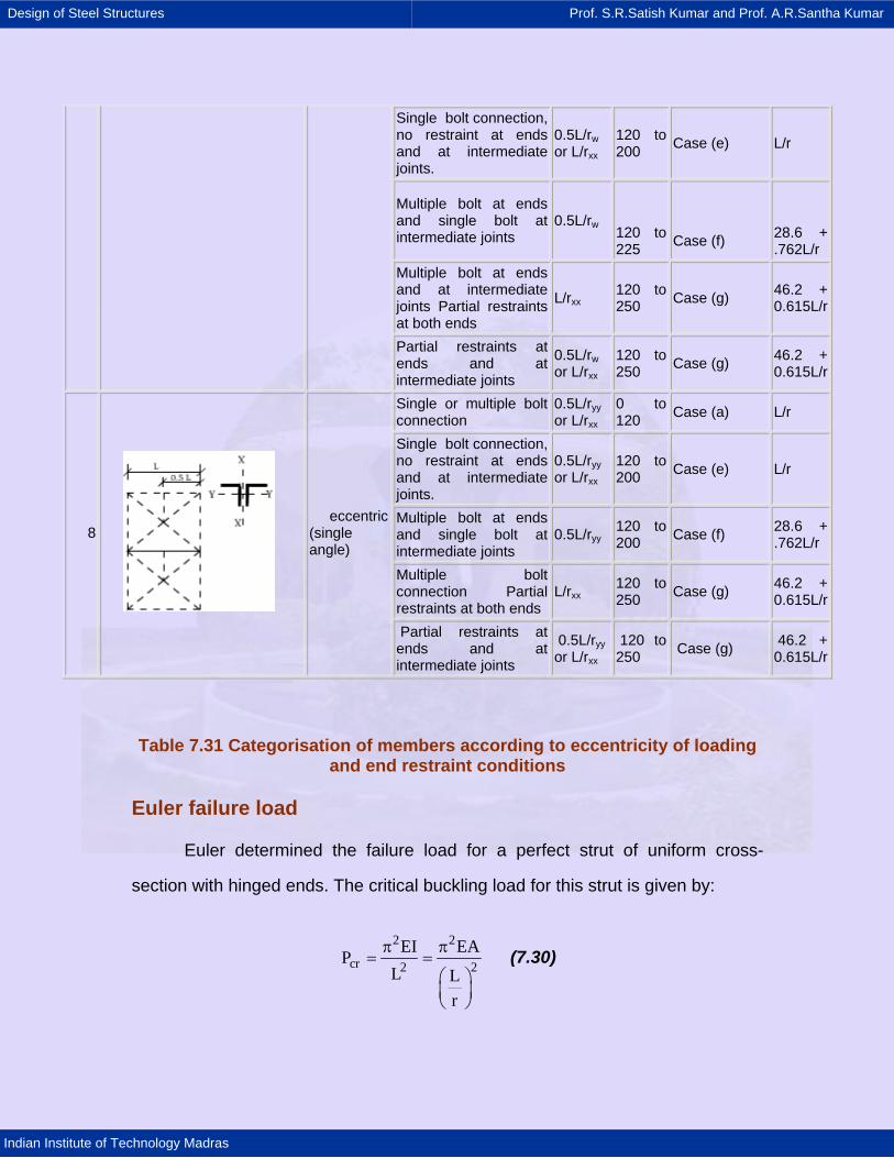
Design of Steel Structures Prof. S.R.Satish Kumar and Prof. A.R.Santha Kumar
Indian Institute of Technology Madras
Table 7.31 Categorisation of members according to eccentricity of loading and end restraint conditions
Euler failure load
Euler determined the failure load for a perfect strut of uniform cross-
section with hinged ends. The critical buckling load for this strut is given by:
2 2
cr 2 2EI EAP
L Lr
π π= =
⎛ ⎞⎜ ⎟⎝ ⎠
(7.30)
Single bolt connection, no restraint at ends and at intermediate joints.
0.5L/rw or L/rxx
120 to 200 Case (e) L/r
Multiple bolt at ends and single bolt at intermediate joints
0.5L/rw
120 to 225
Case (f)
28.6 + .762L/r
Multiple bolt at ends and at intermediate joints Partial restraints at both ends
L/rxx 120 to 250 Case (g) 46.2 +
0.615L/r
Partial restraints at ends and at intermediate joints
0.5L/rw or L/rxx
120 to 250 Case (g) 46.2 +
0.615L/r
Single or multiple bolt connection
0.5L/ryy or L/rxx
0 to 120 Case (a) L/r
Single bolt connection, no restraint at ends and at intermediate joints.
0.5L/ryy or L/rxx
120 to 200 Case (e) L/r
Multiple bolt at ends and single bolt at intermediate joints
0.5L/ryy 120 to 200 Case (f) 28.6 +
.762L/r
Multiple bolt connection Partial restraints at both ends
L/rxx 120 to 250 Case (g) 46.2 +
0.615L/r
8
eccentric (single angle)
Partial restraints at ends and at intermediate joints
0.5L/ryy or L/rxx
120 to 250 Case (g) 46.2 +
0.615L/r
Design of Steel Structures Prof. S.R.Satish Kumar and Prof. A.R.Santha Kumar
Indian Institute of Technology Madras
The effective length for a strut with hinged ends is L.
At values less than π2 EL/L2 the strut is in a stable equilibrium. At values of
P greater than π2 EL/L2 the strut is in a condition of unstable equilibrium and any
small disturbance produces final collapse. This is, however, a hypothetical
situation because all struts have some initial imperfections and thus the load on
the strut can never exceed π2 EL/L2. If the thrust P is plotted against the lateral
displacement ∆ at any section, the P - ∆ relationship for a perfect strut will be as
shown in Figure 7.31 (a).
In this figure, the lateral deflections occurring after reaching critical
buckling load are shown, that is 2 2crP EI / L≥ π , When the strut has small
imperfections, displacement is possible for all values of P and the condition of
neutral equilibrium P = π2 EL/L2is never attained. All materials have a limit of
proportionality. When this is reached, the flexural stiffness decreases initiating
failure before P = π2 EL/L2 is reached (Figure 7.31 (b))
Empirical formulae
The following parameters influence the safe compressive stress on the
column:
1. Yield stress of material
2. Initial imperfectness
3. (L/r) ratio
4. Factor of safety
5. End fixity condition
6. (b/t) ratio (Figure 7.31)) which controls flange buckling
Design of Steel Structures Prof. S.R.Satish Kumar and Prof. A.R.Santha Kumar
Indian Institute of Technology Madras
Figure 7.31 (d) shows a practical application of a twin-angle strut used in a
typical bracing system.
Taking these parameters into consideration, the following empirical
formulae have been used by different authorities for estimating the safe
compressive stress on struts:
1. Straight line formula
2. Parabolic formula
3. Rankine formula
4. Secant or Perry's formula
These formulae have been modified and used in the codes evolved in
different countries.
IS: 802 (Part I) -1977 gives the following formulae which take into account
all the parameters listed earlier.
For the case b / t ≤ 13 (Figure 7.30 (c)),
2
2a
KLrF 2600 kg / cm12
⎧ ⎫⎛ ⎞⎪ ⎪⎜ ⎟⎪ ⎪⎝ ⎠= −⎨ ⎬⎪ ⎪⎪ ⎪⎩ ⎭
(7.31)
Where KL / r ≤ 120
62
a 220 x10F kg / cm
KLr
=⎛ ⎞⎜ ⎟⎝ ⎠
(7.32)
Design of Steel Structures Prof. S.R.Satish Kumar and Prof. A.R.Santha Kumar
Indian Institute of Technology Madras
Where KL / r > 120
Fcr = 4680 - 160(b / t) kg/cm2
Where 13 < b/t < 20 (7.33)
2cr 2
590000F kg / cmbt
=⎛ ⎞⎜ ⎟⎝ ⎠
Where b / t > 20 (7.34)
Where
Fa = buckling unit stress in compression,
Fcr = limiting crippling stress because of large value of b / t,
b = distance from the edge of fillet to the extreme fibre, and
t = thickness of material.
Equations (7.31) and (7.32) indicate the failure load when the member
buckles and Equations (7.33) and (7.34) indicate the failure load when the flange
of the member fails.
Figure 7.30 gives the strut formula for the steel with a yield stress of 2600
kg/sq.cm. with respect to member failure. The upper portion of the figure shows
the variation of unit stress with KL/r and the lower portion variation of KL/r with
L/r. This figure can be used as a nomogram for estimating the allowable stress
on a compression member.
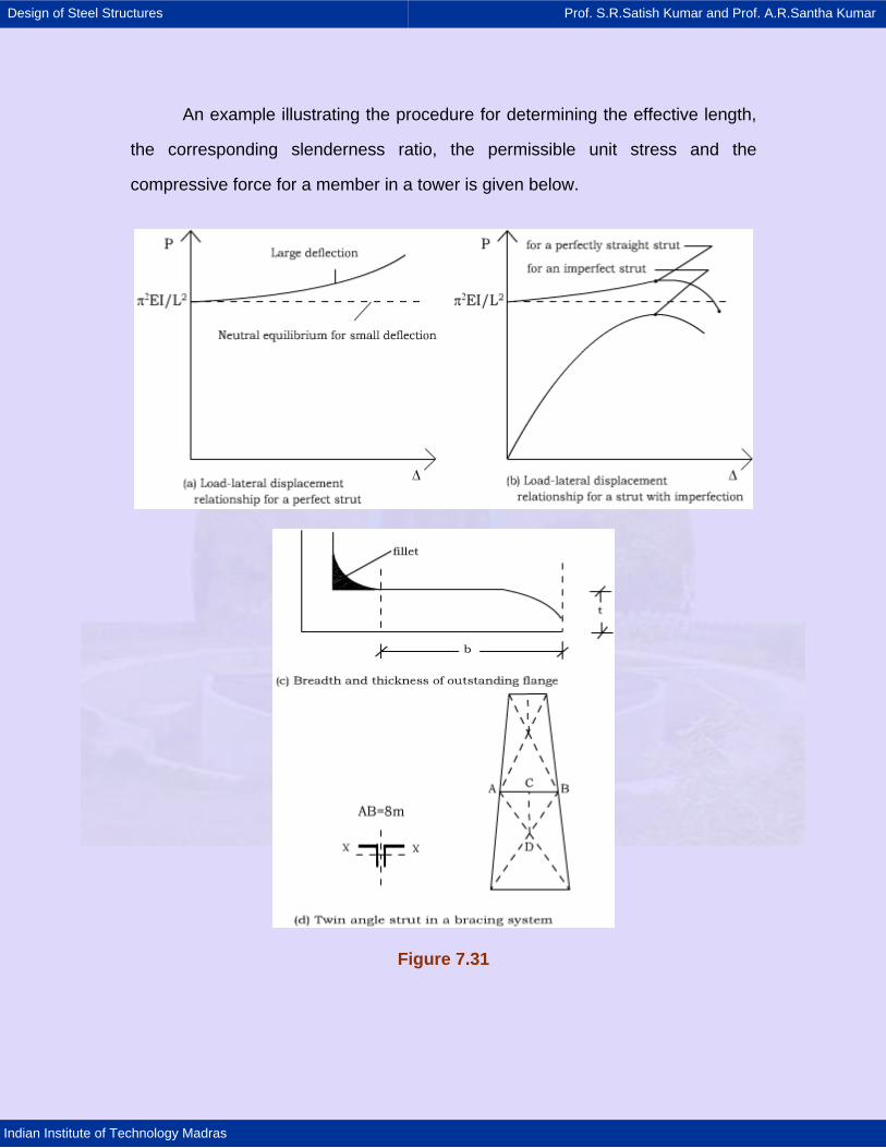
Design of Steel Structures Prof. S.R.Satish Kumar and Prof. A.R.Santha Kumar
Indian Institute of Technology Madras
An example illustrating the procedure for determining the effective length,
the corresponding slenderness ratio, the permissible unit stress and the
compressive force for a member in a tower is given below.
Figure 7.31
Design of Steel Structures Prof. S.R.Satish Kumar and Prof. A.R.Santha Kumar
Indian Institute of Technology Madras
Example
Figure 7.31 (d) shows a twin angle bracing system used for the horizontal
member of length L = 8 m. In order to reduce the effective length of member AB,
single angle CD has been connected to the system. AB is made of two angles
100 x 100mm whose properties are given below:
rxx = 4.38 cm
ryy = 3.05 cm
Area = 38.06 sq.cm.
Double bolt connections are made at A, Band C. Hence it can be assumed
that the joints are partially restrained. The system adopted is given at SL. No.8 in
Table 7.31. For partial restraint at A, B and C,
L/r = 0.5 L/ryy or L/rxx
= 0.5 x 800/3.05 or 800/4.38
= 131.14 or 182.64
The governing value of L/r is therefore182.64, which is the larger of the
two values obtained. This value corresponds to case (g) for which KL/r
= 46.2 + 0.615L/r
= 158.52
Note that the value of KL/r from the curve is also 158.52 (Figure 7.30).
The corresponding stress from the curve above is 795 kg/cm2, which is shown
dotted in the nomogram. The value of unit stress can also be calculated from
equation (7.32). Thus,
Design of Steel Structures Prof. S.R.Satish Kumar and Prof. A.R.Santha Kumar
Indian Institute of Technology Madras
62
a 220 x10F kg / cm
KLr
=⎛ ⎞⎜ ⎟⎝ ⎠
= 20 x 106 / 158.52 x 158.52
= 795 kg/cm2.
The safe compression load on the strut AB is therefore
F = 38.06 x 795
= 30,257 kg
7.4.2 Computer-aided design
Two computer-aided design methods are in vogue, depending on the
computer memory. The first method uses a fixed geometry (configuration) and
minimizes the weight of the tower, while the second method assumes the
geometry as unknown and derives the minimization of weight.
Method 1: Minimum weight design with assumed geometry
Power transmission towers are highly indeterminate and are subjected to
a variety of loading conditions such as cyclones, earthquakes and temperature
variations.
The advent of computers has resulted in more rational and realistic
methods of structural design of transmission towers. Recent advances in
optimisation in structural design have also been incorporated into the design of
such towers.
While choosing the member sizes, the large number of structural
connections in three dimensions should be kept in mind. The selection of
Design of Steel Structures Prof. S.R.Satish Kumar and Prof. A.R.Santha Kumar
Indian Institute of Technology Madras
members is influenced by their position in relation to the other members and the
end connection conditions. The leg sections which carry different stresses at
each panel may be assigned different sizes at various levels; but consideration of
the large number of splices involved indicates that it is usually more economical
and convenient, even though heavier, to use the same section for a number of
panels. Similarly, for other members, it may be economical to choose a section of
relatively large flange width so as to eliminate gusset plates and correspondingly
reduce the number of bolts.
In the selection of structural members, the designer is guided by his past
experience gained from the behavior of towers tested in the test station or
actually in service. At certain critical locations, the structural members are
provided with a higher margin of safety, one example being the horizontal
members where the slope of the tower changes and the web members of panels
are immediately below the neckline.
Optimisation
Many designs are possible to satisfy the functional requirements and a
trial and error procedure may be employed to choose the optimal design.
Selection of the best geometry of a tower or the member sizes is examples of
optimal design procedures. The computer is best suited for finding the optimal
solutions. Optimisation then becomes an automated design procedure, providing
the optimal values for certain design quantities while considering the design
criteria and constraints.
Computer-aided design involving user-ma- chine interaction and
automated optimal design, characterized by pre-programmed logical decisions,
Design of Steel Structures Prof. S.R.Satish Kumar and Prof. A.R.Santha Kumar
Indian Institute of Technology Madras
based upon internally stored information, are not mutually exclusive, but
complement each other. As the techniques of interactive computer-aided design
develop, the need to employ standard routines for automated design of structural
subsystems will become increasingly relevant.
The numerical methods of structure optimisation, with application of
computers, automatically generate a near optimal design in an iterative manner.
A finite number of variables has to be established, together with the constraints,
relating to these variables. An initial guess-solution is used as the starting point
for a systematic search for better designs and the process of search is
terminated when certain criteria are satisfied.
Those quantities defining a structural system that are fixed during the
automated design are- called pre-assigned parameters or simply parameters and
those quantities that are not pre-assigned are called design variables. The
design variables cover the material properties, the topology of the structure, its
geometry and the member sizes. The assignment of the parameters as well as
the definition of their values is made by the designer, based on his experience.
Any set of values for the design variables constitutes a design of the
structure. Some designs may be feasible while others are not. The restrictions
that must be satisfied in order to produce a feasible design are called constraints.
There are two kinds of constraints: design constraints and behavior constraints.
Examples of design constraints are minimum thickness of a member, maximum
height of a structure, etc. Limitations on the maximum stresses, displacements or
buck- ling strength are typical examples of behavior constraints. These
constraints are expressed ma- thematically as a set of inequalities:
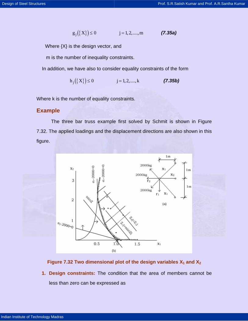
Design of Steel Structures Prof. S.R.Satish Kumar and Prof. A.R.Santha Kumar
Indian Institute of Technology Madras
{ }( )jg X 0 j 1,2,....,m≤ = (7.35a)
Where {X} is the design vector, and
m is the number of inequality constraints. In addition, we have also to consider equality constraints of the form
{ }( )jh X 0 j 1,2,...., k≤ = (7.35b)
Where k is the number of equality constraints.
Example
The three bar truss example first solved by Schmit is shown in Figure
7.32. The applied loadings and the displacement directions are also shown in this
figure.
Figure 7.32 Two dimensional plot of the design variables X1 and X2
1. Design constraints: The condition that the area of members cannot be
less than zero can be expressed as
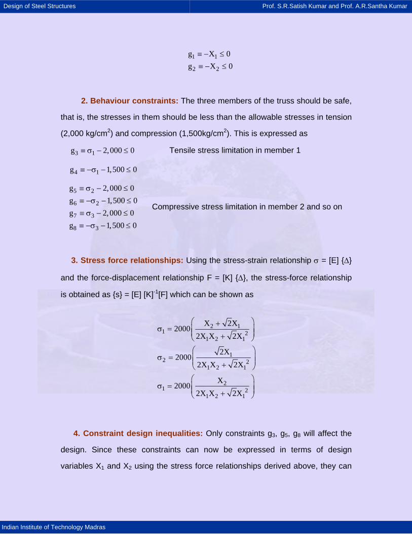
Design of Steel Structures Prof. S.R.Satish Kumar and Prof. A.R.Santha Kumar
Indian Institute of Technology Madras
1 1
2 2
g X 0g X 0
≡ − ≤≡ − ≤
2. Behaviour constraints: The three members of the truss should be safe,
that is, the stresses in them should be less than the allowable stresses in tension
(2,000 kg/cm2) and compression (1,500kg/cm2). This is expressed as
3 1g 2,000 0≡ σ − ≤ Tensile stress limitation in member 1
4 1g 1,500 0≡ −σ − ≤
5 2
6 2
7 3
8 3
g 2,000 0g 1,500 0g 2,000 0g 1,500 0
≡ σ − ≤
≡ −σ − ≤
≡ σ − ≤
≡ −σ − ≤
Compressive stress limitation in member 2 and so on
3. Stress force relationships: Using the stress-strain relationship σ = [E] {∆}
and the force-displacement relationship F = [K] {∆}, the stress-force relationship
is obtained as {s} = [E] [K]-1[F] which can be shown as
2 11 2
1 2 1
12 2
1 2 1
21 2
1 2 1
X 2X2000
2X X 2X
2X2000
2X X 2X
X2000
2X X 2X
⎛ ⎞+σ = ⎜ ⎟⎜ ⎟+⎝ ⎠
⎛ ⎞σ = ⎜ ⎟⎜ ⎟+⎝ ⎠
⎛ ⎞σ = ⎜ ⎟⎜ ⎟+⎝ ⎠
4. Constraint design inequalities: Only constraints g3, g5, g8 will affect the
design. Since these constraints can now be expressed in terms of design
variables X1 and X2 using the stress force relationships derived above, they can
Design of Steel Structures Prof. S.R.Satish Kumar and Prof. A.R.Santha Kumar
Indian Institute of Technology Madras
be represented as the area on one side of the straight line shown in the two-
dimensional plot (Figure 7.32 (b)).
Design space
Each design variable X1, X2 ...is viewed as one- dimension in a design
space and a particular set of variables as a point in this space. In the general
case of n variables, we have an n-dimensioned space. In the example where we
have only two variables, the space reduces to a plane figure shown in Figure
7.32 (b). The arrows indicate the inequality representation and the shaded zone
shows the feasible region. A design falling in the feasible region is an
unconstrained design and the one falling on the boundary is a constrained
design.
Objective function
An infinite number of feasible designs are possible. In order to find the
best one, it is necessary to form a function of the variables to use for comparison
of feasible design alternatives. The objective (merit) function is a function whose
least value is sought in an optimisation procedure. In other words, the
optimization problem consists in the determination of the vector of variables X
that will minimise a certain given objective function:
Z = F ({X}) 7.35(c)
In the example chosen, assuming the volume of material as the objective
function, we get
Z = 2(141 X1) + 100 X2
Design of Steel Structures Prof. S.R.Satish Kumar and Prof. A.R.Santha Kumar
Indian Institute of Technology Madras
The locus of all points satisfying F ({X}) = constant, forms a straight line in
a two-dimensional space. In this general case of n-dimensional space, it will form
a surface. For each value of constraint, a different straight line is obtained. Figure
7.32 (b) shows the objective function contours. Every design on a particular
contour has the same volume or weight. It can be seen that the minimum value
of F ( {X} ) in the feasible region occurs at point A.
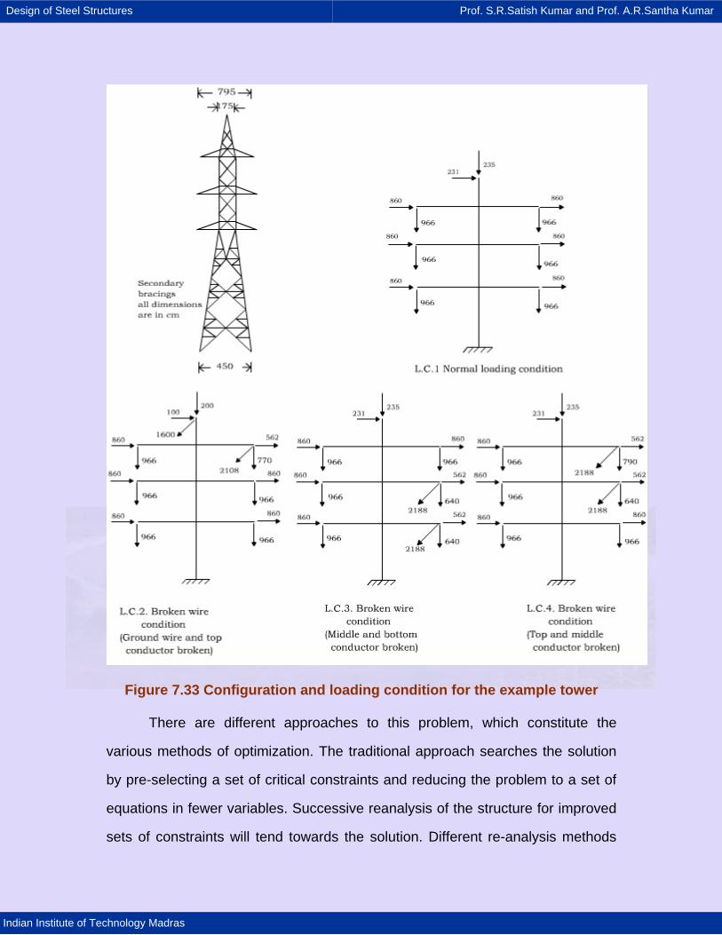
Design of Steel Structures Prof. S.R.Satish Kumar and Prof. A.R.Santha Kumar
Indian Institute of Technology Madras
Figure 7.33 Configuration and loading condition for the example tower
There are different approaches to this problem, which constitute the
various methods of optimization. The traditional approach searches the solution
by pre-selecting a set of critical constraints and reducing the problem to a set of
equations in fewer variables. Successive reanalysis of the structure for improved
sets of constraints will tend towards the solution. Different re-analysis methods
Design of Steel Structures Prof. S.R.Satish Kumar and Prof. A.R.Santha Kumar
Indian Institute of Technology Madras
can be used, the iterative methods being the most attractive in the case of
towers.
Optimality criteria
An interesting approach in optimization is a process known as optimality
criteria. The approach to the optimum is based on the assumption that some
characteristics will be attained at such optimum. The well-known example is the
fully stressed design where it is assumed that, in an optimal structure, each
member is subjected to its limiting stress under at least one loading condition.
The optimality criteria procedures are useful for transmission lines and
towers because they constitute an adequate compromise to obtain practical and
efficient solutions. In many studies, it has been found that the shape of the
objective function around the optimum is flat, which means that an experienced
designer can reach solutions, which are close to the theoretical optimum.
Mathematical programming
It is difficult to anticipate which of the constraints will be critical at the
optimum. Therefore, the use of inequality constraints is essential for a proper
formulation of the optimal design problem.
The mathematical programming (MP) methods are intended to solve the
general optimisation problem by numerical search algorithms while being general
regarding the objective function and constraints. On the other hand,
approximations are often required to be efficient on large practical problems such
as tower optimisation.
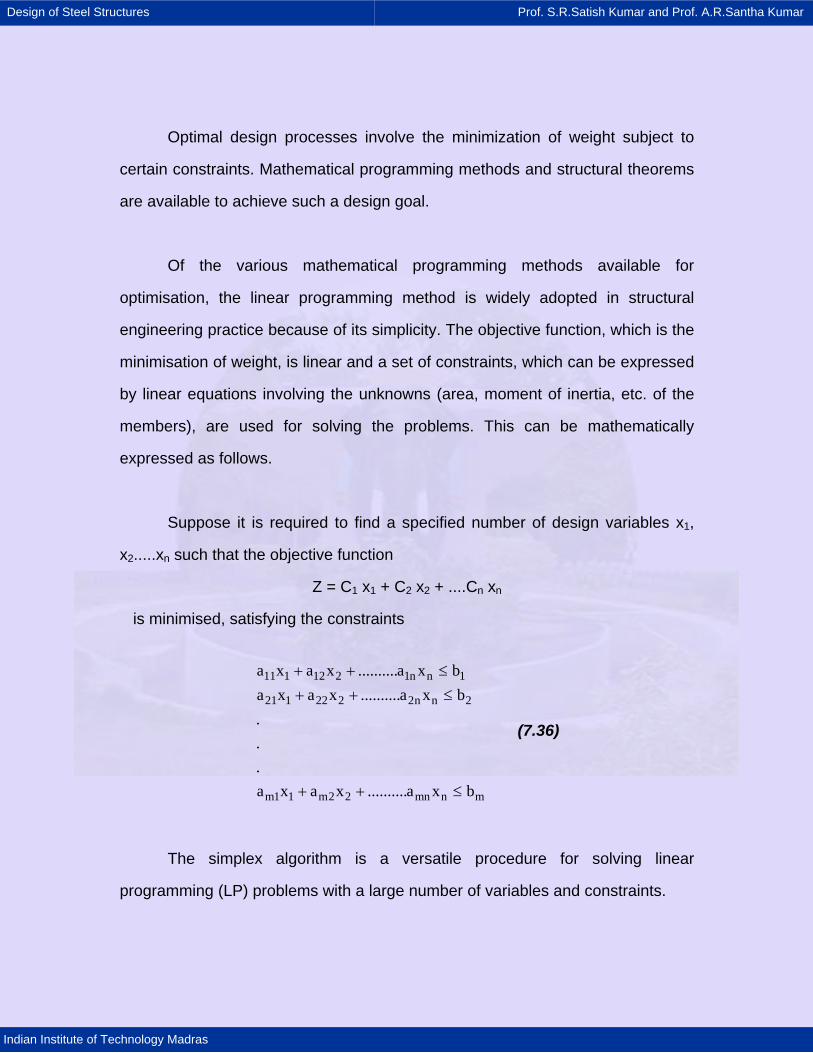
Design of Steel Structures Prof. S.R.Satish Kumar and Prof. A.R.Santha Kumar
Indian Institute of Technology Madras
Optimal design processes involve the minimization of weight subject to
certain constraints. Mathematical programming methods and structural theorems
are available to achieve such a design goal.
Of the various mathematical programming methods available for
optimisation, the linear programming method is widely adopted in structural
engineering practice because of its simplicity. The objective function, which is the
minimisation of weight, is linear and a set of constraints, which can be expressed
by linear equations involving the unknowns (area, moment of inertia, etc. of the
members), are used for solving the problems. This can be mathematically
expressed as follows.
Suppose it is required to find a specified number of design variables x1,
x2.....xn such that the objective function
Z = C1 x1 + C2 x2 + ....Cn xn
is minimised, satisfying the constraints
11 1 12 2 1n n 1
21 1 22 2 2n n 2
m1 1 m2 2 mn n m
a x a x ..........a x ba x a x ..........a x b...a x a x ..........a x b
+ + ≤+ + ≤
+ + ≤
(7.36)
The simplex algorithm is a versatile procedure for solving linear
programming (LP) problems with a large number of variables and constraints.
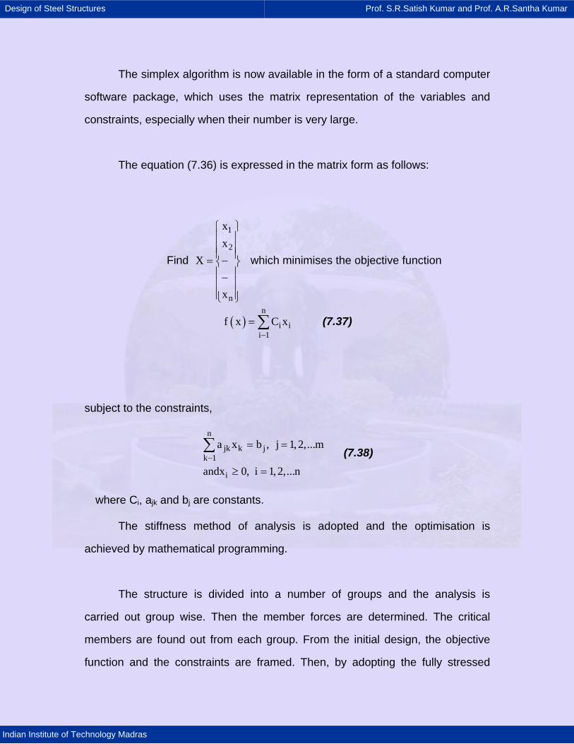
Design of Steel Structures Prof. S.R.Satish Kumar and Prof. A.R.Santha Kumar
Indian Institute of Technology Madras
The simplex algorithm is now available in the form of a standard computer
software package, which uses the matrix representation of the variables and
constraints, especially when their number is very large.
The equation (7.36) is expressed in the matrix form as follows:
Find
1
2
n
xx
X
x
⎧ ⎫⎪ ⎪⎪ ⎪⎪ ⎪= −⎨ ⎬⎪ ⎪−⎪ ⎪⎪ ⎪⎩ ⎭
which minimises the objective function
( )n
i ii 1
f x C x−
= ∑ (7.37)
subject to the constraints,
n
jk k jk 1
i
a x b , j 1, 2,...m
andx 0, i 1, 2,...n−
= =
≥ =
∑ (7.38)
where Ci, ajk and bj are constants.
The stiffness method of analysis is adopted and the optimisation is
achieved by mathematical programming.
The structure is divided into a number of groups and the analysis is
carried out group wise. Then the member forces are determined. The critical
members are found out from each group. From the initial design, the objective
function and the constraints are framed. Then, by adopting the fully stressed
Design of Steel Structures Prof. S.R.Satish Kumar and Prof. A.R.Santha Kumar
Indian Institute of Technology Madras
design (optimality criteria) method, the linear programming problem is solved and
the optimal solution found out. In each group, every member is designed for the
fully stressed condition and the maximum size required is assigned for all the
members in that group. After completion of the design, one more analysis and
design routine for the structure as a whole is completed for alternative cross-
sections.
Example
A 220 k V double circuit tangent tower is chosen for study. The basic
structure, section plan at various levels and the loading conditions are tentatively
fixed. The number of panels in the basic determinate structure is 15 and the
number of members is 238. Twenty standard sections have been chosen in the
increasing order of weight. The members have been divided into eighteen
groups, such as leg groups, diagonal groups and horizontal groups, based on
various panels of the tower. For each group a section is specified.
Normal loading conditions and three broken- wire conditions has been
considered. From the vertical and horizontal lengths of each panel, the lengths of
the members are calculated and the geometry is fixed. For the given loading
conditions, the forces in the various members are computed, from which the
actual stresses are found. These are compared with allowable stresses and the
most stressed member (critical) is found out for each group. Thereafter, an initial
design is evolved as a fully stressed design in which critical members are
stressed up to an allowable limit. This is given as the initial solution to simplex
method, from which the objective function, namely, the weight of the tower, is
formed. The initial solution so obtained is sequentially improved, subject to the
constraints, till the optimal solution is obtained.
Design of Steel Structures Prof. S.R.Satish Kumar and Prof. A.R.Santha Kumar
Indian Institute of Technology Madras
In the given solution, steel structural angles of weights ranging from 5.8
kg/m to 27.20 kg/m are utilised. On the basis of the fully stressed design,
structural sections of 3.4 kg/m to 23.4 kg/m are indicated and the corresponding
weight is 5,398 kg. After the optimal solution, the weight of the tower is 4,956 kg,
resulting in a saving of about 8.1 percent.
Method 2: Minimum weight design with geometry as variable
In Method 1, only the member sizes were treated as variables whereas
the geometry was assumed as fixed. Method 2 treats the geometry also as a
variable and gets the most preferred geometry. The geometry developed by the
computer results in the minimum weight of tower for any practically acceptable
configuration. For solution, since an iterative procedure is adopted for the
optimum structural design, it is obvious that the use of a computer is essential.
The algorithm used for optimum structural design is similar to that given by
Samuel L. Lipson which presumes that an initial feasible configuration is
available for the structure. The structure is divided into a number of groups and
the externally applied loadings are obtained. For the given configuration, the
upper limits and the lower limits on the design variables, namely, the joint
coordinates are fixed. Then (k-1) new configurations are generated randomly as
xij = li + rij( ui - li ) (7.39)
i = 1, 2 ...n
j = 1, 2 ...k
where k is the total number of configurations in the complex, usually larger
than (n + 1), where n is the number of design variables and rij is the random
number for the ith coordinate of the jth point, the random numbers having a
Design of Steel Structures Prof. S.R.Satish Kumar and Prof. A.R.Santha Kumar
Indian Institute of Technology Madras
uniform distribution over the interval 0 to 1 and ui is the upper limit and Li is the
lower limit of the ith independent variable.
Thus, the complex containing k number of feasible solutions is generated
and all these configurations will satisfy the explicit constraints, namely, the upper
and lower bounds on the design variables. Next, for all these k configurations,
analysis and fully stressed designs are carried out and their corresponding total
weights determined. Since the fully stressed design concept is an eco nomical
and practical design, it is used for steel area optimisation. Every area
optimisation problem is associated with more than one analysis and design. For
the analysis of the truss, the matrix method described in the previous chapter has
been used. Therefore, all the generated configurations also satisfy the implicit
constraints, namely, the allowable stress constraints.
From the value of the objective function (total weight of the structure) of k
configurations, the vector, which yields the maximum weight, is searched and
discarded, and the centroid c of each joint of the k-1 configurations is determined
from
( )ic ij iwj 1
1x K x xK 1 −
⎧ ⎫⎪ ⎪= −⎨ ⎬− ⎪ ⎪⎩ ⎭∑ (7.40)
i = 1, 2, 3 ... n
in which xic and xiw are the ith coordinates of the centroid c and the discarded
point w.
Then a new point is generated by reflecting the worst point through the
centroid, xic
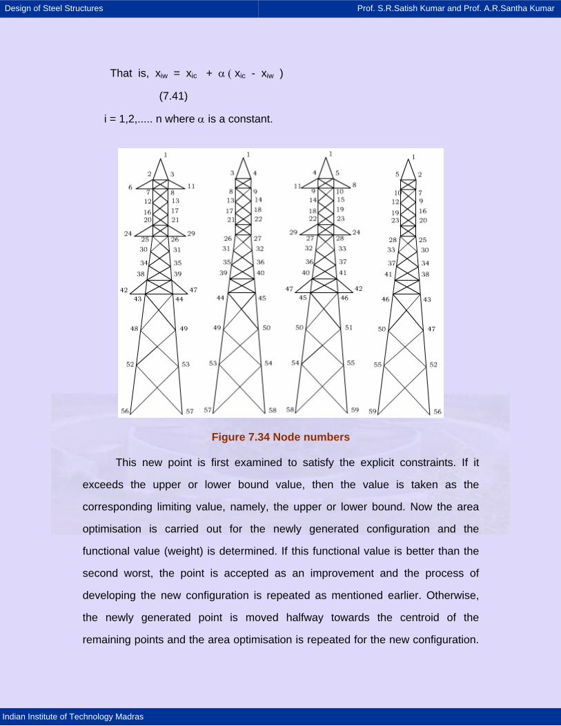
Design of Steel Structures Prof. S.R.Satish Kumar and Prof. A.R.Santha Kumar
Indian Institute of Technology Madras
That is, xiw = xic + α ( xic - xiw )
(7.41)
i = 1,2,..... n where α is a constant.
Figure 7.34 Node numbers
This new point is first examined to satisfy the explicit constraints. If it
exceeds the upper or lower bound value, then the value is taken as the
corresponding limiting value, namely, the upper or lower bound. Now the area
optimisation is carried out for the newly generated configuration and the
functional value (weight) is determined. If this functional value is better than the
second worst, the point is accepted as an improvement and the process of
developing the new configuration is repeated as mentioned earlier. Otherwise,
the newly generated point is moved halfway towards the centroid of the
remaining points and the area optimisation is repeated for the new configuration.
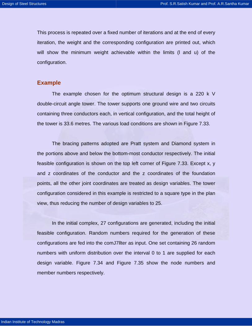
Design of Steel Structures Prof. S.R.Satish Kumar and Prof. A.R.Santha Kumar
Indian Institute of Technology Madras
This process is repeated over a fixed number of iterations and at the end of every
iteration, the weight and the corresponding configuration are printed out, which
will show the minimum weight achievable within the limits (l and u) of the
configuration.
Example
The example chosen for the optimum structural design is a 220 k V
double-circuit angle tower. The tower supports one ground wire and two circuits
containing three conductors each, in vertical configuration, and the total height of
the tower is 33.6 metres. The various load conditions are shown in Figure 7.33.
The bracing patterns adopted are Pratt system and Diamond system in
the portions above and below the bottom-most conductor respectively. The initial
feasible configuration is shown on the top left corner of Figure 7.33. Except x, y
and z coordinates of the conductor and the z coordinates of the foundation
points, all the other joint coordinates are treated as design variables. The tower
configuration considered in this example is restricted to a square type in the plan
view, thus reducing the number of design variables to 25.
In the initial complex, 27 configurations are generated, including the initial
feasible configuration. Random numbers required for the generation of these
configurations are fed into the comJ7llter as input. One set containing 26 random
numbers with uniform distribution over the interval 0 to 1 are supplied for each
design variable. Figure 7.34 and Figure 7.35 show the node numbers and
member numbers respectively.
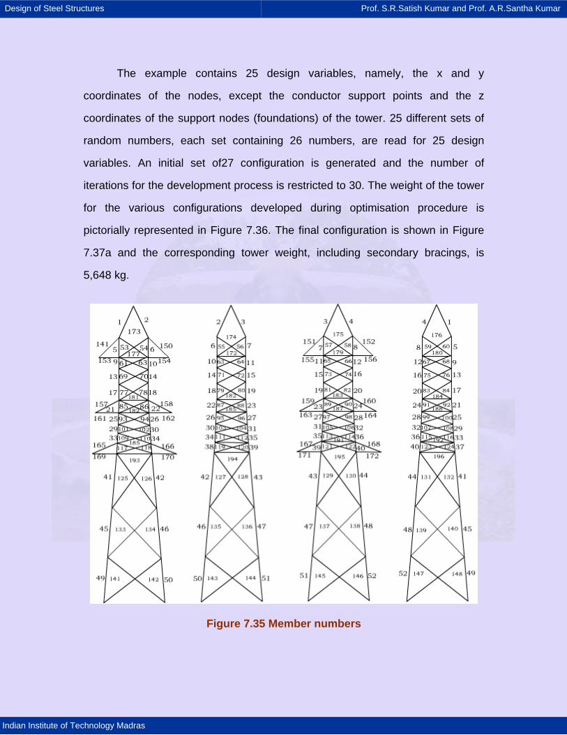
Design of Steel Structures Prof. S.R.Satish Kumar and Prof. A.R.Santha Kumar
Indian Institute of Technology Madras
The example contains 25 design variables, namely, the x and y
coordinates of the nodes, except the conductor support points and the z
coordinates of the support nodes (foundations) of the tower. 25 different sets of
random numbers, each set containing 26 numbers, are read for 25 design
variables. An initial set of27 configuration is generated and the number of
iterations for the development process is restricted to 30. The weight of the tower
for the various configurations developed during optimisation procedure is
pictorially represented in Figure 7.36. The final configuration is shown in Figure
7.37a and the corresponding tower weight, including secondary bracings, is
5,648 kg.
Figure 7.35 Member numbers
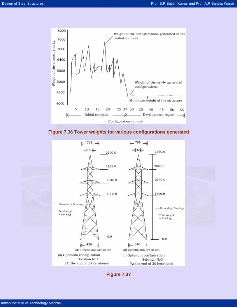
Design of Steel Structures Prof. S.R.Satish Kumar and Prof. A.R.Santha Kumar
Indian Institute of Technology Madras
Figure 7.36 Tower weights for various configurations generated
Figure 7.37
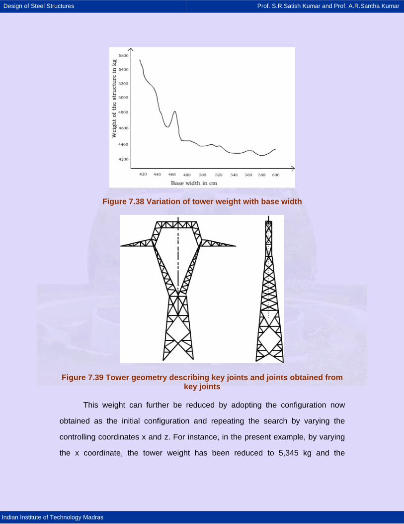
Design of Steel Structures Prof. S.R.Satish Kumar and Prof. A.R.Santha Kumar
Indian Institute of Technology Madras
Figure 7.38 Variation of tower weight with base width
Figure 7.39 Tower geometry describing key joints and joints obtained from key joints
This weight can further be reduced by adopting the configuration now
obtained as the initial configuration and repeating the search by varying the
controlling coordinates x and z. For instance, in the present example, by varying
the x coordinate, the tower weight has been reduced to 5,345 kg and the
Design of Steel Structures Prof. S.R.Satish Kumar and Prof. A.R.Santha Kumar
Indian Institute of Technology Madras
corresponding configuration is shown in Figure 7.37b. Figure 7.38 shows the
variation of tower weight with base width.
In conclusion, the probabilistic evaluation of loads and load combinations
on transmission lines, and the consideration of the line as a whole with towers,
foundations, conductors and hardware, forming interdependent elements of the
total sys- tem with different levels of safety to ensure a preferred sequence of
failure, are all directed towards achieving rational behaviour under various
uncertainties at minimum transmission line cost. Such a study may be treated as
a global optimisation of the line cost, which could also include an examination of
alternative uses of various types of towers in a family, materials to be employed
and the limits to which different towers are utilised as discrete variables and the
objective function as the overall cost.
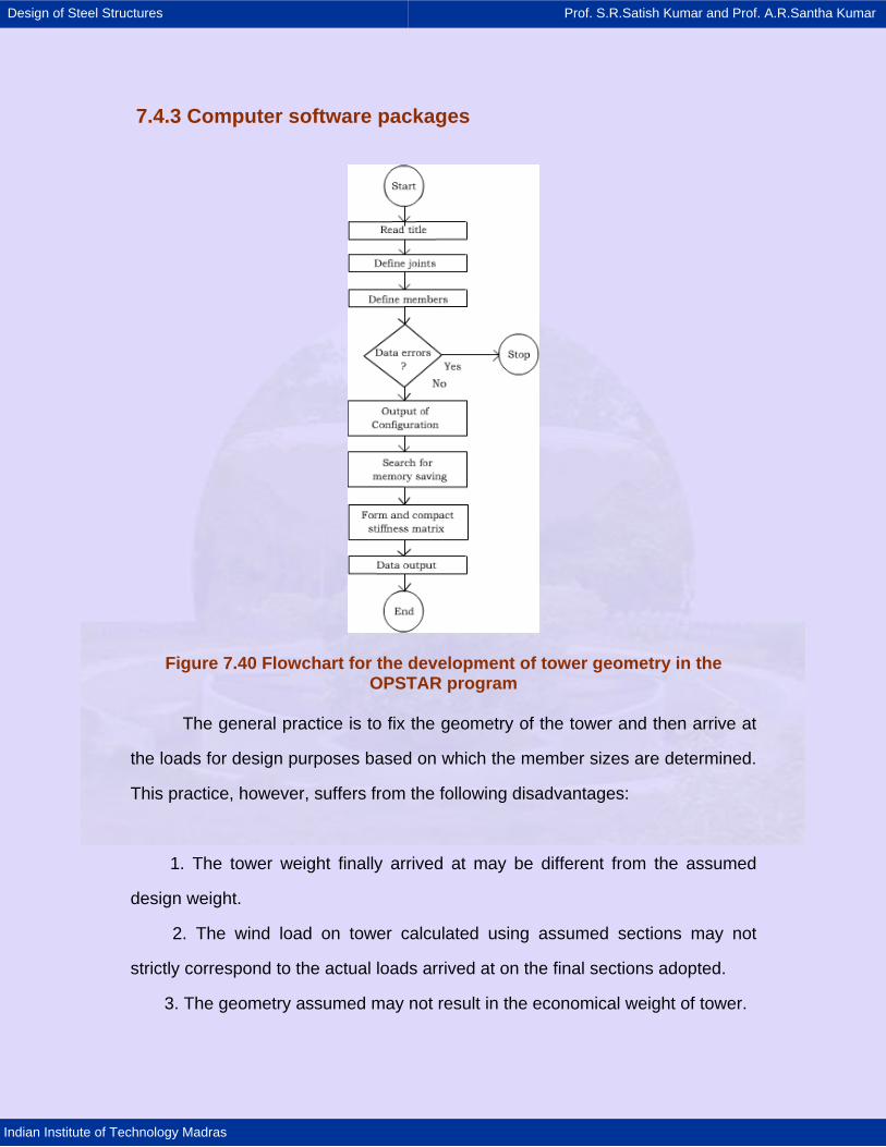
Design of Steel Structures Prof. S.R.Satish Kumar and Prof. A.R.Santha Kumar
Indian Institute of Technology Madras
7.4.3 Computer software packages
Figure 7.40 Flowchart for the development of tower geometry in the OPSTAR program
The general practice is to fix the geometry of the tower and then arrive at
the loads for design purposes based on which the member sizes are determined.
This practice, however, suffers from the following disadvantages:
1. The tower weight finally arrived at may be different from the assumed
design weight.
2. The wind load on tower calculated using assumed sections may not
strictly correspond to the actual loads arrived at on the final sections adopted.
3. The geometry assumed may not result in the economical weight of tower.
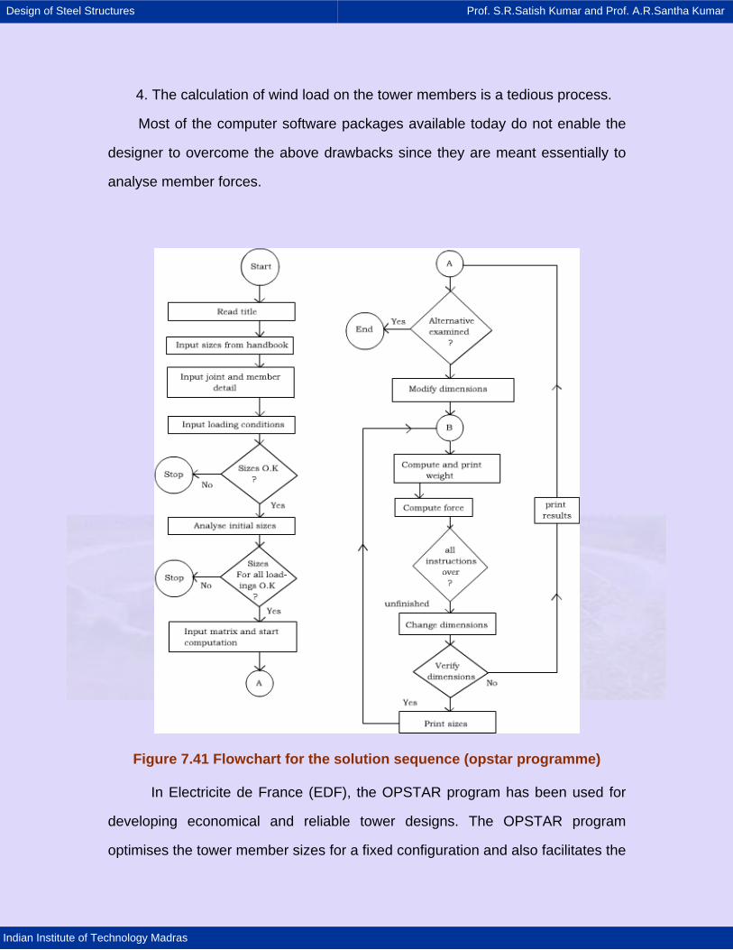
Design of Steel Structures Prof. S.R.Satish Kumar and Prof. A.R.Santha Kumar
Indian Institute of Technology Madras
4. The calculation of wind load on the tower members is a tedious process.
Most of the computer software packages available today do not enable the
designer to overcome the above drawbacks since they are meant essentially to
analyse member forces.
Figure 7.41 Flowchart for the solution sequence (opstar programme)
In Electricite de France (EDF), the OPSTAR program has been used for
developing economical and reliable tower designs. The OPSTAR program
optimises the tower member sizes for a fixed configuration and also facilitates the
Design of Steel Structures Prof. S.R.Satish Kumar and Prof. A.R.Santha Kumar
Indian Institute of Technology Madras
development of new configurations (tower outlines), which will lead to the
minimum weight of towers. The salient features of the program are given below:
Geometry: The geometry of the tower is described by the coordinates of the
nodes. Only the coordinates of the key nodes (8 for a tower in Figure 7.39)
constitute the input. The computer generates the other coordinates, making use
of symmetry as well as interpolation of the coordinates of the nodes between the
key nodes. This simplifies and minimises data input and aids in avoiding data
input errors.
Solution technique: A stiffness matrix approach is used and iterative
analysis is performed for optimisation.
Description of the program: The first part of the program develops the
geometry (coordinates) based on data input. It also checks the stability of the
nodes and corrects the unstable nodes. The flow chart for this part is given in
Figure 7.40.
The second part of the program deals with the major part of the solution
process. The input data are: the list of member sections from tables in
handbooks and is based on availability; the loading conditions; and the boundary
conditions.
The solution sequence is shown in Figure 7.41. The program is capable of
being used for either checking a tower for safety or for developing a new tower
design. The output from the program includes tower configuration; member sizes;
weight of tower; foundation reactions under all loading conditions; displacement
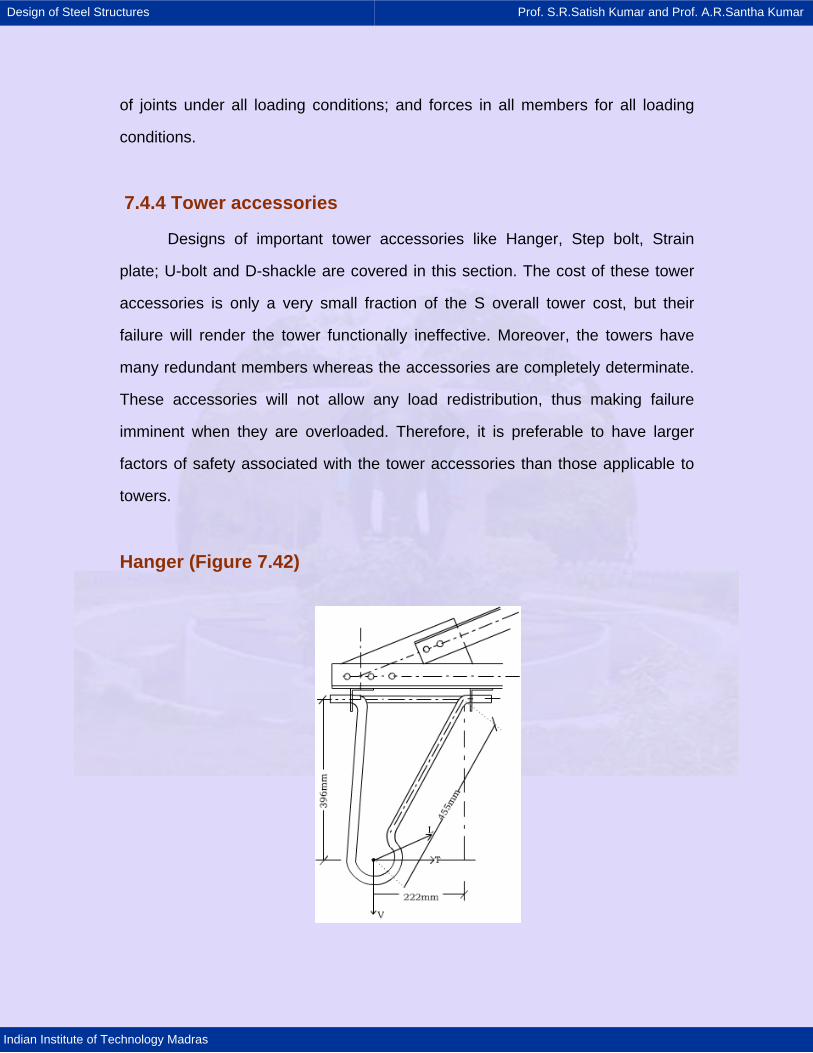
Design of Steel Structures Prof. S.R.Satish Kumar and Prof. A.R.Santha Kumar
Indian Institute of Technology Madras
of joints under all loading conditions; and forces in all members for all loading
conditions.
7.4.4 Tower accessories
Designs of important tower accessories like Hanger, Step bolt, Strain
plate; U-bolt and D-shackle are covered in this section. The cost of these tower
accessories is only a very small fraction of the S overall tower cost, but their
failure will render the tower functionally ineffective. Moreover, the towers have
many redundant members whereas the accessories are completely determinate.
These accessories will not allow any load redistribution, thus making failure
imminent when they are overloaded. Therefore, it is preferable to have larger
factors of safety associated with the tower accessories than those applicable to
towers.
Hanger (Figure 7.42)
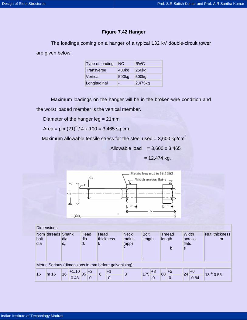
Design of Steel Structures Prof. S.R.Satish Kumar and Prof. A.R.Santha Kumar
Indian Institute of Technology Madras
Figure 7.42 Hanger
The loadings coming on a hanger of a typical 132 kV double-circuit tower
are given below:
Type of loading NC BWC Transverse 480kg 250kg Vertical 590kg 500kg Longitudinal - 2,475kg
Maximum loadings on the hanger will be in the broken-wire condition and
the worst loaded member is the vertical member.
Diameter of the hanger leg = 21mm
Area = p x (21)2 / 4 x 100 = 3.465 sq.cm.
Maximum allowable tensile stress for the steel used = 3,600 kg/cm2
Allowable load = 3,600 x 3.465
= 12,474 kg.
Dimensions Nom bolt dia
threads Shank dia ds
Head dia dk
Head thickness k
Neck radius (app) r
Bolt length
l
Thread length b
Width across flats s
Nut thickness m
Metric Serious (dimensions in mm before galvanising) +1.10 +2 +1 +3 +5 +0
16 m 16 16 -0.43
35 -0
6 -0
3 175-0
60-0
24 -0.84 13 0.55
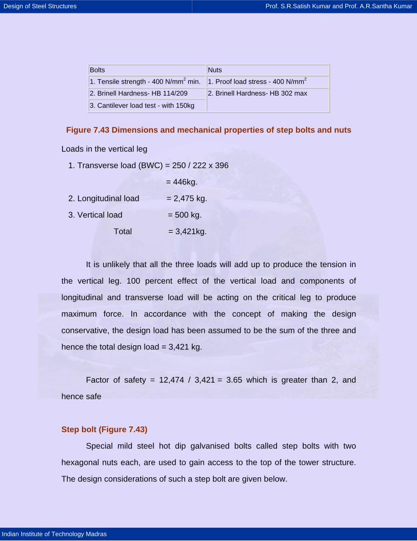
Design of Steel Structures Prof. S.R.Satish Kumar and Prof. A.R.Santha Kumar
Indian Institute of Technology Madras
Figure 7.43 Dimensions and mechanical properties of step bolts and nuts
Loads in the vertical leg
1. Transverse load (BWC) = 250 / 222 x 396
= 446kg.
2. Longitudinal load = 2,475 kg.
3. Vertical load = 500 kg.
Total = 3,421kg.
It is unlikely that all the three loads will add up to produce the tension in
the vertical leg. 100 percent effect of the vertical load and components of
longitudinal and transverse load will be acting on the critical leg to produce
maximum force. In accordance with the concept of making the design
conservative, the design load has been assumed to be the sum of the three and
hence the total design load = 3,421 kg.
Factor of safety = 12,474 / 3,421 = 3.65 which is greater than 2, and
hence safe
Step bolt (Figure 7.43)
Special mild steel hot dip galvanised bolts called step bolts with two
hexagonal nuts each, are used to gain access to the top of the tower structure.
The design considerations of such a step bolt are given below.
Bolts Nuts 1. Tensile strength - 400 N/mm2 min. 1. Proof load stress - 400 N/mm2 2. Brinell Hardness- HB 114/209 3. Cantilever load test - with 150kg
2. Brinell Hardness- HB 302 max
Design of Steel Structures Prof. S.R.Satish Kumar and Prof. A.R.Santha Kumar
Indian Institute of Technology Madras
The total uniformly distributed load over the fixed length = 100 kg
(assumed).
The maximum bending moment
100 x 13 / 2 = 650 kg cm.
The moment of inertia = p x 164 / 64 = 0.3218 cm4
Maximum bending stress = 650 x 0.8 / 0.3218
= 1,616 kg/cm2
Assuming critical strength of the high tensile steel = 3,600 kg/cm2,
factor of safety = 3,600 / 1,616 = 2.23, which is greater than 2, and hence
safe.
Step bolts are subjected to cantilever load test to withstand the weight of
man (150kg).
Strain plate (Figure 7.44)
The typical loadings on a strain plate for a 132 kV double-circuit tower are
given below:
Vertical load = 725kg
Transverse load = 1,375kg
Longitudinal load = 3,300kg
Bending moment due to vertical load = 725 x 8 / 2 = 2,900kg.cm.
Ixx = 17 x (0.95)3 / 12 = 1.2146 cm4
y (half the depth) = 0.475cm.
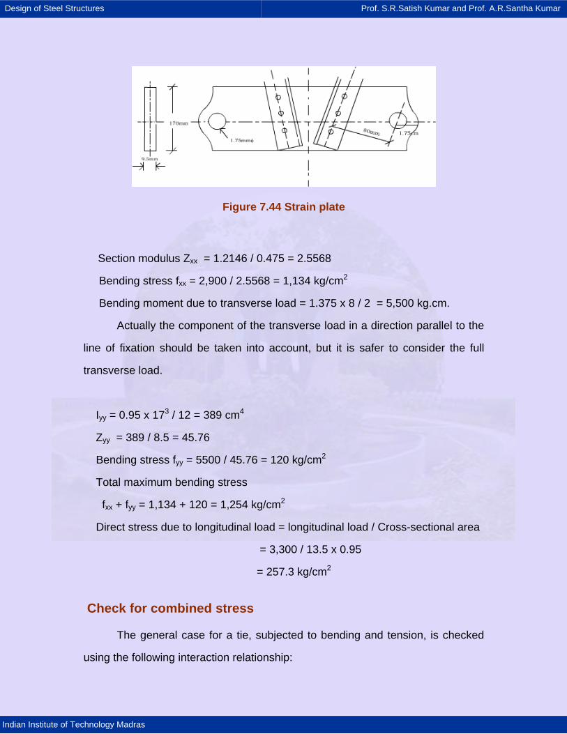
Design of Steel Structures Prof. S.R.Satish Kumar and Prof. A.R.Santha Kumar
Indian Institute of Technology Madras
Figure 7.44 Strain plate
Section modulus Zxx = 1.2146 / 0.475 = 2.5568
Bending stress fxx = 2,900 / 2.5568 = 1,134 kg/cm2
Bending moment due to transverse load = 1.375 x 8 / 2 = 5,500 kg.cm.
Actually the component of the transverse load in a direction parallel to the
line of fixation should be taken into account, but it is safer to consider the full
transverse load.
Iyy = 0.95 x 173 / 12 = 389 cm4
Zyy = 389 / 8.5 = 45.76
Bending stress fyy = 5500 / 45.76 = 120 kg/cm2
Total maximum bending stress
fxx + fyy = 1,134 + 120 = 1,254 kg/cm2
Direct stress due to longitudinal load = longitudinal load / Cross-sectional area
= 3,300 / 13.5 x 0.95
= 257.3 kg/cm2
Check for combined stress
The general case for a tie, subjected to bending and tension, is checked
using the following interaction relationship:
Design of Steel Structures Prof. S.R.Satish Kumar and Prof. A.R.Santha Kumar
Indian Institute of Technology Madras
b t
b T
f f1
F F+ ≤ (7.36)
Where ft = actual axial tensile stress,
fb = actual bending tensile stress
Ft = permissible axial tensile stress, and
Fb = permissible bending tensile stress.
Assuming Ft = 1,400 kg/cm2 and Fb = 1,550 kg/cm2. The expression
reduces to
= 1,254 / 1,550 + 257.3 / 1,400
= 0.9927 <1, hence safe.
Check for the plate in shear
Length of the plate edge under shear = 1.75 cm
Area under shear = 2 x 1.75 x 0.95
= 3.325 sq.cm.
Shearing stress =3,300 / 3,325 = 992 kg/cm2
Permissible shear stress = 1,000 kg/cm2
Hence, it is safe in shear.
Check for the plate in bearing
Pin diameter = 19mm
Bearing area = 1.9 x 0.95 = 1.805 cm2
Maximum tension in the conductor = 3,300 kg.
Bearing stress = = 1,828 kg/cm2
Permissible bearing stress = 1860 kg/cm2
Hence, it is safe in bearing.
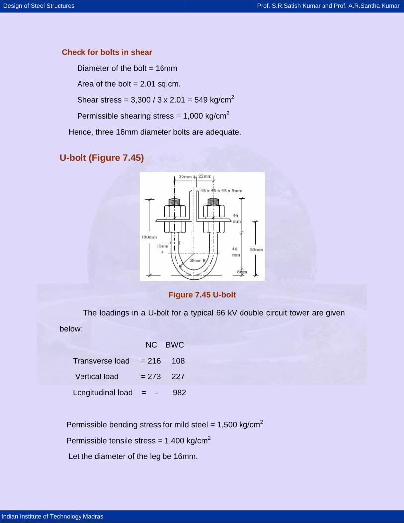
Design of Steel Structures Prof. S.R.Satish Kumar and Prof. A.R.Santha Kumar
Indian Institute of Technology Madras
Check for bolts in shear
Diameter of the bolt = 16mm
Area of the bolt = 2.01 sq.cm.
Shear stress = 3,300 / 3 x 2.01 = 549 kg/cm2
Permissible shearing stress = 1,000 kg/cm2
Hence, three 16mm diameter bolts are adequate.
U-bolt (Figure 7.45)
Figure 7.45 U-bolt
The loadings in a U-bolt for a typical 66 kV double circuit tower are given
below:
NC BWC
Transverse load = 216 108
Vertical load = 273 227
Longitudinal load = - 982
Permissible bending stress for mild steel = 1,500 kg/cm2
Permissible tensile stress = 1,400 kg/cm2
Let the diameter of the leg be 16mm.
Design of Steel Structures Prof. S.R.Satish Kumar and Prof. A.R.Santha Kumar
Indian Institute of Technology Madras
The area of the leg = 2.01 sq.cm.
1. Direct stress due to vertical load = 273 / 2.01 x 2
= 67.91 kg/cm2
2. Bending due to transverse load (NC)
Bending moment = 216 x 5 = 1,080 kg.cm
Section Modulus = 2 x πd3 / 32 = 2 x 3.14 x 1.63 / 32
= 0.804
Bending stress = 1,080 / 0.804
= 1,343 kg/cm2< 1,500 kg/cm2
Hence safe.
3. Bending due to longitudinal load (BWC)
Bending moment = 982 x 5 = 4,910 kg.cm
24 22 4
xxd dI x 2.5 25.77cm64 4
⎛ ⎞π π= + =⎜ ⎟⎜ ⎟
⎝ ⎠
y = 2.5 + 0.8
Bending stress = 4, 90 / 25.77 x (2.5 + 0.8) = 629 kg/cm2
In the broken-wire condition total bending stress = 1,343 / 2 + 629
= 1,300 kg/cm2
Hence, the worst loading will occur during normal condition.
For safe design,
b t
b t
f f1
F F+ ≤
Design of Steel Structures Prof. S.R.Satish Kumar and Prof. A.R.Santha Kumar
Indian Institute of Technology Madras
67.91 / 1400 + 1343 / 1500 = 0.9365 < 1
Hence safe.
Bearing strength of the angle-bolt connection
Safe bearing stress for the steel used = 4,725 kg/cm2
Diameter of hole = 16mm + 1.5mm = 17.5mm
Thickness of the angle leg = 5mm
Under normal condition
Bearing stress = (216 + 273)/1.75 x 0.5 = 558.85 kg/cm2
Factor of safety = 4,725 / 558.85 = 8.45
Under broken-wire condition
Bearing stress = (108+227+982) / 1.75 x 0.5
= 1,505.14 kg/cm2
Therefore, factor of safety = 4,725 /1,505.14 = 3.13
Hence safe.
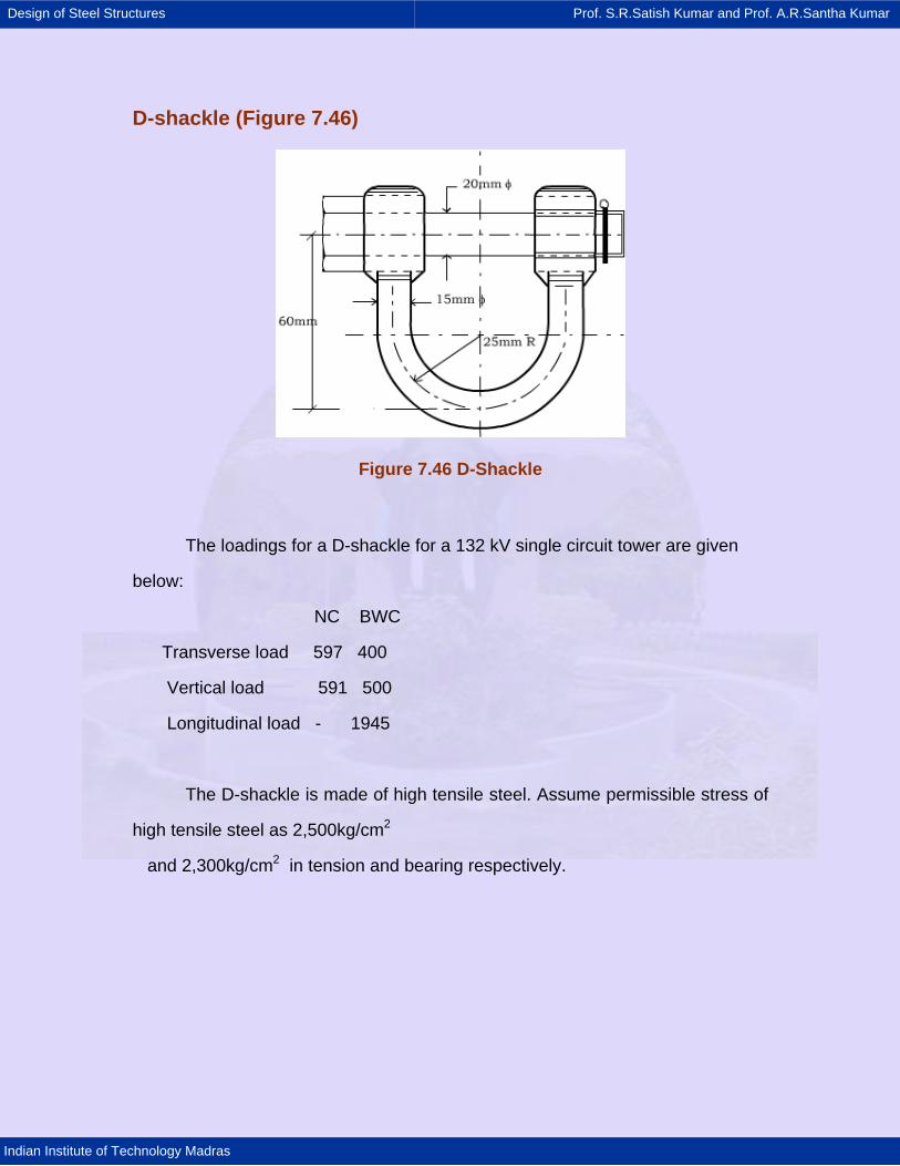
Design of Steel Structures Prof. S.R.Satish Kumar and Prof. A.R.Santha Kumar
Indian Institute of Technology Madras
D-shackle (Figure 7.46)
Figure 7.46 D-Shackle
The loadings for a D-shackle for a 132 kV single circuit tower are given
below:
NC BWC
Transverse load 597 400
Vertical load 591 500
Longitudinal load - 1945
The D-shackle is made of high tensile steel. Assume permissible stress of
high tensile steel as 2,500kg/cm2
and 2,300kg/cm2 in tension and bearing respectively.
Design of Steel Structures Prof. S.R.Satish Kumar and Prof. A.R.Santha Kumar
Indian Institute of Technology Madras
Normal condition
Area of one leg = π / 4 x (1.6) = 2.01 sq.cm.
Assuming the total load to be the sum of vertical and transverse loads
(conservative), the design load
= 597 + 591
= 1,188
Tensile stress = 1,188 / 2 x 1 / 2.01 = 295.5 kg/cm2
Factor of safety = 2,500 / 295.5 = 8.46
Shearing stress in the bolt = 2
597
x 24π
= 190 kg/cm2
Factory of safety = 2,300 / 190 = 12.1
Broken-wire condition
Assuming the total load to be sum of the loads listed for broken-wire
condition,
Tensile stress in shackle = 2,845 / 2 x 1 / 2.01
= 707.711 kg/cm2
Factor of safety = 2,500 / 707.7 = 3.53
Shearing stress in the bolt = ( )2
2,845
2 x x 24π
= 452.8
Factor of safety = 2,300 / 452.8 = 5.07
Hence safe.
Design of Steel Structures Prof. S.R.Satish Kumar and Prof. A.R.Santha Kumar
Indian Institute of Technology Madras
8. FOUNDATION OF TOWERS
8.1 Introduction
Foundation of any structure plays an important role in safety and
satisfactory performance of the structure as it transmits the loads from structure
to earth. Without having a sound and safe foundation, structure cannot perform
the functions for which it has been designed. Therefore, the design of foundation
needs to be given top priority.
Past records show that failures of tower foundations are responsible for
collapse of towers. These failures have usually been associated with certain
deficiencies either in the design or classification or construction of foundations.
Many times, foundation cast are over safe because of inappropriate
classification, resulting in wastage of resources. From engineering point of view,
the task of design and selection of most suitable type of tower foundation is
challenging because of the variety of soil conditions at the site of construction of
tower. The foundations in various types of soils have to be designed to suit the
soil conditions of particular type.
As the concept of safe value for properties of soil has been dispensed with
in the design of foundation, limit value of properties of soil should be obtained
from soil investigation report.
Design of Steel Structures Prof. S.R.Satish Kumar and Prof. A.R.Santha Kumar
Indian Institute of Technology Madras
8.2 Types of load on foundations
The foundations of towers are normally subjected to three types of forces.
These are
a. The compression or downward thrust;
b. The tension or uplift and
c. The lateral forces or side thrusts in both transverse and
longitudinal directions.
The magnitudes of each of these forces depend on the types of tower.
The magnitudes of limit loads for foundations should be taken 10% higher than
those for the corresponding towers.

Design of Steel Structures Prof. S.R.Satish Kumar and Prof. A.R.Santha Kumar
Indian Institute of Technology Madras
8.3 Basic design requirements
To meet the varying needs in respect of soil conditions and
loading quantum, several types of tower foundation have been used for the
communication towers. Design philosophy of tower foundation should be
closely related to the principles adopted for the design of towers, which the
foundation has to support. It should take care of all the loads such as dead load,
live loads, wind loads, seismic loads, erection loads etc. causing vertical thrust,
uplift as well as horizontal reactions. For satisfactory performances, it should be
stable and structurally adequate and be able to transmit these forces to the soil
such that the limit soil bearing capacities are not exceeding.
Design of Steel Structures Prof. S.R.Satish Kumar and Prof. A.R.Santha Kumar
Indian Institute of Technology Madras
8.4 Soil parameters
For designing the foundations, following parameters are required:
a. Limit bearing capacity of soil
b. Density of soil and
c. Angle of earth frustum.
These soil properties are normally obtained either by conducting in-situ or
Laboratory tests on soil samples collected from the field during soil investigation
or from available testing record of the area. The importance of above soil
parameters in foundation design is discussed below in brief.
Limit bearing capacity
This parameter is vital from the point of view of establishing the stability of
Foundation against shear failure of soil and excessive settlement of foundation
when Foundation is subjected to total downward loads and moments due to
horizontal shears and/or eccentricities as applicable.
Recommended limit bearing capacities of various types of soil are given in
Table 9.1 of Annexure for guidance.
Density of soil
This parameter is required to calculate the uplift resistance of the
foundation. Recommended values of angle of earth frustum for different types of
soils/rocks are given in Table.1 of Annexure.
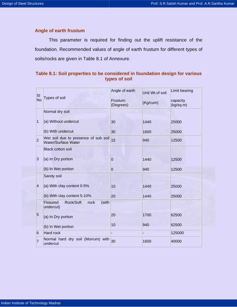
Design of Steel Structures Prof. S.R.Satish Kumar and Prof. A.R.Santha Kumar
Indian Institute of Technology Madras
Angle of earth frustum
This parameter is required for finding out the uplift resistance of the
foundation. Recommended values of angle of earth frustum for different types of
soils/rocks are given in Table 8.1 of Annexure.
Table 8.1: Soil properties to be considered in foundation design for various types of soil
SI No Types of soil
Angle of earth
Frustum (Degrees)
Unit Wt.of soil
(Kg/cum)
Limit bearing
capacity (kg/sq.m)
1
Normal dry soil
(a) Without undercut
(b) With undercut
30
30
1440
1600
25000
25000
2 Wet soil due to presence of sub soil Water/Surface Water 15 940 12500
3
Black cotton soil
(a) In Dry portion
(b) In Wet portion
0
0
1440
940
12500
12500
4
Sandy soil
(a) With clay content 0-5%
(b) With clay content 5-10%
10
20
1440
1440
25000
25000
5
Fissured Rock/Soft rock (with undercut)
(a) In Dry portion
(b) In Wet portion
20
10
1700
940
62500
62500
6 Hard rock - - 125000
7 Normal hard dry soil (Morrum) with undercut 30 1600 40000
Design of Steel Structures Prof. S.R.Satish Kumar and Prof. A.R.Santha Kumar
Indian Institute of Technology Madras
Note:
1. Limit bearing capacity of soil has been arrived at taking FOS 2.5 over
the safe bearing capacity values. Soil research institute will be approached to
furnish the limit bearing capacities of soil. If and when such data are available the
above values can be reviewed.
2. Where clay content is more than 10% but less than 15% the soil will be
classified as normal dry soil.
3. Angle of earth frustum shall be taken with respect to vertical.
(Source: Transmission line manual - Central board of irrigation and power)
Types of foundations
The foundations are designed for the uplift force, down thrust, lateral
forces and over turning moments for varieties of soils.
Depending upon the ground water table and type of soil and rock, the
foundations can be classified as follows.
Normal dry soil foundations
When water table is below foundation level and when soil is cohesive and
homogeneous up to the full depth having clay content of 10-15%.
Wet soil foundations
When water table is below foundation level and up to 1.5m below ground
level. the foundation in the soils which have standing surface water for a long
Design of Steel Structures Prof. S.R.Satish Kumar and Prof. A.R.Santha Kumar
Indian Institute of Technology Madras
period with penetration not exceeding 1.Om below ground level (e.g. paddy
fields) are also classified as wet foundations.
Partially submerged foundations
When water table is at a depth between 1.5m and 0.75 below ground level
and when the soil is normal and cohesive.
Fully submerged foundations
When water table is within 0.75m below ground and the soil is normal and
cohesive.
Black cotton soil foundations
When the soil is cohesive having inorganic clay exceeding 15% and
characterized by high shrinkage and swelling property (need not be always black
in colour)
Partial black cotton foundations
When the top layer of soil up to 1.5m is black cotton and thereafter it is
normal dry cohesive soil.
Soft rock/Fissured rock foundations
When discomposed or fissured rock, hard gravel or any other similar
nature is met this can be executed without blasting. Under cut foundation is to be
used at these locations.
Hard rock foundations
Where chiseling, drilling and blasting are required for execution.

Design of Steel Structures Prof. S.R.Satish Kumar and Prof. A.R.Santha Kumar
Indian Institute of Technology Madras
Sandy soil foundations
Soil with negligible cohesion because of its low clay content (0-10%)
The above categorization of foundations has been done for economizing
the design of foundations; uplift resistance of foundations is a critical design
factor which is greatly affected by the location of water table and the soil
surrounding the foundation.
Design of Steel Structures Prof. S.R.Satish Kumar and Prof. A.R.Santha Kumar
Indian Institute of Technology Madras
8.5 Structural arrangement of foundation
Based on structural arrangement of foundations, the various type of
foundations are possible. The necessity of erecting towers on a variety of soils
has made it possible and necessary for the designers to adopt new innovations
and techniques. As a result, several types of tower foundations have been
devised and successfully used. Some of the more common types of foundations
are described below.
P.C.C. types
This type of foundation consists of a plain concrete footing pad with
reinforced chimney. They is as shown in figure. In this type of foundation, the
stub angle is taken inside and effectively anchored to the bottom pad by cleat
angles and / or keying rods and the chimney with reinforcement and stub angle
inside works as a composite member. The pad may be either pyramidal in shape
as shown in Figure 8.1(a) or stepped as shown in Figure 8.1(b). Stepped footings
will require less shuttering materials but need more attention during construction
to avoid cold joints between the steps. The pyramidal footings on the other hand
will require somewhat costlier formwork. In this pad and chimney type footing,
where the chimney is comparatively slender, the lateral load acting at the top of
the chimney will cause bending moment and, therefore the chimney should be
checked for combined stress due to direct pull / thrust and bending.
If the soil is very hard, conglomerate of soil, containing stones, rubbles,
kankar which can be loosened with the help of pick-axe or if the soil is of
composite nature i.e. combination of normal dry soil, hard murrum, fissured rock
which will not get unified easily with the parent soil after back filling, pyramid
chimney type foundations having 150m side clearance are not advisable and in
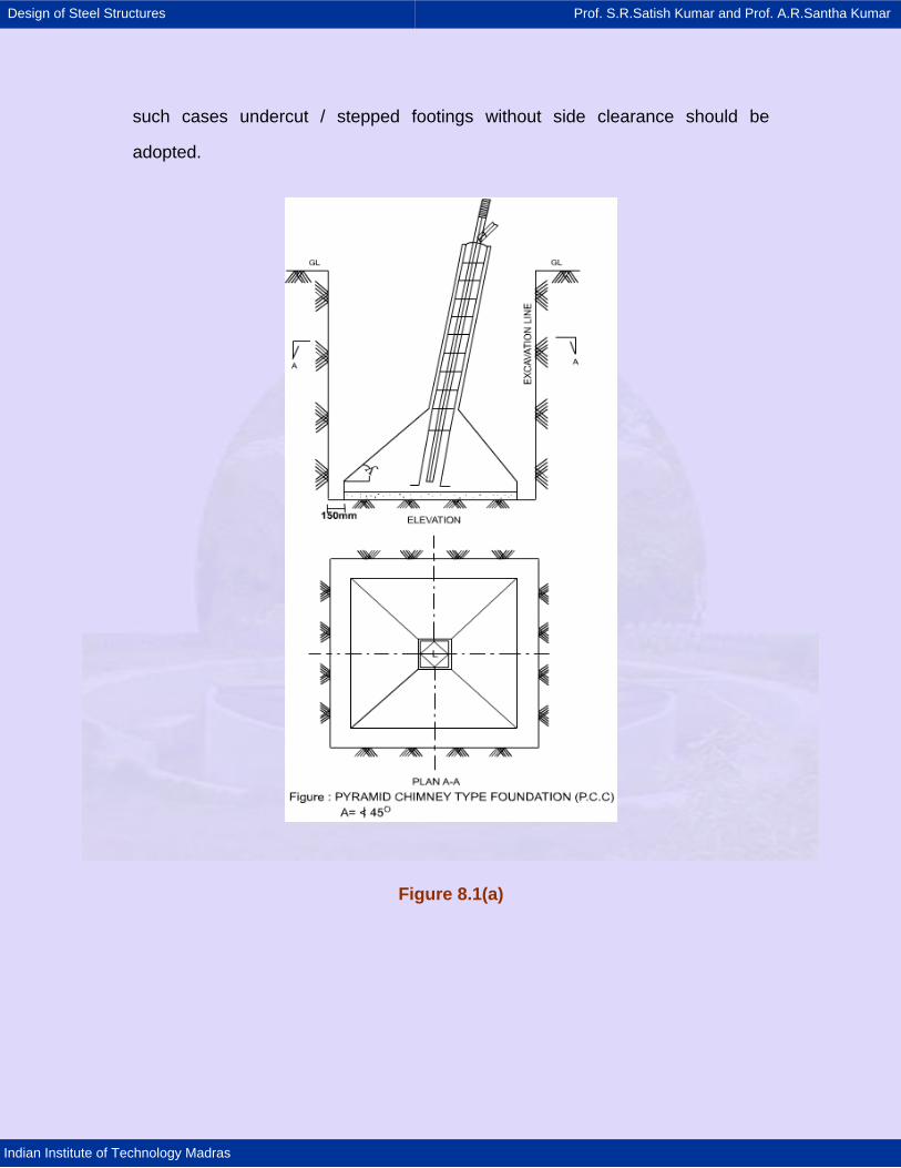
Design of Steel Structures Prof. S.R.Satish Kumar and Prof. A.R.Santha Kumar
Indian Institute of Technology Madras
such cases undercut / stepped footings without side clearance should be
adopted.
Figure 8.1(a)
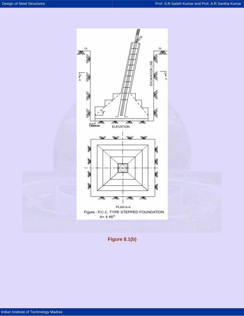
Design of Steel Structures Prof. S.R.Satish Kumar and Prof. A.R.Santha Kumar
Indian Institute of Technology Madras
Figure 8.1(b)
Design of Steel Structures Prof. S.R.Satish Kumar and Prof. A.R.Santha Kumar
Indian Institute of Technology Madras
R.C.C. spread type
Typical types of R.C.C spread footings are shown in figure 8.2. It consists
of a R.C.C base slab or mat and requires a square chimney.
There are several types of R.C.C spread footings which can be designed
for tower foundations. The three most common types of these are shown in figure
8.2(a), (b) and (c). As shown in figures, this type of foundation can be either
single step type or multiple step type and / or chamfered step type.
The R.C.C spread type footing can be suitably designed for variety of soil
conditions. R.C.C footings in some situations may be higher in cost although
structurally these are the best.
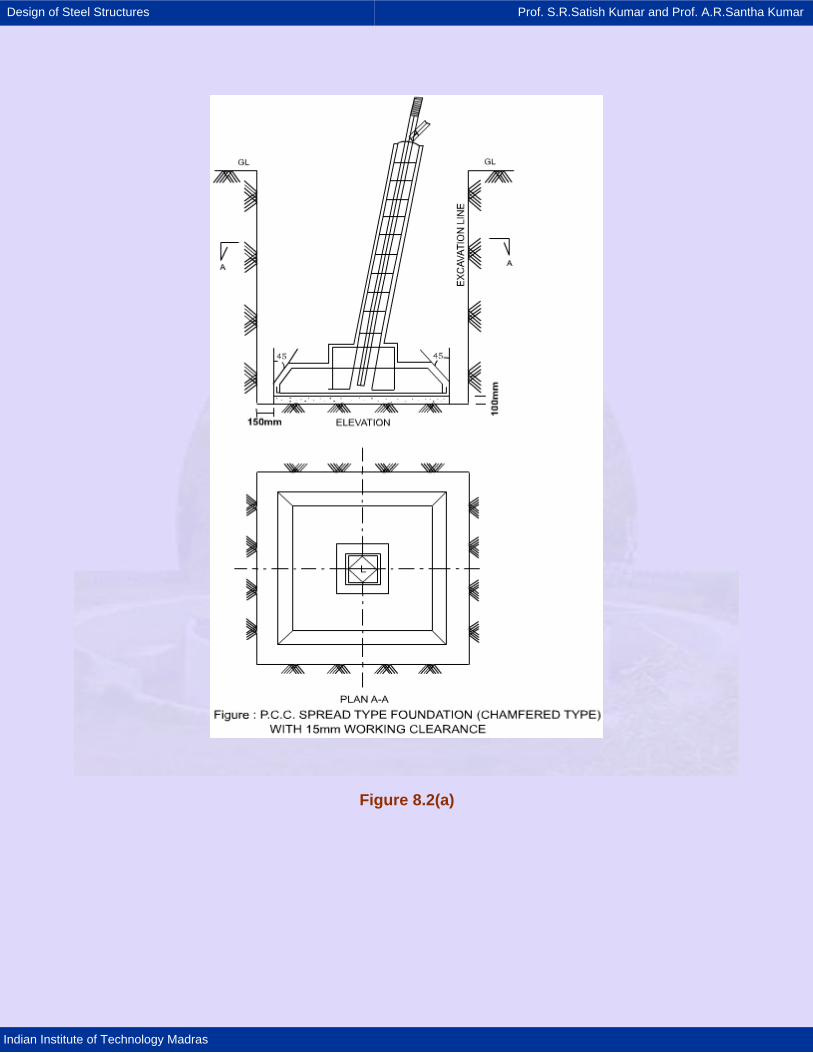
Design of Steel Structures Prof. S.R.Satish Kumar and Prof. A.R.Santha Kumar
Indian Institute of Technology Madras
Figure 8.2(a)
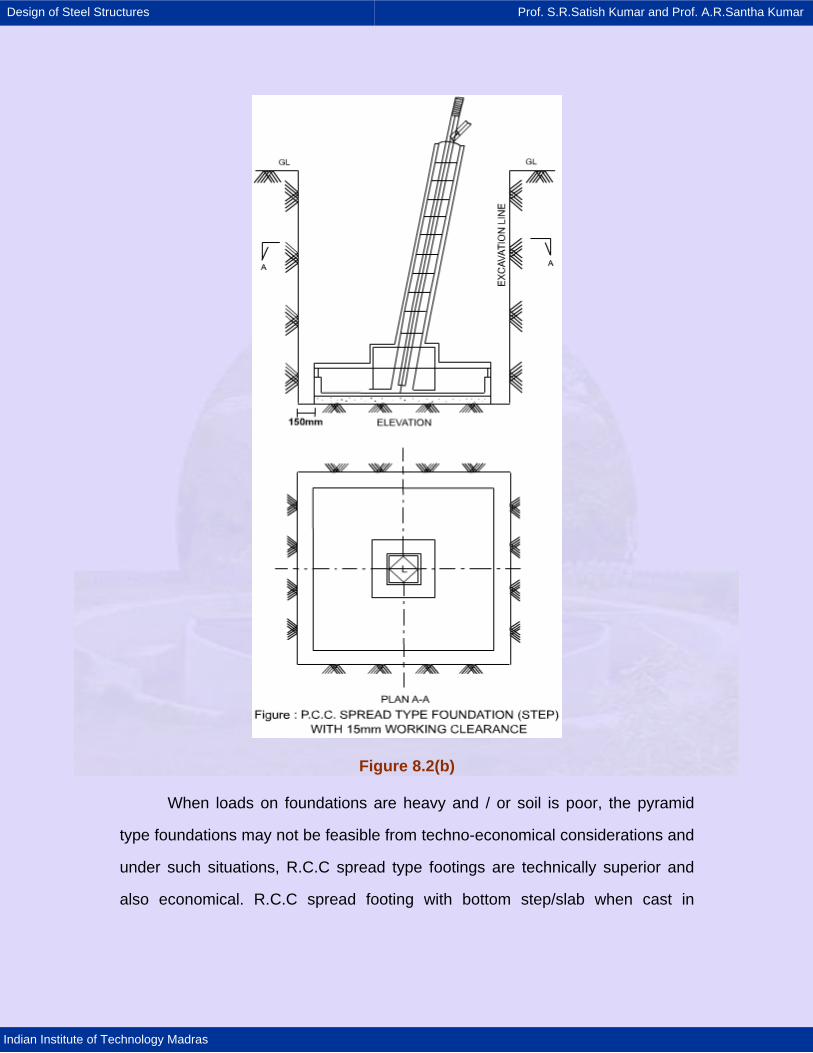
Design of Steel Structures Prof. S.R.Satish Kumar and Prof. A.R.Santha Kumar
Indian Institute of Technology Madras
Figure 8.2(b)
When loads on foundations are heavy and / or soil is poor, the pyramid
type foundations may not be feasible from techno-economical considerations and
under such situations, R.C.C spread type footings are technically superior and
also economical. R.C.C spread footing with bottom step/slab when cast in
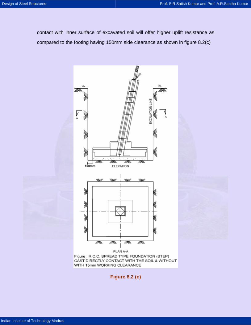
Design of Steel Structures Prof. S.R.Satish Kumar and Prof. A.R.Santha Kumar
Indian Institute of Technology Madras
contact with inner surface of excavated soil will offer higher uplift resistance as
compared to the footing having 150mm side clearance as shown in figure 8.2(c)
Figure 8.2 (c)
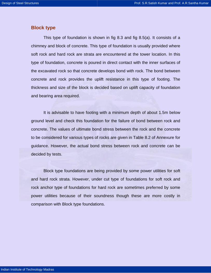
Design of Steel Structures Prof. S.R.Satish Kumar and Prof. A.R.Santha Kumar
Indian Institute of Technology Madras
Block type
This type of foundation is shown in fig 8.3 and fig 8.5(a). It consists of a
chimney and block of concrete. This type of foundation is usually provided where
soft rock and hard rock are strata are encountered at the tower location. In this
type of foundation, concrete is poured in direct contact with the inner surfaces of
the excavated rock so that concrete develops bond with rock. The bond between
concrete and rock provides the uplift resistance in this type of footing. The
thickness and size of the block is decided based on uplift capacity of foundation
and bearing area required.
It is advisable to have footing with a minimum depth of about 1.5m below
ground level and check this foundation for the failure of bond between rock and
concrete. The values of ultimate bond stress between the rock and the concrete
to be considered for various types of rocks are given in Table 8.2 of Annexure for
guidance. However, the actual bond stress between rock and concrete can be
decided by tests.
Block type foundations are being provided by some power utilities for soft
and hard rock strata. However, under cut type of foundations for soft rock and
rock anchor type of foundations for hard rock are sometimes preferred by some
power utilities because of their soundness though these are more costly in
comparison with Block type foundations.
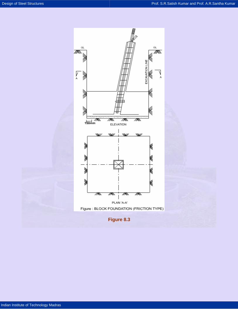
Design of Steel Structures Prof. S.R.Satish Kumar and Prof. A.R.Santha Kumar
Indian Institute of Technology Madras
Figure 8.3
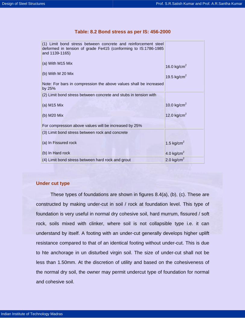
Design of Steel Structures Prof. S.R.Satish Kumar and Prof. A.R.Santha Kumar
Indian Institute of Technology Madras
Table: 8.2 Bond stress as per IS: 456-2000
(1) Limit bond stress between concrete and reinforcement steel deformed in tension of grade Fe415 (conforming to IS:1786-1985 and 1139-1165)
(a) With M15 Mix
(b) With M 20 Mix
Note: For bars in compression the above values shall be increased by 25%
16.0 kg/cm2
19.5 kg/cm2
(2) Limit bond stress between concrete and stubs in tension with
(a) M15 Mix
(b) M20 Mix
For compression above values will be increased by 25%
10.0 kg/cm2
12.0 kg/cm2
(3) Limit bond stress between rock and concrete
(a) In Fissured rock
(b) In Hard rock
1.5 kg/cm2
4.0 kg/cm2 (4) Limit bond stress between hard rock and grout 2.0 kg/cm2
Under cut type
These types of foundations are shown in figures 8.4(a), (b), (c). These are
constructed by making under-cut in soil / rock at foundation level. This type of
foundation is very useful in normal dry cohesive soil, hard murrum, fissured / soft
rock, soils mixed with clinker, where soil is not collapsible type i.e. it can
understand by itself. A footing with an under-cut generally develops higher uplift
resistance compared to that of an identical footing without under-cut. This is due
to hte anchorage in un disturbed virgin soil. The size of under-cut shall not be
less than 1.50mm. At the discretion of utility and based on the cohesiveness of
the normal dry soil, the owner may permit undercut type of foundation for normal
and cohesive soil.
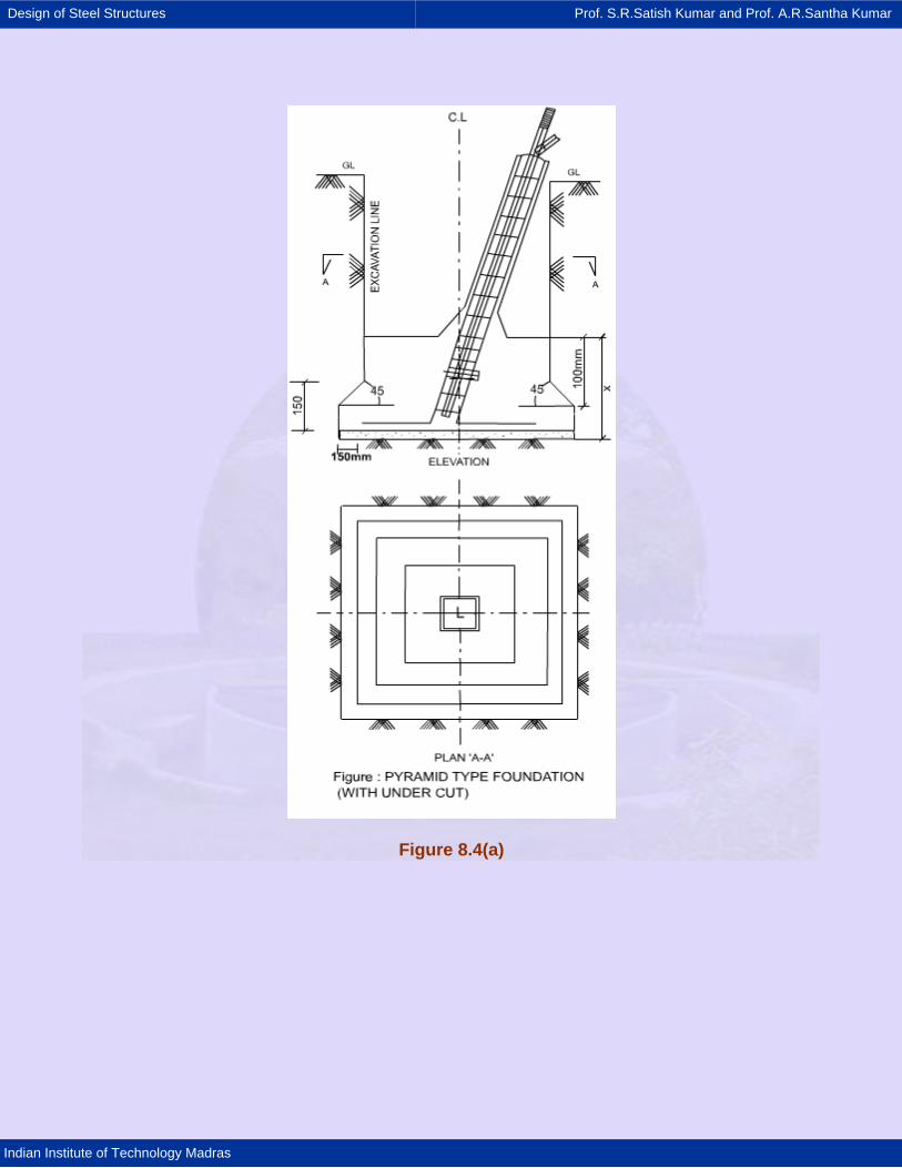
Design of Steel Structures Prof. S.R.Satish Kumar and Prof. A.R.Santha Kumar
Indian Institute of Technology Madras
Figure 8.4(a)
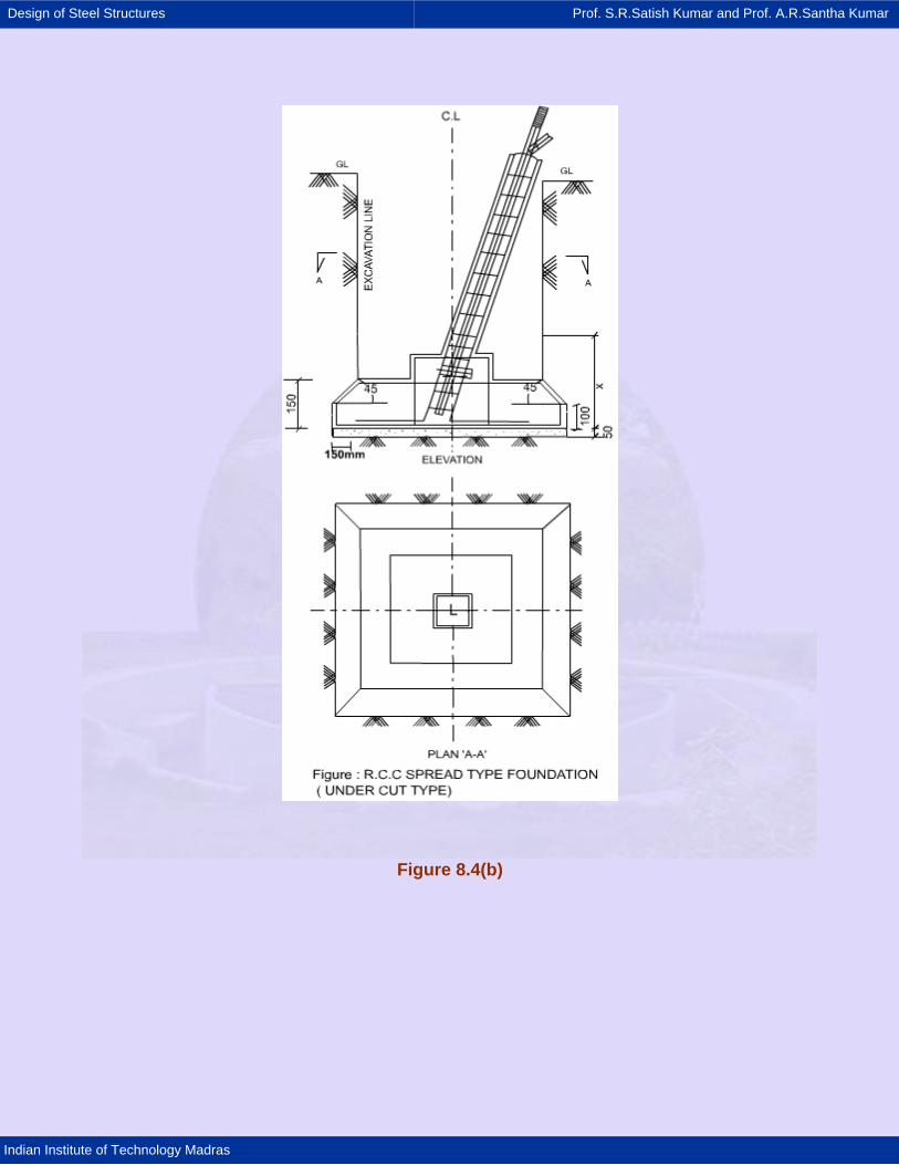
Design of Steel Structures Prof. S.R.Satish Kumar and Prof. A.R.Santha Kumar
Indian Institute of Technology Madras
Figure 8.4(b)
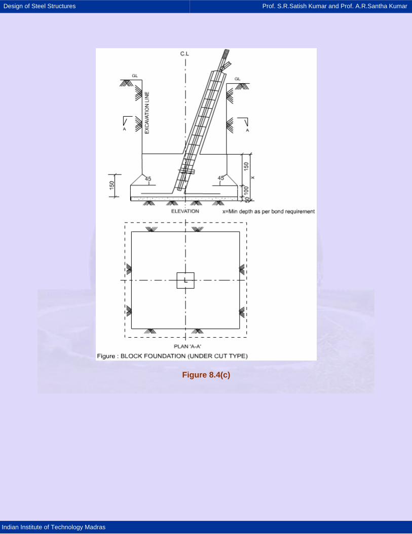
Design of Steel Structures Prof. S.R.Satish Kumar and Prof. A.R.Santha Kumar
Indian Institute of Technology Madras
Figure 8.4(c)
Design of Steel Structures Prof. S.R.Satish Kumar and Prof. A.R.Santha Kumar
Indian Institute of Technology Madras
Grouted rock and Rock anchor type
Typical Grouted rock and Rock anchor type footing is shown in figure
8.5(b). This type of footing is suitable when the rock is very hard. It consists of
two parts viz., Block of small depth followed by anchor bars embedded in the
grouted anchor holes. The top part of the bar is embedded in the concrete of the
shallow block. The depth of embedment, diameter and number of anchor bars
will depend upon the uplift force on the footing. The diameter shall not be less
than 12mm. The grouting hole shall normally be 20mm more than diameter of the
bar.
The determination of whether a rock formation is suitable for installation of
rock anchors is an engineering judgement based on rock quality. Since, the
bearing capacity of rock is usually much greater, care must be exercised in
designing for uplift. The rock surfaces may be roughened grooved or shaped to
increase the uplift capacity.
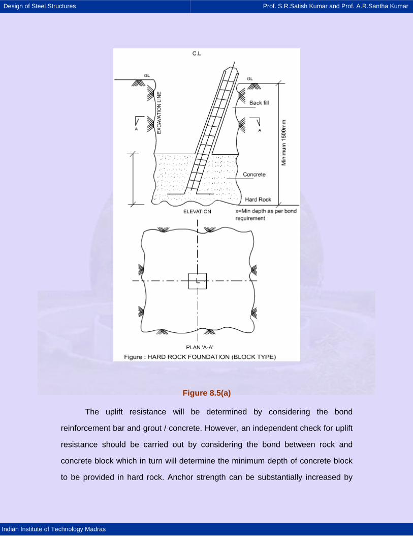
Design of Steel Structures Prof. S.R.Satish Kumar and Prof. A.R.Santha Kumar
Indian Institute of Technology Madras
Figure 8.5(a)
The uplift resistance will be determined by considering the bond
reinforcement bar and grout / concrete. However, an independent check for uplift
resistance should be carried out by considering the bond between rock and
concrete block which in turn will determine the minimum depth of concrete block
to be provided in hard rock. Anchor strength can be substantially increased by
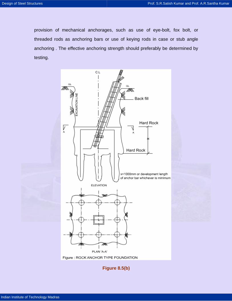
Design of Steel Structures Prof. S.R.Satish Kumar and Prof. A.R.Santha Kumar
Indian Institute of Technology Madras
provision of mechanical anchorages, such as use of eye-bolt, fox bolt, or
threaded rods as anchoring bars or use of keying rods in case or stub angle
anchoring . The effective anchoring strength should preferably be determined by
testing.
Figure 8.5(b)
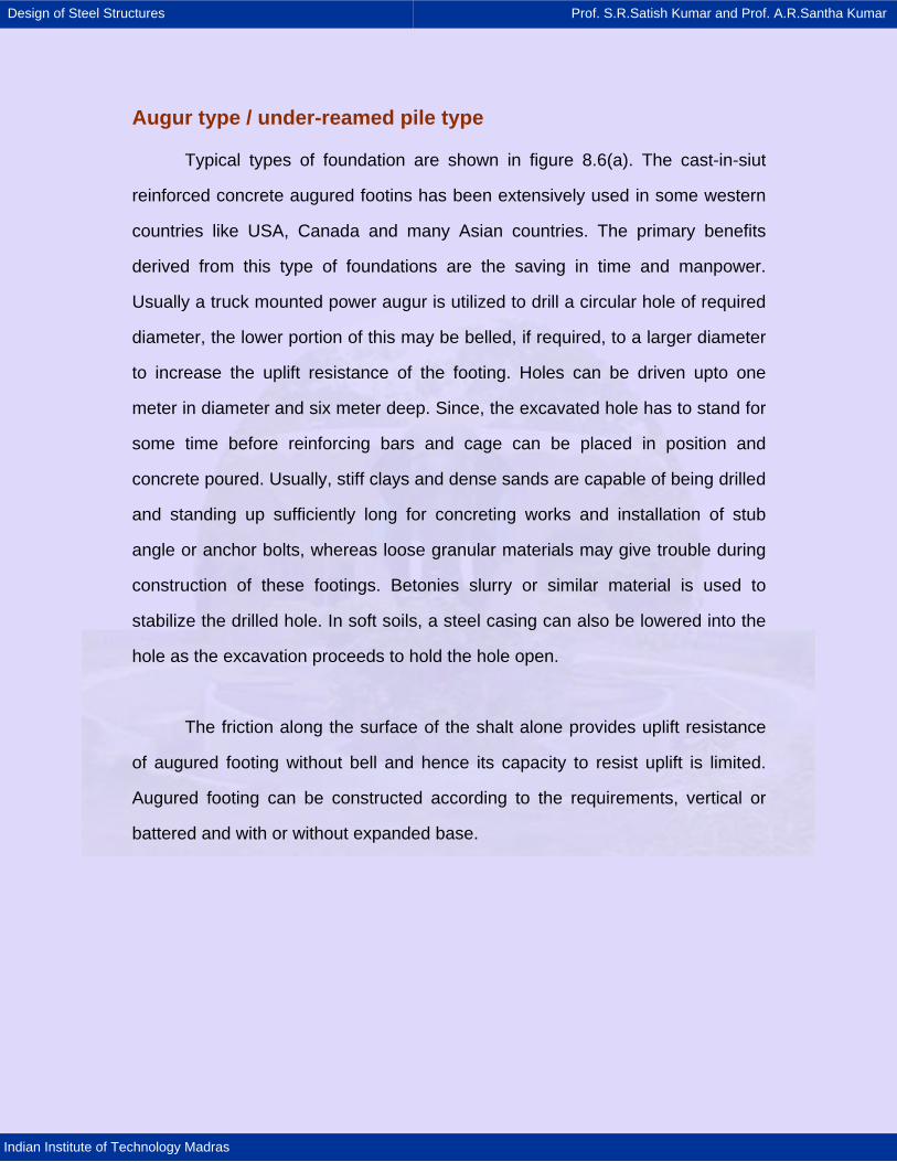
Design of Steel Structures Prof. S.R.Satish Kumar and Prof. A.R.Santha Kumar
Indian Institute of Technology Madras
Augur type / under-reamed pile type
Typical types of foundation are shown in figure 8.6(a). The cast-in-siut
reinforced concrete augured footins has been extensively used in some western
countries like USA, Canada and many Asian countries. The primary benefits
derived from this type of foundations are the saving in time and manpower.
Usually a truck mounted power augur is utilized to drill a circular hole of required
diameter, the lower portion of this may be belled, if required, to a larger diameter
to increase the uplift resistance of the footing. Holes can be driven upto one
meter in diameter and six meter deep. Since, the excavated hole has to stand for
some time before reinforcing bars and cage can be placed in position and
concrete poured. Usually, stiff clays and dense sands are capable of being drilled
and standing up sufficiently long for concreting works and installation of stub
angle or anchor bolts, whereas loose granular materials may give trouble during
construction of these footings. Betonies slurry or similar material is used to
stabilize the drilled hole. In soft soils, a steel casing can also be lowered into the
hole as the excavation proceeds to hold the hole open.
The friction along the surface of the shalt alone provides uplift resistance
of augured footing without bell and hence its capacity to resist uplift is limited.
Augured footing can be constructed according to the requirements, vertical or
battered and with or without expanded base.
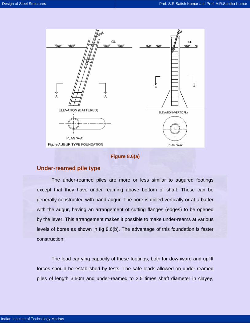
Design of Steel Structures Prof. S.R.Satish Kumar and Prof. A.R.Santha Kumar
Indian Institute of Technology Madras
Figure 8.6(a)
Under-reamed pile type
The under-reamed piles are more or less similar to augured footings
except that they have under reaming above bottom of shaft. These can be
generally constructed with hand augur. The bore is drilled vertically or at a batter
with the augur, having an arrangement of cutting flanges (edges) to be opened
by the lever. This arrangement makes it possible to make under-reams at various
levels of bores as shown in fig 8.6(b). The advantage of this foundation is faster
construction.
The load carrying capacity of these footings, both for downward and uplift
forces should be established by tests. The safe loads allowed on under-reamed
piles of length 3.50m and under-reamed to 2.5 times shaft diameter in clayey,
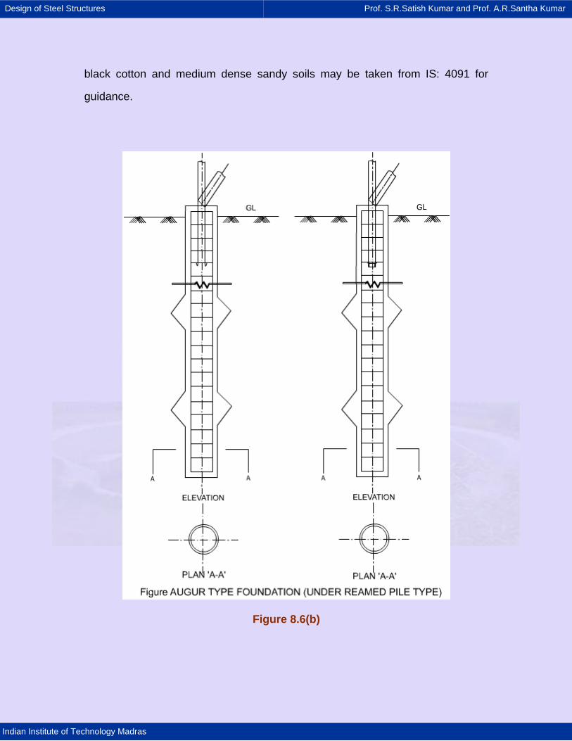
Design of Steel Structures Prof. S.R.Satish Kumar and Prof. A.R.Santha Kumar
Indian Institute of Technology Madras
black cotton and medium dense sandy soils may be taken from IS: 4091 for
guidance.
Figure 8.6(b)
Design of Steel Structures Prof. S.R.Satish Kumar and Prof. A.R.Santha Kumar
Indian Institute of Technology Madras
Pile type
A typical pile type is shown in Figure 8.7. This type of foundation is usually
adopted when soil isvery weak and has very poor bearing capacity or foundation
has to be located in filled-up soil or sea mud to a large depth or where tower
location falls within river bed and creek bed which are likely to get scoured
during floods. The pile foundations are designed based on the data of soil
exploration at the tower location. The important parameter for the design of pile
foundation the type of soil, angle of internal friction, cohesion and unit weight of
soil at various depths along the shaft of pile, maximum discharge of the river,
maximum velocity of water, high flood level, scour depth etc.
Pile foundation usually costs more and may be adopted only after the
detailed examination of the site condition and soil data. The downward vertical
load on the foundation is carried by the dead weight of the concrete in piles and
pile caps and frictional resistance between pile and soil surrounding the pile. For
carrying heavy lateral loads, battered piles may be advantageously used. Piles
are of different types such as driven pre-cast files, cast-in-situ concrete bored
piles and cast-in-situ concrete driven piles, concrete driven piles whether pr-cast
or cast-in-situ, require heavy machinery for their construction and as such may
no be possible to use for transmission line foundations because of the
remoteness of the sites and small volume of work. Mostly, cast-in-situ concrete
bored piles are provided in transmission line projects since, they do not require
heavy machinery for their construction.
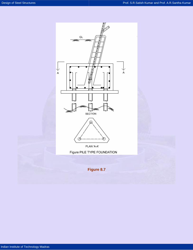
Design of Steel Structures Prof. S.R.Satish Kumar and Prof. A.R.Santha Kumar
Indian Institute of Technology Madras
Figure 8.7
Design of Steel Structures Prof. S.R.Satish Kumar and Prof. A.R.Santha Kumar
Indian Institute of Technology Madras
8.6 Soil resistances for designing foundation
As discussed earlier, the foundations of towers are subjected to three
types of loads viz., the downward trust (compression), the uplift (tension) and the
side trust (horizontal shear). The soil resistances available for transferring the
above forces to earth are described below.
Uplift resistance
The soil surrounding a tower foundation has to resist a considerable
amount of upward force (tension). In fact, in the case of self-supporting towers,
the available uplift resistance of the soil becomes the most decisive factor for
selection for a particular location.
It is generally considered that the resistance to uplift is provided by the
shear strength of the surrounding soil and the weight of the foundation. Various
empirical relationships linking ultimate uplift capacity of foundation to the physical
properties of soil like angle of internal friction (0) and cohesion (C) as well as the
dimensions and depth of the footing have been proposed on the basis of
experimental results. However, the angle of earth frustum is considered for
calculating the uplift resistance of soil. Typical value of angle of earth frustum;
are given in table of annexure for guidance the angle of earth frustum is taken as
2/3 of the angle of internal friction or the value given in the table whichever is
smaller for the type of soil under consideration. The uplift resistance is estimated
by computing the weight of the earth contained in an inverted frustum of cone
whose sides make an angle (0) with the vertical equal to the angle of earth
frustum.
Design of Steel Structures Prof. S.R.Satish Kumar and Prof. A.R.Santha Kumar
Indian Institute of Technology Madras
It should, however, be noted that effective uplift resistance, apart from
being a function of the properties of soil like angle of internal friction (0) and
cohesion (C) is greatly affected by the degree of compaction and the ground
water table. When the backfill is under consolidated with non-cohesive material,
the effective uplift resistance will be greatly reduced. In case of foundation under
water table, the buoyant weights of concrete and backfill are only considered to
be effective. The uplift resistance of footing with under cut projections within
undisturbed soils in firm non-cohesive soils and fissured/soft rock generally is
larger than that of conventional footings.
Lateral soil resistance
In foundation design of towers, the side thrusts on the foundation are
considered to be resisted by the passive earth pressures mobilized the adjoining
soils due to rotation of the footing. Passive pressure/resistance of soil is
calculated based on Rankine's formula for frictional soils and unconfirmed
compressive strength for cohesive soils.
Bearing capacity
The downward compressive loads acting on the foundation including
moments due to horizontal shears and / or eccentricities, where existing, are
transferred from foundation to earth through bearing capacity of soil. The limiting
bearing capacity of soil is the maximum downward intensity of load which the soil
can resist without shear failure or excessive settlement.
Design of Steel Structures Prof. S.R.Satish Kumar and Prof. A.R.Santha Kumar
Indian Institute of Technology Madras
8.7. Design procedure for foundation
The design of any foundation consists of following two parts.
8.7.1 Stability analysis
Stability analysis aims at removing the possibility of failure of foundation
by tilting, overturning, uprooting and sliding due to load intensity imposed on soil
by foundation being in excess of the ultimate capacity of the soil. The most
important aspect of the foundation design is the necessary check for the stability
of foundation under various loads imposed on it by the tower, which it supports.
The foundation should remain stable under all the possible combinations of
loading, to which it is likely to be subjected under the most stringent conditions.
The stability of foundations should be checked for the following aspects.
Check for bearing capacity
The total downward load at the base of footing consists of compression
per leg derived from the tower design, buoyant weight of concrete below ground
level and weight of concrete above ground level.
While calculating over weight of concrete for checking bearing capacity of
soil, the position of water table should be considered at critical location i.e., which
would give maximum over weight of concrete. In case of foundation with chimney
battered along the slope of leg, the center line of chimney may not coincide with
the center of gravity of base slabs/pyramid/block. Under such situation, axial load
in the chimney can be resolved into vertical and horizontal components at the top
of the base slabs/pyramid/block. The additional moments due to the above
horizontal loads should be considered while checking the bearing capacity of soil.
Design of Steel Structures Prof. S.R.Satish Kumar and Prof. A.R.Santha Kumar
Indian Institute of Technology Madras
Further even in cases where full horizontal shear is balanced try the
passive pressure of soil, the horizontal shears would caused moment at the bas
of footing as the line of action of side thrusts (horizontal shears) and resultant of
passive pressure of soil are not in the same line. It may be noted that passive
pressure of soil is reactive forces from heat soil for balancing the external
horizontal forces and as much mobilized passive pressure in soil adjoining the
footing cannot be more than the external horizontal shear.
Thus the maximum soil pressure below the base of the foundation (toe
pressure) will depend up on the vertical thrust (compression load) on the footing
and the moments at the base level due to the horizontal shears and other
eccentric loadings. Under the action of down thrust and moments, the soil
pressure below the footing will not be uniform and the maximum toe pressure 'p'
on the soil can be determined from the equation.
T L
T L
M MWPB x B Z Z
= + +
Where
'W' is the total vertical down thrust including over weight of the footing,
'B' is the dimension of the footing base;
MT & ML are moments at the base of footing about transverse and longitudinal
axes of footing and
ZT & ZL are the section module of footing which are equal to (1/6)B3 for a
square footing.
The above equation is not valid when minimum pressure under the footing
becomes negative. The maximum pressure on the soil so obtained should not
exceed the limit bearing capacity of the soil.
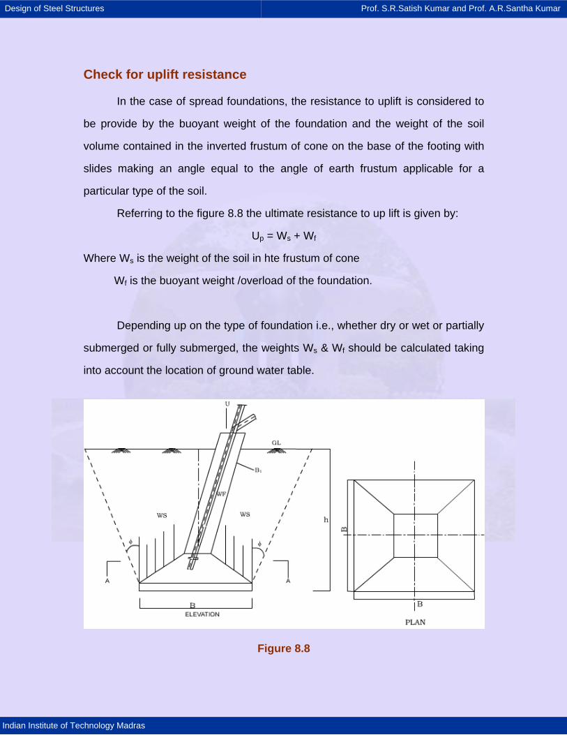
Design of Steel Structures Prof. S.R.Satish Kumar and Prof. A.R.Santha Kumar
Indian Institute of Technology Madras
Check for uplift resistance
In the case of spread foundations, the resistance to uplift is considered to
be provide by the buoyant weight of the foundation and the weight of the soil
volume contained in the inverted frustum of cone on the base of the footing with
slides making an angle equal to the angle of earth frustum applicable for a
particular type of the soil.
Referring to the figure 8.8 the ultimate resistance to up lift is given by:
Up = Ws + Wf
Where Ws is the weight of the soil in hte frustum of cone
Wf is the buoyant weight /overload of the foundation.
Depending up on the type of foundation i.e., whether dry or wet or partially
submerged or fully submerged, the weights Ws & Wf should be calculated taking
into account the location of ground water table.
Figure 8.8
Design of Steel Structures Prof. S.R.Satish Kumar and Prof. A.R.Santha Kumar
Indian Institute of Technology Madras
Under-cut type of foundation offers greater resistance to uplift than an
identical footing without under-cut. This is for the simple reason that the angle of
earth frustum originates from the toe of the under-cut and there is perfect bond
between concrete and the soil surrounding it and there is no need to depend on
the behavior of back filled earth. Substantial additional uplift resistance is
developed due to use of under-cut type of foundation. However, to reflect
advantage of additional uplift resistance in the design the density of soil for
under-cut foundation has been increased as given in Table of Annexure.
In cases where frustum of earth pyramid of two adjoining legs overlap, the
earth frustum is assumed truncated by a vertical plane passing through the
center line of the tower base.
Check for side thrust
In towers with inclined stub angles and having diagonal bracing at the
lowest panel point, the net shearing force of the footing is equal to the horizontal
component of the force in hte diagonal bracing whereas in towers with vertical
footings, the total horizontal load on the tower is divided equally between the
numbers of legs. The shear force causes bending stresses ink the unsupported
length of the stub angles as well as in the chimney and tends to overturn the
foundation.
When acted upon by a lateral load, the chimney will act as a cantilever
beam free at the top and fixed at the base and supported by the soil along its
height. Analysis of such foundations and design of the chimney for bending
moments combined with down thrust uplift is very important. Stability of a footing
under a lateral load depends on the amount of passive pressure mobilized in the
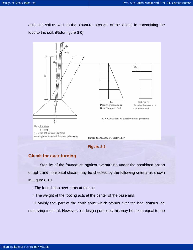
Design of Steel Structures Prof. S.R.Satish Kumar and Prof. A.R.Santha Kumar
Indian Institute of Technology Madras
adjoining soil as well as the structural strength of the footing in transmitting the
load to the soil. (Refer figure 8.9)
Figure 8.9
Check for over-turning
Stability of the foundation against overturning under the combined action
of uplift and horizontal shears may be checked by the following criteria as shown
in Figure 8.10.
i The foundation over-turns at the toe
ii The weight of the footing acts at the center of the base and
iii Mainly that part of the earth cone which stands over the heel causes the
stabilizing moment. However, for design purposes this may be taken equal to the
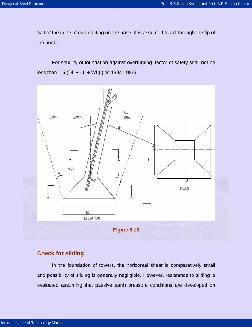
Design of Steel Structures Prof. S.R.Satish Kumar and Prof. A.R.Santha Kumar
Indian Institute of Technology Madras
half of the cone of earth acting on the base. It is assumed to act through the tip of
the heel.
For stability of foundation against overturning, factor of safety shall not be
less than 1.5 (DL + LL + WL) (IS: 1904-1986)
Figure 8.10
Check for sliding
In the foundation of towers, the horizontal shear is comparatively small
and possibility of sliding is generally negligible. However, resistance to sliding is
evaluated assuming that passive earth pressure conditions are developed on
Design of Steel Structures Prof. S.R.Satish Kumar and Prof. A.R.Santha Kumar
Indian Institute of Technology Madras
vertical projections above the toe of foundations. The friction between bottom of
the footing and soil also resist the sliding of footing and can be considered in the
stability of foundation against sliding. The coefficient of friction between concrete
and soil can be considered between 0.2 and 0.3. However, the frictional force is
directly proportional to vertical downward load and as such may not exist under
uplift condition. For cohesive soil the following formula can be applied for
calculating the passive pressure to resist sliding.
Pp = 2C tan + γh tan2 θ
Where C = Cohesion
θ = 45o + 1/2 of angle of earth frustum
H = height of foundation
γ = unit weight of soil
For stability of foundation against sliding. Factor of safety shall not be less
than 1.5(DL + LL + WL) (IS: 1904-1986)
8.7.2 Structural design of foundation
Structural design of concrete foundation comprises the design of chimney
and the design of base slab/pyramid/block. The structural design of different
elements of concrete foundation is discussed below.
Structural design of chimney
The chimney should be designed for maximum bending moments due to
side thrust in both transverse and longitudinal direction combined with direct pull
(Tension)/ direct down thrust (compression).
Design of Steel Structures Prof. S.R.Satish Kumar and Prof. A.R.Santha Kumar
Indian Institute of Technology Madras
Usually, combined uplift and bending will determine the requirement of
longitudinal reinforcement in the chimney. When the stub angle is embedded in
the chimney to its full depth and anchored to the bottom slab/pyramid/block the
chimney is designed considering passive resistance of soil leaving 500mm from
ground level. This is applicable for all soils - cohesive, non-cohesive and mixture
of cohesive and non-cohesive soils. In hilly areas and for fissured rock, passive
resistance of soils will not be considered. Stub angles will not be considered to
provide any reinforcement.
In certain cases, when stub is embedded in the chimney for the required
development length alone and same is not taken up to the bottom of foundation
of leg of the tower is fixed at the top of the chimney/pedestal by anchor bolts,
chimney should be designed by providing reinforcement to withstand combined
stresses due to direct tension/down thrust (compression) and bending moments,
due to side thrust in both transverse and longitudinal direction. The structural
design of chimney for the above cases should comply with the procedures given
in IS: 456-1978 and SP-16 using limit state method of design.
Case 1 when stub angle is anchored in base slab/pyramid/block
When the stub is anchored in base slab/pyramid/block reinforcement shall be
provided in chimney for structural safety on the sides of the chimney at the
periphery.
( )( )ui si ci ck2
ck 1
P0.36k P /100 f f / f
f B⎡ ⎤= + −⎣ ⎦∑ (8.1)
( ) ( )( ) ( )i si ci ck i2ck 1
M 0.36k 0.5 0.416k P /100 f f / f Y / Df B
⎡ ⎤= − + −⎣ ⎦∑ (8.2)
Design of Steel Structures Prof. S.R.Satish Kumar and Prof. A.R.Santha Kumar
Indian Institute of Technology Madras
cbc
cbc st
mK
mσ
=σ + σ
Where
Asi = cross sectional area of reinforcement in it row
Pi = 100 Asi / B12
fci = stress in concrete at the level of ith row of reinforcement
fy = Stress in the ith row of reinforcement, compression being positive and
tension being negative
Yi = distance from the centroid of the section to the ith row of
reinforcement: positive towards the highly compressed edge and negative
towards the least compressed edge
n = Number of rows of reinforcement
fss = stress in stubs
fcs = stress in concrete
fck = characteristic compressive strength of concrete
m = modular ratio
σCbc = permissible bending compressive stress in concrete
σSt = permissible tensile stress in steel
Case 2 when stub is provided in chimney only for its development length
When stub is provided in chimney only for its development length,
chimney has to be designed for and reinforcement provided for combined
stresses due to direct puit (tension) thrust (compression) and bending moments.
The requirement of longitudinal reinforcement should be calculated in
accordance with IS: 456-1978 and SP: 16 as an independent concrete column.
Design of Steel Structures Prof. S.R.Satish Kumar and Prof. A.R.Santha Kumar
Indian Institute of Technology Madras
In this case, from the equilibrium of internal and external forces on the
chimney section and using stress and strains of concrete and steel as per
IS:456-1978 the following equations are given in SP:16 are applicable.
( ) ( )( ) ( )( )ui si ci s ss ci ck
ck 1
P0.36k 0.5 0.416k P /100 f f p /100 f f / f
f B⎡ ⎤= − + − + −⎣ ⎦∑ (8.3)
( ) ( )( ) ( )ui si ci ck i
ck 1
P0.36k 0.5 0.416k P /100 f f / f Y / D
f B⎡ ⎤= − + −⎣ ⎦∑ (8.4)
In each of the above cases, for a given axial force compression or tension,
and for area of reinforcement, the depth of neutral axis Yu = KB1 can be
calculated from Equations using stress strain relationship for concrete and steel
as given in IS: 456-1978. After finding out the value of 'K' the bending capacity of
the chimney section can be worked out using equation. The bending capacity of
the chimney section should be more than the maximum moment caused in the
chimney by side thrust (horizontal shear). Chimney is subjected to biaxial
moments i.e., both longitudinal and transverse. The structural adequacy of the
chimney in combined stresses due to axial force (tension/compression) and
bending should be checked from the following equation:
un un
T L
ut ul
M M1.0
M M⎡ ⎤ ⎡ ⎤
+ <⎢ ⎥ ⎢ ⎥⎣ ⎦ ⎣ ⎦
Where,
MT and ML are the moments about transverse and longitudinal axis of the
chimney
Mut and Mul are the respective moment of resistance with axial loads of Pu
about transverse and longitudinal axis of chimney which would be equal in case
of square chimney with uniform distribution of reinforcement on all four faces.
Design of Steel Structures Prof. S.R.Satish Kumar and Prof. A.R.Santha Kumar
Indian Institute of Technology Madras
N is an exponent whose value would be 1.0 when axial force is tensile and
depends on the value of Pu / Puz when axial force is compressive where:
Puz = 0.45 fck Ac + 0.75 fysAs + 0.75 fysAss
In the above equation
Ac is the area of concrete
As is the area of reinforcement steel
Ass is the cross sectional area on stub to be taken as zero
fy is the yield stress of reinforcement steel and
fys is the yield stress of stub steel to be taken as zero.
Pu / Puz N 0.2
0.3
1.0
2.0
For intermediate values, linear interpolation may be done.
The solution of equations for case-2 is given is SP-16 in the form of
graphs for various grades of concrete and steel and these can be readily used
Important codal provision F
While designing the chimney, the important codal provisions as given
below should be followed:
(a) In any chimney that has a larger cross sectional area than that required to
support the load the minimum percentage of steel shall be based on the
area of concrete required to resist the direct stress and not on the actual
area.
(b) The minimum number longitudinal bars provided in a column shall be four
in square chimney and six in a circular chimney.
(c) The bars shall not be less than 12mm in diameter.
Design of Steel Structures Prof. S.R.Satish Kumar and Prof. A.R.Santha Kumar
Indian Institute of Technology Madras
(d) In case of a chimney in which the longitudinal reinforcement is not required
in strength calculation, nominal longitudinal reinforcement not less than
0.15% of the cross sectional area shall be provided.
(e) The spacing of stirrups/ lateral ties shall be not more than the least of the
following distances:
i. The least lateral dimension of the chimney
ii. Sixteen times the smallest diameter of the longitudinal reinforcement
bar to be tied.
iii. Forty-eight times the diameter of the transverse stirrups / lateral ties.
(f) The diameter of the polygonal links or lateral ties shall be not less than one-
fourth of the diameter of the largest longitudinal bar and in no case less
6mm.
(g) Structural design of base slab
The base slab in R.C.C spread foundations could be single stepped or
multistepped. The design of concrete foundations shall be done as per limit state
method of design given in IS: 456-2000.
Important codal stipulations for R.C.C foundations
The important provisions applicable for concrete foundations which are
necessary and should be considered in the design are explained below:
(a) Footings shall be designed to sustain the applied loads moments and
forces and the included reactions and to ensure that any settlement which may
occur shall be as nearly uniform possible and the bearing capacity of the soil is
not exceeded.
Design of Steel Structures Prof. S.R.Satish Kumar and Prof. A.R.Santha Kumar
Indian Institute of Technology Madras
(b) Thickness at the edge of footing in reinforced concrete footing shall not
be less than 15cm (5cm lean concrete plus 10cm structural concrete). In case of
plain concrete footing thickness at the edge shall not be less than 5cm.
(c) Bending moment
i. The bending moment at any section shall be determined by passing
through the section of a vertical plane which extends completely across the
footing and computing the moment of the forces acting over the entire area of the
footing on the side of the said plane.
ii. The greatest bending moment to be used in the design of an isolated
concrete footing which supports a column / pedestal shall be the moment
computed in the manner prescribed in c(i) above at section located as follow:
a. At the face of the chimney.
b. At the sections where width / thickness of the footing changes.
(d) Shear and bond
The shear strength of footing is governed by the more severe of the following
two conditions:
i. The footing acting essentially as a wide beam with a potential diagonal crack
extending in a place across the entire width; the critical section for this condition
should be assumed as a vertical section located from the face of the chimney at
a distance equal to the effective depth of the footing in case of footings on soils.
ii. Two-way action of the following with potential diagonal cracking along the
surface of truncated cone or pyramid around the concentrated load.
Design of Steel Structures Prof. S.R.Satish Kumar and Prof. A.R.Santha Kumar
Indian Institute of Technology Madras
(e) Critical section
The critical section for checking the development length in a footing shall be
assumed at the same plane as those described for bending moment in para (c)
above and also at all other vertical planes where abrupt changes of section
occurs.
When a plain concrete pyramid and chimney type footing is provided and
pyramidal slopes out from the chimney at an angle less than 45 from vertical, the
pyramid is not required to be checked for bending stresses. Thus, in such cases
the footing is designed to restrict the spread of concrete pyramid of slab block to
45 with respect to vertical.
8.7.3 Concrete technology for tower foundation designs
While designing the various types of concrete footings it is better to know
about certain aspects of concrete technology which are given below:
Properties of concrete
The grade of the structural concrete used for tower foundations should not
be leaner than M15 having a 28-day cube strength of not less than 15 N/mm2
and concrete shall conform to IS: 456, for special foundations like pile
foundations richer concrete of grade of M20 having a 28-day cube strength of not
less than 20 N/mm2 should be used. M15 grade concrete shall have the nominal
strength of not less than 15 N/mm2 at the end of 28 days as ascertained from the
cube test. Such strength at the end of 7 days shall not be less than 10 N/mm2.
The density of the concrete will be 2300 kg/m3 for plain concrete and 2400
kg/m3. For R.C.C other properties of concrete shall be as given in IS: 456-2000.
Design of Steel Structures Prof. S.R.Satish Kumar and Prof. A.R.Santha Kumar
Indian Institute of Technology Madras
Properties of steel
The high yield stress cold deformed reinforcement bars used in the R.C.C
shall conform to IS: 1786-1979 and shall have yield stress of not less than 415
N/mm2. When mild steel reinforcement bars are used in R.C.C., they shall
conform to IS:432 (part-I) and shall have yield stress of not less than 26 N/mm2
for bars of size up to 20mm diameter and 24 N/mm2 for bars above 20mm
diameter.
Pull-out tests on tower foundation
The pull out tests conducted on foundations help in determining the
behaviors of the soil while resisting the uplift forces.
The feed from this pull out test results in a particular type of soil can be
conveniently used in the design of foundations. The procedure of pull out tests,
equipments and results are discussed in detail below.
Selection of site
Trial pits of size 1.0 x 1.0 x 3.0 meter are made and the strata of the soil
are observed. It is ascertained that the strata available at the location is one in
which we are interested (i.e., a particular type of soil or combination of soils is
available). csoil samples are taken from and around the site and subjected to
various rests. Particularly relating to the density of soil, bearing capacity of soil,
cohesion and angle of internal friction etc.
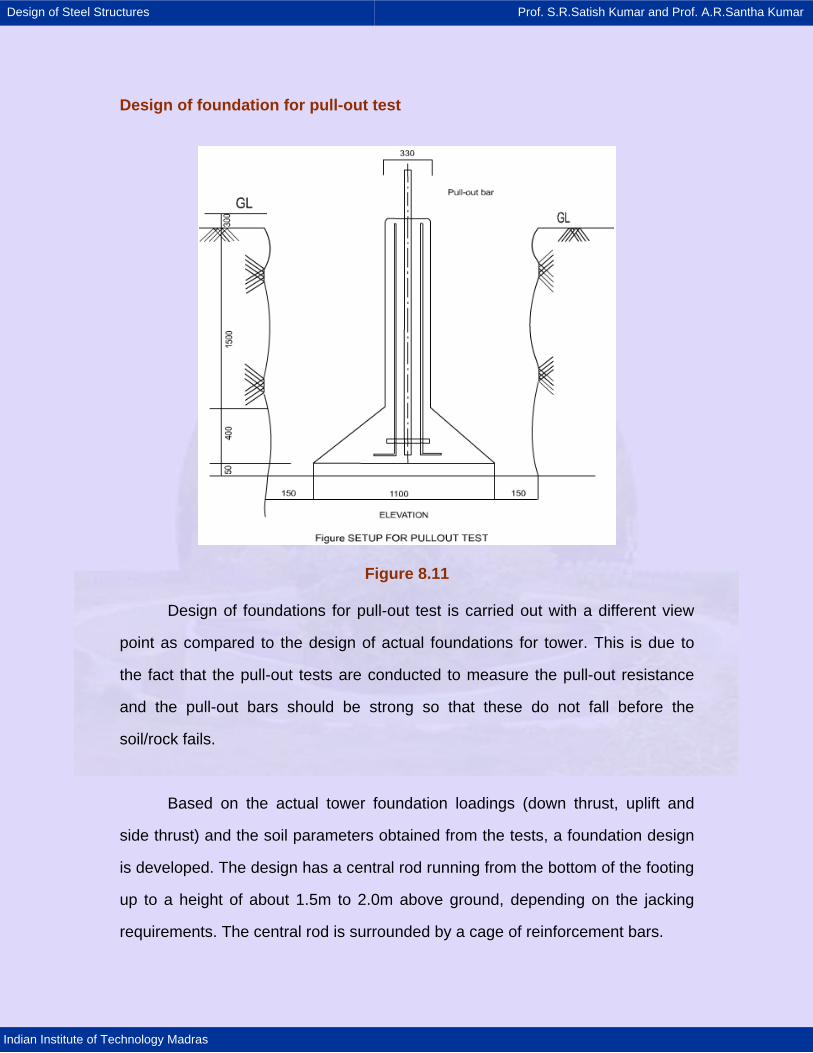
Design of Steel Structures Prof. S.R.Satish Kumar and Prof. A.R.Santha Kumar
Indian Institute of Technology Madras
Design of foundation for pull-out test
Figure 8.11
Design of foundations for pull-out test is carried out with a different view
point as compared to the design of actual foundations for tower. This is due to
the fact that the pull-out tests are conducted to measure the pull-out resistance
and the pull-out bars should be strong so that these do not fall before the
soil/rock fails.
Based on the actual tower foundation loadings (down thrust, uplift and
side thrust) and the soil parameters obtained from the tests, a foundation design
is developed. The design has a central rod running from the bottom of the footing
up to a height of about 1.5m to 2.0m above ground, depending on the jacking
requirements. The central rod is surrounded by a cage of reinforcement bars.
Design of Steel Structures Prof. S.R.Satish Kumar and Prof. A.R.Santha Kumar
Indian Institute of Technology Madras
A typical design development for the pull-out test is shown in Figure 8.11.
Casting of foundation
The pits are excavated accurately. The concrete mix, reinforcement, from
boxes etc. are exactly as per the design. The pouring of the concrete is done
such that voids are minimized. The back filling of the soil should be carried out
using sufficient water to eliminate voids and loose pockets. The foundation
should be cured for 14 days (minimum) and thereafter left undisturbed for a
period not less than 30 days.
Investigation of foundation towers
Normally it is believed that once the foundation is cast and the tower is
erected, the foundations can not be re-opened for investigation or repairing.
If the foundations of the tower have to be investigated, certain locations
are selected at random in such a fashion that foundations for various types of
soils are covered one by one. Out of the four individual footings of selected
tower, two diagonally opposite foundations are selected and one of the four faces
of each of these two foundations is excavated in slanting direction from top to
bottom.
After the investigation is over and corrective measures have been chalked
out it is advisable to backfill the excavating mixing earth with fight cement slurry,
particularly when the soil is non-cohesive such as soft murrum / hard murrum,
softrock / hard rock etc., (say one cement bag for every three to four cubic meter
of earth). This will ensure good bond and safeguard the foundation against uplift
forces, even if corrective repairs of the foundations are delayed.
Design of Steel Structures Prof. S.R.Satish Kumar and Prof. A.R.Santha Kumar
Indian Institute of Technology Madras
Repair of foundation of a tower
After it is established that the foundation is unhealthy, it is better to take
the corrective steps as early as possible. The methods would be different for
rectifying isolated location/locations (one to two) and for rectifying complete
line/line sections including a number of towers. These are discussed below.
(a) Rectification of isolated locations (one or two) is done on individual
basis. Any one of the four footings is taken up first. It is opened up from all the
four sides. The toer legs connected to this footing are guyed. After rectifying the
foundation backfilling is done. A minimum of seven-days time is allowed for
curing of the repaired foundation before excavating the second leg for repairs. In
the similar way the other legs also repaired.
Foundation defects and their repairs
The main possible defects in the cast concrete can be as follows:
(a) Under sizing of foundation due to wrong classification of soil; for example,
the soil may be dry black cotton but the foundation cast may be that for normal
dry soil, if the corrective measures are not taken, the foundation can fail. An
R.C.C collar in designed for the type of soil and tower loadings to remedy such a
defect.
(b) Improper foundation of pyramid/chimney etc., due to improper concrete
laying:
If the concrete is simply poured from the top of the form box, without
taking care to fill the voids (using crow bar, vibrator etc.) the concrete does not
reach to the corners of the form and thus the foundation is not completely
formed.
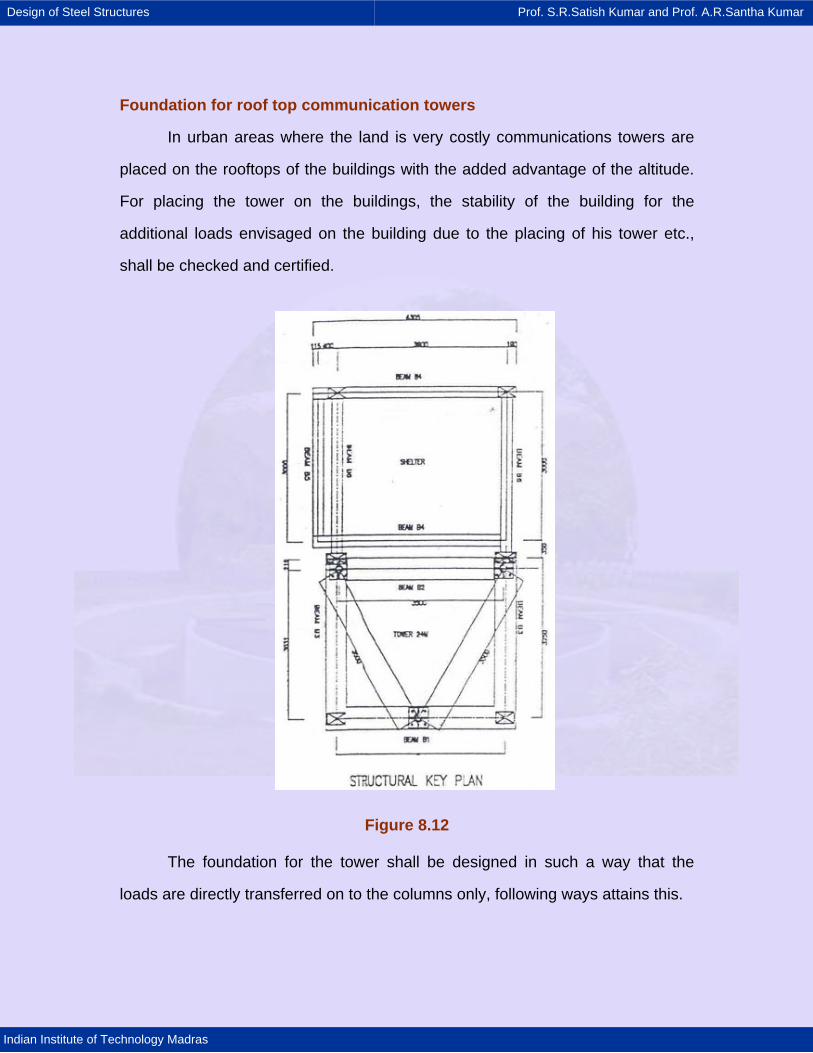
Design of Steel Structures Prof. S.R.Satish Kumar and Prof. A.R.Santha Kumar
Indian Institute of Technology Madras
Foundation for roof top communication towers
In urban areas where the land is very costly communications towers are
placed on the rooftops of the buildings with the added advantage of the altitude.
For placing the tower on the buildings, the stability of the building for the
additional loads envisaged on the building due to the placing of his tower etc.,
shall be checked and certified.
Figure 8.12
The foundation for the tower shall be designed in such a way that the
loads are directly transferred on to the columns only, following ways attains this.
Design of Steel Structures Prof. S.R.Satish Kumar and Prof. A.R.Santha Kumar
Indian Institute of Technology Madras
(a) The column rods of the building are exposed and the reinforcement
required for the tower pedestal is welded to the exposed rods.
(b) Where the exposing of the rods is not possible the pedestal rods can be
anchored by drilling holes vertically on top of the columns and grouting
them with the chemical grouts.
(c) Welding the pedestal rods to the beam rods at the column beam junctions.
Typical details are shown in the figure 8.12
The for the roof top communication tower consists of the pedestal and
beam arrangement. The tower base plate rests on the beam. The beam shall be
designed for both down thrust and uplift forces coming from the tower. Figure
8.13 shows the typical foundation detail for the roof top communication tower.
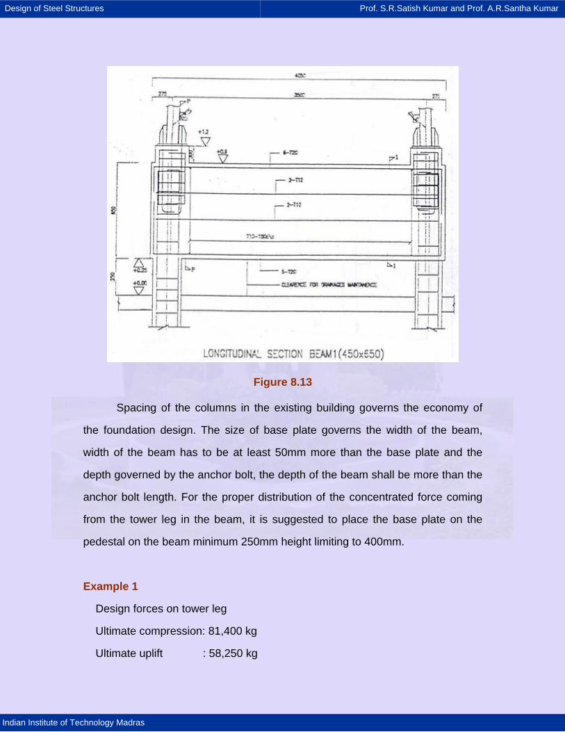
Design of Steel Structures Prof. S.R.Satish Kumar and Prof. A.R.Santha Kumar
Indian Institute of Technology Madras
Figure 8.13
Spacing of the columns in the existing building governs the economy of
the foundation design. The size of base plate governs the width of the beam,
width of the beam has to be at least 50mm more than the base plate and the
depth governed by the anchor bolt, the depth of the beam shall be more than the
anchor bolt length. For the proper distribution of the concentrated force coming
from the tower leg in the beam, it is suggested to place the base plate on the
pedestal on the beam minimum 250mm height limiting to 400mm.
Example 1
Design forces on tower leg
Ultimate compression: 81,400 kg
Ultimate uplift : 58,250 kg
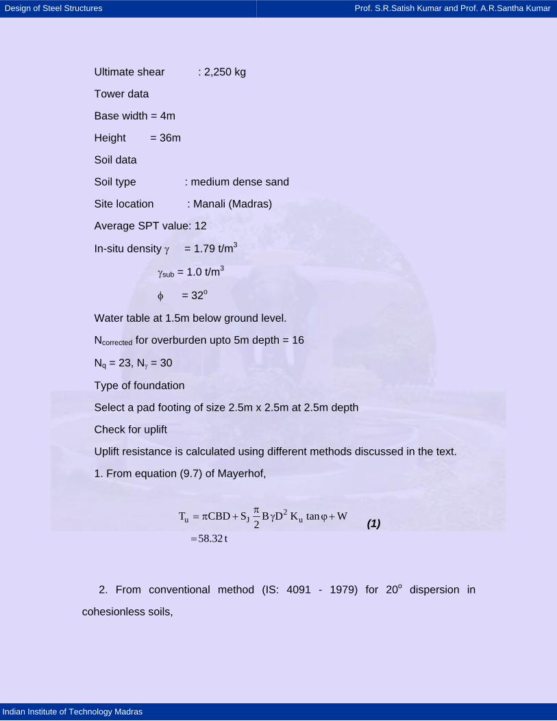
Design of Steel Structures Prof. S.R.Satish Kumar and Prof. A.R.Santha Kumar
Indian Institute of Technology Madras
Ultimate shear : 2,250 kg
Tower data
Base width = 4m
Height = 36m
Soil data
Soil type : medium dense sand
Site location : Manali (Madras)
Average SPT value: 12
In-situ density γ = 1.79 t/m3
γsub = 1.0 t/m3
φ = 32o
Water table at 1.5m below ground level.
Ncorrected for overburden upto 5m depth = 16
Nq = 23, Nγ = 30
Type of foundation
Select a pad footing of size 2.5m x 2.5m at 2.5m depth
Check for uplift
Uplift resistance is calculated using different methods discussed in the text.
1. From equation (9.7) of Mayerhof,
2u J uT CBD S B D K tan W
258.32 t
π= π + γ ϕ+
= (1)
2. From conventional method (IS: 4091 - 1979) for 20o dispersion in
cohesionless soils,
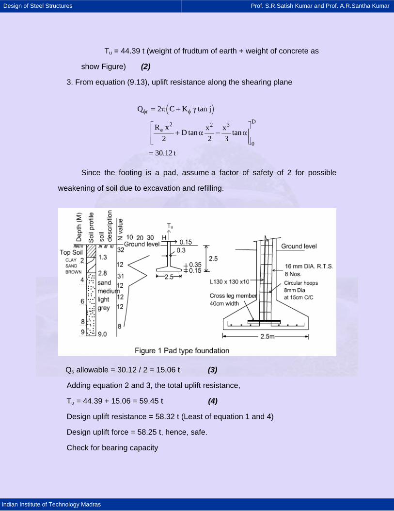
Design of Steel Structures Prof. S.R.Satish Kumar and Prof. A.R.Santha Kumar
Indian Institute of Technology Madras
Tu = 44.39 t (weight of frudtum of earth + weight of concrete as
show Figure) (2)
3. From equation (9.13), uplift resistance along the shearing plane
( )r
D2 2 3e
0
Q 2 C K tan j
R x x xD tan tan2 2 3
30.12 t
φ φ= π + γ
⎡ ⎤+ α − α⎢ ⎥
⎢ ⎥⎣ ⎦=
Since the footing is a pad, assume a factor of safety of 2 for possible
weakening of soil due to excavation and refilling.
Qs allowable = 30.12 / 2 = 15.06 t (3)
Adding equation 2 and 3, the total uplift resistance,
Tu = 44.39 + 15.06 = 59.45 t (4)
Design uplift resistance = 58.32 t (Least of equation 1 and 4)
Design uplift force = 58.25 t, hence, safe.
Check for bearing capacity

Design of Steel Structures Prof. S.R.Satish Kumar and Prof. A.R.Santha Kumar
Indian Institute of Technology Madras
From equation 9.1,
Where values of s, d and i are chosen from Table 9.9.
Area of footing = 2.5 x 2.5 = 6.25 m2
Ultimate bearing capacity of footing = 6.25 x 94.8
This is greater than the ultimate compression 81.4 t, hence safe.
Generally, bearing capacity is not the governing criterion.
Check for settlement
From equation (9.20) instantaneous settlement
2
i P1 vs I qB
Eθ
⎛ ⎞−= ⎜ ⎟⎜ ⎟
⎝ ⎠
Choosing v and Es from table 9.4 and Ip from table 9.14
si = 0.313cm
Since the soil is sandy, settlement due to consolidation does not arise.
Base width of tower = 4m
Maximum possible rotation
θ = 0.313 / 400 = 0.00078
Check for lateral capacity by Reese and Matlock Method
From Table 9.5, ηn = 1.5
Therefore 1 5
n
EIT 89.8⎛ ⎞
= =⎜ ⎟η⎝ ⎠
Zmax = L/T = 2.78
Z = x / T at x = 0, Z = 0;
Design of Steel Structures Prof. S.R.Satish Kumar and Prof. A.R.Santha Kumar
Indian Institute of Technology Madras
From Figure,
Ay = +3, By = 2.0, Am = 0.66, Bm = 0.64
H = Hu / 2 = 1,125 kg
Mt = 1,125 x 15 = 16,875 kg cm
3 2y y i
maxA HT B M T
YEI EI
= +
Ymax at service load = 0.31 cm < 2 cm, hence safe
Mmax = Am HT + BmMt
Mmax at ultimate load = 154,856 kg cm.
Structural design
Deflection at ultimate load = 2 x 0.31 = 0.62cm.
Check for compression and bending
Moment due to eccentricity = 81,400 x 0.62
= 50,468 kg cm
Design moment = 154,856 + 50,468
= 205,324 kg cm
Design compressive load = 81,400 kg
Use M 150 concrete and Fe 415 steel.
fck = 150 kg/cm2, fy = 4,150 kg/cm2
Let d' / D = 0.1
Use chart 56 of IS SP: 16 (S and T) - 1980,
Design of Steel Structures Prof. S.R.Satish Kumar and Prof. A.R.Santha Kumar
Indian Institute of Technology Madras
u3
ck
u2
ck
ck2
c
M0.0467
f DP
0.6f DP 0.15,p 0.15x15 2.25percent
f
A 15.9cm
=
=
= = =
=
Provide 16mm diameter ribbed twisted steel (RTS) 8 numbers.
Use 8mm hoops at 15 cm c/c which satisfy the code requirements.
Check for tension
Design uplift = 58,250 kg
Let the leg section be L 130 x 130 x 10
Perimeter = 52
Design bond stress 1.0 N/mm2 (IS: 456 - 1978)
Development length required
loadperimeter x stress58, 250 11252 x 10
=
= =
Hence safe.
Anchor the leg member in the chimney part with 40cm cross member as
shown in Figure 1 for additional safety

Design of Steel Structures Prof. S.R.Satish Kumar and Prof. A.R.Santha Kumar
Indian Institute of Technology Madras
7. BRIDGES
7.1 Introduction
As discussed in earlier chapters the main advantages of structural steel
over other construction materials are its strength and ductility. It has a higher
strength to cost ratio in tension and a slightly lower strength to cost ratio in
compression when compared with concrete. The stiffness to weight ratio of steel
is much higher than that of concrete. Thus, structural steel is an efficient and
economic material in bridges. Structural steel has been the natural solution for
long span bridges since 1890, when the Firth of Forth cantilever bridge, the
world's major steel bridge at that time was completed. Steel is indeed suitable for
most span ranges, but particularly for longer spans. Howrah Bridge, also known
as Rabindra Setu, is to be looked at as an early classical steel bridge in India.
This cantilever bridge was built in 1943. It is 97 m high and 705 m long. This
engineering marvel is still serving the nation, deriding all the myths that people
have about steel. [See Fig.7.1]
Fig.7.1 Howrah bridge
The following are some of the advantages of steel bridges that have
contributed to their popularity in Europe and in many other developed countries.
Design of Steel Structures Prof. S.R.Satish Kumar and Prof. A.R.Santha Kumar
Indian Institute of Technology Madras
· They could carry heavier loads over longer spans with minimum dead weight,
leading to smaller foundations.
· Steel has the advantage where speed of construction is vital, as many
elements can be prefabricated and erected at site.
· In urban environment with traffic congestion and limited working space, steel
bridges can be constructed with minimum disruption to the community.
· Greater efficiency than concrete structures is invariably achieved in resisting
seismic forces and blast loading.
· The life of steel bridges is longer than that of concrete bridges.
· Due to shallow construction depth, steel bridges offer slender appearance,
which make them aesthetically attractive. The reduced depth also contributes to
the reduced cost of embankments.
· All these frequently leads to low life cycle costs in steel bridges
In India there are many engineers who feel that corrosion is a problem in
steel bridges, but in reality it is not so. Corrosion in steel bridges can be
effectively minimised by employing newly developed paints and special types of
steel. These techniques are followed in Europe and other developed countries.
These have been discussed in chapter 2.
Design of Steel Structures Prof. S.R.Satish Kumar and Prof. A.R.Santha Kumar
Indian Institute of Technology Madras
7.2 Steel used in bridges
Steel used for bridges may be grouped into the following three categories:
(i) Carbon steel: This is the cheapest steel available for structural users
where stiffness is more important than the strength. Indian steels have
yield stress values up to 250 N/mm2 and can be easily welded. The
steel conforming to IS: 2062 - 1969, the American ASTM A36, the
British grades 40 and Euronorm 25 grades 235 and 275 steels belong
to this category.
(ii) High strength steels: They derive their higher strength and other
required properties from the addition of alloying elements. The steel
conforming to IS: 961 - 1975, British grade 50, American ASTM A572
and Euronorm 155 grade 360 steels belong to this category. Another
variety of steel in this category is produced with enhanced resistance
to atmospheric corrosion. These are called 'weathering' steels in
Europe, in America they conform to ASTM A588 and have various
trade names like ' cor-ten'.
(iii) Heat-treated carbon steels: These are steels with the highest
strength. They derive their enhanced strength from some form of heat-
treatment after rolling namely normalisation or quenching and
tempering.

Design of Steel Structures Prof. S.R.Satish Kumar and Prof. A.R.Santha Kumar
Indian Institute of Technology Madras
The physical properties of structural steel such as strength, ductility, brittle
fracture, weldability, weather resistance etc., are important factors for its use in
bridge construction. These properties depend on the alloying elements, the
amount of carbon, cooling rate of the steel and the mechanical deformation of the
steel. The detailed discussion of physical properties of structural steel is
presented in earlier chapter.
Design of Steel Structures Prof. S.R.Satish Kumar and Prof. A.R.Santha Kumar
Indian Institute of Technology Madras
7.3 Classification of steel bridges
Steel bridges are classified according to
· the type of traffic carried
· the type of main structural system
· the position of the carriage way relative to the main structural system
These are briefly discussed in this section.
7.3.1 Classification based on type of traffic carried
Bridges are classified as
· Highway or road bridges
· Railway or rail bridges
· Road - cum - rail bridges
7.3.2 Classification based on the main structural system
Many different types of structural systems are used in bridges depending
upon the span, carriageway width and types of traffic. Classification, according to
make up of main load carrying system, is as follows:
(i) Girder bridges - Flexure or bending between vertical supports is the main
structural action in this type. Girder bridges may be either solid web girders or
truss girders or box girders. Plate girder bridges are adopted for simply
supported spans less than 50 m and box girders for continuous spans upto 250
m. Cross sections of a typical plate girder and box girder bridges are shown in
Fig.7.2 (a) and Fig. 7.2(b) respectively. Truss bridges [See Fig.7. 2(c)] are
suitable for the span range of 30 m to 375 m. Cantilever bridges have been built
with success with main spans of 300 m to 550 m. In the next chapter girder
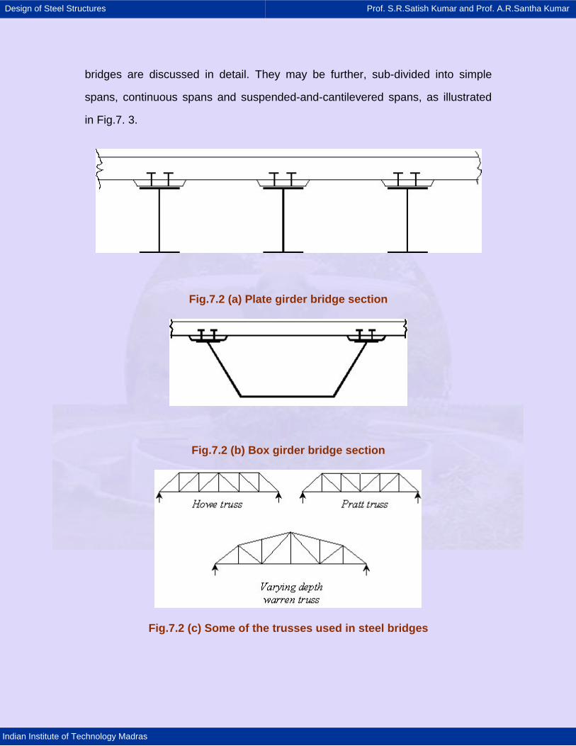
Design of Steel Structures Prof. S.R.Satish Kumar and Prof. A.R.Santha Kumar
Indian Institute of Technology Madras
bridges are discussed in detail. They may be further, sub-divided into simple
spans, continuous spans and suspended-and-cantilevered spans, as illustrated
in Fig.7. 3.
Fig.7.2 (a) Plate girder bridge section
Fig.7.2 (b) Box girder bridge section
Fig.7.2 (c) Some of the trusses used in steel bridges
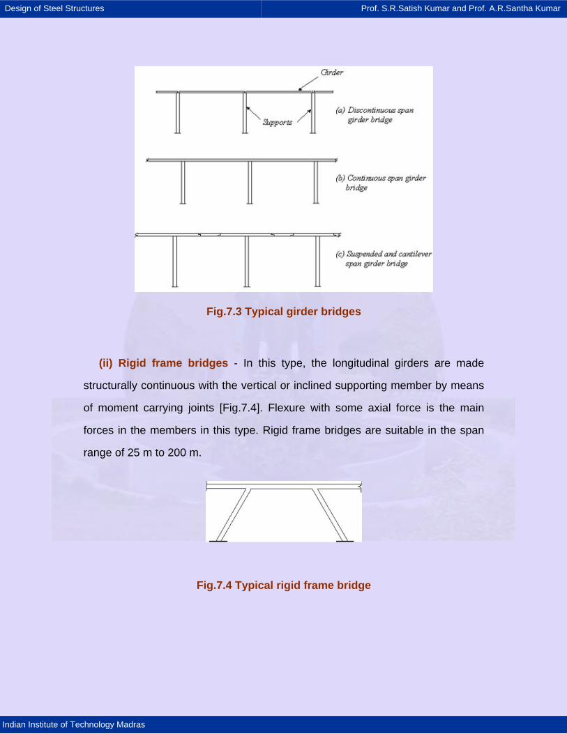
Design of Steel Structures Prof. S.R.Satish Kumar and Prof. A.R.Santha Kumar
Indian Institute of Technology Madras
Fig.7.3 Typical girder bridges
(ii) Rigid frame bridges - In this type, the longitudinal girders are made
structurally continuous with the vertical or inclined supporting member by means
of moment carrying joints [Fig.7.4]. Flexure with some axial force is the main
forces in the members in this type. Rigid frame bridges are suitable in the span
range of 25 m to 200 m.
Fig.7.4 Typical rigid frame bridge
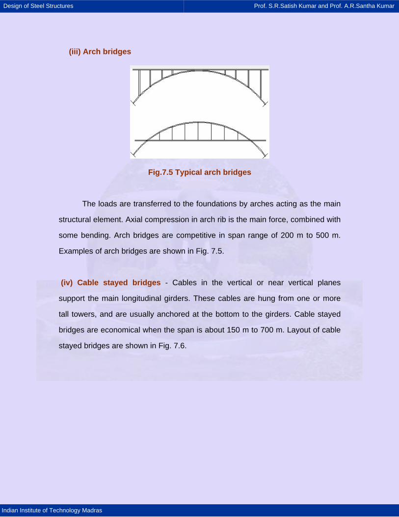
Design of Steel Structures Prof. S.R.Satish Kumar and Prof. A.R.Santha Kumar
Indian Institute of Technology Madras
(iii) Arch bridges
Fig.7.5 Typical arch bridges
The loads are transferred to the foundations by arches acting as the main
structural element. Axial compression in arch rib is the main force, combined with
some bending. Arch bridges are competitive in span range of 200 m to 500 m.
Examples of arch bridges are shown in Fig. 7.5.
(iv) Cable stayed bridges - Cables in the vertical or near vertical planes
support the main longitudinal girders. These cables are hung from one or more
tall towers, and are usually anchored at the bottom to the girders. Cable stayed
bridges are economical when the span is about 150 m to 700 m. Layout of cable
stayed bridges are shown in Fig. 7.6.
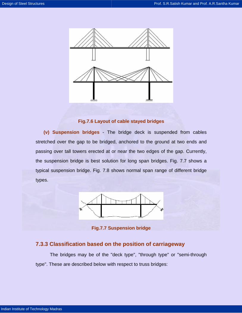
Design of Steel Structures Prof. S.R.Satish Kumar and Prof. A.R.Santha Kumar
Indian Institute of Technology Madras
Fig.7.6 Layout of cable stayed bridges
(v) Suspension bridges - The bridge deck is suspended from cables
stretched over the gap to be bridged, anchored to the ground at two ends and
passing over tall towers erected at or near the two edges of the gap. Currently,
the suspension bridge is best solution for long span bridges. Fig. 7.7 shows a
typical suspension bridge. Fig. 7.8 shows normal span range of different bridge
types.
Fig.7.7 Suspension bridge
7.3.3 Classification based on the position of carriageway
The bridges may be of the "deck type", "through type" or "semi-through
type". These are described below with respect to truss bridges:
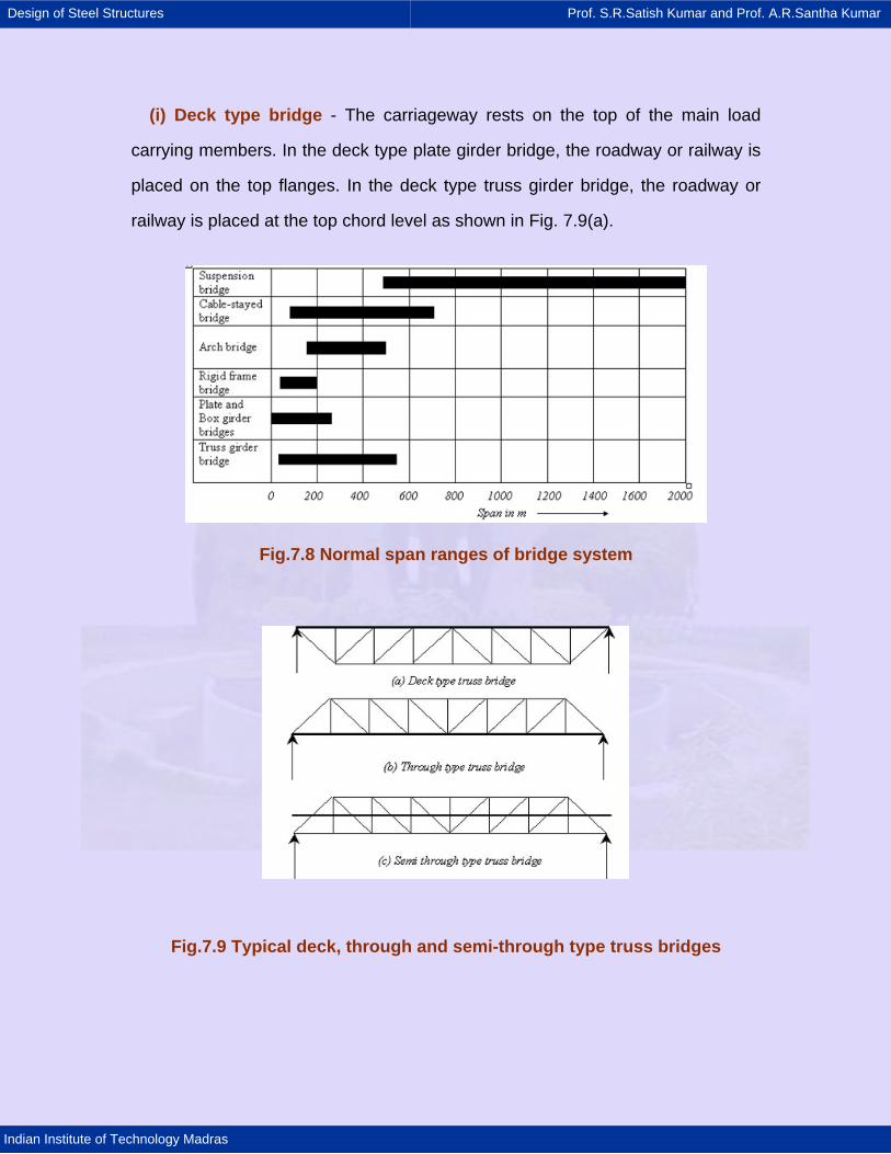
Design of Steel Structures Prof. S.R.Satish Kumar and Prof. A.R.Santha Kumar
Indian Institute of Technology Madras
(i) Deck type bridge - The carriageway rests on the top of the main load
carrying members. In the deck type plate girder bridge, the roadway or railway is
placed on the top flanges. In the deck type truss girder bridge, the roadway or
railway is placed at the top chord level as shown in Fig. 7.9(a).
Fig.7.8 Normal span ranges of bridge system
Fig.7.9 Typical deck, through and semi-through type truss bridges
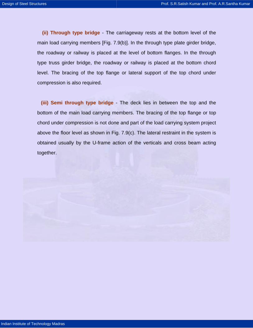
Design of Steel Structures Prof. S.R.Satish Kumar and Prof. A.R.Santha Kumar
Indian Institute of Technology Madras
(ii) Through type bridge - The carriageway rests at the bottom level of the
main load carrying members [Fig. 7.9(b)]. In the through type plate girder bridge,
the roadway or railway is placed at the level of bottom flanges. In the through
type truss girder bridge, the roadway or railway is placed at the bottom chord
level. The bracing of the top flange or lateral support of the top chord under
compression is also required.
(iii) Semi through type bridge - The deck lies in between the top and the
bottom of the main load carrying members. The bracing of the top flange or top
chord under compression is not done and part of the load carrying system project
above the floor level as shown in Fig. 7.9(c). The lateral restraint in the system is
obtained usually by the U-frame action of the verticals and cross beam acting
together.
Design of Steel Structures Prof. S.R.Satish Kumar and Prof. A.R.Santha Kumar
Indian Institute of Technology Madras
7.4 Loads and Load combinations
7.4.1 Loads on bridges
The following are the various loads to be considered for the purpose of
computing stresses, wherever they are applicable.
· Dead load
· Live load
· Impact load
· Longitudinal force
· Thermal force
· Wind load
· Seismic load
· Racking force
· Forces due to curvature.
· Forces on parapets
· Frictional resistance of expansion bearings
· Erection forces
Dead load – The dead load is the weight of the structure and any permanent
load fixed thereon. The dead load is initially assumed and checked after design is
completed.
Live load – Bridge design standards specify the design loads, which are
meant to reflect the worst loading that can be caused on the bridge by traffic,
permitted and expected to pass over it. In India, the Railway Board specifies the
standard design loadings for railway bridges in bridge rules. For the highway
bridges, the Indian Road Congress has specified standard design loadings in
Design of Steel Structures Prof. S.R.Satish Kumar and Prof. A.R.Santha Kumar
Indian Institute of Technology Madras
IRC section II. The following few pages brief about the loadings to be considered.
For more details, the reader is referred to the particular standard.
Railway bridges: Railway bridges including combined rail and road bridges
are to be designed for railway standard loading given in bridge rules. The
standards of loading are given for:
· Broad gauge - Main line and branch line
· Metre gauge - Main line, branch line and Standard C
· Narrow gauge - H class, A class main line and B class branch line
The actual loads consist of axle load from engine and bogies. The actual
standard loads have been expressed in bridge rules as equivalent uniformly
distributed loads (EUDL) in tables to simplify the analysis. These equivalent UDL
values depend upon the span length. However, in case of rigid frame, cantilever
and suspension bridges, it is necessary for the designer to proceed from the
basic wheel loads. In order to have a uniform gauge throughout the country, it is
advantageous to design railway bridges to Broad gauge main line standard
loading. The EUDLs for bending moment and shear force for broad gauge main
line loading can be obtained by the following formulae, which have been obtained
from regression analysis:
For bending moment:
EUDL in kN = 317.97 + 70.83l + 0.0188l2 ≥ 449.2 kN (7.1)
For shear force:
EUDL in kN = 435.58 + 75.15l + 0.0002l2 ≥ 449.2 kN (7.2)
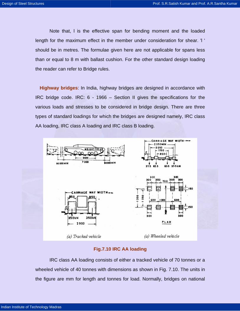
Design of Steel Structures Prof. S.R.Satish Kumar and Prof. A.R.Santha Kumar
Indian Institute of Technology Madras
Note that, l is the effective span for bending moment and the loaded
length for the maximum effect in the member under consideration for shear. 'l '
should be in metres. The formulae given here are not applicable for spans less
than or equal to 8 m with ballast cushion. For the other standard design loading
the reader can refer to Bridge rules.
Highway bridges: In India, highway bridges are designed in accordance with
IRC bridge code. IRC: 6 - 1966 – Section II gives the specifications for the
various loads and stresses to be considered in bridge design. There are three
types of standard loadings for which the bridges are designed namely, IRC class
AA loading, IRC class A loading and IRC class B loading.
Fig.7.10 IRC AA loading
IRC class AA loading consists of either a tracked vehicle of 70 tonnes or a
wheeled vehicle of 40 tonnes with dimensions as shown in Fig. 7.10. The units in
the figure are mm for length and tonnes for load. Normally, bridges on national
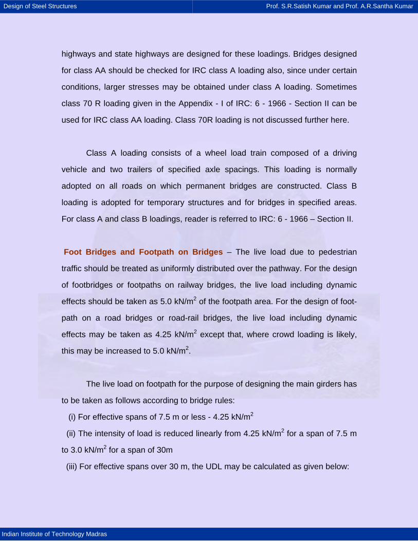
Design of Steel Structures Prof. S.R.Satish Kumar and Prof. A.R.Santha Kumar
Indian Institute of Technology Madras
highways and state highways are designed for these loadings. Bridges designed
for class AA should be checked for IRC class A loading also, since under certain
conditions, larger stresses may be obtained under class A loading. Sometimes
class 70 R loading given in the Appendix - I of IRC: 6 - 1966 - Section II can be
used for IRC class AA loading. Class 70R loading is not discussed further here.
Class A loading consists of a wheel load train composed of a driving
vehicle and two trailers of specified axle spacings. This loading is normally
adopted on all roads on which permanent bridges are constructed. Class B
loading is adopted for temporary structures and for bridges in specified areas.
For class A and class B loadings, reader is referred to IRC: 6 - 1966 – Section II.
Foot Bridges and Footpath on Bridges – The live load due to pedestrian
traffic should be treated as uniformly distributed over the pathway. For the design
of footbridges or footpaths on railway bridges, the live load including dynamic
effects should be taken as 5.0 kN/m2 of the footpath area. For the design of foot-
path on a road bridges or road-rail bridges, the live load including dynamic
effects may be taken as 4.25 kN/m2 except that, where crowd loading is likely,
this may be increased to 5.0 kN/m2.
The live load on footpath for the purpose of designing the main girders has
to be taken as follows according to bridge rules:
(i) For effective spans of 7.5 m or less - 4.25 kN/m2
(ii) The intensity of load is reduced linearly from 4.25 kN/m2 for a span of 7.5 m
to 3.0 kN/m2 for a span of 30m
(iii) For effective spans over 30 m, the UDL may be calculated as given below:
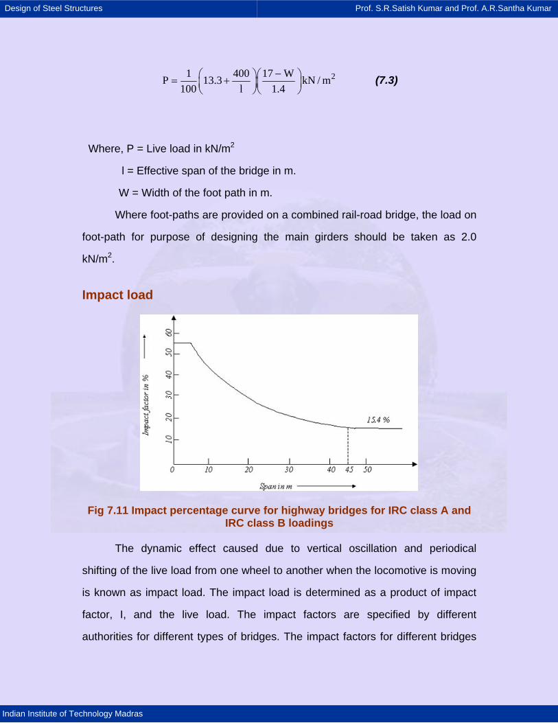
Design of Steel Structures Prof. S.R.Satish Kumar and Prof. A.R.Santha Kumar
Indian Institute of Technology Madras
21 400 17 WP 13.3 kN / m100 l 1.4
−⎛ ⎞⎛ ⎞= +⎜ ⎟⎜ ⎟⎝ ⎠⎝ ⎠
(7.3)
Where, P = Live load in kN/m2
l = Effective span of the bridge in m.
W = Width of the foot path in m.
Where foot-paths are provided on a combined rail-road bridge, the load on
foot-path for purpose of designing the main girders should be taken as 2.0
kN/m2.
Impact load
Fig 7.11 Impact percentage curve for highway bridges for IRC class A and IRC class B loadings
The dynamic effect caused due to vertical oscillation and periodical
shifting of the live load from one wheel to another when the locomotive is moving
is known as impact load. The impact load is determined as a product of impact
factor, I, and the live load. The impact factors are specified by different
authorities for different types of bridges. The impact factors for different bridges
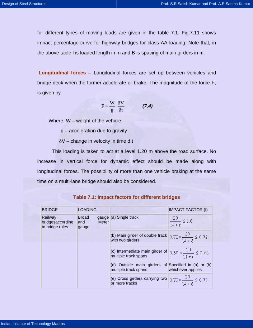
Design of Steel Structures Prof. S.R.Satish Kumar and Prof. A.R.Santha Kumar
Indian Institute of Technology Madras
for different types of moving loads are given in the table 7.1. Fig.7.11 shows
impact percentage curve for highway bridges for class AA loading. Note that, in
the above table l is loaded length in m and B is spacing of main girders in m.
Longitudinal forces – Longitudinal forces are set up between vehicles and
bridge deck when the former accelerate or brake. The magnitude of the force F,
is given by
W VFg t
δ=
δ (7.4)
Where, W – weight of the vehicle
g – acceleration due to gravity
δV – change in velocity in time d t
This loading is taken to act at a level 1.20 m above the road surface. No
increase in vertical force for dynamic effect should be made along with
longitudinal forces. The possibility of more than one vehicle braking at the same
time on a multi-lane bridge should also be considered.
Table 7.1: Impact factors for different bridges
BRIDGE LOADING IMPACT FACTOR (I) (a) Single track
(b) Main girder of double track with two girders (c) Intermediate main girder of multiple track spans (d) Outside main girders of multiple track spans
Specified in (a) or (b) whichever applies
Railway bridgesaccording to bridge rules
Broad gauge and Meter gauge
(e) Cross girders carrying two or more tracks
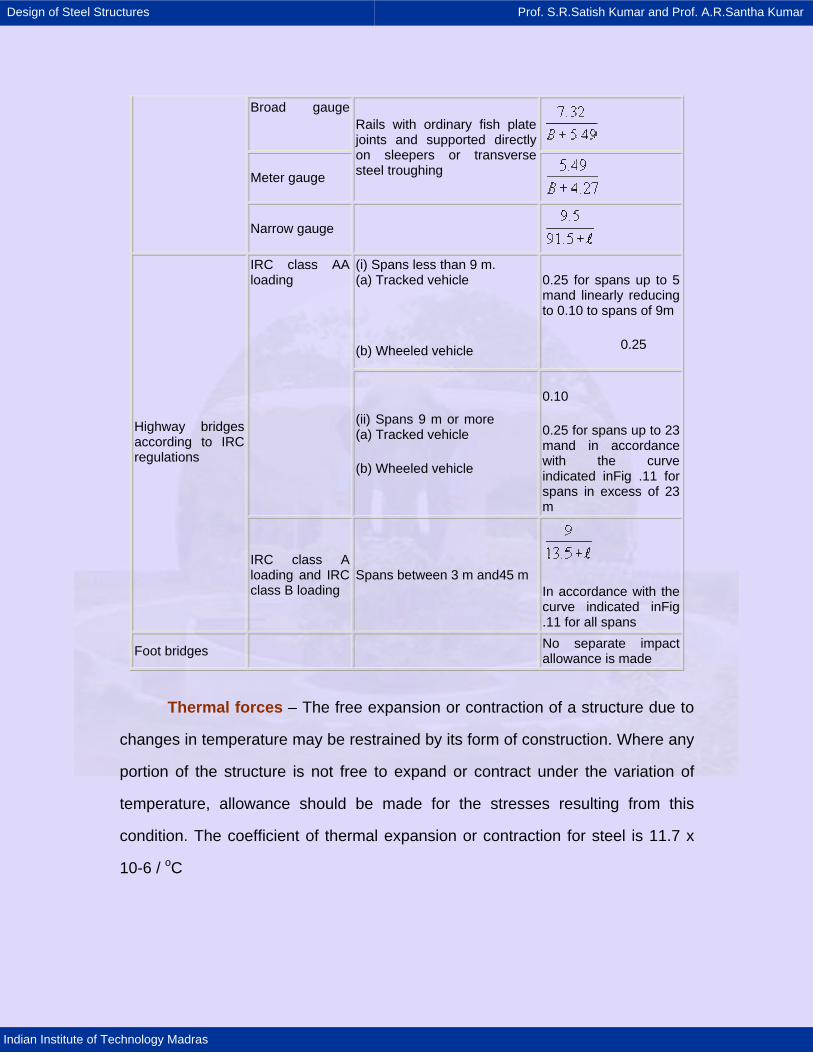
Design of Steel Structures Prof. S.R.Satish Kumar and Prof. A.R.Santha Kumar
Indian Institute of Technology Madras
Broad gauge
Meter gauge
Rails with ordinary fish plate joints and supported directly on sleepers or transverse steel troughing
Narrow gauge
(i) Spans less than 9 m. (a) Tracked vehicle
(b) Wheeled vehicle
0.25 for spans up to 5 mand linearly reducing to 0.10 to spans of 9m
0.25
IRC class AA loading
(ii) Spans 9 m or more (a) Tracked vehicle
(b) Wheeled vehicle
0.10
0.25 for spans up to 23 mand in accordance with the curve indicated inFig .11 for spans in excess of 23 m
Highway bridges according to IRC regulations
IRC class A loading and IRC class B loading
Spans between 3 m and45 m
In accordance with the curve indicated inFig .11 for all spans
Foot bridges No separate impact allowance is made
Thermal forces – The free expansion or contraction of a structure due to
changes in temperature may be restrained by its form of construction. Where any
portion of the structure is not free to expand or contract under the variation of
temperature, allowance should be made for the stresses resulting from this
condition. The coefficient of thermal expansion or contraction for steel is 11.7 x
10-6 / oC
Design of Steel Structures Prof. S.R.Satish Kumar and Prof. A.R.Santha Kumar
Indian Institute of Technology Madras
Wind load – Wind load on a bridge may act
· Horizontally, transverse to the direction of span
· Horizontally, along the direction of span
· Vertically upwards, causing uplift
· Wind load on vehicles
Wind load effect is not generally significant in short-span bridges; for
medium spans, the design of sub-structure is affected by wind loading; the super
structure design is affected by wind only in long spans. For the purpose of the
design, wind loadings are adopted from the maps and tables given in IS: 875
(Part III). A wind load of 2.40 kN/m2 is adopted for the unloaded span of the
railway, highway and footbridges. In case of structures with opening the effect of
drag around edges of members has to be considered.
Racking force – This is a lateral force produced due to the lateral movement
of rolling stocks in railway bridges. Lateral bracing of the loaded deck of railway
spans shall be designed to resist, in addition to the wind and centrifugal loads, a
lateral load due to racking force of 6.0 kN/m treated as moving load. This lateral
load need not be taken into account when calculating stresses in chords or
flanges of main girders.
Forces on parapets - Railings or parapets shall have a minimum height
above the adjacent roadway or footway surface of 1.0 m less one half the
horizontal width of the top rail or top of the parapet. They shall be designed to
resist a lateral horizontal force and a vertical force each of 1.50 kN/m applied
simultaneously at the top of the railing or parapet.
Design of Steel Structures Prof. S.R.Satish Kumar and Prof. A.R.Santha Kumar
Indian Institute of Technology Madras
Seismic load – If a bridge is situated in an earthquake prone region, the
earthquake or seismic forces are given due consideration in structural design.
Earthquakes cause vertical and horizontal forces in the structure that will be
proportional to the weight of the structure. Both horizontal and vertical
components have to be taken into account for design of bridge structures.
IS:1893 – 1984 may be referred to for the actual design loads.
Forces due to curvature - When a track or traffic lane on a bridge is curved
allowance for centrifugal action of the moving load should be made in designing
the members of the bridge. All the tracks and lanes on the structure being
considered are assumed as occupied by the moving load.
This force is given by the following formula:
2W VC12.7 R
= (7.5)
Where, C - Centrifugal force in kN/m
W - Equivalent distributed live load in kN/m
V - Maximum speed in km/hour
R - Radius of curvature in m
Erection forces – There are different techniques that are used for
construction of railway bridges, such as launching, pushing, cantilever method,
lift and place. In composite construction the composite action is mobilised only
after concrete hardens and prior to that steel section has to carry dead and
construction live loads. Depending upon the technique adopted the stresses in
the members of the bridge structure would vary. Such erection stresses should
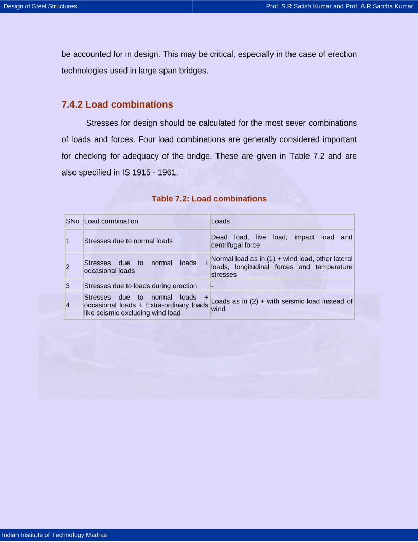
Design of Steel Structures Prof. S.R.Satish Kumar and Prof. A.R.Santha Kumar
Indian Institute of Technology Madras
be accounted for in design. This may be critical, especially in the case of erection
technologies used in large span bridges.
7.4.2 Load combinations
Stresses for design should be calculated for the most sever combinations
of loads and forces. Four load combinations are generally considered important
for checking for adequacy of the bridge. These are given in Table 7.2 and are
also specified in IS 1915 - 1961.
Table 7.2: Load combinations
SNo Load combination Loads
1 Stresses due to normal loads Dead load, live load, impact load and centrifugal force
2 Stresses due to normal loads + occasional loads
Normal load as in (1) + wind load, other lateral loads, longitudinal forces and temperature stresses
3 Stresses due to loads during erection -
4 Stresses due to normal loads + occasional loads + Extra-ordinary loads like seismic excluding wind load
Loads as in (2) + with seismic load instead of wind
Design of Steel Structures Prof. S.R.Satish Kumar and Prof. A.R.Santha Kumar
Indian Institute of Technology Madras
7.5 Analysis of girder bridges
As discussed above, bridge decks are required to support both static and
moving loads. Each element of a bridge must be designed for the most severe
conditions that can possibly be developed in that member. Live loads should be
placed in such a way that they will produce the most severe conditions. The
critical positions of live loads will not be the same for every member. A useful
method for determining the most severe condition of loading is by using
“influence lines”.
An influence line represents some internal force such as shear force,
bending moment etc. at a particular section or in a given member of girder, as a
unit load moves over the span. The ordinate of influence line represents the
value of that function when the unit load is at that particular point on the
structure. Influence lines provide a systematic procedure for determining how the
force (or a moment or shear) in a given part of a structure varies as the applied
load moves about on the structure. Influence lines of responses of statically
determinate structures consist only of straight lines whereas this is not true of
indeterminate structures. It may be noted that a shear or bending moment
diagram shows the variation of shear or moment across an entire structure for
loads fixed in one position. On the other hand an influence line for shear or
moment shows the variation of that response at one particular section in the
structure caused by the movement of a unit load from one end of the structure to
the other. In the following section, influence lines only for statically determinate
structures are discussed.
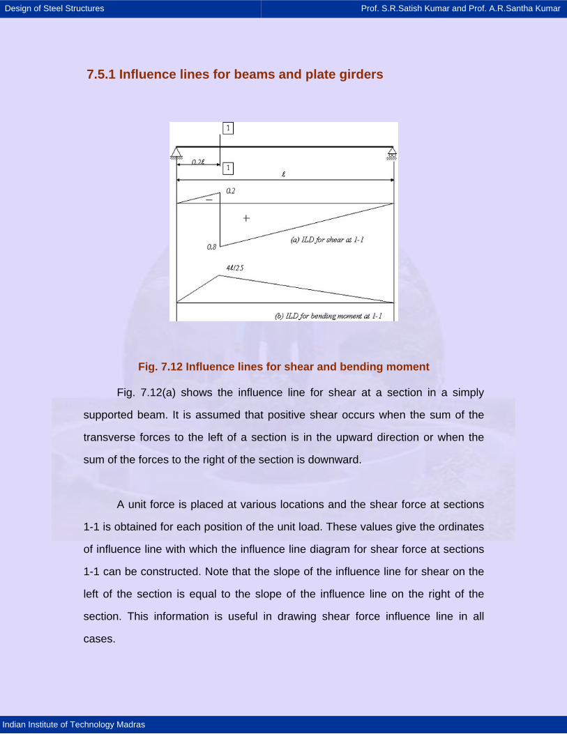
Design of Steel Structures Prof. S.R.Satish Kumar and Prof. A.R.Santha Kumar
Indian Institute of Technology Madras
7.5.1 Influence lines for beams and plate girders
Fig. 7.12 Influence lines for shear and bending moment
Fig. 7.12(a) shows the influence line for shear at a section in a simply
supported beam. It is assumed that positive shear occurs when the sum of the
transverse forces to the left of a section is in the upward direction or when the
sum of the forces to the right of the section is downward.
A unit force is placed at various locations and the shear force at sections
1-1 is obtained for each position of the unit load. These values give the ordinates
of influence line with which the influence line diagram for shear force at sections
1-1 can be constructed. Note that the slope of the influence line for shear on the
left of the section is equal to the slope of the influence line on the right of the
section. This information is useful in drawing shear force influence line in all
cases.
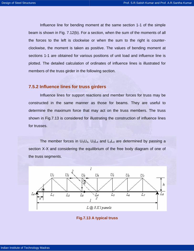
Design of Steel Structures Prof. S.R.Satish Kumar and Prof. A.R.Santha Kumar
Indian Institute of Technology Madras
Influence line for bending moment at the same section 1-1 of the simple
beam is shown in Fig. 7.12(b). For a section, when the sum of the moments of all
the forces to the left is clockwise or when the sum to the right is counter-
clockwise, the moment is taken as positive. The values of bending moment at
sections 1-1 are obtained for various positions of unit load and influence line is
plotted. The detailed calculation of ordinates of influence lines is illustrated for
members of the truss girder in the following section.
7.5.2 Influence lines for truss girders
Influence lines for support reactions and member forces for truss may be
constructed in the same manner as those for beams. They are useful to
determine the maximum force that may act on the truss members. The truss
shown in Fig.7.13 is considered for illustrating the construction of influence lines
for trusses.
The member forces in U3U4, U3L4 and L3L4 are determined by passing a
section X-X and considering the equilibrium of the free body diagram of one of
the truss segments.
Fig.7.13 A typical truss
Design of Steel Structures Prof. S.R.Satish Kumar and Prof. A.R.Santha Kumar
Indian Institute of Technology Madras
Consider a section 1-1 and assume unit-rolling load is at a distance x from L0.
Then, from equilibrium considerations reactions at L8 and L0 are determined. The
reactions are:
Reaction at L8 = xL
⎛ ⎞⎜ ⎟⎝ ⎠
Reaction at L0 = x1L
⎛ ⎞−⎜ ⎟⎝ ⎠
Consider the left-hand side of the section and take moments about L4 by
assuming appropriate directions for the forces in the members.
When unit load is in between L0 and L4:
L4
3 4
3 4
M 0
xU U x h x 4l 0L
x 4l xU U 0.5h L h
=
⎛ ⎞− =⎜ ⎟⎝ ⎠
= =
∑
When unit load is in between L4 and L8:
Then, there will not be rolling unit load in the left-hand side section.
3 44l xU U 1h L⎛ ⎞= −⎜ ⎟⎝ ⎠
Note that the influence diagram gives force in the member U3U4 directly,
due to the unit load.
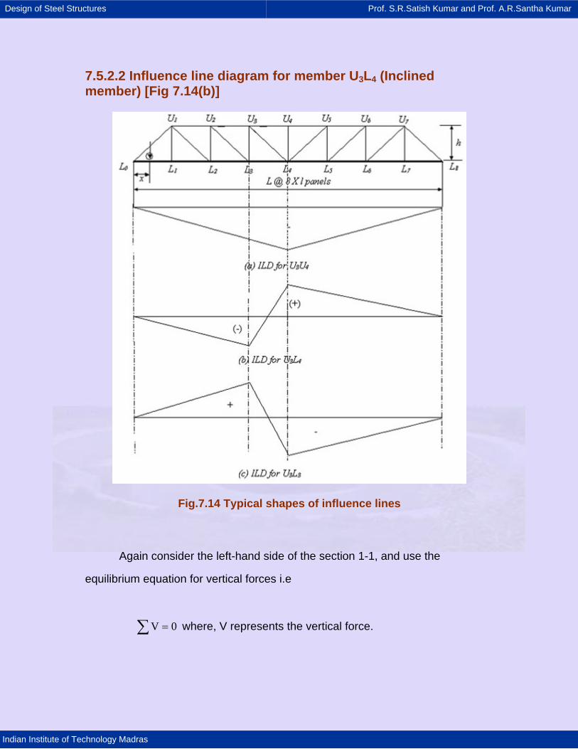
Design of Steel Structures Prof. S.R.Satish Kumar and Prof. A.R.Santha Kumar
Indian Institute of Technology Madras
7.5.2.2 Influence line diagram for member U3L4 (Inclined member) [Fig 7.14(b)]
Fig.7.14 Typical shapes of influence lines
Again consider the left-hand side of the section 1-1, and use the
equilibrium equation for vertical forces i.e
V 0=∑ where, V represents the vertical force.
Design of Steel Structures Prof. S.R.Satish Kumar and Prof. A.R.Santha Kumar
Indian Institute of Technology Madras
When unit load is in between L0 and L3:
3 4
3 4
1
x U L Cos 0L
xU LLcos
lWhere, tanh
−
+ θ=
−⇒ =
θ
⎛ ⎞θ = ⎜ ⎟⎝ ⎠
When unit load is in between L4 and L8:
3 41 xU U 1
Cos L⎛ ⎞= −⎜ ⎟θ ⎝ ⎠
When unit load is in between L3 and L4:
Since the variation of force in member U3L4 is linear as the unit load
moves from L3 to L4 joining the ordinates of influence line at L3 and L4 by a
straight line gives the influence line diagram in that zone. Note that, U3L4
represents the force in that member.
7.5.2.3 Influence line diagram for U3L3 (Vertical member) [Fig. 7.14(c)]
Consider the left-hand side of the section 2-2 shown in Fig.7.13 for illustrating
the construction of influence line for vertical member.
When unit load is in between L0 and L3:
By considering the equilibrium equation on the section left hand side of axis 2-
2.
3 4
3 4
xU L 0L
xU LL
− =
⇒ =
Design of Steel Structures Prof. S.R.Satish Kumar and Prof. A.R.Santha Kumar
Indian Institute of Technology Madras
When unit load is in between L4 and L8:
3 4xU L 1L
⎛ ⎞= − −⎜ ⎟⎝ ⎠
When unit load is in between L3 and L4:
Joining the ordinates of influence line at L3 and L4 by a straight line gives
the influence line diagram between L3 and L4. U3L3 represents the force in that
member.
Similarly influence line diagrams can be drawn for all other members.
Typical shapes of influence line diagrams for the members discussed are shown
in Fig.7.14. The design force in the member is obtained in the following manner.
In this chapter, compressive forces are considered negative and tensile forces
are positive.
Case (1): If the loading is Railway loading (UDL)
· Influence line diagram for force is drawn for that member
· The algebraic sum of areas of influence line under loaded length multiplied by
magnitude of uniformly distributed load gives the design force.
Case (2): If the loading is Highway loading (Concentrated loading)
· Influence line diagram for force is drawn for that member
· The algebraic sum of the respective ordinates of influence line at the
concentrated load location multiplied by concentrated loads gives design load of
that member
· The series of concentrated loads are arranged in such a way that the
maximum value of the desired member force is obtained.
Design of Steel Structures Prof. S.R.Satish Kumar and Prof. A.R.Santha Kumar
Indian Institute of Technology Madras
7.6 Plate girder bridges
Plate girders became popular in the late 1800's, when they were used in
construction of railroad bridges. The plates were joined together using angles
and rivets to obtain plate girders of desired size. By 1950's welded plate girders
replaced riveted and bolted plate girders in developed world due to their better
quality, aesthetics and economy. Fig.7.15 shows the cross sections of two
common types of plate girder bridges. The use of plate girders rather than rolled
beam sections for the two main girders gives the designer freedom to select the
most economical girder for the structure.
If large embankment fills are required in the approaches to the bridge, in
order to comply with the minimum head-room clearance required, the half
through bridge is more appropriate [Fig.7.15 (a)]. This arrangement is commonly
used in railway bridges where the maximum permissible approach gradient for
the track is low. In this case the restraint to lateral buckling of compression flange
is achieved by a moment resisting U-frame consisting of floor beam and vertical
stiffness, which are connected together with a moment resisting joint. If the
construction depth is not critical, then a deck-type bridge, as shown in Fig.7.15
(b) is a better solution, in which case the bracings provide restraint to
compression flange against lateral buckling.
7.6.1 Main plate girders
The design criterion for main girders as used in buildings, was discussed
in chapters on Plate Girders. In the following sections some additional aspects
that are to be considered in the design of plate girders in bridges, are discussed.

Design of Steel Structures Prof. S.R.Satish Kumar and Prof. A.R.Santha Kumar
Indian Institute of Technology Madras
Generally, the main girders require web stiffening (either transverse or
both transverse and longitudinal) to increase efficiency. The functions of these
web stiffeners are described in the chapters on plate girders. Sometimes
variations of bending moments in main girders may require variations in flange
thickness to obtain economical design. This may be accomplished either by
welding additional cover plates or by using thicker flange plate in the region of
larger moment. In very long continuous spans (span> 50 m) variable depth plate
girders may be more economical.
Initial design of main plate girder is generally based on experience or
thumb rules such as those given below. Such rules also give a good estimate of
dead load of the bridge structure to be designed. For highway and railway
bridges, indicative range of values for various overall dimension of the main
girders are given below:
Overall depth, D: l/18 ≤ D ≤ l/12 (Highway bridges)
l/10 ≤ D ≤ l/7 (Railway bridges)
Flange width, 2b: D/4 ≤ 2b ≤ D/3
Flange thickness, T: b/12 ≤ T ≤ b/5
Web thickness, t: t ≈ D/125
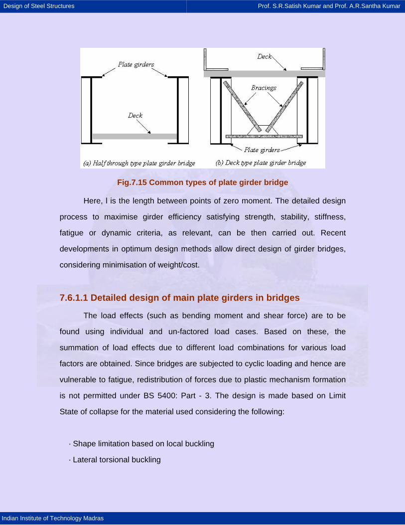
Design of Steel Structures Prof. S.R.Satish Kumar and Prof. A.R.Santha Kumar
Indian Institute of Technology Madras
Fig.7.15 Common types of plate girder bridge
Here, l is the length between points of zero moment. The detailed design
process to maximise girder efficiency satisfying strength, stability, stiffness,
fatigue or dynamic criteria, as relevant, can be then carried out. Recent
developments in optimum design methods allow direct design of girder bridges,
considering minimisation of weight/cost.
7.6.1.1 Detailed design of main plate girders in bridges
The load effects (such as bending moment and shear force) are to be
found using individual and un-factored load cases. Based on these, the
summation of load effects due to different load combinations for various load
factors are obtained. Since bridges are subjected to cyclic loading and hence are
vulnerable to fatigue, redistribution of forces due to plastic mechanism formation
is not permitted under BS 5400: Part - 3. The design is made based on Limit
State of collapse for the material used considering the following:
· Shape limitation based on local buckling
· Lateral torsional buckling
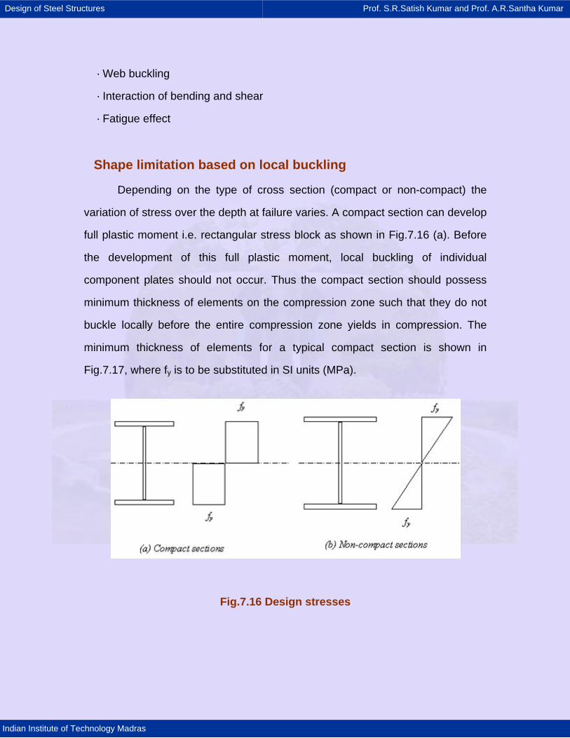
Design of Steel Structures Prof. S.R.Satish Kumar and Prof. A.R.Santha Kumar
Indian Institute of Technology Madras
· Web buckling
· Interaction of bending and shear
· Fatigue effect
Shape limitation based on local buckling
Depending on the type of cross section (compact or non-compact) the
variation of stress over the depth at failure varies. A compact section can develop
full plastic moment i.e. rectangular stress block as shown in Fig.7.16 (a). Before
the development of this full plastic moment, local buckling of individual
component plates should not occur. Thus the compact section should possess
minimum thickness of elements on the compression zone such that they do not
buckle locally before the entire compression zone yields in compression. The
minimum thickness of elements for a typical compact section is shown in
Fig.7.17, where fy is to be substituted in SI units (MPa).
Fig.7.16 Design stresses
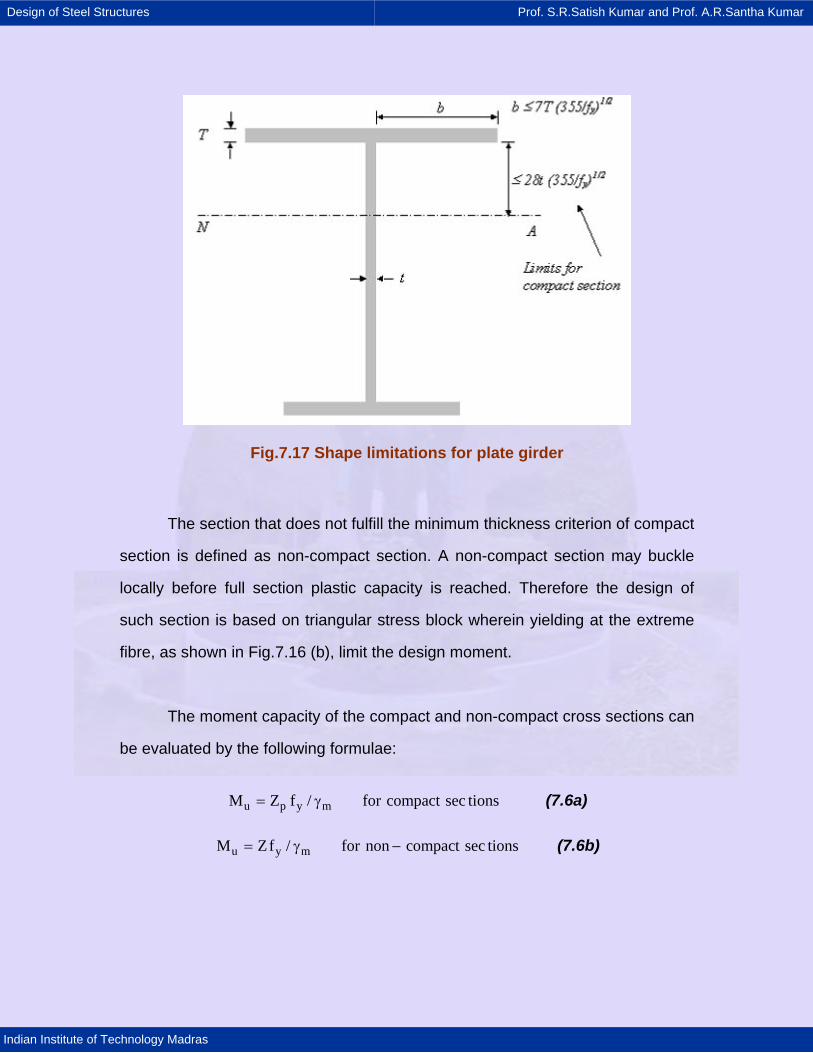
Design of Steel Structures Prof. S.R.Satish Kumar and Prof. A.R.Santha Kumar
Indian Institute of Technology Madras
Fig.7.17 Shape limitations for plate girder
The section that does not fulfill the minimum thickness criterion of compact
section is defined as non-compact section. A non-compact section may buckle
locally before full section plastic capacity is reached. Therefore the design of
such section is based on triangular stress block wherein yielding at the extreme
fibre, as shown in Fig.7.16 (b), limit the design moment.
The moment capacity of the compact and non-compact cross sections can
be evaluated by the following formulae:
u p y mM Z f / for compact sec tions= γ (7.6a)
u y mM Zf / for non compact sec tions= γ − (7.6b)
Design of Steel Structures Prof. S.R.Satish Kumar and Prof. A.R.Santha Kumar
Indian Institute of Technology Madras
Where, fy - yield stress
Zp - plastic modulus
Z - elastic modulus
γm - partial safety factor for material strength (1.15)
Even in the compact section, the use of plastic modulus does not imply
that plastic analysis accounting for moment redistribution is applicable. BS 5400:
Part - 3 precludes plastic analysis and does not allow any moment redistribution
to be considered. This is to avoid repeated plastification under cyclic loading and
the consequent low cycle fatigue failure. When non-compact sections are used
the redistribution will not occur and hence plastic analysis is not applicable.
Lateral torsional buckling
A typical bridge girder with a portion of the span, over which the
compression flange is laterally unrestrained, is shown in Fig. 7.18(a). Such a
girder is susceptible to lateral torsional buckling. Fig. 7.18(b) shows a laterally
buckled view of a portion of the span. The displacements at mid span, where the
beam is laterally restrained, will be only vertical, as shown in Fig. 7.18(c). A part
of the beam between restraints can translate downwards and sideways and
rotate about shear centre [Fig. 7.18(d)]. Failure may then be governed by lateral
torsional buckling. This type of failure depends on the unrestrained length of
compression flange, the geometry of cross section, moment gradient etc. The
procedure in detail for calculating the value of the limiting compressive stress is
given in chapters on laterally unrestrained beams.
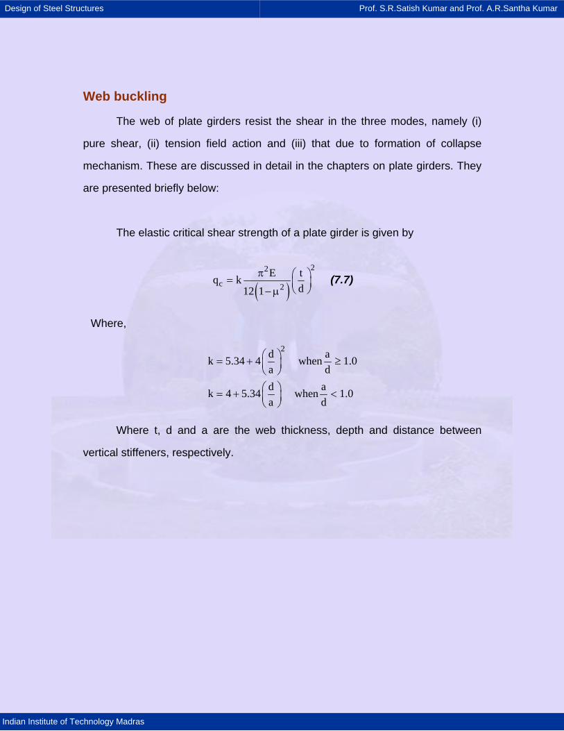
Design of Steel Structures Prof. S.R.Satish Kumar and Prof. A.R.Santha Kumar
Indian Institute of Technology Madras
Web buckling
The web of plate girders resist the shear in the three modes, namely (i)
pure shear, (ii) tension field action and (iii) that due to formation of collapse
mechanism. These are discussed in detail in the chapters on plate girders. They
are presented briefly below:
The elastic critical shear strength of a plate girder is given by
( )22
c 2E tq k
d12 1
π ⎛ ⎞= ⎜ ⎟⎝ ⎠− µ
(7.7)
Where,
2d ak 5.34 4 when 1.0a dd ak 4 5.34 when 1.0a d
⎛ ⎞= + ≥⎜ ⎟⎝ ⎠⎛ ⎞= + <⎜ ⎟⎝ ⎠
Where t, d and a are the web thickness, depth and distance between
vertical stiffeners, respectively.
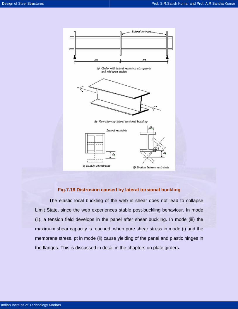
Design of Steel Structures Prof. S.R.Satish Kumar and Prof. A.R.Santha Kumar
Indian Institute of Technology Madras
Fig.7.18 Distrosion caused by lateral torsional buckling
The elastic local buckling of the web in shear does not lead to collapse
Limit State, since the web experiences stable post-buckling behaviour. In mode
(ii), a tension field develops in the panel after shear buckling. In mode (iii) the
maximum shear capacity is reached, when pure shear stress in mode (i) and the
membrane stress, pt in mode (ii) cause yielding of the panel and plastic hinges in
the flanges. This is discussed in detail in the chapters on plate girders.
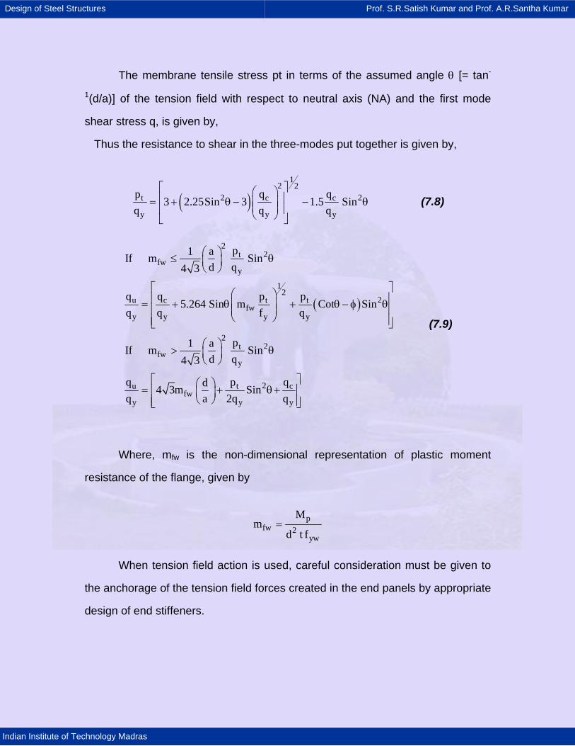
Design of Steel Structures Prof. S.R.Satish Kumar and Prof. A.R.Santha Kumar
Indian Institute of Technology Madras
The membrane tensile stress pt in terms of the assumed angle θ [= tan-
1(d/a)] of the tension field with respect to neutral axis (NA) and the first mode
shear stress q, is given by,
Thus the resistance to shear in the three-modes put together is given by,
( )1
2 22 2t c c
y y y
p q q3 2.25Sin 3 1.5 Sin
q q q
⎡ ⎤⎛ ⎞⎢ ⎥= + θ − − θ⎜ ⎟⎜ ⎟⎢ ⎥⎝ ⎠⎣ ⎦
(7.8)
( )
22t
fwy
12
2u c t tfw
y y y y
22t
fwy
2u t cfw
y y y
p1 aIf m Sind q4 3
q q p p5.264 Sin m Cot Sin
q q f q
p1 aIf m Sind q4 3
q p qd4 3m Sinq a 2q q
⎛ ⎞≤ θ⎜ ⎟⎝ ⎠
⎡ ⎤⎛ ⎞⎢ ⎥= + θ + θ − φ θ⎜ ⎟⎢ ⎥⎜ ⎟⎝ ⎠⎢ ⎥⎣ ⎦
⎛ ⎞> θ⎜ ⎟⎝ ⎠
⎡ ⎤⎛ ⎞= + θ+⎢ ⎥⎜ ⎟⎝ ⎠⎢ ⎥⎣ ⎦
(7.9)
Where, mfw is the non-dimensional representation of plastic moment
resistance of the flange, given by
pfw 2
yw
Mm
d t f=
When tension field action is used, careful consideration must be given to
the anchorage of the tension field forces created in the end panels by appropriate
design of end stiffeners.
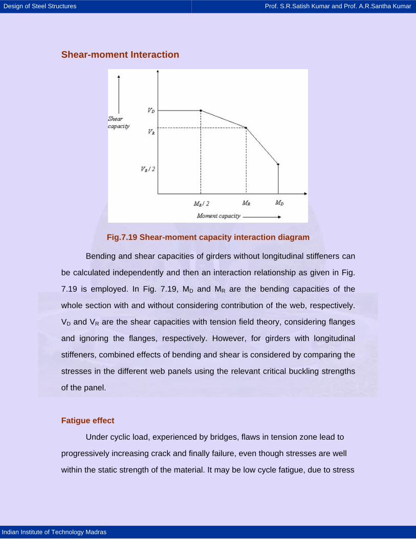
Design of Steel Structures Prof. S.R.Satish Kumar and Prof. A.R.Santha Kumar
Indian Institute of Technology Madras
Shear-moment Interaction
Fig.7.19 Shear-moment capacity interaction diagram
Bending and shear capacities of girders without longitudinal stiffeners can
be calculated independently and then an interaction relationship as given in Fig.
7.19 is employed. In Fig. 7.19, MD and MR are the bending capacities of the
whole section with and without considering contribution of the web, respectively.
VD and VR are the shear capacities with tension field theory, considering flanges
and ignoring the flanges, respectively. However, for girders with longitudinal
stiffeners, combined effects of bending and shear is considered by comparing the
stresses in the different web panels using the relevant critical buckling strengths
of the panel.
Fatigue effect
Under cyclic load, experienced by bridges, flaws in tension zone lead to
progressively increasing crack and finally failure, even though stresses are well
within the static strength of the material. It may be low cycle fatigue, due to stress
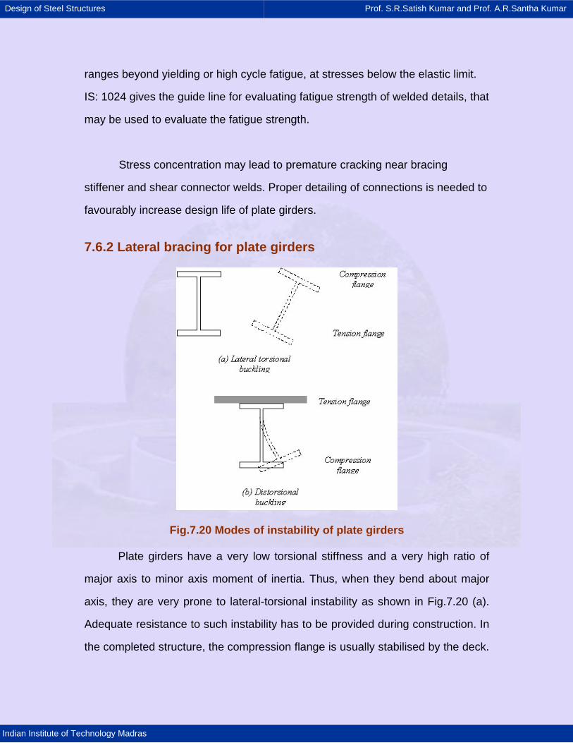
Design of Steel Structures Prof. S.R.Satish Kumar and Prof. A.R.Santha Kumar
Indian Institute of Technology Madras
ranges beyond yielding or high cycle fatigue, at stresses below the elastic limit.
IS: 1024 gives the guide line for evaluating fatigue strength of welded details, that
may be used to evaluate the fatigue strength.
Stress concentration may lead to premature cracking near bracing
stiffener and shear connector welds. Proper detailing of connections is needed to
favourably increase design life of plate girders.
7.6.2 Lateral bracing for plate girders
Fig.7.20 Modes of instability of plate girders
Plate girders have a very low torsional stiffness and a very high ratio of
major axis to minor axis moment of inertia. Thus, when they bend about major
axis, they are very prone to lateral-torsional instability as shown in Fig.7.20 (a).
Adequate resistance to such instability has to be provided during construction. In
the completed structure, the compression flange is usually stabilised by the deck.
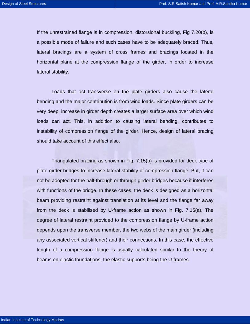
Design of Steel Structures Prof. S.R.Satish Kumar and Prof. A.R.Santha Kumar
Indian Institute of Technology Madras
If the unrestrained flange is in compression, distorsional buckling, Fig 7.20(b), is
a possible mode of failure and such cases have to be adequately braced. Thus,
lateral bracings are a system of cross frames and bracings located in the
horizontal plane at the compression flange of the girder, in order to increase
lateral stability.
Loads that act transverse on the plate girders also cause the lateral
bending and the major contribution is from wind loads. Since plate girders can be
very deep, increase in girder depth creates a larger surface area over which wind
loads can act. This, in addition to causing lateral bending, contributes to
instability of compression flange of the girder. Hence, design of lateral bracing
should take account of this effect also.
Triangulated bracing as shown in Fig. 7.15(b) is provided for deck type of
plate girder bridges to increase lateral stability of compression flange. But, it can
not be adopted for the half-through or through girder bridges because it interferes
with functions of the bridge. In these cases, the deck is designed as a horizontal
beam providing restraint against translation at its level and the flange far away
from the deck is stabilised by U-frame action as shown in Fig. 7.15(a). The
degree of lateral restraint provided to the compression flange by U-frame action
depends upon the transverse member, the two webs of the main girder (including
any associated vertical stiffener) and their connections. In this case, the effective
length of a compression flange is usually calculated similar to the theory of
beams on elastic foundations, the elastic supports being the U-frames.
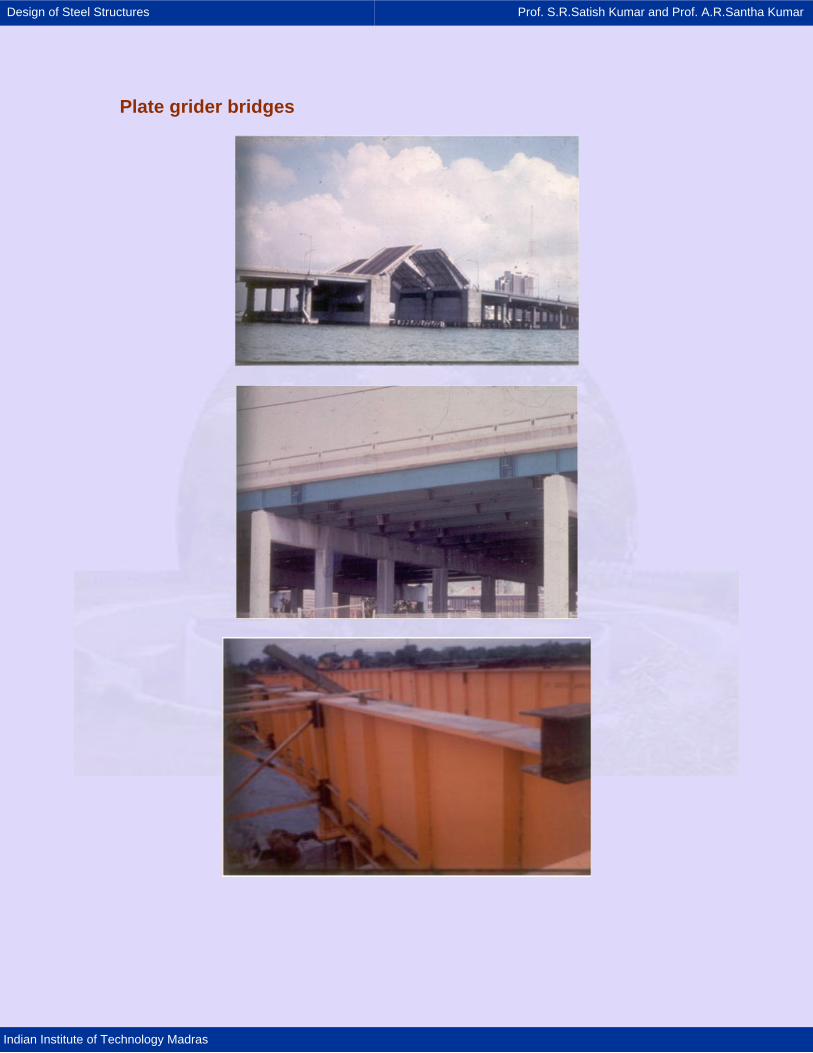
Design of Steel Structures Prof. S.R.Satish Kumar and Prof. A.R.Santha Kumar
Indian Institute of Technology Madras
Plate grider bridges
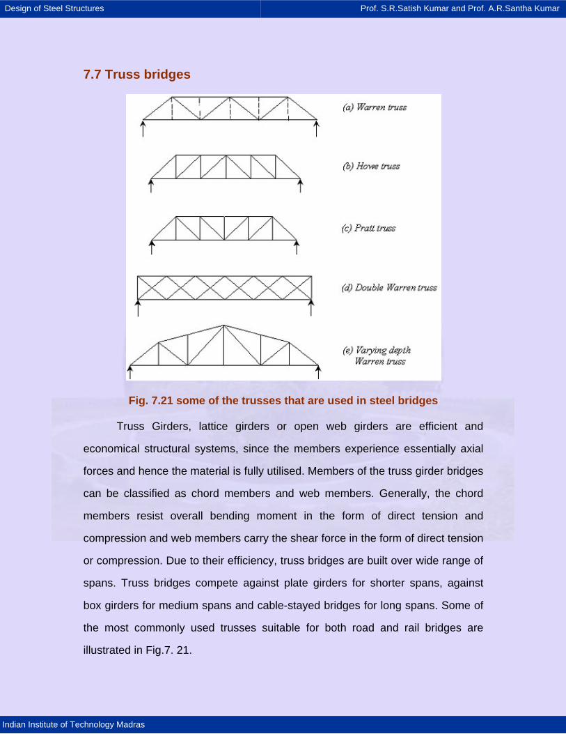
Design of Steel Structures Prof. S.R.Satish Kumar and Prof. A.R.Santha Kumar
Indian Institute of Technology Madras
7.7 Truss bridges
Fig. 7.21 some of the trusses that are used in steel bridges
Truss Girders, lattice girders or open web girders are efficient and
economical structural systems, since the members experience essentially axial
forces and hence the material is fully utilised. Members of the truss girder bridges
can be classified as chord members and web members. Generally, the chord
members resist overall bending moment in the form of direct tension and
compression and web members carry the shear force in the form of direct tension
or compression. Due to their efficiency, truss bridges are built over wide range of
spans. Truss bridges compete against plate girders for shorter spans, against
box girders for medium spans and cable-stayed bridges for long spans. Some of
the most commonly used trusses suitable for both road and rail bridges are
illustrated in Fig.7. 21.
Design of Steel Structures Prof. S.R.Satish Kumar and Prof. A.R.Santha Kumar
Indian Institute of Technology Madras
For short and medium spans it is economical to use parallel chord trusses
such as Warren truss, Pratt truss, Howe truss, etc. to minimise fabrication and
erection costs. Especially for shorter spans the warren truss is more economical
as it requires less material than either the Pratt or Howe trusses. However, for
longer spans, a greater depth is required at the centre and variable depth trusses
are adopted for economy. In case of truss bridges that are continuous over many
supports, the depth of the truss is usually larger at the supports and smaller at
midspan.
As far as configuration of trusses is concerned, an even number of bays
should be chosen in Pratt and modified Warren trusses to avoid a central bay
with crossed diagonals. The diagonals should be at an angle between 50o and
60o to the horizontal. Secondary stresses can be avoided by ensuring that the
centroidal axes of all intersecting members meet at a single point, in both vertical
and horizontal planes. However, this is not always possible, for example when
cross girders are deeper than the bottom chord then bracing members can be
attached to only one flange of the chords.
7.7.1 General design principles
7.7.1.1 Optimum depth of truss girder
The optimum value for span to depth ratio depends on the magnitude of
the live load that has to be carried. The span to depth ratio of a truss girder
bridge producing the greatest economy of material is that which makes the
weight of chord members nearly equal to the weight of web members of truss. It
will be in the region of 10, being greater for road traffic than for rail traffic. IS:
Design of Steel Structures Prof. S.R.Satish Kumar and Prof. A.R.Santha Kumar
Indian Institute of Technology Madras
1915-1961, also prescribes same value for highway and railway bridges. As per
bridge rules published by Railway board, the depth should not be greater than
three times width between centres of main girders. The spacing between main
truss depends upon the railway or road way clearances required.
7.7.1.2 Design of compression chord members
Generally, the effective length for the buckling of compression chord
member in the plane of truss is not same as that for buckling out-of-plane of the
truss i.e. the member is weak in one plane compared to the other. The ideal
compression chord will be one that has a section with radii of gyration such that
the slenderness value is same in both planes. In other words, the member is just
likely to buckle in plane or out of plane. These members should be kept as short
as possible and consideration is given to additional bracing, if economical.
The effective length factors for truss members in compression may be
determined by stability analysis. In the absence of detailed analysis one can
follow the recommendations given in respective codes. The depth of the member
needs to be chosen so that the plate dimensions are reasonable. If they are too
thick, the radius of gyration will be smaller than it would be if the same area of
steel is used to form a larger member using thinner plates. The plates should be
as thin as possible without losing too much area when the effective section is
derived and without becoming vulnerable to local buckling.
Common cross sections used for chord members are shown in Fig. 7.22.
Trusses with spans up to 100 m often have open section compression chords. In
such cases it is desirable to arrange for the vertical posts and struts to enter
inside the top chord member, thereby providing a natural diaphragm and also
Design of Steel Structures Prof. S.R.Satish Kumar and Prof. A.R.Santha Kumar
Indian Institute of Technology Madras
achieving direct connection between member thus minimising or avoiding the
need for gussets. However, packing may be needed in this case. For trusses with
spans greater than about 100 m, the chords will be usually the box shaped such
that the ideal disposition of material to be made from both economic and
maintenance view points. For shorter spans, rolled sections or rolled hollow
sections may be used. For detailed design of compression chord members the
reader is referred to the chapter on Design of axially compressed columns.
7.7.1.3 Design of tension chord members
Tension members should be as compact as possible, but depths have to
be large enough to provide adequate space for bolts at the gusset positions and
easily attach cross beam. The width out-of-plane of the truss should be the same
as that of the verticals and diagonals so that simple lapping gussets can be
provided without the need for packing. It should be possible to achieve a net
section about 85% of the gross section by careful arrangement of the bolts in the
splices. This means that fracture at the net section will not govern for common
steel grades.
In this case also, box sections are preferable for ease of maintenance but
open sections may well prove cheaper. For detailed design reader is referred to
the chapter on Design of Tension members.
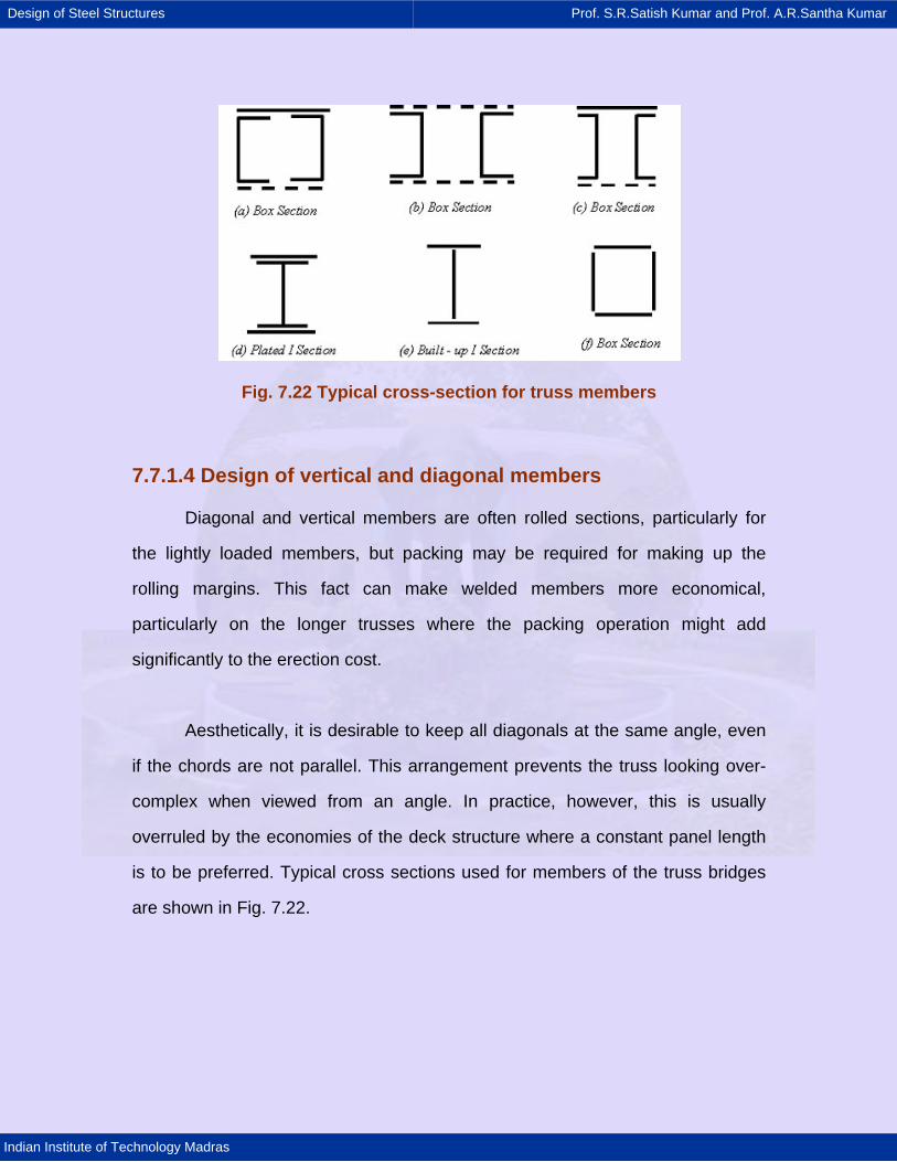
Design of Steel Structures Prof. S.R.Satish Kumar and Prof. A.R.Santha Kumar
Indian Institute of Technology Madras
Fig. 7.22 Typical cross-section for truss members
7.7.1.4 Design of vertical and diagonal members
Diagonal and vertical members are often rolled sections, particularly for
the lightly loaded members, but packing may be required for making up the
rolling margins. This fact can make welded members more economical,
particularly on the longer trusses where the packing operation might add
significantly to the erection cost.
Aesthetically, it is desirable to keep all diagonals at the same angle, even
if the chords are not parallel. This arrangement prevents the truss looking over-
complex when viewed from an angle. In practice, however, this is usually
overruled by the economies of the deck structure where a constant panel length
is to be preferred. Typical cross sections used for members of the truss bridges
are shown in Fig. 7.22.
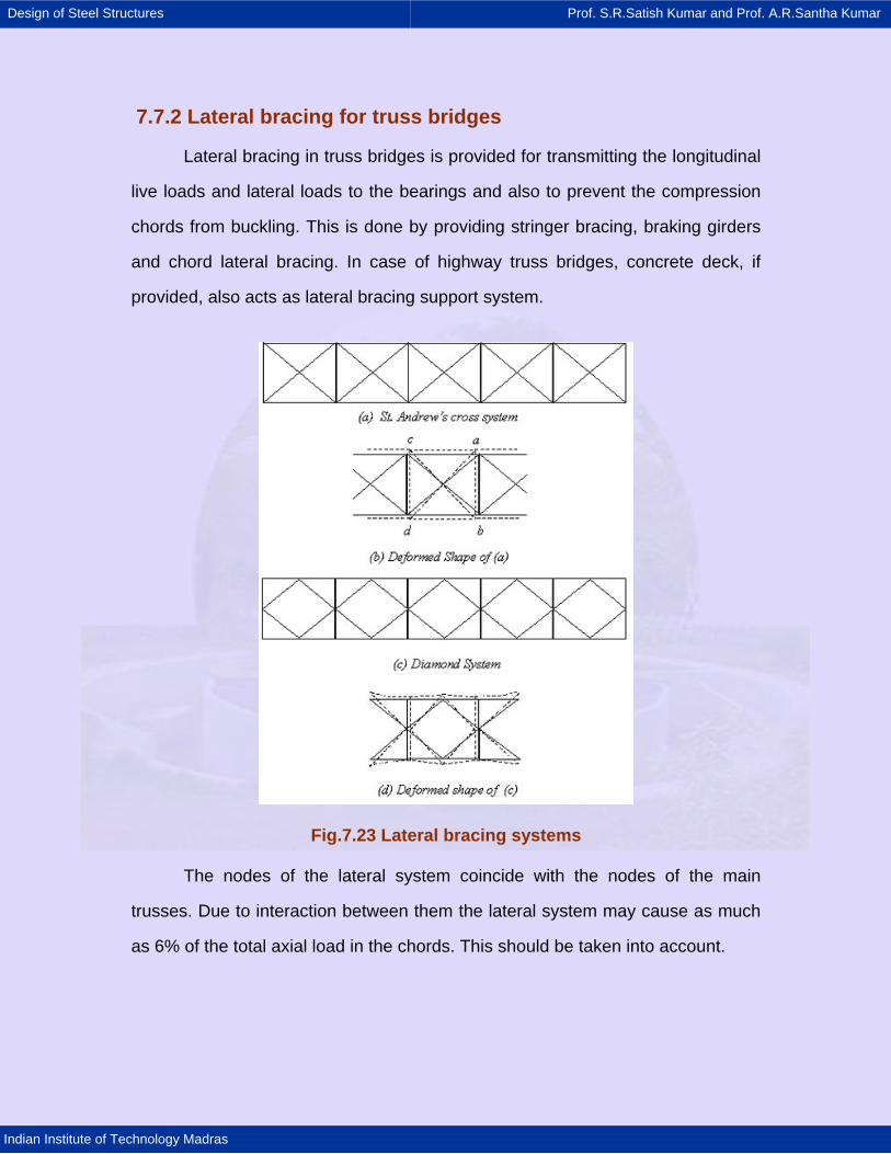
Design of Steel Structures Prof. S.R.Satish Kumar and Prof. A.R.Santha Kumar
Indian Institute of Technology Madras
7.7.2 Lateral bracing for truss bridges
Lateral bracing in truss bridges is provided for transmitting the longitudinal
live loads and lateral loads to the bearings and also to prevent the compression
chords from buckling. This is done by providing stringer bracing, braking girders
and chord lateral bracing. In case of highway truss bridges, concrete deck, if
provided, also acts as lateral bracing support system.
Fig.7.23 Lateral bracing systems
The nodes of the lateral system coincide with the nodes of the main
trusses. Due to interaction between them the lateral system may cause as much
as 6% of the total axial load in the chords. This should be taken into account.
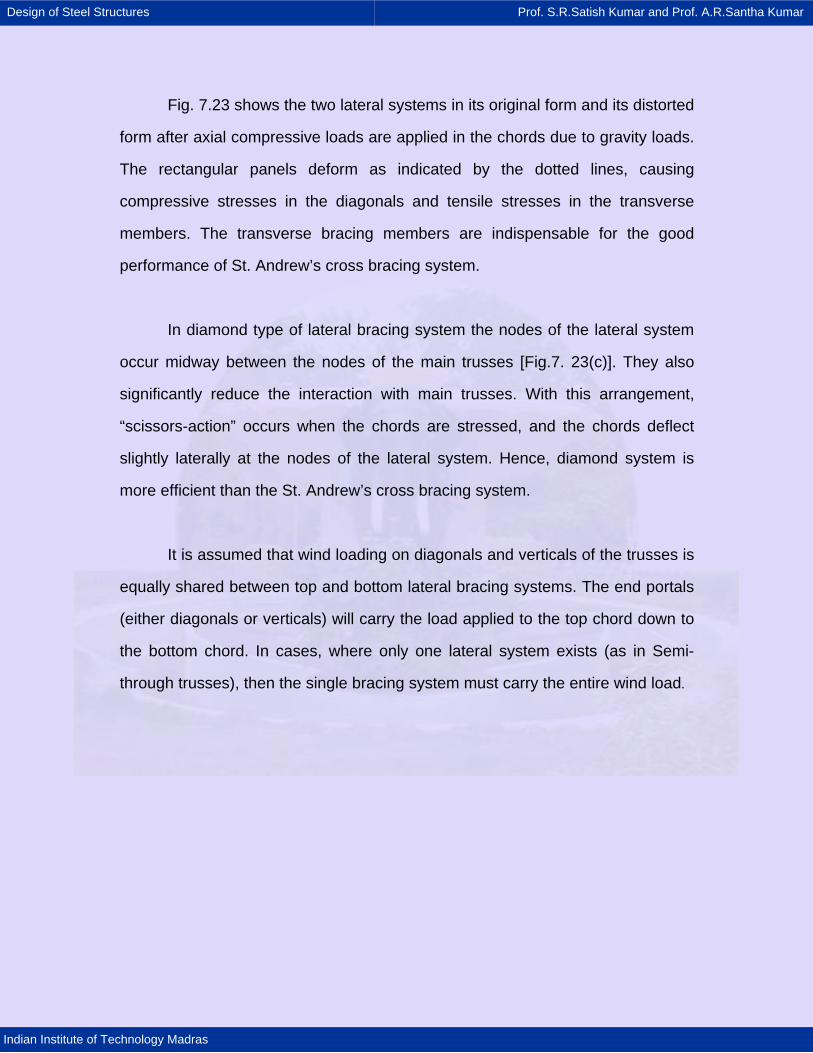
Design of Steel Structures Prof. S.R.Satish Kumar and Prof. A.R.Santha Kumar
Indian Institute of Technology Madras
Fig. 7.23 shows the two lateral systems in its original form and its distorted
form after axial compressive loads are applied in the chords due to gravity loads.
The rectangular panels deform as indicated by the dotted lines, causing
compressive stresses in the diagonals and tensile stresses in the transverse
members. The transverse bracing members are indispensable for the good
performance of St. Andrew’s cross bracing system.
In diamond type of lateral bracing system the nodes of the lateral system
occur midway between the nodes of the main trusses [Fig.7. 23(c)]. They also
significantly reduce the interaction with main trusses. With this arrangement,
“scissors-action” occurs when the chords are stressed, and the chords deflect
slightly laterally at the nodes of the lateral system. Hence, diamond system is
more efficient than the St. Andrew’s cross bracing system.
It is assumed that wind loading on diagonals and verticals of the trusses is
equally shared between top and bottom lateral bracing systems. The end portals
(either diagonals or verticals) will carry the load applied to the top chord down to
the bottom chord. In cases, where only one lateral system exists (as in Semi-
through trusses), then the single bracing system must carry the entire wind load.
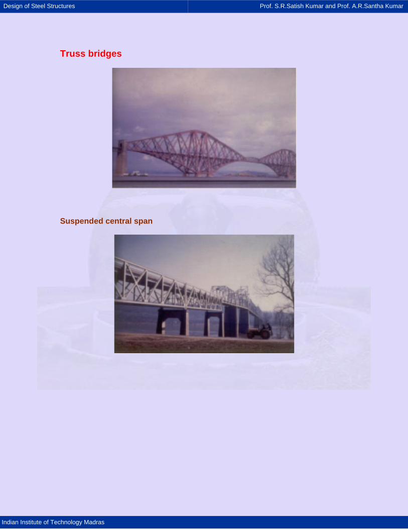
Design of Steel Structures Prof. S.R.Satish Kumar and Prof. A.R.Santha Kumar
Indian Institute of Technology Madras
Truss bridges
Suspended central span
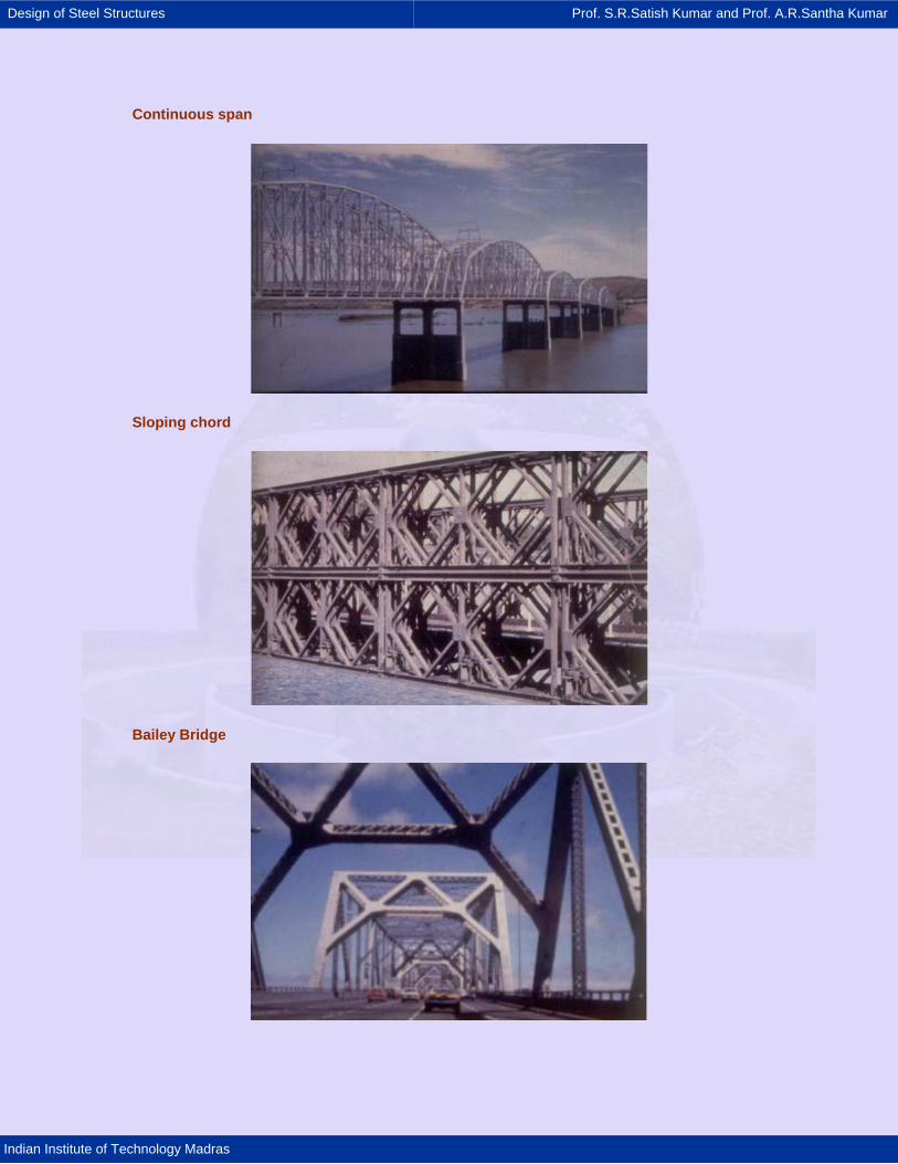
Design of Steel Structures Prof. S.R.Satish Kumar and Prof. A.R.Santha Kumar
Indian Institute of Technology Madras
Continuous span
Sloping chord
Bailey Bridge
Design of Steel Structures Prof. S.R.Satish Kumar and Prof. A.R.Santha Kumar
Indian Institute of Technology Madras
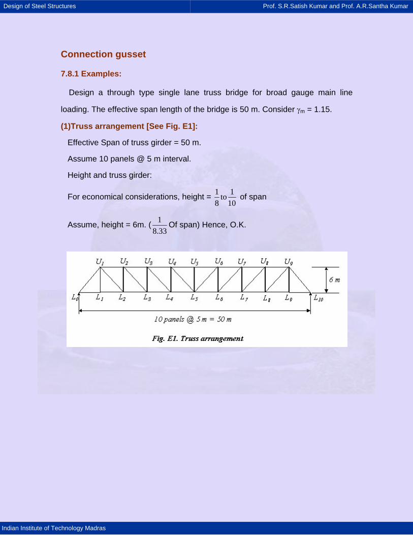
Design of Steel Structures Prof. S.R.Satish Kumar and Prof. A.R.Santha Kumar
Indian Institute of Technology Madras
Connection gusset
7.8.1 Examples:
Design a through type single lane truss bridge for broad gauge main line
loading. The effective span length of the bridge is 50 m. Consider γm = 1.15.
(1)Truss arrangement [See Fig. E1]:
Effective Span of truss girder = 50 m.
Assume 10 panels @ 5 m interval.
Height and truss girder:
For economical considerations, height = 1 1to8 10
of span
Assume, height = 6m. ( 18.33
Of span) Hence, O.K.
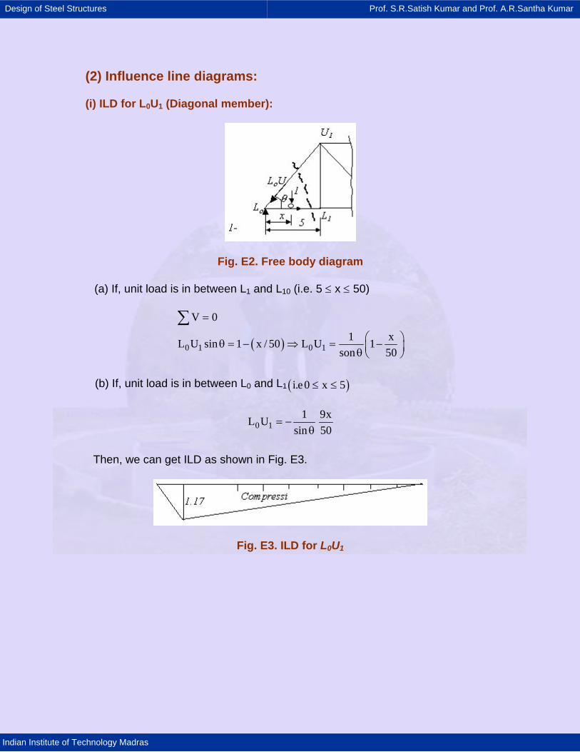
Design of Steel Structures Prof. S.R.Satish Kumar and Prof. A.R.Santha Kumar
Indian Institute of Technology Madras
(2) Influence line diagrams:
(i) ILD for L0U1 (Diagonal member):
Fig. E2. Free body diagram
(a) If, unit load is in between L1 and L10 (i.e. 5 ≤ x ≤ 50)
( )0 1 0 1
V 0
1 xL U sin 1 x / 50 L U 1son 50
=
⎛ ⎞θ = − ⇒ = −⎜ ⎟θ ⎝ ⎠
∑
(b) If, unit load is in between L0 and L1 ( )i.e0 x 5≤ ≤
0 11 9xL U
sin 50= −
θ
Then, we can get ILD as shown in Fig. E3.
Fig. E3. ILD for L0U1
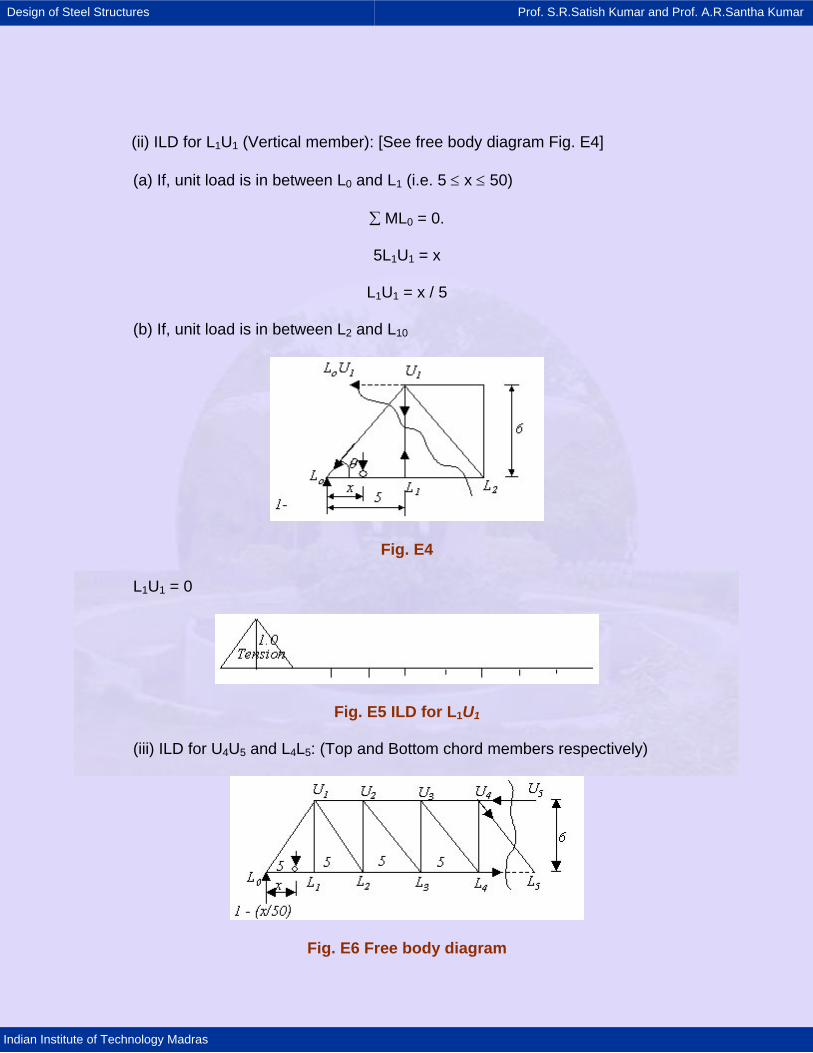
Design of Steel Structures Prof. S.R.Satish Kumar and Prof. A.R.Santha Kumar
Indian Institute of Technology Madras
(ii) ILD for L1U1 (Vertical member): [See free body diagram Fig. E4]
(a) If, unit load is in between L0 and L1 (i.e. 5 ≤ x ≤ 50)
∑ ML0 = 0.
5L1U1 = x
L1U1 = x / 5
(b) If, unit load is in between L2 and L10
Fig. E4
L1U1 = 0
Fig. E5 ILD for L1U1
(iii) ILD for U4U5 and L4L5: (Top and Bottom chord members respectively)
Fig. E6 Free body diagram
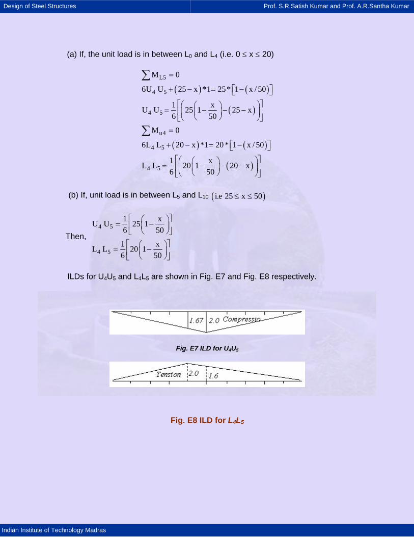
Design of Steel Structures Prof. S.R.Satish Kumar and Prof. A.R.Santha Kumar
Indian Institute of Technology Madras
(a) If, the unit load is in between L0 and L4 (i.e. 0 ≤ x ≤ 20)
( ) ( )
( )
( ) ( )
( )
L5
4 5
4 5
u4
4 5
4 5
M 0
6U U 25 x *1 25* 1 x / 50
1 xU U 25 1 25 x6 50
M 0
6L L 20 x *1 20* 1 x / 50
1 xL L 20 1 20 x6 50
=
+ − = −⎡ ⎤⎣ ⎦⎡ ⎤⎛ ⎞⎛ ⎞= − − −⎢ ⎥⎜ ⎟⎜ ⎟⎝ ⎠⎝ ⎠⎣ ⎦
=
+ − = −⎡ ⎤⎣ ⎦⎡ ⎤⎛ ⎞⎛ ⎞= − − −⎢ ⎥⎜ ⎟⎜ ⎟⎝ ⎠⎝ ⎠⎣ ⎦
∑
∑
(b) If, unit load is in between L5 and L10 ( )i.e 25 x 50≤ ≤
Then, 4 5
4 5
1 xU U 25 16 50
1 xL L 20 16 50
⎡ ⎤⎛ ⎞= −⎜ ⎟⎢ ⎥⎝ ⎠⎣ ⎦⎡ ⎤⎛ ⎞= −⎜ ⎟⎢ ⎥⎝ ⎠⎣ ⎦
ILDs for U4U5 and L4L5 are shown in Fig. E7 and Fig. E8 respectively.
Fig. E7 ILD for U4U5
Fig. E8 ILD for L4L5
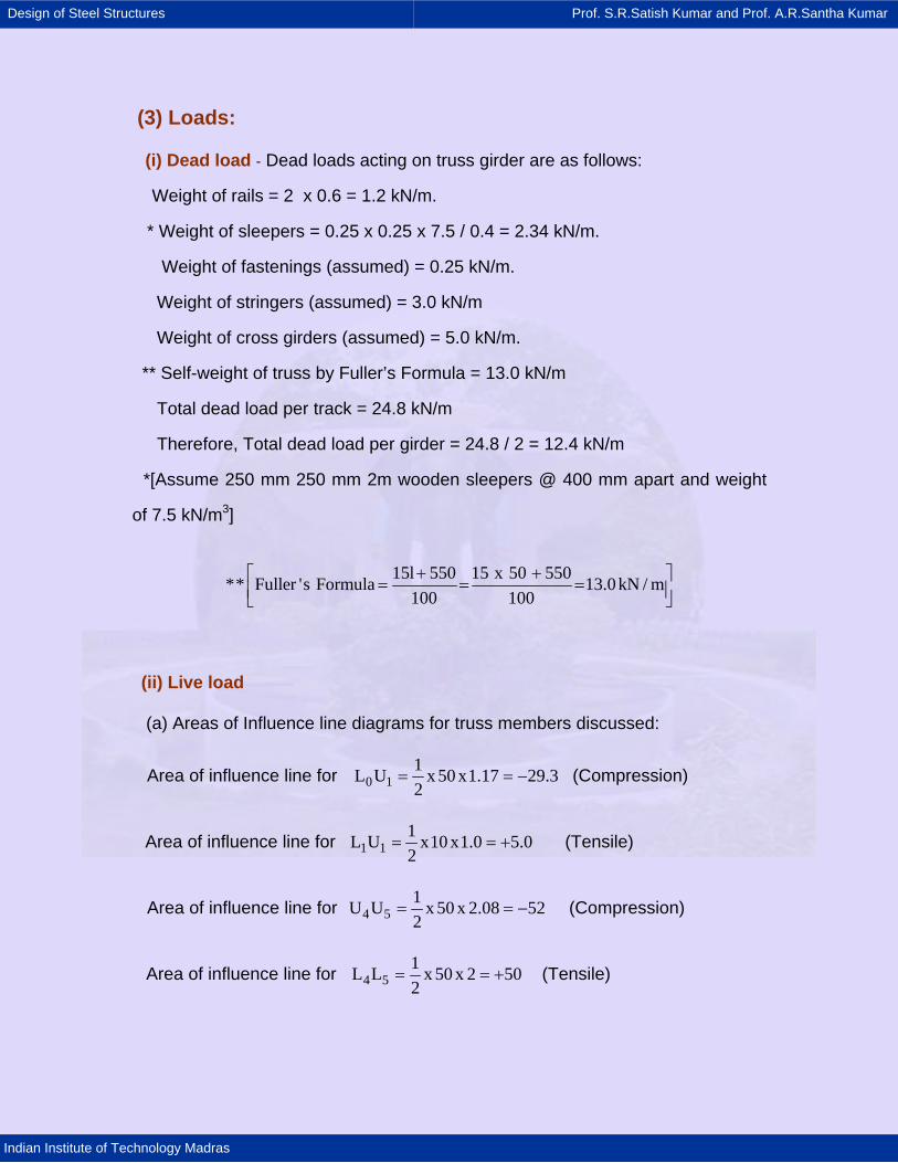
Design of Steel Structures Prof. S.R.Satish Kumar and Prof. A.R.Santha Kumar
Indian Institute of Technology Madras
(3) Loads:
(i) Dead load - Dead loads acting on truss girder are as follows:
Weight of rails = 2 x 0.6 = 1.2 kN/m.
* Weight of sleepers = 0.25 x 0.25 x 7.5 / 0.4 = 2.34 kN/m.
Weight of fastenings (assumed) = 0.25 kN/m.
Weight of stringers (assumed) = 3.0 kN/m
Weight of cross girders (assumed) = 5.0 kN/m.
** Self-weight of truss by Fuller’s Formula = 13.0 kN/m
Total dead load per track = 24.8 kN/m
Therefore, Total dead load per girder = 24.8 / 2 = 12.4 kN/m
*[Assume 250 mm 250 mm 2m wooden sleepers @ 400 mm apart and weight
of 7.5 kN/m3]
15l 550 15 x 50 550** Fuller 's Formula 13.0kN / m100 100+ +⎡ ⎤= = =⎢ ⎥⎣ ⎦
(ii) Live load
(a) Areas of Influence line diagrams for truss members discussed:
Area of influence line for 0 11L U x 50 x1.17 29.32
= = − (Compression)
Area of influence line for 1 11L U x10 x1.0 5.02
= = + (Tensile)
Area of influence line for 4 51U U x 50 x 2.08 522
= = − (Compression)
Area of influence line for 4 51L L x 50 x 2 502
= = + (Tensile)
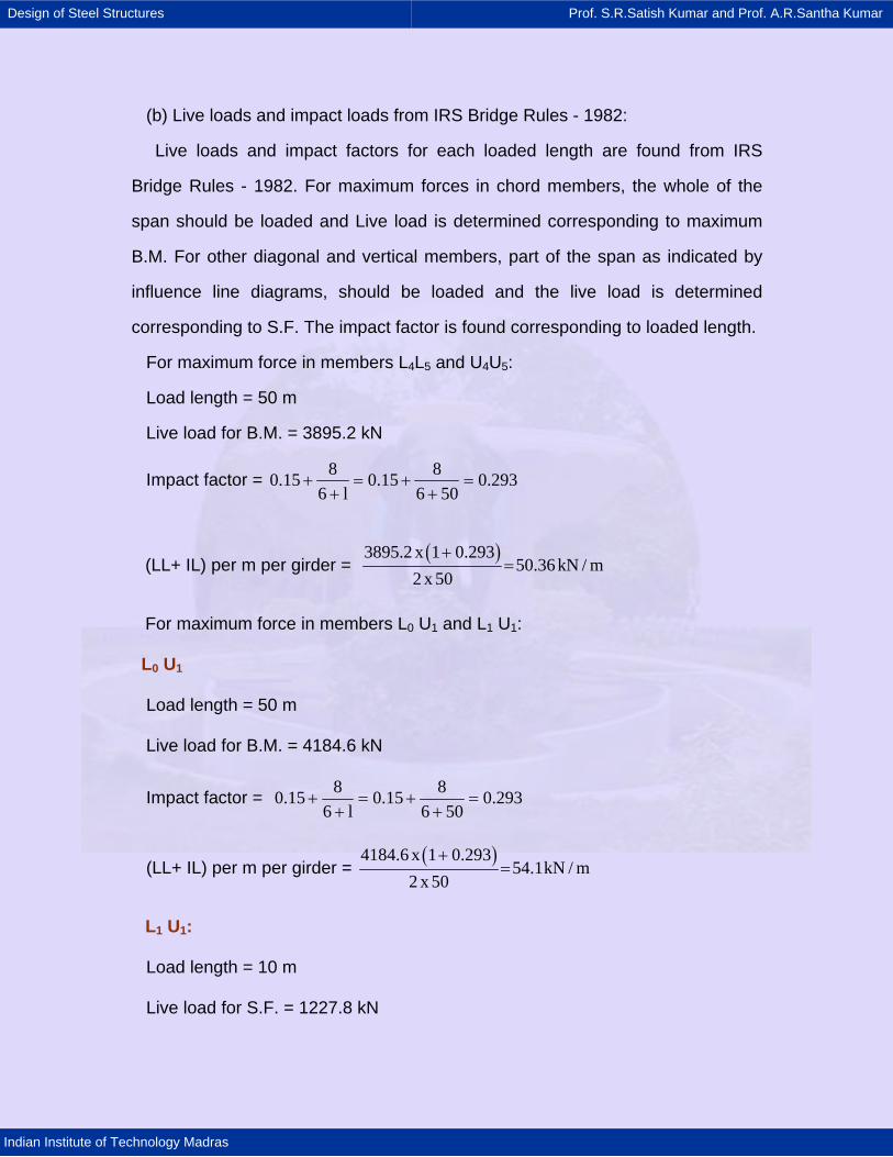
Design of Steel Structures Prof. S.R.Satish Kumar and Prof. A.R.Santha Kumar
Indian Institute of Technology Madras
(b) Live loads and impact loads from IRS Bridge Rules - 1982:
Live loads and impact factors for each loaded length are found from IRS
Bridge Rules - 1982. For maximum forces in chord members, the whole of the
span should be loaded and Live load is determined corresponding to maximum
B.M. For other diagonal and vertical members, part of the span as indicated by
influence line diagrams, should be loaded and the live load is determined
corresponding to S.F. The impact factor is found corresponding to loaded length.
For maximum force in members L4L5 and U4U5:
Load length = 50 m
Live load for B.M. = 3895.2 kN
Impact factor = 8 80.15 0.15 0.2936 l 6 50
+ = + =+ +
(LL+ IL) per m per girder = ( )3895.2 x 1 0.293
50.36kN / m2 x 50
+=
For maximum force in members L0 U1 and L1 U1:
L0 U1
Load length = 50 m
Live load for B.M. = 4184.6 kN
Impact factor = 8 80.15 0.15 0.2936 l 6 50
+ = + =+ +
(LL+ IL) per m per girder = ( )4184.6 x 1 0.293
54.1kN / m2 x 50
+=
L1 U1:
Load length = 10 m
Live load for S.F. = 1227.8 kN
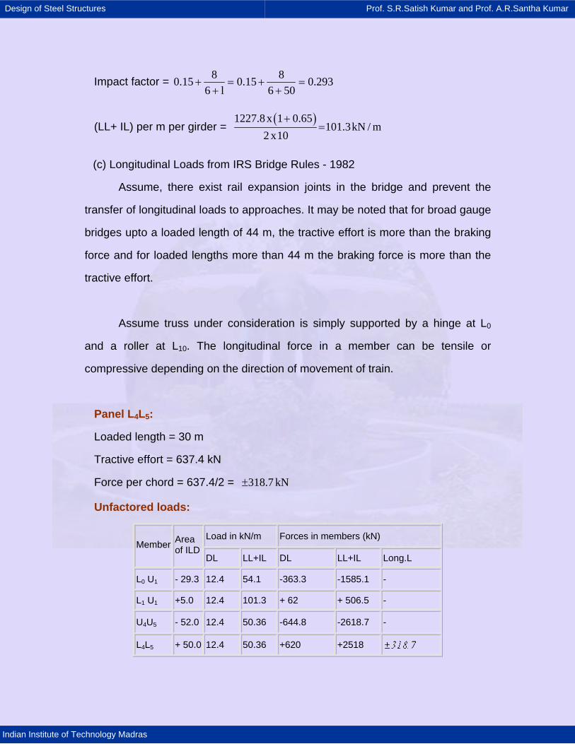
Design of Steel Structures Prof. S.R.Satish Kumar and Prof. A.R.Santha Kumar
Indian Institute of Technology Madras
Impact factor = 8 80.15 0.15 0.2936 l 6 50
+ = + =+ +
(LL+ IL) per m per girder = ( )1227.8x 1 0.65
101.3kN / m2 x10
+=
(c) Longitudinal Loads from IRS Bridge Rules - 1982
Assume, there exist rail expansion joints in the bridge and prevent the
transfer of longitudinal loads to approaches. It may be noted that for broad gauge
bridges upto a loaded length of 44 m, the tractive effort is more than the braking
force and for loaded lengths more than 44 m the braking force is more than the
tractive effort.
Assume truss under consideration is simply supported by a hinge at L0
and a roller at L10. The longitudinal force in a member can be tensile or
compressive depending on the direction of movement of train.
Panel L4L5:
Loaded length = 30 m
Tractive effort = 637.4 kN
Force per chord = 637.4/2 = 318.7 kN±
Unfactored loads:
Load in kN/m Forces in members (kN) Member Area
of ILD DL LL+IL DL LL+IL Long.L
L0 U1 - 29.3 12.4 54.1 -363.3 -1585.1 -
L1 U1 +5.0 12.4 101.3 + 62 + 506.5 -
U4U5 - 52.0 12.4 50.36 -644.8 -2618.7 -
L4L5 + 50.0 12.4 50.36 +620 +2518
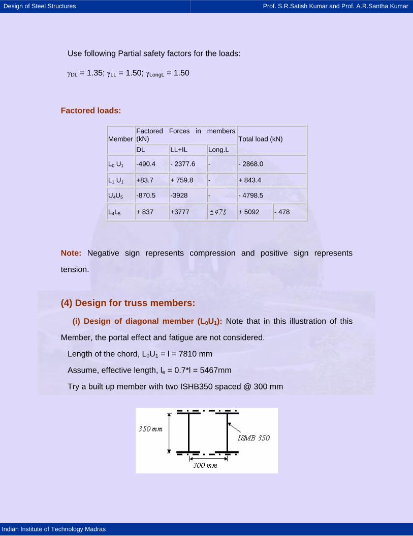
Design of Steel Structures Prof. S.R.Satish Kumar and Prof. A.R.Santha Kumar
Indian Institute of Technology Madras
Use following Partial safety factors for the loads:
γDL = 1.35; γLL = 1.50; γLongL = 1.50
Factored loads:
Factored Forces in members (kN) Member DL LL+IL Long.L
Total load (kN)
L0 U1 -490.4 - 2377.6 - - 2868.0
L1 U1 +83.7 + 759.8 - + 843.4
U4U5 -870.5 -3928 - - 4798.5
L4L5 + 837 +3777 + 5092 - 478
Note: Negative sign represents compression and positive sign represents
tension.
(4) Design for truss members:
(i) Design of diagonal member (L0U1): Note that in this illustration of this
Member, the portal effect and fatigue are not considered.
Length of the chord, L0U1 = l = 7810 mm
Assume, effective length, le = 0.7*l = 5467mm
Try a built up member with two ISHB350 spaced @ 300 mm
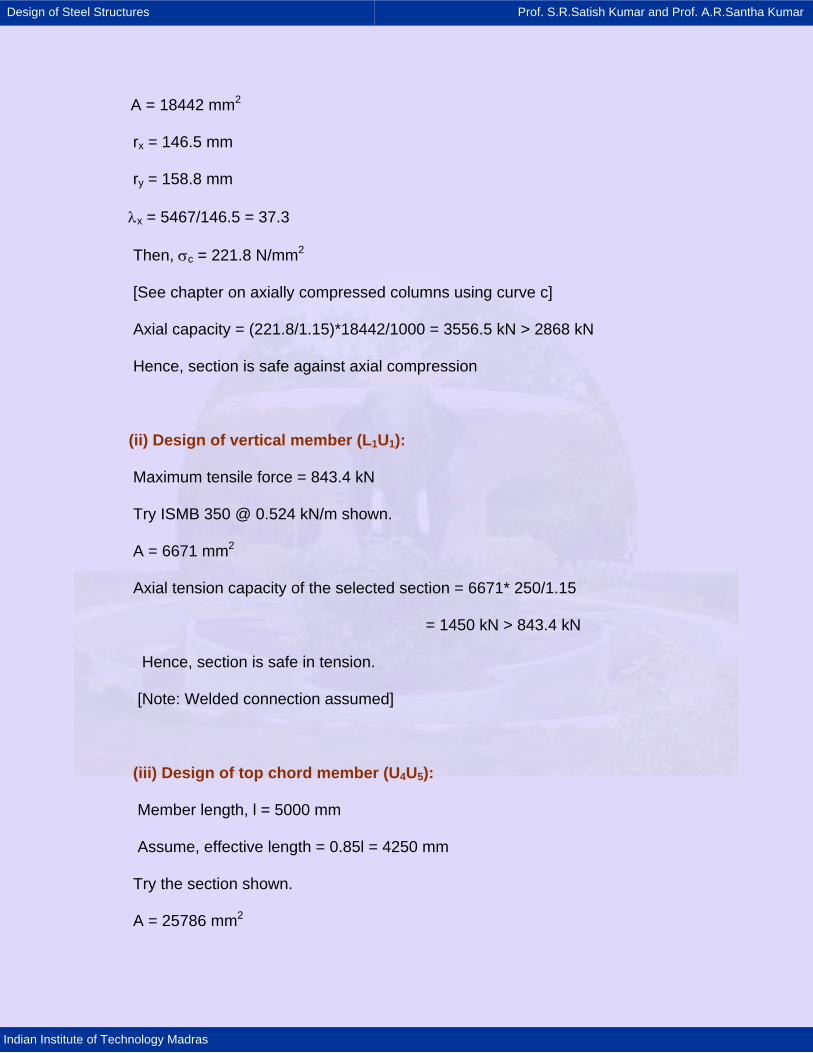
Design of Steel Structures Prof. S.R.Satish Kumar and Prof. A.R.Santha Kumar
Indian Institute of Technology Madras
A = 18442 mm2
rx = 146.5 mm
ry = 158.8 mm
λx = 5467/146.5 = 37.3
Then, σc = 221.8 N/mm2
[See chapter on axially compressed columns using curve c]
Axial capacity = (221.8/1.15)*18442/1000 = 3556.5 kN > 2868 kN
Hence, section is safe against axial compression
(ii) Design of vertical member (L1U1):
Maximum tensile force = 843.4 kN
Try ISMB 350 @ 0.524 kN/m shown.
A = 6671 mm2
Axial tension capacity of the selected section = 6671* 250/1.15
= 1450 kN > 843.4 kN
Hence, section is safe in tension.
[Note: Welded connection assumed]
(iii) Design of top chord member (U4U5):
Member length, l = 5000 mm
Assume, effective length = 0.85l = 4250 mm
Try the section shown.
A = 25786 mm2
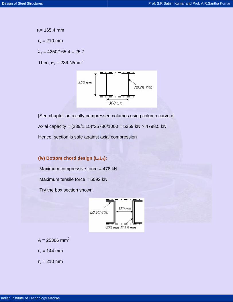
Design of Steel Structures Prof. S.R.Satish Kumar and Prof. A.R.Santha Kumar
Indian Institute of Technology Madras
rx= 165.4 mm
ry = 210 mm
λx = 4250/165.4 = 25.7
Then, σc = 239 N/mm2
[See chapter on axially compressed columns using column curve c]
Axial capacity = (239/1.15)*25786/1000 = 5359 kN > 4798.5 kN
Hence, section is safe against axial compression
(iv) Bottom chord design (L4L5):
Maximum compressive force = 478 kN
Maximum tensile force = 5092 kN
Try the box section shown.
A = 25386 mm2
rx = 144 mm
ry = 210 mm
Design of Steel Structures Prof. S.R.Satish Kumar and Prof. A.R.Santha Kumar
Indian Institute of Technology Madras
Axial tension capacity of the selected section = 25386* 250/1.15
= 5518 kN > 5092 kN
Hence, section is safe in tension.
Maximum unrestrained length = l = 5000 mm
λx = 5000/144 = 34.7
Then, σc = 225 N/mm2
Axial capacity = (225/1.15)* 25386/1000
= 4967 kN > 478 kN
Hence, section is safe against axial compression also.
The example is only an illustration. The following have to be taken into
consideration:
· Design of lacings/batten
· Design of connections and effect of bolt holes on member strength
· Secondary bending effects
· Design for fatigue
Design of Steel Structures Prof. S.R.Satish Kumar and Prof. A.R.Santha Kumar
Indian Institute of Technology Madras
7.9 Summary
After brief introduction, the steel used in bridges and its properties were
discussed. The broad classification of bridges was mentioned and various loads
to be considered in designing railway and highway bridges in India were
discussed. Finally analysis of girder bridges was discussed using influence line
diagrams.
This chapter deals with the design of steel bridges using Limit States
approach. Various types of plate girder and truss girder bridges were covered.
Basic considerations that are to be taken into account while designing the plate
girder bridges are emphasised. Practical considerations in the design of truss
members and lateral bracing systems are discussed briefly. A worked example
on through type truss girder Railway Bridge is given in the appendix.
Design of Steel Structures Prof. S.R.Satish Kumar and Prof. A.R.Santha Kumar
Indian Institute of Technology Madras
7.10 References
1. Owens. G.W., Knowles. P.R., Dowling. P.J. (1994): Steel Designers'
Manual, Fifth edition, Blackwell Scientific Publications.
2. Chatterjee. S. (1991): The Design of Modern Steel Bridges, First
edition, BSP Professional books.
3. Demetrios. E.T. (1994): Design, Rehabilitation and Maintenance of
Modern Highway Bridges, McGraw-Hill Publishers.
4. Victor. D.J. (1973): Essentials of Bridge Engineering, Oxford and IBH
Publishers.
5. IRC: 6 - 2000– Section II, Indian Standard for loads and stresses on
Highway Bridges.
6. Bridge rules - 1982, Specifications for Indian Railway loading.
7. ESDEP, Group 15B, Volume 25: Structural systems - Steel Bridges,
SCI, UK.
8. IS: 1915 - 1961: The Indian Standard Code of Practice for Design of
Steel Bridges
9. BS: 5400 - Part 3: 1982: British Standard Code of Practice for Design
of Steel Bridges