1. Introduction to Rock Properties - Imperial College London

MSc in Petroleum Engineering/Geoscience/Geophysics Rock Properties RW Zimmerman

Imperial College London Department of Earth Science and Engineering

1. Introduction to Rock Properties The most important fact about reservoir rocks is that, by definition, they are not completely solid, but rather are porous to one degree or another. The degree to which they are porous is quantified by a parameter known as the porosity. The fact that the rocks are porous allows them to hold fluid. If these pores are interconnected, which they are in most rocks, then the fluid is able to flow through the rock, and the rock is said to be permeable. The ability of a rock to allow fluid to flow through it is quantified by a parameter called the permeability. As the porosity controls the amount of oil or gas that the rock can hold, and the permeability controls the rate at which this oil or gas can flow to a well, these two parameters, porosity and permeability, are the most important attributes of a rock, for reservoir engineering purposes.

It would be very advantageous to petroleum engineers if the pore space of a reservoir were completely filled with hydrocarbon fluid. Unfortunately, this is never the case, and the pores always contain a mixture of hydrocarbons and water. The relative amounts of oil, gas or water are quantified in terms of parameters known as the fluid saturations. These saturations are in turn controlled by the surface interactions between the rock and the various fluids, which can be described and quantified in terms of properties known as wettability and surface tension.

The ability of a rock to store fluid, and the relationship between the amount of fluid stored in the rock and the pressure of the fluid, is related to the porosity, and specifically to the way that the porosity changes as the pore pressure changes. The relationship between porosity and pressure is quantified by an important mechanical property known as the pore compressibility.

Aside from properties such as porosity, permeability, and compressibility, which are obviously of crucial importance in reservoir engineering, there are other petrophysical (“petros” = rock, in Greek) properties that are important, but for less obvious reasons. One such property is the electrical resistivity. Although the resistivity is not directly related to the oil, it is controlled mainly by the amount of water in the rock, and so knowledge of the electrical resistivity gives us valuable information on the relative amounts of oil and water in the rock.



In this introductory module on rock properties, we will define the various parameters mentioned above, present some simple models to relate these properties to the pore structure of the rock, and give some indication of how these properties are used in petroleum engineering. The definitions and relationships given in this module will be used extensively throughout the rest of the course.

2. Porosity 2.1. Definition of Porosity If one looks at a typical cylindrical core of rock, with radius R and length L, it would have an apparent volume, or bulk volume, of Vb = π R2L. But on a smaller scale, such as under a microscope (Fig. 2.1), it would be clear that some of this volume is occupied by rock minerals, and some of it is void space.

Fig. 2.1. Schematic of a porous sandstone, showing grains and pore space. Typical grain sizes are tens to hundreds of microns.

We can now define the mineral volume of this core, Vm, as the actual volume occupied by minerals. Lastly, we define the pore volume, Vp, as the volume of the void space contained in this cylindrical core. These volumes are obviously related by

Vb = Vm + Vp . (1)

The fraction of the cylinder that is occupied by pore space is known as the porosity, and is usually denoted by φ (although sometimes by n):

φ = Vp /Vb . (2)



The porosity of a reservoir rock can range from a few percent, to as high as 40%.

A distinction is often made between primary porosity, which is the porosity that the sandstone (say) had after it was first deposited and compacted, and secondary porosity, which is any porosity that is subsequently created through mineral dissolution, mineral deposition, fracturing, etc.

One very important type of secondary porosity is the porosity contained in natural fractures. Many reservoirs, which collectively contain roughly half of all known oil reserves, are naturally fractured. These reservoirs are often filled with an interconnected system of fractures. The porosity contained in these fractures is usually on the order of 0.1-1.0%, and is much less than the primary porosity. But the fracture network typically has a much higher permeability than the unfractured rock, often by several orders of magnitude. These types of reservoirs are referred to as dual-porosity reservoirs. Producing oil from such reservoirs is more problematic than producing oil from unfractured reservoirs.

Another distinction that can be made is between total porosity, which is essentially the porosity that is defined by eq. (2), and effective porosity, which measures only the pore space that is interconnected and which can potentially form a flow path for the hydrocarbons. The total porosity is therefore composed of effective/interconnected porosity, and ineffective/unconnected porosity. In most rocks, there is little ineffective porosity. One important exception are carbonate rocks called diatomites, in which most of the porosity is unconnected. The Belridge oilfield in central California has produced 1.5 billion barrels of oil from a diatomite reservoir that has porosities ranging from 45-75%, most of which is unconnected and not “effective”! But this is a special case that requires special production methods, and is not typical of the reservoirs that will be the focus of most of this course.

2.2. Heterogeneity and “Representative Elementary Volume” The property of porosity introduces an issue, that of heterogeneity, which is important for all petrophysical properties. To say that a reservoir is heterogeneous means that its properties vary from point to point. In one sense all rock masses are heterogeneous, because, as we move



away from a given rock at a given location, we will eventually encounter a different rock type. For example, some reservoirs contain beds of sands and shales, with thicknesses on the order of a few meters, such as in Fig. 2.2. These reservoirs are heterogeneous on length scales on the order of tens of meters.

Shale

SandAND

10 m

Fig. 2.2. Sand-shale sequence in a reservoir. Such a reservoir is homogeneous on a length scale of a few centimetres, but heterogeneous on a length scale of a few meters.

At the other extreme of length-scale, all porous rocks are heterogeneous on the scale of the pore size. Consider Figure 2.3a, where x1 and x2 are two locations in the rock. If we ask “what is the porosity at location x1”?, the answer would be “0”, because point x1 lies in a sand grain. On the other hand, point x2 lies in a pore, so, strictly speaking, the porosity at x2 is 1. Clearly, it makes no sense to talk about the porosity at some infinitely small mathematical point in the reservoir. When we discuss the porosity, we implicitly are referring to the average porosity in some small region.

(a) (b)

Fig. 2.3. (a) Porosity at x1 is 0, and at x2 is 1, illustrating that porosity must not be defined at a point, but over a volume. (b) φ(R) can be defined as an average over a region of radius R (length of the arrow).



Imagine that we could measure the porosity in a small spherical region of rock, of radius R, surrounding the point x2, as in Fig. 2.3b. Let’s denote this average value as φ(R). For very small values of R, φ(R) would be 1. As R gets larger, the spherical region encompasses some of the nearby sand grains, and so φ(R) will decrease. In a typical sandstone, φ(R) will fluctuate with R, but eventually stabilise to some constant value. Eventually, as R gets large enough that the region crosses over into the next rock type, φ(R) might change abruptly. Schematically, we can represent this situation as in Fig. 2.4 (Bear, Dynamics of Fluids in Porous Media, 1972):

R

φ

1

0 REV

Fig. 2.4. Porosity as a function of the size of the sampling region, showing the existence of an REV.

The minimum value of R needed for the porosity to stabilise is known as the “representative elementary volume” (REV), or as the “representative volume element” (RVE). When we talk about the porosity, we are usually implicitly referring to the porosity as defined on a length scale at least as large as the REV.

For sandstones with a uniform grain size distribution, the REV must be at least about ten grain diameters. However, for heterogeneous rocks such as many carbonates, the REV may be much larger, as heterogeneity may exist at many scales. In fact, there is no guarantee that an REV scale exists for a given rock. But in petroleum engineering, we always assume that an REV can be defined on the length scale of the gridblocks that are used in the numerical reservoir simulation codes. This will be discussed further in some later modules.



2.3. Saturation Reservoir rocks are never filled completely with oil, for reasons that will be discussed a later section of this module. Consider a rock that contains some oil and some water, as in Fig. 2.5. If the volume of water contained in a region of rock is Vw, the volume of oil is Vo, and the total volume of the pore space is Vp, then the saturation of each of these phases can be defined as the fraction of pore space that is occupied by that phase, i.e.,

Sw = Vw /Vp , So = Vo /Vp . (1)

The saturation of each phase must lie between 0 and 1. If oil and water are the only two phases present, then it is necessarily the case that

Sw + So = 1. (2)

If there is also some hydrocarbon gas in the pore space, then

Sw + So + Sg = 1. (3)

Fig. 2.5. Schematic diagram of a porous rock containing oil and water.

3. Permeability and Darcy’s Law 3.1. Darcy’s Law The ability of a porous rock to transmit fluid is quantified by the property called permeability. Quantitatively, permeability is defined by the “law” that governs the flow of fluids through porous media - Darcy’s law. This law was formulated by French civil engineer Henry Darcy in 1856 on the basis of his experiments on water filtration through sand beds. Darcy’s law is the most important equation in petroleum engineering.



Imagine a fluid having viscosity µ, flowing through a horizontal tube of length L and cross-sectional area A, filled with a rock or sand. The fluid pressure at the inlet is Pi, and at the outlet is Po, as in Fig. 3.1:

Q A

L

P i

P o

P

x

Fig. 3.1. Experimental set-up for measuring the permeability of a porous rock or sand.

According to Darcy’s law, the fluid will flow through the rock in the direction from higher pressure to lower pressure, and the volumetric flowrate of this fluid will be given by

Q =

kA(Pi −Po )µL

, (1)

where: Q = volumetric flowrate, with units of [m3/s]

k = permeability of the rock, with units of [m2]

A = cross-sectional area of the rock core, with units of [m2]

Pi , Po = inlet/outlet pressures, with units of [Pa]

µ = viscosity of the fluid, with units of [Pa s]

L = length of the core, with units of [m]

This equation can be thought of as providing a definition of permeability, and it also shows us how to measure the permeability in the laboratory. This equation tells us that the flowrate is proportional to the area, inversely proportional to the fluid viscosity, and proportional to the pressure gradient, i.e., the pressure drop per unit length, ΔP/L. Note that the permeability is a property of the rock; the influence of the fluid that is flowing through the rock is accounted for by the viscosity term in Darcy’s law.



It is usually more convenient to work with the volumetric flow per unit area, q = Q/A. Darcy’s law is therefore usually written as

q =

QA=

k(Pi −Po )µL

, (2)

where the flux q has dimensions of [m/s]. Please note that the flux is not the same as the velocity of the fluid particles*, and so it is perhaps easier to think of these units as [m3/m2 s].

*Note: q is the flux based on the total nominal area of the core. But the fluid actually flows only through the pores, but not the grains! So, the total flux is given by Q = qA, but it can also be expressed as Q = vApore, where v is the actual mean velocity of the fluid, and Apore is area occupied by pores. Hence, qA = vApore, so v = q(A/Apore) = q/φ. So, if q is 1 cm/hour in a reservoir of 10% porosity, for example, the actual mean velocity of the oil is 10 cm per hour.

For the general case in which the flux may vary from point-to-point, we need a differential form of Darcy’s law. The differential version of equation (2) for horizontal flow is

qx =

−kµ

dPdx

. (3)

The minus sign is included because the fluid flows in the direction from higher to lower pressure.

For vertical flow, we must include a gravitational term in Darcy’s law. To see why, recall from fluid mechanics that if the fluid is stagnant, the pressure distribution will be

P = Po + ρgz , (4)

where z is the depth below some datum level, and Po is the pressure at the datum level.

So, there will be pressure gradient in a stagnant fluid, but there will be no flow. The “equilibrium pressure gradient” is, from eq. (4),



dPdz

⎤

⎦ ⎥ equilibrium

= ρg . (5)

It seems reasonable to assume that fluid will flow through the rock only if the pressure gradient exceeds the equilibrium value given by eq. (5). So, the actual driving force should be (dP/dz)−ρg. For vertical flow, we therefore modify eq. (3) as follows:

qz =

−kµ

dPdz

− ρg⎡

⎣ ⎢

⎤

⎦ ⎥ =

−kµ

d(P − ρgz)dz

. (6)

Actually, this form of the equation holds for horizontal flow, also, because in this case we can say that

qx =

−kµ

d(P − ρgz)dx

=−kµ

dPdx

, (7)

since d(ρgz)/dx = 0.

A convenient way of simplifying the form of these equations is to write them in terms of the fluid potential Φ, defined by

Φ = P − ρgz , (8)

in which case flow in an arbitrary direction n can be described by

qn =

−kµ

dΦdn

. (9)

The above equations assume that the permeability is the same in all directions. But in most reservoirs, the permeability in the horizontal plane, kH, is different than the vertical permeability, kV; typically, kH > kV. The permeabilities in different directions within the horizontal plane may also differ, but this difference is usually not as great as between kH and kV. The property of having different permeabilities in different directions is known as anisotropy.

For flow in an anisotropic rock, we must modify Darcy’s law, as follows:

qx =

−kH

µdΦdx

, qz =−kvµ

dΦdz

. (10)



Caution: if the rock is anisotropic, eq. (9) does not hold in an arbitrary direction, even if we use an appropriate value of k (see de Marsily, Quantitative Hydrogeology, 1986). The correct version of Darcy’s law for an anisotropic rock must be written in terms of the permeability tensor, which is a symmetric 3x3 matrix that has six independent components. However, this tensor form of Darcy’s law is not typically used in most reservoir engineering calculations.

Another way to think about why fluid flow is controlled by the gradient of “ P − ρgz ” is as follows. You may recall from undergraduate fluid mechanics that Bernoulli’s equation, which essentially embodies the principle of “conservation of energy”, contains the terms

Pρ− gz +

v2

2=

1ρ

P − ρgz +ρv2

2⎛

⎝ ⎜

⎞

⎠ ⎟ , (11)

where P/ρ is related to the enthalpy per unit mass, gz is the gravitational potential energy per unit mass, v2/2 is the kinetic energy per unit mass.

Fluid velocities in a reservoir are usually very small, so the kinetic energy term is negligible, in which case the combination “ P − ρgz ” represents the “Bernoulli energy” per unit volume. It seems reasonable that the fluid would flow from regions of higher to lower energy, and, therefore, the driving force for flow should be the gradient (i.e., the rate of spatial change) of the quantity P − ρgz .

These considerations also warn us that we should not expect Darcy’s law to hold in cases where the kinetic energy term is not negligible. In fact, at high flowrates, we must modify Darcy’s law by incorporating a quadratic term q2 on the left-hand side of, say, eq. (3) on p. 8. The resulting more general equation, called the Forchheimer equation, is necessary in some situations, such as in some gas reservoirs, and particularly near the wellbore, where the velocities are higher (Bear 1972). However, Darcy’s law is adequate in the vast majority of situations.



3.2. Units of Permeability

Permeability has dimensions of “area”, so in the SI system it has units of [m2]. However, in most areas of engineering it is conventional to use a unit called the “Darcy”, which is defined by

1Darcy = 0.987×10−12 m2 ≈ 10−12 m2 . (1)

The Darcy unit (D) is defined such that a rock having a permeability of 1 D would transmit 1 cm3 of water (which has a viscosity of 1 centiPoise) per second through a region that has a cross-sectional area of 1 sq cm, if the pressure drop along the direction of flow was 1 atm per cm.

This definition is strange, in that it utilises different systems of units. Some people apply Darcy’s law by first converting flowrates to cm3/s, pressures to atm, etc., in which case you must use the value of k in Darcies. Another method is to first convert all parameters to SI units, in which case you must then use the value of k in units of m2.

Typical ranges of the permeability of various rocks and sands are given in the following table:

Rock type k (D) k (m2) coarse gravel 103 - 104 10-9 - 10-8 sands, gravels 100 - 103 10-12 - 10-9 fine sand, silt 10-4 - 100 10-16 - 10-12 clay, shales 10-9 - 10-6 10-21 - 10-18 limestones 100 - 102 10-12 - 10-10 sandstones 10-5 - 101 10-17 - 10-11 weathered chalk 100 - 102 10-12 - 10-10 unweathered chalk 10-9 - 10-1 10-21 - 10-13 granite, gneiss 10-8 - 10-4 10-20 - 10-16

This table shows that the permeability of geological media varies over many orders of magnitude. However, most reservoir rocks have permeabilities in the range of 0.1 milliDarcies to 10 Darcies, and usually in the much narrower range of 10-1000 mD. Methods for measuring permeability in the laboratory will be discussed in the module on core analysis.



3.3. Relationship between Permeability and Pore Size The permeability depends on the porosity of the rock, and also on the pore size. Many models have been developed to try to relate the permeability to porosity, pore size, and other attributes of the pore space.

The simplest model assumes that the pores are all circular tubes of the same diameter. Consider a set of circular pore tubes, each of diameter d, passing through a cubical rock specimen of side L, as in Fig. 3.2, with a pressure difference ΔP imposed across the two parallel faces (on the page and behind the page) of the rock.

d L

Fig. 3.2. Idealised pore structure used to derive a relationship between permeability, porosity and pore size.

According to Poiseuille’s equation for pipe flow (Dullien, Porous Media, 1992), the flow through each tube is given by

€

Q =πd 4

128µΔPL . (1)

If there are N such pores, the total flow rate will be

€

Q =πNd4

128µΔPL . (2)

The total area of these pores, in the plane of the page, is

€

Ap = Nπd2 /4 , and the porosity is

€

φ = Ap /A = Ap /L2, where A is the macroscopic area normal to the flow. Hence, the total flowrate from (2) can be written as

€

Q =φd2A32µ

ΔPL . (3)



If we compare this flowrate with Darcy’s law, Q = kAΔP/µL, we see that the permeability of this rock is k = φd2/32. Lastly, we note that an isotropic rock should have only one-third of its pores aligned in the x-direction, one-third in the y-direction, etc. So, the permeability of this idealised porous rock is

k = φ d 2/96. (4)

A more realistic model, in which the orientations of the pores are randomly distributed in three-dimensional space, leads to the same result (Scheidegger, The Physics of Flow through Porous Media, 1974).

Equation (4) is often written in terms of the “specific surface”, S/V, which is the total amount of surface area per unit volume of rock; the result is

k = φ 3/[6(S/V)2] . (5)

This is often called the Kozeny-Carman equation. One justification for this equation is that the permeability is the inverse of the “hydraulic resistivity”, and it is plausible that the resistance to flow, which is essentially due to viscous drag of the fluid against the pore walls, should be related to the amount of surface area of the pores.

In some versions of the Kozeny-Carman equation, the factor 6 is replaced by another constant called the “tortuosity”, τ. The tortuosity is sometimes claimed to represent the ratio of the actual fluid flow path from the inlet to the outlet, to the nominal fluid flow path L, but this is not true, and it is better to think of τ as an empirical fitting factor.

There have been many attempts to try to improve upon the Kozeny-Carman equation, by incorporating more information about the distribution of pore sizes, interconnectedness of the pores, etc. For our present purposes, it is sufficient to understand that the permeability is proportional to the square of the mean pore diameter.

3.4. Permeability of Layered Rocks Most reservoir rocks are layered, with each layer having a different permeability. If fluid flows through a layered rock, either in the vertical direction (perpendicular to the layering) or the horizontal direction (parallel to the layering), it is possible to define an effective permeability



that will allow us to treat the rock as if it were homogeneous, and use Darcy’s law in its usual form.

For example, consider horizontal flow through a rock composed of N layers, each having permeability ki and thickness Hi, as in Fig. 3.3. Within each layer, water will flow horizontally, according to Darcy’s law:

€

Qi = −ki (Hiw)µ

ΔΦΔx , (1)

where w is the thickness into the page.

H1H2

HN

.....k1k2

kN

Q1Q2

QN

ΔΦ

Fig. 3.3. Fluid flow parallel to the layering of a layered rock.

The total flowrate is found by summing up the flowrates through each layer:

€

Q = Qii=1

N∑ = −ki (Hiw)

µΔΦΔxi=1

N∑ = −w

µΔΦΔx kiHi

i=1

N∑ . (2)

But if we treat the rock as a homogeneous rock mass with an effective permeability keff, we would write Darcy’s law as

€

Q = −keff (Htotalw)µ

ΔΦΔx =

−wµΔΦΔx keff Hi

i=1

N∑ . (3)

If we compare eqs. (2) and (3), we see that the effective permeability of the layered rock is

keff = kiHi

i=1

N∑ Hi

i=1

N∑ =

1H

kiHii=1

N∑ . (4)



Hence, the effective permeability for flow along the layering is a weighted arithmetic mean of the individual permeabilities, weighted by the thickness of the layers.

Now imagine vertical flow through this layered system (Fig. 3.4). We again start by writing Darcy’s law for each layer:

Qi =

−kiAµ

ΔΦ iHi

, (5)

where A is the area normal to the flow direction, i.e., in the horizontal plane.

In steady-state, the flowrate through each layer is the same, but the potential drop will be different. So, we put Qi = Q in each layer, and re-write eq. (5) in the form

ΔΦ i =

−µQHiAki

, (6)

The total potential drop across all N layers is found by summing up the drops across each layer:

ΔΦ = ΔΦi

i=1

N∑ =

−µQHiAki

=i=1

N∑

−µQA

Hikii=1

N∑ . (7)

H1H2

HN

.....

k1k2

kN

ΔΦ

QArea, A

Fig. 3.4. Fluid flow perpendicularly to the layering through a layered rock.

The potential drop across an “equivalent” homogeneous rock of thickness H and area A would be



ΔΦ =

−µQHAkeff

=−µQAkeff

Hii=1

N∑ . (8)

Comparison of eqs. (7) and (8) shows that

keff =

Hii=1

N∑

Hikii=1

N∑

=1H

Hikii =1

N∑

⎡

⎣ ⎢

⎤

⎦ ⎥

−1

. (9)

The expression on the right side of eq. (9) is called the weighted harmonic mean of the permeabilities.

Equations (4) and (9) are similar to the equations for the overall conductivity of electrical resistors in parallel or series. However, this analogy can easily be remembered incorrectly, because the thickness also appears in the flow equations, and it appears in a different way in the two cases. Rather than try to remember the analogy between electrical circuits and flow through layered rocks, it is safer to derive the laws for the effective permeability from first principles (or to refer to these notes).

Roughly speaking, the effective permeability for flow parallel to the layering is controlled by the permeability of the most permeable layer, whereas for flow transverse to the layering, the least permeable layer plays the controlling role.

3.5. Permeability Heterogeneity In many reservoirs the heterogeneity is more complex than the simple layering shown in Figs. 3.3 and 3.4. Moreover, if oil is flowing towards a well, the flow geometry will be radial, and clearly the “series” and “parallel” models cannot be expected to apply.

In order to calculate fluid flow in a reservoir using either analytical or numerical methods (both of which will be covered later in this course), it is necessary to replace the heterogeneous distribution of permeabilities with a single “effective” permeability. This difficult problem, which is known in petroleum engineering as “upscaling”, will be covered in detail in a later module.



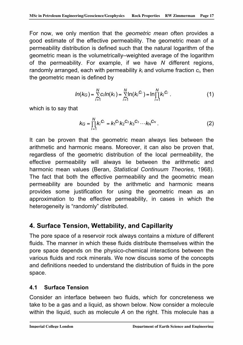
For now, we only mention that the geometric mean often provides a good estimate of the effective permeability. The geometric mean of a permeability distribution is defined such that the natural logarithm of the geometric mean is the volumetrically–weighted average of the logarithm of the permeability. For example, if we have N different regions, randomly arranged, each with permeability ki and volume fraction ci, then the geometric mean is defined by

∏=∑=∑====

N

ii

N

ii

N

iiiG ii ckckklnckln

111ln)ln()()( . (1)

which is to say that

Ni ckckckckckkN

iG i N32 3211

1=∏=

=. (2)

It can be proven that the geometric mean always lies between the arithmetic and harmonic means. Moreover, it can also be proven that, regardless of the geometric distribution of the local permeability, the effective permeability will always lie between the arithmetic and harmonic mean values (Beran, Statistical Continuum Theories, 1968). The fact that both the effective permeability and the geometric mean permeability are bounded by the arithmetic and harmonic means provides some justification for using the geometric mean as an approximation to the effective permeability, in cases in which the heterogeneity is “randomly” distributed.

4. Surface Tension, Wettability, and Capillarity The pore space of a reservoir rock always contains a mixture of different fluids. The manner in which these fluids distribute themselves within the pore space depends on the physico-chemical interactions between the various fluids and rock minerals. We now discuss some of the concepts and definitions needed to understand the distribution of fluids in the pore space.

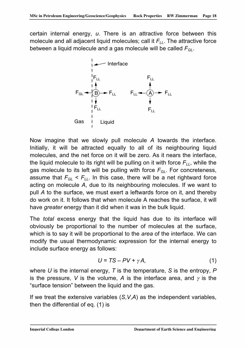
4.1 Surface Tension Consider an interface between two fluids, which for concreteness we take to be a gas and a liquid, as shown below. Now consider a molecule within the liquid, such as molecule A on the right. This molecule has a



certain internal energy, u. There is an attractive force between this molecule and all adjacent liquid molecules; call it FLL. The attractive force between a liquid molecule and a gas molecule will be called FGL.

FLL

FLL

FLL

FLL

FLL

FLL

FLL ABFGL

Gas Liquid

Interface

Now imagine that we slowly pull molecule A towards the interface. Initially, it will be attracted equally to all of its neighbouring liquid molecules, and the net force on it will be zero. As it nears the interface, the liquid molecule to its right will be pulling on it with force FLL, while the gas molecule to its left will be pulling with force FGL. For concreteness, assume that FGL < FLL. In this case, there will be a net rightward force acting on molecule A, due to its neighbouring molecules. If we want to pull A to the surface, we must exert a leftwards force on it, and thereby do work on it. It follows that when molecule A reaches the surface, it will have greater energy than it did when it was in the bulk liquid.

The total excess energy that the liquid has due to its interface will obviously be proportional to the number of molecules at the surface, which is to say it will be proportional to the area of the interface. We can modify the usual thermodynamic expression for the internal energy to include surface energy as follows:

U = TS – PV + γ A, (1)

where U is the internal energy, T is the temperature, S is the entropy, P is the pressure, V is the volume, A is the interface area, and γ is the “surface tension” between the liquid and the gas.

If we treat the extensive variables (S,V,A) as the independent variables, then the differential of eq. (1) is



dU = TdS – PdV + γ dA . (2)

Imagine now that we have a thin film of liquid in a device such as shown below:

F

L

b

Wire frame

Loop

If we pull slowly on the slidable bar with a force F, and move this bar by a distance dL, the work done by the external force on the liquid film will be FdL. By the first law of thermodynamics, the work done must equal the change in internal energy, so

dU = dW = FdL . (3)

If we pull on the bar slowly and adiabatically (i.e., “reversibly”), the entropy change of the liquid film will be zero. Furthermore, the volume of the film is negligible, so PdV will be essentially zero. So, by eq. (2),

dU = γ dA . (4)

But A = bL, and so dA = bdL, and (4) then gives

dU = γ bdL . (5)

Equating expressions (3) and (5) shows that

FdL = γ bdL ⇒ F = γ b . (6)

In other words, the effect of surface tension is the same as if the interface were exerting a force of magnitude γ per unit length of the edge of the interface. Because of this interpretation, it is often convenient to treat an interface like an elastic membrane that exerts a force along its perimeter. Also, note that γ has dimensions of force/length, and so it has SI units of N/m. Typical values for oil/water contact are 0.01-0.05 N/m.



4.2 Capillary Pressure Because of surface tension, the pressures within two fluid phases that are in mechanical equilibrium with each other across a curved interface will not be equal. To prove this, consider a bubble of gas, of radius R, inside a liquid that is contained in a rigid, thermally-insulated container, as shown below. The pressure in the gas is PG, and the pressure in the liquid is PL; the surface tension of the gas-liquid interface is γ.

PG

PL

2R

According to eq. (2), the total differential of the internal energy of this liquid + gas + interface system will be

dU = TdS - PLdVL – PGdVG + γ dA . (7)

Note that we count the “volumetric” term for both the liquid and the gas, but we must count the interface only once.

But VG + VL = Vcontainer = constant, so dVL = – dVG; hence,

dU = TdS + PLdVG – PGdVG + γ dA . (8)

Now assume that the bubble grows slowly. Since the container is rigid and thermally insulated, dS = 0 and dU = 0 (i.e., no heat is added to the system, and no work is done on the system). Hence,

γ dA = PGdVG – PLdVG = (PG – PL)dVG . (9)

But A = 4πR2, and so dA = 8π RdR; and V = 4π R3/3, so dV = 4π R2dR. Eq. (9) can therefore be written as



8π γ RdR = (PG – PL)4πR2dR , (10)

which is equivalent to

(PG – PL) = 2γ /R . (11)

This is the famous Young-Laplace equation, which states that the pressure inside the bubble is greater than the pressure outside, by an amount that is proportional to the surface tension between the two fluids, and inversely proportional to the radius of the bubble.

This pressure difference is known as the capillary pressure, i.e.,

PG – PL = Pcap = 2γ /R . (12)

A capillary pressure difference exists when any two fluids are in contact, not necessarily a liquid and a gas. For example, if we have a bubble of oil surrounded by water, eq. (12) would hold, with the subscripts G and L replaced by o for oil and w for water.

In a rock that is filled with oil and water, the interface between these two phases will be curved, and the pressures in the water and the oil phases will differ by an amount given by eq. (12), where we define R to be the mean radius of curvature of the interface.

Because of the inverse dependence of capillary pressure on radius, capillary pressures are more important in rocks with smaller pores than for rocks having larger pores.

4.3 Contact Angles Let’s consider what happens when two fluids are in contact with a solid surface, as in the figure below, where a drop of liquid is sitting on a solid surface, surrounded by gas:

α

Gas

Liquid

Solid



The slanted line is the tangent to the gas-liquid interface at the point where the interface meets the solid surface. The angle between the solid surface and the tangent, measured by rotating the solid surface towards the tangent, passing through the liquid (by definition the angle is measured through the denser phase), is called the contact angle, α.

Now let’s do a free-body diagram and force-balance on the region where the three phases (solid, liquid, gas) meet; this is exactly like the “method of joints” used in analysing structural trusses. When we “slice” through each interface, the part of the interface that is “removed” will exert a tension γ H on the “joint”, where H is the distance into the page. For each surface tension, we will use subscripts to denote the two fluids that form the interface; i.e., γLS is the surface tension of the liquid-solid interface, etc.

α γLSγGS

γLG

Solid

Gas Liquid

Now let’s do a force-balance in the horizontal direction:

ΣFhorizontal = γLS – γGS + γLG cosα = 0,

=> cosα = (γGS – γLS) / γLG . (13)

Several different cases can arise, depending on the relative magnitudes of the three surface tensions.

Case 1: 0 < γGS – γLS < γLG: In this case, the interfacial energy of a gas-solid interface is greater than that of a liquid-solid interface, so, roughly speaking, the solid will “prefer” to be in contact with the liquid. The right-hand side of eq. (13) will lie between 0 and 1, so α will lie in the range

0 < α < 90o . (14)



In this case, we say that the liquid “wets” the solid surface, and the surface is called “water wet” (although a better name would be “water wettable”, since a “water wet’ surface can be completely dry!).

Case 2: – γLG < γGS – γLS < 0:

In this case, the interfacial energy of a gas-solid interface is less than that of the liquid-solid interface, so the solid will “prefer” to be in contact with the gas. The right-hand side of eq. (13) will lie between –1 and 0, and so α will lie in the range

90o < α < 180o . (14)

In this case, we say that the liquid does not wet the surface; it will sit on the surface in a bubble-shape, with very little interfacial contact between the liquid and the solid surface; see figure below:

S o l i d

G a s

" N o n - w e t t i n g " L i q u i d

" W e t t i n g " L i q u i d

α α

Case 3: |γGS – γLS| > γLG

In this case, the right-hand side of eq. (13) does not lie between -1 and +1, and so there is no value of α that will satisfy equilibrium.

To see what will happen in this case, consider the limiting case in which γGS – γLS = γLG, in which case cosα = 1, and α = 0o. In this case, the liquid will spread out over the surface, creating as much liquid-solid interfacial area as possible (example: oil on water!).

If γGS – γLS > γLG, the same situation will occur, and the liquid will continue to flow until it forms a thin layer on the solid surface. By a similar argument, if γGS – γLS < – γLG, then the gas will spread out to cover as much of the solid surface as possible.

Most reservoir rocks are preferentially “water-wet” as opposed to “oil-wet”. If a water-wet rock is partially saturated with oil and water, the pore walls will “prefer” to be in contact with water rather than with oil, and so the oil will tend to exist in the form of blobs, as in Figure 2.5.



4.4 Capillary Rise Consider a bucket containing some oil and some water, as in figure (a) below. These two fluids are not miscible, and oil is usually less dense than water, so the oil will sit on top of the water. The air on top of the oil is at atmospheric pressure.

Oil

Air

(a)

Water

Oil

(b)

Water

Air A

B

C

D

T

P

θ

(c)

P

z

Now imagine that we put a capillary tube of radius R in the bucket, composed of a water-wet material, as in figure (b). This tube can be thought of as a simple model of a porous rock. The water will rise up in the tube by some height, h, above the original oil-water contact.

We now calculate the capillary rise, h, by performing a vertical force balance on the column of water in the tube, as in figure (c).

The bottom of the column is pushed upwards by the pressure in the water at level C, acting over an area of πR2. With the sign convention that the z-axis decreases with depth, this force is –Pw(zC)πR2.

A the top of the column is a downwards acting force due to the pressure in the oil at level zD; this force is +Po(zD)πR2.

The surface tension exerts an upwards force along the entire wetted perimeter of the tube; its magnitude is T = 2π γowR. But it acts at an angle θ to the vertical, so its vertical component is –2π γowRcosθ.

Finally, gravity acts downwards on the column of water with a force

W = mg = ρwVg = ρwπ R2(zC – zD)g . (15)



Summing all the vertical forces to zero gives

–Pw(zC)πR2 + Po(zD)πR2 – 2πγ Rcosθ + ρwπ R2(zC – zD)g = 0 . (16)

The pressure in the oil at location D is equal to atmospheric pressure plus the pressure due to a column of oil of height (zD – zA), i.e., Po(zD) = Patm + ρog(zD – zA). Similarly, we can see that Pw(zC) = Patm + ρog(zB – zA) + ρwg(zC – zB). Inserting these expressions into eq. (16) gives

–[Patm+ρog(zB – zA)+ρwg(zC – zB)]πR2 + [Patm+ρog(zD – zA)]πR2

–2πγowRcosθ + ρwπ R2(zC – zD)g = 0 , (17)

which can be solved to find the capillary rise, h:

(zB – zD) = h = 2γow cosθ /(ρw – ρo)gR . (18)

So, the height to which water would rise in a tube of radius R is proportional to the surface tension between the water and oil, and is inversely proportional to the radius of the tube.

Now let’s look at the difference in pressures between the oil at depth D (outside the tube), and the water at depth D (inside the tube). By definition, this is the capillary pressure at depth D.

First, recall that Po(zD) = Patm + ρog(zD – zA). Next, by starting at point A, doing down to point B in the oil, and then going back up to point D in the water, we can find that Pw(zD) = Patm + ρog(zB – zA) – ρwg(zB – zD). Hence,

Po(zD) – Pw(zD) = Patm + ρog(zD – zA) – Patm – ρog(zB – zA) + ρwg(zB – zD)

= (ρw – ρo)g(zB – zD) = (ρw – ρo)gh = 2γow cosθ /R. (19)

In other words, Pcap = 2γow cosθ /R. This is identical to the Young-Laplace equation that we derived earlier for an oil bubble in water, modified to account for the contact angle. Note also that the capillary pressure at any height h is equal to (ρw – ρo)gh. The theory we have just described is referred to as “capillary-gravity equilibrium”.



4.5 Oil-Water Transition Zone Most oils are less dense than water, so we might expect that a reservoir would contain only oil down to a certain depth, and only water below that depth, as would occur in a bucket containing oil and water. Although it is true that the rock is usually fully saturated with water below a certain level, on top of this zone is an oil-water transition zone, in which the water saturation decreases gradually with height. We can use the concept of capillary rise in a tube, along with a modified form of the parallel-tube model of a porous medium, to understand the existence of this oil-water transition zone in a reservoir.

Let’s return to our parallel tube model of a porous rock, but now imagine a distribution of different radii. Now let’s place this porous rock into our bucket of oil and water:

Oil

Water

B

A

C

According to eq. (19), water would rise very slightly into a pore that has a large radius, but would rise very high in a small pore. If we have a distribution of pore radii, then at an elevation such as (A) in the figure, all of the pores would be filled with water, and the water saturation would be Sw = 1. At elevation (B) some of the pores will be filled with water, and others with oil, so the water saturation will be 0 < Sw < 1. Finally, at a high enough elevation, such as C, all the pores will be filled with oil, and Sw = 0.

Hence, the water saturation will be a decreasing function of the height h above the “free water level” (FWL), which is defined as the highest point in the reservoir where the capillary pressure is zero; see the figure below.



According to our capillary tube model shown on the previous page, the water saturation will actually be equal to 1 up to some finite height above the free water level that is controlled by the radius of the largest pore. The highest point at which the saturation is equal to 1 is known as the “oil-water contact” (OWC). Note that in a water-wet reservoir, the oil-water contact is above the free water level.

Note from eq. (19) that the “capillary pressure” is given by

Pcap = PG(H) – PL(H) = (ρw – ρo)gh, (20)

and so the y-axis in the figure above essentially represents both the capillary pressure, and the height above the free water level, which differ only by the multiplicative factor (ρw – ρo)g. Hence, this graph represents the water-oil transition zone, but also represents the capillary pressure function as a function of saturation..

Note that the relation Pcap = (ρw – ρo)gh holds regardless of the specific rock geometry, assuming only that the rock is water wet. However, the precise shape of the Pcap(Sw) curve shown above depends on the pore geometry, and specifically on the pore-size distribution.

For the simple bundle-of-parallel-tubes model, one can derive an exact relationship between the Pcap(Sw) curve and the pore-size distribution. For a real rock, the relationship is not so simple, but it is always true that a narrow pore-size distribution corresponds to a Pc curve with a nearly horizontal shape, whereas a broader pore-size distribution yields a curve that increases more gradually, as shown below.



The extreme case of a bundle of tubes in which all pores had the same size would yield a capillary pressure function that was essentially a horizontal line, at the value Pcap = 2γow cosθ /R.

Note that whereas the bundle-of-tubes model predicts that the water saturation becomes zero at some (large) height above the free water level, in a real rock the water saturation never falls below some non-zero value Swi, known as the irreducible water saturation, which is typically about 10%. Hence, there is generally no region in a water–wet reservoir that contains only oil but no water!

4.6 Leverett J-function The capillary pressure function Pcap(Sw) is often discussed in terms of dimensionless form known as the Leverett J-function. We can see how this function arises by starting again with our bundle-of-tubes model.

Recall that for the simplest form of the bundle-of-tubes model, in which every tube has the same radius R, the capillary pressure is given by Pcap = 2γow cosθ /R. In terms of the pore diameter, we can say that Pcap = 4γow cosθ /d. But we also know that this bundle-of-tubes model predicts that k = φ d2/96. So, the pore diameter can be expressed as d = (96k/φ)1/2. If we plug this into our equation for Pcap, we find, after some rearrangement,

61

cos1 =capPk

φθγ . (1)



The left-hand side of eq. (1) is essentially a dimensionless way of writing the capillary pressure function. For the bundle-of-uniform-tubes model, the right-hand side is a constant, but we know that this model is an oversimplification for real rocks. Moreover, we already saw above that capillary pressure in a rock varies with the saturation.

So, we can generalise relation (1) by replacing the constant on the right by some dimensionless function of saturation, which Leverett (Petrol. Trans. AIME, 1941) called the “J-function”. This function will be a property of the rock, and its specific shape depends, in a complicated way, on the details of the pore geometry. We then express the capillary pressure in the form

)cos1

wcap SJPk (=φθγ

. (2)

The logic that underpins the use of the J-function is that, although properties such as k, φ and Pcap may vary throughout a sedimentary unit, it is generally true that the J-function, as defined by eq. (2), is nearly invariant throughout the unit. Hence, if we measure Pcap for one core, and convert it into a J-function, we can then use relation (2) to estimate Pcap for other rocks in same unit.

Another use of J-function is to take capillary pressure curves that are measured in the lab and convert them into capillary pressure curves for the reservoir. Let’s say that we measure Pcap in the lab using two fluids that have certain values of γ and θ, say γlab and θlab. Then, eq. (2) takes the form

€

1γ lab cosθlab

kφ

Pcaplab = J(Sw ) . (3)

In the reservoir, this rock would have the values of same k and φ, but the fluids would be different, so there will be different values of γ and θ, say γres and θres. Hence, in the reservoir we can say that

€

1γres cosθres

kφ

Pcapres = J(Sw ) . (4)

If we equate (3) and (4), we can rearrange and say that

€

Pcapres = Pcap

lab γ res cosθresγ lab cosθlab

⎛

⎝

⎜ ⎜

⎞

⎠

⎟ ⎟ . (5)



This equation shows how capillary pressures measured on a core in the lab can be converted to the values that would occur in the reservoir.

5. Two-Phase Flow and Relative Permeability 5.1 Concept of Relative Permeability In section 3 we defined and discussed the concept of permeability, in the context of a rock that is fully saturated with a single fluid phase. But we learned in section 4 that reservoir rocks always contain at least two fluid phases, oil and water, and sometimes three phases, oil, water and gas. So, the concept of permeability must be extended to apply to situations in which more than one phase is present in the pore space.

The most obvious way to generalise Darcy’s law to account for two-phase flow conditions is to assume that the flow of each phase is governed by Darcy’s law, but with each parameter – pressure, viscosity and permeability itself – being specific to the phase in question, i.e.,

€

qw = −kwµw

dPwdx ,

€

qo = −koµo

dPodx , (1)

where µw is the viscosity of water, kw is the effective permeability of the rock to water, etc. The pressure in the oil and water phases differ from each other by the capillary pressure, which is a function of saturation.

However, it is more common to express the effective permeability of the rock to water as the product of the single-phase permeability, k (also known as the absolute permeability), and another parameter, krw, known as the relative permeability of the rock to water; likewise for oil. Note that the relative permeability function is dimensionless. Eq. (1) can then be written as

€

qw = −kkrwµw

dPwdx ,

€

qo = −kkroµo

dPodx . (2)

The relative permeabilities of each phase are functions of the phase saturations. Obviously, if part of the pore space is occupied by water, then the ability of oil to flow will be hindered, and vice versa. Hence, the relative permeability of a phase will be a monotonically increasing function of the saturation of that phase.



The precise shapes of these curves depend on the process that is occurring. Specifically, they have a different shape during imbibition, which is when a wetting phase displaces a non-wetting phase, than they have during drainage, which is when the non-wetting phase displaces the wetting phase.

Let’s consider imbibition, such as occurs, for example, when we inject water into a water-wet reservoir to displace the oil. This process will start at Sw = Siw, where Siw is the irreducible water saturation, which is the water saturation that remained in the rock after oil had originally migrated into the reservoir. (The saturation Sw = Siw is also precisely the point at which the capillary pressure curve become infinite.) Almost by definition, krw will be zero when Sw = Siw. On the other hand, when Sw = Siw, kro will be finite, but less than 1, as in the figure below.

10

krwkro

Siw Sw1-Sor

1

Now imagine that we inject water into the rock, thereby increasing Sw. Since the relative permeability of a phase is an increasing function of the saturation of that phase, kw will increase, and ko will decrease. This imbibition process will continue until we reach a specific oil saturation, known as the residual oil saturation, So = Sor, at which ko has dropped to zero. The “oil permeability” ko becomes zero at a finite value of the oil saturation, not at zero oil saturation, as one might have thought.

These two values, Siw and Sor, are also known as the relative permeability end-points, and the relative permeability values at these saturations are known as the end-point relative permeabilities.

The precise shapes of the relative permeability curves depend on the details of the pore structure of the rock. Power-law functions are often



found to be useful in fitting these curves. Note that relative permeability curves are never linear functions of the saturation, although this simple linear form is sometimes assumed, particularly in fractured reservoirs, as we rarely have data on the relative permeabilities of the fractures. Finally, note that at any given saturation, the sum kw + ko is not equal to one, but is always less than one.

5.2 Irreducible Saturations The facts that Siw was not equal to zero after primary drainage (when the oil first displaced the water to form the oil reservoir), and Sor is not zero after imbibition (when water is injected to flood out the oil), are of the utmost importance in reservoir engineering. But it is not obvious that these residual saturations will not be zero. And, in contrast to many other rock properties, which can, at least partially, be understood using the parallel-tube model of a porous rock, irreducible/residual saturations cannot be explained by the parallel-tube model. In fact, the parallel tube model would erroneously predict that Siw = Sor = 0. The phenomenon of irreducible/residual saturations is intimately related to the heterogeneity and interconnectedness of the pores in a rock.

We can gain a qualitative understanding of this phenomenon using the simplest pore-space model that incorporates some degree of heterogeneity and interconnectedness. Consider a pore doublet, as shown in figure (a) below, in which one pore branches off into two pores of different diameter, which then re-merge to form a single pore:

water

(a)

oil

water

(b)

oil



water

(c)

oil oil

Imagine that this doublet is initially filled with oil, as in (a). We now slowly inject water from the left. According to the Young-Laplace equation, (4.2.11), the capillary pressure in the each pore is inversely proportional to the pore radius, i.e., it is proportional to R-1.

But according to Poiseuille’s equation, (3.3.1), the “permeability” of a pore is proportional to R2. So, from Darcy’s law, eq. (3.1.3), the mean velocity in either pore is proportional to R-1×R2 = R. Hence, the water moves faster into the larger pore than into the smaller pore, as shown in figure (b).

When the water in the larger pore reaches the end of the doublet, it can enter the smaller pore from the far end, as in figure (c), thereby trapping some of the oil behind it. This is a simple demonstration of why the residual oil saturation, after the imbibition of water, is not equal to zero.

6. Electrical Resistivity The electrical resistivity of a rock is not a property that directly affects oil production, and it does not actually appear in the governing equations of fluid flow in a reservoir. But it is nevertheless very important in reservoir engineering, because it can be measured in situ using logging tools, and its value can then be used to infer the oil saturation. Practical issues related to the measurement of resistivity using logging tools, and the interpretation of these measurements, will be discussed in detail in the module on log analysis. In the present module, we will discuss some of the basic concepts and definitions related to electrical resistivity measurements.

The flow of electrical current is governed by Ohm’s law, which states that the current, I, flowing through any conductor, is equal to the voltage drop, ΔV, divided by the resistance, R:



RVI Δ= . (1)

Electrical charge has units of Coulombs, so current, which is the flow of charge, has units of Coulombs/second. Resistance therefore has units of volt-seconds/Coulomb, which are also known as Ohms. In this form, R will depend on the material properties, but also on the shape and size of the conductor.

Now consider a cylindrically-shaped conductor, of length L and cross-sectional area A, as in the figure below. All other factors being equal, the current will be proportional to A, and inversely proportional to L. So, we expect that the resistance can be expressed as

ALR ρ= , (2)

where ρ is the resistivity, which is an intrinsic property of the material, and does not depend on the geometry of the conductor. The resistivity has units of Ohm-meters.

L A

I

ΔV Hence, eq. (1) can be written as

LVAI Δ=

ρ . (3)

We can also define the conductivity as σ = 1/ρ, in which case we can write (3) as

LVAI Δ=σ . (4)

In this form, it is clear that Ohm’s law is mathematically analogous to Darcy’s law, with current (flow of electrical charge) being analogous to fluid flux, voltage drop analogous to pressure drop, and the electrical conductivity is analogous to the fluid mobility, k/µ.



The electrical conductivities of the minerals that typically form reservoir rocks is very low, as is the conductivity of hydrocarbon fluids. But the water that partially fills the pore space of reservoir rocks always contains salts such as NaCl or KCl, which render the water conductive. The conductivities of these so-called “brines” are typically ten orders of magnitude higher than that of the rock minerals. Hence, electrical current in a reservoir rock will flow mainly through that portion of the pore space that is occupied by water.

As with permeability and capillary pressure, we can get some idea of how the electrical conductivity depends on pore structure by appealing to the bundle of parallel tubes model.

Consider such an idealised rock, as below, where A is the total area of the core, and the An are the areas of the individual pores.

A

A1

A2

A3

Imagine that the pores are all filled with a brine of conductivity σw. If the core has length L into the page, and the rock is subjected to a voltage drop ΔV along its length, then the current through the n-th tube will be

LVAI nwn

Δ=σ . (5)

The total current is the sum of the currents through each tube:

ALVAL

VALV

LVAII wwnwnw pores

N

n

N

n

N

nn φσσσσ Δ=Δ=∑

Δ=∑Δ

=∑==== 111

. (6)

If we compare this with Ohm’s law, eq. (4), we see that the effective conductance of the fluid-saturated rock is φσσ weff = . This quantity depends on the rock and on the brine. But we are not really interested in the brine, so it would be preferable to extract out a parameter that



reflects only the properties of the rock. We do this by defining – in general, independent of any pore geometry model – the formation resistivity factor, also known as the formation factor, as the ratio of the conductance of the brine to the effective conductance of the brine-saturated rock:

€

F ≡σ (brine)

σ (brine −saturatedrock). (7)

The resistivity is the inverse of the conductivity, so we can also say that

(brine)rock)saturated(brine

ρρ −

=F . (8)

For our parallel-tube model, σeff = σwφ, and so F is predicted to be equal to

φσσ 1

rock)saturated(brine(brine)

==−

F . (9)

Note that in contrast to the permeability, which has a strong dependence on pore size, the formation factor has no dependence on pore size, according to the parallel tube model.

If we make the same argument as we did in the case of permeability, i.e., only one-third of the pores are aligned in the direction of the voltage drop, then we would find

€

F =3φ−1. (10)

This parallel-tube model correctly tells us that F will be larger for less porous rocks, but otherwise it is not accurate enough for engineering purposes. Experimental measurements of F tend to show a stronger dependence on porosity than the –1 power that appears in eq. (10). In 1942, Archie (Petrol. Trans. AIME, 1942) proposed generalising eq. (10) by replacing both the factor of 3 and the exponent –1 with parameters that may vary from rock to rock. The result is the famous “Archie’s law”:

mbF −= φ . (11)

The parameter b is often called the tortuosity, and m is called the cementation index, but these names are outdated and not very useful.



Archie’s law in the form of (11) can fit many sets of resistivity data consisting of different rocks from the same reservoir. For sandstones, the exponent m usually lies between 1.5 and 2.5, and is often close to 2; for carbonates, it can be as large as 4. The parameter b is usually close to 1.0.

The figure below shows some data on Vosges and Fontainebleau sandstones, from Ruffet et al. (Geophysics, 1991), fit with b = 0.496, and m = 2.05:

1

10

100

1000

1 10 100

F = 0.496φ-2.05

formation factor, F

porosity, φ (%)

Although Archie’s “law” is extremely useful in reservoir engineering, it should nevertheless be remembered that it is not a fundamental law of rock physics, but is merely a convenient curve-fit that is usually sufficiently accurate for engineering purposes.

It might appear that we could use Archie’s law to estimate porosity, but there are much more accurate ways to estimate φ, as you will learn in the core analysis and log analysis modules. The usefulness of Archie’s law, and of resisitivity measurements in general, is in estimating water saturation. To understand how this is possible, we need to consider rocks that are partially saturated with water, and partially with oil.

For rocks that contain oil and water, we use the following generalisation of Archie’s law, which is sometimes called Archie’s second law:

€

F =bφ−m(Sw )-n, (12)

For

mat

ion

Fact

or, F



where n is called the saturation exponent. In water-wet rocks, n is often close to 2, but in oil-wet rocks it may be as large as 10. If one assumes that n is constant throughout a reservoir, or at least throughout a certain rock unit, then eq. (12) implies that electrical resistivity measurements in a borehole can yield estimates of the water saturation, and hence the oil saturation. This will be discussed in detail in the well logging module.

The scenario described above is more complicated in shaly sands. In these rocks, the sand grains are coated by clay platelets. An ionic electrical double-layer then builds up along the surface of these plates. This surface layer allows another path for current flow, separate from the current flow through the brine-saturated pores that we discussed above. To a good approximation, this surface current can be thought of as being in parallel with the pore-current, and so it adds an extra component to the conductivity of the rock. This extra conductivity depends on the electrochemical properties of the clays, but not on the intrinsic conductivity of the brine. The resulting generalisation of eq. (7) for shaly sands is

( )vBQF

+=− w1rock)saturated(brine σσ , (13)

where Qv is the charge on the double-layer, per unit volume, and B is a constant. Equation (7), called the Waxman-Smits equation, will be discussed further in the core analysis module.

7. Fluid and Pore Compressibility 7.1 Fluid Compressibility Amounts of oil are usually discussed in terms of barrels, which is a measurement of volume. Likewise, gas is often measured in terms of cubic feet. But the amount of volume taken up by a given mass of oil will depend on the pressure to which the oil is subjected. When we say that a well produces 100 barrels of oil a day, for example, we are measuring these barrels at “atmospheric pressure”, which is 14.7 psi, or 101 kPa in SI units.

The relationship between the volume and pressure of a fluid is quantified in terms of the fluid compressibility, Cf, which is defined as the fractional derivative of volume with respect to pressure (at constant temperature, T, and for a fixed amount of mass):



€

Cf = − 1V

∂V∂P⎛

⎝ ⎜

⎞

⎠ ⎟ T

. (1)

Density is the inverse of volume, i.e., ρ = 1/V, so it follows from the chain rule of calculus that the compressibility can also be defined as

€

Cf = 1ρ

∂ρ∂P⎛

⎝ ⎜

⎞

⎠ ⎟ T

. (2)

The dimensions of Cf are 1/pressure, and so the units are 1/psi or 1/Pa. The compressibility of a fluid usually varies with pressure, but typical values of Cf are 0.5×10-9/psi for water, and about 1.0×10-9/psi for oil.

Note: when oil is taken from its pressurised state in the reservoir, up to the surface where it is at atmospheric pressure, any gas that had been dissolved in the oil will be released, and the oil will actually shrink! This phenomenon cannot be described in terms of the compressibility of liquid oil. This shrinkage must be taken into account when doing material balance calculations on a reservoir. However, eqs. (1) and (2) are applicable to the small pressure changes that occur to the oil when it is flowing inside the reservoir.

7.2 Pore Compressibility As oil flows from the reservoir to a well, two changes occur at each location in the reservoir: the pressure in the oil decreases, and the pore space contains less oil. It is important to be able to relate the change in the amount of oil stored in the pore space of the reservoir, to the change in oil pressure. This relation involves the fluid compressibility, but also involves a petrophysical property known as the pore compressibility.

Consider a porous rock as shown below, with total (bulk) volume Vb, pore volume Vp, and mineral grain volume Vm. Imagine that the rock is compressed from the outside by a hydrostatic pressure Pc, called the “confining pressure”. Inside the pore space is a fluid at some “pore pressure”, Pp, which acts over the walls of the pores. The confining pressure tends to compress both the bulk rock and the pores, whereas the pore pressure tends to cause Vb and Vp to increase. (The confining pressure Pc, which acts on the rock, should not be confused with the capillary pressure Pcap, which acts within the fluid).



Pc

Pc

Pc Pp

Recall that for a homogeneous solid or liquid of volume V, subjected to a confining pressure P, the compressibility, C, is defined as

⎟⎟⎠

⎞⎜⎜⎝

⎛∂∂−= PV

VC 1 . (1)

For a porous rock, we need to consider two volumes, the pore volume and the bulk volume, and two pressures, the pore pressure and the confining pressure. So, we can define four different compressibilities (see Zimmerman, Compressibility of Sandstones, 1991):

pPc

bb

bc PV

VC ⎟⎟⎠

⎞⎜⎜⎝

⎛

∂∂−= 1 ,

cPp

bb

bp PV

VC ⎟⎟

⎠

⎞

⎜⎜

⎝

⎛

∂∂−= 1 , (2)

pp Pc

ppc P

VVC ⎟

⎟⎠

⎞⎜⎜⎝

⎛

∂∂

= 1 , c

ppp

Pp

pPV

VC ⎟⎟

⎠

⎞

⎜⎜

⎝

⎛

∂∂

= 1 . (3)

The first subscript refers to the volume in question, either “bulk” or “pore”, and the second subscript refers to the pressure that is varying, either “confining” or “pore”. The pressures written outside the derivative indicates that this pressure is held constant.

The pore compressibility with respect to changes in pore pressure, ppC , is useful in material balance calculations. The numerical sum of the fluid compressibility and the pore compressibility, which is known as the total compressibility,

€

Ct =Cf +Cpp , appears in the pressure diffusivity equation that is used in well-test analysis. The bulk compressibility

€

Cbc influences the velocity of seismic compressional waves. The bulk compressibility

€

Cbp is relevant to subsidence calculations.



The numerical values of the various porous rock compressibilities are controlled, as are all petrophysical properties, by the geometry of the pore space. Roughly speaking, flat, crack-like pores are very compressible, whereas fatter pores in the shape of circular tubes are not very compressible.

The numerical values of the pore compressibility vary from one rock type to another. Furthermore, the pore compressibility often varies strongly with the pore pressure. Roughly, one can say that in a sandstone reservoir, the pore compressibility ppC is on the order of about 2×10-

6/psi, or 3×10-4/MPa. More details and numerical values can be found in Compressibility of Sandstones by Zimmerman (1991), and The Rock Physics Handbook by Mavko, Mukherji and Dvorkin (2009).

References Archie, G.E. 1942. The electrical resistivity log as an aid in determining

some reservoir characteristics. Petrol. Trans. AIME 146: 54–62.

Bear, J. Dynamics of Fluids in Porous Media. New York; American Elsevier, 1972.

Beran, M. Statistical Continuum Theories. London; Interscience, 1968.

de Marsily, G. Quantitative Hydrogeology. San Diego; Academic Press, 1986.

Dullien, F.A.L. Porous Media: Fluid Transport and Pore Structure, 2nd ed. San Diego; Academic Press, 1992.

Leverett, M.C. 1941. Capillary behaviour in porous solids. Petrol. Trans. AIME 142: 159–172.

Mavko, G., Mukerji, T., Dvorkin, J. The Rock Physics Handbook, 2nd ed. Cambridge; Cambridge University Press, 2009.

Ruffet, C., Gueguen, Y., and Darot, M. 1991. Complex Conductivity Measurements and Fractal Nature of Porosity. Geophysics 56(6): 758-768.

Scheidegger, A.E. The Physics of Flow through Porous Media. Toronto; University of Toronto Press, 1974.

Zimmerman, R.W. Compressibility of Sandstones. Amsterdam; Elsevier, 1991.



Rock Properties Questions

1. Consider a reservoir that is shaped like a circular disk, 10 m thick, and with a 5 km radius in the horizontal plane. The mean porosity of the reservoir is 15%, the water saturation is 0.3, and the oil saturation is 0.7.

(a) Ignoring the expansion of the oil that would occur when it is produced from the reservoir, how many barrels of oil are in this reservoir? One barrel = 0.1589 m3.

(b) If the density of the oil is 900 kg/m3, how much oil (in kg) is contained in the reservoir?

2. In a laboratory experiment, a pressure drop of 100 kPa is imposed along a core that has length of 10 cm, and a radius of 2 cm. The permeability of the core is 200 mD, its porosity is 15%, and the viscosity of water is 0.001 Pa s.

(a) What will be the volumetric flowrate Q of the water, in m3/s?

(b) What is the numerical value of q = Q/A, in m/s?

3. Imagine that the rock in problem 2 can be represented by the parallel tube model.

(a) Estimate the mean pore diameter, d, using eq. (3.3.4).

(b) What is the mean velocity, v, of the water particles in the rock?

(c) The importance of the inertia term, relative to the pressure term in, say, eq. (3.11), can be quantified by the Reynolds number, defined as Re = ρvd/µ. What is the Reynolds number in this experiment? Note that Darcy’s law is only accurate when Re < 1 (Bear, 1972).

4. Consider a layered reservoir consisting of alternating layers, 1 m thick, of rock 1, rock 2 and rock 3, where k1 = 1000 mD, k2 = 100 mD, and k3 = 10 mD.

(a) What is the effective permeability of this rock, if fluid is flowing parallel to the layering?



(b) What is the effective permeability of this rock, if fluid is flowing perpendicular to the layering?

(c) Imagine that the reservoir consists of these three rock types, in equal volumetric proportions, but occurring in a “random” spatial distribution. Estimate the effective permeability in this case.

5. Consider a small blob of oil surrounded by water. The surface tension between the oil and water is 0.02 Nm. If the radius of the blob is 0.05 mm, what is the value of the capillary pressure? Is the pressure higher in the oil or the water?

6. Consider again the parallel tube model of a rock. Assume that the diameter of each pore is 20 µm, γ = 0.02 Nm, ρo = 900 kg/m3, ρw = 1000 kg/m3, the contact angle θ is 45o, and g = 9.8 m/s2. If this rock is placed in a tank containing water overlain by oil, as in the figure in the notes, to what height will the water rise in the pores?

7. Consider a homogeneous reservoir with φ = 0.20, k = 200 mD, water-oil surface tension of γ = 0.03 N/m, and oil/water contact angle of 35o. The oil density is 850 kg/m3, and the water density is 1050 kg/m3. In the lab, we determine that the irreducible water saturation occurs when the J-function is equal to 4.23. What will be the height of the oil-water transition zone in the reservoir? Hint: use eq. (2) on p. 29 to convert J(Swi) to Pc, and use eq. (20) on p. 27 to convert Pc to height.

1. Introduction to Rock Properties - Imperial College London

Documents

Transcript of 1. Introduction to Rock Properties - Imperial College London