1 Global analysis of RNA-binding protein dynamics by ...

1

Global analysis of RNA-binding protein dynamics by comparative and 1

enhanced RNA interactome capture 2

Joel I. Perez-Perri1*, Marko Noerenberg2*, Wael Kamel2, Caroline E. Lenz2 3

Shabaz Mohammed2, Matthias W. Hentze1,3,5 and Alfredo Castello2,4,5 4

5

1 European Molecular Biology Laboratory (EMBL), Meyerhofstrasse 1, 69117, 6

Heidelberg, Germany 7

2 Department of Biochemistry, University of Oxford, OX1 3QU Oxford, UK 8

3 Molecular Medicine Partnership Unit (MMPU), Im Neuenheimer Feld 350, 9

69120, Heidelberg, Germany. 10

4 MRC-University of Glasgow Centre for Virus Research, University of 11

Glasgow, 464 Bearsden Road, Glasgow G61 1QH, Scotland (UK). 12

5 correspondence: [email protected] and [email protected] 13

* These authors contributed equally. 14

EDITORIAL SUMMARY This protocol extension describes an improved method 15

for global profiling of poly(A) RNA-binding proteins (RBPs) and quantitative 16

analysis of RBP dynamics in response to biological and pharmacological cues 17

using UV crosslinking, capture with LNA-modified oligo-dT probes, and 18

proteomics. 19

20

TWEET Protocol extension describing an improved procedure for quantitative 21

assessment of RNA-binding protein (RBP) dynamics in response to biological 22

and pharmacological cues. @Castello_lab; @HentzeTeam; @Alf_Castello; 23

#RNA; #RNA-binding_proteins; #interactomics. 24

25

2

COVER TEASER Enhanced RNA-interactome capture 1

2

Related links 3

Key reference(s) using this protocol 4

Perez-Perri, J. et al. Nat Commun 9, 4408 (2018): 5

https://doi.org/10.1038/s41467-018-06557-8 6

Garcia-Moreno, M. et al. Mol Cell 74, 196-211.e11 (2019): 7

https://doi.org/10.1016/j.molcel.2019.01.017 8

Sysoev, V. et al. Nat Commun 7, 12128 (2016): 9

https://doi.org/10.1038/ncomms12128 10

Castello, A. et al. Cell 149, 1393-406 (2012): 11

https://doi.org/10.1016/j.cell.2012.04.031 12

Key data used in this protocol 13

Garcia-Moreno, M. et al. Mol Cell 74, 196-211.e11 (2019): 14

https://doi.org/10.1016/j.molcel.2019.01.017 15

This protocol is an extension to: Nat. Protoc. 16

https://doi.org/10.1038/nprot.2013.020 17

18

ABSTRACT 19

Interactions between RNA-binding proteins (RBPs) and RNAs are critical for 20

cell biology. However, methods to comprehensively and quantitatively assess 21

these interactions within cells were lacking. RNA interactome capture (RIC) 22

employs in vivo UV-crosslinking, oligo(dT) capture and proteomics to identify 23

RNA-binding proteomes. Recent advances have empowered RIC to quantify 24

RBP responses to biological cues such as metabolic imbalance or virus 25

3

infection. Enhanced (e)RIC exploits the stronger binding of locked nucleic 1

acid (LNA)-containing oligo(dT) probes to poly(A) tails to maximize RNA 2

capture selectivity and efficiency, profoundly improving signal-to-noise ratios. 3

The subsequent analytical use of SILAC and TMT proteomic approaches, 4

together with high-sensitivity sample preparation and tailored statistical data 5

analysis, significantly improves RIC’s quantitative accuracy and 6

reproducibility. This optimized approach is an extension of the original RIC 7

protocol. It takes three days plus two weeks for proteomics and data analysis, 8

and will enable the study of RBP dynamics under different physiological and 9

pathological conditions. 10

11

INTRODUCTION 12

Development of the protocol 13

RIC employs irradiation of cultured cells with UV light to trigger crosslinks 14

between protein and RNA interacting at ‘zero distance’. This is followed by 15

cell lysis under denaturing conditions, specific isolation of polyadenylated 16

(poly(A)) RNA and its covalently linked proteins using oligo(dT) magnetic 17

beads and stringent washes and proteomic analysis1-3 (Fig.1). While effective 18

to identify RBPs in multiple cell types1,2,4-7 and organisms8-13, RIC is not 19

readily applicable to comparative analyses aiming to assess the responses of 20

RBPs to physiological and pathological cues. In particular, the original 21

protocol requires a substantial amount of starting material and lacks a 22

specialized proteomics approach and tailored data analysis3. In the last 23

years, several key improvements have empowered RIC to perform 24

comparative analysis efficiently14,15. One of these key advances is the use of 25

4

an oligo (dT) probe that contains locked nucleic acids (LNAs)14. LNAs are 1

nucleic acid analogues that bear a methylene bridge between the 2’-O and 4’-2

C atoms of the ribose ring. This modification “locks” oligonucleotides in the 3

optimal conformation for base pairing with complementary strands, leading to 4

a profound increase in the thermal stability of the nucleic acid duplex. By 5

adding LNAs to the probe, it is possible to increase the stringency of the 6

capture and washes, which profoundly depletes the sample of abundant non-7

poly(A) nucleic acids, such as rRNAs, as well as potential DNA 8

contamination14,16. We describe here this improved variant of RIC that we 9

refer to as enhanced RNA interactome capture (eRIC). 10

To increase the quantitative power or RIC, we have successfully applied two 11

different proteomic strategies that have already shown their efficacy in proof-12

of-principle experiments14,15. The first approach exploits the capacity of stable 13

isotope labelling with amino acids in cell culture (SILAC) to reduce technical 14

noise by combining the samples after cell lysis (Fig.2). By mixing the lysates 15

before the oligo(dT) capture, the isolation of poly(A) RNA and the 16

downstream sample preparation for mass spectrometry becomes equally 17

efficient for all the samples15. This, together with the high quantitative power 18

of SILAC17, allows the discovery of even subtle changes in RBP activity15. 19

SILAC allows to parallelize the analysis of up to three samples 20

simultaneously, reducing mass spectrometry run time and improving cross-21

comparison accuracy when compared to label-free applications. While SILAC 22

has been used in a broad range of cell lines and model systems, it cannot be 23

easily applied to multicellular organisms or to cell types that do not tolerate 24

SILAC reagents or that can only be cultured for a limited time. In such 25

5

scenarios, it is recommended to employ post-elution peptide labelling 1

techniques, such as isobaric labeling with tandem mass tag (TMT) (Fig.2). 2

TMT labelling has been successfully used in RIC experiments applied to 3

cultured cells and fruit fly embryos10,14, and can virtually be extended to any 4

biological system. Isobaric labelling reagents allow higher level multiplexing 5

with TMT enabling the analysis of up to sixteen samples in one mass 6

spectrometry run. However, the RIC protocol is performed separately for each 7

sample (Fig.2), potentially increasing technical noise. It is also recommended 8

to perform sample fractionation and increase mass spectrometry analysis 9

time to offset the reduction of protein identification rate and maximize 10

proteome coverage. 11

The original RIC protocol3 required a substantial amount of starting material, 12

which is not feasible to obtain in many biological models. To reduce the 13

amount of input material, we have combined eRIC with a recently-developed 14

sample preparation approach, called ‘Single-pot solid-phase-enhanced 15

sample preparation’ (SP3), that minimizes peptide loss18,19. As a reference, 16

the eRIC workflow combined with SP3 reduces the amount of starting 17

material by ~10 fold, broadening its applicability. 18

Moreover, the computational workflow used in the past was conceived to 19

compare a UV-irradiated sample versus a non-irradiated control. This 20

comparison yields relatively high fold changes, because the control is largely 21

devoid of proteins. By contrast, the amplitude of the changes in comparisons 22

of two UV-crosslinked samples that have been subjected to different 23

treatments (e.g. uninfected versus infected cells) is expected to be lower, 24

requiring high replicability to gain statistical power. We have implemented an 25

6

analytical workflow that compiles the ratios between conditions, applies batch 1

effect correction, and uses moderated statistical analysis adjusted for false 2

discovery rate. In addition, our approach employs a complementary 3

semiquantitative analysis to allow the study of proteins with ‘zero intensity’ 4

values in one or more conditions. These results are problematic, as ‘zero’ 5

values generate ‘zero’ or ‘infinite’ ratios that cannot be, in principle, analyzed 6

statistically10,14,15. This complementary semiquantitative analysis is important 7

because it allows to study RBPs that switch from a dormant to an active RNA-8

binding state (off/on) and vice versa (on/off) . The importance of RBPs with 9

these extreme behaviors is illustrated by IFI16 and IFIT5, whose RNA-binding 10

activities are triggered upon Sindbis virus infection and are indeed critical 11

antiviral host factors15. 12

13

Applications and target audience 14

Here, we describe a modified RIC protocol that is specifically designed to 15

study RBP dynamics on a proteome-wide scale. Comparative RIC studies 16

have recently been applied to profile RBP dynamics during embryo 17

development10, virus infection15 and acute inhibition of alpha-ketoglutarate 18

dependent dioxygenases14, revealing key regulators of these processes. 19

Comparative RIC analyses have broad applications to understand how RBPs 20

regulate RNA metabolism in response to developmental, physiological or 21

environmental cues, including cell division, differentiation, reprogramming or 22

stress. Given the importance of RBPs in disease20-23, this method can also be 23

used to elucidate pathological mechanisms associated with e.g. infection, 24

malignant transformation or metabolic disorders, as well as the modes of 25

7

action of small molecules. Importantly, recent work has shown that RNA can 1

regulate protein function in response to biological cues, a phenomenon that is 2

referred to here as ‘riboregulation’24-27. Comparative RIC analyses have great 3

potential to identify examples of ‘riboregulation’26 in a proteome-wide manner. 4

Given that the roles of cellular RNA and RBPs have been greatly expanded24-5

26,28-30, we foresee an extensive use of comparative RIC analysis not only by 6

RNA biologists, but also by experts in other disciplines such as cell signaling, 7

molecular medicine, development, immunology and virology. 8

9

Advantages of (e)RIC and comparison to other methods 10

eRIC approach described here shares the same advantages with its 11

predecessor3, while adding specific features to efficiently study RBPome 12

dynamics: (1) The improved workflow substantially reduces the required starting 13

material, making it applicable to a broader range of biological systems; (2) UV 14

light promotes RNA-to-protein crosslinks at ‘zero’ distances and does not 15

induce detectable protein-protein crosslinks with the UV irradiation regime 16

described here2,3,31,32; (3) UV irradiation is applied to living cells, thus providing 17

information on native protein-RNA interactions and their dynamics; (4) The use 18

of an oligo(dT) probe enriches for mRNAs and polyadenylated non-coding 19

RNAs, reducing abundant non-polyadenylated RNAs, (e.g. rRNA and snRNA) 20

and their associated proteins2,14. By depleting these dominant (e.g. ribosome-21

associated) proteins, RIC allows the detection of medium and low abundant 22

RBPs bound to poly(A) RNA. The use of LNAs in the oligo(dT) probe strongly 23

enhances selectivity14,16,33. (5) DNA is virtually undetectable in eluates of eRIC, 24

even for cell types and experimental settings (e.g. nuclear fractionation) where 25

8

DNA contamination was found to be problematic. (6) Incorporation of proteomic 1

labelling strategies reduces the technical noise, improves quantification 2

accuracy and reproducibility, while reducing mass spectrometry time. (7) We 3

used a customized data analysis pipeline that allows the identification of subtle 4

differences in RNA binding as well as a complementary semiquantitative 5

approach to deal with ‘zero’ values and investigate ‘on/off’ and ‘off/on’ RBP 6

states14,15. (8) Importantly, RIC has successfully been applied to many 7

organisms and cell lines1,2,4-13,25,34-36, thus offering solid foundations for 8

adaptation to virtually every eukaryotic system. 9

The original RIC protocol and its enhanced variant (i.e. eRIC) are based on the 10

hybridization of an oligo(dT) probe with poly(A) tails and, thus, can only identify 11

proteins interacting with poly(A) RNA. Recently, other RBP identification 12

methods that also capture non-polyadenylated RNAs have been described37-43. 13

Two approaches employed labelling of nascent RNA transcripts in cells with 5-14

ethynyluridine (5-EU) and were referred to as RNA Interactome using Click 15

Chemistry (RICK)37 and Click Chemistry-Assisted RNA Interactome Capture 16

(CARIC)38. After UV-mediated crosslinking, cells are lysed, EU residues 17

biotinylated via click chemistry and RNA-proteins conjugates purified with 18

streptavidin-coated beads. While successful at identifying RBPs, these methods 19

present some limitations such as the need of nucleotide incorporation, which is 20

not readily applicable to all samples (e.g. organisms), can introduce biases 21

towards highly transcribed genes and can be toxic44. 22

2C39 and TRAPP40 build on the realization that silica-based matrixes do not only 23

bind free RNA but also RNA with proteins covalently linked to it. After UV 24

crosslinking, cells are lysed under strong denaturing conditions and RBPs 25

9

purified using silica columns or beads. Although simple and potent, these 1

approaches demand special considerations to avoid contamination with DNA-2

interacting proteins, as silica matrices can bind both RNA and DNA40. Of note, 3

eRIC was shown to almost completely prevent genomic (g)DNA contamination 4

even in challenging systems exhibiting large gDNA/poly(A) RNA ratios, such as 5

small cells (e.g. T lymphocytes)14 and isolated nuclei33. 6

Global purification of RBPs was also achieved based on the physicochemical 7

properties of covalent RNA-protein conjugates41-43. Acid guanidinium 8

thiocyanate-phenol-chloroform extraction (“Trizol”) involves the generation of 9

two phases, with RNA and proteins specifically locating to the aqueous and 10

organic phase, respectively. XRNAX41 and OOPS42 purify RBPs with Trizol, 11

exploiting the property of UV-crosslinked RNA-protein conjugates to migrate to 12

the aqueous-organic interphase. PTex43 is based on the same rationale, but in 13

this case a neutral phenol-toluol extraction is used to remove DNA and 14

membrane contaminants, followed by an acid-phenol extraction. 15

The main advantage of all the methods based on total RNA purification is that 16

they can be used to study RBPs that interact with non-poly(A) RNA (see below). 17

However, as more than 90% of cellular RNA is composed of rRNA and tRNA, 18

these methods are expected to be biased towards these highly abundant RNA 19

biotypes. mRNA represents only a small fraction of total cellular RNA (~3%) and 20

enrichment of poly(A) RNA with RIC/eRIC have been shown to be instrumental 21

for a comprehensive characterization of poly(A) RNA-bound proteomes. Indeed, 22

RBPomes generated with methods based on total RNA purification lack a 23

significant fraction of RBPs identified by RIC/eRIC in identical systems37,38,40-43. 24

10

These non-overlapping RBPs may interact exclusively or dominantly with 1

poly(A) RNA. 2

3

Limitations of the approach 4

This protocol will not be suitable to study dynamics of RBPs that (i) shift in RNA 5

preference but not in overall RNA binding; (ii) are not expressed or active in the 6

experimental settings tested; (iii) bind exclusively non-polyadenylated RNA (e.g. 7

prokaryotic RNA); (iv) exhibit a protein-RNA interface that is suboptimal for UV 8

crosslinking (e.g. interaction only with the phosphate-ribose backbone); and (v) 9

do not yield mass spectrometry compatible peptides. (vi) The efficacy of this 10

protocol will also be compromised if the input material is extremely limited (we 11

typically aim for 5-10 x107 cells) or if UV cannot penetrate the sample efficiently 12

(e.g. thick tissue samples). 13

As described above, RIC/eRIC are biased towards poly(A) RNA and cannot be 14

used to study non-polyadenylated RNAs. Therefore, XRNAX41, OOPS42, 15

PTex43, 2C39 and TRAPP40 are especially useful when focusing on other (or all) 16

classes of cellular RNAs including rRNA, snoRNA, snRNA and pre-mRNA. 17

Indeed, these methods will be the best option to study bacterial systems where 18

RNA (including mRNA) is not polyadenylated. In eukaryotic systems poly(A) 19

RNA is a small fraction of the total RNA and, hence, the amount of starting 20

material required to perform RIC/eRIC is substantially higher than that for total 21

RNA purification approaches. Therefore, if the starting material is extremely 22

limited, total RNA based methods will have higher chances to succeed at 23

identifying RBPs. However, it is important to consider the substantial 24

contribution of non-poly(A) RNA to the proteomic data. In summary, selection of 25

11

the approach will depend on the specific aim of the project. RIC/eRIC will be the 1

method of choice to study mRNA regulatory processes, while total RNA-based 2

methods will be more appropriate when studying non-poly(A) RNA. Also, the 3

availability of input material will be an important factor to decide between 4

RIC/eRIC and total RNA-based methods. In any case, we consider that both 5

approaches are complementary and can be used in conjunction to generate a 6

complete picture of the cellular RBPome. 7

Experimental design 8

Controls 9

To identify contaminant proteins that may be present in the sample in a UV-10

independent manner, we recommend including a control sample in which UV 11

irradiation was omitted. If the availability of labels for the proteomic analysis is 12

limited, a separate experiment including this control can be performed (as in 3) 13

prior to the comparative analyses. If samples under study are very similar, a 14

single non-irradiated control of a representative condition can be used. 15

However, when comparing more profoundly different samples (e.g. different cell 16

types, differentiation, long treatments, etc.), we strongly recommend 17

parallelizing one non-irradiated control to each UV-irradiated sample/condition 18

under study. To minimize the incidence of false positives, we typically classify 19

as RBP any protein that is enriched in the UV irradiated over the non-irradiated 20

control with 1% false discovery rate (FDR). For the comparative analysis, the 21

‘treated samples’ should be compared to a reference ‘untreated’ or ‘control’ 22

condition. For example, cells infected with a virus would be compared to an 23

uninfected control15. 24

12

Total proteomic analysis of the cell lysates used as inputs for the eRIC 1

experiment is a very informative addition. The protein intensity ratio between 2

eluates and inputs represents the proportion of protein that crosslinks to RNA 3

upon UV irradiation (crosslinked/total)15,36 (Fig. 3a-c). The eluate/input ratio will 4

be influenced by the amino acid and nucleotide composition, geometry, avidity 5

and duration of the protein-RNA interaction, as these parameters control the 6

ability of a protein to crosslink to RNA25. For example, heterogenous 7

ribonucleoproteins (hnRNPs) establish interactions with RNA that involve 8

multiple high-affinity RNA-binding domains (RBDs). Such long-lived, optimal 9

protein-RNA interactions will give rise to high eluate/input ratios15. Conversely, 10

moderate to low eluate/input ratios are expected for RBPs establishing 11

transitory interactions with RNA (e.g. endonucleases) or when only a 12

subpopulation of the protein engages in RNA binding (e.g. moonlighting 13

RBPs24,25,45). Moreover, we advise that proteins with low eluate/input ratios, 14

which typically appear as outliers in the bottom-left corner of scatter plot (Fig. 15

3c), should be taken carefully as they may be contaminants or incidental RNA 16

interactors. If interested in a protein falling into this category, we recommend 17

validation with orthogonal methods. The eluate/input ratios have recently been 18

used to model the RNA-binding activities present in large ribonucleoprotein 19

complexes such as the exosome or the ribosome36. Other important 20

applications of the eluate/input ratios are described in the anticipated results 21

section. 22

23

Selection of the proteomic approach 24

13

We have successfully applied two quantitative proteomic approaches to 1

perform comparative RIC analyses: SILAC and TMT. Use of metabolic 2

labeling (SILAC) aids precision and accuracy but possess limited 3

multiplexing. Isobaric labeling such as TMT resolves the multiplexing issue 4

but at the cost of accuracy. There are reviews describing the strength and 5

weaknesses of these approaches46,47. SILAC involves the metabolic 6

incorporation of heavy, medium or light isotopic amino acids into proteins in 7

cultured cells (Fig. 2). For this, cells are grown in media with dialyzed fetal 8

calf serum containing either isotopic variant of (typically) lysine and arginine. 9

When using this approach, isotope incorporation rate must be measured in a 10

pilot experiment. For efficient SILAC-based proteomics, near-complete 11

incorporation rates are required, as lower incorporation rates will compromise 12

the quantification accuracy. For example, if the isotope is incorporated only in 13

95% of the proteins it would cause on/off changes (i.e. present in condition A 14

and absent in condition B) to be observed as a fold change of 19 (95 divided 15

by 5). As proteins are labelled in cellulo, samples can be mixed immediately 16

after UV crosslinking and cell lysis, and the RNA capture is performed with 17

the combined samples. This reduces technical noise and enhances reliability 18

and accuracy of the protein quantifications. However, the application of 19

SILAC is mostly limited to cultured cells, and specifically to cell types that can 20

be maintained in dialyzed serum. Cells are typically cultured for 5-6 21

population doublings in SILAC medium to reach high labelling efficiencies 22

(>99%), and thus SILAC is not compatible, in principle, with cells that can 23

only be cultured for a limited time (e.g. certain primary cells). 24

14

Isobaric reagents such as TMT employ chemical labelling of peptides, and 1

are thus applied after protein elution, concentration and digestion (Fig. 2). 2

Post-elution peptide labelling is compatible with virtually any biological 3

system. The availability of numerous labels allows multiplexing of presently 4

up to sixteen samples in a single run, in contrast to the three labels available 5

for SILAC. The high multiplexing capability simplifies the execution of 6

experiments with larger sample sets, such as those involving multiple 7

treatment conditions or time points. Nevertheless, as peptide labeling is 8

performed further downstream in the protocol, it does not benefit from the 9

early pooling of samples to reduce technical noise and this can compromise 10

the detection of subtle differences. Moreover, quantification is performed at 11

the ms2 or ms3 level, and thus state-of-the-art mass spectrometers are 12

required for efficient and fast quantification. Quantification and identification 13

with isobaric labelling are performed on the same peptide spectrum thus 14

requiring the mass spectrometry method to strike a balance between 15

identification efficiency and quantification quality. However, the higher 16

‘multiplexing’ of TMT reduces mass spectrometry time per sample, allowing 17

the implementation of fractionation to address the identification and 18

quantification loss. Separation of the sample into 3-5 fractions by, for 19

example, high-pH reverse phase StageTip48 or other methods, is thus highly 20

recommended. 21

Both SILAC and TMT can, in principle, be extended to more conditions than 22

labels available by running a complete experiment in multiple mass 23

spectrometry runs and splitting the conditions between runs. In this case, it is 24

15

a requisite to run a ‘reference’ sample (e.g. untreated cells) as a standard in 1

each run, so that ratios between conditions can be robustly generated. 2

In conclusion, we recommend using SILAC when possible, due to its higher 3

robustness, especially when comparing up to three conditions. TMT or similar 4

isobaric tagging strategies will be the approach of choice when using SILAC-5

incompatible cells, tissues or organisms. It will also be the optimal choice 6

when assessing a large set of conditions. Fractionation is highly 7

recommended when performing TMT experiments. 8

Although SILAC and TMT provide the highest quantification accuracy and 9

multiplexing capacity, RIC/eRIC can be combined with virtually any 10

quantitative proteomic approach. For example, a recent study has applied 11

label-free quantitation successfully to Saccharomyces pombe36. 12

13

DNA vs LNA probes 14

We and others have shown that the use of conventional oligo (dT) DNA 15

capture probes in RIC experiments can lead to contamination with non-16

poly(A) RNAs such as rRNA. Indeed, depending on the cell type employed 17

and the experimental settings, rRNA can represent from 10% to 30% of the 18

eluted RNA 1,2,14. Proteins that copurify with these abundant non-19

polyadenylated RNAs (e.g. ribosomal proteins) generate dominant tryptic 20

peptides that mask those from less abundant RBPs. Co-purification of gDNA 21

can also be problematic as it could lead to contamination with DNA-binding 22

proteins or proteins nonspecifically tangled on the chromatin fibers. This can 23

critically impact the quality of RIC experiments when working with nuclear 24

fractions or cells with a low cytoplasm/nucleoplasm ratio such as T 25

16

lymphocytes. Both contamination with non-polyadenylated RNAs and gDNA 1

can be strongly reduced when using a 20-mer oligo(dT) probe containing 2

locked nucleic acids (LNAs) at every other position (LNA2.T)14. LNAs 3

increase the rigidity of the probe promoting an optimal conformation for 4

hybridization with complementary RNA. The original RIC protocol employs 5

very stringent purification conditions, focused on removing non-covalently 6

linked proteins from the RNA. The increased hybridization strength that the 7

inclusion of LNAs in the oligo(dT) probe provides, allows to additionally 8

maximize the selectivity of the protocol towards poly(A) RNAs. For example, 9

in eRIC the capture of poly(A) RNA and subsequent washes are performed at 10

37 °C instead of 4 °C. Moreover, it includes a ‘pre-elution’ (final wash) step in 11

water to remove partial hybrids and loosely bound RNAs and DNA14,16 (Fig. 12

1). The low ionic strength during this pre-elution step destabilizes nucleic acid 13

duplexes, particularly partial hybrids, resulting in efficient removal of rRNA 14

and gDNA (Fig. 4). 15

Here, we describe how to perform comparative RIC studies with the LNA2.T 16

beads (i.e. eRIC), due to the remarkable advantages that this probe adds to 17

the protocol. However, the original DNA oligo(dT) beads have also been 18

successfully used in comparative RIC experiments10,15,36. If using the original 19

DNA probe, apply the experimental design and protocol described here but 20

employ 4 °C during the hybridization step and washes and omit the pre-21

elution step. Elution can be performed by heating (at 55°C for 3 min) or 22

RNase release as indicated below. 23

24

Starting material 25

17

Incorporation of SP3 together with modifications in the protocol and 1

improvements on mass spectrometry instrumentation have allowed to 2

considerably reduce the starting material required to generate a deep RBPome. 3

For example, we have achieved deep RBPomes from ~50-90 million HeLa and 4

HEK293 cells or ~100-150 million Jurkat cells. For orientation, an optimal eRIC 5

experiment should lead to ~15-30 μg of eluted poly(A) RNA per sample to 6

ensure successful downstream proteomic applications. We have noticed that in 7

some cell lines, such as T lymphocytic cells, nuclear RBPs are substantially 8

more abundant than their cytoplasmic counterparts. In such cases, peptide 9

fractionation prior to mass spectrometry greatly improves the identification and 10

quantification of the cytoplasmic RBPs, increasing the dynamic range of the 11

experiment. 12

RIC and case-specific variations of it have successfully been applied to several 13

unicellular5,8,9,12,34,36 and multicellular organisms8,10,11,35 and it is applicable to 14

tissues13. Starting material and other parameters such as UV light dose must be 15

adapted to the system under study. An excellent starting point is to use the 16

conditions described in the original publications5,8-13,34-36, and to further optimize 17

the protocol with small-scale pilot experiments, if required. 18

19

Successive rounds of capture 20

To maximize poly(A) RNA capture, we perform two sequential rounds of 21

oligo(dT) capture of the same lysate, using 300 μL of oligo(dT) magnetic beads 22

per round. While two rounds of oligo(dT) capture suffice, in most cases, to 23

capture most poly(A) RNAs from cell extracts, a third round could be required in 24

some instances. To evaluate if the poly(A) RNA depletion has been sufficient, 25

18

RNA present in each elution round should be measured with e.g. a NanoDrop, 1

separately. Near complete depletion of poly(A) RNA in the lysate leads to a 2

strong reduction in the RNA isolated in the following round of oligo(dT) capture 3

due to the lack of suitable substrate to hybridize with the probe. For example, a 4

third round of oligo(dT) capture typically leads to only 15-10% of the RNA 5

isolated in the first round. In such case, we only recommend performing 2 6

rounds of capture as the contribution of a third to the proteomic results will be 7

residual. 8

The efficiency of the oligo(dT) capture can be estimated more accurately using 9

RT-qPCR analysis using primers against selected poly(A) RNAs (e.g. ACTB or 10

GAPDH) in cell lysates before and after the oligo(dT) capture. An efficient eRIC 11

experiment will reduce the levels of a given poly(A) RNA by at least 80%. 12

Conversely, rRNAs are not expected to be depleted. 13

14

eRIC optimization 15

When applying eRIC for the first time to a given cell line, tissue or organism, we 16

recommend performing small-scale experiments (Fig. 1 and Fig. 4). RNA in 17

inputs and eluates can be quality controlled using bioanalyzer and RT-qPCR to 18

assess the proportion of poly(A) RNA versus rRNA. A strong enrichment of 19

poly(A) RNA (e.g. ACTB mRNA) over rRNA (e.g. 18S rRNA) is expected in 20

eluates when compared to inputs (Fig. 4a; see ‘anticipated results’). In parallel, 21

RBP isolation can be tested by silver staining (Fig. 4b) or western blotting using 22

antibodies against well-established RBPs and negative controls (e.g. PTBP1 23

and ACTB, respectively)3. RIC’s ability to efficiently isolate RBPs and poly(A) 24

RNA is typically dictated by few key steps that benefit from optimization. These 25

19

include the i) amount of starting material, ii) the UV crosslinking approach, iii) 1

the cell lysis procedure, and the iv) homogenization of the cell lysate. Optimal 2

starting material is thus fundamental to achieve efficient eRIC experiments. 3

Lack of proteins in eluates despite good quality RNA can often be solved by 4

increasing the number of cells. Still, some cell types (e.g. primary T cells, 5

primary macrophages), give inherently low number of proteins even from large 6

amounts of captured RNA. Conversely, high incidence of contaminant proteins 7

can be caused by excessive protein, RNA and DNA concentration in lysates. 8

We have already estimated the optimal number of cells for HeLa, HEK293 and 9

Jurkat (as indicated in ‘Starting material’ above). However, cell numbers may 10

need adjustment when working with other cell types. Correct estimation of the 11

starting material becomes more challenging when dealing with multicellular 12

organisms and tissues. In those cases, the starting material will strongly depend 13

on the ability to crosslink protein-RNA interactions with UV light (see below). 14

Improving UV crosslinking efficiency will effectively reduce the input material 15

required; however, excessive UV irradiation can lead to protein and RNA 16

damage. 17

UV crosslinking can be achieved either exploiting the natural excitability of 18

nucleotide bases at 254 nm (conventional crosslinking; CL)49 or employing 19

nucleotide analogues such as 4-thiouridine (4SU) or 4-thiouracil (4TU) that 20

promote efficient crosslinking between 312 and 365 nm UV light 21

(photoactivatable ribonucleoside-enhanced crosslinking; PAR-CL)50. While CL 22

suffices for most cell lines and is readily applicable to tissues and multicellular 23

organisms, PAR-CL has shown higher performance in budding and fission 24

20

yeast5,36. Hence, the choice of the crosslinking approach will depend on the 1

model system. 2

Moreover, UV crosslinking efficiency may differ depending on the properties of 3

the sample. When using cell monolayers, 150 mJ/cm2 of 254 nm UV is a good 4

balance between crosslinking efficiency and lack of RNA damage. However, the 5

optimal dose might vary slightly from cell line to cell line. Conversely, tissues 6

and multicellular organisms may require substantially higher UV irradiation 7

regimens. For example, the optimal UV dose for Drosophila embryos is 4 J/cm2 8

10. 9

Cell lysates are viscous and one of the key optimization steps is to find the 10

optimal proportion between lysis buffer, biological material and beads. For 11

example, we found that 10 mL of lysis buffer and 300 µL of beads are optimal 12

for selective RBP capture for ~50-90 million HeLa cells or 100-150 million 13

Jurkat cells. Cell lysates are homogenized using a 5 mL syringe and a narrow 14

needle until a water-like solution is achieved. This step is critical as it promotes 15

the disruption of cellular membranes and the breakage of cellular DNA, 16

reducing lysate viscosity and avoiding the generation of precipitates. If despite 17

of an efficient homogenization, precipitates are observed, increase the lysis 18

buffer volume, homogenize as indicate above and pre-clear the lysate by 19

centrifugation prior to the oligo(dT) capture. See TROUBLESHOOTING. 20

21

HPLC and mass spectrometry parameters 22

For a successful comparative eRIC experiment it is critical to have a suitable 23

proteomic workflow in place. Sample preparation can be performed with any 24

classical technique, including filter-aided sample preparation (FASP)51 or TCA 25

21

precipitation52. However, to increase sensitivity while reducing the starting 1

material, we employ SP318,19,53. This approach allows efficient removal of 2

detergents and other mass spec-incompatible chemicals, while ensuring 3

efficient protein trypsinization and peptide recovery. 4

In some experimental settings (see ‘selection of the proteomic approach’), 5

peptide fractionation is required to improve protein coverage. In those cases, 6

we apply high pH reversed-phase peptide fractionation54 or similar 7

approaches55,56 prior to LC/MS analysis. The number of fractions can vary in a 8

case-specific manner, but five fractions normally suffice to provide an excellent 9

depth. Peptides are analyzed on a liquid chromatography–tandem mass 10

spectrometry (LC-MS/MS) platform. We used an Ultimate 3000 ultra-HPLC 11

system (ThermoFisher Scientific) coupled to an Orbitrap Elite, QExactive or 12

QExactive plus mass spectrometer (Thermo Fisher Scientific)14,15. However, it is 13

possible to use other equipment with similar characteristics and performance. 14

During LC/MS analysis, each fraction is further separated on low pH gradient of 15

solvent B, the composition of gradient and duration of the separation depend on 16

the complexity of the sample and it should be adjusted for maximum protein 17

identification. Specific mass-spectrometric parameters (such as dynamic 18

exclusion, collision energy, etc) are dependent on the instrument. The current 19

protocol does not require any specific adjustments and can be adapted to 20

virtually any platform optimized for routine protein identification. We recommend 21

monitoring the LC-MS performance between samples and/or fractions by 22

running a blank sample spiked with 20 fmol digested BSA on a 15 min gradient 23

after each sample and/or fraction. BSA digests have characteristic standard 24

chromatographic peaks, which can be used as a proxy to assess the 25

22

performance of the nanoflow HPLC. Moreover, it will help to clean carryover 1

contaminants between samples. 2

3

Statistical data analysis 4

For robust statistical analysis, it is recommended to generate at least three 5

biologically independent replicates of the complete experimental set, which will 6

include the reference condition (e.g. uninfected cells), treatments (e.g. virus 7

infected cells) and, depending on the experimental design, a negative control 8

(e.g. non-irradiated cells). For more details see ‘controls’. Experimental 9

conditions causing subtle variations in the RBPome or with high intrinsic inter-10

sample variability (e.g. clinical samples), may require higher number of 11

replicates. Peptides are identified and clustered into protein groups and 12

quantified using standard software such as MaxQuant57. Ion counts across 13

samples are summarized and protein intensity ratios between conditions are 14

generated. Significance of the changes is tested using moderated t-test 15

corrected for multiple testing with a Benjamini-Hochberg correction. Software 16

implementation (e.g. Perseus) and customized R packages (Proteus) are 17

available15,32,57,58. In some instances, data normalization and/or batch 18

corrections are required. Analysis of comparative RIC/eRIC experiments are 19

done in two sequential steps. We first compare protein intensities in UV-20

irradiated and non-irradiated controls and define as RBPs those proteins that 21

are enriched in irradiated over non-irradiated samples with 1% FDR. Secondly, 22

responsive RBPs are identified by comparing the protein intensities of each 23

RBP in crosslinked samples subjected to the different experimental conditions. 24

To define the RBP responses it is critical to avoid normalization against non-25

23

irradiated samples, as signal in these controls is low and noisy and provokes 1

artificial distortions of the data when used as normalizer. We typically classify as 2

‘high-confidence’ or ‘candidate’ dynamic RBP any protein that passes the 1% 3

and 10% FDR cut-offs, respectively. 4

Unfortunately, it is not trivial to analyze RBPs with missing ion counts in one 5

experimental condition due to the impossibility to generate a ratio. There are 6

two alternatives to deal which such cases and ‘rescue’ genuine RBPs (if 7

comparing irradiated vs non-irradiated samples) or responsive RBPs (if 8

comparing two experimental conditions). The first employs a semi-quantitative 9

analysis that takes into consideration the incidence of signal in one condition 10

and lack of signal in the other10,15. Alternatively, it is possible to impute missing 11

values using different computational approaches59. The minimum determination 12

method (Mindet)59 is one of the most commonly used strategies, in which the 13

missing values are replaced by the lowest value detected either globally in the 14

entire dataset or within each sample. Either option has strengths and 15

weaknesses: while the semi-quantitative method does not require the 16

imputation of artificial values, it does not provide ratios to estimate the 17

amplitude of the effect, which may hinder downstream interpretation. 18

Conversely, data imputation provides ratios and thus these RBPs can be 19

included in the statistical analysis. However, imputation methods can introduce 20

artefacts that may affect the statistical analysis. In any case, we recommend 21

applying either strategy. 22

23

Complementary analyses 24

24

Cellular stimuli often trigger changes at multiple levels, including transcriptomic 1

and proteomic changes. In order to identify the driving factors of the RBP 2

responses we recommend combining comparative RIC analyses with both total 3

proteome and transcriptome analyses. These analyses will provide a snapshot 4

of the protein and RNA landscapes in the experimental conditions, which can 5

be used to interpret the RIC/eRIC results. In other words, the parallel analysis of 6

both protein and RNA abundance is instrumental to determine if any (or both) of 7

these factors contribute to the comparative RIC results10,15. These 8

complementary analyses will be discussed in greater extent in ‘anticipated 9

results’. 10

11

MATERIAL 12

Reagents 13

Biological materials 14

15

• HeLa cells (ATCC, cat. no. CCL-2; 16

https://scicrunch.org/resolver/CVCL_0030) 17

• Jurkat cells (DSMZ, cat. no. ACC-282, 18

https://scicrunch.org/resolver/CVCL_0065). 19

CAUTION: The cell lines used should be regularly checked to ensure 20

they are authentic and are not infected with mycoplasma. 21

Cell culture reagents 22

• DMEM (Thermo Fisher Scientific, cat. no. 11995065) 23

• DMEM for SILAC (Thermo Scientific, cat. no. 88364) 24

• RPMI 1640 (Thermo Fisher Scientific, cat. no. 21875034) 25

25

• RPMI-1640 for SILAC (SILANTES, cat. no. 283001300) 1

• Fetal bovine serum (FBS; Thermo Fisher Scientific, cat. no. 10500064) 2

• Glutamine (Gibco, cat. no. G7513) 3

• Penicillin/streptomycin (Sigma-Aldrich, cat. no. P4333) 4

• Dialysed fetal bovine serum (SILANTES, cat. no. 281000900) 5

• Unlabeled L-Arginine HCl (SILANTES, 201004102). C6H14N4O2 •HCl 6

• 13C-, 15N-labelled L-Arginine HCl (SILANTES, cat. no. 201604102). 7

13C6H1415N4O2 •HCl 8

• 13C-labelled L-Arginine HCl (SILANTES, cat. no. 201204102). 9

13C6H14N4O2 •HCl 10

• Unlabeled L-Lysine HCl (SILANTES, cat. no. 211004102). 11

C6H14N2O2 •HCl 12

• 13C-, 15N-labelled L-Lysine HCl (SILANTES, cat. no. 211604102): 13

13C6H1415N2O2 •HCl 14

• 2H-labelled D4 L-Lysine 2HCl (SILANTES, cat. no. 211104113). 15

C6D4H10N2O2 •2HCl. D, deuterium 16

• Sterile filter 0.22 µm pore size (Millipore cat no: SCGVU05RE) 17

• 18

19

eRIC reagents 20

• Potassium chloride (KCl) (Merck, cat. no. 1.04936.1000) 21

• Potassium dihydrogen phosphate (KH2PO4) (Merck, cat. no. 22

1.04873.1000) 23

26

• di-Sodium hydrogen phosphate (Na2HPO4) (Merck, cat. no. 1

1.06586.0500) 2

• Sodium chloride (NaCl) (Merck, cat. no. 1.06404.1000) 3

• Calcium chloride (CaCl2) (Merck, cat. no. 1.02382.1000) 4

• RNase T1 (Sigma-Aldrich, cat. no. R1003) 5

• RNase A (Sigma-Aldrich, cat. no. R5503) 6

• Complete Protease Inhibitor Cocktail (Roche, cat. no. 11873580001) 7

• Trizma base (Sigma-Aldrich, cat. no. T1503) 8

• Lithium dodecyl sulfate (LiDS) (Carl Roth, cat. no. CN25.3) 9

CAUTION: Harmful if swallowed or inhaled. Can cause serious eye 10

damage. Wear suitable protective equipment, especially when handling 11

as powder. 12

• Lithium chloride (LiCl) (Sigma-Aldrich, cat. no. 62476) 13

• Ethylenediaminetetraacetic acid (EDTA) Disodium Salt, Dihydrate 14

(Merck, cat. no. 324503) 15

• Dithiothreitol (DTT) (Biomol, cat. no. 04020.100) 16

• IGEPAL® CA-630 (Nonidet P-40 (NP-40) replacement) (Sigma-Aldrich, 17

cat. no. I3021) 18

• Sodium dodecyl sulfate (SDS) (Serva, cat. no. 20765) 19

CAUTION: Harmful if swallowed or inhaled. Can cause serious eye 20

damage. Wear suitable protective equipment, especially when handling 21

as powder. 22

• Triton X-100 (Sigma-Aldrich, cat. no. T8787) 23

• Sodium deoxycholate (Sigma-Aldrich, cat. no. D6750) 24

27

CAUTION: Harmful if swallowed. Causes skin irritation and serious eye 1

irritation. May cause respiratory irritation. Wear dust mask type N95 2

(US), protective goggles and gloves. 3

• Pierce™ 660nm Protein assay kit (Thermo Scientific, cat. no. 22662) 4

• Ionic Detergent Compatibility Reagent (Thermo Scientific, cat. no. 22663) 5

6

Reagents for generation of LNA probes 7

• LNA2.T capture probe: 8

/5AmMC6/+TT+TT+TT+TT+TT+TT+TT+TT+TT+TT (+T: LNA thymidine, 9

T: DNA thymidine) (HPLC purified; Exiqon-Qiagen). The probe bears a 10

primary amine at the 5’ end followed by a flexible C6 linker and 20 11

thymidine nucleotides in which every other nucleotide is an LNA. The 12

required scale of synthesis will depend on the number of samples and 13

capture rounds. A detailed description on this subject is provided in 14

section ´Coupling of the LNA2.T probe to beads´. 15

• Carboxylated magnetic beads M-PVA C11, 50 mg/mL (Perkin Elmer, cat. 16

no. CMG-203) 17

• 2-(N-morpholino)ethanesulfonic acid (MES) (Carl Roth, cat. no. 4256.5) 18

• N-(3-dimethylaminopropyl)-N′-ethylcarbodiimide hydrochloride (EDC-19

HCl) (Sigma-Aldrich, cat. no. E7750). CRITICAL Store EDC powder at -20

20 °C, when required handle it on ice. It is highly hygroscopic, so check 21

that powder is dry before using it. 22

CAUTION: Toxic on contact with skin. Causes serious eye irritation. 23

Wear protective gloves and eye protection. Very toxic for aquatic 24

environments. Follow suitable disposure procedures 25

28

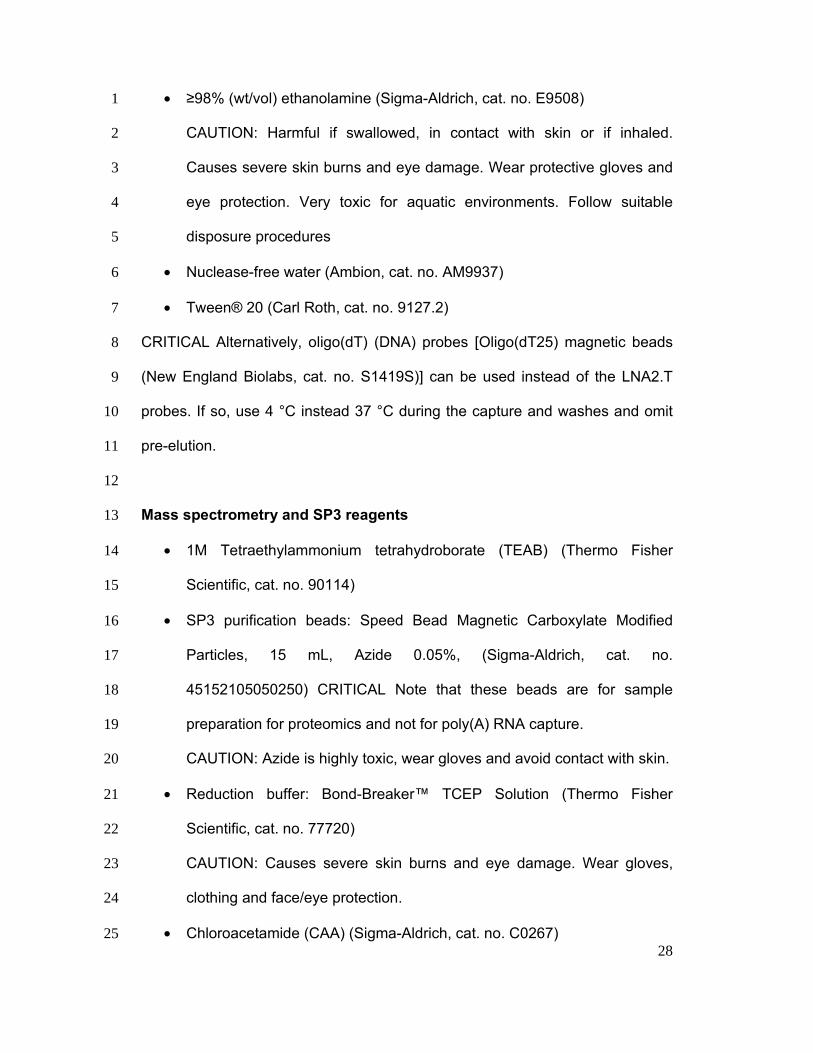
• ≥98% (wt/vol) ethanolamine (Sigma-Aldrich, cat. no. E9508) 1

CAUTION: Harmful if swallowed, in contact with skin or if inhaled. 2

Causes severe skin burns and eye damage. Wear protective gloves and 3

eye protection. Very toxic for aquatic environments. Follow suitable 4

disposure procedures 5

• Nuclease-free water (Ambion, cat. no. AM9937) 6

• Tween® 20 (Carl Roth, cat. no. 9127.2) 7

CRITICAL Alternatively, oligo(dT) (DNA) probes [Oligo(dT25) magnetic beads 8

(New England Biolabs, cat. no. S1419S)] can be used instead of the LNA2.T 9

probes. If so, use 4 °C instead 37 °C during the capture and washes and omit 10

pre-elution. 11

12

Mass spectrometry and SP3 reagents 13

• 1M Tetraethylammonium tetrahydroborate (TEAB) (Thermo Fisher 14

Scientific, cat. no. 90114) 15

• SP3 purification beads: Speed Bead Magnetic Carboxylate Modified 16

Particles, 15 mL, Azide 0.05%, (Sigma-Aldrich, cat. no. 17

45152105050250) CRITICAL Note that these beads are for sample 18

preparation for proteomics and not for poly(A) RNA capture. 19

CAUTION: Azide is highly toxic, wear gloves and avoid contact with skin. 20

• Reduction buffer: Bond-Breaker™ TCEP Solution (Thermo Fisher 21

Scientific, cat. no. 77720) 22

CAUTION: Causes severe skin burns and eye damage. Wear gloves, 23

clothing and face/eye protection. 24

• Chloroacetamide (CAA) (Sigma-Aldrich, cat. no. C0267) 25

29

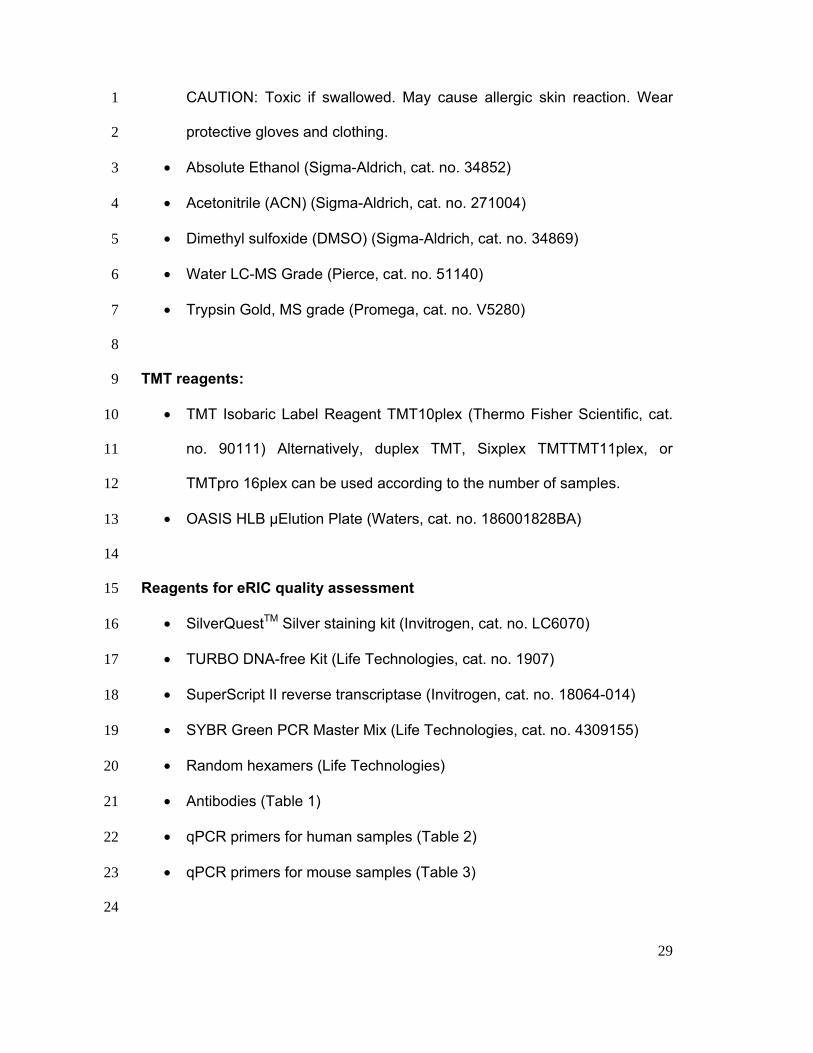
CAUTION: Toxic if swallowed. May cause allergic skin reaction. Wear 1

protective gloves and clothing. 2

• Absolute Ethanol (Sigma-Aldrich, cat. no. 34852) 3

• Acetonitrile (ACN) (Sigma-Aldrich, cat. no. 271004) 4

• Dimethyl sulfoxide (DMSO) (Sigma-Aldrich, cat. no. 34869) 5

• Water LC-MS Grade (Pierce, cat. no. 51140) 6

• Trypsin Gold, MS grade (Promega, cat. no. V5280) 7

8

TMT reagents: 9

• TMT Isobaric Label Reagent TMT10plex (Thermo Fisher Scientific, cat. 10

no. 90111) Alternatively, duplex TMT, Sixplex TMTTMT11plex, or 11

TMTpro 16plex can be used according to the number of samples. 12

• OASIS HLB µElution Plate (Waters, cat. no. 186001828BA) 13

14

Reagents for eRIC quality assessment 15

• SilverQuestTM Silver staining kit (Invitrogen, cat. no. LC6070) 16

• TURBO DNA-free Kit (Life Technologies, cat. no. 1907) 17

• SuperScript II reverse transcriptase (Invitrogen, cat. no. 18064-014) 18

• SYBR Green PCR Master Mix (Life Technologies, cat. no. 4309155) 19

• Random hexamers (Life Technologies) 20

• Antibodies (Table 1) 21

• qPCR primers for human samples (Table 2) 22

• qPCR primers for mouse samples (Table 3) 23

24

30

Antigen Company, catalogue RRID Dilution

β-Actin Sigma-Aldrich, A1978 AB_476692 1:5000

Histone H4 Abcam, ab10158 AB_296888 1:4000

Polypyrimidine tract

binding protein (PTBP1)

Sigma-Aldrich,

WH0005725M1

AB_1843067 1:5000

Cold shock domain-

containing protein E1

(CSDE1)/UNR

Proteintech, 13319–1-

AP

AB_2084902 1:5000

Non-POU domain-

containing octamer-

binding protein (NonO)

Novus Biologicals,

NBP1–95977

AB_11056638 1:1000

ELAV-like protein 1

(ELAVL1)/Hu-antigen R

(HuR)

Proteintech, 11910–1-

AP

AB_11182183 1:5000

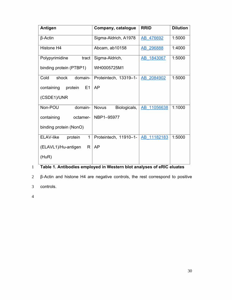
Table 1. Antibodies employed in Western blot analyses of eRIC eluates 1

β-Actin and histone H4 are negative controls, the rest correspond to positive 2

controls. 3

4

31

1

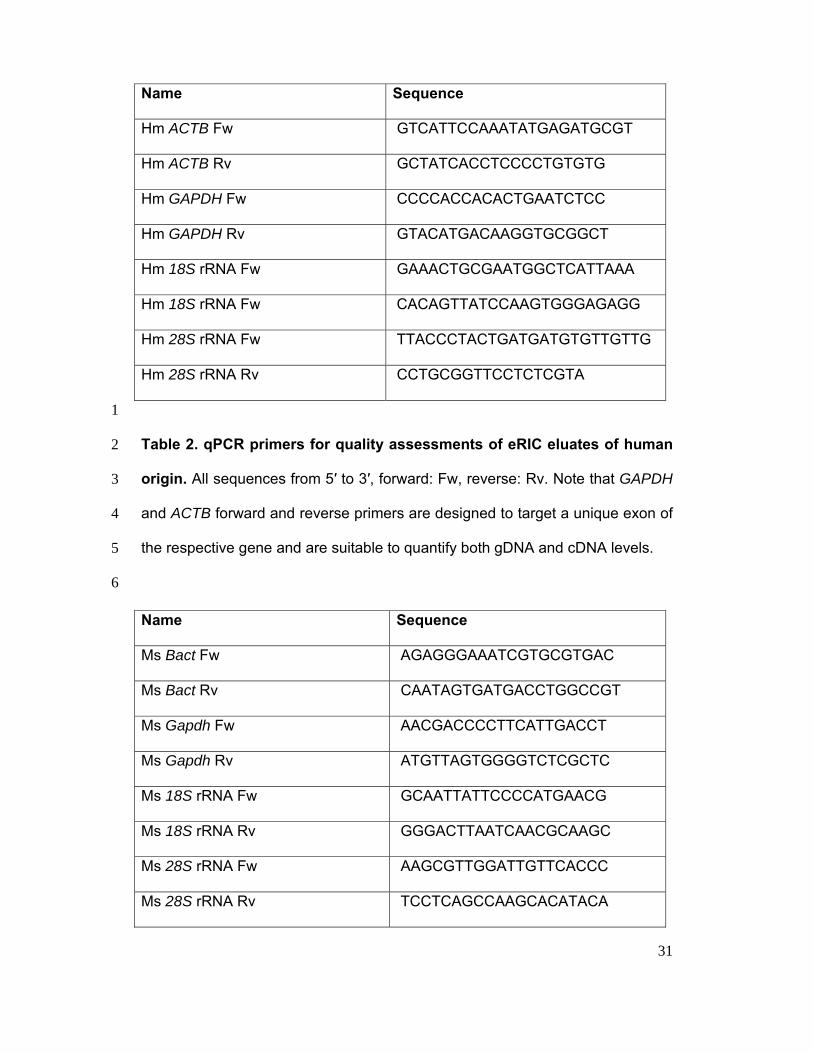
Table 2. qPCR primers for quality assessments of eRIC eluates of human 2

origin. All sequences from 5′ to 3′, forward: Fw, reverse: Rv. Note that GAPDH 3

and ACTB forward and reverse primers are designed to target a unique exon of 4

the respective gene and are suitable to quantify both gDNA and cDNA levels. 5

6

Name Sequence

Hm ACTB Fw GTCATTCCAAATATGAGATGCGT

Hm ACTB Rv GCTATCACCTCCCCTGTGTG

Hm GAPDH Fw CCCCACCACACTGAATCTCC

Hm GAPDH Rv GTACATGACAAGGTGCGGCT

Hm 18S rRNA Fw GAAACTGCGAATGGCTCATTAAA

Hm 18S rRNA Fw CACAGTTATCCAAGTGGGAGAGG

Hm 28S rRNA Fw TTACCCTACTGATGATGTGTTGTTG

Hm 28S rRNA Rv CCTGCGGTTCCTCTCGTA

Name Sequence

Ms Bact Fw AGAGGGAAATCGTGCGTGAC

Ms Bact Rv CAATAGTGATGACCTGGCCGT

Ms Gapdh Fw AACGACCCCTTCATTGACCT

Ms Gapdh Rv ATGTTAGTGGGGTCTCGCTC

Ms 18S rRNA Fw GCAATTATTCCCCATGAACG

Ms 18S rRNA Rv GGGACTTAATCAACGCAAGC

Ms 28S rRNA Fw AAGCGTTGGATTGTTCACCC

Ms 28S rRNA Rv TCCTCAGCCAAGCACATACA

32

1

Table 3. qPCR primers for quality assessments of eRIC eluates of mouse 2

origin. All sequences from 5′ to 3′, forward: Fw, reverse: Rv. Note that GAPDH 3

and ACTB forward and reverse primers are designed to target a unique exon of 4

the respective gene and are suitable to quantify both gDNA and cDNA levels. 5

6

Equipment 7

• Class II biosafety cabinet (generic) 8

• Humidified 37 °C, 5% CO2 incubator (generic) 9

• Spectrolinker XL-1500 UV cross-linkers (Spectroline) (254 nm bulbs, 10

BLE-1T155) 11

• Rotator (e.g. Grant-bio, PTR-35) 12

• Conventional incubator without humidification or CO2 control at 37 °C 13

used for the oligo(dT) capture (Aqualytic, Thermostat Cabinet or similar) 14

• SpeedVac concentrator (Thermo Fisher Scientific) 15

• Refrigerated benchtop centrifuge (e.g. Eppendorf, 5415R) 16

• Thermal block (e.g. Eppendorf, cat. no. 5382000015) 17

• 500 cm2 dishes (Greiner-BioOne, cat. no. 639160) – for adherent cells 18

• 175 cm2 flasks (Falcon, cat. no. 353028) – for suspension cells 19

• 150 mm uncoated petri dishes (Greiner Bio-One, 639102) – for 20

suspension cells 21

• Generic metal plate to accommodate 2 x 150 mm petri dishes into the 22

UV crosslinker - for suspension cells 23

33

• 500 mL Steritop Quick Release-GP funnel (Millipore, cat. no. 1

S2GPT05RE) 2

• Needle 22G × 1 1/4-inch; Nr. 12, 0.7 mm × 30 mm (BD Microlance, cat. 3

no. 300900) or alternatively Sterican blunt Needle 21G, 0.8 x 22 mm 4

(VWR, cat. no. 720-2562). 5

CAUTION: handle needles with precaution to avoid harm. We 6

recommend using blunt variants. Dispose the needles in the appropriate 7

sharp bin. 8

• Sterican blunt Needle 27G, 0.4 x 25mm (VWR, cat. no. 720-2563) 9

CAUTION: handle needles with precaution to avoid harm. We 10

recommend using blunt variants. Dispose the needles in the appropriate 11

sharp bin. 12

• Syringes (5 mL; Luer-lock; Medicina, cat. no. IVL05) 13

• DNA LoBind tubes (Eppendorf, 1.5 mL: cat. no. 022431021; 5.0 mL: cat. 14

no. 0030108310; 15 mL: cat. no. 0030122208; 50 mL: cat. no. 15

0030122232) 16

• Magnetic separation rack, 50 mL (NEB, cat. no. S1507S). For analytical 17

experiments, 12-tube (2 mL) Magnetic separation rack (NEB, cat. no. 18

S1509S) or DynaMag-2 (Invitrogen, cat. no. 123.21D) 19

• NanoDrop spectrophotometer (Thermo Fischer Scientific) 20

• Bioanalyzer with RNA 6000 Pico Kit (Agilent Technologies, cat. no. 5067-21

1513 and G2939BA) 22

• Real-time PCR system (e.g. Bio-Rad, CFX96 Touch Real time system, or 23

similar) 24

34

• Tandem mass spectrometer (e.g. Thermo Scientific Orbitrap Fusion, Q-1

Exactive, Bruker Impact II or similar) 2

3

Software for proteomic data analysis 4

• Protein identification by database searching: Mascot (MatrixScience, 5

http://www.matrixscience.com/distiller_download.html), Sequest (Thermo 6

Fisher Scientific, http://www.selectscience.net/products/sequest-7

cluster/?prodID=10319#tab-2) or Andromeda60 (via MaxQuant 57). 8

• Protein quantification: MaxQuant (https://maxquant.org/)57. 9

• R software (http://www.r-project.org/) 10

• Bioconductor software (http://www.bioconductor.org/), in particular, 11

limma 12

(https://bioconductor.org/packages/release/bioc/html/limma.html)61. 13

14

Reagent setup 15

Cell culture and SILAC reagents 16

• Cell culture media: HeLa cells and Jurkat cells are maintained in DMEM 17

or RPMI-1640, respectively. These media are supplemented with 10% 18

(vol/vol) fetal bovine serum (FBS), glutamine, penicillin/streptomycin, and 19

cells are maintained in a humidified incubator at 37 °C and 5% CO2. 20

• Cell culture media for SILAC: For SILAC, combine medium without 21

arginine and lysine (DMEM for HeLa or RPMI-1640 for Jurkat), with 10% 22

(vol/vol) dialyzed FBS. Prepare one bottle for each SILAC labelling 23

condition by adding either unlabeled arginine and lysine (light medium), 24

13C L-Arginine HCl and 2HD4 L-Lysine 2HCl (medium labeled medium) or 25

35

13C15N L-Arginine HCl and 13C15N L-Lysine HCl (heavy labeled medium). 1

Use 84 mg/L arginine and 146 mg/L lysine for DMEM and 200 mg/L 2

arginine and 40 mg/L lysine for RMPI-1640. Filter the media with a 0.2 3

µm Sterilefilter and store at 4 °C for up to 3 months. 4

eRIC reagents 5

• Phosphate-buffered saline (PBS): combine 0.2 g/L KCl, 0.2 g/L KH2PO4, 6

1.15 g/L Na2HPO4 and 8 g/L NaCl. Prepare, autoclave and store at room 7

temperature for up to 1 year. 8

• 1 M DTT stock: prepare 5 mL aliquots in distilled (d)H2O and store at 9

−20 °C for up to 1 year. 10

• 1 M Tris-HCl (pH 7.5): dissolve 121 g Trizma base in 800 mL dH2O. 11

Adjust pH to 7.5 with concentrated HCl. Bring volume to 1 L, autoclave 12

and store at room temperature for up to 1 year. 13

• 0.5 M EDTA (pH 8.0): dissolve 186.1 g of EDTA disodium salt dihydrate 14

in 700 mL dH2O. Adjust pH to 8.0 with 10 N NaOH. Bring volume to 1 L, 15

autoclave and store at room temperature for up to 1 year. 16

• 10% wt/vol LiDS: dissolve 30 g of LiDS in dH2O to a final volume of 300 17

mL, sterilize by filtration and store at room temperature for up to 1 year. 18

• Lysis buffer: 20 mM Tris-HCl (pH 7.5), 500 mM LiCl, 1 mM EDTA, 5 mM 19

DTT and 0.5% (wt/vol) LiDS. Prepare 1 L without DTT, sterilize by 20

filtration and store at room temperature for up to 1 year. Add DTT and 21

Complete protease inhibitor cocktail immediately before usage. 22

• Buffer 1: 20 mM Tris-HCl (pH 7.5), 500 mM LiCl, 1 mM EDTA, 5 mM DTT 23

and 0.1% (wt/vol) LiDS. Prepare 1 L without DTT, sterilize by filtration 24

36

and store at room temperature for up to 1 year. Add DTT and Complete 1

protease inhibitor cocktail immediately before usage. 2


and 0.02% (vol/vol) NP40. Prepare 1 L without DTT, sterilize by filtration 4




and 0.02% (vol/vol) NP40. Prepare 1 L without DTT, sterilize by filtration 8



• 10x RNase buffer: 100 mM Tris-HCl (pH 7.5), 1.5 mM NaCl and 0.5% 11

(vol/vol) NP-40. Store up to 1 year at 4 °C. 12

• RNase A solution. Prepare 10 mg/mL stock in Tris-HCl (pH 8.0) and 50% 13

(vol/vol) glycerol, aliquot and store at -20 °C. 14

• Heat elution buffer: 20 mM Tris-HCl (pH 7.5) and 1 mM EDTA. Autoclave 15

and store at room temperature for up to 1 year. 16

• RIPA buffer: 50 mM Tris-HCl (pH 7.5), 150 mM NaCl, 0.1% (wt/vol) SDS, 17

0.5% (wt/vol) sodium deoxycholate, 1% (vol/vol) Triton X-100. 18

19

Coupling reagents 20

• 50 mM 2-(N-morpholino)ethanesulfonic acid (MES) buffer pH 6. Prepare, 21

filter and store at room temperature for several months protected from 22

light by covering the bottle with aluminum foil. 23

37

• 20 mg/mL N-(3-dimethylaminopropyl)-N′-ethylcarbodiimide hydrochloride 1

(EDC-HCl) in MES buffer. Prepare immediately before use. 2

• 200 mM ethanolamine pH 8.5. Add 2.493 mL of 98% (wt/vol) 3

ethanolamine to ~150 mL of dH2O. Adjust pH with 10 N NaOH and bring 4

to 200 mL with H2O. Store at room temperature for several months. 5

• 1 M NaCl. Store at room temperature indefinitely. 6

• 0.1% (vol/vol) PBS-Tween. Store at room temperature for several 7

months. 8

9

Coupling of the LNA2.T probe to beads, Timing 8 h 10

Commercial DNA oligo(dT) probes used in the original protocol are already 11

coupled to magnetic beads (New England Biolabs, S1419S). Conversely, the 12

LNA-containing probe, LNA2.T, must be coupled to magnetic beads with free 13

carboxylic groups on their surface. Below, we describe the process for coupling 14

the probe to the beads. 15

1. Calculate the required amounts of LNA2.T probe and of carboxylated 16

beads. We employ 30 nmol of probe (300 µL of a 100 µM solution) 17

coupled to 15 mg of beads (300 μL of the original 50 mg/mL bead 18

suspension) for one round of capture per sample. Note that LNA2.T 19

coupled beads can be reused, at least, up to five times without 20

noticeable loss in performance. We recommend producing enough 21

LNA2.T coupled beads to perform all the biological replicates with the 22

same batch. The following steps show the volumes required to produce 23

LNA2.T-coupled beads for one round of capture in one sample. To 24

obtain final volumes, multiply the indicated volumes of LNA2.T probe and 25

38

beads by the number of samples and rounds of capture (typically two 1

rounds). The size and number of tubes will depend on the amount of 2

LNA2.T-coupled beads and derived final buffer volumes. We recommend 3

using low-binding tubes throughout the process. 4

2. Spin down tube with lyophilized LNA2.T probe. Add 1 mL nuclease free 5

water per 100 nmol of probe to obtain 100 μM concentration. Vortex for 6

30 seconds and spin down briefly. 7

PAUSE POINT. Probe solution can be stored at −20 °C at least for 8

several months. 9

3. Wash 15 mg of beads (300 μL of 50 mg/mL suspension) three times with 10

5 volumes of MES buffer pH 6. 11

4. Freshly prepare 1.5 mL of a 20 mg/mL solution of the coupling activator 12

EDC-HCl in MES buffer. Transfer a small aliquot (~25 μL) of the EDC 13

solution to a new 1.5 mL tube. This will be used as blank to estimate the 14

coupling efficiency (see below). 15

5. Collect the beads from step 3 on a magnet and discard the supernatant. 16

Remove from magnet and reserve. 17

6. Combine 1.5 mL of EDC solution with 30 nmol of probe (300 μL of 100 18

µM probe solution). Transfer a small aliquot (~25 μL) of this probe-EDC 19

solution to a fresh 1.5 mL tube to estimate coupling efficiency (see 20

below). 21

7. Add 1.8 mL of probe-EDC solution (step 6) to 15 mg of beads (step 5) 22

and resuspend. 23

8. Incubate for 5 h at 50 °C and 800 rpm in a thermal block, occasionally 24

spinning down the liquid that condenses on the lid. Incubate likewise the 25

39

small aliquots collected for quality control analysis i.e. EDC solution (step 1

4) and probe-EDC solution (step 6). 2

9. Collect the beads with a magnet. Take a small aliquot (~25 μL) of 3

supernatant to estimate coupling efficiency (see below). Set aside the 4

three ~25 μL test samples collected in steps 4, 6 and 9 and keep them at 5

room temperature (15-25 ºC). 6

10. Wash beads with 1.75 mL of PBS. Repeat wash once. 7

11. Incubate with 1.5 mL 200 mM ethanolamine pH 8.5 for 1 h at 37 °C and 8

800 rpm to inactivate any residual carboxyl residue. Meanwhile estimate 9

coupling efficiency as explained in the next section. 10

12. Using a magnet, wash the LNA2.T-coupled beads three times with 1.75 11

mL of 1 M NaCl. 12

13. Collect the beads with a magnet and resuspend in 300 μL of PBS 13

supplemented with 0.1% (vol/vol) Tween-20. If performing the coupling 14

reaction in multiple tubes in parallel, combine them into a single tube of 15

appropriate size to correct for potential coupling differences and 16

subsequent batch effects. PAUSE POINT Coupled beads can be stored 17

at 4 °C for at least three months. Supplement with 0.02 % sodium azide 18

as preservative for longer storage. 19

14. Estimate the probe concentration in the probe-EDC solution collected 20

before (step 4) and after (step 9) coupling in a NanoDrop device at 260 21

nm wavelength, using the EDC solution (i.e. without probe) taken in step 22

4 as a blank. A robust drop on the absorbance after coupling should be 23

observed. 24

25

40

Recycling of probe-coated beads 1

CRITICAL LNA2.T-coupled magnetic beads can be reused several times (at 2

least five times). Before reusing the beads, the RNase A/T1-resistant poly(A) 3

stretches still associated with the probe must be eluted by heat to release the 4

probe. Beads should also be washed several times for removal of any trace of 5

poly(A) tails and RNases. 6

CRITICAL Steps 1-4 should be performed immediately after eRIC. 7

1. Resuspend 300 μL of the used beads in 400 μL of nuclease-free water 8

and transfer them into a 1.5 mL low binding tube. 9

2. Incubate at 95 °C in a thermal block at 800 rpm for 5 min. Proceed and 10

collect the beads immediately after, using a magnet, to prevent the 11

sample from cooling down. Discard supernatant. 12

3. Resuspend beads in 5 volumes of water. We recommend pooling the 13

beads used for the different conditions to ensure a homogeneous bead 14

batch for subsequent captures. Wash three times with 5 volumes of 15

water, using the magnet to collect the beads. 16

4. Wash the beads three times with 5 volumes of lysis buffer, if the LNA2.T-17

beads will be used immediately after, or with 5 volumes of PBS 18

supplemented with 0.1% (vol/vol) Tween-20 for longer term storage at 19

4 °C. PAUSE POINT Recycled beads can be stored for at least three 20

months. If required, supplement with 0.02 % sodium azide as 21

preservative for longer storage. Beads can be successfully re-used for at 22

least five times. 23

5. Before re-using the beads stored in PBS-Tween-20, wash three times 24

with five volumes of lysis buffer. 25

41

1

Commercial DNA oligo(dT) magnetic beads used in the original RIC protocol 2

can be recycled up to three times. To do so, follow the steps described in 3. 3

4

SP3 reagents 5

• 100 mM TEAB. Prepare it from a 1M TEAB stock solution in LC/MS-6

grade H2O immediately before use. 7

• Alkylation buffer. Prepare 500 mM Chloroacetamide (C-IAA) stock 8

solution by dissolving 0.0467 g of CAA in 1 mL of 100 mM TEAB. This 9

must be prepared immediately before use. 10

• Wash buffer 1: 70% (vol/vol) Ethanol (EtOH) (vol/vol) in LC/MS-grade 11

H2O. Prepared fresh and keep at RT for up to 1 week. 12

• Wash buffer 2: 100% Acetonitrile (ACN). 13

• Trypsin digestion buffer: Use freshly prepared 50 mM TEAB in LC/MS-14

grade H2O for SILAC or 50 mM HEPES pH 8.5 in LC/MS-grade H2O for 15

TMT. 16

• SP3 elution buffer: 2% (vol/vol) DMSO in LC/MS-grade H2O for SILAC or 17

50 mM HEPES pH 8.5 in LC/MS-grade H2O for TMT. Prepare 18

immediately before use. 19

• Mass spectrometry loading buffer: Prepare 5% (vol/vol) DMSO and 5% 20

(vol/vol) formic acid in LC/MS-grade H2O. Keep at 4 °C for one week. 21

22

SP3 purification bead stock preparation: 23

1. Remove bottle of SP3 purification beads from fridge and keep it at 24

room temperature for 10 minutes. 25

42

2. Mix 40 µL of bead slurry with 160 µL of water (LC/MS grade). 1

3. Place tube on a magnetic rack and let the beads settle for 2 minutes. 2

Once beads are fully collected, remove and discard supernatant. 3

4. Resuspend the beads in 200 µL of water (LC/MS grade), collect the 4

beads with a magnet and discard the supernatant. Repeat this step 5

twice. 6

5. Store SP3 purification beads (10 µg/µL) in 200 µL of water at 4 °C. 7

This stock suffices for up to twenty samples and can be stored for up 8

to one month. 9

10

PROCEDURE 11

CRITICAL If you are using SILAC-based proteomics start at step 1, otherwise 12

go to step 4. 13

Incorporation of labelled amino acids in adherent or suspension cells 14

Timing: 14 days. 15

1. Grow three separate populations of cells for 5-6 passages in SILAC 16

media. Each of the three cell populations should be maintained in media 17

lacking arginine and lysine, supplemented with 10% (vol/vol) dialyzed FBS 18

and one set of isotopic labelled arginine and lysine (i.e. light, medium or 19

heavy amino acids, as described in ‘Cell culture and SILAC reagent 20

setup’). 21

CRITICAL STEP: Make sure you do not switch cells from a given isotopic 22

amino acid combination to another e.g. cells growing with heavy arginine and 23

lysine must always be maintained with these heavy amino acids. 24

43

2. Seed one 6 cm dish with each cell population (i.e. incubated with light, 1

medium or heavy amino acids) and keep them in their respective media 2

overnight at 37 °C and 5% CO2. Lyse the cells with 500 µL of RIPA buffer 3

supplemented with protease inhibitors and confirm isotope incorporation 4

by proteomics as in62,63. 5

TROUBLESHOOTING. 6

CRITICAL STEP: It is required a high incorporation rate (optimally >98%) to 7

continue with the experiment. 8

3. Freeze aliquots of each SILAC-labeled cell population with their 9

respective SILAC medium supplemented with 20% (vol/vol) dialyzed FBS 10

and 10% (vol/vol) DMSO. It is possible to initiate any comparative 11

RIC/eRIC experiment from these frozen cell stocks starting from step 4. 12

PAUSE POINT. Cells can be stored indefinitely in liquid nitrogen. 13

14

Cell preparation for eRIC. Timing 1-2 days. 15

For adherent cells follow option A and for suspension cells follow option B. 16

Seeding densities for HeLa and Jurkat cells are provided as a reference. 17

CRITICAL STEP: If using SILAC, labels should be permutated between 18

conditions in different biological replicates to correct for incidental unlabeled 19

contaminants (e.g. keratins from skin) and potential isotope-driven effects. 20

4. 21

A. Adherent cells 22

i. Seed 1 x 500 cm2 dish per condition with ~1.1 x 107 HeLa 23

cells (or 3 x 150 mm dishes per condition with 3 x 106 cells 24

per dish). If using SILAC you must assign one label to each 25

44

condition at this stage (e.g. condition A> light; condition B> 1

medium; condition C> heavy). Incubate the cells at 37 °C 2

and 5% CO2 until 80% confluent (usually 1-2 days) and 3

apply the desired physiological, pathological or 4

pharmacological treatment. TROUBLESHOOTING 5

B. Suspension cells 6

i. Seed 3 x 175 cm2 flasks per condition with Jurkat cells at a 7

density of ~0.5 x 106 cells/mL. If using SILAC you must 8

assign one label to each condition. Incubate cells in a 9

humidified incubator at 37 °C and 5% CO2 until reaching a 10

density of 1-1.5 x 106 cells/mL (typically 1-2 days, with 30-11

45 x 106 cells/175 cm2 flask) and apply the desired 12

physiological, pathological or pharmacological treatment. 13

TROUBLESHOOTING 14

15

UV irradiation and cell lysis. Timing: 1-2 h 16

5. See Option A if working with adherent cells and Option B if working with 17

suspension cells. 18

A Adherent cells 19

i. Aspirate carefully the culture media of one dish and wash 20

twice with 15 mL of ice-cold PBS. After the second wash tilt 21

the plate on ice for a few seconds to collect remaining PBS 22

and remove it by aspiration. Proceed quickly to the next step. 23

ii. Remove the lid of the dish and place the dish inside the 24

crosslinker in an appropriate ice chamber at 15-30 cm from 25

45

the UV source. Irradiate with the dish on ice with 150 mJ/cm2 1

of 254 nm UV light. Proceed quickly to the next step. 2

iii. Add 10 mL of ice-cold lysis buffer supplemented with 3

protease inhibitors to each plate and harvest the cells with a 4

cell scraper. Transfer the lysate to a 50 mL conic tube and 5

place it on ice. 6

7

B Suspension cells 8

i. Ensure that cells are monodispersed by pipetting multiple times 9

using a 25 mL pipette. Take an aliquot and test viability (e.g. with 10

trypan blue). 11

CRITICAL STEP: only proceed if cells show high viability 12

(optimally >90%). 13

ii. Collect 100-130 x 106 living cells by centrifugation at 400 × g for 14

5 min at 4 °C. Resuspend in 30 mL of ice-cold PBS and split into 15

two 150 mm uncoated petri dishes with no lids. Proceed quickly to 16

the next step. 17

CRITICAL STEP: Use uncoated petri dishes to avoid cells 18

attaching to the surface. If cells attach to the uncoated surface, 19

use dishes with low cell binding surfaces instead (e.g. HydroCell, 20

Nunc). 21

iii. Deposit the petri dishes containing the cells on an ice-cooled 22

metal block and place inside the crosslinker at 15-30 cm from the 23

UV source. Irradiate with 150 mJ/cm2 of 254 nm UV light. Proceed 24

quickly to the next step. 25

46

iv. Transfer the cell suspension from the petri dishes to a pre-cooled 1

50 mL conical centrifuge tube and keep on ice. Tilt the dishes on 2

ice for 30 seconds and collect the remaining cell suspension 3

accumulated on the bottom. Combine with the rest in the 50 mL 4

tube and keep on ice. 5

CRITICAL STEP. Check the dishes with a brightfield microscope. 6

If a large number of cells remains on the dish surface, add 10 mL 7

ice-cold PBS and pipet up and down to recover them. Combine 8

with the rest of the suspension. Repeat if necessary. 9

v. Pellet the cells at 400 × g for 5 min at 4 °C. Working on ice, discard 10

the supernatant and lyse immediately after with 10 mL of ice-cold 11

lysis buffer supplemented with protease inhibitors. Keep on ice. 12

13

CRITICAL STEP: We recommend applying a 300 mJ/cm2 program to the 14

crosslinker immediately before irradiating the cells. This will warm up the bulbs 15

and make UV irradiation cycles more homogeneous. UV crosslinkers typically 16

have a sensor in the bottom-deep part of the chamber. Make sure the ice 17

chamber or metal block does not occlude the sensor. 150 mJ/cm2 UV irradiation 18

typically takes from 30 to 60s. If the irradiation takes longer, make sure the UV 19

sensor is not occluded and all the bulbs are in working order. 20

6. Repeat step 5 with the rest of the dishes/conditions until all samples 21

are processed. 22

23

Lysate homogenization. Timing: 60 min 24

47

7. Working on ice, homogenize the lysate to shear genomic DNA and 1

any remaining cellular structures. Do so by passing each sample 3 2

times through a 5 mL syringe with a 22-Gauge (0.7 mm diameter) 3

needle. As the volume of the lysate is larger than 5 mL, transfer the 4

lysate from one 50 mL tube to a new one stepwise. 5

CAUTION: During the homogenization steps, extra care needs to be taken 6

while working with syringes and needles in order to avoid injuries. We 7

recommend the use of blunt needles and syringes with Luer-Lock. 8

Additionally, extra care is recommended to avoid spillage, particularly, when 9

removing the plunger from a syringe. 10

CRITICAL STEP: Efficient homogenization is critical for successful RIC 11

experiments. As the strength required to pass the lysate through the needle 12

relies on the plunger area, syringes bigger than 5 mL are not recommended. To 13

obtain optimal homogenization, apply as much pressure as possible on the 14

syringe’s plunger, releasing the lysate against the wall of the 50 mL tube to 15

avoid the generation of foam. When almost all the lysate has passed through 16

the needle, reduce pressure as this also prevents the generation of foam. 17

Apply all these considerations to the next step. 18

19

8. Repeat step 7 with a 27-Gauge needle (0.4 mm diameter) until the 20

lysate has lost its viscosity, which typically takes three or more 21

homogenization cycles with the 27-Gauge needle. 22

TROUBLESHOOTING 23

9. Either snap freeze the samples in liquid nitrogen and store at −80 °C 24

or proceed directly to step 11. 25

48

PAUSE POINT: Samples can be stored at −80 °C for up to one month. We 1

recommend avoiding repeated freeze thaw cycles. 2

CRITICAL STEP: If using SILAC, you can stop at this stage until all the 3

biological replicates are collected. As the different conditions from each 4

replicate will be combined, the number of tubes will thus be reduced (i.e. 1 x 5

50 mL tube per replicate). Hence, it is feasible to proceed with all 3 replicates 6

in parallel. This parallel processing of replicates will notably reduce technical 7

variation and subsequent batch effects. 8

9

RNP capture. Timing: 2-4 hs. 10

10. Thaw samples in a 37 °C water bath and continue to the next step 11

immediately after defrosting. 12

11. (optional) Incubate samples at 60 °C for 15 min, quickly cool down 13

on ice and centrifuge at 16000 × g for 5 min and 4 °C to remove any 14

insoluble material. Transfer supernatant to a fresh 50 mL low-15

binding conical centrifuge tube. NOTE: This step is particularly 16

recommended when lysates look turbid and/or gDNA/protein 17

contaminants had been detected in the eluates of a previous eRIC 18

experiment. If none of these apply to your samples, you can omit 19

this step. 20

TROUBLESHOOTING 21

CRITICAL STEP: Incubate simultaneously 1 mL of lysis buffer at 60 °C for 15 22

min for use in protein quantification in step 13. 23

12. Take 2% of the volume of each sample as ‘input’ control and store at 24

-80 °C. 25

49

13. Estimate protein concentration of each sample using an ionic 1

detergent compatible commercial kit and following manufacturer’s 2

recommendations. 3

CRITICAL STEP: Not all protein assays are compatible with the ionic detergent 4

and DTT concentration contained in the lysis buffer. We recommend Pierce 5

660nm Protein Assay supplemented with Ionic Detergent Compatibility Reagent 6

(IDCR) (Thermo Fisher Scientific). Importantly, prepare the protein standard in 7

the same lysis buffer to correctly calibrate the assay. If step 11 was performed, 8

use an aliquot of lysis buffer incubated at 60 °C for 15 min as blank and to dilute 9

the protein standard, as DTT influences protein quantification and is unstable at 10

high temperatures. 11

14. If optional step 11 was applied, supplement the lysate with 5 mM 12

DTT from 1 M stock to compensate for DTT loss. 13

15. If using SILAC see A, if using other proteomic approach (e.g. TMT) 14

go to B. 15

A. SILAC 16

i. Transfer the volume corresponding to an equal amount of protein 17

from each sample into a single 50 mL tube to combine samples. 18

Adjust the combined volume with lysis buffer to 10 mL per 19

sample. 20

CRITICAL STEP: Volumes indicated ‘per sample’ across the 21

protocol will be multiplied by the number of SILAC samples 22

combined in this step. 23

B. TMT (or other proteomic approaches) 24

50

i. Transfer the volume corresponding to an equal amount of protein 1

of each sample into separate 15 mL tubes. Adjust the volume of 2

each tube to 10 mL with lysis buffer. 3

CRITICAL STEP: The amount of protein used is determined by the sample with 4

the lowest protein mass. For example, if sample A=10 mL at 1 mg/mL and 5

sample B=10 mL at 2 mg/mL, 10 mg of protein will be used (corresponding to 6

10 mL of A and 5 mL of B). 7

16. Add 300 μL/sample of LNA2.T beads to the tube and mix by 8

pipetting up and down (e.g. use 900 µL for SILAC if 3 samples 9

were combined). 10

17. Incubate for 30 min at 37 °C with gentle rotation. 11

18. Collect beads with a magnet in a thermostat cabinet at 37 °C. Wait 12

until the lysate is fully clarified. This should not take more than a few 13

min. 14

19. Transfer supernatant to a new tube (50 mL tube for SILAC and 15 15

mL tube for TMT) and use it for the second round of capture (step 16

21). 17

20. Add 5 mL of ice-cold lysis buffer to the LNA2.T beads from step 18. 18

Keep them at 4 °C. 19

21. Repeat steps 16 to 18 for the second round of LNA2.T capture. 20

Proceed with the next steps simultaneously with the beads from the 21

first and second round of capture. 22

CRITICAL STEP: Once the protocol is successfully implemented for a given 23

cell type and thus the quality of the outcome of each round of capture is 24

known, the beads from the first and second capture can be combined here. 25

51

Bead combination reduces the number of tubes, which is especially 1

recommended if the experimental design includes numerous conditions. If 2

the beads are combined, double the volumes throughout the protocol from 3

step 22. 4

22. After the second round of capture (step 21), collect the beads and 5

transfer supernatant to a new tube and store at -80 ºC for quality 6

control purpose or proceed to a third capture cycle if required (see 7

‘experimental design’). Discard the supernatant if none of these 8

apply. Resuspend the bead pellet from the first and second capture 9

in 10 mL/sample of lysis buffer at room temperature. Incubate for 5 10

min at 37 °C with gentle rotation in a thermostat cabinet. Collect the 11

beads using a magnet and discard the supernatant. 12

CRITICAL STEP. For this and the consecutive washes steps, it is essential 13

that the beads are monodispersed and do not clump as this can promote the 14

purification of contaminants. Resuspend the beads by pipetting up and down 15

with a 5 mL pipette. If clumps are observed, resuspend in the following 16

washes gently in 1 mL of the corresponding buffer using a p1000 17

micropipette with a low binding tip and then add the remaining volume of 18

buffer. The narrower exit of the p1000 tip facilitates clump disruption. 19

23. Resuspend the beads with 10 mL/sample of buffer 1 (kept at room 20

temperature) and incubate for 5 min at 37 °C with gentle rotation. 21

Collect the beads on the magnet and discard the supernatant. 22

Repeat this step once. 23



52







CRITICAL STEP. In the final wash, make sure that the supernatant has been 7

completely removed. 8

26. For the pre-elution step, resuspend the beads in 220 µL/sample of 9

nuclease-free water and transfer to 1.5 mL low-binding tubes. 10

Incubate in a thermal block at 40 °C and 800 rpm for 5 min. 11

CRITICAL STEP: The pre-elution step should reduce potential contamination 12

with rRNA and gDNA without compromising poly(A) RNA capture when using 13

LNA2.T probe. However, this step is not compatible with the commercial DNA 14

oligo(dT) probe used in the original protocol3. Hence, if using commercial DNA 15

oligo(dT) beads, skip this step. 16

TROUBLESHOOTING. 17

27. Transfer 20 µL/sample of the bead suspension to a fresh 1.5 mL 18

low-binding tube for RNA and DNA quality control analyses. Capture 19

beads with a magnet and discard the supernatant (which contains 20

eluted contaminants). Add 15 μL of heat elution buffer and store on 21

ice until step 33. 22

23

RNase-based elution for protein analysis. Timing: 60-90 min 24

53

28. Place the remaining sample from step 26 (200 μL/sample upon 1

removal of 20 µl in step 27) on a magnet rack. Transfer supernatant 2

(which contains eluted contaminants) to a new tube and keep it on 3

ice. 4

CRITICAL STEP: We recommend keeping this supernatant when adapting 5

the protocol to a new cell type or organism, especially if the yield of captured 6

RNA is low, as it can be used for quality control purposes (see RNA and DNA 7

analysis). No or minimal levels of mRNA should be detected in pre-eluates. 8

29. For RBP elution, resuspend beads in 150 μL/sample of freshly 9

prepared RNase solution (prepare according to the table below) and 10

incubate for 30 min at 37 °C and 800 rpm. 11

Component For 150 μL For 450 μL* 12 Water 133.65 μL 401 μL 13 10x RNase buffer 15 μL (final: 1x) 45 μL 14 1M DTT 0.75 μL (final: 5 mM) 2.25 μL 15 10 mg/mL RNase A 0.2 μL (final: ~100 U) 0.6 μL 16 RNase T1 0.5 μL (final: ~100 U) 0.5 μL 17 *use if 3 SILAC samples were combined 18

CRITICAL STEP: During this incubation perform steps 33 and 34. 19

30. Collect the beads on a magnetic rack and transfer supernatant to a 20

fresh 1.5 mL low-binding tube. 21

CRITICAL STEP: captured proteins are now in the supernatant. 22

31. Combine the supernatants of the first and second round of LNA2.T 23

capture (see steps 22-25) if performing a proteomic experiment. 24

Keep them separate if performing a pilot experiment. 25

54

32. Place samples from step 31 on a magnet to eliminate any remaining 1

traces of beads. Transfer supernatant to a new 1.5 mL low-binding 2

tube. 3

PAUSE STEP: Eluted proteins can be snap frozen in liquid nitrogen and stored 4

at -80 °C indefinitely or be processed immediately (step 44). 5

Heat elution for RNA/DNA analysis. Timing: 15 min 6

33. Elute captured RNA from the aliquots taken in step 27 by incubating 7

for 5 min at 95 °C and 800 rpm. Proceed immediately to next step, 8

before samples cool down to prevent recapture of RNA. 9

34. Collect the beads with a magnet and quickly transfer supernatant to 10

a new 1.5 mL low-binding tube. Place the sample again on a magnet 11

to eliminate any remaining traces of beads and transfer the 12

supernatant to a new low-binding 1.5 mL tube. 13

PAUSE STEP: Samples can be snap frozen in liquid nitrogen and stored 14

at -80 °C for at least one month. 15

Quality control analyses 16

RNA and DNA analyses. Timing: 2d 17

CRITICAL When adapting eRIC to a new biological model, we recommend to 18

analyse RNA and DNA levels on eluates of each round of capture separately. 19

35. Isolate the total RNA from 50 µL of input (step 12) using TRIzol 20

(follow the manufacturer’s protocol). 21

36. Determine RNA concentration in samples from step 34 (eRIC heat 22

eluates) and step 35 (purified input RNA) in a NanoDrop device. 23

Assessment of quality and purity of captured RNA by capillary 24

electrophoresis (bioanalyzer) 25

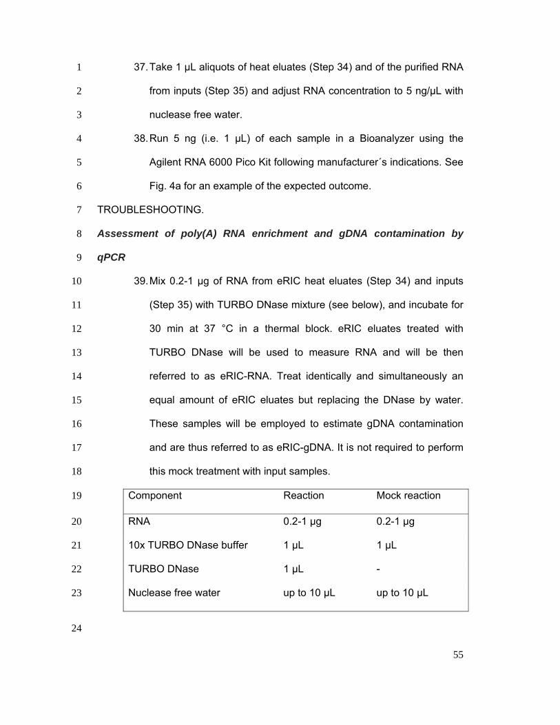
55

37. Take 1 μL aliquots of heat eluates (Step 34) and of the purified RNA 1

from inputs (Step 35) and adjust RNA concentration to 5 ng/μL with 2

nuclease free water. 3

38. Run 5 ng (i.e. 1 μL) of each sample in a Bioanalyzer using the 4

Agilent RNA 6000 Pico Kit following manufacturer´s indications. See 5

Fig. 4a for an example of the expected outcome. 6

TROUBLESHOOTING. 7

Assessment of poly(A) RNA enrichment and gDNA contamination by 8

qPCR 9

39. Mix 0.2-1 μg of RNA from eRIC heat eluates (Step 34) and inputs 10

(Step 35) with TURBO DNase mixture (see below), and incubate for 11

30 min at 37 °C in a thermal block. eRIC eluates treated with 12

TURBO DNase will be used to measure RNA and will be then 13

referred to as eRIC-RNA. Treat identically and simultaneously an 14

equal amount of eRIC eluates but replacing the DNase by water. 15

These samples will be employed to estimate gDNA contamination 16

and are thus referred to as eRIC-gDNA. It is not required to perform 17

this mock treatment with input samples. 18

Component Reaction Mock reaction 19

RNA 0.2-1 μg 0.2-1 μg 20

10x TURBO DNase buffer 1 μL 1 μL 21

TURBO DNase 1 μL - 22

Nuclease free water up to 10 μL up to 10 μL 23

24

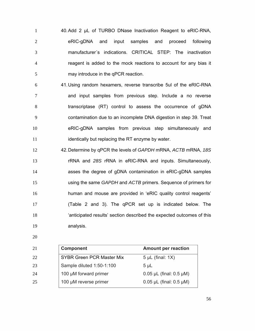
56

40. Add 2 μL of TURBO DNase Inactivation Reagent to eRIC-RNA, 1

eRIC-gDNA and input samples and proceed following 2

manufacturer´s indications. CRITICAL STEP: The inactivation 3

reagent is added to the mock reactions to account for any bias it 4

may introduce in the qPCR reaction. 5

41. Using random hexamers, reverse transcribe 5ul of the eRIC-RNA 6

and input samples from previous step. Include a no reverse 7

transcriptase (RT) control to assess the occurrence of gDNA 8

contamination due to an incomplete DNA digestion in step 39. Treat 9

eRIC-gDNA samples from previous step simultaneously and 10

identically but replacing the RT enzyme by water. 11

42. Determine by qPCR the levels of GAPDH mRNA, ACTB mRNA, 18S 12

rRNA and 28S rRNA in eRIC-RNA and inputs. Simultaneously, 13

asses the degree of gDNA contamination in eRIC-gDNA samples 14

using the same GAPDH and ACTB primers. Sequence of primers for 15

human and mouse are provided in ‘eRIC quality control reagents’ 16

(Table 2 and 3). The qPCR set up is indicated below. The 17

‘anticipated results’ section described the expected outcomes of this 18

analysis. 19

20

Component Amount per reaction 21

SYBR Green PCR Master Mix 5 μL (final: 1X) 22

Sample diluted 1:50-1:100 5 μL 23

100 μM forward primer 0.05 μL (final: 0.5 μM) 24

100 μM reverse primer 0.05 μL (final: 0.5 μM) 25

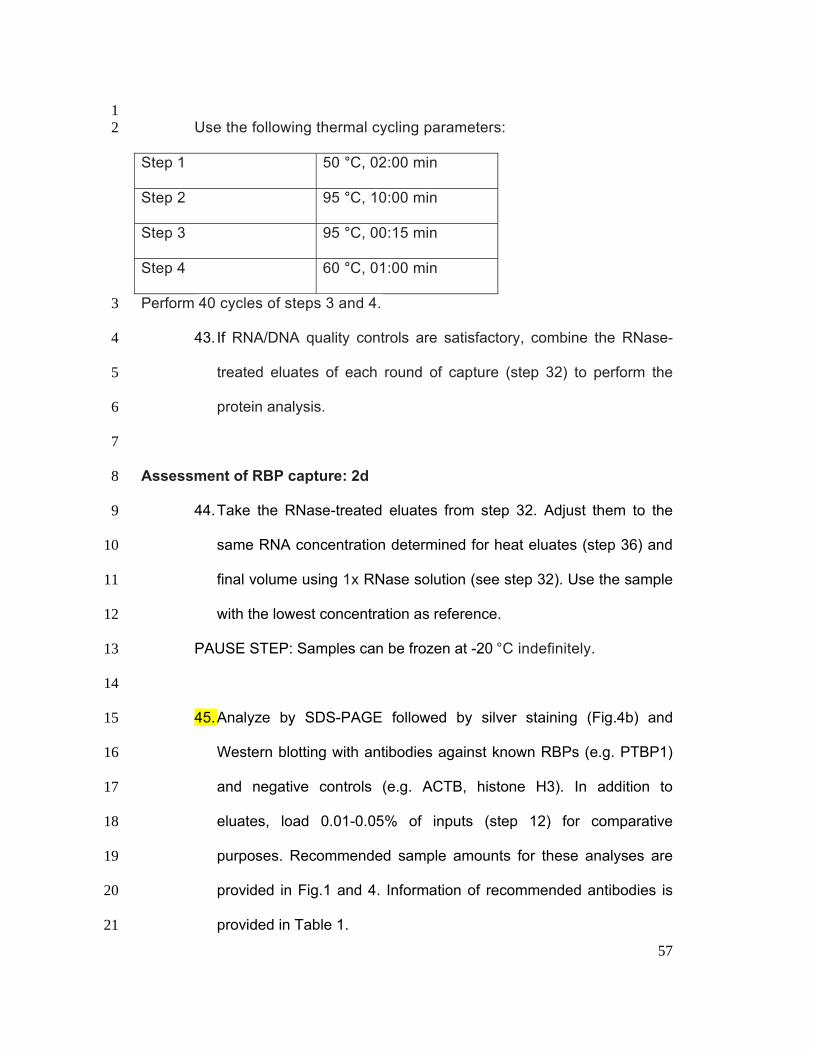
57

1 Use the following thermal cycling parameters: 2

Step 1 50 °C, 02:00 min

Step 2 95 °C, 10:00 min

Step 3 95 °C, 00:15 min

Step 4 60 °C, 01:00 min

Perform 40 cycles of steps 3 and 4. 3

43. If RNA/DNA quality controls are satisfactory, combine the RNase-4

treated eluates of each round of capture (step 32) to perform the 5

protein analysis. 6

7

Assessment of RBP capture: 2d 8

44. Take the RNase-treated eluates from step 32. Adjust them to the 9

same RNA concentration determined for heat eluates (step 36) and 10

final volume using 1x RNase solution (see step 32). Use the sample 11

with the lowest concentration as reference. 12

PAUSE STEP: Samples can be frozen at -20 °C indefinitely. 13

14

45. Analyze by SDS-PAGE followed by silver staining (Fig.4b) and 15

Western blotting with antibodies against known RBPs (e.g. PTBP1) 16

and negative controls (e.g. ACTB, histone H3). In addition to 17

eluates, load 0.01-0.05% of inputs (step 12) for comparative 18

purposes. Recommended sample amounts for these analyses are 19

provided in Fig.1 and 4. Information of recommended antibodies is 20

provided in Table 1. 21

58

CRITICAL STEP: proceed to the next steps only if protein, RNA and DNA 1

quality controls are satisfactory. 2

TROUBLESHOOTING 3

Proteomic analysis 4

Sample concentration. Timing: 60 min 5

46. Add 0.01 volumes of 10% (wt/vol) SDS to the eluates from Step 44 6

for a final concentration of 0.1% (wt/vol) SDS. 7

47. Concentrate equal amounts of each sample using a SpeedVac at 8

37 °C until a volume of ~100 μL is reached. We recommend 9

performing the SILAC or TMT proteomic analysis with the amount of 10

RNase treated eluate equivalent to 15-30 μg of RNA (inferred from 11

the RNA quantification in step 36; Fig. 1). 12

CRITICAL STEP: For the complementary total proteome analysis, use 13

material from step 12. Required protein amount depends on mass 14

spectrometry workflow and equipment, but we usually process up to 2 μg for 15

unfractionated samples per mass spec run. More material is usually required 16

if fractionation is applied (20 µg per 10 fractions). 17

CRITICAL STEP: If the experiment leads to larger quantities of RNA than those 18

indicated above, material excess can be used to perform additional quality 19

control experiments or for validation of candidates from the proteomic approach 20

(see below by Western blotting as in in step 45. 21

CRITICAL STEP. Avoid concentrating the samples to volumes lower than 22

50 μL as RBPs can precipitate. If this occurs, supplement the samples with 23

water to reach 100 μL and incubate at 37 °C until precipitate dissolves. 24

59

PAUSE POINT. Samples can be snap frozen in liquid nitrogen and store 1

at -80 °C. 2

3

SP3 sample purification. Timing: 3 hours 4

5

48. Sample clean up (Steps 48-57). Add 2 μL of 500 mM TCEP (final 6

concentration 10 mM) to the 100 μL of sample from step 47 to 7

disrupt disulfide bonds. Mix by pipetting and incubate at RT for 30 8

min. 9

49. Add 10.2 μL of 500 mM CAA to alkylate the sulfhydryl groups and 10

prevent re-formation of the disulfide bridges. Mix by pipetting and 11

incubate in the dark at RT for 30 min. 12

50. Add 10 μL of SP3 purification beads (see “SP3 purification bead 13

stock preparation”) to each sample. 14

51. Add 409.1 μL of 100% ACN to obtain a final percentage of 77% 15

(vol/vol) ACN. Incubate for 30 min at RT. 16

52. Collect the beads with a magnet and wait until the supernatant is 17

clear. At this stage, proteins are bound to the SP3 purification 18

beads. You can either keep the supernatant for quality control 19

purpose or discard it if the protocol has already been implemented 20

successfully. 21

53. Keep the tubes on the magnetic rack and add 1 mL of 70% (vol/vol) 22

EtOH [Wash buffer 1]. Incubate for 30 seconds and discard the 23

supernatant. Do not resuspend the beads or take the tube off the 24

magnet. 25

60

54. Keeping the tubes on the magnet, add 1 mL of 70% (vol/vol) EtOH 1

and incubate for 30 seconds on the magnetic rack. Remove and 2

discard supernatant. 3

55. Keeping the tubes on the magnetic rack, add 1 mL of 100% ACN 4

[Wash buffer 2] and incubate for 15 seconds on the magnetic rack. 5

Remove and discard the supernatant. 6

56. Repeat steps 53-55 seven times. 7

CRITICAL STEP: It is crucial that at this step, samples are free of any residual 8

detergent, which will negatively affect the nanoflow HPLC system performance 9

and consequentially protein identification. 10

57. Remove any residual ACN. Take the tubes with the beads off the 11

magnetic rack and proceed immediately to the next step. 12

Trypsin-digestion and peptide elution: Timing: 15-17 hours 13

58. Resuspend the SP3 purification beads in 50 μL (SILAC) or 10 μL 14

(TMT) of Trypsin digestion buffer. Avoid excessive pipetting of the 15

beads as they can stick to the tips, causing protein loss. 16

CRITICAL STEP: Avoid TEAB when using TMT as primary amines of TEAB can 17

quench TMT peptide labelling (see Trypsin digestion buffer in ‘Reagent setup’). 18

59. Add 250 ng of sequencing grade trypsin to each sample and 19

incubate in a thermal block at 37 °C and 400 rpm, overnight (~14 20

hours). 21

60. Collect the beads with a magnet and transfer the supernatant 22

containing the tryptic peptides to a new tube (this is referred to as 23

SP3 eluate 1). 24

61

61. Take the tube off the magnetic rack, re-suspend the beads with 1 1

mL 100% ACN, and incubate 5 min at RT. Collect beads with 2

magnet and discard the supernatant. 3

62. Resuspend the beads in 20 µL of SP3 elution buffer. Incubate for 5 4

min at RT. 5

CRITICAL STEP: The composition of the SP3 elution buffer for SILAC or 6

TMT approach is different (See ‘Reagent setup’). 7

63. Collect beads with a magnet making sure the solution becomes 8

clear, carefully collect the supernatant (referred to as SP3 eluate 2), 9

without disturbing the bead pellet, and combine with SP3 eluate 1 10

(step 60). Mix gently by pipetting up and down. If using TMT, 11

proceed to step 64. If using SILAC (or a label-free approach) 12

proceed directly to step 70 if fractionation is required or to 72 if it is 13

not required. 14

TMT labelling. Timing: 2 hours 15

64. Select the kit required for your experimental design based on the 16

number of conditions and replicates: i.e. Duplex TMT, Sixplex TMT, 17

TMT10plex, TMT11plex or TMTpro 16plex for up to 2, 6, 10, 11 or 18

16 samples, respectively. While we have not tested TMTpro 16plex 19

with this protocol yet, we do not anticipate any incompatibility. 20

Although the process is explained in detail in the manufacturer’s 21

manual, we describe it here in the context of our experimental 22

design. 23

65. Dissolve 0.8 mg of each TMT label in 42 μL 100% ACN. One unique 24

label will be used for each sample. 25

62

66. Add 4 μL of label solution to each sample and incubate for 1 hour at 1

RT. 2

67. Terminate the reaction by adding 5% (wt/vol) hydroxylamine for 15 3

min at RT. 4

68. Combine equal amounts of each sample. 5

69. Clean up the peptides with an OASIS HLB µElution Plate following 6

manufacturer´s indications. 7

Sample fractionation. Timing: 2 hours 8

CRITICAL: If using TMT or samples with high dynamic range between nuclear 9

and cytoplasmic proteins (e.g. T lymphocytes), we strongly recommend 10

fractionation. 11

70. Dry the sample completely by vacuum centrifugation. Reconstitute in 12

20 μL of 20 mM ammonium formate pH 10.0. 13

71. Fractionate samples into 5-6 fractions. We typically perform an 14

offline high pH reverse phase fractionation on an Agilent 1200 15

Infinity high-performance liquid chromatography system, equipped 16

with a Gemini C18 column (3 μm, 110 Å, 100 × 1.0 mm2, 17

Phenomenex) or in StageTips54. 18

CRITICAL STEP: These parameters are provided for guidance and other 19

fractionation regimens or approaches can be used. We do not recommend 20

fractionation at the protein level using SDS-PAGE, as RBPs tend to concentrate 21

at 220-100 KDa and 75-50 KDa, resulting in poor protein spread across 22

fractions. We thus recommend fractionation at peptide level using high pH 23

reversed-phase chromatography 54, isoelectric focusing 56 or ion exchange 55 . 24

Peptide identification and quantification by LC–MS. 1 day. 25

63

72. Dry the sample by vacuum centrifugation. Reconstitute in 20 μL of 1

loading buffer (5% (vol/vol) DMSO and 5% (vol/vol) formic acid). 2

73. We recommend performing a pilot run with 10% of sample to 3

estimate the volume needed for maximum protein identification 4

without overloading the nanoflow HPLC system. This can be 5

estimated based on overflow of the sample peptides to the 6

subsequent blank run with digested BSA (see ‘Experimental 7

Design’). 8

74. Based on the results from the pilot run, inject the optimal volume into 9

the LC-MS and separate the digested peptide using a typical 10

gradient for the available mass spectrometry instrumentation. 11

Data analysis. Timing: 1 week 12

CRITICAL Data analysis can be performed on multiple platforms, including 13

MaxQuant57, R packages or Perseus. Here we describe the workflow based on 14

the R package LIMMA but the workflow will be similar using other tools. An R 15

markdown file, including the code developed to perform analysis for a SILAC 16

labelled experiment15, is provided as Supplementary Software and 17

Supplementary Note. 18

75. Analyze the raw data with software based on database searching 19

that also performs intensity-based quantitation. We 20

used MaxQuant57 (version 1.6.3.4). Define the search database (in 21

our case Uniprot, Human, Organism ID 9606, downloaded on 22

16/01/13). Define the search parameters: trypsin as protease with 23

full tryptic specificity and a maximum of two missed cleavage sites, 24

carbamidomethyl (C) as a fixed modification, and acetylation 25

64

(protein N-term, i.e. only the amino terminus of the protein) and 1

oxidation (M) as variable modifications. All other parameters were 2

used as default. By default, MaxQuant will filter the results with a 1% 3

FDR at both the PSM (peptide to spectrum match) and protein level. 4

If working with multiple fractions per sample, define fraction number 5

in the fraction column before using the ‘match between runs’ option. 6

For SILAC-based analyses set up the SILAC labels in the ‘group 7

specific parameters’ tab using the multiplicity option. For isobaric 8

labelling, navigate to the ‘Group-specific parameters’ tab and select 9

'Reporter ion MS2' from the ‘Type’ drop down menu. Then select 10

appropriate kit (e.g. TMT10plex). Consult reference57 for more 11

details. 12

76. Extract the intensities for each peptide from the resulting 13

modificationSpecificPeptide.txt file as in15,32. 14

77. Add the list of reference protein sequences in FASTA format in 15

‘Global parameter-sequence’. Use uniquely mapped peptides and 16

summarize the ion count for each individual sample. 17

78. Perform multidimensional scaling to determine closeness of samples 18

in an unbiased way e.g. plotMDS in LIMMA. Biological samples 19

within the treatment condition should cluster together. Clustering will 20

help to identify technical problems including batch effects and 21

labelling biases. 22

79. Optional: If a batch effect is detected (Fig. 5a-b), we recommend 23

applying a ‘batch correction’ to the data. This can be incorporated in 24

65

the R package LIMMA with an appropriate design matrix before 1

linear modeling. 2

CRITICAL STEP: A batch effect can be detected because samples cluster not 3

because of the treatment, but due to a technical reason, such as differences 4

between replicates, independent mass spectrometry runs, or labelling 5

performance (Fig. 5a-b). As with any data manipulation, batch effect removal 6

can distort data, hence should be applied only if a clear batch effect is detected 7

by principal component analysis. In our experience, the SILAC light label can 8

introduce batch effects in some instances as exogenous contaminants (e.g. 9

keratins) and unlabeled peptides will only be present in the light channel. This 10

potential bias is minimized by the permutation of the SILAC labels but, if 11

problematic, it can easily be removed by applying the batch effect correction to 12

the SILAC labels. 13

80. Transform the protein intensities into log2 scale. 14

81. Using at least 3 biological replicates, use LIMMA to test whether the 15

fold changes between conditions are different from ‘zero’ using a 16

moderated t-test. 17

82. Correct the p-values for multiple testing by the Benjamini-Hochberg 18

procedure. Use 1% and 10% FDR proteins to define ‘high-19

confidence’ and ‘candidate’ responsive RBPs. We have recently 20

shown that a large proportion of the 10% FDR responsive RBPs are 21

truly regulated by the cue (in this case, by virus infection)15. 22

Nevertheless, we recommend orthogonal validation experiments 23

when working with ‘candidate’ responsive RBPs. 24

66

83. Optional: Proteins that are not detected in all conditions or replicates 1

can lead to ‘zero’ or ‘infinite’ ratios, eliminating these proteins 2

effectively from the statistical analysis. As these proteins can 3

represent biologically important on/off and off/on states, we used a 4

semi-quantitative analysis that considers the replicability of these 5

‘zero’ and presence of intensity signal in control and treatment 10,15, 6

as implemented in the R markdown provided in the Supplementary 7

Software and Supplementary Note. Alternatively, imputation 8

methods59 that add a value to each ‘zero’ can be used. The 9

advantages and disadvantages of each option are described in the 10

‘experimental design’. 11

CRITICAL STEP: The comparison between UV-irradiated and non-irradiated 12

samples is used to discover the repertoire of RBPs present in a given biological 13

system. However, to study the RBP responses it is critical to avoid 14

normalization against non-irradiated samples as signal in these samples is low 15

and noisy and creates artificial distortions of the data when used as normalizer. 16

84. Optional: If complementary proteomic analysis of the input was 17

performed, process the sample as described in Step 47-83 for 18

eluates. Then subtract the log2 fold intensity of the input from the 19

log2 fold intensity of the eluate to estimate eluate/input ratios. 20

21

TROUBLESHOOTING 22

Troubleshooting advice can be found in Table 4. 23

Table 4. Troubleshooting table. 24

Step Problem Possible reasons Solutions

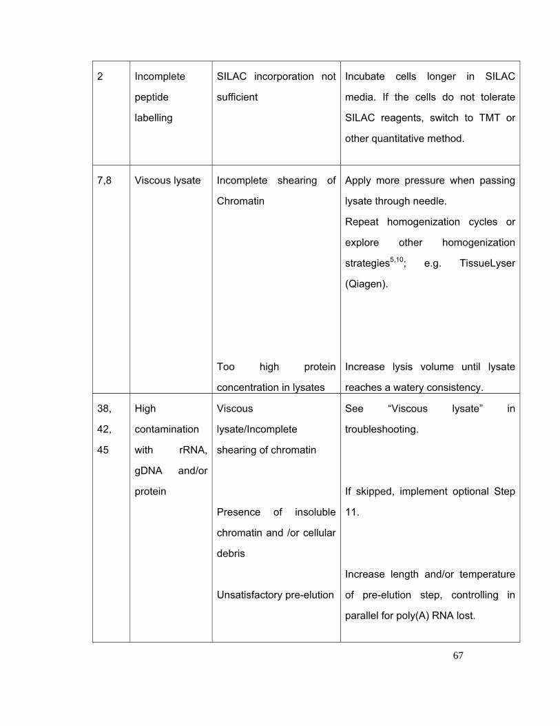
67

2 Incomplete

peptide

labelling

SILAC incorporation not

sufficient

Incubate cells longer in SILAC

media. If the cells do not tolerate

SILAC reagents, switch to TMT or

other quantitative method.

7,8 Viscous lysate Incomplete shearing of

Chromatin

Too high protein

concentration in lysates

Apply more pressure when passing

lysate through needle.

Repeat homogenization cycles or

explore other homogenization

strategies5,10; e.g. TissueLyser

(Qiagen).

Increase lysis volume until lysate

reaches a watery consistency.

38,

42,

45

High

contamination

with rRNA,

gDNA and/or

protein

Viscous

lysate/Incomplete

shearing of chromatin

Presence of insoluble

chromatin and /or cellular

debris

Unsatisfactory pre-elution

See “Viscous lysate” in

troubleshooting.

If skipped, implement optional Step

11.

Increase length and/or temperature

of pre-elution step, controlling in

parallel for poly(A) RNA lost.

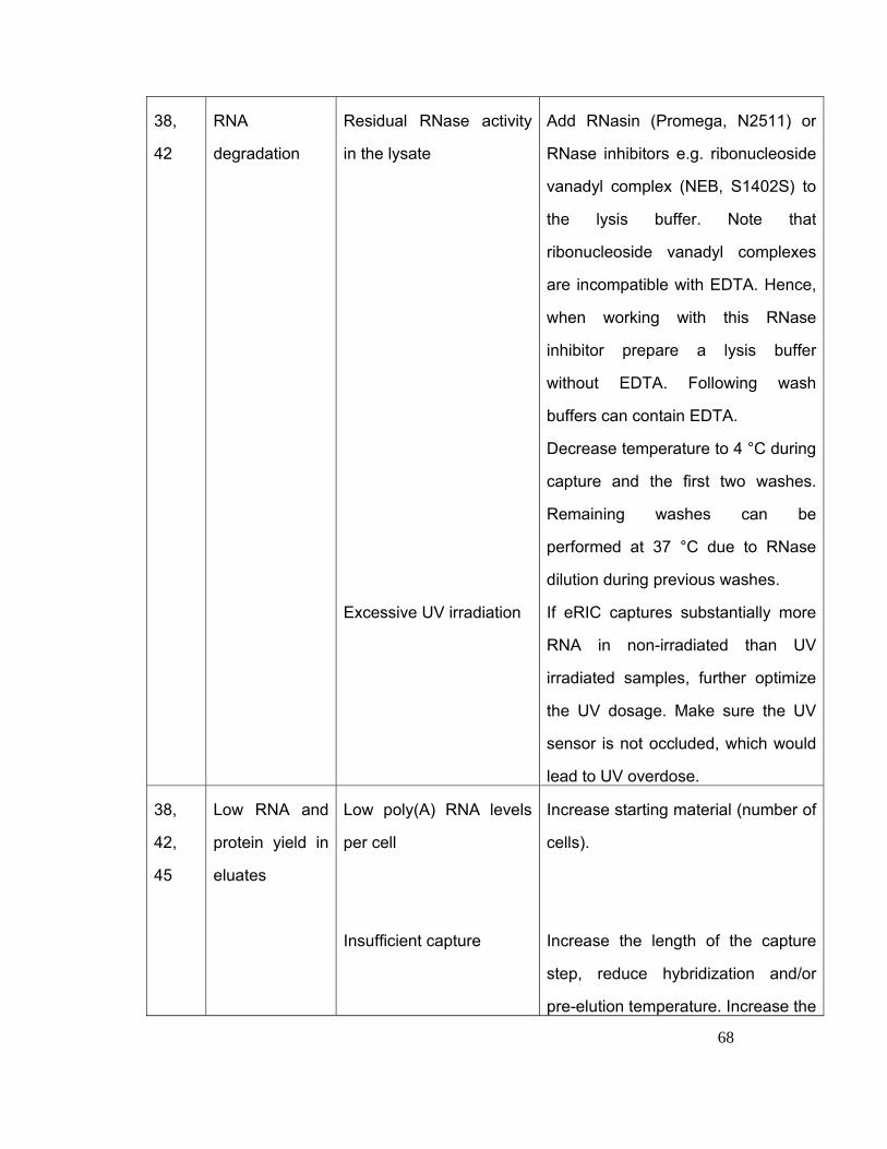
68

38,

42

RNA

degradation

Residual RNase activity

in the lysate

Excessive UV irradiation

Add RNasin (Promega, N2511) or

RNase inhibitors e.g. ribonucleoside

vanadyl complex (NEB, S1402S) to

the lysis buffer. Note that

ribonucleoside vanadyl complexes

are incompatible with EDTA. Hence,

when working with this RNase

inhibitor prepare a lysis buffer

without EDTA. Following wash

buffers can contain EDTA.

Decrease temperature to 4 °C during

capture and the first two washes.

Remaining washes can be

performed at 37 °C due to RNase

dilution during previous washes.

If eRIC captures substantially more

RNA in non-irradiated than UV

irradiated samples, further optimize

the UV dosage. Make sure the UV

sensor is not occluded, which would

lead to UV overdose.

38,

42,

45

Low RNA and

protein yield in

eluates

Low poly(A) RNA levels

per cell

Insufficient capture

Increase starting material (number of

cells).

Increase the length of the capture

step, reduce hybridization and/or

pre-elution temperature. Increase the

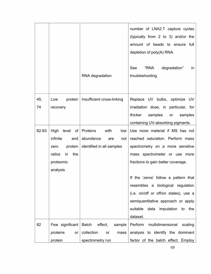
69

RNA degradation

number of LNA2.T capture cycles

(typically from 2 to 3) and/or the

amount of beads to ensure full

depletion of poly(A) RNA.

See “RNA degradation” in

troubleshooting.

45,

74

Low protein

recovery

Insufficient cross-linking Replace UV bulbs, optimize UV

irradiation dose, in particular, for

thicker samples or samples

containing UV-absorbing pigments.

82-83 High level of

infinite and

zero protein

ratios in the

proteomic

analysis

Proteins with low

abundance are not

identified in all samples

Use more material if MS has not

reached saturation. Perform mass

spectrometry on a more sensitive

mass spectrometer or use more

fractions to gain better coverage.

If the ‘zeros’ follow a pattern that

resembles a biological regulation

(i.e. on/off or off/on states), use a

semiquantitative approach or apply

suitable data imputation to the

dataset.

82 Few significant

proteins or

protein

Batch effect, sample

collection or mass

spectrometry run

Perform multidimensional scaling

analysis to identify the dominant

factor of the batch effect. Employ

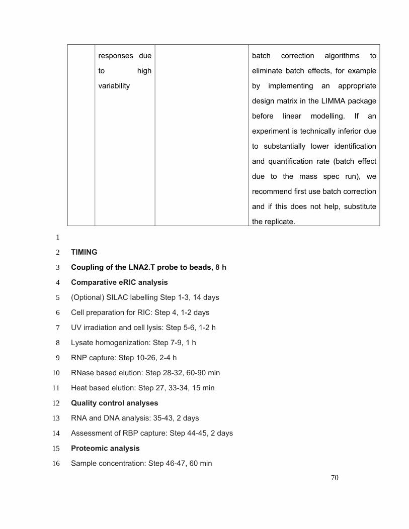
70

responses due

to high

variability

batch correction algorithms to

eliminate batch effects, for example

by implementing an appropriate

design matrix in the LIMMA package

before linear modelling. If an

experiment is technically inferior due

to substantially lower identification

and quantification rate (batch effect

due to the mass spec run), we

recommend first use batch correction

and if this does not help, substitute

the replicate.

1

TIMING 2

Coupling of the LNA2.T probe to beads, 8 h 3

Comparative eRIC analysis 4

(Optional) SILAC labelling Step 1-3, 14 days 5

Cell preparation for RIC: Step 4, 1-2 days 6

UV irradiation and cell lysis: Step 5-6, 1-2 h 7

Lysate homogenization: Step 7-9, 1 h 8

RNP capture: Step 10-26, 2-4 h 9

RNase based elution: Step 28-32, 60-90 min 10

Heat based elution: Step 27, 33-34, 15 min 11

Quality control analyses 12

RNA and DNA analysis: 35-43, 2 days 13

Assessment of RBP capture: Step 44-45, 2 days 14

Proteomic analysis 15

Sample concentration: Step 46-47, 60 min 16

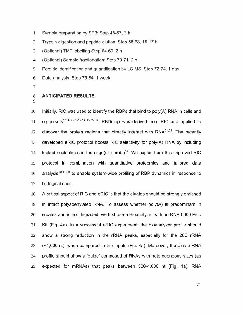
71

Sample preparation by SP3: Step 48-57, 3 h 1

Trypsin digestion and peptide elution: Step 58-63, 15-17 h 2

(Optional) TMT labelling Step 64-69, 2 h 3

(Optional) Sample fractionation: Step 70-71, 2 h 4

Peptide identification and quantification by LC-MS: Step 72-74, 1 day 5

Data analysis: Step 75-84, 1 week 6

7

ANTICIPATED RESULTS 8 9

Initially, RIC was used to identify the RBPs that bind to poly(A) RNA in cells and 10

organisms1,2,4,6,7,9-12,14,15,35,36. RBDmap was derived from RIC and applied to 11

discover the protein regions that directly interact with RNA31,32. The recently 12

developed eRIC protocol boosts RIC selectivity for poly(A) RNA by including 13

locked nucleotides in the oligo(dT) probe14. We exploit here this improved RIC 14

protocol in combination with quantitative proteomics and tailored data 15

analysis10,14,15 to enable system-wide profiling of RBP dynamics in response to 16

biological cues. 17

A critical aspect of RIC and eRIC is that the eluates should be strongly enriched 18

in intact polyadenylated RNA. To assess whether poly(A) is predominant in 19

eluates and is not degraded, we first use a Bioanalyzer with an RNA 6000 Pico 20

Kit (Fig. 4a). In a successful eRIC experiment, the bioanalyzer profile should 21

show a strong reduction in the rRNA peaks, especially for the 28S rRNA 22

(~4,000 nt), when compared to the inputs (Fig. 4a). Moreover, the eluate RNA 23

profile should show a ‘bulge’ composed of RNAs with heterogeneous sizes (as 24

expected for mRNAs) that peaks between 500-4,000 nt (Fig. 4a). RNA 25

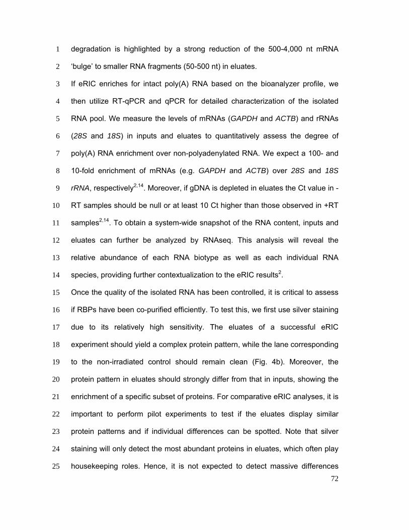
72

degradation is highlighted by a strong reduction of the 500-4,000 nt mRNA 1

‘bulge’ to smaller RNA fragments (50-500 nt) in eluates. 2

If eRIC enriches for intact poly(A) RNA based on the bioanalyzer profile, we 3

then utilize RT-qPCR and qPCR for detailed characterization of the isolated 4

RNA pool. We measure the levels of mRNAs (GAPDH and ACTB) and rRNAs 5

(28S and 18S) in inputs and eluates to quantitatively assess the degree of 6

poly(A) RNA enrichment over non-polyadenylated RNA. We expect a 100- and 7

10-fold enrichment of mRNAs (e.g. GAPDH and ACTB) over 28S and 18S 8

rRNA, respectively2,14. Moreover, if gDNA is depleted in eluates the Ct value in -9

RT samples should be null or at least 10 Ct higher than those observed in +RT 10

samples2,14. To obtain a system-wide snapshot of the RNA content, inputs and 11

eluates can further be analyzed by RNAseq. This analysis will reveal the 12

relative abundance of each RNA biotype as well as each individual RNA 13

species, providing further contextualization to the eRIC results2. 14

Once the quality of the isolated RNA has been controlled, it is critical to assess 15

if RBPs have been co-purified efficiently. To test this, we first use silver staining 16

due to its relatively high sensitivity. The eluates of a successful eRIC 17

experiment should yield a complex protein pattern, while the lane corresponding 18

to the non-irradiated control should remain clean (Fig. 4b). Moreover, the 19

protein pattern in eluates should strongly differ from that in inputs, showing the 20

enrichment of a specific subset of proteins. For comparative eRIC analyses, it is 21

important to perform pilot experiments to test if the eluates display similar 22

protein patterns and if individual differences can be spotted. Note that silver 23

staining will only detect the most abundant proteins in eluates, which often play 24

housekeeping roles. Hence, it is not expected to detect massive differences 25

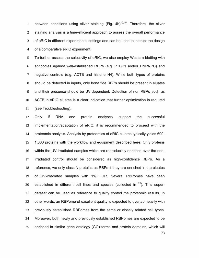
73

between conditions using silver staining (Fig. 4b)10,15. Therefore, the silver 1

staining analysis is a time-efficient approach to assess the overall performance 2

of eRIC in different experimental settings and can be used to instruct the design 3

of a comparative eRIC experiment. 4

To further assess the selectivity of eRIC, we also employ Western blotting with 5

antibodies against well-established RBPs (e.g. PTBP1 and/or HNRNPC) and 6

negative controls (e.g. ACTB and histone H4). While both types of proteins 7

should be detected in inputs, only bona fide RBPs should be present in eluates 8

and their presence should be UV-dependent. Detection of non-RBPs such as 9

ACTB in eRIC eluates is a clear indication that further optimization is required 10

(see Troubleshooting). 11

Only if RNA and protein analyses support the successful 12

implementation/adaptation of eRIC, it is recommended to proceed with the 13

proteomic analysis. Analysis by proteomics of eRIC eluates typically yields 600-14

1,000 proteins with the workflow and equipment described here. Only proteins 15

within the UV-irradiated samples which are reproducibly enriched over the non-16

irradiated control should be considered as high-confidence RBPs. As a 17

reference, we only classify proteins as RBPs if they are enriched in the eluates 18

of UV-irradiated samples with 1% FDR. Several RBPomes have been 19

established in different cell lines and species (collected in 25). This super-20

dataset can be used as reference to quality control the proteomic results. In 21

other words, an RBPome of excellent quality is expected to overlap heavily with 22

previously established RBPomes from the same or closely related cell types. 23

Moreover, both newly and previously established RBPomes are expected to be 24

enriched in similar gene ontology (GO) terms and protein domains, which will 25

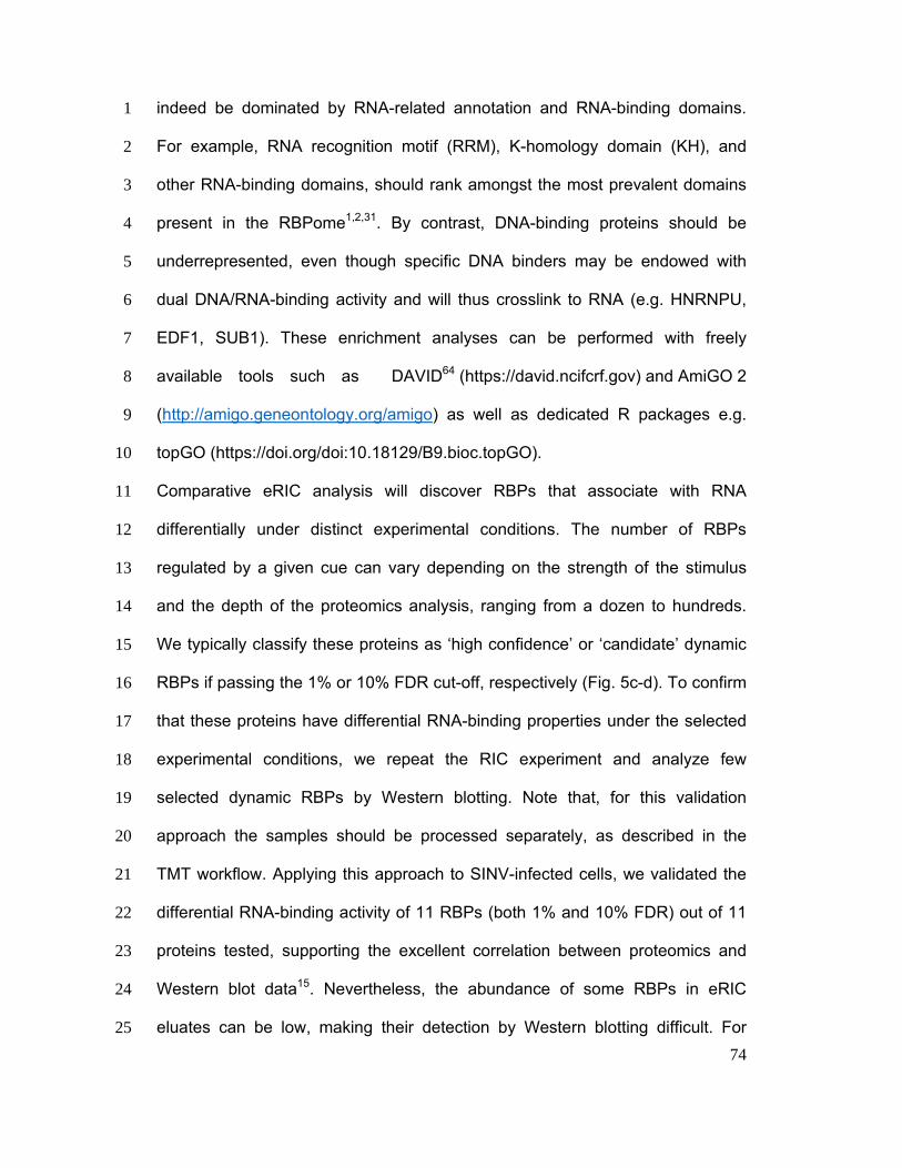
74

indeed be dominated by RNA-related annotation and RNA-binding domains. 1

For example, RNA recognition motif (RRM), K-homology domain (KH), and 2

other RNA-binding domains, should rank amongst the most prevalent domains 3

present in the RBPome1,2,31. By contrast, DNA-binding proteins should be 4

underrepresented, even though specific DNA binders may be endowed with 5

dual DNA/RNA-binding activity and will thus crosslink to RNA (e.g. HNRNPU, 6

EDF1, SUB1). These enrichment analyses can be performed with freely 7

available tools such as DAVID64 (https://david.ncifcrf.gov) and AmiGO 2 8

(http://amigo.geneontology.org/amigo) as well as dedicated R packages e.g. 9

topGO (https://doi.org/doi:10.18129/B9.bioc.topGO). 10

Comparative eRIC analysis will discover RBPs that associate with RNA 11

differentially under distinct experimental conditions. The number of RBPs 12

regulated by a given cue can vary depending on the strength of the stimulus 13

and the depth of the proteomics analysis, ranging from a dozen to hundreds. 14

We typically classify these proteins as ‘high confidence’ or ‘candidate’ dynamic 15

RBPs if passing the 1% or 10% FDR cut-off, respectively (Fig. 5c-d). To confirm 16

that these proteins have differential RNA-binding properties under the selected 17

experimental conditions, we repeat the RIC experiment and analyze few 18

selected dynamic RBPs by Western blotting. Note that, for this validation 19

approach the samples should be processed separately, as described in the 20

TMT workflow. Applying this approach to SINV-infected cells, we validated the 21

differential RNA-binding activity of 11 RBPs (both 1% and 10% FDR) out of 11 22

proteins tested, supporting the excellent correlation between proteomics and 23

Western blot data15. Nevertheless, the abundance of some RBPs in eRIC 24

eluates can be low, making their detection by Western blotting difficult. For 25

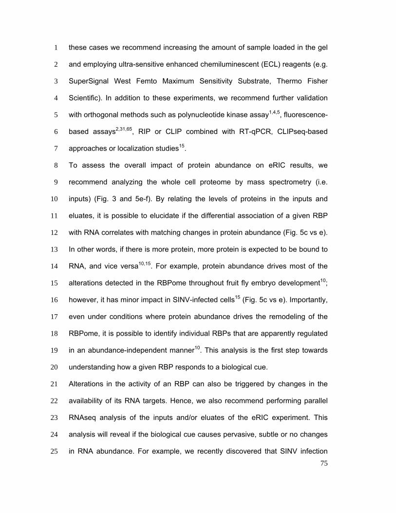
75

these cases we recommend increasing the amount of sample loaded in the gel 1

and employing ultra-sensitive enhanced chemiluminescent (ECL) reagents (e.g. 2

SuperSignal West Femto Maximum Sensitivity Substrate, Thermo Fisher 3

Scientific). In addition to these experiments, we recommend further validation 4

with orthogonal methods such as polynucleotide kinase assay1,4,5, fluorescence-5

based assays2,31,65, RIP or CLIP combined with RT-qPCR, CLIPseq-based 6

approaches or localization studies15. 7

To assess the overall impact of protein abundance on eRIC results, we 8

recommend analyzing the whole cell proteome by mass spectrometry (i.e. 9

inputs) (Fig. 3 and 5e-f). By relating the levels of proteins in the inputs and 10

eluates, it is possible to elucidate if the differential association of a given RBP 11

with RNA correlates with matching changes in protein abundance (Fig. 5c vs e). 12

In other words, if there is more protein, more protein is expected to be bound to 13

RNA, and vice versa10,15. For example, protein abundance drives most of the 14

alterations detected in the RBPome throughout fruit fly embryo development10; 15

however, it has minor impact in SINV-infected cells15 (Fig. 5c vs e). Importantly, 16

even under conditions where protein abundance drives the remodeling of the 17

RBPome, it is possible to identify individual RBPs that are apparently regulated 18

in an abundance-independent manner10. This analysis is the first step towards 19

understanding how a given RBP responds to a biological cue. 20

Alterations in the activity of an RBP can also be triggered by changes in the 21

availability of its RNA targets. Hence, we also recommend performing parallel 22

RNAseq analysis of the inputs and/or eluates of the eRIC experiment. This 23

analysis will reveal if the biological cue causes pervasive, subtle or no changes 24

in RNA abundance. For example, we recently discovered that SINV infection 25

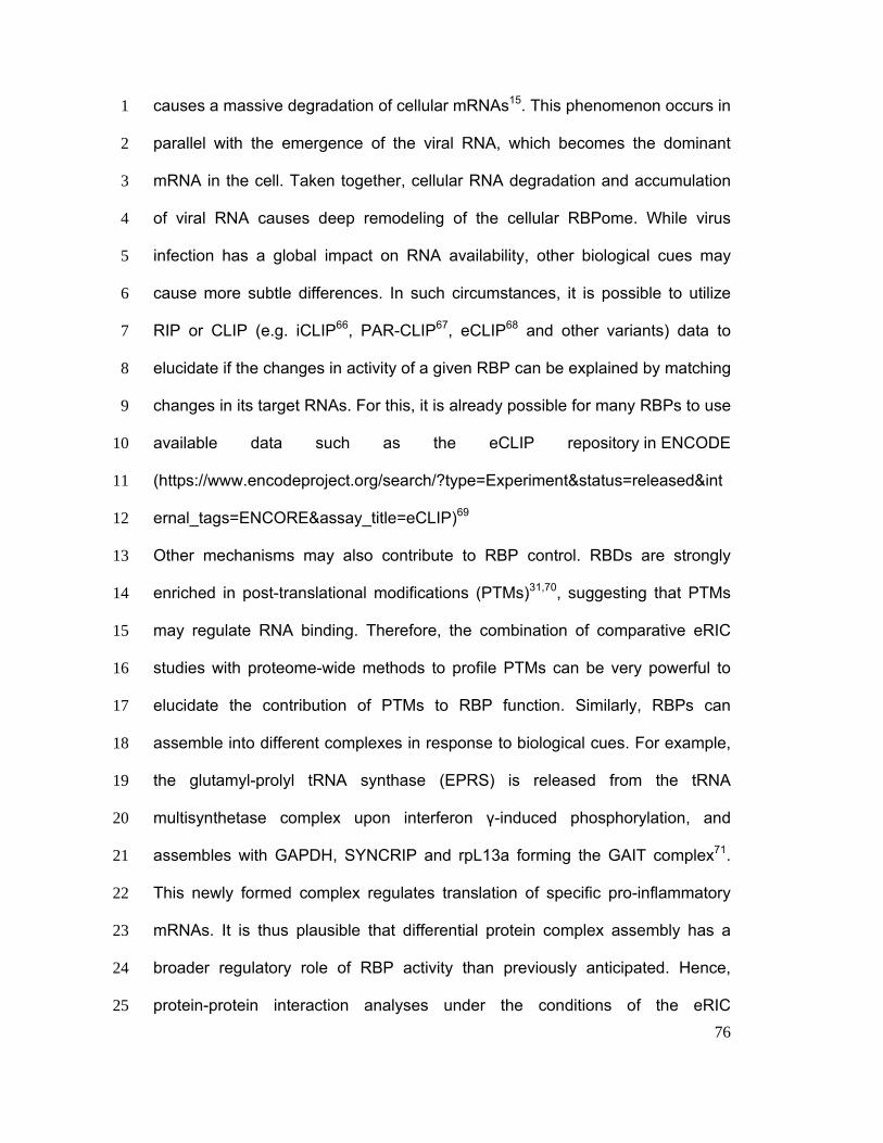
76

causes a massive degradation of cellular mRNAs15. This phenomenon occurs in 1

parallel with the emergence of the viral RNA, which becomes the dominant 2

mRNA in the cell. Taken together, cellular RNA degradation and accumulation 3

of viral RNA causes deep remodeling of the cellular RBPome. While virus 4

infection has a global impact on RNA availability, other biological cues may 5

cause more subtle differences. In such circumstances, it is possible to utilize 6

RIP or CLIP (e.g. iCLIP66, PAR-CLIP67, eCLIP68 and other variants) data to 7

elucidate if the changes in activity of a given RBP can be explained by matching 8

changes in its target RNAs. For this, it is already possible for many RBPs to use 9

available data such as the eCLIP repository in ENCODE 10

(https://www.encodeproject.org/search/?type=Experiment&status=released&int11

ernal_tags=ENCORE&assay_title=eCLIP)69 12

Other mechanisms may also contribute to RBP control. RBDs are strongly 13

enriched in post-translational modifications (PTMs)31,70, suggesting that PTMs 14

may regulate RNA binding. Therefore, the combination of comparative eRIC 15

studies with proteome-wide methods to profile PTMs can be very powerful to 16

elucidate the contribution of PTMs to RBP function. Similarly, RBPs can 17

assemble into different complexes in response to biological cues. For example, 18

the glutamyl-prolyl tRNA synthase (EPRS) is released from the tRNA 19

multisynthetase complex upon interferon γ-induced phosphorylation, and 20

assembles with GAPDH, SYNCRIP and rpL13a forming the GAIT complex71. 21

This newly formed complex regulates translation of specific pro-inflammatory 22

mRNAs. It is thus plausible that differential protein complex assembly has a 23

broader regulatory role of RBP activity than previously anticipated. Hence, 24

protein-protein interaction analyses under the conditions of the eRIC 25

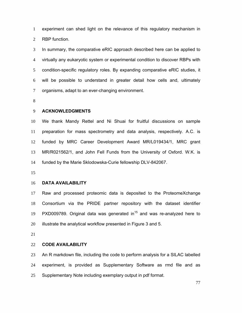
77

experiment can shed light on the relevance of this regulatory mechanism in 1

RBP function. 2

In summary, the comparative eRIC approach described here can be applied to 3

virtually any eukaryotic system or experimental condition to discover RBPs with 4

condition-specific regulatory roles. By expanding comparative eRIC studies, it 5

will be possible to understand in greater detail how cells and, ultimately 6

organisms, adapt to an ever-changing environment. 7

8

ACKNOWLEDGMENTS 9

We thank Mandy Rettel and Ni Shuai for fruitful discussions on sample 10

preparation for mass spectrometry and data analysis, respectively. A.C. is 11

funded by MRC Career Development Award MR/L019434/1, MRC grant 12

MR/R021562/1, and John Fell Funds from the University of Oxford. W.K. is 13

funded by the Marie Sklodowska-Curie fellowship DLV-842067. 14

15

DATA AVAILABILITY 16

Raw and processed proteomic data is deposited to the ProteomeXchange 17

Consortium via the PRIDE partner repository with the dataset identifier 18

PXD009789. Original data was generated in15 and was re-analyzed here to 19

illustrate the analytical workflow presented in Figure 3 and 5. 20

21

CODE AVAILABILITY 22

An R markdown file, including the code to perform analysis for a SILAC labelled 23

experiment, is provided as Supplementary Software as rmd file and as 24

Supplementary Note including exemplary output in pdf format. 25

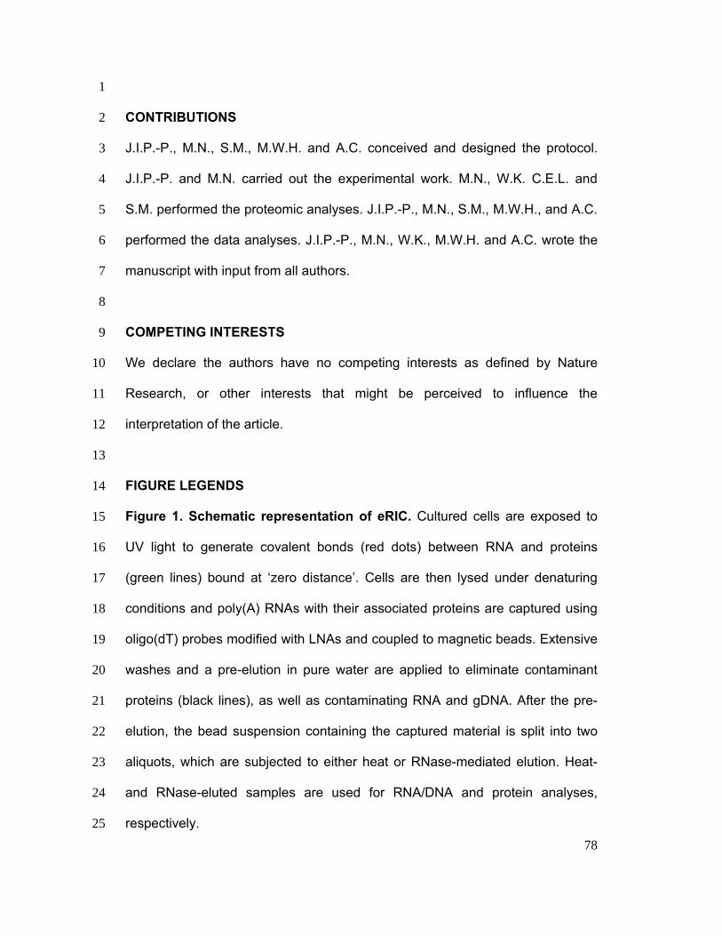
78

1

CONTRIBUTIONS 2

J.I.P.-P., M.N., S.M., M.W.H. and A.C. conceived and designed the protocol. 3

J.I.P.-P. and M.N. carried out the experimental work. M.N., W.K. C.E.L. and 4

S.M. performed the proteomic analyses. J.I.P.-P., M.N., S.M., M.W.H., and A.C. 5

performed the data analyses. J.I.P.-P., M.N., W.K., M.W.H. and A.C. wrote the 6

manuscript with input from all authors. 7

8

COMPETING INTERESTS 9

We declare the authors have no competing interests as defined by Nature 10

Research, or other interests that might be perceived to influence the 11

interpretation of the article. 12

13

FIGURE LEGENDS 14

Figure 1. Schematic representation of eRIC. Cultured cells are exposed to 15

UV light to generate covalent bonds (red dots) between RNA and proteins 16

(green lines) bound at ‘zero distance’. Cells are then lysed under denaturing 17

conditions and poly(A) RNAs with their associated proteins are captured using 18

oligo(dT) probes modified with LNAs and coupled to magnetic beads. Extensive 19

washes and a pre-elution in pure water are applied to eliminate contaminant 20

proteins (black lines), as well as contaminating RNA and gDNA. After the pre-21

elution, the bead suspension containing the captured material is split into two 22

aliquots, which are subjected to either heat or RNase-mediated elution. Heat- 23

and RNase-eluted samples are used for RNA/DNA and protein analyses, 24

respectively. 25

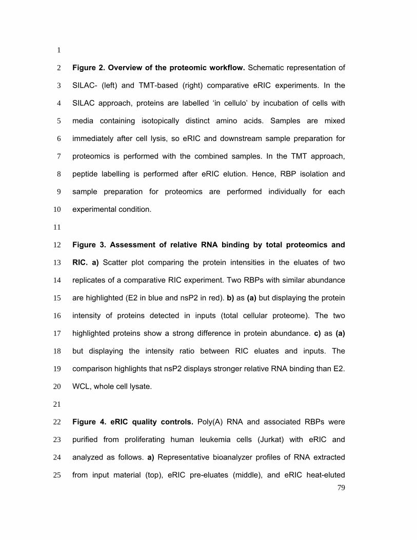
79

1

Figure 2. Overview of the proteomic workflow. Schematic representation of 2

SILAC- (left) and TMT-based (right) comparative eRIC experiments. In the 3

SILAC approach, proteins are labelled ‘in cellulo’ by incubation of cells with 4

media containing isotopically distinct amino acids. Samples are mixed 5

immediately after cell lysis, so eRIC and downstream sample preparation for 6

proteomics is performed with the combined samples. In the TMT approach, 7

peptide labelling is performed after eRIC elution. Hence, RBP isolation and 8

sample preparation for proteomics are performed individually for each 9

experimental condition. 10

11

Figure 3. Assessment of relative RNA binding by total proteomics and 12

RIC. a) Scatter plot comparing the protein intensities in the eluates of two 13

replicates of a comparative RIC experiment. Two RBPs with similar abundance 14

are highlighted (E2 in blue and nsP2 in red). b) as (a) but displaying the protein 15

intensity of proteins detected in inputs (total cellular proteome). The two 16

highlighted proteins show a strong difference in protein abundance. c) as (a) 17

but displaying the intensity ratio between RIC eluates and inputs. The 18

comparison highlights that nsP2 displays stronger relative RNA binding than E2. 19

WCL, whole cell lysate. 20

21

Figure 4. eRIC quality controls. Poly(A) RNA and associated RBPs were 22

purified from proliferating human leukemia cells (Jurkat) with eRIC and 23

analyzed as follows. a) Representative bioanalyzer profiles of RNA extracted 24

from input material (top), eRIC pre-eluates (middle), and eRIC heat-eluted 25

80

samples (bottom). rRNAs, tRNAs and small RNAs are predominant in inputs 1

and still present in pre-eluates. eRIC heat-eluted samples display a strong 2

enrichment of RNA species with a size range characteristic of mRNAs. Both 3

28S rRNA and the small RNAs are undetectable in the heat eluates, although a 4

residual amount of 18S rRNA is consistently observed. [FU] fluorescent units, 5

[nt] length of RNA in number of nucleotides. b) eRIC was performed on Jurkat 6

cells incubated for 6 h with 0.5 mM of the α-ketoglutarate antagonist 7

dimethyloxalylglycine (DMOG) or vehicle (DMSO). Aliquots of the RNase-eluted 8

samples and inputs were analyzed by SDS-PAGE and silver staining. Except 9

for the RNase A and T1 bands (~15 KDa), proteins are only detected in eRIC 10

eluates if cells were UV-irradiated. Protein patterns in untreated and DMOG-11

treated samples are virtually indistinguishable, which agrees with the proteomic 12

results that revealed a very limited RBP pool (61 proteins out of 721) 13

responding to DMOG14. 14

15

Figure 5. Statistical analysis of proteomic data. a) Unbiased clustering of 16

data using multidimensional scaling of 3 biological replicates (1-3) and 2 17

different conditions (Mock in black and Treatment [SINV virus infection] in red). 18

In this case, the clustering of the RIC inputs (WCL) is based on the replicates, 19

rather than experimental conditions, suggesting that the dataset has a batch 20

effect. Batch effects can potentially hide the underlying biological signal and we 21

recommend investigating their cause e.g. assessing if the mean intensity 22

between mass spectrometry runs differ. If the cause of the effect can be 23

identified, a batch correction algorithm can be used after data acquisition. b) 24

Multidimensional scaling as above. In this example, RIC eluates from control 25

81

(mock) samples cluster together with a clear separation from the treated 1

(infected) samples. No batch correction is necessary in this case. However, the 2

RIC eluate from treated cells in the replicate 3 displays a differential signature 3

when compared to the other 2 replicates. Detailed analysis of the proteomic 4

data can help to elucidate whether this results from a technical problem (e.g. an 5

error estimating the amount of protein prior to mixing the samples). c) Scatter 6

plot displaying the treated/untreated protein ratios from two independent 7

replicates. A good correlation between replicates indicates the high quality of 8

the experiment. Every dot represents a protein and they are colored based on 9

the statistical significance of the change between the two conditions (1%, 5% 10

and 10% FDR). d) Volcano plot displaying the fold change and p value of the 11

proteins in (c). Every dot corresponds to a protein and they are colored based 12

on the statistical significance of the change between the two conditions (1%, 13

5% and 10% FDR. e) as (c) but displaying the ratios in the whole cell lysate 14

(input). No significant changes were observed during the time-course of the 15

treatment, suggesting that the changes observed in eluates are not due to 16

matching changes in protein abundance. Original data was generated in 15 and 17

was re-analyzed here to illustrate the analytical workflow. Mock vs 18hpi with 18

SINV infection of RIC data is displayed in panel a, c and d. Panel b and e 19

represents the matching input proteome. 20

21

REFERENCES 22

23

82

1 Baltz, A. G. et al. The mRNA-bound proteome and its global occupancy 1

profile on protein-coding transcripts. Mol Cell 46, 674-690, 2

doi:10.1016/j.molcel.2012.05.021 (2012). 3

2 Castello, A. et al. Insights into RNA biology from an atlas of mammalian 4

mRNA-binding proteins. Cell 149, 1393-1406, 5

doi:10.1016/j.cell.2012.04.031 (2012). 6

3 Castello, A. et al. System-wide identification of RNA-binding proteins by 7

interactome capture. Nat Protoc 8, 491-500, doi:10.1038/nprot.2013.020 8

(2013). 9

4 Kwon, S. C. et al. The RNA-binding protein repertoire of embryonic stem 10

cells. Nature structural & molecular biology 20, 1122-1130, 11

doi:10.1038/nsmb.2638 (2013). 12

5 Beckmann, B. M. et al. The RNA-binding proteomes from yeast to man 13

harbour conserved enigmRBPs. Nat Commun 6, 10127, 14

doi:10.1038/ncomms10127 (2015). 15

6 Liao, Y. et al. The Cardiomyocyte RNA-Binding Proteome: Links to 16

Intermediary Metabolism and Heart Disease. Cell Rep 16, 1456-1469, 17

doi:10.1016/j.celrep.2016.06.084 (2016). 18

7 Liepelt, A. et al. Identification of RNA-binding Proteins in Macrophages 19

by Interactome Capture. Mol Cell Proteomics 15, 2699-2714, 20

doi:10.1074/mcp.M115.056564 (2016). 21

8 Matia-Gonzalez, A. M., Laing, E. E. & Gerber, A. P. Conserved mRNA-22

binding proteomes in eukaryotic organisms. Nature structural & 23

molecular biology 22, 1027-1033, doi:10.1038/nsmb.3128 (2015). 24

83

9 Reichel, M. et al. In Planta Determination of the mRNA-Binding 1

Proteome of Arabidopsis Etiolated Seedlings. Plant Cell 28, 2435-2452, 2

doi:10.1105/tpc.16.00562 (2016). 3

10 Sysoev, V. O. et al. Global changes of the RNA-bound proteome during 4

the maternal-to-zygotic transition in Drosophila. Nat Commun 7, 12128, 5

doi:10.1038/ncomms12128 (2016). 6

11 Despic, V. et al. Dynamic RNA-protein interactions underlie the zebrafish 7

maternal-to-zygotic transition. Genome Res 27, 1184-1194, 8

doi:10.1101/gr.215954.116 (2017). 9

12 Nandan, D. et al. Comprehensive Identification of mRNA-Binding 10

Proteins of Leishmania donovani by Interactome Capture. PLoS One 12, 11

e0170068, doi:10.1371/journal.pone.0170068 (2017). 12

13 Bach-Pages, M. et al. Discovering the RNA-Binding Proteome of Plant 13

Leaves with an Improved RNA Interactome Capture Method. 14

Biomolecules 10, 661, doi:10.3390/biom10040661 (2020). 15

14 Perez-Perri, J. I. et al. Discovery of RNA-binding proteins and 16

characterization of their dynamic responses by enhanced RNA 17

interactome capture. Nat Commun 9, 4408, doi:10.1038/s41467-018-18

06557-8 (2018). 19

15 Garcia-Moreno, M. et al. System-wide Profiling of RNA-Binding Proteins 20

Uncovers Key Regulators of Virus Infection. Mol Cell 74, 196-211 e111, 21

doi:10.1016/j.molcel.2019.01.017 (2019). 22

16 Rogell, B. et al. Specific RNP capture with antisense LNA/DNA mixmers. 23

RNA 23, 1290-1302, doi:10.1261/rna.060798.117 (2017). 24

84

17 Ong, S. E. & Mann, M. A practical recipe for stable isotope labeling by 1

amino acids in cell culture (SILAC). Nat Protoc 1, 2650-2660, 2

doi:10.1038/nprot.2006.427 (2006). 3

18 Hughes, C. S. et al. Ultrasensitive proteome analysis using paramagnetic 4

bead technology. Mol Syst Biol 10, 757, doi:10.15252/msb.20145625 5

(2014). 6

19 Hughes, C. S. et al. Single-pot, solid-phase-enhanced sample 7

preparation for proteomics experiments. Nat Protoc 14, 68-85, 8

doi:10.1038/s41596-018-0082-x (2019). 9

20 Lukong, K. E., Chang, K. W., Khandjian, E. W. & Richard, S. RNA-10

binding proteins in human genetic disease. Trends Genet 24, 416-425, 11

doi:10.1016/j.tig.2008.05.004 (2008). 12

21 Castello, A., Fischer, B., Hentze, M. W. & Preiss, T. RNA-binding 13

proteins in Mendelian disease. Trends Genet 29, 318-327, 14

doi:10.1016/j.tig.2013.01.004 (2013). 15

22 Moore, S., Jarvelin, A. I., Davis, I., Bond, G. L. & Castello, A. Expanding 16

horizons: new roles for non-canonical RNA-binding proteins in cancer. 17

Curr Opin Genet Dev 48, 112-120, doi:10.1016/j.gde.2017.11.006 18

(2018). 19

23 Garcia-Moreno, M., Jarvelin, A. I. & Castello, A. Unconventional RNA-20

binding proteins step into the virus-host battlefront. Wiley Interdiscip Rev 21

RNA 9, e1498, doi:10.1002/wrna.1498 (2018). 22

24 Castello, A., Hentze, M. W. & Preiss, T. Metabolic Enzymes Enjoying 23

New Partnerships as RNA-Binding Proteins. Trends Endocrinol Metab 24

26, 746-757, doi:10.1016/j.tem.2015.09.012 (2015). 25

85

25 Hentze, M. W., Castello, A., Schwarzl, T. & Preiss, T. A brave new world 1

of RNA-binding proteins. Nat Rev Mol Cell Biol 19, 327-341, 2

doi:10.1038/nrm.2017.130 (2018). 3

26 Horos, R. et al. The Small Non-coding Vault RNA1-1 Acts as a 4

Riboregulator of Autophagy. Cell 176, 1054-1067 e1012, 5

doi:10.1016/j.cell.2019.01.030 (2019). 6

27 Choudhury, N. R. et al. RNA-binding activity of TRIM25 is mediated by its 7

PRY/SPRY domain and is required for ubiquitination. BMC Biol 15, 105, 8

doi:10.1186/s12915-017-0444-9 (2017). 9

28 Jiao, A. L. & Slack, F. J. RNA-mediated gene activation. Epigenetics 9, 10

27-36, doi:10.4161/epi.26942 (2014). 11

29 Ivanyi-Nagy, R. et al. The RNA interactome of human telomerase RNA 12

reveals a coding-independent role for a histone mRNA in telomere 13

homeostasis. Elife 7, doi:10.7554/eLife.40037 (2018). 14

30 Kumari, P. & Sampath, K. cncRNAs: Bi-functional RNAs with protein 15

coding and non-coding functions. Semin Cell Dev Biol 47-48, 40-51, 16

doi:10.1016/j.semcdb.2015.10.024 (2015). 17

31 Castello, A. et al. Comprehensive Identification of RNA-Binding Domains 18

in Human Cells. Mol Cell 63, 696-710, doi:10.1016/j.molcel.2016.06.029 19

(2016). 20

32 Castello, A. et al. Identification of RNA-binding domains of RNA-binding 21

proteins in cultured cells on a system-wide scale with RBDmap. Nat 22

Protoc 12, 2447-2464, doi:10.1038/nprot.2017.106 (2017). 23

86

33 Backlund, M. et al. Plasticity of nuclear and cytoplasmic stress responses 1

of RNA-binding proteins. Nucleic Acids Res 48, 4725-4740, 2

doi:10.1093/nar/gkaa256 (2020). 3

34 Bunnik, E. M. et al. The mRNA-bound proteome of the human malaria 4

parasite Plasmodium falciparum. Genome Biol 17, 147, 5

doi:10.1186/s13059-016-1014-0 (2016). 6

35 Wessels, H. H. et al. The mRNA-bound proteome of the early fly embryo. 7

Genome Res 26, 1000-1009, doi:10.1101/gr.200386.115 (2016). 8

36 Kilchert, C. et al. System-wide analyses of the fission yeast poly(A)(+) 9

RNA interactome reveal insights into organization and function of RNA-10

protein complexes. Genome Res, doi:10.1101/gr.257006.119 (2020). 11

37 Bao, X. et al. Capturing the interactome of newly transcribed RNA. Nat 12

Methods 15, 213-220, doi:10.1038/nmeth.4595 (2018). 13

38 Huang, R., Han, M., Meng, L. & Chen, X. Capture and Identification of 14

RNA-binding Proteins by Using Click Chemistry-assisted RNA-15

interactome Capture (CARIC) Strategy. J Vis Exp, doi:10.3791/58580 16

(2018). 17

39 Asencio, C., Chatterjee, A. & Hentze, M. W. Silica-based solid-phase 18

extraction of cross-linked nucleic acid-bound proteins. Life Sci Alliance 1, 19

e201800088, doi:10.26508/lsa.201800088 (2018). 20

40 Shchepachev, V. et al. Defining the RNA interactome by total RNA-21

associated protein purification. Mol Syst Biol 15, e8689, 22

doi:10.15252/msb.20188689 (2019). 23

87

41 Trendel, J. et al. The Human RNA-Binding Proteome and Its Dynamics 1

during Translational Arrest. Cell 176, 391-403 e319, 2

doi:10.1016/j.cell.2018.11.004 (2019). 3

42 Queiroz, R. M. L. et al. Comprehensive identification of RNA-protein 4

interactions in any organism using orthogonal organic phase separation 5

(OOPS). Nat Biotechnol 37, 169-178, doi:10.1038/s41587-018-0001-2 6

(2019). 7

43 Urdaneta, E. C. et al. Purification of cross-linked RNA-protein complexes 8

by phenol-toluol extraction. Nat Commun 10, 990, doi:10.1038/s41467-9

019-08942-3 (2019). 10

44 Burger, K. et al. 4-thiouridine inhibits rRNA synthesis and causes a 11

nucleolar stress response. RNA Biol 10, 1623-1630, 12

doi:10.4161/rna.26214 (2013). 13

45 Muckenthaler, M. U., Rivella, S., Hentze, M. W. & Galy, B. A Red Carpet 14

for Iron Metabolism. Cell 168, 344-361, doi:10.1016/j.cell.2016.12.034 15

(2017). 16

46 Altelaar, A. F. et al. Benchmarking stable isotope labeling based 17

quantitative proteomics. J Proteomics 88, 14-26, 18

doi:10.1016/j.jprot.2012.10.009 (2013). 19

47 Hogrebe, A. et al. Benchmarking common quantification strategies for 20

large-scale phosphoproteomics. Nat Commun 9, 1045, 21

doi:10.1038/s41467-018-03309-6 (2018). 22

48 Dimayacyac-Esleta, B. R. et al. Rapid High-pH Reverse Phase StageTip 23

for Sensitive Small-Scale Membrane Proteomic Profiling. Anal Chem 87, 24

12016-12023, doi:10.1021/acs.analchem.5b03639 (2015). 25

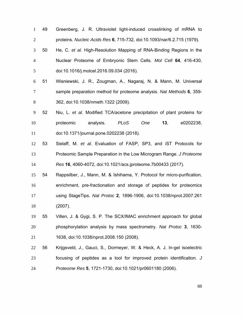
88

49 Greenberg, J. R. Ultraviolet light-induced crosslinking of mRNA to 1

proteins. Nucleic Acids Res 6, 715-732, doi:10.1093/nar/6.2.715 (1979). 2

50 He, C. et al. High-Resolution Mapping of RNA-Binding Regions in the 3

Nuclear Proteome of Embryonic Stem Cells. Mol Cell 64, 416-430, 4

doi:10.1016/j.molcel.2016.09.034 (2016). 5

51 Wisniewski, J. R., Zougman, A., Nagaraj, N. & Mann, M. Universal 6

sample preparation method for proteome analysis. Nat Methods 6, 359-7

362, doi:10.1038/nmeth.1322 (2009). 8

52 Niu, L. et al. Modified TCA/acetone precipitation of plant proteins for 9

proteomic analysis. PLoS One 13, e0202238, 10

doi:10.1371/journal.pone.0202238 (2018). 11

53 Sielaff, M. et al. Evaluation of FASP, SP3, and iST Protocols for 12

Proteomic Sample Preparation in the Low Microgram Range. J Proteome 13

Res 16, 4060-4072, doi:10.1021/acs.jproteome.7b00433 (2017). 14

54 Rappsilber, J., Mann, M. & Ishihama, Y. Protocol for micro-purification, 15

enrichment, pre-fractionation and storage of peptides for proteomics 16

using StageTips. Nat Protoc 2, 1896-1906, doi:10.1038/nprot.2007.261 17

(2007). 18

55 Villen, J. & Gygi, S. P. The SCX/IMAC enrichment approach for global 19

phosphorylation analysis by mass spectrometry. Nat Protoc 3, 1630-20

1638, doi:10.1038/nprot.2008.150 (2008). 21

56 Krijgsveld, J., Gauci, S., Dormeyer, W. & Heck, A. J. In-gel isoelectric 22

focusing of peptides as a tool for improved protein identification. J 23

Proteome Res 5, 1721-1730, doi:10.1021/pr0601180 (2006). 24

89

57 Tyanova, S., Temu, T. & Cox, J. The MaxQuant computational platform 1

for mass spectrometry-based shotgun proteomics. Nat Protoc 11, 2301-2

2319, doi:10.1038/nprot.2016.136 (2016). 3

58 Gierlinski, M., Gastaldello, F., Cole, C. & Barton, G. J. Proteus: an R 4

package for downstream analysis of MaxQuant output. bioRxiv, 416511, 5

doi:10.1101/416511 (2018). 6

59 Lazar, C., Gatto, L., Ferro, M., Bruley, C. & Burger, T. Accounting for the 7

Multiple Natures of Missing Values in Label-Free Quantitative Proteomics 8

Data Sets to Compare Imputation Strategies. J Proteome Res 15, 1116-9

1125, doi:10.1021/acs.jproteome.5b00981 (2016). 10

60 Cox, J. et al. Andromeda: a peptide search engine integrated into the 11

MaxQuant environment. J Proteome Res 10, 1794-1805, 12

doi:10.1021/pr101065j (2011). 13

61 Ritchie, M. E. et al. limma powers differential expression analyses for 14

RNA-sequencing and microarray studies. Nucleic Acids Res 43, e47, 15

doi:10.1093/nar/gkv007 (2015). 16

62 Harsha, H. C., Molina, H. & Pandey, A. Quantitative proteomics using 17

stable isotope labeling with amino acids in cell culture. Nat Protoc 3, 505-18

516, doi:10.1038/nprot.2008.2 (2008). 19

63 Anantharaman, V. & Aravind, L. The PRC-barrel: a widespread, 20

conserved domain shared by photosynthetic reaction center subunits 21

and proteins of RNA metabolism. Genome Biol 3, RESEARCH0061, 22

doi:10.1186/gb-2002-3-11-research0061 (2002). 23

64 Dennis, G., Jr. et al. DAVID: Database for Annotation, Visualization, and 24

Integrated Discovery. Genome Biol 4, P3 (2003). 25

90

65 Strein, C., Alleaume, A. M., Rothbauer, U., Hentze, M. W. & Castello, A. 1

A versatile assay for RNA-binding proteins in living cells. RNA 20, 721-2

731, doi:10.1261/rna.043562.113 (2014). 3

66 Konig, J. et al. iCLIP reveals the function of hnRNP particles in splicing at 4

individual nucleotide resolution. Nature structural & molecular biology 17, 5

909-915, doi:10.1038/nsmb.1838 (2010). 6

67 Hafner, M. et al. Transcriptome-wide identification of RNA-binding protein 7

and microRNA target sites by PAR-CLIP. Cell 141, 129-141, 8

doi:10.1016/j.cell.2010.03.009 (2010). 9

68 Van Nostrand, E. L. et al. Robust transcriptome-wide discovery of RNA-10

binding protein binding sites with enhanced CLIP (eCLIP). Nat Methods 11

13, 508-514, doi:10.1038/nmeth.3810 (2016). 12

69 Van Nostrand, E. L. et al. A Large-Scale Binding and Functional Map of 13

Human RNA Binding Proteins. bioRxiv, 179648, doi:10.1101/179648 14

(2018). 15

70 Jarvelin, A. I., Noerenberg, M., Davis, I. & Castello, A. The new 16

(dis)order in RNA regulation. Cell Commun Signal 14, 9, 17

doi:10.1186/s12964-016-0132-3 (2016). 18

71 Arif, A. et al. The GAIT translational control system. Wiley Interdiscip Rev 19

RNA 9, doi:10.1002/wrna.1441 (2018). 20

21

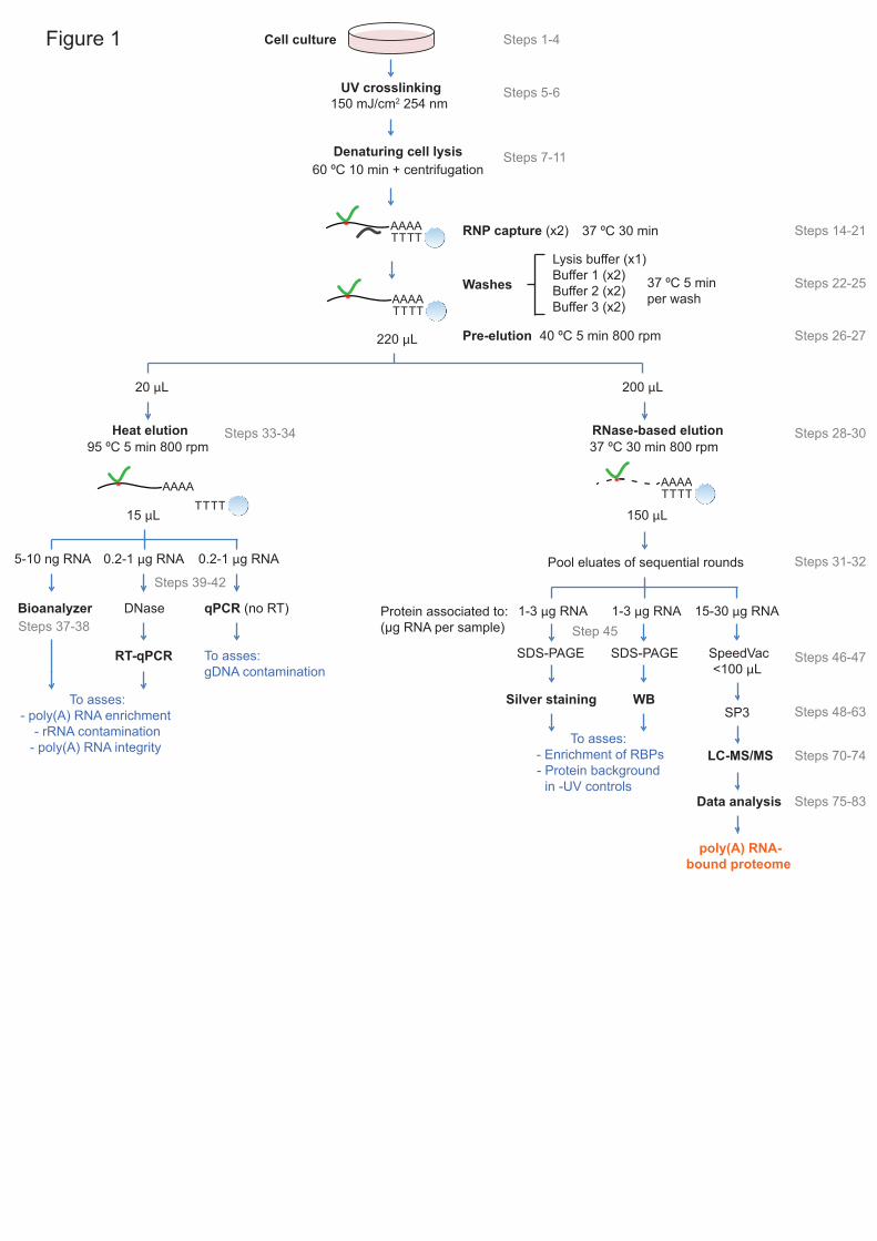
UV crosslinking150 mJ/cm2 254 nm

Denaturing cell lysis60 ºC 10 min + centrifugation

AAAATTTT

Washes

RNP capture (x2)

AAAATTTT

RNase-based elution

AAAATTTTAAAA

220 μL

20 μL 200 μL

Pre-elution

Heat elution

15 μL

qPCR (no RT)DNase

RT-qPCR

Bioanalyzer

150 μL

WBSilver staining

1-3 μg RNA 15-30 μg RNA1-3 μg RNAProtein associated to:(µg RNA per sample)

TTTT

5-10 ng RNA 0.2-1 μg RNA0.2-1 μg RNA Pool eluates of sequential rounds

LC-MS/MS

SP3

SpeedVac <100 μL

To asses:- poly(A) RNA enrichment

- rRNA contamination- poly(A) RNA integrity

To asses:gDNA contamination

37 ºC 30 min

Lysis buffer (x1)Buffer 1 (x2)Buffer 2 (x2)Buffer 3 (x2)

40 ºC 5 min 800 rpm

37 ºC 30 min 800 rpm95 ºC 5 min 800 rpm

37 ºC 5 minper wash

To asses: - Enrichment of RBPs- Protein background

in -UV controls

SDS-PAGE SDS-PAGE

Steps 5-6

Cell culture Steps 1-4

Steps 7-11

Steps 14-21

Steps 22-25

Steps 26-27

Steps 28-30Steps 33-34

Steps 31-32

Steps 37-38

Steps 39-42

Step 45

Steps 46-47

Steps 48-63

Steps 70-74

poly(A) RNA-bound proteome

Steps 75-83Data analysis

Figure 1

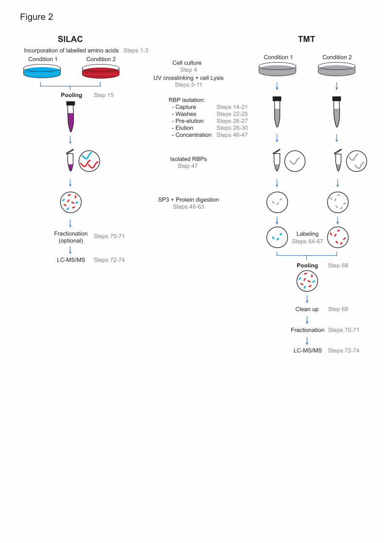
SILAC TMT

Condition 1 Condition 2 Condition 1 Condition 2

RBP isolation: - Capture - Washes - Pre-elution - Elution - Concentration

SP3 + Protein digestionSteps 48-63

Labeling

LC-MS/MS

Clean up

Isolated RBPsStep 47

Pooling

Incorporation of labelled amino acids

Cell culture Step 4

UV crosslinking + cell LysisSteps 5-11

Steps 64-67Steps 70-71Fractionation

(optional)

Step 69

Fractionation

LC-MS/MS

Steps 70-71

Steps 72-74

Steps 72-74

Pooling

Steps 1-3

Step 68

Step 15

Steps 14-21Steps 22-25Steps 26-27Steps 28-30Steps 46-47

Figure 2

Figure 3

a b cProtein Abundance in WCLProtein Abundance in RIC Relative RNA binding activity (RIC/WCL)

20 22 24 26 28 30 32 3420

2224

2628

3032

34

Abundance WCL Replicate 1

Abun

danc

e W

CL

Rep

licat

e 2

nsP2

E2

16 18 20 22 24 26 28

1618

2022

2426

28

Abundance RIC Replicate 1

Abun

danc

e R

IC R

eplic

ate

2

nsP2E2

−10 −8 −6 −4 −2 0

−10

−8−6

−4−2

0

RIC/WCL Replicate 1

RIC

/WC

L R

eplic

ate

2

nsP2

E2

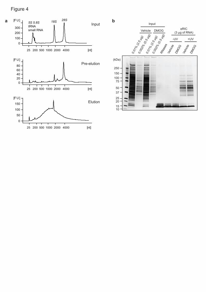
020406080

[F U]

0

50

100

150

[F U]

25 200 1000 4000 [nt]

0100

200300

[F U]

25 200 1000 4000 [nt]

25 200 1000 4000 [nt]

Input

Pre-elution

Elution

a

RNas

esVe

hicle

DMO

G

0.01

% (2

.5 μ

g)0.

002%

(0.5

μg)

Input

-UV

Vehi

cleDM

OG

+UV

0.01

% (2

.5 μ

g)0.

002%

(0.5

μg)

Vehicle DMOG

250

150100

75

5037

25

15

(kDa)

20

10

eRIC(3 μg of RNA)

b28S18S5S 5.8StRNAsmall RNA

2000

2000

2000500

500

500

Figure 4

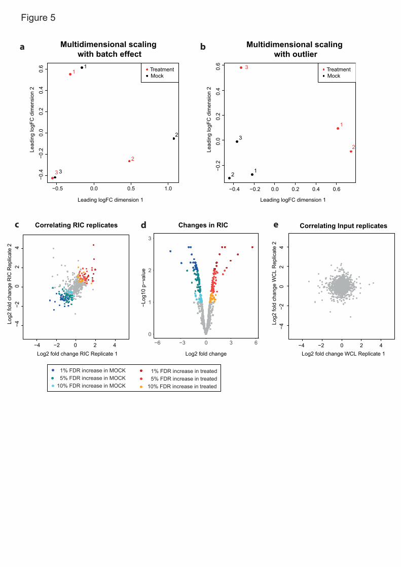
−0.5 0.0 0.5 1.0

−0.4

−0.2

0.0

0.2

0.4

0.6

Multidimensional scaling with batch effect

Leading logFC dimension 1

Lead

ing

logF

C d

imen

sion

2

TreatmentMock

11

2

2

3 3

a

−0.4 −0.2 0.0 0.2 0.4 0.6

−0.2

0.0

0.2

0.4

0.6

Leading logFC dimension 1Le

adin

g lo

gFC

dim

ensi

on 2

1

1

2

2

3

3

Multidimensional scaling with outlier

TreatmentMock

b

−4−2

02

4

−4 −2 0 2 4

Correlating RIC replicates

Log2 fold change RIC Replicate 1

Log2

fold

cha

nge

RIC

Rep

licat

e 2

0

1

2

3

−6 −3 0 3 6

Log2 fold change

−Log

10 p

−val

ue

Changes in RIC

−4−2

02

4

−4 −2 0 2 4

Correlating Input replicates

Log2 fold change WCL Replicate 1

Log2

fold

cha

nge

WC

L R

eplic

ate

2

c d e

5% FDR increase in MOCK1% FDR increase in MOCK

10% FDR increase in MOCK5% FDR increase in treated1% FDR increase in treated

10% FDR increase in treated

Figure 5

1 Global analysis of RNA-binding protein dynamics by ...

Documents

Transcript of 1 Global analysis of RNA-binding protein dynamics by ...