1

Gender grading bias at the university level: quasi-experimental evidence from an

anonymous grading reform

Joakim Janssona and Björn Tyreforsb,*

This version: December 6, 2019

aDepartment of Economics and Statistics, Linnaeus University and Research Institute of

Industrial Economics (IFN), P.O. Box 55665, SE-10215 Stockholm, Sweden, E-mail,

joakim.jansson@ifn.se; telephone: +46(0)8-665 4500).

bResearch Institute of Industrial Economics (IFN), Box 55665, 102 15 Stockholm Stockholm (e-

mail, bjorn.tyrefors@ifn.se; telephone: +46(0)8-665 4500) and Dep. of Economics, Stockholm

University, SE-10691 Stockholm, Sweden (e-mail: bjorn.tyrefors@ne.su.se; telephone: +46(0)8-

674 7459)

*Corresponding author

Tyrefors, Research Institute of Industrial Economics (IFN), Box 55665, 102 15 Stockholm

Stockholm (e-mail, bjorn.tyrefors@ifn.se; telephone: +46(0)8-665 4500) and Dep. of

Economics, Stockholm University, SE-10691 Stockholm, Sweden (e-mail:

bjorn.tyrefors@ne.su.se; telephone: +46(0)8-674 7459)

2

Abstract

In this paper, we first present novel evidence of female university students benefiting from being

graded fairly, i.e., anonymously. This finding conflicts with previous results at the secondary

education level. In contrast to the teacher gender composition at lower levels of education,

teachers at the university level are predominantly male. Thus, an in-group bias mechanism could

consistently explain the evidence at both the university and secondary education levels. We find

that the treatment effect is driven by departments in which male teachers constitute the majority

and estimate a significant in-group bias effect using randomly assigned graders. However,

unexpectedly, further analysis shows that the treatment effect is essentially independent of the

grader/student gender match. Hence, we document evidence of both grading bias stemming from

in-group bias and other match independent factors, for example, shared culture and institutional

factors.

Keywords

Grading bias; University; Discrimination; Education; Anonymous grading; in-group bias

JEL codes

I23; J16

3

1 Introduction

Biased grading has recently received increasing attention in economics. This literature is

generally motivated by the growing gender gap in educational attainment and the sorting of

males and females into specific fields.1 One strand of the grading bias literature has focused on

pre-tertiary education levels and has typically found bias against males.2 This literature finds a

bias effect independent of in-group bias, i.e., independent of the grader-student gender match.

However, another strand of the literature notes that the teaching profession has been increasingly

staffed by women. The majority of female teachers have been proposed as one mechanism

explaining the grading bias against boys through in-group bias.3 In contrast to the lower

education levels, a large majority of university teachers are male. Therefore, a study of grading

bias at the university could inform us about the role of both general and in-group bias

mechanisms. Furthermore, there are very few large-scale studies based on quasi-experimental

methods evaluating gender grading bias at universities.4

This study aims to fill this gap by making the following four main contributions: (i) using

a difference-in-difference design to estimate the treatment effect on female students being graded

1 See, for instance, Lavy and Sand (2018), Kugler et al. (2017) and Terrier (2015).

2 See, for instance, Lavy (2008) or Berg et al. (2019).

3 The phenomenon whereby people tend to favor other people of their own group is usually

referred to as in-group bias effects. See, for instance, Sandberg (2017) for an overview as well as

Dee (2005, 2007), Lee et al. (2014), Lusher et al. (2015), Feld et al. (2016) and Lim and Meer

(2017a)

4 A pilot study on parts of the sample was undertaken by Eriksson and Nolgren (2013).

4

anonymously compared to male students using a large scale anonymous grading reform at

Stockholm University; (ii) exploring the heterogeneous effects across departments with different

male/female teacher majorities, (iii) credibly estimating the in-group bias using random grader

assignments, and (iv) quantifying the extent to which the treatment effect of the grading reform

is caused by a reduction of the in-group bias. To do this, we combine two unique data sets with

two experimental designs. We make use of an exam reform at Stockholm University, where all

standard exams had to be graded with no information about exam-takers’ identity. This reform

was put in place at the beginning of the fall term of 2009. To estimate the in-group bias effect,

we make use of the fact that the graders were randomly assigned to students.

Using a difference-in-difference (DID) design5, we first find a positive effect of the

anonymous grading reform on the test results of female students. Thus, consistent with the

findings reported by previous authors, such as Goldin and Rouse (2000), being evaluated

anonymously can improve evaluations of females relative to males. We argue that this effect is

likely explained by a gender bias in grading.6 One explanation for the sign shift of the effects

5 Since we estimate differential gender effects due to a grading reform, in fact, we estimate a

difference-in-difference-in-difference model, which is discussed in section 2.4.

6 Although we are estimating the causal effect of the anonymous grading reform, we can never

be certain that the outcome is due only to grading bias. In fact, we can think of a situation where

the behavior of the students changes; for instance, they could start to exert more effort as a

consequence of the reform. We share this drawback with many prominent studies in the field

based on anonymous and non-anonymous observations of this outcome. However, we are able to

partly investigate the effort channel by studying the results of multiple-choice questions, which

5

compared to lower levels could be an in-group bias mechanism, as there are more male graders

at the university level than at lower levels. Supportively, when we divided the sample into

departments with a majority of female teachers and departments with a majority of male

teachers, we find that the effect is driven purely by the departments with a majority of male

teachers. However, this finding does not prove that the effect is due to in-group bias as male-

dominated departments could well exhibit cultural gender bias that is also shared by female

teachers. To separate the mechanisms, we conduct a second experiment. By using a particular

exam, namely, the introductory exam in macroeconomics, we can collect more detailed

information on grader gender, and more importantly, we can utilize a nonintentional randomized

experiment setting for this exam in which graders of different genders were randomly assigned to

correct different questions. First, we confirm the substantial positive effect of the anonymous

grading reform on the test results of female students in the subsample using the same type of

DID specification as discussed above for the full sample. Then, through the random assignment

of grader gender, we can estimate the causal effect of same-sex bias among correctors. We find

strong evidence of same-sex bias in the TAs’ exam corrections. It is also comforting, from an

internal validity point of view, that we find that in-group bias disappears once anonymous exams

are introduced at the university. This finding should be a consequence if the reform is effective.

Finally, when quantifying the relation between the total effect of being graded anonymously and

the in-group bias effect, we find that the in-group bias effect is statistically unrelated to the main

effect. Considering the point estimate change at face value, in-group bias accounts at most for 15

are unaffected by the reform. We credibly find no change close to the reform years, which

suggests that females did not change their effort level.

6

%, indicating that the grading reform effect is mainly determined by factors other than the

graders favoring their own gender. Thus, the lion’s share of the effect is explained by cultural or

institutional factors, independent of the gender/grader match. Consistent with these findings are

theories of how gender stereotypes (a genius is male) affect judgement.7 However, we are not

able to distinguish these mechanisms from standard theories of statistical discrimination (Arrow,

1973; Phelps, 1972).

Furthermore, we argue that the economic significance of our findings can hardly be

underestimated. There is a growing literature showing that discrimination in grading can have

long term consequences on further education and earnings.8 As more than 45 % of persons aged

between 25-34 attend university (slightly below the US rate) and a majority of students are

female, the economic consequences could therefore be substantial. Lastly, the effects are also

found in the Swedish context, one of the most gender-equal countries in the world, according to,

for example, the United Nations Human Development Reports.

An increasing number of studies have investigated the different dimensions of grading

bias at the pre-tertiary levels. As a whole, there are two strands in this literature. First and

foremost, there are studies investigating the general gender grading bias of teachers, comparing

test scores across anonymous and non-anonymous exams. Lavy (2008) looks at the gender bias

7 On the issue of a genius being a male, see Elmore and Luna-Lucero (2017). On how

stereotypes may affect grading, see the discussion and references in Lavy (2008) as well as the

idea of stereotypes and implicit discrimination developed and discussed in Bertrand et al. (2005).

8 See, for example, Ebenstein, et al. (2016), Lavy et al. (2018), Lavy and Sand (2018), and

Lavy and Megalokonomou (2019).

7

in Israeli matriculation exams in nine subjects among high school students. Using a DID

approach, he finds evidence of bias against male students. A similar approach is adopted by

Hinnerich et al. (2011).9 Biased grading has also been studied for other groups. In a randomized

field experiment, Hanna and Linden (2012) find that teachers are biased towards lower castes in

India, and Burgess and Greaves (2013) find evidence that some ethnic groups are systematically

underrated relative to their white peers. Relatedly, Kiss (2013) studies the grading of immigrants

and girls once test scores have been taken into account and finds a negative impact on

immigrants’ grades in primary education.10 Second, there are studies looking at more reduced-

form effects of having a male or female teacher depending on a student’s gender. The most

notable study in this strand is probably (Dee, 2005), who looks at the effect of students sharing

their gender or ethnicity with their teacher in eighth grade and finds a positive effect. A similar

approach is taken in (Dee, 2007); however, this study considers more long-run and behavioral

responses.11 It is worth noting that none of these studies are performed at the university level.

There are, however, a few papers using the university as a testing context. Closely related

to our work is Breda and Ly (2015). They use oral (non-blind) and written (blind) entry-level

exams at elite universities in France and find that females’ oral performance is graded better than

males’ in more male-dominated subjects. Our setting differs from theirs in many ways other than

9 See also Cornwell et al. (2013). Moreover, Lindahl (2007) finds that male test scores increase

with the share of male teachers, whereas grades decrease at the same rate.

10 See also Sprietsma (2013) and Hinnerich et al. (2015).

11 Using Swedish data Holmlund and Sund (2008) find no strong support that a same-sex

teacher improves student outcomes

8

the larger scale of our study. We use a change in policy over time, and the examiners in our

study are typically the teachers of the students and not external examiners, as they are in Breda

and Ly (2015). We study a standard examination at a large (approximately 30 000 students per

year) state-financed non-selective university and we document the overall gender effect of

anonymous grading at the university level, and that this effect differs from lower levels of

education as female grades are improved compared to male grades. Breda and Ly (2015)

estimate a non-linear model (an interaction model), and the overall average effect may still be

consistent with our finding.12

Another closely related study, particularly in relation to our second design, is Feld et al.

(2016), who investigate whether biased grading is driven by teachers favoring their own type

(endophilia) or discriminating against other types (exophobia). In their field experiment, they

cover approximately 1,500 examinations in 2012 at the School of Business and Economics

(SBE) of Maastricht University, where graders were randomly allocated. On average, gender

matching seems to be of little importance for grading even though there is some evidence of

male graders favoring male students. In our second design where graders are randomly assigned

we first document in-group bias using a methodology similar to Feld et al. (2016) with the

sample consisting of the exams from the introductory macroeconomics course. Moreover, where

Feld et al. (2016) fail to detect either same-sex bias, we document significant effects.

Furthermore, we can also relate the in-group bias mechanism to the overall effect of being

graded anonymously or not and our findings do suggest that although in-group bias exists, is not

12 Breda and Ly (2012) show an overall grading bias effect of the same sign and size as ours.

See also Breda and Hillion (2016).

9

key in determining the overall bias in grading. Thus, we are able to separate in-group bias from

bias stemming from other match independent factors such as culture or institutions.

Additionally, the effect of teachers as role models at the university level is investigated in

Hoffmann and Oreopoulos (2009). Other papers look at how the classroom gender composition

affects student performance (Lee et al., 2014) and how the matching of TA/teacher and student

ethnicity/gender affects student performance (Coenen and Van Klaveren, 2016; Lim and Meer,

2017a, 2017b; Lusher et al., 2015)

The rest of the paper is organized as follows: section 2 describes the two empirical

strategies and data sets that we use, section 3 presents the results, and section 4 concludes the

paper.

2 Material and methods

2.1 The grading reform of 2009

The head of school decided on a grading reform on March 5, 2009, and the reform began

as a trial for a year starting in the fall term of 2009. The reform included the removal of test-

takers’ identity on standard exams from the start of the fall term of 2009. In May 2010, the

reform was evaluated, and it was decided that the university should continue with anonymous

grading on exams. Some implementation problems with the IT system were noted during the trial

period in the first year. For example, some students’ identities were revealed due to poor IT

systems (Stockholm University, 2010). Unfortunately, we did not observe which students might

have had their identities revealed during the first year, so we cannot classify and control for this.

Thus, we acknowledge that the effect might be dampened during the first year of the reform.

10

2.2 Data from all graded activities at Stockholm University

We have data on the universe of graded activities from the fall term of 2005 to the fall

term of 2013. We consider the fact that unlike standard exams, other graded activities such as

theses and oral and home assignments were not anonymized for practical reasons. All

departments except the law department were affected by this reform; the law department already

had a long-standing practice of anonymous grading.13 Thus, all examinations at the law

department and activities such as thesis work and oral and home assignments at other

departments serve as a control group in the DID design.

In the relevant time period, there were three main grading systems in place: the original,

consisting of G (pass), VG (pass with distinction) and U (fail); a special grading scheme

implemented for most courses at the department of law, consisting of AB (highest), BA (middle),

B (lowest) and U (fail); and the system imposed by the Bologna process in the European Union.

The Bologna scheme had to be implemented from the fall of 2008 at the latest, although it was

used at certain departments and courses before that deadline.14 The numeration of these different

systems is given in Table A1, while Figs. A1-A3 provide histograms for each of them. The

histogram plots all appear approximately normally distributed, except for the grades in the

13 Table A3 shows that our results are robust when we exclude the law department.

14 However, the department of law still has an exception to this rule. It uses the letters A

through F, where A is the highest grade and F (along with Fx) indicates failure. Table A3 shows

that our results are robust when we exclude different grading schemes.

11

department of law.15 To make the different grading systems comparable, we standardized each of

them separately by subtracting the mean and dividing it by the standard deviation.16

We collected data from the administrative system Ladok.17 Our data contain information

on the date of the exam, the course, the course credits, and the responsible department as well as

basic information on the individual taking the exam. Summary statistics at the student-activity

level are provided in Table 1. Table 1, Panel A, shows the data for all graded student activities.

15 Anecdotal evidence suggests that the department of law strives for normally distributed

grading on both main exams and retakes, which could explain why the distribution does not look

normal. However, it could also be because being accepted as a law student requires high grades

starting in high school. Other anecdotal evidence suggests that students always received the

highest grade on their final thesis up until recently. (Dropping all observations classified as

theses at the department of law does not change our results.)

16 It is important to note that although all departments had to adopt the new grading scheme by

the start of the fall 2008, some students still received grades from the old system (i.e., VG-U)

after that point. This occurred for two reasons. First, certain courses are still either graded as pass

(G) or fail (U); these courses are typically seminars requiring attendance or hand-in assignments.

However, if a student first registered into a course when the old grades were still in use in that

department, failed first and then passed it later on when the new A-F grades had been introduced,

that student would still be awarded a grade on the VG-U scale.

17 We should note that we drop the department “Lärarutbildningskansliet” since it was not a

formal department over the full period and was affected by massive reforms.

12

We find that there is a majority of female students for these activities (63 percent) and that

students are, on average, 28 years old.

Table 1. Summary statistics

(1)

Mean

(2)

S.D.

(3)

Min.

(4)

Max.

Panel A: Full sample

female student 0.628 0.483 0 1

age 28.196 8.964 16 88

papers and hand-ins 0.169 0.375 0 1

department of law 0.065 0.247 0 1

treated 0.768 0.422 0 1

after fall 2009 0.565 0.496 0 1

Observations 1830461

Panel B. Introductory macroeconomics sample

female student 0.488 0.410 0 1

female grader 0.325 0.468 0 1

same-sex grader 0.499 0.500 0 1

after fall 2009 0.799 0.401 0 1

retake 0.209 0.407 0 1

age of student 23.231 4.156 18 71

essay 0.934 0.248 0 1

multiple choice 0.066 0.248 0 1

Observations 51177

The data do not explicitly document whether the grades were for a written exam (graded

anonymously after the fall of 2009). To identify examination forms that were still not

anonymous after the introduction of the reform, we made use of the fact that graded activities

come with a text-based name indicating the type of examination. For example, a bachelor’s

thesis grade comes with text stating “thesis.” Since thesis and term papers are never

anonymously graded, as the name is written on the front page, we coded them as being non-

13

anonymous. Other examination forms that can never truly be anonymously graded are lab

assignments and different types of presentations requiring physical attendance. We define non-

anonymously graded activities by searching through the column of text indicating examinations

of these types. For example, if the word “thesis” or “home assignment” is found, that activity is

coded as non-anonymous. We thus obtain a dummy indicating whether we know that a particular

test is always non-anonymous even from the fall of 2009 and onwards. We then combine this

with all examinations from the department of law that were anonymous throughout the entire

period.18 Our treatment group is then residually determined. We admit that we face a potential

measurement error by misclassification.19 However, this error would imply, if anything, that we

were underestimating the true effect.20 Table 1, Panel A, shows that 77 percent of the activities

are classified as affected (treated) by the reform and it also shows that approximately half of the

data is generated after the reform in the fall of 2009.

18 For the entire coding, contact us for the code file (Stata).

19 The misclassification problem when using the full population is also one motivation for why

we subsequently focus on the data set from the department of economics, since treated and non-

treated activities are clearly categorized in that setting. Furthermore, we can use a more precise

outcome since we observe the students’ score on each question, which varies between 0 and 10.

20 The logic behind this is simple: since we determine treatment status residually, we will

likely classify some activities as treated when they are in fact not treated. Hence, our treatment

indicator will capture some of the effect of the non-treated activities, thus biasing our estimates

towards zero. This is usually referred to as classical measurement error and attenuation bias.

14

2.3 The introductory macroeconomics sample

For our second design, we hand-collected more detailed information from one particular

exam. We employ data from the macroeconomics exam of the introductory course at Stockholm

University from the spring of 2008 to the fall of 2014. This approach allows us to estimate

possible in-group bias and to evaluate the importance of this bias, as the graders were randomly

allocated to questions by ballot. In addition to the random assignment of teachers, which is

enough to consistently estimate the in-group bias effect, our design is supported by the fact that

this course was affected by the grading reform of 2009. This gives us the opportunity to replicate

the main effect and to perform sanity checks, as the in-group bias effect should vanish when

anonymous grading is implemented. Lastly, we can determine how much of the total effect that

can be accounted for by in-group bias.

The data on student performance were collected from the course administrator and the

course coordinator. The main benefit of the introductory exam is that it consists of two multiple-

choice questions as well as seven essay questions. Before the fall term of 2013, each question

was worth ten points, while starting in that term, the essay questions were worth 12 points and

the multiple-choice questions were a prerequisite for eligibility to take the exam.21

21 Details regarding the exam and the correction process are described in the appendix. To

make the 12- and 10-point questions comparable, we standardize the points for each set of

questions. Dropping the exams with 12 points for each question does not alter our results in any

major way.

15

The 7 essay questions were corrected by a separate TAs who were assigned to the

specific questions by ballot, thus creating a nonintentional experiment.22 The first names of the

TAs were collected from the course coordinator’s correction templates and then typed into a

spreadsheet by hand. These two sets of information were then merged together. Table 1, Panel B,

provides some key characteristics of the collected data. In total, 49 % of the students are female,

while most exams are from the anonymous period, and most TAs are male. Hence, if the male

students performed better than the female students on average, we would overestimate a positive

in-group bias effect simply because the most TAs are male. Thus, we must condition on the

female students’ average score in both the pre- and post-anonymization periods when we

estimate the in-group bias effect. Since we collected both the gender of the students and the

name (and thus the gender) of the TAs assigned to each question, these exams provide an

optimal context for studying possible same-sex bias effects. More specifically, the randomization

of TAs to questions ensured that there was no selection by gender or ability into questions of

different difficulty levels. It is thus possible to compare one student’s score on each question

depending on whether the corrector shared their gender, as long as we condition on the average

performance of each gender in order to avoid including general gender discrimination into our

estimates.23

22 The exam also contains an 8th essay-like question that a typical student does not have to

answer due to a credit system. Hence, these questions are excluded from the analysis.

23 It is important to note that the gender of the corrector is unknown to the student at the time

the exam is taken.

16

When testing for in-group bias as such, there is no need to have a control group

unaffected by the reform, as we can rely on the randomization of graders. However, for the

replication of the main bias effect and the subsequent quantitative analysis, we need the

combination of randomization and the grading reform as exogenous variation. When using the

introductory macroeconomics sample in combination with the grading reform, we use a different

control group, namely, the multiple-choice questions. It is impossible, or at least very costly, to

correct multiple-choice questions with a bias because only one correct answer exists and is

publicly known and postulated. The treatment group is the essay questions. There is no

measurement error when classifying the graded activities in this sample.

For brevity, in the empirical specifications, we define the exam and essay questions from

the introductory macroeconomics exam as the treated group and theses, oral assignments, home

assignments, exams at the department of law and multiple-choice tests as the control group. We

are fully aware that our different assessment types may measure different skills and that the

difference between the treated and control groups in a given cross section is not informative with

respect to grading bias, as we would be comparing apples and oranges. Fortunately, we can make

use of the time dimension and the policy intervention in a DID setting. Consequently, the control

and treatment test types may well be measuring different skills without posing a threat to internal

validity. The important assumption is that for each assessment type, treatment and control, the

difference in the test scores between the sexes should move in parallel over time in the absence

of anonymization, representing a regularity that can be partially evaluated by estimating pre-

trends across series.

17

2.4 Empirical designs

2.4.1 The effect of anonymization on females’ grades

Our main approach uses a reform that required the removal of test-takers’ identity on

standard exams starting in the fall of 2009. This reform is used to study the differential effect

with respect to gender. This implies that we use a fully interacted difference-in-difference-in-

difference (DDD) model (Katz (1996), Yelowitz (1995)), although for simplicity, we continue to

refer to it as a DID model as discussed below. Our estimating equation is:

(1) 𝑡𝑒𝑠𝑡𝑠𝑐𝑜𝑟𝑒𝑖𝑗𝑡 = 𝛿0 + 𝛿1𝑓𝑒𝑚𝑎𝑙𝑒𝑖 ∗ 𝑎𝑓𝑡𝑒𝑟 𝑡 ∗ 𝑒𝑥𝑎𝑚𝑗 + 𝛿2𝑎𝑓𝑡𝑒𝑟𝑡 ∗ 𝑓𝑒𝑚𝑎𝑙𝑒𝑖 + 𝛿3𝑓𝑒𝑚𝑎𝑙𝑒𝑖 ∗

𝑒𝑥𝑎𝑚𝑗 + 𝛿4𝑎𝑓𝑡𝑒𝑟𝑡 ∗ 𝑒𝑥𝑎𝑚𝑗 + 𝛿5𝑎𝑓𝑡𝑒𝑟𝑡 + 𝛿6𝑓𝑒𝑚𝑎𝑙𝑒𝑖 + 𝛿7𝑒𝑥𝑎𝑚𝑗 + 휀𝑖𝑗𝑡.

Thus, we study test/question-type j for individual i during time period t; exam is an

indicator that assumes the value of one if it is an exam question when using the full sample or

essay question when using the introductory macroeconomics exam. Thus, this dummy indicates

which test type is being treated by anonymous grading. This variable assumes the value of zero if

it is a thesis when using the full sample or multiple-choice question when using the introductory

macroeconomics exam. Thus, equation (1) can be used to estimate the total effect of

anonymization in both samples. The dummy after assumes a value of one for the time period

18

after anonymization was implemented in the fall of 2009;24 and female is a gender dummy. The

variable of interest is the triple interaction femalei ∗ after t ∗ examj. The coefficient of interest is

δ1, and it measures the effect of anonymization on female grades compared to male grades.

Although the estimating equation seems complicated, the identifying assumption is similar to a

standard DID design but is applied to the difference in test scores between the sexes. Hence, for

internal validity, we need the difference in test scores between sexes to move in parallel in the

absence of anonymization across the two test types. Under that identifying assumption, we

estimate 𝛿1 with no bias, and it represents the causal effect of anonymization on female grades

compared to male grades. To test this identifying assumption, we estimate time-separate

treatment effects over time in accordance with Angrist and Pischke (2008). We estimate 𝛿1 first

using the full sample of graded activities and then using the introductory macroeconomics

sample.

Moreover, we acknowledge that the estimations of the standard errors are problematic in

this type of DID setting since the treatment changes only once for one group (standard written

exams), as discussed by Bertrand et al. (2004), Donald and Lang (2007) and Conley and Taber

(2011). We begin by clustering the standard errors at the student level. However, in appendix

Table A2, column 2, we follow Pettersson-Lidbom and Thoursie (2013) application of the results

in Donald and Lang (2007). We aggregate the data to the group level twice, estimate a time

series model with a structural break, and use standard errors that are robust to heteroscedasticity

24 In Table A2 in the appendix, we allow for a flexible modeling of time, such as by expanding

after to be month fixed effects. The results are not sensitive to a more flexible modeling of the

time fixed effects.

19

and serial correlation by applying the Newey-West estimator with one lag. Our results are robust

to this treatment.

2.4.2 In-group bias

A part of the treatment effect in equation (1) could be determined regardless of the

graders’ gender, but another part could be attributed to in-group bias. In-group bias in our

context is the inclination of teachers to give superior grades to students who belong to the group

with which they identify. In equation (1), 𝛿1 could capture both, particularly as most teachers at

Stockholm University are men. The main benefit of the data from the introductory

macroeconomics course is that the graders are randomized. This is enough to consistently

estimate a pure in-group bias effect based on the period before anonymous grading was

implemented as:

(2) 𝑡𝑒𝑠𝑡𝑠𝑐𝑜𝑟𝑒𝑖𝑡 = 𝜗 + 𝜆4𝑠𝑎𝑚𝑒_𝑠𝑒𝑥_𝑔𝑟𝑎𝑑𝑒𝑟 + 𝜖𝑖𝑡,

where 𝑠𝑎𝑚𝑒_𝑠𝑒𝑥_𝑔𝑟𝑎𝑑𝑒𝑟 is a dummy variable for cases in which the student answers the

question and the grader correcting it has shares the student’s gender and 𝜆4 measures in-group

bias. We could also verify that in-group bias disappears when the anonymous grading

reform is introduced by including and interaction with after as:

(3) 𝑡𝑒𝑠𝑡𝑠𝑐𝑜𝑟𝑒𝑖𝑡 = 𝛼 + 𝜆4𝑠𝑎𝑚𝑒_𝑠𝑒𝑥_𝑔𝑟𝑎𝑑𝑒𝑟 + 𝜆5𝑠𝑎𝑚𝑒_𝑠𝑒𝑥_𝑔𝑟𝑎𝑑𝑒𝑟 ∗ 𝑎𝑓𝑡𝑒𝑟𝑡 + 𝜋𝑖𝑡 .

2.4.3 Relating in-group bias to the overall effect of anonymous grading

20

To further understand the degree to which the treatment effect is culturally determined

and how much is explained by in-group bias we can unfortunately not simply add interacted

indicators of same-sex graders to equation (1). The macroeconomics exam consists of two types

of questions: essay questions and multiple-choice questions. Although we perfectly observe the

grader’s identity for the essay questions, we do not observe the grader’s identity for the multiple-

choice questions. Thus, we have no control contrast in the multiple-choice questions dimension,

ruling out the simple expansion of equation (1). To separate the in-group bias effect, we first

need to be able to estimate the treatment effect by relying on a before-and-after design and

studying only the essay questions of the introductory macroeconomics exam. In fact, the two

models (DID and before-and-after) are equivalent under one assumption. Specifically, we need

the difference in gender ability in exam performance to be constant from the control period to the

treatment period. This corresponds to 𝛿2 = 0 in equation (1), a condition that we will test for.

Under this condition, the treatment effect can be retrieved by estimating a simple before-and-

after model as follows: 25

(4) 𝑡𝑒𝑠𝑡𝑠𝑐𝑜𝑟𝑒𝑖𝑡 = 𝛿0 + 𝛿1𝑓𝑒𝑚𝑎𝑙𝑒𝑖 ∗ 𝑎𝑓𝑡𝑒𝑟 𝑡 + 𝜃2𝑓𝑒𝑚𝑎𝑙𝑒𝑖 + 𝜃3𝑎𝑓𝑡𝑒𝑟 𝑡 + 𝑒𝑖𝑡,

where testscoreit measures the essay questions of the introductory macroeconomics test score.

The variable of interest collapses to femalei ∗ after t and again the coefficient of interest is δ1,

and it measures the effect of anonymization on female grades compared to male grades. Next, we

25 This is verified in a simple simulation exercise in Stata in the file generating the main results

and can be shown analytically as in appendix 6.2. See also Cameron et al. (2005, pp. 55).

21

can separate the in-group bias effect from the total effect by using the following regression

equation:

(5) 𝑡𝑒𝑠𝑡𝑠𝑐𝑜𝑟𝑒𝑖𝑡 = 𝜆0 + 𝜆1𝑓𝑒𝑚𝑎𝑙𝑒𝑖 ∗ 𝑎𝑓𝑡𝑒𝑟 𝑡 + 𝜆2𝑎𝑓𝑡𝑒𝑟 𝑡 + 𝜆3𝑓𝑒𝑚𝑎𝑙𝑒𝑖 +

𝜆4𝑠𝑎𝑚𝑒_𝑠𝑒𝑥_𝑔𝑟𝑎𝑑𝑒𝑟 + 𝜆5𝑠𝑎𝑚𝑒_𝑠𝑒𝑥_𝑔𝑟𝑎𝑑𝑒𝑟 ∗ 𝑎𝑓𝑡𝑒𝑟𝑡 + 𝑢𝑖𝑡 ,

First, if �̂�1 differs from 𝛿1 estimated in equation (2), a part of the overall bias effect is due to

in-group bias. Moreover, 𝜆4 measures in-group bias, and 𝜆5 measures whether the in-group bias

changes after the introduction of anonymous grading. Again, 𝜆4 and 𝜆5 are estimated

consistently due to randomization.26 No other assumption is needed for these parameters.27 With

regard to the standard errors in this specification, we use a two-way cluster at the individual and

TA levels.

3 Results

3.1 The treatment effect of female students being graded anonymously

In this section, we present our results of the treatment effect of females being graded

anonymously. Since the underlying assumption is the parallel trends assumption, we begin by

plotting the difference in standardized grades across gender as a two-time series (Fig. 1, Panel

A). Panel A displays the difference between the control and treatment test types over time for

26 As a validity check, we present different combinations of estimating the in-group bias

27 The balance tests of a few available variables are presented in Table 3.

22

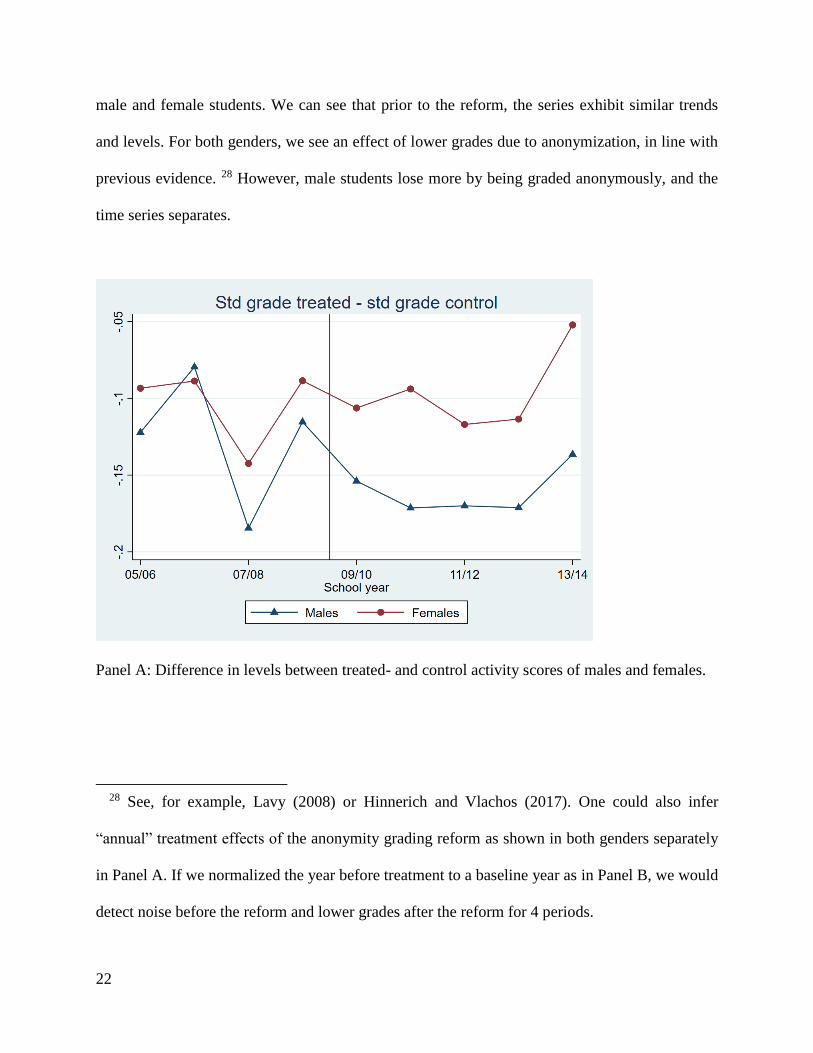
male and female students. We can see that prior to the reform, the series exhibit similar trends

and levels. For both genders, we see an effect of lower grades due to anonymization, in line with

previous evidence. 28 However, male students lose more by being graded anonymously, and the

time series separates.

Panel A: Difference in levels between treated- and control activity scores of males and females.

28 See, for example, Lavy (2008) or Hinnerich and Vlachos (2017). One could also infer

“annual” treatment effects of the anonymity grading reform as shown in both genders separately

in Panel A. If we normalized the year before treatment to a baseline year as in Panel B, we would

detect noise before the reform and lower grades after the reform for 4 periods.

23

Panel B: Difference in levels between males’ and females’ scores in the treated and control

activities

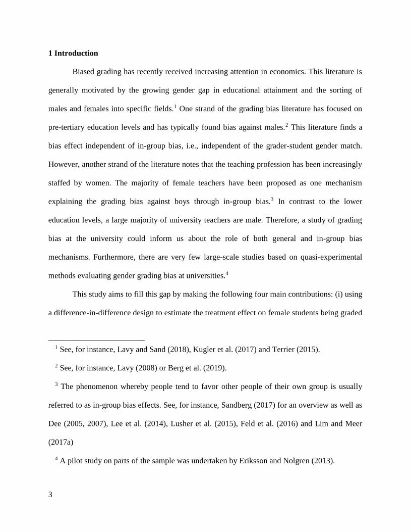
Panel C: Annual effects across the treated and non-treated groups.

24

Note: Standard errors clustered at the individual level.

Fig. 1 Impact of anonymous grading

In Panel B, we plot the difference between the male and female test scores in the control

and treatment test types over time. As a validity check, we are interested in the degree to which

the treatment effect is driven by changes in the control dimension. As shown in Panel B, both the

treated and non-treated activities exhibited a similar downward trend before the reform. This

finding indicates that the positive female grade gap is closing over time. However, after the

reform, the downward trends in the grade gap are abruptly halted in the treated activities and the

gender gaps remain rather constant for treated activities. Reassuringly, the downward trend in the

control activity gender gap continues also after the reform. Thus, we conclude that Panel A in

Fig. 1 supports the parallel trend assumption and that Panel B demonstrates that the change in the

trend of the gender gap is caused by the treated activities.

Moreover, as proposed by Angrist and Pischke (2008), we plot annual treatment effect

(𝛿1𝑡) estimates from a regression analysis of both before and after the implementation of the

reform, showing “placebo” effects before the reform and dynamic causal effects after the reform

(Fig. 1, Panel C). Panel C quantifies this difference during the post-treatment period and plots the

coefficient of the treatment effect over time. Not surprisingly, the estimates are fairly stable

around zero in the pre-treatment period and then increase in the post-treatment periods, with the

estimates being consistently positive, in contrast to the pre-treatment period. We conclude that

even if the test types may measure different skills, there is strong evidence that this does not pose

a threat to internal validity, as the parallel trends assumption seems likely to hold. There is some

evidence of a dynamically growing treatment effect, as the first year post-treatment effect is

25

smaller than that in the second year. The somewhat delayed treatment effect could be in line with

the evidence of the discussed reform implementation problems, but given the rather sizable

standard errors, we cannot rule out a stable treatment effect.

We continue with our regression results, which are presented in Table 2. Column 1

reports the results from a regression corresponding to equation (1). As observed, the anonymous

examination raises female grades relative to male grades by approximately 0.04 of a standard

deviation. For males, there is a 0.042 decrease in grades on exams (column 1, row 2), while for

females, there is an additional effect the 0.04 increase discussed above. Thus, female students’

exam scores are only slightly lowered by anonymous grading, while male students’ exam scores

are lowered to a larger extent (relative to the development of the control test type). Overall, this

finding suggests an average decrease of approximately 0.02 of a standard deviation in exam

scores due to anonymous grading, in line with previous research as discussed before.29 In column

2, we present the results from a regression corresponding to equation (1), but this time, we use

the number of course credits as weights, giving more weight to more important examinations. As

the introductory macroeconomics course is as extensive course accounting for 15 ECTS-points

and since many minor courses in the full sample are only pass or fail and thus allow limited room

for biased grading, we argue that this is an important specification for subsequent comparability

with introductory macroeconomics designs. We expect our estimates to increase when we assign

more weight to more important examinations. Indeed, the coefficient increases slightly,

indicating that the effect is larger for more important examinations. Another way to increase

29 The calculation of 0.02 is based on the assumption of 50 % female students. In fact, a DID

estimate of the effect of anonymization yields 0.018.

26

comparability with the macro exam is to use only activities with a similar ECTS weight. In

column 3, we estimate the model in equation (1) using only graded activities accounting for 15

or more ECTS points. We conclude that the estimate of 0.066 is of the same magnitude as the

weighted estimate and is highly significant. Moreover, we conclude that approximately 75 % of

the sample is still included after excluding activities with less than 15 ECTC credits.

27

Table 2. Overall gender grading bias

(1) (2) (3) (4) (5)

Full

Sample,

Using

DID

Design

Full

Sample,

Using

DID

Design

15 ECTC

Sample,

Using

DID

Design

Macro

Sample,

Using DID

Design

Macro

Sample,

Using

Before-and-

After

Design

female*after*exam 0.040*** 0.063*** 0.066*** 0.085**

(0.011) (0.011) (0.011) (0.038)

exam*after -0.042*** -0.030*** -0.035*** -0.15***

(0.0085) (0.0084) (0.0085) (0.027)

female*exam 0.023** -0.018** -0.010 -0.071**

(0.0094) (0.0087) (0.0086) (0.032)

female*after -0.046*** -0.064*** -0.061*** 0.009 0.10**

(0.0091) (0.0085) (0.0090) (0.043) (0.040)

exam -0.12*** -0.15*** -0.14*** -0.42***

(0.0073) (0.0069) (0.0067) (0.023)

female 0.11*** 0.15*** 0.14*** -0.041 -0.11***

(0.0080) (0.0070) (0.0073) (0.038) (0.037)

after -0.062*** -0.062*** -0.080*** 0.088*** -0.065**

(0.0066) (0.0060) (0.0065) (0.031) (0.027)

Constant 0.070*** 0.094*** 0.083*** 0.38*** 0.065***

(0.0057) (0.0050) (0.0053) (0.028) (0.025)

Course credits

weights

No Yes No No No

N 1830461 1830461 1349181 49700 51177

Note: Standard errors clustered at the student level. The dependent variable is the standardized

score. The period in the first three columns is from autumn 2005 to autumn 2013; in the fourth

column, the period is from spring 2008 to spring 2013; and in the fifth column, the period is from

spring 2008 to autumn 2014. In the fifth column the treatment effect is estimated by equation (4)

and thus female*after is the variable of interest.* p < 0.10, ** p < 0.05, *** p < 0.01

28

In column 4, we present the results from estimating equation 1 but where we use the

subsample from the introductory macroeconomics course.30 We observe a slightly higher

coefficient of approximately 0.085 of the standard deviation compared to the full sample, which

is more similar to the weighted estimate. However, this finding is consistent with the fact that we

see no measurement error in relation to the dependent variable and hence have no attenuation

bias, in contrast to the previous design.

Notably, the coefficient of female*𝑎𝑓𝑡𝑒𝑟, 𝛿2 in equation (1) is very close to zero (0.009)

and is far from significant at any level. This enables us to use a before-and-after design and still

obtain an unbiased estimate of 𝛿1 in this setting, as discussed in section 2.4.3. Furthermore, it

suggests that the estimated bias is not due to increased effort by female students, since

female* 𝑎𝑓𝑡𝑒𝑟 measures the change in females’ performance on multiple-choice questions in

relation to males’ performance. Arguably, any increased effort by females to answer to the essay

questions better should spill over to some degree into the multiple-choice questions. Thus, this is

evidence that female students are not exerting a different level of effort when grading is

anonymous.

The results from a before-and-after regression (estimating equation 4) are presented in

column 5. Recall that if δ2 is zero in equation (1) then female*after is the variable interests and

30 Figure A4 in the appendix shows the equivalent of the event study graph shown in Panel C

of Figure 1 but for introductory macroeconomics sample. Due to the short period of observation

before the reform, we show semester effects instead of yearly effects. Aggregating to a lower

frequency could provide very minimal guidance regarding the parallel trends before the reform.

Overall, A4 is well aligned with the results shown in Panel C of Figure 1.

29

the relevant regressor in order to estimate 𝛿1, the effect of anonymization on female grades

compared to male grades. We note that the coefficient is essentially unchanged at approximately

0.1 of the standard deviation and is still highly significant. The before-and-after design uses only

essay questions, as discussed previously, and for this test type, we are able to retrieve another

year of data that explain the increase in the number of observations between columns 4 and 5.

Table A2 in the appendix provides additional control specifications to the main estimates.

Column 1 replicates the first column in Table 2 above; however, column 2 presents the results

from a regression on the collapsed data as a time series. We note that the standard error is

essentially unchanged compared to the first column. Moreover, the fact that aggregation leaves

the estimate unchanged makes it likely that any potential compositional bias is of little

importance. In column 3, we restrict our analysis to a narrow window surrounding the reform

date (2007-2011). The effect is smaller, indicating that there is some evidence of a dynamically

growing treatment effect consistent with the evidence suggesting reform implementation

problems, but given the sizable standard errors, the effect is not statistically distinguishable when

comparing columns 1 to 3.

In column 4, we include nonparametric gender- and exam-specific trends.31 This is

possible thanks to the DDD-like identification design and adds more flexibility in how time is

allowed to affect the model. The estimate decreases slightly, though it is still close to the

coefficient in column one. Hence, the results in this column further support the credibly of our

design, as the estimated effect does not seem to be driven by unobserved trends. In column 5, we

31 In other words, we include gender*month fixed effects and treatment group (exams or

papers)*month fixed effects.

30

add department fixed effects. Thus, all time-invariant department factors are controlled for such

that some departments have a larger share of home assignments or other specific types of tests.

The estimate decreases to 0.022, which, taken at face value, may be interpreted as a large

decrease in the effects. However, as discussed by Wooldridge (2002), fixed effects

transformations “exacerbate” classical measurement errors. Thus, we argue that even though we

add department fixed effects in a setting of attenuation bias, we still retrieve a positive and

statistically significant effect, although it is somewhat attenuated. Column 5 includes individual

fixed effects, and column 6 uses only a sample of students who appear in all test-type activities

both before and after the reform, resulting in a loss of precision as we use only students who

appear in all test-type activities. Table A3 reports the same information for activities of 15 or

more ECTS credits. The pattern is rather similar, although the point estimates are larger.

Additional robustness tests are performed in Table A4 in the appendix. The first column

replicates column 1 in Table 2, column 2 excludes the department of law from the analysis

entirely, and columns 3 and 4 restrict the analysis to A-F grades and A-F grades during the

mandatory period, respectively. All of these restrictions slightly increase the coefficient. Finally,

column 5 alternates the numbers from Table A1 such that B for law students is 1, BA is 2 and

AB 3, while G is 1 and VG is 2. Reassuringly, this does not change any estimate at all likely

because we standardize each grading scheme. Thus, our results are not driven by changes in the

enumeration of grades.

A very interesting result reported by Lavy (2008) is that external graders with no personal

ties to the students grade with no bias even though they know the gender of the student. Thus,

biased grading is driven by a combination of some repeated personal interaction. Table 3

presents results based on the approximation of the number of participants in a course. Here, we

31

approximate the size by exam type, course and term. Interestingly, we observe that the effect is

visible in smaller classes but not in large classes, implying that large classes act as a de-biasing

device.

Table 3. Effect depending on the course size

(1) (2) (3)

stand. score stand. score stand. score

female*after*exam -0.0057 0.052*** 0.038***

(0.022) (0.010) (0.012)

Course participants More than 99 Less than 100 Less than median

(48)

N 548326 1282135 910550

Note: Standard errors are clustered at the student level. The dependent variable is the

standardized score.

* p < 0.10, ** p < 0.05, *** p < 0.01

As discussed in the introduction, literature documents gender differences that depend on

subjects, departments and majors.32 For example, the gender composition of teachers is likely to

vary depending on the department and major. If the main effect is driven by the in-group bias

mechanism and the fact that there are more male teachers at the university level, then it is

reasonable to expect the grading bias to vary across departments with different gender

compositions. Table 4 below divides the sample into departments with a 2/3 majority of female

teachers (Column 1), a rather gender balanced group below 2/3 to above 1/3 (Column 2) and

32 See, for example, Breda and Ly (2015) for a discussion on the literature.

32

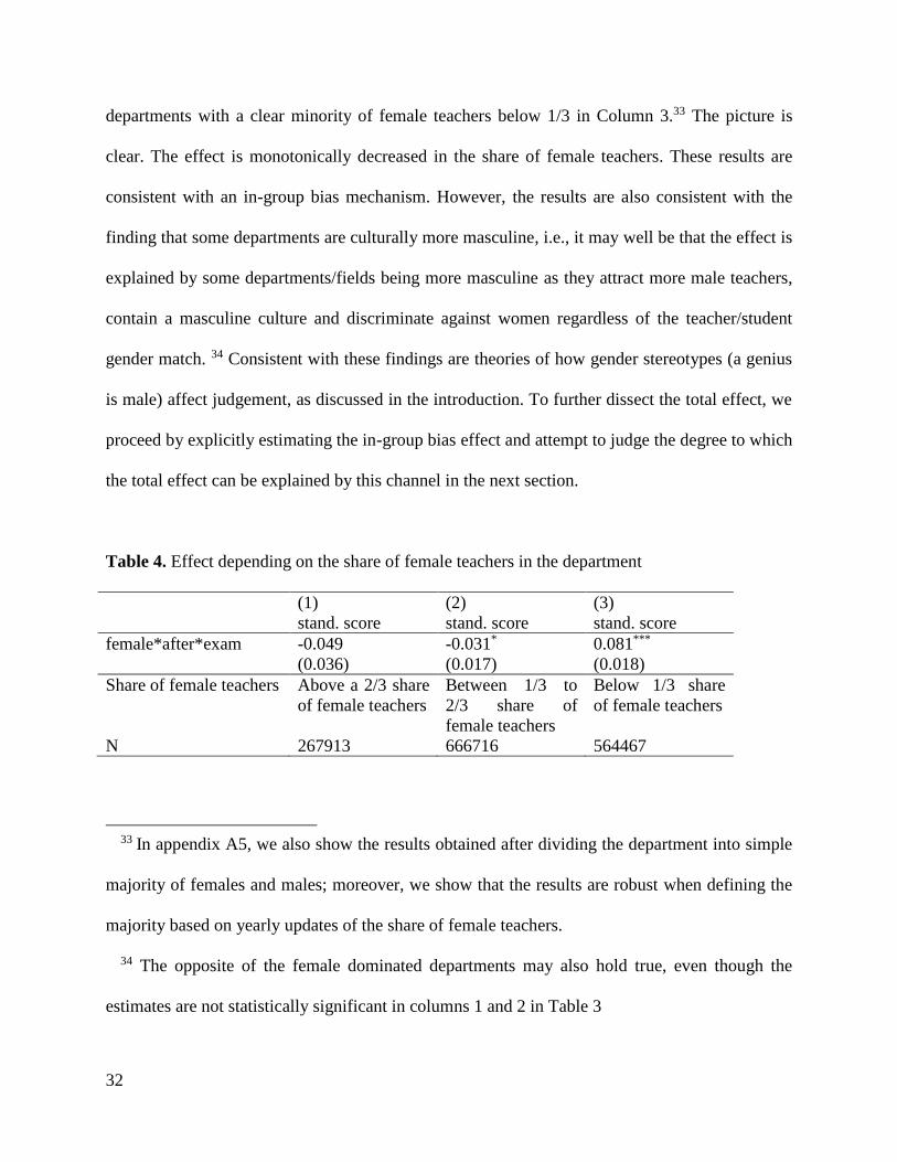
departments with a clear minority of female teachers below 1/3 in Column 3.33 The picture is

clear. The effect is monotonically decreased in the share of female teachers. These results are

consistent with an in-group bias mechanism. However, the results are also consistent with the

finding that some departments are culturally more masculine, i.e., it may well be that the effect is

explained by some departments/fields being more masculine as they attract more male teachers,

contain a masculine culture and discriminate against women regardless of the teacher/student

gender match. 34 Consistent with these findings are theories of how gender stereotypes (a genius

is male) affect judgement, as discussed in the introduction. To further dissect the total effect, we

proceed by explicitly estimating the in-group bias effect and attempt to judge the degree to which

the total effect can be explained by this channel in the next section.

Table 4. Effect depending on the share of female teachers in the department

(1) (2) (3)

stand. score stand. score stand. score

female*after*exam -0.049 -0.031* 0.081***

(0.036) (0.017) (0.018)

Share of female teachers Above a 2/3 share

of female teachers

Between 1/3 to

2/3 share of

female teachers

Below 1/3 share

of female teachers

N 267913 666716 564467

33 In appendix A5, we also show the results obtained after dividing the department into simple

majority of females and males; moreover, we show that the results are robust when defining the

majority based on yearly updates of the share of female teachers.

34 The opposite of the female dominated departments may also hold true, even though the

estimates are not statistically significant in columns 1 and 2 in Table 3

33

3.2 In-group-bias? Results of the introductory macroeconomics sample

As discussed in section 2.4.2, to estimate the in-group bias consistently, we need the

graders to be randomized. As a consequence, the background characteristics should be balanced

across the grader types. Table 5 shows the background characteristics we include as outcome

variables in the regressions using a dummy for the TA gender. If the TAs are successfully

randomly assigned to the questions, then the question characteristics and student characteristics

should be the same for male and female TAs.35 Column 1 starts by comparing the question

number between male and female correctors. Indeed, there is no significant difference between

the genders. The second column then examines the probability that a female TA corrects a

female student’s exam. If female TAs corrected questions that female students found easier to

answer, we might see that female TAs were more likely to correct answers by female students

because fewer females answered the questions corrected by male TAs. However, if anything, the

reverse seems to be true, as we find a small negative coefficient that is significant at the 10

percent level. As the coefficient is so small, approximately 1 percent with a baseline of 49

percent, we argue that it is to be interpreted as a rather precisely estimated zero that should not

cause any concern. Next, the third column looks at the age of the answering student, following a

similar reasoning as in column 2. Again, the coefficient is very small and indicates that female

TAs correct questions answered by students who are 0.08 years younger, though the estimate is

insignificant. Finally, column 4 shows the probability that females are more likely to correct

questions on retake exams. Since randomization takes place within exams, it could be the case

35 The latter is an indication that certain students do not avoid answering questions corrected

by, for instance, females.

34

that there is still sorting in gender across exams, though the fixed effects of questions, added as

controls in the appendix, take care of any such bias. Nonetheless, it is reassuring to see an

insignificant coefficient. In total, this finding shows that our in-group bias effects are likely to be

consistently estimated.

Table 5. Randomization of TAs to questions

(1) (2) (3) (4)

question number female student age of student retake

female teacher 0.083 -0.011* -0.080 -0.016

(0.44) (0.0059) (0.051) (0.068)

Constant 6.22*** 0.49*** 23.3*** 0.21***

(0.30) (0.0072) (0.064) (0.028)

N 51177 51177 51177 51177

Note: Standard errors clustered at the TA (49 clusters) and student (6 521 clusters) levels. * p <

0.10, ** p < 0.05, *** p < 0.01

As the second design also passes the internal validity check, we proceed with the

estimation. We start by estimating in-group bias in a separate model of the pre-reform period.

Due to randomization, we should estimate the in-group bias effect consistently. In column 1 in

Table 6 we estimate equation (2) and we show that being graded by one’s own sex increases

grades by 4 % of a standard deviation. In column 2-5 we include an interaction with after and

estimate equation (3). Starting with column 2, the in-group bias disappears during the period in

which the graders do not know the sex of the students due to anonymization as the interaction is

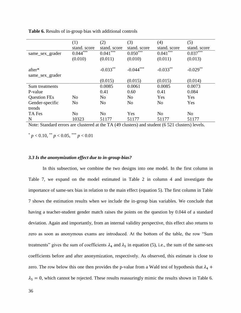
approximately the same size as the pre-reform effect. At the bottom of the table, the row “Sum

treatments” gives the sum of coefficients 𝜆4 and 𝜆5 in equation (3), i.e., the sum of the same-sex

coefficients before and after anonymization, respectively. As observed, this estimate is close to

35

zero for all columns 2-5. The row below provides the p-value of a Wald test of the hypothesis

that 𝜆4 + 𝜆5 = 0, which cannot be rejected. Thus, removing the student’s name from the exam

seems to be sufficient to prevent same-sex bias in correctional behavior. Since many suspect that

content and handwriting style may also signal gender after the anonymization reform, this is

indeed an interesting finding.36 In column 3, we add TA fixed effects, while in column 4, we add

question-specific fixed effects, and the coefficients in essence are unchanged. This finding is

reassuring as the randomization of TAs to questions seems to have worked.37 Column 5 adds

gender-specific nonparametric trends, i.e., the female student dummy multiplied by the date of

the exam fixed effects. This step was performed to ensure that the estimated same-sex effects are

not driven by any underlying trends in gender performance at the cost of not being able to

estimate the female student coefficients in Table 6. Since the in-group bias coefficients are

essentially unchanged, we conclude that this does not seem to be a concern.

36 However, Breda and Ly (2015) demonstrate that female handwriting is not easily

distinguishable from male handwriting.

37 Notably, the question-specific fixed effects are even more flexible and reliable than the TA

fixed effects.

36

Table 6. Results of in-group bias with additional controls

(1) (2) (3) (4) (5)

stand. score stand. score stand. score stand. score stand. score

same_sex_grader 0.044*** 0.041*** 0.050*** 0.041*** 0.037***

(0.010) (0.011) (0.010) (0.011) (0.013)

after*

same_sex_grader

-0.033** -0.044*** -0.033** -0.029**

(0.015) (0.015) (0.015) (0.014)

Sum treatments 0.0085 0.0061 0.0085 0.0073

P-value 0.41 0.60 0.41 0.084

Question FEs No No No Yes Yes

Gender-specific

trends

No No No No Yes

TA Fes No No Yes No No

N 10323 51177 51177 51177 51177

Note: Standard errors are clustered at the TA (49 clusters) and student (6 521 clusters) levels.

* p < 0.10, ** p < 0.05, *** p < 0.01

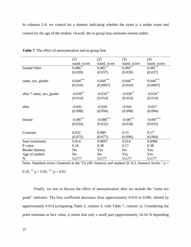
3.3 Is the anonymization effect due to in-group-bias?

In this subsection, we combine the two designs into one model. In the first column in

Table 7, we expand on the model estimated in Table 2 in column 4 and investigate the

importance of same-sex bias in relation to the main effect (equation 5). The first column in Table

7 shows the estimation results when we include the in-group bias variables. We conclude that

having a teacher-student gender match raises the points on the question by 0.044 of a standard

deviation. Again and importantly, from an internal validity perspective, this effect also returns to

zero as soon as anonymous exams are introduced. At the bottom of the table, the row “Sum

treatments” gives the sum of coefficients 𝜆4 and 𝜆5 in equation (5), i.e., the sum of the same-sex

coefficients before and after anonymization, respectively. As observed, this estimate is close to

zero. The row below this one then provides the p-value from a Wald test of hypothesis that 𝜆4 +

𝜆5 = 0, which cannot be rejected. These results reassuringly mimic the results shown in Table 6.

37

In columns 2-4, we control for a dummy indicating whether the exam is a retake exam and

control for the age of the student. Overall, the in-group bias estimates remain stable.

Table 7. The effect of anonymization and in-group bias

(1) (2) (3) (4)

stand. score stand. score stand. score stand. score

female*after 0.086** 0.082** 0.085** 0.081**

(0.039) (0.037) (0.039) (0.037)

same_sex_grader 0.044*** 0.044*** 0.044*** 0.044***

(0.010) (0.0097) (0.010) (0.0097)

after * same_sex_grader -0.030** -0.034** -0.030** -0.034**

(0.014) (0.014) (0.014) (0.014)

after -0.041 -0.028 -0.041 -0.027

(0.098) (0.094) (0.098) (0.094)

female -0.087** -0.088*** -0.087** -0.087***

(0.034) (0.032) (0.034) (0.032)

Constant 0.032 0.089 0.15 0.17*

(0.075) (0.077) (0.096) (0.094)

Sum treatments 0.014 0.0097 0.014 0.0096

P-value 0.16 0.38 0.17 0.38

Retake dummy No Yes No Yes

Age of student No No Yes Yes

N 51177 51177 51177 51177

Note: Standard errors clustered at the TA (49 clusters) and student (6 521 clusters) levels.* p <

0.10, ** p < 0.05, *** p < 0.01

Finally, we aim to discuss the effect of anonymization after we include the “same sex

grade” indicator. The bias coefficient decreases from approximately 0.010 to 0.086, altered by

approximately 0.014 (comparing Table 2, column 4, with Table 7, column 1). Considering the

point estimates at face value, it seems that only a small part (approximately 14-16 % depending

38

on the base) of the gender difference is due to in-group bias. However, we must acknowledge

that the estimate shown in Table 7 in column one is not statistically distinguishable from that

shown in Table 2 in column 4. Therefore, we conclude that the overall effect is independent of

the in-group bias mechanism and that the evidence is consistent with grading bias stemming

from other match independent factors, apart from the in-group bias effect.

4 Conclusions

There are few studies investigating biased grading at the university level. Bias at the

university level is important since it typically is not enough for students to be accepted at a

university to get a job in their field. For many jobs a master’s degree is necessary and admission

is highly competitive and based on grades from the bachelor level. Furthermore, students’ choice

of courses, and ultimately the degree they end up with, might depend on the signals they receive

from their grades in that area, as suggested by the model presented in Mechtenberg (2009). We

find evidence of overall bias against female students.38 This finding is in sharp contrast to most

of the literature studying bias before the university level, which has typically found bias against

boys or no effects.

Biased grading could in theory be explained by in-group bias. At first glance, the

reversed sign compared to studies at lower levels seems to verify this explanation, since a major

difference between the university level and lower levels of education is that a majority of the

teachers are male. We also document that the effect is driven by departments with a majority of

38 Our results suggest that the estimated effect is consistent with biased grading and is not due to

changed behavior (effort) among female students as discussed in section 3.1.

39

male teachers. However, this finding does not prove that the effect is due to in-group bias as

male-dominated departments could well exhibit cultural gender bias, which is also shared by

female teachers. To test for this explanation, we performed a second experiment in which we use

an unintended randomized experiment to provide evidence that TAs correcting exams at the

university level favor students of their own gender. As expected, we find a sizable and

significant in-group bias effect. Moreover, the in-group bias disappears when exams are graded

anonymously, indicating the effectiveness of removing identity from exams, even though

handwriting and content are otherwise left unchanged.

In addition, our unique design allows us to relate the total effect to in-group bias. When

estimating both the effect of anonymous grading on female student grades and in-group bias

mechanisms in the same model, we find that the effects are approximately independent. Thus, in

addition to graders favoring their own sex, our findings note cultural or institutional factors

independent of the student-grader gender match, such as gender stereotypes and their

consequences on grading, as discussed by previous authors, such as Bertrand et al. (2005) and

Lavy (2008). As the bias effect stemming from other factors could be as large as 10 % of a

standard deviation in our analysis and the in-group bias effect adds an additional factor, the total

gain for female students from anonymous grading at the university level is not trivial. As

acceptance into master´s programs is selective and determined by outcomes at the bachelor level,

a non-anonymous grading system could directly affect the probability of continuation into higher

studies for females. Moreover, our finding implies that an equal gender representation of

university teachers would not provide unbiased grading, at least not in the short run, as

stereotyped students will continue to be unfairly rewarded. Further, our results directly prove the

40

effectiveness of anonymous evaluation and could also potentially provide guidance, for example,

for public sector recruitment.

Acknowledgments

We thank Jan Wallanders och Tom Hedelius stiftelse and the Marianne and Marcus Wallenberg

Foundation for financial support, Karin Blomqvist and Peter Langenius for supplying us with

parts of the data material, Per Pettersson-Lidbom, Mahmood Arai, Jonas Vlachos, Peter

Skogman Thoursie, Fredrik Heyman, Joachim Tåg, David Neumark, Lena Hensvik, Björn

Öckert, seminar participants at Stockholm University and IFN, at SUDSWEC 2015, at the 2nd

Conference on Discrimination and Labour Market Research, at the gender workshop at SOFI

2019 and 31st EALE Conference 2019 Uppsala.

Funding

This research did not receive any specific grant from funding agencies in the public, commercial,

or not-for-profit sectors.

Role of the funding source

None

Declarations of interest

None

Data availability

41

Data used in this study is student level data in from LADOK. They can be asked for at

Stockholm University as they are public information. However, we cannot legally post individual

data publicly. But, we can provide original do-files that can be used, after asking for data at

Stockholm University, to replicate our results. Moreover, as treatment is on a higher level than

individual data, we can post aggregated data that clearly can be used for replication.

42

References

Angrist JD, Pischke JS. Mostly harmless econometrics: An empiricist's companion. Princeton

University Press: Princeton, New Jersey; 2008.

Arrow KJ. The theory of discrimination. In Discrimination in Labor Markets, ed. O. Ashenfelter,

A. Rees, pp. 3–33. Princeton, NJ: Princeton Univ. Press. 1973.

Berg P, Palmgren O, Tyrefors B. Gender grading bias in junior high school mathematics.

Applied Economics Letters 2019; 1-5. doi: 10.1080/13504851.2019.1646862

Bertrand M, Duflo E, Mullainathan S. How Much Should We Trust Differences-In-Differences

Estimates? The Quarterly Journal of Economics, 2004;119; 249–275.

Bertrand M, Dolly C, Mullainathan S. Implicit discrimination. The American Economic Review

2005;95; 94-98.

Breda T, Hillion M. Teaching accreditation exams reveal grading biases favor women in male-

dominated disciplines in France. Science 2016;353; 474.

Breda T, Ly ST. Do professors really perpetuate the gender gap in science? Evidence from a

natural experiment in a French higher education institution. CEE DP 138. Centre for the

Economics of Education (NJ1); 2012.

Breda T, Ly ST. Professors in core science fields are not always biased against women: Evidence

from France. American Economic Journal: Applied Economics 2015;7; 53-75.

Burgess S, Greaves E. Test Scores, subjective assessment, and stereotyping of ethnic minorities.

Journal of Labor Economics 2013;31; 535-576.

Cameron AC, Trivedi PK, Trivedi PK, Trivedi PK, Press CU, Library E, Corporation E.

Microeconometrics: Methods and applications. Cambridge University Press: Cambridge;

2005.

43

Coenen J, Van Klaveren C. Better test scores with a same-gender teacher? European

Sociological Review 2016;32; 452-464.

Conley TG, Taber CR. Inference with “difference in differences” with a small number of policy

changes. The Review of Economics and Statistics 2011;93; 113-125.

Cornwell C, Mustard D, Van Parys J. Noncognitive skills and the gender disparities in test scores

and teacher assessments: Evidence from primary school. Journal of Human Resources

2013;48; 236-264.

Dee TS. A teacher like me: Does race, ethnicity, or gender matter? The American Economic

Review 2005;95; 158-165.

Dee TS. Teachers and the gender gaps in student achievement. The Journal of Human Resources

2007;42; 528-554.

Donald SG, Lang K. Inference with difference-in-differences and other panel data. The Review

of Economics and Statistics 2007;89; 221-233.

Ebenstein, Avraham, Victor Lavy, and Sefi Roth. 2016. "The Long-Run Economic

Consequences of High-Stakes Examinations: Evidence from Transitory Variation in

Pollution." American Economic Journal: Applied Economics, 8 (4): 36-65.

Elmore KC, Luna-Lucero M. Light bulbs or seeds? How metaphors for ideas influence

judgments about genius. Social Psychological and Personality Science 2017;8; 200-208.

Eriksson A, Nolgren J. Effekter av anonym rättning på tentamensbetyg vid Stockholms

universitet – En empirisk studie i hur kvinnors och mäns betyg påverkas av anonym

rättning. Mimeo Stockholm University: Sweden; 2013.

Feld J, Salamanca N, Hamermesh DS. Endophilia or exophobia: Beyond discrimination. The

Economic Journal 2016;126; 1503-1527.

44

Goldin C, Rouse C. Orchestrating impartiality: The impact of "blind" auditions on female

musicians. The American Economic Review 2000;90; 715-741.

Hanna RN, Linden LL. Discrimination in grading. American Economic Journal: Economic

Policy 2012;4; 146-168.

Hinnerich BT, Höglin E, Johannesson M. Are boys discriminated in Swedish high schools?

Economics of Education Review 2011;30; 682-690.

Hinnerich BT, Höglin E, Johannesson M. Discrimination against students with foreign

backgrounds: Evidence from grading in Swedish public high schools. Education

Economics 2015;23; 660-676.

Hinnerich BT, Vlachos J. The impact of upper-secondary voucher school attendance on student

achievement. Swedish evidence using external and internal evaluations. Labour

Economics 2017;47; 1-14.

Hoffmann F, Oreopoulos P. A professor like me: The influence of instructor gender on college

achievement. The Journal of Human Resources 2009;44; 479-494.

Holmlund, Helena, and Krister Sund. 2008. “Is the Gender Gap in School Performance Affected

by the Sex of the Teacher?” Labour Economics 15 (1): 37–53

Katz LF. Wage subsidies for the disadvantaged (No. w5679). National Bureau of Economic

Research: Cambridge; 1996.

Kiss D. Are immigrants and girls graded worse? Results of a matching approach. Education

Economics 2013;21; 447-463.

Kugler AD, Tinsley CH, Ukhaneva O. Choice of majors: Are women really different from men?

(No. w23735). National Bureau of Economic Research: Cambridge; 2017.

45

Lavy V. Do gender stereotypes reduce girls' or boys' human capital outcomes? Evidence from a

natural experiment. Journal of public Economics 2008;92; 2083-2105.

Lavy, V. and E. Sand (2018). On The Origins of the Gender Human Capital Gap: Short and

Long Term Effect of Teachers’ Stereotypes. Journal of Public Economics. 167, 263–279.

Lavy, V., E. Sand, and M. Shayo, Charity Begins at Home (and at School): Effects of Religion

Based Discrimination in Education. Working Paper no. 24922, NBER, Cambridge, MA,

2018.

Lavy, V. and R. Megalokonomou (2019). Persistency in Teachers' Grading Bias and Effects on

Longer-Term Outcomes: University Admissions Exams and Choice of Field of Study.

Working Paper no. 26021, NBER, Cambridge, MA, 2019.

Lee S, Turner LJ, Woo S, Kim K. All or nothing? The impact of school and classroom gender

composition on effort and academic achievement (No. w20722). National Bureau of

Economic Research: Stanford, CA; 2014.

Lim J, Meer J. The impact of teacher-student gender matches: Random assignment evidence

from South Korea. Journal of Human Resources 2017a;52; 1215-7585R1211.

Lim J, Meer J. Persistent effects of teacher-student gender matches (No. w24128). National

Bureau of Economic Research: Cambridge; 2017b.

Lindahl E. Does gender and ethnic background matter when teachers set school grades?

Evidence from Sweden, Working Paper, 25. Institute for Labour Market Policy

Evaluation (IFAU): Uppsala; 2007.

Lusher L, Campbell D, Carrell S. TAs like me: Racial interactions between graduate teaching

assistants and undergraduates (No. w21568). National Bureau of Economic Research:

Cambridge; 2015.

46

Mechtenberg L. Cheap talk in the classroom: How biased grading at school explains gender

differences in achievements, career choices and wages. The Review of Economic Studies

2009;76; 1431-1459.

Pettersson-Lidbom P, Thoursie PS. Temporary disability insurance and labor supply: Evidence

from a natural experiment. The Scandinavian Journal of Economics 2013;115; 485-507.

Phelps ES. The statistical theory of racism and sexism. The American Economic Review

1972;62; 659-661.

Sandberg A. Competing identities: A field study of in‐group bias among professional evaluators.

The Economic Journal 2017;128; 2131-2159.

Sprietsma M. Discrimination in grading: Experimental evidence from primary school teachers.

Empirical Economics 2013;45; 523-538.

Stockholm University. 2010. Införande av anonyma tentamina vid Stockholms Universitet.

http://www.su.se/polopoly_fs/1.26344.1320939789!/Beslut_om_anonyma_tentamina_vid

_Stockholms_universitet_Dnr_SU_459_2690_08.pdf.

Terrier C. Giving a little help to girls? Evidence on grade discrimination and its effect on

students' achievement. CEP Discussion Paper 1341, March 2015. London School of

Economics: London; 2015.

Wooldridge JM. Econometric analysis of cross section and panel data. MIT Press: Cambridge;

2002.

Yelowitz AS. The medicaid notch, labor supply, and welfare participation: Evidence from

eligibility expansions. The Quarterly Journal of Economics 1995;110; 909-939.

47

Appendix

The procedure underlying the correction of exams in the introductory macroeconomics course

Each of the 7 questions is corrected by a TA, usually a separate TA for each question,

although there are some exceptions, particularly for retakes. Before the correcting process starts,

all TAs, the lecturer and the course coordinator assemble and discuss in broad terms how many

points should be given for different answers. At the end of this meeting, the allocation of TAs to

questions 4-10 is determined by lottery.

Once this process is completed, each TA receives approximately 500 answers to the

questions assigned to him or her (approximately 100 if it is a retake) and is then left with the

daunting task of correcting each answer as fairly as possible. Swedish law requires that students

know the results within 3 weeks the latest, and thus, graders have less time than this to actually

complete the correction. Hence, after approximately 2-2.5 weeks, the TAs and the course

coordinator gather once more to look at students 1-2 points below a higher grade and then try to

move them above the threshold. Students are still anonymous in this stage as of the fall of 2009.

After this, the results are posted, and a session is announced, during which the template that

everyone agreed upon during the first meeting is presented to the students. At the end of this

session, students are allowed to make complaints directly in person to the TAs, which usually

leads to a 1-2 point increase to 1-2 students at most. It is important to note that we generally have

data on the students’ points immediately after they have been determined by the TAs only; thus,

they are not subject to bias from anyone other than the TA. The exceptions are one exam from

the fall of 2009 and one question on another exam.

Reduction of DD to before and after

48

It is stated in section 2.4.2 that if 𝛿2 = 0, we can consistently estimate the DD effect

using a simple before-and-after framework. Equations (4)-(8) illustrate how this works in our

simple regression framework, where 𝑌j=1,t=1,f=1 is the standardized test score for females in the

treated group in the post-treatment period, 𝑌101 is the standardized test score for females in the

treated group in the pre-treatment period, 𝑌110 is the standardized test score for males in the

treated group in the post-treatment period, and 𝑌100 is the standardized test score for males in the

treated group in the pre-treatment period. Formally, we can write this as follows:

(6) 𝑌𝑗=1,𝑡=1,𝑓=1 = 𝛿0 + 𝛿1𝑡𝑟𝑒𝑎𝑚𝑒𝑛𝑡 + 𝛿2𝑎𝑓𝑡𝑒𝑟𝑡=1 ∗ 𝑓𝑒𝑚𝑎𝑙𝑒𝑓=1 + 𝛿3𝑓𝑒𝑚𝑎𝑙𝑒𝑓=1 ∗

𝑒𝑥𝑎𝑚𝑗=1 + 𝛿4𝑎𝑓𝑡𝑒𝑟𝑡=1 ∗ 𝑒𝑥𝑎𝑚 + 𝛿5𝑎𝑓𝑡𝑒𝑟𝑡=1 + 𝛿6𝑓𝑒𝑚𝑎𝑙𝑒𝑓=1 + 𝛿7𝑒𝑥𝑎𝑚𝑗=1 + 휀111

= 𝛿0 + 𝛿1 + 𝛿2 + 𝛿3 + 𝛿4 + 𝛿5 + 𝛿6 + 𝛿7 + 휀111

(7) 𝑌101 = 𝛿0 + 𝛿3 + 𝛿6 + 𝛿7 + 휀101

(8) 𝑌110 = 𝛿0 + 𝛿4 + 𝛿5 + 𝛿7 + 휀110

(9) 𝑌100 = 𝛿0 + 𝛿7 + 휀100

Thus, we obtain the difference:

(10) (𝑌111 − 𝑌101) − (𝑌110 − 𝑌100) = ( 𝛿0 + 𝛿1 + 𝛿2 + 𝛿3 + 𝛿4 + 𝛿5 + 𝛿6 + 𝛿7 + 휀111 − 𝛿0 −

𝛿3 − 𝛿6 − 𝛿7 − 휀101) − (𝛿0 + 𝛿4 + 𝛿5 + 𝛿7 + 휀110 − 𝛿0 − 𝛿7 − 휀100)

= 𝛿1 + 𝛿2 + 휀111 − 휀101 + 휀110 − 휀100

Thus, if 𝛿2 = 0, we can estimate the true treatment effect 𝛿1 using equation (8), which is

the simple before and after in gender difference in the treatment group, by a regression

corresponding to equation (2).

Figures and tables

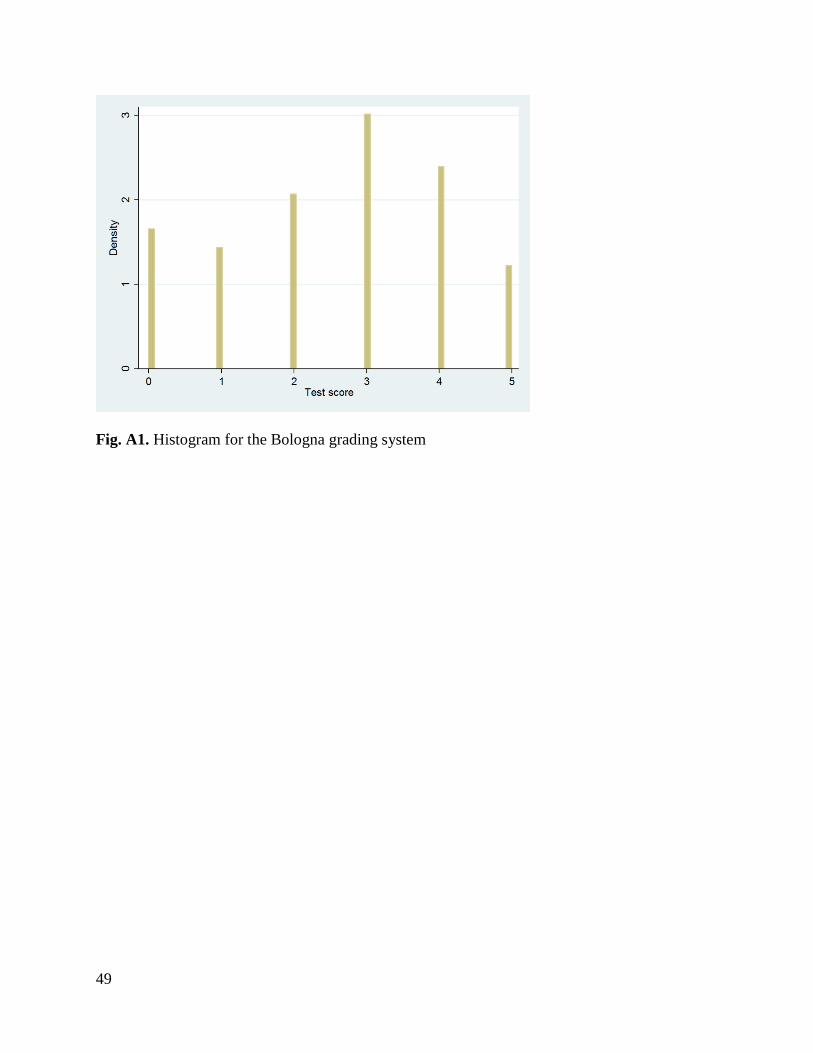
49

Fig. A1. Histogram for the Bologna grading system

50

Fig. A2. Histogram for the department of law grading system

51

Fig. A3. Histogram for the original grading system

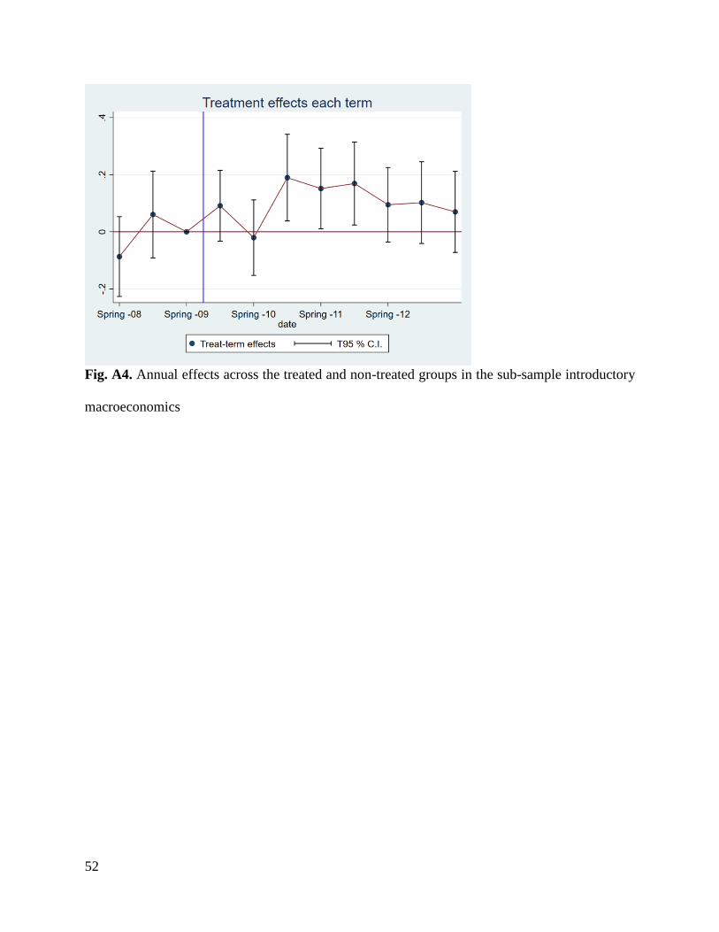
52

Fig. A4. Annual effects across the treated and non-treated groups in the sub-sample introductory

macroeconomics

53

Tables

Table A1. Grades and their values

Grades A-

F

Values Grades AB-

U

Values Grades

VG-U

Values

A 5 AB 5 VG 5

B 4 BA 3.33 G 2.5

C 3 B 1.67 U 0

D 2 U 0 - -

E 1 - - - -

F/Fx 0 - - - -

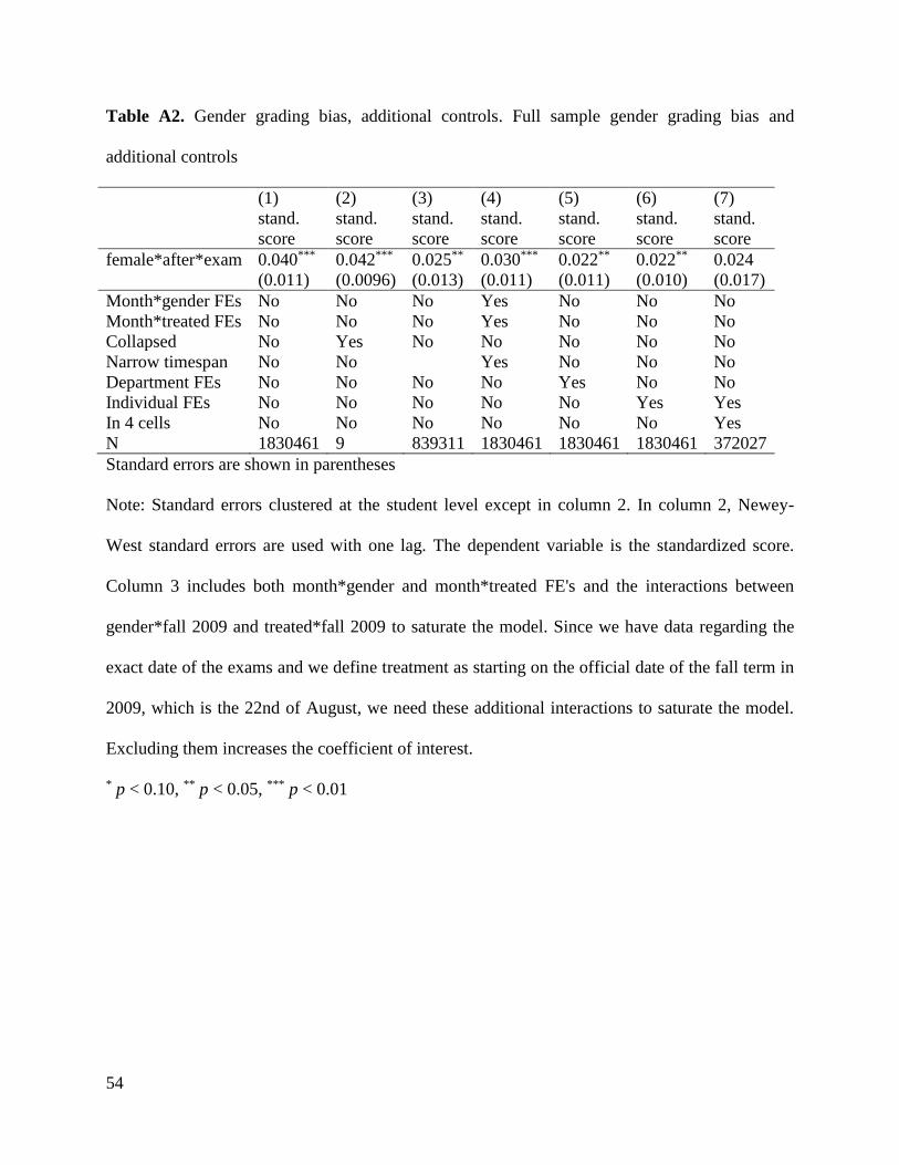
54

Table A2. Gender grading bias, additional controls. Full sample gender grading bias and

additional controls

(1) (2) (3) (4) (5) (6) (7)

stand.

score

stand.

score

stand.

score

stand.

score

stand.

score

stand.

score

stand.

score

female*after*exam 0.040*** 0.042*** 0.025** 0.030*** 0.022** 0.022** 0.024

(0.011) (0.0096) (0.013) (0.011) (0.011) (0.010) (0.017)

Month*gender FEs No No No Yes No No No

Month*treated FEs No No No Yes No No No

Collapsed No Yes No No No No No

Narrow timespan No No Yes No No No

Department FEs No No No No Yes No No

Individual FEs No No No No No Yes Yes

In 4 cells No No No No No No Yes

N 1830461 9 839311 1830461 1830461 1830461 372027

Standard errors are shown in parentheses

Note: Standard errors clustered at the student level except in column 2. In column 2, Newey-

West standard errors are used with one lag. The dependent variable is the standardized score.

Column 3 includes both month*gender and month*treated FE's and the interactions between

gender*fall 2009 and treated*fall 2009 to saturate the model. Since we have data regarding the

exact date of the exams and we define treatment as starting on the official date of the fall term in

2009, which is the 22nd of August, we need these additional interactions to saturate the model.

Excluding them increases the coefficient of interest.

* p < 0.10, ** p < 0.05, *** p < 0.01

55

Table A3. Gender grading bias and additional controls. Sample of activities of 15 or more ECTS

points.

(1) (2) (3) (4) (5) (6) (7)

stand.

score

stand.

score

stand.

score

stand.

score

stand.

score

stand.

score

stand.

score

female*after*exam 0.066*** 0.069*** 0.040*** 0.053*** 0.051*** 0.036*** 0.035*

(0.011) (0.015) (0.014) (0.011) (0.011) (0.011) (0.020)

Month*gender FEs No No No Yes No No No

Month*treated FEs No No No Yes No No No

Collapsed No Yes No No No No No

Narrow timespan No No Yes No No No No

Department FEs No No No No Yes No No

Individual FEs No No No No No Yes Yes

In 4 cells No No No No No No Yes

N 1349181 9 620968 1349181 1349181 1349181 232038

Standard errors are shown in parentheses

Note: Standard errors are clustered at the student level, except for in column 2. In column 2,

Newey-West standard errors are used with one lag. The dependent variable is the standardized

score. Column 3 includes both month*gender and month*treated FE's and the interactions

between gender*fall 2009 and treated*fall 2009 to saturate the model. Since we have data

regarding the exact date of the exams and we define treatment as starting on the official date of

the fall term in 2009, which is the 22nd of August, we need these additional interactions to

saturate the model. Excluding these interactions increases the coefficient of interest.

* p < 0.10, ** p < 0.05, *** p < 0.01

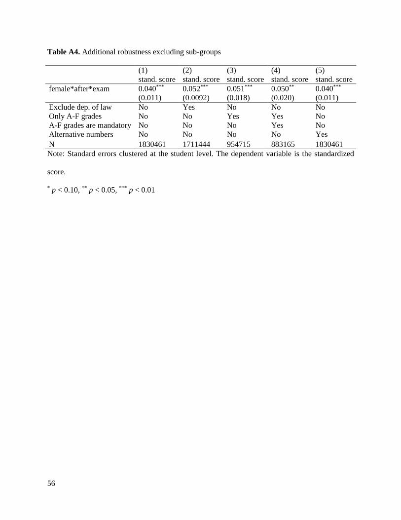
56

Table A4. Additional robustness excluding sub-groups

(1) (2) (3) (4) (5)

stand. score stand. score stand. score stand. score stand. score

female*after*exam 0.040*** 0.052*** 0.051*** 0.050** 0.040***

(0.011) (0.0092) (0.018) (0.020) (0.011)

Exclude dep. of law No Yes No No No

Only A-F grades No No Yes Yes No

A-F grades are mandatory No No No Yes No

Alternative numbers No No No No Yes

N 1830461 1711444 954715 883165 1830461

Note: Standard errors clustered at the student level. The dependent variable is the standardized

score.

* p < 0.10, ** p < 0.05, *** p < 0.01

57

Table A5. Effect depending on the share of female teachers in the department

(1) (2) (3) (4)

stand. score stand. score stand. score stand. score

female*after*exam -0.012 0.037*** -0.028 0.055***

(0.021) (0.014) (0.023) (0.015)

Share female

teachers

Majority female

teachers 2008

Majority male

teachers 2008

Majority female

teachers

Majority male

teachers

N 673765 1100479 582285 916811

Standard errors are shown in parentheses. Note: Standard errors are clustered at the student level.

The dependent variable is the standardized score. * p < 0.10, ** p < 0.05, *** p < 0.01