Memetic Comp. (2013) 5:275–293DOI 10.1007/s12293-013-0119-1

REGULAR RESEARCH PAPER

Distributed mixed variant differential evolution algorithmsfor unconstrained global optimization

G. Jeyakumar · C. Shunmuga Velayutham

Received: 28 June 2012 / Accepted: 17 May 2013 / Published online: 2 July 2013© Springer-Verlag Berlin Heidelberg 2013

Abstract This paper proposes a novel distributed differ-ential evolution algorithm called Distributed Mixed VariantDifferential Evolution (dmvDE). To alleviate the time con-suming trial-and-error selection of appropriate DifferentialEvolution (DE) variant to solve a given optimization prob-lem, dmvDE proposes to mix effective DE variants withdiverse characteristics in a distributed framework. The nov-elty of dmvDEs lies in mixing different DE variants in anisland based distributed framework. The 19 dmvDE algo-rithms, discussed in this paper, constitute various propor-tions and combinations of four DE variants (DE/rand/1/bin,DE/rand/2/bin, DE/best/2/bin and DE/rand-to-best/1/bin)as subpopulations with each variant evolving indepen-dently but also exchanging information amongst others toco-operatively enhance the efficacy of the distributed DEas a whole. The dmvDE algorithms have been run on a setof test problems and compared to the distributed versionsof the constituent DE variants. Simulation results show thatdmvDEs display a consistent overall improvement in perfor-mance than that of distributed DEs. The best of dmvDE algo-rithms has also been benchmarked against five distributeddifferential evolution algorithms. Simulation results reiteratethe superior performance of the mixing of the DE variantsin a distributed frame work. The best of dmvDE algorithmsoutperforms, on average, all five algorithms considered.

G. Jeyakumar (B) · C. Shunmuga VelayuthamDepartment of Computer Science and Engineering, Amrita Schoolof Engineering, Amrita Vishwa Vidyapeetham University,Coimbatore, Indiae-mail: g_jeyakumar@cb.amrita.edu

C. Shunmuga Velayuthame-mail: cs_velayutham@cb.amrita.edu

Keywords Evolutionary algorithm · Differentialevolution · Distributed differential evolution · Mixingdifferential evolution variants · Distributed mixed variantDE

1 Introduction

Differential evolution (DE), proposed by Storn and Pricein 1995 [30], is a simple yet powerful evolutionary algo-rithm (EA) capable of handling non-differentiable, non-linearand multimodal objective functions [25,31,26,33]. DE isa population-based stochastic global optimizer employingmutation, recombination and selection operators like otherEAs. However unlike other EAs, DE employs a differen-tial mutation operation based on the distribution of parentsolutions in the current population, coupled with recombi-nation with a predetermined target vector to generate a trialvector followed by a one-to-one greedy selection betweenthe trial vector and the target vector. Depending on the waythe parent solutions are perturbed to generate a trial vector,there exists many trial vector generation strategies and con-sequently many DE variants.

The conceptual and algorithmic simplicity, high conver-gence characteristics and robustness of DE have attractedmany researchers, who are working on its improvement,resulting in multitude of DE variants. Nevertheless, so far,no single DE variant has turned out to be best for all prob-lems which is quiet understandable with regard to the NoFree Lunch Theorem [39]. Therefore, successful solving ofan optimization problem requires a trial-and-error searchingof appropriate DE variant. Few research attempts have beenundertaken [27,23] to alleviate this problem.

In this paper, we propose to mix effective DE variantsin a distributed framework to result in a novel distributed

123

276 Memetic Comp. (2013) 5:275–293

differential evolution algorithm called distributed mixed vari-ant differential evolution (dmvDE). The distributed mixedvariants DE algorithms constitute various proportions andcombinations of top performing DE variants (out of 14 clas-sical DE variants considered in our earlier work [14,15]) assubpopulations with each variant evolving independently butalso exchanging information among others to co-operativelyenhance the efficacy of the DE algorithm as a whole. The 19dmvDE algorithms, discussed in this paper, have been bench-marked, on unconstrained global optimization problems,against distributed differential evolution (dDE) implemen-tation of constituent DE variants as well as against five dis-tributed differential evolution algorithms from the literature.The simulation results validate the performance enhance-ment arising out of the mixing of DE variants in a distributedframework.

This paper has been organized as follows: Section 2 pro-vides the introductory details of DE algorithm. Section 3discusses related works. Section 4 describes the proposeddistributed mixed variant differential evolution algorithm.Section 5 describes the design of experiments followed byanalysis of simulation results in Sect. 6 and benchmarkingbest of dmvDEs against existing algorithms in literature inSect. 7. Finally, Sect. 8 concludes the paper.

2 Differential evolution

DE algorithm aims at exploring the search space by samplingat multiple, randomly chosen NP (number of candidate solu-tions in the population) D-dimensional parameter vectors(population of initial points), so-called individuals, whichencode the candidate solution Xi,G = {x1

i,G , . . . , x Di,G}, i =

1, . . . , NP (for initial population Xi,0 = {x1i,0, . . . , x D

i,0}).The initial population should sufficiently cover the searchspace as much as possible, by uniformly randomizing indi-viduals, for better exploration. After population initializationan iterative process is started and at each iteration (genera-tion) a new population is produced until a stopping criterionis satisfied.

At each generation, DE employs the differential mutationoperation to produce a mutant vector, Vi,G ={v1

i,G , . . . , vDi,G},

with respect to each individual, the so called target vectorXi,G , in the current population. The mutant vector is cre-ated using the weighted difference of parent solutions inthe current population. A number of differential mutationstrategies have been proposed in the literature that primarilydiffers in the way the mutant vector is created. Along withthe strategies came a notation scheme to classify the variousDE-variants. The notation is defined by DE/a/b/c where ‘a’denotes the base vector or the vector to be perturbed (whichcan be a random vector, best vector or sum of target vec-

tor and weighted vector difference between random and bestvectors/random vectors/best vectors); ‘b’ denotes the num-ber of vector differences used for perturbation (which can beone or two pairs); and ‘c’ denotes the crossover scheme used(which can be binomial or exponential) between the mutantvector Vi,G and the target vector Xi,G to create a trial vectorUi,G = {u1

i,G , . . . , u Di,G}.

The seven commonly used mutation strategies are enu-merated as follows:

1. DE/rand/1

Vi,G = Xri1,G

+ F.(

Xri2,G − Xri

3,G

)(1)

2. DE/best/1

Vi,G = Xbest,G + F.(

Xri1,G

− Xri2,G

)(2)

3. DE/rand/2

Vi,G = Xri1,G

+ F.(

Xri2,G − Xri

3,G+ Xri

4,G− Xri

5,G

)

(3)

4. DE/best/2

Vi,G = Xbest,G +F.(

Xri1,G

−Xri2,G +Xri

3,G−Xri

4,G

)

(4)

5. DE/current-to-rand/1

Vi,G = Xi,G +K .(

Xri3,G

−Xi,G

)+F.

(Xri

1,G−Xri

2,G

)

(5)

6. DE/current-to-best/1

Vi,G = Xi,G +K .(Xbest,G −Xi,G

)+F.(

Xri1,G

−Xri2,G

)

(6)

7. DE/rand-to-best/1

Vi,G = Xri3,G

+K .(

Xbest,G −Xri3,G

)

+F.(

Xri1,G

−Xri2,G

)(7)

where Xbest,G denotes the best parent vector in the currentpopulation, F and K commonly known as the scaling fac-tors or amplification factors are positive real numbers thatcontrols the rate of evolution of the population. The indicesr i

1, r i2, r i

3, r i4, r i

5, i ∈ 1, . . . , NP are randomly generatedanew for each mutant vector and are mutually exclusiver i

1 �= r i2 �= r i

3 �= r i4 �= r i

5 �= i .

123

Memetic Comp. (2013) 5:275–293 277

After the differential mutation strategy, DE then uses acrossover operation in which the mutant vector Vi,G mixeswith target vector Xi,G and generates a trial vector Ui,G oroffspring. The two frequently used crossover schemes arebinomial (uniform) crossover and exponential crossover. Thebinomial crossover is defined as follows.

u ji.G =

{v

ji,G , if (rand j [0, 1) ≤ Cr ) ∨ ( j = jrand)

X ji,G , otherwise

(8)

where Cr ∈ (0, 1) (crossover probability) is a user-specifiedconstant and rand j [0, 1) is the j th evaluation of uniformrandom number generator. jrand ∈ 1, . . . , D is a randomparameter index, chosen once for each i to make sure that atleast one parameter is always selected from the mutant vectorVi,G . The exponential crossover is defined as follows

u ji,G =

{v

ji,G , for〈n〉D, 〈n + 1〉D, . . . , 〈n + L − 1〉D

x ji,G , for all other j ∈ [1, D]

(9)

where the acute brackets 〈〉D denote modulo functions withmodulus D, the starting index n is a randomly selected inte-ger in the range [1,D], and the integer L , which denotes thenumber of parameters that are going to be exchanged betweenthe mutant and trial vectors, is drawn from the same rangewith the probability Cr .

After the mutation and crossover operations, a one-to-oneknockout competition between the target vector Xi,G andits corresponding trial vector Ui,G based on the objectivefunction values decides the survivor, among the two, for thenext generation. The greedy selection scheme is defined asfollows (assuming a minimization problem without the lossof generality).

Xi,G+1 ={

Ui,G , if f (Ui,G) ≤ f (Xi,G)

Xi,G , otherwise(10)

The above three steps of differential mutation, crossover,followed by selection marks the end of one DE generation.These steps are repeated generation after generation until astopping criterion is satisfied.

With the above given classical mutation strategies andtwo crossover schemes, there are 14 possible, so calledclassical variants of DE viz. DE/rand/1/bin, DE/rand/1/exp,DE/best/1/bin, DE/best/1/exp, DE/rand/2/bin, DE/rand/2/exp,DE/best/2/bin, DE/best/2/exp, DE/current-to-rand/1/bin, DE/current-to-rand/1/exp, DE/current-to-best/1/bin, DE/current-to-best/1/exp, DE/rand-to-best/1/bin and DE/rand-to-best/1/exp.

3 Related works

There has been several research works in the field of parallelDE and island based distributed DE. The investigation on

DE parallelization has been carried out way back in 1999 in[19]. Zaharie and Petcu [41] proposed coarse-grained par-allelization of adaptive differential evolution with randomconnection topology. A distributed DE with ring topologyand best solution emigrating to random solution of neigh-bor subpopulation has been proposed in [32]. Pavlidis et al.[24] employed the distributed DE proposed in [32] to trainan artificial neural network. Similarly, a distributed DE withring topology has been employed in [18] to train a neuralnetwork. Continuing this application trend, [29] attemptedparallelizing DE for solving a medical imaging problem. Insimilar line [5–7] employed a distributed DE to solve imageregistration problem.

Subsequently, the research works in distributed DE havefocused more towards proposing novel parametric schemes.Two new enhancements to parallel differential evolution areproposed in [38]. Apolloni et al. [1] proposed migration basedon probabilistic criterion. A distributed evolution employingscale factor inheritance, a novel self-adaptive scheme hasbeen proposed in [35]. Weber et al. [36] studied the combi-nation of structured populations and variable scale factorson three different variants of distributed DE proposed in[1,29,32]. The same algorithm has been chosen, but mod-ified to employ a DE with exponential crossover in [37], toanalyze the effect of combining a varying scale factor andthe exponential crossover on large scale problems.

Almost all of the works described above concern researchissues regarding distributed DE but with same variants onevery island. The possibility of mixing various DE variantsin distributed framework has not been addressed. Howeverthere has been very few research works attempted in thisdirection. A variant of DE called SaDE has been proposedin [27] which is essentially a serial DE which adapts dif-ferent DE strategies in a pool of predetermined strategies atdifferent phases of DE evolution. To alleviate trial-and-errorsearch of appropriate DE variants for a given problem, SaDEemploys a pool of effective DE strategies. At every pointof evolution only one strategy chosen, based on its prob-ability of generating promising solutions previously, fromthe strategy pool is allowed to generate target vector. UnlikeSaDE, which employs competing DE strategies in a pool ofvariants, the proposed dmvDE co-operatively mixes effec-tive DE variants in an island based distributed framework.While in SaDE every DE strategy competes to produce a trialvector, all constituent DE strategies in dmvDE contribute bygenerating their trial vectors and co-operate by exchangingtheir best of solution vectors once in a while amongst oth-ers to enhance the efficacy of dmvDE as a whole. This veryco-operative characteristic of dmvDE makes it a simple buteffective DE as against SaDE (inspite of it serial in nature)which employs success and failure memories and stochas-tic universal selection method to choose the winner strategyamong the competing strategies in the pool.

123

278 Memetic Comp. (2013) 5:275–293

Weber et al. [34] proposed Distributed DE withexplorative–exploitative populations (DDE-EEPF) where aDE variant has been employed in one family for explorationand in other family of subpopulation for exploitation of thedecision space. Although distributed DE variants have notbeen mixed, this work attempts to mix DE variants with dif-ferent characteristics to enhance the efficacy as a whole. Inthis paper we propose distributed mixed variant DE (dmvDE)class of algorithms in its barebones form.

The hybridization of metaheuristics has been attemptedby many researchers. In DE’s perspective, hybridizationhas been achieved with particle swarm optimization [11,21,17,22], ant colony optimization [3,42], bacterial foragingoptimization [2], artificial immune system [10], simulatedannealing [4][13] etc. However the possibility of hybridiz-ing/mixing different DE variants in an island based distrib-uted framework has not yet been addressed. Although thevery idea of co-operative evolution by employing geneticalgorithms with different configurations in each island hasbeen attempted in [12].

4 Distributed mixed variant differential evolution(dmvDE)

Our earlier study which involved empirical performanceanalysis of above mentioned 14 DE variants on 14 uncon-strained test functions grouped by their modality and decom-posability identified the DE variants viz. DE/rand/1/bin,DE/rand/2/bin, DE/best/2/bin and DE/rand-to-best/1/bin aseffective variants [14,15]. In this paper, we initially imple-ment the island based distributed DE (dDE) framework forthe above mentioned four DE variants whereby the popula-tion is partitioned into small subsets (islands) each, com-prising the same DE variant, evolving independently butalso exchanging (migrating) solutions among them. The effi-cacy of, thus implemented, four dDE variants is tested on 14unconstrained test functions. The island based dDE is char-acterized by the following parameters—number of islands ni,number of migrants nm, migration frequency mf, the migra-tion topology mt that decides which islands can send (orreceive) the migrants, selection policy sp that decides whatindividual migrate and the replacement policy rp that deter-mines which individual(s) the migrant(s) replace.

Given an optimization problem, searching for the appro-priate DE variant and tuning its associated parameter val-ues is a general practice followed for successfully solvingthe problem. This is because different DE variants performwith different efficacies when solving different optimizationproblems. Rather than searching for appropriate variant orimproving individual variants to solve the given optimiza-tion problem, we propose to mix effective DE variants withdiverse characteristics in a distributed framework.

The proposed distributed mixed variant class of DE algo-rithms (dmvDEs) is, however, different from the abovesaid dDE in that the islands are populated by differentDE variant. The distributed mixed variant DE algorithmsconstitute various proportions (among islands) and combina-tions (as to which DE variants mix with each other) of effec-tive variants with diverse characteristics (DE/rand/1/bin,DE/rand/2/bin, DE/best/2/bin and DE/rand-to-best/1/binidentified from [14,15]) as subpopulations with each vari-ant evolving independently but also exchanging informationamongst others to co-operatively enhance the efficacy of thedistributed DE as a whole. The novelty of dmvDEs lies inmixing different DE variants in an island based distributedframework.

The empirical analysis of dmvDE algorithms necessitatesthe implementation of all possible combinations and propor-tions of identified four DE variants. Accordingly, we haveimplemented 19 dmvDEs of which 18 are obtained by mix-ing two of four DE variants in three possible proportions (1:3,2:2 and 3:1) and the 19th one is obtained by distributing thefour DE variants in each island. The experimental parameterslike number of islands, migration frequency and policy etc,for empirical analysis of 19 dmvDE’s were adopted from thatof dDE. Since our analysis considered the island size of 4, werestricted the mixing between variants to be not more than 2.

For the sake of brevity, we adopt the following nota-tional scheme henceforth in this paper. We use dmv/v1v2/x:ywhere dmv stands for distributed mixed variant, v1 and v2are the variants to be mixed and x, y respectively representsthe number of sub populations the former and later variantsoccupy. The following acronym has been used for variants:r1-rand/1/bin, r2-rand/2/bin, b2-best/2/bin and rtb1-rand-to-best/1/bin. The notation dmv/all, is an exception, whichrepresents all four variants occupying one subpopulationeach. Table 1 lists different mixing schemes that give 19dmvDEs. Figure 1 depicts the all possible combinationsbetween best/2/bin and rand/1/bin variants as well as thedmv/all by the way of an example. The algorithmic repre-sentation of a typical dmvDE (for the variant dmv/b2r1/3:1)is depicted in Fig. 2.

5 Design of experiments

In [14,15], the following were the experimental details usedfor empirical analysis of 14 classical variants of DE on 14benchmark functions. Classical DE has three control para-meters that must be set by the user: NP, F and Cr . We fixedthe population size (NP) as 60. Based on [20] (Personal Com-munication with Mezura-Montes), we fixed a range for theparameter F ∈ [0.3, 0.9], and it was generated anew at eachgeneration. The same value of F is used for the parameterK , which is also used for mutation. The crossover rate, Cr ,

123

Memetic Comp. (2013) 5:275–293 279

Table 1 The 19 different mixeddistribution schemes S. no. Variant name Variant—mixing

1. dmv/all DE/rand/1/bin in one node, DE/best/2/bin in one node,DE/rand/2/bin in one node and DE/rand-to-best/1/bin inone node

2. dmv/b2r1/1:3 DE/best/2/bin in one node, DE/rand/1/bin in three nodes

3. dmv/b2r1/2:2 DE/best/2/bin in two nodes, DE/rand/1/bin in two nodes

4. dmv/b2r1/3:1 DE/best/2/bin in three nodes, DE/rand/1/bin in one node

5. dmv/b2r2/1:3 DE/best/2/bin in one node, DE/rand/2/bin in three nodes

6. dmv/b2r2/2:2 DE/best/2/bin in two nodes, DE/rand/2/bin in two nodes

7. dmv/b2r2/3:1 DE/best/2/bin in three nodes, DE/rand/2/bin in one node

8. dmv/b2rtb1/1:3 DE/best/2/bin in one node, DE/rand-to-best/1/bin in three nodes

9. dmv/b2rtb1/2:2 DE/best/2/bin in two nodes, DE/rand-to-best/1/bin in two nodes

10. dmv/b2rtb1/3:1 DE/best/2/bin in three nodes, DE/rand-to-best/1/bin in one node

11. dmv/r2r1/1:3 DE/rand/2/bin in one node, DE/rand/1/bin in three nodes

12. dmv/r2r1/2:2 DE/rand/2/bin in two nodes, DE/rand/1/bin in two nodes

13. dmv/r2r1/3:1 DE/rand/2/bin in three nodes, DE/rand/1/bin in one node

14. dmv/r2rtb1/1:3 DE/rand/2/bin in one node, DE/rand-to-best/1/bin in three nodes

15. dmv/r2rtb1/2:2 DE/rand/2/bin in two nodes, DE/rand-to-best/1/bin in two nodes

16. dmv/r2rtb1/3:1 DE/rand/2/bin in three nodes, DE/rand-to-best/1/bin in one node

17. dmv/r1rtb1/1:3 DE/rand/1/bin in one node, DE/rand-to-best/1/bin in three nodes

18. dmv/r1rtb1/2:2 DE/rand/1/bin in two nodes, DE/rand-to-best/1/bin in two nodes

19. dmv/r1rtb1/3:1 DE/rand/1/bin in three nodes, DE/rand-to-best/1/bin in one node

Fig. 1 The operational scheme of the dmvDE variants a dmv/all, b dmv/b2r1/1:3, c dmv/b2r1/2:2, d dmv/b2r1/3:1

was tuned for each variant-test function combination. Elevendifferent values for the Cr viz. {0.0, 0.1, 0.2, 0.3, 0.4, 0.5, 0.6,0.7, 0.8, 0.9 and 1.0} were tested for each variant-test func-tion combination for DE. For each combination of variant-test function-Cr value, 50 independent runs were performed.Based on the obtained results, a bootstrap test was conductedin order to determine the confidence interval for the meanobjective function value. The Cr value corresponding to the

best confidence interval, of 95 %, was chosen to be used inour experiment.

We have chosen 14 test functions [20,40], of dimen-sionality 30, grouped by features—unimodal separable, uni-modal nonseparable, multimodal separable and multimodalnonseparable. All the test functions have an optimum valueat zero except for f08. The details of the benchmark functionsare described in Table 2. In order to show the similar

123

280 Memetic Comp. (2013) 5:275–293

Fig. 2 The algorithmicstructure of dmv/b2r1/3:1variant

Initialize with Compute Divide the population of size NP into 4 subpopulations of size NP/4Scatter the sub populations to all nodes Place best/2/bin variant in 3 nodes and rand/1/bin in 1 nodeWHILE stopping criterion is not satisfied DO

1. Mutation Step2. Crossover Step3. Selection Step

(For every mf generation)1. Send nm candidates, selected by sp, to next node as per mt2. Receive the nm candidate from the previous node as per mt3. Replace the candidates selected by rp by the received nm

candidates

; Compute

results, the description of f08 was adjusted to have itsoptimum value at zero by just adding the optimal value(12,569.486618164879) [20].

In this paper we initially implement the island based dis-tributed DE (dDE) framework for the identified variants viz.rand/1/bin, best/2/bin, rand/2/bin and rand-to-best/1/bin.The parameters used to design the island based dDE are ni,nm, mf, mt, sp and rp. Of the above parameters, the numberof islands ni and number of migrants nm have been set as 4and 1, respectively, for the sake of easier analysis. The pop-ulation size (NP = 60) is distributed over 4 subpopulations(or islands) with each subpopulation having 15 individualseach. The migration frequency mf has been kept as 45 basedon earlier empirical analysis. To decide on migration topol-ogy, the distributed versions of 14 different DE variants havebeen implemented with mesh and ring migration topologies.The simulation results favored the ring topology hence hasbeen considered for subsequent distributed experiments. Todecide on selection-cum-replacement policies, six differentmigration policies (arising out of combinations of two differ-ent selection polices and three different replacement polices)have been experimented. The migration policies considered[16] are (1) best solution migrates and replaces a randomsolution (b–r–r), (2) best solution migrates and replaces arandom solution (except best solution) (b–r–r!b), (3) bestsolution migrates and replaces the worst solution (b–r–w),(4) random solution migrates and replaces a random solution(r–r–r), (5) random solution migrates and replaces a randomsolution (except the best solution), (r–r–r!b) and (6) randomsolution migrates and replaces the worst solution (r–r–w).The results obtained by the variants with above mentioned

migration policies showed the relative superiority of b-r–∗polices over r–r–∗ policies. Consequently, this paper choosesto employ b–r–r!b policy taking an elitist approach. Thus thedistributed framework experiments, henceforth in this paper,employ the following parameters: ni = 4; mf = 45; nm = 1and the migration policy being best solution migrates using aring topology and replaces random solution (except the bestsolution) in the neighboring islands.

The fundamental DE parameters, F and Cr , have beenadopted from their respective serial versions as describedabove. Each experiment was repeated 100 times (runs). AsEA’s are stochastic in nature, we initialize the populationfor every run with uniform random initialization within thesearch space. In all the runs, we kept the maximum numberof generations (GMax = 3,000) and the maximum number offunction evaluations (MaxFE = NP × GMax) as constant tofacilitate a fair performance comparison. We fixed the stop-ping criteria as an error value of 1 × 10−12. The algorithmwill stop either at maximum function evaluation or if thetolerance error is reached.

6 Simulation results and discussion

As has been detailed in the previous section, the island baseddistributed DE framework for the identified four DE vari-ants were implemented and were empirically analyzed onthe 14 test functions to serve as a frame of reference andcomparison. The Table 3, presents the mean objective func-tion value (MOV) and the standard deviation measured for

123

Memetic Comp. (2013) 5:275–293 281

Table 2 Details of the benchmark functions used in our experiments

Test problem Decision space Function description

f01—Sphere model [−100, 100]n fsp(x) = ∑ni=1 x2

i

f02—Schwefel’s problem 2.22 [−10, 10]n fsch1(x) = ∑ni=1 |xi | + ∏n

i=1 |xi |f03—Schwefel’s problem 1.2 [−100, 100]n fsch2(x) = ∑n

i=1

(∑ij=1 x j

)2

f04—Schwefel’s problem 2.21 [−100, 100]n fsch3(x) = maxi {|xi |, 1 ≤ i ≤ n}f05—Generalized Rosenbrock’s [−30, 30]n fgr (x) = ∑n

i=1

∣∣∣100(xi+1 − x2

i

)2 + (xi − 1)2∣∣∣

f06—Step function [−100, 100]n fst (x) = ∑ni=1 (xi + 0.5)2

f07—Quartic function with noise [−1.28, 1.28]n fq f (x) = ∑ni=1 i x4

i + random [0, 1)

f08—Generalized Schwefel’s problem 2.26 [−500, 500]n fsch4(x) = ∑ni=1

(xi sin

(√|xi |))

f09—Generalized Rastrigin’s function [−5.12, 5.12]n fgr f (x) = ∑ni=1

[x2

i − 10cos(2πxi ) + 10]

f10—Ackley’s function [−30, 30]n fack(x) = 20 + e − 20exp

(−0.2

√1n

∑ni=1 x2

i

)

− exp( 1

n

∑ni=1 cos(2πxi )

)

f11—Generalized Griewank’s function [−600, 600]n fgri (x) = 14,000

∑ni=1 x2

i − ∏ni=1 cos

(xi√

i

)+ 1

f12—Generalized penalized functions [−50, 50]n

fgp f 12(x) = πn

{10sin2(πy1) + ∑n−1

i=1 (yi − 1)2

[1 + 10sin2(πyi+1)

] + (yn − 1)2}

+ ∑ni=1 u(xi , 100, 100, 4)

f13—Generalized penalized function [−50, 50]nfgp f 13(x) = π

30

{sin2(π3x1) + ∑n−1

i=1 (xi − 1)2[1 + sin2(3πxi+1)

]

+(xn − 1)2[1+sin2(2πxn)

] }+ ∑n

i=1 u(xi , 5, 100, 4)

f14—Bohachevsky function [−100, 100]n fb f (x) = x2i + 2x2

i+1 − 0.3cos (3πxi ) − 0.4cos (4πxi+1) + 0.7

where yi = 1 + 14 (xi + 1)

u(xi , a, k, m) =⎧⎨⎩

k (xi − a)m , xi > a0, −a ≤ xi ≤ ak (−xi − a)m , xi < −a

the four DE variants (rand/1/bin, best/2/bin, rand/2/bin andrand-to-best/1/bin) and their dDE counterparts.

The probability of convergence (Pc) [8,16], the percent-age of successful runs to total runs, is calculated for eachvariant-function combination. This measure identifies vari-ants having higher convergence capability to global opti-mum. It is calculated as the mean percentage of number ofsuccessful runs out of total number of runs i.e. Pc = (nc/nt) %where nc is total number of successful runs made by eachvariant for all the functions (within the predetermined num-ber of function evaluations) and nt is total number of runs, inour experiment nt = 14 × 100 = 1, 400. The results are pre-sented in Table 4. As expected, the dDE variants outperformtheir serial counterpart in most of the cases both in terms ofMOV and Pc %.

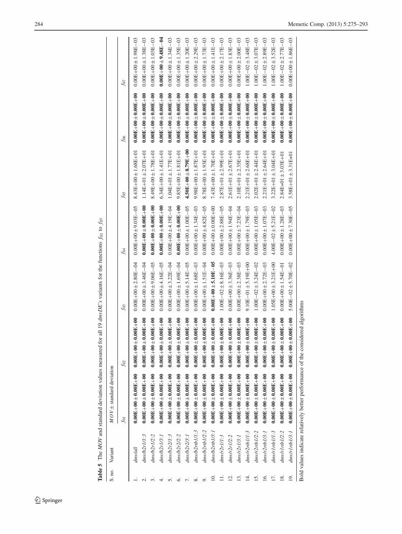
The MOV values obtained for all 19 dmvDE’s are shown inTable 5 (for f01 to f07) and 6 (for f08 to f14), and the Pc val-ues are shown in Table 7. As can be seen from the Tables 3, 5and 6, with respect to MOV, most of the dmvDE’s consistentlyretain the performance of/outperform dDE variants exceptfor function f05 where */best/2/bin variant outperform thedmvDE’s. Table 8 compares the number of functions solvedby DE, dDE and 18 dmvDE variants. There has been increasein performance, by dmvDE’s, in terms of the number of func-

tions solved. In terms of Pc %, most of the dmvDE’s (except 4variants) display higher probability of convergence than thatof DE and dDE variants as can be seen in Tables 4, 7 and 9.

To reiterate the observation that most distributed mixedvariants DE’s consistently show relatively good performance,we calculated and compare the overall performance of 19dmvDEs and 4 dDEs on all functions by plotting empiricaldistribution of normalized success performance [9,16,27].Empirical distribution is measured over the number of suc-cessful runs given by an algorithm for the individual func-tions. The algorithm which gives successful runs to all thealgorithms will get the empirical distribution over all 14 func-tions as 1. The success performance (SP) has been calculatedas follows.

S P = mean(#Function evaluations for successful runs) ∗ (#Total runs)

#Successful runs

(11)

The success performances of all twenty three variants (19dmvDEs + 4 dDEs) on each benchmark function are cal-culated and are normalized by dividing them by the bestSP on the respective function. Results of all the benchmarkfunctions are used where at least one variant was successful inat least one run. In our experiments, for all functions always

123

282 Memetic Comp. (2013) 5:275–293

Tabl

e3

The

MO

Van

dst

anda

rdde

viat

ion

valu

esm

easu

red

for

DE

and

dDE

vari

ants

for

f 01

tof 1

4

S.no

.V

aria

ntM

OV

±st

anda

rdde

viat

ion

f 01

f 02

f 03

f 04

f 05

f 06

f 07

1.D

E/r

and/

1/bi

n0.

00E+0

0±0

.00E

+00

0.00

E+0

0±0

.00E

+00

7.00

E−0

2±4

.20E

−01

0.00

E+0

0±0

.00E

+00

2.20

E+0

1±1

.81E

+01

2.00

E−0

2±1

.40E

−01

0.00

E+0

0±0

.00E

+00

dDE

/ran

d/1/

bin

0.00

E+0

0±0

.00E

+00

0.00

E+0

0±0

.00E

+00

4.00

E−0

2±4

.06E

−02

0.00

E+0

0±1

.00E

−05

3.45

E+0

1±3

.14E

+01

0.00

E+0

0±0

.00E

+00

0.00

E+0

0±1

.87E

−03

2.D

E/r

and/

2/bi

n0.

00E+0

0±0

.00E

+ 00

0.00

E+0

0±0

.00E

+00

1.64

E+0

0±2

.12E

+00

6.00

E−0

2±1

.00E

−02

1.90

E+0

1±1

.44E

+01

0.00

E+0

0±0

.00E

+00

1.00

E−0

2±0

.00E

+00

dDE

/ran

d/2/

bin

0.00

E+0

0±0

.00E

+00

0.00

E+0

0±0

.00E

+00

0.00

E+0

0±1

.12

E−0

31.

00E

−02±1

.57E

−03

2.54

E+0

1±2

.41E

+01

0.00

E+0

0±0

.00E

+00

0.00

E+0

0±2

.56E

−03

3.D

E/b

est/

2/bi

n0.

00E+0

0±0

.00E

+00

0.00

E+0

0±0

.00E

+00

0.00

E+0

0±0

.00E

+00

0.00

E+0

0±0

.00E

+00

2.32

E+0

0±9

.85E

+00

7.00

E−0

2±3

.30E

−01

1.00

E−0

2±1

.00E

−02

dDE

/bes

t/2/

bin

0.00

E+0

0±0

.00E

+00

0.00

E+0

0±0

.00E

+00

0.00

E+0

0±2

.88E

−05

0.00

E+0

0±0

.00E

+00

3.24

E+0

0±6

.88E

+00

0.00

E+0

0±0

.00E

+00

0.00

E+0

0±1

.18E

−03

4.D

E/r

and-

to-b

est/

1/bi

n0.

00E+0

0±0

.00E

+00

0.00

E+0

0±0

.00E

+00

7.00

E−0

2±4

.00E

−01

0.00

E+ 0

0±0

.00E

+00

1.74

E+0

1±1

.28E

+01

0.00

E+0

0±0

.00E

+00

0.00

E+0

0±0

.00E

+00

dDE

/ran

d-to

-bes

t/1/

bin

0.00

E+0

0±0

.00E

+00

0.00

E+0

0±0

.00E

+00

4.00

E−0

2±3

.95E

−02

0.00

E+0

0±0

.00E

+00

2.26

E+0

1±2

.50E

+01

0.00

E+0

0±0

.00E

+00

0.00

E+0

0±1

.23E

−03

S.no

.V

aria

ntf 0

8f 0

9f 1

0f 1

1f 1

2f 1

3f 1

4

1.D

E/r

and/

1/bi

n1.

30E−0

1±1

.30E

−01

0.00

E+0

0±0

.00E

+00

9.00

E−0

2±0

.00E

+00

0.00

E+0

0±0

.00E

+00

0.00

E+0

0±0

.00E

+00

0.00

E+0

0±0

.00E

+00

0.00

E+0

0±0

.00E

+00

dDE

/ran

d/1/

bin

8.00

E−0

2±1

.08E

−01

0.00

E+0

0±0

.00E

+00

1.80

E−0

1±3

.81E

−01

0.00

E+0

0±0

.00E

+00

0.00

E+0

0±0

.00E

+00

0.00

E+0

0±0

.00E

+00

0.00

E+0

0±0

.00E

+00

2.D

E/r

and/

2/bi

n2.

20E−0

1±2

.10E

−01

0.00

E+0

0±0

.00E

+00

9.00

E−0

2±0

.00E

+00

0.00

E+0

0±0

.00E

+00

0.00

E+0

0±0

.00E

+00

0.00

E+0

0±0

.00E

+00

0.00

E+0

0±0

.00E

+00

dDE

/ran

d/2/

bin

0.00

E+0

0±1

.09E

−03

0.00

E+0

0±0

.00E

+00

0.00

E+0

0±0

.00E

+00

0.00

E+0

0±0

.00E

+00

0.00

E+0

0±0

.00E

+00

0.00

E+0

0±0

.00E

+00

0.00

E+0

0±0

.00E

+00

3.D

E/b

est/

2/bi

n1.

70E−0

1±2

.00E

−01

6.90

E−0

1±1

.13E

+00

9.00

E−0

2±0

.00E

+ 00

0.00

E+0

0±0

.00E

+00

0.00

E+0

0±1

.00E

−02

0.00

E+0

0±1

.00E

−02

1.20

E−0

1±3

.30E

−01

dDE

/bes

t/2/

bin

0.00

E+0

0±0

.00E

+00

2.70

E−0

1±4

.66E

−01

0.00

E+0

0±0

.00E

+00

0.00

E+0

0±0

.00E

+00

0.00

E+0

0±0

.00E

+00

0.00

E+0

0±0

.00E

+00

0.00

E+0

0±0

.00E

+00

4.D

E/r

and-

to-b

est/

1/bi

n2.

20E−0

1±2

.00E

−01

0.00

E+0

0±0

.00E

+00

9.00

E−0

2±0

.00E

+00

0.00

E+0

0±0

.00E

+00

0.00

E+ 0

0±0

.00E

+00

0.00

E+0

0±0

.00E

+00

0.00

E+0

0±0

.00E

+00

dDE

/ran

d-to

-bes

t/1/

bin

1.80

E−0

1±2

.20E

−01

0.00

E+0

0±0

.00E

+00

3.20

E−0

1±5

.02E

−01

0.00

E+0

0±0

.00E

+00

0.00

E+0

0±0

.00E

+00

0.00

E+0

0±0

.00E

+00

0.00

E+0

0±0

.00E

+00

Bol

dva

lues

indi

cate

rela

tivel

ybe

tter

perf

orm

ance

ofth

eco

nsid

ered

algo

rith

ms

123

Memetic Comp. (2013) 5:275–293 283

Table 4 Probability of convergence (Pc %) measured for DE and dDE variants for f01 to f14

S. no. Variants DE/dDE

f01 f02 f03 f04 f05 f06 f07 f08 f09 f10 f11 f12 f13 f14 nc Pc (%)

1. DE/rand/1/bin 100 100 73 100 0 98 60 4 100 0 100 100 100 100 1,035 73.93

dDE/rand/1/bin 100 100 8 100 0 100 88 11 100 82 100 100 100 100 1,089 77.79

2. DE/rand/2/bin 100 100 0 0 0 100 2 1 100 0 100 100 100 100 803 57.36

dDE/rand/2/bin 100 100 100 1 1 100 71 99 100 100 100 100 100 100 1,173 83.79

3. DE/best/2/bin 100 100 100 100 38 95 75 1 47 0 100 99 100 89 1,044 74.57

dDE/best/2/bin 100 100 100 100 22 100 96 100 74 100 100 100 100 100 1,292 92.29

4. DE/rand-to-best/1/bin 100 100 79 100 0 100 60 0 100 0 100 100 100 100 1,039 74.21

dDE/rand-to-best/1/bin 100 100 7 100 9 100 96 3 100 70 100 100 100 100 1,085 77.50

Bold values indicate relatively better performance of the considered algorithms

at least one variant was successful in at least one run. Weplot the result of all functions for the best performing (withrespect to Pc %) dmvDE variant dmv/b2r1/3:1 (best/2/binand rand/1/bin mixed in 3:1 proportion), and the four dDEvariants in Fig. 3. The variant which could achieve at leastone successful run to all functions will reach the empiricalvalue of 1.00. The first variant to reach the top of the graph(by virtue of smallest SP and largest empirical distribution)is regarded as the best variant. For each algorithm consideredwe calculate the SP value using the equation 11. The mini-mum SP value is regarded as SPbest. For the algorithm whoseSP value is the SPbest, the SP/SPbest = 1. As can be seen inFig. 3, the dmvDE variant outperforms the four dDE variants.Apart from the best dmvDE, the SP vs empirical distributionvalues of other dmvDEs are presented in Table 10 along withthat of dDE variants. Most of the dmvDEs outperform dDEvariants (except dDE/best/2/bin).

To supplement the above observation, we have used Q-Measure (by definition it is akin to SP) to study the con-vergence of dmvDE variants against the constituent DE andtheir dDE counterparts. Q-Measure combines convergencerate and probability of convergence as follows [8]

Qm = C/Pc (12)

The convergence measure (C) is calculated as C =∑ncJ=1 F E j

nc where j = 1, . . ., nc are successful trials and F E j

is the number of function evaluations in the j th trial. Theprobability of convergence (Pc) is calculated as describedearlier in this paper. A best performing variant is expected tohave, higher probability of convergence and successful tri-als; lower number of function evaluations and consequently,lower Qm measure. Table 11 presents the Qm measuresobtained for the 18 dmvDEs, their constituent DE variantsand their dDE counterparts. The Qm measure obtained fordmv/all was 1,017.85. As can be seen from Table 11, almostall dmvDEs outperform the DE and dDE variants, reiteratingthat mixing the DE variants display a consistent, if not con-

siderable, overall improvement in the performance than thatof dDEs.

7 Benchmarking dmvDE

To verify and benchmark the efficacy of distributed mixedvariants DE, we chose the best performing (with respect toPc %) dmvDE variant dmv/b2r1/3:1 to be compared againstfive distributed differential evolution algorithms viz. paralleldifferential evolution (PDE) [32], island based distributeddifferential evolution (IBDDE) [1], distributed differentialevolution (DDE) [5–7], distributed differential evolution withexplorative–exploitative population families (DDE-EEPF)[34] and a variant of DDE-EEPF called parallel differentialevolution with random injections (PDE-WRI) [34].

The 13 test problems (rotated versions not considered)for dimensions 500 and 1,000 and the experimental resultsof above said five distributed differential evolution algo-rithms on those test problems are all adopted from [34]. Theparameter settings for dmv/b2r1/3:1 has also been closelyadopted from [34]. The dmvDE has been run with a popu-lation size of 200 with 50 individuals (for 500 dimension)and with a population size of 400 with 100 individuals (for1,000 dimension) in each of the four islands. The crossoverrate Cr , was tuned using bootstrap test and the parameterF was generated anew at each generation from the range of[0.3, 0.9]. As with the case of five distributed differentialevolution algorithms, the dmvDE was run for 500,000 and1,000,000 fitness evaluations for dimensions 500 and 1,000,respectively. Fifty independent runs were performed for eachexperiment.

Tables 12 and 13 show the mean objective function val-ues and the standard deviation obtained by each algorithmfor dimensions 500 and 1,000, respectively. As can be seenfrom Table 12, for 500 dimensions, the dmvDE displays bet-ter performance in 9 out of 13 problems. PDE and PDE-WRIobtained best results in one case-each. DDE-EEPF obtained

123

284 Memetic Comp. (2013) 5:275–293

Tabl

e5

The

MO

Van

dst

anda

rdde

viat

ion

valu

esm

easu

red

for

all1

9dm

vDE

’sva

rian

tsfo

rth

efu

nctio

nsf 0

1to

f 07

S.no

.V

aria

ntM

OV

±st

anda

rdde

viat

ion

f 01

f 02

f 03

f 04

f 05

f 06

f 07

1.dm

v/al

l0.

00E

+00±0

.00E

+00

0.00

E+0

0±0

.00E

+00

0.00

E+0

0±2

.80E

−04

0.00

E+0

0±9

.03E

−05

8.43

E+0

0±1

.68E

+01

0.00

E+0

0±0

.00E

+00

0.00

E+0

0±1

.98E

−03

2.dm

v/b2

r1/1

:30.

00E

+00±0

.00E

+00

0.00

E+0

0±0

.00E

+00

0.00

E+0

0±3

.46E

−04

0.00

E+0

0±0

.00E

+00

1.14

E+0

1±2

.07E

+01

0.00

E+0

0±0

.00E

+00

0.00

E+0

0±1

.38E

−03

3.dm

v/b2

r1/2

:20.

00E+0

0±0

.00E

+00

0.00

E+0

0±0

.00E

+00

0.00

E+0

0±9

.06E

−05

0.00

E+0

0±0

.00E

+00

8.49

E+0

0±1

.78E

+01

0.00

E+0

0±0

.00E

+00

0.00

E+0

0±1

.03E

−03

4.dm

v/b2

r1/3

:10.

00E

+00±0

.00E

+00

0.00

E+0

0±0

.00E

+00

0.00

E+0

0±4

.16E

−05

0.00

E+0

0±0

.00E

+00

6.34

E+0

0±1

.41E

+01

0.00

E+0

0±0

.00E

+00

0.00

E+0

0±9

.48E

−04

5.dm

v/b2

r2/1

:30.

00E

+00±0

.00E

+00

0.00

E+0

0±0

.00E

+00

0.00

E+0

0±3

.22E

−04

0.00

E+0

0±4

.19E

−04

1.04

E+0

1±1

.77E

+01

0.00

E+0

0±0

.00E

+00

0.00

E+0

0±1

.34E

−03

6.dm

v/b2

r2/2

:20.

00E

+00±0

.00E

+00

0.00

E+0

0±0

.00E

+00

0.00

E+0

0±1

.69E

−04

0.00

E+0

0±0

.00E

+00

9.85

E+0

0±1

.81E

+01

0.00

E+0

0±0

.00E

+00

0.00

E+0

0±1

.35E

−03

7.dm

v/b2

r2/3

:10.

00E

+00±0

.00E

+ 00

0.00

E+0

0±0

.00E

+00

0.00

E+0

0±5

.14E

−05

0.00

E+0

0±1

.00E

−05

4.50

E+0

0±8

.79E

+00

0.00

E+0

0±0

.00E

+00

0.00

E+0

0±1

.20E

−03

8.dm

v/b2

rtb1

/1:3

0.00

E+0

0±0

.00E

+00

0.00

E+0

0±0

.00E

+00

0.00

E+0

0±1

.68E

−03

0.00

E+0

0±1

.34E

−03

9.98

E+0

0±1

.87E

+01

0.00

E+0

0±0

.00E

+00

0.00

E+0

0±2

.29E

−03

9.dm

v/b2

rtb1

/2:2

0.00

E+0

0±0

.00E

+00

0.00

E+0

0±0

.00E

+00

0.00

E+0

0±1

.51E

−04

0.00

E+0

0±4

.82E

−05

8.78

E+0

0±1

.93E

+01

0.00

E+0

0±0

.00E

+00

0.00

E+0

0±1

.73E

−03

10.

dmv/

b2rt

b1/3

:10.

00E

+00±0

.00E

+00

0.00

E+0

0±0

.00E

+00

0.00

E+0

0±5

.10E

−05

0.00

E+0

0±0

.00E

+00

7.43

E+0

0±1

.70E

+01

0.00

E+0

0±0

.00E

+00

0.00

E+0

0±1

.41E

−03

11.

dmv/

r2r1

/1:3

0.00

E+0

0±0

.00E

+00

0.00

E+0

0±0

.00E

+00

1.00

E−0

2±8

.16E

−03

0.00

E+0

0±2

.88E

−05

2.87

E+0

1±2

.99E

+01

0.00

E+0

0±0

.00E

+00

0.00

E+0

0±2

.17E

−03

12.

dmv/

r2r1

/2:2

0.00

E+0

0±0

.00E

+00

0.00

E+0

0±0

.00E

+00

0.00

E+0

0±3

.36E

−03

0.00

E+0

0±1

.94E

−04

2.61

E+0

1±2

.67E

+01

0.00

E+0

0±0

.00E

+00

0.00

E+0

0±1

.83E

−03

13.

dmv/

r2r1

/3:1

0.00

E+0

0±0

.00E

+00

0.00

E+0

0±0

.00E

+00

0.00

E+0

0±2

.38E

−03

0.00

E+ 0

0±7

.23E

−04

2.10

E+0

1±2

.35E

+01

0.00

E+0

0±0

.00E

+00

0.00

E+0

0±2

.00E

−03

14.

dmv/

r2rt

b1/1

:30.

00E

+00±0

.00E

+00

0.00

E+0

0±0

.00E

+00

9.10

E−0

1±5

.19E

+00

0.00

E+0

0±1

.79E

−03

2.21

E+0

1±2

.68E

+01

0.00

E+0

0±0

.00E

+00

1.00

E−0

2±3

.48E

−03

15.

dmv/

r2rt

b1/2

:20.

00E

+00±0

.00E

+00

0.00

E+0

0±0

.00E

+00

1.00

E−0

2±3

.24E

−02

0.00

E+0

0±1

.05E

−03

2.02

E+0

1±2

.44E

+01

0.00

E+0

0±0

.00E

+00

1.00

E−0

2±3

.07E

−03

16.

dmv/

r2rt

b1/3

:10.

00E

+00±0

.00E

+00

0.00

E+0

0±0

.00E

+00

0.00

E+0

0±2

.72E

−03

0.00

E+0

0±1

.07E

−03

2.21

E+0

1±2

.64E

+01

0.00

E+0

0±0

.00E

+00

1.00

E−0

2±2

.89E

−03

17.

dmv/

r1rt

b1/1

:30.

00E

+00±0

.00E

+00

0.00

E+0

0±0

.00E

+00

1.05

E+0

0±3

.21E

+00

4.00

E−0

2±5

.21E

−02

3.22

E+0

1±3

.04E

+ 01

0.00

E+0

0±0

.00E

+00

1.00

E−0

2±3

.52E

−03

18.

dmv/

r1rt

b1/2

:20.

00E

+00±0

.00E

+00

0.00

E+0

0±0

.00E

+00

0.00

E+0

0±1

.54E

−01

0.00

E+0

0±1

.28E

−03

2.84

E+

01±3

.03E

+01

0.00

E+0

0±0

.00E

+00

1.00

E−0

2±2

.77E

−03

19.

dmv/

r1rt

b1/3

:10.

00E

+00±0

.00E

+00

0.00

E+0

0±0

.00E

+00

5.00

E−0

2±5

.70E

−02

0.00

E+0

0±7

.30E

−05

3.58

E+0

1±3

.31E

+01

0.00

E+0

0±0

.00E

+00

0.00

E+0

0±1

.86E

−03

Bol

dva

lues

indi

cate

rela

tivel

ybe

tter

perf

orm

ance

ofth

eco

nsid

ered

algo

rith

ms

123

Memetic Comp. (2013) 5:275–293 285

Tabl

e6

The

MO

Van

dst

anda

rdde

viat

ion

valu

esm

easu

red

for

all1

9dm

vDE

’sva

rian

tsfo

rth

efu

nctio

nsf 0

8to

f 14

S.no

.V

aria

ntM

OV

±st

anda

rdde

viat

ion

f 08

f 09

f 10

f 11

f 12

f 13

f 14

1.dm

v/al

l0.

00E

+00

±2.9

7E−0

20.

00E

+00±0

.00E

+00

0.00

E+0

0±0

.00E

+00

0.00

E+0

0±0

.00E

+00

0.00

E+0

0±0

.00E

+00

0.00

E+0

0±0

.00E

+00

0.00

E+0

0±0

.00E

+00

2.dm

v/b2

r1/1

:30.

00E

+00

±1.4

1E−0

20.

00E

+00±0

.00E

+00

0.00

E+0

0±0

.00E

+00

0.00

E+0

0±0

.00E

+00

0.00

E+0

0±0

.00E

+00

0.00

E+0

0±0

.00E

+00

0.00

E+0

0±0

.00E

+00

3.dm

v/b2

r1/2

:20.

00E

+00±0

.00E

+00

0.00

E+0

0±0

.00E

+00

0.00

E+0

0±0

.00E

+00

0.00

E+0

0±0

.00E

+00

0.00

E+0

0±0

.00E

+00

0.00

E+0

0±0

.00E

+00

0.00

E+0

0±0

.00E

+00

4.dm

v/b2

r1/3

:10.

00E

+00±0

.00E

+00

0.00

E+0

0±0

.00E

+00

0.00

E+0

0±0

.00E

+00

0.00

E+0

0±0

.00E

+00

0.00

E+0

0±0

.00E

+00

0.00

E+0

0±0

.00E

+00

0.00

E+0

0±0

.00E

+00

5.dm

v/b2

r2/1

:30.

00E

+00±0

.00E

+00

0.00

E+0

0±0

.00E

+00

0.00

E+0

0±0

.00E

+00

0.00

E+0

0±0

.00E

+00

0.00

E+0

0±0

.00E

+00

0.00

E+0

0±0

.00E

+00

0.00

E+0

0±0

.00E

+00

6.dm

v/b2

r2/2

:20.

00E

+00±0

.00E

+00

0.00

E+0

0±0

.00E

+00

0.00

E+0

0±0

.00E

+00

0.00

E+0

0±0

.00E

+00

0.00

E+0

0±0

.00E

+00

0.00

E+0

0±0

.00E

+00

0.00

E+0

0±0

.00E

+00

7.dm

v/b2

r2/3

:10.

00E

+00±0

.00E

+00

1.00

E−0

2±9

.95E

−02

0.00

E+0

0±0

.00E

+00

0.00

E+0

0±0

.00E

+00

0.00

E+0

0±0

.00E

+00

0.00

E+0

0±0

.00E

+00

0.00

E+0

0±0

.00E

+00

8.dm

v/b2

rtb1

/1:3

0.00

E+0

0±0

.00E

+00

2.00

E−0

2±1

.40E

−01

5.00

E−0

2±2

.12E

−01

0.00

E+0

0±0

.00E

+00

0.00

E+0

0±0

.00E

+00

0.00

E+0

0±0

.00E

+00

0.00

E+0

0±0

.00E

+00

9.dm

v/b2

rtb1

/2:2

0.00

E+0

0±0

.00E

+00

9.00

E−0

2±3

.19E

−01

0.00

E+0

0±0

.00E

+00

0.00

E+0

0±0

.00E

+00

0.00

E+0

0±0

.00E

+00

0.00

E+0

0±0

.00E

+00

0.00

E+0

0±0

.00E

+00

10.

dmv/

b2rt

b1/3

:10.

00E

+00

±1.6

6E−0

34.

70E−0

1±6

.08E

−01

0.00

E+0

0±0

.00E

+00

0.00

E+0

0±0

.00E

+00

0.00

E+0

0±0

.00E

+00

0.00

E+0

0±0

.00E

+00

0.00

E+0

0±0

.00E

+00

11.

dmv/

r2r1

/1:3

0.00

E+

00±1

.11E

−02

0.00

E+0

0±0

.00E

+00

0.00

E+0

0±0

.00E

+00

0.00

E+0

0±0

.00E

+00

0.00

E+0

0±0

.00E

+00

0.00

E+0

0±0

.00E

+00

0.00

E+0

0±0

.00E

+00

12.

dmv/

r2r1

/2:2

0.00

E+

00±1

.55E

−02

0.00

E+0

0±0

.00E

+00

0.00

E+0

0±0

.00E

+00

0.00

E+0

0±0

.00E

+00

0.00

E+0

0±0

.00E

+00

0.00

E+0

0±0

.00E

+00

0.00

E+0

0±0

.00E

+00

13.

dmv/

r2r1

/3:1

0.00

E+

00±0

.00E

+00

0.00

E+0

0±0

.00E

+00

0.00

E+0

0±0

.00E

+00

0.00

E+0

0±0

.00E

+00

0.00

E+0

0±0

.00E

+00

0.00

E+0

0±0

.00E

+00

0.00

E+0

0±0

.00E

+00

14.

dmv/

r2rt

b1/1

:30.

00E

+00

±1.6

9E−0

40.

00E

+00±0

.00E

+00

0.00

E+0

0±0

.00E

+00

0.00

E+0

0±0

.00E

+00

0.00

E+0

0±0

.00E

+00

0.00

E+0

0±0

.00E

+00

0.00

E+0

0±0

.00E

+00

15.

dmv/

r2rt

b1/2

:20.

00E

+00

±3.1

1E−0

30.

00E

+00±0

.00E

+00

0.00

E+0

0±0

.00E

+00

0.00

E+0

0±0

.00E

+00

0.00

E+0

0±0

.00E

+00

0.00

E+0

0±0

.00E

+00

0.00

E+0

0±0

.00E

+00

16.

dmv/

r2rt

b1/3

:10.

00E

+00

±2.3

4E−0

21.

00E−0

2±9

.95E

−02

0.00

E+0

0±0

.00E

+00

0.00

E+0

0±0

.00E

+00

0.00

E+0

0±0

.00E

+00

0.00

E+0

0±0

.00E

+00

0.00

E+0

0±0

.00E

+00

17.

dmv/

r1rt

b1/1

:30.

00E

+00

±1.6

5E−0

30.

00E

+00±0

.00E

+00

1.50

E−0

1±4

.98E

−01

0.00

E+0

0±0

.00E

+00

0.00

E+0

0±0

.00E

+00

0.00

E+0

0±0

.00E

+00

0.00

E+0

0±0

.00E

+00

18.

dmv/

r1rt

b1/2

:20.

00E

+00

±7.5

9E−0

30.

00E

+00±0

.00E

+00

1.00

E−0

2±9

.95E

−02

0.00

E+0

0±0

.00E

+00

0.00

E+0

0±0

.00E

+00

0.00

E+0

0±0

.00E

+00

0.00

E+0

0±0

.00E

+00

19.

dmv/

r1rt

b1/3

:10.

00E

+00

±7.7

6E−0

30.

00E

+00±0

.00E

+00

2.00

E−0

2±1

.40E

−01

0.00

E+0

0±0

.00E

+00

0.00

E+0

0±0

.00E

+00

0.00

E+0

0±0

.00E

+00

0.00

E+0

0±0

.00E

+00

Bol

dva

lues

indi

cate

rela

tivel

ybe

tter

perf

orm

ance

ofth

eco

nsid

ered

algo

rith

ms

123

286 Memetic Comp. (2013) 5:275–293

Table 7 The Pc values measured for the dmvDE’s variants

S. no. Variants f01 f02 f03 f04 f05 f06 f07 f08 f09 f10 f11 f12 f13 f14 nc Pc (%)

1 dmv/all 100 100 100 100 27 100 77 100 100 100 100 100 100 100 1,304 93.14

2 dmv/b2r1/1:3 100 100 100 100 17 100 93 98 100 100 100 100 100 100 1,308 93.43

3 dmv/b2r1/2:2 100 100 100 100 20 100 96 100 100 100 100 100 100 100 1,316 94.00

4 dmv/b2r1/3:1 100 100 100 100 22 100 100 100 100 100 100 100 100 100 1,322 94.43

5 dmv/b2r2/1:3 100 100 100 100 12 100 90 100 100 100 100 100 100 100 1,302 93.00

6 dmv/b2r2/2:2 100 100 100 100 12 100 95 100 100 100 100 100 100 100 1,307 93.36

7 dmv/b2r2/3:1 100 100 100 100 21 100 95 100 100 100 100 100 100 100 1,316 94.00

8 dmv/b2rtb1/1:3 100 100 96 98 20 100 64 100 98 95 100 100 100 100 1,271 90.79

9 dmv/b2rtb1/2:2 100 100 100 100 32 100 79 100 92 100 100 100 100 100 1,303 93.07

10 dmv/b2rtb1/3:1 100 100 100 100 27 100 89 99 58 100 100 100 100 100 1,273 90.93

11 dmv/r2r1/1:3 100 100 53 100 4 100 88 93 100 100 100 100 100 100 1,238 88.43

12 dmv/r2r1/2:2 100 100 84 100 3 100 79 97 100 100 100 100 100 100 1,263 90.21

13 dmv/r2r1/3:1 100 100 93 100 2 100 69 100 100 100 100 100 100 100 1,264 90.29

14 dmv/r2rtb1/1:3 100 100 5 64 5 100 24 100 100 100 100 100 100 100 1,098 78.43

15 dmv/r2rtb1/2:2 100 100 57 93 5 100 33 99 100 100 100 100 100 100 1,187 84.79

16 dmv/r2rtb1/3:1 100 100 86 100 4 100 49 100 100 100 100 100 100 100 1,239 88.50

17 dmv/r1rtb1/1:3 100 100 0 10 1 100 42 99 100 90 100 100 100 100 1,042 74.43

18 dmv/r1rtb1/2:2 100 100 100 100 4 100 59 98 100 100 100 100 100 100 1,261 90.07

19 dmv/r1rtb1/3:1 100 100 1 100 2 100 69 99 100 100 100 100 100 100 1,171 83.64

Total 23,785 89.42

Bold values indicate relatively better performance of the considered algorithms

Table 8 The number of functions solved by the DE, dDE and dmvDE’svariants

Variants DE dDE Mixed variants dmvDE

1:3 2:2 3:1

best/2/bin 8 12 dmv/b2r1 13 13 13

rand/1/bin 9 10

best/2/bin 8 12 dmv/b2r2 13 13 12

rand/2/bin 8 12

best/2/bin 8 12 dmv/b2rtb1 11 12 12

rand-to-best/1/bin 10 10

rand/2/bin 8 12 dmv/r2r1 12 13 13

rand/1/bin 9 10

rand/2/bin 8 12 dmv/r2rtb1 11 11 11

rand-to-best/1/bin 10 10

rand/1/bin 9 10 dmv/r1rtb1 9 11 11

rand-to-best/1/bin 10 10

best results in two cases. In case of 1,000 dimensions, astable 13 shows, the dmvDE consistently displays better per-formance over others in 9 out of 13 cases. PDE and DDE-EEPF outperforms others in two cases each.

To reiterate the efficacy of dmvDE, the two-trial unequalvariance t-test was applied for confidence interval of 0.95(as was done in [34]), following the description in [28]. The

Table 9 The Pc values measured for the DE, dDE and dmvDE’s,variants

Variants DE dDE Mixedvariants

dmvDE

1:3 2:2 3:1

best/2/bin 74.57 92.29 dmv/b2r1 93.43 94.00 94.43

rand/1/bin 73.93 77.79

best/2/bin 74.57 92.29 dmv/b2r2 93.00 93.36 94.00

rand/2/bin 57.36 83.79

best/2/bin 74.57 92.29 dmv/b2rtb1 90.79 93.07 90.93

rand-to-best/1/bin 74.21 77.50

rand/2/bin 57.36 83.79 dmv/r2r1 88.43 90.21 90.29

rand/1/bin 73.93 77.79

rand/2/bin 57.36 83.79 dmv/r2rtb1 78.43 84.79 88.50

rand-to-best/1/bin 74.21 77.50

rand/1/bin 73.93 77.79 dmv/r1rtb1 74.43 90.07 83.64

rand-to-best/1/bin 74.21 77.50

results of the test have been depicted in Tables 14 and 15 for500 and 1,000 dimensions, respectively. The tables depictthe statistical performance of the dmvDE over other algo-rithms with ‘+’ indicating dmvDE’s superior performanceover others, ‘−’ indicating dmvDE outperformed by the cor-responding algorithm and ‘=’ indicating equal performance.

123

Memetic Comp. (2013) 5:275–293 287

Fig. 3 Empirical distribution ofnormalized success performanceof the algorithms on all fourteentest problems. a dmv/b2r1/3:1variant with best performingdDE variants. b dmv/b2r1/3:1with dDE/best/2bin

Table 10 SP/SPbest andempirical distribution of the bestdDE variants and their dmvDE’svariants

S. no. Variants SP/SPbest Empiricaldistribu-tion

S.no. Variants SP/SPbest Empiricaldistribu-tion

1. dmv/b2r2/2:2 2.67 1.00 12. dmv/r2r1/1:3 8.00 1.00

2. dDE/best/2/bin 7.80 1.00 13. dmv/r2rtb1/3:1 8.00 1.00

3. dmv/all 7.80 1.00 14. dmv/r1rtb1/2:2 8.00 1.00

4. dmv/b2r1/1:3 7.80 1.00 15. dmv/r2rtb1/2:2 8.38 1.00

5. dmv/b2r1/2:2 7.80 1.00 16. dmv/r2r1/2:2 10.67 1.00

6. dmv/b2r1/3:1 7.80 1.00 17. dmv/r2r1/3:1 16.00 1.00

7. dmv/b2r2/1:3 7.80 1.00 18. dmv/r2rtb1/1:3 44.46 1.00

8. dmv/b2r2/3:1 7.80 1.00 19. dDE/rand-to-best/1/bin 57.45 1.00

9. dmv/b2rtb1/2:2 7.80 1.00 20. dmv/r1rtb1/3:1 222.31 1.00

10. dmv/b2rtb1/3:1 7.80 1.00 21. dDE/rand/2/bin 779.73 1.00

11. dmv/b2rtb1/1:3 7.96 1.00 22. dDE/rand/1/bin 27.79 0.93

23. dmv/r1rtb1/1:3 77.97 0.93

Table 11 Qm values measuredof DE, dDE and dmvDE variants Variants DE dDE Mixed variants dmvDE

1:3 2:2 3:1

best/2/bin 1,431.83 1,143.65 dmv/b2r1 1,097.89 1,091.38 1,094.52

rand/1/bin 1,364.15 1,363.42

best/2/bin 1,431.83 1,143.65 dmv/b2r2 1,196.69 1,008.02 1,128.71

rand/2/bin 2,055.56 1,508.31

best/2/bin 1,431.83 1,143.65 dmv/b2rtb1 979.28 954.29 1,033.12

rand-to-best/1/bin 1,373.13 1,276.15

rand/2/bin 2,055.56 1,508.31 dmv/r2r1 1,228.87 1,241.27 1,266.19

rand/1/bin 1,364.15 1,363.42

rand/2/bin 2,055.56 1,508.31 dmv/r2rtb1 1,038.25 1,044.63 1,119.19

rand-to-best/1/bin 1,373.13 1,276.15

rand/1/bin 1,364.15 1,363.42 dmv/r1rtb1 999.88 958.90 1,107.58

rand-to-best/1/bin 1,373.13 1,276.15

123

288 Memetic Comp. (2013) 5:275–293

Tabl

e12

Mea

nob

ject

ive

func

tion

valu

esan

dst

anda

rdde

viat

ion

for

500

dim

ensi

onal

prob

lem

s

S.no

.Fu

nctio

nsM

OV

±st

anda

rdde

viat

ion

PD

EIB

DD

ED

DE

PD

E-W

RI

DD

E-E

EP

Fdm

v/b2

r1/3

:1

1.A

ckle

y1.

62E−0

1±1

.67E

−02

3.55

E+0

0±2

.96E

−02

1.51

E−0

1±6

.96E

−02

1.45

E−0

1±1

.76E

−02

1.06

E−0

1±1

.05E

−02

8.08

E−0

2±

1.23

E−0

2

2.A

lpin

e8.

88E+0

1±1

.26E

+01

1.21

E+0

3±3

.43E

+01

1.50

E+0

2±4

.35E

+01

6.29

E+0

1±9

.95E

+00

4.34

E+0

1±6

.87E

+00

6.00

E+0

0±

8.15

E+0

0

3.A

xPa

r3.

68E+0

3±6

.84E

+02

7.27

E+0

5±3

.70E

+04

4.09

E+0

3±4

.73E

+03

2.77

E+0

3±5

.37E

+02

1.63

E+0

3±2

.39E

+02

1.22

E+0

1±

1.09

E+0

1

4.D

eJon

g1.

92E+0

1±3

.57E

+00

3.19

E+0

3±2

.67E

+02

1.61

E+0

1±1

.15E

+01

1.57

E+0

1±2

.26E

+00

8.22

E+0

0±1

.01E

+00

4.79

E−0

2±

2.24

E−0

2

5.D

ropW

ave

−4.1

1E−0

3±3

.96E

−04

−1.1

3E−0

3±8

.03E

−05

−2.5

6E−0

3±2

.69E

−04

−3.4

5E−0

3±2

.08E

−04

−5.9

6E−0

3±4

.16E

−04

−1.2

1E−0

2±

1.15

E−0

3

6.G

riew

angk

5.62

E+0

2±1

.09E

+01

1.13

E+0

4±7

.65E

+02

5.68

E+0

2±4

.86E

+01

5.52

E+0

2±1

.09E

+01

8.22

E+0

0±1

.01E

+00

1.06

E+0

0±

1.61

E−0

1

7.M

icha

lew

icz

−3.0

6E+0

2±5

.68E

+00

−9.1

3E+0

1±2

.09E

+00

−2.6

0E+0

2±8

.56E

+00

−3.3

9E+0

2±4

.77E

+00

−3.4

9E+0

2±

4.98

E+0

0−2

.60E

+02±6

.77E

+00

8.Pa

thol

ogic

al−3

.34E

+02

±5.

98E

+00

−3.3

4E+0

2±7

.40E

+00

−3.0

6E+0

2±7

.28E

+00

−3.3

1E+0

2±6

.02E

+00

−3.2

7E+0

2±5

.70E

+00

−4.4

1E+0

1±2

.66E

+00

9.R

astr

igin

1.91

E+0

3±9

.94E

+01

7.78

E+0

3±7

.78E

+03

2.73

E+0

3±2

.73E

+03

1.62

E+0

3±8

.41E

+01

1.24

E+0

3±5

.74E

+01

1.07

E+0

3±

1.29

E+0

2

10.

Ros

enbr

ock

2.11

E+0

3±1

.77E

+02

1.35

E+0

5±1

.61E

+04

1.82

E+0

3±6

.14E

+02

2.37

E+0

3±1

.98E

+02

2.24

E+0

3±2

.10E

+02

5.02

E+0

2±

1.54

E+0

1

11.

Schw

efel

−1.3

0E+0

5±3

.17E

+03

−4.4

8E+0

4±8

.15E

+02

−1.0

6E+0

5±4

.19E

+03

−1.4

1E+0

5±2

.78E

+03

−1.5

3E+0

5±2

.20E

+03

−6.4

0E+

06±

6.09

E+

06

12.

Sum

ofpo

wer

s1.

06E−0

5±5

.19E

+05

3.09

E−0

1±1

.67E

−01

1.02

E−0

3±2

.51E

−03

3.35

E−0

6±

1.05

E−0

55.

84E−0

5±2

.02E

−04

5.64

E−0

6±2

.35E

−05

13.

Tir

rone

n−1

.57E

+00±3

.44E

−02

−1.0

1E+0

0±1

.90E

−02

−1.3

8E+0

0±6

.76E

−02

−1.4

9E+0

0±4

.05E

−02

−1.5

8E+0

0±

4.79

E−0

2−9

.09E

−01±3

.56E

−02

Bol

dva

lues

indi

cate

best

resu

lts

123

Memetic Comp. (2013) 5:275–293 289

Tabl

e13

Mea

nob

ject

ive

func

tion

valu

esan

dst

anda

rdde

viat

ion

for

1,00

0di

men

sion

alpr

oble

ms

S.no

.Fu

nctio

nsM

OV

±st

anda

rdde

viat

ion

PD

EIB

DD

ED

DE

PD

E-W

RI

DD

E-E

EP

Fdm

v/b2

r1/3

:1

1.A

ckle

y9.

75E−0

1±4

.77E

−02

3.72

E+0

0±4

.77E

−02

7.25

E−0

1±8

.17E

−02

7.33

E−0

1±5

.62E

−02

6.06

E−0

1±3

.39E

−02

1.38

E−0

1±

2.48

E−0

2

2.A

lpin

e6.

24E+0

2±3

.28E

+01

2.66

E+0

3±6

.16E

+01

3.85

E+0

2±4

.99E

+01

3.76

E+0

2±2

.04E

+01

3.66

E+0

2±1

.90E

+01

7.28

E+0

1±

1.55

E+0

1

3.A

xPa

r1.

81E+0

5±1

.23E

+04

3.20

E+0

6±1

.62E

+05

1.06

E+0

5±1

.86E

+04

1.31

E+0

5±9

.03E

+03

1.08

E+0

5±8

.53E

+03

3.53

E+0

3±

9.11

E+0

2

4.D

eJon

g4.

66E+0

2±2

.81E

+01

6.29

E+0

3±3

.74E

+02

2.83

E+0

2±5

.12E

+01

3.43

E+0

2±2

.52E

+01

3.26

E+0

2±3

.19E

+01

1.01

E+0

1±

2.81

E+0

0

5.D

ropW

ave

−1.6

2E−0

3±9

.29E

−05

−5.2

0E−0

4±2

.21E

−05

−1.1

7E−0

3±9

.73E

−05

−1.4

5E−0

3±5

.33E

−05

−1.8

2E−0

3±1

.05E

−04

−4.9

5E−0

3±

4.04

E−0

4

6.G

riew

angk

2.58

E+0

3±1

.03E

+02

2.38

E+0

4±1

.55E

+03

1.96

E+0

3±1

.80E

+02

2.17

E+0

3±8

.73E

+01

2.13

E+0

3±1

.12E

+02

3.37

E+0

1±

1.09

E+0

1

7M

icha

lew

icz

−4.1

8E+0

2±9

.73E

+00

−1.4

9E+0

2±2

.24E

+00

−4.4

3E+0

2±1

.22E

+01

−5.0

4E+0

2±9

.17E

+00

−5.0

7E+0

2±

9.84

E+0

0−4

.08E

+02±1

.46E

+01

8.Pa

thol

ogic

al−6

.39E

+02

±8.

43E

+00

−1.8

7E+0

2±3

.77E

+01

−5.7

0E+0

2±1

.30E

+01

−6.3

7E+0

2±8

.00E

+00

−6.3

4E+0

2±9

.41E

+00

−4.6

6E+0

1±2

.32E

+00

9.R

astr

igin

6.65

E+0

3±2

.16E

+02

1.69

E+0

4±3

.40E

+02

6.18

E+0

3±3

.96E

+02

5.13

E+0

3±1

.98E

+02

5.01

E+0

3±1

.91E

+02

2.19

E+0

3±

2.48

E+0

2

10.

Ros

enbr

ock

1.34

E+0

4±9

.17E

+02

2.90

E+0

5±3

.35E

+04

8.96

E+0

3±1

.82E

+03

1.13

E+0

4±7

.02E

+02

1.12

E+0

4±6

.85E

+02

1.30

E+0

3±

9.24

E+0

1

11.

Schw

efel

−1.9

1E+0

5±4

.04E

+03

−6.4

5E+0

4±1

.08E

+03

−1.8

6E+0

5±8

.61E

+03

−2.3

2E+0

5±4

.51E

+03

−2.3

3E+0

5±4

.31E

+03

−2.7

9E+0

7±

3.31

E+0

7

12.

Sum

ofpo

wer

s3.

07E

−06

±1.

01E

−05

1.07

E+0

0±3

.69E

−01

4.68

E−0

4±1

.64E

−03

6.88

E−0

6±2

.94E

−05

1.40

E−0

4±5

.34E

−04

1.64

E−0

2±1

.53E

−02

13.

Tir

rone

n−1

.45E

+00±2

.04E

−02

−8.6

3E−0

1±1

.40E

−02

−1.3

5E+0

0±5

.11E

−02

−1.4

4E+0

0±2

.66E

−02

−1.4

5E+0

0±

1.94

E−0

2−6

.25E

−01±1

.98E

−02

Bol

dva

lues

indi

cate

best

resu

lts

123

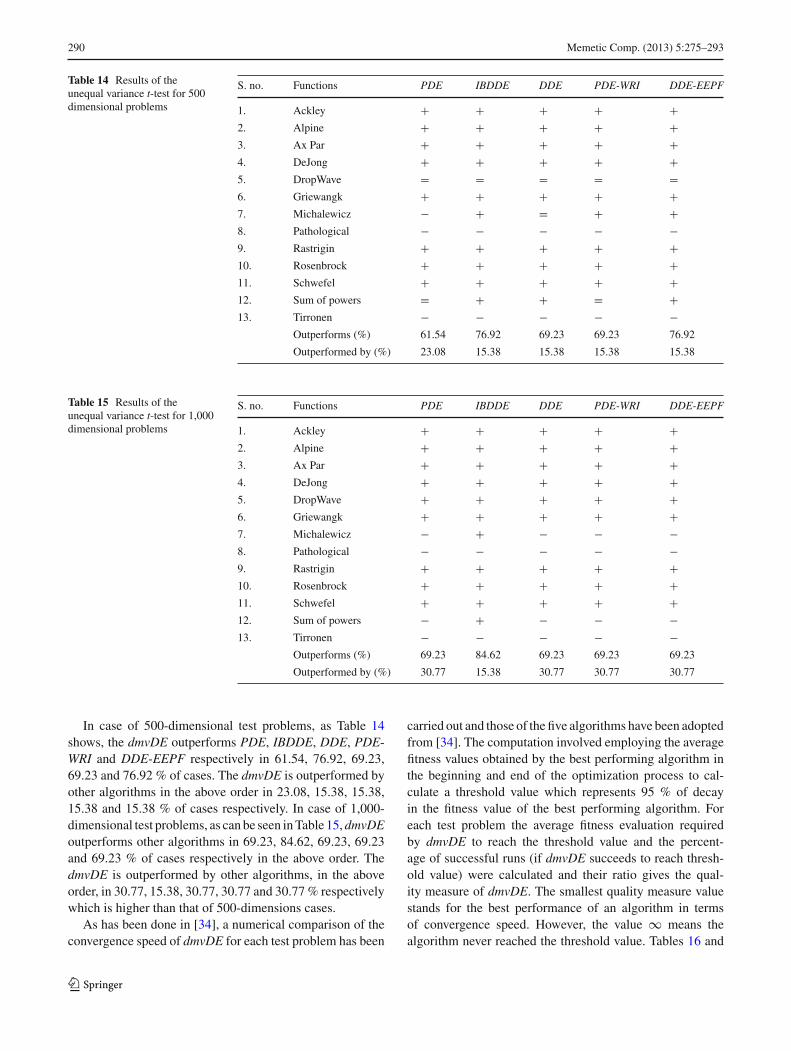
290 Memetic Comp. (2013) 5:275–293

Table 14 Results of theunequal variance t-test for 500dimensional problems

S. no. Functions PDE IBDDE DDE PDE-WRI DDE-EEPF

1. Ackley + + + + +2. Alpine + + + + +3. Ax Par + + + + +4. DeJong + + + + +5. DropWave = = = = =6. Griewangk + + + + +7. Michalewicz − + = + +8. Pathological − − − − −9. Rastrigin + + + + +10. Rosenbrock + + + + +11. Schwefel + + + + +12. Sum of powers = + + = +13. Tirronen − − − − −

Outperforms (%) 61.54 76.92 69.23 69.23 76.92

Outperformed by (%) 23.08 15.38 15.38 15.38 15.38

Table 15 Results of theunequal variance t-test for 1,000dimensional problems

S. no. Functions PDE IBDDE DDE PDE-WRI DDE-EEPF

1. Ackley + + + + +2. Alpine + + + + +3. Ax Par + + + + +4. DeJong + + + + +5. DropWave + + + + +6. Griewangk + + + + +7. Michalewicz − + − − −8. Pathological − − − − −9. Rastrigin + + + + +10. Rosenbrock + + + + +11. Schwefel + + + + +12. Sum of powers − + − − −13. Tirronen − − − − −

Outperforms (%) 69.23 84.62 69.23 69.23 69.23

Outperformed by (%) 30.77 15.38 30.77 30.77 30.77

In case of 500-dimensional test problems, as Table 14shows, the dmvDE outperforms PDE, IBDDE, DDE, PDE-WRI and DDE-EEPF respectively in 61.54, 76.92, 69.23,69.23 and 76.92 % of cases. The dmvDE is outperformed byother algorithms in the above order in 23.08, 15.38, 15.38,15.38 and 15.38 % of cases respectively. In case of 1,000-dimensional test problems, as can be seen in Table 15, dmvDEoutperforms other algorithms in 69.23, 84.62, 69.23, 69.23and 69.23 % of cases respectively in the above order. ThedmvDE is outperformed by other algorithms, in the aboveorder, in 30.77, 15.38, 30.77, 30.77 and 30.77 % respectivelywhich is higher than that of 500-dimensions cases.

As has been done in [34], a numerical comparison of theconvergence speed of dmvDE for each test problem has been

carried out and those of the five algorithms have been adoptedfrom [34]. The computation involved employing the averagefitness values obtained by the best performing algorithm inthe beginning and end of the optimization process to cal-culate a threshold value which represents 95 % of decayin the fitness value of the best performing algorithm. Foreach test problem the average fitness evaluation requiredby dmvDE to reach the threshold value and the percent-age of successful runs (if dmvDE succeeds to reach thresh-old value) were calculated and their ratio gives the qual-ity measure of dmvDE. The smallest quality measure valuestands for the best performance of an algorithm in termsof convergence speed. However, the value ∞ means thealgorithm never reached the threshold value. Tables 16 and

123

Memetic Comp. (2013) 5:275–293 291

Table 16 Quality Measure values obtained for 500 dimensional problems

S. no. Functions PDE IBDDE DDE PDE-WRI DDE-EEPF dmv/b2r1/3:1

1. Ackley 4.30E+05 ∞ 3.22E+05 3.93E+05 3.69E+05 1.56E+03

2. Alpine 4.87E+05 ∞ ∞ 4.62E+05 3.98E+05 2.34E+03

3. Ax Par 2.11E+05 ∞ 1.31E+05 1.69E+05 1.69E+05 1.07E+03

4. DeJong 2.57E+05 ∞ 1.24E+05 2.15E+05 2.15E+05 1.15E+03

5. DropWave ∞ ∞ ∞ ∞ ∞ 2.76E+03

6. Griewangk 2.31E+05 ∞ 2.85E+05 3.60E+05 3.27E+05 1.13E+03

7. Michalewicz ∞ ∞ ∞ 4.74E+05 4.47E+05 ∞8. Pathological 1.64E+05 4.05E+05 ∞ 1.86E+05 1.86E+05 ∞9. Rastrigin ∞ ∞ ∞ ∞ 4.28E+05 2.06E+03

10. Rosenbrock 1.68E+05 ∞ 9.34E+04 1.34E+05 1.34E+05 2.61E+02

11. Schwefel ∞ ∞ ∞ ∞ ∞ 8.33E+01

12. Sum of powers 2.06E+04 4.65E+05 9.00E+03 1.12E+04 1.12E+04 2.03E+03

13. Tirronen 2.69E+05 ∞ ∞ 4.95E+05 3.33E+05 ∞Bold values indicae best results

Table 17 Quality measure values obtained for 1,000 dimensional problems

S. no. Functions PDE IBDDE DDE PDE-WRI DDE-EEPF dmv/b2r1/3:1

1. Ackley ∞ ∞ ∞ ∞ ∞ 3.88E+03

2. Alpine ∞ ∞ ∞ ∞ ∞ 6.79E+03

3. Ax Par 9.32E+04 ∞ 5.84E+05 6.12E+04 7.52E+05 3.75E+03

4. DeJong 9.96E+05 ∞ 7.13E+05 8.91E+05 9.44E+05 4.09E+03

5. DropWave ∞ ∞ ∞ ∞ ∞ 9.74E+03

6. Griewangk ∞ ∞ ∞ ∞ ∞ 3.98E+03

7. Michalewicz ∞ ∞ ∞ 9.30E+05 9.65E+05 ∞8. Pathological 7.00E+05 ∞ ∞ 4.85E+05 4.85E+05 ∞9. Rastrigin ∞ ∞ ∞ ∞ ∞ 5.95E+03

10. Rosenbrock 7.01E+05 ∞ 3.15E+05 3.88E+04 5.17E+05 5.81E+02

11. Schwefel ∞ ∞ ∞ ∞ ∞ 1.60E+02

12. Sum of powers 7.76E+04 ∞ 1.68E+04 3.04E+04 3.04E+04 6.51E+03

13. Tirronen 6.55E+05 ∞ 1.99E+05 4.87E+05 5.22E+05 ∞Bold values indicate best results

17 shows the quality measure values obtained for dmvDEand other five algorithms for 500 and 1,000 dimensionsrespectively.

From Tables 16 and 17, it is noticed that DDE-EEPFdisplays competitive performance unlike other algorithms.However, dmvDE outperformed other algorithms in 10 outof 13 cases for both 500 and 1,000-dimensional problemsreiterating its efficacy. It is worth mentioning that the distrib-uted mixed variants differential evolution algorithms werenot only promising in 30 dimensions, but also scaled well to500 and 1,000 dimension (as in the case of dmv/b2r1/3:1)displaying a very competitive performance.

The parallel differential evolution (PDE) [32] employsDE/best/1 across all subpopulations with migration of bestindividual amongst each node based on a given probability.

The island based differential evolution (IBDDE) [1] employsDE/rand/1 mutation across all subpopulations migrating arandom individual with a predetermined migration frequencyamongst the nodes. The distributed differential evolution(DDE) [5–7] differs from PDE and IBDDE by the topol-ogy. While the latter employs a torus topology, the other twoemploys unidirectional ring topology. Each node in DDEruns DE/rand/1 strategy exchanging its best individual withits neighbors. DDE-EEPF [34] however uses two familiesof subpopulation. The first family with constant populationsize employing DE/rand/1 explores the search space. Thesecond subpopulation in the second family employing samestrategy exploits solution space, but with dynamic populationsize. Unlike above algorithms, dmvDE employs different DEvariants in each island enabling co-operative evolution.

123

292 Memetic Comp. (2013) 5:275–293

Table 18 Average execution time taken by dmv/b2r1/3:1 variant, for500 and 1,000 dimensional problems

S. no. Function ExeTime (in seconds)

D = 500 D = 1,000

1. Ackley 54.42 94.60

2. Alpine 9.26 42.70

3. Ax Par 4.81 18.73

4. DeJong 4.84 16.84

5. DropWave 5.59 18.87

6. Griewangk 13.92 48.22

7. Michalewicz 29.46 101.31

8. Pathological 37.19 124.46

9. Rastrigin 13.80 47.89

10. Rosenbrock 11.57 43.38

11. Schwefel 0.58 1.12

12. Sum of powers 21.83 82.21

13. Tirronen 17.09 73.21

The competitive performance of dmvDE as against fivedistributed differential evolution algorithms may be attribu-ted to the co-operative evolution of constituent DE variantswith each of them evolving independently but also exchang-ing information amongst themselves to co-operativelyenhance the efficacy of dmvDE as a whole. The effect ofheterogeneity of the dmvDE (by virtue of different DE vari-ants in each island) has been evident in the simulation results.However a better insight about the dynamics of this hetero-geneity calls for extensive empirical analyzes and hence itwould be the major part of our future work.

The details about the computational platform and the aver-age execution time of the simulations are not provided in [34].The average execution time taken by dmv/b2r1/3:1 variantfor the 500 and 1,000 dimensions problems is presented inTable 18 (for Intel Core 2 Duo 1.86 GHz PC with 2 GBDDR2 RAM in linux environment). However, the opera-tional scheme of dmvDE reveals that it is similar to classicaldistributed DE in terms of processing time. The operationalscheme of DDE-EEPF reveals that it includes populationsize reduction (dynamic population size) apart from explo-ration, exploitation and inter, intra migration by two familiesof subpopulations. Hence, the competitive performance ofdmvDE may not have been obtained at the cost of greatercomputation times.

It is also worth admitting that dmvDE is just an efforttowards alleviating the trial-and-error search of appropriateDE variant(s) given an optimization problem. The dmvDEinvolved pre-selection of very competitive DE variantsthrough empirical analyses. However, when put together andbenchmarked on a different test suite, they exhibited com-petitive performance.

8 Conclusion

The distributed mixed variant differential evolution algo-rithms, proposed in this paper, employ four effective DEvariants: DE/rand/1/bin, DE/rand/2/bin, DE/best/2/bin andDE/rand-to-best/1/bin with diverse characteristics in vari-ous proportions (among islands) and in various combinations(as to which DE variants mix with each other). In order tostudy the viability and efficacy of 19 dmvDE’s, arising out ofvarious proportions and combinations of 4 DE variants, thedmvDEs have been run on 14 unconstrained benchmark prob-lems. The dmvDEs display a consistent, if not considerable,overall improvement in performance than that of the distrib-uted versions of the four DE variants in terms of mean objec-tive function values, probability of convergence, success per-formance and Q-measure. Subsequently, the best of dmvDEs(based on Pc %) has been benchmarked against five distrib-uted differential evolution algorithms. The dmvDE outper-formed, on average, the other algorithms on 500 and 1,000dimensional test problems. The benchmark experiments reit-erate the efficacy of mixing DE variants to co-operativelyenhance the performance of dmvDE as a whole.

Future enhancement of this work will include a generaliza-tion of mixing DE variants in a distributed framework. Apartfrom pre-selection of DE variants for dmvDE, the empiri-cal setting of parameters like migration strategy, proportionof migrants, topology etc., also implicates dmvDE’s perfor-mance. Mixing DE variants on different number of subpop-ulations with different distributed parameter settings wouldprovide better insight about the dynamics of mixing differ-ent variants. Also, careful mixing of DE variants to matchthe optimization problem characteristics leading to a recipeof variants’ mixing for a given problem is another potentialdirection of research.

References

1. Apolloni J, Leguizamo′n G, Garcı’a-Nieto J, Alba E (2008) Islandbased distributed differential evolution: an experimental study onhybrid testbeds. In: Proceedings of the IEEE international confer-ence on hybrid intelligent systems, pp 696–701

2. Biswas A, Dasgupta S, Das S, Abraham A (2007) A synergy ofdifferential evolution and bacterial foraging algorithm for globaloptimization. Neural Netw World 17(6):607–626

3. Chiou JP, Chang CF, Su CT (2004) Ant direction hybrid differentialevolution for solving large capacitor placement problems. IEEETrans Power Syst 19:1794–1800

4. Das S, Konar A, Chakraborty UK (2007) Annealed differentialevolution. In: Proceedings of the IEEE congress on evolutionary,computing, pp 1926–1933

5. Falco ID, Cioppa AD, Maisto D, Scafuri U, Tarantino E (2007a)Satellite image registration by distributed differential evolution,Lectures Notes in Computer Science, vol 4448. In: Proceedings ofapplications of evolutionary computing, pp 251–260

6. Falco ID, Cioppa AD, Maisto D, Scafuri U, Tarantino E (2007b)Distributed differential evolution for the registration of remotely

123

Memetic Comp. (2013) 5:275–293 293

sensed images. In: Proceedings of the IEEE euromicro internationalconference on parallel, distributed and network-based processing,pp 358–362

7. Falco ID, Cioppa AD, Maisto D, Scafuri U, Tarantino E (2007c)A distributed differential evolution approach for mapping in a gridenvironment. In: Proceedings of the IEEE euromicro internationalconference on parallel, distributed and network-based processing,pp 442–449

8. Feoktistov V (2006) Differential evolution in search of solutions.Springer, USA

9. Hansen N (2006) Compilation of results on the 2005 CEC bench-mark function set. http://www/ntu.edu.sg/home/epnsugan/index_files/CEC-05/compareresults.pdf

10. He H, Han L (2007) A novel binary differential evolution algo-rithm based on artificial immune system. In: Proceedings of IEEEcongress on, evolutionary computation, pp 2267–2272

11. Hendtlass T (2001) A combined swarm differential evolutionalgorithm for optimization problems. Lecture Notes Comput Sci2070:11–18

12. Herrera F, Lozano M (2000) Gradual distributed real-coded geneticalgorithms. IEEE Trans Evol Comput 4(1):43–63

13. Hu ZB, Su QH, Xiong SW, Hu FG (2008) Self-adaptive hybrid dif-ferential evolution with simulated annealing algorithm for numer-ical optimization. In: Proceedings of the IEEE congress on evolu-tionary computation, pp 1189–1194

14. Jeyakumar G, Shunmuga Velayutham C (2009) An empirical com-parison of differential evolution variants on different classes ofunconstrained global optimization problems. In: Proceedings ofthe international conference on computer information systems andindustrial management application, pp 866–871

15. Jeyakumar G, ShunmugaVelayutham C (2010a) An empirical per-formance analysis of differential evolution variants on uncon-strained global optimization problems. Int J Comput Inf Syst IndManag Appl 2:077–086

16. Jeyakumar G, Shunmuga Velayutham C (2010b) Empirical studyon migration topologies and migration policies for island based dis-tributed differential evolution variants. Lecture Notes in ComputerScience, vol 6466. Springer, Berlin, pp 95–102

17. Kannan S, Slochanal SMR, Subbaraj P, Padhy NP (2004) Appli-cation of particle swarm optimization technique and its vari-ants to generation expansion planning. Electric Power Syst Res70(3):203–210

18. Kwedlo W, Bandurski K (2006) A parallel differential evo-lution algorithm. In: Proceedings of the IEEE internationalsymposium on parallel computing in, electrical engineering,pp 319–324

19. Lampinen J (1999) Differential evolution—new naturally parallelapproach for engineering design optimization. In: Topping BHV(eds) Development in computational mechanics with high perfor-mance computing. Civil-Comp Press, pp 217–228

20. Mezura-Montes E, Velazquez-Reyes J, Coello Coello CA (2006) Acomparative study on differential evolution variants for global opti-mization. In: Proceedings of the 8th annual conference on geneticand evolutionary computation, pp 485–492

21. Moore PW, Venayagamoorthy GK (2006) Evolving digital circuitusing hybrid particle swarm optimization and differential evolu-tion. Neural Syst 16(3):163–177

22. Omran MGH, Engelbrecht AP, Salman A (2009) Bare bones dif-ferential evolution. Eur J Oper Res 196(1):128–139

23. Pan QK, Suganthan PN, Wang L, Gao L, Mallipeddi R (2011)A differential evolution algorithm with self-adapting strategy andcontrol parameters. Comput Oper Res 38(1):394–408

24. Pavlidis NG, Tasoulis DK, Plagianakos VP, Nikiforidis G, Vra-hatis MN (2005) Spiking neural network training using evolution-ary algorithms. In: IEEE international joint conference on neuralnetworks, pp 2190–2194

25. Price KV et al (1999) An introduction to differential evolution.In: Corne D (ed) New ideas in optimization. Mc Graw-Hill, UK,pp 79–108

26. Price KV, Storn RM, Lampinen JA (2005) Differential evolution:a practical approach to global optimization. Springer, Berlin

27. Qin AK, Huang VL, Suganthan PN (2009) Differential evolutionalgorithm with strategy adaptation for global numerical optimiza-tion. IEEE Trans Evol Comput 13(12):397–417

28. Ruxton GD (2006) The unequal variance t-test is an underusedalternative to student’s t-test and the Mann–Whitney test. BehavEcol 17(4):688–690

29. Salomon M, Perrin GR, Heitz F, Armspach JP (2005) Parallel dif-ferential evolution: application to 3-d medical image registration.In: Price KV et al (eds) Differential evolution—a practical approachto global optimization, Natural Computing Series, pp 353–411

30. Storn R, Price K (1995) Differential evolution—a simple and effi-cient adaptive scheme for global optimization over continuousspaces, Technical Report TR-95-012. ICSI

31. Storn R, Price K (1997) Differential evolution—a simple and effi-cient heuristic strategy for global optimization and continuousspaces. J Global Optim 11(4):341–359

32. Tasoulis DK, Pavlidis NG, Plagianakos VP, Vrahatis MN (2004)Parallel differential evolution. In: Proceedings of the IEEE congresson evolutionary computation, Portland, pp 2023–2029

33. Vesterstrom J, Thomsen R (2004) A comparative study of differen-tial evolution, particle swarm optimization and evolutionary algo-rithm on numerical benchmark problems. In: Proceedings of theIEEE congress on evolutionary computation, Portland, pp 1980–1987

34. Weber M, Tirronen V, Neri F (2009) Distributed differential evo-lution with explorative–exploitative population families. In: Pro-ceedings of genetic programming and evolvable machine, vol 10,pp 343–371

35. Weber M, Tirronen V, Neri F (2010) Scale factor inheritancemechanism in distributed differential evolution. Soft Comput14(11):1187–1207

36. Weber M, Tirronen V, Neri F (2011a) A study on scale factor indistributed differential evolution. Artif Intell Rev 181(12):2488–2511

37. Weber M, Tirronen V, Neri F (2011b) A study on scale fac-tor/crossover interaction in distributed differential evolution. ArtifIntell Rev 39(3):195–224

38. Weber M, Tirronen V, Neri F (2011c) Two algorithmic enhance-ments for parallel differential evolution. Int J Innov Comput Appl3(11):20–30

39. Wolpert DH, Macreedy WG (1997) No free lunch theorems foroptimization. IEEE Trans Evol Comput 1(1):67–82

40. Yao X, Liu Y, Liang KH, Lin G et al (2003) Fast evolutionary algo-rithms. In: Rozenberg G (ed) Advances in evolutionary computing:theory and applications. Springer, New York, pp 45–94

41. Zaharie D, Petcu D (2003) Parallel implementation of multi-population differential evolution. In: Grigoras D et al (eds) Pro-ceedings of the concurrent information processing and computing.A.I.Cuza University Press, Nato Advanced Research Workshop,pp 262–269

42. Zhang X, Duan H, Jin J (2008) DEACO: hybrid ant colony opti-mization with differential evolution. In: Proceedings of the IEEEcongress on evolutionary computation, pp 921–927

123