1 Electric Methods

Cairo University

Instructor : Mahmoud Mekkawi

Professor of Applied Geophysics

* National Research Institute of Astronomy

and Geophysics (NRIAG-Helwan), Cairo.

Geomagnetism & Geoelectricity Dept.

https://nriag.academia.edu/mahmoudmekkawi

E-mail: mekkawi05@yahoo.com

Mobil: 01000 643 221

Electric methods Course -2017

- Yungul S., 1996. Electrical Method in Geophysical Exploration of Deep Sedimentary Basins.

Champman & Hall Press. - Reynolds M. John, 1997. An Introduction to Applied &

Environmental Geophysics. Geo-Sciences Ltd, UK. - Zhdanov S. Michael. 2009. Geophysical

Electromagnetic Theory & Methods. Elsevier. - Chave A. & Jones A. 2012. The Magnetotelluric Method, Theory & Practice. Cambridge Univ. Press.

I Electric methods:

- Units & Symbols

- Electrical Resistivity (Conductivity)

- Self Potential (SP)

- Induced Polarization (IP)

- Application

II EM Methods

- EM theory, Propagation & Spectrum

- Frequency Domain (FEM)

- Time Domain (TEM )

- EM Applications

III Magnetotelluric Method (MT)

- MT source field & Acquisition

- MT Types & systems

- MT processing & Interpretation

- MT Applications

IV Airborne &Marine EM

- Airborne (AEM) systems & Application

- Marine EM (Seaborne) & Application

Contents

Electrical Methods

(electric galvanic)

Soil contacting methods (EM-induction)

Non-contacting Electromagnetic

Electric

Resistivity

Induced

Polariztion

(IP)

Self Potential

(SP) Magnetotelluric (MT)

Electromagnetic (EM)

Variations of the electrical conductivity

of the subsurface

- Electrical conductivity

- Electrochemical polarization

Electromagnetic (inductive; a.c) methods

Electrical (galvanic; d.c) methods in the sub-surface investigations (DC, IP and SP)

Resistance : resistance to movement of charge Capacitance : ability to store charge Inductance : ability to generate current from changing magnetic field arising from moving charges in circuit

(Galvanic d.c. methods), electric direct current (I) is injected into the subsurface through the electrodes A & B. The potential, voltage difference (V), caused by the currents in the subsurface are measured with the potential electrodes M & N (voltage between the electrodes). * The mutual location of the electrodes A, B, M and N define the geometric (array) factor G. Resistivity:

Depth of investigation is controlled by the length of the array (roughly AB/3). Expanding the array provides deeper penetration.

I Electrical Methods Resistivity, Self Potential

& Induced Polarization

𝝆 = 𝑮𝚫𝐕

𝐈

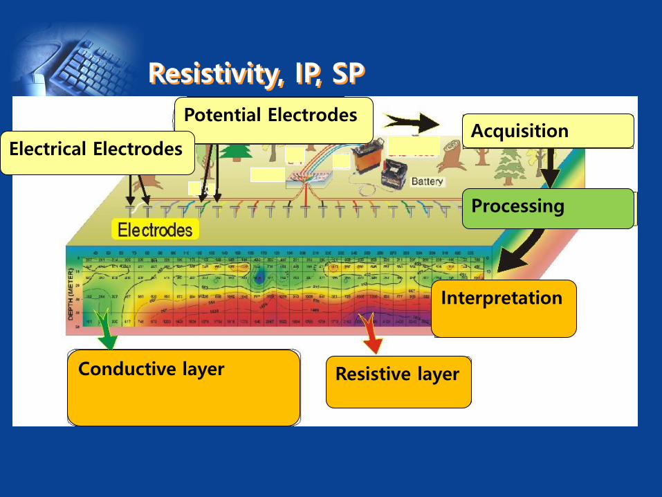
Resistivity, IP, SP

Potential Electrodes

Electrical Electrodes

Conductive layer Resistive layer

Acquisition

Processing

Interpretation

The (EM) have the broadest range of different

instrumental systems:

* Time domain EM (TEM), measure with Time

* Frequency domain (FEM), measure one or more frequencies.

or

* Passive, utilizing natural ground signals (MT, AMT)

* Active, where an artificial transmitter is used

- Near field as in ground conductivity meters)

- Far field (using remote high powered military &

civil radio transmitters (VLF & RMT).

II EM Methods:

EM Induction

Methods

TX RX

Determination of resistivity as a function of distance Time (frequency) & depth.

Time (frequency) 1D -MT(m)

2D-MT (m)

Depth

Resistivity

Log Resistivity

3D-MT resistivity model at Kharga Reservoir Water Mekkawi et al., 2014

EM systems - Frequency Domain (FEM)

- Time Domain (TEM )

EM Applications: Groundwater-Mineral , Geothermal, Cavities, Faults, Landfill Survey, Geological and Permafrost mapping

III Magnetotellurics (MT) - MT source field & acquisition

- (AMT, CSAMT, MT & LMT)

- MT processing & Interpret.

- MT Applications

Deep structures, Geothermal

And volcanicity, active zones and Earthquakes, ground water, mineral and petroleum exploration.

Hx

Hy

Hz

Ex

Ey

MT Data Record vs. Time

MT Data Spectral (FFT)

Magnetotelluric (MT) :

MT method can be used to determine electrical properties of materials at relatively great depths.

Naturally occurring electrical currents, generated by magnetic induction of electrical currents in the ionosphere.

Recorded electrical (Ex, Ey) and magnetic signals (Hx,Hy, Hz) are used to estimate subsurface distribution of electrical resistivity.

2

,

,1 ))(

)((tan)(

xy

yx

H

E

2

,

,

5

1)(

H xya

E

f

yx

2D-MT resistivity for hydrocarbon reservoir exploration

MT Marine acquisition

3D-MT resistivity model at Kharga Reservoir Water. Mekkawi et al., 2014

2D-MT resistivity model Mekkawi et al., 2011.

IV

Airborne ElectroMagnetic (AEM)

Seaborne Marine ElectroMagnetic (Seaborne)

Types of Electric & EM methods

SP

Ground Airborne

*

Electric methods

EM-methods

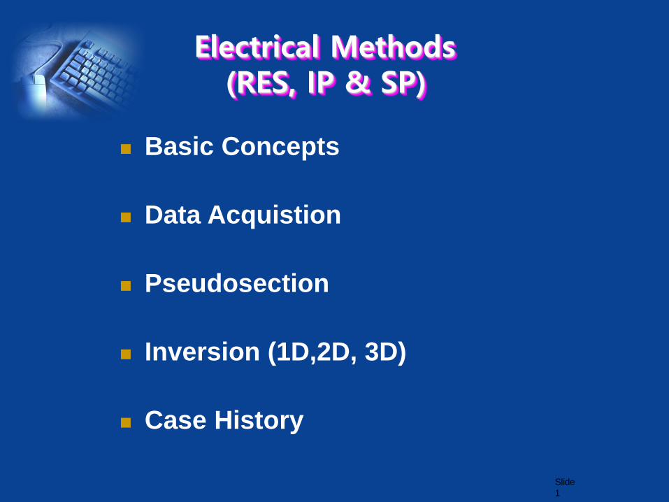
Electrical Methods (RES, IP & SP)

Slide

1

Basic Concepts

Data Acquistion

Pseudosection

Inversion (1D,2D, 3D)

Case History

Typical Electrical Conductivity Values

Electrical Resistivity

Electrical (Conductivity) Resistivity:

is a property of rock or material which determine how easily

electric current to flow when voltage is applied to the rock.

In the environment of the earth’s surface, most rock forming are: conductors (metals & water), semiconductors & insulators.

Metals

• Charge carriers are electrons that are not firmly attached to atoms in the lattice.

• Both the number of charge carriers and mobility are high.

• This gives a very low resistivity (e.g. copper ρ < 10-8 ohm-m).

Water

• Close to the surface, the fluid in the pore space is often water. If the water contains dissolved ions, then the resistivity of the water will be low because the ions can easily move.

• As the salinity of the brine increases, the resistivity decreases as more charge carriers become available and the resistivity decreases.

Semiconductors

• Semi conduction occurs in minerals such as sulphides and the charge carriers are electrons or ions.

• Compared to metals, the mobility number of charge carriers are lower, and thus the resistivity is higher (typically 10-3 to 10-5 ohm-m).

• This type of conduction occurs in igneous rocks and usually shows a temperature dependence of the form (thermally activated). When a mineral is molten, ions can freely move and the resistivity decreases.

Insulators

• In minerals such as diamond, there are very few charge carriers. To produce a charge carrier, a carbon atom would need to be removed from the crystal lattice. This requires a lot of effort and thus the mobility would be very low. As a consequence, the resistivity of pure diamond is very high resistive (ρ > 1010 Ωm)

• Carbon occurs in two forms, graphite and diamond.

While diamond has a high resistivity (no charge carriers), graphite has a structure that allows electrons to easily move parallel to sheets of carbon atoms. This gives a

very low resistivity (ρ = 8 x 10-6 Ωm)

Depends on directly on:

- Porosity,

- Permeability,

- Pore fluid saturation,

- Temperature and

- The presence of the conducting materials.

other causes of electrical conductivity: - Add clay minerals

- Graphite films,

- Iron oxides and metallic sulphides

- Partial melting

- Increase the salinity of the pore fluid

- Fracture rock to create extra pathways for current flow

- improve interconnection between pores

Electrical Resistivity (Conductivity):

Influencing factors

Influencing degree Geological

conditions of

rock mass Low resistivity ------

High resistivity

Porosity

Saturated

condition Large ----------- Small Weathered

and fault

fractured zones Unsaturated condi

tion Small ----------- Large

Pore fluid resistivity

(Groundwater) Low -------------- High

Components of

groundwater

Water saturation Large ----------- Small Groundwater

table

Water content by volume

(Porosity and water

saturation)

Large ----------- Small

Weathered

and fault fractured z

ones

Clay content Much ----------- Little Weathered and altere

d zones

porosity

R w w

nF S

F aR

w

m ( )

R

w

a

1) by Archie (1942)

F : factor

: res. Rock (ohm-m)

: res. water(ohm-m)

S : saturation

(0.5-2.5), m (1.3-2.5), n (2)

+ - V

RF I

+ +

+ +

- -

- -

Pore Fluid

1 1 1

R w sF

2) by Patnode and Wyllie (1950)

: resis soil (ohm-m) s

+ -

V

Rm I

Rf

Rock Matrix

Pore Fluid

+ + + +

- - - -

Clay Content (after Patnode & Wyllie,1950)

Cation Exchange Capacity (CEC) (after Waxman & Smith, 1968)

Surface Conduction (after Katube & Fume, 1987)

: Clay Content (after Patnode & Wyllie,1950)

Cation Exchange Capacity (CEC) (after Waxman & Smith, 1968)

Surface Conduction (after Katube & Fume, 1987)

Conductive Pore Fluid

Insulating Rock Matrix

Conductive

Ion Double Layer

(Surface Conduction)

Fd cs

d

c

1 1 1

R w sF

s

Dispersed Sphere Particles Model

w

c

r

c

w

m

r

1

1

11

(after Bussian, 1983)

Porous

Media

Archie’s

Formula

Parallel Resistance

Model

Dispersed Sphere

Particle Model

Insulating matrix Conductive matrix Pore Fluid

Experiment

Specimen

PC PC

Tap water

Spindle Spindle

Lid

Filter papers

Specimen

PC PC

Tap water

Spindle Spindle

Lid

Filter papersA

L

I

VR ( )( )

V A AR

I L L

),( : R m)(ohm:

)(: mL

)(: 2mA

Data processor

Specimen holder

Function

generator Signal conditioner

Data processor

Specimen holder

Function

generator Signal conditioner

Result

10-1

100

101

102

103

Pore fluid resistivity (ohm-m)

102

103

104

105

Res

isti

vit

y (

oh

m-m

)

Measured values

Archie's fomula

Parallel resistances model

100

101

102

103

Pore fluid resistivity (ohm-m)

100

101

102

103

104

Resi

stiv

ity

(o

hm

-m)

Glass beads

Archie'formula

Clayey sands

Parallel resistances model

0

10

20

30

40

50

60

70

80

90

100

110

120

130

140

150

160

1x10 0

1x10 1

1x10 2

1x10 3

1x10 4

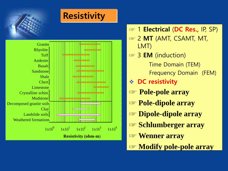
Granite

Rhyolite

Tuff

Andesite

Basalt

Sandstone

Shale

Chert

Limestone

Crystalline schist

Mudstone

Decomposed granite soils

Clay

Landslide soils

Weathered formations

Resistivity (ohm-m)

1 Electrical (DC Res., IP, SP)

2 MT (AMT, CSAMT, MT, LMT)

3 EM (induction)

Time Domain (TEM)

Frequency Domain (FEM)

DC resistivity

Pole-pole array

Pole-dipole array

Dipole-dipole array

Schlumberger array

Wenner array

Modify pole-pole array

Resistivity

1) Ohm’s Law

V IR

RL

A

Resistivity is measured ohm-m and is reciprocal of conductivity

L= length (m) A= area (m)

2

(1)

(2)

A

LR

A

L

V

I

(1)and (2)

JE

(J ): current density (E ) : electrical field

Electric field )( : Rm)(ohm: m)(ohm:

2) Point Current Source

r

P I

C

Ohm’s law

22 r

IJ

22 r

I

r

VE

Potential difference

r

IEdrV

r

2

Current density

3) Two current sources

C1(+)

C2(-)

P1

P2

r11

r12 r21

r22

1211

1

11

2 rrr

IV

2221

2

11

2 rrr

IV

(C1)

(C2)

22211211

21

1111

2 rrrrr

IVVV

I

VG

1

22211211

11112

rrrrG

P1, P2 are potential difference

Resistivity

G (geometric factor)

Res.Apparent a

I

VG

I

VGa

1 Sounding-Profiling

2) Wenner 1) Schlumberger

ana na na nana

M N A B M N A B

Sounding survey

VES

Profiling survey

Resistivity Curve

Initial Model

Curve fitting

Field data

Initial Model Field data

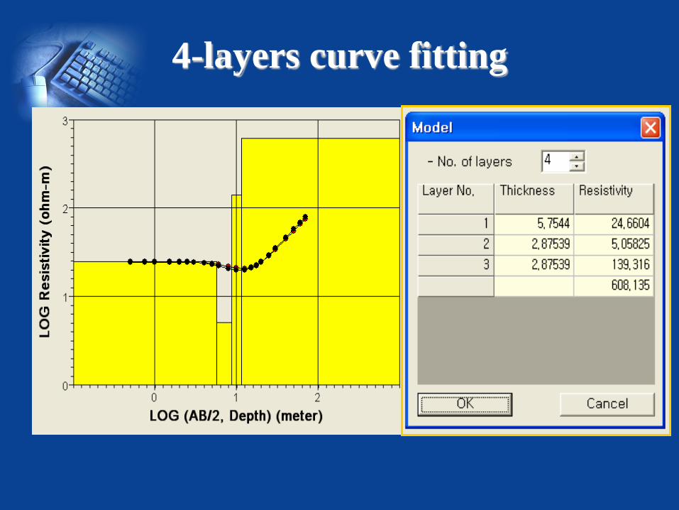
4-layers curve fitting

methods

3. Dipole-dipole

na

5. Wenner

1. Pole - pole

2. Pole - dipole na a

aa na

4. Schlumberger ana na

na nana

2 different Array

aa na

Dipole-dipole array

Sounding & Profiling survey

M N M N M N M N M N A B A B

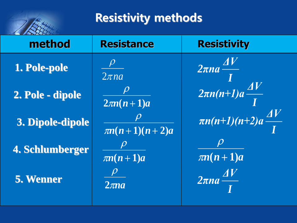
Resistivity methods

3. Dipole-dipole

5. Wenner

1. Pole-pole

2. Pole - dipole

4. Schlumberger

2 na

2 1n n a( )

n n n a( )( ) 1 2

n n a( ) 1

2 na

ΔV2πna

IΔV

2πn(n+1)aI

ΔVπn(n+1)(n+2)a

I

n n a( ) 1

ΔV2πna

I

method Resistivity Resistance

0 2 4 6

Depth

0

20

40

60

80

100

Resis

tivity

Pole-Pole

Pole-dipole

Dipole-dipole

Schlumberger

Wenner

(Depth of investigation)

Pole-pole > Pole-dipole >

Dipole-dipole > Schlumberger >

Wenner

Pole-pole array Pole-dipole array

Dipole-dipole array Schlumberger array

Wenner array

Pole-pole > pole-dipole > dipole-dipole

>> Schlumberger >> Wenner

Model Study

After, KIGAM, 2008 (S. Korea)

pole-pole, pole-dipole, dipole-dipole : n = 2.

Schlumberger, Wenner :

model 1 5 6 7 8 9 10 11 12 13 14 15 16 17 18 19

0

20

40

60

80

Dep

th

100 ohm-m

1,000 ohm-m 1,000 ohm-m10 ohm-m

4321 20 21 22

100

Pole-pole array

Pole-dipole array

Dipole-dipole array

Schlumberger array

Wenner array

Case History After, KIGAM 2008

Potential Electrodes

Electrical Electrodes

Conductive layer Resistive layer

Acquisition

Processing

Interpretation

Inversion

2D-Model acquisition

0.0

0.5

1.0

1.5

2.0

2.5

3.0

3.5

4.0

4.5

0 20 40 60 80 100 120 140

Distance (m)

Inversion

Field Survey

Res.-layers

processing interpretation

3D-Modeling

Borehole information

DH-06

DH-05

BH-78

DH-07

BH-93

BH-91

BH-92

BH-76

BH-75

BH-77

DH-09

DH-08

N

0 50 100m

Scale

Afetr, KIGAM, 2008

Line 4

Line 5 Line 6

Line 7

Line 8

Line 9

Line 10

Line 12

2D-Resistivity modeling

0

70

98

139

198

279

392

562

791

1113

1595

2246

3160

4529

Resistivity(ohm-m)

152300 152400 152500 152600 152700

167500

167600

167700

167800

167900

168000

168100

° °

°

° °

°

pumping well

borehole

BH-93

BH-92

BH-75

DH-05

DH-06

(10m) borehole

10m

Phase I (21 Aug.)

Phase II (4 Oct.)

Phase III (19 Nov.)

Results

(Phase III/ Phase I)

(Phase II/ Phase I)

(Resistivity Ratio)

3D resistivity

3D resistivity