1. Chapter 1: Framing, context, and methods - IPCC
215
Final Government Distribution Chapter 1 IPCC AR6 WGI Do Not Cite, Quote or Distribute 1-1 Total pages: 215 1. Chapter 1: Framing, context, and methods 1 2 Coordinating Lead Authors: 3 Deliang Chen (Sweden), Maisa Rojas (Chile), Bjørn H. Samset (Norway) 4 5 Lead Authors: 6 Kim Cobb (USA), Aida Diongue-Niang (Senegal), Paul Edwards (USA), Seita Emori (Japan), Sergio 7 Henrique Faria (Spain/Brazil), Ed Hawkins (UK), Pandora Hope (Australia), Philippe Huybrechts 8 (Belgium), Malte Meinshausen (Australia/Germany), Sawsan Mustafa (Sudan), Gian-Kasper Plattner 9 (Switzerland), Anne Marie Treguier (France) 10 11 Contributing Authors: 12 Hui-Wen Lai (Sweden), Tania Villaseñor (Chile), Maarten van Aalst (Netherlands), Rondrotiana Barimalala 13 (South Africa/Madagascar), Rosario Carmona (Chile), Peter Cox (UK), Wolfgang Cramer 14 (France/Germany), Francisco Doblas-Reyes (Spain), Hans Dolman (Netherlands), Alessandro Dosio (Italy), 15 Axel von Engeln (Germany), Veronika Eyring (Germany), Greg Flato (Canada), Piers Forster (UK), David 16 Frame (New Zealand), Katja Frieler (Germany), Jan S. Fuglestvedt (Norway), John Fyfe (Canada), Mathias 17 Garschagen (Germany), Joelle Gergis (Australia), Nathan Gillet (Canada/UK), Michael Grose (Australia), 18 Eric Guilyardi (France), Celine Guivarch (France), Susan Hassol (USA), Zeke Hausfather (USA), Hans 19 Hersbach (UK/Netherlands), Helene Hewitt (UK), Mark Howden (Australia), Christian Huggel 20 (Switzerland), Bart van den Hurk (Netherlands), Margot Hurlbert (Canada), Christopher Jones (UK), 21 Richard Jones (UK), Darrell Kaufman (USA), Robert Kopp (USA), Anthony Leiserowitz (USA), Robert J. 22 Lempert (USA), Jared Lewis (Australia/New Zealand), Hong Liao (China), Nikki Lovenduski (USA), 23 Marianne T. Lund (Norway), Katharine Mach (USA), Douglas Maraun (Austria/Germany), Jochem 24 Marotzke (Germany), Jan Minx (Germany), Zebedee Nicholls (Australia), Brian O’Neill (USA), M. Giselle 25 Ogaz (Chile), Friederike Otto (UK/Germany), Wendy Parker (UK), Camille Parmesan (France/UK/USA), 26 Warren Pearce (UK), Roque Pedace (Argentina), Andy Reisinger (New Zealand), James Renwick (New 27 Zealand), Keywan Riahi (Austria), Paul Ritchie (UK), Joeri Rogelj (UK/Belgium), Rodolfo Sapiains (Chile), 28 Yusuke Satoh (Japan), Karina von Schuckmann (France), Sonia I. Seneviratne (Switzerland), Ted Shepherd 29 (UK), Jana Sillmann (Norway/Germany), Lucas Silva (Portugal/Switzerland), Aimee Slangen (Netherlands), 30 Anna Sorensson (Argentina), Peter Steinele (Australia), Thomas F. Stocker (Switzerland), Martina 31 Stockhause (Germany), Daithi Stone (New Zealand), Abigail Swann (USA), Sophie Szopa (France), Izuru 32 Takayabu (Japan), Claudia Tebaldi (USA), Laurent Terray (France), Peter Thorne (Ireland/UK), Blair 33 Trewin (Australia), Isabel Trigo (Portugal), Robert Vautard (France), Carolina Vera (Argentina), David 34 Viner (UK), Detlef van Vuuren (Netherlands), Xuebin Zhang (Canada) 35 36 Review Editors: 37 Nares Chuersuwan (Thailand), Gabriele Hegerl (UK/Germany), Tetsuzo Yasunari (Japan) 38 39 Chapter Scientist: 40 Hui-Wen Lai (Sweden), Tania Villaseñor (Chile) 41 42 Date of Draft: 43 3/05/2021 44 45 Note: 46 TSU compiled version 47 48 49 50
-
Upload
khangminh22 -
Category
Documents
-
view
1 -
download
0
Transcript of 1. Chapter 1: Framing, context, and methods - IPCC
Final Government Distribution Chapter 1 IPCC AR6 WGI
Do Not Cite, Quote or Distribute 1-1 Total pages: 215
1. Chapter 1: Framing, context, and methods 1 2 Coordinating Lead Authors: 3 Deliang Chen (Sweden), Maisa Rojas (Chile), Bjørn H. Samset (Norway) 4 5 Lead Authors: 6 Kim Cobb (USA), Aida Diongue-Niang (Senegal), Paul Edwards (USA), Seita Emori (Japan), Sergio 7 Henrique Faria (Spain/Brazil), Ed Hawkins (UK), Pandora Hope (Australia), Philippe Huybrechts 8 (Belgium), Malte Meinshausen (Australia/Germany), Sawsan Mustafa (Sudan), Gian-Kasper Plattner 9 (Switzerland), Anne Marie Treguier (France) 10 11 Contributing Authors: 12 Hui-Wen Lai (Sweden), Tania Villaseñor (Chile), Maarten van Aalst (Netherlands), Rondrotiana Barimalala 13 (South Africa/Madagascar), Rosario Carmona (Chile), Peter Cox (UK), Wolfgang Cramer 14 (France/Germany), Francisco Doblas-Reyes (Spain), Hans Dolman (Netherlands), Alessandro Dosio (Italy), 15 Axel von Engeln (Germany), Veronika Eyring (Germany), Greg Flato (Canada), Piers Forster (UK), David 16 Frame (New Zealand), Katja Frieler (Germany), Jan S. Fuglestvedt (Norway), John Fyfe (Canada), Mathias 17 Garschagen (Germany), Joelle Gergis (Australia), Nathan Gillet (Canada/UK), Michael Grose (Australia), 18 Eric Guilyardi (France), Celine Guivarch (France), Susan Hassol (USA), Zeke Hausfather (USA), Hans 19 Hersbach (UK/Netherlands), Helene Hewitt (UK), Mark Howden (Australia), Christian Huggel 20 (Switzerland), Bart van den Hurk (Netherlands), Margot Hurlbert (Canada), Christopher Jones (UK), 21 Richard Jones (UK), Darrell Kaufman (USA), Robert Kopp (USA), Anthony Leiserowitz (USA), Robert J. 22 Lempert (USA), Jared Lewis (Australia/New Zealand), Hong Liao (China), Nikki Lovenduski (USA), 23 Marianne T. Lund (Norway), Katharine Mach (USA), Douglas Maraun (Austria/Germany), Jochem 24 Marotzke (Germany), Jan Minx (Germany), Zebedee Nicholls (Australia), Brian O’Neill (USA), M. Giselle 25 Ogaz (Chile), Friederike Otto (UK/Germany), Wendy Parker (UK), Camille Parmesan (France/UK/USA), 26 Warren Pearce (UK), Roque Pedace (Argentina), Andy Reisinger (New Zealand), James Renwick (New 27 Zealand), Keywan Riahi (Austria), Paul Ritchie (UK), Joeri Rogelj (UK/Belgium), Rodolfo Sapiains (Chile), 28 Yusuke Satoh (Japan), Karina von Schuckmann (France), Sonia I. Seneviratne (Switzerland), Ted Shepherd 29 (UK), Jana Sillmann (Norway/Germany), Lucas Silva (Portugal/Switzerland), Aimee Slangen (Netherlands), 30 Anna Sorensson (Argentina), Peter Steinele (Australia), Thomas F. Stocker (Switzerland), Martina 31 Stockhause (Germany), Daithi Stone (New Zealand), Abigail Swann (USA), Sophie Szopa (France), Izuru 32 Takayabu (Japan), Claudia Tebaldi (USA), Laurent Terray (France), Peter Thorne (Ireland/UK), Blair 33 Trewin (Australia), Isabel Trigo (Portugal), Robert Vautard (France), Carolina Vera (Argentina), David 34 Viner (UK), Detlef van Vuuren (Netherlands), Xuebin Zhang (Canada) 35 36 Review Editors: 37 Nares Chuersuwan (Thailand), Gabriele Hegerl (UK/Germany), Tetsuzo Yasunari (Japan) 38 39 Chapter Scientist: 40 Hui-Wen Lai (Sweden), Tania Villaseñor (Chile) 41 42 Date of Draft: 43 3/05/2021 44 45 Note: 46 TSU compiled version 47 48 49 50

Final Government Distribution Chapter 1 IPCC AR6 WGI
Do Not Cite, Quote or Distribute 1-2 Total pages: 215
Table of contents 1 2 Executive Summary ................................................................................................................................. 5 3 4 1.1 Report and chapter overview .......................................................................................................... 8 5
1.1.1 The AR6 WGI Report ................................................................................................................... 8 6 1.1.2 Rationale for the new AR6 WGI structure and its relation to the previous AR5 WGI Report .......... 9 7 1.1.3 Integration of AR6 WGI assessments with other Working Groups ............................................... 12 8 1.1.4 Chapter preview .......................................................................................................................... 13 9
10 1.2 Where we are now .......................................................................................................................... 13 11
1.2.1 The changing state of the physical climate system ....................................................................... 13 12 1.2.1.1 Recent changes in multiple climate indicators ............................................................................. 14 13 1.2.1.2 Long-term perspectives on anthropogenic climate change ........................................................... 15 14 1.2.2 The policy and governance context ............................................................................................. 18 15
16 Cross-Chapter Box 1.1: The WGI contribution to the AR6 and its potential relevance for the global 17
stocktake ................................................................................................................ 19 18 19
1.2.3 Linking science and society: communication, values, and the IPCC assessment process .............. 29 20 1.2.3.1 Climate change understanding, communication, and uncertainties .............................................. 29 21
22 Box 1.1: Treatment of uncertainty and calibrated uncertainty language in AR6 ............................ 30 23
24 1.2.3.2 Values, science, and climate change communication .................................................................. 32 25 1.2.3.3 Climate information, co-production, and climate services ........................................................... 34 26 1.2.3.4 Media coverage of climate change .............................................................................................. 35 27
28 1.3 How we got here: the scientific context ......................................................................................... 36 29
1.3.1 Lines of evidence: instrumental observations ............................................................................... 36 30 1.3.2 Lines of evidence: paleoclimate .................................................................................................. 39 31 1.3.3 Lines of evidence: identifying natural and human drivers ............................................................ 40 32 1.3.4 Lines of evidence: understanding and attributing climate change ................................................. 43 33 1.3.5 Projections of future climate change ............................................................................................ 45 34 1.3.6 How do previous climate projections compare with subsequent observations? ............................. 48 35
36 Box 1.2: Special Reports in the sixth IPCC assessment cycle: key findings...................................... 50 37
38 1.4 AR6 foundations and concepts ...................................................................................................... 53 39
1.4.1 Baselines, reference periods and anomalies ................................................................................. 53 40 41 Cross-Chapter Box 1.2: Changes in global temperature between 1750 and 1850 ................................. 55 42 43
1.4.2 Variability and emergence of the climate change signal ............................................................... 56 44
Final Government Distribution Chapter 1 IPCC AR6 WGI
Do Not Cite, Quote or Distribute 1-3 Total pages: 215
1.4.2.1 Climate variability can influence trends over short periods .......................................................... 57 1 1.4.2.2 The emergence of the climate change signal ............................................................................... 57 2 1.4.3 Sources of uncertainty in climate simulations .............................................................................. 59 3 1.4.3.1 Sources of uncertainty ................................................................................................................ 59 4 1.4.3.2 Uncertainty quantification .......................................................................................................... 60 5 1.4.4 Considering an uncertain future ................................................................................................... 61 6 1.4.4.1 Low-likelihood outcomes ........................................................................................................... 62 7 1.4.4.2 Storylines ............................................................................................................................... 62 8
9 Cross-Chapter Box 1.3: Risk framing in IPCC AR6 .............................................................................. 63 10 11
1.4.4.3 Abrupt change, tipping points and surprises ................................................................................ 65 12 13 Cross-Working Group Box: Attribution ................................................................................................. 67 14 15
1.4.5 Climate regions used in AR6 ....................................................................................................... 70 16 1.4.5.1 Defining climate regions ............................................................................................................ 70 17 1.4.5.2 Types of regions used in AR6..................................................................................................... 71 18
19 1.5 Major developments and their implications .................................................................................. 72 20
1.5.1 Observational data and observing systems ................................................................................... 72 21 1.5.1.1 Major expansions of observational capacity ................................................................................ 73 22 1.5.1.2 Threats to observational capacity or continuity ........................................................................... 77 23 1.5.2 New developments in reanalyses ................................................................................................. 78 24 1.5.3 Climate Models ........................................................................................................................... 82 25 1.5.3.1 Earth System Models .................................................................................................................. 82 26 1.5.3.2 Model tuning and adjustment ..................................................................................................... 84 27 1.5.3.3 From global to regional models .................................................................................................. 85 28 1.5.3.4 Models of lower complexity ....................................................................................................... 86 29
30 Box 1.3: Emission metrics in AR6 WGI............................................................................................. 88 31
32 1.5.4 Modelling techniques, comparisons and performance assessments ............................................... 89 33 1.5.4.1 Model ‘fitness for purpose’ ......................................................................................................... 89 34 1.5.4.2 Ensemble modelling techniques ................................................................................................. 89 35 1.5.4.3 The sixth phase of the Coupled Model Intercomparison Project (CMIP6) ................................... 91 36 1.5.4.4 Coordinated Regional Downscaling Experiment (CORDEX) ...................................................... 93 37 1.5.4.5 Model Evaluation Tools ............................................................................................................. 94 38 1.5.4.6 Evaluation of process-based models against observations ........................................................... 94 39 1.5.4.7 Emergent constraints on climate feedbacks, sensitivities and projections .................................... 95 40 1.5.4.8 Weighting techniques for model comparisons ............................................................................. 96 41
42

Final Government Distribution Chapter 1 IPCC AR6 WGI
Do Not Cite, Quote or Distribute 1-4 Total pages: 215
1.6 Dimensions of Integration: Scenarios, global warming levels and cumulative carbon emissions 97 1 1.6.1 Scenarios ............................................................................................................................... 98 2 1.6.1.1 Shared Socio-economic Pathways ............................................................................................ 100 3
4 Cross-Chapter Box 1.4: The SSP scenarios as used in Working Group I ............................................ 102 5 6
1.6.1.2 Scenario generation process for CMIP6 .................................................................................... 107 7 1.6.1.3 History of scenarios within the IPCC ........................................................................................ 108 8 1.6.1.4 The likelihood of reference scenarios, scenario uncertainty and storylines ................................ 109 9 1.6.2 Global warming levels .............................................................................................................. 111 10 1.6.3 Cumulative CO2 emissions ........................................................................................................ 112 11
12 Box 1.4: The relationships between ‘net zero’ emissions, temperature outcomes and carbon dioxide 13
removal ............................................................................................................................. 113 14 15 1.7 Final remarks ............................................................................................................................. 114 16 17 Frequently Asked Questions .................................................................................................................. 116 18 FAQ 1.1: Do we understand climate change better now compared to when the IPCC started? 116 19 FAQ 1.2: Where is climate change most apparent?................................................................ 117 20 FAQ 1.3: What can past climate teach us about the future? ................................................... 118 21 22 Acknowledgements ............................................................................................................................. 120 23 24 References ............................................................................................................................. 121 25 26 Appendix 1.A ............................................................................................................................. 165 27 28 Figures ............................................................................................................................. 175 29 30 31
Final Government Distribution Chapter 1 IPCC AR6 WGI
Do Not Cite, Quote or Distribute 1-5 Total pages: 215
Executive Summary 1 2 Working Group I (WGI) of the Intergovernmental Panel on Climate Change (IPCC) assesses the current 3 evidence on the physical science of climate change, evaluating knowledge gained from observations, 4 reanalyses, paleoclimate archives and climate model simulations, as well as physical, chemical and 5 biological climate processes. This chapter sets the scene for the WGI assessment, placing it in the context of 6 ongoing global and regional changes, international policy responses, the history of climate science and the 7 evolution from previous IPCC assessments, including the Special Reports prepared as part of this 8 Assessment Cycle. Key concepts and methods, relevant recent developments, and the modelling and scenario 9 framework used in this assessment are presented. 10 11 Framing and Context of the WGI Report 12 13 The WGI contribution to the IPCC Sixth Assessment Report (AR6) assesses new scientific evidence 14 relevant for a world whose climate system is rapidly changing, overwhelmingly due to human 15 influence. The five IPCC assessment cycles since 1990 have comprehensively and consistently laid out the 16 rapidly accumulating evidence of a changing climate system, with the Fourth Assessment Report (AR4, 17 2007) being the first to conclude that warming of the climate system is unequivocal. Sustained changes have 18 been documented in all major elements of the climate system, including the atmosphere, land, cryosphere, 19 biosphere and ocean. Multiple lines of evidence indicate the unprecedented nature of recent large-scale 20 climatic changes in context of all human history, and that they represent a millennial-scale commitment for 21 the slow-responding elements of the climate system, resulting in continued worldwide loss of ice, increase in 22 ocean heat content, sea level rise and deep ocean acidification. {1.2.1, 1.3, Box 1.2, Appendix 1.A} 23 24 Since the IPCC Fifth Assessment Report (AR5), the international policy context of IPCC reports has 25 changed. The UN Framework Convention on Climate Change (UNFCCC, 1992) has the overarching 26 objective of preventing ‘dangerous anthropogenic interference with the climate system’. Responding to that 27 objective, the Paris Agreement (2015) established the long-term goals of ‘holding the increase in global 28 average temperature to well below 2°C above pre-industrial levels and pursuing efforts to limit the 29 temperature increase to 1.5°C above pre-industrial levels’ and of achieving ‘a balance between 30 anthropogenic emissions by sources and removals by sinks of greenhouse gases in the second half of this 31 century’. Parties to the Agreement have submitted Nationally Determined Contributions (NDCs) indicating 32 their planned mitigation and adaptation strategies. However, the NDCs submitted as of 2020 are insufficient 33 to reduce greenhouse gas emission enough to be consistent with trajectories limiting global warming to well 34 below 2°C above pre-industrial levels (high confidence). {1.1, 1.2} 35 36 This report provides information of potential relevance to the 2023 global stocktake. The 5-yearly 37 stocktakes called for in the Paris Agreement will evaluate alignment among the Agreement’s long-term 38 goals, its means of implementation and support, and evolving global efforts in climate change mitigation 39 (efforts to limit climate change) and adaptation (efforts to adapt to changes that cannot be avoided). In this 40 context, WGI assesses, among other topics, remaining cumulative carbon emission budgets for a range of 41 global warming levels, effects of long-lived and short-lived climate forcers, projected changes in sea level 42 and extreme events, and attribution to anthropogenic climate change. {Cross-Chapter Box 1.1} 43 44 Understanding of the fundamental features of the climate system is robust and well established. 45 Scientists in the 19th-century identified the major natural factors influencing the climate system. They also 46 hypothesized the potential for anthropogenic climate change due to carbon dioxide (CO2) emitted by fossil 47 fuel combustion. The principal natural drivers of climate change, including changes in incoming solar 48 radiation, volcanic activity, orbital cycles, and changes in global biogeochemical cycles, have been studied 49 systematically since the early 20th century. Other major anthropogenic drivers, such as atmospheric aerosols 50 (fine solid particles or liquid droplets), land-use change and non-CO2 greenhouse gases, were identified by 51 the 1970s. Since systematic scientific assessments began in the 1970s, the influence of human activity on the 52 warming of the climate system has evolved from theory to established fact. Past projections of global surface 53 temperature and the pattern of warming are broadly consistent with subsequent observations (limited 54 evidence, high agreement), especially when accounting for the difference in radiative forcing scenarios used 55
Final Government Distribution Chapter 1 IPCC AR6 WGI
Do Not Cite, Quote or Distribute 1-6 Total pages: 215
for making projections and the radiative forcings that actually occurred. {1.3.1 - 1.3.6} 1 2 Global surface temperatures increased by about 0.1°C (likely range –0.1°C to +0.3°C, medium 3 confidence) between the period around 1750 and the 1850–1900 period, with anthropogenic factors 4 responsible for a warming of 0.0°C–0.2°C (likely range, medium confidence). This assessed change in 5 temperature before 1850–1900 is not included in the AR6 assessment of global warming to date, to ensure 6 consistency with previous IPCC assessment reports, and because of the lower confidence in the estimate. 7 There was likely a net anthropogenic forcing of 0.0–0.3 Wm-2 in 1850–1900 relative to 1750 (medium 8 confidence), with radiative forcing from increases in atmospheric greenhouse gas concentrations being 9 partially offset by anthropogenic aerosol emissions and land-use change. Net radiative forcing from solar and 10 volcanic activity is estimated to be smaller than ±0.1 Wm-2 for the same period. {Cross Chapter Box 1.2, 11 1.4.1, Cross Chapter Box 2.3} 12 13 Natural climate variability can temporarily obscure or intensify anthropogenic climate change on 14 decadal time scales, especially in regions with large internal interannual-to-decadal variability. At the 15 current level of global warming, an observed signal of temperature change relative to the 1850–1900 16 baseline has emerged above the levels of background variability over virtually all land regions (high 17 confidence). Both the rate of long-term change and the amplitude of interannual (year-to-year) variability 18 differ from global to regional to local scales, between regions and across climate variables, thus influencing 19 when changes become apparent. Tropical regions have experienced less warming than most others, but also 20 exhibit smaller interannual variations in temperature. Accordingly, the signal of change is more apparent in 21 tropical regions than in regions with greater warming but larger interannual variations (high confidence). 22 {1.4.2, FAQ1.2} 23 24 The AR6 has adopted a unified framework of climate risk, supported by an increased focus in WGI on 25 low-likelihood, high-impact events. Systematic risk framing is intended to aid the formulation of effective 26 responses to the challenges posed by current and future climatic changes and to better inform risk assessment 27 and decision-making. AR6 also makes use of the ‘storylines’ approach, which contributes to building a 28 robust and comprehensive picture of climate information, allows a more flexible consideration and 29 communication of risk, and can explicitly address low-likelihood, high-impact events. {1.1.2, 1.4.4, Cross-30 Chapter Box 1.3} 31 32 The construction of climate change information and communication of scientific understanding are 33 influenced by the values of the producers, the users and their broader audiences. Scientific knowledge 34 interacts with pre-existing conceptions of weather and climate, including values and beliefs stemming from 35 ethnic or national identity, traditions, religion or lived relationships to land and sea (high confidence). 36 Science has values of its own, including objectivity, openness and evidence-based thinking. Social values 37 may guide certain choices made during the construction, assessment and communication of information 38 (high confidence). {1.2.3, Box 1.1} 39 40 Data, Tools and Methods Used across the WGI Report 41 42 Capabilities for observing the physical climate system have continued to improve and expand overall, 43 but some reductions in observational capacity are also evident (high confidence). Improvements are 44 particularly evident in ocean observing networks and remote-sensing systems, and in paleoclimate 45 reconstructions from proxy archives. However, some climate-relevant observations have been interrupted by 46 the discontinuation of surface stations and radiosonde launches, and delays in the digitisation of records. 47 Further reductions are expected to result from the COVID-19 pandemic. In addition, paleoclimate archives 48 such as mid-latitude and tropical glaciers as well as modern natural archives used for calibration (e.g., corals 49 and trees) are rapidly disappearing owing to a host of pressures, including increasing temperatures (high 50 confidence). {1.5.1} 51 52 Reanalyses have improved since AR5 and are increasingly used as a line of evidence in assessments of 53 the state and evolution of the climate system (high confidence). Reanalyses, where atmosphere or ocean 54 forecast models are constrained by historical observational data to create a climate record of the past, provide 55
Final Government Distribution Chapter 1 IPCC AR6 WGI
Do Not Cite, Quote or Distribute 1-7 Total pages: 215
consistency across multiple physical quantities and information about variables and locations that are not 1 directly observed. Since AR5, new reanalyses have been developed with various combinations of increased 2 resolution, extended records, more consistent data assimilation, estimation of uncertainty arising from the 3 range of initial conditions, and an improved representation of the ocean. While noting their remaining 4 limitations, the WGI report uses the most recent generation of reanalysis products alongside more standard 5 observation-based datasets. {1.5.2, Annex 1} 6 7 Since AR5, new techniques have provided greater confidence in attributing changes in climate 8 extremes to climate change. Attribution is the process of evaluating the relative contributions of multiple 9 causal factors to an observed change or event. This includes the attribution of the causal factors of changes in 10 physical or biogeochemical weather or climate variables (e.g., temperature or atmospheric CO2) as done in 11 WGI, or of the impacts of these changes on natural and human systems (e.g., infrastructure damage or 12 agricultural productivity), as done in WGII. Attributed causes include human activities (such as emissions of 13 greenhouse gases and aerosols, or land-use change), and changes in other aspects of the climate, or natural or 14 human systems. {Cross-WG Box 1.1} 15 16 The latest generation of complex climate models has an improved representation of physical processes, 17 and a wider range of Earth system models now represent biogeochemical cycles. Since the AR5, 18 higher-resolution models that better capture smaller-scale processes and extreme events have become 19 available. Key model intercomparisons supporting this assessment include the Coupled Model 20 Intercomparison Project Phase 6 (CMIP6) and the Coordinated Regional Climate Downscaling Experiment 21 (CORDEX), for global and regional models respectively. Results using CMIP Phase 5 (CMIP5) simulations 22 are also assessed. Since the AR5, large ensemble simulations, where individual models perform multiple 23 simulations with the same climate forcings, are increasingly used to inform understanding of the relative 24 roles of internal variability and forced change in the climate system, especially on regional scales. The 25 broader availability of ensemble model simulations has contributed to better estimations of uncertainty in 26 projections of future change (high confidence). A broad set of simplified climate models is assessed and used 27 as emulators to transfer climate information across research communities, such as for evaluating impacts or 28 mitigation pathways consistent with certain levels of future warming. {1.4.2, 1.5.3, 1.5.4, Cross-chapter Box 29 7.1} 30 31 Assessments of future climate change are integrated within and across the three IPCC Working 32 Groups through the use of three core components: scenarios, global warming levels, and the 33 relationship between cumulative carbon emissions and global warming. Scenarios have a long history in 34 the IPCC as a method for systematically examining possible futures. A new set of scenarios, derived from 35 the Shared Socio-economic Pathways (SSPs), is used to synthesize knowledge across the physical sciences, 36 impact, and adaptation and mitigation research. The core set of SSP scenarios used in the WGI report, SSP1-37 1.9, SSP1-2.6, SSP2-4.5, SSP3-7.0 and SSP5-8.5, cover a broad range of emission pathways, including new 38 low-emissions pathways. The feasibility or likelihood of individual scenarios is not part of this assessment, 39 which focuses on the climate response to possible, prescribed emission futures. Levels of global surface 40 temperature change (global warming levels), which are closely related to a range of hazards and regional 41 climate impacts, also serve as reference points within and across IPCC Working Groups. Cumulative carbon 42 emissions, which have a nearly linear relationship to increases in global surface temperature, are also used. 43 {1.6.1-1.6.4, Cross-Chapter Box 1.5, Cross-Chapter Box 11.1} 44 45 46 47

Final Government Distribution Chapter 1 IPCC AR6 WGI
Do Not Cite, Quote or Distribute 1-8 Total pages: 215
1.1 Report and chapter overview 1 2 The role of the Intergovernmental Panel on Climate Change (IPCC) is to critically assess the scientific, 3 technical, and socio-economic information relevant to understanding the physical science and impacts of 4 human-induced climate change and natural variations, including the risks, opportunities and options for 5 adaptation and mitigation. This task is performed through a comprehensive assessment of the scientific 6 literature. The robustness of IPCC assessments stems from the systematic consideration and combination of 7 multiple lines of independent evidence. In addition, IPCC reports undergo one of the most comprehensive, 8 open, and transparent review and revision processes ever employed for science assessments. 9 10 Starting with the First Assessment Report (FAR; IPCC, 1990) the IPCC assessments have been structured 11 into three working groups. Working Group I (WGI) assesses the physical science basis of climate change, 12 Working Group II (WGII) assesses associated impacts, vulnerability and adaptation options, and Working 13 Group III (WGIII) assesses mitigation response options. Each report builds on the earlier comprehensive 14 assessments by incorporating new research and updating previous findings. The volume of knowledge 15 assessed and the cross-linkages between the three working groups have substantially increased over time. 16 17 As part of its sixth assessment cycle, from 2015 to 2022, the IPCC is producing three Working Group 18 Reports, three targeted Special Reports, a Refinement to the 2006 IPCC Guidelines for National Greenhouse 19 Gas Inventories, and a Synthesis Report. The AR6 Special Reports covered the topics of ‘Global Warming of 20 1.5°C’ (SR1.5; IPCC, 2018), ‘Climate Change and Land’ (SRCCL; IPCC, 2019a) and ‘The Ocean and 21 Cryosphere in a Changing Climate’ (SROCC; IPCC, 2019b). The SR1.5 and SRCCL are the first IPCC 22 reports jointly produced by all three Working Groups. This evolution towards a more integrated assessment 23 reflects a broader understanding of the interconnectedness of the multiple dimensions of climate change. 24 25 26 1.1.1 The AR6 WGI Report 27 28 The Sixth Assessment Report (AR6) of the IPCC marks more than 30 years of global collaboration to 29 describe and understand, through expert assessments, one of the defining challenges of the 21st century: 30 human-induced climate change. Since the inception of the IPCC in 1988, our understanding of the physical 31 science basis of climate change has advanced markedly. The amount and quality of instrumental 32 observations and information from paleoclimate archives have substantially increased. Understanding of 33 individual physical, chemical and biological processes has improved. Climate model capabilities have been 34 enhanced, through the more realistic treatment of interactions among the components of the climate system, 35 and improved representation of the physical processes, in line with the increased computational capacities of 36 the world's supercomputers. 37 38 This report assesses both observed changes, and the components of these changes that are attributable to 39 anthropogenic influence (or human-induced), distinguishing between anthropogenic and naturally forced 40 changes (see Section 1.2.1.1, Section 1.4.1, Cross Working Group Box: Attribution, and Chapter 3). The 41 core assessment conclusions from previous IPCC reports are confirmed or strengthened in this report, 42 indicating the robustness of our understanding of the primary causes and consequences of anthropogenic 43 climate change. 44 45 The WGI contribution to AR6 is focused on physical and biogeochemical climate science information, with 46 particular emphasis on regional climate changes. These are relevant for mitigation, adaptation and risk 47 assessment in the context of complex and evolving policy settings, including the Paris Agreement, the 48 Global Stocktake, the Sendai Framework and the Sustainable Development Goals (SDGs) Framework. 49 50 The core of this report consists of twelve chapters plus the Atlas (Figure 1.1), which can together be grouped 51 into three categories (excluding this framing chapter): 52 53 Large-Scale Information (Chapters 2, 3 and 4). These chapters assess climate information from global to 54 continental or ocean-basin scales. Chapter 2 presents an assessment of the changing state of the climate 55
Final Government Distribution Chapter 1 IPCC AR6 WGI
Do Not Cite, Quote or Distribute 1-9 Total pages: 215
system, including the atmosphere, biosphere, ocean and cryosphere. Chapter 3 continues with an assessment 1 of the human influence on this changing climate, covering the attribution of observed changes, and 2 introducing the fitness-for-purpose approach for the evaluation of climate models used to conduct the 3 attribution studies. Finally, Chapter 4 assesses climate change projections, from the near to the long term, 4 including climate change beyond 2100, as well as the potential for abrupt and ‘low-likelihood, high-impact’ 5 changes. 6 7 Process Understanding (Chapters 5, 6, 7, 8 and 9). These five chapters provide end-to-end assessments of 8 fundamental Earth system processes and components: the carbon budget and biogeochemical cycles (Chapter 9 5), short-lived climate forcers and their links to air quality (Chapter 6), the Earth’s energy budget and climate 10 sensitivity (Chapter 7), the water cycle (Chapter 8), and the ocean, cryosphere and sea-level changes 11 (Chapter 9). All these chapters provide assessments of observed changes, including relevant paleoclimatic 12 information and understanding of processes and mechanisms as well as projections and model evaluation. 13 14 Regional Information (Chapters 10, 11, 12 and Atlas). New knowledge on climate change at regional 15 scales is reflected in this report with four chapters covering regional information. Chapter 10 provides a 16 framework for assessment of regional climate information, including methods, physical processes, an 17 assessment of observed changes at regional scales, and the performance of regional models. Chapter 11 18 addresses extreme weather and climate events, including temperature, precipitation, flooding, droughts and 19 compound events. Chapter 12 provides a comprehensive, region-specific assessment of changing climatic 20 conditions that may be hazardous or favourable (hence influencing climate risk) for various sectors to be 21 assessed in WGII. Lastly, the Atlas assesses and synthesizes regional climate information from the whole 22 report, focussing on the assessments of mean changes in different regions and on model assessments for the 23 regions. It also introduces the online Interactive Atlas, a novel compendium of global and regional climate 24 change observations and projections. It includes a visualization tool combining various warming levels and 25 scenarios on multiple scales of space and time. 26 27 Embedded in the chapters are Cross-Chapter Boxes that highlight cross-cutting issues. Each chapter also 28 includes an Executive Summary (ES), and several Frequently Asked Questions (FAQs). To enhance 29 traceability and reproducibility of report figures and tables, detailed information on the input data used to 30 create them, as well as links to archived code, are provided in the Input Data Tables in chapter 31 Supplementary Material. Additional metadata on the model input datasets is provided via the report website. 32 33 The AR6 WGI report includes a Summary for Policy Makers (SPM) and a Technical Summary (TS). The 34 integration among the three IPCC Working Groups is strengthened by the implementation of the Cross-35 Working-Group Glossary. 36 37 38 [START FIGURE 1.1 HERE] 39 40 Figure 1.1: The structure of the AR6 WGI Report. Shown are the three pillars of the AR6 WGI, its relation to the 41
WGII and WGIII contributions, and the cross-working-group AR6 Synthesis Report (SYR). 42 43 [END FIGURE 1.1 HERE] 44 45 46 1.1.2 Rationale for the new AR6 WGI structure and its relation to the previous AR5 WGI Report 47 48 The AR6 WGI report, as a result of its scoping process, is structured around topics such as large-scale 49 information, process understanding and regional information (Figure 1.1). This represents a rearrangement 50 relative to the structure of the WGI contribution to the IPCC Fifth Assessment Report (AR5; IPCC, 2013a), 51 as summarized in Figure 1.2. The AR6 approach aims at a greater visibility of key knowledge developments 52 potentially relevant for policymakers, including climate change mitigation, regional adaptation planning 53 based on a risk management framework, and the Global Stocktake. 54 55
Final Government Distribution Chapter 1 IPCC AR6 WGI
Do Not Cite, Quote or Distribute 1-10 Total pages: 215
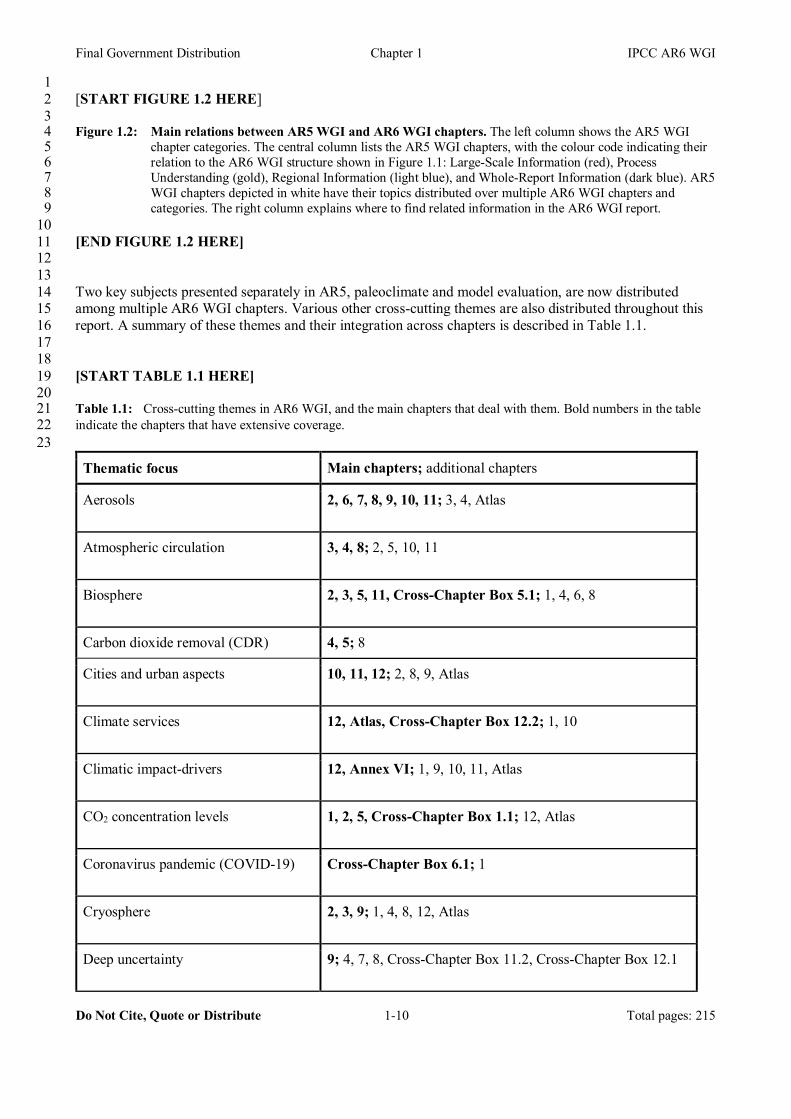
1 [START FIGURE 1.2 HERE] 2 3 Figure 1.2: Main relations between AR5 WGI and AR6 WGI chapters. The left column shows the AR5 WGI 4
chapter categories. The central column lists the AR5 WGI chapters, with the colour code indicating their 5 relation to the AR6 WGI structure shown in Figure 1.1: Large-Scale Information (red), Process 6 Understanding (gold), Regional Information (light blue), and Whole-Report Information (dark blue). AR5 7 WGI chapters depicted in white have their topics distributed over multiple AR6 WGI chapters and 8 categories. The right column explains where to find related information in the AR6 WGI report. 9
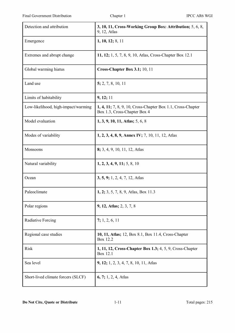
10 [END FIGURE 1.2 HERE] 11 12 13 Two key subjects presented separately in AR5, paleoclimate and model evaluation, are now distributed 14 among multiple AR6 WGI chapters. Various other cross-cutting themes are also distributed throughout this 15 report. A summary of these themes and their integration across chapters is described in Table 1.1. 16 17 18 [START TABLE 1.1 HERE] 19 20 Table 1.1: Cross-cutting themes in AR6 WGI, and the main chapters that deal with them. Bold numbers in the table 21 indicate the chapters that have extensive coverage. 22 23
Thematic focus Main chapters; additional chapters
Aerosols 2, 6, 7, 8, 9, 10, 11; 3, 4, Atlas
Atmospheric circulation 3, 4, 8; 2, 5, 10, 11
Biosphere 2, 3, 5, 11, Cross-Chapter Box 5.1; 1, 4, 6, 8
Carbon dioxide removal (CDR) 4, 5; 8
Cities and urban aspects 10, 11, 12; 2, 8, 9, Atlas
Climate services 12, Atlas, Cross-Chapter Box 12.2; 1, 10
Climatic impact-drivers 12, Annex VI; 1, 9, 10, 11, Atlas
CO2 concentration levels 1, 2, 5, Cross-Chapter Box 1.1; 12, Atlas
Coronavirus pandemic (COVID-19) Cross-Chapter Box 6.1; 1
Cryosphere 2, 3, 9; 1, 4, 8, 12, Atlas
Deep uncertainty 9; 4, 7, 8, Cross-Chapter Box 11.2, Cross-Chapter Box 12.1
Final Government Distribution Chapter 1 IPCC AR6 WGI
Do Not Cite, Quote or Distribute 1-11 Total pages: 215
Detection and attribution 3, 10, 11, Cross-Working Group Box: Attribution; 5, 6, 8, 9, 12, Atlas
Emergence 1, 10, 12; 8, 11
Extremes and abrupt change 11, 12; 1, 5, 7, 8, 9, 10, Atlas, Cross-Chapter Box 12.1
Global warming hiatus Cross-Chapter Box 3.1; 10, 11
Land use 5; 2, 7, 8, 10, 11
Limits of habitability 9, 12; 11
Low-likelihood, high-impact/warming 1, 4, 11; 7, 8, 9, 10, Cross-Chapter Box 1.1, Cross-Chapter Box 1.3, Cross-Chapter Box 4
Model evaluation 1, 3, 9, 10, 11, Atlas; 5, 6, 8
Modes of variability 1, 2, 3, 4, 8, 9, Annex IV; 7, 10, 11, 12, Atlas
Monsoons 8; 3, 4, 9, 10, 11, 12, Atlas
Natural variability 1, 2, 3, 4, 9, 11; 5, 8, 10
Ocean 3, 5, 9; 1, 2, 4, 7, 12, Atlas
Paleoclimate 1, 2; 3, 5, 7, 8, 9, Atlas, Box 11.3
Polar regions 9, 12, Atlas; 2, 3, 7, 8
Radiative Forcing 7; 1, 2, 6, 11
Regional case studies 10, 11, Atlas; 12, Box 8.1, Box 11.4, Cross-Chapter Box 12.2
Risk 1, 11, 12, Cross-Chapter Box 1.3; 4, 5, 9, Cross-Chapter Box 12.1
Sea level 9, 12; 1, 2, 3, 4, 7, 8, 10, 11, Atlas
Short-lived climate forcers (SLCF) 6, 7; 1, 2, 4, Atlas

Final Government Distribution Chapter 1 IPCC AR6 WGI
Do Not Cite, Quote or Distribute 1-12 Total pages: 215
Solar radiation modification (SRM) 4, 5; 6, 8
Tipping points 5, 8, 9; 4, 11, 12, Cross-Chapter Box 12.1
Values and beliefs 1, 10; 12
Volcanic forcing 2, 4, 7, 8; 1, 3, 5, 9, 10, Annex III
Water cycle 8, 11; 2, 3, 10, Box 11.1
1 [END TABLE 1.1 HERE] 2 3 4 1.1.3 Integration of AR6 WGI assessments with other Working Groups 5 6 Integration of assessments across the chapters of the WGI Report, and with WGII and WGIII, occurs in a 7 number of ways, including work on a common Glossary, risk framework (see Cross-Chapter Box 1.3), 8 scenarios and projections of future large-scale changes, and the presentation of results at various global 9 warming levels (see Section 1.6). 10 11 Chapters 8 through 12, and the Atlas, cover topics also assessed by WGII in several areas, including regional 12 climate information and climate-related risks. This approach produces a more integrated assessment of 13 impacts of climate change across Working Groups. In particular, Chapter 10 discusses the generation of 14 regional climate information for users, the co-design of research with users, and the translation of 15 information into the user context (in particular directed towards WGII). Chapter 12 provides a direct bridge 16 between physical climate information (climatic impact-drivers) and sectoral impacts and risk, following the 17 chapter organization of the WGII assessment. Notably, Cross-Chapter Box 12.1 draws a connection to 18 representative key risks and Reasons for Concern (RFC). 19 20 The science assessed in Chapters 2 to 7, such as the carbon budget, short-lived climate forcers and emission 21 metrics, are topics in common with WGIII, and relevant for the mitigation of climate change. This includes a 22 consistent presentation of the concepts of carbon budget and net zero emission targets within chapters, in 23 order to support integration in the Synthesis Report. Emission-driven emulators (simple climate models), 24 summarised in Cross-Chapter Box 7.1 in Chapter 7 are used to approximate large-scale climate responses of 25 complex Earth System Models (ESMs) and have been used as tools to explore the expected GSAT response 26 to multiple scenarios consistent with those assessed in WGI for the classification of scenarios in WGIII. 27 Chapter 6 provides information about the impact of climate change on global air pollution, relevant for 28 WGII, including Cross-Chapter Box 6.1 on the implications of the recent coronavirus pandemic (COVID-19) 29 for climate and air quality. Cross-Chapter Box 2.3 in Chapter 2 presents an integrated cross-WG discussion 30 of global temperature definitions, with implications for many aspects of climate change science. 31 32 In addition, Chapter 1 sets out a shared terminology on cross-cutting topics, including climate risk, 33 attribution and storylines, as well as an introduction to emission scenarios, global warming levels and 34 cumulative carbon emissions as an overarching topic for integration across all three Working Groups. 35 36 All these integration efforts are aimed at enhancing the bridges and ‘handshakes’ among Working Groups, 37 enabling the final cross-working group exercise of producing the integrated Synthesis Report. 38 39 40

Final Government Distribution Chapter 1 IPCC AR6 WGI
Do Not Cite, Quote or Distribute 1-13 Total pages: 215
1.1.4 Chapter preview 1 2 The main purposes of this chapter are: (1) to set the scene for the WGI assessment and to place it in the 3 context of ongoing global changes, international policy processes, the history of climate science and the 4 evolution from previous IPCC assessments, including the Special Reports prepared as part of the sixth 5 assessment cycle; (2) to describe key concepts and methods, relevant developments since AR5, and the 6 modelling framework used in this assessment; and (3) together with the other chapters of this report, to 7 provide context and support for the WGII and WGIII contributions to AR6, particularly on climate 8 information to support mitigation, adaptation and risk management. 9 10 The chapter comprises seven sections (Figure 1.3). Section 1.2 describes the present state of Earth’s climate, 11 in the context of reconstructed and observed long-term changes and variations caused by natural and 12 anthropogenic factors. It also provides context for the present assessment by describing recent changes in 13 international climate change governance and fundamental scientific values. The evolution of knowledge 14 about climate change and the development of earlier IPCC assessments are presented in Section 1.3. 15 Approaches, methods, and key concepts of this assessment are introduced in Section 1.4. New developments 16 in observing networks, reanalyses, modelling capabilities and techniques since the AR5 are discussed in 17 Section 1.5. The three main ‘dimensions of integration’ across Working Groups in the AR6, i.e. emission 18 scenarios, global warming levels and cumulative carbon emissions, are described in Section 1.6. The Chapter 19 closes with a discussion of opportunities and gaps in knowledge integration in Section 1.7. 20 21 22 [START FIGURE 1.3 HERE] 23 24 Figure 1.3: A roadmap to the contents of Chapter 1. 25 26 [END FIGURE 1.3 HERE] 27 28 29 1.2 Where we are now 30 31 The IPCC sixth assessment cycle occurs in the context of increasingly apparent climatic changes observed 32 across the physical climate system. Many of these changes can be attributed to anthropogenic influences, 33 with impacts on natural and human systems. AR6 also occurs in the context of efforts in international climate 34 governance such as the Paris Agreement, which sets a long-term goal to hold the increase in global average 35 temperature to ‘well below 2°C above pre-industrial levels, and to pursue efforts to limit the temperature 36 increase to 1.5°C above pre-industrial levels, recognizing that this would significantly reduce the risks and 37 impacts of climate change’. This section summarises key elements of the broader context surrounding the 38 assessments made in the present report. 39 40 41 1.2.1 The changing state of the physical climate system 42 43 The WGI contribution to the AR5 (AR5 WGI; IPCC, 2013a) assessed that ‘warming of the climate system is 44 unequivocal’, and that since the 1950s, many of the observed changes are unprecedented over decades to 45 millennia. Changes are evident in all components of the climate system: the atmosphere and the ocean have 46 warmed, amounts of snow and ice have diminished, sea level has risen, the ocean has acidified and its 47 oxygen content has declined, and atmospheric concentrations of greenhouse gases have increased (IPCC, 48 2013b). This Report documents that, since the AR5, changes to the state of the physical and biogeochemical 49 climate system have continued, and these are assessed in full in later chapters. Here, we summarize changes 50 to a set of key large-scale climate indicators over the modern era (1850 to present). We also discuss the 51 changes in relation to the longer-term evolution of the climate. These ongoing changes throughout the 52 climate system form a key part of the context of the present report. 53 54 55
Final Government Distribution Chapter 1 IPCC AR6 WGI
Do Not Cite, Quote or Distribute 1-14 Total pages: 215
1.2.1.1 Recent changes in multiple climate indicators 1 2 The physical climate system comprises all processes that combine to form weather and climate. The early 3 chapters of this report broadly organize their assessments according to overarching realms: the atmosphere, 4 the biosphere, the cryosphere (surface areas covered by frozen water, such as glaciers and ice sheets), and the 5 ocean. Elsewhere in the report, and in previous IPCC assessments, the land is also used as an integrating 6 realm that includes parts of the biosphere and the cryosphere. These overarching realms have been studied 7 and measured in increasing detail by scientists, institutions, and the general public since the 18th century, 8 over the era of instrumental observation (see Section 1.3). Today, observations include those taken by 9 numerous land surface stations, ocean surface measurements from ships and buoys, underwater 10 instrumentation, satellite and surface-based remote sensing, and in situ atmospheric measurements from 11 airplanes and balloons. These instrumental observations are combined with paleoclimate reconstructions and 12 historical documentations to produce a highly detailed picture of the past and present state of the whole 13 climate system, and to allow assessments about rates of change across the different realms (see Chapter 2 14 and Section 1.5). 15 16 Figure 1.4 documents that the climate system is undergoing a comprehensive set of changes. It shows a 17 selection of key indicators of change through the instrumental era that are assessed and presented in the 18 subsequent chapters of this report. Annual mean values are shown as stripes, with colours indicating their 19 value. The transitions from one colour to another over time illustrate how conditions are shifting in all 20 components of the climate system. For these particular indicators, the observed changes go beyond the 21 yearly and decadal variability of the climate system. In this Report, this is termed an ‘emergence’ of the 22 climate signal (see Section 1.4.2 and FAQ 1.2). 23 24 Warming of the climate system is most commonly presented through the observed increase in global mean 25 surface temperature (GMST). Taking a baseline of 1850–1900, GMST change until present (2011–2020) is 26 1.09 °C (0.95–1.20 °C) (see Chapter 2, Section 2.3, Cross-Chapter Box 2.3). This evolving change has been 27 documented in previous Assessment Reports, with each reporting a higher total global temperature change 28 (see Section 1.3, Cross-Chapter Box 1.2). The total change in Global Surface Air Temperature (GSAT; see 29 Section 1.4.1 and Cross-Chapter Box 2.3 in Chapter 2) attributable to anthropogenic activities is assessed to 30 be consistent with the observed change in GSAT (see Chapter 3, Section 3.3)1. 31 32 Similarly, atmospheric concentrations of a range of greenhouse gases are increasing. Carbon dioxide (CO2, 33 shown in Figure 1.4 and Figure 1.5a), found in AR5 and earlier reports to be the current strongest driver of 34 anthropogenic climate change, has increased from 285.5 ± 2.1 ppm in 1850 to 409.9 ± 0.4 ppm in 2019; 35 concentrations of methane (CH4), and nitrous oxide (N2O) have increased as well (see Chapter 2, Sections 36 2.2, Chapter 5, section 5.2, and Annex V). These observed changes are assessed to be in line with known 37 anthropogenic and natural emissions, when accounting for observed and inferred uptake by land, ocean, and 38 biosphere respectively (see Chapter 5, Section 5.2), and are a key source of anthropogenic changes to the 39 global energy balance (or radiative forcing; see Chapter 2, Section 2.2 and Chapter 7, Section 7.3). 40 41 The hydrological (or water) cycle is also changing and is assessed to be intensifying, through a higher 42 exchange of water between the surface and the atmosphere (see Chapter 3, Section 2.3 and Chapter 8, 43 Section 8.3). The resulting regional patterns of changes to precipitation are, however, different from surface 44 temperature change, and interannual variability is larger, as illustrated in Figure 1.4. Annual land area mean 45 precipitation in the Northern Hemisphere temperate regions has increased, while the sub-tropical dry regions 46 have experienced a decrease in precipitation in recent decades (see Chapter 2, Section 2.3). 47 48 The cryosphere is undergoing rapid changes, with increased melting and loss of frozen water mass in most 49
1 Note that GMST and GSAT are physically distinct but closely related quantities, see Section 1.4.1 and Cross-Chapter Box 2.3 in Chapter 2.
Final Government Distribution Chapter 1 IPCC AR6 WGI
Do Not Cite, Quote or Distribute 1-15 Total pages: 215
regions. This includes all frozen parts of the globe, such as terrestrial snow, permafrost, sea ice, glaciers, 1 freshwater ice, solid precipitation, and the ice sheets covering Greenland and Antarctica (see Chapter 9; 2 SROCC, IPCC, 2019b). Figure 1.4 illustrates how, globally, glaciers have been increasingly losing mass for 3 the last fifty years. The total glacier mass in the most recent decade (2010-2019) was the lowest since the 4 beginning of the 20th century. (See Chapter 2, Section 2.3 and Chapter 9, Section 9.5). 5 6 The global ocean has warmed unabatedly since at least 1970 (Sections 1.3, 2.3, 9.2; SROCC, IPCC, 2019b) . 7 Figure 1.4 shows how the averaged ocean heat content is steadily increasing, with a total increase of [0.28–8 0.55] yottajoule (1024 joule) between 1971 and 2018. (see Chapter 9, Section 9.2). In response to this ocean 9 warming, as well as to the loss of mass from glaciers and ice sheets, the global mean sea level (GMSL) has 10 risen by 0.20 [0.15 to 0.25] metres between 1900 and 2018. GMSL rise has accelerated since the late 1960s. 11 (See Chapter 9, Section 9.6). 12 13 Overall, the changes in these selected climatic indicators have progressed beyond the range of natural year-14 to-year variability (see Chapters 2, 3, 8, and 9, and further discussion in Sections 1.2.1.2 and 1.4.2). The 15 indicators presented in Figure 1.4 document a broad set of concurrent and emerging changes across the 16 physical climate system. All indicators shown here, along with many others, are further presented in the 17 coming chapters, together with a rigorous assessment of the supporting scientific literature. Later chapters 18 (Chapter 10, 11, 12, and the Atlas) present similar assessments at the regional level, where observed changes 19 do not always align with the global mean picture shown here. 20 21 22 [START FIGURE 1.4 HERE] 23 24 Figure 1.4: Changes are occurring throughout the climate system. Left: Main realms of the climate system: 25
atmosphere, biosphere, cryosphere, and ocean. Right: Six key indicators of ongoing changes since 1850, 26 or the start of the observational or assessed record, through 2018. Each stripe indicates the global (except 27 for precipitation which shows two latitude band means), annual mean anomaly for a single year, relative 28 to a multi-year baseline (except for CO2 concentration and glacier mass loss, which are absolute values). 29 Grey indicates that data are not available. Datasets and baselines used are: (1) CO2: Antarctic ice cores 30 (Lüthi et al., 2008; Bereiter et al., 2015) and direct air measurements (Tans and Keeling, 2020) (see 31 Figure 1.5 for details); (2) precipitation: Global Precipitation Climatology Centre (GPCC) V8 (updated 32 from Becker et al. 2013), baseline 1961-1990 using land areas only with latitude bands 33°N–66°N and 33 15°S–30°S; (3) glacier mass loss: Zemp et al., 2019; (4) global surface air temperature (GMST): 34 HadCRUT5 (Morice et al., 2021), baseline 1961–1990; (5) sea level change: (Dangendorf et al., 2019), 35 baseline 1900–1929; (6) ocean heat content (model-observation hybrid): Zanna et al., (2019), baseline 36 1961–1990. Further details on data sources and processing are available in the chapter data table (Table 37 1.SM.1). 38
39 [END FIGURE 1.4 HERE] 40 41 42 1.2.1.2 Long-term perspectives on anthropogenic climate change 43 44 Paleoclimate archives (e.g, ice cores, corals, marine and lake sediments, speleothems, tree rings, borehole 45 temperatures, soils) permit the reconstruction of climatic conditions before the instrumental era. This 46 establishes an essential long-term context for the climate change of the past 150 years and the projected 47 changes in the 21st century and beyond (IPCC, 2013a; Masson-Delmotte et al., 2013) Chapter 3). Figure 1.5 48 shows reconstructions of three key indicators of climate change over the past 800,000 years2 – atmospheric 49 CO2 concentrations, global mean surface temperature (GMST) and global mean sea level (GMSL) – 50
2 as old as the longest continuous climate records based on the ice core from EPICA Dome Concordia (Antarctica). Polar ice cores are the only paleoclimatic archive providing direct information on past greenhouse gas concentrations.

Final Government Distribution Chapter 1 IPCC AR6 WGI
Do Not Cite, Quote or Distribute 1-16 Total pages: 215
comprising at least eight complete glacial-interglacial cycles (EPICA Community Members, 2004; Jouzel et 1 al., 2007) that are largely driven by oscillations in the Earth’s orbit and consequent feedbacks on multi-2 millennial time scales (Berger, 1978; Laskar et al., 1993). The dominant cycles – recurring approximately 3 every 100,000 years – can be found imprinted in the natural variations of these three key indicators. Before 4 industrialisation, atmospheric CO2 concentrations varied between 174 ppm and 300 ppm, as measured 5 directly in air trapped in ice at Dome Concordia, Antarctica (Bereiter et al., 2015; Nehrbass-Ahles et al., 6 2020). Relative to 1850–1900, the reconstructed GMST changed in the range of -6 to +1°C across these 7 glacial-interglacial cycles (see Chapter 2, Section 2.3.1 for an assessment of different paleo reference 8 periods). GMSL varied between about -130 m during the coldest glacial maxima and +5 to +25 m during the 9 warmest interglacial periods (Spratt and Lisiecki, 2016; Chapter 2). They represent the amplitudes of natural, 10 global-scale climate variations over the last 800,000 years prior to the influence of human activity. Further 11 climate information from a variety of paleoclimatic archives are assessed in Chapters 2, 5, 7, 9. 12 13 Paleoclimatic information also provides a long-term perspective on rates of change of these three key 14 indicators. The rate of increase in atmospheric CO2 observed over 1919-2019 CE is one order of magnitude 15 higher than the fastest CO2 fluctuations documented during the last glacial maximum and the last deglacial 16 transition in high-resolution reconstructions from polar ice cores (Marcott et al., 2014, see Chapter 2, Section 17 2.2.3.2.1). Current multi-decadal GMST exhibit a higher rate of increase than over the past two thousand 18 years (PAGES 2k Consortium, 2019; Chapter 2, Section 2.3.1.1.2), and in the 20th century GMSL rise was 19 faster than during any other century over the past three thousand years (Chapter 2, Section 2.3.3.3). 20 21 22 [START FIGURE 1.5 HERE] 23 24 Figure 1.5: Long-term context of anthropogenic climate change based on selected paleoclimatic reconstructions 25
over the past 800,000 years for three key indicators: atmospheric CO2 concentrations, Global Mean 26 Surface Temperature (GMST), and Global Mean Sea Level (GMSL). a) Measurements of CO2 in air 27 enclosed in Antarctic ice cores (Lüthi et al., 2008; Bereiter et al., 2015 [a compilation]; uncertainty 28 ±1.3ppm; see Chapter 2, Section 2.2.3 and Chapter 5, Section 5.1.2 for an assessment) and direct air 29 measurements (Tans and Keeling, 2020; uncertainty ±0.12 ppm). Projected CO2 concentrations for five 30 Shared Socioeconomic Pathways (SSP) scenarios are indicated by dots on the right-hand side panels of 31 the figure (grey background) (Meinshausen et al., 2020; SSPs are described in Section 1.6). b) 32 Reconstruction of GMST from marine paleoclimate proxies (light grey: Snyder (2016); dark grey: 33 Hansen et al. (2013); see Chapter 2, Section 2.3.1 for an assessment). Observed and reconstructed 34 temperature changes since 1850 are the AR6 assessed mean (referenced to 1850–1900; Box TS.3; 35 2.3.1.1); dots/whiskers on the right-hand side panels of the figure (grey background) indicate the 36 projected mean and ranges of warming derived from Coupled Model Intercomparison Project Phase 6 37 (CMIP6) SSP-based (2081–2100) and Model for the Assessment of Greenhouse Gas Induced Climate 38 Change (MAGICC7) (2300) simulations (Chapter 4, Tables 4.5 and 4.9). c) Sea level changes 39 reconstructed from a stack of oxygen isotope measurements on seven ocean sediment cores (Spratt and 40 Lisiecki, 2016; see Chapter 2, Section 2.3.3.3 and Chapter 9, Section 9.6.2 for an assessment). The sea 41 level record from 1850 to 1900 is from Kopp et al. (2016), while the 20th century record is an updated 42 ensemble estimate of GMSL change (Palmer et al., 2021; see also Chapter 2, Section 2.3.3.3 and Chapter 43 9, Section 9.6.1.1). Dots/whiskers on the right-hand side panels of the figure (grey background) indicate 44 the projected median and ranges derived from SSP-based simulations (2081–2100: Chapter 9, Table 9.9; 45 2300: Chapter 9, Section 9.6.3.5). Best estimates (dots) and uncertainties (whiskers) as assessed by 46 Chapter 2 are included in the left and middle panels for each of the three indicators and selected paleo-47 reference periods used in this report (CO2: Chapter 2, Table 2.1; GMST: Chapter 2, Section 2.3.1.1 and 48 Cross-Chapter Box 2.3, Table 1 in Chapter 2; GMSL: Chapter 2, Section 2.3.3.3 and Chapter 9, Section 49 9.6.2. See also Cross-Chapter Box 2.1 in Chapter 2). Selected paleo-reference periods: LIG – Last 50 Interglacial; LGM – Last Glacial Maximum; MH – mid-Holocene (Cross-Chapter Box 2.1, Table 1 in 51 Chapter 2). The non-labelled best estimate in panel c) corresponds to the sea level high-stand during 52 Marine Isotope Stage 11, about 410,000 years ago (see Chapter 9, Section 9.6.2). Further details on data 53 sources and processing are available in the chapter data table (Table 1.SM.1). 54
55 [END FIGURE 1.5 HERE] 56 57 58

Final Government Distribution Chapter 1 IPCC AR6 WGI
Do Not Cite, Quote or Distribute 1-17 Total pages: 215
Paleoclimate reconstructions also shed light on the causes of these variations, revealing processes that need 1 to be considered when projecting climate change. The paleorecords show that sustained changes in global 2 mean temperature of a few degrees Celsius are associated with increases in sea level of several tens of metres 3 (Figure 1.5). During two extended warm periods (interglacials) of the last 800,000 years, sea level is 4 estimated to have been at least six metres higher than today (Chapter 2; Dutton et al., 2015). During the last 5 interglacial, sustained warmer temperatures in Greenland preceded the peak of sea level rise (Figure 5.15 in 6 Masson-Delmotte et al., 2013). The paleoclimate record therefore provides substantial evidence directly 7 linking warmer GMST to substantially higher GMSL. 8 9 GMST will remain above present-day levels for many centuries even if net CO2 emissions are reduced to 10 zero, as shown in simulations with coupled climate models (Plattner et al., 2008; Section 12.5.3 in Collins et 11 al., 2013; Zickfeld et al., 2013; MacDougall et al., 2020; Chapter 4, Section 4.7.1). Such persistent warm 12 conditions in the atmosphere represent a multi-century commitment to long-term sea level rise, summer sea 13 ice reduction in the Arctic, substantial ice sheet melting, potential ice sheet collapse, and many other 14 consequences in all components of the climate system (Clark et al., 2016; Pfister and Stocker, 2016; Fischer 15 et al., 2018; see also Chapter 9, Section 9.4) (Figure 1.5). 16 17 Paleoclimate records also show centennial- to millennial-scale variations, particularly during the ice ages, 18 which indicate rapid or abrupt changes of the Atlantic Meridional Overturning Circulation (AMOC; see 19 Chapter 9, Section 9.2.3.1) and the occurrence of a ‘bipolar seesaw’ (opposite-phase surface temperature 20 changes in both hemispheres; Stocker and Johnsen, 2003; EPICA Community Members, 2006; Members 21 WAIS Divide Project et al., 2015; Lynch-Stieglitz, 2017; Pedro et al., 2018; Weijer et al., 2019, see Chapter 22 2, Section 2.3.3.4.1). This process suggests that instabilities and irreversible changes could be triggered if 23 critical thresholds are passed (Section 1.4.4.3). Several other processes involving instabilities are identified 24 in climate models (Drijfhout et al., 2015), some of which may now be close to critical thresholds (Joughin et 25 al., 2014; Section 1.4.4.3; see also Chapters 5, 8 and 9 regarding tipping points). 26 27 Based on Figure 1.5, the reconstructed, observed and projected ranges of changes in the three key indicators 28 can be compared. By the first decade of the 20th century, atmospheric CO2 concentrations had already 29 moved outside the reconstructed range of natural variation over the past 800,000 years. On the other hand, 30 global mean surface temperature and sea level were higher than today during several interglacials of that 31 period (Chapter 2, Section 2.3.1, Figure 2.34 and Section 2.3.3). Projections for the end of the 21st century, 32 however, show that GMST will have moved outside of its natural range within the next few decades, except 33 for the strong mitigation scenarios (Section 1.6). There is a risk that GMSL may potentially leave the 34 reconstructed range of natural variations over the next few millennia (Clark et al., 2016; Chapter 9, Section 35 9.6.3.5; SROCC (IPCC, 2019b). In addition, abrupt changes can not be excluded (Section 1.4.4.3). 36 37 An important time period in the assessment of anthropogenic climate change is the last 2000 years. Since 38 AR5, new global datasets have emerged, aggregating local and regional paleorecords (PAGES 2k 39 Consortium, 2013, 2017, 2019; McGregor et al., 2015; Tierney et al., 2015; Abram et al., 2016; Hakim et al., 40 2016; Steiger et al., 2018; Brönnimann et al., 2019b). Before the global warming that began around the mid-41 19th century (Abram et al., 2016), a slow cooling in the Northern Hemisphere from roughly 1450 to 1850 is 42 consistently recorded in paleoclimate archives (PAGES 2k Consortium, 2013; McGregor et al., 2015). While 43 this cooling, primarily driven by an increased number of volcanic eruptions (PAGES 2k Consortium, 2013; 44 Owens et al., 2017; Brönnimann et al., 2019b; Chapter 3, Section 3.3.1), shows regional differences, the 45 subsequent warming over the past 150 years exhibits a global coherence that is unprecedented in the last 46 2000 years (Neukom et al., 2019). 47 48 The rate, scale, and magnitude of anthropogenic changes in the climate system since the mid-20th century 49 suggested the definition of a new geological epoch, the Anthropocene (Crutzen and Stoermer, 2000; Steffen 50 et al., 2007), referring to an era in which human activity is altering major components of the Earth system 51 and leaving measurable imprints that will remain in the permanent geological record (IPCC, 2018) (Figure 52 1.5). These alterations include not only climate change itself, but also chemical and biological changes in the 53 Earth system such as rapid ocean acidification due to uptake of anthropogenic carbon dioxide, massive 54 destruction of tropical forests, a worldwide loss of biodiversity and the sixth mass extinction of species 55
Final Government Distribution Chapter 1 IPCC AR6 WGI
Do Not Cite, Quote or Distribute 1-18 Total pages: 215
(Hoegh-Guldberg and Bruno, 2010; Ceballos et al., 2017; IPBES, 2019). According to the key messages of 1 the last global assessment of the Intergovernmental Science-Policy Platform on Biodiversity and Ecosystem 2 Services (IPBES, 2019), climate change is a ‘direct driver that is increasingly exacerbating the impact of 3 other drivers on nature and human well-being’, and ‘the adverse impacts of climate change on biodiversity 4 are projected to increase with increasing warming’. 5 6 7 1.2.2 The policy and governance context 8 9 The contexts of both policymaking and societal understanding about climate change have evolved since the 10 AR5 was published (2013–2014). Increasing recognition of the urgency of the climate change threat, along 11 with still-rising emissions and unresolved issues of mitigation and adaptation, including aspects of 12 sustainable development, poverty eradication and equity, have led to new policy efforts. This section 13 summarizes these contextual developments and how they have shaped, and been used during the preparation 14 of this Report. 15 16 IPCC reports and the UN Framework Convention on Climate Change (UNFCCC). The IPCC First 17 Assessment Report (FAR, IPCC, 1990a) provided the scientific background for the establishment of the 18 United Nations Framework Convention on Climate Change (UNFCCC, 1992), which committed parties to 19 negotiate ways to ‘prevent dangerous anthropogenic interference with the climate system’ (the ultimate 20 objective of the UNFCCC). The Second Assessment Report (SAR, IPCC, 1995a) informed governments in 21 negotiating the Kyoto Protocol (1997), the first major agreement focusing on mitigation under the UNFCCC. 22 The Third Assessment report (TAR, IPCC, 2001a) highlighted the impacts of climate change and need for 23 adaptation and introduced the treatment of new topics such as policy and governance in IPCC reports. The 24 Fourth and Fifth Assessment Reports (AR4, IPCC, 2007a; AR5, IPCC, 2013a) provided the scientific 25 background for the second major agreement under the UNFCCC: the Paris Agreement (2015), which entered 26 into force in 2016. 27 28 The Paris Agreement (PA). Parties to the PA commit to the goal of limiting global average temperature 29 increase to ‘well below 2°C above pre-industrial levels, and to pursue efforts to limit the temperature 30 increase to 1.5°C in order to ‘significantly reduce the risks and impacts of climate change’. In AR6, as in 31 many previous IPCC reports, observations and projections of changes in global temperature are expressed 32 relative to 1850-1900 as an approximation for pre-industrial levels (Cross-Chapter Box 1.2). 33 34 The PA further addresses mitigation (Article 4) and adaptation to climate change (Article 7), as well as loss 35 and damage (Article 8), through the mechanisms of finance (Article 9), technology development and transfer 36 (Article 10), capacity-building (Article 11) and education (Article 12). To reach its long-term temperature 37 goal, the PA recommends ‘achieving a balance between anthropogenic emissions by sources and removals 38 by sinks of greenhouse gases in the second half of this century’, a state commonly described as ‘net zero’ 39 emissions (Article 4) (Section 6, Box 1.4). Each Party to the PA is required to submit a Nationally 40 Determined Contribution (NDC) and pursue, on a voluntary basis, domestic mitigation measures with the 41 aim of achieving the objectives of its NDC (Article 4). 42 43 Numerous studies of the NDCs submitted since adoption of the PA in 2015 (Fawcett et al., 2015; UNFCCC, 44 2015, 2016; Lomborg, 2016; Rogelj et al., 2016, 2017; Benveniste et al., 2018; Gütschow et al., 2018; 45 United Nations Environment Programme (UNEP), 2019) conclude that they are insufficient to meet the Paris 46 temperature goal. In the present IPCC Sixth Assessment cycle, a Special Report on Global Warming of 47 1.5°C (SR1.5, IPCC, 2018) assessed high agreement that current NDCs ‘are not in line with pathways that 48 limit warming to 1.5°C by the end of the century’. The PA includes a ratcheting mechanism designed to 49 increase the ambition of voluntary national pledges over time. Under this mechanism, NDCs will be 50 communicated or updated every five years. Each successive NDC will represent a ‘progression beyond’ the 51 ‘then current’ NDC and reflect the ‘highest possible ambition’ (Article 4). These updates will be informed by 52 a five-yearly periodic review including the ‘Structured Expert Dialogue’ (SED), as well as a ‘global 53 stocktake’, to assess collective progress toward achieving the PA long-term goals. These processes will rely 54 upon the assessments prepared during the IPCC sixth assessment cycle (e.g., Schleussner et al., 2016b; 55
Final Government Distribution Chapter 1 IPCC AR6 WGI
Do Not Cite, Quote or Distribute 1-19 Total pages: 215
Cross-Chapter Box 1.1). 1 2 The Structured Expert Dialogue (SED). Since AR5, the formal dialogue between the scientific and policy 3 communities has been strengthened through a new science-policy interface, the Structured Expert Dialogue 4 (SED). The SED was established by UNFCCC to support the work of its two subsidiary bodies, the 5 Subsidiary Body for Scientific and Technological Advice (SBSTA) and the Subsidiary Body for 6 Implementation (SBI). The first SED aimed to ‘ensure the scientific integrity of the first periodic review’ of 7 the UNFCCC, the 2013-2015 review. The Mandate of the periodic review is to ‘assess the adequacy of the 8 long-term (temperature) goal in light of the ultimate objective of the convention’ and the ‘overall progress 9 made towards achieving the long-term global goal, including a consideration of the implementation of the 10 commitments under the Convention'. 11 12 The SED of the first periodic review (2013-2015) provided an important opportunity for face-to-face 13 dialogue between decision makers and experts on review themes, based on ‘the best available scientific 14 knowledge, including the assessment reports of the IPCC’. That SED was instrumental in informing the 15 long-term global goal of the PA and in providing the scientific argument of the consideration of limiting 16 warming to 1.5°C warming (Fischlin et al., 2015; Fischlin, 2017). The SED of the second periodic review, 17 initiated in the second half of 2020, focuses on, inter alia, ‘enhancing Parties’ understanding of the long-term 18 global goal and the scenarios towards achieving it in the light of the ultimate objective of the Convention’. 19 The second SED provides a formal venue for the scientific and the policy communities to discuss the 20 requirements and benchmarks to achieve the ‘long-term temperature goal’ (LTTG) of 1.5°C and well below 21 2°C global warming. The discussions also concern the associated timing of net zero emissions targets and the 22 different interpretations of the PA LTTG, including the possibility of overshooting the 1.5° C warming level 23 before returning to it by means of negative emissions (e.g., Schleussner and Fyson, 2020; Section 1.6). The 24 second periodic review is planned to continue until November 2022 and its focus includes the review of the 25 progress made since the first review, with minimising ‘possible overlaps’ and profiting from ‘synergies with 26 the Global Stocktake’. 27 28 29 [START CROSS-CHAPTER BOX 1.1 HERE] 30 31 Cross-Chapter Box 1.1: The WGI contribution to the AR6 and its potential relevance for the global 32
stocktake 33 34 Contributing Authors: Malte Meinshausen (Australia/Germany), Gian-Kasper Plattner (Switzerland), Aïda 35 Diongue-Niang (Senegal), Francisco Doblas-Reyes (Spain), David Frame (New Zealand), Nathan Gillett 36 (Canada/UK), Helene Hewitt (UK), Richard Jones (UK), Hong Liao (China), Jochem Marotzke (Germany), 37 James Renwick (New Zealand), Joeri Rogelj (Belgium), Maisa Rojas (Chile), Sonia I. Seneviratne 38 (Switzerland), Claudia Tebaldi (USA), Blair Trewin (Australia) 39 40 The global stocktake under the Paris Agreement (PA) evaluates the collective progress of countries’ 41 actions towards attaining the Agreement’s purpose and long-term goals every five years. The first 42 global stocktake is due in 2023, and then every five years thereafter, unless otherwise decided by the 43 Conference of the Parties. The purpose and long-term goals of the PA are captured in Article 2: to 44 ‘strengthen the global response to the threat of climate change, in the context of sustainable development and 45 efforts to eradicate poverty, including by’: mitigation3, specifically, ‘holding the increase in the global 46 average temperature to well below 2°C above pre-industrial levels and to pursue efforts to limit the 47 temperature increase to 1.5°C above pre-industrial levels, recognizing that this would significantly reduce 48
3 the labels of mitigation, adaptation and means of implementation and support are here provided for reader's guidance only, with no presumption about the actual legal content of the paragraphs and to which extent they encompass mitigation, adaptation and means of implementation in its entirety.
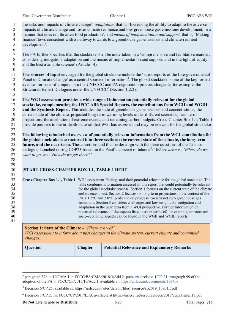
Final Government Distribution Chapter 1 IPCC AR6 WGI
Do Not Cite, Quote or Distribute 1-20 Total pages: 215
the risks and impacts of climate change’; adaptation, that is, ‘Increasing the ability to adapt to the adverse 1 impacts of climate change and foster climate resilience and low greenhouse gas emissions development, in a 2 manner that does not threaten food production’; and means of implementation and support, that is, ‘Making 3 finance flows consistent with a pathway towards low greenhouse gas emissions and climate-resilient 4 development’. 5 6 The PA further specifies that the stocktake shall be undertaken in a ‘comprehensive and facilitative manner, 7 considering mitigation, adaptation and the means of implementation and support, and in the light of equity 8 and the best available science’ (Article 14). 9 10 The sources of input envisaged for the global stocktake include the ‘latest reports of the Intergovernmental 11 Panel on Climate Change’ as a central source of information4. The global stocktake is one of the key formal 12 avenues for scientific inputs into the UNFCCC and PA negotiation process alongside, for example, the 13 Structured Expert Dialogues under the UNFCCC5 (Section 1.2.2). 14 15 The WGI assessment provides a wide range of information potentially relevant for the global 16 stocktake, complementing the IPCC AR6 Special Reports, the contributions from WGII and WGIII 17 and the Synthesis Report. This includes the state of greenhouse gas emissions and concentrations, the 18 current state of the climate, projected long-term warming levels under different scenarios, near-term 19 projections, the attribution of extreme events, and remaining carbon budgets. Cross-Chapter Box 1.1, Table 1 20 provide pointers to the in-depth material that WGI has assessed and may be relevant for the global stocktake. 21 22 The following tabularised overview of potentially relevant information from the WGI contribution for 23 the global stocktake is structured into three sections: the current state of the climate, the long-term 24 future, and the near-term. These sections and their order align with the three questions of the Talanoa 25 dialogue, launched during COP23 based on the Pacific concept of talanoa6: ‘Where are we’, ‘Where do we 26 want to go’ and ‘How do we get there?’. 27 28 29 [START CROSS-CHAPTER BOX 1.1, TABLE 1 HERE] 30 31 Cross-Chapter Box 1.1, Table 1: WGI assessment findings and their potential relevance for the global stocktake. The 32
table combines information assessed in this report that could potentially be relevant 33 for the global stocktake process. Section 1 focuses on the current state of the climate 34 and its recent past. Section 2 focuses on long-term projections in the context of the 35 PA’s 1.5°C and 2.0°C goals and on progress towards net zero greenhouse gas 36 emissions. Section 3 considers challenges and key insights for mitigation and 37 adaptation in the near term from a WGI perspective. Further Information on 38 potential relevance of the aspects listed here in terms of, for example, impacts and 39 socio-economic aspects can be found in the WGII and WGIII reports 40
41
Section 1: State of the Climate – ‘Where are we?’ WGI assessment to inform about past changes in the climate system, current climate and committed changes.
Question Chapter Potential Relevance and Explanatory Remarks
4 paragraph 37b in 19/CMA.1 in FCCC/PA/CMA/2018/3/Add.2, pursuant decision 1/CP.21, paragraph 99 of the adoption of the PA in FCCC/CP/2015/10/Add.1, available at: https://unfccc.int/documents/193408 5 Decision 5/CP.25, available at: https://unfccc.int/sites/default/files/resource/cp2019_13a01E.pdf 6 Decision 1/CP.23, in FCCC/CP/2017/L.13, available at https://unfccc.int/resource/docs/2017/cop23/eng/l13.pdf

Final Government Distribution Chapter 1 IPCC AR6 WGI
Do Not Cite, Quote or Distribute 1-21 Total pages: 215
How much warming have we observed in global mean surface air temperatures?
Cross-Chapter Box 1.2; Cross-Chapter Box 2.3; 2.3.1.1, especially 2.3.1.1.3
Knowledge about the current warming relative to pre-industrial levels allows us to quantify the remaining distance to the PA goal of keeping global mean temperatures well below 2°C above pre-industrial level or pursue best efforts to limit warming to 1.5°C above pre-industrial level. Many of the report’s findings are provided against a proxy for pre-industrial temperature levels with Cross-Chapter Box 1.2 examining the difference between pre-industrial levels and the 1850–1900 period.
How much has the ocean warmed?
2.3.3.1, 9.2.1.1; Box 9.1; 7.2; Box 7.2
A warming ocean can affect marine life (e.g., coral bleaching) and also are among the main contributors to long-term sea level rise (thermal expansion). Marine heatwaves can accentuate the impacts of ocean warming on marine ecosystems. Also, knowing the heat uptake of the ocean helps to better understand the response of the climate system and hence helps to project future warming.
How much have the land areas warmed and how has precipitation changed?
2.3.4; 5.4.3; 5.4.8; 8.2.1; 8.2.3; 8.5.1;
A stronger than global-average warming over land, combined with changing precipitation patterns, and/or increased aridity in some regions (like the Mediterranean) can severely affect land ecosystems and species distributions, the terrestrial carbon cycle and food production systems. Amplified warming in the Arctic can enhance permafrost thawing, which in turn can result in overall stronger anthropogenic warming (a positive feedback loop). Intensification of heavy precipitation events can cause more severe impacts related to flooding.
How did the sea ice area change in recent decades in both the Arctic and Antarctic?
2.3.2.1.1; 2.3.2.1.2; 9.3; Cross-Chapter Box 10.1; 12.4.9
Sea ice area influences mass and energy (ice-albedo, heat and momentum) exchange between the atmosphere and the ocean, and its changes in turn impact polar life, adjacent land and ice masses and complex dynamical flows in the atmosphere. The loss of a year-round sea-ice cover in the Arctic can severely impact Arctic ecosystems, affect the livelihood of First Nations in the Arctic, and amplify Arctic warming with potential consequences for the warming of the surrounding permafrost regions and ice sheets.
How much have atmospheric CO2 and other GHG concentrations increased?
2.2.3; 2.2.4; 5.1.1; 5.2.2; 5.2.3; 5.2.4
The main human influence on the climate is via combustion of fossil fuels and land use-change-related CO2 emissions, the principal causes of increased CO2 concentrations since the pre-industrial period. Historical observations indicate that current atmospheric concentrations are unprecedented within at least the last 800,000 years. An understanding of historical fossil fuel emissions and the carbon cycle interactions, as well as CH4 and N2O sinks and sources are crucial for better estimates of future GHG emissions compatible with the PA’s long-term goals.
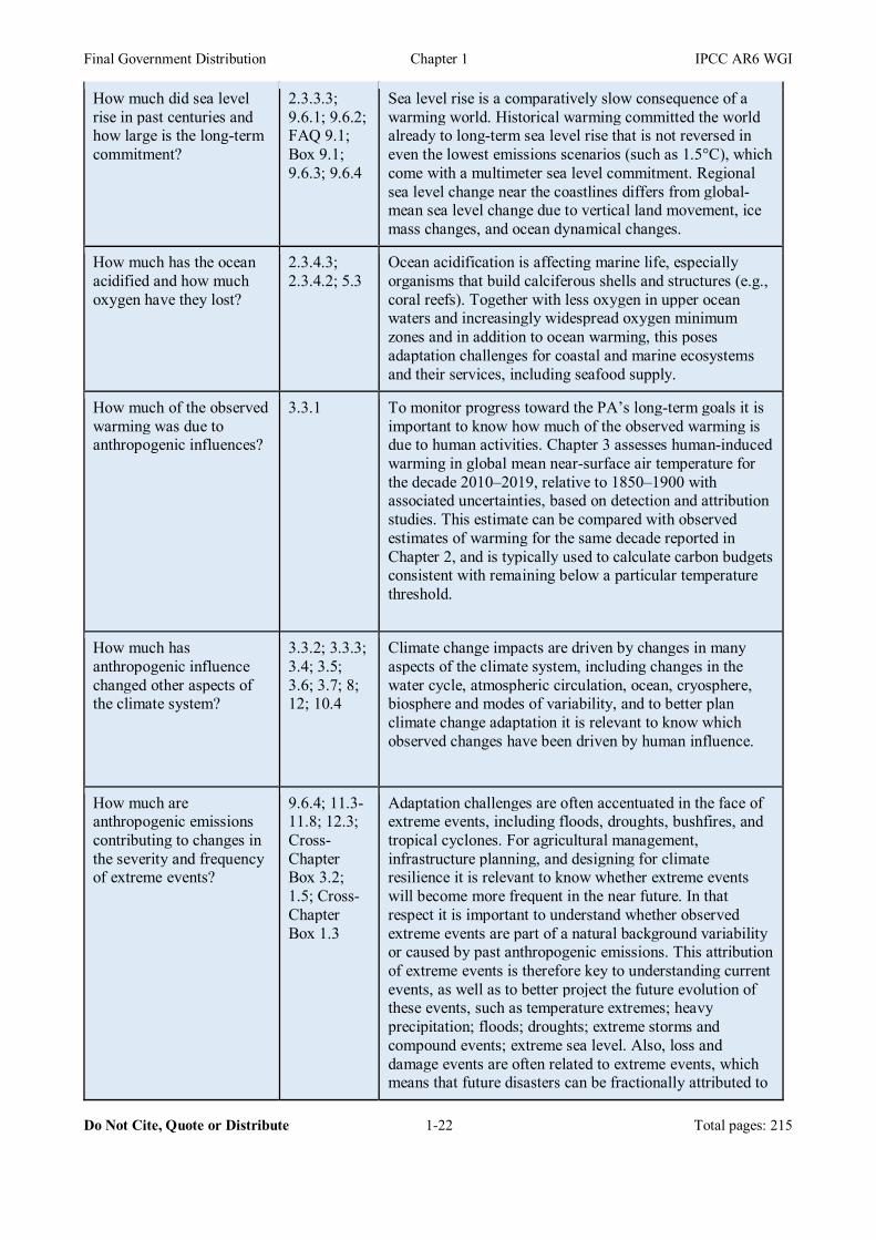
Final Government Distribution Chapter 1 IPCC AR6 WGI
Do Not Cite, Quote or Distribute 1-22 Total pages: 215
How much did sea level rise in past centuries and how large is the long-term commitment?
2.3.3.3; 9.6.1; 9.6.2; FAQ 9.1; Box 9.1; 9.6.3; 9.6.4
Sea level rise is a comparatively slow consequence of a warming world. Historical warming committed the world already to long-term sea level rise that is not reversed in even the lowest emissions scenarios (such as 1.5°C), which come with a multimeter sea level commitment. Regional sea level change near the coastlines differs from global-mean sea level change due to vertical land movement, ice mass changes, and ocean dynamical changes.
How much has the ocean acidified and how much oxygen have they lost?
2.3.4.3; 2.3.4.2; 5.3
Ocean acidification is affecting marine life, especially organisms that build calciferous shells and structures (e.g., coral reefs). Together with less oxygen in upper ocean waters and increasingly widespread oxygen minimum zones and in addition to ocean warming, this poses adaptation challenges for coastal and marine ecosystems and their services, including seafood supply.
How much of the observed warming was due to anthropogenic influences?
3.3.1 To monitor progress toward the PA’s long-term goals it is important to know how much of the observed warming is due to human activities. Chapter 3 assesses human-induced warming in global mean near-surface air temperature for the decade 2010–2019, relative to 1850–1900 with associated uncertainties, based on detection and attribution studies. This estimate can be compared with observed estimates of warming for the same decade reported in Chapter 2, and is typically used to calculate carbon budgets consistent with remaining below a particular temperature threshold.
How much has anthropogenic influence changed other aspects of the climate system?
3.3.2; 3.3.3; 3.4; 3.5; 3.6; 3.7; 8; 12; 10.4
Climate change impacts are driven by changes in many aspects of the climate system, including changes in the water cycle, atmospheric circulation, ocean, cryosphere, biosphere and modes of variability, and to better plan climate change adaptation it is relevant to know which observed changes have been driven by human influence.
How much are anthropogenic emissions contributing to changes in the severity and frequency of extreme events?
9.6.4; 11.3-11.8; 12.3; Cross-Chapter Box 3.2; 1.5; Cross-Chapter Box 1.3
Adaptation challenges are often accentuated in the face of extreme events, including floods, droughts, bushfires, and tropical cyclones. For agricultural management, infrastructure planning, and designing for climate resilience it is relevant to know whether extreme events will become more frequent in the near future. In that respect it is important to understand whether observed extreme events are part of a natural background variability or caused by past anthropogenic emissions. This attribution of extreme events is therefore key to understanding current events, as well as to better project the future evolution of these events, such as temperature extremes; heavy precipitation; floods; droughts; extreme storms and compound events; extreme sea level. Also, loss and damage events are often related to extreme events, which means that future disasters can be fractionally attributed to
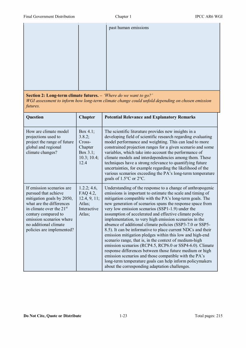
Final Government Distribution Chapter 1 IPCC AR6 WGI
Do Not Cite, Quote or Distribute 1-23 Total pages: 215
past human emissions
Section 2: Long-term climate futures. – ‘Where do we want to go?’ WGI assessment to inform how long-term climate change could unfold depending on chosen emission futures.
Question Chapter Potential Relevance and Explanatory Remarks
How are climate model projections used to project the range of future global and regional climate changes?
Box 4.1; 3.8.2; Cross-Chapter Box 3.1; 10.3; 10.4; 12.4
The scientific literature provides new insights in a developing field of scientific research regarding evaluating model performance and weighting. This can lead to more constrained projection ranges for a given scenario and some variables, which take into account the performance of climate models and interdependencies among them. These techniques have a strong relevance to quantifying future uncertainties, for example regarding the likelihood of the various scenarios exceeding the PA’s long-term temperature goals of 1.5°C or 2°C.
If emission scenarios are pursued that achieve mitigation goals by 2050, what are the differences in climate over the 21st century compared to emission scenarios where no additional climate policies are implemented?
1.2.2; 4.6, FAQ 4.2, 12.4, 9, 11; Atlas; Interactive Atlas;
Understanding of the response to a change of anthropogenic emissions is important to estimate the scale and timing of mitigation compatible with the PA’s long-term goals. The new generation of scenarios spans the response space from very low emission scenarios (SSP1-1.9) under the assumption of accelerated and effective climate policy implementation, to very high emission scenarios in the absence of additional climate policies (SSP3-7.0 or SSP5-8.5). It can be informative to place current NDCs and their emission mitigation pledges within this low and high-end scenario range, that is, in the context of medium-high emission scenarios (RCP4.5, RCP6.0 or SSP4-6.0). Climate response differences between those future medium or high emission scenarios and those compatible with the PA’s long-term temperature goals can help inform policymakers about the corresponding adaptation challenges.

Final Government Distribution Chapter 1 IPCC AR6 WGI
Do Not Cite, Quote or Distribute 1-24 Total pages: 215
What is the climatic effect of net zero GHG emissions and a balance between anthropogenic sources and anthropogenic sinks?
Box 1.4; 4.7.2; 5.2.2; 5.2.3 and 5.2.4; 7.6
Understanding the long-term climate effect of global emission levels, including the effect of net zero emission targets adopted by countries as part of their long-term climate strategies, can be important when assessing whether the collective level of mitigation action is consistent with long-term goals of the PA. Understanding the dynamics of natural sources of CO2, CH4 and N2O is a fundamental prerequisite to derive climate projections. Net zero GHG emissions, that is, the balance between anthropogenic sources and anthropogenic sinks of CO2 and other greenhouse gases, will halt human-induced global warming and/or lead to slight reversal below peak warming levels. Net zero CO2 emissions will approximately lead to a stabilisation of CO2-induced global warming.
What is the remaining carbon budget that is consistent with the PA’s long-term temperature goals?
5.5 The remaining carbon budget provides an estimate of how much CO2 can still be emitted into the atmosphere by human activities while keeping global mean surface temperature to a specific warming level. It thus provides key geophysical information about emissions limits consistent with limiting global warming to well below 2°C above pre-industrial levels and to pursue efforts to limit the temperature increase to 1.5°C. Remaining carbon budgets can be seen in the context of historical CO2 emissions to date. The concept of the transient climate response to cumulative emissions of CO2 (TCRE) indicates that one tonne of CO2 has the same effect on global warming irrespective of whether it is emitted in the past, today, or in the future. In contrast, the global warming from short-lived climate forcers is dependent on their rate of emission rather than their cumulative emission.
What is our current knowledge on the ‘Reasons for Concern’ related to the PA’s long-term temperature goals and higher warming levels?
Cross-Chapter Box 12.1; with individual domains discussed in 2.3.3, 3.5.4, 4.3.2; 5.3; 8.4.1; 9.4.2, 9.5; 11; 12
Synthesis information on projected changes in indices of climatic impact-drivers feeds into different ‘Reasons for Concern’. Where possible, an explicit transfer function between different warming levels and indices quantifying characteristics of these hazards is provided, or the difficulties in doing so documented. Those indices include Arctic sea ice area in September; global average change in ocean acidification; volume of glaciers or snow cover; ice volume change for the West Antarctic Ice Sheet (WAIS) and Greenland Ice Sheet (GIS); Atlantic Meridional Overturning Circulation (AMOC) strength ; amplitude and variance of El Niño Southern Oscillation (ENSO) mode (Nino3.4 index); and weather and climate extremes.
What are the climate effects and air pollution co-benefits of rapid decarbonisation due to the reduction of co-emitted short-lived climate forcers (SLCF)?
6.6.3 ; 6.7.3 ; Box 6.2
Understanding to what degree rapid decarbonisation strategies bring about reduced air pollution due to reductions in co-emitted short-lived climate forcers can be useful to consider integrated and/or complementary policies, with synergies for pursuing the PA goals, the World Health Organization (WHO) air quality guidelines and the Sustainable Development Goals (SDGs).

Final Government Distribution Chapter 1 IPCC AR6 WGI
Do Not Cite, Quote or Distribute 1-25 Total pages: 215
What are the Equilibrium Climate Sensitivity, the Transient Climate Response, and Transient Climate Response to Emissions and what do these indicators tell us about expected warming over the 21st century under various scenarios?
Box 4.1; 5.4, 5.5.1, 7.5
Equilibrium Climate Sensitivity (ECS) measures the long-term global-mean warming in response to doubling CO2 concentrations from pre-industrial levels, while Transient Climate Response (TCR) also takes into account the inertia of the climate system and is an indicator for the near- and medium-term warming. TCRE is similar to TCR, but asks the question of what is the implied warming is in response to cumulative CO2 emissions (rather than CO2 concentration changes). The higher the ECS, TCR or TCRE, the lower are the greenhouse gas emissions that are consistent with the PA’s long-term temperature goals.
What is the Earth's energy imbalance and why does it matter?
7.2.2 The current global energy imbalance implies that one can expect additional warming before the Earth’s climate system attains equilibrium with the current level of concentrations and radiative forcing. Note though, that future warming commitments can be different depending on how future concentrations and radiative forcing change.
What are the regional and long-term changes in precipitation, evaporation and runoff?
8.4.1, 8.5; 8.6; 10.4; 10.6; 12.4; 11.4; 11.9; 11.6; 11.7; Atlas; Interactive Atlas
Changes in regional precipitation – in terms of both extremes and long-term averages – are important for estimating adaptation challenges. Projected changes of precipitation minus evaporation (P-E) are closely related to surface water availability and drought probability. Understanding water cycle changes over land, including seasonality, variability and extremes, and their uncertainties, is important to estimate a broad range of climate impacts and adaptation, including food production, water supply and ecosystem functioning.
Are we committed to irreversible sea level rise and what is the expected sea level rise by the end of the century if we pursue strong mitigation or high emission scenarios?
4.7.2; 9.6.3; 9.6.4; 12.4; Interactive Atlas
Unlike many regional climate responses, global-mean sea level keeps rising even in the lowest scenarios and is not halted when warming is halted. This is due to the long timescales on which ocean heat uptake, glacier melt, ice sheets react to temperature changes. Tipping points and thresholds in polar ice sheets need to be considered. Thus, sea level rise commitments and centennial-scale irreversibility of ocean warming and sea level rise are important for future impacts under even the lowest of the emission scenarios.
Can we project future climate extremes under various global warming levels in the long term?
11, 12.4; Interactive Atlas
Projections of future weather and climate extreme events and their regional occurrence, including at different global warming levels, are important for adaptation and disaster risk reduction. The attribution of these extreme events to natural variability and human-induced changes can be of relevance for both assessing adaptation challenges and issues of loss and damage.

Final Government Distribution Chapter 1 IPCC AR6 WGI
Do Not Cite, Quote or Distribute 1-26 Total pages: 215
What is the current knowledge of potential surprises, abrupt changes, tipping points and low-likelihood, high impact events related to different levels of future emissions or warming?
1.4.4; 4.7.2; 4.8; 5.4.8; Box 5.1; 8.5.3.2; 8.6.2; Box 9.4; 11.2.4; Cross-Chapter Box 4.1; Cross-Chapter Box 12.1
From a risk perspective, it is useful to have information of lower probability events and system changes, if they could potentially result in high impacts, given the dynamic interactions between climate-related hazards and socio-economic drivers (exposure, vulnerability of the affected human or ecological systems). Examples include permafrost thaw, CH4 clathrate feedbacks, ice sheet mass loss, ocean turnover circulation changes, either accelerating warming globally or yielding particular regional responses and impacts.
Section 3: The near term. – ‘How do we get there?’ WGI assessment to inform near-term adaptation and mitigation options
Questions Chapter Potential Relevance and Explanatory Remarks
What are projected key climate indices under low, medium and high emission scenarios in the near term, that is, the next 20 years?
4.3; 4.4; FAQ 4.1, 10.6; 12.3; Atlas; Interactive Atlas
Much of the near-term information and comparison to historical observations allows us to quantify the climate adaptation challenges for the next decades as well as the opportunities to reduce climate change by pursuing lower emissions. For this timescale both the forced changes and the internal variability are important.
How can the climate benefit of mitigating emissions of different greenhouse gases be compared?
7.6 For mitigation challenges, it is important to compare efforts to reduce emissions of CO2 versus emissions of other climate forcers, such as, short-lived CH4 or long-lived N2O. Global Warming Potentials (GWPs), which are used in the UNFCCC and in emission inventories, are updated and various other metrics are also investigated. While the NDCs of Parties to the PA, emission inventories under the UNFCCC, and various emission trading schemes work on the basis of GWP-weighted emissions, some recent discussion in the scientific literature also considers projecting temperatures induced by short-lived climate forcers on the basis of emission changes, not emissions per se.
Do mountain glaciers shrink currently and in the near-future in regions that are currently dependent on this seasonal freshwater supply?
2.3.2.3; 9.5; Cross-chapter Box 10.4; 12.4: 8.4.1; Atlas.5.2.2; Atlas.5.3.2; Atlas.6.2; Atlas.9.2
Mountain glaciers and seasonal snow cover often feed downstream river systems during the melting period, and can be an important source of freshwater. Changing river discharge can pose adaptation challenges. Melting mountain glaciers are among the main contributors to observed global mean sea level rise.

Final Government Distribution Chapter 1 IPCC AR6 WGI
Do Not Cite, Quote or Distribute 1-27 Total pages: 215
What are the capacities and limitations in the provision of regional climate information for adaptation and risk management?
10.5;10.6; Box 10.2; Cross-Chapter Box 10.4; 11.9; Cross-Chapter Box 1.3; 12.6; Cross-Chapter Box 12.1
Challenges for adaptation and risk management are predominantly local, even if globally interlinked. There are a number of approaches used in the production of regional climate information for adaptation purposes focusing on regional scales. All of them consider a range of sources of data and knowledge that are distilled into, at times contextual, climate information. A wealth of examples can be found in this Report, including assessments of extremes and climatic impact-drivers, and attribution at regional scales. Specific regions and case studies for regional projections are considered, like the Sahel and West African monsoon drought and recovery, the Southern Australian rainfall decline, the Caribbean small island summer drought, and regional projections are discussed for Cape Town, the Mediterranean region and Hindu Kush Himalaya.
How important are reductions in short-lived climate forcers compared to the reduction of CO2 and other long-lived greenhouse gases?
6.1; 6.6; 6.7; 7.6
While most of the radiative forcing which causes climate change comes from CO2 emissions, short-lived climate forcers also play an important role in the anthropogenic effect on climate change. Many aerosol species, especially SO4, tend to cool the climate and their reduction leads to a masking of greenhouse gas induced warming. On the other hand, many short-lived species themselves exert a warming effect, including black carbon and CH4, the second most important anthropogenic greenhouse gas (in terms of current radiative forcing). Notably, the climate response to aerosol emissions has a strong regional pattern and is different from that of greenhouse gas driven warming.
What are potential co-benefits and side-effects of climate change mitigation?
5.6.2; 6.1; 6.7.5
The reduction of fossil-fuel-related emissions often goes hand-in-hand with a reduction of air pollutants, such as aerosols and ozone. Reductions will improve air quality and result in broader environmental benefits (reduced acidification, eutrophication, and often tropospheric ozone recovery). More broadly, various co-benefits are discussed in WGII and WGIII, as well as co-benefits and side-effects related to certain mitigation actions, like increased biomass use and associated challenges to food security and biodiversity conservation.
What large near-term surprises could result in particular adaptation challenges?
1.4; 4.4.4; Cross-Chapter Box 4.1; 8.5.2; 11.2.4; Cross-
Surprises can come from a range of sources: from incomplete understanding of the climate system, from surprises in emissions of natural (e.g., volcanic) sources, or from disruptions to the carbon cycle associated with a warming climate (e.g., methane release from permafrost thawing, tropical forest dieback). There could be large natural variability in the near-term; or also accelerated climate
Final Government Distribution Chapter 1 IPCC AR6 WGI
Do Not Cite, Quote or Distribute 1-28 Total pages: 215
Chapter Box 12.1
change due to a markedly more sensitive climate than previously thought. When the next large explosive volcanic eruption will happen is unknown. The largest volcanic eruptions over the last few hundred years led to substantial but temporary cooling, including precipitation changes.
1 [END CROSS-CHAPTER BOX 1.1, TABLE 1 HERE] 2 3 4 [END CROSS-CHAPTER BOX 1.1 HERE] 5 6 7 Sustainable Development Goals (SDGs). Many interactions among environmental problems and 8 development are addressed in the United Nations 2030 Agenda for Sustainable Development and its 9 Sustainable Development Goals. The 2030 Agenda, supported by the finance-oriented Addis Ababa Action 10 Agenda (UN DESA, 2015), calls on nations to ‘take the bold and transformative steps which are urgently 11 needed to shift the world onto a sustainable and resilient path.’ The 2030 Agenda recognizes that ‘climate 12 change is one of the greatest challenges of our time and its adverse impacts undermine the ability of all 13 countries to achieve sustainable development.’ SDG 13 deals explicitly with climate change, establishing 14 several targets for adaptation, awareness-raising and finance. Climate and climate change are also highly 15 relevant to most other SDGs, while acknowledging UNFCCC as the main forum to negotiate the global 16 response to climate change. For example, both long-lived greenhouse gases (LLGHGs), through mitigation 17 decisions, and SLCFs, through air quality, are relevant to SDG 11 (sustainable cities and communities). 18 Chapter 6 assesses SLCF effects on climate and the implications of changing climate for air quality, 19 including opportunities for mitigation relevant to the SDGs (Chapter 6, Box 6.2). Also, the UN Conference 20 on Housing and Sustainable Development established a New Urban Agenda (United Nations, 2017) 21 envisaging cities as part of the solutions for sustainable development, climate change adaptation and 22 mitigation. 23 24 The Sendai Framework for Disaster Risk Reduction (SFDRR). The Sendai Framework for Disaster Risk 25 Reduction is a non-binding agreement to reduce risks associated with disasters of all scales, frequencies and 26 onset rates caused by natural or human-made hazards, including climate change. The SFDRR outlines targets 27 and priorities for action including ‘Understanding disaster risk’, along the dimensions of vulnerability, 28 exposure of persons and assets and hazard characteristics. Chapter 12 assesses climate information relevant 29 to regional impact and risk assessment with a focus on climate hazards and other aspects of climate that 30 influence society and ecosystem and makes the link with Working Group II. AR6 adopts a consistent risk 31 and solution-oriented framing (Cross-Chapter Box 1.3) that calls for a multidisciplinary approach and cross-32 working group coordination in order to ensure integrative discussions of major scientific issues associated 33 with integrative risk management and sustainable solutions (IPCC, 2017). 34 35 The Intergovernmental Science-Policy Platform on Biodiversity and Ecosystem Services (IPBES). 36 Efforts to address climate change take place alongside and in the context of other major environmental 37 problems, such as biodiversity loss. The Intergovernmental Science-Policy Platform on Biodiversity and 38 Ecosystem Services (IPBES), established in 2012, builds on the IPCC model of a science-policy interface 39 and assessment. The Platform's objective is to ‘strengthen the science-policy interface for biodiversity and 40 ecosystem services for the conservation and sustainable use of biodiversity, long-term human well-being and 41 sustainable development’ (UNEP, 2012). SROCC (IPCC, 2019b) and SRCCL (IPCC, 2019a) assessed the 42 relations between changes in biodiversity and in the climate system. The rolling work programme of IPBES 43 up to 2030 will address interlinkages among biodiversity, water, food and health. This assessment will use a 44 nexus approach to examine interlinkages between biodiversity and the above-mentioned issues, including 45 climate change mitigation and adaptation. Furthermore, IPBES and IPCC will directly collaborate on 46 biodiversity and climate change under the rolling work programme. 47 48 Addressing climate change alongside other environmental problems, while simultaneously supporting 49
Final Government Distribution Chapter 1 IPCC AR6 WGI
Do Not Cite, Quote or Distribute 1-29 Total pages: 215
sustainable socioeconomic development, requires a holistic approach. Since AR5, there is increasing 1 attention on the need for coordination among previously independent international agendas, recognizing that 2 climate change, disaster risk, economic development, biodiversity conservation and human well-being are 3 tightly interconnected. The current COVID-19 pandemic provides an example of the need for such 4 interconnection, with its widespread impacts on economy, society and environment (e.g., Shan et al., 2020). 5 Cross Chapter Box 6.1 in Chapter 6 assesses the consequences of the COVID-19 lockdowns on emissions of 6 GHGs and SLCFs and related implications for the climate. Another example is the close link between SLCF 7 emissions, climate evolution and air quality concerns (see Chapter 6). Emissions of halocarbons have 8 previously been successfully regulated under the Montreal Protocol and its Kigali Amendment. This has 9 been achieved in an effort to reduce ozone depletion that has also modulated anthropogenic climate influence 10 (Estrada et al., 2013; Wu et al., 2013). In the process, emissions of some SLCFs are jointly regulated to 11 reduce environmental and health impacts from air pollution (e.g., Gothenburg Protocol; Reis et al., 2012). 12 Considering the recognized importance of SLCFs for climate, the IPCC decided in May 2019 to approve that 13 the IPCC Task Force on National Greenhouse Gas Inventories produces an IPCC Methodology Report on 14 SLCFs to develop guidance for national SLCFs inventories. 15 16 The evolving governance context since AR5 challenges the IPCC to provide policymakers and other actors 17 with information relevant for both adaptation to and mitigation of climate change and for the loss and 18 damage induced. 19 20 21 1.2.3 Linking science and society: communication, values, and the IPCC assessment process 22 23 This section assesses how the process of communicating climate information has evolved since AR5. It 24 summarizes key issues regarding scientific uncertainty addressed in previous IPCC assessments and 25 introduces the IPCC calibrated uncertainty language. Next it discusses the role of values in problem-driven, 26 multidisciplinary science assessments such as this one. The section introduces climate services and how 27 climate information can be tailored for greatest utility in specific contexts, such as the global stocktake. 28 Finally, we briefly evaluate changes in media coverage of climate information since AR5, including the 29 increasing role of internet sources and social media. 30 31 32 1.2.3.1 Climate change understanding, communication, and uncertainties 33 34 The response to climate change is facilitated when leaders, policymakers, resource managers, and their 35 constituencies share basic understanding of the causes, effects, and possible future course of climate change 36 (SR1.5, IPCC, 2018; SRCCL, IPCC, 2019a). Achieving shared understanding is complicated, since scientific 37 knowledge interacts with pre-existing conceptions of weather and climate built up in diverse world cultures 38 over centuries and often embedded in strongly held values and beliefs stemming from ethnic or national 39 identities, traditions, religion, and lived relationships to weather, land and sea (Van Asselt and Rotmans, 40 1996; Rayner and Malone, 1998; Hulme, 2009, 2018; Green et al., 2010; Jasanoff, 2010; Orlove et al., 2010; 41 Nakashima et al., 2012; Shepherd and Sobel, 2020). These diverse, more local understandings can both 42 contrast with and enrich the planetary-scale analyses of global climate science (high confidence). 43 44 Political cultures also give rise to variation in how climate science knowledge is interpreted, used, and 45 challenged (Leiserowitz, 2006; Oreskes and Conway, 2010; Brulle et al., 2012; Dunlap and Jacques, 2013; 46 Mahony, 2014, 2015; Brulle, 2019). A meta-analysis of 87 studies carried out between 1998 and 2016 (62 47 USA national, 16 non-USA national, 9 cross-national) found that political orientation and political party 48 identification were the second-most important predictors of views on climate change after environmental 49 values (the strongest predictor) (McCright et al. 2016). Ruiz et al. (2020) systematically reviewed 34 studies 50 of non-US nations or clusters of nations and 30 studies of the USA alone. They found that in the non-US 51 studies, ‘changed weather’ and ‘socio-altruistic values’ were the most important drivers of public attitudes. 52 For the USA case, by contrast, political affiliation and the influence of corporations were most important. 53 Widely varying media treatment of climate issues also affects public responses (see Section 1.2.3.4). In 54 summary, environmental and socio-altruistic values are the most significant influences on public opinion 55
Final Government Distribution Chapter 1 IPCC AR6 WGI
Do Not Cite, Quote or Distribute 1-30 Total pages: 215
about climate change globally, while political views, political party affiliation, and corporate influence also 1 had strong effects, especially in the USA (high confidence). 2 3 Furthermore, climate change itself is not uniform. Some regions face steady, readily observable change, 4 while others experience high variability that masks underlying trends (Section 1.4.1); most regions are 5 subject to hazards, but some may also experience benefits, at least temporarily (see Chapters 11, 12, and 6 Atlas). This non-uniformity may lead to wide variation in public climate change awareness and risk 7 perceptions at multiple scales (Howe et al., 2015; Lee et al., 2015). For example, short-term temperature 8 trends, such as cold spells or warm days, have been shown to influence public concern (Hamilton and 9 Stampone, 2013; Zaval et al., 2014; Bohr, 2017). 10 11 Given these manifold influences and the highly varied contexts of climate change communication, special 12 care is required when expressing findings and uncertainties, including IPCC assessments that inform 13 decision making. Throughout the IPCC’s history, all three Working Groups (WGs) have sought to explicitly 14 assess and communicate scientific uncertainty (Le Treut et al., 2007; Cubasch et al., 2013). Over time, the 15 IPCC has developed and revised a framework to treat uncertainties consistently across assessment cycles, 16 reports, and Working Groups through the use of calibrated language (Moss and Schneider, 2000; IPCC, 17 2005). Since its First Assessment Report (IPCC, 1990a), the IPCC specified terms and methods for 18 communicating authors’ expert judgments (Mastrandrea and Mach, 2011). During the AR5 cycle, this 19 calibrated uncertainty language was updated and unified across all WGs (Mastrandrea et al., 2010, 2011). 20 Box 1.1 summarizes this framework as used in AR6. 21 22 23 [START BOX 1.1 HERE] 24 25 Box 1.1: Treatment of uncertainty and calibrated uncertainty language in AR6 26 27 The AR6 follows the approach developed for AR5 (Box 1.1, Figure 1), as described in the ‘Guidance Notes 28 for Lead Authors of the IPCC Fifth Assessment Report on Consistent Treatment of Uncertainties’ 29 (Mastrandrea et al., 2010). The uncertainty Guidance Note used in AR6 clarifies the relationship between the 30 qualitative description of confidence and the quantitative representation of uncertainty expressed by the 31 likelihood scale. The calibrated uncertainty language emphasizes traceability of the assessment throughout 32 the process. Key chapter findings presented in the chapter Executive Summary are supported in the chapter 33 text by a summary of the underlying literature that is assessed in terms of evidence and agreement, 34 confidence, and also likelihood if applicable. 35 36 In all three WGs, author teams evaluate underlying scientific understanding and use two metrics to 37 communicate the degree of certainty in key findings. These metrics are: 38 39
1. Confidence: a qualitative measure of the validity of a finding, based on the type, amount, quality and 40 consistency of evidence (e.g., data, mechanistic understanding, theory, models, expert judgment) and 41 the degree of agreement. 42
2. Likelihood: a quantitative measure of uncertainty in a finding, expressed probabilistically (e.g., 43 based on statistical analysis of observations or model results, or both, and expert judgement by the 44 author team or from a formal quantitative survey of expert views, or both). 45
46 Throughout IPCC reports, the calibrated language indicating a formal confidence assessment is clearly 47 identified by italics (e.g., medium confidence). Where appropriate, findings can also be formulated as 48 statements of fact without uncertainty qualifiers. 49 50 51 [START BOX 1.1, FIGURE 1 HERE] 52 53 Box 1.1, Figure 1: The IPCC AR6 approach for characterizing understanding and uncertainty in assessment findings. 54
This diagram illustrates the step-by-step process authors use to evaluate and communicate the state 55
Final Government Distribution Chapter 1 IPCC AR6 WGI
Do Not Cite, Quote or Distribute 1-31 Total pages: 215
of knowledge in their assessment (Mastrandrea et al., 2010). Authors present evidence/agreement, 1 confidence, or likelihood terms with assessment conclusions, communicating their expert judgments 2 accordingly. Example conclusions drawn from this report are presented in the box at the bottom of 3 the figure. [adapted from Mach et al. (2017)]. 4
5 [END BOX 1.1, FIGURE 1 HERE] 6 7 8 Box.1.1, Figure 1 (adapted from Mach et al., 2017) shows the idealized step-by-step process by which IPCC 9 authors assess scientific understanding and uncertainties. It starts with the evaluation of the available 10 evidence and agreement (Steps 1–2). The following summary terms are used to describe the available 11 evidence: limited, medium, or robust; and the degree of agreement: low, medium, or high. Generally, 12 evidence is most robust when there are multiple, consistent, independent lines of high-quality evidence. 13 14 If the author team concludes that there is sufficient evidence and agreement, the level of confidence can be 15 evaluated. In this step, assessments of evidence and agreement are combined into a single metric (Steps 3–5). 16 The assessed level of confidence is expressed using five qualifiers: very low, low, medium, high, and very 17 high. Step 4 depicts how summary statements for evidence and agreement relate to confidence levels. For a 18 given evidence and agreement statement, different confidence levels can be assigned depending on the 19 context, but increasing levels of evidence and degrees of agreement correlate with increasing confidence. 20 When confidence in a finding is assessed to be low, this does not necessarily mean that confidence in its 21 opposite is high, and vice versa. Similarly, low confidence does not imply distrust in the finding; instead, it 22 means that the statement is the best conclusion based on currently available knowledge. Further research and 23 methodological progress may change the level of confidence in any finding in future assessments. 24 25 If the expert judgement of the author team concludes that there is sufficient confidence and 26 quantitative/probabilistic evidence, assessment conclusions can be expressed with likelihood statements 27 (Box.1.1, Figure 1, Steps 5–6). Unless otherwise indicated, likelihood statements are related to findings for 28 which the authors’ assessment of confidence is ‘high’ or ‘very high’. Terms used to indicate the assessed 29 likelihood of an outcome include: virtually certain: 99–100% probability, very likely: 90–100%, likely: 66–30 100%, about as likely as not: 33–66%, unlikely: 0–33%, very unlikely: 0–10%, exceptionally unlikely: 0–1%. 31 Additional terms (extremely likely: 95–100%, more likely than not >50–100%, and extremely unlikely 0–5%) 32 may also be used when appropriate. 33 34 Likelihood can indicate probabilities for single events or broader outcomes. The probabilistic information 35 may build from statistical or modelling analyses, other quantitative analyses, or expert elicitation. The 36 framework encourages authors, where appropriate, to present probability more precisely than can be done 37 with the likelihood scale, for example with complete probability distributions or percentile ranges, including 38 quantification of tails of distributions important for risk management (Mach et al., 2017; see also Sections 39 1.2.2 and 1.4.4). In some instances, multiple combinations of confidence and likelihood are possible to 40 characterize key findings. For example, a very likely statement might be made with high confidence, whereas 41 a likely statement might be made with very high confidence. In these instances, the author teams consider 42 which statement will convey the most balanced information to the reader. 43 44 Throughout this WGI report and unless stated otherwise, uncertainty is quantified using 90% uncertainty 45 intervals. The 90% uncertainty interval, reported in square brackets [x to y], is estimated to have a 90% 46 likelihood of covering the value that is being estimated. The range encompasses the median value and there 47 is an estimated 10% combined likelihood of the value being below the lower end of the range (x) and above 48 its upper end (y). Often the distribution will be considered symmetric about the corresponding best estimate 49 (as in the illustrative example in the figure), but this is not always the case. In this report, an assessed 90% 50 uncertainty interval is referred to as a ‘very likely range’. Similarly, an assessed 66% uncertainty interval is 51 referred to as a ‘likely range’. 52 53 [END BOX 1.1 HERE] 54 55
Final Government Distribution Chapter 1 IPCC AR6 WGI
Do Not Cite, Quote or Distribute 1-32 Total pages: 215
1 Considerable critical attention has focused on whether applying the IPCC framework effectively achieves 2 consistent treatment of uncertainties and clear communication of findings to users (Shapiro et al., 2010; 3 Adler and Hirsch Hadorn, 2014). Specific concerns include, for example, the transparency and traceability of 4 expert judgements underlying the assessment conclusions (Oppenheimer et al., 2016) and the context-5 dependent representations and interpretations of probability terms (Budescu et al., 2009, 2012; Janzwood, 6 2020). Budescu et al. (2014) surveyed 25 samples in 24 countries (a total of 10,792 individual responses), 7 finding that even when shown IPCC uncertainty guidance, lay readers systematically misunderstood IPCC 8 likelihood statements. When presented with a ‘high likelihood’ statement, they understood it as indicating a 9 lower likelihood than intended by the IPCC authors. Conversely, they interpreted ‘low likelihood’ statements 10 as indicating a higher likelihood than intended. In another study, British lay readers interpreted uncertainty 11 language somewhat differently from IPCC guidance, but Chinese lay people reading the same uncertainty 12 language translated into Chinese differed much more in their interpretations (Harris et al., 2013). Further, 13 even though it is objectively more probable that wide uncertainty intervals will encompass true values, wide 14 intervals were interpreted by lay people as implying subjective uncertainty or lack of knowledge on the part 15 of scientists (Løhre et al., 2019). Mach et al. (2017) investigated the advances and challenges in approaches 16 to expert judgment in the AR5. Their analysis showed that the shared framework increased the overall 17 comparability of assessment conclusions across all WGs and topics related to climate change, from the 18 physical science basis to resulting impacts, risks, and options for response. Nevertheless, many challenges in 19 developing and communicating assessment conclusions persist, especially for findings drawn from multiple 20 disciplines and Working Groups, for subjective aspects of judgments, and for findings with substantial 21 uncertainties (Adler and Hirsch Hadorn, 2014). In summary, the calibrated language cannot entirely prevent 22 misunderstandings, including a tendency to systematically underestimate the probability of the IPCC’s 23 higher-likelihood conclusions and overestimate the probability of the lower-likelihood ones (high 24 confidence), however a consistent and systematic approach across Working Groups to communicate the 25 assessment outcomes is an important characteristic of the IPCC. 26 27 Some suggested alternatives are impractical, such as always including numerical values along with calibrated 28 language (Budescu et al., 2014). Others, such as using positive instead of negative expressions of low to 29 medium probabilities, show promise but were not proposed in time for adoption in AR6 (Juanchich et al., 30 2020). This report therefore retains the same calibrated language used in AR5 (Box 1.1). Like previous 31 reports, AR6 also includes FAQs that express its chief conclusions in plain language designed for lay 32 readers. 33 34 The framework for communicating uncertainties does not address when "deep uncertainty" is identified in 35 the assessment (Adler and Hirsch Hadorn, 2014). The definition of deep uncertainty in IPCC assessments 36 has been described in the context of the SROCC (IPCC, 2019b; Box 5 in Abram et al. (2019)). A situation of 37 deep uncertainty exists when experts or stakeholders do not know or cannot agree on: (1) appropriate 38 conceptual models that describe relationships among key driving forces in a system; (2) the probability 39 distributions used to represent uncertainty about key variables and parameters; and/or (3) how to weigh and 40 value desirable alternative outcomes (Abram et al., 2019). (See also Cross-Chapter Box 1.2, Annex VII 41 Glossary) Since AR5, the ‘storylines’ or ‘narratives’ approach has been used to address issues related to deep 42 uncertainty, for example low-likelihood events that would have high impact if they occurred, to better inform 43 risk assessment and decision making (see Section 1.4.4). Chapter 9 (Section 9.2.3) notes deep uncertainty in 44 long term projections for sea level rise, and in processes related to Marine Ice Sheet Instability and Marine 45 Ice Cliff Instability. 46 47 48 1.2.3.2 Values, science, and climate change communication 49 50 As noted above, values — fundamental attitudes about what is important, good, and right — play critical 51 roles in all human endeavours, including climate science. In AR5, Chapters 3 and 4 of the WGIII assessment 52 addressed the role of cultural, social, and ethical values in climate change mitigation and sustainable 53 development (Fleurbaey et al., 2014; Kolstad et al., 2014). These values include widely accepted concepts of 54 human rights, enshrined in international law, that are relevant to climate impacts and policy objectives (Hall 55

Final Government Distribution Chapter 1 IPCC AR6 WGI
Do Not Cite, Quote or Distribute 1-33 Total pages: 215
and Weiss, 2012; Peel and Osofsky, 2018; Setzer and Vanhala, 2019). Specific values – human life, 1 subsistence, stability, and equitable distribution of the costs and benefits of climate impacts and policies – 2 are explicit in the texts of the UNFCCC and the PA (Breakey et al., 2016; Dooley and Parihar, 2016). Here 3 we address the role of values in how scientific knowledge is created, verified, and communicated. Chapters 4 10, 12, and Cross-Chapter Box 12.2 address how the specific values and contexts of users can be addressed 5 in the co-production of climate information. 6 7 The epistemic (knowledge-related) values of science include explanatory power, predictive accuracy, 8 falsifiability, replicability, and justification of claims by explicit reasoning (Popper, 1959; Kuhn, 1977). 9 These are supported by key institutional values, including openness, ‘organized scepticism,’ and objectivity 10 or ‘disinterestedness’ (Merton, 1973), operationalized as well-defined methods, documented evidence, 11 publication, peer review, and systems for institutional review of research ethics (COSEPUP, 2009). In recent 12 decades, open data, open code, and scientific cyberinfrastructure (notably the Earth System Grid Federation, 13 a partnership of climate modeling centers dedicated to supporting climate research by providing secure, web-14 based, distributed access to climate model data) have facilitated scrutiny from a larger range of participants, 15 and FAIR data stewardship principles – making data Findable, Accessible, Interoperable and Reusable 16 (FAIR) – are being mainstreamed in many fields (Wilkinson et al., 2016). Climate science norms and 17 practices embodying these scientific values and principles include the publication of data and model code, 18 multiple groups independently analysing the same problems and data, model intercomparison projects 19 (MIPs), explicit evaluations of uncertainty, and comprehensive assessments by national academies of science 20 and the IPCC. 21 22 The formal Principles Governing IPCC Work (1998, amended 2003, 2006, 2012, 2013) specify that 23 assessments should be ‘comprehensive, objective, open and transparent.’ The IPCC assessment process 24 seeks to achieve these goals in several ways: by evaluating evidence and agreement across all relevant peer-25 reviewed literature, especially that published or accepted since the previous assessment; by maintaining a 26 traceable, transparent process that documents the reasoning, data, and tools used in the assessment; and by 27 maximizing the diversity of participants, authors, experts, reviewers, institutions, and communities 28 represented, across scientific discipline, geographical location, gender, ethnicity, nationality, and other 29 characteristics. The multi-stage review process is critical to ensure an objective, comprehensive and robust 30 assessment, with hundreds of scientists, other experts, and governments providing comments to a series of 31 drafts before the report is finalised. 32 33 Social values are implicit in many choices made during the construction, assessment, and communication of 34 climate science information (Heymann et al., 2017; Skelton et al., 2017). Some climate science questions are 35 prioritised for investigation, or given a specific framing or context, because of their relevance to climate 36 policy and governance. One example is the question of how the effects of a 1.5°C global warming would 37 differ from those of a 2°C warming, an assessment specifically requested by Parties to the PA. SR1.5 (2018) 38 explicitly addressed this issue ‘within the context of sustainable development; considerations of ethics, 39 equity and human rights; and the problem of poverty’ (Chapters 1 and 5; see also Hoegh-Guldberg et al., 40 2019) following the outcome of the approval of the outline of the Special Report by the IPCC during its 44th 41 Session (Bangkok, Thailand, 17-20 October 2016). Likewise, particular metrics are sometimes prioritized in 42 climate model improvement efforts because of their practical relevance for specific economic sectors or 43 stakeholders. Examples include reliable simulation of precipitation in a specific region, or attribution of 44 particular extreme weather events to inform rebuilding and future policy (see Chapters 8 and 11; Intemann, 45 2015; Otto et al., 2018; James et al., 2019). Sectors or groups whose interests do not influence research and 46 modelling priorities may thus receive less information in support of their climate-related decisions (Parker 47 and Winsberg, 2018). 48 49 Recent work also recognizes that choices made throughout the research process can affect the relative 50 likelihood of false alarms (overestimating the probability and/or magnitude of hazards) or missed warnings 51 (underestimating the probability and/or magnitude of hazards), known respectively as Type I and Type II 52 errors. Researchers may choose different methods depending on which type of error they view as most 53 important to avoid, a choice that may reflect social values (Douglas, 2009; Knutti, 2018; Lloyd and Oreskes, 54 2018). This reflects a fundamental trade-off between the values of reliability and informativeness. When 55
Final Government Distribution Chapter 1 IPCC AR6 WGI
Do Not Cite, Quote or Distribute 1-34 Total pages: 215
uncertainty is large, researchers may choose to report a wide range as ‘very likely’, even though it is less 1 informative about potential consequences. By contrast, high-likelihood statements about a narrower range 2 may be more informative, yet also prove less reliable if new evidence later emerges that widens the range. 3 Furthermore, the difference between narrower and wider uncertainty intervals has been shown to be 4 confusing to lay readers, who often interpret wider intervals as less certain (Løhre et al., 2019). 5 6 7 1.2.3.3 Climate information, co-production, and climate services 8 9 In AR6, ‘climate information’ refers to specific information about the past, current, or future state of the 10 climate system that is relevant for mitigation, adaptation and risk management. Cross-Chapter Box 1.1 is an 11 example of climate information at the global scale. It provides climate change information potentially 12 relevant to the global stocktake, and indicates where in AR6 this information may be found. 13 14 Responding to national and regional policymakers' needs for tailored information relevant to risk assessment 15 and adaptation, AR6 emphasizes assessment of regional information more than earlier reports. Here the 16 phrase ‘regional climate information’ refers to predefined reference sets of land and ocean regions; various 17 typological domains (such as mountains or monsoons); temporal frames including baseline periods as well as 18 near-term (2021–2040), medium-term (2041–2060), and long-term (2081–2100); and global warming levels 19 (Sections 1.4.1 and 1.4.5; Chapters 10, 12, and Atlas). Regional climate change information is constructed 20 from multiple lines of evidence including observations, paleoclimate proxies, reanalyses, attribution of 21 changes and climate model projections from both global and regional climate models (Section 1.5.3, Chapter 22 10, Section 10.2 to 10.4). The constructed regional information needs to take account of user context and 23 values for risk assessment, adaptation and policy decisions (Section 1.2.3, Chapter 10, Section 10.5). 24 25 As detailed in Chapter 10, scientific climate information often requires ‘tailoring’ to meet the requirements 26 of specific decision-making contexts. In a study of the UK Climate Projections 2009 project, researchers 27 concluded that climate scientists struggled to grasp and respond to users’ information needs because they 28 lacked experience interacting with users, institutions, and scientific idioms outside the climate science 29 domain (Porter and Dessai, 2017). Economic theory predicts the value of ‘polycentric’ approaches to climate 30 change informed by specific global, regional, and local knowledge and experience (Ostrom, 1996, 2012). 31 This is confirmed by numerous case studies of extended, iterative dialogue among scientists, policymakers, 32 resource managers, and other stakeholders to produce mutually understandable, usable, task-related 33 information and knowledge, policymaking and resource management around the world (Lemos and 34 Morehouse, 2005; Lemos et al., 2012, 2014, 2018; see Vaughan and Dessai, 2014 for a critical view). SR1.5 35 (2018) assessed that ‘education, information, and community approaches, including those that are informed 36 by indigenous knowledge and local knowledge, can accelerate the wide-scale behaviour changes consistent 37 with adapting to and limiting global warming to 1.5°C. These approaches are more effective when combined 38 with other policies and tailored to the motivations, capabilities and resources of specific actors and contexts 39 (high confidence).’ These extended dialogic ‘co-production’ and education processes have thus been 40 demonstrated to improve the quality of both scientific information and governance (high confidence) 41 (Chapter 10, Section 10.5; Cross Chapter Box 12.2 in Chapter 12). 42 43 Since AR5, ‘climate services’ have increased at multiple levels (local, national, regional, and global) to aid 44 decision-making of individuals and organizations and to enable preparedness and early climate change 45 action. These services include appropriate engagement from users and providers, are based on scientifically 46 credible information and producer and user expertise, have an effective access mechanism, and respond to 47 the users’ needs (Hewitt et al., 2012; Annex VII Glossary). A Global Framework for Climate Services 48 (GFCS) was established in 2009 by the World Meteorological Organization (WMO) in support of these 49 efforts (Hewitt et al., 2012; Lúcio and Grasso, 2016). Climate services are provided across sectors and 50 timescales, from sub-seasonal to multi-decadal and support co-design and co-production processes that 51 involve climate information providers, resource managers, planners, practitioners and decision makers 52 (Brasseur and Gallardo, 2016; Trenberth et al., 2016; Hewitt et al., 2017). For example, they may provide 53 high-quality data on temperature, rainfall, wind, soil moisture and ocean conditions, as well as maps, risk 54 and vulnerability analyses, assessments, and future projections and scenarios. These data and information 55
Final Government Distribution Chapter 1 IPCC AR6 WGI
Do Not Cite, Quote or Distribute 1-35 Total pages: 215
products may be combined with non-meteorological data, such as agricultural production, health trends, 1 population distributions in high-risk areas, road and infrastructure maps for the delivery of goods, and other 2 socio-economic variables, depending on users’ needs (WMO, 2020a). Cross-chapter Box 12.2 in Chapter 12 3 illustrates the diversity of climate services with three examples from very different contexts. 4 5 The current landscape of climate services is assessed in detail in Chapter 12 (Section 12.6), with a focus on 6 multi-decadal timescales relevant for climate change risk assessment. Other information relevant to 7 improving climate services for decision making includes the assessment of methods to construct regional 8 information (Chapter 10), as well as projections at the regional level (Atlas) relevant for impact and risk 9 assessment in different sectors (Chapter 12). 10 11 12 1.2.3.4 Media coverage of climate change 13 14 Climate services focus on users with specific needs for climate information, but most people learn about 15 climate science findings from media coverage. Since AR5, research has expanded on how mass media report 16 climate change and how their audiences respond (Dewulf, 2013; Jaspal and Nerlich, 2014; Jaspal et al., 17 2014). For example, in five European Union (EU) countries, television coverage of the AR5 used ‘disaster’ 18 and ‘opportunity’ as its principal themes, but virtually ignored the ‘risk’ framing introduced by AR5 WGII 19 (Painter, 2015) and now extended by the AR6 (see Cross-Chapter Box 1.3). Other studies show that people 20 react differently to climate change news when it is framed as a catastrophe (Hine et al., 2015), as associated 21 with local identities (Sapiains et al., 2016), or as a social justice issue (Howell, 2013). Similarly, audience 22 segmentation studies show that responses to climate change vary between groups of people with different, 23 although not necessarily opposed, views on this phenomenon (e.g., Maibach et al., 2011; Sherley et al., 2014; 24 Detenber et al., 2016). In Brazil, two studies have shown the influence of mass media on the high level of 25 public climate change concern in that country (Rodas and DiGiulio, 2017; Dayrell, 2019). In the USA, 26 analyses of television network news show that climate change receives minimal attention, is most often 27 framed in a political context, and largely fails to link extreme weather events to climate change using 28 appropriate probability framing (Hassol et al., 2016). However, recent evidence suggests that Climate 29 Matters (an Internet resource for US TV weathercasters to link weather to climate change trends) may have 30 had a positive effect on public understanding of climate change (Myers et al., 2020). Also, some media 31 outlets have recently adopted and promoted terms and phrases stronger than the more neutral ‘climate 32 change’ and ‘global warming’, including ‘climate crisis’, ‘global heating’, and ‘climate emergency’ (Zeldin-33 O’Neill, 2019). Google searches on those terms, and on ‘climate action,’ increased 20-fold in 2019, when 34 large social movements such as the School Strikes for Climate gained worldwide attention (Thackeray et al., 35 2020). We thus assess that specific characteristics of media coverage play a major role in climate 36 understanding and perception (high confidence), including how IPCC assessments are received by the 37 general public. 38 39 Since AR5, social media platforms have dramatically altered the mass-media landscape, bringing about a 40 shift from uni-directional transfer of information and ideas to more fluid, multi-directional flows (Pearce et 41 al., 2019). A survey covering 18 Latin American countries (StatKnows-CR2, 2019) found that the main 42 sources of information about climate change mentioned were the Internet (52% of mentions), followed by 43 social media (18%). There are well-known challenges with social media, such as misleading or false 44 presentations of scientific findings, incivility that diminishes the quality of discussion around climate change 45 topics, and ‘filter bubbles’ that restrict interactions to those with broadly similar views (Anderson and 46 Huntington, 2017). However, at certain moments (such as at the release of the AR5 WGI report), Twitter 47 studies have found that more mixed, highly-connected groups existed, within which members were less 48 polarized (Pearce et al., 2014; Williams et al., 2015). Thus, social media platforms may in some 49 circumstances support dialogic or co-production approaches to climate communication. Because the contents 50 of IPCC reports speak not only to policymakers, but also to the broader public, the character and effects of 51 media coverage are important considerations across Working Groups. 52 53 54

Final Government Distribution Chapter 1 IPCC AR6 WGI
Do Not Cite, Quote or Distribute 1-36 Total pages: 215
1.3 How we got here: the scientific context 1 2 Scientific understanding of the climate system’s fundamental features is robust and well established. This 3 section briefly presents the major lines of evidence in climate science (Figure 1.6). It illustrates their long 4 history and summarises key findings from the WGI contribution to AR5, where relevant referencing 5 previous IPCC assessments for comparison. Box 1.2 summarises major findings from three Special Reports 6 already released during the sixth IPCC assessment cycle. This chapter’s Appendix 1A summarises the 7 principal findings of all six IPCC WGI Assessment Reports, including the present one, in a single table for 8 ready reference. 9 10 11 [START FIGURE 1.6 HERE] 12 13 Figure 1.6: Climate science milestones, between 1817-2021. Milestones in observations (top); Curves of global 14
surface air temperature (GMST) using HadCRUT5 (Morice et al., 2021) and atmospheric CO2 15 concentrations from Antarctic ice cores (Lüthi et al., 2008; Bereiter et al., 2015) and direct air 16 measurements from 1957 onwards (Tans and Keeling, 2020) (see Figure 1.4 for details) (middle). 17 Milestone in scientific understanding of the CO2 enhanced greenhouse effect (bottom). Further details on 18 each milestone are available in Chapter 1, Section 1.3, and Chapter 1 of AR4. 19
20 [END FIGURE 1.6 HERE] 21 22 23 1.3.1 Lines of evidence: instrumental observations 24 25 Instrumental observations of the atmosphere, ocean, land, biosphere, and cryosphere underpin all 26 understanding of the climate system. This section describes the evolution of instrumental data for major 27 climate variables at Earth’s land and ocean surfaces, at altitude in the atmosphere, and at depth in the ocean. 28 Many data records exist, of varying length, continuity, and spatial distribution; Figure 1.7 gives a schematic 29 overview of temporal coverage. 30 31 Instrumental weather observation at the Earth’s surface dates to the invention of thermometers and 32 barometers in the 1600s. National and colonial weather services built networks of surface stations in the 33 1800s. By the mid-19th century, semi-standardized naval weather logs recorded winds, currents, 34 precipitation, air pressure, and temperature at sea, initiating the longest continuous quasi-global instrumental 35 record (Maury, 1849, 1855, 1860). Because the ocean covers over 70% of global surface area and constantly 36 exchange energy with the atmosphere, both air and sea surface temperatures (SST) recorded in these naval 37 logs are crucial variables in climate studies. Dove (1853) mapped seasonal isotherms over most of the globe. 38 By 1900, a patchy weather data-sharing system reached all continents except Antarctica. Regular 39 compilation of climatological data for the world began in 1905 with the Réseau Mondial (Meteorological 40 Office and Shaw, 1920), and the similar compilations World Weather Records (Clayton, 1927) and Monthly 41 Climatic Data for the World (est. 1948) have been published continuously since their founding. 42 43 Land and ocean surface temperature data have been repeatedly evaluated, refined, and extended (Section 44 1.5.1). As computer power increased and older data were recovered from handwritten records, the number of 45 surface station records used in published global land temperature time series grew. A pioneering study for 46 1880–1935 used fewer than 150 stations (Callendar, 1938). A benchmark study of 1880–2005 incorporated 47 4300 stations (Brohan et al., 2006). A study of the 1753–2011 period included previously unused station 48 data, for a total of 36,000 stations (Rohde et al., 2013); recent versions of this dataset comprise over 40,000 49 land stations (Rohde and Hausfather, 2020). Several centres, including NOAA, Hadley, and Japan 50 Meteorological Agency (JMA), each produce SST datasets independently calculated from instrumental 51 records. In the 2000s, adjustments for bias due to different measurement methods (buckets, engine intake 52 thermometers, moored and drifting buoys) resulted in major improvements of SST data (Thompson et al., 53 2008), and these improvements continue (Huang et al., 2017; Kennedy et al., 2019). SST and land-based data 54 are incorporated into global surface temperature datasets calculated independently by multiple research 55
Final Government Distribution Chapter 1 IPCC AR6 WGI
Do Not Cite, Quote or Distribute 1-37 Total pages: 215
groups, including NOAA, NASA, Berkeley Earth, Hadley-CRU, JMA, and China Meteorological 1 Administration (CMA). Each group aggregates the raw measurement data, applies various adjustments for 2 non-climatic biases such as urban heat-island effects, and addresses unevenness in geospatial and temporal 3 sampling with various techniques (see Chapter 2, Section 2.3.1.1.3 and Table 2.4 for references). Other 4 research groups provide alternative interpolations of these datasets using different methods (e.g., Cowtan and 5 Way, 2014; Kadow et al., 2020). Using the then available global surface temperature datasets, WGI AR5 6 assessed that the global mean surface temperature (GMST) increased by 0.85°C from 1880 to 2012 and 7 found that each of the three decades following 1980 was successively warmer at the Earth’s surface than any 8 preceding decade since 1850 (IPCC, 2013b). Marine air temperatures, especially those measured during 9 night-time, are increasingly also used to examine variability and long-term trends (e.g., Rayner et al., 2006; 10 Kent et al., 2013; Cornes et al., 2020; Junod and Christy, 2020). Cross-Chapter Box 2.3 in Chapter 2 11 discusses updates to the global temperature datasets, provides revised estimates for the observed changes and 12 considers whether marine air temperatures are changing at the same rate as SSTs. 13 14 Data at altitude came initially from scattered mountain summits, balloons, and kites, but the upper 15 troposphere and stratosphere were not systematically observed until radiosonde (weather balloon) networks 16 emerged in the 1940s and 1950s. These provide the longest continuous quasi-global record of the 17 atmosphere’s vertical dimension (Stickler et al., 2010). New methods for spatial and temporal 18 homogenisation (intercalibration and quality control) of radiosonde records were introduced in the 2000s 19 (Sherwood et al., 2008, 2015; Haimberger et al., 2012). Since 1978, Microwave Sounding Units (MSU) 20 mounted on Earth-orbiting satellites have provided a second high-altitude data source, measuring 21 temperature, humidity, ozone, and liquid water throughout the atmosphere. Over time, these satellite data 22 have required numerous adjustments to account for such factors as orbital precession and decay (Edwards, 23 2010). Despite repeated adjustments, however, marked differences remain in the temperature trends from 24 surface, radiosonde, and satellite observations; between the results from three research groups that analyse 25 satellite data (UAH, RSS, and NOAA); and between modelled and satellite-derived tropospheric warming 26 trends (Thorne et al., 2011; Santer et al., 2017). These differences are the subject of ongoing research 27 (Maycock et al., 2018). In the 2000s, Atmospheric Infrared Sounder (AIRS) and radio occultation (GNSS-28 RO) measurements provided new ways to measure temperature at altitude, complementing data from the 29 MSU. GNSS-RO is a new independent, absolutely calibrated source, using the refraction of radio-frequency 30 signals from the Global Navigation Satellite System (GNSS) to measure temperature, pressure, and water 31 vapour (Chapter 2, Section 2.3.1.2.1; Foelsche et al., 2008; Anthes, 2011). 32 33 Heat-retaining properties of the atmosphere’s constituent gases were closely investigated in the 19th century. 34 Foote, (1856) measured solar heating of CO2 experimentally and argued that higher concentrations in the 35 atmosphere would increase Earth’s temperature. Water vapour, ozone, carbon dioxide, and certain 36 hydrocarbons were found to absorb longwave (infrared) radiation, the principal mechanism of the 37 greenhouse effect (Tyndall, 1861). 19th-century investigators also established the existence of a natural 38 biogeochemical carbon cycle. CO2 emitted by volcanoes is removed from the atmosphere through a 39 combination of silicate rock weathering, deep-sea sedimentation, oceanic absorption, and biological storage 40 in plants, shellfish, and other organisms. On multi-million-year timescales, the compression of fossil organic 41 matter stores carbon as coal, oil, and natural gas (Chamberlin, 1897, 1898; Ekholm, 1901). 42 43 Arrhenius (1896) calculated that a doubling of atmospheric carbon dioxide would produce a 5–6°C warming, 44 but in 1900 new measurements seemed to rule out CO2 as a greenhouse gas due to overlap with the 45 absorption bands of water vapour (Ångström, 1900; Very and Abbe, 1901). Further investigation and more 46 sensitive instruments later overturned Ångström’s conclusion (Fowle, 1917; Callendar, 1938). Nonetheless, 47 the major role of CO2 in the energy balance of the atmosphere was not widely accepted until the 1950s 48 (Callendar, 1949; Plass, 1956, 1961; Manabe and Möller, 1961; Weart, 2008; Edwards, 2010). Revelle and 49 Keeling established carbon dioxide monitoring stations in Antarctica and Hawaii during the 1957–1958 50 International Geophysical Year (Revelle and Suess, 1957; Keeling, 1960). These stations have tracked rising 51 atmospheric CO2 concentrations from 315 ppm in 1958 to 414 ppm in 2020. Ground-based monitoring of 52 other greenhouse gases followed. The Greenhouse Gases Observing Satellite (GOSat) was launched in 2009, 53 and two Orbiting Carbon Observatory satellite instruments have been in orbit since 2014. 54 55
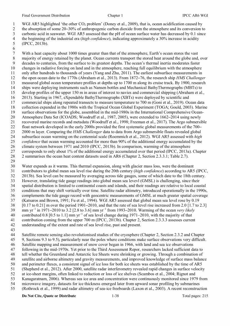
Final Government Distribution Chapter 1 IPCC AR6 WGI
Do Not Cite, Quote or Distribute 1-38 Total pages: 215
WGI AR5 highlighted ‘the other CO2 problem’ (Doney et al., 2009), that is, ocean acidification caused by 1 the absorption of some 20–30% of anthropogenic carbon dioxide from the atmosphere and its conversion to 2 carbonic acid in seawater. WGI AR5 assessed that the pH of ocean surface water has decreased by 0.1 since 3 the beginning of the industrial era (high confidence), indicating approximately a 30% increase in acidity 4 (IPCC, 2013b). 5 6 With a heat capacity about 1000 times greater than that of the atmosphere, Earth’s ocean stores the vast 7 majority of energy retained by the planet. Ocean currents transport the stored heat around the globe and, over 8 decades to centuries, from the surface to its greatest depths. The ocean’s thermal inertia moderates faster 9 changes in radiative forcing on land and in the atmosphere, reaching full equilibrium with the atmosphere 10 only after hundreds to thousands of years (Yang and Zhu, 2011). The earliest subsurface measurements in 11 the open ocean date to the 1770s (Abraham et al., 2013). From 1872–76, the research ship HMS Challenger 12 measured global ocean temperature profiles at depths up to 1700 m along its cruise track. By 1900, research 13 ships were deploying instruments such as Nansen bottles and Mechanical BathyThermographs (MBTs) to 14 develop profiles of the upper 150 m in areas of interest to navies and commercial shipping (Abraham et al., 15 2013). Starting in 1967, eXpendable BathyThermographs (XBTs) were deployed by scientific and 16 commercial ships along repeated transects to measure temperature to 700 m (Goni et al., 2019). Ocean data 17 collection expanded in the 1980s with the Tropical Ocean Global Experiment (TOGA; Gould, 2003). Marine 18 surface observations for the globe, assembled in the mid-1980s in the International Comprehensive Ocean-19 Atmosphere Data Set (ICOADS; Woodruff et al., 1987, 2005), were extended to 1662–2014 using newly 20 recovered marine records and metadata (Woodruff et al., 1998; Freeman et al., 2017). The Argo submersible 21 float network developed in the early 2000s provided the first systematic global measurements of the 700–22 2000 m layer. Comparing the HMS Challenger data to data from Argo submersible floats revealed global 23 subsurface ocean warming on the centennial scale (Roemmich et al., 2012). WGI AR5 assessed with high 24 confidence that ocean warming accounted for more than 90% of the additional energy accumulated by the 25 climate system between 1971 and 2010 (IPCC, 2013b). In comparison, warming of the atmosphere 26 corresponds to only about 1% of the additional energy accumulated over that period (IPCC, 2013a). Chapter 27 2 summarises the ocean heat content datasets used in AR6 (Chapter 2, Section 2.3.3.1; Table 2.7). 28 29 Water expands as it warms. This thermal expansion, along with glacier mass loss, were the dominant 30 contributors to global mean sea level rise during the 20th century (high confidence) according to AR5 (IPCC, 31 2013b). Sea level can be measured by averaging across tide gauges, some of which date to the 18th century. 32 However, translating tide gauge readings into global mean sea levevl (GMSL) is challenging, since their 33 spatial distribution is limited to continental coasts and islands, and their readings are relative to local coastal 34 conditions that may shift vertically over time. Satellite radar altimetry, introduced operationally in the 1990s, 35 complements the tide gauge record with geocentric measurements of GMSL at much greater spatial coverage 36 (Katsaros and Brown, 1991; Fu et al., 1994). WGI AR5 assessed that global mean sea level rose by 0.19 37 [0.17 to 0.21] m over the period 1901–2010, and that the rate of sea level rise increased from 2.0 [1.7 to 2.3] 38 mm yr–1 in 1971–2010 to 3.2 [2.8 to 3.6] mm yr–1 from 1993–2010. Warming of the ocean very likely 39 contributed 0.8 [0.5 to 1.1] mm yr–1 of sea level change during 1971–2010, with the majority of that 40 contribution coming from the upper 700 m (IPCC, 2013b). Chapter 2, Section 2.3.3.3 assesses current 41 understanding of the extent and rate of sea level rise, past and present. 42 43 Satellite remote sensing also revolutionised studies of the cryosphere (Chapter 2, Section 2.3.2 and Chapter 44 9, Sections 9.3 to 9.5), particularly near the poles where conditions make surface observations very difficult. 45 Satellite mapping and measurement of snow cover began in 1966, with land and sea ice observations 46 following in the mid-1970s. Yet prior to the Third Assessment Repor, researchers lacked sufficient data to 47 tell whether the Greenland and Antarctic Ice Sheets were shrinking or growing. Through a combination of 48 satellite and airborne altimetry and gravity measurements, and improved knowledge of surface mass balance 49 and perimeter fluxes, a consistent signal of ice loss for both ice sheets was established by the time of AR5 50 (Shepherd et al., 2012). After 2000, satellite radar interferometry revealed rapid changes in surface velocity 51 at ice-sheet margins, often linked to reduction or loss of ice shelves (Scambos et al., 2004; Rignot and 52 Kanagaratnam, 2006). Whereas sea ice area and concentration were continuously monitored since 1979 from 53 microwave imagery, datasets for ice thickness emerged later from upward sonar profiling by submarines 54 (Rothrock et al., 1999) and radar altimetry of sea-ice freeboards (Laxon et al., 2003). A recent reconstruction 55
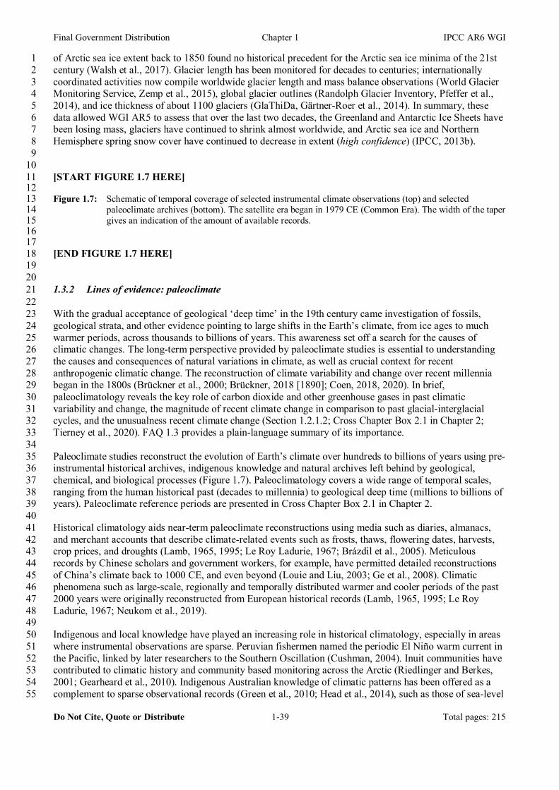
Final Government Distribution Chapter 1 IPCC AR6 WGI
Do Not Cite, Quote or Distribute 1-39 Total pages: 215
of Arctic sea ice extent back to 1850 found no historical precedent for the Arctic sea ice minima of the 21st 1 century (Walsh et al., 2017). Glacier length has been monitored for decades to centuries; internationally 2 coordinated activities now compile worldwide glacier length and mass balance observations (World Glacier 3 Monitoring Service, Zemp et al., 2015), global glacier outlines (Randolph Glacier Inventory, Pfeffer et al., 4 2014), and ice thickness of about 1100 glaciers (GlaThiDa, Gärtner-Roer et al., 2014). In summary, these 5 data allowed WGI AR5 to assess that over the last two decades, the Greenland and Antarctic Ice Sheets have 6 been losing mass, glaciers have continued to shrink almost worldwide, and Arctic sea ice and Northern 7 Hemisphere spring snow cover have continued to decrease in extent (high confidence) (IPCC, 2013b). 8 9 10 [START FIGURE 1.7 HERE] 11 12 Figure 1.7: Schematic of temporal coverage of selected instrumental climate observations (top) and selected 13
paleoclimate archives (bottom). The satellite era began in 1979 CE (Common Era). The width of the taper 14 gives an indication of the amount of available records. 15 16
17 [END FIGURE 1.7 HERE] 18 19 20 1.3.2 Lines of evidence: paleoclimate 21 22 With the gradual acceptance of geological ‘deep time’ in the 19th century came investigation of fossils, 23 geological strata, and other evidence pointing to large shifts in the Earth’s climate, from ice ages to much 24 warmer periods, across thousands to billions of years. This awareness set off a search for the causes of 25 climatic changes. The long-term perspective provided by paleoclimate studies is essential to understanding 26 the causes and consequences of natural variations in climate, as well as crucial context for recent 27 anthropogenic climatic change. The reconstruction of climate variability and change over recent millennia 28 began in the 1800s (Brückner et al., 2000; Brückner, 2018 [1890]; Coen, 2018, 2020). In brief, 29 paleoclimatology reveals the key role of carbon dioxide and other greenhouse gases in past climatic 30 variability and change, the magnitude of recent climate change in comparison to past glacial-interglacial 31 cycles, and the unusualness recent climate change (Section 1.2.1.2; Cross Chapter Box 2.1 in Chapter 2; 32 Tierney et al., 2020). FAQ 1.3 provides a plain-language summary of its importance. 33 34 Paleoclimate studies reconstruct the evolution of Earth’s climate over hundreds to billions of years using pre-35 instrumental historical archives, indigenous knowledge and natural archives left behind by geological, 36 chemical, and biological processes (Figure 1.7). Paleoclimatology covers a wide range of temporal scales, 37 ranging from the human historical past (decades to millennia) to geological deep time (millions to billions of 38 years). Paleoclimate reference periods are presented in Cross Chapter Box 2.1 in Chapter 2. 39 40 Historical climatology aids near-term paleoclimate reconstructions using media such as diaries, almanacs, 41 and merchant accounts that describe climate-related events such as frosts, thaws, flowering dates, harvests, 42 crop prices, and droughts (Lamb, 1965, 1995; Le Roy Ladurie, 1967; Brázdil et al., 2005). Meticulous 43 records by Chinese scholars and government workers, for example, have permitted detailed reconstructions 44 of China’s climate back to 1000 CE, and even beyond (Louie and Liu, 2003; Ge et al., 2008). Climatic 45 phenomena such as large-scale, regionally and temporally distributed warmer and cooler periods of the past 46 2000 years were originally reconstructed from European historical records (Lamb, 1965, 1995; Le Roy 47 Ladurie, 1967; Neukom et al., 2019). 48 49 Indigenous and local knowledge have played an increasing role in historical climatology, especially in areas 50 where instrumental observations are sparse. Peruvian fishermen named the periodic El Niño warm current in 51 the Pacific, linked by later researchers to the Southern Oscillation (Cushman, 2004). Inuit communities have 52 contributed to climatic history and community based monitoring across the Arctic (Riedlinger and Berkes, 53 2001; Gearheard et al., 2010). Indigenous Australian knowledge of climatic patterns has been offered as a 54 complement to sparse observational records (Green et al., 2010; Head et al., 2014), such as those of sea-level 55
Final Government Distribution Chapter 1 IPCC AR6 WGI
Do Not Cite, Quote or Distribute 1-40 Total pages: 215
rise (Nunn and Reid, 2016). Ongoing research seeks to conduct further dialogue, utilise Indigenous and local 1 knowledge as an independent line of evidence complementing scientific understanding, and analyse their 2 utility for multiple purposes, especially adaptation (Laidler, 2006; Alexander et al., 2011; IPCC, 2019c). 3 Indigenous and local knowledge are used most extensively by IPCC Working Group II. 4 5 Certain geological and biological materials preserve evidence of past climate changes. These ‘natural 6 archives’ include corals, trees, glacier ice, speleothems (stalactites and stalagmites), loess deposits (dust 7 sediments), fossil pollen, peat, lake sediment, and marine sediment (Stuiver, 1965; Eddy, 1976; Haug et al., 8 2001; Wang et al., 2001; Jones et al., 2009; Bradley, 2015). By the early 20th century, laboratory research 9 had begun using tree rings to reconstruct precipitation and the possible influence of sunspots on climatic 10 change (Douglass, 1914, 1919, 1922). Radiocarbon dating, developed in the 1940s (Arnold and Libby, 11 1949), allows accurate determination of the age of carbon-containing materials from the past 50,000 years; 12 this dating technique ushered in an era of rapid progress in paleoclimate studies. 13 14 On longer timescales, tiny air bubbles trapped in polar ice sheets provide direct evidence of past atmospheric 15 composition, including CO2 levels (Petit et al., 1999), and the 18O isotope in frozen precipitation serves as a 16 proxy marker for temperature (Dansgaard, 1954). Sulphate deposits in glacier ice and as ash layers within 17 sediment record major volcanic eruptions, providing another mechanism for dating. The first paleoclimate 18 reconstructions used an almost 100,000-year ice core taken at Camp Century, Greenland (Dansgaard et al., 19 1969; Langway Jr, 2008). Subsequent cores from Antarctica extended this climatic record to 800,000 years 20 (EPICA Community Members, 2004; Jouzel, 2013). Comparisons of air contained in these ice samples 21 against measurements from the recent past enabled WGI AR5 to assess that atmospheric concentrations of 22 CO2, methane (CH4), and nitrous oxide (N2O) had all increased to levels unprecedented in at least the last 23 800,000 years (IPCC, 2013b) (see Section 1.2.1.2, Figure 1.5). 24 25 Global reconstructions of sea surface temperature were developed from material contained in deep-sea 26 sediment cores (CLIMAP Project Members et al., 1976), providing the first quantitative constraints for 27 model simulations of ice age climates (e.g., Rind and Peteet, 1985). Paleoclimate data and modelling showed 28 that the Atlantic Ocean circulation has not been stable over glacial-interglacial time periods, and that many 29 changes in ocean circulation are associated with abrupt transitions in climate in the North Atlantic region 30 (Ruddiman and McIntyre, 1981; Broecker et al., 1985; Boyle and Keigwin, 1987; Manabe and Stouffer, 31 1988). 32 33 By the early 20th century, cyclical changes in insolation due to the interacting periodicities of orbital 34 eccentricity, axial tilt, and axial precession had been hypothesised as a chief pacemaker of ice age-35 interglacial cycles on multi-millennial timescales (Milankovich, 1920). Paleoclimate information derived 36 from marine sediment provides quantitative estimates of past temperature, ice volume, and sea level over 37 millions of years (Section 1.2.1.2, Figure 1.5) (Emiliani, 1955; Shackleton and Opdyke, 1973; Siddall et al., 38 2003; Lisiecki and Raymo, 2005; Past Interglacials Working Group of PAGES, 2016). These estimates have 39 bolstered the orbital cycles hypothesis (Hays et al., 1976; Berger, 1977, 1978). However, paleoclimatology 40 of multi-million to billion-year periods reveals that methane, carbon dioxide, continental drift, silicate rock 41 weathering, and other factors played a greater role than orbital cycles in climate changes during ice-free 42 ‘hothouse’ periods of Earth’s distant past (Frakes et al., 1992; Bowen et al., 2015; Zeebe et al., 2016). 43 44 The WGI AR5 (IPCC, 2013b) used paleoclimatic evidence to put recent warming and sea level rise in a 45 multi-century perspective and assessed that 1983–2012 was likely the warmest 30-year period of the last 46 1400 years in the Northern Hemisphere (medium confidence). AR5 also assessed that the rate of sea level 47 rise since the mid-19th century has been larger than the mean rate during the previous two millennia (high 48 confidence). 49 50 51 1.3.3 Lines of evidence: identifying natural and human drivers 52 53 The climate is a globally interconnected system driven by solar energy. Scientists in the 19th-century 54 established the main physical principles governing Earth’s temperature. By 1822, the principle of radiative 55

Final Government Distribution Chapter 1 IPCC AR6 WGI
Do Not Cite, Quote or Distribute 1-41 Total pages: 215
equilibrium (the balance between absorbed solar radiation and the energy Earth re-radiates into space) had 1 been articulated, and the atmosphere’s role in retaining heat had been likened to a greenhouse (Fourier, 2 1822). The primary explanations for natural climate change — greenhouse gases, orbital factors, solar 3 irradiance, continental position, volcanic outgassing, silicate rock weathering, and the formation of coal and 4 carbonate rock — were all identified by the late 1800s (Fleming, 1998; Weart, 2008). 5 6 The natural and anthropogenic factors responsible for climate change are known today as radiative ‘drivers’ 7 or ‘forcers’. The net change in the energy budget at the top of the atmosphere, resulting from a change in one 8 or more such drivers, is termed radiative forcing (RF; see Annex VII: Glossary) and measured in Watts per 9 square metre (W m-2). The total radiative forcing over a given time interval (often since 1750) represents the 10 sum of positive drivers (inducing warming) and negative ones (inducing cooling). Past IPCC reports have 11 assessed scientific knowledge of these drivers, quantified their range for the period since 1750, and presented 12 the current understanding of how they interact in the climate system. Like all previous IPCC reports, AR5 13 assessed that total radiative forcing has been positive at least since 1850–1900, leading to an uptake of 14 energy by the climate system, and that the largest single contribution to total radiative forcing is the rising 15 atmospheric concentration of CO2 since 1750 (IPCC, 2013a; see Cross-Chapter Box 1.2 and Chapter 7). 16 17 Natural drivers include changes in solar irradiance, ocean currents, naturally occurring aerosols, and natural 18 sources and sinks of radiatively active gases such as water vapour, carbon dioxide, methane, and sulphur 19 dioxide. Detailed global measurements of surface-level solar irradiance were first conducted during the 20 1957–1958 International Geophysical Year (Landsberg, 1961), while top-of-atmosphere irradiance has been 21 measured by satellites since 1959 (House et al., 1986). Measured changes in solar irradiance have been small 22 and slightly negative since about 1980 (Matthes et al., 2017). Water vapour is the most abundant radiatively 23 active gas, accounting for about 75% of the terrestrial greenhouse effect, but because its residence time in the 24 atmosphere averages just 8–10 days, its atmospheric concentration is largely governed by temperature (van 25 der Ent and Tuinenburg, 2017; Nieto and Gimeno, 2019). As a result, non-condensing greenhouse gases with 26 much longer residence times serve as ‘control knobs’, regulating planetary temperature, with water vapour 27 concentrations as a feedback effect (Lacis et al., 2010, 2013). The most important of these non-condensing 28 gases is carbon dioxide (a positive driver), released naturally by volcanism at about 637 MtCO2 yr-1 in recent 29 decades, or roughly 1.6% of the 37 GtCO2 emitted by human activities in 2018 (Burton et al., 2013; Le 30 Quéré et al., 2018). Absorption by the ocean and uptake by plants and soils are the primary natural CO2 sinks 31 on decadal to centennial time scales (see Chapter 5, Section 5.1.2 and Figure 5.3). 32 33 Aerosols (tiny airborne particles) interact with climate in numerous ways, some direct (e.g. reflecting solar 34 radiation back into space) and others indirect (e.g., cloud droplet nucleation); specific effects may cause 35 either positive or negative radiative forcing. Major volcanic eruptions inject sulphur dioxide (SO2, a negative 36 driver) into the stratosphere, creating aerosols that can cool the planet for years at a time by reflecting some 37 incoming solar radiation. The history and climatic effects of volcanic activity have been traced through 38 historical records, geological traces, and observations of major eruptions by aircraft, satellites, and other 39 instruments (Dörries, 2006). The negative RF of major volcanic eruptions was considered in the First 40 Assessment Report (FAR; IPCC, 1990a). In subsequent assessments, the negative RF of smaller eruptions 41 has also been considered (e.g., Chapter 2, section 2.4.3 in IPCC, 1995; Cross-Chapter Box 4.1 in Chapter 4 42 of this report). Dust and other natural aerosols have been studied since the 1880s (e.g., Aitken, 1889; 43 Ångström, 1929, 1964; Twomey, 1959), particularly in relation to their role in cloud nucleation, an aerosol 44 indirect effect whose RF may be either positive or negative depending on such factors as cloud altitude, 45 depth, and albedo (Stevens and Feingold, 2009; Boucher et al., 2013). 46 47 Anthropogenic (human) drivers of climatic change were hypothesised as early as the 17th century, with a 48 primary focus on forest clearing and agriculture (Grove, 1995; Fleming, 1998). In the 1890s, Arrhenius was 49 first to calculate the effects of increased or decreased CO2 concentrations on planetary temperature, and 50 Högbom estimated that worldwide coal combustion of about 500 Mt yr-1 had already completely offset the 51 natural absorption of CO2 by silicate rock weathering (Högbom, 1894; Arrhenius, 1896; Berner, 1995; 52 Crawford, 1997). As coal consumption reached 900 Mt yr-1 only a decade later, Arrhenius wrote that 53 anthropogenic carbon dioxide from fossil fuel combustion might eventually warm the planet (Arrhenius, 54 1908). In 1938, analysing records from 147 stations around the globe, Callendar calculated atmospheric 55
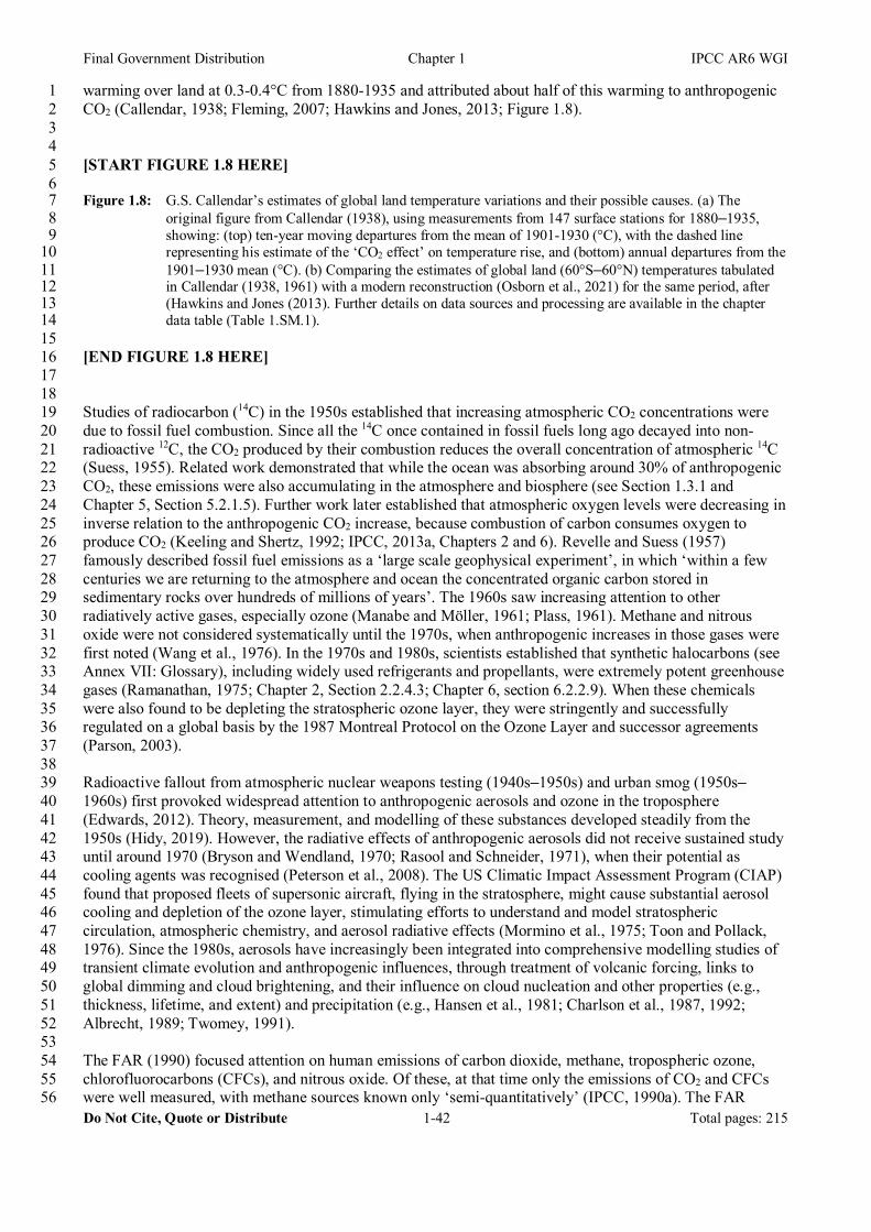
Final Government Distribution Chapter 1 IPCC AR6 WGI
Do Not Cite, Quote or Distribute 1-42 Total pages: 215
warming over land at 0.3-0.4°C from 1880-1935 and attributed about half of this warming to anthropogenic 1 CO2 (Callendar, 1938; Fleming, 2007; Hawkins and Jones, 2013; Figure 1.8). 2 3 4 [START FIGURE 1.8 HERE] 5 6 Figure 1.8: G.S. Callendar’s estimates of global land temperature variations and their possible causes. (a) The 7
original figure from Callendar (1938), using measurements from 147 surface stations for 1880–1935, 8 showing: (top) ten-year moving departures from the mean of 1901-1930 (°C), with the dashed line 9 representing his estimate of the ‘CO2 effect’ on temperature rise, and (bottom) annual departures from the 10 1901–1930 mean (°C). (b) Comparing the estimates of global land (60°S–60°N) temperatures tabulated 11 in Callendar (1938, 1961) with a modern reconstruction (Osborn et al., 2021) for the same period, after 12 (Hawkins and Jones (2013). Further details on data sources and processing are available in the chapter 13 data table (Table 1.SM.1). 14
15 [END FIGURE 1.8 HERE] 16 17 18 Studies of radiocarbon (14C) in the 1950s established that increasing atmospheric CO2 concentrations were 19 due to fossil fuel combustion. Since all the 14C once contained in fossil fuels long ago decayed into non-20 radioactive 12C, the CO2 produced by their combustion reduces the overall concentration of atmospheric 14C 21 (Suess, 1955). Related work demonstrated that while the ocean was absorbing around 30% of anthropogenic 22 CO2, these emissions were also accumulating in the atmosphere and biosphere (see Section 1.3.1 and 23 Chapter 5, Section 5.2.1.5). Further work later established that atmospheric oxygen levels were decreasing in 24 inverse relation to the anthropogenic CO2 increase, because combustion of carbon consumes oxygen to 25 produce CO2 (Keeling and Shertz, 1992; IPCC, 2013a, Chapters 2 and 6). Revelle and Suess (1957) 26 famously described fossil fuel emissions as a ‘large scale geophysical experiment’, in which ‘within a few 27 centuries we are returning to the atmosphere and ocean the concentrated organic carbon stored in 28 sedimentary rocks over hundreds of millions of years’. The 1960s saw increasing attention to other 29 radiatively active gases, especially ozone (Manabe and Möller, 1961; Plass, 1961). Methane and nitrous 30 oxide were not considered systematically until the 1970s, when anthropogenic increases in those gases were 31 first noted (Wang et al., 1976). In the 1970s and 1980s, scientists established that synthetic halocarbons (see 32 Annex VII: Glossary), including widely used refrigerants and propellants, were extremely potent greenhouse 33 gases (Ramanathan, 1975; Chapter 2, Section 2.2.4.3; Chapter 6, section 6.2.2.9). When these chemicals 34 were also found to be depleting the stratospheric ozone layer, they were stringently and successfully 35 regulated on a global basis by the 1987 Montreal Protocol on the Ozone Layer and successor agreements 36 (Parson, 2003). 37 38 Radioactive fallout from atmospheric nuclear weapons testing (1940s–1950s) and urban smog (1950s–39 1960s) first provoked widespread attention to anthropogenic aerosols and ozone in the troposphere 40 (Edwards, 2012). Theory, measurement, and modelling of these substances developed steadily from the 41 1950s (Hidy, 2019). However, the radiative effects of anthropogenic aerosols did not receive sustained study 42 until around 1970 (Bryson and Wendland, 1970; Rasool and Schneider, 1971), when their potential as 43 cooling agents was recognised (Peterson et al., 2008). The US Climatic Impact Assessment Program (CIAP) 44 found that proposed fleets of supersonic aircraft, flying in the stratosphere, might cause substantial aerosol 45 cooling and depletion of the ozone layer, stimulating efforts to understand and model stratospheric 46 circulation, atmospheric chemistry, and aerosol radiative effects (Mormino et al., 1975; Toon and Pollack, 47 1976). Since the 1980s, aerosols have increasingly been integrated into comprehensive modelling studies of 48 transient climate evolution and anthropogenic influences, through treatment of volcanic forcing, links to 49 global dimming and cloud brightening, and their influence on cloud nucleation and other properties (e.g., 50 thickness, lifetime, and extent) and precipitation (e.g., Hansen et al., 1981; Charlson et al., 1987, 1992; 51 Albrecht, 1989; Twomey, 1991). 52 53 The FAR (1990) focused attention on human emissions of carbon dioxide, methane, tropospheric ozone, 54 chlorofluorocarbons (CFCs), and nitrous oxide. Of these, at that time only the emissions of CO2 and CFCs 55 were well measured, with methane sources known only ‘semi-quantitatively’ (IPCC, 1990a). The FAR 56

Final Government Distribution Chapter 1 IPCC AR6 WGI
Do Not Cite, Quote or Distribute 1-43 Total pages: 215
assessed that some other trace gases, especially CFCs, have global warming potentials hundreds to thousands 1 of times greater than CO2 and methane, but are emitted in much smaller amounts. As a result, CO2 remains 2 by far the most important positive anthropogenic driver, with methane next most significant (Section 1.6.3); 3 anthropogenic methane stems from such sources as fossil fuel extraction, natural gas pipeline leakage, 4 agriculture, and landfills. In 2001, increased greenhouse forcing attributable to CO2, methane, ozone, CFC-5 11, and CFC-12 was detected by comparing satellite measurements of outgoing longwave radiation 6 measurements taken in 1970 and in 1997 (Harries et al., 2001). AR5 assessed that the 40% increase in 7 atmospheric CO2 contributed most to positive RF since 1750. Together, changes in atmospheric 8 concentrations of CO2, methane, nitrous oxide, and halocarbons from 1750–2011 were assessed to contribute 9 a positive RF of 2.83 [2.26 to 3.40] W m–2 (IPCC, 2013b). 10 11 All IPCC reports have assessed the total RF as positive when considering all sources. However, due to the 12 considerable variability of both natural and anthropogenic aerosol loads, the FAR characterised total aerosol 13 RF as ‘highly uncertain’ and was unable even to determine its sign (positive or negative). Major advances in 14 quantification of aerosol loads and their effects have taken place since then, and IPCC reports since 1992 15 have consistently assessed total forcing by anthropogenic aerosols as negative (IPCC, 1992, 1995a, 1996). 16 However, due to their complexity and the difficulty of obtaining precise measurements, aerosol effects have 17 been consistently assessed as the largest single source of uncertainty in estimating total RF (Stevens and 18 Feingold, 2009; IPCC, 2013a). Overall, AR5 assessed that total aerosol effects, including cloud adjustments, 19 resulted in a negative RF of –0.9 [–1.9 to −0.1] W m−2 (medium confidence), offsetting a substantial portion 20 of the positive RF resulting from the increase in greenhouse gases (high confidence) (IPCC, 2013b). Chapter 21 7 provides an updated assessment of the total and per-component RF for the WGI contribution to AR6. 22 23 24 1.3.4 Lines of evidence: understanding and attributing climate change 25 26 Understanding the global climate system requires both theoretical understanding and empirical measurement 27 of the major forces and factors that govern the transport of energy and mass (air, water and water vapour) 28 around the globe; the chemical and physical properties of the atmosphere, ocean, cryosphere, and land 29 surfaces; and the biological and physical dynamics of natural ecosystems, as well as the numerous feedbacks 30 (both positive and negative) among these processes. Attributing climatic changes or extreme weather events 31 to human activity (see Cross Working Group Box: Attribution) requires, additionally, understanding of the 32 many ways that human activities may affect the climate, along with statistical and other techniques for 33 separating the ‘signal’ of anthropogenic climate change from the ‘noise’ of natural climate variability (see 34 Section 1.4.2). This inter- and trans-disciplinary effort requires contributions from many sciences. 35 36 Due to the complexity of many interacting processes ranging in scale from the molecular to the global, and 37 occurring on timescales from seconds to millennia, attribution makes extensive use of conceptual, 38 mathematical, and computer simulation models. Modelling allows scientists to combine a vast range of 39 theoretical and empirical understanding from physics, chemistry, and other natural sciences, producing 40 estimates of their joint consequences as simulations of past, present, or future states and trends (Nebeker, 41 1995; Edwards, 2010, 2011). 42 43 In addition to radiative transfer (discussed above in Section 1.3.3), forces and factors such as 44 thermodynamics (energy conversions), gravity, surface friction, and the Earth's rotation govern the 45 planetary-scale movements or ‘circulation’ of air and water in the climate system. The scientific theory of 46 climate began with Halley (1686), who hypothesized vertical atmospheric circulatory cells driven by solar 47 heating, and Hadley (1735), who showed how the Earth’s rotation affects that circulation. Ferrel (1856) 48 added the Coriolis force to existing theory, explaining the major structures of the global atmospheric 49 circulation. In aggregate, prevailing winds and ocean currents move energy poleward from the equatorial 50 regions where the majority of incoming solar radiation is received. 51 52 Climate models provide the ability to simulate these complex circulatory processes, and to improve the 53 physical theory of climate by testing different mathematical formulations of those processes. Since 54 controlled experiments at planetary scale are impossible, climate simulations provide one important way to 55
Final Government Distribution Chapter 1 IPCC AR6 WGI
Do Not Cite, Quote or Distribute 1-44 Total pages: 215
explore the differential effects and interactions of variables such as solar irradiance, aerosols, and greenhouse 1 gases. To assess their quality, models or compontents of models may be compared with observations. For 2 this reason, they can be used to attribute observed climatic effects to different natural and human drivers 3 (Hegerl et al., 2011). As early as Arrhenius (1896), simple mathematical models were used to calculate the 4 effects of doubling atmospheric carbon dioxide over pre-industrial concentrations (~550 ppm vs ~275 ppm). 5 In the early 1900s Bjerknes formulated the Navier-Stokes equations of fluid dynamics for motion of the 6 atmosphere (Bjerknes, 1906; Bjerknes et al., 1910), and Richardson (1922) developed a system for numerical 7 weather prediction based on these equations. When electronic computers became available in the late 1940s, 8 the methods of Bjerknes and Richardson were successfully applied to weather forecasting (Charney et al., 9 1950; Nebeker, 1995; Harper, 2008). 10 11 In the 1960s similar approaches to modelling the weather were used to model the climate, but with much 12 longer runs than daily forecasting (Smagorinsky et al., 1965; Manabe and Wetherald, 1967). Simpler 13 statistical and one- and two-dimensional modelling approaches continued in tandem with the more complex 14 General Circulation Models (GCMs) (Manabe and Wetherald, 1967; Budyko, 1969; Sellers, 1969). The first 15 coupled atmosphere-ocean model (AOGCM) with realistic topography appeared in 1975 (Bryan et al., 1975; 16 Manabe et al., 1975). Rapid increases in computer power enabled higher resolutions, longer model 17 simulations, and the inclusion of additional physical processes in GCMs, such as aerosols, atmospheric 18 chemistry, sea ice, and snow. 19 20 In the 1990s, AOGCMs were state of the art. By the 2010s, Earth system models (ESMs, also known as 21 coupled carbon-cycle climate models) incorporated land surface, vegetation, the carbon cycle, and other 22 elements of the climate system. Since the 1990s, some major modelling centres have deployed ‘unified’ 23 models for both weather prediction and climate modelling, with the goal of a seamless modelling approach 24 that uses the same dynamics, physics, and parameterisations at multiple scales of time and space (Cullen, 25 1993; Brown et al., 2012; NRC Committee on a National Strategy for Advancing Climate Modeling, 2012; 26 Brunet et al., 2015; Chapter 10, Section 10.1.2). Because weather forecast models make short-term 27 predictions that can be frequently verified, and improved models are introduced and tested iteratively on 28 cycles as short as 18 months, this approach allows major portions of the climate model to be evaluated as a 29 weather model and more frequently improved. However, all climate models exhibit biases of different 30 degrees and types, and the practice of ‘tuning’ parameter values in models to make their outputs match 31 variables such as historical warming trajectories has generated concern throughout their history (Randall and 32 Wielicki, 1997; Edwards, 2010; Hourdin et al., 2017; see also 1.5.3.2). Overall, the WGI AR5 assessed that 33 climate models had improved since previous reports (IPCC, 2013b) . 34 35 Since climate models vary along many dimensions, such as grid type, resolution, and parameterizations, 36 comparing their results requires special techniques. To address this problem, the climate modelling 37 community developed increasingly sophisticated Model Intercomparison Projects (MIPs) (Gates et al., 1999; 38 Covey et al., 2003). MIPs prescribe standardised experiment designs, time periods, output variables, or 39 observational reference data, to facilitate direct comparison of model results. This aids in diagnosing the 40 reasons for biases and other differences among models, and furthers process understanding (Section 1.5). 41 Both the CMIP3 and CMIP5 model intercomparison projects included experiments testing the ability of 42 models to reproduce 20th century global surface temperature trends both with and without anthropogenic 43 forcings. Although some individual model runs failed to achieve this (Hourdin et al., 2017), the mean trends 44 of multi-model ensembles did so successfully (Meehl et al., 2007a; Taylor et al., 2012). When only natural 45 forcings were included (creating the equivalent of a ‘control Earth’ without human influences), similar multi-46 model ensembles could not reproduce the observed post-1970 warming at either global or regional scales 47 (Edwards, 2010; Jones et al., 2013). The GCMs and ESMs compared in CMIP6 (used in this report) offer 48 more explicit documentation and evaluation of tuning procedures (Schmidt et al., 2017; Burrows et al., 2018; 49 Mauritsen and Roeckner, 2020); see Section 1.5). 50 51 The FAR (IPCC, 1990a) concluded that while both theory and models suggested that anthropogenic 52 warming was already well underway, its signal could not yet be detected in observational data against the 53 ‘noise’ of natural variability (also see Barnett and Schlesinger (1987) and Section 1.4.2). Since then, 54 increased warming and progressively more conclusive attribution studies have identified human activities as 55
Final Government Distribution Chapter 1 IPCC AR6 WGI
Do Not Cite, Quote or Distribute 1-45 Total pages: 215
the ‘dominant cause of the observed warming since the mid-20th century’ (IPCC, 2013b). ‘Fingerprint’ 1 studies seek to detect specific observed changes – expected from theoretical understanding and model results 2 – that could not be explained by natural drivers alone, and to attribute statistically the proportion of such 3 changes that is due to human influence. These include global-scale surface warming, nights warming faster 4 than days, tropospheric warming and stratospheric cooling, a rising tropopause, increasing ocean heat 5 content, changed global patterns of precipitation and sea-level air pressure, increasing downward longwave 6 radiation, and decreasing upward longwave radiation (Hasselmann, 1979; Schneider, 1994; Karoly et al., 7 1994; Santer et al., 1995, 2013, Hegerl et al., 1996, 1997; Gillett et al., 2003; Santer, 2003; Zhang et al., 8 2007; Stott et al., 2010; Davy et al., 2017; Mann et al., 2017). Cross Working Group Box 1.1 outlines 9 attribution methods and uses from across the AR6, now including event attribution (specifying the influence 10 of climate change on individual extreme events such as floods, or on the frequency of classes of events such 11 as tropical cyclones). Overall, the evidence for human influence has grown substantially over time and from 12 each IPCC report to the subsequent one. 13 14 A key indicator of climate understanding is whether theoretical climate system budgets or ‘inventories’, such 15 as the balance of incoming and outgoing energy at the surface and at the top of the atmosphere, can be 16 quantified and closed observationally. The global energy budget, for example, includes energy retained in 17 the atmosphere, upper ocean, deep ocean, ice, and land surface. Church et al. (2013) assessed in AR5 with 18 high confidence that independent estimates of effective radiative forcing (ERF), observed heat storage, and 19 surface warming combined to give an energy budget for the Earth that is consistent with the WGI AR5 20 assessed likely range of equilibrium climate sensitivity (ECS) [1.5°C to 4.5°C] to within estimated 21 uncertainties (IPCC, 2013a; on ECS, see Section 1.3.5 below). Similarly, over the period 1993 to 2010, when 22 observations of all sea level components were available, WGI AR5 assessed the observed global mean sea 23 level rise to be consistent with the sum of the observed contributions from ocean thermal expansion (due to 24 warming) combined with changes in glaciers, the Antarctic and Greenland Ice Sheets, and land water storage 25 (high confidence). Verification that the terms of these budgets balance over recent decades provides strong 26 evidence for our understanding of anthropogenic climate change (Cross-Chapter Box 9.1 in Chapter 9). 27 28 The Appendix to Chapter 1 (Appendix 1A) lists the key detection and attribution statements in the 29 Summaries for Policymakers of WGI reports since 1990. The evolution of these statements over time reflects 30 the improvement of scientific understanding and the corresponding decrease in uncertainties regarding 31 human influences. The SAR stated that ‘the balance of evidence suggests a discernible human influence on 32 global climate’ (IPCC, 1995b). Five years later, the TAR concluded that ‘there is new and stronger evidence 33 that most of the warming observed over the last 50 years is attributable to human activities’ (IPCC, 2001b). 34 AR4 further strengthened previous statements, concluding that ‘most of the observed increase in global 35 average temperatures since the mid-20th century is very likely due to the observed increase in anthropogenic 36 greenhouse gas concentrations’ (IPCC, 2007b). AR5 assessed that a human contribution had been detected to 37 changes in warming of the atmosphere and ocean; changes in the global water cycle; reductions in snow and 38 ice; global mean sea level rise; and changes in some climate extremes. AR5 concluded that ‘it is extremely 39 likely that human influence has been the dominant cause of the observed warming since the mid-20th 40 century’ (IPCC, 2013b). 41 42 43 1.3.5 Projections of future climate change 44 45 It was recognised in IPCC AR5 that information about the near term was increasingly relevant for adaptation 46 decisions. In response, WGI AR5 made a specific assessment for how global surface temperature was 47 projected to evolve over the next two decades, concluding that the change for the period 2016–2035 relative 48 to 1986–2005 will likely be in the range of 0.3°C to 0.7°C (medium confidence), assuming no major volcanic 49 eruptions or secular changes in total solar irradiance (IPCC, 2013b). AR5 was also the first IPCC assessment 50 report to assess ‘decadal predictions’ of the climate, where the observed state of the climate system was used 51 to start forecasts for a few years ahead. AR6 examines updates to these decadal predictions (Chapter 4, 52 Section 4.4.1). 53 54 The assessments and predictions for the near-term evolution of global climate features are largely 55
Final Government Distribution Chapter 1 IPCC AR6 WGI
Do Not Cite, Quote or Distribute 1-46 Total pages: 215
independent of future carbon emissions pathways. However, WGI AR5 assessed that limiting climate change 1 in the long-term future will require substantial and sustained reductions of greenhouse gas emissions (IPCC, 2 2013b). This assessment results from decades of research on understanding the climate system and its 3 perturbations, and projecting climate change into the future. Each IPCC report has considered a range of 4 emission scenarios, typically including a scenario in which societies choose to continue on their present 5 course as well as several others reflecting socioeconomic and policy responses that may limit emissions 6 and/or increase the rate of carbon dioxide removal from the atmosphere. Climate models are used to project 7 the outcomes of each scenario. However, future human climate influence cannot be precisely predicted 8 because greenhouse gas and aerosol emissions, land use, energy use, and other human activities may change 9 in numerous ways. Common emission scenarios used in the WGI contribution to AR6 are detailed in Section 10 1.6. 11 12 Based on model results and steadily increasing CO2 concentrations (Bolin and Bischof, 1970; SMIC, 1971; 13 Meadows et al., 1972), concerns about future ‘risk of effects on climate’ were addressed in Recommendation 14 70 of the Stockholm Action Plan, resulting from the 1972 United Nations Conference on the Human 15 Environment. Numerous other scientific studies soon amplified these concerns (summarised in Schneider 16 (1975), and Williams (1978); see also Nordhaus (1975, 1977). In 1979, a US National Research Council 17 (NRC) group led by Jule Charney reported on the ‘best present understanding of the carbon dioxide/climate 18 issue for the benefit of policymakers’, initiating an era of regular and repeated large-scale assessments of 19 climate science findings. 20 21 The 1979 Charney NRC report estimated equilibrium climate sensitivity (ECS) at 3°C, stating the range as 22 2°C–4.5°C, based on ‘consistent and mutually supporting’ model results and expert judgment (NRC, 1979). 23 ECS is defined in IPCC assessments as the global surface air temperature (GSAT) response to CO2 doubling 24 (from pre-industrial levels) after the climate has reached equilibrium (stable energy balance between the 25 atmosphere and ocean). Another quantity, transient climate response (TCR), was later introduced as the 26 global surface air temperature change, averaged over a 20-year period, at the time of CO2 doubling in a 27 scenario of concentration increasing at 1% per year). Calculating ECS from historical or paleoclimate 28 temperature records in combination with energy budget models has produced estimates both lower and 29 higher than those calculated using GCMs and ESMs; in AR6, these are assessed in Chapter 7, Section 7.5.2. 30 31 ECS is typically characterised as most relevant on centennial timescales, while TCR was long seen as a more 32 appropriate measure of the 50-100 year response to gradually increasing CO2; however, recent studies have 33 raised new questions about how accurately both quantities are estimated by GCMs and ESMs (Grose et al., 34 2018; Meehl et al., 2020; Sherwood et al., 2020). Further, as climate models evolved to include a full-depth 35 ocean, the time scale for reaching full equilibrium became longer and new methods to estimate ECS had to 36 be developed (Gregory et al., 2004; Meehl et al., 2020; Meinshausen et al., 2020). Because of these 37 considerations as well as new estimates from observation-based, paleoclimate, and emergent-constraints 38 studies (Sherwood et al., 2020), the AR6 definition of ECS has changed from previous reports; it now 39 includes all feedbacks except those associated with ice sheets. Accordingly, unlike previous reports, the AR6 40 assessments of ECS and TCR are not based primarily on GCM and ESM model results (see Chapter 7, Box. 41 7.1 and Section 7.5.5 for a full discussion). 42 43 Today, other sensitivity terms are sometimes used, such as transient climate response to emissions (TCRE, 44 defined as the ratio of warming to cumulative CO2 emissions in a CO2-only simulation) and Earth system 45 sensitivity (ESS), which includes multi-century Earth system feedbacks such as changes in ice sheets. Table 46 1.2 shows estimates of ECS and TCR for major climate science assessments since 1979. The table shows 47 that despite some variation in the range of GCM and (for the later assessments) ESM results, expert 48 assessment of ECS changed little between 1979 and the present report. Based on multiple lines of evidence, 49 AR6 has narrowed the likely range of ECS to 2.5-4.0 °C (Chapter 7, Section 7.5.5). 50 51 52 [START TABLE 1.2 HERE] 53 54
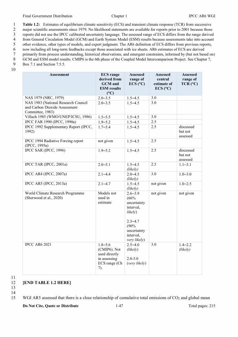
Final Government Distribution Chapter 1 IPCC AR6 WGI
Do Not Cite, Quote or Distribute 1-47 Total pages: 215
Table 1.2: Estimates of equilibrium climate sensitivity (ECS) and transient climate response (TCR) from successive 1 major scientific assessments since 1979. No likelihood statements are available for reports prior to 2001 because those 2 reports did not use the IPCC calibrated uncertainty language. The assessed range of ECS differs from the range derived 3 from General Circulation Model (GCM) and Earth System Model (ESM) results because assessments take into account 4 other evidence, other types of models, and expert judgment. The AR6 definition of ECS differs from previous reports, 5 now including all long-term feedbacks except those associated with ice sheets. AR6 estimates of ECS are derived 6 primarily from process understanding, historical observations, and emergent constraints, informed by (but not based on) 7 GCM and ESM model results. CMIP6 is the 6th phase of the Coupled Model Intercomparison Project. See Chapter 7, 8 Box 7.1 and Section 7.5.5. 9 10
Assessment ECS range derived from
GCM and ESM results
(°C)
Assessed range of ECS (°C)
Assessed central
estimate of ECS (°C)
Assessed range of
TCR (°C)
NAS 1979 (NRC, 1979) 2.0–3.5 1.5–4.5 3.0 NAS 1983 (National Research Council and Carbon Dioxide Assessment Committee, 1983)
2.0–3.5 1.5–4.5 3.0
Villach 1985 (WMO/UNEP/ICSU, 1986) 1.5–5.5 1.5–4.5 3.0 IPCC FAR 1990 (IPCC, 1990a) 1.9–5.2 1.5–4.5 2.5 IPCC 1992 Supplementary Report (IPCC, 1992)
1.7–5.4 1.5–4.5 2.5 discussed but not assessed
IPCC 1994 Radiative Forcing report (IPCC, 1995a)
not given 1.5–4.5 2.5
IPCC SAR (IPCC, 1996) 1.9–5.2 1.5–4.5 2.5 discussed but not assessed
IPCC TAR (IPCC, 2001a) 2.0–5.1 1.5–4.5 (likely)
2.5 1.1–3.1
IPCC AR4 (IPCC, 2007a) 2.1–4.4 2.0–4.5 (likely)
3.0 1.0–3.0
IPCC AR5 (IPCC, 2013a) 2.1–4.7 1.5–4.5 (likely)
not given 1.0–2.5
World Climate Research Programme (Sherwood et al., 2020)
Models not used in estimate
2.6–3.9 (66% uncertainty interval, likely) 2.3–4.7 (90% uncertainty interval, very likely)
not given not given
IPCC AR6 2021 1.8–5.6 (CMIP6). Not used directly in assessing ECS range (Ch 7).
2.5–4.0 (likely) 2.0-5.0 (very likely)
3.0 1.4–2.2 (likely)
11 [END TABLE 1.2 HERE] 12 13 14 WGI AR5 assessed that there is a close relationship of cumulative total emissions of CO2 and global mean 15

Final Government Distribution Chapter 1 IPCC AR6 WGI
Do Not Cite, Quote or Distribute 1-48 Total pages: 215
surface temperature response that is approximately linear (IPCC, 2013b). This finding implies that continued 1 emissions of carbon dioxide will cause further warming and changes in all components of the climate 2 system, independent of any specific scenario or pathway. Scenario-based climate projections using the 3 Representative Concentration Pathways (RCPs) assessed in WGI AR5 result in continued warming over the 4 21st century in all scenarios except a strong climate change mitigation scenario (RCP2.6). Similarly, under 5 all RCP scenarios, AR5 assessed that the rate of sea level rise over the 21st century will very likely exceed 6 that observed during 1971–2010 due to increased ocean warming and increased loss of mass from glaciers 7 and ice sheets. Further increases in atmospheric CO2 will also lead to further uptake of carbon by the ocean, 8 which will increase ocean acidification. By the mid-21st century the magnitudes of the projected changes are 9 substantially affected by the choice of scenario. The set of scenarios used in climate change projections 10 assessed as part of the AR6 are discussed in Section 1.6. 11 12 From the close link between cumulative emissions and warming it follows that any given level of global 13 warming is associated with a total budget of GHG emissions, especially CO2 as it is the largest long-lasting 14 contributor to radiative forcing (Allen et al., 2009; Collins et al., 2013; Rogelj et al., 2019). Higher emissions 15 in earlier decades imply lower emissions later on to stay within the Earth's carbon budget. Stabilising the 16 anthropogenic influence on global surface temperature thus requires that CO2 emissions and removals reach 17 net zero once the remaining carbon budget is exhausted (see Cross-Chapter Box 1.4). 18 19 Past, present and future emissions of CO2 therefore commit the world to substantial multi-century climate 20 change, and many aspects of climate change would persist for centuries even if emissions of CO2 were 21 stopped immediately (IPCC, 2013b). According to AR5, a large fraction of this change is essentially 22 irreversible on a multi-century to millennial time scale, barring large net removal (‘negative emissions’) of 23 CO2 from the atmosphere over a sustained period through as yet unavailable technological means (IPCC, 24 2013a, 2018; see Chapters 4 and 5). However, significant reductions of warming due to SLCFs could reduce 25 the level at which temperature stabilises once CO2 emissions reach net zero, and also reduce the long-term 26 global warming commitment by reducing radiative forcing from SLCFs (Chapter 5). 27 28 In summary, major lines of evidence – observations, paleoclimate, theoretical understanding, and natural and 29 human drivers — have been studied and developed for over 150 years. Methods for projecting climate 30 futures have matured since the 1950s and attribution studies since the 1980s. We conclude that 31 understanding of the principal features of the climate system is robust and well established. 32 33 34 1.3.6 How do previous climate projections compare with subsequent observations? 35 36 Many different sets of climate projections have been produced over the past several decades, so it is valuable 37 to assess how well those projections have compared against subsequent observations. Consisent findings 38 build confidence in the process of making projections for the future. For example, Stouffer and Manabe 39 (2017) compared projections made in the early 1990s with subsequent observations. They found that the 40 projected surface pattern of warming, and the vertical structure of temperature change in both the atmosphere 41 and ocean, were realistic. Rahmstorf et al. (2007, 2012) examined projections of global surface 42 temperatureand global mean sea level assessed by the TAR and AR4 and found that the global surface 43 temperature projections were in good agreement with the subsequent observations, but that sea level 44 projections were underestimates compared to subsequent observations. WGI AR5 also examined earlier 45 IPCC Assessment Reports to evaluate their projections of how global surface temperature and global mean 46 sea level would change (Cubasch et al., 2013) with similar conclusions. 47 48 Although these studies generally showed good agreement between the past projections and subsequent 49 observations, this type of analysis is complicated because the scenarios of future radiative forcing used in 50 earlier projections do not precisely match the actual radiative forcings that subsequently occurred. 51 Mismatches between the projections and subsequent observations could be due to incorrectly projected 52 radiative forcings (e.g., aerosol emissions, greenhouse gas concentrations or volcanic eruptions that were not 53 included), an incorrect modelled response to those forcings, or both. Alternatively, agreement between 54 projections and observations may be fortuitous due to a compensating balance of errors, for example, too low 55
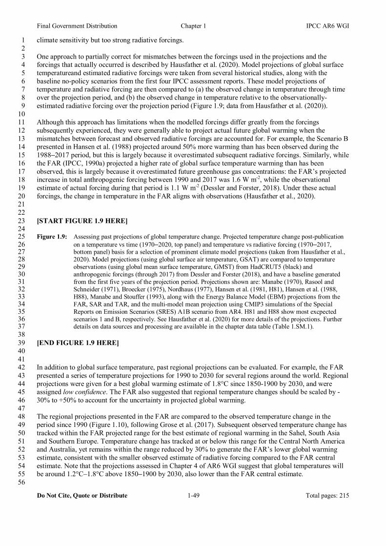
Final Government Distribution Chapter 1 IPCC AR6 WGI
Do Not Cite, Quote or Distribute 1-49 Total pages: 215
climate sensitivity but too strong radiative forcings. 1 2 One approach to partially correct for mismatches between the forcings used in the projections and the 3 forcings that actually occurred is described by Hausfather et al. (2020). Model projections of global surface 4 temperatureand estimated radiative forcings were taken from several historical studies, along with the 5 baseline no-policy scenarios from the first four IPCC assessment reports. These model projections of 6 temperature and radiative forcing are then compared to (a) the observed change in temperature through time 7 over the projection period, and (b) the observed change in temperature relative to the observationally-8 estimated radiative forcing over the projection period (Figure 1.9; data from Hausfather et al. (2020)). 9 10 Although this approach has limitations when the modelled forcings differ greatly from the forcings 11 subsequently experienced, they were generally able to project actual future global warming when the 12 mismatches between forecast and observed radiative forcings are accounted for. For example, the Scenario B 13 presented in Hansen et al. (1988) projected around 50% more warming than has been observed during the 14 1988–2017 period, but this is largely because it overestimated subsequent radiative forcings. Similarly, while 15 the FAR (IPCC, 1990a) projected a higher rate of global surface temperature warming than has been 16 observed, this is largely because it overestimated future greenhouse gas concentrations: the FAR’s projected 17 increase in total anthropogenic forcing between 1990 and 2017 was 1.6 W m-2, while the observational 18 estimate of actual forcing during that period is 1.1 W m-2 (Dessler and Forster, 2018). Under these actual 19 forcings, the change in temperature in the FAR aligns with observations (Hausfather et al., 2020). 20 21 22 [START FIGURE 1.9 HERE] 23 24 Figure 1.9: Assessing past projections of global temperature change. Projected temperature change post-publication 25
on a temperature vs time (1970–2020, top panel) and temperature vs radiative forcing (1970–2017, 26 bottom panel) basis for a selection of prominent climate model projections (taken from Hausfather et al., 27 2020). Model projections (using global surface air temperature, GSAT) are compared to temperature 28 observations (using global mean surface temperature, GMST) from HadCRUT5 (black) and 29 anthropogenic forcings (through 2017) from Dessler and Forster (2018), and have a baseline generated 30 from the first five years of the projection period. Projections shown are: Manabe (1970), Rasool and 31 Schneider (1971), Broecker (1975), Nordhaus (1977), Hansen et al. (1981, H81), Hansen et al. (1988, 32 H88), Manabe and Stouffer (1993), along with the Energy Balance Model (EBM) projections from the 33 FAR, SAR and TAR, and the multi-model mean projection using CMIP3 simulations of the Special 34 Reports on Emission Scenarios (SRES) A1B scenario from AR4. H81 and H88 show most excpected 35 scenarios 1 and B, respectively. See Hausfather et al. (2020) for more details of the projections. Further 36 details on data sources and processing are available in the chapter data table (Table 1.SM.1). 37
38 [END FIGURE 1.9 HERE] 39 40 41 In addition to global surface temperature, past regional projections can be evaluated. For example, the FAR 42 presented a series of temperature projections for 1990 to 2030 for several regions around the world. Regional 43 projections were given for a best global warming estimate of 1.8°C since 1850-1900 by 2030, and were 44 assigned low confidence. The FAR also suggested that regional temperature changes should be scaled by -45 30% to +50% to account for the uncertainty in projected global warming. 46 47 The regional projections presented in the FAR are compared to the observed temperature change in the 48 period since 1990 (Figure 1.10), following Grose et al. (2017). Subsequent observed temperature change has 49 tracked within the FAR projected range for the best estimate of regional warming in the Sahel, South Asia 50 and Southern Europe. Temperature change has tracked at or below this range for the Central North America 51 and Australia, yet remains within the range reduced by 30% to generate the FAR’s lower global warming 52 estimate, consistent with the smaller observed estimate of radiative forcing compared to the FAR central 53 estimate. Note that the projections assessed in Chapter 4 of AR6 WGI suggest that global temperatures will 54 be around 1.2°C–1.8°C above 1850–1900 by 2030, also lower than the FAR central estimate. 55 56
Final Government Distribution Chapter 1 IPCC AR6 WGI
Do Not Cite, Quote or Distribute 1-50 Total pages: 215
Overall, there is medium confidence that past projections of global temperature are consistent with 1 subsequent observations, especially when accounting for the difference in radiative forcings used and those 2 which actually occurred (limited evidence, high agreement). FAR regional projections are broadly consistent 3 with subsequent observations, allowing for regional-scale climate variability and differences in projected and 4 actual forcings. There is medium confidence that the spatial warming pattern has been reliably projected in 5 past IPCC reports (limited evidence, high agreement). 6 7 8 [START FIGURE 1.10 HERE] 9 10 Figure 1.10: Range of projected temperature change for 1990–2030 for various regions defined in IPCC First 11
Assessment Report (FAR).The left panel shows the FAR projections (IPCC, 1990a) for Southern 12 Europe, with darker red bands representing the range of projected change given for the best estimate of 13 1.8°C global warming since pre-industrial to 2030, and the fainter red bands show the range scaled by –14 30% to +50% for lower and higher estimates of global warming. Blue lines show the regionally averaged 15 observations from several global temperature gridded datasets, and blue dashed lines show the linear 16 trends in those datasets for 1990–2020 extrapolated to 2030. Observed datasets are: HadCRUT5, Cowtan 17 and Way, GISTEMP, Berkeley Earth and NOAA GlobalTemp. The inset map shows the definition of the 18 FAR regions used. The right panel shows projected temperature changes by 2030 for the various FAR 19 regions, compared to the extrapolated observational trends, following Grose et al. (2017). Further details 20 on data sources and processing are available in the chapter data table (Table 1.SM.1). 21
22 [END FIGURE 1.10 HERE] 23 24 25 [START BOX 1.2 HERE] 26 27 Box 1.2: Special Reports in the sixth IPCC assessment cycle: key findings 28 29 The Sixth Assessment Cycle started with three Special Reports. The Special Report on Global Warming of 30 1.5°C (SR1.5, (IPCC, 2018), invited by the Parties to the UNFCCC in the context of the Paris Agreement, 31 assessed current knowledge on the impacts of global warming of 1.5°C above pre-industrial levels and 32 related global greenhouse gas (GHG) emission pathways. The Special Report on Climate Change and Land 33 (SRCCL, IPCC, 2019a) addressed GHG fluxes in land-based ecosystems, land use and sustainable land 34 management in relation to climate change adaptation and mitigation, desertification, land degradation and 35 food security. The Special Report on the Ocean and Cryosphere in a Changing Climate (SROCC, IPCC, 36 2019b) assessed new literature on observed and projected changes of the ocean and the cryosphere, and their 37 associated impacts, risks, and responses. 38 39 The SR1.5 and SRCCL were produced through a collaboration between the three IPCC Working Groups, the 40 SROCC by only WGs I and II. Here we focus on key findings relevant to the physical science basis covered 41 by WGI. 42 43 1) Observations of climate change 44 45
The SR1.5 estimated with high confidence that human activities caused a global warming of approximately 46 1°C between the 1850-1900 and 2017. For the period 2006–2015, observed global mean surface temperature 47 (GMST7) was 0.87±0.12°C higher than the average over the 1850–1900 period (very high confidence). 48 Anthropogenic global warming was estimated to be increasing at 0.2±0.1°C per decade (high confidence) 49 and likely matches the level of observed warming to within ±20%. The SRCCL found with high confidence 50 that over land, mean surface air temperature increased by 1.53±0.15°C from 1850–1900 to 2006–2015, or 51 nearly twice as much as the global average. This observed warming has already led to increases in the 52
7 Box 1.2 reproduces the temperature metrics as they appeared in the respective SPMs of the SRs. In AR6 long-term changes of GMST (Global Mean Surface Temperature) and GSAT (Global Surface Air Temperature) are considered to be equivalent, differing in uncertainty estimates only (see Cross-Chapter Box 2.3 in Chapter 2).
Final Government Distribution Chapter 1 IPCC AR6 WGI
Do Not Cite, Quote or Distribute 1-51 Total pages: 215
frequency and intensity of climate and weather extremes in many regions and seasons, including heat waves 1 in most land regions (high confidence), increased droughts in some regions (medium confidence), and 2 increases in the intensity of heavy precipitation events at the global scale (medium confidence). These 3 climate changes have contributed to desertification and land degradation in many regions (high confidence). 4 Increased urbanisation can enhance warming in cities and their surroundings (heat island effect), especially 5 during heat waves (high confidence), and intensify extreme rainfall (medium confidence). 6 7 With respect to the ocean, the SROCC assessed that it is virtually certain that the ocean has warmed 8 unabated since 1970 and has taken up more than 90% of the excess heat contributed by global warming. The 9 rate of ocean warming has likely more than doubled since 1993. Over the period 1982–2016, marine 10 heatwaves have very likely doubled in frequency and are increasing in intensity (very high confidence). In 11 addition, the surface ocean acidified further (virtually certain) and loss of oxygen occurred from the surface 12 to a depth of 1000 m (medium confidence). The report expressed medium confidence that the Atlantic 13 Meridional Overturning Circulation (AMOC) weakened in 2004–2017 relative to 1850–1900. 14 15 Concerning the cryosphere, the SROCC reported widespread continued shrinking of nearly all components. 16 Mass loss from the Antarctic Ice Sheet tripled over the period 2007–2016 relative to 1997–2006, while mass 17 loss doubled for the Greenland Ice Sheet (likely, medium confidence). The report concludes with very high 18 confidence that due to the combined increased loss from the ice sheets, global mean sea level (GMSL) rise 19 has accelerated (extremely likely). The rate of recent GMSL rise (3.6±0.5 mm yr-1 for 2006–2015) is about 20 2.5 times larger than for 1901–1990. The report also found that Arctic sea ice extent has very likely 21 decreased for all months of the year since 1979 and that September sea ice reductions of 12.8±2.3% per 22 decade are likely unprecedented for at least 1000 years. Feedbacks from the loss of summer sea ice and 23 spring snow cover on land have contributed to amplified warming in the Arctic (high confidence), where 24 surface air temperature likely increased by more than double the global average over the last two decades. By 25 contrast, Antarctic sea ice extent overall saw no statistically significant trend for the period 1979 to 2018 26 (high confidence). 27 28 The SROCC assessed that anthropogenic climate change has increased observed precipitation (medium 29 confidence), winds (low confidence), and extreme sea level events (high confidence) associated with some 30 tropical cyclones. It also found evidence for an increase in annual global proportion of Category 4 or 5 31 tropical cyclones in recent decades (low confidence). 32 33 2) Drivers of climate change 34 35 The SRCCL stated that the land is simultaneously a source and sink of CO2 due to both anthropogenic and 36 natural drivers. It estimates with medium confidence that Agriculture, Forestry and Other Land Use 37 (AFOLU) activities accounted for around 13% of CO2, 44% of methane, and 82% of nitrous oxide emissions 38 from human activities during 2007–2016, representing 23% (12.0±3.0 GtCO2 equivalent yr-1) of the total net 39 anthropogenic emissions of GHGs. The natural response of land to human-induced environmental change 40 such as increasing atmospheric CO2 concentration, nitrogen deposition, and climate change, caused a net 41 CO2 sink equivalent of around 29% of total CO2 emissions (medium confidence); however, the persistence of 42 the sink is uncertain due to climate change (high confidence). 43 44 The SRCCL also assessed how changes in land conditions affect global and regional climate. It found that 45 changes in land cover have led to both a net release of CO2, contributing to global warming, and an increase 46 in global land albedo, causing surface cooling. However, the report estimated that the resulting net effect on 47 globally averaged surface temperature was small over the historical period (medium confidence). 48 49 The SROCC found that the carbon content of Arctic and boreal permafrost is almost twice that of the 50 atmosphere (medium confidence), and assessed medium evidence with low agreement that thawing northern 51 permafrost regions are currently releasing additional net methane and CO2. 52 53 3) Projections of climate change 54 55

Final Government Distribution Chapter 1 IPCC AR6 WGI
Do Not Cite, Quote or Distribute 1-52 Total pages: 215
The SR1.5 concluded that global warming is likely to reach 1.5°C between 2030 and 2052 if it continues to 1 increase at the current rate (high confidence). However, even though warming from anthropogenic emissions 2 will persist for centuries to millennia and will cause ongoing long-term changes, past emissions alone are 3 unlikely to raise global surface temperatur to 1.5°C above 1850-1900 levels. 4 5 The SR1.5 also found that reaching and sustaining net zero anthropogenic CO2 emissions and reducing net 6 non-CO2 radiative forcing would halt anthropogenic global warming on multi-decadal time scales (high 7 confidence). The maximum temperature reached is then determined by cumulative net global anthropogenic 8 CO2 emissions up to the time of net zero CO2 emissions (high confidence) and the level of non-CO2 radiative 9 forcing in the decades prior to the time that maximum temperatures are reached (medium confidence). 10 11 Furthermore, climate models project robust differences in regional climate characteristics between the 12 present day and a global warming of 1.5°C, and between 1.5°C and 2°C, including mean temperature in most 13 land and ocean regions and hot extremes in most inhabited regions (high confidence). There is medium 14 confidence in robust differences in heavy precipitation events in several regions and the probability of 15 droughts in some regions. 16 17 The SROCC projected that global-scale glacier mass loss, permafrost thaw, and decline in snow cover and 18 Arctic sea ice extent will continue in the near term (2031–2050) due to surface air temperature increases 19 (high confidence). The Greenland and Antarctic Ice Sheets are projected to lose mass at an increasing rate 20 throughout the 21st century and beyond (high confidence). Sea level rise will also continue at an increasing 21 rate. For the period 2081–2100 with respect to 1986–2005, the likely ranges of global mean sea level 22 (GMSL) rise are projected at 0.26–0.53 m for RCP2.6 and 0.51–0.92 m for RCP8.5. For the RCP8.5 23 scenario, projections of GMSL rise by 2100 are higher by 0.1 m than in AR5 due to a larger contribution 24 from the Antarctic Ice Sheet (medium confidence). Extreme sea level events that occurred once per hundred 25 years in the recent past are projected to occur at least once per year at many locations by 2050, especially in 26 tropical regions, under all RCP scenarios (high confidence). According to SR1.5, by 2100, GMSL rise would 27 be around 0.1 m lower with 1.5°C global warming compared to 2°C (medium confidence). If warming is held 28 to 1.5°, GMSLwill still continue to rise well beyond 2100, but at a slower rate and a lower magnitude. 29 However, instability and/or irreversible loss of the Greenland and Antarctic Ice Sheets, resulting in multi-30 metre rise in sea level over hundreds to thousands of years, could be triggered at 1.5°C to 2°C of global 31 warming (medium confidence). According to the SROCC, sea level rise in an extended RCP2.6 scenario 32 would be limited to around 1 m in 2300 (low confidence) while multi-metre sea-level rise is projected under 33 RCP8.5 by then (medium confidence). 34 35 The SROCC projected that over the 21st century, the ocean will transition to unprecedented conditions with 36 increased temperatures (virtually certain), further acidification (virtually certain), and oxygen decline 37 (medium confidence). Marine heatwaves are projected to become more frequent (very high confidence) as are 38 extreme El Niño and La Niña events (medium confidence). The AMOC is projected to weaken during the 39 21st century (very likely), but a collapse is deemed very unlikely (albeit with medium confidence due to 40 known biases in the climate models used for the assessment). 41 42 4) Emission pathways to limit global warming 43 44 The SR1.5 focused on emission pathways and system transitions consistent with 1.5°C global warming over 45 the 21st century. Building upon the understanding from WGI AR5 of the quasi-linear relationship between 46 cumulative net anthropogenic CO2 emissions since 1850–1900 and maximum global mean temperature, the 47 report assessed the remaining carbon budgets compatible with the 1.5°C or 2°C warming goals of the Paris 48 Agreement. Starting from year 2018, the remaining carbon budget for a one-in-two chance of limiting global 49 warming to 1.5°C is about 580 GtCO2, and about 420 GtCO2 for a two-in-three chance (medium confidence). 50 At constant 2017 emissions, these budgets would be depleted by about the years 2032 and 2028, 51 respectively. Using GMST instead of GSAT gives estimates of 770 and 570 GtCO2, respectively (medium 52 confidence). Each budget is further reduced by approximately 100 GtCO2 over the course of this century 53 when permafrost and other less well represented Earth-system feedbacks are taken into account. 54 55

Final Government Distribution Chapter 1 IPCC AR6 WGI
Do Not Cite, Quote or Distribute 1-53 Total pages: 215
It is concluded that all emission pathways with no or limited overshoot of 1.5°C imply that global net 1 anthropogenic CO2 emissions would need to decline by about 45% from 2010 levels by 2030, reaching net 2 zero around 2050, together with deep reductions in other anthropogenic emissions, such as methane and 3 black carbon. To limit global warming to below 2°C, CO2 emissions would have to decline by about 25% by 4 2030 and reach net zero around 2070. 5 6 [END BOX 1.2 HERE] 7 8 9 1.4 AR6 foundations and concepts 10 11 AR6 WGI builds on previous assessments using well established foundations and concepts. This section 12 highlights some of the cross-cutting methods applied in the climate change literature and topics discussed 13 repeatedly throughout this report. The choices related to baseline, or reference periods, are first highlighted 14 (Section 1.4.1), including a specific discussion on the pre-industrial baseline used in AR6 WGI (Cross-15 Chapter Box 1.2). The relationships between long-term trends, climate variability and the concept of 16 emergence of changes (Section 1.4.2) and the sources of uncertainty in climate simulations (Section 1.4.3) 17 are discussed next. The topic of low-likelihood outcomes, storylines, abrupt changes and surprises follows 18 (Section 1.4.4), including a description of the AR6 WGI risk framing (Cross-Chapter Box 1.3). The Cross-19 Working Group Box: Attribution describes attribution methods, including those for extreme events. Various 20 sets of geographical regions used in later Chapters are also defined and introduced (Section 1.4.5). 21 22 23 1.4.1 Baselines, reference periods and anomalies 24 25 Several ‘baselines’ or ‘reference periods’ are used consistently throughout AR6 WGI. Baseline refers to a 26 period against which differences are calculated whereas reference period is used more generally to indicate a 27 time period of interest, or a period over which some relevant statistics are calculated (see Annex VII: 28 Glossary). Variations in observed and simulated climate variables over time are often presented as 29 ‘anomalies’, i.e., the differences relative to a baseline, rather than using the absolute values. This is done for 30 several reasons. 31 32 First, anomalies are often used when combining data from multiple locations, because the absolute values 33 can vary over small spatial scales which are not densely observed or simulated, whereas anomalies are 34 representative for much larger scales (e.g., for temperature, Hansen and Lebedeff 1987). Since their baseline 35 value is zero by definition, anomalies are also less susceptible to biases arising from changes in the 36 observational network. Second, the seasonality in different climate indicators can be removed using 37 anomalies to more clearly distinguish variability from long-term trends. 38 39 Third, different datasets can have different absolute values for the same climate variable that should be 40 removed for effective comparisons of variations with time. This is often required when comparing climate 41 simulations with each other, or when comparing simulations with observations, as simulated climate 42 variables are also affected by model bias that can be removed when they are presented as anomalies. It can 43 also be required when comparing observational datasets or reanalyses (see Section 1.5.2) with each other, 44 due to systematic differences in the underlying measurement system (see Figure 1.11). Understanding the 45 reasons for any absolute difference is important, but whether the simulated absolute value matters when 46 projecting future change will depend on the variable of interest. For example, there is not a strong 47 relationship between climate sensitivity of a model (which is an indicator of the degree of future warming) 48 and the simulated absolute global surface temperature (Mauritsen et al. 2012; Hawkins and Sutton 2016). 49 50 For some variables, such as precipitation, anomalies are often expressed as percentages in order to more 51 easily compare changes in regions with very different climatological means. However, for situations where 52 there are important thresholds (e.g., phase transitions around 0°C) or for variables which can only take a 53 particular sign or be in a fixed range (e.g., sea ice extent or relative humidity), absolute values are normally 54 used. 55

Final Government Distribution Chapter 1 IPCC AR6 WGI
Do Not Cite, Quote or Distribute 1-54 Total pages: 215
1 The choice of a baseline period has important consequences for evaluating both observations and simulations 2 of the climate, for comparing observations with simulations, and for presenting climate projections. There is 3 usually no perfect choice of baseline as many factors have to be considered and compromises may be 4 required (Hawkins and Sutton 2016). It is important to evaluate the sensitivity of an analysis or assessment to 5 the choice of the baseline. 6 7 For example, the collocation of observations and reanalyses within the model ensemble spread depends on 8 the choice of the baseline, and uncertainty in future projections of climate is reduced if using a more recent 9 baseline, especially for the near-term (Figure 1.11). The length of an appropriate baseline or reference period 10 depends on the variable being considered, the rates of change of the variable and the purpose of the period, 11 but is usually 20 to 50 years long. The World Meteorological Organization (WMO) uses 30-year periods to 12 define ‘climate normals’, which indicate conditions expected to be experienced in a given location. 13 14 15 [START FIGURE 1.11 HERE] 16 17 Figure 1.11: Choice of baseline matters when comparing observations and model simulations. Global surface air 18
temperature (GSAT, grey) from a range of CMIP6 historical simulations (1850–2014, 25 models) and 19 SSP1-2.6 (2015–2100) using absolute values (top) and anomalies relative to two different baselines: 20 1850–1900 (middle) and 1995–2014 (bottom). An estimate of GSAT from a reanalysis (ERA-5, orange, 21 1979–2020) and an observation-based estimate of global mean surface air temperature (GMST) (Berkeley 22 Earth, black, 1850–2020) are shown, along with the mean GSAT for 1961–1990 estimated by Jones et al. 23 (1999), light blue shading, 14.0±0.5°C). Using the more recent baseline (bottom) allows the inclusion of 24 datasets which do not include the periods of older baselines. The middle and bottom panels have scales 25 which are the same size but offset. Further details on data sources and processing are available in the 26 chapter data table (Table 1.SM.1). 27
28 [END FIGURE 1.11 HERE] 29 30 31 For AR6 WGI, the period 1995–2014 is used as a baseline to calculate the changes in future climate using 32 model projections and also as a ‘modern’ or ‘recent past’ reference period when estimating past observed 33 warming. The equivalent period in AR5 was 1986–2005, and in SR1.5, SROCC and SRCCL it was 2006–34 2015. The primary reason for the different choice in AR6 is that 2014 is the final year of the historical 35 CMIP6 simulations. These simulations subsequently assume different emission scenarios and so choosing 36 any later baseline end date would require selecting a particular emissions scenario. For certain assessments, 37 the most recent decade possible (e.g. 2010–2019 or 2011–2020, depending on the availability of 38 observations) is also used as a reference period (see Cross Chapter Box 2.3 in Chapter 2). 39 40 Figure 1.12 shows changes in observed global mean surface temperature (GMST) relative to 1850–1900 and 41 illustrates observed global warming levels for a range of reference periods that are either used in AR6 or 42 were used in previous IPCC Reports. This allows changes to be calculated between different periods and 43 compared to previous assessments. For example, AR5 assessed the change in GMST from the 1850–1900 44 baseline to 1986–2005 reference period as 0.61 (0.55–0.67) °C, whereas it is now assessed to be 0.69 (0.52–45 0.82) °C using improved GMST datasets (also see Cross-Chapter Box 2.3 in Chapter 2). 46 47 The commonly used metric for global surface warming tends to be global mean surface temperature (GMST) 48 but, as shown in Figure 1.11, climate model simulations tend to use global surface air temperature (GSAT). 49 Although GMST and GSAT are closely related, the two measures are physically distinct. GMST is a 50 combination of land surface air temperatures (LSAT) and sea surface temperatures (SSTs), whereas GSAT is 51 surface air temperatures over land, ocean and ice. A key development in AR6 is the assessment that long-52 term changes in GMST and GSAT differ by at most 10% in either direction, with low confidence in the sign 53 of any differences (see Cross Chapter Box 2.3 for details). 54 55 Three future reference periods are used in AR6 WGI for presenting projections: near-term (2021–2040), 56
Final Government Distribution Chapter 1 IPCC AR6 WGI
Do Not Cite, Quote or Distribute 1-55 Total pages: 215
mid-term (2041–2060) and long-term (2081–2100) (see Figure 1.11). In AR6, 20-year reference periods are 1 considered long enough to show future changes in many variables when averaging over ensemble members 2 of multiple models, and short enough to enable the time dependence of changes to be shown throughout the 3 21st century. Projections with alternative recent baselines (such as 1986–2005 or the current WMO climate 4 normal period of 1981–2010) and a wider range of future reference periods are presented in the Interactive 5 Atlas. Note that ‘long-term’ is also sometimes used to refer to durations of centuries to millennia when 6 examining past climate, as well as future climate change beyond the year 2100. Cross-Chapter Box 2.1 in 7 Chapter 2 discusses the paleo reference periods used in AR6. 8 9 10 [START FIGURE 1.12 HERE] 11 12 Figure 1.12: Global warming over the instrumental period. Observed global mean surface temperature (GMST) from 13
four datasets, relative to the average temperature of 1850–1900 in each dataset (see Cross-Chapter Box 14 2.3 and Section 2.3.1.1 for more details). The shaded grey band indicates the assessed likely range for the 15 period around 1750 (see Cross-Chapter Box 1.2). Different reference periods are indicated by the 16 coloured horizontal lines, and an estimate of total GMST change up to that period is given, enabling a 17 translation of the level of warming between different reference periods. The reference periods are all 18 chosen because they have been used in the AR6 or previous IPCC assessment reports. The value for the 19 1981–2010 reference period, used as a ‘climate normal’ period by the World Meteorological 20 Organization, is the same as the 1986–2005 reference period shown. Further details on data sources and 21 processing are available in the chapter data table (Table 1.SM.1). 22
23 [END FIGURE 1.12 HERE] 24 25 26 [START CROSS-CHAPTER BOX 1.2 HERE] 27 28 Cross-Chapter Box 1.2: Changes in global temperature between 1750 and 1850 29 30 Contributing Authors: Ed Hawkins (UK), Paul Edwards (USA), Piers Forster (UK), Darrell Kaufman 31 (USA), Jochem Marotzke (Germany), Malte Meinshausen (Australia/Germany), Maisa Rojas (Chile), Bjørn 32 H. Samset (Norway), Peter Thorne (Ireland/UK). 33 34 35 The Paris Agreement aims to limit global temperatures to specific thresholds ‘above pre-industrial levels’. In 36 AR6 WGI, as in previous IPCC reports, observations and projections of changes in global temperature are 37 generally expressed relative to 1850–1900 as an approximate pre-industrial state (SR1.5, IPCC, 2018). This 38 is a pragmatic choice based upon data availability considerations, though both anthropogenic and natural 39 changes to the climate occurred before 1850. The remaining carbon budgets, the chance of crossing global 40 temperature thresholds, and projections of extremes and sea level rise at a particular level of global warming 41 can all be sensitive to the chosen definition of the approximate pre-industrial baseline (Millar et al., 2017a; 42 Schurer et al., 2017; Pfleiderer et al., 2018; Rogelj et al., 2019; Tokarska et al., 2019). This Cross-Chapter 43 Box assesses the evidence on change in radiative forcing and global temperature from the period around 44 1750 to 1850–1900; variations in the climate before 1750 are discussed in Chapter 2. 45 46 Although there is some evidence for human influence on climate before 1750 (e.g., Ruddiman and Thomson, 47 2001; Koch et al., 2019), the magnitude of the effect is still disputed (e.g., Joos et al., 2004; Beck et al., 48 2018b; see Chapter 5, Section 5.1.2.3), and most studies analyse the human influence on climate over the 49 industrial period. Historically, the widespread use of coal-powered machinery started the Industrial 50 Revolution in Britain in the late 18th century (Ashton, 1997), but the global effects were small for several 51 decades. In line with this, previous IPCC assessment reports considered changes in radiative forcing relative 52 to 1750, and temperature changes were often reported relative to the ‘late 19th century’. AR5 and SR1.5 53 made the specific pragmatic choice to approximate pre-industrial global temperatures by the average of the 54 1850–1900 period, when permanent surface observing networks emerged that provide sufficiently accurate 55
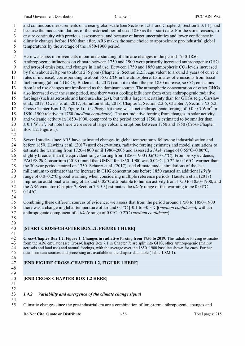
Final Government Distribution Chapter 1 IPCC AR6 WGI
Do Not Cite, Quote or Distribute 1-56 Total pages: 215
and continuous measurements on a near-global scale (see Sections 1.3.1 and Chapter 2, Section 2.3.1.1), and 1 because the model simulations of the historical period used 1850 as their start date. For the same reasons, to 2 ensure continuity with previous assessments, and because of larger uncertainties and lower confidence in 3 climatic changes before 1850 than after, AR6 makes the same choice to approximate pre-industrial global 4 temperatures by the average of the 1850-1900 period. 5 6 Here we assess improvements in our understanding of climatic changes in the period 1750-1850. 7 Anthropogenic influences on climate between 1750 and 1900 were primarily increased anthropogenic GHG 8 and aerosol emissions, and changes in land use. Between 1750 and 1850 atmospheric CO2 levels increased 9 by from about 278 ppm to about 285 ppm (Chapter 2, Section 2.2.3, equivalent to around 3 years of current 10 rates of increase), corresponding to about 55 GtCO2 in the atmosphere. Estimates of emissions from fossil 11 fuel burning (about 4 GtCO2, Boden et al., 2017) cannot explain the pre-1850 increase, so CO2 emissions 12 from land use changes are implicated as the dominant source. The atmospheric concentration of other GHGs 13 also increased over the same period, and there was a cooling influence from other anthropogenic radiative 14 forcings (such as aerosols and land use changes), but with a larger uncertainty than for GHGs (e.g., Carslaw 15 et al., 2017; Owens et al., 2017; Hamilton et al., 2018; Chapter 2, Section 2.2.6; Chapter 7, Section 7.3.5.2; 16 Cross-Chapter Box 1.2, Figure 1). It is likely that there was a net anthropogenic forcing of 0.0–0.3 Wm-2 in 17 1850–1900 relative to 1750 (medium confidence). The net radiative forcing from changes in solar activity 18 and volcanic activity in 1850–1900, compared to the period around 1750, is estimated to be smaller than 19 ± 0.1 W m-2, but note there were several large volcanic eruptions between 1750 and 1850 (Cross-Chapter 20 Box 1.2, Figure 1). 21 22 Several studies since AR5 have estimated changes in global temperatures following industrialisation and 23 before 1850. Hawkins et al. (2017) used observations, radiative forcing estimates and model simulations to 24 estimate the warming from 1720–1800 until 1986–2005 and assessed a likely range of 0.55°C–0.80°C, 25 slightly broader than the equivalent range starting from 1850–1900 (0.6°C–0.7°C). From proxy evidence, 26 PAGES 2k Consortium (2019) found that GMST for 1850–1900 was 0.02°C [-0.22 to 0.16°C] warmer than 27 the 30-year period centred on 1750. Schurer et al. (2017) used climate model simulations of the last 28 millennium to estimate that the increase in GHG concentrations before 1850 caused an additional likely 29 range of 0.0–0.2°C global warming when considering multiple reference periods. Haustein et al. (2017) 30 implies an additional warming of around 0.05°C attributable to human activity from 1750 to 1850–1900, and 31 the AR6 emulator (Chapter 7, Section 7.3.5.3) estimates the likely range of this warming to be 0.04°C–32 0.14°C. 33 34 Combining these different sources of evidence, we assess that from the period around 1750 to 1850–1900 35 there was a change in global temperature of around 0.1°C [-0.1 to +0.3°C](medium confidence), with an 36 anthropogenic component of a likely range of 0.0°C–0.2°C (medium confidence). 37 38 39 [START CROSS-CHAPTER BOX1.2, FIGURE 1 HERE] 40 41 Cross-Chapter Box 1.2, Figure 1: Changes in radiative forcing from 1750 to 2019. The radiative forcing estimates 42 from the AR6 emulator (see Cross-Chapter Box 7.1 in Chapter 7) are split into GHG, other anthropogenic (mainly 43 aerosols and land use) and natural forcings, with the average over the 1850–1900 baseline shown for each. Further 44 details on data sources and processing are available in the chapter data table (Table 1.SM.1). 45 46 [END FIGURE CROSS-CHAPTER 1.2, FIGURE 1 HERE] 47 48 49 [END CROSS-CHAPTER BOX 1.2 HERE] 50 51 52 1.4.2 Variability and emergence of the climate change signal 53 54 Climatic changes since the pre-industrial era are a combination of long-term anthropogenic changes and 55
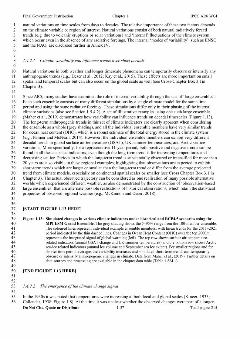
Final Government Distribution Chapter 1 IPCC AR6 WGI
Do Not Cite, Quote or Distribute 1-57 Total pages: 215
natural variations on time scales from days to decades. The relative importance of these two factors depends 1 on the climate variable or region of interest. Natural variations consist of both natural radiatively forced 2 trends (e.g. due to volcanic eruptions or solar variations) and ‘internal’ fluctuations of the climate system 3 which occur even in the absence of any radiative forcings. The internal ‘modes of variability’, such as ENSO 4 and the NAO, are discussed further in Annex IV. 5 6 7 1.4.2.1 Climate variability can influence trends over short periods 8 9 Natural variations in both weather and longer timescale phenomena can temporarily obscure or intensify any 10 anthropogenic trends (e.g., Deser et al., 2012; Kay et al., 2015). These effects are more important on small 11 spatial and temporal scales but can also occur on the global scale as well (see Cross-Chapter Box 3.1in 12 Chapter 3). 13 14 Since AR5, many studies have examined the role of internal variability through the use of ‘large ensembles’. 15 Each such ensemble consists of many different simulations by a single climate model for the same time 16 period and using the same radiative forcings. These simulations differ only in their phasing of the internal 17 climate variations (also see Section 1.5.4.2). A set of illustrative examples using one such large ensemble 18 (Maher et al., 2019) demonstrates how variability can influence trends on decadal timescales (Figure 1.13). 19 The long-term anthropogenic trends in this set of climate indicators are clearly apparent when considering 20 the ensemble as a whole (grey shading), and all the individual ensemble members have very similar trends 21 for ocean heat content (OHC), which is a robust estimate of the total energy stored in the climate system 22 (e.g., Palmer and McNeall, 2014). However, the individual ensemble members can exhibit very different 23 decadal trends in global surface air temperature (GSAT), UK summer temperatures, and Arctic sea-ice 24 variations. More specifically, for a representative 11-year period, both positive and negative trends can be 25 found in all these surface indicators, even though the long-term trend is for increasing temperatures and 26 decreasing sea ice. Periods in which the long-term trend is substantially obscured or intensified for more than 27 20 years are also visible in these regional examples, highlighting that observations are expected to exhibit 28 short-term trends which are larger or smaller than the long-term trend or differ from the average projected 29 trend from climate models, especially on continental spatial scales or smaller (see Cross Chapter Box 3.1 in 30 Chapter 3). The actual observed trajectory can be considered as one realisation of many possible alternative 31 worlds which experienced different weather, as also demonstrated by the construction of ‘observation-based 32 large ensembles’ that are alternate possible realisations of historical observations, which retain the statistical 33 properties of observed regional weather (e.g., McKinnon and Deser, 2018). 34 35 36 [START FIGURE 1.13 HERE] 37 38 Figure 1.13: Simulated changes in various climate indicators under historical and RCP4.5 scenarios using the 39
MPI ESM Grand Ensemble. The grey shading shows the 5–95% range from the 100-member ensemble. 40 The coloured lines represent individual example ensemble members, with linear trends for the 2011–2021 41 period indicated by the thin dashed lines. Changes in Ocean Heat Content (OHC) over the top 2000m 42 represents the integrated signal of global warming (left). The top row shows surface air temperature-43 related indicators (annual GSAT change and UK summer temperatures) and the bottom row shows Arctic 44 sea-ice related indicators (annual ice volume and September sea ice extent). For smaller regions and for 45 shorter time period averages the variability increases and simulated short-term trends can temporarily 46 obscure or intensify anthropogenic changes in climate. Data from Maher et al., (2019). Further details on 47 data sources and processing are available in the chapter data table (Table 1.SM.1). 48
49 [END FIGURE 1.13 HERE] 50 51 52 1.4.2.2 The emergence of the climate change signal 53 54 In the 1930s it was noted that temperatures were increasing at both local and global scales (Kincer, 1933; 55 Callendar, 1938; Figure 1.8). At the time it was unclear whether the observed changes were part of a longer-56
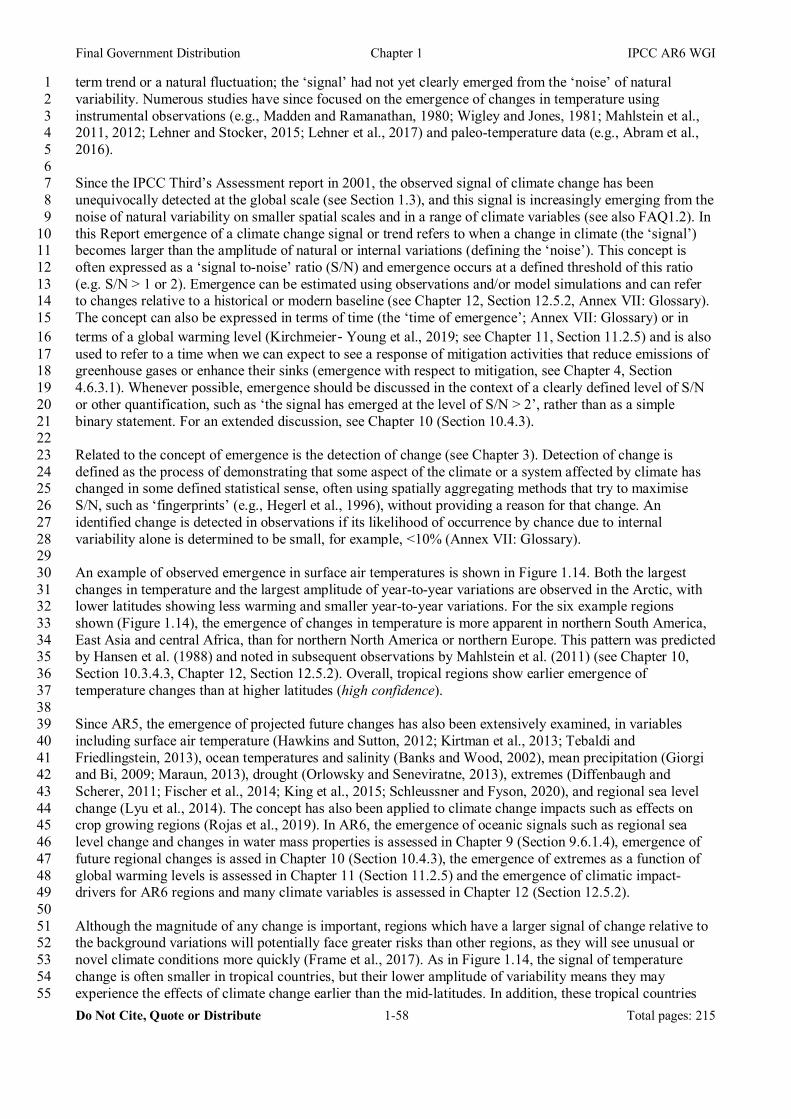
Final Government Distribution Chapter 1 IPCC AR6 WGI
Do Not Cite, Quote or Distribute 1-58 Total pages: 215
term trend or a natural fluctuation; the ‘signal’ had not yet clearly emerged from the ‘noise’ of natural 1 variability. Numerous studies have since focused on the emergence of changes in temperature using 2 instrumental observations (e.g., Madden and Ramanathan, 1980; Wigley and Jones, 1981; Mahlstein et al., 3 2011, 2012; Lehner and Stocker, 2015; Lehner et al., 2017) and paleo-temperature data (e.g., Abram et al., 4 2016). 5 6 Since the IPCC Third’s Assessment report in 2001, the observed signal of climate change has been 7 unequivocally detected at the global scale (see Section 1.3), and this signal is increasingly emerging from the 8 noise of natural variability on smaller spatial scales and in a range of climate variables (see also FAQ1.2). In 9 this Report emergence of a climate change signal or trend refers to when a change in climate (the ‘signal’) 10 becomes larger than the amplitude of natural or internal variations (defining the ‘noise’). This concept is 11 often expressed as a ‘signal to-noise’ ratio (S/N) and emergence occurs at a defined threshold of this ratio 12 (e.g. S/N > 1 or 2). Emergence can be estimated using observations and/or model simulations and can refer 13 to changes relative to a historical or modern baseline (see Chapter 12, Section 12.5.2, Annex VII: Glossary). 14 The concept can also be expressed in terms of time (the ‘time of emergence’; Annex VII: Glossary) or in 15 terms of a global warming level (Kirchmeier‐Young et al., 2019; see Chapter 11, Section 11.2.5) and is also 16 used to refer to a time when we can expect to see a response of mitigation activities that reduce emissions of 17 greenhouse gases or enhance their sinks (emergence with respect to mitigation, see Chapter 4, Section 18 4.6.3.1). Whenever possible, emergence should be discussed in the context of a clearly defined level of S/N 19 or other quantification, such as ‘the signal has emerged at the level of S/N > 2’, rather than as a simple 20 binary statement. For an extended discussion, see Chapter 10 (Section 10.4.3). 21 22 Related to the concept of emergence is the detection of change (see Chapter 3). Detection of change is 23 defined as the process of demonstrating that some aspect of the climate or a system affected by climate has 24 changed in some defined statistical sense, often using spatially aggregating methods that try to maximise 25 S/N, such as ‘fingerprints’ (e.g., Hegerl et al., 1996), without providing a reason for that change. An 26 identified change is detected in observations if its likelihood of occurrence by chance due to internal 27 variability alone is determined to be small, for example, <10% (Annex VII: Glossary). 28 29 An example of observed emergence in surface air temperatures is shown in Figure 1.14. Both the largest 30 changes in temperature and the largest amplitude of year-to-year variations are observed in the Arctic, with 31 lower latitudes showing less warming and smaller year-to-year variations. For the six example regions 32 shown (Figure 1.14), the emergence of changes in temperature is more apparent in northern South America, 33 East Asia and central Africa, than for northern North America or northern Europe. This pattern was predicted 34 by Hansen et al. (1988) and noted in subsequent observations by Mahlstein et al. (2011) (see Chapter 10, 35 Section 10.3.4.3, Chapter 12, Section 12.5.2). Overall, tropical regions show earlier emergence of 36 temperature changes than at higher latitudes (high confidence). 37 38 Since AR5, the emergence of projected future changes has also been extensively examined, in variables 39 including surface air temperature (Hawkins and Sutton, 2012; Kirtman et al., 2013; Tebaldi and 40 Friedlingstein, 2013), ocean temperatures and salinity (Banks and Wood, 2002), mean precipitation (Giorgi 41 and Bi, 2009; Maraun, 2013), drought (Orlowsky and Seneviratne, 2013), extremes (Diffenbaugh and 42 Scherer, 2011; Fischer et al., 2014; King et al., 2015; Schleussner and Fyson, 2020), and regional sea level 43 change (Lyu et al., 2014). The concept has also been applied to climate change impacts such as effects on 44 crop growing regions (Rojas et al., 2019). In AR6, the emergence of oceanic signals such as regional sea 45 level change and changes in water mass properties is assessed in Chapter 9 (Section 9.6.1.4), emergence of 46 future regional changes is assed in Chapter 10 (Section 10.4.3), the emergence of extremes as a function of 47 global warming levels is assessed in Chapter 11 (Section 11.2.5) and the emergence of climatic impact-48 drivers for AR6 regions and many climate variables is assessed in Chapter 12 (Section 12.5.2). 49 50 Although the magnitude of any change is important, regions which have a larger signal of change relative to 51 the background variations will potentially face greater risks than other regions, as they will see unusual or 52 novel climate conditions more quickly (Frame et al., 2017). As in Figure 1.14, the signal of temperature 53 change is often smaller in tropical countries, but their lower amplitude of variability means they may 54 experience the effects of climate change earlier than the mid-latitudes. In addition, these tropical countries 55
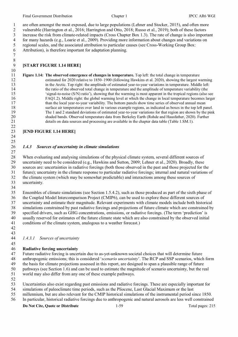
Final Government Distribution Chapter 1 IPCC AR6 WGI
Do Not Cite, Quote or Distribute 1-59 Total pages: 215
are often amongst the most exposed, due to large populations (Lehner and Stocker, 2015), and often more 1 vulnerable (Harrington et al., 2016; Harrington and Otto, 2018; Russo et al., 2019); both of these factors 2 increase the risk from climate-related impacts (Cross Chapter Box 1.3). The rate of change is also important 3 for many hazards (e.g., Loarie et al., 2009). Providing more information about changes and variations on 4 regional scales, and the associated attribution to particular causes (see Cross-Working Group Box: 5 Attribution), is therefore important for adaptation planning. 6 7 8 [START FIGURE 1.14 HERE] 9 10 Figure 1.14: The observed emergence of changes in temperature. Top left: the total change in temperature 11
estimated for 2020 relative to 1850–1900 (following Hawkins et al. 2020), showing the largest warming 12 in the Arctic. Top right: the amplitude of estimated year-to-year variations in temperature. Middle left: 13 the ratio of the observed total change in temperature and the amplitude of temperature variability (the 14 ‘signal-to-noise (S/N) ratio’), showing that the warming is most apparent in the tropical regions (also see 15 FAQ1.2). Middle right: the global warming level at which the change in local temperature becomes larger 16 than the local year-to-year variability. The bottom panels show time series of observed annual mean 17 surface air temperatures over land in various example regions, as indicated as boxes in the top left panel. 18 The 1 and 2 standard deviations of estimated year-to-year variations for that region are shown by the pink 19 shaded bands. Observed temperature data from Berkeley Earth (Rohde and Hausfather, 2020). Further 20 details on data sources and processing are available in the chapter data table (Table 1.SM.1). 21
22 [END FIGURE 1.14 HERE] 23 24 25 1.4.3 Sources of uncertainty in climate simulations 26 27 When evaluating and analysing simulations of the physical climate system, several different sources of 28 uncertainty need to be considered (e.g., Hawkins and Sutton, 2009; Lehner et al., 2020). Broadly, these 29 sources are: uncertainties in radiative forcings (both those observed in the past and those projected for the 30 future); uncertainty in the climate response to particular radiative forcings; internal and natural variations of 31 the climate system (which may be somewhat predictable) and interactions among these sources of 32 uncertainty. 33 34 Ensembles of climate simulations (see Section 1.5.4.2), such as those produced as part of the sixth phase of 35 the Coupled Model Intercomparison Project (CMIP6), can be used to explore these different sources of 36 uncertainty and estimate their magnitude. Relevant experiments with climate models include both historical 37 simulations constrained by past radiative forcings and projections of future climate which are constrained by 38 specified drivers, such as GHG concentrations, emissions, or radiative forcings. (The term ‘prediction’ is 39 usually reserved for estimates of the future climate state which are also constrained by the observed initial 40 conditions of the climate system, analogous to a weather forecast.) 41 42 43 1.4.3.1 Sources of uncertainty 44 45 Radiative forcing uncertainty 46 Future radiative forcing is uncertain due to as-yet-unknown societal choices that will determine future 47 anthropogenic emissions; this is considered ‘scenario uncertainty’. The RCP and SSP scenarios, which form 48 the basis for climate projections assessed in this report, are designed to span a plausible range of future 49 pathways (see Section 1.6) and can be used to estimate the magnitude of scenario uncertainty, but the real 50 world may also differ from any one of these example pathways. 51 52 Uncertainties also exist regarding past emissions and radiative forcings. These are especially important for 53 simulations of paleoclimate time periods, such as the Pliocene, Last Glacial Maximum or the last 54 millennium, but are also relevant for the CMIP historical simulations of the instrumental period since 1850. 55 In particular, historical radiative forcings due to anthropogenic and natural aerosols are less well constrained 56

Final Government Distribution Chapter 1 IPCC AR6 WGI
Do Not Cite, Quote or Distribute 1-60 Total pages: 215
by observations than the greenhouse gas radiative forcings. There is also uncertainty in the size of large 1 volcanic eruptions (and in the location for some that occurred before around 1850), and the amplitude of 2 changes in solar activity, before satellite observations. The role of historical radiative forcing uncertainty was 3 considered previously (Knutti et al., 2002; Forster et al., 2013) but, since AR5, specific simulations have 4 been performed to examine this issue, particularly for the effects of uncertainty in anthropogenic aerosol 5 radiative forcing (e.g., Jiménez-de-la-Cuesta and Mauritsen, 2019; Dittus et al., 2020). 6 7 Climate response uncertainty 8 Under any particular scenario (see Section 1.6.1), there is uncertainty in how the climate will respond to the 9 specified emissions or radiative forcing combinations. A range of climate models is often used to estimate 10 the range of uncertainty in our understanding of the key physical processes and to define the ‘model response 11 uncertainty’ (see Section 1.5.4 and Chapter 4, Section 4.2.5). However, this range does not necessarily 12 represent the full ‘climate response uncertainty’ in how the climate may respond to a particular radiative 13 forcing or emissions scenario. This is because, for example, the climate models used in CMIP experiments 14 have structural uncertainties not explored in a typical multi-model exercise (e.g., Murphy et al., 2004) and 15 are not entirely independent of each other (Masson and Knutti, 2011; Abramowitz et al., 2019; see Section 16 1.5.4.8); there are small spatial-scale features which cannot be resolved; and long time-scale processes or 17 tipping points are not fully represented. Section 1.4.4 discusses how some of these issues can still be 18 considered in a risk assessment context. For some metrics, such as Equilibrium Climate Sensitivity (ECS), 19 the CMIP6 model range is found to be broader than the very likely range assessed by combining multiple 20 lines of evidence (see Chapter 4, Section 4.3.4 and Chapter 7, Section 7.5.6). 21 22 Natural and internal climate variations 23 Even without any anthropogenic radiative forcing, there would still be uncertainty in projecting future 24 climate because of unpredictable natural factors such as variations in solar activity and volcanic eruptions. 25 For projections of future climate, such as those presented in Chapter 4, the uncertainty in these factors is not 26 normally considered. However, the potential effects on the climate of large volcanic eruptions (Cross-27 Chapter Box 4.1in Chapter 4, Zanchettin et al., 2016; Bethke et al., 2017) and large solar variations (Feulner 28 and Rahmstorf, 2010; Maycock et al., 2015) are studied. On longer timescales, orbital effects and plate 29 tectonics also play a role. 30 31 Further, even in the absence of any anthropogenic or natural changes in radiative forcing, Earth’s climate 32 fluctuates on timescales from days to decades or longer. These ‘internal’ variations, such as those associated 33 with modes of variability (e.g., ENSO, Pacific Decadal Variability (PDV), or Atlantic Multi-decadal 34 Variability (AMV) – see Annex IV) are unpredictable on timescales longer than a few years ahead and are a 35 source of uncertainty for understanding how the climate might become in a particular decade, especially 36 regionally. The increased use of ‘large ensembles’ of complex climate model simulations to sample this 37 component of uncertainty is discussed above in Section 1.4.2.1 and further in Chapter 4. 38 39 Interactions between variability and radiative forcings 40 It is plausible that there are interactions between radiative forcings and climate variations, such as influences 41 on the phasing or amplitude of internal or natural climate variability (Zanchettin, 2017). For example, the 42 timing of volcanic eruptions may influence Atlantic multi-decadal variability (e.g., Otterå et al., 2010; Birkel 43 et al., 2018) or ENSO (e.g., Maher et al., 2015; Khodri et al., 2017; Zuo et al., 2018), and anthropogenic 44 aerosols may influence decadal modes of variability in the Pacific (e.g., Smith et al., 2016). In addition, 45 melting of glaciers and ice caps due to anthropogenic influences has been speculated to increase volcanic 46 activity (e.g., a specific example for Iceland is discussed in Swindles et al., 2018). 47 48 49 1.4.3.2 Uncertainty quantification 50 51 Not all of these listed sources of uncertainty are of the same type. For example, internal climate variations 52 are an intrinsic uncertainty that can be estimated probabilistically, and could be more precisely quantified, 53 but cannot usually be reduced. However, advances in decadal prediction offer the prospect of narrowing 54 uncertainties in the trajectory of the climate for a few years ahead (e.g., Meehl et al., 2014; Yeager and 55

Final Government Distribution Chapter 1 IPCC AR6 WGI
Do Not Cite, Quote or Distribute 1-61 Total pages: 215
Robson, 2017; Chapter 4, Section 4.2.3). 1 2 Other sources of uncertainty, such as model response uncertainty, can in principle be reduced, but are not 3 amenable to a frequency-based interpretation of probability, and Bayesian methods to quantify the 4 uncertainty have been considered instead (e.g., Tebaldi, 2004; Rougier, 2007; Sexton et al., 2012). The 5 scenario uncertainty component is distinct from other uncertainties, given that future anthropogenic 6 emissions can be considered as the outcome of a set of societal choices (see Section 1.6.1). 7 8 For climate model projections it is possible to approximately quantify the relative amplitude of various 9 sources of uncertainty (e.g., Hawkins and Sutton, 2009; Lehner et al., 2020). A range of different climate 10 models are used to estimate the model response uncertainty to a particular emissions pathway, and multiple 11 pathways are used to estimate the scenario uncertainty. The unforced component of internal variability can 12 be estimated from individual ensemble members of the same climate model (e.g., Deser et al., 2012; Maher 13 et al., 2019; Section 1.5.4.8). 14 15 Figure 1.15 illustrates the relative size of these different uncertainty components using a ‘cascade of 16 uncertainty’ (Wilby and Dessai, 2010), with examples shown for global mean temperature, northern South 17 American annual temperatures and East Asian summer precipitation changes. For global mean temperature, 18 the role of internal variability is small, and the total uncertainty is dominated by emissions scenario and 19 model response uncertainties. Note that there is considerable overlap between individual simulations for 20 different emissions scenarios even for the mid-term (2041–2060). For example, the slowest-warming 21 simulation for SSP5-8.5 produces less mid-term warming than the fastest-warming simulation for SSP1-1.9. 22 For the long-term, emissions scenario uncertainty becomes dominant. 23 24 The relative uncertainty due to internal variability and model uncertainty increases for smaller spatial scales. 25 In the regional example shown for changes in temperature, the same scenario and model combination has 26 produced two simulations which differ by 1°C in their projected 2081–2100 averages due solely to internal 27 climate variability. For regional precipitation changes, emissions scenario uncertainty is often small relative 28 to model response uncertainty. In the example shown, the SSPs overlap considerably, but SSP1-1.9 shows 29 the largest precipitation change in the near-term even though global mean temperature warms the least; this 30 is due to differences between regional aerosol emissions projected in this and other scenarios (Wilcox et al., 31 2020). These cascades of uncertainty would branch out further if applying the projections to derive estimates 32 of changes in hazard (e.g., Wilby and Dessai, 2010; Halsnæs and Kaspersen, 2018; Hattermann et al., 2018). 33 34 35 [START FIGURE 1.15 HERE] 36 37 Figure 1.15: The ‘cascade of uncertainties’ in CMIP6 projections. Changes in GSAT (left), northern South 38
America (region NSA) temperature change (middle), and East Asia (region EAS) summer (JJA) 39 precipitation change (right) are shown for two time periods (2041–2060, top, and 2081–2100, bottom). 40 The SSP-radiative forcing combination is indicated at the top of each cascade at the value of the multi-41 model mean for each scenario. This branches downwards to show the ensemble mean for each model, and 42 further branches into the individual ensemble members, although often only a single member is available. 43 These diagrams highlight the relative importance of different sources of uncertainty in climate 44 projections, which varies for different time periods, regions and climate variables. See Section 1.4.5 for 45 the definition of the regions used. Further details on data sources and processing are available in the 46 chapter data table (Table 1.SM.1). 47
48 [END FIGURE 1.15 HERE] 49 50 51 1.4.4 Considering an uncertain future 52 53 Since AR5 there have been developments in how to consider and describe future climate outcomes which are 54 considered possible but very unlikely, highly uncertain, or potentially surprising. To examine such futures 55 there is a need to move beyond the usual ‘likely’ or ‘very likely’ assessed ranges and consider low-likelihood 56

Final Government Distribution Chapter 1 IPCC AR6 WGI
Do Not Cite, Quote or Distribute 1-62 Total pages: 215
outcomes, especially those that would result in significant impacts if they occurred (e.g., Sutton, 2018; 1 Sillmann et al., 2021). This section briefly outlines some of the different approaches used in the AR6 WGI. 2 3 4 1.4.4.1 Low-likelihood outcomes 5 6 In the AR6, certain low-likelihood outcomes are described and assessed because they may be associated with 7 high levels of risk and the greatest risks may not be associated with the most expected outcome. The aim of 8 assessing these possible futures is to better inform risk assessment and decision making. Two types are 9 considered: (1) low-likelihood high warming (LLHW) scenarios, which describe the climate in a world with 10 very high climate sensitivity, and (2) low-likelihood high impact (LLHI) events that have a low likelihood of 11 occurring, but would cause large potential impacts on society or ecosystems. 12 13 An illustrative example of how low-likelihood outcomes can produce significant additional risks is shown in 14 Figure 1.16. The Reasons for Concern (RFCs) produced by the IPCC AR5 WGII define the additional risks 15 due to climate change at different global warming levels. These have been combined with Chapter 4 16 assessments of projected global temperature for different emissions scenarios (SSPs; see Section 1.6), and 17 Chapter 7 assessments about ECS. For example, even following a medium emissions scenario could result in 18 high levels of additional risk if ECS is at the upper end of the very likely range. However, not all possible 19 low-likelihood outcomes relate to ECS, and AR6 considers these issues in more detail than previous IPCC 20 assessment reports (see Table 1.1 and below for some examples). 21 22 23 [START FIGURE 1.16 HERE] 24 25 Figure 1.16: Illustrating concepts of low-likelihood scenarios. Left: schematic likelihood distribution consistent with 26
the IPCC AR6 assessments that equilibrium climate sensitivity (ECS) is likely in the range 2.5 to 4.0°C, 27 and very likely between 2.0 and 5.0°C (Chapter 7). ECS values outside the assessed very likely range are 28 designated low-likelihood scenarios in this example (light grey). Middle and right columns: additional 29 risks due to climate change for 2020–2090 using the Reasons For Concern (RFCs, see IPCC, 2014), 30 specifically RFC1 describing the risks to unique and threatened systems and RFC3 describing risks from 31 the distribution of impacts (O’Neill et al., 2017b; Zommers et al., 2020). The projected changes of GSAT 32 used are the 95%, median and 5% assessed ranges from Chapter 4 for each SSP (top, middle and bottom); 33 these are designated High ECS, Mid-range ECS and Low ECS respectively. The burning-ember risk 34 spectrum is usually associated with levels of committed GSAT change; instead, this illustration associates 35 the risk spectrum with the GSAT reached in each year from 2020 to 2090. Note that this illustration does 36 not include the vulnerability aspect of each SSP scenario. Further details on data sources and processing 37 are available in the chapter data table (Table 1.SM.1). 38
39 [END FIGURE 1.16 HERE] 40 41 42 1.4.4.2 Storylines 43 44 As societies are increasingly experiencing the impacts of climate change related events, the climate science 45 community is developing climate information tailored for particular regions and sectors. There is a growing 46 focus on explaining and exploring complex physical chains of events or on predicting climate under various 47 future socio-economic developments. Since AR5, ‘storylines’ or ‘narratives’ approaches have been used to 48 better inform risk assessment and decision making, to assist understanding of regional processes, and 49 represent and communicate climate projection uncertainties more clearly. The aim is to help build a cohesive 50 overall picture of potential climate change pathways that moves beyond the presentation of data and figures 51 (Annex VII: Glossary; Fløttum and Gjerstad, 2017; Moezzi et al., 2017; Dessai et al., 2018; Shepherd et al., 52 2018b). 53 54 In the broader IPCC context, the term ‘scenario storyline’ refers to a narrative description of one or more 55 scenarios, highlighting their main characteristics, relationships between key driving forces and the dynamics 56
Final Government Distribution Chapter 1 IPCC AR6 WGI
Do Not Cite, Quote or Distribute 1-63 Total pages: 215
of their evolution (for example, short-lived climate forcers emissions assessed in Chapter 6 are driven by 1 ‘scenario storylines’, see Section 1.6). WGI is mainly concerned with ‘physical climate storylines’. These are 2 self-consistent and possible unfolding of a physical trajectory of the climate system, or a weather or climate 3 event, on timescales from hours to multiple decades (Shepherd et al., 2018b). This approach can be used to 4 constrain projected changes or specific events on specified explanatory elements such as projected changes 5 of large-scale indicators (Chapter 10, Box 10.2). For example, Hazeleger et al. (2015) suggested using ‘tales 6 of future weather’, blending numerical weather prediction with a climate projection to illustrate the potential 7 behaviour of future high-impact events (also see Hegdahl et al. 2020). Several studies describe how possible 8 large changes in atmospheric circulation would affect regional precipitation and other climate variables, and 9 discuss the various climate drivers which could cause such a circulation response (James et al., 2015; Zappa 10 and Shepherd, 2017; Mindlin et al., 2020). Physical climate storylines can also help frame the causal factors 11 of extreme weather events (Shepherd, 2016) and then be linked to event attribution (Chapter 11, Section 12 11.2.2; Cross Working Group Box: Attribution). 13 14 Storyline approaches can be used to communicate and contextualise climate change information in the 15 context of risk for policymakers and practitioners (e.g., de Bruijn et al., 2016; Dessai et al., 2018; Scott et al., 16 2018; Jack et al., 2020; Chapter 10, Box 10.2). They can also help in assessing risks associated with LLHI 17 events (Weitzman, 2011; Sutton, 2018), because they consider the ‘physically self-consistent unfolding of 18 past events, or of plausible future events or pathways’ (Shepherd et al., 2018b), which would be masked in a 19 probabilistic approach. These aspects are important as the greatest risk need not be associated with the 20 highest-likelihood outcome, and in fact will often be associated with low-likelihood outcomes. The storyline 21 approach can also acknowledge that climate-relevant decisions in a risk-oriented framing will rarely be taken 22 on the basis of physical climate change alone; instead, such decisions will normally take into account socio-23 economic factors as well (Shepherd, 2019). 24 25 In the AR6 WGI Assessment Report, these different storyline approaches are used in several places (see 26 Table 1.1). Chapter 4 uses a storyline approach to assess the upper tail of the distribution of global warming 27 levels (the storylines of high global warming levels) and their manifestation in global patterns of temperature 28 and precipitation changes. Chapter 9 uses a storyline approach to examine the potential for, and early 29 warning signals of, a high-end sea-level scenario, in the context of deep uncertainty related to our current 30 understanding the physical processes that contribute to long-term sea-level rise. Chapter 10 assesses the use 31 of physical climate storylines and narratives as a way to explore uncertainties in regional climate projections, 32 and to link to the specific risk and decision context relevant to a user, for developing integrated and context-33 relevant regional climate change information. Chapter 11 uses the term storyline in the framework of 34 extreme event attribution. Chapter 12 assesses the use of a storylines approach with narrative elements for 35 communicating climate (change) information in the context of climate services (Cross-Chapter Box 12.2 in 36 Chapter 12). 37 38 39 [START CROSS-CHAPTER BOX 1.3 HERE] 40 41 Cross-Chapter Box 1.3: Risk framing in IPCC AR6 42 43 Contributing Authors: Andy Reisinger (New Zealand), Maisa Rojas (Chile), Maarten van Aalst 44 (Netherlands), Aïda Diongue-Niang (Senegal), Mathias Garschagen (Germany), Mark Howden (Australia), 45 Margot Hurlbert (Canada), Katie Mach (USA), Sawsan Mustafa (Sudan), Brian O’Neill (USA), Roque 46 Pedace (Argentina), Jana Sillmann (Norway), Carolina Vera (Argentina), David Viner (UK). 47 48 The IPCC SREX presented a framework for assessing risks from climate change, linking hazards (due to 49 changes in climate) with exposure and vulnerability (Cardona et al., 2012). This framework was further 50 developed by AR5 WGII (IPCC, 2014b), while AR5 WGI focussed only on the hazard component of risk. 51 As part of AR6, a cross-Working Group process expanded and refined the concept of risk to allow for a 52 consistent risk framing to be used across the three IPCC working groups (IPCC, 2019b; Box 2 in Abram et 53 al., 2019; Reisinger et al., 2020). 54 55
Final Government Distribution Chapter 1 IPCC AR6 WGI
Do Not Cite, Quote or Distribute 1-64 Total pages: 215
In this revised definition, risk is the ‘potential for adverse consequences for human or ecological systems, 1 recognising the diversity of values and objectives associated with such systems. In the context of climate 2 change, risks can arise not only from impacts of climate change, but also from potential human responses 3 to climate change. Relevant adverse consequences include those on lives, livelihoods, health and wellbeing, 4 economic, social and cultural assets and investments, infrastructure, services (including ecosystem services), 5 ecosystems and species. 6 7 In the context of climate change impacts, risks result from dynamic interactions between climate-related 8 hazards with the exposure and vulnerability of the affected human or ecological system to hazards. Hazards, 9 exposure and vulnerability may each be subject to uncertainty in terms of magnitude and likelihood of 10 occurrence, and each may change over time and space due to socio-economic changes and human decision-11 making. 12 13 In the context of climate change responses, risks result from the potential for such responses not achieving 14 the intended objective(s), or from potential trade-offs with, or negative side-effects on, other societal 15 objectives, such as the Sustainable Development Goals. Risks can arise for example from uncertainty in 16 implementation, effectiveness or outcomes of climate policy, climate-related investments, technology 17 development or adoption, and system transitions’. 18 19 The following concepts are also relevant for the definition of risk (see Annex VII: Glossary): 20 21 Exposure: The presence of people, livelihoods, species or ecosystems, environmental functions, services, 22 and resources, infrastructure, or economic, social, or cultural assets in places and settings that could be 23 adversely affected. 24 25 Vulnerability: The propensity or predisposition to be adversely affected. Vulnerability encompasses a 26 variety of concepts and elements including sensitivity or susceptibility to harm and lack of capacity to cope 27 and adapt. 28 29 Hazard: The potential occurrence of a natural or human-induced physical event or trend that may cause loss 30 of life, injury, or other health impacts, as well as damage and loss to property, infrastructure, livelihoods, 31 service provision, ecosystems and environmental resources. 32 33 Impacts: The consequences of realised risks on natural and human systems, where risks result from the 34 interactions of climate-related hazards (including extreme weather and climate events), exposure, and 35 vulnerability. Impacts generally refer to effects on lives, livelihoods, health and wellbeing, ecosystems and 36 species, economic, social and cultural assets, services (including ecosystem services), and infrastructure. 37 Impacts may be referred to as consequences or outcomes, and can be adverse or beneficial. 38 39 Risk in AR6 WGI 40 41 The revised risk framing clarifies the role and contribution of WGI to risk assessment. Risk in IPCC 42 terminology applies only to human or ecological systems, not to physical systems on their own. 43 44 Climatic impact-drivers: CIDs are physical climate system conditions (e.g., means, extremes, events) that 45 affect an element of society or ecosystems. Depending on system tolerance, CIDs and their changes can be 46 detrimental, beneficial, neutral, or a mixture of each across interacting system elements and regions. 47 48 In AR6, WGI uses the term ‘climatic impact-drivers’ (CIDs) to describe changes in physical systems rather 49 than ‘hazards’, because the term hazard already assumes an adverse consequence. The terminology of 50 ‘climatic impact-driver’ therefore allows WGI to provide a more value-neutral characterisation of climatic 51 changes that may be relevant for understanding potential impacts, without pre-judging whether specific 52 climatic changes necessarily lead to adverse consequences, as some could also result in beneficial outcomes 53 depending on the specific system and associated values. Chapter 12 and the Atlas assess and provide 54 information on climatic impact-drivers for different regions and sectors to support and link to WGII 55

Final Government Distribution Chapter 1 IPCC AR6 WGI
Do Not Cite, Quote or Distribute 1-65 Total pages: 215
assessment of the impacts and risks (or opportunities) related to the changes in the climatic impact-drivers. 1 Although CIDs can lead to adverse or beneficial outcomes, focus is given to CIDs connected to hazards, and 2 hence inform risk. 3 4 ‘Extremes’ are a category of CID, corresponding to unusual events with respect to the range of observed 5 values of the variable. Chapter 11 assesses changes in weather and climate extremes, their attribution and 6 future projections. 7 8 As examples of the use of this terminology, the term ‘flood risk’ should not be used if it only describes 9 changes in the frequency and intensity of flood events (a hazard); the risk from flooding to human and 10 ecological systems is caused by the flood hazard, the exposure of the system affected (e.g., topography, 11 human settlements or infrastructure in the area potentially affected by flooding) and the vulnerability of the 12 system (e.g., design and maintenance of infrastructure, existence of early warning systems). As another 13 example, climate-related risk to food security can arise from both potential climate change impacts and 14 responses to climate change and can be exacerbated by other stressors. Drivers for risks related to climate 15 change impacts include climate hazards (e.g., drought, temperature extremes, humidity), mediated by other 16 climatic impact-drivers (e.g., increased CO2 fertilisation of certain types of crops may help increase yields), 17 the potential for indirect climate-related impacts (e.g., pest outbreaks triggered by ecosystem responses to 18 weather patterns), exposure of people (e.g., how many people depend on a particular crop) and vulnerability 19 or adaptability (how able are affected people to substitute other sources of food, which may be related to 20 financial access and markets). 21 22 Information provided by WGI may or may not be relevant to understand risks related to climate change 23 responses. For example, the risk to a company arising from emissions pricing, or the societal risk from 24 reliance on an unproven mitigation technology, are not directly dependent on actual or projected changes in 25 climate but arise largely from human choices. However, WGI climate information may be relevant to 26 understand the potential for maladaptation, such as the potential for specific adaptation responses not 27 achieving the desired outcome or having negative side-effects. For example, WGI information about the 28 range of sea level rise can help inform understanding of whether coastal protection, accommodation, or 29 retreat would be the most effective risk management strategy in a particular context. 30 31 From a WGI perspective also relevant for risk assessment are low-likelihood high impact events and the 32 concept of deep uncertainty. 33 34 Low-likelihood, high-impact events: (LLHI) ‘These are events whose probability of occurrence is low but 35 whose potential impacts on society and ecosystems are high. To better inform risk assessment and decision 36 making, such low likelihood outcomes are described as they may be associated with very high levels of risk 37 and because the greatest risks might not be associated with the most expected outcome. 38 39 The AR6 WGI report provides more detailed information about these types of events compared to the AR5 40 (see Table 1.1, Section 1.4.4). 41 42 Recognising the need for assessing and managing risk in situations of high uncertainty, the SROCC 43 advanced the treatment of situations with deep uncertainty (IPCC, 2019b; Box 5 in Abram et al., 2019); 44 Section 1.2.3). A situation of deep uncertainty exists when experts or stakeholders do not know or cannot 45 agree on: (1) appropriate conceptual models that describe relationships among key driving forces in a 46 system; (2) the probability distributions used to represent uncertainty about key variables and parameters; 47 and/or (3) how to weigh and value desirable alternative outcomes (Abram et al., 2019). The concept of deep 48 uncertainty can complement the IPCC calibrated language and thereby broaden the communication of risk. 49 50 [END CROSS-CHAPTER BOX 1.3 HERE] 51 52 53 1.4.4.3 Abrupt change, tipping points and surprises 54 55

Final Government Distribution Chapter 1 IPCC AR6 WGI
Do Not Cite, Quote or Distribute 1-66 Total pages: 215
An abrupt change is defined in this report as a change that takes place substantially faster than the rate of 1 change in the recent history of the affected component of a system (see Annex VII: Glossary). In some cases, 2 abrupt change occurs because the system state actually becomes unstable, such that the subsequent rate of 3 change is independent of the forcing. We refer to this class of abrupt change as a tipping point, defined as a 4 critical threshold beyond which a system reorganizes, often abruptly and/or irreversibly (Lenton et al., 2008); 5 Annex VII: Glossary). Some of the abrupt climate changes and climate tipping points discussed in this report 6 could have severe local climate responses, such as extreme temperature, droughts, forest fires, ice sheet loss 7 and collapse of the thermohaline circulation (see Chapter 4, Section 4.7.2, Chapter 5, Section 5.4.9, Chapter 8 8, Section 8.6 and Chapter 9, Section 9.2.3). 9 10 There is evidence of abrupt change in Earth’s history, and some of these events have been interpreted as 11 tipping points (Dakos et al., 2008) . Some of these are associated with significant changes in the global 12 climate, such as deglaciations in the Quaternary (past 2.5 million years) and rapid warming at the 13 Palaeocene-Eocene Thermal Maximum (around 55.5 million years ago) (Bowen et al., 2015; Hollis et al., 14 2019). Such events changed the planetary climate for tens to hundreds of thousands of years, but at a rate 15 that is actually much slower than projected anthropogenic climate change over this century, even in the 16 absence of tipping points. 17 18 Such paleoclimate evidence has even fuelled concerns that anthropogenic GHGs could tip the global climate 19 into a permanent hot state (Steffen et al., 2018). However, there is no evidence of such non-linear responses 20 at the global scale in climate projections for the next century, which indicate a near-linear dependence of 21 global temperature on cumulative GHG emissions (Section 1.3.5, Chapter 5, Section 5.5 and Chapter 7, 22 Section 7.4.3.1). At the regional scale, abrupt changes and tipping points, such as Amazon forest dieback and 23 permafrost collapse, have occurred in projections with Earth System Models (Drijfhout et al., 2015; Bathiany 24 et al., 2020; Chapter 4, Section 4.7.3). In such simulations, tipping points occur in narrow regions of 25 parameter space (e.g., CO2 concentration or temperature increase), and for specific climate background 26 states. This makes them difficult to predict using ESMs relying on parmeterizations of known processes. In 27 some cases, it is possible to detect forthcoming tipping points through time-series analysis that identifies 28 increased sensitivity to perturbations as the tipping point is approached (e.g., ‘critical slowing-down’, 29 Scheffer et al., 2012). 30 31 Some suggested climate tipping points prompt transitions from one steady state to another (see Figure 1.17). 32 Transitions can be prompted by perturbations such as climate extremes which force the system outside of its 33 current well of attraction in the stability landscape; this is called noise-induced tipping (Ashwin et al., 2012; 34 Figure 1.17, panels a/b). For example, the tropical forest dieback seen in some ESM projections is 35 accelerated by longer and more frequent droughts over tropical land (Good et al., 2013). 36 37 Alternatively, transitions from one state to another can occur if a critical threshold is exceeded; this is called 38 bifurcation tipping (Ashwin et al., 2012; Figure 1.17, panels c/d). The new state is defined as irreversible on 39 a given timescale if the recovery from this state takes substantially longer than the timescale of interest, 40 which is decades to centuries for the projections presented in this report. A well-known example is the 41 modelled irreversibility of the ocean’s thermohaline circulation in response to North Atlantic changes such 42 as freshwater input from rainfall and ice-sheet melt (Rahmstorf et al., 2005; Alkhayuon et al., 2019), which 43 is assessed in detail in Chapter 9, Section 9.2.3. 44 45 The tipping point concept is most commonly framed for systems in which the forcing changes relatively 46 slowly. However, this is not the case for most scenarios of anthropogenic forcing projected for the 21st 47 century. Systems with inertia lag behind rapidly-increasing forcing, which can lead to the failure of early 48 warning signals or even the possibility of temporarily overshooting a bifurcation point without provoking 49 tipping (Ritchie et al., 2019). 50 51 52 [START FIGURE 1.17 HERE] 53 54 Figure 1.17: Illustration of two types of tipping points: noise-induced (panels a, b) and bifurcation (panels c, d). 55

Final Government Distribution Chapter 1 IPCC AR6 WGI
Do Not Cite, Quote or Distribute 1-67 Total pages: 215
(a), (c) example time-series (coloured lines) through the tipping point with black solid lines indicating 1 stable climate states (e.g., low or high rainfall) and dashed lines represent the boundary between stable 2 states. (b), (d) stability landscapes provide an intuitive understanding for the different types of tipping 3 point. The valleys represent different climate states the system can occupy, with hill tops separating the 4 stable states. The resilience of a climate state is implied by the depth of the valley. The current state of the 5 system is represented by a ball. Both scenarios assume that the ball starts in the left-hand valley (black 6 dashed lines) and then through different mechanisms dependent on the type of tipping transitions to the 7 right valley (coloured lines). Noise-induced tipping events, for instance drought events causing sudden 8 dieback of the Amazonian rainforest, develop from fluctuations within the system. The stability landscape 9 in this scenario remains fixed and stationary. A series of perturbations in the same direction or one large 10 perturbation are required to force the system over the hill top and into the alternative stable state. 11 Bifurcation tipping events, such as a collapse of the thermohaline circulation in the Atlantic Ocean under 12 climate change, occur when a critical level in the forcing is reached. Here the stability landscape is 13 subjected to a change in shape. Under gradual anthropogenic forcing the left valley begins to shallow and 14 eventually vanishes at the tipping point, forcing the system to transition to the right-hand valley. 15
16 [END FIGURE 1.17 HERE] 17 18 19 Surprises are a class of risk that can be defined as low-likelihood but well-understood events, and events that 20 cannot be predicted with current understanding. The risk from such surprises can be accounted for in risk 21 assessments (Parker and Risbey, 2015). Examples relevant to climate science include: a series of major 22 volcanic eruptions or a nuclear war, either of which would cause substantial planetary cooling (Robock et al., 23 2007; Mills et al., 2014); significant 21st century sea level rise due to marine ice sheet instability (MISI, 24 Chapter 9, Box 9.4); the potential for collapse of the stratocumulus cloud decks (Schneider et al., 2019) or 25 other substantial changes in climate feedbacks (see Chapter 7, Section 7.4); and unexpected biological 26 epidemics among humans or other species, such as the COVID-19 pandemic (Forster et al., 2020; Le Quéré 27 et al., 2020; see Cross-Chapter Box 6.1 in Chapter 6). The discovery of the ozone hole was also a surprise 28 even though some of the relevant atmospheric chemistry was known at the time. The term ‘unknown 29 unknowns’ (Parker and Risbey, 2015) is also sometimes used in this context to refer to events that cannot be 30 anticipated with present knowledge or were of an unanticipated nature before they occurred. 31 32 33 [START CROSS-WORKING GROUP BOX: ATTRIBUTION HERE] 34 35 Cross-Working Group Box: Attribution 36 37 Contributing Authors: Wolfgang Cramer (France/Germany), Pandora Hope (Australia), Maarten van Aalst 38 (Netherlands), Greg Flato (Canada), Katja Frieler (Germany), Nathan Gillett (Canada/UK), Christian Huggel 39 (Switzerland), Jan Minx (Germany), Friederike Otto (UK/Germany), Camille Parmesan (France/UK/USA), 40 Joeri Rogelj (UK/Belgium), Maisa Rojas (Chile), Sonia I. Seneviratne (Switzerland), Aimee Slangen 41 (Netherlands), Daithi Stone (New Zealand), Laurent Terray (France), Robert Vautard (France), Xuebin 42 Zhang (Canada) 43 44 Introduction 45 46 Changes in the climate system are becoming increasingly apparent, as are the climate-related impacts on 47 natural and human systems. Attribution is the process of evaluating the contribution of one or more causal 48 factors to such observed changes or events. Typical questions addressed by the IPCC are for example: ‘To 49 what degree is an observed change in global temperature induced by anthropogenic greenhouse gas and 50 aerosol concentration changes or influenced by natural variability?’ or ‘What is the contribution of climate 51 change to observed changes in crop yields that are also influenced by changes in agricultural management?’ 52 Changes in the occurrence and intensity of extreme events can also be attributed, addressing questions such 53 as: ‘Have human greenhouse gas emissions increased the likelihood or intensity of an observed heat wave?’ 54 55 This Cross-Working Group Box briefly describes why attribution studies are important. It also describes 56

Final Government Distribution Chapter 1 IPCC AR6 WGI
Do Not Cite, Quote or Distribute 1-68 Total pages: 215
some new developments in the methods used and provides recommendations for interpretation. 1 2 Attribution studies serve to evaluate and communicate linkages associated with climate change, for example: 3 between the human-induced increase in greenhouse gas concentrations and the observed increase in air 4 temperature or extreme weather events (WGI Chapter 3, 10, 11); or between observed changes in climate 5 and changing species distributions and food production (WGII Chapters 2 and others, summarised in Chapter 6 16) (e.g., Verschuur et al., 2021); or between climate change mitigation policies and atmospheric greenhouse 7 gas concentrations (WGI Chapter 5; WGIII Chapter 14). As such, they support numerous statements made 8 by the IPCC (IPCC, 2013b, 2014b; WGI Chapter 1, Section 1.3, Appendix 1A). 9 10 Attribution assessments can also serve to monitor mitigation and assess the efficacy of applied climate 11 protection policies (e.g., Nauels et al., 2019; Banerjee et al., 2020; WGI Chapter 4, Section 4.6.3), inform 12 and constrain projections (Gillett et al., 2021; Ribes et al., 2021; WGI Chapter 4, Section 4.2.3) or inform the 13 loss and damages estimates and potential climate litigation cases by estimating the costs of climate change 14 (Huggel et al., 2015; Marjanac et al., 2017; Frame et al., 2020). These findings can thus inform mitigation 15 decisions as well as risk management and adaptation planning (e.g., CDKN, 2017). 16 17 Steps towards an attribution assessment 18 19 The unambiguous framing of what is being attributed to what is a crucial first step for an assessment 20 (Easterling et al., 2016; Hansen et al., 2016; Stone et al., 2021), followed by the identification of the possible 21 and plausible drivers of change and the development of a hypothesis or theory for the linkage (see Cross-22 Working Group Box: Attribution, Figure 1). The next step is to clearly define the indicators of the observed 23 change or event and note the quality of the observations. There has been significant progress in the 24 compilation of fragmented and distributed observational data, broadening and deepening the data basis for 25 attribution research (e.g., Poloczanska et al., 2013; Ray et al., 2015; Cohen et al., 2018; WGI Chapter 1, 26 Section 1.5). The quality of the observational record of drivers should also be considered (e.g., volcanic 27 eruptions: WGI Chapter 2, section 2.2.2). Impacted systems also change in the absence of climate change; 28 this baseline and its associated modifiers such as agricultural developments or population growth need to be 29 considered, alongside the exposure and vulnerability of people depending on these systems. 30 31 There are many attribution approaches, and several methods are detailed below. In physical and biological 32 systems, attribution often builds on the understanding of the mechanisms behind the observed changes and 33 numerical models are used, while in human systems other methods of evidence-building are employed. 34 Confidence in the attribution can be increased if more than one approach is used and the model is evaluated 35 as fit-for-purpose (Hegerl et al., 2010; Vautard et al., 2019; Otto et al., 2020; Philip et al., 2020) (WGI 36 Chapter 1, Section 1.5). Finally, appropriate communication of the attribution assessment and the 37 accompanying confidence in the result (e.g., Lewis et al., 2019). 38 39 Attribution methods 40 41 Attribution of changes in atmospheric greenhouse gas concentrations to anthropogenic activity 42 43 AR6 WGI Chapter 5 presents multiple lines of evidence that unequivocally establish the dominant role of 44 human activities in the growth of atmospheric CO2, including through analysing changes in atmospheric 45 carbon isotope ratios and the atmospheric O2-N2 ratio (WGI Chapter 5, Section 5.2.1.1). Decomposition 46 approaches can be used to attribute emissions underlying those changes to various drivers such as 47 population, energy efficiency, consumption or carbon intensity (Hoekstra and van den Bergh, 2003; Raupach 48 et al., 2007; Rosa and Dietz, 2012). Combined with attribution of their climate outcomes, the attribution of 49 the sources of greenhouse gas emissions can inform the attribution of anthropogenic climate change to 50 specific countries or actors (Matthews, 2016; Otto et al., 2017; Skeie et al., 2017; Nauels et al., 2019), and in 51 turn inform discussions on fairness and burden sharing (WGIII Chapter 14). 52 53 54 Attribution of observed climate change to anthropogenic forcing 55
Final Government Distribution Chapter 1 IPCC AR6 WGI
Do Not Cite, Quote or Distribute 1-69 Total pages: 215
1 Changes in large-scale climate variables (e.g., global mean temperature) have been reliably attributed to 2 anthropogenic and natural forcings (e.g., Hegerl et al., 2010; Bindoff et al., 2013; WGI Chapter 1, Section 3 1.3.4). The most established method is to identify the ‘fingerprint’ of the expected space-time response to a 4 particular climate forcing agent such as the concentration of anthropogenically induced greenhouse gases or 5 aerosols, or natural variation of solar radiation. This technique disentangles the contribution of individual 6 forcing agents to an observed change (e.g., Gillett et al., 2021). New statistical approaches have been applied 7 to better account for internal climate variability and the uncertainties in models and observations (e.g., 8 Naveau et al., 2018; Santer et al., 2019) (WGI, Chapter 3 Section 3.2). There are many other approaches, for 9 example, global mean sea-level change has been attributed to anthropogenic climate forcing by attributing 10 the individual contributions from, for example, glacier melt or thermal expansion, while also examining 11 which aspects of the observed change are inconsistent with internal variability (WGI Chapter 3, Section 3.5.2 12 and WGI Chapter 9, Section 9.6.1.4). 13 14 Specific regional conditions and responses may simplify or complicate attribution on those scales. For 15 example, some human forcings, such as regional land use change or aerosols, may enhance or reduce 16 regional signals of change (Lejeune et al., 2018; Undorf et al., 2018; Boé et al., 2020; Thiery et al., 2020; see 17 also WGI Chapter 10, Section 10.4.2; WGI Chapter 11, Sections 11.1.6 and 11.2.2. In general, regional 18 climate variations are larger than the global mean climate, adding additional uncertainty to attribution (e.g., 19 in regional sea-level change, WGI Chapter 9, Section 9.6.1). These statistical limitations may be reduced by 20 ‘process-based attribution’, focusing on the physical processes known to influence the response to external 21 forcing and internal variability (WGI Chapter 10, Section 10.4.2). 22 23 Attribution of weather and climate events to anthropogenic forcing 24 25 New methods have emerged since AR5 to attribute the change in likelihood or characteristics of weather or 26 climate events or classes of events to underlying drivers (National Academies of Sciences Engineering and 27 Medicine, 2016; Stott et al., 2016; Jézéquel et al., 2018; Wehner et al., 2018; Wang et al., 2020; WGI 28 Chapter 10, Section 10.4.1; WG1 Chapter 11, Section 11.2.2). Typically, historical changes, simulated under 29 observed forcings, are compared to a counterfactual climate simulated in the absence of anthropogenic 30 forcing. Another approach examines facets of the weather and thermodynamic status of an event through 31 process-based attribution (Hauser et al., 2016; Shepherd et al., 2018b; Grose et al., 2019; WGI Chapter 10 32 Section 10.4.1 and Chapter 11). Events where attributable human influences have been found include hot and 33 cold temperature extremes (including some with wide-spread impacts), heavy precipitation, and certain types 34 of droughts and tropical cyclones (e.g., Vogel et al., 2019; Herring et al., 2021; AR6 WGI Chapter 11, 35 Section 11.9). Event attribution techniques have sometimes been extended to ‘end-to-end’ assessments from 36 climate forcing to the impacts of events on natural or human systems (Otto, 2017, examples in WGII Table 37 16.1, SI of WGII Chapter 16, Section 16.2). 38 39 Attribution of observed changes in natural or human systems to climate-related drivers 40 41 The attribution of observed changes to climate-related drivers across a diverse set of sectors, regions and 42 systems is part of each chapter in the WGII contribution to the AR6 and is synthesised in WGII Chapter 16 43 (Section 16.2). The number of attribution studies on climate change impacts has grown substantially since 44 AR5, generally leading to higher confidence levels in attributing the causes of specific impacts. New studies 45 include the attribution of changes in socio-economic indicators such as economic damages due to river 46 floods (e.g., Schaller et al., 2016; Sauer et al., 2021), the occurrence of heat related human mortality (e.g., 47 Sera et al., 2020, Vicedo-Cabrera et al., 2018;) or economic inequality (e.g., Diffenbaugh and Burke, 2019). 48 49 Impact attribution covers a diverse set of qualitative and quantitative approaches, building on experimental 50 approaches, observations from remote sensing, long-term in situ observations, and monitoring efforts, 51 teamed with local knowledge, process understanding and empirical or dynamical modelling (WGII Chapter 52 16, Section 16.2; Stone et al., 2013; Cramer et al., 2014). The attribution of a change in a natural or human 53 system (e.g., wild species, natural ecosystems, crop yields, economic development, infrastructure or human 54 health) to changes in climate-related systems (i.e., climate, and ocean acidification, permafrost thawing or 55

Final Government Distribution Chapter 1 IPCC AR6 WGI
Do Not Cite, Quote or Distribute 1-70 Total pages: 215
sea-level rise) requires accounting for other potential drivers of change, such as technological and economic 1 changes in agriculture affecting crop production (Hochman et al., 2017; Butler et al., 2018), changes in 2 human population patterns and vulnerability affecting flood or wildfire induced damages (Huggel et al., 3 2015; Sauer et al., 2021), or habitat loss driving declines in wild species (IPBES, 2019). These drivers are 4 accounted for by estimating a baseline condition that would exist in the absence of climate change. The 5 baseline might be stationary and be approximated by observations from the past, or it may change over time 6 and be simulated by statistical or process-based impact models (Cramer et al. 2014, WGII Chapter 16, 7 Section 16.2). Assessment of multiple independent lines of evidence, taken together, can provide rigorous 8 attribution when more quantitative approaches are not available (Parmesan et al., 2013). These include 9 paleodata, physiological and ecological experiments, natural ‘experiments’ from very long-term datasets 10 indicating consistent responses to the same climate trend/event, and ‘fingerprints’ in species' responses that 11 are uniquely expected from climate change (e.g. poleward range boundaries expanding and equatorial range 12 boundaries contracting in a coherent pattern world-wide, Parmesan and Yohe, 2003). Meta-analyses of 13 species/ecosystem responses, when conducted with wide geographic coverage, also provide a globally 14 coherent signal of climate change at an appropriate scale for attribution to anthropogenic climate change 15 (Parmesan and Yohe, 2003; Parmesan et al., 2013). 16 17 Impact attribution does not always involve attribution to anthropogenic climate forcing. However, a growing 18 number of studies include this aspect (e.g., Frame et al., 2020 for the attribution of damages induced by 19 hurricane Harvey; or Diffenbaugh and Burke, 2019 for the attribution of economic inequality between 20 countries; or Schaller et al., 2016 for flood damages). 21 22 23 [START CROSS-WORKING GROUP BOX: ATTRIBUTION, FIGURE 1 HERE] 24 25 Cross-Working Group Box: Attribution, Figure 1: Schematic of the steps to develop an attribution assessment, 26
and the purposes of such assessments. Methods and systems 27 used to test the attribution hypothesis or theory include model-28 based fingerprinting, other model-based methods, evidence-29 based fingerprinting, process-based approaches, empirical or 30 decomposition methods and the use of multiple lines of 31 evidence. Many of the methods are based on the comparison of 32 the observed state of a system to a hypothetical counterfactual 33 world that does not include the driver of interest to help estimate 34 the causes of the observed response. 35
36 [END CROSS-WORKING GROUP BOX: ATTRIBUTION, FIGURE 1 HERE] 37 38 39 [END CROSS-WORKING GROUP BOX: ATTRIBUTION HERE] 40 41 42 1.4.5 Climate regions used in AR6 43 44 1.4.5.1 Defining climate regions 45 46 AR5 assessed regional scale detection and attribution and assessed key regional climate phenomena and their 47 relevance for future regional climate projections. This report shows that past and future climate changes and 48 extreme weather events can be substantial on local and regional scales (Chapters 8–12, Atlas), where they 49 may differ considerably from global trends, not only in intensity but even in sign (e.g., Fischer et al., 2013). 50 51 Although the evolution of global climate trends emerges as the net result of regional phenomena, average or 52 aggregate estimates often do not reflect the intensity, variability, and complexity of regional climate changes 53 (Stammer et al., 2018; Shepherd, 2019). A fundamental aspect of the study of regional climate changes is the 54 definition of characteristic climate zones, clusters or regions, across which the emergent climate change 55 signal can be properly analysed and projected (see Atlas). Suitable sizes and shapes of such zones strongly 56
Final Government Distribution Chapter 1 IPCC AR6 WGI
Do Not Cite, Quote or Distribute 1-71 Total pages: 215
depend not only on the climate variable and process of interest, but also on relevant multiscale feedbacks. 1 2 There are several approaches to the classification of climate regions. When climate observation data was 3 sparse and limited, the aggregation of climate variables was implicitly achieved through the consideration of 4 biomes, giving rise to the traditional vegetation-based classification of Köppen (1936). In the last decades, 5 the substantial increases in climate observations, climate modelling, and data processing capabilities have 6 allowed new approaches to climate classification, e.g., through interpolation of aggregated global data from 7 thousands of stations (Peel et al., 2007; Belda et al., 2014; Beck et al., 2018a) or through data-driven 8 approaches applied to delineate ecoregions that behave in a coherent manner in response to climate 9 variability (Papagiannopoulou et al., 2018). Experience shows that each method has strengths and 10 weaknesses through trade-offs between detail and convenience. For instance, a very detailed classification, 11 with numerous complexly shaped regions derived from a large set of variables, may be most useful for the 12 evaluation of climate models (Rubel and Kottek, 2010; Belda et al., 2015; Beck et al., 2018a) and climate 13 projections (Feng et al., 2014; Belda et al., 2016). In contrast, geometrically simple regions are often best 14 suited for regional climate modelling and downscaling (e.g., the Coordinated Regional Climate Downscaling 15 Experiment (CORDEX) domains; see Giorgi and Gutowski, 2015, and Section 1.5.3). 16 17 18 1.4.5.2 Types of regions used in AR6 19 20 IPCC’s recognition of the importance of regional climates can be traced back to its First Assessment Report 21 (IPCC, 1990a), where climate projections for 2030 were presented for five subcontinental regions (see 22 Section 1.3.6 for an assessment of those projections). In subsequent reports, there has been a growing 23 emphasis on the analysis of regional climate, including two special reports: one on regional impacts (IPCC, 24 1998) and another on extreme events (SREX, IPCC, 2012). A general feature of previous IPCC reports is 25 that the number and coverage of climate regions vary according to the subject and across WGs. Such varied 26 definitions have the advantage of optimizing the results for a particular application (e.g., national boundaries 27 are crucial for decision making, but they rarely delimit distinctive climate regions), whereas variable region 28 definitions may have the disadvantage of hindering multidisciplinary assessments and comparisons between 29 studies or WGs. 30 31 In this Report, regional climate change is primarily addressed through the introduction of four classes of 32 regions (unless otherwise explicitly mentioned and justified). The first two are the unified WGI Reference 33 Sets of (1) Land and (2) Ocean Regions, which are used in the entire Report. These are supplemented by 34 additional sets of (3) Typological Regions — used in Chapters 5, 8–12 and Atlas — and (4) Continental 35 Regions, which are mainly used for linking Chapters 11, 12 and Atlas with WGII (Figure 1.18). All four 36 classes of regions are defined and described in detail in the Atlas. Here we summarize their basic features. 37 38 39 [START FIGURE 1.18 HERE] 40 41 Figure 1.18: Main types of regions used in this report. (a) AR6 WGI Reference Set of Land and Ocean Regions 42
(Iturbide et al., 2020), consisting of 46 land regions and 15 ocean regions, including 3 hybrid regions 43 (CAR, MED, SEA) that are both land and ocean regions. Acronyms are explained on the right of the map. 44 Notice that RAR, SPO, NPO and EPO extend beyond the 180º meridian, therefore appearing at both sides 45 of the map (indicated by dashed lines). A comparison with the previous reference regions of AR5 WGI 46 (IPCC, 2013a) is presented in the Atlas. (b) Example of typological regions: monsoon domains adopted in 47 Chapter 8. Acronyms are explained on the right of the map. The black contour lines represent the global 48 monsoon zones, while the coloured regions denote the regional monsoon domains. The two stippled 49 regions (EqAmer and SAfri) do receive seasonal rainfall, but their classification as monsoon regions is 50 still under discussion. (c) Continental Regions used mainly in Chapter 12 and the Atlas. Stippled zones 51 define areas that are assessed in both regions (e.g., the Caribbean is assessed as Small Islands and also as 52 part of Central America). Small Islands are ocean regions containing small islands with consistent climate 53 signals and/or climatological coherence. 54
55 [END FIGURE 1.18 HERE] 56

Final Government Distribution Chapter 1 IPCC AR6 WGI
Do Not Cite, Quote or Distribute 1-72 Total pages: 215
1 2 Reference Land and Ocean Regions are polygonal, sub-continental domains defined through a combination 3 of environmental, climatic and non-climatic (e.g., pragmatic, technical, historical) factors, in accordance 4 with the literature and climatological reasoning based on observed and projected future climate. Merging the 5 diverse functions and purposes of the regions assessed in the literature into a common reference set implies a 6 certain degree of compromise between simplicity, practicality, and climate consistency. For instance, Spain 7 is fully included in the Mediterranean (MED) Reference Region, but is one of the most climatically diverse 8 countries in the world. Likewise, a careful comparison of panels (a) and (b) of Figure 1.18) reveals that the 9 simplified southern boundary of the Sahara (SAH) Reference Region slightly overlaps the northern boundary 10 of the West African Monsoon Typological Region. As such, the resulting Reference Regions are not 11 intended to precisely represent climates, but rather to provide simple domains suitable for regional synthesis 12 of observed and modelled climate and climate change information (Iturbide et al., 2020). In particular, 13 CMIP6 model results averaged over Reference Regions are presented in the Atlas. 14 15 The starting point for defining the AR6 Reference Sets of Land Regions was the collection of 26 regions 16 introduced in SREX (IPCC, 2012). The SREX collection was then revised, reshaped, complemented and 17 optimized to reflect the recent scientific literature and observed climate-change trends, giving rise to the 18 novel AR6 reference set of 46 land regions. Additionally, AR6 introduces a new reference set of 15 ocean 19 regions (including 3 hybrid regions that are treated as both, land and ocean), which complete the coverage of 20 the whole Earth (Iturbide et al., 2020). 21 22 Particular aspects of regional climate change are described by specialized domains called Typological 23 Regions (Figure 1.18b). These regions cover a wide range of spatial scales and are defined by specific 24 features, called typologies. Examples of typologies include: tropical forests, deserts, mountains, monsoon 25 regions, and megacities, among others. Typological Regions are powerful tools to summarize complex 26 aspects of climate defined by a combination of multiple variables. For this reason, they are used in many 27 chapters of AR6 WGI and WGII (e.g., Chapters 8–12 and the Atlas). 28 29 Finally, consistency with WGII is also pursued in Chapter 11, 12 and Atlas through the use of a set of 30 Continental Regions (Figure 1.18c), based on the nine continental domains defined in AR5 WGII Part B 31 (Hewitson et al., 2014). These are classical geopolitical divisions of Africa, Asia, Australasia, Europe, North 32 America, Central and South America, plus Small Islands, Polar Regions, and the Ocean. In AR6 WGI, five 33 hybrid zones (Caribbean–Small islands, East Europe–Asia, European Arctic, North American Arctic, and 34 North Central America) are also identified, which are assessed in more than one continental region. 35 Additional consistency with WGIII is pursued by Chapter 6 through the use of sub-continental domains 36 which essentially form a subset of the Continental Set of Regions (Figure 1.18c and Chapter 6, Section 6.1). 37 38 39 1.5 Major developments and their implications 40 41 This section presents a selection of key developments since the AR5 of the capabilities underlying the lines 42 of evidence used in the present report: observational data and observing systems (Section 1.5.1), new 43 developments in reanalyses (Section 1.5.2), climate models (Section 1.5.3), and modelling techniques, 44 comparisons and performance assessments (Section 1.5.4). For brevity, we focus on the developments that 45 are of particular importance to the conclusions drawn in later chapters, though we also provide an assessment 46 of potential losses of climate observational capacity. 47 48 49 1.5.1 Observational data and observing systems 50 51 Progress in climate science relies on the quality and quantity of observations from a range of platforms: 52 surface-based instrumental measurements, aircraft, radiosondes and other upper-atmospheric observations, 53 satellite-based retrievals, ocean observations, and paleoclimatic records. An historical perspective to these 54 types of observations is presented in Section 1.3.1. 55

Final Government Distribution Chapter 1 IPCC AR6 WGI
Do Not Cite, Quote or Distribute 1-73 Total pages: 215
1 Observed large-scale climatic changes assessed in Chapter 2, attribution of these changes in Chapter 3, and 2 regional observations of specific physical or biogeochemical processes presented in other Chapters, are 3 supported by improvements in observational capacity since the AR5. Attribution assessments can be made at 4 a higher likelihood level than AR5, due in part to the availability of longer observational datasets (Chapter 5 3). Updated assessments are made based on new and improved datasets, for example of global temperature 6 change (Cross-Chapter Box 2.3 in Chapter 2) or regional climate information (Chapter 10, Section 10.2). Of 7 particular relevance to the AR6 assessment are the ‘Essential Climate Variables’ (ECVs, Hollmann et al., 8 2013; Bojinski et al., 2014), and ‘Essential Ocean Variables’ (EOVs; Lindstrom et al., 2012), compiled by 9 the Global Climate Observing System (GCOS; WMO, 2016), and the Global Ocean Observing System 10 (GOOS), respectively. These variables include physical, chemical, and biological variables or groups of 11 linked variables and underpin ‘headline indicators’ for climate monitoring (Trewin et al., 2021). 12 13 We highlight below the key advances in observational capacity since the AR5, including major expansions 14 of existing observational platforms as well as new and/or emerging observational platforms that play a key 15 role in AR6. We then discuss potential near-term losses in key observational networks due to climate change 16 or other adverse human-caused influence. 17 18 19 1.5.1.1 Major expansions of observational capacity 20 21 Atmosphere, land and hydrological cycle 22 23 Satellites provide observations of a large number of key atmospheric and land surface variables, ensuring 24 sustained observations over wide areas. Since AR5, such observations have expanded to include satellite 25 retrievals of atmospheric CO2 via the NASA Orbiting Carbon Observatory satellites (OCO-2 and OCO-3, 26 Eldering et al., 2017), following on from similar efforts employing the Greenhouse Gases Observing 27 Satellite (GOSAT, Yokota et al., 2009; Inoue et al., 2016). Improved knowledge of fluxes between the 28 atmosphere and land surface results from combining remote sensing and in situ measurements (Rebmann et 29 al., 2018). FLUXNET (https://fluxnet.org/) has been providing eddy covariance measurements of carbon, 30 water, and energy fluxes between the land and the atmosphere, with some of the stations operating for over 31 20 years (Pastorello et al., 2017), while the Baseline Surface Radiation Network (BSRN) has been 32 maintaining high-quality radiation observations since the 1990s (Ohmura et al., 1998; Driemel et al., 2018). 33 34 Observations of the composition of the atmosphere have been further improved through expansions of 35 existing surface observation networks (Bodeker et al., 2016; De Mazière et al., 2018) and through in situ 36 measurements such as aircraft campaigns (Chapter 2, Section 2.2; Chapter 5, Section 5.2; Chapter 6, Section 37 6.2). Examples of expanded networks include Aerosols, Clouds, and Trace Gases Research InfraStructure 38 (ACTRIS) (Pandolfi et al., 2018), which focuses on short-lived climate forcers, and the Integrated Carbon 39 Observation System (ICOS), which allows scientists to study and monitor the global carbon cycle and 40 greenhouse gas emissions (Colomb et al., 2018). Examples of recent aircraft observations include the 41 Atmospheric Tomography Mission (ATom), which has flown repeatedly along the north-south axis of both 42 the Pacific and Atlantic oceans, and the continuation of the In-service Aircraft for a Global Observing 43 System (IAGOS) effort, which measures atmospheric composition from commercial aircraft (Petzold et al., 44 2015). 45 46 Two distinctly different but important remote sensing systems can provide information about temperature 47 and humidity since the early 2000s. Global Navigation Satellite Systems (e.g., GPS) radio occultation and 48 limb soundings provide information, although only data for the upper troposphere and lower stratosphere are 49 suitable to support climate change assessments (Angerer et al., 2017; Scherllin-Pirscher et al., 2017; Steiner 50 et al., 2019; Gleisner et al., 2020). These measurements complement those from the Atmospheric Infrared 51 Sounder (AIRS; Chahine et al., 2006). AIRS has limitations in cloudy conditions, although these limitations 52 have been partly solved using new methods of analysis (Blackwell and Milstein, 2014; Susskind et al., 53 2014). These new data sources now have a sufficient length of the record to strengthen the analysis of 54 atmospheric warming in Chapter 2, Section 2.3.1.2. 55
Final Government Distribution Chapter 1 IPCC AR6 WGI
Do Not Cite, Quote or Distribute 1-74 Total pages: 215
1 Assessments of the hydrological cycle in Chapters 2 and 8 are supported by longer time series and new 2 developments. Examples are new satellites (McCabe et al., 2017) and measurements of water vapor using 3 commercial laser absorption spectrometers and water vapor isotopic composition (Steen-Larsen et al., 2015; 4 Zannoni et al., 2019). Data products of higher quality have been developed since AR5, such as the multi-5 source weighted ensemble precipitation (Beck et al., 2017), and multi-satellite terrestrial evaporation (Fisher 6 et al., 2017). Longer series are available for satellite-derived global inundation (Prigent et al., 2020). 7 Observations of soil moisture are now available via the Soil Moisture and Ocean Salinity (SMOS) and the 8 Soil Moisture Active Passive (SMAP) satellite retrievals, filling critical gaps in the observation of 9 hydrological trends and variability over land (Dorigo et al., 2017). Similarly, the Gravity Recovery and 10 Climate Experiment GRACE and GRACE-FO satellites (Tapley et al., 2019) have provided key constraints 11 on groundwater variability and trends around the world (Frappart and Ramillien, 2018). The combination of 12 new observations with other sources of information has led to updated estimates of heat storage in inland 13 waters (Vanderkelen et al., 2020), contributing to revised estimates of heat storage on the continents (von 14 Schuckmann et al., 2020; Chapter 7, Section 7.2.2.3). 15 16 The ongoing collection of information about the atmosphere as it evolves is supplemented by the 17 reconstruction and digitization of data about past conditions. Programs aimed at recovering information from 18 sources such as handwritten weather journals and ship logs continue to make progress, and are steadily 19 improving spatial coverage and extending our knowledge backward in time. For example, Brönnimann et al. 20 (2019) has recently identified several thousand sources of climate data for land areas in the pre-1890 period, 21 with many from the 18th century. The vast majority of these data are not yet contained in international 22 digital data archives, and substantial quantities of undigitized ship’s weather log data exist for the same 23 period (Kaspar et al., 2015). Since the AR5 there has been a growth of ‘citizen science’ activities to rapidly 24 transcribe substantial quantities of weather observations involving volunteers. Examples of projects include: 25 oldWeather.org, and SouthernWeatherDiscovery.org that both used ship-based logbook sources, and the 26 DRAW (Data Rescue: Archival and Weather) project, WeatherRescue.org, JungleWeather.org and the 27 Climate History Australia project, which recovered land-based station data from Canada, Europe, the Congo 28 and Australia respectively (e.g., Park et al., 2018; Hawkins et al., 2019). Undergraduate students have also 29 been recruited to successfully digitise rainfall data in Ireland (Ryan et al., 2018). Such observations are an 30 invaluable source of weather and climate information for the early historical period that continues to expand 31 the digital archives (e.g., Freeman et al., 2017) which underpin observational datasets used across several 32 Chapters. 33 34 Ocean 35 36 Observations of the ocean have expanded significantly since the AR5, with expanded global coverage of in 37 situ ocean temperature and salinity observations, in situ ocean biogeochemistry observations, and satellite 38 retrievals of a variety of EOVs. Many recent advances are extensively documented in a compilation by Lee 39 et al. (2019). Below we discuss those most relevant for the current assessment. 40 41 Argo is a global network of nearly 4000 autonomous profiling floats (Roemmich et al., 2019), delivering 42 detailed constraints on the horizontal and vertical structure of temperature and salinity across the global 43 ocean. Argo has greatly expanded since AR5, including biogeochemistry and measurements deeper than 44 2000 m (Jayne et al., 2017), and the longer timeseries enable more rigorous climate assessments of direct 45 relevance to estimates of ocean heat content (Chapter 2, Section 2.3.3.1 ; Chapter 7, section 7.2.2.2). Argo 46 profiles are complemented by animal-borne sensors in several key areas, such as the seasonally ice-covered 47 sectors of the Southern Ocean (Harcourt et al., 2019). 48 49 Most basin-scale arrays of moored ocean instruments have expanded since AR5, providing decades-long 50 records of the ocean and atmosphere properties relevant for climate, such as the El Niño-Southern 51 Oscillation (Chen et al., 2018), deep convection (de Jong et al., 2018) or transports through straits 52 (Woodgate, 2018). Key basin-scale arrays include transport-measuring arrays in the Atlantic Ocean, 53 continuing (McCarthy et al., 2020) or newly added since AR5 (Lozier et al., 2019), supporting the 54 assessment of regional ocean circulation (Chapter 9, section 9.2.3). Tropical ocean moorings in the Pacific, 55
Final Government Distribution Chapter 1 IPCC AR6 WGI
Do Not Cite, Quote or Distribute 1-75 Total pages: 215
Indian and Atlantic oceans include new sites, improved capability for real time transmission, and new 1 oxygen and CO2 sensors (Bourlès et al., 2019; Hermes et al., 2019; Smith et al., 2019b). 2 3 A decade of observations of sea-surface salinity is now available via the SMOS and SMAP satellite 4 retrievals, providing continuous and global monitoring of surface salinity in the open ocean and coastal areas 5 for the first time (Vinogradova et al., 2019; Reul et al., 2020) (Chapter 9, Section 9.2.2.2). 6 7 The global network of tide gauges, complemented by a growing number of satellite-based altimetry datasets, 8 allows for more robust estimates of global and regional sea level rise (Chapter 2, Section 2.3.3.3; Chapter 9, 9 Section 9.6.1.3). Incorporating vertical land motion derived from the Global Positioning System (GPS), the 10 comparison with tide gauges has allowed the correction of a drift in satellite altimetry series over the period 11 1993–1999 (Watson et al., 2015; Chen et al., 2017), thus improving our knowledge of the recent acceleration 12 of sea level rise (Chapter 2, Section 2.3.3.3). These datasets, combined with Argo and observations of the 13 cryosphere, allow a consistent closure of the global mean sea level budget (Cross-Chapter Box 9.1 in 14 Chapter 9; WCRP Global Sea Level Budget, 2018). 15 16 Cryosphere 17 18 For the cryosphere, there has been much recent progress in synthesizing global datasets covering larger areas 19 and longer time periods from multi-platform observations. For glaciers, the Global Terrestrial Network for 20 Glaciers, which combines data on glacier fluctuations, mass balance and elevation change with glacier 21 outlines and ice thickness, has expanded and provided input for assessing global glacier evolution and its 22 role in sea level rise (Chapter 2, Section 2.3.2.3; Chapter 9, Section 9.5.1; Zemp et al., 2019). New data 23 sources include archived and declassified aerial photographs and satellite missions, and high-resolution (10 24 m or less) digital elevation models (Porter et al., 2018; Braun et al., 2019). 25 26 Improvements have also been made in the monitoring of permafrost. The Global Terrestrial Network for 27 Permafrost (Biskaborn et al., 2015) provides long-term records of permafrost temperature and active layer 28 thickness at key sites to assess their changes over time. Substantial improvements to our assessments of 29 large-scale snow changes come from intercomparison and blending of several datasets, for snow water 30 equivalent (Mortimer et al., 2020) and snow cover extent (Mudryk et al., 2020), and from bias corrections of 31 combined datasets using in situ data (Pulliainen et al., 2020; Chapter 2, Section 2.3.2.5; Chapter 9, Section 32 9.5.2). 33 34 The value of gravity-based estimates of changes in ice sheet mass has increased as the time series from the 35 GRACE and GRACE-FO satellites, homogenised and absolutely calibrated, is close to 20 years in length. 36 The ESA’s Cryosat-2 radar altimetry satellite mission has continued to provide measurements of the changes 37 in the thickness of sea ice and the elevation of the Greenland and Antarctic Ice Sheets (Tilling et al., 2018). 38 Other missions include NASA’s Operation IceBridge, collecting airborne remote sensing measurements to 39 bridge the gap between ICESat (Ice, Cloud and land Elevation Satellite) and the upcoming ICESat-2 laser 40 altimetry missions. Longer time series from multiple missions have led to considerable advances in 41 understanding the origin of inconsistencies between the mass balances of different glaciers and reducing 42 uncertainties in estimates of changes in the Greenland and Antarctic Ice Sheets (Bamber et al., 2018; 43 Shepherd et al., 2018a, 2020). Last, the first observed climatology of snowfall over Antarctica was obtained 44 using the cloud/precipitation radar onboard NASA’s CloudSat (Palerme et al., 2014). 45 46 Biosphere 47 48 Satellite observations have recently expanded to include data on the fluorescence of land plants as a measure 49 of photosynthetic activity via the Global Ozone Monitoring Experiment (Guanter et al., 2014; Yang et al., 50 2015) and OCO-2 satellites (Sun et al., 2017). Climate data records of Leaf Area Index (LAI), characterizing 51 the area of green leaves per unit of ground area, and the fraction of absorbed photosynthetically active 52 radiation (FAPAR) – an important indicator of photosynthetic activity and plant health (Gobron et al., 2009) 53 – are now available for over 30-years (Claverie et al., 2016). In addition, key indicators such as fire 54 disturbances/burned areas are now retrieved via satellite (Chuvieco et al., 2019). In the US, the National 55

Final Government Distribution Chapter 1 IPCC AR6 WGI
Do Not Cite, Quote or Distribute 1-76 Total pages: 215
Ecological Observational Network (NEON) provides continental-scale observations relevant to the 1 assessment of changes in aquatic and terrestrial ecosystems via a wide variety of ground-based, airborne, and 2 satellite platforms (Keller et al., 2008). All these long-term records reveal range shifts in ecosystems 3 (Chapter 2, Section 2.3.4). 4 5 The ability to estimate changes in global land biomass has improved due to the use of different microwave 6 satellite data (Liu et al., 2015) and in situ forest census data and co-located lidar, combined with the 7 MODerate resolution Imaging Spectroradiometer (MODIS; Baccini et al., 2017). This has allowed for 8 improved quantification of land temperature (Duan et al., 2019), carbon stocks and human-induced changes 9 due to deforestation (Chapter 2, Section 2.2.7). Time series of Normalized Difference Vegetation Index 10 (NDVI) from MODIS and other remote sensing platforms is widely applied to assess the effects of climate 11 change on vegetation in drought-sensitive regions (Atampugre et al., 2019). New satellite imaging 12 capabilities for meteorological observations, such as the advanced multi-spectral imager aboard Himawari-8 13 (Bessho et al., 2016), also allow for improved monitoring of challenging quantities such as seasonal changes 14 of vegetation in cloudy regions (Miura et al., 2019; Chapter 2, section 2.3.4.3). 15 16 In the ocean, efforts are underway to coordinate observations of biologically-relevant EOVs around the 17 globe (Muller-Karger et al., 2018; Canonico et al., 2019) and to integrate observations across disciplines 18 (e.g., the Global Ocean Acidification Observing Network; Tilbrook et al., 2019). A large number of 19 coordinated field campaigns during the 2015/2016 El Niño event enabled the collection of short-lived 20 biological phenomena such as coral bleaching and mortality caused by a months-long ocean heatwave 21 (Hughes et al., 2018); beyond this event, coordinated observations of coral reef systems are increasing in 22 number and quality (Obura et al., 2019). Overall, globally coordinated efforts focused on individual 23 components of the biosphere (e.g., the Global Alliance of Continuous Plankton Recorder Surveys; Batten et 24 al., 2019) contribute to improved knowledge of the changing marine ecosystems (Chapter 2, Section 2.3.4.2). 25 26 Given widespread evidence for decreases in global biodiversity in recent decades related to climate change 27 and other forms of human disturbance (IPBES, 2019), a new international effort to identify a set of Essential 28 Biodiversity Variables is underway (Pereira et al., 2013; Navarro et al., 2017). 29 30 In summary, the observational coverage of ongoing changes to the climate system is improved at the time of 31 AR6, relative to what was available for AR5 (high confidence). 32 33 Paleoclimate 34 35 Major paleo reconstruction efforts completed since AR5 include a variety of large-scale, multi-proxy 36 temperature datasets and associated reconstructions spanning the last 2000 years (PAGES 2k Consortium, 37 2017, 2019; Neukom et al., 2019), the Holocene (Kaufman et al., 2020), the Last Glacial Maximum (Cleator 38 et al., 2020; Tierney et al., 2020b), the Mid-Pliocene Warm Period (McClymont et al., 2020), and the Early 39 Eocene Climate Optimum (Hollis et al., 2019). Newly compiled borehole data (Cuesta-Valero et al., 2019), 40 as well as advances in statistical applications to tree ring data, result in more robust reconstructions of key 41 indices such as Northern Hemisphere temperature over the last millennium (e.g., Wilson et al., 2016; 42 Anchukaitis et al., 2017). Such reconstructions provide a new context for recent warming trends (Chapter 2) 43 and serve to constrain the response of the climate system to natural and anthropogenic forcing (Chapters 3 44 and 7). 45 46 Ongoing efforts have expanded the number of large-scale, tree-ring-based drought reconstructions that span 47 the last centuries to millennium at annual resolution (Chapter 8; Cook et al., 2015; Stahle et al., 2016; 48 Aguilera-Betti et al., 2017; Morales et al., 2020). Likewise, stalagmite records of oxygen isotopes have 49 increased in number, resolution, and geographic distribution since AR5, providing insights into regional to 50 global-scale hydrological change over the last centuries to millions of years (Chapter 8; Cheng et al., 2016; 51 Denniston et al., 2016; Comas-Bru and Harrison, 2019). A new global compilation of water isotope-based 52 paleoclimate records spanning the last 2,000 years (PAGES Iso2K) lays the groundwork for quantitative 53 multi-proxy reconstructions of regional to global scale hydrological and temperature trends and extremes 54 (Konecky et al., 2020). 55

Final Government Distribution Chapter 1 IPCC AR6 WGI
Do Not Cite, Quote or Distribute 1-77 Total pages: 215
1 Recent advances in the reconstruction of climate extremes beyond temperature and drought include 2 expanded datasets of past El Niño-Southern Oscillation extremes (Chapter 2, Section 2.4.2; e.g., Barrett et 3 al., 2018; Freund et al., 2019; Grothe et al., 2019) and other modes of variability (Hernández et al., 2020), 4 hurricane activity (e.g., Burn and Palmer, 2015; Donnelly et al., 2015), jet stream variability (Trouet et al., 5 2018), and wildfires (e.g., Taylor et al., 2016). 6 7 New datasets as well as recent data compilations and syntheses of sea level over the last millennia (Kopp et 8 al., 2016; Kemp et al., 2018), the last 20,000 years (Khan et al., 2019), the last interglacial period (Dutton et 9 al., 2015; Chapter 2, Section 2.3.3.3), and the Pliocene (Dumitru et al., 2019; Grant et al., 2019; Cross-10 Chapter Box 2.4 in Chapter 2) help constrain sea level variability and its relationship to global and regional 11 temperature variability, and to contributions from different sources on centennial to millennial timescales 12 (Chapter 9, Section 9.6.2). 13 14 Reconstructions of paleoocean pH (Chapter 2, Section 2.3.3.5) have increased in number and accuracy, 15 providing new constraints on ocean pH across the last centuries (e.g., Wu et al., 2018), the last glacial cycles 16 (e.g., Moy et al., 2019), and the last several million years (e.g., Anagnostou et al., 2020). Such 17 reconstructions inform processes and act as benchmarks for Earth system models of the global carbon cycle 18 over the recent geologic past (Chapter 5, Section 5.3.1), including previous high-CO2 warm intervals such as 19 the Pliocene (Cross-Chapter Box 2.4 in Chapter 2). Particularly relevant to such investigations are 20 reconstructions of atmospheric CO2 (Hönisch et al., 2012; Foster et al., 2017) that span the past millions to 21 tens of millions of years. 22 23 Constraints on the timing and rates of past climate changes have improved since AR5. Analytical methods 24 have increased the precision and reduced sample-size requirements for key radiometric dating techniques 25 including radiocarbon (Gottschalk et al., 2018; Lougheed et al., 2018) and Uranium-Thorium dating (Cheng 26 et al., 2013). More accurate ages of many paleoclimate records are also facilitated by recent improvements in 27 the radiocarbon calibration datasets (IntCal20, Reimer et al., 2020). A recent compilation of global 28 cosmogenic nuclide-based exposure dates (Balco, 2020b) allows for a more rigorous assessment of the 29 evolution of glacial landforms since the Last Glacial Maximum (Balco, 2020a). 30 31 Advances in paleoclimate data assimilation (Chapter 10, Section 10.2.3.2) leverage the expanded set of 32 paleoclimate observations to create physically consistent gridded fields of climate variables for data-rich 33 intervals of interest (e.g., over the last millennium, Hakim et al. 2016) or last glacial period (Cleator et al., 34 2020; Tierney et al., 2020b). Such efforts mirror advances in our understanding of the relationship between 35 proxy records and climate variables of interest, as formalized in so-called proxy system models (e.g., 36 Tolwinski-Ward et al., 2011; Dee et al., 2015; Dolman and Laepple, 2018). 37 38 Overall, the number, temporal resolution, and chronological accuracy of paleoclimate reconstructions have 39 increased since AR5, leading to improved understanding of climate system processes (or Earth system 40 processes) (high confidence). 41 42 43 1.5.1.2 Threats to observational capacity or continuity 44 45 The lock-downs and societal outcomes arising due to the COVID-19 pandemic pose a new threat to 46 observing systems. For example, WMO and UNESCO-IOC published a summary of the changes to Earth 47 system observations during COVID-19 (WMO, 2020b). Fewer aircraft flights (down 75–90% in May 2020, 48 depending on region) and ship transits (down 20% in May 2020) mean that onboard observations from those 49 networks have reduced in number and frequency (James et al., 2020; Ingleby et al., 2021). Europe has 50 deployed more radiosonde soundings to account for the reduction in data from air traffic. Fewer ocean 51 observing buoys were deployed during 2020, and reductions have been particularly prevalent in the tropics 52 and Southern Hemisphere. The full consequences of the pandemic and responses will come to light over 53 time. Estimates of the effect of the reduction in aircraft data assimilation on weather forecasting skill are 54 small (James et al., 2020; Ingleby et al., 2021), potentially alleviating concerns about veracity of future 55
Final Government Distribution Chapter 1 IPCC AR6 WGI
Do Not Cite, Quote or Distribute 1-78 Total pages: 215
atmospheric reanalyses of the COVID-19 pandemic period. 1 2 Surface-based networks have reduced in their coverage or range of variables measured due to COVID-19 3 and other factors. Over land, several factors, including the ongoing transition from manual to automatic 4 observations of weather, have reduced the spatial coverage of certain measurement types including rainfall 5 intensity, radiosonde launches and pan evaporation, posing unique risks to datasets used for climate 6 assessment (WMO, 2017; Lin and Huybers, 2019). Ship-based measurements, which are important for ocean 7 climate and reanalyses through time (Smith et al., 2019c), have been in decline due to the number of ships 8 contributing observations. There has also been a decline in the number of variables recorded by ships, but an 9 increase in the quality and time-resolution of others (e.g., sea level pressure, Kent et al. 2019). 10 11 Certain satellite frequencies are used to detect meteorological features that are vital to climate change 12 monitoring. These can be disturbed by certain radio communications (Anterrieu et al., 2016), although 13 scientists work to remove noise from the signal (Oliva et al., 2016). For example, water vapour in the 14 atmosphere naturally produces a weak signal at 23.8 gigahertz, which is within the range of frequencies of 15 the 5G communications network (Liu et al., 2021). Concern has been raised about potential leakage from 5G 16 network transmissions into the operating frequencies of passive sensors on existing weather satellites, which 17 could adversely influence their ability to remotely observe water vapour in the atmosphere (Yousefvand et 18 al., 2020). 19 20 Threats to observational capacity also include the loss of natural climate archives that are disappearing as a 21 direct consequence of warming temperatures. Ice core records from vulnerable alpine glaciers in the tropics 22 (Permana et al., 2019) and the mid-latitudes (Gabrielli et al., 2016; Winski et al., 2018; Moreno et al., 2021) 23 document more frequent melt layers in recent decades, with glacial retreat occurring at a rate and geographic 24 scale that is unusual in the Holocene (Solomina et al., 2015). The scope and severity of coral bleaching and 25 mortality events have increased in recent decades (Hughes et al., 2018), with profound implications for the 26 recovery of coral climate archives from new and existing sites. An observed increase in the mortality of 27 larger, long-lived trees over the last century is attributed to a combination of warming, land use change, and 28 disturbance (e.g., McDowell et al., 2020). The ongoing loss of these natural, high-resolution climate archives 29 endanger an end in their coverage over recent decades, given that many of the longest monthly- to annually-30 resolved paleoclimate records were collected in the 1960s to 1990s (e.g., the PAGES2K database as 31 represented in PAGES 2k Consortium, 2017). This gap presents a barrier to the calibration of existing 32 decades-to-centuries-long records needed to constrain past temperature and hydrology trends and extremes. 33 34 Historical archives of weather and climate observations contained in ship’s logs, weather diaries, observatory 35 logbooks and other sources of documentary data are also at jeopardy of loss from natural disasters or 36 accidental destruction. These include measurements of temperature (air and sea surface), rainfall, surface 37 pressure, wind strength and direction, sunshine amount, and many other variables back into the 19th century. 38 While internationally coordinated data rescue efforts are focused on recovering documentary sources of past 39 weather and climate data (e.g., Allan et al., 2011), no such coordinated efforts exist for vulnerable 40 paleoclimate archives. Furthermore, oral traditions about local and regional weather and climate from 41 indigenous peoples represent valuable sources of information, especially when used in combination with 42 instrumental climate data (Makondo and Thomas, 2018), but are in danger of being lost as indigenous 43 knowledge-holders pass away. 44 45 In summary, while the quantity, quality, and diversity of climate system observations have grown since AR5, 46 the loss or potential loss of several critical components of the observational network is also evident (high 47 confidence). 48 49 50 1.5.2 New developments in reanalyses 51 52 Reanalyses are usually the output of a model (e.g., a numerical weather prediction model) constrained by 53 observations using data assimilation techniques, but the term has also been used to describe observation-54 based datasets produced using simpler statistical methods and models (see Annex I). This section focuses on 55
Final Government Distribution Chapter 1 IPCC AR6 WGI
Do Not Cite, Quote or Distribute 1-79 Total pages: 215
the model-based methods and their recent developments. 1 2 Reanalyses complement datasets of observations in describing changes through the historical record and are 3 sometimes considered as ‘maps without gaps’ because they provide gridded output in space and time, often 4 global, with physical consistency across variables on sub-daily timescales, and information about sparsely-5 observed variables (such as evaporation) (Hersbach et al., 2020). They can be globally complete, or 6 regionally focussed and constrained by boundary conditions from a global reanalysis (Chapter 10, Section 7 10.2.1.2). They can also provide feedback about the quality of the observations assimilated, including 8 estimates of biases and critical gaps for some observing systems. 9 10 Many early reanalyses are described in Box 2.3 of Hartmann et al. (2013). These were often limited by the 11 underlying model, the data assimilation schemes and observational issues (Thorne and Vose, 2010; Zhou et 12 al., 2018). Observational issues include the lack of underlying observations in some regions, changes in the 13 observational systems over time (e.g., spatial coverage, introduction of satellite data), and time-dependent 14 errors in the underlying observations or in the boundary conditions, which may lead to stepwise biases in 15 time. The assimilation of sparse or inconsistent observations can introduce mass or energy imbalances 16 (Valdivieso et al., 2017; Trenberth et al., 2019). Further limitations and some efforts to reduce the 17 implications of these observational issues will be detailed below. 18 19 The methods used in the development of reanalyses have progressed since AR5 and, in some cases, this has 20 important implications for the information they provide on how the climate is changing. Annex I includes a 21 list of reanalysis datasets used in the AR6. Recent major developments in reanalyses include the assimilation 22 of a wider range of observations, higher spatial and temporal resolution, extensions further back in time, and 23 greater efforts to minimise the influence of a temporally varying observational network. 24 25 Atmospheric reanalyses 26 Extensive improvements have been made in global atmospheric reanalyses since AR5. The growing demand 27 for high-resolution data has led to the development of higher-resolution atmospheric reanalyses, such as the 28 Modern-Era Retrospective Analysis for Research and Applications, version 2 (MERRA2; Gelaro et al., 29 2017) and ERA5 (Hersbach et al., 2020). There is a focus on ERA5 here because it has been assessed as of 30 high enough quality to present temperature trends alongside more traditional observational datasets (Chapter 31 2, Section 2.3.1.1) and is also used in the Interactive Atlas. 32 33 Atmospheric reanalyses that were assessed in AR5 are still being used in the literature, and results from 34 ERA-Interim (Dee et al., 2011, ~80 km resolution, production stopped in August 2019), the Japanese 55-year 35 Reanalysis (JRA-55) (Ebita et al., 2011; Kobayashi et al., 2015; Harada et al., 2016) and Climate Forecast 36 System Reanalysis (CFSR) (Saha et al., 2010) are assessed in AR6. Some studies still also use the 37 NCEP/NCAR reanalysis, particularly because it extends back to 1948 and is updated in near real-time 38 (Kistler et al., 2001). Older reanalyses have a number of limitations, which have to be accounted for when 39 assessing the results of any study that uses them. 40 41 ERA5 provides hourly atmospheric fields at about 31 km resolution on 137 levels in the vertical, as well as 42 land surface variables and ocean waves, and is available from 1979 onwards and is updated in near real-time, 43 with plans to extend back to 1950. A 10-member ensemble is also available at coarser resolution, allowing 44 uncertainty estimates to be provided (e.g., Chapter 2, Section 2.3). MERRA-2 includes many updates from 45 the earlier version, including the assimilation of aerosol observations, several improvements to the 46 representation of the stratosphere, including ozone, and improved representations of cryospheric processes. 47 All of these improvements increase the usefulness of these reanalyses (Hoffmann et al., 2019; Chapter 7, 48 Section 7.3). 49 50 Models of atmospheric composition and emission sources and sinks allow the forecast and reanalysis of 51 constituents such as O3, CO, NOx and aerosols. The Copernicus Atmosphere Monitoring Service (CAMS) 52 reanalysis shows improvement against earlier atmospheric composition reanalyses, giving greater confidence 53 for its use to study trends and evaluate models (e.g., Inness et al., 2019; Chapter 7, Section 7.3). 54 55
Final Government Distribution Chapter 1 IPCC AR6 WGI
Do Not Cite, Quote or Distribute 1-80 Total pages: 215
The inter-comparison of reanalyses with each other, or with earlier versions, is often done for particular 1 variables or aspects of the simulation. ERA5 is assessed as the most reliable reanalysis for climate trend 2 assessment (Chapter 2, Section 2.3). Compared to ERA-Interim, the ERA5 forecast model and assimilation 3 system, as well as the availability of improved reprocessing of observations, resulted in relatively smaller 4 errors when compared to observations, including a better representation of global energy budgets, radiative 5 forcing from volcanic eruptions (e.g., Mt. Pinatubo: Allan et al., 2020), the partitioning of surface energy 6 (Martens et al., 2020) and wind (Kaiser-Weiss et al., 2015, 2019; Borsche et al., 2016; Scherrer, 2020). In 7 ERA5, higher resolution means a better representation of Lagrangian motion convective updrafts, gravity 8 waves, tropical cyclones, and other meso- to synoptic-scale features of the atmosphere (Hoffmann et al., 9 2019; Martens et al., 2020). Low-frequency variability is found to be generally well represented and, from 10 10 hPa downwards, patterns of anomalies in temperature match those from the ERA-Interim, MERRA-2 and 11 JRA-55 reanalyses. Inhomogeneities in the water cycle have also been reduced (Hersbach et al., 2020). 12 13 Precipitation is not usually assimilated in reanalyses and, depending on the region, reanalysis precipitation 14 can differ from observations by more than the observational error (Zhou and Wang, 2017; Sun et al., 2018; 15 Alexander et al., 2020; Bador et al., 2020), although these studies did not include ERA5. Assimilation of 16 radiance observations from microwave imagers which, over ice-free ocean surfaces, improve the analysis of 17 lower-tropospheric humidity, cloud liquid water and ocean surface wind speed have resulted in improved 18 precipitation outputs in ERA5 (Hersbach et al., 2020). Global averages of other fields, particularly 19 temperature, from ERA-Interim and JRA-55 reanalyses continue to be consistent over the last 20 years with 20 surface observational data sets that include the polar regions (Simmons and Poli, 2015), although biases in 21 precipitation and radiation can influence temperatures regionally (Zhou et al., 2018). The global average 22 surface temperature from MERRA-2 is far cooler in recent years than temperatures derived from ERA-23 Interim and JRA-55, which may be due to the assimilation of aerosols and their interactions (see Chapter 2, 24 Section 2.3). 25 26 A number of regional atmospheric reanalyses (see Chapter 10, Section 10.2.1.2) have been developed, such 27 as COSMO-REA (Wahl et al., 2017), and the Australian Bureau of Meteorology Atmospheric high-28 resolution Regional Reanalysis for Australia (BARRA) (Su et al., 2019). Regional reanalyses can add value 29 to global reanalyses due to the lower computational requirements, and can allow multiple numerical weather 30 prediction models to be tested (e.g., Kaiser-Weiss et al., 2019). There is some evidence that these higher 31 resolution reanalyses better capture precipitation variability than global lower resolution reanalyses (Jermey 32 and Renshaw, 2016; Cui et al., 2017) and are further assessed in Chapter 10, Section 10.2.1.2 and used in the 33 Interactive Atlas. 34 35 In summary, the improvements in atmospheric reanalyses, and the greater number of years since the routine 36 ingestion of satellite data began relative to AR5, mean that there is increased confidence in using 37 atmospheric reanalyses products alongside more standard observation-based datasets in AR6 (high 38 confidence). 39 40 Sparse input reanalyses of the instrumental era 41 42 Although reanalyses such as ERA5 take advantage of new observational datasets and present a great 43 improvement in atmospheric reanalyses, the issues introduced by the evolving observational network remain. 44 Sparse input reanalyses, where only a limited set of reliable and long observed records are assimilated, 45 address these issues, with the limitation of fewer observational constraints. These efforts are sometimes 46 called centennial-scale reanalyses. One example is the atmospheric 20th Century Reanalysis (Compo et al., 47 2011; Slivinski et al., 2021) which assimilates only surface and sea-level pressure observations, and is 48 constrained by time-varying observed changes in atmospheric constituents, prescribed sea surface 49 temperatures and sea ice concentration, creating a reconstruction of the weather over the whole globe every 3 50 hours for the period 1806–2015. The ERA-20C atmospheric reanalysis (covering 1900–2010; Poli et al., 51 2016) also assimilates marine wind observations, and CERA-20C is a centennial-scale reanalysis that 52 assimilates both atmospheric and oceanic observations for the 1901–2010 period (Laloyaux et al., 2018). 53 These centennial-scale reanalyses are often run as ensembles that provide an estimate of the uncertainty in 54 the simulated variables over space and time. Slivinski et al. (2021) conclude that the uncertainties in surface 55
Final Government Distribution Chapter 1 IPCC AR6 WGI
Do Not Cite, Quote or Distribute 1-81 Total pages: 215
circulation fields in version 3 of the 20th Century Reanalysis are reliable and that there is also skill in its 1 tropospheric reconstruction over the 20th century. Long-term changes in other variables, such as 2 precipitation, also agree well with direct observation-based datasets (Chapter 2, Section 2.3.1.3; Chapter 8, 3 Section 8.3.2.8). 4 5 Ocean reanalyses 6 7 Since AR5, ocean reanalyses have improved due to: increased model resolution (Zuo et al., 2017; Lellouche 8 et al., 2018; Heimbach et al., 2019); improved physics (Storto et al., 2019); improvements in the atmospheric 9 forcing from atmospheric reanalyses (see preceding subsection); and improvements in the data quantity and 10 quality available for assimilation (e.g., Lellouche et al., 2018; Heimbach et al., 2019), particularly due to 11 Argo observations (Zuo et al., 2019) (see Annex I). 12 13 The first Ocean Reanalyses Intercomparison project (Balmaseda et al., 2015) focussed on the uncertainty in 14 key climate indicators, such as ocean heat content (Palmer et al., 2017), thermosteric sea level (Storto et al., 15 2017, 2019), salinity (Shi et al., 2017), sea ice extent (Chevallier et al., 2017), and the AMOC (Karspeck et 16 al., 2017). Reanalysis uncertainties occur in areas of inhomogeneous or sparse observational data sampling, 17 such as for the deep ocean, the Southern Ocean and western boundary currents (Lellouche et al., 2018; Storto 18 et al., 2019). Intercomparisons have also been dedicated to specific variables such as mixed-layer depths 19 (Toyoda et al., 2017), eddy kinetic energy (Masina et al., 2017) of the polar regions (Uotila et al., 2019). 20 Karspeck et al. (2017) found disagreement in the Atlantic meridional overturning circulation (AMOC)` 21 variability and strength in reanalyses over observation-sparse periods, whereas Jackson et al. (2019) reported 22 a lower spread in AMOC strength across an ensemble of ocean reanalyses of the recent period (1993-2010) 23 linked to improved observation availability for assimilation. Reanalyses also have a larger spread of ocean 24 heat uptake than data-only products and can produce spurious overestimates of heat uptake (Palmer et al., 25 2017), which is important in the context of estimating climate sensitivity (Storto et al., 2019). The ensemble 26 approach for ocean reanalyses provides another avenue for estimating uncertainties across ocean reanalyses 27 (Storto et al., 2019). 28 29 While there are still limitations in their representation of oceanic features, ocean reanalyses add value to 30 observation-only based products and are used to inform assessments in AR6 (Chapters 2, 3, 7 and 9). 31 Reanalyses of the atmosphere or ocean alone may not account for important atmosphere-ocean coupling, 32 motivating the development of coupled reanalyses (Laloyaux et al., 2018; Schepers et al., 2018; Penny et al., 33 2019), but these are not assessed in AR6. 34 35 Reanalyses of the pre-instrumental era 36 37 Longer reanalyses that extend further back in time than the beginning of the instrumental record are being 38 developed. They include the complete integration of paleoclimate archives and newly available early 39 instrumental data into extended reanalysis datasets. Such integration leverages ongoing development of 40 climate models that can simulate paleoclimate records in their units of analysis (i.e., oxygen isotope 41 composition, tree ring width, etc.), in many cases using physical climate variables as input for so-called 42 ‘proxy system models’ (Evans et al., 2013; Dee et al., 2015). Ensemble Kalman filter data assimilation 43 approaches allow to combine paleoclimate data and climate model data to generate annually resolved fields 44 (Last Millenium Reanalysis, Hakim et al., 2016; Tardif et al., 2018) or even monthly fields (Franke et al., 45 2017). This allows for a greater understanding of decadal variability (Parsons and Hakim, 2019) and greater 46 certainty around the full range of the frequency and severity of climate extremes, allowing for better-defined 47 detection of change. It also helps to identify the links between biogeochemical cycles, ecosystem structure 48 and ecosystem functioning, and to provide initial conditions for further model experiments or downscaling 49 (see Chapter 2). 50 51 Applications of reanalyses 52 53 The developments in reanalyses described above mean that they are now used across a range of applications. 54 In AR6, reanalyses provide information for fields and in regions where observations are limited. There is 55
Final Government Distribution Chapter 1 IPCC AR6 WGI
Do Not Cite, Quote or Distribute 1-82 Total pages: 215
growing confidence that modern reanalyses can provide another line of evidence in describing recent 1 temperature trends (see Chapter 2, Tables 2.4 and 2.5) As their spatial resolution increases, the exploration of 2 fine-scale extremes in both space and time becomes possible (e.g., wind; Kaiser-Weiss et al., 2015). Longer 3 reanalyses can be used to describe the change in the climate over the last 100 to 1000 years. Reanalyses have 4 been used to help post-process climate model output, and drive impact models, however, they are often bias 5 adjusted first (e.g., Weedon et al., 2014). See Cross-Chapter Box 10.2 in Chapter 10. Copernicus Climate 6 Change Service (C3S) provides a bias adjusted dataset for global land areas based on ERA5 called WFDE5 7 (Cucchi et al., 2020) which, combined with ERA5 information over the ocean (W5E5; Lange, 2019), is used 8 as the AR6 Interactive Atlas reference for the bias adjustment of model output. 9 10 The growing interest in longer-term climate forecasts (from seasonal to multi-year and decadal) means that 11 reanalyses are now more routinely being used to develop the initial state for these forecasts, such as for the 12 Decadal Climate Prediction Project (DCPP; Boer et al., 2016). Ocean reanalyses are now being used 13 routinely in the context of climate monitoring, (e.g., the Copernicus Marine Environment Monitoring Service 14 Ocean State Report; von Schuckmann et al., 2019). 15 16 In summary, reanalyses have improved since AR5 and can increasingly be used as a line of evidence in 17 assessments of the state and evolution of the climate system (high confidence). Reanalyses provide 18 consistency across multiple physical quantities, and information about variables and locations that are not 19 directly observed. Since AR5, new reanalyses have been developed with various combinations of increased 20 resolution, extended records, more consistent data assimilation, estimation of uncertainty arising from the 21 range of initial conditions, and an improved representation of the atmosphere or ocean system. While noting 22 their remaining limitations, the WGI Report uses the most recent generation of reanalysis products alongside 23 more standard observation-based datasets. 24 25 26 1.5.3 Climate Models 27 28 A wide range of numerical models are widely used in climate science to study the climate system and its 29 behaviour across multiple temporal and spatial scales. These models are the main tools available to look 30 ahead into possible climate futures under a range of scenarios (see Section 1.6). Global Earth System Models 31 (ESMs) are the most complex models which contribute to AR6. At the core of each ESM is a GCM (General 32 Circulation Model) representing the dynamics of the atmosphere and ocean. ESMs are complemented by 33 regional models (see Chapter 10, Section 10.3.1) and by a hierarchy of models of lower complexity. This 34 section summarizes major developments in these different types of models since AR5. Past IPCC reports 35 have made use of multi-model ensembles generated through various phases of the World Climate Research 36 Programme (WCRP) Coupled Model Intercomparison Project (CMIP). Analysis of the latest CMIP Phase 6 37 (CMIP6, Eyring et al., 2016) simulations constitute a key line of evidence supporting this assessment report 38 (see Section 1.5.4). The key characteristics of models participating in CMIP6 are listed in Annex II. 39 40 41 1.5.3.1 Earth System Models 42 43 Earth system models are mathematical formulations of the natural laws that govern the evolution of climate-44 relevant systems: atmosphere, ocean, cryosphere, land, and biosphere, and the carbon cycle (Flato, 2011). 45 They build on the fundamental laws of physics (e.g., Navier-Stokes or Clausius-Clapeyron equations) or 46 empirical relationships established from observations and, when possible, constrained by fundamental 47 conservation laws (e.g., mass and energy). The evolution of climate-relevant variables is computed 48 numerically using high performance computers (André et al., 2014; Balaji et al., 2017), on three-dimensional 49 discrete grids (Staniforth and Thuburn, 2012). The spatial (and temporal) resolution of these grids in both the 50 horizontal and vertical directions determines which processes need to be parameterised or whether they can 51 be explicitly resolved. Developments since AR5 in model resolution, parameterizations and modelling of the 52 land and ocean biosphere and of biogeochemical cycles are discussed below. 53 54 Model grids and resolution 55
Final Government Distribution Chapter 1 IPCC AR6 WGI
Do Not Cite, Quote or Distribute 1-83 Total pages: 215
1 The horizontal resolution and the number of vertical levels in ESMs is generally higher in CMIP6 than in 2 CMIP5 (Figure 1.19). Global models with finer horizontal grids represent better many aspects of the 3 circulation of the atmosphere (Gao et al., 2020; Schiemann et al., 2020) and ocean (Bishop et al., 2016; 4 Storkey et al., 2018), bringing improvements in the simulation of the global hydrological cycle (Roberts et 5 al., 2018). CMIP6 includes a dedicated effort (HighResMIP, Haarsma et al., 2016) to explore the effect of 6 higher horizontal resolution, such as ~50 km, ~25 km and even ~10 km (see 1.5.4.2 and Annex II, Table 7 AII.6). Improvements are documented in the highest resolution coupled models used for HighResMip 8 (Hewitt et al., 2017b; Roberts et al., 2019). Flexible grids allowing spatially variable resolution are more 9 widely used than at the time of the AR5 in the atmosphere (McGregor, 2015; Giorgetta et al., 2018) and in 10 the ocean (Wang et al., 2014; Petersen et al., 2019). 11 12 The number of vertical levels in the atmosphere of global models has increased (Figure 1.19) partly to enable 13 simulations to include higher levels in the atmosphere and better represent stratospheric processes (Charlton-14 Perez et al., 2013; Kawatani et al., 2019). Half the modelling groups now use ‘high top’ models with a top 15 level above the stratopause (a pressure of about 1 hPa). The number of vertical levels in the ocean models 16 has also increased in order to achieve finer resolution over the water column and especially in the upper 17 mixed layer, and better resolve the diurnal cycle (Bernie et al., 2008) (see Chapter 3, Section 3.5 and Annex 18 II). 19 20 Despite the documented progress of higher resolution, the model evaluation carried out in subsequent 21 chapters shows that improvements between CMIP5 and CMIP6 remain modest at the global scale (Bock et 22 al., 2020; Chapter 3, Section 3.8.2). Lower resolution alone does not explain all model biases, for example, a 23 low blocking frequency (Davini and D’Andrea, 2020) or a wrong shape of the Intertropical Convergence 24 Zone (Tian and Dong, 2020). Model performance depends on model formulation and parameterizations as 25 much as on resolution (Chapter 3, Chapter 8, Chapter 10). 26 27 28 [START FIGURE 1.19 HERE] 29 30 Figure 1.19: Resolution of the atmospheric and oceanic components of global climate models participating in 31
CMIP5, CMIP6, and HighResMIP: (a) (b) horizontal resolution (km), and (c) (d) number of vertical 32 levels. Darker colour circles indicate high-top models (whose top of the atmosphere is above 50 km). The 33 crosses are the median values. These models are documented in Annex II. Note that duplicated models in 34 a modelling group are counted as one entry when their horizontal and vertical resolutions are same. For 35 HighResMIP, one atmosphere-ocean coupled model with the highest resolution from each modelling 36 group is used. The horizontal resolution (rounded to 10km) is the square root of the number of grid points 37 divided by the surface area of the Earth, or the number of surface ocean grid points divided by the area of 38 the ocean surface, for the atmosphere and ocean respectively. 39
40 [END FIGURE 1.19 HERE] 41 42 43 Representation of physical and chemical processes in ESMs 44 Atmospheric models include representations of physical processes such as clouds, turbulence, convection 45 and gravity waves that are not fully represented by grid-scale dynamics. The CMIP6 models have undergone 46 updates in some of their parameterization schemes compared to their CMIP5 counterparts, with the aim of 47 better representing the physics and bringing the climatology of the models closer to newly available 48 observational datasets. Most notable developments are to schemes involving radiative transfer, cloud 49 microphysics, and aerosols, in particular a more explicit representation of the aerosol indirect effects through 50 aerosol-induced modification of cloud properties. Broadly, aerosol-cloud microphysics has been a key topic 51 for the aerosol and chemistry modelling communities since AR5, leading to improved understanding of the 52 climate influence of short-lived climate forcers, but they remain the single largest source of spread in ESM 53 calculations of climate sensitivity (Meehl et al., 2020), with numerous parameterization schemes in use 54 (Gettelman and Sherwood, 2016; Zhao et al., 2018; Gettelman et al., 2019). See also Chapter 6, section 6.4. 55 The treatment of droplet size and mixed-phase clouds (liquid and ice) was found to lead to changes in 56
Final Government Distribution Chapter 1 IPCC AR6 WGI
Do Not Cite, Quote or Distribute 1-84 Total pages: 215
climate sensitivity (Annex VII: Glossary) of some models between AR5 and AR6 (Bodas-Salcedo et al., 1 2019; Gettelman et al., 2019; Zelinka et al., 2020, Chapter 7, Section 7.4). 2 3 The representation of ocean and cryosphere processes has also evolved significantly since CMIP5. The 4 explicit representation of ocean eddies, due to increased grid resolution (typically, from 1° to ¼°), is a major 5 advance in a number of CMIP6 ocean model components (Hewitt et al., 2017b). Advances in sea ice models 6 have been made, for example, through correcting known shortcomings in CMIP5 simulations, in particular 7 the persistent underestimation of the rapid decline in summer Arctic sea ice extent (Rosenblum and 8 Eisenman, 2016, 2017; Turner and Comiso, 2017; Notz and Stroeve, 2018). The development of glacier and 9 ice-sheet models has been motivated and guided by an improved understanding of key physical processes, 10 including grounding line dynamics, stratigraphy and microstructure evolution, sub-shelf melting, and glacier 11 and ice-shelf calving, among others (Faria et al., 2014, 2018; Hanna et al., 2020). The resolution of ice sheet 12 models has continuously increased, including the use of nested grids, sub-grid interpolation schemes, and 13 adaptive mesh approaches (Cornford et al., 2016), mainly for a more accurate representation of grounding-14 line migration and data assimilation (Pattyn, 2018). Ice-sheet models are increasingly interactively coupled 15 with global and regional climate models, accounting for the height mass-balance feedback (Vizcaino et al., 16 2015; Le clec’h et al., 2019), and enabling a better representation of ice-ocean processes, in particular for the 17 Antarctic Ice Sheet (Asay-Davis et al., 2017). 18 19 Sea level rise is caused by multiple processes acting on multiple time scales: ocean warming, glaciers and ice 20 sheet melting, change in water storage on land, glacial isostatic adjustment (Chapter 9, Box 9.1) but no 21 single model can represent all these processes (Chapter 9, Section 9.6). In this report, the contributions are 22 computed separately (Chapter 9, Figure 9.28) and merged into a common probabilistic framework and 23 updated from AR5 (Church et al., 2013; Kopp et al., 2014; Chapter 9, Section 9.6). 24 25 Another notable development since AR5 is the inclusion of stochastic parameterizations of sub-grid 26 processes in some comprehensive climate models (Sanchez et al., 2016). Here, the deterministic differential 27 equations that govern the dynamical evolution of the model are complemented by knowledge of the 28 stochastic variability in unresolved processes. While not yet widely implemented, the approach has been 29 shown to improve the forecasting skill of weather models, to reduce systematic biases in global models 30 (Berner et al., 2017; Palmer, 2019) and to influence simulated climate sensitivity (Strommen et al., 2019). 31 32 Representation of biogeochemistry, including the carbon cycle 33 Since AR5, more sophisticated land use and land cover change representations in ESMs have been 34 developed to simulate the effects of land management on surface fluxes of carbon, water and energy 35 (Lawrence et al., 2016), although the integration of many processes (e.g., wetland drainage, fire as a 36 management tool) remains a challenge (Pongratz et al., 2018). The importance of nitrogen availability to 37 limit the terrestrial carbon sequestration has been recognised (Zaehle et al., 2014; Chapter 5, Section 5.4) and 38 so an increasing number of models now include a prognostic representation of the terrestrial nitrogen cycle 39 and its coupling to the land carbon cycle (Jones et al., 2016a; Arora et al., 2020), leading to a reduction in 40 uncertainty for carbon budgets (Jones and Friedlingstein, 2020; Chapter 5, Section 5.1). As was the case in 41 CMIP5 (Ciais et al., 2013), the land surface processes represented vary across CMIP6 models, with at least 42 some key processes (fire, permafrost carbon, microbes, nutrients, vegetation dynamics, plant demography) 43 absent from any particular ESM land model (Chapter 5, Table 5.4). Ocean biogeochemical models have 44 evolved to enhance the consistency of the exchanges between ocean, atmosphere and land, through riverine 45 input and dust deposition (Stock et al., 2014; Aumont et al., 2015). Other developments include flexible 46 plankton stoichiometric ratios (Galbraith and Martiny, 2015), improvements in the representation of nitrogen 47 fixation (Paulsen et al., 2017), and the limitation of plankton growth by iron (Aumont et al., 2015). Due to 48 the long time scale of biogeochemical processes, spin-up strategies have been shown to affect the 49 performance of models used in AR5 (Séférian et al., 2016). 50 51 52 1.5.3.2 Model tuning and adjustment 53 54 When developing climate models, choices have to be made in a number of areas. Besides model formulation 55
Final Government Distribution Chapter 1 IPCC AR6 WGI
Do Not Cite, Quote or Distribute 1-85 Total pages: 215
and resolution, parameterizations of unresolved processes also involve many choices as, for each of these, 1 several parameters can be set. The acceptable range for these parameters is set by mathematical consistency 2 (e.g., convergence of a numerical scheme), physical considerations (e.g., energy conservation), observations, 3 or a combination of factors. Model developers choose a set of parameters that both falls within this range and 4 mimics observations of individual processes or their statistics. 5 6 An initial set of such choices is usually made by (often extensive) groups of modellers working on individual 7 components of the Earth system (e.g., ocean, atmosphere, land or sea ice). As components are assembled to 8 build an ESM, the choices are refined so that the simulated climate best represents a number of pre-defined 9 climate variables, or ‘tuning targets’. When these are met the model is released for use in intercomparisons 10 such as CMIP. Tuning targets can be one of three types: mean climate, regional phenomena and features, and 11 historical trends (Hourdin et al., 2017). One example of such a goal is that the climate system should reach a 12 mean equilibrium temperature close to observations when energy received from the sun is close to its 13 observed value. Whether tuning should be performed to accurate simulating long-term trends such as 14 changes in global mean temperature over the historical era, or rather be performed for each process 15 independently such that all collective behaviour is emergent, is an open question (Schmidt et al., 2017; 16 Burrows et al., 2018). 17 18 Each modelling group has its own strategy and, after AR5, a survey was conducted to understand the tuning 19 approach used in 23 CMIP5 modelling centres. The results are discussed in Hourdin et al. (2017), which 20 stresses that the behaviour of ESMs depends on the tuning strategy. An important recommendation is that the 21 calibration steps that lead to particular model tuning should be carefully documented. In CMIP6 each 22 modelling group now describes the three levels of tuning, both for the complete ESM and for the individual 23 components (available at https://explore.es-doc.org/ and in the published model descriptions, Annex II). The 24 most important global tuning target for CMIP6 models is the net top-of-the-atmosphere (TOA) heat flux and 25 its radiative components. Other global targets include: the decomposition of each of these TOA fluxes into a 26 clear sky component and a component due to the radiative effect of clouds, global mean air and ocean 27 temperature, sea ice extent, sea ice volume, glacial mass balance, global root mean square error of 28 precipitation. The TOA heat flux balance is achieved using a diversity of approaches, usually unique to each 29 modelling group. Adjustments are made for parameters associated with uncertain or poorly constrained 30 processes (Schmidt et al., 2017), for example the aerosol indirect effects, adjustments to ocean albedo, 31 marine dimethyl sulfide (DMS) parameterization, or cloud properties (Mauritsen and Roeckner, 2020). 32 33 Regional tuning targets include the meridional overturning circulation in the Atlantic Ocean, the Southern 34 Ocean circulation and temperature profiles in ocean basins (Golaz et al., 2019; Sellar et al., 2019); regional 35 land properties and precipitations (Mauritsen et al., 2019; Yukimoto et al., 2019), latitudinal distribution of 36 radiation (Boucher et al., 2020), spatial contrasts in TOA radiative fluxes or surface fluxes, and stationary 37 waves in the Northern Hemisphere (Schmidt et al., 2017; Yukimoto et al., 2019). 38 39 Even with some core commonalities of approaches to model tuning, practices can differ, such as the use of 40 initial drift from initialized forecasts, the explicit use of the transient observed record for the historical 41 period, or the use of the present-day radiative imbalance at the TOA as a tuning target rather than an 42 equilibrated pre-industrial balance. The majority of CMIP6 modelling groups report that they do not tune 43 their model for the observed trends during the historical period (23 out of 29), nor for equilibrium climate 44 sensitivity (25 out of 29). ECS and TCR are thus emergent properties for a large majority of models. The 45 effect of tuning on model skill and ensemble spread in CMIP6 is further discussed in Chapter 3, Section 3.3. 46 47 48 1.5.3.3 From global to regional models 49 50 The need for accurate climate information at the regional scale is increasing (Chapter 10, Section 10.1). 51 High-resolution global climate models, such as those taking part in HighResMIP, provide more detailed 52 information at the regional scale (Roberts et al., 2018). However, due to the large computational resources 53 required by these models, only a limited number of simulations per model are available. In addition to CMIP 54 global models, regional information can be derived using Regional Climate Models (RCMs) and 55
Final Government Distribution Chapter 1 IPCC AR6 WGI
Do Not Cite, Quote or Distribute 1-86 Total pages: 215
downscaling techniques, presented in Chapter 10 and the Atlas. RCMs are dynamical models similar to 1 GCMs that simulate a limited region and are forced with boudary conditions from a global simulation, often 2 correcting for biases (Chapter 10, Section 10.3 and Cross-Chapter Box 10.2, Annex II). This approach allows 3 the use of a higher resolution within the chosen domain, and thus better represent important drivers of 4 regional climate such as mountain ranges, land management and urban effects. RCMs resolving atmospheric 5 convection explicitly are now included in intercomparisons (Coppola et al., 2020) and used in Chapters 10, 6 11 and 12. Other approaches are also used to generate regional climate projections, such as statistical 7 downscaling (Maraun and Widmann, 2018; Chapter 10, Section 10.3). 8 9 The number of climate centres or consortia that carry out global climate simulations and projections has 10 grown from 11 in the first CMIP to 19 in CMIP5 and 28 for CMIP6 (see Section 1.5.4.2 and Annex II). 11 Regional climate models participating in the Coordinated Regional Downscaling Experiment (CORDEX) are 12 more diverse than the global ESMs (see Section 1.5.4.3 and Annex II) and engage an even wider 13 international community (Figure 1.20). 14 15 16 [START FIGURE 1.20 HERE] 17 18 Figure 1.20: A world map showing the increased diversity of modelling centres contributing to CMIP and 19
CORDEX. Climate models are often developed by international consortia. EC-Earth is shown as an 20 example (involving SMHI, Sweden; KNMI, The Netherlands; DMI, Denmark; AEMET, Spain; Met 21 Éireann, Ireland; CNR‐ISAC, Italy; Instituto de Meteorologia, Portugal; FMI, Finland), but there are too 22 many such collaborations to display all of them on this map. More complete information about 23 institutions contributing to CORDEX and CMIP6 is found in Annex II. 24
25 [END FIGURE 1.20 HERE] 26 27 28 1.5.3.4 Models of lower complexity 29 30 Earth System Models of Intermediate Complexity (EMICs) complement the model hierarchy and fill the 31 gap between conceptual, simple climate models and complex GCMs or ESMs (Claussen et al., 2002). 32 EMICs are simplified; they include processes in a more parameterized, rather than explicitly calculated, form 33 and generally have lower spatial resolution compared to the complex ESMs. As a result, EMICs require 34 much less computational resource and can be integrated for many thousands of years without 35 supercomputers (Hajima et al., 2014). The range of EMICs used in climate change research is highly 36 heterogeneous, ranging from zonally averaged or mixed-layer ocean models coupled to statistical-dynamical 37 models of the atmosphere to low-resolution 3-dimensional ocean models coupled to simplified dynamical 38 models of the atmosphere. An increasing number of EMICs include interactive representations of the global 39 carbon cycle, with varying levels of complexity and numbers of processes considered (Plattner et al., 2008; 40 Zickfeld et al., 2013; MacDougall et al., 2020). Given the heterogeneity of the EMIC community, modelers 41 tend to focus on specific research questions and develop individual models accordingly. As for any type of 42 models assessed in this report, the set of EMICs undergoes thorough evaluation and fit-for-purpose testing 43 before being applied to address specific climate aspects. 44 45 EMICs have been used extensively in past IPCC reports, providing long-term integrations on paleoclimate 46 and future timescales, including stabilization pathways and a range of commitment scenarios, with perturbed 47 physics ensembles and sensitivity studies, or with simulations targeting the uncertainty in global climate-48 carbon cycle systems (e.g., Meehl et al., 2007; Collins et al., 2013). More recently, a number of studies have 49 pointed to the possibility of systematically different climate responses to external forcings in EMICs and 50 complex ESMs (Frölicher and Paynter, 2015; Pfister and Stocker, 2017, 2018) that need to be considered in 51 the context of this report. For example, Frölicher and Paynter (2015) showed that EMICs have a higher 52 simulated realized warming fraction (i.e., the TCR/ECS ratio) than CMIP5 ESMs and speculated that this 53 may bias the temperature response to zero carbon emissions. But, in a recent comprehensive multi-model 54 analysis of the zero CO2 emissions commitment, MacDougall et al. (2020) did not find any significant 55

Final Government Distribution Chapter 1 IPCC AR6 WGI
Do Not Cite, Quote or Distribute 1-87 Total pages: 215
differences in committed temperatures 90 years after halting emissions between EMICs and ESMs. While 1 some EMICs contribute to parts of the CMIP6-endorsed MIPs, a coordinated EMICs modeling effort similar 2 to the ones for the AR4 (Plattner et al., 2008) and AR5 (Eby et al., 2013; Zickfeld et al., 2013) is not in place 3 for IPCC AR6; however, EMICs are assessed in a number of chapters. For example, Chapters 4 and 5 use 4 EMICs in the assessment of long-term climate change beyond 2100 (Chapter 5, Section 5.5), zero-emission 5 commitments, overshoot and recovery (Chapter 4, Section 4.7), consequences of carbon dioxide removal 6 (CDR) on the climate system and the carbon cycle (Chapter 4, Sections 4.6 and Chapter 5, Section 5.6) and 7 long-term carbon cycle–climate feedbacks (Chapter 5, Section 5.4). 8 9 Physical emulators and simple climate models make up a broad class of heavily parametrized models 10 designed to reproduce the responses of the more complex, process-based models, and provide rapid 11 translations of emissions, via concentrations and radiative forcing, into probabilistic estimates of changes to 12 the physical climate system. The main application of emulators is to extrapolate insights from ESMs and 13 observational constraints to a larger set of emission scenarios (see Cross-Chapter Box 7.1 in Chapter 7). The 14 computational efficiency of various emulating approaches opens new analytical possibilities given that 15 ESMs take a lot of computational resources for each simulation. The applicability and usefulness of 16 emulating approaches are however constrained by their skill in capturing the global mean climate responses 17 simulated by the ESMs (mainly limited to global-mean or hemispheric land/ocean temperatures) and by their 18 ability to extrapolate skilfully outside the calibrated range. 19 20 The terms emulator and simple climate model (SCM) are different, although they are sometimes used 21 interchangeably. SCM refers to a broad class of lower-dimensional models of the energy balance, radiative 22 transfer, carbon cycle, or a combination of such physical components. SCMs can also be tuned to reproduce 23 the calculations of climate-mean variables of a given ESM, assuming that their structural flexibility can 24 capture both the parametric and structural uncertainties across process-oriented ESM responses. When run in 25 this setup, they are termed emulators. Simple climate models do not have to be run in ‘emulation’ mode, 26 though, as they can also be used to test consistency across multiple lines of evidence with regard to ranges in 27 ECS, TCR, TCRE and carbon cycle feedbacks (see Chapters 5 and 7). Physical emulation can also be 28 performed with very simple parameterisations (‘one-or-few-line climate models’), statistical methods like 29 neural networks, genetic algorithms, or other artificial intelligence approaches, where the emulator behaviour 30 is explicitly tuned to reproduce the response of a given ESM or model ensemble (Chapters 4, 5, and 7). 31 32 Current emulators and SCMs include the generic impulse response model outlined in Chapter 8 of the AR5 33 (AR5-IR (Supplementary Material 8.SM.11 of Myhre et al. (2013)), two-layer models (Held et al., 2010; 34 Rohrschneider et al., 2019; Nicholls et al., 2020), and higher complexity approaches that include upwelling, 35 diffusion and entrainment in the ocean component (e.g., MAGICC Version 5.3 (Raper et al., 2001; Wigley et 36 al., 2009), Version 6/7 (Meinshausen et al., 2011a); OSCAR (Gasser et al., 2017); CICERO SCM (Skeie et 37 al., 2017); FaIR (Millar et al., 2017b; Smith et al., 2018); and a range of statistical approaches (Schwarber et 38 al., 2019; Beusch et al., 2020b)). An example of recent use of an emulator approach is an early estimate of 39 the climate implications of the COVID-19 lockdowns (Forster et al. 2020; see Cross-Chapter Box 6.1 in 40 Chapter 6). 41 42 Since AR5, simplified climate models have been developed further, and their use is increasing. Different 43 purposes motivating development include: being as simple as possible for teaching purposes (e.g., a two-44 layer energy balance model), as comprehensive as possible to allow for propagation of uncertainties across 45 multiple Earth System domains (MAGICC and others), or focus on higher complexity representation of 46 specific domains (e.g., OSCAR). The common theme in many models is to improve parameterisations that 47 reflect the latest findings in complex ESM interactions, such as the nitrogen cycle addition to the carbon 48 cycle, or tropospheric and stratospheric ozone exchange, with the aim of emulating their global mean 49 temperature response. Also, within the simple models that have a rudimentary representation of spatial 50 heterogeneity (e.g., four-box simple climate models), the ambition is to represent heterogeneous forcers such 51 as black carbon more adequately (Stjern et al., 2017), provide an appropriate representation of the forcing-52 feedback framework (see e.g., Sherwood et al., 2015), investigate new parameterisations of ocean heat 53 uptake, and implement better representations of volcanic aerosol induced cooling (Gregory et al., 2016a). 54 55
Final Government Distribution Chapter 1 IPCC AR6 WGI
Do Not Cite, Quote or Distribute 1-88 Total pages: 215
MAGICC (Wigley et al., 2009; Meinshausen et al., 2011a) and FaIR (Smith et al., 2018) were used in the 1 SR1.5 (IPCC, 2018) to categorize mitigation pathways into classes of scenarios that peak near 1.5°C, 2 overshoot 1.5°C, or stay below 2°C. The SR1.5 (Rogelj et al., 2018) concluded that there was a high 3 agreement in the relative temperature response of pathways, but medium agreement on the precise absolute 4 magnitude of warming, introducing a level of imprecision in the attribution of a single pathway to a given 5 category. 6 7 In this Report, there are two notable uses of simple climate models. One is the connection between the 8 assessed range of ECS in Chapter 7, and the projections of future global surface air temperature (GSAT) 9 change in Chapter 4, which is done via a two-layer model based on Held et al. (2010). It is also used as input 10 to sea level projections in Chapter 9. The other usage is the transfer of Earth system assessment knowledge 11 to Working Group III, via a set of models (MAGICC, FaIR, CICERO-SCM) specifically tuned to represent 12 the Working Group I assessment. For an overview of the uses, and an assessment of the related Reduced 13 Complexity Model Intercomparison Project (RCMIP), see Nicholls et al. (2020) and Cross-Chapter Box 7.1 14 in Chapter 7. 15 16 17 [START BOX 1.3 HERE] 18 19 Box 1.3: Emission metrics in AR6 WGI 20
Emission metrics compare the radiative forcing, temperature change, or other climate effects arising from 21 emissions of CO2 versus those from emissions of non-CO2 radiative forcing agents (such as CH4 or N2O). 22 They have been discussed in the IPCC since the First Assessment Report and are used as a means of 23 aggregating emissions and removals of different gases and placing them on a common (‘CO2 equivalent’, or 24 ‘CO2-eq’) scale. 25
AR5 included a thorough assessment of common pulse emission metrics, and how these address various 26 indicators of future climate change (Myhre et al., 2013). Most prominently used are the Global Warming 27 Potentials (GWPs), which integrate the calculated radiative forcing contribution following an idealized pulse 28 (or one-time) emission, over a chosen time horizon (IPCC, 1990a), or the Global Temperature-change 29 Potential (GTP), which considers the contribution of emission to the global-mean temperature at a specific 30 time after emission. Yet another metric is the Global Precipitation change Potential (GPP), used to quantify 31 the precipitation change per unit mass of emission of a given forcing agent (Shine et al., 2015). 32
As an example of usage, the Paris Rulebook [Decision 18/CMA.1, annex, paragraph 37] states that ‘Each 33 Party shall use the 100-year time-horizon global warming potential (GWP) values from the IPCC Fifth 34 Assessment Report, or 100-year time-horizon GWP values from a subsequent IPCC assessment report as 35 agreed upon by the ‘Conference of the Parties serving as the meeting of the Parties to the Paris Agreement’ 36 (CMA), to report aggregate emissions and removals of GHGs, expressed in CO2-eq. Each Party may in 37 addition also use other metrics (e.g., global temperature potential) to report supplemental information on 38 aggregate emissions and removals of GHGs, expressed in CO2-eq’. 39
Since AR5, improved knowledge of the radiative properties, lifetimes, and other characteristics of emitted 40 species, and the response of the climate system, have led to updates to the numerical values of a range of 41 metrics; see Chapter 7, Table 7.15. Another key development is a set of metrics that compare a pulse 42 emission of CO2 (as considered by GWP and GTP) to step-changes of emission rates for short-lived 43 components (i.e., also considering emission trends). Termed GWP* (which also includes a pulse component) 44 and Combined Global Temperature change Potential (CGTP), these metrics allow the construction of a near-45 linear relationship between global surface temperature change and cumulative CO2 and CO2-equivalent 46 emissions of both short and long lived forcing agents (Allen et al., 2016; Cain et al., 2019; Collins et al., 47 2019). For example, the temperature response to a sustained methane reduction has a similar behaviour to the 48 temperature response to a pulse CO2 removal (or avoided emission). 49
In this Report, recent scientific developments underlying emission metrics, as relevant for Working Group I, 50
Final Government Distribution Chapter 1 IPCC AR6 WGI
Do Not Cite, Quote or Distribute 1-89 Total pages: 215
are assessed in full in Chapter 7, Section 7.6. In particular, see Box 7.3, which discusses the choice of metric 1 for different usages, and Section 7.6.1, which treats the challenge of comparing the climate implication of 2 emissions of short-lived and long-lived compounds. Also, the choice of metric is of key importance when 3 defining and quantifying net zeronet-zero greenhouse gas emissions; see Box 1.4 and Chapter 7, Section 4 7.6.2. Chapter 6 applies metrics to attribute GSAT change to short-lived climate forcer (SLCF) and long-5 lived greenhouse gas (LLGHG) emissions from different sectors and regions (Section 6.6.2). 6
The metrics assessed in this Report are also used, and separately assessed, by Working Group III. See Cross-7 Chapter Box 2: GHG emissions metrics and Annex B in Chapter 2 of the WGIII contribution to the AR6. 8
[END BOX 1.3 HERE] 9 10 11 1.5.4 Modelling techniques, comparisons and performance assessments 12 13 Numerical models, however complex, cannot be a perfect representation of the real world. Results from 14 climate modelling simulations constitute a key line of evidence for the present report, which requires 15 considering the limitations of each model simulation. This section presents recent developments in 16 techniques and approaches to robustly extract, quantify and compare results from multiple, independent 17 climate models, and how their performance can be assessed and validated. 18 19 20 1.5.4.1 Model ‘fitness for purpose’ 21 22 A key issue addressed in this report is whether climate models are adequate or ‘fit’ for purposes of interest, 23 that is, whether they can be used to successfully answer particular research questions, especially about the 24 causes of recent climate change and the future evolution of climate (e.g., Parker, 2009; Notz, 2015; Knutti, 25 2018; Winsberg, 2018). Assessment of a model’s fitness-for-purpose can be informed both by how the 26 model represents relevant physical processes and by relevant performance metrics (Baumberger et al., 2017; 27 Parker, 2020). The processes and metrics that are most relevant can vary with the question of interest, for 28 example, a question about changes in deep ocean circulation versus a question about changes in regional 29 precipitation (Notz, 2015; Gramelsberger et al., 2020). New model evaluation tools (Section 1.5.4.5) and 30 emergent constraint methodologies (Section 1.5.4.7) can also aid the assessment of fitness-for-purpose, 31 especially in conjunction with process understanding (Klein and Hall, 2015; Knutti, 2018). The broader 32 availability of large model ensemble may allow for novel tests of fitness that better account for natural 33 climate variability (see Section 1.5.4.2). Fitness-for-purpose of models used in this report is discussed in 34 Chapter 3 (Section 3.8.4) for the global scale, in Chapter 10 (Section 10.3) for regional climate, and in the 35 other chapters at the process level. 36 37 Typical strategies for enhancing the fitness-for-purpose of a model include increasing resolution in order to 38 explicitly simulate key processes, improving relevant parameterizations, and careful tuning. Changes to a 39 model that enhance its fitness for one purpose can sometimes decrease its fitness for others, by upsetting a 40 pre-existing balance of approximations. When it is unclear whether a model is fit for a purpose of interest, 41 there is often a closely-related purpose for which the evidence of fitness is clearer; for example, it might be 42 unclear whether a model is fit for providing highly accurate projections of precipitation changes in a region, 43 but reasonable to think that the model is fit for providing projections of precipitation changes that cannot yet 44 be ruled out (Parker, 2009). Such information about plausible or credible changes can be useful to inform 45 adaptation. Note that challenges associated with assessing model fitness-for-purpose need not prevent 46 reaching conclusions with high confidence if there are multiple other lines of evidence supporting those 47 same conclusions. 48 49 50 1.5.4.2 Ensemble modelling techniques 51 52 A key approach in climate science is the comparison of results from multiple model simulations with each 53
Final Government Distribution Chapter 1 IPCC AR6 WGI
Do Not Cite, Quote or Distribute 1-90 Total pages: 215
other and against observations. These simulations have typically been performed by separate models with 1 consistent boundary conditions and prescribed emissions or radiative forcings, as in the Coupled Model 2 Intercomparison Project phases (CMIP, Meehl et al., 2000, 2007a; Taylor et al., 2012; Eyring et al., 2016). 3 Such multi-model ensembles (MMEs) have proven highly useful in sampling and quantifying model 4 uncertainty, within and between generations of climate models. They also reduce the influence on 5 projections of the particular sets of parametrizations and physical components simulated by individual 6 models. The primary usage of MMEs is to provide a well quantified model range, but when used carefully 7 they can also increase confidence in projections (Knutti et al., 2010). Presently, however, many models also 8 share provenance (Masson and Knutti, 2011) and may have common biases that should be acknowledged 9 when presenting and building on MME-derived conclusions (Boé, 2018; Abramowitz et al., 2019) (see 10 Section 1.5.4.6). 11 12 Since AR5, an increase in computing power has made it possible to investigate simulated internal variability 13 and to provide robust estimates of forced model responses, using Large Initial Condition Ensembles (ICEs), 14 also referred to as Single Model Initial condition Large Ensembles (SMILEs). Examples using GCMs or 15 ESMs that support assessments in AR6 include the CESM Large Ensemble (Kay et al., 2015), the MPI 16 Grand Ensemble (Maher et al., 2019), and the CanESM2 large ensembles (Kirchmeier-Young et al., 2017). 17 Such ensembles employ a single GCM or ESM in a fixed configuration, but starting from a variety of 18 different initial states. In some experiments, these initial states only differ slightly. As the climate system is 19 chaotic, such tiny changes in initial conditions lead to different evolutions for the individual realizations of 20 the system as a whole. Other experiments start from a set of well-separated ocean initial conditions to sample 21 the uncertainty in the circulation state of the ocean and its role in longer-timescale variations. These two 22 types of ICEs have been referred to as ‘micro’ and ‘macro’ perturbation ensembles respectively (Hawkins et 23 al., 2016). In support of this report, most models contributing to CMIP6 have produced ensembles of 24 multiple realizations of their historical and scenario simulations (see Chapters 3 and 4). 25 26 Recently, the ICE technique has been extended to atmosphere-only simulations (Mizuta et al., 2017), single-27 forcer influences such as volcanic eruptions (Bethke et al., 2017) to regional modelling (Mote et al., 2015; 28 Fyfe et al., 2017; Schaller et al., 2018; Leduc et al., 2019) and to attribution of extreme weather events using 29 crowd-sourced computing (climateprediction.net; Massey et al., 2015). 30 31 ICEs can also be used to evaluate climate model parameterizations, if models are initialized appropriately 32 (Phillips et al., 2004; Williams et al., 2013), mostly within the framework of seamless weather and climate 33 predictions (e.g., Palmer et al., 2008; Hurrell et al., 2009; Brown et al., 2012). Initializing an atmospheric 34 model in hindcast mode and observing the biases as they develop permits testing of the parameterized 35 processes, by starting from a known state rather than one dominated by quasi-random short term variability 36 (Williams et al., 2013; Ma et al., 2014; Vannière et al., 2014). However, single-model initial-conditions 37 ensembles cannot cover the same degrees of freedom as a multi-model ensemble, because model 38 characteristics substantially affect model behaviour (Flato et al., 2013). 39 40 A third common modelling technique is the perturbed parameter ensemble (PPE; note that the abbreviation 41 also sometimes refers to the sub-category ‘perturbed physics ensemble’). These methods are used to assess 42 uncertainty based on a single model, with individual parameters perturbed to reflect the full range of their 43 uncertainty (Murphy et al., 2004; Knutti et al., 2010; Lee et al., 2011; Shiogama et al., 2014). Statistical 44 methods can then be used to detect which parameters are the main causes of uncertainty across the ensemble. 45 PPEs have been used frequently in simpler models, such as EMICs, and are being applied to more complex 46 models. A caveat of PPEs is that the estimated uncertainty will depend on the specific parameterizations of 47 the underlying model and may well be an underestimation of the ‘true’ uncertainty. It is also challenging to 48 disentangle forced responses from internal variability using a PPE alone. 49 50 Together, the three ensemble methods (MMEs, ICEs, PPEs) allow investigation of climate model uncertainty 51 arising from internal variability, initial and internal boundary conditions, model formulations and 52 parameterizations (Parker, 2013). Figure 1.21 illustrates the different ensemble types. Recent studies have 53 also started combining multiple ensemble types or using ensembles in combination with statistical analytical 54 techniques. For example, Murphy et al. (2018) combine MMEs and PPEs to give a fuller assessment of 55
Final Government Distribution Chapter 1 IPCC AR6 WGI
Do Not Cite, Quote or Distribute 1-91 Total pages: 215
modelling uncertainty. Wagman and Jackson (2018) use PPEs to evaluate the robustness of MME-based 1 emergent constraints. Sexton et al. (2019) study the robustness of ICE approaches by identifying parameters 2 and processes responsible for model errors at the two different timescales. 3 4 Overall, we assess that increases in computing power and the broader availability of larger and more varied 5 ensembles of model simulations have contributed to better estimations of uncertainty in projections of future 6 change (high confidence). Note, however, that despite their widespread use in climate science today, the cost 7 of the ensemble approach in human and computational resources, and the challenges associated with the 8 interpretation of multi-model ensembles, has been questioned (Palmer and Stevens, 2019; Touzé-Peiffer et 9 al., 2020). 10 11 12 [START FIGURE 1.21 HERE] 13 14 Figure 1.21: Illustration of common types of model ensemble, simulating the time evolution of a quantity Q 15
(such as global mean surface temperature). (a) Multi-model ensemble, where each model has its own 16 realization of the processes affecting Q, and its own internal variability around the baseline value (dashed 17 line). The multi-model mean (black) is commonly taken as the ensemble average. (b) Initial condition 18 ensemble, where several realizations from a single model are compared. These differ only by minute 19 (‘micro’) perturbations to the initial conditions of the simulation, such that over time, internal variability 20 will progress differently in each ensemble member. (c) Perturbed physics ensemble, which also compares 21 realizations from a single model, but where one or more internal parameters that may affect the 22 simulations of Q are systematically changed to allow for a quantification of the effects of those quantities 23 on the model results. Additionally, each parameter set may be taken as the starting point for an initial 24 condition ensemble. In this figure, each set has three ensemble members. 25
26 [END FIGURE 1.21 HERE] 27 28 29 1.5.4.3 The sixth phase of the Coupled Model Intercomparison Project (CMIP6) 30 31 The Coupled Model Intercomparison Project (CMIP) provides a framework to compare the results of 32 different GCMs or ESMs performing similar experiments. Since its creation in the mid-1990s, it has evolved 33 in different phases, involving all major climate modelling centres in the world (Figure 1.20). The results of 34 these phases have played a key role in previous IPCC reports, and the present Report assesses a range of 35 results from CMIP5 that were not published until after the AR5, as well as the first results of the 6th phase of 36 CMIP (CMIP6) (Eyring et al., 2016). The CMIP6 experiment design is somewhat different from previous 37 phases. It now consists of a limited set of DECK (Diagnostic, Evaluation and Characterization of Klima) 38 simulations and an historical simulation that must be performed by all participating models, as well as a wide 39 range of CMIP6-endorsed Model Intercomparison Projects (MIPs) covering specialized topics (Eyring et al., 40 2016) (see Figure 1.22). Each MIP activity consists of a series of model experiments, documented in the 41 literature (see Table 1.3) and in an online database (https://es-doc.org, see Pascoe et al. (2019) and Annex II). 42 43 The CMIP DECK simulations form the basis for a range of assessments and projections in the following 44 chapters. As in CMIP5, they consist of a ‘pre-industrial’ control simulation (piControl, where ‘pre-industrial’ 45 is taken as fixed 1850 conditions in these experiments), an idealized, abrupt quadrupling of CO2 46 concentrations relative to piControl (to estimate equilibrium climate sensitivity), a 1% per year increase in 47 CO2 concentrations relative to piControl (to estimate the transient climate response), and a transient 48 simulation with prescribed sea-surface temperatures for the period 1979–2014 (termed ‘AMIP’ for historical 49 reasons). In addition, all participating models perform a historical simulation for the period 1850–2014. For 50 the latter, common CMIP6 forcings are prescribed (Cross-Chapter Box 1.4, Table 2). Depending on the 51 model setup, these include emissions and concentrations of short-lived species (Hoesly et al., 2018; Gidden 52 et al., 2019), long-lived greenhouse gases (Meinshausen et al., 2017), biomass burning emissions (van Marle 53 et al., 2017), global gridded land use forcing data (Ma et al., 2020a), solar forcing (Matthes et al., 2017), and 54 stratospheric aerosol data from volcanoes (Zanchettin et al., 2016). The methods for generating gridded 55 datasets are described in (Feng et al., 2019). For AMIP simulations, common sea surface temperatures 56
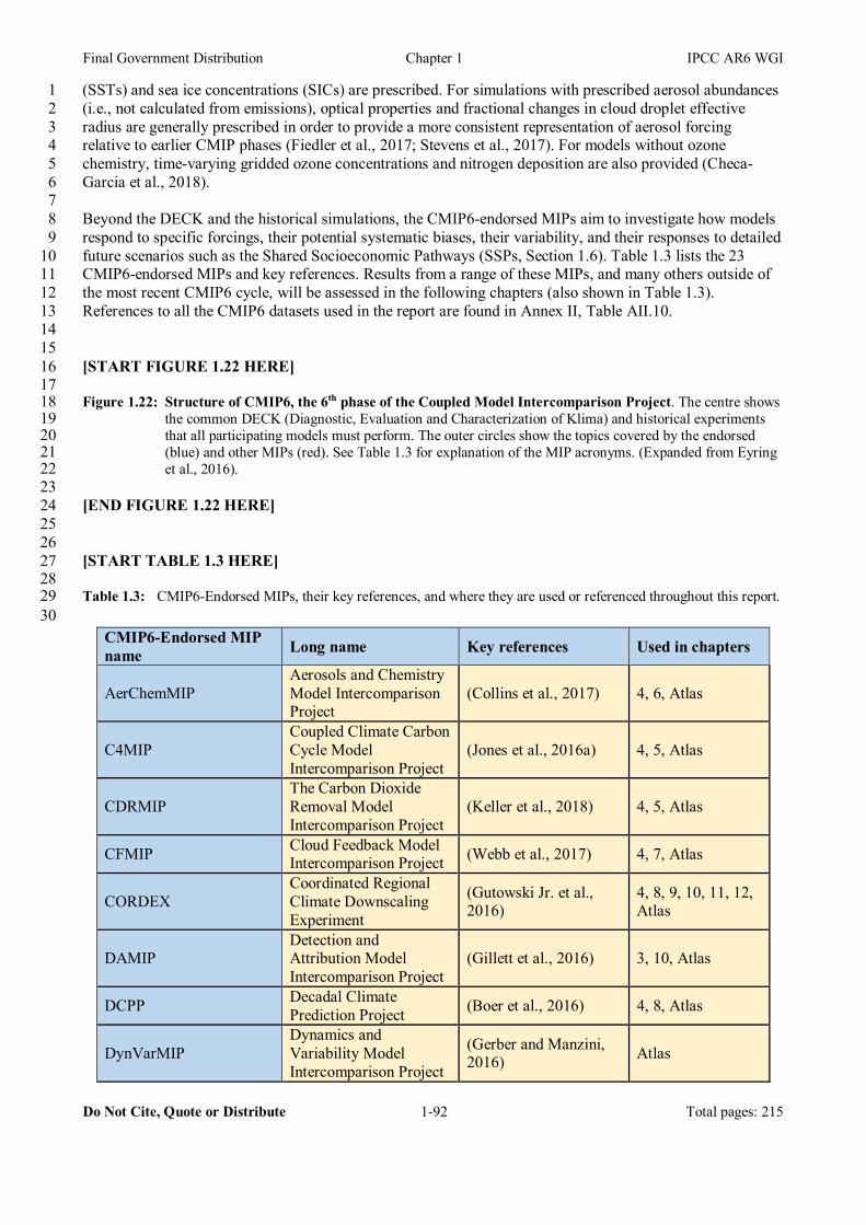
Final Government Distribution Chapter 1 IPCC AR6 WGI
Do Not Cite, Quote or Distribute 1-92 Total pages: 215
(SSTs) and sea ice concentrations (SICs) are prescribed. For simulations with prescribed aerosol abundances 1 (i.e., not calculated from emissions), optical properties and fractional changes in cloud droplet effective 2 radius are generally prescribed in order to provide a more consistent representation of aerosol forcing 3 relative to earlier CMIP phases (Fiedler et al., 2017; Stevens et al., 2017). For models without ozone 4 chemistry, time-varying gridded ozone concentrations and nitrogen deposition are also provided (Checa-5 Garcia et al., 2018). 6 7 Beyond the DECK and the historical simulations, the CMIP6-endorsed MIPs aim to investigate how models 8 respond to specific forcings, their potential systematic biases, their variability, and their responses to detailed 9 future scenarios such as the Shared Socioeconomic Pathways (SSPs, Section 1.6). Table 1.3 lists the 23 10 CMIP6-endorsed MIPs and key references. Results from a range of these MIPs, and many others outside of 11 the most recent CMIP6 cycle, will be assessed in the following chapters (also shown in Table 1.3). 12 References to all the CMIP6 datasets used in the report are found in Annex II, Table AII.10. 13 14 15 [START FIGURE 1.22 HERE] 16 17 Figure 1.22: Structure of CMIP6, the 6th phase of the Coupled Model Intercomparison Project. The centre shows 18
the common DECK (Diagnostic, Evaluation and Characterization of Klima) and historical experiments 19 that all participating models must perform. The outer circles show the topics covered by the endorsed 20 (blue) and other MIPs (red). See Table 1.3 for explanation of the MIP acronyms. (Expanded from Eyring 21 et al., 2016). 22
23 [END FIGURE 1.22 HERE] 24 25 26 [START TABLE 1.3 HERE] 27 28 Table 1.3: CMIP6-Endorsed MIPs, their key references, and where they are used or referenced throughout this report. 29 30
CMIP6-Endorsed MIP name Long name Key references Used in chapters
AerChemMIP Aerosols and Chemistry Model Intercomparison Project
(Collins et al., 2017) 4, 6, Atlas
C4MIP Coupled Climate Carbon Cycle Model Intercomparison Project
(Jones et al., 2016a) 4, 5, Atlas
CDRMIP The Carbon Dioxide Removal Model Intercomparison Project
(Keller et al., 2018) 4, 5, Atlas
CFMIP Cloud Feedback Model Intercomparison Project (Webb et al., 2017) 4, 7, Atlas
CORDEX Coordinated Regional Climate Downscaling Experiment
(Gutowski Jr. et al., 2016)
4, 8, 9, 10, 11, 12, Atlas
DAMIP Detection and Attribution Model Intercomparison Project
(Gillett et al., 2016) 3, 10, Atlas
DCPP Decadal Climate Prediction Project (Boer et al., 2016) 4, 8, Atlas
DynVarMIP Dynamics and Variability Model Intercomparison Project
(Gerber and Manzini, 2016) Atlas
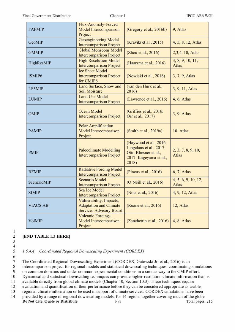
Final Government Distribution Chapter 1 IPCC AR6 WGI
Do Not Cite, Quote or Distribute 1-93 Total pages: 215
FAFMIP Flux-Anomaly-Forced Model Intercomparison Project
(Gregory et al., 2016b) 9, Atlas
GeoMIP Geoengineering Model Intercomparison Project (Kravitz et al., 2015) 4, 5, 8, 12, Atlas
GMMIP Global Monsoons Model Intercomparison Project (Zhou et al., 2016) 2,3,4, 10, Atlas
HighResMIP High Resolution Model Intercomparison Project (Haarsma et al., 2016) 3, 8, 9, 10, 11,
Atlas
ISMIP6 Ice Sheet Model Intercomparison Project for CMIP6
(Nowicki et al., 2016) 3, 7, 9, Atlas
LS3MIP Land Surface, Snow and Soil Moisture
(van den Hurk et al., 2016) 3, 9, 11, Atlas
LUMIP Land Use Model Intercomparison Project (Lawrence et al., 2016) 4, 6, Atlas
OMIP Ocean Model Intercomparison Project
(Griffies et al., 2016; Orr et al., 2017) 3, 9, Atlas
PAMIP Polar Amplification Model Intercomparison Project
(Smith et al., 2019a) 10, Atlas
PMIP Paleoclimate Modelling Intercomparison Project
(Haywood et al., 2016; Jungclaus et al., 2017; Otto-Bliesner et al., 2017; Kageyama et al., 2018)
2, 3, 7, 8, 9, 10, Atlas
RFMIP Radiative Forcing Model Intercomparison Project (Pincus et al., 2016) 6, 7, Atlas
ScenarioMIP Scenario Model Intercomparison Project (O’Neill et al., 2016) 4, 5, 6, 9, 10, 12,
Atlas
SIMIP Sea Ice Model Intercomparison Project (Notz et al., 2016) 4, 9, 12, Atlas
VIACS AB Vulnerability, Impacts, Adaptation and Climate Services Advisory Board
(Ruane et al., 2016) 12, Atlas
VolMIP Volcanic Forcings Model Intercomparison Project
(Zanchettin et al., 2016) 4, 8, Atlas
1 [END TABLE 1.3 HERE] 2 3 4 1.5.4.4 Coordinated Regional Downscaling Experiment (CORDEX) 5 6 The Coordinated Regional Downscaling Experiment (CORDEX, Gutowski Jr. et al., 2016) is an 7 intercomparison project for regional models and statistical downscaling techniques, coordinating simulations 8 on common domains and under common experimental conditions in a similar way to the CMIP effort. 9 Dynamical and statistical downscaling techniques can provide higher-resolution climate information than is 10 available directly from global climate models (Chapter 10, Section 10.3). These techniques require 11 evaluation and quantification of their performance before they can be considered appropriate as usable 12 regional climate information or be used in support of climate services. CORDEX simulations have been 13 provided by a range of regional downscaling models, for 14 regions together covering much of the globe 14
Final Government Distribution Chapter 1 IPCC AR6 WGI
Do Not Cite, Quote or Distribute 1-94 Total pages: 215
(Atlas, Figure Atlas.7), and they are used extensively in the AR6 WGI Atlas (Atlas.1.4; see also Annex II). 1 2 In support of AR6, CORDEX has undertaken a new experiment (CORDEX-CORE) where regional climate 3 models downscale a common set of global model simulations, performed at a coarser resolution, to a spatial 4 resolution spanning from 12 to 25 km over most of the CORDEX domains (Atlas, Box Atlas.1). CORDEX-5 CORE represents an improved level of coordinated intercomparison of downscaling models (Remedio et al., 6 2019). 7 8 9 1.5.4.5 Model Evaluation Tools 10 11 For the first time in CMIP, a range of comprehensive evaluation tools are now available that can run 12 alongside the commonly used distributed data platform Earth System Grid Federation (ESGF, see Annex II), 13 to produce comprehensive results as soon as the model output is published to the CMIP archive. 14 15 For instance, the Earth System Model Evaluation Tool (ESMValTool; Eyring et al., 2020; Lauer et al., 2020; 16 Righi et al., 2020) is used by a number of chapters. It is an open-source community software tool that 17 includes a large variety of diagnostics and performance metrics relevant for coupled Earth System processes, 18 such as for the mean, variability and trends, and it can also examine emergent constraints (see Section 19 1.5.4.7). ESMValTool also includes routines provided by the WMO Expert Team on Climate Change 20 Detection and Indices for the evaluation of extreme events (Min et al., 2011; Sillmann et al., 2013) and 21 diagnostics for key processes and variability. Another example of evaluation tool is the CLIVAR 2020 22 ENSO metrics package (Planton et al., 2021). 23 24 These tools are used in several chapters of this report for the creation of the figures that show CMIP results. 25 Together with the Interactive Atlas, they allow for traceability of key results, and an additional level of 26 quality control on whether published figures can be reproduced. It also provides the capability to update 27 published figures with, as much as possible, the same set of models in all figures, and to assess model 28 improvements across different phases of CMIP (Chapter 3, Section 3.8.2). 29 30 These new developments are facilitated by the definition of common formats for CMIP model output (Balaji 31 et al., 2018) and the availability of reanalyses and observations in the same format as CMIP output 32 (obs4MIPs, Ferraro et al., 2015). The tools are also used to support routine evaluation at individual model 33 centres and simplify the assessment of improvements of individual models or generations of model 34 ensembles (Eyring et al., 2019). Note, however, that while tools such as ESMValTool can produce an 35 estimate of overall model performance, dedicated model evaluation still needs to be performed when 36 analysing projections for a particular purpose, such as assessing changing hazards in a given particular 37 region. Such evaluation is discussed in the next section, and in greater detail in later chapters of this Report. 38 39 40 1.5.4.6 Evaluation of process-based models against observations 41 42 Techniques used for evaluating process-based climate models against observations were assessed in AR5 43 (Flato et al., 2013), and have progressed rapidly since (Eyring et al., 2019). The most widely used technique 44 is to compare climatologies (long-term averages of specific climate variables) or time series of simulated 45 (process-based) model output with observations, considering the observational uncertainty. A further 46 approach is to compare the results of process-based models with those from statistical models. In addition to 47 a comparison of climatological means, trends and variability, AR5 already made use of a large set of 48 performance metrics for a quantitative evaluation of the models. 49 50 Since AR5, a range of studies has investigated model agreement with observations well beyond large scale 51 mean climate properties (e.g., Bellenger et al., 2014; Covey et al., 2016; Pendergrass and Deser, 2017; 52 Goelzer et al., 2018; Beusch et al., 2020a), providing information on the performance of recent model 53 simulations across multiple variables and components of the Earth system (e.g., Anav et al., 2013; Guan and 54 Waliser, 2017). Based on such studies, this Report assesses model improvements across different CMIP 55
Final Government Distribution Chapter 1 IPCC AR6 WGI
Do Not Cite, Quote or Distribute 1-95 Total pages: 215
DECK, CMIP6 historical and CMIP6-Endorsed MIP simulations, and of differences in model performance 1 between different classes of models, such as high- versus low-resolution models (see e.g., Chapter 3, Section 2 3.8.2). 3 4 In addition, process- or regime-oriented evaluation of models has been expanded since AR5. By focusing on 5 processes, causes of systematic errors in the models can be identified and insights can be gained as to 6 whether a mean state or trend is correctly simulated for the right reasons. This approach is commonly used 7 for the evaluation of clouds (e.g., Williams and Webb, 2009; Konsta et al., 2012; Bony et al., 2015; Dal 8 Gesso et al., 2015; Jin et al., 2017), dust emissions (e.g., Parajuli et al., 2016; Wu et al., 2016) as well as 9 aerosol-cloud (e.g., Gryspeerdt and Stier, 2012) and chemistry-climate (SPARC, 2010) interactions. Process-10 oriented diagnostics have also been used to evaluate specific phenomena such as the El Niño Southern 11 Oscillation (ENSO, Guilyardi et al., 2016), the Madden–Julian Oscillation (MJO; Ahn et al., 2017; Jiang et 12 al., 2018), Southern Ocean clouds (Hyder et al., 2018), monsoons (Boo et al., 2011; James et al., 2015), and 13 tropical cyclones (Kim et al., 2018). 14 15 Instrument simulators provide estimates of what a satellite would see if looking down on the model 16 simulated planet, and improve the direct comparison of modelled variables such as clouds, precipitation and 17 upper tropospheric humidity with observations from satellites (e.g., Kay et al., 2011; Klein et al., 2013; 18 Cesana and Waliser, 2016; Konsta et al., 2016; Jin et al., 2017; Chepfer et al., 2018; Swales et al., 2018; 19 Zhang et al., 2018). Within the framework of the Cloud Feedback Model Intercomparison Project (CFMIP) 20 contribution to CMIP6 (Webb et al., 2017), a new version of the Cloud Feedback Model Intercomparison 21 Project Observational Simulator (COSP, Swales et al., 2018) has been released which makes use of a 22 collection of observation proxies or satellite simulators. Related approaches in this rapidly evolving field 23 include simulators for Arctic Ocean observations (Burgard et al., 2020) and measurements of aerosol 24 observations along aircraft trajectories (Watson-Parris et al., 2019). 25 26 In this Report, model evaluation is performed in the individual chapters, rather than in a separate chapter as 27 was the case for AR5. This applies to the model types discussed above, and also to dedicated models of 28 subsystems that are not (or not yet) part of usual climate models, for example, glacier or ice sheet models 29 (Annex II). Further discussions are found in Chapter 3 (attribution), Chapter 5 (carbon cycle), Chapter 6 30 (short-lived climate forcers), Chapter 8 (water cycle), Chapter 9 (ocean, cryosphere and sea level), Chapter 31 10 (regional scale information) and the Atlas (regional models). 32 33 34 1.5.4.7 Emergent constraints on climate feedbacks, sensitivities and projections 35 36 An emergent constraint is the relationship between an uncertain aspect of future climate change and an 37 observable feature of the Earth System, evident across an ensemble of models (Allen and Ingram, 2002; 38 Mystakidis et al., 2016; Wenzel et al., 2016; Hall et al., 2019; Winkler et al., 2019). Complex Earth System 39 Models (ESMs) simulate variations on timescales from hours to centuries, telling us how aspects of the 40 current climate relate to its sensitivity to anthropogenic forcing. Where an ensemble of different ESMs 41 displays a relationship between a short-term observable variation and a longer-term sensitivity, an 42 observation of the short-term variation in the real world can be converted, via the model-based relationship, 43 into an ‘emergent constraint’ on the sensitivity. This is shown schematically in Figure 1.23 (Eyring et al., 44 2019), see also Annex VII: Glossary. 45 46 Emergent constraints use the spread in model projections to estimate the sensitivities of the climate system to 47 anthropogenic forcing, providing another type of ensemble-wide information that is not readily available 48 from simulations with one ESM alone. As emergent constraints depend on identifying those observable 49 aspects of the climate system that are most related to climate projections, they also help to focus model 50 evaluation on the most relevant observations (Hall et al., 2019). However, there is a chance that 51 indiscriminate data-mining of the multi-dimensional outputs from ESMs could lead to spurious correlations 52 (Caldwell et al., 2014; Wagman and Jackson, 2018) and less than robust emergent constraints on future 53 changes (Bracegirdle and Stephenson, 2013). To avoid this, emergent constraints need to be tested ‘out of 54 sample’ on parts of the dataset that were not included in its construction (Caldwell et al., 2018) and should 55
Final Government Distribution Chapter 1 IPCC AR6 WGI
Do Not Cite, Quote or Distribute 1-96 Total pages: 215
also always be based on sound physical understanding and mathematical theory (Hall et al., 2019). Their 1 conclusions should also be reassessed when a new generation of MMEs becomes available, such as CMIP6. 2 As an example, Chapter 7 (Section 7.5.4) discusses and assesses recent studies where equilibrium climate 3 sensitivities (ECS) diagnosed in a multi-model ensemble are compared with the same models’ estimates of 4 an observable quantity, such as post-1970s global warming or tropical sea-surface temperatures of past 5 climates like the last glacial maximum or the Pliocene. Assessments of other emergent constraints appear 6 throughout later chapters, such as Chapter 4 (Section 4.2.5), Chapter 5 (Section 5.4.6) and Chapter 7 (Section 7 7.5.4). 8 9 10 [START FIGURE 1.23 HERE] 11 12 Figure 1.23: The principle of emergent constraints. An ensemble of models (blue dots) defines a relationship 13
between an observable, mean, trend or variation in the climate (x-axis) and an uncertain projection, 14 climate sensitivity or feedback (y-axis). An observation of the x-axis variable can then be combined with 15 the model-derived relationship to provide a tighter estimate of the climate projection, sensitivity or 16 feedback on the y-axis (adapted from Eyring et al. 2019). 17
18 [END FIGURE 1.23 HERE] 19 20 21 1.5.4.8 Weighting techniques for model comparisons 22 23 Assessments of climate model ensembles have commonly assumed that each individual model is of equal 24 value (‘model democracy’) and when combining simulations to estimate the mean and variance of quantities 25 of interest, they are typically unweighted (Haughton et al., 2015). This practice has been noted to diminish 26 the influence of models exhibiting a good match with observations (Tapiador et al., 2020). However, 27 exceptions to this approach exist, notably AR5 projections of sea ice, which only selected a few models 28 which passed a model performance assessment (Collins et al., 2013), and more studies on this topic have 29 appeared since the AR5 (e.g., Eyring et al., 2019). Ensembles are typically sub-selected by removing either 30 poorly performing model simulations (McSweeney et al., 2015) or model simulations that are perceived to 31 add little additional information, typically where multiple simulations have come from the same model. They 32 may also be weighted based on model performance. 33 34 Several recent studies have attempted to quantify the effect of various strategies for selection or weighting of 35 ensemble members based on some set of criteria (Haughton et al., 2015; Olonscheck and Notz, 2017; 36 Sanderson et al., 2017). Model weighting strategies have been further employed since AR5 to reduce the 37 spread in climate projections for a given scenario by using weights based on one or more model performance 38 metrics (Wenzel et al., 2016; Knutti et al., 2017; Sanderson et al., 2017; Lorenz et al., 2018; Liang et al., 39 2020). However, models may share representations of processes, parameterization schemes, or even parts of 40 code, leading to common biases. The models may therefore not be fully independent, calling into question 41 inferences derived from multi-model ensembles (Abramowitz et al., 2019). Emergent constraints (see 42 Section 1.5.4.5) also represent an implicit weighting technique that explicitly links present performance to 43 future projections (Bracegirdle and Stephenson, 2013). 44 45 Concern has been raised about the large extent to which code is shared within the CMIP5 multi-model 46 ensemble (Sanderson et al., 2015a). Boé (2018) showed that a clear relationship exists between the number 47 of components shared by climate models and how similar the simulations are. The resulting similarities in 48 behaviour need to be accounted for in the generation of best-estimate multi-model climate projections. This 49 has led to calls to move beyond equally-weighted multi-model means towards weighted means that take into 50 account both model performance and model independence (Sanderson et al., 2015b, 2017; Knutti et al., 51 2017). Model independence has been defined in terms of performance differences within an ensemble 52 (Masson and Knutti, 2011; Knutti et al., 2013, 2017, Sanderson et al., 2015b, 2015a, 2017; Lorenz et al., 53 2018). However, this definition is sensitive to the choice of variable, observational data set, metric, time 54 period, and region, and a performance ranked ensemble has been shown to sometimes perform worse than a 55
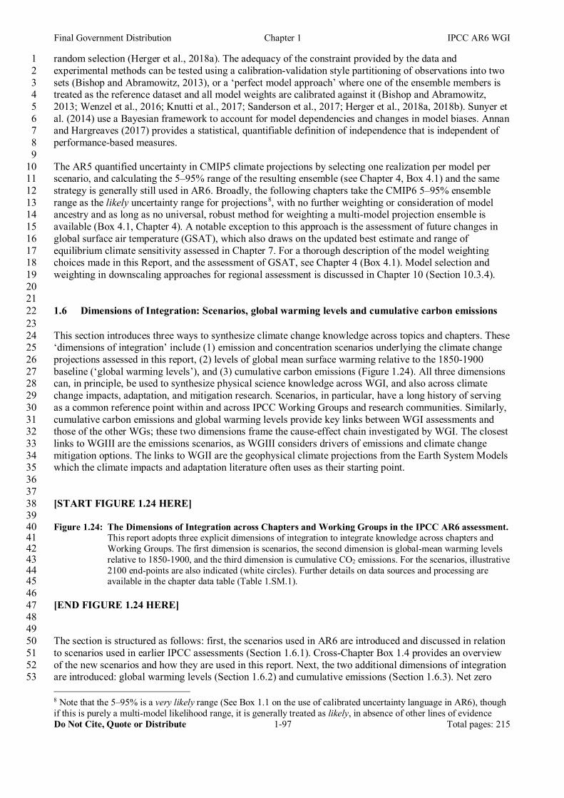
Final Government Distribution Chapter 1 IPCC AR6 WGI
Do Not Cite, Quote or Distribute 1-97 Total pages: 215
random selection (Herger et al., 2018a). The adequacy of the constraint provided by the data and 1 experimental methods can be tested using a calibration-validation style partitioning of observations into two 2 sets (Bishop and Abramowitz, 2013), or a ‘perfect model approach’ where one of the ensemble members is 3 treated as the reference dataset and all model weights are calibrated against it (Bishop and Abramowitz, 4 2013; Wenzel et al., 2016; Knutti et al., 2017; Sanderson et al., 2017; Herger et al., 2018a, 2018b). Sunyer et 5 al. (2014) use a Bayesian framework to account for model dependencies and changes in model biases. Annan 6 and Hargreaves (2017) provides a statistical, quantifiable definition of independence that is independent of 7 performance-based measures. 8 9 The AR5 quantified uncertainty in CMIP5 climate projections by selecting one realization per model per 10 scenario, and calculating the 5–95% range of the resulting ensemble (see Chapter 4, Box 4.1) and the same 11 strategy is generally still used in AR6. Broadly, the following chapters take the CMIP6 5–95% ensemble 12 range as the likely uncertainty range for projections8, with no further weighting or consideration of model 13 ancestry and as long as no universal, robust method for weighting a multi-model projection ensemble is 14 available (Box 4.1, Chapter 4). A notable exception to this approach is the assessment of future changes in 15 global surface air temperature (GSAT), which also draws on the updated best estimate and range of 16 equilibrium climate sensitivity assessed in Chapter 7. For a thorough description of the model weighting 17 choices made in this Report, and the assessment of GSAT, see Chapter 4 (Box 4.1). Model selection and 18 weighting in downscaling approaches for regional assessment is discussed in Chapter 10 (Section 10.3.4). 19 20 21 1.6 Dimensions of Integration: Scenarios, global warming levels and cumulative carbon emissions 22 23 This section introduces three ways to synthesize climate change knowledge across topics and chapters. These 24 ‘dimensions of integration’ include (1) emission and concentration scenarios underlying the climate change 25 projections assessed in this report, (2) levels of global mean surface warming relative to the 1850-1900 26 baseline (‘global warming levels’), and (3) cumulative carbon emissions (Figure 1.24). All three dimensions 27 can, in principle, be used to synthesize physical science knowledge across WGI, and also across climate 28 change impacts, adaptation, and mitigation research. Scenarios, in particular, have a long history of serving 29 as a common reference point within and across IPCC Working Groups and research communities. Similarly, 30 cumulative carbon emissions and global warming levels provide key links between WGI assessments and 31 those of the other WGs; these two dimensions frame the cause-effect chain investigated by WGI. The closest 32 links to WGIII are the emissions scenarios, as WGIII considers drivers of emissions and climate change 33 mitigation options. The links to WGII are the geophysical climate projections from the Earth System Models 34 which the climate impacts and adaptation literature often uses as their starting point. 35 36 37 [START FIGURE 1.24 HERE] 38 39 Figure 1.24: The Dimensions of Integration across Chapters and Working Groups in the IPCC AR6 assessment. 40
This report adopts three explicit dimensions of integration to integrate knowledge across chapters and 41 Working Groups. The first dimension is scenarios, the second dimension is global-mean warming levels 42 relative to 1850-1900, and the third dimension is cumulative CO2 emissions. For the scenarios, illustrative 43 2100 end-points are also indicated (white circles). Further details on data sources and processing are 44 available in the chapter data table (Table 1.SM.1). 45
46 [END FIGURE 1.24 HERE] 47 48 49 The section is structured as follows: first, the scenarios used in AR6 are introduced and discussed in relation 50 to scenarios used in earlier IPCC assessments (Section 1.6.1). Cross-Chapter Box 1.4 provides an overview 51 of the new scenarios and how they are used in this report. Next, the two additional dimensions of integration 52 are introduced: global warming levels (Section 1.6.2) and cumulative emissions (Section 1.6.3). Net zero 53 8 Note that the 5–95% is a very likely range (See Box 1.1 on the use of calibrated uncertainty language in AR6), though if this is purely a multi-model likelihood range, it is generally treated as likely, in absence of other lines of evidence
Final Government Distribution Chapter 1 IPCC AR6 WGI
Do Not Cite, Quote or Distribute 1-98 Total pages: 215
emissions are discussed in Box 1.4. The relation between global warming levels and scenarios is further 1 assessed in Cross-Chapter Box 11.1 in Chapter 11. 2 3 4 1.6.1 Scenarios 5 6 A scenario is a description of how the future may develop based on a coherent and internally consistent set 7 of assumptions about key drivers including demography, economic processes, technological innovation, 8 governance, lifestyles and relationships among these driving forces (IPCC, 2000; Rounsevell and Metzger, 9 2010; O’Neill et al., 2014; see Section 1.6.1.1). Scenarios can also be defined by geophysical driving forces 10 only, such as emissions or abundances of greenhouse gases, aerosols, and aerosol precursors or land use 11 patterns. Scenarios are not predictions; instead, they provide a ‘what-if’ investigation of the implications of 12 various developments and actions (Moss et al., 2010). WGI investigates potential future climate change 13 principally by assessing climate model simulations using emission scenarios originating from the WGIII 14 community (Section 1.6.1.2). The scenarios used in this WGI report cover various hypothetical ‘baseline 15 scenarios’ or ‘reference futures’ that could unfold in the absence of any or any additional climate policies 16 (see Annex VII: Glossary). These ‘reference scenarios’ originate from a comprehensive analysis of a wide 17 array of socio-economic drivers, such as population growth, technological development, and economic 18 development, and their broad spectrum of associated energy, land use and emission implications (Riahi et al., 19 2017). With direct policy relevance to the Paris Agreement’s 1.5°C and ‘well below’ 2°C goals, this report 20 also assesses climate futures where the effects of additional climate change mitigation action are explored, 21 i.e., so-called mitigation scenarios (for a broader discussion on scenarios and futures analysis, see Cross-22 Chapter Box 1, Table 1 in SRCCL, IPCC, 2019b). 23 24 For this Report, the main emissions, concentration and land use scenarios considered are a subset of 25 scenarios recently developed using the Shared Socioeconomic Pathways framework (SSPs) (Riahi et al., 26 2017; see Section 1.6.1.1 and Cross-Chapter Box 1.4). Initially, the term ‘SSP’ described five broad 27 narratives of future socio-economic development only (O’Neill et al., 2014). However, at least in the WGI 28 community, the term ‘SSP scenario’ is now more widely used to refer directly to future emission and 29 concentration scenarios that result from combining these socio-economic development pathways with 30 climate change mitigation assumptions. These are assessed in detail in WGIII (WGIII, Chapter 3; Cross-31 Chapter Box 1.4, Table 1). 32 33 The WGI report uses a core set of five SSP scenarios to assist cross-Chapter integration and cross-WG 34 applications: SSP1-1.9, SSP1-2.6, SSP2-4.5, SSP3-7.0 and SSP5-8.5 (Cross-Chapter Box 1.4, Table 1). 35 These scenarios span a wide range of plausible societal and climatic futures from potentially below 1.5°C 36 best-estimate warming to over 4°C warming by 2100 (Figure 1.25). The set of five SSP scenarios includes 37 those in ‘Tier 1’ simulations of the CMIP6 ScenarioMIP intercomparison project (O’Neill et al., 2016; see 38 Section 1.5.4) that participating climate modelling groups were asked to prioritize (SSP1-2.6, SSP2-4.5, 39 SSP3-7.0 and SSP5-8.5), plus the low emission scenario SSP1-1.9. SSP1-1.9 is used in combination with 40 SSP1-2.6 to explore differential outcomes of approximately 1.5 and 2.0 °C warming relative to pre-industrial 41 levels, relevant to the Paris Agreement goals. Further SSP scenarios are used in this report to assess specific 42 aspects, e.g., air pollution policies in Chapter 6 (Cross-Chapter Box 1.4). In addition, the previous generation 43 of Representative Concentration Pathways (RCPs) is also used in this report when assessing future climate 44 change (Section 1.6.1.3; Cross-Chapter Box 1.4, Table 1). 45 46 Climatic changes over the 21st century (and beyond) are projected and assessed in subsequent chapters, 47 using a broad range of climate models, conditional on the various SSP scenarios. The projected future 48 changes can then be put into the context of longer-term paleoclimate data and historical observations, 49 showing how the higher emission and higher concentration scenarios diverge further from the range of 50 climate conditions that ecosystems and human societies experienced in the past 2000 years in terms of global 51 mean temperature and other key climate variables (Figure 1.26; see also Figure 1.5). 52 53 54 [START FIGURE 1.25 HERE] 55

Final Government Distribution Chapter 1 IPCC AR6 WGI
Do Not Cite, Quote or Distribute 1-99 Total pages: 215
1 Figure 1.25: Global mean surface air temperature (GSAT) illustrated as warming stripes from blue (cold) to red 2
(warm) over three different time periods. From 1750 to 1850 based on PAGES 2K reconstructions 3 (2017, 2019); from 1850 to 2018 showing the composite GSAT time series assessed in Chapter 2; and 4 from 2020 onwards using the assessed GSAT projections for each Shared Socio-economic Pathway (SSP) 5 (from Chapter 4). For the projections, the upper end of each arrow aligns with colour corresponding to the 6 95th percentile of the projected temperatures and the lower end aligns with the colour corresponding to the 7 5th percentile of the projected temperature range. Projected temperatures are shown for five scenarios 8 from ‘very low’ SSP1-1.9 to ‘very high’ SSP5-8.5 (see Cross-Chapter Box 1.4 for more details on the 9 scenarios). For illustrative purposes, natural variability has been added from a single CMIP6 Earth system 10 model (MRI ESM2). The points in time when total CO2 emissions peak, reach halved levels of the peak 11 and reach net-zero emissions are indicated with arrows, ‘½’ and ‘0’ marks, respectively. Further details 12 on data sources and processing are available in the chapter data table (Table 1.SM.1). 13
14 15 [END FIGURE 1.25 HERE] 16 17 18 While scenarios are a key tool for integration across IPCC Working Groups, they also allow the integration 19 of knowledge among scientific communities and across timescales. For example, agricultural yield, 20 infrastructure and human health impacts of increased drought frequency, extreme rainfall events and 21 hurricanes are often examined in isolation. New insights on climate impacts in WGII can be gained if 22 compound effects of multiple cross-sectoral impacts are considered across multiple research communities 23 under consistent scenario frameworks (Leonard et al., 2014; Warszawski et al., 2014; see also Chapter 11, 24 Section 11.8). Similarly, a synthesis of WGI knowledge on sea level rise contributions is enabled by a 25 consistent application of future scenarios across all specialised research communities, such as ice-sheet mass 26 balance analyses, glacier loss projections and thermosteric change from ocean heat uptake (e.g. Kopp et al., 27 2014; see Chapter 9). 28 29 30 [START FIGURE 1.26 HERE] 31 32 Figure 1.26: Historical and projected future concentrations of CO2, CH4 and N2O and global mean surface 33
temperatures (GMST). GMST temperature reconstructions over the last 2000 years were compiled by 34 the PAGES 2k Consortium (2017, 2019) (grey line, with 95% uncertainty range), joined by historical 35 GMST timeseries assessed in Chapter 2 (black line) – both referenced against the 1850-1900 period. 36 Future GSAT temperature projections are from CMIP6 ESM models across all concentration-driven SSP 37 scenario projections (Chapter 4). The discontinuity around year 2100 for CMIP6 temperature projections 38 results from the fact that not all ESM models ran each scenario past 2100. The grey vertical band 39 indicates the future 2015-2300 period. The concentrations used to drive CMIP6 Earth System Models are 40 derived from ice core, firn and instrumental datasets (Meinshausen et al., 2017) and projected using an 41 emulator (Cross-Chapter Box 7.1 in Chapter 7; Meinshausen et al., 2020). The colours of the lines 42 indicate the SSP scenarios used in this report (see Cross-Chapter Box 1.4, Figure 1). Further details on 43 data sources and processing are available in the chapter data table (Table 1.SM.1). 44
45 [END FIGURE 1.26 HERE] 46 47 48 In addition to the comprehensive SSP scenario set and the RCPs, multiple idealized scenarios and time-slice 49 experiments using climate models are assessed in this report. Idealized scenarios refer to experiments where, 50 for example, CO2 concentrations are increased by 1% per year, or instantly quadrupled. Such idealized 51 experiments have been extensively used in previous model intercomparison projects and constitute the core 52 ‘DECK’ set of model experiments of CMIP6 (see Section 1.5.4). They are, for example, used to diagnose the 53 patterns of climate feedbacks across the suite of models assessed in this report (Chapter 7). 54 55 In the following, we further introduce the SSP scenarios and how they relate to the Shared Socioeconomic 56 Pathways framework (Section 1.6.1.1), describe the scenario generation process (Section 1.6.1.2), and 57
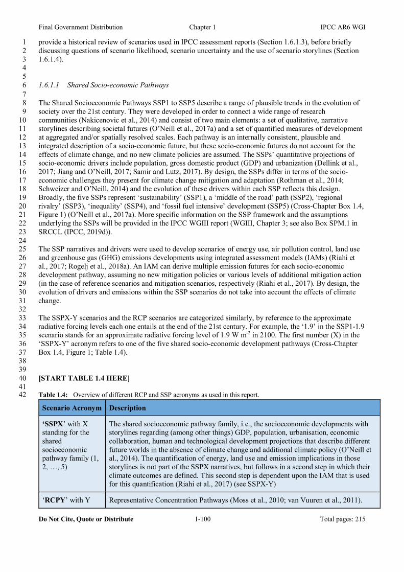
Final Government Distribution Chapter 1 IPCC AR6 WGI
Do Not Cite, Quote or Distribute 1-100 Total pages: 215
provide a historical review of scenarios used in IPCC assessment reports (Section 1.6.1.3), before briefly 1 discussing questions of scenario likelihood, scenario uncertainty and the use of scenario storylines (Section 2 1.6.1.4). 3 4 5 1.6.1.1 Shared Socio-economic Pathways 6 7 The Shared Socioeconomic Pathways SSP1 to SSP5 describe a range of plausible trends in the evolution of 8 society over the 21st century. They were developed in order to connect a wide range of research 9 communities (Nakicenovic et al., 2014) and consist of two main elements: a set of qualitative, narrative 10 storylines describing societal futures (O’Neill et al., 2017a) and a set of quantified measures of development 11 at aggregated and/or spatially resolved scales. Each pathway is an internally consistent, plausible and 12 integrated description of a socio-economic future, but these socio-economic futures do not account for the 13 effects of climate change, and no new climate policies are assumed. The SSPs’ quantitative projections of 14 socio-economic drivers include population, gross domestic product (GDP) and urbanization (Dellink et al., 15 2017; Jiang and O’Neill, 2017; Samir and Lutz, 2017). By design, the SSPs differ in terms of the socio-16 economic challenges they present for climate change mitigation and adaptation (Rothman et al., 2014; 17 Schweizer and O’Neill, 2014) and the evolution of these drivers within each SSP reflects this design. 18 Broadly, the five SSPs represent ‘sustainability’ (SSP1), a ‘middle of the road’ path (SSP2), ‘regional 19 rivalry’ (SSP3), ‘inequality’ (SSP4), and ‘fossil fuel intensive’ development (SSP5) (Cross-Chapter Box 1.4, 20 Figure 1) (O’Neill et al., 2017a). More specific information on the SSP framework and the assumptions 21 underlying the SSPs will be provided in the IPCC WGIII report (WGIII, Chapter 3; see also Box SPM.1 in 22 SRCCL (IPCC, 2019d)). 23 24 The SSP narratives and drivers were used to develop scenarios of energy use, air pollution control, land use 25 and greenhouse gas (GHG) emissions developments using integrated assessment models (IAMs) (Riahi et 26 al., 2017; Rogelj et al., 2018a). An IAM can derive multiple emission futures for each socio-economic 27 development pathway, assuming no new mitigation policies or various levels of additional mitigation action 28 (in the case of reference scenarios and mitigation scenarios, respectively (Riahi et al., 2017). By design, the 29 evolution of drivers and emissions within the SSP scenarios do not take into account the effects of climate 30 change. 31 32 The SSPX-Y scenarios and the RCP scenarios are categorized similarly, by reference to the approximate 33 radiative forcing levels each one entails at the end of the 21st century. For example, the ‘1.9’ in the SSP1-1.9 34 scenario stands for an approximate radiative forcing level of 1.9 W m-2 in 2100. The first number (X) in the 35 ‘SSPX-Y’ acronym refers to one of the five shared socio-economic development pathways (Cross-Chapter 36 Box 1.4, Figure 1; Table 1.4). 37 38 39 [START TABLE 1.4 HERE] 40 41 Table 1.4: Overview of different RCP and SSP acronyms as used in this report. 42
Scenario Acronym Description
‘SSPX’ with X standing for the shared socioeconomic pathway family (1, 2, …, 5)
The shared socioeconomic pathway family, i.e., the socioeconomic developments with storylines regarding (among other things) GDP, population, urbanisation, economic collaboration, human and technological development projections that describe different future worlds in the absence of climate change and additional climate policy (O’Neill et al., 2014). The quantification of energy, land use and emission implications in those storylines is not part of the SSPX narratives, but follows in a second step in which their climate outcomes are defined. This second step is dependent upon the IAM that is used for this quantification (Riahi et al., 2017) (see SSPX-Y)
‘RCPY’ with Y Representative Concentration Pathways (Moss et al., 2010; van Vuuren et al., 2011).
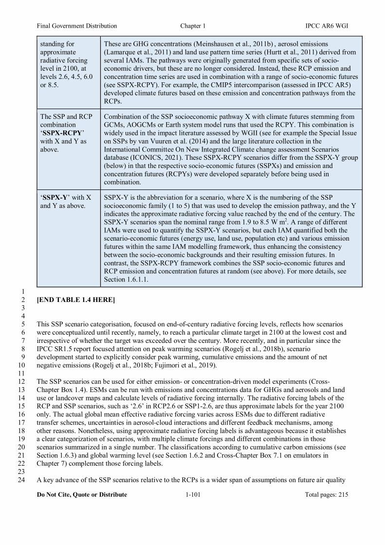
Final Government Distribution Chapter 1 IPCC AR6 WGI
Do Not Cite, Quote or Distribute 1-101 Total pages: 215
standing for approximate radiative forcing level in 2100, at levels 2.6, 4.5, 6.0 or 8.5.
These are GHG concentrations (Meinshausen et al., 2011b) , aerosol emissions (Lamarque et al., 2011) and land use pattern time series (Hurtt et al., 2011) derived from several IAMs. The pathways were originally generated from specific sets of socio-economic drivers, but these are no longer considered. Instead, these RCP emission and concentration time series are used in combination with a range of socio-economic futures (see SSPX-RCPY). For example, the CMIP5 intercomparison (assessed in IPCC AR5) developed climate futures based on these emission and concentration pathways from the RCPs.
The SSP and RCP combination ‘SSPX-RCPY’ with X and Y as above.
Combination of the SSP socioeconomic pathway X with climate futures stemming from GCMs, AOGCMs or Earth system model runs that used the RCPY. This combination is widely used in the impact literature assessed by WGII (see for example the Special Issue on SSPs by van Vuuren et al. (2014) and the large literature collection in the International Committee On New Integrated Climate change assessment Scenarios database (ICONICS, 2021). These SSPX-RCPY scenarios differ from the SSPX-Y group (below) in that the respective socio-economic futures (SSPXs) and emission and concentration futures (RCPYs) were developed separately before being used in combination.
‘SSPX-Y’ with X and Y as above.
SSPX-Y is the abbreviation for a scenario, where X is the numbering of the SSP socioeconomic family (1 to 5) that was used to develop the emission pathway, and the Y indicates the approximate radiative forcing value reached by the end of the century. The SSPX-Y scenarios span the nominal range from 1.9 to 8.5 W m2. A range of different IAMs were used to quantify the SSPX-Y scenarios, but each IAM quantified both the scenario-economic futures (energy use, land use, population etc) and various emission futures within the same IAM modelling framework, thus enhancing the consistency between the socio-economic backgrounds and their resulting emission futures. In contrast, the SSPX-RCPY framework combines the SSP socio-economic futures and RCP emission and concentration futures at random (see above). For more details, see Section 1.6.1.1.
1 [END TABLE 1.4 HERE] 2 3 4 This SSP scenario categorisation, focused on end-of-century radiative forcing levels, reflects how scenarios 5 were conceptualized until recently, namely, to reach a particular climate target in 2100 at the lowest cost and 6 irrespective of whether the target was exceeded over the century. More recently, and in particular since the 7 IPCC SR1.5 report focused attention on peak warming scenarios (Rogelj et al., 2018b), scenario 8 development started to explicitly consider peak warming, cumulative emissions and the amount of net 9 negative emissions (Rogelj et al., 2018b; Fujimori et al., 2019). 10 11 The SSP scenarios can be used for either emission- or concentration-driven model experiments (Cross-12 Chapter Box 1.4). ESMs can be run with emissions and concentrations data for GHGs and aerosols and land 13 use or landcover maps and calculate levels of radiative forcing internally. The radiative forcing labels of the 14 RCP and SSP scenarios, such as ‘2.6’ in RCP2.6 or SSP1-2.6, are thus approximate labels for the year 2100 15 only. The actual global mean effective radiative forcing varies across ESMs due to different radiative 16 transfer schemes, uncertainties in aerosol-cloud interactions and different feedback mechanisms, among 17 other reasons. Nonetheless, using approximate radiative forcing labels is advantageous because it establishes 18 a clear categorization of scenarios, with multiple climate forcings and different combinations in those 19 scenarios summarized in a single number. The classifications according to cumulative carbon emissions (see 20 Section 1.6.3) and global warming level (see Section 1.6.2 and Cross-Chapter Box 7.1 on emulators in 21 Chapter 7) complement those forcing labels. 22 23 A key advance of the SSP scenarios relative to the RCPs is a wider span of assumptions on future air quality 24

Final Government Distribution Chapter 1 IPCC AR6 WGI
Do Not Cite, Quote or Distribute 1-102 Total pages: 215
mitigation measures, and hence emissions of short-lived climate forcers (SLCFs) (Rao et al., 2017; Lund et 1 al., 2020). This allows for a more detailed investigation into the relative roles of GHG and SLCF emissions 2 in future global and regional climate change, and hence the implications of policy choices. For instance, 3 SSP1-2.6 builds on an assumption of stringent air quality mitigation policy, leading to rapid reductions in 4 particle emissions, while SSP3-7.0 assumes slow improvements, with pollutant emissions over the 21st 5 century comparable to current levels (Cross-Chapter Box 1.4, Figure 2, Chapter 6, Figure 6.19). 6 7 One limitation of the SSP scenarios used for CMIP6 and in this Report is that they reduce emissions from all 8 the major ozone-depleting substances controlled under the Montreal Protocol (CFCs, halons, and 9 hydrochlorofluorocarbons (HCFCs)) uniformly, rather than representing a fuller range of possible high and 10 low emission futures (UNEP, 2016). Hydrofluorocarbon (HFC) emissions, on the other hand, span a wider 11 range within the SSPs than in the RCPs (Cross-Chapter Box 1.4, Figure 2). 12 13 The SSP scenarios and previous RCP scenarios are not directly comparable. First, the gas-to-gas 14 compositions differ; for example, the SSP5-8.5 scenario has higher CO2 concentrations but lower methane 15 concentrations compared to RCP8.5. Second, the projected 21st-century trajectories may differ, even if they 16 result in the same radiative forcing by 2100. Third, the overall effective radiative forcing (see Chapter 7) 17 may differ, and tends to be higher for the SSPs compared to RCPs that share the same nominal stratospheric-18 temperature adjusted radiative forcing label. The stratospheric-temperature adjusted radiative forcings of the 19 SSPs and RCPs, however, remain relatively close, at least by 2100 (Tebaldi et al., 2021). In summary, 20 differences in, for example, CMIP5 RCP8.5 and CMIP6 SSP5-8.5 ESM outputs, are partially due to different 21 scenario characteristics rather than different ESM characteristics only (Chapter 4, Section 4.6.2). 22 23 When investigating various mitigation futures, WGIII goes beyond the core set of SSP scenarios assessed in 24 WGI (SSP1-1.9, SSP1-2.6, etc.) to consider the characteristics of more than 1000 scenarios (see Cross-25 Chapter Box 7.1 in Chapter 7). In addition, while staying within the framework of socio-economic 26 development pathways (SSP1 to SSP5), WGIII also considers various mitigation possibilities through so-27 called illustrative pathways (IPs). These illustrative pathways help to highlight key narratives in the literature 28 concerning various technological, social and behavioral options for mitigation, various timings for 29 implementation, or varying emphasis on different GHG and land use options. Just as with the SSPX-Y 30 scenarios considered in this report, these illustrative pathways can be placed in relation to the matrix of SSP 31 families and approximate radiative forcing levels in 2100 (see Cross-Chapter Box 1.4, Figure 1 and Working 32 Group III, Chapter 3). 33 34 No likelihood is attached to the scenarios assessed in this report, and the feasibility of specific scenarios in 35 relation to current trends is best informed by the WGIII contribution to AR6. In the scenario literature, the 36 plausibility of the high emissions levels underlying scenarios such as RCP8.5 or SSP5-8.5 has been debated 37 in light of recent developments in the energy sector. (see Section 1.6.1.4). 38 39 40 [START CROSS CHAPTER BOX 1.4 HERE] 41 42 Cross-Chapter Box 1.4: The SSP scenarios as used in Working Group I 43 44 Contributing Authors: Jan Fuglestvedt (Norway), Celine Guivarch (France), Chris Jones (UK), Malte 45 Meinshausen (Australia/Germany), Zebedee Nicholls (Australia), Gian-Kasper Plattner (Switzerland), 46 Keywan Riahi (Austria), Joeri Rogelj (UK/Belgium), Sophie Szopa (France), Claudia Tebaldi (USA/Italy), 47 Anne-Marie Treguier (France), and Detlef van Vuuren (Netherlands) 48 49 The new nine SSP emission and concentration scenarios (SSP1-1.9 to SSP5-8.5; Cross-Chapter Box 1.4, 50 Table 1) offer unprecedented detail of input data for climate model simulations. They allow for a more 51 comprehensive assessment of climate drivers and responses than has previously been available, in particular 52 because some of the scenarios’ time series, e.g., pollutants, emissions or changes in land use and land cover, 53 are more diverse in the SSP scenarios than in the RCPs used in AR5 (e.g., Chuwah et al., 2013) (Cross-54 Chapter Box 1.4, Figure 2). 55

Final Government Distribution Chapter 1 IPCC AR6 WGI
Do Not Cite, Quote or Distribute 1-103 Total pages: 215
1 The core set of five SSP scenarios SSP1-1.9, SSP1-2.6, SSP2-4.5, SSP3-7.0 and SSP5-8.5 was selected in 2 this Report to align with the objective that the new generation of SSP scenarios should fill certain gaps 3 identified in the RCPs. For example, a scenario assuming reduced air pollution control and thus higher 4 aerosol emissions was missing from the RCPs. Likewise, nominally the only ‘no-additional-climate-policy’ 5 scenario in the set of RCPs was RCP8.5. The new SSP3-7.0 ‘no-additional-climate-policy’ scenario fills both 6 these gaps. A very strong mitigation scenario in line with the 1.5°C goal of the Paris Agreement was also 7 missing from the RCPs, and the SSP1-1.9 scenario now fills this gap, complementing the other strong 8 mitigation scenario SSP1-2.6. The five core SSPs were also chosen to ensure some overlap with the RCP 9 levels for radiative forcing at the year 2100 (specifically 2.6, 4.5, and 8.5) (O’Neill et al., 2016; Tebaldi et 10 al., 2021), although effective radiative forcings are generally higher in the SSP scenarios compared to the 11 equivalently-named RCP pathways (Cross-Chapter Box 1.4, Figure 1; Chapter 4, Section 4.6.2). In theory, 12 running scenarios with similar radiative forcings would permit analysis of the CMIP5 and CMIP6 outcomes 13 for pairs of scenarios (e.g., RCP8.5 and SSP5-8.5) in terms of varying model characteristics rather than 14 differences in the underlying scenarios. In practice, however, there are limitations to this approach (Section 15 1.6.1.1 and Chapter 4, Section 4.6.2). 16 17 18 [START Cross-Chapter Box 1.4, FIGURE 1 HERE] 19 20 Cross-Chapter Box 1.4, Figure 1: The SSP scenarios used in this report, their indicative temperature evolution 21 and radiative forcing categorization, and the five socio-economic storylines upon which they are built. The core 22 set of scenarios used in this report, i.e., SSP1-1.9, SSP1-2.6, SSP2-4.5, SSP3-7.0 and SSP5-8.5, is shown together with 23 an additional four SSPs that are part of ScenarioMIP, as well as previous RCP scenarios. In the left panel, the indicative 24 temperature evolution is shown (adapted from Meinshausen et al., 2020). The black stripes on the respective scenario 25 family panels on the left side indicate a larger set of IAM-based SSP scenarios that span the scenario range more fully, 26 but are not used in this report. The SSP-radiative forcing matrix is shown on the right, with the SSP socioeconomic 27 narratives shown as columns and the indicative radiative forcing categorisation by 2100 shown as rows. Note that the 28 descriptive labels for the five SSP narratives refer mainly to the reference scenario futures without additional climate 29 policies. For example, SSP5 can accommodate strong mitigation scenarios leading to net zero emissions; these do not 30 match a ‘fossil-fueled development’ label. Further details on data sources and processing are available in the chapter 31 data table (Table 1.SM.1). 32 33 [END Cross-Chapter Box 1.4, FIGURE 1 HERE] 34 35 36 [START Cross-Chapter Box 1.4, TABLE 1 HERE] 37 38 Cross-Chapter Box 1.4, Table 1: Overview of SSP scenarios used in this report. The middle column briefly 39 describes the SSP scenarios and the right column indicates the previous RCP scenarios that most closely 40 match that SSP’s assessed global-mean temperatures (GSAT) trajectory. RCP scenarios are generally found 41 to result in larger modelled warming for the same nominal radiative forcing label (Chapter 4, Section 42 4.6.2.2). The five core SSP scenarios used most commonly in this report are highlighted in bold. Further SSP 43 scenarios are used where they allow assessment of specific aspects, e.g., air pollution policies in Chapter 6 44 (SSP3-7.0-lowNTCF). RCPs are used in this report wherever the relevant scientific literature makes 45 substantial use of regional or domain-specific model output that is based on these previous RCP pathways, 46 such as sea level rise projections in Chapter 9 (Section 9.6.3.1) or regional climate aspects in Chapters 10 47 and 12. See Chapter 4 (Section 4.3.4) for the GSAT assessment for the SSP scenarios and Section 4.6.2.2 for 48 a comparison between SSPs and RCPs in terms of both radiative forcing and global surface temperature. 49 50
SSPX-Y scenario
Description from an emission / concentration and temperature perspective (Chapter 4, Table 4.2)
Closest RCP scenarios
SSP1-1.9 Holds warming to approximately 1.5°C above 1850-1900 in 2100 after slight overshoot (median) and implied net zero
Not available. No equivalently low RCP scenario exists.

Final Government Distribution Chapter 1 IPCC AR6 WGI
Do Not Cite, Quote or Distribute 1-104 Total pages: 215
CO2 emissions around the middle of the century.
SSP1-2.6 Stays below 2.0°C warming relative to 1850-1900 (median) with implied net zero emissions in the second half of the century.
RCP2.6, although RCP2.6 might be cooler for the same model settings.
SSP4-3.4 A scenario in between SSP1-2.6 and SSP2-4.5 in terms of end-of-century radiative forcing. It does not stay below 2.0°C in most CMIP6 runs (Chapter 4) relative to 1850-1900.
No 3.4 level of end-of-century radiative forcing was available in the RCPs. Nominally SSP4-3.4 sits between RCP 2.6 and RCP 4.5, although SSP4-3.4 might be more similar to RCP4.5. Also, in the early decades of the 21st century, SSP4-3.4 is close to RCP6.0, which featured lower radiative forcing than RCP4.5 in the first decades of the 21st century.
SSP2-4.5 Scenario approximately in line with the upper end of aggregate NDC emission levels by 2030 (see Section 1.2.2 and Chapter 4, Section 4.3; SR1.5, (IPCC, 2018) , Box 1). SR1.5 assessed temperature projections for NDCs to be between 2.7 and 3.4°C by 2100 (Section 1.2.2; SR1.5 (IPCC, 2018); Cross-Chapter Box 11 in Chapter 11), corresponding to the upper half of projected warming under SSP2-4.5 (Chapter 4). New or updated NDCs by the end of 2020 did not significantly change the emissions projections up to 2030, although more countries adopted 2050 net zero targets in line with SSP1-1.9 or SSP1-2.6. The SSP2-4.5 scenario deviates mildly from a ‘no-additional-climate-policy’ reference scenario, resulting in a best-estimate warming around 2.7°C by the end of the 21st century relative to 1850-1900 (Chapter 4).
RCP4.5 and, until 2050, also RCP6.0. Forcing in the latter was even lower than RCP4.5 in the early decades of the 21st century.
SSP4-6.0 The end-of-century nominal radiative forcing level of 6.0 W/m2 can be considered a ‘no-additional-climate-policy’ reference scenario, under SSP1 and SSP4 socioeconomic development narratives.
RCP6.0 is nominally closest in the second half of the century, although global mean temperatures are estimated to be generally lower in RCPs compared to SSPs. Furthermore, RCP6.0 features lower warming than SSP4-6.0, as it has very similar temperature projections compared to the nominally lower RCP4.5 scenario in the first half of the century.
SSP3-7.0 A medium to high reference scenario resulting from no additional climate policy under the SSP3 socioeconomic development narrative. SSP3-7.0 has particularly high non-CO2 emissions, including high aerosols emissions.
In between RCP6.0 and RCP8.5, although SSP3-7.0 non-CO2 emissions and aerosols are higher than in any of the RCPs.
SSP3-7.0-lowNTCF
A variation of the medium to high reference scenario SSP3-7.0 but with
SSP3-7.0-lowNTCF is between RCP6.0 and RCP8.5, as RCP scenarios generally
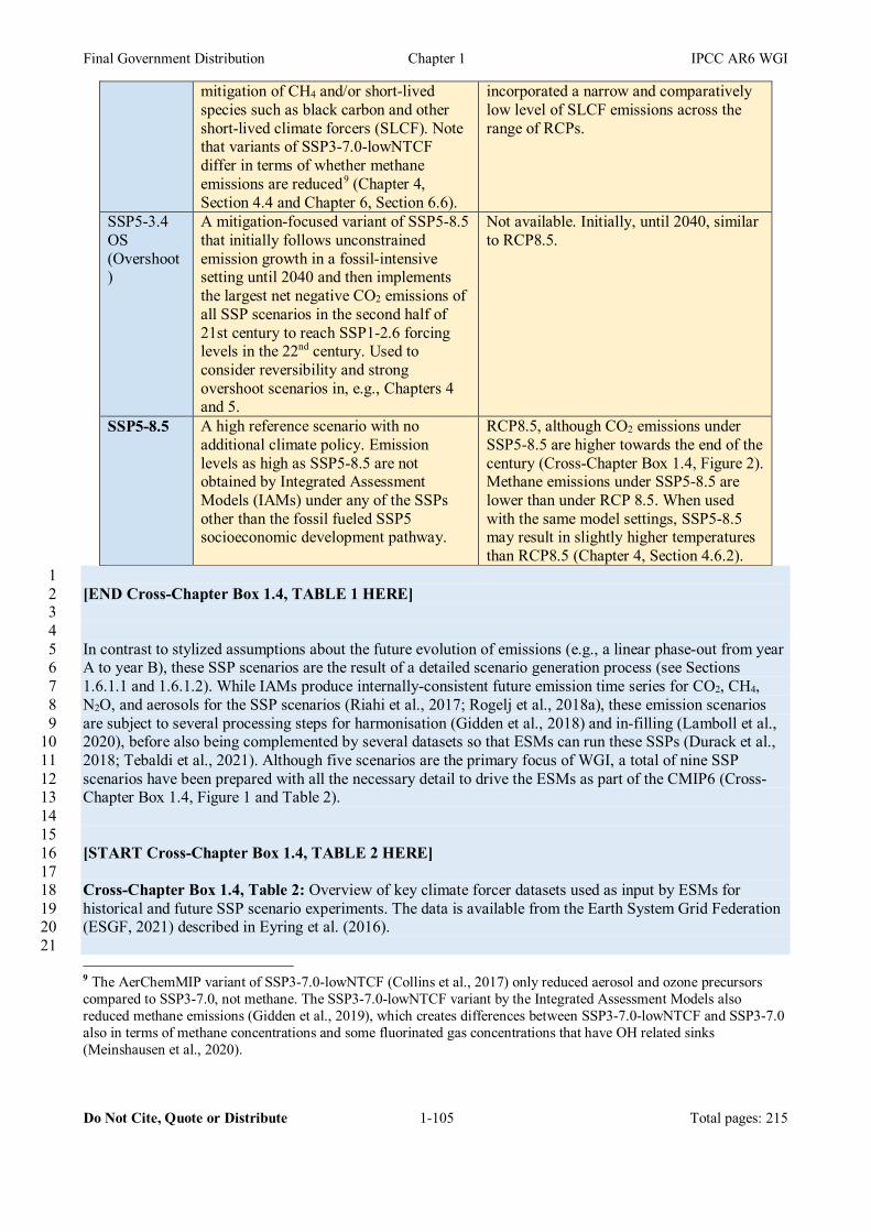
Final Government Distribution Chapter 1 IPCC AR6 WGI
Do Not Cite, Quote or Distribute 1-105 Total pages: 215
mitigation of CH4 and/or short-lived species such as black carbon and other short-lived climate forcers (SLCF). Note that variants of SSP3-7.0-lowNTCF differ in terms of whether methane emissions are reduced9 (Chapter 4, Section 4.4 and Chapter 6, Section 6.6).
incorporated a narrow and comparatively low level of SLCF emissions across the range of RCPs.
SSP5-3.4 OS (Overshoot)
A mitigation-focused variant of SSP5-8.5 that initially follows unconstrained emission growth in a fossil-intensive setting until 2040 and then implements the largest net negative CO2 emissions of all SSP scenarios in the second half of 21st century to reach SSP1-2.6 forcing levels in the 22nd century. Used to consider reversibility and strong overshoot scenarios in, e.g., Chapters 4 and 5.
Not available. Initially, until 2040, similar to RCP8.5.
SSP5-8.5 A high reference scenario with no additional climate policy. Emission levels as high as SSP5-8.5 are not obtained by Integrated Assessment Models (IAMs) under any of the SSPs other than the fossil fueled SSP5 socioeconomic development pathway.
RCP8.5, although CO2 emissions under SSP5-8.5 are higher towards the end of the century (Cross-Chapter Box 1.4, Figure 2). Methane emissions under SSP5-8.5 are lower than under RCP 8.5. When used with the same model settings, SSP5-8.5 may result in slightly higher temperatures than RCP8.5 (Chapter 4, Section 4.6.2).
1 [END Cross-Chapter Box 1.4, TABLE 1 HERE] 2 3 4 In contrast to stylized assumptions about the future evolution of emissions (e.g., a linear phase-out from year 5 A to year B), these SSP scenarios are the result of a detailed scenario generation process (see Sections 6 1.6.1.1 and 1.6.1.2). While IAMs produce internally-consistent future emission time series for CO2, CH4, 7 N2O, and aerosols for the SSP scenarios (Riahi et al., 2017; Rogelj et al., 2018a), these emission scenarios 8 are subject to several processing steps for harmonisation (Gidden et al., 2018) and in-filling (Lamboll et al., 9 2020), before also being complemented by several datasets so that ESMs can run these SSPs (Durack et al., 10 2018; Tebaldi et al., 2021). Although five scenarios are the primary focus of WGI, a total of nine SSP 11 scenarios have been prepared with all the necessary detail to drive the ESMs as part of the CMIP6 (Cross-12 Chapter Box 1.4, Figure 1 and Table 2). 13 14 15 [START Cross-Chapter Box 1.4, TABLE 2 HERE] 16 17 Cross-Chapter Box 1.4, Table 2: Overview of key climate forcer datasets used as input by ESMs for 18 historical and future SSP scenario experiments. The data is available from the Earth System Grid Federation 19 (ESGF, 2021) described in Eyring et al. (2016). 20 21 9 The AerChemMIP variant of SSP3-7.0-lowNTCF (Collins et al., 2017) only reduced aerosol and ozone precursors compared to SSP3-7.0, not methane. The SSP3-7.0-lowNTCF variant by the Integrated Assessment Models also reduced methane emissions (Gidden et al., 2019), which creates differences between SSP3-7.0-lowNTCF and SSP3-7.0 also in terms of methane concentrations and some fluorinated gas concentrations that have OH related sinks (Meinshausen et al., 2020).
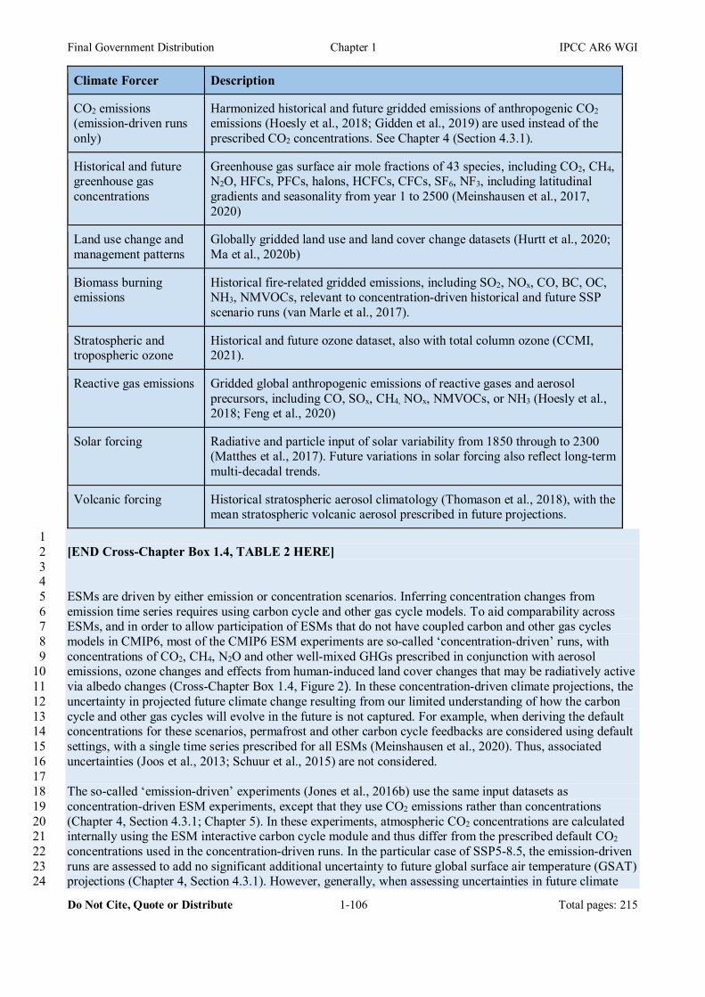
Final Government Distribution Chapter 1 IPCC AR6 WGI
Do Not Cite, Quote or Distribute 1-106 Total pages: 215
Climate Forcer Description
CO2 emissions (emission-driven runs only)
Harmonized historical and future gridded emissions of anthropogenic CO2 emissions (Hoesly et al., 2018; Gidden et al., 2019) are used instead of the prescribed CO2 concentrations. See Chapter 4 (Section 4.3.1).
Historical and future greenhouse gas concentrations
Greenhouse gas surface air mole fractions of 43 species, including CO2, CH4, N2O, HFCs, PFCs, halons, HCFCs, CFCs, SF6, NF3, including latitudinal gradients and seasonality from year 1 to 2500 (Meinshausen et al., 2017, 2020)
Land use change and management patterns
Globally gridded land use and land cover change datasets (Hurtt et al., 2020; Ma et al., 2020b)
Biomass burning emissions
Historical fire-related gridded emissions, including SO2, NOx, CO, BC, OC, NH3, NMVOCs, relevant to concentration-driven historical and future SSP scenario runs (van Marle et al., 2017).
Stratospheric and tropospheric ozone
Historical and future ozone dataset, also with total column ozone (CCMI, 2021).
Reactive gas emissions Gridded global anthropogenic emissions of reactive gases and aerosol precursors, including CO, SOx, CH4, NOx, NMVOCs, or NH3 (Hoesly et al., 2018; Feng et al., 2020)
Solar forcing Radiative and particle input of solar variability from 1850 through to 2300 (Matthes et al., 2017). Future variations in solar forcing also reflect long-term multi-decadal trends.
Volcanic forcing Historical stratospheric aerosol climatology (Thomason et al., 2018), with the mean stratospheric volcanic aerosol prescribed in future projections.
1 [END Cross-Chapter Box 1.4, TABLE 2 HERE] 2 3 4 ESMs are driven by either emission or concentration scenarios. Inferring concentration changes from 5 emission time series requires using carbon cycle and other gas cycle models. To aid comparability across 6 ESMs, and in order to allow participation of ESMs that do not have coupled carbon and other gas cycles 7 models in CMIP6, most of the CMIP6 ESM experiments are so-called ‘concentration-driven’ runs, with 8 concentrations of CO2, CH4, N2O and other well-mixed GHGs prescribed in conjunction with aerosol 9 emissions, ozone changes and effects from human-induced land cover changes that may be radiatively active 10 via albedo changes (Cross-Chapter Box 1.4, Figure 2). In these concentration-driven climate projections, the 11 uncertainty in projected future climate change resulting from our limited understanding of how the carbon 12 cycle and other gas cycles will evolve in the future is not captured. For example, when deriving the default 13 concentrations for these scenarios, permafrost and other carbon cycle feedbacks are considered using default 14 settings, with a single time series prescribed for all ESMs (Meinshausen et al., 2020). Thus, associated 15 uncertainties (Joos et al., 2013; Schuur et al., 2015) are not considered. 16 17 The so-called ‘emission-driven’ experiments (Jones et al., 2016b) use the same input datasets as 18 concentration-driven ESM experiments, except that they use CO2 emissions rather than concentrations 19 (Chapter 4, Section 4.3.1; Chapter 5). In these experiments, atmospheric CO2 concentrations are calculated 20 internally using the ESM interactive carbon cycle module and thus differ from the prescribed default CO2 21 concentrations used in the concentration-driven runs. In the particular case of SSP5-8.5, the emission-driven 22 runs are assessed to add no significant additional uncertainty to future global surface air temperature (GSAT) 23 projections (Chapter 4, Section 4.3.1). However, generally, when assessing uncertainties in future climate 24

Final Government Distribution Chapter 1 IPCC AR6 WGI
Do Not Cite, Quote or Distribute 1-107 Total pages: 215
projections, it is important to consider which elements of the cause-effect chain from emissions to the 1 resulting climate change are interactively included as part of the model projections, and which are externally 2 prescribed using default settings. 3 4 5 [START Cross-Chapter Box 1.4, FIGURE 2 HERE] 6 7 Cross-Chapter Box 1.4, Figure 2: Comparison between the Shared Socio-economic Pathways (SSP) scenarios 8 and the Representative Concentration Pathway (RCP) scenarios in terms of their CO2, CH4 and N2O 9 atmospheric concentrations (panels a-c), and their global emissions (panels d-o). Also shown are gridded emission 10 differences for sulfur (panel p) and black carbon (panel q) for the year 2000 between the input emission datasets that 11 underpinned the CMIP5 and CMIP6 model intercomparisons. Historical emission estimates are provided in black in 12 panels d to o. The range of concentrations and emissions investigated under the RCP pathways is grey shaded. Panels p 13 and q adapted from Figure 7 in Hoesly et al. (2018). Further details on data sources and processing are available in the 14 chapter data table (Table 1.SM.1). 15 16 [END Cross-Chapter Box 1.4, FIGURE 2 HERE] 17 18 19 [END CROSS CHAPTER BOX 1.4 HERE] 20 21 22 1.6.1.2 Scenario generation process for CMIP6 23 24 The scenario generation process involves research communities linked to all three IPCC Working Groups 25 (Figure 1.27). It generally starts in the scientific communities associated with WGII and WGIII with the 26 definition of new socio-economic scenario storylines (IPCC, 2000; O’Neill et al., 2014) that are quantified in 27 terms of their drivers, i.e., GDP, population, technology, energy and land use and their resulting emissions 28 (Riahi et al., 2017). Then, numerous complementation and harmonisation steps are necessary for datasets 29 within the WGI and WGIII science communities, including gridding emissions of anthropogenic short-lived 30 forcers, providing open biomass burning emission estimates, preparing land use patterns, aerosol fields, 31 stratospheric and tropospheric ozone, nitrogen deposition datasets, solar irradiance and aerosol optical 32 property estimates, and observed and projected greenhouse gas concentration time series (documented for 33 CMIP6 through input4mips; Durack et al., 2018; Cross-Chapter Box 1.4, Table 2). 34 35 Once these datasets are completed, ESMs are run in coordinated model intercomparison projects in the WGI 36 science community, using standardized simulation protocols and scenario data. The most recent example of 37 such a coordinated effort is the CMIP6 exercise (Eyring et al., 2016; see also Section 1.5.4) with, in 38 particular, ScenarioMIP (O’Neill et al., 2016). The WGI science community feeds back climate information 39 to WGIII via climate emulators (Cross-Chapter Box 7.1 in Chapter 7) that are updated and calibrated with 40 the ESMs’ temperature responses and other lines of evidence. Next, this climate information is used to 41 compute several high-level global climate indicators (e.g., atmospheric concentrations, global temperatures) 42 for a much wider set of hundreds of scenarios that are assessed as part of IPCC WGIII assessment (WGIII 43 Annex C). The outcomes from climate models run under the different scenarios are then used to calculate the 44 evolution of climatic impact-drivers (Chapter 12), and utilized by impact researchers together with exposure 45 and vulnerability information, in order to characterize risk from future climate change to human and natural 46 systems. The climate impacts associated with these scenarios or different warming levels are then assessed as 47 part of WGII reports (Figure 1.27). 48 49 50 [START FIGURE 1.27 HERE] 51 52 Figure 1.27: A simplified illustration of the scenario generation process that involves the scientific communities 53
represented in the three IPCC Working Groups. The circular set of arrows at the top indicate the main 54 set of models and workflows used in that scenario generation process, with the lower level indicating the 55 datasets. 56

Final Government Distribution Chapter 1 IPCC AR6 WGI
Do Not Cite, Quote or Distribute 1-108 Total pages: 215
1 [END FIGURE 1.27 HERE] 2 3 4 1.6.1.3 History of scenarios within the IPCC 5 6 Scenario modelling experiments have been a core element of physical climate science since the first transient 7 simulations with a General Circulation Model in 1988 (Hansen et al., 1988; see Section 1.3). Scenarios and 8 modelling experiments assessed in IPCC reports have evolved over time, which provides a ‘history of how 9 the future was seen’. The starting time for the scenarios moves as actual emissions supersede earlier 10 emission assumptions, while new scientific insights into the range of plausible population trends, 11 behavioural changes and technology options and other key socioeconomic drivers of emissions also emerge 12 (see WGIII; Legget, 1992; IPCC, 2000; Moss et al., 2010; Riahi et al., 2017). Many different sets of climate 13 projections have been produced over the past several decades, using different sets of scenarios. Here, we 14 compare those earlier scenarios against the most recent ones. 15 16 Climate science research involving scenarios necessarily follows a series of consecutive steps (see Figure 17 1.27). As each step waits for input from the preceding one, delays often occur that result in the impact 18 literature basing its analyses on earlier scenarios than those most current in the climate change mitigation and 19 climate system literature. It is hence important to provide an approximate comparison across the various 20 scenario generations (Figure 1.28; Cross-Chapter Box 1.4, Table 1; Chapter 4). 21 22 23 [START FIGURE 1.28 HERE] 24 25 Figure 1.28: Comparison of the range of fossil and industrial CO2 emissions from scenarios used in previous 26
assessments up to AR6. Previous assessments are the IS92 scenarios from 1992 (top panel), the Special 27 Report on Emissions Scenarios (SRES) scenarios from the year 2000 (second panel), the Representative 28 Concentration Pathway (RCP) scenarios designed around 2010 (third panel) and the Shared Socio-29 economic Pathways (SSP) scenarios (second bottom panel). In addition, historical emissions are shown 30 (black line) (Chapter 5, Figure 5.5); a more complete set of scenarios is assessed in SR1.5 (bottom panel) 31 (Huppmann et al., 2018). Further details on data sources and processing are available in the chapter data 32 table (Table 1.SM.1). 33
34 [END FIGURE 1.28 HERE] 35 36 37 The first widely used set of IPCC emission scenarios was the IS92 scenarios in 1992 (Leggett et al., 1992). 38 Apart from reference scenarios, IS92 also included a set of stabilisation scenarios, the so-called ‘S’ 39 scenarios. Those ‘S’ pathways were designed to lead to CO2 stabilisation levels such as 350 ppm or 450 40 ppm. By 1996, those latter stabilisation levels were complemented in the scientific literature by alternative 41 trajectories that assumed a delayed onset of climate change mitigation action (Figure 1.28; Wigley et al., 42 1996). 43 44 By 2000, the IPCC Special Report on Emission Scenarios (SRES) produced the SRES scenarios (IPCC, 45 2000), albeit without assuming any climate-policy-induced mitigation. The four broad groups of SRES 46 scenarios (scenario ‘families’) A1, A2, B1 and B2 were the first scenarios to emphasize socio-economic 47 scenario storylines, and also first to emphasize other greenhouse gases, land use change and aerosols. 48 Represented by three scenarios for the high-growth A1 scenario family, those 6 SRES scenarios (A1FI, A1B, 49 A1T, A2, B1, and B2) can still sometimes be found in today’s climate impact literature. The void of missing 50 climate change mitigation scenarios was filled by a range of community exercises, including the so-called 51 post-SRES scenarios (Swart et al., 2002). 52 53 The RCP scenarios (van Vuuren et al., 2011) then broke new ground by providing low emission pathways 54 that implied strong climate change mitigation including an example with negative CO2 emissions on a large 55 scale, namely RCP2.6. As shown in Figure 1.28, the upper end of the scenario range has not substantially 56

Final Government Distribution Chapter 1 IPCC AR6 WGI
Do Not Cite, Quote or Distribute 1-109 Total pages: 215
shifted. Building on the SRES multi-gas scenarios, the RCPs include time series of emissions and 1 concentrations of the full suite of greenhouse gases and aerosols and chemically active gases, as well as land 2 use and land cover (Moss et al., 2010). The word ‘representative’ signifies that each RCP is only one of 3 many possible scenarios that would lead to the specific radiative forcing characteristics. The term pathway 4 emphasizes that not only the long-term concentration levels are of interest, but also the trajectory taken over 5 time to reach that outcome (Moss et al., 2010). RCPs usually refer to the concentration pathway extending to 6 2100, for which IAMs produced corresponding emission scenarios. Four RCPs produced from IAMs were 7 selected from the published literature and are used in AR5 as well as in this report, spanning approximately 8 the range from below 2°C warming to high (>4°C) warming best-estimates by the end of the 21st century: 9 RCP2.6, RCP4.5 and RCP6.0 and RCP8.5 (Cross-Chapter Box 1.4, Table 1). Extended Concentration 10 Pathways (ECPs) describe extensions of the RCPs from 2100 to 2300 that were calculated using simple rules 11 generated by stakeholder consultations; these do not represent fully consistent scenarios (Meinshausen et al., 12 2011b). 13 14 By design, the RCP emission and concentration pathways were originally developed using particular socio-15 economic development pathways, but those are no longer considered (Moss et al., 2010). The different levels 16 of emissions and climate change represented in the RCPs can hence be explored against the backdrop of 17 different socio-economic development pathways (SSP1 to SSP5) (Section 1.6.1.1; Cross-Chapter Box 1.4). 18 This integrative SSP-RCP framework (‘SSPX-RCPY’ in Table 1.4) is now widely used in the climate impact 19 and policy analysis literature (e.g., ICONICS, 2021; Green et al., 2020; O’Neill et al., 2020), where climate 20 projections obtained under the RCP scenarios are analysed against the backdrop of various SSPs. 21 Considering various levels of future emissions and climate change for each socio-economic development 22 pathway was an evolution from the previous SRES framework (IPCC, 2000), in which socio-economic and 23 emission futures were closely aligned. 24 25 The new set of scenarios (SSP1-1.9 to SSP5-8.5) now features a higher top level of CO2 emissions (SSP5-8.5 26 compared to RCP8.5), although the most significant change is again the addition of a very low climate 27 change mitigation scenario (SSP1-1.9, compared to the previous low scenario, RCP2.6). Also, historically, 28 none of the previous scenario sets featured a scenario that involves a very pronounced peak-and-decline 29 emissions trajectory, but SSP1-1.9 does so now. The full set of nine SSP scenarios now includes a high 30 aerosol emission scenario (SSP3-7.0). The RCPs featured more uniformly low aerosol trajectories across all 31 scenarios (Cross-Chapter Box 1.4, Figure 2). More generally, the SSP scenarios feature a later peak of global 32 emission for the lower scenarios, simply as a consequence of historical emissions not having followed the 33 trajectory projected by previous low scenarios (Figure 1.28). 34 35 Over the last decades, discussions around scenarios have often focussed on whether recent trends make 36 certain future scenarios more or less probable or whether all scenarios are too high or too low. When the 37 SRES scenarios first appeared, the debate was often whether the scenarios were overestimating actual world 38 emissions developments (e.g., Castles and Henderson, 2003). With the strong emissions increase throughout 39 the 2000s, that debate then shifted towards the question of whether the lower future climate change 40 mitigation scenarios were rendered unfeasible (Pielke et al., 2008; van Vuuren and Riahi, 2008). Historical 41 emissions over 2000 to 2010 approximately track the upper half of SRES and RCP projections (Figure 1.28). 42 More generally, the global fossil and industrial CO2 emissions of recent decades tracked approximately the 43 middle of the projected scenario ranges (see Fig 1.28), although with regional differences (Pedersen et al., 44 2020). 45 46 47 1.6.1.4 The likelihood of reference scenarios, scenario uncertainty and storylines 48 49 In general, no likelihood is attached to the scenarios assessed in this Report. The use of different scenarios 50 for climate change projections allows to explore ‘scenario uncertainty’ (Collins et al., 2013; SR1.5; see also 51 Section 1.4.4). Scenario uncertainty is fundamentally different from geophysical uncertainties, which result 52 from limitations in the understanding and predictability of the climate system (Smith and Stern, 2011). In 53 scenarios, by contrast, future emissions depend to a large extent on the collective outcome of choices and 54 processes related to population dynamics and economic activity, or on choices that affect a given activity’s 55
Final Government Distribution Chapter 1 IPCC AR6 WGI
Do Not Cite, Quote or Distribute 1-110 Total pages: 215
energy and emissions intensity (Jones, 2000; Knutti et al., 2008; Kriegler et al., 2012; van Vuuren et al., 1 2014). Even if identical socio-economic futures are assumed, the associated future emissions still face 2 uncertainties, since different experts and model frameworks diverge in their estimates of future emission 3 ranges (Ho et al., 2019). 4 5 When exploring various climate futures, scenarios with no, or no additional, climate policies are often 6 referred to as ‘baseline’ or ‘reference scenarios’ (Section 1.6.1.1; Annex VII: Glossary). Among the five core 7 scenarios used most in this report, SSP3-7.0 and SSP5-8.5 are explicit ‘no-climate-policy’ scenarios (Gidden 8 et al., 2019; Cross-Chapter Box 1.4, Table 1), assuming a carbon price of zero. These future ‘baseline’ 9 scenarios are hence counterfactuals that include less climate policies compared to ‘business-as-usual’ 10 scenarios – given that ‘business-as-usual’ scenarios could be understood to imply a continuation of existing 11 climate policies. Generally, future scenarios are meant to cover a broad range of plausible futures, due for 12 example to unforeseen discontinuities in development pathways (Raskin and Swart, 2020), or to large 13 uncertainties in underlying long-term projections of economic drivers (Christensen et al., 2018). However, 14 the likelihood of high emission scenarios such as RCP8.5 or SSP5-8.5 is considered low in light of recent 15 developments in the energy sector (Hausfather and Peters, 2020a, 2020b). Studies that consider possible 16 future emission trends in the absence of additional climate policies, such as the recent IEA 2020 World 17 Energy Outlook ‘stated policy’ scenario (International Energy Agency, 2020), project approximately 18 constant fossil and industrial CO2 emissions out to 2070, approximately in line with the medium RCP4.5, 19 RCP6.0 and SSP2-4.5 scenarios (Hausfather and Peters, 2020b) and the 2030 global emission levels that are 20 pledged as part of the Nationally Determined Contributions (NDCs) under the Paris Agreement (Section 21 1.2.2; (Fawcett et al., 2015; Rogelj et al., 2016; UNFCCC, 2016; IPCC, 2018). On the other hand, the default 22 concentrations aligned with RCP8.5 or SSP5-8.5 and resulting climate futures derived by ESMs could be 23 reached by lower emission trajectories than RCP8.5 or SSP5-8.5. That is because the uncertainty range on 24 carbon-cycle feedbacks includes stronger feedbacks than assumed in the default derivation of RCP8.5 and 25 SSP5-8.5 concentrations (Ciais et al., 2013; Friedlingstein et al., 2014; Booth et al., 2017; see also Chapter 5, 26 Section 5.4). 27 28 To address long-term scenario uncertainties, scenario storylines (or ‘narratives’) are often used (Rounsevell 29 and Metzger, 2010; O’Neill et al., 2014) (see Section 1.4.4 for a more general discussion on ‘storylines’ also 30 covering ‘physical climate storylines’). Scenario storylines are descriptions of a future world, and the related 31 large-scale socio-economic development path towards that world that are deemed plausible within the 32 current state of knowledge and historical experience (WGIII; Section 1.2.3). Scenario storylines attempt to 33 ‘stimulate, provoke, and communicate visions of what the future could hold for us’ (Rounsevell and 34 Metzger, 2010) in settings where either limited knowledge or inherent unpredictability in social systems 35 prevent a forecast or numerical prediction. Scenario storylines have been used in previous climate research, 36 and they are the explicit or implicit starting point of any scenario exercise, including for the SRES scenarios 37 (IPCC, 2000) and the SSPs (e.g., O’Neill et al., 2017a). 38 39 Recent technological or socio-economic trends might be informative for bounding near-term future trends, 40 for example, if technological progress renders a mitigation technology cheaper than previously assumed. 41 However, short-term emission trends alone do not generally rule out an opposite trend in the future (van 42 Vuuren et al., 2010). The ranking of individual RCP emission scenarios from the IAMs with regard to 43 emission levels is different for different time horizons, e.g., 2020 versus longer-term emission levels; For 44 example, the strongest climate change mitigation scenario RCP2.6 was in fact the second highest CO2 45 emission scenario (jointly with RCP4.5) before 2020 in the set of RCPs and the strong global emission 46 decline in RCP2.6 only followed after 2020. Implicitly, this scenario feature was cautioning against the 47 assumption that short-term trends predicate particular long-term trajectories. This is also the case in relation 48 to the COVID-19 related drop in 2020 emissions. Potential changes in underlying drivers of emissions, such 49 as those potentially incentivised by COVID-19 recovery stimulus packages, are more significant for longer-50 term emissions than the short-term deviation from recent emission trends (Cross-Chapter Box 6.1 on 51 COVID-19 in Chapter 6). 52 53 54
Final Government Distribution Chapter 1 IPCC AR6 WGI
Do Not Cite, Quote or Distribute 1-111 Total pages: 215
1.6.2 Global warming levels 1 2 The global mean surface temperature change, or ‘global warming level’ (GWL), is a ‘dimension of 3 integration’ that is highly relevant across scientific disciplines and socioeconomic actors. First, global 4 warming levels relative to pre-industrial conditions are the quantity in which the 1.5°C and ‘well below 2°C’ 5 Paris Agreement goals were formulated. Second, global mean temperature change has been found to be 6 nearly-linearly related to a number of regional climate effects (Mitchell et al., 2000; Mitchell, 2003; Tebaldi 7 and Arblaster, 2014; Seneviratne et al., 2016; Li et al., 2020; Seneviratne and Hauser, 2020). Even where 8 non-linearities are found, some regional climate effects can be considered to be almost scenario-independent 9 for a given level of warming (Cross-Chapter Box 11.1 in Chapter 11; Chapter 4, Sections 4.2.4 and 4.6.1; 10 Chapter 8, Section 8.5.3; Chapter 10, Section 10.4.3.1). Finally, the evolution of aggregated impacts with 11 warming levels has been widely used and embedded in the assessment of the ‘Reasons for Concern’ (RFC) 12 in IPCC WGII (Smith et al., 2009; IPCC, 2014a). The RFC framework was further expanded in SR1.5 13 (2018), SROCC (2019) and SRCCL (2019) by explicitly describing the differential impacts of half-degree 14 warming steps (cf. King et al., 2017) (Section 1.4.4; Cross-Chapter Box 12.1 in Chapter 12). 15 16 In this Report, the term ‘global warming level’ refers to the categorisation of global and regional climate 17 change, associated impacts, emission and concentration scenarios by global mean surface temperature 18 relative to 1850-1900, which is the period used as a proxy for pre-industrial levels (see Cross-Chapter Box 19 11.1 in Chapter 11). By default, GWLs are expressed as global surface air temperature (GSAT; see Section 20 1.4.1; Cross-Chapter Box 2.3 in Chapter 2). 21 22 As the SR1.5 concluded, even half-degree global mean temperature steps carry robust differences in climate 23 impacts (see SR1.5,IPCC, 2018; Schleussner et al., 2016a; Wartenburger et al., 2017; see also Chapter 11). 24 This Report adopts half-degree warming levels which allows integration within and across the three WGs for 25 climate projections, impacts, adaptation challenges and mitigation challenges. The core set of - GWLs 1.5, 26 2.0, 3.0 and 4.0°C - are highlighted (Chapters 4, 8, 11, 12 and the Atlas). Given that much impact analysis is 27 based on previous scenarios, i.e., RCPs or SRES, and climate change mitigation analysis is based on new 28 emission scenarios in addition to the main SSP scenarios, these global warming levels assist in the 29 comparison of climate states across scenarios and in the synthesis across the broader literature. 30 31 The transient and equilibrium states of certain global warming levels can differ in their climate impacts 32 (IPCC, 2018; King et al., 2020). Climate impacts in a ‘transient’ world relate to a scenario in which the 33 world is continuing to warm. On the other hand, climate impacts at the same warming levels can also be 34 estimated from equilibrium states after a (relatively) short-term stabilisation by the end of the 21st century or 35 at a (near-) equilibrium state after a long-term (multi-decadal to multi-millennial) stabilisation. Different 36 methods to estimate these climate states come with challenges and limitations (Chapter 4, Section 4.6.1; 37 Cross-Chapter Box 11.1 in Chapter 11). First, information can be drawn from GCM or ESM simulations that 38 ‘pass through’ the respective warming levels (as used and demonstrated in the Interactive Atlas to this 39 report), also called ‘epoch’ or ‘time-shift’ approaches (Chapter 4, Sections 4.2.4 and 4.6.1) (Herger et al., 40 2015; James et al., 2017; Tebaldi and Knutti, 2018). Information from transient simulations can also be used 41 through an empirical scaling relationship (Seneviratne et al., 2016, 2018; Wartenburger et al., 2017) or using 42 ‘time sampling’ approaches, as described in James et al. (2017). Second, information can be drawn from 43 large ESM ensembles with prescribed SST at particular global warming levels (Mitchell et al., 2017), 44 although an underrepresentation of variability can arise when using prescribed SST temperatures (Fischer et 45 al., 2018a). 46 47 In order to fully derive climate impacts, warming levels will need to be complemented by additional 48 information, such as their associated CO2 concentrations (e.g., fertilization or ocean acidification), 49 composition of the total radiative forcing (aerosols vs greenhouse gases, with varying regional distributions) 50 or socioeconomic conditions (e.g., to estimate societal impacts). More fundamentally, while a global 51 warming level is a good proxy for the state of the climate (Cross-Chapter Box 11.1 in Chapter 11), it does 52 not uniquely define a change in global or regional climate state. For example, regional precipitation 53 responses depend on the details of the individual forcing mechanisms that caused the change (Samset et al., 54 2016), on whether the temperature level is stabilized or transient (King et al., 2020; Zappa et al., 2020), on 55

Final Government Distribution Chapter 1 IPCC AR6 WGI
Do Not Cite, Quote or Distribute 1-112 Total pages: 215
the vertical structure of the troposphere (Andrews et al., 2010), and, in particular, on the global distribution 1 of atmospheric aerosols (Frieler et al., 2012). Another aspect is how Earth system components with century 2 to millennial response timescales, such as long-term sea level rise or permafrost thaw, are affected by global 3 mean warming. For example, sea level rise 50 years after a 1°C warming will be lower than sea level rise 4 150 years after that same 1°C warming (Chapter 9). 5 6 Also, forcing or response patterns that vary in time can create differences in regional climates for the same 7 global mean warming level, or can create non-linearities when scaling patterns from one warming level to 8 another (King et al., 2018), depending on whether near-term transient climate, end of the century, 9 equilibrium climate or climate states after an initial overshoot are considered. 10 11 In spite of these challenges, and thanks to recent methodological advances in quantifying or overcoming 12 them, global warming levels provide a robust and useful integration mechanism. They allow knowledge from 13 various domains within WGI and across the three WGs to be integrated and communicated (Cross Chapter 14 Box 11.1). In this report, Chapters 4, 8, 11, 12 and the Atlas provide information specific to certain warming 15 levels, highlighting the regional differences, but also the approximate scalability of regional climate change, 16 that can arise from even a 0.5°C shift in global-mean temperatures. Furthermore, building on WGI insights 17 into physical climate system responses (Cross-Chapter Box 7.1 in Chapter 7), WGIII will use peak and end-18 of-century global warming levels to classify a broad set of scenarios. 19 20 21 1.6.3 Cumulative CO2 emissions 22 23 The WGI AR5 (IPCC, 2013a) and the SR1.5 (IPCC, 2018) highlighted the near-linear relationship between 24 cumulative carbon emissions and global mean warming (Section 1.3; Section 5.5). This implies that 25 continued CO2 emissions will cause further warming and changes in all components of the climate system, 26 independent of any specific scenario or pathway. This is captured in the TCRE concept, which relates CO2-27 induced global mean warming to cumulative carbon emissions (Chapter 5). This Report thus uses cumulative 28 CO2 emissions to compare the climate response across scenarios, and to categorise emission scenarios 29 (Figure 1.29). The advantage of using cumulative CO2 emissions is that it is an inherent emission scenario 30 characteristic rather than an outcome of the scenario-based projections, where uncertainties in the cause-31 effect chain from emissions to atmospheric concentrations to temperature change are important. 32 33 There is also a close relationship between cumulative total greenhouse gas emissions and cumulative CO2 34 emissions for scenarios in the SR1.5 scenario database (IPCC, 2018; Figure 1.29). The dominance of CO2 35 compared to other well-mixed greenhouse gases (Figure 1.29; Chapter 5, Section 5.2.4) allows policymakers 36 to make use of the carbon budget concept (Chapter 5, Section 5.5) in a policy context, in which GWP-37 weighted combinations of multiple greenhouse gases are used to define emission targets. A caveat is that 38 cumulative GWP-weighted CO2 equivalent emissions over the next decades do not yield exactly the same 39 temperature outcomes as the same amount of cumulative CO2 emissions, because atmospheric perturbation 40 lifetimes of the various greenhouse gases differ. While carbon budgets are not derived using GWP-weighted 41 emission baskets but rather by explicit modelling of non-CO2 induced warming (Chapter 5, Section 5.5; 42 Cross-Chapter Box 7.1 in Chapter 7), the policy frameworks based on GWP-weighted emission baskets can 43 still make use of the insights from remaining cumulative carbon emissions for different warming levels. 44 45 The same cumulative CO2 emissions could lead to a slightly different level of warming over time (Box 1.4). 46 Rapid emissions followed by steep cuts and potentially net-negative emissions would be characterised by a 47 higher maximum warming and faster warming rate, compared with the same cumulative CO2 emissions 48 spread over a longer period. As further explored in the WGIII assessment, one potential limitation when 49 presenting emission pathway characteristics in cumulative emission budget categories is that path 50 dependencies and lock-in effects (e.g. today’s decisions regarding fossil fuel related infrastructure) play an 51 important role in long-term mitigation strategies (Davis et al., 2010; Luderer et al., 2018). Similarly, high 52 emissions early on might imply strongly net negative emissions (Minx et al., 2018) later on to reach the same 53 cumulative emission and temperature target envelope by the end of the century (Box 1.4). This report 54 explores options to address some of those potential issues from a WGI perspective (see Chapter 5, Sections 55

Final Government Distribution Chapter 1 IPCC AR6 WGI
Do Not Cite, Quote or Distribute 1-113 Total pages: 215
5.5.2 and 5.6.2). 1 2 3 [START FIGURE 1.29 HERE] 4 5 Figure 1.29: The role of CO2 in driving future climate change in comparison to other greenhouse gases (GHGs). 6
The GHGs included here are CH4, N2O, and 40 other long-lived, well-mixed GHGs. The blue shaded area 7 indicates the approximate forcing exerted by CO2 in Shared Socio-economic Pathways (SSP) scenarios, 8 ranging from very low SSP1-1.9 to very high SSP5-8.5 (Chapter 7). The CO2 concentrations under the 9 SSP1-1.9 scenarios reach approximately 350 ppm after 2150, while those of SSP5-8.5 exceed 2000 ppm 10 CO2 in the longer term (through year 2300). Similarly to the dominant radiative forcing share at each 11 point in time (lower area plots), cumulative GWP-100-weighted GHG emissions happen to be closely 12 correlated with cumulative CO2 emissions, allowing policymakers to make use of the carbon budget 13 concept in a policy context with multi-gas GHG baskets as it exhibits relatively low variation across 14 scenarios with similar cumulative emissions until 2050 (inset panel). Further details on data sources and 15 processing are available in the chapter data table (Table 1.SM.1). 16
17 [END FIGURE 1.29 HERE] 18 19 20 [START BOX 1.4 HERE] 21 22 Box 1.4: The relationships between ‘net zero’ emissions, temperature outcomes and carbon dioxide 23
removal 24 Article 4 of the Paris Agreement sets an objective to ‘achieve a balance between anthropogenic emissions by 25 sources and removals by sinks of greenhouse gases’ (Section 1.2). This box addresses the relationship 26 between such a balance and the corresponding evolution of global surface temperature, with or without the 27 deployment of large-scale Carbon Dioxide Removal (CDR), using the definitions of ‘net zero CO2 28 emissions’ and ‘net zero greenhouse gas (GHG) emissions’ of the AR6 Glossary (Annex VII: Glossary). 29 30 ‘Net zero CO2 emissions’ is defined in AR6 as the condition in which anthropogenic CO2 emissions are 31 balanced by anthropogenic CO2 removals over a specified period. Similarly, ‘net zero GHG emissions’ is the 32 condition in which metric-weighted anthropogenic GHG emissions are balanced by metric-weighted 33 anthropogenic GHG removals over a specified period. The quantification of net zero GHG emissions thus 34 depends on the GHG emission metric chosen to compare emissions of different gases, as well as the time 35 horizon chosen for that metric. (For a broader discussion of metrics, see Box 1.3 and Chapter 7, Section 7.6, 36 and WGIII Cross-Chapter Box 2.) 37 38 Technical notes expanding on these definitions can be found as part of their respective entries in the Annex 39 VII: Glossary. The notes clarify the relation between ‘net zero’ CO2 and GHG emissions and the concept of 40 carbon and GHG neutrality, and the metric usage set out in the Paris Rulebook (Decision 18/CMA.1, annex, 41 paragraph 37). 42 43 A global net zero level of CO2, or GHG, emissions will be achieved when the sum of anthropogenic 44 emissions and removals across all countries, sectors, sources and sinks reaches zero. Achieving net zero CO2 45 or GHG emissions globally, at a given time, does not imply that individual entities (i.e., countries, sectors) 46 have to reach net zero emissions at that same point in time, or even at all (see WGIII, TS Box 4 and Chapter 47 3). 48 49 Net zero CO2 and net zero GHG emissions differ in their implications for the subsequent evolution of global 50 surface temperature. Net zero CO2 emissions result in approximately stable CO2-induced warming, but 51 overall warming will depend on any further warming contribution of non-CO2 GHGs. The effect of net zero 52 GHG emissions on global surface temperature depends on the GHG emission metric chosen to aggregate 53 emissions and removals of different gases. For GWP100 (the metric in which Parties to the Paris Agreement 54 have decided to report their aggregated emissions and removals), net zero GHG emissions would generally 55 imply a peak in global surface temperature, followed by a gradual decline (Chapter 7, Section 7.6.2; see also 56
Final Government Distribution Chapter 1 IPCC AR6 WGI
Do Not Cite, Quote or Distribute 1-114 Total pages: 215
Chapter 4, Section 4.7.1 regarding the Zero Emission Commitment). However, other anthropogenic factors, 1 such as aerosol emissions or land use-induced changes in albedo, may still affect the climate. 2 3 The definitions of net zero CO2 and GHG should also be seen in relation to the various CDR methods 4 discussed in the context of climate change mitigation (see Chapter 5, Section 5.6, which also includes an 5 assessment of the response of natural sinks to CDR), and how it is employed in scenarios used throughout 6 the WG I and III reports, as described in Section 1.6.1. (See also WGIII, Chapters 3, 7 and 12.) 7 8 For virtually all scenarios assessed by the IPCC, CDR is necessary to reach both global net zero CO2 and net 9 zero GHG emissions, to compensate for residual anthropogenic emissions. This is in part because for some 10 sources of CO2 and non-CO2 emissions, abatement options to eliminate them have not yet been identified. 11 For a given scenario, the choice of GHG metric determines how much net CDR is necessary to compensate 12 for residual non-CO2 emissions, in order to reach net zero GHG emissions (Chapter 7, Section 7.6.2). 13 14 If CDR is further used to go beyond net zero, to a situation with net-negative CO2 emissions (i.e., where 15 anthropogenic removals exceed anthropogenic emissions), anthropogenic CO2-induced warming will 16 decline. A further increase of CDR, until a situation with net zero or even net-negative GHG emissions is 17 reached, would increase the pace at which historical human-induced warming is reversed after its peak 18 (SR1.5, IPCC, 2018). Net-negative anthropogenic GHG emissions may become necessary to stabilize the 19 global surface temperature in the long term, should climate feedbacks further affect natural GHG sinks and 20 sources (see Chapter 5). 21 22 CDR can be achieved through a number of measures (Chapter 5, Section 5.6, and SRCCL). These include 23 additional afforestation, reforestation, soil carbon management, biochar, direct air capture and carbon capture 24 and storage (DACCS), and bioenergy with carbon capture and storage (BECCS) (de Coninck et al., 2018, 25 SR1.5 Ch4; Minx et al., 2018; see also WGIII Chapters 7 and 12). Differences between Land Use, Land Use 26 Change and Forestry (LULUCF) accounting rules, and scientific book-keeping approaches for CO2 27 emissions and removals from the terrestrial biosphere, can result in significant differences between the 28 amount of CDR that is reported in different studies (Grassi et al., 2017). Different measures to achieve CDR 29 come with different risks, negative side effects and potential co-benefits – also in conjunction with 30 sustainable development goals – that can inform choices around their implementation (Fuss et al., 2018; Roe 31 et al., 2019, Chapter 5, Section 5.6). Technologies to achieve direct large-scale anthropogenic removals of 32 non-CO2 GHGs are speculative at present (Yoon et al., 2009; Ming et al., 2016; Kroeger et al., 2017; Jackson 33 et al., 2019). 34 35 [END BOX 1.4 HERE] 36 37 38 1.7 Final remarks 39 40 The assessment in this Report is based on a rapidly growing body of new evidence from the peer-reviewed 41 literature. Recently, scientific climate change research has doubled in output every 5–6 years; the majority of 42 publications deal with issues related to the physical climate system (Burkett et al., 2014; Haunschild et al., 43 2016). The sheer volume of published, peer-reviewed literature on climate change presents a challenge to 44 comprehensive, robust and transparent assessment. 45 46 The enhanced focus on regional climate in WGI AR6 further expands the volume of literature relative to 47 AR5, including non-English language publications sometimes presented as reports (‘grey’ literature), 48 particularly on topics such as regional observing networks and climate services. These factors enhance the 49 challenge of discovering, accessing and assessing the relevant literature. The international, multi-lingual 50 author teams of the IPCC AR6, combined with the open expert review process, help to minimise these 51 concerns, but they remain a challenge. 52 53 Despite the key role of CMIP6 in this Report (Section 1.5), the number of studies evaluating its results and 54 modelling systems remains relatively limited. At the time of publication, additional model results are still 55

Final Government Distribution Chapter 1 IPCC AR6 WGI
Do Not Cite, Quote or Distribute 1-115 Total pages: 215
becoming available. This reflects the need for close temporal alignment of the CMIP cycle with the IPCC 1 assessment process, and the growing complexity of coordinated international modelling efforts. 2 3 Indigenous and local knowledge includes information about past and present climate states. However, 4 assessing this knowledge, and integrating it with the scientific literature, remains a challenge to be met. This 5 lack of assessment capability and integration leads to most WGI chapters still not including Indigenous and 6 local knowledge in their assessment findings. 7 8 Spatial and temporal gaps in both historical and current observing networks, and the limited extent of 9 paleoclimatic archives, have always posed a challenge for IPCC assessments. A relative paucity of long-term 10 observations is particularly evident in Antarctica and in the depths of the ocean. Knowledge of previous 11 cryospheric and oceanic processes is therefore incomplete. Sparse instrumental temperature observations 12 prior to the industrial revolution makes it difficult to uniquely characterize a ‘pre-industrial’ baseline, 13 although this report extends the assessment of anthropogenic temperature change further back in time than 14 previous assessment cycles (Cross-Chapter Box 1.2, Chapter 7). 15 16 Common, integrating scenarios can never encompass all possible events that might induce radiative forcing 17 in the future (Section 1.4). These may include large volcanic eruptions (see Cross-Chapter Box 4.1 in 18 Chapter 4), the consequences of a major meteorite, smoke plumes following a conflict involving nuclear 19 weapons, extensive geo-engineering, or a major pandemic (Cross-Chapter Box 1.6). Scenario-related 20 research also often focuses on the 21st century. Post-2100 climate changes are not covered as 21 comprehensively, and their assessment is limited. Those long-term climate changes, potentially induced by 22 forcing over the 21st century (as in the case of sea level rise), are nevertheless relevant for decision making. 23 24 At the time of publication, the consequences of the COVID-19 pandemic on emissions, atmospheric 25 abundances, radiative forcing and the climate (see Cross-Chapter Box 6.1 in Chapter 6), and on observations 26 (Section 1.5.1), are not yet fully evident. Their assessment in this report is thus limited. 27 28 29 30 31 32 33 34 35
Final Government Distribution Chapter 1 IPCC AR6 WGI
Do Not Cite, Quote or Distribute 1-116 Total pages: 215
Frequently Asked Questions 1 2 3 FAQ 1.1: Do we understand climate change better now compared to when the IPCC started? 4 Yes, much better. The first IPCC report, released in 1990, concluded that human-caused climate change 5 would soon become evident, but could not yet confirm that it was already happening. Today, evidence is 6 overwhelming that the climate has indeed changed since the pre-industrial era and that human activities are 7 the principal cause of that change. With much more data and better models, we also understand more about 8 how the atmosphere interacts with the ocean, ice, snow, ecosystems and land surfaces of the Earth. 9 Computer climate simulations have also improved dramatically, incorporating many more natural processes 10 and providing projections at much higher resolutions. 11 12 Since the first IPCC report in 1990, large numbers of new instruments have been deployed to collect data in 13 the air, on land, at sea and from outer space. These instruments measure temperature, clouds, winds, ice, 14 snow, ocean currents, sea level, soot and dust in the air, and many other aspects of the climate system. New 15 satellite instruments have also provided a wealth of increasingly fine-grained data. Additional data from 16 older observing systems and even hand-written historical records are still being incorporated into 17 observational datasets, and these datasets are now better integrated and adjusted for historical changes in 18 instruments and measurement techniques. Ice cores, sediments, fossils, and other new evidence from the 19 distant past have taught us much about how Earth’s climate has changed throughout its history. 20 21 Understanding of climate system processes has also improved. For example, in 1990 very little was known 22 about how the deep ocean responds to climate change. Today, reconstructions of deep ocean temperatures 23 extend as far back as 1871. We now know that the oceans absorb most of the excess energy trapped by 24 greenhouse gases and that even the deep ocean is warming up. As another example, in 1990, relatively little 25 was known about exactly how or when the gigantic ice sheets of Greenland and Antarctica would respond to 26 warming. Today, much more data and better models of ice sheet behaviour reveal unexpectedly high melt 27 rates that will lead to major changes within this century, including substantial sea level rise (see FAQ 9.2). 28 29 The major natural factors contributing to climate change on time scales of decades to centuries are volcanic 30 eruptions and variations in the sun’s energy output. Today, data show that changes in incoming solar energy 31 since 1900 have contributed only slightly to global warming, and they exhibit a slight downward trend since 32 the 1970s. Data also show that major volcanic eruptions have sometimes cooled the entire planet for 33 relatively short periods of time (typically several years) by erupting aerosols (tiny airborne particles) high 34 into the atmosphere. 35 The main human causes of climate change are the heat-absorbing greenhouse gases released by fossil fuel 36 combustion, deforestation, and agriculture, which warm the planet, and aerosols such as sulphate from 37 burning coal, which have a short-term cooling effect that partially counteracts human-caused warming. Since 38 1990, we have more and better observations of these human factors as well as improved historical records, 39 resulting in more precise estimates of human influences on the climate system (see FAQ 3.1). 40 41 While most climate models in 1990 focused on the atmosphere, using highly simplified representations of 42 oceans and land surfaces, today’s Earth system simulations include detailed models of oceans, ice, snow, 43 vegetation and many other variables. An important test of models is their ability to simulate Earth’s climate 44 over the period of instrumental records (since about 1850). Several rounds of such testing have taken place 45 since 1990, and the testing itself has become much more rigorous and extensive. As a group and at large 46 scales, models have predicted the observed changes well in these tests (see FAQ 3.3). Since there is no way 47 to do a controlled laboratory experiment on the actual Earth, climate model simulations can also provide a 48 kind of ‘alternate Earth’ to test what would have happened without human influences. Such experiments 49 show that the observed warming would not have occurred without human influence. . 50 51 Finally, physical theory predicts that human influences on the climate system should produce specific 52 patterns of change, and we see those patterns in both observations and climate simulations. For example, 53 nights are warming faster than days, less heat is escaping to space, and the lower atmosphere (troposphere) is 54 warming but the upper atmosphere (stratosphere) has cooled. These confirmed predictions are all evidence of 55

Final Government Distribution Chapter 1 IPCC AR6 WGI
Do Not Cite, Quote or Distribute 1-117 Total pages: 215
changes driven primarily by increases in greenhouse gas concentrations rather than natural causes. 1 2 3 [START FAQ 1.1, FIGURE 1 HERE] 4 5 FAQ 1.1, Figure 1: Sample elements of climate understanding, observations and models as assessed in the IPCC First 6 Assessment Report (1990) and Sixth Assessment Report (2021). Many other advances since 1990, such as key aspects 7 of theoretical understanding, geological records and attribution of change to human influence, are not included in this 8 figure because they are not readily represented in this simple format. Fuller explications of the history of climate 9 knowledge are available in the introductory chapters of the IPCC Fourth and Sixth Assessment Reports. 10 11 [END FAQ 1.1, FIGURE 1 HERE] 12 13 14 FAQ 1.2: Where is climate change most apparent? 15
16 The signs of climate change are unequivocal at the global scale and are increasingly apparent on smaller 17 spatial scales. The high northern latitudes show the largest temperature increase with clear effects on sea 18 ice and glaciers. The warming in the tropical regions is also apparent because the natural year-to-year 19 variations in temperature there are small. Long-term changes in other variables such as rainfall and some 20 weather and climate extremes have also now become apparent in many regions. 21 22 It was first noticed that the planet’s land areas were warming in the 1930s. Although increasing atmospheric 23 carbon dioxide concentrations were suggested as part of the explanation, it was not certain at the time 24 whether the observed warming was part of a long-term trend or a natural fluctuation – global warming had 25 not yet become apparent. But the planet continued to warm, and by the 1980s the changes in temperature had 26 become obvious or, in other words, the signal had emerged. 27 28 Imagine you had been monitoring temperatures at the same location for the past 150 years. What would you 29 have experienced? When would the warming have become noticeable in your data? The answers to these 30 questions depend on where on the planet you are. 31 32 Observations and climate model simulations both demonstrate that the largest long-term warming trends are 33 in the high northern latitudes and the smallest warming trends over land are in tropical regions. However, the 34 year-to-year variations in temperature are smallest in the tropics, meaning that the changes there are also 35 apparent, relative to the range of past experiences (see FAQ 1.2, Figure 1). 36 37 Changes in temperature also tend to be more apparent over land areas than over the open ocean and are often 38 most apparent in regions which are more vulnerable to climate change. It is expected that future changes will 39 continue to show the largest signals at high northern latitudes, but with the most apparent warming in the 40 tropics. The tropics also stand to benefit the most from climate change mitigation in this context, as limiting 41 global warming will also limit how far the climate shifts relative to past experience. 42 43 Changes in other climate variables have also become apparent at smaller spatial scales. For example, 44 changes in average rainfall are becoming clear in some regions, but not in others, mainly because natural 45 year-to-year variations in precipitation tend to be large relative to the magnitude of the long-term trends. 46 However, extreme rainfall is becoming more intense in many regions, potentially increasing the impacts 47 from inland flooding (see FAQ 8.2). Sea levels are also clearly rising on many coastlines, increasing the 48 impacts of inundation from coastal storm surges, even without any increase in the number of storms reaching 49 land. A decline in the amount of Arctic sea ice is apparent, both in the area covered and in its thickness, with 50 implications for polar ecosystems. 51 52 When considering climate-related impacts, it is not necessarily the size of the change which is most 53 important. Instead, it can be the rate of change or it can also be the size of the change relative to the natural 54 variations of the climate to which ecosystems and society are adapted. As the climate is pushed further away 55
Final Government Distribution Chapter 1 IPCC AR6 WGI
Do Not Cite, Quote or Distribute 1-118 Total pages: 215
from past experiences and enters an unprecedented state, the impacts can become larger, along with the 1 challenge of adapting to them. 2 3 How and when a long-term trend becomes distinguishable from shorter-term natural variations depends on 4 the aspect of climate being considered (e.g., temperature, rainfall, sea ice or sea level), the region being 5 considered, the rate of change, and the magnitude and timing of natural variations. When assessing the local 6 impacts from climate change, both the size of the change and the amplitude of natural variations matter. 7 8 9 [START FAQ 1.2, FIGURE 1 HERE] 10 11 FAQ 1.2, Figure 1: Observed variations in regional temperatures since 1850 (data from Berkeley Earth). Regions in 12 high latitudes, such as mid-North America (40ºN–64ºN, 140ºW–60ºW, left), have warmed by a larger amount than 13 regions at lower latitudes, such as Tropical South America (10ºS–10ºN, 84ºW–16ºW, right), but the natural variations 14 are also much larger at high latitudes (darker and lighter shading represents 1 and 2 standard deviations, respectively, of 15 natural year-to-year variations). The signal of observed temperature change emerged earlier in Tropical South America 16 than mid-North America even though the changes were of a smaller magnitude. (Note that those regions were chosen 17 because of the longer length of their observational record, see Figure 1.14 for more regions). 18 19 [END FAQ 1.2, FIGURE 1 HERE] 20 21 22 FAQ 1.3: What can past climate teach us about the future? 23 24 In the past, the Earth has experienced prolonged periods of elevated greenhouse gas concentrations that 25 caused global temperatures and sea levels to rise. Studying these past warm periods informs us about the 26 potential long-term consequences of increasing greenhouse gases in the atmosphere. 27 28 Rising greenhouse gas concentrations are driving profound changes to the Earth system, including global 29 warming, sea level rise, increases in climate and weather extremes, ocean acidification, and ecological shifts 30 (see FAQ 2.2, FAQ 7.1). The vast majority of instrumental observations of climate began during the 20th 31 century, when greenhouse gas emissions from human activities became the dominant driver of changes in 32 Earth’s climate (see FAQ 3.1). 33 34 As scientists seek to refine our understanding of Earth’s climate system and how it may evolve in coming 35 decades to centuries, past climate states provide a wealth of insights. Data about these past states help to 36 establish the relationship between natural climate drivers and the history of changes in global temperature, 37 global sea levels, the carbon cycle, ocean circulation, and regional climate patterns, including climate 38 extremes. Guided by such data, scientists use Earth system models to identify the chain of events underlying 39 the transitions between past climatic states (see FAQ 3.3). This is important because during present-day 40 climate change, just as in past climate changes, some aspects of the Earth system (e.g., surface temperature) 41 respond to changes in greenhouse gases on a time scale of decades to centuries, while others (e.g., sea level 42 and the carbon cycle) respond over centuries to millennia (see FAQ 5.3). In this way, past climate states 43 serve as critical benchmarks for climate model simulations, improving our understanding of the sequences, 44 rates, and magnitude of future climate change over the next decades to millennia. 45 46 Analyzing previous warm periods caused by natural factors can help us understand how key aspects of the 47 climate system evolve in response to warming. For example, one previous warm-climate state occurred 48 roughly 125,000 years ago, during the Last Interglacial period, when slight variations in the Earth’s orbit 49 triggered a sequence of changes that caused about 1°C–2°C of global warming and about 2–8 m of sea level 50 rise relative to the 1850-1900, even though atmospheric carbon dioxide concentrations were similar to 1850-51 1900 values (FAQ 1.3, Figure 1). Modelling studies highlight that increased summer heating in the higher 52 latitudes of the Northern Hemisphere during this time caused widespread melting of snow and ice, reducing 53 the reflectivity of the planet and increasing the absorption of solar energy by the Earth’s surface. This gave 54 rise to global-scale warming, which led in turn to further ice loss and sea level rise. These self-reinforcing 55 positive feedback cycles are a pervasive feature of Earth’s climate system, with clear implications for future 56
Final Government Distribution Chapter 1 IPCC AR6 WGI
Do Not Cite, Quote or Distribute 1-119 Total pages: 215
climate change under continued greenhouse gas emissions. In the case of sea level rise, these cycles evolved 1 over several centuries to millennia, reminding us that the rates and magnitude of sea level rise in the 21st 2 century are just a fraction of the sea level rise that will ultimately occur after the Earth system fully adjusts to 3 current levels of global warming. 4 5 Roughly 3 million years ago, during the Pliocene Epoch, the Earth witnessed a prolonged period of elevated 6 temperatures (2.5°C–4°C higher than 1850-1900) and higher sea levels (5–25 m higher than 1850-1900), in 7 combination with atmospheric carbon dioxide concentrations similar to present-day. The fact that Pliocene 8 atmospheric carbon dioxide concentrations were similar to present, while global temperatures and sea levels 9 were significantly higher, reflects the difference between an Earth system that has fully-adjusted to changes 10 in natural drivers (the Pliocene) and one where greenhouse gases concentrations, temperature, and sea level 11 rise are still increasing (present-day). Much about the transition into the Pliocene climate state – in terms of 12 key causes, the role of cycles that hastened or slowed the transition, and the rate of change in climate 13 indicators such as sea level – remain topics of intense study by climate researchers using a combination of 14 paleoclimate observations and Earth system models. Insights from such studies may help to reduce the large 15 uncertainties around estimates of global sea level rise by 2300, which range from 0.3 m to 3 m above 1850-16 1900 (in a low-emissions scenario) to as much as 16 m higher than 1850-1900 (in a very high-emissions 17 scenario that includes accelerating structural disintegration of the polar ice sheets). 18 19 While present-day warming is unusual in the context of the recent geologic past in several different ways 20 (see FAQ 2.1), past warm climate states present a stark reminder that the long-term adjustment to present-21 day atmospheric carbon dioxide concentrations has only just begun. That adjustment will continue over the 22 coming centuries to millennia. 23 24 25 [START FAQ 1.3, FIGURE 1 HERE] 26 27 FAQ 1.3, Figure 1: Comparison of past, present and future. Schematic of atmospheric carbon dioxide 28 concentrations, global temperature, and global sea level during previous warm periods as compared to 1850-1900, 29 present-day (2011-2020), and future (2100) climate change scenarios corresponding to low-emissions scenarios (SSP1-30 2.6; lighter colour bars) and very high emissions scenarios (SSP5-8.5; darker colour bars). 31 32 33 [END FAQ 1.3, FIGURE 1 HERE] 34 35 36 37

Final Government Distribution Chapter 1 IPCC AR6 WGI
Do Not Cite, Quote or Distribute 1-120 Total pages: 215
Acknowledgements 1 2 We thank Alejandro Cearreta (UPV/EHU, Spain) for his invaluable contribution to the Glossary. 3

Final Government Distribution Chapter 1 IPCC AR6 WGI
Do Not Cite, Quote or Distribute 1-121 Total pages: 215
References 1 2 Abraham, J.P. et al., 2013: A review of global ocean temperature observations: Implications for ocean heat content 3
estimates and climate change. Reviews of Geophysics, 51(3), 450–483, doi:10.1002/rog.20022. 4 Abram, N. et al., 2019: Framing and Context of the Report. In: IPCC Special Report on the Ocean and Cryosphere in a 5
Changing Climate []. In Press, pp. 73–129. 6 Abram, N.J. et al., 2016: Early onset of industrial-era warming across the oceans and continents. Nature, 536(7617), 7
411–418, doi:10.1038/nature19082. 8 Abramowitz, G. et al., 2019: ESD Reviews: Model dependence in multi-model climate ensembles: weighting, sub-9
selection and out-of-sample testing. Earth System Dynamics, 10(1), 91–105, doi:10.5194/esd-10-91-2019. 10 Adler, C.E. and G. Hirsch Hadorn, 2014: The IPCC and treatment of uncertainties: topics and sources of dissensus. 11
Wiley Interdisciplinary Reviews: Climate Change, 5(5), 663–676, doi:10.1002/wcc.297. 12 Aguilera-Betti, I. et al., 2017: The First Millennium-Age Araucaria Araucana in Patagonia. Tree-Ring Research, 73(1), 13
53–56, doi:10.3959/1536-1098-73.1.53. 14 Ahn, M.-S. et al., 2017: MJO simulation in CMIP5 climate models: MJO skill metrics and process-oriented diagnosis. 15
Climate Dynamics, 49(11–12), 4023–4045, doi:10.1007/s00382-017-3558-4. 16 Aitken, J., 1889: I. – On the Number of Dust Particles in the Atmosphere. Transactions of the Royal Society of 17
Edinburgh, 35(1), 1–19, doi:10.1017/s0080456800017592. 18 Albrecht, B.A., 1989: Aerosols, Cloud Microphysics, and Fractional Cloudiness. Science, 245(4923), 1227–1230, 19
doi:10.1126/science.245.4923.1227. 20 Alexander, C. et al., 2011: Linking Indigenous and Scientific Knowledge of Climate Change. BioScience, 61(6), 477–21
484, doi:10.1525/bio.2011.61.6.10. 22 Alexander, L. et al., 2020: Intercomparison of annual precipitation indices and extremes over global land areas from 23
<i>in situ</i> , space-based and reanalysis products. Environmental Research Letters, 15(5), 055002, 24 doi:10.1088/1748-9326/ab79e2. 25
Alkhayuon, H., P. Ashwin, L.C. Jackson, C. Quinn, and R.A. Wood, 2019: Basin bifurcations, oscillatory instability 26 and rate-induced thresholds for Atlantic meridional overturning circulation in a global oceanic box model. 27 Proceedings of the Royal Society A: Mathematical, Physical and Engineering Sciences, 475(2225), 20190051, 28 doi:10.1098/rspa.2019.0051. 29
Allan, R. et al., 2011: The International Atmospheric Circulation Reconstructions over the Earth (ACRE) Initiative. 30 Bulletin of the American Meteorological Society, 92(11), 1421–1425, doi:10.1175/2011bams3218.1. 31
Allan, R.P. et al., 2020: Advances in understanding large-scale responses of the water cycle to climate change. Annals 32 of the New York Academy of Sciences, 1472(1), 49–75, doi:10.1111/nyas.14337. 33
Allen, M.R. and W.J. Ingram, 2002: Constraints on future changes in climate and the hydrologic cycle. Nature, 34 419(6903), 228–232, doi:10.1038/nature01092. 35
Allen, M.R. et al., 2009: Warming caused by cumulative carbon emissions towards the trillionth tonne. Nature, 36 458(7242), 1163–1166, doi:10.1038/nature08019. 37
Allen, M.R. et al., 2016: New use of global warming potentials to compare cumulative and short-lived climate 38 pollutants. Nature Climate Change, 6(8), 773–776, doi:10.1038/nclimate2998. 39
Anagnostou, E. et al., 2020: Proxy evidence for state-dependence of climate sensitivity in the Eocene greenhouse. 40 Nature Communications, 11(1), 4436, doi:10.1038/s41467-020-17887-x. 41
Anav, A. et al., 2013: Evaluating the Land and Ocean Components of the Global Carbon Cycle in the CMIP5 Earth 42 System Models. Journal of Climate, 26(18), 6801–6843, doi:10.1175/jcli-d-12-00417.1. 43
Anchukaitis, K.J. et al., 2017: Last millennium Northern Hemisphere summer temperatures from tree rings: Part II, 44 spatially resolved reconstructions. Quaternary Science Reviews, 163, 1–22, 45 doi:10.1016/j.quascirev.2017.02.020. 46
Anderson, A.A. and H.E. Huntington, 2017: Social Media, Science, and Attack Discourse: How Twitter Discussions of 47 Climate Change Use Sarcasm and Incivility. Science Communication, 39(5), 598–620, 48 doi:10.1177/1075547017735113. 49
André, J.-C. et al., 2014: High-Performance Computing for Climate Modeling. Bulletin of the American Meteorological 50 Society, 95(5), ES97–ES100, doi:10.1175/bams-d-13-00098.1. 51
Andrews, T., P.M. Forster, O. Boucher, N. Bellouin, and A. Jones, 2010: Precipitation, radiative forcing and global 52 temperature change. Geophysical Research Letters, 37(14), n/a–n/a, doi:10.1029/2010gl043991. 53
Angerer, B. et al., 2017: Quality aspects of the Wegener Center multi-satellite GPS radio occultation record OPSv5.6. 54 Atmospheric Measurement Techniques, 10(12), 4845–4863, doi:10.5194/amt-10-4845-2017. 55
Ångström, A., 1929: On the Atmospheric Transmission of Sun Radiation and on Dust in the Air. Geografiska Annaler, 56 11(2), 156–166, doi:10.1080/20014422.1929.11880498. 57
Ångström, A., 1964: The parameters of atmospheric turbidity. Tellus, 16(1), 64–75, doi:10.3402/tellusa.v16i1.8885. 58 Ångström, K., 1900: Über die Bedeutung des Wasserdampfes und der Kohlensäure bei der Absorption der 59
Erdatmosphäre. Annalen der Physik, 3, 720–732. 60

Final Government Distribution Chapter 1 IPCC AR6 WGI
Do Not Cite, Quote or Distribute 1-122 Total pages: 215
Annan, J.D. and J.C. Hargreaves, 2017: On the meaning of independence in climate science. Earth System Dynamics, 1 8(1), 211–224, doi:10.5194/esd-8-211-2017. 2
Anterrieu, E., A. Khazaal, F. Cabot, and Y. Kerr, 2016: Geolocation of RFI sources with sub-kilometric accuracy from 3 SMOS interferometric data. Remote Sensing of Environment, 180, 76–84, doi:10.1016/j.rse.2016.02.007. 4
Anthes, R.A., 2011: Exploring Earth’s atmosphere with radio occultation: contributions to weather, climate and space 5 weather. Atmospheric Measurement Techniques, 4(6), 1077–1103, doi:10.5194/amt-4-1077-2011. 6
Arnold, J.R. and W.F. Libby, 1949: Age determinations by radiocarbon content: Checks with samples of known age. 7 Science, 110, 678–680, doi:10.1126/science.110.2869.678. 8
Arora, V.K. et al., 2020: Carbon--concentration and carbon--climate feedbacks in CMIP6 models and their comparison 9 to CMIP5 models. Biogeosciences, 17(16), 4173–4222, doi:10.5194/bg-17-4173-2020. 10
Arrhenius, S., 1896: On the influence of carbonic acid in the air upon the temperature of the ground. The London, 11 Edinburgh, and Dublin Philosophical Magazine and Journal of Science, 41(251), 237–276, 12 doi:10.1080/14786449608620846. 13
Arrhenius, S., 1908: Worlds in the Making: The Evolution of the Universe. Harper & Brothers Publishers, New York, 14 NY, USA and London, UK, 230 pp. 15
Asay-Davis, X.S., N.C. Jourdain, and Y. Nakayama, 2017: Developments in Simulating and Parameterizing 16 Interactions Between the Southern Ocean and the Antarctic Ice Sheet. Current Climate Change Reports, 3(4), 17 316–329, doi:10.1007/s40641-017-0071-0. 18
Ashton, T.S., 1997: The Industrial Revolution 1760-1830. Oxford University Press, Oxford, UK, 162 pp. 19 Ashwin, P., S. Wieczorek, R. Vitolo, and P. Cox, 2012: Tipping points in open systems: bifurcation, noise-induced and 20
rate-dependent examples in the climate system. Philosophical Transactions of the Royal Society A: 21 Mathematical, Physical and Engineering Sciences, 370(1962), 1166–1184, doi:10.1098/rsta.2011.0306. 22
Atampugre, G., M. Nursey-Bray, and R. Adade, 2019: Using geospatial techniques to assess climate risks in savannah 23 agroecological systems. Remote Sensing Applications: Society and Environment, 14, 100–107, 24 doi:10.1016/j.rsase.2019.01.006. 25
Aumont, O., C. Ethé, A. Tagliabue, L. Bopp, and M. Gehlen, 2015: PISCES-v2: an ocean biogeochemical model for 26 carbon and ecosystem studies. Geoscientific Model Development, 8(8), 2465–2513, doi:10.5194/gmd-8-2465-27 2015. 28
Baccini, A. et al., 2017: Tropical forests are a net carbon source based on aboveground measurements of gain and loss. 29 Science, 358(6360), 230–234, doi:10.1126/science.aam5962. 30
Bador, M. et al., 2020: Impact of Higher Spatial Atmospheric Resolution on Precipitation Extremes Over Land in 31 Global Climate Models. Journal of Geophysical Research: Atmospheres, 125(13), e2019JD032184, 32 doi:10.1029/2019jd032184. 33
Balaji, V. et al., 2017: CPMIP: measurements of real computational performance of Earth system models in CMIP6. 34 Geoscientific Model Development, 10(1), 19–34, doi:10.5194/gmd-10-19-2017. 35
Balaji, V. et al., 2018: Requirements for a global data infrastructure in support of CMIP6. Geoscientific Model 36 Development, 11(9), 3659–3680, doi:10.5194/gmd-11-3659-2018. 37
Balco, G., 2020a: Glacier Change and Paleoclimate Applications of Cosmogenic-Nuclide Exposure Dating. Annual 38 Review of Earth and Planetary Sciences, 48(1), 21–48, doi:10.1146/annurev-earth-081619-052609. 39
Balco, G., 2020b: Technical note: A prototype transparent-middle-layer data management and analysis infrastructure 40 for cosmogenic-nuclide exposure dating. Geochronology, 2(2), 169–175, doi:10.5194/gchron-2-169-2020. 41
Balmaseda, M.A. et al., 2015: The Ocean Reanalyses Intercomparison Project (ORA-IP). Journal of Operational 42 Oceanography, 8(sup1), s80–s97, doi:10.1080/1755876x.2015.1022329. 43
Bamber, J.L., R.M. Westaway, B. Marzeion, and B. Wouters, 2018: The land ice contribution to sea level during the 44 satellite era. Environmental Research Letters, 13(6), 063008, doi:10.1088/1748-9326/aac2f0. 45
Banerjee, A., J.C. Fyfe, L.M. Polvani, D. Waugh, and K.L. Chang, 2020: A pause in Southern Hemisphere circulation 46 trends due to the Montreal Protocol. Nature, 579(7800), 544–548, doi:10.1038/s41586-020-2120-4. 47
Banks, H. and R. Wood, 2002: Where to look for anthropogenic climate change in the ocean. Journal of Climate, 48 doi:10.1175/1520-0442(2002)015<0879:wtlfac>2.0.co;2. 49
Barnett, T.P. and M.E. Schlesinger, 1987: Detecting changes in global climate induced by greenhouse gases. Journal of 50 Geophysical Research, 92(D12), 14772, doi:10.1029/jd092id12p14772. 51
Barrett, H.G., J.M. Jones, and G.R. Bigg, 2018: Reconstructing El Niño Southern Oscillation using data from ships’ 52 logbooks, 1815–1854. Part II: Comparisons with existing ENSO reconstructions and implications for 53 reconstructing ENSO diversity. Climate Dynamics, 50(9–10), 3131–3152, doi:10.1007/s00382-017-3797-4. 54
Bathiany, S., J. Hidding, and M. Scheffer, 2020: Edge Detection Reveals Abrupt and Extreme Climate Events. Journal 55 of Climate, 33(15), 6399–6421, doi:10.1175/jcli-d-19-0449.1. 56
Batten, S.D. et al., 2019: A Global Plankton Diversity Monitoring Program . Frontiers in Marine Science , 6 , 321. 57 Baumberger, C., R. Knutti, and G. Hirsch Hadorn, 2017: Building confidence in climate model projections: an analysis 58
of inferences from fit. WIREs Climate Change, 8(3), e454, doi:10.1002/wcc.454. 59 Beck, H.E. et al., 2017: MSWEP: 3-hourly 0.25° global gridded precipitation (1979–2015) by merging gauge, satellite, 60
and reanalysis data. Hydrology and Earth System Sciences, 21(1), 589–615, doi:10.5194/hess-21-589-2017. 61
Final Government Distribution Chapter 1 IPCC AR6 WGI
Do Not Cite, Quote or Distribute 1-123 Total pages: 215
Beck, H.E. et al., 2018: Present and future Köppen-Geiger climate classification maps at 1-km resolution. Scientific 1 Data, 5, 180214. 2
Beck, J. et al., 2018: Bipolar carbon and hydrogen isotope constraints on the Holocene methane budget. Biogeosciences, 3 15(23), 7155–7175, doi:10.5194/bg-15-7155-2018. 4
Becker, A. et al., 2013: A description of the global land-surface precipitation data products of the Global Precipitation 5 Climatology Centre with sample applications including centennial (trend) analysis from 1901–present. Earth 6 System Science Data, 5(1), 71–99, doi:10.5194/essd-5-71-2013. 7
Belda, M., E. Holtanová, T. Halenka, and J. Kalvová, 2014: Climate classification revisited: from Köppen to Trewartha. 8 Climate Research, 59(1), 1–13, doi:10.3354/cr01204. 9
Belda, M., E. Holtanová, J. Kalvová, and T. Halenka, 2016: Global warming-induced changes in climate zones based 10 on CMIP5 projections. Climate Research, 71(1), 17–31, doi:10.3354/cr01418. 11
Belda, M., E. Holtanová, T. Halenka, J. Kalvová, and Z. Hlávka, 2015: Evaluation of CMIP5 present climate 12 simulations using the Köppen-Trewartha climate classification. Climate Research, 64(3), 201–212, 13 doi:10.3354/cr01316. 14
Bellenger, H., E. Guilyardi, J. Leloup, M. Lengaigne, and J. Vialard, 2014: ENSO representation in climate models: 15 from CMIP3 to CMIP5. Climate Dynamics, 42(7–8), 1999–2018, doi:10.1007/s00382-013-1783-z. 16
Benveniste, H., O. Boucher, C. Guivarch, H. Treut, and P. Criqui, 2018: Impacts of nationally determined contributions 17 on 2030 global greenhouse gas emissions: uncertainty analysis and distribution of emissions. Environmental 18 Research Letters, 13(1), 014022, doi:10.1088/1748-9326/aaa0b9. 19
Bereiter, B. et al., 2015: Revision of the EPICA Dome C CO2 record from 800 to 600 kyr before present. Geophysical 20 Research Letters, 42(2), 542–549, doi:10.1002/2014gl061957. 21
Berger, A.L., 1977: Support for the astronomical theory of climatic change. Nature, 269(5623), 44–45, 22 doi:10.1038/269044a0. 23
Berger, A.L., 1978: Long-Term Variations of Daily Insolation and Quaternary Climatic Changes. Journal of the 24 Atmospheric Sciences, 35(12), 2362–2367, doi:10.1175/1520-0469(1978)035<2362:ltvodi>2.0.co;2. 25
Berner, J. et al., 2017: Stochastic Parameterization: Toward a New View of Weather and Climate Models. Bulletin of 26 the American Meteorological Society, 98(3), 565–588, doi:10.1175/bams-d-15-00268.1. 27
Berner, R.A., 1995: A. G. Högbom and the development of the concept of the geochemical carbon cycle. American 28 Journal of Science, 295(5), 491–495, doi:10.2475/ajs.295.5.491. 29
Bernie, D.J. et al., 2008: Impact of resolving the diurnal cycle in an ocean–atmosphere GCM. Part 2: A diurnally 30 coupled CGCM. Climate Dynamics, 31(7), 909–925, doi:10.1007/s00382-008-0429-z. 31
Bessho, K. et al., 2016: An Introduction to Himawari-8/9— Japan’s New-Generation Geostationary 32 Meteorological Satellites. Journal of the Meteorological Society of Japan. Ser. II, 94(2), 151–183, 33 doi:10.2151/jmsj.2016-009. 34
Bethke, I. et al., 2017: Potential volcanic impacts on future climate variability. Nature Climate Change, 7(11), 799–805, 35 doi:10.1038/nclimate3394. 36
Beusch, L., L. Gudmundsson, and S.I. Seneviratne, 2020a: Crossbreeding CMIP6 Earth System Models With an 37 Emulator for Regionally Optimized Land Temperature Projections. Geophysical Research Letters, 47(15), 38 e2019GL086812, doi:10.1029/2019gl086812. 39
Beusch, L., L. Gudmundsson, and S.I. Seneviratne, 2020b: Emulating Earth system model temperatures with 40 MESMER: from global mean temperature trajectories to grid-point-level realizations on land. Earth System 41 Dynamics, 11(1), 139–159, doi:10.5194/esd-11-139-2020. 42
Bindoff, N.L. et al., 2013: Detection and Attribution of Climate Change: from Global to Regional. In: Climate Change 43 2013: The Physical Science Basis. Contribution of Working Group I to the Fifth Assessment Report of the 44 Intergovernmental Panel on Climate Change [Stocker, T.F., D. Qin, G.-K. Plattner, M. Tignor, S.K. Allen, J. 45 Boschung, A. Nauels, Y. Xia, V. Bex, and P.M. Midgley (eds.)]. Cambridge University Press, Cambridge, 46 United Kingdom and New York, NY, USA, pp. 867–952, doi:10.1017/cbo9781107415324.022. 47
Birkel, S.D., P.A. Mayewski, K.A. Maasch, A. Kurbatov, and B. Lyon, 2018: Evidence for a volcanic underpinning of 48 the Atlantic multidecadal oscillation. npj Climate and Atmospheric Science, 1(1), 24, doi:10.1038/s41612-018-49 0036-6. 50
Bishop, C.H. and G. Abramowitz, 2013: Climate model dependence and the replicate Earth paradigm. Climate 51 Dynamics, 41(3–4), 885–900, doi:10.1007/s00382-012-1610-y. 52
Bishop, S.P. et al., 2016: Southern Ocean Overturning Compensation in an Eddy-Resolving Climate Simulation. 53 Journal of Physical Oceanography, 46(5), 1575–1592, doi:10.1175/jpo-d-15-0177.1. 54
Biskaborn, B.K. et al., 2015: The new database of the Global Terrestrial Network for Permafrost (GTN-P). Earth 55 System Science Data, 7(2), 245–259, doi:10.5194/essd-7-245-2015. 56
Bjerknes, V.F.K., 1906: Fields of force; supplementary lectures, applications to meteorology; a course of lectures in 57 mathematical physics delivered December 1 to 23, 1905. Columbia University Press, New York, NY, USA, 58 160 pp. 59
Bjerknes, V.F.K., J.W. Sandström, T. Hesselberg, and O.M. Devik, 1910: Dynamic Meteorology and Hydrography. 60 Carnegie Institution of Washington, Washington, DC, USA, 2 v. pp. 61
Final Government Distribution Chapter 1 IPCC AR6 WGI
Do Not Cite, Quote or Distribute 1-124 Total pages: 215
Blackwell, W.J. and A.B. Milstein, 2014: A Neural Network Retrieval Technique for High-Resolution Profiling of 1 Cloudy Atmospheres. IEEE Journal of Selected Topics in Applied Earth Observations and Remote Sensing, 2 7(4), 1260–1270, doi:10.1109/jstars.2014.2304701. 3
Bock, L. et al., 2020: Quantifying Progress Across Different CMIP Phases With the ESMValTool. Journal of 4 Geophysical Research: Atmospheres, 125(21), e2019JD032321, doi:10.1029/2019jd032321. 5
Bodas-Salcedo, A. et al., 2019: Strong Dependence of Atmospheric Feedbacks on Mixed-Phase Microphysics and 6 Aerosol-Cloud Interactions in HadGEM3. Journal of Advances in Modeling Earth Systems, 11(6), 1735–1758, 7 doi:10.1029/2019ms001688. 8
Bodeker, G.E. et al., 2016: Reference Upper-Air Observations for Climate: From Concept to Reality. Bulletin of the 9 American Meteorological Society, 97(1), 123–135, doi:10.1175/bams-d-14-00072.1. 10
Boden, T., G. Marland, and R.J. Andres, 2017: Global, Regional, and National Fossil-Fuel CO2 Emissions (1751 - 11 2014) (V. 2017). Carbon Dioxide Information Analysis Center (CDIAC), Oak Ridge National Laboratory 12 (ORNL), Oak Ridge, TN, USA. 13
Boé, J., 2018: Interdependency in Multimodel Climate Projections: Component Replication and Result Similarity. 14 Geophysical Research Letters, 45(6), 2771–2779, doi:10.1002/2017gl076829. 15
Boé, J. et al., 2020: Past long-term summer warming over western Europe in new generation climate models: Role of 16 large-scale atmospheric circulation. Environmental Research Letters, 15(8), doi:10.1088/1748-9326/ab8a89. 17
Boer, G.J. et al., 2016: The Decadal Climate Prediction Project (DCPP) contribution to CMIP6. Geoscientific Model 18 Development, 9(10), 3751–3777, doi:10.5194/gmd-9-3751-2016. 19
Bohr, J., 2017: Is it hot in here or is it just me? Temperature anomalies and political polarization over global warming in 20 the American public. Climatic Change, 142(1–2), 271–285, doi:10.1007/s10584-017-1934-z. 21
Bojinski, S. et al., 2014: The Concept of Essential Climate Variables in Support of Climate Research, Applications, and 22 Policy. Bulletin of the American Meteorological Society, 95(9), 1431–1443, doi:10.1175/bams-d-13-00047.1. 23
Bolin, B.E.R.T. and W.A.L.T.E.R. Bischof, 1970: Variations of the carbon dioxide content of the atmosphere in the 24 northern hemisphere. Tellus, 22(4), 431–442, doi:10.1111/j.2153-3490.1970.tb00508.x. 25
Bony, S. et al., 2015: Clouds, circulation and climate sensitivity. Nature Geoscience, 8(4), 261–268, 26 doi:10.1038/ngeo2398. 27
Boo, K.-O., G. Martin, A. Sellar, C. Senior, and Y.-H. Byun, 2011: Evaluating the East Asian monsoon simulation in 28 climate models. Journal of Geophysical Research, 116(D1), D01109, doi:10.1029/2010jd014737. 29
Booth, B.B.B. et al., 2017: Narrowing the Range of Future Climate Projections Using Historical Observations of 30 Atmospheric CO 2 . Journal of Climate, 30(8), 3039–3053, doi:10.1175/jcli-d-16-0178.1. 31
Borsche, M., A.K. Kaiser-Weiss, and F. Kaspar, 2016: Wind speed variability between 10 and 116\\,m height from the 32 regional reanalysis COSMO-REA6 compared to wind mast measurements over Northern Germany 33 and~the~Netherlands. Advances in Science and Research, 13, 151–161, doi:10.5194/asr-13-151-2016. 34
Boucher, O. et al., 2013: Clouds and Aerosols. In: Climate Change 2013: The Physical Science Basis. Contribution of 35 Working Group I to the Fifth Assessment Report of the Intergovernmental Panel on Climate Change [Stocker, 36 T.F., D. Qin, G.-K. Plattner, M. Tignor, S.K. Allen, J. Boschung, A. Nauels, Y. Xia, V. Bex, and P.M. Midgley 37 (eds.)]. Cambridge University Press, Cambridge, United Kingdom and New York, NY, USA, pp. 571–658, 38 doi:10.1017/cbo9781107415324.016. 39
Boucher, O. et al., 2020: Presentation and Evaluation of the IPSL-CM6A-LR Climate Model. Journal of Advances in 40 Modeling Earth Systems, 12(7), doi:10.1029/2019ms002010. 41
Bourlès, B. et al., 2019: PIRATA: A Sustained Observing System for Tropical Atlantic Climate Research and 42 Forecasting. Earth and Space Science, 6(4), 577–616, doi:10.1029/2018ea000428. 43
Bowen, G.J. et al., 2015: Two massive, rapid releases of carbon during the onset of the Palaeocene–Eocene thermal 44 maximum. Nature Geoscience, 8(1), 44–47, doi:10.1038/ngeo2316. 45
Boyle, E.A. and L. Keigwin, 1987: North Atlantic thermohaline circulation during the past 20,000 years linked to high-46 latitude surface temperature. Nature, 330(6143), 35–40, doi:10.1038/330035a0. 47
Bracegirdle, T.J. and D.B. Stephenson, 2013: On the Robustness of Emergent Constraints Used in Multimodel Climate 48 Change Projections of Arctic Warming. Journal of Climate, 26(2), 669–678, doi:10.1175/jcli-d-12-00537.1. 49
Bradley, R.S., 2015: Paleoclimatology. Elsevier, 675 pp., doi:10.1016/c2009-0-18310-1. 50 Brasseur, G.P. and L. Gallardo, 2016: Climate services: Lessons learned and future prospects. Earth’s Future, 4(3), 79–51
89, doi:10.1002/2015ef000338. 52 Braun, M.H. et al., 2019: Constraining glacier elevation and mass changes in South America. Nature Climate Change, 53
9(2), 130–136, doi:10.1038/s41558-018-0375-7. 54 Brázdil, R., C. Pfister, H. Wanner, H. Storch, and J. Luterbacher, 2005: Historical Climatology In Europe – The State 55
Of The Art. Climatic Change, 70(3), 363–430, doi:10.1007/s10584-005-5924-1. 56 Breakey, H., T. Cadman, and C. Sampford, 2016: Governance values and institutional integrity. In: Governing the 57
Climate Change Regime [Cadman, T., R. Maguire, and C. Sampford (eds.)]. Routledge, London, UK, pp. 34–58 62, doi:10.4324/9781315442365. 59
Broecker, W.S., 1975: Climatic Change: Are We on the Brink of a Pronounced Global Warming? Science, 189(4201), 60 460–463, doi:10.1126/science.189.4201.460. 61
Final Government Distribution Chapter 1 IPCC AR6 WGI
Do Not Cite, Quote or Distribute 1-125 Total pages: 215
Broecker, W.S., D.M. Peteet, and D. Rind, 1985: Does the ocean–atmosphere system have more than one stable mode 1 of operation? Nature, 315(6014), 21–26, doi:10.1038/315021a0. 2
Brohan, P., J.J. Kennedy, I. Harris, S.F.B. Tett, and P.D. Jones, 2006: Uncertainty estimates in regional and global 3 observed temperature changes: A new data set from 1850. Journal of Geophysical Research: Atmospheres, 4 111(D12), doi:10.1029/2005jd006548. 5
Brönnimann, S. et al., 2019a: Unlocking pre-1850 instrumental meteorological records: A global inventory. Bulletin of 6 the American Meteorological Society, doi:10.1175/bams-d-19-0040.1. 7
Brönnimann, S. et al., 2019b: Last phase of the Little Ice Age forced by volcanic eruptions. Nature Geoscience, 12(8), 8 650–656, doi:10.1038/s41561-019-0402-y. 9
Brown, A. et al., 2012: Unified Modeling and Prediction of Weather and Climate: A 25-Year Journey. Bulletin of the 10 American Meteorological Society, 93(12), 1865–1877, doi:10.1175/bams-d-12-00018.1. 11
Brückner, E., 1890: Klima-Schwankungen Seit 1700, Nebst Bemerkungen über Die Klimaschwankungen Der 12 Diluvialzeit. Eduard Hölzel, Vienna and Olmütz, 324 pp. 13
Brulle, R.J., 2019: Networks of Opposition: A Structural Analysis of U.S. Climate Change Countermovement 14 Coalitions 1989–2015. Sociological Inquiry, soin.12333, doi:10.1111/soin.12333. 15
Brulle, R.J., J. Carmichael, and J.C. Jenkins, 2012: Shifting public opinion on climate change: an empirical assessment 16 of factors influencing concern over climate change in the U.S., 2002–2010. Climatic Change, 114(2), 169–17 188, doi:10.1007/s10584-012-0403-y. 18
Bryan, K., S. Manabe, and R.C. Pacanowski, 1975: A Global Ocean-Atmosphere Climate Model. Part II. The Oceanic 19 Circulation. Journal of Physical Oceanography, 5(1), 30–46, doi:10.1175/1520-20 0485(1975)005<0030:agoacm>2.0.co;2. 21
Bryson, R.A. and W.M. Wendland, 1970: Climatic effects of atmospheric pollution. In: Global Effects of 22 Environmental Pollution: A Symposium Organized by the American Association for the Advancement of 23 Science Held in Dallas, Texas, December 1968 [Singer, S.F. (ed.)]. Springer, Dordrecht, The Netherlands, pp. 24 139–147, doi:10.1007/978-94-010-3290-2_14. 25
Budescu, D., S. Broomell, and H.-H. Por, 2009: Improving Communication of Uncertainty in the Reports of the 26 Intergovernmental Panel on Climate Change. Psychological Science, 20(3), 299–308, doi:10.1111/j.1467-27 9280.2009.02284.x. 28
Budescu, D., H.-H. Por, and S.B. Broomell, 2012: Effective communication of uncertainty in the IPCC reports. 29 Climatic Change, 113(2), 181–200, doi:10.1007/s10584-011-0330-3. 30
Budescu, D., H.-H. Por, S.B. Broomell, and M. Smithson, 2014: The interpretation of IPCC probabilistic statements 31 around the world. Nature Climate Change, 4(6), 508–512, doi:10.1038/nclimate2194. 32
Budyko, M.I., 1969: The effect of solar radiation variations on the climate of the Earth. Tellus, 33 doi:10.3402/tellusa.v21i5.10109. 34
Burgard, C., D. Notz, L.T. Pedersen, and R.T. Tonboe, 2020: The Arctic Ocean Observation Operator for 6.9 GHz 35 (ARC3O) – Part 2: Development and evaluation. The Cryosphere, 14(7), 2387–2407, doi:10.5194/tc-14-2387-36 2020. 37
Burkett, V.R. et al., 2014: Point of departure. In: Climate Change 2014: Impacts, Adaptation, and Vulnerability. Part 38 A: Global and Sectoral Aspects. Contribution of Working Group II to the Fifth Assessment Report of the 39 Intergovernmental Panel on Climate Change [Field, C.B., V.R. Barros, D.J. Dokken, K.J. Mach, M.D. 40 Mastrandrea, T.E. Bilir, M. Chatterjee, K.L. Ebi, Y.O. Estrada, R.C. Genova, B. Girma, E.S. Kissel, A.N. 41 Levy, S. MacCracken, P.R. Mastrandrea, and L.L. White (eds.)]. Cambridge University Press, Cambridge, 42 United Kingdom and New York, NY, USA, pp. 169–194, doi:10.1017/cbo9781107415379.006. 43
Burn, M.J. and S.E. Palmer, 2015: Atlantic hurricane activity during the last millennium. Scientific Reports, 5(1), 44 12838, doi:10.1038/srep12838. 45
Burrows, S.M. et al., 2018: Characterizing the Relative Importance Assigned to Physical Variables by Climate 46 Scientists when Assessing Atmospheric Climate Model Fidelity. Advances in Atmospheric Sciences, 35(9), 47 1101–1113, doi:10.1007/s00376-018-7300-x. 48
Burton, M.R., G.M. Sawyer, and D. Granieri, 2013: Deep Carbon Emissions from Volcanoes. Reviews in Mineralogy 49 and Geochemistry, 75(1), 323–354, doi:10.2138/rmg.2013.75.11. 50
Butler, E.E., N.D. Mueller, and P. Huybers, 2018: Peculiarly pleasant weather for US maize. Proceedings of the 51 National Academy of Sciences of the United States of America, 115(47), 11935–11940, 52 doi:10.1073/pnas.1808035115. 53
Cain, M. et al., 2019: Improved calculation of warming-equivalent emissions for short-lived climate pollutants. npj 54 Climate and Atmospheric Science, 2(1), doi:10.1038/s41612-019-0086-4. 55
Caldwell, P.M., M.D. Zelinka, and S.A. Klein, 2018: Evaluating Emergent Constraints on Equilibrium Climate 56 Sensitivity. Journal of Climate, 31(10), 3921–3942, doi:10.1175/jcli-d-17-0631.1. 57
Caldwell, P.M. et al., 2014: Statistical significance of climate sensitivity predictors obtained by data mining. 58 Geophysical Research Letters, 41(5), 1803–1808, doi:10.1002/2014gl059205. 59
Callendar, G.S., 1938: The artificial production of carbon dioxide and its influence on temperature. Quarterly Journal 60 of the Royal Meteorological Society, 64(275), 223–240, doi:10.1002/qj.49706427503. 61
Final Government Distribution Chapter 1 IPCC AR6 WGI
Do Not Cite, Quote or Distribute 1-126 Total pages: 215
Callendar, G.S., 1949: Can Carbon Dioxide Influence Climate? Weather, 4(10), 310–314, doi:10.1002/j.1477-1 8696.1949.tb00952.x. 2
Callendar, G.S., 1961: Temperature Fluctuations and Trends over the Earth. Quarterly Journal of the Royal 3 Meteorological Society, 87(371), 1–12, doi:10.1002/qj.49708737102. 4
Canonico, G. et al., 2019: Global Observational Needs and Resources for Marine Biodiversity. Frontiers in Marine 5 Science, 6, 367, doi:10.3389/fmars.2019.00367. 6
Cardona, O.-D. et al., 2012: Determinants of Risk: Exposure and Vulnerability. In: Managing the Risks of Extreme 7 Events and Disasters to Advance Climate Change Adaptation [Field, C.B., V. Barros, T.F. Stocker, and Q. 8 Dahe (eds.)]. Cambridge University Press, Cambridge, United Kingdom and New York, NY, USA, pp. 65–9 108, doi:10.1017/cbo9781139177245.005. 10
Carslaw, K.S. et al., 2017: Aerosols in the Pre-industrial Atmosphere. Current Climate Change Reports, 3(1), 1–15, 11 doi:10.1007/s40641-017-0061-2. 12
CCMI, 2021: IGAC/SPARC CCMI Ozone Database and Mitrogen-Deposition Fields in Support of CMIP6. 13 International Global Atmospheric Chemistry (IGAC) / Stratosphere-troposphere Processes And their Role in 14 Climate (SPARC) Chemistry Climate Model Initiative (CCMI). Retrieved from: 15 https://blogs.reading.ac.uk/ccmi/forcing-databases-in-support-of-cmip6. 16
CDKN, 2017: Building capacity for risk management in a changing climate: A synthesis report from the Raising Risk 17 Awareness project. , 30. 18
Ceballos, G., P.R. Ehrlich, and R. Dirzo, 2017: Biological annihilation via the ongoing sixth mass extinction signaled 19 by vertebrate population losses and declines. Proceedings of the National Academy of Sciences, 114(30), 20 E6089–E6096, doi:10.1073/pnas.1704949114. 21
Cesana, G. and D.E. Waliser, 2016: Characterizing and understanding systematic biases in the vertical structure of 22 clouds in CMIP5/CFMIP2 models. Geophysical Research Letters, 43(19), 10,538–10,546, 23 doi:10.1002/2016gl070515. 24
Chahine, M.O.U.S.T.A.F.A.T. et al., 2006: AIRS: Improving Weather Forecasting and Providing New Data on 25 Greenhouse Gases. Bulletin of the American Meteorological Society, 87(7), 911–926, doi:10.1175/bams-87-7-26 911. 27
Chamberlin, T.C., 1897: A Group of Hypotheses Bearing on Climatic Changes. Journal of Geology, 5, 653–683, 28 doi:10.1086/607921. 29
Chamberlin, T.C., 1898: The Influence of Great Epochs of Limestone Formation upon the Constitution of the 30 Atmosphere. Journal of Geology, 6, 609–621, doi:10.1086/608185. 31
Charlson, R.J., J.E. Lovelock, M.O. Andreae, and S.G. Warren, 1987: Oceanic phytoplankton, atmospheric sulphur, 32 cloud albedo and climate. Nature, 326(6114), 655–661, doi:10.1038/326655a0. 33
Charlson, R.J. et al., 1992: Climate Forcing by Anthropogenic Aerosols. Science, 255(5043), 423–430, 34 doi:10.1126/science.255.5043.423. 35
Charlton-Perez, A.J. et al., 2013: On the lack of stratospheric dynamical variability in low-top versions of the CMIP5 36 models. Journal of Geophysical Research: Atmospheres, 118(6), 2494–2505, doi:10.1002/jgrd.50125. 37
Charney, J.G., R. Fjörtoft, and J. Neumann, 1950: Numerical Integration of the Barotropic Vorticity Equation. Tellus, 38 2(4), 237–254, doi:10.1111/j.2153-3490.1950.tb00336.x. 39
Checa-Garcia, R., M.I. Hegglin, D. Kinnison, D.A. Plummer, and K.P. Shine, 2018: Historical Tropospheric and 40 Stratospheric Ozone Radiative Forcing Using the CMIP6 Database. Geophysical Research Letters, 45(7), 41 3264–3273, doi:10.1002/2017gl076770. 42
Chen, D., N. Smith, and W. Kessler, 2018: The evolving ENSO observing system. National Science Review, 5(6), 805–43 807, doi:10.1093/nsr/nwy137. 44
Chen, X. et al., 2017: The increasing rate of global mean sea-level rise during 1993–2014. Nature Climate Change, 45 7(7), 492–495, doi:10.1038/nclimate3325. 46
Cheng, H. et al., 2013: Improvements in 230Th dating, 230Th and 234U half-life values, and U–Th isotopic 47 measurements by multi-collector inductively coupled plasma mass spectrometry. Earth and Planetary Science 48 Letters, 371–372, 82–91, doi:10.1016/j.epsl.2013.04.006. 49
Cheng, H. et al., 2016: Climate variations of Central Asia on orbital to millennial timescales. Scientific Reports, 6(1), 50 36975, doi:10.1038/srep36975. 51
Chepfer, H. et al., 2018: The Potential of a Multidecade Spaceborne Lidar Record to Constrain Cloud Feedback. 52 Journal of Geophysical Research: Atmospheres, 123(10), 5433–5454, doi:10.1002/2017jd027742. 53
Chevallier, M. et al., 2017: Intercomparison of the Arctic sea ice cover in global ocean–sea ice reanalyses from the 54 ORA-IP project. Climate Dynamics, 49(3), 1107–1136, doi:10.1007/s00382-016-2985-y. 55
Christensen, P., K. Gillingham, and W. Nordhaus, 2018: Uncertainty in forecasts of long-run economic growth. 56 Proceedings of the National Academy of Sciences, 115(21), 5409–5414, doi:10.1073/pnas.1713628115. 57
Church, J.A. et al., 2013: Sea Level Change. In: Climate Change 2013: The Physical Science Basis. Contribution of 58 Working Group I to the Fifth Assessment Report of the Intergovernmental Panel on Climate Change [Stocker, 59 T.F., D. Qin, G.-K. Plattner, M. Tignor, S.K. Allen, J. Boschung, A. Nauels, Y. Xia, V. Bex, and P.M. Midgley 60 (eds.)]. Cambridge University Press, Cambridge, United Kingdom and New York, NY, USA, pp. 1137–1216, 61
Final Government Distribution Chapter 1 IPCC AR6 WGI
Do Not Cite, Quote or Distribute 1-127 Total pages: 215
doi:10.1017/cbo9781107415324.026. 1 Chuvieco, E. et al., 2019: Historical background and current developments for mapping burned area from satellite Earth 2
observation. Remote Sensing of Environment, 225, 45–64, doi:10.1016/j.rse.2019.02.013. 3 Chuwah, C. et al., 2013: Implications of alternative assumptions regarding future air pollution control in scenarios 4
similar to the Representative Concentration Pathways. Atmospheric Environment, 79, 787–801, 5 doi:10.1016/j.atmosenv.2013.07.008. 6
Ciais, P. et al., 2013: Carbon and Other Biogeochemical Cycles. In: Climate Change 2013: The Physical Science Basis. 7 Contribution of Working Group I to the Fifth Assessment Report of the Intergovernmental Panel on Climate 8 Change [Stocker, T.F., D. Qin, G.-K. Plattner, M. Tignor, S.K. Allen, J. Boschung, A. Nauels, Y. Xia, V. Bex, 9 and P.M. Midgley (eds.)]. Cambridge University Press, Cambridge, United Kingdom and New York, NY, 10 USA, pp. 465–570, doi:10.1017/cbo9781107415324.015. 11
Clark, P.U. et al., 2016: Consequences of twenty-first-century policy for multi-millennial climate and sea-level change. 12 Nature Climate Change, 6(4), 360–369, doi:10.1038/nclimate2923. 13
Claussen, M. et al., 2002: Earth system models of intermediate complexity: closing the gap in the spectrum of climate 14 system models. Climate Dynamics, 18(7), 579–586, doi:10.1007/s00382-001-0200-1. 15
Claverie, M., J.L. Matthews, E.F. Vermote, and C.O. Justice, 2016: A 30+ Year AVHRR LAI and FAPAR Climate 16 Data Record: Algorithm Description and Validation. Remote Sensing, 8(3), doi:10.3390/rs8030263. 17
Clayton, H.H., 1927: World Weather Records. Smithsonian Institution, Washington, DC, USA, 1199 pp. 18 Cleator, S.F., S.P. Harrison, N.K. Nichols, I.C. Prentice, and I. Roulstone, 2020: A new multivariable benchmark for 19
Last Glacial Maximum climate simulations. Climate of the Past, 16(2), 699–712, doi:10.5194/cp-16-699-2020. 20 CLIMAP Project Members et al., 1976: The Surface of the Ice-Age Earth. Science, 191(4232), 1131–1137, 21
doi:10.1126/science.191.4232.1131. 22 Coen, D.R., 2018: Climate in Motion: Science, Empire, and the Problem of Scale. University of Chicago Press, 23
Chicago, IL, USA, 423 pp., doi:10.7208/chicago/9780226555027.001.0001. 24 Coen, D.R., 2020: The Advent of Climate Science. In: Oxford Research Encyclopedia of Climate Science. Oxford 25
University Press, Oxford, UK, doi:10.1093/acrefore/9780190228620.013.716. 26 Cohen, J.M., M.J. Lajeunesse, and J.R. Rohr, 2018: A global synthesis of animal phenological responses to climate 27
change. Nature Climate Change, 8(3), 224–228, doi:10.1038/s41558-018-0067-3. 28 Collins, M. et al., 2013: Long-term Climate Change: Projections, Commitments and Irreversibility. In: Climate Change 29
2013: The Physical Science Basis. Contribution of Working Group I to the Fifth Assessment Report of the 30 Intergovernmental Panel on Climate Change [Stocker, T.F., D. Qin, G.-K. Plattner, M. Tignor, S.K. Allen, J. 31 Boschung, A. Nauels, Y. Xia, V. Bex, and P.M. Midgley (eds.)]. Cambridge University Press, Cambridge, 32 United Kingdom and New York, NY, USA, pp. 1029–1136, doi:10.1017/cbo9781107415324.024. 33
Collins, W.J., D.J. Frame, J. Fuglestvedt, and K.P. Shine, 2019: Stable climate metrics for emissions of short and long-34 lived species – combining steps and pulses. Environmental Research Letters, doi:10.1088/1748-9326/ab6039. 35
Collins, W.J. et al., 2017: AerChemMIP: quantifying the effects of chemistry and aerosols in CMIP6. Geoscientific 36 Model Development, 10(2), 585–607, doi:10.5194/gmd-10-585-2017. 37
Colomb, A. et al., 2018: ICOS Atmospheric Greenhouse Gas Mole Fractions of CO2, CH4, CO, 14CO2 and 38 Meteorological Observations 2016-2018, final quality controlled Level 2 data. Integrated Carbon Observation 39 System (ICOS) – European Research Infrastructure Consortium (ERIC). 40
Comas-Bru, L. and S.P. Harrison, 2019: SISAL: Bringing Added Value to Speleothem Research. Quaternary, 2(1), 41 doi:10.3390/quat2010007. 42
Compo, G.P. et al., 2011: The Twentieth Century Reanalysis Project. Quarterly Journal of the Royal Meteorological 43 Society, 137(654), 1–28, doi:10.1002/qj.776. 44
Cook, E.R. et al., 2015: Old World megadroughts and pluvials during the Common Era. Science Advances, 1(10), 45 doi:10.1126/sciadv.1500561. 46
Coppola, E. et al., 2020: A first-of-its-kind multi-model convection permitting ensemble for investigating convective 47 phenomena over Europe and the Mediterranean. Climate Dynamics, 55(1), 3–34, doi:10.1007/s00382-018-48 4521-8. 49
Cornes, R.C., E.C. Kent, D.I. Berry, and J.J. Kennedy, 2020: CLASSnmat: A global night marine air temperature data 50 set, 1880–2019. Geoscience Data Journal, 7(2), 170–184, doi:10.1002/gdj3.100. 51
Cornford, S.L., D.F. Martin, V. Lee, A.J. Payne, and E.G. Ng, 2016: Adaptive mesh refinement versus subgrid friction 52 interpolation in simulations of Antarctic ice dynamics. Annals of Glaciology, 57(73), 1–9, doi: 53 10.1017/aog.2016.13. 54
COSEPUP, 2009: On Being a Scientist: A Guide to Responsible Conduct in Research (3rd Edition). Committee on 55 Science, Engineering, and Public Policy (COSEPUP), National Academy of Science, National Academy of 56 Engineering, and Institute of Medicine of the National Academies. The National Academies Press, 57 Washington, DC, USA, 63 pp. 58
Covey, C. et al., 2003: An overview of results from the Coupled Model Intercomparison Project. Global and Planetary 59 Change, 37(1–2), 103–133, doi:10.1016/s0921-8181(02)00193-5. 60
Covey, C. et al., 2016: Metrics for the Diurnal Cycle of Precipitation: Toward Routine Benchmarks for Climate 61

Final Government Distribution Chapter 1 IPCC AR6 WGI
Do Not Cite, Quote or Distribute 1-128 Total pages: 215
Models. Journal of Climate, 29(12), 4461–4471, doi:10.1175/jcli-d-15-0664.1. 1 Cowtan, K. and R.G. Way, 2014: Coverage bias in the HadCRUT4 temperature series and its impact on recent 2
temperature trends. Quarterly Journal of the Royal Meteorological Society, doi:10.1002/qj.2297. 3 Cramer, W. et al., 2014: Detection and attribution of observed impacts. In: Climate Change 2014: Impacts, Adaptation, 4
and Vulnerability. Part A: Global and Sectoral Aspects. Contribution of Working Group II to the Fifth 5 Assessment Report of the Intergovernmental Panel on Climate [Field, C.B., V.R. Barros, D.J. Dokken, K.J. 6 Mach, M.D. Mastrandrea, T.E. Bilir, M. Chatterjee, K.L. Ebi, Y.O. Estrada, R.C. Genova, B. Girma, E.S. 7 Kissel, A.N. Levy, S. MacCracken, P.R. Mastrandrea, and L.L. White (eds.)]. Cambridge University Press, 8 Cambridge, United Kingdom and New York, NY, USA, pp. 979–1037, doi:10.1017/cbo9781107415379.023. 9
Crawford, E., 1997: Arrhenius’ 1896 Model of the Greenhouse Effect in Context. Ambio, 26(1), 6–11. 10 Crutzen, P.J. and E.F. Stoermer, 2000: The ”Anthropocene”. IGBP Newsletter, 17–18. 11 Cubasch, U. et al., 2013: Introduction. In: Climate Change 2013: The Physical Science Basis. Contribution of Working 12
Group I to the Fifth Assessment Report of the Intergovernmental Panel on Climate Change [Stocker, T.F., D. 13 Qin, G.-K. Plattner, M. Tignor, S.K. Allen, J. Boschung, A. Nauels, Y. Xia, V. Bex, and P.M. Midgley (eds.)]. 14 Cambridge University Press, Cambridge, United Kingdom and New York, NY, USA, pp. 119–158, 15 doi:10.1017/cbo9781107415324.007. 16
Cucchi, M. et al., 2020: WFDE5: bias-adjusted ERA5 reanalysis data for impact studies. Earth System Science Data, 17 12(3), 2097–2120, doi:10.5194/essd-12-2097-2020. 18
Cuesta-Valero, F.J., A. Garcia-Garcia, H. Beltrami, E. Zorita, and F. Jaume-Santero, 2019: Long-term Surface 19 Temperature (LoST) database as a complement for GCM preindustrial simulations. Climate of the Past, 15(3), 20 1099–1111, doi:10.5194/cp-15-1099-2019. 21
Cui, W., X. Dong, B. Xi, and A. Kennedy, 2017: Evaluation of Reanalyzed Precipitation Variability and Trends Using 22 the Gridded Gauge-Based Analysis over the CONUS. Journal of Hydrometeorology, 18(8), 2227–2248, 23 doi:10.1175/jhm-d-17-0029.1. 24
Cullen, M.J.P., 1993: The unified forecast/climate model. Meteorological Magazine, 122(1449), 81–94. 25 Cushman, G.T., 2004: Enclave Vision: Foreign Networks in Peru and the Internationalization of El Niño Research 26
during the 1920s. In: Proceedings of the International Commission on History of Meteorology 1.1. 27 International Commission on the History of Meteorology, pp. 65–74. 28
Dakos, V. et al., 2008: Slowing down as an early warning signal for abrupt climate change. Proceedings of the National 29 Academy of Sciences, 105(38), 14308–14312, doi:10.1073/pnas.0802430105. 30
Dal Gesso, S., A.P. Siebesma, and S.R. de Roode, 2015: Evaluation of low-cloud climate feedback through single-31 column model equilibrium states. Quarterly Journal of the Royal Meteorological Society, 141(688), 819–832, 32 doi:10.1002/qj.2398. 33
Dangendorf, S. et al., 2019: Persistent acceleration in global sea-level rise since the 1960s. Nature Climate Change, 34 9(9), 705–710, doi:10.1038/s41558-019-0531-8. 35
Dansgaard, W., 1954: The O18-abundance in fresh water. Geochimica et Cosmochimica Acta, 6, 241–260. 36 Dansgaard, W., S.J. Johnsen, J. Möller, and C.C. Langway, 1969: One thousand centuries of climatic record from Camp 37
Century on the Greenland ice sheet. Science, 166(3903), 377–380, doi:10.1126/science.166.3903.377. 38 Davini, P. and F. D’Andrea, 2020: From CMIP3 to CMIP6: Northern Hemisphere Atmospheric Blocking Simulation in 39
Present and Future Climate. Journal of Climate, 33(23), 10021–10038, doi:10.1175/jcli-d-19-0862.1. 40 Davis, S.J., K. Caldeira, and H.D. Matthews, 2010: Future CO2 Emissions and Climate Change from Existing Energy 41
Infrastructure. Science, 329(5997), 1330–1333, doi:10.1126/science.1188566. 42 Davy, R., I. Esau, A. Chernokulsky, S. Outten, and S. Zilitinkevich, 2017: Diurnal asymmetry to the observed global 43
warming. International Journal of Climatology, 37(1), 79–93, doi:10.1002/joc.4688. 44 Dayrell, C., 2019: Discourses around climate change in Brazilian newspapers: 2003–2013. Discourse and 45
Communication, 13(2), 149–171, doi:10.1177/1750481318817620. 46 de Bruijn, K.M., N. Lips, B. Gersonius, and H. Middelkoop, 2016: The storyline approach: a new way to analyse and 47
improve flood event management. Natural Hazards, 81(1), 99–121, doi:10.1007/s11069-015-2074-2. 48 de Coninck, H. et al., 2018: Strengthening and Implementing the Global Response. In: Global Warming of 1.5°C. An 49
IPCC Special Report on the impacts of global warming of 1.5°C above pre-industrial levels and related global 50 greenhouse gas emission pathways, in the context of strengthening the global response to the threat of climate 51 change, [Masson-Delmotte, V., P. Zhai, H.-O. Pörtner, D. Roberts, J. Skea, P.R. Shukla, A. Pirani, W. 52 Moufouma-Okia, C. Péan, R. Pidcock, S. Connors, J.B.R. Matthews, Y. Chen, X. Zhou, M.I. Gomis, E. 53 Lonnoy, T. Maycock, M. Tignor, and T. Waterfield (eds.)]. In Press, pp. 313–443. 54
de Jong, M.F., M. Oltmanns, J. Karstensen, and L. de Steur, 2018: Deep Convection in the Irminger Sea Observed with 55 a Dense Mooring Array. Oceanography, 31(1), 50–59, doi:10.5670/oceanog.2018.109. 56
De Mazière, M. et al., 2018: The Network for the Detection of Atmospheric Composition Change (NDACC): history, 57 status and perspectives. Atmospheric Chemistry and Physics, 18(7), 4935–4964, doi:10.5194/acp-18-4935-58 2018. 59
Dee, D.P. et al., 2011: The ERA-Interim reanalysis: Configuration and performance of the data assimilation system. 60 Quarterly Journal of the Royal Meteorological Society, 137(656), 553–597, doi:10.1002/qj.828. 61
Final Government Distribution Chapter 1 IPCC AR6 WGI
Do Not Cite, Quote or Distribute 1-129 Total pages: 215
Dee, S. et al., 2015: PRYSM: An open-source framework for PRoxY System Modeling, with applications to oxygen-1 isotope systems. Journal of Advances in Modeling Earth Systems, 7(3), 1220–1247, 2 doi:10.1002/2015ms000447. 3
Dellink, R., J. Chateau, E. Lanzi, and B. Magné, 2017: Long-term economic growth projections in the Shared 4 Socioeconomic Pathways. Global Environmental Change, 42, 200–214, doi:10.1016/j.gloenvcha.2015.06.004. 5
Denniston, R.F. et al., 2016: Expansion and Contraction of the Indo-Pacific Tropical Rain Belt over the Last Three 6 Millennia. Scientific Reports, 6(1), 34485, doi:10.1038/srep34485. 7
Deser, C., R. Knutti, S. Solomon, and A.S. Phillips, 2012: Communication of the role of natural variability in future 8 North American climate. Nature Climate Change, 2(11), 775–779, doi:10.1038/nclimate1562. 9
Dessai, S. et al., 2018: Building narratives to characterise uncertainty in regional climate change through expert 10 elicitation. Environmental Research Letters, 13(7), 074005, doi:10.1088/1748-9326/aabcdd. 11
Dessler, A.E. and P.M. Forster, 2018: An Estimate of Equilibrium Climate Sensitivity From Interannual Variability. 12 Journal of Geophysical Research: Atmospheres, 123(16), 8634–8645, doi:10.1029/2018jd028481. 13
Detenber, B., S. Rosenthal, Y. Liao, and S. Ho, 2016: Audience Segmentation for Campaign Design: Addressing 14 Climate Change in Singapore.. International Journal of Communication, 10, 4736–4758. 15
Dewulf, A., 2013: Contrasting frames in policy debates on climate change adaptation. Wiley Interdisciplinary Reviews: 16 Climate Change, 4(4), 321–330, doi:10.1002/wcc.227. 17
Diffenbaugh, N.S. and M. Scherer, 2011: Observational and model evidence of global emergence of permanent, 18 unprecedented heat in the 20th and 21st centuries. Climatic Change, 107(3–4), 615–624, doi:10.1007/s10584-19 011-0112-y. 20
Diffenbaugh, N.S. and M. Burke, 2019: Global warming has increased global economic inequality. Proceedings of the 21 National Academy of Sciences, 116(20), 9808–9813, doi:10.1073/pnas.1816020116. 22
Ditlevsen, P.D. and S.J. Johnsen, 2010: Tipping points: Early warning and wishful thinking. Geophysical Research 23 Letters, 37(19), n/a–n/a, doi:10.1029/2010gl044486. 24
Dittus, A.J. et al., 2020: Sensitivity of Historical Climate Simulations to Uncertain Aerosol Forcing. Geophysical 25 Research Letters, 47(13), doi:10.1029/2019gl085806. 26
Dolman, A.M. and T. Laepple, 2018: Sedproxy: a forward model for sediment-archived climate proxies. Climate of the 27 Past, 14(12), 1851–1868, doi:10.5194/cp-14-1851-2018. 28
Doney, S.C., V.J. Fabry, R.A. Feely, and J.A. Kleypas, 2009: Ocean Acidification: The Other CO2 Problem. Annual 29 Review of Marine Science, 1(1), 169–192, doi:10.1146/annurev.marine.010908.163834. 30
Donnelly, J.P. et al., 2015: Climate forcing of unprecedented intense-hurricane activity in the last 2000 years. Earth’s 31 Future, 3(2), 49–65, doi:10.1002/2014ef000274. 32
Dooley, K. and G. Parihar, 2016: Human rights and equity: Governing values for the international climate regime. In: 33 Governing the Climate Change Regime: Institutional Integrity and Integrity Systems [Cadman, T., R. Maguire, 34 and C. Sampford (eds.)]. Routledge, London, UK, pp. 136–154, doi:10.4324/9781315442365. 35
Dorigo, W. et al., 2017: ESA CCI Soil Moisture for improved Earth system understanding: State-of-the art and future 36 directions. Remote Sensing of Environment, 203, 185–215, doi:10.1016/j.rse.2017.07.001. 37
Dörries, M., 2006: In the public eye: Volcanology and climate change studies in the 20th century. Historical Studies in 38 the Physical and Biological Sciences, 37(1), 87–125, doi:10.1525/hsps.2006.37.1.87. 39
Douglas, H.E., 2009: Science, Policy, and the Value-Free Ideal. University of Pittsburgh Press, Pittsburgh, PA, USA, 40 256 pp. 41
Douglass, A.E., 1914: A method of estimating rainfall by the growth of trees. Bulletin of the American Geographical 42 Society, 46(5), 321–335, doi:10.2307/201814. 43
Douglass, A.E., 1919: Climatic cycles and tree-growth. A study of the annual rings of trees in relation to climate and 44 solar activity. Carnegie Institution of Washington, Washington, DC, USA, 126 pp. 45
Douglass, A.E., 1922: Some aspects of the use of the annual rings of trees in climatic study. The Scientific Monthly, 46 15(1), 5–21. 47
Dove, H.W., 1853: The Distribution of Heat over the Surface of the Globe: Illustrated by Isothermal, Thermic 48 Isabnormal, and Other Curves of Temperature. Taylor and Francis, London, UK, 27 pp. 49
Driemel, A. et al., 2018: Baseline Surface Radiation Network (BSRN): structure and data description (1992–2017). 50 Earth System Science Data, 10(3), 1491–1501, doi:10.5194/essd-10-1491-2018. 51
Drijfhout, S. et al., 2015: Catalogue of abrupt shifts in Intergovernmental Panel on Climate Change climate models. 52 Proceedings of the National Academy of Sciences, 112(43), E5777–E5786, doi:10.1073/pnas.1511451112. 53
Duan, S.-B. et al., 2019: Validation of Collection 6 MODIS land surface temperature product using in situ 54 measurements. Remote Sensing of Environment, 225, 16–29, doi:10.1016/j.rse.2019.02.020. 55
Dumitru, O.A. et al., 2019: Constraints on global mean sea level during Pliocene warmth. Nature, 574(7777), 233–236, 56 doi:10.1038/s41586-019-1543-2. 57
Dunlap, R.E. and P.J. Jacques, 2013: Climate Change Denial Books and Conservative Think Tanks. American 58 Behavioral Scientist, 57(6), 699–731, doi:10.1177/0002764213477096. 59
Durack, P. et al., 2018: Toward Standardized Data Sets for Climate Model Experimentation. Eos, 99, 60 doi:10.1029/2018eo101751. 61
Final Government Distribution Chapter 1 IPCC AR6 WGI
Do Not Cite, Quote or Distribute 1-130 Total pages: 215
Dutton, A. et al., 2015: Sea-level rise due to polar ice-sheet mass loss during past warm periods. Science, 349(6244), 1 aaa4019–aaa4019, doi:10.1126/science.aaa4019. 2
Easterling, D.R., K.E. Kunkel, M.F. Wehner, and L. Sun, 2016: Detection and attribution of climate extremes in the 3 observed record. Weather and Climate Extremes, 11, 17–27, doi:10.1016/j.wace.2016.01.001. 4
Ebita, A. et al., 2011: The Japanese 55-year Reanalysis “JRA-55”: An Interim Report. SOLA, 7, 149–5 152, doi:10.2151/sola.2011-038. 6
Eby, M. et al., 2013: Historical and idealized climate model experiments: an intercomparison of Earth system models of 7 intermediate complexity. Climate of the Past, 9(3), 1111–1140, doi:10.5194/cp-9-1111-2013. 8
Eddy, J.A., 1976: The Maunder Minimum. Science, 192(4245), 1189–1202, doi:10.1126/science.192.4245.1189. 9 Edwards, P.N., 2010: A Vast Machine: Computer Models, Climate Data, and the Politics of Global Warming. MIT 10
Press, Cambridge. MA, USA, 552 pp. 11 Edwards, P.N., 2011: History of climate modeling. Wiley Interdisciplinary Reviews: Climate Change, 2(1), 128–139, 12
doi:10.1002/wcc.95. 13 Edwards, P.N., 2012: Entangled histories: Climate science and nuclear weapons research. Bulletin of the Atomic 14
Scientists, 68(4), 28–40, doi:10.1177/0096340212451574. 15 Ekholm, N., 1901: On the variations of the climate of the geological and historical past and their causes. Quarterly 16
Journal of the Royal Meteorological Society, 27(117), 1–62, doi:10.1002/qj.49702711702. 17 Eldering, A. et al., 2017: The Orbiting Carbon Observatory-2: first 18~months of science data products. Atmospheric 18
Measurement Techniques, 10(2), 549–563, doi:10.5194/amt-10-549-2017. 19 Elliott, K.C., 2017: A Tapestry of Values: An Introduction to Values in Science. Oxford University Press, Oxford, UK, 20
224 pp. 21 Emiliani, C., 1955: Pleistocene Temperatures. The Journal of Geology, 63(6), 538–578, doi:10.1086/626295. 22 EPICA Community Members, 2004: Eight glacial cycles from an Antarctic ice core. Nature, 429(6992), 623–628, 23
doi:10.1038/nature02599. 24 EPICA Community Members, 2006: One-to-one coupling of glacial climate variability in Greenland and Antarctica. 25
Nature, 444(7116), 195–198, doi:10.1038/nature05301. 26 ESGF, 2021: input4MIPs Data Search on Earth System Grid Federation. Earth System Grid Federation (ESGF). 27
Retrieved from: https://esgf-node.llnl.gov/search/input4mips. 28 Estrada, F., P. Perron, and B. Martínez-López, 2013: Statistically derived contributions of diverse human influences to 29
twentieth-century temperature changes. Nature Geoscience, 6(12), 1050–1055, doi:10.1038/ngeo1999. 30 Evans, M.N., S.E. Tolwinski-Ward, D.M. Thompson, and K.J. Anchukaitis, 2013: Applications of proxy system 31
modeling in high resolution paleoclimatology. Quaternary Science Reviews, 76, 16–28, 32 doi:10.1016/j.quascirev.2013.05.024. 33
Eyring, V. et al., 2016: Overview of the Coupled Model Intercomparison Project Phase 6 (CMIP6) experimental design 34 and organization. Geoscientific Model Development, 9(5), 1937–1958, doi:10.5194/gmd-9-1937-2016. 35
Eyring, V. et al., 2019: Taking climate model evaluation to the next level. Nature Climate Change, 9(2), 102–110, 36 doi:10.1038/s41558-018-0355-y. 37
Eyring, V. et al., 2020: Earth System Model Evaluation Tool (ESMValTool) v2.0 – an extended set of large-scale 38 diagnostics for quasi-operational and comprehensive evaluation of Earth system models in CMIP. 39 Geoscientific Model Development, 13(7), 3383–3438, doi:10.5194/gmd-13-3383-2020. 40
Faria, S.H., I. Weikusat, and N. Azuma, 2014: The microstructure of polar ice. Part II: State of the art. Journal of 41 Structural Geology, 61, 21–49, doi:10.1016/j.jsg.2013.11.003. 42
Faria, S.H., S. Kipfstuhl, and A. Lambrecht, 2018: The EPICA-DML Deep Ice Core: A Visual Record. Springer-Verlag, 43 Berlin and Heidelberg, Germany, 305 pp., doi:10.1007/978-3-662-55308-4. 44
Fawcett, A.A. et al., 2015: Can Paris pledges avert severe climate change? Science, 350(6265), 1168–1169, 45 doi:10.1126/science.aad5761. 46
Feng, L. et al., 2019: Gridded Emissions for CMIP6. Geoscientific Model Development Discussions, 1–25, 47 doi:10.5194/gmd-2019-195. 48
Feng, L. et al., 2020: The generation of gridded emissions data for CMIP6. Geoscientific Model Development, 13(2), 49 461–482, doi:10.5194/gmd-13-461-2020. 50
Feng, S. et al., 2014: Projected climate regime shift under future global warming from multi-model, multi-scenario 51 CMIP5 simulations. Global and Planetary Change, 112, 41–52, doi:10.1016/j.gloplacha.2013.11.002. 52
Ferraro, R., D.E. Waliser, P. Gleckler, K.E. Taylor, and V. Eyring, 2015: Evolving Obs4MIPs to Support Phase 6 of the 53 Coupled Model Intercomparison Project (CMIP6). Bulletin of the American Meteorological Society, 96(8), 54 ES131–ES133, doi:10.1175/bams-d-14-00216.1. 55
Ferrel, W., 1856: An Essay on the Winds and Currents of the Ocean. Nashville Journal of Medicine and Surgery, 11(4–56 5), 287–301,375–389. 57
Feulner, G. and S. Rahmstorf, 2010: On the effect of a new grand minimum of solar activity on the future climate on 58 Earth. Geophysical Research Letters, doi:10.1029/2010gl042710. 59
Fiedler, S., B. Stevens, and T. Mauritsen, 2017: On the sensitivity of anthropogenic aerosol forcing to model-internal 60 variability and parameterizing a Twomey effect. Journal of Advances in Modeling Earth Systems, 9(2), 1325–61

Final Government Distribution Chapter 1 IPCC AR6 WGI
Do Not Cite, Quote or Distribute 1-131 Total pages: 215
1341, doi:10.1002/2017ms000932. 1 Fischer, E.M., U. Beyerle, and R. Knutti, 2013: Robust spatially aggregated projections of climate extremes. Nature 2
Climate Change, 3, 1033, doi:10.1038/nclimate2051. 3 Fischer, E.M., J. Sedláček, E. Hawkins, and R. Knutti, 2014: Models agree on forced response pattern of precipitation 4
and temperature extremes. Geophysical Research Letters, 41(23), 8554–8562, doi:10.1002/2014gl062018. 5 Fischer, E.M., U. Beyerle, C.F. Schleussner, A.D. King, and R. Knutti, 2018: Biased Estimates of Changes in Climate 6
Extremes From Prescribed SST Simulations. Geophysical Research Letters, 45(16), 8500–8509, 7 doi:10.1029/2018gl079176. 8
Fischer, H. et al., 2018: Palaeoclimate constraints on the impact of 2°C anthropogenic warming and beyond. Nature 9 Geoscience, 11(7), 474–485, doi:10.1038/s41561-018-0146-0. 10
Fischlin, A., 2017: Background and role of science. In: The Paris Agreement on Climate Change [Klein, D., M.P. 11 Carazo, M. Doelle, J. Bulmer, and A. Higham (eds.)]. Oxford University Press, Oxford, UK, pp. 3–16. 12
Fischlin, A., Z. Ji, F. Vladu, and A. Bisiaux, 2015: Report on the Structured Expert Dialogue on the 2013-2015 Review 13 of the United Nations Framework Convention on Climate Change (UNFCCC). FCCC/SB/2015/INF.1, 14 Subsidiary Body for Implementation (SBI) and Subsidiary Body for Scientific and Technological Advice 15 (SBSTA). UNFCCC Secretariat, Bonn, Germany, 182 pp. 16
Fisher, J.B. et al., 2017: The future of evapotranspiration: Global requirements for ecosystem functioning, carbon and 17 climate feedbacks, agricultural management, and water resources. Water Resources Research, 53(4), 2618–18 2626, doi:10.1002/2016wr020175. 19
Flato, G. et al., 2013: Evaluation of Climate Models. In: Climate Change 2013: The Physical Science Basis. 20 Contribution of Working Group I to the Fifth Assessment Report of the Intergovernmental Panel on Climate 21 Change [Stocker, T.F., D. Qin, G.-K. Plattner, M. Tignor, S.K. Allen, J. Boschung, A. Nauels, Y. Xia, V. Bex, 22 and P.M. Midgley (eds.)]. Cambridge University Press, Cambridge, United Kingdom and New York, NY, 23 USA, pp. 741–866, doi:10.1017/cbo9781107415324.020. 24
Flato, G.M., 2011: Earth system models: an overview. WIREs Climate Change, 2(6), 783–800, doi:10.1002/wcc.148. 25 Fleming, J.R., 1998: Historical Perspectives on Climate Change. Oxford University Press, New York, NY, USA and 26
Oxford, UK, 194 pp. 27 Fleming, J.R., 2007: The Callendar Effect: The Life and Work of Guy Stewart Callendar (1898–1964), the Scientist 28
Who Established the Carbon Dioxide Theory of Climate Change. American Meteorological Society (AMS), 29 Boston, MA, USA, 155 pp. 30
Fleurbaey, M. et al., 2014: Sustainable Development and Equity. In: Climate Change 2014: Mitigation of Climate 31 Change. Contribution of Working Group III to the Fifth Assessment Report of the Intergovernmental Panel on 32 Climate Change [Edenhofer, O., R. Pichs-Madruga, Y. Sokona, E. Farahani, S. Kadner, K. Seyboth, A. Adler, 33 I. Baum, S. Brunner, P. Eickemeier, B. Kriemann, J. Savolainen, S. Schlömer, C. von Stechow, T. Zwickel, 34 and J.C. Minx (eds.)]. Cambridge University Press, Cambridge, United Kingdom and New York, NY, USA, 35 pp. 283–350, doi:10.1017/cbo9781107415416.010. 36
Fløttum, K. and Gjerstad, 2017: Narratives in climate change discourse. Wiley Interdisciplinary Reviews: Climate 37 Change, 8(1), e429, doi:10.1002/wcc.429. 38
Foelsche, U. et al., 2008: An observing system simulation experiment for climate monitoring with GNSS radio 39 occultation data: Setup and test bed study. Journal of Geophysical Research, 113(D11), D11108, 40 doi:10.1029/2007jd009231. 41
Foote, E., 1856: Circumstances affecting the Heat of the Sun’s Rays. The American Journal of Science and Arts, 42 22(65), 382–383. 43
Forster, P.M. et al., 2013: Evaluating adjusted forcing and model spread for historical and future scenarios in the 44 CMIP5 generation of climate models. Journal of Geophysical Research: Atmospheres, 118(3), 1139–1150, 45 doi:10.1002/jgrd.50174. 46
Forster, P.M. et al., 2020: Current and future global climate impacts resulting from COVID-19. Nature Climate 47 Change, 10(10), 913–919, doi:10.1038/s41558-020-0883-0. 48
Foster, G.L., D.L. Royer, and D.J. Lunt, 2017: Future climate forcing potentially without precedent in the last 420 49 million years. Nature Communications, 8, 14845, doi:10.1038/ncomms14845. 50
Fourier, J.B.J., 1822: Théorie Analytique de la Chaleur. Firmin Didot, Paris, France, 639 pp. 51 Fowle, F.E., 1917: Water-Vapor Transparency to Low-Temperature Radiation. Smithsonian Miscellaneous Collections, 52
68(8), 1–68. 53 Frakes, L.A., J.E. Francis, and J.I. Syktus, 1992: Climate modes of the Phanerozoic. Cambridge University Press, 54
Cambridge, UK, 274 pp., doi:10.1017/cbo9780511628948. 55 Frame, D., M.F. Wehner, I. Noy, and S.M. Rosier, 2020: The economic costs of Hurricane Harvey attributable to 56
climate change. Climatic Change, 160(2), 271–281, doi:10.1007/s10584-020-02692-8. 57 Frame, D., M. Joshi, E. Hawkins, L.J. Harrington, and M. de Roiste, 2017: Population-based emergence of unfamiliar 58
climates. Nature Climate Change, 7(6), 407, doi:10.1038/nclimate3297. 59 Franke, J., S. Brönnimann, J. Bhend, and Y. Brugnara, 2017: A monthly global paleo-reanalysis of the atmosphere from 60
1600 to 2005 for studying past climatic variations. Scientific Data, 4(1), 170076, doi:10.1038/sdata.2017.76. 61

Final Government Distribution Chapter 1 IPCC AR6 WGI
Do Not Cite, Quote or Distribute 1-132 Total pages: 215
Frappart, F. and G. Ramillien, 2018: Monitoring Groundwater Storage Changes Using the Gravity Recovery and 1 Climate Experiment (GRACE) Satellite Mission: A Review. Remote Sensing, 10(6), 829, 2 doi:10.3390/rs10060829. 3
Freeman, E. et al., 2017: ICOADS Release 3.0: a major update to the historical marine climate record. International 4 Journal of Climatology, 37(5), 2211–2232, doi:10.1002/joc.4775. 5
Freund, M.B. et al., 2019: Higher frequency of Central Pacific El Niño events in recent decades relative to past 6 centuries. Nature Geoscience, 12(6), 450–455, doi:10.1038/s41561-019-0353-3. 7
Friedlingstein, P. et al., 2014: Uncertainties in CMIP5 Climate Projections due to Carbon Cycle Feedbacks. Journal of 8 Climate, 27(2), 511–526, doi:10.1175/jcli-d-12-00579.1. 9
Frieler, K. et al., 2012: A Scaling Approach to Probabilistic Assessment of Regional Climate Change. Journal of 10 Climate, 25(9), 3117–3144, doi:10.1175/jcli-d-11-00199.1. 11
Frölicher, T.L. and D.J. Paynter, 2015: Extending the relationship between global warming and cumulative carbon 12 emissions to multi-millennial timescales. Environmental Research Letters, 10(7), 075002, doi:10.1088/1748-13 9326/10/7/075002. 14
Fu, L.-L. et al., 1994: TOPEX/POSEIDON mission overview. Journal of Geophysical Research, 99(C12), 24369, 15 doi:10.1029/94jc01761. 16
Fujimori, S., K. Oshiro, H. Shiraki, and T. Hasegawa, 2019: Energy transformation cost for the Japanese mid-century 17 strategy. Nature Communications, 10(1), 4737, doi:10.1038/s41467-019-12730-4. 18
Fuss, S. et al., 2018: Negative emissions-Part 2: Costs, potentials and side effects. Environmental Research Letters, 19 13(6), 063002, doi:10.1088/1748-9326/aabf9f. 20
Fyfe, J.C. et al., 2017: Large near-term projected snowpack loss over the western United States. Nature 21 Communications, 8(1), 14996, doi:10.1038/ncomms14996. 22
Gabrielli, P. et al., 2016: Age of the Mt.~Ortles ice cores, the Tyrolean Iceman and glaciation of the highest summit of 23 South Tyrol since the Northern Hemisphere Climatic Optimum. The Cryosphere, 10(6), 2779–2797, 24 doi:10.5194/tc-10-2779-2016. 25
Galbraith, E.D. and A.C. Martiny, 2015: A simple nutrient-dependence mechanism for predicting the stoichiometry of 26 marine ecosystems. Proceedings of the National Academy of Sciences, 112(27), 8199–8204, 27 doi:10.1073/pnas.1423917112. 28
Gao, J. et al., 2020: Influence of model resolution on bomb cyclones revealed by HighResMIP-PRIMAVERA 29 simulations. Environmental Research Letters, 15(8), 84001, doi:10.1088/1748-9326/ab88fa. 30
Gärtner-Roer, I. et al., 2014: A database of worldwide glacier thickness observations. Global and Planetary Change, 31 122, 330–344, doi:10.1016/j.gloplacha.2014.09.003. 32
Gasser, T. et al., 2017: The compact Earth system model OSCAR v2.2: description and first results. Geosci. Model Dev, 33 10, 271–319, doi:10.5194/gmd-10-271-2017. 34
Gates, W.L. et al., 1999: An Overview of the Results of the Atmospheric Model Intercomparison Project (AMIP I). 35 Bulletin of the American Meteorological Society, 80(1), 29–55, doi:10.1175/1520-36 0477(1999)080<0029:aootro>2.0.co;2. 37
Ge, Q. et al., 2008: Coherence of climatic reconstruction from historical documents in China by different studies. 38 International Journal of Climatology, 28(8), 1007–1024, doi:10.1002/joc.1552. 39
Gearheard, S., M. Pocernich, R. Stewart, J. Sanguya, and H.P. Huntington, 2010: Linking Inuit knowledge and 40 meteorological station observations to understand changing wind patterns at Clyde River, Nunavut. Climatic 41 Change, 100(2), 267–294, doi:10.1007/s10584-009-9587-1. 42
Gelaro, R. et al., 2017: The modern-era retrospective analysis for research and applications, version 2 (MERRA-2). 43 Journal of Climate, 30(14), 5419–5454, doi:10.1175/jcli-d-16-0758.1. 44
Gerber, E.P. and E. Manzini, 2016: The Dynamics and Variability Model Intercomparison Project (DynVarMIP) for 45 CMIP6: assessing the stratosphere–troposphere system. Geoscientific Model Development, 9(9), 3413–3425, 46 doi:10.5194/gmd-9-3413-2016. 47
Gettelman, A. and S.C. Sherwood, 2016: Processes Responsible for Cloud Feedback. Current Climate Change Reports, 48 2(4), 179–189, doi:10.1007/s40641-016-0052-8. 49
Gettelman, A. et al., 2019: High Climate Sensitivity in the Community Earth System Model Version 2 (CESM2). 50 Geophysical Research Letters, 46(14), 8329–8337, doi:10.1029/2019gl083978. 51
Gidden, M.J. et al., 2018: A methodology and implementation of automated emissions harmonization for use in 52 Integrated Assessment Models. Environmental Modelling & Software, 105, 187–200, 53 doi:10.1016/j.envsoft.2018.04.002. 54
Gidden, M.J. et al., 2019: Global emissions pathways under different socioeconomic scenarios for use in CMIP6: a 55 dataset of harmonized emissions trajectories through the end of the century. Geoscientific Model Development, 56 12(4), 1443–1475, doi:10.5194/gmd-12-1443-2019. 57
Gillett, N.P., F.W. Zwiers, A.J. Weaver, and P.A. Stott, 2003: Detection of human influence on sea-level pressure. 58 Nature, 422(6929), 292–294, doi:10.1038/nature01487. 59
Gillett, N.P. et al., 2016: The Detection and Attribution Model Intercomparison Project (DAMIP v1.0) contribution to 60 CMIP6. Geoscientific Model Development, 9(10), 3685–3697, doi:10.5194/gmd-9-3685-2016. 61

Final Government Distribution Chapter 1 IPCC AR6 WGI
Do Not Cite, Quote or Distribute 1-133 Total pages: 215
Gillett, N.P. et al., 2021: Constraining human contributions to observed warming since the pre-industrial period. Nature 1 Climate Change, 11, doi:10.1038/s41558-020-00965-9. 2
Giorgetta, M.A. et al., 2018: ICON-A, the Atmosphere Component of the ICON Earth System Model: I. Model 3 Description. Journal of Advances in Modeling Earth Systems, 10(7), 1613–1637, doi:10.1029/2017ms001242. 4
Giorgi, F. and X. Bi, 2009: Time of emergence (TOE) of GHG-forced precipitation change hot-spots. Geophysical 5 Research Letters, 36(6), 653–656, doi:10.1029/2009gl037593. 6
Giorgi, F. and W.J. Gutowski, 2015: Regional Dynamical Downscaling and the CORDEX Initiative. Annual Review of 7 Environment and Resources, 40(1), 467–490, doi:10.1146/annurev-environ-102014-021217. 8
Gleisner, H., K.B. Lauritsen, J.K. Nielsen, and S. Syndergaard, 2020: Evaluation of the 15-year ROM SAF monthly 9 mean GPS radio occultation climate data record. Atmospheric Measurement Techniques, 13(6), 3081–3098, 10 doi:10.5194/amt-13-3081-2020. 11
Gobron, N., M.M. Verstraete, B. Pinty, M. Taberner, and O. Aussedat, 2009: Potential of long time series of FAPAR 12 products for assessing and monitoring land surface changes: Examples in Europe and the Sahel. In: Recent 13 Advances in Remote Sensing and Geoinformation Processing for Land Degradation Assessment [Roeder, A. 14 and H. Joachim (eds.)]. CRC Press, London, UK, pp. 89–102. 15
Goelzer, H. et al., 2018: Design and results of the ice sheet model initialisation experiments initMIP-Greenland: an 16 ISMIP6 intercomparison. The Cryosphere, 12(4), 1433–1460, doi:10.5194/tc-12-1433-2018. 17
Golaz, J.-C. et al., 2019: The DOE E3SM Coupled Model Version 1: Overview and Evaluation at Standard Resolution. 18 Journal of Advances in Modeling Earth Systems, 11(7), 2089–2129, doi:10.1029/2018ms001603. 19
Goni, G.J. et al., 2019: More Than 50 Years of Successful Continuous Temperature Section Measurements by the 20 Global Expendable Bathythermograph Network, Its Integrability, Societal Benefits, and Future. Frontiers in 21 Marine Science, 6, doi:10.3389/fmars.2019.00452. 22
Good, P., C. Jones, J. Lowe, R. Betts, and N. Gedney, 2013: Comparing Tropical Forest Projections from Two 23 Generations of Hadley Centre Earth System Models, HadGEM2-ES and HadCM3LC. Journal of Climate, 24 26(2), 495–511, doi:10.1175/jcli-d-11-00366.1. 25
Gottschalk, J. et al., 2018: Radiocarbon Measurements of Small-Size Foraminiferal Samples with the Mini Carbon 26 Dating System (MICADAS) at the University of Bern: Implications for Paleoclimate Reconstructions. 27 Radiocarbon, 60(2), 469–491, doi:10.1017/rdc.2018.3. 28
Gould, J., 2003: WOCE and TOGA-The Foundations of the Global Ocean Observing System. Oceanography, 16(4), 29 24–30, doi:10.5670/oceanog.2003.05. 30
Gramelsberger, G., J. Lenhard, and W.S. Parker, 2020: Philosophical Perspectives on Earth System Modeling: Truth, 31 Adequacy, and Understanding. Journal of Advances in Modeling Earth Systems, 12(1), e2019MS001720, 32 doi:10.1029/2019ms001720. 33
Grant, G.R. et al., 2019: The amplitude and origin of sea-level variability during the Pliocene epoch. Nature, 574(7777), 34 237–241, doi:10.1038/s41586-019-1619-z. 35
Grassi, G. et al., 2017: The key role of forests in meeting climate targets requires science for credible mitigation. Nature 36 Climate Change, 7(3), 220–226, doi:10.1038/nclimate3227. 37
Green, C. et al., 2020: Shared Socioeconomic Pathways (SSPs) Literature Database, Version 1, 2014-2019. National 38 Aeronautics and Space Administration (NASA) Socioeconomic Data and Applications Center (SEDAC), 39 Palisades, NY, USA. 40
Green, D., J. Billy, and A. Tapim, 2010: Indigenous Australians’ knowledge of weather and climate. Climatic Change, 41 100(2), 337–354, doi:10.1007/s10584-010-9803-z. 42
Gregory, J.M., T. Andrews, P. Good, T. Mauritsen, and P.M. Forster, 2016a: Small global-mean cooling due to 43 volcanic radiative forcing. Climate Dynamics, 47(12), 3979–3991, doi:10.1007/s00382-016-3055-1. 44
Gregory, J.M. et al., 2004: A new method for diagnosing radiative forcing and climate sensitivity. Geophysical 45 Research Letters, 31(3), L03205, doi:10.1029/2003gl018747. 46
Gregory, J.M. et al., 2016b: The Flux-Anomaly-Forced Model Intercomparison Project (FAFMIP) contribution to 47 CMIP6: investigation of sea-level and ocean climate change in response to CO2 forcing. Geoscientific Model 48 Development, 9(11), 3993–4017, doi:10.5194/gmd-9-3993-2016. 49
Griffies, S.M. et al., 2016: OMIP contribution to CMIP6: experimental and diagnostic protocol for the physical 50 component of the Ocean Model Intercomparison Project. Geoscientific Model Development, 9(9), 3231–3296, 51 doi:10.5194/gmd-9-3231-2016. 52
Grose, M.R., J.S. Risbey, and P.H. Whetton, 2017: Tracking regional temperature projections from the early 1990s in 53 light of variations in regional warming, including ‘warming holes’. Climatic Change, 140(2), 307–322, 54 doi:10.1007/s10584-016-1840-9. 55
Grose, M.R., J. Gregory, R. Colman, and T. Andrews, 2018: What Climate Sensitivity Index Is Most Useful for 56 Projections? Geophysical Research Letters, 45(3), 1559–1566, doi:10.1002/2017gl075742. 57
Grose, M.R. et al., 2019: The warm and extremely dry spring in 2015 in Tasmania contained the fingerprint of human 58 influence on the climate. Journal of Southern Hemisphere Earth Systems Science, 69(1), 183, 59 doi:10.1071/es19011. 60
Grothe, P.R. et al., 2019: Enhanced El Niño-Southern Oscillation variability in recent decades. Geophysical Research 61

Final Government Distribution Chapter 1 IPCC AR6 WGI
Do Not Cite, Quote or Distribute 1-134 Total pages: 215
Letters, 46(n/a), doi:10.1029/2019gl083906. 1 Grove, R.H., 1995: Green Imperialism: Colonial Expansion, Tropical Island Edens and the Origins of 2
Environmentalism, 1600-1860. Cambridge University Press, Cambridge, UK, 540 pp. 3 Gryspeerdt, E. and P. Stier, 2012: Regime-based analysis of aerosol-cloud interactions. Geophysical Research Letters, 4
39(21), n/a–n/a, doi:10.1029/2012gl053221. 5 Guan, B. and D.E. Waliser, 2017: Atmospheric rivers in 20 year weather and climate simulations: A multimodel, global 6
evaluation. Journal of Geophysical Research: Atmospheres, 122(11), 5556–5581, doi:10.1002/2016jd026174. 7 Guanter, L. et al., 2014: Global and time-resolved monitoring of crop photosynthesis with chlorophyll fluorescence. 8
Proceedings of the National Academy of Sciences, 111(14), E1327 LP – E1333, 9 doi:10.1073/pnas.1320008111. 10
Guilyardi, E. et al., 2016: Fourth CLIVAR Workshop on the Evaluation of ENSO Processes in Climate Models: ENSO 11 in a Changing Climate. Bulletin of the American Meteorological Society, 97(5), 817–820, doi:10.1175/bams-d-12 15-00287.1. 13
Gutowski Jr., W.J. et al., 2016: WCRP COordinated Regional Downscaling EXperiment (CORDEX): a diagnostic MIP 14 for CMIP6. Geoscientific Model Development, 9(11), 4087–4095, doi:10.5194/gmd-9-4087-2016. 15
Gütschow, J., M.L. Jeffery, M. Schaeffer, and B. Hare, 2018: Extending Near-Term Emissions Scenarios to Assess 16 Warming Implications of Paris Agreement NDCs. Earth’s Future, 6(9), 1242–1259, 17 doi:10.1002/2017ef000781. 18
Haarsma, R.J. et al., 2016: High Resolution Model Intercomparison Project (HighResMIP v1.0) for CMIP6. 19 Geoscientific Model Development, 9(11), 4185–4208, doi:10.5194/gmd-9-4185-2016. 20
Hadley, G., 1735: Concerning the Cause of the General Trade-Winds. Philosophical Transactions of the Royal Society 21 of London, 39, 58–62, doi:10.1098/rstl.1735.0014. 22
Haimberger, L., C. Tavolato, and S. Sperka, 2012: Homogenization of the global radiosonde temperature dataset 23 through combined comparison with reanalysis background series and neighboring stations. Journal of Climate, 24 25(23), 8108–8131, doi:10.1175/jcli-d-11-00668.1. 25
Hajima, T. et al., 2014: Modeling in Earth system science up to and beyond IPCC AR5. Progress in Earth and 26 Planetary Science, 1(1), 29, doi:10.1186/s40645-014-0029-y. 27
Hakim, G.J. et al., 2016: The last millennium climate reanalysis project: Framework and first results. Journal of 28 Geophysical Research: Atmospheres, 121(12), 6745–6764, doi:10.1002/2016jd024751. 29
Hall, A., P. Cox, C. Huntingford, and S. Klein, 2019: Progressing emergent constraints on future climate change. 30 Nature Climate Change, 9(4), 269–278, doi:10.1038/s41558-019-0436-6. 31
Hall, M.J. and D.C. Weiss, 2012: Avoiding Adaptation Apartheid: Climate Change Adaptation and Human Rights Law. 32 Yale Journal of International Law, 37(2), 310–366. 33
Halley, E., 1686: An Historical Account of the Trade Winds, and Monsoons, Observable in the Seas between and Near 34 the Tropicks, with an Attempt to Assign the Phisical Cause of the Said Winds. Philosophical Transactions of 35 the Royal Society of London, 1(183), 153–168, doi:10.1098/rstl.1686.0026. 36
Halsnæs, K. and P.S. Kaspersen, 2018: Decomposing the cascade of uncertainty in risk assessments for urban flooding 37 reflecting critical decision-making issues. Climatic Change, 151(3–4), 491–506, doi:10.1007/s10584-018-38 2323-y. 39
Hamilton, D.S. et al., 2018: Reassessment of pre-industrial fire emissions strongly affects anthropogenic aerosol 40 forcing. Nature Communications, 9(1), 3182, doi:10.1038/s41467-018-05592-9. 41
Hamilton, L.C. and M.D. Stampone, 2013: Blowin’ in the Wind: Short-Term Weather and Belief in Anthropogenic 42 Climate Change. Weather, Climate, and Society, 5(2), 112–119, doi:10.1175/wcas-d-12-00048.1. 43
Hanna, E. et al., 2020: Mass balance of the ice sheets and glaciers – Progress since AR5 and challenges. Earth-Science 44 Reviews, 201, 102976, doi:10.1016/j.earscirev.2019.102976. 45
Hansen, G., D. Stone, M. Auffhammer, C. Huggel, and W. Cramer, 2016: Linking local impacts to changes in climate: 46 a guide to attribution. Regional Environmental Change, 16(2), 527–541, doi:10.1007/s10113-015-0760-y. 47
Hansen, J. and S. Lebedeff, 1987: Global Trends of Measured Surface Air Temperature. Journal of Geophysical 48 Research, doi:10.1029/jd092id11p13345. 49
Hansen, J., M. Sato, G. Russell, and P. Kharecha, 2013: Climate sensitivity, sea level and atmospheric carbon dioxide. 50 Philosophical Transactions of the Royal Society A: Mathematical, Physical and Engineering Sciences, 51 371(2001), 20120294, doi:10.1098/rsta.2012.0294. 52
Hansen, J. et al., 1981: Climate Impact of Increasing Atmospheric Carbon Dioxide. Science, 213(4511), 957–966, 53 doi:10.1126/science.213.4511.957. 54
Hansen, J. et al., 1988: Global climate changes as forecast by Goddard Institute for Space Studies three-dimensional 55 model. Journal of Geophysical Research, 93(D8), 9341, doi:10.1029/jd093id08p09341. 56
Harada, Y. et al., 2016: The JRA-55 Reanalysis: Representation of Atmospheric Circulation and Climate Variability. 57 Journal of the Meteorological Society of Japan. Ser. II, 94(3), 269–302, doi:10.2151/jmsj.2016-015. 58
Harcourt, R. et al., 2019: Animal-Borne Telemetry: An Integral Component of the Ocean Observing Toolkit. Frontiers 59 in Marine Science, 6, 326, doi:10.3389/fmars.2019.00326. 60
Harper, K.C., 2008: Weather by the Numbers: The Genesis of Modern Meteorology. MIT Press, Cambridge, MA, USA, 61
Final Government Distribution Chapter 1 IPCC AR6 WGI
Do Not Cite, Quote or Distribute 1-135 Total pages: 215
320 pp. 1 Harries, J.E., H.E. Brindley, P.J. Sagoo, and R.J. Bantges, 2001: Increases in greenhouse forcing inferred from the 2
outgoing longwave radiation spectra of the Earth in 1970 and 1997. Nature, 410(6826), 355–357, 3 doi:10.1038/35066553. 4
Harrington, L.J. and F.E.L. Otto, 2018: Changing population dynamics and uneven temperature emergence combine to 5 exacerbate regional exposure to heat extremes under 1.5 ◦C and 2 ◦C of warming. Environmental Research 6 Letters, doi:10.1088/1748-9326/aaaa99. 7
Harrington, L.J. et al., 2016: Poorest countries experience earlier anthropogenic emergence of daily temperature 8 extremes. Environmental Research Letters, 11(5), 055007, doi:10.1088/1748-9326/11/5/055007. 9
Harris, A.J.L., A. Corner, J. Xu, and X. Du, 2013: Lost in translation? Interpretations of the probability phrases used by 10 the Intergovernmental Panel on Climate Change in China and the UK. Climatic Change, 121(2), 415–425, 11 doi:10.1007/s10584-013-0975-1. 12
Hartmann, D.L. et al., 2013: Observations: Atmosphere and Surface. In: Climate Change 2013: The Physical Science 13 Basis. Contribution of Working Group I to the Fifth Assessment Report of the Intergovernmental Panel on 14 Climate Change [Stocker, T.F., D. Qin, G.-K. Plattner, M. Tignor, S.K. Allen, J. Boschung, A. Nauels, Y. Xia, 15 V. Bex, and P.M. Midgley (eds.)]. Cambridge University Press, Cambridge, United Kingdom and New York, 16 NY, USA, pp. 159–254, doi:10.1017/cbo9781107415324.008. 17
Hasselmann, K., 1979: On the signal-to-noise problem in atmospheric response studies. In: Meteorology Over the 18 Tropical Oceans [Shaw, D.B. (ed.)]. Royal Meteorological Society, Bracknell, UK, pp. 251–259. 19
Hassol, S.J., S. Torok, and S.L. Lewis Patrick, 2016: (Un)Natural Disasters: Communicating Linkages Between 20 Extreme Events and Climate Change. WMO Bulletin, 65(2). 21
Hattermann, F.F. et al., 2018: Sources of uncertainty in hydrological climate impact assessment: a cross-scale study. 22 Environmental Research Letters, 13(1), 015006, doi:10.1088/1748-9326/aa9938. 23
Haug, G.H., K.A. Hughen, D.M. Sigman, L.C. Peterson, and U. Röhl, 2001: Southward Migration of the Intertropical 24 Convergence Zone Through the Holocene. Science, 293(5533), 1304–1308, doi:10.1126/science.1059725. 25
Haughton, N., G. Abramowitz, A. Pitman, and S.J. Phipps, 2015: Weighting climate model ensembles for mean and 26 variance estimates. Climate Dynamics, 45(11–12), 3169–3181, doi:10.1007/s00382-015-2531-3. 27
Haunschild, R., L. Bornmann, and W. Marx, 2016: Climate Change Research in View of Bibliometrics. PLOS ONE, 28 11(7), e0160393, doi:10.1371/journal.pone.0160393. 29
Hauser, M., R. Orth, and S.I. Seneviratne, 2016: Role of soil moisture versus recent climate change for the 2010 heat 30 wave in western Russia. Geophysical Research Letters, 43(6), 2819–2826, doi:10.1002/2016gl068036. 31
Hausfather, Z. and G.P. Peters, 2020a: Emissions – the ‘business as usual’ story is misleading. Nature, 577(7792), 618–32 620, doi:10.1038/d41586-020-00177-3. 33
Hausfather, Z. and G.P. Peters, 2020b: RCP8.5 is a problematic scenario for near-term emissions. Proceedings of the 34 National Academy of Sciences, 117(45), 27791–27792, doi:10.1073/pnas.2017124117. 35
Hausfather, Z., H.F. Drake, T. Abbott, and G.A. Schmidt, 2020: Evaluating the performance of past climate model 36 projections. Geophysical Research Letters, 47, e2019GL085378, doi:10.1029/2019gl085378. 37
Haustein, K. et al., 2017: A real-time Global Warming Index. Scientific Reports, 7(1), 15417, doi:10.1038/s41598-017-38 14828-5. 39
Hawkins, E. and R. Sutton, 2009: The Potential to Narrow Uncertainty in Regional Climate Predictions. Bulletin of the 40 American Meteorological Society, 90(8), 1095–1108, doi:10.1175/2009bams2607.1. 41
Hawkins, E. and R. Sutton, 2012: Time of emergence of climate signals. Geophysical Research Letters, 39(1), 42 doi:10.1029/2011gl050087. 43
Hawkins, E. and P.D. Jones, 2013: On increasing global temperatures: 75 years after Callendar. Quarterly Journal of 44 the Royal Meteorological Society, 139(677), doi:10.1002/qj.2178. 45
Hawkins, E. and R. Sutton, 2016: Connecting climate model projections of global temperature change with the real 46 world. Bulletin of the American Meteorological Society, 97(6), doi:10.1175/bams-d-14-00154.1. 47
Hawkins, E., R.S. Smith, J.M. Gregory, and D.A. Stainforth, 2016: Irreducible uncertainty in near-term climate 48 projections. Climate Dynamics, 46(11), 3807–3819, doi:10.1007/s00382-015-2806-8. 49
Hawkins, E. et al., 2017: Estimating changes in global temperature since the preindustrial period. Bulletin of the 50 American Meteorological Society, 98(9), doi:10.1175/bams-d-16-0007.1. 51
Hawkins, E. et al., 2019: Hourly weather observations from the Scottish Highlands (1883–1904) rescued by volunteer 52 citizen scientists. Geoscience Data Journal, n/a(n/a), doi:10.1002/gdj3.79. 53
Hawkins, E. et al., 2020: Observed emergence of the climate change signal: from the familiar to the unknown. 54 Geophysical Reasearch Letters, 47(6), e2019GL086259. 55
Hays, J.D., J. Imbrie, and N.J. Shackleton, 1976: Variations in the Earth’s Orbit: Pacemaker of the Ice Ages. Science, 56 194(4270), 1121–1132, doi:10.1126/science.194.4270.1121. 57
Haywood, A.M. et al., 2016: The Pliocene Model Intercomparison Project (PlioMIP) Phase 2: scientific objectives and 58 experimental design. Climate of the Past, 12(3), 663–675, doi:10.5194/cp-12-663-2016. 59
Hazeleger, W. et al., 2015: Tales of future weather. Nature Climate Change, 5(2), 107–113, doi:10.1038/nclimate2450. 60 Head, L., M. Adams, H. Mcgregor, and S. Toole, 2014: Climate change and Australia. WIREs Clim Change, 5, 175–61
Final Government Distribution Chapter 1 IPCC AR6 WGI
Do Not Cite, Quote or Distribute 1-136 Total pages: 215
197, doi:10.1002/wcc.255. 1 Hegdahl, T.J., K. Engeland, M. Müller, and J. Sillmann, 2020: An Event-Based Approach to Explore Selected Present 2
and Future Atmospheric River–Induced Floods in Western Norway. Journal of Hydrometeorology, 21(9), 3 2003–2021, doi:10.1175/jhm-d-19-0071.1. 4
Hegerl, G. et al., 2011: Influence of human and natural forcing on European seasonal temperatures. Nature Geoscience, 5 4(2), 99–103, doi:10.1038/ngeo1057. 6
Hegerl, G.C. et al., 1996: Detecting Greenhouse-Gas-Induced Climate Change with an Optimal Fingerprint Method. 7 Journal of Climate, 9(10), 2281–2306, doi:10.1175/1520-0442(1996)009<2281:dggicc>2.0.co;2. 8
Hegerl, G.C. et al., 1997: Multi-fingerprint detection and attribution analysis of greenhouse gas, greenhouse gas-plus-9 aerosol and solar forced climate change. Climate Dynamics, 13(9), 613–634, doi:10.1007/s003820050186. 10
Hegerl, G.C. et al., 2010: Good Practice Guidance Paper on Detection and Attribution Related to Anthropogenic 11 Climate Change. In: Meeting Report of the Intergovernmental Panel on Climate Change Expert Meeting on 12 Detection and Attribution of Anthropogenic Climate Change []. IPCC Working Group I Technical Support 13 Unit, Bern, Switzerland, pp. 1–8. 14
Heimbach, P. et al., 2019: Putting It All Together: Adding Value to the Global Ocean and Climate Observing Systems 15 With Complete Self-Consistent Ocean State and Parameter Estimates. Frontiers in Marine Science, 6, 55, 16 doi:10.3389/fmars.2019.00055. 17
Held, I.M. et al., 2010: Probing the Fast and Slow Components of Global Warming by Returning Abruptly to 18 Preindustrial Forcing. Journal of Climate, 23(9), 2418–2427, doi:10.1175/2009jcli3466.1. 19
Herger, N., B.M. Sanderson, and R. Knutti, 2015: Improved pattern scaling approaches for the use in climate impact 20 studies. Geophysical Research Letters, 42(9), 3486–3494, doi:10.1002/2015gl063569. 21
Herger, N. et al., 2018a: Selecting a climate model subset to optimise key ensemble properties. Earth System Dynamics, 22 9(1), 135–151, doi:10.5194/esd-9-135-2018. 23
Herger, N. et al., 2018b: Calibrating Climate Model Ensembles for Assessing Extremes in a Changing Climate. Journal 24 of Geophysical Research: Atmospheres, 123(11), 5988–6004, doi:10.1029/2018jd028549. 25
Hermes, J.C. et al., 2019: A Sustained Ocean Observing System in the Indian Ocean for Climate Related Scientific 26 Knowledge and Societal Needs. Frontiers in Marine Science, 6, 355, doi:10.3389/fmars.2019.00355. 27
Hernández, A. et al., 2020: Modes of climate variability: Synthesis and review of proxy-based reconstructions through 28 the Holocene. Earth-Science Reviews, 209, 103286, doi:10.1016/j.earscirev.2020.103286. 29
Herring, S.C., N. Christidis, A. Hoell, M.P. Hoerling, and P.A. Stott, 2021: Explaining Extreme Events of 2019 from a 30 Climate Perspective. Bulletin of the American Meteorological Society, 102(1), S1–S116, doi:10.1175/bams-31 explainingextremeevents2019.1. 32
Hersbach, H. et al., 2020: The ERA5 global reanalysis. Quarterly Journal of the Royal Meteorological Society, 33 doi:10.1002/qj.3803. 34
Hewitson, B. et al., 2014: Regional context. In: Climate Change 2014: Impacts, Adaptation, and Vulnerability. Part B: 35 Regional Aspects. Contribution of Working Group II to the Fifth Assessment Report of the Intergovernmental 36 Panel on Climate Change [Barros, V.R., C.B. Field, D.J. Dokken, M.D. Mastrandrea, K.J. Mach, T.E. Bilir, 37 M. Chatterjee, K.L. Ebi, Y.O. Estrada, R.C. Genova, B. Girma, E.S. Kissel, A.N. Levy, S. MacCracken, P.R. 38 Mastrandrea, and L.L. White (eds.)]. Cambridge University Press, Cambridge, United Kingdom and New 39 York, NY, USA, pp. 1133–1197, doi:10.1017/cbo9781107415386.001. 40
Hewitt, C., S. Mason, and D. Walland, 2012: The Global Framework for Climate Services. Nature Climate Change, 41 2(12), 831–832, doi:10.1038/nclimate1745. 42
Hewitt, C.D., R.C. Stone, and A.B. Tait, 2017: Improving the use of climate information in decision-making. Nature 43 Climate Change, 7(9), doi:10.1038/nclimate3378. 44
Hewitt, H.T. et al., 2017: Will high-resolution global ocean models benefit coupled predictions on short-range to 45 climate timescales? Ocean Modelling, 120, 120–136, doi:10.1016/j.ocemod.2017.11.002. 46
Heymann, M., G. Gramelsberger, and M. Mahony (eds.), 2017: Cultures of Prediction in Atmospheric and Climate 47 Science: Epistemic and Cultural Shifts in Computer-based Modelling and Simulation. Taylor & Francis, 48 Abingdon, Oxon, UK and New York, NY, USA, 272 pp. 49
Hidy, G.M., 2019: Atmospheric Aerosols: Some Highlights and Highlighters, 1950 to 2018. Aerosol Science and 50 Engineering, 3(1), 1–20, doi:10.1007/s41810-019-00039-0. 51
Hine, D.W. et al., 2015: Preaching to different choirs: How to motivate dismissive, uncommitted, and alarmed 52 audiences to adapt to climate change? Global Environmental Change, 36, 1–11. 53
Ho, E., D. Budescu, V. Bosetti, D.P. van Vuuren, and K. Keller, 2019: Not all carbon dioxide emission scenarios are 54 equally likely: a subjective expert assessment. Climatic Change, 155(4), 545–561, doi:10.1007/s10584-019-55 02500-y. 56
Hochman, Z., D.L. Gobbett, and H. Horan, 2017: Climate trends account for stalled wheat yields in Australia since 57 1990. Global Change Biology, 23(5), 2071–2081, doi:10.1111/gcb.13604. 58
Hoegh-Guldberg, O. and J.F. Bruno, 2010: The Impact of Climate Change on the World’s Marine Ecosystems. Science, 59 328(5985), 1523–1528, doi:10.1126/science.1189930. 60
Hoegh-Guldberg, O. et al., 2019: The human imperative of stabilizing global climate change at 1.5°C. Science, 61

Final Government Distribution Chapter 1 IPCC AR6 WGI
Do Not Cite, Quote or Distribute 1-137 Total pages: 215
365(6459), eaaw6974, doi:10.1126/science.aaw6974. 1 Hoekstra, R. and J.C.J.M. van den Bergh, 2003: Comparing structural decomposition analysis and index. Energy 2
Economics, 25(1), 39–64, doi:10.1016/s0140-9883(02)00059-2. 3 Hoesly, R.M. et al., 2018: Historical (1750–2014) anthropogenic emissions of reactive gases and aerosols from the 4
Community Emissions Data System (CEDS). Geoscientific Model Development, 11(1), 369–408, 5 doi:10.5194/gmd-11-369-2018. 6
Hoffmann, L. et al., 2019: From ERA-Interim to ERA5: The considerable impact of ECMWF’s next-generation 7 reanalysis on Lagrangian transport simulations. Atmospheric Chemistry and Physics, 19(5), 3097–3214, 8 doi:10.5194/acp-19-3097-2019. 9
Högbom, A., 1894: Om sannolikheten för sekulära förändringar i atmosfärens kolsyrehalt. Svensk Kemisk Tidskrift, 4, 10 169–177. 11
Hollis, C.J. et al., 2019: The DeepMIP contribution to PMIP4: methodologies for selection, compilation and analysis of 12 latest Paleocene and early Eocene climate proxy data, incorporating version 0.1 of the DeepMIP database. 13 Geoscientific Model Development, 12(7), 3149–3206, doi:10.5194/gmd-12-3149-2019. 14
Hollmann, R. et al., 2013: The ESA Climate Change Initiative: Satellite Data Records for Essential Climate Variables. 15 Bulletin of the American Meteorological Society, 94(10), 1541–1552, doi:10.1175/bams-d-11-00254.1. 16
Hönisch, B. et al., 2012: The Geological Record of Ocean Acidification. Science, 335(6072), 1058 LP – 1063, 17 doi:10.1126/science.1208277. 18
Hourdin, F. et al., 2017: The Art and Science of Climate Model Tuning. Bulletin of the American Meteorological 19 Society, 98(3), 589–602, doi:10.1175/bams-d-15-00135.1. 20
House, F.B., A. Gruber, G.E. Hunt, and A.T. Mecherikunnel, 1986: History of satellite missions and measurements of 21 the Earth Radiation Budget (1957–1984). Reviews of Geophysics, 24(2), 357–377, 22 doi:10.1029/rg024i002p00357. 23
Howe, P.D., M. Mildenberger, J.R. Marlon, and A. Leiserowitz, 2015: Geographic variation in opinions on climate 24 change at state and local scales in the USA. Nature Climate Change, 5(6), 596–603, 25 doi:10.1038/nclimate2583. 26
Howell, R.A., 2013: It’s not (just) ”the environment, stupid!” Values, motivations, and routes to engagement of people 27 adopting lower-carbon lifestyles. Global Environmental Change, 23(1), 281–290, 28 doi:10.1016/j.gloenvcha.2012.10.015. 29
Huang, B. et al., 2017: Extended Reconstructed Sea Surface Temperature, Version 5 (ERSSTv5): Upgrades, 30 Validations, and Intercomparisons. Journal of Climate, 30(20), 8179–8205, doi:10.1175/jcli-d-16-0836.1. 31
Huggel, C., D. Stone, H. Eicken, and G. Hansen, 2015: Potential and limitations of the attribution of climate change 32 impacts for informing loss and damage discussions and policies. Climatic Change, 133(3), 453–467, 33 doi:10.1007/s10584-015-1441-z. 34
Hughes, T.P. et al., 2018: Spatial and temporal patterns of mass bleaching of corals in the Anthropocene. Science, 35 359(6371), 80–83, doi:10.1126/science.aan8048. 36
Hulme, M., 2009: Why We Disagree about Climate Change: Understanding Controversy, Inaction and Opportunity. 37 Cambridge University Press, Cambridge, UK, 432 pp. 38
Hulme, M., 2018: “Gaps” in Climate Change Knowledge. Environmental Humanities, 10(1), 330–337, 39 doi:10.1215/22011919-4385599. 40
Huppmann, D., J. Rogelj, E. Kriegler, V. Krey, and K. Riahi, 2018: A new scenario resource for integrated 1.5°C 41 research. Nature Climate Change, 8(12), 1027–1030, doi:10.1038/s41558-018-0317-4. 42
Hurrell, J. et al., 2009: A Unified Modeling Approach to Climate System Prediction. Bulletin of the American 43 Meteorological Society, 90(12), 1819–1832, doi:10.1175/2009bams2752.1. 44
Hurtt, G.C. et al., 2011: Harmonization of land-use scenarios for the period 1500–2100: 600 years of global gridded 45 annual land-use transitions, wood harvest, and resulting secondary lands. Climatic Change, 109(1–2), 117–46 161, doi:10.1007/s10584-011-0153-2. 47
Hurtt, G.C. et al., 2020: Harmonization of global land use change and management for the period 850–2100 (LUH2) for 48 CMIP6. Geoscientific Model Development, 13(11), 5425–5464, doi:10.5194/gmd-13-5425-2020. 49
Hyder, P. et al., 2018: Critical Southern Ocean climate model biases traced to atmospheric model cloud errors. Nature 50 Communications, 9(1), 3625, doi:10.1038/s41467-018-05634-2. 51
ICONICS, 2021: International Committee On New Integrated Climate change assessment Scenarios. Retrieved from: 52 http://iconics-ssp.org. 53
Ingleby, B. et al., 2021: The Impact of COVID-19 on Weather Forecasts: A Balanced View. Geophysical Research 54 Letters, 48(4), e2020GL090699, doi:10.1029/2020gl090699. 55
Inness, A. et al., 2019: The CAMS reanalysis of atmospheric composition. Atmospheric Chemistry and Physics, 19(6), 56 3515–3556, doi:10.5194/acp-19-3515-2019. 57
Inoue, M. et al., 2016: Bias corrections of GOSAT SWIR XCO2 and XCH4 with TCCON data and their evaluation 58 using aircraft measurement data. Atmospheric Measurement Techniques, 9(8), 3491–3512, doi:10.5194/amt-9-59 3491-2016. 60
Intemann, K., 2015: Distinguishing Between Legitimate and Illegitimate Values in Climate Modeling. European 61

Final Government Distribution Chapter 1 IPCC AR6 WGI
Do Not Cite, Quote or Distribute 1-138 Total pages: 215
Journal for Philosophy of Science, 5, doi:10.1007/s13194-014-0105-6. 1 IPBES, 2019: Summary for policymakers of the global assessment report on biodiversity and ecosystem services of the 2
Intergovernmental Science-Policy Platform on Biodiversity and Ecosystem Services. In: Global assessment 3 report on biodiversity and ecosystem services of the Intergovernmental Science-Policy Platform on 4 Biodiversity and Ecosystem Services [Díaz, S., J. Settele, E.S. Brondízio, H.T. Ngo, M. Guèze, J. Agard, A. 5 Arneth, P. Balvanera, K.A. Brauman, S.H.M. Butchart, K.M.A. Chan, L.A. Garibaldi, K. Ichii, J. Liu, S.M. 6 Subramanian, G.F. Midgley, P. Miloslavich, Z. Molnár, D. Obura, A. Pfaff, S. Polasky, A. Purvis, J. Razzaque, 7 B. Reyers, R.R. Chowdhury, Y.J. Shin, I.J. Visseren-Hamakers, K.J. Willis, and C.N. Zayas (eds.)]. 8 Intergovernmental Science-Policy Platform on Biodiversity and Ecosystem Services (IPBES) Secretariat, 9 Bonn, Germany, pp. 56, doi:10.5281/zenodo.3553579. 10
IPCC, 1990a: Climate Change: The IPCC Scientific Assessment. [Houghton, J.T., G.J. Jenkins, and J.J. Ephraums 11 (eds.)]. Cambridge University Press, Cambridge, United Kingdom and New York, NY, USA, 365 pp. 12
IPCC, 1990b: Policymaker summary of Working Group I. IPCC First Assessment Report, 24. 13 IPCC, 1992: Climate Change 1992: The Supplementary Report to the IPCC Scientific Assessment. [Houghton, J.T., 14
B.A. Callander, and S.K. Varney (eds.)]. Cambridge University Press, Cambridge, United Kingdom and New 15 York, NY, USA, 200 pp. 16
IPCC, 1995a: Climate Change 1994: Radiative Forcing of Climate change and An Evaluation of the IPCC IS92 17 Emission Scenarios. [Houghton, J.T., L.G.M. Filho, J. Bruce, H. Lee, B.A. Callander, E. Haites, N. Harris, and 18 K. Maskell. (eds.)]. Cambridge University Press, Cambridge, United Kingdom and New York, NY, USA, 339 19 pp. 20
IPCC, 1995b: Summary for Policymakers. Climate Change 1995: The Science of Climate Change. Contribution of 21 Working Group I to the Second Assessment Report of the Intergovernmental Panel on Climate Change, 6. 22
IPCC, 1996: Climate Change 1995: The Science of Climate Change. Contribution of Working Group I to the Second 23 Assessment Report of the Intergovernmental Panel on Climate Change. [Houghton, J.T., L.G.M. Filho, B.A. 24 Callander, N. Harris, A. Kattenberg, and K. Maskell (eds.)]. Cambridge University Press, Cambridge, United 25 Kingdom and New York, NY, USA, 584 pp. 26
IPCC, 1998: The Regional Impacts of Climate Change: An Assessment of Vulnerability. A Special Report of IPCC 27 Working Group II. [Watson, R.T., M.C. Zinyowera, and R.H. Moss (eds.)]. Cambridge University Press, 28 Cambridge, United Kingdom and New York, NY, USA, 517 pp. 29
IPCC, 2000: Special Report on Emissions Scenarios. A Special Report of Working Group III of the Intergovernmental 30 Panel on Climate Change. [Nakićenović, N. and R. Swart (eds.)]. Cambridge University Press, Cambridge, 31 United Kingdom and New York, NY, USA, 570 pp. 32
IPCC, 2001a: Climate Change 2001: The Scientific Basis. Contribution of Working Group I to the Third Assessment 33 Report of the Intergovernmental Panel on Climate Change. [Houghton, J.T., Y. Ding, D.J. Griggs, M. Noguer, 34 P.J. van der Linden, X. Dai, K. Maskell, and C.A. Johnson (eds.)]. Cambridge University Press, Cambridge, 35 United Kingdom and New York, NY, USA, 881 pp. 36
IPCC, 2001b: Summary for Policymakers. Climate Change 2001: The Scientific Basis. Contribution of Worling Group 37 I to the Thirs Assessment Report of the Intergovernmental Panel on Climate Change, 20. 38
IPCC, 2005: Guidance notes for lead authors of the IPCC Fourth Assessment Report on addressing uncertainties. 39 Intergovernmental Panel on Climate Change (IPCC) Secretariat, Geneva, Switzerland, 4 pp. 40
IPCC, 2007a: Climate Change 2007: The Physical Science Basis. Contribution of Working Group I to the Fourth 41 Assessment Report of the Intergovernmental Panel on Climate Change. [Solomon, S., D. Qin, M. Manning, Z. 42 Chen, M. Marquis, K.B. Averyt, M. Tignor, and H.L. Miller (eds.)]. Cambridge University Press, Cambridge, 43 United Kingdom and New York, NY, USA, 996 pp. 44
IPCC, 2007b: Summary for Policymakers. Climate Change 2007: The Physical Science Basis. Contribution of Working 45 Group I to the Fourth Assessment Report of the Intergovernmental Panel on Climate Changelimate Change 46 2007: The Physical Science Basis. Contribution of Working Group I to the Fourth. 47
IPCC, 2012: Managing the Risks of Extreme Events and Disasters to Advance Climate Change Adaptation. A Special 48 Report of Working Groups I and II of the Intergovernmental Panel on Climate Change. [Field, C.B., V. Barros, 49 T.F. Stocker, D. Qin, D.J. Dokken, K.L. Ebi, M.D. Mastrandrea, K.J. Mach, G.-K. Plattner, S.K. Allen, M. 50 Tignor, and P.M. Midgley (eds.)]. Cambridge University Press, Cambridge, United Kingdom, and New York, 51 NY, USA, 582 pp., doi:10.1017/cbo9781139177245. 52
IPCC, 2013a: Climate Change 2013: The Physical Science Basis. Contribution of Working Group I to the Fifth 53 Assessment Report of the Intergovernmental Panel on Climate Change. , 1535, 54 doi:10.1017/cbo9781107415324.004. 55
IPCC, 2013b: Summary for Policymakers. In: Climate Change 2013: The Physical Science Basis. Contribution of 56 Working Group I to the Fifth Assessment Report of the Intergovernmental Panel on Climate Change [Stocker, 57 T.F., D. Qin, G.-K. Plattner, M. Tignor, S.K. Allen, J. Boschung, A. Nauels, Y. Xia, V. Bex, and P.M. Midgley 58 (eds.)]. Cambridge University Press, Cambridge, United Kingdom and New York, NY, USA, pp. 1–30, 59 doi:10.1017/cbo9781107415324.004. 60
IPCC, 2014a: Climate Change 2014: Impacts, Adaptation, and Vulnerability. Part A: Global and Sectoral Aspects. 61
Final Government Distribution Chapter 1 IPCC AR6 WGI
Do Not Cite, Quote or Distribute 1-139 Total pages: 215
Contribution of Working Group II to the Fifth Assessment Report of the Intergovernmental Panel on Climate 1 Change. [Field, C.B., V.R. Barros, D.J. Dokken, K.J. Mach, M.D. Mastrandrea, T.E. Bilir, M. Chatterjee, K.L. 2 Ebi, Y.O. Estrada, R.C. Genova, B. Girma, E.S. Kissel, A.N. Levy, S. MacCracken, P.R. Mastrandrea, and 3 L.L. White (eds.)]. Cambridge University Press, Cambridge, United Kingdom and New York, NY, USA, 1132 4 pp., doi:10.1017/cbo9781107415379. 5
IPCC, 2014b: Summary for Policymakers. In: Climate Change 2014: Impacts,Adaptation, and Vulnerability. Part A: 6 Global and Sectoral Aspects. Contribution of Working Group II to the Fifth Assessment Report of the 7 Intergovernmental Panel on Climate Change [Field, C.B., V.R. Barros, D.J. Dokken, K.J. Mach, M.D. 8 Mastrandrea, T.E. Bilir, M. Chatterjee, K.L. Ebi, Y.O. Estrada, R.C. Genova, B. Girma, E.S. Kissel, A.N. 9 Levy, S. MacCracken, P.R. Mastrandrea, and L.L. White (eds.)]. Cambridge University Press, Cambridge, 10 United Kingdom and New York, NY, USA, pp. 1–32, doi:10.1017/cbo9781107415379.003. 11
IPCC, 2017: AR6 Scoping Meeting – Chair’s Vision Paper. Intergovernmental Panel on Climate Change (IPCC) 12 Secretariat, Geneva, Switzerland, 44 pp. 13
IPCC, 2018: Global Warming of 1.5°C. An IPCC Special Report on the impacts of global warming of 1.5°C above pre-14 industrial levels and related global greenhouse gas emission pathways, in the context of strengthening the 15 global response to the threat of climate change,. [Masson-Delmotte, V., P. Zhai, H.-O. Pörtner, D. Roberts, J. 16 Skea, P.R. Shukla, A. Pirani, W. Moufouma-Okia, C. Péan, R. Pidcock, S. Connors, J.B.R. Matthews, Y. 17 Chen, X. Zhou, M.I. Gomis, E. Lonnoy, T. Maycock, M. Tignor, and T. Waterfield (eds.)]. In Press, 616 pp. 18
IPCC, 2019a: Climate Change and Land, An IPCC special report on climate change, desertification, land degradation, 19 sustainable land management, food security, and greenhouse gas fluxes in terrestrial ecosystems. [Shukla, P.R., 20 J. Skea, E.C. Buendia, V. Masson-Delmotte, H.-O. Pörtner, D.C. Roberts, P. Zhai, R. Slade, S. Connors, R. 21 Diemen, M. Ferrat, E. Haughey, S. Luz, S. Neogi, M. Pathak, J. Petzold, J.P. Pereira, P. Vyas, E. Huntley, K. 22 Kissick, M. Belkacemi, and J. Malley (eds.)]. In Press, 896 pp. 23
IPCC, 2019b: IPCC Special Report on the Ocean and Cryosphere in a Changing Climate. [Pörtner, H.-O., D.C. Roberts, 24 V. Masson-Delmotte, P. Zhai, M. Tignor, E. Poloczanska, K. Mintenbeck, A. Alegría, M. Nicolai, and A. 25 Okem (eds.)]. In Press, 755 pp. 26
IPCC, 2019c: Summary for Policymakers. [Pörtner, H.-O., D.C. Roberts, V. Masson-Delmotte, P. Zhai, M. Tignor, E. 27 Poloczanska, K. Mintenbeck, A. Alegría, M. Nicolai, A. Okem, J. Petzold, B. Rama, and N.M. Weyer (eds.)]. 28 In Press, 755 pp. 29
IPCC, 2019d: Summary for Policymakers. Climate Change and Land: an IPCC special report on climate change, 30 desertification, land degradation, sustainable land management, food security, and greenhouse gas fluxes in 31 terrestrial ecosystems, doi:10.4337/9781784710644. 32
Iturbide, M. et al., 2020: An update of IPCC climate reference regions for subcontinental analysis of climate model 33 data: definition and aggregated datasets. Earth System Science Data, 12(4), 2959–2970, doi:10.5194/essd-12-34 2959-2020. 35
Jack, C.D., R. Jones, L. Burgin, and J. Daron, 2020: Climate risk narratives: An iterative reflective process for co-36 producing and integrating climate knowledge. Climate Risk Management, 29, 100239, 37 doi:10.1016/j.crm.2020.100239. 38
Jackson, L.C. et al., 2019: The Mean State and Variability of the North Atlantic Circulation: A Perspective From Ocean 39 Reanalyses. Journal of Geophysical Research: Oceans, 124(12), 9141–9170, doi:10.1029/2019jc015210. 40
James, E.P., S.G. Benjamin, and B.D. Jamison, 2020: Commercial-Aircraft-Based Observations for NWP: Global 41 Coverage, Data Impacts, and COVID-19. Journal of Applied Meteorology and Climatology, 59(11), 1809–42 1825, doi:10.1175/jamc-d-20-0010.1. 43
James, R., R. Washington, and R. Jones, 2015: Process-based assessment of an ensemble of climate projections for 44 West Africa. Journal of Geophysical Research: Atmospheres, 120(4), 1221–1238, doi:10.1002/2014jd022513. 45
James, R., R. Washington, C.-F. Schleussner, J. Rogelj, and D. Conway, 2017: Characterizing half-a-degree difference: 46 a review of methods for identifying regional climate responses to global warming targets. Wiley 47 Interdisciplinary Reviews: Climate Change, 8(2), e457, doi:10.1002/wcc.457. 48
James, R.A. et al., 2019: Attribution: How Is It Relevant for Loss and Damage Policy and Practice? In: Loss and 49 Damage from Climate Change: Concepts, Methods and Policy Options [Mechler, R., L.M. Bouwer, T. 50 Schinko, S. Surminski, and J.A. Linnerooth-Bayer (eds.)]. Springer, Cham, Switzerland, pp. 113–154, 51 doi:10.1007/978-3-319-72026-5_5. 52
Janzwood, S., 2020: Confident, likely, or both? The implementation of the uncertainty language framework in IPCC 53 special reports. Climatic Change, doi:10.1007/s10584-020-02746-x. 54
Jasanoff, S., 2010: A New Climate for Society. Theory, Culture & Society, 27(2–3), 233–253, 55 doi:10.1177/0263276409361497. 56
Jaspal, R. and B. Nerlich, 2014: When climate science became climate politics: British media representations of climate 57 change in 1988. Public Understanding of Science, 23(2), 122–141, doi:10.1177/0963662512440219. 58
Jaspal, R., B. Nerlich, and M. Cinnirella, 2014: Human Responses to Climate Change: Social Representation, Identity 59 and Socio-psychological Action. Environmental Communication, 8(1), 110–130, 60 doi:10.1080/17524032.2013.846270. 61
Final Government Distribution Chapter 1 IPCC AR6 WGI
Do Not Cite, Quote or Distribute 1-140 Total pages: 215
Jayne, S.R. et al., 2017: The Argo Program: Present and Future. Oceanography, 30(2), 18–28. 1 Jermey, P.M. and R.J. Renshaw, 2016: Precipitation representation over a two-year period in regional reanalysis. 2
Quarterly Journal of the Royal Meteorological Society, 142(696), 1300–1310, doi:10.1002/qj.2733. 3 Jézéquel, A. et al., 2018: Behind the veil of extreme event attribution. Climatic Change, 149(3–4), 367–383, 4
doi:10.1007/s10584-018-2252-9. 5 Jiang, L. and B.C. O’Neill, 2017: Global urbanization projections for the Shared Socioeconomic Pathways. Global 6
Environmental Change, 42, 193–199, doi:10.1016/j.gloenvcha.2015.03.008. 7 Jiang, X., F. Adames, M. Zhao, D. Waliser, and E. Maloney, 2018: A Unified Moisture Mode Framework for 8
Seasonality of the Madden–Julian Oscillation. Journal of Climate, 31(11), 4215–4224, doi:10.1175/jcli-d-17-9 0671.1. 10
Jiménez-de-la-Cuesta, D. and T. Mauritsen, 2019: Emergent constraints on Earth’s transient and equilibrium response 11 to doubled CO2 from post-1970s global warming. Nature Geoscience, 12(11), 902–905, doi:10.1038/s41561-12 019-0463-y. 13
Jin, D., L. Oreopoulos, and D. Lee, 2017: Regime-based evaluation of cloudiness in CMIP5 models. Climate Dynamics, 14 48(1–2), 89–112, doi:10.1007/s00382-016-3064-0. 15
Jones, C.D. and P. Friedlingstein, 2020: Quantifying process-level uncertainty contributions to {TCRE} and carbon 16 budgets for meeting Paris Agreement climate targets. Environmental Research Letters, 15(7), 74019, 17 doi:10.1088/1748-9326/ab858a. 18
Jones, C.D. et al., 2016a: The C4MIP experimental protocol for CMIP6. Geoscientific Model Development Discussions, 19 1–52, doi:10.5194/gmd-2016-36. 20
Jones, C.D. et al., 2016b: C4MIP - The Coupled Climate–Carbon Cycle Model Intercomparison Project: experimental 21 protocol for CMIP6. Geoscientific Model Development, 9(8), 2853–2880, doi:10.5194/gmd-9-2853-2016. 22
Jones, G.S., P.A. Stott, and N. Christidis, 2013: Attribution of observed historical near-surface temperature variations to 23 anthropogenic and natural causes using CMIP5 simulations. Journal of Geophysical Research: Atmospheres, 24 118(10), 4001–4024, doi:10.1002/jgrd.50239. 25
Jones, P.D., M. New, D.E. Parker, S. Martin, and I.G. Rigor, 1999: Surface air temperature and its changes over the 26 past 150 years. Reviews of Geophysics, 37(2), 173–199, doi:10.1029/1999rg900002. 27
Jones, P.D. et al., 2009: High-resolution palaeoclimatology of the last millennium: a review of current status and future 28 prospects. The Holocene, 19(1), 3–49, doi:10.1177/0959683608098952. 29
Jones, R.N., 2000: Managing Uncertainty in Climate Change Projections – Issues for Impact Assessment. Climatic 30 Change, 45, 403–419, doi:10.1023/a:1005551626280. 31
Joos, F., S. Gerber, I.C. Prentice, B.L. Otto-Bliesner, and P.J. Valdes, 2004: Transient simulations of Holocene 32 atmospheric carbon dioxide and terrestrial carbon since the Last Glacial Maximum. Global Biogeochemical 33 Cycles, 18(2), n/a–n/a, doi:10.1029/2003gb002156. 34
Joos, F. et al., 2013: Carbon dioxide and climate impulse response functions for the computation of greenhouse gas 35 metrics: a multi-model analysis. Atmos. Chem. Phys, 13, 2793–2825, doi:10.5194/acp-13-2793-2013. 36
Joughin, I., B.E. Smith, and B. Medley, 2014: Marine Ice Sheet Collapse Potentially Under Way for the Thwaites 37 Glacier Basin, West Antarctica. Science, 344(6185), 735–738, doi:10.1126/science.1249055. 38
Jouzel, J., 2013: A brief history of ice core science over the last 50 yr. Climate of the Past, 9(6), 2525–2547, 39 doi:10.5194/cp-9-2525-2013. 40
Jouzel, J. et al., 2007: Orbital and Millennial Antarctic Climate Variability over the Past 800,000 Years. Science, 41 317(5839), 793–796, doi:10.1126/science.1141038. 42
Juanchich, M., T.G. Shepherd, and M. Sirota, 2020: Negations in uncertainty lexicon affect attention, decision-making 43 and trust. Climatic Change, doi:10.1007/s10584-020-02737-y. 44
Jungclaus, J.H. et al., 2017: The PMIP4 contribution to CMIP6 -- Part 3: The last millennium, scientific objective, and 45 experimental design for \\hack{\\newline} the PMIP4 \\textit{past1000} simulations. Geoscientific Model 46 Development, 10(11), 4005–4033, doi:10.5194/gmd-10-4005-2017. 47
Junod, R.A. and J.R. Christy, 2020: A new compilation of globally gridded night-time marine air temperatures: The 48 UAHNMATv1 dataset. International Journal of Climatology, 40(5), 2609–2623, doi:10.1002/joc.6354. 49
Kadow, C., D.M. Hall, and U. Ulbrich, 2020: Artificial intelligence reconstructs missing climate information. Nature 50 Geoscience, 13(6), 408–413, doi:10.1038/s41561-020-0582-5. 51
Kageyama, M. et al., 2018: The PMIP4 contribution to CMIP6 – Part 1: Overview and over-arching analysis plan. 52 Geoscientific Model Development, 11(3), 1033–1057, doi:10.5194/gmd-11-1033-2018. 53
Kaiser-Weiss, A.K. et al., 2015: Comparison of regional and global reanalysis near-surface winds with station 54 observations over Germany. Advances in Science and Research, 12(1), 187–198, doi:10.5194/asr-12-187-55 2015. 56
Kaiser-Weiss, A.K. et al., 2019: Added value of regional reanalyses for climatological applications. Environmental 57 Research Communications, 1(7), 071004, doi:10.1088/2515-7620/ab2ec3. 58
Karoly, D.J. et al., 1994: An example of fingerprint detection of greenhouse climate change. Climate Dynamics, 10(1–59 2), 97–105, doi:10.1007/bf00210339. 60
Karspeck, A.R. et al., 2017: Comparison of the Atlantic meridional overturning circulation between 1960 and 2007 in 61
Final Government Distribution Chapter 1 IPCC AR6 WGI
Do Not Cite, Quote or Distribute 1-141 Total pages: 215
six ocean reanalysis products. Climate Dynamics, 49(3), 957–982, doi:10.1007/s00382-015-2787-7. 1 Kaspar, F., B. Tinz, H. Mächel, and L. Gates, 2015: Data rescue of national and international meteorological 2
observations at Deutscher Wetterdienst. Advances in Science and Research, 12(1), 57–61, doi:10.5194/asr-12-3 57-2015. 4
Katsaros, K.B. and R.A. Brown, 1991: Legacy of the Seasat Mission for Studies of the Atmosphere and Air-Sea-Ice 5 Interactions. Bulletin of the American Meteorological Society, 72(7), 967–981, doi:10.1175/1520-6 0477(1991)072<0967:lotsmf>2.0.co;2. 7
Kaufman, D. et al., 2020: A global database of Holocene paleotemperature records. Scientific Data, 7(1), 115, 8 doi:10.1038/s41597-020-0445-3. 9
Kawatani, Y. et al., 2019: The effects of a well-resolved stratosphere on the simulated boreal winter circulation in a 10 climate model. Journal of the Atmospheric Sciences, JAS–D–18–0206.1, doi:10.1175/jas-d-18-0206.1. 11
Kay, J.E., M.M. Holland, and A. Jahn, 2011: Inter-annual to multi-decadal Arctic sea ice extent trends in a warming 12 world. Geophysical Research Letters, 38(15), doi:10.1029/2011gl048008. 13
Kay, J.E. et al., 2015: The Community Earth System Model (CESM) Large Ensemble Project: A Community Resource 14 for Studying Climate Change in the Presence of Internal Climate Variability. Bulletin of the American 15 Meteorological Society, 96(8), 1333–1349, doi:10.1175/bams-d-13-00255.1. 16
Keeling, C.D., 1960: The Concentration and Isotopic Abundances of Carbon Dioxide in the Atmosphere. Tellus, 12(2), 17 200–203, doi:10.3402/tellusa.v12i2.9366. 18
Keeling, R.F. and S.R. Shertz, 1992: Seasonal and interannual variations in atmospheric oxygen and implications for 19 the global carbon cycle. Nature, 358(6389), 723–727, doi:10.1038/358723a0. 20
Keller, D.P. et al., 2018: The Carbon Dioxide Removal Model Intercomparison Project (CDRMIP): rationale and 21 experimental protocol for CMIP6. Geoscientific Model Development, 11(3), 1133–1160, doi:10.5194/gmd-11-22 1133-2018. 23
Keller, M., D.S. Schimel, W.W. Hargrove, and F.M. Hoffman, 2008: A continental strategy for the National Ecological 24 Observatory Network. Frontiers in Ecology and the Environment, 6(5), 282–284, doi:10.1890/1540-25 9295(2008)6[282:acsftn]2.0.co;2. 26
Kemp, A.C. et al., 2018: Relative sea-level change in Newfoundland, Canada during the past ∼3000 years. Quaternary 27 Science Reviews, 201, 89–110, doi:10.1016/j.quascirev.2018.10.012. 28
Kennedy, J.J., N.A. Rayner, C.P. Atkinson, and R.E. Killick, 2019: An Ensemble Data Set of Sea Surface Temperature 29 Change From 1850: The Met Office Hadley Centre HadSST.4.0.0.0 Data Set. Journal of Geophysical 30 Research: Atmospheres, 124(14), 7719–7763, doi:10.1029/2018jd029867. 31
Kent, E.C. et al., 2013: Global analysis of night marine air temperature and its uncertainty since 1880: The HadNMAT2 32 data set. Journal of Geophysical Research: Atmospheres, 118(3), 1281–1298, doi:10.1002/jgrd.50152. 33
Kent, E.C. et al., 2019: Observing Requirements for Long-Term Climate Records at the Ocean Surface. Frontiers in 34 Marine Science, 6, 441, doi:10.3389/fmars.2019.00441. 35
Khan, N.S. et al., 2019: Inception of a global atlas of sea levels since the Last Glacial Maximum. Quaternary Science 36 Reviews, 220, 359–371, doi:10.1016/j.quascirev.2019.07.016. 37
Khodri, M. et al., 2017: Tropical explosive volcanic eruptions can trigger El Niño by cooling tropical Africa. Nature 38 Communications, 8(1), 778, doi:10.1038/s41467-017-00755-6. 39
Kim, W.M., S. Yeager, P. Chang, and G. Danabasoglu, 2018: Low-Frequency North Atlantic Climate Variability in the 40 Community Earth System Model Large Ensemble. Journal of Climate, 31(2), 787–813, doi:10.1175/jcli-d-17-41 0193.1. 42
Kincer, J., 1933: Is our climate changing? A study of long-time temperature trends. Monthly Weather Review, 43 doi:10.1175/1520-0493(1933)61<251:ioccas>2.0.co;2. 44
King, A.D., D.J. Karoly, and B.J. Henley, 2017: Australian climate extremes at 1.5°C and 2°C of global warming. 45 Nature Climate Change, 7(6), 412–416, doi:10.1038/nclimate3296. 46
King, A.D., T.P. Lane, B.J. Henley, and J.R. Brown, 2020: Global and regional impacts differ between transient and 47 equilibrium warmer worlds. Nature Climate Change, 10(1), 42–47, doi:10.1038/s41558-019-0658-7. 48
King, A.D. et al., 2015: The timing of anthropogenic emergence in simulated climate extremes. Environmental 49 Research Letters, 10(9), 094015, doi:10.1088/1748-9326/10/9/094015. 50
King, A.D. et al., 2018: On the Linearity of Local and Regional Temperature Changes from 1.5°C to 2°C of Global 51 Warming. Journal of Climate, 31(18), 7495–7514, doi:10.1175/jcli-d-17-0649.1. 52
Kirchmeier-Young, M.C., F.W. Zwiers, and N.P. Gillett, 2017: Attribution of Extreme Events in Arctic Sea Ice Extent. 53 Journal of Climate, 30(2), 553–571, doi:10.1175/jcli-d-16-0412.1. 54
Kirchmeier-Young, M.C., H. Wan, X. Zhang, and S.I. Seneviratne, 2019: Importance of Framing for Extreme Event 55 Attribution: The Role of Spatial and Temporal Scales. Earth’s Future, 7(10), 1192–1204, 56 doi:10.1029/2019ef001253. 57
Kirtman, B. et al., 2013: Near-term Climate Change: Projections and Predictability. In: Climate Change 2013: The 58 Physical Science Basis. Contribution of Working Group I to the Fifth Assessment Report of the 59 Intergovernmental Panel on Climate Change [Stocker, T.F., D. Qin, G.-K. Plattner, M. Tignor, S.K. Allen, J. 60 Boschung, A. Nauels, Y. Xia, V. Bex, and P.M. Midgley (eds.)]. Cambridge University Press, Cambridge, 61
Final Government Distribution Chapter 1 IPCC AR6 WGI
Do Not Cite, Quote or Distribute 1-142 Total pages: 215
United Kingdom and New York, NY, USA, pp. 953–1028, doi:10.1017/cbo9781107415324.023. 1 Kistler, R. et al., 2001: The NCEP-NCAR 50-year reanalysis: Monthly means CD-ROM and documentation. Bulletin of 2
the American Meteorological Society, 74, 247–268, doi:10.1175/1520-0477(2001)082<0247:tnnyrm>2.3.co;2. 3 Klein, S.A. and A. Hall, 2015: Emergent Constraints for Cloud Feedbacks. Current Climate Change Reports, 1(4), 4
276–287, doi:10.1007/s40641-015-0027-1. 5 Klein, S.A. et al., 2013: Are climate model simulations of clouds improving? An evaluation using the ISCCP simulator. 6
Journal of Geophysical Research: Atmospheres, 118(3), 1329–1342, doi:10.1002/jgrd.50141. 7 Knutti, R., 2018: Climate Model Confirmation: From Philosophy to Predicting Climate in the Real World. In: Climate 8
Modelling: Philosophical and Conceptual Issues [A. Lloyd, E. and E. Winsberg (eds.)]. Palgrave Macmillan, 9 Cham, Switzerland, pp. 325–359, doi:10.1007/978-3-319-65058-6_11. 10
Knutti, R., D. Masson, and A. Gettelman, 2013: Climate model genealogy: Generation CMIP5 and how we got there. 11 Geophysical Research Letters, 40(6), 1194–1199, doi:10.1002/grl.50256. 12
Knutti, R., T.F. Stocker, F. Joos, and G.-K. Plattner, 2002: Constraints on radiative forcing and future climate change 13 from observations and climate model ensembles. Nature, 416(6882), 719–723, doi:10.1038/416719a. 14
Knutti, R., R. Furrer, C. Tebaldi, J. Cermak, and G.A. Meehl, 2010: Challenges in Combining Projections from 15 Multiple Climate Models. Journal of Climate, 23(10), 2739–2758, doi:10.1175/2009jcli3361.1. 16
Knutti, R. et al., 2008: A Review of Uncertainties in Global Temperature Projections over the Twenty-First Century. 17 Journal of Climate, 21(11), 2651–2663, doi:10.1175/2007jcli2119.1. 18
Knutti, R. et al., 2017: A climate model projection weighting scheme accounting for performance and interdependence. 19 Geophysical Research Letters, doi:10.1002/2016gl072012. 20
Kobayashi, S. et al., 2015: The JRA-55 reanalysis: General specifications and basic characteristics. Journal of the 21 Meteorological Society of Japan, 93(1), 5–48, doi:10.2151/jmsj.2015-001. 22
Koch, A., C. Brierley, M.M. Maslin, and S.L. Lewis, 2019: Earth system impacts of the European arrival and Great 23 Dying in the Americas after 1492. Quaternary Science Reviews, 207, 13–36, 24 doi:10.1016/j.quascirev.2018.12.004. 25
Kolstad, C. et al., 2014: Social, Economic and Ethical Concepts and Methods. In: Climate Change 2014: Mitigation of 26 Climate Change. Contribution of Working Group III to the Fifth Assessment Report of the Intergovernmental 27 Panel on Climate Change [Edenhofer, O., R. Pichs-Madruga, Y. Sokona, E. Farahani, S. Kadner, K. Seyboth, 28 A. Adler, I. Baum, S. Brunner, P. Eickemeier, B. Kriemann, J. Savolainen, S. Schlömer, C. von Stechow, T. 29 Zwickel, and J.C. Minx (eds.)]. Cambridge University Press, Cambridge, United Kingdom and New York, 30 NY, USA, pp. 207–282, doi:10.1017/cbo9781107415416.009. 31
Konecky, B.L. et al., 2020: The Iso2k database: a global compilation of paleo-δ18O and δ2H records to aid 32 understanding of Common Era climate. Earth System Science Data, 12(3), 2261–2288, doi:10.5194/essd-12-33 2261-2020. 34
Konsta, D., H. Chepfer, and J.-L. Dufresne, 2012: A process oriented characterization of tropical oceanic clouds for 35 climate model evaluation, based on a statistical analysis of daytime A-train observations. Climate Dynamics, 36 39(9–10), 2091–2108, doi:10.1007/s00382-012-1533-7. 37
Konsta, D., J.-L. Dufresne, H. Chepfer, A. Idelkadi, and G. Cesana, 2016: Use of A-train satellite observations 38 (CALIPSO-PARASOL) to evaluate tropical cloud properties in the LMDZ5 GCM. Climate Dynamics, 47(3–39 4), 1263–1284, doi:10.1007/s00382-015-2900-y. 40
Kopp, R.E. et al., 2014: Probabilistic 21st and 22nd century sea-level projections at a global network of tide-gauge 41 sites. Earth’s Future, 2(8), 383–406, doi:10.1002/2014ef000239. 42
Kopp, R.E. et al., 2016: Temperature-driven global sea-level variability in the Common Era. Proceedings of the 43 National Academy of Sciences, 113(11), E1434–E1441, doi:10.1073/pnas.1517056113. 44
Köppen, W., 1936: Das geographische System der Klimate. In: Handbuch der Klimatologie (Band I). Gebrueder 45 Borntraeger, Berlin, Germany, pp. 43. 46
Kravitz, B. et al., 2015: The Geoengineering Model Intercomparison Project Phase 6 (GeoMIP6): simulation design and 47 preliminary results. Geoscientific Model Development, 8(10), 3379–3392, doi:10.5194/gmd-8-3379-2015. 48
Kriegler, E. et al., 2012: The need for and use of socio-economic scenarios for climate change analysis: A new 49 approach based on shared socio-economic pathways. Global Environmental Change, 22(4), 807–822, 50 doi:10.1016/j.gloenvcha.2012.05.005. 51
Kroeger, K.D., S. Crooks, S. Moseman-Valtierra, and J. Tang, 2017: Restoring tides to reduce methane emissions in 52 impounded wetlands: A new and potent Blue Carbon climate change intervention. Scientific Reports, 7(1), 53 11914, doi:10.1038/s41598-017-12138-4. 54
Kuhn, T.S., 1977: The Essential Tension: Selected Studies in Scientific Tradition and Change. University of Chicago 55 Press, Chicago, IL, USA, 390 pp. 56
Lacis, A.A., G.A. Schmidt, D. Rind, and R.A. Ruedy, 2010: Atmospheric CO2: Principal Control Knob Governing 57 Earth’s Temperature. Science, 330(6002), 356–359, doi:10.1126/science.1190653. 58
Lacis, A.A., J.E. Hansen, G.L. Russell, V. Oinas, and J. Jonas, 2013: The role of long-lived greenhouse gases as 59 principal LW control knob that governs the global surface temperature for past and future climate change. 60 Tellus B: Chemical and Physical Meteorology, 65(1), 19734, doi:10.3402/tellusb.v65i0.19734. 61

Final Government Distribution Chapter 1 IPCC AR6 WGI
Do Not Cite, Quote or Distribute 1-143 Total pages: 215
Laidler, G.J., 2006: Inuit and Scientific Perspectives on the Relationship Between Sea Ice and Climate Change: The 1 Ideal Complement? Climatic Change, 78(2–4), 407–444, doi:10.1007/s10584-006-9064-z. 2
Laloyaux, P. et al., 2018: CERA-20C: A Coupled Reanalysis of the Twentieth Century. Journal of Advances in 3 Modeling Earth Systems, 10(5), 1172–1195, doi:10.1029/2018ms001273. 4
Lamarque, J.-F. et al., 2011: Global and regional evolution of short-lived radiatively-active gases and aerosols in the 5 Representative Concentration Pathways. Climatic Change, 109(1–2), 191–212, doi:10.1007/s10584-011-0155-6 0. 7
Lamb, H.H., 1965: The early medieval warm epoch and its sequel. Palaeogeography, Palaeoclimatology, 8 Palaeoecology, 1, 13–37, doi:10.1016/0031-0182(65)90004-0. 9
Lamb, H.H., 1995: Climate, History, and the Modern World. Routledge, London, UK, 464 pp. 10 Lamboll, R.D., Z.R.J. Nicholls, J.S. Kikstra, M. Meinshausen, and J. Rogelj, 2020: Silicone v1.0.0: an open-source 11
Python package for inferringmissing emissions data for climate change research. Geosci. Model Dev., 13, 12 5259–5275. 13
Landsberg, H.E., 1961: Solar radiation at the earth’s surface. Solar Energy, 5(3), 95–98, doi:10.1016/0038-14 092x(61)90051-2. 15
Lange, S., 2019: WFDE5 over land merged with ERA5 over the ocean (W5E5). V. 1.0.. GFZ Data Services, 16 doi:10.5880/pik.2019.023. 17
Langway Jr, C.C., 2008: The history of early polar ice cores. ERDC/CRREL TR-08-1, U.S. Army Engineer Research 18 and Development Center (ERDC), Cold Regions Research and Engineering Laboratory (CRREL), Hanover, 19 NH, USA, 47 pp. 20
Laskar, J.; Joutel, F.; Boudin, F., 1993: Orbital, precessional, and insolation quantities for the earth from -20 Myr to 21 +10 Myr. Astronomy and Astrophysics, 270, 522–533. 22
Lauer, A. et al., 2020: Earth System Model Evaluation Tool (ESMValTool) v2.0 -- diagnostics for emergent constraints 23 and future projections from Earth system models in CMIP. Geoscientific Model Development, 13(9), 4205–24 4228, doi:10.5194/gmd-13-4205-2020. 25
Lawrence, D.M. et al., 2016: The Land Use Model Intercomparison Project (LUMIP) contribution to CMIP6: rationale 26 and experimental design. Geoscientific Model Development, 9(9), 2973–2998, doi:10.5194/gmd-9-2973-2016. 27
Laxon, S., N. Peacock, and D. Smith, 2003: High interannual variability of sea ice thickness in the Arctic region. 28 Nature, 425(6961), 947–950, doi:10.1038/nature02050. 29
Le clec’h, S. et al., 2019: A rapidly converging initialisation method to simulate the present-day Greenland ice sheet 30 using the GRISLI ice sheet model (version 1.3). Geoscientific Model Development, 12(6), 2481–2499, 31 doi:10.5194/gmd-12-2481-2019. 32
Le Quéré, C. et al., 2018: Global Carbon Budget 2018. Earth System Science Data, 10(4), 2141–2194, 33 doi:10.5194/essd-10-2141-2018. 34
Le Quéré, C. et al., 2020: Temporary reduction in daily global CO2 emissions during the COVID-19 forced 35 confinement. Nature Climate Change, 10(7), 647–653, doi:10.1038/s41558-020-0797-x. 36
Le Roy Ladurie, E., 1967: Histoire du climat depuis l’an mil. Flammarion, Paris, France, 376 pp. 37 Le Treut, H. et al., 2007: Historical Overview of Climate Change. In: Climate Change 2007: The Physical Science 38
Basis. Contribution of Working Group I to the Fourth Assessment Report of the Intergovernmental Panel on 39 Climate Change [Solomon, S., D. Qin, M. Manning, Z. Chen, M. Marquis, K.B. Averyt, M. Tignor, and H.L. 40 Miller (eds.)]. Cambridge University Press, Cambridge, United Kingdom and New York, NY, USA, pp. 93–41 127. 42
Leduc, M. et al., 2019: The ClimEx Project: A 50-Member Ensemble of Climate Change Projections at 12-km 43 Resolution over Europe and Northeastern North America with the Canadian Regional Climate Model 44 (CRCM5). Journal of Applied Meteorology and Climatology, 58(4), 663–693, doi:10.1175/jamc-d-18-0021.1. 45
Lee, L.A., K.S. Carslaw, K.J. Pringle, G.W. Mann, and D. Spracklen, 2011: Emulation of a complex global aerosol 46 model to quantify sensitivity to uncertain parameters. Atmospheric Chemistry and Physics, 11(23), 12253–47 12273, doi:10.5194/acp-11-12253-2011. 48
, 2019: OceanObs’19: An Ocean of Opportunity. Volume 1. Frontiers Media, 783 pp. 49 Lee, T.M., E.M. Markowitz, P.D. Howe, C.-Y. Ko, and A.A. Leiserowitz, 2015: Predictors of public climate change 50
awareness and risk perception around the world. Nature Climate Change, 5(11), 1014–1020, 51 doi:10.1038/nclimate2728. 52
Leggett, J., W.J. Pepper, and R.J. Swart, 1992: Emissions scenarios for the IPCC: an Update. In: Climate change 1992: 53 The Supplementary Report to the IPCC Scientific Assessment [Houghton, J.T., B.A. Callander, and S.K. 54 Varney (eds.)]. Cambridge University Press, Cambridge, United Kingdom and New York, NY, USA, pp. 69–55 95. 56
Lehner, F. and T.F. Stocker, 2015: From local perception to global perspective. Nature Climate Change, 5(8), 731–734, 57 doi:10.1038/nclimate2660. 58
Lehner, F., C. Deser, and L. Terray, 2017: Toward a New Estimate of “Time of Emergence” of Anthropogenic 59 Warming: Insights from Dynamical Adjustment and a Large Initial-Condition Model Ensemble. Journal of 60 Climate, 30(19), 7739–7756, doi:10.1175/jcli-d-16-0792.1. 61
Final Government Distribution Chapter 1 IPCC AR6 WGI
Do Not Cite, Quote or Distribute 1-144 Total pages: 215
Lehner, F. et al., 2020: Partitioning climate projection uncertainty with multiple large ensembles and CMIP5/6. Earth 1 System Dynamics, 11(2), 491–508, doi:10.5194/esd-11-491-2020. 2
Leiserowitz, A., 2006: Climate Change Risk Perception and Policy Preferences: The Role of Affect, Imagery, and 3 Values. Climatic Change, 77(1–2), 45–72, doi:10.1007/s10584-006-9059-9. 4
Lejeune, Q., E.L. Davin, L. Gudmundsson, J. Winckler, and S.I. Seneviratne, 2018: Historical deforestation locally 5 increased the intensity of hot days in northern mid-latitudes. Nature Climate Change, 8(5), 386–390, 6 doi:10.1038/s41558-018-0131-z. 7
Lellouche, J.-M. et al., 2018: Recent updates to the Copernicus Marine Service global ocean monitoring and forecasting 8 real-time 1∕12° high-resolution system. Ocean Science, 14(5), 1093–1126, doi:10.5194/os-14-1093-2018. 9
Lemos, M.C. and B.J. Morehouse, 2005: The co-production of science and policy in integrated climate assessments. 10 Global Environmental Change, doi:10.1016/j.gloenvcha.2004.09.004. 11
Lemos, M.C., C.J. Kirchhoff, and V. Ramprasad, 2012: Narrowing the climate information usability gap. Nature 12 Climate Change, 2(11), 789–794, doi:10.1038/nclimate1614. 13
Lemos, M.C., C.J. Kirchhoff, S.E. Kalafatis, D. Scavia, and R.B. Rood, 2014: Moving Climate Information off the 14 Shelf: Boundary Chains and the Role of RISAs as Adaptive Organizations. Weather, Climate, and Society, 15 6(2), 273–285, doi:10.1175/wcas-d-13-00044.1. 16
Lemos, M.C. et al., 2018: To co-produce or not to co-produce. Nature Sustainability, 1(12), 722–724, 17 doi:10.1038/s41893-018-0191-0. 18
Lenton, T.M. et al., 2008: Tipping elements in the Earth’s climate system. Proceedings of the National Academy of 19 Sciences, 105(6), 1786–1793, doi:10.1073/pnas.0705414105. 20
Leonard, M. et al., 2014: A compound event framework for understanding extreme impacts. Wiley Interdisciplinary 21 Reviews: Climate Change, 5(1), 113–128, doi:10.1002/wcc.252. 22
Lewis, S.C., A.D. King, S.E. Perkins-Kirkpatrick, and M.F. Wehner, 2019: Toward Calibrated Language for Effectively 23 Communicating the Results of Extreme Event Attribution Studies. Earth’s Future, 7(9), 1020–1026, 24 doi:10.1029/2019ef001273. 25
Li, D., J. Yuan, and R.E. Kopp, 2020: Escalating global exposure to compound heat-humidity extremes with warming. 26 Environmental Research Letters, 15(6), 064003, doi:10.1088/1748-9326/ab7d04. 27
Liang, Y., N.P. Gillett, and A.H. Monahan, 2020: Climate Model Projections of 21st Century Global Warming 28 Constrained Using the Observed Warming Trend. Geophysical Research Letters, 47(12), e2019GL086757, 29 doi:10.1029/2019gl086757. 30
Lin, M. and P. Huybers, 2019: If Rain Falls in India and No One Reports It, Are Historical Trends in Monsoon 31 Extremes Biased? Geophysical Research Letters, 46(3), 1681–1689, doi:10.1029/2018gl079709. 32
Lindstrom, E., J. Gunn, A. Fischer, A. McCurdy, and L.K. Glover, 2012: A Framework for ocean observing. , 28, 33 doi:10.5270/oceanobs09-foo. 34
Lisiecki, L.E. and M.E. Raymo, 2005: A Pliocene-Pleistocene stack of 57 globally distributed benthic δ 18 O records. 35 Paleoceanography, 20(1), n/a–n/a, doi:10.1029/2004pa001071. 36
Liu, Q.M., C. Cao, C. Grassotti, and Y.K. Lee, 2021: How can microwave observations at 23.8 GHz help in acquiring 37 water vapor in the atmosphere over land? Remote Sensing, 13(3), 1–10, doi:10.3390/rs13030489. 38
Liu, Y.Y. et al., 2015: Recent reversal in loss of global terrestrial biomass. Nature Climate Change, 5, 470, 39 doi:10.1038/nclimate2581. 40
Lloyd, E.A. and N. Oreskes, 2018: Climate Change Attribution: When Is It Appropriate to Accept New Methods? 41 Earth’s Future, 6(3), 311–325, doi:10.1002/2017ef000665. 42
Loarie, S.R. et al., 2009: The velocity of climate change. Nature, 462(7276), 1052–1055, doi:10.1038/nature08649. 43 Løhre, E., M. Juanchich, M. Sirota, K.H. Teigen, and T.G. Shepherd, 2019: Climate Scientists’ Wide Prediction 44
Intervals May Be More Likely but Are Perceived to Be Less Certain. Weather, Climate, and Society, 11(3), 45 565–575, doi:10.1175/wcas-d-18-0136.1. 46
Lomborg, B., 2016: Impact of Current Climate Proposals. Global Policy, 7(1), 109–118, doi:10.1111/1758-5899.12295. 47 Lorenz, R. et al., 2018: Prospects and Caveats of Weighting Climate Models for Summer Maximum Temperature 48
Projections Over North America. Journal of Geophysical Research: Atmospheres, 123(9), 4509–4526, 49 doi:10.1029/2017jd027992. 50
Lougheed, B.C., B. Metcalfe, U.S. Ninnemann, and L. Wacker, 2018: Moving beyond the age–depth model paradigm 51 in deep-sea palaeoclimate archives: dual radiocarbon and stable isotope analysis on single foraminifera. 52 Climate of the Past, 14(4), 515–526, doi:10.5194/cp-14-515-2018. 53
Louie, K.- and K.- Liu, 2003: Earliest historical records of typhoons in China. Journal of Historical Geography, 29(3), 54 299–316, doi:10.1006/jhge.2001.0453. 55
Lozier, M.S. et al., 2019: A sea change in our view of overturning in the subpolar North Atlantic. Science, 363(6426), 56 516–521, doi:10.1126/science.aau6592. 57
Lúcio, F.D.F. and V. Grasso, 2016: The Global Framework for Climate Services (GFCS). Climate Services, 2–3, 52–58 53, doi:10.1016/j.cliser.2016.09.001. 59
Luderer, G. et al., 2018: Residual fossil CO2 emissions in 1.5–2°C pathways. Nature Climate Change, 8(7), 626–633, 60 doi:10.1038/s41558-018-0198-6. 61
Final Government Distribution Chapter 1 IPCC AR6 WGI
Do Not Cite, Quote or Distribute 1-145 Total pages: 215
Lund, M.T. et al., 2020: A continued role of short-lived climate forcers under the Shared Socioeconomic Pathways. 1 Earth System Dynamics, 11(4), 977–993, doi:10.5194/esd-11-977-2020. 2
Lüthi, D. et al., 2008: High-resolution carbon dioxide concentration record 650,000–800,000 years before present. 3 Nature, 453(7193), 379–382, doi:10.1038/nature06949. 4
Lynch-Stieglitz, J., 2017: The Atlantic Meridional Overturning Circulation and Abrupt Climate Change. Annual Review 5 of Marine Science, 9(1), 83–104, doi:10.1146/annurev-marine-010816-060415. 6
Lyu, K., X. Zhang, J.A. Church, A.B.A. Slangen, and J. Hu, 2014: Time of emergence for regional sea-level change. 7 NATURE CLIMATE CHANGE, 4(11), 1006–1010, doi:10.1038/nclimate2397. 8
Ma, H.-Y. et al., 2014: On the Correspondence between Mean Forecast Errors and Climate Errors in CMIP5 Models. 9 Journal of Climate, 27(4), 1781–1798, doi:10.1175/jcli-d-13-00474.1. 10
Ma, L. et al., 2020a: Global rules for translating land-use change (LUH2) to land-cover change for CMIP6 using 11 GLM2. Geoscientific Model Development, 13(7), 3203–3220, doi:10.5194/gmd-13-3203-2020. 12
Ma, L. et al., 2020b: Global rules for translating land-use change (LUH2) to land-cover change for CMIP6 using 13 GLM2. Geoscientific Model Development, 13(7), 3203–3220, doi:10.5194/gmd-13-3203-2020. 14
MacDougall, A.H. et al., 2020: Is there warming in the pipeline? A multi-model analysis of the Zero Emissions 15 Commitment from CO2. Biogeosciences, 17(11), 2987–3016, doi:10.5194/bg-17-2987-2020. 16
Mach, K.J., M.D. Mastrandrea, P.T. Freeman, and C.B. Field, 2017: Unleashing expert judgment in assessment. Global 17 Environmental Change, 44, 1–14, doi:10.1016/j.gloenvcha.2017.02.005. 18
Madden, R.A. and V. Ramanathan, 1980: Detecting climate change due to increasing carbon dioxide. Science, 19 doi:10.1126/science.209.4458.763. 20
Maher, N., S. McGregor, M.H. England, and A. Gupta, 2015: Effects of volcanism on tropical variability. Geophysical 21 Research Letters, doi:10.1002/2015gl064751. 22
Maher, N. et al., 2019: The Max Planck Institute Grand Ensemble: Enabling the Exploration of Climate System 23 Variability. Journal of Advances in Modeling Earth Systems, 11(7), 2050–2069, doi:10.1029/2019ms001639. 24
Mahlstein, I., G. Hegerl, and S. Solomon, 2012: Emerging local warming signals in observational data. Geophysical 25 Research Letters, 39(21), n/a–n/a, doi:10.1029/2012gl053952. 26
Mahlstein, I., R. Knutti, S. Solomon, and R.W. Portmann, 2011: Early onset of significant local warming in low latitude 27 countries. Environmental Research Letters, 6(3), 034009, doi:10.1088/1748-9326/6/3/034009. 28
Mahony, M., 2014: The predictive state: Science, territory and the future of the Indian climate. Social Studies of 29 Science, 44(1), 109–133, doi:10.1177/0306312713501407. 30
Mahony, M., 2015: Climate change and the geographies of objectivity: the case of the IPCC’s burning embers diagram. 31 Transactions of the Institute of British Geographers, 40(2), 153–167, doi:10.1111/tran.12064. 32
Maibach, E.W., A. Leiserowitz, C. Roser-Renouf, and C.K. Mertz, 2011: Identifying Like-Minded Audiences for 33 Global Warming Public Engagement Campaigns: An Audience Segmentation Analysis and Tool 34 Development. PLoS ONE, 6(3), e17571, doi:10.1371/journal.pone.0017571. 35
Makondo, C.C. and D.S.G. Thomas, 2018: Climate change adaptation: Linking indigenous knowledge with western 36 science for effective adaptation. Environmental Science & Policy, 88, 83–91, 37 doi:10.1016/j.envsci.2018.06.014. 38
Manabe, S., 1970: The Dependence of Atmospheric Temperature on the Concentration of Carbon Dioxide. In: Global 39 Effects of Environmental Pollution [Singer, S.F. (ed.)]. Springer, Dordrecht, The Netherlands, pp. 25–29, 40 doi:10.1007/978-94-010-3290-2_4. 41
Manabe, S. and F. Möller, 1961: On the Radiative Equilibrium and Heat Balance of the AtmosphereE. Monthly 42 Weather Review, 89(12), 503–532, doi:10.1175/1520-0493(1961)089<0503:otreah>2.0.co;2. 43
Manabe, S. and R.T. Wetherald, 1967: Thermal Equilibrium of the Atmosphere with a Given Distribution of Relative 44 Humidity. Journal of the Atmospheric Sciences, 24(3), 241–259, doi:10.1175/1520-45 0469(1967)024<0241:teotaw>2.0.co;2. 46
Manabe, S. and R.J. Stouffer, 1988: Two Stable Equilibria of a Coupled Ocean-Atmosphere Model. Journal of Climate, 47 1(9), 841–866, doi:10.1175/1520-0442(1988)001<0841:tseoac>2.0.co;2. 48
Manabe, S. and R.J. Stouffer, 1993: Century-scale effects of increased atmospheric C02 on the ocean-atmosphere 49 system. Nature, doi:10.1038/364215a0. 50
Manabe, S., K. Bryan, and M.J. Spelman, 1975: A Global Ocean-Atmosphere Climate Model. Part I. The Atmospheric 51 Circulation. Journal of Physical Oceanography, 5(1), 3–29, doi:10.1175/1520-52 0485(1975)005<0003:agoacm>2.0.co;2. 53
Mann, M.E., S.K. Miller, S. Rahmstorf, B.A. Steinman, and M. Tingley, 2017: Record temperature streak bears 54 anthropogenic fingerprint. Geophysical Research Letters, 44(15), 7936–7944, doi:10.1002/2017gl074056. 55
Maraun, D., 2013: When will trends in European mean and heavy daily precipitation emerge? Environmental Research 56 Letters, 8(1), 014004, doi:10.1088/1748-9326/8/1/014004. 57
Maraun, D. and M. Widmann, 2018: Statistical Downscaling and Bias Correction for Climate Research. Cambridge 58 University Press, Cambridge, UK, 347 pp., doi:10.1017/9781107588783. 59
Marcott, S.A. et al., 2014: Centennial-scale changes in the global carbon cycle during the last deglaciation. Nature, 60 514(7524), 616–619, doi:10.1038/nature13799. 61

Final Government Distribution Chapter 1 IPCC AR6 WGI
Do Not Cite, Quote or Distribute 1-146 Total pages: 215
Marjanac, S., L. Patton, and J. Thornton, 2017: Acts of god, human infuence and litigation. Nature Geoscience, 10(9), 1 616–619, doi:10.1038/ngeo3019. 2
Martens, B. et al., 2020: Evaluating the land-surface energy partitioning in ERA5. Geoscientific Model Development, 3 13(9), 4159–4181, doi:10.5194/gmd-13-4159-2020. 4
Masina, S. et al., 2017: An ensemble of eddy-permitting global ocean reanalyses from the MyOcean project. Climate 5 Dynamics, 49(3), 813–841, doi:10.1007/s00382-015-2728-5. 6
Massey, N. et al., 2015: weather@home-development and validation of a very large ensemble modelling system for 7 probabilistic event attribution. Quarterly Journal of the Royal Meteorological Society, 141(690), 1528–1545, 8 doi:10.1002/qj.2455. 9
Masson, D. and R. Knutti, 2011: Climate model genealogy. Geophysical Research Letters, 38(8), n/a–n/a, 10 doi:10.1029/2011gl046864. 11
Masson-Delmotte, V. et al., 2013: Information from Paleoclimate Archives. In: Climate Change 2013: The Physical 12 Science Basis. Contribution of Working Group I to the Fifth Assessment Report of the Intergovernmental Panel 13 on Climate Change [Stocker, T.F., D. Qin, G.-K. Plattner, M. Tignor, S.K. Allen, J. Boschung, A. Nauels, Y. 14 Xia, V. Bex, and P.M. Midgley (eds.)]. Cambridge University Press, Cambridge, United Kingdom and New 15 York, NY, USA, pp. 383–464, doi:10.1017/cbo9781107415324.013. 16
Mastrandrea, M.D. and K.J. Mach, 2011: Treatment of uncertainties in IPCC Assessment Reports: past approaches and 17 considerations for the Fifth Assessment Report. Climatic Change, 108(4), 659–673, doi:10.1007/s10584-011-18 0177-7. 19
Mastrandrea, M.D. et al., 2010: Guidance Note for Lead Authors of the IPCC Fifth Assessment Report on Consistent 20 Treatment of Uncertainties. Intergovernmental Panel on Climate Change (IPCC), 7 pp. 21
Mastrandrea, M.D. et al., 2011: The IPCC AR5 guidance note on consistent treatment of uncertainties: A common 22 approach across the working groups. Climatic Change, 108(4), 675–691, doi:10.1007/s10584-011-0178-6. 23
Matthes, K. et al., 2017: Solar forcing for CMIP6 (v3.2). Geoscientific Model Development, 10(6), 2247–2302, 24 doi:10.5194/gmd-10-2247-2017. 25
Matthews, H.D., 2016: Quantifying historical carbon and climate debts among nations. Nature Climate Change, 6(1), 26 60–64, doi:10.1038/nclimate2774. 27
Mauritsen, T. and E. Roeckner, 2020: Tuning the MPI-ESM1.2 Global Climate Model to Improve the Match With 28 Instrumental Record Warming by Lowering Its Climate Sensitivity. Journal of Advances in Modeling Earth 29 Systems, 12(5), e2019MS002037, doi:10.1029/2019ms002037. 30
Mauritsen, T. et al., 2012: Tuning the climate of a global model. Journal of Advances in Modeling Earth Systems, 31 doi:10.1029/2012ms000154. 32
Mauritsen, T. et al., 2019: Developments in the MPI-M Earth System Model version 1.2 (MPI-ESM 1.2) and its 33 response to increasing CO2. Journal of Advances in Modeling Earth Systems, doi:10.1029/2018ms001400. 34
Maury, M.F., 1849: Wind and Current Charts of the North and South Atlantic. National Observatory, Washington, DC, 35 USA, 31 maps pp. 36
Maury, M.F., 1855: The Physical Geography of the Sea. Harper & Brothers Publishers, New York, NY, USA, 274 pp. 37 Maury, M.F., 1860: The Physical Geography of the Sea, and its Meteorology. Harper & Brothers Publishers, New 38
York, NY, USA, 474 pp. 39 Maycock, A.C. et al., 2015: Possible impacts of a future grand solar minimum on climate: Stratospheric and global 40
circulation changes. Journal of Geophysical Research: Atmospheres, 120(18), 9043–9058, 41 doi:10.1002/2014jd022022. 42
Maycock, A.C. et al., 2018: Revisiting the Mystery of Recent Stratospheric Temperature Trends. Geophysical Research 43 Letters, 45(18), 9919–9933, doi:10.1029/2018gl078035. 44
McCabe, M.F. et al., 2017: The future of Earth observation in hydrology. Hydrology and Earth System Sciences, 21(7), 45 3879–3914, doi:10.5194/hess-21-3879-2017. 46
McCarthy, G.D. et al., 2020: Sustainable Observations of the AMOC: Methodology and Technology. Reviews of 47 Geophysics, 58(1), e2019RG000654, doi:10.1029/2019rg000654. 48
McClymont, E.L. et al., 2020: Lessons from a high-CO2 world: an ocean view from ~3million years ago. Climate of the 49 Past, 16(4), 1599–1615, doi:10.5194/cp-16-1599-2020. 50
McCright, A.M., S.T. Marquart-Pyatt, R.L. Shwom, S.R. Brechin, and S. Allen, 2016: Ideology, capitalism, and 51 climate: Explaining public views about climate change in the United States. Energy Research & Social 52 Science, 21, 180–189, doi:10.1016/j.erss.2016.08.003. 53
McDowell, N.G. et al., 2020: Pervasive shifts in forest dynamics in a changing world. Science, 368(6494), eaaz9463, 54 doi:10.1126/science.aaz9463. 55
McGregor, H. et al., 2015: Robust global ocean cooling trend for the pre-industrial Common Era. Nature Geoscience, 56 8(9), 671–677, doi:10.1038/ngeo2510. 57
McGregor, J.L., 2015: Recent developments in variable-resolution global climate modelling. Climatic Change, 129(3), 58 369–380, doi:10.1007/s10584-013-0866-5. 59
McKinnon, K.A. and C. Deser, 2018: Internal Variability and Regional Climate Trends in an Observational Large 60 Ensemble. Journal of Climate, 31(17), 6783–6802, doi:10.1175/jcli-d-17-0901.1. 61
Final Government Distribution Chapter 1 IPCC AR6 WGI
Do Not Cite, Quote or Distribute 1-147 Total pages: 215
McSweeney, C.F., R.G. Jones, R.W. Lee, and D.P. Rowell, 2015: Selecting CMIP5 GCMs for downscaling over 1 multiple regions. Climate Dynamics, 44(11–12), 3237–3260, doi:10.1007/s00382-014-2418-8. 2
Meadows, D.H., D.L. Meadows, J. Randers, and W.W. Behrens III, 1972: The Limits to Growth: A Report for the Club 3 of Rome’s Project on the Predicament of Mankind. Universe Books, New York, NY, USA, 205 pp. 4
Meehl, G.A., G.J. Boer, C. Covey, M. Latif, and R.J. Stouffer, 2000: The Coupled Model Intercomparison Project 5 (CMIP). Bulletin of the American Meteorological Society, 81(2), 313–318, doi:10.1175/1520-6 0477(2000)081<0313:tcmipc>2.3.co;2. 7
Meehl, G.A. et al., 2007a: The WCRP CMIP3 Multimodel Dataset: A New Era in Climate Change Research. Bulletin of 8 the American Meteorological Society, 88(9), 1383–1394, doi:10.1175/bams-88-9-1383. 9
Meehl, G.A. et al., 2007b: Global Climate Projections. In: Climate Change 2007: The Physical Science Basis. 10 Contribution of Working Group I to the Fourth Assessment Report of the Intergovernmental Panel on Climate 11 Change [Solomon, S., D. Qin, M. Manning, Z. Chen, M. Marquis, K.B. Averyt, M. Tignor, and H.L. Miller 12 (eds.)]. Cambridge University Press, Cambridge, United Kingdom and New York, NY, USA, pp. 747–846. 13
Meehl, G.A. et al., 2014: Decadal climate prediction an update from the trenches. Bulletin of the American 14 Meteorological Society, doi:10.1175/bams-d-12-00241.1. 15
Meehl, G.A. et al., 2020: Context for interpreting equilibrium climate sensitivity and transient climate response from 16 the CMIP6 Earth system models. Science Advances, 6(26), doi:10.1126/sciadv.aba1981. 17
Meinshausen, M., S.C.B. Raper, and T.M.L. Wigley, 2011a: Emulating coupled atmosphere-ocean and carbon cycle 18 models with a simpler model, MAGICC6 – Part 1: Model description and calibration. Atmospheric Chemistry 19 and Physics, 11(4), 1417–1456, doi:10.5194/acp-11-1417-2011. 20
Meinshausen, M. et al., 2011b: The RCP greenhouse gas concentrations and their extensions from 1765 to 2300. 21 Climatic Change, 109(1–2), 213–241, doi:10.1007/s10584-011-0156-z. 22
Meinshausen, M. et al., 2017: Historical greenhouse gas concentrations for climate modelling (CMIP6). Geoscientific 23 Model Development, 10(5), 2057–2116, doi:10.5194/gmd-10-2057-2017. 24
Meinshausen, M. et al., 2020: The shared socio-economic pathway (SSP) greenhouse gas concentrations and their 25 extensions to 2500. Geoscientific Model Development, 13(8), 3571–3605, doi:10.5194/gmd-13-3571-2020. 26
Members WAIS Divide Project et al., 2015: Precise interpolar phasing of abrupt climate change during the last ice age. 27 Nature, 520(7549), 661–665, doi:10.1038/nature14401. 28
Merton, R.K., 1973: The Sociology of Science: Theoretical and Empirical Investigations. University of Chicago Press, 29 Chicago, IL, USA, 636 pp. 30
Meteorological Office and N. Shaw, 1920: Réseau Mondial, 1910: Monthly and Annual Summaries of Pressure, 31 Temperature, and Precipitation at Land Stations. H. M. Stationery Office, London, UK. 32
Milankovich, M., 1920: Théorie Mathématique des Phénomènes Thermiques Produits par la Radiation Solaire. 33 Gauthier-Villars et Cie, Paris, France, 338 pp. 34
Millar, R.J., Z.R. Nicholls, P. Friedlingstein, and M.R. Allen, 2017a: A modified impulse-response representation of the 35 global near-surface air temperature and atmospheric concentration response to carbon dioxide emissions. 36 Atmospheric Chemistry and Physics, 17(11), 7213–7228, doi:10.5194/acp-17-7213-2017. 37
Millar, R.J. et al., 2017b: Emission budgets and pathways consistent with limiting warming to 1.5°C. Nature 38 Geoscience, 10(10), 741–747, doi:10.1038/ngeo3031. 39
Mills, M.J., O.B. Toon, J. Lee-Taylor, and A. Robock, 2014: Multidecadal global cooling and unprecedented ozone loss 40 following a regional nuclear conflict. Earth’s Future, 2(4), 161–176, doi:10.1002/2013ef000205. 41
Min, S.-K., X. Zhang, F.W. Zwiers, and G.C. Hegerl, 2011: Human contribution to more-intense precipitation 42 extremes. Nature, 470(7334), 378–381, doi:10.1038/nature09763. 43
Mindlin, J. et al., 2020: Storyline description of Southern Hemisphere midlatitude circulation and precipitation response 44 to greenhouse gas forcing. Climate Dynamics, 54(9–10), 4399–4421, doi:10.1007/s00382-020-05234-1. 45
Ming, T., R. de_Richter, S. Shen, and S. Caillol, 2016: Fighting global warming by greenhouse gas removal: destroying 46 atmospheric nitrous oxide thanks to synergies between two breakthrough technologies. Environmental Science 47 and Pollution Research, 23(7), 6119–6138, doi:10.1007/s11356-016-6103-9. 48
Minx, J.C. et al., 2018: Negative emissions-Part 1: Research landscape and synthesis. Environmental Research Letters, 49 13(6), 063001, doi:10.1088/1748-9326/aabf9b. 50
Mitchell, D. et al., 2017: Half a degree additional warming, prognosis and projected impacts (HAPPI): background and 51 experimental design. Geoscientific Model Development, 10(2), 571–583, doi:10.5194/gmd-10-571-2017. 52
Mitchell, J.F.B., T.C. Johns, W.J. Ingram, and J.A. Lowe, 2000: The effect of stabilising atmospheric carbon dioxide 53 concentrations on global and regional climate change. Geophysical Research Letters, 27(18), 2977–2980, 54 doi:10.1029/1999gl011213. 55
Mitchell, T.D., 2003: Pattern Scaling: An Examination of the Accuracy of the Technique for Describing Future 56 Climates. Climatic Change, 60(3), 217–242, doi:10.1023/a:1026035305597. 57
Miura, T., S. Nagai, M. Takeuchi, K. Ichii, and H. Yoshioka, 2019: Improved Characterisation of Vegetation and Land 58 Surface Seasonal Dynamics in Central Japan with Himawari-8 Hypertemporal Data. Scientific Reports, 9(1), 59 doi:10.1038/s41598-019-52076-x. 60
Mizuta, R. et al., 2017: Over 5,000 Years of Ensemble Future Climate Simulations by 60-km Global and 20-km 61
Final Government Distribution Chapter 1 IPCC AR6 WGI
Do Not Cite, Quote or Distribute 1-148 Total pages: 215
Regional Atmospheric Models. Bulletin of the American Meteorological Society, 98(7), 1383–1398, 1 doi:10.1175/bams-d-16-0099.1. 2
Moezzi, M., K.B. Janda, and S. Rotmann, 2017: Using stories, narratives, and storytelling in energy and climate change 3 research. Energy Research & Social Science, 31, 1–10, doi:10.1016/j.erss.2017.06.034. 4
Morales, M.S. et al., 2020: Six hundred years of South American tree rings reveal an increase in severe hydroclimatic 5 events since mid-20th century. Proceedings of the National Academy of Sciences, 117(29), 16816 LP – 16823, 6 doi:10.1073/pnas.2002411117. 7
Moreno, A. et al., 2021: The case of a southern European glacier which survived Roman and medieval warm periods 8 but is disappearing under recent warming. The Cryosphere, 15(2), 1157–1172, doi:10.5194/tc-15-1157-2021. 9
Morice, C.P. et al., 2021: An Updated Assessment of Near-Surface Temperature Change From 1850: The HadCRUT5 10 Data Set. Journal of Geophysical Research: Atmospheres, 126(3), doi:10.1029/2019jd032361. 11
Mormino, J., D. Sola, and C. Patten, 1975: Climatic Impact Assessment Program: Development and Accomplishments, 12 1971-1975. DOT-TST-76-41, U. S. Dept. of Transportation, Climatic Impact Assessment Program Office, 206 13 pp. 14
Mortimer, C. et al., 2020: Evaluation of long-term Northern Hemisphere snow water equivalent products. The 15 Cryosphere, 14(5), 1579–1594, doi:10.5194/tc-14-1579-2020. 16
Moss, R.H. and S.H. Schneider, 2000: Uncertainties in the IPCC TAR: Recommendations to lead authors for more 17 consistent assessment and reporting. In: Guidance Papers on the Cross Cutting Issues of the Third Assessment 18 Report of the IPCC [Pachauri, R., T. Taniguchi, and K. Tanaka (eds.)]. World Meteorological Organization 19 (WMO), Geneva, Switzerland, pp. 33–51. 20
Moss, R.H. et al., 2010: The next generation of scenarios for climate change research and assessment. Nature, 463, 747, 21 doi:10.1038/nature08823. 22
Mote, P.W. et al., 2015: Superensemble Regional Climate Modeling for the Western United States. Bulletin of the 23 American Meteorological Society, 97(2), 203–215, doi:10.1175/bams-d-14-00090.1. 24
Moy, A.D. et al., 2019: Varied contribution of the Southern Ocean to deglacial atmospheric CO2 rise. Nature 25 Geoscience, 12(12), 1006–1011, doi:10.1038/s41561-019-0473-9. 26
Mudryk, L. et al., 2020: Historical Northern Hemisphere snow cover trends and projected changes in the CMIP6 multi-27 model ensemble. The Cryosphere, 14(7), 2495–2514, doi:10.5194/tc-14-2495-2020. 28
Muller-Karger, F.E. et al., 2018: Advancing Marine Biological Observations and Data Requirements of the 29 Complementary Essential Ocean Variables (EOVs) and Essential Biodiversity Variables (EBVs) Frameworks. 30 Frontiers in Marine Science, 5, doi:10.3389/fmars.2018.00211. 31
Murphy, J.M. et al., 2004: Quantification of modelling uncertainties in a large ensemble of climate change simulations. 32 Nature, 430(7001), 768–772, doi:10.1038/nature02771. 33
Murphy, J.M. et al., 2018: UKCP18 Land Projections: Science Report. 00830/d, Met Office, Exeter, UK, 191 pp. 34 Myers, T.A. et al., 2020: Impact of the Climate Matters Program on Public Understanding of Climate Change. Weather, 35
Climate, and Society, 12(4), 863–876, doi:10.1175/wcas-d-20-0026.1. 36 Myhre, G. et al., 2013: Anthropogenic and Natural Radiative Forcing Supplementary Material. In: Climate Change 37
2013: The Physical Science Basis. Contribution of Working Group I to the Fifth Assessment Report of the 38 Intergovernmental Panel on Climate Change [Stocker, T.F., D. Qin, G.-K. Plattner, M. Tignor, S.K. Allen, J. 39 Boschung, A. Nauels, Y. Xia, V. Bex, and P.M. Midgley (eds.)]. Cambridge University Press, Cambridge, 40 United Kingdom and New York, NY, USA, pp. 44. 41
Mystakidis, S., E.L. Davin, N. Gruber, and S.I. Seneviratne, 2016: Constraining future terrestrial carbon cycle 42 projections using observation-based water and carbon flux estimates. Global Change Biology, 22(6), 2198–43 2215, doi:10.1111/gcb.13217. 44
NA SEM, 2016: Attribution of Extreme Weather Events in the Context of Climate Change. National Academies of 45 Sciences Engineering and Medicine (NA SEM). The National Academies Press, Washington, DC, USA, 200 46 pp., doi:10.17226/21852. 47
Nakashima, D.J., K. Galloway McLean, H.D. Thulstrup, A. Ramos Castillo, and J.T. Rubis, 2012: Weathering 48 Uncertainty: Traditional knowledge for climate change assessment and adaptation. United Nations 49 Educational, Scientific and Cultural Organization (UNESCO) and United Nations University Traditional 50 Knowledge Initiative, Paris, France and Darwin, Australia, 120 pp. 51
Nakicenovic, N., R.J. Lempert, and A.C. Janetos, 2014: A Framework for the Development of New Socio-economic 52 Scenarios for Climate Change Research: Introductory Essay. Climatic Change, 122(3), 351–361, 53 doi:10.1007/s10584-013-0982-2. 54
National Research Council and Carbon Dioxide Assessment Committee, 1983: Changing Climate. National Academies 55 Press, Washington, D.C, doi:10.17226/18714. 56
Nauels, A. et al., 2019: Attributing long-term sea-level rise to Paris Agreement emission pledges. Proceedings of the 57 National Academy of Sciences of the United States of America, 116(47), 23487–23492, 58 doi:10.1073/pnas.1907461116. 59
Navarro, L.M. et al., 2017: Monitoring biodiversity change through effective global coordination. Current Opinion in 60 Environmental Sustainability, 29, 158–169, doi:10.1016/j.cosust.2018.02.005. 61
Final Government Distribution Chapter 1 IPCC AR6 WGI
Do Not Cite, Quote or Distribute 1-149 Total pages: 215
Naveau, P. et al., 2018: Revising return periods for record events in a climate event attribution context. Journal of 1 Climate, 31(9), 3411–3422, doi:10.1175/jcli-d-16-0752.1. 2
Nebeker, F., 1995: Calculating the Weather: Meteorology in the 20th Century. Academic Press, San Diego, CA, USA, 3 265 pp. 4
Nehrbass-Ahles, C. et al., 2020: Abrupt CO 2 release to the atmosphere under glacial and early interglacial climate 5 conditions. Science, 369(6506), 1000–1005, doi:10.1126/science.aay8178. 6
Neukom, R., N. Steiger, J.J. Gómez-Navarro, J. Wang, and J.P. Werner, 2019: No evidence for globally coherent warm 7 and cold periods over the preindustrial Common Era. Nature, 571(7766), 550–554, doi:10.1038/s41586-019-8 1401-2. 9
Nicholls, R.J.Z. et al., 2020: Reduced complexity model intercomparison project phase 1: Protocol, results and initial 10 observations. Geoscientific Model Development Discussions, 13(11), 5175–5190, doi:10.5194/gmd-13-5175-11 2020. 12
Nieto, R. and L. Gimeno, 2019: A database of optimal integration times for Lagrangian studies of atmospheric moisture 13 sources and sinks. Scientific Data, 6(1), 59, doi:10.1038/s41597-019-0068-8. 14
Nordhaus, W.D., 1975: Can We Control Carbon Dioxide? IIASA Working Paper WP-75-63, International Institute for 15 Applied Systems Analysis (IIASA), Laxenberg, Austria, 47 pp. 16
Nordhaus, W.D., 1977: Strategies for the Control of Carbon Dioxide. Cowles Foundation Discussion Paper No. 443, 17 Cowles Foundation for Research in Economics. Yale University, New Haven, CN, USA, 79 pp. 18
Notz, D., 2015: How well must climate models agree with observations? Philosophical Transactions of the Royal 19 Society A: Mathematical, Physical and Engineering Sciences, 373(2052), 20140164, 20 doi:10.1098/rsta.2014.0164. 21
Notz, D. and J. Stroeve, 2018: The Trajectory Towards a Seasonally Ice-Free Arctic Ocean. Current Climate Change 22 Reports, 4(4), 407–416, doi:10.1007/s40641-018-0113-2. 23
Notz, D. et al., 2016: The CMIP6 Sea-Ice Model Intercomparison Project (SIMIP): understanding sea ice through 24 climate-model simulations. Geoscientific Model Development, 9(9), 3427–3446, doi:10.5194/gmd-9-3427-25 2016. 26
Nowicki, S.M.J. et al., 2016: Ice Sheet Model Intercomparison Project (ISMIP6) contribution to CMIP6. Geoscientific 27 Model Development, 9(12), 4521–4545, doi:10.5194/gmd-9-4521-2016. 28
NRC, 1979: Carbon Dioxide and Climate: A Scientific Assessment. National Research Council (NRC) Ad Hoc Study 29 Group on Carbon Dioxide and Climate. The National Academies Press, Washington, DC, USA, 34 pp., 30 doi:10.17226/12181. 31
NRC, 2012: Synergies Between Weather and Climate Modeling. In: A National Strategy for Advancing Climate 32 Modeling. National Research Council (NRC) Committee on a National Strategy for Advancing Climate 33 Modeling. The National Academies Press, Washington, DC, USA, pp. 197–208, doi:10.17226/13430. 34
Nunn, P.D. and N.J. Reid, 2016: Aboriginal Memories of Inundation of the Australian Coast Dating from More than 35 7000 Years Ago. Australian Geographer, 47(1), 11–47, doi:10.1080/00049182.2015.1077539. 36
O’Neill, B.C. et al., 2014: A new scenario framework for climate change research: The concept of shared 37 socioeconomic pathways. Climatic Change, 122(3), 387–400, doi:10.1007/s10584-013-0905-2. 38
O’Neill, B.C. et al., 2016: The Scenario Model Intercomparison Project (ScenarioMIP) for CMIP6. Geoscientific Model 39 Development, 9(9), 3461–3482, doi:10.5194/gmd-9-3461-2016. 40
O’Neill, B.C. et al., 2017a: The roads ahead: Narratives for shared socioeconomic pathways describing world futures in 41 the 21st century. Global Environmental Change, 42, 169–180, doi:10.1016/j.gloenvcha.2015.01.004. 42
O’Neill, B.C. et al., 2017b: IPCC reasons for concern regarding climate change risks. Nature Climate Change, 7(1), 28–43 37, doi:10.1038/nclimate3179. 44
O’Neill, B.C. et al., 2020: Achievements and needs for the climate change scenario framework. Nature Climate 45 Change, 10(12), 1074–1084, doi:10.1038/s41558-020-00952-0. 46
Obura, D.O. et al., 2019: Coral Reef Monitoring, Reef Assessment Technologies, and Ecosystem-Based Management. 47 Frontiers in Marine Science, 6, 580, doi:10.3389/fmars.2019.00580. 48
Ohmura, A. et al., 1998: Baseline Surface Radiation Network (BSRN/WCRP): New Precision Radiometry for Climate 49 Research. Bulletin of the American Meteorological Society, 79(10), 2115–2136, doi:10.1175/1520-50 0477(1998)079<2115:bsrnbw>2.0.co;2. 51
Oliva, R. et al., 2016: Status of Radio Frequency Interference (RFI) in the 1400–1427MHz passive band based on six 52 years of SMOS mission. Remote Sensing of Environment, 180, 64–75, doi:10.1016/j.rse.2016.01.013. 53
Olonscheck, D. and D. Notz, 2017: Consistently estimating internal climate variability from climate model simulations. 54 Journal of Climate, 30(23), 9555–9573, doi:10.1175/jcli-d-16-0428.1. 55
Oppenheimer, M., C.M. Little, and R.M. Cooke, 2016: Expert judgement and uncertainty quantification for climate 56 change. Nature Climate Change, 6(5), 445–451, doi:10.1038/nclimate2959. 57
Oreskes, N. and E.M. Conway, 2010: Merchants of Doubt: How a Handful of Scientists Obscured the Truth on Issues 58 from Tobacco Smoke to Global Warming. Bloomsbury Press, New York, NY, USA, 368 pp. 59
Orlove, B., C. Roncoli, M. Kabugo, and A. Majugu, 2010: Indigenous climate knowledge in southern Uganda: the 60 multiple components of a dynamic regional system. Climatic Change, 100(2), 243–265, doi:10.1007/s10584-61
Final Government Distribution Chapter 1 IPCC AR6 WGI
Do Not Cite, Quote or Distribute 1-150 Total pages: 215
009-9586-2. 1 Orlowsky, B. and S.I. Seneviratne, 2013: Elusive drought: uncertainty in observed trends and short- and long-term 2
CMIP5 projections. Hydrology and Earth System Sciences, 17(5), 1765–1781, doi:10.5194/hess-17-1765-3 2013. 4
Orr, J.C. et al., 2017: Biogeochemical protocols and diagnostics for the CMIP6 Ocean Model Intercomparison Project 5 (OMIP). Geoscientific Model Development, 10(6), 2169–2199, doi:10.5194/gmd-10-2169-2017. 6
Osborn, T.J. et al., 2021: Land Surface Air Temperature Variations Across the Globe Updated to 2019: The CRUTEM5 7 Data Set. Journal of Geophysical Research: Atmospheres, 126(2), e2019JD032352, 8 doi:10.1029/2019jd032352. 9
Ostrom, E., 1996: Crossing the great divide: Coproduction, synergy, and development. World Development, 24(6), 10 1073–1087, doi:10.1016/0305-750x(96)00023-x. 11
Ostrom, E., 2012: Nested externalities and polycentric institutions: must we wait for global solutions to climate change 12 before taking actions at other scales? Economic Theory, 49(2), 353–369, doi:10.1007/s00199-010-0558-6. 13
Otterå, O.H., M. Bentsen, H. Drange, and L. Suo, 2010: External forcing as a metronome for Atlantic multidecadal 14 variability. Nature Geoscience, doi:10.1038/ngeo955. 15
Otto, F.E.L., 2017: Attribution of Weather and Climate Events. Annual Review of Environment and Resources, 42(1), 16 627–646, doi:10.1146/annurev-environ-102016-060847. 17
Otto, F.E.L., R.B. Skeie, J.S. Fuglestvedt, T. Berntsen, and M.R. Allen, 2017: Assigning historic responsibility for 18 extreme weather events. Nature Publishing Group, 7, 757–759, doi:10.1038/nclimate3419. 19
Otto, F.E.L. et al., 2018: Attributing high-impact extreme events across timescales-a case study of four different types 20 of events. Climatic Change, 149(3–4), 399–412, doi:10.1007/s10584-018-2258-3. 21
Otto, F.E.L. et al., 2020: Toward an Inventory of the Impacts of Human-Induced Climate Change. Bulletin of the 22 American Meteorological Society, 101(11), E1972–E1979, doi:10.1175/bams-d-20-0027.1. 23
Otto-Bliesner, B.L. et al., 2017: The PMIP4 contribution to CMIP6 -- Part 2: Two interglacials, scientific objective and 24 experimental design for Holocene and \\hack{\\newline} Last Interglacial simulations. Geoscientific Model 25 Development, 10(11), 3979–4003, doi:10.5194/gmd-10-3979-2017. 26
Owens, M.J. et al., 2017: The Maunder minimum and the Little Ice Age: an update from recent reconstructions and 27 climate simulations. Journal of Space Weather and Space Climate, 7, A33, doi:10.1051/swsc/2017034. 28
PAGES 2k Consortium, 2013: Continental-scale temperature variability during the past two millennia. Nature 29 Geoscience, 6(5), 339–346, doi:10.1038/ngeo1797. 30
PAGES 2k Consortium, 2017: A global multiproxy database for temperature reconstructions of the Common Era. 31 Scientific Data, 4, 170088, doi:10.1038/sdata.2017.88. 32
PAGES 2k Consortium, 2019: Consistent multidecadal variability in global temperature reconstructions and simulations 33 over the Common Era. Nature Geoscience, 12(8), 643–649, doi:10.1038/s41561-019-0400-0. 34
Painter, J., 2015: Disaster, uncertainty, opportunity or risk? Key messages from the television coverage of the IPCC’s 35 2013/2014 reports. MÈTODE Science Studies Journal, 81–87, doi:10.7203/metode.85.4179. 36
Palerme, C. et al., 2014: How much snow falls on the Antarctic ice sheet? The Cryosphere, 8(4), 1577–1587, 37 doi:10.5194/tc-8-1577-2014. 38
Palmer, M.D. and D.J. McNeall, 2014: Internal variability of Earth’s energy budget simulated by CMIP5 climate 39 models. Environmental Research Letters, doi:10.1088/1748-9326/9/3/034016. 40
Palmer, M.D., C.M. Domingues, A.B.A. Slangen, and F. Boeira Dias, 2021: An ensemble approach to quantify global 41 mean sea-level rise over the 20th century from tide gauge reconstructions. Environmental Research Letters, 42 doi:10.1088/1748-9326/abdaec. 43
Palmer, M.D. et al., 2017: Ocean heat content variability and change in an ensemble of ocean reanalyses. Climate 44 Dynamics, 49(3), 909–930, doi:10.1007/s00382-015-2801-0. 45
Palmer, T. and B. Stevens, 2019: The scientific challenge of understanding and estimating climate change. Proceedings 46 of the National Academy of Sciences, 116(49), 24390 LP – 24395, doi:10.1073/pnas.1906691116. 47
Palmer, T.N., 2019: Stochastic weather and climate models. Nature Reviews Physics, 1(7), 463–471, 48 doi:10.1038/s42254-019-0062-2. 49
Palmer, T.N., F.J. Doblas-Reyes, A. Weisheimer, and M.J. Rodwell, 2008: Toward Seamless Prediction: Calibration of 50 Climate Change Projections Using Seasonal Forecasts. Bulletin of the American Meteorological Society, 89(4), 51 459–470, doi:10.1175/bams-89-4-459. 52
Pandolfi, M. et al., 2018: A European aerosol phenomenology – 6: scattering properties of atmospheric aerosol particles 53 from 28 ACTRIS sites. Atmospheric Chemistry and Physics, 18(11), 7877–7911, doi:10.5194/acp-18-7877-54 2018. 55
Papagiannopoulou, C., D.G. Miralles, M. Demuzere, N.E.C. Verhoest, and W. Waegeman, 2018: Global hydro-climatic 56 biomes identified via multitask learning. Geosci. Model Dev., 11(10), 4139–4153, doi:10.5194/gmd-11-4139-57 2018. 58
Parajuli, S.P., Z.-L. Yang, and D.M. Lawrence, 2016: Diagnostic evaluation of the Community Earth System Model in 59 simulating mineral dust emission with insight into large-scale dust storm mobilization in the Middle East and 60 North Africa (MENA). Aeolian Research, 21, 21–35, doi:10.1016/j.aeolia.2016.02.002. 61

Final Government Distribution Chapter 1 IPCC AR6 WGI
Do Not Cite, Quote or Distribute 1-151 Total pages: 215
Park, E.G., G. Burr, V. Slonosky, R. Sieber, and L. Podolsky, 2018: Data rescue archive weather (DRAW). Journal of 1 Documentation, 74(4), 763–780. 2
Parker, W.S., 2009: Confirmation and adequacy-for-purpose in climate modelling. Aristotelian Society Supplementary 3 Volume, 83(1), 233–249, doi:10.1111/j.1467-8349.2009.00180.x. 4
Parker, W.S., 2013: Ensemble modeling, uncertainty and robust predictions. WIREs Climate Change, 4(3), 213–223, 5 doi:10.1002/wcc.220. 6
Parker, W.S., 2020: Model Evaluation: An Adequacy-for-Purpose View. Philosophy of Science, 87(3), 457–477, 7 doi:10.1086/708691. 8
Parker, W.S. and J.S. Risbey, 2015: False precision, surprise and improved uncertainty assessment. Philosophical 9 Transactions of the Royal Society A: Mathematical, Physical and Engineering Sciences, 373(2055), 20140453, 10 doi:10.1098/rsta.2014.0453. 11
Parker, W.S. and E. Winsberg, 2018: Values and evidence: how models make a difference. European Journal for 12 Philosophy of Science, 8(1), 125–142, doi:10.1007/s13194-017-0180-6. 13
Parmesan, C. and G. Yohe, 2003: A globally coherent fingerprint of climate change. Nature, 421, 37–42, 14 doi:10.1038/nature01286. 15
Parmesan, C. et al., 2013: Beyond climate change attribution in conservation and ecological research. Ecology Letters, 16 16, 58–71, doi:10.1111/ele.12098. 17
Parson, E.A., 2003: Protecting the Ozone Layer: Science and Strategy. Oxford University Press, Oxford, UK, 400 pp., 18 doi:10.1093/0195155491.001.0001. 19
Parsons, L.A. and G.J. Hakim, 2019: Local Regions Associated With Interdecadal Global Temperature Variability in 20 the Last Millennium Reanalysis and CMIP5 Models. Journal of Geophysical Research: Atmospheres, 21 doi:10.1029/2019jd030426. 22
Pascoe, C., B.N. Lawrence, E. Guilyardi, M. Juckes, and K.E. Taylor, 2019: Designing and Documenting Experiments 23 in CMIP6. Geoscientific Model Development Discussions, 2019, 1–27, doi:10.5194/gmd-2019-98. 24
Past Interglacials Working Group of PAGES, 2016: Interglacials of the last 800,000 years. Reviews of Geophysics, 25 54(1), 162–219, doi:10.1002/2015rg000482. 26
Pastorello, G.Z. et al., 2017: A new data set to keep a sharper eye on land-air exchanges. Eos, Transactions American 27 Geophysical Union, doi:10.1029/2017eo071597. 28
Pattyn, F., 2018: The paradigm shift in Antarctic ice sheet modelling. Nature Communications, 9(1), 2728, 29 doi:10.1038/s41467-018-05003-z. 30
Paulsen, H., T. Ilyina, K.D. Six, and I. Stemmler, 2017: Incorporating a prognostic representation of marine nitrogen 31 fixers into the global ocean biogeochemical model HAMOCC. Journal of Advances in Modeling Earth 32 Systems, 9(1), 438–464, doi:10.1002/2016ms000737. 33
Pearce, W., K. Holmberg, I. Hellsten, and B. Nerlich, 2014: Climate Change on Twitter: Topics, Communities and 34 Conversations about the 2013 IPCC Working Group 1 Report. PLoS ONE, 9(4), e94785, 35 doi:10.1371/journal.pone.0094785. 36
Pearce, W., S. Niederer, S.M. Özkula, and N. Sánchez Querubín, 2019: The social media life of climate change: 37 Platforms, publics, and future imaginaries. Wiley Interdisciplinary Reviews: Climate Change, 10(2), e569, 38 doi:10.1002/wcc.569. 39
Pedersen, J.S.T. et al., 2020: Variability in historical emissions trends suggests a need for a wide range of global 40 scenarios and regional analyses. Communications Earth & Environment, 1(1), 41, doi:10.1038/s43247-020-41 00045-y. 42
Pedro, J.B. et al., 2018: Beyond the bipolar seesaw: Toward a process understanding of interhemispheric coupling. 43 Quaternary Science Reviews, 192, 27–46, doi:10.1016/j.quascirev.2018.05.005. 44
Peel, J. and H.M. Osofsky, 2018: A Rights Turn in Climate Change Litigation? Transnational Environmental Law, 45 7(1), 37–67, doi:10.1017/s2047102517000292. 46
Peel, M.C., B.L. Finlayson, and T.A. McMahon, 2007: Updated world map of the Köppen-Geiger climate 47 classification. Hydrology and Earth System Sciences, 11(5), 1633–1644, doi:10.5194/hess-11-1633-2007. 48
Pendergrass, A.G. and C. Deser, 2017: Climatological Characteristics of Typical Daily Precipitation. Journal of 49 Climate, 30(15), 5985–6003, doi:10.1175/jcli-d-16-0684.1. 50
Penny, S.G. et al., 2019: Observational Needs for Improving Ocean and Coupled Reanalysis, S2S Prediction, and 51 Decadal Prediction. Frontiers in Marine Science, 6, 391, doi:10.3389/fmars.2019.00391. 52
Pereira, H.M. et al., 2013: Essential Biodiversity Variables. Science, 339(6117), 277–278, 53 doi:10.1126/science.1229931. 54
Permana, D.S. et al., 2019: Disappearance of the last tropical glaciers in the Western Pacific Warm Pool (Papua, 55 Indonesia) appears imminent. Proceedings of the National Academy of Sciences, 116(52), 26382 LP – 26388, 56 doi:10.1073/pnas.1822037116. 57
Petersen, M.R. et al., 2019: An Evaluation of the Ocean and Sea Ice Climate of E3SM Using MPAS and Interannual 58 CORE-II Forcing. Journal of Advances in Modeling Earth Systems, 11(5), 1438–1458, 59 doi:10.1029/2018ms001373. 60
Peterson, T.C., W.M. Connolley, and J. Fleck, 2008: The Myth of the 1970s Global Cooling Consensus. Bulletin of the 61
Final Government Distribution Chapter 1 IPCC AR6 WGI
Do Not Cite, Quote or Distribute 1-152 Total pages: 215
American Meteorological Society, 89(9), 1325–1338, doi:10.1175/2008bams2370.1. 1 Petit, J.R. et al., 1999: Climate and atmospheric history of the past 420,000 years from the Vostok ice core, Antarctica. 2
Nature, 399(6735), 429–436, doi:10.1038/20859. 3 Petzold, A. et al., 2015: Global-scale atmosphere monitoring by in-service aircraft – current achievements and future 4
prospects of the European Research Infrastructure IAGOS. Tellus B: Chemical and Physical Meteorology, 5 67(1), 28452, doi:10.3402/tellusb.v67.28452. 6
Pfeffer, W.T. et al., 2014: The Randolph Glacier Inventory: a globally complete inventory of glaciers. Journal of 7 Glaciology, 60(221), 537–552, doi:10.3189/2014jog13j176. 8
Pfister, P.L. and T.F. Stocker, 2016: Earth system commitments due to delayed mitigation. Environmental Research 9 Letters, 11(1), 014010, doi:10.1088/1748-9326/11/1/014010. 10
Pfister, P.L. and T.F. Stocker, 2017: State-Dependence of the Climate Sensitivity in Earth System Models of 11 Intermediate Complexity. Geophysical Research Letters, 44(20), 10,643–10,653, doi:10.1002/2017gl075457. 12
Pfister, P.L. and T.F. Stocker, 2018: The realized warming fraction: a multi-model sensitivity study. Environmental 13 Research Letters, 13(12), 124024, doi:10.1088/1748-9326/aaebae. 14
Pfleiderer, P., C.-F. Schleussner, M. Mengel, and J. Rogelj, 2018: Global mean temperature indicators linked to 15 warming levels avoiding climate risks. Environmental Research Letters, doi:10.1088/1748-9326/aac319. 16
Philip, S. et al., 2020: A protocol for probabilistic extreme event attribution analyses. Advances in Statistical 17 Climatology, Meteorology and Oceanography, 6(2), 177–203, doi:10.5194/ascmo-6-177-2020. 18
Phillips, T.J. et al., 2004: Evaluating Parameterizations in General Circulation Models: Climate Simulation Meets 19 Weather Prediction. Bulletin of the American Meteorological Society, 85(12), 1903–1916, doi:10.1175/bams-20 85-12-1903. 21
Pielke, R., T. Wigley, and C. Green, 2008: Dangerous assumptions. Nature, 452(7187), 531–532, doi:10.1038/452531a. 22 Pincus, R., P.M. Forster, and B. Stevens, 2016: The Radiative Forcing Model Intercomparison Project (RFMIP): 23
experimental protocol for CMIP6. Geoscientific Model Development, 9(9), 3447–3460, doi:10.5194/gmd-9-24 3447-2016. 25
Planton, Y.Y. et al., 2021: Evaluating Climate Models with the CLIVAR 2020 ENSO Metrics Package. Bulletin of the 26 American Meteorological Society, 102(2), E193–E217, doi:10.1175/bams-d-19-0337.1. 27
Plass, G.N., 1956: Effect of Carbon Dioxide Variations on Climate. American Journal of Physics, 24(5), 376–387, 28 doi:10.1119/1.1934233. 29
Plass, G.N., 1961: The Influence of Infrared Absorptive Molecules on the Climate. Annals of the New York Academy of 30 Sciences, 95(1), 61–71, doi:10.1111/j.1749-6632.1961.tb50025.x. 31
Plattner, G.-K. et al., 2008: Long-Term Climate Commitments Projected with Climate–Carbon Cycle Models. Journal 32 of Climate, 21(12), 2721–2751, doi:10.1175/2007jcli1905.1. 33
Poli, P. et al., 2016: ERA-20C: An atmospheric reanalysis of the twentieth century. Journal of Climate, 29(11), 4083–34 4097, doi:10.1175/jcli-d-15-0556.1. 35
Poloczanska, E.S. et al., 2013: Global imprint of climate change on marine life. Nature Climate Change, 3(10), 919–36 925, doi:10.1038/nclimate1958. 37
Pongratz, J. et al., 2018: Models meet data: Challenges and opportunities in implementing land management in Earth 38 system models. Global Change Biology, 24(4), 1470–1487, doi:10.1111/gcb.13988. 39
Popper, S.K.R., 1959: The Logic of Scientific Discovery. Hutchinson & Co., London, UK, 480 pp. 40 Porter, C. et al., 2018: ArcticDEM V1. Harvard Dataverse. 41 Porter, J.J. and S. Dessai, 2017: Mini-me: Why do climate scientists’ misunderstand users and their needs? 42
Environmental Science & Policy, 77, 9–14, doi:10.1016/j.envsci.2017.07.004. 43 Prigent, C., C. Jimenez, and P. Bousquet, 2020: Satellite-Derived Global Surface Water Extent and Dynamics Over the 44
Last 25 Years (GIEMS-2). Journal of Geophysical Research: Atmospheres, 125(3), e2019JD030711, 45 doi:10.1029/2019jd030711. 46
Pulliainen, J. et al., 2020: Patterns and trends of Northern Hemisphere snow mass from 1980 to 2018. Nature, 47 581(7808), 294–298, doi:10.1038/s41586-020-2258-0. 48
Rahmstorf, S., G. Foster, and A. Cazenave, 2012: Comparing climate projections to observations up to 2011. 49 Environmental Research Letters, 7(4), 044035, doi:10.1088/1748-9326/7/4/044035. 50
Rahmstorf, S. et al., 2005: Thermohaline circulation hysteresis: A model intercomparison. Geophysical Research 51 Letters, 32(23), L23605, doi:10.1029/2005gl023655. 52
Rahmstorf, S. et al., 2007: Recent Climate Observations Compared to Projections. Science, 316(5825), 709–709, 53 doi:10.1126/science.1136843. 54
Ramanathan, V., 1975: Greenhouse Effect Due to Chlorofluorocarbons: Climatic Implications. Science, 190(4209), 50–55 52, doi:10.1126/science.190.4209.50. 56
Randall, D.A. and B.A. Wielicki, 1997: Measurements, Models, and Hypotheses in the Atmospheric Sciences. Bulletin 57 of the American Meteorological Society, 78(3), 399–406, doi:10.1175/1520-58 0477(1997)078<0399:mmohit>2.0.co;2. 59
Rao, S. et al., 2017: Future air pollution in the Shared Socio-economic Pathways. Global Environmental Change, 42, 60 346–358, doi:10.1016/j.gloenvcha.2016.05.012. 61
Final Government Distribution Chapter 1 IPCC AR6 WGI
Do Not Cite, Quote or Distribute 1-153 Total pages: 215
Raper, S.C.B., J.M. Gregory, and T.J. Osborn, 2001: Use of an upwelling-diffusion energy balance climate model to 1 simulate and diagnose A/OGCM results. Climate Dynamics, 17(8), 601–613, doi:10.1007/pl00007931. 2
Raskin, P. and R. Swart, 2020: Excluded futures: the continuity bias in scenario assessments. Sustainable Earth, 3(1), 8, 3 doi:10.1186/s42055-020-00030-5. 4
Rasool, S.I. and S.H. Schneider, 1971: Atmospheric Carbon Dioxide and Aerosols: Effects of Large Increases on 5 Global Climate. Science, 173(3992), 138–141, doi:10.1126/science.173.3992.138. 6
Raupach, M.R. et al., 2007: Global and regional drivers of accelerating CO2 emissions. Proceedings of the National 7 Academy of Sciences, 104(24), 10288–10293, doi:10.1073/pnas.0700609104. 8
Ray, D.K., J.S. Gerber, G.K. Macdonald, and P.C. West, 2015: Climate variation explains a third of global crop yield 9 variability. Nature Communications, 6, doi:10.1038/ncomms6989. 10
Rayner, N.A. et al., 2006: Improved Analyses of Changes and Uncertainties in Sea Surface Temperature Measured In 11 Situ since the Mid-Nineteenth Century: The HadSST2 Dataset. Journal of Climate, 19(3), 446–469, 12 doi:10.1175/jcli3637.1. 13
Rayner, S. and E.L. Malone, 1998: Human Choice and Climate Change: The Societal Framework. Battelle Press, 14 Columbus, OH, USA, 536 pp. 15
Rebmann, C. et al., 2018: ICOS eddy covariance flux-station site setup: a review. International Agrophysics, 32(4), 16 471–494. 17
Reimer, P.J. et al., 2020: The IntCal20 Northern Hemisphere Radiocarbon Age Calibration Curve (0–55 cal kBP). 18 Radiocarbon, 62(4), 725–757, doi:10.1017/rdc.2020.41. 19
Reis, S. et al., 2012: From acid rain to climate change. Science, 338(6111), 1153–1154, doi:10.1126/science.1226514. 20 Reisinger, A. et al., 2020: The concept of risk in the IPCC Sixth Assessment Report: a summary of crossWorking Group 21
discussions. Intergovernmental Panel on Climate Change (IPCC), Geneva, Switzerland, 15 pp. 22 Remedio, A.R. et al., 2019: Evaluation of New CORDEX Simulations Using an Updated Köppen-Trewartha Climate 23
Classification. Atmosphere, 10(11), doi:10.3390/atmos10110726. 24 Reul, N. et al., 2020: Sea surface salinity estimates from spaceborne L-band radiometers: An overview of the first 25
decade of observation (2010–2019). Remote Sensing of Environment, 242, 111769, 26 doi:10.1016/j.rse.2020.111769. 27
Revelle, R. and H.E. Suess, 1957: Carbon Dioxide Exchange Between the Atmosphere and Ocean and the Question of 28 an Increase of Atmospheric CO2 during the Past Decades. Tellus, 9(1), 18–27, doi:10.1111/j.2153-29 3490.1957.tb01849.x. 30
Riahi, K. et al., 2017: The Shared Socioeconomic Pathways and their energy, land use, and greenhouse gas emissions 31 implications: An overview. Global Environmental Change, 42, 153–168, 32 doi:10.1016/j.gloenvcha.2016.05.009. 33
Ribes, A., S. Qasmi, and N.P. Gillett, 2021: Making climate projections conditional on historical observations. Science 34 Advances, 7(4), 1–10, doi:10.1126/sciadv.abc0671. 35
Richardson, L.F., 1922: Weather Prediction by Numerical Process. Cambridge University Press, Cambridge, UK, 236 36 pp. 37
Riedlinger, D. and F. Berkes, 2001: Contributions of traditional knowledge to understanding climate change in the 38 Canadian Arctic. Polar Record, 37(203), 315–328. 39
Righi, M. et al., 2020: Earth System Model Evaluation Tool (ESMValTool) v2.0 – technical overview. Geoscientific 40 Model Development, 13(3), 1179–1199, doi:10.5194/gmd-13-1179-2020. 41
Rignot, E. and P. Kanagaratnam, 2006: Changes in the Velocity Structure of the Greenland Ice Sheet. Science, 42 311(5763), 986–990, doi:10.1126/science.1121381. 43
Rind, D. and D. Peteet, 1985: Terrestrial Conditions at the Last Glacial Maximum and CLIMAP Sea-Surface 44 Temperature Estimates: Are They Consistent? Quaternary Research, 24(01), 1–22, doi:10.1016/0033-45 5894(85)90080-8. 46
Ritchie, P., Karabacak, and J. Sieber, 2019: Inverse-square law between time and amplitude for crossing tipping 47 thresholds. Proceedings of the Royal Society A: Mathematical, Physical and Engineering Sciences, 475(2222), 48 20180504, doi:10.1098/rspa.2018.0504. 49
Roberts, M.J. et al., 2018: The benefits of global high-resolution for climate simulation: process-understanding and the 50 enabling of stakeholder decisions at the regional scale.. Bulletin of the American Meteorological Society, null, 51 doi:10.1175/bams-d-15-00320.1. 52
Roberts, M.J. et al., 2019: Description of the resolution hierarchy of the global coupled HadGEM3-GC3.1 model as 53 used in CMIP6 HighResMIP experiments. Geoscientific Model Development, 12(12), 4999–5028, 54 doi:10.5194/gmd-12-4999-2019. 55
Robock, A., L. Oman, and G.L. Stenchikov, 2007: Nuclear winter revisited with a modern climate model and current 56 nuclear arsenals: Still catastrophic consequences. Journal of Geophysical Research: Atmospheres, 112(D13), 57 n/a–n/a, doi:10.1029/2006jd008235. 58
Rodas, C.D.A. and G.M. Di Giulio, 2017: Mídia brasileira e mudanças climáticas: uma análise sobre tendências da 59 cobertura jornalística, abordagens e critérios de noticiabilidade. Desenvolvimento e Meio Ambiente, 40, 101–60 124, doi:10.5380/dma.v40i0.49002. 61
Final Government Distribution Chapter 1 IPCC AR6 WGI
Do Not Cite, Quote or Distribute 1-154 Total pages: 215
Roe, S. et al., 2019: Contribution of the land sector to a 1.5°C world. Nature Climate Change, 9(11), 817–828, 1 doi:10.1038/s41558-019-0591-9. 2
Roemmich, D., W. John Gould, and J. Gilson, 2012: 135 years of global ocean warming between the Challenger 3 expedition and the Argo Programme. Nature Climate Change, 2(6), 425–428, doi:10.1038/nclimate1461. 4
Roemmich, D. et al., 2019: On the Future of Argo: A Global, Full-Depth, Multi-Disciplinary Array. Frontiers in 5 Marine Science, 6, 439, doi:10.3389/fmars.2019.00439. 6
Rogelj, J., P.M. Forster, E. Kriegler, C.J. Smith, and R. Séférian, 2019: Estimating and tracking the remaining carbon 7 budget for stringent climate targets. Nature, 571(7765), 335–342, doi:10.1038/s41586-019-1368-z. 8
Rogelj, J. et al., 2016: Paris Agreement climate proposals need a boost to keep warming well below 2°C. Nature, 9 534(7609), 631–639, doi:10.1038/nature18307. 10
Rogelj, J. et al., 2017: Understanding the origin of Paris Agreement emission uncertainties. Nature Communications, 11 8(1), doi:10.1038/ncomms15748. 12
Rogelj, J. et al., 2018a: Scenarios towards limiting global mean temperature increase below 1.5°C. Nature Climate 13 Change, 8(4), 325–332, doi:10.1038/s41558-018-0091-3. 14
Rogelj, J. et al., 2018b: Mitigation Pathways Compatible with 1.5°C in the Context of Sustainable Development. In: 15 Global Warming of 1.5°C. An IPCC Special Report on the impacts of global warming of 1.5°C above pre-16 industrial levels and related global greenhouse gas emission pathways, in the context of strengthening the 17 global response to the threat of climate change, [Masson-Delmotte, V., P. Zhai, H.-O. Pörtner, D. Roberts, J. 18 Skea, P.R. Shukla, A. Pirani, W. Moufouma-Okia, C. Péan, R. Pidcock, S. Connors, J.B.R. Matthews, Y. 19 Chen, X. Zhou, M.I. Gomis, E. Lonnoy, T. Maycock, M. Tignor, and T. Waterfield (eds.)]. In Press, pp. 93–20 174. 21
Rohde, R., R.A. Muller, R. Jacobsen, E. Muller, and C. Wickham, 2013: A New Estimate of the Average Earth Surface 22 Land Temperature Spanning 1753 to 2011. Geoinformatics & Geostatistics: An Overview, 01(01), 23 doi:10.4172/2327-4581.1000101. 24
Rohde, R.A. and Z. Hausfather, 2020: The Berkeley Earth Land/Ocean Temperature Record. Earth System Science 25 Data, 12(4), 3469–3479, doi:10.5194/essd-12-3469-2020. 26
Rohrschneider, T., B. Stevens, and T. Mauritsen, 2019: On simple representations of the climate response to external 27 radiative forcing. Climate Dynamics, 53(5), 3131–3145, doi:10.1007/s00382-019-04686-4. 28
Rojas, M., F. Lambert, J. Ramirez-Villegas, and A.J. Challinor, 2019: Emergence of robust precipitation changes across 29 crop production areas in the 21st century. Proceedings of the National Academy of Sciences, 116(14), 6673–30 6678, doi:10.1073/pnas.1811463116. 31
Rosa, E.A. and T. Dietz, 2012: Human drivers of national greenhouse-gas emissions. Nature Climate Change, 2, 581–32 586. 33
Rosenblum, E. and I. Eisenman, 2016: Faster Arctic Sea Ice Retreat in CMIP5 than in CMIP3 due to Volcanoes. 34 Journal of Climate, 29(24), 9179–9188, doi:10.1175/jcli-d-16-0391.1. 35
Rosenblum, E. and I. Eisenman, 2017: Sea Ice Trends in Climate Models Only Accurate in Runs with Biased Global 36 Warming. Journal of Climate, 30(16), 6265–6278, doi:10.1175/jcli-d-16-0455.1. 37
Rothman, D.S., P. Romero-Lankao, V.J. Schweizer, and B.A. Bee, 2014: Challenges to adaptation: a fundamental 38 concept for the shared socio-economic pathways and beyond. Climatic Change, 122(3), 495–507, 39 doi:10.1007/s10584-013-0907-0. 40
Rothrock, D.A., Y. Yu, and G.A. Maykut, 1999: Thinning of the Arctic sea-ice cover. Geophysical Research Letters, 41 26(23), 3469–3472, doi:10.1029/1999gl010863. 42
Rougier, J., 2007: Probabilistic Inference for Future Climate Using an Ensemble of Climate Model Evaluations. 43 Climatic Change, 81(3–4), 247–264, doi:10.1007/s10584-006-9156-9. 44
Rounsevell, M.D.A. and M.J. Metzger, 2010: Developing qualitative scenario storylines for environmental change 45 assessment. Wiley Interdisciplinary Reviews: Climate Change, 1(4), 606–619, doi:10.1002/wcc.63. 46
Ruane, A.C. et al., 2016: The Vulnerability, Impacts, Adaptation and Climate Services Advisory Board (VIACS AB 47 v1.0) contribution to CMIP6. Geoscientific Model Development, 9(9), 3493–3515, doi:10.5194/gmd-9-3493-48 2016. 49
Rubel, F. and M. Kottek, 2010: Observed and projected climate shifts 1901-2100 depicted by world maps of the 50 Köppen-Geiger climate classification. Meteorologische Zeitschrift, 19(2), 135–141, doi:10.1127/0941-51 2948/2010/0430. 52
Ruddiman, W.F. and A. McIntyre, 1981: The North Atlantic Ocean during the last deglaciation. Palaeogeography, 53 Palaeoclimatology, Palaeoecology, 35, 145–214, doi:10.1016/0031-0182(81)90097-3. 54
Ruddiman, W.F. and J.S. Thomson, 2001: The case for human causes of increased atmospheric CH4 over the last 5000 55 years. Quaternary Science Reviews, 20(18), 1769–1777, doi:10.1016/s0277-3791(01)00067-1. 56
Ruiz, I., S.H. Faria, and M.B. Neumann, 2020: Climate change perception: Driving forces and their interactions. 57 Environmental Science & Policy, 108, 112–120, doi:10.1016/j.envsci.2020.03.020. 58
Russo, S. et al., 2019: Half a degree and rapid socioeconomic development matter for heatwave risk. Nature 59 Communications, 10(1), 136, doi:10.1038/s41467-018-08070-4. 60
Ryan, C. et al., 2018: Integrating Data Rescue into the Classroom. Bulletin of the American Meteorological Society, 61

Final Government Distribution Chapter 1 IPCC AR6 WGI
Do Not Cite, Quote or Distribute 1-155 Total pages: 215
99(9), 1757–1764, doi:10.1175/bams-d-17-0147.1. 1 Saha, S. et al., 2010: The NCEP climate forecast system reanalysis. Bulletin of the American Meteorological Society, 2
91(8), 1015–1057, doi:10.1175/2010bams3001.1. 3 Samir, K.C. and W. Lutz, 2017: The human core of the shared socioeconomic pathways: Population scenarios by age, 4
sex and level of education for all countries to 2100. Global Environmental Change, 42, 181–192, 5 doi:10.1016/j.gloenvcha.2014.06.004. 6
Samset, B.H. et al., 2016: Fast and slow precipitation responses to individual climate forcers: A PDRMIP multimodel 7 study. Geophysical Research Letters, 43(6), 2782–2791, doi:10.1002/2016gl068064. 8
Sanchez, C., K.D. Williams, and M. Collins, 2016: Improved stochastic physics schemes for global weather and climate 9 models. Quarterly Journal of the Royal Meteorological Society, 142(694), 147–159, doi:10.1002/qj.2640. 10
Sanderson, B.M., R. Knutti, and P. Caldwell, 2015a: A Representative Democracy to Reduce Interdependency in a 11 Multimodel Ensemble. Journal of Climate, 28(13), 5171–5194, doi:10.1175/jcli-d-14-00362.1. 12
Sanderson, B.M., R. Knutti, and P. Caldwell, 2015b: Addressing Interdependency in a Multimodel Ensemble by 13 Interpolation of Model Properties. Journal of Climate, 28(13), 5150–5170, doi:10.1175/jcli-d-14-00361.1. 14
Sanderson, B.M., M. Wehner, and R. Knutti, 2017: Skill and independence weighting for multi-model assessments. 15 Geosci. Model Dev, 10, 2379–2395, doi:10.5194/gmd-10-2379-2017. 16
Santer, B.D., 2003: Contributions of Anthropogenic and Natural Forcing to Recent Tropopause Height Changes. 17 Science, 301(5632), 479–483, doi:10.1126/science.1084123. 18
Santer, B.D. et al., 1995: Towards the detection and attribution of an anthropogenic effect on climate. Climate 19 Dynamics, 12(2), 77–100, doi:10.1007/bf00223722. 20
Santer, B.D. et al., 2013: Human and natural influences on the changing thermal structure of the atmosphere. 21 Proceedings of the National Academy of Sciences, 110(43), 17235–17240, doi:10.1073/pnas.1305332110. 22
Santer, B.D. et al., 2017: Causes of differences in model and satellite tropospheric warming rates. Nature Geoscience, 23 10(7), 478–485, doi:10.1038/ngeo2973. 24
Santer, B.D. et al., 2019: Quantifying stochastic uncertainty in detection time of human-caused climate signals. 25 Proceedings of the National Academy of Sciences, 116(40), 19821–19827, doi:10.1073/pnas.1904586116. 26
Sapiains, R., R.J.S. Beeton, and I.A. Walker, 2016: Individual responses to climate change: Framing effects on pro-27 environmental behaviors. Journal of Applied Social Psychology, 46(8), 483–493, doi:10.1111/jasp.12378. 28
Sauer, I. et al., 2021: Climate Signals in River Flood Damages Emerge under Sound Regional Disaggregation. Nature 29 Communications, 1–24, doi:10.21203/rs.3.rs-37259/v1. 30
Scambos, T.A., J.A. Bohlander, C.A. Shuman, and P. Skvarca, 2004: Glacier acceleration and thinning after ice shelf 31 collapse in the Larsen B embayment, Antarctica. Geophysical Research Letters, 31(18), L18402, 32 doi:10.1029/2004gl020670. 33
Schaller, N. et al., 2016: Human influence on climate in the 2014 southern England winter floods and their impacts. 34 Nature Climate Change, 6(6), 627–634, doi:10.1038/nclimate2927. 35
Schaller, N. et al., 2018: Influence of blocking on Northern European and Western Russian heatwaves in large climate 36 model ensembles. Environmental Research Letters, 13(5), 054015, doi:10.1088/1748-9326/aaba55. 37
Scheffer, M. et al., 2012: Anticipating Critical Transitions. Science, 338(6105), 344–348, doi:10.1126/science.1225244. 38 Schepers, D., E. de Boisseson, R. Eresmaa, C. Lupu, and P. Rosnay, 2018: CERA-SAT: A coupled satellite-era 39
reanalysis. ECMWF Newsletter, 155, 32–37, doi:10.21957/sp619ds74g. 40 Scherllin-Pirscher, B., A.K. Steiner, G. Kirchengast, M. Schwärz, and S.S. Leroy, 2017: The power of vertical 41
geolocation of atmospheric profiles from GNSS radio occultation. Journal of Geophysical Research: 42 Atmospheres, 122(3), 1595–1616, doi:10.1002/2016jd025902. 43
Scherrer, S.C., 2020: Temperature monitoring in mountain regions using reanalyses: lessons from the Alps. 44 Environmental Research Letters, 15(4), 044005, doi:10.1088/1748-9326/ab702d. 45
Schiemann, R. et al., 2020: Northern Hemisphere blocking simulation in current climate models: evaluating progress 46 from the Climate Model Intercomparison Project Phase~5 to 6 and sensitivity to resolution. Weather and 47 Climate Dynamics, 1(1), 277–292, doi:10.5194/wcd-1-277-2020. 48
Schleussner, C.-F. and C.L. Fyson, 2020: Scenarios science needed in UNFCCC periodic review. Nature Climate 49 Change, 10(4), 272–272, doi:10.1038/s41558-020-0729-9. 50
Schleussner, C.-F. et al., 2016a: Differential climate impacts for policy-relevant limits to global warming: the case of 51 1.5°C and 2°C. Earth System Dynamics, 7(2), 327–351, doi:10.5194/esd-7-327-2016. 52
Schleussner, C.-F. et al., 2016b: Science and policy characteristics of the Paris Agreement temperature goal. Nature 53 Climate Change, 6(9), 827–835, doi:10.1038/nclimate3096. 54
Schmidt, G.A. et al., 2017: Practice and philosophy of climate model tuning across six US modeling centers. 55 Geoscientific Model Development, 10(9), 3207–3223, doi:10.5194/gmd-10-3207-2017. 56
Schneider, S.H., 1975: On the Carbon Dioxide–Climate Confusion. Journal of the Atmospheric Sciences, 32(11), 2060–57 2066, doi:10.1175/1520-0469(1975)032<2060:otcdc>2.0.co;2. 58
Schneider, S.H., 1994: Detecting Climatic Change Signals: Are There Any ”Fingerprints”? Science, 263(5145), 341–59 347, doi:10.1126/science.263.5145.341. 60
Schneider, T., C.M. Kaul, and K.G. Pressel, 2019: Possible climate transitions from breakup of stratocumulus decks 61

Final Government Distribution Chapter 1 IPCC AR6 WGI
Do Not Cite, Quote or Distribute 1-156 Total pages: 215
under greenhouse warming. Nature Geoscience, 12(3), 163–167, doi:10.1038/s41561-019-0310-1. 1 Schurer, A.P., M.E. Mann, E. Hawkins, S.F.B. Tett, and G.C. Hegerl, 2017: Importance of the pre-industrial baseline 2
for likelihood of exceeding Paris goals. Nature Climate Change, 7(8), doi:10.1038/nclimate3345. 3 Schuur, E.A.G. et al., 2015: Climate change and the permafrost carbon feedback. Nature, 520(7546), 171–179, 4
doi:10.1038/nature14338. 5 Schwarber, A.K., S.J. Smith, C.A. Hartin, B.A. Vega-Westhoff, and R. Sriver, 2019: Evaluating climate emulation: 6
fundamental impulse testing of simple climate models. Earth System Dynamics, 10(4), 729–739, 7 doi:10.5194/esd-10-729-2019. 8
Schweizer, V.J. and B.C. O’Neill, 2014: Systematic construction of global socioeconomic pathways using internally 9 consistent element combinations. Climatic Change, 122(3), 431–445, doi:10.1007/s10584-013-0908-z. 10
Scott, D. et al., 2018: The Story of Water in Windhoek: A Narrative Approach to Interpreting a Transdisciplinary 11 Process. Water, 10(10), 1366, doi:10.3390/w10101366. 12
Séférian, R. et al., 2016: Inconsistent strategies to spin up models in CMIP5: implications for ocean biogeochemical 13 model performance assessment. Geoscientific Model Development, 9(5), 1827–1851, doi:10.5194/gmd-9-14 1827-2016. 15
Sellar, A.A. et al., 2019: UKESM1: Description and Evaluation of the U.K. Earth System Model. Journal of Advances 16 in Modeling Earth Systems, n/a(n/a), doi:10.1029/2019ms001739. 17
Sellers, W.D., 1969: A Global Climatic Model Based on the Energy Balance of the Earth-Atmosphere System. Journal 18 of Applied Meteorology, 8(3), 392–400, doi:10.1175/1520-0450(1969)008<0392:agcmbo>2.0.co;2. 19
Seneviratne, S.I. and M. Hauser, 2020: Regional Climate Sensitivity of Climate Extremes in CMIP6 Versus CMIP5 20 Multimodel Ensembles. Earth’s Future, 8(9), doi:10.1029/2019ef001474. 21
Seneviratne, S.I., M.G. Donat, A.J. Pitman, R. Knutti, and R.L. Wilby, 2016: Allowable CO2 emissions based on 22 regional and impact-related climate targets. Nature, 529(7587), 477–483, doi:10.1038/nature16542. 23
Seneviratne, S.I. et al., 2018: Climate extremes, land–climate feedbacks and land-use forcing at 1.5°C. Philosophical 24 Transactions of the Royal Society A: Mathematical,\n\t\t\t\tPhysical and Engineering Sciences, 376(2119), 25 20160450, doi:10.1098/rsta.2016.0450. 26
Sera, F. et al., 2020: Air Conditioning and Heat-related Mortality. Epidemiology, 31(6), 779–787, 27 doi:10.1097/ede.0000000000001241. 28
Setzer, J. and L.C. Vanhala, 2019: Climate change litigation: A review of research on courts and litigants in climate 29 governance. Wiley Interdisciplinary Reviews: Climate Change, 10(3), e580, doi:10.1002/wcc.580. 30
Sexton, D.M.H., J.M. Murphy, M. Collins, and M.J. Webb, 2012: Multivariate probabilistic projections using imperfect 31 climate models part I: outline of methodology. Climate Dynamics, 38(11–12), 2513–2542, 32 doi:10.1007/s00382-011-1208-9. 33
Sexton, D.M.H. et al., 2019: Finding plausible and diverse variants of a climate model. Part 1: establishing the 34 relationship between errors at weather and climate time scales. Climate Dynamics, 53(1), 989–1022, 35 doi:10.1007/s00382-019-04625-3. 36
Shackleton, N.J. and N.D. Opdyke, 1973: Oxygen Isotope and Palaeomagnetic Stratigraphy of Equatorial Pacific Core 37 V28-238: Oxygen Isotope Temperatures and Ice Volumes on a 105 Year and 106 Year Scale. Quaternary 38 Research, 3(01), 39–55, doi:10.1016/0033-5894(73)90052-5. 39
Shan, Y. et al., 2020: Impacts of COVID-19 and fiscal stimuli on global emissions and the Paris Agreement. Nature 40 Climate Change, doi:10.1038/s41558-020-00977-5. 41
Shapiro, H.T. et al., 2010: Climate change assessments: Review of the processes and procedures of the IPCC. 42 InterAcademy Council, Amsterdam, The Netherlands. 43
Shepherd, A. et al., 2012: A Reconciled Estimate of Ice-Sheet Mass Balance. Science, 338(6111), 1183–1189, 44 doi:10.1126/science.1228102. 45
Shepherd, A. et al., 2018: Mass balance of the Antarctic Ice Sheet from 1992 to 2017. Nature, 558(7709), 219–222, 46 doi:10.1038/s41586-018-0179-y. 47
Shepherd, A. et al., 2020: Mass balance of the Greenland Ice Sheet from 1992 to 2018. Nature, 579(7798), 233–239, 48 doi:10.1038/s41586-019-1855-2. 49
Shepherd, T.G., 2016: A Common Framework for Approaches to Extreme Event Attribution. Current Climate Change 50 Reports, 2(1), 28–38, doi:10.1007/s40641-016-0033-y. 51
Shepherd, T.G., 2019: Storyline approach to the construction of regional climate change information. Proceedings of 52 the Royal Society A: Mathematical, Physical and Engineering Sciences, 475(2225), 20190013, 53 doi:10.1098/rspa.2019.0013. 54
Shepherd, T.G. and A.H. Sobel, 2020: Localness in Climate Change. Comparative Studies of South Asia, Africa and the 55 Middle East, 40(1), 7–16, doi:10.1215/1089201x-8185983. 56
Shepherd, T.G. et al., 2018: Storylines: an alternative approach to representing uncertainty in physical aspects of 57 climate change. Climatic Change, 151(3–4), 555–571, doi:10.1007/s10584-018-2317-9. 58
Sherley, C., M. Morrison, R. Duncan, and K. Parton, 2014: Using Segmentation and Prototyping in Engaging 59 Politically-Salient Climate-Change Household Segments. Journal of Nonprofit & Public Sector Marketing, 60 26(3), 258–280, doi:10.1080/10495142.2014.918792. 61
Final Government Distribution Chapter 1 IPCC AR6 WGI
Do Not Cite, Quote or Distribute 1-157 Total pages: 215
Sherwood, S.C., C.L. Meyer, R.J. Allen, and H.A. Titchner, 2008: Robust Tropospheric Warming Revealed by 1 Iteratively Homogenized Radiosonde Data. Journal of Climate, 21(20), 5336–5352, 2 doi:10.1175/2008jcli2320.1. 3
Sherwood, S.C. et al., 2015: Adjustments in the Forcing-Feedback Framework for Understanding Climate Change. 4 Bulletin of the American Meteorological Society, 96(2), 217–228, doi:10.1175/bams-d-13-00167.1. 5
Sherwood, S.C. et al., 2020: An Assessment of Earth’s Climate Sensitivity Using Multiple Lines of Evidence. Reviews 6 of Geophysics, 58(4), doi:10.1029/2019rg000678. 7
Shi, L. et al., 2017: An assessment of upper ocean salinity content from the Ocean Reanalyses Inter-comparison Project 8 (ORA-IP). Climate Dynamics, 49(3), 1009–1029, doi:10.1007/s00382-015-2868-7. 9
Shine, K.P., R.P. Allan, W.J. Collins, and J.S. Fuglestvedt, 2015: Metrics for linking emissions of gases and aerosols to 10 global precipitation changes. Earth System Dynamics, 6(2), 525–540, doi:10.5194/esd-6-525-2015. 11
Shiogama, H., M. Watanabe, T. Ogura, T. Yokohata, and M. Kimoto, 2014: Multi-parameter multi-physics ensemble 12 (MPMPE): a new approach exploring the uncertainties of climate sensitivity. Atmospheric Science Letters, 13 15(2), 97–102, doi:10.1002/asl2.472. 14
Siddall, M. et al., 2003: Sea-level fluctuations during the last glacial cycle. Nature, 423(6942), 853–858, 15 doi:10.1038/nature01690. 16
Sillmann, J., V. Kharin, X. Zhang, F.W. Zwiers, and D. Bronaugh, 2013: Climate extremes indices in the CMIP5 17 multimodel ensemble: Part 1. Model evaluation in the present climate. Journal of Geophysical Research: 18 Atmospheres, 118(4), 1716–1733, doi:10.1002/jgrd.50203. 19
Sillmann, J. et al., 2021: Event-Based Storylines to Address Climate Risk. Earth’s Future, 9(2), 20 doi:10.1029/2020ef001783. 21
Simmons, A.J. and P. Poli, 2015: Arctic warming in ERA-Interim and other analyses. Quarterly Journal of the Royal 22 Meteorological Society, 141(689), 1147–1162, doi:10.1002/qj.2422. 23
Skeie, R.B. et al., 2017: Perspective has a strong effect on the calculation of historical contributions to global warming. 24 Environmental Research Letters, 12(2), 024022, doi:10.1088/1748-9326/aa5b0a. 25
Skelton, M., J.J. Porter, S. Dessai, D.N. Bresch, and R. Knutti, 2017: The social and scientific values that shape national 26 climate scenarios: a comparison of the Netherlands, Switzerland and the UK. Regional Environmental Change, 27 17(8), 2325–2338, doi:10.1007/s10113-017-1155-z. 28
Slivinski, L.C. et al., 2021: An Evaluation of the Performance of the Twentieth Century Reanalysis Version 3. Journal 29 of Climate, 34(4), 1417–1438, doi:10.1175/jcli-d-20-0505.1. 30
Smagorinsky, J., S. Manabe, and J.L. Holloway, 1965: Numerical results from a Nine-level General Circulation Model 31 of the Atmosphere. Monthly Weather Review, 93(12), 727–768, doi:10.1175/1520-32 0493(1965)093<0727:nrfanl>2.3.co;2. 33
SMIC, 1971: Inadvertent Climate Modification: Report of the Study of Man’s Impact on Climate. Study of Man’s 34 Impact on Climate (SMIC). MIT Press, Cambridge, MA, USA, 334 pp. 35
Smith, C.J. et al., 2018: FAIR v1.3: a simple emissions-based impulse response and carbon cycle model. Geoscientific 36 Model Development, 11(6), 2273–2297, doi:10.5194/gmd-11-2273-2018. 37
Smith, D.M. et al., 2016: Role of volcanic and anthropogenic aerosols in the recent global surface warming slowdown. 38 Nature Climate Change, 6(10), 936–940, doi:10.1038/nclimate3058. 39
Smith, D.M. et al., 2019: The Polar Amplification Model Intercomparison Project (PAMIP) contribution to CMIP6: 40 investigating the causes and consequences of polar amplification. Geoscientific Model Development, 12(3), 41 1139–1164, doi:10.5194/gmd-12-1139-2019. 42
Smith, J.B. et al., 2009: Assessing dangerous climate change through an update of the Intergovernmental Panel on 43 Climate Change (IPCC) ”reasons for concern”. Proceedings of the National Academy of Sciences, 106(11), 44 4133–4137, doi:10.1073/pnas.0812355106. 45
Smith, L.A. and N. Stern, 2011: Uncertainty in science and its role in climate policy. Philosophical Transactions of the 46 Royal Society A: Mathematical, Physical and Engineering Sciences, 369(1956), 4818–4841, 47 doi:10.1098/rsta.2011.0149. 48
Smith, N. et al., 2019: Tropical Pacific Observing System. Frontiers in Marine Science, 6, 31, 49 doi:10.3389/fmars.2019.00031. 50
Smith, S.R. et al., 2019: Ship-Based Contributions to Global Ocean, Weather, and Climate Observing Systems. 51 Frontiers in Marine Science, 6, 434, doi:10.3389/fmars.2019.00434. 52
Snyder, C.W., 2016: Evolution of global temperature over the past two million years. Nature, 538(7624), 226–228, 53 doi:10.1038/nature19798. 54
Solomina, O.N. et al., 2015: Holocene glacier fluctuations. Quaternary Science Reviews, 111, 9–34, 55 doi:10.1016/j.quascirev.2014.11.018. 56
Eyring, V., T.G. Shepherd, and D.W. Waugh (eds.), 2010: SPARC CCMVal Report on the Evaluation of Chemistry-57 Climate Models. SPARC Report No. 5, WCRP-30/2010, WMO/TD – No. 40, Stratosphere-troposphere 58 Processes And their Role in Climate (SPARC), 426 pp. 59
Spratt, R.M. and L.E. Lisiecki, 2016: A Late Pleistocene sea level stack. Climate of the Past, 12(4), 1079–1092, 60 doi:10.5194/cp-12-1079-2016. 61
Final Government Distribution Chapter 1 IPCC AR6 WGI
Do Not Cite, Quote or Distribute 1-158 Total pages: 215
Stahle, D.W. et al., 2016: The Mexican Drought Atlas: Tree-ring reconstructions of the soil moisture balance during the 1 late pre-Hispanic, colonial, and modern eras. Quaternary Science Reviews, 149, 34–60, 2 doi:10.1016/j.quascirev.2016.06.018. 3
Stammer, D. et al., 2018: Science Directions in a Post COP21 World of Transient Climate Change: Enabling Regional 4 to Local Predictions in Support of Reliable Climate Information. Earth’s Future, 6(11), 1498–1507, 5 doi:10.1029/2018ef000979. 6
Staniforth, A. and J. Thuburn, 2012: Horizontal grids for global weather and climate prediction models: a review. 7 Quarterly Journal of the Royal Meteorological Society, 138(662), 1–26, doi:10.1002/qj.958. 8
StatKnows-CR2, 2019: International Survey on Climate Change. StatKnows and the Center for Climate and Resilience 9 Research (CR2), 30 pp. 10
Steen-Larsen, H.C. et al., 2015: Moisture sources and synoptic to seasonal variability of North Atlantic water vapor 11 isotopic composition. Journal of Geophysical Research: Atmospheres, 120(12), 5757–5774, 12 doi:10.1002/2015jd023234. 13
Steffen, W., P.J. Crutzen, and J.R. McNeill, 2007: The Anthropocene: Are Humans Now Overwhelming the Great 14 Forces of Nature. AMBIO: A Journal of the Human Environment, 36(8), 614–621, doi:10.1579/0044-15 7447(2007)36[614:taahno]2.0.co;2. 16
Steffen, W. et al., 2018: Trajectories of the Earth System in the Anthropocene. Proceedings of the National Academy of 17 Sciences of the United States of America, doi:10.1073/pnas.1810141115. 18
Stehr, N. and H. Storch (eds.), 2000: Eduard Brückner: The Sources and Consequences of Climate Change and Climate 19 Variability in Historical Times. Springer, Dordrecth, The Netherlands, 338 pp., doi:10.1007/978-94-015-9612-20 1. 21
Steiger, N.J., J.E. Smerdon, E.R. Cook, and B.I. Cook, 2018: A reconstruction of global hydroclimate and dynamical 22 variables over the Common Era. Scientific Data, 5(1), 180086, doi:10.1038/sdata.2018.86. 23
Steiner, A.K. et al., 2019: Consistency and structural uncertainty of multi-mission GPS radio occultation records. 24 Atmospheric Measurement Techniques Discussions, 2019, 1–43, doi:10.5194/amt-2019-358. 25
Stevens, B. and G. Feingold, 2009: Untangling aerosol effects on clouds and precipitation in a buffered system. Nature, 26 461(7264), 607–613, doi:10.1038/nature08281. 27
Stevens, B. et al., 2017: MACv2-SP: a parameterization of anthropogenic aerosol optical properties and an associated 28 Twomey effect for use in CMIP6. Geoscientific Model Development, 10(1), 433–452, doi:10.5194/gmd-10-29 433-2017. 30
Stickler, A. et al., 2010: The Comprehensive Historical Upper-Air Network. Bulletin of the American Meteorological 31 Society, 91(6), 741–752, doi:10.1175/2009bams2852.1. 32
Stjern, C.W. et al., 2017: Rapid Adjustments Cause Weak Surface Temperature Response to Increased Black Carbon 33 Concentrations. Journal of Geophysical Research: Atmospheres, 122(21), 11,462–11,481, 34 doi:10.1002/2017jd027326. 35
Stock, C.A., J.P. Dunne, and J.G. John, 2014: Global-scale carbon and energy flows through the marine planktonic food 36 web: An analysis with a coupled physical–biological model. Progress in Oceanography, 120(Complete), 1–37 28, doi:10.1016/j.pocean.2013.07.001. 38
Stocker, T.F. and S.J. Johnsen, 2003: A minimum thermodynamic model for the bipolar seesaw. Paleoceanography, 39 18(4), n/a–n/a, doi:10.1029/2003pa000920. 40
Stone, D. et al., 2013: The challenge to detect and attribute effects of climate change on human and natural systems. 41 Climatic Change, 121(2), 381–395, doi:10.1007/s10584-013-0873-6. 42
Stone, D.A., S.M. Rosier, and D.J. Frame, 2021: The question of life, the universe and event attribution. Nature Climate 43 Change, 11(4), 276–278, doi:10.1038/s41558-021-01012-x. 44
Storkey, D. et al., 2018: UK Global Ocean GO6 and GO7: a traceable hierarchy of model resolutions. Geoscientific 45 Model Development, 11(8), 3187–3213, doi:10.5194/gmd-11-3187-2018. 46
Storto, A. et al., 2017: Steric sea level variability (1993–2010) in an ensemble of ocean reanalyses and objective 47 analyses. Climate Dynamics, 49(3), 709–729, doi:10.1007/s00382-015-2554-9. 48
Storto, A. et al., 2019: The added value of the multi-system spread information for ocean heat content and steric sea 49 level investigations in the CMEMS GREP ensemble reanalysis product. Climate Dynamics, 53(1–2), 287–312, 50 doi:10.1007/s00382-018-4585-5. 51
Stott, P.A. et al., 2010: Detection and attribution of climate change: a regional perspective. Wiley Interdisciplinary 52 Reviews: Climate Change, 1(2), 192–211, doi:10.1002/wcc.34. 53
Stott, P.A. et al., 2016: Attribution of extreme weather and climate-related events. Wiley Interdisciplinary Reviews: 54 Climate Change, 7(1), 23–41, doi:10.1002/wcc.380. 55
Stouffer, R.J. and S. Manabe, 2017: Assessing temperature pattern projections made in 1989. Nature Climate Change, 56 doi:10.1038/nclimate3224. 57
Strommen, K., P.A.G. Watson, and T.N. Palmer, 2019: The Impact of a Stochastic Parameterization Scheme on 58 Climate Sensitivity in EC-Earth. Journal of Geophysical Research: Atmospheres, 124(23), 12726–12740, 59 doi:10.1029/2019jd030732. 60
Stuiver, M., 1965: Carbon-14 Content of 18th- and 19th-Century Wood: Variations Correlated with Sunspot Activity. 61
Final Government Distribution Chapter 1 IPCC AR6 WGI
Do Not Cite, Quote or Distribute 1-159 Total pages: 215
Science, 149(3683), 533–534, doi:10.1126/science.149.3683.533. 1 Su, C.-H. et al., 2019: BARRA v1.0: the Bureau of Meteorology Atmospheric high-resolution Regional Reanalysis for 2
Australia. Geoscientific Model Development, 12(5), 2049–2068, doi:10.5194/gmd-12-2049-2019. 3 Suess, H.E., 1955: Radiocarbon Concentration in Modern Wood. Science, 122(3166), 415–417, 4
doi:10.1126/science.122.3166.415-a. 5 Sun, Q. et al., 2018: A Review of Global Precipitation Data Sets: Data Sources, Estimation, and Intercomparisons. 6
Reviews of Geophysics, 56(1), 79–107, doi:10.1002/2017rg000574. 7 Sun, Y. et al., 2017: OCO-2 advances photosynthesis observation from space via solar-induced chlorophyll 8
fluorescence. Science, 358(6360), eaam5747, doi:10.1126/science.aam5747. 9 Sunyer, M.A., H. Madsen, D. Rosbjerg, and K. Arnbjerg-Nielsen, 2014: A Bayesian Approach for Uncertainty 10
Quantification of Extreme Precipitation Projections Including Climate Model Interdependency and 11 Nonstationary Bias. Journal of Climate, 27(18), 7113–7132, doi:10.1175/jcli-d-13-00589.1. 12
Susskind, J., J.M. Blaisdell, and L. Iredell, 2014: Improved methodology for surface and atmospheric soundings, error 13 estimates, and quality control procedures: the atmospheric infrared sounder science team version-6 retrieval 14 algorithm. Journal of Applied Remote Sensing, 8(1), 1–34, doi:10.1117/1.jrs.8.084994. 15
Sutton, R.T., 2018: ESD Ideas: a simple proposal to improve the contribution of IPCC WGI to the assessment and 16 communication of climate change risks. Earth System Dynamics, 9(4), 1155–1158, doi:10.5194/esd-9-1155-17 2018. 18
Swales, D.J., R. Pincus, and A. Bodas-Salcedo, 2018: The Cloud Feedback Model Intercomparison Project 19 Observational Simulator Package: Version 2. Geoscientific Model Development, 11(1), 77–81, 20 doi:10.5194/gmd-11-77-2018. 21
Swart, R., J. Mitchell, T. Morita, and S. Raper, 2002: Stabilisation scenarios for climate impact assessment. Global 22 Environmental Change, 12(3), 155–165, doi:10.1016/s0959-3780(02)00039-0. 23
Swindles, G.T. et al., 2018: Climatic control on Icelandic volcanic activity during the mid-Holocene. Geology, 24 doi:10.1130/g39633.1. 25
Tanoue, M., Y. Hirabayashi, and H. Ikeuchi, 2016: Global-scale river flood vulnerability in the last 50 years. Scientific 26 Reports, 6(1), 36021, doi:10.1038/srep36021. 27
Tans, P. and R.F. Keeling, 2020: Trends in Atmospheric Carbon Dioxide. Global Monitoring Laboratory, National 28 Oceanic & Atmospheric Administration Earth System Research Laboratories (NOAA/ESRL). Retrieved from: 29 www.esrl.noaa.gov/gmd/ccgg/trends. 30
Tapiador, F.J., A. Navarro, R. Moreno, J.L. Sánchez, and E. García-Ortega, 2020: Regional climate models: 30 years of 31 dynamical downscaling. Atmospheric Research, 235, 104785, doi:10.1016/j.atmosres.2019.104785. 32
Tapley, B.D. et al., 2019: Contributions of GRACE to understanding climate change. Nature Climate Change, 9(5), 33 358–369, doi:10.1038/s41558-019-0456-2. 34
Tardif, R. et al., 2019: Last Millennium Reanalysis with an expanded proxy database and seasonal proxy modeling. 35 Climate of the Past, 15(4), 1251–1273, doi:10.5194/cp-15-1251-2019. 36
Taylor, A.H., V. Trouet, C.N. Skinner, and S. Stephens, 2016: Socioecological transitions trigger fire regime shifts and 37 modulate fire–climate interactions in the Sierra Nevada, USA, 1600–2015 CE. Proceedings of the National 38 Academy of Sciences, 113(48), 13684 LP – 13689, doi:10.1073/pnas.1609775113. 39
Taylor, K.E., R.J. Stouffer, and G.A. Meehl, 2012: An Overview of CMIP5 and the Experiment Design. Bulletin of the 40 American Meteorological Society, 93(4), 485–498, doi:10.1175/bams-d-11-00094.1. 41
Tebaldi, C., 2004: Regional probabilities of precipitation change: A Bayesian analysis of multimodel simulations. 42 Geophysical Research Letters, 31(24), L24213, doi:10.1029/2004gl021276. 43
Tebaldi, C. and P. Friedlingstein, 2013: Delayed detection of climate mitigation benefits due to climate inertia and 44 variability. Proceedings of the National Academy of Sciences of the United States of America, 45 doi:10.1073/pnas.1300005110. 46
Tebaldi, C. and J.M. Arblaster, 2014: Pattern scaling: Its strengths and limitations, and an update on the latest model 47 simulations. Climatic Change, 122(3), 459–471, doi:10.1007/s10584-013-1032-9. 48
Tebaldi, C. and R. Knutti, 2018: Evaluating the accuracy of climate change pattern emulation for low warming targets. 49 Environmental Research Letters, 13(5), 055006, doi:10.1088/1748-9326/aabef2. 50
Tebaldi, C. et al., 2021: Climate model projections from the Scenario Model Intercomparison Project (ScenarioMIP) of 51 CMIP6. Earth System Dynamics, 12(1), 253–293, doi:10.5194/esd-12-253-2021. 52
Thackeray, S.J. et al., 2020: Civil disobedience movements such as School Strike for the Climate are raising public 53 awareness of the climate change emergency. Global Change Biology, 26(3), 1042–1044, 54 doi:10.1111/gcb.14978. 55
Thiery, W. et al., 2020: Warming of hot extremes alleviated by expanding irrigation. Nature Communications, 11(1), 56 290, doi:10.1038/s41467-019-14075-4. 57
Thomason, L.W. et al., 2018: A global space-based stratospheric aerosol climatology: 1979–2016. Earth System 58 Science Data, 10(1), 469–492, doi:10.5194/essd-10-469-2018. 59
Thompson, D.W.J., J.J. Kennedy, J.M. Wallace, and P.D. Jones, 2008: A large discontinuity in the mid-twentieth 60 century in observed global-mean surface temperature. Nature, 453(7195), 646–649, doi:10.1038/nature06982. 61

Final Government Distribution Chapter 1 IPCC AR6 WGI
Do Not Cite, Quote or Distribute 1-160 Total pages: 215
Thorne, P.W. and R.S. Vose, 2010: Reanalyses suitable for characterizing long-term trends. Bulletin of the American 1 Meteorological Society, 91(3), 353–361, doi:10.1175/2009bams2858.1. 2
Thorne, P.W., J.R. Lanzante, T.C. Peterson, D.J. Seidel, and K.P. Shine, 2011: Tropospheric temperature trends: history 3 of an ongoing controversy. Wiley Interdisciplinary Reviews: Climate Change, 2(1), 66–88, 4 doi:10.1002/wcc.80. 5
Tian, B. and X. Dong, 2020: The Double-ITCZ Bias in CMIP3, CMIP5, and CMIP6 Models Based on Annual Mean 6 Precipitation. Geophysical Research Letters, 47(8), e2020GL087232, doi:10.1029/2020gl087232. 7
Tierney, J.E. et al., 2015: Tropical sea surface temperatures for the past four centuries reconstructed from coral 8 archives. Paleoceanography, 30(3), 226–252, doi:10.1002/2014pa002717. 9
Tierney, J.E. et al., 2020a: Past climates inform our future. Science, 370(6517), eaay3701, 10 doi:10.1126/science.aay3701. 11
Tierney, J.E. et al., 2020b: Glacial cooling and climate sensitivity revisited. Nature, 584(7822), 569–573, 12 doi:10.1038/s41586-020-2617-x. 13
Tilbrook, B. et al., 2019: An Enhanced Ocean Acidification Observing Network: From People to Technology to Data 14 Synthesis and Information Exchange. Frontiers in Marine Science, 6, 337, doi:10.3389/fmars.2019.00337. 15
Tilling, R.L., A. Ridout, and A. Shepherd, 2018: Estimating Arctic sea ice thickness and volume using CryoSat-2 radar 16 altimeter data. Advances in Space Research, 62(6), 1203–1225, doi:10.1016/j.asr.2017.10.051. 17
Tokarska, K.B. et al., 2019: Recommended temperature metrics for carbon budget estimates, model evaluation and 18 climate policy. Nature Geoscience, 12(12), 964–971, doi:10.1038/s41561-019-0493-5. 19
Tolwinski-Ward, S.E., M.N. Evans, M.K. Hughes, and K.J. Anchukaitis, 2011: An efficient forward model of the 20 climate controls on interannual variation in tree-ring width. Climate Dynamics, 36(11), 2419–2439, 21 doi:10.1007/s00382-010-0945-5. 22
Toon, O.B. and J.B. Pollack, 1976: A Global Average Model of Atmospheric Aerosols for Radiative Transfer 23 Calculations. Journal of Applied Meteorology, 15(3), 225–246, doi:10.1175/1520-24 0450(1976)015<0225:agamoa>2.0.co;2. 25
Touzé-Peiffer, L., A. Barberousse, and H. Le Treut, 2020: The Coupled Model Intercomparison Project: History, uses, 26 and structural effects on climate research. WIREs Climate Change, 11(4), e648, doi:10.1002/wcc.648. 27
Toyoda, T. et al., 2017: Interannual-decadal variability of wintertime mixed layer depths in the North Pacific detected 28 by an ensemble of ocean syntheses. Climate Dynamics, 49(3), 891–907, doi:10.1007/s00382-015-2762-3. 29
Trenberth, K.E., M. Marquis, and S. Zebiak, 2016: The vital need for a climate information system. Nature Climate 30 Change, doi:10.1038/nclimate3170. 31
Trenberth, K.E., Y. Zhang, J.T. Fasullo, and L. Cheng, 2019: Observation-based estimates of global and basin ocean 32 meridional heat transport time series. Journal of Climate, 32(14), 4567–4583, doi:10.1175/jcli-d-18-0872.1. 33
Trewin, B. et al., 2021: Headline Indicators for Global Climate Monitoring. Bulletin of the American Meteorological 34 Society, 102(1), E20–E37, doi:10.1175/bams-d-19-0196.1. 35
Trouet, V., F. Babst, and M. Meko, 2018: Recent enhanced high-summer North Atlantic Jet variability emerges from 36 three-century context. Nature Communications, 9(1), 180, doi:10.1038/s41467-017-02699-3. 37
Turner, J. and J. Comiso, 2017: Solve Antarctica’s sea-ice puzzle. Nature, 547, 275–277, doi:10.1038/547275a. 38 Twomey, S., 1959: The nuclei of natural cloud formation part II: The supersaturation in natural clouds and the variation 39
of cloud droplet concentration. Geofisica Pura e Applicata, 43(1), 243–249, doi:10.1007/bf01993560. 40 Twomey, S., 1991: Aerosols, clouds and radiation. Atmospheric Environment. Part A. General Topics, 25(11), 2435–41
2442, doi:10.1016/0960-1686(91)90159-5. 42 Tyndall, J., 1861: I. The Bakerian Lecture – On the absorption and radiation of heat by gases and vapours, and on the 43
physical connexion of radiation, absorption, and conduction. Philosophical Transactions of the Royal Society 44 of London, 151, 1–36, doi:10.1098/rstl.1861.0001. 45
UN DESA, 2015: Addis Ababa Action Agenda of the Third International Conference on Financing for Development 46 (Addis Ababa Action Agenda). UN Department of Economic and Social Affairs (UN DESA), 61 pp. 47
Undorf, S. et al., 2018: Detectable Impact of Local and Remote Anthropogenic Aerosols on the 20th Century Changes 48 of West African and South Asian Monsoon Precipitation. Journal of Geophysical Research: Atmospheres, 49 123(10), 4871–4889, doi:10.1029/2017jd027711. 50
UNEP, 2012: Report of the second session of the plenary meeting to determine modalities and institutional 51 arrangements for an intergovernmental science-policy platform on biodiversity and ecosystem services. 52 UNEP/IPBES.MI/2/9, United Nations Environment Programme (UNEP), Nairobi, Kenya, 26 pp. 53
UNEP, 2016: The Montreal Protocol on Substances that Deplete the Ozone Layer – as adjusted and amended up to 15 54 October 2016 (Kigali Agreement). United Nations Environment Programme (UNEP), Nairobi, Kenya, 33 pp. 55
UNFCCC, 1992: United Nations Framework Convention on Climate Change. FCCC/INFORMAL/84, United Nations 56 Framework Convention on Climate Change (UNFCCC), 24 pp. 57
UNFCCC, 2015: Report on the Structured Expert Dialogue on the 2013–2015 Review. FCCC/SB/2015/INF.1, 182 pp. 58 UNFCCC, 2016: Aggregate effect of the Intended Nationally Determined Contributions: An Update – Synthesis Report 59
by the Secretariat. FCCC/CP/2016/2, United Nations Framework Convention on Climate Change (UNFCCC), 60 75 pp. 61
Final Government Distribution Chapter 1 IPCC AR6 WGI
Do Not Cite, Quote or Distribute 1-161 Total pages: 215
United Nations, 2017: New Urban Agenda. A/RES/71/256, Conference on Housing and Sustainable Urban 1 Development (Habitat III) Secretariat, 66 pp. 2
United Nations Environment Programme (UNEP), 2019: Emissions Gap Report 2018. United Nations Environment 3 Programme (UNEP), Nairobi, Kenya, 112 pp. 4
Uotila, P. et al., 2019: An assessment of ten ocean reanalyses in the polar regions. Climate Dynamics, 52(3–4), 1613–5 1650, doi:10.1007/s00382-018-4242-z. 6
Valdivieso, M. et al., 2017: An assessment of air–sea heat fluxes from ocean and coupled reanalyses. Climate 7 Dynamics, 49(3), 983–1008, doi:10.1007/s00382-015-2843-3. 8
Van Asselt, M. and J. Rotmans, 1996: Uncertainty in perspective. Global Environmental Change, 6(2), 121–157, 9 doi:10.1016/0959-3780(96)00015-5. 10
van den Hurk, B. et al., 2016: LS3MIP (v1.0) contribution to CMIP6: the Land Surface, Snow and Soil moisture Model 11 Intercomparison Project – aims, setup and expected outcome. Geoscientific Model Development, 9(8), 2809–12 2832, doi:10.5194/gmd-9-2809-2016. 13
van der Ent, R.J. and O.A. Tuinenburg, 2017: The residence time of water in the atmosphere revisited. Hydrology and 14 Earth System Sciences, 21(2), 779–790, doi:10.5194/hess-21-779-2017. 15
van Marle, M.J.E. et al., 2017: Historic global biomass burning emissions for CMIP6 (BB4CMIP) based on merging 16 satellite observations with proxies and fire models (1750–2015). Geoscientific Model Development, 10(9), 17 3329–3357, doi:10.5194/gmd-10-3329-2017. 18
van Vuuren, D.P. and K. Riahi, 2008: Do recent emission trends imply higher emissions forever? Climatic Change, 19 91(3–4), 237–248, doi:10.1007/s10584-008-9485-y. 20
van Vuuren, D.P. et al., 2010: What do near-term observations tell us about long-term developments in greenhouse gas 21 emissions? Climatic Change, 103(3–4), 635–642, doi:10.1007/s10584-010-9940-4. 22
van Vuuren, D.P. et al., 2011: The representative concentration pathways: an overview. Climatic Change, 109(1–2), 5–23 31, doi:10.1007/s10584-011-0148-z. 24
van Vuuren, D.P. et al., 2014: A new scenario framework for Climate Change Research: scenario matrix architecture. 25 Climatic Change, 122(3), 373–386, doi:10.1007/s10584-013-0906-1. 26
Vanderkelen, I. et al., 2020: Global Heat Uptake by Inland Waters. Geophysical Research Letters, 47(12), 27 e2020GL087867, doi:10.1029/2020gl087867. 28
Vannière, B., E. Guilyardi, T. Toniazzo, G. Madec, and S. Woolnough, 2014: A systematic approach to identify the 29 sources of tropical SST errors in coupled models using the adjustment of initialised experiments. Climate 30 Dynamics, 43(7–8), 2261–2282, doi:10.1007/s00382-014-2051-6. 31
Vaughan, C. and S. Dessai, 2014: Climate services for society: origins, institutional arrangements, and design elements 32 for an evaluation framework. Wiley Interdisciplinary Reviews: Climate Change, 5(5), 587–603, 33 doi:10.1002/wcc.290. 34
Vautard, R. et al., 2019: Evaluation of the HadGEM3-A simulations in view of detection and attribution of human 35 influence on extreme events in Europe. Climate Dynamics, 52(1–2), 1187–1210, doi:10.1007/s00382-018-36 4183-6. 37
Verschuur, J., S. Li, P. Wolski, and F.E.L. Otto, 2021: Climate change as a driver of food insecurity in the 2007 38 Lesotho-South Africa drought. Scientific Reports, 11(1), 3852, doi:10.1038/s41598-021-83375-x. 39
Very, F.W. and C. Abbe, 1901: Knut Angstrom on Atmospheric Absorption. 268 pp., doi:10.1175/1520-40 0493(1901)29[268a:kaoaa]2.0.co;2. 41
Vicedo-Cabrera, A.M. et al., 2018: A multi-country analysis on potential adaptive mechanisms to cold and heat in a 42 changing climate. Environment International, 111, 239–246, doi:10.1016/j.envint.2017.11.006. 43
Vinogradova, N. et al., 2019: Satellite Salinity Observing System: Recent Discoveries and the Way Forward. Frontiers 44 in Marine Science, 6, 243, doi:10.3389/fmars.2019.00243. 45
Vizcaino, M. et al., 2015: Coupled simulations of Greenland Ice Sheet and climate change up to A.D. 2300. 46 Geophysical Research Letters, 42(10), 3927–3935, doi:10.1002/2014gl061142. 47
Vogel, M.M., J. Zscheischler, R. Wartenburger, D. Dee, and S.I. Seneviratne, 2019: Concurrent 2018 Hot Extremes 48 Across Northern Hemisphere Due to Human-Induced Climate Change. Earth’s Future, 7(7), 692–703, 49 doi:10.1029/2019ef001189. 50
von Schuckmann, K. et al., 2019: Copernicus Marine Service Ocean State Report, Issue 3. Journal of Operational 51 Oceanography, 12(sup1), S1–S123, doi:10.1080/1755876x.2019.1633075. 52
von Schuckmann, K. et al., 2020: Heat stored in the Earth system: where does the energy go? Earth System Science 53 Data, 12(3), 2013–2041, doi:10.5194/essd-12-2013-2020. 54
Wagman, B.M. and C.S. Jackson, 2018: A Test of Emergent Constraints on Cloud Feedback and Climate Sensitivity 55 Using a Calibrated Single-Model Ensemble. Journal of Climate, 31(18), 7515–7532, doi:10.1175/jcli-d-17-56 0682.1. 57
Wahl, S. et al., 2017: A novel convective-scale regional reanalysis COSMO-REA2: Improving the representation of 58 precipitation. Meteorologische Zeitschrift, 26(4), 345–361, doi:10.1127/metz/2017/0824. 59
Walsh, J.E., F. Fetterer, J. Scott Stewart, and W.L. Chapman, 2017: A database for depicting Arctic sea ice variations 60 back to 1850. Geographical Review, 107(1), 89–107, doi:10.1111/j.1931-0846.2016.12195.x. 61

Final Government Distribution Chapter 1 IPCC AR6 WGI
Do Not Cite, Quote or Distribute 1-162 Total pages: 215
Wang, H. et al., 2020: Aerosols in the E3SM Version 1: New Developments and Their Impacts on Radiative Forcing. 1 Journal of Advances in Modeling Earth Systems, 12(1), e2019MS001851, doi:10.1029/2019ms001851. 2
Wang, Q. et al., 2014: The Finite Element Sea Ice-Ocean Model (FESOM) v.1.4: formulation of an ocean general 3 circulation model. Geoscientific Model Development, 7(2), 663–693, doi:10.5194/gmd-7-663-2014. 4
Wang, W.C., Y.L. Yung, A.A. Lacis, T. Mo, and J.E. Hansen, 1976: Greenhouse Effects due to Man-Made 5 Perturbations of Trace Gases. Science, 194(4266), 685–690, doi:10.1126/science.194.4266.685. 6
Wang, Y.J. et al., 2001: A high-resolution absolute-dated late pleistocene monsoon record from Hulu Cave, China. 7 Science, 294(5550), 2345–2348, doi:10.1126/science.1064618. 8
Warszawski, L. et al., 2014: The Inter-Sectoral Impact Model Intercomparison Project (ISI-MIP): project framework.. 9 Proceedings of the National Academy of Sciences of the United States of America, 111(9), 3228–32, 10 doi:10.1073/pnas.1312330110. 11
Wartenburger, R. et al., 2017: Changes in regional climate extremes as a function of global mean temperature: an 12 interactive plotting framework. Geoscientific Model Development, 10(9), 3609–3634, doi:10.5194/gmd-10-13 3609-2017. 14
Watson, C.S. et al., 2015: Unabated global mean sea-level rise over the satellite altimeter era. Nature Climate Change, 15 5(6), 565–568, doi:10.1038/nclimate2635. 16
Watson-Parris, D. et al., 2019: In situ constraints on the vertical distribution of global aerosol. Atmospheric Chemistry 17 and Physics, 19(18), 11765–11790, doi:10.5194/acp-19-11765-2019. 18
WCRP Global Sea Level Budget, 2018: Global sea-level budget 1993--present. Earth System Science Data, 10(3), 19 1551–1590, doi:10.5194/essd-10-1551-2018. 20
Weart, S.R., 2008: The Discovery of Global Warming: Revised and Expanded Edition (2nd edition). Harvard University 21 Press, Cambridge, MA, USA, 240 pp. 22
Webb, M.J. et al., 2017: The Cloud Feedback Model Intercomparison Project (CFMIP) contribution to CMIP6. 23 Geoscientific Model Development, 10(1), 359–384, doi:10.5194/gmd-10-359-2017. 24
Weedon, G.P. et al., 2014: The WFDEI meteorological forcing data set: WATCH Forcing data methodology applied to 25 ERA-Interim reanalysis data. Water Resources Research, 50(9), 7505–7514, doi:10.1002/2014wr015638. 26
Wehner, M.F., C. Zarzycki, and C. Patricola, 2018: Estimating the human influence on tropical cyclone intensity as the 27 climate changes. In: Hurricane Risk [Collins, J.M. and K. Walsh (eds.)]. Springer, Cham, Switzerland, pp. 28 235–260, doi:10.1007/978-3-030-02402-4_12. 29
Weijer, W. et al., 2019: Stability of the Atlantic Meridional Overturning Circulation: A Review and Synthesis. Journal 30 of Geophysical Research: Oceans, 124(8), 5336–5375, doi:10.1029/2019jc015083. 31
Weitzman, M.L., 2011: Fat-Tailed Uncertainty in the Economics of Catastrophic Climate Change. Review of 32 Environmental Economics and Policy, 5(2), 275–292, doi:10.1093/reep/rer006. 33
Wenzel, S., V. Eyring, E.P. Gerber, and A.Y. Karpechko, 2016: Constraining Future Summer Austral Jet Stream 34 Positions in the CMIP5 Ensemble by Process-Oriented Multiple Diagnostic Regression. Journal of Climate, 35 29(2), 673–687, doi:10.1175/jcli-d-15-0412.1. 36
Wigley, T.M.L. and P.D. Jones, 1981: Detecting CO2-induced climatic change. Nature, doi:10.1038/292205a0. 37 Wigley, T.M.L., R. Richels, and J.A. Edmonds, 1996: Economic and environmental choices in the stabilization of 38
atmospheric CO2concentrations. Nature, 379(6562), 240–243, doi:10.1038/379240a0. 39 Wigley, T.M.L. et al., 2009: Uncertainties in climate stabilization. Climatic Change, 97(1–2), 85–121, 40
doi:10.1007/s10584-009-9585-3. 41 Wilby, R.L. and S. Dessai, 2010: Robust adaptation to climate change. Weather, 65(7), 180–185, doi:10.1002/wea.543. 42 Wilcox, L.J. et al., 2020: Accelerated increases in global and Asian summer monsoon precipitation from future aerosol 43
reductions. Atmospheric Chemistry and Physics, 20(20), 11955–11977, doi:10.5194/acp-20-11955-2020. 44 Wilkinson, M.D. et al., 2016: The FAIR Guiding Principles for scientific data management and stewardship. Scientific 45
Data, 3(1), 160018, doi:10.1038/sdata.2016.18. 46 Williams, H.T.P., J.R. McMurray, T. Kurz, and F. Hugo Lambert, 2015: Network analysis reveals open forums and 47
echo chambers in social media discussions of climate change. Global Environmental Change, 32, 126–138, 48 doi:10.1016/j.gloenvcha.2015.03.006. 49
Williams, J. (ed.), 1978: Carbon Dioxide, Climate and Society: Proceedings of a IIASA Workshop cosponsored by 50 WMO, UNEP, and SCOPE, February 21-24, 1978. Pergamon Press, Oxford, UK, 332 pp. 51
Williams, K.D. and M.J. Webb, 2009: A quantitative performance assessment of cloud regimes in climate models. 52 Climate Dynamics, 33(1), 141–157, doi:10.1007/s00382-008-0443-1. 53
Williams, K.D. et al., 2013: The Transpose-AMIP II Experiment and Its Application to the Understanding of Southern 54 Ocean Cloud Biases in Climate Models. Journal of Climate, 26(10), 3258–3274, doi:10.1175/jcli-d-12-55 00429.1. 56
Wilson, R. et al., 2016: Last millennium northern hemisphere summer temperatures from tree rings: Part I: The long 57 term context. Quaternary Science Reviews, 134, 1–18, doi:10.1016/j.quascirev.2015.12.005. 58
Winkler, A.J., R.B. Myneni, and V. Brovkin, 2019: Investigating the applicability of emergent constraints. Earth 59 System Dynamics, 10(3), 501–523, doi:10.5194/esd-10-501-2019. 60
Winsberg, E., 2018: Philosophy and Climate Science. Cambridge University Press, Cambridge, UK, 270 pp., 61
Final Government Distribution Chapter 1 IPCC AR6 WGI
Do Not Cite, Quote or Distribute 1-163 Total pages: 215
doi:10.1017/9781108164290. 1 Winski, D. et al., 2018: A 400-Year Ice Core Melt Layer Record of Summertime Warming in the Alaska Range. 2
Journal of Geophysical Research: Atmospheres, 123(7), 3594–3611, doi:10.1002/2017jd027539. 3 WMO, 2015: Seamless Prediction of the Earth System: From Minutes to Months. WMO-No. 1156, World 4
Meteorological Organization (WMO), Geneva, Switzerland, 471 pp. 5 WMO, 2016: The Global Observing System for Climate: Implementation Needs. GCOS No. 200, Global Climate 6
Observing System (GCOS) Secretariat, World Meteorological Organization (WMO), Geneva, Switzerland, 7 315 pp. 8
WMO, 2017: Challenges in the Transition from Conventional to Automatic Meteorological Observing Networks for 9 Long-term Climate Records. WMO-No. 1202, World Meteorological Organization (WMO), Geneva, 10 Switzerland, 20 pp. 11
WMO, 2020a: State of Climate Services 2020: Risk Information and Early Warning Systems. WMO-No. 1252, World 12 Meteorological Organization (WMO), Geneva, Switzerland, 47 pp. 13
WMO, 2020b: United In Science: A multi-organization high-level compilation of the latest climate science information. 14 World Meteorological Organization (WMO), Geneva, Switzerland, 25 pp. 15
WMO/UNEP/ICSU, 1986: Report of the International Conference on the Assessment of the Role of Carbon Dioxide 16 and of Other Greenhouse Gases in Climate Variations and Associated Impacts, Villach, Austria, 9-15 October 17 1985. WMO - No.661, World Meteorological Organization (WMO), United Nations Environment Programme 18 (UNEP), International Council of Scientific Unions (ICSU). WMO, Geneva, Switzerland, 78 pp. 19
Woodgate, R.A., 2018: Increases in the Pacific inflow to the Arctic from 1990 to 2015, and insights into seasonal trends 20 and driving mechanisms from year-round Bering Strait mooring data. Progress in Oceanography, 160, 124–21 154, doi:10.1016/j.pocean.2017.12.007. 22
Woodruff, S.D., R.J. Slutz, R.L. Jenne, and P.M. Steurer, 1987: A Comprehensive Ocean-Atmosphere Data Set. 23 Bulletin of the American Meteorological Society, 68(10), 1239–1250, doi:10.1175/1520-24 0477(1987)068<1239:acoads>2.0.co;2. 25
Woodruff, S.D., H.F. Diaz, J.D. Elms, and S.J. Worley, 1998: COADS Release 2 data and metadata enhancements for 26 improvements of marine surface flux fields. Physics and Chemistry of the Earth, 23(5–6), 517–526, 27 doi:10.1016/s0079-1946(98)00064-0. 28
Woodruff, S.D., H.F. Diaz, S.J. Worley, R.W. Reynolds, and S.J. Lubker, 2005: Early Ship Observational Data and 29 Icoads. Climatic Change, 73(1–2), 169–194, doi:10.1007/s10584-005-3456-3. 30
Wu, C. et al., 2016: A process-oriented evaluation of dust emission parameterizations in CESM: Simulation of a typical 31 severe dust storm in East Asia. Journal of Advances in Modeling Earth Systems, 8(3), 1432–1452, 32 doi:10.1002/2016ms000723. 33
Wu, H.C. et al., 2018: Surface ocean pH variations since 1689 CE and recent ocean acidification in the tropical South 34 Pacific. Nature Communications, 9(1), 2543, doi:10.1038/s41467-018-04922-1. 35
Wu, Y., L.M. Polvani, and R. Seager, 2013: The importance of the montreal protocol in protecting Earth’s 36 hydroclimate. Journal of Climate, 26(12), 4049–4068, doi:10.1175/jcli-d-12-00675.1. 37
Yang, H. and J. Zhu, 2011: Equilibrium thermal response timescale of global oceans. Geophysical Research Letters, 38 38(14), n/a–n/a, doi:10.1029/2011gl048076. 39
Yang, X. et al., 2015: Solar-induced chlorophyll fluorescence that correlates with canopy photosynthesis on diurnal and 40 seasonal scales in a temperate deciduous forest. Geophysical Research Letters, 42(8), 2977–2987, 41 doi:10.1002/2015gl063201. 42
Yeager, S.G. and J.I. Robson, 2017: Recent Progress in Understanding and Predicting Atlantic Decadal Climate 43 Variability. Current Climate Change Reports, doi:10.1007/s40641-017-0064-z. 44
Yokota, T. et al., 2009: Global Concentrations of CO<SUB>2</SUB> and CH<SUB>4</SUB> Retrieved from 45 GOSAT: First Preliminary Results. SOLA, 5, 160–163, doi:10.2151/sola.2009-041. 46
Yoon, S., J.N. Carey, and J.D. Semrau, 2009: Feasibility of atmospheric methane removal using methanotrophic 47 biotrickling filters. Applied Microbiology and Biotechnology, 83(5), 949–956, doi:10.1007/s00253-009-1977-48 9. 49
Yousefvand, M., C.-T.M. Wu, R.-Q. Wang, J. Brodie, and N. Mandayam, 2020: Modeling the Impact of 5G Leakage 50 on Weather Prediction. 2020 IEEE 3rd 5G World Forum (5GWF), 291–296, 51 doi:10.1109/5gwf49715.2020.9221472. 52
Yukimoto, S. et al., 2019: The Meteorological Research Institute Earth System Model Version 2.0, MRI-ESM2.0: 53 Description and Basic Evaluation of the Physical Component. Journal of the Meteorological Society of Japan. 54 Ser. II, 97(5), 931–965, doi:10.2151/jmsj.2019-051. 55
Zaehle, S., C.D. Jones, B. Houlton, J.-F. Lamarque, and E. Robertson, 2014: Nitrogen Availability Reduces CMIP5 56 Projections of Twenty-First-Century Land Carbon Uptake. Journal of Climate, 28(6), 2494–2511, 57 doi:10.1175/jcli-d-13-00776.1. 58
Zanchettin, D., 2017: Aerosol and Solar Irradiance Effects on Decadal Climate Variability and Predictability. Current 59 Climate Change Reports, doi:10.1007/s40641-017-0065-y. 60
Zanchettin, D. et al., 2016: The Model Intercomparison Project on the climatic response to Volcanic forcing (VolMIP): 61

Final Government Distribution Chapter 1 IPCC AR6 WGI
Do Not Cite, Quote or Distribute 1-164 Total pages: 215
experimental design and forcing input data for CMIP6. Geoscientific Model Development, 9(8), 2701–2719, 1 doi:10.5194/gmd-9-2701-2016. 2
Zanna, L., S. Khatiwala, J.M. Gregory, J. Ison, and P. Heimbach, 2019: Global reconstruction of historical ocean heat 3 storage and transport. Proceedings of the National Academy of Sciences of the United States of America, 4 116(4), 1126–1131, doi:10.1073/pnas.1808838115. 5
Zannoni, D. et al., 2019: The atmospheric water cycle of a coastal lagoon: An isotope study of the interactions between 6 water vapor, precipitation and surface waters. Journal of Hydrology, 572, 630–644, 7 doi:10.1016/j.jhydrol.2019.03.033. 8
Zappa, G. and T.G. Shepherd, 2017: Storylines of atmospheric circulation change for European regional climate impact 9 assessment. Journal of Climate, 30(16), 6561–6577, doi:10.1175/jcli-d-16-0807.1. 10
Zappa, G., P. Ceppi, and T.G. Shepherd, 2020: Time-evolving sea-surface warming patterns modulate the climate 11 change response of subtropical precipitation over land. Proceedings of the National Academy of Sciences, 12 117(9), 4539–4545, doi:10.1073/pnas.1911015117. 13
Zaval, L., E.A. Keenan, E.J. Johnson, and E.U. Weber, 2014: How warm days increase belief in global warming. 14 Nature Climate Change, 4(2), 143–147, doi:10.1038/nclimate2093. 15
Zeebe, R.E., A. Ridgwell, and J.C. Zachos, 2016: Anthropogenic carbon release rate unprecedented during the past 66 16 million years. Nature Geoscience, 9(4), 325–329, doi:10.1038/ngeo2681. 17
Zeldin-O’Neill, S., 2019: ’It’s a crisis, not a change’: the six Guardian language changes on climate matters. The 18 Guardian. 19
Zelinka, M.D. et al., 2020: Causes of Higher Climate Sensitivity in CMIP6 Models. Geophysical Research Letters, 20 47(1), e2019GL085782, doi:10.1029/2019gl085782. 21
Zemp, M. et al., 2015: Historically unprecedented global glacier decline in the early 21st century. Journal of 22 Glaciology, 61(228), 745–762, doi:10.3189/2015jog15j017. 23
Zemp, M. et al., 2019: Global glacier mass changes and their contributions to sea-level rise from 1961 to 2016. Nature, 24 568(7752), 382–386, doi:10.1038/s41586-019-1071-0. 25
Zhang, X. et al., 2007: Detection of human influence on twentieth-century precipitation trends. Nature, 448(7152), 461–26 465, doi:10.1038/nature06025. 27
Zhang, Y. et al., 2018: The ARM Cloud Radar Simulator for Global Climate Models: Bridging Field Data and Climate 28 Models. Bulletin of the American Meteorological Society, 99(1), 21–26, doi:10.1175/bams-d-16-0258.1. 29
Zhao, M. et al., 2018: The GFDL Global Atmosphere and Land Model AM4.0/LM4.0: 1. Simulation Characteristics 30 With Prescribed SSTs. Journal of Advances in Modeling Earth Systems, 10(3), 691–734, 31 doi:10.1002/2017ms001208. 32
Zhou, C. and K. Wang, 2017: Contrasting Daytime and Nighttime Precipitation Variability between Observations and 33 Eight Reanalysis Products from 1979 to 2014 in China. Journal of Climate, 30(16), 6443–6464, 34 doi:10.1175/jcli-d-16-0702.1. 35
Zhou, C., Y. He, and K. Wang, 2018: On the suitability of current atmospheric reanalyses for regional warming studies 36 over China. Atmospheric Chemistry and Physics, 18(11), 8113–8136, doi:10.5194/acp-18-8113-2018. 37
Zhou, T. et al., 2016: GMMIP (v1.0) contribution to CMIP6: Global Monsoons Model Inter-comparison Project. 38 Geoscientific Model Development, 9(10), 3589–3604, doi:10.5194/gmd-9-3589-2016. 39
Zickfeld, K. et al., 2013: Long-Term Climate Change Commitment and Reversibility: An EMIC Intercomparison. 40 Journal of Climate, 26(16), 5782–5809, doi:10.1175/jcli-d-12-00584.1. 41
Zommers, Z. et al., 2020: Burning embers: towards more transparent and robust climate-change risk assessments. 42 Nature Reviews Earth & Environment, 1(10), 516–529, doi:10.1038/s43017-020-0088-0. 43
Zuo, H., M.A. Balmaseda, and K. Mogensen, 2017: The new eddy-permitting ORAP5 ocean reanalysis: description, 44 evaluation and uncertainties in climate signals. Climate Dynamics, 49(3), 791–811, doi:10.1007/s00382-015-45 2675-1. 46
Zuo, H., M.A. Balmaseda, S. Tietsche, K. Mogensen, and M. Mayer, 2019: The ECMWF operational ensemble 47 reanalysis--analysis system for ocean and sea ice: a description of the system and assessment. Ocean Science, 48 15(3), 779–808, doi:10.5194/os-15-779-2019. 49
Zuo, M., W. Man, T. Zhou, and Z. Guo, 2018: Different Impacts of Northern, Tropical, and Southern Volcanic 50 Eruptions on the Tropical Pacific SST in the Last Millennium. Journal of Climate, 31(17), 6729–6744, 51 doi:10.1175/jcli-d-17-0571.1. 52
53
54 55 56

Final Government Distribution Chapter 1 IPCC AR6 WGI
Do Not Cite, Quote or Distribute 1-165 Total pages: 215
Appendix 1.A [START TABLE 1.A.1 HERE]
Table 1.A.1: Historical overview of major conclusions of IPCC assessment reports. The table repeats Table 1.1 from the IPCC Fifth Assessment Report (AR5; Cubasch et al., 2013) and extends it with the AR5 and AR6 key findings. The table provides a non-comprehensive selection of key Summary for Policymakers (SPM) statements from previous assessment reports—IPCC First Assessment Report (FAR; IPCC, 1990b), IPCC Second Assessment Report (SAR; IPCC, 1995b), IPCC Third Assessment Report (TAR; IPCC, 2001b), IPCC Fourth Assessment Report (AR4; IPCC, 2007b) , IPCC Fifth Assessment Report (AR5; IPCC, 2013b), and the IPCC Sixth Assessment Report (AR6; IPCC, 2021) —with a focus on global mean surface air temperature and sea level change as two policy relevant quantities that have been covered in IPCC since the FAR.
[Placeholder: the column for AR6 will be filled out once the SPM is drafted, and this column will be finalized once the final version of the AR6 SPM is approved]
Topic FAR SPM Statement (1990)
SAR SPM Statement (1995)
TAR SPM Statement (2001)
AR4 SPM Statement (2007)
AR5 SPM statement (2013)
AR6 SPM statement (2021)
Human and Natural Drivers of Climate Change
There is a natural greenhouse effect, which already keeps the Earth warmer than it would otherwise be. Emissions resulting from human activities are substantially increasing the atmospheric concentrations of the greenhouse gases carbon dioxide, methane, chlorofluorocarbons and nitrous oxide. These increases will enhance the greenhouse effect, resulting on average in an additional warming of the Earth’s surface.
Greenhouse gas concentrations have continued to increase. These trends can be attributed largely to human activities, mostly fossil fuel use, land use change and agriculture.
Emissions of greenhouse gases and aerosols due to human activities continue to alter the atmosphere in ways that are expected to affect the climate. The atmospheric concentration of CO2
has increased by 31% since 1750 and that of methane by 151%.
Global atmospheric concentrations of carbon dioxide, methane and nitrous oxide have increased markedly as a result of human activities since 1750 and now far exceed pre-industrial values determined from ice cores spanning many thousands of years. The global increases in carbon dioxide concentration are due primarily to fossil fuel use and land use change, while those of
Total radiative forcing is positive, and has led to an uptake of energy by the climate system. The largest contribution to total radiative forcing is caused by the increase in the atmospheric concentration of CO2 since 1750.
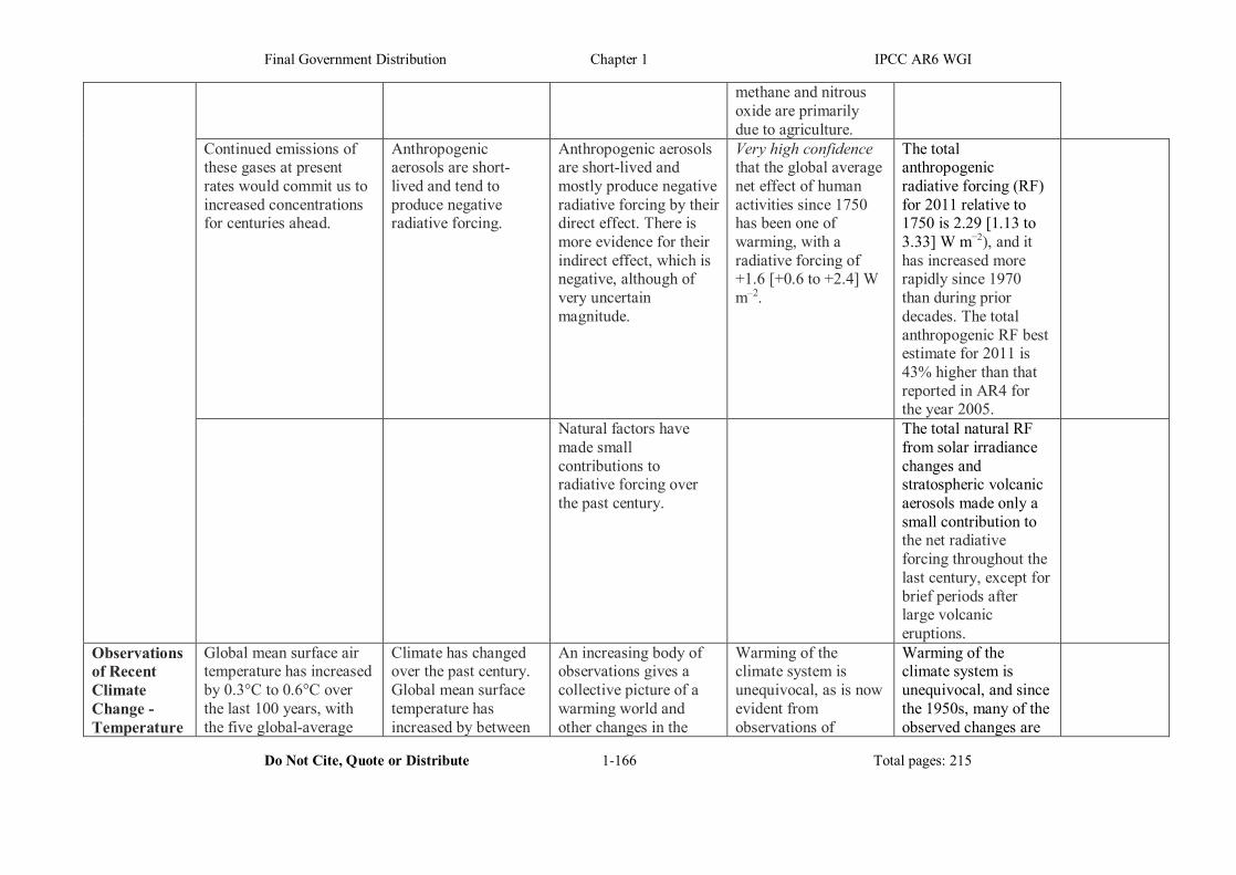
Final Government Distribution Chapter 1 IPCC AR6 WGI
Do Not Cite, Quote or Distribute 1-166 Total pages: 215
methane and nitrous oxide are primarily due to agriculture.
Continued emissions of these gases at present rates would commit us to increased concentrations for centuries ahead.
Anthropogenic aerosols are short-lived and tend to produce negative radiative forcing.
Anthropogenic aerosols are short-lived and mostly produce negative radiative forcing by their direct effect. There is more evidence for their indirect effect, which is negative, although of very uncertain magnitude.
Very high confidence that the global average net effect of human activities since 1750 has been one of warming, with a radiative forcing of +1.6 [+0.6 to +2.4] W m–2.
The total anthropogenic radiative forcing (RF) for 2011 relative to 1750 is 2.29 [1.13 to 3.33] W m−2), and it has increased more rapidly since 1970 than during prior decades. The total anthropogenic RF best estimate for 2011 is 43% higher than that reported in AR4 for the year 2005.
Natural factors have made small contributions to radiative forcing over the past century.
The total natural RF from solar irradiance changes and stratospheric volcanic aerosols made only a small contribution to the net radiative forcing throughout the last century, except for brief periods after large volcanic eruptions.
Observations of Recent Climate Change - Temperature
Global mean surface air temperature has increased by 0.3°C to 0.6°C over the last 100 years, with the five global-average
Climate has changed over the past century. Global mean surface temperature has increased by between
An increasing body of observations gives a collective picture of a warming world and other changes in the
Warming of the climate system is unequivocal, as is now evident from observations of
Warming of the climate system is unequivocal, and since the 1950s, many of the observed changes are
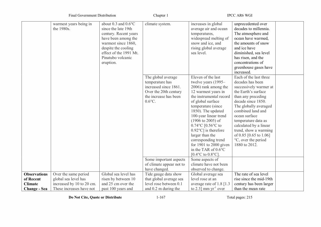
Final Government Distribution Chapter 1 IPCC AR6 WGI
Do Not Cite, Quote or Distribute 1-167 Total pages: 215
warmest years being in the 1980s.
about 0.3 and 0.6°C since the late 19th century. Recent years have been among the warmest since 1860, despite the cooling effect of the 1991 Mt. Pinatubo volcanic eruption.
climate system. increases in global average air and ocean temperatures, widespread melting of snow and ice, and rising global average sea level.
unprecedented over decades to millennia. The atmosphere and ocean have warmed, the amounts of snow and ice have diminished, sea level has risen, and the concentrations of greenhouse gases have increased.
The global average temperature has increased since 1861. Over the 20th century the increase has been 0.6°C.
Eleven of the last twelve years (1995–2006) rank among the 12 warmest years in the instrumental record of global surface temperature (since 1850). The updated 100-year linear trend (1906 to 2005) of 0.74°C [0.56°C to 0.92°C] is therefore larger than the corresponding trend for 1901 to 2000 given in the TAR of 0.6°C [0.4°C to 0.8°C].
Each of the last three decades has been successively warmer at the Earth’s surface than any preceding decade since 1850. The globally averaged combined land and ocean surface temperature data as calculated by a linear trend, show a warming of 0.85 [0.65 to 1.06] °C, over the period 1880 to 2012.
Some important aspects of climate appear not to have changed.
Some aspects of climate have not been observed to change.
Observations of Recent Climate Change - Sea
Over the same period global sea level has increased by 10 to 20 cm. These increases have not
Global sea level has risen by between 10 and 25 cm over the past 100 years and
Tide gauge data show that global average sea level rose between 0.1 and 0.2 m during the
Global average sea level rose at an average rate of 1.8 [1.3 to 2.3] mm yr-1 over
The rate of sea level rise since the mid-19th century has been larger than the mean rate
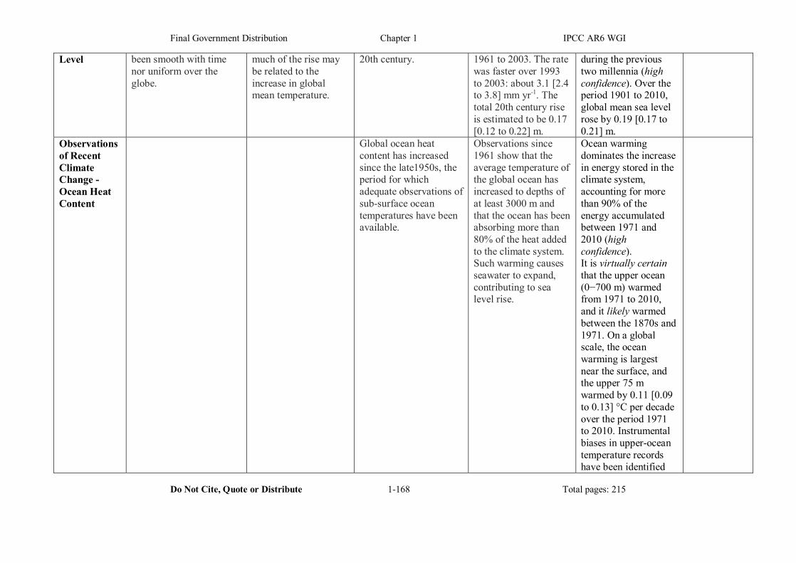
Final Government Distribution Chapter 1 IPCC AR6 WGI
Do Not Cite, Quote or Distribute 1-168 Total pages: 215
Level been smooth with time nor uniform over the globe.
much of the rise may be related to the increase in global mean temperature.
20th century. 1961 to 2003. The rate was faster over 1993 to 2003: about 3.1 [2.4 to 3.8] mm yr-1. The total 20th century rise is estimated to be 0.17 [0.12 to 0.22] m.
during the previous two millennia (high confidence). Over the period 1901 to 2010, global mean sea level rose by 0.19 [0.17 to 0.21] m.
Observations of Recent Climate Change - Ocean Heat Content
Global ocean heat content has increased since the late1950s, the period for which adequate observations of sub-surface ocean temperatures have been available.
Observations since 1961 show that the average temperature of the global ocean has increased to depths of at least 3000 m and that the ocean has been absorbing more than 80% of the heat added to the climate system. Such warming causes seawater to expand, contributing to sea level rise.
Ocean warming dominates the increase in energy stored in the climate system, accounting for more than 90% of the energy accumulated between 1971 and 2010 (high confidence). It is virtually certain that the upper ocean (0−700 m) warmed from 1971 to 2010, and it likely warmed between the 1870s and 1971. On a global scale, the ocean warming is largest near the surface, and the upper 75 m warmed by 0.11 [0.09 to 0.13] °C per decade over the period 1971 to 2010. Instrumental biases in upper-ocean temperature records have been identified
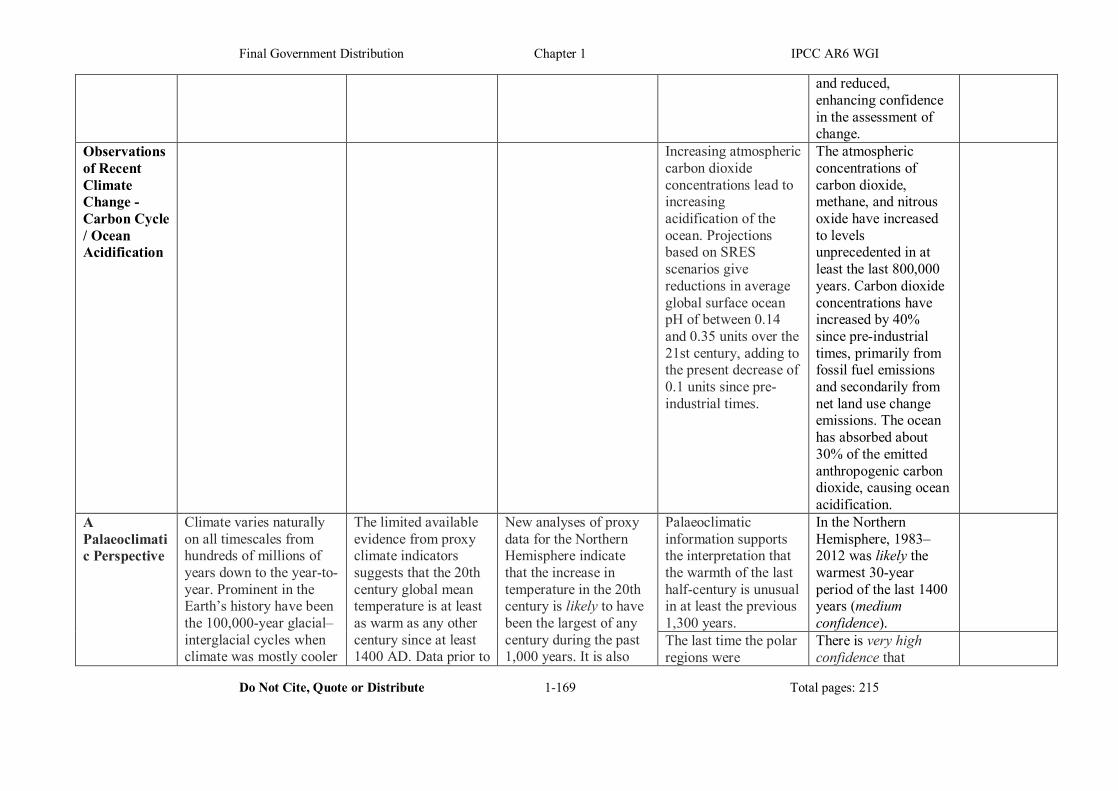
Final Government Distribution Chapter 1 IPCC AR6 WGI
Do Not Cite, Quote or Distribute 1-169 Total pages: 215
and reduced, enhancing confidence in the assessment of change.
Observations of Recent Climate Change - Carbon Cycle / Ocean Acidification
Increasing atmospheric carbon dioxide concentrations lead to increasing acidification of the ocean. Projections based on SRES scenarios give reductions in average global surface ocean pH of between 0.14 and 0.35 units over the 21st century, adding to the present decrease of 0.1 units since pre-industrial times.
The atmospheric concentrations of carbon dioxide, methane, and nitrous oxide have increased to levels unprecedented in at least the last 800,000 years. Carbon dioxide concentrations have increased by 40% since pre-industrial times, primarily from fossil fuel emissions and secondarily from net land use change emissions. The ocean has absorbed about 30% of the emitted anthropogenic carbon dioxide, causing ocean acidification.
A Palaeoclimatic Perspective
Climate varies naturally on all timescales from hundreds of millions of years down to the year-to-year. Prominent in the Earth’s history have been the 100,000-year glacial–interglacial cycles when climate was mostly cooler
The limited available evidence from proxy climate indicators suggests that the 20th century global mean temperature is at least as warm as any other century since at least 1400 AD. Data prior to
New analyses of proxy data for the Northern Hemisphere indicate that the increase in temperature in the 20th century is likely to have been the largest of any century during the past 1,000 years. It is also
Palaeoclimatic information supports the interpretation that the warmth of the last half-century is unusual in at least the previous 1,300 years.
In the Northern Hemisphere, 1983–2012 was likely the warmest 30-year period of the last 1400 years (medium confidence).
The last time the polar regions were
There is very high confidence that
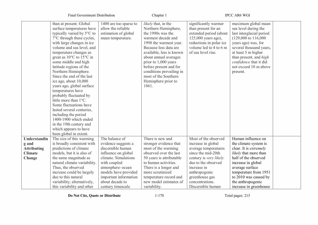
Final Government Distribution Chapter 1 IPCC AR6 WGI
Do Not Cite, Quote or Distribute 1-170 Total pages: 215
than at present. Global surface temperatures have typically varied by 5°C to 7°C through these cycles, with large changes in ice volume and sea level, and temperature changes as great as 10°C to 15°C in some middle and high latitude regions of the Northern Hemisphere. Since the end of the last ice age, about 10,000 years ago, global surface temperatures have probably fluctuated by little more than 1°C. Some fluctuations have lasted several centuries, including the period 1400-1900 which ended in the 19th century and which appears to have been global in extent.
1400 are too sparse to allow the reliable estimation of global mean temperature.
likely that, in the Northern Hemisphere, the 1990s was the warmest decade and 1998 the warmest year. Because less data are available, less is known about annual averages prior to 1,000 years before present and for conditions prevailing in most of the Southern Hemisphere prior to 1861.
significantly warmer than present for an extended period (about 125,000 years ago), reductions in polar ice volume led to 4 to 6 m of sea level rise.
maximum global mean sea level during the last interglacial period (129,000 to 116,000 years ago) was, for several thousand years, at least 5 m higher than present, and high confidence that it did not exceed 10 m above present.
Understanding and Attributing Climate Change
The size of this warming is broadly consistent with predictions of climate models, but it is also of the same magnitude as natural climate variability. Thus, the observed increase could be largely due to this natural variability; alternatively, this variability and other
The balance of evidence suggests a discernible human influence on global climate. Simulations with coupled atmosphere–ocean models have provided important information about decade to century timescale
There is new and stronger evidence that most of the warming observed over the last 50 years is attributable to human activities. There is a longer and more scrutinized temperature record and new model estimates of variability.
Most of the observed increase in global average temperatures since the mid-20th century is very likely due to the observed increase in anthropogenic greenhouse gas concentrations. Discernible human
Human influence on the climate system is clear. It is extremely likely that more than half of the observed increase in global average surface temperature from 1951 to 2010 was caused by the anthropogenic increase in greenhouse
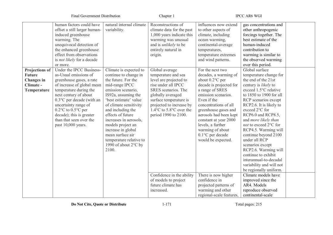
Final Government Distribution Chapter 1 IPCC AR6 WGI
Do Not Cite, Quote or Distribute 1-171 Total pages: 215
human factors could have offset a still larger human-induced greenhouse warming. The unequivocal detection of the enhanced greenhouse effect from observations is not likely for a decade or more.
natural internal climate variability.
Reconstructions of climate data for the past 1,000 years indicate this warming was unusual and is unlikely to be entirely natural in origin.
influences now extend to other aspects of climate, including ocean warming, continental-average temperatures, temperature extremes and wind patterns.
gas concentrations and other anthropogenic forcings together. The best estimate of the human-induced contribution to warming is similar to the observed warming over this period.
Projections of Future Changes in Climate - Temperature
Under the IPCC Business-as-Usual emissions of greenhouse gases, a rate of increase of global mean temperature during the next century of about 0.3°C per decade (with an uncertainty range of 0.2°C to 0.5°C per decade); this is greater than that seen over the past 10,000 years.
Climate is expected to continue to change in the future. For the mid-range IPCC emission scenario, IS92a, assuming the ‘best estimate’ value of climate sensitivity and including the effects of future increases in aerosols, models project an increase in global mean surface air temperature relative to 1990 of about 2°C by 2100.
Global average temperature and sea level are projected to rise under all IPCC SRES scenarios. The globally averaged surface temperature is projected to increase by 1.4°C to 5.8°C over the period 1990 to 2100.
For the next two decades, a warming of about 0.2°C per decade is projected for a range of SRES emission scenarios. Even if the concentrations of all greenhouse gases and aerosols had been kept constant at year 2000 levels, a further warming of about 0.1°C per decade would be expected.
Global surface temperature change for the end of the 21st century is likely to exceed 1.5°C relative to 1850 to 1900 for all RCP scenarios except RCP2.6. It is likely to exceed 2°C for RCP6.0 and RCP8.5, and more likely than not to exceed 2°C for RCP4.5. Warming will continue beyond 2100 under all RCP scenarios except RCP2.6. Warming will continue to exhibit interannual-to-decadal variability and will not be regionally uniform.
Confidence in the ability of models to project future climate has increased.
There is now higher confidence in projected patterns of warming and other regional-scale features,
Climate models have improved since the AR4. Models reproduce observed continental-scale
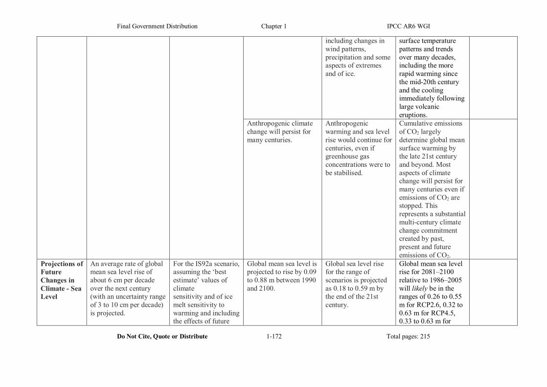
Final Government Distribution Chapter 1 IPCC AR6 WGI
Do Not Cite, Quote or Distribute 1-172 Total pages: 215
including changes in wind patterns, precipitation and some aspects of extremes and of ice.
surface temperature patterns and trends over many decades, including the more rapid warming since the mid-20th century and the cooling immediately following large volcanic eruptions.
Anthropogenic climate change will persist for many centuries.
Anthropogenic warming and sea level rise would continue for centuries, even if greenhouse gas concentrations were to be stabilised.
Cumulative emissions of CO2 largely determine global mean surface warming by the late 21st century and beyond. Most aspects of climate change will persist for many centuries even if emissions of CO2 are stopped. This represents a substantial multi-century climate change commitment created by past, present and future emissions of CO2.
Projections of Future Changes in Climate - Sea Level
An average rate of global mean sea level rise of about 6 cm per decade over the next century (with an uncertainty range of 3 to 10 cm per decade) is projected.
For the IS92a scenario, assuming the ‘best estimate’ values of climate sensitivity and of ice melt sensitivity to warming and including the effects of future
Global mean sea level is projected to rise by 0.09 to 0.88 m between 1990 and 2100.
Global sea level rise for the range of scenarios is projected as 0.18 to 0.59 m by the end of the 21st century.
Global mean sea level rise for 2081–2100 relative to 1986–2005 will likely be in the ranges of 0.26 to 0.55 m for RCP2.6, 0.32 to 0.63 m for RCP4.5, 0.33 to 0.63 m for
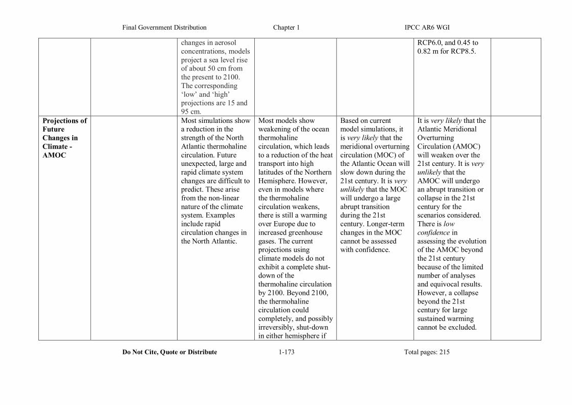
Final Government Distribution Chapter 1 IPCC AR6 WGI
Do Not Cite, Quote or Distribute 1-173 Total pages: 215
changes in aerosol concentrations, models project a sea level rise of about 50 cm from the present to 2100. The corresponding ‘low’ and ‘high’ projections are 15 and 95 cm.
RCP6.0, and 0.45 to 0.82 m for RCP8.5.
Projections of Future Changes in Climate - AMOC
Most simulations show a reduction in the strength of the North Atlantic thermohaline circulation. Future unexpected, large and rapid climate system changes are difficult to predict. These arise from the non-linear nature of the climate system. Examples include rapid circulation changes in the North Atlantic.
Most models show weakening of the ocean thermohaline circulation, which leads to a reduction of the heat transport into high latitudes of the Northern Hemisphere. However, even in models where the thermohaline circulation weakens, there is still a warming over Europe due to increased greenhouse gases. The current projections using climate models do not exhibit a complete shut-down of the thermohaline circulation by 2100. Beyond 2100, the thermohaline circulation could completely, and possibly irreversibly, shut-down in either hemisphere if
Based on current model simulations, it is very likely that the meridional overturning circulation (MOC) of the Atlantic Ocean will slow down during the 21st century. It is very unlikely that the MOC will undergo a large abrupt transition during the 21st century. Longer-term changes in the MOC cannot be assessed with confidence.
It is very likely that the Atlantic Meridional Overturning Circulation (AMOC) will weaken over the 21st century. It is very unlikely that the AMOC will undergo an abrupt transition or collapse in the 21st century for the scenarios considered. There is low confidence in assessing the evolution of the AMOC beyond the 21st century because of the limited number of analyses and equivocal results. However, a collapse beyond the 21st century for large sustained warming cannot be excluded.

Final Government Distribution Chapter 1 IPCC AR6 WGI
Do Not Cite, Quote or Distribute 1-174 Total pages: 215
[END TABLE 1.A.1 HERE]
the change in radiative forcing is large enough and applied long enough.
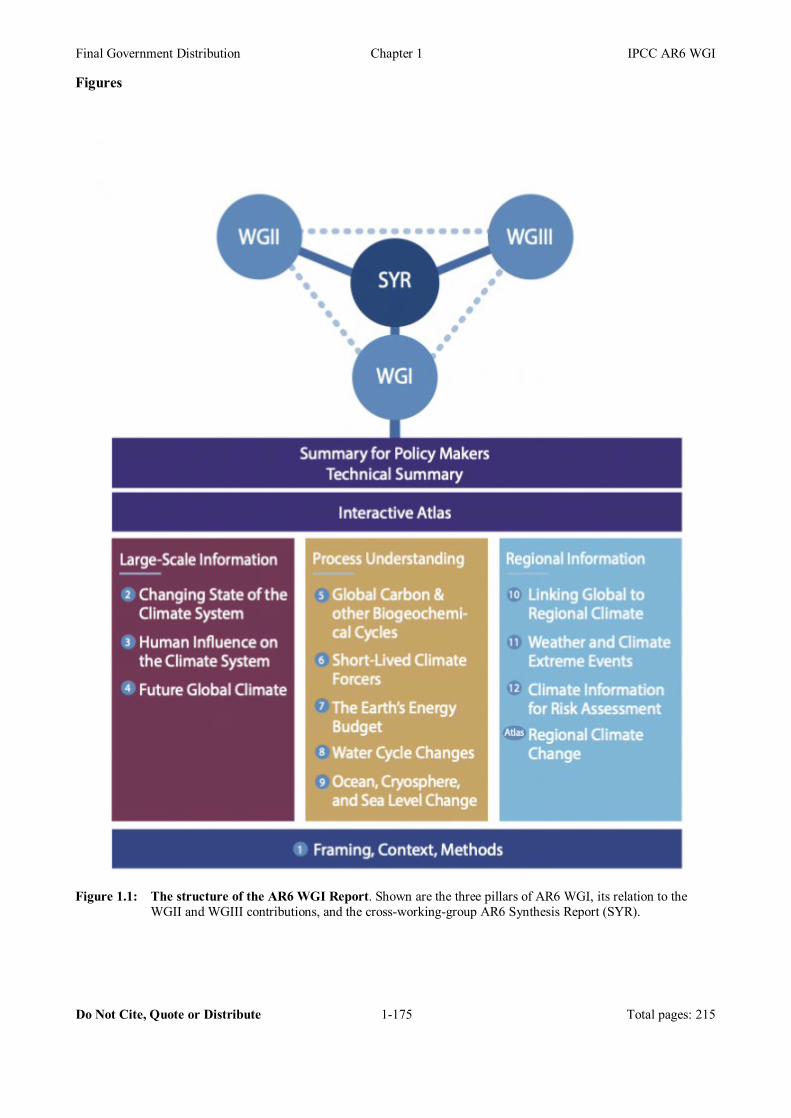
Final Government Distribution Chapter 1 IPCC AR6 WGI
Do Not Cite, Quote or Distribute 1-175 Total pages: 215
Figures
Figure 1.1: The structure of the AR6 WGI Report. Shown are the three pillars of AR6 WGI, its relation to the
WGII and WGIII contributions, and the cross-working-group AR6 Synthesis Report (SYR).
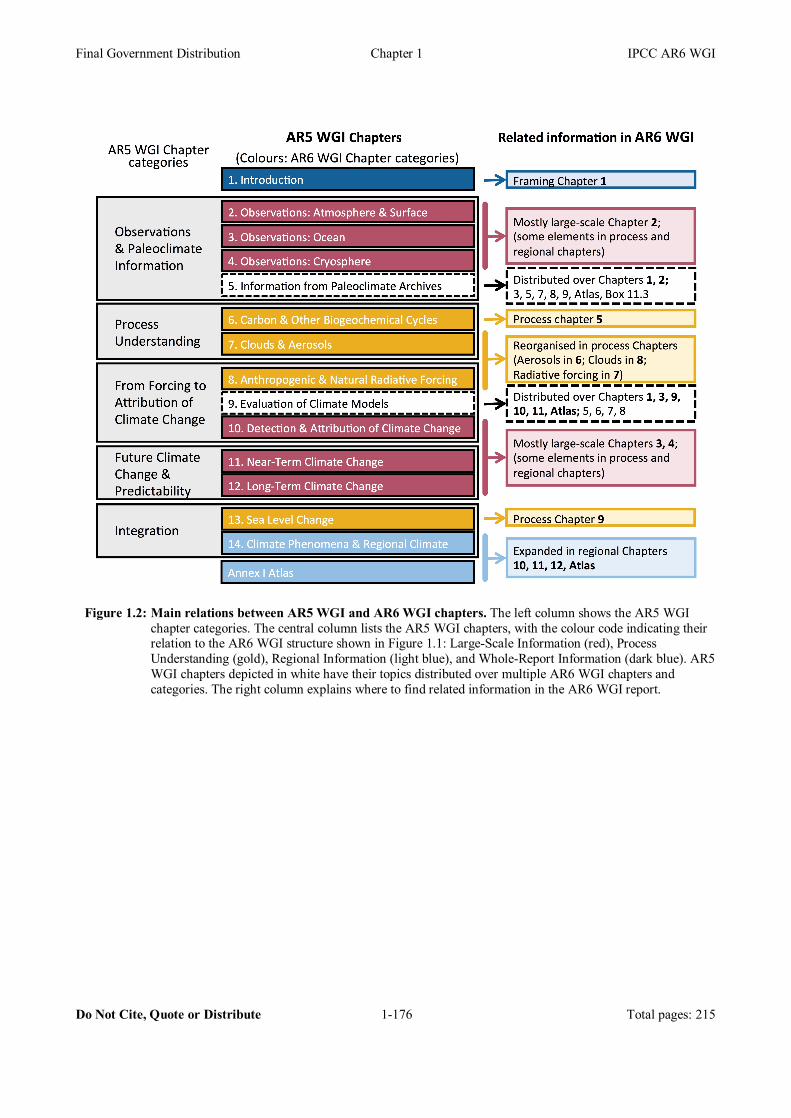
Final Government Distribution Chapter 1 IPCC AR6 WGI
Do Not Cite, Quote or Distribute 1-176 Total pages: 215
Figure 1.2: Main relations between AR5 WGI and AR6 WGI chapters. The left column shows the AR5 WGI chapter categories. The central column lists the AR5 WGI chapters, with the colour code indicating their relation to the AR6 WGI structure shown in Figure 1.1: Large-Scale Information (red), Process Understanding (gold), Regional Information (light blue), and Whole-Report Information (dark blue). AR5 WGI chapters depicted in white have their topics distributed over multiple AR6 WGI chapters and categories. The right column explains where to find related information in the AR6 WGI report.
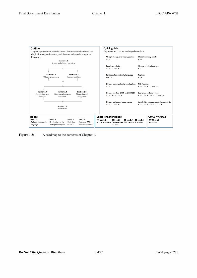
Final Government Distribution Chapter 1 IPCC AR6 WGI
Do Not Cite, Quote or Distribute 1-177 Total pages: 215
Figure 1.3: A roadmap to the contents of Chapter 1.
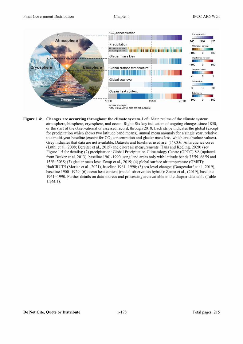
Final Government Distribution Chapter 1 IPCC AR6 WGI
Do Not Cite, Quote or Distribute 1-178 Total pages: 215
Figure 1.4: Changes are occurring throughout the climate system. Left: Main realms of the climate system: atmosphere, biosphere, cryosphere, and ocean. Right: Six key indicators of ongoing changes since 1850, or the start of the observational or assessed record, through 2018. Each stripe indicates the global (except for precipitation which shows two latitude band means), annual mean anomaly for a single year, relative to a multi-year baseline (except for CO2 concentration and glacier mass loss, which are absolute values). Grey indicates that data are not available. Datasets and baselines used are: (1) CO2: Antarctic ice cores (Lüthi et al., 2008; Bereiter et al., 2015) and direct air measurements (Tans and Keeling, 2020) (see Figure 1.5 for details); (2) precipitation: Global Precipitation Climatology Centre (GPCC) V8 (updated from Becker et al. 2013), baseline 1961-1990 using land areas only with latitude bands 33°N–66°N and 15°S–30°S; (3) glacier mass loss: Zemp et al., 2019; (4) global surface air temperature (GMST): HadCRUT5 (Morice et al., 2021), baseline 1961–1990; (5) sea level change: (Dangendorf et al., 2019), baseline 1900–1929; (6) ocean heat content (model-observation hybrid): Zanna et al., (2019), baseline 1961–1990. Further details on data sources and processing are available in the chapter data table (Table 1.SM.1).
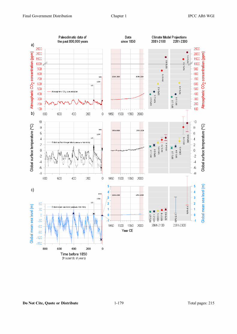
Final Government Distribution Chapter 1 IPCC AR6 WGI
Do Not Cite, Quote or Distribute 1-179 Total pages: 215
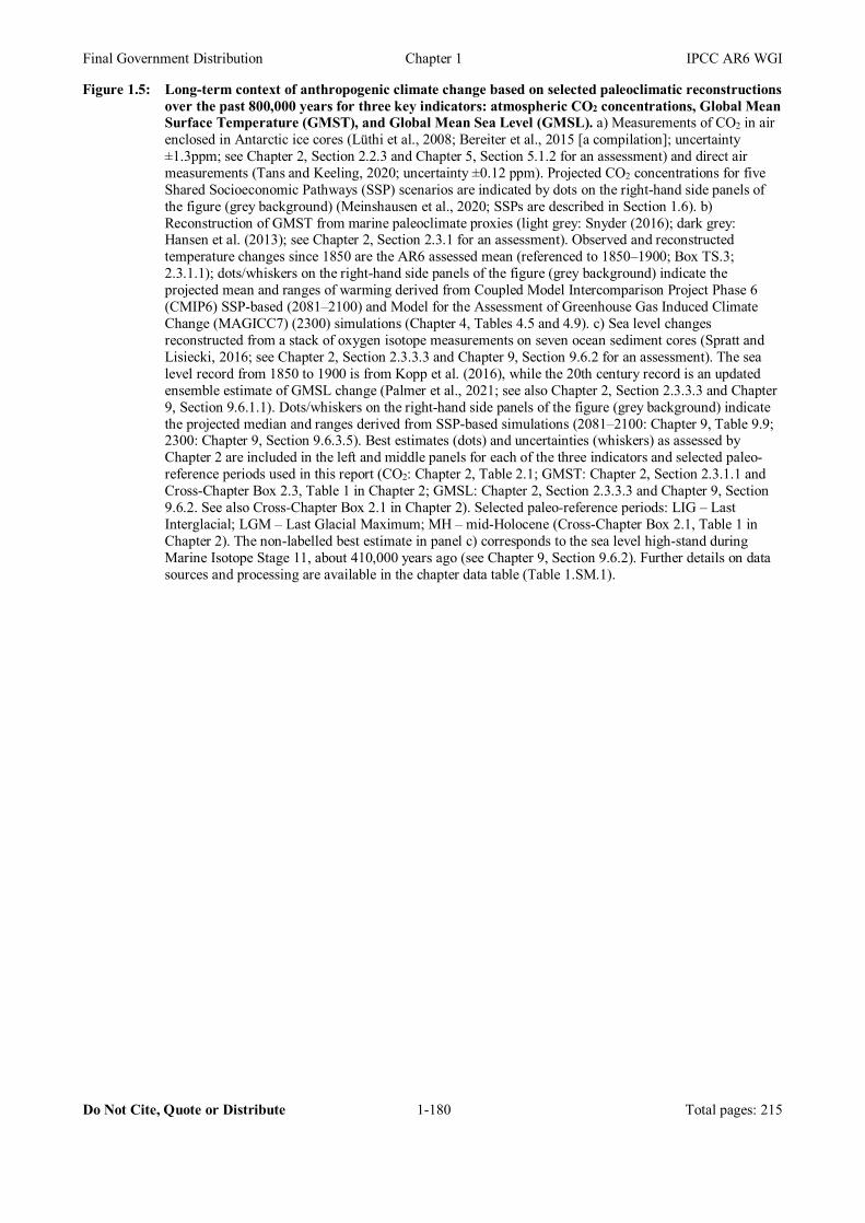
Final Government Distribution Chapter 1 IPCC AR6 WGI
Do Not Cite, Quote or Distribute 1-180 Total pages: 215
Figure 1.5: Long-term context of anthropogenic climate change based on selected paleoclimatic reconstructions over the past 800,000 years for three key indicators: atmospheric CO2 concentrations, Global Mean Surface Temperature (GMST), and Global Mean Sea Level (GMSL). a) Measurements of CO2 in air enclosed in Antarctic ice cores (Lüthi et al., 2008; Bereiter et al., 2015 [a compilation]; uncertainty ±1.3ppm; see Chapter 2, Section 2.2.3 and Chapter 5, Section 5.1.2 for an assessment) and direct air measurements (Tans and Keeling, 2020; uncertainty ±0.12 ppm). Projected CO2 concentrations for five Shared Socioeconomic Pathways (SSP) scenarios are indicated by dots on the right-hand side panels of the figure (grey background) (Meinshausen et al., 2020; SSPs are described in Section 1.6). b) Reconstruction of GMST from marine paleoclimate proxies (light grey: Snyder (2016); dark grey: Hansen et al. (2013); see Chapter 2, Section 2.3.1 for an assessment). Observed and reconstructed temperature changes since 1850 are the AR6 assessed mean (referenced to 1850–1900; Box TS.3; 2.3.1.1); dots/whiskers on the right-hand side panels of the figure (grey background) indicate the projected mean and ranges of warming derived from Coupled Model Intercomparison Project Phase 6 (CMIP6) SSP-based (2081–2100) and Model for the Assessment of Greenhouse Gas Induced Climate Change (MAGICC7) (2300) simulations (Chapter 4, Tables 4.5 and 4.9). c) Sea level changes reconstructed from a stack of oxygen isotope measurements on seven ocean sediment cores (Spratt and Lisiecki, 2016; see Chapter 2, Section 2.3.3.3 and Chapter 9, Section 9.6.2 for an assessment). The sea level record from 1850 to 1900 is from Kopp et al. (2016), while the 20th century record is an updated ensemble estimate of GMSL change (Palmer et al., 2021; see also Chapter 2, Section 2.3.3.3 and Chapter 9, Section 9.6.1.1). Dots/whiskers on the right-hand side panels of the figure (grey background) indicate the projected median and ranges derived from SSP-based simulations (2081–2100: Chapter 9, Table 9.9; 2300: Chapter 9, Section 9.6.3.5). Best estimates (dots) and uncertainties (whiskers) as assessed by Chapter 2 are included in the left and middle panels for each of the three indicators and selected paleo-reference periods used in this report (CO2: Chapter 2, Table 2.1; GMST: Chapter 2, Section 2.3.1.1 and Cross-Chapter Box 2.3, Table 1 in Chapter 2; GMSL: Chapter 2, Section 2.3.3.3 and Chapter 9, Section 9.6.2. See also Cross-Chapter Box 2.1 in Chapter 2). Selected paleo-reference periods: LIG – Last Interglacial; LGM – Last Glacial Maximum; MH – mid-Holocene (Cross-Chapter Box 2.1, Table 1 in Chapter 2). The non-labelled best estimate in panel c) corresponds to the sea level high-stand during Marine Isotope Stage 11, about 410,000 years ago (see Chapter 9, Section 9.6.2). Further details on data sources and processing are available in the chapter data table (Table 1.SM.1).

Final Government Distribution Chapter 1 IPCC AR6 WGI
Do Not Cite, Quote or Distribute 1-181 Total pages: 215
Box 1.1, Figure 1: The IPCC AR6 approach for characterizing understanding and uncertainty in assessment findings. This diagram illustrates the step-by-step process authors use to evaluate and communicate the state of knowledge in their assessment (Mastrandrea et al., 2010). Authors present evidence/agreement, confidence, or likelihood terms with assessment conclusions, communicating their expert judgments accordingly. Example conclusions drawn from this report are presented in the box at the bottom of the figure. [adapted from Mach et al. (2017)].

Final Government Distribution Chapter 1 IPCC AR6 WGI
Do Not Cite, Quote or Distribute 1-182 Total pages: 215
Figure 1.6: Climate science milestones, between 1817-2021. Milestones in observations (top); Curves of global
surface air temperature (GMST) using HadCRUT5 (Morice et al., 2021) and atmospheric CO2 concentrations from Antarctic ice cores (Lüthi et al., 2008; Bereiter et al., 2015) and direct air measurements from 1957 onwards (Tans and Keeling, 2020) (see Figure 1.4 for details) (middle). Milestone in scientific understanding of the CO2 enhanced greenhouse effect (bottom). Further details on each milestone are available in Chapter 1, Section 1.3, and Chapter 1 of AR4.
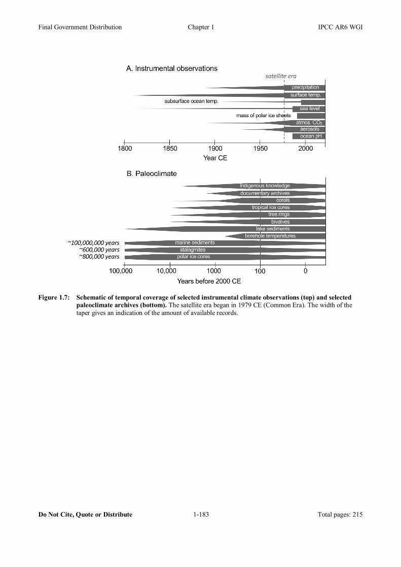
Final Government Distribution Chapter 1 IPCC AR6 WGI
Do Not Cite, Quote or Distribute 1-183 Total pages: 215
Figure 1.7: Schematic of temporal coverage of selected instrumental climate observations (top) and selected
paleoclimate archives (bottom). The satellite era began in 1979 CE (Common Era). The width of the taper gives an indication of the amount of available records.
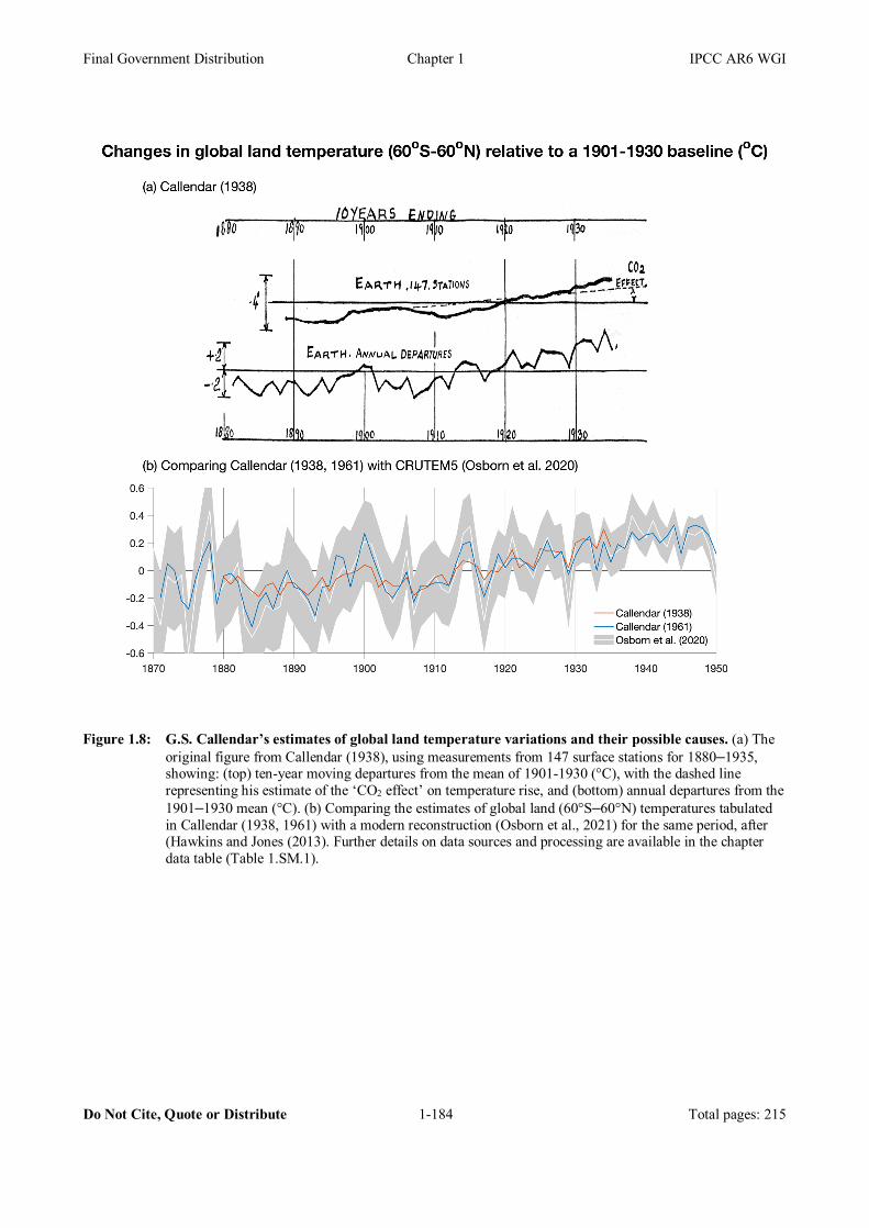
Final Government Distribution Chapter 1 IPCC AR6 WGI
Do Not Cite, Quote or Distribute 1-184 Total pages: 215
Figure 1.8: G.S. Callendar’s estimates of global land temperature variations and their possible causes. (a) The original figure from Callendar (1938), using measurements from 147 surface stations for 1880–1935, showing: (top) ten-year moving departures from the mean of 1901-1930 (°C), with the dashed line representing his estimate of the ‘CO2 effect’ on temperature rise, and (bottom) annual departures from the 1901–1930 mean (°C). (b) Comparing the estimates of global land (60°S–60°N) temperatures tabulated in Callendar (1938, 1961) with a modern reconstruction (Osborn et al., 2021) for the same period, after (Hawkins and Jones (2013). Further details on data sources and processing are available in the chapter data table (Table 1.SM.1).

Final Government Distribution Chapter 1 IPCC AR6 WGI
Do Not Cite, Quote or Distribute 1-185 Total pages: 215
Figure 1.9: Assessing past projections of global temperature change. Projected temperature change post-publication on a temperature vs time (1970–2020, top panel) and temperature vs radiative forcing (1970–2017, bottom panel) basis for a selection of prominent climate model projections (taken from Hausfather et al., 2020). Model projections (using global surface air temperature, GSAT) are compared to temperature observations (using global mean surface temperature, GMST) from HadCRUT5 (black) and anthropogenic forcings (through 2017) from Dessler and Forster (2018), and have a baseline generated from the first five years of the projection period. Projections shown are: Manabe (1970), Rasool and

Final Government Distribution Chapter 1 IPCC AR6 WGI
Do Not Cite, Quote or Distribute 1-186 Total pages: 215
Schneider (1971), Broecker (1975), Nordhaus (1977), Hansen et al. (1981, H81), Hansen et al. (1988, H88), Manabe and Stouffer (1993), along with the Energy Balance Model (EBM) projections from the FAR, SAR and TAR, and the multi-model mean projection using CMIP3 simulations of the Special Reports on Emission Scenarios (SRES) A1B scenario from AR4. H81 and H88 show most expected scenarios 1 and B, respectively. See Hausfather et al. (2020) for more details of the projections. Further details on data sources and processing are available in the chapter data table (Table 1.SM.1).
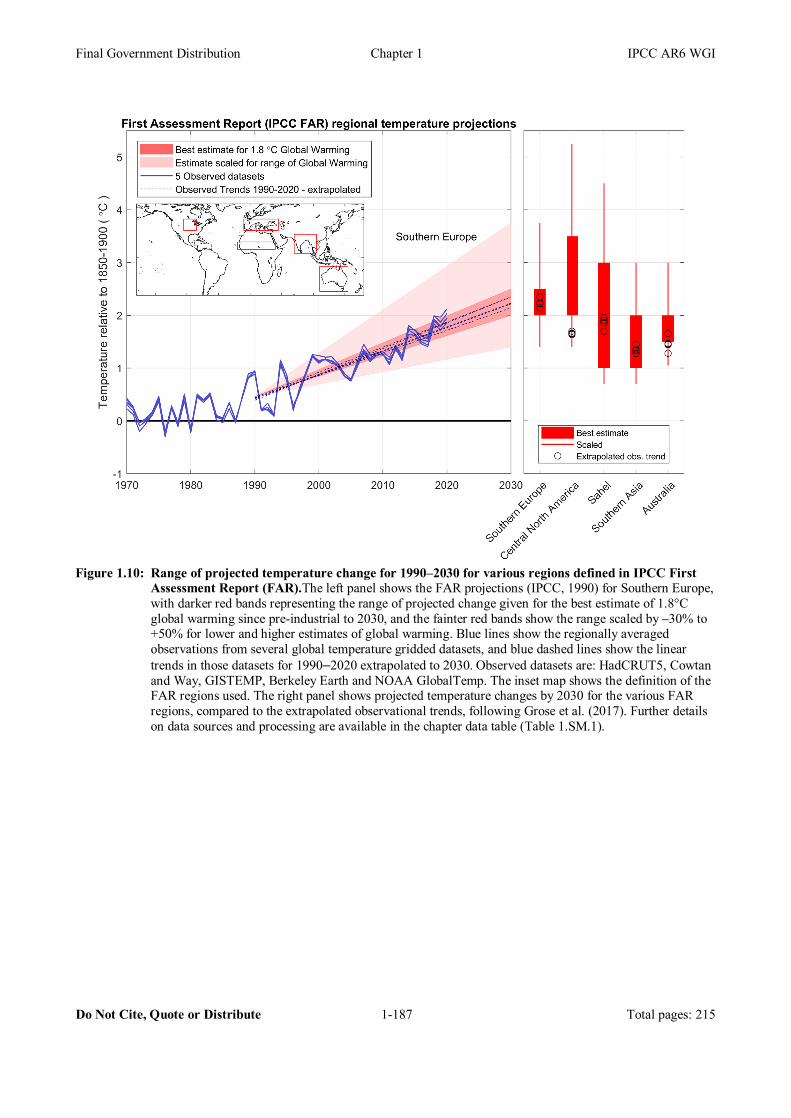
Final Government Distribution Chapter 1 IPCC AR6 WGI
Do Not Cite, Quote or Distribute 1-187 Total pages: 215
Figure 1.10: Range of projected temperature change for 1990–2030 for various regions defined in IPCC First
Assessment Report (FAR).The left panel shows the FAR projections (IPCC, 1990) for Southern Europe, with darker red bands representing the range of projected change given for the best estimate of 1.8°C global warming since pre-industrial to 2030, and the fainter red bands show the range scaled by –30% to +50% for lower and higher estimates of global warming. Blue lines show the regionally averaged observations from several global temperature gridded datasets, and blue dashed lines show the linear trends in those datasets for 1990–2020 extrapolated to 2030. Observed datasets are: HadCRUT5, Cowtan and Way, GISTEMP, Berkeley Earth and NOAA GlobalTemp. The inset map shows the definition of the FAR regions used. The right panel shows projected temperature changes by 2030 for the various FAR regions, compared to the extrapolated observational trends, following Grose et al. (2017). Further details on data sources and processing are available in the chapter data table (Table 1.SM.1).

Final Government Distribution Chapter 1 IPCC AR6 WGI
Do Not Cite, Quote or Distribute 1-188 Total pages: 215
Figure 1.11: Choice of baseline matters when comparing observations and model simulations. Global mean
surface air temperature (GSAT, grey) from a range of CMIP6 historical simulations (1850–2014, 25 models) and SSP1-2.6 (2015–2100) using absolute values (top) and anomalies relative to two different baselines: 1850–1900 (middle) and 1995–2014 (bottom). An estimate of GSAT from a reanalysis (ERA-5, orange, 1979–2020) and an observation-based estimate of global mean surface air temperature (GMST) (Berkeley Earth, black, 1850–2020) are shown, along with the mean GSAT for 1961–1990 estimated by Jones et al. (1999), light blue shading, 14.0±0.5°C). Using the more recent baseline (bottom) allows the inclusion of datasets which do not include the periods of older baselines. The middle and bottom panels have scales which are the same size but offset. Further details on data sources and processing are available in the chapter data table (Table 1.SM.1).
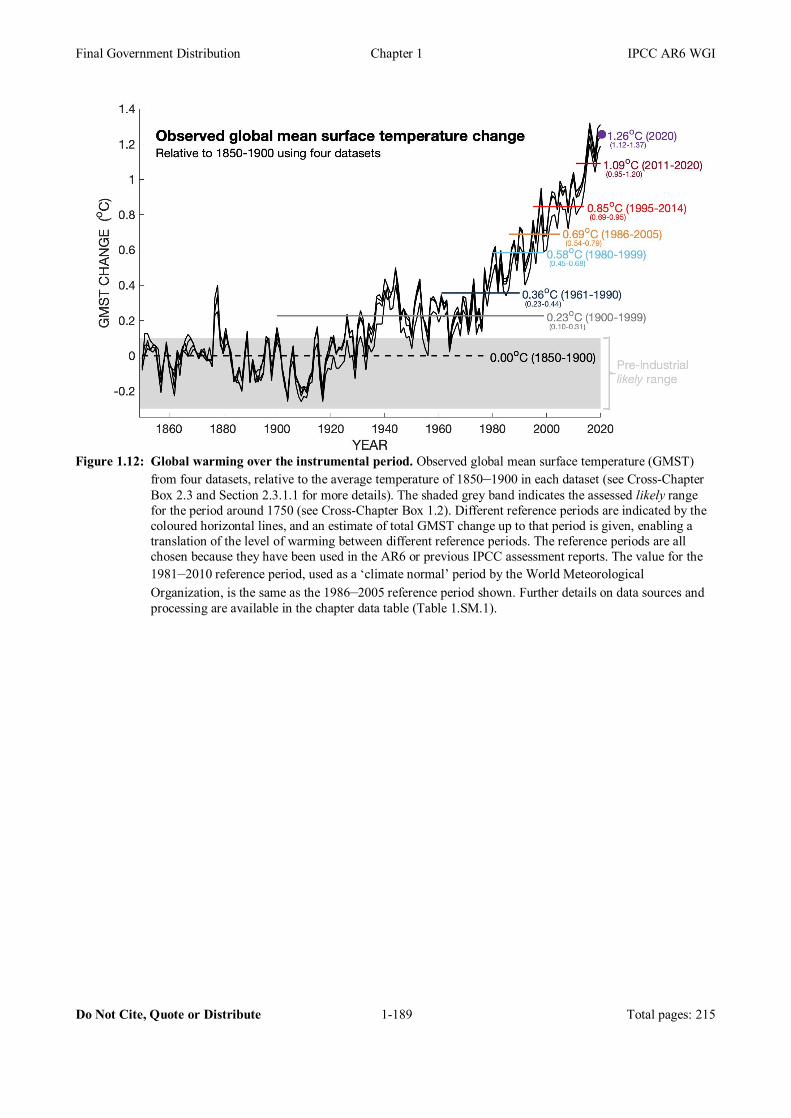
Final Government Distribution Chapter 1 IPCC AR6 WGI
Do Not Cite, Quote or Distribute 1-189 Total pages: 215
Figure 1.12: Global warming over the instrumental period. Observed global mean surface temperature (GMST)
from four datasets, relative to the average temperature of 1850–1900 in each dataset (see Cross-Chapter Box 2.3 and Section 2.3.1.1 for more details). The shaded grey band indicates the assessed likely range for the period around 1750 (see Cross-Chapter Box 1.2). Different reference periods are indicated by the coloured horizontal lines, and an estimate of total GMST change up to that period is given, enabling a translation of the level of warming between different reference periods. The reference periods are all chosen because they have been used in the AR6 or previous IPCC assessment reports. The value for the 1981–2010 reference period, used as a ‘climate normal’ period by the World Meteorological Organization, is the same as the 1986–2005 reference period shown. Further details on data sources and processing are available in the chapter data table (Table 1.SM.1).
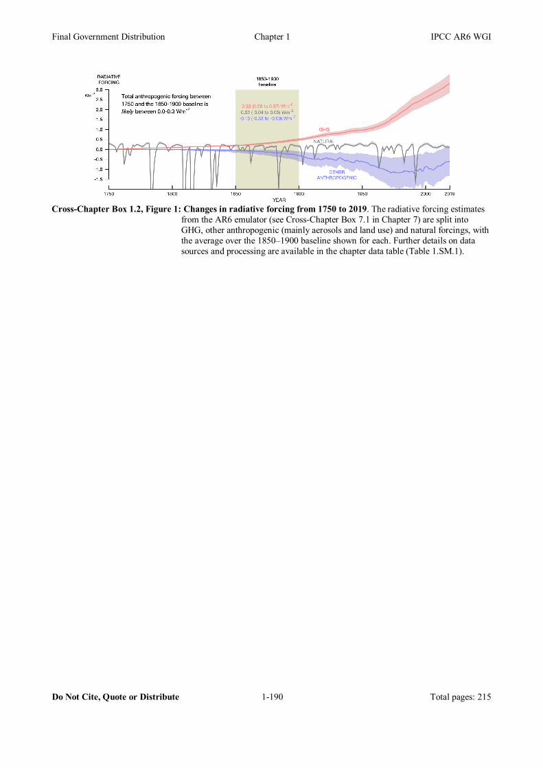
Final Government Distribution Chapter 1 IPCC AR6 WGI
Do Not Cite, Quote or Distribute 1-190 Total pages: 215
Cross-Chapter Box 1.2, Figure 1: Changes in radiative forcing from 1750 to 2019. The radiative forcing estimates
from the AR6 emulator (see Cross-Chapter Box 7.1 in Chapter 7) are split into GHG, other anthropogenic (mainly aerosols and land use) and natural forcings, with the average over the 1850–1900 baseline shown for each. Further details on data sources and processing are available in the chapter data table (Table 1.SM.1).
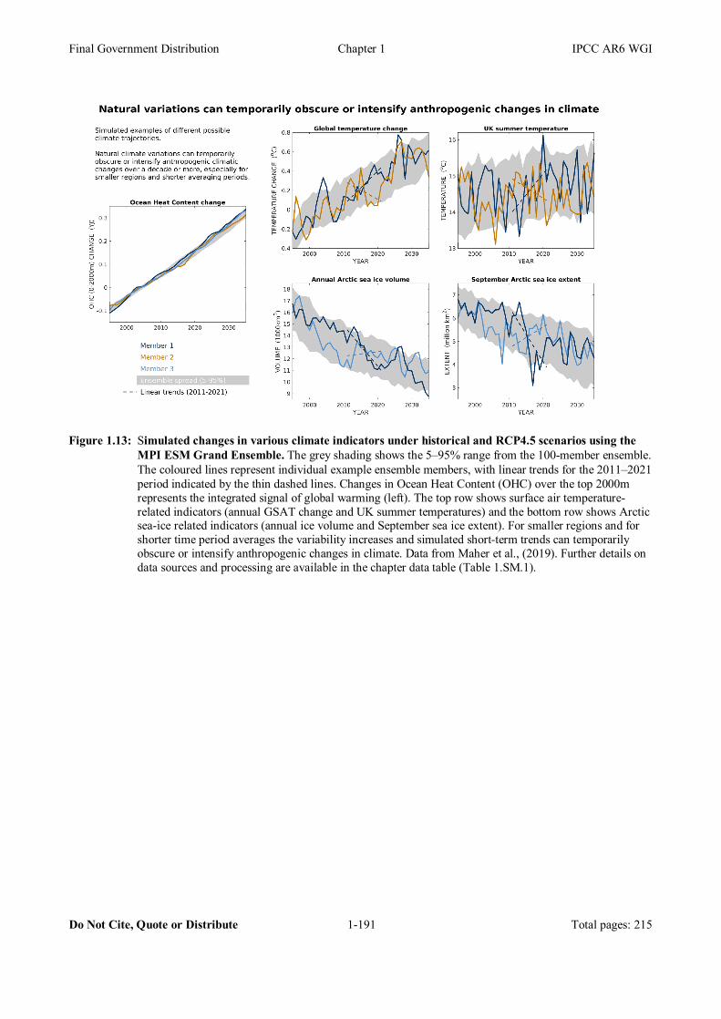
Final Government Distribution Chapter 1 IPCC AR6 WGI
Do Not Cite, Quote or Distribute 1-191 Total pages: 215
Figure 1.13: Simulated changes in various climate indicators under historical and RCP4.5 scenarios using the
MPI ESM Grand Ensemble. The grey shading shows the 5–95% range from the 100-member ensemble. The coloured lines represent individual example ensemble members, with linear trends for the 2011–2021 period indicated by the thin dashed lines. Changes in Ocean Heat Content (OHC) over the top 2000m represents the integrated signal of global warming (left). The top row shows surface air temperature-related indicators (annual GSAT change and UK summer temperatures) and the bottom row shows Arctic sea-ice related indicators (annual ice volume and September sea ice extent). For smaller regions and for shorter time period averages the variability increases and simulated short-term trends can temporarily obscure or intensify anthropogenic changes in climate. Data from Maher et al., (2019). Further details on data sources and processing are available in the chapter data table (Table 1.SM.1).
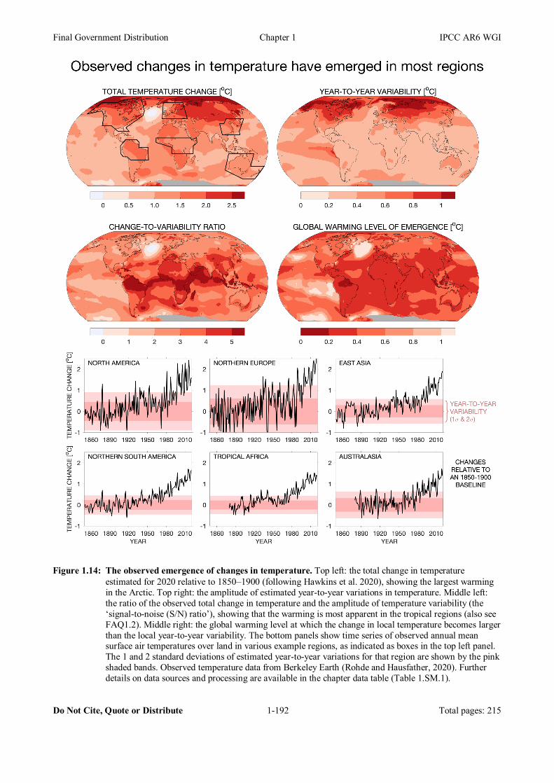
Final Government Distribution Chapter 1 IPCC AR6 WGI
Do Not Cite, Quote or Distribute 1-192 Total pages: 215
Figure 1.14: The observed emergence of changes in temperature. Top left: the total change in temperature estimated for 2020 relative to 1850–1900 (following Hawkins et al. 2020), showing the largest warming in the Arctic. Top right: the amplitude of estimated year-to-year variations in temperature. Middle left: the ratio of the observed total change in temperature and the amplitude of temperature variability (the ‘signal-to-noise (S/N) ratio’), showing that the warming is most apparent in the tropical regions (also see FAQ1.2). Middle right: the global warming level at which the change in local temperature becomes larger than the local year-to-year variability. The bottom panels show time series of observed annual mean surface air temperatures over land in various example regions, as indicated as boxes in the top left panel. The 1 and 2 standard deviations of estimated year-to-year variations for that region are shown by the pink shaded bands. Observed temperature data from Berkeley Earth (Rohde and Hausfather, 2020). Further details on data sources and processing are available in the chapter data table (Table 1.SM.1).
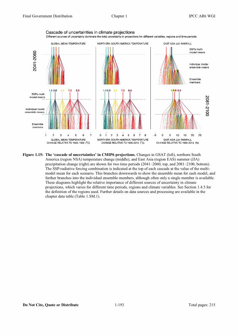
Final Government Distribution Chapter 1 IPCC AR6 WGI
Do Not Cite, Quote or Distribute 1-193 Total pages: 215
Figure 1.15: The ‘cascade of uncertainties’ in CMIP6 projections. Changes in GSAT (left), northern South
America (region NSA) temperature change (middle), and East Asia (region EAS) summer (JJA) precipitation change (right) are shown for two time periods (2041–2060, top, and 2081–2100, bottom). The SSP-radiative forcing combination is indicated at the top of each cascade at the value of the multi-model mean for each scenario. This branches downwards to show the ensemble mean for each model, and further branches into the individual ensemble members, although often only a single member is available. These diagrams highlight the relative importance of different sources of uncertainty in climate projections, which varies for different time periods, regions and climate variables. See Section 1.4.5 for the definition of the regions used. Further details on data sources and processing are available in the chapter data table (Table 1.SM.1).
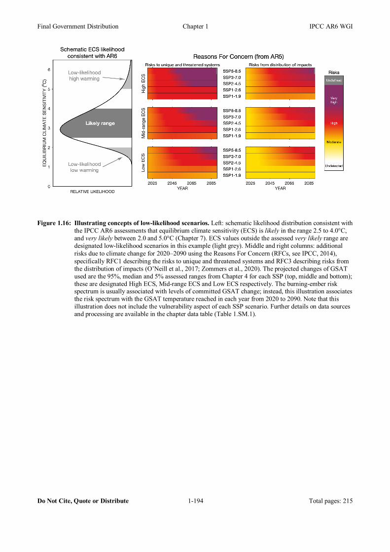
Final Government Distribution Chapter 1 IPCC AR6 WGI
Do Not Cite, Quote or Distribute 1-194 Total pages: 215
Figure 1.16: Illustrating concepts of low-likelihood scenarios. Left: schematic likelihood distribution consistent with
the IPCC AR6 assessments that equilibrium climate sensitivity (ECS) is likely in the range 2.5 to 4.0°C, and very likely between 2.0 and 5.0°C (Chapter 7). ECS values outside the assessed very likely range are designated low-likelihood scenarios in this example (light grey). Middle and right columns: additional risks due to climate change for 2020–2090 using the Reasons For Concern (RFCs, see IPCC, 2014), specifically RFC1 describing the risks to unique and threatened systems and RFC3 describing risks from the distribution of impacts (O’Neill et al., 2017; Zommers et al., 2020). The projected changes of GSAT used are the 95%, median and 5% assessed ranges from Chapter 4 for each SSP (top, middle and bottom); these are designated High ECS, Mid-range ECS and Low ECS respectively. The burning-ember risk spectrum is usually associated with levels of committed GSAT change; instead, this illustration associates the risk spectrum with the GSAT temperature reached in each year from 2020 to 2090. Note that this illustration does not include the vulnerability aspect of each SSP scenario. Further details on data sources and processing are available in the chapter data table (Table 1.SM.1).

Final Government Distribution Chapter 1 IPCC AR6 WGI
Do Not Cite, Quote or Distribute 1-195 Total pages: 215
Figure 1.17: Illustration of two types of tipping points: noise-induced (panels a, b) and bifurcation (panels c, d).
(a), (c) example time-series (coloured lines) through the tipping point with black solid lines indicating stable climate states (e.g., low or high rainfall) and dashed lines represent the boundary between stable states. (b), (d) stability landscapes provide an intuitive understanding for the different types of tipping point. The valleys represent different climate states the system can occupy, with hill tops separating the stable states. The resilience of a climate state is implied by the depth of the valley. The current state of the system is represented by a ball. Both scenarios assume that the ball starts in the left-hand valley (black dashed lines) and then through different mechanisms dependent on the type of tipping transitions to the right valley (coloured lines). Noise-induced tipping events, for instance drought events causing sudden dieback of the Amazonian rainforest, develop from fluctuations within the system. The stability landscape in this scenario remains fixed and stationary. A series of perturbations in the same direction or one large perturbation are required to force the system over the hill top and into the alternative stable state. Bifurcation tipping events, such as a collapse of the thermohaline circulation in the Atlantic Ocean under climate change, occur when a critical level in the forcing is reached. Here the stability landscape is subjected to a change in shape. Under gradual anthropogenic forcing the left valley begins to shallow and eventually vanishes at the tipping point, forcing the system to transition to the right-hand valley.

Final Government Distribution Chapter 1 IPCC AR6 WGI
Do Not Cite, Quote or Distribute 1-196 Total pages: 215
Cross-Working Group Box: Attribution, Figure 1: Schematic of the steps to develop an attribution assessment,
and the purposes of such assessments. Methods and systems used to test the attribution hypothesis or theory include model-based fingerprinting, other model-based methods, evidence-based fingerprinting, process-based approaches, empirical or decomposition methods and the use of multiple lines of evidence. Many of the methods are based on the comparison of the observed state of a system to a hypothetical counterfactual world that does not include the driver of interest to help estimate the causes of the observed response.
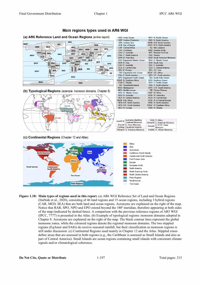
Final Government Distribution Chapter 1 IPCC AR6 WGI
Do Not Cite, Quote or Distribute 1-197 Total pages: 215
Figure 1.18: Main types of regions used in this report. (a) AR6 WGI Reference Set of Land and Ocean Regions
(Iturbide et al., 2020), consisting of 46 land regions and 15 ocean regions, including 3 hybrid regions (CAR, MED, SEA) that are both land and ocean regions. Acronyms are explained on the right of the map. Notice that RAR, SPO, NPO and EPO extend beyond the 180º meridian, therefore appearing at both sides of the map (indicated by dashed lines). A comparison with the previous reference regions of AR5 WGI (IPCC, 7777) is presented in the Atlas. (b) Example of typological regions: monsoon domains adopted in Chapter 8. Acronyms are explained on the right of the map. The black contour lines represent the global monsoon zones, while the coloured regions denote the regional monsoon domains. The two stippled regions (EqAmer and SAfri) do receive seasonal rainfall, but their classification as monsoon regions is still under discussion. (c) Continental Regions used mainly in Chapter 12 and the Atlas. Stippled zones define areas that are assessed in both regions (e.g., the Caribbean is assessed as Small Islands and also as part of Central America). Small Islands are ocean regions containing small islands with consistent climate signals and/or climatological coherence.
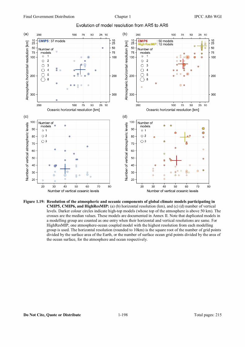
Final Government Distribution Chapter 1 IPCC AR6 WGI
Do Not Cite, Quote or Distribute 1-198 Total pages: 215
Figure 1.19: Resolution of the atmospheric and oceanic components of global climate models participating in
CMIP5, CMIP6, and HighResMIP: (a) (b) horizontal resolution (km), and (c) (d) number of vertical levels. Darker colour circles indicate high-top models (whose top of the atmosphere is above 50 km). The crosses are the median values. These models are documented in Annex II. Note that duplicated models in a modelling group are counted as one entry when their horizontal and vertical resolutions are same. For HighResMIP, one atmosphere-ocean coupled model with the highest resolution from each modelling group is used. The horizontal resolution (rounded to 10km) is the square root of the number of grid points divided by the surface area of the Earth, or the number of surface ocean grid points divided by the area of the ocean surface, for the atmosphere and ocean respectively.

Final Government Distribution Chapter 1 IPCC AR6 WGI
Do Not Cite, Quote or Distribute 1-199 Total pages: 215
Figure 1.20: A world map showing the increased diversity of modelling centres contributing to CMIP and CORDEX. Climate models are often developed by international consortia. EC-Earth is shown as an example (involving SMHI, Sweden; KNMI, The Netherlands; DMI, Denmark; AEMET, Spain; Met Éireann, Ireland; CNR‐ISAC, Italy; Instituto de Meteorologia, Portugal; FMI, Finland), but there are too many such collaborations to display all of them on this map. More complete information about institutions contributing to CORDEX and CMIP6 is found in Annex II.

Final Government Distribution Chapter 1 IPCC AR6 WGI
Do Not Cite, Quote or Distribute 1-200 Total pages: 215
Figure 1.21: Illustration of common types of model ensemble, simulating the time evolution of a quantity Q
(such as global mean surface temperature). (a) Multi-model ensemble, where each model has its own realization of the processes affecting Q, and its own internal variability around the baseline value (dashed line). The multi-model mean (black) is commonly taken as the ensemble average. (b) Initial condition ensemble, where several realizations from a single model are compared. These differ only by minute (‘micro’) perturbations to the initial conditions of the simulation, such that over time, internal variability will progress differently in each ensemble member. (c) Perturbed physics ensemble, which also compares realizations from a single model, but where one or more internal parameters that may affect the simulations of Q are systematically changed to allow for a quantification of the impact of those quantities on the model results. Additionally, each parameter set may be taken as the starting point for an initial condition ensemble. In this figure, each set has three ensemble members.

Final Government Distribution Chapter 1 IPCC AR6 WGI
Do Not Cite, Quote or Distribute 1-201 Total pages: 215
Figure 1.22: Structure of CMIP6, the 6th phase of the Coupled Model Intercomparison Project. The centre shows
the common DECK (Diagnostic, Evaluation and Characterization of Klima) and historical experiments that all participating models must perform. The outer circles show the topics covered by the endorsed (blue) and other MIPs (red). See Table 1.3 for explanation of the MIP acronyms. (expanded from Eyring et al., 2016).
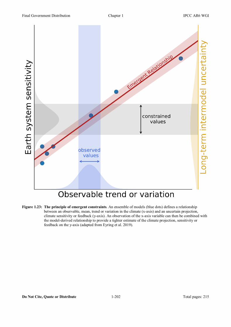
Final Government Distribution Chapter 1 IPCC AR6 WGI
Do Not Cite, Quote or Distribute 1-202 Total pages: 215
Figure 1.23: The principle of emergent constraints. An ensemble of models (blue dots) defines a relationship
between an observable, mean, trend or variation in the climate (x-axis) and an uncertain projection, climate sensitivity or feedback (y-axis). An observation of the x-axis variable can then be combined with the model-derived relationship to provide a tighter estimate of the climate projection, sensitivity or feedback on the y-axis (adapted from Eyring et al. 2019).
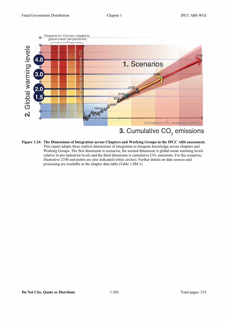
Final Government Distribution Chapter 1 IPCC AR6 WGI
Do Not Cite, Quote or Distribute 1-203 Total pages: 215
Figure 1.24: The Dimensions of Integration across Chapters and Working Groups in the IPCC AR6 assessment.
This report adopts three explicit dimensions of integration to integrate knowledge across chapters and Working Groups. The first dimension is scenarios, the second dimension is global-mean warming levels relative to pre-industrial levels and the third dimension is cumulative CO2 emissions. For the scenarios, illustrative 2100 end-points are also indicated (white circles). Further details on data sources and processing are available in the chapter data table (Table 1.SM.1).
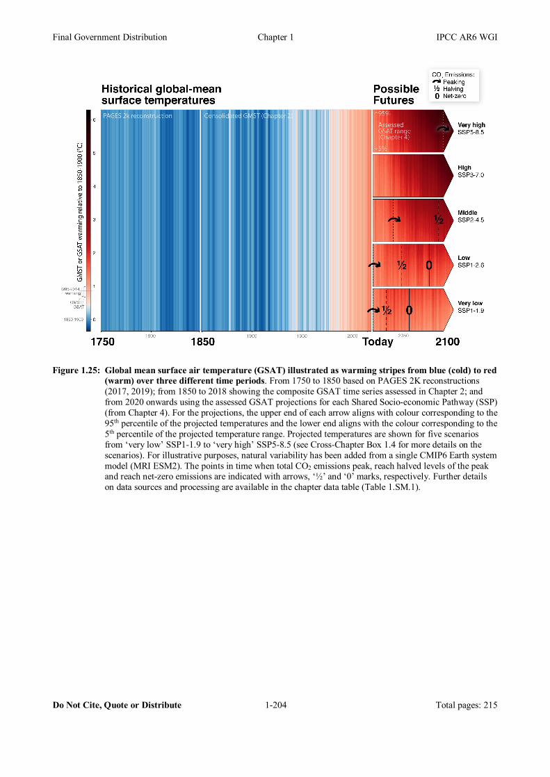
Final Government Distribution Chapter 1 IPCC AR6 WGI
Do Not Cite, Quote or Distribute 1-204 Total pages: 215
Figure 1.25: Global mean surface air temperature (GSAT) illustrated as warming stripes from blue (cold) to red (warm) over three different time periods. From 1750 to 1850 based on PAGES 2K reconstructions (2017, 2019); from 1850 to 2018 showing the composite GSAT time series assessed in Chapter 2; and from 2020 onwards using the assessed GSAT projections for each Shared Socio-economic Pathway (SSP) (from Chapter 4). For the projections, the upper end of each arrow aligns with colour corresponding to the 95th percentile of the projected temperatures and the lower end aligns with the colour corresponding to the 5th percentile of the projected temperature range. Projected temperatures are shown for five scenarios from ‘very low’ SSP1-1.9 to ‘very high’ SSP5-8.5 (see Cross-Chapter Box 1.4 for more details on the scenarios). For illustrative purposes, natural variability has been added from a single CMIP6 Earth system model (MRI ESM2). The points in time when total CO2 emissions peak, reach halved levels of the peak and reach net-zero emissions are indicated with arrows, ‘½’ and ‘0’ marks, respectively. Further details on data sources and processing are available in the chapter data table (Table 1.SM.1).
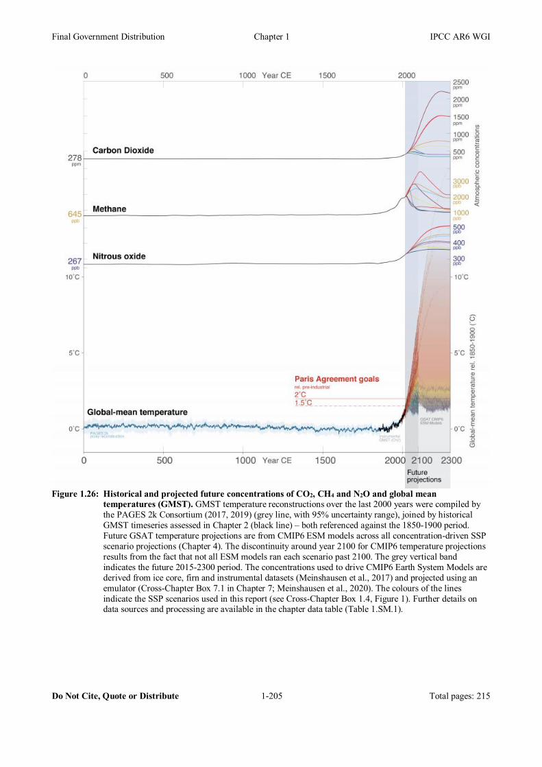
Final Government Distribution Chapter 1 IPCC AR6 WGI
Do Not Cite, Quote or Distribute 1-205 Total pages: 215
Figure 1.26: Historical and projected future concentrations of CO2, CH4 and N2O and global mean
temperatures (GMST). GMST temperature reconstructions over the last 2000 years were compiled by the PAGES 2k Consortium (2017, 2019) (grey line, with 95% uncertainty range), joined by historical GMST timeseries assessed in Chapter 2 (black line) – both referenced against the 1850-1900 period. Future GSAT temperature projections are from CMIP6 ESM models across all concentration-driven SSP scenario projections (Chapter 4). The discontinuity around year 2100 for CMIP6 temperature projections results from the fact that not all ESM models ran each scenario past 2100. The grey vertical band indicates the future 2015-2300 period. The concentrations used to drive CMIP6 Earth System Models are derived from ice core, firn and instrumental datasets (Meinshausen et al., 2017) and projected using an emulator (Cross-Chapter Box 7.1 in Chapter 7; Meinshausen et al., 2020). The colours of the lines indicate the SSP scenarios used in this report (see Cross-Chapter Box 1.4, Figure 1). Further details on data sources and processing are available in the chapter data table (Table 1.SM.1).
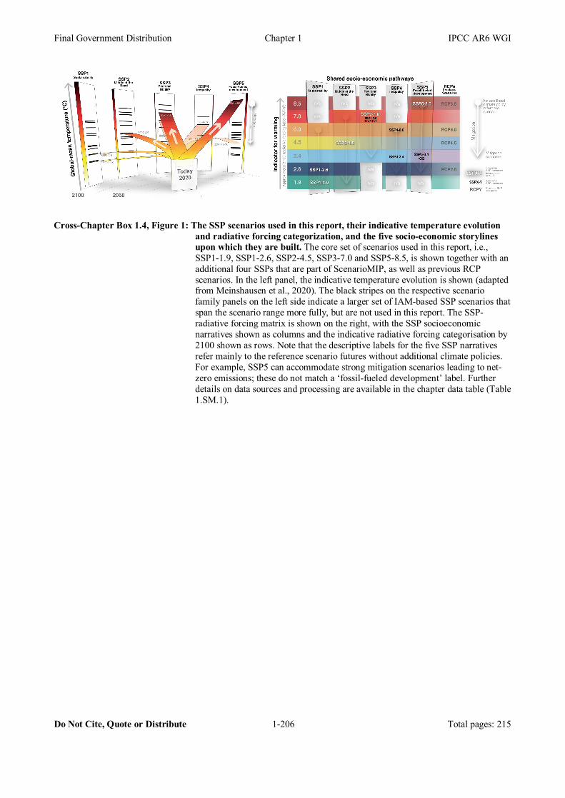
Final Government Distribution Chapter 1 IPCC AR6 WGI
Do Not Cite, Quote or Distribute 1-206 Total pages: 215
Cross-Chapter Box 1.4, Figure 1: The SSP scenarios used in this report, their indicative temperature evolution
and radiative forcing categorization, and the five socio-economic storylines upon which they are built. The core set of scenarios used in this report, i.e., SSP1-1.9, SSP1-2.6, SSP2-4.5, SSP3-7.0 and SSP5-8.5, is shown together with an additional four SSPs that are part of ScenarioMIP, as well as previous RCP scenarios. In the left panel, the indicative temperature evolution is shown (adapted from Meinshausen et al., 2020). The black stripes on the respective scenario family panels on the left side indicate a larger set of IAM-based SSP scenarios that span the scenario range more fully, but are not used in this report. The SSP-radiative forcing matrix is shown on the right, with the SSP socioeconomic narratives shown as columns and the indicative radiative forcing categorisation by 2100 shown as rows. Note that the descriptive labels for the five SSP narratives refer mainly to the reference scenario futures without additional climate policies. For example, SSP5 can accommodate strong mitigation scenarios leading to net-zero emissions; these do not match a ‘fossil-fueled development’ label. Further details on data sources and processing are available in the chapter data table (Table 1.SM.1).
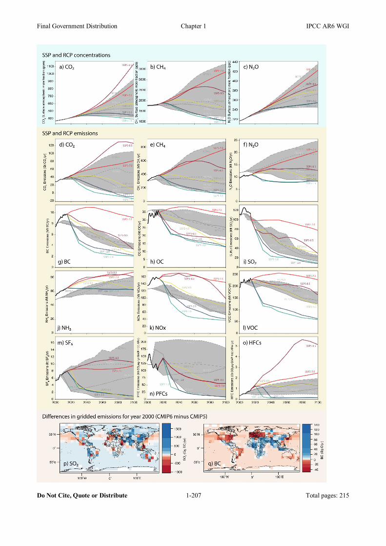
Final Government Distribution Chapter 1 IPCC AR6 WGI
Do Not Cite, Quote or Distribute 1-207 Total pages: 215

Final Government Distribution Chapter 1 IPCC AR6 WGI
Do Not Cite, Quote or Distribute 1-208 Total pages: 215
Cross-Chapter Box 1.4, Figure 2: Comparison between the Shared Socio-economic Pathways (SSP) scenarios and the Representative Concentration Pathway (RCP) scenarios in terms of their CO2, CH4 and N2O atmospheric concentrations (panels a-c), and their global emissions (panels d-o). Also shown are gridded emission differences for sulfur (panel p) and black carbon (panel q) for the year 2000 between the input emission datasets that underpinned the CMIP5 and CMIP6 model intercomparisons. Historical emission estimates are provided in black in panels d to o. The range of concentrations and emissions investigated under the RCP pathways is grey shaded. Panels p and q adapted from Figure 7 in Hoesly et al. (2018). Further details on data sources and processing are available in the chapter data table (Table 1.SM.1).
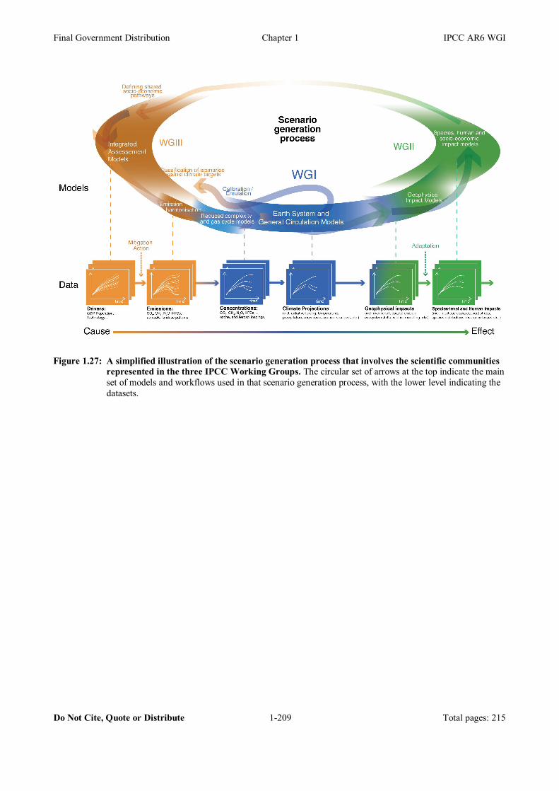
Final Government Distribution Chapter 1 IPCC AR6 WGI
Do Not Cite, Quote or Distribute 1-209 Total pages: 215
Figure 1.27: A simplified illustration of the scenario generation process that involves the scientific communities
represented in the three IPCC Working Groups. The circular set of arrows at the top indicate the main set of models and workflows used in that scenario generation process, with the lower level indicating the datasets.
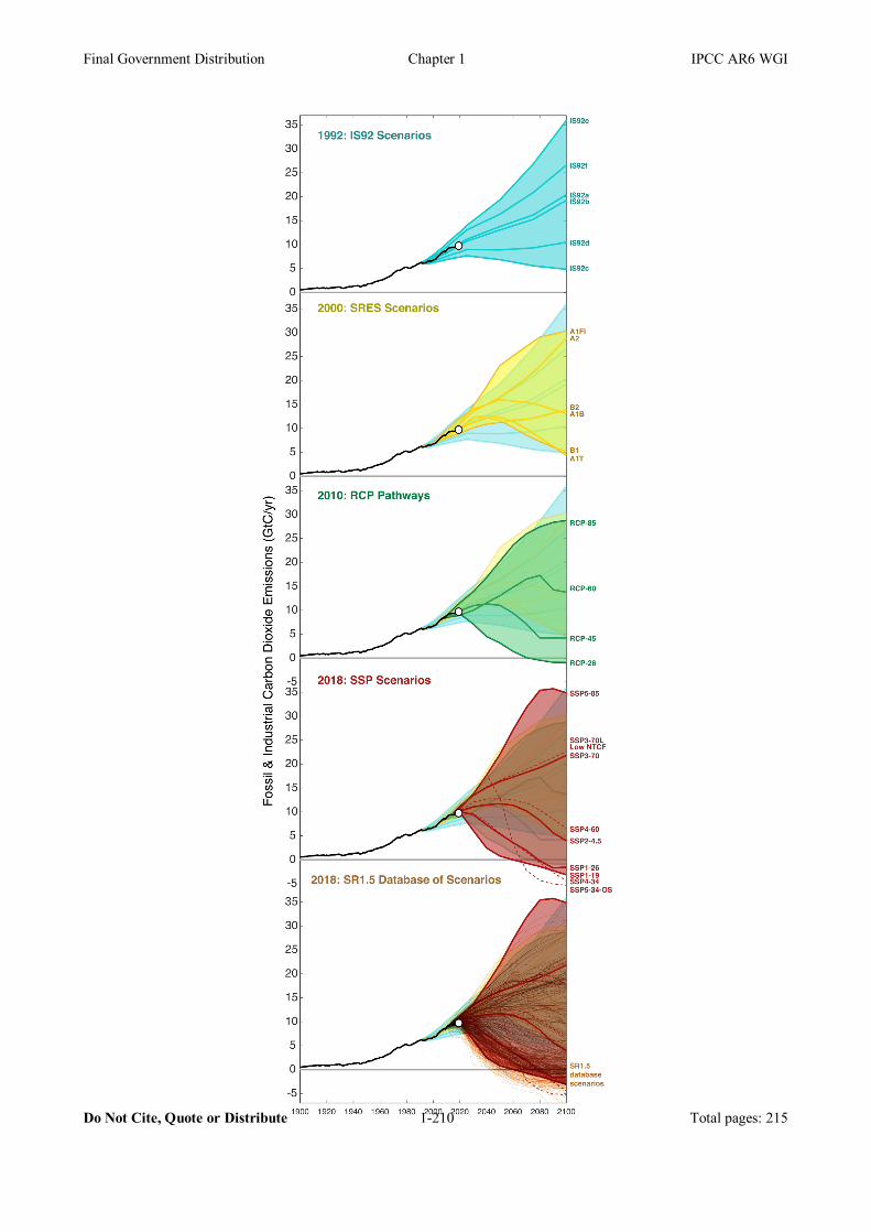
Final Government Distribution Chapter 1 IPCC AR6 WGI
Do Not Cite, Quote or Distribute 1-210 Total pages: 215

Final Government Distribution Chapter 1 IPCC AR6 WGI
Do Not Cite, Quote or Distribute 1-211 Total pages: 215
Figure 1.28: Comparison of the range of fossil and industrial CO2 emissions from scenarios used in previous assessments up to AR6. Previous assessments are the IS92 scenarios from 1992 (top panel), the Special Report on Emissions Scenarios (SRES) scenarios from the year 2000 (second panel), the Representative Concentration Pathway (RCP) scenarios designed around 2010 (third panel) and the Shared Socio-economic Pathways (SSP) scenarios (second bottom panel). In addition, historical emissions are shown (black line) (Chapter 5, Figure 5.5); a more complete set of scenarios is assessed in SR1.5 (bottom panel) (Huppmann et al., 2018). Further details on data sources and processing are available in the chapter data table (Table 1.SM.1).
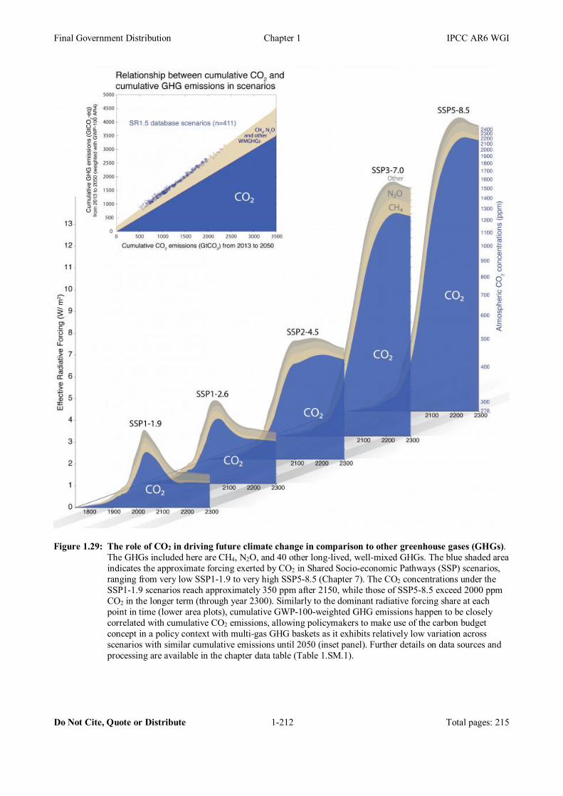
Final Government Distribution Chapter 1 IPCC AR6 WGI
Do Not Cite, Quote or Distribute 1-212 Total pages: 215
Figure 1.29: The role of CO2 in driving future climate change in comparison to other greenhouse gases (GHGs).
The GHGs included here are CH4, N2O, and 40 other long-lived, well-mixed GHGs. The blue shaded area indicates the approximate forcing exerted by CO2 in Shared Socio-economic Pathways (SSP) scenarios, ranging from very low SSP1-1.9 to very high SSP5-8.5 (Chapter 7). The CO2 concentrations under the SSP1-1.9 scenarios reach approximately 350 ppm after 2150, while those of SSP5-8.5 exceed 2000 ppm CO2 in the longer term (through year 2300). Similarly to the dominant radiative forcing share at each point in time (lower area plots), cumulative GWP-100-weighted GHG emissions happen to be closely correlated with cumulative CO2 emissions, allowing policymakers to make use of the carbon budget concept in a policy context with multi-gas GHG baskets as it exhibits relatively low variation across scenarios with similar cumulative emissions until 2050 (inset panel). Further details on data sources and processing are available in the chapter data table (Table 1.SM.1).

Final Government Distribution Chapter 1 IPCC AR6 WGI
Do Not Cite, Quote or Distribute 1-213 Total pages: 215
FAQ 1.1, Figure 1: Sample elements of climate understanding, observations and models as assessed in the IPCC First Assessment Report (1990) and Sixth Assessment Report (2021). Many other advances since 1990, such as key aspects of theoretical understanding, geological records and attribution of change to human influence, are not included in this figure because they are not readily represented in this simple format. Fuller explications of the history of climate knowledge are available in the introductory chapters of the IPCC fourth and sixth Assessment Reports.
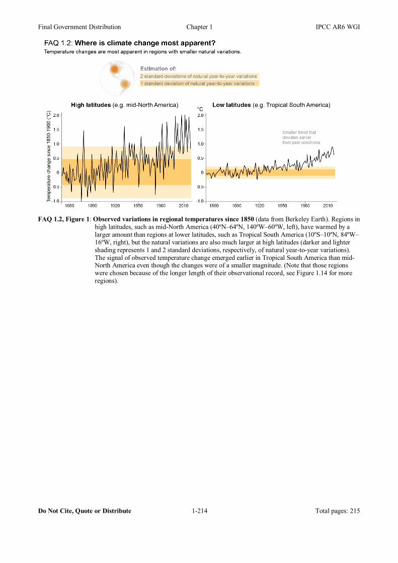
Final Government Distribution Chapter 1 IPCC AR6 WGI
Do Not Cite, Quote or Distribute 1-214 Total pages: 215
FAQ 1.2, Figure 1: Observed variations in regional temperatures since 1850 (data from Berkeley Earth). Regions in
high latitudes, such as mid-North America (40ºN–64ºN, 140ºW–60ºW, left), have warmed by a larger amount than regions at lower latitudes, such as Tropical South America (10ºS–10ºN, 84ºW–16ºW, right), but the natural variations are also much larger at high latitudes (darker and lighter shading represents 1 and 2 standard deviations, respectively, of natural year-to-year variations). The signal of observed temperature change emerged earlier in Tropical South America than mid-North America even though the changes were of a smaller magnitude. (Note that those regions were chosen because of the longer length of their observational record, see Figure 1.14 for more regions).
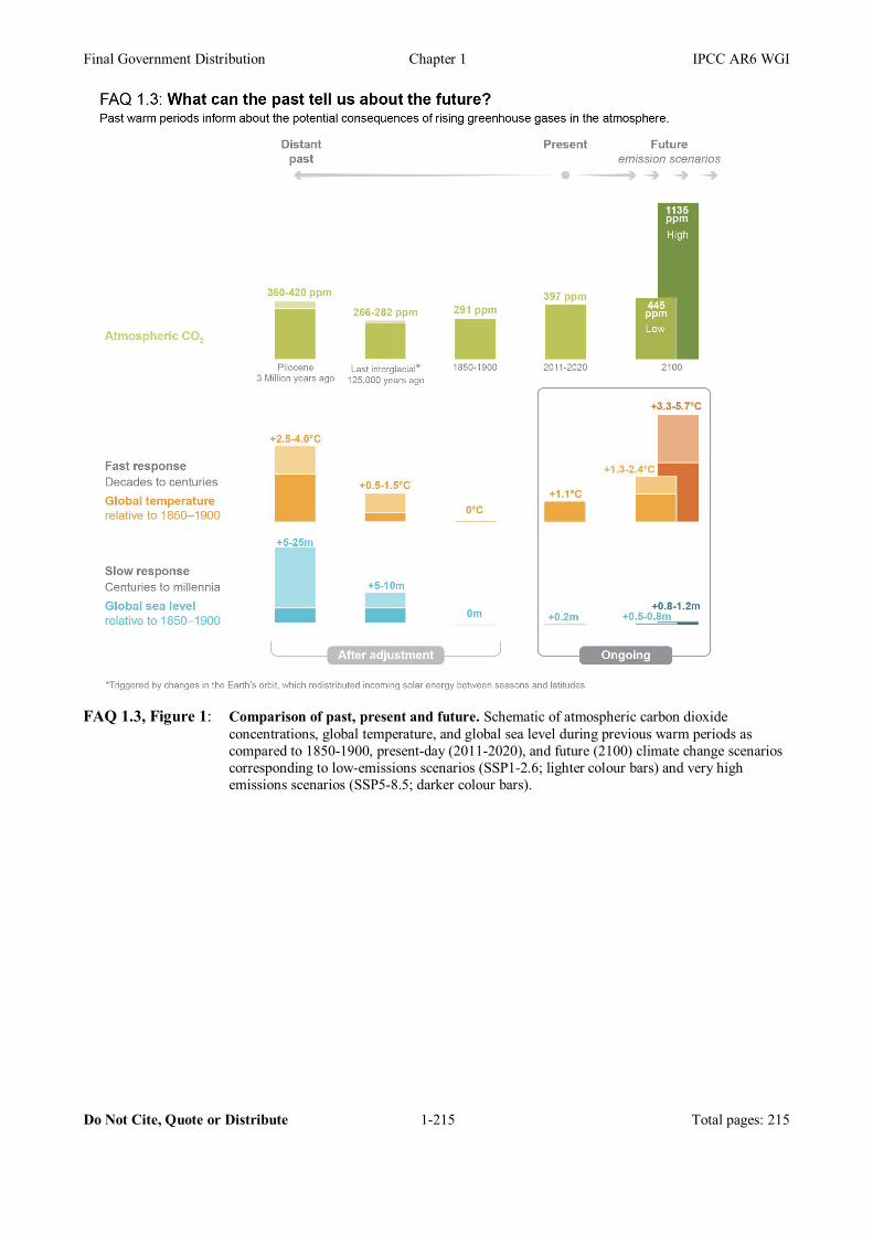
Final Government Distribution Chapter 1 IPCC AR6 WGI
Do Not Cite, Quote or Distribute 1-215 Total pages: 215
FAQ 1.3, Figure 1: Comparison of past, present and future. Schematic of atmospheric carbon dioxide
concentrations, global temperature, and global sea level during previous warm periods as compared to 1850-1900, present-day (2011-2020), and future (2100) climate change scenarios corresponding to low-emissions scenarios (SSP1-2.6; lighter colour bars) and very high emissions scenarios (SSP5-8.5; darker colour bars).