C4C DeliverableFP7-ICT-2007.3.7.(c) grant agreement nr. INFSO-ICT-223844

CON4COORDWP9 Informatics for Control of Distributed

Systems — Final Report

Christoforos (Chris) Hadjicostis, D. A. (Bert)van Beek, Marta Capiluppi, Maria Halkidi,

George Iosifidis, Iordanis Koutsopoulos,Jasen Markovski, J. (Koos) E. Rooda,

Roberto Segala, Leandros Tassiulas

Title CON4COORD WP9 Informatics for Control of Distributed Systems —Final Report

Authors Christoforos (Chris) Hadjicostis, D. A. (Bert) van Beek, Marta Capiluppi,Maria Halkidi, George Iosifidis, Iordanis Koutsopoulos, Jasen Markovski,J. (Koos) E. Rooda, Roberto Segala, Leandros Tassiulas

Main participant CER, TUE, UCY, UGE, UVRDeliverable nr D-WP9.3Version 0.1Date May 1, 2011

Abstract

This deliverable presents the report of the partners of project CON4COORD on theresearch of Workpackage 9 Informatics for Control of Distributed Systems during the thirdyear of the project.

Contents

1 Introduction 3

2 WP9 Teams 3

3 WP9 Description 4

4 WP9 Final Report 54.1 CER Team . . . . . . . . . . . . . . . . . . . . . . . . . . . . . . . . . . . . . . . 54.2 TUE Team . . . . . . . . . . . . . . . . . . . . . . . . . . . . . . . . . . . . . . . 54.3 UCY Team . . . . . . . . . . . . . . . . . . . . . . . . . . . . . . . . . . . . . . . 74.4 UGE Team . . . . . . . . . . . . . . . . . . . . . . . . . . . . . . . . . . . . . . . 74.5 UVR Team . . . . . . . . . . . . . . . . . . . . . . . . . . . . . . . . . . . . . . . 7

5 Summary of WP9 Progress and Concluding Remarks 9

A CE.RE.TE.TH Report: Online Clustering of Distributed Streaming Datausing Belief Propagation Techniques 10A.1 Introduction and Motivation . . . . . . . . . . . . . . . . . . . . . . . . . . . . . . 10A.2 Representative Related Work . . . . . . . . . . . . . . . . . . . . . . . . . . . . . 13A.3 Background: Affinity Propagation algorithm . . . . . . . . . . . . . . . . . . . . . 13A.4 Streaming Data and Clustering Models . . . . . . . . . . . . . . . . . . . . . . . . 15A.5 Clustering Streaming Data with Belief Propagation Techniques . . . . . . . . . . 17A.6 Distributed Data Stream Clustering Approach . . . . . . . . . . . . . . . . . . . 18A.7 Experimental Study . . . . . . . . . . . . . . . . . . . . . . . . . . . . . . . . . . 19

A.7.1 Evaluation Criterion . . . . . . . . . . . . . . . . . . . . . . . . . . . . . . 19A.7.2 Clustering Quality Evaluation . . . . . . . . . . . . . . . . . . . . . . . . . 19A.7.3 Evaluating the Distributed Stream Clustering approach . . . . . . . . . . 22

A.8 Conclusion . . . . . . . . . . . . . . . . . . . . . . . . . . . . . . . . . . . . . . . 23

B UCY Report: Reduced-Complexity Verification for Initial-State Opacity inModular Discrete Event Systems 24B.1 Preliminaries and Background . . . . . . . . . . . . . . . . . . . . . . . . . . . . . 25B.2 Initial-State Opacity . . . . . . . . . . . . . . . . . . . . . . . . . . . . . . . . . . 26B.3 Modular Methods for Verifying Initial-State Opacity . . . . . . . . . . . . . . . . 27

B.3.1 Systems with Two Modules . . . . . . . . . . . . . . . . . . . . . . . . . . 27B.3.2 Systems with More than Two Modules . . . . . . . . . . . . . . . . . . . . 30

B.4 Conclusion . . . . . . . . . . . . . . . . . . . . . . . . . . . . . . . . . . . . . . . 31

2

1 Introduction

The purpose of Deliverable WP9.3 (D-WP9.3) of the CON4COORD project is to report to theEuropean Commission on the progress of the consortium in Workpackage 9 (WP9), includingall subworkpackages of WP9. The reporting period is May 1, 2010 until April 30, 2011.

The teams active for WP9 of the CON4COORD project are: the Center for R&D Hellas(CER) at Volos, Greece; Eindhoven University of Technology (TUE) at Eindhoven, The Nether-lands; the University of Cyprus (UCY) at Nicosia, Cyprus; the University of Gent (UGE) atGent, Belgium; the University of Verona (UVR) at Verona, Italy.

The character of this deliverable is that of an administrative report that has to be read jointlywith papers and reports containing technical results, some of which are referenced and/or areattached to this report. The next section contains information on the teams and the personnel,active for WP9 and paid by the project. Section 3 summarizes the workpackage descriptionand Section 4 includes a report on the investigations of WP9 for the second year of the project.Conclusions and future plans are stated in Section 5. The Appendix includes reports on relevantwork that has been completed. A bibliography is listed at the end of the deliverable.

2 WP9 Teams

The list of teams involved in WP9 is provided below; more details about the person months forWP9 are provided in the Executive Summary for the overall project.

CER This team belongs to the CEnter for REsearch and TEchnology - THessaly (CERETETH),which is a legal, non-profit entity organized under the auspices of the General Secretariat forResearch and Technology (GSRT) of the Greek Ministry of Development. The team consistsof senior researchers Prof. Leandros Tassiulas, Dr. Dimitris Katsaros and Dr. Iordanis Kout-sopoulos. Since October 15, 2008, Mrs. Maria Halkidi has been working part time on thisproject.

TUE This team belongs to the Eindhoven University of Technology, Department of Mechan-ical Engineering, Systems Engineering group. The team consists of senior researchers Prof. J.(Koos) E. Rooda and Dr. D. A. (Bert) van Beek. Since August 15, 2008, the postdoctoralresearch assistant J. Markovski has been assigned to the project.

UCY This team belongs to the University of Cyprus, Department of Electrical and ComputerEngineering. The team for WP9 consists of senior researchers Prof. Charalambos (Bambos)Charalambous and Prof. Christoforos (Chris) Hadjicostis. Since February 1, 2011, Mr. Christo-foros Keroglou and Mr. Apostolos Rikos have been working part time on this workpackage.

UGE This team belongs to Universiteit Gent (UGE) in Belgium, Department of Electrical andComputer Engineering. The team consists of senior researchers Prof. Rene K. Boel, JonathanRogge, and doctoral students Nicolae-Emanuel Marinica and Mohammad Moradzadeh.

UVR This team belongs to the University of Verona, Department of Computer Science. Theteam for this workpackage consists of senior researchers Prof. Roberto Segala. Since February1, 2009, Dr. Marta Capiluppi has been working full-time as postdoctoral researcher on thisproject.

3

3 WP9 Description

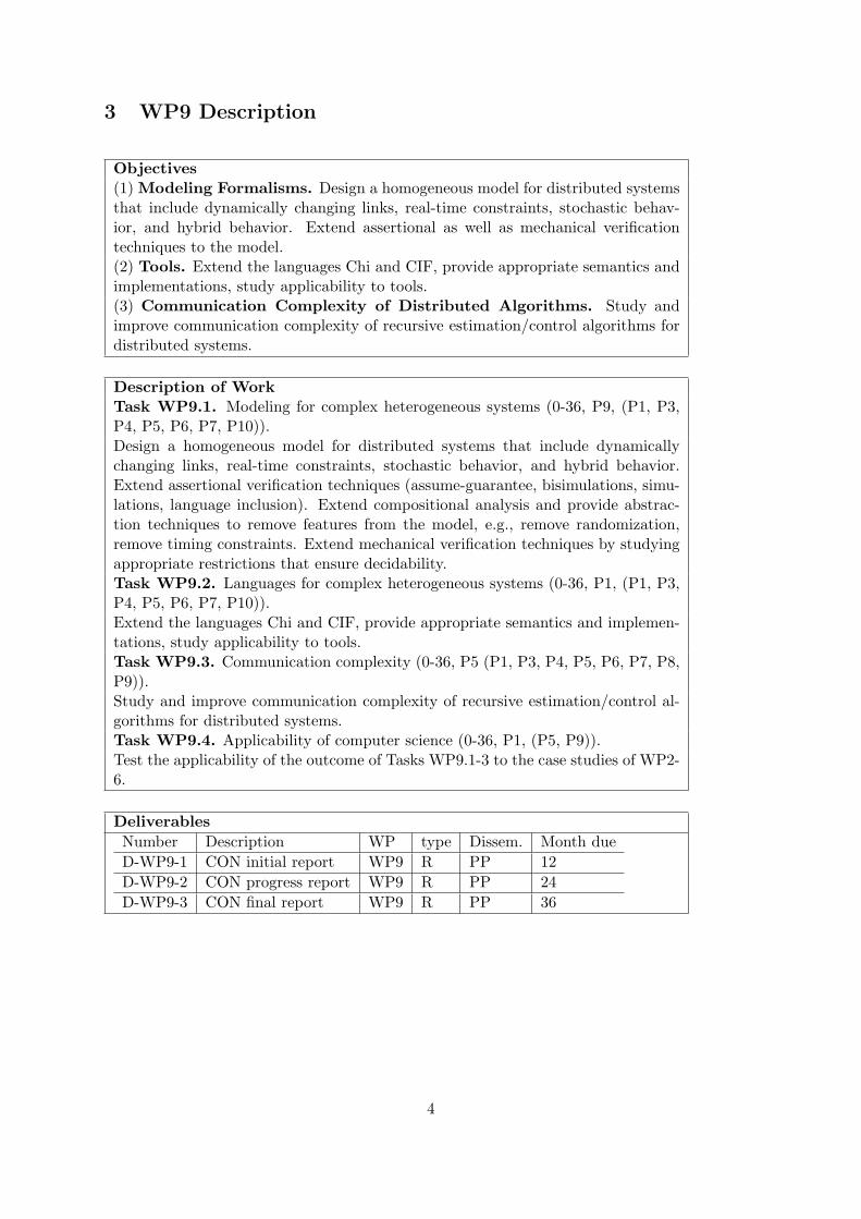
Objectives(1) Modeling Formalisms. Design a homogeneous model for distributed systemsthat include dynamically changing links, real-time constraints, stochastic behav-ior, and hybrid behavior. Extend assertional as well as mechanical verificationtechniques to the model.(2) Tools. Extend the languages Chi and CIF, provide appropriate semantics andimplementations, study applicability to tools.(3) Communication Complexity of Distributed Algorithms. Study andimprove communication complexity of recursive estimation/control algorithms fordistributed systems.

Description of WorkTask WP9.1. Modeling for complex heterogeneous systems (0-36, P9, (P1, P3,P4, P5, P6, P7, P10)).Design a homogeneous model for distributed systems that include dynamicallychanging links, real-time constraints, stochastic behavior, and hybrid behavior.Extend assertional verification techniques (assume-guarantee, bisimulations, simu-lations, language inclusion). Extend compositional analysis and provide abstrac-tion techniques to remove features from the model, e.g., remove randomization,remove timing constraints. Extend mechanical verification techniques by studyingappropriate restrictions that ensure decidability.Task WP9.2. Languages for complex heterogeneous systems (0-36, P1, (P1, P3,P4, P5, P6, P7, P10)).Extend the languages Chi and CIF, provide appropriate semantics and implemen-tations, study applicability to tools.Task WP9.3. Communication complexity (0-36, P5 (P1, P3, P4, P5, P6, P7, P8,P9)).Study and improve communication complexity of recursive estimation/control al-gorithms for distributed systems.Task WP9.4. Applicability of computer science (0-36, P1, (P5, P9)).Test the applicability of the outcome of Tasks WP9.1-3 to the case studies of WP2-6.

DeliverablesNumber Description WP type Dissem. Month dueD-WP9-1 CON initial report WP9 R PP 12D-WP9-2 CON progress report WP9 R PP 24D-WP9-3 CON final report WP9 R PP 36

4

4 WP9 Final Report

4.1 CER Team

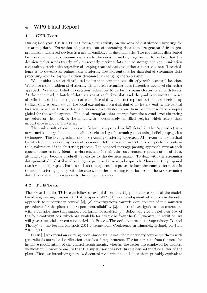
During last year, CE.RE.TE.TH focused its activity on the area of distributed clustering forstreaming data. Extraction of patterns out of streaming data that are generated from geo-graphically dispersed devices is a major challenge in data analysis. The sequential, distributedfashion in which data become available to the decision maker, together with the fact that thedecision maker needs to rely only on recently received data due to storage and communicationconstraints, render the objective of keeping track of data evolution a nontrivial one. The chal-lenge is to develop an online data clustering method suitable for distributed streaming dataprocessing and for capturing their dynamically changing characteristics.

We consider a set of distributed nodes that communicate directly with a central location.We address the problem of clustering distributed streaming data through a two-level clusteringapproach. We adopt belief propagation techniques to perform stream clustering at both levels.At the node level, a batch of data arrives at each time slot, and the goal is to maintain a setof salient data (local exemplars) at each time slot, which best represents the data received upto that slot. At each epoch, the local exemplars from distributed nodes are sent to the centrallocation, which in turn performs a second-level clustering on them to derive a data synopsisglobal for the whole system. The local exemplars that emerge from the second level clusteringprocedure are fed back to the nodes with appropriately modified weights which reflect theirimportance in global clustering.

The end result of our approach (which is reported in full detail in the Appendix) is anovel methodology for online distributed clustering of streaming data using belief propagationtechniques. The key ingredient of our streaming clustering approach, APStream, is the methodby which a compressed, synoptical version of data is passed on to the next epoch and aids inre-initialization of the clustering process. The adopted message passing approach runs at eachepoch, it successfully identifies clusters, and it maintains an accurate representation of data,although they become gradually available to the decision maker. To deal with the streamingdata generated in distributed setting, we proposed a two-level approach. Moreover, the proposedtwo-level belief propagation-based clustering approach is proved to have the same performance interms of clustering quality with the case where the clustering is performed on the raw streamingdata that are sent from nodes to the central location.

4.2 TUE Team

The research of the TUE team followed several directions: (1) general extensions of the model-based engineering framework that supports WP6 [1], (2) development of a process-theoreticapproach to supervisory control [2], (3) investigations towards development of minimizationprocedures for the plant that respect controllability [3], and (4) investigations into extensionswith stochastic time that support performance analysis [4]. Below, we give a brief overview ofthe four contributions, which are available for download from the C4C website. In addition, wewill give a tutorial presentation titled “A Process-Theoretic Approach to Supervisory ControlTheory” at the Formal Methods 2011 International Conference in Limerick, Ireland, on June20th, 2011.

(1) In [1] we extend an existing model-based framework for supervisory control synthesis withgeneralized control and verification state-based requirements. The former stem from the need forintuitive specification of the control requirements, whereas the latter are employed for livenessverification in order to ensure that the supervisor does not disable desired functionalities of theplant. First, we introduce generalized control requirements and show them provably equivalent

5

to the standard state-based control requirements. In the process, we identify a class of state-based liveness requirements, which can be efficiently verified and employed in the supervisorsynthesis framework to provide early feedback to the modeler.

(2) In [2] we revisit the central notion of controllability in supervisory control theory fromprocess-theoretic perspective. To this end, we investigate partial bisimulation preorder, a behav-ioral preorder that is coarser than bisimulation equivalence and finer than simulation preorder.It is parameterized by a subset of the set of actions that need to be bisimulated, whereas theactions outside this set need only to be simulated. This preorder proves a viable means todefine controllability in a nondeterministic setting as a refinement relation on processes. Thenew approach provides for a generalized characterization of controllability of nondeterministicdiscrete-event systems. We characterize the existence of a deterministic supervisor and com-pare our approach to existing ones in the literature. It helped identify the coarsest minimizationprocedure for nondeterministic plants that respects controllability. At the end, we define thenotion of a maximally permissive supervisor, nonblocking property, and partial observability inour setting.

(3) In [3] we present an efficient algorithm for computing the simulation preorder and equiv-alence for labeled transition systems. The algorithm improves an existing space-efficient algo-rithm and improves its time complexity by employing a variant of the stability condition andexploiting properties of the underlying relations and partitions. It has comparable space andtime complexity with the most efficient counterpart algorithms for Kripke structures. Our mainmotivation for developing a new algorithm for minimization by simulation, focused on labeledtransitions systems, is ongoing research in process-theoretic approaches to automated generationof control software. There, the underlying refinement relation between the implementation andspecification is a so-called partial bisimulation preorder. This relation lies between simulationand bisimulation, by requiring that the specification simulates all actions of the implementation,whereas in the other direction only a subset of the actions needs to be (bi)simulated. So, thestability conditions that identify when the partition relation pair represents partial bisimula-tion are a combination of the stability conditions for simulation and bisimulation. Thus, in thispaper, we rewrite the stability conditions for simulation to stability condition for bisimulation,which deals with the partitioning of states, and stability condition for the simulation preorderof the partition classes.

(4) In [4] we propose a model-based systems engineering framework for supervisory controlof stochastic discrete-event systems with unrestricted nondeterminism. We intend to developthe proposed framework in four phases outlined in this paper. Here, we study in detail thefirst step which comprises investigation of the underlying model and development of a corre-sponding notion of controllability. The model of choice is termed Interactive Markov Chains,which is a natural semantic model for stochastic variants of process calculi and Petri nets, andit requires a process-theoretic treatment of supervisory control theory. To this end, we definea new behavioral preorder, termed Markovian partial bisimulation, that captures the notion ofcontrollability while preserving correct stochastic behavior. We provide a sound and ground-complete axiomatic characterization of the preorder and, based on it, we define two notions ofcontrollability. The first notion conforms to the traditional way of reasoning about supervisionand control requirements, whereas in the second proposal we abstract from the stochastic be-havior of the system. For the latter, we intend to separate the concerns regarding synthesisof an optimal supervisor. The control requirements cater only for controllability, whereas weensure that the stochastic behavior of the supervised plant meets the performance specificationby extracting directive optimal supervisors.

6

4.3 UCY Team

Within the context of Task 9.1, the UCY team has been focusing on efforts to develop modelsthat appropriately formulate and enable the analysis of methodologies to verify various notionsof opacity in distributed systems that are modeled as (possibly non-deterministic) finite au-tomata with partial observation on their transitions. These notions of opacity are motivated byemerging applications where the exchange of vital information takes place over shared cyber-infrastructures; such applications range from defense and banking to health care and powerdistribution systems. More specifically, opacity is a security notion that aims at determiningwhether a given system’s secret behavior (i.e., a subset of the behavior of the system that isconsidered critical and is usually represented by a predicate) is kept opaque to outsiders [5, 6].This requires that an intruder (modeled as an observer of the system’s behavior) is never ableto establish (with absolute certainty) the truth of the predicate.

During the third year of the project, we have considered reduced-complexity methodologiesfor verifying initial-state opacity in modular discrete event systems [7]. Initial-state opacityrequires that the membership of the system initial state to a given set of secret states S re-mains opaque (uncertain) to an intruder who has complete knowledge of the system modeland observes system activity through some natural projection map. In the modular setting weconsider, the given system is modeled as a composition (synchronous product) of M modules{G1, G2, . . . , GM} where each module Gi is a non-deterministic finite automaton with Ni stateswith the set of secret states S is of the form S = {(x1, x2, . . . , xM )|xi ∈ Si}, where Si is the setof secret states for module Gi. Assuming that the pairwise shared events are pairwise observableand that the intruder observes events that are observable in at least one module, we provide amodular algorithm for verifying initial-state opacity with O(MNM−12N

2) state and time com-

plexity, where N = maxiNi. This is a considerable reduction compared to the O(2(NM )2) stateand time complexity of the centralized verification method, which verifies initial-state opacityby considering the composed system as a monolithic system.

A more detailed report on reduced complexity methods for verifying initial-state opacity inmodular systems is provided in the Appendix.

4.4 UGE Team

The UGE team has reformulated the problem of collision avoidance and deadlock avoidancefor autonomous vehicles traveling in a common free space into a problem of interacting com-municating timed automata. Each AGV has a local control agent that ensures that this AGVfollows as closely as possible a reference trajectory with restricted directions and speeds. Thebehavior of each AGV, of its sensors, and of its control law can be represented by concurrentlyexecuting timed automata. These automata interact and communicate with each other throughthe sensors that detect the position of some of the other AGVs that are sufficiently close. Atleast formally, this representation of AGVs allows the use of tools for communicating automatain order to design local controllers for the AGVs so as to avoid collisions, and so as to avoiddeadlock.

4.5 UVR Team

Within the context of Task 9.1, the work of the UVR team in this third year of the projecthas been devoted to formalize further the problems expressed in Deliverable D-WP9.1 andunderstanding the ways to handle dynamically changing topologies. In particular starting fromthe analysis of the case studies, performed in the first year of the project, the necessity ofa formal model for describing and verifying dynamically changing systems has been enlighten.

7

The case studies that gave the main motivation for this research are: aerial vehicles in WP3 (see[8]), underwater vehicles in WP2 (see [9]), and partly road traffic control in WP4, as describedin [10] and [11]. The UVR team exchanged some ideas with the groups involved with those casestudies, trying to find out the main problems related to the formulation of a scenario for systemscomposed by different agents in need to communicate and coordinate to reach a specific goal.Moreover these systems move in a world which can collect more of them and raise a differentkind of communication depending on their hierarchy. The UVR team had contacts with teamsin WP2 and WP3 in order to formalize a model able to describe as much as possible of thecharacteristics of the related case studies, sticking to the real scenarios.

After a deep analysis of the already existing modeling tools for these systems, it came outthat the most suitable model should be an extension to one of the existing models for hybridsystems: the Hybrid I/O Automata (HIOA) of [12]. With the proposed method it is possibleto model faithfully the fact that a collection of hybrid automata live in a world, occupyingspecific positions, and derive information about other automata from their observations of thesurrounding world.

Since automata live in a world, it is still missing a way to describe a world and how itevolves. The choice made by UVR team is to describe a world by means of automata as well.In other words, an automaton lives in a world, interacts with other automata that live in thesame world according to the classical mechanisms of HIOAs, and at the same time defines aworld for other automata to live in. The world defined by an automaton has input and outputvariables, used respectively to transfer properties to the inner automata and to receive stimuli,as well as internal variables that are used to keep information about the status of each point inspace. Consider as an example a perfectly flat sandy area. This is described by an automaton Awith a world state variable x that represents the level of the ground at each point with respectto some fixed reference point (e.g., sea level). The automaton has also an input world statevariable u that is used to know the pressure at each point. If a car moves in the area, then thecar sends continuously a stimulus to the points of its location via variable u, and the stimuluscauses the level x of the ground to decrease, which is reflected in new values variable x. If Ahas a world output variable y that reflects the value of x, then each car can observe the shapeof the area. If in addition the transition function of the car is described so that it dependsonly on the values of y on a neighborhood of its location, then limitations are imposed on theobservational capabilities of the car.

So the main difference with HIOAs is that these new automata, World Automata (WAs)have some special variables, called world variables, used to communicate with the world outside(the world the automaton lives in) and the world inside (the world the automaton creates forother automata). An important observation is that the variables of the world assume a valuefor each position ofM. Thus, a variable of the world represents implicitly a possibly infinite setof variables. Alternatively, a real-valued variable of the world assumes values from the domainof functions from M to the reals.

Another important difference with HIOAs is that a level has been added to variables andactions of a WA. This allows to establish different levels of communication with other automatain order to model the hierarchical interaction between worlds. Imagine as an example an aircraftcarrier on the sea. The ship lives in a world represented by the sea, but it represents also aworld for the aircraft landed on it. What happens when a new aircraft wants to land on theship? And what happens if another ship is entering in the same portion of sea? In this lastcase the two ships have to communicate at the same level, i.e. the variables and actions used tointeract with the outside world are the ones at the world level (which it has been called level 0).To this end the WAs have been equipped with an operation of parallel composition, analogousto the one of HIOAs, with the only difference that communication at levels different from 0 is

8

disabled and that effects of stimuli on the same output world variables of level 0 are summedup.

In the described framework, if an automaton wants to enter in a world, it has to interactwith the local variables created by that world. In particular with the input signals that theworld takes from agents inside it. This means that the world inputs will update each timeanother agents enters the world. This establish the dynamical communication from the insidelevels and the outside level. To this end WAs have been equipped also with an operator, calledinplacement, that defines the rules for communication from the inside to the outside. Similarlyto parallel composition, the rules for communication of inplacement prevent communication atlevel different from the interested one (in this case it will be level 1), and allow summing of theeffects of the world variables that are input for the outside world and output from the insideworld.

The UVR team has applied the introduced theory to one of the case studies: aerial vehicles(WP3), following the scenario presented in [8]. Furthermore, the UVR team has prepared aseries of scenarios for underwater vehicles where the compositional aspect of WAs can be ex-ploited. The main aim of these experiments is to provide a collection of case studies that canillustrate even to non experts in formal methods the potentials that arise from the ability todescribe their problems within hybrid automata and WAs. The scenarios include situationswhere a vehicle has to follow another vehicle without sharing any information about the tra-jectories to follow, and where a vehicle is completely lost and tries to reach a buoy by trackingthe acoustic signal emitted by the buoy. With these experiments it was evident that WAs arealready in a position to describe dynamically changing environments without the need to addany extra features. The results are reported in a comprehensive technical report which will besubject of further dissemination [13].

5 Summary of WP9 Progress and Concluding Remarks

The five teams involved in WP9 pursued multiple important directions within this work package.Collaboration between different teams and different work packages has been close and fruitful.For instance, the UVR team has taken important steps developing a model appropriate forcapturing the requirements in the coordination of underwater or aerial vehicles. Similarly, theTUE team has been incorporating such modeling issues into the capabilities of the various toolsthat are under development. We envision that these collaborative efforts will continue beyondthe completion of the project.

9

A CE.RE.TE.TH Report: Online Clustering of Distributed Stream-ing Data using Belief Propagation Techniques

As mentioned in the body of the report, during last year, CE.RE.TE.TH focuses its activity onthe area of distributed clustering for streaming data.

Extraction of patterns out of streaming data that are generated from geographically dis-persed devices is a major challenge in data analysis. The sequential, distributed fashion inwhich data become available to the decision maker, together with the fact that the decisionmaker needs to rely only on recently received data due to storage and communication con-straints, render the objective of keeping track of data evolution a nontrivial one. The challengeis to develop an online data clustering method suitable for distributed streaming data processingand for capturing their dynamically changing characteristics.

We consider a set of distributed nodes that communicate directly with a central location.We address the problem of clustering distributed streaming data through a two-level clusteringapproach. We adopt belief propagation techniques to perform stream clustering at both levels.At the node level, a batch of data arrives at each time slot, and the goal is to maintain a setof salient data (local exemplars) at each time slot, which best represents the data received upto that slot. At each epoch, the local exemplars from distributed nodes are sent to the centrallocation, which in turn performs a second-level clustering on them to derive a data synopsisglobal for the whole system. The local exemplars that emerge from the second level clusteringprocedure are fed back to the nodes with appropriately modified weights which reflect theirimportance in global clustering.

A.1 Introduction and Motivation

Mining streaming data that are generated continuously at high rates is an area of data miningwith many unresolved challenges. This area has recently spurred the interest of the community[16–19] due to the diverse range of real life applications where such problems arise. Sensornetwork data emerging from continuous measurements, online Internet traffic and web usage logsmonitoring, streaming video from surveillance cameras and RFID data are some examples whereinformation naturally becomes available to the decision maker in sequential and distributedfashion through data streams.

Clustering is a fundamental task in data mining, aiming at identifying significant underlyingpatterns in data [20]. Such patterns may refer to statistical distributions followed by data orsimply to certain distinct clusters to which the data can be categorized. Clustering is widelyrecognized as means to provide a synopsis, that is a compressed version of the data volume athand. Since the transmission of huge amount of raw streaming data is prohibitively expensive,clustering is an approach that can assist with overcoming this problem.

Distributed streaming data management possesses some distinct challenges which arise dueto the sequential, online fashion in which data from distributed sources become available tothe decision maker. One could argue that the decision maker could wait until all data reachhim and then apply a conventional clustering or other approach to make a decision. Or, thatshe/he could simply wait long enough so as to have a larger portion of the data available andmake a more informed decision. There are two objections to that. First, in distributed dataprocessing, the transmission of entire streaming data to a central site is infeasible, since itwill dramatically increase the network communication cost. Therefore, a local clustering canassist with providing a compact version of data generated at each of the remote sites. Second,in streaming data, it is crucial for the decision maker to be able to make a decision online,precisely at the time the last segment of data arrives. Identifying a change in patterns of data

10

should involve a series of reaction measures that will follow decision making. For example, invideo surveillance, identifying a change in the received video segments should mobilize certainmechanisms for immediate reaction. Hence it would not be meaningful for the decision makerto wait much due to the incurred delay in decision making. Moreover, at each time instant, thelocal sites (and decision maker) may not have access to the full amount of previously receiveddata due to storage constraints. Although storage space becomes cheaper and more availableas a resource, it is evident that data volume grows gigantic, and it is many more orders ofmagnitude higher than available storage space, especially when considered over a certain timehorizon. In light of the above, the goal of the local node and the decision maker at the end ofeach time slot is to maintain a set of salient data items that best represent data received up tothat slot. These items will be fed as input to the next slot, they will be updated with the newarriving data and will be used in subsequent decision making.

In this work, we develop an online data clustering method suitable for distributed streamingdata. We adopt belief propagation techniques, also known as message passing ones, which mi-grated from statistical physics and have found fertile ground in computer science and networking([21], [22], [23], [24]) in addressing computationally hard combinatorial optimization problems.The key idea at the interface between computer science and statistical physics is to view thecomputer science problem at hand as an evolving system of entities that interact with each otherin a random and competing manner. The computer science optimization problem with a givenobjective over a space of possible configurations can then be mapped onto a statistical physicsproblem instance, with a given probability distribution over the set of possible configurationsof a set of interacting particles. Computing the optimal solution of the optimization problemis then equivalent to identifying the minimum energy configurations at which the probabilitydistribution concentrates.

In our case, the problem at each time slot is to identify a set of representative data items (ex-emplar items) based on certain similarity metrics. The innovative feature of belief propagation isthat all data items in each slot are treated as representatives with different preferences. At eachtime slot, simple messages are exchanged among data items and update the appropriateness ofeach data item to serve as representative of another, until the set of optimal representativesemerges. Belief propagation methods are suitable for online stream processing since they donot require a priori knowledge of classification patterns. We provide evidence that belief propa-gation techniques can efficiently materialize the key ingredient of online clustering, namely thetransfer of salient information from previous slots to the next one. Specifically, representativedata items from previous slots are taken into account in the next slot through a sophisticatedinitialization of arising preferences in the belief propagation algorithm.

Our starting point is the Affinity Propagation (AP) [24] clustering algorithm which formu-lates the K-centroid clustering problem and uses a message passing algorithm to solve it. Weintroduce an online version of the AP clustering algorithm, StreamAP, that makes full use ofits flexibility in addressing the evolution of streaming data clusters. Since streaming data flowcontinuously and there are storage constraints at the decision maker node, a succinct synopsisof data from previous slots is indispensable so as to keep track of trends of previously receiveddata. This synopsis is a set of exemplars, also known as the cluster-heads, and it providescompact information about patterns of knowledge and significant data distributions identifiedin past data.

Data clusters are formed at each time slot based on current data similarities and appropri-ate statistics of previously defined clusters. The exchanged messages among data items carryinformation about data similarities, the significance of a data item to serve as exemplar, and itstendencies to select other items as exemplars. A most attractive feature of the AP algorithm isthat the number of clusters need not be decided a priori as in conventional clustering algorithms.

11

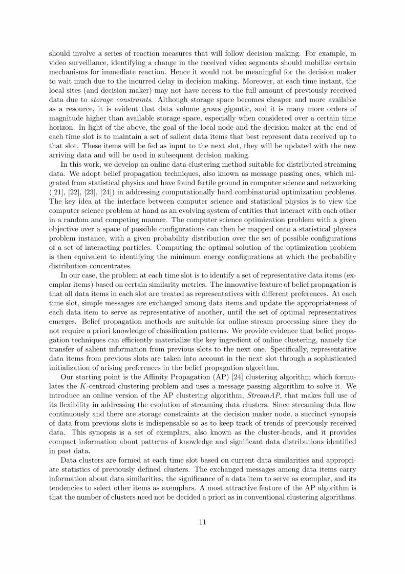
with weights that reflect their importance in global clustering

Online local clustering data

with StreamAP algorithmOnline local clustering data

...with StreamAP algorithm

Global clustering on exemplars...

with StreamAP algorithmNode n

Node 1

passed to central location

Exemplars from global clustering fed back to originating nodes

Central location

Local exemplars

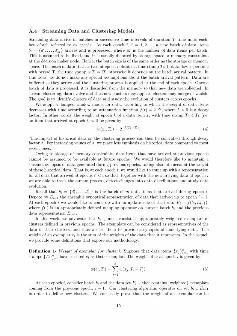
Figure 1: Architecture of the proposed clustering approach for distributed streaming data.

Instead, clusters evolve based on data similarities and knowledge from previous slots about thesuitability of a item to be an exemplar. At different time slots, new clusters may emerge, vanishor merge. Most importantly, if the number of clusters or cluster composition tends to change,our method detects it in the evolving dynamics of the data stream.

We consider a set of distributed nodes that communicate directly with a central location,the decision maker. The StreamAP algorithm is executed locally at each node, where a batchof local data arrives at each time slot. The goal of each node at each time slot is to maintainan appropriate set of salient data items (local exemplars) that best represent data received upto that slot. These are used as input at the next slot, and they are updated after considerationof the new data. At each epoch, local exemplars are sent to the central location, which inturn performs a high-level clustering to derive a global picture of the data in the system.The StreamAP algorithm is applied at the central location on the local exemplars. The localexemplars that emerge from the high-level clustering procedure are fed back to the nodes withappropriately modified weights which reflect their importance in global clustering. This feedbackis used by local nodes in subsequent slots. Figure 1 presents the main components of theproposed clustering approach for distributed streaming data.

Summarizing, the main contributions of our work are as follows:

• We address the problem of streaming data online clustering with the framework of statis-tical physics belief propagation methods.

• We define a model for building a succinct synopsis of data processed at each time period.Our model does not make any assumptions about underlying statistical properties of data,yet it succeeds in maintaining the most significant information at each time slot.

• We develop a method to pass salient information to subsequent time instants and showhow it can actually guide the clustering algorithm in the next time slots. This method isthe crucial step towards realizing an efficient online version of an algorithm.

• We develop a clustering framework for distributed streaming data that allows aggregationof clustering results from remote sites. Also it allows remote sites to receive a feedbackfrom the central site in terms of the global data distribution and thus they can properlyadjust their local clustering.

• We provide ample evidence that our approach can identify changes in streaming dataalthough it is completely oblivious to underlying data distribution and the number ofclusters involved. Our approach builds, merges or removes clusters on the fly as data flowinto the controller.

• We eliminate the dependence of the cluster extraction method on input information (inputparameters) that a user or decision maker needs to provide. Our algorithm exploits

12

inherent data properties (e.g. data similarities) along the clustering process, thus removingthe barriers placed by user defined parameters.

A.2 Representative Related Work

The approaches that tackle the problem of stream clustering can be categorized into: i) one-passmethods, that assume a unique underlying model of streaming data. These approaches cannotstudy the evolution of data distribution, ii) evolving clustering methods that take into accountthe behavior of data as it may evolve over time.

One-pass clustering methods use a divide-and-conquer method that achieves a constantfactor approximation using a small amount of storage space [25], [26], [27]. Every time a newchunk of data arrives, a local clustering is performed to generate the cluster centers out of chunkdata. Since all original data items have been processed, clustering is applied to all intermediatemedians so that the k final medians are defined.

In [28], a stream clustering algorithm is proposed, which includes two clustering phases.At the online phase, the proposed approach periodically stores detailed summary statistics,while at the off-line phase, the decision maker uses these statistics to provide a descriptionof clusters in the data stream. The main drawback of this algorithm is that the number ofmicro-clusters needs to be predefined. HPStream [29] incorporates a fading cluster structureand a projection-based clustering methodology to deal with the problem of high-dimensionalityin data streams.

The Denstream [30] is based on DBSCAN [31], an algorithm that forms local clusters progres-sively by detecting and connecting dense data item neighborhoods. Cluster adjustment involvesdetection of data items that are neighbors to the newly inserted data, re-computation of theirneighborhoods [32] and respective micro-clusters [30], and re-assignment of neighborhoods andmicro-clusters to clusters if deemed necessary [32]. In Denstream, incremental computation isfurther enhanced through the treatment of (potential) outlier micro-clusters. The algorithm isa two-phase clustering approach. During the online phase micro-cluster are maintained whilethe final clusters are defined (offline) on demand by the user.

An EM-based clustering approach for distributed data streams was presented in [33]. Theremote site defines their clustering model based on the idea of test-and-cluster while the coor-dinator combine all Gaussian models from each site directly, and the Gaussian mixture modelcomponents represent the distribution of overall distributed data streams.

Zhang et al. [34] presented a version of the AP algorithm that is closer to handling datastreaming. According to their approach, as data flows, data items are compared one-by-oneto the exemplars and they are assigned to their nearest one if a distance threshold conditionis satisfied. Otherwise, data are considered outliers and are put in a reservoir. A clusterredefinition is triggered if the number of outliers exceeds a heuristic (user-defined) reservoirsize or if a change in data distribution is detected. That is, the quality of clustering dependsdecisively on user defined thresholds. Moreover, at each time instant, there exists a number ofdata items in the reservoir that are similarly handled as outliers. The clustering algorithm runsanew to define a clustering of all data items arrived until the current time item only if a restartcondition is satisfied.

A.3 Background: Affinity Propagation algorithm

Affinity propagation (AP) [24] belongs to the class of message passing methods and it is appliedto a given data set in order to identify a set of representative items (exemplars) out of thedata. A most attractive feature of the AP algorithm is that the number of clusters need not bedecided a priori as in conventional clustering algorithms.

13

Assume that X = {x1, x2, . . . , xn} is a set of distinct data points and let S(xi, xj) denote thesimilarity between the data points xi and xj , with i 6= j. Usually, similarity is set to a negativesquared error S(xi, xj) = −||xi − xj ||2. For i = j, the similarity of a item i, S(xi, xi) indicateshow likely the i-th item is to be chosen as an exemplar, and it is further called preference. TheAP algorithm searches for a mapping φ(·) which assigns each data point xi to its nearest datapoint, referred to as exemplar of xi (i.e. φ(xi)). This mapping should maximize an appropriatelychosen energy function defined as:

E [φ] =n∑i=1

S(xi, φ(xi))−n∑i=1

χi[φ] (1)

with χi[φ] = ∞, if φ(φ(xi)) 6= φ(xi) and 0 otherwise. The first term in (1) denotes the overallsimilarity of the data points to their exemplars, while the second term expresses the constraintthat if a data point is selected as an exemplar by some data points, it should be its own exemplar.

The optimization problem in (1) is solved using a message passing algorithm. Consideringdata points as nodes in a network, real-valued messages are exchanged among data points, untila set of representative points together with the respective clusters emerges. These messages areupdated at each iteration and they reflect the current affinity that a data point has to selectanother point as an exemplar at that iteration. The number of selected exemplars is influencedby the preference values, but it also comes out of the message passing procedure. There are twotypes of exchanged messages between data points [24]:

1. A Responsibility message, r(i, k) that a data item i sends to candidate exemplar k. Thismessage shows the accumulated evidence for how well item k serves as exemplar for itemi. Its value is iteratively adjusted as follows:

r(i, k) = S(xi, xk)− maxk′,k′ 6=k

{α(i, k′) + S(xi, xk′)} (2)

where α(i, k′) is the availability message presented below.

If k = i, the responsibility message is adjusted as: r(k, k) = S(xk, xk)−maxk′,k′ 6=k{S(xk, xk′)}.

2. An Availability message, α(i, k), that a candidate exemplar k sends to data item i. Thismessage captures evidence as to how appropriate it would be for item i to select item k′

as its exemplar. The value of α(i, k) is updated as:

α(i, k) = min

0, r(k, k) +∑

i′,i′ /∈i,k

max{0, r(i′, k)}

(3)

For k = i, the availability message reflects accumulated evidence that item k is an exem-plar and is adjusted by: α(k, k) =

∑i′,i′ 6=k max{0, r(i′, k)}.

At each iteration, the assignments of items to exemplars (clusters) are defined as,

φ(xi) = arg maxk{r(i, k) + α(i, k)}

where φ(xi) denotes the exemplar for data item xi. The message passing procedure stops after aspecific number of iterations, or after cluster structure does not significantly change for a givennumber of iterations.

14

A.4 Streaming Data and Clustering Models

Streaming data arrive in batches in successive time intervals of duration T time units each,henceforth referred to as epochs. At each epoch i, i = 1, 2 . . ., a new batch of data itemsbi = {di1, . . . , diM} arrives and is processed, where M is the number of data items per batch.This is assumed to be fixed, and it is usually dictated by storage space or memory constraintsat the decision maker node. Hence, the batch size is of the same order as the storage or memoryspace. The batch of data that arrived at epoch i obtains a time stamp Ti. If data flow is periodicwith period T, the time stamp is Ti = iT , otherwise it depends on the batch arrival pattern. Inthis work, we do not make any special assumptions about the batch arrival pattern. Data arebuffered as they arrive and the clustering process is applied at the end of each epoch. Once abatch of data is processed, it is discarded from the memory so that new data are collected. Instream clustering, data evolve and thus new clusters may appear, clusters may merge or vanish.The goal is to identify clusters of data and study the evolution of clusters across epochs.

We adopt a damped window model for data, according to which the weight of data itemsdecreases with time according to an attenuation function f(t) = 2−λt, where λ > 0 is a decayfactor. In other words, the weight at epoch k of a data item xi with time stamp Ti < Tk (i.e.an item that arrived at epoch i) will be given by:

w(xi, Tk) = 2−λ(Tk−Ti). (4)

The impact of historical data on the clustering process can then be controlled through decayfactor λ. For increasing values of λ, we place less emphasis on historical data compared to mostrecent ones.

Owing to storage of memory constraints, data items that have arrived at previous epochscannot be assumed to be available at future epochs. We would therefore like to maintain asuccinct synopsis of data generated during previous epochs, taking also into account the weightof these historical data. That is, at each epoch i, we would like to come up with a representationfor all data that arrived at epochs i′ < i so that, together with the new arriving data at epoch iwe are able to track the stream process, detect changes into data distributions and study dataevolution.

Recall that bi = {di1, . . . , dim} is the batch of m data items that arrived during epoch i.Denote by Ei−1 the ensemble synoptical representation of data that arrived up to epoch i− 1.At each epoch i we would like to come up with an update rule of the form: Ei = f(bi, Ei−1),where f(·) is an appropriately defined mapping operator on current batch bi and the previousdata representation Ei−1.

In this work, we advocate that Ei−1 must consist of appropriately weighted exemplars ofclusters defined in previous epochs. The exemplars can be considered as representatives of thedata in their clusters, and thus we use them to provide a synopsis of underlying data. Theweight of an exemplar ei is the sum of the weights of the data that it represents. In the sequel,we provide some definitions that expose our methodology.

Definition 1- Weight of exemplar (or cluster). Suppose that data items {xj}nj=1 with timestamps {Tj}nj=1 have selected ei as their exemplar. The weight of ei at epoch i is given by:

w(ei, Ti) =n∑j=1

w(xj , Ti − Tj). (5)

At each epoch i, consider batch bi and the data set Ei−1 that contains (weighted) exemplarscoming from the previous epoch, i − 1. Our clustering algorithm operates on set bi ∪ Ei−1

in order to define new clusters. We can easily prove that the weight of an exemplar can be

15

calculated incrementally at each epoch. Specifically, assume that w(ek, Ti−1) is the weight ofexemplar ek at epoch i − 1 and {di1, . . . , dim} is the subset of data items that arrived duringthe next epoch, i (with time stamp Ti) and have also selected ek as their exemplar. Based on(4) the weight of data items arrived at the current epoch i is: w(dij , Ti) = 1, j = 1, . . . ,m. IfTi − Ti−1 = 1, the weight of ek defined in (5) will be updated as follows:

w(ek, Ti) = 2−λ · w(ek, Ti−1) +m (6)

where m is the number of data items that arrived during epoch i and are assigned to the clusterof ek (which is denoted by C(ek)).

For each exemplar ek, the following vector is forwarded to the next epoch, i+1: [ ek, w(ek, Ti), D(C(ek), Ti) ] ,where D(C(ek), Ti) is the sum of weighted dissimilarities between data items in C(ek) and theirexemplar ek, that is:

D(C(ek), Ti) =∑

x∈C(ek)

w(x, Ti) · ||x− ek||2 (7)

It can be proved that D(C(ek), Ti) can be maintained incrementally, i.e.

D(C(ek), Ti) = 2−λ · D(C(ek), Ti−1) +∑

dij∈C(ek)

||dij − ek||2 (8)

At each epoch i, pairwise similarities S(xi, xj) of data items xi, xj ∈ (bi∪Ei−1) are properlyadjusted, so that patterns of knowledge extracted from previously arrived data are also exploitedin data clustering. At each epoch, our algorithm takes as input the updated similarities anddefines clusters based on a message passing procedure. In the sequel, we provide a method forupdating similarities between new arrived data at each epoch and exemplars from the previousepoch. This turns out to be the key for transferring salient data features from one epoch to thenext one.

Definition 2.1 - Preference of exemplars from a previous epoch. The preference of an exemplarek at epoch i+1 will be defined based on its preference in the previous epoch i and the statisticsof its cluster in i. Specifically, the preference of ek are updated as follows:

Si+1(ek, ek) = Si(ek, ek) ·

(1− w(ek, Ti)∑

j w(ej , Ti)

)− var(C(ek), Ti) (9)

where var(C(ek), Ti) = D(C(ek),Ti)w(ek,Ti)

is the weighted variance of cluster C(ek) which capturesdissimilarities between the exemplar and the other data items in its cluster. At each epoch,the variance of a cluster changes as its structure changes, i.e. as data items can be added orforgotten. Thus, each of the previously defined exemplars gains an advantage over the otherdata items that is analogous to the weight of the data items that have selected it, while itundergoes a penalty related to the variance of its cluster.

Definition 2.2 - Preference of current data items. The preferences of the data items generatedat the current epoch i+ 1 are defined as follows:∀ di+1

j ∈ bi+1, j = 1, . . . ,M ,

Si+1(di+1j , di+1

j ) =

∑x∈(bi+1∪Ei),x 6=di+1

jSi+1(x, di+1

j )

|bi+1 ∪ Ei|(10)

where |bi+1 ∪Ei| is the number of data under analysis (i.e. exemplars from the previous epochand the current set of arrived data items) at epoch i+ 1.

16

Definition 2.3 - Similarities between an exemplar from a previous epoch and a current dataitem. At each epoch i + 1, the similarities between an exemplar ek coming from the previousepoch and a current data item are defined as follows:

Si+1(di+1j , ek) = −||ek − di+1

j ||2 (11)

Si+1(ek, di+1j ) = −w(ek, Ti) · ||ek − di+1

j ||2 (12)

Equation (11) indicates that the suitability of an old defined exemplar ek to be selected asan exemplar of a current item depends on their distance. On the other hand, an old exemplarwill evaluate the suitability of a currently arrived data item to be its exemplar based on theirsimilarity and the significance of its cluster (see (12)). This is due to the fact that an exemplaris not actually a single item but it carries a synopsis of the data in its cluster. Then the assign-ment of an exemplar, ek, to a new exemplar (cluster) results in the redefinition of exemplar forall data items in C(ek) and the cost of this reassignment is related to the weight of its clusterdata (weight of the ek’s cluster).

Definition 2.4 - Similarity between exemplars coming from previous epoch. If ek, em are twoexemplars coming from epoch i their similarity at epoch i+ 1 will be defined as:

Si+1(ek, em) = −w(ek, Ti) · ||ek − em||2 (13)

Since an exemplar ek represents all data items in its cluster, we assume that it approximatelycorresponds to a set of nk identical copies of data items (where nk denotes the number of itemsthat have selected ek as their exemplar). Then, the similarity of ek to an exemplar em shouldreflect the similarity of the respective data cluster (i.e. nk copies) to em. Considering that eachdata item in C(ek) influence the similarity analogously to its significance (weight), the sum ofsimilarities of nk copies to em is modeled as w(ek, Ti) · ||ek − em||2.

Definition 2.5. The similarity between a pair of data items arrived at the current epoch, Ti+1,will be given by

Si+1(di+1j , di+1

k ) = −||di+1j − di+1

k ||2 (14)

A.5 Clustering Streaming Data with Belief Propagation Techniques

We now develop StreamAP a variation of the initially proposed AP clustering algorithm, that iscapable of handling sequences of data in an online fashion under the limited memory constraintsimposed by streaming applications. Data arrive and are processed in batches. At each epoch,a synopsis of data is defined through their cluster representatives (exemplars) and statistics(weight of cluster and variance). Both the current batch of data and the representatives ofpreviously processed data items are used in the clustering procedure. Once a batch of dataarrives, the similarity matrix of data is updated based on the proposed stream clustering modeldiscussed in section A.4. The clusters of data are defined using the AP algorithm and the resultsare forwarded to the next epoch. Specifically, the proposed algorithm, StreamAP involves thefollowing steps:STEP1: The first batch of data arrives at epoch 0 and the AP algorithm (presented in SectionA.3) is used to initialize the clustering process.While the stream flows,STEP2: For each exemplar, ek of the i-th epoch,

• Vector [ ek, w(ek, Ti), D(C(ek), Ti) ] (defined in section A.4) is forwarded to the next epoch.

17

• The preferences of defined exemplars are updated based on (9).

STEP3: At the next epoch i+ 1, a new batch of data, bi+1 is received. The currently receivedbatch of data and the set of weighted exemplars Ei received from previous epoch define the newset of data considered for clustering, referred to as bi+1 ∪ Ei.

The similarity matrix of data items in bi+1 ∪ Ei is updated. Specifically:

• ∀ dj ∈ bi+1, preferences Si+1(dj , dj) are updated as in (10).

• ∀, di, dj ∈ (bi+1 ∪ Ei), similarities Si+1(di, dj) are adjusted according to (11)-(13), asdescribed in section A.4.

STEP4: The extended version of AP clustering algorithm is applied to bi+1 ∪ Ei.Then the values of messages exchanged between data items in bi+1 ∪ Ei are adjusted as inequations (2) and (3).

Based on the method outlined above, our approach provides a mechanism that efficientlysummarizes the most significant information from previously processed data and transfers thisinformation to the next epoch of the clustering process. Thus, it enables online adaptive(re)definition of clusters and monitoring of their evolution while new batches of data arrive. Theclustering results only depend on intrinsic properties of data such as data similarities, while thedecision maker may control the impact of historical data to the current data clustering thoughdecay factor λ.

A.6 Distributed Data Stream Clustering Approach

We consider a distributed computing environment with n remote sites (nodes), {si}ni=1, and acentral site (CS) of a decision maker. At each remote site, streaming data arrive continuously.At each epoch t, the StreamAP algorithm (discussed in section A.5) runs at each node, si, todefine a local clustering model, Cti . The local clustering of si is described by its exemplars andtheir respective weights, that is Cti = {(lei1, w(e1, Ti)) . . . , (leik, w(ek, Ti))}. The local clusteringmodels are sent to the central site (CS) in the form of stream. After receiving the clusteringmodels of all remote sites at each epoch, the CS properly aggregates them so as to define anupdated global clustering. Specifically, at epoch t, the exemplars selected in remote sites arriveto CS and the StreamAP algorithm runs on them to properly update the previously definedglobal clustering, i.e. Ct = f(Ct−1, Ct1, . . . , C

tn), where f(·) is the defined clustering operator on

new arrived exemplars, {Ct1, . . . , Ctn} and the previous selected ones, Ct−1. The updated globalclustering Ct is transmitted back to the remote sites so that they adjust their local clusters(exemplars). Hence the remote sites obtain a holistic view of the data generated in the entirenetwork though the global clustering that is disseminated to them.The main steps of the proposed distributed stream clustering approach can be summarized asfollows:While the stream flows,

1. StreamAP runs at remote sites, {si}ni=1. Let Cti be the clustering model of site si at epocht.

2. The remote sites transmit their clusterings {Cti}ni=1 to CS.

3. The CS receives the stream of local clusterings (exemplars) and runs StreamAP to updatethe global clustering defined in epoch t − 1 with the new arrived local clusters. Let Ct

be the global clustering at epoch t and {get1, . . . , getm} be the respective set of selectedexemplars. We note that the global exemplars could be exemplars defined in previousepochs, or one of the exemplars that arrived from the remote sites at the current epoch.

18

4. The weight factor of global exemplars at CS is defined as fw(geti) = w(geti,t)P

k w(geti,t)

. It indicates

the global significance of each exemplar geti with respect to the weight of points that haveselected it as their exemplar.

5. CS provides feedback to remote sites, forwarding them the global clustering and respectiveweight factors, that is, it sends the vector [(get1, fw(get1)), . . . , (getm, fw(getm))].

6. Once a remote site si receives the feedback from CS, it updates the weights of its exemplarsthat belong to the intersection of the set denoting its local clustering Cti and the setdenoting the global clustering. That is, ∀ leij ∈ Cti , if leij ∈ Ct ∩ Cti then w(leij , t) =w(leij , t) · (1 + fw(getk)), where getk ≡ leij .

A.7 Experimental Study

In this section we evaluate the performance of our approach in terms of clustering accuracyusing synthetic and real data sets.

A.7.1 Evaluation Criterion

We evaluate clustering quality based on the purity of clusters. Evaluation of quality of cluster-ing amounts to measuring the purity of defined clusters with respect to the true class labels.For experimental purposes, we assume that we know the label of data items. Then, we run ourapproach on the set of unlabeled data and we assess the purity of the defined clusters. An itemassignment to an exemplar is correct if its class is the same as its exemplar class. Then wecan define the purity measure as follows: Purity = 1

k ·∑k

i=1|Cd

i ||Ci| , where |Cdi | denotes the num-

ber of majority class items in cluster i, |Ci| is the size of cluster i and k is the number of clusters.

A.7.2 Clustering Quality Evaluation

We evaluate the effectiveness of our approach to capture data evolution and identify the emerg-ing clusters as data flows using synthetic data. The synthetic collection of streaming data wascreated with different numbers of clusters and dimensions. We assume that the data follow aset of Gaussian distributions, while the mean and variance of data distribution vary during datageneration.

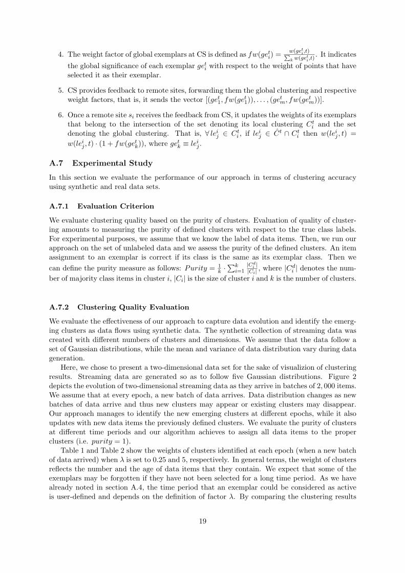
Here, we chose to present a two-dimensional data set for the sake of visualizion of clusteringresults. Streaming data are generated so as to follow five Gaussian distributions. Figure 2depicts the evolution of two-dimensional streaming data as they arrive in batches of 2, 000 items.We assume that at every epoch, a new batch of data arrives. Data distribution changes as newbatches of data arrive and thus new clusters may appear or existing clusters may disappear.Our approach manages to identify the new emerging clusters at different epochs, while it alsoupdates with new data items the previously defined clusters. We evaluate the purity of clustersat different time periods and our algorithm achieves to assign all data items to the properclusters (i.e. purity = 1).

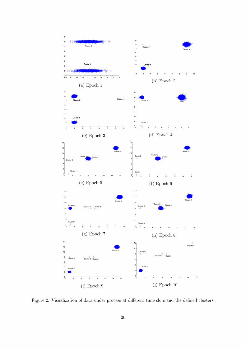
Table 1 and Table 2 show the weights of clusters identified at each epoch (when a new batchof data arrived) when λ is set to 0.25 and 5, respectively. In general terms, the weight of clustersreflects the number and the age of data items that they contain. We expect that some of theexemplars may be forgotten if they have not been selected for a long time period. As we havealready noted in section A.4, the time period that an exemplar could be considered as activeis user-defined and depends on the definition of factor λ. By comparing the clustering results

19

2.6 2.7 2.8 2.9 3 3.1 3.2 3.3 3.4 3.51

2

3

4

5

6

7

8

9

Cluster 1Cluster 1Cluster 1

Cluster 2

(a) Epoch 1

2 3 4 5 6 7 8 9 101

2

3

4

5

6

7

8

9

Cluster 1Cluster 1

Cluster 2Cluster 4

(b) Epoch 2

2 3 4 5 6 7 8 91

2

3

4

5

6

7

8

9

Cluster 1

Cluster 2Cluster 2 Cluster 4

(c) Epoch 3

2 3 4 5 6 7 8 9 102

3

4

5

6

7

8

9

Cluster 1

Cluster 2 Cluster 4

(d) Epoch 4

2 4 6 8 10 12 14 162

4

6

8

10

12

14

Cluster 1

Cluster 2

Cluster 3 Cluster 4

Cluster 5

(e) Epoch 5

2 4 6 8 10 12 14 162

4

6

8

10

12

14

Cluster 1

Cluster 2 Cluster 3Cluster 4

Cluster 5

(f) Epoch 6

2 4 6 8 10 12 14 162

4

6

8

10

12

14

Cluster 1

Cluster 2 Cluster 3 Cluster 4

Cluster 5

(g) Epoch 7

2 4 6 8 10 12 14 162

4

6

8

10

12

14

Cluster 1

Cluster 2Cluster 3 Cluster 4

Cluster 5

(h) Epoch 8

2 4 6 8 10 12 14 160

2

4

6

8

10

12

14

Cluster 1

Cluster 2 Cluster 3 Cluster 4

Cluster 5

(i) Epoch 9

2 4 6 8 10 12 14 160

2

4

6

8

10

12

Cluster 1

Cluster 2

Cluster 3 Cluster 4

Cluster 5

(j) Epoch 10

Figure 2: Visualization of data under process at different time slots and the defined clusters.

20

Cluster weightsEpochs Cluster 1 Cluster 2 Cluster 3 Cluster 4 Cluster 5

1 1000 1000 - - -2 1841.89 841.89 - 1000 -3 2049.84 2208.95 - 841.89 -4 1724.71 2358.49 - 2208.95 -5 1451.29 1984.25 993 1865.49 10006 1221.39 1669.55 1823.01 1582.69 1841.897 1028.065 1904.92 1533.96 1331.877 3049.848 865.495 1602.838 1786.903 1124.971 4065.609 1728.792 1348.82 1503.60 946.98 4419.7510 2454.735 1135.219 1265.373 797.315 3717.553

Table 1: Evolution and weights of clusters extracted from synthetic streaming data at differentepochs when λ = 0.25.

Cluster weightsEpoch Cluster 1 Cluster 2 Cluster 3 Cluster 4 Cluster 5

1 1000 1000 - - -2 1841.89 32.25 - 1000 -3 533.26 1502.01 - 32.25 -4 17.667 547.94 - 1502.008 -5 1.55 18.12 993 54.94 10006 1.049 1.56 1019.03 15.716805 1032.257 1.033 501.05 32.84 1.491150 1533.268 1.032 16.66 503.026 - 1548.9149 1001.032 1.52 16.72 - 1049.403610 1032.28 1.047 1.52 - 33.79

Table 2: Evolution and weights of clusters extracted from synthetic streaming data at differentepochs when λ = 5.

in Table 1 and Table 2, we can observe that by increasing λ, we eliminate the influence ofhistorical data and thus only the most recently updated clusters are kept. For instance, Figure2 manifests that no new data assigned into to cluster 4 during the last three epochs. BesidesTables 1 and 2 show that the weight of cluster 4 decreases as time passes (for both values ofλ value). Specifically, when λ = 5, the importance of previously arrived data is significantlyeliminated and thus cluster 4 is totally forgotten during the last three epochs.

Also we evaluate the clustering quality of APStream using the KDD CUP’99 Network In-trusion Detection data set [35]. For our experiments we use a sample of the KDD CUP’99 dataset (as in [34], [30]) that contains 10% of its data (494, 021 items) and all continuous attributesout of the total 42 available. The data set is converted into data stream by taking the datainput order as order of streaming. The decay factor λ is set to 0.25 and the stream rate isset at 1, 000 data items per time slot. Assessing the purity of clusters at the end of streamflow, our algorithm achieves to build a clustering model with purity 99%. Moreover, the qualityof clustering is comparable to that in the results of static clustering, i.e. when we run theAP algorithm on the whole data set. Thus our approach seems to efficiently identify the datadistribution as data flows, even though only a portion of the data becomes available at each

21

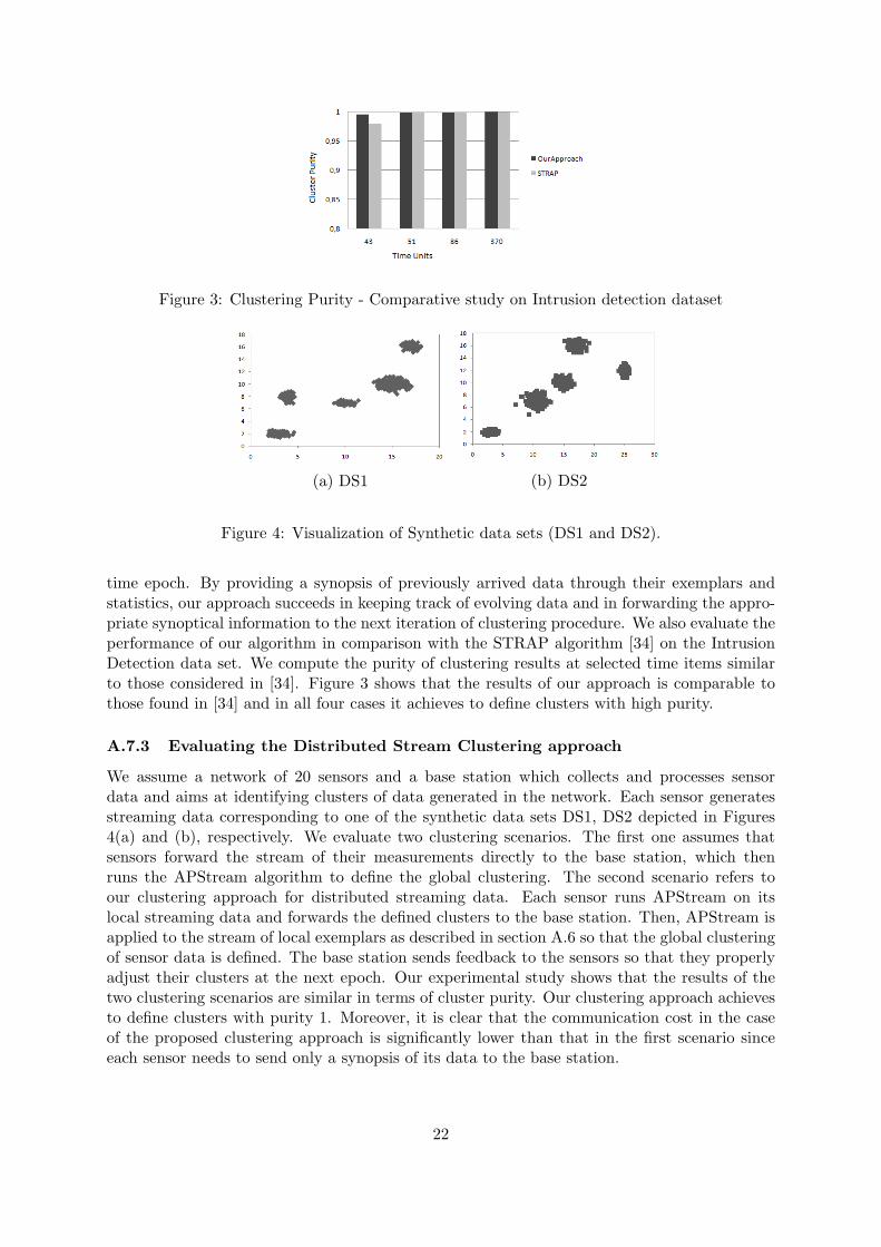
Figure 3: Clustering Purity - Comparative study on Intrusion detection dataset

(a) DS1 (b) DS2

Figure 4: Visualization of Synthetic data sets (DS1 and DS2).

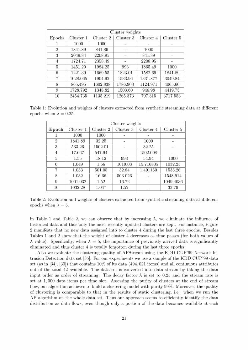
time epoch. By providing a synopsis of previously arrived data through their exemplars andstatistics, our approach succeeds in keeping track of evolving data and in forwarding the appro-priate synoptical information to the next iteration of clustering procedure. We also evaluate theperformance of our algorithm in comparison with the STRAP algorithm [34] on the IntrusionDetection data set. We compute the purity of clustering results at selected time items similarto those considered in [34]. Figure 3 shows that the results of our approach is comparable tothose found in [34] and in all four cases it achieves to define clusters with high purity.

A.7.3 Evaluating the Distributed Stream Clustering approach

We assume a network of 20 sensors and a base station which collects and processes sensordata and aims at identifying clusters of data generated in the network. Each sensor generatesstreaming data corresponding to one of the synthetic data sets DS1, DS2 depicted in Figures4(a) and (b), respectively. We evaluate two clustering scenarios. The first one assumes thatsensors forward the stream of their measurements directly to the base station, which thenruns the APStream algorithm to define the global clustering. The second scenario refers toour clustering approach for distributed streaming data. Each sensor runs APStream on itslocal streaming data and forwards the defined clusters to the base station. Then, APStream isapplied to the stream of local exemplars as described in section A.6 so that the global clusteringof sensor data is defined. The base station sends feedback to the sensors so that they properlyadjust their clusters at the next epoch. Our experimental study shows that the results of thetwo clustering scenarios are similar in terms of cluster purity. Our clustering approach achievesto define clusters with purity 1. Moreover, it is clear that the communication cost in the caseof the proposed clustering approach is significantly lower than that in the first scenario sinceeach sensor needs to send only a synopsis of its data to the base station.

22

A.8 Conclusion

We develop a novel approach for online distributed clustering of streaming data using beliefpropagation techniques. The key ingredient of our streaming clustering approach, APStream, isthe method by which a compressed, synoptical version of data is passed on to the next epoch andaids in re-initialization of the clustering process. The adopted message passing approach runsat each epoch, it successfully identifies clusters, and it maintains an accurate representationof data, although they become gradually available to the decision maker. To deal with thestreaming data generated in distributed setting, we proposed a two-level approach. Moreoverthe proposed two-level belief propagation-based clustering approach is proved to have the sameperformance in terms of clustering quality with the case where the clustering is performed onthe raw streaming data that are sent from nodes to the central location.

23

B UCY Report: Reduced-Complexity Verification for Initial-State Opacity in Modular Discrete Event Systems

Motivated by the increased reliance on shared cyber-infrastructures in many application areas(ranging from defense and banking to health care and power distribution systems), variousnotions of security and privacy have received considerable attention from researchers. Onecategory of such notions focuses on the information flow from the system to the intruder [36,37].Opacity is a security notion that falls in this category and aims to determine whether a givensystem’s secret behavior (i.e., a subset of the behavior of the system that is considered criticaland is usually represented by a predicate) is kept opaque to outsiders [5, 6]. More specifically,this requires that the intruder (modeled as a passive observer of the system’s behavior) neverbe able to establish the truth of the predicate.

In our earlier work [38], we considered opacity with respect to predicates that are state-based. More specifically, we considered a scenario where we are given a discrete event system(DES) that can be modeled as a non-deterministic finite automaton with partial observationon its transitions. The intruder is assumed to have full knowledge of the system model andbe able to track its observable transitions. Assuming that the initial state of the system is(partially) unknown, we defined the notion of initial-state opacity by requiring that no sequenceof transitions allows the intruder to unambiguously determine (by analyzing the associatedsequence of observations) that the initial state of the system belonged to a given set of secretstates S. In order to verify initial-state opacity, we introduced in [38] the initial-state estimatorfor the given discrete event system. We also analyzed the state-complexity of this verificationmethod and showed that it is O(2N

2) where N is the number of states of the given system.

In this report, we assume that the given system is the synchronous product of M modules{G1, G2, . . . , GM} where each module Gi is modelled as a non-deterministic automaton withNi states and the set of secret states S is of the form S = {(x1, x2, . . . , xM )|xi ∈ Si} where setSi represents secret states for module Gi. Assuming that pairwise shared events are pairwiseobservable (and the intruder observes events that are observable in at least one module) we showthat the composed system is initial-state opaque if and only if the strings that violate initial-state opacity in a given module are disabled due to synchronization between that module andthe other modules. [This implies that if each module is individually initial-state opaque, thenthe composed system is also initial-state opaque.] We use this property to provide a modularalgorithm for verifying initial-state opacity with O(MNM−12N

2) state and time complexity,

where N = maxiNi. This is a considerable reduction compared to the O(2(NM )2) state andtime complexity of the centralized method, which verifies initial-state opacity by consideringthe composed system as a monolithic system (with a maximum of NM states).

The notion of initial-state opacity first appeared in [38]. Apart from this work, the modularverification method introduced in this report is related to some of the existing work in the area ofmodular DESs. In particular, the authors of [39] introduced the notion of modular diagnosabilityas a variation of diagnosability [40] for modular systems. This notion1 requires each module tobe able to diagnose its failures given its local observations and the limitations imposed by thesynchronization between modules. While (modular) diagnosability and initial-state opacity arenot easily comparable, the techniques used for verifying them are related. The authors of [39]verify modular diagnosability by first checking whether the given modules are diagnosable. If

1Note that modular diagnosability is a weaker notion than diagnosability because if a failure f1 occurs inmodule G1 and there is a sequence of observations of arbitrary length in the monolithic system that prohibitsdiagnosis of f1 but cannot be observed by G1, then the monolithic system may still be modularly diagnosablealthough it will not be diagnosable. In this report, we do not need to distinguish such cases; when we talk aboutinitial-state opacity, we assume that it is defined with respect to the monolithic system.

24

so, it is shown that the (composed) system is modularly diagnosable. Otherwise, the stringsthat violate diagnosability in each module are checked incrementally against the rest of themodules to verify whether they survive the synchronization due to the composition operator. Itis shown that if no string that violates diagnosability survives the composition, then the givensystem is modularly diagnosable. The technique used here for verifying initial-state opacity issimilar but, as we argue later, we do not need to use an incremental approach.

B.1 Preliminaries and Background

Let Σ be an alphabet and denote by Σ∗ the set of all finite-length strings of elements of Σ,including the empty string ε. A language L ⊆ Σ∗ is a subset of finite-length strings from Σ∗ [41,42]. The natural projection PΣ1 : Σ∗ → Σ∗1 is defined recursively as PΣ1(ts) = PΣ1(t)PΣ1(s), t ∈Σ, s ∈ Σ∗, with PΣ1(t) = t if t ∈ Σ1 and PΣ1(t) = ε if t ∈ (Σ− Σ1) ∪ {ε} [41]. P−1

Σ1(s), s ∈ Σ∗1,

denotes the inverse projection, i.e., the set of strings t ∈ Σ∗ such that PΣ1(t) = s. We cansimilarly define natural projection PΣ1(L) = {PΣ1(s)|s ∈ L} for a language L ⊆ Σ∗ and inverseprojection P−1

Σ1(L) = {P−1

Σ1(s)|s ∈ L} for a language L ⊆ Σ∗1.

For L1 ⊆ Σ∗1, L2 ⊆ Σ∗2, we define the synchronous product L1‖L2 ⊆ (Σ1 ∪Σ2)∗ according to

L1‖L2 = P−1Σ1

(L1) ∩ P−1Σ2

(L2),

where PΣi : (Σ1∪Σ2)∗ → Σ∗i , i = 1, 2. It follows from the definition of the synchronous productthat

s ∈ L1‖L2 ⇔ PΣ1(s) ∈ L1, PΣ2(s) ∈ L2. (15)

Moreover, for strings s1 ∈ L1 and s2 ∈ L2, we have [42]

{s1}‖{s2} 6= ∅ ⇔ PΣ2(s1) = PΣ1(s2). (16)

Lemma 1 (Chapter 3 of [42]) For alphabets Σ0, Σ1, Σ2 with Σ0 ⊆ Σ1 ∪ Σ2, let L1 ⊆Σ∗1, L2 ⊆ Σ∗2, and let PΣ0 : (Σ1 ∪ Σ2)∗ → Σ∗0 be the natural projection. If Σ1 ∩ Σ2 ⊆ Σ0,then PΣ0(L1‖L2) = PΣ0(L1)‖PΣ0(L2). �

A non-deterministic finite automaton (NFA) is denoted by G = (X,Σ, δ,X0), where X ={0, 1, . . . , N − 1} is the set of states, Σ is the set of events, δ : X × Σ→ 2X (where 2X denotesthe power set of X) is the non-deterministic state transition function, and X0 ⊆ X is the set ofpossible initial states. The function δ can be extended from the domain X × Σ to the domainX × Σ∗ in the routine recursive manner: δ(i, ts) :=

⋃j∈δ(i,t) δ(j, s), for t ∈ Σ and s ∈ Σ∗, with

δ(i, ε) := i. The behavior of NFA G is captured by L(G) := {s ∈ Σ∗ | ∃i ∈ X0{δ(i, s) 6= ∅}}.We use L(G, i) = {s ∈ Σ∗|δ(i, s) 6= ∅} to denote the set of all traces that originate from state iof G (so that L(G) =

⋃i∈X0

L(G, i)). Similarly, for any S ⊆ X, we use L(G,S) to denote theset of all traces that originate from a state in S.

In general, only a subset Σobs of the events of NFA G can be observed. Typically, oneassumes that Σ can be partitioned into two sets, the set of observable events Σobs and the set ofunobservable events Σuo (so that Σobs ∩ Σuo = ∅ and Σobs ∪ Σuo = Σ). The natural projectionPΣobs

: Σ∗ → Σ∗obs can be used to map any trace executed in the system to the sequence ofobservations associated with it.

Given automaton G = (X,Σ, δ,X0) with observable events Σobs, a state mapping m ∈ 2X2

is a set whose elements are pairs of states: the first component of each element (pair) is thestarting state and the second component is the ending state; thus, for a state mapping m ∈ 2X

2,

we use m(1) to denote the set of starting states and m(0) to denote the set of ending states.We define the composition operator ◦ : 2X

2 × 2X2 → 2X

2for state mappings m1,m2 ∈ 2X

2

as m1 ◦m2 := {(j1, j3)|∃j2 ∈ X{(j1, j2) ∈ m1, (j2, j3) ∈ m2}}. For any Z ⊆ X, we define the

25

operator � : 2X → 2X2

as �(Z) = {(i, i)|i ∈ Z} where the pairs involve identical elements. Wecan map any observation ω ∈ Σ∗obs of finite but arbitrary length in DES G to a state mappingby using the mapping M : Σ∗obs → 2X

2defined as: M(ω) = {(i, j)|i, j ∈ X,∃s ∈ Σ∗{PΣobs

(s) =ω, j ∈ δ(i, s)}}. We also define M(ε) = �(X).

The synchronous product of two non-deterministic automata G1 = (X1,Σ1, δ1, X01) andG2 = (X2,Σ2, δ2, X02) is the non-deterministic automatonG1‖G2 := AC(X1×X2,Σ1∪Σ2, δ1‖2, X01×X02), where for ij ∈ Xj , j = 1, 2, we define

δ1‖2((i1, i2), α) :={(i′1, i′2)|i′j ∈ δj(ij , α), j = 1, 2, }, if δj(ij , α) 6= ∅, j = 1, 2,{(i′1, i2)|i′1 ∈ δ1(i1, α)}, if α ∈ Σ1 − Σ2 and δ1(i1, α) 6= ∅,{(i1, i′2)|i′2 ∈ δ2(i2, α)}, if α ∈ Σ2 − Σ1 and δ2(i2, α) 6= ∅,∅, otherwise,

and AC denotes the accessible part of the automaton (i.e., the set of states reachable from theset of initial state(s) via some string s ∈ (Σ1 ∪ Σ2)∗). The construction of the synchronousproduct automaton implies that L(G1‖G2) = L(G1)‖L(G2) [42]. In the synchronous product,a common event, i.e., an event in Σ1 ∩ Σ2 can only be executed if both automata can executeit simultaneously. The private events, i.e., those in Σ1 − Σ2 and Σ2 − Σ1 are not subjectto such constraint and can be executed whenever possible. We refer to this phenomenon assynchronization due to the composition operator.

B.2 Initial-State Opacity

We recall the definition of initial-state opacity from [38].

Definition 1 (Initial-State Opacity) Given anon-deterministic finite automaton G = (X,Σ, δ,X0), a natural projection map PΣobs

with re-spect to the set of observable events Σobs (Σobs ⊆ Σ), and a set of secret states S ⊆ X, automatonG is initial-state opaque with respect to S and PΣobs

(or (S, PΣobs,∞) initial-state opaque) if for

all t ∈ L(G,X0 ∩ S):∃s ∈ L(G,X0 − S){PΣobs

(s) = PΣobs(t)}.

�

Examples to motivate the study of initial-state opacity in the context of sensor network coverageand encryption using pseudo-random generators were provided in [38]. According to Definition1, DES G is (S, P,∞) initial-state opaque if for every string t that originates from a systeminitial state in the set of secret states S, there exists a string s that originates from a systeminitial state outside the set of secret states S and has the same projection as t. This impliesthat NFA G is initial-state opaque with respect to S and PΣobs

iff

PΣobs(L(G,X0 ∩ S)) ⊆ PΣobs

(L(G,X0 − S)). (17)

To verify initial-state opacity we can model the intruder as a state estimator, called the initial-state estimator (ISE), which uses state mappings to reconstruct the states from which thesequence of observations seen up to this point could have been initiated [38]. In particular,each state of the ISE is associated with a unique state mapping and, since the initial state ofthe system belongs to X0, the mapping associated with the initial state is the mapping �(X0).Given a new observation, the ISE current state transitions into an ISE state whose associatedstate mapping is the composition of the state mapping associated with the ISE current stateand the state mapping induced by the new observation.

26

Definition 2 (Initial-State Estimator (ISE)) Given a non-deterministic finite automatonG = (X,Σ, δ,X0) and a natural projection map PΣobs

with respect to the set of observableevents Σobs (Σobs ⊆ Σ), the initial-state estimator is the deterministic automaton G∞,obs =AC(2X×X ,Σobs, δ∞,obs, X∞,0) with state set 2X×X (power set of X ×X), event set Σobs, initialstate X∞,0 = �(X0), and state transition function δ∞,obs : 2X×X × Σobs → 2X×X defined forα ∈ Σobs as m′ = δ∞,obs(m,α) := m ◦M(α), where m,m′ ∈ 2X×X .

[AC denotes the states of this automaton that are accessible starting from state X∞,0.We also define X∞,obs ⊆ 2X×X to be the reachable states from X∞,0 under δ∞,obs, so thatAC(2X×X ,Σobs, δ∞,obs, X∞,0) = (X∞,obs,Σobs, δ∞,obs, X∞,0).] �

Clearly, the ISE is a finite structure with at most 2N2

states, where N is the number of states ofDES G. It is shown in [38] that DES G is initial-state opaque if and only if for each reachablestate in X∞,obs, with associated state mapping m, the set of starting states (if nonempty)contains elements outside S, i.e.,

∀m ∈ X∞,obs : m(1) * S or m = ∅. (18)

B.3 Modular Methods for Verifying Initial-State Opacity

B.3.1 Systems with Two Modules

In this section, we consider modular systems and use their structure to reduce the complexityof verifying initial-state opacity. We start by assuming that the given system G is composed oftwo modules G1 and G2, i.e., G = G1‖G2, such that each state of the composed system is a pairof states. The set of secret states in the composed system is defined as all pairs of states suchthat at least one of the component states is a secret state in the corresponding module. Recallthat in order to verify initial-state opacity for the composed system G, we need to verify thatfor each string that originates from a secret initial state (i.e., from a secret initial state in G1 orin G2), there exists at least one other string that originates from a non-secret initial state (i.e.,from a non-secret initial state in G1 and/or G2) with the same projection.

In our model, the set of strings that originate from secret initial states inG is the synchronousproduct of the strings in G1 that originate from secret initial states (in G1) with L(G2), inaddition to the synchronous product of the strings in G2 that originate from secret initial states(in G2) with L(G1). Moreover, the set of strings that originate from non-secret initial states inG is the synchronous product of the strings in G1 that originate from non-secret initial states(in G1) with the strings in G2 that originate from non-secret initial states (in G2). Therefore, toverify initial-state opacity for G, one can obtain all strings t1 in G1 that originate from a secretinitial state such that t1 is not disabled due to the synchronous product with L(G2), and verifythat there exists at least one string s1 with the same projection as t1 such that s1 originatesfrom a non-secret initial state in G1 and is not disabled due to the synchronous product withthe set of strings in G2 that originate from non-secret initial states. This procedure needs to berepeated for strings t2 that originate from secret initial states in G2.

In the sequel, we assume that the shared events are all observable. In other words, modulesonly synchronize on a subset of observable events. This is a common assumption in modular DES[39]. This implies that if a string t1 ∈ Σ∗1 in G1 cannot be executed in G1 due to synchronizationdue to synchronous product (and thus also in G1‖G2), then all strings s1 ∈ Σ∗1 with the sameprojection with respect to the observable events cannot be executed in G1. Therefore, if modulesare initial-state opaque, the composed system will also be initial-state opaque. This can be usedas a sufficient condition to verify initial-state opacity in a modular manner. [We formally provethis statement later in this section.] However, even if the modules are not initial-state opaque,

27

the composed system may still be initial-state opaque. For example, if the string t1 ∈ Σ∗1 inG1 that violates initial-state opacity (i.e., upon observing the projection of t1, the intruderis certain that the initial-state of G1 belongs to the set of secret states) is disabled in thesynchronous product (by the activity of the other module), then the composed system mightstill be initial-state opaque. In the following theorem, we prove this formally.

Theorem 1 Consider a pair of non-deterministic finite automata G1 = (X1,Σ1, δ1, X01) andG2 = (X2,Σ2, δ2, X02), projection maps PΣo1 and PΣo2 with respect to the sets of observableevents Σo1 (Σo1 ⊆ Σ1) and Σo2 (Σo2 ⊆ Σ2), respectively, and sets of secret states S1 ⊆ X1 andS2 ⊆ X2. Take the synchronous product G = G1‖G2 ≡ (X,Σ, δ,X0), assume that

Σ1 ∩ Σ2 ⊆ Σo1 ∩ Σo2 (A1)

and let the set of secret states of G be S = {(i, j) ∈ X|i ∈ S1 or j ∈ S2}. Then, G is initial-state opaque with respect to S and projection map PΣo (where the set of observable eventsΣo = Σo1 ∪ Σo2) if and only if for all t1 ∈ L(G1, X01 ∩ S1) (t2 ∈ L(G2, X02 ∩ S2)) such thatthere exists t2 ∈ L(G2) (t1 ∈ L(G1)) with

PΣ2(t1) = PΣ1(t2), (19)

there exist s1 ∈ L(G1, X01 − S1) and s2 ∈ L(G2, X02 − S2), such that

PΣ2(s1) = PΣ1(s2) (20)

andPΣo1(s1) = PΣo1(t1), PΣo2(s2) = PΣo2(t2). (21)

�

Proof: (IF) Denote the natural projections PΣi : Σ1 ∪ Σ2 → Σi, i = 1, 2. Define the languageL = {s1}‖{s2}, the language K = {t1}‖{t2}, and Σo = Σo1 ∪ Σo2. We have

PΣo(L) = PΣo({s1})‖PΣo({s2}) (By Lemma 1)= PΣo1

({s1})‖PΣo2({s2}) (22)

= PΣo1({t1})‖PΣo2

({t2}) (By (21))

= PΣo({t1})‖PΣo({t2}) (23)= PΣo(K) (By Lemma 1) (24)

where (22) follows from the fact that s1 (s2) does not contain events in Σo2 − Σo1 (Σo1 − Σo2)and (23) follows from the fact that t1 (t2) does not contain events in Σo2−Σo1 (Σo1−Σo2). Now,if t1 ∈ L(G1, X01 ∩S1) (or t2 ∈ L(G2, X02 ∩S2)), then for every t ∈ K we have t ∈ L(G,X0 ∩S)since by definition L(G,X0 ∩ S) contains strings t such that either PΣ1(t) can originate from asecret initial state in G1 or PΣ2(t) can originate from a secret initial state in G2. Similarly, ifs1 ∈ L(G1, X01−S1) and s2 ∈ L(G2, X02−S2), then for every s ∈ L we have s ∈ L(G,X0−S).Also, (24) implies that for every t ∈ K there exists at least one s ∈ L such that PΣo(s) = PΣo(t).Putting all these together, we have

∀t ∈ L(G,X0 ∩ S), ∃s ∈ L(G,X0 − S){PΣo(s) = PΣo(t)},

or equivalently, G is initial-state opaque with respect to S and PΣo . This completes the prooffor the (IF) part.(ONLY IF) If G is initial-state opaque with respect to S and PΣo , then

∀t ∈ L(G,X0 ∩ S),∃s ∈ L(G,X0 − S){PΣo(s) = PΣo(t)}.

28

Moreover, by (15), t ∈ L(G,X0 ∩ S) implies that there exist t1 ∈ L(G1, X01 ∩ S1) (or t2 ∈L(G2, X02 ∩ S2)) and t2 ∈ L(G2) (or t1 ∈ L(G1)) with t1 = PΣ1(t) and t2 = PΣ2(t) such thatPΣ2(t1) = PΣ1(t2). Similarly, s ∈ L(G,X0 − S) implies that there exist s1 ∈ L(G1, X01 − S1)and s2 ∈ L(G2, X02 − S2) with s1 = PΣ1(s) and s2 = PΣ2(s), such that PΣ2(s1) = PΣ1(s2).Moreover, since Σo = Σo1 ∪ Σo2, PΣo(s) = PΣo(t) implies that

PΣo1(s) = PΣo1(t) and PΣo2(s) = PΣo2(t). (25)

Therefore, we have PΣo1(s1) = PΣo1(PΣ1(s)) = PΣo1(s). Similarly, we have PΣo2(s2) = PΣo2(s),PΣo1(t1) = PΣo1(t), and PΣo2(t2) = PΣo2(t). Thus, (25) implies (21). This completes the prooffor the (ONLY IF) part. �

We use Theorem 1 to reduce the complexity of verifying initial-state opacity of the composedsystem by first verifying initial-state opacity separately for each of the modules via the con-structions of the associated ISEs. If the modules are indeed initial-state opaque, the composedsystem is initial-state opaque (refer to Corollary 1 below); otherwise, we obtain the synchronousproduct of each of the ISEs with the other module to check whether the strings that violateinitial-state opacity are disabled due to the synchronous product. In this way, we avoid con-structing the composed system G = G1‖G2 and its ISE. In the sequel, we formally describe thismethod.

Theorem 2 Consider a pair of non-deterministic finite automata G1 = (X1,Σ1, δ1, X01) andG2 = (X2,Σ2, δ2, X02), projection maps PΣo1 and PΣo2 with respect to the sets of observableevents Σo1 (Σo1 ⊆ Σ1) and Σo2 (Σo2 ⊆ Σ2), respectively, and sets of secret states S1 ⊆X1 and S2 ⊆ X2. Also assume that Σ1 ∩ Σ2 ⊆ Σo1 ∩ Σo2. Construct the ISE Gi∞,obs =(Xi∞,obs,Σoi, δ

i∞,obs, X

i∞,0) for Gi, i = 1, 2, and also construct (for i 6= j)

Ki = Gi∞,obs‖Gj= AC(Xi

∞,obs ×Xj ,Σoi ∪ Σj , δKi , Xi∞,0 ×X0j)

≡ (XKi ,ΣKi , δKi , X0Ki), i, j ∈ {1, 2}.

Then, G = G1‖G2 ≡ (X,Σ, δ,X0) is initial-state opaque with respect to

S = {(i, j) ∈ X|i ∈ S1 or j ∈ S2},

and projection map PΣo with respect to the set of observable events Σo = Σo1 ∪ Σo2 if and onlyif for all xk = (m,x) ∈ XK1 ,m ∈ X1

∞,obs, and x ∈ X2:

m(1) * S1 or m = ∅, (26)

and for all x′k = (m′, x′) ∈ XK2, m′ ∈ X2∞,obs, and x′ ∈ X1:

m′(1) * S2 or m′ = ∅. (27)

�

Proof: Assume that xk = (m,x) is reachable in K1 via ω1. This implies that m is reachable inG1∞,obs via PΣo1(ω1). By properties of ISE [38], m(1) * S1 is equivalent to

∀t1 ∈ L(G1, X01 ∩ S1), ∃s1 ∈ L(G1, X01 − S1){PΣo1(t1) = PΣo1(s1)}, (28)

such that m is reachable in G1∞,obs via PΣo1(t1) = PΣo1(s1) = PΣo1(ω1). Now, since xk = (m,x)

is reachable in K1 via ω1, m is reachable in G1∞,obs via PΣo1(t1), then by (16), x is reachable in

29

G2 via t2 such that PΣo1(t2) = PΣ2(PΣo1(t1)). Since all shared events are observable, t1 doesnot contain events in Σ2−Σo2, therefore, PΣ2(PΣo1(t1)) = PΣo2(PΣo1(t1)). For the same reason,t1 does not contain events in Σo2 −Σo1; therefore, PΣo2(PΣo1(t1)) = PΣo2(t1). Putting all thesetogether, we have

PΣo1(t2) = PΣo2(t1). (29)

Note that (29) is equivalent toPΣ1(t2) = PΣ2(t1), (30)

since t2 does not contain events in Σ1 − Σo1 and t1 does not contain events in Σ2 − Σo2.Next, assuming that state x′ is reachable in G1 via t1 and state mapping m′ is reachable in

G2∞,obs via PΣo2(t2), we show that state x′k = (m′, x′) is reachable in G2

∞,obs‖G1. We can use asimilar discussion as in the previous part to show that PΣo2(t1) = PΣ1(PΣo2(t2)), which by (16),proves that state x′k = (m′, x′) is reachable in G2

∞,obs‖G1. By (27), we have m′(1) * S2, whichby properties of ISE [38] is equivalent to

∀t2 ∈ L(G2, X02 ∩ S2), ∃s2 ∈ L(G2, X02 − S2){PΣo2(t2) = PΣo2(s2)}, (31)

such that m′ is reachable in G2∞,obs via PΣo2(t2) = PΣo2(s2). Using a similar discussion as

previous part, we can show thatPΣ1(s2) = PΣ2(s1). (32)

By Theorem 1, (28), (30), (31), and (32) are equivalent to the fact that G is initial-state opaquewith respect to S and PΣo . Therefore, (26) and (27) are equivalent to the fact that G isinitial-state opaque with respect to S and PΣo . This completes the proof. �

Corollary 1 Consider non-deterministic finite automata G1 = (X1,Σ1, δ1, X01) and G2 =(X2,Σ2, δ2, X02), projection maps PΣo1 and PΣo2 with respect to the sets of observable eventsΣo1 (Σo1 ⊆ Σ1) and Σo2 (Σo2 ⊆ Σ2), respectively, and sets of secret states S1 ⊆ X1 andS2 ⊆ X2. Also assume that every shared event is observable, i.e., Σ1 ∩ Σ2 ⊆ Σo1 ∩ Σo2. Then,the composed automaton G = G1‖G2 ≡ (X,Σ, δ,X0) is initial-state opaque with respect toS = {(i, j) ∈ X|i ∈ S1 or j ∈ S2}, and projection map PΣo (where the set of observable eventsis Σo = Σo1 ∪Σo2) if automaton Gi is initial-state opaque with respect to Si and PΣoi, i = 1, 2.�

Corollary 1 proves that initial-state opacity of G1 and G2 is sufficient for initial-state opacityof G = G1‖G2. One can easily demonstrate that that initial-state opacity of G1 (or similarlyG2) is not necessary for initial-state opacity of G. In other words, the verification method basedon Corollary 1 is sound but not complete.

B.3.2 Systems with More than Two Modules

Theorem 2 can be used to verify initial-state opacity when the system consists of only twomodules. This verification method can be extended to the general case when the given systemis composed of M modules Gi = (Xi,Σi, δi, X0i), i = 1, 2, . . . ,M , with projection maps PΣoi

with respect to the sets of observable events Σoi (Σoi ⊆ Σi), and with the sets of secret statesSi ⊆ Xi, 1 ≤ i ≤ M , as follows: for each module Gi, 1 ≤ i ≤ M , we view the system as thecomposition of two modules, Gi and Gi ≡ G1‖G2‖ . . . ‖Gi−1‖Gi+1‖ . . . ‖GM . In order to use thedevelopments of the previous section, we assume that the pairwise shared events are observablepairwise, i.e.,

Σi ∩ (⋃i 6=j

Σj) ⊆ Σoi ∩ (⋃i 6=j

Σoj).

30

Note that⋃i 6=j Σj(

⋃i 6=j Σoj) denotes the set of events (observable events) of Gi. Following

the developments of the previous section, for each module Gi, 1 ≤ i ≤ M , we construct thecorresponding ISE Gi∞,obs = (Xi

∞,obs,Σoi, δi∞,obs, X

i∞,0) and for each ISE Gi∞,obs, 1 ≤ i ≤M , we

construct automatonKi = Gi∞,obs‖Gi ≡ (XKi ,ΣKi , δKi , X0Ki).

Then, G = G1‖G2‖ . . . ‖GM ≡ (X,Σ, δ,X0) is initial-state opaque with respect to S = {(i1, i2, . . . , iM ) ∈X|i1 ∈ S1 or i2 ∈ S2 or . . . or iM ∈ SM}, and projection map PΣo with respect to the set ofobservable events Σo = Σo1 ∪ Σo2 ∪ . . . ∪ ΣoM if and only if for all 1 ≤ i ≤ M and for allxk = (m,x1, x2, . . . , xi−1, xi+1, . . . , xM ) ∈ XKi ,m ∈ Xi

∞,obs, xj ∈ Xj , 1 ≤ j ≤ M, i 6= j :m(1) * Si or m = ∅. If module Gi has Ni states, then each automaton Ki, 1 ≤ i ≤ M , hasstate complexity O(NM−12N

2) where N = maxiNi. Verifying initial-state opacity in this way

requires constructing M automata Ki, 1 ≤ i ≤M , and therefore has state and time complexityO(MNM−12N

2).

Verifying initial-state opacity using Corollary 1 can also be easily extended to the generalcase where the given system is composed of M modules. If each module has at most N states,then verifying initial-state opacity in this way has state and time complexity O(M2N

2) which

is far less than the state and time complexity O(2(NM )2) of the centralized method [38] and lessthan the state and time complexity O(MNM−12N

2) of the method based on Theorem 2. For

example, for a system consisting of 2 modules each with 10 states (i.e., M = 2, N = 10), thestate and time complexity of the centralized method is O(210000), the state and time complexityof the method based on Theorem 2 is O(2105), and the state and time complexity of the methodbased on Corollary 1 is O(2× 2100) = O(2101).

B.4 Conclusion

We have studied reduced-complexity verification of initial-state opacity for discrete event sys-tems that are composed (via the synchronous product) of M ≥ 2 modules. Initial-state opacityrequires that the membership of the system initial state to the set of secret states (defined asstates in which at least one of modules resides within its set of secret states) remains opaqueto an intruder who has complete knowledge of the system model and monitors the observableevents in the system. Assuming that the events shared between pairs of modules are pairwiseobservable, we show that the composed system is initial-state opaque if and only if the stringsthat violate initial-state opacity in a given module are disabled due to synchronization betweenthat module and the rest of the modules. We use this to provide a modular algorithm for ver-ifying initial-state opacity with O(MNM−12N

2) state and time complexity, where N denotes

the maximum number of states of the modules. This is a considerable reduction compared tothe O(2(NM )2) state and time complexity of the centralized method, which verifies initial-stateopacity by considering the composed system as a monolithic system.

In future work, we are interested in designing distributed supervisory strategies that enforceinitial-state opacity using the Ramadge and Wonham framework [43].

31

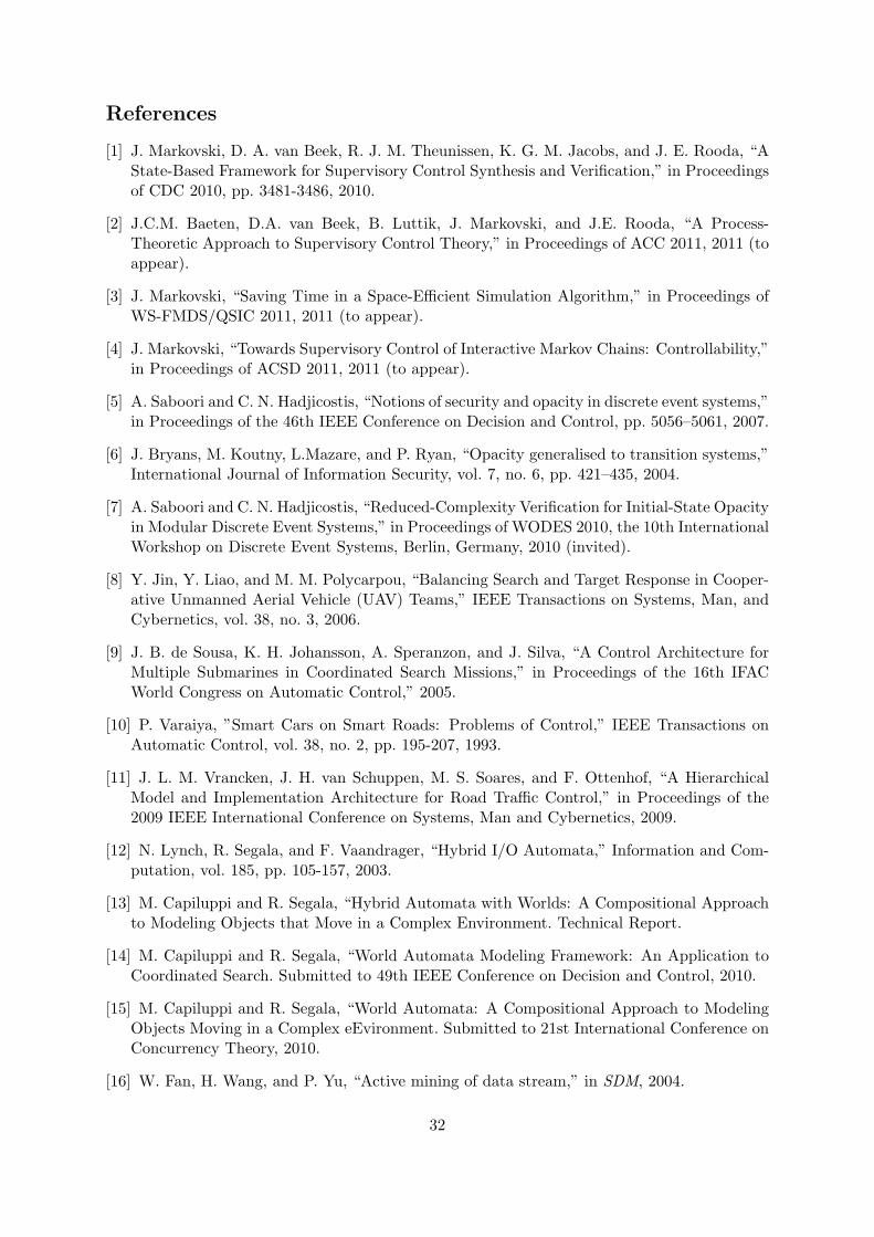
References

[1] J. Markovski, D. A. van Beek, R. J. M. Theunissen, K. G. M. Jacobs, and J. E. Rooda, “AState-Based Framework for Supervisory Control Synthesis and Verification,” in Proceedingsof CDC 2010, pp. 3481-3486, 2010.

[2] J.C.M. Baeten, D.A. van Beek, B. Luttik, J. Markovski, and J.E. Rooda, “A Process-Theoretic Approach to Supervisory Control Theory,” in Proceedings of ACC 2011, 2011 (toappear).

[3] J. Markovski, “Saving Time in a Space-Efficient Simulation Algorithm,” in Proceedings ofWS-FMDS/QSIC 2011, 2011 (to appear).

[4] J. Markovski, “Towards Supervisory Control of Interactive Markov Chains: Controllability,”in Proceedings of ACSD 2011, 2011 (to appear).

[5] A. Saboori and C. N. Hadjicostis, “Notions of security and opacity in discrete event systems,”in Proceedings of the 46th IEEE Conference on Decision and Control, pp. 5056–5061, 2007.

[6] J. Bryans, M. Koutny, L.Mazare, and P. Ryan, “Opacity generalised to transition systems,”International Journal of Information Security, vol. 7, no. 6, pp. 421–435, 2004.

[7] A. Saboori and C. N. Hadjicostis, “Reduced-Complexity Verification for Initial-State Opacityin Modular Discrete Event Systems,” in Proceedings of WODES 2010, the 10th InternationalWorkshop on Discrete Event Systems, Berlin, Germany, 2010 (invited).

[8] Y. Jin, Y. Liao, and M. M. Polycarpou, “Balancing Search and Target Response in Cooper-ative Unmanned Aerial Vehicle (UAV) Teams,” IEEE Transactions on Systems, Man, andCybernetics, vol. 38, no. 3, 2006.

[9] J. B. de Sousa, K. H. Johansson, A. Speranzon, and J. Silva, “A Control Architecture forMultiple Submarines in Coordinated Search Missions,” in Proceedings of the 16th IFACWorld Congress on Automatic Control,” 2005.

[10] P. Varaiya, ”Smart Cars on Smart Roads: Problems of Control,” IEEE Transactions onAutomatic Control, vol. 38, no. 2, pp. 195-207, 1993.

[11] J. L. M. Vrancken, J. H. van Schuppen, M. S. Soares, and F. Ottenhof, “A HierarchicalModel and Implementation Architecture for Road Traffic Control,” in Proceedings of the2009 IEEE International Conference on Systems, Man and Cybernetics, 2009.

[12] N. Lynch, R. Segala, and F. Vaandrager, “Hybrid I/O Automata,” Information and Com-putation, vol. 185, pp. 105-157, 2003.

[13] M. Capiluppi and R. Segala, “Hybrid Automata with Worlds: A Compositional Approachto Modeling Objects that Move in a Complex Environment. Technical Report.

[14] M. Capiluppi and R. Segala, “World Automata Modeling Framework: An Application toCoordinated Search. Submitted to 49th IEEE Conference on Decision and Control, 2010.

[15] M. Capiluppi and R. Segala, “World Automata: A Compositional Approach to ModelingObjects Moving in a Complex eEvironment. Submitted to 21st International Conference onConcurrency Theory, 2010.

[16] W. Fan, H. Wang, and P. Yu, “Active mining of data stream,” in SDM, 2004.

32

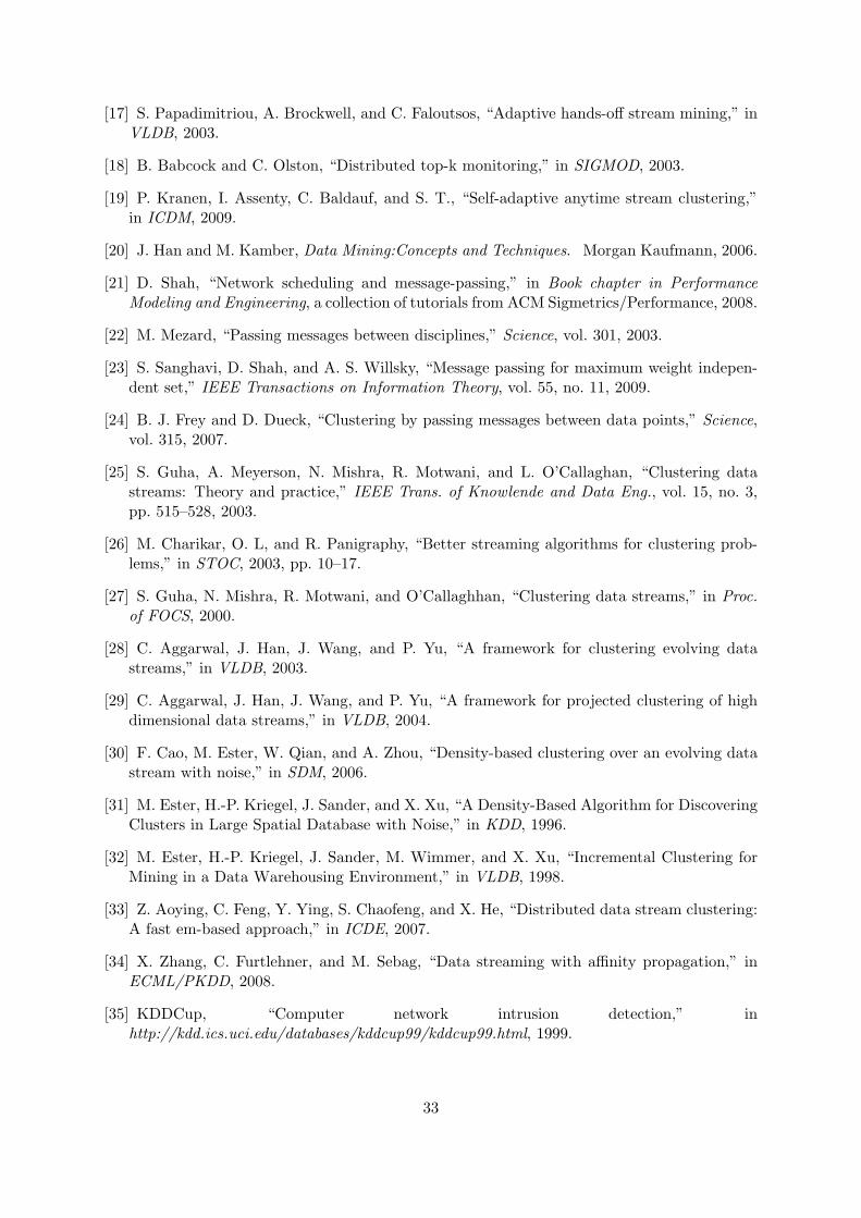
[17] S. Papadimitriou, A. Brockwell, and C. Faloutsos, “Adaptive hands-off stream mining,” inVLDB, 2003.

[18] B. Babcock and C. Olston, “Distributed top-k monitoring,” in SIGMOD, 2003.

[19] P. Kranen, I. Assenty, C. Baldauf, and S. T., “Self-adaptive anytime stream clustering,”in ICDM, 2009.

[20] J. Han and M. Kamber, Data Mining:Concepts and Techniques. Morgan Kaufmann, 2006.

[21] D. Shah, “Network scheduling and message-passing,” in Book chapter in PerformanceModeling and Engineering, a collection of tutorials from ACM Sigmetrics/Performance, 2008.

[22] M. Mezard, “Passing messages between disciplines,” Science, vol. 301, 2003.

[23] S. Sanghavi, D. Shah, and A. S. Willsky, “Message passing for maximum weight indepen-dent set,” IEEE Transactions on Information Theory, vol. 55, no. 11, 2009.

[24] B. J. Frey and D. Dueck, “Clustering by passing messages between data points,” Science,vol. 315, 2007.

[25] S. Guha, A. Meyerson, N. Mishra, R. Motwani, and L. O’Callaghan, “Clustering datastreams: Theory and practice,” IEEE Trans. of Knowlende and Data Eng., vol. 15, no. 3,pp. 515–528, 2003.

[26] M. Charikar, O. L, and R. Panigraphy, “Better streaming algorithms for clustering prob-lems,” in STOC, 2003, pp. 10–17.

[27] S. Guha, N. Mishra, R. Motwani, and O’Callaghhan, “Clustering data streams,” in Proc.of FOCS, 2000.

[28] C. Aggarwal, J. Han, J. Wang, and P. Yu, “A framework for clustering evolving datastreams,” in VLDB, 2003.

[29] C. Aggarwal, J. Han, J. Wang, and P. Yu, “A framework for projected clustering of highdimensional data streams,” in VLDB, 2004.

[30] F. Cao, M. Ester, W. Qian, and A. Zhou, “Density-based clustering over an evolving datastream with noise,” in SDM, 2006.

[31] M. Ester, H.-P. Kriegel, J. Sander, and X. Xu, “A Density-Based Algorithm for DiscoveringClusters in Large Spatial Database with Noise,” in KDD, 1996.

[32] M. Ester, H.-P. Kriegel, J. Sander, M. Wimmer, and X. Xu, “Incremental Clustering forMining in a Data Warehousing Environment,” in VLDB, 1998.

[33] Z. Aoying, C. Feng, Y. Ying, S. Chaofeng, and X. He, “Distributed data stream clustering:A fast em-based approach,” in ICDE, 2007.

[34] X. Zhang, C. Furtlehner, and M. Sebag, “Data streaming with affinity propagation,” inECML/PKDD, 2008.

[35] KDDCup, “Computer network intrusion detection,” inhttp://kdd.ics.uci.edu/databases/kddcup99/kddcup99.html, 1999.

33

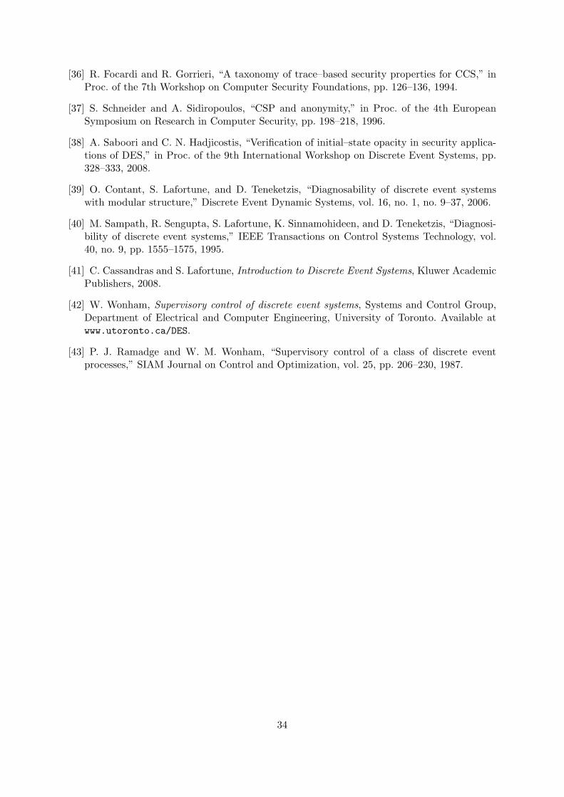
[36] R. Focardi and R. Gorrieri, “A taxonomy of trace–based security properties for CCS,” inProc. of the 7th Workshop on Computer Security Foundations, pp. 126–136, 1994.

[37] S. Schneider and A. Sidiropoulos, “CSP and anonymity,” in Proc. of the 4th EuropeanSymposium on Research in Computer Security, pp. 198–218, 1996.

[38] A. Saboori and C. N. Hadjicostis, “Verification of initial–state opacity in security applica-tions of DES,” in Proc. of the 9th International Workshop on Discrete Event Systems, pp.328–333, 2008.

[39] O. Contant, S. Lafortune, and D. Teneketzis, “Diagnosability of discrete event systemswith modular structure,” Discrete Event Dynamic Systems, vol. 16, no. 1, no. 9–37, 2006.

[40] M. Sampath, R. Sengupta, S. Lafortune, K. Sinnamohideen, and D. Teneketzis, “Diagnosi-bility of discrete event systems,” IEEE Transactions on Control Systems Technology, vol.40, no. 9, pp. 1555–1575, 1995.

[41] C. Cassandras and S. Lafortune, Introduction to Discrete Event Systems, Kluwer AcademicPublishers, 2008.

[42] W. Wonham, Supervisory control of discrete event systems, Systems and Control Group,Department of Electrical and Computer Engineering, University of Toronto. Available atwww.utoronto.ca/DES.

[43] P. J. Ramadge and W. M. Wonham, “Supervisory control of a class of discrete eventprocesses,” SIAM Journal on Control and Optimization, vol. 25, pp. 206–230, 1987.

34