
Object names and object functions serve as cues to categories for infants
Upload
khangminh22Category
view
1download
0
รายงานวจยฉบบสมบรณ โครงการ ระเบยบวธเชงสถตสาหรบการวเคราะหขอมลทางชววทยา
สงแวดลอมและการแพทย: ทฤษฎและการประยกต II
Statistical Methods of data Analysis in Biology Environment and Medicine: Theory and Applications II
โดย รองศาสตราจารย ดร. มนตทพย เทยนสวรรณ
พฤษภาคม 2556

สญญาเลขท BRG5380004
รายงานวจยฉบบสมบรณ โครงการ ระเบยบวธเชงสถตสาหรบการวเคราะหขอมลทางชววทยา
สงแวดลอมและการแพทย: ทฤษฎและการประยกต II
Statistical Methods of data Analysis in Biology Environment and Medicine: Theory and Applications II
ผวจย สงกด
1. รศ.ดร. มนตทพย เทยนสวรรณ มหาวทยาลยมหดล 2. ดร. สาธน เลศประไพ มหาวทยาลยบรพา 3. ดร. สขมาล สารกะวณช ม.เทคโนโลยพระจอมเกลาธนบร 4. น.ส. หนงฤทย สนธมล มหาวทยาลยมหดล 5. นายวฒชย ศรโสดาพล มหาวทยาลยมหดล 6. น.ส. ภทรพร ตสโต มหาวทยาลยมหดล 7. น.ส. รชนกร ทบประดษฐ มหาวทยาลยมหดล 8. Mr. Ananta R Dhungana มหาวทยาลยมหดล
สนบสนนโดยสานกงานกองทนสนบสนนการวจย
(ความเหนในรายงานนเปนของผวจย สกว.ไมจาเปนตองเหนดวยเสมอไป)

Contract Number BRG5380004
Project Title: Statistical Methods of data Analysis in Biology Environment and Medicine:
Theory and Applications II
Principal Investigator: Assoc. Prof. Dr. Montip Tiensuwan
Address: Department of Mathematics Faculty of Science, Mahidol University,
Rama 6 Road, Bangkok, Thailand 10400
Telphone:02-2015538, 02-2015340, Fax: 02-2015343, e-mail: [email protected]
Abstract
Data analysis is an integral part of statistics, and statistical methods to analyze data
arising from various sources abound in the literature. Nevertheless, the need for new methods
of data analysis or application of conventional methods to new area often arises because of
emerging new and difficult data collection methods and innovative statistical problems. In the
context of biology environment and medicine, we focused on nutritional assessment based on
prices, and eleven nutrient indicators, namely energy, carbohydrates, fats, proteins, calcium,
iron, vitamin A, thiamin, riboflavin, vitamin C, and niacin from groups of vegetables, foods,
fruits, and desserts. Nutrient indicators and prices are assessed by the Multiple Criteria
Decision Making (MCDM) and Electre methods. The overall index average is ranked from
the highest to the lowest based on these indicators. Hence, the MCDM and Electre methods
are shown to be feasible measures to compare and rank the types of vegetables, foods, fruits,
and desserts based on nutrient indicators and prices within each category. A time series
analysis is adopted as a technique for forecasting of monthly rainfall and water level along
the Chao Phraya River in Thailand. The Box-Jenkins technique is used for identifying the
parameters of an Autoregressive Integrated Moving Average (ARIMA) model. The Akaike
information criterion, the Schwarz’s Bayesian criterion and the mean square error are used
throughout to test for simplification of any particular model. The periodogram analysis is
used to confirm the existence of a seasonal period in the ARIMA model. The ARIMA with
seasonal model possibly predicts the monthly rainfall and water level along the Chao Phraya
River one year ahead with acceptable accuracy. The nonlinear mixed effects model is also
proposed for repeated measures data to describe longitudinal changes in Carcinoembryonic Antigen
(CEA) levels of colorectal cancer patients over time. The CEA level of colorectal cancer patients is
regarded as the marker choice for monitoring. Parameters of the proposed model are estimated by

[ii]
using Lindstrom and Bates (LB) and the Stochastic Approximation version of the standard
Expectation and Maximization step (SAEM) algorithms. The results show that the estimates of the
recurrent time ( 2φ ) by using LB and SAEM are equal to 17.4 and 22.8 months, respectively. Further,
the residual sum of squares of the proposed model by using the LB and SAEM algorithms are also
compared. Dose response models are the mathematical functions that relate the dose to the measure
of observed effect. Three models are considered, namely, the multistage Weibull, logistic and log-
logistic models. The study focuses on estimating parameters and comparing estimates in these three
models based on the method of maximum likelihood and Berkson’s minimum chi-square method. The
two methods are also applied to four real experimental data sets for each of the three models. Lastly,
we focused on apply the concept of sufficiency and Fisher information for the comparison of
experiments of different bivariate normal populations with arbitrarily specified means and variances
and with different forms of the correlation parameter rho ( )ρ and to apply the concept of sufficiency
for the simple linear regression model x xy x eα β= + + , xe ∼ ( )20, , [ 1,1]N xσ ∈ − non – stochastic
regression and for the one-way random normal model.
Keywords: Akaike’s information criteria, asymptotic comparison, Berkson minimum chi-square,
bivariate/trivariate normal populations, Box-Jenkins models, carcinoembryonic antigen, electre
method, Fisher information, fixed effects, information, linear models, logistic model, log-logistic
model, maximum likelihood, most uniform allocation, multistage Weibull model, multiple criteria
decision making method, nonlinear mixed effects model, nutrient indicators, one-way random effects
model, optimal designs, prices, random effects, repeated measures, Schwartz’s Bayesian criterion,
sufficient experiments, sufficiency, variance of white noise

Contract Number BRG5380004
ชอโครงการ: ระเบยบวธเชงสถตสาหรบการวเคราะหขอมลทางชววทยา สงแวดลอมและการแพทย: ทฤษฎและการประยกต II
หวหนาโครงการ: รองศาสตราจารย ดร. มนตทพย เทยนสวรรณ
ทอย: ภาควชาคณตศาสตร คณะวทยาศาสตร มหาวทยาลยมหดล ถนนพระรามท 6 กรงเทพมหานคร 10400
โทรศพท: 02-2015538, 02-2015340, Fax: 02-2015343, e-mail: [email protected]
บทคดยอ
การวเคราะหขอมลคอภาคจานวนเตมของสถตและวธเชงสถตในการวเคราะหขอมลทเกดขนจากแหลงแตกตางกนมมากมายในเอกสารขอมลหรอวรรณกรรม อยางไรกตามความตองการวธการใหมๆสาหรบการวเคราะหขอมลหรอการประยกตวธธรรมดาทนาไปสเนอหาใหมจะเกดขนเสมอๆเพราะขอมลใหมทปรากฎและวธการเกบรวบรวมขอมลทไดยากและปญหาเชงสถตใหมๆ ในสวนขอมลทางชววทยา สงแวดลอมและการแพทย ผวจยไดใหความสนใจการประเมนตวชวดราคาและสารอาหารทงหมด 11 ชนด ไดแก พลงงาน คารโบไฮเดรต ไขมน โปรตน แคลเซยม เหลก วตามนเอ วตามนบ 1 วตามนบ 2 วตามนซ และวตามนบ 3 จากกลมของผก อาหาร ผลไม และขนมหวาน ตวชวดสารอาหารไดถกประเมนและเปรยบเทยบโดยใชวธเกณฑการตดสนใจพหคณและวธ Electre คาเฉลยดชนทงหมด ไดถกจดอนดบจากคาสงสดไปยงคาตาสดโดยอาศยตวชวดสารอาหารและราคาทงหมด ดงนน จะเหนไดวาวธเกณฑการตดสนใจพหคณและวธ Electre เหมาะสมในการเปรยบเทยบและการวดจดอนดบสาหรบผก อาหาร ผลไม และขนมหวานแตละชนดในแตละประเภท อนกรมเวลาไดนามาใชสาหรบการพยากรณปรมาณนาฝนและระดบนารายเดอนของแมนาเจาพระยาในประเทศไทย เทคนคบอกซ-เจนกนสไดถกนามาใชในการระบพารามเตอรของตวแบบการถดถอยในตวเองรวมคาเฉลยเคลอนท (ARIMA) เกณฑทใชในการพจารณาความเหมาะสมของตวแบบ คอ เกณฑสารสนเทศของอากาอเคะ (AIC) เกณฑชวารซเบเชยน (SBC) และคาประมาณความแปรปรวนของสวนรบกวน การวเคราะหแผนภาพเปนคาบไดถกนามาใชเพอยนยนการมอยของคาบฤดกาลในตวแบบARIMA ตวแบบARIMAแบบฤดกาลอาจจะใชทานายปรมาณนาฝนรายเดอนและระดบนารายเดอนของแมนาเจาพระยา หนงปลวงหนาดวยความแมนทยอมรบได ผวจยไดนาเสนอตวแบบอทธพลผสมไมเชงเสน สาหรบขอมลทมการวดซาในชวงเวลา เพออธบายการเปลยนแปลงระดบ Carcinoembryonic Antigen (CEA) ของผปวยโรคมะเรงลาไสใหญ ระดบCEAของผปวยโรคมะเรงลาไสใหญไดใชเปนตวบงชตวหนงสาหรบการดแลผปวยโรคมะเรงลาไสใหญ กลาวคอถาระดบCEAในผปวยโรคมะเรงลาไสใหญ ภายหลงไดรบการผาตด มคาสงขนเรอยๆ บงถงวาอาจมการกลบมาเปนซาของโรคอก ผวจยไดเสนอตวแบบอทธพลผสมไมเชงเสนของระดบCEA ของผปวยมะเรงลาไสใหญ โดยอทธพลผสมเกดจากอทธพลคงทและ

[iv]
อทธพลสม พารามเตอร 2φ ในตวแบบทนาเสนอใชแทนเวลาเมอเกดการกลบมาเปนซาของโรค(จานวนเดอนภายหลงการผาตด) พารามเตอรในตวแบบประมาณคาใชขนตอนวธ Lindstrom and Bates (LB) และ Stochastic Approximation version of the standard Expectation and Maximization step (SAEM) ผลการศกษาพบวา ตวประมาณคาโดยใชขนตอนวธLB และ SAEM ใหคากลบมาเปนซาเมอผปวยไดรบการผาตดไปแลว 17.4 และ 22.8 เดอน ตามลาดบ ตวแบบการตอบสนองขนาดยาคอฟงกชนทางคณตศาสตรทเกยวของกบขนาดยาและการวดผลกระทบคาสงเกต ตวแบบทพจารณา 3 ตวแบบคอ ตวแบบไวบลลหลายขนตอน ตวแบบลอจสตกและตวแบบลอก-ลอจสตก การศกษาครงนใหความสนใจกบการประมาณคาพารามเตอรและการเปรยบเทยบตวประมาณคาจากตวแบบทง 3 ตวแบบดงกลาวดวยวธภาวะนาจะเปนสงสดและวธไคกาลงสองตาสดของเบอรคสน วธประมาณคาพารามเตอรทงสองวธไดประยกตใชกบขอมล 4 ชดการทดลองสาหรบแตละตวแบบ สดทายผวจยใหความสนใจเชงแนวคดของความเพยงพอและสารสนเทศของฟชเชอรสาหรบการเปรยบเทยบการทดลองทแตกตางของประชากรแบบทวปรกต เมอ กาหนดคาเฉลยและคาแปรปรวนในรปแบบตางๆของพารามเตอรสหสมพนธ ( )ρ และประยกตแนวคดความเพยงพอสาหรบตวแบบถดถอยเชงเสนอยางงาย x xy x eα β= + + , xe ∼ ( )20, , [ 1,1]N xσ ∈ − การถดถอยไมใชเชงสม และสาหรบตวแบบเชงสมปรกตทางเดยว คาสาคญ: เกณฑสารสนเทศของอากาอเคะ, การเปรยบเทยบขนาดตวอยางใหญ, วธไคกาลงสองตาสดของเบอรคสน, ประชากรปรกตสอง/สามตวแปร, ตวแบบบอกซ-เจนกนส, สารกอภมตานทานคารซโนเอมไบรโอนค, วธอเลคเตอร, สารสนเทศของฟชเชอร, อทธพลตรง, สารสนเทศ, ตวแบบเชงเสน, ตวแบบลอจสตก, ตวแบบลอก-ลอจสตก, ความควรจะเปนสงสด, การจดสรรเอกรปยง, ตวแบบไวบลลหลายขนตอน, การตดสนใจเกณฑพหคณ, ตวแบบอทธพลผสมไมเชงเสน, ตวชวดสารอาหาร, ตวแบบอทธพลสมทางเดยว, การออกแบบทเหมาะสม, ราคา, อทธพลสม, การวดซา, เกณฑชวารซเบเชยน, การทดลองพอเพยง, พอเพยง, ความแปรปรวนรบกวน

Executive Summary Project Title: Statistical Methods of Data Analysis in Biology, Environment and Medicine: Theory and Applications II (วธเชงสถตสาหรบการวเคราะหขอมลทางชววทยา สงแวดลอม และการแพทย : ทฤษฎและการประยกต II) Principal Investigator: Assoc.Prof. Dr.Montip Tiensuwan Department of Mathematics, Faculty of Science, Mahidol University, Rama 6 Road, Bangkok, 10400 Tel.: 02-2015340, 02-2015538 Fax: 02 2015343 e-mail: [email protected] Objectives We proposed and/or applied statistical methods of data analysis on multiple criterion decision making (MCDM) to nutrient and vitamin in food, fruit, vegetable, soft drink in term of quantity, quality and price; forecasted rainfall and water level in each province along the Chao Praya river by using Box-Jenkins models and Fourier analysis; proposed nonlinear mixed effects models of colorectal cancer patients to find out the recurrent time of cancer patients; estimated parameters on dose response relationship and applications; and proposed comparison of sufficient experiments. We will use various data sets to test our methods, i.e. for numerical examples and for applications in biology, environment and medicine. Following the objectives the research has been done as follows. 1. Multiple Criterion Decision Making (MCDM) We have collected the data and examined the nutrient and vitamin in food, fruit, vegetables, soft drink in term of quantity, quality and price. 2. Rainfall and water level forecasting 2.1 Forecasting rainfall and water level in each province along the Chao Praya River separately by using Box Jenkins models. 2.2 Using the Fourier analysis in order to confirm the seasonal period of Box Jenkins models. 3. Nonlinear mixed effects models 3.1 Estimating the parameters, 2 ,σ θ and θ∑ , of the nonlinear mixed effects models by NLME and SAEM algorithms. 3.2 Computing the variance of estimators of the proposed model. 3.3 Comparing the variance of estimators based on the NLME and SAEM. 4. Dose Response Relationship with Applications 4.1 Estimated parameters on the dose response models, i.e. multistage Weibull, logistic and log-logistic models involving two parameters 0θ and 1θ and evaluating estimators 4.2 Deriving the properties of estimators by using the maximum likelihood and Berkson's minimum chi-square methods in large sample. 4.3 Comparing the estimators based on the maximum likelihood and Berkson's minimum chi-square methods by using asymptotic comparison of MSE for Case I: 1θ is known and 0θ is unknown, Case II: 0θ is known and 1θ is unknown Case III: 0θ and 1θ are unknown 5. Comparison of experiments 5.1 Sufficiency in bivariate and trivariate normal populations. 5.2 Sufficiency in linear and quadratic regression models with/without intercept term. 5.3 Sufficiency on one-way random effect models.

Contents Page
Abstract (English) [i]
Abstract (Thai) [iii]
Executive Summary [v]
1. Project Title 1
2. Research Team 1
3. Research Field 2
4. Keywords 2
5. Background and Rationale 2
6. Project Objectives 3
7. Research Activities 8
7.1 Data Envelopment Decision Analysis (DEA) and Multiple Criteria 8
Decision Making (MCDM)
7.2 Rainfall and Water Level Forecasting 76
7.3 Nonlinear Mixed Effects Models 167
7.4 Dose Response Relationship with Applications 209
7.5 Comparison of Experiemnts 351
8. Overall Output 438
8.1 Summary Table 438
8.2 Papers appeared in international journals 439
8.3 Papers submitted for publication in international journal 440
8.4 Papers presented in the international conferences 440
8.5 Papers appeared in international journals (BRG4980012) 441
8.6 Other research papers appeared in international journals 441
8.7 Graduated Students 443
9. Appendix 443
9.1 Papers appeared / accepted for publication 444

BRG5380004 Report 36 months
Contract Number BRG5380004
Final Report =============================================
Report Period 31 May 2010 – 30 May 2013
1. Project Title: Statistical Methods of data Analysis in Biology Environment and
Medicine: Theory and Applications II
(ระเบยบวธเชงสถตสาหรบการวเคราะหขอมลทางชววทยาสงแวดลอมและการแพทย : ทฤษฎและการประยกต II)
2. Research Team:
2.1 Principal Investigator: Assoc. Prof. Dr. Montip Tiensuwan Address: Department of Mathematics Faculty of Science, Mahidol University, Rama 6 Road, Bangkok, Thailand 10400 Telphone: 02-2015538, 02-2015340, Fax: 02- 2015343,
e-mail: [email protected] Devoted Time per week: 40 hours
2.2 Team Members: 2.2.1 Miss Satinee Lertprapai, Ph.D.
Address: Department of Mathematics, Faculty of Science, Burapha University
Telephone: 038-745900 Ext.3099 Fax: 038-745900 Ext. 3078,
e-mail: [email protected]
Devoted Time per week: 20 hours
2.2.2 Miss Sukuman Sarikavanij, Ph.D.
Address: Department of Mathematics, Faculty of Science, King Mongkut’s University of
Technology Thonburi
Telephone: 02-4708822, 02-4708997 Fax: 02-4284025, e-mail: [email protected]
Devoted Time per week: 20 hours

BRG5380004 Report 36 months 2
2.3 Ph.D. Students: (1) Miss Nuengruithai Sontimool
(2) Mr. Wuttichai Srisodaphol
(3) Mr. Ananta R. Dhungana
2.4 M.Sc. Students:
(1) Miss Pattaraporn Tusto (2) Miss Ratchaneekorn Thoppradid
2.5 Expert Contacts: (1) Prof. Bimal K. Sinha ( The University of Maryland Baltimore County, USA)
(2) Prof. Bikas K. Sinha (Stat-Math Unit, Indian Statistical Institute, Kolkata, India)
(3) Assoc.Prof. Timothy E. O’Brien (Loyola University Chicago, USA)
3. Research Field: Mathematical Science (Mathematical Statistics, Statistical
Modelling, Data Analysis)
4. Keywords: Multiple criteria decision making(MCDM), Box-Jenkins ARIMA models,
Fourier analysis, nonlinear mixed effects models, dose response models, sufficient
experiments, bivariate normal models
5. Background and Rationale Data analysis is an integral part of statistics, and statistical methods to analyze data
arising from various sources abound in the literature. Nevertheless, the need for new
methods of data analysis or application of conventional methods to new area often arises
because of emerging new and difficult data collection methods and innovative statistical
problems. For example, in the context of environmental science, it is necessary to study
the overall pollution level or state of the environment in a given region on the basis of
several key factors such as the pollution level of air, land, water, and the like. It is thus
necessary to suitably and meaningfully define an aggregate index which captures the
essential features of the component indices and yet represents an overall picture of the

BRG5380004 Report 36 months 3
environment. Data Envelopment Analysis (DEA) and its variations such as Multiple
Criterion Decision Making (MCDM) are recent statistical techniques which are used to
compute this aggregate index. In another context, Time series analysis is one of the
statistical analyses and one of the most powerful techniques used to develop a model and
produce a reliable forecast, which is used in many applications such as: economic
forecasting, sales forecasting, meteorology, quality control, inventory studies, census
analysis and etc. There are many methods of model fitting including the following: Box-
Jenkins ARIMA models, Box-Jenkins multivariate models and Fourier analysis. As a third
application, we mention that in the context of mathematical modeling based on non-linear
mixed effects (NLME) models of cancer and non-linear dose response models i.e. estimate
parameters of the proposed model by using the algorithm of Linstrom and Bates and the
stochastic approximation version of EM (Expectation and Maximization), i.e. SAEM
algorithm. Further the maximum likelihood, Berkson's minimum chi-square, and Bayesian
methods are going to use for estimating parameters of the proposed non-linear dose
response models. Lastly comparison of some experiments is an interested problem which
can be further developed and applied in some theory and practical cases.
We believe that there are ample opportunities to carry out several statistical data
analyses projects along the above lines which would be very helpful in the context of
Thailand.
6. Project Objectives
The main objectives of this research project are given as the followings.
6.1 Data Envelopment Analysis (DEA) and Multiple Criterion Decision Making
(MCDM)
Comparing several competing estimates in terms of their biases or variances or
mean squared errors or tests in terms of their local and global powers is a common practice
in statistics. This is an extremely important problem because of the nonexistence of a best
estimate or test which can be used on all occasions. Although the fascinating area of
decision theory deals with this problem, and notions of admissibility and minimaxity along
with the property of Bayesness play a crucial role, nevertheless other different approaches

BRG5380004 Report 36 months 4
are also welcome and often contribute significantly in this domain. DEA/MCDM is one
such procedure which has proved it self to be very valuable during the last few years.
DEA/MCDM is based on the premise that to compare and possibly rank several
facilities (estimates, tests, machines, products, etc) in regard to their chemical emissions
(bias, variance, MSE, price, defects, etc), there does not exist a facility which is uniformly
the best or the worst for all possible scenarios (for all values of unknown parameters). One
can then define what are called ideal and anti-ideal facilities, and compute the distances of
any facility from these special facilities. It should be noted that ideal and anti-ideal
facilities may not exist in practice. One can then compute an index of performance of any
given facility based on its distance from ideal and anti-ideal facilities, and rank all the
facilities under the condition that a facility is considered good if its distance from ideal is
small as well as its distance from anti-idfeal is large. This is essentially the basis of
DEA/MCDM.
A specific research project in connection with DEA/MCDM is outlined below.
We will examine the nutrient and vitamins in foods, fruits, vegetables, soft drinks in term
of quantity, quality and price and investigate which is the best or the worst among each
kind of food, fruit, and vegetable, and make some recommendations for consumer to
select. The technical tool used for this purpose will be Multiple Criterion Decision Making
(MCDM), which is a variation of DEA. We will apply all the methods mentioned above to
carry out an extensive MCDM strategy.
6.2 Rainfall and water level forecasting
As mentioned above, rainfall and water level forecasting are important topics in
meteorology in Thailand. The prime minister mentioned that rainfall forecasting in
Thailand is not accuracy. Not only there was a flood in Chiangmai province in 2005 but
also there lack of water in eastern part of Thailand. Therefore the main objectives of this
study are outlined below.
1. Forecasting rainfall and water level in each province along the Chao Praya river
separately by using Box Jenkins models.
2. Forecasting rainfall and water level in each province along the Chao Praya river by
using Fourier analysis.

BRG5380004 Report 36 months 5
3. Comparing the results between Box Jenkins and Fourier analysis.
6.3 Nonlinear Mixed Effects Models
In the field of medical science, data usually consists of repeated measurements on
individuals observed under varying conditions. For example, data from clinical trials are
often longitudinal clinical studies; measurements are taken on each of number of subjects
over time. Similarly, clinically useful to know when prostate-specific antigen (PSA) levels
first begin to rise rapidly and to determine if the natural history of PSA progression is
different in men with locally confined prostate cancers compared to men with metastatic
tumors.
Prostate cancer is the most common cancer in male populations in many parts of
the world. It is a slowing growing deadly cancer with very few signs and symptoms in the
early stage. In the United States an estimated 244,000 new cases and 40,400 deaths from
prostate cancer will occur in the United States in 1995 (Wingo et al., 1995).
Prostate Specific Antigen (PSA) is a glycoprotein that is produced by the prostatic
epithelium and can be measured in serum samples by immunoassay. It is made by prostate
cells and is released into the bloodstream. Large prostates have more PSA, so a rise in PSA
means that the gland is enlarging rapidly, which can be a sign of cancer or is irritated by
infection. Any manipulation of the prostate raises blood PSA levels (Webber et al., 1995
[14]).
Another example, a rising Carcinoembryonic Antigen (CEA) level indicates
progression or recurrence of the cancer. CEA is a type of protein molecule that can be
found in many different cells of the body, but is typically associated with certain tumors
and the developing fetus (Benchimol et al., 1989). CEA is as a tumor marker, especially
for cancers of the gastrointestinal tract. When the CEA level is abnormally high before
surgery or other treatment, it is expected to fall to normal following successful to remove
all of cancer.
By definition, studies of growth and decay involve repeated measurements taken
on sample units, which could be human or animal subjects, plants, or cultures.
Modeling data of this kind usually involves characterization of the relationship
between the measured response, y , and the repeated measurement factor, or covariate, x .
In many applications, the proposed systematic relationship between y and x is nonlinear

BRG5380004 Report 36 months 6
in unknown parameters of interest. The model has two types of parameters: global
parameters that correspond to the fixed effects and parameters which vary among the
population that correspond to the random effects.
We use nonlinear mixed effects model estimator (NLME) by Lindstrom and Bates
algorithm, stochastic approximation version of the standard EM (Expectation and
Maximization step) (SAEM) algorithm for estimating the parameters in the proposed
model. The SAEM is very efficient for computing the maximum likelihood estimate of
parameter and useful for fitting model that belong to the exponential family
The main objectives of this topic are:
1. Estimating the parameters, 2 ,σ θ and θ∑ , of the nonlinear mixed effects models by
NLME and SAEM algorithms.
2. Computing the variance of estimators of the proposed model.
3. Comparing the variance of estimators based on the NLME and SAEM.
4. Deriving the test statistic to test the parameters of the proposed model.
6.4 Dose Response Relationship with Applications
Dose response models are mathematical relationships (functions) that relate
(predict) between the dose and the measure of observed effect. The observed effect can be
extremely complex, depending on a variety of factors including the absorption,
metabolism and elimination of the drug; and the presence of other drugs of disease.
Dose response models have been used to model quantal response data. Quantal
response data may be classified by one of two possibilities, e.g. dead or alive, with or
without a particular type of tumor, normal or abnormal level of a hormone. Researchers
have considered the experiment about carcinogen with animal (mice). They would like to
know levels of the dose of the drug that the mice will get cancer. Dose response models
have been used to utilize about these problems.
The multistage Weibull model, logistic model and log-logistic model are three
popular dose response models. There are many examples of research that utilize dose
response models 9Guess et.al., 1977; Feldstein, 1978. For example, first, these models
have been centered on the problems to experimental animal-carcinogenesis data. To
consider low-dose-rate extrapolations for DDT and chloroform are examples for using the
models. Responders are animals with liver hepatomas and kidney epithelial tumors for

BRG5380004 Report 36 months 7
DDT and chloroform, respectively. Second, there are 37 breast cancer patients who
underwent chemotherapy. The laboratory procedures are used to measure their tumor
enzyme profile. The problem of the clinician is that of evaluating relationship between a
patient's chance to respond to cytotoxic chemotherapy and the knowledge of the patient's
enzyme activity profile. Third, the Harrogate benzopyrene skin painting experiment in
mice where the responses are for infiltrating carcinomas; the units of dose rate are µ g of
benzopyrene per week for the 69-week duration of experiment.
In Thailand, the most extreme cases of cancers that could occur in people are
human papilloma, breast cancer, liver cancer and lung cancer. There are many factors
leading to further progression of cancers, i.e., tobacco smoking, drinking, radiation,
chemicals or virus. If we can obtain the patient's chance who will get cancer after they got
carcinogen or the decreasing chance of cancer after it can be treated of the patients, these
information are useful to decrease the mortality rate of people with cancer.
The main purposes of this study are as follows.
1. To study the dose response models, measure of increased risk and method for
estimating and evaluating estimators.
2. To derive the properties of estimators by using the maximum likelihood, Berkson's
minimum chi-square and Bayesian methods.
3. To derive the properties of the measure of increased risk.
4. To compare the estimators based on the maximum likelihood, Berkson's minimum
chi-square and Bayesian methods by using MSE. 6.5 Comparison of Experiemnts
The purpose of this study is to apply the concept of sufficiency and Fisher
information for the comparison of experiments of different bivariate normal populations
with arbitrarily specified means and variances and with different forms of the correlation
parameter rho ( )ρ and to apply the concept of sufficiency for the simple linear regression
model x xy x eα β= + + , ( )20, , [ 1,1]xe N xσ ∈ −∼ non – stochastic regression and for the
one-way random normal model. The main objectives of this study are:
1. Applying the appropriate stochastic transformation for the given bivariate normal
population and examine the applicability of the concept of ‘sufficiency’ of one experiment
for another.

BRG5380004 Report 36 months 8
2. Comparing the experiments in terms of Information of the parameter ‘rho’ provided by
the given bivariate normal experiments.
3. Studying the concept to generate the random variable ˆxy having the same distribution as
xy for simple regression model x xy x eα β= + + , ( )20, , [ 1,1]xe N xσ ∈ −∼ using the data
at the two ends of [ 1,1]x∈ − .
4. Studying the condition to generate independent random variables ˆxy having the same
distribution as xy for simple regression model x xy x eα β= + + , ( )20, , [ 1,1]xe N xσ ∈ −∼
taking the different number of data at the two ends of [ 1,1]x∈ − .
5. Applying the concept of sufficiency for one-way random normal model by using
sufficient criteria.
7. Research Activities The activities in this project have been progressing very well, keeping up with the
proposed plan. These activities can be shown as follows.
7.1 Data Envelopment Analysis (DEA) and Multiple Criterion Decision Making (MCDM)
People, including professional decision makers, have dealt with multiple criteria
for as long as there were decisions to be made (Zeleny, 1982). It has become more and
more difficult to see the world around us in a unidimensional way and to use only a single
criterion when judging what we see. We always compare, rank and order the objects of our
choice with respect to various criteria of choice. But only in a very simple,
straightforward, or routine situation can we assume that a single criterion of choice will be
fully satisfactory. One of the methods to compare, rank and order several alternatives, such
as countries or stations within a country in regard to their environmental qualities, or
several estimators with respect to their mean squared errors, is based on the notion of
“Multiple Criteria Decision Making (MCDM)”.
Multiple criteria decision making was introduced as a promising and important
field of study in the early 1970’s (Fuller and Carlsson, 1996). Since then the number of
contributions to theories and models, which could be used as a basis for more systematic

BRG5380004 Report 36 months 9
and rational decision making with multiple criteria, has continued to grow at a steady rate.
There has been a growing interest and activity in the area of multiple criteria decision
making (Carlsson and Fuller, 1995). The field of multiple criteria decision making
provides a set of mathematical techniques which helps to reach a decision in optimization
problems in which more than one objective plays a role.
A typical MCDM problem involves a number of alternatives to be assessed and a
number of criteria or indicators to assess the alternatives. Each alternative has a value for
each indicator and based on these values the alternatives can be assessed and ranked.
Multiple criteria decision making approaches seek to take explicit account of more than
one criterion in supporting the decision process. It is becoming widely recognized that
there are substantial benefits to be gained in practice from their use. However, many
different approaches satisfying this description has been proposed leading to potential
confusion. Some of these approaches are appropriate in different situations. Some are
alternative ways of tackling the same type of problem. Moreover, multiple criteria decision
making research has developed rapidly and has become a main area of research for dealing
with complex decision problems which require the consideration of multiple objectives or
criteria. Over the past twenty years, numerous multiple criterion decision methods have
been developed which are able to solve such problems (Hanne, 2000). The following
section is some literature concerned with MCDM.
As advocated by Hwang and Yoon (1981), Zeleny (1982), and Yoon and Hwang
(1995), Multiple Criteria Decision Making (MCDM) is a body of techniques used for
meaningful integration of component indices to an overall index in order to decide on the
ranking of a number of ‘locations’ from the best to worst. This is based on the premises
that in the absence of a natural ideal ‘location’, a best alternative would be the one which
has the shortest distance from the hypothetical ideal ‘location’ and at the same time
farthest distance from the hypothetical anti-ideal (negative ideal) ‘location’
In particular, Yoon (1995) and Hwang and Yoon (1981) develop an MCDM
approach called technique for order preference by similarity to ideal solution (TOPSIS),
using the intuitive principle that the best alternatives should have the shortest distance
from the ideal alternative and the farthest distance from the negative-ideal alternative.
In 1999, Filar et al. focused on the application of multiple criteria decision making
(MCDM) techniques to assess the effectiveness of US environmental policies for the

BRG5380004 Report 36 months 10
reduction of toxic release. They described in detail the above TOPSIS method. They used
entropy as a basis to determine the importance weights and applied the MCDM technique
to assess the state and movement of US toxic release of priority chemicals constituting the
“33/50 program”.
In 2002, Maitra et al. discussed some extensions and generalizations of MCDM,
and applied MCDM to data on air, water and land quality of the fifty US states, and similar
indices for 106 countries in the United Nations human environmental indicators (HEI)
study.
Many other applications of MCDM in a variety of different contexts can be found
in 1991 Jung et al., in 1995 Carlsson et al., in 2004 Ageev et al., in 2001 Corner et al., in
2003 Steuer et al., Dong et al. in 2001, in 2001 Buchanan et al., in 1997 Kaliszewski et al.,
in 2002 Ortega et al., in 1995 Tarp et al., in 1997 Bakker et al., in 1992 Alvisi et al., in
2002 Karamouz et al., in 1999 Buchanan et al., in 2004 Lertprapai et al., in 2005
Tiensuwan et al., in 2006 Tiensuwan et al., in 2009 Lertprapai et a.l, and in 2010
Lertprapai et al..
1.1 Description of The Multiple Criteria Decision Making (MCDM) Method
The Multiple Criteria Decision Making (MCDM) method has recently been
recognized as an efficient statistical method to combine component ‘indices’ arising from
many ‘sources’ into a single overall meaningful index. Such an index can be effectively
used to compare relevant ‘facilities’.
The Multiple Criteria Decision Making (MCDM) method is a procedure to
integrate multiple indicators into a single meaningful and overall index by combining
1( ,..., )i iNx x for any row i , 1, 2,...,i K= across all indicators 1,2,..., .j N= This is based
on the premise that in the absence of a natural ideal location, a best alternative would be
the one which has the shortest distance from the hypothetical ideal location.
We begin with the description of the problem. We are given a data matrix X with
K rows and N columns ( )( ) :ijX x K N= ×

BRG5380004 Report 36 months 11
11 1
221
1
( )
N
Nij
K KN
x xxx
X x
x x
⎛ ⎞⎜ ⎟⎜ ⎟= =⎜ ⎟⎜ ⎟⎝ ⎠
……
…
where the rows represent facilities which need to be compared or ranked with respect to
the elements ijx , the columns represent various sources of the elements ijx and the
ijx themselves represent some quantitative information about the facilities. The MCDM
method provides a statistical method to combine the elements in any row into a single
value which can then be used to compare the rows on a linear scale.
We can define an Ideal Row (IDR) as one with the smallest observed value for
each column as
1 1(min ,..., min ) ( ,..., ).i iN Ni iIDR x x u u= = (1.1)
and a Negative Ideal Row (NIDR) as one with the largest observed value for each column
as
1 1(max ,..., max ) ( ,..., ).i iN Ni iNIDR x x v v= = (1.2)
For any given row i , we now compute the distance of each row from the Ideal row and
from the Negative Ideal row based on the 2L -norm by using the formulae:
1 2
2
221
1
( )( , ) ,
Nij j j
Kj
iji
x u wL i IDR
x=
=
⎡ ⎤⎢ ⎥−⎢ ⎥=⎢ ⎥⎢ ⎥⎣ ⎦
∑∑
(1.3)
1 2
2
221
1
( )( , ) ,
Nij j j
Kj
iji
x v wL i NIDR
x=
=
⎡ ⎤⎢ ⎥−⎢ ⎥=⎢ ⎥⎢ ⎥⎣ ⎦
∑∑
(1.4)
where 1 2, ,..., Nw w w are suitably chosen nonnegative weights between 0 and 1. An
objective way to select the weights is to use Shannon’s entropy (Shannon and Weaver,
1947) measure φ based on the proportions 1 ,...,j Kjp p for the j th column where

BRG5380004 Report 36 months 12
1
.ijij K
iji
xp
x=
=
∑ (1.5)
For the j th column, jφ is computed as
1log( )
.log( )
K
ij iji
j
p p
Kφ =
−=
∑ (1.6)
Obviously, it is assumed here that the ijx are positive.
The quantity φ essentially provides a measure of closeness of the different proportions.
The smaller the value of φ , the larger is the variation among the proportions for
classifying the rows. So we can select the weights as
1
(1 ), 1,..., .
(1 )
jj N
jj
w j Nφ
φ=
−= =
−∑ (1.7)
In addition to Shannon’s entropy measure, we can also use the sample variance of these
proportions, given by
2
2 1( )
.( 1)
K
ij ji
j prop
p ps
K=
−=
−
∑ (1.8)
If jx and 2js denote the mean and variance of ijx in the j th column, 2
j props is directly
proportional to 2 2j js x , which is the square of the sample coefficient of the variation jcv for
the j th column. Therefore we propose to use j jw cv= for all j .
The various rows are now ranked based on an overall index I computed as
( )2
2 2
,, 1,..., .
( , ) ( , )i
L i IDRI i K
L i IDR L i NIDR= =
+
( )1
1 1
,, 1,..., .
( , ) ( , )i
L i IDRI i K
L i IDR L i NIDR= =
+
In addition to the 2L -norm we can also use the 1L -norm as a distance measure and rank
the rows once again. The 1L -norm distance is defined as
11
1
( , ) ,N
ij j jK
jij
i
x u wL i IDR
x=
=
−= ∑
∑ (1.9)

BRG5380004 Report 36 months 13
11
1
( , ) ,N
ij j jK
jij
i
x v wL i NIDR
x=
=
−= ∑
∑ (1.10)
where jw are the appropriate weights.
We have weights of two kinds that is weights for use with Shannon’s entropy
measure φ and weights for use with coefficients of variation ( )cv . We are now
using normalized values of combined indices for each category of 1L -norm and 2L -norm.
Finally, we rank index I from large to small values.
1.2 Description of Electre Method
The Electre method requires more extensive computations than the MCDM
method. It is used for comparing the status of two locations rather than ranking all of them
together. We start with the K N× data matrix X of observations and proceed as follows:
Step 1: Transform matrix X [ ]1 2, ,..., NX X X= to matrix R 1 2, ,..., ,NR R R⎡ ⎤= ⎣ ⎦
where 2
.ii
i
XRX
=
Step 2: Transform matrix R to matrix V where V = RW where matrix
W [ ]1 2, ,..., Ndiag w w w= is based on the weight of the coefficient of
variation (w2).
Step 3: Construct two matrices C and D,
where :
,ik jk
ij kk v v
c w≥
= ∑
and :max.
maxik jkk v v ik jk
ijk ik jk
V Vd
V V< −
=−
Compute ( )
,1
iji jc
cK K
≠=−
∑∑ and
( ).
1iji j
dd
K K≠=−
∑∑
Step 4: Construct matrices F and G such that
1 ;
0 ;ij
ij
c cf
otherwise
≥⎧⎪= ⎨⎪⎩
and 1 ;
.0 ;
ijij
d dg
otherwise
⎧ ≤⎪= ⎨⎪⎩
Step 5: Define matrix E where .ij ij ije f g= ⋅

BRG5380004 Report 36 months 14
It should be noted that the weights iw are obtained as discussed and that 0ije =
means that row i is better than row j or 1ije = means that column j is better than row i.
In this study, the Excel program is used for the computation of the MCDM and
Electre methods.
1.3 Data Collection
An important aspect of nutrition is the daily intake of nutrients. Nutrients consist of
various chemical substances in the food that makes up each person's diet. Many nutrients
are essential for life, and an adequate amount of nutrients in the diet is necessary for
providing energy, building and maintaining body organs, and for various metabolic
processes. People depend on nutrients in their diet because the human body is not able to
produce many of these nutrients or it cannot produce them in adequate amounts.
Nutrients are essential to the human diet if they meet two characteristics. First,
omitting the nutrient from the diet leads to a nutritional deficiency and a decline in some
aspect of health. Second, if the omitted nutrient is put back into the diet, the symptoms of
nutritional deficiency will decline and the individual will return to normal, barring any
permanent damage caused by its absence. There are six major of nutrients found in food:
carbohydrates, proteins, lipids (fats and oils), vitamins (both fat-soluble and water-
soluble), minerals and water.
The implication of MCDM and Electre methods are used to determine when the
alternative is to evaluate a number. Which was based indicators and criteria for each. We
decide to choose the best option. Based on those values in various ways.
Therefore, in this topic, we extend our study the MCDM and Electre methods and
apply these techniques to the nutrients data in order to rank, which can then be ranked the
foods from the best to the worst in terms of the various nutrients and prices.
We have collected data, that is UHT milk, UHT fruit juice, foods, fruits vegetables
and deserts. In this study, nutrients data on vegetables, foods, fruits and desserts were
collected by using the INMUCAL-Nutrients program from the Institute of Nutrition,
Mahidol University. The nutrient indicators are energy, carbohydrate, fat, protein, calcium,
iron, vitamin A, thiamin, riboflavin, vitamin C and niacin. Prices were collected on April
2, 2011 at Mahanak market, Bangkok.

BRG5380004 Report 36 months 15
The nutrients data were considered as amounts of nutrients derived from energy,
carbohydrate, fat, protein, calcium, iron, vitamin A, thiamin, riboflavin, vitamin C and
niacin from vegetables, foods, fruits and desserts. In addition, nutrient indicators were
classified into four types as follows.
Type І Vegetables. Vegetables are separated into seven groups, namely blossom,
chili, leaf and apex, pod, fruit, plant and tuber.
Type П Foods. Foods are separated into five groups, namely stir frying, broth,
blend, roast and rice noodles.
Type Ш Fruits. Fruits are separated into seven groups, namely foreign fruit,
numerative noun for fruits, bunch fruit, apple, rose apple, orange and mongo.
Type IV Desserts. Desserts are separated into five groups, namely coconut milk,
steam, fried, roast and conserved.
We have managed these data by classifying into various groups and investigated
/find indicators in each group. Next step we will apply the MCDM and Electre methods to
these data for each group.
1.4 Results
1.4.1 The MCDM Application
The results of the MCDM application to each type of vegetables, foods, fruits or
desserts based on the eleven nutrient indicators and prices are given in the following
sections.
1.4.1.1 Vegetables
Vegetables are classified into seven groups, namely blossom, chili, leaf and apex,
pod, fruit, plant and tuber. The data matrix X with eleven rows of blossom vegetable types
including abalone mushroom, chinese chives, chinese mustard green, cowslip creeper,
dried mushroom, ear mushroom, onion flowers, sajor-caju mushroom, sesban, shiitake
mushroom, straw mushroom and thirteen columns of nutrient indicators namely energy,
carbohydrate, fat, protein, protein-vegetable, calcium, iron, iron-vegetable, vitamin A,
thiamin, riboflavin, vitamin C, niacin and price. In matrix X, we use the actual nutrient
indicator values and the reciprocal of price for each type of blossom vegetables for
reasonable comparing and ranking.

BRG5380004 Report 36 months 16
The results of the overall index of blossom vegetables based on the L1-norm and
L2-norm are shown in Tables 1.4.1- 4.
Table 1.4.1 Results on blossom vegetables based on the L1-norm and L2-norms by using the weight of Shannon’s entropy (w1).
Type L1(IDR) L1(NIDR) L1(index) Rank L2(IDR) L2(NIDR) L2(index) Rank
1 0.0636 0.2694 0.1909 5 0.1956 0.6223 0.2391 5
2 0.0711 0.2619 0.2136 4 0.2066 0.6171 0.2508 4
3 0.0856 0.2474 0.2572 3 0.2702 0.6074 0.3079 3
4 0.1165 0.2165 0.3497 2 0.3639 0.5481 0.3990 2
5 0.2482 0.0848 0.7455 1 0.6510 0.3378 0.6584 1
6 0.0165 0.3165 0.0496 11 0.0686 0.7145 0.0876 11
7 0.0357 0.2973 0.1073 10 0.1403 0.6847 0.1700 9
8 0.0382 0.2948 0.1147 9 0.1272 0.6709 0.1594 10
9 0.0488 0.2842 0.1466 7 0.1658 0.6508 0.2030 7
10 0.0427 0.2903 0.1281 8 0.1722 0.6704 0.2043 6
11 0.0543 0.2787 0.1630 6 0.1595 0.6319 0.2015 8
From Table 1.4.1, the overall index I with Shannon’s entropy weight (w1) based on
the L1-norm and L2-norm are similar and we observe that most of the first rank of blossom
vegetables has type 5 (dried mushroom), followed by type 4 (cowslip creeper) while the
last rank has type 6 (ear mushroom).
Table 1.4.2 Results on blossom vegetables based on the L1-norm and L2-norm by using the weight of coefficient of variation (w2).
Type L1(IDR) L1(NIDR) L1(index) Rank L2(IDR) L2(NIDR) L2(index) Rank
1 0.0754 0.4131 0.1544 5 0.2062 0.7735 0.2105 5
2 0.1181 0.3704 0.2418 4 0.2865 0.7375 0.2798 4
3 0.1478 0.3407 0.3026 2 0.3766 0.7209 0.3431 3
4 0.1434 0.3452 0.2935 3 0.3932 0.6905 0.3628 2
5 0.3442 0.1443 0.7046 1 0.7704 0.4358 0.6387 1
6 0.0215 0.4670 0.0440 11 0.0748 0.8610 0.0799 11
7 0.0565 0.4320 0.1157 8 0.1694 0.8195 0.1713 9
8 0.0472 0.4413 0.0966 10 0.1364 0.8175 0.1430 10
9 0.0581 0.4304 0.1189 7 0.1775 0.8018 0.1812 7
10 0.0487 0.4398 0.0998 9 0.1748 0.8222 0.1753 8
11 0.0695 0.4190 0.1422 6 0.1846 0.7757 0.1923 6

BRG5380004 Report 36 months 17
From Table 1.4.2, the overall index I with coefficient of variation (w2) based on the
L1-norm and L2-norm are similar and we observe that most of the first rank of blossom
vegetables has type 5 (dried mushroom). The last rank has type 6 (ear- mushroom).
Table 1.4.3 Results of overall index I based on the L1-norm and L2-norm with w1 and w2 weights on blossom vegetables.
Type
1. Abalone mushroom 0.1909 0.2391 0.1544 0.2105
2. Chinese chives 0.2136 0.2508 0.2418 0.2798
3. Chinese mustard green 0.2572 0.3079 0.3026 0.3431
4. Cowslip creeper 0.3497 0.3990 0.2935 0.3628
5. Dried mushroom 0.7455 0.6584 0.7046 0.6387
6. Ear mushroom 0.0496 0.0876 0.0440 0.0799
7. Onion flowers 0.1073 0.1700 0.1157 0.1713
8. Sajor-caju mushroom 0.1147 0.1594 0.0966 0.1430
9. Sesban 0.1466 0.2030 0.1189 0.1812
10. Shiitake mushroom 0.1281 0.2043 0.0998 0.1753
11. Straw mushroom 0.1630 0.2015 0.1422 0.1923
As can be seen in Table 1.4.3, we cannot compare the mean and rank the overall
indices I because of difference weights. Hence the normalized overall index based on the
L1-norm and L2-norm with w1 and w2 weights are necessary before computing the mean
and standard deviation for each type of blossom vegetables.
The results of the normalized overall index based on the L1-norm and L2-norm with
w1 and w2 weights are shown in Table 1.4.4.
From Table 1.4.4, we observe that most of the first rank of blossom vegetables has
dried mushroom with the mean of 0.7186, followed by cowslip creeper with the mean of
0.3658. The last rank has ear mushroom with the mean of 0.0677.
Similarly, the results of the MCDM method with other vegetable groups are shown
in Tables 1.4.5- 10.
2L 2L1L 1L
iI
1w 2w

BRG5380004 Report 36 months 18
Table 1.4.4 Results of the MCDM method on blossom vegetables with normalized overall indices.
Type
Mean
Rank SD
1. Abalone mushroom 0.1993 0.2400 0.1700 0.2175 0.2067 0.0296 5
2. Chinese chives 0.2229 0.2517 0.2662 0.2891 0.2575 0.0277 4
3. Chinese mustard green 0.2684 0.3090 0.3330 0.3546 0.3162 0.0369 3
4. Cowslip creeper 0.3651 0.4004 0.3230 0.3749 0.3658 0.0322 2
5. Dried mushroom 0.7781 0.6607 0.7755 0.6600 0.7186 0.0673 1
6. Ear mushroom 0.0517 0.0879 0.0484 0.0826 0.0677 0.0204 11
7. Onion flowers 0.1120 0.1706 0.1273 0.1770 0.1467 0.0320 9
8. Sajor-caju mushroom 0.1197 0.1600 0.1064 0.1477 0.1335 0.0247 10
9. Sesban 0.1530 0.2037 0.1308 0.1873 0.1687 0.0329 7
10. Shiitake mushroom 0.1337 0.2050 0.1098 0.1811 0.1574 0.0434 8
11. Straw mushroom 0.1701 0.2022 0.1566 0.1987 0.1819 0.0222 6
Table 1.4.5 Results of the MCDM method on chili vegetables with normalized overall indices.
Type
Mean
Rank SD
1. Bell pepper 0.0597 0.0983 0.0628 0.1032 0.0810 0.0229 9
2. Bird pepper 0.1277 0.1490 0.1266 0.1484 0.1379 0.0125 6
3. Black pepper 0.1562 0.2507 0.1549 0.2458 0.2019 0.0535 3
4. Chili spur pepper 0.0153 0.0366 0.0174 0.0400 0.0273 0.0128 10
5. Dried goat pepper 0.6788 0.6397 0.6849 0.6407 0.6610 0.0242 1
6. Dried guinea pepper 0.6614 0.6196 0.6538 0.6146 0.6374 0.0237 2
7. Piment rouge 0.1537 0.2059 0.1534 0.2077 0.1802 0.0308 5
8. Piment vert 0.0658 0.1323 0.0711 0.1434 0.1031 0.0404 7
9. Sweet pepper 0.0553 0.1040 0.0585 0.1101 0.0820 0.0291 8
10. Yellow pepper 0.1619 0.2000 0.1648 0.2030 0.1824 0.0221 4
From Table 1.4.5, we observe that dried goat pepper has of the first rank of chili
vegetables with the mean of 0.6610 while chili spur pepper has the last rank of the group
with the mean of 0.0273.
2L 2L1L 1L
iI
1w 2w
2L 2L1L 1L
iI
1w 2w

BRG5380004 Report 36 months 19
Table 1.4.6 Results of the MCDM method on leaf and apex vegetables with normalized overall indices.
Type
Mean
Rank SD
1. Acacia 0.3724 0.3803 0.3552 0.3737 0.3704 0.0107 2
2. Basil 0.3281 0.3377 0.3142 0.3301 0.3275 0.0098 4
3. Bitter gourd 0.3526 0.3454 0.3189 0.3258 0.3357 0.0159 3
4. Chinese chive 0.1083 0.1165 0.1040 0.1149 0.1109 0.0058 11
5. Coconut 0.0976 0.1306 0.1029 0.1362 0.1168 0.0194 10
6. Feuille de menthe 0.2854 0.2884 0.2752 0.2821 0.2828 0.0057 6
7. Gord gourd 0.1605 0.1854 0.1478 0.1752 0.1672 0.0165 9
8. Kaffir lime leaves 0.5502 0.4823 0.6124 0.5215 0.5416 0.0548 1
9. Lettuce 0.0744 0.0852 0.0693 0.0821 0.0778 0.0073 12
10.Sauropus androgynus 0.2842 0.3198 0.2637 0.3106 0.2946 0.0255 5
11.Stem of sweet basil 0.2658 0.3038 0.2551 0.3001 0.2812 0.0244 7
12.Stem of sweet basil 0.2028 0.1985 0.2001 0.1952 0.1992 0.0032 8
As can be seen in Table 1.4.6, the first rank of leaf and apex vegetables has kaffir
lime leaves with the mean of 0.5416, followed by acacia with the mean of 0.3704. On the
other hand, the last rank has for lettuce representing the 12th with the mean of 0.0778.
Table 1.4.7 Results of the MCDM method on pod vegetables with normalized overall indices.
Type
SD Rank Mean
1. Green pea 0.4112 0.4078 0.4186 0.4110 0.4121 0.0046 3
2. Holland bean 0.3181 0.3081 0.3300 0.3265 0.3207 0.0098 4
3. Horse radish tree 0.4545 0.4383 0.4036 0.3983 0.4237 0.0271 2
4. Lotus stem 0.0575 0.1034 0.0363 0.0801 0.0693 0.0289 10
5. Ripe tamarind 0.5701 0.5059 0.5813 0.5055 0.5407 0.0407 1
6. Smooth loofah 0.1358 0.2321 0.1587 0.2467 0.1933 0.0543 7
7. Snake gourd 0.0862 0.1136 0.0960 0.1311 0.1067 0.0198 9
8. Sponge gourd 0.0552 0.0717 0.0660 0.0832 0.0690 0.0116 11
9. String bean 0.2401 0.2563 0.2711 0.2833 0.2627 0.0187 6
10. Winged bean 0.3048 0.3348 0.2733 0.3045 0.3044 0.0251 5
11. Young corn 0.1236 0.1745 0.1638 0.2141 0.1690 0.0372 8
iI
1w 2w
2L 2L1L 1L
iI
1w 2w
2L 2L1L 1L

BRG5380004 Report 36 months 20
From Table 1.4.7, ripe tamarind represents the first rank of pod vegetables with the
mean of 0.5407 while sponge gourd has the last rank of the group with the mean of 0.0690.
From Table 1.4.8, the first rank of fruit vegetables has pea eggplant with the mean
of 0.5665, followed by pumpkin with the mean of 0.4086. The last rank has long cucumber
with the mean of 0.0681.
Table 1.4.8 Results of the MCDM method on fruit vegetables with normalized overall indices.
Type
Mean
Rank SD
1. Cherry tomatoes 0.1196 0.1582 0.1430 0.1745 0.1488 0.0233 10
2. Chinese bitter gourd 0.1985 0.1970 0.1844 0.1897 0.1924 0.0066 7
3. Cucumber 0.1032 0.1097 0.1094 0.1183 0.1101 0.0062 13
4. Eggplant 0.2040 0.2171 0.2349 0.2387 0.2237 0.0162 6
5. Green papaya 0.0973 0.1312 0.1146 0.1447 0.1220 0.0205 12
6. Lemon 0.2808 0.3469 0.2745 0.3372 0.3099 0.0375 3
7. Long cucumber 0.0429 0.0827 0.0532 0.0935 0.0681 0.0239 15
8. Long eggplant 0.1040 0.1362 0.1217 0.1552 0.1293 0.0217 11
9. Pea eggplant 0.6010 0.5065 0.6381 0.5204 0.5665 0.0634 1
10. Pumpkin 0.4580 0.4154 0.3877 0.3734 0.4086 0.0373 2
11. Purple eggplant 0.1583 0.1826 0.1758 0.2025 0.1798 0.0183 9
12. Small eggplant 0.1652 0.1959 0.1876 0.2176 0.1916 0.0217 8
13. Tomato 0.3236 0.3153 0.2729 0.2786 0.2976 0.0256 4
14. Wax gourd 0.0728 0.0958 0.0791 0.1012 0.0872 0.0134 14
15. Wild bitter gourd 0.2443 0.3234 0.2605 0.3295 0.2894 0.0433 5
As can be seen in Table 1.4.9, the first rank of plant vegetables has parsley with the
mean of 0.4381, followed by water mimosa with the mean of 0.4367. The last rank has for
chinese cabbage with the mean of 0.0652.
iI
1w 2w
2L 2L1L 1L

BRG5380004 Report 36 months 21
Table 1.4.9 Results of the MCDM method on plant vegetables with normalized overall indices.
Type
Mean
Rank SD
1. Asparagus 0.1154 0.1447 0.0984 0.1339 0.1231 0.0204 12
2. Cabbage chick 0.2004 0.2341 0.1639 0.2169 0.2038 0.0300 9
3. Celery 0.2230 0.2352 0.2198 0.2295 0.2269 0.0068 7
4. Chinese cabbage 0.2036 0.2178 0.2072 0.2180 0.2117 0.0074 8
5. Chinese cabbage 0.0545 0.0769 0.0535 0.0759 0.0652 0.0130 15
6. Chinese kale 0.2449 0.2589 0.2482 0.2597 0.2529 0.0075 6
7. Coriander 0.2649 0.2695 0.2683 0.2695 0.2681 0.0022 5
8. Dill 0.3503 0.3385 0.3411 0.3299 0.3399 0.0084 3
9. Lettuce Taiwan 0.0956 0.1383 0.0997 0.1403 0.1185 0.0241 13
10. Parsley 0.4156 0.4023 0.4825 0.4519 0.4381 0.0363 1
11. Spinate 0.3585 0.3381 0.3324 0.3194 0.3371 0.0163 4
12. Spring onion 0.1116 0.1375 0.0957 0.1221 0.1167 0.0176 14
13. Swamp cabbage 0.1508 0.1706 0.1363 0.1609 0.1546 0.0147 11
14. Swamp morning glory 0.1901 0.2163 0.1774 0.2104 0.1985 0.0180 10
15. Water minosa 0.4667 0.4138 0.4549 0.4113 0.4367 0.0283 2
Table 1.4.10 Results of the MCDM method on tuber vegetables with normalized overall indices.
Type
Mean
Rank SD
1. Banana blossom 0.1252 0.1320 0.1375 0.1444 0.1348 0.0082 13
2. Broccoli 0.3626 0.3574 0.3646 0.3486 0.3583 0.0071 2
3. Cabbage 0.1195 0.1213 0.1276 0.1250 0.1233 0.0036 14
4. Carrot 0.6093 0.4632 0.4762 0.3862 0.4837 0.0927 1
5. Cauliflower 0.1785 0.2212 0.2076 0.2290 0.2091 0.0222 8
6. Chinese cabbage 0.1271 0.1891 0.1564 0.2006 0.1683 0.0332 11
7. Curcuma 0.0773 0.1603 0.1236 0.1907 0.1380 0.0489 12
8. Fingerroot 0.2421 0.3143 0.3251 0.3428 0.3061 0.0442 4
9. Fresh ginger 0.0425 0.0674 0.0505 0.0745 0.0587 0.0148 18
10. Garlic 0.2057 0.2739 0.2890 0.3153 0.2710 0.0468 5
11. Old ginger 0.0552 0.0875 0.0758 0.0989 0.0794 0.0187 16
12. Onion 0.0535 0.0772 0.0666 0.0826 0.0700 0.0128 17
iI
1w 2w
2L 2L1L 1L
iI
1w 2w
2L 2L1L 1L

BRG5380004 Report 36 months 22
Table 1.4.10 Results of the MCDM method on tuber vegetables with normalized overall indices (cont.).
Type
Mean
Rank SD
13. Potato 0.2286 0.2262 0.2584 0.2429 0.2390 0.0149 6
14. Radish 0.0696 0.0991 0.0951 0.1148 0.0947 0.0188 15
15. Red cabbage 0.4126 0.3514 0.3509 0.2992 0.3535 0.0464 3
16. Shallot 0.1252 0.2018 0.1611 0.2148 0.1757 0.0407 10
17. Sweet potato 0.1570 0.2025 0.1940 0.2205 0.1935 0.0268 9
18. Taro 0.1923 0.2390 0.2404 0.2612 0.2332 0.0291 7
From Table 1.4.10, we observe that most of the first rank of tuber vegetables has
carrot with the mean of 0.4837. The last rank has fresh ginger with the mean of 0.0587.
1.4.1.2 Foods
Foods are classified into five groups, namely stir frying, broth, blend, roast and rice
noodles, respectively. The results of the normalized overall index based on the L1-norm
and L2-norm with w1 and w2 weights in each group is shown in Tables 1.4.11- 26.
Table 1.4.11 Results of the MCDM method on stir frying (vegetable) foods with normalized overall indices.
Type
Mean
Rank SD
1 0.2640 0.3508 0.3047 0.3676 0.3218 0.0468 3
2 0.0472 0.1466 0.0803 0.1827 0.1142 0.0616 7
3 0.2379 0.2934 0.2673 0.3059 0.2761 0.0301 4
4 0.1101 0.1690 0.1297 0.1908 0.1499 0.0366 6
5 0.1684 0.2282 0.1923 0.2548 0.2109 0.0382 5
6 0.7502 0.6535 0.6943 0.6035 0.6753 0.0622 1
7 0.5180 0.5116 0.5417 0.5220 0.5233 0.0130 2
Note: 1: quick-fried water spinach seasoned with chili and soy sauce 2: mushroom fried with ginger
3: water minosa fried in oyster sauce 4: sugar pea fried in oyster sauce
5: chinese kale fried in oyster sauce 6: tofu fried with cabbage
7: cowslip creeper fried in oyster sauce
iI
1w 2w
2L 2L1L 1L
iI
1w 2w
2L 2L1L 1L

BRG5380004 Report 36 months 23
As can be seen in Table 1.4.11, the first rank of stir frying (vegetable) foods has
tofu fried with cabbage with the mean of 0.6753, followed by cowslip creep fried in oyster
sauce with a mean of 0.5233. On the other hand, the last rank has mushroom fried with
ginger with the mean of 0.1142.
Table 1.4.12 Results of the MCDM method on stir frying (meat) foods with normalized overall indices.
Type
Mean
Rank SD
1 0.4015 0.3972 0.3661 0.3640 0.3822 0.0199 2
2 0.1574 0.2174 0.1984 0.2419 0.2038 0.0357 8
3 0.1213 0.1860 0.1526 0.1983 0.1645 0.0347 9
4 0.7505 0.6225 0.6879 0.5756 0.6591 0.0764 1
5 0.2641 0.3037 0.2983 0.3169 0.2957 0.0225 3
6 0.1953 0.2644 0.2457 0.2858 0.2478 0.0386 5
7 0.1901 0.2443 0.2299 0.2711 0.2338 0.0338 6
8 0.1943 0.2345 0.2178 0.2487 0.2238 0.0234 7
9 0.0113 0.0262 0.0137 0.0307 0.0205 0.0094 10
10 0.2329 0.3088 0.2834 0.3464 0.2929 0.0476 4
Note: 1: stir fried pork with green peppers 2: spicy meat and tomato dip
3: pork fried roasted chili paste 4: fried seafood in yellow curry
5: spicy fried pork 6: stir fried pork tenderloin with black peppercorn
7: tofu and pork with chili paste 8: pork fried in oyster sauce
9: dried fried chicken 10: fried fish with tamarind sauce
As can be seen in Table 1.4.12, the first rank of stir frying (meat) foods has fried
seafood in yellow curry with the mean of 0.6591, followed by stir fried pork with green
peppers with the mean of 0.3822. On the other hand, the last rank has dried fried chicken
with the mean of 0.0205.
From Table 1.4.13, we observe that stir fried pork liver with black peppercorn has
the first rank of stir frying (mixed) foods with the mean of 0.8476 while fried chinese kale
with crispy pork has the last rank of the group with the mean of 0.0099.
iI
1w 2w
2L 2L1L 1L

BRG5380004 Report 36 months 24
Table 1.4.13 Results of the MCDM method on stir frying (mixed) foods with normalized overall indices.
Type
Mean
Rank SD
1 0.0328 0.1110 0.0504 0.1326 0.0817 0.0477 12
2 0.0809 0.2327 0.1094 0.2401 0.1658 0.0825 3
3 0.0890 0.2456 0.1211 0.2549 0.1777 0.0849 2
4 0.0297 0.0846 0.0438 0.0984 0.0641 0.0326 23
5 0.0373 0.1021 0.0522 0.1193 0.0777 0.0392 15
6 0.0411 0.1049 0.0574 0.1165 0.0800 0.0364 13
7 0.0364 0.1202 0.0562 0.1381 0.0877 0.0491 10
8 0.0364 0.1299 0.0596 0.1554 0.0953 0.0564 7
9 0.0495 0.1659 0.0726 0.1768 0.1162 0.0645 5
10 0.0258 0.0950 0.0410 0.1110 0.0682 0.0412 20
11 0.0315 0.1086 0.0465 0.1180 0.0762 0.0435 17
12 0.0383 0.1275 0.0612 0.1504 0.0944 0.0532 8
13 0.0215 0.0832 0.0359 0.1009 0.0604 0.0377 25
14 0.0416 0.1009 0.0602 0.1170 0.0799 0.0350 14
15 0.0262 0.0915 0.0401 0.1040 0.0655 0.0381 22
16 0.0501 0.1150 0.0686 0.1299 0.0909 0.0377 9
17 0.9768 0.7662 0.9503 0.6972 0.8476 0.1372 1
18 0.0348 0.1136 0.0540 0.1306 0.0832 0.0461 11
19 0.0205 0.0508 0.0295 0.0592 0.0400 0.0180 27
20 0.0259 0.0656 0.0371 0.0761 0.0512 0.0236 26
21 0.0292 0.1030 0.0429 0.1102 0.0713 0.0412 19
22 0.0247 0.1094 0.0423 0.1330 0.0773 0.0521 16
23 0.0227 0.0835 0.0376 0.1019 0.0614 0.0374 24
24 0.0672 0.1918 0.1010 0.2178 0.1445 0.0718 4
25 0.0059 0.0264 0.0094 0.0309 0.0181 0.0123 28
26 0.0030 0.0158 0.0041 0.0168 0.0099 0.0074 29
27 0.0331 0.0854 0.0470 0.0999 0.0663 0.0314 21
28 0.0290 0.1041 0.0417 0.1111 0.0715 0.0422 18
29 0.0451 0.1333 0.0681 0.1542 0.1002 0.0519 6
Note: 1: chicken wing fried with cabbage pickled 2: stir fried chinese kale and pork with oyster sauce
3: sauted mixed vegetables with pork in oyster sauce 4: stir fried mung bean noodle
5: stir fried pork sausage with egg and garnished with seafood 6: stuffed omelet
7: thai rich tofu 8: chicken fried with cashews
iI
1w 2w
2L 2L1L 1L
BRG5380004 Report 36 months 25
9: stir fried pork with string bean in soybean paste white 10: shrimps fried with fresh coconut
11: fried pork minced and string bean with chili 12: seabass spicy stir fried
13: chicken stir fried with ginger 14: saute sponge gourd egg and shrimps
15: pork fried with bamboo shoots and chili 16: fried egg garnished with seafood
17: stir fried pork liver with black peppercorn 18: pork fried with chili, ginger and string bean
19: saute chayote tops and young leaves egg and shrimps 20: radish dried salted fried with egg
21: sweet and sour sauce fried with pork 22: catfish spicy stir fried
23: stir fried seabass with chinese celery 24: deep fried fish with sweet chili sauce
25: fried chinese kale with salted fish 26: fried chinese kale with crispy
27: stir fried crispy basil with pork and black preserved eggs
28: chicken stir fried with chili pepper 29: seafood spicy stir fried
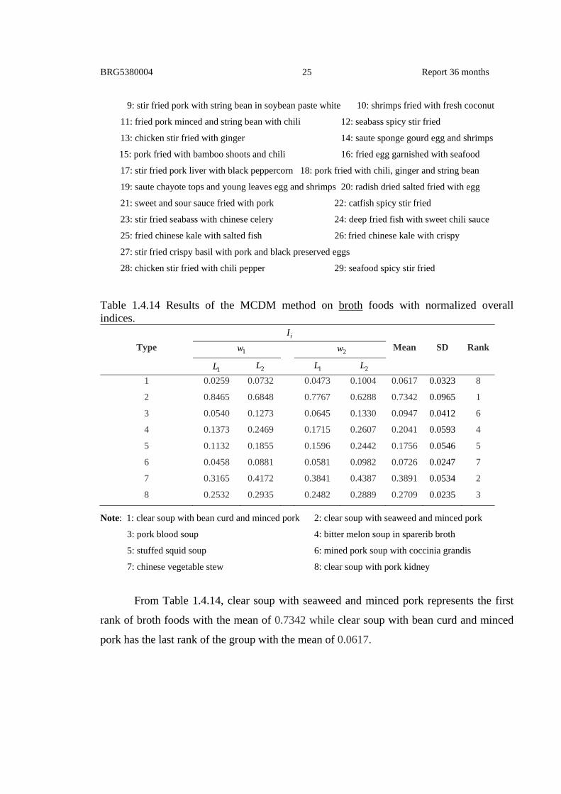
Table 1.4.14 Results of the MCDM method on broth foods with normalized overall indices.
Type
Mean
Rank SD
1 0.0259 0.0732 0.0473 0.1004 0.0617 0.0323 8
2 0.8465 0.6848 0.7767 0.6288 0.7342 0.0965 1
3 0.0540 0.1273 0.0645 0.1330 0.0947 0.0412 6
4 0.1373 0.2469 0.1715 0.2607 0.2041 0.0593 4
5 0.1132 0.1855 0.1596 0.2442 0.1756 0.0546 5
6 0.0458 0.0881 0.0581 0.0982 0.0726 0.0247 7
7 0.3165 0.4172 0.3841 0.4387 0.3891 0.0534 2
8 0.2532 0.2935 0.2482 0.2889 0.2709 0.0235 3
Note: 1: clear soup with bean curd and minced pork 2: clear soup with seaweed and minced pork
3: pork blood soup 4: bitter melon soup in sparerib broth
5: stuffed squid soup 6: mined pork soup with coccinia grandis
7: chinese vegetable stew 8: clear soup with pork kidney
From Table 1.4.14, clear soup with seaweed and minced pork represents the first
rank of broth foods with the mean of 0.7342 while clear soup with bean curd and minced
pork has the last rank of the group with the mean of 0.0617.
iI
1w 2w
2L 2L1L 1L

BRG5380004 Report 36 months 26
Table 1.4.15 Results of the MCDM method on broth (spicy) foods with normalized overall indices.
Type
Mean Rank
SD
1 0.1964 0.0719 0.1747 0.0854 0.1321 0.0626 7
2 0.1850 0.0718 0.1676 0.0867 0.1278 0.0568 8
3 0.0652 0.0472 0.0737 0.0652 0.0628 0.0111 15
4 0.1410 0.0615 0.1360 0.0786 0.1043 0.0401 11
5 0.1348 0.0547 0.1267 0.0684 0.0961 0.0405 13
6 0.1198 0.0604 0.1190 0.0784 0.0944 0.0298 14
7 0.7762 0.2354 0.6803 0.2768 0.4922 0.2759 1
8 0.3673 0.1339 0.3199 0.1562 0.2443 0.1166 3
9 0.3651 0.1426 0.3090 0.1650 0.2454 0.1086 2
10 0.3081 0.1196 0.2482 0.1317 0.2019 0.0915 4
11 0.1591 0.0698 0.1420 0.0830 0.1135 0.0437 9
12 0.1457 0.0521 0.1290 0.0618 0.0972 0.0471 12
13 0.0797 0.0323 0.0722 0.0391 0.0558 0.0236 16
14 0.2838 0.1102 0.2335 0.1231 0.1876 0.0847 5
15 0.0664 0.0344 0.0635 0.0436 0.0520 0.0155 18
16 0.0649 0.0372 0.0607 0.0475 0.0525 0.0127 17
17 0.2364 0.0889 0.2065 0.1047 0.1591 0.0733 6
18 0.1390 0.0853 0.1271 0.1025 0.1135 0.0242 10
19 0.0481 0.0234 0.0446 0.0283 0.0361 0.0121 19
Note: 1: sour prawn soup 2: hot and sour chicken soup
3: spicy soup with striped snakehead fish 4: fresh mackerel soup
5: carp fish soup 6: sour and spicy fish grilled
7: spicy seafood soup 8: hot and sour pork spare ribs
9: steamed egg with tom yum 10: sour and spicy fish crispy with tamarind apex
11: tom yum with multiply mushroom 12: hot and sour snapper filet
13: tom yum canned mackerel in tomato sauce
14: hot and spicy pork rib hot pot with tamarind and thai herbs
15: thai hot soup with beef 16: pork organ soup
17: sour and spicy soup of thai chicken 18: sour and spicy smoked fish soup
19: hot and sour nile tilapia
As can be seen in Table 1.4.15, the first rank of broth (spicy) foods has spicy
seafood soup with the mean of 0.4922, followed by steamed egg with tom yum with the
iI
1w 2w
2L 2L1L 1L

BRG5380004 Report 36 months 27
mean of 0.2454. On the other hand, the last rank has for hot and sour nile tilapia
representing the 19th rank with the mean of 0.0361.
Table 1.4.16 Results of the MCDM method on broth (coconut milk) foods with normalized overall indices.
Type
Mean
Rank SD
1 0.1052 0.1690 0.0947 0.1584 0.1318 0.0373 8
2 0.4749 0.4470 0.4644 0.4396 0.4565 0.0161 2
3 0.1549 0.1640 0.1576 0.1675 0.1610 0.0058 7
4 0.2227 0.2630 0.2551 0.2879 0.2572 0.0269 5
5 0.2109 0.2415 0.2427 0.2682 0.2408 0.0235 6
6 0.4816 0.4606 0.4284 0.4278 0.4496 0.0263 3
7 0.2088 0.2999 0.2281 0.3080 0.2612 0.0501 4
8 0.6081 0.5614 0.6253 0.5666 0.5904 0.0313 1
Note: 1: sour soup with shrimp and morning glory 2: fish organs sour soup
3: spicy vegetable and prawn soup 4: chicken and eggplant in spicy soup
5: un-coconut curry fish balls 6: pork with vegetables curry
7: hot yellow fish curry 8: shrimp and fried egg sour soup
From Table 1.4.16, shrimp and fried egg sour soup represents the first rank of broth
(coconut milk) foods with the mean of 0.5904 while sour soup with shrimp and morning
glory has the last rank of group by with the mean of 0.1318.
Table 1.4.17 Results of the MCDM method on broth (without coconut milk) foods with normalized overall indices.
Type
Mean
Rank SD
1 0.2232 0.4286 0.2557 0.4551 0.3407 0.1181 2
2 0.0141 0.0364 0.0164 0.0403 0.0268 0.0135 8
3 0.0078 0.0170 0.0087 0.0187 0.0131 0.0056 11
4 0.0178 0.0495 0.0201 0.0522 0.0349 0.0185 7
5 0.0178 0.0813 0.0201 0.0907 0.0525 0.0389 6
6 0.0330 0.0704 0.0377 0.0773 0.0546 0.0225 5
7 0.0383 0.1472 0.0441 0.1637 0.0983 0.0663 3
iI
1w 2w
2L 2L1L 1L
iI
1w 2w
2L 2L1L 1L

BRG5380004 Report 36 months 28
Table 1.4.17 Results of the MCDM method on broth (without coconut milk) foods with
normalized overall indices (cont.).
Type
Mean
Rank SD
8 0.0451 0.1301 0.0535 0.1442 0.0932 0.0512 4
9 0.0086 0.0359 0.0102 0.0402 0.0237 0.0167 10
10 0.0126 0.0344 0.0145 0.0379 0.0248 0.0132 9
11 0.9718 0.8716 0.9628 0.8505 0.9142 0.0621 1
Note: 1: soup with chicken, galangal root and coconut 2: soup shrimp and galangal in coconut milk
3: hot thai curry with chicken and bamboo shoot 4: curry with chicken
5: savory curry with pork 6: muslim-style curry with chicken and potatoes
7: green chicken curry 8: pork curry with water spinach
9: northern style pork curry with garlic 10: chicken curry with banana stalk
11: whisker sheatfish chu chee curry
From Table 1.4.17, the first rank of broth (without coconut milk) foods has whisker
sheatfish chu chee curry with the mean of 0.9142, followed by soup with chicken, galangal
root and coconut with the mean of 0.3407. The last rank has hot thai curry with chicken
and bamboo shoot with the mean of 0.0131.
Table 1.4.18 Results of the MCDM method on blend (vegetable) foods with normalized overall indices.
Type
Mean
Rank SD
1 0.1621 0.2347 0.1982 0.2605 0.2139 0.0430 3
2 0.1324 0.2147 0.1739 0.2518 0.1932 0.0515 4
3 0.0232 0.0744 0.0326 0.0848 0.0537 0.0304 9
4 0.6676 0.6242 0.6911 0.6288 0.6529 0.0320 1
5 0.1030 0.1300 0.1081 0.1424 0.1209 0.0185 7
6 0.6855 0.6435 0.6309 0.5956 0.6389 0.0371 2
7 0.0848 0.1771 0.1074 0.2016 0.1427 0.0555 6
8 0.1335 0.1642 0.1563 0.1829 0.1592 0.0204 5
9 0.0664 0.1201 0.0787 0.1310 0.0990 0.0314 8
Note: 1: wing bean spicy and sour salad 2: chinese kale and seafood in spicy sauce
3: white jelly fungus in spicy sauce 4: thai spicy water minosa salad
iI
1w 2w
2L 2L1L 1L
iI
1w 2w
2L 2L1L 1L

BRG5380004 Report 36 months 29
5: crispy water convolvulus 6: fried gord gourd spicy salad
7: lemongrass and windbetal leaves spicy salad 8: yum hua plee
9: spicy long eggplant salad
From Table 1.4.18, thai spicy water minosa salad represents the first rank of blend
(vegetable) foods with the mean of 0.6529 while white jelly fungus in spicy sauce has the
last rank of the group with the mean of 0.0537.
Table 1.4.19 Results of the MCDM method on blend (meat) foods with normalized overall indices.
Type
Mean
Rank SD
1 0.0284 0.0878 0.0324 0.0995 0.0620 0.0368 5
2 0.0154 0.0497 0.0189 0.0703 0.0386 0.0262 7
3 0.0460 0.1035 0.0536 0.1327 0.0840 0.0413 2
4 0.0124 0.0327 0.0145 0.0424 0.0255 0.0145 10
5 0.0235 0.1021 0.0258 0.1104 0.0655 0.0472 4
6 0.0203 0.1162 0.0235 0.1286 0.0721 0.0582 3
7 0.0094 0.0605 0.0139 0.0796 0.0408 0.0346 6
8 0.0057 0.0380 0.0080 0.0528 0.0261 0.0231 9
9 0.0054 0.0174 0.0062 0.0226 0.0129 0.0085 15
10 0.0147 0.0260 0.0159 0.0319 0.0221 0.0083 11
11 0.0074 0.0162 0.0080 0.0204 0.0130 0.0064 14
12 0.9974 0.9716 0.9965 0.9597 0.9813 0.0187 1
13 0.0146 0.0202 0.0151 0.0221 0.0180 0.0037 12
14 0.0084 0.0206 0.0095 0.0270 0.0164 0.0090 13
15 0.0140 0.0545 0.0163 0.0614 0.0365 0.0249 8
Note: 1: spicy cockle salad 2: spicy striped snakehead fish crispy salad
3: crispy catfish salad with green mango 4: sour steamed pork sausage salad
5: spicy fried egg and bacon 6: spicy pork small intestine
7: tuna spicy salad 8: spicy chicken feet salad
9: sliced grilled pork tenderloin salad old thai style 10: chinese sausage salad
11: sour canned fish salad 12: spicy friture salad
13: spicy snake skin gourami 14: shreded chicken spicy salad
15: spicy oyster salad
iI
1w 2w
2L 2L1L 1L

BRG5380004 Report 36 months 30
As can be seen in Table 1.4.19, the first rank of blend (meat) foods has spicy friture
salad with the mean of 0.9813, followed by crispy catfish salad with green mango with the
mean of 0.0840. On the other hand, the last rank has sliced grilled pork tenderloin salad
old thai style with the mean of 0.0129.
Table 1.4.20 Results of MCDM method on blend (mixed) foods with normalized overall indices.
Type
Mean
Rank SD
1 0.8508 0.7965 0.8780 0.8167 0.8355 0.0361 1
2 0.1026 0.1620 0.1096 0.1663 0.1351 0.0337 3
3 0.0552 0.1242 0.0639 0.1323 0.0939 0.0399 6
4 0.0759 0.1452 0.0773 0.1482 0.1117 0.0405 4
5 0.0793 0.1260 0.0869 0.1324 0.1062 0.0269 5
6 0.0622 0.0787 0.0610 0.0775 0.0699 0.0096 7
7 0.4953 0.5204 0.4403 0.4793 0.4838 0.0336 2
8 0.0198 0.0675 0.0239 0.0762 0.0469 0.0292 9
9 0.0316 0.0731 0.0360 0.0827 0.0559 0.0258 8
Note: 1: mungbean noodle salad 2: spicy combination seafood salad
3: mixed crispy spicy salad 4: boiled egg spicy salad
5: instant noodle yam 6: egg preserved spicy salad
7: yum yai 8: stir fried chicken with pomelo salad
9: hot spicy cavilla salad
From Table 1.4.20, mungbean noodle salad represents the first rank of blend
(mixed) foods with the mean of 0.8355 while stir fried chicken with pomelo salad has the
last rank of the group with the mean of 0.0469. Table 1.4.21 Results of the MCDM method on roast foods with normalized overall indices.
Type
Mean
Rank SD
1 0.1123 0.1462 0.1283 0.1581 0.1362 0.0201 9
2 0.1118 0.1632 0.1218 0.1771 0.1435 0.0316 8
3 0.2228 0.2693 0.2712 0.2972 0.2651 0.0310 5
4 0.2004 0.2255 0.2102 0.2251 0.2153 0.0122 6
iI
1w 2w
2L 2L1L 1L
iI
1w 2w
2L 2L1L 1L

BRG5380004 Report 36 months 31
Table 1.4.21 Results of the MCDM method on roast foods with normalized overall indices(cont.).
Type
Mean
Rank SD
5 0.2527 0.3396 0.3069 0.3626 0.3154 0.0477 4
6 0.5222 0.4582 0.4777 0.4305 0.4721 0.0386 2
7 0.1160 0.1994 0.1614 0.2345 0.1778 0.0509 7
8 0.5586 0.5024 0.5845 0.5005 0.5365 0.0418 1
9 0.0941 0.1493 0.1215 0.1691 0.1335 0.0327 10
10 0.4551 0.4103 0.3651 0.3560 0.3966 0.0456 3
11 0.0846 0.1436 0.1136 0.1645 0.1266 0.0349 11
Note: 1: shrimps with glass noodles 2: roasted chicken with soy sauce
3: roasted chicken with ketchup 4: baked pork spare rib
5: roasted mungbean with termite mushroom 6: roasted crab with chili paste fried in oil
7: roasted chicken wing
8: one whole piece of roasted young mountain pork bathed in wild honey
9: grilled lemongrass chicken 10: egg hen water add steamed
11: roasted chicken with lemon
From Table 1.4.21, the first rank of roast foods has one whole piece of roasted young
mountain pork bathed in wild honey with the mean of 0.5365, followed by roasted crab
with chili paste fried in oil with the mean of 0.4721. The last rank has roasted chicken with
lemon with the mean of 0.1266.
Table 1.4.22 Results of the MCDM method on steamed foods with normalized overall indices.
Type
Mean
Rank SD
1 0.1195 0.1785 0.1441 0.2034 0.1614 0.0370 8
2 0.1386 0.1651 0.1566 0.1784 0.1597 0.0167 10
3 0.0810 0.1022 0.0703 0.0939 0.0869 0.014 12
4 0.3126 0.3471 0.3092 0.3443 0.3283 0.0202 5
5 0.1875 0.2220 0.1962 0.2251 0.2077 0.0187 7
6 0.1185 0.1873 0.1368 0.1988 0.1604 0.0387 9
7 0.1199 0.1174 0.1237 0.1206 0.1204 0.0026 11
8 0.4360 0.3948 0.4043 0.3734 0.4021 0.0260 3
iI
1w 2w
2L 2L1L 1L
iI
1w 2w
2L 2L1L 1L

BRG5380004 Report 36 months 32
Table 1.4.22 Results of the MCDM method on steamed foods with normalized overall indices(cont.).
Type
Mean
Rank SD
9 0.4590 0.4079 0.4217 0.3838 0.4181 0.0315 2
10 0.4482 0.4077 0.4616 0.4125 0.4325 0.0265 1
11 0.2326 0.2763 0.2472 0.2796 0.2589 0.0228 6
12 0.3780 0.3834 0.4076 0.3997 0.3922 0.0138 4
Note: 1: ear mushroom with many materials 2: spotted featherback steamed
3: snapper steamed with lemon 4: fish steamed with tofu
5: fish steamed with vegetable and chili paste 6: silver pomfret steamed
7: nile tilapia steamed with vegetable 8: salmon steamed with lemon
9: salmon steamed with soy sauce
10: steamed fish with coconut milk in a banana leaf wrapping
11: chicken steamed with ear mushroom in soy sauce paste 12: giant seaperch steamed
From Table 1.4.22, we observe that the first rank of steamed foods has steamed fish
with coconut milk in a banana leaf wrapping with the mean of 0.4325 while snapper
steamed with lemon has the last rank of the group with the mean of 0.0869.
Table 1.4.23 Results of the MCDM method on grilled foods with normalized overall indices.
Type
Mean
Rank SD
1 0.7694 0.6921 0.8285 0.7284 0.7546 0.0585 1
2 0.3288 0.3990 0.3227 0.3970 0.3619 0.0418 3
3 0.5476 0.6015 0.4577 0.5584 0.5413 0.0604 2
Note: 1: chicken grilled with herb 2: fish grilled with lemon sauce
3: fish grilled with soy sauce
As can be seen in Table 1.4.23, the first rank of grilled foods has chicken grilled
with herb with the mean of 0.7546, followed by fish grilled with soy sauce with the mean
of 0.5413. The last rank has fish grilled with lemon sauce representing the third with the
mean of 0.3619.
iI
1w 2w
2L 2L1L 1L
iI
1w 2w
2L 2L1L 1L

BRG5380004 Report 36 months 33
Table 1.4.24 Results of the MCDM method on rice noodle food (water) with normalized overall indices.
Type
Mean
Rank SD
1 0.0769 0.1560 0.1217 0.1856 0.1350 0.0467 8
2 0.0896 0.1783 0.1397 0.2141 0.1554 0.0534 7
3 0.1757 0.2492 0.2352 0.2912 0.2378 0.0477 4
4 0.1255 0.2180 0.1998 0.2666 0.2025 0.0586 6
5 0.0498 0.1042 0.0757 0.1246 0.0886 0.0327 9
6 0.0328 0.0782 0.0513 0.0983 0.0652 0.0289 11
7 0.6572 0.5553 0.5762 0.4839 0.5681 0.0713 1
8 0.1764 0.2554 0.2260 0.2753 0.2333 0.0430 5
9 0.5803 0.4805 0.5256 0.4372 0.5059 0.0613 2
10 0.0259 0.0659 0.0427 0.0833 0.0544 0.0252 12
11 0.0321 0.0998 0.0565 0.1289 0.0793 0.0433 10
12 0.3666 0.4455 0.4448 0.4628 0.4299 0.0430 3
Note: 1: small size rice noodle fresh with beef 2: wide rice noodle with fish ball swamp cabbage
3: boiled vermicelli 4: small size rice noodle with stewed beef ball beef and soup
5: rice noodle fine thread stewed with beef and beef soup
6: big size rice noodle with stewed beef ball beef and soup
7: big size rice noodle with pork and soup 8: wheat noodle with roasted pork
9: wheat noodle with meat ball and ball fried
10: fried rice noodle with dark soy sauce topped with shirmp
11: rice noodle fine thread with stewed beef 12: guay-jub northeasterm style
From Table 1.4.24, big sized rice noodle with pork and soup represents the first
rank of rice noodle (water) foods with the mean of 0.5681 while fried rice noodle with
dark soy sauce topped with shirmp has the last rank of the group with the mean of 0.0544.
From Table 1.4.25, we observe that the first rank of rice noodle (dried) food has
wide rice noodle with pork egg and soy sauce with the mean of 0.5445. The last rank has
small size rice noodle fried with stewed beef ball with the mean of 0.1186.
iI
1w 2w
2L 2L1L 1L

BRG5380004 Report 36 months 34
Table 1.4.25 Results of the MCDM method on rice noodle (dried) food with normalized overall indices.
Type
Mean
Rank SD
1 0.5859 0.5310 0.5533 0.5079 0.5445 0.0332 1
2 0.4722 0.4838 0.5017 0.4970 0.4887 0.0133 3
3 0.5474 0.5195 0.5449 0.5149 0.5317 0.0169 2
4 0.0860 0.1326 0.1052 0.1507 0.1186 0.0287 8
5 0.0892 0.1676 0.0997 0.1757 0.1330 0.0449 7
6 0.2908 0.3244 0.2906 0.3270 0.3082 0.0202 4
7 0.1426 0.1727 0.1418 0.1742 0.1578 0.0181 6
8 0.1176 0.1825 0.1405 0.1978 0.1596 0.0371 5
Note: 1: wide rice noodle with pork egg and soy sauce 2: pad thai
3: macaroni fried with pork 4: small size rice noodle fried with stewed beef ball
5: rice noodle fried fine thread with stewed beef ball 6: saute mungbean noodle and hen egg
7: small size rice noodle with pork 8: rice noodle fried with pork and spicy
Table 1.4.26 Results of the MCDM method on fermented rice noodle food with normalized overall indices.
Type
Mean
Rank SD
1 0.2187 0.2632 0.2949 0.3176 0.2736 0.0429 4
2 0.2308 0.2492 0.2122 0.2376 0.2325 0.0155 8
3 0.2685 0.2749 0.2658 0.2735 0.2707 0.0043 5
4 0.2679 0.2892 0.2789 0.3008 0.2842 0.0141 3
5 0.1795 0.2098 0.1913 0.2212 0.2005 0.0186 9
6 0.6587 0.5929 0.6397 0.5719 0.6158 0.0402 1
7 0.2421 0.2863 0.2480 0.2868 0.2658 0.0241 6
8 0.2321 0.2858 0.1995 0.2648 0.2456 0.0378 7
9 0.4201 0.3875 0.4153 0.3860 0.4023 0.0180 2
Note: 1: rice vermicelli with tofu fried in coconut cream 2: fermented rice noodle with minced pork
3: fermented rice noodle with fish curry 4: fermented rice noodle with fish soup
5: fermented rice noodle with chicken feet 6: fermented rice noodle with southern curry
7: fermented rice noodle with chicken curry 8: fermented rice noodle with fish organs soup
9: fermented rice noodle with green curry chicken
iI
1w 2w
2L 2L1L 1L
iI
1w 2w
2L 2L1L 1L

BRG5380004 Report 36 months 35
From Table 1.4.26, the first rank of fermented rice noodle food has fermented rice
noodle with southern curry with the mean of 0.6158, followed by fermented rice noodle
with green curry chicken with the mean of 0.4023. On the other hand, the last rank has
fermented rice noodle with chicken feet with the mean of 0.2005.
1.4.1.3 Fruits
Fruits are classified into seven groups, namely foreign fruit, numerative noun fruit,
bunch fruit, apple, rose apple, orange and mango, respectively. The results of the
normalized overall index based on the L1-norm and L2-norm with w1 and w2 weights in
each group is shown in Tables 1.4.27- 33.
Table 1.4.27 Results of the MCDM method on foreign fruits with normalized overall indices.
Type
Mean
Rank SD
1. Pears 0.0974 0.2143 0.1240 0.2288 0.1661 0.0652 5
2. Cantaloupe 0.5856 0.5506 0.5227 0.5043 0.5408 0.0354 2
3. Hard - type ripe 0.6132 0.5551 0.5209 0.4993 0.5471 0.0497 1 persimmon 4. Kiwi 0.4552 0.4857 0.5498 0.5371 0.5070 0.0443 3
5. Cherries eating raw 0.2539 0.3270 0.3712 0.3944 0.3366 0.0618 4
As can be seen in Table 1.4.27, the first rank of foreign fruits is hard-type ripe
persimmon with the mean of 0.5471, followed by cantaloupe with the mean of 0.5408. The
last rank has pears with the mean of 0.1661.
Table 1.4.28 Results of the MCDM method on numerative noun for fruits with normalized overall indices.
Type
Mean
Rank SD
1. Dragon fruit 0.0945 0.1318 0.0996 0.1335 0.1149 0.0206 14
2. Papaya ripe 0.2858 0.2696 0.2296 0.2343 0.2548 0.0273 5
3. Pomelo thong dee 0.0973 0.1009 0.0967 0.0998 0.0987 0.0020 17
4. Jackfruit mature 0.1419 0.1449 0.1551 0.1589 0.1502 0.0081 11
5. Watermelon red 0.3276 0.3104 0.2590 0.2720 0.2923 0.0321 3
6. Guava common 0.1477 0.2193 0.1490 0.2149 0.1827 0.0397 8
iI
1w 2w
2L 2L1L 1L
iI
1w 2w
2L 2L1L 1L

BRG5380004 Report 36 months 36
Table 1.4.28 Results of the MCDM method on numerative noun for fruits with normalized overall indices(cont.).
Type
Mean
Rank SD
7. Native mature melon 0.0576 0.0759 0.0575 0.0745 0.0664 0.0102 24
8. Pineapple 0.0731 0.0809 0.0800 0.0849 0.0797 0.0049 22
9. Sapodilla common 0.1555 0.1826 0.1542 0.1778 0.1675 0.0148 9
10. Sweet tamarind 0.5569 0.4548 0.6019 0.4791 0.5232 0.0682 1
11. Gandaria marian plum 0.2262 0.2159 0.2001 0.2000 0.2105 0.0128 7
12. Yumbean 0.0757 0.0980 0.0873 0.1095 0.0926 0.0145 20
13. Toddy palm 0.1746 0.2579 0.1998 0.2798 0.2281 0.0491 6
14. Rambutan 0.0868 0.1052 0.0983 0.1128 0.1008 0.0111 16
15. Mangosteen 0.0617 0.0759 0.0682 0.0810 0.0717 0.0085 23
16. Litchi 0.0776 0.1019 0.0863 0.1078 0.0934 0.0139 19
17. Banana khai variety 0.1302 0.1449 0.1408 0.1586 0.1436 0.0117 13
18. Pomegranate solft seed 0.1273 0.1605 0.1370 0.1640 0.1472 0.0179 12
19. Durian mon-thong 0.4097 0.3784 0.3949 0.3677 0.3877 0.0185 2
20. Jujube thai variety 0.2503 0.2878 0.2617 0.2918 0.2729 0.0201 4
21. Sala 0.0747 0.1004 0.0772 0.1026 0.0887 0.0148 21
22. Sugar apple 0.1418 0.1548 0.1567 0.1646 0.1545 0.0094 10
23. Salak palm fruit 0.0799 0.1152 0.0922 0.1224 0.1024 0.0198 15
24. Carambola 0.0853 0.1086 0.0869 0.1089 0.0974 0.0131 18
From Table 1.4.28, we observe that most of the first rank of numerative noun fruits
has sweet tamarind with the mean of 0.5232. The last rank has native mature melon with
the mean of 0.0664.
Table 1.4.29 Results of the MCDM method on bunch fruits with normalized overall indices.
Type
Mean
Rank SD
1. Grapes green 0.1662 0.2463 0.1452 0.2224 0.1951 0.0472 5
2. Rambai 0.7422 0.6362 0.7496 0.6391 0.6918 0.0626 1
3. Star gooseberry 0.3129 0.3772 0.3200 0.3851 0.3488 0.0376 3
4. Longan 0.0957 0.1884 0.1490 0.2332 0.1666 0.0585 6
5. Longkong 0.1620 0.2926 0.2156 0.3203 0.2477 0.0723 4
6. Langsad 0.5368 0.5208 0.4959 0.4865 0.5100 0.0230 2
iI
1w 2w
2L 2L1L 1L
iI
1w 2w
2L 2L1L 1L

BRG5380004 Report 36 months 37
From Table 1.4.29, rambai represents the first rank of bunch fruits with the mean of
0.6918 while longan has the last rank of the group with the mean of 0.1666. Table 1.4.30 Results of MCDM method on apple fruits with normalized overall indices.
Type
Mean
Rank SD
1. Apple 0.9833 0.9786 0.9851 0.9797 0.9817 0.0030 1
2. Green apple 0.1810 0.2028 0.1703 0.1961 0.1875 0.0146 2
3. Fuji apple 0.0165 0.0349 0.0245 0.0423 0.0295 0.0114 3
From Table 1.4.30, the first rank of apple fruits has apple with the mean of 0.9817,
followed by green apple with the mean of 0.1875. On the other hand, the last rank has fuji
apple with the mean of 0.0295.
Table 1.4.31 Results of the MCDM method on rose apple fruits with normalized overall indices.
Type
Mean
Rank SD
1. Rose apple red color 0.2329 0.3746 0.2467 0.3737 0.3070 0.0778 2
variety
2. Rose apple green 0.9428 0.8252 0.9180 0.7961 0.8706 0.0709 1
3. Rose apple 0.1956 0.2999 0.2285 0.3224 0.2616 0.0595 3
4. Rose apple green color 0.1362 0.2980 0.2101 0.3501 0.2486 0.0946 4
variety
As can be seen in Table 1.4.31, the first rank of rose apple fruits has rose apple
green with the mean of 0.8706, followed by rose apple red color variety with the mean of
0.3070. On the other hand, the last rank has rose apple green color variety with the mean
of 0.2486.
From Table 1.4.32, we observe that the first rank of orange fruits has sweet orange
with the mean of 0.6820. On the other hand, the rank has kalanchoe with the mean of
0.3514.
iI
1w 2w
2L 2L1L 1L
iI
1w 2w
2L 2L1L 1L

BRG5380004 Report 36 months 38
Table 1.4.32 Results of the MCDM method on orange fruits with normalized overall indices.
Type
Mean
Rank SD
1. Kalanchoe 0.2952 0.3617 0.3548 0.3938 0.3514 0.0412 3
2. Mandarin 0.7034 0.6900 0.5431 0.6035 0.6350 0.0756 2
3. Sweet orange 0.6466 0.6270 0.7610 0.6933 0.6820 0.0596 1
Table 1.4.33 Results of the MCDM method on mango fruits with normalized overall indices.
Type
Mean Rank
SD
1. Unripe mango kaew 0.3917 0.4417 0.4028 0.4385 0.4187 0.0252 3
variety
2. Unripe mango pimsaen 0.1601 0.2227 0.2052 0.2639 0.2130 0.0430 5
variety
3. Ripe mango rad 0.1599 0.1982 0.1764 0.2112 0.1864 0.0228 7
variety
4. Ripe mango kaew 0.4515 0.4724 0.4348 0.4548 0.4534 0.0154 2
variety
5. Ripe mango nam-dok- 0.7321 0.6177 0.7051 0.5948 0.6624 0.0664 1
mai variety
6. Ripe mango pimsaen- 0.1410 0.2236 0.1829 0.2555 0.2007 0.0497 6
mun variety
7. Unripe mango kiew-sa- 0.1890 0.2476 0.2120 0.2600 0.2272 0.0326 4
weya variety
From Table 1.4.33, we observe that the first rank of mango fruits has ripe mango
nam-dok-mai variety with the mean of 0.6624 while unripe mango rad variety has the last
rank of the group with the mean of 0.1864.
1.4.1.4 Desserts
Desserts are classified into five groups, namely coconut milk, steamed, fried,
roast and conserved, respectively. The results of the normalized overall index based on the
L1-norm and L2-norm with w1 and w2 weights in each group is shown in Tables 1.4.34- 38.
iI
1w 2w
2L 2L1L 1L
iI
1w 2w
2L 2L1L 1L

BRG5380004 Report 36 months 39
Table 1.4.34 Results of the MCDM method on coconut milk desserts with normalized overall indices.
Type
Mean
Rank SD
1 0.1796 0.2189 0.1639 0.2022 0.1912 0.0243 7
2 0.0596 0.0819 0.0690 0.0960 0.0766 0.0158 12
3 0.4487 0.4347 0.4608 0.4386 0.4457 0.0117 2
4 0.0306 0.0884 0.0444 0.1050 0.0671 0.0353 13
5 0.0591 0.1156 0.0736 0.1301 0.0946 0.0337 10
6 0.3735 0.3769 0.3911 0.3845 0.3815 0.0079 3
7 0.0421 0.1051 0.0565 0.1208 0.0811 0.0378 11
8 0.0433 0.0762 0.0530 0.0882 0.0652 0.0206 14
9 0.0068 0.0328 0.0123 0.0512 0.0258 0.0203 19
10 0.0252 0.0754 0.0370 0.0925 0.0575 0.0317 16
11 0.3681 0.3701 0.3749 0.3686 0.3704 0.0031 4
12 0.0376 0.0545 0.0400 0.0573 0.0473 0.0100 17
13 0.5525 0.4562 0.5328 0.4433 0.4962 0.0545 1
14 0.2803 0.2912 0.2478 0.2681 0.2719 0.0186 5
15 0.0142 0.0523 0.0202 0.0610 0.0369 0.0232 18
16 0.0416 0.0706 0.0505 0.0799 0.0607 0.0177 15
17 0.2401 0.2714 0.2458 0.2706 0.2570 0.0164 6
18 0.0771 0.1100 0.0870 0.1205 0.0987 0.0200 9
19 0.1686 0.2079 0.1727 0.2069 0.1890 0.0213 8
Note: 1: banana in coconut milk 2: tab tim krob with coconut milk and syrup
3: black sticky rice with coconut milk and syrup 4: taro balls in coconut milk
5: taro in coconut milk 6: tao suan
7: rice drops in sweet coconut milk 8: sago with coconut milk
9: nata de coco in syrup 10: mungbean thread in coconut milk
Note (cont.): 11: boiled cowpea seeds with sugar and coconut milk
12: boiled rice flour chunk with coconut milk
13: rice green flake with coconut milk and syrup 14: native melon in coconut milk
15: jelly with coconut cream pandanus leaves flavor 16: sticky rice in coconut milk
17: kanom tue pap 18: kanom tom khaw
19: kanom tom daeng
From Table 1.4.34, the first rank of coconut milk desserts has rice green flake with
coconut milk and syrup with the mean of 0.4962, followed by black sticky rice with
iI
1w 2w
2L 2L1L 1L

BRG5380004 Report 36 months 40
coconut milk and syrup with the mean of 0.4457. On the other hand, the last rank has nata
de coco in syrup with the mean of 0.0258.
Table 1.4.35 Results of the MCDM method on steamed desserts with normalized overall indices.
Type
Mean
Rank SD
1 0.0045 0.0229 0.0076 0.0288 0.0160 0.0118 21
2 0.1811 0.2406 0.1878 0.2365 0.2115 0.0314 7
3 0.2169 0.3247 0.2432 0.3329 0.2794 0.0581 3
4 0.0841 0.1935 0.1046 0.2083 0.1476 0.0624 10
5 0.0922 0.1794 0.1075 0.1920 0.1428 0.0502 11
6 0.2376 0.2912 0.2625 0.3051 0.2741 0.0301 4
7 0.0104 0.0354 0.0152 0.0433 0.0261 0.0158 18
8 0.1903 0.2438 0.2061 0.2500 0.2226 0.029 6
9 0.7464 0.5548 0.7253 0.5374 0.6410 0.1101 1
10 0.1362 0.1948 0.1443 0.1962 0.1679 0.0321 9
11 0.0520 0.0819 0.0535 0.0799 0.0668 0.0163 13
12 0.2588 0.2568 0.2433 0.2400 0.2497 0.0095 5
13 0.0347 0.0715 0.0454 0.0903 0.0605 0.0252 15
14 0.0405 0.0604 0.0428 0.0605 0.0511 0.0109 17
15 0.0056 0.0272 0.0094 0.0340 0.0190 0.0137 20
16 0.0161 0.0747 0.0283 0.0973 0.0541 0.0383 16
17 0.0255 0.0842 0.0386 0.1032 0.0629 0.0368 14
18 0.1902 0.1979 0.1875 0.1961 0.1929 0.0049 8
19 0.3411 0.3234 0.3354 0.3158 0.3289 0.0115 2
20 0.1005 0.1893 0.0926 0.1750 0.1394 0.0499 12
21 0.0059 0.0315 0.0099 0.0395 0.0217 0.0163 19
Note: 1: banana paste 2: taro paste
3: sticky rice flour coconut milk and sugar boiled 4: mock fruits
5: egg custard baked 6: mock jackfruit seed
7: coconut pudding with water chestnut 8: egg yolk dropped in heavy syrup
9: gold threads egg yolk strained in heavy syrup 10: kanom piak poon
11: kanom touy 12: kanom Sali
13: kanom chun 14: kanom num dok mai
15: tong muan 16: sam pan nee
17: glutinous rice steeped in coconut milk
iI
1w 2w
2L 2L1L 1L

BRG5380004 Report 36 months 41
18: sticky rice with shrimp and coconut meat 19: sticky rice with custard
20: steamed mixture of pumpkin rice flour and coconut 21: steamed toddy palm cake
From Table 1.4.35, gold threads egg yolk strained in heavy syrup represents the
first rank of steamed desserts with the mean of 0.6410 while banana paste has the last rank
of the group with the mean of 0.0160.
Table 1.4.36 Results of the MCDM method on fried desserts with normalized overall indices.
Type
Mean
Rank SD
1 0.0124 0.0956 0.0314 0.1463 0.0714 0.0613 7
2 0.2753 0.3701 0.2746 0.3616 0.3204 0.0526 3
3 0.1179 0.2113 0.1314 0.2216 0.1706 0.0534 6
4 0.4139 0.4377 0.3926 0.4173 0.4154 0.0185 2
5 0.8340 0.7143 0.8382 0.7113 0.7744 0.0712 1
6 0.0324 0.0726 0.0425 0.0895 0.0592 0.0265 8
7 0.0065 0.0467 0.0149 0.0676 0.0339 0.0283 10
8 0.0054 0.0568 0.0122 0.0797 0.0385 0.0357 9
9 0.1521 0.1895 0.1637 0.1972 0.1756 0.0212 5
10 0.0040 0.0289 0.0091 0.0430 0.0212 0.0180 11
11 0.1378 0.2451 0.1433 0.2430 0.1923 0.0598 4
Note: 1: deep fried banana 2: kanom khai nok krata
3: doughnut with sugar 4: glutinous rice cooked deep fried
5: krong krang krob kem 6: kanom nang led
7: taro slided deep fried sugar coated 8: banana slided deep fried sugar coated
9: kanom khai hong 10: deep fried rice cake
11: large soft rice pancake topped with shredded
From Table 1.4.36, we observe that the first rank of fried desserts has krong krang
krob kem with the mean of 0.7744. On the other hand, the last rank has deep fried rice
cake with the mean of 0.0212.
iI
1w 2w
2L 2L1L 1L

BRG5380004 Report 36 months 42
Table 1.4.37 Results of the MCDM method on roast desserts with normalized overall indices.
Type
Mean
Rank SD
1. Kanom ping 0.1210 0.1384 0.1265 0.1472 0.1333 0.0118 6
2. Kanom krok 0.4442 0.5087 0.5284 0.5420 0.5058 0.0433 2
3. Tokyo snack similar to 0.3716 0.3942 0.3717 0.3883 0.3815 0.0116 3
pancake
4. Kanom babin 0.0927 0.1581 0.0894 0.1464 0.1216 0.0357 7
5. Cake sponge 0.1004 0.1996 0.1263 0.2222 0.1621 0.0580 5
commercially prepared
6. Kanom kleeb lamduan 0.1192 0.2418 0.1632 0.2708 0.1987 0.0699 4
7. Coconut meat and rice 0.0464 0.1424 0.0719 0.1711 0.1079 0.0585 8
flour in coconut milk
8. Kanom naa nual 0.7842 0.6505 0.7148 0.6003 0.6874 0.0797 1
As can be seen in Table 1.4.37, the first rank of roast desserts has kanom naa nual
with the mean of 0.6874, followed by kanom krok with the mean of 0.5058. On the other
hand, the last rank has coconut meat and rice flour in coconut milk representing the 8th
with the mean of 0.1079.
Table 1.4.38 Results of the MCDM method on conserved desserts with normalized overall indices.
Type
Mean
Rank SD
1. Pumpkin in syrup 0.4602 0.4817 0.4284 0.4569 0.4568 0.0219 2
2. Cassava boiled in syrup 0.8060 0.6945 0.8177 0.6968 0.7537 0.0672 1
3.Toddy palm in heavy 0.0097 0.0852 0.0363 0.1536 0.0712 0.0632 5
syrup
4. Artocarpus altilis in 0.3513 0.4320 0.3549 0.4258 0.3910 0.0439 3
concentrated syrup
5. Mango pickled sweet 0.1231 0.3028 0.1436 0.3176 0.2218 0.1026 4
iI
1w 2w
2L 2L1L 1L
iI
1w 2w
2L 2L1L 1L

BRG5380004 Report 36 months 43
From Table 1.4.38, cassava boiled in syrup represents the first rank of conserved
desserts with the mean of 0.7537 while toddy palm in heavy syrup has the last rank of the
group with the mean of 0.0712.
1.4.2 Electre Method
We apply the Electre method on vegetables, foods, fruits and desserts based on
eleven nutrient indicators and prices by using the following procedure.
Given a data matrix X with K rows and N columns ( )( ) :ijX x K N= × , where the
row represents each type of vegetable, food, fruit or dessert to be compared with respect to
the element ijx and the columns represent the eleven nutrient indicators and prices for each
type of vegetable, food, fruit or dessert.
Step 1: Transform matrix X [ ]1 2, ,..., NX X X= to matrix R 1 2, ,..., ,NR R R⎡ ⎤= ⎣ ⎦
where 2
.ii
i
XRX
=
Step 2: Transform matrix R to matrix V where V = RW where matrix
W [ ]1 2, ,..., Ndiag w w w= is based on the weight of the coefficient of
variation(w2).
Step 3: Construct two matrices C and D,
where :
,ik jk
ij kk v v
c w≥
= ∑
and :max.
maxik jkk v v ik jk
ijk ik jk
V Vd
V V< −
=−
(1.11)
Compute ( )
,1
iji jc
cK K
≠=−
∑∑ and
( ).
1iji j
dd
K K≠=−
∑∑ (1.12)
Step 4: Construct matrices F and G such that
1 ;
0 ;ij
ij
c cf
otherwise
≥⎧⎪= ⎨⎪⎩
and 1 ;
.0 ;
ijij
d dg
otherwise
⎧ ≤⎪= ⎨⎪⎩
(1.13)
Step 5: Define matrix E where .ij ij ije f g= ⋅ (1.14)
It should be noted that the weights iw are obtained as discussed and 0ije = means
that row i is better than row j or 1ije = means that column j is better than row i.

BRG5380004 Report 36 months 44
The results of the Electre method applied to each type of vegetable, food, fruit or
dessert are based on the eleven nutrient indicators and prices as given in the following
sections.
1.4.2.1 Vegetables
Vegetables are classified into seven groups, namely blossom, chili, leaf and apex,
pod, fruit, plant and tuber. The data matrix X has eleven rows for blossom vegetable types
including abalone mushroom, chinese chives, chinese mustard green, cowslip creeper,
dried mushroom, ear mushroom, onion flowers, sajor-caju mushroom, sesban, shiitake
mushroom, straw mushroom and thirteen columns of nutrient indicators namely energy,
carbohydrate, fat, protein, protein-vegetable, calcium, iron, iron-vegetable, vitamin A,
thiamin, riboflavin, vitamin C, niacin and price. In matrix X, we use the actual nutrient
indicator values and the reciprocal of price for each type of blossom vegetables for
reasonable comparison.
Finally, the results of the E-matrices for seven groups of vegetables are shown in
Table 1.4.39.
Table 1.4.39 E-matrices of the seven groups of vegetable
blossom Type 1 2 3 4 5 6 7 8 9 10 11 Rank
1 1 1 1 0 0 0 0 1 0 0 0 3
2 1 1 1 1 1 0 0 1 0 0 0 2
3 1 1 1 1 1 1 0 1 1 0 0 1
4 1 1 1 1 0 0 0 1 1 0 0 2
5 1 1 1 1 1 0 0 1 1 0 1 1
6 0 0 0 0 0 0 0 0 0 0 0 6
7 0 1 0 0 0 0 0 0 0 0 0 5
8 0 1 0 0 0 0 0 0 0 0 0 5
9 0 1 1 0 0 0 0 0 0 0 0 4
10 0 1 0 0 0 0 0 0 0 0 0 5
11 1 1 0 0 0 0 0 0 0 0 0 4
Note: 1: abalone mushroom 2: chinese chives 3: chinese mustard green 4: cowslip creeper 5: dried mushroom 6: ear mushroom 7: onion flowers 8: sajor-caju mushroom
9: Sesban 10: shiitake mushroom 11: straw mushroom

BRG5380004 Report 36 months 45
We observe that the blossom vegetables, chinese mustard green and dried
mushroom have the best type while chinese chives and cowslip creeper have the second
best, respectively. The worst has ear mushroom.
chili Type 1 2 3 4 5 6 7 8 9 10 Rank
1 0 0 0 0 1 0 0 0 0 0 4
2 1 0 1 0 1 0 0 0 0 0 3
3 1 1 1 0 1 0 0 0 1 0 2
4 0 0 0 0 0 0 0 0 0 0 5
5 1 1 1 1 1 1 0 1 1 0 1
6 1 1 1 1 1 1 0 1 1 0 1
7 1 1 1 0 1 0 0 0 1 0 2
8 0 0 0 0 1 0 0 0 0 0 4
9 0 0 0 0 1 0 0 0 0 0 4
10 1 1 1 0 1 0 0 0 1 0 2
Note: 1: bell pepper 2: bird pepper 3: black pepper 4: chili spur pepper 5: dried goat pepper
6: dried guinea pepper 7: piment rouge 8: piment vert 9: sweet pepper 10: yellow pepper
For the chili vegetables based on nutrient indicators and prices, we found that dried
goat pepper and dried guinea pepper have the best while yellow pepper, black pepper and
piment rouge have the second best. The worst has chili spur pepper.
leaf and apex Type 1 2 3 4 5 6 7 8 9 10 11 12 Rank
1 1 0 1 0 1 0 1 1 0 0 1 0 3
2 0 1 1 1 1 0 1 1 0 0 1 0 2
3 0 0 1 0 1 0 1 1 0 0 1 0 4
4 0 0 0 0 0 0 1 0 0 0 0 0 8
5 0 0 0 0 0 0 0 0 0 0 0 0 9
6 0 1 1 0 1 0 1 1 0 0 1 0 3
7 0 0 0 0 0 0 1 1 0 0 0 0 7
8 1 1 1 1 1 1 1 1 0 1 1 1 1
9 0 0 0 0 0 0 0 0 0 0 0 0 9
10 0 1 0 0 0 0 1 1 0 0 1 0 5
11 0 0 1 0 1 0 1 1 0 0 1 0 4
12 0 0 0 0 1 0 1 1 0 0 0 0 6

BRG5380004 Report 36 months 46
Note: 1: acacia 2: basil 3: bitter gourd 4: chinese chive 5: coconut 6: feuille de menthe
7: gord gourd 8: kaffir lime leaves 9: lettuce 10: sauropus androgynous
11: stem of sweet basil 12: stem of sweet basil
From leaf and apex vegetables based on nutrient indicators and prices, we observe
that the best has kaffir lime leaves and the second best is basil. The worst have coconut
and lettuce.
pod Type 1 2 3 4 5 6 7 8 9 10 11 Rank
1 0 0 1 1 1 1 0 0 0 0 1 3
2 0 0 1 0 1 1 0 0 0 0 1 4
3 0 1 1 1 1 1 1 0 0 0 1 2
4 0 0 0 0 0 0 0 0 0 0 0 7
5 1 1 1 1 1 1 1 1 0 0 1 1
6 0 0 0 0 1 1 0 0 0 0 1 5
7 0 0 0 0 0 1 0 0 0 0 0 6
8 0 0 0 0 0 0 0 0 0 0 0 7
9 0 0 1 0 1 1 0 0 0 0 1 4
10 0 0 0 0 1 1 0 0 0 0 1 5
11 0 0 1 0 1 1 0 0 0 0 1 4
Note: 1: green pea 2: holland bean 3: horse radish tree 4: lotus stem 5: ripe tamarind
6: smooth loofah 7: snake gourd 8: sponge gourd 9: string bean 10: winged bean 11: young corn
For pod vegetables based on nutrient indicators and prices, the best type has ripe
tamarind and second best has horse radish tree. In addition, the worst types have lotus stem
and sponge gourd.

BRG5380004 Report 36 months 47
fruit Type 1 2 3 4 5 6 7 8 9 10 11 12 13 14 15 Rank
1 0 0 0 0 0 0 0 0 1 0 0 0 0 1 1 6
2 1 0 0 0 1 1 0 0 1 0 0 0 0 1 1 4
3 0 0 0 0 0 0 0 0 0 0 0 0 0 0 1 8
4 1 1 0 0 1 0 0 0 1 0 0 0 0 1 1 4
5 0 0 0 0 0 0 0 0 0 0 0 0 0 0 1 8
6 0 1 0 0 0 0 0 0 0 0 0 0 0 1 1 6
7 0 0 0 0 0 0 0 0 0 0 0 0 0 0 0 9
8 1 0 0 0 0 0 0 0 0 0 0 0 0 0 1 7
9 1 1 1 0 1 1 0 1 1 1 1 1 1 1 1 1
10 1 1 1 0 1 1 0 0 1 1 0 0 1 1 1 2
11 0 0 0 0 0 0 0 0 1 0 0 0 0 1 1 6
12 1 0 0 0 0 1 0 0 0 0 0 0 0 0 1 6
13 1 0 1 0 1 0 0 0 1 1 0 0 0 1 1 3
14 0 0 0 0 0 0 0 0 0 0 0 0 0 0 1 8
15 0 1 0 0 0 0 0 0 1 0 0 0 0 1 1 5
Note: 1: cherry tomatoes 2: chinese bitter gourd 3: cucumber 4: eggplant 5: green papaya
6: lemon 7: long cucumber 8: long cucumber 9: pea eggplant 10: pumpkin
11: purple eggplant 12: small eggplant 13: tomato 14: wax gourd 15: wild bitter gourd
Next, for the fruit vegetables based on nutrient indicators and prices, the best type
has pea eggplant and the second best has pumpkin. The worst type has long cucumber.

BRG5380004 Report 36 months 48
plant Type 1 2 3 4 5 6 7 8 9 10 11 12 13 14 15 Rank
1 0 0 0 0 0 0 0 0 0 0 0 0 1 0 0 8
2 0 0 0 1 0 0 1 1 0 0 0 0 1 0 0 6
3 0 0 0 1 0 0 1 1 0 1 0 0 1 0 0 5
4 0 0 0 1 0 0 1 1 0 1 0 0 1 0 0 5
5 0 0 0 0 0 0 0 0 0 0 0 0 0 0 0 9
6 0 0 0 1 0 0 1 1 0 1 0 0 1 0 0 5
7 0 0 0 1 0 1 1 1 0 1 1 0 1 0 1 4
8 0 1 0 1 0 1 1 1 0 1 1 1 1 0 0 3
9 0 0 0 0 0 0 0 0 0 0 0 0 1 0 0 8
10 1 1 0 1 0 1 1 1 0 1 1 1 1 0 1 1
11 0 0 0 1 0 1 1 1 0 1 1 1 1 0 0 4
12 0 0 0 0 0 0 0 0 0 0 0 0 1 0 0 8
13 0 0 0 0 0 0 0 1 0 0 0 0 1 0 0 7
14 0 0 0 1 0 0 0 0 0 0 0 0 1 0 0 7
15 1 0 0 1 1 1 1 1 0 1 1 1 1 0 0 2
Note : 1: asparagus 2: cabbage chick 3: celery 4: chinese cabbage 5: chinese cabbage
6: chinese kale 7: coriander 8: dill 9: lettuce Taiwan 10: parsley 11: spinate
12: spring onion 13: swamp cabbage 14: swamp morning glory 15: water minosa
Moreover, the plant vegetables based on nutrient indicators and prices, the best
type has parsley and the second best has water mimosa. The worst type has chinese
cabbage.

BRG5380004 Report 36 months 49
tuber Type 1 2 3 4 5 6 7 8 9 10 11 12 13 14 15 16 17 18 Rank
1 1 0 0 0 0 1 1 0 0 0 1 0 0 1 0 0 0 0 6
2 1 1 1 0 1 1 1 1 0 1 1 1 1 1 0 1 1 1 1
3 0 0 0 0 0 1 1 0 0 0 1 0 0 0 0 0 0 0 7
4 1 0 0 0 1 1 1 0 1 0 1 1 0 1 0 0 1 1 2
5 1 0 0 0 1 1 1 0 0 0 1 1 0 1 0 0 1 0 4
6 1 0 0 0 1 1 1 0 0 0 1 0 0 0 0 0 0 0 6
7 0 0 0 0 0 1 0 0 0 0 1 0 0 0 0 0 0 0 8
8 1 1 0 0 1 1 1 0 0 0 1 1 0 1 0 0 1 0 3
9 0 0 0 0 0 0 0 0 0 0 0 0 0 0 0 0 0 0 10
10 0 0 0 0 1 1 1 0 0 0 1 1 1 1 0 1 0 0 4
11 0 0 0 0 0 0 1 0 0 0 0 0 0 0 0 0 0 0 9
12 0 0 0 0 0 0 0 0 0 0 0 0 0 0 0 0 0 0 10
13 1 0 0 0 0 1 1 0 0 0 1 0 0 1 0 0 0 0 6
14 0 0 0 0 0 1 1 0 0 0 1 0 0 0 0 0 0 0 7
15 1 1 0 0 1 1 1 0 0 0 1 1 1 1 0 0 1 0 2
16 0 0 0 0 1 1 1 0 0 0 1 0 0 1 0 0 1 0 5
17 0 0 0 0 0 1 1 0 0 0 1 0 0 1 0 0 1 0 6
18 1 1 0 0 1 1 1 0 0 0 1 0 1 1 0 0 0 0 4
Note: 1: banana blossom 2: broccoli 3: cabbage 4: carrot 5: cauliflower 6: chinese cabbage 7: curcuma 8: fingerroot 9: fresh ginger
10: garlic 11: old ginger 12: onion 13: potato 14: radish 15: red cabbage 16: shallot 17: sweet potato 18: taro
BR
G5380004 49 R
eport 36 months

BRG5380004 Report 36 months 50
Finally, the tuber vegetables based on nutrient indicators and prices, broccoli
has the best type while second best have carrot and red cabbage. The worst types have
fresh ginger and onion.
1.4.2.2 Foods
Foods are classified into five groups, namely stir frying, broth, blend, roast and
rice noodles, respectively. The results of the E-matrices in each food groups are shown
in Table 1.4.40.
Table 1.4.40 E-matrices of the five groups of foods
stir frying (vegetable) Type 1 2 3 4 5 6 7 Rank
1 0 1 0 1 1 0 0 3
2 0 0 0 0 0 0 0 5
3 0 1 0 1 1 0 0 3
4 0 0 0 0 0 0 0 5
5 0 0 0 1 0 0 0 4
6 1 1 1 1 1 0 0 1
7 0 1 1 1 1 0 0 2
Note: 1: quick-fried water spinach seasoned with chili and soy sauce 2: mushroom fried with ginger
3: water minosa fried in oyster sauce 4: sugar pea fried in oyster sauce
5: chinese kale fried in oyster sauce 6: tofu fried with cabbage
7: cowslip creeper fried in oyster sauce
For the stir frying (vegetable) foods, tofu fried with cabbage has the best type
while mushroom fried with ginger, sugar pea fried in oyster sauce have the worst
types.

BRG5380004 Report 36 months 51
stir frying (meat) Type 1 2 3 4 5 6 7 8 9 10 Rank
1 0 1 1 0 0 1 1 1 1 0 2
2 0 0 0 0 0 0 1 0 1 0 5
3 0 0 0 0 0 0 0 0 1 0 6
4 1 1 1 0 1 1 1 1 1 1 1
5 0 1 1 0 0 1 1 1 1 0 2
6 0 0 1 0 0 0 0 0 1 0 5
7 0 0 1 0 0 0 0 0 1 0 5
8 0 0 1 0 0 0 1 0 1 0 4
9 0 0 0 0 0 0 0 0 0 0 7
10 0 1 1 0 0 1 0 1 1 0 3
Note: 1: stir fried pork with green peppers 2: spicy meat and tomato dip
3: pork fried roasted chili paste 4: fried seafood in yellow curry 5: spicy fried pork
6: stir fried pork tenderloin with black peppercorn 7: tofu and pork with chili paste
8: pork fried in oyster sauce 9: dried fried chicken 10: fried fish with tamarind sauce
As can be seen, the best type of stir frying (meat) foods has fried seafood in
yellow curry and then spicy fried pork, stir fried pork with green peppers have the
second best. The worst has dried fried chicken.

BRG5380004 Report 36 months 51
stir frying (mixed) Type 1 2 3 4 5 6 7 8 9 10 11 12 13 14 15 16 17 18 19 20 21 22 23 24 25 26 27 28 29 Rank
1 0 0 0 0 0 0 0 0 0 0 0 0 1 0 0 0 0 0 1 1 0 0 1 0 1 1 1 0 0 9
2 0 0 0 1 0 0 1 1 0 1 1 1 1 0 1 0 0 1 1 0 1 1 1 1 1 1 0 1 0 3
3 0 1 0 1 1 1 1 1 1 1 1 1 1 1 1 0 0 1 1 1 1 1 1 1 1 1 1 1 1 2
4 0 0 0 0 0 0 0 0 0 0 0 0 1 0 0 0 0 0 0 0 0 0 1 0 1 1 0 0 0 12
5 0 0 0 0 0 0 0 0 0 0 0 0 0 0 0 0 0 0 1 1 0 0 1 0 1 1 1 0 0 10
6 0 0 0 0 0 0 0 0 0 0 0 1 1 1 0 0 0 0 1 1 0 0 1 0 1 1 0 0 0 8
7 0 0 0 1 0 0 0 0 0 0 1 0 1 0 1 0 0 0 1 0 1 1 1 0 1 1 0 0 0 7
8 0 0 0 0 0 0 0 0 0 0 0 0 1 0 1 0 0 0 1 0 0 0 1 0 1 1 0 0 0 10
9 0 0 0 1 1 1 0 1 0 1 1 0 1 0 1 0 0 0 1 1 1 0 1 0 1 1 0 1 0 5
10 0 0 0 0 0 0 0 0 0 0 0 0 1 0 0 0 0 0 0 0 0 0 1 0 1 1 0 0 0 12
11 0 0 0 0 0 0 0 0 0 0 0 0 1 0 0 0 0 0 0 0 1 0 0 0 1 1 0 0 0 12
12 0 0 0 0 0 0 0 0 0 1 0 0 1 0 0 0 0 0 1 1 0 0 1 0 1 1 0 0 0 9
13 0 0 0 0 0 0 0 0 0 0 0 0 0 0 0 0 0 0 0 0 0 0 0 0 1 1 0 0 0 14
14 0 0 0 1 0 0 0 0 0 0 0 0 1 0 1 0 0 0 1 1 0 0 1 0 1 0 0 0 0 9
15 0 0 0 0 0 0 0 0 0 0 0 0 1 0 0 0 0 0 1 0 0 0 0 0 1 1 0 0 0 12
16 0 0 0 1 1 1 0 0 0 0 1 0 1 0 1 0 0 1 1 1 1 0 1 0 1 1 1 0 0 6
BR
G5380004 52 R
eport 36 months

BRG5380004 Report 36 months 52
stir frying (mixed) (cont.) Type 1 2 3 4 5 6 7 8 9 10 11 12 13 14 15 16 17 18 19 20 21 22 23 24 25 26 27 28 29 Rank
17 1 1 1 1 1 1 1 1 1 1 1 1 1 1 1 1 0 1 1 1 1 1 1 1 1 1 1 1 1 1
18 0 0 0 0 0 0 0 0 0 0 0 0 1 0 1 0 0 0 1 0 0 0 0 0 1 1 0 0 0 11
19 0 0 0 0 0 0 0 0 0 0 0 0 0 0 0 0 0 0 0 0 0 0 0 0 1 0 0 0 0 15
20 0 0 0 0 0 0 0 0 0 0 0 0 0 0 0 0 0 0 0 0 0 0 0 0 1 0 0 0 0 15
21 0 0 0 0 0 0 0 0 0 0 0 0 0 0 0 0 0 0 0 0 0 0 0 0 1 1 0 0 0 14
22 0 0 0 0 0 0 0 0 0 0 0 0 1 0 0 0 0 0 0 0 0 0 0 0 1 1 0 0 0 13
23 0 0 0 0 0 0 0 0 0 0 0 0 0 0 0 0 0 0 1 0 0 0 0 0 1 1 0 0 0 13
24 1 0 0 0 1 0 1 1 0 1 1 0 1 0 1 0 0 1 0 1 1 1 1 0 1 1 0 1 0 4
25 0 0 0 0 0 0 0 0 0 0 0 0 0 0 0 0 0 0 0 0 0 0 0 0 0 1 0 0 0 15
26 0 0 0 0 0 0 0 0 0 0 0 0 0 0 0 0 0 0 0 0 0 0 0 0 0 0 0 0 0 16
27 0 0 0 0 0 0 0 0 0 0 0 0 0 0 0 0 0 0 1 0 0 0 0 0 1 1 0 0 0 13
28 0 0 0 0 0 0 0 0 0 0 0 0 0 0 0 0 0 0 0 0 0 0 0 0 1 1 0 0 0 14
29 0 0 0 1 0 0 0 1 0 1 0 0 1 0 0 0 0 0 1 1 0 0 1 0 1 0 0 0 0 8
BR
G 5380004 53 R
eport 36 months

BRG5380004 Report 36 months 54
Note: 1: chicken wing fried with cabbage pickled 2: stir fried chinese kale and pork with oyster sauce
3: sauted mixed vegetables with pork in oyster sauce 4: stir fried mung bean noodle
5: stir fried pork sausage with egg and garnished with seafood 6: stuffed omelet 7: thai rich tofu
8: chicken fried with cashews 9: stir fried pork with string bean in soybean paste white
10: shrimps fried with fresh coconut 11: fried pork minced and string bean with chili
12: seabass spicy stir fried 13: chicken stir fried with ginger
14: saute sponge gourd egg and shrimps 15: pork fried with bamboo shoots and chili
16: fried egg garnished with seafood 17: stir fried pork liver with black peppercorn
18: pork fried with chili, ginger and string bean
19: saute chayote tops and young leaves egg and shrimps 20: radish dried salted fried with egg
21: sweet and sour sauce fried with pork 22: catfish spicy stir fried
23: stir fried seabass with chinese celery 24: deep fried fish with sweet chili sauce
25: fried chinese kale with salted fish 26: fried chinese kale with crispy pork
27: stir fried crispy basil with pork and black preserved eggs
28: chicken stir fried with chili pepper 29: seafood spicy stir fried
For stir frying (mixed) foods, the best type has stir fried pork liver with black
peppercorn. The worst type has fried chinese kale with crispy pork.
broth
Type 1 2 3 4 5 6 7 8 Rank
1 0 0 0 0 0 0 0 0 7
2 1 0 1 1 1 1 1 1 1
3 1 0 0 0 0 0 0 0 6
4 1 0 1 0 0 1 0 0 4
5 1 0 0 0 0 1 0 0 5
6 1 0 0 0 0 0 0 0 6
7 1 0 1 1 1 1 0 0 2
8 1 0 1 0 1 1 0 0 3
Note: 1: clear soup with bean curd and minced pork 2: clear soup with seaweed and minced pork
3: pork blood soup 4: bitter melon soup in sparerib broth 5: stuffed squid soup
6: mined pork soup with coccinia grandis 7: chinese vegetable stew
8: clear soup with pork kidney
For broth foods, the best type has clear soup with seaweed and minced
pork. The worst type has clear soup with bean curd and minced pork.

BRG5380004 Report 36 months 56 broth (spicy)
Type 1 2 3 4 5 6 7 8 9 10 11 12 13 14 15 16 17 18 19 Rank
1 0 0 0 0 1 0 0 0 0 0 0 1 1 0 1 1 0 0 1 7
2 0 0 1 0 1 0 0 0 0 0 0 1 1 0 1 1 0 0 1 6
3 0 0 0 0 0 0 0 0 0 0 0 0 0 0 0 0 0 0 0 12
4 0 0 1 0 0 0 0 0 0 0 0 0 1 0 1 1 0 0 1 8
5 0 0 1 0 0 0 0 0 0 0 0 0 1 0 1 1 0 0 1 8
6 0 0 1 0 0 0 0 0 0 0 0 0 1 0 1 1 0 0 1 8
7 1 1 1 1 1 1 0 1 0 0 1 1 1 1 1 1 1 1 1 1
8 1 1 1 1 1 1 0 0 0 0 1 1 1 0 1 1 1 1 1 2
9 1 0 1 0 1 1 0 0 0 0 1 1 1 0 1 1 1 1 1 3
10 0 1 1 1 1 1 0 0 0 0 1 1 1 0 1 1 0 1 1 3
11 0 0 1 0 0 0 0 0 0 0 0 0 1 0 1 1 0 0 1 8
12 0 0 1 0 0 0 0 0 0 0 0 0 1 0 1 0 0 0 1 9
13 0 0 0 0 0 0 0 0 0 0 0 0 0 0 1 0 0 0 1 10
14 0 1 1 1 1 1 0 0 0 0 1 1 1 0 1 1 0 0 1 4
15 0 0 0 0 0 0 0 0 0 0 0 0 0 0 0 0 0 0 1 11
16 0 0 0 0 0 0 0 0 0 0 0 0 0 0 0 0 0 0 0 12
17 0 1 1 1 1 1 0 0 0 0 0 1 1 0 1 1 0 0 1 5
18 0 0 0 0 0 0 0 0 0 0 0 0 0 0 0 0 0 0 0 12
19 0 0 0 0 0 0 0 0 0 0 0 0 0 0 0 0 0 0 0 12
BR
G 5380004 55 R
eport 36 months

BRG5380004 Report 36 months 56
Note: 1: sour prawn soup 2: hot and sour chicken soup 3: spicy soup with striped snakehead fish
4: fresh mackerel soup 5: carp fish soup 6: sour and spicy fish grilled 7: spicy seafood soup
8: hot and sour pork spare ribs 9: egg water add steamed with tom yum
10: sour and spicy fish crispy with tamarind apex 11: tom yum with multiply mushroom
12: hot and sour snapper filet 13: tom yam canned mackerel in tomato sauce
14: hot and spicy pork rib hot pot with tamarind and thai herbs 15: thai hot soup with beef
16: pork organ soup 17: sour and spicy soup of thai chicken
18: sour and spicy smoked fish soup 19: hot and sour nile tilapia
As can be seen, the best type from this group of broth (spicy) foods has spicy
seafood soup. The worst have spicy soup with striped snakehead fish, pork organ soup,
sour and spicy smoked fish soup and hot and sour nile tilapia.
broth (coconut milk) Type 1 2 3 4 5 6 7 8 Rank
1 0 0 0 0 0 0 0 0 5
2 1 0 1 1 1 0 0 0 2
3 0 0 0 0 0 0 0 0 5
4 1 0 1 0 1 0 0 0 3
5 0 0 1 0 0 0 0 0 4
6 1 0 1 0 1 0 1 0 2
7 1 0 0 0 0 0 0 0 4
8 1 1 1 1 1 0 1 0 1
Note: 1: sour soup with shrimp and morning glory 2: fish organs sour soup
3: spicy vegetable and prawn soup 4: chicken and eggplant in spicy soup
5: un-coconut curry fish balls 6: pork with vegetables curry 7: hot yellow fish curry
8: shrimp and fried egg sour soup
Next, for another group of the broth (coconut milk) foods, the best type has
shrimp and fried egg sour soup, the worst types have sour soup with shrimp and
morning glory and spicy vegetable and prawn soup.

BRG5380004 Report 36 months 57
broth (without coconut milk) Type 1 2 3 4 5 6 7 8 9 10 11 Rank
1 0 1 1 1 1 1 1 1 1 1 0 1
2 0 0 1 0 0 0 0 0 0 0 0 6
3 0 0 0 0 0 0 0 0 0 0 0 7
4 0 0 1 0 0 0 0 0 1 0 0 5
5 0 1 1 1 0 0 0 0 1 1 0 3
6 0 1 1 0 0 0 0 0 1 1 0 4
7 0 1 1 1 1 1 0 0 1 1 0 2
8 0 1 1 1 1 1 0 0 1 1 0 2
9 0 0 0 0 0 0 0 0 0 0 0 7
10 0 0 0 0 0 0 0 0 0 0 0 7
11 0 1 1 1 1 1 1 1 1 1 0 1
Note: 1: soup with chicken, galangal root and coconut 2: soup shrimp and galangal in coconut milk
3: hot thai curry with chicken and bamboo shoot 4: curry with chicken
5: savory curry with pork 6: muslim-style curry with chicken and potatoes
7: green chicken curry 8: pork curry with water spinach 9: northern style pork curry with garlic
10: chicken curry with banana stalk 11: whisker sheatfish chu chee curry
From the broth (without coconut milk) foods, whisker sheatfish chu chee curry
and soup with chicken, galangal root and coconut have the best types and the worst
have hot thai curry with chicken and bamboo shoot, northern style pork curry with
garlic and chicken curry with banana stalk.
blend (vegetable) Type 1 2 3 4 5 6 7 8 9 Rank
1 0 1 1 0 1 0 1 0 1 2
2 0 0 1 0 1 0 1 1 1 2
3 0 0 0 0 0 0 0 0 0 5
4 1 1 1 0 1 0 1 1 1 1
5 0 0 1 0 0 0 0 0 0 4
6 1 1 1 0 1 0 1 1 1 1
7 0 0 1 0 0 0 0 0 0 4
8 0 0 1 0 1 0 0 0 0 3
9 0 0 1 0 0 0 0 0 0 4
Note: 1: wing bean spicy and sour salad 2: chinese kale and seafood in spicy sauce
3: white jelly fungus in spicy sauce 4: thai spicy water minosa salad

BRG5380004 Report 36 months 58
Note (cont.): 5: crispy water convolvulus 6: fried gord gourd spicy salad
7: lemongrass and windbetal leaves spicy salad 8: yum hua plee
9: spicy long eggplant salad
As can be seen, the best types of blend (vegetable) foods h thaive spicy water
minosa salad and fried gord gourd spicy salad. The worst has white jelly fungus in
spicy sauce.
blend (meat) Type 1 2 3 4 5 6 7 8 9 10 11 12 13 14 15 Rank
1 0 0 0 1 0 0 0 1 1 0 1 0 1 1 1 3
2 0 0 0 1 0 0 0 1 1 1 1 0 1 1 0 3
3 0 1 0 1 0 0 1 1 1 1 1 0 1 1 0 2
4 0 0 0 0 0 0 0 0 1 0 0 0 0 1 0 6
5 0 0 0 1 0 0 1 1 1 0 0 0 0 1 1 4
6 0 0 0 1 0 0 1 1 0 0 1 0 0 0 0 5
7 0 0 0 0 0 0 0 1 0 0 0 0 0 0 0 7
8 0 0 0 0 0 0 0 0 0 0 0 0 0 0 0 8
9 0 0 0 0 0 0 0 0 0 0 0 0 0 0 0 8
10 0 0 0 0 0 0 0 0 1 0 0 0 0 0 0 7
11 0 0 0 0 0 0 0 0 0 0 0 0 0 0 0 8
12 1 1 1 1 1 1 1 1 1 1 1 0 1 1 1 1
13 0 0 0 0 0 0 0 0 1 0 1 0 0 0 0 6
14 0 0 0 0 0 0 0 0 0 0 0 0 0 0 0 8
15 0 0 0 0 0 0 0 0 1 0 1 0 0 0 0 6
Note: 1: spicy cockle salad 2: spicy striped snakehead fish crispy salad
3: crispy catfish salad with green mango 4: sour steamed pork sausage salad
5: spicy fried egg and bacon 6: spicy pork small intestine 7: tuna spicy salad
8: spicy chicken feet salad 9: sliced grilled pork tenderloin salad old thai style
10: chinese sausage salad 11: sour canned fish salad 12: spicy friture salad
13: spicy snake skin gourami 14: shreded chicken spicy salad 15: spicy oyster salad
Next, for the blend (meat) foods, the best type has spicy friture salad and the
worst types have spicy chicken feet salad, sliced grilled pork tenderloin salad old thai
style, sour canned fish salad and shreded chicken spicy salad.

BRG5380004 Report 36 months 59
blend (mixed) Type 1 2 3 4 5 6 7 8 9 Rank
1 0 1 1 1 1 1 0 1 1 1
2 0 0 0 0 0 1 0 1 1 3
3 0 0 0 0 0 1 0 1 1 3
4 0 0 1 0 0 1 0 1 1 2
5 0 0 0 0 0 1 0 0 0 4
6 0 0 0 0 0 0 0 0 0 5
7 0 1 1 1 1 1 0 1 1 1
8 0 0 0 0 0 0 0 0 0 5
9 0 0 0 0 0 0 0 1 0 4
Note: 1: mungbean noodle salad 2: spicy combination seafood salad 3: mixed crispy spicy salad
4: boiled egg spicy salad 5: instant noodle yam 6: egg preserved spicy salad
7: yum yai 8: stir fried chicken with pomelo salad 9: hot spicy cavilla salad
From the blend (mixed) foods, mungbean noodle salad and yum yai have the
best types and the worst have stir fried chicken with pomelo salad and egg preserved
spicy salad.
roast
Type 1 2 3 4 5 6 7 8 9 10 11 Rank
1 0 0 0 0 0 0 0 0 0 0 1 4
2 0 0 0 0 0 0 0 0 0 0 1 4
3 1 1 0 0 0 0 0 0 1 0 1 3
4 1 1 0 0 0 0 0 0 1 0 1 3
5 1 1 1 0 0 0 1 0 1 0 1 2
6 1 1 0 1 1 0 1 0 1 1 1 1
7 0 0 0 0 0 0 0 0 1 0 0 4
8 1 1 1 1 1 0 1 0 1 0 1 1
9 0 0 0 0 0 0 0 0 0 0 0 5
10 1 1 0 0 1 0 1 0 1 0 1 2
11 0 0 0 0 0 0 0 0 0 0 0 5
Note: 1: shrimps with glass noodles 2: roasted chicken with soy sauce 3: roasted chicken with ketchup
4: baked pork spare rib 5: roasted mungbean with termite mushroom
6: roasted crab with chili paste fried in oil 7: roasted chicken wing
8: one whole roasted young mountain pork bathed in wild honey 9: grilled lemongrass chicken
10: egg hen water add steamed 11: roasted chicken with lemon

BRG5380004 Report 36 months 60
As can be seen, the best types of roast foods have roasted crab with chili paste
fried in oil and one whole roasted piece of young mountain pork bathed in wild honey.
The worst have grilled lemongrass chicken and roasted chicken with lemon.
steamed Type 1 2 3 4 5 6 7 8 9 10 11 12 Rank
1 0 1 1 0 0 0 0 0 0 0 0 0 6
2 0 0 1 0 0 0 0 0 0 0 0 0 7
3 0 0 0 0 0 0 0 0 0 0 0 0 8
4 1 1 1 0 0 1 1 0 0 0 1 0 3
5 1 1 1 0 0 1 1 0 0 0 0 0 4
6 0 0 1 0 0 0 0 0 0 0 0 0 7
7 0 0 1 0 0 0 0 0 0 0 0 0 7
8 1 1 1 0 1 1 1 0 0 0 1 0 2
9 1 1 1 0 1 1 1 0 0 0 1 1 1
10 1 1 1 0 1 1 1 0 0 0 1 0 2
11 0 1 1 0 0 1 1 0 0 0 0 0 5
12 1 1 1 0 1 1 1 0 0 0 1 0 2
Note: 1: mushroom with many materials 2: spotted featherback steamed
3: steamed snapper with lemon 4: steamed fish with tofu
5: steamed fish with vegetable and chili paste 6: silver pomfret steamed
7: steamed nile tilapia with vegetable 8: steamed salmon with lemon
9: steamed salmon with soy sauce 10: steamed fish with coconut milk in a banana leaf wrapping
11: steamed chicken with ear mushroom in soy sauce paste 12: steamed giant seaperch
From the data of steamed foods, the best type has steamed salmon with soy
sauce, steamed fish with coconut milk in a banana leaf wrapping and steamed giant
seaperch have the second best while the worst has steamed snapper with lemon.
grilled Type 1 2 3 Rank
1 0 1 0 1
2 0 0 0 2
3 0 0 0 2
Note: 1: chicken grilled with herb 2: fish grilled with lemon sauce 3: fish grilled with soy sauce

BRG5380004 Report 36 months 61
As can be seen, the best type has chicken grilled with herb. The worst types
have fish grilled with lemon sauce and fish grilled with soy sauce.
rice noodle (water) Type 1 2 3 4 5 6 7 8 9 10 11 12 Rank
1 0 0 0 0 1 1 0 0 0 1 1 0 5
2 0 0 0 0 1 1 0 0 0 1 1 0 5
3 1 1 0 1 1 1 0 0 0 1 1 0 3
4 0 1 0 0 1 1 0 0 0 1 1 0 4
5 0 0 0 0 0 0 0 0 0 1 1 0 7
6 0 0 0 0 0 0 0 0 0 1 0 0 8
7 1 1 1 1 1 1 0 1 0 1 1 0 1
8 1 0 0 0 1 0 0 0 0 0 1 0 6
9 1 1 1 1 1 1 0 0 0 1 1 1 1
10 0 0 0 0 0 0 0 0 0 0 0 0 9
11 0 0 0 0 0 0 0 0 0 1 0 0 8
12 1 1 1 1 1 1 0 0 0 1 1 0 2
Note: 1: small size rice noodle fresh with beef 2: wide rice noodle with fish ball swamp cabbage
3: boiled vermicelli 4: small size rice noodle with beef ball beef and stewed soup
5: rice noodle fine thread with beef and beef stewed soup
6: big size rice noodle with beef ball beef and stewed soup
7: big size rice noodle with pork and soup 8: wheat noodle with roasted pork
9: wheat noodle with meat ball and ball fried
10: fried rice noodle with dark soy sauce topped with shirmp
11: rice noodle fine thread with stewed beef 12: guay-jub northeasterm style
From the rice noodle (water) foods, big sized rice noodle with pork and soup
and wheat noodle with fried meat ball have the best types. The worst has fried rice
noodle with dark soy sauce topped with shirmp.

BRG5380004 Report 36 months 62
rice noodle (dried) Type 1 2 3 4 5 6 7 8 Rank
1 0 0 0 1 1 1 1 1 1
2 0 0 0 1 1 1 1 1 1
3 0 0 0 1 1 1 1 1 1
4 0 0 0 0 0 0 0 0 4
5 0 0 0 0 0 0 0 0 4
6 0 0 0 1 1 0 1 0 2
7 0 0 0 0 0 0 0 0 4
8 0 0 0 1 0 0 0 0 3
Note: 1: wide rice noodle with pork egg and soy sauce 2: pad thai
3: macaroni fried with pork 4: small size rice noodle fried with stewed beef ball
5: fried fine thread rice noodle with stewed beef ball 6: saute mungbean noodle and hen egg
7: small size rice noodle with pork 8: rice noodle fried with pork and spicy
For the rice noodle (dried) foods wide rice noodle with pork egg and soy sauce,
pad thai and macaroni fried with pork have the best types and the worst types have
small sized rice noodle fried with stewed beef ball, fried fine thread rice noodle with
stewed beef ball and small sized rice noodle with pork.
fermented rice noodle Type 1 2 3 4 5 6 7 8 9 Rank
1 0 0 0 0 0 0 0 0 0 5
2 0 0 0 0 0 0 0 0 0 5
3 0 0 0 1 1 0 0 0 0 4
4 0 1 0 0 1 0 0 0 0 4
5 0 0 0 0 0 0 0 0 0 5
6 1 1 1 1 1 0 1 1 0 1
7 0 0 1 1 1 0 0 0 0 3
8 0 0 0 0 0 0 0 0 0 5
9 1 1 1 0 1 0 1 1 0 2
Note: 1: rice vermicelli with tofu fried in coconut cream 2: fermented rice noodle with minced pork
3: fermented rice noodle with fish curry 4: fermented rice noodle with fish soup
5: fermented rice noodle with chicken feet 6: fermented rice noodle with southern curry
7: fermented rice noodle with chicken curry 8: fermented rice noodle with fish organs soup
9: fermented rice noodle with green curry chicken

BRG5380004 Report 36 months 63
As can be seen, the best type of fermented rice noodle food has fermented rice
noodle with southern curry. The worst have rice vermicelli with tofu fried in coconut
cream, fermented rice noodle with minced pork, fermented rice noodle with chicken
feet and fermented rice noodle with fish organs soup.
1.4.2.3 Fruits
Fruits are classified into seven groups, namely foreign fruit, numerative
noun fruit, bunch fruit, apple, rose apple, orange and mango, respectively. The results
of the E-matrices in each group is shown in Table 1.4.41.
Table 1.4.41 E-matrices of the five group of fruits
foreign fruits Type 1 2 3 4 5 Rank
1 0 0 0 0 0 3
2 1 0 0 0 0 2
3 1 0 0 0 0 2
4 1 0 0 0 1 1
5 0 0 0 0 0 3
Note: 1: pear 2: cantaloupe 3: hard-type ripe persimmon 4: kiwi 5: cherries eaten raw
From the foreign fruits, kiwi has the best type while pear and cherries eaten
raw have the worst types.

BRG5380004 Report 36 months 64
numerative noun for fruits Type 1 2 3 4 5 6 7 8 9 10 11 12 13 14 15 16 17 18 19 20 21 22 23 24 Rank
1 0 0 0 0 0 0 1 0 0 0 0 0 0 0 1 1 0 0 0 0 0 0 0 1 7
2 1 0 0 0 0 0 1 1 0 0 0 1 1 1 1 1 0 0 0 0 1 0 1 1 3
3 0 0 0 0 0 0 1 0 0 0 0 0 0 0 1 0 0 0 0 0 0 0 0 0 9
4 0 0 0 0 0 0 0 1 0 0 0 1 0 0 1 1 0 0 0 0 0 0 0 0 7
5 0 0 1 0 0 0 1 0 0 0 0 1 1 0 1 1 0 0 0 0 1 0 0 1 5
6 1 0 1 0 0 0 1 1 0 0 0 1 0 1 1 1 0 0 0 0 1 0 1 1 3
7 0 0 0 0 0 0 0 0 0 0 0 0 0 0 0 0 0 0 0 0 0 0 0 0 11
8 0 0 0 0 0 0 0 0 0 0 0 0 0 0 1 0 0 0 0 0 0 0 0 0 10
9 1 0 1 0 0 0 1 1 0 0 0 1 0 1 1 1 0 1 0 0 1 0 1 0 3
10 1 1 1 1 1 1 1 1 1 0 1 1 1 1 1 1 1 1 0 1 1 1 1 1 1
11 0 0 1 0 0 1 1 1 0 0 0 1 0 1 1 1 0 0 0 0 1 0 0 1 4
12 0 0 0 0 0 0 1 0 0 0 0 0 0 0 1 0 0 0 0 0 0 0 0 0 9
13 0 0 0 0 0 0 1 0 0 0 0 1 0 0 1 1 0 1 0 0 1 0 1 1 5
14 0 0 0 0 0 0 0 0 0 0 0 0 0 0 0 1 0 0 0 0 0 0 0 0 10
15 0 0 0 0 0 0 0 0 0 0 0 0 0 0 0 0 0 0 0 0 0 0 0 0 11
16 0 0 0 0 0 0 0 0 0 0 0 0 0 0 0 0 0 0 0 0 0 0 0 0 11
17 0 0 0 0 0 0 0 0 0 0 0 1 0 0 1 1 0 0 0 0 1 0 1 1 6
18 1 0 1 0 0 0 1 1 0 0 0 0 0 1 1 1 0 0 0 0 1 0 1 1 4
19 1 0 1 1 0 1 1 1 1 0 0 1 1 1 1 1 1 1 0 1 1 1 1 1 2
20 1 0 1 1 0 1 1 1 1 0 1 1 1 1 1 1 1 1 0 0 1 1 1 1 2
BR
G 5380004 64 R
eport 36 months

BRG5380004 Report 36 months 65
numerative noun for fruits (cont.)
Type 1 2 3 4 5 6 7 8 9 10 11 12 13 14 15 16 17 18 19 20 21 22 23 24 Rank
21 0 0 0 0 0 0 1 0 0 0 0 0 0 0 0 0 0 0 0 0 0 0 0 0 10
22 0 0 1 0 0 0 1 1 0 0 0 1 0 1 1 1 0 0 0 0 1 0 1 1 4
23 0 0 0 0 0 0 1 0 0 0 0 0 0 0 0 0 0 0 0 0 0 0 0 0 10
24 0 0 0 0 0 0 0 1 0 0 0 1 0 0 0 1 0 0 0 0 0 0 0 0 8
Note: 1: dragon fruit 2: papaya ripe 3: pomelo thong dee 4: jackfruit mature 5: watermelon red 6: guava common 7: native mature melon
8: pineapple 9: Sapodilla common 10: tamarind sweet 11: gandaria marian plum 12: yumbean 13: toddy palm 14: rambutan 15: mangosteen 16: litchi 17: banana khai variety 18: pomegranate solft seed 19: durian mon-thong 20: jujube thai variety 21: sala
22: sugar apple 23: salak palm fruit 24: carambola
As can be seen, the best type of numerative noun fruits is sweet tamarind and then mon-thong durian and
Jujube thai variety have the second best types. The worst have native mature melon, mangosteen and litchi.
BR
G 5380004 65 R
eport 36 months

BRG5380004 Report 36 months 66
bunch fruit Type 1 2 3 4 5 6 Rank
1 0 0 0 0 0 0 3
2 1 0 1 1 1 0 1
3 1 0 0 1 1 0 2
4 0 0 0 0 0 0 3
5 0 0 0 0 0 0 3
6 1 0 0 1 1 0 2
Note: 1: grapes green 2: rambai 3: star gooseberry 4: longan 5: longkong 6: langsad
As can be seen, the best type of bunch fruits has rambai. The worst have
longan, longkong and grapes green.
apple Type 1 2 3 Rank
1 0 1 1 1
2 0 0 1 2
3 0 0 0 3
Note: 1: apple 2: green apple 3: fuji apple
For the apple fruits, apple has the best type. The worst type has fuji apple.
rose apple Type 1 2 3 4 Rank
1 0 0 0 1 2
2 1 0 1 1 1
3 0 0 0 0 3
4 0 0 0 0 3
Note: 1: rose apple red color variety 2: green rose apple 3: rose apple 4: rose apple green color variety
As can be seen, green rose apple has the best type in the group. The worst have
rose apple and rose apple green color variety.

BRG5380004 Report 36 months 67
orange Type 1 2 3 Rank
1 0 0 0 2
2 0 0 0 2
3 1 0 0 1
Note: 1: kalanchoe 2: mandarin 3: sweet orange
For the data of the orange group in the fruit, sweet orange has the best type and
then kalanchoe and mandarin tave the worst.
mango Type 1 2 3 4 5 6 7 Rank
1 0 1 1 0 0 0 1 2
2 0 0 1 0 0 0 0 3
3 0 0 0 0 0 0 0 4
4 0 0 0 0 0 0 0 4
5 1 1 1 0 0 1 1 1
6 0 0 0 0 0 0 0 4
7 0 0 1 0 0 0 0 3
Note: 1: unripe mango kaew variety 2: unripe mango pimsaen variety 3: unripe mango rad variety
4: ripe mango kaew variety 5: ripe mango nam-dok-mai variety
6: ripe mango pimsaen-mun variety 7: unripe mango kiew-sa-weya variety
From the fruit of the mango group, ripe mango nam-dok-mai variety has the
best type while unripe mango rad variety, ripe mango kaew variety and ripe mango
pimsaen-mun variety have the worst types.
1.4.2.4 Desserts
Desserts are classified into five groups, namely coconut milk, steamed,
fried, roast and conserved, respectively. The results of the E-matrices in each group
are shown in Table 1.4.42.

BRG5380004 Report 36 months 67
Table 1.4.42 E-matrices of the five group of desserts
coconut milk Type 1 2 3 4 5 6 7 8 9 10 11 12 13 14 15 16 17 18 19 Rank
1 0 0 0 1 0 0 1 0 1 1 0 1 0 0 1 1 0 0 0 5
2 0 0 0 1 1 0 0 1 1 1 0 0 0 0 1 0 0 0 0 6
3 1 1 0 1 1 0 1 1 1 1 1 1 0 1 1 1 1 1 1 1
4 0 0 0 0 1 0 0 1 1 0 0 0 0 0 1 0 0 0 0 8
5 0 0 0 0 0 0 0 0 1 0 0 0 0 0 0 0 0 0 0 10
6 1 1 0 1 1 0 1 1 1 1 1 1 0 1 1 1 1 1 1 1
7 0 0 0 1 1 0 0 0 1 1 0 1 0 0 1 0 0 0 0 6
8 0 0 0 0 1 0 0 0 1 0 0 0 0 0 1 0 0 0 0 9
9 0 0 0 0 0 0 0 0 0 0 0 0 0 0 0 0 0 0 0 11
10 0 0 0 1 1 0 0 0 1 0 0 0 0 0 1 0 0 0 0 8
11 1 1 0 1 1 0 1 1 1 1 0 1 0 1 1 1 0 1 1 2
12 0 0 0 1 0 0 0 0 1 0 0 0 0 0 1 0 0 0 0 9
13 1 1 0 1 1 0 1 1 1 1 0 1 0 1 1 1 0 1 1 2
14 0 0 0 1 0 0 1 1 1 1 0 0 0 0 1 0 0 0 0 6
15 0 0 0 0 0 0 0 0 1 0 0 0 0 0 0 0 0 0 0 10
16 0 0 0 1 1 0 0 0 1 1 0 0 0 0 1 0 0 0 0 7
BR
G 5380004 68 R
eport 36 months

BRG5380004 Report 36 months 68
coconut milk (cont.) Type 1 2 3 4 5 6 7 8 9 10 11 12 13 14 15 16 17 18 19 Rank
17 1 1 0 1 1 0 1 1 1 1 0 1 0 1 1 1 0 1 1 2
18 1 0 0 1 1 0 1 1 1 1 0 1 0 1 1 1 0 0 1 3
19 0 1 0 1 1 0 1 1 1 1 0 1 0 0 1 1 0 0 0 4
Note: 1: banana in coconut milk 2: tab tim krob with coconut milk and syrup 3: sticky rice black with coconut milk and syrup
4: taro balls in coconut milk 5: taro in coconut milk 6: tao suan 7: rice drops in sweet coconut milk 8: sago with coconut milk
9: nata de coco in syrup 10: mungbean thread in coconut milk 11: boiled cowpea seeds with sugar and coconut milk
12: boiled rice flour chunk with coconut milk 13: rice green flake with coconut milk and syrup 14: native melon in coconut milk
15: jelly with coconut cream pandanus leaves flavor 16: sticky rice in coconut milk 17: kanom tue pap 18: kanom tom khaw
19: kanom tom daeng
As can be seen, sticky rice black with coconut milk and syrup and tao suan have the best types in the group.
The worst has nata de coco in syrup.
BR
G 5380004 69 R
eport 36 months

BRG5380004 Report 36 months 69 steamed
Type 1 2 3 4 5 6 7 8 9 10 11 12 13 14 15 16 17 18 19 20 21 Rank
1 0 0 0 0 0 0 0 0 0 0 0 0 0 0 0 0 0 0 0 0 0 15
2 1 0 0 1 1 0 1 0 0 1 1 0 1 1 1 1 1 0 0 1 1 3
3 1 0 0 1 1 0 1 0 0 1 1 0 1 1 1 1 1 0 0 0 1 4
4 1 0 0 0 1 0 1 0 0 0 1 0 1 1 1 1 1 0 0 0 1 6
5 1 0 0 0 0 0 1 0 0 0 1 0 1 1 1 1 1 0 0 0 1 7
6 1 0 0 1 1 0 1 0 0 0 1 0 1 1 1 1 1 0 0 0 1 5
7 1 0 0 0 0 0 0 0 0 0 0 0 0 0 1 0 0 0 0 0 1 13
8 1 0 0 0 1 0 1 0 0 0 1 0 1 1 1 1 1 0 0 0 1 6
9 1 1 0 1 1 1 1 1 0 1 1 1 1 1 1 1 1 1 1 1 1 1
10 1 0 0 0 0 0 1 0 0 0 1 0 1 1 1 1 1 0 0 0 1 7
11 1 0 0 0 0 0 1 0 0 0 0 0 1 1 1 1 0 0 0 0 1 9
12 1 0 0 1 1 0 1 0 0 0 1 0 1 1 1 1 1 0 0 0 1 5
13 1 0 0 0 0 0 1 0 0 0 0 0 0 0 1 0 0 0 0 0 1 12
14 1 0 0 0 0 0 1 0 0 0 0 0 0 0 1 0 0 0 0 0 1 12
15 0 0 0 0 0 0 0 0 0 0 0 0 0 0 0 0 0 0 0 0 1 14
16 1 0 0 0 0 0 1 0 0 0 0 0 0 0 1 0 0 0 0 0 1 12
17 1 0 0 0 0 0 1 0 0 0 0 0 0 0 1 1 0 0 0 0 1 11
18 1 0 0 0 0 0 1 0 0 0 1 0 1 1 1 1 1 0 0 0 1 7
19 1 1 0 1 1 0 1 0 0 1 1 1 1 1 1 1 1 1 0 1 1 2
20 1 0 0 0 0 0 1 0 0 0 0 0 0 0 1 1 1 0 0 0 1 10
21 0 0 0 0 0 0 0 0 0 0 0 0 0 0 0 0 0 0 0 0 0 15
BR
G 5380004 70 R
eport 36 months

BRG5380004 Report 36 months
Note: 1: banana paste 2: taro paste 3: sticky rice flour coconut milk and sugar boiled 4: mock fruits
5: egg custard baked 6: mock jackfruit seed 7: coconut pudding with water chestnut
8: egg yolk dropped in heavy syrup 9: gold threads egg yolk strained in heavy syrup
10: kanom piak poon 11: kanom touy 12: kanom sali 13: kanom chun 14: kanom num dok mai
15: tong muan 16: sam pan nee 17: glutinous rice steeped in coconut milk
18: sticky rice with shrimp and coconut meat 19: sticky rice with custard
20: steamed mixture of pumpkin rice flour and coconut 21: steamed toddy palm cake
As can be seen, gold thread egg yolk strained in heavy syrup has the best type in the
group. The worst have banana paste and steamed toddy palm cake.
fried Type 1 2 3 4 5 6 7 8 9 10 11 Rank
1 0 0 0 0 0 0 1 1 0 1 0 5
2 1 0 0 0 0 1 1 1 0 1 0 3
3 1 0 0 0 0 1 1 1 0 1 0 3
4 1 0 1 0 0 1 1 1 0 1 1 2
5 1 0 1 1 0 1 1 1 1 1 1 1
6 0 0 0 0 0 0 1 1 0 1 0 5
7 0 0 0 0 0 0 0 0 0 1 0 6
8 0 0 0 0 0 0 0 0 0 1 0 6
9 0 0 0 0 0 1 1 1 0 1 0 4
10 0 0 0 0 0 0 0 0 0 0 0 7
11 1 0 0 0 0 1 1 1 0 1 0 3
Note: 1: deep fried banana 2: kanom khai nok krata 3: doughnut with sugar
4: glutinous rice cooked deep fried 5: krong krang krob kem 6: kanom nang led
7: taro slided deep fried sugar coated 8: banana slided deep fried sugar coated
9: deep fried kanom khai hong 10: rice cake 11: large soft rice pancake topped with shredded
From the fried desserts, krong krang krob kem has the best type while rice cake has the
worst type.

BRG5380004 Report 36 months 72
roast Type 1 2 3 4 5 6 7 8 Rank
1 0 0 0 0 0 0 0 0 4
2 1 0 0 1 1 1 1 0 2
3 1 0 0 1 1 1 1 0 2
4 0 0 0 0 0 0 1 0 3
5 0 0 0 0 0 0 0 0 4
6 0 0 0 0 0 0 1 0 3
7 0 0 0 0 0 0 0 0 4
8 1 0 1 1 1 1 1 0 1
Note: 1: kanom ping 2: kanom krok 3: tokyo snack similar to pancake 4: kanom babin
5: cake prepared sponge commercially 6: kanom kleeb lamduan
7: coconut meat and rice flour in coconut milk 8: kanom naa nual
For the roast desserts, kanom naa nual has the best type and then cake prepared sponge
commercially, coconut meat and rice flour in coconut milk and kanom ping have the worst.
conserved Type 1 2 3 4 5 Rank
1 0 0 1 0 1 1
2 0 0 1 0 1 1
3 0 0 0 0 0 3
4 0 0 1 0 1 1
5 0 0 1 0 0 2
Note: 1: pumpkin in syrup 2: cassava boiled in syrup 3: toddy palm in heavy syrup
4: artocarpus altilis in concentrated syrup 5: mango pickled sweet
As can be seen, pumpkin in syrup, cassava boiled in syrup and artocarpus altilis in
concentrated syrup have the best types in the group of conserved dessert. The worst has toddy
palm in heavy syrup.

BRG5380004 Report 36 months 73
1.5 Conclusion
The MCDM method provides us with a natural technique to integrate the various
columns of a data matrix so that each row is endowed with a single overall index, summarizing
the different component indices, thus making a ranking of the rows and hence their comparison
feasible. For nutrient data, we can rank types of vegetable, food, fruit and dessert with respect to
all such indicators to see the best and the worst types in terms of nutrient.
The Electre method is used for comparing the status of two locations rather than ranking
all of them together. Pairwise comparison is used where for each pair one is better than the other.
However the row with the largest number of zero elements will be the best one and then with the
smallest will be the worst one.
By comparing the results of both methods, we observe that the Multiple Criteria Decision
Making (MCDM) method is better than the Electre method because we compute the mean and
standard deviation of the overall index based on the L1-norm and the L2-norm with two weights
and the averages of the overall index are ranked from the large value to the small value while the
Electre method provides the E matrix with element having only value equal to 0 or 1.
The data for vegetables, foods, fruits and desserts using the Multiple Criteria Decision
Making (MCDM) and Electre methods can provide a guidelines for consumers to choose the best
value nutrients and lower prices of vegetables, foods, fruits and desserts. Data should be
considered for each amount of nutrient in each of the four groups, based on eleven nutrient
indicators, namely energy, carbohydrate, fat, protein, calcium, iron, vitamin A, thiamin,
riboflavin, vitamin C and niacin.
References
1. Ageev I., Trenev V. and Leontiev S. Multiple criteria decision making in the adaptive
mechanism, The 17th International Conference on Multiple Criteria Decision Making,
Whistler, British Columbia, Canada, August 6-11, 2004.
2. Alvisi F., Malagoli C. and Regazzi D. Multifru: Multiple-criteria decision making in orchard
management. Third International Symposium on Computer Modeling in Fruit Research and
Orchard Management, Palmerston North, New Zealand; 1992.

BRG5380004 Report 36 months 74
3. Bakker E. and Sanden P.A. Application of multiple criteria decision making for the design
and analysis of greenhouse cropping systems. Second International Smposium on Models for
plant growth, Environmental control and farm management in protected cultivation,
Wageningen, Netherlands, August 25-28, 1997.
4. Buchanan J., Sheppard P. and Vanderpooten D.(1999). Project ranking using ELECTRE III.
Research Report 99-01, Department of Management System, University of Waikato, New
Zealand.
5. Buchanan J. and Kock N.(2001). Information overload: A decision making perspective.
Springer Verlag, Berlin, 49-59.
6. Carlsson C. and Fuller R. (1995). Multiple criteria decision making: The case for
interdependence. Computers and Operations Research, 22: 251-260.
7. Corner J., Buchanan J. and Henig M.(2001). A dynamic model for structuring decision
problems. Journal of Multi-Criteria Decision Analysis, 10: 129-141.
8. Dong J., Zhang D. and Nagurney A.(2002). Supply chain networks with multicriteria
decision makers. Transportation and Traffic Theory in the 21st Century, Amsterdam,
Netherlands, 170-196.
9. Filar J.A., Ross N.P. and Wu M.L. (1999). Environmental assessment based on multiple
indicators. Technical Report, Department of Applied Mathematics, University of South
Australia.
10. Fuller R. and Carlsson C. (1996). Fuzzy multiple criteria decision making: Recent
developments. Fuzzy sets and systems, 78: 139-153.
11. Hanne T. (2000). Intelligent strategies for meta multiple criteria decision making.
International Series in Operations Research and Management Science 33, Hardbound.
12. Hwang C.L. and Yoon K. (1981). Multiple attribute decision making: Methods and
applications, A State-of-the-Art-Survey, Lecture Note in Economics and Mathematical
System, Springer-Verlag,Berlin.
13. Jung E.S. and Freivalds A. (1991). Multiple criteria decision-making for the resolution of
conflicting ergonomic knowledge in manual materials handling. Ergonomics, 34(11): 1351-6.
14. Karamouz M. (2002). Monitoring and evaluation scheme using the multiple-criteria decision-
making technique: Application to irrigation projects. Journal of Irrigation and Drainage
Engineering, 128: 341-350.

BRG5380004 Report 36 months 75
15. Kaliszewski I. and Michalowski W. (1997). Psychological stability of solutions in the
multiple criteria decision problems. Interim Report to IIASA.
16. Lertprapai, S. ;Tiensuwan, M. ; and Sinha, B. (2004). A Statistical Approach to Combining Environmental Indices with an Application to Air Pollution Data from Bangkok, Thailand. PJS, Vol. 20(2), pp. 245-261.
17. Lertprapai, S. ;Tiensuwan, M. ; and Sinha, B. (2004). On a comparison of three estimators of binomial variance by multiple criteria decision making method. IJSS, Vol.3, pp.105-117.
18. Lertprapai, S.; Tiensuwan, M.; and Sinha, B.(2004). On a comparison of two standard estimates of a binomial proportion based on multiple criteria decision making method. JSTA, Vol.3, No.2, pp.141-149.
19. Lertprapai S, Tiensuwan M. (2009). An application of multiple criteria decision making in combining environmental indices of five air pollution indicators. Thailand Statistician. 7(2), pp.131-145.
20. Lertprapai, S., Tiensuwan, M. (2010). An application of multiple criteria decision making to water quality data in Thailand. Far East Journal of Applied Mathematics. 40(2), pp.103-124.
21. Maitra R., Ross N.P. and Sinha B.K.(2002). On some aspects of data integration techniques
with applications. Technical Report, Department of Mathematics and Statistics, University of
Maryland Baltimore County.
22. Ortega J.F. (2002). Multi-criteria decision making for low income & labor market: A
literature review, UTC-UIC Working Paper.
23. Shannon C.E. and Weaver W. (1947). The Mathematical theory of communication. The
University of Illinois Press, Urbaba, Illinois
24. Sinha Bikas K and Shah KR. (2003). On some aspects of data integration techniques with
environmental applications. Environmetrics, 14: 409-416.
25. Sinha Bikas K and Sinha Bimal K. (2002). On some aspects of MCDM with environmental
applications.
26. Steuer R. E. and Na P. (2003). Multiple criteria decision making combined with finance: A
categorized bibliographic study. European Journal of Operational Research, 150(3): 496-515.
27. Tarp P. and Helles F. (1995). Multi-criteria decision-making in forest management planning:
An overview. Journal of Forest Economics, 1(3): 273-306.
28. Tiensuwan, M.; Lertprapai, S. and Sinha, B. (2005). On a comparison of four estimates of a
common mean by multiple criteria decision making method. JSR, Vol.39, No.2, pp.23-35.

BRG5380004 Report 36 months 76
29. Tiensuwan M.; Lertprapai S. and Sinha B.(2006). On a comparison of several competing
estimates of a univariate normal mean by multiple criteria decision making method.
Communications in Statistics: Simulation and Computation, Vol. 35, No.4, pp.877-891.
30. Yoon K. and Hwang C.L. (1995). Multiple attribute decision making: An introduction. Sage
Publication, California.
31. Zeleny M. (1982). Multiple criteria decision making. McGraw-Hill, New York.
7.2 Rainfall and Water Level Forecasting Rivers and canals are important and supportive for living. They are used for
consumption, agriculture and communication. When many canals flow to join together then this
is called "the River". There are many main rivers in Thailand such as Ping, Wang, Yom, Nan,
Chao Phraya etc. However one of the most important rivers is the Chao-Phraya river because it is
the largest river in Thailand. The Chao-Phraya begins at the confluence of the Ping and Nan
rivers. The two rivers converge at Paknampo district in Nakhonsawan province, which is the
north of Thailand. The Chao-Phraya flows through Chainat, Singburi, Angthong, Ayutthaya,
Pathumthani, Nonthaburi, Bangkok and ends in Samut Prakarn. It is 372 kilometers long from
north to south.
A water level of the Chao Phraya river depends on many factors such as river flow,
rainfall, tide, sea level etc. One of the important factors is rainfall which relates to water-related
problems such as flood and drought. Rainfall information is an important water resource for food
production plan, agricultural purposes, helping ensure the safety of all people and all activity
plans. So an accurate prediction of monthly rainfall and water level can help to solve these
problems.
A time series is a collection of observations recorded at intervals of time. In real world
data, there are many data which are in a time series such as daily stock prices, weekly sales
figures, monthly bookings for an airline or the quarterly gross national product. Time series
forecasting is the use of a model to forecast future data based on known past data. There are
several methods used to forecast the model of time series data such as Box-Jenkins, Exponential
smoothing (single, double, triple), Batch Least Squares, Artificial Neural Networks etc.
In this subtopic, we examine two time series namely, rainfall and water level by using
Box-Jenkins model for forecasting, since the Box-Jenkins method is the most suitable method for

BRG5380004 Report 36 months 77
forecasting rainfall data (Panichkitkosolkul, 2009). At each station, rainfall and water level is
represented along the Chao Phraya river. These stations are forecasted by using the Box-Jenkins
ARIMA model in order to obtain the best model for forecasting, for each station, the rainfall and
water level.
This study focuses on the data of monthly rainfall amounts and water level along the
Chao-Phraya river of Thailand in 1976-2006. The data of monthly rainfall is selected from nine
representative stations while the data of water level is selected from four representative stations.
In this study, we wish to obtain the best model of rainfall and water level series for each station
located in the province along the Chao Phraya river by using Akaike's Information Criterion
(AIC) and Schwarz's Bayesian Criterion (SBC). All the predicted stations are shown in Table 2.1
and Figure 2.1, respectively.
Table 2.1 Station location and period of rainfall and water level Data Station Location Period
Rainfall
1 Nakhonsawan 1976-2003 2 Chainat 1976-2006 3 Sing Buri 1976-2002 4 Ang Thong 1976-2006 5 Ayutthaya 1976-2006 6 Pathum Thani 1976-2002 7 Nonthaburi 1976-2006 8 Bangkok 1976-2006 9 Samutprakarn 1976-2006
Water level
1 Nakhonsawan 1976-2003 2 Chainat 1976-2006 3 Sing Buri 1976-2002 4 Ang Thong 1976-2006
For water level series, we use only four locations because we can measure the water level
at only four locations which are not related with the sea level.
In time series analysis, there are several techniques to forecast time series data such as
artificial neural networks, batch least squares, exponential smoothing (single, double, triple),
Box-Jenkins etc. Many authors have used these methods for rainfall and water level forecasting.
A review of univariate time series models research is presented as follows.
In 1998, Lee et al. used artificial neural networks to predict rainfall in Switzerland. They
divided the region into 4 sub-areas that is two larger areas and two smaller areas. The two larger
areas are predicted by radial basis function (RBF) networks while the two smaller areas used a

BRG5380004 Report 36 months 78
simple linear model. The predicted results indicated that the RBF network was better than linear
models.
In 2000, Jung et al. studied the prediction of hourly rainfall surface by using multi-layer
neural networks with hidden layers. The criterions which are used to consider accuracy are the
normalized root mean square error (NRMSE) and the cross correlation coefficients. The results
showed that the neural network was the best for one and two hour predictions.
Figure 2.1 Location of rainfall and water level along the Chao Phraya river(Onodera, 1986)
In 2000, Sosa et al. used ARIMA models to predict rain attenuation in a Mexican tropical
area namely, the Villahermosa region. By using the ARIMA model and MINITAB software,
they had 25 different models which were 16 non-seasonal and 9 seasonal models. After taking a
square root transformation in the original series, it was shown that the modified data should be
from the seasonal model. The best model is selected by choosing the smallest residual average

BRG5380004 Report 36 months 79
and residual variance. The ARIMA (0, 0, 0) × (0, 1, 1) was the best model to forecast rain
attenuation in the Mexican tropical area.
In 2000, Tingsachali used a neural network model with a back-propagation algorithm
(BP) to forecast Chao-Phraya river flood level in Bangkok. The networks are divided into two,
the first had three layer networks with five input nodes, five hidden nodes and one output node.
The second had ten input nodes, five hidden nodes and one output node. It was shown that the
second network gave better accuracy than the first network. This study suggested that the neural
networks model were appropriate for forecasting hourly water level and discharge for more time
steps ahead in the Chao Phraya river.
In 2003, Sen presented new forecast models for Indian south-west monsoon season
rainfall. The forecast during 1988-2002 used a 16- parameter power regression statistical model.
It found that the forecast deviated in 2002, so the model was adjusted. The parameters were
revised from 16 to 8 and 10 parameters. A new 8-parameter probabilistic model was used for
giving a qualitative forecast while a new 10-parameter power regression model was used for the
purpose of a long-range forecast update to be issued in mid-July. The comparative chart showed
that 8-parameter and 10-parameter models were better than 16-parameter models.
In 2004, Mebrhatu et al. developed a simple statistical model to forecast the peak rainfall
months of July-August in the highlands of Eritrea. They used rainfall amounts from the previous
November-December and five values of South Indian ocean sea surface temperature from the
previous year which were from January-February, March-April, May-June, September-October
and November-December. The Jack-knife method of cross-validation and hit rate were used for
consideration of the accuracy of the model. The results showed that this model can be describe
and validate the pattern of the rainfall for the highlands of Eritrea.
In 2004, Boochabun et al. presented new techniques to study rainfall and river flow. The
rainfall and discharge time series across Thailand was analyzed by using Dynamic Harmonic
Regression (DHR) models. This model had a little error of forecast; it was a fitted model for
forecasting the rainfall and discharge data.
In 2005, Weesakul et al. developed a mathematical model for forecasting annual rainfall
in Thailand. The method in the study was Box-Jenkins techniques. The results showed that the
ARIMA model was appropriate for most rainfall stations while the ARMA model was fitted for

BRG5380004 Report 36 months 80
8 stations from the total 31 rainfall stations. A mean relative accuracy for planning was
proposed.
In 2008, Zaw et al. presented an empirical statistical modeling of rainfall prediction over
Myanmar. They compared two methods between multi-variable polynomial regression (MPR)
and multiple linear regression (MLR). Experiments showed that the model forecasting with MPR
was closer to the actual values than MLR.
This review of the literature shows that there is no model developed to forecast one year
ahead for rainfall and water level stations along the Chao Phraya river in Thailand. In this study,
we focus on forecasting the amount of monthly rainfall and water level for locations along the
Chao Phraya river by using Box-Jenkins techniques. The SAS® software version 9.1 is used to
analyze the seasonal ARIMA models with the volume of monthly rainfall and water level.
2.1 Time Series Procedure
A time series is a set of observations obtained by measuring a single variable over a time
period. Analyzing time series is to try to discover systematic patterns of the series as a
mathematical model which can be explained by past data. The Box-Jenkins technique is one of
the most popular strategies for building a model that we use to analyze our time series data.
Figure below summarizes the iterative approach to model building for forecasting which is
employed in this topic.
In model building of Box-Jenkins, there are three major stages to consider.
Stage 1 Identification
A tentative model is selected by considering the historical data, autocorrelation and
partial autocorrelation function of the data to find out trends or seasonal patterns.
Stage 2 Estimation
The tentative model is fitted by the data to estimate its parameters and testing them for
significance. If the estimated parameters are not satisfactory on statistical grounds, we have to
return to the identification stage.
Stage 3 Diagnosis

BRG5380004 Report 36 months 81
Figure 2.2 Flow Diagram of Box-Jenkins Method.
Source : Box GEP, Jenkins GM, Reinsel GC. Time series analysis forecasting and control. 3rd
ed. New Jersey: Prentice-Hall; 1994. p17
The tentative model is examined as to how well it fits the data. Various diagnostics are
used to check with which confidence the model can be used or whether we should return to the
first stage. In this stage, we have to assess model adequacy by checking whether the model
assumptions are satisfied. The basic assumption is that the residuals ta are white noise. To check
PostulateGeneral Class of Models
IdentifyModel to Be
Tentatively Entertained
EstimateParameters in Tentatively
Entertained Model
Diagnostic Checking (Is the model adequate?)
Use Model for Forecasting
Yes
No

BRG5380004 Report 36 months 82
whether the residuals are white noise, we use the Ljung-Box test (1978). Figure 2.2 summarizes
the iterative approach to model building for forecasting.
Box-Jenkins models or ARIMA models stand for Autoregressive Integrated Moving
Average model which combines three types of processes: Autoregression (AR); differencing to
remove the integration (I) of the series; and moving average (MA). The most general ARIMA
model is traditionally written as ARIMA(p,d,q) while neglecting seasonality, where p is the order
of autoregression, d is the degree of differencing, and q is the order of moving average involved.
We can examine the pth and qth order by a sample autocorrelation function (ACF) and partial
autocorrelation function (PACF) of any time series.
Many business, economics and agriculture time series contain a seasonal phenomenon
that repeats itself after a regular period of time. The smallest time period for this repetitive
phenomenon is called the seasonal period. Seasonal phenomenon is mostly caused by the
weather. For the model with seasonality, we have to include the seasonal period relationship in
the general ARIMA model. The seasonal ARIMA models are denoted as
ARIMA(p,d,q)×(P,D,Q)s, where P is the order of seasonal autoregression, D is the degree of
seasonal differencing, Q is the order of seasonal moving average and the sub-index s refers to the
seasonal period. We can also examine the Pth and Qth order by the sample autocorrelation
function (ACF) and partial autocorrelation function (PACF) patterns at the seasonal lags or the
multiples of the seasonal period.
We review theoretical background for Box-Jenkins models as follows.
2.1.1 Sample Autocorrelation Function
In a time series data set with n observations, we define Zt to be values of each datum for t =
1, 2, ..., n. For a stationary process Zt, we have the mean E(Zt) = µ and variance Var(Zt) =
E(Zt-µ)2 = σ2, which are constant, and the covariance Cov(Zt,Zs), which are functions only of the
time difference |t-s|. Hence, in this case, we write the covariance between Zt and Zt+k as
)Z)(ZE()Z,Z(Cov kttkttk µ−µ−==γ ++
and the correlation between Zt and Zt+k as
0
k
ktt
kttk )Z(Var)Z(Var
),ZZ(Covγγ
==ρ+
+

BRG5380004 Report 36 months 83
where we note that Var(Zt) = Var(Zt+k) = 0γ . As functions of k, kγ is called the autocovariance
function and kρ is called the autocorrelation function (ACF) in time series analysis since they
represented the covariance and correlation between Zt and Zt+k from the same process, separated
only by k time lags.
In practice, iρ (i = 1, 2, …, k) are unknown and are replaced by their sample estimates iρ .
For a given observed time series Z1, Z2,…, Zn, the sample ACF is defined as
... 2, 1, 0, k,)ZZ(
)ZZ)(ZZ(ˆˆ
ˆn
1t2
t
kn1t ktt
0
kk =
−
−−=
γγ
=ρ∑
∑
=
−= +
where ∑ == n1t t n/ZZ is the sample mean of the series. For processes in which kρ = 0 for k > m
the standard error of kρ by Bartlett’s approximation (Bartlett, 1946) is
)ˆ2ˆ21(n1S m1ˆ k
ρ++ρ+=ρ .
2.1.2 Sample Partial Autocorrelation Function
The conditional correlation Corr(Zt, Zt+k | Zt+1,…,Zt+k-1) is usually referred to as the
partial autocorrelation in time series analysis. Wei (1990) has shown the value of PACF by
considering the regression model, where the dependent variable Zt+k from a zero mean stationary
is regressed on k lagged variables Zt+k-1, Zt+k-2, …, Zt, i.e.,
kttkk2kt2k1kt1kkt eZZZZ +−+−++ +φ++φ+φ=
where φki denotes the ith regression parameter and et+k is a normal error term uncorrelated with
Zt+k-j for j ≥ 1. Multiplying Zt+k-j on both sides of the above regression equation and taking the
expectation, we get
kjkk2j2k1j1kj −−− γφ++γφ+γφ=γ
and hence, kjkk2j2k1j1kj −−− ρφ++ρφ+ρφ=ρ
For j = 1, 2, …,k, we have the following system of equations :
1 1 0 2 1 1
2 1 1 2 0 2
1 1 2 2 0.
k k kk k
k k kk k
k k k k k kk
ρ φ ρ φ ρ φ ρρ φ ρ φ ρ φ ρ
ρ φ ρ φ ρ φ ρ
−
−
− −
= + + +
= + + +
= + + +
Using Cramer’s rule successively for k = 1, 2, …. , we have

BRG5380004 Report 36 months 84
11
1
1
1
21
1
22
111
ρρρρρ
=φ
ρ=φ
11
1
11
12
11
21
312
21
11
33
ρρρρρρρρρρρρρ
=φ
1
11
11
13k2k1k
2k3k11
1k2k21
k
2
1
1
3k
2k
3k
1
2
2k
1
1k
1
kk
ρρρρ
ρρρρρρρρ
ρ
ρρ
ρ
ρρ
ρ
ρρ
ρ
ρ
ρ
ρ
=φ
−−−
−−
−−
−
−
−−− .
φkk is usually referred to as the partial autocorrelation function (PACF). Durbin(1960)
computes the sample PACF kkφ by a recursive method starting with 111 ˆˆ ρ=φ as follows.
kk 1 kj k 1 jj 1
k 1,k 1 kkj jj 1
ˆˆ ˆˆ
ˆ ˆ1+ + −=
+ +
=
ρ − φ ρφ =
− φ ρ
∑∑
and
k 1, j kj k 1,k 1 k,k 1 jˆ ˆ ˆ ˆ , j 1,2,..., k.+ + + + −φ = φ −φ φ =
The standard error of kkφ can be approximated by
kkˆ1Snφ
≈ .

BRG5380004 Report 36 months 85
2.1.3 Autoregressive Processes
In an autoregressive process, each value in a series is a linear function of the preceding
value or values. In a first-order autoregressive process only the single preceding value is used; in
a second-order process the two preceding values are used; and so on. These processes are
commonly indicated by the notation AR(p), where the number in parentheses indicates the order.
AR(p) expresses the current time series Zt as a function of the past time series value Zt-1, Zt-2,
…,Zt-p as follows :
t 1 t 1 2 t 2 p t p tZ Z Z Z a− − −= φ + φ + + φ + ,
where t tZ Z= −µ
φi is the autoregressive parameter; i = 1, 2, …, p, and
at is a zero mean Gaussian white noise process.
We can express the form of the backshift operators
φp(B)Zt = at,
where φp(B) = (1 - φ1B - φ2B2 - ⋅⋅⋅ - φpBp)
and the backshift operator BiZt = Zt-i.
The coefficient φ is estimated from the observed series and indicates how strongly each
value depends on the preceding value. Since pjj 1= φ < ∞∑ , the process is always invertible. To
be stationary the roots of p (B) 0φ = must lie outside of the unit circle.
For a stationary process, the ACF tails off as exponential decay or damped sine wave.
The PACF of AR(p) process cuts off after lag p.
2.1.4 Moving Average Processes
In a moving average, each value is determined by the average of the current disturbance or
error and one or more previous disturbances. The order of the moving average process specifies
how many previous disturbances are averaged into the new value. In the standard notation, a
MA(q) or ARIMA(0,0,q) process uses q previous disturbances along with the current one. In
another way, a MA(q) is represented by the current time series Zt and is a function of the current
and the past random shocks or errors at, at-1, at-2, …, at-q as follows.
t t 1 t 1 q t qZ a a a− −= −θ − −θ

BRG5380004 Report 36 months 86
where t tZ Z= −µ ,
θj is the autoregressive parameter ; j = 1, 2, …, p,
at is a zero mean Gaussian white noise process.
We can also express the form of the backshift operators
t q tZ (B)a= θ ,
where qq 1 q(B) (1 B B )θ = −θ − −θ and j
t t jB a a −= .
A finite moving average process is always stationary. The moving average process is
invertible if the roots of θq(B) = 0 lie outside the unit circle.
For an invertible process, the ACF of MA(q) cuts off after lag q. The PACF tails off as
exponential decay or damped sine wave.
2.1.5 Autoregressive Integrated Moving Average (ARIMA) Models
The General ARIMA Models
Most built models may be necessary to include both autoregressive and moving average
terms in a model which are more parsimonious than pure autoregressive or pure moving average
terms. This leads to the following useful mixed autoregressive moving average (ARIMA)
process
p t q t(B)Z (B)aφ = θ .
The stationary process which results from a properly differenced homogeneous
nonstationary series has the differenced series (1-B)dZt. In general, we can write the
autoregressive integrated moving average (ARIMA) model as follows. d
p t 0 q t(B)(1 B) Z (B)aφ − = θ + θ ,
where pp 1 p(B) 1 B Bφ = −φ − −φ , q
q 1 q(B) 1 B Bθ = −θ − −θ
and θ0 = µ(1-φ1 - ⋅⋅⋅ - φp).
For the invertible MA operator, we require that the roots of θq(B) = 0 lie outside the unit
circle. For the stationary AR operator, we require that the roots of φq(B) = 0 also lie outside the
unit circle. Also, we assume that θq(B) = 0 and φq(B) = 0 share no common factors. The
parameter θ0 plays very different roles for d = 0 and d > 0, the original process is stationary if θ0

BRG5380004 Report 36 months 87
is related to the mean of the process, i.e. θ0 = µ(1-φ1 - ⋅⋅⋅ - φp). However, when d ≥ 1 θ0 is called
the deterministic trend term which is often omitted from the model unless it is really needed.
The Seasonal ARIMA Models
The seasonal stationary ARIMA process is written as s s
P p t q Q t(B ) (B)Z (B) (B )aΦ φ = θ Θ .
The seasonal stationary process which results from a properly differenced and seasonal
differenced homogeneous nonstationary series has the differenced series (1-B)dZt and (1-
Bs)DZt. The following equation is well known as the Box-Jenkins multiplicative seasonal
ARIMA model: s d s D s
P p t q Q t(B ) (B)(1 B) (1 B ) Z (B) (B )aΦ φ − − = θ Θ
where tt
t
Z if d D 0Z
Z otherwise,−µ = =⎧
= ⎨⎩
s s 2s PsP 1 2 P(B ) 1 B B BΦ = −Φ −Φ − −Φ ,
and s s 2s QsQ 1 2 Q(B ) 1 B B BΘ = −Θ −Θ − −Θ .
We usually call φp(B) and θq(B) the regular autoregressive and moving average factors
and ΦP(Bs) and ΘQ(Bs) the seasonal autoregressive and moving average factors, respectively. In
general, the above equation is denoted as ARIMA(p,d,q)×(P,D,Q)s, where the subindex s refers
to the seasonal period.
2.1.6 Data Transformation
The most commonly used transformation are differencing and variance stabilizing
transformation. Differencing is replacing each value in the series by a difference between that
value and the preceding value. We use the differencing when a series is nonstationary. First, we
determine the plotting time series data Z1, Z2, ..., Zn. If a series is not stationary, its average level
varies in the short term or the short-term variation is greater in some places than in others. We
must transform the series until we obtain a series that is stationary.
Using differencing in our nonstationary data, we should first investigate whether the series
is stationary in variance by applying variance-stabilizing transformations before taking
differencing. The power transformation of Box-Cox (1964) is

BRG5380004 Report 36 months 88
( ) tt t
Z 1T(Z ) Zλ
λ −= =
λ
where Zt is an observation at time t and λ is called the transformation parameter. Some
commonly used values of λ and their associated transformations are as follows in Table 2.2.
Table 2.2 The associated transformation of λ
Values of λ (lambda) Transformation
t
t
t
t
t
11.0Z
0.5 1/ Z0.0 ln Z
0.5 Z1.0 Z (no transforms)
−
−
Source: Wei WWS. Time series analysis. America: Addison-Wesley; 1990. p84
We apply the transformation that gives the minimum of residual sum of squares n
2t
t 1
ˆS( ) (Z ( ) )=
λ = λ −µ∑
where µ is the corresponding sample mean of the transformed series Zt(λ).
For the data without the stationary in variance, there is no need to transform Zt (λ = 1),
and we have to consider whether it is the stationary in means or trends. Diminishing that factor is
the way to investigate the other effects of ARIMA model. The differencing is denoted by
Zt - Zt-1 = (1-B)dZt
where Zt is the value of data for t = 1, 2, ..., n observations and d is either 0,1 or 2 and B is back
shift operator.
In the seasonal data, we must first difference the seasonal period which is denoted by
Zt - Zt-sD = (1-Bs)DZt
where s is the seasonal period and D is either 0,1 or 2 and B is back shift operator.

BRG5380004 Report 36 months 89
2.2 Analyzing ARIMA Models
2.2.1 Identification
To identify the process underlying a series, we first determine the plotting time series data
Z1, Z2, …, Zn. In general, we need a minimum of n = 50 observations to identify the appropriate
model (Wei, 1990). Plotting data gives a good idea about whether the series contains a trend,
seasonality or outliers or is nonstationary. Variance stabilizing transformations or differencing
are needed for nonstationary data. To confirm a necessary degree of differencing we have to
compute and examine the sample ACF and the sample PACF of the original series or
transformed series. If the sample ACF decay very slowly and the sample PACF cuts off after lag
1, this indicates that differencing is needed.
For a stationary process with nonseasonality, we examine the sample ACF and PACF of the
properly transformed and differenced series to identify the order of p and q. Usually, the needed
order of these p and q are less than or equal to 2 (Wei, 1990). We identify the order p and q by
matching the patterns in the sample ACF and PACF with the theoretical pattern of known
models (Wei, 1990). Table 2.3 summarizes the important characteristics for selecting p and q.
To identify the seasonal ARIMA model, first transform the data by a variance stabilizing
transformation and differencing, if it is necessary. Then determining the order of P and Q by
matching the patterns in Table 2.3 at lags of multiples of seasonal period. These orders are
usually also less than or equal 2.
To test whether the deterministic trend parameter θ0 is needed, we can test for its inclusion
by comparing the sample mean, W , of the transformed series with its approximate standard error
WS . If the t-ratio test
T = W / WS ,
where 1/ 201 2 kW
ˆ ˆ ˆ ˆS [ (1 2 2 2 )]nγ
= + ρ + ρ + + ρ
is not significant at the α significant level, then the deterministic trend term θ0 is not needed.

BRG5380004 Report 36 months 90
Table 2.3 Characteristics of theoretical ACF and PACF for stationary processes
Process ACF PACF
AR(p)
MA(q)
ARMA(p,q)
Tails off as exponential
Decay or damped sine wave
Cuts off after lag q
Tails off after lag (q-p)
Cuts off after lags p
Tails off as exponential
Decay or damped sine wave
Tails off after lag (p-q)
Source: Wei WWS. Time series analysis. America: Addison-Wesley; 1990. p106
2.2.2 Estimation and Forecasting
The next step of analyzing ARIMA models is to estimate the parameters in the model.
Estimation methods which are more efficient and commonly used in time series analysis are the
maximum likelihood method and the nonlinear estimation method. There are several statistical
packages to obtain tentative models and estimate parameters. The maximum likelihood method
is used in SPSS for windows to analyze ARIMA models in this study.
One of the most important objectives in the analysis of a time series is to forecast its
future values. Most forecasting results are derived from a general theory of linear prediction
developed by Kolmogorov (1939, 1941), Wiener (1949), Kalman (1960), Yaglom (1962), and
Whittle (1983), among others. To forecast l-steps ahead of the future value Zn+l as a linear
combination of the observations Zn, Zn-1, Zn-2, ….,we can let the minimum mean square error
forecast nZ (l) of Zn+l be
n n l n n 1Z (l) E(Z Z , Z , )+ −= …
where nZ (l) is usually read as the l-step ahead of the forecast of Zn+l at the forecast origin n.
The forecast error is
en(l) = Zn+l - )(lZ n = an+l,
and en-j(l) = Zn+l-j - )(lZ jn− = an+l-j
which are made at the same lead time l but different origins n and n-j for j < l. This is also true
for the forecast errors for different lead times made from the same time origin.
The (1-α)100% forecast limits are

BRG5380004 Report 36 months 91
1/ 2l 1
2n / 2 j a
j 1Z (l) z 1
−
α=
⎡ ⎤± + ϕ σ⎢ ⎥
⎣ ⎦∑ ,
where zα/2 is the standard normal deviate such that P(Z > zα/2) = α/2 and ϕj are the weighted
values of the individual ARIMA model. The l-step ahead forecasting data are also calculated by
the statistical package.
2.2.2 Diagnosis Checking
Time series model building is an iterative procedure. Starting with model identification
followed by estimated parameters, on this section we have to assess model adequacy by checking
whether the model assumptions are satisfied. The basic assumption is that the at are white
noise. That is, the at's are uncorrelated random shocks with zero mean and constant variance. For
any estimated model, the residuals ta 's are estimates of these unobserved white noise at's.
To check whether the residuals are white noise, we compute the sample ACF and PACF of
the residual to see whether they do not form any pattern and are all statistically insignificant, i.e.,
within two standard deviations for α = 0.05.
Box and Pierce (1970) proposed the most widely used test, the portmanteau test lack of fit
which uses all the residual sample ACF's as a unit to contrast the null hypothesis:
H0 : ρ1 = ρ2 = ≡ = ρK = 0
against the general alternative
H1 : not all ρj = 0.
Based on the residual correlogram, Ljung and Box (1978) suggested the modified Q statistic K
1 2k
j 1
ˆQ n(n 2) (n k)−=
= + − ρ∑
where n denotes the length of the series after any differencing and K is the number of lags. Box
and Pierce (1970) show that, under H0, Q is asymptotically distributed as chi-squared with (K-m)
degrees of freedom where m is the number of parameters estimated in the model.
2.3 Model Selection Criteria
There are several adequate models that can be used to represent a given data set which
residuals from all adequate models are white noise. Model selection criteria based on residuals is

BRG5380004 Report 36 months 92
another method to make a more accurate decision for adequate models. For the statistical
package SPSS for windows, it introduces 2 criteria for consideration.
1. AIC : Akaike's Information Criterion
Akaike (1973, 1974) introduced an information criterion to assess the quality of the model
fitting. For a statistical model of M parameters AIC is defined as
AIC(M) = nln 2aσ + n(1+ln2π) + 2M.
The optimal order of the model is chosen by the value of M, which is a function of p and q.
Models that yield a minimum value for the AIC criterion are to be used.
2. SBC : Schwartz's Bayesian Criterion
Schwartz (1978) suggested the following Bayesian criterion of model selection which is
SBC(M) = nln 2aσ + Mlnn,
where M is the number of parameters in the model and n is the effective number of observations
that is equivalent to the number of residuals that can be calculated from the series. The models
with minimum SBC are used.
2.4 Model Selection Based on Forecasting Errors
Mostly, several adequate models can represent a series. The ultimate choice of a model
may depend on the goodness of fit, such as the residual mean square or model selection criteria.
If the main purpose of a model is to forecast future values, alternative criteria of model selection
can be based on forecast errors.
The l-step ahead forecast error is el = Zn+l - nZ (l) where n is the forecast origin larger
than or equal to the length of the series. Wei (1990) introduced the comparison that is usually
based on the following summary statistics.
1. Mean percentage error, which is also referred to as bias since it measures forecast bias,
MPE = M
l
l 1 n l
e1( )100%M Z= +∑ .
2. Mean square error MSE = M
2l
l 1
1 eM =∑ .
3. Mean absolute error MAE = M
ll 1
1 eM =∑ .

BRG5380004 Report 36 months 93
4. Mean absolute percentage error MAPE = M
l
l 1 n l
e1( )100%M Z= +∑ .
These summary statistics are used to indicate the adequate model which is given the
minimum of summary statistics.
For Box-Jenkins models with SAS system, we can use SAS/ETS software with the
procedures, PROC ARIMA to analyze the model and select an appropriate model for the data.
We can use PROC ARIMA to fit the general ARIMA and seasonal ARIMA model, forecast
future values, and provide forecast intervals.
2.5 Rainfall and Water Level Forecasting
Univariate Time Series Models
In this topic, two time series data sets, monthly rainfall and monthly water level, are
analyzed by using the Box-Jenkins method. The model is fitted and forecasted by using
Autoregressive Integrated Moving Average (ARIMA) model procedures with SAS® software
version 9.1. To ensure the best model for each series, we use the model selection criteria, that is
an Akaike’s Information Criterion (AIC) and Schwartz’s Bayesian Criterion (SBC). The model
which has the minimum value of AIC and SBC is chosen to be the best ARIMA model and it is
used to forecast one year ahead for each series.
2.5.1 Monthly Rainfall Data
The monthly rainfall series include data from nine locations, that is Nakhonsawan,
Chainat, Singburi, Angthong, Ayutthaya, Pathumthani, Nonthaburi, Bangkok and Samutprakarn.
The results for each location are shown as follows.
Nakhonsawan Location
The monthly rainfall series from 1976 to 2003 is plotted in Figure 2.3. It shows that the
series is stationary in the mean. To investigate whether the series is stationary in the variance, we
use the Box-Cox power transformation. The preliminary residual mean square errors are
calculated by using the power transformation via the SAS® system software version 9.1 as shown
in Table 2.4. The power transformation analysis indicates that it is not necessary to transform the
data.

BRG5380004 Report 36 months 94
0
100
200
300
400
500
600
Year
1976 1977 1978 1979 1980 1981 1982 1983 1984 1985 1986 1987 1988 1989 1990 1991 1992 1993 1994 1995 1996 1997 1998 1999 2000 2001 2002 2003 2004
Figure 2.3 Monthly rainfall series at Nakhonsawan location
Table 2.4 Residual mean square error from the power transformation of monthly
rainfall series at Nakhonsawan location
λ Residual mean square error (RMSE) -1.0 2651900000000 -0.5 7391100000000
0 35724.89 0.5 5290.58 1.0 5190.47
The sample ACF shows a damping sine-cosine wave and the sample PACF have large
spike at multiples of the seasonal period of 12 months, implying that a seasonal differencing (1−
B12) is needed in order to achieve stationarity.
The sample ACF and sample PACF for seasonal differencing at periods of 12 months
show a large spike at lag 12, at lag 24 and a possible one at lag 36 whereas the sample ACF has a
large spike at lag 12. We use the theoretical ACF and PACF patterns to identify the model.
These show the pattern of one spike in ACF and the PACF tails off which appears at the seasonal
lags and indicates that the model ARIMA (0, 1, 1) 12 is appropriate.
To identify the nonseasonal components of the ARIMA model, the residual ACF and
PACF of ARIMA (0, 1, 1)12 are considered. The residual ACF and PACF are close to zero.
These indicate that the series is nonstationary and differencing is required.

BRG5380004 Report 36 months 95
The differenced residual sample ACF has a large spike at lag 1 whereas the differenced
residual sample PACF cuts off at lag 1. Thus all tentative models of monthly rainfall series at
Nakhonsawan location are ARIMA (1, 1, 0) × (0, 1, 1)12, ARIMA (0, 1, 1) × (0, 1, 1)12 and
ARIMA (1, 1, 1) × (0, 1, 1)12.
Table 2.5 Summary of tentative models fitted for monthly rainfall at Nakhonsawan location Model Estimated parameters 2
aσ 1. ARIMA (1, 1, 0) × (0, 1, 1) 12 (1+ 0.48969 B) (1–B) (1− B 12 ) Z = ( 1 - 0.79023 B 12 ) at 4851.344 (0.04867) (0.03484 ) 2. ARIMA (0, 1, 1) × (0, 1, 1) 12 (1–B) (1− B12 ) Z =(1 – B) ( 1 - 0.80963 B12 ) at 3549.353 (0.0080401 ) (0.03398) 3. ARIMA (1, 1, 1) × (0, 1, 1) 12 (1–0.12088 B) (1–B) (1− B12 ) Z =(1 – B) ( 1 - 0.80592 B 12 ) at 3526.721 (0.05624) (0.0092256 ) (0.03410)
The parameters of all tentative models are estimated and shown in Table 2.5, where the
values in the parentheses under each estimate refer to the standard errors of those estimates. The
estimation of parameters for all models are considered at a 0.05 significance level.
To check model adequacy, we consider whether the residuals of the model are white
noise by using a Q statistic test with K = 24. The values of the Q statistic and p-values are given
in Table 2.6. Model 1 is not adequate for the monthly rainfall at Nakhonsawan location because
the residuals are not white noise.
For model selection, we use AIC and SBC to select the best model. From Table 2.7, we
see that it is difficult to decide which model has the minimum AIC and SBC, therefore an
alternative criteria for model selection is based on estimates of the variance of white noise( 2aσ ).
The ARIMA (1, 1, 1) × (0, 1, 1) 12 model is selected to describe the monthly rainfall series at
Nakhonsawan location with the minimum estimated variance of white noise.
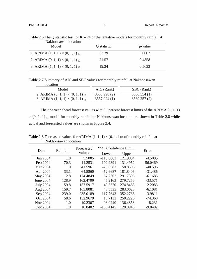
BRG5380004 Report 36 months 96
Table 2.6 The Q statistic test for K = 24 of the tentative models for monthly rainfall at Nakhonsawan location
Model Q statistic p-value
1. ARIMA (1, 1, 0) × (0, 1, 1) 12 53.39 0.0002
2. ARIMA (0, 1, 1) × (0, 1, 1) 12 21.57 0.4858
3. ARIMA (1, 1, 1) × (0, 1, 1) 12 19.34 0.5633
Table 2.7 Summary of AIC and SBC values for monthly rainfall at Nakhonsawan location
Model AIC (Rank) SBC (Rank) 2. ARIMA (0, 1, 1) × (0, 1, 1) 12 3558.998 (2) 3566.554 (1) 3. ARIMA (1, 1, 1) × (0, 1, 1) 12 3557.924 (1) 3569.257 (2)
The one year ahead forecast values with 95 percent forecast limits of the ARIMA (1, 1, 1)
× (0, 1, 1) 12 model for monthly rainfall at Nakhonsawan location are shown in Table 2.8 while
actual and forecasted values are shown in Figure 2.4.
Table 2.8 Forecasted values for ARIMA (1, 1, 1) × (0, 1, 1)12 of monthly rainfall at Nakhonsawan location
Date Rainfall Forecasted values
95% Confidence Limit Error Lower Upper
Jan 2004 1.0 5.5085 -110.8863 121.9034 -4.5085 Feb 2004 70.3 14.2531 -102.9891 131.4952 56.0469 Mar 2004 1.0 41.5961 -75.6583 158.8506 -40.596 Apr 2004 33.1 64.5860 -52.6687 181.8406 -31.486
May 2004 112.8 174.4849 57.2302 291.7395 -61.685 June 2004 128.9 162.4709 45.2163 279.7256 -33.571 July 2004 159.8 157.5917 40.3370 274.8463 2.2083 Aug 2004 159.7 165.8081 48.5535 283.0628 -6.1081 Sep 2004 239.0 235.0189 117.7643 352.2736 3.9811 Oct 2004 58.6 132.9679 15.7133 250.2226 -74.368
Nov 2004 1.0 19.2307 -98.0240 136.4853 -18.231 Dec 2004 1.0 10.8402 -106.4145 128.0948 -9.8402

BRG5380004 Report 36 months 97
Ac t ua lFor ec as t ed Va l ues
0
100
200
300
400
500
600
Year
1976 1977 1978 1979 1980 1981 1982 1983 1984 1985 1986 1987 1988 1989 1990 1991 1992 1993 1994 1995 1996 1997 1998 1999 2000 2001 2002 2003 2004 2005
Figure 2.4 Actual and Forecasted values for ARIMA (1, 1, 1) × (0, 1, 1)12 of monthly
rainfall at Nakhonsawan location from January 1976 to December 2004
Chainat Location
The monthly rainfall series of Chainat location between January 1976 to December 2006
is plotted in Figure 2.5. It shows that this series is stationary in the mean. To investigate whether
the series is stationary in variance, we use the Box-Cox power transformation. The preliminary
residual mean square errors are calculated by using the power transformation via the SAS®
system software version 9.1 as shown in Table 2.9. The power transformation analysis indicates
that a square root transformation is needed for monthly rainfall series at Chainat location as
shown in Figure 2.6.

BRG5380004 Report 36 months 98
0
100
200
300
400
500
600
Year
1976 1978 1980 1982 1984 1986 1988 1990 1992 1994 1996 1998 2000 2002 2004 2006 2008
Figure 2.5 Monthly rainfall series at Chainat location Table 2.9 Residual mean square errors from the power transformation of monthly rainfall at Chainat location
λ Residual mean square error (RMSE) -1.0 6774273605.33 -0.5 129875112000000
0 38491.5 0.5 6425.91 1.0 6447.77
The sample ACF for square root transformed monthly rainfall shows a damping sine-
cosine wave and the sample PACF for square root transformed monthly rainfall has large spike
at multiples of seasonal periods of 12 months implying that a seasonal differencing (1− B12) is
needed in order to achieve stationarity.

BRG5380004 Report 36 months 99
0
100
200
300
400
500
600
Year
1976 1978 1980 1982 1984 1986 1988 1990 1992 1994 1996 1998 2000 2002 2004 2006 2008
Figure 2.6 Square root transformed monthly rainfall series at Chainat location
The sample ACF for seasonal differencing at period 12 months of monthly rainfall series
has a large spike at lag 12 and the sample PACF for seasonal differencing at period 12 months of
monthly rainfall series shows a large spike at lag 12, at lag 24 and a possible one at lag 36. It
indicates that the ARIMA (0, 1, 1) 12 model is appropriate.
To identify the nonseasonal components of the ARIMA model, the residual ACF and
PACF of ARIMA (0, 1, 1)12 are considered. The residual ACF and PACF cut off at lag 5. Hence,
the tentative models are ARIMA (5, 0, 0)×(0, 1, 1)12, ARIMA (0, 0, 5)×(0, 1, 1)12 and ARIMA
(5, 0, 5) × (0, 1, 1)12.
We consider that the residual sample ACF and PACF are close to zero. These indicate
that the series is not stationary and differencing is required. The first difference residual sample
ACF cuts off after lag 1 whereas the first difference residual sample PACF has a large spike at
lag 1 or 4. The tentative models are ARIMA (1, 1, 0) × (0, 1, 1)12, ARIMA (4, 1, 0) × (0, 1, 1)12
and ARIMA (0, 1, 1) × (0, 1, 1)12.
Non-differenced models, ARIMA (5, 0, 0) × (0, 1, 1)12, ARIMA (0, 0, 5) × (0, 1, 1)12 and
ARIMA (5, 0, 5) × (0,1,1)12 , need the t-ratio test for checking whether a deterministic trend
parameter 0θ should be in the model. All non-differenced models do not need the deterministic
trend term because the t-ratio test of each model is not significant at 0.05 significance level.

BRG5380004 Report 36 months 100
Table 2.10 Summary of tentative models fitted for monthly rainfall at Chainat location
Model Estimated parameters 2aσ
1. ARIMA (5, 0, 0) × (0, 1, 1) 12 (1−0.18529 5B )(1−B 12 ) tZ = (1−0.77240 B 12 ) at 10.9655 (0.05234) (0.03499 )
2. ARIMA (0, 0, 5) × (0, 1, 1) 12 (1− B 12 ) tZ = (1+ 0.18477 5B )( 1−0.76975 B 12 ) at 10.9657 (0.05259 ) (0.03515)
3. ARIMA (5, 0, 5) × (0, 1, 1) 12 (1–0.62477 B – 0.3438 4B +0.37131 5B ) (1−B 12 ) tZ = (0.16549) (0.19370) (0.20060) (1–0.57110 B – 0.42411 4B + 0.56531 5B )( 1–0.75791 B 12 ) at 10.84721 (0.15658) (0.17313) (0.17516) (0.37773)
4. ARIMA (1, 1, 0) × (0, 1, 1) 12 (1+0.52838 B )(1−B)(1−B12 ) tZ = (1– 0.80618B12 ) at 15.8029 (0.04473) (0.03348 ) 5. ARIMA (4, 1, 0) × (0, 1, 1) 12 (1+0.81384B+0.57103 2B +0.42698 3B +0.30988 4B )(1−B)(1−B 12 ) tZ = (0.05046) (0.06157) (0.06196) (0.04907) ( 1−0.78450 B12 ) at 12.5011 (0.03477) 6. ARIMA (0, 1, 1) × (0, 1, 1) 12 (1– B )(1−B12 ) tZ = (1– 0.96273 B)(1– 0.79144B 12 ) at 11.3443 (0.01599) (0.03333)
Hence, the parameters of all tentative models are estimated and shown in Table 2.10,
where the values in the parentheses under each the estimates refer to the standard errors of those
estimates. The estimation of all models gives all parameters being significant at 0.05 significance
level.

BRG5380004 Report 36 months 101
To check model adequacy, we consider whether the residuals of the model are white
noise by using a Q statistic test with K = 24. The values of the Q statistic and p-values are given
in Table 2.11. The models 4, 5 and 6 (ARIMA (1, 1, 0) × (0, 1, 1) 12, ARIMA (4, 1, 0) × (0, 1, 1)
12, ARIMA (0, 1, 1) × (0, 1, 1) 12) are not adequate for the monthly rainfall at Chainat location
because the residuals are not white noise.
For model selection, we use AIC and SBC to select the best model. From Table 2.12, we
see that the first model ARIMA (5, 0, 0) × (0, 1, 1) 12 has the minimum AIC and SBC. Similarly,
if we use the variance of white noise ( 2aσ ) to select the best model then ARIMA (5, 0, 0) × (0, 1,
1) 12 has minimum variance of white noise. Thus the model ARIMA (5, 0, 0) × (0, 1, 1) 12 is
selected to describe the monthly rainfall series at Chainat location.
The one year ahead forecast values with 95 percent forecast limits of the ARIMA (5, 0, 0)
× (0, 1, 1) 12 model for monthly rainfall at Chainat location are shown in Table 2.13 while actual
and forecast values are shown in Figure 2.7.
Table 2.11 The Q statistic test for K = 24 of the tentative models for monthly rainfall at Chainat location
Model Q statistic p-value
1. ARIMA (5, 0, 0) × (0, 1, 1) 12 24.91 0.3016
2. ARIMA (0, 0, 5) × (0, 1, 1) 12 24.84 0.3046
3. ARIMA (5, 0, 5) × (0, 1, 1) 12 20.67 0.2414
4. ARIMA (1, 1, 0) × (0, 1, 1) 12 83.22 0.0001
5. ARIMA (4, 1, 0) × (0, 1, 1) 12 36.46 0.0093
6. ARIMA (0, 1, 1) × (0, 1, 1) 12 37.70 0.0198
Table 2.12 Summary of AIC and SBC values for monthly rainfall at Chainat location
Model AIC (Rank) SBC (Rank) 1. ARIMA (5, 0, 0) × (0, 1, 1) 12 1875.276 (1) 1883.037 (1) 2. ARIMA (0, 0, 5) × (0, 1, 1) 12 1875.282 (2) 1883.043 (2) 3. ARIMA (5, 0, 5) × (0, 1, 1) 12 1876.330 (3) 1903.493 (3)

BRG5380004 Report 36 months 102
Table 2.13 Forecasted values for ARIMA (5, 0, 0) × (0, 1, 1)12 of monthly rainfall at Chainat location
Ac t ua lFor ec as t ed Va l ues
0
100
200
300
400
500
600
Year
1976 1978 1980 1982 1984 1986 1988 1990 1992 1994 1996 1998 2000 2002 2004 2006 2008
Figure 2.7 Actual and forecasted values for ARIMA (5, 0, 0) × (0, 1, 1)12 of monthly
rainfall at Chainat location from January 1976 to December 2007
Date Rainfall Forecasted Values
95% Confidence Limit Error Lower Upper
Jan 2007 0 0.908 26.1031 61.959 -0.908 Feb 2007 0 11.951 8.3607 101.789 -11.951 Mar 2007 1.8 27.301 1.3698 139.479 -25.501 Apr 2007 69.9 26.510 1.5507 137.716 43.39
May 2007 220.9 80.290 6.3798 240.447 140.61 June 2007 138 81.625 6.1957 246.195 56.375 July 2007 51.9 95.799 10.4839 270.253 -43.899 Aug 2007 47.1 93.571 9.7596 266.522 -46.471 Sep 2007 167.9 227.685 72.6175 471.891 -59.785 Oct 2007 212.2 89.282 8.4155 259.288 122.918
Nov 2007 1.8 15.776 6.2935 114.497 -13.976 Dec 2007 0 1.121 26.5019 64.980 -1.121

BRG5380004 Report 36 months 103
Singburi Location
The monthly rainfall series of Singburi location in January 1977 to December 2002 is
plotted in Figure 2.8. It shows that the series is stationary in the mean. To investigate whether the
series is stationary in variance, we use the Box-Cox power transformation. The preliminary
residual mean square errors are calculated by using the power transformation via the SAS®
system software version 9.1 as shown in Table 2.14. The power transformation analysis indicates
that it is not necessary to transform the data.
0
100
200
300
400
500
600
Year
1976 1977 1978 1979 1980 1981 1982 1983 1984 1985 1986 1987 1988 1989 1990 1991 1992 1993 1994 1995 1996 1997 1998 1999 2000 2001 2002 2003
Figure 2.8 Monthly rainfall series of Singburi location Table 2.14 Residual mean square error from the power transformation of monthly rainfall series at Singburi location
λ Residual mean square error (RMSE) -1.0 6635204.48 -0.5 267171000000000000
0 46505.48 0.5 6476.70 1.0 6430.52
We consider the sample ACF and sample PACF of monthly rainfall data and find out that
the sample ACF shows a damping sine-cosine wave and the sample PACF has a large spike at
multiples of seasonal period 12 months implying that a seasonal differencing (1− B12) is needed
in order to achieve stationarity.

BRG5380004 Report 36 months 104
We investigate the sample ACF and PACF for seasonal differencing at period 12 months.
The sample ACF has a large spike at lag 12 and the sample PACF show a large spike at lag 12, at
lag 24 and a possible one at lag 36. It indicates that the model ARIMA (0, 1, 1) 12 is appropriate.
To identify the nonseasonal components of the ARIMA model, the sample residual ACF
and PACF of ARIMA (0, 1, 1)12 are considered. We see that the sample ACF cuts off after lag 1
and PACF tails off. Hence the tentative model is the ARIMA (0, 0, 1) × (0, 1, 1)12 model.
Alternatively, we may consider the first difference residual of the ARIMA (0, 1, 1) 12 model. We
see that the sample ACF and the sample PACF have large spikes at lag 1. Hence, the tentative
models are ARIMA (1, 1, 0) × (0, 1, 1)12, ARIMA (0, 1, 1) × (0, 1, 1)12 and ARIMA (1, 1, 1) ×
(0, 1, 1)12 .
Non-differenced models, ARIMA (0, 0, 1) × (0, 1, 1)12, need the t-ratio test for checking
whether a deterministic trend parameter 0θ should be in the model. It shows that the ARIMA (1,
0, 0) × (0, 1, 1)12 model does not need the deterministic trend term because the t-ratio test of the
model is not significant at 0.05 significance level.
Table 2.15 Summary of tentative models fitted for monthly rainfall at Singburi location Model Estimated parameters 2
aσ 1. ARIMA (0, 0, 1) × (0, 1, 1) 12 (1−B12 )Zt = (1+0.14936B)( 1−0.92399 B 12 ) at 4583.831 (0.05852) (0.02446 ) 2. ARIMA (1, 1, 0) × (0, 1, 1) 12 (1+0.44789B) (1−B) (1−B 12 )Zt =(1 - 0.91636 B 12 ) at 6401.820 (0.05383 ) (0.02589) 3. ARIMA (0, 1, 1) × (0, 1, 1) 12 (1– B)(1−B12 ) Zt = (1– B)( 1–0.89760 B 12 ) at 4829.532 (0.00168) (0.03381) 4. ARIMA (1, 1, 1) × (0, 1, 1) 12 (1–0.19547B)(1– B)(1– B12)Z t = (1 – B) (1 – 0.91077B12) at 4696.02 (0.05896) ( 0.0019926) ( 0.03099 )

BRG5380004 Report 36 months 105
The parameters of all tentative models are estimated and presented in Table 2.15, where
the values in the parentheses under each estimate refer to the standard errors of those estimates.
The estimation of parameters for all models are considered at 0.05 significance level.
To check model adequacy, we consider whether the residuals of the model are white
noise by using a Q statistic test with K = 24. The values of the Q statistic and p-values are given
in Table 2.16. Model 2 is not adequate for the monthly rainfall at Singburi location because the
residuals are not white noise.
For model selection, we use AIC and SBC to select the best model. From Table 2.17, we
see that model 4 has the minimum AIC and SBC. Thus the model ARIMA (1, 1, 1) × (0, 1, 1) 12
is selected to describe the monthly rainfall series at Singburi location.
The one year ahead forecast values with 95 percent forecast limits of the ARIMA (1, 1, 1)
× (0, 1, 1) 12 model for monthly rainfall at Singburi location are shown in Table 2.18 while actual
and forecasted values are shown in Figure 2.9.
Table 2.16 The Q statistic test for K = 24 of the tentative models for monthly rainfall at Singburi location
Model Q statistic p-value
1. ARIMA (0, 0, 1) × (0, 1, 1) 12 15.54 0.8381
2. ARIMA (1, 1, 0) × (0, 1, 1) 12 52.47 0.0003
3. ARIMA (0, 1, 1) × (0, 1, 1) 12 24.52 0.3205
4. ARIMA (1, 1, 1) × (0, 1, 1) 12 15.80 0.7806
Table 2.17 Summary of AIC and SBC values for monthly rainfall at Singburi location
Model AIC (Rank) SBC (Rank) 1. ARIMA (0, 0, 1) × (0, 1, 1) 12 3235.957 (3) 3243.276 (3) 3. ARIMA (0, 1, 1) × (0, 1, 1) 12 3205.661 (2) 3212.952 (2) 4. ARIMA (1, 1, 1) × (0, 1, 1) 12 3198.718 (1) 3209.655 (1)

BRG5380004 Report 36 months 106
Table 2.18 Forecasted values for ARIMA (1, 1, 1) × (0, 1, 1)12 of monthly rainfall at Singburi location
Date Rainfall Forecasted Values
95% Confidence Limit Error Lower Upper
Jan 2003 0 0.457 -134.826 137.741 -0.457Feb 2003 0 3.374 -134.632 143.380 -3.374Mar 2003 18.3 17.582 -120.533 157.697 0.718Apr 2003 48.9 53.954 -84.165 194.073 -5.054
May 2003 135.7 146.931 8.811 287.050 -11.231June 2003 101.7 95.167 -42.952 235.286 6.533July 2003 106.8 88.374 -49.745 228.494 18.426Aug 2003 145.6 138.885 0.766 279.004 6.715Sep 2003 207.9 184.760 46.641 324.879 23.14Oct 2003 140 129.712 -8.408 269.831 10.288
Nov 2003 21.2 15.242 -122.877 155.361 5.958Dec 2003 3.1 1.284 -136.835 141.403 1.816
Ac t ua lFor ec as t ed Va l ues
0
100
200
300
400
500
600
Year
1976 1977 1978 1979 1980 1981 1982 1983 1984 1985 1986 1987 1988 1989 1990 1991 1992 1993 1994 1995 1996 1997 1998 1999 2000 2001 2002 2003 2004
Figure 2.9 Actual and forecasted values for ARIMA (1, 1, 1) × (0, 1, 1)12 of monthly rainfall at Singburi location from January 1976 to December 2003
Angthong Location
The monthly rainfall series of Angthong location between January 1976 to December
2006 is plotted in Figure 2.10. It shows that this series is stationary in the mean. To investigate
whether the series is stationary in the variance, we use the Box-Cox power transformation. The
preliminary residual mean square errors are calculated by using the power transformation via the

BRG5380004 Report 36 months 107
SAS® system software version 9.1 which is shown in Table 2.19. The power transformation
analysis indicates that it is not necessary to transform the data.
0
100
200
300
400
500
600
Year
1976 1978 1980 1982 1984 1986 1988 1990 1992 1994 1996 1998 2000 2002 2004 2006 2008
Figure 2.10 Monthly rainfall series at Angthong location
Table 2.19 Residual mean square error from the power transformation of monthly rainfall at Angthong location
λ Residual mean square error (RMSE) -1.0 18404643312.48 -0.5 370457125900000000
0 60605.41 0.5 8305.88 1.0 8173.41
We consider the sample ACF and sample PACF of monthly rainfall data. The sample
ACF shows a damping sine-cosine wave and the sample PACF has large spike at multiples of
seasonal period 12 months implying that a seasonal differencing (1− B12) is needed in order to
achieve stationarity.
We consider the sample ACF and PACF for seasonal differencing at period 12 months.
The sample ACF has a large spike at lag 12 and the sample PACF shows large spikes at lag 12,
at lag 24 and a possible one at lag 36. This indicates that the model ARIMA (0, 1, 1)12 is
appropriate.

BRG5380004 Report 36 months 108
To identify the nonseasonal components of the ARIMA model, the residual ACF and
PACF of ARIMA (0, 1, 1)12 are considered .The residual sample ACF and PACF are close to
zero and we consider the first differenced residual of the ARIMA (0, 1, 1)12 model.
The first differenced residual of the sample ACF cuts off after lag 1 and the sample
PACF has large spikes at lag 1 and 5. Hence, the tentative models are ARIMA (1, 1, 0) × (0, 1,
1)12, ARIMA (5, 1, 0) × (0, 1, 1) 12, ARIMA (0, 1, 1) × (0, 1, 1) 12, ARIMA (1, 1, 1) × (0, 1, 1) 12
and ARIMA (5, 1, 1) × (0, 1, 1) 12.
The parameters of all tentative models are estimated and shown in Table 2.20, where the
values in the parentheses under each estimate refer to the standard errors of those estimates. The
estimation of parameters 1φ in model 4 and 1φ 5− φ in model 5 are not significant at 0.05
significance level. It implies that the model can be refitted with 1φ and 1φ 5− φ removed if it is
necessary. This would be considered as a tentative model 3.
Table 2.20 Summary of tentative models fitted for monthly rainfall at Angthong location Model Estimated parameters 2ˆ aσ 1. ARIMA (1, 1, 0) × (0, 1, 1) 12 (1+ 0.55558 B)(1–B) (1−B12 ) Zt = ( 1− 0.90751 B 12 ) at 7902.849 (0.04402) (0.02377 ) 2. ARIMA (5, 1, 0) × (0, 1, 1) 12 (1+0.8768B+0.6357 2B +0.54293 3B +0.44202 4B +0.24488 5B )(1–B) (1−B 12 ) Zt = (0.05194) (0.06717) (0.07044) (0.06969) (0.05448)
(1 – 0.90132 B 12 ) at 6279.693 (0.02455) 3. ARIMA (0, 1, 1) × (0, 1, 1)12
(1–B) (1− B12 ) Zt =(1 – 0.97780B) ( 1− 0.89478 B 12 ) at 5637.677 (0.01188 ) (0.02589)

BRG5380004 Report 36 months 109
Table 2.20 Summary of tentative models fitted for monthly rainfall at Angthong location (continued) Model Estimated parameters 2
aσ 4. ARIMA (1, 1, 1) × (0, 1, 1) 12 (1+0.03764 B)(1–B) (1−B12 ) Zt =(1– 0.97652B)( 1– 0.89547 B 12 ) at 5645.792 (0.05628) (0.01259 ) (0.02580)
5. ARIMA (5, 1, 1) × (0, 1, 1)12. (1+0.03415B–0.07757 2B +0.05625 3B +0.05611 4B +0.00251 5B )(1–B) (1−B 12 ) Zt = (0.05509) (0.05504) (0.05576) (0.05825) (0.05811)
(1 – 0.97519B)(1 – 0.89945 B 12 ) at 5648.209 (0.01437) (0.02580)
To check model adequacy, we consider whether the residuals of the model are white
noise by using a Q statistic test with K = 24. The values of the Q statistic and p-values are given
in Table 2.21. Models 1 and 2 are not adequate for the monthly rainfall at Angthong location
because the residuals are not white noise. Hence model 3 is the best model for monthly rainfall
series at Angthong location. Table 2.22 shows summary of AIC and SBC values for the best
model of monthly rainfall at Angthong location.
Table 2.21 The Q statistic test for K = 24 of the tentative models for monthly rainfall at Angthong location
Model Q statistic p-value
1. ARIMA (1, 1, 0) × (0, 1, 1) 12 62.65 <0.0001
2. ARIMA (5, 1, 0) × (0, 1, 1) 12 29.95 0.0379
3. ARIMA (0, 1, 1) × (0, 1, 1) 12 20.56 0.5483

BRG5380004 Report 36 months 110
Table 2.22 Summary of AIC and SBC values for monthly rainfall at Angthong location
MODEL AIC SBC 3. ARIMA (5, 1, 1) × (0, 1, 1) 12 4127.163 4154.347
The one year ahead forecast values with 95 percent forecast limits of the ARIMA (0, 1, 1)
× (0, 1, 1) 12 model for monthly rainfall at Angthong location are shown in Table 2.23 and actual
and forecasted values are shown in Figure 2.11.
Table 2.23 Forecasted values for ARIMA (0, 1, 1) × (0, 1, 1)12 of monthly rainfall at Angthong location
Date Rainfall Forecasted Values
95% Confidence Limit Error Lower Upper
Jan 2007 1 11.9398 -135.2230 159.1027 -10.94 Feb 2007 1 18.3671 -128.8320 165.5662 -17.367 Mar 2007 1 45.4696 -101.7657 192.7049 -44.47 Apr 2007 39.9 75.5637 -71.7079 222.8352 -35.664
May 2007 349.5 141.9006 -5.4072 289.2084 207.599 June 2007 122.4 128.0041 -19.3399 275.3481 -5.6041 July 2007 73.5 119.2910 -28.0892 266.6712 -45.791 Aug 2007 30.8 139.7486 -7.6678 287.1650 -108.95 Sep 2007 15.4 266.1273 118.6748 413.5799 -250.73 Oct 2007 80.1 173.1885 25.6997 320.6772 -93.089
Nov 2007 40.7 46.1192 -101.4057 193.6441 -5.4192 Dec 2007 5.2 15.7215 -131.8396 163.2825 -10.522
Ac t ua lFor ec as t ed Va l ues
0
100
200
300
400
500
600
Year
1976 1978 1980 1982 1984 1986 1988 1990 1992 1994 1996 1998 2000 2002 2004 2006 2008
Figure 2.11 Actual and forecasted values for ARIMA (0, 1, 1) × (0, 1, 1)12 of rainfall at Angthong location from January 1976 to December 2007
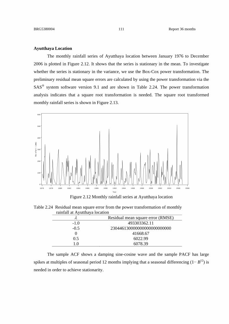
BRG5380004 Report 36 months 111
Ayutthaya Location
The monthly rainfall series of Ayutthaya location between January 1976 to December
2006 is plotted in Figure 2.12. It shows that the series is stationary in the mean. To investigate
whether the series is stationary in the variance, we use the Box-Cox power transformation. The
preliminary residual mean square errors are calculated by using the power transformation via the
SAS® system software version 9.1 and are shown in Table 2.24. The power transformation
analysis indicates that a square root transformation is needed. The square root transformed
monthly rainfall series is shown in Figure 2.13.
0
100
200
300
400
500
600
Year
1976 1978 1980 1982 1984 1986 1988 1990 1992 1994 1996 1998 2000 2002 2004 2006 2008
Figure 2.12 Monthly rainfall series at Ayutthaya location
Table 2.24 Residual mean square error from the power transformation of monthly rainfall at Ayutthaya location
λ Residual mean square error (RMSE) -1.0 493303362.11 -0.5 230446130000000000000000000
0 41668.67 0.5 6022.99 1.0 6078.39
The sample ACF shows a damping sine-cosine wave and the sample PACF has large
spikes at multiples of seasonal period 12 months implying that a seasonal differencing (1− B12) is
needed in order to achieve stationarity.

BRG5380004 Report 36 months 112
The sample ACF has a large spike at lag 12 and the sample PACF shows large spike at
lag 12, at lag 24 and a possible one at lag 36. This indicates that the model ARIMA (0, 1, 1) 12 is
appropriate.
To identify the nonseasonal components of the ARIMA model, the residual ACF and
PACF of ARIMA (0, 1, 1)12 are considered. The residual ACF and PACF are close to zero.
Alternatively, we may consider the sample ACF and PACF of first seasonal differencing at
period 12 months. We see that the sample ACF and PACF have large spikes at lag 1. Hence, all
tentative models of monthly rainfall series at Ayutthaya location are ARIMA (1, 1, 0) × (0, 1,
1)12, ARIMA (0, 1, 1) × (0, 1, 1)12 and ARIMA (1, 1, 1) × (0, 1, 1)12.
0
100
200
300
400
500
600
Year
1976 1978 1980 1982 1984 1986 1988 1990 1992 1994 1996 1998 2000 2002 2004 2006 2008
Figure 2.13 The square root transformed monthly rainfall series at Ayutthaya location
Parameters of all tentative models are estimated and shown in Table 2.25, where the
values in the parentheses under each estimate refer to the standard errors of those estimates. The
estimation of parameters for all models are considered at 0.05 significance level.

BRG5380004 Report 36 months 113
Table 2.25 Summary of tentative models fitted for monthly rainfall at Ayutthaya location Model Estimated parameters 2
aσ 1. ARIMA (1, 1, 0) × (0, 1, 1) 12 (1+ 0.55163 B)(1–B)(1− B12 ) tZ = (1–0.79399 B 12 ) at 16.996 (0.04620) (0.03548) 2. ARIMA (0, 1, 1) × (0, 1, 1) 12 (1–B)(1−B12 ) tZ = (1–0.95250 B)( 1–0.81134 B 12 ) at 12.627 (0.01779 ) (0.03434) 3. ARIMA (1, 1, 1) × (0, 1, 1) 12 (1+0.02675 B)(1–B) (1− B12 ) tZ =(1– 0.94636B)( 1–0.81222 B12 ) at 12.659 (0.05897) (0.01995 ) (0.03430)
To check model adequacy, we consider whether the residuals of the model are white
noise by using a Q statistic test with K = 24. The values of the Q statistic and p-values are given
in Table 2.26. Model 1 is not adequate for the monthly rainfall at Ayutthaya location because the
residuals are not white noise.
Table 2.26 The Q statistic test for K = 24 of the tentative models for monthly rainfall at Ayutthaya location
Model Q statistic p-value
1. ARIMA (1, 1, 0) × (0, 1, 1) 12 53.41 0.0002
2. ARIMA (0, 1, 1) × (0, 1, 1) 12 10.01 0.9862
3. ARIMA (1, 1, 1) × (0, 1, 1) 12 9.88 0.9804
For model selection, we use AIC and SBC to select the best model. From Table 2.27, we
see that the ARIMA (0, 1, 1) × (0, 1, 1) 12 model has the minimum AIC and SBC. Hence it is
selected to describe the monthly rainfall series at Ayutthaya with minimum estimated variance of
white noise.

BRG5380004 Report 36 months 114
Table 2.27 Summary of AIC and SBC values for monthly rainfall at Ayutthaya location
Model AIC (Rank) SBC (Rank) 2. ARIMA (0, 1, 1) × (0, 1, 1) 12 1759.210 (1) 1766.790 (1) 3. ARIMA (1, 1, 1) × (0, 1, 1) 12 1761.030 (2) 1772.399 (2)
Table 2.28 Forecasted values for ARIMA (0, 1, 1) × (0, 1, 1)12 of monthly rainfall at Ayutthaya location
The one year ahead forecast values with 95 percent forecast limits of the ARIMA (0, 1, 1)
× (0, 1, 1) 12 model for monthly rainfall at Ayutthaya location are shown in Table 2.28 while
actual and forecasted values are shown in Figure 2.14.
Date Rainfall Forecasted Values
95% Confidence Limit Error Lower Upper
Jan 2007 0 1.219 29.9788 71.474 -1.219 Feb 2007 0 0.715 32.0701 68.594 -0.715 Mar 2007 4.8 21.095 5.1980 136.445 -16.295 Apr 2007 84.8 35.389 0.9138 169.537 49.411
May 2007 354.1 97.274 8.5100 285.928 256.826 June 2007 109.0 112.779 13.4160 312.251 -3.779 July 2007 38.2 81.129 4.2057 258.381 -42.929 Aug 2007 35.4 89.282 6.1612 272.951 -53.882 Sep 2007 175.2 232.742 68.2491 498.002 -57.542 Oct 2007 83.5 99.200 8.8499 290.535 -15.7
Nov 2007 10.2 11.072 12.7334 110.615 -0.872 Dec 2007 0 -0.207 37.9458 63.064 0.207

BRG5380004 Report 36 months 115
Ac t ua lFor ec as t ed Va l ues
0
100
200
300
400
500
600
Year
1976 1978 1980 1982 1984 1986 1988 1990 1992 1994 1996 1998 2000 2002 2004 2006 2008
Figure 2.14 Actual and forecasted values for ARIMA (0, 1, 1) × (0, 1, 1)12 of monthly rainfall at Ayutthaya location from January 1976 to December 2007
Pathumtani Location
The monthly rainfall series of Pathumtani location from January 1976 to December 2003
is plotted in Figure 2.15. It shows that the series is stationary in the mean. To investigate whether
the series is stationary in the variance, we use the Box-Cox power transformation. The
preliminary residual mean square errors are calculated by using the power transformation via the
SAS® system software version 9.1 as shown in Table 2.29. The power transformation analysis
indicates that it is not necessary to transform the data.

BRG5380004 Report 36 months 116
0
100
200
300
400
500
600
Year
1976 1977 1978 1979 1980 1981 1982 1983 1984 1985 1986 1987 1988 1989 1990 1991 1992 1993 1994 1995 1996 1997 1998 1999 2000 2001 2002 2003 2004
Figure 2.15 Monthly rainfall series at Pathumtani location
Table 2.29 Residual mean square error from the power transformation of monthly rainfall series at Pathumtani location
λ Residual mean square error (RMSE) -1.0 84599249060.22 -0.5 621843027500000
0 44534.83 0.5 6866.05 1.0 6785.24
The sample ACF shows a damping sine-cosine wave and the sample PACF has large
spikes at multiples of seasonal period 12 months implying that a seasonal differencing (1− B12) is
needed in order to achieve stationarity.
The sample PACF still shows a large spike at lag 12, at lag 24 and a possible one at lag
36. The sample ACF has a large spike at lag 12. Comparing the theoretical ACF and PACF
patterns, the pattern of one spike in ACF and the PACF tails off which appears at the seasonal
lags indicates that the model ARIMA (0, 1, 1)12 is appropriate.
To identify the nonseasonal components of the ARIMA model, the residual ACF and
PACF of ARIMA (0, 1, 1)12 are considered. The residual ACF cuts off at lag 1 and the residual
PACF cuts off at lag 1 or 2. Hence, all the tentative models are ARIMA (1, 0, 0)×(0, 1, 1)12,
ARIMA (2, 0, 0)×(0, 1, 1)12, ARIMA (0, 0, 1)×(0, 1, 1)12, ARIMA (1, 0, 1)×(0, 1, 1)12 and
ARIMA (2, 0, 1)×(0, 1, 1)12.

BRG5380004 Report 36 months 117
The parameters of all tentative models are estimated and shown in Table 2.30, where the
values in the parentheses under each estimate refer to the standard errors of those estimates. The
estimation of parameters of all models are considered at 0.05 significance level. There is only
one estimation of 2φ in model 2 which is not significant.
Table 2.30 Summary of tentative models fitted for monthly rainfall at Pathumthani location Model Estimated parameters 2
aσ 1. ARIMA (1, 0, 0) × (0, 1, 1) 12 (1−0.24296B) (1− B 12 ) Z t = ( 1−0.82734 B 12 ) at 5721.007 (0.05708) (0.03318 ) 2. ARIMA (2, 0, 0) × (0, 1, 1) 12 (1−0.21874 B −0.10361B 2 )(1− B 12 ) Z t = ( 1−0.82737 B 12 ) at 5680.740 (0.05854) (0.05919) (0.03318 ) 3. ARIMA (0, 0, 1) × (0, 1, 1) 12 (1− B 12 ) Z t =(1+0.20161 B) ( 1–0.82057 B 12 ) at 5781.594 (0.05758 ) (0.03380) 4. ARIMA (1, 0, 1) × (0, 1, 1) 12 (1–0.72846 B)(1− B12 ) Z =(1 – 0.52847B)( 1–0.82977 B 12 ) at 5636.292 (0.12588) (0.15530 ) (0.03295)
To check model adequacy, we consider whether the residuals of the model are white
noise by using a Q statistic test with K = 24. The values of the Q statistic and p-values are given
in Table 2.31. All models are adequate for the monthly rainfall at Pathumthani location.
For model selection, we use AIC and SBC to select the best model. From Table 2.32, we
see that the ARIMA (1, 0, 1) × (0, 1, 1) 12 model has the minimum AIC whereas the ARIMA (1,
0, 0) × (0, 1, 1) 12 model has the minimum SBC. We give the estimate variance of white noise
( 2aσ ) in Table 2.30. The minimum estimate variance of white noise ( 2
aσ ) of the ARIMA (1, 0, 1)
× (0, 1, 1) 12 model is less than that of the ARIMA (1, 0, 0) × (0, 1, 1) 12 model. Hence the

BRG5380004 Report 36 months 118
ARIMA (1, 0, 1) × (0, 1, 1) 12 model is selected to describe the monthly rainfall series at
Pathumtani location.
Table 2.31 The Q statistic test for K = 24 of the tentative models for monthly rainfall at Pathumtani location
Model Q statistic p-value
1. ARIMA (1, 0, 0) × (0, 1, 1) 12 32.64 0.0671
3. ARIMA (0, 0, 1) × (0, 1, 1) 12 33.45 0.0558
4. ARIMA (1, 0, 1) × (0, 1, 1) 12 31.63 0.0638
Table 2.32 Summary of AIC and SBC values for monthly rainfall at Pathumthani location
Model AIC (Rank) SBC (Rank) 1. ARIMA (1, 0, 0) × (0, 1, 1) 12 3483.396 (2) 3490.823 (1) 3. ARIMA (0, 0, 1) × (0, 1, 1) 12 3486.588 (3) 3494.015 (3) 4. ARIMA (1, 0, 1) × (0, 1, 1) 12 3479.867 (1) 3491.008 (2)
The one year ahead forecast values with 95 percent forecast limits of the ARIMA (1, 0, 1)
× (0, 1, 1) 12 model for monthly rainfall at Pathumtani location are shown in Table 2.33 while
actual and forecasted values are shown in Figure 2.16.
Table 2.33 Forecasted values for ARIMA (1, 0, 1) × (0, 1, 1)12 of monthly rainfall at Pathumtani location
Date Rainfall Forecasted Values
95% Confidence Limit Error Lower Upper
Jan 2004 0 17.0626 -130.0822 164.2074 -17.063 Feb 2004 80.6 17.9229 -132.1355 167.9813 62.6771 Mar 2004 100.3 88.2630 -63.3189 239.8448 12.037 Apr 2003 22.3 51.5072 -100.8768 203.8913 -29.207
May 2004 73.9 128.3915 -24.4165 281.1995 -54.492 June 2004 124.9 96.0559 -56.9766 249.0884 28.8441 July 2004 82.5 82.4227 -70.7288 235.5742 0.0773 Aug 2004 114.2 109.1829 -44.0317 262.3975 5.0171 Sep 2004 141.6 155.9382 2.6901 309.1863 -14.338 Oct 2004 93.6 119.5989 -33.6670 272.8647 -25.999
Nov 2004 1 20.5350 -132.7403 173.8103 -19.535 Dec 2004 1 2.1763 -151.1039 155.4566 -1.1763

BRG5380004 Report 36 months 119
Ac t ua lFor ec as t ed Va l ues
0
100
200
300
400
500
600
Year
1976 1977 1978 1979 1980 1981 1982 1983 1984 1985 1986 1987 1988 1989 1990 1991 1992 1993 1994 1995 1996 1997 1998 1999 2000 2001 2002 2003 2004 2005
Figure 2.16 Actual and forecasted values for ARIMA (1, 0, 1) × (0, 1, 1)12 of monthly rainfall at Pathumtani location from January 1976 to December 2004
Nonthaburi Location
The monthly rainfall series of Nonthaburi location from January 1976 to December 2006
is plotted in Figure 2.17. It shows that the series is stationary in the mean. To investigate whether
the series is stationary in the variance, we use the Box-Cox power transformation. The
preliminary residual mean square errors are calculated by using the power transformation via the
SAS® system software version 9.1 as shown in Table 2.34. The power transformation analysis
indicates that a square root transformation is needed. Figure 2.41 shows the plot of the
transformed series.

BRG5380004 Report 36 months 120
0
100
200
300
400
500
600
Year
1976 1978 1980 1982 1984 1986 1988 1990 1992 1994 1996 1998 2000 2002 2004 2006 2008
Figure 2.17 Monthly rainfall series at Nonthaburi location
Table 2.34 Residual mean square errors from the power transformation of monthly rainfall series at Nonthaburi location
λ Residual mean square error (RMSE) -1.0 6317021710.21 -0.5 5431799614.81
0 29744.09 0.5 8441.86 1.0 8518.80
The sample ACF shows a damped sine-cosine wave and the sample PACF has large spike
at multiples of seasonal period 12 months implying that a seasonal differencing (1−B12) is needed
in order to achieve stationarity.

BRG5380004 Report 36 months 121
0
100
200
300
400
500
600
Year
1976 1978 1980 1982 1984 1986 1988 1990 1992 1994 1996 1998 2000 2002 2004 2006 2008
Figure 2.18 The square root transformed monthly rainfall series at Nonthaburi location
The sample ACF and PACF for seasonal differencing at period 12 months are considered.
The sample ACF has a large spike at lag 12 and the sample PACF shows large spikes at lag 12,
at lag 24 and a possible one at lag 36. It indicates that the ARIMA (0, 1, 1) 12 model is
appropriate.
To identify the nonseasonal components of the ARIMA model, the residual ACF and
PACF of ARIMA (0, 1, 1)12 are considered. The residual ACF and PACF cut off at lag 1. Hence,
all tentative models are ARIMA (1, 0, 0) × (0, 1, 1)12, ARIMA (0, 0, 1) × (0, 1, 1)12 and ARIMA
(1, 0, 1) × (0, 1, 1)12.
The parameters of all tentative models are estimated and shown in Table 2.35, where the
values in the parentheses under each of the estimates refer to the standard errors of those
estimates. The estimation of parameters of all models are considered at 0.05 or 0.01 significance
level.
To check model adequacy, we consider whether the residuals of the model are white
noise by using a Q statistic test with K = 24. The values of the Q statistic and p-values are given
in Table 2.36. Models 1, 2 and 3 are not adequate for the monthly rainfall series at Nonthaburi
location because the residuals are not white noise. So we consider the first difference of the
residual.
BRG5380004 Report 36 months 122
Table 2.35 Summary of tentative models fitted for monthly rainfall at Nonthaburi location Model Estimated parameters 2
aσ 1. ARIMA (1, 0, 0) × (0, 1, 1) 12 (1−0.41836B)(1−B12 ) Zt = ( 1−0.77298B 12 ) at
12.842 (0.04851) (0.03602) 2. ARIMA (0, 0, 1) × (0, 1, 1) 12 (1− B 12 )Zt = (1 + 0.30166B) ( 1–0.72349B 12 ) at 13.403 (0.05058) (0.03834) 3. ARIMA (1, 0, 1) × (0, 1, 1) 12 (1–0.78799B)(1−B12 ) Zt =(1–0.46749B)(1−0.79748 B 12 ) at 12.300 (0.06567) (0.09340) (0.03446)
Table 2.36 The Q statistic test for K = 24 of the tentative models for monthly rainfall at Nonthaburi location
Model Q statistic p-value
1. ARIMA (1, 0, 0) × (0, 1, 1) 12 63.84 <0.0001
2. ARIMA (0, 0, 1) × (0, 1, 1) 12 101.99 <0.0001
3. ARIMA (1, 0, 1) × (0, 1, 1) 12 42.17 0.0040
The differenced residual sample ACF and PACF have large spike at lag 1. Thus all
tentative models are ARIMA(1, 1, 0) × (0, 1, 1)12, ARIMA(0, 1, 1)×(0, 1, 1)12 and ARIMA (1, 1,
1) × (0, 1, 1)12.
The parameters of all tentative models are estimated and shown in Table 2.37, where the
values in the parentheses under each estimates refer to the standard errors of those estimates. The
estimation of parameters of all models are considered at 0.05 significance level.
To check model adequacy, we consider whether the residuals of the model are white
noise by using a Q statistic test with K = 24. The values of the Q statistic and p-values are given

BRG5380004 Report 36 months 123
in Table 2.38. Models 1 and 2 are not adequate for the monthly rainfall at Nontaburi location
because the residuals are not white noise.
Table 2.37 Summary of tentative models fitted for monthly rainfall at Nonthaburi location Model Estimated parameters 2
aσ 1. ARIMA (1, 1, 0) × (0, 1, 1) 12 (1+ 0.40105B)(1–B)(1−B 12 )Zt = ( 1–0.83799B 12 ) at 14.893 (0.04859) (0.03139) 2. ARIMA (0, 1, 1) × (0, 1, 1) 12 (1−B)(1−B 12 )Zt = (1 – 0.78376B) ( 1– 0.80393B 12 ) at 13.000 (0.03309) (0.03354) 3. ARIMA (1, 1, 1) × (0, 1, 1) 12 (1–0.28292 B) (1–B) (1− B12 ) Zt =(1 – 0.91804B) ( 1 – 0.82187B12 ) at 12.394 (0.05918) (0.02451) (0.03264)
Table 2.38 The Q statistic test for K = 24 of the tentative models for monthly rainfall at Nontaburi location
Model Q statistic p-value
1. ARIMA (1, 1, 0) × (0, 1, 1) 12 68.99 <0.0001
2. ARIMA (0, 1, 1) × (0, 1, 1) 12 58.72 <0.0001
3. ARIMA (1, 1, 1) × (0, 1, 1) 12 36.25 0.0221
Hence the best model is model 3. Table 2.39, shows summary AIC and SBC values for
the best model of monthly rainfall series at Nonthaburi location.
The one year ahead forecasted values with 95 percent forecast limits of the ARIMA (1, 1,
1) × (0, 1, 1) 12 model for monthly rainfall at Nonthaburi location are shown in Table 2.40 while
actual and forecasted values are shown in Figure 2.49.
Table 2.39 Summary of AIC and SBC values for monthly rainfall at Nonthaburi location
Model AIC SBC 3. ARIMA (1, 1, 1) × (0, 1, 1) 12 1925.477 1937.127

BRG5380004 Report 36 months 124
Table 2.40 Forecasted values for ARIMA (1, 1, 1) × (0, 1, 1)12 of monthly rainfall at Nonthaburi location
Date Rainfall Forecasted Values
95% Confidence Limit Error Lower Upper
Jan 2007 6.1 0.824 29.5387 59.854 5.276 Feb 2007 9.8 11.177 10.0398 100.059 -1.377 Mar 2007 28.3 26.481 1.9360 138.771 1.819 Apr 2007 46.4 26.019 2.0624 137.720 20.381
May 2007 132.6 80.145 5.7337 242.301 52.455 June 2007 89.1 81.551 5.5629 248.308 7.549 July 2007 105.4 95.844 9.7086 272.748 9.556 Aug 2007 116.3 93.691 9.0337 269.118 22.609 Sep 2007 252.5 227.134 70.3576 474.681 25.366 Oct 2007 181.2 89.259 7.6979 261.590 91.941
Nov 2007 42.8 14.782 7.8080 112.632 28.018 Dec 2007 2.6 1.005 29.9937 62.892 1.595

BRG5380004 Report 36 months 125
Ac t ua lFor ec as t ed Val ues
0
100
200
300
400
500
600
Year
1976 1978 1980 1982 1984 1986 1988 1990 1992 1994 1996 1998 2000 2002 2004 2006 2008
Figure 2.19 Actual and forecasted values for ARIMA (1, 1, 1) × (0, 1, 1)12of monthly rainfall at Nonthaburi location from January 1976 to December 2007
Bangkok Location
The monthly rainfall series of Bangkok location from January 1976 to December
2006 is plotted in Figure 2.20. It shows that this series is stationary in the mean. To investigate
whether the series is stationary in the variance, we use the Box-Cox power transformation. The
preliminary residual mean square errors are calculated by using the power transformation via the
SAS® system software version 9.1 as shown in Table 2.41. The power transformation analysis
indicates that it is not necessary to transform the data.

BRG5380004 Report 36 months 126
0
100
200
300
400
500
600
Year
1976 1978 1980 1982 1984 1986 1988 1990 1992 1994 1996 1998 2000 2002 2004 2006 2008
Figure 2.20 Monthly rainfall series at Bangkok location Table 2.41 Residual mean square error from the power transformation of monthly rainfall series at Bangkok location
λ Residual mean square error (RMSE) -1.0 124292313.30 -0.5 313240216085.94
0 83118.00 0.5 8109.87 1.0 7841.06
The sample ACF shows a damping sine-cosine wave and the sample PACF has large
spikes at multiples of seasonal period 12 months implying that a seasonal differencing (1−B12) is
needed in order to achieve stationarity.
We consider the sample ACF and PACF for seasonal differencing at period 12 months.
The sample ACF has a large spike at lag 12 and the sample PACF shows large spikes at lag 12,
at lag 24 and a possible one at lag 36. It indicates that the model ARIMA (0, 1, 1) 12 is
appropriate.
To identify the nonseasonal components of the ARIMA model, the residual ACF and
PACF of ARIMA (0, 1, 1)12 are computed. The residual ACF and PACF are close to zero and we
consider the first differenced residual of the ARIMA (0, 1, 1)12 model.

BRG5380004 Report 36 months 127
The first differenced residual of the sample ACF cuts off after lag 1 and the sample
PACF has large spikes at lag 1 or 4. Hence, all the tentative models are ARIMA (1, 1, 0) × (0, 1,
1)12, ARIMA (4, 1, 0) × (0, 1, 1)12, ARIMA (0, 1, 1) × (0, 1, 1)12, ARIMA (1, 1, 1) × (0, 1, 1)12
and ARIMA (4, 1, 1) × (0, 1, 1)12.
Table 2.42 Summary of tentative models for monthly rainfall at Bangkok location.
Model Estimated parameters 2aσ
1. ARIMA (1, 1, 0) × (0, 1, 1) 12 (1+ 0.43872B)(1–B) (1−B 12 ) Zt = ( 1−0.88263 B 12 ) at 6183.982 (0.04793) (0.02668) 2. ARIMA (4, 1, 0) × (0, 1, 1) 12 (1+ 0.63843B + 0.45793 2B + 0.29858 3B + 0.22579 4B )(1−B 12 ) Zt = (0.05205) (0.06081) (0.06091) (0.05297) (1 – B)( 1– 0.87251B 12 ) at 5322.739 (0.02740) 3. ARIMA (0, 1, 1) × (0, 1, 1) 12 (1–B)(1−B12 ) Zt =(1 – 0.87670B)( 1 – 0.87185B 12 ) at 4909.798 (0.02605) (0.02709) 4. ARIMA (1, 1, 1) × (0, 1, 1) 12 (1–0.15527B)(1–B) (1−B12 )Zt =(1– 0.91125B)(1–0.8605B 12 ) at 4830.067 (0.06016) (0.02585) (0.02901)
The parameters of all tentative models are estimated and shown in Table 2.42, where the
values in parentheses under each estimate refer to the standard errors of those estimates. The
estimation of parameters of all models are considered at 0.05 significance level.
To check model adequacy, we consider whether the residuals of the model are white
noise by using a Q statistic test with K = 24. The values of the Q statistic and p-values are given
in Table 2.43. Models 1 and 2 are not adequate for the monthly rainfall at Bangkok location
because the residuals are not white noise.

BRG5380004 Report 36 months 128
For model selection, we use AIC and SBC to select the best model. From Table 2.44,
model 4 has the minimum AIC and SBC. The model ARIMA (1, 1, 1) × (0, 1, 1) 12 is selected to
describe the monthly rainfall series at Bangkok location.
Table 2.43 The Q statistic test for K = 24 of the tentative models for monthly rainfall at Bangkok location
Model Q statistic p-value
1. ARIMA (1, 1, 0) × (0, 1, 1) 12 52.94 0.0002
2. ARIMA (4, 1, 0) × (0, 1, 1) 12 32.62 0.0266
3. ARIMA (0, 1, 1) × (0, 1, 1) 12 20.47 0.5539
4. ARIMA (1, 1, 1) × (0, 1, 1) 12 13.60 0.8863
Table 2.44 Summary of AIC and SBC values for monthly rainfall at Bangkok location
Model AIC (Rank) SBC (Rank) 3. ARIMA (0, 1, 1) × (0, 1, 1) 12 4049.255 (2) 4057.011 (2) 4. ARIMA (1, 1, 1) × (0, 1, 1) 12 4044.403 (1) 4056.036 (1)
The one year ahead forecast values with 95 percent forecast limits of the ARIMA (1, 1, 1)
× (0, 1, 1) 12 model for monthly rainfall at Bangkok location are shown in Table 2.45 while actual
and forecasted values are shown in Figure 2.21.
Table 2.45 Forecasted values for ARIMA (1, 1, 1) × (0, 1, 1)12 of monthly rainfall at Bangkok location
Date Rainfall Forecasted Values
95% Confidence Limit Error Lower Upper
Jan 2007 3.7 5.4226 -176.9281 166.0828 -1.2774 Feb 2007 1 16.9730 -157.7238 191.6698 -15.973 Mar 2007 1 36.0593 -139.4871 211.6057 -35.059 Apr 2007 115.1 73.9337 -102.2328 250.1002 41.1663
May 2007 263.3 192.0030 15.2505 368.7556 71.297 June 2007 229.8 165.1739 -12.1580 342.5058 64.6261 July 2007 233.4 166.6020 -11.3066 344.5106 66.798 Aug 2007 152.5 174.6766 -3.8068 353.1599 -22.177 Sep 2007 254.3 292.4590 113.4028 471.5151 -38.159 Oct 2007 278.1 172.0350 -7.5922 351.6622 106.065
Nov 2007 23.1 34.2741 -145.9223 214.4705 -11.174 Dec 2007 1 43.9441 -204.0818 157.4459 -42.944

BRG5380004 Report 36 months 129
Ac t ua lFor ec as t ed Va l ues
0
100
200
300
400
500
600
Year
1976 1978 1980 1982 1984 1986 1988 1990 1992 1994 1996 1998 2000 2002 2004 2006 2008
Figure 2.21 Actual and forecasted values for ARIMA (1, 1, 1) × (0, 1, 1)12 of monthly rainfall at Bangkok location from January 1976 to December 2007
Samutprakarn Location
The monthly rainfall series of Samutprakarn location from January 1976 to December
2006 is plotted in Figure 2.22. It shows that the series is stationary in the mean. To investigate
whether the series is stationary in the variance, we use the Box-Cox power transformation. The
preliminary residual mean square errors are calculated by using the power transformation via the
SAS® system software version 9.1 as shown in Table 2.46. The power transformation analysis
indicates that a square root transformation is needed. The transformation of the monthly rainfall
series is shown in Figure 2.23.

BRG5380004 Report 36 months 130
0
100
200
300
400
500
600
Year
1976 1978 1980 1982 1984 1986 1988 1990 1992 1994 1996 1998 2000 2002 2004 2006 2008
Figure 2.22 Monthly rainfall series at Samutprakarn location
Table 2.46 Residual mean square errors from the power transformation of monthly rainfall series at Samutprakarn location
λ Residual mean square error (RMSE) -1.0 96865055.01 -0.5 1013509000000000000
0 58835.01 0.5 10210.34 1.0 10238.47
We consider the sample ACF and sample PACF for square root transformed rainfall
series. The sample ACF shows a damping sine-cosine wave and the sample PACF has large
spike at multiples of seasonal period 12 months implying that a seasonal differencing (1− B12) is
needed in order to achieve stationarity.
The sample ACF and PACF for seasonal differencing at period 12 months are considered.
The sample ACF has a large spike at lag 12 and the sample PACF shows large spikes at lag 12,
at lag 24 and a possible one at lag 36. It indicates that the ARIMA (0, 1, 1) 12 model is
appropriate.
To identify the nonseasonal components of the ARIMA model, the residual ACF and
PACF of ARIMA (0, 1, 1)12 are computed. The residual ACF and PACF cut off at lag 1. Hence,
the tentative models are ARIMA (1, 0, 0) × (0, 1, 1)12, ARIMA (0, 0, 1) × (0, 1, 1)12 and ARIMA
(1, 0, 1) × (0, 1, 1)12.

BRG5380004 Report 36 months 131
0
100
200
300
400
500
600
Year
1976 1978 1980 1982 1984 1986 1988 1990 1992 1994 1996 1998 2000 2002 2004 2006 2008
Figure 2.23 The square root transformed monthly rainfall series at Samutprakarn Location Table 2.47 Summary of tentative models fitted for monthly rainfall at Samutprakarn location Model Estimated parameters 2
aσ 1. ARIMA (1, 1, 0) × (0, 1, 1) 12 (1+ 0.46546B)(1–B) (1−B12 ) tZ = ( 1−0.75055B 12 ) at 21.964 (0.04782) (0.03646) 2. ARIMA (0, 1, 1) × (0, 1, 1) 12 (1–0.88989B)(1− B12 ) tZ = (1 – B)(1– 0.78424 B 12 ) at 16.862 (0.02412) (0.03368) 3. ARIMA (1, 1, 1) × (0, 1, 1) 12 (1–0.12088 B)(1–B) (1−B 12 ) tZ =(1– B)(1– 0.80592 B 12 ) at 16.801 (0.05624) (0.0092256 ) (0.03410)

BRG5380004 Report 36 months 132
The first differenced residuals of the sample ACF are considered. The sample ACF cuts
off after lag 1 and the sample PACF has a large spike at lag 1. Hence, all tentative models are
ARIMA (1, 1, 0)× (0, 1, 1)12, ARIMA (0, 1, 1) × (0, 1, 1) 12 and ARIMA (1, 1, 1) × (0, 1, 1) 12.
The parameters of all tentative models are estimated and shown in Table 2.47, where the values
in the parentheses under the estimates refer to the standard errors of those estimates. The
estimation of parameters of all models are considered at 0.05 significance level. The parameter
1θ of model 3 is not significant, which implies that model 3 can be refitted with 1θ removed if
necessary. The model 3 becomes the tentative model 1.
To check model adequacy, we consider whether the residuals of the model are white
noise by using a Q statistic test with K = 24. The values of the Q statistic and p-values are given
in Table 2.48. Model 1 is not adequate for the monthly rainfall at Samutprakarn location because
the residuals are not white noise. Hence the best model is ARIMA (0, 1, 1) × (0, 1, 1) 12. Table
2.49 shows summary of AIC and SBC values for the best model of monthly rainfall at
Samutprakarn location.
Table 2.48 The Q statistic test for K = 24 of the tentative models for monthly rainfall at Samutprakarn location
Model Q statistic p-value
1. ARIMA (1, 1, 0) × (0, 1, 1) 12 78.20 0.0001
2. ARIMA (0, 1, 1) × (0, 1, 1) 12 29.84 0.1224
Table 2.49 Summary of AIC and SBC values for monthly rainfall at Samutprakarn location
MODEL AIC SBC 2. ARIMA (0, 1, 1) × (0, 1, 1) 12 1978.367 1986.078

BRG5380004 Report 36 months 133
Table 2.50 Forecasted values for ARIMA (0, 1, 1) × (0, 1, 1)12 of monthly rainfall at Samutprakarn location
The one year ahead forecasted values with 95 percent forecast limits of the ARIMA (0, 1,
1) × (0, 1, 1) 12 model for monthly rainfall at Samutprakarn location are shown in Table 2.50
while actual and forecast values are shown in Figure 2.24.
Ac t ua lFor ec as t ed Va l ues
0
100
200
300
400
500
600
Year
1976 1978 1980 1982 1984 1986 1988 1990 1992 1994 1996 1998 2000 2002 2004 2006 2008
Figure 2.24 Actual and forecasted values for ARIMA (0, 1, 1) × (0, 1, 1)12 of monthly rainfall at Samutprakarn location from January 1976 to December 2007
Date Rainfall Forecasted Values
95% Confidence Limit Error Lower Upper
Jan 2007 43 8.408 24.812 123.556 34.592 Feb 2007 0 25.757 8.551 176.087 -25.757 Mar 2007 38.4 35.319 4.489 200.843 3.081 Apr 2007 158.8 83.550 1.003 302.362 75.25
May 2007 311.2 119.163 7.402 368.759 192.037 June 2007 282.9 147.172 15.084 418.666 135.728 July 2007 226.9 116.671 6.309 368.011 110.229 Aug 2007 69.7 120.957 7.078 377.384 -51.257 Sep 2007 122.1 334.339 97.666 715.130 -212.24 Oct 2007 175.6 103.752 3.093 350.100 71.848
Nov 2007 2.7 5.885 34.790 124.241 -3.185 Dec 2007 7.1 4.763 38.041 120.316 2.337

BRG5380004 Report 36 months 134
2.5.2 Monthly Water level Data
The monthly water level series include data from four locations that is Nakhonsawan,
Chainat, Singburi, and Angthong. The results of water level analysis for each location are shown
as follows.
Nakhonsawan Location
The water level series of the Chao-Phraya River in Nakhonsawan location is plotted in
Figure 2.25. This shows that the series is stationary in the mean. To investigate whether the
series is stationary in the variance, we use the Box-Cox power transformation. The preliminary
residual mean square errors are calculated by using the power transformation via the SAS®
system software version 9.1 as shown in Table 2.51. The power transformation analysis indicates
that it is not necessary to transform the data.
0
2
4
6
8
10
12
14
16
18
20
22
24
26
28
30
Year
1976 1977 1978 1979 1980 1981 1982 1983 1984 1985 1986 1987 1988 1989 1990 1991 1992 1993 1994 1995 1996 1997 1998 1999 2000 2001 2002 2003 2004
Figure 2.25 Water level of the Chao-Phraya River at Nakhonsawan location
Table 2.51 Residual mean square errors from the power transformation of water level at Nakhonsawan location
λ Residual mean square error (RMSE) -1.0 0.91753 -0.5 0.91254
0 0.90875 0.5 0.90624 1.0 0.90511

BRG5380004 Report 36 months 135
The sample ACF shows a damping sine-cosine wave and the sample PACF cuts off after
lag 2. Hence the tentative model is AR(2). The estimates of parameters in the AR(2) model are
shown in Table 2.52. To check model adequacy, we use a Q statistic. For K = 24, the Q statistic
is 149.22, which is significant as )22(205.0χ = 42.796, the chi-square value at the significance level
05.0=α for the degrees of freedom = K-m = 24-2 = 22. Thus, we conclude that the AR(2)
model is not adequate for the series. Next, we consider the sample ACF and PACF of the first
differencing. The sample ACF shows large spikes at lag 12, 24, 36 and so on. Then we consider
the differencing at period 12 months. The sample ACF and PACF of differencing at period 12
months. The sample ACF shows that it has a large spike at lag 12. To ensure that the first and
twelfth differencing are needed, we consider the sample ACF and PACF of first and twelfth
differencing. The sample ACF has a large spike at lag 12. Hence the model needs only the
twelfth differencing. This indicates that the model ARIMA (0, 1, 1) 12 is appropriate.
Table 2.52 Summary of tentative models fitted for monthly water level at Nakhonsawan location Model Estimated parameters 2
aσ 1. AR (2) (1–1.03335B+0.47508 2B )Zt = 20.01935 + at 0.916 (0.04829) (0.04829) (0.11767)
To identify the nonseasonal components of the ARIMA model, the residual ACF and
PACF of ARIMA (0, 1, 1)12 are computed. The residual ACF and residual PACF cut off after lag
1. The tentative models are ARIMA (1, 0, 0) × (0, 1, 1)12, ARIMA (0, 0, 1) × (0, 1, 1)12 and
ARIMA (1, 0, 1) × (0, 1, 1)12.
Parameters of all tentative models are estimated and shown in Table 2.53, where the
values in the parentheses under each estimate refer to the standard errors of those estimates. The
estimation of parameters of all models are considered at 0.05 significance level.

BRG5380004 Report 36 months 136
Table 2.53 Summary of tentative model fitted for monthly water level at Nakhonsawan location. Model Estimated parameters 2
aσ 1. ARIMA (1, 0, 0) × (0, 1, 1) 12 (1–0.69758B)( 121 B− ) Zt = )88431.01( 12B− at 0.609 (0.04000) (0.02653) 2. ARIMA (0, 0, 1) × (0, 1, 1) 12 ( 121 B− )Zt = (1+0.61616B)( 1283628.01 B− ) at 0.708 (0.04405) (0.03135) 3. ARIMA (1, 0, 1) × (0, 1, 1) 12 (1–0.61026 B)( 121 B− )Zt = (1+0.16701 B) ( 1287965.01 B+ ) at 0.604 (0.06322) (0.07883) (0.02716)
To check model adequacy, we consider whether the residuals of the model are white
noise by using a Q statistic test with K = 24. The values of the Q statistic and p-values are given
in Table 2.54. Models 1 and 2 are not adequate for the water level at Nakhonsawan location
because the residuals are not white noise. Hence model 3 is the best model for the water level at
Nakhonsawan location. Table 2.55 shows summary of AIC and SBC values for the best model of
monthly water level at Nakhonsawan location.
Table 2.54 The Q statistic test for K = 24 of the tentative models for monthly water level at Nakhonsawan location.
Model Q statistic p-value
1. ARIMA (1, 0, 0) × (0, 1, 1) 12 35.36 0.0355
2. ARIMA (0, 0, 1) × (0, 1, 1) 12 171.66 <0.0001
3. ARIMA (1, 0, 1) × (0, 1, 1) 12 32.03 0.0582

BRG5380004 Report 36 months 137
Table 2.55 Summary of AIC and SBC values for monthly water level at Nakhonsawan location
Model AIC SBC 3. ARIMA (1, 0, 1) × (0, 1, 1) 12 759.0837 770.426
The one year ahead forecast values with 95 percent forecast limits of the ARIMA (1, 0, 1)
× (0, 1, 1) 12 model for monthly water level at Nakhonsawan location are shown in Table 2.56
while actual and forecasted values are shown in Figure 2.26.
Table 2.56 Forecasted values for ARIMA (1, 0, 1) × (1, 1, 0) 12 of water level at Nakhonsawan location
Ac t ua lFor ec as t ed Va l ues
0
2
4
6
8
10
12
14
16
18
20
22
24
26
28
30
Year
1976 1977 1978 1979 1980 1981 1982 1983 1984 1985 1986 1987 1988 1989 1990 1991 1992 1993 1994 1995 1996 1997 1998 1999 2000 2001 2002 2003 2004 2005
Figure 2.26 Actual and forecasted values for ARIMA (1, 0, 1) × (1, 1, 0) 12 of monthly water level at Nakhonsawan location from January 1976 to December 2003
Date Water Level Forecasted Values
95% Confidence Limit Error Lower Upper
Jan 2003 18.72 18.2085 16.6853 19.7317 0.5115 Feb 2003 18.82 18.8509 16.9217 20.7801 -0.0309 Mar 2003 18.81 19.2258 17.1658 21.2859 -0.4158 Apr 2003 18.85 19.1876 17.0809 21.2944 -0.3376
May 2003 19.02 19.5889 17.4651 21.7127 -0.5689 June 2003 20.39 19.8081 17.6780 21.9383 0.5819 July 2003 20.57 19.5107 17.3782 21.6432 1.0593 Aug 2003 21.42 20.3593 18.2259 22.4927 1.0607 Sep 2003 21.54 22.0773 19.9436 24.2110 -0.5373 Oct 2003 21.71 22.7555 20.6216 24.8893 -1.0455
Nov 2003 19.29 21.4914 19.3575 23.6253 -2.2014 Dec 2003 18.78 19.5850 17.4511 21.7189 -0.805

BRG5380004 Report 36 months 138
Chainat Location
The water level series for the Chao Phraya River at Chainat location is plotted in Figure
2.27. It shows that the series is stationary in the mean. To investigate whether the series is
stationary in the variance, we use the Box-Cox power transformation. The preliminary residual
mean square errors are calculated by using the power transformation via the SAS® system
software version 9.1 as shown in Table 2.57. The power transformation analysis indicates that a
square root transformation is needed .
0
2
4
6
8
10
12
14
16
18
20
22
24
26
28
30
Year
1976 1978 1980 1982 1984 1986 1988 1990 1992 1994 1996 1998 2000 2002 2004 2006 2008
Figure 2.27 Monthly water level of the Chao-Phraya River at Chainat location Table 2.57 Residual mean square errors from the power transformation of water level at Chainat location
λ Residual mean square error (RMSE) -1.0 2.22160 -0.5 2.17622
0 2.14040 0.5 2.12122 1.0 2.12632
The square root transformed water level of Chao Phraya River at Chainat location series
is plotted. The sample ACF shows a damped sine-cosine wave and the sample PACF cuts off
after lag 1. The appropriate model is AR(1). We compute the Q-statistic of the AR(1) model; it
indicates that the model is not appropriate. Next, we consider the sample ACF and PACF of the
first differencing. The sample ACF shows large spikes at lag 12, 24, 36 and so on. Then we
consider the differencing at period 12 months. We considered the sample ACF and PACF of

BRG5380004 Report 36 months 139
differencing at period 12 months. The sample ACF shows that it has a large spike at lag 12. To
ensure that the first and twelfth differencing are needed, we consider the sample ACF and PACF
of first and twelfth differencing. The sample ACF has a large spike at lag 12. Hence the model
needs only the twelfth differencing. This indicates that the model ARIMA (0, 1, 1) 12 is
appropriate.
0
2
4
6
8
10
12
14
16
18
20
22
24
26
28
30
Year
1976 1978 1980 1982 1984 1986 1988 1990 1992 1994 1996 1998 2000 2002 2004 2006 2008
Figure 2.28 The square root transformed monthly water level of the Chao-Phraya
River at Chainat location
To identify the nonseasonal components of the ARIMA model, the residual ACF and
PACF of ARIMA (0, 1, 1)12 are computed. The residual ACF tails off after lag 2 and the residual
PACF cuts off after lag 1. Hence the tentative models are ARIMA (1, 0, 0)× (0, 1, 1)12, ARIMA
(0, 0, 2)× (0, 1, 1)12 and ARIMA (1, 0, 2)× (0, 1, 1)12.

BRG5380004 Report 36 months 140
Table 2.58 Summary of tentative models fitted for water level at Chainat location
Model Estimated parameters 2aσ
1. ARIMA (1, 0, 0) × (0, 1, 1) 12 (1−0.67008 B)(1− B 12 ) tZ = ( 1 - 0.85349B 12 ) at 0.044 (0.03926) (0.02908 ) 2. ARIMA (0, 0, 2) × (0, 1, 1) 12 (1− B 12 ) tZ = (1+0.72921 B+0.26594 2B )(1 – 0.83489B 12 ) at 0.045 (0.05112) (0.05131) (0.03052) 3. ARIMA (1, 0, 2) × (0, 1, 1) 12 (1–0.62231B)(1−B12 ) tZ =(1+0.12762B–0.0561 2B )(1–0.84683B 12 ) at 0.043 (0.10871) (0.12365) (0.09414) (0.02971)
The parameters of all tentative models are estimated and shown in Table 2.58, where the
values in the parentheses under each estimate refer to the standard errors of those estimates. The
estimation of parameters for all models are considered at 0.05 significance level. The
parameters 1φ and 2φ of model 3 are not significant. If we eliminate 1φ and 2φ from model 3, it
becomes model 1.
To check model adequacy, we consider whether the residuals of the model are white
noise by using a Q statistic test with K = 24. The values of the Q statistic and p-values are given
in Table 2.59. Model 2 is not adequate for the water level at Chainat location because the
residuals are not white noise. Hence the model 3 is the best model for the water level series at
Chainat location. Table 2.60 shows summary of AIC and SBC values for the best model of water
level at Chainat location
Table 2.59 The Q statistic test for K = 24 of the tentative models for water level at Chainat location
Model Q statistic p-value
1. ARIMA (1, 0, 0) × (0, 1, 1) 12 28.56 0.1578
2. ARIMA (0, 0, 2) × (0, 1, 1) 12 48.41 0.0006

BRG5380004 Report 36 months 141
Table 2.60 Summary of AIC and SBC values for water level at Chainat location
Model AIC SBC 1. ARIMA (1, 0, 0) × (0, 1, 1) 12 -104.013 -96.2412
Table 2.61 Forecasted values for ARIMA (1, 0, 0) × (0, 1, 1)12 of water level at Chainat location
The one year ahead forecasted values with 95 percent forecast limits of the ARIMA (1, 0,
0) × (0, 1, 1) 12 model for water level at Chainat location are shown in Table 2.61 while actual
and forecasted values are shown in Figure 2.29.
Ac t ua lFor ec as t ed Va l ues
0
2
4
6
8
10
12
14
16
18
20
22
24
26
28
30
Year
1976 1978 1980 1982 1984 1986 1988 1990 1992 1994 1996 1998 2000 2002 2004 2006 2008
Figure 2.29 Actual and forecasted values for ARIMA (1, 0, 0) × (0, 1, 1)12 of monthly
water level at Chainat location from January 1976 to December 2007
Date Water Level Forecasted Values
95% Confidence Limit Error Lower Upper
Jan 2007 6 6.3646 4.4668 8.5975 -0.3646 Feb 2007 6.04 6.4027 4.1519 9.1390 -0.3627 Mar 2007 5.98 6.5280 4.1173 9.4918 -0.548 Apr 2007 6.21 6.4064 3.9639 9.4322 -0.1964
May 2007 10.35 7.2096 4.5740 10.4422 3.1404 June 2007 8.89 8.1293 5.2993 11.5625 0.7607 July 2007 9.36 7.7141 4.9596 11.0746 1.6459 Aug 2007 8.42 8.2625 5.3985 11.7336 0.1575 Sep 2007 12.13 11.0002 7.6476 14.9605 1.1298 Oct 2007 13.61 12.2196 8.6690 16.3783 1.3904
Nov 2007 9.38 9.4668 6.3778 13.1639 -0.0868 Dec 2007 6.02 6.8502 4.2679 10.0408 -0.8302

BRG5380004 Report 36 months 142
Singburi Location
The water level series of the Chao-Phraya River at Singburi location is plotted in Figure
2.30. This shows that the series is stationary in the mean. To investigate whether the series is
stationary in the variance, we use the Box-Cox power transformation. The preliminary residual
mean square errors are calculated by using the power transformation via the SAS® system
software version 9.1 as shown in Table 2.62. The power transformation analysis indicates that a
square root transformation is needed.
0
2
4
6
8
10
12
14
16
18
20
22
24
26
28
30
Year
1976 1977 1978 1979 1980 1981 1982 1983 1984 1985 1986 1987 1988 1989 1990 1991 1992 1993 1994 1995 1996 1997 1998 1999 2000 2001 2002 2003
Figure 2.30 Water level of the Chao-Phraya River at Singburi location Table 2.62 Residual mean square errors from the power transformation of water level at Singburi location
λ Residual mean square error (RMSE) -1.0 2.45988 -0.5 2.36734
0 2.30177 0.5 2.25589 1.0 2.25791
The square root transform of water level series of the Chao-Phraya River at Singburi
location is plotted, the sample ACF shows a damped sine-cosine wave and the sample PACF cuts
off after lag 1. Thus the appropriate model is AR(1). The tentative model AR(1) is not
appropriate because for K = 24, the Q-statistic is Q = 205.58, which is significant as

BRG5380004 Report 36 months 143
.17.35)23(205.0 =χ Next, we consider the sample ACF and PACF of the first differencing. The
sample ACF shows large spikes at lag 12, 24, 36 and so on. Then we consider the differencing at
period 12 months. The sample ACF shows that it has a large spike at lag 12. To ensure that the
first and twelfth differencing are needed, we consider the sample ACF and PACF of the first and
twelfth differencing. The sample ACF has a large spike at lag 12. Hence the model needs only
the twelfth differencing. This indicates that the model ARIMA (0, 1, 1) 12 is appropriate.
0
2
4
6
8
10
12
14
16
18
20
22
24
26
28
30
Year
1976 1977 1978 1979 1980 1981 1982 1983 1984 1985 1986 1987 1988 1989 1990 1991 1992 1993 1994 1995 1996 1997 1998 1999 2000 2001 2002 2003
Figure 2.31 The square root transform of the water level of the Chao-Phraya River at Singburi location
To identify the nonseasonal components of the ARIMA model, the residual ACF and
PACF of ARIMA (0, 1, 1)12 are computed. The residual ACF tails off after lag 1 and the residual
PACF cuts off after lag 1. Hence the tentative models are ARIMA (1, 0, 0)× (0, 1, 1)12, ARIMA
(0, 0, 1)× (0, 1, 1)12 and ARIMA (1, 0, 1)× (0, 1, 1)12.
The parameters for all tentative models are estimated and shown in Table 2.63, where the
values in the parentheses under each estimate refer to the standard errors of those estimates. The
estimation of parameters of all models are considered at 0.05 significance level.
To check model adequacy, we consider whether the residuals of the model are white
noise by using a Q statistic test with K = 24. The values of the Q statistic and p-values are given
in Table 2.64. The model 2 is not adequate for the water level at Singburi location because the
residuals are not white noise.

BRG5380004 Report 36 months 144
According to AIC and SBC, in Table 2.65, we see that the ARIMA(1, 0, 1)×(0, 1, 1)12
has minimum AIC while the ARIMA(1, 0, 0)×(0, 1, 1) 12 has minimum SBC.
Alternatively, we consider the minimum variance of estimate. We found that variance of
estimate of ARIMA(1, 0, 0)×(0, 1, 1) 12 equals the variance of estimate of ARIMA (1, 0, 1)×(0,
1, 1) 12. Hence we choose the model ARIMA(1, 0, 0)×(0, 1, 1) 12 to describe the water level
series at Singburi location due to parsimony parameters.
Table 2.63 Summary of estimated parameters for tentative models of water level at Singburi location Model Estimated parameters 2
aσ 1. ARIMA (1, 0, 0) × (0, 1, 1) 12 (1−0.60132 B)(1− B 12 ) tZ = ( 1 - 0.71133B 12 ) at 0.098 (0.04724) (0.04359) 2. ARIMA (0, 0, 1) × (0, 1, 1) 12 (1− B 12 ) tZ = (1+0.60889B)(1 – 0.68609B 12 ) at 0.104 (0.04726) (0.04866) 3. ARIMA (1, 0, 1) × (0, 1, 1) 12 (1–0.46291B)(1−B 12 ) tZ =(1+0.21255B)(1–0.69923B 12 ) at 0.098 (0.08283) (0.09903) (0.04789)
Table 2.64 The Q statistic test for K = 24 of the tentative models for water level at Singburi location
Model Q statistic p-value
1. ARIMA (1, 0, 0) × (0, 1, 1) 12 29.60 0.1285
2. ARIMA (0, 0, 1) × (0, 1, 1) 12 60.31 <0.0001
3. ARIMA (1, 0, 1) × (0, 1, 1) 12 26.99 0.1712
Table 2.65 Summary of AIC and SBC values for water level at Singburi location
Model AIC (Rank) SBC (Rank) 1. ARIMA (1, 0, 0) × (0, 1, 1) 12 150.5144 (2) 157.8263 (1) 3. ARIMA (1, 0, 1) × (0, 1, 1) 12 150.4274 (1) 161.3954 (2)

BRG5380004 Report 36 months 145
The one year ahead forecasted values with 95 percent forecast limits of the ARIMA(1, 0,
0)×(0, 1, 1) 12 model for water level at Singburi location are shown in Table 2.66 while actual
and forecasted values are shown in Figure 2.32.
Table 2.66 Forecasted values for ARIMA (1, 0, 0) × (0, 1, 1)12 of water level at Singburi location
Date Water Level Forecast 95% Confidence Limit Error Lower Upper
Jan 2003 1.89 3.1055 1.31651 5.6507 -1.2155 Feb 2003 2.4 3.0154 1.03841 6.0219 -0.6154 Mar 2003 2.11 3.3643 1.17305 6.6839 -1.2543 Apr 2003 2.89 2.6699 0.75876 5.7452 0.2201
May 2003 2.81 3.5858 1.26893 7.0797 -0.7758 June 2003 4.19 3.6714 1.31658 7.2079 0.5186 July 2003 4.78 3.2681 1.07865 6.6410 1.5119 Aug 2003 5.31 4.0116 1.52147 7.6857 1.2984 Sep 2003 6.76 6.9196 3.46344 11.5601 -0.1596 Oct 2003 6.83 9.2170 5.13676 14.4816 -2.387
Nov 2003 2.5 7.0930 3.58625 11.7840 -4.593 Dec 2003 1.97 3.7626 1.36938 7.3401 -1.7926
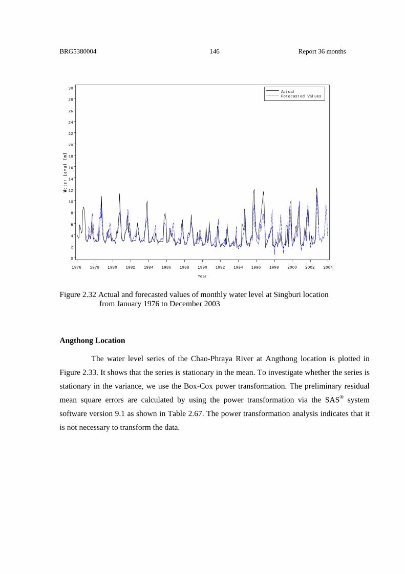
BRG5380004 Report 36 months 146
Ac t ua lFor ec as t ed Val ues
0
2
4
6
8
10
12
14
16
18
20
22
24
26
28
30
Year
1976 1978 1980 1982 1984 1986 1988 1990 1992 1994 1996 1998 2000 2002 2004
Figure 2.32 Actual and forecasted values of monthly water level at Singburi location from January 1976 to December 2003 Angthong Location
The water level series of the Chao-Phraya River at Angthong location is plotted in
Figure 2.33. It shows that the series is stationary in the mean. To investigate whether the series is
stationary in the variance, we use the Box-Cox power transformation. The preliminary residual
mean square errors are calculated by using the power transformation via the SAS® system
software version 9.1 as shown in Table 2.67. The power transformation analysis indicates that it
is not necessary to transform the data.

BRG5380004 Report 36 months 147
0
2
4
6
8
10
12
14
16
18
20
22
24
26
28
30
Year
1976 1978 1980 1982 1984 1986 1988 1990 1992 1994 1996 1998 2000 2002 2004 2006 2008
Figure 2.33 The water level of the Chao-Phraya River at Angthong location
Table 2.67 Residual mean square errors from the power transformation of water level at Angthong location
λ Residual mean square error (RMSE) -1.0 217664484.87 -0.5 2.06
0 1.49 0.5 1.37 1.0 1.32
The sample ACF shows a damped sine-cosine wave and the sample PACF cuts off after
lag 1. Thus the appropriate model is AR(1). The tentative model AR(1) is not appropriate
because for K = 24, the Q-statistic is Q = 174.48, which is significant as .17.35)23(205.0 =χ Next,
we consider the sample ACF and PACF of the first differencing. The sample ACF shows large
spikes at lag 12, 24, 36 and so on. Then we consider the differencing at period 12 months. The
sample ACF shows that it has a large spike at lag 12. To ensure that the first and twelfth
differencing are needed, we consider the sample ACF and PACF of first and twelfth
differencing. The sample ACF has a large spike only at lag 12. Hence the model needs only the
twelfth differencing. This indicates that the ARIMA (0, 1, 1) 12 model is appropriate.
To identify the nonseasonal components of the ARIMA model, the residual ACF and
PACF of ARIMA (0, 1, 1)12 are considered. The residual ACF tails off after lag 1 and the

BRG5380004 Report 36 months 148
residual PACF also cuts off after lag 1. Hence the tentative models are ARIMA (1, 0, 0)× (0, 1,
1)12, ARIMA (0, 0, 1)× (0, 1, 1)12 and ARIMA (1, 0, 1)× (0, 1, 1)12.
The parameters of all tentative models are estimated and shown in Table 2.68, where the
values in the parentheses under each estimate refer to the standard errors of those estimates. The
estimation of parameters of all models are considered at 0.05 significance level.
Table 2.68 Summary of tentative model fitted for water level at Angthong location.
Model Estimated parameters 2aσ
1. ARIMA (1, 0, 0) × (0, 1, 1) 12 (1−0.66394B)(1− B 12 ) tZ = ( 1−0.81532B 12 ) at 1.103 (0.03872) (0.03341 ) 2. ARIMA (0, 0, 1) × (0, 1, 1) 12 (1− B12 ) tZ = (1+0.60708 B)(1 – 0.75416B 12 ) at 1.223 (0.04308) (0.03828) 3. ARIMA (1, 0, 1) × (0, 1, 1) 12 (1–0.5295B)(1−B12 ) tZ =(1+0.24755B)(1–0.80922B 12 ) at 1.076 (0.06604) (0.07776) (0.03378)
To check model adequacy, we consider whether the residuals of the model are white
noise by using a Q statistic test with K = 24. The values of the Q statistic and p-values are given
in Table 2.69. The model 2 is not adequate for the water level at Angthong location because the
residuals are not white noise.
For model selection, we use two criteria, AIC and SBC, to select the best model. From
Table 2.70, we see that the minimum AIC and SBC occur for the ARIMA (1, 0, 1) × (0, 1, 1) 12
model. Hence the ARIMA (1, 0, 1) × (0, 1, 1) 12 model is used to describe the monthly water
level series at Angthong location.
Table 2.69 The Q statistic test for K = 24 of the tentative models for water level at Angthong location
Model Q statistic p-value
1. ARIMA (1, 0, 0) × (0, 1, 1) 12 27.02 0.2106
2. ARIMA (0, 0, 1) × (0, 1, 1) 12 64.73 <0.0001
3. ARIMA (1, 0, 1) × (0, 1, 1) 12 20.96 0.4613

BRG5380004 Report 36 months 149
Table 2.70 Summary of AIC and SBC values for water level at Angthong location
Model AIC (Rank) SBC (Rank) 1. ARIMA (1, 0, 0) × (0, 1, 1) 12 1029.560 (2) 1037.276 (2) 3. ARIMA (1, 0, 1) × (0, 1, 1) 12 1021.894 (1) 1033.468 (1)
Table 2.71 Forecasted values for ARIMA (1, 0, 1) × (0, 1, 1)12 of water level at Angthong location
The one year ahead forecasted values with 95 percent forecast limits of the ARIMA (1, 0,
1) × (0, 1, 1) 12 model for water level at Angthong location are shown in Table 2.70 while actual
and forecast values are shown in Figure 2.34.
Date Water Level Forecasted Values
95% Confidence Limit Error Lower Upper
Jan 2007 0.86 0.6185 -1.4147 2.6516 0.2415 Feb 2007 0.93 0.5466 -2.0281 3.1214 0.3834 Mar 2007 0.74 0.6349 -2.0723 3.3422 0.1051 Apr 2007 0.68 0.5626 -2.1806 3.3058 0.1174
May 2007 3.92 1.0234 -1.7298 3.7766 2.8966 June 2007 2.38 1.8732 -0.8828 4.6292 0.5068 July 2007 2.93 1.6393 -1.1175 4.3962 1.2907 Aug 2007 2.04 2.0241 -0.7329 4.7812 0.0159 Sep 2007 5.65 4.4117 1.6546 7.1688 1.2383 Oct 2007 6.87 5.3782 2.6210 8.1353 1.4918
Nov 2007 3.39 3.3949 0.6378 6.1520 -0.0049 Dec 2007 1.45 1.3285 -1.4286 4.0856 0.1215

BRG5380004 Report 36 months 150
Ac t ua lFor ec as t ed Va l ues
0
2
4
6
8
10
12
14
16
18
20
22
24
26
28
30
Year
1976 1978 1980 1982 1984 1986 1988 1990 1992 1994 1996 1998 2000 2002 2004 2006 2008
Figure 2.34 Actual and forecasted values for ARIMA (1, 0, 1) × (0, 1, 1)12 of monthly water level at Angthong location from January 1976 to December 2007
Periodogram Analysis Periodogram analysis of rainfall in Nakhonsawan

BRG5380004 Report 36 months 151
The periodogram is clearly dominated by a very large peak at frequency
282 (28) 0.52360
336πω = = , 56
2 (56) 1.04720336πω = = , and 84
2 (84) 1.57080336πω = = .
This frequency corresponds to a period of 28
2 12P πω
= = months, 56
2 6P πω
= = months, and
84
2 4P πω
= = months. It indicates that the data exhibit a 12-month cycle. Also included in Table
are the values of the F statistics to test the significance of the periodogram at each Fourier
frequency. For significance level 0.050.05, (2,333) 3.00Fα = = , and the periodogram is
significant only at frequency 28 0.52360ω = , 56 1.04720ω = , and 84 1.57080ω = .
Periodogram analysis of water level in Chainat

BRG5380004 Report 36 months 152
The periodogram is clearly dominated by a very large peak at frequency
12 (1) 0.01689372πω = = , 5
2 (5) 0.08445372πω = = , 6
2 (6) 0.10134372πω = = , 8
2 (8) 0.13512372πω = = ,
122 (12) 0.20268
372πω = = , 25
2 (25) 0.42226372πω = = , 26
2 (26) 0.43915372πω = = ,
312 (31) 0.52360
372πω = = , 62
2 (62) 1.04720372πω = = , and 93
2 (93) 1.57080372πω = = .
This frequency corresponds to a period of 1
2 372P πω
= = months, 5
2 74.4P πω
= = months,
6
2 62P πω
= = months, 8
2 46.5P πω
= = months, 12
2 31P πω
= = months, 25
2 14.88P πω
= = months,
26
2 14.31P πω
= = months, 31
2 12P πω
= = months, 62
2 6P πω
= = months, and 93
2 4P πω
= = months. It
indicates that the data exhibit a 12-month cycle. Also included in Table are the values of the F
statistics to test the significance of the periodogram at each Fourier frequency. For significance
level 0.050.05, (2,369) 3.00Fα = = , and the periodogram is significant only at frequency
1 0.01689ω = , 5 0.08445ω = , 6 0.10134ω = , 8 0.13512ω = , 12 0.20268ω = , 25 0.42226ω = ,
26 0.43915ω = , 31 0.52360ω = , 62 1.04720ω = , and 93 1.57080ω = .

BRG5380004 Report 36 months 153
Periodogram analysis of water level in Singburi
The periodogram is clearly dominated by a very large peak at frequency
12 (1) 0.02033309πω = = , 4
2 (14) 0.08134309πω = = , 7
2 (7) 0.14234309πω = = , 8
2 (8) 0.16267309πω = = ,
102 (10) 0.20334
309πω = = , 18
2 (18) 0.36601309πω = = , 22
2 (22) 0.44735309πω = = ,
252 (25) 0.50835
309πω = = , 26
2 (26) 0.52868309πω = = , 44
2 (44) 0.89469309πω = = ,
522 (52) 1.05737
309πω = = , and 53
2 (53) 1.07770309πω = = .
This frequency corresponds to a period of 1
2 309P πω
= = months, 4
2 77.25P πω
= = months,
7
2 44.14P πω
= = months, 8
2 38.63P πω
= = months, 10
2 30.90P πω
= = months, 18
2 17.17P πω
= =

BRG5380004 Report 36 months 154
months, 22
2 14.05P πω
= = months, 25
2 12.36P πω
= = months, 26
2 11.88P πω
= = months,
44
2 7.02P πω
= = months, 52
2 5.94P πω
= = months, and 53
2 5.83P πω
= = months.
It indicates that the data exhibit a 12-month cycle. Also included in Table are the values of the F
statistics to test the significance of the periodogram at each Fourier frequency. For significance
level 0.050.05, (2,306) 3.00Fα = = , and the periodogram is significant only at frequency
1 0.02033ω = , 4 0.08134ω = , 7 0.14234ω = , 8 0.16267ω = , 10 0.20334ω = , 18 0.36601ω = ,
22 0.44735ω = , 25 0.50835ω = , 26 0.52868ω = , 44 0.89469ω = , 52 1.05737ω = , and
53 1.07770ω = .
Periodogram analysis of rainfall in Angthong
The periodogram is clearly dominated by a very large peak at frequency
312 (31) 0.52360
372πω = = , 62
2 (62) 1.04720372πω = = , and 93
2 (93) 1.57080372πω = = .

BRG5380004 Report 36 months 155
This frequency corresponds to a period of 31
2 12P πω
= = months, 62
2 6P πω
= = months, and
93
2 4P πω
= = months. It indicates that the data exhibit a 12-month cycle. Also included in Table
are the values of the F statistics to test the significance of the periodogram at each Fourier
frequency. For significance level 0.050.05, (2,333) 3.00Fα = = , and the periodogram is
significant only at frequency 31 0.52360ω = , 62 1.04720ω = , and 93 1.57080ω = .
Periodogram analysis of rainfall in Ayutthaya
The periodogram is clearly dominated by a very large peak at frequency
312 (31) 0.52360
372πω = = , 62
2 (62) 1.04720372πω = = , and 93
2 (93) 1.57080372πω = = .
This frequency corresponds to a period of 31
2 12P πω
= = months, 62
2 6P πω
= = months, and
93
2 4P πω
= = months. It indicates that the data exhibit a 12-month cycle. Also included in Table

BRG5380004 Report 36 months 156
are the values of the F statistics to test the significance of the periodogram at each Fourier
frequency. For significance level 0.050.05, (2,369) 3.00Fα = = , and the periodogram is
significant only at frequency 31 0.52360ω = , 62 1.04720ω = , and 93 1.57080ω = .
Periodogram analysis of rainfall in Pathumthani
The periodogram is clearly dominated by a very large peak at frequency
12 (1) 0.01939324πω = = , 27
2 (27) 0.52360324πω = = , 54
2 (54) 1.04720324πω = = , and
812 (81) 1.57080
324πω = = .
This frequency corresponds to a period of 1
2 324P πω
= = months, 27
2 12P πω
= = months,
54
2 6P πω
= = months, and 81
2 4P πω
= = months. It indicates that the data exhibit a 12-month cycle.
Also included in Table are the values of the F statistics to test the significance of the
periodogram at each Fourier frequency. For significance level 0.050.05, (2,321) 3.00Fα = = , and

BRG5380004 Report 36 months 157
the periodogram is significant only at frequency 1 0.01939ω = , 27 0.52360ω = , 54 1.04720ω = ,
and 81 1.57080ω = .
Periodogram analysis of rainfall in Nonthaburi
The periodogram is clearly dominated by a very large peak at frequency
12 (1) 0.01689372πω = = , 2
2 (2) 0.03378372πω = = , 3
2 (3) 0.05067372πω = = , 31
2 (31) 0.52360372πω = = ,
622 (62) 1.04720
372πω = = , and 93
2 (93) 1.57080372πω = = .
This frequency corresponds to a period of 1
2 372P πω
= = months, 2
2 186P πω
= = months,
3
2 124P πω
= = months, 31
2 12P πω
= = months, 62
2 6P πω
= = months, and 93
2 4P πω
= = months. It
indicates that the data exhibit a 12-month cycle. Also included in Table are the values of the F
statistics to test the significance of the periodogram at each Fourier frequency. For significance
level 0.050.05, (2,369) 3.00Fα = = , and the periodogram is significant only at frequency
1 0.01689ω = , 2 0.03378ω = , 3 0.05067ω = 31 0.52360ω = , 62 1.04720ω = , and 93 1.57080ω = .

BRG5380004 Report 36 months 158
Periodogram analysis of rainfall in Bangkok
The periodogram is clearly dominated by a very large peak at frequency
312 (31) 0.52360
372πω = = , 62
2 (62) 1.04720372πω = = , and 93
2 (93) 1.57080372πω = = .
This frequency corresponds to a period of 31
2 12P πω
= = months, 62
2 6P πω
= = months, and
93
2 4P πω
= = months. It indicates that the data exhibit a 12-month cycle. Also included in Table
are the values of the F statistics to test the significance of the periodogram at each Fourier
frequency. For significance level 0.050.05, (2,369) 3.00Fα = = , and the periodogram is
significant only at frequency 31 0.52360ω = , 62 1.04720ω = , and 93 1.57080ω = .

BRG5380004 Report 36 months 159
Periodogram analysis of rainfall in Samutprakarn
The periodogram is clearly dominated by a very large peak at frequency
312 (31) 0.52360
372πω = = , 62
2 (62) 1.04720372πω = = , and 93
2 (93) 1.57080372πω = = .
This frequency corresponds to a period of 31
2 12P πω
= = months, 62
2 6P πω
= = months, and
93
2 4P πω
= = months. It indicates that the data exhibit a 12-month cycle. Also included in Table
are the values of the F statistics to test the significance of the periodogram at each Fourier
frequency. For significance level 0.050.05, (2,369) 3.00Fα = = , and the periodogram is
significant only at frequency 31 0.52360ω = , 62 1.04720ω = , and 93 1.57080ω = .

BRG5380004 Report 36 months 160
Periodogram analysis of water level in Nakhonsawan
The periodogram is clearly dominated by a very large peak at frequency
12 (1) 0.01870336πω = = , 4
2 (4) 0.07480336πω = = , 5
2 (5) 67.2336πω = = , 6
2 (6) 0.11220336πω = = ,
282 (28) 0.52360
336πω = = , 56
2 (56) 1.04720336πω = = , and 84
2 (84) 1.57080336πω = = .
This frequency corresponds to a period of 1
2 336P πω
= = months, 4
2 84P πω
= = months,
5
2 67.2P πω
= = months, 6
2 56P πω
= = months, 28
2 12P πω
= = months, 56
2 6P πω
= = months, and
84
2 4P πω
= = months. It indicates that the data exhibit a 12-month cycle. Also included in Table
are the values of the F statistics to test the significance of the periodogram at each Fourier
frequency. For significance level 0.050.05, (2,333) 3.00Fα = = , and the periodogram is
significant only at frequency 1 0.01870ω = , 4 0.07480ω = , 5 0.09350ω = , 6 0.11220ω = ,
28 0.52360ω = , 56 1.04720ω = , and 84 1.57080ω = .
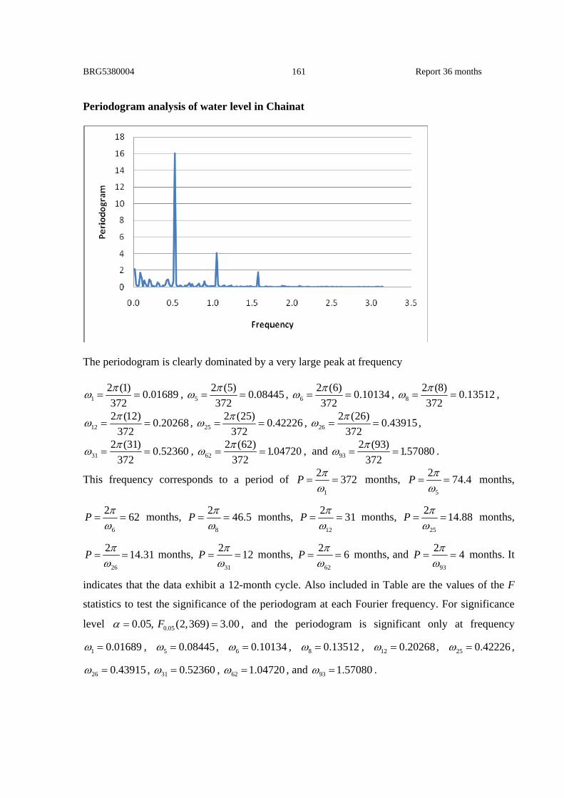
BRG5380004 Report 36 months 161
Periodogram analysis of water level in Chainat
The periodogram is clearly dominated by a very large peak at frequency
12 (1) 0.01689372πω = = , 5
2 (5) 0.08445372πω = = , 6
2 (6) 0.10134372πω = = , 8
2 (8) 0.13512372πω = = ,
122 (12) 0.20268
372πω = = , 25
2 (25) 0.42226372πω = = , 26
2 (26) 0.43915372πω = = ,
312 (31) 0.52360
372πω = = , 62
2 (62) 1.04720372πω = = , and 93
2 (93) 1.57080372πω = = .
This frequency corresponds to a period of 1
2 372P πω
= = months, 5
2 74.4P πω
= = months,
6
2 62P πω
= = months, 8
2 46.5P πω
= = months, 12
2 31P πω
= = months, 25
2 14.88P πω
= = months,
26
2 14.31P πω
= = months, 31
2 12P πω
= = months, 62
2 6P πω
= = months, and 93
2 4P πω
= = months. It
indicates that the data exhibit a 12-month cycle. Also included in Table are the values of the F
statistics to test the significance of the periodogram at each Fourier frequency. For significance
level 0.050.05, (2,369) 3.00Fα = = , and the periodogram is significant only at frequency
1 0.01689ω = , 5 0.08445ω = , 6 0.10134ω = , 8 0.13512ω = , 12 0.20268ω = , 25 0.42226ω = ,
26 0.43915ω = , 31 0.52360ω = , 62 1.04720ω = , and 93 1.57080ω = .

BRG5380004 Report 36 months 162
Periodogram analysis of water level in Singburi
The periodogram is clearly dominated by a very large peak at frequency
12 (1) 0.02033309πω = = , 4
2 (14) 0.08134309πω = = , 7
2 (7) 0.14234309πω = = , 8
2 (8) 0.16267309πω = = ,
102 (10) 0.20334
309πω = = , 18
2 (18) 0.36601309πω = = , 22
2 (22) 0.44735309πω = = ,
252 (25) 0.50835
309πω = = , 26
2 (26) 0.52868309πω = = , 44
2 (44) 0.89469309πω = = ,
522 (52) 1.05737
309πω = = , and 53
2 (53) 1.07770309πω = = .
This frequency corresponds to a period of 1
2 309P πω
= = months, 4
2 77.25P πω
= = months,
7
2 44.14P πω
= = months, 8
2 38.63P πω
= = months, 10
2 30.90P πω
= = months, 18
2 17.17P πω
= =
months, 22
2 14.05P πω
= = months, 25
2 12.36P πω
= = months, 26
2 11.88P πω
= = months,
44
2 7.02P πω
= = months, 52
2 5.94P πω
= = months, and 53
2 5.83P πω
= = months.
It indicates that the data exhibit a 12-month cycle. Also included in Table are the values of the F
statistics to test the significance of the periodogram at each Fourier frequency. For significance

BRG5380004 Report 36 months 163
level 0.050.05, (2,306) 3.00Fα = = , and the periodogram is significant only at frequency
1 0.02033ω = , 4 0.08134ω = , 7 0.14234ω = , 8 0.16267ω = , 10 0.20334ω = , 18 0.36601ω = ,
22 0.44735ω = , 25 0.50835ω = , 26 0.52868ω = , 44 0.89469ω = , 52 1.05737ω = , and
53 1.07770ω = .
Periodogram analysis of water level in Angthong
The periodogram is clearly dominated by a very large peak at frequency
12 (1) 0.01712367πω = = , 5
2 (5) 0.08560367πω = = , 6
2 (6) 0.10272367πω = = , 12
2 (12) 0.20545367πω = = ,
182 (18) 0.30817
367πω = = , 26
2 (26) 0.44513367πω = = , 28
2 (28) 0.47937367πω = = ,
292 (29) 0.49649
367πω = = , 30
2 (30) 0.51361367πω = = , 31
2 (31) 0.53073367πω = = ,
322 (32) 0.54785
367πω = = , and 92
2 (92) 1.57508367πω = = .
This frequency corresponds to a period of 1
2 367P πω
= = months, 5
2 73.40P πω
= = months,
6
2 61.17P πω
= = months, 12
2 30.58P πω
= = months, 18
2 20.39P πω
= = months, 26
2 14.12P πω
= =

BRG5380004 Report 36 months 164
months, 28
2 13.11P πω
= = months, 29
2 12.66P πω
= = months, 30
2 12.23P πω
= = months,
31
2 11.84P πω
= = months, 32
2 11.47P πω
= = months, and 92
2 3.99P πω
= = months.
It indicates that the data exhibit a 12-month cycle. Also included in Table are the values of the F
statistics to test the significance of the periodogram at each Fourier frequency. For significance
level 0.050.05, (2,364) 3.00Fα = = , and the periodogram is significant only at frequency
1 0.01712ω = , 5 0.08560ω = , 6 0.10272ω = , 12 0.20545ω = , 18 0.30817ω = , 26 0.44513ω = ,
28 0.47937ω = , 29 0.49649ω = , 30 0.51361ω = , 31 0.53073ω = , 32 0.54785ω = , and
92 1.57508ω = .
According to our results, time series forecasting models are used to forecast the monthly
rainfall and water level series of the locations along the Chao-Phraya River in Thailand.
However, there are some remarks to discuss.
Rainfall and water level data are important information for food production plans,
helping ensure the safety of all people and all activities. There are many factors which effect to
the amount of rainfall. These are the monsoon, topography and season whereas the water level
depends on the amount of rainfall, the season and the seawater level. Hence the accuracy of
prediction of rainfall and water level series is important and useful with information to decide or
plan related activities.
From the results, both of the rainfall and water level series have the same seasonal period
at 12-months which are supported by the periodogram of Fourier analysis. This indicates that
season is one of factors of rainfall and water level amounts. For some locations, rainfall and
water level are nonstationary in the variance, but can be reduced to stationary series by proper
transformation. The best models of rainfall series are divided into 4 classes while water level
series are divided into 2 classes. For rainfall series, the first class (ARIMA (1, 1, 1) × (0, 1, 1) 12 )
consists of Nakhonsawan, Singburi, Nonthaburi and Bangkok location. The second class
(ARIMA (5, 0, 0) × (0, 1, 1) 12 ) consists of Chainat alone. The third class (ARIMA (0, 1, 1) × (0,
1, 1)12 ) includes Angthong, Ayutthaya and Samutprakarn. The fourth class ((1, 0, 1) × (0, 1, 1)
12) consists of Pathumtani alone. For water level series, the first class (ARIMA (1, 0, 1) × (1, 1,
0) 12) consists of Nakhonsawan and Angthong while the second class (ARIMA (1, 0, 0) × (0, 1,

BRG5380004 Report 36 months 165
1) 12) consists of Chainat and Singburi. We see that, at the same location, the best model for
rainfall and water level is different. It means that we can not use the same model to forecast both
rainfall and water level at the same location. water level and rainfall depend on many factors
which are different; the pattern of data is also different.
References
1. Akaike H, (1973). Information theory and an extension of the minimum likelihood
principle, Proc. 2nd International Symposium on Information Theory, Akademiai Kiado,
Budapest, 267-281.
2. Akaike H, (1974). A new look at the statistic model identification, IEEE Transactions on
Automatic Control, 19, 716-723.
3. Boochabun K, Tych W, Chappell NA, Carling PA, Lorsirirat K and Pa-Obsaeng S (2004).
Statistical Modelling of Rainfall and River in Thailand. Journal Geological Society of India,
4: 503-516.
4. Box GEP and Cox DR, (1964). An analysis of transformation, Journal of the Royal
Statistical Society , 26, 211-252.
5. Box GEP, Jenkins GM, Reinsel GC.(1994). Time series analysis forecasting andcontrol. 3rd
Edition. New Jersey: Prentice-Hall, USA.
6. Box GEP and Pierce DA, (1970). Distribution of residual autocorrelations in autoregressive-
intergrated moving average time series models, J.Amer. Statist. Assoc., 65, 1509-1526.
7. Durbin J, (1960). The fitting of time series models, Review of the Institute of International
Statistics, 28, 233-244.
8. Jung JS, Kim KS and Lee JH (2000). Short-term Prediction Model of Local Rainfall. 4th
International Conference on Hydro-Science and Engineering
http://kfki.baw.de/conferences/ICHE/2000-Seoul/pdf/.../PAP_083.PDF
9. Kalman RE, (1960). A new approach to linear filtering and prediction problems, Trans. ASME
J. Basic Engrg., Ser. D, 82, 35-45.
10. Kolmogorov A, (1939). Sur Pinterpolation et l’extrapolation des suits stationnaires, C.R.
Acad. Sci. Paris, 208, 2043-2045.
11. Kolmogorov A, (1941). Interpolation und extrapolation von stationaren Zufalligen Folgen,
Bull. Acad. Sci. (Nauk), USSA, Ser. Math., 5, 3-14.

BRG5380004 Report 36 months 166
12. Lee S, Cho S and Wong M.P (1998). Rainfall Prediction using Artificial Neural Networks,
Journal of Geographic Information and Decision Analysis 2(2): 233-242.
13. Ljung GM and Box GEP. (978).On a measure of lack of fit in the time series models,
Biometrika, 65, 297-303.
14. Mebrhatu MT, Tsubo M and Walker S (2004). A Statistical Model for Seasonal Rainfall
Forecasting over the Highlands of Eritrea. 4th International Crop Science Congress.
15. Onodera S, and Sriratanatabuchanon M. (1986). Organochlorine Pesticide Residues in the
Lower Chao Phraya River and Klongs along the River at Bangkok Metropolitan Area, J.
Sci. Soc, 12, 225-238.
16. Panichkitkosolkul W. (2009). Forecasting of rainfall of Nakhonratchasima, Thammasat Int. J.
Science Technology, 17, 1-12.
17. Schwartz G, (1978). Estimating the dimension of a model, The Annals of Statistic,
6, 461-464.
18. Sen N (2003).New forecast models for Indian south-west monsoon season rainfall. Journal of
Current Science, 84(10) : 1290-1292.
19. Sosa J, Sosa C and Paz B (2000). ARIMA Models in the Rain Attenuation Prediction in a
Mexican Tropical Area. IEEE Transactions on Antennas and Propagation Society
International Symposium, 2 : 546-549.
20. Tingsanchali T (2000). Forecasting model of Chao Phraya river flood levels at Bangkok,
International Conference on Chao Phraya Delta Bangkok Thailand.
21. Weesakul U and Lowanichchai S (2005). Rainfall Forecast for Agricultural Water Allocation
Planning in Thailand. Thammasat Int. J. Science Technology, 10(3) : 18-27.
22. Wei WW, (1990). Time series analysis univariate and multivariate methods, Addison-
Wesley, USA.
23. Whittle P, (1983). Prediction and Regulation by Linear Least-Square Methods, 2nd ed.,
University of Minnesota, Minneapolis.
24. Wiener N, (1949). The Extrapolation, Interpolation and Smoothing of Stationary Time Series
with Engineering Applications, Wiley, New York, USA.
25. Yaglom AM, (1952). An Introduction to the Theory of Stationary RandomFunctions,
Pentice-Hall, Englewood Cliffs, NJ, USA.

BRG5380004 Report 36 months 167
26. Zaw W.T.and Naing T.T.(2008). Empirical Statistical Modeling of Rainfall Prediction
over Myanmar, Proceedings of World Academy of Science, Engineering and
Technology, 36, 569-572.
7.3 Nonlinear Mixed Effects Models In the field of medical science, data usually consists of repeated measurements on
individuals observed under various conditions. Repeated measurements arise in many diverse
fields and possibly are even more common than single measurements. The term ‘repeated’ will
be used here to describe measurements which are made of the same characteristic on the same
observational unit but on more than one occasion. In longitudinal studies, individuals may be
monitored over a period of time to record the developing pattern of their observed values. Over
such a period the conditions may be deliberately changed, as in crossover trials, to study the
effects on the individual. Even in the studies which are not intentionally longitudinal, once a
sample of individual units has been assembled, or identified, it is often easier and more efficient
in practice to monitor and observe them repeatedly rather than to discard each one after a single
observation and start afresh with another sample (Crowder et al., 1990). For example, in
longitudinal clinical studies, measurements are taken on each subject over time. Participants in
pharmacokinetic experiments undergo serial blood sampling following administration of a test
agent. Pharmacodynamic studies may involve repeated measurement of physiological effects in
the same subject in response to differing doses of a drug. Data from clinical trials such as
prostate-specific antigen (PSA), are clinically useful to know when PSA levels first begin to rise
rapidly and to determine if the natural history of PSA progression is different in men with locally
confined prostate cancers compared to men with metastatic tumors.
Prostate cancer is the most common cancer for male populations in many parts of the
world. It is a slowly growing deadly cancer with very few signs and symptoms in the early
stage. In the United States, an estimated 244,000 new cases and 40,400 deaths from prostate
cancer occurred in Morrell, 1995. The PSA is made by prostate cells and is released into the
bloodstream. Large prostates have more PSA, therefore a rise in PSA means that the gland is
enlarging rapidly, which can either be a sign of cancer or irritation by infection (Phyllis, 1997).

BRG5380004 Report 36 months 168
Another clinical usefulness is that a rising Carcinoembryonic Antigen (CEA) level
indicates progression or recurrence of the cancer. The CEA is a type of protein molecule that
can be found in many different cells of the body, but it is typically associated with certain tumors
and the developing fetus (Benchimol, 1989). The CEA is used as a tumor marker, especially for
cancers of the gastrointestinal tract such as colon cancer or colorectal cancer.
When the CEA level is abnormally high before surgery or other treatment, it is expected
to fall to a normal level after success in removing all of cancer. It is recommended by Bast et
al.(2001) that the data were insufficient to recommend routine use of the serum CEA alone for
monitoring response to treatment. If no other simple test is available to indicate a response, the
CEA should be measured at the start of treatment for metastatic disease and every two to three
months during active treatment. Two values above the baseline are adequate to document
progressive disease even in the absence of corroborating radiographs. The CEA is regarded as
the marker of choice for monitoring colorectal cancer. This recommendation is consistent with
Zheng et al.(2001) who found that the measurement of preoperative serum levels of CEA will
aid in predicting the prognosis of patients with colorectal cancer who have been treated
surgically. Elevated serum levels of tumor markers indicate high risk of cancer recurrence and
poor survival. Such patients should receive adjuvant therapy at the earlier stages of this disease.
After surgery, the CEA level can be periodically monitored. If the level begins to rise above 6
ng/ml, there will be a high correlation of recurrence of the cancer. However, this does not
always happen in every case as there might be other factors which can increase the CEA level,
including diverticulitis, pancreatitis, hepatitis and smoking. If these other causes are excluded,
then one must look for recurrence of cancer.
Local recurrence of colorectal cancer after ‘curative’ surgery is a major clinical problem.
Typically, 50-70 per cent of patients presented to a surgical clinic will undergo apparently
curative surgery for disease and about 10-25 per cent of those will develop local recurrence in
either the tumor bed or bowel wall (Doccherty, 1994). In 1987, Claudio et al. made a
comparative study of sixty-four consecutive patients who had undergone curative resection for
colorectal carcinoma which was conducted to evaluate the roles of sequential CEA
determinations and independent instrumental. The study was also a follow-up in the early
detection of respective recurrences. They found that CEA was the best predictor of recurrence
when compared with the other two markers (tissue polypeptide antigen (TPA), colon cancer

BRG5380004 Report 36 months 169
antigen detected with a monoclonal antibody (Ca19-9)). It is in accordance with 2000 update of
American Society of Clinical Oncology colorectal cancer surveillance guidelines by Benson et
al.(2000) that follow up testing was done by protocol guidelines. Ninety-six of the 421 patients
who developed recurrent disease underwent surgical resection with curative intent. For the
subgroup of patients with resectable, the first test to detect recurrence was CEA, chest x-ray,
colonoscopy, and other tests. The CEA was the most cost-effective approach to detect
potentially metastases from colon cancer. Another study followed up patients with a specified
testing strategy after curative colorectal surgery. Here, 64% of recurrences were detected first by
CEA, far more than the other tests in the battery (Castells, 1998).
By definition, studies of growth and decay involve repeated measurements taken on
sample units, which could be human or animal subjects, plants, or cultures. Modeling data of
this kind usually involves characterization of the relationship between the measured response, ,y
and the repeated measurement factor, or covariate, x . In many applications, the proposed
systematic relationship between y and x is nonlinear with unknown parameters of interest. The
model has two types of parameters, that is global parameters that correspond to the fixed effects
and parameters which vary among the population that correspond to the random effects.
We propose a nonlinear mixed-effects model to describe the longitudinal data in the CEA
value of colorectal cancer patients. The model will be approached to find a recurrent time of
disease after surgery. The parameters of the model will be estimated by using Lindstrom and
Bates (LB) and Stochastic Approximation version of the standard Expectation and Maximization
step (SAEM) algorithms. Therefore, the aims of this study are to propose the nonlinear mixed
effects model of colorectal cancer patients, estimate the parameters of the proposed model by
using LB and SAEM algorithms and compare the residual of the prediction model based on these
algorithms. Further, the recurrent time of colorectal cancer patients will be presented and
illustrated.
We address the LB and SAEM algorithms for estimating parameters of repeated
measurements in the nonlinear model. We consider the general nonlinear mixed effects model
for repeated data by using the notation of Linstrom and Bates (1990), and apply the nonlinear
mixed effects model to CEA values which are obtained from colorectal cancer patients. Further,
the concepts of LB and SAEM algorithms are illustrated.

BRG5380004 Report 36 months 170
Algorithms
Individual repeated measurement data often exhibit a relationship between response and
measurement factors that is best characterized by a model nonlinear in its parameters. In some
settings, an appropriate nonlinear model may be derived on the basis of theoretical
considerations. In other situations, a nonlinear relationship may be employed to provide an
empirical description of the data. Several authors have investigated the problem of parameter
estimation for the nonlinear model as the following.
In 1990, Lindstrom and Bates proposed a general, nonlinear mixed effects model for
repeated measures data and defined estimators for its parameters by a combination of least
squares estimators for nonlinear fixed effects models and maximum likelihood (or restricted
maximum likelihood, RML) estimators for linear mixed effects models. They applied Newton-
Raphson estimation using previously developed computational methods for nonlinear fixed
effects models and for linear mixed effects models.
In 1995, Morrell et al. used a nonlinear mixed effects model to describe longitudinal
changes in PSA in men before their prostate cancers were detected clinically. The model was
linear in PSA values a long time before the cancer was detected and becomes exponential after
the cancer was detected. The time when the PSA levels changed from linear to exponential PSA
progression was unknown but could be estimated by including random terms that allowed each
subject to have his own transition time. They used software developed by Lindstrom and Bates
(1990) to estimate the parameters of their model.
In 1996, Walker simulated data and obtained the following nonlinear population
pharmacodynamic model, is
21
3
i jij i ij
i j
dy
dθ
θ εθ
= − ++
,
ijy is blood pressure for the jth response on the ith individual,
jd is dose for the jth response,
1iθ is absence of treatment for the ith individual,
2iθ is maximum effect of the drug for the ith individual,
3iθ is dose which gives 50% of the maximum effect for the ith individual, and

BRG5380004 Report 36 months 171
ijε 2 (0, )N σ∼ .
The exact maximum likelihood estimates (MLEs) obtained from the expectation
maximization (EM) algorithm are compared, over ten simulated data sets, with the approximate
MLEs from a first order conditional estimation (FOCE) and Laplacian methods of nonlinear
mixed effects models. A summary of the simulations is given by the averages of the parameters
estimates (mean) and also the averages of the mean squared errors (MSE). The MSE is a suitable
criterion for judging the merit of the estimates when the variance is unsuitable as a result of the
bias in the estimates. This suggests that the extra computing time is worthwhile in order to
overcome the difficulties that the EM algorithm is more conservative than the FOCE and
Laplacian methods.
In 1999, Delyon et al. suggested that the Expectation and Maximization (EM) algorithm
was a powerful computational technique for locating maxima of functions. It is widely used in
statistics for maximum likelihood estimation in incomplete data models but the expectation step
cannot be performed in close form. To deal with these problems, a novel method, the Stochastic
Approximation version of the standard Expectation and Maximization step (SAEM), is
introduced in order to replace the expectation step of the EM algorithm by one iteration of a
stochastic approximation procedure.
In 2003, Fieuws et al. suggested that a series of marker measurements turns out to be a
better screening tool than a single measurement. Classical discriminated analysis can be applied
whenever the data have a balance structure. Extensions have been proposed for unbalancedata
by using linear mixed effects models or linearized versions of nonlinear models to describe the
longitudinal profiles in each group.
In 2004, Liang and Sha investigated patterns of tumor response in mouse xenograft
tumors. They applied a biexponential nonlinear mixed-effects model to an analysis of changes in
tumor volume over a given period of treatment. The model gave a good fit to the data, even for
small sample sizes.
In 2005, Kuhn and Lavielle developed an algorithm for parameter estimation of nonlinear
mixed effects models which combined the SAEM algorithm and a Markov Chain Monte Carlo
procedure. They showed good statistical convergence properties of this algorithm. Further, they
showed that the SAEM algorithm was very efficient for computing the maximum likelihood

BRG5380004 Report 36 months 172
estimates of parameters. The SAEM algorithm can be used for estimation homoscedastic
models, but also heteroscedastic models. The main advantage of this algorithm was its ability to
provide an estimator closed to the MLE in very few iterations. They reproduced the values from
Walker (1996) and compared different popular methods of estimation, such as the FOCE and
Laplacian methods, with the standard errors obtained by the SAEM algorithm in the
pharmacodynamic model. They clearly saw that the EM algorithm of Walker and the SAEM
algorithm showed similar results where the later had the smallest values not only of the MSE's
but also of the variance-covariance matrix.
Theoretical Background
A nonlinear mixed effects framework is widely used in modeling repeated measurement
data, where measures are obtained for a number of individuals under varying experimental
conditions. Nonlinear mixed effects models incorporate the population (fixed), with parameters
associated with an entire population or with certain repeatable levels of experimental factors as
well as individual specifics (random), which are associated with individual experimental units
drawn at random from population characteristics. This enables us to make an interest for both
random and fixed effects. Mixed effects models for repeated measures data have become
popular in part because their flexible variance covariance structure allows for non constant
correlation among the observation and/or unbalanced data (designs that vary among individuals).
Mixed effects models are also intuitively appealing. The notation that individuals’ responses all
follow a similar functional form with parameters that vary among individuals seems to be
appropriate in many situations. Within the framework, much of the interest is focused on
representing the mean function describing the dynamic relationship between the response and
explanatory variables such as time.
Let us consider the following general nonlinear mixed effects model by using the
notation of Linstrom and Bates (1990), the model for the jth observation on the i th individual in
the study is written as
( , )ij ij i ijy f x eφ= + ,
where ijy is the jth response on the i th individual, i = 1,…, m ,
ijx is the vector of predictor variables for the jth response on the
individual i ,

BRG5380004 Report 36 months 173
f is a nonlinear function of the predictor variables and parameter vector,
iφ is a 1r × vector of parameters for the i th individual, and
ije 2 (0, )iN Iσ∼ .
The nonlinear function is at least one of the derivatives of the expectation function with
respect to the parameters and depends on at least one of the parameters (Bates, et al., 1998).
Random-effects terms may be included in the parameter vector to allow the parameter value to
vary from individual to individual by writing
,i i i iA B bφφ = +
(0, ) ,ib N D∼
where φ is a 1p× vector of fixed population parameters,
ib is a 1q× vector of random effects associated with individual i,
iA is a design matrix of size r p× for the fixed effects,
iB is a design matrix of size r q× for the random effects, and
D is a positive definite variance covariance matrix.
This is a general form of the nonlinear mixed effects model since any nonlinear function
of fixed and random effects can be written as i( b , )i i ijf A B xφ + . From the statistical model the
intra-individual variation is written as
( , )ij ij i ijy f x eφ= + ,
2(0, ) ,ij ie N Iσ∼
0 1 2( , ) exp( )exp( ( ))ij i i i ij if x xφ φ φ φ= − ,
where ije is a random error term reflecting uncertainty in the response, given the i th individual,
with E( ij ie φ ) = 0. Collecting the responses and errors for the i th individual into the 1in × . This
is accomplished by letting

BRG5380004 Report 36 months 174
1
.
.y
.
i
i
i
in
y
y
⎡ ⎤⎢ ⎥⎢ ⎥⎢ ⎥=⎢ ⎥⎢ ⎥⎢ ⎥⎣ ⎦
,
1
i
.
.e
.
i
i
in
e
e
⎡ ⎤⎢ ⎥⎢ ⎥⎢ ⎥=⎢ ⎥⎢ ⎥⎢ ⎥⎣ ⎦
, and
( , )..f ( ).
( , )i
ij i
i i
in i
f x
f x
φ
φ
φ
⎡ ⎤⎢ ⎥⎢ ⎥⎢ ⎥=⎢ ⎥⎢ ⎥⎢ ⎥⎣ ⎦
,
so that
y f ( ) e ,i i i iφ= +
where 2e (0, )i iN Iσ∼ and iI is an identity matrix for individual i . We may summarize the data
for the i th individual as
( )2y b f ( ),i i iN Iσφ∼ ,
y f ( ) ei i i iφ= + ,
b ,i i i iA Bφφ = + b (0, ) .i N D∼
Let iφ be a 1r× vector of regression parameters specific to the i th individual. Let ia be
an 1a× covariate vector corresponding to individual attributes for individual i , let bi be a 1k ×
vector of random effects associated with the i th individual, and let φ be a 1p× vector of fixed
parameters, or fixed effects. Then a general model for iφ is given by
( , , b )i i id aφ φ= ,
where d is a p − dimensional vector-valued function. Each element of d is associated with the
corresponding element of iφ , so that the functional relationship may be of a different form for
each element. In a model of the form of the above equation, a complete characterization of inter-
individual variation requires an assumption about the distribution of the random effects bi . In
this study, we assume that bi has mean 0 and variance covariance matrix D .
With the nonlinear mixed effects model there are many methods to estimate the unknown
parameter vector. One method is the algorithm proposed by Lindstrom and Bates (LB)(1990) to
estimate the parameters of their model. This algorithm is used by Lewis and Stuart (1980) in a
similar approximation but evaluated at the expectation of the random effects rather than at the

BRG5380004 Report 36 months 175
current estimates ( b 0= ) by Taylor series expansion for the function ( , , )i if b xθ which is given
by
b 0
( , b 0, )( , b , ) ( , b 0, ) (b 0) ,b
i
i ii i i i i i
i
f xf x f x eθθ θ=
∂ =≈ = + − +
∂
b 0, (b ) 0 , i iE= =
2(0, ),ie N σ∼
so that the expected values of ( , b , )i if xθ are given as
( )b 0
( , b 0, )( ( , b , )) ( , b 0, ) (b 0) ( )b
i
i ii i i i i i
i
f xE f x E f x E E eθθ θ=
⎛ ⎞∂ =⎜ ⎟= = + − +⎜ ⎟∂⎝ ⎠
b 0
( ) = ( , b 0, ) (b 0)b
i
ii i i
i
f xf x Eθ=
∂= + −
∂
= ( , b 0, ), i if xθ =
and the variance of ( , b , )i if xθ is
b 0 b 0
( , b , ) ( , b , )( ( , b , )) (b ) ( )b b
i i
T
i i i ii i i i
i i
f x f xVar f x Var Var eθ θθ= =
∂ ∂= +
∂ ∂.
Hence, the response variables are distributed as
b 0 b 0
( , b 0, ) ( , b 0, )( , b 0, ), (b ) ( )b b
i i
T
i i i ii i i i i
i i
f x f xy N f x Var Var eθ θθ= =
⎛ ⎞∂ = ∂ =⎜ ⎟= +⎜ ⎟∂ ∂⎝ ⎠
∼
The probability density function of iy is given as
11/ 2
1 1( ) exp ( ( , 0, )) ( ) ( ( , 0, )) ,22
Ti i i i i i i i ip y y f b x V y f b x
Vθ θ
π−⎛ ⎞= − − = − =⎜ ⎟
⎝ ⎠
where b 0 b 0
( , b 0, ) ( , b 0, )(b ) ( )b b
i i
T
i i i ii i
i i
f x f xV Var Var eθ θ
= =
∂ = ∂ == +
∂ ∂.
The likelihood function of iy , is written as

BRG5380004 Report 36 months 176
/ 2/ 21
( , 0)
1 1 1 exp ( ( , 0, )) ( ) ( ( , 0, )) ,2 2
i
mmT
i i i i i i i i
L p y b
y f b x V y f b xV
θ θπ
−
= =
⎛ ⎞⎛ ⎞ ⎛ ⎞= − − = − =⎜ ⎟⎜ ⎟ ⎜ ⎟⎜ ⎟⎝ ⎠ ⎝ ⎠⎝ ⎠
∏
∑
and the log-likelihood function of iy is given as
11log log(2 ) log ( ( , 0, )) ( ) ( ( , 0, )). 2 2 2
Ti i i i i i
m mL V y f b x V y f b xπ θ θ−= − − − − = − =∑
Now the objective function is given by
( ) ( )( )1
1log ( , 0, ) ( ) ( , 0, ) .
mT
i i i i i ii
V y f b x V y f b xθ θ−
=
+ − = − =∑
Lindstrom and Bates (1990) used a combination of least squares estimators for the
nonlinear fixed-effects model and maximum likelihood (ML) estimators for a linear mixed-
effects model. The linear mixed-effects model is used to estimate parameters from an
approximation to the marginal distribution of the complete data vector, .y This combination
provides for approximate maximum likelihood estimates for the nonlinear mixed-effects model.
An orthogonality convergence criterion is used to determine convergence.
Another method is the Stochastic Approximation version of the standard Expectation and
Maximization step (SAEM) algorithm developed by Kuhn and Lavielle (2005). They developed
an estimation method which combines the SAEM algorithm with the Markov Chain Monte Carlo
(MCMC) procedure for maximum likelihood estimation in nonlinear mixed effects models
without linearization. This method is implemented in the MATLAB software, namely
MONOLIX which is available at http://software.monolix.org. The details of using this software
can be found either from this webpage or the online manual. One of the objectives of this
software is to perform parameter estimation for nonlinear mixed effects models by the following
steps.
1. Computing the maximum likelihood estimator of the population parameters without any
approximation of the model (linearization, quadrature approximation, etc) using the Stochastic
Approximation version of the standard Expectation Maximization (SAEM) algorithm,
2. Computing the standard error for the maximum likelihood estimator,

BRG5380004 Report 36 months 177
3. Computing the conditional modes, the conditional means and the conditional standard
deviations of the individual parameters, using the Hastings-Metropolis algorithm.
In this study we modify MONOLIX to analyse the CEA level of the colorectal cancer
patients. Standard errors derived from the Fisher information matrix and confidence intervals
based on normality of the estimators are obtained.
Methodology
This section presents the concept of a nonlinear model which is used for this topic. The
basic knowledge as well as Lindstrom and Bates (LB) and Stochastic Approximation version of
the standard Expectation and Maximization step (SAEM) algorithms used for parameters
estimation are also presented.
The nonlinear model
Nonlinear models are often mechanistic, that is based on a model for the mechanism
producing the response. As a consequence, the model parameters in a nonlinear model generally
have a natural physical interpretation. Even when derived empirically, nonlinear models usually
incorporate known, theoretical characteristics of the data such as asymptotes and monotonic, and
in these cases, can be considered as semi-mechanistic models. A nonlinear model such as a
polynomial, generally uses fewer parameters than a competitor linear model, giving a more
parsimonious description of the data. Nonlinear models also provide more reliable predictions
for the response variable outside the observed range of the data than polynomial models would
(Davidian, and Giltinan, 1995). From the statistical model the intra-individual variation is
( , )ij ij i ijy f x eφ= + ,
2(0, ) .iij ne N Iσ∼
We consider each of the elements of iφ , assuming there is no systematic dependence on
individual attributes for applying with carcinoembryonic antigen (CEA) data. Let us call the
nonlinear model a CEA model which is written as
0 1 2( , ) exp( )exp( ( ))ij i i i ij if x xφ φ φφ = − .
Since, i i i iA B bφ φ= + then 0 0 0i ibφ φ= + , 1 1 1i ibφ φ= + , and 2 2 2i ibφ φ= + .
Therefore we can rewrite the CEA model as follows

BRG5380004 Report 36 months 178
( )( )0 0 1 1 2 2( , ) exp( )exp ( ) ( )ij i i i ij if x b b x bφ φ φφ = + + − +
( )( )0 0 1 1 2 2exp( )exp( )exp ( ) ( )i i ij ib b x bφ φ φ= + − + .
Here, [ ]0 1 2bi i i ib b b ′= has mean zero and variance covariance matrix D .
Let iφ be a 1r× vector of regression parameters specific to the i th individual,
ia be an 1a× covariate vector corresponding to individual attributes for individual i ,
bi be a 1k × vector of random effects associated with the i th individual,
and φ be a 1p× vector of fixed parameters, or fixed effects.
Then a general model for iφ is given by ( , , b )i i id aφ φ= , where d is a p − dimensional
vector-valued function. Each element of d is associated with the corresponding element of iφ ,
so that the functional relationship may be of a different form for each element. For our model
may be expressed by defining the elements of d to be
0 ( , , b )i id a φ = 0 0ibφ + , 1( , , b )i id a φ = 1 1ibφ + , and 2 ( , , b )i id a φ = 2 2ibφ + .
Let us transform the CEA level to a natural logarithm CEA level to fit the CEA model.
We explain the parameters of CEA model as follows.
The 0φ is the log(CEA) level at the exponential phase, 1φ represents the exponential rate
constant during the exponential phase, and 2φ represents the time point (months after surgery
date) between the flat and rapid increase in the exponential phase which we assume is the time
when the recurrent disease is developed.
Starting values of parameters must be specified from the beginning. As in standard
nonlinear estimation, poor starting values can lead to poor results. Recommendations of
Davidian and Giltinan (1995) for selecting starting values, are required for all parameters at
STEP 1 of the initial iterate in the LB algorithm. As the procedures already have been discussed,
they suggested use of the OLS estimator as the initial values.
The Ordinary Least Squares (OLS) method
The ordinary least squares (OLS) estimator (Davidian, and Giltinan, 1995) for ˆ, OLSβ β ,
minimizes

BRG5380004 Report 36 months 179
2
1 ( , ) ;
n
j jj
y f x β=
−∑
equivalently, ˆOLSβ are solved by the p estimating equations
1 ( , ) ( , ) 0,
n
j j jj
y f x f xββ β=
− =∑
where ( , )jf xβ β is the 1p× vector of derivatives of f with respect to the elements of β , that is
the vector with thk element / ( , ), 1,..., .k jf x k pβ β∂ ∂ =
The nonlinear mixed effects framework is widely used in modeling repeated
measurement data, where measures are obtain for a number of individuals under varying
experimental conditions. Within the framework of the nonlinear mixed effects model, most of
the interest is focused on representing the mean function describing the dynamic relationship
between the response and explanatory variables. There are many methods to estimate the
unknown parameter vector. One method is the algorithm proposed by Lindstrom and Bates
(LB)(1990) to estimate the parameters of their model. Another method is the Stochastic
Approximation version of the standard Expectation and Maximization step (SAEM) algorithm
developed by Kuhn and Lavielle (2005). These two algorithms are illustrated as follows.
The Lindstrom and Bates (LB) algorithm
Lindstrom and Bates (1990) used Taylor Series to expand the function ( )f x which is
given by
0
0 0( )( ) ( ) ( )
x x
f xf x f x x xx
ε=
∂≈ + − +
∂,
with 0 ( )x E x= , so that the expected value of ( )f x is
0
0 0( )( ( )) ( ( )) ( ) ( )
x x
f xE f x E f x E x x Ex
ε=
⎛ ⎞∂= + − +⎜ ⎟⎜ ⎟∂⎝ ⎠
0
0 0( ) = ( ) ( )
x x
f xf x E x xx =
∂+ −
∂
0 = ( ) ,f x
and the variance of ( )f x is

BRG5380004 Report 36 months 180
0
0 0( )( ( )) ( ( )) ( ) ( )
x x
f xVar f x Var f x Var x x Varx
ε=
⎛ ⎞∂= + − +⎜ ⎟⎜ ⎟∂⎝ ⎠
0 0
0( ) ( ) = 0+ ( )
T
x x x x
f x f xVar x xx x= =
∂ ∂−
∂ ∂
0 0
( ) ( ) = ( ) .T
x x x x
f x f xVar xx x= =
∂ ∂∂ ∂
Hence, the response variables are distributed as a normal distribution with
0 0
0( ) ( )( ), ( ) .
T
ix x x x
f x f xy N f x Var xx x= =
⎛ ⎞∂ ∂⎜ ⎟⎜ ⎟∂ ∂⎝ ⎠
∼ (3.1)
The function ( , , )if b xθ is given by
0
( , 0, )( , , ) ( , 0, ) ( 0) ; 0, ( ) 0 ;i
ii i i i i
i b
f b xf b x f b x b b E bb
θθ θ ε=
∂ =≈ = + − + = =
∂
2 (0, ),Nε σ∼
so that the expected value of ( , , )if b xθ is
( )0
( , 0, )( ( , , )) ( , 0, ) ( 0) ( )i
ii i i
i b
f b xE f b x E f b x E b Eb
θθ θ ε=
⎛ ⎞∂ =⎜ ⎟= = + − +⎜ ⎟∂⎝ ⎠
0
( ) = ( , 0, ) ( 0)i
i ii b
f xf b x E bb
θ=
∂= + −
∂
= ( , 0, ), if b xθ =
and the variance of ( , , )if b xθ is
0 0
( , , )( ( , , )) ( ) ( )i i
T
ii i
i ib b
f b xfVar f b x Var b Varb b
θθ ε= =
∂∂= +
∂ ∂.
Hence, the response variables ijy , are distributed as a normal distribution; that is
0 0
( , 0, ) ( , 0, )( , 0, ) , ( ) ( )i i
T
i iij i i
i ib b
f b x f b xy N f b x Var b Varb b
θ θθ ε= =
⎛ ⎞∂ = ∂ =⎜ ⎟= +⎜ ⎟∂ ∂⎝ ⎠
∼
(3.2)

BRG5380004 Report 36 months 181
Lindstrom and Bates (1990) showed that φ is a maximum likelihood estimate relative to an
approximate marginal distribution of y . As in the linear case these estimates can be calculated
as the solution to a (nonlinear) least squares problem formed by augmenting the data vector with
“pseudo-data” as
y (x , , b ) e ,i i i i i if φ= +
where 2e (0, )i iN Iσ∼ . The probability density function of yi is given by
( ) ( )2 11/ 22
1 1(y ) .exp y (x , , b ) ( ) y (x , , b ) .22
Ti i i i i i i i i i i i
i
p f I fI
φ σ φπ σ
−⎛ ⎞= − − −⎜ ⎟⎝ ⎠
Since bi has a normal distribution with mean zero and variance covariance matrix D that is
b (0, )i N D∼ the probability density function of bi is
11/ 2
1 1(b ) .exp b b22
Ti i ip D
Dπ−⎛ ⎞= −⎜ ⎟
⎝ ⎠.
Thus the joint probability density function of the response yi and bi is written as
2 11/ 22
1 1(y , b ) .exp (y (x , , b )) ( ) (y (x , , b ))22
Ti i i i i i i i i i i i i
i
p f I fI
φ σ φπ σ
−⎛ ⎞= − − −⎜ ⎟⎝ ⎠
11/ 2
1 1 exp b ( ) b ,22
Ti iD
Dπ−⎛ ⎞−⎜ ⎟
⎝ ⎠
the likelihood function of the response yi , is given by
(y, b)
L p=∏
( ) ( )/ 2
/ 22 1
2
1 1 1 exp y (x , , b ) ( ) y (x , , b )2 2
mm
Ti i i i i i i i i i i
i
f I fI
φ σ φπ σ
−⎛ ⎞⎛ ⎞ ⎛ ⎞⎜ ⎟= − − −⎜ ⎟ ⎜ ⎟⎜ ⎟⎝ ⎠ ⎝ ⎠⎝ ⎠
∑
/ 2/ 2
11 1 1 ˆ exp b b .2 2
−⎛ ⎞⎛ ⎞ ⎛ ⎞−⎜ ⎟⎜ ⎟ ⎜ ⎟⎜ ⎟⎝ ⎠ ⎝ ⎠⎝ ⎠∑
mmTi iD
Dπ (3.3)
Then the log-likelihood function of the response yi is written as
( ) ( )2 2 11log log(2 ) log y (x , , b ) ( ) y (x , , b )2 2 2
Ti i i i i i i i i i i i
m mL I f I fπ σ φ σ φ−= − − − − −∑

BRG5380004 Report 36 months 182
11 ˆ log(2 ) log b b . 2 2 2
Ti i
m m D Dπ −− − − ∑
For known ω , that is ω , we get 2σ and D . The values of φ and bi that jointly minimize
( ) ( )( )1 2 2 1
1
ˆ ˆ ˆ ˆlog b b log y (x , , b ) ( ) y (x , , b )m
TTi i i i i i i i i i i i i i
iD D I f I fσ φ σ φ− −
=
+ + + − −∑
(STEP1)
are twice the negative log of the posterior density of bi for fixed φ and twice the negative log-
likelihood for φ for fixed bi . Thus an obvious strategy for estimation of bi is to minimize and
evaluate at suitable estimates of 2σ and D ( Davidian and Giltinan, 1995).
Lindstrom and Bates (1990) defined maximum likelihood estimators for φ with respect to the
marginal density function of y, that is
(y) (y | b) (b) b,p p p d= ∫ (3.4)
however, the expectation function f ( )i iφ is nonlinear in b, and there is no closed-form expression
for this density function and the calculation of such estimates would be very difficult. Instead,
they approximated the conditional distribution of y for b near b by a multivariate normal with
expectation that is linear in b. To accomplish this they approximated the residual y ( )f φ− near
b as Taylor series expansion about ˆb bi i= of ( , , b )i i if d a φ so that
yi = ˆ ˆ ˆˆ ( , , b ) ( , , b ) ( , b ).(b b ) ei i i i i i i i i i if d a f d a Zφ φ φ≈ + − + , (3.5)
b (0, )i N D∼ , 2e (0, ),i iN Iσ∼
where ˆˆ( , b )i iZ φ is the in k× matrix of derivatives of ( , , b )i i if d a φ with respect to bi evaluated
at ˆˆ( , , b )i i id a φφ = and ˆb bi i= . The expectation of yi is given as
( )( )ˆ ˆ ˆˆ(y ) ( , , b ) ( , b ) b b ei i i i i i i i iE E f d a Z Eφ φ= + − +
( ) ( )ˆ ˆ ˆˆ ( , , b ) ( , b ) b b (e )i i i i i i i iE f d a Z E Eφ φ= + − +
ˆ ˆ ˆˆ ( , , b ) ( , b )bi i i i i if d a Zφ φ= − ,
and the variance of yi is given by

BRG5380004 Report 36 months 183
( )( )ˆ ˆ ˆˆ(y ) ( , , b ) ( , b ) b b ei i i i i i i i iVar Var f d a Z Eφ φ= + − +
( ) ( )ˆ ˆ ˆ ˆˆ ˆ ( , , b ) ( , b ) b b ( , b ) (e )Ti i i i i i i i i iVar f d a Z Var Z Varφ φ φ= + − +
2ˆ ˆˆ ˆ ( , b ) (b ) ( , b )Ti i i i i iZ Var Z Iφ φ σ= +
2ˆ ˆˆ ˆ ( , b ) ( , b ) .Ti i i i iZ DZ Iφ φ σ= +
Then, the response variables, yi are distributed as a normal distribution with
( )2ˆ ˆ ˆ ˆ ˆˆ ˆ ˆy ( , , b ) ( , b )b , ( , b ) ( , b )Ti i i i i i i i i i i iN f d a Z Z DZ Iφ φ φ φ σ− +∼ .
Therefore, the marginal distribution of yi is written as
( )
( ) )
11/ 2
1 1 ˆ ˆ ˆˆ(y ) exp y ( , , b ) ( , b )b22
ˆ ˆ ˆˆ y ( , , b ) ( , b )b ,
T
i i i i i i i i ii
i i i i i i i
p f d a Z VV
f d a Z
φ φπ
φ φ
−⎛= − − +⎜⎝
− +
where 2ˆ ˆˆ ˆ( , b ) ( , b )Ti i i i i iV Z DZ Iφ φ σ= + .
The likelihood function of yi , is written as
( )/ 2/ 21 1 1 ˆ ˆ ˆˆ(y ) exp y ( , , b ) ( , b )b
2 2
mmT
i i i i i i i ii
L p f d a ZV
φ φπ
⎛ ⎞⎛ ⎞ ⎛= = − − +⎜ ⎟⎜ ⎟ ⎜⎜ ⎟⎝ ⎠ ⎝⎝ ⎠∑∏
( ) )1 ˆ ˆ ˆˆ y ( , , b ) ( , b )b .i i i i i i i iiV f d a Zφ φ− − +
The log-likelihood function of yi is obtained by
( )1 ˆ ˆ ˆˆlog log(2 ) log( ) y ( , , b ) ( , b )b2 2 2
T
i i i i i i i im mL V f d a Zπ φ φ= − − − − +∑
( ) )1 ˆ ˆ ˆˆ y ( , , b ) ( , b )b .i i i i i i i iiV f d a Zφ φ− − +
Hence, the twice negative log-likelihood function is given as
( ) ( )1ˆ ˆ ˆ ˆ ˆ ˆˆ ˆlog y ( , , b ) ( ,b )b y ( , , b ) ( , b )b .T
i i i i i i i i i i i i i i i iV f d a Z V f d a Zφ φ φ φ−⎛ ⎞+ − + − +⎜ ⎟⎝ ⎠∑
(STEP 2)
We can rewrite the LB process which consists of the following two-step estimation scheme as
follows.

BRG5380004 Report 36 months 184
STEP 1. Given the current estimate of ˆ, ω ω (and thus 2σ and D ), minimize in φ and bi ,
1,...,i m= . The twice negative log-likelihood is given as
( )( 1 2
1
ˆ ˆ ˆ2 log log b b log y (x , , b ) m
TTi i i i i i i i
i
L D D I fσ φ−
=
− = + + + −∑
( ))2 1ˆ ( ) y (x , , b ) ,i i i i i iI fσ φ− −
where D is variance covariance of random effects,
bi is random effects,
yi is observations, and
(x , , b )i i i if φ is the nonlinear fixed effects model.
Denote the resulting estimates of bi and 0φ as bi and 0φ .
STEP 2. Estimate φ and ω as the values φ and ω that give twice the negative approximate
marginal normal log-likelihood function is obtained as
( )( ))
1ˆ ˆ ˆˆ2 log log y ( , , b ) ( , b )b
ˆ ˆ ˆˆ y ( , , b ) ( , b )b ,
T
i i i i i i i i i
i i i i i i i
L V f d a Z V
f d a Z
φ φ
φ φ
−⎛− = + − +⎜⎝
− +
∑
where 2ˆ ˆˆ ˆ( , b ) ( , b )Ti i i i i iV Z DZ Iφ φ σ= + .
Iterate this process to a convergence, denoting the final estimates as ˆ ˆ, LB LBφ ω and ,bi LB .
Lindstrom and Bates (1990) called STEP 1 the ‘pseudo-data’ step, because joint estimation of φ
and bi by minimization of STEP 1 may be accomplished simultaneously by specifying and
augmenting the nonlinear least square problem, analogous to the linear case. The STEP 2 of the
algorithm is referred to as the ‘linear mixed effects’ step for the following reason. A further
approximation allows the minimization in STEP 2 to be expressed as a linear estimation
problem. Specifically, they approximate ˆ ( , , b )i i if d a φ by a linear function of φ by expansion
about the current estimate 0φ from STEP 1. They obtain
( )0 0 0 0ˆ ˆ ˆ ˆ ˆˆ ˆ ˆ ˆy ( , , b ) ( , b )b y ( , , b ) ( , b )( )i i i i i i i i i i i i if d a Z f d a Xφ φ φ φ φ φ− + ≈ − + −
0ˆ ˆˆ ( , b )bi i iZ φ+

BRG5380004 Report 36 months 185
*0
ˆˆ y ( , b )i i iX φ φ= − ,
where *0 0 0 0
ˆ ˆ ˆ ˆˆ ˆ ˆ ˆy y ( , , b ) ( , b ) ( , b )bi i i i i i i i i if d a X Zφ φ φ φ= − + + .
Substituting *0
ˆˆy ( , b )i i iX φ φ− for ˆ ˆ ˆˆy ( , , b ) ( , b )bi i i i i i if d a Zφ φ− + in STEP 2 yields a problem
similar in the form of the linear case.
Lindstrom and Bates (1990) implemented Newton-Raphson estimation by using
previously developed computational methods for nonlinear fixed effects and linear mixed effects
models in the LB algorithm.
A Newton-Raphson method
Lindstrom and Bates (1988) developed an efficient and effective implementation of the
Newton-Raphson algorithm for estimating the parameters in mixed effects models for repeated
data measurement. The maximum likelihood (ML) estimators for σ and θ are obtained by
maximizing the log-likelihood corresponding to the marginal density of
( )2ˆ ˆ ˆ ˆ ˆˆ ˆ ˆy ( , , b ) ( , b )b , ( , b ) ( , b )Ti i i i i i i i i i i iN f d a Z Z DZ Iφ φ φ φ σ− +∼ .
This log-likelihood, Fl is given as
2 2 1
1 1
1 1( , , | y) log ( ) ( )2 2
m mT
F i i i ii i
l V r V rφ σ θ σ θ σ θ−
= =
= − −∑ ∑ ,
where 2ˆ ˆ ˆ ˆ ˆˆ ˆ ˆ ( , , b ) ( , b )b , ( ) ( , b ) ( , b )Ti i i i i i i i i i i ir f d a Z V Z DZ Iφ φ θ φ φ σ= − = + .
They solved for the ML estimate of 2σ as a function of φ andθ .
That is 2 1
1 1
1ˆ ( ) , m m
Ti i i i
i ir V r N n
Nσ θ−
= =
= =∑ ∑ .
They obtain the profile log-likelihood, Fp of φ and θ by substituting 2σ into Fl . The profile
log-likelihood is 1
1 1
1( , | y) log ( ) log ( )2 2
m mT
F i i i ii i
Np V r V rφ θ θ θ−
= =
⎡ ⎤= − − ⎢ ⎥
⎣ ⎦∑ ∑ .
The derivatives of the profile log-likelihood for the Newton-Raphson algorithm can be calculated
as follows;
1 1
ˆˆ2 ( , b ) , ,T T
T T Ti i i i i ii i i i i ij i
i
r V r r V rZ V r r A rφφ θ
− −∂ ∂= − = −
∂ ∂

BRG5380004 Report 36 months 186
2 11logˆˆ( , b )( ) , ,
TiT Ti i i i
i i ij ij i ij j j
Vr V r VZ A A r tr Vφθ φ θ θ
−−
⎡ ⎤∂∂ ∂= + = ⎢ ⎥
∂ ∂ ∂ ∂⎢ ⎥⎣ ⎦
where 2
1 1 1 1 1 1, .iji i i i i iij i i i i i i
j k k j k j j k
AV V V V V VA V V V V V Vθ θ θ θ θ θ θ θ
− − − − − −⎛ ⎞∂∂ ∂ ∂ ∂ ∂ ∂
= = − − +⎜ ⎟⎜ ⎟∂ ∂ ∂ ∂ ∂ ∂ ∂ ∂⎝ ⎠
In the mixed effects model each individual’s vector of responses is modeled as a
parametric function, where some of the parameters of ‘effects’ are random variables with a
multivariate normal distribution.
The Stochastic Approximation version of the standard Expectation and Maximization step
(SAEM) algorithm
The Stochastic Approximation version of the standard Expectation and Maximization step
(SAEM) algorithm which is proposed by Kuhn and Lavielle (2005) is an another algorithm to
estimate parameters of nonlinear mixed effects models. The general form of the model can be
written as
2 ( , ) ( , ) ; (0, ),ij ij i ij i ij ijy f x g x e e Nφ φ σ= + ∼ (3.6)
i ibφ φ= + (3.7)
where ijy is the jth response on the i th individual, i = 1,…,m,
ijx is the vector of predictor variables for the jth response on the
individual i ,
( , )ij if x φ and ( , )ij ig x φ are nonlinear functions of the predictor variables,
iφ is unknown random vector of dimension 1r × for the i th individual, and
ije are independent 2(0, )N σ random error terms.
The expected value of ijy is given by
( )( ) ( , ) ( , )ij ij i ij i ijE y E f x g x eφ φ= +
( ( , )) ( ( , ) )ij i ij i ijE f x E g x eφ φ= +
( , ) ( , ) ( )ij i ij i ijf x g x E eφ φ= +
( , ),ij if x φ=

BRG5380004 Report 36 months 187
and the variance of ijy is given as
( )( ) ( , ) ( , )ij ij i ij i ijVar y Var f x g x eφ φ= +
( ) ( ) ( , ) ( , )ij i ij i ijVar f x Var g x eφ φ= +
2 0 ( , ) ( )ij i ijg x Var eφ= +
2 2 = 0 ( , ) ij ig x φ σ+
2 2 = ( , ) .ij ig x φ σ
Hence, the probability density function of the model (3.6) is written as
2
1/ 2 22 2
( , )1 1( ) exp .2 ( , )2 ( , )
ij ij iij
ij iij i
y f xf y
g xg x
φσ φπσ φ
⎛ ⎞⎛ ⎞−⎜ ⎟= − ⎜ ⎟⎜ ⎟⎜ ⎟⎝ ⎠⎝ ⎠
The expected value of iφ from (3.7) is given by
( )( ) i iE E bφ φ= +
( ) ( )iE E bφ= −
,φ=
and the variance of iφ is given as
( )( )i iVar Var bφ φ= +
( ) ( ) iVar Var bφ= +
.D=
Hence, the probability density function of the model (3.7) is written as
( ) ( )11 1( ) exp22
Ti i if D
Dφ φ φ φ φ
π−⎛ ⎞= − − −⎜ ⎟
⎝ ⎠.
The complete probability density function of the model which is defined by equations (3.6) and
(3.7) can be written as
2
1/ 2 22 2
( , )1 1( , ) = .exp2 ( , )2 ( , )
ij ij iij
ij iij i
y f xf y
g xg x
φφ
σ φπσ φ
⎛ ⎞⎛ ⎞−⎜ ⎟− ⎜ ⎟⎜ ⎟⎜ ⎟⎝ ⎠⎝ ⎠

BRG5380004 Report 36 months 188
11 1 exp ( ) ( ) .22
Ti iD
Dφ φ φ φ
π−⎛ ⎞− − − −⎜ ⎟
⎝ ⎠
Therefore, the log-likelihood of ( , )ijf y φ is obtained by
2
2
( , )1log ( , ) = log( ( , ))2 ( , )
i in nm mij ij i
ij ij ii j i j ij i
y f xf y g x
g xφ
φ φσ φ
⎛ ⎞−− − ⎜ ⎟⎜ ⎟
⎝ ⎠∑∑ ∑∑
1
1
1 log( ) ( ) ( ) log(2 ),2 2 2
mT tot
i ii
N Nm D Dφ φ φ φ π−
=
+− − − − −∑
where 1
m
tot ii
N n=
= ∑ is the total number of observations.
The Stochastic Approximation version of the standard Expectation and Maximization step
(SAEM) algorithm consists in replacing the usual Expectation step of Expectation and
Maximization step by a stochastic procedure. They perform an iteration k of the SAEM
algorithm, as the following
1. Simulation-step: draw ( )kφ from the conditional distribution (. ; )kf y θ .
2. Stochastic approximation: update kS according to
( )1 ( ( , ) )k
k k k kS S S y Sγ φ−= + − ,
where kγ is a decreasing sequence of step sizes used in MONOLIX which decreases as ak − .
More precisely, for any sequence of integers 1 2, ,..., JK K K and any sequence 1 2, ,..., Ja a a of real
numbers such that 1 20 ... 1,Ja a a≤ < < < ≤ they define the sequence of step sizes ( )kγ as
follows.
1
1k ak
γ = for any 11 k K≤ ≤ and for 2 ,j J≤ ≤
( )1
1 /1
1j
j
j
k aaj Kk K
γγ
−
−−
=− +
for any 1
1 11
j j
i ii i
K k K−
= =
+ ≤ ≤∑ ∑ .
Here, 1
Jjj
K K=
=∑ is the total number of iteration. They recommend to use 1 0a = (that is
1kγ = ) during the first iterations, and 1Ja = during the last iteration. Indeed, the initial guess 0θ
may be far from the maximum likelihood value they were looking for and the first iteration with

BRG5380004 Report 36 months 189
1kγ = which is allowed to converge quickly to a neighborhood of the maximum likelihood
estimator. Then smaller step sizes ensure that the algorithm converge to the maximum
likelihood estimator. In the case where J =2 with 1 0a = and 2 1a = , the sequence of step sizes is
1kγ = for 11 k K≤ ≤
1
11k k K
γ =− +
for 1 1 21K k K K+ ≤ ≤ +
3. Maximization-step: update kθ according to
max ( , ).k kArg L Sθ
θ θ=
The model (3.6) is considered in the case of ( , )ij ig x φ = 1. The set of parameters to estimate is
2( , , )Dθ φ σ= , where the complete model belongs to the exponential family and the
approximation step reduces to only updating the sufficient statistics of the complete model.
[ ]1, , 1, , 1 1, , 1( ), 1,..., ,k
i k i k k i i kS S S i mγ φ− −= + − =
/[ ] [ ]2, 2, 1 2, 1
1( ),
mk k
k k k i i ki
S S Sγ φ φ− −=
= + −∑
[ ] 23, 3, 1 3, 1( ( ( , )) ).k
k k k ij ij i kij
S S y f x Sγ φ− −= + − −∑
Then, kθ is obtained in the maximization step as follows
1
[ 1] / 1 / 11, ,
1 1,
m mk
i k i i k i ki i
C D C C D Sφ−
+ − −
= =
⎛ ⎞= ⎜ ⎟⎝ ⎠∑ ∑
[ 1] / / /2, 1 1, , 1, , 1 1 1
1 1 1
1 ( ) ( ) ( )( ) ,m m m
kk i k i k i k i k i k i k
i i iD S C S S C C C
mφ φ φ φ+
+ + + += = =
⎛ ⎞= − − +⎜ ⎟
⎝ ⎠∑ ∑ ∑
[ 1] 3,2 ,k k
tot
SN
σ+
=
where [ ]kφ is simulated according to the conditional distribution [ 1](. | , )kf y θ − either directly or
using a Metropolis-Hastings algorithm.
Metropolis-Hastings algorithm

BRG5380004 Report 36 months 190
The Metropolis-Hasting algorithm is a method for creating a Markov chain that can be
used to generate a sequence of samples directly. This sequence can be used in Markov Chain
Monte Carlo simulation to approximate the distribution, or to compute an integral such as an
expected value as the following (Chib and Greenberg, 1995).
For 1,2,...,i m= , let [ 1],0
ki iφ φ −= for 1,2,..., ,p m= then
1. Generate u from (0,1)U ,
2. draw ,i pφ using the normal distribution and draw , 1i pφ − from OLS,
3. find ,( , ; )i p kf y φ θ and , 1( , ; )i p kf y φ θ− by substituting ,i pφ and
, 1i pφ − , respectively,
4. ,, 1 ,
, 1
( | ; )( , ) min 1,
( | ; )i p k
i p i pi p k
f yf y
φ θα φ φ
φ θ−−
⎛ ⎞= ⎜ ⎟⎜ ⎟
⎝ ⎠,
5. if , 1 ,( , )i p i pu α φ φ−≤ then , ,i p i pφ φ= else , , 1i p i pφ φ −= .
The SAEM algorithm uses the sufficient statistics in the process of estimating
parameters. The sufficient statistics is illustrated in the next section.
Sufficient Statistics
A statistic ( )T X is a sufficient statistic for θ if the conditional distribution
of the sample X given the value of ( )T X does not depend on θ . To verify that a statistic
( )T X is a sufficient statistic for θ , by verification for any fixed values of x and t, the
conditional probability ( x| ( ) (x))P X T X Tθ = = is the same for all values of θ . Now, this
probability is equal to 0 for all values of θ if ( )T X t≠ . So, we verify only that
( x| ( ) (x))P X T X Tθ = = does not depend on θ . But since xX = is a subset of
( ) (x) ,T X T= hence
( x and ( ) (x))( x | ( ) (x)) ( ( ) (x))
P X T X TP X T X TP T X T
θθ
θ
= == = =
=
( x) ( ( ) (x))P X
P T X Tθ
θ
==
=

BRG5380004 Report 36 months 191
(x | ) ,( (x) | )p
q Tθθ
=
where (x | )p θ is the joint probability density function of the sample X and ( | )q t θ is the
probability density function of ( )T X . Thus, ( )T X is a sufficient statistic for θ if and only if,
for every x , the above ratio of probability density functions is constant as a function of
θ (Casella and Berger, 2002).
The standard error of parameters derived from the Fisher information matrix is in the
following section.
Estimation of the Fisher Information matrix
Let *θ be the true unknown value of θ , and let θ be the maximum likelihood
estimate of θ . If the observed likelihood function l is sufficiently smooth, the asymptotic
theory for maximum likelihood estimation holds and * * 1ˆ( ) (0, ( ) )NN N Iθ θ θ −
→∞− ⎯⎯⎯→ ,
where * 2 *( ) log ( ; )I l yθθ θ= −∂ is the true Fisher information matrix. Thus, an estimate of the
asymptotic covariance of θ is the inverse of the Fisher information matrix 2ˆ ˆ( ) log ( ; )I l yθθ θ= −∂ .
The Fisher information matrix of the nonlinear mixed effects model cannot be computed in a
closed-form. A stochastic approximation of this matrix is used in previous versions of
MONOLIX. An alternative is to approximate this information matrix by the Fisher information
matrix of the Gaussian model deduced from the nonlinear mixed effects model after linearization
of the function f around the conditional expectation of the individual parameters
ˆ( ( | ; ), 1 )iE y i Nφ θ ≤ ≤ . The Fisher information matrix of this Gaussian model is a block
matrix (no correlations between the estimated fixed effects and the estimated variances). The
gradient of f is numerically computed (Davidian and Giltinan, 1995).
Applications and results
In this section, we consider the carcinoembryonic antigen (CEA) values of colorectal cancer
patients. We propose the statistical model (CEA model) and obtain the coefficient of
determination ( 2R ) of the predicted model. The numerical results for the parameters in the CEA
model which are estimated by the ordinary least squares (OLS) method are also presented. The

BRG5380004 Report 36 months 192
results from the OLS method for individuals will be averaged to be the initial value for estimate
parameters by Lindstrom and Bates (LB) and the Stochastic Approximation version of the
standard Expectation and Maximization step (SAEM) algorithms. The numerical results are
shown in this chapter. Finally, the comparison between the numerical results of the LB and
SAEM algorithms are presented, and show the observation values and predicted curves of the
CEA model with parameters estimated by the LB and SAEM algorithms.
Carcinoembryonic Antigen (CEA) Data
In this study the subjects have participated in the National Cancer Institute of Thailand
from July 1998 to April 2008. All of seven cancer cases have been detected clinically and
confirmed histologically from biopsy tissue specimens. All subjects have undergone colorectal
surgery after the colorectal cancer diagnosis and were recurrences appeared later. The follow
ups started at the surgery date and are in the range negative two to 55 months with a median of
18 months over their follow up period. The follow ups started at the surgery date and then at
least six times for measurement of CEA (ng/ml) values and had a median of 10 observations over
their follow up period. The recurrent times are in the range three to 38 months after the surgery
date and have a median of nine months over their follow up period. Table 3.1 contains
descriptive statistics for times of the participants, the amount of follow-up, number of repeated
CEA measurements and the recurrent time.
We plot the data for each group of participants. Figure 3.1 shows the scatter plot of
the observed CEA levels for each subject. It shows the scatter plot of the CEA levels on the
large scale. Therefore we transformed these CEA values with the logarithm to make it easier to
visualize. We plot the logarithm of the CEA data for each group of participants in Figure 3.2.
The logarithm of the CEA value increases slowly exponentially for each curve. The black dot
for each curve is the recurrent time (month after surgery). The logarithms of the CEA values
after the recurrent time are higher than the logarithms of the CEA values before the recurrent
time.

BRG5380004 Report 36 months 193
Table 3.1 Description of study participants after surgery
Colorectal cancer patients
No. of participants 7
Months of follow up
- median
18
- range -2 – 55
No. of repeated measurements
- median
10
- range 6 – 20
Recurrent time (months)
- median
9
- range 3 – 38
CEA values (ng/ml)
0100200300400500600700800900
1000
-5 5 15 25 35 45 55Time (months)
CE
A
Figure 3.1 CEA (in nanograms per milliliter) versus time (months) of
seven subjects.

BRG5380004 Report 36 months 194
0
12
3
45
6
78
9
-5 0 5 10 15 20 25 30 35 40 45 50 55
Time (months)
log(
CE
A)
Figure 3.2 Log(CEA) (in nanograms per milliliter) versus time (months) seven subjects. The
black dots are the recurrent time for each subject.
Statistical Modeling
From the logarithm of the CEA value curve (Figure 3.2) we see that trends in each
subject case represent a period of slow exponential increase in the peripheral logarithm of CEA
levels. Next we try to use the exponential model for these data. The exponential model will be
approached to find a recurrent time after surgery, which is the time point between the flat and
rapid increase in the exponential phase.
We used the LB and SAEM algorithms to estimate the parameters of the proposed
model. Let ijy is logarithm of CEA value for the j th response on the i th individual, the
nonlinear model is ( , ) .φ= +ij ij i ijy f x e
The proposed model is written as
0 1 2( , ) exp( )exp( ( ))ij i i i ij if x xφ φ φφ = − .
Since, i i i iA B bφ φ= + , then 0 0 0i ibφ φ= + ,
1 1 1i ibφ φ= + , and
2 2 2i ibφ φ= + .
Therefore we can rewrite the CEA model as follows

BRG5380004 Report 36 months 195
( )( )0 0 1 1 2 2( , ) exp( )exp ( ) ( )ij i i i ij if x b b x bφ φ φφ = + + − +
( )( )0 0 1 1 2 2exp( )exp( )exp ( ) ( )i i ij ib b x bφ φ φ= + − + . (3.8)
Here, [ ]0 1 2bi i i ib b b ′= has mean zero and variance-covariance matrix D .
ijx is time(months) (at surgery date, ijx = 0),
0φ is the log(CEA) level (ng/ml) at the exponential phase,
1φ is the exponential rate constant during the exponential log(CEA) phase,
2φ represents the time (months after surgery date) between the flat and rapid
increase in the exponential log(CEA) phase,
0ib is random and allows the exponential phase to vary among participants,
1ib is random and allows the exponential rate constant to vary among
participants, and
2ib is random and allows the time between flat and rapid increase in the
exponential log(CEA) phase to vary among participants.
Initial values
Initial values for parameters 0 1 2, ,φ φ φ and 2σ must be specified for the first step. As
in a standard nonlinear estimation, poor starting values can lead to poor results. We use the
ordinary least square (OLS) method to find the initial values. Lindstrom and Bates (1990)
discussed a number of computational issues regarding implementation of the algorithm,
including recommendations for selecting starting values, which are required for all parameters at
STEP1 of the initial iterate. As the procedures already have been discussed, they suggested the
OLS estimator minimizing
[ ] [ ]1
y (a , ,0) y (a , ,0)m
i i i i i ii
f d f dφ φ=
′− −∑ for φ and bi = 0, 1,...,i m= .
We obtain the individual parameters 0 1 2, ,φ φ φ which are estimated by the OLS method.
We fit the data for each subject by using the proposed model and compute the coefficient of
determination (R2). The R2 of each subject was greater than 0.5. Table 3.2 contains the number

BRG5380004 Report 36 months 196
of repeated measurements and individual parameters 0 1 2, ,φ φ φ and 2R of proposed model for each
subject.
Table 3.2 The individual parameters for each subject by the OLS method
Subject
No.of repeated measurements
0φ
1φ
2φ
2R
1 20 0.45573 0.044651 0.53271 0.95812
2 7 2.3821 0.042363 16.038 0.86748
3 10 0.70245 0.022613 5.3244 0.68099
4 6 0.96852 0.061193 3.4735 0.89942
5 19 1.3659 0.02237 3.6023 0.78796
6 14 -0.65292 0.035884 1.9065 0.65062
7 8 -0.429 0.053346 1.8518 0.50668
Mean 0.684683 0.040346 4.675601
Table 3.2, shows that the coefficient of determination ( 2R ) of all subjects are greater than
0.5, and the average means of parameters 0 1, φ φ and 2φ are 0.68463, 0.040346 and 4.675601
respectively. Let 0 1, φ φ and 2φ be the average mean of parameters 0 1, φ φ and 2φ respectively.
We find the estimates of random effects ( bi ) by using
0 0 0i ib φ φ= − , 1 1 1i ib φ φ= − , 2 2 2i ib φ φ= − ,
which are shown in Table 3.3.
Table 3.3 Estimates of random effects of the proposed model
Subject 0ib 1ib 2ib
1 -0.22895 0.004305 -4.14289
2 1.697417 0.002017 11.3624
3 0.017767 -0.01773 0.648799
4 0.283837 0.020847 -1.2021
5 0.681217 -0.01798 -1.0733
6 -1.3376 -0.00446 -2.7691
7 -1.11368 0.013 -2.8238

BRG5380004 Report 36 months 197
The trajectories of the change in log(CEA) volumes with time for the individual subjects
as estimated by OLS are shown in Figure 3.2. The individual curves are indicated by solid lines,
and the observed data are indicated by open circles. For each subject, the individual curve is
much closer to the observed values. This reflects the benefit of mixed effects models in that
subject variations are simultaneously accounted for.
Subject 1
0123456789
-5 5 15 25 35 45 55
Time (months)
log(
CEA
)
Subject 2
0123456789
-5 5 15 25 35 45 55
Time (months)
log(
CEA
)

BRG5380004 Report 36 months 198
Subject 3
0123456789
-5 5 15 25 35 45 55
Time (months)
log(
CEA
)
Subject 4
0123456789
-5 5 15 25 35 45 55
Time (months)
log(
CEA
)
Subject 5
0123456789
-5 5 15 25 35 45 55
Time (months)
log(
CEA
)

BRG5380004 Report 36 months 199
Subject 6
0123456789
-5 5 15 25 35 45 55
Time (months)
log(
CEA
)
Subject 7
0123456789
-5 5 15 25 35 45 55
Time (months)
log(
CEA
)
Figure 3.3 Estimated values by OLS method of the log(CEA) from model (3.8) for seven subjects. The solid lines are estimated individual curves and the observed values are indicated by the open circles.
The Lindstrom and Bates (LB) algorithm
In the above model there are many methods to estimate the unknown parameter
vector. One method is a nonlinear mixed effects model algorithm as proposed by Lindstrom and
Bates(1990). We also employed the LB algorithm to estimate the parameters of our proposed
model. The algorithm uses a combination of least square estimators for nonlinear fixed effects
models and maximum likelihood estimators for a linear mixed effects model. The linear mixed
effects model is used to estimate parameters from an approximation to the marginal distribution
of the complete data vector. This combination provides approximate maximum likelihood

BRG5380004 Report 36 months 200
estimates for the nonlinear mixed effects model. The LB algorithm comprised of two steps of
estimation schemes as follows.
STEP 1 Pseudo-data (PD)
Give the current estimate of ˆ, ω ω (and thus 2σ and D ), and minimize in φ and bi , 1,...,i m= .
The twice negative log-likelihood is
( )(( ))
1 2
1
2 1
ˆ ˆ ˆ2 log log b b log y (x , , b )
ˆ ( ) y (x , , b ) .
mTT
i i i i i i ii
i i i i i
L D D I f
I f
σ φ
σ φ
−
=
−
− = + + + −
−
∑
where
D is the variance covariance of random effects,
bi represents random effects,
yi is observations, and
(x , , b )i i if φ is the nonlinear fixed effects model.
We denote the resulting estimates as bi and 0φ .
STEP 2 Linear mixed effects (LME)
Estimate φ and ω as the values of φ and ω . The log-likelihood is
01 ˆ
10
ˆ
( , , )ˆ ˆˆ( , ) log ( , , ) ( , , )
( , , )ˆ ˆˆ ( , , ) ( , , ) .
i i
i i
Tm
i i iLB i i i i i i i
i i b b
i i ii i i i i i i
i b b
f d a bL V b y f d a b b
b
f d a bV b y f d a b b
b
ββ ω β ω β
ββ ω β
= =
−
=
⎛ ⎛ ⎞∂⎜ ⎜ ⎟= + − +⎜ ⎟∂⎜ ⎝ ⎠⎝
⎞⎛ ⎞∂ ⎟⎜ ⎟− +⎜ ⎟∂ ⎟⎝ ⎠⎠
∑
The twice negative approximate marginal normal log-likelihood is
( )( ))
1ˆ ˆ ˆˆ2 log log y (a , , b ) ( , b )b
ˆ ˆ ˆˆ y (a , , b ) ( , b )b ,
T
i i i i i i i i i
i i i i i i i
L V f Z V
f Z
φ φ
φ φ
−⎛− = + − +⎜⎝
− +
∑

BRG5380004 Report 36 months 201
where 2ˆ ˆˆ ˆ( , b ) ( , b )Ti i i i iV Z DZ Iφ φ σ= + and ˆˆ( , b )i iZ φ is the in k× matrix of derivatives of
( , , b )i i if d a φ with respect to bi and evaluated at ˆˆ(a , , b )i i id φφ = so that ˆb bi i= .
From the marginal distribution of response yi
ˆ ˆ ˆˆy (a , , b ) ( , b )(b b ) ei i i i i i i i if d Zφ φ= + − + ,
we obtain the expected value and variance as the following.
The expectation of yi is obtained as
( )( )ˆ ˆ ˆˆ(y ) (a , , b ) ( , b ). b b ei i i i i i i i iE E f d Z Eφ φ= + − +
( ) ( )ˆ ˆ ˆˆ (a , , b ) ( , b ) b b (e )i i i i i i i iE f d Z E Eφ φ= + − +
ˆ ˆ ˆˆ (a , , b ) ( , b )b ,i i i i i if d Zφ φ= −
and the variance of yi is given as
( )( )ˆ ˆ ˆˆ(y ) (a , , b ) ( , b ) b b ei i i i i i i i iVar Var f d Z Eφ φ= + − +
( ) ( )ˆ ˆ ˆ ˆˆ ˆ (a , , b ) ( , b ) b b ( , b ) (e )Ti i i i i i i i i iVar f d Z Var Z Varφ φ φ= + − +
2ˆ ˆˆ ˆ ( , b ) (b ) ( , b )Ti i i i i iZ Var Z Iφ φ σ= +
2ˆ ˆˆ ˆ ( , b ) ( , b ) .Ti i i i iZ DZ Iφ φ σ= +
Hence, the response variables are distributed with
( )2ˆ ˆ ˆ ˆ ˆˆ ˆ ˆy (a , , b ) ( , b )b , ( , b ) ( , b )Ti i i i i i i i i i i iN f d Z Z DZ Iφ φ φ φ σ− +∼ .
We obtain the parameter estimates ˆ ˆ, φ ω and go to STEP1. We iterate this process until its
convergence and denote the final estimates as ˆ ˆ,LB LBφ ω , and ,bi LB .
The estimates of the fixed effects parameters (the φ ’s) as well as their asymptotic z
values (z value = estimate/standard error) and estimates of the error variance and variance-
covariance matrix for random effects ( D ) by the LB algorithm are given in Table 3.4.

BRG5380004 Report 36 months 202
Table 3.4. Estimates of the fixed effects, standard errors (SE) and approximate estimates of the error variance and variance-covariance matrix for the random effects by the LB algorithm
LB
parameters Estimates SE z CI
0φ 1.1325 0.5138 2.204 ( 0.125 , 2.139 )
1φ 0.0283 0.0062 4.564 ( 0.016 , 0.040 )
2φ 17.489 8.584 2.037 ( 0.664 , 34.313 ) 2σ 0.831
11D 0.9044
22D 0.0007
33D 0.1868
From Table 3.4 the fixed parameters 0φ , 1φ , and 2φ of CEA model which are estimated by the LB
algorithm as equal to 1.1325, 0.0283, and 17.489 respectively. The standard errors of each fixed
parameters are 0.5138, 0.0062, and 8.584. The asymptotic z values (z value = estimate/standard
error) of 0φ , 1φ , and 2φ are 2.204, 4.564, and 2.037 respectively. Therefore the population and
individual curves are computed, respectively as follows
( )( )( , ) exp(1.1325)exp 0.0283 17.489ij i ijf x xφ = − ,
( )( )0 1 2( , ) exp(1.1325)exp( )exp (0.0283 ) (17.489 )ij i i i ij if x b b x bφ = + − + .
The trajectories of the log(CEA) volumes with time for the population and for the
individual subjects which are estimated by the LB algorithm are shown in Figure 3.4. The
population and individual curves are indicated by dashed and solid lines, respectively, and the
observed data are indicated by open circles. For each subject, the individual curve is much
closer to the observed values and also shows the slow exponential phase of log(CEA) values.
All individual curves are similar to the population curve. This reflects the benefit of mixed
effects models in that subject variations are simultaneously accounted for.

BRG5380004 Report 36 months 203
Subject 1
0123456789
-5 5 15 25 35 45 55
Time (months)
log(
CEA
)
Subject 2
0123456789
-5 5 15 25 35 45 55
Time (months)
log(
CEA
)
Subject 3
0123456789
-5 5 15 25 35 45 55
Time (months)
log(
CEA
)

BRG5380004 Report 36 months 204
Subject 4
0123456789
-5 5 15 25 35 45 55
Time (months)
log(
CEA
)
Subject 5
0123456789
-5 5 15 25 35 45 55
Time (months)
log(
CEA
)
Subject 6
0123456789
-5 5 15 25 35 45 55Time (months)
log(
CEA
)

BRG5380004 Report 36 months 205
Subject 7
0123456789
-5 5 15 25 35 45 55Time (months)
log(
CEA
)
Figure 3.4 Curves of estimated values from the LB algorithm of the log(CEA) volumes from the CEA model for seven subjects. The solid and dashed lines represent estimated individual and population curves respectively. The observed values are indicated by the open circles.
0
2
4
6
8
10
12
14
16
-5 5 15 25 35 45 55
Time (months)
log(
CEA
)
Figure 3.5 Log(CEA) level (in ng/ml) of seven patients: Data (open circles) and individual (solid lines) fitted curves from LB estimation. The dashed line represents the mean curve.
From Figure 3.4 we found that the estimated individual curves of the CEA model fit the
observed values of colorectal cancer patients for each of the subjects very well; better than the
population curves.
The predicted curves for the LB estimates are shown in Figure 3.5. The dashed line
represents the mean curve, that is the curve fitted from model (3.8) with b = 0.

BRG5380004 Report 36 months 206
From Figure 3.5 we found that the individual curves of the CEA model, which is
estimated by the LB algorithm, fit the observed values of colorectal cancer patients very well.
While the mean curve of the CEA model fits the logarithm of the CEA of colorectal cancer
patients less than individual curves.
The goodness of fit of the quality of CEA model with time for population and individual
prediction plots by the LB algorithm are displayed in Figure 3.6.
Population parameters
02
46
810
1214
16
0 1 2 3 4 5 6 7 8 9
Predictions
Obs
erva
tions
(a)
Individual parameters
02468
10121416
0 1 2 3 4 5 6 7 8 9
Predictions
Obs
erva
tions
(b)
Figure 3.6 Goodness of fit plots by the LB algorithm for the CEA model. Observation versus (a) population prediction (in ng/ml), (b) individual prediction (in ng/ml). The triangles represent observation and squares represent prediction.

BRG5380004 Report 36 months 207
References
1. Bast R.C., Ravdin Jr.P., Hayes D.F., Bates S., Fritsche H., Jessup J.M., Kemeny N., Locker
G.Y., Mennel R.G., and Mark R. (2001). 2000 Update of Recommendations for the Use of
Tumor Markers in Breast and Colorectal Cancer: Clinical Practice Guidelines of the
American Society of Clinical Oncology. Journal of Clinical Oncology; 15:1865-1878.
2. Bates D.M. and Watts D.G. (1998). Nonlinear Regression Analysis and its Applications.
Wiley, New York.
3. Benchimol S., Fuks A., Jothy S., Beauchemin N., Shirota K., and Stanners C.P. (1989).
Carcinoembryonic Antigen, a human tumor marker, functions as an intercellular adhesion
molecule. Cell; 57: 327-334.
4. Benson III Al.B., Desch C.E., Benson III Al.B., Smith T.J., Flynn P.J., Krause C., Loprinzi
C.L., Minsky B.D., Petrelli N.J., Pfister D.G., and Somerfield M.R. (2000). 2000 Update of
American Society of Clinical Oncology Colorectal Cancer surveillance guidelines. Journal
of Clinical Oncology; 18(20):3586-3588.
5. Casella G. and Berger R.L.(2002). Statistical inference. California: Duxbury Press.
6. Castells A., Bessa X., Daniels M., Ascaso C., Lacy A.M., Garcia-Valdecasas J.C., Gargallo
L., Novell F., Astudillo E., Filella X., and Piqu e′ J.M. (1998). Value of postoperative
surveillance after radical surgery for colorectal cancer. Diseases of the Colon & Rectum;
41:714-724.
7 Chib S., and Greenberg E. (1995). Understanding the Metropolis-Hastings algorithm.
American Statistical Association; 49(4): 327-335.
8. Claudio F., Silvia M.T., Stefano R., Giorgio M., Gaetano C., Sergio P., and Ugo B. (1987).
Follow-up of colorectal cancer resected for cure an experience with CEA, TPA, Ca19-9
analysis and second-look surgery. Diseases of the Colon & Rectum; 30:273-277.
9. Crowder, M.J. and Hand, D.J.(1990). Analysis of Repeated Measures. London: Chapman
and Hall.
10. Davidian, M. and Giltinan, D.M. (1995). Nonlinear models for repeated measurement data.
London, Chapman and Hall.
11. Delyon B., Lavielle M. and Moulines E. (1999). Convergence of a stochastic approximation
version of the EM algorithm. The annals of statistics, 27: 94-128.

BRG5380004 Report 36 months 208
12. Doccherty J.G., Mc Gregor J.R., O’Dwyer P.J., Galloway D.J. (1994). Local recurrence of
colorectal cancer: the problem, mechanisms management and adjuvant therapy. British
Journal of Surgery, Jan; 81(1): 7-19.
13. Fieuws, S., Verbeke, G. and L. J. Brant (2003). Classification of longitudinal profiles using
nonlinear mixed-effects models. Technical Report.IAP Statistics Network.
14. Kuhn E. and Lavielle M. (2005). Maximum likelihood estimation in nonlinear mixed effects
models. Computational Statistics and Data Analysis, 49: 1020-1038.
15. Lewis B.S. and Stuart L.B. (1980). Evaluation of Methods for Estimating Population
Pharmacokinetic Parameters. I. Michaelis-Menten Model: Routine Clinical Pharmacokinetic
Data. Journal of Pharmacokinetics and Biopharmaceutics; 8(6): 553-571.
16. Liang H. and Sha N. (2004). Modeling antitumor activity by using a non-linear mixed-
effects model. Mathematical Biosciences 189: 61-73.
17. Lindstrom M.J. and Bates D.M. (1988). Newton-Raphson and EM algorithms for linear
mixed effects models for repeated measures data. Journal of the American Statistical
Association; 83: 1014-1022.
18. Lindstrom M.J. and Bates D.M. (1990). Nonlinear mixed effects model for repeated
measures data. Biometrics, 46: 673-678.
19. Morrell C.H., Pearson J.D., Carter H.B. and Brant L.J.(1995). Estimating unknown
transition times using a piecewise nonlinear mixed-effects model in men with prostate
cancer. Journal of the American Statistical Association; 90: 45-53.
20. Mukta M.W., Anuradha W., and Diana B. (1995). Prostate-specific antigen, a serin protease,
facilitates human prostate cancer cell invasion. Clinical cancer research; 1: 1089-1094.
21. Phyllis A.W, Sarah L., and Lynn A.G.R. (1997). An adjustment to the 1997 estimate for new
prostate cancer cases. American cancer society; 80(9): 1810-1813.
22. Walker S. (1996). An EM algorithm for nonlinear random effects models. Biometrics; 52:
934-944.
23. Zheng C.X., Zhan W.H., Zhao J.Z., Wang D.P., He Y.L., and Zheng Z.Q. (2001).The
prognostic value of preoperative serum levels of CEA, CA19-9 and CA72-4 in patients with
colorectal cancer. World J of Gastroenterology; 7(3): 431-434.
24. http://software.monolix.org
25. http://www.cudahychamber.com/NutritionTheDigestiveSystem.htm

BRG5380004 Report 36 months 209
7.4 Dose Response Relationship with Applications Dose response models are mathematical relationships (functions) that relate (predict)
between the dose and the measure of observed effect. The observed effect can be extremely
complex, depending on a variety of factors including the absorption, metabolism and elimination
of the drug, and the presence of other drugs or disease.
Dose response models have been used to model quantal response data. Quantal response
data may be classified by one of two possibilities, e.g. dead or alive, with or without a particular
type of tumor, normal or abnormal level of a hormone. Researchers have considered the
experiment about carcinogen with animal (mice). They would like to know levels of the dose of
the drug that the mice will get cancer. Dose response models have been used to utilize about
these problems.
The multistage Weibull model, logistic model and log-logistic model are three popular
dose response models. There are many examples of research that utilize dose response models
Guess, 1997; Feldstein, 1978). For example, first, these models have been centered on the
problems to experimental animal-carcinogenesis data. Low-dose-rate extrapolations for DDT and
chloroform are examples for using the models. Responders are animals with liver hepatomas and
kidney epithelial tumors for DDT and chloroform, respectively. Second, there are 37 breast
cancer patients who underwent chemotherapy. The laboratory procedures are used to measure
their tumor enzyme profile. The problem of the clinician is that of evaluating relationship
between a patient's chance to respond to cytotoxic chemotherapy and the knowledge of the
patient's enzyme activity profile. Third, the Harrogate benzopyrene skin painting experiment in
mice where the responses are for infiltrating carcinomas; the units of dose rate are µ g of
benzopyrene per week for the 69-week duration of experiment.
In Thailand, the most extreme cases of cancers that could occur in people are human papilloma,
breast cancer, liver cancer and lung cancer (http://www.nci.go.th/Knowledge/thaicancer.html).
There are many factors leading to further progression of cancers, i.e., tobacco smoking, drinking,
radiation, chemicals or virus. If we can obtain the patient's chance who will get cancer after they
got carcinogen or the decreasing chance of cancer after it can be treated of the patients, these
information are useful to decrease the mortality rate of people with cancer.
In this topic we consider the multistage Weibull, logistic and log-logistic models
involving two parameters 0θ and 1θ . We classify the parameters of interest into three cases, that

BRG5380004 Report 36 months 210
is Case I: 1θ is known and 0θ is unknown, Case II: 0θ is known and 1θ is unknown, and Case
III: 0θ and 1θ are unknown.
Many authors have considered dose response models and estimated parameters of the
models as the followings. In 1944, Berkson considered the logistic function of mortality rate versus x
corresponding to parameters α and β
11 xQ
eα β−=+
where x is dose in log unit. The logistic function is close to the integrated normal curve if the
dosage of a drug is expressed in proportion to its logarithm. For the application of the logistic
function, he estimated parameters α and β based on the least squares method. For the LD50,
that is, the dose which is lethal to just 50 per cent of the population exposed is compared
between the logistic and normal curves. He found that on the basis of the comparison the logistic
and normal curves are the same.
In 1953, Berkson considered the logistic function
( )11
1 xP Qe α β− +
= − =+
or ( )logit lnP P Q xα β= = +
where P is the probability of death at the dosage x and α , β are unknown parameters. The
quantal response is the familiar situation of trials where the observation may take one of two
forms, that is, death or survival. This function is assumed that the observation p at x can be
considered a random variable binomially distributed around P at x . He estimated α and β by
using the modified minimum logit 2χ estimate based on the minimization of the following
quantity
( )22 ˆnpq l lχ = −∑
where n is the number exposed at x , 1p q= − is the observed proportion affected,
( )lnl P Q xα β= = + is the logit of P , ( )ˆ ˆ ˆlnl p q= is the logit of p , where p is the estimate
of P at x .

BRG5380004 Report 36 months 211
In 1955, Berkson used the maximum likelihood and minimum 2χ methods to estimate
parameters α and β in the logistic function. He found that the equations to be solved for the
maximum likelihood estimate of α and β are
( )ˆ 0i i in p p− =∑
( )ˆ 0i i i in x p p− =∑ ,
where in is the number at ix , ip is the proportion of in observed to respond, and ˆ ip is the
estimate of iP . For the minimum 2χ estimate the equations to be solved are
( ) ( )ˆ ˆ
ˆ 0ˆ ˆ
i i i ii i i
i i
p q q pn p p
p q+
− =∑
( ) ( )ˆ ˆ
ˆ 0ˆ ˆ
i i i ii i i i
i i
p q q pn x p p
p q+
− =∑ .
The minimum 2χ and maximum likelihood estimates required iterative methods for solution
because ˆ ip was not linear in the parameters. He considered two cases to estimate α and β , one
in which β was known and only α to be estimated, the other in which α and β were to be
estimated. Finally, he obtained that for α to be estimated with β unknown, both the variance
and mean square error of the estimate of α for the minimum 2χ estimate were smaller than the
maximum likelihood estimate and also when he estimated α and β , the results were the same
with the latter case.
In 1962, Hitchcock considered the literatures of Berkon (1953) and Anscombe (1956).
Berkson estimated α and β by using modified minimum 2χ method in logistic form and
chosen a and b to minimize
( )22
1
k
i i ij
w l a bxχ=
= − −∑ ,
where ln ii
i i
rln r
=−
, ( )i i i i iw r n r n= − and i i ip r n= . He knew that l is a biased estimator of
( )ln P Q . Anscombe has shown that the bias can be practically eliminated by taking
1 2ln1 2
rln r
+=
− +,

BRG5380004 Report 36 months 212
provided that n is fairly large and neither P nor Q is close to zero. Hitchcock supposed that in
general
ln ii
i
rln r
εε
+=
− +,
and found that for 3k > it would be sufficient to take ln rln r
=−
.
In 1980, Amemiya derived the mean squared error matrices to the order of 2n− for the
maximum likelihood and Berkson's modified minimum chi-square estimator in the dichotomous
logit regression model. He proposed the model as follow.
( )0
111 ttv txP y P
e β′−= = ≡+
,
where tx is a K-dimensional vector of known constants and 0β is a K-dimensional vector of
known parameters. He defined the 1
T
tt
n=∑ observable dichotomous random variables tvy with
1, 2, ,t T= … and 1, 2, , tv n= … . He presented many numerical examples and found that the mean
squared error of the minimum chi-square estimator has a smaller MSE than the maximum
likelihood estimator. Further he had not been able to show theoretically that the mean square
error of the minimum chi-square estimator is smaller than the maximum likelihood estimator to
the order of 2n− .
In 1981, Ghosh and Sinha proved a theorem which gives a necessary and sufficient
condition for improving the mean squared error of the maximum likelihood estimate. In the one
unknown parameter case, the comparison of mean squared errors up to ( )2o n− was considered.
If there is no ( )d θ (a continuously differentiable function) satisfying the condition
( ) ( )2
2ˆ
ˆ ˆd
E Enθ θ
θθ θ θ θ⎧ ⎫⎪ ⎪+ − ≤ −⎨ ⎬⎪ ⎪⎩ ⎭
up to ( )2o n− for all θ , then θ is admissible up to ( )2o n− . They showed an application of the
theorem to Berkson's problem of estimating θ on the basis of observations on independent
random variables having the binomial distribution ( ), iB n π , 1, ,i k= … , with

BRG5380004 Report 36 months 213
( ) 11 expi idπ θ β
−= + − −⎡ ⎤⎣ ⎦ ,
where β is known, n trials represent the number of responses at dose level id . They found that
the maximum likelihood estimate θ is inadmissible, and the Berkson's estimate θ is admissible
for 4k ≥ and inadmissible for 4k < , respectively.
In 2007, Sinha considered the logistic model involving two parameters θ and β ,
( ) 11 expi idπ θ β
−= + − −⎡ ⎤⎣ ⎦ .
He used the maximum likelihood and Berkson's minimum chi-square methods to estimate the
unknown parameter θ , assuming that β is known.
4.1 Theoretical Background
Model specification
We assume that there are 1m+ dose groups with doses 0 0d = (control), 1, , md d… ; two
unknown parameters and in subjects to the ith dose group, the number of respondents are
independent and distributed as binomial distribution ( )~ , ,i i i iX B n dπ θ⎡ ⎤⎣ ⎦ , 0, ,i m= … . The
three popular dose response models that we consider in this study are given below.
The multistage Weibull model (MWM)(Portier, 1983), is
( ) ( )0 1, 1 e dd θ θπ θ − += − , 0 1, 0θ θ > .
The logistic model (LM) (Agresti, 2007), is
( ) ( )0 1
1,1 e dd θ θπ θ
− +=
+, 0 1,θ θ−∞ < < ∞ .
The log-logistic model (LLM) (Filipsson, 2003), is
( ) ( )( )0 1 ln
1,1 e d
dθ θ
π θ− +
=+
, 0 1,θ θ−∞ < < ∞ .
For each model, d is the average lifetime dose of the chemical, ( ),dπ θ is the lifetime
probability of effect from the dose level d. In these models, the parameters ( )θ are constrained
to ensure that ( )0 , 1dπ θ< < .
Methods of finding estimators

BRG5380004 Report 36 months 214
Three methods of finding estimators and the method of evaluating estimators are
explained in the following.
The method of maximum likelihood (Casella, 2001) is the popular technique for deriving
estimators. Recall that if 1, , nX X… are independent and identically distributed (iid) sample from
a population with probability density function (pdf) or probability mass function (pmf)
( )1| , , kf x θ θ… , the likelihood function is defined by
( ) ( ) ( )1 1 11| , , | , , | , ,n
k n i kiL x L x x f xθ θ θ θ θ
== =∏… … … .
If the likelihood function is differentiable (with respect to each iθ ), possible candidates for the
MLE are the values of ( )1, , kθ θ… that solve
( )| 0i
L xθθ∂
=∂
, 1, ,i k= … .
The maximum likelihood estimators of parameters are parameter values at which the
likelihood function attains its maximum as a function of parameters.
In most cases, especially when differentiation is used, it is easier to work with the natural
logarithm of ( )|L xθ , ( )log |L xθ (known as the log likelihood), than it is to work with
( )|L xθ directly. This is possible because the log function is strictly increasing on ( )0,∞ , which
implies that the extremes of ( )|L xθ and ( )log |L xθ coincide.
The Berkson's minimum chi-square estimation (Harris, 1983) is the method for
minimizing a chi-square function. So the chi-square function is the summation of the squared
different between the observed frequencies and their expectations and divided by their variances.
Estimates which come from minimization of chi-squared function are chi-squared estimators. In
the two extreme cases when x n= or 0, we modify the observe proportion p as 1 1 2p n= − if
x n= and, 1 2p n= if 0x = .
Method of evaluating estimators
We first investigate finite sample measures of the quality of an estimator, beginning with
its mean squared error (Casella, 2001). The mean squared error (MSE) of an estimator θ of a
parameter θ is a function of θ defined by ( )2ˆE θ θ− .

BRG5380004 Report 36 months 215
Notice that the MSE measures the average squared difference between the estimator θ
and the parameter θ . It is quite tractable analytically and, second, it has the interpretation
( ) ( ) ( )( ) ( ) ( )( )2 22ˆ ˆ ˆ ˆ ˆBiasE Var E Varθ θ θ θ θ θ θ− = + − = + ,
where the bias of a point estimator θ of a parameter θ is the difference between the expected
value of θ and θ ; that is, ( ) ( )ˆ ˆBias Eθ θ θ= − .
We consider MSEs of one and two parameters and derive asymptotically to the order of
approximation 2n− .
The case of one parameter
Assume the general conditions of estimators (Ghosh and Sinha, 1981; Sinha, 2007):
( ) ( ) ( )1ˆ bE o n
nθ
θ θ −= + + (4.1.1)
( ) ( )( ) ( )2
22
1ˆE o nnI n
ϕ θθ θ
θ−− = + + (4.1.2)
( ) ( ) ( )( )
2 2bb
Iθ
ϕ θ θθ′
= + (4.1.3)
where ( )b θ is a leading bias term of estimator, ( )I θ is the Fisher information and ( )ϕ θ is a
part of MSE of estimator. The above equation follows from the first order efficient (FOE)
property of an estimator T whose asymptotic variance (via Rao-Cramer inequality) equals
( )( )( )( )
2'2
1 TT
bb
nIθ
θθ
++ , along with an asymptotic expansion of ( ) ( ) ( )1
T
bb o n
nθ
θ −= + . Obviously,
( )I θ depends only on the model, and is given by
( ) ( )( )0
1mi
MWi i
Iπ θ
θπ θ=
−=∑ for multistage Weibull model, (4.1.4)
( ) ( ) ( )( )0
1m
L i ii
I θ π θ π θ=
= −∑ for logistic model, (4.1.5)
( ) ( ) ( )( )0
1m
LL i ii
I θ π θ π θ=
= −∑ for log-logistic model. (4.1.6)

BRG5380004 Report 36 months 216
To compare ( )MLEϕ θ and ( )Bϕ θ , following Ghosh and Sinha (1981), we equivalently compare
( ) ( ) ( )4 *MLE MLEIϕ θ θ ϕ θ× = and ( ) ( ) ( )4 *
B BIϕ θ θ ϕ θ× = .
The case of two parameters
Suppose that ( )0 1θ θ θ ′= and ( ) ( )0 0 0ˆE bθ θ θ= + , ( ) ( )1 1 1
ˆE bθ θ θ= + ,
( )( ) ( )( )ˆ ˆ ˆ ˆi i j j ijE E E vθ θ θ θ⎡ ⎤− − =⎢ ⎥⎣ ⎦
, , 0, 1i j = where variance-covariance matrix of 0θ and 1θ is
00 01
10 11
v vV
v v⎛ ⎞
= ⎜ ⎟⎝ ⎠
and the bias terms of estimates ( )0b θ and ( )1b θ , ( ) ( ) ( )0 10
MLEbb o n
nθ
θ −= + ,
( ) ( ) ( )1 11
MLEbb o n
nθ
θ −= + for MLEs, and ( ) ( ) ( )0 10
Bbb o n
nθ
θ −= + , ( ) ( ) ( )1 11
Bbb o n
nθ
θ −= + for
Berkson’s minimum chi-square estimates. We obtain the MSE of 0θ and 1θ ,
( ) ( )2
20 0 00 0ˆE v bθ θ θ− = + , ( ) ( )
22
1 1 11 1ˆE v bθ θ θ− = + and
( )( ) ( )( ) ( ) ( )0 0 1 1 01 0 1ˆ ˆ ˆ ˆE E E v b bθ θ θ θ θ θ⎡ ⎤− − = +⎢ ⎥⎣ ⎦
.
Then, the MSE matrix of 0θ and 1θ is
( ) ( ) ( )( ) ( ) ( )
20 0 1
21 0 1
b b bV
b b bθ θ θ
θ θ θ⎛ ⎞
+ ⎜ ⎟⎜ ⎟⎝ ⎠
.
From Rao-Cramer information inequality (Rao, 1973), ( )1V I θ− ′≥ ∆ ∆ where ( )I θ is Fisher
information matrix and
( ) ( )
( ) ( )
0 0
0 1
1 1
0 1
g g
g g
θ θθ θθ θ
θ θ
∂ ∂⎛ ⎞⎜ ⎟∂ ∂⎜ ⎟∆ = ⎜ ⎟∂ ∂⎜ ⎟⎜ ⎟∂ ∂⎝ ⎠
where ( ) ( ) ( )ˆi i i ig E bθ θ θ θ= = + . Then,
( ) ( )
( ) ( )
0 0
0 1
1 1
0 1
1
1
b b
b b
θ θθ θθ θθ θ
∂ ∂⎛ ⎞+⎜ ⎟∂ ∂⎜ ⎟∆ = ⎜ ⎟∂ ∂
⎜ ⎟+⎜ ⎟∂ ∂⎝ ⎠
.
For MLEs, ignoring the terms of a smaller order than 1n− of ( )0b θ and ( )1b θ , we obtain

BRG5380004 Report 36 months 217
1In
∆ = + Λ where
( ) ( )
( ) ( )
0 0
0 1
1 1
0 1
MLE MLE
MLE MLE
b b
b b
θ θθ θ
θ θθ θ
∂ ∂⎛ ⎞⎜ ⎟∂ ∂⎜ ⎟Λ = ⎜ ⎟∂ ∂⎜ ⎟⎜ ⎟∂ ∂⎝ ⎠
and 1 00 1
I⎛ ⎞
= ⎜ ⎟⎝ ⎠
.
We have inverse of Fisher information matrix, ( ) 00 011
10 11
1 1In n
σ σθ
σ σ− ⎛ ⎞
= ∑ = ⎜ ⎟⎝ ⎠
, then
( ) [ ]12
1 1 1I I In n n n n
θ− ∑ ∑⎡ ⎤ ⎡ ⎤′ ′ ′∆ ∆ = + Λ + Λ = + Λ∑+∑Λ⎢ ⎥ ⎢ ⎥⎣ ⎦ ⎣ ⎦. (4.1.7)
The MSE matrix of 0MLEθ and 1MLEθ is written as
[ ] ( ) ( ) ( )( ) ( ) ( )
20 0 1
22 21 0 1
1 1 MLE MLE MLE
MLE MLE MLE
b b bb b bn n n
θ θ θθ θ θ
⎛ ⎞∑ ′+ Λ∑+∑Λ + ⎜ ⎟⎜ ⎟⎝ ⎠
.
Therefore, we obtain the mean squared errors of 0MLEθ and 1MLEθ ,
( ) ( ) ( ) ( )22 0 0 0000 0 00 012 2
0 1
1ˆ 2 MLE MLE MLEMLE
b b bE
n n nθ θ θσθ θ σ σ
θ θ⎡ ⎤∂ ∂⎛ ⎞
− = + + +⎢ ⎥⎜ ⎟∂ ∂⎢ ⎥⎝ ⎠⎣ ⎦, (4.1.8)
( ) ( ) ( ) ( )22 1 1 1111 1 10 112 2
0 1
1ˆ 2 MLE MLE MLEMLE
b b bE
n n nθ θ θσθ θ σ σ
θ θ⎡ ⎤∂ ∂⎛ ⎞
− = + + +⎢ ⎥⎜ ⎟∂ ∂⎢ ⎥⎝ ⎠⎣ ⎦. (4.1.9)
For Berkson’s minimum chi-square estimates, the MSE of 0Bθ and 1Bθ could be
processed in the same manner with MLEs and we obtain
( ) ( ) ( ) ( )22 0 0 0000 0 00 012 2
0 1
1ˆ 2 B B BB
b b bE
n n nθ θ θσθ θ σ σ
θ θ⎡ ⎤∂ ∂⎛ ⎞
− = + + +⎢ ⎥⎜ ⎟∂ ∂⎢ ⎥⎝ ⎠⎣ ⎦, (4.1.10)
( ) ( ) ( ) ( )22 1 1 1111 1 10 112 2
0 1
1ˆ 2 B B BB
b b bE
n n nθ θ θσθ θ σ σ
θ θ⎡ ⎤∂ ∂⎛ ⎞
− = + + +⎢ ⎥⎜ ⎟∂ ∂⎢ ⎥⎝ ⎠⎣ ⎦. (4.1.11)
Remark:
1. The MSEs of one unknown (4.1.2) and two unknown (4.1.7) parameters are different
depending on the number of unknown parameters.
2. For asymptotic comparison, we assume that subject in the ith dose group 0 1 mn n n n= = = = ;
0,1, ,i m= … are equal and n is large.

BRG5380004 Report 36 months 218
3. Our comparison depends on MSEs (4.1.2) and (4.1.7), the number of dose groups m and
dosage amounts 0 1, , , md d d… .
4.2 Case I: 0θ is unknown and 1θ is known
In this section, the maximum likelihood and Berkson's minimum chi-square estimations are
employed in fitting dose response models. The multistage Weibull, logistic and log-logistic
models with 0θ is unknown and 1θ is known are considered separately. The mean squared errors
of estimators are derived asymptotically to the order of approximation 2n− . Therefore, there are
two expressions of the part of MSEs that we derive in this chapter that is ( )*0 0MLEϕ θ for MLE
and ( )*0 0Bϕ θ for Berkson's minimum chi-square estimate. Moreover, these expressions could be
applied to real data sets to compare between these two methods.
Multistage Weibull model
Maximum likelihood estimator
The likelihood function of multistage Weibull model is given by
( ) ( ) ( ) 0 1 0 10
0
| data 1i i
i im x nd d
i
L e eθ θ θ θθ + − +
=
∝ −∏ ,
and the log-likelihood function is written as
( ) ( )( )0 10 0 1
0 0 0log | data log 1i
m m md
i i i ii i i
L n d n x e θ θθ θ θ +
= = =
⎛ ⎞= − + + −⎜ ⎟⎝ ⎠∑ ∑ ∑ .
Differentiating ( )0log | dataL θ with respect to 0θ and setting its derivative equal to zero, then
the normal equation is
( )0 1ˆ
0 0 1 MLE i
m mi
i di i
xne θ θ− +
= =
=−
∑ ∑ ,
where 0MLEθ is the maximum likelihood estimator of 0θ . We assume that in n= for all i and
i ip x n= , then
( )( )0 1, ,0
11 m i
mi
p p di
pme ψ θ− +
=
+ =−
∑ …, (4.2.1)
where ( )0 0ˆ , ,MLE mp pθ ψ= … . To compute the biased term of 0θ , ( )0 0MLEb θ , we use Taylor series
to express ( )0 , , mp pψ … , that is

BRG5380004 Report 36 months 219
( )0 0ˆ , ,MLE mp pθ ψ= …
( ) ( ) ( )2
20 2
0 0
1, ,2
i i
m m
m i i i ii ii iP P
P P p P p Pp pψ ψψ
= =
∂ ∂= + − + −
∂ ∂∑ ∑…
( )( )2
,
.i j
m
i i j ji j i j P P
p P p Pp pψ
≠
∂+ − − +
∂ ∂∑ (4.2.2)
The mean of 0MLEθ could be found by taking expectation on both sides of (4.2.2), that is
( ) ( ) ( )2
20 0 2
0 0
1ˆ2
i i
m m
MLE i i i ii ii iP P
E E p P E p Pp pψ ψθ θ
= =
∂ ∂= + − + −
∂ ∂∑ ∑
( ) ( ) 2
,
.i j
m
i i j ji j i j P P
E p P p Pp pψ
≠
∂+ − − +
∂ ∂∑
We note that ( )i iE p P− and ( )( ) i i j jE p P p P− − are equal to zero. Also,
( ) ( ) ( )( )20 01i i i iE p P nπ θ π θ− = − . By using (1.1) and ignore the terms of a smaller order than
1n− , we have
( ) ( )2
20 00 0 2
0
12
i
mMLE
i ii i P
bE p P
n pθ ψθ θ
=
∂+ = + −
∂∑ . (4.2.3)
To find the second derivative of ( )0 , , mp pψ … with respect to ip replacing by iP , 2
2
ii P
pψ∂
∂. First,
the expression (4.2.1) is expressed as below,
( ) ( ) ( )1 11 0 1
0 1111 1 m
mdd d
p ppmee eψ θψ θ ψ θ− +− + − +
+ = + + +−− −
.
The first derivative of (4.2.1) with respect to 0p is
( )
( )
( )( )( )
( )( )1 0 1
1 01 0 1
02 2
10 0
101 1 1
i
i
d dmi
d d di
p e p ep pe e e
ψ θ ψ θ
ψ θ ψ θ ψ θ
ψ ψ− + − +
− + − + − +=
∂ ∂= − −
∂ ∂− − −∑
( )
( )
( )( )1
1 01
20 0
11 1
i
i
dmi
d di
p epe e
ψ θ
ψ θ ψ θ
ψ− +
− + − +=
∂= −
∂− −∑ .

BRG5380004 Report 36 months 220
The first derivative of (4.2.1) with respect to 1p is
( )
( )
( )( )1
1 11
20 1
101 1
i
i
dmi
d di
p epe e
ψ θ
ψ θ ψ θ
ψ− +
− + − +=
∂= −
∂− −∑ .
We proceed in the same process, then the first derivative of (4.2.1) with respect to mp is
( )
( )
( )( )1
11
20
101 1
i
mi
dmi
d di m
p epe e
ψ θ
ψ θ ψ θ
ψ− +
− + − +=
∂= −
∂− −∑ .
Therefore, we obtain the first derivative of (4.2.1) with respect to ip for 0,1, ,i m= …
( )
( )
( )( )1
11
20
101 1
i
ii
dmi
d dii
p epe e
ψ θ
ψ θ ψ θ
ψ − +
− + − +=
∂= −
∂− −∑
or
( )( )( )
( )( )1
1
12
0
1
11
ii
i
i dmd i
di
pp ee
e
ψ θψ θ
ψ θ
ψ
− +− +
− +=
∂=
∂ ⎡ ⎤⎢ ⎥− ⎢ ⎥−⎢ ⎥⎣ ⎦∑
. (4.2.4)
After we obtain the first derivative of (4.2.1) with respect to ip , then we find the second
derivative of (4.2.1) with respect to ip . The second derivative of (4.2.1) with respect to 0p is
( )
( )( )( )
( )( )1 01 0
1 0 1 0
20
2 2 20 0
01 1
dd
d d
p eep pe e
ψ θψ θ
ψ θ ψ θ
ψ ψ− +− +
− + − +
− ∂ ∂= −
∂ ∂− −
( ) ( )
( )( )( )
( )( )
1 0 1 0
1 0
1 0 1 0
0 20 0
2 30 0
2
1 1
d dd
d d
p e ep p e
p pe e
ψ θ ψ θψ θ
ψ θ ψ θ
ψψ ψ
− + − +− +
− + − +
∂⎧ ⎫− +⎪ ⎪∂∂ ∂⎪ ⎪− −⎨ ⎬∂ ∂⎪ ⎪− −⎪ ⎪⎩ ⎭
( )
( )( )1 1
1 1
21
2 201
d
d
p epe
ψ θ
ψ θ
ψ− +
− +
∂−
∂−
( )
( )( )( )
( )( )1 1 1 1
1 1 1 1
21 1
2 30 0 0
2
1 1
d d
d d
p e p ep p pe e
ψ θ ψ θ
ψ θ ψ θ
ψ ψ ψ− + − +
− + − +
⎧ ⎫−∂ ∂ ∂⎪ ⎪− − −⎨ ⎬∂ ∂ ∂⎪ ⎪− −⎩ ⎭
( )
( )( )1
1
2
2 201
m
m
dm
d
p epe
ψ θ
ψ θ
ψ− +
− +
∂−
∂−
( )
( )( )( )
( )( )1 1
1 1
2
2 30 0 0
2 .1 1
m m
m m
d dm m
d d
p e p ep p pe e
ψ θ ψ θ
ψ θ ψ θ
ψ ψ ψ− + − +
− + − +
⎧ ⎫−∂ ∂ ∂⎪ ⎪− −⎨ ⎬∂ ∂ ∂⎪ ⎪− −⎩ ⎭

BRG5380004 Report 36 months 221
( )
( )( )( )
( )( )11 0
1 0 1
2
2 2 200 0
201 1
i
i
dd mi
d di
p eep pe e
ψ θψ θ
ψ θ ψ θ
ψ ψ− +− +
− + − +=
− ∂ ∂= −
∂ ∂− −∑
( )
( )( )( )
( )( )1 1
1 1
2 22
2 30 00 0
2
1 1
i i
i i
d dm mi i
d di i
p e p ep pe e
ψ θ ψ θ
ψ θ ψ θ
ψ ψ− + − +
− + − += =
⎛ ⎞ ⎛ ⎞∂ ∂+ +⎜ ⎟ ⎜ ⎟∂ ∂⎝ ⎠ ⎝ ⎠− −∑ ∑ .
The second derivative of (4.2.1) with respect to 1p is
( )
( )( )( )
( )( )11 1
1 1 1
2
2 2 201 1
201 1
i
i
dd mi
d di
p eep pe e
ψ θψ θ
ψ θ ψ θ
ψ ψ− +− +
− + − +=
− ∂ ∂= −
∂ ∂− −∑
( )
( )( )( )
( )( )1 1
1 1
2 22
2 30 01 1
2
1 1
i i
i i
d dm mi i
d di i
p e p ep pe e
ψ θ ψ θ
ψ θ ψ θ
ψ ψ− + − +
− + − += =
⎛ ⎞ ⎛ ⎞∂ ∂+ +⎜ ⎟ ⎜ ⎟∂ ∂⎝ ⎠ ⎝ ⎠− −∑ ∑ .
We proceed in the same process, then the second derivative of (4.2.1) with respect to mp is
( )
( )( )( )
( )( )11
1 1
2
2 2 20
201 1
im
m i
dd mi
d dim m
p eep pe e
ψ θψ θ
ψ θ ψ θ
ψ ψ− +− +
− + − +=
− ∂ ∂= −
∂ ∂− −∑
( )
( )( )( )
( )( )1 1
1 1
2 22
2 30 0
2
1 1
i i
i i
d dm mi i
d di im m
p e p ep pe e
ψ θ ψ θ
ψ θ ψ θ
ψ ψ− + − +
− + − += =
⎛ ⎞ ⎛ ⎞∂ ∂+ +⎜ ⎟ ⎜ ⎟∂ ∂⎝ ⎠ ⎝ ⎠− −∑ ∑ .
Therefore, we obtain the second derivative of (4.2.1) with respect to ip for 0,1, ,i m= …
( )
( )( )( )
( )( )11
1 1
2
2 220
201 1
ii
i i
dd mi
d dii i
p eep pe e
ψ θψ θ
ψ θ ψ θ
ψ ψ − +− +
− + − +=
− ∂ ∂= −
∂ ∂− −∑
( )
( )( )( )
( )( )1 1
1 1
2 2 2
2 30 0
2
1 1
i i
i i
d dm mi i
d di ii i
p e p ep pe e
ψ θ ψ θ
ψ θ ψ θ
ψ ψ− + − +
− + − += =
⎛ ⎞ ⎛ ⎞∂ ∂+ +⎜ ⎟ ⎜ ⎟∂ ∂⎝ ⎠ ⎝ ⎠− −
∑ ∑
or
( )
( )( )( )
( )( )( )
( )( )( )
( )( )
1 11
1 1 1
1
1
2 2 2
2 2 30 02
2
20
22
1 1 1
1
i ii
i i i
i
i
d dd m mi i
d d di ii i i
dmj i
di
p e p eep p pe e e
p p e
e
ψ θ ψ θψ θ
ψ θ ψ θ ψ θ
ψ θ
ψ θ
ψ ψ ψ
ψ
− + − +− +
− + − + − += =
− +
− +=
⎛ ⎞ ⎛ ⎞− ∂ ∂ ∂+ +⎜ ⎟ ⎜ ⎟∂ ∂ ∂⎝ ⎠ ⎝ ⎠− − −∂
=∂
−
∑ ∑
∑.
(4.2.5)

BRG5380004 Report 36 months 222
Substituting (4.2.4) in (4.2.5), 2
2
ii P
pψ∂
∂ is written as
( )( )( ) ( ) ( )
( )( ) ( )( )( )
( ) ( )
0 0 02 22
00 0 0 0
2 20 0
2 1 1 21
i
mi i i
ii i MW i
i i MWP
I
p I
π θ π θ π θπ θ π θ θ π θψ
π θ θ=
⎡ ⎤− − −− + ⎢ ⎥
∂ ⎢ ⎥⎣ ⎦=∂
∑, (4.2.6)
where ( )0i iP π θ= and ( )0MWI θ is the Fisher information per observation,
( ) ( )( ) ( )0 0 00
1m
MW i ii
I θ π θ π θ=
= −∑ .
From (4.2.3) and (4.2.6), ( )0 0MLEb θ based on MLE can be simplified as
( ) ( )2
20 00 0 2
0
12
i
mMLE
i ii i P
bE p P
n pθ ψθ θ
=
∂+ = + −
∂∑
( ) ( ) ( )( ) ( )( )( ) ( )
( )( ) ( )( )( )
( ) ( )
0 02
0 00 0 00 03 2 2 3
0 0 0 0 0
1 21 2 11
2
mi i
m i ii i iMLE
i i MW i MW
bn n I I
π θ π θπ θπ θ π θ π θθ
π θ θ π θ θ=
=
⎧ ⎫⎡ ⎤− −⎪ ⎪⎢ ⎥
− −⎪ ⎪⎢ ⎥⎣ ⎦= − +⎨ ⎬⎪ ⎪⎪ ⎪⎩ ⎭
∑∑
( ) ( )( )( ) ( )
( )( ) ( )( )( )
( )( )( ) ( )
20 0 0 0
0 0 2 2 2 30 0 00 0 0 0 0
1 1 2 12
m m mi i i i
MLEi i ii MW i i MW
bI I
π θ π θ π θ π θθ
π θ θ π θ π θ θ= = =
⎡ ⎤ ⎡ ⎤ ⎡ ⎤− − − −⎢ ⎥= − + ⎢ ⎥ ⎢ ⎥⎢ ⎥ ⎢ ⎥ ⎢ ⎥⎣ ⎦ ⎣ ⎦⎣ ⎦∑ ∑ ∑
( )( )( ) ( ) ( )
( )( ) ( )( )( )
20 0 0
2 2 2 20 00 0 0 0
1 1 212
m mi i i
i ii MW MW iI Iπ θ π θ π θ
π θ θ θ π θ= =
⎡ ⎤ ⎡ ⎤− − −⎢ ⎥= − + ⎢ ⎥⎢ ⎥ ⎢ ⎥⎣ ⎦⎣ ⎦∑ ∑
( ) ( )( )( ) ( )0 0
2 20 0 0
12
mi i
i i MWIπ θ π θπ θ θ=
−=∑
( )0
12 MWI θ
= . (4.2.7)
We find the first derivative of ( )0 0MLEb θ with respect to 0θ for substituting in (4.1.3) and obtain
( )
( )( )( )
02
0 00 0 2
0
1
2
mi
i iMLE
MW
bI
π θπ θ
θθ
=
⎡ ⎤−⎢ ⎥⎣ ⎦′ =
∑. (4.2.8)
From (4.1.3), (4.2.7) and (4.2.8), we obtain the part of MSE of MLE, that is ( )*0 0MLEϕ θ ,

BRG5380004 Report 36 months 223
( ) ( )( )
( )( )
( )( )
2
0 0 0*0 0 2
0 0 00 0 0
1 1 114
m m mi i i
MLEi i ii i i
π θ π θ π θϕ θ
π θ π θ π θ= = =
⎡ ⎤ ⎡ ⎤ ⎡ ⎤− − −= +⎢ ⎥ ⎢ ⎥ ⎢ ⎥
⎣ ⎦ ⎣ ⎦ ⎣ ⎦∑ ∑ ∑ . (4.2.9)
Therefore, we obtain the part of MSEs of MLE at the two extreme values,
( ) ( )( ) ( )( )2 2
*0 0 0 0
0 0
1 1 14
m m
MLE i ii i
ϕ θ π θ π θ= =
⎡ ⎤ ⎡ ⎤− + −⎢ ⎥ ⎢ ⎥⎣ ⎦ ⎣ ⎦
∑ ∑
( )( )2
00
5 14
m
ii
π θ=
⎡ ⎤= −⎢ ⎥⎣ ⎦
∑ as 0θ →∞ . (4.2.10)
( )( )
1 1 1
1 11
2*0 0 2
0 0 0
14 1 1 1
i i i
i ii
d d dm m m
MLE d d di i i
e e ee e e
θ θ θ
θ θ θϕ θ
− − −
− − −= = =
⎡ ⎤⎡ ⎤ ⎡ ⎤ ⎢ ⎥+⎢ ⎥ ⎢ ⎥ ⎢ ⎥− −⎣ ⎦ ⎣ ⎦ −⎣ ⎦∑ ∑ ∑ as 0 0θ → (4.2.11)
These limiting values of ( )*0 0MLEϕ θ will be used later.
Berkson’s minimum chi-square estimator
Let us consider
( ) ( )0 101 de θ θπ θ − +− =
( )( )0 0 1ln 1 dπ θ θ θ− − = + .
We denote the observed frequencies by i i ip x n= where 0, ,i m= … ;
( ) ( )ln 1 i i i iVar p p n q− − =⎡ ⎤⎣ ⎦ and when i ix n= then 1 1 2i ip n= − and 0ix = then 1 2i ip n= .
Therefore a chi-square function ( )0Q θ is given by
( ) ( ) ( ) 20 0 1
0
1ln 1
mi i
i ii i
n pQ p d
pθ θ θ
=
−= − + +⎡ ⎤⎣ ⎦∑ .
The Berkson’s minimum chi-square estimator of 0θ , 0Bθ is computed by minimizing ( )0Q θ
with respect to 0θ . Differentiating ( )0Q θ with respect to 0θ and setting its derivative equal to
zero, then the normal equation is written as
( ) ( ) 0 10
1ln 1 0
mi i
i ii i
n pp d
pθ θ
=
−− + + =⎡ ⎤⎣ ⎦∑ . (4.2.12)
We obtain 0Bθ by solving (4.2.12),

BRG5380004 Report 36 months 224
( ) ( )
( )1
00
0
11
ˆ1
mi i
i ii i
B mi i
i i
n pln p d
pn p
p
θθ =
=
−− − −⎡ ⎤⎣ ⎦
=−
∑
∑.
We suppose in n= and write ( )0 0ˆ , ,B mp pθ ψ= … . By Taylor expansion (4.2.2), we obtain the
mean of 0Bθ ,
( ) ( ) ( )2
20 0 2
0 0
1ˆ2
i i
m m
B i i i ii ii iP P
E E p P E p Pp pψ ψθ θ
= =
∂ ∂= + − + −
∂ ∂∑ ∑
( ) ( ) 2
,
.i j
m
i i j ji j i j P P
E p P p Pp pψ
≠
∂+ − − +
∂ ∂∑
Ignoring the terms of a smaller order than 1n− , we have
( ) ( )2
20 00 0 2
0
12
i
mB
i ii i P
bE p P
n pθ ψθ θ
=
∂+ = + −
∂∑ . (4.2.13)
We find the second derivative of ( )0 , , mp pψ … with respect to ip replacing by iP .
First, we find the first derivative of ( )0 , , mp pψ … with respect to ip , and obtain
( )( )( )
( ) ( )( )
( )
11 220
2
0 0
111 1 ln 1ln 1
1 1
mi
i ii iii ii i
m mii i
i i i i
pp dp d
p pp ppp p
p p
θθψ =
= =
−⎛ ⎞⎛ ⎞⎛ ⎞− − − −+ − − − − ⎜ ⎟⎜ ⎟⎜ ⎟
∂ ⎝ ⎠⎝ ⎠ ⎝ ⎠= −−∂ −⎡ ⎤
⎢ ⎥⎣ ⎦
∑
∑ ∑.
The second derivative of ( )0 , , mp pψ … with respect to ip replacing by iP is
( )( )( )
012 3 32
2
0
2 22ln 11
1i
ii i
i i i im
ii P
i i
P nn nP dP P P P
n PpP
θθψ
=
⎛ ⎞ ⎛ ⎞−− + − − − −⎜ ⎟ ⎜ ⎟−∂ ⎝ ⎠ ⎝ ⎠=
−∂ ∑
( )( )
( )
2
1 02 2 2 2
2
0
2 ln 1 2
1
i ii i i i
mi
i i
n n n nP dP P P P
n PP
θ θ
=
⎡ ⎤⎛ ⎞ ⎛ ⎞ ⎛ ⎞+ + − − − − +⎢ ⎥⎜ ⎟ ⎜ ⎟ ⎜ ⎟
⎝ ⎠ ⎝ ⎠ ⎝ ⎠⎣ ⎦+−⎡ ⎤
⎢ ⎥⎣ ⎦∑
. (4.2.14)

BRG5380004 Report 36 months 225
From (4.2.13) and (4.2.14), the biased term of 0θ , ( )0 0Bb θ based on Berkson’s minimum chi-
square estimator can be simplified as (using ( )0i iP π θ= )
( ) ( )2
20 00 0 2
0
12
i
mB
i ii i P
bE p P
n pθ ψθ θ
=
∂+ = + −
∂∑
( )( )( )
( )
0 120 0
0 0
0
2 11 ln 12
1
m mi i
i ii ii i
B mi
i i
P P P dP P
bP
P
θ θθ = =
=
⎛ ⎞ ⎛ ⎞− −− + − − − −⎜ ⎟ ⎜ ⎟
⎝ ⎠ ⎝ ⎠=−
∑ ∑
∑
( )( )
( )
0 12 30 0
2
0
1 1 ln 1
1
m mi i
i ii ii i
mi
i i
P P P dP P
PP
θ θ= =
=
⎛ ⎞ ⎛ ⎞− −− − − − −⎜ ⎟ ⎜ ⎟
⎝ ⎠ ⎝ ⎠+−⎛ ⎞
⎜ ⎟⎝ ⎠
∑ ∑
∑
( ) ( )
20 0
2
00
1 212
11
m mi i
i ii imm ii
i ii i
P PP P
PPPP
= =
==
⎛ ⎞ ⎛ ⎞− −⎜ ⎟ ⎜ ⎟⎝ ⎠ ⎝ ⎠= −
−−⎛ ⎞⎜ ⎟⎝ ⎠
∑ ∑
∑∑
( )( ) ( )
( )
( )( ) ( )
( )
20 0 0 0
0 02
0 0
1 2
2
m m
i i i ii i
MW MWI I
π θ π θ π θ π θ
θ θ= =
− −= −∑ ∑
. (4.2.15)
The first derivative of ( )0 0Bb θ with respect to 0θ for substituting in (4.1.3) is written as
( )
( )( )( )( )
( )( ) ( )( )( )( )
2
0 0 02 3
0 0 0 00 0 3 2
0 0
1 1 22m mi i i
i i i iB
MW MW
bI I
π θ π θ π θπ θ π θ
θθ θ
= =
⎡ ⎤− − −⎢ ⎥⎢ ⎥⎣ ⎦′ = −∑ ∑
( )( )
( )( )
( )
( )( )( )
0 0 02 2
0 00 0 0 02
0 0
1 2 1
2
m m mi i i
i ii i i i
MW MWI I
π θ π θ π θπ θ π θ π θ
θ θ= = =
⎡ ⎤ ⎡ ⎤− − −⎢ ⎥ ⎢ ⎥⎣ ⎦ ⎣ ⎦− +∑ ∑ ∑
. (4.2.16)
From (4.1.3), (4.2.15) and (4.2.16), we obtain the part of MSE of Berkson’s minimum chi-
square estimate, that is ( )*0 0Bϕ θ ,

BRG5380004 Report 36 months 226
( ) ( )( )( )
( )( )( )
( )( )( )
( )( )( )
2
0 0 0 0*0 0 2 2
0 0 0 00 0 0 0
1 1 1 25 2
m m m mi i i i
Bi i i ii i i i
π θ π θ π θ π θϕ θ
π θ π θ π θ π θ= = = =
⎡ ⎤ ⎡ ⎤ ⎡ ⎤ ⎡ ⎤− − − −= −⎢ ⎥ ⎢ ⎥ ⎢ ⎥ ⎢ ⎥
⎢ ⎥ ⎢ ⎥ ⎢ ⎥ ⎢ ⎥⎣ ⎦ ⎣ ⎦ ⎣ ⎦ ⎣ ⎦∑ ∑ ∑ ∑
( )( )
( )( )( )
( )
2 2
0 0
0 00 0
1 214
m mi i
i ii i
π θ π θπ θ π θ= =
⎡ ⎤ ⎡ ⎤− −+ ⎢ ⎥ ⎢ ⎥
⎢ ⎥ ⎢ ⎥⎣ ⎦ ⎣ ⎦∑ ∑
( )( )
( )( )( ) ( )( )
( )0 0 0
30 00 0
1 1 22
m mi i i
i ii i
π θ π θ π θπ θ π θ= =
⎡ ⎤ ⎡ ⎤− − −− ⎢ ⎥ ⎢ ⎥
⎢ ⎥ ⎢ ⎥⎣ ⎦ ⎣ ⎦∑ ∑
( )( )
( )( )( )( )
2
0 02
0 00 0
1 12
m mi i
i ii i
π θ π θπ θ π θ= =
⎡ ⎤ ⎡ ⎤− −+ ⎢ ⎥ ⎢ ⎥
⎢ ⎥ ⎢ ⎥⎣ ⎦ ⎣ ⎦∑ ∑ . (4.2.17)
Therefore, we obtain the part of MSEs of Berkson’s minimum chi-square estimate at two
extreme values,
( ) ( )( ) ( ) ( )( ) ( ) ( )( )22 2 2
*0 0 0 0 0
0 0 0
15 1 2 1 1 1
4
m m m
B i i ii i i
mmϕ θ π θ π θ π θ
= = =
+⎡ ⎤ ⎡ ⎤ ⎡ ⎤− − + − + −⎢ ⎥ ⎢ ⎥ ⎢ ⎥⎣ ⎦ ⎣ ⎦ ⎣ ⎦∑ ∑ ∑
( )( ) ( )( )2 3
0 00 0
2 1 2 1m m
i ii i
π θ π θ= =
⎡ ⎤ ⎡ ⎤− − − −⎢ ⎥ ⎢ ⎥⎣ ⎦ ⎣ ⎦∑ ∑
( ) ( ) ( )( )2 2
00
12 1 3 1
4
m
ii
mm π θ
=
⎛ ⎞+ ⎡ ⎤= − + + −⎜ ⎟ ⎢ ⎥⎜ ⎟ ⎣ ⎦⎝ ⎠∑ as 0θ →∞ . (4.2.18)
( )( ) ( )
1 1 1 1
1 11 1
2
*0 0 2 2
0 0 0 0
15 21 11 1
i i i i
i ii i
d d d dm m m m
B d dd di i i i
e e e ee ee e
θ θ θ θ
θ θθ θϕ θ
− − − −
− −− −= = = =
⎡ ⎤ ⎡ ⎤⎡ ⎤ ⎡ ⎤+⎢ ⎥ ⎢ ⎥− ⎢ ⎥ ⎢ ⎥⎢ ⎥ ⎢ ⎥− −⎣ ⎦ ⎣ ⎦− −⎣ ⎦ ⎣ ⎦∑ ∑ ∑ ∑
( )
( )1 11 1 1
1 1 11
2 2
30 0 0 0
11 1 24 1 1 1 1
i ii i i
i i ii
d dd d dm m m m
d d d di i i i
e ee e ee e e e
θ θθ θ θ
θ θ θ θ
− −− − −
− − − −= = = =
⎡ ⎤+⎡ ⎤ ⎡ ⎤ ⎡ ⎤+ ⎢ ⎥+ −⎢ ⎥ ⎢ ⎥ ⎢ ⎥ ⎢ ⎥− − −⎣ ⎦ ⎣ ⎦ ⎣ ⎦ −⎣ ⎦∑ ∑ ∑ ∑
( )
1 1
11
2
20 0
21 1
i i
ii
d dm m
d di i
e ee e
θ θ
θ θ
− −
− −= =
⎡ ⎤⎡ ⎤ ⎢ ⎥+ ⎢ ⎥ ⎢ ⎥−⎣ ⎦ −⎣ ⎦∑ ∑ as 0 0θ → (4.2.19)
These limiting values of ( )*0 0Bϕ θ will be use later.
Logistic model
Maximum likelihood estimator
The likelihood function of logistic model is given by

BRG5380004 Report 36 months 227
( )( )( )
( )
0 10
0 100
1| data1
mii i i
i
i
nmd n x
di
L ee
θ θ
θ θθ =
− + −
− +=
∑ ⎛ ⎞∝ ⎜ ⎟+⎝ ⎠∏ ,
and the log-likelihood function is written as
( ) ( ) ( ) ( )0 10 0 10 0
1log | data log1 i
m m
i i i i di i
L d n x ne θ θθ θ θ− +
= =
⎛ ⎞= − + − + ⎜ ⎟+⎝ ⎠∑ ∑ .
Differentiating ( )0log | dataL θ with respect to 0θ and setting its derivative equal to zero, then
the normal equation is
( )00 0
ˆm m
i i i MLEi i
x nπ θ= =
=∑ ∑ , (4.2.20)
where 0MLEθ is the maximum likelihood estimator of 0θ . To study the properties of 0MLEθ , we
use Taylor series to express ( )0i MLEπ θ , that is
( ) ( ) ( ) ( ) ( ) ( )0 0
22
0 0 0 00 0 0 0 2
0 0
ˆ ˆ ˆˆ ˆ
ˆ ˆ2i MLE MLE i MLE
i MLE i MLEMLE MLE
θ θ
π θ θ θ π θπ θ π θ θ θ
θ θ
∂ − ∂= + − + +
∂ ∂.
From (4.2.20), we assume in n= , hence
( ) ( ) ( ) ( ) ( )0 0
22
0 0 0 00 0 0 2
0 0 0 00 0
ˆ ˆ ˆˆ
ˆ ˆ2
m m m mi MLE MLE i MLEi i MLE
i i i iMLE MLE
n nx n
θ θ
π θ θ θ π θπ θ θ θ
θ θ= = = =
∂ − ∂= + − + +
∂ ∂∑ ∑ ∑ ∑ (4.2.21)
The mean of 0MLEθ could be found by taking expectation on both sides of (4.2.21), that is
( ) ( ) ( ) ( )0 0
22
0 0 0 00 0 2
0 00 0
ˆ ˆ ˆˆ0 ˆ ˆ2
m mi MLE MLE i MLEMLE
i iMLE MLE
n E nE
θ θ
π θ θ θ π θθ θ
θ θ= =
∂ − ∂= − + +
∂ ∂∑ ∑ .
Ignoring the terms of a smaller order than 1n− , we have the biased term of 0θ , ( )0 0MLEb θ ,
( )
( )
( )( )
0
0
20
20 0
0 0
00
0 0
ˆ
ˆ
ˆ2 ˆ
m i MLE
i MLE
MLE
m i MLEL
i MLE
b
I
θ
θ
π θ
θθ
π θθ
θ
=
=
⎡ ⎤∂⎢ ⎥− ⎢ ⎥∂⎢ ⎥⎣ ⎦=⎡ ⎤∂⎢ ⎥⎢ ⎥∂⎢ ⎥⎣ ⎦
∑
∑
, (4.2.22)

BRG5380004 Report 36 months 228
where ( )0LI θ is the Fisher information per observation, ( ) ( ) ( )( )0 0 00
1m
L i ii
I θ π θ π θ=
= −∑ .
We find the first and the second derivative of ( )0i MLEπ θ with respect to 0MLEθ replacing by 0θ ,
and obtain
( )( ) ( )( )
0
0
0 00
ˆ1ˆ
i MLE
i iMLE
θ
π θπ θ π θ
θ
∂= −
∂ (4.2.23)
( )( ) ( )( ) ( )( )
0
20
0 0 020
ˆ1 2 1ˆ
i MLE
i i iMLE
θ
π θπ θ π θ π θ
θ
∂= − −
∂. (4.2.24)
From (4.2.22) - (4.2.24), ( )0 0MLEb θ based on MLE can be simplified as
( )( ) ( )( ) ( )( )
( ) ( ) ( )( )
0 0 00
0 0
0 0 00
1 2 1
2 1
m
i i ii
MLE m
L i ii
bI
π θ π θ π θθ
θ π θ π θ
=
=
− −=
−
∑
∑
( ) ( )( ) ( )( )
( )0 0 0
02
0
1 2 1
2
m
i i ii
LI
π θ π θ π θ
θ=
− −=∑
. (4.2.25)
The first derivative of ( )0 0MLEb θ with respect to 0θ for substituting in (4.1.3) is written as
( )( ) ( )( ) ( ) ( )( )
( )
20 0 0 0
00 0 2
0
1 6 6 1
2
m
i i i ii
MLEL
bI
π θ π θ π θ π θθ
θ=
− − + −′ =
∑
( ) ( )( ) ( )( )
( )
2
0 0 00
30
1 2 1m
i i ii
LI
π θ π θ π θ
θ=
⎡ ⎤− −⎢ ⎥⎣ ⎦+∑
. (4.2.26)
From (4.1.3), (4.2.25) and (4.2.26), we obtain the part of MSE of MLE, that is ( )*0 0MLEϕ θ ,
( )( ) ( )( ) ( )( )
2
0 0 00*
0 0
1 2 1
4
m
i i ii
MLE
π θ π θ π θϕ θ =
⎡ ⎤− −⎢ ⎥⎣ ⎦=
∑
( ) ( )( ) ( ) ( )( ) ( ) ( )( )20 0 0 0 0 0
0 01 1 6 6 1
m m
i i i i i ii iπ θ π θ π θ π θ π θ π θ
= =
⎡ ⎤ ⎡ ⎤+ − − − + −⎢ ⎥ ⎢ ⎥⎣ ⎦ ⎣ ⎦∑ ∑

BRG5380004 Report 36 months 229
( ) ( )( ) ( )( )2
0 0 00
2 1 1 2m
i i ii
π θ π θ π θ=
⎡ ⎤+ − −⎢ ⎥⎣ ⎦∑ . (4.2.27)
Therefore, we obtain the following limiting values which will be used later.
( ) ( )( ) ( )( ) ( )( )2 2 2
*0 0 0 0 0
0 0 0
1 1 1 2 14
m m m
MLE i i ii i i
ϕ θ π θ π θ π θ= = =
⎡ ⎤ ⎡ ⎤ ⎡ ⎤− − − + −⎢ ⎥ ⎢ ⎥ ⎢ ⎥⎣ ⎦ ⎣ ⎦ ⎣ ⎦∑ ∑ ∑
( )( )2
00
5 14
m
ii
π θ=
⎡ ⎤= −⎢ ⎥⎣ ⎦
∑ as 0θ →∞ . (4.2.28)
( ) ( ) ( ) ( )2 2 2
*0 0 0 0 0
0 0 0
1 24
m m m
MLE i i ii i i
ϕ θ π θ π θ π θ= = =
⎡ ⎤ ⎡ ⎤ ⎡ ⎤− +⎢ ⎥ ⎢ ⎥ ⎢ ⎥⎣ ⎦ ⎣ ⎦ ⎣ ⎦∑ ∑ ∑
( )2
00
54
m
ii
π θ=
⎡ ⎤= ⎢ ⎥⎣ ⎦∑ as 0θ → −∞ . (4.2.29)
These are ( )*0 0MLEϕ θ at two extreme values.
Berkson’s minimum chi-square estimator
Let us consider
( )( )
( )
0 1
0 1011
d
d
ee
θ θ
θ θπ θ− +
− +− =
+
( )( )
( )0 10
0
1 de θ θπ θπ θ
− +−=
( )( )0
0 10
ln1
dπ θ
θ θπ θ
⎛ ⎞= +⎜ ⎟⎜ ⎟−⎝ ⎠
.
We denote the obesrved frequencies by i i ip x n= where 0, ,i m= … and
ln1
ii i i
i
pVar n p qp
⎡ ⎤⎛ ⎞=⎢ ⎥⎜ ⎟−⎝ ⎠⎣ ⎦
. Therefore a chi-square function ( )0Q θ is given by
( ) ( )2
0 0 10
1 ln1
mi
i i i ii i
pQ n p p dp
θ θ θ=
⎡ ⎤⎛ ⎞= − − −⎢ ⎥⎜ ⎟−⎝ ⎠⎣ ⎦∑ .

BRG5380004 Report 36 months 230
The Berkson’s minimum chi-square estimator of 0θ , 0Bθ is computed by minimizing ( )0Q θ
with respect to 0θ . Differentiating ( )0Q θ with respect to 0θ and setting its derivative equal to
zero, then the normal equation is written as
( ) 0 10
1 ln 01
mi
i i i ii i
pn p p dp
θ θ=
⎡ ⎤⎛ ⎞− − − =⎢ ⎥⎜ ⎟−⎝ ⎠⎣ ⎦
∑ . (4.2.30)
We obtain 0Bθ by solving (4.2.30),
( )
( )
10
0
0
1 ln1ˆ
1
mi
i i i ii i
B m
i i ii
pn p p dp
n p p
θθ =
=
⎡ ⎤⎛ ⎞− −⎢ ⎥⎜ ⎟−⎝ ⎠⎣ ⎦=
−
∑
∑.
We assume in n= and write ( )0 0ˆ , ,B mp pθ ψ= … . By Taylor expansion (4.2.2), we obtain the
mean of 0Bθ ,
( ) ( ) ( )2
20 0 2
0 0
1ˆ2
i i
m m
B i i i ii ii iP P
E E p P E p Pp pψ ψθ θ
= =
∂ ∂= + − + −
∂ ∂∑ ∑
( )( ) 2
,
.i j
m
i i j ji j i j P P
E p P p Pp pψ
≠
∂+ − − +
∂ ∂∑
Ignoring the terms of a smaller order than 1n− , we have
( ) ( )2
20 00 0 2
0
12
i
mB
i ii i P
bE p P
n pθ ψθ θ
=
∂+ = + −
∂∑ . (4.2.31)
We find the second derivative of ( )0 , , mp pψ … with respect to ip replacing by iP .
First, we find the first derivative of ( )0 , , mp pψ … with respect to ip , and obtain
( )
( )
( ) ( )
( )
1 10
2
0 0
1 ln 1 2 1 2 1 ln1 1
1 1
mi i
i i i i i iii i
m mi
i i i ii i
p pd p p p p dp p
p p p p p
θ θψ =
= =
⎡ ⎤ ⎡ ⎤⎛ ⎞ ⎛ ⎞⎛ ⎞ ⎛ ⎞+ − − − − −⎢ ⎥ ⎢ ⎥⎜ ⎟ ⎜ ⎟⎜ ⎟ ⎜ ⎟− −∂ ⎢ ⎥ ⎢ ⎥⎝ ⎠ ⎝ ⎠⎝ ⎠ ⎝ ⎠⎣ ⎦ ⎣ ⎦= −
∂ ⎡ ⎤− −⎢ ⎥⎣ ⎦
∑
∑ ∑.
The second derivative of ( )0 , , mp pψ … with respect to ip replacing by iP is

BRG5380004 Report 36 months 231
( )( )
( )
1 02
2
0
1 22 ln 2
1 1
1i
iii
i i im
i Pi i
i
PP dP P P
p P P
θ θψ
=
⎛ ⎞ ⎛ ⎞−⎛ ⎞− − + +⎜ ⎟ ⎜ ⎟⎜ ⎟− −∂ ⎝ ⎠ ⎝ ⎠⎝ ⎠=
∂ −∑
( ) ( ) ( )
( )
2 21 0
2
0
2 1 2 2 ln 1 2 2 1 21
1
ii i i i
i
m
i ii
PP d P PP
P P
θ θ
=
⎛ ⎞⎛ ⎞− + − − − −⎜ ⎟⎜ ⎟−⎝ ⎠⎝ ⎠−
⎡ ⎤−⎢ ⎥⎣ ⎦∑
. (4.2.32)
From (4.2.31) and (4.2.32), the biased term of 0θ , ( )0 0Bb θ based on Berkson’s minimum chi-
square estimator can be simplified as (using ( )0i iP π θ= )
( ) ( )2
20 00 0 2
0
12
i
mB
i ii i P
bE p P
n pθ ψθ θ
=
∂+ = + −
∂∑
( )( ) ( ) ( )
( )
1 00 0 0
0 0
0
11 ln 1 2 11 2
1
m m mi
i i i i i ii i ii
B m
i ii
PP P d P P PP
bP P
θ θθ = = =
=
⎛ ⎞⎛ ⎞− − − + − + −⎜ ⎟⎜ ⎟−⎝ ⎠⎝ ⎠=
−
∑ ∑ ∑
∑
( ) ( ) ( )( )
( )
21
0 02
0
1 2 1 1 2 1 ln1
1
m mi
i i i i i i ii i i
m
i ii
PP P P P P P dP
P P
θ= =
=
⎛ ⎞⎛ ⎞− − − − − −⎜ ⎟⎜ ⎟−⎝ ⎠⎝ ⎠+
⎡ ⎤−⎢ ⎥⎣ ⎦
∑ ∑
∑
( )( )
( )
20
02
0
1 2 1
1
m
i i ii
m
i ii
P P P
P P
θ=
=
− −+
⎡ ⎤−⎢ ⎥⎣ ⎦
∑
∑
( )
( )
( )( )
( )
0 02
0 0
1 1 2 1 2 12
1 1
m m
i i i ii i
m m
i i i ii i
P P P P
P P P P
= =
= =
− − −= +
⎡ ⎤− −⎢ ⎥⎣ ⎦
∑ ∑
∑ ∑
( ) ( )
( )
( )
( )0 0
2
00
2 1 2 1 2 1
2 12 1
m m
i i i ii i
mm
i ii iii
P P P P
P PP P
= =
==
− − −= −
⎡ ⎤ −−⎢ ⎥⎣ ⎦
∑ ∑
∑∑

BRG5380004 Report 36 months 232
( ) ( )( ) ( )( )
( )
( )( )( )
0 0 0 00 0
20 0
2 1 2 1 2 1
2 2
m m
i i i ii i
L LI I
π θ π θ π θ π θ
θ θ= =
− − −= −∑ ∑
. (4.2.33)
The first derivative of ( )0 0Bb θ with respect to 0θ for substituting in (4.1.3) is written as
( )( ) ( )( ) ( ) ( )( )
( )
20 0 0 0
00 0 2
0
1 6 6 1m
i i i ii
BL
bI
π θ π θ π θ π θθ
θ=
− − + −′ =
∑
( ) ( )( ) ( )( )
( )
2
0 0 00
30
2 1 2 11
m
i i ii
LI
π θ π θ π θ
θ=
⎡ ⎤− −⎢ ⎥
⎣ ⎦+ −∑
( )( ) ( ) ( )( ) ( )( )
( )0 0 0 0
0 02
0
2 1 1 2 1
2
m m
i i i ii i
LI
π θ π θ π θ π θ
θ= =
⎡ ⎤ ⎡ ⎤− − −⎢ ⎥ ⎢ ⎥⎣ ⎦ ⎣ ⎦−∑ ∑
. (4.2.34)
From (4.1.3), (4.2.33) and (4.2.34), we obtain the part of MSE of Berkson’s minimum chi-
square estimate, that is ( )*0 0Bϕ θ ,
( ) ( ) ( )( ) ( )( )2
*0 0 0 0 0
0
5 1 2 1m
B i i ii
ϕ θ π θ π θ π θ=
⎡ ⎤= − −⎢ ⎥⎣ ⎦
∑
( )( ) ( ) ( )( )2 2
0 0 00 0
1 2 1 14
m m
i i ii i
π θ π θ π θ= =
⎡ ⎤ ⎡ ⎤+ − −⎢ ⎥ ⎢ ⎥⎣ ⎦ ⎣ ⎦∑ ∑
( ) ( )( ) ( ) ( )( ) ( ) ( )( )20 0 0 0 0 0
0 02 1 6 6 1 1
m m
i i i i i ii iπ θ π θ π θ π θ π θ π θ
= =
⎡ ⎤ ⎡ ⎤+ − − + − −⎢ ⎥ ⎢ ⎥⎣ ⎦ ⎣ ⎦∑ ∑
( ) ( )( )3
0 00
2 1m
i ii
π θ π θ=
⎡ ⎤− −⎢ ⎥⎣ ⎦∑
( ) ( )( ) ( )( ) ( )( ) ( ) ( )( )0 0 0 0 0 00 0 0
2 1 1 2 2 1 1m m m
i i i i i ii i iπ θ π θ π θ π θ π θ π θ
= = =
⎡ ⎤ ⎡ ⎤ ⎡ ⎤+ − − − −⎢ ⎥ ⎢ ⎥ ⎢ ⎥⎣ ⎦ ⎣ ⎦ ⎣ ⎦∑ ∑ ∑ .
(4.2.35)
Therefore, we obtain the following limiting values as 0θ → ±∞ . These limiting values will be
used later.
( ) ( )( ) ( ) ( )( ) ( )( )22 2 2
*0 0 0 0 0
0 0 0
15 1 1 2 1
4
m m m
B i i ii i i
mϕ θ π θ π θ π θ
= = =
+⎡ ⎤ ⎡ ⎤ ⎡ ⎤− + − − −⎢ ⎥ ⎢ ⎥ ⎢ ⎥⎣ ⎦ ⎣ ⎦ ⎣ ⎦∑ ∑ ∑

BRG5380004 Report 36 months 233
( )( ) ( ) ( )( )3 2
0 00 0
2 1 2 1 1m m
i ii i
mπ θ π θ= =
⎡ ⎤ ⎡ ⎤+ − − + −⎢ ⎥ ⎢ ⎥⎣ ⎦ ⎣ ⎦∑ ∑
( ) ( ) ( )( )2 2
00
12 1 3 1
4
m
ii
mm π θ
=
⎛ ⎞+ ⎡ ⎤= − + + −⎜ ⎟ ⎢ ⎥⎜ ⎟ ⎣ ⎦⎝ ⎠∑ as 0θ →∞ . (4.2.36)
( ) ( ) ( ) ( ) ( )22 2 2
*0 0 0 0 0
0 0 0
15 2
4
m m m
B i i ii i i
mϕ θ π θ π θ π θ
= = =
+⎡ ⎤ ⎡ ⎤ ⎡ ⎤+ −⎢ ⎥ ⎢ ⎥ ⎢ ⎥⎣ ⎦ ⎣ ⎦ ⎣ ⎦
∑ ∑ ∑
( ) ( ) ( )3 2
0 00 0
2 2 1m m
i ii i
mπ θ π θ= =
⎡ ⎤ ⎡ ⎤− − +⎢ ⎥ ⎢ ⎥⎣ ⎦ ⎣ ⎦∑ ∑
( ) ( ) ( )2 2
00
12 1 3
4
m
ii
mm π θ
=
⎛ ⎞+ ⎡ ⎤= − + +⎜ ⎟ ⎢ ⎥⎜ ⎟ ⎣ ⎦⎝ ⎠∑ as 0θ → −∞ . (4.2.37)
Log-logistic model
In this study we consider the one unknown parameter case, that is 0θ . Therefore, log-logistic
model could be processed in the same manner with logistic model. We find that similar
expressions of ( )*0 0MLEϕ θ and ( )*
0 0Bϕ θ hold with “d” replaced by “ ( )ln d ”.
Comparison and conclusion
In all the models considered above, it turns out that both the maximum likelihood and Berkson’s
minimum chi-square estimators of 0θ are FOE with their asymptotic variance equal to the
inverse of Fisher informaion. Therefore, a comparison of the two takes us beyond the first order,
and hence the necessity of our calculations for terms of order 2n− in their asymptotic variances.
As expected none dominates the other over the entire parameter space, and our computations for
0θ and 1θ , separately at the two extremes enable us to draw the following conclusions.

BRG5380004 Report 36 months 234
Table 4.2.1 Each data set with dose, number responding, and number in experiment
Data set Dose Number of respondents Number of animals tested
1
0 0 50 1 10 50
3.1064 25 50 8.2131 42 50
2
0 0 50 1 10 50
1.4591 25 50 2.0176 42 50
3
0 0 50 22.5 3 50 45 10 50 90 29 50
4
0 0 50 6.25 0 50 20 0 50
62.5 1 49 200 21 50
In this study, we use four real data sets in Table 4.2.1 for analyzing the difference between two
MSEs in each model for some cases that they are complicated to derive mathematical
relationship between two MSEs. Data sets 1 and 2 are the number of animals with tumors for
four groups of 50 animals with the low doses and the numbers of respondents are the same,
USEPA, 1985. Data set 3 is the number of male F344/N rats exhibiting squamous cell papilloma
of the fore stomach after they were exposed to 2,4-hexadienal via gavages for four groups of 50
rats, Wheeler and Bailer, 2008. Data set 4 is the number of female B6C3F1 rats exhibiting heart
hemangiosarcomas after they were exposed to 1,3-Butadiene, NTP, 1993.
Multistage Weibull model
We compare ( )*0 0ϕ θ between ( )*
0 0MLEϕ θ (4.2.10) and ( )*0 0Bϕ θ (4.2.18) when 0θ →∞ , and
obtain that (4.2.10) is greater than (4.2.18) in the case 5m ≤ . For 7m ≥ , (4.2.10) is less than
(4.2.18). They are the same for 6m = . This shows that, for 5m ≤ , there is an interval 0I of
values of 0θ within which the MLE is better than the Berkson’s minimum chi-square estimate in
the sense of second order asymtotic variance, and outside which it’s the other way around. On
the other hand, for 7m ≥ , there is an interval 0I of values of 0θ within which the MLE is worse

BRG5380004 Report 36 months 235
than the Berkson’s minimum chi-square estimate in the sense of second order asymtotic
variance, and outside which it’s the other way around. For 6m = , the MLE and Berkson’s
minimum chi-square estimate are second order equivalent.
We compare ( )*0 0MLEϕ θ (4.2.11) and ( )*
0 0Bϕ θ (4.2.19) when 0 0θ → by using the
number of dose groups and the dosage amounts in Table 4.2.1. We compute the expressions of
( )*0 0MLEϕ θ and ( )*
0 0Bϕ θ for a few cases in Table 4.2.2 with 1θ =0.0001, 0.001, 0.01, 0.1, 0.5 and
1.0 by assuming 0 0.00005d = . Our observation is that ( )*0 0Bϕ θ is less than ( )*
0 0MLEϕ θ . This
shows that, Berkson’s minimum chi-square estimate is better than MLE.

BRG5380004 Report 36 months 236
Table 4.2.2 Values of ( )*0 0MLEϕ θ and ( )*
0 0Bϕ θ for 1 =θ 0.0001, 0.001, 0.01, 0.1, 0.5 and 1.0
1θ Data set m ( )*0 0MLEϕ θ ( )*
0 0Bϕ θ
0.0001
1 1 8.000e+24 -3.199e+29 2 8.001e+24 -4.229e+29 3 8.001e+24 -4.619e+29
2 1 8.000e+24 -3.199e+29 2 8.001e+24 -5.392e+29 3 8.001e+24 -6.978e+29
3 1 8.000e+24 -1.421e+28 2 8.000e+24 -2.131e+28 3 8.000e+24 -2.486e+28
4
1 8.000e+24 -5.118e+28 2 8.000e+24 -6.717e+28 3 8.000e+24 -7.229e+28 4 8.000e+24 -7.388e+28
0.001
1 1 8.000e+21 -3.198e+25 2 8.001e+21 -4.227e+25 3 8.001e+21 -4.616e+25
2 1 8.000e+21 -3.198e+25 2 8.001e+21 -5.390e+25 3 8.001e+21 -6.975e+25
3 1 8.000e+21 -1.406e+24 2 8.000e+21 -2.109e+24 3 8.000e+21 -2.457e+24
4
1 8.000e+21 -5.104e+24 2 8.000e+21 -6.696e+24 3 8.000e+21 -7.200e+24 4 8.000e+21 -7.353e+24
0.01
1 1 8.000e+18 -3.184e+21 2 8.001e+18 -4.206e+21 3 8.001e+18 -4.587e+21
2 1 8.000e+18 -3.184e+21 2 8.001e+18 -5.368e+21 3 8.001e+18 -6.946e+21
3 1 8.000e+18 -1.268e+20 2 8.000e+18 -1.911e+20 3 8.000e+18 -2.211e+20
4
1 8.000e+18 -4.962e+20 2 8.000e+18 -6.487e+20 3 8.000e+18 -6.935e+20 4 8.000e+18 -7.065e+20

BRG5380004 Report 36 months 237
Table 4.2.2 Values of ( )*0 0MLEϕ θ and ( )*
0 0Bϕ θ for 1 =θ 0.0001, 0.001, 0.01, 0.1, 0.5 and 1.0(cont.)
1θ Data set m ( )*0 0MLEϕ θ ( )*
0 0Bϕ θ
0.1
1 1 8.000e+15 -3.042e+17 2 8.000e+15 -4.000e+17 3 8.001e+15 -4.332e+17
2 1 8.000e+15 -3.042e+17 2 8.001e+15 -5.159e+17 3 8.001e+15 -6.670e+17
3 1 8.000e+15 -3.770e+15 2 8.000e+15 -1.213e+16 3 8.000e+15 -2.013e+16
4
1 8.000e+15 -3.686e+16 2 8.000e+15 -4.986e+16 3 8.000e+15 -5.793e+16 4 8.000e+15 -6.593e+16
0.5
1 1 6.400e+13 -3.946e+14 2 6.400e+13 -5.272e+14 3 6.400e+13 -5.955e+14
2 1 6.400e+13 -3.946e+14 2 6.400e+13 -6.968e+14 3 6.400e+13 -9.077e+14
3 1 6.400e+13 -3.330e+09 2 6.400e+13 -6.400e+13 3 6.400e+13 -1.280e+14
4
1 6.400e+13 -1.176e+13 2 6.400e+13 -7.577e+13 3 6.400e+13 -1.398e+14 4 6.400e+13 -2.038e+14
1.0
1 1 8.000e+12 -1.862e+13 2 8.000e+12 -2.812e+13 3 8.000e+12 -3.613e+13
2 1 8.000e+12 -1.862e+13 2 8.000e+12 -3.631e+13 3 8.000e+12 -3.613e+13
3 1 8.000e+12 -5.312e+03 2 8.000e+12 -8.000e+12 3 8.000e+12 -1.600e+13
4
1 8.000e+12 -6.189e+10 2 8.000e+12 -8.062e+12 3 8.000e+12 -1.606e+13 4 8.000e+12 -2.406e+13

BRG5380004 Report 36 months 238
Logistic model
We compare ( )*0 0ϕ θ between ( )*
0 0MLEϕ θ (4.2.28) and ( )*0 0Bϕ θ (4.2.36) when 0θ →∞ , and
obtain that (4.2.28) is greater than (4.2.36) in the case 5m ≤ . For 7m ≥ , (4.2.28) is less than
(4.2.36). They are the same for 6m = . We compare ( )*0 0ϕ θ between ( )*
0 0MLEϕ θ (4.2.29) and
( )*0 0Bϕ θ (4.2.37) when 0θ → −∞ , and obtain that (4.2.29) is greater than (4.2.37) in the case
5m ≤ . In the case for 7m ≥ , (4.2.29) is less than (4.2.37). They are the same for 6m = . This
shows that, for 5m ≤ , there is an interval 0I of values of 0θ within which the MLE is better than
the Berkson’s minimum chi-square estimate in the sense of second order asymtotic variance, and
outside which it’s the other way around. On the other hand, for 7m ≥ , there is an interval 0I of
values of 0θ within which the MLE is worse than the Berkson’s minimum chi-square estimate in
the sense of second order asymtotic variance, and outside which it’s the other way around. For
6m = , the MLE and Berkson’s minimum chi-square estimate are second order equivalent.
Log-logistic model
The log-logistic model could be processed in the same manner with the logistic model,
we find that similar expressions of ( )*0 0MLEϕ θ and ( )*
0 0Bϕ θ hold with “d” replaced by “ ( )ln d ”.
Therefore, the results are the same as the results of the logistic model .
4.3 Case II: 0θ is known and 1θ is unknown
In this section, the multistage Weibull, logistic and log-logistic models with 1θ is
unknown and 0θ is known could be processed in the same manner with section 4.2, that is
( )*1 1MLEϕ θ for MLE and ( )*
1 1Bϕ θ for Berkson's minimum chi-square estimates are derived.
4.3.1 Multistage Weibull model
Maximum likelihood estimator
The likelihood function of multistage Weibull model is given by
( ) ( ) ( ) 0 1 0 11
0
| data 1i
i im xd d
i
L e eθ θ θ θθ + − +
=
∝ −∏ ,
and the log-likelihood function is given by

BRG5380004 Report 36 months 239
( ) ( )( )0 11 0 1
0 0 0log | data log 1i
m m md
i i i ii i i
L n d n x e θ θθ θ θ +
= = =
⎛ ⎞= − + + −⎜ ⎟⎝ ⎠∑ ∑ ∑ .
Differentiating ( )1log | dataL θ with respect to 1θ and setting its derivative equal to zero, then the
normal equation is
( )0 10 0 1 MLE i
m mi i
i i di i
x dn de θ θ− +
= =
=−
∑ ∑ ,
where 1MLEθ is the maximum likelihood estimator of 1θ . We assume that in n= for all i and
i ip x n= , then
( )0 0 , ,0 0 1 m i
m mi i
i p p di i
d pde θ ψ⎡ ⎤− +⎣ ⎦= =
=−
∑ ∑ …, (4.3.1)
where ( )1 0ˆ , ,MLE mp pθ ψ= … . To compute the biased term of 1θ , ( )1 1MLEb θ , we use Taylor series
to express ( )0 , , mp pψ … , that is
( )1 0ˆ , ,MLE mp pθ ψ= …
( ) ( ) ( )2
20 2
0 0
1, ,2
i i
m m
m i i i ii ii iP P
P P p P p Pp pψ ψψ
= =
∂ ∂= + − + −
∂ ∂∑ ∑…
( )( )2
,
.i j
m
i i j ji j i j P P
p P p Pp pψ
≠
∂+ − − +
∂ ∂∑ (4.3.2)
The mean of 1MLEθ is obtained by taking expectation on both sides of (4.3.2), that is
( ) ( ) ( )2
21 1 2
0 0
1ˆ2
i i
m m
MLE i i i ii ii iP P
E E p P E p Pp pψ ψθ θ
= =
∂ ∂= + − + −
∂ ∂∑ ∑
( )( ) 2
,
.i j
m
i i j ji j i j P P
E p P p Pp pψ
≠
∂+ − − +
∂ ∂∑
We note that ( )i iE p P− and ( )( ) i i j jE p P p P− − , i j≠ , are equal to zero. Also,
( ) ( ) ( )( )21 11− = −i i i iE p P nπ θ π θ . By using (1.1) and ignoring the terms of smaller order than
1n− , we have

BRG5380004 Report 36 months 240
( ) ( )2
21 11 1 2
0
12
i
mMLE
i ii i P
bE p P
n pθ ψθ θ
=
∂+ = + −
∂∑ . (4.3.3)
We find the second derivative of ( )0 , , mp pψ … with respect to ip replacing by iP .
First, we would like to find the first derivative of (4.3.1) with respect to ip ,
( ) ( ) ( )0 0 0 1 0
0 0 1 1
0 1 1 1 m
mm m
i d d di
d p d pd pde e eθ ψ θ ψ θ ψ− + − + − +
=
= + + +− − −
∑ .
The first derivative of (4.3.1) with respect to 0p is
( )
( )
( )( )( )
( )( )0 0 0
0 00 0 0
2 20 0 0
2 210 0
01 1 1
i
i
d dmi i
d d di
d d p e d p ep pe e e
θ ψ θ ψ
θ ψ θ ψ θ ψ
ψ ψ− + − +
− + − + − +=
∂ ∂= − −
∂ ∂− − −∑
( )
( )
( )( )0
0 00
20
20 01 1
i
i
dmi i
d di
d d p epe e
θ ψ
θ ψ θ ψ
ψ− +
− + − +=
∂= −
∂− −∑ .
The first derivative of (4.3.1) with respect to 1p is
( )
( )
( )( )0
0 10
21
20 1
01 1
i
i
dmi i
d di
d p edpe e
θ ψ
θ ψ θ ψ
ψ− +
− + − +=
∂= −
∂− −∑ .
We proceed in the same process, then the first derivative of (4.3.1) with respect to mp is
( )
( )
( )( )0
00
2
20
01 1
i
mi
dmm i i
d di m
d d p epe e
θ ψ
θ ψ θ ψ
ψ− +
− + − +=
∂= −
∂− −∑ .
We obtain the first derivative of (3.1) with respect to ip for 0,1, ,i m= …
( )
( )
( )( )0
00
2
20
01 1
i
ii
dmi i i
d dii
d d p epe e
θ ψ
θ ψ θ ψ
ψ − +
− + − +=
∂= −
∂− −∑
or
( )( )( )
( )( )0
0
0
2
20
11
ii
i
i
i dmd i i
di
dp
d p eee
θ ψθ ψ
θ ψ
ψ
− +− +
− +=
∂=
∂ ⎡ ⎤⎢ ⎥− ⎢ ⎥−⎢ ⎥⎣ ⎦∑
. (4.3.4)
After we obtain the first derivative of (4.3.1) with respect to ip , then we find the second
derivative of (4.2.1) with respect to ip . The second derivative of (4.3.1) with respect to 0p is

BRG5380004 Report 36 months 241
( )
( )( )( )
( )( )0 0 0 0
0 0 0 0
2 2 20 0 0
2 2 20 0
01 1
d d
d d
d e d p ep pe e
θ ψ θ ψ
θ ψ θ ψ
ψ ψ− + − +
− + − +
− ∂ ∂= −
∂ ∂− −
( ) ( )
( )( )( )
( )( )
0 0 0 0
0 0
0 0 0 0
3 20 0 0 23
0 0 02 3
0 0
2
1 1
d dd
d d
d p e d ep d p e
p pe e
θ ψ θ ψθ ψ
θ ψ θ ψ
ψψ ψ
− + − +− +
− + − +
∂⎧ ⎫− +⎪ ⎪∂∂ ∂⎪ ⎪− −⎨ ⎬∂ ∂⎪ ⎪− −⎪ ⎪⎩ ⎭
( )
( )( )0 1
0 1
2 21 1
2 201
d
d
d p epe
θ ψ
θ ψ
ψ− +
− +
∂−
∂−
( )
( )( )( )
( )( )0 1 0 1
0 1 0 1
23 31 1 1 1
2 30 0 0
2
1 1
d d
d d
d p e d p ep p pe e
θ ψ θ ψ
θ ψ θ ψ
ψ ψ ψ− + − +
− + − +
⎧ ⎫−∂ ∂ ∂⎪ ⎪− − −⎨ ⎬∂ ∂ ∂⎪ ⎪− −⎩ ⎭
( )
( )( )0
0
2 2
2 201
m
m
dm m
d
d p epe
θ ψ
θ ψ
ψ− +
− +
∂−
∂−
( )
( )( )( )
( )( )0 0
0 0
23 3
2 30 0 0
2 .1 1
m m
m m
d dm m m m
d d
d p e d p ep p pe e
θ ψ θ ψ
θ ψ θ ψ
ψ ψ ψ− + − +
− + − +
⎧ ⎫−∂ ∂ ∂⎪ ⎪− −⎨ ⎬∂ ∂ ∂⎪ ⎪− −⎩ ⎭
( )
( )( )( )
( )( )0 0 0
0 0 0
2 2 20
2 2 200 0
201 1
i
i
d dmi i
d di
d e d p ep pe e
θ ψ θ ψ
θ ψ θ ψ
ψ ψ− + − +
− + − +=
− ∂ ∂= −
∂ ∂− −∑
( )
( )( )( )
( )( )0 0
0 0
2 223 3
2 30 00 0
2
1 1
i i
i i
d dm mi i i i
d di i
d p e d p ep pe e
θ ψ θ ψ
θ ψ θ ψ
ψ ψ− + − +
− + − += =
⎛ ⎞ ⎛ ⎞∂ ∂+ +⎜ ⎟ ⎜ ⎟∂ ∂⎝ ⎠ ⎝ ⎠− −∑ ∑ .
The second derivative of (4.3.1) with respect to 1p is
( )
( )( )( )
( )( )00 1
0 1 0
22 21
2 2 201 1
201 1
i
i
dd mi i
d di
d p ed ep pe e
θ ψθ ψ
θ ψ θ ψ
ψ ψ− +− +
− + − +=
− ∂ ∂= −
∂ ∂− −∑
( )
( )( )( )
( )( )0 0
0 0
2 223 3
2 30 01 1
2
1 1
i i
i i
d dm mi i i i
d di i
d p e d p ep pe e
θ ψ θ ψ
θ ψ θ ψ
ψ ψ− + − +
− + − += =
⎛ ⎞ ⎛ ⎞∂ ∂+ +⎜ ⎟ ⎜ ⎟∂ ∂⎝ ⎠ ⎝ ⎠− −∑ ∑ .
We proceed in the same process, then the second derivative of (4.3.1) with respect to mp is
( )
( )( )( )
( )( )0 0
0 0
2 2 2
2 2 20
201 1
m i
m i
d dmm i i
d dim m
d e d p ep pe e
θ ψ θ ψ
θ ψ θ ψ
ψ ψ− + − +
− + − +=
− ∂ ∂= −
∂ ∂− −∑
( )
( )( )( )
( )( )0 0
0 0
2 223 3
2 30 0
2
1 1
i i
i i
d dm mi i i i
d di im m
d p e d p ep pe e
θ ψ θ ψ
θ ψ θ ψ
ψ ψ− + − +
− + − += =
⎛ ⎞ ⎛ ⎞∂ ∂+ +⎜ ⎟ ⎜ ⎟∂ ∂⎝ ⎠ ⎝ ⎠− −∑ ∑ .

BRG5380004 Report 36 months 242
We obtain the second derivative of (4.3.1) with respect to ip for 0,1, ,i m= …
( )
( )( )( )
( )( )0 0
00
2 2 2
2 2 20
2011
j i
ij
d dmi i i
dd ii i
d e d p ep pee
θ ψ θ ψ
θ ψθ ψ
ψ ψ− + − +
− +− + =
− ∂ ∂= −
∂ ∂−−∑
( )
( )( )( )
( )( )0 0
0 0
2 2 23 3
2 30 0
2
1 1
i i
i i
d dm mi i i i
d di ii i
d p e d p ep pe e
θ ψ θ ψ
θ ψ θ ψ
ψ ψ− + − +
− + − += =
⎛ ⎞ ⎛ ⎞∂ ∂+ +⎜ ⎟ ⎜ ⎟∂ ∂⎝ ⎠ ⎝ ⎠− −
∑ ∑
or ( )
( )( )( )
( )( )( )
( )( )( )
( )( )
0 0 0
0 0 0
0
0
2 22 23 3
2 2 30 02
2 2
20
2 2
1 1 1
1
i i i
i i i
i
i
d d dm mj i i i i
d d di ii i i
dmi i i
di
d e d p e d p ep p pe e e
p d p e
e
θ ψ θ ψ θ ψ
θ ψ θ ψ θ ψ
θ ψ
θ ψ
ψ ψ ψ
ψ
− + − + − +
− + − + − += =
− +
− +=
− ⎛ ⎞ ⎛ ⎞∂ ∂ ∂+ +⎜ ⎟ ⎜ ⎟∂ ∂ ∂⎝ ⎠ ⎝ ⎠− − −∂=
∂
−
∑ ∑
∑. (4.3.5)
We substitute (4.3.4) in (4.3.5) and obtain
( )( )( ) ( ) ( )
( )( ) ( )( )( )
( ) ( )
3 321 1 1
2 2201 1 1 1
2 21 1
2 1 1 2
i
mi i i i ii
ii i MW i
i i MWP
d ddI
p I
π θ π θ π θπ θ π θ θ π θψ
π θ θ=
⎡ ⎤− − −− + ⎢ ⎥
∂ ⎢ ⎥⎣ ⎦=∂
∑, (4.3.6)
where ( )1i iP π θ= and ( )1MWI θ is the Fisher information per observation,
( ) ( )( )( )
21
10 1
1mi i
MWi i
dI
π θθ
π θ=
−=∑ .
From (4.3.3) and (4.3.6), ( )1 1MLEb θ based on MLE can be simplified as
( ) ( )2
21 11 1 2
0
12
i
mMLE
i ii i P
bE p P
n pθ ψθ θ
=
∂+ = + −
∂∑

BRG5380004 Report 36 months 243
( ) ( ) ( )( ) ( )( )( ) ( )
( )( ) ( )( )( )
( ) ( )
31 1223
0 11 1 11 13 2 2 3
0 1 1 1 1
1 21 2 11
2
mi i i
im i ii i i iMLE
i i MW i MW
dd
dbn n I I
π θ π θπ θπ θ π θ π θθ
π θ θ π θ θ=
=
⎧ ⎫⎡ ⎤− −⎪ ⎪⎢ ⎥
− −⎪ ⎪⎢ ⎥⎣ ⎦= − +⎨ ⎬⎪ ⎪⎪ ⎪⎩ ⎭
∑∑
( ) ( )( )( ) ( )
( )( ) ( )( )( )
( )( )( ) ( )
23 3 21 1 1 1
1 1 2 2 2 30 0 01 1 1 1 1
1 1 2 12
m m mi i i i i i i
MLEi i ii MW i i MW
d d db
I Iπ θ π θ π θ π θ
θπ θ θ π θ π θ θ= = =
⎡ ⎤ ⎡ ⎤ ⎡ ⎤− − − −⎢ ⎥= − + ⎢ ⎥ ⎢ ⎥⎢ ⎥ ⎢ ⎥ ⎢ ⎥⎣ ⎦ ⎣ ⎦⎣ ⎦∑ ∑ ∑
( )( )( ) ( ) ( )
( )( ) ( )( )( )
23 31 1 1
2 2 2 20 01 1 1 1
1 1 212
m mi i i i i
i ii MW MW i
d dI Iπ θ π θ π θ
π θ θ θ π θ= =
⎡ ⎤ ⎡ ⎤− − −⎢ ⎥= − + ⎢ ⎥⎢ ⎥ ⎢ ⎥⎣ ⎦⎣ ⎦∑ ∑
( )( )
( ) ( )
31
20 1 1
12
mi i
i i MW
dIπ θ
π θ θ=
−=∑ . (4.3.7)
We find the first derivative of ( )1 1MLEb θ with respect to 1θ for substituting in (4.1.3) and obtain
( )
( )( )( )
( )( )( )
( )
( )( )( )
( )
3 3 41 1 1
2 20 0 01 1 1
1 1 3 21 1
1 1 12
m m mi i i i i i
i i ii i iMLE
MW MW
d d d
bI I
π θ π θ π θπ θ π θ π θ
θθ θ
= = =
⎡ ⎤ ⎡ ⎤ ⎡ ⎤− − −⎢ ⎥ ⎢ ⎥ ⎢ ⎥⎢ ⎥ ⎢ ⎥ ⎢ ⎥⎣ ⎦ ⎣ ⎦ ⎣ ⎦′ = −∑ ∑ ∑
. (4.3.8)
From (4.1.3), (4.3.7) and (4.3.8), we obtain the part of MSE of MLE, that is ( )*1 1MLEϕ θ ,
( ) ( )( )( )
( )( )( )
( )( )( )
23 2 41 1 1*
1 1 20 0 01 1 1
1 1 114
m m mi i i i i i
MLEi i ii i i
d d dπ θ π θ π θϕ θ
π θ π θ π θ= = =
⎡ ⎤ ⎡ ⎤ ⎡ ⎤− − −= −⎢ ⎥ ⎢ ⎥ ⎢ ⎥
⎢ ⎥ ⎢ ⎥ ⎢ ⎥⎣ ⎦ ⎣ ⎦ ⎣ ⎦∑ ∑ ∑
( )( )
( )( )( )
( )
3 31 1
20 01 1
1 12
m mi i i i
i ii i
d dπ θ π θπ θ π θ= =
⎡ ⎤ ⎡ ⎤− −+ ⎢ ⎥ ⎢ ⎥
⎢ ⎥ ⎢ ⎥⎣ ⎦ ⎣ ⎦∑ ∑ . (4.3.9)
Therefore, we obtain the part of MSEs of MLE at the two extreme values,
( ) ( )( ) ( )( ) ( )( )2
* 3 2 41 1 1 1 1
0 0 0
1 1 1 14
m m m
MLE i i i i i ii i i
d d dϕ θ π θ π θ π θ= = =
⎡ ⎤ ⎡ ⎤ ⎡ ⎤− − − −⎢ ⎥ ⎢ ⎥ ⎢ ⎥⎣ ⎦ ⎣ ⎦ ⎣ ⎦∑ ∑ ∑
( )( )2
31
0
2 1m
i ii
d π θ=
⎡ ⎤+ −⎢ ⎥⎣ ⎦∑
( )( ) ( )( ) ( )( )2
3 2 41 1 1
0 0 0
9 1 1 14
m m m
i i i i i ii i i
d d dπ θ π θ π θ= = =
⎡ ⎤ ⎡ ⎤ ⎡ ⎤= − − − −⎢ ⎥ ⎢ ⎥ ⎢ ⎥⎣ ⎦ ⎣ ⎦ ⎣ ⎦∑ ∑ ∑
as 1θ →∞ (4.3.10)

BRG5380004 Report 36 months 244
( )( ) ( )
0 0 0 0 0
0 0 00 0
23 2 4 3 3*1 1 2 2
0 0 0 0 0
1 24 1 1 11 1
m m m m mi i i i i
MLEi i i i i
d e d e d e d e d ee e ee e
θ θ θ θ θ
θ θ θθ θϕ θ
− − − − −
− − −− −= = = = =
⎡ ⎤ ⎡ ⎤⎡ ⎤ ⎡ ⎤ ⎡ ⎤⎢ ⎥ ⎢ ⎥− +⎢ ⎥ ⎢ ⎥ ⎢ ⎥⎢ ⎥ ⎢ ⎥− − −⎣ ⎦ ⎣ ⎦ ⎣ ⎦− −⎣ ⎦ ⎣ ⎦∑ ∑ ∑ ∑ ∑
as 1 0θ → (4.3.11)
The limiting values of ( )*1 1MLEϕ θ as 1θ →∞ and 1 0θ → will be used later.
Berkson’s minimum chi-square estimator
Let us consider
( ) ( )0 111 de θ θπ θ − +− =
( )( )1 0 1ln 1 dπ θ θ θ− − = + .
We denote the observed frequencies by i i ip x n= where 0, ,i m= … ;
( ) ( )ln 1 i i i iVar p p n q− − =⎡ ⎤⎣ ⎦ , when i ix n= then 1 1 2i ip n= − and 0ix = then 1 2i ip n= .
Therefore a chi-square function ( )1Q θ is given by
( ) ( ) ( ) 21 0 1
0
11
mi i
i ii i
n pQ ln p d
pθ θ θ
=
−= − − − −⎡ ⎤⎣ ⎦∑ .
We compute the Berkson’s minimum chi-square estimator of 1θ , 1Bθ , based on minimizing
( )1Q θ with respect to 1θ . Differentiating ( )1Q θ with respect to 1θ and setting its derivative
equal to zero, then the normal equation is written as
( ) ( ) 0 10
1ln 1 0
mi i i
i ii i
n d pp d
pθ θ
=
−− + + =⎡ ⎤⎣ ⎦∑ . (4.3.12)
We obtain 1Bθ by solving (4.3.12),
( ) ( )
( )0
01 2
0
11
ˆ1
mi i i
ii i
B mi i i
i i
n d pln p
pn d p
p
θθ =
=
−− − −⎡ ⎤⎣ ⎦
=−
∑
∑.
We assume in n= and write ( )1 0ˆ , ,B mp pθ ψ= … . By Taylor expansion (4.3.2), we obtain the
mean of 1Bθ ,
( ) ( ) ( )2
21 1 2
0 0
1ˆ2
i i
m m
B i i i ii ii iP P
E E p P E p Pp pψ ψθ θ
= =
∂ ∂= + − + −
∂ ∂∑ ∑

BRG5380004 Report 36 months 245
( )( ) 2
,
.i j
m
i i j ji j i j P P
E p P p Pp pψ
≠
∂+ − − +
∂ ∂∑
Ignoring the terms of a smaller order than 1n− , we have
( ) ( )2
21 11 1 2
0
12
i
mB
i ii i P
bE p P
n pθ ψθ θ
=
∂+ = + −
∂∑ . (4.3.13)
We find the second derivative of ( )0 , , mp pψ … with respect to ip replacing by iP .
First, we find the first derivative of ( )0 , , mp pψ … with respect to ip , and obtain
( )( )
( )
( ) ( )( )
( )
2
0 2 020
2 22
0 0
1ln 1 ln 1
1 1
mi ii i i
i iii i i i
m mi ii i i
i i i i
d pd d dp pp p p p
d pp d pp p
θ θψ =
= =
⎡ ⎤⎛ ⎞ −⎛ ⎞⎛ ⎞+ − − − − − − − −⎢ ⎥⎜ ⎟ ⎜ ⎟⎜ ⎟
∂ ⎝ ⎠ ⎝ ⎠⎣ ⎦ ⎝ ⎠= −−∂ ⎡ ⎤−
⎢ ⎥⎣ ⎦
∑
∑ ∑.
The second derivative of ( )0 , , mp pψ … with respect to ip replacing by iP is
( )( )( )
21
02 3 32
22
0
2 2 2ln 11
1i
i i i ii
i i i im
i ii P
i i
d P d dPP P P P
P dpP
θθψ
=
⎛ ⎞ ⎛ ⎞−− + − − − −⎜ ⎟ ⎜ ⎟−∂ ⎝ ⎠ ⎝ ⎠=
−∂ ∑
( )( )
( )
3 3 41
03 4 4
22
0
2 22 ln 1
1
i i ii
i i i
mi i
i i
d d dPP P P
P dP
θθ
=
⎡ ⎤⎛ ⎞+ − − − − +⎢ ⎥⎜ ⎟
⎝ ⎠⎣ ⎦+⎛ ⎞−⎜ ⎟⎝ ⎠∑
. (4.3.14)
From (4.3.13) and (4.3.14), the bias term of 1θ , ( )1 1Bb θ based on Berkson’s minimum chi-square
estimator can be simplified as (using ( )1i iP π θ= )
( ) ( )2
21 11 1 2
0
12
i
mB
i ii i P
bE p P
n pθ ψθ θ
=
∂+ = + −
∂∑
( )( )( )
( )
20 12 2
0 0 01 1 2
0
2 1 11 ln 12
1
m m mi i i
i i i ii i ii i i
B mi i
i i
P P Pd d P dP P P
bd P
P
θ θθ = = =
=
⎛ ⎞ ⎛ ⎞ ⎛ ⎞− − −− + − − − −⎜ ⎟ ⎜ ⎟ ⎜ ⎟
⎝ ⎠ ⎝ ⎠ ⎝ ⎠=−
∑ ∑ ∑
∑

BRG5380004 Report 36 months 246
( )( )
( )
3 3 40 12 3 3
0 0 022
0
1 1 1ln 1
1
m m mi i i
i i i ii i ii i i
mi i
i i
P P Pd d P dP P P
d PP
θ θ= = =
=
⎛ ⎞ ⎛ ⎞ ⎛ ⎞− − −− − − − +⎜ ⎟ ⎜ ⎟ ⎜ ⎟
⎝ ⎠ ⎝ ⎠ ⎝ ⎠+⎡ ⎤−⎢ ⎥⎣ ⎦
∑ ∑ ∑
∑
( )( )
( )
0 120 0
2
0
2 11 ln 12
1
m mi i
i i i ii ii i
mi i
i i
P Pd d P dP P
d PP
θ θ= =
=
⎛ ⎞ ⎛ ⎞− −− + − − − −⎜ ⎟ ⎜ ⎟
⎝ ⎠ ⎝ ⎠=−
∑ ∑
∑
( )( )
( )
3 30 12 3
0 022
0
1 1 ln 1
1
m mi i
i i i ii ii i
mi i
i i
P Pd d P dP P
d PP
θ θ= =
=
⎛ ⎞ ⎛ ⎞− −− − − − −⎜ ⎟ ⎜ ⎟
⎝ ⎠ ⎝ ⎠+⎡ ⎤−⎢ ⎥⎣ ⎦
∑ ∑
∑
( )( )( )( )
( )( )( )( )
31 1
20 01 1
21 1
1 2
2
m mi i i i
i ii i
MW MW
d d
I I
π θ π θπ θ π θ
θ θ= =
− −
= −∑ ∑
. (4.3.15)
We find the first derivative of ( )1 1Bb θ with respect to 1θ for substituting in (4.1.3) and obtain
( )
( )( )( )( )
( )( ) ( )( )( )( )
23 41 1 1
2 30 1 0 1
1 1 3 21 1
1 1 22m mi i i i i
i i i iB
MW MW
d d
bI I
π θ π θ π θπ θ π θ
θθ θ
= =
⎡ ⎤− − −⎢ ⎥⎢ ⎥⎣ ⎦′ = −∑ ∑
( )( )( )
( )( )( )
( )
( )( )( )( )
3 21 1 1
2 20 01 1 0 1
21 1
1 2 1
2
m m mi i i i i i
i ii i i i
MW MW
d d d
I I
π θ π θ π θπ θ π θ π θ
θ θ= = =
⎡ ⎤ ⎡ ⎤− − −⎢ ⎥ ⎢ ⎥⎢ ⎥ ⎢ ⎥⎣ ⎦ ⎣ ⎦− +∑ ∑ ∑
. (4.3.16)
From (4.1.3), (4.3.15) and (4.3.16), we obtain the part of MSE of Berkson’s minimum chi-
square estimate, that is ( )*1 1Bϕ θ ,
( ) ( )( )( )
( )( )( )
( )( )( )
2 2 23 21 1 1*
1 1 20 0 01 1 1
1 1 2154
m m mi i i i i i
Bi i ii i i
d d dπ θ π θ π θϕ θ
π θ π θ π θ= = =
⎡ ⎤ ⎡ ⎤ ⎡ ⎤− − −= +⎢ ⎥ ⎢ ⎥ ⎢ ⎥
⎢ ⎥ ⎢ ⎥ ⎢ ⎥⎣ ⎦ ⎣ ⎦ ⎣ ⎦∑ ∑ ∑
( )( )
( )( )( )
( )( )( )
( )
3 21 1 1
20 0 01 1 1
1 1 22
m m mi i i i i i
i i ii i i
d d dπ θ π θ π θπ θ π θ π θ= = =
⎡ ⎤ ⎡ ⎤ ⎡ ⎤− − −− ⎢ ⎥ ⎢ ⎥ ⎢ ⎥
⎢ ⎥ ⎢ ⎥ ⎢ ⎥⎣ ⎦ ⎣ ⎦ ⎣ ⎦∑ ∑ ∑

BRG5380004 Report 36 months 247
( )( )
( )( )( ) ( )( )
( )
2 41 1 1
30 01 1
1 1 22
m mi i i i i
i ii i
d dπ θ π θ π θπ θ π θ= =
⎡ ⎤ ⎡ ⎤− − −− ⎢ ⎥ ⎢ ⎥
⎢ ⎥ ⎢ ⎥⎣ ⎦ ⎣ ⎦∑ ∑
( )( )
( )( )( )
( )
22 21 1
20 01 1
1 12
m mi i i i
i ii i
d dπ θ π θπ θ π θ= =
⎡ ⎤ ⎡ ⎤− −+ ⎢ ⎥ ⎢ ⎥
⎢ ⎥ ⎢ ⎥⎣ ⎦ ⎣ ⎦∑ ∑ . (4.3.17)
Therefore, we obtain the part of MSEs of Berkson’s minimum chi-square estimate at two
extreme values,
( ) ( )( ) ( )( ) ( )( )2
* 3 3 21 1 1 1 1
0 0 0 0
5 1 2 1 1m m m m
B i i i i i i ii i i i
d d d dϕ θ π θ π θ π θ= = = =
⎡ ⎤ ⎡ ⎤ ⎡ ⎤ ⎡ ⎤− − − −⎢ ⎥ ⎢ ⎥ ⎢ ⎥ ⎢ ⎥⎣ ⎦ ⎣ ⎦ ⎣ ⎦ ⎣ ⎦
∑ ∑ ∑ ∑
( )( ) ( )( ) ( )( )2 2
2 2 41 1 1
0 0 0 0
1 1 2 1 14
m m m m
i i i i i i ii i i i
d d d dπ θ π θ π θ= = = =
⎡ ⎤ ⎡ ⎤ ⎡ ⎤ ⎡ ⎤+ − − − −⎢ ⎥ ⎢ ⎥ ⎢ ⎥ ⎢ ⎥⎣ ⎦ ⎣ ⎦ ⎣ ⎦ ⎣ ⎦∑ ∑ ∑ ∑
( )( )3
21
0
2 1m
i ii
d π θ=
⎡ ⎤+ −⎢ ⎥⎣ ⎦∑ as 1θ →∞ (4.3.18)
( )( )
( )00 0
0 00
2 223 2*1 1 2
0 0 0
1154 1 11
m m mii i
Bi i i
d ed e d ee ee
θθ θ
θ θθϕ θ
−− −
− −−= = =
⎡ ⎤ ⎡ ⎤+⎡ ⎤⎢ ⎥ ⎢ ⎥+ ⎢ ⎥⎢ ⎥ − −⎢ ⎥⎣ ⎦− ⎣ ⎦⎣ ⎦∑ ∑ ∑
( )
( )00 0
0 00
3 2
20 0 0
12
1 11
m m mii i
i i i
d ed e d ee ee
θθ θ
θ θθ
−− −
− −−= = =
⎡ ⎤ ⎡ ⎤+⎡ ⎤⎢ ⎥ ⎢ ⎥− ⎢ ⎥⎢ ⎥ − −⎢ ⎥⎣ ⎦− ⎣ ⎦⎣ ⎦∑ ∑ ∑
( )
( ) ( )0 00 0 0
0 00 0
242 2 2
3 20 0 0 0
12 2
1 11 1
m m m mii i i
i i i i
d e ed e d e d ee ee e
θ θθ θ θ
θ θθ θ
− −− − −
− −− −= = = =
⎡ ⎤ ⎡ ⎤+⎡ ⎤ ⎡ ⎤⎢ ⎥ ⎢ ⎥− +⎢ ⎥ ⎢ ⎥⎢ ⎥ ⎢ ⎥− −⎣ ⎦ ⎣ ⎦− −⎣ ⎦ ⎣ ⎦∑ ∑ ∑ ∑
as 1 0θ → (4.3.19)
These limiting values of ( )*1 1Bϕ θ will be used later.
4.3.2 Logistic model
Maximum likelihood estimator
The likelihood function of logistic model is given by
( )( )( )
( )
0 10
0 110
1| data1
mii i i
i
i
nmd n x
di
L ee
θ θ
θ θθ =
− + −
− +=
∑ ⎛ ⎞∝ ⎜ ⎟+⎝ ⎠∏ ,
and the log-likelihood function is given by

BRG5380004 Report 36 months 248
( ) ( )( ) ( )0 11 0 10 0
1log | data log1 i
m m
i i i i di i
L d n x ne θ θθ θ θ− +
= =
⎛ ⎞= − + − + ⎜ ⎟+⎝ ⎠∑ ∑ .
Differentiating ( )1log | dataL θ with respect to 1θ and setting its derivative equal to zero, then the
normal equation is
( )10 0
ˆm m
i i i i i MLEi i
d x n d π θ= =
=∑ ∑ , (4.3.20)
where 1MLEθ is the maximum likelihood estimator of 1θ . To study the properties of 1MLEθ , we use
Taylor series to express ( )1i MLEπ θ , that is
( ) ( ) ( ) ( ) ( ) ( )1 1
2 21 1 1 1
1 1 1 1 21 1
ˆ ˆ ˆˆ ˆ
ˆ ˆ2i MLE MLE i MLE
i MLE i MLEMLE MLE
θ θ
π θ θ θ π θπ θ π θ θ θ
θ θ
∂ − ∂= + − + +
∂ ∂.
From (4.3.20), we assume in n= ,
( ) ( ) ( ) ( ) ( )1 1
22
1 1 1 11 1 1 2
0 0 0 01 1
ˆ ˆ ˆˆ .ˆ ˆ2
m m m mi i MLE MLE i i MLEi i i i MLE
i i i iMLE MLE
nd ndd x nd
θ θ
π θ θ θ π θπ θ θ θ
θ θ= = = =
∂ − ∂= + − + +
∂ ∂∑ ∑ ∑ ∑ (4
.3.21)
We find the mean of 1MLEθ by taking expectation on both sides of (4.3.21), that is
( ) ( ) ( ) ( )1 1
22
1 1 1 11 1 2
0 01 1
ˆ ˆ ˆˆ0 ˆ ˆ2
m mi i MLE MLE i i MLEMLE
i iMLE MLE
nd E ndE
θ θ
π θ θ θ π θθ θ
θ θ= =
∂ − ∂= − + +
∂ ∂∑ ∑ .
Ignoring the terms of a smaller order than 1n− , we have
( )
( )
( )( )
1
1
21
20 1
1 1
11
0 1
ˆ
ˆ
ˆ2 ˆ
m i i MLE
i MLE
MLE
m i i MLEL
i MLE
d
bd
I
θ
θ
π θ
θθ
π θθ
θ
=
=
⎡ ⎤∂⎢ ⎥− ⎢ ⎥∂⎢ ⎥⎣ ⎦=⎡ ⎤∂⎢ ⎥⎢ ⎥∂⎢ ⎥⎣ ⎦
∑
∑
, (4.3.22)
where ( )1LI θ is the Fisher information per observation, ( ) ( ) ( )( )21 1 1
0
1m
L i i ii
I dθ π θ π θ=
= −∑ .

BRG5380004 Report 36 months 249
We find the first and the second derivative of ( )1i MLEπ θ with respect to 1MLEθ replacing by 1θ ,
and obtain
( )( ) ( )( )
1
1
1 11
ˆ1ˆ
i MLE
i i iMLE
d
θ
π θπ θ π θ
θ
∂= −
∂ (4.3.23)
( )( ) ( )( ) ( )( )
1
21 2
1 1 121
ˆ1 2 1ˆ
i MLE
i i i iMLE
d
θ
π θπ θ π θ π θ
θ
∂= − −
∂. (4.3.24)
From (4.3.22) - (4.3.24), the bias term of 1θ , ( )1 1MLEb θ based on MLE can be simplified as
( )( ) ( )( ) ( )( )
( ) ( ) ( )( )
31 1 1
01 1
21 1 1
0
1 2 1
2 1
m
i i i ii
MLE m
L i i ii
db
I d
π θ π θ π θθ
θ π θ π θ
=
=
− −=
−
∑
∑
( ) ( )( ) ( )( )
( )
31 1 1
02
1
1 2 1
2=
− −=∑
m
i i i ii
L
d
I
π θ π θ π θ
θ. (4.3.25)
We find the first derivative of ( )1 1MLEb θ with respect to 1θ for substituting in (4.1.3) and obtain
( )( ) ( )( ) ( ) ( )( )
( )
4 21 1 1 1
01 1 2
1
1 6 6 1
2
m
i i i i ii
MLEL
db
I
π θ π θ π θ π θθ
θ=
− − + −′ =
∑
( ) ( )( ) ( )( )
( )
23
1 1 10
31
1 2 1m
i i i ii
L
d
I
π θ π θ π θ
θ=
⎡ ⎤− −⎢ ⎥⎣ ⎦+∑
. (4.3.26)
From (4.1.3), (4.3.25) and (4.3.26), we obtain the part of MSE of MLE, that is ( )*1 1MLEϕ θ ,
( ) ( ) ( )( ) ( )( )2
* 31 1 1 1 1
0
9 1 2 14
m
MLE i i i ii
dϕ θ π θ π θ π θ=
⎡ ⎤= − −⎢ ⎥⎣ ⎦
∑
( ) ( )( ) ( ) ( )( ) ( ) ( )( )2 4 21 1 1 1 1 1
0 01 1 6 6 1
m m
i i i i i i i ii i
d dπ θ π θ π θ π θ π θ π θ= =
⎡ ⎤ ⎡ ⎤− − − − +⎢ ⎥ ⎢ ⎥⎣ ⎦ ⎣ ⎦∑ ∑ .
(4.3.27)
Therefore, we obtain the following limiting values which will be used later.

BRG5380004 Report 36 months 250
( ) ( )( ) ( )( ) ( )( )2
* 3 4 21 1 1 1 1
0 0 0
9 1 1 14
m m m
MLE i i i i i ii i i
d d dϕ θ π θ π θ π θ= = =
⎡ ⎤ ⎡ ⎤ ⎡ ⎤− − − −⎢ ⎥ ⎢ ⎥ ⎢ ⎥⎣ ⎦ ⎣ ⎦ ⎣ ⎦
∑ ∑ ∑
as 1θ →∞ . (4.3.28)
( ) ( ) ( ) ( )2
* 3 4 21 1 1 1 1
0 0 0
94
m m m
MLE i i i i i ii i i
d d dϕ θ π θ π θ π θ= = =
⎡ ⎤ ⎡ ⎤ ⎡ ⎤−⎢ ⎥ ⎢ ⎥ ⎢ ⎥⎣ ⎦ ⎣ ⎦ ⎣ ⎦∑ ∑ ∑ as 1θ → −∞ . (4.3.29)
These are ( )*1 1MLEϕ θ at two extreme values.
Berkson’s minimum chi-square estimator
Let us consider
( )( )
( )
0 1
0 1111
d
d
ee
θ θ
θ θπ θ− +
− +− =
+
( )( )
( )0 11
1
1 de θ θπ θπ θ
− +−=
( )( )1
0 11
ln1
dπ θ
θ θπ θ
⎛ ⎞= +⎜ ⎟⎜ ⎟−⎝ ⎠
.
We denote the observed frequencies by i i ip x n= where 0, ,i m= … and
ln1
ii i i
i
pVar n p qp
⎡ ⎤⎛ ⎞=⎢ ⎥⎜ ⎟−⎝ ⎠⎣ ⎦
. Therefore a chi-square function ( )1Q θ is given by
( ) ( )2
1 0 10
1 ln1
mi
i i i ii i
pQ n p p dp
θ θ θ=
⎡ ⎤⎛ ⎞= − − −⎢ ⎥⎜ ⎟−⎝ ⎠⎣ ⎦∑ .
We compute the Berkson’s minimum chi-square estimator of 1θ , 1Bθ , based on minimizing
( )1Q θ with respect to 1θ . Differentiating ( )1Q θ with respect to 1θ and setting its derivative
equal to zero, then the normal equation is written as
( ) 0 10
1 ln 01
mi
i i i i ii i
pn d p p dp
θ θ=
⎡ ⎤⎛ ⎞− − − =⎢ ⎥⎜ ⎟−⎝ ⎠⎣ ⎦
∑ . (4.3.30)
We obtain 1Bθ by solving (4.3.30),

BRG5380004 Report 36 months 251
( )
( )
00
12
0
1 ln1ˆ
1
mi
i i i ii i
B m
i i i ii
pn d p pp
n d p p
θθ =
=
⎡ ⎤⎛ ⎞− −⎢ ⎥⎜ ⎟−⎝ ⎠⎣ ⎦=
−
∑
∑.
We suppose in n= and write ( )1 0ˆ , ,B mp pθ ψ= … . By Taylor expansion (4.3.2), we obtain the
mean of 1Bθ ,
( ) ( ) ( )2
21 1 2
0 0
1ˆ2
i i
m m
B i i i ii ii iP P
E E p P E p Pp pψ ψθ θ
= =
∂ ∂= + − + −
∂ ∂∑ ∑
( )( ) 2
,
.i j
m
i i j ji j i j P P
E p P p Pp pψ
≠
∂+ − − +
∂ ∂∑
Ignoring the terms of a smaller order than 1n− , we have
( ) ( )2
21 11 1 2
0
12
i
mB
i ii i P
bE p P
n pθ ψθ θ
=
∂+ = + −
∂∑ . (4.3.31)
We find the second derivative of ( )0 , , mp pψ … with respect to ip replacing by iP .
First, we find the first derivative of ( )0 , , mp pψ … with respect to ip , and obtain
( )( )
( )
0
2
0
ln 1 21
1
ii i i
im
ii i i
i
pd d pp
p d p p
θψ
=
⎡ ⎤⎛ ⎞⎛ ⎞+ − −⎢ ⎥⎜ ⎟⎜ ⎟−∂ ⎢ ⎥⎝ ⎠⎝ ⎠⎣ ⎦=
∂ −∑
( ) ( )
( )
20
0
22
0
1 2 1 ln1
1
mi
i i i i ii i
m
i i ii
pd p d p pp
d p p
θ=
=
⎡ ⎤⎛ ⎞⎛ ⎞⎡ ⎤− − −⎢ ⎥⎜ ⎟⎜ ⎟⎣ ⎦ −⎢ ⎥⎝ ⎠⎝ ⎠⎣ ⎦−
⎡ ⎤−⎢ ⎥⎣ ⎦
∑
∑.
The second derivative of ( )0 , , mp pψ … with respect to ip replacing by iP is
( )( )
( )
20 12
22
0
1 22 ln 2
1 1
1i
i iii i
i i im
i Pi i i
i
d PPd dP P P
p d P P
θ θψ
=
⎛ ⎞ ⎛ ⎞−⎛ ⎞− − + +⎜ ⎟ ⎜ ⎟⎜ ⎟− −∂ ⎝ ⎠ ⎝ ⎠⎝ ⎠=
∂ −∑

BRG5380004 Report 36 months 252
( ) ( ) ( )( )
( )
223 3 20 1
22
0
2 1 2 2 1 2 ln 2 1 21
1
ii i i i i i
i
m
i i ii
Pd P d P d PP
d P P
θ θ
=
⎛ ⎞⎛ ⎞− − − − − + −⎜ ⎟⎜ ⎟−⎝ ⎠⎝ ⎠+
⎡ ⎤−⎢ ⎥⎣ ⎦∑
.(4.3.32)
From (4.3.31) and (4.3.32), the bias term of 1θ , ( )1 1Bb θ based on Berkson’s minimum chi-square
estimator can be simplified as (using ( )1i iP π θ= )
( ) ( )2
21 11 1 2
0
12
i
mB
i ii i P
bE p P
n pθ ψθ θ
=
∂+ = + −
∂∑
( )( ) ( ) ( )
( )
20 1
0 0 01 1
2
0
11 ln 1 2 11 2
1
m m mi
i i i i i i i ii i ii
B m
i i ii
Pd P P d P d P PP
bd P P
θ θθ = = =
=
⎛ ⎞⎛ ⎞− − − + − + −⎜ ⎟⎜ ⎟−⎝ ⎠⎝ ⎠=
−
∑ ∑ ∑
∑
( )( ) ( )( )
( )
23 30
0 02
2
0
1 2 1 1 2 1 ln1
1
m mi
i i i i i i i ii i i
m
i i ii
Pd P P P d P P PP
d P P
θ= =
=
⎛ ⎞⎛ ⎞− − − − − −⎜ ⎟⎜ ⎟−⎝ ⎠⎝ ⎠+
⎡ ⎤−⎢ ⎥⎣ ⎦
∑ ∑
∑
( ) ( )
( )
241
02
2
0
1 2 1
1
m
i i i ii
m
i i ii
d P P P
d P P
θ=
=
− −+
⎡ ⎤−⎢ ⎥⎣ ⎦
∑
∑
( )( )
( )
( )
( )
3
0 02
22
00
1 2 1 2 1
2 11
m m
i i i i i ii i
mm
i i ii i iii
d P P P d P
d P Pd P P
= =
==
− − −= −
⎡ ⎤ −−⎢ ⎥⎣ ⎦
∑ ∑
∑∑
( ) ( )( ) ( )( )
( ) ( )( )
( )( )
( ) ( )( )
31 1 1 1
0 02
221 11 1
00
1 2 1 2 1
2 11
m m
i i i i i ii i
mm
i i ii i iii
d d
dd
π θ π θ π θ π θ
π θ π θπ θ π θ
= =
==
− − −= −
⎡ ⎤ −−⎢ ⎥⎣ ⎦
∑ ∑
∑∑
( ) ( )( ) ( )( )
( )
( )( )( )
31 1 1 1
0 02
1 1
1 2 1 2 1
2
m m
i i i i i ii i
L L
d d
I I
π θ π θ π θ π θ
θ θ= =
− − −= −∑ ∑
. (4.3.33)

BRG5380004 Report 36 months 253
We find the first derivative of ( )1 1Bb θ with respect to 1θ for substituting in (4.1.3) and obtain
( )( ) ( )( ) ( ) ( )( )
( )
4 21 1 1 1
01 1 2
1
1 6 6 1m
i i i i ii
BL
db
I
π θ π θ π θ π θθ
θ=
− − + −′ =
∑
( ) ( )( ) ( )( )
( )
23
1 1 10
31
2 1 2 11
m
i i i ii
L
d
I
π θ π θ π θ
θ=
⎡ ⎤− −⎢ ⎥⎣ ⎦+ −
∑
( )( ) ( ) ( )( ) ( )( )
( )
31 1 1 1
0 02
1
2 1 1 2 1
2
m m
i i i i i ii i
L
d d
I
π θ π θ π θ π θ
θ= =
⎡ ⎤ ⎡ ⎤− − −⎢ ⎥ ⎢ ⎥⎣ ⎦ ⎣ ⎦−∑ ∑
. (4.3.34)
From (4.1.3) and (4.3.31), we obtain the part of MSE of Berkson’s minimum chi-square
estimate, that is ( )*1 1Bϕ θ ,
( ) ( ) ( )( ) ( )( )2
* 31 1 1 1 1
0
5 1 2 1m
B i i i ii
dϕ θ π θ π θ π θ=
⎡ ⎤= − −⎢ ⎥⎣ ⎦
∑
( ) ( )( ) ( )( ) ( )( )31 1 1 1
0 0
2 1 2 1 2 1m m
i i i i i ii i
d dπ θ π θ π θ π θ= =
⎡ ⎤ ⎡ ⎤− − − −⎢ ⎥ ⎢ ⎥⎣ ⎦ ⎣ ⎦∑ ∑
( ) ( )( )21 1
0
1m
i i ii
d π θ π θ=
⎡ ⎤× −⎢ ⎥⎣ ⎦∑
( )( ) ( ) ( )( )2 2
21 1 1
0 0
1 2 1 14
m m
i i i i ii i
d dπ θ π θ π θ= =
⎡ ⎤ ⎡ ⎤+ − −⎢ ⎥ ⎢ ⎥⎣ ⎦ ⎣ ⎦
∑ ∑
( ) ( )( ) ( ) ( )( ) ( ) ( )( )4 2 21 1 1 1 1 1
0 0
2 1 6 6 1 1m m
i i i i i i i ii i
d dπ θ π θ π θ π θ π θ π θ= =
⎡ ⎤ ⎡ ⎤− − − + −⎢ ⎥ ⎢ ⎥⎣ ⎦ ⎣ ⎦∑ ∑
( ) ( )( )3
21 1
0
2 1m
i i ii
d π θ π θ=
⎡ ⎤− −⎢ ⎥⎣ ⎦∑ . (4.3.35)
Therefore, we obtain the following limiting values as 1θ → ±∞ . These limiting values will be
used later.
( ) ( )( ) ( )( ) ( )( )2
* 3 3 21 1 1 1 1
0 0 0 0
5 1 2 1 1m m m m
B i i i i i i ii i i i
d d d dϕ θ π θ π θ π θ= = = =
⎡ ⎤ ⎡ ⎤ ⎡ ⎤ ⎡ ⎤− − − −⎢ ⎥ ⎢ ⎥ ⎢ ⎥ ⎢ ⎥⎣ ⎦ ⎣ ⎦ ⎣ ⎦ ⎣ ⎦
∑ ∑ ∑ ∑

BRG5380004 Report 36 months 254
( )( ) ( )( ) ( )( )2 2
2 4 21 1 1
0 0 0 0
1 1 2 1 14
m m m m
i i i i i i ii i i i
d d d dπ θ π θ π θ= = = =
⎡ ⎤ ⎡ ⎤ ⎡ ⎤ ⎡ ⎤+ − − − −⎢ ⎥ ⎢ ⎥ ⎢ ⎥ ⎢ ⎥⎣ ⎦ ⎣ ⎦ ⎣ ⎦ ⎣ ⎦
∑ ∑ ∑ ∑
( )( )3
21
0
2 1m
i ii
d π θ=
⎡ ⎤− −⎢ ⎥⎣ ⎦∑ as 1θ →∞ . (4.3.36)
( ) ( ) ( ) ( )2
* 3 3 21 1 1 1 1
0 0 0 0
5 2m m m m
B i i i i i i ii i i i
d d d dϕ θ π θ π θ π θ= = = =
⎡ ⎤ ⎡ ⎤ ⎡ ⎤ ⎡ ⎤−⎢ ⎥ ⎢ ⎥ ⎢ ⎥ ⎢ ⎥⎣ ⎦ ⎣ ⎦ ⎣ ⎦ ⎣ ⎦∑ ∑ ∑ ∑
( ) ( ) ( )2 2
2 4 21 1 1
0 0 0 0
1 24
m m m m
i i i i i i ii i i i
d d d dπ θ π θ π θ= = = =
⎡ ⎤ ⎡ ⎤ ⎡ ⎤ ⎡ ⎤+ −⎢ ⎥ ⎢ ⎥ ⎢ ⎥ ⎢ ⎥⎣ ⎦ ⎣ ⎦ ⎣ ⎦ ⎣ ⎦
∑ ∑ ∑ ∑
( )3
21
0
2m
i ii
d π θ=
⎡ ⎤− ⎢ ⎥⎣ ⎦∑ as 1θ → −∞ . (4.3.37)
4.3.3 Log-logistic model
The log-logistic model could be processed in the same manner with the logistic model,
we find that similar expressions of ( )*1 1MLEϕ θ and ( )*
1 1Bϕ θ hold with “d” replaced by “ ( )ln d ”.
4.3.4 Comparison and conclusion
In this section we provide an asymptotic comparison of 1MLEθ and 1Bθ under the three
dose response models. For the multistage Weibull model, considering (4.3.9) (MLE) and (4.3.17)
(Berkson), we find that a direct comparison of the asymptotic MSEs would involve computing
these expressions for various values of 1θ . To examine what happens at the two extremes as
1θ →∞ or 0, [(4.3.10),(4.3.18)] and [(4.3.11),(4.3.19)] are helpful. A similar idea holds in the
other two models.
4.3.4.1 Comparison of MSEs for simpler cases of m = 1 and 2
Multistage Weibull model
Comparing (4.3.10) and (4.3.18), we assume ( )11 iπ θ ε− = for 1θ →∞ and obtain
( ) ( ) ( ) ( )2
* 2 3 2 4 2 2 21 1 1
0 0 0
94
m m m
MLE i i ii i i
d d d o A d oϕ θ ε ε ε ε= = =
⎡ ⎤⎛ ⎞ ⎛ ⎞⎛ ⎞− + = +⎢ ⎥⎜ ⎟ ⎜ ⎟⎜ ⎟⎝ ⎠ ⎝ ⎠⎝ ⎠⎢ ⎥⎣ ⎦∑ ∑ ∑ ,
( )2 2 2
* 2 3 3 2 21 1
0 0 0 0 0 0
15 24
m m m m m m
B i i i i i ii i i i i i
d d d d d dϕ θ ε= = = = = =
⎡ ⎛ ⎞ ⎛ ⎞⎛ ⎞⎛ ⎞ ⎛ ⎞ ⎛ ⎞− +⎢ ⎜ ⎟ ⎜ ⎟⎜ ⎟⎜ ⎟ ⎜ ⎟ ⎜ ⎟⎝ ⎠ ⎝ ⎠⎝ ⎠⎝ ⎠ ⎝ ⎠ ⎝ ⎠⎢⎣∑ ∑ ∑ ∑ ∑ ∑

BRG5380004 Report 36 months 255
( ) ( ) ( )3
2 4 2 2 2 22
0 0 0
2 2m m m
i i ii i i
d d d o A d oε ε ε ε= = =
⎤⎛ ⎞⎛ ⎞ ⎛ ⎞− + + = +⎥⎜ ⎟⎜ ⎟ ⎜ ⎟⎝ ⎠⎝ ⎠ ⎝ ⎠ ⎥⎦∑ ∑ ∑ .
We compare two MSEs between ( )1A d and ( )2A d for m = 1 and 2.
Case 1m = and 0 0d = , we obtain
( ) 6 6 61 1 1 1
9 54 4
A d d d d= − = and ( ) 6 6 6 6 6 6 62 1 1 1 1 1 1 1
1 55 2 2 2 24 4
A d d d d d d d dε ε= − + − + = + .
Then, ( ) ( )1 2A d A d when 0ε → . We conclude that 1MLEθ and 1Bθ are quite the same.
Case 2m = and 0 0d = , we obtain
( ) ( ) ( )( )23 3 2 2 4 4 6 4 2 3 3 2 4 61 1 2 1 2 1 2 1 1 2 1 2 1 2 2
9 5 9 54 4 2 4
A d d d d d d d d d d d d d d d= + − + + = − + − + , and
( ) ( ) ( )( )( ) ( ) ( )2 2 23 3 3 3 2 2 2 22 1 2 1 2 1 2 1 2 1 2 1 2
15 24
A d d d d d d d d d d d d d= + − + + + + + +
( )( ) ( )32 2 4 4 2 21 2 1 2 1 22 2d d d d d dε− + + + +
( )36 5 4 2 3 3 2 4 5 6 2 21 1 2 1 2 1 2 1 2 1 2 2 1 2
5 3 13 13 3 57 24 2 4 4 2 4
d d d d d d d d d d d d d dε= − − + − − + + + .
To consider,
( ) ( ) ( )35 4 2 3 3 2 4 5 2 21 2 1 2 1 2 1 2 1 2 1 2 1 2
3 9 5 9 3 2 02 4 2 4 2
A d A d d d d d d d d d d d d dε− = + − + + − + > , then ( )1A d is
greater than ( )2A d when 0ε → . Therefore, 1Bθ is preferred to 1MLEθ .
Comparing (4.3.11) and (4.3.19), we assume ( ) 01 1i e θπ θ −≈ − for 1 0θ → and obtain
( )( )
0
0 00
2 22* 3 2 4 31 1 2
0 0 0 0
1 1 124 1 11
m m m m
MLE i i i ii i i i
e d d d de ee
θ
θ θθϕ θ
−
− −− = = = =
⎡ ⎤⎛ ⎞ ⎛ ⎞⎛ ⎞ ⎛ ⎞− +⎢ ⎥⎜ ⎟ ⎜ ⎟⎜ ⎟ ⎜ ⎟− −⎝ ⎠ ⎝ ⎠⎝ ⎠ ⎝ ⎠⎢ ⎥− ⎣ ⎦∑ ∑ ∑ ∑
( )
( )0
0
2
121
e B de
θ
θ
−
−=
−,
( )( ) ( )
( )( )
00
0 0 0
22 2 22* 3 21 1 2 2 2
0 0 0
11 1541 1 1
m m m
B i i ii i i
ee d d de e e
θθ
θ θ θϕ θ
−−
− − −= = =
⎡ +⎛ ⎞ ⎛ ⎞ ⎛ ⎞⎢ +⎜ ⎟ ⎜ ⎟ ⎜ ⎟⎢ ⎝ ⎠ ⎝ ⎠ ⎝ ⎠− − −⎣∑ ∑ ∑

BRG5380004 Report 36 months 256
( )
0
0
3 22
0 0 0
121
m m m
i i ii i i
ed d de
θ
θ
−
−= = =
+⎛ ⎞⎛ ⎞⎛ ⎞− ⎜ ⎟⎜ ⎟⎜ ⎟⎝ ⎠⎝ ⎠⎝ ⎠ −∑ ∑ ∑
( ) ( )
0 0
0 0
32 4 2
2 20 0 0
12 21 1
m m m
i i ii i i
e ed d de e
θ θ
θ θ
− −
− −= = =
⎤+⎛ ⎞⎛ ⎞ ⎛ ⎞ ⎥− +⎜ ⎟⎜ ⎟ ⎜ ⎟ ⎥⎝ ⎠⎝ ⎠ ⎝ ⎠− − ⎦∑ ∑ ∑
( )
( )0
0
2
221
e B de
θ
θ
−
−=
−.
We consider 0 0θ → , and assume 0
11
Ne θ−=
−, then
( )2 2
3 2 4 31
0 0 0 0
1 24
m m m m
i i i ii i i i
B d d d d N d N= = = =
⎛ ⎞ ⎛ ⎞⎛ ⎞ ⎛ ⎞= − +⎜ ⎟ ⎜ ⎟⎜ ⎟ ⎜ ⎟⎝ ⎠ ⎝ ⎠⎝ ⎠ ⎝ ⎠∑ ∑ ∑ ∑ ,
( )2 2 2
3 2 3 22
0 0 0 0 0 0
5 4m m m m m m
i i i i i ii i i i i i
B d d d d d d d= = = = = =
⎡ ⎛ ⎞ ⎛ ⎞ ⎛ ⎞ ⎛ ⎞⎛ ⎞⎛ ⎞= + −⎢ ⎜ ⎟ ⎜ ⎟ ⎜ ⎟ ⎜ ⎟⎜ ⎟⎜ ⎟⎝ ⎠ ⎝ ⎠ ⎝ ⎠ ⎝ ⎠⎝ ⎠⎝ ⎠⎢⎣∑ ∑ ∑ ∑ ∑ ∑
3
2 4 2 2
0 0 0
4 2m m m
i i ii i i
d d d N= = =
⎤⎛ ⎞⎛ ⎞ ⎛ ⎞− + ⎥⎜ ⎟⎜ ⎟ ⎜ ⎟⎝ ⎠⎝ ⎠ ⎝ ⎠ ⎥⎦∑ ∑ ∑ .
We compare two MSEs between ( )1B d and ( )2B d for m = 1 and 2.
Case 1m = and 0 0d = , we obtain
( ) 6 6 6 6 61 1 1 1 1 1
1 124 4
B d d d N d N d d N= − + = + and
( ) ( )6 6 6 6 6 22 1 1 1 1 15 4 4 2 0B d d d d d d N= + − − + = .
We obtain that ( )1B d is greater than ( )2B d when N →∞ . Therefore, 1Bθ is preferred to 1MLEθ .
Case 2m = and 0 0d = , it is complicated to derive mathematical relationship between the two
MSEs. Therefore, we will show the comparison based on numerical computation with real data
in Section 4.3.4.2.
Logistic model
Comparing (4.3.28) and (4.3.36), we assume ( )11 iπ θ ε− = for 1θ →∞ and obtain
( ) ( ) ( ) ( )2
* 2 3 2 4 2 2 21 1 2
0 0 0
94
m m m
MLE i i ii i i
d d d o A d oϕ θ ε ε ε ε= = =
⎡ ⎤⎛ ⎞ ⎛ ⎞⎛ ⎞− + = +⎢ ⎥⎜ ⎟ ⎜ ⎟⎜ ⎟⎝ ⎠ ⎝ ⎠⎝ ⎠⎢ ⎥⎣ ⎦∑ ∑ ∑ ,

BRG5380004 Report 36 months 257
( )2 2 2
* 2 3 3 2 21 1
0 0 0 0 0 0
15 24
m m m m m m
B i i i i i ii i i i i i
d d d d d dϕ θ ε= = = = = =
⎡ ⎛ ⎞ ⎛ ⎞⎛ ⎞⎛ ⎞ ⎛ ⎞ ⎛ ⎞− +⎢ ⎜ ⎟ ⎜ ⎟⎜ ⎟⎜ ⎟ ⎜ ⎟ ⎜ ⎟⎝ ⎠ ⎝ ⎠⎝ ⎠⎝ ⎠ ⎝ ⎠ ⎝ ⎠⎢⎣∑ ∑ ∑ ∑ ∑ ∑
( ) ( ) ( )3
2 4 2 2 2 22
0 0 0
2 2m m m
i i ii i i
d d d o A d oε ε ε ε= = =
⎤⎛ ⎞⎛ ⎞ ⎛ ⎞− − + = +⎥⎜ ⎟⎜ ⎟ ⎜ ⎟⎝ ⎠⎝ ⎠ ⎝ ⎠ ⎥⎦∑ ∑ ∑ .
Comparing (3.29) and (3.37), we assume ( )1iπ θ ε= for 1θ → −∞ and obtain
( ) ( ) ( ) ( )2
* 2 3 2 4 2 2 21 1 1
0 0 0
94
m m m
MLE i i ii i i
d d d o A d oϕ θ ε ε ε ε= = =
⎡ ⎤⎛ ⎞ ⎛ ⎞⎛ ⎞− + = +⎢ ⎥⎜ ⎟ ⎜ ⎟⎜ ⎟⎝ ⎠ ⎝ ⎠⎝ ⎠⎢ ⎥⎣ ⎦∑ ∑ ∑ ,
( )2 2 2
* 2 3 3 2 21 1
0 0 0 0 0 0
15 24
m m m m m m
B i i i i i ii i i i i i
d d d d d dϕ θ ε= = = = = =
⎡ ⎛ ⎞ ⎛ ⎞⎛ ⎞⎛ ⎞ ⎛ ⎞ ⎛ ⎞− +⎢ ⎜ ⎟ ⎜ ⎟⎜ ⎟⎜ ⎟ ⎜ ⎟ ⎜ ⎟⎝ ⎠ ⎝ ⎠⎝ ⎠⎝ ⎠ ⎝ ⎠ ⎝ ⎠⎢⎣∑ ∑ ∑ ∑ ∑ ∑
( ) ( ) ( )3
2 4 2 2 2 22
0 0 0
2 2m m m
i i ii i i
d d d o A d oε ε ε ε= = =
⎤⎛ ⎞⎛ ⎞ ⎛ ⎞− − + = +⎥⎜ ⎟⎜ ⎟ ⎜ ⎟⎝ ⎠⎝ ⎠ ⎝ ⎠ ⎥⎦∑ ∑ ∑ .
We compare two MSEs between ( )1A d and ( )2A d for m = 1 and 2.
Case 1m = and 0 0d = , we obtain
( ) 6 6 61 1 1 1
9 54 4
A d d d d= − = and ( ) 6 6 6 6 6 6 62 1 1 1 1 1 1 1
1 55 2 2 2 24 4
A d d d d d d d dε ε= − + − − = − .
Therefore, ( ) ( )1 2A d A d when 0ε → . We conclude that 1MLEθ and 1Bθ are quite the same.
Case 2m = and 0 0d = , we obtain
( ) ( ) ( )( )23 3 2 2 4 4 6 4 2 3 3 2 4 61 1 2 1 2 1 2 1 1 2 1 2 1 2 2
9 5 9 54 4 2 4
A d d d d d d d d d d d d d d d= + − + + = − + − + , and
( ) ( ) ( )( )( ) ( ) ( )2 2 23 3 3 3 2 2 2 22 1 2 1 2 1 2 1 2 1 2 1 2
15 24
A d d d d d d d d d d d d d= + − + + + + + +
( )( ) ( )32 2 4 4 2 21 2 1 2 1 22 2d d d d d dε− + + − +
( )36 5 4 2 3 3 2 4 5 6 2 21 1 2 1 2 1 2 1 2 1 2 2 1 2
5 3 13 13 3 57 24 2 4 4 2 4
d d d d d d d d d d d d d dε= − − + − − + − + .
We see that,
( ) ( ) ( )35 4 2 3 3 2 4 5 2 21 2 1 2 1 2 1 2 1 2 1 2 1 2
3 9 5 9 3 2 02 4 2 4 2
A d A d d d d d d d d d d d d dε− = + − + + + + > , then ( )1A d is
greater than ( )2A d when 0ε → . Therefore, 1Bθ is preferred to 1MLEθ .

BRG5380004 Report 36 months 258
Log-logistic model
For the log-logistic model, we can derive ( )1A d and ( )2A d in the same manner with “d”
replaced by “ ( )ln d ” in the logistic model, taking 0 0.00005d = for m = 1 and 2.
Case = 1m , we consider these expressions,
( ) ( ) ( ) ( ) ( ) ( ) ( ) ( ) ( ) ( )5 4 2 3 3 2 41 2 0 1 0 1 0 1 0 1
3 9 5 9ln ln ln ln ln ln ln ln2 4 2 4
A d A d d d d d d d d d− = + − +
( ) ( ) ( ) ( )35 2 2
0 1 0 13 ln ln 2 ln ln2
d d d dε ⎡ ⎤+ + +⎣ ⎦ .
If 1 1d = , we obtain ( ) ( ) ( )61 2 02 ln 0A d A d dε− = → when 0→ε , then ( ) ( )1 2A d A d that is
1MLEθ and 1Bθ are quite the same.
If 1 1d < then ( )1A d is greater than ( )2A d when 0ε → . We conclude that 1Bθ is preferred to
1MLEθ .
In case of 1 1d > , it is complicated to analyze the difference between ( )1A d and ( )2A d , then it
could be considered with numerical computation in section 4.3.4.2.
Case = 2m , it is complicated to derive mathematical relationship between two MSEs.
Therefore, we will show the comparison based on numerical computation with real data in
section 4.3.4.2.
4.3.4.2 Comparison of MSEs for complicated cases
In this section, we use four real data sets in Table 4.2.1 for analyzing the difference
between two MSEs in each model for some cases that they are complicated to derive
mathematical relationship between two MSEs.
Multistage Weibull model
To consider 1θ →∞ , we compute the values of ( )1A d and ( )2A d when 3m = for Data
sets 4.1-3, and 3m = , 4 for Data set 4 in Table 4.3.1 by using data in Table 4.2.1. Our
observation is that, 1Bθ is preferred to 1MLEθ for large values of 1θ .

BRG5380004 Report 36 months 259
Table 4.3.1: Values of ( )1A d and ( )2A d where =ε 0.01 for MWM
Data set m ( )1A d ( )2A d 1 3 4.072e+05 1.008e+05 2 3 1.823e+02 -8.640e+01 3 3 8.119e+11 -9.024e+10
4 3 7.632e+10 2.864e+10 4 8.159e+13 2.863e+13
To consider 1 0θ → , we would like to consider the relationship of
( )( )
( )( )
*1 1 1
*1 1 2
lim 0MLE
NB
B dB d
ϕ θϕ θ→∞
= = .
We compare ( )*1 1MLEϕ θ and ( )*
1 1Bϕ θ when 1 0θ → for 2m = , 3 for Data sets 4.1-3, and 2m = , 3
and 4 for Data set 4, we use data in Table 4.2.1 to compute the ratio ( )( )
1
2
B dB d
. The results are
shown in Table 4.3.2.
Table 4.3.2: Values of ( ) ( )1 2B d B d where 0 =θ 0.00000005 for MWM
Data set m ( )1B d ( )2B d ( ) ( )1 2B d B d
1 2 1.833e+10 -1.208e+17 -1.517e-07 3 6.434e+12 -4.506e+19 -1.428e-07
2 2 3.283e+08 3.662e+15 8.965e-08 3 2.888e+09 1.277e+17 2.262e-08
3 2 1.998e+17 0 - 3 1.278e+19 4.775e+25 2.677e-07
4 2 1.300e+15 -8.721e+21 -1.491e-07 3 1.208e+18 -1.042e+25 -1.160e-07 4 1.291e+21 -1.214e+28 -1.064e-07
We conclude that, for 1 0θ → , 1Bθ is preferred to 1MLEθ when 1m ≥ for small values of 0θ . On
the other hand, 1MLEθ is preferred to 1Bθ in Data set 2 and Data set 3 for 3m = .
We also consider some other values of 0θ , i.e. 0 1.5θ = , 2, 2.5 and 3 for case
2m = , 3 for Data sets 4.1-3, and 2m = , 3 and 4 for Data set 4.4, and compute below the values
of ( )1B d and ( )2B d for a few cases in Table 4.3.3 by using data in Table 4.2.1. Our observation
is that, 1Bθ is preferred to 1MLEθ for moderate values of 0θ except Data set 2 for 3m = .

BRG5380004 Report 36 months 260
Table 4.3.3: Values of ( )1B d and ( )2B d where 0 =θ 1.5, 2, 2.5 and 3 for MWM
0θ Data set m ( )1B d ( )2B d
1.5
1 2 1.420e+03 -5.006e+02 3 4.996e+05 -1.867e+05
2 2 2.534e+01 1.517e+01 3 2.238e+02 5.290e+02
3 2 1.549e+10 0 3 9.954e+11 1.978e+11
4 2 1.007e+08 -3.613e+07 3 9.366e+10 -4.315e+10 4 1.001e+14 -5.028e+13
2
1 2 1.300e+03 -4.041e+02 3 4.576e+05 -1.507e+05
2 2 2.320e+01 1.224e+01 3 2.049e+02 4.270e+02
3 2 1.418e+10 0 3 9.119e+11 1.597e+11
4 2 9.218e+07 -2.916e+07 3 8.577e+10 -3.483e+10 4 9.170e+13 -4.058e+13
2.5
1 2 1.239e+03 -3.586e+02 3 4.360e+05 -1.337e+05
2 2 2.210e+01 1.087e+01 3 1.953e+02 3.789e+02
3 2 1.351e+10 0 3 8.690e+11 1.417e+11
4 2 8.782e+07 -2.588e+07 3 8.172e+10 -3.091e+10 4 8.737e+13 -3.601e+13
3
1 2 1.205e+03 -3.346e+02 3 4.241e+05 -1.248e+05
2 2 2.149e+01 1.014e+01 3 1.899e+02 3.536e+02
3 2 1.314e+10 0 3 8.453e+11 1.322e+11
4 2 8.541e+07 -2.415e+07 3 7.948e+10 -2.884e+10 4 8.498e+13 -3.361e+13

BRG5380004 Report 36 months 261
Logistic model
We compute the values of ( )1A d and ( )2A d when 3m = for Data sets 1-3, and 3m =
and 4 for Data set 4 in Table 4.3.4 by using data in Table 4.2.1. Our observation is that, 1Bθ is
preferred to 1MLEθ .
Table 4.3.4: Values of ( )1A d and ( )2A d where 0.01ε = for LM
Data set m ( )1A d ( )2A d 1 3 4.072e+05 8.175e+04 2 3 1.823e+02 -1.013e+02 3 3 8.119e+11 -1.383e+11
4 3 8.159e+13 2.514e+13 4 7.632e+10 2.536e+10
Log-logistic model
We compute the expressions of ( )1A d and ( )2A d in Table 4.3.5 with taking
0 0.00005d = and 0.010=ε , 0.015, 0.020, and 0.025 by using data in Table 4.2.1. For Data sets
1 and 2, we have 1 1d = and we have had the conclusion that 1MLEθ and 1Bθ are quite the same.
Therefore, we only compute the expressions of ( )1A d and ( )2A d for 2m = and 3. For Data
sets 3 and 4, we have 1 1d > , then we would like to compute the expressions of ( )1A d and
( )2A d when 1m = , 2 and 3 for Data set 3, and also compute them when 1m = , 2, 3 and 4 for
Data set 4. Our observation based on several other choices of 0d and ε (not reported here) is
that, 1MLEθ is preferred to 1Bθ .

BRG5380004 Report 36 months 262
Table 4.3.5: Values of ( )1A d and ( )2A d where =ε 0.010, 0.015, 0.020 and 0.025 for LLM
ε Data set m ( )1A d ( )2A d
0.010
1 2 1.161e+06 1.271e+06 3 1.075e+06 1.380e+06
2 2 1.178e+06 1.210e+06 3 1.172e+06 1.293e+06
3 1 9.461e+05 1.067e+06 2 5.529e+05 8.486e+05 3 -5.106e+04 5.112e+05
4
1 1.119e+06 1.270e+06 2 9.086e+05 1.257e+06 3 4.180e+05 9.664e+05 4 -5.164e+05 2.401e+05
0.015
1 2 1.161e+06 1.261e+06 3 1.075e+06 1.369e+06
2 2 1.178e+06 1.200e+06 3 1.172e+06 1.284e+06
3 1 9.461e+05 1.054e+06 2 5.529e+05 8.304e+05 3 -5.106e+04 4.822e+05
4
1 1.119e+06 1.260e+06 2 9.086e+05 1.244e+06 3 4.180e+05 9.457e+05 4 -5.164e+05 2.025e+05
0.020
1 2 1.161e+06 1.252e+06 3 1.075e+06 1.358e+06
2 2 1.178e+06 1.191e+06 3 1.172e+06 1.274e+06
3 1 9.461e+05 1.041e+06 2 5.529e+05 8.121e+05 3 -5.106e+04 4.533e+05
4
1 1.119e+06 1.249e+06 2 9.086e+05 1.231e+06 3 4.180e+05 9.250e+05 4 -5.164e+05 1.648e+05

BRG5380004 Report 36 months 263
Table 4.3.5: Values of ( )1A d and ( )2A d where =ε 0.010, 0.015, 0.020 and 0.025 for LLM (cont.)
ε Data set m ( )1A d ( )2A d
0.025
1 2 1.161e+06 1.242e+06 3 1.075e+06 1.347e+06
2 2 1.178e+06 1.181e+06 3 1.172e+06 1.264e+06
3 1 9.461e+05 1.029e+06 2 5.529e+05 7.938e+05 3 -5.106e+04 4.243e+05
4
1 1.119e+06 1.240e+06 2 9.086e+05 1.217e+06 3 4.180e+05 9.042e+05 4 -5.164e+05 1.271e+05
4.3.4.3 Numerical example
For the four real data sets in Table 4.2.1, we assume some known values of 0θ when
1m = , 2 and 3 for Data sets 1-3 and, m = 3 and 4 for Data set 4 to estimate parameter ( 1θ ) .
Since, there are no the number of respondents when m = 1 and 2 for Data set 4, then m = 3 and 4
are considered. ( )*1 1MLEϕ θ and ( )*
1 1Bϕ θ with 1θ replaced by respective estimates are computed
based on MLE and Berkson. The comparison of two MSEs [(4.3.9),(4.3.17)] for multistage
Weibull model, [(4.3.27),(4.3.35)] for logistic model and “d” replaced by “ ( )ln d ” in logistic
model for log-logistic model are shown in Tables 4.3.6-3.8, respectively.

BRG5380004 Report 36 months 264
Table 4.3.6: Values of 1MLEθ , 1Bθ , ( )*1 1MLEϕ θ , and ( )*
1 1Bϕ θ for MWM assuming 0 5.0e-06θ = ,
5.0e-05, 5.0e-04, and 5.0e-03 Data set 0θ m 1MLEθ 1Bθ ( )*
1 1MLEϕ θ ( )*1 1Bϕ θ Conclusion
1
5.0e-06 1 2.231e-01 2.231e-01 8.404e+01 8.404e+01 Same 2 2.231e-01 2.231e-01 2.908e+03 2.089e+03 Berkson 3 2.231e-01 2.231e-01 2.943e+04 4.614e+03 Berkson
5.0e-05 1 2.231e-01 2.231e-01 8.399e+01 8.399e+01 Same 2 2.231e-01 2.231e-01 2.907e+03 2.087e+03 Berkson 3 2.231e-01 2.231e-01 2.943e+04 4.602e+03 Berkson
5.0e-04 1 2.226e-01 2.226e-01 8.405e+01 8.405e+01 Same 2 2.229e-01 2.229e-01 2.907e+03 2.078e+03 Berkson 3 2.230e-01 2.230e-01 2.943e+04 4.521e+03 Berkson
5.0e-03 1 2.181e-01 2.181e-01 8.405e+01 8.405e+01 Same 2 2.205e-01 2.205e-01 2.921e+03 2.014e+03 Berkson 3 2.215e-01 2.215e-01 2.976e+04 3.883e+03 Berkson
2
5.0e-06 1 2.231e-01 2.232e-01 8.404e+01 8.393e+01 Berkson 2 3.577e-01 3.107e-01 1.404e+02 2.873e+02 MLE 3 5.194e-01 3.778e-01 1.503e+02 1.199e+03 MLE
5.0e-05 1 2.231e-01 2.231e-01 8.399e+01 8.399e+01 Same 2 3.577e-01 3.106e-01 1.403e+02 2.876e+02 MLE 3 5.194e-01 3.777e-01 1.503e+02 1.200e+03 MLE
5.0e-04 1 2.226e-01 2.226e-01 8.405e+01 8.405e+01 Same 2 3.573e-01 3.102e-01 1.404e+02 2.876e+02 MLE 3 5.191e-01 3.773e-01 1.503e+02 1.201e+03 MLE
5.0e-03 1 2.181e-01 2.181e-01 8.405e+01 8.405e+01 Same 2 3.539e-01 3.062e-01 1.401e+02 2.879e+02 MLE 3 5.163e-01 3.735e-01 1.502e+02 1.209e+03 MLE
3
5.0e-06 1 2.750e-03 2.750e-03 5.386e+11 5.386e+11 Same 2 4.182e-03 3.866e-03 1.432e+12 1.522e+13 MLE 3 6.810e-03 5.412e-03 4.151e+12 5.907e+13 MLE
5.0e-05 1 2.749e-03 2.748e-03 5.380e+11 5.386e+11 Same 2 4.180e-03 3.864e-03 2.325e+12 1.523e+13 MLE 3 6.810e-03 5.411e-03 4.149e+12 5.906e+13 MLE
5.0e-04 1 2.729e-03 2.728e-03 5.380e+11 5.386e+11 Same 2 4.168e-03 3.849e-03 2.202e+12 1.520e+13 MLE 3 6.803e-03 5.399e-03 4.147e+12 5.905e+13 MLE
5.0e-03 1 2.528e-03 2.528e-03 5.386e+11 5.386e+11 Same 2 4.046e-03 3.700e-03 2.187e+12 1.489e+13 MLE 3 6.730e-03 5.276e-03 4.130e+12 5.916e+13 MLE

BRG5380004 Report 36 months 265
Table 4.3.6: Values of 1MLEθ , 1Bθ , ( )*1 1MLEϕ θ , and ( )*
1 1Bϕ θ for MWM assuming 0 5.0e-06θ = ,
5.0e-05, 5.0e-04, and 5.0e-03 (cont.) Data set 0θ m 1MLEθ 1Bθ ( )*
1 1MLEϕ θ ( )*1 1Bϕ θ Conclusion
4
5.0e-06 3 2.294e-04 3.808e-04 3.172e+16 1.444e+18 MLE 4 1.806e-03 8.330e-04 1.868e+15 1.273e+18 MLE
5.0e-05 3 2.261e-04 3.797e-04 3.248e+16 1.406e+18 MLE 4 1.806e-03 8.320e-04 1.866e+15 1.264e+18 MLE
5.0e-04 3 2.189e-04 3.688e-04 2.996e+16 1.101e+18 MLE 4 1.804e-03 8.228e-04 1.854e+15 1.181e+18 MLE
5.0e-03 3 1.469e-04 2.597e-04 2.307e+16 1.875e+17 MLE 4 1.779e-03 7.304e-04 1.775e+15 7.854e+17 MLE
Table 4.3.7: Values of 1MLEθ , 1Bθ , ( )*1 1MLEϕ θ , and ( )*
1 1Bϕ θ for LM assuming 0θ =
-8.0, -7.0, -6.0, and -5.0 Data set 0θ m 1MLEθ 1Bθ ( )*
1 1MLEϕ θ ( )*1 1Bϕ θ Conclusion
1
-8.0 1 6.614e+00 6.614e+00 1.972e-02 1.972e-02 Same 2 2.657e+00 2.827e+00 2.786e+01 3.340e+01 MLE 3 1.994e+00 1.541e+00 8.972e+00 -3.418e+01 Berkson
-7.0 1 5.614e+00 5.614e+00 1.972e-02 1.972e-02 Same 2 2.333e+00 2.462e+00 2.790e+01 3.342e+01 MLE 3 1.677e+00 1.365e+00 -1.374e+00 -7.296e+01 Berkson
-6.0 1 4.614e+00 4.614e+00 1.972e-02 1.972e-02 Same 2 2.007e+00 2.098e+00 2.797e+01 3.324e+01 MLE 3 1.376e+00 1.190e+00 -3.881e+01 -1.439e+02 Berkson
-5.0 1 3.614e+00 3.614e+00 1.972e-02 1.972e-02 Same 2 1.678e+00 1.734e+00 2.812e+01 3.206e+01 MLE 3 1.113e+00 1.015e+00 -9.443e+01 -2.439e+02 Berkson
2
-8.0 1 6.614e+00 6.614e+00 1.972e-02 1.972e-02 Same 2 5.690e+00 5.744e+00 2.909e-01 2.023e-01 Berkson 3 5.347e+00 5.322e+00 7.742e-02 -1.165e+00 Berkson
-7.0 1 5.614e+00 5.614e+00 1.972e-02 1.972e-02 Same 2 4.958e+00 4.986e+00 3.114e-01 1.691e-01 Berkson 3 4.693e+00 4.679e+00 1.626e-01 -1.512e+00 Berkson
-6.0 1 4.614e+00 4.614e+00 1.972e-02 1.972e-02 Same 2 4.218e+00 4.228e+00 3.417e-01 1.612e-01 Berkson 3 4.042e+00 4.037e+00 3.669e-01 -1.873e+00 Berkson
-5.0 1 3.614e+00 3.614e+00 1.972e-02 1.972e-02 Same 2 3.469e+00 3.470e+00 3.772e-01 1.265e-01 Berkson 3 3.396e+00 3.395e+00 7.492e-01 -2.212e+00 Berkson

BRG5380004 Report 36 months 266
Table 4.3.7: Values of 1MLEθ , 1Bθ , ( )*1 1MLEϕ θ , and ( )*
1 1Bϕ θ for LM assuming 0θ =
-8.0, -7.0, -6.0, and -5.0 (cont.) Data set 0θ m 1MLEθ 1Bθ ( )*
1 1MLEϕ θ ( )*1 1Bϕ θ Conclusion
3
-8.0 1 2.333e-01 2.333e-01 4.466e+05 4.466e+05 Same 2 1.503e-01 1.540e-01 1.872e+08 1.126e+08 Berkson 3 9.733e-02 1.018e-01 1.450e+10 2.163e+10 MLE
-7.0 1 1.888e-01 1.888e-01 4.457e+05 4.457e+05 Same 2 1.277e-01 1.299e-01 1.871e+08 1.036e+08 Berkson 3 8.578e-02 8.873e-02 1.452e+10 2.224e+10 MLE
-6.0 1 1.444e-01 1.444e-01 4.465e+05 4.465e+05 Same 2 1.048e-01 1.059e-01 1.864e+08 9.569e+07 Berkson 3 7.401e-02 7.566e-02 1.469e+10 2.168e+10 MLE
-5.0 1 9.993e-02 9.993e-02 4.460e+05 4.460e+05 Same 2 8.163e-02 8.189e-02 1.854e+08 8.815e+07 Berkson 3 6.191e-02 6.259e-02 1.521e+10 1.991e+10 MLE
4
-8.0 3 6.569e-02 7.331e-02 2.720e+07 3.406e+07 MLE 4 3.849e-02 3.868e-02 1.979e+12 1.830e+12 Berkson
-7.0 3 4.930e-02 5.500e-02 2.604e+07 2.588e+07 Berkson 4 3.346e-02 3.357e-02 1.981e+12 1.797e+12 Berkson
-6.0 3 3.251e-02 3.669e-02 2.382e+07 1.923e+07 Berkson 4 2.841e-02 2.846e-02 1.986e+12 1.761e+12 Berkson
-5.0 3 1.482e-02 1.838e-02 1.966e+07 1.362e+07 Berkson 4 2.331e-02 2.334e-02 1.995e+12 1.718e+12 Berkson
Table 4.3.8: Values of 1MLEθ , 1Bθ , ( )*1 1MLEϕ θ , and ( )*
1 1Bϕ θ for LLM assuming 0θ =
-4.25, -4.00, -3.75, and -3.50 Data set 0θ m 1MLEθ 1Bθ ( )*
1 1MLEϕ θ ( )*1 1Bϕ θ Conclusion
1
-4.25 1 6.957e+00 3.485e-02 3.432e-58 1.128e+02 MLE 2 3.750e+00 9.582e-01 6.627e-02 1.013e-01 MLE 3 3.193e+00 1.541e+00 7.827e-02 3.271e+01 MLE
-4.00 1 8.898e+00 6.009e-02 1.138e-74 1.128e+02 MLE 2 3.529e+00 9.223e-01 6.627e-02 1.454e-01 MLE 3 3.026e+00 1.479e+00 1.577e-01 3.575e+01 MLE
-3.75 1 11.367e+00 8.534e-02 1.083e-95 1.128e+02 MLE 2 3.308e+00 8.865e-01 6.627e-02 2.054e-01 MLE 3 2.861e+00 1.417e+00 2.520e-01 3.860e+01 MLE
-3.50 1 14.501e+00 1.106e-01 1.964e-122 1.128e+02 MLE 2 3.088e+00 8.506e-01 6.627e-02 2.836e-01 MLE 3 2.698e+00 1.355e+00 3.613e-01 4.116e+01 MLE

BRG5380004 Report 36 months 267
Table 4.3.8: Values of 1MLEθ , 1Bθ , ( )*
1 1MLEϕ θ , and ( )*1 1Bϕ θ for LLM assuming 0θ =
-4.25, -4.00, -3.75, and -3.50 (cont.) Data set 0θ m 1MLEθ 1Bθ ( )*
1 1MLEϕ θ ( )*1 1Bϕ θ Conclusion
2
-4.25 1 6.957e+00 3.485e-02 3.432e-58 1.128e+02 MLE 2 11.249e+00 4.324e-01 9.090e-05 3.139e-02 MLE 3 9.578e+00 9.252e-01 1.077e-04 6.755e-03 MLE
-4.00 1 8.898e+00 6.009e-02 1.138e-74 1.128e+02 MLE 2 10.587e+00 4.333e-01 9.090e-05 5.081e-02 MLE 3 9.079e+00 9.041e-01 2.158e-04 1.015e-02 MLE
-3.75 1 11.367e+00 8.534e-02 1.083e-95 1.128e+02 MLE 2 9.925e+00 4.342e-01 9.090e-05 8.234e-02 MLE 3 8.584e+00 8.829e-01 3.452e-04 1.495e-02 MLE
-3.50 1 14.501e+00 1.106e-01 1.964e-122 1.128e+02 MLE 2 9.264e+00 4.351e-01 9.090e-05 1.336e-01 MLE 3 8.094e+00 8.618e-01 4.956e-04 2.144e-02 MLE
3
-4.25 1 4.834e-01 1.957e-01 1.731e+00 -1.651e+01 Berkson 2 6.838e-01 5.321e-01 9.326e+01 1.916e+02 MLE 3 8.767e-01 8.044e-01 7.845e+02 1.749e+03 MLE
-4.00 1 4.068e-01 1.829e-01 -6.607e-01 -2.806e+01 Berkson 2 6.135e-01 4.873e-01 9.164e+01 2.119e+02 MLE 3 8.141e-01 7.536e-01 7.999e+02 1.814e+03 MLE
-3.75 1 3.357e-01 1.701e-01 -6.404e+00 -4.611e+01 Berkson 2 5.432e-01 4.426e-01 8.754e+01 2.260e+02 MLE 3 7.513e-01 7.028e-01 8.137e+02 1.878e+03 MLE
-3.50 1 2.747e-01 1.573e-01 -1.766e+01 -7.246e+01 Berkson 2 4.731e-01 3.978e-01 7.725e+01 2.229e+02 MLE 3 6.885e-01 6.519e-01 8.248e+02 1.936e+03 MLE
4
-4.25 3 6.672e-02 3.391e-02 -2.881e+01 1.044e+01 MLE 4 6.064e-01 6.185e-01 1.170e+03 1.556e+03 MLE
-4.00 3 5.258e-02 2.826e-02 -2.748e+01 5.046e+01 MLE 4 5.513e-01 5.786e-01 1.166e+03 1.636e+03 MLE
-3.75 3 4.223e-02 2.261e-02 -1.084e+01 1.421e+02 MLE 4 4.958e-01 5.386e-01 1.149e+03 1.708e+03 MLE
-3.50 3 3.456e-02 1.696e-02 3.561e+01 3.349e+02 MLE 4 4.400e-01 4.986e-01 1.108e+03 1.761e+03 MLE
We observe the following from the above data analysis.
For multistage Weibull model (Table 4.3.6): For Data set 1, the MLE and Berkson
estimate perform equally when m = 1 and Berkson estimate is preferred for m = 2 and 3. For

BRG5380004 Report 36 months 268
Data sets 2 and 3, the MLE and Berkson estimate perform the same for m = 1 while for m = 2
and 3, the MLE performs better. For Data set 4, the MLE is preferred for m = 3 and 4.
For logistic model (Table 4.3.7): For Data set 1, the MLE and Berkson are equivalence
for m = 1 and MLE is preferred for m = 2 while Berkson estimate is preferred for m = 3. For Data
set 2, the MLE and Berkson estimate perform equally m = 1 while Berkson estimate is preferred
for m = 2 and 3. For Data set 3, the MLE and Berkson are equivalence for m = 1 and Berkson
estimate is preferred for m = 2 while MLE is preferred for m = 3. For Data set 4, often Berkson
estimate is preferred for m = 3 and 4.
For log-logistic model (Table 4.3.8): For Data sets 1 and 2, the MLE performs better for
m = 1, 2 and 3. For Data set 3, Berkson estimate is preferred for m = 1 while MLE is preferred
for m = 2 and 3. For Data set 4, the MLE performs better for m = 3 and 4.
4.3.4.4 Overall conclusion
The above results show that in general unlike in the case when 0θ is unknown and 1θ is
known, here (when 1θ is unknown and 0θ is known) the mean squared error of the maximum
likelihood and Berkson’s minimum chi-square estimators behave differently depending on the
number of dose groups and also on the dosage amounts. It turns out that the Berkson’s minimum
chi-square estimates often have preference over MLEs in large samples. Otherwise, unless 1m =
and 1 1d ≤ , MLEs have preference over Berkson’s minimum chi-square estimates for the log-
logistic model.
4.4 Case III: 0θ and 1θ are unknown
In this chapter, the multistage Weibull, logistic and log-logistic models with 0θ and 1θ are
unknown that could be processed in the same manner as Chapters 2 and 3. For the case of two
unknown parameters, we examine the mean squared errors in (1.8) and (1.9) for maximum
likelihood estimates, and (1.10) and (1.11) for Berkson’s minimum chi-square estimates. We
refer to the mean squared errors of maximum likelihood estimates, that is
( ) ( ) ( ) ( )22 0 0 0000 0 00 012 2
0 1
1ˆ 2 MLE MLE MLEMLE
b b bE
n n nθ θ θσθ θ σ σ
θ θ⎡ ⎤∂ ∂⎛ ⎞
− = + + +⎢ ⎥⎜ ⎟∂ ∂⎢ ⎥⎝ ⎠⎣ ⎦

BRG5380004 Report 36 months 269
( )*000 0MLEn
σ ϕ θ= + ,
( ) ( ) ( ) ( )22 1 1 1111 1 10 112 2
0 1
1ˆ 2 MLE MLE MLEMLE
b b bE
n n nθ θ θσθ θ σ σ
θ θ⎡ ⎤∂ ∂⎛ ⎞
− = + + +⎢ ⎥⎜ ⎟∂ ∂⎢ ⎥⎝ ⎠⎣ ⎦
( )*111 1MLEn
σ ϕ θ= + ,
and the mean squared errors of Berkson’s minimum chi-square estimates,
( ) ( ) ( ) ( )22 0 0 0000 0 00 012 2
0 1
1ˆ 2 B B BB
b b bE
n n nθ θ θσθ θ σ σ
θ θ⎡ ⎤∂ ∂⎛ ⎞
− = + + +⎢ ⎥⎜ ⎟∂ ∂⎢ ⎥⎝ ⎠⎣ ⎦
( )*000 0Bn
σ ϕ θ= + ,
( ) ( ) ( ) ( )22 1 1 1111 1 10 112 2
0 1
1ˆ 2 B B BB
b b bE
n n nθ θ θσθ θ σ σ
θ θ⎡ ⎤∂ ∂⎛ ⎞
− = + + +⎢ ⎥⎜ ⎟∂ ∂⎢ ⎥⎝ ⎠⎣ ⎦
( )*111 1Bn
σ ϕ θ= + .
The elements of variance-covariance matrix, that is 00σ , 01σ , 10σ and 11σ are considered in each
model.
The multistage Weibull model, the expressions of 00σ , 01σ , 10σ and 11σ are given as
( )
( ) ( ) ( )
2
000 22
0 0 0
11
1 1 1=
= = =
−
=− − −⎡ ⎤
− ⎢ ⎥⎣ ⎦
∑
∑ ∑ ∑
mi i
i i
m m mi i i i i
i i ii i i
dnd d
ππσ
π π ππ π π
,
( )
( ) ( ) ( )0
01 10 22
0 0 0
11
1 1 1=
= = =
−
= = −− − −⎡ ⎤
− ⎢ ⎥⎣ ⎦
∑
∑ ∑ ∑
mi i
i i
m m mi i i i i
i i ii i i
dnd d
ππσ σ
π π ππ π π
, and
( )
( ) ( ) ( )0
11 22
0 0 0
11
1 1 1=
= = =
−
=− − −⎡ ⎤
− ⎢ ⎥⎣ ⎦
∑
∑ ∑ ∑
mi
i i
m m mi i i i i
i i ii i i
nd d
ππσ
π π ππ π π
, where ( )0 11 e− += − dθ θπ .
The logistic model, the expressions of 00σ , 01σ , 10σ and 11σ are given as

BRG5380004 Report 36 months 270
( )
( ) ( ) ( )
2
000 2
2
0 0 0
1 1
1 1 1
m
i i ii
m m m
i i i i i i i ii i i
dn
d d
π πσ
π π π π π π
=
= = =
−=
⎡ ⎤− − − −⎢ ⎥⎣ ⎦
∑
∑ ∑ ∑,
( )
( ) ( ) ( )
001 10 2
2
0 0 0
1 1
1 1 1
m
i i ii
m m m
i i i i i i i ii i i
dn
d d
π πσ σ
π π π π π π
=
= = =
−= = −
⎡ ⎤− − − −⎢ ⎥⎣ ⎦
∑
∑ ∑ ∑, and
( )
( ) ( ) ( )
011 2
2
0 0 0
1 1
1 1 1
m
i ii
m m m
i i i i i i i ii i i
n
d d
π πσ
π π π π π π
=
= = =
−=
⎡ ⎤− − − −⎢ ⎥⎣ ⎦
∑
∑ ∑ ∑, where ( )0 1
11 e− +
=+ dθ θπ .
The log-logistic model, the expressions of 00σ , 01σ , 10σ and 11σ could be replaced d by
( )ln d in logistic model. Therefore, ( )( )0 1 ln
11 e dθ θ
π− +
=+
.
The mean squared errors are used to compare the estimates for these three models.
Therefore, we find the bias terms of estimates, ( )0MLEb θ , ( )1MLEb θ , ( )0Bb θ and ( )1Bb θ for each
model and compare MSEs between ( )*0 0MLEϕ θ and ( )*
0 0Bϕ θ and also compare MSEs between
( )*1 1MLEϕ θ and ( )*
1 1Bϕ θ .
4.4.1 Multistage Weibull model 4.4.1.1 Maximum likelihood estimator
The likelihood function of multistage Weibull model is given by
( ) ( ) ( )0 1 0 10 1
0
, | data 1i i i
i im x n xd di
i i
nL e e
xθ θ θ θθ θ
−− + − +
=
⎛ ⎞ ⎡ ⎤ ⎡ ⎤= −⎜ ⎟ ⎣ ⎦ ⎣ ⎦⎝ ⎠∏
( ) ( )0 1 0 1
0
1i i
i im x nd d
i
e eθ θ θ θ+ − +
=
⎡ ⎤ ⎡ ⎤∝ −⎣ ⎦ ⎣ ⎦∏ ,
and the log-likelihood function is written as
( ) ( )( )0 10 1 0 1
0 0 0ln , | data ln 1i
m m md
i i i ii i i
L n d n x e θ θθ θ θ θ +
= = =
⎛ ⎞= − + + −⎜ ⎟⎝ ⎠∑ ∑ ∑ .

BRG5380004 Report 36 months 271
Differentiating ( )0 1log , | dataL θ θ with respect to 0θ and 1θ , and setting its derivative equal to
zero, then the normal equations are
( )0 1ˆ ˆ
0 0 1 MLE MLE i
m mi
i di i
xne θ θ− +
= =
=−
∑ ∑ (4.4.1)
( )0 1ˆ ˆ
0 0 1 MLE MLE i
m mi i
i i di i
x dn de θ θ− +
= =
=−
∑ ∑ (4.4.2)
where 0MLEθ and 1MLEθ are the maximum likelihood estimators of 0θ and 1θ . We assume that
in n= for all i and i ip x n= , then
( ) ( )( )0 0, , 1 0, ,01
1 m m i
mi
p p p p di
pme ψ ψ− +
=
+ =−
∑… …
(4.4.3)
( ) ( )( )0 0, , 1 0, ,0 0 1 m m i
m mi i
i p p p p di i
d pde ψ ψ− +
= =
=−
∑ ∑… …
(4.4.4)
where ( )0 0 0ˆ , ,MLE mp pθ ψ= … and ( )1 1 0
ˆ , ,MLE mp pθ ψ= … . Taylor series are used to express
( )0 0 , , mp pψ … and ( )1 0 , , mp pψ … , that is
( )0 0 0ˆ , ,MLE mp pθ ψ= …
( ) ( ) ( )2
20 00 0 2
0 0
1, ,2
i i
m m
m i i i ii ii iP P
P P p P p Pp pψ ψ
ψ= =
∂ ∂= + − + −
∂ ∂∑ ∑…
( )( )2
0
,i j
m
i i j ji j i j P P
p P p Pp pψ
≠
∂+ − − +
∂ ∂∑ . (4.4.5)
( )1 1 0ˆ , ,MLE mp pθ ψ= …
( ) ( ) ( )2
21 11 0 2
0 0
1, ,2
i i
m m
m i i i ii ii iP P
P P p P p Pp pψ ψψ
= =
∂ ∂= + − + −
∂ ∂∑ ∑…
( )( )2
1
,i j
m
i i j ji j i j P P
p P p Pp pψ
≠
∂+ − − +
∂ ∂∑ . (4.4.6)
The mean of 0MLEθ and 1MLEθ are obtained by taking expectation on both sides of (4.5) and (4.6),
that is

BRG5380004 Report 36 months 272
( ) ( ) ( )2
20 00 0 2
0 0
1ˆ2
i i
m m
MLE i i i ii ii iP P
E E p P E p Pp pψ ψθ θ
= =
∂ ∂= + − + −
∂ ∂∑ ∑
( )( ) 2
0
,i j
m
i i j ji j i j P P
E p P p Pp pψ
≠
∂+ − − +
∂ ∂∑
( ) ( ) ( )2
21 11 1 2
0 0
1ˆ2
i i
m m
MLE i i i ii ii iP P
E E p P E p Pp pψ ψθ θ
= =
∂ ∂= + − + −
∂ ∂∑ ∑
( ) ( ) 2
1
,
.i j
m
i i j ji j i j P P
E p P p Pp pψ
≠
∂+ − − +
∂ ∂∑
We note that ( )i iE p P− and ( )( ) i i j jE p P p P− − are equal to zero.
Ignoring the terms of a smaller order than 2n− , the mean of 0MLEθ and 1MLEθ are obtained as
follows
( ) ( ) 20
0 0 20
11ˆ2
i
mi i
MLEi i P
P PE
n pψθ θ
=
− ∂= +
∂∑ ,
( ) ( ) 21
1 1 20
11ˆ2
i
mi i
MLEi i P
P PE
n pψθ θ
=
− ∂= +
∂∑
where ( ) ( )2 1i i i iE p P P P n− = − . Therefore, the bias terms of 0MLEθ and 1MLEθ , that is ( )0MLEb θ
and ( )1MLEb θ , are written as
( ) ( )2
00 2
0
1 12
i
m
MLE i ii i P
b P Pn p
ψθ=
∂= −
∂∑ (4.4.7)
( ) ( )2
11 2
0
1 12
i
m
MLE i ii i P
b P Pn p
ψθ=
∂= −
∂∑ . (4.4.8)
We find the second derivative of ( )0 0 , , mp pψ … and ( )1 0 , , mp pψ … with respect to ip replacing
by iP for 0,1, ,i m= … , that is 2
02
ii P
pψ∂∂
and 2
12
ii P
pψ∂∂
.
To find the first derivative of ( )0 0 , , mp pψ … and ( )1 0 , , mp pψ … with respect to jp for
0,1, ,j m= … , we differentiate (4.4.3) and (4.4.4) with respect to jp on both sides and obtain

BRG5380004 Report 36 months 273
( )
( )
( )( )( )
( )( )0 1 0 1
0 1 0 1 0 1
0 12 2
0 0
101 1 1
i i
j i i
d dm mi i i
d d di ij j
p e d p ep pe e e
ψ ψ ψ ψ
ψ ψ ψ ψ ψ ψ
ψ ψ− + − +
− + − + − += =
⎛ ⎞ ⎛ ⎞∂ ∂= − −⎜ ⎟ ⎜ ⎟⎜ ⎟ ⎜ ⎟∂ ∂− − −⎝ ⎠ ⎝ ⎠
∑ ∑ , (4.4.9)
( )
( )
( )( )( )
( )( )0 1 0 1
0 1 0 1 0 1
20 1
2 20 0
01 1 1
i i
j i i
d dm mj i i i i
d d di ij j
d d p e d p ep pe e e
ψ ψ ψ ψ
ψ ψ ψ ψ ψ ψ
ψ ψ− + − +
− + − + − += =
⎛ ⎞ ⎛ ⎞∂ ∂= − −⎜ ⎟ ⎜ ⎟⎜ ⎟ ⎜ ⎟∂ ∂− − −⎝ ⎠ ⎝ ⎠
∑ ∑ . (4.4.10)
To find the second derivative of ( )0 0 , , mp pψ … and ( )1 0 , , mp pψ … with respect to jp , we
differentiate (4.4.9) and (4.4.10) with respect to jp on both sides and obtain
( )
( )( )
( )
( )( )( )
( )( )
0 1 0 1
0 1
0 10 1 0 1
0 12
02 2 2 2
0
2 20
11 1
j j
i
ij j
d dj dm
j j i
dd d i j
e d ep p p e
pee e
ψ ψ ψ ψ
ψ ψ
ψ ψψ ψ ψ ψ
ψ ψψ
− + − +
− +
− +− + − + =
⎛ ⎞ ⎛ ⎞∂ ∂⎜ ⎟ ⎜ ⎟⎜ ⎟ ⎜ ⎟∂ ∂ ⎛ ⎞∂⎝ ⎠ ⎝ ⎠= − − − ⎜ ⎟⎜ ⎟∂− ⎝ ⎠− −
∑
( )
( )( )( )
( )( )0 1 0 1
0 1 0 1
22
0 112 22
0 01 1
i i
i i
d dm mi i i i
d di ij j j
d p e p e dp p pe e
ψ ψ ψ ψ
ψ ψ ψ ψ
ψ ψψ− + − +
− + − += =
⎛ ⎞ ⎛ ⎞∂ ∂∂− + +⎜ ⎟ ⎜ ⎟⎜ ⎟ ⎜ ⎟∂ ∂ ∂− −⎝ ⎠ ⎝ ⎠∑ ∑
( )
( )( )0 1
0 1
220 1
30
2
1
i
i
dmi i
di j j
p e dp pe
ψ ψ
ψ ψ
ψ ψ− +
− +=
⎛ ⎞∂ ∂+ +⎜ ⎟⎜ ⎟∂ ∂− ⎝ ⎠∑ . (4.4.11)
( )
( )( )
( )
( )( )( )
( )( )
0 1 0 1
0 1
0 10 1 0 1
20 12
02 2 2 2
0
2 20
11 1
j j
i
ij j
d dj j dm
j j i i
dd d i j
d e d ep p d p e
pee e
ψ ψ ψ ψ
ψ ψ
ψ ψψ ψ ψ ψ
ψ ψψ
− + − +
− +
− +− + − + =
⎛ ⎞ ⎛ ⎞∂ ∂⎜ ⎟ ⎜ ⎟⎜ ⎟ ⎜ ⎟∂ ∂ ⎛ ⎞∂⎝ ⎠ ⎝ ⎠= − − − ⎜ ⎟⎜ ⎟∂− ⎝ ⎠− −
∑
( )
( )( )( )
( )( )0 1 0 1
0 1 0 1
22 2
0 112 22
0 01 1
i i
i i
d dm mi i i i i
d di ij j j
d p e d p e dp p pe e
ψ ψ ψ ψ
ψ ψ ψ ψ
ψ ψψ− + − +
− + − += =
⎛ ⎞ ⎛ ⎞∂ ∂∂− + +⎜ ⎟ ⎜ ⎟⎜ ⎟ ⎜ ⎟∂ ∂ ∂− −⎝ ⎠ ⎝ ⎠∑ ∑
( )
( )( )0 1
0 1
220 1
30
2
1
i
i
dmi i i
di j j
d p e dp pe
ψ ψ
ψ ψ
ψ ψ− +
− +=
⎛ ⎞∂ ∂+ +⎜ ⎟⎜ ⎟∂ ∂− ⎝ ⎠∑ . (4.4.12)
From (4.4.9) and (4.4.10), we find 0
jpψ∂∂
and 1
jpψ∂∂
by solving two linear equations,
( )
( )( )( )
( )( ) ( )
0 1 0 1
0 10 1 0 1
0 12 2
0 0
1
11 1
i i
ji i
d dm mi i i
dd di ij j
p e d p ep p ee e
ψ ψ ψ ψ
ψ ψψ ψ ψ ψ
ψ ψ− + − +
− +− + − += =
⎛ ⎞ ⎛ ⎞∂ ∂+ =⎜ ⎟ ⎜ ⎟⎜ ⎟ ⎜ ⎟∂ ∂ −− −⎝ ⎠ ⎝ ⎠
∑ ∑
BRG5380004 Report 36 months 274
( )
( )( )( )
( )( ) ( )
0 1 0 1
0 10 1 0 1
20 1
2 20 0 11 1
i i
ji i
d dm mji i i i
dd di ij j
dd p e d p ep p ee e
ψ ψ ψ ψ
ψ ψψ ψ ψ ψ
ψ ψ− + − +
− +− + − += =
⎛ ⎞ ⎛ ⎞∂ ∂+ =⎜ ⎟ ⎜ ⎟⎜ ⎟ ⎜ ⎟∂ ∂ −− −⎝ ⎠ ⎝ ⎠
∑ ∑ ,
and obtain
( )
( )
( )( ) ( )
( )
( )( )( )
( )( )( )
( )( )( )
( )( )
0 1 0 1
0 1 0 10 1 0 1
0 1 0 1 0 1
0 1 0 1 0 1
2
2 20 0
02
2
2 2 20 0 0
1
1 11 1
1 1 1
i i
j ji i
i i i
i i i
d dm mji i i i
d dd di i
j d d dm m mi i i i i
d d di i i
dd p e d p e
e ee e
pp e d p e d p e
e e e
ψ ψ ψ ψ
ψ ψ ψ ψψ ψ ψ ψ
ψ ψ ψ ψ ψ ψ
ψ ψ ψ ψ ψ ψ
ψ
− + − +
− + − +− + − += =
− + − + − +
− + − + − += = =
−− −− −∂
=∂ ⎡ ⎤
⎢ ⎥− ⎢ ⎥− − −⎢ ⎥⎣ ⎦
∑ ∑
∑ ∑ ∑
(4.4.13)
( )
( )
( )( ) ( )
( )
( )( )( )
( )( )( )
( )( )( )
( )( )
0 1 0 1
0 1 0 10 1 0 1
0 1 0 1 0 1
0 1 0 1 0 1
2 20 0
12
2
2 2 20 0 0
1
1 11 1
1 1 1
i i
j ji i
i i i
i i i
d dm mj i i i
d dd di i
j d d dm m mi i i i i
d d di i i
d p e d p e
e ee e
pp e d p e d p e
e e e
ψ ψ ψ ψ
ψ ψ ψ ψψ ψ ψ ψ
ψ ψ ψ ψ ψ ψ
ψ ψ ψ ψ ψ ψ
ψ
− + − +
− + − +− + − += =
− + − + − +
− + − + − += = =
−− −− −∂
=∂ ⎡ ⎤
⎢ ⎥− ⎢ ⎥− − −⎢ ⎥⎣ ⎦
∑ ∑
∑ ∑ ∑
. (4.4.14)
From (4.4.11) and (4.4.12), we find 2
02jp
ψ∂∂
and 2
12jp
ψ∂∂
by solving two linear equations,
( )
( )( )( )
( )( )0 1 0 1
0 1 0 1
2 20 1
2 22 20 01 1
i i
i i
d dm mi i i
d di ij j
p e d p ep pe e
ψ ψ ψ ψ
ψ ψ ψ ψ
ψ ψ− + − +
− + − += =
⎛ ⎞ ⎛ ⎞∂ ∂+⎜ ⎟ ⎜ ⎟⎜ ⎟ ⎜ ⎟∂ ∂− −⎝ ⎠ ⎝ ⎠
∑ ∑
( )
( )( )
( )
( )( )
0 1 0 1
0 1 0 1
0 1
2 2
2 2
1 1
j j
j j
d dj
j j
d d
e d ep p
e e
ψ ψ ψ ψ
ψ ψ ψ ψ
ψ ψ− + − +
− + − +
⎛ ⎞ ⎛ ⎞∂ ∂⎜ ⎟ ⎜ ⎟⎜ ⎟ ⎜ ⎟∂ ∂⎝ ⎠ ⎝ ⎠= − −
− −
( ) ( )( )
( )( )0 1 0 1
0 1
2
0 13
0
1
1
i i
i
d dm i i
di j j
p e e dp pe
ψ ψ ψ ψ
ψ ψ
ψ ψ− + − +
− +=
+ ⎛ ⎞∂ ∂+ +⎜ ⎟⎜ ⎟∂ ∂− ⎝ ⎠∑ ,
( )
( )( )( )
( )( )0 1 0 1
0 1 0 1
2 2 20 1
2 22 20 01 1
i i
i i
d dm mi i i i
d di ij j
d p e d p ep pe e
ψ ψ ψ ψ
ψ ψ ψ ψ
ψ ψ− + − +
− + − += =
⎛ ⎞ ⎛ ⎞∂ ∂+⎜ ⎟ ⎜ ⎟⎜ ⎟ ⎜ ⎟∂ ∂− −⎝ ⎠ ⎝ ⎠
∑ ∑
( )
( )( )
( )
( )( )
0 1 0 1
0 1 0 1
20 1
2 2
2 2
1 1
j j
j j
d dj j
j j
d d
d e d ep p
e e
ψ ψ ψ ψ
ψ ψ ψ ψ
ψ ψ− + − +
− + − +
⎛ ⎞ ⎛ ⎞∂ ∂⎜ ⎟ ⎜ ⎟⎜ ⎟ ⎜ ⎟∂ ∂⎝ ⎠ ⎝ ⎠= − −
− −

BRG5380004 Report 36 months 275
( ) ( )( )
( )( )0 1 0 1
0 1
2
0 13
0
1
1
i i
i
d dm i i i
di j j
d p e e dp pe
ψ ψ ψ ψ
ψ ψ
ψ ψ− + − +
− +=
+ ⎛ ⎞∂ ∂+ +⎜ ⎟⎜ ⎟∂ ∂− ⎝ ⎠∑ ,
and obtain ( )
( )( )( )
( )( )0 1 0 1
0 1 0 1
2
1 22 20 02
02
1 1
i i
i i
d dm mi i i i
d di i
j
d p e d p eb be e
p B
ψ ψ ψ ψ
ψ ψ ψ ψψ
− + − +
− + − += =
−− −∂
=∂
∑ ∑ (4.4.15)
( )
( )( )( )
( )( )0 1 0 1
0 1 0 12 12 2
0 021
2
1 1
i i
i i
d dm mi i i
d di i
j
p e d p eb be e
p B
ψ ψ ψ ψ
ψ ψ ψ ψψ
− + − +
− + − += =
−− −∂
=∂
∑ ∑ (4.4.16)
where
( )
( )( )( )
( )( )( )
( )( )0 1 0 1 0 1
0 1 0 1 0 1
2
2
2 2 20 0 01 1 1
i i i
i i i
d d dm m mi i i i i
d d di i i
p e d p e d p eBe e e
ψ ψ ψ ψ ψ ψ
ψ ψ ψ ψ ψ ψ
− + − + − +
− + − + − += = =
⎡ ⎤⎢ ⎥= − ⎢ ⎥
− − −⎢ ⎥⎣ ⎦∑ ∑ ∑ ,
( )
( )( )
( )
( )( )
0 1 0 1
0 1 0 1
0 1
1 2 2
2 2
1 1
j j
j j
d dj
j j
d d
e d ep p
be e
ψ ψ ψ ψ
ψ ψ ψ ψ
ψ ψ− + − +
− + − +
⎛ ⎞ ⎛ ⎞∂ ∂⎜ ⎟ ⎜ ⎟⎜ ⎟ ⎜ ⎟∂ ∂⎝ ⎠ ⎝ ⎠= − −
− −
( ) ( )( )
( )( )0 1 0 1
0 1
2
0 13
0
1
1
i i
i
d dm i i
di j j
p e e dp pe
ψ ψ ψ ψ
ψ ψ
ψ ψ− + − +
− +=
+ ⎛ ⎞∂ ∂+ +⎜ ⎟⎜ ⎟∂ ∂− ⎝ ⎠∑ ,
( )
( )( )
( )
( )( )
0 1 0 1
0 1 0 1
20 1
2 2 2
2 2
1 1
j j
j j
d dj j
j j
d d
d e d ep p
be e
ψ ψ ψ ψ
ψ ψ ψ ψ
ψ ψ− + − +
− + − +
⎛ ⎞ ⎛ ⎞∂ ∂⎜ ⎟ ⎜ ⎟⎜ ⎟ ⎜ ⎟∂ ∂⎝ ⎠ ⎝ ⎠= − −
− −
( ) ( )( )
( )( )0 1 0 1
0 1
2
0 13
0
1
1
i i
i
d dm i i i
di j j
d p e e dp pe
ψ ψ ψ ψ
ψ ψ
ψ ψ− + − +
− +=
+ ⎛ ⎞∂ ∂+ +⎜ ⎟⎜ ⎟∂ ∂− ⎝ ⎠∑ .
Therefore, the second derivative of ( )0 0 , , mp pψ … and ( )1 0 , , mp pψ … with respect to ip and
substitute ip by iP for 0,1, ,i m= … , that is 2
02
ii P
pψ∂∂
and 2
12
ii P
pψ∂∂
are given as below.

BRG5380004 Report 36 months 276
Remark: ( )0 11 − += − idi e ψ ψπ when ip is replaced by iP .
( ) ( ) ( ) ( ) ( )22 220
2 3 30 0 0
2 1 1 2 1 1 1
= = =
⎧ ⎡ ⎤ ⎡ ⎤− − − − − −⎡ ⎤∂ ⎪= +⎨ ⎢ ⎥ ⎢ ⎥⎢ ⎥∂ ⎣ ⎦⎣ ⎦ ⎣ ⎦⎪⎩∑ ∑ ∑
i
m m mi i i i i i i i i
i i ii i i i i iP
d d d dp
π π π π πψπ π π π π
( ) ( ) ( )2 2
30 0
2 1 1 1
= =
⎡ ⎤− − −⎡ ⎤− ⎢ ⎥⎢ ⎥
⎣ ⎦ ⎣ ⎦∑ ∑
m mi i i i i
i ii i i
d dπ π ππ π π
( ) ( ) ( )2
30 0
2 1 1 1
= =
⎡ ⎤− − −⎡ ⎤+ ⎢ ⎥⎢ ⎥
⎣ ⎦ ⎣ ⎦∑ ∑
m mi i i i i i
i ii i i
d d dπ π ππ π π
( ) ( ) ( )2
30 0
2 1 1 1
= =
⎡ ⎤− − −⎡ ⎤+ ⎢ ⎥⎢ ⎥
⎣ ⎦ ⎣ ⎦∑ ∑
m mi i i i i i
i ii i i
d d dπ π ππ π π
( ) ( ) 22
30
2 1 1
=
− −⎡ ⎤− ⎢ ⎥
⎣ ⎦∑
mi i i i
ii i
d dπ ππ π
( ) ( ) ( )3
30 0
2 1 1 1
= =
− − −⎡ ⎤ ⎡ ⎤+ ⎢ ⎥ ⎢ ⎥
⎣ ⎦ ⎣ ⎦∑ ∑
m mi i i i i
i ii i i
d dπ π ππ π π
( ) ( ) 22
30
2 1 1
=
⎫− −⎡ ⎤ ⎪− ⎬⎢ ⎥⎣ ⎦ ⎪⎭∑
mi i i i
ii i
d dπ ππ π
( ) ( ) ( )222
0 0 0
1 1 1
= = =
⎡ ⎤− − −⎡ ⎤⎢ ⎥− ⎢ ⎥⎢ ⎥⎣ ⎦⎣ ⎦∑ ∑ ∑
m m mi i i i i
i i ii i i
d dπ π ππ π π
( ) ( ) ( )32
2 20 0
1 1 21= =
⎧ ⎡ ⎤− − −⎡ ⎤⎪+ ⎨ ⎢ ⎥ ⎢ ⎥⎣ ⎦⎣ ⎦⎪⎩
∑ ∑m m
i i i i
i ii i i
d π π ππ π π
( ) ( ) ( ) ( )22
2 20 0 0
1 1 1 22= = =
⎡ ⎤− − − −⎡ ⎤ ⎡ ⎤− ⎢ ⎥ ⎢ ⎥ ⎢ ⎥
⎣ ⎦ ⎣ ⎦⎣ ⎦∑ ∑ ∑
m m mi i i i i ii
i i ii i i i
d dd π π π ππ π π π
( ) ( ) ( )( )222
2 20 0 0
1 1 1 2
= = =
⎡ ⎤− − − −⎡ ⎤ ⎡ ⎤+ ⎢ ⎥ ⎢ ⎥ ⎢ ⎥
⎣ ⎦ ⎣ ⎦⎣ ⎦∑ ∑ ∑
m m mi i i i i ii
i i ii i i i
d dd π π π ππ π π π
( ) ( ) ( )( )22
2 20 0 0
1 1 2 1 2
= = =
⎡ ⎤− − − −⎡ ⎤ ⎡ ⎤+ ⎢ ⎥ ⎢ ⎥ ⎢ ⎥
⎣ ⎦ ⎣ ⎦⎣ ⎦∑ ∑ ∑
m m mi i i i i ii
i i ii i i i
d dd π π π ππ π π π
( ) ( ) ( )( )22
2 20 0 0
1 1 2 1 21= = =
⎡ ⎤− − − −⎡ ⎤ ⎡ ⎤− ⎢ ⎥ ⎢ ⎥ ⎢ ⎥
⎣ ⎦ ⎣ ⎦⎣ ⎦∑ ∑ ∑
m m mi i i i i i i
i i ii i i i
d d dπ π π ππ π π π

BRG5380004 Report 36 months 277
( ) ( ) ( ) ( )( )22
2 20 0 0 0
1 1 1 2 1 2
= = = =
⎡ ⎤− − − − −⎡ ⎤ ⎡ ⎤ ⎡ ⎤− ⎢ ⎥ ⎢ ⎥ ⎢ ⎥ ⎢ ⎥
⎣ ⎦ ⎣ ⎦ ⎣ ⎦⎣ ⎦∑ ∑ ∑ ∑
m m m mi i i i i i i ii
i i i ii i i i i
d d dd π π π π ππ π π π π
( ) ( ) ( ) ( )22
2 20 0 0
1 1 2 1 2
= = =
⎡ ⎤− − − −⎡ ⎤ ⎡ ⎤+ ⎢ ⎥ ⎢ ⎥ ⎢ ⎥
⎣ ⎦ ⎣ ⎦⎣ ⎦∑ ∑ ∑
m m mi i i i i i ii
i i ii i i i
d d dd π π π ππ π π π
( ) ( ) ( )( )22 22
2 20 0 0
1 1 1 2
= = =
⎡ ⎤ ⎡ ⎤− − − −⎡ ⎤+ ⎢ ⎥ ⎢ ⎥⎢ ⎥
⎣ ⎦⎣ ⎦ ⎣ ⎦∑ ∑ ∑
m m mi i i i i ii
i i ii i i i
d dd π π π ππ π π π
( ) ( ) ( ) ( )( )2 2
2 20 0 0 0
1 1 1 1 22= = = =
⎡ ⎤ ⎡ ⎤− − − − −⎡ ⎤ ⎡ ⎤− ⎢ ⎥ ⎢ ⎥⎢ ⎥ ⎢ ⎥
⎣ ⎦ ⎣ ⎦⎣ ⎦ ⎣ ⎦∑ ∑ ∑ ∑
m m m mi i i i i i i ii
i i i ii i i i i
d d dd π π π π ππ π π π π
( ) ( ) ( )( )22 2
2 20 0 0
1 1 1 21= = =
⎡ ⎤ ⎡ ⎤− − − −⎡ ⎤+ ⎢ ⎥ ⎢ ⎥⎢ ⎥
⎣ ⎦⎣ ⎦ ⎣ ⎦∑ ∑ ∑
m m mi i i i i i i
i i ii i i i
d d dπ π π ππ π π π
( ) ( ) ( ) ( )22
2 20 0 0
1 1 1 21= = =
⎡ ⎤− − − −⎡ ⎤ ⎡ ⎤− ⎢ ⎥ ⎢ ⎥ ⎢ ⎥
⎣ ⎦ ⎣ ⎦⎣ ⎦∑ ∑ ∑
m m mi i i i i i i
i i ii i i i
d d dπ π π ππ π π π
( ) ( ) ( )( )22
2 20 0 0
1 1 1 22= = =
⎡ ⎤− − − −⎡ ⎤ ⎡ ⎤+ ⎢ ⎥ ⎢ ⎥ ⎢ ⎥
⎣ ⎦ ⎣ ⎦⎣ ⎦∑ ∑ ∑
m m mi i i i i i ii
i i ii i i i
d d dd π π π ππ π π π
( ) ( ) ( )32
2 20 0
1 1 2
= =
− − −⎡ ⎤ ⎡ ⎤− ⎢ ⎥ ⎢ ⎥
⎣ ⎦ ⎣ ⎦∑ ∑
m mi i i i ii
i ii i i
d dd π π ππ π π
( ) ( ) ( ) ( )( )2 2
2 20 0 0 0
1 1 1 2 1 2
= = = =
⎡ ⎤ ⎡ ⎤− − − − −⎡ ⎤ ⎡ ⎤− ⎢ ⎥ ⎢ ⎥⎢ ⎥ ⎢ ⎥
⎣ ⎦ ⎣ ⎦⎣ ⎦ ⎣ ⎦∑ ∑ ∑ ∑
m m m mi i i i i i i ii
i i i ii i i i i
d d dd π π π π ππ π π π π
( ) ( ) ( ) ( )22 2
2 20 0 0
1 1 2 1 21= = =
⎡ ⎤ ⎡ ⎤− − − −⎡ ⎤+ ⎢ ⎥ ⎢ ⎥⎢ ⎥
⎣ ⎦⎣ ⎦ ⎣ ⎦∑ ∑ ∑
m m mi i i i i i i
i i ii i i i
d d dπ π π ππ π π π
( ) ( ) ( )( )2 22
2 20 0 0
1 1 2 1 2
= = =
⎡ ⎤− − − −⎡ ⎤ ⎡ ⎤+ ⎢ ⎥⎢ ⎥ ⎢ ⎥
⎣ ⎦ ⎣ ⎦ ⎣ ⎦∑ ∑ ∑
m m mi i i i i ii
i i ii i i i
d dd π π π ππ π π π
( ) ( )( )3 2
2 20 0
1 2 1 2
= =
⎡ ⎤− − −⎡ ⎤− ⎢ ⎥⎢ ⎥
⎣ ⎦ ⎣ ⎦∑ ∑
m mi i i i ii
i ii i i
d dd π π ππ π π
( ) ( ) ( )( )2 32
2 20 0 0
1 1 1 2
= = =
⎡ ⎤− − − −⎡ ⎤ ⎡ ⎤− ⎢ ⎥⎢ ⎥ ⎢ ⎥
⎣ ⎦ ⎣ ⎦ ⎣ ⎦∑ ∑ ∑
m m mi i i i i ii
i i ii i i i
d dd π π π ππ π π π

BRG5380004 Report 36 months 278
( ) ( ) ( )( )2 3
2 20 0 0
1 1 1 22= = =
⎡ ⎤− − − −⎡ ⎤ ⎡ ⎤+ ⎢ ⎥⎢ ⎥ ⎢ ⎥
⎣ ⎦ ⎣ ⎦ ⎣ ⎦∑ ∑ ∑
m m mi i i i i ii
i i ii i i i
d dd π π π ππ π π π
( ) ( ) ( )3 3
2 20 0
1 1 21= =
⎫⎡ ⎤− − −⎡ ⎤ ⎪− ⎬⎢ ⎥⎢ ⎥⎣ ⎦ ⎣ ⎦⎪⎭∑ ∑
m mi i i i i
i ii i i
d dπ π ππ π π
( ) ( ) ( )322
0 0 0
1 1 1
= = =
⎡ ⎤− − −⎡ ⎤⎢ ⎥− ⎢ ⎥⎢ ⎥⎣ ⎦⎣ ⎦∑ ∑ ∑
m m mi i i i i
i i ii i i
d dπ π ππ π π
. (4.4.17)
( ) ( ) ( )221
2 30 0
2 1 1 1
= =
⎧ ⎡ ⎤− − − −⎡ ⎤∂ ⎪= ⎨ ⎢ ⎥⎢ ⎥∂ ⎪ ⎣ ⎦ ⎣ ⎦⎩∑ ∑
i
m mi i i i i
i ii i i iP
d dp
π π πψπ π π
( ) ( ) ( )2
30 0
2 1 1 1
= =
− − −⎡ ⎤ ⎡ ⎤+ ⎢ ⎥ ⎢ ⎥
⎣ ⎦ ⎣ ⎦∑ ∑
m mi i i i i
i ii i i
d dπ π ππ π π
( ) ( ) 23
30
2 1 1
=
− −⎡ ⎤− ⎢ ⎥
⎣ ⎦∑
mi i i
ii i
d π ππ π
( ) ( ) ( )2
30 0
2 1 1 1
= =
− − −⎡ ⎤ ⎡ ⎤+ ⎢ ⎥ ⎢ ⎥
⎣ ⎦ ⎣ ⎦∑ ∑
m mi i i i i
i ii i i
d dπ π ππ π π
( ) ( ) ( )2
30 0
2 1 1 1
= =
⎡ ⎤− − −⎡ ⎤+ ⎢ ⎥⎢ ⎥
⎣ ⎦ ⎣ ⎦∑ ∑
m mi i i i i
i ii i i
d dπ π ππ π π
( ) ( ) 2
30
2 1 1
=
− −⎡ ⎤− ⎢ ⎥
⎣ ⎦∑
mi i i i
ii i
d dπ ππ π
( ) ( ) ( )2
30 0
2 1 1 1
= =
− − −⎡ ⎤ ⎡ ⎤+ ⎢ ⎥ ⎢ ⎥
⎣ ⎦ ⎣ ⎦∑ ∑
m mi i i i i
i ii i i
d dπ π ππ π π
( ) ( ) 2
30
2 1 1
=
⎫− −⎡ ⎤ ⎪− ⎬⎢ ⎥⎣ ⎦ ⎪⎭∑
mi i i i
ii i
d dπ ππ π
( ) ( ) ( )222
0 0 0
1 1 1
= = =
⎡ ⎤− − −⎡ ⎤⎢ ⎥− ⎢ ⎥⎢ ⎥⎣ ⎦⎣ ⎦∑ ∑ ∑
m m mi i i i i
i i ii i i
d dπ π ππ π π
( ) ( ) ( )( )22
2 20 0 0
1 1 1 21= = =
⎧ ⎡ ⎤− − − −⎡ ⎤ ⎡ ⎤⎪+ ⎨ ⎢ ⎥⎢ ⎥ ⎢ ⎥⎣ ⎦ ⎣ ⎦⎣ ⎦⎪⎩∑ ∑ ∑
m m mi i i i i i
i i ii i i i
d dπ π π ππ π π π
( ) ( ) ( ) ( )( )2
2 20 0 0 0
1 1 1 1 22= = = =
⎡ ⎤− − − − −⎡ ⎤ ⎡ ⎤ ⎡ ⎤− ⎢ ⎥⎢ ⎥ ⎢ ⎥ ⎢ ⎥
⎣ ⎦ ⎣ ⎦ ⎣ ⎦⎣ ⎦∑ ∑ ∑ ∑
m m m mi i i i i i i ii
i i i ii i i i i
d d dd π π π π ππ π π π π
( ) ( ) ( ) ( )22
2 20 0 0
1 1 1 2
= = =
− − − −⎡ ⎤ ⎡ ⎤ ⎡ ⎤+ ⎢ ⎥ ⎢ ⎥ ⎢ ⎥
⎣ ⎦ ⎣ ⎦ ⎣ ⎦∑ ∑ ∑
m m mi i i i i ii
i i ii i i i
d dd π π π ππ π π π

BRG5380004 Report 36 months 279
( ) ( ) ( )( )2 2 2
2 20 0 0
1 1 2 1 2
= = =
⎡ ⎤ ⎡ ⎤− − − −⎡ ⎤+ ⎢ ⎥ ⎢ ⎥⎢ ⎥
⎣ ⎦ ⎣ ⎦ ⎣ ⎦∑ ∑ ∑
m m mi i i i i ii
i i ii i i i
d dd π π π ππ π π π
( ) ( ) ( ) ( )( )2 2
2 20 0 0 0
1 1 1 2 1 21= = = =
⎡ ⎤ ⎡ ⎤− − − − −⎡ ⎤ ⎡ ⎤− ⎢ ⎥ ⎢ ⎥⎢ ⎥ ⎢ ⎥
⎣ ⎦ ⎣ ⎦ ⎣ ⎦ ⎣ ⎦∑ ∑ ∑ ∑
m m m mi i i i i i i i
i i i ii i i i i
d d dπ π π π ππ π π π π
( ) ( ) ( )( )2 22
2 20 0 0
1 1 2 1 2
= = =
⎡ ⎤− − − −⎡ ⎤ ⎡ ⎤− ⎢ ⎥⎢ ⎥ ⎢ ⎥
⎣ ⎦ ⎣ ⎦ ⎣ ⎦∑ ∑ ∑
m m mi i i i i ii
i i ii i i i
d dd π π π ππ π π π
( ) ( ) ( )( )2 2
2 20 0 0
1 1 2 1 2
= = =
⎡ ⎤− − − −⎡ ⎤ ⎡ ⎤+ ⎢ ⎥⎢ ⎥ ⎢ ⎥
⎣ ⎦ ⎣ ⎦ ⎣ ⎦∑ ∑ ∑
m m mi i i i i ii
i i ii i i i
d dd π π π ππ π π π
( ) ( )( )3 32
2 20 0
1 1 2
= =
⎡ ⎤− − −⎡ ⎤+ ⎢ ⎥⎢ ⎥
⎣ ⎦ ⎣ ⎦∑ ∑
m mi i i ii
i ii i i
dd π π ππ π π
( ) ( ) ( )( )2 3
2 20 0 0
1 1 1 22= = =
⎡ ⎤− − − −⎡ ⎤ ⎡ ⎤− ⎢ ⎥⎢ ⎥ ⎢ ⎥
⎣ ⎦ ⎣ ⎦ ⎣ ⎦∑ ∑ ∑
m m mi i i i i ii
i i ii i i i
d dd π π π ππ π π π
( ) ( ) ( )( )2 3
2 20 0 0
1 1 1 21= = =
⎡ ⎤− − − −⎡ ⎤ ⎡ ⎤+ ⎢ ⎥⎢ ⎥ ⎢ ⎥
⎣ ⎦ ⎣ ⎦ ⎣ ⎦∑ ∑ ∑
m m mi i i i i i
i i ii i i i
d dπ π π ππ π π π
( ) ( ) ( )( )22
2 20 0 0
1 1 1 21= = =
⎡ ⎤− − − −⎡ ⎤ ⎡ ⎤− ⎢ ⎥⎢ ⎥ ⎢ ⎥
⎣ ⎦ ⎣ ⎦⎣ ⎦∑ ∑ ∑
m m mi i i i i i
i i ii i i i
d dπ π π ππ π π π
( ) ( ) ( ) ( )2 2
2 20 0 0
1 1 1 22= = =
⎡ ⎤− − − −⎡ ⎤ ⎡ ⎤+ ⎢ ⎥⎢ ⎥ ⎢ ⎥
⎣ ⎦ ⎣ ⎦⎣ ⎦∑ ∑ ∑
m m mi i i i i ii
i i ii i i i
d dd π π π ππ π π π
( ) ( ) ( )32
2 20 0
1 1 2
= =
− − −⎡ ⎤ ⎡ ⎤− ⎢ ⎥ ⎢ ⎥
⎣ ⎦ ⎣ ⎦∑ ∑
m mi i i ii
i ii i i
dd π π ππ π π
( ) ( ) ( ) ( )( )2
2 20 0 0 0
1 1 1 2 1 2
= = = =
⎡ ⎤− − − − −⎡ ⎤ ⎡ ⎤ ⎡ ⎤− ⎢ ⎥⎢ ⎥ ⎢ ⎥ ⎢ ⎥
⎣ ⎦ ⎣ ⎦ ⎣ ⎦⎣ ⎦∑ ∑ ∑ ∑
m m m mi i i i i i i ii
i i i ii i i i i
d d dd π π π π ππ π π π π
( ) ( ) ( ) ( )2 2
2 20 0 0
1 1 2 1 21= = =
⎡ ⎤− − − −⎡ ⎤ ⎡ ⎤+ ⎢ ⎥⎢ ⎥ ⎢ ⎥
⎣ ⎦ ⎣ ⎦⎣ ⎦∑ ∑ ∑
m m mi i i i i i i
i i ii i i i
d d dπ π π ππ π π π
( ) ( ) ( ) ( )22
2 20 0 0
1 1 2 1 2
= = =
− − − −⎡ ⎤ ⎡ ⎤ ⎡ ⎤+ ⎢ ⎥ ⎢ ⎥ ⎢ ⎥
⎣ ⎦ ⎣ ⎦ ⎣ ⎦∑ ∑ ∑
m m mi i i i i ii
i i ii i i i
d dd π π π ππ π π π

BRG5380004 Report 36 months 280
( ) ( )( )3
2 20 0
1 2 1 2
= =
− − −⎡ ⎤ ⎡ ⎤− ⎢ ⎥ ⎢ ⎥
⎣ ⎦ ⎣ ⎦∑ ∑
m mi i i i ii
i ii i i
d dd π π ππ π π
( ) ( ) ( )( )2 22
2 20 0 0
1 1 1 2
= = =
⎡ ⎤− − − −⎡ ⎤ ⎡ ⎤− ⎢ ⎥⎢ ⎥ ⎢ ⎥
⎣ ⎦ ⎣ ⎦ ⎣ ⎦∑ ∑ ∑
m m mi i i i i ii
i i ii i i i
d dd π π π ππ π π π
( ) ( ) ( )( )2 2
2 20 0 0
1 1 1 22= = =
⎡ ⎤− − − −⎡ ⎤ ⎡ ⎤+ ⎢ ⎥⎢ ⎥ ⎢ ⎥
⎣ ⎦ ⎣ ⎦ ⎣ ⎦∑ ∑ ∑
m m mi i i i i ii
i i ii i i i
d dd π π π ππ π π π
( ) ( )( )3 2
2 20 0
1 1 21= =
⎫⎡ ⎤− − −⎡ ⎤ ⎪− ⎬⎢ ⎥⎢ ⎥⎣ ⎦ ⎣ ⎦⎪⎭∑ ∑
m mi i i i i
i ii i i
d dπ π ππ π π
( ) ( ) ( )322
0 0 0
1 1 1
= = =
⎡ ⎤− − −⎡ ⎤⎢ ⎥− ⎢ ⎥⎢ ⎥⎣ ⎦⎣ ⎦∑ ∑ ∑
m m mi i i i i
i i ii i i
d dπ π ππ π π
. (4.4.18)
The bias terms of 0MLEθ and 1MLEθ , that is ( )0MLEb θ and ( )1MLEb θ are obtained by substituting
(4.4.17) in (4.4.7) and substituting (4.4.18) in (4.4.8), respectively.
( ) ( ) ( ) 22 2
0 20 0
1 1
= =
⎧ ⎡ ⎤ ⎡ ⎤− −⎪= − ⎢ ⎥⎨ ⎢ ⎥⎢ ⎥ ⎣ ⎦⎪ ⎣ ⎦⎩∑ ∑
m mi i i
MLEi ii i
db
π πθ
π π
( ) ( ) ( )2 2
20 0 0
1 1 13
= = =
⎡ ⎤ ⎡ ⎤− − −⎡ ⎤+ ⎢ ⎥ ⎢ ⎥⎢ ⎥
⎢ ⎥ ⎣ ⎦ ⎣ ⎦⎣ ⎦∑ ∑ ∑
m m mi i i i i i
i i ii i i
d d dπ π ππ π π
( ) ( ) ( )22 2
20 0 0
1 1 1
= = =
⎡ ⎤− − −⎡ ⎤− ⎢ ⎥⎢ ⎥
⎣ ⎦ ⎣ ⎦∑ ∑ ∑
m m mi i i i i
i i ii i i
d dπ π ππ π π
( ) ( ) 222
20 0
1 12
= =
⎡ ⎤− −⎡ ⎤− ⎢ ⎥ ⎢ ⎥
⎢ ⎥ ⎣ ⎦⎣ ⎦∑ ∑
m mi i i i
i ii i
d dπ ππ π
( ) ( ) ( )23
20 0 0
1 1 1
= = =
⎫⎡ ⎤− − −⎡ ⎤ ⎡ ⎤⎪+ ⎢ ⎥ ⎬⎢ ⎥ ⎢ ⎥⎢ ⎥ ⎣ ⎦ ⎣ ⎦⎪⎣ ⎦ ⎭∑ ∑ ∑
m m mi i i i i
i i ii i i
d dπ π ππ π π
( ) ( ) ( )222
0 0 0
1 1 1
= = =
⎡ ⎤− − −⎡ ⎤⎢ ⎥− ⎢ ⎥⎢ ⎥⎣ ⎦⎣ ⎦∑ ∑ ∑
m m mi i i i i
i i ii i i
d dn
π π ππ π π
( ) ( ) ( ) ( ) ( )22
20 0 0 0
1 1 1 1 232 = = = =
⎧ ⎡ ⎤− − − − −⎡ ⎤ ⎡ ⎤ ⎡ ⎤⎪+ −⎨ ⎢ ⎥⎢ ⎥ ⎢ ⎥ ⎢ ⎥⎣ ⎦ ⎣ ⎦ ⎣ ⎦⎣ ⎦⎪⎩∑ ∑ ∑ ∑
m m m mi i i i i i i i
i i i ii i i i
d d dπ π π π ππ π π π

BRG5380004 Report 36 months 281
( ) ( ) ( )( )3 2
20 0 0
1 1 1 232 = = =
⎡ ⎤− − − −⎡ ⎤ ⎡ ⎤+ ⎢ ⎥⎢ ⎥ ⎢ ⎥
⎣ ⎦ ⎣ ⎦⎣ ⎦∑ ∑ ∑
m m mi i i i i i i
i i ii i i
d d dπ π π ππ π π
( ) ( ) ( )( )22 2 2
20 0 0
1 1 1 212 = = =
⎡ ⎤ ⎡ ⎤− − − −⎡ ⎤+ ⎢ ⎥ ⎢ ⎥⎢ ⎥
⎣ ⎦ ⎣ ⎦ ⎣ ⎦∑ ∑ ∑
m m mi i i i i i
i i ii i i
d dπ π π ππ π π
( ) ( ) ( ) ( )( )2 2 2
20 0 0 0
1 1 1 1 212 = = = =
⎡ ⎤ ⎡ ⎤− − − − −⎡ ⎤ ⎡ ⎤+ ⎢ ⎥ ⎢ ⎥⎢ ⎥ ⎢ ⎥
⎣ ⎦ ⎣ ⎦ ⎣ ⎦ ⎣ ⎦∑ ∑ ∑ ∑
m m m mi i i i i i i i
i i i ii i i i
d d dπ π π π ππ π π π
( ) ( )( )4 2
20 0
1 1 2
= =
⎡ ⎤− − −⎡ ⎤− ⎢ ⎥⎢ ⎥⎣ ⎦ ⎣ ⎦∑ ∑
m mi i i i i
i ii i
d dπ π ππ π
( ) ( ) ( ) ( )32
20 0 0
1 1 1 212 = = =
⎡ ⎤− − − −⎡ ⎤ ⎡ ⎤+ ⎢ ⎥⎢ ⎥ ⎢ ⎥
⎣ ⎦ ⎣ ⎦⎣ ⎦∑ ∑ ∑
m m mi i i i i
i i ii i i
dπ π π ππ π π
( ) ( ) ( ) ( )22 2
20 0 0
1 1 1 212 = = =
⎡ ⎤− − − −⎡ ⎤ ⎡ ⎤− ⎢ ⎥⎢ ⎥ ⎢ ⎥
⎣ ⎦ ⎣ ⎦⎣ ⎦∑ ∑ ∑
m m mi i i i i i
i i ii i i
d dπ π π ππ π π
( ) ( ) ( ) ( ) ( )2 2 3
20 0 0 0
1 1 1 1 212 = = = =
⎡ ⎤ ⎡ ⎤− − − − −⎡ ⎤ ⎡ ⎤− ⎢ ⎥ ⎢ ⎥⎢ ⎥ ⎢ ⎥
⎣ ⎦ ⎣ ⎦ ⎣ ⎦ ⎣ ⎦∑ ∑ ∑ ∑
m m m mi i i i i i i i
i i i ii i i i
d d dπ π π π ππ π π π
( ) ( ) ( )( )3 3
20 0 0
1 1 1 212 = = =
⎫⎡ ⎤− − − −⎡ ⎤ ⎡ ⎤ ⎪+ ⎬⎢ ⎥⎢ ⎥ ⎢ ⎥⎣ ⎦ ⎣ ⎦ ⎣ ⎦⎪⎭∑ ∑ ∑
m m mi i i i i i
i i ii i i
d dπ π π ππ π π
( ) ( ) ( )322
0 0 0
1 1 1
= = =
⎡ ⎤− − −⎡ ⎤⎢ ⎥− ⎢ ⎥⎢ ⎥⎣ ⎦⎣ ⎦∑ ∑ ∑
m m mi i i i i
i i ii i i
d dn
π π ππ π π
. (4.4.19)
( ) ( ) ( ) ( )2 2
1 20 0 0
1 1 1
= = =
⎧ ⎡ ⎤ ⎡ ⎤− − −⎡ ⎤⎪= − ⎢ ⎥⎨ ⎢ ⎥⎢ ⎥⎢ ⎥ ⎣ ⎦ ⎣ ⎦⎪ ⎣ ⎦⎩∑ ∑ ∑
m m mi i i i i
MLEi i ii i i
d db
π π πθ
π π π
( ) ( ) ( )22
20 0 0
1 1 13
= = =
⎡ ⎤− − −⎡ ⎤ ⎡ ⎤+ ⎢ ⎥ ⎢ ⎥ ⎢ ⎥
⎢ ⎥ ⎣ ⎦ ⎣ ⎦⎣ ⎦∑ ∑ ∑
m m mi i i i i
i i ii i i
d dπ π ππ π π
( ) ( ) 223
20 0
1 1
= =
⎡ ⎤− −⎡ ⎤− ⎢ ⎥ ⎢ ⎥⎢ ⎥ ⎣ ⎦⎣ ⎦∑ ∑
m mi i i
i ii i
d π ππ π
( ) ( ) ( )2 2
20 0 0
1 1 1
= = =
⎡ ⎤ ⎡ ⎤− − −⎡ ⎤+ ⎢ ⎥ ⎢ ⎥⎢ ⎥⎢ ⎥ ⎣ ⎦ ⎣ ⎦⎣ ⎦∑ ∑ ∑
m m mi i i i i
i i ii i i
d dπ π ππ π π

BRG5380004 Report 36 months 282
( ) ( ) 22
20 0
1 12
= =
⎫⎡ ⎤− −⎡ ⎤ ⎪− ⎢ ⎥ ⎬⎢ ⎥⎢ ⎥ ⎣ ⎦ ⎪⎣ ⎦ ⎭∑ ∑
m mi i i i
i ii i
d dπ ππ π
( ) ( ) ( )222
0 0 0
1 1 1
= = =
⎡ ⎤− − −⎡ ⎤⎢ ⎥− ⎢ ⎥⎢ ⎥⎣ ⎦⎣ ⎦∑ ∑ ∑
m m mi i i i i
i i ii i i
d dn
π π ππ π π
( ) ( ) ( ) ( )22 2
20 0 0
1 1 1 212 = = =
⎧ ⎡ ⎤− − − −⎡ ⎤ ⎡ ⎤⎪+ ⎨ ⎢ ⎥⎢ ⎥ ⎢ ⎥⎣ ⎦ ⎣ ⎦⎣ ⎦⎪⎩∑ ∑ ∑
m m mi i i i i i
i i ii i i
d dπ π π ππ π π
( ) ( ) ( ) ( ) ( )2 2
20 0 0 0
1 1 1 1 212 = = = =
⎡ ⎤− − − − −⎡ ⎤ ⎡ ⎤ ⎡ ⎤+ ⎢ ⎥⎢ ⎥ ⎢ ⎥ ⎢ ⎥
⎣ ⎦ ⎣ ⎦ ⎣ ⎦⎣ ⎦∑ ∑ ∑ ∑
m m m mi i i i i i i i
i i i ii i i i
d d dπ π π π ππ π π π
( ) ( ) ( )4
20 0
1 1 2
= =
− − −⎡ ⎤ ⎡ ⎤− ⎢ ⎥ ⎢ ⎥⎣ ⎦ ⎣ ⎦∑ ∑
m mi i i i i
i ii i
d dπ π ππ π
( ) ( ) ( ) ( )( )2 2 2
20 0 0 0
1 1 1 1 232 = = = =
⎡ ⎤ ⎡ ⎤− − − − −⎡ ⎤ ⎡ ⎤− ⎢ ⎥ ⎢ ⎥⎢ ⎥ ⎢ ⎥
⎣ ⎦ ⎣ ⎦ ⎣ ⎦ ⎣ ⎦∑ ∑ ∑ ∑
m m m mi i i i i i i i
i i i ii i i i
d d dπ π π π ππ π π π
( ) ( ) ( )( )3 2
20 0 0
1 1 1 232 = = =
⎡ ⎤− − − −⎡ ⎤ ⎡ ⎤+ ⎢ ⎥⎢ ⎥ ⎢ ⎥
⎣ ⎦ ⎣ ⎦ ⎣ ⎦∑ ∑ ∑
m m mi i i i i i
i i ii i i
d dπ π π ππ π π
( ) ( ) ( )( )2 2 3
20 0 0
1 1 1 212 = = =
⎡ ⎤− − − −⎡ ⎤ ⎡ ⎤− ⎢ ⎥⎢ ⎥ ⎢ ⎥
⎣ ⎦ ⎣ ⎦ ⎣ ⎦∑ ∑ ∑
m m mi i i i i i
i i ii i i
d dπ π π ππ π π
( ) ( ) ( )( )3 2 3
20 0 0
1 1 1 212 = = =
⎡ ⎤ ⎡ ⎤− − − −⎡ ⎤+ ⎢ ⎥ ⎢ ⎥⎢ ⎥
⎣ ⎦ ⎣ ⎦ ⎣ ⎦∑ ∑ ∑
m m mi i i i i i
i i ii i i
d dπ π π ππ π π
( ) ( ) ( ) ( )( )22
20 0 0 0
1 1 1 1 212 = = = =
⎡ ⎤− − − − −⎡ ⎤ ⎡ ⎤ ⎡ ⎤− ⎢ ⎥⎢ ⎥ ⎢ ⎥ ⎢ ⎥
⎣ ⎦ ⎣ ⎦ ⎣ ⎦⎣ ⎦∑ ∑ ∑ ∑
m m m mi i i i i i i
i i i ii i i i
d dπ π π π ππ π π π
( ) ( ) ( )( )3 2
20 0 0
1 1 1 212 = = =
⎫⎡ ⎤− − − −⎡ ⎤ ⎡ ⎤⎪+ ⎬⎢ ⎥⎢ ⎥ ⎢ ⎥⎣ ⎦ ⎣ ⎦⎣ ⎦ ⎪⎭∑ ∑ ∑
m m mi i i i i i
i i ii i i
d dπ π π ππ π π
( ) ( ) ( )322
0 0 0
1 1 1
= = =
⎡ ⎤− − −⎡ ⎤⎢ ⎥− ⎢ ⎥⎢ ⎥⎣ ⎦⎣ ⎦∑ ∑ ∑
m m mi i i i i
i i ii i i
d dn
π π ππ π π
. (4.4.20)

BRG5380004 Report 36 months 283
To find ( )*0 0MLEϕ θ and ( )*
1 1MLEϕ θ , the expressions of ( )0
0
MLEb θθ
∂∂
, ( )0
1
MLEb θθ
∂∂
, ( )1
0
MLEb θθ
∂∂
and
( )1
1
MLEb θθ
∂∂
are obtained by using Maple and the values of ( )*0 0MLEϕ θ and ( )*
1 1MLEϕ θ in (4.4.21)
and (4.4.22) are respectively computed by using MATLAB with real data sets from Table 4.2.1,
( ) ( ) ( ) ( )20 0 0*
0 0 00 012 20 1
1 2 MLE MLE MLEMLE
b b bn n
θ θ θϕ θ σ σ
θ θ⎡ ⎤∂ ∂⎛ ⎞
= + +⎢ ⎥⎜ ⎟∂ ∂⎢ ⎥⎝ ⎠⎣ ⎦ (4.4.21)
( ) ( ) ( ) ( )21 1 1*
1 1 10 112 20 1
1 2 MLE MLE MLEMLE
b b bn n
θ θ θϕ θ σ σ
θ θ⎡ ⎤∂ ∂⎛ ⎞
= + +⎢ ⎥⎜ ⎟∂ ∂⎢ ⎥⎝ ⎠⎣ ⎦. (4.4.22)
The values of these expressions ( )*0 0MLEϕ θ and ( )*
1 1MLEϕ θ are shown in Section 4.4.4.1.
4.4.1.2 Berkson’s minimum chi-square estimator
Let us consider
( ) ( )0 10 11 , ide θ θπ θ θ − +− =
( )( )0 1 0 1ln 1 , idπ θ θ θ θ− − = + .
We denote the observed frequencies by i i ip x n= where 0, ,i m= … ;
( ) ( )ln 1 1i i i iVar p nπ π− − = −⎡ ⎤ ⎡ ⎤⎣ ⎦ ⎣ ⎦ , when i ix n= then 1 1 2i ip n= − and 0ix = then 1 2i ip n= .
Therefore a chi-square function ( )0 1,Q θ θ is given by
( ) ( ) ( ) 20 1 0 1
0
1, ln 1
mi i
i ii i
n pQ p d
pθ θ θ θ
=
−= − + +⎡ ⎤⎣ ⎦∑ .
Berkson’s minimum chi-square estimator of 0θ and 1θ , that is 0Bθ and 1Bθ , are respectively
estimated based on minimizing ( )0 1,Q θ θ with respect to 0θ and 1θ . Differentiating ( )0 1,Q θ θ
with respect to 0θ and 1θ and setting its derivative equal to zero, then the normal equations are
written as
( ) ( ) 0 10
1ln 1 0
mi i
i ii i
n pp d
pθ θ
=
−− + + =⎡ ⎤⎣ ⎦∑ (4.4.23)
( ) ( ) 0 10
1ln 1 0
mi i i
i ii i
n d pp d
pθ θ
=
−− + + =⎡ ⎤⎣ ⎦∑ . (4.4.24)

BRG5380004 Report 36 months 284
We assume that in n= for all i, from (4.4.23) and (4.4.24) and obtain
( ) ( ) ( ) ( )0 10 0 0
1 1 1ln 1
m m mi i i i
ii i ii i i
p d p pp
p p pθ θ
= = =
− − −+ = − −∑ ∑ ∑ (4.4.25)
( ) ( ) ( ) ( )2
0 10 0 0
1 1 1ln 1
m m mi i i i i i
ii i ii i i
d p d p d pp
p p pθ θ
= = =
− − −+ = − −∑ ∑ ∑ . (4.4.26)
Berkson’s minimum chi-square estimates, 0Bθ and 1Bθ are obtained by solving (4.4.25) and
(4.4.26),
( ) ( ) ( ) ( ) ( ) ( )
( ) ( ) ( )
2
0 0 0 00 22
0 0 0
1 1 1 1ln 1 ln 1
ˆ1 1 1
m m m mi i i i i i i
i ii i i ii i i i
Bm m m
i i i i i
i i ii i i
d p d p d p pp p
p p p pp d p d p
p p p
θ = = = =
= = =
− − − −− − −
=− − −⎡ ⎤
− ⎢ ⎥⎣ ⎦
∑ ∑ ∑ ∑
∑ ∑ ∑ (4.4.27)
( ) ( ) ( ) ( ) ( ) ( )
( ) ( ) ( )0 0 0 0
1 22
0 0 0
1 1 1 1ln 1 ln 1
ˆ1 1 1
m m m mi i i i i i
i ii i i ii i i i
Bm m m
i i i i i
i i ii i i
d p p p d pp p
p p p pp d p d p
p p p
θ = = = =
= = =
− − − −− − −
=− − −⎡ ⎤
− ⎢ ⎥⎣ ⎦
∑ ∑ ∑ ∑
∑ ∑ ∑. (4.4.28)
By Taylor expansion as (4.4.5) and (4.4.6), we write ( )0 0 0ˆ , ,B mp pθ ψ= … and
( )1 1 0ˆ , ,B mp pθ ψ= … and obtain the mean of 0Bθ and 1Bθ by ignoring the terms of a smaller order
than 2n− ,
( ) ( ) 20
0 0 20
11ˆ2
i
mi i
Bi i P
P PE
n pψθ θ
=
− ∂= +
∂∑ ,
( ) ( ) 21
1 1 20
11ˆ2
i
mi i
Bi i P
P PE
n pψθ θ
=
− ∂= +
∂∑
where ( ) ( )2 1i i i iE p P P P n− = − . Therefore, the bias terms of 0Bθ and 1Bθ , that is ( )0Bb θ and
( )1Bb θ , are written as
( ) ( )2
00 2
0
1 12
i
m
B i ii i P
b P Pn p
ψθ=
∂= −
∂∑ (4.4.29)
( ) ( )2
11 2
0
1 12
i
m
B i ii i P
b P Pn p
ψθ=
∂= −
∂∑ . (4.4.30)

BRG5380004 Report 36 months 285
We find the second derivative of ( )0 0 , , mp pψ … and ( )1 0 , , mp pψ … with respect to ip replacing
ip by iP for 0,1, ,i m= … , that is 2
02
ii P
pψ∂∂
and 2
12
ii P
pψ∂∂
.
To find the first derivative of ( )0 0 , , mp pψ … and ( )1 0 , , mp pψ … with respect to jp for
0,1, ,j m= … , we differentiate (4.4.27) and (4.4.28) with respect to jp and obtain
( ) ( ) ( ) ( )
( ) ( ) ( )
2 20 00
22
0 0 0
ln 1 1 1ln 1
1 1 1
m mi i i i i ii i
ii ii i i i i
m m mi i i i i i
i i ii i i
d p d p d pd d pp p p p p
p p d p d pp p p
ψ = =
= = =
− − −⎛ ⎞− − − −⎜ ⎟
∂ ⎝ ⎠=∂ − − −⎡ ⎤
− ⎢ ⎥⎣ ⎦
∑ ∑
∑ ∑ ∑
( ) ( ) ( ) ( )
( ) ( ) ( )
2 2
2 20 0
22
0 0 0
ln 1 1 11 ln 1
1 1 1
m mi i i ii
ii ii i i i i
m m mi i i i i
i i ii i i
p d p pd pp p p p p
p d p d pp p p
= =
= = =
− − −⎛ ⎞− − − + −⎜ ⎟⎝ ⎠+
− − −⎡ ⎤− ⎢ ⎥⎣ ⎦
∑ ∑
∑ ∑ ∑
( ) ( ) ( ) ( ) ( ) ( )
( ) ( ) ( )
2
0 0 0 022
0 0 0
1 1 1 1ln 1 ln 1
1 1 1
m m m mi i i i i i i
i ii i i ii i i i
m m mi i i i i
i i ii i i
d p d p d p pp p
p p p p
p d p d pp p p
= = = =
= = =
⎧⎡ ⎤− − − −− − −⎪⎢ ⎥
⎪⎣ ⎦+ ⎨− − −⎡ ⎤⎪ − ⎢ ⎥⎪
⎣ ⎦⎩
∑ ∑ ∑ ∑
∑ ∑ ∑
( ) ( ) ( )
( ) ( ) ( )
22
2 2 20 0 0
22
0 0 0
1 1 121
1 1 1
m m mi i i i ii i
i i ii i i i i i
m m mi i i i i
i i ii i i
p d p d pd dp p p p p p
p d p d pp p p
= = =
= = =
⎫⎡ ⎤− − −+ − ⎪⎢ ⎥
⎪⎣ ⎦× ⎬− − −⎡ ⎤ ⎪− ⎢ ⎥ ⎪
⎣ ⎦ ⎭
∑ ∑ ∑
∑ ∑ ∑, (4.4.29)
( ) ( ) ( ) ( )
( ) ( ) ( )
2 20 01
22
0 0 0
ln 1 1 11 ln 1
1 1 1
m mi i i ii
ii ii i i i i
m m mi i i i i i
i i ii i i
p d p pd pp p p p p
p p d p d pp p p
ψ = =
= = =
− − −⎛ ⎞− − − −⎜ ⎟
∂ ⎝ ⎠=∂ − − −⎡ ⎤
− ⎢ ⎥⎣ ⎦
∑ ∑
∑ ∑ ∑
( ) ( ) ( ) ( )
( ) ( ) ( )
2 20 0
22
0 0 0
ln 1 1 11 ln 1
1 1 1
m mi i i i ii
ii ii i i i i
m m mi i i i i
i i ii i i
d p p d pd pp p p p p
p d p d pp p p
= =
= = =
− − −⎛ ⎞+ + −⎜ ⎟
⎝ ⎠+− − −⎡ ⎤
− ⎢ ⎥⎣ ⎦
∑ ∑
∑ ∑ ∑

BRG5380004 Report 36 months 286
( ) ( ) ( ) ( ) ( ) ( )
( ) ( ) ( )0 0 0 0
22
0 0 0
1 1 1 1ln 1 ln 1
1 1 1
m m m mi i i i i i
i ii i i ii i i i
m m mi i i i i
i i ii i i
d p p p d pp p
p p p p
p d p d pp p p
= = = =
= = =
⎧ − − − −⎡ ⎤⎪ − − −⎢ ⎥⎪⎣ ⎦+ ⎨
− − −⎡ ⎤⎪ − ⎢ ⎥⎪⎣ ⎦⎩
∑ ∑ ∑ ∑
∑ ∑ ∑
( ) ( ) ( )
( ) ( ) ( )
22
2 2 20 0 0
22
0 0 0
1 1 121
1 1 1
m m mi i i i ii i
i i ii i i i i i
m m mi i i i i
i i ii i i
p d p d pd dp p p p p p
p d p d pp p p
= = =
= = =
⎫⎡ ⎤− − −+ − ⎪⎢ ⎥
⎪⎣ ⎦× ⎬− − −⎡ ⎤ ⎪− ⎢ ⎥ ⎪
⎣ ⎦ ⎭
∑ ∑ ∑
∑ ∑ ∑. (4.4.30)
To find the second derivative of ( )0 0 , , mp pψ … and ( )1 0 , , mp pψ … with respect to jp , we
differentiate (4.4.29) and (4.4.30) with respect to jp and obtain
( )( ) ( )
( ) ( ) ( )
2 2 3200
22 2
0 0 0
2 ln 1 11
1 1 1
mi i i ii i
ii i i i i
m m mi i i i i i
i i ii i i
d p d pd dp p p p p
p p d p d pp p p
ψ =
= = =
⎛ ⎞− −+ +⎜ ⎟−∂ ⎝ ⎠=
∂ − − −⎡ ⎤− ⎢ ⎥⎣ ⎦
∑
∑ ∑ ∑
( ) ( )
( ) ( ) ( )
30
22
0 0 0
12 ln 1
1 1 1
mi ii
iii i
m m mi i i i i
i i ii i i
d pd pp p
p d p d pp p p
=
= = =
−⎛ ⎞−⎜ ⎟
⎝ ⎠+− − −⎡ ⎤
− ⎢ ⎥⎣ ⎦
∑
∑ ∑ ∑
( )
( ) ( )
( ) ( ) ( )
2
2 2 30
22
0 0 0
2 ln 1 11 11
1 1 1
mi i i
ii i i i i
m m mi i i i i
i i ii i i
p d pp p p p p
p d p d pp p p
=
= = =
⎛ ⎞− −+ +⎜ ⎟−⎝ ⎠−− − −⎡ ⎤
− ⎢ ⎥⎣ ⎦
∑
∑ ∑ ∑
( ) ( )
( ) ( ) ( )
2
30
22
0 0 0
12 ln 1
1 1 1
mii
iii i
m m mi i i i i
i i ii i i
pd pp p
p d p d pp p p
=
= = =
−⎛ ⎞−⎜ ⎟
⎝ ⎠−− − −⎡ ⎤
− ⎢ ⎥⎣ ⎦
∑
∑ ∑ ∑
( ) ( ) ( ) ( )
( ) ( ) ( )
2 20 0
22
0 0 0
ln 1 1 1ln 1
1 1 1
m mi i i i i ii i
ii ii i i i i
m m mi i i i i
i i ii i i
d p d p d pd d pp p p p p
p d p d pp p p
= =
= = =
⎧ − − −⎛ ⎞ ⎛ ⎞⎪ − − − −⎜ ⎟ ⎜ ⎟⎪ ⎝ ⎠⎝ ⎠−⎨
− − −⎡ ⎤⎪ − ⎢ ⎥⎪⎣ ⎦⎩
∑ ∑
∑ ∑ ∑

BRG5380004 Report 36 months 287
( ) ( ) ( ) ( )
( ) ( ) ( )
2 2
2 20 0
22
0 0 0
ln 1 1 11 ln 1
1 1 1
m mi i i ii
ii ii i i i i
m m mi i i i i
i i ii i i
p d p pd pp p p p p
p d p d pp p p
= =
= = =
⎫− − −⎛ ⎞ ⎛ ⎞⎪− − − + −⎜ ⎟ ⎜ ⎟⎪⎝ ⎠⎝ ⎠+ ⎬
− − −⎡ ⎤ ⎪− ⎢ ⎥ ⎪⎣ ⎦ ⎭
∑ ∑
∑ ∑ ∑
( ) ( ) ( )
( ) ( ) ( )
22
2 2 20 0 0
22
0 0 0
1 1 121
1 1 1
m m mi i i i ii i
i i ii i i i i i
m m mi i i i i
i i ii i i
p d p d pd dp p p p p p
p d p d pp p p
= = =
= = =
⎧ ⎫− − −⎛ ⎞ ⎛ ⎞ ⎛ ⎞⎪ ⎪− + − − −⎜ ⎟ ⎜ ⎟ ⎜ ⎟⎪ ⎪⎝ ⎠ ⎝ ⎠ ⎝ ⎠×⎨ ⎬
− − −⎡ ⎤⎪ ⎪− ⎢ ⎥⎪ ⎪⎣ ⎦⎩ ⎭
∑ ∑ ∑
∑ ∑ ∑
( ) ( ) ( ) ( ) ( ) ( )
( ) ( ) ( )
2
0 0 0 022
0 0 0
1 1 1 1ln 1 ln 1
1 1 1
m m m mi i i i i i i
i ii i i ii i i i
m m mi i i i i
i i ii i i
d p d p d p pp p
p p p p
p d p d pp p p
= = = =
= = =
⎧⎡ ⎤− − − −− − −⎪⎢ ⎥
⎪⎣ ⎦+ ⎨− − −⎡ ⎤⎪ − ⎢ ⎥⎪
⎣ ⎦⎩
∑ ∑ ∑ ∑
∑ ∑ ∑
( ) ( ) ( )
( ) ( ) ( )
22
3 3 30 0 0
22
0 0 0
1 1 12 42
1 1 1
m m mi i i i ii i
i i ii i i i i i
m m mi i i i i
i i ii i i
p d p d pd dp p p p p p
p d p d pp p p
= = =
= = =
⎡ ⎤− − −− − +⎢ ⎥⎣ ⎦×
− − −⎡ ⎤− ⎢ ⎥⎣ ⎦
∑ ∑ ∑
∑ ∑ ∑
( ) ( ) ( )
( ) ( ) ( )
22
2 2 20 0 0
22
0 0 0
1 1 121
1 1 1
m m mi i i i ii i
i i ii i i i i i
m m mi i i i i
i i ii i i
p d p d pd dp p p p p p
p d p d pp p p
= = =
= = =
⎡ ⎤− − −+ −⎢ ⎥
⎣ ⎦+− − −⎡ ⎤
− ⎢ ⎥⎣ ⎦
∑ ∑ ∑
∑ ∑ ∑
( ) ( ) ( ) ( )
( ) ( ) ( )
2 20 0
22
0 0 0
ln 1 1 1ln 1
1 1 1
m mi i i i i ii i
ii ii i i i i
m m mi i i i i
i i ii i i
d p d p d pd d pp p p p p
p d p d pp p p
= =
= = =
⎡ − − −⎛ ⎞−− − −⎢⎜ ⎟
⎝ ⎠⎣×− − −⎡ ⎤
− ⎢ ⎥⎣ ⎦
∑ ∑
∑ ∑ ∑
( ) ( ) ( ) ( )
( ) ( ) ( )
2 2
2 20 0
22
0 0 0
ln 1 1 11 ln 1
1 1 1
m mi i i ii
ii ii i i i i
m m mi i i i i
i i ii i i
p d p pd pp p p p p
p d p d pp p p
= =
= = =
⎤− − −⎛ ⎞−− − + − ⎥⎜ ⎟⎝ ⎠ ⎦+
− − −⎡ ⎤− ⎢ ⎥⎣ ⎦
∑ ∑
∑ ∑ ∑

BRG5380004 Report 36 months 288
( ) ( ) ( ) ( ) ( ) ( )
( ) ( ) ( )
2
0 0 0 022
0 0 0
1 1 1 12 ln 1 ln 1
1 1 1
m m m mi i i i i i i
i ii i i ii i i i
m m mi i i i i
i i ii i i
d p d p d p pp p
p p p p
p d p d pp p p
= = = =
= = =
⎡ ⎤− − − −− − −⎢ ⎥
⎣ ⎦−− − −⎡ ⎤
− ⎢ ⎥⎣ ⎦
∑ ∑ ∑ ∑
∑ ∑ ∑
( ) ( ) ( )
( ) ( ) ( )
22
2 2 20 0 0
22
0 0 0
1 1 121
1 1 1
m m mi i i i ii i
i i ii i i i i i
m m mi i i i i
i i ii i i
p d p d pd dp p p p p p
p d p d pp p p
= = =
= = =
⎡ ⎤− − −+ −⎢ ⎥
⎣ ⎦×− − −⎡ ⎤
− ⎢ ⎥⎣ ⎦
∑ ∑ ∑
∑ ∑ ∑
( ) ( ) ( )
( ) ( ) ( )
22
2 2 20 0 0
22
0 0 0
1 1 121
1 1 1
m m mi i i i ii i
i i ii i i i i i
m m mi i i i i
i i ii i i
p d p d pd dp p p p p p
p d p d pp p p
= = =
= = =
⎫⎡ ⎤− − −− − + ⎪⎢ ⎥
⎪⎣ ⎦× ⎬− − −⎡ ⎤ ⎪− ⎢ ⎥ ⎪
⎣ ⎦ ⎭
∑ ∑ ∑
∑ ∑ ∑, (4.4.31)
( )( ) ( )
( ) ( ) ( )
2 2 3201
22 2
0 0 0
2 ln 1 11 11
1 1 1
mi i i
ii i i i i
m m mi i i i i i
i i ii i i
p d pp p p p p
p p d p d pp p p
ψ =
= = =
⎛ ⎞− −+ +⎜ ⎟−∂ ⎝ ⎠=
∂ − − −⎡ ⎤− ⎢ ⎥⎣ ⎦
∑
∑ ∑ ∑
( ) ( )
( ) ( ) ( )
30
22
0 0 0
12 ln 1
1 1 1
mii
iii i
m m mi i i i i
i i ii i i
pd pp p
p d p d pp p p
=
= = =
−⎛ ⎞−⎜ ⎟
⎝ ⎠+− − −⎡ ⎤
− ⎢ ⎥⎣ ⎦
∑
∑ ∑ ∑
( )
( ) ( )
( ) ( ) ( )
2 2 30
22
0 0 0
2 ln 1 11
1 1 1
mi i ii i
ii i i i i
m m mi i i i i
i i ii i i
d p pd dp p p p p
p d p d pp p p
=
= = =
⎛ ⎞− −− − −⎜ ⎟−⎝ ⎠+
− − −⎡ ⎤− ⎢ ⎥⎣ ⎦
∑
∑ ∑ ∑
( ) ( )
( ) ( ) ( )
30
22
0 0 0
12 ln 1
1 1 1
mi i
iii i
m m mi i i i i
i i ii i i
d pp
p p
p d p d pp p p
=
= = =
−⎛ ⎞−⎜ ⎟
⎝ ⎠−− − −⎡ ⎤
− ⎢ ⎥⎣ ⎦
∑
∑ ∑ ∑
BRG5380004 Report 36 months 289
( ) ( ) ( ) ( )
( ) ( ) ( )
2 20 0
22
0 0 0
ln 1 1 11 ln 1
1 1 1
m mi i i ii
ii ii i i i i
m m mi i i i i
i i ii i i
p d p pd pp p p p p
p d p d pp p p
= =
= = =
⎧ − − −⎛ ⎞ ⎛ ⎞⎪ − − − −⎜ ⎟ ⎜ ⎟⎪ ⎝ ⎠⎝ ⎠−⎨
− − −⎡ ⎤⎪ − ⎢ ⎥⎪⎣ ⎦⎩
∑ ∑
∑ ∑ ∑
( ) ( ) ( ) ( )
( ) ( ) ( )
2 20 0
22
0 0 0
ln 1 1 11 ln 1
1 1 1
m mi i i i ii
ii ii i i i i
m m mi i i i i
i i ii i i
d p p d pd pp p p p p
p d p d pp p p
= =
= = =
⎫− − −⎛ ⎞ ⎛ ⎞⎪+ + −⎜ ⎟ ⎜ ⎟⎪⎝ ⎠⎝ ⎠+ ⎬
− − −⎡ ⎤ ⎪− ⎢ ⎥ ⎪⎣ ⎦ ⎭
∑ ∑
∑ ∑ ∑
( ) ( ) ( )
( ) ( ) ( )
22
2 2 20 0 0
22
0 0 0
1 1 121
1 1 1
m m mi i i i ii i
i i ii i i i i i
m m mi i i i i
i i ii i i
p d p d pd dp p p p p p
p d p d pp p p
= = =
= = =
⎧ ⎫− − −⎛ ⎞ ⎛ ⎞ ⎛ ⎞⎪ ⎪− + − − −⎜ ⎟ ⎜ ⎟ ⎜ ⎟⎪ ⎪⎝ ⎠ ⎝ ⎠ ⎝ ⎠×⎨ ⎬
− − −⎡ ⎤⎪ ⎪− ⎢ ⎥⎪ ⎪⎣ ⎦⎩ ⎭
∑ ∑ ∑
∑ ∑ ∑
( ) ( ) ( ) ( ) ( ) ( )
( ) ( ) ( )0 0 0 0
22
0 0 0
1 1 1 1ln 1 ln 1
1 1 1
m m m mi i i i i i
i ii i i ii i i i
m m mi i i i i
i i ii i i
d p p p d pp p
p p p p
p d p d pp p p
= = = =
= = =
⎧ − − − −⎡ ⎤⎪ − − −⎢ ⎥⎪⎣ ⎦+ ⎨
− − −⎡ ⎤⎪ − ⎢ ⎥⎪⎣ ⎦⎩
∑ ∑ ∑ ∑
∑ ∑ ∑
( ) ( ) ( )
( ) ( ) ( )
22
3 3 30 0 0
22
0 0 0
1 1 12 42
1 1 1
m m mi i i i ii i
i i ii i i i i i
m m mi i i i i
i i ii i i
p d p d pd dp p p p p p
p d p d pp p p
= = =
= = =
⎡ ⎤− − −− − +⎢ ⎥⎣ ⎦×
− − −⎡ ⎤− ⎢ ⎥⎣ ⎦
∑ ∑ ∑
∑ ∑ ∑
( ) ( ) ( )
( ) ( ) ( )
22
2 2 20 0 0
22
0 0 0
1 1 121
1 1 1
m m mi i i i ii i
i i ii i i i i i
m m mi i i i i
i i ii i i
p d p d pd dp p p p p p
p d p d pp p p
= = =
= = =
⎡ ⎤− − −+ −⎢ ⎥
⎣ ⎦+− − −⎡ ⎤
− ⎢ ⎥⎣ ⎦
∑ ∑ ∑
∑ ∑ ∑
( ) ( ) ( ) ( )
( ) ( ) ( )
2 20 0
22
0 0 0
ln 1 1 11 ln 1
1 1 1
m mi i i ii
ii ii i i i i
m m mi i i i i
i i ii i i
p d p pd pp p p p p
p d p d pp p p
= =
= = =
⎡ − − −⎛ ⎞− − − −⎢⎜ ⎟⎝ ⎠⎣×
− − −⎡ ⎤− ⎢ ⎥⎣ ⎦
∑ ∑
∑ ∑ ∑

BRG5380004 Report 36 months 290
( ) ( ) ( ) ( )
( ) ( ) ( )
2 20 0
22
0 0 0
ln 1 1 11 ln 1
1 1 1
m mi i i i ii
ii ii i i i i
m m mi i i i i
i i ii i i
d p p d pd pp p p p p
p d p d pp p p
= =
= = =
⎤− − −⎛ ⎞+ + − ⎥⎜ ⎟
⎝ ⎠ ⎦+− − −⎡ ⎤
− ⎢ ⎥⎣ ⎦
∑ ∑
∑ ∑ ∑
( ) ( ) ( ) ( ) ( ) ( )
( ) ( ) ( )0 0 0 0
22
0 0 0
1 1 1 12 ln 1 ln 1
1 1 1
m m m mi i i i i i
i ii i i ii i i i
m m mi i i i i
i i ii i i
d p p p d pp p
p p p p
p d p d pp p p
= = = =
= = =
− − − −⎡ ⎤− − −⎢ ⎥
⎣ ⎦−− − −⎡ ⎤
− ⎢ ⎥⎣ ⎦
∑ ∑ ∑ ∑
∑ ∑ ∑
( ) ( ) ( )
( ) ( ) ( )
22
2 2 20 0 0
22
0 0 0
1 1 121
1 1 1
m m mi i i i ii i
i i ii i i i i i
m m mi i i i i
i i ii i i
p d p d pd dp p p p p p
p d p d pp p p
= = =
= = =
⎡ ⎤− − −+ −⎢ ⎥
⎣ ⎦×− − −⎡ ⎤
− ⎢ ⎥⎣ ⎦
∑ ∑ ∑
∑ ∑ ∑
( ) ( ) ( )
( ) ( ) ( )
22
2 2 20 0 0
22
0 0 0
1 1 121
1 1 1
m m mi i i i ii i
i i ii i i i i i
m m mi i i i i
i i ii i i
p d p d pd dp p p p p p
p d p d pp p p
= = =
= = =
⎫⎡ ⎤− − −− − + ⎪⎢ ⎥
⎪⎣ ⎦× ⎬− − −⎡ ⎤ ⎪− ⎢ ⎥ ⎪
⎣ ⎦ ⎭
∑ ∑ ∑
∑ ∑ ∑. (4.4.32)
Therefore, the second derivative of ( )0 0 , , mp pψ … and ( )1 0 , , mp pψ … with respect to ip
replacing ip by iP for 0,1, ,i m= … , that is 2
02
ii P
pψ∂∂
and 2
12
ii P
pψ∂∂
are given as below.
Remark: ( )0 11 − += − idi e ψ ψπ when ip is replaced by iP .
( )( ) ( )
( ) ( ) ( )
02 2 3 32
0022 2
0 0 0
2 ln 1 141
1 1 1i
mi i i ii i i
ii i i i i i
m m mi P i i i i i
i i ii i i
d dd d d
p d d
π πθπ π π π π πψ
π π ππ π π
=
= = =
⎛ ⎞− −+ + +⎜ ⎟
−∂ ⎝ ⎠=∂ − − −⎡ ⎤
− ⎢ ⎥⎣ ⎦
∑
∑ ∑ ∑
( ) ( )
( ) ( ) ( )
30
22
0 0 0
12 ln 1
1 1 1
mi ii
iii i
m m mi i i i i
i i ii i i
dd
d d
ππ
π π
π π ππ π π
=
= = =
−−
+− − −⎡ ⎤
− ⎢ ⎥⎣ ⎦
∑
∑ ∑ ∑

BRG5380004 Report 36 months 291
( )
( ) ( )
( ) ( ) ( )
20
2 2 3 30
22
0 0 0
2 ln 1 121 11
1 1 1
mi i i
ii i i i i i
m m mi i i i i
i i ii i i
d
d d
π πθπ π π π π π
π π ππ π π
=
= = =
⎛ ⎞− −+ + +⎜ ⎟−⎝ ⎠−
− − −⎡ ⎤− ⎢ ⎥⎣ ⎦
∑
∑ ∑ ∑
( ) ( ) ( )
( ) ( ) ( )
2 20
3 30 0
22
0 0 0
1 12 2ln 1
1 1 1
m mi ii i
ii ii i i i
m m mi i i i i
i i ii i i
d d
d d
π πθππ π π π
π π ππ π π
= =
= = =
− −− − −
+− − −⎡ ⎤
− ⎢ ⎥⎣ ⎦
∑ ∑
∑ ∑ ∑
( ) ( ) ( ) ( )
( ) ( ) ( )
02 2 2
0 0222
0 0 0
ln 1 1 12 ln 1
1 1 1
m mi i i i i ii i i
ii ii i i i i i
m m mi i i i i
i i ii i i
d d dd d d
d d
π π πθ ππ π π π π π
π π ππ π π
= =
= = =
⎧− − −⎛ ⎞⎪ − − − − −⎜ ⎟⎪⎪⎝ ⎠+ ⎨
⎡ ⎤⎪ − − −⎡ ⎤⎢ ⎥−⎪ ⎢ ⎥⎢ ⎥⎣ ⎦⎪ ⎣ ⎦⎩
∑ ∑
∑ ∑ ∑
( ) ( ) ( ) ( )
( ) ( ) ( )
2 20
2 2 20 0
22
0 0 0
ln 1 1 11 ln 1
1 1 1
m mi i i ii
ii ii i i i i i
m m mi i i i i
i i ii i i
d d
d d
π π πθ ππ π π π π π
π π ππ π π
= =
= = =
− − −⎛ ⎞− − − − + −⎜ ⎟⎝ ⎠+
− − −⎡ ⎤− ⎢ ⎥⎣ ⎦
∑ ∑
∑ ∑ ∑
( )
( ) ( ) ( )
20
20
22
0 0 0
1
1 1 1
mii
ii i
m m mi i i i i
i i ii i i
d
d d
πθπ π
π π ππ π π
=
= = =
⎫− ⎪⎪+ ⎬
− − −⎡ ⎤ ⎪− ⎢ ⎥ ⎪⎣ ⎦ ⎭
∑
∑ ∑ ∑
( ) ( ) ( )
( ) ( ) ( )
22
2 2 20 0 0
22
0 0 0
1 1 12 42
1 1 1
m m mi i i i ii i
i i ii i i i i i
m m mi i i i i
i i ii i i
d dd d
d d
π π ππ π π π π π
π π ππ π π
= = =
= = =
⎧ ⎫− − −⎪ ⎪+ −⎪ ⎪×⎨ ⎬
− − −⎡ ⎤⎪ ⎪− ⎢ ⎥⎪ ⎪⎣ ⎦⎩ ⎭
∑ ∑ ∑
∑ ∑ ∑, (4.4.33)
( )( ) ( )
( ) ( ) ( )
12 2 3 32
0122 2
0 0 0
2 ln 1 141 11
1 1 1i
mi i ii
ii i i i i i
m m mi P i i i i i
i i ii i i
dd
p d d
π πθπ π π π π πψ
π π ππ π π
=
= = =
⎛ ⎞− −+ + +⎜ ⎟
−∂ ⎝ ⎠=∂ − − −⎡ ⎤
− ⎢ ⎥⎣ ⎦
∑
∑ ∑ ∑

BRG5380004 Report 36 months 292
( ) ( )
( ) ( ) ( )
30
22
0 0 0
12 ln 1
1 1 1
mii
iii i
m m mi i i i i
i i ii i i
d
d d
ππ
π π
π π ππ π π
=
= = =
−−
+− − −⎡ ⎤
− ⎢ ⎥⎣ ⎦
∑
∑ ∑ ∑
( )
( ) ( )
( ) ( ) ( )
21
2 2 3 30
22
0 0 0
2 ln 1 121
1 1 1
mi i ii i i
ii i i i i i
m m mi i i i i
i i ii i i
dd d d
d d
π πθπ π π π π π
π π ππ π π
=
= = =
⎛ ⎞− −− − − −⎜ ⎟−⎝ ⎠+
− − −⎡ ⎤− ⎢ ⎥⎣ ⎦
∑
∑ ∑ ∑
( ) ( ) ( )
( ) ( ) ( )
21
3 30 0
22
0 0 0
1 122 ln 1
1 1 1
m mi i i i
ii ii i i i
m m mi i i i i
i i ii i i
d d
d d
π πθππ π π π
π π ππ π π
= =
= = =
− −− − −
+− − −⎡ ⎤
− ⎢ ⎥⎣ ⎦
∑ ∑
∑ ∑ ∑
( ) ( ) ( ) ( )
( ) ( ) ( )
12 2 2
0 022
0 0 0
ln 1 1 121 ln 1
1 1 1
m mi i i ii i
ii ii i i i i i
m m mi i i i i
i i ii i i
dd d
d d
π π πθ ππ π π π π π
π π ππ π π
= =
= = =
⎧ − − −⎛ ⎞⎪ − − − − −⎜ ⎟⎪⎝ ⎠+ ⎨
− − −⎡ ⎤⎪ − ⎢ ⎥⎪⎣ ⎦⎩
∑ ∑
∑ ∑ ∑
( ) ( ) ( ) ( )
( ) ( ) ( )
21
2 2 20 0
22
0 0 0
ln 1 1 11 ln 1
1 1 1
m mi i i i ii i
ii ii i i i i i
m m mi i i i i
i i ii i i
d dd d
d d
π π πθ ππ π π π π π
π π ππ π π
= =
= = =
− − −⎛ ⎞+ + + −⎜ ⎟
⎝ ⎠+− − −⎡ ⎤
− ⎢ ⎥⎣ ⎦
∑ ∑
∑ ∑ ∑
( )
( ) ( ) ( )
212
022
0 0 0
1
1 1 1
mi i
ii i
m m mi i i i i
i i ii i i
d
d d
πθπ π
π π ππ π π
=
= = =
⎫− ⎪⎪+ ⎬
− − −⎡ ⎤ ⎪− ⎢ ⎥ ⎪⎣ ⎦ ⎭
∑
∑ ∑ ∑
( ) ( ) ( )
( ) ( ) ( )
22
2 2 20 0 0
22
0 0 0
1 1 12 42
1 1 1
m m mi i i i ii i
i i ii i i i i i
m m mi i i i i
i i ii i i
d dd d
d d
π π ππ π π π π π
π π ππ π π
= = =
= = =
⎧ ⎫− − −⎪ ⎪+ −⎪ ⎪×⎨ ⎬
− − −⎡ ⎤⎪ ⎪− ⎢ ⎥⎪ ⎪⎣ ⎦⎩ ⎭
∑ ∑ ∑
∑ ∑ ∑. (4.4.34)
The bias terms of 0Bθ and 1Bθ , that is ( )0Bb θ and ( )1Bb θ are obtained by substituting (4.4.33) in
(4.4.29) and substituting (4.4.34) in (4.4.30), respectively.

BRG5380004 Report 36 months 293
( ) ( ) ( ) ( ) ( ) ( ) 00 2
0 0
1 1 2 1 ln 1 4 112
m mi i i i i i i i i i
Bi ii i i
d d d d db
π π π π π θθ
π π π= =
⎧ − − + − − + −⎡ ⎤ ⎡ ⎤⎪= +⎨ ⎢ ⎥ ⎢ ⎥⎪ ⎣ ⎦ ⎣ ⎦⎩
∑ ∑
( ) ( ) ( )2
0 0
1 1ln 1
m mi i i i
ii ii i
d dπ ππ
π π= =
− −⎡ ⎤ ⎡ ⎤+ −⎢ ⎥ ⎢ ⎥⎣ ⎦ ⎣ ⎦∑ ∑
( ) ( ) ( ) ( ) ( )20
20 0
1 1 1 2 1 ln 1 2 112
m mi i i i i i
i ii i i
d π π π π π θπ π π= =
⎡ ⎤− − + − − + −⎡ ⎤− +⎢ ⎥ ⎢ ⎥
⎣ ⎦⎣ ⎦∑ ∑
( ) ( ) ( )2
20 0
1 1ln 1
m mi i i
ii ii i
dπ ππ
π π= =
⎡ ⎤− −⎡ ⎤− − ⎢ ⎥⎢ ⎥⎣ ⎦ ⎣ ⎦∑ ∑ ( ) ( )2
02
0 0
1 1m mi i i
i ii i
dπ π θπ π= =
⎫⎡ ⎤− −⎡ ⎤ ⎪− ⎬⎢ ⎥⎢ ⎥⎪⎣ ⎦ ⎣ ⎦⎭
∑ ∑
( ) ( ) ( ) 22
0 0 0
1 1 1m m mi i i i i
i i ii i i
d dn
π π ππ π π= = =
− − −⎡ ⎤− ⎢ ⎥⎣ ⎦
∑ ∑ ∑
( ) ( ) ( ) ( ) ( ) ( )3 3 30
2 30 0 0
1 1 1 1 ln 1 2 1m m mi i i i i i i i i i
i i ii i i i
d d d dπ π π π π π θπ π π π= = =
⎧ ⎡ ⎤− − − − − + −⎡ ⎤ ⎡ ⎤⎪+ − +⎨ ⎢ ⎥⎢ ⎥ ⎢ ⎥⎪ ⎣ ⎦ ⎣ ⎦ ⎣ ⎦⎩∑ ∑ ∑
( ) ( ) ( ) ( )3
30 0 0
1 1 1ln 1
m m mi i i i i
ii i ii i i
d dπ π ππ
π π π= = =
⎡ ⎤− − −⎡ ⎤ ⎡ ⎤− − ⎢ ⎥⎢ ⎥ ⎢ ⎥⎣ ⎦ ⎣ ⎦ ⎣ ⎦∑ ∑ ∑
( ) ( ) ( ) ( ) ( ) ( )2 2 2 20
2 30 0 0
1 1 1 1 ln 1 1m m mi i i i i i i i i i
i i ii i i i
d d d dπ π π π π π θπ π π π= = =
⎡ ⎤ ⎡ ⎤− − − − − + −⎡ ⎤+ +⎢ ⎥ ⎢ ⎥⎢ ⎥
⎣ ⎦⎣ ⎦ ⎣ ⎦∑ ∑ ∑
( ) ( ) ( ) ( )4
30 0 0
1 1 1ln 1
m m mi i i i
ii i ii i i
dπ π ππ
π π π= = =
⎡ ⎤− − −⎡ ⎤ ⎡ ⎤+ − ⎢ ⎥⎢ ⎥ ⎢ ⎥⎣ ⎦ ⎣ ⎦ ⎣ ⎦∑ ∑ ∑
( ) ( )2 40
30 0
1 1m mi i i
i ii i
dπ π θπ π= =
⎡ ⎤− −⎡ ⎤+ ⎢ ⎥⎢ ⎥⎣ ⎦ ⎣ ⎦∑ ∑
( ) ( ) ( ) ( ) ( ) ( )20
2 30 0 0
1 1 1 1 ln 1 2 1m m mi i i i i i i i i i i
i i ii i i i
d d d d dπ π π π π π θπ π π π= = =
⎡ ⎤− − − − − + −⎡ ⎤ ⎡ ⎤− +⎢ ⎥⎢ ⎥ ⎢ ⎥⎣ ⎦ ⎣ ⎦⎣ ⎦∑ ∑ ∑
( ) ( ) ( ) ( )2
30 0 0
1 1 1ln 1
m m mi i i i i i
ii i ii i i
d d dπ π ππ
π π π= = =
⎡ ⎤− − −⎡ ⎤ ⎡ ⎤− − ⎢ ⎥⎢ ⎥ ⎢ ⎥⎣ ⎦ ⎣ ⎦⎣ ⎦∑ ∑ ∑
( ) ( ) ( ) ( ) ( )220
2 30 0
1 1 1 ln 1 1m mi i i i i i
i ii i i
d π π π π π θπ π π= =
⎡ ⎤− − − − + −⎡ ⎤+ +⎢ ⎥ ⎢ ⎥
⎣ ⎦⎣ ⎦∑ ∑

BRG5380004 Report 36 months 294
( ) ( ) ( ) ( )2 2
30 0 0
1 1 1ln 1
m m mi i i i i
ii i ii i i
d dπ π ππ
π π π= = =
⎡ ⎤ ⎡ ⎤− − −⎡ ⎤+ − ⎢ ⎥ ⎢ ⎥⎢ ⎥⎣ ⎦ ⎣ ⎦ ⎣ ⎦∑ ∑ ∑
( ) ( ) ( )2 20
30 0 0
1 1 1m m mi i i i i
i i ii i i
d dπ π π θπ π π= = =
⎡ ⎤ ⎡ ⎤− − −⎡ ⎤+ ⎢ ⎥ ⎢ ⎥⎢ ⎥⎣ ⎦ ⎣ ⎦ ⎣ ⎦∑ ∑ ∑
( ) ( ) ( ) ( ) ( )2 2 2 20
2 30 0
1 1 1 ln 1 2 12
m mi i i i i i i i i
i ii i i
d d d dπ π π π π θπ π π= =
⎡ ⎤− − − − + −⎡ ⎤+ +⎢ ⎥⎢ ⎥
⎣ ⎦ ⎣ ⎦∑ ∑
( ) ( ) ( ) ( )2
30 0 0
1 1 12 ln 1
m m mi i i i i i
ii i ii i i
d d dπ π ππ
π π π= = =
⎡ ⎤− − −⎡ ⎤ ⎡ ⎤+ − ⎢ ⎥⎢ ⎥ ⎢ ⎥
⎣ ⎦ ⎣ ⎦ ⎣ ⎦∑ ∑ ∑
( ) ( ) ( ) ( ) ( ) ( )20
2 30 0 0
1 1 1 1 ln 1 12
m m mi i i i i i i i i i i
i i ii i i i
d d d d dπ π π π π π θπ π π π= = =
⎡ ⎤− − − − − + −⎡ ⎤ ⎡ ⎤− +⎢ ⎥ ⎢ ⎥ ⎢ ⎥
⎣ ⎦ ⎣ ⎦⎣ ⎦∑ ∑ ∑
( ) ( ) ( ) ( )3
30 0 0
1 1 12 ln 1
m m mi i i i i
ii i ii i i
d dπ π ππ
π π π= = =
⎡ ⎤− − −⎡ ⎤ ⎡ ⎤− − ⎢ ⎥⎢ ⎥ ⎢ ⎥
⎣ ⎦ ⎣ ⎦ ⎣ ⎦∑ ∑ ∑
( ) ( ) ( )30
30 0 0
1 1 12
m m mi i i i i
i i ii i i
d dπ π π θπ π π= = =
⎫⎡ ⎤− − −⎡ ⎤ ⎡ ⎤ ⎪− ⎬⎢ ⎥⎢ ⎥ ⎢ ⎥⎪⎣ ⎦ ⎣ ⎦ ⎣ ⎦⎭
∑ ∑ ∑
( ) ( ) ( )222
0 0 0
1 1 1m m mi i i i i
i i ii i i
d dn
π π ππ π π= = =
⎡ ⎤− − −⎡ ⎤⎢ ⎥− ⎢ ⎥⎢ ⎥⎣ ⎦⎣ ⎦∑ ∑ ∑ , (4.4.35)
( ) ( ) ( ) ( ) ( ) ( ) 11 2
0 0
1 1 1 2 1 ln 1 4 112
m mi i i i i i i
Bi ii i i
d db
π π π π π θθ
π π π= =
⎧ − − + − − + −⎡ ⎤ ⎡ ⎤⎪= + +⎨ ⎢ ⎥ ⎢ ⎥⎪ ⎣ ⎦ ⎣ ⎦⎩
∑ ∑
( ) ( ) ( )2
0 0
1 1ln 1
m mi i i
ii ii i
dπ ππ
π π= =
− −⎡ ⎤ ⎡ ⎤+ −⎢ ⎥ ⎢ ⎥⎣ ⎦ ⎣ ⎦∑ ∑
( ) ( ) ( ) ( ) ( )21
20 0
1 1 2 1 ln 1 2 1m mi i i i i i i i i
i ii i i
d d d dπ π π π π θπ π π= =
⎡ ⎤− − + − − + −⎡ ⎤− +⎢ ⎥⎢ ⎥⎣ ⎦ ⎣ ⎦∑ ∑
( ) ( ) ( )2
0 0
1 1ln 1
m mi i i
ii ii i
d π ππ
π π= =
− −⎡ ⎤ ⎡ ⎤− −⎢ ⎥ ⎢ ⎥⎣ ⎦ ⎣ ⎦∑ ∑
( ) ( )21
20 0
1 1m mi i i
i ii i
d π π θπ π= =
⎫⎡ ⎤− −⎡ ⎤⎪− ⎬⎢ ⎥ ⎢ ⎥⎪⎣ ⎦⎣ ⎦ ⎭
∑ ∑

BRG5380004 Report 36 months 295
( ) ( ) ( ) 22
0 0 0
1 1 1m m mi i i i i
i i ii i i
d dn
π π ππ π π= = =
− − −⎡ ⎤− ⎢ ⎥⎣ ⎦
∑ ∑ ∑
( ) ( ) ( ) ( ) ( ) ( )2 2 31
2 30 0 0
1 1 1 1 ln 1 2 1m m mi i i i i i i i i i
i i ii i i i
d d d dπ π π π π π θπ π π π= = =
⎧ ⎡ ⎤− − − − − + −⎡ ⎤ ⎡ ⎤⎪+ − +⎨ ⎢ ⎥⎢ ⎥ ⎢ ⎥⎪ ⎣ ⎦ ⎣ ⎦ ⎣ ⎦⎩∑ ∑ ∑
( ) ( ) ( ) ( )3
30 0 0
1 1 1ln 1
m m mi i i i
ii i ii i i
dπ π ππ
π π π= = =
⎡ ⎤− − −⎡ ⎤ ⎡ ⎤− − ⎢ ⎥⎢ ⎥ ⎢ ⎥⎣ ⎦ ⎣ ⎦ ⎣ ⎦∑ ∑ ∑
( ) ( ) ( ) ( ) ( )2 3 3 41
2 30 0
1 1 1 ln 1 1m mi i i i i i i i
i ii i i
d d dπ π π π π θπ π π= =
⎡ ⎤− − − − + −⎡ ⎤+ +⎢ ⎥⎢ ⎥⎣ ⎦ ⎣ ⎦∑ ∑
( ) ( ) ( ) ( )2
30 0 0
1 1 1ln 1
m m mi i i i i
ii i ii i i
d dπ π ππ
π π π= = =
⎡ ⎤− − −⎡ ⎤ ⎡ ⎤+ − ⎢ ⎥⎢ ⎥ ⎢ ⎥⎣ ⎦ ⎣ ⎦ ⎣ ⎦∑ ∑ ∑
( ) ( ) ( )2 21
30 0 0
1 1 1m m mi i i i i
i i ii i i
d dπ π π θπ π π= = =
⎡ ⎤ ⎡ ⎤− − −⎡ ⎤+ ⎢ ⎥ ⎢ ⎥⎢ ⎥⎣ ⎦ ⎣ ⎦ ⎣ ⎦∑ ∑ ∑
( ) ( ) ( ) ( ) ( ) ( )21
20 0 0
1 1 1 1 ln 1 2 1m m mi i i i i i i i i
i i ii i i i
d d dπ π π π π π θπ π π π= = =
⎡ ⎤− − − − − + −⎡ ⎤ ⎡ ⎤− +⎢ ⎥⎢ ⎥ ⎢ ⎥⎣ ⎦ ⎣ ⎦⎣ ⎦∑ ∑ ∑
( ) ( ) ( ) ( )2
20 0 0
1 1 1ln 1
m m mi i i i i
ii i ii i i
d dπ π ππ
π π π= = =
⎡ ⎤− − −⎡ ⎤ ⎡ ⎤− −⎢ ⎥ ⎢ ⎥ ⎢ ⎥
⎣ ⎦ ⎣ ⎦⎣ ⎦∑ ∑ ∑
( ) ( ) ( ) ( ) ( ) ( )2 21
20 0 0
1 1 1 1 ln 1 1m m mi i i i i i i i i i
i i ii i i i
d d d dπ π π π π π θπ π π π= = =
⎡ ⎤ ⎡ ⎤− − − − − + −⎡ ⎤+ +⎢ ⎥ ⎢ ⎥⎢ ⎥
⎣ ⎦⎣ ⎦ ⎣ ⎦∑ ∑ ∑
( ) ( ) ( ) ( )2
20 0 0
1 1 1ln 1
m m mi i i i i
ii i ii i i
d dπ π ππ
π π π= = =
⎡ ⎤− − −⎡ ⎤ ⎡ ⎤+ −⎢ ⎥ ⎢ ⎥ ⎢ ⎥
⎣ ⎦ ⎣ ⎦⎣ ⎦∑ ∑ ∑
( ) ( )221
20 0
1 1m mi i i
i ii i
d π π θπ π= =
⎡ ⎤− −⎡ ⎤+ ⎢ ⎥ ⎢ ⎥
⎣ ⎦⎣ ⎦∑ ∑
( ) ( ) ( ) ( ) ( )2 21
2 30 0
1 1 1 ln 1 2 12
m mi i i i i i i i i
i ii i i
d d d dπ π π π π θπ π π= =
⎡ ⎤− − − − + −⎡ ⎤− +⎢ ⎥⎢ ⎥
⎣ ⎦ ⎣ ⎦∑ ∑
( ) ( ) ( ) ( )2
30 0 0
1 1 12 ln 1
m m mi i i i i
ii i ii i i
d dπ π ππ
π π π= = =
⎡ ⎤− − −⎡ ⎤ ⎡ ⎤+ − ⎢ ⎥⎢ ⎥ ⎢ ⎥
⎣ ⎦ ⎣ ⎦ ⎣ ⎦∑ ∑ ∑
BRG5380004 Report 36 months 296
( ) ( ) ( ) ( ) ( ) ( )2 2 31
2 30 0 0
1 1 1 1 ln 1 12
m m mi i i i i i i i i i
i i ii i i i
d d d dπ π π π π π θπ π π π= = =
⎡ ⎤− − − − − + −⎡ ⎤ ⎡ ⎤− +⎢ ⎥⎢ ⎥ ⎢ ⎥
⎣ ⎦ ⎣ ⎦ ⎣ ⎦∑ ∑ ∑
( ) ( ) ( ) ( )3
0 0 0
1 1 12 ln 1
m m mi i i i i i
ii i ii i i
d d dπ π ππ
π π π= = =
− − −⎡ ⎤ ⎡ ⎤ ⎡ ⎤− −⎢ ⎥ ⎢ ⎥ ⎢ ⎥
⎣ ⎦ ⎣ ⎦ ⎣ ⎦∑ ∑ ∑
( ) ( ) ( )21
30 0 0
1 1 12
m m mi i i i i i
i i ii i i
d d dπ π π θπ π π= = =
⎫⎡ ⎤− − −⎡ ⎤ ⎡ ⎤⎪− ⎬⎢ ⎥⎢ ⎥ ⎢ ⎥⎪⎣ ⎦ ⎣ ⎦⎣ ⎦ ⎭
∑ ∑ ∑
( ) ( ) ( )222
0 0 0
1 1 1m m mi i i i i
i i ii i i
d dn
π π ππ π π= = =
⎡ ⎤− − −⎡ ⎤⎢ ⎥− ⎢ ⎥⎢ ⎥⎣ ⎦⎣ ⎦∑ ∑ ∑ . (4.4.36)
To find ( )*0 0Bϕ θ and ( )*
1 1Bϕ θ , the expressions of ( )0
0
Bb θθ
∂∂
, ( )0
1
Bb θθ
∂∂
, ( )1
0
Bb θθ
∂∂
and ( )1
1
Bb θθ
∂∂
are
obtained by using Maple. The values of ( )*0 0Bϕ θ and ( )*
1 1Bϕ θ in (4.4.37) and (4.4.38) are
respectively computed by using MATLAB with real data sets from Table 4.2.1,
( ) ( ) ( ) ( )20 0 0*
0 0 00 012 20 1
1 2 B B BB
b b bn n
θ θ θϕ θ σ σ
θ θ⎡ ⎤∂ ∂⎛ ⎞
= + +⎢ ⎥⎜ ⎟∂ ∂⎢ ⎥⎝ ⎠⎣ ⎦ (4.4.37)
( ) ( ) ( ) ( )21 1 1*
1 1 10 112 20 1
1 2 B B BB
b b bn n
θ θ θϕ θ σ σ
θ θ⎡ ⎤∂ ∂⎛ ⎞
= + +⎢ ⎥⎜ ⎟∂ ∂⎢ ⎥⎝ ⎠⎣ ⎦. (4.4.38)
The values of these expressions ( )*0 0Bϕ θ and ( )*
1 1Bϕ θ are shown in Section 4.4.4.1.
4.4.2 Logistic model 4.4.2.1 Maximum likelihood estimator
The likelihood function of logistic model is given by
( ) ( )
( )
( )
0 1
0 1 0 10 10
1, | data1 1
i ii i
i i
n xx dmi
d di i
n eLx e e
θ θ
θ θ θ θθ θ−− +
− + − +=
⎡ ⎤⎛ ⎞ ⎡ ⎤= ⎢ ⎥⎜ ⎟ ⎢ ⎥+ +⎣ ⎦⎝ ⎠ ⎣ ⎦∏
( )( )
0 1
0 10
11
ii i
i
i
nm n xdd
i
ee
θ θθ θ
−− +− +
=
⎡ ⎤⎡ ⎤∝ ⎢ ⎥⎣ ⎦ +⎣ ⎦∏
( )( )
( )
0 10
0 10
11
mii i i
i
i
nmd n x
di
ee
θ θ
θ θ=
− + −
− +=
∑ ⎡ ⎤∝ ⎢ ⎥+⎣ ⎦∏ ,
and the log-likelihood function is written as

BRG5380004 Report 36 months 297
( ) ( ) ( ) ( )0 10 1 0 10 0
1ln , | data ln1 i
m m
i i i i di i
L d n x ne θ θθ θ θ θ− +
= =
⎛ ⎞= − + − + ⎜ ⎟+⎝ ⎠∑ ∑ .
Differentiating ( )0 1ln , | dataL θ θ with respect to 0θ and 1θ , and setting its derivative equal to
zero, then the normal equation are
( )0 1ˆ ˆ
0 0 1 MLE MLE i
m mi
i di i
nxe θ θ− +
= =
=+
∑ ∑ (4.4.39)
( )0 1ˆ ˆ
0 0 1 MLE MLE i
m mi i
i i di i
n dd xe θ θ− +
= =
=+
∑ ∑ (4.4.40)
where 0MLEθ and 1MLEθ are the maximum likelihood estimators of 0θ and 1θ . We assume that
in n= for all i and i ip x n= , then
( ) ( )( )0 0, , 1 0, ,0 0
1
1 m m i
m m
i p p p p di i
pe ψ ψ− +
= =
=+
∑ ∑… …
(4.4.41)
( ) ( )( )0 0, , 1 0, ,0 0 1 m m i
m mi
i i p p p p di i
dd pe ψ ψ− +
= =
=+
∑ ∑… …
(4.4.42)
where ( )0 0 0ˆ , ,MLE mp pθ ψ= … and ( )1 1 0
ˆ , ,MLE mp pθ ψ= … . Taylor series are used to express
( )0 0 , , mp pψ … and ( )1 0 , , mp pψ … , that is
( )0 0 0ˆ , ,MLE mp pθ ψ= …
( ) ( ) ( )2
20 00 0 2
0 0
1, ,2
i i
m m
m i i i ii ii iP P
P P p P p Pp pψ ψ
ψ= =
∂ ∂= + − + −
∂ ∂∑ ∑…
( )( )2
0
,i j
m
i i j ji j i j P P
p P p Pp pψ
≠
∂+ − − +
∂ ∂∑ . (4.4.43)
( )1 1 0ˆ , ,MLE mp pθ ψ= …
( ) ( ) ( )2
21 11 0 2
0 0
1, ,2
i i
m m
m i i i ii ii iP P
P P p P p Pp pψ ψψ
= =
∂ ∂= + − + −
∂ ∂∑ ∑…
( )( )2
1
,i j
m
i i j ji j i j P P
p P p Pp pψ
≠
∂+ − − +
∂ ∂∑ . (4.4.44)

BRG5380004 Report 36 months 298
The mean of 0MLEθ and 1MLEθ are obtained by taking expectation on both sides of (4.4.43) and
(4.4.44), and ignoring the terms of a smaller order than 2n− , we obtain
( ) ( ) 20
0 0 20
11ˆ2
i
mi i
MLEi i P
P PE
n pψθ θ
=
− ∂= +
∂∑ ,
( ) ( ) 21
1 1 20
11ˆ2
i
mi i
MLEi i P
P PE
n pψθ θ
=
− ∂= +
∂∑ ,
where ( ) ( )2 1i i i iE p P P P n− = − . Therefore, the bias terms of 0MLEθ and 1MLEθ , that is ( )0MLEb θ
and ( )1MLEb θ , are written as
( ) ( )2
00 2
0
1 12
i
m
MLE i ii i P
b P Pn p
ψθ=
∂= −
∂∑ (4.4.45)
( ) ( )2
11 2
0
1 12
i
m
MLE i ii i P
b P Pn p
ψθ=
∂= −
∂∑ . (4.4.46)
We find the second derivative of ( )0 0 , , mp pψ … and ( )1 0 , , mp pψ … with respect to ip and
substitute ip by iP for 0,1, ,i m= … , that is 2
02
ii P
pψ∂∂
and 2
12
ii P
pψ∂∂
.
To find the first derivative of ( )0 0 , , mp pψ … and ( )1 0 , , mp pψ … with respect to jp for
0,1, ,j m= … , we differentiate (4.4.41) and (4.4.42) with respect to jp on both sides and obtain
( )
( )( )( )
( )( )0 10 1
0 1 0 1
0 12 2
0 0
11 1
ii
i i
ddm mi
d di ij j
d eep pe e
ψ ψψ ψ
ψ ψ ψ ψ
ψ ψ− +− +
− + − += =
∂ ∂= +
∂ ∂+ +∑ ∑ , (4.4.47)
( )
( )( )( )
( )( )0 1 0 1
0 1 0 1
20 1
2 20 01 1
i i
i i
d dm mi i
jd di ij j
d e d edp pe e
ψ ψ ψ ψ
ψ ψ ψ ψ
ψ ψ− + − +
− + − += =
⎛ ⎞ ⎛ ⎞∂ ∂= +⎜ ⎟ ⎜ ⎟⎜ ⎟ ⎜ ⎟∂ ∂+ +⎝ ⎠ ⎝ ⎠∑ ∑ . (4.4.48)
To find the second derivative of ( )0 0 , , mp pψ … and ( )1 0 , , mp pψ … with respect to jp , we
differentiate (4.4.47) and (4.4.48) with respect to jp on both sides and obtain
( )
( )( )0 1
0 1
20
2 20
01
i
i
dm
di j
epe
ψ ψ
ψ ψ
ψ− +
− +=
⎛ ⎞∂= ⎜ ⎟⎜ ⎟∂+ ⎝ ⎠∑
( )
( )( )0 1
0 1
21
2 20 1
i
i
dmi
di j
d epe
ψ ψ
ψ ψ
ψ− +
− +=
⎛ ⎞∂+ ⎜ ⎟⎜ ⎟∂+ ⎝ ⎠∑

BRG5380004 Report 36 months 299
( )
( )( )0 1
0 1
2
0 12
0 1
i
i
dmi
di j j
dep pe
ψ ψ
ψ ψ
ψ ψ− +
− +=
⎛ ⎞∂ ∂− +⎜ ⎟⎜ ⎟∂ ∂+ ⎝ ⎠∑
( )
( )( )0 1
0 1
220 1
30
2
1
i
i
dmi
di j j
dep pe
ψ ψ
ψ ψ
ψ ψ− +
− +=
⎛ ⎞∂ ∂+ +⎜ ⎟⎜ ⎟∂ ∂+ ⎝ ⎠∑ , (4.4.49)
( )
( )( )0 1
0 1
20
2 20
01
i
i
dmi
di j
d epe
ψ ψ
ψ ψ
ψ− +
− +=
⎛ ⎞∂= ⎜ ⎟⎜ ⎟∂+ ⎝ ⎠∑
( )
( )( )0 1
0 1
2 21
2 20 1
i
i
dmi
di j
d epe
ψ ψ
ψ ψ
ψ− +
− +=
⎛ ⎞∂+ ⎜ ⎟⎜ ⎟∂+ ⎝ ⎠∑
( )
( )( )0 1
0 1
2
0 12
0 1
i
i
dmi i
di j j
d e dp pe
ψ ψ
ψ ψ
ψ ψ− +
− +=
⎛ ⎞∂ ∂− +⎜ ⎟⎜ ⎟∂ ∂+ ⎝ ⎠∑
( )
( )( )0 1
0 1
220 1
30
2
1
i
i
dmi i
di j j
d e dp pe
ψ ψ
ψ ψ
ψ ψ− +
− +=
⎛ ⎞∂ ∂+ +⎜ ⎟⎜ ⎟∂ ∂+ ⎝ ⎠∑ . (4.4.50)
From (4.4.47) and (4.4.48), we find 0
jpψ∂∂
and 1
jpψ∂∂
by solving two linear equations,
( )
( )( )( )
( )( )0 10 1
0 1 0 1
0 12 2
0 01
1 1
ii
i i
ddm mi
d di ij j
d eep pe e
ψ ψψ ψ
ψ ψ ψ ψ
ψ ψ− +− +
− + − += =
⎛ ⎞ ⎛ ⎞∂ ∂= +⎜ ⎟ ⎜ ⎟⎜ ⎟ ⎜ ⎟∂ ∂+ +⎝ ⎠ ⎝ ⎠∑ ∑
( )
( )( )( )
( )( )0 1 0 1
0 1 0 1
20 1
2 20 01 1
i i
i i
d dm mi i
jd di ij j
d e d edp pe e
ψ ψ ψ ψ
ψ ψ ψ ψ
ψ ψ− + − +
− + − += =
⎛ ⎞ ⎛ ⎞∂ ∂= +⎜ ⎟ ⎜ ⎟⎜ ⎟ ⎜ ⎟∂ ∂+ +⎝ ⎠ ⎝ ⎠∑ ∑ ,
and obtain ( )
( )( )( )
( )( )( )
( )( )( )
( )( )( )
( )( )
0 1 0 1
0 1 0 1
0 1 0 10 1
0 1 0 1 0 1
2
2 20 0
02
2
2 2 20 0 0
1 1
1 1 1
i i
i i
i ii
i i i
d dm mi i
jd di i
j d ddm m mi i
d d di i i
d e d ede e
pd e d ee
e e e
ψ ψ ψ ψ
ψ ψ ψ ψ
ψ ψ ψ ψψ ψ
ψ ψ ψ ψ ψ ψ
ψ
− + − +
− + − += =
− + − +− +
− + − + − += = =
−+ +∂
=∂ ⎡ ⎤
⎢ ⎥− ⎢ ⎥+ + +⎢ ⎥⎣ ⎦
∑ ∑
∑ ∑ ∑
(4.4.51)
( )
( )( )( )
( )( )( )
( )( )( )
( )( )( )
( )( )
0 10 1
0 1 0 1
0 1 0 10 1
0 1 0 1 0 1
2 20 0
12
2
2 2 20 0 0
1 1
1 1 1
ii
i i
i ii
i i i
ddm mi
j d di i
j d ddm m mi i
d d di i i
d eede e
pd e d ee
e e e
ψ ψψ ψ
ψ ψ ψ ψ
ψ ψ ψ ψψ ψ
ψ ψ ψ ψ ψ ψ
ψ
− +− +
− + − += =
− + − +− +
− + − + − += = =
−− −∂
=∂ ⎡ ⎤
⎢ ⎥− ⎢ ⎥+ + +⎢ ⎥⎣ ⎦
∑ ∑
∑ ∑ ∑
. (4.4.52)
From (4.4.49) and (4.4.50), we find 2
02jp
ψ∂∂
and 2
12jp
ψ∂∂
by solving two linear equations,
( )
( )( )0 1
0 1
20
2 20 1
i
i
dm
di j
epe
ψ ψ
ψ ψ
ψ− +
− +=
⎛ ⎞∂⎜ ⎟⎜ ⎟∂+ ⎝ ⎠
∑( )
( )( )0 1
0 1
21
2 20 1
i
i
dmi
di j
d epe
ψ ψ
ψ ψ
ψ− +
− +=
⎛ ⎞∂+ =⎜ ⎟⎜ ⎟∂+ ⎝ ⎠∑

BRG5380004 Report 36 months 300
( )
( )( )0 1
0 1
2
0 12
0 1
i
i
dmi
di j j
dep pe
ψ ψ
ψ ψ
ψ ψ− +
− +=
⎛ ⎞∂ ∂+⎜ ⎟⎜ ⎟∂ ∂+ ⎝ ⎠
∑( )
( )( )0 1
0 1
220 1
30
2
1
i
i
dmi
di j j
dep pe
ψ ψ
ψ ψ
ψ ψ− +
− +=
⎛ ⎞∂ ∂− +⎜ ⎟⎜ ⎟∂ ∂+ ⎝ ⎠∑ ,
( )
( )( )0 1
0 1
20
2 20 1
i
i
dmi
di j
d epe
ψ ψ
ψ ψ
ψ− +
− +=
⎛ ⎞∂⎜ ⎟⎜ ⎟∂+ ⎝ ⎠
∑( )
( )( )0 1
0 1
2 21
2 20 1
i
i
dmi
di j
d epe
ψ ψ
ψ ψ
ψ− +
− +=
⎛ ⎞∂+ =⎜ ⎟⎜ ⎟∂+ ⎝ ⎠∑
( )
( )( )0 1
0 1
2
0 12
0 1
i
i
dmi i
di j j
d e dp pe
ψ ψ
ψ ψ
ψ ψ− +
− +=
⎛ ⎞∂ ∂+⎜ ⎟⎜ ⎟∂ ∂+ ⎝ ⎠
∑( )
( )( )0 1
0 1
220 1
30
2
1
i
i
dmi i
di j j
d e dp pe
ψ ψ
ψ ψ
ψ ψ− +
− +=
⎛ ⎞∂ ∂− +⎜ ⎟⎜ ⎟∂ ∂+ ⎝ ⎠∑ ,
and obtain ( )
( )( )( )
( )( )0 1 0 1
0 1 0 1
2
1 22 20 02
02
1 1
i i
i i
d dm mi i
d di i
j
d e d eb be e
p B
ψ ψ ψ ψ
ψ ψ ψ ψψ
− + − +
− + − += =
−+ +∂
=∂
∑ ∑ (4.4.53)
( )
( )( )( )
( )( )0 10 1
0 1 0 12 12 2
0 021
2
1 1
ii
i i
ddm mi
d di i
j
d eeb be e
p B
ψ ψψ ψ
ψ ψ ψ ψψ
− +− +
− + − += =
−+ +∂
=∂
∑ ∑ (4.4.54)
where
( )
( )( )( )
( )( )( )
( )( )0 1 0 10 1
0 1 0 1 0 1
2
2
2 2 20 0 01 1 1
i ii
i i i
d ddm m mi i
d d di i i
d e d eeBe e e
ψ ψ ψ ψψ ψ
ψ ψ ψ ψ ψ ψ
− + − +− +
− + − + − += = =
⎡ ⎤⎢ ⎥= − ⎢ ⎥
+ + +⎢ ⎥⎣ ⎦∑ ∑ ∑ ,
( ) ( )( )
( )( )0 1 0 1
0 1
2
0 11 3
0
1
1
i i
i
d dm
i
di j j
e e dbp pe
ψ ψ ψ ψ
ψ ψ
ψ ψ− + − +
− +=
− ⎛ ⎞∂ ∂= +⎜ ⎟⎜ ⎟∂ ∂+ ⎝ ⎠∑ ,
( ) ( )( )
( )( )0 1 0 1
0 1
2
0 12 3
0
1
1
i i
i
d dm i i
di j j
d e e dbp pe
ψ ψ ψ ψ
ψ ψ
ψ ψ− + − +
− +=
− ⎛ ⎞∂ ∂= +⎜ ⎟⎜ ⎟∂ ∂+ ⎝ ⎠∑ .
Therefore, the second derivative of ( )0 0 , , mp pψ … and ( )1 0 , , mp pψ … with respect to ip and
substitute ip by iP for 0,1, ,i m= … , that is 2
02
ii P
pψ∂∂
and 2
12
ii P
pψ∂∂
are given as below.
Remark: ( )0 1
11 ii de ψ ψπ
− +=
+ when ip is replaced by iP .

BRG5380004 Report 36 months 301
( ) ( )( )32
202
0 01 1 2 1
i
m m
i i i i i ii ii P
dpψ π π π π π
= =
⎧∂ ⎡ ⎤ ⎡ ⎤⎪= − − −⎨⎢ ⎥ ⎢ ⎥∂ ⎣ ⎦ ⎣ ⎦⎪⎩∑ ∑
( ) ( ) ( )( )2
2
0 0 0
2 1 1 1 2 1m m m
i i i i i i i i i ii i i
d d dπ π π π π π π= = =
⎡ ⎤ ⎡ ⎤ ⎡ ⎤− − − − −⎢ ⎥ ⎢ ⎥ ⎢ ⎥⎣ ⎦ ⎣ ⎦ ⎣ ⎦∑ ∑ ∑
( ) ( ) ( ) ( )2
2 2
0 0 0
1 1 1 2 1m m m
i i i i i i i i i ii i i
d d dπ π π π π π π= = =
⎡ ⎤ ⎡ ⎤ ⎡ ⎤+ − − − −⎢ ⎥ ⎢ ⎥ ⎢ ⎥⎣ ⎦ ⎣ ⎦ ⎣ ⎦∑ ∑ ∑
( ) ( ) ( )( )2
2
0 0 0
2 1 1 1 2 1m m m
i i i i i i i i i ii i i
d d dπ π π π π π π= = =
⎡ ⎤ ⎡ ⎤ ⎡ ⎤+ − − − −⎢ ⎥ ⎢ ⎥ ⎢ ⎥⎣ ⎦ ⎣ ⎦ ⎣ ⎦
∑ ∑ ∑
( ) ( ) ( ) ( )2
2
0 0 0
2 1 1 1 2 1m m m
i i i i i i i i i ii i i
d d dπ π π π π π π= = =
⎡ ⎤ ⎡ ⎤ ⎡ ⎤− − − − −⎢ ⎥ ⎢ ⎥ ⎢ ⎥⎣ ⎦ ⎣ ⎦ ⎣ ⎦∑ ∑ ∑
( ) ( ) ( ) ( )( )2 2
0 0 0 02 1 1 1 1 2 1
m m m m
i i i i i i i i i i i i ii i i i
d d d dπ π π π π π π π π= = = =
⎡ ⎤ ⎡ ⎤ ⎡ ⎤ ⎡ ⎤− − − − − −⎢ ⎥ ⎢ ⎥ ⎢ ⎥ ⎢ ⎥
⎣ ⎦ ⎣ ⎦ ⎣ ⎦ ⎣ ⎦∑ ∑ ∑ ∑
( ) ( ) ( )( )2
2
0 0 0
2 1 1 1 2 1m m m
i i i i i i i i i i ii i i
d d d dπ π π π π π π= = =
⎡ ⎤ ⎡ ⎤ ⎡ ⎤+ − − − −⎢ ⎥ ⎢ ⎥ ⎢ ⎥⎣ ⎦ ⎣ ⎦ ⎣ ⎦
∑ ∑ ∑
( ) ( ) ( )( )2
2 2 2
0 0 0
1 1 1 2 1m m m
i i i i i i i i i ii i i
d d dπ π π π π π π= = =
⎡ ⎤ ⎡ ⎤ ⎡ ⎤+ − − − −⎢ ⎥ ⎢ ⎥ ⎢ ⎥⎣ ⎦ ⎣ ⎦ ⎣ ⎦∑ ∑ ∑
( ) ( ) ( ) ( )( )2 2
0 0 0 02 1 1 1 1 2 1
m m m m
i i i i i i i i i i i i ii i i i
d d d dπ π π π π π π π π= = = =
⎡ ⎤ ⎡ ⎤ ⎡ ⎤ ⎡ ⎤− − − − − −⎢ ⎥ ⎢ ⎥ ⎢ ⎥ ⎢ ⎥
⎣ ⎦ ⎣ ⎦ ⎣ ⎦ ⎣ ⎦∑ ∑ ∑ ∑
( ) ( ) ( )( )2
2 2
0 0 0
1 1 1 2 1m m m
i i i i i i i i i ii i i
d d dπ π π π π π π= = =
⎡ ⎤ ⎡ ⎤ ⎡ ⎤+ − − − −⎢ ⎥ ⎢ ⎥ ⎢ ⎥⎣ ⎦ ⎣ ⎦ ⎣ ⎦∑ ∑ ∑
( ) ( ) ( )( )2
2
0 0 0
1 1 1 2 1m m m
i i i i i i i i i ii i i
d d dπ π π π π π π= = =
⎡ ⎤ ⎡ ⎤ ⎡ ⎤− − − − −⎢ ⎥ ⎢ ⎥ ⎢ ⎥⎣ ⎦ ⎣ ⎦ ⎣ ⎦∑ ∑ ∑
( ) ( ) ( )( )2
2
0 0 0
2 1 1 1 2 1m m m
i i i i i i i i i i ii i i
d d d dπ π π π π π π= = =
⎡ ⎤ ⎡ ⎤ ⎡ ⎤+ − − − −⎢ ⎥ ⎢ ⎥ ⎢ ⎥⎣ ⎦ ⎣ ⎦ ⎣ ⎦∑ ∑ ∑
( ) ( ) ( )3
2
0 0
1 1 2 1m m
i i i i i i i ii i
d d dπ π π π π= =
⎡ ⎤ ⎡ ⎤− − − −⎢ ⎥ ⎢ ⎥⎣ ⎦ ⎣ ⎦
∑ ∑
( ) ( ) ( ) ( )( )2 2
0 0 0 02 1 1 1 1 2 1
m m m m
i i i i i i i i i i i i ii i i i
d d d dπ π π π π π π π π= = = =
⎡ ⎤ ⎡ ⎤ ⎡ ⎤ ⎡ ⎤− − − − − −⎢ ⎥ ⎢ ⎥ ⎢ ⎥ ⎢ ⎥
⎣ ⎦ ⎣ ⎦ ⎣ ⎦ ⎣ ⎦∑ ∑ ∑ ∑

BRG5380004 Report 36 months 302
( ) ( ) ( ) ( )2
2 2
0 0 0
1 1 2 1 2 1m m m
i i i i i i i i i ii i i
d d dπ π π π π π π= = =
⎡ ⎤ ⎡ ⎤ ⎡ ⎤+ − − − −⎢ ⎥ ⎢ ⎥ ⎢ ⎥⎣ ⎦ ⎣ ⎦ ⎣ ⎦∑ ∑ ∑
( ) ( ) ( ) ( )2
2 2
0 0 0
2 1 1 1 2 1m m m
i i i i i i i i i ii i i
d d dπ π π π π π π= = =
⎡ ⎤ ⎡ ⎤ ⎡ ⎤+ − − − −⎢ ⎥ ⎢ ⎥ ⎢ ⎥⎣ ⎦ ⎣ ⎦ ⎣ ⎦
∑ ∑ ∑
( ) ( ) ( )3
2
0 0
2 1 1 2 1m m
i i i i i i i ii i
d d dπ π π π π= =
⎡ ⎤ ⎡ ⎤− − − −⎢ ⎥ ⎢ ⎥⎣ ⎦ ⎣ ⎦∑ ∑
( ) ( ) ( ) ( )2
2 3
0 0 0
1 1 1 2 1m m m
i i i i i i i i i ii i i
d d dπ π π π π π π= = =
⎡ ⎤ ⎡ ⎤ ⎡ ⎤− − − − −⎢ ⎥ ⎢ ⎥ ⎢ ⎥⎣ ⎦ ⎣ ⎦ ⎣ ⎦
∑ ∑ ∑
( ) ( ) ( )( )2
3
0 0 0
2 1 1 1 2 1m m m
i i i i i i i i i ii i i
d d dπ π π π π π π= = =
⎡ ⎤ ⎡ ⎤ ⎡ ⎤+ − − − −⎢ ⎥ ⎢ ⎥ ⎢ ⎥⎣ ⎦ ⎣ ⎦ ⎣ ⎦
∑ ∑ ∑
( ) ( )( )3
3
0 0
1 1 2 1m m
i i i i i i ii i
d dπ π π π π= =
⎫⎡ ⎤ ⎡ ⎤⎪− − − − ⎬⎢ ⎥ ⎢ ⎥⎣ ⎦ ⎣ ⎦⎪⎭∑ ∑
( ) ( ) ( )32
2
0 0 0
1 1 1m m m
i i i i i i i ii i i
d dπ π π π π π= = =
⎡ ⎤⎡ ⎤− − − −⎢ ⎥⎢ ⎥⎣ ⎦⎢ ⎥⎣ ⎦
∑ ∑ ∑ . (4.4.55)
( ) ( ) ( )( )22
212
0 0 0
1 1 1 2 1i
m m m
i i i i i i i i ii i ii P
d dpψ π π π π π π π
= = =
⎧∂ ⎡ ⎤ ⎡ ⎤ ⎡ ⎤⎪= − − − −⎨⎢ ⎥ ⎢ ⎥ ⎢ ⎥∂ ⎣ ⎦ ⎣ ⎦ ⎣ ⎦⎪⎩∑ ∑ ∑
( ) ( ) ( ) ( ) ( )2
0 0 0 02 1 1 1 1 2 1
m m m m
i i i i i i i i i i i i ii i i i
d d d dπ π π π π π π π π= = = =
⎡ ⎤ ⎡ ⎤ ⎡ ⎤ ⎡ ⎤− − − − − −⎢ ⎥ ⎢ ⎥ ⎢ ⎥ ⎢ ⎥
⎣ ⎦ ⎣ ⎦ ⎣ ⎦ ⎣ ⎦∑ ∑ ∑ ∑
( ) ( ) ( ) ( )2
2
0 0 0
1 1 1 2 1m m m
i i i i i i i i i ii i i
d d dπ π π π π π π= = =
⎡ ⎤ ⎡ ⎤ ⎡ ⎤+ − − − −⎢ ⎥ ⎢ ⎥ ⎢ ⎥⎣ ⎦ ⎣ ⎦ ⎣ ⎦
∑ ∑ ∑
( ) ( ) ( )( )2
2 2
0 0 0
1 1 2 1 2 1m m m
i i i i i i i i i ii i i
d d dπ π π π π π π= = =
⎡ ⎤ ⎡ ⎤ ⎡ ⎤+ − − − −⎢ ⎥ ⎢ ⎥ ⎢ ⎥⎣ ⎦ ⎣ ⎦ ⎣ ⎦∑ ∑ ∑
( ) ( ) ( ) ( )( )2 2
0 0 0 01 1 1 2 1 2 1
m m m m
i i i i i i i i i i i ii i i i
d d dπ π π π π π π π π= = = =
⎡ ⎤ ⎡ ⎤ ⎡ ⎤ ⎡ ⎤− − − − − −⎢ ⎥ ⎢ ⎥ ⎢ ⎥ ⎢ ⎥⎣ ⎦ ⎣ ⎦ ⎣ ⎦ ⎣ ⎦∑ ∑ ∑ ∑
( ) ( ) ( )( )2
2 2
0 0 0
1 1 2 1 2 1m m m
i i i i i i i i i ii i i
d d dπ π π π π π π= = =
⎡ ⎤ ⎡ ⎤ ⎡ ⎤− − − − −⎢ ⎥ ⎢ ⎥ ⎢ ⎥⎣ ⎦ ⎣ ⎦ ⎣ ⎦
∑ ∑ ∑
( ) ( ) ( )( )2
2
0 0 0
1 1 2 1 2 1m m m
i i i i i i i i i ii i i
d d dπ π π π π π π= = =
⎡ ⎤ ⎡ ⎤ ⎡ ⎤+ − − − −⎢ ⎥ ⎢ ⎥ ⎢ ⎥⎣ ⎦ ⎣ ⎦ ⎣ ⎦∑ ∑ ∑

BRG5380004 Report 36 months 303
( ) ( ) ( )3
2 3
0 0
1 1 2 1m m
i i i i i i ii i
d dπ π π π π= =
⎡ ⎤ ⎡ ⎤+ − − −⎢ ⎥ ⎢ ⎥⎣ ⎦ ⎣ ⎦
∑ ∑
( ) ( ) ( )( )2
3
0 0 0
2 1 1 1 2 1m m m
i i i i i i i i i ii i i
d d dπ π π π π π π= = =
⎡ ⎤ ⎡ ⎤ ⎡ ⎤− − − − −⎢ ⎥ ⎢ ⎥ ⎢ ⎥⎣ ⎦ ⎣ ⎦ ⎣ ⎦
∑ ∑ ∑
( ) ( ) ( ) ( )2
3
0 0 0
1 1 1 2 1m m m
i i i i i i i i ii i i
d dπ π π π π π π= = =
⎡ ⎤ ⎡ ⎤ ⎡ ⎤+ − − − −⎢ ⎥ ⎢ ⎥ ⎢ ⎥⎣ ⎦ ⎣ ⎦ ⎣ ⎦∑ ∑ ∑
( ) ( ) ( )( )2
2
0 0 0
1 1 1 2 1m m m
i i i i i i i i ii i i
d dπ π π π π π π= = =
⎡ ⎤ ⎡ ⎤ ⎡ ⎤− − − − −⎢ ⎥ ⎢ ⎥ ⎢ ⎥⎣ ⎦ ⎣ ⎦ ⎣ ⎦∑ ∑ ∑
( ) ( ) ( )( )2
2
0 0 0
2 1 1 1 2 1m m m
i i i i i i i i i ii i i
d d dπ π π π π π π= = =
⎡ ⎤ ⎡ ⎤ ⎡ ⎤+ − − − −⎢ ⎥ ⎢ ⎥ ⎢ ⎥⎣ ⎦ ⎣ ⎦ ⎣ ⎦
∑ ∑ ∑
( ) ( )( )3
2
0 0
1 1 2 1m m
i i i i i i ii i
d d π π π π π= =
⎡ ⎤ ⎡ ⎤− − − −⎢ ⎥ ⎢ ⎥⎣ ⎦ ⎣ ⎦∑ ∑
( ) ( ) ( ) ( ) ( )2
0 0 0 01 1 1 2 1 2 1
m m m m
i i i i i i i i i i i i ii i i i
d d d dπ π π π π π π π π= = = =
⎡ ⎤ ⎡ ⎤ ⎡ ⎤ ⎡ ⎤− − − − − −⎢ ⎥ ⎢ ⎥ ⎢ ⎥ ⎢ ⎥
⎣ ⎦ ⎣ ⎦ ⎣ ⎦ ⎣ ⎦∑ ∑ ∑ ∑
( ) ( ) ( )( )2
2
0 0 0
1 1 2 1 2 1m m m
i i i i i i i i i ii i i
d d dπ π π π π π π= = =
⎡ ⎤ ⎡ ⎤ ⎡ ⎤+ − − − −⎢ ⎥ ⎢ ⎥ ⎢ ⎥⎣ ⎦ ⎣ ⎦ ⎣ ⎦∑ ∑ ∑
( ) ( ) ( ) ( )2
2
0 0 0
1 1 2 1 2 1m m m
i i i i i i i i i ii i i
d d dπ π π π π π π= = =
⎡ ⎤ ⎡ ⎤ ⎡ ⎤+ − − − −⎢ ⎥ ⎢ ⎥ ⎢ ⎥⎣ ⎦ ⎣ ⎦ ⎣ ⎦∑ ∑ ∑
( ) ( )( )3
0 0
1 2 1 2 1m m
i i i i i i i ii i
d d dπ π π π π= =
⎡ ⎤ ⎡ ⎤− − − −⎢ ⎥ ⎢ ⎥⎣ ⎦ ⎣ ⎦∑ ∑
( ) ( ) ( ) ( )2
2 2
0 0 0
1 1 1 2 1m m m
i i i i i i i i i ii i i
d d dπ π π π π π π= = =
⎡ ⎤ ⎡ ⎤ ⎡ ⎤− − − − −⎢ ⎥ ⎢ ⎥ ⎢ ⎥⎣ ⎦ ⎣ ⎦ ⎣ ⎦
∑ ∑ ∑
( ) ( ) ( )( )2
2
0 0 0
2 1 1 1 2 1m m m
i i i i i i i i i ii i i
d d dπ π π π π π π= = =
⎡ ⎤ ⎡ ⎤ ⎡ ⎤+ − − − −⎢ ⎥ ⎢ ⎥ ⎢ ⎥⎣ ⎦ ⎣ ⎦ ⎣ ⎦∑ ∑ ∑
( ) ( )( )3
2
0 0
1 1 2 1m m
i i i i i i ii i
d dπ π π π π= =
⎫⎡ ⎤ ⎡ ⎤⎪− − − − ⎬⎢ ⎥ ⎢ ⎥⎣ ⎦ ⎣ ⎦⎪⎭∑ ∑
( ) ( ) ( )32
2
0 0 0
1 1 1m m m
i i i i i i i ii i i
d dπ π π π π π= = =
⎡ ⎤⎡ ⎤− − − −⎢ ⎥⎢ ⎥⎣ ⎦⎢ ⎥⎣ ⎦
∑ ∑ ∑ . (4.4.56)

BRG5380004 Report 36 months 304
The bias terms of 0MLEθ and 1MLEθ , that is ( )0MLEb θ and ( )1MLEb θ are obtained by substituting
(4.4.55) in (4.4.45) and substituting (4.4.56) in (4.4.46), respectively.
( ) ( ) ( ) ( )( )3
20
0 0 0
1 1 1 1 2 12
m m m
MLE i i i i i i i ii i i
b dθ π π π π π π π= = =
⎧ ⎡ ⎤ ⎡ ⎤ ⎡ ⎤⎪= − − − −⎨ ⎢ ⎥ ⎢ ⎥ ⎢ ⎥⎣ ⎦ ⎣ ⎦ ⎣ ⎦⎪⎩∑ ∑ ∑
( ) ( ) ( )( )2 2
2
0 0 0
1 1 1 1 2 12
m m m
i i i i i i i i ii i i
d dπ π π π π π π= = =
⎡ ⎤ ⎡ ⎤ ⎡ ⎤− − − − −⎢ ⎥ ⎢ ⎥ ⎢ ⎥⎣ ⎦ ⎣ ⎦ ⎣ ⎦
∑ ∑ ∑
( ) ( ) ( ) ( )( )2
2
0 0 0 0
3 1 1 1 1 2 12
m m m m
i i i i i i i i i i i ii i i i
d d dπ π π π π π π π π= = = =
⎡ ⎤ ⎡ ⎤ ⎡ ⎤ ⎡ ⎤− − − − − −⎢ ⎥ ⎢ ⎥ ⎢ ⎥ ⎢ ⎥⎣ ⎦ ⎣ ⎦ ⎣ ⎦ ⎣ ⎦∑ ∑ ∑ ∑
( ) ( ) ( )( )3
2
0 0 0
3 1 1 1 2 12
m m m
i i i i i i i i i ii i i
d d dπ π π π π π π= = =
⎡ ⎤ ⎡ ⎤ ⎡ ⎤+ − − − −⎢ ⎥ ⎢ ⎥ ⎢ ⎥⎣ ⎦ ⎣ ⎦ ⎣ ⎦∑ ∑ ∑
( ) ( ) ( ) ( )2 2
2 2
0 0 0
1 1 1 1 2 12
m m m
i i i i i i i i ii i i
d dπ π π π π π π= = =
⎡ ⎤ ⎡ ⎤ ⎡ ⎤+ − − − −⎢ ⎥ ⎢ ⎥ ⎢ ⎥⎣ ⎦ ⎣ ⎦ ⎣ ⎦
∑ ∑ ∑
( ) ( ) ( ) ( )( )2
2 2
0 0 0 0
1 1 1 1 1 2 12
m m m m
i i i i i i i i i i i ii i i i
d d dπ π π π π π π π π= = = =
⎡ ⎤ ⎡ ⎤ ⎡ ⎤ ⎡ ⎤+ − − − − −⎢ ⎥ ⎢ ⎥ ⎢ ⎥ ⎢ ⎥⎣ ⎦ ⎣ ⎦ ⎣ ⎦ ⎣ ⎦∑ ∑ ∑ ∑
( ) ( )( )4
2
0 0
1 1 2 1m m
i i i i i i ii i
d dπ π π π π= =
⎡ ⎤ ⎡ ⎤− − − −⎢ ⎥ ⎢ ⎥⎣ ⎦ ⎣ ⎦∑ ∑
( ) ( ) ( ) ( )( )2
2 3
0 0 0 0
1 1 1 1 1 2 12
m m m m
i i i i i i i i i i i ii i i i
d d dπ π π π π π π π π= = = =
⎡ ⎤ ⎡ ⎤ ⎡ ⎤ ⎡ ⎤− − − − − −⎢ ⎥ ⎢ ⎥ ⎢ ⎥ ⎢ ⎥⎣ ⎦ ⎣ ⎦ ⎣ ⎦ ⎣ ⎦
∑ ∑ ∑ ∑
( ) ( ) ( )( )3
3
0 0 0
1 1 1 1 2 12
m m m
i i i i i i i i ii i i
d dπ π π π π π π= = =
⎫⎡ ⎤ ⎡ ⎤ ⎡ ⎤⎪+ − − − − ⎬⎢ ⎥ ⎢ ⎥ ⎢ ⎥⎣ ⎦ ⎣ ⎦ ⎣ ⎦⎪⎭∑ ∑ ∑
( ) ( ) ( )32
2
0 0 0
1 1 1m m m
i i i i i i i ii i i
n d dπ π π π π π= = =
⎡ ⎤⎡ ⎤− − − −⎢ ⎥⎢ ⎥⎣ ⎦⎢ ⎥⎣ ⎦
∑ ∑ ∑ . (4.4.57)
( ) ( ) ( ) ( ) ( )2 2
21
0 0 0
1 1 1 1 2 12
m m m
MLE i i i i i i i i ii i i
b d dθ π π π π π π π= = =
⎧ ⎡ ⎤ ⎡ ⎤ ⎡ ⎤⎪= − − − −⎨ ⎢ ⎥ ⎢ ⎥ ⎢ ⎥⎣ ⎦ ⎣ ⎦ ⎣ ⎦⎪⎩∑ ∑ ∑
( ) ( ) ( ) ( )( )2
2
0 0 0 0
1 1 1 1 1 2 12
m m m m
i i i i i i i i i i i ii i i i
d d dπ π π π π π π π π= = = =
⎡ ⎤ ⎡ ⎤ ⎡ ⎤ ⎡ ⎤+ − − − − −⎢ ⎥ ⎢ ⎥ ⎢ ⎥ ⎢ ⎥⎣ ⎦ ⎣ ⎦ ⎣ ⎦ ⎣ ⎦
∑ ∑ ∑ ∑
( ) ( )( )4
0 0
1 1 2 1m m
i i i i i i ii i
d dπ π π π π= =
⎡ ⎤ ⎡ ⎤− − − −⎢ ⎥ ⎢ ⎥⎣ ⎦ ⎣ ⎦∑ ∑

BRG5380004 Report 36 months 305
( ) ( ) ( ) ( )( )2
2 2
0 0 0 0
3 1 1 1 1 2 12
m m m m
i i i i i i i i i i i ii i i i
d d dπ π π π π π π π π= = = =
⎡ ⎤ ⎡ ⎤ ⎡ ⎤ ⎡ ⎤− − − − − −⎢ ⎥ ⎢ ⎥ ⎢ ⎥ ⎢ ⎥⎣ ⎦ ⎣ ⎦ ⎣ ⎦ ⎣ ⎦
∑ ∑ ∑ ∑
( ) ( ) ( )( )3
2
0 0 0
3 1 1 1 2 12
m m m
i i i i i i i i ii i i
d dπ π π π π π π= = =
⎡ ⎤ ⎡ ⎤ ⎡ ⎤+ − − − −⎢ ⎥ ⎢ ⎥ ⎢ ⎥⎣ ⎦ ⎣ ⎦ ⎣ ⎦
∑ ∑ ∑
( ) ( ) ( )( )3
2 3
0 0 0
1 1 1 1 2 12
m m m
i i i i i i i i ii i i
d dπ π π π π π π= = =
⎡ ⎤ ⎡ ⎤ ⎡ ⎤+ − − − −⎢ ⎥ ⎢ ⎥ ⎢ ⎥⎣ ⎦ ⎣ ⎦ ⎣ ⎦∑ ∑ ∑
( ) ( ) ( )( )2 2
3
0 0 0
1 1 1 1 2 12
m m m
i i i i i i i i ii i i
d dπ π π π π π π= = =
⎡ ⎤ ⎡ ⎤ ⎡ ⎤− − − − −⎢ ⎥ ⎢ ⎥ ⎢ ⎥⎣ ⎦ ⎣ ⎦ ⎣ ⎦
∑ ∑ ∑
( ) ( ) ( ) ( ) ( )2
2
0 0 0 0
1 1 1 1 1 2 12
m m m m
i i i i i i i i i i ii i i i
d dπ π π π π π π π π= = = =
⎡ ⎤ ⎡ ⎤ ⎡ ⎤ ⎡ ⎤− − − − − −⎢ ⎥ ⎢ ⎥ ⎢ ⎥ ⎢ ⎥⎣ ⎦ ⎣ ⎦ ⎣ ⎦ ⎣ ⎦
∑ ∑ ∑ ∑
( ) ( ) ( )( )3
2
0 0 0
1 1 1 1 2 12
m m m
i i i i i i i i ii i i
d dπ π π π π π π= = =
⎫⎡ ⎤ ⎡ ⎤ ⎡ ⎤⎪+ − − − − ⎬⎢ ⎥ ⎢ ⎥ ⎢ ⎥⎣ ⎦ ⎣ ⎦ ⎣ ⎦⎪⎭∑ ∑ ∑
( ) ( ) ( )32
2
0 0 0
1 1 1m m m
i i i i i i i ii i i
n d dπ π π π π π= = =
⎡ ⎤⎡ ⎤− − − −⎢ ⎥⎢ ⎥⎣ ⎦⎢ ⎥⎣ ⎦
∑ ∑ ∑ . (4.4.58)
To find ( )*0 0MLEϕ θ and ( )*
1 1MLEϕ θ , the expressions of ( )0
0
MLEb θθ
∂∂
, ( )0
1
MLEb θθ
∂∂
, ( )1
0
MLEb θθ
∂∂
and
( )1
1
MLEb θθ
∂∂
are obtained by using Maple. The values of ( )*0 0MLEϕ θ and ( )*
1 1MLEϕ θ in (4.4.59) and
(4.4.60) are respectively computed by using MATLAB with real data sets from Table 4.2.1,
( ) ( ) ( ) ( )20 0 0*
0 0 00 012 20 1
1 2 MLE MLE MLEMLE
b b bn n
θ θ θϕ θ σ σ
θ θ⎡ ⎤∂ ∂⎛ ⎞
= + +⎢ ⎥⎜ ⎟∂ ∂⎢ ⎥⎝ ⎠⎣ ⎦ (4.4.59)
( ) ( ) ( ) ( )21 1 1*
1 1 10 112 20 1
1 2 MLE MLE MLEMLE
b b bn n
θ θ θϕ θ σ σ
θ θ⎡ ⎤∂ ∂⎛ ⎞
= + +⎢ ⎥⎜ ⎟∂ ∂⎢ ⎥⎝ ⎠⎣ ⎦. (4.4.60)
The values of these expressions ( )*0 0MLEϕ θ and ( )*
1 1MLEϕ θ are shown in Section 4.4.4.2.
4.4.2.2 Berkson’s minimum chi-square estimator
Let us consider
( )( )
( )
0 1
0 10 11 ,1
i
i
d
d
ee
θ θ
θ θπ θ θ− +
− +− =
+
BRG5380004 Report 36 months 306
( )( )
( )0 10 1
0 1
1 ,,
ide θ θπ θ θπ θ θ
− +−=
( )( )0 1
0 10 1
,ln
1 , idπ θ θ
θ θπ θ θ
⎛ ⎞= +⎜ ⎟⎜ ⎟−⎝ ⎠
.
We denote the observed frequencies by i i ip x n= where 0, ,i m= … ;
( )( ) ( )ln 1 1i i i i iVar p p nπ π⎡ ⎤− = −⎣ ⎦ , when i ix n= then 1 1 2i ip n= − and 0ix = then 1 2i ip n= .
Therefore a chi-square function ( )0 1,Q θ θ is given by
( ) ( )2
0 1 0 10
, 1 ln1
mi
i i i ii i
pQ n p p dp
θ θ θ θ=
⎡ ⎤⎛ ⎞= − − −⎢ ⎥⎜ ⎟−⎝ ⎠⎣ ⎦∑ .
Berkson’s minimum chi-square estimator of 0θ and 1θ , that is 0Bθ and 1Bθ , are respectively
estimated based on minimizing ( )0 1,Q θ θ with respect to 0θ and 1θ . Differentiating ( )0 1,Q θ θ
with respect to 0θ and 1θ and setting its derivative equal to zero, then the normal equations are
written as
( ) 0 10
1 ln 01
mi
i i i ii i
pn p p dp
θ θ=
⎡ ⎤⎛ ⎞− − − =⎢ ⎥⎜ ⎟−⎝ ⎠⎣ ⎦
∑ (4.4.61)
( ) 0 10
1 ln 01
mi
i i i i ii i
pn d p p dp
θ θ=
⎡ ⎤⎛ ⎞− − − =⎢ ⎥⎜ ⎟−⎝ ⎠⎣ ⎦
∑ . (4.4.62)
Suppose that in n= for all i, from (4.4.61) and (4.4.62) and obtain
( ) ( ) ( )0 10 0 0
1 1 1 ln1
m m mi
i i i i i i ii i i i
pp p d p p p pp
θ θ= = =
⎛ ⎞− + − = − ⎜ ⎟−⎝ ⎠
∑ ∑ ∑ (4.4.63)
( ) ( ) ( )20 1
0 0 01 1 1 ln
1
m m mi
i i i i i i i i ii i i i
pd p p d p p d p pp
θ θ= = =
⎛ ⎞− + − = − ⎜ ⎟−⎝ ⎠
∑ ∑ ∑ . (4.4.64)
Berkson’s minimum chi-square estimates, 0Bθ and 1Bθ are obtained by solving (4.4.63) and
(4.4.64),

BRG5380004 Report 36 months 307
( ) ( ) ( ) ( )
( ) ( ) ( )
2
0 0 0 00 2
2
0 0 0
1 1 ln 1 1 ln1 1ˆ
1 1 1
m m m mi i
i i i i i i i i i i ii i i ii i
B m m m
i i i i i i i ii i i
p pd p p p p d p p d p pp p
p p d p p d p pθ = = = =
= = =
⎛ ⎞ ⎛ ⎞− − − − −⎜ ⎟ ⎜ ⎟− −⎝ ⎠ ⎝ ⎠=
⎡ ⎤− − − −⎢ ⎥⎣ ⎦
∑ ∑ ∑ ∑
∑ ∑ ∑(4.4.65)
( ) ( ) ( ) ( )
( ) ( ) ( )
0 0 0 01 2
2
0 0 0
1 1 ln 1 1 ln1 1ˆ
1 1 1
m m m mi i
i i i i i i i i i ii i i ii i
B m m m
i i i i i i i ii i i
p pp p d p p d p p p pp p
p p d p p d p pθ = = = =
= = =
⎛ ⎞ ⎛ ⎞− − − − −⎜ ⎟ ⎜ ⎟− −⎝ ⎠ ⎝ ⎠=
⎡ ⎤− − − −⎢ ⎥⎣ ⎦
∑ ∑ ∑ ∑
∑ ∑ ∑.
(4.4.66)
By Taylor expansion as (4.4.5) and (4.4.6), we write ( )0 0 0ˆ , ,B mp pθ ψ= … and
( )1 1 0ˆ , ,B mp pθ ψ= … and obtain the mean of 0Bθ and 1Bθ by ignoring the terms of a smaller order
than 2n− ,
( ) ( ) 20
0 0 20
11ˆ2
i
mi i
Bi i P
P PE
n pψθ θ
=
− ∂= +
∂∑ ,
( ) ( ) 21
1 1 20
11ˆ2
i
mi i
Bi i P
P PE
n pψθ θ
=
− ∂= +
∂∑
where ( ) ( )2 1i i i iE p P P P n− = − . Therefore, the bias terms of 0Bθ and 1Bθ , that is ( )0Bb θ and
( )1Bb θ , are written as
( ) ( )2
00 2
0
1 12
i
m
B i ii i P
b P Pn p
ψθ=
∂= −
∂∑ (4.4.67)
( ) ( )2
11 2
0
1 12
i
m
B i ii i P
b P Pn p
ψθ=
∂= −
∂∑ . (4.4.68)
We find the second derivative of ( )0 0 , , mp pψ … and ( )1 0 , , mp pψ … with respect to ip and
substitute ip by iP for 0,1, ,i m= … , that is 2
02
ii P
pψ∂∂
and 2
12
ii P
pψ∂∂
.
To find the first derivative of ( )0 0 , , mp pψ … and ( )1 0 , , mp pψ … with respect to jp for
0,1, ,j m= … , we differentiate (4.4.65) and (4.4.66) with respect to jp and obtain

BRG5380004 Report 36 months 308
( ) ( ) ( ) ( )
( ) ( ) ( )
2 2
0 002
2
0 0 0
1 1 2 ln 1 1 2 1 ln1 1
1 1 1
m mi i
i i i i i i i ii ii i
m m mi
i i i i i i i ii i i
p pp d p p d p p pp p
pp p d p p d p p
ψ = =
= = =
⎛ ⎞⎛ ⎞ ⎛ ⎞+ − − + − −⎜ ⎟⎜ ⎟ ⎜ ⎟− −∂ ⎝ ⎠ ⎝ ⎠⎝ ⎠=
∂ ⎡ ⎤− − − −⎢ ⎥⎣ ⎦
∑ ∑
∑ ∑ ∑
( ) ( ) ( ) ( )
( ) ( ) ( )
0 02
2
0 0 0
1 2 ln 1 1 2 1 ln1 1
1 1 1
m mi i
i i i i i i i i i i ii ii i
m m m
i i i i i i i ii i i
p pd d p d p p d p d p pp p
p p d p p d p p
= =
= = =
⎛ ⎞⎛ ⎞ ⎛ ⎞− + − − − − −⎜ ⎟⎜ ⎟ ⎜ ⎟− −⎝ ⎠ ⎝ ⎠⎝ ⎠+
⎡ ⎤− − − −⎢ ⎥⎣ ⎦
∑ ∑
∑ ∑ ∑
( ) ( ) ( ) ( )
( ) ( ) ( )
2
0 0 0 02
2
0 0 0
1 1 ln 1 1 ln1 1
1 1 1
m m m mi i
i i i i i i i i i i ii i i ii i
m m m
i i i i i i i ii i i
p pd p p p p d p p d p pp p
p p d p p d p p
= = = =
= = =
⎧ ⎡ ⎤⎛ ⎞ ⎛ ⎞− − − − −⎪⎢ ⎥⎜ ⎟ ⎜ ⎟− −⎪ ⎝ ⎠ ⎝ ⎠⎣ ⎦−⎨
⎡ ⎤⎪ − − − −⎢ ⎥⎪ ⎣ ⎦⎩
∑ ∑ ∑ ∑
∑ ∑ ∑
( ) ( ) ( ) ( ) ( ) ( )
( ) ( ) ( )
2 2
0 0 02
2
0 0 0
1 2 1 1 2 1 2 1 2 1
1 1 1
m m m
i i i i i i i i i i i i ii i i
m m m
i i i i i i i ii i i
d p p p p d p p d p d p p
p p d p p d p p
= = =
= = =
⎫⎡ ⎤− − + − − − − − ⎪⎢ ⎥ ⎪⎣ ⎦× ⎬
⎡ ⎤ ⎪− − − −⎢ ⎥ ⎪⎣ ⎦ ⎭
∑ ∑ ∑
∑ ∑ ∑,
(4.4.69)
( ) ( ) ( ) ( )
( ) ( ) ( )
0 012
2
0 0 0
1 2 ln 1 1 2 1 ln1 1
1 1 1
m mi i
i i i i i i i i ii ii i
m m mi
i i i i i i i ii i i
p pd d p p p p d p pp p
pp p d p p d p p
ψ = =
= = =
⎛ ⎞⎛ ⎞ ⎛ ⎞− − − + − −⎜ ⎟⎜ ⎟ ⎜ ⎟− −∂ ⎝ ⎠ ⎝ ⎠⎝ ⎠=
∂ ⎡ ⎤− − − −⎢ ⎥⎣ ⎦
∑ ∑
∑ ∑ ∑
( ) ( ) ( ) ( )
( ) ( ) ( )
0 02
2
0 0 0
1 1 2 ln 1 1 2 1 ln1 1
1 1 1
m mi i
i i i i i i i ii ii i
m m m
i i i i i i i ii i i
p pp d p p d p p pp p
p p d p p d p p
= =
= = =
⎛ ⎞⎛ ⎞ ⎛ ⎞− + − − − − −⎜ ⎟⎜ ⎟ ⎜ ⎟− −⎝ ⎠ ⎝ ⎠⎝ ⎠+
⎡ ⎤− − − −⎢ ⎥⎣ ⎦
∑ ∑
∑ ∑ ∑
( ) ( ) ( ) ( )
( ) ( ) ( )
0 0 0 02
2
0 0 0
1 1 ln 1 1 ln1 1
1 1 1
m m m mi i
i i i i i i i i i ii i i ii i
m m m
i i i i i i i ii i i
p pp p d p p d p p p pp p
p p d p p d p p
= = = =
= = =
⎧ ⎡ ⎤⎛ ⎞ ⎛ ⎞− − − − −⎪⎢ ⎥⎜ ⎟ ⎜ ⎟− −⎪ ⎝ ⎠ ⎝ ⎠⎣ ⎦−⎨
⎡ ⎤⎪ − − − −⎢ ⎥⎪ ⎣ ⎦⎩
∑ ∑ ∑ ∑
∑ ∑ ∑

BRG5380004 Report 36 months 309
( ) ( ) ( ) ( ) ( ) ( )
( ) ( ) ( )
2 2
0 0 02
2
0 0 0
1 2 1 1 2 1 2 1 2 1
1 1 1
m m m
i i i i i i i i i i i i ii i i
m m m
i i i i i i i ii i i
d p p p p d p p d p d p p
p p d p p d p p
= = =
= = =
⎫⎡ ⎤− − + − − − − − ⎪⎢ ⎥ ⎪⎣ ⎦× ⎬
⎡ ⎤ ⎪− − − −⎢ ⎥ ⎪⎣ ⎦ ⎭
∑ ∑ ∑
∑ ∑ ∑.
(4.4.70)
To find the second derivative of ( )0 0 , , mp pψ … and ( )1 0 , , mp pψ … with respect to jp , we
differentiate (4.4.69) and (4.4.70) with respect to jp and obtain
( ) ( )
( ) ( ) ( )
2
200
222
0 0 0
1 2 2ln 11 1
1 1 1
mi i
i i iii i i
m m mi
i i i i i i i ii i i
p p d p pp p p
pp p d p p d p p
ψ =
= = =
⎛ ⎞⎛ ⎞ ⎛ ⎞−− −⎜ ⎟⎜ ⎟ ⎜ ⎟⎜ ⎟− −∂ ⎝ ⎠⎝ ⎠⎝ ⎠=
∂ ⎡ ⎤− − − −⎢ ⎥⎣ ⎦
∑
∑ ∑ ∑
( )
( ) ( ) ( )
2
02
2
0 0 0
2 1 ln1
1 1 1
mi
i i ii i
m m m
i i i i i i i ii i i
pd p pp
p p d p p d p p
=
= = =
⎛ ⎞− ⎜ ⎟−⎝ ⎠−
⎡ ⎤− − − −⎢ ⎥⎣ ⎦
∑
∑ ∑ ∑
( ) ( )
( ) ( ) ( )
0
22
0 0 0
1 2 2ln 11 1
1 1 1
mi i
i i i iii i i
m m m
i i i i i i i ii i i
p pd d p pp p p
p p d p p d p p
=
= = =
⎛ ⎞⎛ ⎞ ⎛ ⎞−− −⎜ ⎟⎜ ⎟ ⎜ ⎟⎜ ⎟− −⎝ ⎠⎝ ⎠⎝ ⎠−
⎡ ⎤− − − −⎢ ⎥⎣ ⎦
∑
∑ ∑ ∑
( )
( ) ( ) ( )
02
2
0 0 0
2 1 ln1
1 1 1
mi
i i i ii i
m m m
i i i i i i i ii i i
pd d p pp
p p d p p d p p
=
= = =
⎛ ⎞− ⎜ ⎟−⎝ ⎠+
⎡ ⎤− − − −⎢ ⎥⎣ ⎦
∑
∑ ∑ ∑
( ) ( ) ( ) ( )
( ) ( ) ( )
2 2
0 02
2
0 0 0
1 1 2 ln 1 1 2 1 ln1 1
1 1 1
m mi i
i i i i i i i ii ii i
m m m
i i i i i i i ii i i
p pp d p p d p p pp p
p p d p p d p p
= =
= = =
⎧⎛ ⎞⎛ ⎞ ⎛ ⎞+ − − + − −⎪⎜ ⎟⎜ ⎟ ⎜ ⎟− −⎪ ⎝ ⎠ ⎝ ⎠⎝ ⎠−⎨
⎡ ⎤⎪ − − − −⎢ ⎥⎪ ⎣ ⎦⎩
∑ ∑
∑ ∑ ∑

BRG5380004 Report 36 months 310
( ) ( ) ( ) ( )
( ) ( ) ( )
0 02
2
0 0 0
1 2 ln 1 1 2 1 ln1 1
1 1 1
m mi i
i i i i i i i i i i ii ii i
m m m
i i i i i i i ii i i
p pd d p d p p d p d p pp p
p p d p p d p p
= =
= = =
⎫⎛ ⎞⎛ ⎞ ⎛ ⎞− + − − − − − ⎪⎜ ⎟⎜ ⎟ ⎜ ⎟− − ⎪⎝ ⎠ ⎝ ⎠⎝ ⎠+ ⎬
⎡ ⎤ ⎪− − − −⎢ ⎥ ⎪⎣ ⎦ ⎭
∑ ∑
∑ ∑ ∑
( ) ( ) ( ) ( ) ( ) ( )
( ) ( ) ( )
2 2
0 0 02
2
0 0 0
1 2 1 1 2 1 2 1 2 1
1 1 1
m m m
i i i i i i i i i i i i ii i i
m m m
i i i i i i i ii i i
d p p p p d p p d p d p p
p p d p p d p p
= = =
= = =
⎧ ⎫⎪ ⎪− − + − − − − −⎪ ⎪×⎨ ⎬
⎡ ⎤⎪ ⎪− − − −⎢ ⎥⎪ ⎪⎣ ⎦⎩ ⎭
∑ ∑ ∑
∑ ∑ ∑
( ) ( ) ( ) ( )
( ) ( ) ( )
2
0 0 0 02
2
0 0 0
1 1 ln 1 1 ln1 1
1 1 1
m m m mi i
i i i i i i i i i i ii i i ii i
m m m
i i i i i i i ii i i
p pd p p p p d p p d p pp p
p p d p p d p p
= = = =
= = =
⎧ ⎫⎛ ⎞ ⎛ ⎞− − − − −⎪ ⎪⎜ ⎟ ⎜ ⎟− −⎪ ⎪⎝ ⎠ ⎝ ⎠−⎨ ⎬
⎡ ⎤⎪ ⎪− − − −⎢ ⎥⎪ ⎪⎣ ⎦⎩ ⎭
∑ ∑ ∑ ∑
∑ ∑ ∑
( ) ( ) ( )
( ) ( ) ( )
2 2
0 0 02
2
0 0 0
2 1 2 1 4 1
1 1 1
m m m
i i i i i i i i i ii i i
m m m
i i i i i i i ii i i
d p p d p p d d p p
p p d p p d p p
= = =
= = =
⎧ ⎫⎪ ⎪− − − − + −⎪ ⎪×⎨ ⎬
⎡ ⎤⎪ ⎪− − − −⎢ ⎥⎪ ⎪⎣ ⎦⎩ ⎭
∑ ∑ ∑
∑ ∑ ∑
( ) ( ) ( ) ( ) ( ) ( )
( ) ( ) ( )
2 2
0 0 02
2
0 0 0
1 2 1 1 2 1 2 1 2 1
1 1 1
m m m
i i i i i i i i i i i i ii i i
m m m
i i i i i i i ii i i
d p p p p d p p d p d p p
p p d p p d p p
= = =
= = =
⎧ ⎫⎪ ⎪− − + − − − − −⎪ ⎪−⎨ ⎬
⎡ ⎤⎪ ⎪− − − −⎢ ⎥⎪ ⎪⎣ ⎦⎩ ⎭
∑ ∑ ∑
∑ ∑ ∑
( ) ( ) ( ) ( )
( ) ( ) ( )
2 2
0 02
2
0 0 0
1 1 2 ln 1 1 2 1 ln1 1
1 1 1
m mi i
i i i i i i i ii ii i
m m m
i i i i i i i ii i i
p pp d p p d p p pp p
p p d p p d p p
= =
= = =
⎧⎛ ⎞⎛ ⎞ ⎛ ⎞+ − − + − −⎪⎜ ⎟⎜ ⎟ ⎜ ⎟− −⎪ ⎝ ⎠ ⎝ ⎠⎝ ⎠×⎨
⎡ ⎤⎪ − − − −⎢ ⎥⎪ ⎣ ⎦⎩
∑ ∑
∑ ∑ ∑

BRG5380004 Report 36 months 311
( ) ( ) ( ) ( )
( ) ( ) ( )
0 02
2
0 0 0
1 2 ln 1 1 2 1 ln1 1
1 1 1
m mi i
i i i i i i i i i i ii ii i
m m m
i i i i i i i ii i i
p pd d p d p p d p d p pp p
p p d p p d p p
= =
= = =
⎫⎛ ⎞⎛ ⎞ ⎛ ⎞− + − − − − − ⎪⎜ ⎟⎜ ⎟ ⎜ ⎟− − ⎪⎝ ⎠ ⎝ ⎠⎝ ⎠+ ⎬
⎡ ⎤ ⎪− − − −⎢ ⎥ ⎪⎣ ⎦ ⎭
∑ ∑
∑ ∑ ∑
( ) ( ) ( ) ( )
( ) ( ) ( )
2
0 0 0 02
2
0 0 0
1 1 ln 1 1 ln1 1
21 1 1
m m m mi i
i i i i i i i i i i ii i i ii i
m m m
i i i i i i i ii i i
p pd p p p p d p p d p pp p
p p d p p d p p
= = = =
= = =
⎧ ⎫⎛ ⎞ ⎛ ⎞− − − − −⎪ ⎪⎜ ⎟ ⎜ ⎟− −⎪ ⎪⎝ ⎠ ⎝ ⎠+ ⎨ ⎬
⎡ ⎤⎪ ⎪− − − −⎢ ⎥⎪ ⎪⎣ ⎦⎩ ⎭
∑ ∑ ∑ ∑
∑ ∑ ∑
( ) ( ) ( ) ( ) ( ) ( )
( ) ( ) ( )
2 2
0 0 02
2
0 0 0
1 2 1 1 2 1 2 1 2 1
1 1 1
m m m
i i i i i i i i i i i i ii i i
m m m
i i i i i i i ii i i
d p p p p d p p d p d p p
p p d p p d p p
= = =
= = =
⎧ ⎫⎪ ⎪− − + − − − − −⎪ ⎪×⎨ ⎬
⎡ ⎤⎪ ⎪− − − −⎢ ⎥⎪ ⎪⎣ ⎦⎩ ⎭
∑ ∑ ∑
∑ ∑ ∑
( ) ( ) ( ) ( ) ( ) ( )
( ) ( ) ( )
2 2
0 0 02
2
0 0 0
1 2 1 1 2 1 2 1 2 1
1 1 1
m m m
i i i i i i i i i i i i ii i i
m m m
i i i i i i i ii i i
d p p p p d p p d p d p p
p p d p p d p p
= = =
= = =
⎧ ⎫⎪ ⎪− − + − − − − −⎪ ⎪×⎨ ⎬
⎡ ⎤⎪ ⎪− − − −⎢ ⎥⎪ ⎪⎣ ⎦⎩ ⎭
∑ ∑ ∑
∑ ∑ ∑,
(4.4.71)
( ) ( )
( ) ( ) ( )
201
222
0 0 0
1 2 2ln 11 1
1 1 1
mi i
i i iii i i
m m mi
i i i i i i i ii i i
p pd p pp p p
pp p d p p d p p
ψ =
= = =
⎛ ⎞⎛ ⎞ ⎛ ⎞−− −⎜ ⎟⎜ ⎟ ⎜ ⎟⎜ ⎟− −∂ ⎝ ⎠⎝ ⎠⎝ ⎠=
∂ ⎡ ⎤− − − −⎢ ⎥⎣ ⎦
∑
∑ ∑ ∑
( )
( ) ( ) ( )
02
2
0 0 0
2 1 ln1
1 1 1
mi
i i ii i
m m m
i i i i i i i ii i i
pd p pp
p p d p p d p p
=
= = =
⎛ ⎞− ⎜ ⎟−⎝ ⎠−
⎡ ⎤− − − −⎢ ⎥⎣ ⎦
∑
∑ ∑ ∑
( ) ( )
( ) ( ) ( )
0
22
0 0 0
1 2 2ln 11 1
1 1 1
mi i
i i iii i i
m m m
i i i i i i i ii i i
p p d p pp p p
p p d p p d p p
=
= = =
⎛ ⎞⎛ ⎞ ⎛ ⎞−− −⎜ ⎟⎜ ⎟ ⎜ ⎟⎜ ⎟− −⎝ ⎠⎝ ⎠⎝ ⎠−
⎡ ⎤− − − −⎢ ⎥⎣ ⎦
∑
∑ ∑ ∑

BRG5380004 Report 36 months 312
( )
( ) ( ) ( )
02
2
0 0 0
2 1 ln1
1 1 1
mi
i i ii i
m m m
i i i i i i i ii i i
pd p pp
p p d p p d p p
=
= = =
⎛ ⎞− ⎜ ⎟−⎝ ⎠+
⎡ ⎤− − − −⎢ ⎥⎣ ⎦
∑
∑ ∑ ∑
( ) ( ) ( ) ( )
( ) ( ) ( )
0 02
2
0 0 0
1 2 ln 1 1 2 1 ln1 1
1 1 1
m mi i
i i i i i i i i ii ii i
m m m
i i i i i i i ii i i
p pd d p p p p d p pp p
p p d p p d p p
= =
= = =
⎧⎛ ⎞⎛ ⎞ ⎛ ⎞+ − − + − −⎪⎜ ⎟⎜ ⎟ ⎜ ⎟− −⎪ ⎝ ⎠ ⎝ ⎠⎝ ⎠−⎨
⎡ ⎤⎪ − − − −⎢ ⎥⎪ ⎣ ⎦⎩
∑ ∑
∑ ∑ ∑
( ) ( ) ( ) ( )
( ) ( ) ( )
0 02
2
0 0 0
1 1 2 ln 1 1 2 1 ln1 1
1 1 1
m mi i
i i i i i i i ii ii i
m m m
i i i i i i i ii i i
p pp d p p d p p pp p
p p d p p d p p
= =
= = =
⎫⎛ ⎞⎛ ⎞ ⎛ ⎞− + − − − − − ⎪⎜ ⎟⎜ ⎟ ⎜ ⎟− − ⎪⎝ ⎠ ⎝ ⎠⎝ ⎠+ ⎬
⎡ ⎤ ⎪− − − −⎢ ⎥ ⎪⎣ ⎦ ⎭
∑ ∑
∑ ∑ ∑
( ) ( ) ( ) ( ) ( ) ( )
( ) ( ) ( )
2 2
0 0 02
2
0 0 0
1 2 1 1 2 1 2 1 2 1
1 1 1
m m m
i i i i i i i i i i i i ii i i
m m m
i i i i i i i ii i i
d p p p p d p p d p d p p
p p d p p d p p
= = =
= = =
⎧ ⎫⎪ ⎪− − + − − − − −⎪ ⎪×⎨ ⎬
⎡ ⎤⎪ ⎪− − − −⎢ ⎥⎪ ⎪⎣ ⎦⎩ ⎭
∑ ∑ ∑
∑ ∑ ∑
( ) ( ) ( ) ( )
( ) ( ) ( )
0 0 0 02
2
0 0 0
1 1 ln 1 1 ln1 1
1 1 1
m m m mi i
i i i i i i i i i ii i i ii i
m m m
i i i i i i i ii i i
p pp p d p p d p p p pp p
p p d p p d p p
= = = =
= = =
⎧ ⎫⎛ ⎞ ⎛ ⎞− − − − −⎪ ⎪⎜ ⎟ ⎜ ⎟− −⎪ ⎪⎝ ⎠ ⎝ ⎠−⎨ ⎬
⎡ ⎤⎪ ⎪− − − −⎢ ⎥⎪ ⎪⎣ ⎦⎩ ⎭
∑ ∑ ∑ ∑
∑ ∑ ∑
( ) ( ) ( )
( ) ( ) ( )
2 2
0 0 02
2
0 0 0
2 1 2 1 4 1
1 1 1
m m m
i i i i i i i i i ii i i
m m m
i i i i i i i ii i i
d p p d p p d d p p
p p d p p d p p
= = =
= = =
⎧ ⎫⎪ ⎪− − − − + −⎪ ⎪×⎨ ⎬
⎡ ⎤⎪ ⎪− − − −⎢ ⎥⎪ ⎪⎣ ⎦⎩ ⎭
∑ ∑ ∑
∑ ∑ ∑
( ) ( ) ( ) ( ) ( ) ( )
( ) ( ) ( )
2 2
0 0 02
2
0 0 0
1 2 1 1 2 1 2 1 2 1
1 1 1
m m m
i i i i i i i i i i i i ii i i
m m m
i i i i i i i ii i i
d p p p p d p p d p d p p
p p d p p d p p
= = =
= = =
⎧ ⎫⎪ ⎪− − + − − − − −⎪ ⎪−⎨ ⎬
⎡ ⎤⎪ ⎪− − − −⎢ ⎥⎪ ⎪⎣ ⎦⎩ ⎭
∑ ∑ ∑
∑ ∑ ∑

BRG5380004 Report 36 months 313
( ) ( ) ( ) ( )
( ) ( ) ( )
0 02
2
0 0 0
1 2 ln 1 1 2 1 ln1 1
1 1 1
m mi i
i i i i i i i ii ii i
m m m
i i i i i i i ii i i
p pd d p p p p p pp p
p p d p p d p p
= =
= = =
⎧⎛ ⎞⎛ ⎞ ⎛ ⎞+ − − + − −⎪⎜ ⎟⎜ ⎟ ⎜ ⎟− −⎪ ⎝ ⎠ ⎝ ⎠⎝ ⎠×⎨
⎡ ⎤⎪ − − − −⎢ ⎥⎪ ⎣ ⎦⎩
∑ ∑
∑ ∑ ∑
( ) ( ) ( ) ( )
( ) ( ) ( )
0 02
2
0 0 0
1 1 2 ln 1 1 2 1 ln1 1
1 1 1
m mi i
i i i i i i i ii ii i
m m m
i i i i i i i ii i i
p pp d p p d p p pp p
p p d p p d p p
= =
= = =
⎫⎛ ⎞⎛ ⎞ ⎛ ⎞− + − − − − − ⎪⎜ ⎟⎜ ⎟ ⎜ ⎟− − ⎪⎝ ⎠ ⎝ ⎠⎝ ⎠+ ⎬
⎡ ⎤ ⎪− − − −⎢ ⎥ ⎪⎣ ⎦ ⎭
∑ ∑
∑ ∑ ∑
( ) ( ) ( ) ( )
( ) ( ) ( )
0 0 0 02
2
0 0 0
1 1 ln 1 1 ln1 1
21 1 1
m m m mi i
i i i i i i i i i ii i i ii i
m m m
i i i i i i i ii i i
p pp p d p p d p p p pp p
p p d p p d p p
= = = =
= = =
⎧ ⎫⎛ ⎞ ⎛ ⎞− − − − −⎪ ⎪⎜ ⎟ ⎜ ⎟− −⎪ ⎪⎝ ⎠ ⎝ ⎠+ ⎨ ⎬
⎡ ⎤⎪ ⎪− − − −⎢ ⎥⎪ ⎪⎣ ⎦⎩ ⎭
∑ ∑ ∑ ∑
∑ ∑ ∑
( ) ( ) ( ) ( ) ( ) ( )
( ) ( ) ( )
2 2
0 0 02
2
0 0 0
1 2 1 1 2 1 2 1 2 1
1 1 1
m m m
i i i i i i i i i i i i ii i i
m m m
i i i i i i i ii i i
d p p p p d p p d p d p p
p p d p p d p p
= = =
= = =
⎧ ⎫⎪ ⎪− − + − − − − −⎪ ⎪×⎨ ⎬
⎡ ⎤⎪ ⎪− − − −⎢ ⎥⎪ ⎪⎣ ⎦⎩ ⎭
∑ ∑ ∑
∑ ∑ ∑
( ) ( ) ( ) ( ) ( ) ( )
( ) ( ) ( )
2 2
0 0 02
2
0 0 0
1 2 1 1 2 1 2 1 2 1
1 1 1
m m m
i i i i i i i i i i i i ii i i
m m m
i i i i i i i ii i i
d p p p p d p p d p d p p
p p d p p d p p
= = =
= = =
⎧ ⎫⎪ ⎪− − + − − − − −⎪ ⎪×⎨ ⎬
⎡ ⎤⎪ ⎪− − − −⎢ ⎥⎪ ⎪⎣ ⎦⎩ ⎭
∑ ∑ ∑
∑ ∑ ∑.
(4.4.72)
Therefore, the second derivative of ( )0 0 , , mp pψ … and ( )1 0 , , mp pψ … with respect to ip
replacing ip by iP for 0,1, ,i m= … , that is 2
02
ii P
pψ∂∂
and 2
12
ii P
pψ∂∂
are given as below.
Remark: ( )0 1
11 ii de ψ ψπ
− +=
+ when ip is replaced by iP .
( ) ( )
( ) ( ) ( )
202
0022
2
0 0 0
1 2 2ln 2 11 1
1 1 1i
mi i
i i iii i i
m m mi P
i i i i i i i ii i i
d
pd d
π π θ π ππ π πψ
π π π π π π
=
= = =
⎛ ⎞⎛ ⎞ ⎛ ⎞−− + −⎜ ⎟⎜ ⎟ ⎜ ⎟⎜ ⎟− −∂ ⎝ ⎠⎝ ⎠⎝ ⎠=
∂ ⎡ ⎤− − − −⎢ ⎥⎣ ⎦
∑
∑ ∑ ∑

BRG5380004 Report 36 months 314
( )
( ) ( ) ( )
2
02
2
0 0 0
2 1 ln1
1 1 1
mi
i i ii i
m m m
i i i i i i i ii i i
d
d d
ππ ππ
π π π π π π
=
= = =
⎛ ⎞− ⎜ ⎟−⎝ ⎠−
⎡ ⎤− − − −⎢ ⎥⎣ ⎦
∑
∑ ∑ ∑
( ) ( )
( ) ( ) ( )
00
22
0 0 0
1 2 2ln 4 11 1
1 1 1
mi i
i i i iii i i
m m m
i i i i i i i ii i i
d d
d d
π π θ π ππ π π
π π π π π π
=
= = =
⎛ ⎞⎛ ⎞ ⎛ ⎞−− + −⎜ ⎟⎜ ⎟ ⎜ ⎟⎜ ⎟− −⎝ ⎠⎝ ⎠⎝ ⎠−
⎡ ⎤− − − −⎢ ⎥⎣ ⎦
∑
∑ ∑ ∑
( )
( ) ( ) ( )
02
2
0 0 0
2 1 ln1
1 1 1
mi
i i i ii i
m m m
i i i i i i i ii i i
d d
d d
ππ ππ
π π π π π π
=
= = =
⎛ ⎞− ⎜ ⎟−⎝ ⎠+
⎡ ⎤− − − −⎢ ⎥⎣ ⎦
∑
∑ ∑ ∑
( )
( ) ( ) ( )
20
02
2
0 0 0
2 1
1 1 1
m
i i ii
m m m
i i i i i i i ii i i
d
d d
θ π π
π π π π π π
=
= = =
−+
⎡ ⎤− − − −⎢ ⎥⎣ ⎦
∑
∑ ∑ ∑
( ) ( ) ( ) ( ) ( ) ( )
( ) ( ) ( )
2 2
0 0 02
2
0 0 0
1 2 1 1 2 1 2 1 2 12
1 1 1
m m m
i i i i i i i i i i i i ii i i
m m m
i i i i i i i ii i i
d p d d d
d d
π π π π π π π π
π π π π π π
= = =
= = =
⎧ ⎫⎪ ⎪− − + − − − − −⎪ ⎪− ⎨ ⎬
⎡ ⎤⎪ ⎪− − − −⎢ ⎥⎪ ⎪⎣ ⎦⎩ ⎭
∑ ∑ ∑
∑ ∑ ∑
( ) ( ) ( )
( ) ( ) ( )
20
02
2
0 0 0
1 1 2 ln 1 2 11
1 1 1
mi
i i i i iii
m m m
i i i i i i i ii i i
d
d d
ππ π θ π ππ
π π π π π π
=
= = =
⎧⎛ ⎞⎛ ⎞+ − − − −⎪⎜ ⎟⎜ ⎟−⎪ ⎝ ⎠⎝ ⎠×⎨
⎡ ⎤⎪ − − − −⎢ ⎥⎪ ⎣ ⎦⎩
∑
∑ ∑ ∑
( ) ( )
( ) ( ) ( )
2
02
2
0 0 0
1 2 1 ln1
1 1 1
mi
i i i ii i
m m m
i i i i i i i ii i i
d
d d
ππ π ππ
π π π π π π
=
= = =
⎛ ⎞− − ⎜ ⎟−⎝ ⎠+
⎡ ⎤− − − −⎢ ⎥⎣ ⎦
∑
∑ ∑ ∑
( ) ( ) ( )
( ) ( ) ( )
00
22
0 0 0
1 2 ln 2 1 2 11
1 1 1
mi
i i i i i i i iii
m m m
i i i i i i i ii i i
d d d d
d d
ππ π θ π ππ
π π π π π π
=
= = =
⎛ ⎞⎛ ⎞+ − − − −⎜ ⎟⎜ ⎟−⎝ ⎠⎝ ⎠−
⎡ ⎤− − − −⎢ ⎥⎣ ⎦
∑
∑ ∑ ∑

BRG5380004 Report 36 months 315
( ) ( )
( ) ( ) ( )
02
2
0 0 0
1 2 1 ln1
1 1 1
mi
i i i i ii i
m m m
i i i i i i i ii i i
d d
d d
ππ π ππ
π π π π π π
=
= = =
⎛ ⎞− − ⎜ ⎟−⎝ ⎠−
⎡ ⎤− − − −⎢ ⎥⎣ ⎦
∑
∑ ∑ ∑
( ) ( )
( ) ( ) ( )
20
02
2
0 0 0
1 2 1
1 1 1
m
i i i ii
m m m
i i i i i i i ii i i
d
d d
π θ π π
π π π π π π
=
= = =
⎫⎪− −⎪− ⎬
⎡ ⎤ ⎪− − − −⎢ ⎥ ⎪⎣ ⎦ ⎭
∑
∑ ∑ ∑, (4.4.73)
( ) ( )
( ) ( ) ( )
1201
222
0 0 0
1 2 2ln 2 11 1
1 1 1i
mi i
i i iii i i
m m mi P
i i i i i i i ii i i
d
pd d
π π θ π ππ π πψ
π π π π π π
=
= = =
⎛ ⎞⎛ ⎞ ⎛ ⎞−− + −⎜ ⎟⎜ ⎟ ⎜ ⎟⎜ ⎟− −∂ ⎝ ⎠⎝ ⎠⎝ ⎠=
∂ ⎡ ⎤− − − −⎢ ⎥⎣ ⎦
∑
∑ ∑ ∑
( )
( ) ( ) ( )
02
2
0 0 0
2 1 ln1
1 1 1
mi
i i ii i
m m m
i i i i i i i ii i i
d
d d
ππ ππ
π π π π π π
=
= = =
⎛ ⎞− ⎜ ⎟−⎝ ⎠−
⎡ ⎤− − − −⎢ ⎥⎣ ⎦
∑
∑ ∑ ∑
( ) ( )
( ) ( ) ( )
10
22
0 0 0
1 2 2ln 4 11 1
1 1 1
mi i
i i i iii i i
m m m
i i i i i i i ii i i
d d
d d
π π θ π ππ π π
π π π π π π
=
= = =
⎛ ⎞⎛ ⎞ ⎛ ⎞−− + −⎜ ⎟⎜ ⎟ ⎜ ⎟⎜ ⎟− −⎝ ⎠⎝ ⎠⎝ ⎠−
⎡ ⎤− − − −⎢ ⎥⎣ ⎦
∑
∑ ∑ ∑
( )
( ) ( ) ( )
02
2
0 0 0
2 1 ln1
1 1 1
mi
i i ii i
m m m
i i i i i i i ii i i
d
d d
ππ ππ
π π π π π π
=
= = =
⎛ ⎞− ⎜ ⎟−⎝ ⎠+
⎡ ⎤− − − −⎢ ⎥⎣ ⎦
∑
∑ ∑ ∑
( )
( ) ( ) ( )
21
02
2
0 0 0
2 1
1 1 1
m
i i ii
m m m
i i i i i i i ii i i
d
d d
θ π π
π π π π π π
=
= = =
−+
⎡ ⎤− − − −⎢ ⎥⎣ ⎦
∑
∑ ∑ ∑
( ) ( ) ( ) ( ) ( ) ( )
( ) ( ) ( )
2 2
0 0 02
2
0 0 0
1 2 1 1 2 1 2 1 2 12
1 1 1
m m m
i i i i i i i i i i i i ii i i
m m m
i i i i i i i ii i i
d p d d d
d d
π π π π π π π π
π π π π π π
= = =
= = =
⎧ ⎫⎪ ⎪− − + − − − − −⎪ ⎪− ⎨ ⎬
⎡ ⎤⎪ ⎪− − − −⎢ ⎥⎪ ⎪⎣ ⎦⎩ ⎭
∑ ∑ ∑
∑ ∑ ∑

BRG5380004 Report 36 months 316
( ) ( ) ( )
( ) ( ) ( )
21
02
2
0 0 0
1 2 ln 1 2 11
1 1 1
mi
i i i i i i iii
m m m
i i i i i i i ii i i
d d d
d d
ππ π θ π ππ
π π π π π π
=
= = =
⎧⎛ ⎞⎛ ⎞+ − − − −⎪⎜ ⎟⎜ ⎟−⎪ ⎝ ⎠⎝ ⎠×⎨
⎡ ⎤⎪ − − − −⎢ ⎥⎪ ⎣ ⎦⎩
∑
∑ ∑ ∑
( ) ( )
( ) ( ) ( )
02
2
0 0 0
1 2 1 ln1
1 1 1
mi
i i i ii i
m m m
i i i i i i i ii i i
d
d d
ππ π ππ
π π π π π π
=
= = =
⎛ ⎞− − ⎜ ⎟−⎝ ⎠+
⎡ ⎤− − − −⎢ ⎥⎣ ⎦
∑
∑ ∑ ∑
( ) ( ) ( )
( ) ( ) ( )
10
22
0 0 0
1 1 2 ln 2 1 2 11
1 1 1
mi
i i i i i iii
m m m
i i i i i i i ii i i
d d
d d
ππ π θ π ππ
π π π π π π
=
= = =
⎛ ⎞⎛ ⎞+ − − − −⎜ ⎟⎜ ⎟−⎝ ⎠⎝ ⎠−
⎡ ⎤− − − −⎢ ⎥⎣ ⎦
∑
∑ ∑ ∑
( ) ( )
( ) ( ) ( )
02
2
0 0 0
1 2 1 ln1
1 1 1
mi
i i i ii i
m m m
i i i i i i i ii i i
d
d d
ππ π ππ
π π π π π π
=
= = =
⎛ ⎞− − ⎜ ⎟−⎝ ⎠−
⎡ ⎤− − − −⎢ ⎥⎣ ⎦
∑
∑ ∑ ∑
( ) ( )
( ) ( ) ( )
21
02
2
0 0 0
1 2 1
1 1 1
m
i i i ii
m m m
i i i i i i i ii i i
d
d d
π θ π π
π π π π π π
=
= = =
⎫⎪− −⎪+ ⎬
⎡ ⎤ ⎪− − − −⎢ ⎥ ⎪⎣ ⎦ ⎭
∑
∑ ∑ ∑. (4.4.74)
The bias terms of 0Bθ and 1Bθ , that is ( )0Bb θ and ( )1Bb θ are obtained by substituting (4.4.73) in
(4.4.67) and substituting (4.4.74) in (4.4.68), respectively.
( ) ( ) ( ) ( ) ( )20 0
0 0
1 1 2 2 1 ln 2 1 12 1
m mi
B i i i i i i i ii ii
b dπθ π π π π π θ π ππ= =
⎧ ⎡ ⎤⎛ ⎞ ⎡ ⎤⎪= − − − + − −⎨ ⎢ ⎥⎜ ⎟ ⎢ ⎥− ⎣ ⎦⎝ ⎠⎪ ⎣ ⎦⎩∑ ∑
( ) ( )2
0 01 1 ln
1
m mi
i i i i ii i i
d ππ π π ππ= =
⎡ ⎤⎛ ⎞⎡ ⎤− − −⎢ ⎥⎜ ⎟⎢ ⎥ −⎣ ⎦ ⎝ ⎠⎣ ⎦∑ ∑
( ) ( ) ( ) ( )00 0
1 1 2 2 1 ln 4 1 12 1
m mi
i i i i i i i i i i ii ii
d d d dππ π π π π θ π ππ= =
⎡ ⎤⎛ ⎞ ⎡ ⎤− − − − + − −⎢ ⎥⎜ ⎟ ⎢ ⎥− ⎣ ⎦⎝ ⎠⎣ ⎦∑ ∑
( ) ( )0 0
1 1 ln1
m mi
i i i i i ii i i
d d ππ π π ππ= =
⎡ ⎤⎛ ⎞⎡ ⎤+ − −⎢ ⎥⎜ ⎟⎢ ⎥ −⎣ ⎦ ⎝ ⎠⎣ ⎦∑ ∑

BRG5380004 Report 36 months 317
( ) ( )20
0 0
1 1m m
i i i i ii i
d π π θ π π= =
⎫⎡ ⎤ ⎡ ⎤+ − − ⎬⎢ ⎥ ⎢ ⎥⎣ ⎦ ⎣ ⎦⎭∑ ∑
( ) ( ) ( )2
2
0 0 0
1 1 1m m m
i i i i i i i ii i i
n d dπ π π π π π= = =
⎡ ⎤− − − −⎢ ⎥⎣ ⎦
∑ ∑ ∑
( )( ) ( ) ( )3
0 0 01 1 2 1 1
m m m
i i i i i i i i ii i i
d dπ π π π π π π= = =
⎧⎡ ⎤ ⎡ ⎤ ⎡ ⎤+ − − − −⎨⎢ ⎥ ⎢ ⎥ ⎢ ⎥⎣ ⎦ ⎣ ⎦ ⎣ ⎦⎩∑ ∑ ∑
( )( ) ( ) ( )2 2
0 0 01 1 2 ln 1 1
1
m m mi
i i i i i i i i ii i ii
d dππ π π π π π ππ= = =
⎡ ⎤⎛ ⎞ ⎡ ⎤ ⎡ ⎤+ − − − −⎢ ⎥⎜ ⎟ ⎢ ⎥ ⎢ ⎥− ⎣ ⎦ ⎣ ⎦⎝ ⎠⎣ ⎦∑ ∑ ∑
( ) ( ) ( ) ( )22 20
0 0 01 1 2 1 1
m m m
i i i i i i i i ii i i
d dπ π π θ π π π π= = =
⎡ ⎤ ⎡ ⎤ ⎡ ⎤− − − − −⎢ ⎥ ⎢ ⎥ ⎢ ⎥⎣ ⎦ ⎣ ⎦ ⎣ ⎦∑ ∑ ∑
( ) ( ) ( ) ( )24
0 0 01 1 2 1 1 ln
1
m m mi
i i i i i i i ii i i i
d ππ π π π π π ππ= = =
⎡ ⎤⎛ ⎞⎡ ⎤ ⎡ ⎤− − − − −⎢ ⎥⎜ ⎟⎢ ⎥ ⎢ ⎥ −⎣ ⎦ ⎣ ⎦ ⎝ ⎠⎣ ⎦∑ ∑ ∑
( )( ) ( ) ( )3
0 0 01 1 2 1 1
m m m
i i i i i i i i ii i i
d dπ π π π π π π= = =
⎡ ⎤ ⎡ ⎤ ⎡ ⎤+ − − − −⎢ ⎥ ⎢ ⎥ ⎢ ⎥⎣ ⎦ ⎣ ⎦ ⎣ ⎦∑ ∑ ∑
( )( ) ( ) ( )23
0 0 01 1 2 ln 1 1
1
m m mi
i i i i i i i i ii i ii
d dππ π π π π π ππ= = =
⎡ ⎤⎛ ⎞ ⎡ ⎤ ⎡ ⎤+ − − − −⎢ ⎥⎜ ⎟ ⎢ ⎥ ⎢ ⎥− ⎣ ⎦ ⎣ ⎦⎝ ⎠⎣ ⎦∑ ∑ ∑
( ) ( ) ( ) ( )230
0 0 02 1 1 2 1 1
m m m
i i i i i i i i ii i i
d dπ π π θ π π π π= = =
⎡ ⎤ ⎡ ⎤ ⎡ ⎤− − − − −⎢ ⎥ ⎢ ⎥ ⎢ ⎥⎣ ⎦ ⎣ ⎦ ⎣ ⎦∑ ∑ ∑
( )( ) ( ) ( )23
0 0 01 1 2 1 1 ln
1
m m mi
i i i i i i i i ii i i i
d d ππ π π π π π ππ= = =
⎡ ⎤⎛ ⎞⎡ ⎤ ⎡ ⎤+ − − − −⎢ ⎥⎜ ⎟⎢ ⎥ ⎢ ⎥ −⎣ ⎦ ⎣ ⎦ ⎝ ⎠⎣ ⎦∑ ∑ ∑
( )( ) ( )2
240
0 0
1 1 2 1m m
i i i i i ii i
d π π π θ π π= =
⎡ ⎤ ⎡ ⎤+ − − −⎢ ⎥ ⎢ ⎥⎣ ⎦ ⎣ ⎦∑ ∑
( )( ) ( )2
2
0 0
1 1 2 1m m
i i i i i ii i
dπ π π π π= =
⎡ ⎤ ⎡ ⎤− − − −⎢ ⎥ ⎢ ⎥⎣ ⎦ ⎣ ⎦∑ ∑
( )( ) ( )2
2 2
0 01 1 2 ln 1
1
m mi
i i i i i ii ii
dππ π π π ππ= =
⎡ ⎤⎛ ⎞ ⎡ ⎤− − − −⎢ ⎥⎜ ⎟ ⎢ ⎥− ⎣ ⎦⎝ ⎠⎣ ⎦∑ ∑
( ) ( ) ( )2
2 20
0 0
1 1 2 1m m
i i i i i ii i
dπ π π θ π π= =
⎡ ⎤ ⎡ ⎤+ − − −⎢ ⎥ ⎢ ⎥⎣ ⎦ ⎣ ⎦∑ ∑

BRG5380004 Report 36 months 318
( ) ( ) ( ) ( )22 2
0 0 01 1 2 1 1 ln
1
m m mi
i i i i i i i i ii i i i
d d ππ π π π π π ππ= = =
⎡ ⎤⎛ ⎞⎡ ⎤ ⎡ ⎤− − − − −⎢ ⎥⎜ ⎟⎢ ⎥ ⎢ ⎥ −⎣ ⎦ ⎣ ⎦ ⎝ ⎠⎣ ⎦∑ ∑ ∑
( ) ( ) ( ) ( )2
0 0 01 1 2 1 1
m m m
i i i i i i i i i ii i i
d d dπ π π π π π π= = =
⎡ ⎤ ⎡ ⎤ ⎡ ⎤+ − − − −⎢ ⎥ ⎢ ⎥ ⎢ ⎥⎣ ⎦ ⎣ ⎦ ⎣ ⎦∑ ∑ ∑
( )( ) ( ) ( )2 2
0 0 01 1 2 ln 1 1
1
m m mi
i i i i i i i i i ii i ii
d d dππ π π π π π ππ= = =
⎡ ⎤⎛ ⎞ ⎡ ⎤ ⎡ ⎤+ − − − −⎢ ⎥⎜ ⎟ ⎢ ⎥ ⎢ ⎥− ⎣ ⎦ ⎣ ⎦⎝ ⎠⎣ ⎦∑ ∑ ∑
( )( ) ( ) ( )2 20
0 0 02 1 1 2 1 1
m m m
i i i i i i i i i ii i i
d d dπ π π θ π π π π= = =
⎡ ⎤ ⎡ ⎤ ⎡ ⎤− − − − −⎢ ⎥ ⎢ ⎥ ⎢ ⎥⎣ ⎦ ⎣ ⎦ ⎣ ⎦∑ ∑ ∑
( )( ) ( ) ( )2 2
0 0 01 1 2 1 1 ln
1
m m mi
i i i i i i i i i ii i i i
d d d ππ π π π π π ππ= = =
⎡ ⎤⎛ ⎞⎡ ⎤ ⎡ ⎤+ − − − −⎢ ⎥⎜ ⎟⎢ ⎥ ⎢ ⎥ −⎣ ⎦ ⎣ ⎦ ⎝ ⎠⎣ ⎦∑ ∑ ∑
( ) ( ) ( ) ( )22 20
0 0 01 1 2 1 1
m m m
i i i i i i i i ii i i
d dπ π π θ π π π π= = =
⎡ ⎤ ⎡ ⎤ ⎡ ⎤+ − − − −⎢ ⎥ ⎢ ⎥ ⎢ ⎥⎣ ⎦ ⎣ ⎦ ⎣ ⎦∑ ∑ ∑
( )( ) ( ) ( )2
0 0 02 1 1 2 1 1
m m m
i i i i i i i i i ii i i
d d dπ π π π π π π= = =
⎡ ⎤ ⎡ ⎤ ⎡ ⎤+ − − − −⎢ ⎥ ⎢ ⎥ ⎢ ⎥⎣ ⎦ ⎣ ⎦ ⎣ ⎦∑ ∑ ∑
( )( ) ( ) ( )2 2
0 0 02 1 1 2 ln 1 1
1
m m mi
i i i i i i i i i ii i ii
d d dππ π π π π π ππ= = =
⎡ ⎤⎛ ⎞ ⎡ ⎤ ⎡ ⎤+ − − − −⎢ ⎥⎜ ⎟ ⎢ ⎥ ⎢ ⎥− ⎣ ⎦ ⎣ ⎦⎝ ⎠⎣ ⎦∑ ∑ ∑
( )( ) ( ) ( )2 20
0 0 02 1 1 2 1 1
m m m
i i i i i i i i i ii i i
d d dπ π π θ π π π π= = =
⎡ ⎤ ⎡ ⎤ ⎡ ⎤− − − − −⎢ ⎥ ⎢ ⎥ ⎢ ⎥⎣ ⎦ ⎣ ⎦ ⎣ ⎦∑ ∑ ∑
( ) ( ) ( ) ( )23
0 0 02 1 1 2 1 1 ln
1
m m mi
i i i i i i i i ii i i i
d d ππ π π π π π ππ= = =
⎡ ⎤⎛ ⎞⎡ ⎤ ⎡ ⎤+ − − − −⎢ ⎥⎜ ⎟⎢ ⎥ ⎢ ⎥ −⎣ ⎦ ⎣ ⎦ ⎝ ⎠⎣ ⎦∑ ∑ ∑
( )( ) ( )2
2
0 0
2 1 1 2 1m m
i i i i i i ii i
d dπ π π π π= =
⎡ ⎤ ⎡ ⎤− − − −⎢ ⎥ ⎢ ⎥⎣ ⎦ ⎣ ⎦∑ ∑
( )( ) ( )2
22
0 02 1 1 2 ln 1
1
m mi
i i i i i i ii ii
d dππ π π π ππ= =
⎡ ⎤⎛ ⎞ ⎡ ⎤− − − −⎢ ⎥⎜ ⎟ ⎢ ⎥− ⎣ ⎦⎝ ⎠⎣ ⎦∑ ∑
( )( ) ( )2
220
0 0
4 1 1 2 1m m
i i i i i i ii i
d dπ π π θ π π= =
⎡ ⎤ ⎡ ⎤+ − − −⎢ ⎥ ⎢ ⎥⎣ ⎦ ⎣ ⎦∑ ∑
( )( ) ( ) ( )22
0 0 02 1 1 2 1 1 ln
1
m m mi
i i i i i i i i i ii i i i
d d d ππ π π π π π ππ= = =
⎡ ⎤⎛ ⎞⎡ ⎤ ⎡ ⎤− − − − −⎢ ⎥⎜ ⎟⎢ ⎥ ⎢ ⎥ −⎣ ⎦ ⎣ ⎦ ⎝ ⎠⎣ ⎦∑ ∑ ∑

BRG5380004 Report 36 months 319
( ) ( ) ( ) ( )230
0 0 0
2 1 1 2 1 1m m m
i i i i i i i i ii i i
d dπ π π θ π π π π= = =
⎫⎡ ⎤ ⎡ ⎤ ⎡ ⎤− − − − − ⎬⎢ ⎥ ⎢ ⎥ ⎢ ⎥⎣ ⎦ ⎣ ⎦ ⎣ ⎦⎭∑ ∑ ∑
( ) ( ) ( )22
2
0 0 0
1 1 1m m m
i i i i i i i ii i i
n d dπ π π π π π= = =
⎡ ⎤⎡ ⎤− − − −⎢ ⎥⎢ ⎥⎣ ⎦⎢ ⎥⎣ ⎦∑ ∑ ∑ , (4.4.75)
( ) ( ) ( ) ( ) ( )21 1
0 0
1 1 2 2 1 ln 2 1 12 1
m mi
B i i i i i i i i i ii ii
b d d dπθ π π π π π θ π ππ= =
⎧ ⎡ ⎤⎛ ⎞ ⎡ ⎤⎪= − − − + − −⎨ ⎢ ⎥⎜ ⎟ ⎢ ⎥− ⎣ ⎦⎝ ⎠⎪ ⎣ ⎦⎩∑ ∑
( ) ( )0 0
1 1 ln1
m mi
i i i i ii i i
d ππ π π ππ= =
⎡ ⎤⎛ ⎞⎡ ⎤− − −⎢ ⎥⎜ ⎟⎢ ⎥ −⎣ ⎦ ⎝ ⎠⎣ ⎦∑ ∑
( ) ( ) ( ) ( )10 0
1 1 2 2 1 ln 4 1 12 1
m mi
i i i i i i i i ii ii
d dππ π π π π θ π ππ= =
⎡ ⎤⎛ ⎞ ⎡ ⎤− − − − + − −⎢ ⎥⎜ ⎟ ⎢ ⎥− ⎣ ⎦⎝ ⎠⎣ ⎦∑ ∑
( ) ( )0 0
1 1 ln1
m mi
i i i i ii i i
d ππ π π ππ= =
⎡ ⎤⎛ ⎞⎡ ⎤+ − −⎢ ⎥⎜ ⎟⎢ ⎥ −⎣ ⎦ ⎝ ⎠⎣ ⎦∑ ∑
( ) ( )21
0 01 1
m m
i i i i ii i
dπ π θ π π= =
⎫⎡ ⎤ ⎡ ⎤+ − − ⎬⎢ ⎥ ⎢ ⎥⎣ ⎦ ⎣ ⎦⎭∑ ∑
( ) ( ) ( )2
2
0 0 0
1 1 1m m m
i i i i i i i ii i i
n d dπ π π π π π= = =
⎡ ⎤− − − −⎢ ⎥⎣ ⎦
∑ ∑ ∑
( ) ( ) ( )2
3
0 0
1 1 2 1m m
i i i i i ii i
d π π π π π= =
⎧ ⎡ ⎤ ⎡ ⎤⎪+ − − − −⎨ ⎢ ⎥ ⎢ ⎥⎣ ⎦ ⎣ ⎦⎪⎩∑ ∑
( )( ) ( )2
23
0 01 1 2 ln 1
1
m mi
i i i i i ii ii
d ππ π π π ππ= =
⎡ ⎤⎛ ⎞ ⎡ ⎤− − − −⎢ ⎥⎜ ⎟ ⎢ ⎥− ⎣ ⎦⎝ ⎠⎣ ⎦∑ ∑
( )( ) ( )2
241
0 0
1 1 2 1m m
i i i i i ii i
d π π π θ π π= =
⎡ ⎤ ⎡ ⎤+ − − −⎢ ⎥ ⎢ ⎥⎣ ⎦ ⎣ ⎦∑ ∑
( )( ) ( ) ( )22
0 0 01 1 2 1 1 ln
1
m m mi
i i i i i i i i ii i i i
d d ππ π π π π π ππ= = =
⎡ ⎤⎛ ⎞⎡ ⎤ ⎡ ⎤− − − − −⎢ ⎥⎜ ⎟⎢ ⎥ ⎢ ⎥ −⎣ ⎦ ⎣ ⎦ ⎝ ⎠⎣ ⎦∑ ∑ ∑
( ) ( ) ( ) ( )2
0 0 01 1 2 1 1
m m m
i i i i i i i i ii i i
d dπ π π π π π π= = =
⎡ ⎤ ⎡ ⎤ ⎡ ⎤+ − − − −⎢ ⎥ ⎢ ⎥ ⎢ ⎥⎣ ⎦ ⎣ ⎦ ⎣ ⎦∑ ∑ ∑
( ) ( ) ( ) ( )22
0 0 01 1 2 ln 1 1
1
m m mi
i i i i i i i ii i ii
d dππ π π π π π ππ= = =
⎡ ⎤⎛ ⎞ ⎡ ⎤ ⎡ ⎤+ − − − −⎢ ⎥⎜ ⎟ ⎢ ⎥ ⎢ ⎥− ⎣ ⎦ ⎣ ⎦⎝ ⎠⎣ ⎦∑ ∑ ∑

BRG5380004 Report 36 months 320
( )( ) ( ) ( )231
0 0 02 1 1 2 1 1
m m m
i i i i i i i ii i i
d dπ π π θ π π π π= = =
⎡ ⎤ ⎡ ⎤ ⎡ ⎤− − − − −⎢ ⎥ ⎢ ⎥ ⎢ ⎥⎣ ⎦ ⎣ ⎦ ⎣ ⎦∑ ∑ ∑
( )( ) ( ) ( )23
0 0 01 1 2 1 1 ln
1
m m mi
i i i i i i i ii i i i
d ππ π π π π π ππ= = =
⎡ ⎤⎛ ⎞⎡ ⎤ ⎡ ⎤+ − − − −⎢ ⎥⎜ ⎟⎢ ⎥ ⎢ ⎥ −⎣ ⎦ ⎣ ⎦ ⎝ ⎠⎣ ⎦∑ ∑ ∑
( )( ) ( ) ( )22 21
0 0 01 1 2 1 1
m m m
i i i i i i i i ii i i
d dπ π π θ π π π π= = =
⎡ ⎤ ⎡ ⎤ ⎡ ⎤+ − − − −⎢ ⎥ ⎢ ⎥ ⎢ ⎥⎣ ⎦ ⎣ ⎦ ⎣ ⎦∑ ∑ ∑
( ) ( ) ( ) ( )2
0 0 01 1 2 1 1
m m m
i i i i i i i i ii i i
d dπ π π π π π π= = =
⎡ ⎤ ⎡ ⎤ ⎡ ⎤− − − − −⎢ ⎥ ⎢ ⎥ ⎢ ⎥⎣ ⎦ ⎣ ⎦ ⎣ ⎦∑ ∑ ∑
( )( ) ( ) ( )2 2
0 0 01 1 2 ln 1 1
1
m m mi
i i i i i i i i ii i ii
d dππ π π π π π ππ= = =
⎡ ⎤⎛ ⎞ ⎡ ⎤ ⎡ ⎤− − − − −⎢ ⎥⎜ ⎟ ⎢ ⎥ ⎢ ⎥− ⎣ ⎦ ⎣ ⎦⎝ ⎠⎣ ⎦∑ ∑ ∑
( )( ) ( ) ( )22 21
0 0 01 1 2 1 1
m m m
i i i i i i i i ii i i
d dπ π π θ π π π π= = =
⎡ ⎤ ⎡ ⎤ ⎡ ⎤+ − − − −⎢ ⎥ ⎢ ⎥ ⎢ ⎥⎣ ⎦ ⎣ ⎦ ⎣ ⎦∑ ∑ ∑
( )( ) ( ) ( )2 2
0 0 01 1 2 1 1 ln
1
m m mi
i i i i i i i i ii i i i
d d ππ π π π π π ππ= = =
⎡ ⎤⎛ ⎞⎡ ⎤ ⎡ ⎤− − − − −⎢ ⎥⎜ ⎟⎢ ⎥ ⎢ ⎥ −⎣ ⎦ ⎣ ⎦ ⎝ ⎠⎣ ⎦∑ ∑ ∑
( )( ) ( ) ( )2
0 0 01 1 2 1 1
m m m
i i i i i i i i ii i i
d dπ π π π π π π= = =
⎡ ⎤ ⎡ ⎤ ⎡ ⎤+ − − − −⎢ ⎥ ⎢ ⎥ ⎢ ⎥⎣ ⎦ ⎣ ⎦ ⎣ ⎦∑ ∑ ∑
( )( ) ( ) ( )2 2
0 0 01 1 2 ln 1 1
1
m m mi
i i i i i i i i ii i ii
d dππ π π π π π ππ= = =
⎡ ⎤⎛ ⎞ ⎡ ⎤ ⎡ ⎤+ − − − −⎢ ⎥⎜ ⎟ ⎢ ⎥ ⎢ ⎥− ⎣ ⎦ ⎣ ⎦⎝ ⎠⎣ ⎦∑ ∑ ∑
( ) ( ) ( ) ( )2 21
0 0 02 1 1 2 1 1
m m m
i i i i i i i i i ii i i
d d dπ π π θ π π π π= = =
⎡ ⎤ ⎡ ⎤ ⎡ ⎤− − − − −⎢ ⎥ ⎢ ⎥ ⎢ ⎥⎣ ⎦ ⎣ ⎦ ⎣ ⎦∑ ∑ ∑
( ) ( ) ( ) ( )2 2
0 0 01 1 2 1 1 ln
1
m m mi
i i i i i i i i ii i i i
d d ππ π π π π π ππ= = =
⎡ ⎤⎛ ⎞⎡ ⎤ ⎡ ⎤+ − − − −⎢ ⎥⎜ ⎟⎢ ⎥ ⎢ ⎥ −⎣ ⎦ ⎣ ⎦ ⎝ ⎠⎣ ⎦∑ ∑ ∑
( )( ) ( )2
2 21
0 0
1 1 2 1m m
i i i i i ii i
dπ π π θ π π= =
⎡ ⎤ ⎡ ⎤+ − − −⎢ ⎥ ⎢ ⎥⎣ ⎦ ⎣ ⎦∑ ∑
( ) ( ) ( ) ( )2
0 0 02 1 1 2 1 1
m m m
i i i i i i i i ii i i
d dπ π π π π π π= = =
⎡ ⎤ ⎡ ⎤ ⎡ ⎤+ − − − −⎢ ⎥ ⎢ ⎥ ⎢ ⎥⎣ ⎦ ⎣ ⎦ ⎣ ⎦∑ ∑ ∑
( )( ) ( ) ( )22
0 0 02 1 1 2 ln 1 1
1
m m mi
i i i i i i i i ii i ii
d dππ π π π π π ππ= = =
⎡ ⎤⎛ ⎞ ⎡ ⎤ ⎡ ⎤+ − − − −⎢ ⎥⎜ ⎟ ⎢ ⎥ ⎢ ⎥− ⎣ ⎦ ⎣ ⎦⎝ ⎠⎣ ⎦∑ ∑ ∑

BRG5380004 Report 36 months 321
( )( ) ( ) ( )231
0 0 02 1 1 2 1 1
m m m
i i i i i i i i ii i i
d dπ π π θ π π π π= = =
⎡ ⎤ ⎡ ⎤ ⎡ ⎤− − − − −⎢ ⎥ ⎢ ⎥ ⎢ ⎥⎣ ⎦ ⎣ ⎦ ⎣ ⎦∑ ∑ ∑
( )( ) ( ) ( )2
0 0 02 1 1 2 1 1 ln
1
m m mi
i i i i i i i i i ii i i i
d d d ππ π π π π π ππ= = =
⎡ ⎤⎛ ⎞⎡ ⎤ ⎡ ⎤− − − − −⎢ ⎥⎜ ⎟⎢ ⎥ ⎢ ⎥ −⎣ ⎦ ⎣ ⎦ ⎝ ⎠⎣ ⎦∑ ∑ ∑
( ) ( ) ( )2
0 0
2 1 1 2 1m m
i i i i i i ii i
d dπ π π π π= =
⎡ ⎤ ⎡ ⎤− − − −⎢ ⎥ ⎢ ⎥⎣ ⎦ ⎣ ⎦∑ ∑
( ) ( ) ( )2
2
0 02 1 1 2 ln 1
1
m mi
i i i i i i ii ii
d dππ π π π ππ= =
⎡ ⎤⎛ ⎞ ⎡ ⎤− − − −⎢ ⎥⎜ ⎟ ⎢ ⎥− ⎣ ⎦⎝ ⎠⎣ ⎦∑ ∑
( )( ) ( )2
221
0 0
4 1 1 2 1m m
i i i i i i ii i
d dπ π π θ π π= =
⎡ ⎤ ⎡ ⎤+ − − −⎢ ⎥ ⎢ ⎥⎣ ⎦ ⎣ ⎦∑ ∑
( )( ) ( ) ( )22
0 0 02 1 1 2 1 1 ln
1
m m mi
i i i i i i i i ii i i i
d d ππ π π π π π ππ= = =
⎡ ⎤⎛ ⎞⎡ ⎤ ⎡ ⎤− − − − −⎢ ⎥⎜ ⎟⎢ ⎥ ⎢ ⎥ −⎣ ⎦ ⎣ ⎦ ⎝ ⎠⎣ ⎦∑ ∑ ∑
( )( ) ( ) ( )2 21
0 0 02 1 1 2 1 1
m m m
i i i i i i i i i ii i i
d d dπ π π θ π π π π= = =
⎫⎡ ⎤ ⎡ ⎤ ⎡ ⎤− − − − − ⎬⎢ ⎥ ⎢ ⎥ ⎢ ⎥⎣ ⎦ ⎣ ⎦ ⎣ ⎦⎭∑ ∑ ∑
( ) ( ) ( )22
2
0 0 0
1 1 1m m m
i i i i i i i ii i i
n d dπ π π π π π= = =
⎡ ⎤⎡ ⎤− − − −⎢ ⎥⎢ ⎥⎣ ⎦⎢ ⎥⎣ ⎦∑ ∑ ∑ . (4.4.76)
To find ( )*0 0Bϕ θ and ( )*
1 1Bϕ θ , the expressions of ( )0
0
Bb θθ
∂∂
, ( )0
1
Bb θθ
∂∂
, ( )1
0
Bb θθ
∂∂
and ( )1
1
Bb θθ
∂∂
are
obtained by using Maple. The values of ( )*0 0Bϕ θ and ( )*
1 1Bϕ θ in (4.4.77) and (4.4.78) are
respectively computed by using MATLAB with real data sets from Table 2.1,
( ) ( ) ( ) ( )20 0 0*
0 0 00 012 20 1
1 2 B B BB
b b bn n
θ θ θϕ θ σ σ
θ θ⎡ ⎤∂ ∂⎛ ⎞
= + +⎢ ⎥⎜ ⎟∂ ∂⎢ ⎥⎝ ⎠⎣ ⎦ (4.4.77)
( ) ( ) ( ) ( )21 1 1*
1 1 10 112 20 1
1 2 B B BB
b b bn n
θ θ θϕ θ σ σ
θ θ⎡ ⎤∂ ∂⎛ ⎞
= + +⎢ ⎥⎜ ⎟∂ ∂⎢ ⎥⎝ ⎠⎣ ⎦. (4.4.78)
The values of these expressions ( )*0 0Bϕ θ and ( )*
1 1Bϕ θ are shown in Section 4.4.4.2.

BRG5380004 Report 36 months 322
4.4.3 Log-logistic model The log-logistic model could be processed in the same manner as the logistic model, we
find that similar expressions of ( )*0 0MLEϕ θ , ( )*
1 1MLEϕ θ , ( )*0 0Bϕ θ and ( )*
1 1Bϕ θ hold with “d”
replaced by “ ( )ln d ”. Therefore, the comparison of MSEs of estimates between MLEs and
Berkson’s minimum chi-square estimates are shown in Section 4.4.4.3.
4.4.4 Comparison and conclusion In this section we provide the comparison of MLEs and Berkson’s minimum chi-square
estimates under the three dose response models. For the multistage Weibull model, considering
(4.4.21) (MLE) and (4.4.37) (Berkson) for 0θ and, considering (4.4.22) (MLE) and (4.4.38)
(Berkson) for 1θ , we find a direct comparison of the asymptotic MSEs would involve computing
these expressions for various values of 0θ and 1θ . The real data sets in Table 4.2.1 are used to
estimate parameters which based on the two methods. We can compare the estimates between
MLE and Berkson by choosing the values of 0θ and 1θ around the estimates 0θ and 1θ then
compute and compare the expressions of ( )*0 0MLEϕ θ and ( )*
0 0Bϕ θ for 0θ , and the expressions of
( )*1 1MLEϕ θ and ( )*
1 1Bϕ θ for 1θ . The appropriate estimates are preferred when ( )*0 0ϕ θ or ( )*
1 1ϕ θ
are smaller. A similar idea holds for the other two models.
4.4.4.1 Multistage Weibull model
We estimate parameters, 0θ and 1θ by using MATLAB based on the two methods for
multistage Weibull model (MWM). The estimates are shown in Table 4.4.1.
Table 4.4.1: Values of 0MLEθ , 0Bθ , 1MLEθ and 1Bθ for MWM
Data Set 0MLEθ 0Bθ 1MLEθ 1Bθ 1 7.039e-10 9.817e-03 2.231e-01 2.199e-01 2 1.677e-07 7.278e-03 5.194e-01 3.716e-01 3 3.493e-08 2.428e-03 6.811e-03 5.346e-03 4 1.485e-10 1.000e-10 1.816e-03 8.397e-04
BRG5380004 Report 36 months 323
We consider the values of 0θ and 1θ around the estimates 0θ and 1θ , and then compute
the expressions of ( )*0 0MLEϕ θ and ( )*
0 0Bϕ θ for 0θ , and the expressions of ( )*1 1MLEϕ θ and ( )*
1 1Bϕ θ
for 1θ . These values are shown in Tables 4.4.2-4.4.15.
Table 4.4.2: Values of ( )*0 0MLEϕ θ and ( )*
0 0Bϕ θ of MWM for Data set 1 when values of 0θ
and 1θ around 0MLEθ and 1MLEθ
0θ 1θ 5.000e-10 6.000e-10 7.000e-10 8.000e-10 9.000e-10
0.150 ( )*
0 0MLEϕ θ ( )*
0 0Bϕ θ 2.631e-171.057e-13
3.157e-178.776e-14
3.683e-17-7.737e-14
4.209e-17 -6.803e-14
4.735e-17-6.081e-14
0.175 ( )*
0 0MLEϕ θ ( )*
0 0Bϕ θ 2.477e-171.059e-13
2.973e-178.800e-14
3.468e-17-7.709e-14
3.963e-17 -6.771e-14
4.459e-17-6.044e-14
0.200 ( )*
0 0MLEϕ θ ( )*
0 0Bϕ θ 2.336e-171.061e-13
2.803e-178.818e-14
3.270e-17-7.687e-14
3.737e-17 -6.746e-14
4.204e-17-6.016e-14
0.225 ( )*
0 0MLEϕ θ ( )*
0 0Bϕ θ 2.210e-171.062e-13
2.651e-178.834e-14
3.093e-17-7.669e-14
3.535e-17 -6.725e-14
3.977e-17-5.993e-14
0.250 ( )*
0 0MLEϕ θ ( )*
0 0Bϕ θ 2.101e-171.063e-13
2.522e-178.846e-14
2.942e-17-7.654e-14
3.362e-17 -6.709e-14
3.783e-17-5.974e-14
Table 4.4.3: Values of ( )*0 0MLEϕ θ and ( )*
0 0Bϕ θ of MWM for Data set 1 when values of 0θ
and 1θ around 0Bθ and 1Bθ 0θ
1θ 7.000e-03 8.000e-03 9.000e-03 1.000e-02 1.100e-02
0.150 ( )*
0 0MLEϕ θ ( )*
0 0Bϕ θ 3.305e-10
-5.489e-093.728e-10
-5.789e-094.140e-10
-5.991e-094.544e-10
-6.100e-09 4.939e-10
-6.124e-09
0.175 ( )*
0 0MLEϕ θ ( )*
0 0Bϕ θ 3.155e-10
-3.652e-093.563e-10
-3.813e-093.962e-10
-3.899e-094.353e-10
-3.913e-09 4.737e-10
-3.859e-09
0.200 ( )*
0 0MLEϕ θ ( )*
0 0Bϕ θ 3.003e-10
-2.089e-093.395e-10
-2.109e-093.779e-10
-2.069e-094.156e-10
-1.972e-09 4.526e-10
-1.820e-09
0.225 ( )*
0 0MLEϕ θ ( )*
0 0Bϕ θ 2.860e-10
-7.348e-103.236e-10
-6.182e-103.604e-10
-4.526e-103.967e-10
-2.399e-10 4.322e-101.812e-11
0.250 ( )*
0 0MLEϕ θ ( )*
0 0Bϕ θ 2.734e-104.553e-10
3.094e-107.024e-10
3.448e-109.903e-10
3.797e-10 1.318e-09
4.139e-101.684e-09

BRG5380004 Report 36 months 324
Table 4.4.4: Values of ( )*1 1MLEϕ θ and ( )*
1 1Bϕ θ of MWM for Data set 1 when values of 0θ
and 1θ around 0MLEθ and 1MLEθ 0θ
1θ 5.000e-10 6.000e-10 7.000e-10 8.000e-10 9.000e-10
0.150 ( )*
1 1MLEϕ θ ( )*
1 1Bϕ θ 3.776e-091.495e-10
3.776e-091.495e-10
3.776e-091.495e-10
3.776e-09 1.495e-10
3.776e-091.495e-10
0.175 ( )*
1 1MLEϕ θ ( )*
1 1Bϕ θ 5.328e-09
-6.248e-105.328e-09
-6.248e-105.328e-09
-6.248e-105.328e-09
-6.248e-10 5.328e-09
-6.248e-10
0.200 ( )*
1 1MLEϕ θ ( )*
1 1Bϕ θ 7.297e-09
-1.850e-097.297e-09
-1.850e-097.297e-09
-1.850e-097.297e-09
-1.850e-09 7.297e-09
-1.850e-09
0.225 ( )*
1 1MLEϕ θ ( )*
1 1Bϕ θ 9.747e-09
-3.712e-099.747e-09
-3.712e-099.747e-09
-3.712e-099.747e-09
-3.712e-09 9.747e-09
-3.712e-09
0.250 ( )*
1 1MLEϕ θ ( )*
1 1Bϕ θ 1.274e-08
-6.444e-091.274e-08
-6.444e-091.274e-08
-6.444e-091.274e-08
-6.444e-09 1.274e-08
-6.444e-09
Table 4.4.5: Values of ( )*1 1MLEϕ θ and ( )*
1 1Bϕ θ of MWM for Data set 1 when values of 0θ
and 1θ around 0Bθ and 1Bθ 0θ
1θ 7.000e-03 8.000e-03 9.000e-03 1.000e-02 1.100e-02
0.150 ( )*
1 1MLEϕ θ ( )*
1 1Bϕ θ 3.870e-092.777e-09
3.884e-093.018e-09
3.899e-093.231e-09
3.915e-09 3.419e-09
3.930e-093.583e-09
0.175 ( )*
1 1MLEϕ θ ( )*
1 1Bϕ θ 5.460e-091.780e-09
5.480e-092.013e-09
5.501e-092.223e-09
5.522e-09 2.411e-09
5.543e-092.578e-09
0.200 ( )*
1 1MLEϕ θ ( )*
1 1Bϕ θ 7.478e-093.501e-10
7.505e-095.708e-10
7.533e-097.713e-10
7.560e-09 9.526e-10
7.589e-091.116e-09
0.225 ( )*
1 1MLEϕ θ ( )*
1 1Bϕ θ 9.987e-09
-1.712e-091.002e-08
-1.508e-091.006e-08
-1.321e-091.010e-08
-1.152e-09 1.013e-08
-9.995e-10
0.250 ( )*
1 1MLEϕ θ ( )*
1 1Bϕ θ 1.305e-08
-4.652e-091.310e-08
-4.469e-091.314e-08
-4.302e-091.319e-08
-4.150e-09 1.324e-08
-4.013e-09
For Data set 1, we see that there are intervals 0I of 0θ and 1I of 1θ within which
( )*0 0Bϕ θ is less than ( )*
0 0MLEϕ θ in Tables 4.4.2-4.4.3 and also ( )*1 1Bϕ θ is less than ( )*
1 1MLEϕ θ in
Tables 4.4.4-4.4.5. Therefore, we conclude that 0Bθ is preferred to 0MLEθ and 1Bθ is preferred to
1MLEθ while outside they are the other way around.

BRG5380004 Report 36 months 325
Table 4.4.6: Values of ( )*0 0MLEϕ θ and ( )*
0 0Bϕ θ of MWM for Data set 2 when values of 0θ
and 1θ around 0MLEθ and 1MLEθ
0θ 1θ 9.000e-08 1.000e-07 2.000e-07 3.000e-07 4.000e-07
0.25 ( )*
0 0MLEϕ θ ( )*
0 0Bϕ θ 1.326e-149.267e-14
1.473e-141.030e-13
2.946e-142.074e-13
4.419e-14 3.107e-13
5.891e-144.144e-13
0.35 ( )*
0 0MLEϕ θ ( )*
0 0Bϕ θ 1.325e-148.422e-14
1.472e-148.971e-14
2.944e-141.808e-13
4.415e-14 3.611e-13
5.887e-143.768e-13
0.45 ( )*
0 0MLEϕ θ ( )*
0 0Bϕ θ 1.324e-148.069e-14
1.471e-148.971e-14
2.942e-141.808e-13
4.413e-14 2.707e-13
5.884e-143.611e-13
0.55 ( )*
0 0MLEϕ θ ( )*
0 0Bϕ θ 1.323e-147.945e-14
1.470e-148.834e-14
2.940e-141.780e-13
4.410e-14 2.666e-13
5.880e-143.556e-13
0.65 ( )*
0 0MLEϕ θ ( )*
0 0Bϕ θ 1.322e-147.949e-14
1.469e-148.838e-14
2.939e-141.781e-13
4.408e-14 2.668e-13
5.877e-143.558e-13
Table 4.4.7: Values of ( )*0 0MLEϕ θ and ( )*
0 0Bϕ θ of MWM for Data set 2 when values of 0θ
and 1θ around 0Bθ and 1Bθ
0θ 1θ 5.000e-03 6.000e-03 7.000e-03 8.000e-03 9.000e-03
0.25 ( )*
0 0MLEϕ θ ( )*
0 0Bϕ θ 7.327e-106.739e-09
8.784e-108.451e-09
1.024e-091.028e-08
1.169e-09 1.223e-08
1.314e-091.429e-08
0.35 ( )*
0 0MLEϕ θ ( )*
0 0Bϕ θ 7.355e-105.611e-09
8.825e-106.947e-09
1.030e-098.354e-09
1.177e-09 9.830e-09
1.324e-091.138e-08
0.45 ( )*
0 0MLEϕ θ ( )*
0 0Bϕ θ 7.369e-105.130e-09
8.846e-106.303e-09
1.033e-097.525e-09
1.181e-09 8.796e-09
1.329e-091.012e-08
0.55 ( )*
0 0MLEϕ θ ( )*
0 0Bϕ θ 7.376e-104.911e-09
8.858e-106.005e-09
1.034e-097.136e-09
1.183e-09 8.305e-09
1.332e-099.511e-09
0.65 ( )*
0 0MLEϕ θ ( )*
0 0Bϕ θ 7.381e-104.824e-09
8.865e-105.879e-09
1.035e-096.965e-09
1.184e-09 8.081e-09
1.334e-099.227e-09

BRG5380004 Report 36 months 326
Table 4.4.8: Values of ( )*1 1MLEϕ θ and ( )*
1 1Bϕ θ of MWM for Data set 2 when values of 0θ
and 1θ around 0MLEθ and 1MLEθ 0θ
1θ 9.000e-08 1.000e-07 2.000e-07 3.000e-07 4.000e-07
0.35 ( )*
1 1MLEϕ θ ( )*
1 1Bϕ θ 1.122e-08
-4.846e-091.122e-08
-4.846e-091.122e-08
-4.846e-091.122e-08
-4.846e-09 1.122e-08
-4.846e-09
0.40 ( )*
1 1MLEϕ θ ( )*
1 1Bϕ θ 1.454e-08
-8.135e-091.454e-08
-8.135e-091.454e-08
-8.135e-091.454e-08
-8.135e-09 1.454e-08
-8.135e-09
0.45 ( )*
1 1MLEϕ θ ( )*
1 1Bϕ θ 1.855e-08
-1.199e-081.855e-08
-1.199e-081.855e-08
-1.199e-081.855e-08
-1.199e-08 1.855e-08
-1.199e-08
0.50 ( )*
1 1MLEϕ θ ( )*
1 1Bϕ θ 2.335e-08
-1.651e-082.335e-08
-1.651e-082.335e-08
-1.651e-082.335e-08
-1.651e-08 2.335e-08
-1.651e-08
0.55 ( )*
1 1MLEϕ θ ( )*
1 1Bϕ θ 2.907e-08
-2.181e-082.907e-08
-2.181e-082.907e-08
-2.181e-082.907e-08
-2.181e-08 2.907e-08
-2.181e-08
Table 4.4.9: Values of ( )*1 1MLEϕ θ and ( )*
1 1Bϕ θ of MWM for Data set 2 when values of 0θ
and 1θ around 0Bθ and 1Bθ 0θ
1θ 5.000e-03 6.000e-03 7.000e-03 8.000e-03 9.000e-03
0.35 ( )*
1 1MLEϕ θ ( )*
1 1Bϕ θ 1.169e-085.275e-09
1.178e-087.192e-09
1.188e-089.074e-09
1.197e-08 1.092e-08
1.206e-081.274e-08
0.40 ( )*
1 1MLEϕ θ ( )*
1 1Bϕ θ 1.505e-087.554e-10
1.516e-082.452e-09
1.526e-084.121e-09
1.536e-08 5.765e-09
1.546e-087.382e-09
0.45 ( )*
1 1MLEϕ θ ( )*
1 1Bϕ θ 1.911e-08
-4.085e-091.922e-08
-2.568e-091.933e-08
-1.073e-091.944e-08 4.023e-10
1.955e-081.857e-09
0.50 ( )*
1 1MLEϕ θ ( )*
1 1Bϕ θ 2.396e-08
-9.417e-092.408e-08
-8.051e-092.420e-08
-6.701e-092.433e-08
-5.368e-09 2.445e-08
-4.052e-09
0.55 ( )*
1 1MLEϕ θ ( )*
1 1Bϕ θ 2.975e-08
-1.294e-082.988e-08
-1.417e-083.002e-08
-1.294e-083.016e-08
-1.173e-08 3.029e-08
-1.054e-08
For Data set 2, we see that there are intervals 0I of 0θ and 1I of 1θ within which
( )*0 0MLEϕ θ is less than ( )*
0 0Bϕ θ in Tables 4.4.6-4.4.7 and also ( )*1 1Bϕ θ is less than ( )*
1 1MLEϕ θ in
Tables 4.4.8-4.4.9.Therefore, we conclude that 0MLEθ is preferred to 0Bθ and 1Bθ is preferred to
1MLEθ while outside they are the other way around.

BRG5380004 Report 36 months 327
Table 4.4.10: Values of ( )*0 0MLEϕ θ and ( )*
0 0Bϕ θ of MWM for Data set 3 when values of 0θ
and 1θ around 0MLEθ and 1MLEθ
0θ 1θ 1.000e-08 2.000e-08 3.000e-08 4.000e-08 5.000e-08
0.0035 ( )*
0 0MLEϕ θ ( )*
0 0Bϕ θ 1.128e-15
-1.184e-142.255e-15
-2.635e-143.383e-15
-3.552e-144.510e-15
-5.003e-14 5.638e-15
-6.240e-14
0.0045 ( )*
0 0MLEϕ θ ( )*
0 0Bϕ θ 1.123e-15
-7.205e-152.247e-15
-1.708e-143.370e-15
-2.162e-144.493e-15
-3.149e-14 5.617e-15
-3.922e-14
0.0055 ( )*
0 0MLEϕ θ ( )*
0 0Bϕ θ 1.119e-15
-4.209e-152.238e-15
-1.108e-143.358e-15
-1.263e-144.477e-15
-1.950e-14 5.596e-15
-2.424e-14
0.0065 ( )*
0 0MLEϕ θ ( )*
0 0Bϕ θ 1.115e-15
-2.095e-152.230e-15
-6.854e-153.345e-15
-6.284e-154.460e-15
-1.104e-14 5.575e-15
-1.367e-14
0.0075 ( )*
0 0MLEϕ θ ( )*
0 0Bϕ θ 1.111e-15
-5.085e-162.222e-15
-3.682e-153.333e-15
-1.525e-154.444e-15
-4.698e-15 5.555e-15
-5.740e-15
Table 4.4.11: Values of ( )*0 0MLEϕ θ and ( )*
0 0Bϕ θ of MWM for Data set 3 when values of 0θ
and 1θ around 0Bθ and 1Bθ
0θ 1θ 1.000e-03 2.000e-03 3.000e-03 4.000e-03 5.000e-03
0.0035 ( )*
0 0MLEϕ θ ( )*
0 0Bϕ θ 1.100e-10
-9.310e-102.150e-10
-1.296e-093.152e-10
-1.156e-094.112e-10
-5.663e-10 5.032e-104.252e-10
0.0045 ( )*
0 0MLEϕ θ ( )*
0 0Bϕ θ 1.103e-10
-5.854e-102.167e-10
-8.162e-103.195e-10
-7.223e-104.188e-10
-3.307e-10 5.150e-103.343e-10
0.0055 ( )*
0 0MLEϕ θ ( )*
0 0Bϕ θ 1.103e-10
-3.460e-102.175e-10
-4.482e-103.218e-10
-3.229e-104.233e-10 1.458e-11
5.222e-105.504e-10
0.0065 ( )*
0 0MLEϕ θ ( )*
0 0Bϕ θ 1.102e-10
-1.694e-102.179e-10
-1.599e-103.231e-101.856e-11
4.261e-10 3.567e-10
5.268e-108.460e-10
0.0075 ( )*
0 0MLEϕ θ ( )*
0 0Bϕ θ 1.100e-10
-3.271e-112.179e-107.221e-11
3.238e-103.084e-10
4.278e-10 6.697e-10
5.298e-101.151e-09

BRG5380004 Report 36 months 328
Table 4.4.12: Values of ( )*1 1MLEϕ θ and ( )*
1 1Bϕ θ of MWM for Data set 3 when values of 0θ
and 1θ around 0MLEθ and 1MLEθ 0θ
1θ 1.000e-08 2.000e-08 3.000e-08 4.000e-08 5.000e-08
0.0035 ( )*
1 1MLEϕ θ ( )*
1 1Bϕ θ 2.197e-125.042e-12
2.197e-125.042e-12
2.197e-125.042e-12
2.197e-12 5.042e-12
2.197e-125.042e-12
0.0045 ( )*
1 1MLEϕ θ ( )*
1 1Bϕ θ 3.126e-124.451e-12
3.126e-124.452e-12
3.126e-124.452e-12
3.126e-12 4.452e-12
3.126e-124.452e-12
0.0055 ( )*
1 1MLEϕ θ ( )*
1 1Bϕ θ 4.222e-123.749e-12
4.222e-123.749e-12
4.222e-123.749e-12
4.222e-12 3.749e-12
4.222e-123.749e-12
0.0065 ( )*
1 1MLEϕ θ ( )*
1 1Bϕ θ 5.507e-122.912e-12
5.507e-122.913e-12
5.507e-122.913e-12
5.507e-12 2.913e-12
5.507e-122.913e-12
0.0075 ( )*
1 1MLEϕ θ ( )*
1 1Bϕ θ 7.002e-121.920e-12
7.002e-121.920e-12
7.002e-121.920e-12
7.002e-12 1.920e-12
7.002e-121.920e-12
Table 4.4.13: Values of ( )*1 1MLEϕ θ and ( )*
1 1Bϕ θ of MWM for Data set 3 when values of 0θ
and 1θ around 0Bθ and 1Bθ 0θ
1θ 1.000e-03 2.000e-03 3.000e-03 4.000e-03 5.000e-03
0.0035 ( )*
1 1MLEϕ θ ( )*
1 1Bϕ θ 2.232e-0121.074e-011
2.265e-0121.576e-011
2.296e-0122.016e-011
2.327e-012 2.401e-011
2.356e-0122.735e-011
0.0045 ( )*
1 1MLEϕ θ ( )*
1 1Bϕ θ 3.164e-0128.998e-012
3.200e-0121.312e-011
3.235e-0121.685e-011
3.270e-012 2.022e-011
3.304e-0122.325e-011
0.0055 ( )*
1 1MLEϕ θ ( )*
1 1Bϕ θ 4.263e-0127.545e-012
4.303e-0121.105e-011
4.343e-0121.428e-011
4.381e-012 1.726e-011
4.419e-0122.000e-011
0.0065 ( )*
1 1MLEϕ θ ( )*
1 1Bϕ θ 5.551e-0126.180e-012
5.596e-0129.235e-012
5.639e-0121.209e-011
5.682e-012 1.475e-011
5.725e-0121.723e-011
0.0075 ( )*
1 1MLEϕ θ ( )*
1 1Bϕ θ 7.052e-0124.794e-012
7.101e-0127.506e-012
7.149e-0121.006e-011
7.197e-012 1.247e-011
7.244e-0121.474e-011
For Data set 3, we see that there are intervals 0I of 0θ and 1I of 1θ within which
( )*0 0MLEϕ θ is less than ( )*
0 0Bϕ θ in Tables 4.10-4.11 then, 0MLEθ is preferred to 0Bθ while outside
it is the other way around. In Table 4.4.12, ( )*1 1Bϕ θ is less than ( )*
1 1MLEϕ θ but ( )*1 1MLEϕ θ is less

BRG5380004 Report 36 months 329
than ( )*1 1Bϕ θ in Table 4.4.13. Moreover, ( )*
1 1MLEϕ θ in Table 4.4.12 is less than ( )*1 1Bϕ θ in Table
4.4.13. Therefore, we obtain that 1MLEθ is preferred to 1Bθ while outside it is the other way
around.
Table 4.4.14: Values of ( )*0 0MLEϕ θ and ( )*
0 0Bϕ θ of MWM for Data set 4 when values of 0θ and 1θ around the estimates from MLE and Berkson
0θ 1θ 1.000e-12 1.000e-11 1.000e-10 1.000e-09 1.000e-08
0.0001 ( )*
0 0MLEϕ θ ( )*
0 0Bϕ θ -2.125e-20 -1.078e-15
-2.124e-19 -1.078e-14
-2.123e-18 -1.078e-13
-2.123e-17 -1.131e-12
-2.123e-16 -1.077e-11
0.0010 ( )*
0 0MLEϕ θ ( )*
0 0Bϕ θ -2.900e-20 -1.064e-16
-2.883e-19 -1.064e-15
-2.884e-18 -1.064e-14
-2.884e-17 -1.597e-13
-2.884e-16 -1.059e-12
0.0015 ( )*
0 0MLEϕ θ ( )*
0 0Bϕ θ -3.309e-20 -7.042e-17
-3.316e-19 -7.042e-16
-3.315e-18 -7.042e-15
-3.315e-17 -1.237e-13
-3.315e-16 -6.989e-13
0.0020 ( )*
0 0MLEϕ θ ( )*
0 0Bϕ θ -3.754e-20 -5.239e-17
-3.750e-19 -5.240e-16
-3.751e-18 -5.240e-15
-3.751e-17 -1.057e-13
-3.751e-16 -5.186e-13
0.0025 ( )*
0 0MLEϕ θ ( )*
0 0Bϕ θ -4.195e-20 -4.157e-17
-4.189e-19 -4.157e-16
-4.189e-18 -4.157e-15
-4.189e-17 -9.486e-14
-4.189e-16 -4.103e-13
Table 4.4.15: Values of ( )*1 1MLEϕ θ and ( )*
1 1Bϕ θ of MWM for Data set 4 when values of 0θ and 1θ around the estimates from MLE and Berkson
0θ 1θ 1.000e-12 1.000e-11 1.000e-10 1.000e-09 1.000e-08
0.0001 ( )*
1 1MLEϕ θ ( )*
1 1Bϕ θ 3.017e-14 1.922e-12
3.017e-14 1.926e-12
3.017e-14 1.926e-12
3.017e-14 1.926e-12
3.017e-14 1.929e-12
0.0010 ( )*
1 1MLEϕ θ ( )*
1 1Bϕ θ 3.713e-13 1.983e-12
3.713e-13 1.983e-12
3.713e-13 1.983e-12
3.713e-13 1.983e-12
3.713e-13 1.983e-12
0.0015 ( )*
1 1MLEϕ θ ( )*
1 1Bϕ θ 6.227e-13 2.003e-12
6.227e-13 2.006e-12
6.227e-13 2.006e-12
6.227e-13 2.006e-12
6.227e-13 2.006e-12
0.0020 ( )*
1 1MLEϕ θ ( )*
1 1Bϕ θ 9.260e-13 2.016e-12
9.260e-13 2.018e-12
9.260e-13 2.018e-12
9.260e-13 2.018e-12
9.260e-13 2.018e-12
0.0025 ( )*
1 1MLEϕ θ ( )*
1 1Bϕ θ 1.288e-12 2.005e-12
1.288e-12 2.013e-12
1.288e-12 2.013e-12
1.288e-12 2.013e-12
1.288e-12 2.013e-12

BRG5380004 Report 36 months 330
For Data set 4, we see that there are intervals 0I of 0θ and 1I of 1θ within which
( )*0 0MLEϕ θ is greater than ( )*
0 0Bϕ θ in Table 4.4.14, then 0Bθ is preferred to 0MLEθ while outside it
is the other way around. In Table 4.4.15, we see that ( )*1 1Bϕ θ is greater than ( )*
1 1MLEϕ θ , then
1MLEθ is preferred to 1Bθ while outside it is the other way around.
For multistage Weibull model, the results show that MLEs are preferred to Berkson
estimates or Berkson estimates are preferred to MLEs depending on each data set. Therefore,
there are intervals 0I of 0θ and 1I of 1θ within which the Berkson’s minimum chi-square
estimates or MLEs are better based on each data set.
4.4.4.2 Logistic model
For data sets in Table 4.2.1, parameters 0θ and 1θ are estimated by using MATLAB
which based on the two methods for logistic model (LM). The estimates are shown in Table
4.4.16.
Table 4.4.16: Values of 0MLEθ , 0Bθ , 1MLEθ and 1Bθ for LM
Data Set 0MLEθ 0Bθ 1MLEθ 1Bθ 1 -2.118 -1.661 5.149e-01 4.294e-01 2 -4.662 -4.423 3.178 3.025 3 -3.798 -3.579 4.680e-02 4.402e-02 4 -6.401 -4.959 3.044e-02 2.314e-02
We consider the values of 0θ and 1θ around the estimates 0θ and 1θ , and then compute
the expressions of ( )*0 0MLEϕ θ and ( )*
0 0Bϕ θ for 0θ and, the expressions of ( )*1 1MLEϕ θ and ( )*
1 1Bϕ θ
for 1θ . These values are shown in Tables 4.4.17-4.4.24.
BRG5380004 Report 36 months 331
Table 4.4.17: Values of ( )*0 0MLEϕ θ and ( )*
0 0Bϕ θ of LM for Data set 1 when values of 0θ and
1θ around the estimates from MLE and Berkson
0θ 1θ -4 -3 -2 -1 -0.15
0.2 ( )*
0 0MLEϕ θ ( )*
0 0Bϕ θ 6.009e-05
-4.144e-058.918e-06
-6.228e-061.579e-06
-1.049e-064.615e-07
-1.831e-07 3.398e-07
-3.632e-08
0.3 ( )*
0 0MLEϕ θ ( )*
0 0Bϕ θ 4.579e-05
-3.312e-057.010e-06
-5.215e-061.401e-06
-9.118e-075.502e-07
-9.872e-08 4.636e-07
-7.917e-09
0.4 ( )*
0 0MLEϕ θ ( )*
0 0Bϕ θ 3.376e-05
-2.592e-055.516e-06
-4.337e-061.432e-06
-7.109e-077.811e-07
-6.220e-09 6.141e-07
-1.982e-07
0.5 ( )*
0 0MLEϕ θ ( )*
0 0Bϕ θ 2.437e-05
-1.994e-054.647e-06
-3.555e-061.891e-06
-3.875e-071.079e-06
-2.312e-07 6.369e-07
-8.807e-07
0.6 ( )*
0 0MLEϕ θ ( )*
0 0Bϕ θ 1.776e-05
-1.524e-054.917e-06
-2.667e-062.873e-06
-3.499e-071.136e-06
-1.196e-06 4.828e-07
-1.770e-06
Table 4.4.18: Values of ( )*1 1MLEϕ θ and ( )*
1 1Bϕ θ of LM for Data set 1 when values of 0θ and
1θ around the estimates from MLE and Berkson
0θ 1θ -4 -3 -2 -1 -0.15
0.2 ( )*
1 1MLEϕ θ ( )*
1 1Bϕ θ 1.109e-06
-2.358e-071.829e-07
-3.318e-084.709e-082.193e-09
3.631e-08 1.919e-08
6.876e-084.086e-08
0.3 ( )*
1 1MLEϕ θ ( )*
1 1Bϕ θ 7.152e-07
-3.836e-071.289e-07
-5.925e-085.257e-084.423e-09
7.801e-08 4.132e-08
1.748e-075.889e-08
0.4 ( )*
1 1MLEϕ θ ( )*
1 1Bϕ θ 5.188e-07
-3.598e-071.162e-07
-5.595e-089.682e-082.811e-08
1.863e-07 5.743e-08
3.752e-07-8.492e-08
0.5 ( )*
1 1MLEϕ θ ( )*
1 1Bϕ θ 3.965e-07
-3.001e-071.518e-07
-3.225e-082.307e-077.025e-08
3.526e-07 -1.118e-07
5.824e-07-7.764e-07
0.6 ( )*
1 1MLEϕ θ ( )*
1 1Bϕ θ 3.510e-07
-2.382e-073.175e-073.218e-08
4.793e-07-3.568e-08
4.378e-07 -7.696e-07
6.808e-07-2.126e-06

BRG5380004 Report 36 months 332
Table 4.4.19: Values of ( )*0 0MLEϕ θ and ( )*
0 0Bϕ θ of LM for Data set 2 when values of 0θ and
1θ around the estimates from MLE and Berkson
0θ 1θ -6 -5 -4 -3 -2
1 ( )*
0 0MLEϕ θ ( )*
0 0Bϕ θ 3.561e-03
-3.466e-035.041e-04
-4.684e-047.693e-05
-6.225e-051.411e-05
-7.165e-06 3.671e-061.373e-07
2 ( )*
0 0MLEϕ θ ( )*
0 0Bϕ θ 4.155e-04
-8.583e-046.778e-05
-1.447e-041.637e-05
-2.950e-057.856e-06
-5.446e-06 4.803e-067.172e-07
3 ( )*
0 0MLEϕ θ ( )*
0 0Bϕ θ 4.581e-05
-1.097e-041.841e-05
-4.132e-051.592e-05
-2.269e-051.660e-05
-7.723e-06 9.214e-063.872e-07
4 ( )*
0 0MLEϕ θ ( )*
0 0Bϕ θ 3.804e-05
-5.300e-053.030e-05
-6.315e-054.581e-05
-6.259e-054.539e-05
-1.366e-05 1.256e-05
-1.395e-06
5 ( )*
0 0MLEϕ θ ( )*
0 0Bϕ θ 4.141e-05
-1.149e-049.806e-05
-2.286e-042.084e-04
-1.387e-047.425e-05
-1.896e-05 1.353e-05
-2.522e-06
Table 4.4.20: Values of ( )*1 1MLEϕ θ and ( )*
1 1Bϕ θ of LM for Data set 2 when values of 0θ and
1θ around the estimates from MLE and Berkson
0θ 1θ -6 -5 -4 -3 -2
1 ( )*
1 1MLEϕ θ ( )*
1 1Bϕ θ 8.631e-04
-1.298e-031.244e-04
-1.769e-041.997e-05
-2.396e-054.184e-06
-2.819e-06 1.428e-061.366e-07
2 ( )*
1 1MLEϕ θ ( )*
1 1Bϕ θ 9.663e-05
-2.411e-041.654e-05
-4.305e-054.944e-06
-9.732e-063.505e-06
-1.941e-06 3.109e-062.696e-07
3 ( )*
1 1MLEϕ θ ( )*
1 1Bϕ θ 1.197e-05
-3.051e-056.983e-06
-1.443e-058.759e-06
-1.049e-051.219e-05
-4.895e-06 9.284e-06
-2.789e-06
4 ( )*
1 1MLEϕ θ ( )*
1 1Bϕ θ 1.785e-05
-2.309e-051.908e-05
-3.653e-053.833e-05
-4.293e-054.329e-05
-1.467e-05 2.282e-05
-1.406e-05
5 ( )*
1 1MLEϕ θ ( )*
1 1Bϕ θ 2.922e-05
-7.780e-059.294e-05
-1.763e-042.008e-04
-1.148e-048.870e-05
-2.949e-05 8.839e-05
-6.041e-05

BRG5380004 Report 36 months 333
Table 4.4.21: Values of ( )*0 0MLEϕ θ and ( )*
0 0Bϕ θ of LM for Data set 3 when values of 0θ and
1θ around the estimates from MLE and Berkson
0θ 1θ -5 -4 -3 -2 -1
0.02 ( )*
0 0MLEϕ θ ( )*
0 0Bϕ θ 4.001e-04
-3.227e-045.689e-05
-4.579e-058.859e-06
-6.872e-061.797e-06
-1.042e-06 6.640e-07
-4.136e-08
0.03 ( )*
0 0MLEϕ θ ( )*
0 0Bϕ θ 2.482e-04
-2.121e-043.615e-05
-3.166e-056.139e-06
-5.231e-061.642e-06
-7.904e-07 8.533e-076.451e-08
0.04 ( )*
0 0MLEϕ θ ( )*
0 0Bϕ θ 1.442e-04
-1.328e-042.209e-05
-2.144e-054.621e-06
-3.972e-061.974e-06
-4.647e-07 1.174e-06
-4.028e-08
0.05 ( )*
0 0MLEϕ θ ( )*
0 0Bϕ θ 7.986e-05
-7.961e-051.384e-05
-1.459e-054.681e-06
-2.899e-062.843e-06
-4.729e-07 1.443e-06
-6.718e-07
0.06 ( )*
0 0MLEϕ θ ( )*
0 0Bϕ θ 4.380e-05
-4.701e-051.083e-05
-1.034e-056.884e-06
-2.332e-063.672e-06
-1.821e-06 1.606e-06
-1.522e-06
Table 4.4.22: Values of ( )*1 1MLEϕ θ and ( )*
1 1Bϕ θ of LM for Data set 3 when values of 0θ and
1θ around the estimates from MLE and Berkson
0θ 1θ -5 -4 -3 -2 -1
0.02 ( )*
1 1MLEϕ θ ( )*
1 1Bϕ θ 5.539e-08
-3.596e-088.154e-09
-5.230e-091.427e-09
-7.860e-104.280e-10
-4.423e-11 3.464e-101.510e-10
0.03 ( )*
1 1MLEϕ θ ( )*
1 1Bϕ θ 3.092e-08
-2.488e-084.728e-09
-3.901e-099.989e-10
-6.610e-105.434e-10 3.240e-11
7.044e-101.948e-10
0.04 ( )*
1 1MLEϕ θ ( )*
1 1Bϕ θ 1.772e-08
-1.618e-082.969e-09
-2.811e-091.004e-09
-4.940e-101.060e-09 1.590e-10
1.395e-09-3.063e-10
0.05 ( )*
1 1MLEϕ θ ( )*
1 1Bϕ θ 1.002e-08
-1.003e-082.213e-09
-2.044e-091.720e-09
-2.655e-102.132e-09
-2.805e-10 2.215e-09
-2.344e-09
0.06 ( )*
1 1MLEϕ θ ( )*
1 1Bϕ θ 5.949e-09
-6.249e-092.769e-09
-1.546e-093.760e-09
-5.753e-103.306e-09
-2.695e-09 3.055e-09
-5.760e-09

BRG5380004 Report 36 months 334
Table 4.4.23: Values of ( )*0 0MLEϕ θ and ( )*
0 0Bϕ θ of LM for Data set 4 when values of 0θ and
1θ around the estimates from MLE and Berkson 0θ
1θ -7 -6 -5 -4 -3
0.01 ( )*
0 0MLEϕ θ ( )*
0 0Bϕ θ 1.230e-02
-1.038e-021.671e-03
-1.418e-032.286e-04
-1.967e-043.186e-05
-2.843e-05 4.687e-06
-4.560e-06
0.02 ( )*
0 0MLEϕ θ ( )*
0 0Bϕ θ 7.243e-03
-6.166e-039.864e-04
-8.470e-041.359e-04
-1.195e-041.945e-05
-1.817e-05 3.245e-06
-3.304e-06
0.03 ( )*
0 0MLEϕ θ ( )*
0 0Bϕ θ 3.631e-03
-3.073e-034.982e-04
-4.269e-047.093e-05
-6.319e-051.246e-05
-1.124e-05 5.247e-06
-2.068e-06
0.04 ( )*
0 0MLEϕ θ ( )*
0 0Bϕ θ 1.581e-03
-1.291e-032.270e-04
-1.888e-044.684e-05
-3.375e-053.069e-05
-9.269e-06 8.534e-06
-1.483e-05
0.05 ( )*
0 0MLEϕ θ ( )*
0 0Bϕ θ 6.552e-04
-4.941e-041.904e-04
-8.922e-051.834e-04
-7.731e-053.859e-05
-8.057e-05 4.992e-06
-7.910e-06
Table 4.4.24: Values of ( )*1 1MLEϕ θ and ( )*
1 1Bϕ θ of LM for Data set 4 when values of 0θ and
1θ around the estimates from MLE and Berkson 0θ
1θ -7 -6 -5 -4 -3
0.01 ( )*
1 1MLEϕ θ ( )*
1 1Bϕ θ 3.585e-07
-2.842e-084.900e-08
-4.027e-096.812e-09
-6.132e-009.967e-10
-1.088e-10 1.732e-10
-2.225e-11
0.02 ( )*
1 1MLEϕ θ ( )*
1 1Bϕ θ 1.763e-07
-1.355e-072.409e-08
-1.866e-083.369e-09
-2.669e-095.316e-10
-4.311e-10 1.862e-10
-6.007e-11
0.03 ( )*
1 1MLEϕ θ ( )*
1 1Bϕ θ 9.026e-08
-7.480e-081.251e-08
-1.052e-081.971e-09
-1.682e-098.729e-10
-2.534e-10 1.672e-099.671e-11
0.04 ( )*
1 1MLEϕ θ ( )*
1 1Bϕ θ 4.008e-08
-3.251e-086.725e-09
-5.243e-094.693e-09
-7.899e-108.941e-09
-2.921e-09 1.754e-09
-1.081e-08
0.05 ( )*
1 1MLEϕ θ ( )*
1 1Bϕ θ 2.237e-08
-1.410e-082.819e-08
-2.935e-094.947e-08
-3.395e-086.749e-09
-3.628e-08 6.441e-10
-1.193e-09
For logistic model in Tables 4.4.17-4.4.24, the results show that there are intervals 0I of
0θ and 1I of 1θ within which ( )*0 0MLEϕ θ is greater than ( )*
0 0Bϕ θ and also ( )*1 1MLEϕ θ is greater
than ( )*1 1Bϕ θ for all data sets. Therefore, the Berkson’s minimum chi-square estimates are better
than the MLEs while outside they are the other way around.

BRG5380004 Report 36 months 335
4.4.4.3 Log-logistic model
For data sets in Table 4.2.1, parameters, 0θ and 1θ are estimated by using MATLAB
which based on the two methods for log-logistic model (LLM). The estimates are shown in Table
4.4.25.
Table 4.4.25: Values of 0MLEθ , 0Bθ , 1MLEθ and 1Bθ for LLM
Data Set 0MLEθ 0Bθ 1MLEθ 1Bθ 1 -1.487 -6.222e-01 1.432 6.415e-01 2 -1.487 -1.752e-01 4.296 5.805e-01 3 -10.033 -2.210 2.295 3.897e-01 4 -16.774 -2.586 3.105 3.529e-01
We consider the values of 0θ and 1θ around the estimates 0θ and 1θ , and then compute
the expressions of ( )*0 0MLEϕ θ and ( )*
0 0Bϕ θ for 0θ and, the expressions of ( )*1 1MLEϕ θ and ( )*
1 1Bϕ θ
for 1θ . These values are shown in Tables 4.4.26-4.4.41.
Table 4.4.26: Values of ( )*
0 0MLEϕ θ and ( )*0 0Bϕ θ of LLM for Data set 1 when values of 0θ
and 1θ around 0MLEθ and 1MLEθ
0θ 1θ -1.9 -1.7 -1.5 -1.3 -1.1
1.1 ( )*
0 0MLEϕ θ ( )*
0 0Bϕ θ 3.980e-064.110e-05
3.169e-063.424e-05
2.557e-062.934e-05
2.083e-06 2.589e-05
1.707e-062.356e-05
1.3 ( )*
0 0MLEϕ θ ( )*
0 0Bϕ θ 4.198e-064.332e-05
3.480e-063.667e-05
2.909e-063.190e-05
2.443e-06 2.857e-05
2.058e-062.637e-05
1.5 ( )*
0 0MLEϕ θ ( )*
0 0Bϕ θ 4.513e-064.624e-05
3.841e-063.964e-05
3.259e-063.486e-05
2.749e-06 3.150e-05
2.309e-062.927e-05
1.7 ( )*
0 0MLEϕ θ ( )*
0 0Bϕ θ 5.091e-065.079e-05
4.371e-064.396e-05
3.697e-063.895e-05
3.084e-06 3.535e-05
2.547e-063.292e-05
1.9 ( )*
0 0MLEϕ θ ( )*
0 0Bϕ θ 5.936e-065.737e-05
5.043e-064.995e-05
4.187e-064.438e-05
3.414e-06 4.028e-05
2.755e-063.740e-05

BRG5380004 Report 36 months 336
Table 4.4.27: Values of ( )*0 0MLEϕ θ and ( )*
0 0Bϕ θ of LLM for Data set 1 when values of 0θ
and 1θ around 0Bθ and 1Bθ
0θ 1θ -0.9 -0.7 -0.5 -0.3 -0.1
0.4 ( )*
0 0MLEϕ θ ( )*
0 0Bϕ θ 5.671e-06
-2.389e-064.615e-06
-9.326e-073.747e-06
-1.787e-083.020e-06 5.053e-07
2.408e-067.494e-07
0.5 ( )*
0 0MLEϕ θ ( )*
0 0Bϕ θ 1.917e-06
-2.003e-052.420e-06
-1.504e-052.860e-06
-1.093e-053.208e-06
-7.501e-06 3.424e-06
-4.682e-06
0.6 ( )*
0 0MLEϕ θ ( )*
0 0Bϕ θ -4.349e-06-2.663e-05
-3.697e-06-2.464e-05
-2.977e-06-2.292e-05
-2.116e-06 -2.114e-05
-1.062e-06-1.903e-05
0.7 ( )*
0 0MLEϕ θ ( )*
0 0Bϕ θ -4.047e-06-1.058e-05
-4.288e-06-1.226e-05
-4.587e-06-1.433e-05
-4.907e-06 -1.685e-05
-5.164e-06-1.972e-05
0.8 ( )*
0 0MLEϕ θ ( )*
0 0Bϕ θ -1.511e-065.885e-06
-1.959e-063.847e-06
-2.503e-061.652e-06
-3.189e-06 -9.731e-07
-4.065e-06-4.350e-06
Table 4.4.28: Values of ( )*1 1MLEϕ θ and ( )*
1 1Bϕ θ of LLM for Data set 1 when values of 0θ
and 1θ around 0MLEθ and 1MLEθ
0θ 1θ -1.9 -1.7 -1.5 -1.3 -1.1
1.1 ( )*
1 1MLEϕ θ ( )*
1 1Bϕ θ 1.477e-062.729e-05
1.315e-062.406e-05
1.198e-062.190e-05
1.112e-06 2.059e-05
1.048e-062.001e-05
1.3 ( )*
1 1MLEϕ θ ( )*
1 1Bϕ θ 1.853e-062.942e-05
1.739e-062.690e-05
1.656e-062.540e-05
1.598e-06 2.477e-05
1.565e-062.497e-05
1.5 ( )*
1 1MLEϕ θ ( )*
1 1Bϕ θ 2.366e-063.349e-05
2.280e-063.163e-05
2.204e-063.083e-05
2.144e-06 3.100e-05
2.114e-063.217e-05
1.7 ( )*
1 1MLEϕ θ ( )*
1 1Bϕ θ 3.148e-064.060e-05
3.041e-063.950e-05
2.923e-063.958e-05
2.825e-06 4.083e-05
2.784e-064.335e-05
1.9 ( )*
1 1MLEϕ θ ( )*
1 1Bϕ θ 4.230e-065.212e-05
4.016e-065.199e-05
3.795e-065.326e-05
3.634e-06 5.602e-05
3.597e-066.050e-05

BRG5380004 Report 36 months 337
Table 4.4.29: Values of ( )*1 1MLEϕ θ and ( )*
1 1Bϕ θ of LLM for Data set 1 when values of 0θ
and 1θ around 0Bθ and 1Bθ
0θ 1θ -0.9 -0.7 -0.5 -0.3 -0.1
0.4 ( )*
1 1MLEϕ θ ( )*
1 1Bϕ θ 3.234e-06
-1.931e-062.892e-06
-8.098e-072.570e-06
-4.318e-082.255e-06 4.469e-07
1.943e-067.201e-07
0.5 ( )*
1 1MLEϕ θ ( )*
1 1Bϕ θ 4.834e-07
-1.393e-051.238e-06
-1.100e-051.956e-06
-8.368e-062.615e-06
-5.945e-06 3.168e-06
-3.735e-06
0.6 ( )*
1 1MLEϕ θ ( )*
1 1Bϕ θ -3.697e-06-1.807e-05
-3.161e-06-1.808e-05
-2.507e-06-1.812e-05
-1.625e-06 -1.792e-05
-4.131e-07-1.715e-05
0.7 ( )*
1 1MLEϕ θ ( )*
1 1Bϕ θ -3.334e-06-6.581e-06
-3.586e-06-9.009e-06
-3.910e-06-1.199e-05
-4.251e-06 -1.567e-05
-4.486e-06-2.005e-05
0.8 ( )*
1 1MLEϕ θ ( )*
1 1Bϕ θ -1.439e-065.466e-06
-1.798e-063.491e-06
-2.299e-061.087e-06
-2.995e-06 -2.142e-06
-3.941e-06-6.740e-06
For Data set 1, we see that ( )*0 0MLEϕ θ is less than ( )*
0 0Bϕ θ when we consider the values
of 0θ and 1θ around MLEs in Table 4.4.26. We also see that ( )*0 0Bϕ θ is less than ( )*
0 0MLEϕ θ
when we consider the values of 0θ and 1θ around Berkson estimates in Table 4.4.27. Moreover,
there are intervals 0I of 0θ and 1I of 1θ within which ( )*0 0Bϕ θ in Table 4.4.27 is less than
( )*0 0MLEϕ θ in Table 4.4.26. For ( )*
1 1MLEϕ θ and ( )*1 1Bϕ θ in Tables 4.4.28-4.4.29, we proceed the
same as ( )*0 0MLEϕ θ and ( )*
0 0Bϕ θ and obtain that ( )*1 1Bϕ θ is less than ( )*
1 1MLEϕ θ . Therefore, there
are intervals 0I of 0θ and 1I of 1θ within which 0Bθ is preferred to 0MLEθ and 1Bθ is preferred to
1MLEθ while outside they are the other way around.

BRG5380004 Report 36 months 338
Table 4.4.30: Values of ( )*0 0MLEϕ θ and ( )*
0 0Bϕ θ of LLM for Data set 2 when values of 0θ
and 1θ around 0MLEθ and 1MLEθ
0θ 1θ -1.9 -1.7 -1.5 -1.3 -1.1
3.0 ( )*
0 0MLEϕ θ ( )*
0 0Bϕ θ 4.244e-064.554e-04
3.353e-063.689e-04
2.700e-063.063e-04
2.213e-06 2.611e-04
1.846e-062.289e-04
3.5 ( )*
0 0MLEϕ θ ( )*
0 0Bϕ θ 4.176e-064.612e-04
3.393e-063.794e-04
2.796e-063.194e-04
2.333e-06 2.755e-04
1.967e-062.439e-04
4.0 ( )*
0 0MLEϕ θ ( )*
0 0Bϕ θ 4.258e-064.789e-04
3.552e-063.999e-04
2.984e-063.408e-04
2.516e-06 2.968e-04
2.128e-062.645e-04
4.5 ( )*
0 0MLEϕ θ ( )*
0 0Bϕ θ 4.518e-065.106e-04
3.846e-064.318e-04
3.264e-063.715e-04
2.755e-06 3.255e-04
2.315e-062.909e-04
5.0 ( )*
0 0MLEϕ θ ( )*
0 0Bϕ θ 4.976e-065.583e-04
4.272e-064.764e-04
3.620e-064.119e-04
3.028e-06 3.615e-04
2.510e-063.228e-04
Table 4.4.31: Values of ( )*0 0MLEϕ θ and ( )*
0 0Bϕ θ of LLM for Data set 2 when values of 0θ
and 1θ around 0Bθ and 1Bθ
0θ 1θ -0.5 -0.4 -0.3 -0.2 -0.1
0.3 ( )*
0 0MLEϕ θ ( )*
0 0Bϕ θ 4.481e-079.909e-08
3.838e-076.596e-08
3.321e-073.784e-08
2.911e-07 1.362e-08
2.592e-07-7.623e-09
0.4 ( )*
0 0MLEϕ θ ( )*
0 0Bϕ θ 1.855e-061.303e-06
1.543e-061.076e-06
1.285e-068.856e-07
1.074e-06 7.253e-07
9.015e-075.900e-07
0.5 ( )*
0 0MLEϕ θ ( )*
0 0Bϕ θ 8.401e-065.609e-06
7.110e-064.914e-06
6.012e-064.289e-06
5.077e-06 3.728e-06
4.283e-063.227e-06
0.6 ( )*
0 0MLEϕ θ ( )*
0 0Bϕ θ 2.357e-051.581e-06
2.129e-053.404e-06
1.918e-054.723e-06
1.722e-05 5.617e-06
1.540e-056.160e-06
0.7 ( )*
0 0MLEϕ θ ( )*
0 0Bϕ θ 1.517e-05
-7.582e-051.716e-05
-6.308e-051.887e-05
-5.158e-052.031e-05
-4.121e-05 2.144e-05
-3.190e-05

BRG5380004 Report 36 months 339
Table 4.4.32: Values of ( )*1 1MLEϕ θ and ( )*
1 1Bϕ θ of LLM for Data set 2 when values of 0θ
and 1θ around 0MLEθ and 1MLEθ
0θ 1θ -1.9 -1.7 -1.5 -1.3 -1.1
3.0 ( )*
1 1MLEϕ θ ( )*
1 1Bϕ θ 1.371e-052.419e-03
1.202e-052.106e-03
1.086e-051.894e-03
1.009e-05 1.760e-03
9.634e-061.694e-03
3.5 ( )*
1 1MLEϕ θ ( )*
1 1Bϕ θ 1.501e-052.520e-03
1.371e-052.263e-03
1.282e-052.098e-03
1.224e-05 2.008e-03
1.193e-051.987e-03
4.0 ( )*
1 1MLEϕ θ ( )*
1 1Bϕ θ 1.743e-052.764e-03
1.648e-052.558e-03
1.578e-052.439e-03
1.530e-05 2.398e-03
1.507e-052.431e-03
4.5 ( )*
1 1MLEϕ θ ( )*
1 1Bϕ θ 2.132e-053.186e-03
2.056e-053.030e-03
1.988e-052.960e-03
1.934e-05 2.973e-03
1.909e-053.076e-03
5.0 ( )*
1 1MLEϕ θ ( )*
1 1Bϕ θ 2.698e-053.838e-03
2.609e-053.730e-03
2.514e-053.714e-03
2.433e-05 3.795e-03
2.399e-053.986e-03
Table 4.4.33: Values of ( )*1 1MLEϕ θ and ( )*
1 1Bϕ θ of LLM for Data set 2 when values of 0θ
and 1θ around 0Bθ and 1Bθ
0θ 1θ -0.5 -0.4 -0.3 -0.2 -0.1
0.3 ( )*
1 1MLEϕ θ ( )*
1 1Bϕ θ 1.881e-061.810e-06
1.561e-061.505e-06
1.295e-061.251e-06
1.076e-06 1.040e-06
8.940e-078.641e-07
0.4 ( )*
1 1MLEϕ θ ( )*
1 1Bϕ θ 1.147e-051.026e-05
9.587e-068.653e-06
8.013e-067.295e-06
6.696e-06 6.144e-06
5.593e-065.169e-06
0.5 ( )*
1 1MLEϕ θ ( )*
1 1Bϕ θ 5.662e-053.986e-05
4.868e-053.554e-05
4.181e-053.156e-05
3.586e-05 2.790e-05
3.070e-052.456e-05
0.6 ( )*
1 1MLEϕ θ ( )*
1 1Bϕ θ 1.606e-047.608e-06
1.483e-042.233e-05
1.366e-043.342e-05
1.253e-04 4.140e-05
1.144e-044.670e-05
0.7 ( )*
1 1MLEϕ θ ( )*
1 1Bϕ θ 9.592e-05
-5.453e-041.155e-04
-4.591e-001.332e-04
-3.796e-041.490e-04
-3.061e-04 1.625e-04
-2.386e-04
For Data set 2 in Tables 4.4.30-4.4.33, we proceed the same as case of Data set 1 and
obtain that there are intervals 0I of 0θ and 1I of 1θ within which 0Bθ is preferred to 0MLEθ and
1Bθ is preferred to 1MLEθ while outside they are the other way around.

BRG5380004 Report 36 months 340
Table 4.4.34: Values of ( )*0 0MLEϕ θ and ( )*
0 0Bϕ θ of LLM for Data set 3 when values of 0θ
and 1θ around 0MLEθ and 1MLEθ
0θ 1θ -13.5 -12.0 -10.5 -9.0 -7.5
1.60 ( )*
0 0MLEϕ θ ( )*
0 0Bϕ θ 9.049e+004.822e+02
4.525e-012.424e+01
2.299e-021.259e+00
1.262e-03 7.520e-02
1.058e-047.585e-03
1.85 ( )*
0 0MLEϕ θ ( )*
0 0Bϕ θ 1.539e+008.057e+01
7.749e-024.115e+00
4.065e-032.293e-01
2.677e-04 1.808e-02
5.613e-053.939e-03
2.10 ( )*
0 0MLEϕ θ ( )*
0 0Bϕ θ 2.587e-011.359e+01
1.325e-027.248e-01
7.621e-044.842e-02
9.385e-05 6.888e-03
5.934e-054.207e-03
2.35 ( )*
0 0MLEϕ θ ( )*
0 0Bϕ θ 4.316e-022.338e+00
2.315e-031.400e-01
1.867e-041.438e-02
8.191e-05 5.115e-03
9.636e-058.570e-03
2.60 ( )*
0 0MLEϕ θ ( )*
0 0Bϕ θ 7.237e-034.250e-01
4.547e-043.420e-02
1.136e-047.794e-03
9.088e-05 7.101e-03
3.696e-042.953e-02
Table 4.4.35: Values of ( )*0 0MLEϕ θ and ( )*
0 0Bϕ θ of LLM for Data set 3 when values of 0θ
and 1θ around 0Bθ and 1Bθ
0θ 1θ -6.0 -4.5 -3.0 -1.5 -0.1
0.10 ( )*
0 0MLEϕ θ ( )*
0 0Bϕ θ 1.958e-021.428e-02
9.815e-047.162e-04
5.030e-053.680e-05
2.828e-06 2.074e-06
3.062e-071.613e-07
0.35 ( )*
0 0MLEϕ θ ( )*
0 0Bϕ θ 2.480e-01
-2.378e-011.405e-02
-1.086e-021.113e-03
-2.372e-041.456e-04 8.420e-05
1.668e-051.595e-05
0.60 ( )*
0 0MLEϕ θ ( )*
0 0Bϕ θ -3.684e-022.203e-02
-2.859e-03-2.063e-04
-6.415e-04-1.185e-03
-2.614e-04 -2.364e-03
1.074e-035.591e-04
0.85 ( )*
0 0MLEϕ θ ( )*
0 0Bϕ θ 2.522e-044.100e-02
-1.053e-064.261e-03
-5.517e-051.736e-03
-1.390e-03 -5.603e-04
5.778e-03-3.547e-02
1.10 ( )*
0 0MLEϕ θ ( )*
0 0Bϕ θ 1.367e-041.007e-02
2.635e-052.402e-03
2.284e-053.808e-03
-1.269e-03 2.322e-02
-1.043e-01-3.476e-01

BRG5380004 Report 36 months 341
Table 4.4.36: Values of ( )*1 1MLEϕ θ and ( )*
1 1Bϕ θ of LLM for Data set 3 when values of 0θ
and 1θ around 0MLEθ and 1MLEθ
0θ 1θ -13.5 -12.0 -10.5 -9.0 -7.5
1.60 ( )*
1 1MLEϕ θ ( )*
1 1Bϕ θ 4.476e-012.771e+01
2.239e-021.394e+00
1.140e-037.263e-02
6.321e-05 4.403e-03
5.710e-064.674e-04
1.85 ( )*
1 1MLEϕ θ ( )*
1 1Bϕ θ 7.576e-024.519e+00
3.817e-032.313e-01
2.011e-041.302e-02
1.371e-05 1.067e-03
3.520e-062.577e-04
2.10 ( )*
1 1MLEϕ θ ( )*
1 1Bϕ θ 1.270e-027.469e-01
6.517e-044.011e-02
3.802e-052.753e-03
5.355e-06 4.266e-04
4.446e-063.031e-04
2.35 ( )*
1 1MLEϕ θ ( )*
1 1Bϕ θ 2.118e-031.267e-01
1.142e-047.725e-03
9.847e-068.463e-04
5.558e-06 3.476e-04
8.763e-066.836e-04
2.60 ( )*
1 1MLEϕ θ ( )*
1 1Bϕ θ 3.556e-042.290e-02
2.292e-051.929e-03
7.095e-064.976e-04
7.276e-06 5.400e-04
3.741e-052.555e-03
Table 4.4.37: Values of ( )*1 1MLEϕ θ and ( )*
1 1Bϕ θ of LLM for Data set 3 when values of 0θ
and 1θ around 0Bθ and 1Bθ
0θ 1θ -6.0 -4.5 -3.0 -1.5 -0.1
0.10 ( )*
1 1MLEϕ θ ( )*
1 1Bϕ θ 1.094e-031.085e-03
5.490e-055.450e-05
2.829e-062.817e-06
1.626e-07 1.619e-07
1.711e-081.489e-08
0.35 ( )*
1 1MLEϕ θ ( )*
1 1Bϕ θ 1.486e-02
-1.621e-028.523e-04
-7.469e-047.005e-05
-1.770e-059.831e-06 5.699e-06
1.229e-061.101e-06
0.60 ( )*
1 1MLEϕ θ ( )*
1 1Bϕ θ -2.395e-031.953e-03
-1.871e-041.925e-05
-4.301e-05-7.648e-05
-1.717e-05 -1.667e-04
8.253e-054.290e-05
0.85 ( )*
1 1MLEϕ θ ( )*
1 1Bϕ θ 1.019e-052.622e-03
-4.456e-072.793e-04
-3.778e-061.193e-04
-1.010e-04 -5.615e-05
5.292e-04-2.694e-03
1.10 ( )*
1 1MLEϕ θ ( )*
1 1Bϕ θ 7.309e-066.351e-04
1.692e-061.611e-04
2.058e-062.758e-04
-9.301e-05 1.732e-03
-7.969e-03-2.860e-02
For Data set 3 in Tables 4.4.34-4.4.37, we proceed the same as case of Data set 1 and
obtain that there are intervals 0I of 0θ and 1I of 1θ within which 0Bθ is preferred to 0MLEθ and
1Bθ is preferred to 1MLEθ while outside they are the other way around.

BRG5380004 Report 36 months 342
Table 4.4.38: Values of ( )*0 0MLEϕ θ and ( )*
0 0Bϕ θ of LLM for Data set 4 when values of 0θ
and 1θ around 0MLEθ and 1MLEθ
0θ 1θ -19 -17 -15 -13 -11
2.5 ( )*
0 0MLEϕ θ ( )*
0 0Bϕ θ 1.137e+023.745e+03
2.086e+006.910e+01
3.859e-021.338e+00
7.854e-04 3.786e-02
2.088e-046.543e-03
2.8 ( )*
0 0MLEϕ θ ( )*
0 0Bϕ θ 1.007e+013.633e+02
1.854e-016.843e+00
3.542e-031.566e-01
2.186e-04 1.483e-02
3.361e-047.841e-03
3.1 ( )*
0 0MLEϕ θ ( )*
0 0Bϕ θ 8.794e-013.407e+01
1.642e-026.955e-01
4.318e-043.345e-02
8.897e-04 2.245e-02
1.704e-048.057e-03
3.4 ( )*
0 0MLEϕ θ ( )*
0 0Bϕ θ 7.631e-023.201e+00
1.569e-039.526e-02
9.319e-043.907e-02
6.714e-04 2.227e-02
5.145e-041.568e-02
3.7 ( )*
0 0MLEϕ θ ( )*
0 0Bϕ θ 6.777e-033.419e-01
7.085e-045.142e-02
3.037e-037.981e-02
3.272e-04 1.929e-02
1.784e-033.892e-02
Table 4.4.39: Values of ( )*0 0MLEϕ θ and ( )*
0 0Bϕ θ of LLM for Data set 4 when values of 0θ
and 1θ around 0Bθ and 1Bθ
0θ 1θ -5 -4 -3 -2 -1
0.1 ( )*
0 0MLEϕ θ ( )*
0 0Bϕ θ 1.703e-037.049e-04
2.343e-049.892e-05
3.312e-051.465e-05
4.978e-06 2.410e-06
8.489e-074.540e-07
0.2 ( )*
0 0MLEϕ θ ( )*
0 0Bϕ θ 3.244e-03
-1.341e-034.667e-04
-1.613e-047.341e-05
-1.372e-051.367e-05 1.542e-06
3.034e-061.489e-06
0.3 ( )*
0 0MLEϕ θ ( )*
0 0Bϕ θ 5.220e-04
-7.627e-039.425e-05
-1.116e-032.446e-05
-1.797e-041.086e-05
-3.115e-05 6.710e-06
-2.176e-06
0.4 ( )*
0 0MLEϕ θ ( )*
0 0Bϕ θ -4.765e-04-3.340e-03
-8.310e-05-5.798e-04
-1.912e-05-1.391e-04
-5.192e-06 -5.480e-05
3.964e-06-2.511e-05
0.5 ( )*
0 0MLEϕ θ ( )*
0 0Bϕ θ -4.084e-053.003e-04
-1.462e-052.116e-05
-7.834e-06-1.422e-05
-7.195e-06 -2.680e-05
-6.472e-06-5.108e-05

BRG5380004 Report 36 months 343
Table 4.4.40: Values of ( )*1 1MLEϕ θ and ( )*
1 1Bϕ θ of LLM for Data set 4 when values of 0θ
and 1θ around 0MLEθ and 1MLEθ
0θ 1θ -19 -17 -15 -13 -11
2.5 ( )*
1 1MLEϕ θ ( )*
1 1Bϕ θ 4.027e+001.378e+02
7.386e-022.546e+00
1.367e-034.971e-02
2.818e-05 1.501e-03
1.150e-053.378e-04
2.8 ( )*
1 1MLEϕ θ ( )*
1 1Bϕ θ 3.574e-011.324e+01
6.578e-032.504e-01
1.260e-045.921e-03
1.062e-05 6.889e-04
2.022e-054.979e-04
3.1 ( )*
1 1MLEϕ θ ( )*
1 1Bϕ θ 3.124e-021.235e+00
5.837e-042.560e-02
1.707e-051.412e-03
5.180e-05 1.270e-03
1.346e-056.332e-04
3.4 ( )*
1 1MLEϕ θ ( )*
1 1Bϕ θ 2.714e-031.162e-01
5.705e-053.726e-03
5.318e-052.038e-03
4.060e-05 1.466e-03
5.559e-051.531e-03
3.7 ( )*
1 1MLEϕ θ ( )*
1 1Bϕ θ 2.423e-041.276e-02
3.711e-052.456e-03
1.780e-044.746e-03
2.780e-05 1.567e-03
1.986e-044.355e-03
Table 4.4.41: Values of ( )*1 1MLEϕ θ and ( )*
1 1Bϕ θ of LLM for Data set 4 when values of 0θ
and 1θ around 0Bθ and 1Bθ
0θ 1θ -5 -4 -3 -2 -1
0.1 ( )*
1 1MLEϕ θ ( )*
1 1Bϕ θ 8.655e-055.103e-05
1.202e-057.275e-06
1.737e-061.118e-06
2.751e-07 1.983e-07
5.190e-084.227e-08
0.2 ( )*
1 1MLEϕ θ ( )*
1 1Bϕ θ 1.545e-04
-1.126e-042.276e-05
-1.396e-053.787e-06
-1.352e-067.891e-07 6.337e-08
2.078e-071.127e-07
0.3 ( )*
1 1MLEϕ θ ( )*
1 1Bϕ θ -1.048e-05-4.614e-04
-3.948e-07-6.864e-05
5.477e-07-1.149e-05
5.604e-07 -2.140e-06
5.006e-07-1.531e-07
0.4 ( )*
1 1MLEϕ θ ( )*
1 1Bϕ θ -4.137e-05-1.663e-04
-7.104e-06-3.037e-05
-1.612e-06-8.054e-06
-4.469e-07 -3.682e-06
3.738e-07-1.946e-06
0.5 ( )*
1 1MLEϕ θ ( )*
1 1Bϕ θ -6.717e-063.421e-05
-1.586e-064.051e-06
-6.429e-07-3.492e-07
-5.375e-07 -1.841e-06
-3.984e-07-4.382e-06
For Data set 4 in Tables 4.4.38-4.4.41, we proceed the same as case of Data set 1 and
obtain that there are intervals 0I of 0θ and 1I of 1θ within which 0Bθ is preferred to 0MLEθ and
1Bθ is preferred to 1MLEθ while outside they are the other way around.

BRG5380004 Report 36 months 344
For log-logistic model, the results show that there are intervals 0I of 0θ and 1I of 1θ
within which the Berkson’s minimum chi-square estimates are better than the MLEs while
outside they are the other way around.
4.4.4.4 Model selection
In this thesis there are two criterions which are used to compare models with the same
data set as follows.
1. Akaike’s information criterion (AIC) [21] is computed as
AIC 2 2 ln( )k L= − ,
where k is the number of parameters in the model, and L is the maximized value of the likelihood
function for the estimated model.
2. Log-likelihood ratio statistic (Deviance) [22] is defined as
( )0
2 log logˆ ˆ
mi i i
i i ii i i i
y n yD y n yy n y=
⎡ ⎤⎛ ⎞ ⎛ ⎞−= + −⎢ ⎥⎜ ⎟ ⎜ ⎟−⎝ ⎠ ⎝ ⎠⎣ ⎦∑ ,
where iy is the observed value, ˆiy denotes the fitted value and in is the number of subjects or
cases tested.
We apply these criteria to choose the appropriate model for these four data sets. We have
the estimates which are preferred. For the logistic and log-logistic models, Berkson’s minimum
chi-square estimates are better than MLEs for all data sets. Otherwise, the multistage Weibull
model, the estimates [ 0Bθ , 1Bθ ], [ 0MLEθ , 1Bθ ], [ 0MLEθ , 1MLEθ ] and [ 0Bθ , 1MLEθ ] are used for Data sets
1, 2, 3 and 4, respectively. The value of AIC and deviance (D) are respectively presented for
each model in Tables 4.4.42-4.4.43, with the one having the lowest AIC or deviance being the
best model.
Table 4.4.42: AIC values for Data sets 1 - 4 of MWM, LM and LLM
Data set MWM LM LLM 1 168.315 186.518 179.993 2 201.324 168.520 200.139 3 152.273 147.984 171.151 4 95.127 87.765 136.916

BRG5380004 Report 36 months 345
Table 4.4.43: Deviance values for Data sets 1 - 4 of MWM, LM and LLM
Data set MWM LM LLM 1 0.019 0.338 0.117 2 0.219 0.023 0.314 3 0.109 0.061 0.384 4 0.239 0.053 0.983
From Tables 4.4.42-4.4.43, the results show that the preference model for Data sets
2-4 is logistic model, and multistage Weibull model is the preference model for Data set 1
according to AIC and deviance criteria. Moreover, these results are illustrated to fit Data sets 1-4
in Figures 4.4.1-4.4.4, respectively.
Figure 4.4.1(a) shows the proportional to the number of respondents and the number of
animals tested against dose. The proportions increase sharply as dose increases before leveling
off at high dose. The multistage Weibull model fits the data perfectly for Data set 1. As is shown
in Figure 4.4.1(b), the proportions of the observed data against logarithm of dose are plotted by a
logistic curve (S-shaped) and log-logistic model does not fit the data particularly well. Therefore,
the multistage Weibull model is adequate to Data set 1.
Figures 4.4.2-4.4.4 show the proportions of the observed data against dose and logarithm
of dose in (a) and (b), respectively by the S-shaped. The results show that the logistic model fits
the data perfectly that is this model is adequate to Data sets 2-4.

BRG5380004 Report 36 months 346
0 1 2 3 4 5 6 7 8 90
0.1
0.2
0.3
0.4
0.5
0.6
0.7
0.8
0.9
1
Dose
Res
pons
e
Observed data 1MWMLM
(a)
-10 -8 -6 -4 -2 0 2 40
0.1
0.2
0.3
0.4
0.5
0.6
0.7
0.8
0.9
Log(dose)
Res
pons
e
Observed data 1LLM
(b)
Figure 4.4.1: Dose response data for Data set 1 is fitted with the multistage Weibull, logistic
models (a) and log-logistic model (b)

BRG5380004 Report 36 months 347
0 0.2 0.4 0.6 0.8 1 1.2 1.4 1.6 1.8 20
0.1
0.2
0.3
0.4
0.5
0.6
0.7
0.8
0.9
1
Dose
Pesp
onse
Observed data 2MWMLM
(a)
-10 -8 -6 -4 -2 0 20
0.1
0.2
0.3
0.4
0.5
0.6
0.7
0.8
0.9
1
Log(dose)
Res
pons
e
Observed data 2LLM
(b)
Figure 4.4.2: Dose response data for Data set 2 is fitted with the multistage Weibull, logistic
models (a) and log-logistic model (b)

BRG5380004 Report 36 months 348
0 10 20 30 40 50 60 70 80 900
0.1
0.2
0.3
0.4
0.5
0.6
0.7
0.8
0.9
1
Dose
Res
pons
e
Observed data 3MWMLM
(a)
-10 -5 0 50
0.1
0.2
0.3
0.4
0.5
0.6
0.7
0.8
0.9
1
Log(dose)
Res
pons
e
Observed data 3LLM
(b)
Figure 4.4.3: Dose response data for Data set 3 is fitted with the multistage Weibull, logistic
models (a) and log-logistic model (b)

BRG5380004 Report 36 months 349
0 20 40 60 80 100 120 140 160 180 2000
0.1
0.2
0.3
0.4
0.5
Dose
Res
pons
e
Observed data 4MWMLM
(a)
-10 -5 0 50
0.1
0.2
0.3
0.4
0.5
Log(dose)
Res
pons
e
Observed data 4LLM
(b)
Figure 4.4.4: Dose response data for Data set 4 is fitted with the multistage Weibull, logistic
models (a) and log-logistic model (b)

BRG5380004 Report 36 months 350
References
1. Agresti A. (2007). An introduction to categorical data analysis. John Wiley and Sons, Inc.,
New Jersey, USA.
2. Anscombe FJ. (1956). On estimating binomial response relations. Biometrika. 43(3/4), 461-
464.
3. Amemiya T. (1980). The 2n− -order mean squared errors of the maximum likelihood and the
minimum logit chi-square estimator. The Annals of Statistics. 8(3), 488-505.
4. Berkson J. (1944). Application of the logistic function to bio-assay. Journal of the American
Statistical Association. 39(227), 357-365.
5. Berkson J. (1953). A statistically precise and relatively simple method of estimating the bio-
assay with quantal response, based on the logistic function. Journal of the American
Statistical Association. 48(263), 565-599.
6. Berkson J. (1955). Maximum likelihood and minimum 2χ estimates of the logistic function.
Journal of the American Statistical Association. 50(269), 130-162.
7. Casella G., Berger R.L. (2001). Statistical Inference. Duxbury Press, California, USA.
8. Feldstein ML., Savlov ED., Hilf R. (1978). A statistical model for predicting response of
breast cancer patients to cytotoxic chemotherapy. Cancer Research. 38, 2544-2548.
9. Filipsson AF., Sand S., Nilsson J. (2003). The benchmark dose method-review of available
models, and recommendations for application in health risk assessment. Critical Reviews in
Toxicology. 33(5), 505-542.
10 Ghosh JK., Sinha BK. (1981). A necessary and sufficient condition for second order
admissibility with application to Berkson's bioassay problem. The Annals of Statistics. 9(6),
1334-1338.
11. Guess H., Crump K., Peto R. (1977). Uncertainty estimates for low-dose-rate extrapolations
of animal carcinogenicity data. Cancer Research. 37, 3475-3483.
12. Harris RR., Kanji GK. (1983). On the use of minimum chi-square estimation. The
Statistician. 32, 379-394.
13. Hitchcock SE. (1962). A note on the estimation of the logistic function, using the minimum
logit 2χ method. Biometrika. 49(1/2), 250-252.
14. http://www.nci.go.th/Knowledge/thaicancer.html

BRG5380004 Report 36 months 351
15. Portier C., Hoel D. Low-dose-rate extrapolation using the multistage model. Biometrics.
1983; 39(4), 897-906.
16. Rao CR. (1973). Linear statistical inference and its applications. John Wiley and Sons, Inc.,
New York, USA.
17. Sinha BK. (2007). On some aspects of Berkson’s bioassay problem: issues and controversies.
International Conference on Advances in Interdisciplinary Statistics and Combinatorics.
October 12-14, 2007.
18. U.S. Environmental Protection Agency (USEPA), (1985). Estimation of lifetime cancer
risks using a multistage theory of carcinogenesis. Internal review draft. U.S. Environmental
Protection Agency, Washington, DC.
19. Wheeler MW, Bailer AJ, (2008). Model averaging software for dichotomous dose response
risk estimation. Journal of statistical software, 26(5), 1-14.
20. National Toxicology Program (NTP), (1993). Toxicology and carcinogenesis studies of 1,3-
Butadiene (CAS NO. 106-99-0) in B6C3F1 mice (Inhalation Studies), NTP TR 434.
21. Wei WS. Time series analysis “Univariate and Multivariate methods”. Addison-Wesley
Publishing Company, California; 1990. 22. Dobson AJ. An introduction to generalized linear models. Chapman & Hall, London; 1990.
7.5 Comparison of Experiments We often define ‘Statistics’ as the ‘Science’ of collection, classification, summarization,
organization, analysis and interpretation of data. Our focus in this study will be on the
summarization aspect, the reduction of large amount of data into a set of ‘summary measures’ to
get the effective results of analysis. These summary results are referred to as ‘statistics’. The
intriguing questions faced by statisticians relate to choice of appropriate summary statistics so as
to summarize a given data set in a given context.
A statistic that summarizes an entire data set without losing any information about the
family of distributions or the model is often called a sufficient statistic. Generally we like to use
the statistic that provides the most information about the model. A very large data set can be
rather unwieldy to work with. In this case, we can use sufficient statistic(s) that will provide the
same information about the model.

BRG5380004 Report 36 months 352
A ‘Statistical Experiment’ results in a sample as a consequence of performing the
experiment and, subsequently, we form a statistic based on the sample data. Two different
experiments can yield two different statistics. Under certain conditions, we can compare these
statistics by comparing the experiments.
The concept of sufficient experiment provides a method of comparing the effectiveness
of certain experiments. Suppose we have two kinds of experiments E and F. The outputs of
these experiments have two different laws of distribution depending on the same parameter set.
Then the experiment E is said to be ‘Sufficient’ for the other experiment F iff given an outcome
on ‘E ’, we can generate an outcome of ‘F ’, without actually performing the experiment F
(Blackwell, 1951).
Some examples of comparison of experiments are given as follows.
1. E ∼Binomial( , )n pα VS F∼Binomial( , )n pβ where 0α β> > are known and
p is an unknown parameter.
2. E∼Poisson( )αλ VS F∼Poisson( )βλ where 0α β> > are known and λ is an
unknown parameter.
3. E∼ 2( , )N θ σ VS F∼ 2( , (1 ))N θ σ δ+ when 2 0σ > and 0δ > are both known
and θ is an unknown parameter. Under normality with the same mean, sufficiency of ‘E ’ for
‘F ’ works only when population variance under E < population variance under F and the
difference is a known positive quantity.
This subtopic is exclusively based on the concept of sufficiency as applied to statistical
experiments. This is an old concept with many applications in the statistical literature. Yet,
there are fascinating research problems and we have attempted to solve some of the problems
in different areas or applications. The main focus of our research is towards:
1. Sufficiency in bivariate and trivariate normal populations.
2. Sufficiency in linear and quadratic regression models with/without intercept term.
3. Sufficiency in one-way random effects analysis of variance model.

BRG5380004 Report 36 months 353
Some important remarks concerning the models are also given which give us more
insightful information about our research. This also provides some open questions which will
provide guidance for further research.
Many useful results have been obtained by researchers on the comparison of various
types of experiments. An overview of the results is given below.
In 1951 and 1953, Blackwell established a method for comparing two experiments which
states that an experiment X is sufficient for another experiment Y with the same parameter space
as X if there exists a stochastic transformation of X to a random variable Z(X) such that, all
parameters belonging to the same parameter space, the random variables Z(X) and Y have
identical distributions. He also mentioned that if the sufficiency holds when only one observation
is taken in each experiment, then the same relation holds when a random sample of ‘n’
observations is taken from each experiment. Further, if X is sufficient for Y and also the reverse
sufficiency holds, we can say that X and Y are equivalent.
In 1954, Blackwell and Girshick showed that if ( )1,..., rX X X= and ( )1,..., rY Y Y= are
experiments such that iX is sufficient for ( 1,..., )iY i r= , then ( 1,..., rX X ) is sufficient for
( 1 ,..., rY Y ).
In 1966, DeGroot defined the term ‘allocation’ and found some results that are useful in
determining whether one of the two extreme allocations, in which one observation is made on ‘n’
randomly selected Z’s or all ‘n’ observations are made on a single randomly selected Z, is
optimal. He also explained how the existence of complete, sufficient statistics under various
allocations can be used to simplify the search for an optimal allocation. Further he presented
some problems on the optimal allocation of Bernoulli observations.
In 1973, Sinha generalized the concept of comparison of experiments under the heading
of 'Restricted Experiments' with restriction on k , the number of classes, and/or restriction on the
sample space X to a proper subspace 0X of X . He presented various results on the comparison
of experiments based on the full space as against the subspaces. For populations which are
symmetric about zero, it was pointed that only the transformations of the form
with probability oneX X′ = ± establish equivalence of the experiments Ei’s considered.
Further, he investigated that the converse of above statement also holds under certain mild
restrictions on the family of distributions. Next, he established a connection between simple

BRG5380004 Report 36 months 354
random sampling with replacement as against without replacement by showing that simple
random sampling without replacement is sufficient for simple random sampling with
replacement. This result is then used to show that stratified random sampling without
replacement from each stratum is sufficient for the stratified random sampling with replacement.
In 1974, Hansen and Torgersen introduced the comparison of linear normal experiments.
They considered independent and normally distributed random variables 1 ,..., nX X such that
( ) 20 Var ; 1,...,iX i nσ< = = and ( )1,..., nE X X A β′ ′= where A′ is a known n k× matrix and
( )1,..., kβ β β ′= is unknown column matrix. Further they considered the cases of known and
totally unknown 2σ . Denoting the experiment obtained by observing 1,..., nX X as Aε , then
taking A and B matrices of, respectively, dimensions An k× and Bn k× , they proved that if 2σ
is known, (if 2σ is unknown) Aε is more informative than Bε if and only if AA BB′ ′− is
nonnegative definite ( and rank( )A Bn n AA BB′ ′≥ + − ).
In 1979, Goel and DeGroot showed that for a scale parameter θ , and 1 2 0k k> > , the
experiment with parameter 1kθ is proved to be sufficient for the experiment with parameter 2kθ
on a class of distributions including gamma and normal distributions with known mean. They
proposed a concept of sufficiency in which Xε is more informative than Yε for a fixed prior
distribution of θ if the expected Bayes risk from Xε is not greater than Yε for every decision
problems involving θ . He used this concept to develop a definition of marginal Bayesian
sufficiency in the presence of nuisance parameters.
In 1982, Stepniak presented some complements to the result of DeGroot (1966). One of
them concerns optimal allocation of the observations when the number of subclasses is fixed. He
showed that the most uniform allocation of the observations in subclasses is optimal. The second
problem involved the case when one of the variance components is unknown. He gave some
results connected with the choice of an allocation in this situation. However, an optimal
allocation exists. He included some remarks on allocations of the observations when both
variance components are unknown. It appears that there are no two essentially different
allocations, i.e. such allocations that one of them cannot be obtained from the other by a
denumeration of subclasses, are comparable.

BRG5380004 Report 36 months 355
In 1988, Lehmann reviewed the classical theory of the comparison of two experiments
with particular reference to the comparison of two location experiments. It is shown that the
requirement of domination of one experiment by another for all decision problems is too strong
to provide a reasonable basis for comparison. For one - parameter problems with monotone
likelihood ratio, it is therefore proposed to restrict the comparison to decision problems that are
monotone in the sense of Karlin and Rubin (1956). Application of this weaker definition to the
location problem is shown to give satisfactory results. It is also explored that a scale – free
comparison of this type leads to a new tail – ordering of distributions.
In 1992, Shaked and Tong presented the comparison of experiments via the positive
dependence of normal variables with common univariate marginal distribution. They showed
that positive dependence has an adverse effect on the information concerning the common
meanθ , and give a partial ordering of the information via a majorization ordering of the
correlation matrices. In a special case when the random variables are equally correlated, the main
theorem yields a result for the comparison of experiments for permutation symmetric normal
variables.
In 1993, Shaked and Tong reviewed some works on comparison of experiments of some
multivariate distributions. They showed that positively dependent random variables contain less
information than independent random variables. They described some results regarding the
comparison of experiments of exchangeable and nonexchangeable normal random vectors. In
particular, they showed how the majorization ordering can be used to identify various
information orderings of multivariate normal random vectors which have a common marginal
density.
In 1996, Greenshtein described a generalization for the theory of comparison of
experiments to the case of sequential experiments. He investigated the case of ‘0’ deficiency and
some applications are given to the case of exponential experiments.
In 1997, Stepniak considered X and Y as observation vectors in normal linear
experiments, E = ( ),N A Vβ σ and F = ( ),N B Wβ σ , respectively. He proved that E is sufficient
for F, i.e. E F if for any quadratic form Y GY′ there exists a quadratic form X HX′ such that
( )E X HX′ = ( )E Y GY′ and ( ) ( )Var VarX HX Y GY′ ′≤ . The relation is characterized by the

BRG5380004 Report 36 months 356
matrices A, B, V and W. Moreover he introduced some connections with known orderings of
linear experiments.
Many concepts about comparison of experiments are given in Le Cam (1996) and Goel
and Ginebra (2003).
5.1 Theoretical Background
Suppose X = X, A ; Pθ , θ ∈ Ω and Y = Y, B ; Qθ , θ ∈ Ω are two experiments with
the same parameter space Ω. The concept of X being sufficient for Y has been precisely defined
by Blackwell (1951, 1953) and redefined by DeGroot (1966), Sinha (1973). Roughly speaking,
an experiment involving the observation of the random variable X is sufficient for another
experiment involving the observation of the random variable Y if it is possible, from an
observation on X and an auxiliary known randomization, to generate a random variable with the
same distribution as Y for all possible values of any unknown parameters.
We restate the concept of sufficient experiments in the following two definitions due to
Blackwell (1951, 1953).
Suppose we have two experiments X = X, A ; Pθ , θ ∈ Ω and Y = Y, B; Qθ , θ ∈ Ω
with the same parameter space Ω.
(i) A stochastic transformation from X to Y is a non-negative function ( ). | .π defined on B × X
such that for each fixed x∈X, ( ). | xπ is a probability measure on B and for each fixed
B ∈B, ( )| .Bπ is an A-measurable function on X.
(ii) The experiment X is sufficient for the experiment Y if there exists a stochastic transformation
( ). | .π from X to Y such that
( )Q Bθ = ∫X ( ) ( )|B x dP xθπ , for all B ∈B and θ∈Ω. Information about an unknown correlation parameter ( ρ ) from bivariate normal
distribution, ( ),X Y ∼ ( )2 0,0,1,1,N ρ is given by
( ) ( ) ( )( )( )
2 2
22
1| , log ,1
dI X Y E f x yd
ρρρ ρ
⎡ ⎤⎧ ⎫ += =⎢ ⎥⎨ ⎬
⎢ ⎥⎩ ⎭ −⎣ ⎦,

BRG5380004 Report 36 months 357
where probability density function (p.d.f.) of (X, Y) is given by (Casella and Berger, 2001)
( ),f x y = ( ) ( )2 2
22
1 1 22 12 1
exp y xy xρρπ ρ
⎡ ⎤⎢ ⎥− − +
−⎢ ⎥− ⎣ ⎦
.
Model specification
Some bivariate normal experiments:
Firstly we assume a pair of bivariate normal experiments, ( )1 1 2: ,X Xε ∼ ( )2 0,0,1,1,N ρ
and ( )2 1 2: ,Y Yε ∼ ( )2 0,0,1,1,N cρ for all 1c > , where ρ is an unknown parameter.
Then we assume another pair of bivariate normal experiments, ( )1 1 2: ,X Xε
∼ ( )2 10,0,1,1,N c ρ and ( )2 1 2: ,Y Yε ∼ ( )2 20,0,1,1,N c ρ for all 2 1 0c c> > , where ρ is an unknown
parameter.
Next we assume a third pair of bivariate normal experiments ( )1 1 2: ,X Xε ∼
( )2 22 1 2 1 2 1, , , ,N m m cσ σ ρ and ( )2 1 2: ,Y Yε ∼ ( )2 2
2 1 2 1 2 2, , , ,N cθ θ δ δ ρ where all the parameters are
known except ρ with 2 1 0c c> > .
Finally we assume a fourth pair of bivariate normal experiments ( )1 : ,X Yε ∼
( )2 0,0,1,1,N ρ and ( )* *2 : ,X Yε ∼ ( )2 0,0,1,1, ( )N h ρ with an unknown parameter ρ . Here we have
to characterize the function of correlation parameter ( ρ ), i.e. ( )h ρ such that
( ) ( )2 1| |I Iρ ε ρ ε≥ for all ρ where ( ) 1|I ρ ε is an information about ρ from 1ε and
( ) 2|I ρ ε is information about ρ from 2ε . Some particular cases are given to address the above
condition through characterization of ( )h ρ .
Some trivariate normal experiments:
First, we consider a pair of trivariate normal experiments,
1
1 2
3
:XXX
ε⎛ ⎞⎜ ⎟⎜ ⎟⎜ ⎟⎝ ⎠
∼ 3
0 10 , 10 1
Nρ ρ
ρ ρρ ρ
⎛ ⎞⎛ ⎞ ⎛ ⎞⎜ ⎟⎜ ⎟ ⎜ ⎟⎜ ⎟⎜ ⎟ ⎜ ⎟⎜ ⎟ ⎜ ⎟⎜ ⎟⎝ ⎠ ⎝ ⎠⎝ ⎠
and 1
2 2
3
:YYY
ε⎛ ⎞⎜ ⎟⎜ ⎟⎜ ⎟⎝ ⎠
∼ 3
0 10 , 10 1
c cN c c
c c
ρ ρρ ρρ ρ
⎛ ⎞⎛ ⎞ ⎛ ⎞⎜ ⎟⎜ ⎟ ⎜ ⎟⎜ ⎟⎜ ⎟ ⎜ ⎟⎜ ⎟ ⎜ ⎟⎜ ⎟⎝ ⎠ ⎝ ⎠⎝ ⎠

BRG5380004 Report 36 months 358
for all 1c > , where ρ is an unknown parameter.
Then we study another pair of trivariate normal experiments with equal pair-wise
correlation,
1
1 2
3
:XXX
ε⎛ ⎞⎜ ⎟⎜ ⎟⎜ ⎟⎝ ⎠
∼1 1
3 1 1
1 1
0 10 , 10 1
c cN c c
c c
ρ ρρ ρρ ρ
⎛ ⎞⎛ ⎞ ⎛ ⎞⎜ ⎟⎜ ⎟ ⎜ ⎟⎜ ⎟⎜ ⎟ ⎜ ⎟⎜ ⎟ ⎜ ⎟⎜ ⎟⎝ ⎠ ⎝ ⎠⎝ ⎠
and 1
2 2
3
:YYY
ε⎛ ⎞⎜ ⎟⎜ ⎟⎜ ⎟⎝ ⎠
∼ 2 2
3 2 2
2 2
0 10 , 10 1
c cN c c
c c
ρ ρρ ρρ ρ
⎛ ⎞⎛ ⎞ ⎛ ⎞⎜ ⎟⎜ ⎟ ⎜ ⎟⎜ ⎟⎜ ⎟ ⎜ ⎟⎜ ⎟ ⎜ ⎟⎜ ⎟⎝ ⎠ ⎝ ⎠⎝ ⎠
,
for all 2 1 0c c> > , where ρ is an unknown parameter.
Next we assume another model of two trivariate normal experiments
with equal pair-wise correlation,
1
1 2
3
:XXX
ε⎛ ⎞⎜ ⎟⎜ ⎟⎜ ⎟⎝ ⎠
∼
21 1 1 1 2 1 1 3
23 2 1 1 2 2 1 2 3
23 1 1 3 1 2 3 3
,m c c
N m c cm c c
σ ρσσ ρσσρσσ σ ρσσρσσ ρσσ σ
⎛ ⎞⎛ ⎞⎛ ⎞⎜ ⎟⎜ ⎟⎜ ⎟⎜ ⎟⎜ ⎟⎜ ⎟⎜ ⎟⎜ ⎟⎜ ⎟⎝ ⎠ ⎝ ⎠⎝ ⎠
and 1
2 2
3
:YYY
ε⎛ ⎞⎜ ⎟⎜ ⎟⎜ ⎟⎝ ⎠
∼
21 1 2 1 2 2 1 3
23 2 2 1 2 2 2 2 3
23 2 1 3 2 2 3 3
,c c
N c cc c
θ δ ρδ δ ρδ δθ ρδ δ δ ρδ δθ ρδ δ ρδ δ δ
⎛ ⎞⎛ ⎞⎛ ⎞⎜ ⎟⎜ ⎟⎜ ⎟⎜ ⎟⎜ ⎟⎜ ⎟⎜ ⎟⎜ ⎟⎜ ⎟⎝ ⎠ ⎝ ⎠⎝ ⎠
,
where all the parameters are known except ρ with 2 1 0c c> > .
Then we assume different models of two trivariate normal experiments with different
pair-wise correlation,
1
1 2
3
:XXX
ε⎛ ⎞⎜ ⎟⎜ ⎟⎜ ⎟⎝ ⎠
∼1 2
3 1 3
2 3
0 10 , 10 1
Nρ ρ
ρ ρρ ρ
⎛ ⎞⎛ ⎞ ⎛ ⎞⎜ ⎟⎜ ⎟ ⎜ ⎟⎜ ⎟⎜ ⎟ ⎜ ⎟⎜ ⎟ ⎜ ⎟⎜ ⎟⎝ ⎠ ⎝ ⎠⎝ ⎠
and 1
2 2
3
:YYY
ε⎛ ⎞⎜ ⎟⎜ ⎟⎜ ⎟⎝ ⎠
∼ 1 2
3 1 3
2 3
0 10 , 10 1
c cN c c
c c
ρ ρρ ρρ ρ
⎛ ⎞⎛ ⎞ ⎛ ⎞⎜ ⎟⎜ ⎟ ⎜ ⎟⎜ ⎟⎜ ⎟ ⎜ ⎟⎜ ⎟ ⎜ ⎟⎜ ⎟⎝ ⎠ ⎝ ⎠⎝ ⎠
,
for all 1c > , where all iρ ’s are unknown parameters.
Next we assume another model of two trivariate normal experiments,

BRG5380004 Report 36 months 359
1
1 2
3
:XXX
ε⎛ ⎞⎜ ⎟⎜ ⎟⎜ ⎟⎝ ⎠
∼
21 1 1 1 1 2 1 2 1 3
23 2 1 1 1 2 2 1 3 2 3
23 1 2 1 3 1 3 2 3 3
,m c c
N m c cm c c
σ ρσ σ ρ σ σρσ σ σ ρ σ σρ σ σ ρ σ σ σ
⎛ ⎞⎛ ⎞⎛ ⎞⎜ ⎟⎜ ⎟⎜ ⎟⎜ ⎟⎜ ⎟⎜ ⎟⎜ ⎟⎜ ⎟⎜ ⎟⎝ ⎠ ⎝ ⎠⎝ ⎠
and
21 1 1 2 1 1 2 2 2 1 3
22 2 3 2 2 1 1 2 2 2 3 2 3
23 3 2 2 1 3 2 3 2 3 3
: ,Y c cY N c cY c c
θ δ ρ δ δ ρ δ δε θ ρ δ δ δ ρ δ δ
θ ρ δ δ ρ δ δ δ
⎛ ⎞⎛ ⎞⎛ ⎞ ⎛ ⎞⎜ ⎟⎜ ⎟⎜ ⎟ ⎜ ⎟⎜ ⎟⎜ ⎟⎜ ⎟ ⎜ ⎟
⎜ ⎟ ⎜ ⎟⎜ ⎟⎜ ⎟⎝ ⎠ ⎝ ⎠ ⎝ ⎠⎝ ⎠
∼ ,
where all the parameters are known except all iρ ’s with 2 1 0c c> > .
Finally we assume a model of two trivariate normal experiments,
1 1 2
1 2 3 1 3
3 2 3
0 1: 0 , 1
0 1
XX NX
ρ ρε ρ ρ
ρ ρ
⎛ ⎞⎛ ⎞ ⎛ ⎞ ⎛ ⎞⎜ ⎟⎜ ⎟ ⎜ ⎟ ⎜ ⎟⎜ ⎟⎜ ⎟ ⎜ ⎟ ⎜ ⎟
⎜ ⎟ ⎜ ⎟ ⎜ ⎟⎜ ⎟⎝ ⎠ ⎝ ⎠ ⎝ ⎠⎝ ⎠
∼
and 1 1 1 2 2
2 2 3 1 1 3 3
3 2 2 3 3
0 1: 0 , 1
0 1
Y c cY N c cY c c
ρ ρε ρ ρ
ρ ρ
⎛ ⎞⎛ ⎞ ⎛ ⎞ ⎛ ⎞⎜ ⎟⎜ ⎟ ⎜ ⎟ ⎜ ⎟⎜ ⎟⎜ ⎟ ⎜ ⎟ ⎜ ⎟
⎜ ⎟ ⎜ ⎟ ⎜ ⎟⎜ ⎟⎝ ⎠ ⎝ ⎠ ⎝ ⎠⎝ ⎠
∼ ,
where 1ρ , 2ρ , 3ρ are unknown but 1 2 3, , 1c c c > are all known with 1 2 3c c c< , 2 1 3c c c< and
3 1 2c c c< .
Simple linear regression model
We assume a simple linear regression model, x xY x eα β= + + , where xY is dependent
variable, [ 1,1]x∈ − is independent variable(non-stochastic), ( )20,xe N σ∼ is error term, 2σ is
known and α , β are unknown parameters. If [ , ]x a b∈ with a b< , then
2 1 [ 1,1].x aub a−⎛ ⎞= − ∈ −⎜ ⎟−⎝ ⎠
So, without any loss of generality, we have assumed all throughout this
chapter that [ 1,1]x∈ − .
Quadratic regression model with intercept term
We assume a quadratic regression model, 2x xY x x eα β γ= + + + , where xY is dependent
variable, [ 1,1]x∈ − is independent variable(non-stochastic), ( )20,xe N σ∼ , 2σ is known and
α , β , γ are unknown parameters.

BRG5380004 Report 36 months 360
Quadratic regression model without intercept term
We assume a quadratic regression model, 2x xY x x eβ γ= + + , where xY is dependent
variable, [ 1,1]x∈ − is independent variable(non-stochastic), ( )20,xe N σ∼ , 2σ is known and β ,
γ are unknown parameters.
One-way analysis of variance random effects model:
We assume a one-way ANOVA random effects model, ij i ijY d eµ= + + ,
1,..., ; 1,..., ;i ii
i k j n n n= = =∑ , where ijY is variable of our study with parameters µ , 2dσ , 2
eσ ,
and µ is the population mean, 2(0, )i dd N σ∼ represents variability between treatments and
2(0, )ij ee N σ∼ represents variability within treatments and id and ije are independent of each
other for all i and j.
5.2 Sufficiency in bivariate and trivariate normal populations
Bivariate normal populations
A random sample (X, Y) has the bivariate normal distribution in the form ( )2 0,0,1,1,N ρ
if p.d.f. is written as
( ) ( ) ( )2 222
1 1, 22 12 1
f x y exp y xy xρρπ ρ
⎡ ⎤⎢ ⎥= − − +
−⎢ ⎥− ⎣ ⎦
. (5.2.1)
Comparison by sufficiency
We can compare bivariate normal experiments in terms of sufficiency. A bivariate
normal experiment generating a random vector ( )1 2,Y Y is sufficient for another bivariate normal
experiment generating a different random vector ( )1 2,X X if with random vector ( )1 2,Y Y and an
auxiliary randomization, we can generate another random vector Z ( )1 2,Y Y which has the same
distribution as the random vector ( )1 2,X X . Some comparisons of bivariate normal experiments
with theorems and remarks are given as follows:

BRG5380004 Report 36 months 361
Theorem 5.2.1 Given two bivariate normal experiments, ( ) ( )1 1 2 2: , 0,0,1,1,X X Nε ρ∼ and
( ) ( )2 1 2 2: , 0,0,1,1,Y Y N cε ρ∼ where 1c > is a known scalar and ρ is an unknown parameter, it
follows that 2ε is sufficient for 1ε .
Proof: Given a bivariate normal experiment ( ) ( )2 1 2 2: , 0,0,1,1,Y Y N cε ρ∼ .
Let * 11
1Y c UYc
+ −= and * 2
21Y c VY
c+ −
= , where ( )0,1U N∼ and ( )0,1V N∼ are independent and
identically distributed(i.i.d.) and independent of 1 2,Y Y .
Here ( )*1 0E Y = , ( )*
2 0E Y = , ( )*1Var 1Y = and ( )*
2Var 1Y = . The correlation between *1Y and *
2Y
is obtained by
( )* *1 2Corr ,Y Y =
( )( ) ( )
* *1 2
* *1 2
Cov ,
Var Var
Y Y
Y Y
= ( )* *1 2Cov ,Y Y
= 1 21 1Cov ,Y c U Y c Vc c
⎛ ⎞+ − + −⎜ ⎟⎜ ⎟⎝ ⎠
= ( )1 21 Cov ,c
Y Y
= ( )1 21 Corr ,c
Y Y
= ρ .
Hence ( ) ( )* *1 2 2, 0,0,1,1,Y Y N ρ∼ .
Thus from the given bivariate normal experiment ( ) ( )2 1 2 2: , 0,0,1,1,Y Y N cε ρ∼ , we can generate
the output of another bivariate normal experiments ( )* *1 2,Y Y which has the same distribution as
1ε of ( )1 2,X X . Hence 2ε is sufficient for 1ε .
The next theorem compares two bivariate normal experiments with different correlation
parameters.

BRG5380004 Report 36 months 362
Theorem 5.2.2 Given two bivariate normal experiments, ( ) ( )1 1 2 2 1: , 0,0,1,1,X X N cε ρ∼ and
( ) ( )2 1 2 2 2: , 0,0,1,1,Y Y N cε ρ∼ , where 2 1 0c c> > are two known scalars, and ρ is an unknown
parameter, it follows that 2ε is sufficient for 1ε .
Proof: Start with a bivariate normal experiment ( ) ( )2 1 2 2 2: , 0,0,1,1,Y Y N cε ρ∼ .
Let 1 1 2 1*1
2
c Y c c UY
c+ −
= and 1 2 2 1*2
2
c Y c c VY
c+ −
= , where ( )0,1U N∼ and
( )0,1V N∼ are i.i.d. and independent of 1 2,Y Y .
Here ( )*1 0E Y = , ( )*
2 0E Y = , ( )*1Var 1Y = and ( )*
2Var 1Y = . The correlation between *1Y and *
2Y
is obtained by
( )* *1 2Corr ,Y Y =
( )( ) ( )
* *1 2
* *1 2
Cov ,
Var Var
Y Y
Y Y
= ( )* *1 2Cov ,Y Y
= 1 1 2 1 1 2 2 1
2 2
Cov ,c Y c c U c Y c c V
c c
⎛ ⎞+ − + −⎜ ⎟⎜ ⎟⎝ ⎠
= ( )11 2
2
Cov ,cc Y Y
= ( )11 2
2
Corr ,cc Y Y
= 1c ρ .
Therefore, ( ) ( )* *1 2 2 1, 0,0,1,1,Y Y N c ρ∼ .
Thus from the given bivariate normal experiment, ( ) ( )2 1 2 2 2: , 0,0,1,1,Y Y N cε ρ∼ , we can
generate the output of another bivariate normal experiment ( )* *1 2,Y Y which has the same
distribution as 1ε of ( )1 2,X X . Hence 2ε is sufficient for 1ε .
Corollary 5.2.2.1 Given two bivariate normal experiments,
( ) ( )2 21 1 2 2 1 2 1 2 1: , , , , ,X X N m m cε σ σ ρ∼ and ( ) ( )2 2
2 1 2 2 1 2 1 2 2: , , , , ,Y Y N cε θ θ δ δ ρ∼ , where all the
parameters are known except ρ with 2 1 0c c> > , it follows that 2ε is sufficient for 1ε .

BRG5380004 Report 36 months 363
Proof: Given a bivariate normal experiment ( ) ( )2 21 1 2 2 1 2 1 2 1: , , , , ,X X N m m cε σ σ ρ∼ .
Let * 1 11
1
X mXσ−
= and * 2 22
2
X mXσ−
= .
Here ( )*1 0E X = , ( )*
2 0E X = , ( )*1Var 1X = and ( )*
2Var 1X = . The correlation between *1X and
*2X is obtained by
( )* *1 2Corr ,X X = ( )1 2Corr ,X X = 1c ρ .
Hence ( ) ( )* *3 1 2 2 1: , 0,0,1,1,X X N cε ρ∼ .
Therefore, 3ε is equivalent to 1ε .
Given a bivariate normal experiment ( ) ( )2 22 1 2 2 1 2 1 2 2: , , , , ,Y Y N cε θ θ δ δ ρ∼ .
Let * 1 11
1
YY θδ−
= and * 2 22
2
YY θδ−
= .
Here ( )*1 0E Y = , ( )*
2 0E Y = , ( )*1Var 1Y = and ( )*
2Var 1Y = . The correlation between *1Y and *
2Y
is obtained by
( )* *1 2Corr ,Y Y = ( )1 2Corr ,Y Y = 2c ρ .
Hence ( ) ( )* *4 1 2 2 2: , 0,0,1,1,Y Y N cε ρ∼ .
Therefore, 4ε is equivalent to 2ε .
But from Theorem 5.2.2, we have 4 3ε ε .
Hence we can say that 2ε is sufficient for 1ε .
Comparison in terms of information about ρ
The Fisher information or simply called information, ( )I … is a way of measuring the
amount of information that an observable random vector (X, Y) carries about an unknown
parameter θ upon which the likelihood function of θ , ( ) ( )( , );L f X Yθ θ= , depends.
Information about an unknown parameter correlation ( ρ ) from bivariate normal random
vector (X, Y) having bivariate normal distribution with the form ( )2 0,0,1,1,N ρ is given by

BRG5380004 Report 36 months 364
( ) ( )| ,I X Yρ = ( )( )2
log ,dE f x ydρ
⎡ ⎤⎧ ⎫⎢ ⎥⎨ ⎬⎢ ⎥⎩ ⎭⎣ ⎦
, (5.2.2)
where ( ),f x y is p.d.f. of bivariate normal random variable (X, Y). Some comparisons of
bivariate normal experiments in terms of information about rho ( ρ ) with some particular cases
are given as the following theorem.
Theorem 5.2.3 Given two bivariate normal experiments, ( ) ( )1 2: , 0,0,1,1,X Y Nε ρ∼ and
( ) ( )* *2 2: , 0,0,1,1, ( )X Y N hε ρ∼ , where ( )h ρ is the function of unknown parameter rho ( ρ ).
The following characterization of the function ( )h ρ ensures ( ) ( )2 1| |I Iρ ε ρ ε≥ , where
( ) 2|I ρ ε is an information about correlation parameter ( ρ ) from 2ε and ( ) 1|I ρ ε is an
information about the correlation parameter ( ρ ) from 1ε ,
( )( )
( )( )
2 22
2 22 2
1 ( ) 1'( )
1 ( ) 1
hh
h
ρ ρρ
ρ ρ
+ +≥
− −.
Proof: Let ( ) 1|I ρ ε be an information about correlation parameter ( ρ ) from
( ) ( )1 2: , 0,0,1,1,X Y Nε ρ∼ .
The p.d.f. of ( ),X Y is given by
( ),f x y = ( ) ( )2 2
22
1 1 22 12 1
Exp y xy xρρπ ρ
⎡ ⎤⎢ ⎥− − +
−⎢ ⎥− ⎣ ⎦
= ( ) ( ) ( )( )2 2 2
22
1 1 12 12 1
Exp y x xρ ρρπ ρ
⎡ ⎤⎢ ⎥− − + −
−⎢ ⎥− ⎣ ⎦
= ( )
2
2
2 2
1 122 1 1
y xExp xρπ ρ ρ
⎡ ⎤⎛ ⎞⎧ ⎫⎢ ⎥⎜ ⎟−⎪ ⎪− +⎨ ⎬⎢ ⎥⎜ ⎟− −⎪ ⎪⎢ ⎥⎜ ⎟⎩ ⎭⎝ ⎠⎣ ⎦
.
The logarithm of ( ),f x y is given as
log ( , )f x y = ( ) ( )( ) ( )
22 2
2
1 1log 1 log 22 22 1
y xx
ρρ π
ρ−
− − − − −−
.

BRG5380004 Report 36 months 365
The first derivative of log ( , )f x y with respect to ρ is obtained by
log ( , )d f x ydρ
= ( )( )
( ) ( ) ( )( )
( ) ( )( )
22
2 22 2 2
1 .2 .2 . 2122 1 1 1
y x x y xρ ρρ ρ ρρ ρ ρ
⎡ ⎤− − −− − −⎢ ⎥− − −⎢ ⎥− − −⎣ ⎦
= ( )
( )( )
( )( )
2
22 2 21 1 1
x y x y xρ ρ ρρρ ρ ρ
− −+ −
− − −
= ( )
( )( )
( )( )2 2 21 1 1
y x y xx
ρ ρ ρρρ ρ ρ
⎡ ⎤− −⎢ ⎥+ −
− − −⎢ ⎥⎣ ⎦
= ( )
( )( ) ( )
2 2
2 2 21 1 1y x x x y xρρ ρ ρ ρ
ρ ρ ρ
⎡ ⎤− − − +⎢ ⎥+− − −⎢ ⎥⎣ ⎦
= ( )
( )( )( )22 21 1
y x x yρ ρρρ ρ
− −+
− −.
Squaring both sides, we get
2
log ( , )d f x ydρ⎡ ⎤⎢ ⎥⎣ ⎦
= ( )
( )( )
( )( )
22
22 2 21 1 1
x y x y xρ ρ ρρρ ρ ρ
⎡ ⎤− −⎢ ⎥+ −⎢ ⎥− − −⎣ ⎦
= ( )
( )( )
( )( )
( )( )
( )( )
( )( )
4 2 3 32 2 22
2 4 2 3 3 22 2 2 2 2 22 2 2 .
1 1 1 1 1 1
y x x y x y x x y x x y xρ ρ ρ ρ ρ ρ ρ ρ ρρ
ρ ρ ρ ρ ρ ρ
− − − − −+ + − − +
− − − − − −
Taking the expectation on both sides, we get
2
log ( , )dE f x ydρ⎡ ⎤⎢ ⎥⎣ ⎦
= ( )
( )( )
( )( )
( )( )
( )( )
( )( )
4 2 2 32 2 22
2 4 2 3 3 22 2 2 2 2 22 2 2
1 1 1 1 1 1
y x x y x y x x y x x y xE
ρ ρ ρ ρ ρ ρ ρ ρ ρρ
ρ ρ ρ ρ ρ ρ
⎡ ⎤− − − − −⎢ ⎥+ + − − +⎢ ⎥− − − − − −⎣ ⎦
= ( ) ( )
( ) ( )( )
( )
2 22 2 222 4 322 2 2
11.3 1 2 0 011 1 1
ρ ρρ ρ ρρρ ρ ρ
−+ − + − − +
−− − −

BRG5380004 Report 36 months 366
= ( ) ( )
2
2 22
2 111
ρρρ
+−−
= ( )
2 2
22
2 1
1
ρ ρ
ρ
+ −
−
= ( )( )
2
22
1
1
ρ
ρ
+
−.
Hence, ( ) 1|I ρ ε , an information about correlation parameter ( ρ ) from
( ) ( )1 2: , 0,0,1,1,X Y Nε ρ∼ is ( )( )
2
22
1
1
ρ
ρ
+
−.
Similarly, ( ) 2|I ρ ε is an information about correlation parameter ( ρ ) from
( ) ( )* *2 2: , 0,0,1,1, ( )X Y N hε ρ∼ .
Let * ( )hρ ρ= .
Differentiating both sides with respect to ρ , we get *
' ( )d hdρ ρρ
= , i.e.
( ) ( ) ( ) *
* * * * ' * ** *log , log , . ( ) log ,d d d df x y f x y h f x y
d d d dρ ρ
ρ ρ ρ ρ= = .
From ( ) ( )* * *2 2: , 0,0,1,1,X Y Nε ρ∼ , the information about *ρ is obtained as
*( )I ρ = ( ) 2
* ** log ,dE f x y
dρ⎡ ⎤⎢ ⎥⎣ ⎦
= ( ) ( )
2*
22*
1
1
ρ
ρ
+
−.
Therefore, ( ) 2|I ρ ε = ( ) 2
* *log ,dE f x ydρ⎡ ⎤⎢ ⎥⎣ ⎦
= ( ) 2
* **'( ) log ,dE h f x y
dρ
ρ⎡ ⎤⎢ ⎥⎣ ⎦

BRG5380004 Report 36 months 367
= ( ) ( )
2*
2'22*
1( )
1h
ρρ
ρ
+
−
= ( )( )
2
2'22
1 ( )( )
1 ( )
hh
h
ρρ
ρ
+
−.
Hence, we have to characterize a function ( )h ρ such that
( ) ( )2 1| |I Iρ ε ρ ε≥
( )( )
( )( )
2 22'
2 22 2
1 ( ) 1( )
1 ( ) 1
hh
h
ρ ρρ
ρ ρ
+ +≥
− −. (5.2.3)
Next we consider some particular cases of the function of unknown correlation parameter ( ρ ),
i.e. ( )h ρ which follows the above condition in equation (5.2.3).
1. ( ) , 1h c cρ ρ= ≥
Applying ( )h ρ in equation (5.2.3), we get
( )( )
( )( )
2 2 22
2 22 2 2
1 1.
1 1
cc
c
ρ ρ
ρ ρ
+ +≤
− −
( )( ) ( ) ( )2 22 2 2 2 2 2 21 1 1 1c c cρ ρ ρ ρ+ − ≤ − + .
Let 2 tρ = , then we obtain
( )( ) ( ) ( )2 22 2 21 1 1 1t c t t c t c+ − ≤ − +
( )( ) ( )( )2 4 2 2 2 41 1 2 1 2t c t c t t t c c t+ − + ≤ − + +
2 4 2 2 2 4 3 2 2 2 2 4 4 2 4 31 2 2 2 2c t c t t c t c t c c t c t c t c t c t− + + − + ≤ − + + − + 4 2 2 4 2 21 3 3t c t c c t c t+ + ≤ + +
( )2 2 2 4 21 3 1 3c c t t t c t+ + ≥ + +
( ) ( )2 2 2 4 21 3 1 3 0c c t t t c t+ + − + + ≥
( ) ( ) 2 2 2 21 1 1 3 0c t c c t− + − − ≥
( )2 2 21 1 3 0t c c t+ − − ≥

BRG5380004 Report 36 months 368
Let ( ) ( )2 2 21 1 3t t c c tψ = + − − .
For maxima and minima, we take the first derivative of ( )tψ equal to zero.
Therefore, ( )' 0tψ = which gives us 2
2
16
ctc+
= .
Taking second derivative of ( )tψ , we get ( )'' 0tψ < .
Hence, ( )2
2
1has maximum value at 6
ct tc
ψ += .
But the value of ‘t’ lies between 0 and 2
1c
.
Then, ( )0 1 0tψ = = > and ( )2
2 2
2 11 0c
tc c
ψ−⎛ ⎞= = >⎜ ⎟
⎝ ⎠, since 1c > .
Therefore, ( ) 2
10, 0, and 1t t cc
ψ ⎛ ⎞≥ ∀ ∈ ∀ ≥⎜ ⎟⎝ ⎠
.
Hence we can conclude that (5.2.3) holds true for ( ) ,h cρ ρ= 1c ≥ only for 2
10,tc
⎛ ⎞∈⎜ ⎟⎝ ⎠
,
where 2 tρ = . Therefore ( ) ( ) ( ) ( )2 2| 0,0,1,1, | 0,0,1,1, ,I N I N cρ ρ ρ ρ≤ 1,c ≥ only for
2
10,tc
⎛ ⎞∈⎜ ⎟⎝ ⎠
, where 2 tρ = .
2. ( )h ρ ρ=
Applying ( )h ρ in equation (5.2.3), we get
( )( )
( )( )
2
2 22
1 1 1.411
ρ ρρρρ
+ +≤
−−
( ) ( )324 1 1ρ ρ ρ+ ≤ +
3 2 34 4 1 3 3ρ ρ ρ ρ ρ+ ≤ + + + 3 23 1 3ρ ρ ρ+ ≤ +
( ) ( )2 21 3 1 3ρ ρ ρ+ ≤ +
1ρ ≤ , which is true. Therefore, we can say that

BRG5380004 Report 36 months 369
( ) ( ) ( ) ( )2 2| 0,0,1,1, | 0,0,1,1,I N I Nρ ρ ρ ρ≤ .
3. ( ) ,0 1sh sρ ρ= < ≤
Applying ( )h ρ in equation (5.2.3), we get
( )( )
( )( )
( )2 2
2 122 22 2
1 1. .
1 1
ss
ss
ρ ρρ
ρ ρ−
+ +≤
− −
Let 2 tρ = , then
( )( )
( )( )
( )122 2
11. .
1 1
ss
s
tts t
t t−
++≤
− −
( )( )
( )( )
22 2
11. .
1 1
ss
s
tt ts t
t t
++≤
− −
( )( )
22
1 2 11 1 .1 11 s s
t ts
t tt
+ ⎛ ⎞⎛ ⎞≤ − −⎜ ⎟⎜ ⎟− −⎝ ⎠⎝ ⎠−. (5.2.4)
Here for s =1, LHS is equal to RHS, and also for fixed ‘t’, if we show the above right function is
decreasing in s, the above inequality will be true.
Let ( ) 22 11 1 .1 1s sg s s
t t⎛ ⎞⎛ ⎞= − −⎜ ⎟⎜ ⎟− −⎝ ⎠⎝ ⎠
.
Then, the first derivative of ( )g s with respect to s is given as
( )'g s = ( ) ( )
2 22 2
2 log 1 log 2 2 11 . 1 . 2 1 1 .1 1 1 11 1
s s
s s s ss s
t t t ts s st t t tt t
⎛ ⎞ ⎛ ⎞ ⎛ ⎞⎛ ⎞− + − + − −⎜ ⎟ ⎜ ⎟ ⎜ ⎟⎜ ⎟− − − −⎝ ⎠ ⎝ ⎠ ⎝ ⎠⎝ ⎠− −
If ( )g s is decreasing in s, we must have ( )' 0g s ≤ , hence we get
( ) ( )2 2
2 2
2 log 1 log 2 2 11 . 1 . 2 1 1 01 1 1 11 1
s s
s s s ss s
t t t ts s st t t tt t
⎛ ⎞ ⎛ ⎞ ⎛ ⎞⎛ ⎞− + − + − − ≤⎜ ⎟ ⎜ ⎟ ⎜ ⎟⎜ ⎟− − − −⎝ ⎠ ⎝ ⎠ ⎝ ⎠⎝ ⎠− −
( ) ( )2 2
2 2
2 log 1 log 2 2 11 . 1 . 2 1 1 01 1 1 11 1
s s
s s s ss s
t t t ts s st t t tt t
⎛ ⎞ ⎛ ⎞ ⎛ ⎞⎛ ⎞− + − + − − ≤⎜ ⎟ ⎜ ⎟ ⎜ ⎟⎜ ⎟− − − −⎝ ⎠ ⎝ ⎠ ⎝ ⎠⎝ ⎠− −
( )( )
( )( ) ( )
22 3 3
2 1 2 1log1 1 1
s s s ss
s s s
st t t tt t st t t
⎡ ⎤+ +⎢ ⎥≤ − +⎢ ⎥− − −⎣ ⎦

BRG5380004 Report 36 months 370
( ) ( ) ( )22 1 log 1 3s st t s t− ≤ − + .
Let ,st eλ= 0λ−∞ ≤ < so that logs t λ= .
Hence from above inequality, we get
( ) ( )22 1 1 3e eλ λλ− ≤− + .
Let , 0u uλ− = ≤ < ∞ , then we obtain
( )22 2 1 3u ue u e− −≤ + +
( )2 22 2 3u u ue u e e≤ + +
( ) ( )2
22 1
3u
u ue
e eu
−≤ +
( ) ( )2 2 22 22 1 2 1 1 2 3 12! 2! 2!u u uu u u
u
⎛ ⎞ ⎛ ⎞+ + + − ≤ + + + + + + +⎜ ⎟ ⎜ ⎟⎜ ⎟ ⎝ ⎠⎝ ⎠
( )( )
112 1 2 1
2 38 2 74 4 4 53 ! 2 1 !
nnn nu u u u u u
n n
−+− −
++ + + + + ≤ + + + + +
− . (5.2.5)
Here comparing the coefficients of u , 2u , …, 1nu − , we see that the above inequality is true.
Hence, we get
( ) ( ) ( ) ( )2 2| 0,0,1,1, | 0,0,1,1, sI N I Nρ ρ ρ ρ≤ , 0 1s< ≤ .
Trivariate normal populations
A multivariate normal distribution in three variables is called trivariate normal
distribution. So a random variable ( )1 2 3, ,X X X follows trivariate normal distribution if it has
probability density function as
( )1 2 3, ,f x x x = ( )
( )
2 2212 13 23 12 13 23
3 2 2 2212 13 23 12 13 23
2 2 1
2 2 1 2
exp w ρ ρ ρ ρ ρ ρ
π ρ ρ ρ ρ ρ ρ
⎡ ⎤− + + − −⎣ ⎦− + + +
, (5.2.6)
where w = ( ) ( ) ( )2 2 2 2 2 21 23 2 13 3 121 1 1x x xρ ρ ρ− + − + −
+ ( ) ( ) ( )1 2 12 13 23 1 3 13 12 23 2 3 23 12 132 x x x x x xρ ρ ρ ρ ρ ρ ρ ρ ρ− + − + −⎡ ⎤⎣ ⎦ .
We denote a random variable ( )1 2 3, ,X X X following trivariate normal distribution as

BRG5380004 Report 36 months 371
21 1 1 1 1 1 2 1 2 1 3
22 3 2 1 1 1 2 2 1 3 2 3
23 3 1 2 1 3 1 3 2 3 3
,X c cX N c cX c c
µ σ ρσ σ ρ σ σµ ρσ σ σ ρ σ σµ ρ σ σ ρ σ σ σ
⎛ ⎞⎛ ⎞⎛ ⎞ ⎛ ⎞⎜ ⎟⎜ ⎟⎜ ⎟ ⎜ ⎟⎜ ⎟⎜ ⎟⎜ ⎟ ⎜ ⎟
⎜ ⎟ ⎜ ⎟⎜ ⎟⎜ ⎟⎝ ⎠ ⎝ ⎠ ⎝ ⎠⎝ ⎠
∼ ,
where ( )21 1 1,X N µ σ∼ , ( )2
2 2 2,X N µ σ∼ , ( )23 3 3,X N µ σ∼ , ( )1 2,Cor X X = 1 1c ρ ,
( )1 3,Cor X X = 1 2c ρ and ( )2 3,Cor X X = 1 3c ρ .
With same pair-wise correlation
Here we compare different trivariate normal experiments having the same pair-wise
correlation, i.e. ( )1 2Corr ,X X = ( )1 3Corr ,X X = ( )2 3Corr ,X X and ( )1 2Corr ,Y Y = ( )1 3Corr ,Y Y
= ( )2 3Corr ,Y Y . Some comparisons with these structures are given as follows.
Theorem 5. 2.4 Given two trivariate normal experiments,
1
1 2 3
3
0 1: 0 , 1
0 1
XX NX
ρ ρε ρ ρ
ρ ρ
⎛ ⎞⎛ ⎞ ⎛ ⎞ ⎛ ⎞⎜ ⎟⎜ ⎟ ⎜ ⎟ ⎜ ⎟⎜ ⎟⎜ ⎟ ⎜ ⎟ ⎜ ⎟
⎜ ⎟ ⎜ ⎟ ⎜ ⎟⎜ ⎟⎝ ⎠ ⎝ ⎠ ⎝ ⎠⎝ ⎠
∼ and 1
2 2 3
3
0 1: 0 , 1
0 1
Y c cY N c cY c c
ρ ρε ρ ρ
ρ ρ
⎛ ⎞⎛ ⎞ ⎛ ⎞ ⎛ ⎞⎜ ⎟⎜ ⎟ ⎜ ⎟ ⎜ ⎟⎜ ⎟⎜ ⎟ ⎜ ⎟ ⎜ ⎟
⎜ ⎟ ⎜ ⎟ ⎜ ⎟⎜ ⎟⎝ ⎠ ⎝ ⎠ ⎝ ⎠⎝ ⎠
∼
for all 1c > , where ρ is an unknown parameter. Then 2ε is sufficient for 1ε .
Proof: Given a trivariate normal experiment 1
2 2 3
3
0 1: 0 , 1
0 1
Y c cY N c cY c c
ρ ρε ρ ρ
ρ ρ
⎛ ⎞⎛ ⎞ ⎛ ⎞ ⎛ ⎞⎜ ⎟⎜ ⎟ ⎜ ⎟ ⎜ ⎟⎜ ⎟⎜ ⎟ ⎜ ⎟ ⎜ ⎟
⎜ ⎟ ⎜ ⎟ ⎜ ⎟⎜ ⎟⎝ ⎠ ⎝ ⎠ ⎝ ⎠⎝ ⎠
∼ .
Let * 11
1Y c UYc
+ −= , * 2
21Y c VY
c+ −
= and * 33
1Y c WYc
+ −= ,
where ( )0,1U N∼ , ( )0,1V N∼ and ( )0,1W N∼ are i.i.d. and independent of 1 2 3, ,Y Y Y .
Here ( )*1 0E Y = , ( )*
2 0E Y = , ( )*3 0E Y = , ( )*
1Var 1Y = , ( )*2Var 1Y = and ( )*
3Var 1Y = . Then,
( )* *1 2Cov ,Y Y = 1 21 1Cov ,Y c U Y c V
c c⎛ ⎞+ − + −⎜ ⎟⎜ ⎟⎝ ⎠
= ( )1 21Cov ,c
Y Y
= ( )1 21 Corr ,c
Y Y
= ρ ,

BRG5380004 Report 36 months 372
( )* *1 3Cov ,Y Y = 31 11Cov ,Y c WY c U
c c
⎛ ⎞+ −+ −⎜ ⎟⎜ ⎟⎝ ⎠
= ( )1 31 Cov ,c
Y Y
= ( )1 31 Corr ,c
Y Y
= ρ ,
and ( )* *2 3Cov ,Y Y = 32 11Cov , Y c WY c V
c c
⎛ ⎞+ −+ −⎜ ⎟⎜ ⎟⎝ ⎠
= ( )2 31 Cov ,c
Y Y
= ( )2 31 Corr ,c
Y Y
= ρ .
Therefore,
*1*
2 3*
3
0 10 , 10 1
YY NY
ρ ρρ ρρ ρ
⎛ ⎞ ⎛ ⎞⎛ ⎞ ⎛ ⎞⎜ ⎟ ⎜ ⎟⎜ ⎟ ⎜ ⎟⎜ ⎟ ⎜ ⎟⎜ ⎟ ⎜ ⎟
⎜ ⎟ ⎜ ⎟⎜ ⎟⎜ ⎟ ⎝ ⎠ ⎝ ⎠⎝ ⎠⎝ ⎠
∼ .
Thus from the trivariate normal variables ( )1 2 3, ,Y Y Y , we can generate other trivariate normal
variables ( )* * *1 2 3, ,Y Y Y which has the same distribution as ( )1 2 3, ,X X X .
Hence the trivariate normal experiment 2ε is sufficient for another trivariate normal experiment
1ε .
Next some corollaries are given as follows.
Corollary 5.2.4.1 Given two trivariate normal experiments,
1 1 1
1 2 3 1 1
3 1 1
0 1: 0 , 1
0 1
X c cX N c cX c c
ρ ρε ρ ρ
ρ ρ
⎛ ⎞⎛ ⎞ ⎛ ⎞ ⎛ ⎞⎜ ⎟⎜ ⎟ ⎜ ⎟ ⎜ ⎟⎜ ⎟⎜ ⎟ ⎜ ⎟ ⎜ ⎟
⎜ ⎟ ⎜ ⎟ ⎜ ⎟⎜ ⎟⎝ ⎠ ⎝ ⎠ ⎝ ⎠⎝ ⎠
∼ and 1 2 2
2 2 3 2 2
3 2 2
0 1: 0 , 1
0 1
Y c cY N c cY c c
ρ ρε ρ ρ
ρ ρ
⎛ ⎞⎛ ⎞ ⎛ ⎞ ⎛ ⎞⎜ ⎟⎜ ⎟ ⎜ ⎟ ⎜ ⎟⎜ ⎟⎜ ⎟ ⎜ ⎟ ⎜ ⎟
⎜ ⎟ ⎜ ⎟ ⎜ ⎟⎜ ⎟⎝ ⎠ ⎝ ⎠ ⎝ ⎠⎝ ⎠
∼ for all
2 1 0c c> > , where ρ is an unknown parameter. Then 2ε is sufficient for 1ε .

BRG5380004 Report 36 months 373
Proof: Given a trivariate normal experiment 1 2 2
2 2 3 2 2
3 2 2
0 1: 0 , 1
0 1
Y c cY N c cY c c
ρ ρε ρ ρ
ρ ρ
⎛ ⎞⎛ ⎞ ⎛ ⎞ ⎛ ⎞⎜ ⎟⎜ ⎟ ⎜ ⎟ ⎜ ⎟⎜ ⎟⎜ ⎟ ⎜ ⎟ ⎜ ⎟
⎜ ⎟ ⎜ ⎟ ⎜ ⎟⎜ ⎟⎝ ⎠ ⎝ ⎠ ⎝ ⎠⎝ ⎠
∼ .
Let 1 1 2 1*1
2
c Y c c UY
c+ −
= , 1 2 2 1*2
2
c Y c c VY
c+ −
= and 1 3 2 1*3
2
c Y c c WY
c+ −
= , where
( )0,1U N∼ , ( )0,1V N∼ and ( )0,1W N∼ are i.i.d. and independent of 1 2 3, ,Y Y Y .
Here ( )*1 0E Y = , ( )*
2 0E Y = , ( )*3 0E Y = , ( )*
1Var 1Y = , ( )*2Var 1Y = and ( )*
3Var 1Y = .
Then, ( )* *1 2Cov ,Y Y = 1 1 2 1 1 2 2 1
2 2
Cov ,c Y c c U c Y c c V
c c
⎛ ⎞+ − + −⎜ ⎟⎜ ⎟⎝ ⎠
= ( )11 2
2
c Cov ,c
Y Y
= ( )11 2
2
c Corr ,c
Y Y
= 1c ρ ,
( )* *1 3Cov ,Y Y = 1 1 2 1 1 3 2 1
2 2
Cov ,c Y c c U c Y c c W
c c
⎛ ⎞+ − + −⎜ ⎟⎜ ⎟⎝ ⎠
= ( )11 3
2
c Cov ,c
Y Y
= ( )11 3
2
c Corr ,c
Y Y
= 1c ρ ,
and ( )* *2 3Cov ,Y Y = 1 2 2 1 1 3 2 1
2 2
Cov ,c Y c c V c Y c c W
c c
⎛ ⎞+ − + −⎜ ⎟⎜ ⎟⎝ ⎠
= ( )12 3
2
c Cov ,c
Y Y
= ( )12 3
2
c Corr ,c
Y Y
= 1c ρ .

BRG5380004 Report 36 months 374
Therefore,
*1 1 1*
2 3 1 1*
3 1 1
0 10 , 10 1
Y c cY N c cY c c
ρ ρρ ρρ ρ
⎛ ⎞ ⎛ ⎞⎛ ⎞ ⎛ ⎞⎜ ⎟ ⎜ ⎟⎜ ⎟ ⎜ ⎟⎜ ⎟ ⎜ ⎟⎜ ⎟ ⎜ ⎟
⎜ ⎟ ⎜ ⎟⎜ ⎟⎜ ⎟ ⎝ ⎠ ⎝ ⎠⎝ ⎠⎝ ⎠
∼ .
Thus from the trivariate normal variables ( )1 2 3, ,Y Y Y , we can generate other trivariate normal
variables ( )* * *1 2 3, ,Y Y Y which has the same distribution as ( )1 2 3, ,X X X .
Hence the trivariate normal experiment 2ε is sufficient for another trivariate normal experiment
1ε .
Corollary 5.2.4.2 Given two trivariate normal experiments, 2
1 1 1 1 1 2 1 1 32
1 2 3 2 1 1 2 2 1 2 32
3 3 1 1 3 1 2 3 3
: ,X m c cX N m c cX m c c
σ ρσ σ ρσ σε ρσ σ σ ρσ σ
ρσ σ ρσ σ σ
⎛ ⎞⎛ ⎞⎛ ⎞ ⎛ ⎞⎜ ⎟⎜ ⎟⎜ ⎟ ⎜ ⎟⎜ ⎟⎜ ⎟⎜ ⎟ ⎜ ⎟
⎜ ⎟ ⎜ ⎟⎜ ⎟⎜ ⎟⎝ ⎠ ⎝ ⎠ ⎝ ⎠⎝ ⎠
∼
and
21 1 1 2 1 2 2 1 3
22 2 3 2 2 1 2 2 2 2 3
23 3 2 1 3 2 2 3 3
: ,Y c cY N c cY c c
θ δ ρδ δ ρδ δε θ ρδ δ δ ρδ δ
θ ρδ δ ρδ δ δ
⎛ ⎞⎛ ⎞⎛ ⎞ ⎛ ⎞⎜ ⎟⎜ ⎟⎜ ⎟ ⎜ ⎟⎜ ⎟⎜ ⎟⎜ ⎟ ⎜ ⎟
⎜ ⎟ ⎜ ⎟⎜ ⎟⎜ ⎟⎝ ⎠ ⎝ ⎠ ⎝ ⎠⎝ ⎠
∼ ,
where all the parameters are known except ρ with 2 1 0c c> > . Then 2ε is sufficient for 1ε .
Proof: Given a trivariate normal experiment 2
1 1 1 1 1 2 1 1 32
1 2 3 2 1 1 2 2 1 2 32
3 3 1 1 3 1 2 3 3
: ,X m c cX N m c cX m c c
σ ρσ σ ρσ σε ρσ σ σ ρσ σ
ρσ σ ρσ σ σ
⎛ ⎞⎛ ⎞⎛ ⎞ ⎛ ⎞⎜ ⎟⎜ ⎟⎜ ⎟ ⎜ ⎟⎜ ⎟⎜ ⎟⎜ ⎟ ⎜ ⎟
⎜ ⎟ ⎜ ⎟⎜ ⎟⎜ ⎟⎝ ⎠ ⎝ ⎠ ⎝ ⎠⎝ ⎠
∼ .
Let * 1 11
1
X mXσ−
= , * 2 22
2
X mXσ−
= and * 3 33
3
X mXσ−
= .
Here ( )*1 0E X = , ( )*
2 0E X = , ( )*3 0E X = , ( )*
1Var 1X = , ( )*2Var 1X = and ( )*
3Var 1X = .
Further, ( )* *1 2Cov ,X X = ( )* *
1 2Corr ,X X = ( )1 2Corr ,X X = 1c ρ ,
( )* *2 3Cov ,X X = ( )* *
2 3Corr ,X X = ( )2 3 1Corr ,X X c ρ= ,
and ( )* *1 3Cov ,X X = ( )* *
1 3Corr ,X X = ( )1 3 1Corr ,XX c ρ= .

BRG5380004 Report 36 months 375
Hence,
*1 1 1*
3 2 3 1 1*3 1 1
0 1: 0 , 1
0 1
X c cX N c cX c c
ρ ρε ρ ρ
ρ ρ
⎛ ⎞ ⎛ ⎞⎛ ⎞ ⎛ ⎞⎜ ⎟ ⎜ ⎟⎜ ⎟ ⎜ ⎟⎜ ⎟ ⎜ ⎟⎜ ⎟ ⎜ ⎟
⎜ ⎟ ⎜ ⎟⎜ ⎟⎜ ⎟ ⎝ ⎠ ⎝ ⎠⎝ ⎠⎝ ⎠
∼ .
Therefore, 3ε is equivalent to 1ε .
Given another trivariate normal experiment
21 1 1 2 1 2 2 1 3
22 2 3 2 2 1 2 2 2 2 3
23 3 2 1 3 2 2 3 3
: ,Y c cY N c cY c c
θ δ ρδ δ ρδ δε θ ρδ δ δ ρδ δ
θ ρδ δ ρδ δ δ
⎛ ⎞⎛ ⎞⎛ ⎞ ⎛ ⎞⎜ ⎟⎜ ⎟⎜ ⎟ ⎜ ⎟⎜ ⎟⎜ ⎟⎜ ⎟ ⎜ ⎟
⎜ ⎟ ⎜ ⎟⎜ ⎟⎜ ⎟⎝ ⎠ ⎝ ⎠ ⎝ ⎠⎝ ⎠
∼ .
Let * 1 11
1
YY θδ−
= , * 2 22
2
YY
θδ−
= and * 3 33
3
YY θδ−
= .
Here ( )*1 0E Y = , ( )*
2 0E Y = , ( )*3 0E Y = , ( )*
1Var 1Y = , ( )*2Var 1Y = and ( )*
3Var 1Y = .
Further, ( )* *1 2Cov ,Y Y = ( )* *
1 2Corr ,Y Y = ( )1 2Corr ,Y Y = 2c ρ ,
( )* *2 3Cov ,Y Y = ( )* *
2 3Corr ,Y Y = ( )2 3 2Corr ,Y Y c ρ= ,
and ( )* *1 3Cov ,Y Y = ( )* *
1 3Corr ,Y Y = ( )1 3Corr ,Y Y = 2c ρ .
Hence
*1 2 2*
4 2 3 2 2*
3 2 2
0 1: 0 , 1
0 1
Y c cY N c cY c c
ρ ρε ρ ρ
ρ ρ
⎛ ⎞ ⎛ ⎞⎛ ⎞ ⎛ ⎞⎜ ⎟ ⎜ ⎟⎜ ⎟ ⎜ ⎟⎜ ⎟ ⎜ ⎟⎜ ⎟ ⎜ ⎟
⎜ ⎟ ⎜ ⎟⎜ ⎟⎜ ⎟ ⎝ ⎠ ⎝ ⎠⎝ ⎠⎝ ⎠
∼ .
Therefore, 4ε is equivalent to 2ε .
But from Corollary 2.4.1, we have 4ε is sufficient for 3ε .
Hence we can say that the trivariate normal experiment 2ε is sufficient for another trivariate
normal experiment 1ε .
With different pair-wise correlation
Here we compare different trivariate normal experiments having different pair-wise
correlation, i.e. ( )1 2Corr ,X X ≠ ( )1 3Corr ,X X ≠ ( )2 3Corr ,X X and ( )1 2Corr ,Y Y ≠
( )1 3Corr ,Y Y ≠ ( )2 3Corr ,Y Y . Some comparisons with these structures are given as follows.

BRG5380004 Report 36 months 376
Theorem 5.2.5 Given two trivariate normal experiments, 1 1 2
1 2 3 1 3
3 2 3
0 1: 0 , 1
0 1
XX NX
ρ ρε ρ ρ
ρ ρ
⎛ ⎞⎛ ⎞ ⎛ ⎞ ⎛ ⎞⎜ ⎟⎜ ⎟ ⎜ ⎟ ⎜ ⎟⎜ ⎟⎜ ⎟ ⎜ ⎟ ⎜ ⎟
⎜ ⎟ ⎜ ⎟ ⎜ ⎟⎜ ⎟⎝ ⎠ ⎝ ⎠ ⎝ ⎠⎝ ⎠
∼
and 1 1 2
2 2 3 1 3
3 2 3
0 1: 0 , 1
0 1
Y c cY N c cY c c
ρ ρε ρ ρ
ρ ρ
⎛ ⎞⎛ ⎞ ⎛ ⎞ ⎛ ⎞⎜ ⎟⎜ ⎟ ⎜ ⎟ ⎜ ⎟⎜ ⎟⎜ ⎟ ⎜ ⎟ ⎜ ⎟
⎜ ⎟ ⎜ ⎟ ⎜ ⎟⎜ ⎟⎝ ⎠ ⎝ ⎠ ⎝ ⎠⎝ ⎠
∼
for all 1c > , where 1ρ , 2ρ , 3ρ are unknown parameters. Then 2ε is sufficient for 1ε .
Proof: Given a trivariate normal experiment 1 1 2
2 2 3 1 3
3 2 3
0 1: 0 , 1
0 1
Y c cY N c cY c c
ρ ρε ρ ρ
ρ ρ
⎛ ⎞⎛ ⎞ ⎛ ⎞ ⎛ ⎞⎜ ⎟⎜ ⎟ ⎜ ⎟ ⎜ ⎟⎜ ⎟⎜ ⎟ ⎜ ⎟ ⎜ ⎟
⎜ ⎟ ⎜ ⎟ ⎜ ⎟⎜ ⎟⎝ ⎠ ⎝ ⎠ ⎝ ⎠⎝ ⎠
∼ .
Let * 11
1Y c UYc
+ −= , * 2
21Y c VY
c+ −
= and * 33
1Y c WYc
+ −= ,
where ( )0,1U N∼ , ( )0,1V N∼ and ( )0,1W N∼ are i.i.d. and independent of 1 2 3, ,Y Y Y .
Here ( )*1 0E Y = , ( )*
2 0E Y = , ( )*3 0E Y = , ( )*
1Var 1Y = , ( )*2Var 1Y = and ( )*
3Var 1Y = .
Then, ( )* *1 2Cov ,Y Y = 1 21 1Cov ,Y c U Y c V
c c⎛ ⎞+ − + −⎜ ⎟⎜ ⎟⎝ ⎠
= ( )1 21Cov ,c
Y Y
= ( )1 21 Corr ,c
Y Y
= 1ρ ,
( )* *1 3Cov ,Y Y = 31 11Cov , Y c WY c U
c c
⎛ ⎞+ −+ −⎜ ⎟⎜ ⎟⎝ ⎠
= ( )1 31 Cov ,c
Y Y
= ( )1 31 Corr ,c
Y Y
= 2ρ ,

BRG5380004 Report 36 months 377
and ( )* *2 3Cov ,Y Y = 32 11Cov , Y c WY c V
c c
⎛ ⎞+ −+ −⎜ ⎟⎜ ⎟⎝ ⎠
= ( )2 31 Cov ,c
Y Y
= ( )2 31 Corr ,c
Y Y
= 3ρ .
Therefore,
*1 1 2*
2 3 1 3*
3 2 3
0 10 , 10 1
YY NY
ρ ρρ ρρ ρ
⎛ ⎞ ⎛ ⎞⎛ ⎞ ⎛ ⎞⎜ ⎟ ⎜ ⎟⎜ ⎟ ⎜ ⎟⎜ ⎟ ⎜ ⎟⎜ ⎟ ⎜ ⎟
⎜ ⎟ ⎜ ⎟⎜ ⎟⎜ ⎟ ⎝ ⎠ ⎝ ⎠⎝ ⎠⎝ ⎠
∼ .
Thus from the trivariate normal variables ( )1 2 3, ,Y Y Y , we can generate next trivariate normal
variables ( )* * *1 2 3, ,Y Y Y which has the same distribution as ( )1 2 3, ,X X X .
Hence the trivariate normal experiment 2ε is sufficient for another trivariate normal experiment
1ε .
Corollary 5.2.5.1 Given two trivariate normal experiments,
1 1 1 1 2
1 2 3 1 1 1 3
3 1 2 1 3
0 1: 0 , 1
0 1
X c cX N c cX c c
ρ ρε ρ ρ
ρ ρ
⎛ ⎞⎛ ⎞ ⎛ ⎞ ⎛ ⎞⎜ ⎟⎜ ⎟ ⎜ ⎟ ⎜ ⎟⎜ ⎟⎜ ⎟ ⎜ ⎟ ⎜ ⎟
⎜ ⎟ ⎜ ⎟ ⎜ ⎟⎜ ⎟⎝ ⎠ ⎝ ⎠ ⎝ ⎠⎝ ⎠
∼ and 1 2 1 2 2
2 2 3 2 1 2 3
3 2 2 2 3
0 1: 0 , 1
0 1
Y c cY N c cY c c
ρ ρε ρ ρ
ρ ρ
⎛ ⎞⎛ ⎞ ⎛ ⎞ ⎛ ⎞⎜ ⎟⎜ ⎟ ⎜ ⎟ ⎜ ⎟⎜ ⎟⎜ ⎟ ⎜ ⎟ ⎜ ⎟
⎜ ⎟ ⎜ ⎟ ⎜ ⎟⎜ ⎟⎝ ⎠ ⎝ ⎠ ⎝ ⎠⎝ ⎠
∼ for all
2 1 0c c> > , where 1ρ , 2ρ , 3ρ are unknown parameters. Then 2ε is sufficient for 1ε .
Proof: Given a trivariate normal experiment 1 2 1 2 2
2 2 3 2 1 2 3
3 2 2 2 3
0 1: 0 , 1
0 1
Y c cY N c cY c c
ρ ρε ρ ρ
ρ ρ
⎛ ⎞⎛ ⎞ ⎛ ⎞ ⎛ ⎞⎜ ⎟⎜ ⎟ ⎜ ⎟ ⎜ ⎟⎜ ⎟⎜ ⎟ ⎜ ⎟ ⎜ ⎟
⎜ ⎟ ⎜ ⎟ ⎜ ⎟⎜ ⎟⎝ ⎠ ⎝ ⎠ ⎝ ⎠⎝ ⎠
∼ .
Let 1 1 2 1*1
2
c Y c c UY
c+ −
= , 1 2 2 1*2
2
c Y c c VY
c+ −
= and 1 3 2 1*3
2
c Y c c WY
c+ −
= ,
where ( )0,1U N∼ , ( )0,1V N∼ and ( )0,1W N∼ are i.i.d. and independent of 1 2 3, ,Y Y Y .
Here ( )*1 0E Y = , ( )*
2 0E Y = , ( )*3 0E Y = , ( )*
1Var 1Y = , ( )*2Var 1Y = and ( )*
3Var 1Y = .

BRG5380004 Report 36 months 378
Then, ( )* *1 2Cov ,Y Y = 1 1 2 1 1 2 2 1
2 2
Cov ,c Y c c U c Y c c V
c c
⎛ ⎞+ − + −⎜ ⎟⎜ ⎟⎝ ⎠
= ( )11 2
2
c Cov ,c
Y Y
= ( )11 2
2
c Corr ,c
Y Y
= 1 1c ρ ,
( )* *1 3Cov ,Y Y = 1 1 2 1 1 3 2 1
2 2
Cov ,c Y c c U c Y c c W
c c
⎛ ⎞+ − + −⎜ ⎟⎜ ⎟⎝ ⎠
= ( )11 3
2
c Cov ,c
Y Y
= ( )11 3
2
c Corr ,c
Y Y
= 1 2c ρ ,
and ( )* *2 3Cov ,Y Y = 1 2 2 1 1 3 2 1
2 2
Cov ,c Y c c V c Y c c W
c c
⎛ ⎞+ − + −⎜ ⎟⎜ ⎟⎝ ⎠
= ( )12 3
2
c Cov ,c
Y Y
= ( )12 3
2
c Corr ,c
Y Y
= 1 3c ρ .
Therefore,
*1 1 1 1 2*
2 3 1 1 1 3*
3 1 2 1 3
0 10 , 10 1
Y c cY N c cY c c
ρ ρρ ρρ ρ
⎛ ⎞ ⎛ ⎞⎛ ⎞ ⎛ ⎞⎜ ⎟ ⎜ ⎟⎜ ⎟ ⎜ ⎟⎜ ⎟ ⎜ ⎟⎜ ⎟ ⎜ ⎟
⎜ ⎟ ⎜ ⎟⎜ ⎟⎜ ⎟ ⎝ ⎠ ⎝ ⎠⎝ ⎠⎝ ⎠
∼ .
Thus from the trivariate normal variables ( )1 2 3, ,Y Y Y , we can generate next trivariate normal
variables ( )* * *1 2 3, ,Y Y Y which has the same distribution as ( )1 2 3, ,X X X .
Hence 2ε is sufficient for 1ε .
Corollary 5.2.5.2 Given two trivariate normal experiments,

BRG5380004 Report 36 months 379
21 1 1 1 1 1 2 1 2 1 3
21 2 3 2 1 1 1 2 2 1 3 2 3
23 3 1 2 1 3 1 3 2 3 3
: ,X m c cX N m c cX m c c
σ ρσ σ ρ σ σε ρ σ σ σ ρ σ σ
ρ σ σ ρ σ σ σ
⎛ ⎞⎛ ⎞⎛ ⎞ ⎛ ⎞⎜ ⎟⎜ ⎟⎜ ⎟ ⎜ ⎟⎜ ⎟⎜ ⎟⎜ ⎟ ⎜ ⎟
⎜ ⎟ ⎜ ⎟⎜ ⎟⎜ ⎟⎝ ⎠ ⎝ ⎠ ⎝ ⎠⎝ ⎠
∼
and
21 1 1 2 1 1 2 2 2 1 3
22 2 3 2 2 1 1 2 2 2 3 2 3
23 3 2 2 1 3 2 3 2 3 3
: ,Y c cY N c cY c c
θ δ ρ δ δ ρ δ δε θ ρ δ δ δ ρ δ δ
θ ρ δ δ ρ δ δ δ
⎛ ⎞⎛ ⎞⎛ ⎞ ⎛ ⎞⎜ ⎟⎜ ⎟⎜ ⎟ ⎜ ⎟⎜ ⎟⎜ ⎟⎜ ⎟ ⎜ ⎟
⎜ ⎟ ⎜ ⎟⎜ ⎟⎜ ⎟⎝ ⎠ ⎝ ⎠ ⎝ ⎠⎝ ⎠
∼ ,
where all the parameters are known except 1ρ , 2ρ , 3ρ with 2 1 0c c> > . Then 2ε is sufficient for
1ε .
Proof: Given a trivariate normal experiment 2
1 1 1 1 1 1 2 1 2 1 32
1 2 3 2 1 1 1 2 2 1 3 2 32
3 3 1 2 1 3 1 3 2 3 3
: ,X m c cX N m c cX m c c
σ ρσ σ ρ σ σε ρ σ σ σ ρ σ σ
ρ σ σ ρ σ σ σ
⎛ ⎞⎛ ⎞⎛ ⎞ ⎛ ⎞⎜ ⎟⎜ ⎟⎜ ⎟ ⎜ ⎟⎜ ⎟⎜ ⎟⎜ ⎟ ⎜ ⎟
⎜ ⎟ ⎜ ⎟⎜ ⎟⎜ ⎟⎝ ⎠ ⎝ ⎠ ⎝ ⎠⎝ ⎠
∼ .
Let * 1 11
1
X mXσ−
= , * 2 22
2
X mXσ−
= and * 3 33
3
X mXσ−
= .
Here ( )*1 0E X = , ( )*
2 0E X = , ( )*3 0E X = , ( )*
1Var 1X = , ( )*2Var 1X = and ( )*
3Var 1X = .
Further, ( )* *1 2Cov ,X X = ( )* *
1 2Corr ,X X = ( )1 2Corr ,X X = 1 1c ρ ,
( )* *2 3Cov ,X X = ( )* *
2 3Corr ,X X = ( )2 3Corr ,X X = 1 3c ρ ,
and ( )* *1 3Cov ,X X = ( )* *
1 3Corr ,X X = ( )1 3Corr ,X X = 1 2c ρ .
Hence,
*1 1 1 1 2*
3 2 3 1 1 1 3*3 1 2 1 3
0 1: 0 , 1
0 1
X c cX N c cX c c
ρ ρε ρ ρ
ρ ρ
⎛ ⎞ ⎛ ⎞⎛ ⎞ ⎛ ⎞⎜ ⎟ ⎜ ⎟⎜ ⎟ ⎜ ⎟⎜ ⎟ ⎜ ⎟⎜ ⎟ ⎜ ⎟
⎜ ⎟ ⎜ ⎟⎜ ⎟⎜ ⎟ ⎝ ⎠ ⎝ ⎠⎝ ⎠⎝ ⎠
∼ .
Therefore, 3ε is equivalent to 1ε .
Given
21 1 1 2 1 1 2 2 2 1 3
22 3 2 2 1 1 2 2 2 3 2 3
23 3 2 2 1 3 2 3 2 3 3
,Y c cY N c cY c c
θ δ ρ δ δ ρ δ δθ ρ δ δ δ ρ δ δθ ρ δ δ ρ δ δ δ
⎛ ⎞⎛ ⎞⎛ ⎞ ⎛ ⎞⎜ ⎟⎜ ⎟⎜ ⎟ ⎜ ⎟⎜ ⎟⎜ ⎟⎜ ⎟ ⎜ ⎟
⎜ ⎟ ⎜ ⎟⎜ ⎟⎜ ⎟⎝ ⎠ ⎝ ⎠ ⎝ ⎠⎝ ⎠
∼ .
Let * 1 11
1
YY θδ−
= , * 2 22
2
YY θδ−
= and * 3 33
3
YY θδ−
= .
Here ( )*1 0E Y = , ( )*
2 0E Y = , ( )*3 0E Y = , ( )*
1Var 1Y = , ( )*2Var 1Y = and ( )*
3Var 1Y = .

BRG5380004 Report 36 months 380
Further, ( )* *1 2Cov ,Y Y = ( )* *
1 2Corr ,Y Y = ( )1 2Corr ,Y Y = 2 1c ρ ,
( )* *2 3Cov ,Y Y = ( )* *
2 3Corr ,Y Y = ( )2 3Corr ,Y Y = 2 3c ρ ,
and ( )* *1 3Cov ,Y Y = ( )* *
1 3Corr ,Y Y = ( )1 3Corr ,Y Y = 2 2c ρ .
Hence,
*1 2 1 2 2*
4 2 3 2 1 2 3*
3 2 2 2 3
0 1: 0 , 1
0 1
Y c cY N c cY c c
ρ ρε ρ ρ
ρ ρ
⎛ ⎞ ⎛ ⎞⎛ ⎞ ⎛ ⎞⎜ ⎟ ⎜ ⎟⎜ ⎟ ⎜ ⎟⎜ ⎟ ⎜ ⎟⎜ ⎟ ⎜ ⎟
⎜ ⎟ ⎜ ⎟⎜ ⎟⎜ ⎟ ⎝ ⎠ ⎝ ⎠⎝ ⎠⎝ ⎠
∼ .
Therefore, 4ε is equivalent to 2ε .
But from Corollary 2.5.1, we have 4ε is sufficient for 3ε .
Hence we can say that 2ε is sufficient for 1ε .
Theorem 5.2.6 Given two trivariate normal experiments, 1 1 2
1 2 3 1 3
3 2 3
0 1: 0 , 1
0 1
XX NX
ρ ρε ρ ρ
ρ ρ
⎛ ⎞⎛ ⎞ ⎛ ⎞ ⎛ ⎞⎜ ⎟⎜ ⎟ ⎜ ⎟ ⎜ ⎟⎜ ⎟⎜ ⎟ ⎜ ⎟ ⎜ ⎟
⎜ ⎟ ⎜ ⎟ ⎜ ⎟⎜ ⎟⎝ ⎠ ⎝ ⎠ ⎝ ⎠⎝ ⎠
∼ and
1 1 1 2 2
2 2 3 1 1 3 3
3 2 2 3 3
0 1: 0 , 1
0 1
Y c cY N c cY c c
ρ ρε ρ ρ
ρ ρ
⎛ ⎞⎛ ⎞ ⎛ ⎞ ⎛ ⎞⎜ ⎟⎜ ⎟ ⎜ ⎟ ⎜ ⎟⎜ ⎟⎜ ⎟ ⎜ ⎟ ⎜ ⎟
⎜ ⎟ ⎜ ⎟ ⎜ ⎟⎜ ⎟⎝ ⎠ ⎝ ⎠ ⎝ ⎠⎝ ⎠
∼ ,
where 1ρ , 2ρ , 3ρ are unknown but 1 2 3, , 1c c c > are all known. Then 2ε is sufficient for 1ε
whenever 1 2 3c c c< , 2 1 3c c c< and 3 1 2c c c< .
Proof: Given a trivariate normal experiment 1 1 1 2 2
2 2 3 1 1 3 3
3 2 2 3 3
0 1: 0 , 1
0 1
Y c cY N c cY c c
ρ ρε ρ ρ
ρ ρ
⎛ ⎞⎛ ⎞ ⎛ ⎞ ⎛ ⎞⎜ ⎟⎜ ⎟ ⎜ ⎟ ⎜ ⎟⎜ ⎟⎜ ⎟ ⎜ ⎟ ⎜ ⎟
⎜ ⎟ ⎜ ⎟ ⎜ ⎟⎜ ⎟⎝ ⎠ ⎝ ⎠ ⎝ ⎠⎝ ⎠
∼ .
Let 1 1*1
1 1a Y U
Ya
+=
+, 2 2*
22 1
a Y VY
a+
=+
and 3 3*3
3 1a Y W
Ya
+=
+, where ( )0,1U N∼ , ( )0,1V N∼
and ( )0,1W N∼ are i.i.d. and independent of 1 2 3, ,Y Y Y .
Here ( )*1 0E Y = , ( )*
2 0E Y = , ( )*3 0E Y = , ( )*
1Var 1Y = , ( )*2Var 1Y = and ( )*
3Var 1Y = .
Then, ( )* *1 2Cov ,Y Y = 1 1 2 2
1 2
Cov ,1 1
a Y U a Y Va a
⎛ ⎞+ +⎜ ⎟⎜ ⎟+ +⎝ ⎠

BRG5380004 Report 36 months 381
= ( )1 21 2
1 2
Cov ,1 1a a
Y Ya a+ +
= 1 21 1
1 21 1a a
ca a
ρ+ +
,
( )* *1 3Cov ,Y Y = 3 31 1
1 3
Cov ,1 1
a Y Wa Y Ua a
⎛ ⎞++⎜ ⎟⎜ ⎟+ +⎝ ⎠
= ( )1 31 3
1 3
Cov ,1 1a a
Y Ya a+ +
= 1 32 2
1 31 1a a
ca a
ρ+ +
,
and ( )* *2 3Cov ,Y Y = 3 32 2
2 3
Cov ,1 1
a Y Wa Y Va a
⎛ ⎞++⎜ ⎟⎜ ⎟+ +⎝ ⎠
= ( )2 32 3
2 3
Cov ,1 1a a
Y Ya a+ +
= 2 33 3
2 31 1a a
ca a
ρ+ +
.
Therefore,
1 31 21 1 2 2
1 2 1 3*1
2 31 2*3 2 3 1 1 3 3
* 1 2 2 33
1 3 2 32 2 3 3
1 3 2 3
11 1 1 1
0: 0 , 1
1 1 1 10
11 1 1 1
a aa ac c
a a a aY
a aa aY N c c
a a a aYa a a a
c ca a a a
ρ ρ
ε ρ ρ
ρ ρ
⎛ ⎞⎛ ⎞⎜ ⎟⎜ ⎟
+ + + +⎜ ⎟⎜ ⎟⎛ ⎞ ⎜ ⎟⎜ ⎟⎛ ⎞⎜ ⎟ ⎜ ⎟⎜ ⎟ ⎜ ⎟⎜ ⎟ ⎜ ⎟⎜ ⎟ ⎜ ⎟+ + + +⎜ ⎟⎜ ⎟ ⎜ ⎟⎜ ⎟⎝ ⎠⎝ ⎠ ⎜ ⎟⎜ ⎟
⎜ ⎟⎜ ⎟⎜ ⎟⎜ ⎟+ + + +⎝ ⎠⎝ ⎠
∼ .
Hence 2ε is sufficient for 3ε . To make 2ε sufficient for 1ε , we must have 3ε which is equivalent
to 1ε . Further for 3ε equivalent with 1ε , we must have
1 21 1
1 21 1a a
ca a
ρ+ +
= 1ρ

BRG5380004 Report 36 months 382
( )( )1 2
1 21 1a a
a a+ += 2
1
1c
(5.2.7)
1 32 2
1 31 1a a
ca a
ρ+ +
= 2ρ
( )( )1 3
1 31 1a a
a a+ + = 2
2
1c
(5.2.8)
2 33 3
2 31 1a a
ca a
ρ+ +
= 3ρ
( ) ( )2 3
2 31 1a a
a a+ + = 2
3
1c
(5.2.9)
Multiplying (5.2.7) and (5.2.8) and using (5.2.9), we get
( ) ( ) ( )2
2 312
2 31
.1 11a aa
a aa + ++= 2 2
1 2
1c c
1
1 1a
a += 3
1 2
1cc c
<
31
1 2 3
cac c c
=−
and 3 1 2c c c< .
Similarly multiplying (5.2.7) and (5.2.9) and using (5.2.8) we get
( ) ( )( )2
1 322
1 32
.1 11a aa
a aa + ++= 2 2
1 3
1c c
2
2 1a
a += 2
1 3
1cc c
<
22
1 3 2
cac c c
=−
and 2 1 3c c c< .
Similarly multiplying (5.2.8) and (5.2.9) and using (5.2.7) we get
( ) ( )( )2
3 1 22
1 23
.1 11
a a aa aa + ++
= 2 22 3
1c c
3
3 1a
a += 1
2 3
1cc c
<

BRG5380004 Report 36 months 383
13
2 3 1
cac c c
=−
and 1 2 3c c c< .
Here with the values of 1a , 2a and 3a , equations (5.2.7), (5.2.8) and (5.2.9) are satisfied.
Hence 2ε sufficient for 1ε whenever 1 2 3c c c< , 2 1 3c c c< and 3 1 2c c c< .
Remark 5.2.1 For the bivariate and trivariate normal experiments, we have two and three
different correlation parameters. Further we also have two and three variables to transform. So,
we can make transformation of these two and three variables to cover two and three correlation
parameters under the stated conditions. Therefore, it is possible to claim and establish sufficiency
under the stated conditions.
Remark 5.2.2 For four and more variables in normal experiments, we have less number of
variables to transform than the number of different correlation parameters. In general, we can not
make transformation from these variables to cover all different correlation parameters. Hence we
can not establish sufficiency in general. However, in the special case of equicorrelation, it is
possible to establish sufficiency, by making suitable transformation, generalizing the result
mentioned in Theorem 5.2.4.
5.3 Sufficiency in linear and quadratic regression models
In this topic, we first consider a simple linear regression model with intercept term. Next
we consider quadratic regression model with/without intercept term. Then we apply the concept
of sufficiency in these models for generating the unobservable random variables. Moreover,
some important theorems and remarks are presented in order to clear our pictures towards the
application of the concept of sufficiency in these models.
5.3.1 Simple linear regression model with intercept term
Here we consider a simple linear regression model, x xY x eα β= + + where xY is
dependent variable, [ 1,1]x∈ − is independent variable (non-stochastic), ( )20,xe N σ∼ is error
term, 2σ is known and α , β are unknown parameters. Then we apply the concept of sufficiency
in this model to generate a random variable which has the same distribution as xY . Further we
present some important remarks giving the conditions for the independence of the generated

BRG5380004 Report 36 months 384
random variables xY at different points of [ 1,1]x∈ − . This we do based on observations made at
‘x = 1’ and ‘x = -1’.
Theorem 5.3.1 Given a simple linear model x xY x eα β= + + where ( )20,xe N σ∼ , [ 1,1]x∈ − ,
2σ is known and α , β are unknown parameter, we can claim that data points 1Y+ and 1Y− are
jointly sufficient for generating , [ 1,1].xY x∀ ∈ −
Proof: From the given model, we have ( )2,xY N xα β σ+∼ .
For x = +1, 1 1Y eα β+ += + + and ( )21 ,Y N α β σ+ +∼ . For x = -1, 1 1Y eα β− −= − + and
( )21 ,Y N α β σ− −∼ .
Let 1Y Y+ += and 1Y Y− −= . Taking expectation of 2
Y Y+ −+ , we get
2Y YE α+ −+⎛ ⎞ =⎜ ⎟⎝ ⎠
. Similarly taking expectation of 2
Y Y+ −− , we get 2
Y YE β+ −−⎛ ⎞ =⎜ ⎟⎝ ⎠
.
Then the fitted value of xY is given by
xY = ˆˆ xα β+
= 2 2
Y Y Y Y x+ − + −+ −⎛ ⎞ ⎛ ⎞+⎜ ⎟ ⎜ ⎟⎝ ⎠ ⎝ ⎠
= ( ) ( )1 12 2
Y Yx x+ −+ + − .
Here, expectation of xY is ˆ( )xE Y = xα β+ and the variance is
( )ˆVar xY = ( ) ( )Var 1 12 2
Y Yx x+ −⎡ ⎤+ + −⎢ ⎥⎣ ⎦
= ( ) ( )2 21 1
Var(Y ) Var(Y )4 4x x
+ −
+ −+
= ( ) ( )2 2
2 21 14 4x x
σ σ+ −
+
= ( )2
2 212
xσ σ+ ≤ for [ 1,1]x∈ − .

BRG5380004 Report 36 months 385
Therefore, ( )2
2ˆ , 1 .2xY N x xσα β
⎛ ⎞+ +⎜ ⎟
⎝ ⎠∼
This settles the part of sufficiency of the observations corresponding to the given data
points for generating a single observation at any data point [ 1,1]x∈ − . For a given ‘x’, one would
add another independent random variable xZ to xY , where xZ is normally distributed with mean
zero and variance ( )2
212
xσ− . Then x x xY Z Y+ = would have distributional equivalence with xY .
Remark 5.3.1 We can generate 1x
Y and 2xY at two points 1x and 2x such that 1 21 , 1x x− ≤ ≤ but
they will not form a pair of independent random variables unless 1 2 2 10, i.e. = -x x x x+ = .
Solution: We have 112 2 x
Y Y Y Y x Z+ − + −+ −⎛ ⎞ ⎛ ⎞+ +⎜ ⎟ ⎜ ⎟⎝ ⎠ ⎝ ⎠
= ( ) ( )1 11 11 1
2 2 x xY Yx x Z Y+ −+ + − + ≡ and
222 2 xY Y Y Y x Z+ − + −+ −⎛ ⎞ ⎛ ⎞+ +⎜ ⎟ ⎜ ⎟⎝ ⎠ ⎝ ⎠
= ( ) ( )2 22 21 1
2 2 x xY Yx x Z Y+ −+ + − + ≡ , where
( )2
20, 1 , 1,22ix iZ N x iσ⎛ ⎞
− =⎜ ⎟⎝ ⎠
∼ .
Here from1x
Y , we can generate a random variable which has the same distribution as 1x
Y
and from 2xY , we can generate a random variable which has the same distribution as
2xY . Now
our problem is how to generate two independent random variables, i.e. 1x
Y and 2xY . For this
problem, we must have 1 2
Cov( , ) 0x xY Y = .
Let 2 1= -x x . Then taking 2 1x xZ Z= − , we get
1 2Cov( , )x xY Y = ( ) ( ) ( ) ( )
1 11 1 1 1Cov 1 1 , 1 12 2 2 2x x
Y Y Y Yx x Z x x Z+ − + −⎛ ⎞+ + − + − + + −⎜ ⎟⎝ ⎠
= ( ) ( ) ( ) ( ) ( )1
2 21 + 1 x
1 11 Var Y 1 Var Var Z4 4
x x Y−− + − −
= ( ) ( ) ( )2 2 2
2 2 21 1 11 1 1
4 4 2x x xσ σ σ
− + − − − = 0.

BRG5380004 Report 36 months 386
Also it can be shown that this condition viz., 2 1= -x x is necessary for independence of
1xY and
2xY . Therefore, we conclude that we can generate two independent random variables 1x
Y
and 2xY at two points 1x and 2x if and only if 1 2 2 10, i.e. = -x x x x+ = . Generalizing this, we can
conclude that we can generate any pair of two random variables xY± using 1Y+ and 1Y− . We can
see that we can generate many pairs of independent random variables like 0.3Y± , 0.9Y± , ….
However, we cannot claim that 0.3Y and 0.9Y are independent because 0.9 0.3≠ − .
Remark 5.3.2 Taking three data points, i.e. one data point at – 1 to yield (1)Y − at x = - 1 and two
data points at 1 so that (1) (2),Y Y+ + at x = +1 are independently obtained, we can generate 1x
Y ,2xY
and 3xY at three points 1x , 2x and 3x such that 1 2 31 , , 1x x x− ≤ ≤ but they will not be independent
random variables unless 1 2 3 1x x x+ + = .
This is summarized in the following Theorem 5.3.2.
Theorem 5.3.2 Based on (1) (2),Y Y+ + and (1)Y − , we can generate three independent random
variables 1x
Y , 2xY and
3xY under the condition 1 2 3 1x x x+ + = such that ixY ’s are independently
distributed as in the linear regression model.
Solution: We are given three data points, i.e. (1)Y − at x = - 1 and (1) (2),Y Y+ + at x = +1. From
x xY x eα β= + + , we have ( )2,Y N α β σ+ +∼ and ( )2,Y N α β σ− −∼ .
Let ( ) ( )1 2
2Y YY + +
++
= , then 2
,2
Y N σα β+
⎛ ⎞+⎜ ⎟
⎝ ⎠∼ .
Taking expectation of 2
Y Y+ −+ , we obtain 2
Y YE α+ −⎛ ⎞+=⎜ ⎟
⎝ ⎠ and taking expectation of
2Y Y+ −− , we
obtain 2
Y YE β+ −⎛ ⎞−=⎜ ⎟
⎝ ⎠.
Then the fitted value of xY is given by
xY = ˆˆ xα β+
= 2 2
Y Y Y Y x+ − + −⎛ ⎞ ⎛ ⎞+ −+⎜ ⎟ ⎜ ⎟
⎝ ⎠ ⎝ ⎠

BRG5380004 Report 36 months 387
= ( ) ( )1 12 2
Y Yx x+ −+ + − .
Here, the expectation of xY is ( )xE Y xα β= + and the variance is
( )ˆVar xY = Var2 2
Y Y Y Y x+ − + −⎡ ⎤⎛ ⎞ ⎛ ⎞+ −
+⎢ ⎥⎜ ⎟ ⎜ ⎟⎝ ⎠ ⎝ ⎠⎣ ⎦
= ( ) ( )Var 1 12 2
Y Yx x+ −⎡ ⎤
+ + −⎢ ⎥⎣ ⎦
= ( ) ( ) ( ) ( )
2 21 1Var Var
4 4x x
Y Y+ −
+ −+
= ( ) ( )2 2
2 21 18 4x x
σ σ+ −
+
= ( )2
2 23 2 38
x xσ σ− + ≤ for [ 1,1]x∈ − .
This settles the part of sufficiency of the observations corresponding to the given
data points for generating a single observation at any data point [ 1,1]x∈ − . For a given ‘x’, one
would add another independent random variable xZ to xY , where xZ is normally distributed
with mean zero and variance ( )2
25 2 38
x xσ+ − . Then x x xY Z Y+ = would have distributional
equivalence with xY .
Further using the transformation 2 2i ix i x
Y Y Y YY x Z+ − + −⎛ ⎞ ⎛ ⎞+ −= + +⎜ ⎟ ⎜ ⎟⎝ ⎠ ⎝ ⎠
,
where ( )2
20, 5 2 38ix i iZ N x xσ⎛ ⎞
+ −⎜ ⎟⎝ ⎠
∼ , we can generate 1x
Y , 2xY and
3xY at three points 1x , 2x
and 3x such that 1 2 31 , , 1x x x− ≤ ≤ with the same distribution as 1x
Y , 2xY and
3xY . Now we can
generate three independent random variables, i.e. 1x
Y , 2xY and
3xY at three points 1x , 2x and 3x
such that 1 2 31 , , 1x x x− ≤ ≤ , if 1 2 3 1x x x+ + =− which we can proceed to establish as follows.
To make 1x
Y ,2xY and
3xY independent, we must have Cov( , ) 0i jx xY Y = .
Thus, we consider

BRG5380004 Report 36 months 388
Cov( , )i jx xY Y = ( ) ( ) ( ) ( )Cov 1 1 , 1 1
2 2 2 2i ji i x j j xY Y Y Yx x Z x x Z+ − + −⎛ ⎞
+ + − + + + − +⎜ ⎟⎝ ⎠
= ( )( ) ( ) ( )( ) ( ) ( )1 1 1 1
Var Var Cov Z ,Z4 4 i j
i j i jx x
x x x xY Y+ −
+ + − −+ +
= ( )( ) ( )( ) ( )2 2
1 1 1 1 Cov Z ,Z8 4 i ji j i j x xx x x xσ σ
+ + + − − +
= ( ) ( )2
3 3 Cov Z ,Z8 i ji j i j x xx x x xσ
− − + + = 0.
Therefore, ( ) ( )2
Cov Z ,Z 3 38i jx x i j i jx x x xσ
=− − − + and
12
2 3
3
00 , ,0
ZZ NZ
σ⎛ ⎞⎛ ⎞ ⎛ ⎞⎜ ⎟⎜ ⎟ ⎜ ⎟ Λ⎜ ⎟⎜ ⎟ ⎜ ⎟
⎜ ⎟ ⎜ ⎟⎜ ⎟⎝ ⎠ ⎝ ⎠⎝ ⎠
∼ where
( ) ( ) ( )
( ) ( ) ( )
( ) ( ) ( )
21 1 1 2 1 2 1 3 1 3
22 21 2 1 2 2 3 2 3
23 31 3 1 3 2 3 2 3
5 2 3 3 3 3 38 8 8
5 2 33 3 3 38 8 8
5 2 33 3 3 38 8 8
x x x x x x x x x x
x xx x x x x x x x
x xx x x x x x x x
⎛ ⎞+ − − − + − − +⎜ ⎟− −⎜ ⎟⎜ ⎟+ −− − + − − +⎜ ⎟Λ = − −⎜ ⎟⎜ ⎟
+ −− − + − − +⎜ ⎟− −⎜ ⎟⎝ ⎠
.
For the generation of three independent random variables, i.e. 1x
Y ,2xY and
3xY , we need to
ensure that Λ is non-negative definite (nnd) under the condition 1 2 3 1x x x+ + = . Here for Λ ,
each row total is zero when 1 2 3 1x x x+ + = .
After simplification, we get
Λ = [ ] [ ]1 1
3 3 2 1 2 3 2 1 2 3
3 3
1 11 8 1 1 1 1 2 1 1 1 18
1 1
x xI x x x x x x x x
x x×
⎧ ⎫⎡ + − ⎤⎡ ⎤ ⎡ ⎤⎪ ⎪⎢ ⎥⎢ ⎥ ⎢ ⎥− + + + + + − − − −⎨ ⎬⎢ ⎥⎢ ⎥ ⎢ ⎥⎪ ⎪⎢ ⎥⎢ ⎥ ⎢ ⎥+ −⎣ ⎦ ⎣ ⎦⎣ ⎦⎩ ⎭
= ( )3 31 88
I A× − = 18
B ,

BRG5380004 Report 36 months 389
where ( )3 38B I A×= − and [ ] [ ]1 1
2 1 2 3 2 1 2 3
3 3
1 11 1 1 1 2 1 1 1 11 1
x xA x x x x x x x x
x x
⎡ + − ⎤⎡ ⎤ ⎡ ⎤⎢ ⎥⎢ ⎥ ⎢ ⎥= + + + + + − − − −⎢ ⎥⎢ ⎥ ⎢ ⎥⎢ ⎥⎢ ⎥ ⎢ ⎥+ −⎣ ⎦ ⎣ ⎦⎣ ⎦
.
Further, Λ is nnd if 18
B has non-negative eigenvalues.
This will be proved if we can show that ( )3 38 I A× − has non-negative eigenvalues.
To show all eigenvalues of ( )3 38 I A× − non-negative, we proceed as the following steps.
• 1 0B = , 1 is 3 1× column matrix with each element one. So 0 is one eigenvalue of B .
• 3 38 I B A× − = has rank 2. So, B has one eigenvalue 8.
• Sum of eigenvalues of B is obtained as 3
1i
iλ
=∑ = ( )trace B = ( ) ( )
3 32 2
1 18 3 1 2 1i i
i ix x
= =
⎡ ⎤× − + + −⎢ ⎥
⎣ ⎦∑ ∑
= 3 3 3 3
2 2
1 1 1 124 3 2 6 2 2i i i i
i i i ix x x x
= = = =
⎡ ⎤− + + + − +⎢ ⎥⎣ ⎦
∑ ∑ ∑ ∑
= 3
2
117 3 i
ix
=
− ∑ .
The third root is 3
2
117 3 8i
ix
=
− −∑ = 3
2
19 3 i
ix
=
− ∑
= ( )3
2
13 1 0,i
ix
=
− ≥∑ since 1 1ix− ≤ ≤ .
Thus, ultimately, the theorem is proved.
Remark 5.3.3 Taking 3 data points, i.e. (1) (2),Y Y− − at x = - 1 and (1)Y + at x = + 1, we can
generate random variables having the same distribution as xY for every single value x in [-1, 1].
Further we can generate 1x
Y , 2xY and
3xY at three points 1x , 2x and 3x such that
1 2 31 , , 1x x x− ≤ ≤ but they will not be independent random variables unless 1 2 3 1x x x+ + =− .
Solution: We are given three data points, i.e. (1) (2),Y Y− − at x = - 1 and (1)Y + at x = +1.
From x xY x eα β= + + , we have ( )2,Y N α β σ− −∼ and ( )2,Y N α β σ+ +∼ .

BRG5380004 Report 36 months 390
Let ( ) ( )1 2
2Y YY − −
−
+= . Then,
2
,2
Y N σα β−
⎛ ⎞−⎜ ⎟
⎝ ⎠∼ .
Taking the expectation of 2
Y Y+ −+ , we get 2
Y YE α+ −⎛ ⎞+=⎜ ⎟
⎝ ⎠ and taking the expectation of
2Y Y+ −− , we get
2Y YE β+ −⎛ ⎞−
=⎜ ⎟⎝ ⎠
. Then the fitted value of xY is given by
xY = ˆˆ xα β+
=2 2
Y Y Y Y x+ − + −⎛ ⎞ ⎛ ⎞+ −+⎜ ⎟ ⎜ ⎟
⎝ ⎠ ⎝ ⎠
= ( ) ( )1 12 2
Y Yx x+ −+ + − .
The expectation of xY is ( )xE Y xα β= + and the variance is
( )ˆVar xY = ( ) ( )Var 1 12 2
Y Yx x+ −⎡ ⎤+ + −⎢ ⎥
⎣ ⎦
= ( ) ( ) ( ) ( )2 21 1
Var Var4 8x x
Y Y+ −
+ −+
= ( ) ( )2 2
2 21 14 8x x
σ σ+ −
+
= ( )2
2 23 2 38
x xσ σ+ + ≤ for [ 1,1]x∈ − .
This settles the part of sufficiency of the observations corresponding to the given data
points for generating a single observation at any data point [ 1,1]x∈ − . For a given ‘x’, one would
add another independent random variable xZ to xY , where xZ is normally distributed with mean
zero and variance ( )2
25 2 38
x xσ− − . Then x x xY Z Y+ = would have distributional equivalence
with xY .
Further using the transformation 2 2i ix i x
Y Y Y YY x Z+ − + −⎛ ⎞ ⎛ ⎞+ −= + +⎜ ⎟ ⎜ ⎟⎝ ⎠ ⎝ ⎠
,

BRG5380004 Report 36 months 391
where ( )2
20, 5 2 38ix i iZ N x xσ⎛ ⎞
− −⎜ ⎟⎝ ⎠
∼ , we can generate 1x
Y , 2xY and
3xY at three points 1x , 2x
and 3x such that 1 2 31 , , 1x x x− ≤ ≤ with the same distribution as 1x
Y , 2xY and
3xY . Now we can
generate three independent random variables, i.e. 1x
Y , 2xY and
3xY at three points 1x , 2x and 3x
such that 1 2 31 , , 1x x x− ≤ ≤ , if 1 2 3 1x x x+ + =− which we can proceed to establish as follows.
To make 1x
Y ,2xY and
3xY independent, we must have Cov( , ) 0i jx xY Y = . Hence,
Cov( , )i jx xY Y = ( ) ( ) ( ) ( )Cov 1 1 , 1 1
2 2 2 2i ji i x j j xY Y Y Yx x Z x x Z+ − + −⎛ ⎞
+ + − + + + − +⎜ ⎟⎝ ⎠
= ( )( ) ( ) ( )( ) ( ) ( )1 1 1 1
Var Var Cov Z ,Z4 4 i j
i j i jx x
x x x xY Y− +
− − + ++ +
= ( )( ) ( )( ) ( )2 2
1 1 1 1 Cov Z ,Z8 4 i ji j i j x xx x x xσ σ
− − + + + +
= ( ) ( )2
3 3 Cov Z ,Z8 i ji j i j x xx x x xσ
+ + + + = 0.
Therefore, ( )Cov Z ,Zi jx x = ( )
2
3 38 i j i jx x x xσ
− + + + and
12
2 3
3
00 , ,0
ZZ NZ
σ⎛ ⎞⎛ ⎞ ⎛ ⎞⎜ ⎟⎜ ⎟ ⎜ ⎟ Λ⎜ ⎟⎜ ⎟ ⎜ ⎟
⎜ ⎟ ⎜ ⎟⎜ ⎟⎝ ⎠ ⎝ ⎠⎝ ⎠
∼ where
( ) ( ) ( )
( ) ( ) ( )
( ) ( ) ( )
21 1 1 2 1 2 1 3 1 3
22 21 2 1 2 2 3 2 3
23 31 3 1 3 2 3 2 3
5 2 3 3 3 3 38 8 8
5 2 33 3 3 38 8 8
5 2 33 3 3 38 8 8
x x x x x x x x x x
x xx x x x x x x x
x xx x x x x x x x
⎛ ⎞− − + + + + + +⎜ ⎟− −⎜ ⎟⎜ ⎟− −+ + + + + +⎜ ⎟Λ = − −⎜ ⎟⎜ ⎟
− −+ + + + + +⎜ ⎟− −⎜ ⎟⎝ ⎠
.
For the generation of three independent random variables, i.e. 1x
Y ,2xY and
3xY , we need to
ensure that Λ is nnd under the condition 1 2 3 1x x x+ + =− . Here for Λ , each row total is zero
when 1 2 3 1x x x+ + =− .
After simplification, we obtain

BRG5380004 Report 36 months 392
Λ = [ ] [ ]1 1
3 3 2 1 2 3 2 1 2 3
3 3
1 11 8 2 1 1 1 1 1 1 1 18
1 1
x xI x x x x x x x x
x x×
⎧ ⎫⎡ + − ⎤⎡ ⎤ ⎡ ⎤⎪ ⎪⎢ ⎥⎢ ⎥ ⎢ ⎥− + + + + + − − − −⎨ ⎬⎢ ⎥⎢ ⎥ ⎢ ⎥⎪ ⎪⎢ ⎥⎢ ⎥ ⎢ ⎥+ −⎣ ⎦ ⎣ ⎦⎣ ⎦⎩ ⎭
= ( )3 31 88
I A× − = 18
B ,
where ( )3 38B I A×= − and
[ ] [ ]1 1
2 1 2 3 2 1 2 3
3 3
1 12 1 1 1 1 1 1 1 1
1 1
x xA x x x x x x x x
x x
⎡ + − ⎤⎡ ⎤ ⎡ ⎤⎢ ⎥⎢ ⎥ ⎢ ⎥= + + + + + − − − −⎢ ⎥⎢ ⎥ ⎢ ⎥⎢ ⎥⎢ ⎥ ⎢ ⎥+ −⎣ ⎦ ⎣ ⎦⎣ ⎦
.
Further, Λ is nnd if 18
B has non-negative eigenvalues.
This will be proved if we can show that ( )3 38 I A× − has non-negative eigenvalues.
To show all eigenvalues of ( )3 38 I A× − non-negative, we proceed as the following steps.
• 1 0B = , 1 is 3 1× column matrix with each element one. So 0 is one eigenvalue of B .
• 3 38 I B A× − = has rank 2. So, B has one eigenvalue 8.
• Sum of eigenvalues of B is obtained as 3
1i
iλ
=∑ = ( )trace B = ( ) ( )
3 32 2
1 18 3 2 1 1i i
i ix x
= =
⎡ ⎤× − + + −⎢ ⎥
⎣ ⎦∑ ∑
= 3 3 3 3
2 2
1 1 1 124 6 4 2 3 2i i i i
i i i ix x x x
= = = =
⎡ ⎤− + + + − +⎢ ⎥⎣ ⎦
∑ ∑ ∑ ∑
= 3
2
1
17 3 ii
x=
− ∑ .
The third root is 3
2
117 3 8i
ix
=
− −∑ = 3
2
19 3 i
ix
=
− ∑
= ( )3
2
1
3 1 0,ii
x=
− ≥∑ since 1 1ix− ≤ ≤ .
Thus, ultimately, the theorem is proved.
Remark 5.3.4 Taking four data points, i.e. two viz., (1) (2),Y Y− − at x = - 1 and other two viz.,
(1) (2),Y Y+ + at x = + 1, we can generate random variables which have the same distribution as xY

BRG5380004 Report 36 months 393
for each x in [-1, 1]. Further we can generate 1x
Y , 2xY ,
3xY and 4xY at four points 1x , 2x , 3x and
4x such that 1 2 3 41 , , , 1x x x x− ≤ ≤ but they will not be independent unless 1 2 3 4 0x x x x+ + + = .
Solution: Given (1) (2) (1) (2), , and Y Y Y Y+ + − − .
Let ( ) ( )1 2
2Y YY + +
++
= and ( ) ( )1 2
2Y YY − −
−+
= .
Then, 2
,2
Y N σα β+
⎛ ⎞+⎜ ⎟
⎝ ⎠∼ and
2
,2
Y N σα β−
⎛ ⎞−⎜ ⎟
⎝ ⎠∼ .
Taking the expectation of 2
Y Y+ −+ , we obtain 2
Y YE α+ −⎛ ⎞+
=⎜ ⎟⎝ ⎠
and the variance of 2
Y Y+ −+ is
Var2
Y Y+ −⎛ ⎞+⎜ ⎟⎝ ⎠
= 2
4σ . Hence,
2
,2 4
Y Y N σα+ − ⎛ ⎞+∼ ⎜ ⎟
⎝ ⎠.
Similarly, taking the expectation of 2
Y Y+ −− , we obtain 2
Y YE β+ −⎛ ⎞−
=⎜ ⎟⎝ ⎠
and the variance of
2Y Y+ −− is Var
2Y Y+ −⎛ ⎞−⎜ ⎟⎝ ⎠
= 2
4σ .
Hence, 2
,2 4
Y Y N σβ+ − ⎛ ⎞−∼ ⎜ ⎟
⎝ ⎠. Then the fitted value of xY is given by
xY = ˆˆ xα β+
= 2 2
Y Y Y Y x+ − + −⎛ ⎞ ⎛ ⎞+ −+⎜ ⎟ ⎜ ⎟
⎝ ⎠ ⎝ ⎠
= ( ) ( )1 12 2
Y Yx x+ −+ + − .
Here, the expected value of xY is ( )xE Y = xα β+ and the variance is
( )ˆVar xY = ( ) ( )Var 1 12 2
Y Yx x+ −⎡ ⎤+ + −⎢ ⎥
⎣ ⎦
= ( ) ( )2 2
2 21 18 8x x
σ σ+ −
+
= ( )2
2 214
xσ σ+ ≤ for [ 1,1]x∈ − .

BRG5380004 Report 36 months 394
As before, for a given ‘x’, one would add another independent random variable xZ to xY ,
where xZ is normally distributed with mean zero and variance ( )2
234
xσ− . Then x x xY Z Y+ =
would have distributional equivalence with xY . This settles the part of sufficiency of the
observations corresponding to the given data points for generating a single observation at any
data point [ 1,1]x∈ − .
Further using the transformation 2 2i ix i x
Y Y Y YY x Z+ − + −⎛ ⎞ ⎛ ⎞+ −= + +⎜ ⎟ ⎜ ⎟⎝ ⎠ ⎝ ⎠
where
( )2
20, 34ix iZ N xσ⎛ ⎞
−⎜ ⎟⎝ ⎠
∼ , we can generate 1x
Y , 2xY ,
3xY and 4xY at four points 1x , 2x , 3x and 4x
such that 1 2 3 41 , , , 1x x x x− ≤ ≤ with the same distribution as 1xY ,
2xY , 3xY and
4xY . Now we can
generate four independent random variables, i.e. 1x
Y , 2xY ,
3xY and 4xY at four points 1x , 2x , 3x
and 4x such that 1 2 3 41 , , , 1x x x x− ≤ ≤ , if 1 2 3 4 0x x x x+ + + = which we can proceed to establish
as follows.
To make 1x
Y ,2xY ,
3xY and 4xY independent, we must have
Cov( , ) 0i jx xY Y = . Then, we obtain
Cov( , )i jx xY Y = ( ) ( ) ( ) ( )Cov 1 1 , 1 1
2 2 2 2i ji i x j j xY Y Y Yx x Z x x Z+ − + −⎛ ⎞
+ + − + + + − +⎜ ⎟⎝ ⎠
= ( )( ) ( ) ( )( ) ( ) ( )1 1 1 1
Var Var Cov Z ,Z4 4 i j
i j i jx x
x x x xY Y− +
− − + ++ +
= ( )( ) ( )( ) ( )2 2
1 1 1 1 Cov Z ,Z8 8 i ji j i j x xx x x xσ σ
− − + + + +
= ( ) ( )2
1 Cov Z ,Z4 i ji j x xx xσ
+ + = 0.
Therefore, ( )Cov Z ,Zi jx x = ( )
2
14 i jx xσ
− + and

BRG5380004 Report 36 months 395
12
2 4
3
4
00 , ,00
ZZ NZZ
σ
⎛ ⎞⎛ ⎞ ⎛ ⎞⎜ ⎟⎜ ⎟ ⎜ ⎟⎜ ⎟⎜ ⎟ ⎜ ⎟⎜ ⎟⎜ ⎟ ⎜ ⎟ Λ⎜ ⎟⎜ ⎟ ⎜ ⎟⎜ ⎟⎜ ⎟ ⎜ ⎟⎜ ⎟⎜ ⎟ ⎜ ⎟⎝ ⎠⎝ ⎠ ⎝ ⎠
∼ where
( ) ( ) ( ) ( )
( ) ( ) ( ) ( )
( ) ( ) ( ) ( )
( ) ( ) ( ) ( )
21 1 2 1 3 1 4
221 2 2 3 2 4
231 3 2 3 3 4
241 4 2 4 3 4
3 1 1 14 4 4 4
31 1 14 4 4 4
31 1 14 4 4 4
31 1 14 4 4 4
x x x x x x x
xx x x x x x
xx x x x x x
xx x x x x x
⎛ ⎞− + + +⎜ ⎟− − −⎜ ⎟⎜ ⎟−+ + +⎜ ⎟− − −⎜ ⎟Λ = ⎜ ⎟−+ + +⎜ ⎟− − −⎜ ⎟⎜ ⎟
−+ + +⎜ ⎟− − −⎜ ⎟⎝ ⎠
.
Here for the generation of four independent random variables, i.e. 1x
Y , 2xY ,
3xY and 4xY ,
we need to ensure that Λ is nnd. Here for each row of Λ , row total is zero when
1 2 3 4 0x x x x+ + + = such that 1 2 3 41 , , , 1x x x x− ≤ ≤ .
After simplification, we obtain
Λ = [ ]1
21 2 3 4
3
4
3 1 1 11 3 1 11 11 1 3 14 41 1 1 3
xx
x x x xxx
− − − ⎡ ⎤⎡ ⎤⎢ ⎥⎢ ⎥− − − ⎢ ⎥⎢ ⎥ −⎢ ⎥⎢ ⎥− − −⎢ ⎥⎢ ⎥− − −⎣ ⎦ ⎣ ⎦
.
Further Λ is nnd if it has non-negative eigenvalues.
Here
3 1 1 11 3 1 11 1 3 11 1 1 3
− − −⎡ ⎤⎢ ⎥− − −⎢ ⎥⎢ ⎥− − −⎢ ⎥− − −⎣ ⎦
has eigenvalues 0, 4, 4 and 4
and the eigenvectors are respectively given by 1 2 3 4
1 1 1 11 1 1 1
, , ,1 0 2 11 0 0 3
α α α α
⎡ ⎤ ⎡ ⎤ ⎡ ⎤ ⎡ ⎤⎢ ⎥ ⎢ ⎥ ⎢ ⎥ ⎢ ⎥−⎢ ⎥ ⎢ ⎥ ⎢ ⎥ ⎢ ⎥= = = =⎢ ⎥ ⎢ ⎥ ⎢ ⎥ ⎢ ⎥−⎢ ⎥ ⎢ ⎥ ⎢ ⎥ ⎢ ⎥−⎣ ⎦ ⎣ ⎦ ⎣ ⎦ ⎣ ⎦
.

BRG5380004 Report 36 months 396
Similarly [ ]1
21 2 3 4
3
4
xx
x x x xxx
⎡ ⎤⎢ ⎥⎢ ⎥⎢ ⎥⎢ ⎥⎣ ⎦
has eigenvalues 0, 0, 0 and 2 2 2 21 2 3 4x x x x+ + +
and the corresponding eigenvectors are given by
1
21 2 3 2 3 4 4
3
4
11
, , linear in , , , and11
xxxx
γ γ γ α α α γ
⎡ ⎤⎡ ⎤⎢ ⎥⎢ ⎥⎢ ⎥⎢ ⎥= =⎢ ⎥⎢ ⎥⎢ ⎥⎢ ⎥
⎣ ⎦ ⎣ ⎦
.
But 2 2 2 21 2 3 4 4x x x x+ + + ≤ since 1 1ix− ≤ ≤ .
Hence, the eigenvalues of Λ are given by 0, 1, 1,
2
11 04
k
ii
x=− ≥∑
.
Therefore, Λ has non-negative eigenvalues. This proves Remark 5.3.4.
5.3.2 Quadratic regression model with intercept term
Here we consider a quadratic regression model, 2x xY x x eα β γ= + + + , where xY is
dependent variable, [ 1,1]x∈ − is independent variable (non-stochastic), ( )20,xe N σ∼ , 2σ is
known and α , β , γ are unknown parameters. Then we apply the concept of sufficiency in this
model to generate a random variable which has the same distribution as xY . Further we present
some important remarks, special case and general case related to the sufficient problems of our
model.
Theorem 5.3.3 Given a quadratic regression model with intercept term, 2x xY x x eα β γ= + + + ,
where ( )20,xe N σ∼ , [ 1,1]x∈ − , 2σ is known and α , β , γ are unknown parameters, we claim
that data points 1Y+ , 1Y− and 0Y are jointly sufficient for generating xY for any given x only
inside [-1, 1]. Further, for any two given x' s, say 1x and 2x inside [-1, 1], 1x
Y and 2xY can not
always be simultaneously independently generated. However,
(i) assuming 1 2 0x x+ = , this is possible iff ( )11assumed positive3
x ≥

BRG5380004 Report 36 months 397
(ii) assuming 2 21 2 1x x+ = , this is possible iff ( )1 assumed positivex satisfies the condition:
10.1691 0.9856x< < and 2x is negative.
Proof: From the given model, we have ( )2 2,xY N x xα β γ σ+ +∼ .
Further, 1 1Y eα β γ+ += + + + and ( )21 ,Y N α β γ σ+ + +∼ ,
1 1Y eα β γ− −= − + + and ( )21 ,Y N α β γ σ− − +∼ .
At x = 0, 0Y = 0eα+ and ( )20 ,Y N α σ∼ .
Taking the expectation of 2
Y Y+ −+ , we obtain 2
Y YE α γ+ −+⎛ ⎞ = +⎜ ⎟⎝ ⎠
and taking the expectation of
2Y Y+ −− , we obtain
2Y Y
E β+ −−⎛ ⎞ =⎜ ⎟⎝ ⎠
. Then, the fitted value of xY is given by xY
= 2ˆˆ ˆx xα β γ+ +
= ( )2 20 1
2 2Y Y Y YY x x x+ − + −− +⎛ ⎞ ⎛ ⎞− + +⎜ ⎟ ⎜ ⎟⎝ ⎠ ⎝ ⎠
= ( ) ( ) ( )2 2 20 1 .
2 2Y YY x x x x x+ −− + + + −
Here, the expected value of xY is ˆ( )xE Y = 2x xα β γ+ + and the variance is
( )ˆVar xY = ( ) ( ) ( )2 2 20Var 1
2 2Y YY x x x x x+ −⎡ ⎤− + + + −⎢ ⎥⎣ ⎦
= ( ) ( ) ( )2 22 222 2 2 21
4 4
x x x xx σ σ σ
+ −− + +
= ( )2
2 4 22 3 3 for [ 1,1]2
x x xσ σ− + ≤ ∈ − .
As before, for a given ‘x’, one would add another independent random variable xZ to
xY , where xZ is normally distributed with mean zero and variance ( )2
2 23 1 .2
x xσ− Then
x x xY Z Y+ = would have distributional equivalence with xY . This settles the part of sufficiency of
the observations corresponding to the given data points for generating a single observation at any
data point [ 1,1]x∈ − .

BRG5380004 Report 36 months 398
For generating simultaneously two independent observations corresponding to two data
points, say 1x and 2x ; different from one another and each lying inside [-1, 1], we proceed as
follows. First we compute an expression for the covariance between 1x
Y and 2xY .
( )1 2ˆ ˆ,x xCov Y Y
= ( ) ( ) ( ) ( ) ( ) ( )2 2 2 2 2 20 1 1 1 1 1 0 2 2 2 2 21 , 1
2 2 2 2Y Y Y YCov Y x x x x x Y x x x x x+ − + −⎛ ⎞− + + + − − + + + −⎜ ⎟
⎝ ⎠
= ( )( ) ( )( ) ( )( )2 2 2 21 1 2 2 1 1 2 22 2 2
1 21 14 4
x x x x x x x xx xσ
⎡ ⎤+ + − −⎢ ⎥− − + +⎢ ⎥⎣ ⎦
=2 2
2 2 2 1 2 1 21 2
31
2 2x x x x
x xσ⎡ ⎤− − + +⎢ ⎥
⎣ ⎦.
Next we define the 2 2× matrix ( )2 2ijW wσ σ= as the variance-covariance matrix of
1 2ˆ ˆ[ , ]x xY Y
where
W =
2 4 2 22 21 1 1 2 1 2
1 2
2 2 2 42 2 1 2 1 2 2 2
1 2
3 3 31 1
2 2 2 23 3 3
1 12 2 2 2
x x x x x xx x
x x x x x xx x
⎛ ⎞− + − − + +⎜ ⎟
⎜ ⎟⎜ ⎟− − + + − +⎜ ⎟
⎝ ⎠
.
Then for simultaneous independent generation of 1x
Y and 2xY , we need to ensure that the matrix
( )1 2 2 2,A x x I W×= − is nnd.
Once this is achieved, we can define two auxiliary random variables 1Z and 2Z having
jointly bivariate normal distribution with means zeroes and variance -covariance matrix given by
the above matrix A multiplied by 2σ . This we do independently of the observations realized at
the data points [ ]1,0± . Clearly, this condition is also necessary.
The 2 2× matrix A above, after simplification, is given by
( )
( )
2 2 2 21 1 2 2 1 2 1 2
1 2
2 22 22 22 2 1 2 1 2
1 2
3 1 31
2 2 2
3 131
2 2 2
x x x x x xx x
x xx x x xx x
⎛ ⎞− ⎛ ⎞⎜ ⎟− − − + +⎜ ⎟⎜ ⎟⎝ ⎠⎜ ⎟
−⎜ ⎟⎛ ⎞− − − + +⎜ ⎟⎜ ⎟⎝ ⎠⎝ ⎠
.
We now examine the nnd – ness of ‘A’. Note that the diagonal elements of A are

BRG5380004 Report 36 months 399
always non-negative since 1 21 1.x x− ≤ ≠ ≤ Here the determinant of ‘A’ simplifies to
2 2 4 4 2 2 3 3 4 2 2 4 3 31 2 1 2 1 2 1 2 1 2 1 2 1 2 1 2 1 2
1 4 8 8 4 4 4 12 4 4 3 3 6 .4
x x x x x x x x x x x x x x x x x x⎡ ⎤− + + − − − − + + + + −⎣ ⎦ Specia
l Case: Set 1 2x x t= − = , so that 1 2 0.x x+ = Then the determinant of A is given by
( )( ) 2 22 2 2 4
21 2
3 1 31 2 . ,2 2 2
t t t tt t F Fφ⎡ ⎤− ⎡ ⎤⎢ ⎥= − − − + =⎢ ⎥⎢ ⎥ ⎣ ⎦⎣ ⎦
where
1F = ( )2 2 2 4
23 1 31 2
2 2 2
t t t tt−
+ − − + = 21 t− and
2F = ( )2 2 2 4
23 1 31 2
2 2 2
t t t tt−
− + + −
= 2 41 4 3t t− + −
= ( )( )( )2 21 1 1 3t t− − − .
Hence ( )tφ = ( )( ) ( )22 21 1 1 3 0t t− − − > iff 2 1 1, i.e. .3 3
t t> >
General Case: In the most general case, results may be uninteresting. However, we have an
interesting result in the case: 2 21 2 1x x+ = , 2 10 .x x< <
Set 21 .x t= Clearly, in this case,
( )11 22
3 12
t ta a
−= = and ( )
( )1 212 21
3 11
2x x t t
a a⎡ ⎤+ −⎣ ⎦= = − .
The matrix A will be nnd iff
( ) ( )2 21 23 1 3 1t t x x t t⎡ ⎤ ⎡ ⎤− > + −⎣ ⎦ ⎣ ⎦ ,
( ) ( )1 2 1 26 1 1 0.t t x x x x⎡ ⎤ ⎡ ⎤− + − >⎣ ⎦ ⎣ ⎦
Since 1 2 0x x < , the above holds iff
( ) ( ) 1 26 1 1 ,t t x x− > − ( ) ( ) 1i.e. 36 1 1, i.e. 136
t t t t− > − > and this yields 0.0286 0.9714.t< <
These in turn lead to: 2 21 2 10.1691 0.9856, 1x x x< < = − and 2x is negative.
Other reciprocal choice corresponds to 1x being negative and 2x being positive.
With this we conclude the proof of Theorem 5.3.3.

BRG5380004 Report 36 months 400
5.3.3 Quadratic regression model without intercept term
Here we consider a quadratic regression model, 2x xY x x eβ γ= + + , where xY is
dependent variable, [ 1,1]x∈ − is independent variable(non-stochastic), ( )20,xe N σ∼ , 2σ is
known and β , γ are unknown parameters. Then we apply the concept of sufficiency in this
model to generate a random variable which has the same distribution as xY . Further we present
some important generalizations.
Theorem 5.3.4 Given a quadratic regression model without the intercept term, 2
x xY x x eβ γ= + + , where ( )20,xe N σ∼ , [ 1,1]x∈ − , 2σ is known and β , γ are unknown
parameters, we claim that data points 1Y+ and 1Y− are jointly sufficient for generating xY for any
given x only inside [-1, 1].
Proof: From the given model, we have ( )2 2,xY N x xβ γ σ+∼ .
Further 1 1Y eβ γ+ += + + and ( )21 ,Y N β γ σ+ +∼ .
1 1Y eβ γ− −=− + + and ( )21 ,Y N β γ σ− − +∼ .
Expected value of 2
Y Y+ −+ is 2
Y YE γ+ −+⎛ ⎞ =⎜ ⎟⎝ ⎠
and expected value of 2
Y Y+ −− is
2Y Y
E β+ −−⎛ ⎞ =⎜ ⎟⎝ ⎠
. Then, the fitted value of xY is given by
xY = 2ˆ ˆx xβ γ+
= 2
2 2Y Y Y Yx x+ − + −− +⎛ ⎞ ⎛ ⎞+⎜ ⎟ ⎜ ⎟⎝ ⎠ ⎝ ⎠
= ( ) ( )2 2 .2 2
Y Yx x x x+ −+ + −
Expectation of xY is ˆ( )xE Y = 2x xβ γ+ and the variance is
( )ˆVar xY = ( ) ( )2 2Var2 2
Y Yx x x x+ −⎡ ⎤+ + −⎢ ⎥⎣ ⎦
= ( ) ( )2 22 22 2
4 4x x x xσ σ+ + −

BRG5380004 Report 36 months 401
= ( )2
2 4 2
2x xσ σ+ ≤ for [ 1,1]x∈ − .
As before, for a given ‘x’, one would add another independent random variable xZ to
xY , where xZ is normally distributed with mean zero and variance ( )2
2 422
x xσ− − . Then
x x xY Z Y+ = would have distributional equivalence with xY . This settles the part of sufficiency of
the observations corresponding to the given data points for generating a single observation at any
data point [ 1,1]x∈ − .
Remark 5.3.5 We can generate 1x
Y and 2xY at two points 1x and 2x such that 1 21 , 1x x− ≤ ≤ and
they will form a pair of independent random variables when 1 2 2 10, i.e. = -x x x x+ = .
Proof: We have ( ) ( ) 1 1
2 21 1 1 12 2 x x
Y Yx x x x Z Y+ −+ + − + ≡ and
( ) ( ) 2 2
2 22 2 2 22 2 x x
Y Yx x x x Z Y+ −+ + − + ≡ , where ( )2
2 40, 2 , 1,22ix i iZ N x x iσ⎛ ⎞
− − =⎜ ⎟⎝ ⎠
∼ .
Here from1x
Y , we can generate a random variable which has the same distribution as 1xY
and from 2xY , we can generate a random variable which has the same distribution as
2xY .
For generating simultaneously two independent observations corresponding to the two
data points, say 1x and 2x ; different from one another and each lying inside [-1, 1], we proceed
as follows. First we compute an expression for the covariance between 1x
Y and 2xY under the
condition 2 1= -x x .
( )1 2ˆ ˆ,x xCov Y Y = ( )1 1
ˆ ˆ,x xCov Y Y−
= ( ) ( ) ( ) ( )2 2 2 21 1 1 1 1 1 1 1,
2 2 2 2Y Y Y YCov x x x x x x x x+ − + −⎛ ⎞+ + − − + +⎜ ⎟⎝ ⎠
= ( ) ( )2 2 21 11
12
x xσ −− .
Next we define the 2 2× matrix ( )2 2ijW wσ σ= as the variance-covariance matrix of
1 2ˆ ˆ[ , ]x xY Y
under the condition 2 1= -x x where

BRG5380004 Report 36 months 402
W =
( ) ( )
( ) ( )
2 2 2 21 1 1 1
2 2 2 21 1 1 1
1 1
2 21 1
2 2
x x x x
x x x x
⎛ ⎞+ − −⎜ ⎟⎜ ⎟⎜ ⎟− − +⎜ ⎟⎜ ⎟⎝ ⎠
.
Then for simultaneous independent generation of 1x
Y and 2xY under the condition 2 1= -x x , we
need to ensure that the matrix ( )1 2 2 2,A x x I W×= − is nnd.
Once this is achieved, we can define two auxiliary random variables 1Z and 2Z having
jointly bivariate normal distribution with means zeros and variance -covariance matrix given by
the above matrix A multiplied by 2σ . This we do independently of the observations realized at
the data points [ ]1± . Clearly, this condition is also necessary.
The 2 2× matrix A above, after simplification, is given by
( )
( )
2 22 41 11 1
2 2 2 41 1 1 1
122 2
1 22 2
x xx x
x x x x
⎛ ⎞−− −⎜ ⎟⎜ ⎟⎜ ⎟− − −⎜ ⎟⎜ ⎟⎝ ⎠
.
We now examine the nnd – ness of ‘A’. Note that the diagonal elements of A are always non-
negative since 1 21 1x x− ≤ ≠ ≤ . Here the determinant of ‘A’ simplifies to
( ) 22 2 22 41 11 1
122 2
x xx x ⎡ ⎤−⎡ ⎤− − ⎢ ⎥−⎢ ⎥⎢ ⎥⎣ ⎦ ⎣ ⎦
= ( ) ( ) 222 4 2 21 1 1 1
1 2 14
x x x x⎡ ⎤− − − −⎢ ⎥⎣ ⎦
= ( )( )2 41 11 1 0x x− − ≥ for [ 1,1]x∈ − .
Hence we can generate simultaneously two independent observations corresponding to two data
points, say 1x and 2x ; different from one another and each lying inside [-1, 1] when
1 2 2 10, i.e. = -x x x x+ = .
It is interesting to note that xY and ˆxY− are themselves orthogonal iff 1x = ± .
Remark 5.3.6 We can generate simultaneously two independent random variables, i.e. 1x
Y and
2xY at two points 1x and 2x such that 1 21 , 1x x− ≤ ≤ even when 1 2 0x x+ ≠ .

BRG5380004 Report 36 months 403
Proof: We have ( )1 2ˆ ˆ,x xCov Y Y = ( )2
1 2 1 212
x x x xσ +.
Next we define the 2 2× variance-covariance matrix of 1x
Y and 2xY and let it be 2Wσ .
Then for simultaneous and independent generation of 1x
Y and 2xY , we need to ensure that the
matrix 2 2A I W×= − is nnd. Hence, we have to show that
( )( )
2 41 1 1 2 1 2*
2 41 2 1 2 2 2
2 11 2
x x x x x xA
x x x x x x⎛ ⎞− − − +
= ⎜ ⎟⎜ ⎟− + − −⎝ ⎠ is nnd.
The diagonal elements of *A are non-negative. For the determinant, it simplifies to
( ) ( ) ( )22 2 4 4 2 21 2 1 2 1 2 1 24 2 2x x x x x x x x− + − + + − . (5.3.1)
Set 2 1.x x p= and take 12
p = .
Then the above expression simplifies to 2 4 6
1 1 164 40 3416
x x x− − + . (5.3.2)
The limiting value of the above [as 1 1x → ] is 916
− which is negative.
There are plenty of pair-wise values of 1x and 2x for which simultaneous and independent
generation of 1 2,x xY Y⎡ ⎤⎣ ⎦ is not possible.
For example, with 21 0.95x = , the above simplifies to 3.8273 0
16− < .
However, taking 21 0.81x = , the above is positive.
That means, for [ ]0.9 0.45,Y Y simultaneous and independent generation is possible. Indeed our
choice is also extended to the following pairs:
( ) ( ) ( ) ( )0.9,0.45 ; 0.9, 0.45 ; 0.9,0.45 ; 0.9, 0.45⎡ ⎤− − − −⎣ ⎦ .
Table 5.3.1 shows various values of p [0.1, 0.2,…, 0.9, 0.95, 0.99] and for each such
value of p, we indicate the critical value of 1x for which the quantity above in (5.3.1) is zero.
This will specify the range of values of 1x [and hence, those of 2x as well] for simultaneous
independent generation of 1xY and
2xY .

BRG5380004 Report 36 months 404
Table 5.3.1 Various values of p for the critical value of 1x
p 20 1t x= Range of 1x
0.1 0.998 (0, 0.9989)
0.2 0.9904 (0, 0.9952)
0.3 0.9748 (0, 0.9873)
0.4 0.949 (0, 0.9742)
0.5 0.912 (0, 0.955)
0.6 0.8641 (0, 0.9295)
0.7 0.8074 (0, 0.8985)
0.8 0.7453 (0, 0.8633)
0.9 0.6812 (0, 0.8253)
0.95 0.6493 (0, 0.8058)
0.99 0.6242 (0, 0.7901)
Note: Our work is different from ‘fitting’ the linear model and estimating the value of the linear
parametric function corresponding to a given value of x. This estimation problem is a standard
exercise in the context of linear models. For data ‘generation’, we need to assure that eventually,
we have an observation having the same distributional property as ‘unobserved’ data. In our
study, xY served this purpose and this was possible only because ( ) 2ˆVar xY σ< .
In this study, we can see that for the fitted value of xY , we can use the range of x
outside [-1,1]. But for the generation of random variable which has the same distribution as xY ,
the range of x must lie inside [-1, 1]. If not, then the variance of fitted value will be greater than 2σ , i.e. variance of xY .
5.4 Sufficiency in one-way ANOVA random effects model
In this section, we consider one-way ANOVA random effects model. Then we apply the
concept of sufficiency in different pairs of allocation of the observations under this model. In
order to do this, we take some pairs of generalized allocations and compare these allocations in
terms of sufficient experiments.

BRG5380004 Report 36 months 405
5.4.1 One-way ANOVA random effects model
In fixed effects ANOVA model, we take observations on all treatments of interest. If we
have a large number or a population of treatments and we have to test all of them, it will not be
easy. Therefore, if we randomly select some, i.e. k of these, we can call it as random effects
ANOVA model. We want our conclusions to apply to the whole population, not just to those
treatments tested. We are not interested in the particular treatment effects differences but in the
variability among all treatment effects. Hence random effects models are sometimes called
“components of variance” models.
The model
The one-way ANOVA random effects model is given by
, 1,..., ; 1,..., ;k
ij i ij i ii
Y d e i k j n n nµ= + + = = =∑ , (5.4.1)
where ijY ’s form a set of random realizations out of the experiment with parameters µ , 2dσ and
2eσ , µ is the population mean, 2(0, )i dd N σ∼ represents variability between treatments,
2(0, )ij ee N σ∼ represents variability within treatments and id and ije are independent of each
other for all i and j.
5.4.2 Sufficient allocation of the observations
A specific choice of values for k and 1 2, ,..., kn n n is called an allocation and denoted
by ( )1 2; ; , ,..., kA n k n n n where 1
k
ii
n n=
= ∑ . Suppose we have two allocations
( )1 2; ; , ,..., kA n k n n n and ( )* * *1 2; ; , , ..., kA n k n n n under one-way ANOVA random effects model
(4.1) such that *
1 1
k k
i ii i
n n n= =
= =∑ ∑ . Then allocation ( )1 2; ; , ,..., kA n k n n n is said to be sufficient for
the other allocation ( )* * *1 2; ; , , ..., kA n k n n n in the sense of sufficient experiments if we can generate
the observations under allocation ( )* * *1 2; ; , , ..., kA n k n n n using the observations under
allocation ( )1 2; ; , ,..., kA n k n n n . Some important theorems regarding these allocations along with
some remarks and examples are given in this chapter.

BRG5380004 Report 36 months 406
5.4.3 Application and Results
Theorem 5.4.1 Under one-way random effects model with unknown mean ( )µ and known
variance components ( )2 2and d eσ σ , for n = mk, the allocation ( ); ; , ,...,A n k m m m is sufficient for
any other allocation ( )1 2; ; , ,..., kA n k n n n in the sense of sufficient experiment, where 1
k
ii
n n=
= ∑
and ‘k’ stands for the number of ‘treatments’.
Proof: Let E ≡ ( ); ; , ,...,A n k m m m result in the outcome vector ( ) ( ) ( )( )1 2, ,..., kX X X X≡ of
dimensions ( ), ,...,m m m , respectively and F ≡ ( )1 2; ; , ,..., kA n k n n n result in the outcome
vector ( ) ( ) ( )( )1 2, ,..., kY Y Y Y≡ of dimensions ( )1 2, ,..., kn n n , respectively. It is claimed that E is
sufficient for F, i.e. from X , we can ‘create’ Y using known random variables, without actually
performing the experiment F.
To establish this claim, we proceed through the following steps.
Step 1: Define t = grand mean of all ‘n’ observations on ( ) ( ) ( )( )1 2, ,..., kx x x . Then,
2 2
, d et Nk nσ σµ
⎛ ⎞+⎜ ⎟
⎝ ⎠∼ . (5.4.2)
Step 2: Define 21 10 , k k
k k d k kJz N Ik
σ ×× × ×
⎛ ⎞⎛ ⎞−⎜ ⎟⎜ ⎟⎝ ⎠⎝ ⎠
∼ , (5.4.3)
where I is an identity matrix and J is a matrix having all elements one. Note that z has a
singular distribution.
Step 3: Define 210 , n n
n n e n nJS N In
σ ×× ×
⎛ ⎞⎛ ⎞−⎜ ⎟⎜ ⎟⎝ ⎠⎝ ⎠
∼ . (5.4.4)
Decompose S as ( ) , 1,...iS i k= of dimensions ( )1 2, ,..., kn n n , respectively. Note that S has a
singular distribution as well.
Step 4: Set ( ) ( )1 1 1 11 1
p p p p
p pn n p n nY t z S× × × ×= + + ; 1 p k≤ ≤ , (5.4.5)
where 1 is a column vector with all elements one.

BRG5380004 Report 36 months 407
Then ( )1 2; ; , ,..., kY Y A n k n n n≡ ≡ , where ( ) ( ) ( )( )1 2, ,..., kY Y Y Y= and
( ) ( ) ( )( ) ( )1 21 2, ,..., ; ; , ,...,k
kY Y Y Y A n k n n n= ≡ .
We can prove above theorem in detail as follows.
First we compute ‘t’ which is a grand mean of all ‘n’ observations on ( ) ( ) ( )( ) ( )1 2, ,..., ; ; , ,...,kx x x A n k m m m≡ .
Under one-way ANOVA random effects model,
t = 1 1
ink
iji j
x
n= =∑∑
= 1 ... kmd md en
µ + +⎡ ⎤+ +⎢ ⎥⎣ ⎦.
Here the expected value of ‘t’, ( )E t µ= and the variance is
( )Var t = 2 2
22
ed
kmn nσ σ+
= 2 2
d e
k nσ σ
+ .
Therefore, 2 2
, d et Nk nσ σµ
⎛ ⎞+⎜ ⎟
⎝ ⎠∼ .
Recall 21 10 , k k
k k k d k kJz N Ik
σ ×× × ×
⎛ ⎞⎛ ⎞−⎜ ⎟⎜ ⎟⎝ ⎠⎝ ⎠
∼ and
210 , n n
n n e n nJS N In
σ ×× ×
⎛ ⎞⎛ ⎞−⎜ ⎟⎜ ⎟⎝ ⎠⎝ ⎠
∼ .
Then we make a stochastic transformation to generate ( )piY as
( )pp it z S+ + , 1 pi n≤ ≤ , 1 p k≤ ≤ . (5.4.6)
Here, the variance of ( )piY is given as
( )( )Var piY =
2 22 21 11 1d e
d ek n k nσ σ σ σ⎛ ⎞ ⎛ ⎞+ + − + −⎜ ⎟ ⎜ ⎟
⎝ ⎠ ⎝ ⎠
= 2 2d eσ σ+ , (5.4.7)

BRG5380004 Report 36 months 408
which is the same as ( )( )Var piY .
This is true for all ‘i’ and ‘p’.
The covariance within the same group, i.e. p is given by ( ) ( )( ),p p
i jCov Y Y = ( ) ( )( ),p pp i p jCov t z S t z S+ + + +
= ( ) ( ) ( ) ( )( ),p pp i jVar t Var z Cov S S+ +
= 2 2 2
211d e edk n k n
σ σ σσ⎛ ⎞+ + − −⎜ ⎟⎝ ⎠
= 2dσ , (5.4.8)
which is the same as ( ) ( )( ),p pi jCov Y Y .
This is true for all i j≠ and all 1 p k≤ ≤ .
The covariance between two different groups, i.e. p and q is given by ( ) ( )( ),p q
i jCov Y Y = ( ) ( )( ),p qp i q jCov t z S t z S+ + + +
= ( ) ( ) ( ) ( )( ), ,p qp q i jVar t Cov z z Cov S S+ +
= 2 2 2 2
d e d e
k n k nσ σ σ σ
+ − −
= 0, (5.4.9)
which is the same as ( ) ( )( ),p qi jCov Y Y .
This is true for all p q≠ and all ‘i’ within group ‘p’ and all ‘j’ within group ‘q’. HenceY Y≡ ,
where ( ) ( ) ( )( )1 2, ,..., kY Y Y Y=
and ( ) ( ) ( )( ) ( )1 21 2, ,..., ; ; , ,...,k
kY Y Y Y A n k n n n= ≡ .
Using ‘t’ which is the grand mean together with z and S which are independent of unknown
parameterµ , we can generate all ‘n’ observations ( ) ( ) ( )( )1 2, ,..., kY Y Y .
Hence the allocation ( ); ; , ,...,A n k m m m is sufficient for any other allocation ( )1 2; ; , ,..., kA n k n n n
in the sense of sufficient experiment.

BRG5380004 Report 36 months 409
Theorem 5.4.2 Under one-way random effects model with unknown mean ( )µ and known
variance components ( )2 2and d eσ σ , for n = r (mod k), the allocation
( ); ; , ,..., , 1, 1,..., 1A n k m m m m m m+ + + where ‘m’ appears ‘k-r’ times and ‘m+1’ appears ‘r’ times
is sufficient for any allocation ( )1 2; ; , ,..., kA n k n n n in the sense of sufficient experiment, where
1
k
ii
n n=
= ∑ and ‘k’ stands for the number of ‘treatments’.
Proof: Let E ≡ ( ); ; ,... , 1,..., 1A n k m m m m+ + result in the outcome vector
( ) ( ) ( )( )1 2, ,..., kX X X X≡ of dimensions ( ), ,..., , 1, 1,..., 1m m m m m m+ + + , respectively and
F ≡ ( )1 2; ; , ,..., kA n k n n n result in the outcome vector ( ) ( ) ( )( )1 2, ,..., kY Y Y Y≡ of dimensions
( )1 2, ,..., kn n n , respectively. It is claimed that E is sufficient for F, i.e. from X , we can ‘create’
Y using known random variables, without actually performing the experiment F.
To establish this claim, we proceed as follows.
First we compute ‘t’ which is weighted mean of all ‘n’ observations on ( ) ( ) ( )( ) ( )1 2, ,..., ; ; , ,..., , 1, 1,..., 1kx x x A n k m m m m m m≡ + + + .
Under one-way ANOVA random effects model,
( )2
2,i ed i
i
x N vmσµ σ
⎛ ⎞+ =⎜ ⎟
⎝ ⎠∼ ; 1 i k≤ ≤ ,
where im m= for 1 i k r≤ ≤ − and 1im m= + for 1k r i k− + ≤ ≤ . Then, we get
( )
1
11
ki
ii
k
ii
x vt
v
=
=
=∑
∑.
Therefore,
1
1, ( )1
k
ii
t N V tv
µ
=
⎛ ⎞⎜ ⎟⎜ ⎟=⎜ ⎟⎜ ⎟⎝ ⎠∑
∼ . (5.4.10)

BRG5380004 Report 36 months 410
Our purpose is to establish that based on the available data, i.e. ( ) ( ) ( )( )1 2, ,..., kX X X , we can
generate observations on the other allocation ( ) ( ) ( )( )1 2, ,..., kY Y Y .
For this purpose, we generate ( )10 ,n n n nS N × ×∑∼ and decompose S as
( ) , 1,...iS i k= of dimensions 1 2( , ,..., )kn n n respectively, where
n n×∑ =
11 12 1
21 22 2
1 2
k
k
k k kk
A A AA A A
A A A
⎛ ⎞⎜ ⎟⎜ ⎟⎜ ⎟⎜ ⎟⎝ ⎠
with ( )2 2 ; 1, 2,...,i i i i i i i iii n n e n n d n n n nA A I J V t J i kσ σ× × × ×= = + − = ;
( ) ; 1i j i jij n n n nA A V t J i j k× ×= = − ≤ ≠ ≤ (5.4.11)
and ‘ I ’ is an identity matrix and ‘ J ’ is a matrix having all elements one.
We first deduce that n n×∑ is nnd.
Once this is done, in the above, using ‘t’ and S , we can generate observations
( ) 1 1 21 2 ...|1 ; |1 ;...; |1i n j n n k kt S i n t S j n t S k n+ + + ++ ≤ ≤ + ≤ ≤ + ≤ ≤ which we claim to be equivalent to the
observations ( ) ( ) ( )( )1 2, ,..., kY Y Y .
Essentially, then, we have to prove:
(I) n n×∑ is nnd,
(II) The within and between properties of the generated observations
( ) 1 1 21 2 ...|1 ; |1 ;...; |1i n j n n k kt S i n t S j n t S k n+ + + ++ ≤ ≤ + ≤ ≤ + ≤ ≤ will be equivalent to these properties of
( ) ( ) ( )( )1 2, ,..., kY Y Y .
However, it may be noted that our choice of n n×∑ has the built-in property of satisfying the
condition (II) laid down above. This follows essentially from the steps outlined in Theorem
5.4.1. Therefore, we are done once we settle (I) above.

BRG5380004 Report 36 months 411
Set n n×∑ =
aI bJ cJ cJcJ aI bJ cJ
cJ cJ aI bJ
+⎛ ⎞⎜ ⎟+⎜ ⎟⎜ ⎟⎜ ⎟
+⎝ ⎠
,
where 2ea σ= , 2 ( )db V tσ= − and ( )c V t=− . (5.4.12)
Consider the quadratic form as below. ( ) ( ) ( )( )1 2
1 21 1 1, ,...,
k
kn n nQ x x x× × ×
= ( ) ( ) ( )( )1 2' ' 'kx x x
aI bJ cJ cJcJ aI bJ cJ
cJ cJ aI bJ
+⎛ ⎞⎜ ⎟+⎜ ⎟⎜ ⎟⎜ ⎟
+⎝ ⎠
( )
( )
( )
1
2
k
x
x
x
⎛ ⎞⎜ ⎟⎜ ⎟⎜ ⎟⎜ ⎟⎜ ⎟⎝ ⎠
= ( ) ( ) ( )( ) ( )( ) ( )( )2' ' ' '
1 1 1
1 1 1k k k
i i i i j
i i i j
a x x b x c x x= = ≠ =
+ +∑ ∑ ∑∑
( )( ) ( )( ) ( )( ) ( )( )
2'
2' ' '
1 1 1
11 1 1
ik k k
i i j
i i i ji
xa b x c x x
n= = ≠ =
≥ + +∑ ∑ ∑∑ , (5.4.13)
since 2ea σ= and 2 0eσ > .
The last expression in (5.4.13) is a quadratic form involving ( )( )'1ix and ( )( )'1jx and is equal to
( ) ( ) ( )( )1 2' ' '1 1 1kx x x
1
2
k
a b c cn
a bc cn
ac c bn
⎛ ⎞+⎜ ⎟⎜ ⎟⎜ ⎟
+⎜ ⎟⎜ ⎟⎜ ⎟⎜ ⎟⎜ ⎟+⎜ ⎟⎝ ⎠
( )
( )
( )
1 '
2 '
'
1
1
1k
x
x
x
⎛ ⎞⎜ ⎟⎜ ⎟⎜ ⎟⎜ ⎟⎜ ⎟⎝ ⎠
. (5.4.14)
Let ( )( )'1iix u= ; 1, 2,...i k= in above expression, we get

BRG5380004 Report 36 months 412
( )1 2 ku u u
1
2
k
a b c cn
a bc cn
ac c bn
⎛ ⎞+⎜ ⎟⎜ ⎟⎜ ⎟
+⎜ ⎟⎜ ⎟⎜ ⎟⎜ ⎟⎜ ⎟+⎜ ⎟⎝ ⎠
1
2
k
uu
u
⎛ ⎞⎜ ⎟⎜ ⎟⎜ ⎟⎜ ⎟⎝ ⎠
(5.4.15)
= 2
2
1 1 1
k k ki
i i ji i i ji
ua b u c u un= = ≠ =
+ +∑ ∑ ∑∑ .
Now we have to prove
2
2
1 1 10
k k ki
i i ji i i ji
ua b u c u un= = ≠ =
+ + >∑ ∑ ∑∑
222 2
1 1 1 1
0k k k k
ii i i
i i i ii
ua b u c u un= = = =
⎡ ⎤⎛ ⎞+ + − >⎢ ⎥⎜ ⎟
⎝ ⎠⎢ ⎥⎣ ⎦∑ ∑ ∑ ∑
22
1 1
0k k
i ii ii
au b c c un= =
⎛ ⎞ ⎛ ⎞+ − + >⎜ ⎟ ⎜ ⎟
⎝ ⎠⎝ ⎠∑ ∑
( )2
2
1 1
k k
i ii ii
au b c c un= =
⎛ ⎞ ⎛ ⎞+ − > −⎜ ⎟ ⎜ ⎟
⎝ ⎠⎝ ⎠∑ ∑ . (5.4.16)
Using Cauchy-Schwarz inequality,
22
1 1
1
1k k
i iki ii
i i
au b c un a b c
n= =
=
⎡ ⎤⎢ ⎥⎛ ⎞ ⎛ ⎞⎢ ⎥+ − ≥⎜ ⎟ ⎜ ⎟⎢ ⎥⎛ ⎞ ⎝ ⎠⎝ ⎠ + −⎢ ⎥⎜ ⎟⎢ ⎥⎝ ⎠⎣ ⎦
∑ ∑∑
(5.4.17)
2
12
1
1
1
k
iki
ii i
k
i i
uau b cn
a b cn
=
=
=
⎛ ⎞⎜ ⎟⎛ ⎞ ⎝ ⎠+ − ≥⎜ ⎟
⎝ ⎠⎛ ⎞
+ −⎜ ⎟⎝ ⎠
∑∑
∑
. (5.4.18)
Applying (5.4.12), (5.4.18) in (5.4.16), we get

BRG5380004 Report 36 months 413
2
21
12
1 2
( )1
k
i ki
iki
i ed
i
uV t u
nσ σ
=
=
=
⎛ ⎞⎜ ⎟ ⎛ ⎞⎝ ⎠ ≥ ⎜ ⎟
⎝ ⎠⎛ ⎞
+⎜ ⎟⎝ ⎠
∑∑
∑
122
1
1 ( )k
ed
i i
V t
nσ σ
−
=
≥⎛ ⎞
+⎜ ⎟⎝ ⎠
∑
( )1
1 ( )1k
i i
V t
v n=
≥⎛ ⎞⎜ ⎟⎝ ⎠
∑ (5.4.19)
( )1
1 1( )
k
i iV t v n=
⎛ ⎞≥ ⎜ ⎟⎜ ⎟
⎝ ⎠∑ ,
which is true that follows from Stepniak [8].
Hence the claim is established.
Theorem 5.4.3 Under one-way random effects model with unknown mean ( )µ and known
variance components ( )2 2and d eσ σ , the allocation ( )1 2;2; ,A n n n is sufficient for any other
allocation ( )1 2;2; ,A n m m in the sense of sufficient experiment, where
1 2 1 2 1 1 2 2;n n n m m m n n m= + = + < < < .
Proof: From allocation ( )1 2;2; ,A n n n , we obtain observations 11 2, ,..., nx x x on the first treatment
and observations 21 2, ,..., ny y y on the second treatment.
Clearly, 1i ix d eµ= + + , 11 i n≤ ≤ ,
2j jy d fµ= + + , 21 j n≤ ≤ ,
where ( )21 2, 0, dd d iid N σ∼ and 1 2,d d are independent of ie ’s and jf ’s which are iid as
( )20, eN σ .
Then, ( )2
21
1
, edx N v n
nσµ σ
⎛ ⎞+ =⎜ ⎟
⎝ ⎠∼ and

BRG5380004 Report 36 months 414
( )2
22
2
, edy N v n
nσµ σ
⎛ ⎞+ =⎜ ⎟
⎝ ⎠∼ .
First we compute ‘t’ which is weighted mean of all ‘n’ observations from allocation
1 2( ;2; , )A n n n . We get
( ) ( )( ) ( )
1 2
1 21 1x v n y v n
tv n v n
+⎡ ⎤ ⎡ ⎤⎣ ⎦ ⎣ ⎦=+⎡ ⎤ ⎡ ⎤⎣ ⎦ ⎣ ⎦
.
Then, ( ) ( ) ( )
1 2
1,1 1
t N V tv n v n
µ⎛ ⎞
=⎜ ⎟⎜ ⎟+⎝ ⎠∼ .
Our purpose is to establish the relation that based on the available data, i.e.
( ) ( ) 1 21 2 1 2, ,..., ; , ,...,n nx x x y y y , we can generate observations on the other allocation
( )1 2;2; ,A n m m whenever 1 2 1 2 1 1 2 2;n n n m m m n n m= + = + < < < .
Denote by ( ) ( ) 1 21 2 1 2, ,..., ; , ,...,m mU U U V V V the potential observations from ( )1 2;2; ,A n m m .
Note that 1i iU D Eµ= + + , 11 i m≤ ≤ ,
while 2j jV D Fµ= + + , 21 j m≤ ≤ ,
where ( )21 2, 0, dD D iid N σ∼ and 1 2,D D are independent of iE ’s and jF ’s which are iid as
( )20, eN σ .
We describe below a method for generating the iU ’s and jV ’s from the ix ’s and jy ’s.
For this purpose, we generate ( )10 ,n n n nW N × ×∑∼ , where
n n×∑ = 1 1 1 2
2 1 2 2
'
m m m m
m m m m
A B
B C× ×
× ×
⎛ ⎞⎜ ⎟⎜ ⎟⎝ ⎠
with ( )1 1 1 1 1 1 1 1
2 2m m e m m d m m m mA I J V t Jσ σ× × × ×= + − ;
( )2 2 2 2 2 2 2 2
2 2m m e m m d m m m mC I J V t Jσ σ× × × ×= + − ; ( )
1 2 1 2m m m mB V t J× ×= − (5.4.20)
and ‘ I ’ is an identity matrix and ‘ J ’ is a matrix having all elements one.
We first deduce that n n×∑ is nnd.

BRG5380004 Report 36 months 415
Once this is done, in the above, using ‘t’ and W , we can generate observations
( ) 11 2|1 ; |1i m jt W i m t W j m++ ≤ ≤ + ≤ ≤ which we claim to be equivalent to the observations
( ) ( ) 1 21 2 1 2, ,..., ; , ,...,m mU U U V V V .
Essentially, then, we have to prove:
(I) n n×∑ is nnd,
(II) ( )1|1it W i m+ ≤ ≤ follow the joint distribution of ( )1,1iU i m≤ ≤ ,
(III) ( )1 2|1m jt W j m++ ≤ ≤ follow the joint distribution of ( )2,1jV j m≤ ≤ ,
(IV) ( ) ( )1,i m jt W t W ++ + are independently distributed for 11 i m≤ ≤ ; 21 j m≤ ≤ .
However, it may be noted that our choice of n n×∑ has the built-in property of satisfying the
conditions (II), (III) and (IV) laid down above. This follows essentially from the steps outlined in
Theorem 5.4.1. Therefore, we are done once we settle (I) above.
Set n n×∑ = aI bJ cJ
cJ dI eJ+⎛ ⎞
⎜ ⎟+⎝ ⎠,
where 2 2, ( )e da d b e V tσ σ= = = = − and ( )c V t=− . (5.4.21)
Consider the quadratic form as below.
( )1 21 1,m mQ x y× × = ( )' 'x yaI bJ cJ
cJ dI eJ+⎛ ⎞
⎜ ⎟+⎝ ⎠
xy
⎛ ⎞⎜ ⎟⎜ ⎟⎝ ⎠
= ( )' 'x yax bJx cJy
cJx dy eJy
+ +⎛ ⎞⎜ ⎟⎜ ⎟+ +⎝ ⎠
= ' ' ' ' ' 'x ax bx Jx cx Jy cy Jx dy y ey Jy+ + + + +
= ( ) ( ) ( ) ( )22' '1 2 '1 '1 ' '1ax x b x c x y dy y e y+ + + +
( ) ( ) ( )( ) ( ) ( )2 22 2
1 2
'1 '1 2 '1 '1 '1 '1a dx b x c x y y e ym m
≥ + + + + (5.4.22)
since 2ea d σ= = and 2 0eσ > .
The last expression in (5.4.22) is a quadratic form involving '1x and '1y and the underlying
matrix is given by

BRG5380004 Report 36 months 416
1
2
a b cm
Qdc em
⎛ ⎞+⎜ ⎟⎜ ⎟=⎜ ⎟
+⎜ ⎟⎝ ⎠
.
To ensure that Q is non-negative definite (nnd), we have to show the followings:
(I) 1
0a bm
+ > , 2
0d em
+ > . (5.4.23)
(II) 1
2
0
a b cm
dc em
+
>+
. (5.4.24)
Recall ( )2
2 ei d
i
v nnσσ= + .
Set ( )2
2 ei d
i
v mmσσ= + , 1, 2i = . (5.4.25)
It follows from Stepniak [8] that
( ) ( ) ( ) ( )1 2 1 2
1 1 1 1 1( )v m v m v n v n V t
+ < + =
( ) ( ) ( ) ( )1 2 1 2
1 1 ( )1 1 1 1 V t
v m v m v n v n
> =+ +
(5.4.26)
( ) ( ) ( )1 2
1 1 ( )1 1 1i
V t
v m v n v n
> =+
for 1, 2i = . (5.4.27)
It now follows from (5.4.21), (5.4.25) and (5.4.27) that (I) holds, i.e. (5.4.23) is true.
For (II), we note that (5.4.24) is equivalent to
( )1v m ( )2v m - ( )V t ( ) ( )1 2v m v m+⎡ ⎤⎣ ⎦ >0
( ) ( ) ( ) ( )1 2 1 2
1 1 ( )1 1 1 1 V t
v m v m v n v n
> =+ +
,
which is the expression (5.4.26) stated earlier.
Hence the claim is established.

BRG5380004 Report 36 months 417
We can see the following example to know about the above concepts of sufficiency under
one-way random effects model with unknown mean ( )µ and known variance components
( )2 2and d eσ σ .
Example 5.4.1 Under one-way random effects model with unknown mean ( )µ and known
variance components ( )2 2and d eσ σ , the allocation ( )5;2;2,3A is sufficient for another
allocation ( )5;2;1,4A in the sense of sufficient experiment.
Proof: From allocation ( )5;2;2,3A , we obtain observations 1 2,x x on the first treatment and
observations 1 2 3, ,y y y on the second treatment.
Clearly, 1i ix d eµ= + + , 1, 2i = ,
2j jy d fµ= + + , 1 3j≤ ≤ ,
where ( )21 2, 0, dd d iid N σ∼ and 1 2,d d are independent of ie ’s and jf ’s which are iid as
( )20, eN σ .
Then, ( )2
2, 22e
dx N vσµ σ⎛ ⎞
+ =⎜ ⎟⎝ ⎠
∼ and
( )2
2, 33e
dy N vσµ σ⎛ ⎞
+ =⎜ ⎟⎝ ⎠
∼ .
First we compute ‘t’ which is weighted mean of all observations from allocation ( )5;2;2,3A .
We get
( ) ( )( ) ( )2 3
1 2 1 3x v y v
tv v
+⎡ ⎤ ⎡ ⎤⎣ ⎦ ⎣ ⎦=+⎡ ⎤ ⎡ ⎤⎣ ⎦ ⎣ ⎦
.
Then,
( ) ( )
( )1, 1 12 3
t N V t
v v
µ
⎛ ⎞⎜ ⎟⎜ ⎟=⎜ ⎟+⎜ ⎟⎝ ⎠
∼ .

BRG5380004 Report 36 months 418
Our purpose is to establish the relation that based on the available data, i.e. ( ) ( ) 1 2 1 2 3, ; , ,x x y y y ,
we can generate observations on the other allocation ( )5;2;1,4A . Denote by
( ) ( ) 1 1 2 3 4; , , ,U V V V V the potential observations from ( )5;2;1,4A .
Note that 1 1 1U D Eµ= + + ,
while 2j jV D Fµ= + + , 1 4j≤ ≤ ,
where ( )21 2, 0, dD D iid N σ∼ and 1 2,D D are independent of 1E and jF ’s which are iid as
( )20, eN σ .
We describe below a method for generating the 1U ’s and jV ’s.
We generate ( )5 5 1 5 50 ,W N × ×∑∼ , where
5 5×∑ = 1 4'4 1 4 4
A BB C
×
× ×
⎛ ⎞⎜ ⎟⎝ ⎠
with ( )2 2e dA V tσ σ= + − ;
( )2 24 4 4 4 4 4 4 4e dC I J V t Jσ σ× × × ×= + − ;
( )1 4 1 4B V t J× ×= − , (5.4.28)
‘ I ’ is an identity matrix and ‘ J ’ is a matrix having all elements one.
We first deduce that 5 5×∑ is nnd.
Once this is done, in the above, using ‘t’ and W , we can generate observations
( ) 1; | 2 5it W t W i+ + ≤ ≤ which we claim to be equivalent to the observations
( ) ( ) 1 1 2 3 4; , , ,U V V V V .
Essentially, then, we have to prove:
(I) n n×∑ is nnd.
(II) ( )1t W+ follow the distribution of 1U .
(III) ( )| 2 5it W i+ ≤ ≤ follow the joint distribution of ( ),1 4jV j≤ ≤ .
(IV) ( ) ( )1 , it W t W+ + are independently distributed for 2 5i≤ ≤ .

BRG5380004 Report 36 months 419
However, it may be noted that our choice of n n×∑ has the built-in property of satisfying the
conditions (II), (III) and (IV) laid down above. This follows essentially from the steps outlined in
Theorem 4.1. Therefore, we are done once we settle (I) above.
Set n n×∑ = a b cJcJ dI eJ+⎛ ⎞
⎜ ⎟+⎝ ⎠,
where 2 2, ( )e da d b e V tσ σ= = = = − and ( )c V t=− . (5.4.29)
Consider the quadratic form as below.
( )1 21 1,n nQ x y× × = ( )' 'x ya b cJcJ dI eJ+⎛ ⎞
⎜ ⎟+⎝ ⎠
xy
⎛ ⎞⎜ ⎟⎜ ⎟⎝ ⎠
= ( )' 'x yax bx cJy
cJx dy eJy
+ +⎛ ⎞⎜ ⎟⎜ ⎟+ +⎝ ⎠
= ' ' ' ' ' 'x ax bx x cx Jy cy Jx dy y ey Jy+ + + + +
= ( )( ) ( )2' ' 2 '1 '1 ' '1ax x bx x c x y dy y e y+ + + +
= ( ) ( ) ( ) ( )2' 2 '1 '1 ' '1a b x x c x y dy y e y+ + + +
( )( ) ( )( ) ( ) ( )2 22'1 2 '1 '1 '1 '14da b x c x y y e y≥ + + + + (5.4.30)
since 0; 0d a b> + > .
The last expression in (5.4.30) is a quadratic form involving '1x and '1y and the underlying
matrix is given by
4
a b cQ dc e
+⎛ ⎞⎜ ⎟=⎜ ⎟+⎝ ⎠
.
To ensure that Q is non-negative definite (nnd), we have to show the followings.
(I) 0a b+ > , 04d e+ > . (5.4.31)
(II) 04
a b cdc e
+>
+. (5.4.32)
Recall for allocation ( )5;2;1,4A ,

BRG5380004 Report 36 months 420
( ) 2 21 d ev σ σ= + and ( )2
244e
dv σσ= + . (5.4.33)
We have, ( )2
222e
dv σσ= + and ( )2
233e
dv σσ= + . (5.4.34)
It follows from Stepniak [8] that
( ) ( ) ( ) ( )1 1 1 1 11 4 2 3 ( )v v v v V t+ < + =
( ) ( ) ( ) ( )
1 1 ( )1 1 1 11 4 2 3
V t
v v v v
> =+ +
(5.4.35)
( ) ( ) ( )
1 1 ( )1 1 11 2 3
V t
v v v
> =+
;
( ) ( ) ( )
1 1 ( )1 1 14 2 3
V t
v v v
> =+
. (5.4.36)
It now follows from (5.4.29), (5.4.33) and (5.4.36) that (I) holds, i.e. (5.4.31) is true.
For (II), we note that (5.4.32) is equivalent to
( ) ( )1v V t−⎡ ⎤⎣ ⎦ ( ) ( )4v V t−⎡ ⎤⎣ ⎦ - ( )2V t >0
( )1v ( )4v - ( )V t ( ) ( )1 4v v+⎡ ⎤⎣ ⎦ >0
( ) ( )
1 ( )1 11 4
V t
v v
>+
,
which is the expression (5.4.35) stated earlier.
Hence the claim is established.
Remark 5.4.1 Under one-way random effects model with unknown mean ( )µ and known
variance components ( )2 2and d eσ σ , the allocation ( );2; , 1A n m m+ is sufficient for any other
allocation ( )1 2;2; ,A n n n in the sense of sufficient experiment, where 1 22 1n m n n= + = + .
Proof: From allocation ( );2; , 1A n m m+ , we obtain observations 1 2, ,..., mx x x on the first
treatment and observations 1 2 1, ,..., my y y + on the second treatment.
Clearly, 1i ix d eµ= + + , 1 i m≤ ≤ ,
2j jy d fµ= + + , 1 1j m≤ ≤ + ,

BRG5380004 Report 36 months 421
where ( )21 2, 0, dd d iid N σ∼ and 1 2,d d are independent of ie ’s and jf ’s which are iid as
( )20, eN σ .
Then, ( )2
2, edx N v m
mσµ σ
⎛ ⎞+ =⎜ ⎟
⎝ ⎠∼ and
( )2
2, 11
edy N v m
mσµ σ
⎛ ⎞+ = +⎜ ⎟+⎝ ⎠
∼ .
First we compute ‘t’ which is weighted mean of all ‘n’ observations from allocation
( ;2; , 1)A n m m+ . Hence, we get
( ) ( )( ) ( )
11 1 1x v m y v m
tv m v m
+ +⎡ ⎤ ⎡ ⎤⎣ ⎦ ⎣ ⎦=+ +⎡ ⎤ ⎡ ⎤⎣ ⎦ ⎣ ⎦
.
Then, ( ) ( ) ( )1,
1 1 1t N V t
v m v mµ⎛ ⎞
=⎜ ⎟⎜ ⎟+ +⎝ ⎠∼ .
Our purpose is to establish the relation that based on the available data, i.e.
( ) ( ) 1 2 1 2 1, ,..., ; , ,...,m mx x x y y y + , we can generate observations on the other allocation
( )1 2;2; ,A n n n . Denote by ( ) ( ) 1 21 2 1 2, ,..., ; , ,...,n nU U U V V V the potential observations from
( )1 2;2; ,A n n n .
Note that 1i iU D Eµ= + + , 11 i n≤ ≤ ,
while 2j jV D Fµ= + + , 21 j n≤ ≤ ,
where ( )21 2, 0, dD D iid N σ∼ and 1 2,D D are independent of iE ’s and jF ’s which are iid as
( )20, eN σ .
We describe below a method for generating the iU ’s and jV ’s from the ix ’s and jy ’s.
For this purpose, we generate ( )10 ,n n n nW N × ×∑∼ , where
n n×∑ = 1 1 1 2
2 1 2 2
'
n n n n
n n n n
A B
B C× ×
× ×
⎛ ⎞⎜ ⎟⎜ ⎟⎝ ⎠

BRG5380004 Report 36 months 422
with ( )1 1 1 1 1 1 1 1
2 2n n e n n d n n n nA I J V t Jσ σ× × × ×= + − ; ( )
2 2 2 2 2 2 2 2
2 2n n e n n d n n n nC I J V t Jσ σ× × × ×= + − ;
( )1 2 1 2n n n nB V t J× ×= − (5.4.37)
and ‘ I ’ is an identity matrix and ‘ J ’ is a matrix having all elements one.
We first deduce that n n×∑ is nnd.
Once this is done, in the above, using ‘t’ and W , we can generate observations
( ) 11 2|1 ; |1i n jt W i n t W j n++ ≤ ≤ + ≤ ≤ which we claim to be equivalent to the observations
( ) ( )1 21 2 1 2 , ,..., ; , ,..., n nU U U V V V .
Essentially, then, we have to prove:
(I) n n×∑ is nnd,
(II) ( )1|1it W i n+ ≤ ≤ follow the joint distribution of ( )1,1iU i n≤ ≤ ,
(III) ( )1 2|1n jt W j n++ ≤ ≤ follow the joint distribution of ( )2,1jV j n≤ ≤ ,
(IV) ( ) ( )1,i n jt W t W ++ + are independently distributed for 11 i n≤ ≤ ; 21 j n≤ ≤ .
However, it may be noted that our choice of n n×∑ has the built-in property of satisfying the
conditions (II), (III) and (IV) laid down above. This follows essentially from the steps outlined in
Theorem 5.4.1. Therefore, we are done once we settle (I) above.
Set n n×∑ = aI bJ cJ
cJ dI eJ+⎛ ⎞
⎜ ⎟+⎝ ⎠,
where 2 2, ( )e da d b e V tσ σ= = = = − and ( )c V t=− . (5.4.38)
Consider the quadratic form as below.
( )1 21 1,n nQ x y× × = ( )' 'x yaI bJ cJ
cJ dI eJ+⎛ ⎞
⎜ ⎟+⎝ ⎠
xy
⎛ ⎞⎜ ⎟⎜ ⎟⎝ ⎠
= ( )' 'x yax bJx cJy
cJx dy eJy
+ +⎛ ⎞⎜ ⎟⎜ ⎟+ +⎝ ⎠
= ' ' ' ' ' 'x ax bx Jx cx Jy cy Jx dy y ey Jy+ + + + +
= ( ) ( ) ( ) ( )22' '1 2 '1 '1 ' '1ax x b x c x y dy y e y+ + + +

BRG5380004 Report 36 months 423
( ) ( ) ( )( ) ( ) ( )2 22 2
1 2
'1 '1 2 '1 '1 '1 '1a dx b x c x y y e yn n
≥ + + + + (5.4.39)
since 2ea d σ= = and 2 0eσ > .
The last expression in (4.39) is a quadratic function involving '1x and '1y and the underlying
matrix is given by
1
2
a b cn
Qdc en
⎛ ⎞+⎜ ⎟⎜ ⎟=⎜ ⎟
+⎜ ⎟⎝ ⎠
.
To ensure that Q is non-negative definite (nnd), we have to show the followings.
(I) 1
0a bn+ > ,
2
0d en
+ > . (5.4.40)
(II) 1
2
0
a b cn
dc en
+
>+
. (5.4.41)
Recall ( )2
2 edv m
mσσ= + and ( )
221
1e
dv mmσσ+ = ++
.
Set ( )2
2 ei d
i
v nnσσ= + for 1, 2i = . (5.4.42)
It follows from Stepniak [8] that
( ) ( ) ( ) ( )1 2
1 1 1 1 11 ( )v n v n v m v m V t
+ < + =+
( ) ( ) ( ) ( )1 2
1 1 ( )1 1 1 11
V t
v n v n v m v m
> =+ +
+
(5.4.43)
( ) ( ) ( )
1 1 ( )1 1 11i
V t
v n v m v m
> =+
+
for 1, 2i = . (5.4.44)
It now follows from (5.4.38), (5.4.42) and (5.4.44) that (I) holds, i.e. (5.4.40) is true.
For (II), we note that (5.4.41) is equivalent to

BRG5380004 Report 36 months 424
( ) ( )1v n V t−⎡ ⎤⎣ ⎦ ( ) ( )2v n V t−⎡ ⎤⎣ ⎦ - ( )2V t >0
( )1v n ( )2v n - ( )V t ( ) ( )1 2v n v n+⎡ ⎤⎣ ⎦ >0
( ) ( ) ( ) ( )1 2
1 1 ( )1 1 1 11
V t
v n v n v m v m
> =+ +
+
,
which is the expression (5.4.43) stated earlier.
Hence the claim is established.
Remark 5.4.2 Under one-way random effects model with unknown mean ( )µ and known
variance components ( )2 2and d eσ σ , the allocation ( );3; , , 1A n m m m+ is sufficient for any other
allocation ( )1 2 3;3; , ,A n n n n in the sense of sufficient experiment, where 1 2 33 1n m n n n= + = + + .
Proof: From allocation ( );3; , , 1A n m m m+ , we obtain observations 1 2, ,..., mx x x on the first
treatment, observations 1 2, ,..., my y y on the second treatment and observations 1 2 1, ,..., mz z z + on
the third treatment.
Clearly, 1i ix d eµ= + + , 1 i m≤ ≤ ,
2j jy d fµ= + + , 1 j m≤ ≤ ,
3k kz d qµ= + + , 1 1k m≤ ≤ + ,
where ( )21 2 3, , 0, dd d d iid N σ∼ and 1 2 3, ,d d d are independent of ie ’s, jf ’s and kq ’s which are
iid as ( )20, eN σ . Then,
( )2
21, e
dx N v mmσµ σ
⎛ ⎞+ =⎜ ⎟
⎝ ⎠∼ ,
( )2
22, e
dy N v mmσµ σ
⎛ ⎞+ =⎜ ⎟
⎝ ⎠∼ and
( )2
23, 1
1e
dz N v mmσµ σ
⎛ ⎞+ = +⎜ ⎟+⎝ ⎠
∼ .
First we compute ‘t’ which is weighted mean of all observations from allocation
( );3; , , 1A n m m m+ . Therefore,

BRG5380004 Report 36 months 425
( ) ( ) ( )( ) ( ) ( )
1 2 3
1 2 3
1
1 1 1 1
x v m y v m z v mt
v m v m v m
⎡ ⎤+ + +⎡ ⎤ ⎡ ⎤⎣ ⎦ ⎣ ⎦⎣ ⎦=+ + +⎡ ⎤ ⎡ ⎤ ⎡ ⎤⎣ ⎦ ⎣ ⎦ ⎣ ⎦
.
Then, ( ) ( ) ( ) ( )
1 2 3
1,1 1 1 1
t N V tv m v m v m
µ⎛ ⎞
=⎜ ⎟⎜ ⎟+ + +⎝ ⎠∼ .
Our purpose is to establish the relation that based on the available data, i.e.
( ) ( ) ( ) 1 2 1 2 1 2 1, ,..., ; , ,..., ; , ,...,m m mx x x y y y z z z + , we can generate observations on the other
allocation ( )1 2 3;3; , ,A n n n n .
Denote by ( ) ( ) ( ) 1 2 31 2 1 2 1 2, ,..., ; , ,..., ; , ,...,n n nU U U V V V W W W the potential observations from
( )1 2 3;3; , ,A n n n n .
Note that 1i iU D Eµ= + + , 11 i n≤ ≤ ,
while 2j jV D Fµ= + + , 21 j n≤ ≤ ,
and 2k kW D Qµ= + + , 31 k n≤ ≤ ,
where ( )21 2 3, , 0, dD D D iid N σ∼ and 1 2 3, ,D D D are independent of iE ’s, jF ’s and kQ ’s which
are iid as ( )20, eN σ .
We describe below a method for generating the iU ’s, jV ’s and kW ’s from the ix ’s, jy ’s and
kz ’s.
We generate ( )10 ,n n n nS N × ×∑∼ , where
n n×∑ = 1 1 1 2 1 3
2 1 2 2 2 3
3 1 3 2 3 3
'
' '
n n n n n n
n n n n n n
n n n n n n
A B C
B D E
C E F
× × ×
× × ×
× × ×
⎛ ⎞⎜ ⎟⎜ ⎟⎜ ⎟⎜ ⎟⎝ ⎠
with ( )1 1 1 1 1 1 1 1
2 2n n e n n d n n n nA I J V t Jσ σ× × × ×= + − ; ( )
2 2 2 2 2 2 2 2
2 2n n e n n d n n n nD I J V t Jσ σ× × × ×= + − ;
( )3 3 3 3 3 3 3 3
2 2n n e n n d n n n nF I J V t Jσ σ× × × ×= + − ;
( )1 2 1 2n n n nB V t J× ×= − ; ( )
1 3 1 3n n n nC V t J× ×= − ; ( )2 3 2 3n n n nE V t J× ×= − , (5.4.45)
‘ I ’ is an identity matrix and ‘ J ’ is a matrix having all elements one.
We first deduce that n n×∑ is nnd.

BRG5380004 Report 36 months 426
Once this is done, in the above, using ‘t’ and S , we can generate observations
( ) 1 1 21 2 3|1 ; |1 ; |1i n j n n kt S i n t S j n t S k n+ + ++ ≤ ≤ + ≤ ≤ + ≤ ≤ which we claim to be equivalent to the
observations ( ) ( ) ( ) 1 2 31 2 1 2 1 2, ,..., ; , ,..., ; , ,...,n n nU U U V V V W W W .
Essentially, then, we have to prove:
(I) n n×∑ is nnd.
(II) ( )1|1it S i n+ ≤ ≤ follow the joint distribution of ( )1,1iU i n≤ ≤ .
(III) ( )1 2|1n jt S j n++ ≤ ≤ follow the joint distribution of ( )2,1jV j n≤ ≤ .
(IV) ( )1 2 3|1n n kt S k n+ ++ ≤ ≤ follow the joint distribution of ( )3,1kW k n≤ ≤ .
(V) ( ) ( )1,i n jt S t S ++ + are independently distributed for 11 i n≤ ≤ ; 21 j n≤ ≤ .
(VI) ( ) ( )1 2,i n n kt S t S + ++ + are independently distributed for 11 i n≤ ≤ ; 31 k n≤ ≤ .
(VII) ( ) ( )1 2 1,n n k n jt S t S+ + ++ + are independently distributed for 31 k n≤ ≤ ; 21 j n≤ ≤ .
However, it may be noted that our choice of n n×∑ has the built-in property of satisfying the
conditions (II) - (VII) laid down above. This follows essentially from the steps outlined in
Theorem 4.1. Therefore, we are done once we settle (I) above.
Set n n×∑ = aI bJ cJ dJ
cJ eI fJ pJdJ pJ pI hJ
+⎛ ⎞⎜ ⎟+⎜ ⎟⎜ ⎟+⎝ ⎠
,
where 2ea e q σ= = = , 2 ( )db f h V tσ= = = − and ( )c d p V t= = =− . (5.4.46)
Consider the quadratic form as below.
( )1 2 31 1 1, ,n n nQ x y z× × ×
= ( )' ' 'x y zaI bJ cJ dJ
cJ eI fJ pJdJ pJ pI hJ
+⎛ ⎞⎜ ⎟+⎜ ⎟⎜ ⎟+⎝ ⎠
xy
z
⎛ ⎞⎜ ⎟⎜ ⎟⎜ ⎟⎝ ⎠

BRG5380004 Report 36 months 427
= ( )' ' 'x y z( )'1 1ax b x cJy dJz
cJx ey fJy pJz
dJx pJy qz hJz
⎛ ⎞+ + +⎜ ⎟
+ + +⎜ ⎟⎜ ⎟⎜ ⎟+ + +⎝ ⎠
= ( ) ( ) ( )( ) ( )( ) ( ) ( )22' '1 2 '1 '1 2 '1 '1 ' '1a x x b x c x y d x z e y y f y+ + + + +
+ ( )( ) ( ) ( )22 '1 '1 ' '1p y z q z z h z+ +
( ) ( ) ( ) ( ) ( ) ( )( ) ( )
22
22
1 2
'1'1'1 2 '1 '1 2 '1 '1 '1
yxa b x c x y d x z e f y
n n≥ + + + + +
+ ( )( ) ( ) ( )2
2
3
'12 '1 '1 '1
zp y z q h z
n+ + (5.4.47)
since 2ea e q σ= = = and 2 0eσ > .
The last expression in (5.4.47) is a quadratic form involving '1x , '1y and '1z and the
underlying matrix is given by
1
2
3
a b c dn
eQ c f pn
qd p hn
⎛ ⎞+⎜ ⎟
⎜ ⎟⎜ ⎟
= +⎜ ⎟⎜ ⎟⎜ ⎟
+⎜ ⎟⎝ ⎠
.
To ensure that Q is non-negative definite(nnd), we have to show the followings.
(I) 1
0a bn+ > ,
2
0e fn
+ > , 3
0q hn+ > . (5.4.48)
(II) All 2 2× “principal” minors 0> . (5.4.49)
(III)
1
2
3
0
a b c dn
ec f pn
qd p hn
+
+ >
+
. (5.4.50)
Recall

BRG5380004 Report 36 months 428
( )2
21
edv m
mσσ= + ,
( )2
22
edv m
mσσ= + and
( )2
23 1
1e
dv mmσσ+ = ++
.
Set ( )2
2 ei d
i
v nnσσ= + , 1, 2,3i = . (5.4.51)
It follows from Stepniak [8] that
( ) ( ) ( ) ( ) ( ) ( )1 2 3 1 2 3
1 1 1 1 1 11v n v n v n v m v m v m
+ + < + ++
( ) ( ) ( ) ( ) ( ) ( )1 2 3 1 2 3
1 1 ( )1 1 1 1 1 11
V t
v n v n v n v m v m v m
> =+ + + +
+
. (5.4.52)
Hence, ( )1 ( )
1 i
V tv n
> for 1 3i≤ ≤ (5.4.53)
and also ( ) ( )
1 ( )1 1i j
V tv n v n
>+
for 1 3i j≤ ≠ ≤ . (5.4.54)
It now follows from (5.4.46), (5.4.51) and (5.4.53) that (I) holds, i.e. (5.4.48) is true.
Also it follows from (5.4.46), (5.4.51) and (5.4.54) that (II) holds, i.e. (5.4.49) is true.
For (III), we note that (5.4.50) is equivalent to (Schott [18])
( )
1
1 1
3
2 2
0
a ab c b cn n dq h d p
e e pnc f c fn n
−⎡ ⎤⎛ ⎞+ +⎢ ⎥⎜ ⎟⎛ ⎞ ⎛ ⎞⎢ ⎥⎜ ⎟+ − >⎜ ⎟ ⎜ ⎟⎢ ⎥⎜ ⎟ ⎝ ⎠⎝ ⎠+ +⎢ ⎥⎜ ⎟⎢ ⎥⎝ ⎠⎣ ⎦
( )1 2
3
2 1
0
a eb c f cn n dq h d p
e a pn c f c bn n
⎛ ⎞+ + −⎜ ⎟⎛ ⎞ ⎛ ⎞⎜ ⎟+ − >⎜ ⎟ ⎜ ⎟⎜ ⎟⎝ ⎠⎝ ⎠ + − +⎜ ⎟⎝ ⎠
( ) ( )3v n V t−⎡ ⎤⎣ ⎦ ( ) ( ) ( ) ( ) ( )21 2v n V t v n V t V t⎡ ⎤− − −⎣ ⎦ - ( )d p
( ) ( )( ) ( )
2
1
v n V t
v n V t
−⎛ ⎞⎜ ⎟⎜ ⎟−⎝ ⎠
>0

BRG5380004 Report 36 months 429
( ) ( )3v n V t−⎡ ⎤⎣ ⎦ ( ) ( ) ( ) ( ) ( )21 2v n V t v n V t V t⎡ ⎤− − −⎣ ⎦ - ( ) ( ) ( )2
2 1V t v n v n+⎡ ⎤⎣ ⎦ >0
( )1v n ( )2v n ( )3v n > ( )V t ( ) ( ) ( ) ( ) ( ) ( )1 2 1 3 2 3v n v n v n v n v n v n+ +⎡ ⎤⎣ ⎦
( ) ( ) ( )1 2 3
1 ( )1 1 1 V t
v n v n v n
>+ +
,
which is the expression (5.4.52) stated earlier.
Hence the claim is established.
Remark 5.4.3 Under one-way random effects model with unknown mean ( )µ and known
variance components ( )2 2and d eσ σ , the allocation ( );3; , 1, 1A n m m m+ + is sufficient for any
other allocation ( )1 2 3;3; , ,A n n n n in the sense of sufficient experiment, where
1 2 33 2n m n n n= + = + + .
Proof: From allocation ( );3; , 1, 1A n m m m+ + , we obtain observations 1 2, ,..., mx x x on the first
treatment, observations 1 2 1, ,..., my y y + on the second treatment and observations 1 2 1, ,..., mz z z + on
the third treatment.
Clearly, 1i ix d eµ= + + , 1 i m≤ ≤ ,
2j jy d fµ= + + , 1 1j m≤ ≤ + ,
3k kz d qµ= + + , 1 1k m≤ ≤ + ,
where ( )21 2 3, , 0, dd d d iid N σ∼ and 1 2 3, ,d d d are independent of ie ’s, jf ’s and kq ’s which are
iid as ( )20, eN σ . Then,
( )2
21, e
dx N v mmσµ σ
⎛ ⎞+ =⎜ ⎟
⎝ ⎠∼ ,
( )2
22, 1
1e
dy N v mmσµ σ
⎛ ⎞+ = +⎜ ⎟+⎝ ⎠
∼ and
( )2
23, 1
1e
dz N v mmσµ σ
⎛ ⎞+ = +⎜ ⎟+⎝ ⎠
∼ .

BRG5380004 Report 36 months 430
First we compute ‘t’ which is weighted mean of all observations from allocation
( ;3; , , 1)A n m m m+ . Hence,
( ) ( ) ( )( ) ( ) ( )
1 2 3
1 2 3
1 1
1 1 1 1 1
x v m y v m z v mt
v m v m v m
⎡ ⎤+ + + +⎡ ⎤ ⎡ ⎤⎣ ⎦ ⎣ ⎦⎣ ⎦=+ + + +⎡ ⎤ ⎡ ⎤ ⎡ ⎤⎣ ⎦ ⎣ ⎦ ⎣ ⎦
.
Then, ( ) ( ) ( ) ( )
1 2 3
1,1 1 1 1 1
t N V tv m v m v m
µ⎛ ⎞
=⎜ ⎟⎜ ⎟+ + + +⎝ ⎠∼ .
Our purpose is to establish the relation that based on the available data, i.e.
( ) ( ) ( ) 1 2 1 2 1 1 2 1, ,..., ; , ,..., ; , ,...,m m mx x x y y y z z z+ + , we can generate observations on the other
allocation ( )1 2 3;3; , ,A n n n n .
Denote by ( ) ( ) ( ) 1 2 31 2 1 2 1 2, ,..., ; , ,..., ; , ,...,n n nU U U V V V W W W the potential observations from
( )1 2 3;3; , ,A n n n n .
Note that 1i iU D Eµ= + + , 11 i n≤ ≤ ,
while 2j jV D Fµ= + + , 21 j n≤ ≤ ,
and 2k kW D Qµ= + + , 31 k n≤ ≤
where ( )21 2 3, , 0, dD D D iid N σ∼ and 1 2 3, ,D D D are independent of iE ’s, jF ’s and kQ ’s which
are iid as ( )20, eN σ .
We describe below a method for generating the iU ’s, jV ’s and kW ’s from the ix ’s, jy ’s and
kz ’s.
We generate ( )10 ,n n n nS N × ×∑∼ , where
n n×∑ = 1 1 1 2 1 3
2 1 2 2 2 3
3 1 3 2 3 3
'
' '
n n n n n n
n n n n n n
n n n n n n
A B C
B D E
C E F
× × ×
× × ×
× × ×
⎛ ⎞⎜ ⎟⎜ ⎟⎜ ⎟⎜ ⎟⎝ ⎠
With ( )1 1 1 1 1 1 1 1
2 2n n e n n d n n n nA I J V t Jσ σ× × × ×= + − ;
( )2 2 2 2 2 2 2 2
2 2n n e n n d n n n nD I J V t Jσ σ× × × ×= + − ;
( )3 3 3 3 3 3 3 3
2 2n n e n n d n n n nF I J V t Jσ σ× × × ×= + − ;

BRG5380004 Report 36 months 431
( )1 2 1 2n n n nB V t J× ×= − ; ( )
1 3 1 3n n n nC V t J× ×= − ; ( )2 3 2 3n n n nE V t J× ×= − , (5.4.55)
‘ I ’ is an identity matrix and ‘ J ’ is a matrix having all elements one.
We first deduce that n n×∑ is nnd.
Once this is done, in the above, using ‘t’ and S , we can generate observations
( ) 1 1 21 2 3|1 ; |1 ; |1i n j n n kt S i n t S j n t S k n+ + ++ ≤ ≤ + ≤ ≤ + ≤ ≤ which we claim to be equivalent to the
observations ( ) ( ) ( ) 1 2 31 2 1 2 1 2, ,..., ; , ,..., ; , ,...,n n nU U U V V V W W W .
Essentially, then, we have to prove:
(I) n n×∑ is nnd.
(II) ( )1|1it S i n+ ≤ ≤ follow the joint distribution of ( )1,1iU i n≤ ≤ .
(III) ( )1 2|1n jt S j n++ ≤ ≤ follow the joint distribution of ( )2,1jV j n≤ ≤ .
(IV) ( )1 2 3|1n n kt S k n+ ++ ≤ ≤ follow the joint distribution of ( )3,1kW k n≤ ≤ .
(V) ( ) ( )1,i n jt S t S ++ + are independently distributed for 11 i n≤ ≤ ; 21 j n≤ ≤ .
(VI) ( ) ( )1 2,i n n kt S t S + ++ + are independently distributed for 11 i n≤ ≤ ; 31 k n≤ ≤ .
(VII) ( ) ( )1 2 1,n n k n jt S t S+ + ++ + are independently distributed for 31 k n≤ ≤ ; 21 j n≤ ≤ .
However, it may be noted that our choice of n n×∑ has the built-in property of satisfying the
conditions (II) - (VII) laid down above. This follows essentially from the steps outlined in
Theorem 5.4.1. Therefore, we are done once we settle (I) above.
Set n n×∑ = aI bJ cJ dJ
cJ eI fJ pJdJ pJ pI hJ
+⎛ ⎞⎜ ⎟+⎜ ⎟⎜ ⎟+⎝ ⎠
,
where 2ea e q σ= = = , 2 ( )db f h V tσ= = = − and ( )c d p V t= = =− . (5.4.56)
Consider the quadratic form as below.
( )1 2 31 1 1, ,n n nQ x y z× × ×

BRG5380004 Report 36 months 432
= ( )' ' 'x y zaI bJ cJ dJ
cJ eI fJ pJdJ pJ pI hJ
+⎛ ⎞⎜ ⎟+⎜ ⎟⎜ ⎟+⎝ ⎠
xy
z
⎛ ⎞⎜ ⎟⎜ ⎟⎜ ⎟⎝ ⎠
= ( )' ' 'x y z( )'1 1ax b x cJy dJz
cJx ey fJy pJz
dJx pJy qz hJz
⎛ ⎞+ + +⎜ ⎟
+ + +⎜ ⎟⎜ ⎟⎜ ⎟+ + +⎝ ⎠
= ( ) ( ) ( )( ) ( )( ) ( ) ( )22' '1 2 '1 '1 2 '1 '1 ' '1a x x b x c x y d x z e y y f y+ + + + +
+ ( )( ) ( ) ( )22 '1 '1 ' '1p y z q z z h z+ +
( ) ( ) ( ) ( ) ( ) ( )( ) ( )
22
22
1 2
'1'1'1 2 '1 '1 2 '1 '1 '1
yxa b x c x y d x z e f y
n n≥ + + + + +
+ ( )( ) ( ) ( )2
2
3
'12 '1 '1 '1
zp y z q h z
n+ + , (5.4.57)
since 2ea e q σ= = = and 2 0eσ > .
The last expression in (5.4.57) is a quadratic function involving '1x , '1y and '1z and the
underlying matrix is given by
1
2
3
a b c dn
eQ c f pn
qd p hn
⎛ ⎞+⎜ ⎟
⎜ ⎟⎜ ⎟
= +⎜ ⎟⎜ ⎟⎜ ⎟
+⎜ ⎟⎝ ⎠
.
To ensure that Q is non-negative definite(nnd), we have to show the followings.
(I) 1
0a bn+ > ,
2
0e fn
+ > , 3
0q hn+ > . (5.4.58)
(II) All 2 2× “principal” minors 0> . (5.4.59)

BRG5380004 Report 36 months 433
(III)
1
2
3
0
a b c dn
ec f pn
qd p hn
+
+ >
+
. (5.4.60)
Recall ( )2
21
edv m
mσσ= + , ( )
22
2 11
edv m
mσσ+ = ++
and ( )2
23 1
1e
dv mmσσ+ = ++
.
Set ( )2
2 ei d
i
v nnσσ= + , 1, 2,3i = . (5.4.61)
It follows from Stepniak [8] that
( ) ( ) ( ) ( ) ( ) ( )1 2 3 1 2 3
1 1 1 1 1 11 1v n v n v n v m v m v m
+ + < + ++ +
( ) ( ) ( ) ( ) ( ) ( )1 2 3 1 2 3
1 1 ( )1 1 1 1 1 11 1
V t
v n v n v n v m v m v m
> =+ + + +
+ +
(5.4.62)
Hence, ( )1 ( )
1 i
V tv n
> for 1 3i≤ ≤ , (5.4.63)
and also ( ) ( )
1 ( )1 1i j
V tv n v n
>+
for 1 3i j≤ ≠ ≤ . (5.4.64)
It now follows from (5.4.56), (5.4.61) and (5.4.63) that (I) holds, i.e. (5.4.58) is true.
Also it follows from (5.4.56), (5.4.61) and (5.4.64) that (II) holds, i.e. (5.4.59) is true.
For (III), we note that (5.4.60) is equivalent to
( )
1
1 1
3
2 2
0
a ab c b cn n dq h d p
e e pnc f c fn n
−⎡ ⎤⎛ ⎞+ +⎢ ⎥⎜ ⎟⎛ ⎞ ⎛ ⎞⎢ ⎥⎜ ⎟+ − >⎜ ⎟ ⎜ ⎟⎢ ⎥⎜ ⎟ ⎝ ⎠⎝ ⎠+ +⎢ ⎥⎜ ⎟⎢ ⎥⎝ ⎠⎣ ⎦
( )1 2
3
2 1
0
a eb c f cn n dq h d p
e a pn c f c bn n
⎛ ⎞+ + −⎜ ⎟⎛ ⎞ ⎛ ⎞⎜ ⎟+ − >⎜ ⎟ ⎜ ⎟⎜ ⎟⎝ ⎠⎝ ⎠ + − +⎜ ⎟⎝ ⎠

BRG5380004 Report 36 months 434
( ) ( )3v n V t−⎡ ⎤⎣ ⎦ ( ) ( ) ( ) ( ) ( )21 2v n V t v n V t V t⎡ ⎤− − −⎣ ⎦ - ( )d p
( ) ( )( ) ( )
2
1
v n V t
v n V t
−⎛ ⎞⎜ ⎟⎜ ⎟−⎝ ⎠
>0
( ) ( )3v n V t−⎡ ⎤⎣ ⎦ ( ) ( ) ( ) ( ) ( )21 2v n V t v n V t V t⎡ ⎤− − −⎣ ⎦ - ( ) ( ) ( )2
2 1V t v n v n+⎡ ⎤⎣ ⎦ >0
( )1v n ( )2v n ( )3v n > ( )V t ( ) ( ) ( ) ( ) ( ) ( )1 2 1 3 2 3v n v n v n v n v n v n+ +⎡ ⎤⎣ ⎦ >0
( ) ( ) ( )1 2 3
1 ( )1 1 1 V t
v n v n v n
>+ +
,
which is the expression (5.4.62) stated earlier.
Hence the claim is established.
Theorem 5.4.4 Under one-way random effects model with unknown mean ( )µ and known
variance components ( )2 2and d eσ σ , the allocation ( ); ;1,1,...,1A n n is sufficient for any other
allocation ( )1 2; ; , ,..., kA n k n n n in the sense of sufficient experiment, where 1
k
ii
n n=
= ∑ and ‘k’
stands for the number of ‘treatments’.
Proof: It is enough to prove that the allocation ( ); ;1,1,...,1A n n is sufficient for other allocation
( );1;A n n .
From allocation ( ); ;1,1,...,1A n n , we obtain observations 1 2, ,..., nx x x .
Clearly, i i ix d eµ= + + , 1 i n≤ ≤ ,
where ( )21 2, ,..., 0,n dd d d iid N σ∼ and ( )2
1 2, ,..., 0,n ee e e iid N σ∼ and all id ’s are independent of
all ie ’s.
We compute ‘t’ = x = grand mean of all observations from allocation ( ); ;1,1,...,1A n n .
Then, 2 2
, d et Nn
σ σµ⎛ ⎞+⎜ ⎟⎝ ⎠
∼ .
Our purpose is to establish the relation that based on the available data, i.e. ( )1 2, ,..., nx x x , we can
generate observations on the other allocation ( );1;A n n . Denote by ( )1 2, ,..., nY Y Y the
observations from ( );1;A n n .

BRG5380004 Report 36 months 435
Note that 1i iY D Eµ= + + , 1 i n≤ ≤ .
Then, we define 210, 1 dz Nn
σ⎛ ⎞⎛ ⎞= −⎜ ⎟⎜ ⎟⎝ ⎠⎝ ⎠
and 21 10 , n n
n n n e n nJS N In
σ ×× × ×
⎛ ⎞⎛ ⎞−⎜ ⎟⎜ ⎟⎝ ⎠⎝ ⎠
∼ ,
where I is an identity matrix and J is a matrix having all elements one.
Then we make a stochastic transformation to generate iY as
it z S+ + ,1 i n≤ ≤ .
Here ( )Var iY = 2 2
2 21 11 1d ed en n n
σ σ σ σ+ ⎛ ⎞ ⎛ ⎞+ − + −⎜ ⎟ ⎜ ⎟⎝ ⎠ ⎝ ⎠
= 2 2d eσ σ+ , (5.4.65)
which is the same as ( )Var iY . This is true for all ‘i’. The covariance between iY and jY is given
as
( ),i jCov Y Y = ( ),i jCov t z S t z S+ + + +
= ( ) ( ) ( )Var Var ,i jt z Cov S S+ +
= 2 2 2
211d e edn n n
σ σ σσ+ ⎛ ⎞+ − −⎜ ⎟⎝ ⎠
= 2dσ , (5.4.66)
which is the same as ( ),i jCov Y Y . This is true for all 1 i j n≤ ≠ ≤ .
Hence Y Y≡ where ( )1 2, ,..., nY Y Y Y= and ( )1 2, ,..., nY Y Y Y= .
Hence, using ‘t’ which is the grand mean together with z and S which are independent of
unknown parameter µ , we can generate all ‘n’ observations ( )1 2, ,..., nY Y Y Y= .
Therefore, the allocation ( ); ;1,1,...,1A n n is sufficient for other allocation ( );1;A n n .
Here ( ) ( ) ( ) ( )1 2 1 1 2 2; ; , ,..., ;1; ;1; ;1;k k kA n k n n n A n n A n n A n n≡ × × ×
Using above result, ( ) ( ) ( ) ( )1 1 2 2; ;1,1,...,1 ; ;1,1,...,1 ; ;1,1,...,1 ; ;1,1,...,1k kA n n A n n A n n A n n≡ × × × is
sufficient for ( ) ( ) ( )1 1 2 2;1; ;1; ;1;k kA n n A n n A n n× × × .

BRG5380004 Report 36 months 436
Hence, the allocation ( ); ;1,1,...,1A n n is sufficient for any other allocation ( )1 2; ; , ,..., kA n k n n n in
the sense of sufficient experiment.
References
1. Blackwell, D. (1951). Comparison of experiments. Proc. Second Berkeley Symp. Math.
Statist. Prob. University of california Press. 93-102.
2. Blackwell, D. Equivalent comparisons of experiments. Ann. Math. Statist. 1953; 24, 265-
272.
3. Blackwell D. and Girshick M. A. (1954). Theory of Games and Statistical Decisions. Wiley,
New York, USA.
4. Casella, G. and Berger, R.L. (2001). Statistical Inference (2nd ed.), Duxbury Press,
California, USA.
5. DeGroot, M. H. (1966). Optimal allocation of observations. Ann. Inst. Statist. Math.
18, 13-28.
6. Goel, P.K. and DeGroot, M.H. (1979). Comparison of experiments and information
measures. Ann. Statist. 7, 1066-1077.
7. Goel, P. K. and Ginebra, J. (2003). When is one experiment always better than Another?. J.
Royal Statist. Soc. 52, 515-537.
8. Greenshtein, E. (1996). Comparison of sequential experiments. Ann. Statist. 24, 436-448.
9. Hansen, O.H. and Torgersen, E. N. (1974). Comparison of linear normal experiments. Ann.
Statist. 2, 367-373.
10. Karlin, S. and Rubin, H. (1956). The theory of decision procedures for distributions with
monotone likelihood ratio. Ann. Math. Statist. 27, 72-299.
11. Le Cam, L. (1996). Comparison of experiments: a short review. IMS Lect. Notes Monogr.
Ser. 30, 127-138.
12. Lehmann, E.L. (1988). Comparing location experiments. Ann. Statist. 16, 521- 533.
13. Schott, J. R. Matrix Analysis For Statistics, John Wiley and Sons, Inc., Hoboken, New
Jersey; 2005.
14. Shaked, M. and Tong, Y.L. (1992). Comparison of experiments via dependence of normal
variables with a common marginal distribution. Ann. Statist. 20, 614- 618.

BRG5380004 Report 36 months 437
15. Shaked, M. and Tong, Y.L. (1993). Comparison of experiments of some Multivariate
distributions with a common marginal. Stochastic Inequalities. 22, 388 – 398.
16. Sinha, B.K. (1973). Comparison of experiments with sufficiency consideration. Ann. Inst.
Statist. Math. 25, 501-520.
17. Stepniak, C. (1982). Optimal allocation of observations in one – way random normal
model. Ann. Inst. Statist. Math. 34, 175-180.
18. Stepniak, C. (1997). Comparison of normal linear experiments by quadratic forms. Ann.
Inst. Statist. Math. 1997; 49, 569-584.

BRG5380004 438 Report 36 months
8. Overall Output 8.1 Summary Table
Table: Outputs
Outputs Proposed No. / Actual No.
1. Papers submitted in international journals* 6 / 8
2. Papers accepted for publication* 6 / 7
3. Papers appeared in international journals* 6 / 7
4. Papers presented in international conferences* 3 /6
5. Graduated Students
M.Sc.: Two students graduated
Ph.D.: Three students graduated
4/5
6. Invited speaker and give seminars on
6.1 Topic: A statistical study of dose response relationship
with applications at the Statistics Unit,
Tampere School of Public Health, University of
Tampere, Tampere, Finland, October 5, 2010
6.2 Topic: Nonlinear mixed effects model of colorectal
cancer patients at Department of Statistics, Faculty
of Science, Khon Kaen University, June 6, 2011
0/3
6.3 Topic: Estimating recurrent time using nonlinear
mixed effects model in patients with
colorectal cancer at the Statistics Unit, Tampere
School of Public Health, University of Tampere,
Tampere, Finland, September 26, 2011
7. Research Award 2008: The Consolation Research Award
from the National Research Council of Thailand (NRCT)
"Statistical Modeling of Malaria and Cancer Patients in i
Thailand"
-
(* see Appendices)

BRG5380004 439 Report 36 months
8.2 Papers appeared in international journals 8.2.1 Dhungana, A.R., Tiensuwan, M*., Sinha, B.K. (2010). Sufficiency in bivariate and
trivariate normal populations. Far East Journal of Theoretical Statistics, 32(1), pp.59-80. (Indexed/Abstract in MathSciNet, Zentralblatt MATH)
8.2.2 Tiensuwan, M., Dhungana, A.R Sinha, B.K. (2010). Sufficiency in linear and quadratic regression models. Journal of Statistical Theory and Applications, Vol. 9(3), pp.387- 404. (Indexed/Abstract in MathSciNet, Zentralblatt MATH)
8.2.3 Sontimoon N, Tiensuwan M, Panunzi S, Sumetchotimaytha W. (2010). Estimating recurrent time using nonlinear mixed effects model in patients with colorectal cancer, Advances and Applications in Statistics, Vol. 17(1), pp. 41-60. (Indexed/Abstract in MathSciNet, Zentralblatt MATH)
8.2.4 Srisodaphol, W., Tiensuwan, M*., Sinha, B.K. (2011). On an asymptotic comparison of the maximum likelihood and Berkson’s minimum chi-square estimators in some standard dose response models with one unknown parameter, Model Assisted Statistics and Applications, Vol.6(1), pp.21-38. (Indexed/Abstract in MathSciNet, Scopus, Zentralblatt MATH) Indexed in Scopus : h indexed = 3 / SNIP : 0.226 / SJR : 0.028 / Category : Applied Mathematics
8.2.5 Tiensuwan, M. and Dhungana, A.R (2011). Understanding sufficiency in one-way random effects model, Sankhya B, Vol. 73, Number 2, pp. 263-275. (Indexed/Abstract in Scopus, Zentralblatt MATH) Indexed in Scopus : h indexed = 6 / SNIP : 0.377 / SJR : 0.029 / Category : Statistics and Probability
8.2.6 Thoppradid R and Tiensuwan M. (2012). On comparison of vegetabbles nutrition by multiple criteria decision making, East-West J. of Mathematics, Special Vol (2012), pp. 361-373. (Indexed/Abstract in MathSciNet, Zentralblatt MATH)
8.2.7 Srisodaphol W, Tiensuwan M and Sinha BK.(2013). On an asymptotic comparison of maximum likelihood and Berkson’s modified minimum chi-square estimates in the two parameter dose response models, Journal of Applied Statistical Science, Vol.19(4), pp.49-69. (Indexed/Abstract in MathSciNet, Scopus, Zentralblatt MATH)
Indexed in Scopus : h indexed = 1 / SNIP : 0.103 / SJR : 0.100/ Category : Statistics and Probability

BRG5380004 440 Report 36 months
8.3 Papers submitted for publication in international journals
8.3.1 Tusto P, Tiensuwan M. Applications of Box-Jenkins Models on Rainfall and Water Level Predictions along the Cha Phraya River in Thailand (Submitted).
8.4 Papers presented in the international conferences 8.4.1 Tusto P, Tiensuwan M (2009). Applications of Box-Jenkins models on rainfall
prediction for the chao phraya river in Thailand, Proceeding of ICMA-MU 2009: International Conference in Mathematics and Applications, Decmer 17-19, 2009, Twin Tower Hotel, Bangkok, Thailand, pp.455-463.
8.4.2 Srisodaphol W, Tiensuwan M and Sinha BK. (2009). On an asymptotic comparison of
maximum likelihood and Berkson’s minimum chi-square estimates in the dose response models with one unknown parameter, Proceeding of ICMA-MU 2009: International Conference in Mathematics and Applications, December 17-19, 2009, Twin Tower Hotel, Bangkok, Thailand, p.125.
8.4.3 Dhungana AR, Sinha BK, Tiensuwan M (2009). Comparison of experiment in the framework of bivariate normal populations, Proceeding of ICMA-MU 2009: International Conference in Mathematics and Applications, December 17-19, 2009, Twin Tower Hotel, Bangkok, Thailand, p.90.
8.4.4 Thoppradid, R. and Tiensuwan, M. (2011) On comparison of vegetables nutrition by
multiple criteria decision making. Proceeding of the International Conference in Mathematics and Applications (ICMA – MU 2011), December 17-19, 2011, Twin Towers Hotel, Bangkok Thailand, pp. 441-450.
8.4.5 Tiensuwan, M. and Sontimoon, N. (2012) Recurrence of Colorectal Cancer Using
Nonlinear Mixed-Effects Models. Abstracts for the XXVIth International Biometric Conference, 26-31 August, 2012, Kobe, Japan. International Biometric Society (http://secretariat.ne.jp/ibc2012/programme.html). ISBN 978-0-9821919-2-7.
8.4.6 Srisodaphol, W., Tiensuwan, M*, Sinha, B.K. (2012) On An Asymptotic Comparison of
the Maximum Likelihood and Berkson’s Minimum Chi-square Estimators in Some Standard Dose Response Models with One Unknown Parameter, การประชม “นกวจยรนใหม…พบ…เมธวจยอาวโส สกว. “ครงท 12 : 10-12 ตลาคม 2555 ณ โรงแรมฮอลเดยอนน รสอรทรเจนท บชชะอา จงหวดเพชรบร
8.4.7 Tiensuwan, M. and Sontimoon, N. (2012) Recurrence of Colorectal Cancer Using Nonlinear Mixed-Effects Models. การประชม “นกวจยรนใหม…พบ…เมธวจยอาวโส สกว. “ครงท 13 : 16-18 ตลาคม 2556 ณ โรงแรมฮอลเดยอนน รสอรทรเจนท บชชะอา จงหวดเพชรบร

BRG5380004 441 Report 36 months
8.5 Papers appeared in international journals (BRG4980012)
8.5.1 Tiensuwan, M. and Sarikavanich, S. (2010). Applications of Box-Jenkins models to rainfall data of Chiang Mai province in Thailand. Advances and Applications in Statistics, 15(1), pp.27-48.
(Indexed/Abstract in MathSciNet, Zentralblatt MATH)
8.5.2 Lertprapai, S., Tiensuwan, M. (2010). An application of multiple criteria decision making to water quality data in Thailand. Far East Journal of Applied Mathematics, 40(2), pp.103-124.
(Indexed/Abstract in MathSciNet, Zentralblatt MATH)
8.6 Other research papers appeared in international journals
8.6.1 Arom KV, Ruengsakulrach P, Belkin M, Tiensuwan M.(2009). Efficacy of intramyocardial injection of angiogenic cell precursors for non-ischemic dilated cardiomyopathy: a case match study, Asian Cardiovascular & Thoracic Annals;17(4), pp. 382-388.
(Indexed/Abstracted in Scopus, PubMed) Indexed in : Scopus : h index = 10 / SJR = 0.060 / Category = Cardiology and Cardiovascular Medicine
8.6.2 Pattarapanitchai, N., Tiensuwan, M*. and Riengrojpitak, S. (2010). A Retrospective Study on Homicidal Autopsy Cases at Ramathibodi Hospital in Bangkok Thailand. Chiang Mai Journal of Science, 37(2), pp. 282-292.
(Indexed/Abstracted in MathSciNet, ISI, Scopus, Zentralblatt MATH) Indexed in Scopus : h indexed = 3 / SNIP : 0.584 / SJR : 0.032 / Category : Materials Science (miscellaneous)
8.6.3 Tangprasittipap A, Tiensuwan M, Withyachumnarkul B. (2010). Characterization of candidate genes involved in growth of black tiger shrimp Penaeus monodon, Aquaculture, 307(1-2), pp.150-156. (Indexed/Abstracted in ISI-WOS, Scopus) Indexed in WOS : Impact Factor = 1.925 Category : Fisheries (with median IF = 1.227) Indexed in Scopus : h indexed = 81 / SNIP : 1.482 / SJR : 0.096 / Category : Aquatic Science
8.6.4 Chantaren P, Ruamviboonsuk P, Ponglikitmongkol M, Tiensuwan M, and Promso S.
(2012). Major single nucleotide polymorphisms in polypoidal choroidal vasculopathy: a comparative analysis between Thai and other Asian populations, Clinical Ophthalmology, Vol. 6, pp.465–471. (Indexed/Abstracted in Scopus) Indexed in Scopus : h indexed = 9 / SNIP : 0.592 / SJR : 0.361 / Category : Ophthalmology

BRG5380004 442 Report 36 months
8.6.5 Sawasdee K, Tiensuwan M, Siripinyanond A, Chirachariyavejd C, and Meejoo S.S. (2012). Elemental analysis of burnt human bone for classifying sex and age at death by logistic regression, Analytical Methods, Jun;4(6):1769-75. (Indexed/Abstracted in Scopus) Indexed in WOS : Impact Factor = 1.547 / Category : Food Science & Technology (with median IF = 1.165) - Q2 Indexed in Scopus : h indexed = 10 / SNIP : 0.667 / SJR : 0.486 / Category : Engineering (miscellaneous)
8.6.6 Lertprapai, S. and Tiensuwan, M. On a Comparison of the Variance Estimates of Exponential Distribution by Multiple Criteria Decision Making Method, Model Assisted Statistics and Application, 7(2012): 251-260. (Indexed/Abstract in MathSciNet, Scopus, Zentralblatt MATH) Indexed in Scopus : h indexed = 4 / SNIP : 0.226 / SJR : 0.195 / Category : Applied Mathematics
8.6.7 Sarikavanij, S., Kasala, S., Sinha, B. And Tiensuwan, M. Estimation of Location and Scale Parameters in Two-Parameter Exponential Distribution based on Ranked Set Sample, Communications in Statistics: Simulation and Computation (In press). (Indexed/Abstracted in ISI-WOS, SCOPUS) (Impact factor = 1.831 (from JCR: Science Edition 2008 – ISI Database) Subject
Indexed in Scopus : h indexed = 21 / SNIP : 0.525 / SJR : 0.421 / Category : Modeling and Simulation
8.6.8 Pongsumpun, P. and Tiensuwan, M. Applications of log-linear models to dengue virus infection patients in Thailand, Model Assisted Statistics and Application (In Press). (Indexed/Abstract in MathSciNet, Scopus, Zentralblatt MATH) Indexed in Scopus : h indexed = 4 / SNIP : 0.226 / SJR : 0.195 / Category : Applied Mathematics , Modeling and Simulation , Statistics and Probability
8.6.9 Tiensuwan, M. and O’Brien, T. Modeling dengue virus infection patients for each
severity of dengue disease in Thailand, Far East Journal of Mathematical Science, Special Volume Part I (Mathematical aspects in Computer Sciences, Information Sciences, Financial Management and Biological Sciences), 2013, pp.1-20. (Indexed/Abstract in MathSciNet, Scopus, Zentralblatt MATH) Indexed in Scopus : h indexed = 5 / SNIP : 0.159 / SJR : 0.227 / Category : Mathematics (miscellaneous)
8.6.10 Lertprapai, S. and Tiensuwan, M. (2013). On a Comparison of the Variance Estimates
of Two-Parameter Exponential Distribution by Multiple Criteria Decision Making Method, Applied Mathematical Sciences, Vol. 7(36), pp.1785 – 1795. (Indexed/Abstract in MathSciNet, Scopus, Zentralblatt MATH) Indexed in Scopus : h indexed = 6 / SNIP : 0.468 / SJR : 0.245 / Category : Applied Mathematics

BRG5380004 443 Report 36 months
8.7 Graduated Students
8.7.1 Ph.D. Students
(1) Mr.Wuttichai Srisodaphol
(2) Mrs. Nuengruithai Sontimool
(3) Mr. Ananta Raj Dhungana
8.7.2 M.Sc. Students
(1) Mrs. Pattaraporn Tusto
(2) Mrs. Ratchaneekorn Thoppradid
9. Appendix
9.1 Papers appeared in international journal
Signature…………………………………….
(Assoc.Prof. MONTIP TIENSUWAN, Ph.D.)
Principal Investigator
Date....10........June.....2013...............
Copyright © 2022 FDOKUMEN