Teknik Forecasting - Gunadarma...
43
Teknik Forecasting Pendekatan Basis Teknik Hasil Peramalan ekstrapolatif Ekstrapolasi trend Analisis rangkaian-waktu Teknik benang-hitam Projeksi Teknik OLS Pembobotan eksponensial Transformasi data Metode katastrofi Metode katastrofi Peramalan Teoretis Teori Pemetaan teori Analisis jalur Analisis Input Output Prediksi Analisis Input-Output Pemrograman linier Analisis regresi Estimasi interval Analisis hubungan Peramalan intuitif Penilaian subjektif Delphi konvensional Delphi kebijakan Konjektur 1 Analisis dampak-silang Penilaian kelayakan
-
Upload
dangkhuong -
Category
Documents
-
view
542 -
download
43
Transcript of Teknik Forecasting - Gunadarma...
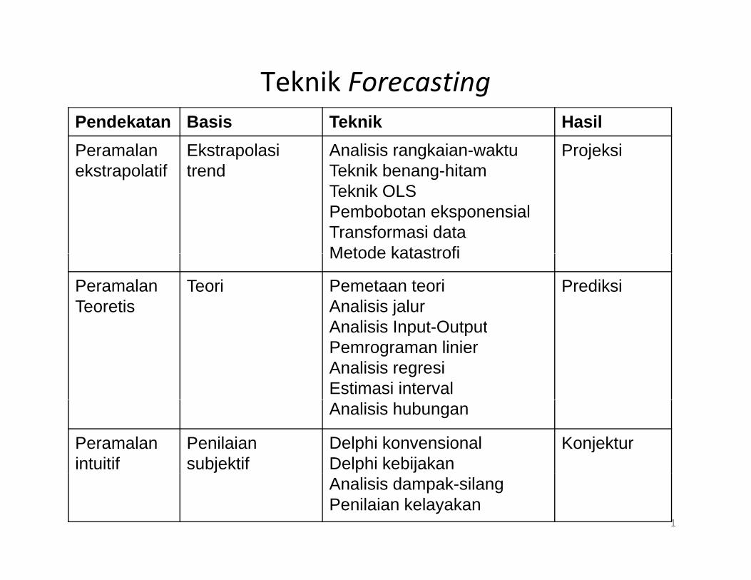
Teknik ForecastingPendekatan Basis Teknik HasilPeramalan ekstrapolatif
Ekstrapolasi trend
Analisis rangkaian-waktuTeknik benang-hitam
Projeksi
Teknik OLSPembobotan eksponensialTransformasi dataMetode katastrofiMetode katastrofi
PeramalanTeoretis
Teori Pemetaan teoriAnalisis jalurAnalisis Input Output
Prediksi
Analisis Input-OutputPemrograman linierAnalisis regresiEstimasi intervalAnalisis hubungan
Peramalan intuitif
Penilaian subjektif
Delphi konvensionalDelphi kebijakan
Konjektur
1
Analisis dampak-silangPenilaian kelayakan

Asumsi Peramalan Ekstrapolatif1. Keajegan (persistence): Pola yang terjadi di masa
lalu akan tetap terjadi di masa mendatang. Mis: jika konsumsi energi di masa lalu meningkat, iajika konsumsi energi di masa lalu meningkat, ia akan selalu meningkat di masa depan.
2. Keteraturan (regularity): Variasi di masa lalu akan secara teratur muncul di masa depan Mis: jikasecara teratur muncul di masa depan. Mis: jika banjir besar di Jakarta terjadi setiap 16 tahun sekali, pola yg sama akan terjadi lagi.
3. Keandalan (reliability) dan kesahihan (validity) data: Ketepatan ramalan tergantung kepada keandalan dan kesahihan data yg tersedia. Mis: ygdata ttg laporan kejahatan seringkali tidak sesuai dg insiden kejahatan yg sesungguhnya, data ttg gaji bukan merupakan ukuran tepat dari pendapatan
2
bukan merupakan ukuran tepat dari pendapatan masyarakat.
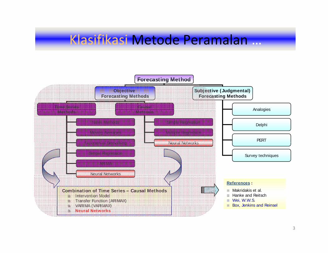
Klasifikasi Metode Peramalan …
Forecasting MethodForecasting Method
Objective Forecasting Methods
Subjective (Judgmental)Forecasting Methods
Time SeriesM th d
CausalM th d AnalogiesMethods Methods Analogies
Delphi
PERT
Simple Regression
Multiple Regression
Neural Networks
Naïve Methods
Moving Averages
Exponential Smoothing
Survey techniques
Neural NetworksExponential Smoothing
Simple Regression
ARIMA
Neural NetworksNeural Networks
Combination of Time Series – Causal MethodsIntervention ModelTransfer Function (ARIMAX)VARIMA (VARIMAX)
References :
Makridakis et al. Hanke and Reitsch Wei, W.W.S. Box, Jenkins and Reinsel
3
VARIMA (VARIMAX)Neural Networks
Box, Jenkins and Reinsel
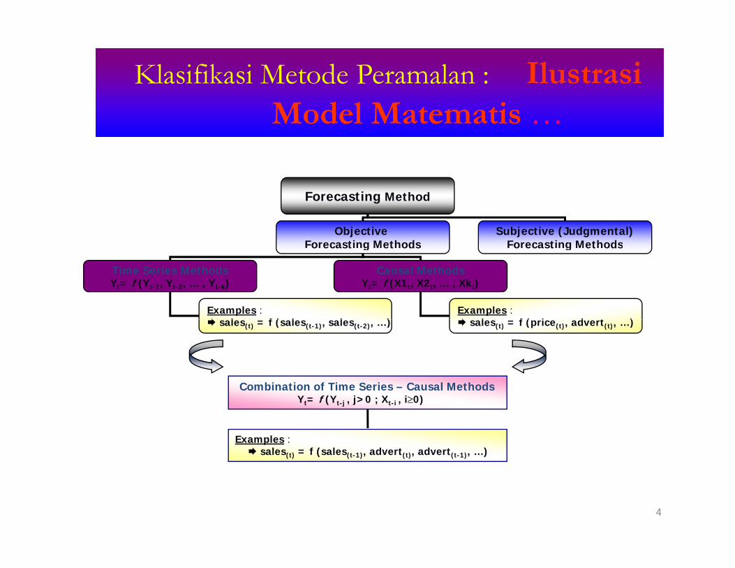
Klasifikasi Metode Peramalan : Ilustrasi M d l M iModel Matematis …
Forecasting Method
Objective Forecasting Methods
Subjective (Judgmental)Forecasting Methodso ecast g et ods o ecast g et ods
Time Series MethodsYt= f (Yt-1, Yt-2, … , Yt-k)
Causal MethodsYt= f (X1t, X2t, … , Xkt)
Examples :l f ( l l )
Examples :l f ( i d t )sales(t) = f (sales(t-1), sales(t-2), …) sales(t) = f (price(t), advert(t), …)
Combination of Time Series – Causal MethodsYt= f (Yt-j , j>0 ; Xt-i , i≥0)
Examples :sales(t) = f (sales(t-1), advert(t), advert(t-1), …)
4
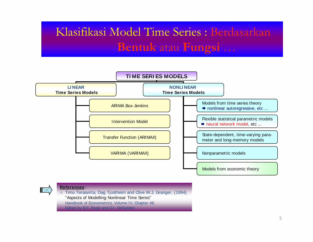
Klasifikasi Model Time Series : Berdasarkan B t k t F i
TIME SERIES MODELS
Bentuk atau Fungsi …
TIME SERIES MODELS
LINEARTime Series Models
NONLINEARTime Series Models
ARIMA Box-Jenkins Models from time series theoryARIMA Box-Jenkins nonlinear autoregressive, etc ...
Flexible statistical parametric models neural network model, etc ...
State-dependent, time-varying para-
Intervention Model
T f F ti (ARIMAX) p , y g pmeter and long-memory models
Nonparametric models
Transfer Function (ARIMAX)
VARIMA (VARIMAX)
Models from economic theory
References : Timo Terasvirta, Dag Tjostheim and Clive W.J. Granger, (1994)“Aspects of Modelling Nonlinear Time Series”
5
Aspects of Modelling Nonlinear Time Series Handbook of Econometrics, Volume IV, Chapter 48. Edited by R.F. Engle and D.I. McFadden
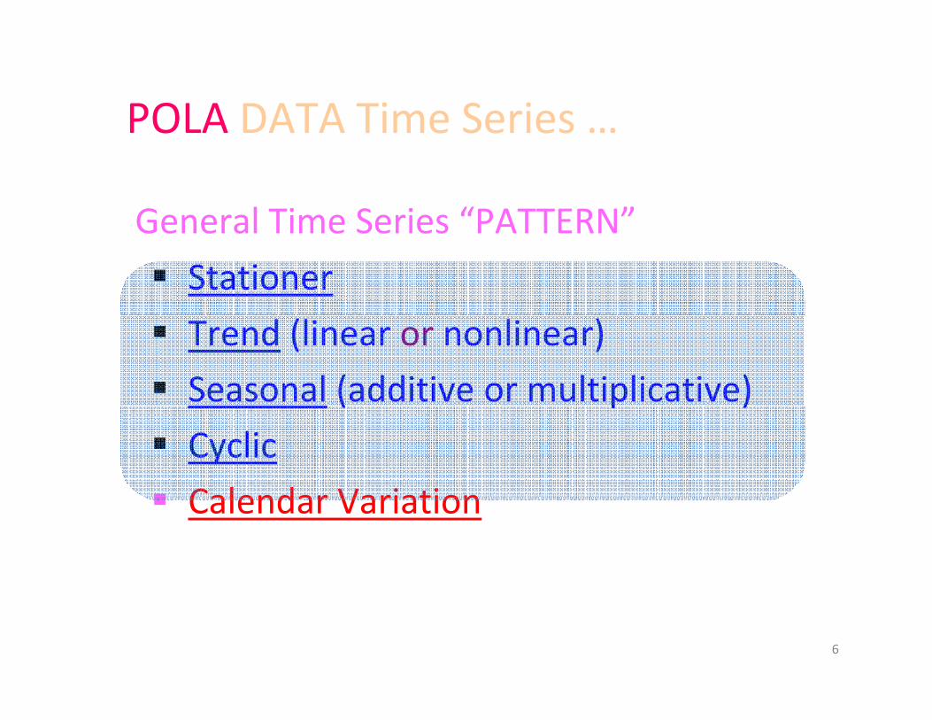
POLA DATA Time Series …O e Se es
General Time Series “PATTERN”General Time Series PATTERN
Stationer
Trend (linear or nonlinear)
Seasonal (additive or multiplicative)( p )
Cyclic
Calendar VariationCalendar Variation
6
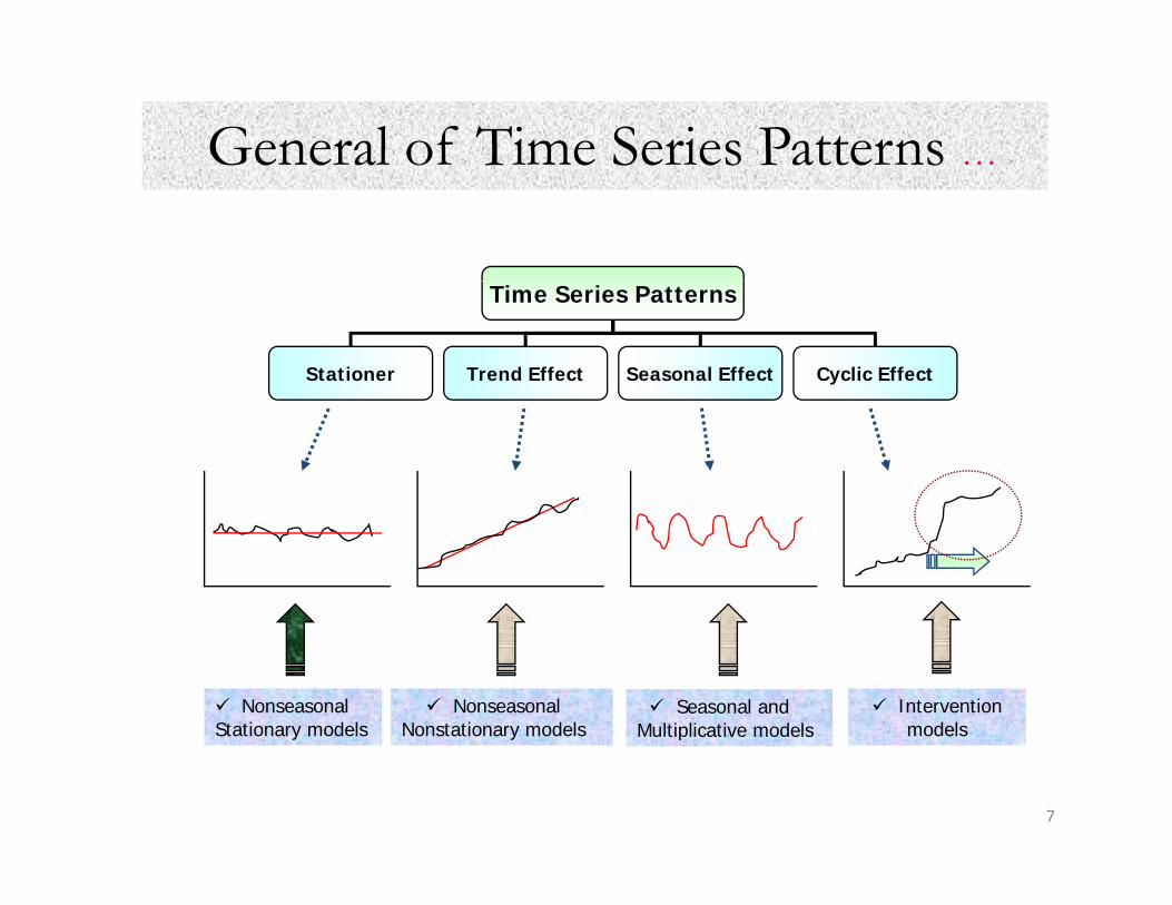
General of Time Series Patterns …
Time Series Patterns
Stationer Trend Effect Seasonal Effect Cyclic Effect
Nonseasonal Nonstationary models
Seasonal and Multiplicative models
Intervention models
Nonseasonal Stationary models
7
y py
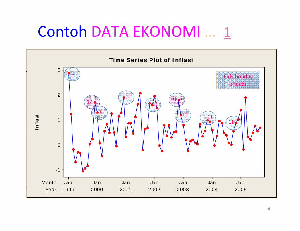
Contoh DATA EKONOMI … 1
3
Time Series Plot of Inflasi
13
2
1
12 1112
Eids holiday effects
Infla
si
1
12
1
12
12 1111
0
YeaMonth
2005200420032002200120001999JanJanJanJanJanJanJan
-1
8
Year 2005200420032002200120001999
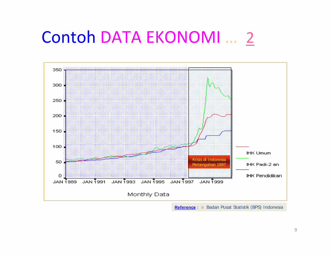
Contoh DATA EKONOMI … 2
Krisis di Indonesia Pertengahan 1997
Reference : Badan Pusat Statistik (BPS) Indonesia
9
Reference : Badan Pusat Statistik (BPS) Indonesia
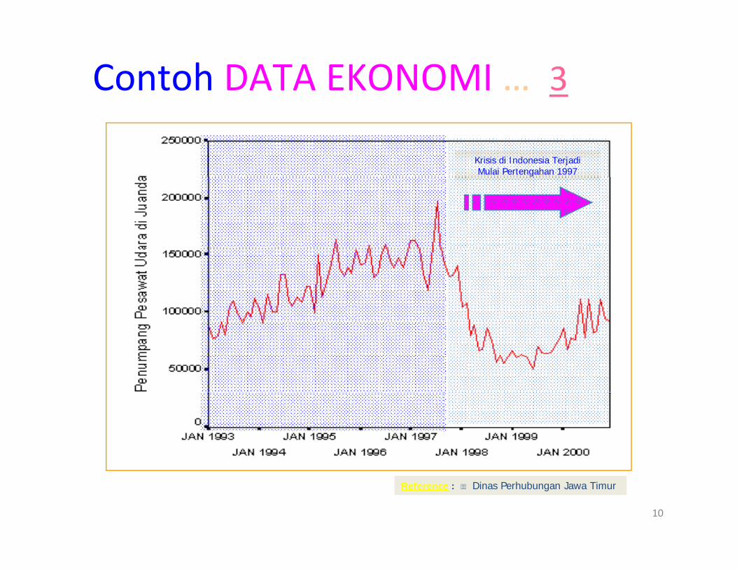
Contoh DATA EKONOMI … 3
Krisis di Indonesia Terjadi Mulai Pertengahan 1997
10
Reference : Dinas Perhubungan Jawa Timur
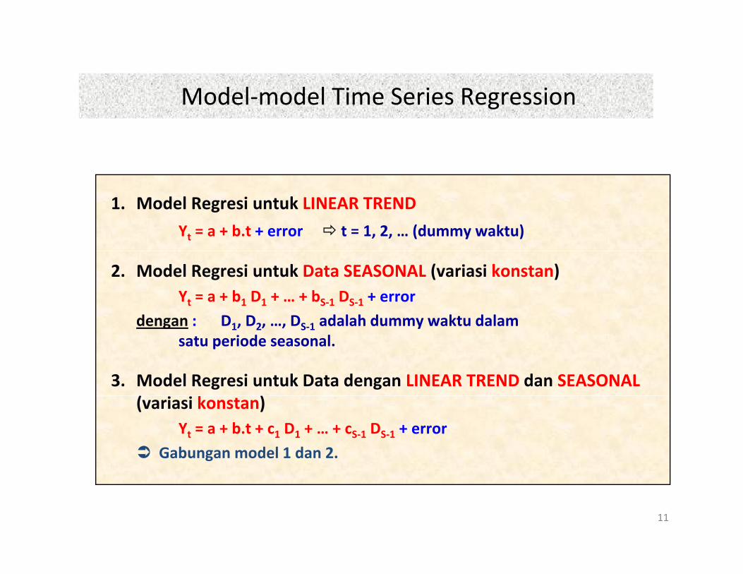
Model‐model Time Series Regressiong
1. Model Regresi untuk LINEAR TREND
Yt = a + b.t + error t = 1, 2, … (dummy waktu)
2. Model Regresi untuk Data SEASONAL (variasi konstan)Yt = a + b1 D1 + … + bS‐1 DS‐1 + error
dengan : D1 D2 DS 1 adalah dummy waktu dalamdengan : D1, D2, …, DS‐1 adalah dummy waktu dalam satu periode seasonal.
3. Model Regresi untuk Data dengan LINEAR TREND dan SEASONAL( )(variasi konstan)
Yt = a + b.t + c1 D1 + … + cS‐1 DS‐1 + error
Gabungan model 1 dan 2.
11
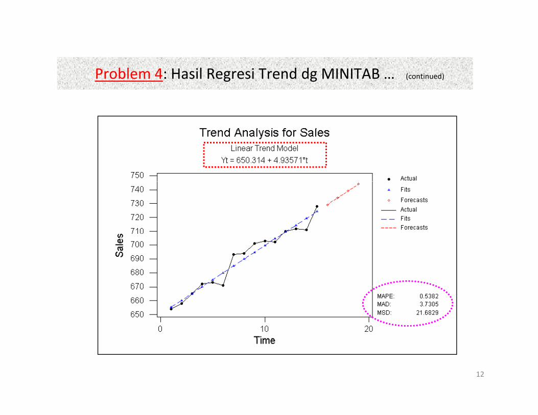
Problem 4: Hasil Regresi Trend dg MINITAB (continued)Problem 4: Hasil Regresi Trend dg MINITAB … (continued)
12
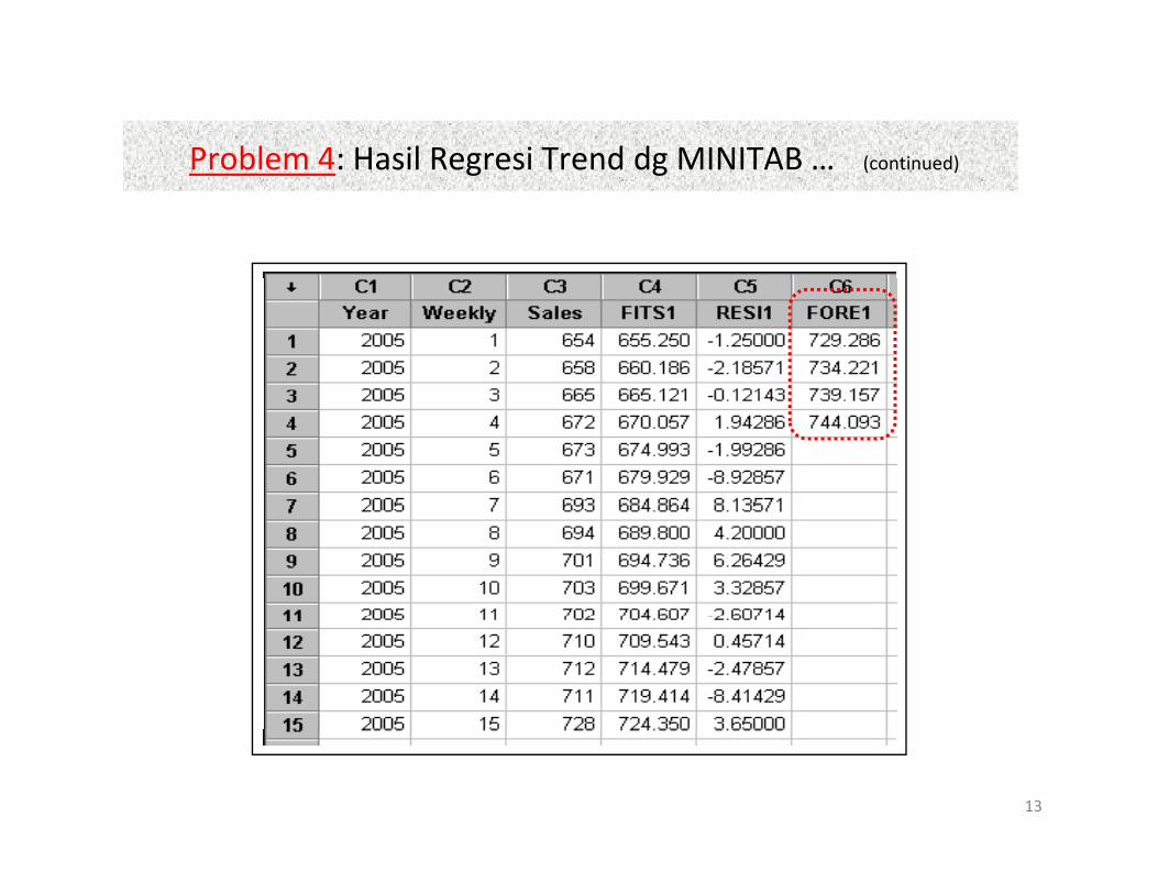
Problem 4: Hasil Regresi Trend dg MINITAB (continued)Problem 4: Hasil Regresi Trend dg MINITAB … (continued)
13
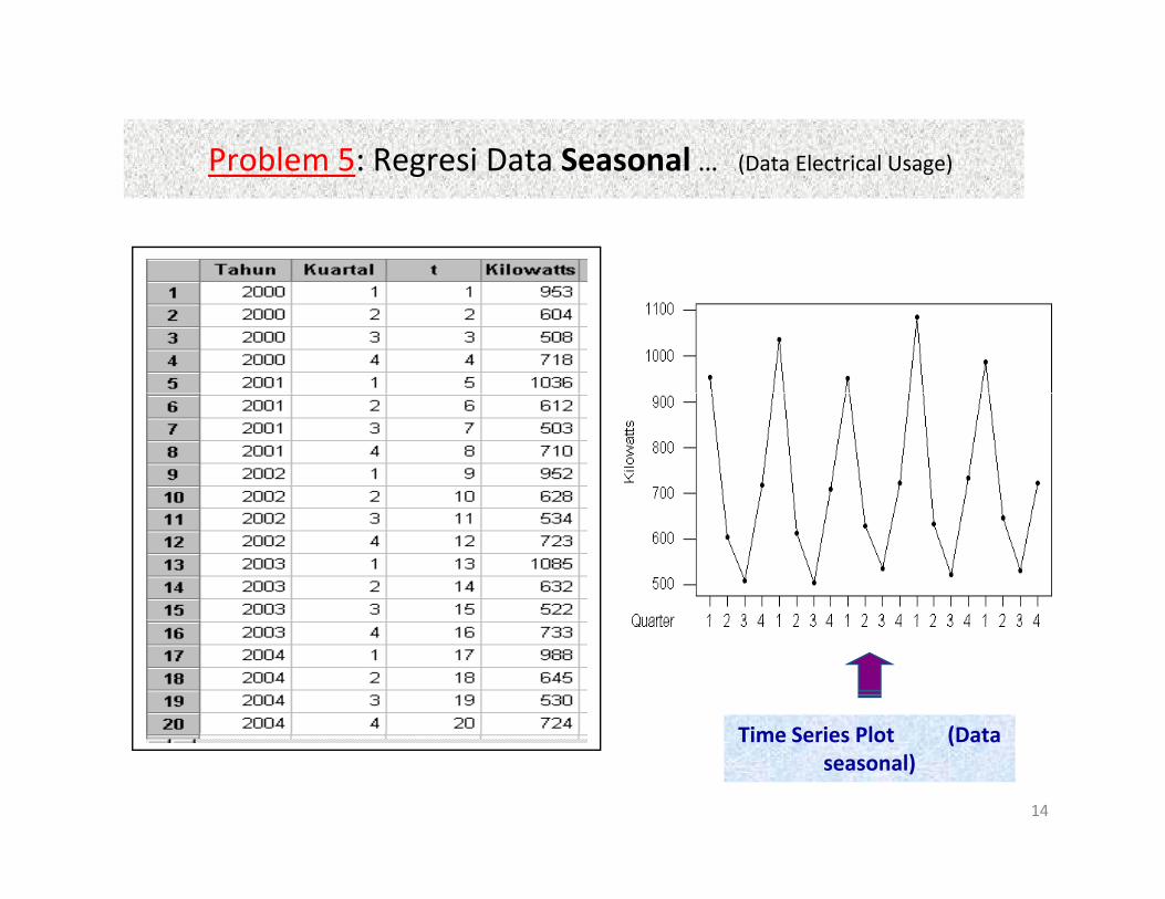
Problem 5: Regresi Data Seasonal (Data Electrical Usage)Problem 5: Regresi Data Seasonal … (Data Electrical Usage)
Time Series Plot (Data
14
Time Series Plot (Data seasonal)
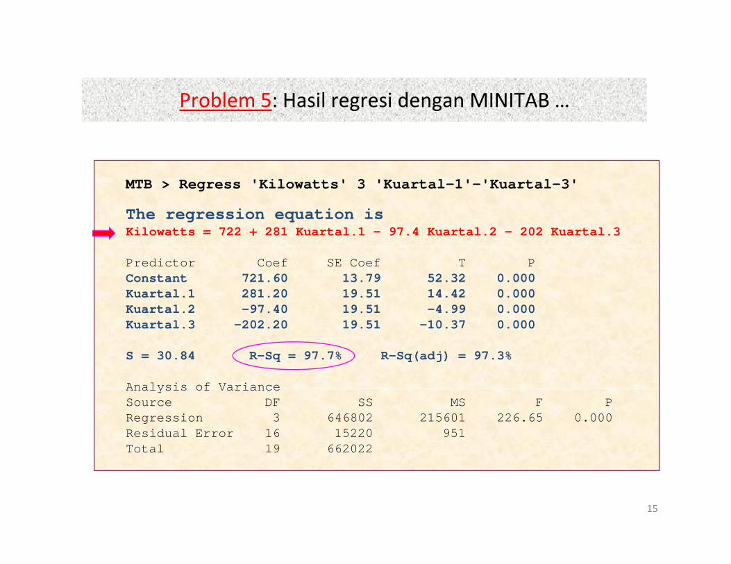
Problem 5: Hasil regresi dengan MINITABProblem 5: Hasil regresi dengan MINITAB …
MTB > Regress 'Kilowatts' 3 'Kuartal-1'-'Kuartal-3'
The regression equation isKilowatts = 722 + 281 Kuartal.1 - 97.4 Kuartal.2 - 202 Kuartal.3
Predictor Coef SE Coef T PConstant 721.60 13.79 52.32 0.000Kuartal.1 281.20 19.51 14.42 0.000Kuartal.2 -97.40 19.51 -4.99 0.000Kuartal.3 -202.20 19.51 -10.37 0.000
S = 30.84 R-Sq = 97.7% R-Sq(adj) = 97.3%
Analysis of VarianceAnalysis of VarianceSource DF SS MS F PRegression 3 646802 215601 226.65 0.000Residual Error 16 15220 951Total 19 662022
15
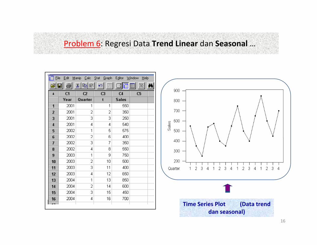
Problem 6: Regresi Data Trend Linear dan Seasonal …Problem 6: Regresi Data Trend Linear dan Seasonal …
16
Time Series Plot (Data trend dan seasonal)
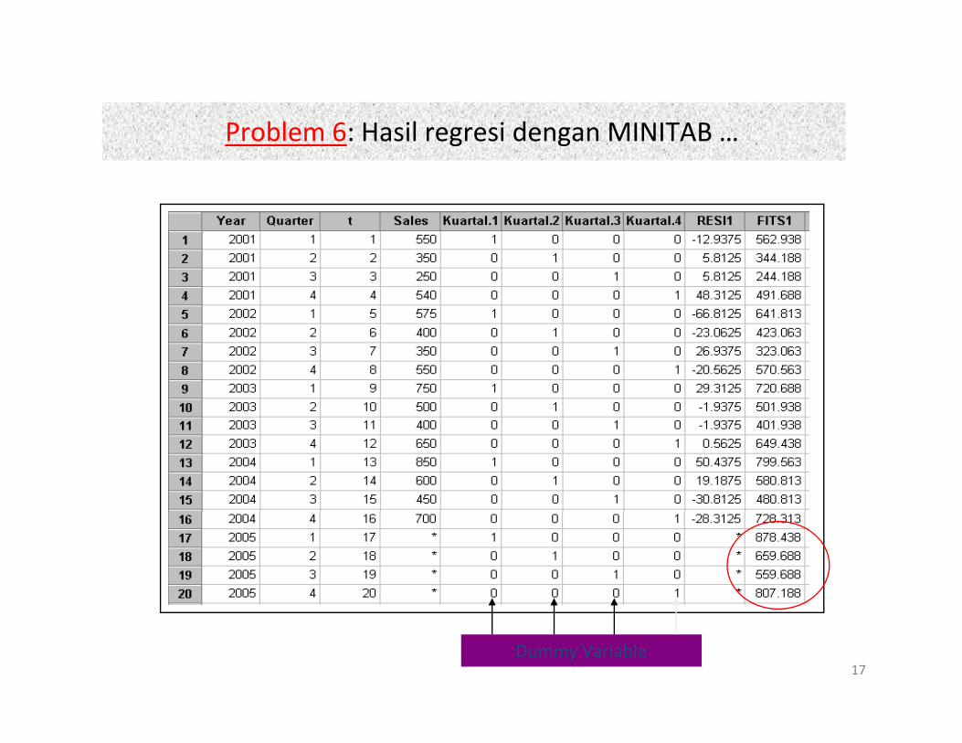
Problem 6: Hasil regresi dengan MINITABProblem 6: Hasil regresi dengan MINITAB …
17Dummy Variable
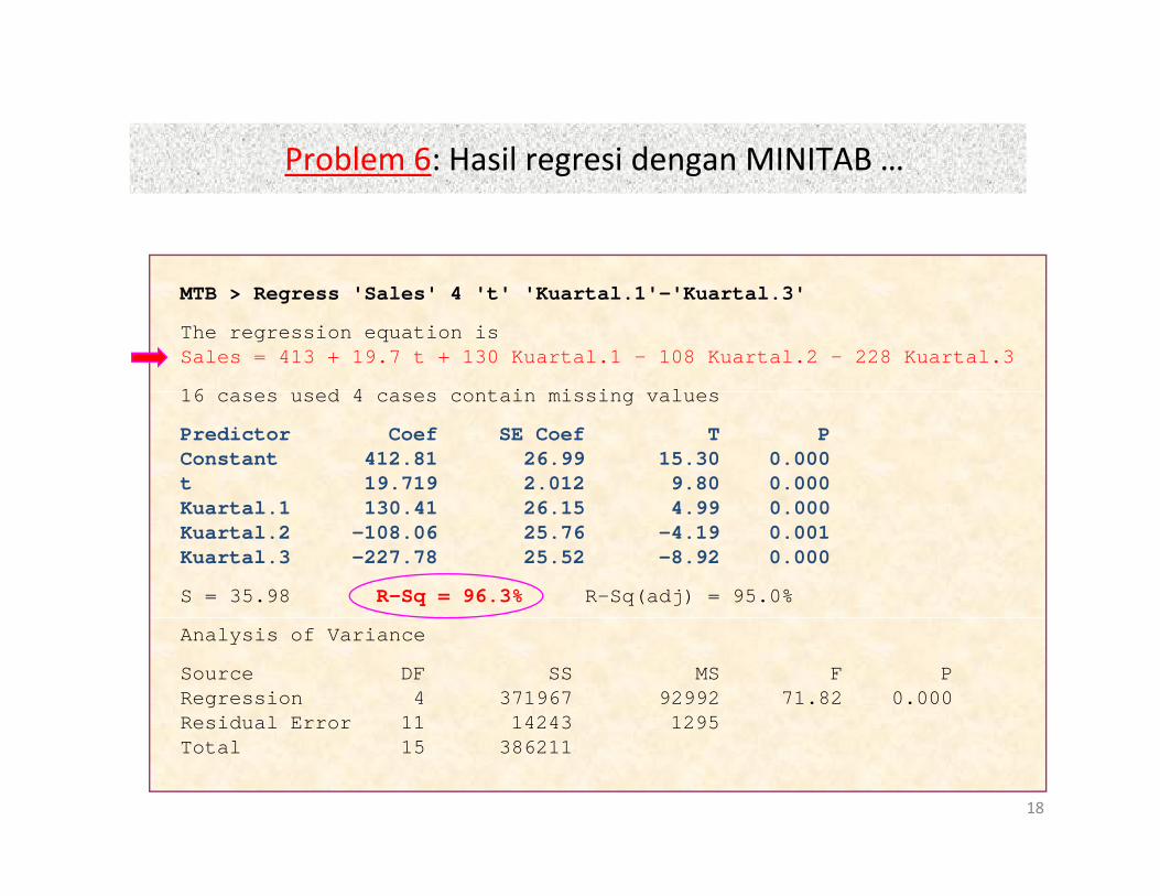
Problem 6: Hasil regresi dengan MINITABProblem 6: Hasil regresi dengan MINITAB …
MTB > Regress 'Sales' 4 't' 'Kuartal.1'-'Kuartal.3'
The regression equation isSales = 413 + 19.7 t + 130 Kuartal.1 - 108 Kuartal.2 - 228 Kuartal.3
16 d 4 t i i i l16 cases used 4 cases contain missing values
Predictor Coef SE Coef T PConstant 412.81 26.99 15.30 0.000t 19.719 2.012 9.80 0.000K artal 1 130 41 26 15 4 99 0 000Kuartal.1 130.41 26.15 4.99 0.000Kuartal.2 -108.06 25.76 -4.19 0.001Kuartal.3 -227.78 25.52 -8.92 0.000
S = 35.98 R-Sq = 96.3% R-Sq(adj) = 95.0%
Analysis of Variance
Source DF SS MS F PRegression 4 371967 92992 71.82 0.000Residual Error 11 14243 1295
18
Total 15 386211
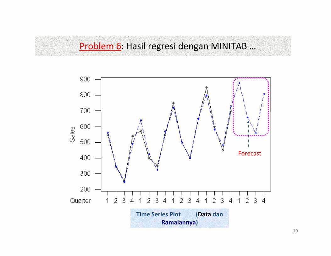
Problem 6: Hasil regresi dengan MINITABProblem 6: Hasil regresi dengan MINITAB …
Forecast
19
Time Series Plot (Data dan Ramalannya)
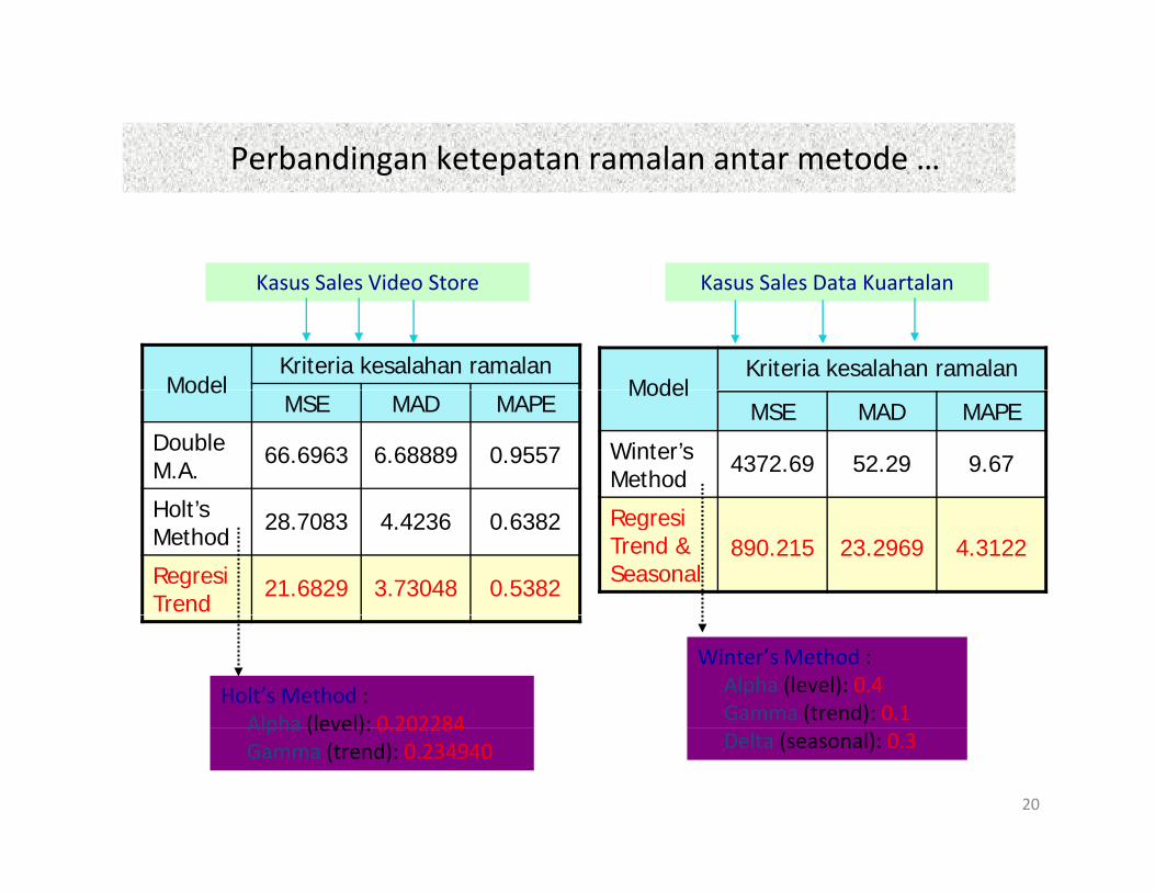
Perbandingan ketepatan ramalan antar metodePerbandingan ketepatan ramalan antar metode …
K S l Vid St K S l D t K t l
ModelKriteria kesalahan ramalan
Kasus Sales Video Store
ModelKriteria kesalahan ramalan
Kasus Sales Data Kuartalan
ModelMSE MAD MAPE
Double M.A.
66.6963 6.68889 0.9557
H lt’
ModelMSE MAD MAPE
Winter’s Method
4372.69 52.29 9.67
Holt’s Method
28.7083 4.4236 0.6382
Regresi Trend
21.6829 3.73048 0.5382
Regresi Trend &Seasonal
890.215 23.2969 4.3122
Holt’s Method :Alpha (level): 0 202284
Winter’s Method :Alpha (level): 0.4Gamma (trend): 0.1
20
Alpha (level): 0.202284Gamma (trend): 0.234940 Delta (seasonal): 0.3
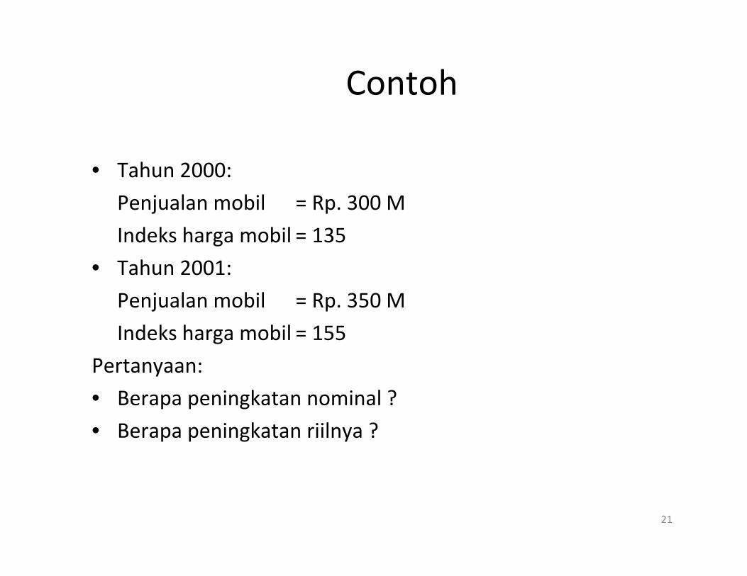
Contoh
• Tahun 2000:
Penjualan mobil = Rp. 300 M
Indeks harga mobil = 135
• Tahun 2001:
Penjualan mobil = Rp. 350 M
Indeks harga mobil = 155
Pertanyaan:
• Berapa peningkatan nominal ?• Berapa peningkatan nominal ?
• Berapa peningkatan riilnya ?
21
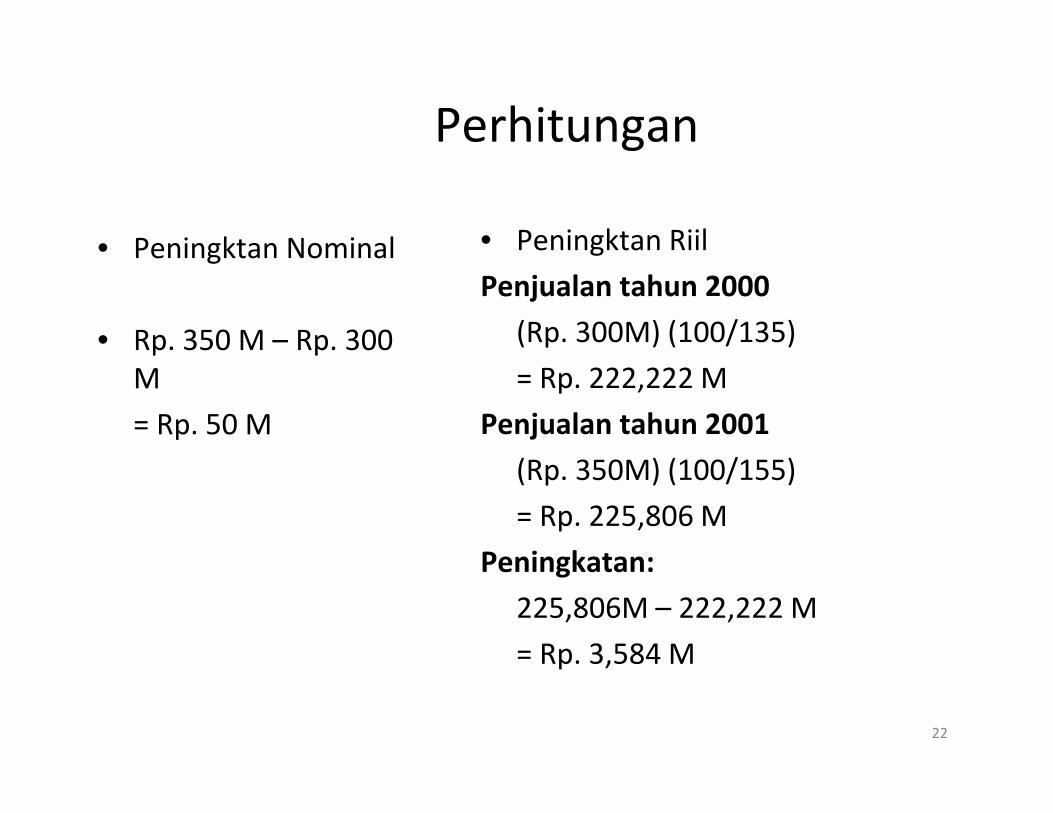
Perhitungang
• Peningktan Nominal • Peningktan RiilPeningktan Nominal
• Rp. 350 M – Rp. 300
g
Penjualan tahun 2000
(Rp. 300M) (100/135)p pM
= Rp. 50 M
= Rp. 222,222 M
Penjualan tahun 2001
( ) ( / )(Rp. 350M) (100/155)
= Rp. 225,806 M
Peningkatan:Peningkatan:
225,806M – 222,222 M
= Rp. 3,584 M
22
Rp. 3,584 M
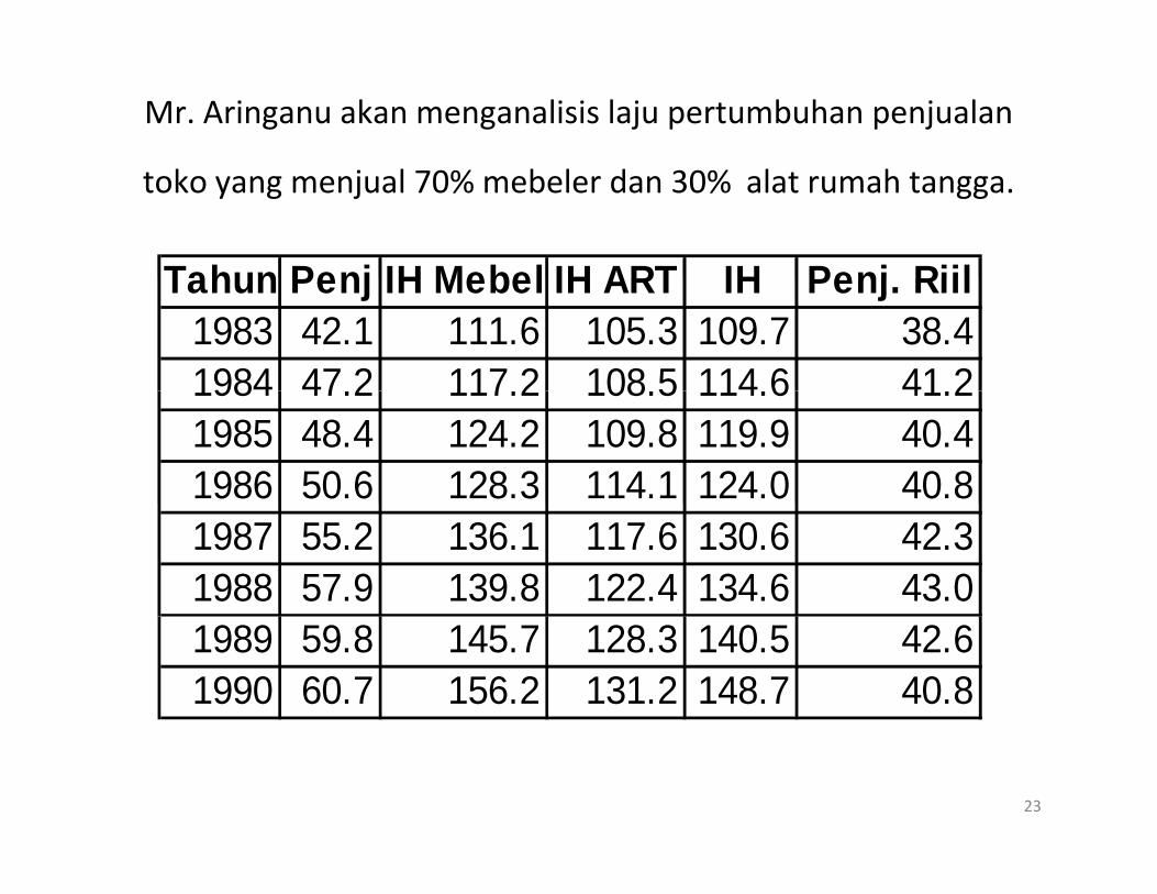
Mr. Aringanu akan menganalisis laju pertumbuhan penjualan
toko yang menjual 70% mebeler dan 30% alat rumah tangga.
Tahun Penj IH Mebel IH ART IH Penj RiilTahun Penj IH Mebel IH ART IH Penj. Riil1983 42.1 111.6 105.3 109.7 38.41984 47 2 117 2 108 5 114 6 41 21984 47.2 117.2 108.5 114.6 41.21985 48.4 124.2 109.8 119.9 40.41986 50.6 128.3 114.1 124.0 40.81987 55.2 136.1 117.6 130.6 42.31988 57.9 139.8 122.4 134.6 43.01989 59.8 145.7 128.3 140.5 42.61990 60.7 156.2 131.2 148.7 40.8
23
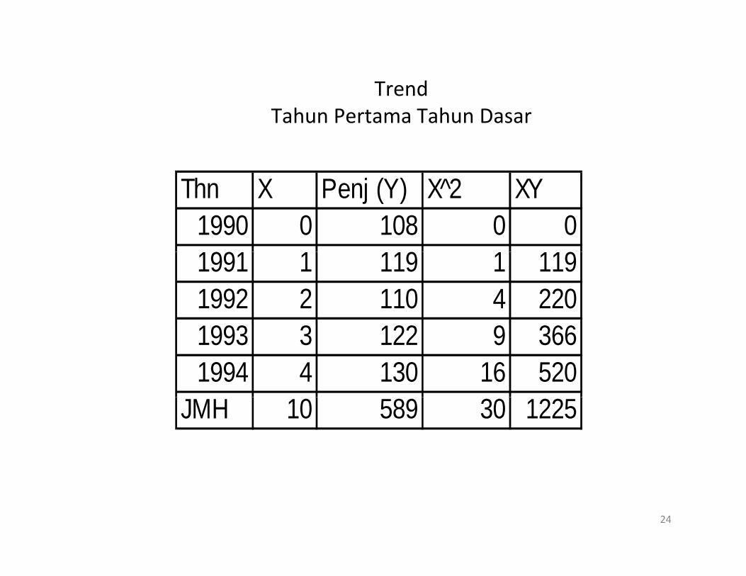
TrendTahun Pertama Tahun Dasar
Th X P j (Y) X̂ 2 XYThn X Penj (Y) X̂ 2 XY1990 0 108 0 01991 1 119 1 1191991 1 119 1 1191992 2 110 4 2201993 3 122 9 3661994 4 130 16 520
JMH 10 589 30 1225
24
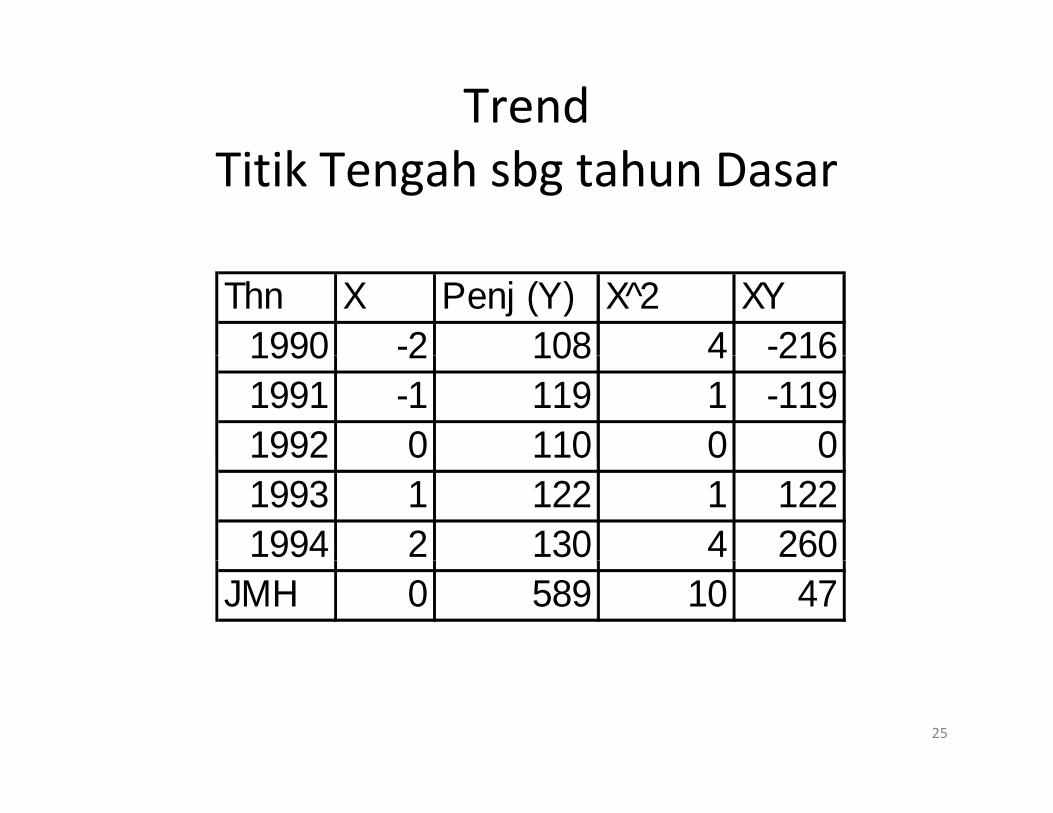
Trendk h b hTitik Tengah sbg tahun Dasar
Thn X Penj (Y) X̂ 2 XY1990 -2 108 4 -2161990 2 108 4 2161991 -1 119 1 -1191992 0 110 0 01993 1 122 1 1221994 2 130 4 260
JMH 0 589 10 47
25
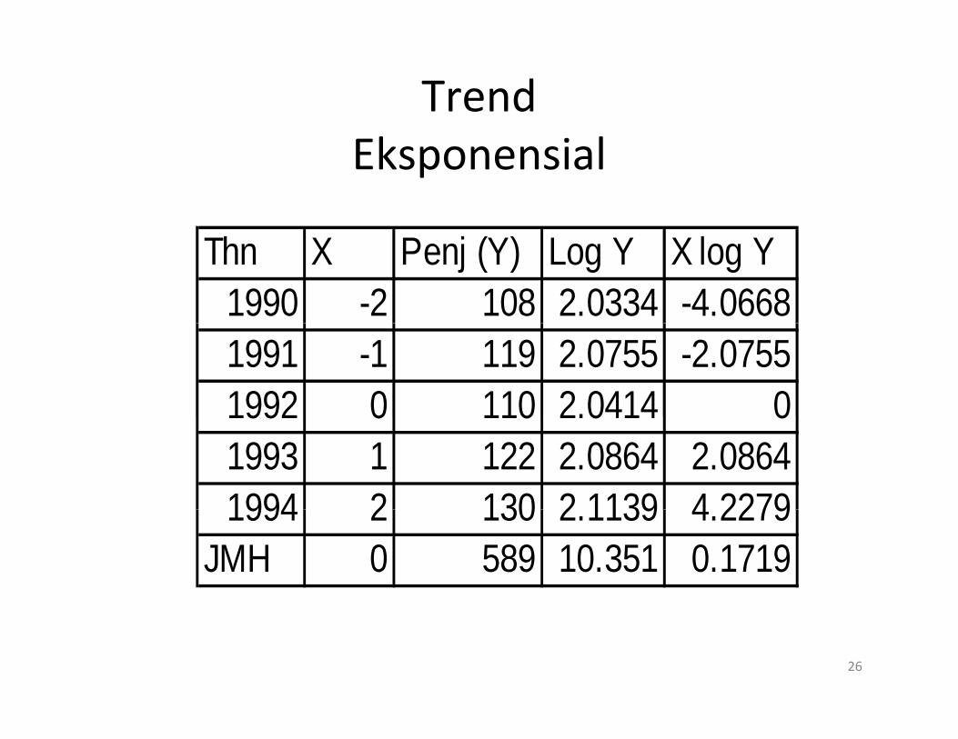
Trendk lEksponensial
Thn X Penj (Y) Log Y X log Y1990 -2 108 2.0334 -4.06681991 -1 119 2.0755 -2.07551992 0 110 2.0414 01992 0 110 2.0414 01993 1 122 2.0864 2.08641994 2 130 2 1139 4 22791994 2 130 2.1139 4.2279
JMH 0 589 10.351 0.1719
26
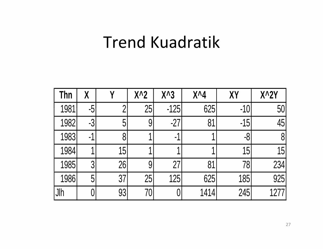
Trend KuadratikTrend Kuadratik
Thn X Y X^2 X^3 X^4 XY X^2Y1981 5 2 25 125 625 10 501981 -5 2 25 -125 625 -10 501982 -3 5 9 -27 81 -15 451983 -1 8 1 -1 1 -8 8983 8 8 81984 1 15 1 1 1 15 151985 3 26 9 27 81 78 2341986 5 37 25 125 625 185 925
Jlh 0 93 70 0 1414 245 1277
27
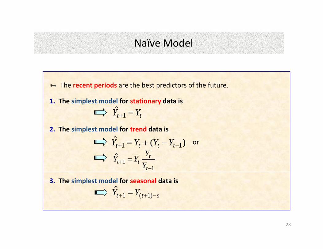
Naïve ModelNaïve Model
The recent periods are the best predictors of the future.
1. The simplest model for stationary data isˆ
2. The simplest model for trend data is
tt YY =+1
)(ˆ YYYY or
11
ˆ−
+ =t
ttt Y
YYY
)( 11 −+ −+= tttt YYYY
3. The simplest model for seasonal data is
stt YY −++ = )1(1ˆ
28
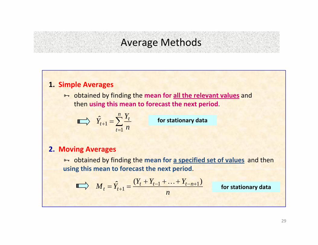
Average MethodsAverage Methods
1. Simple Averagesobtained by finding the mean for all the relevant values and then using this mean to forecast the next period.g p
∑=
+ =n
t
tt n
YY1
1ˆ for stationary data
2. Moving Averagesobtained by finding the mean for a specified set of values and then
using this mean to forecast the next periodusing this mean to forecast the next period.
nYYYYM nttt
tt)(ˆ 11
1+−−
++++
==K
for stationary data
29
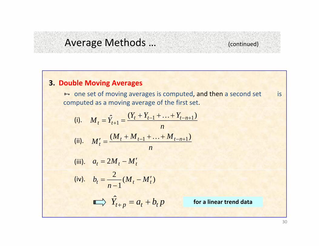
Average Methods … (continued)Average Methods … (continued)
3. Double Moving Averagesone set of moving averages is computed, and then a second set is
computed as a moving average of the first set.
(i).
(ii)
nYYYYM nttt
tt)(ˆ 11
1+−−
++++
==K
MMM nttt )( 11 ++++′ K(ii).
(iii).
nMMMM nttt
t)( 11 +−− +++
=′K
ttt MMa ′−= 2
(iv).
pbaY +ˆ f li t d d t
)(1
2ttt MM
nb ′−
−=
30
pbaY ttpt +=+ for a linear trend data
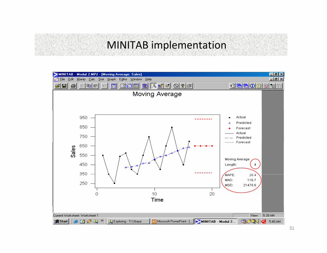
MINITAB implementationMINITAB implementation
31
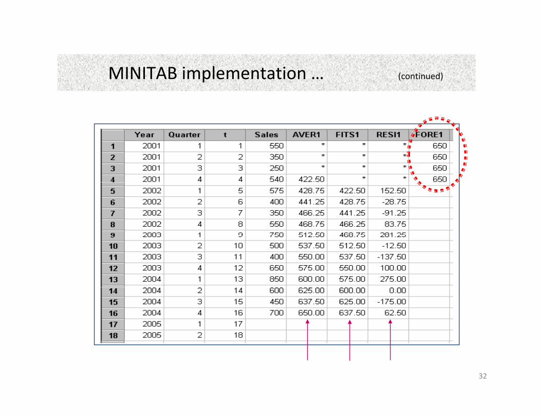
MINITAB implementation … (continued)MINITAB implementation … (continued)
32
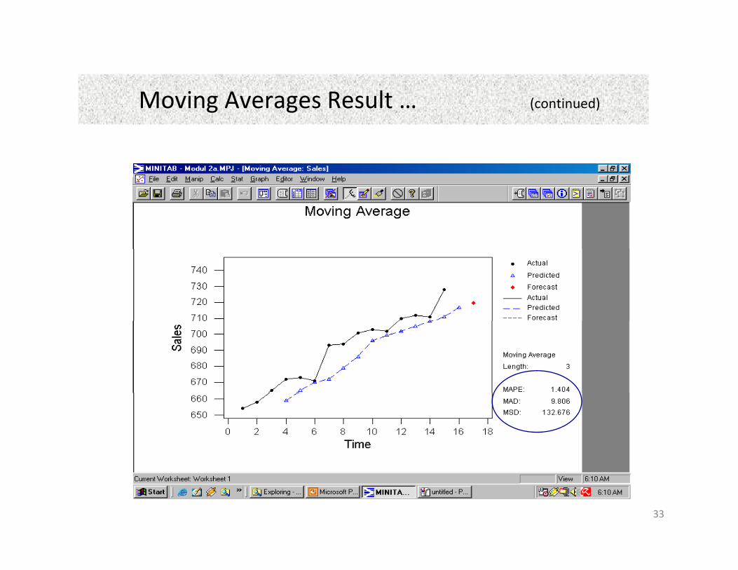
Moving Averages Result … (continued)Moving Averages Result … (continued)
33
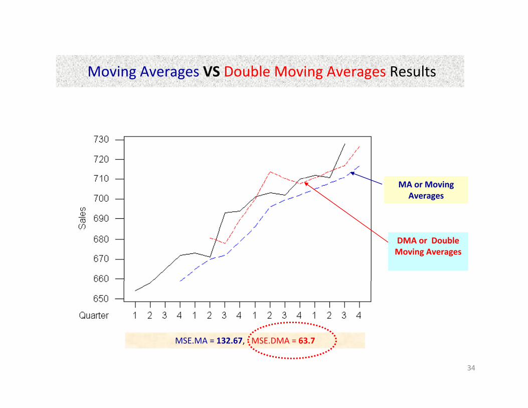
Moving Averages VS Double Moving Averages ResultsMoving Averages VS Double Moving Averages Results
MA or Moving Averages
DMA or Double Moving Averages
34
MSE.MA = 132.67, MSE.DMA = 63.7
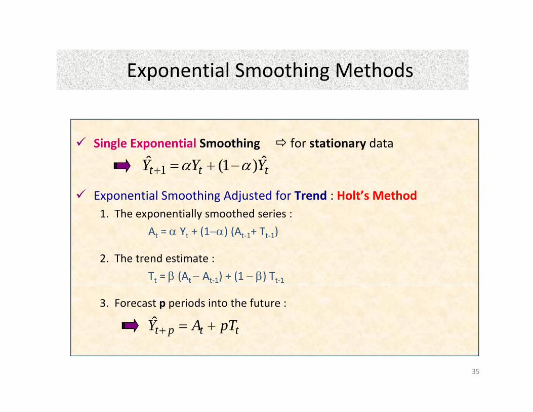
Exponential Smoothing MethodsExponential Smoothing Methods
Single Exponential Smoothing for stationary data
ttt YYY ˆ)1(ˆ 1 αα −+=+
Exponential Smoothing Adjusted for Trend : Holt’s Method1. The exponentially smoothed series :
A = α Y + (1−α) (A + T )At = α Yt + (1−α) (At‐1+ Tt‐1)
2. The trend estimate :
Tt = β (At − At‐1) + (1 − β) Tt‐1
3. Forecast p periods into the future :
ttpt pTAY +=+ˆ
35
p
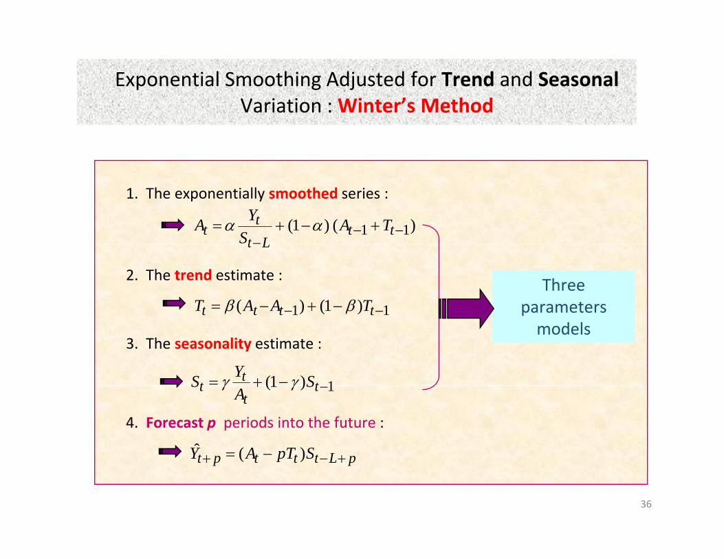
Exponential Smoothing Adjusted for Trend and SeasonalVariation :Winter’s MethodVariation : Winter’s Method
1. The exponentially smoothed series :
)( )1( 11 −−−
+−+= ttLt
tt TA
SYA αα
2. The trend estimate :
Lt
11 )1()( −− −+−= tttt TAAT ββThree
parameters
3. The seasonality estimate :
11 tttt
1)1( −+= tt
t SYS γγ
pmodels
4. Forecast p periods into the future :
1)1( −+ tt
t SA
S γγ
Ltttt SpTAY ++ −= )(ˆ
36
pLtttpt SpTAY +−+ = )(
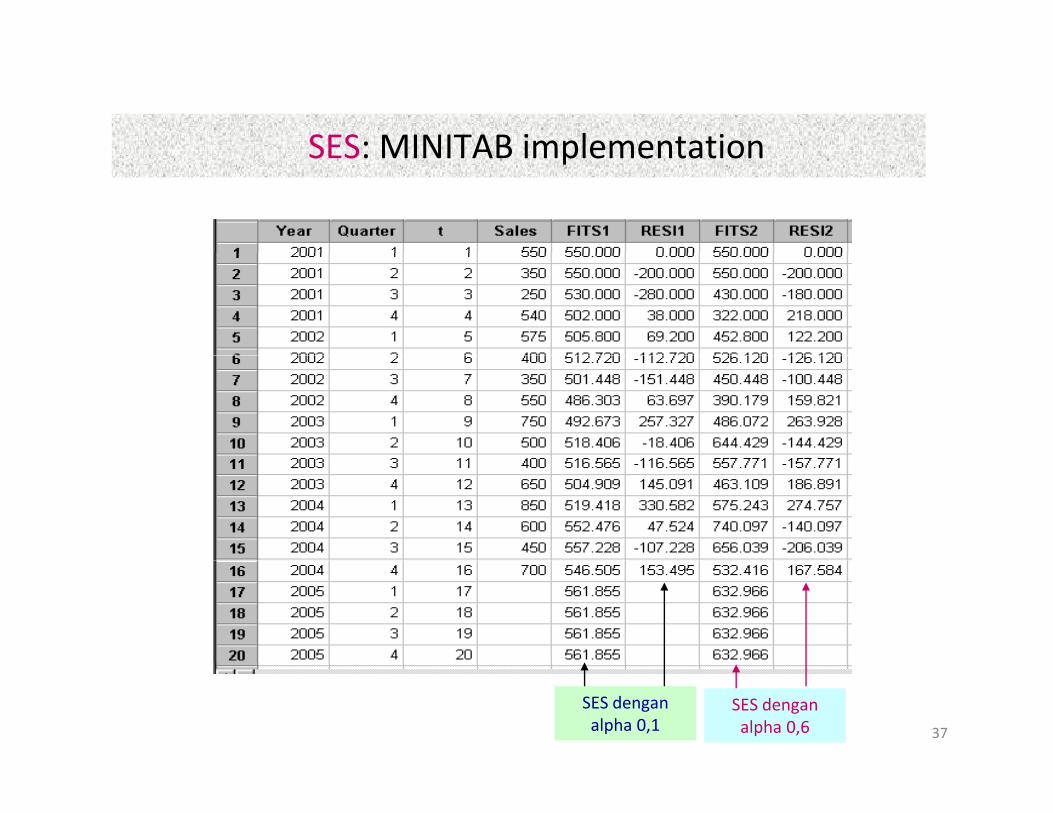
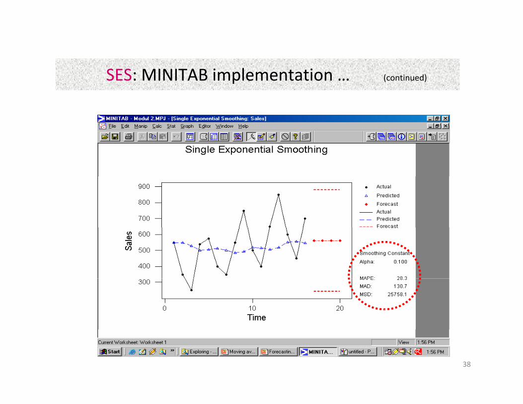
SES: MINITAB implementationSES: MINITAB implementation
37
SES dengan alpha 0,1
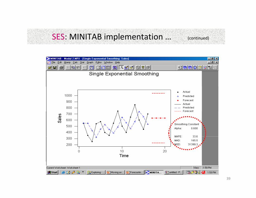
SES dengan alpha 0,6
SES: MINITAB implementation ( i d)SES: MINITAB implementation … (continued)
38
SES: MINITAB implementation ( i d)SES: MINITAB implementation … (continued)
39
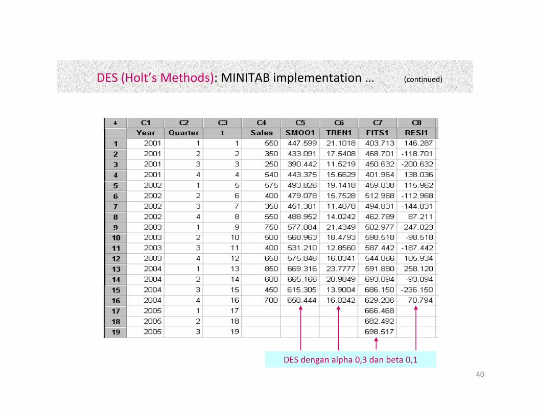
DES (Holt’s Methods): MINITAB implementation ( i d)DES (Holt s Methods): MINITAB implementation … (continued)
40
DES dengan alpha 0,3 dan beta 0,1
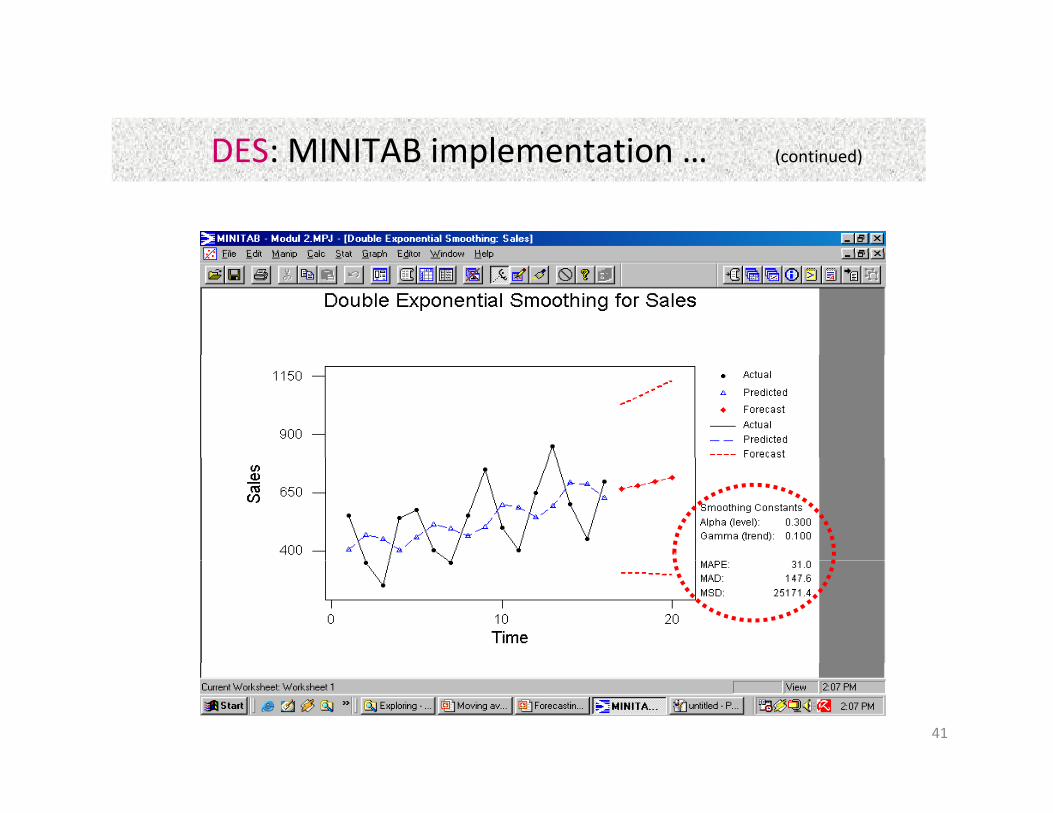
DES: MINITAB implementation ( i d)DES: MINITAB implementation … (continued)
41
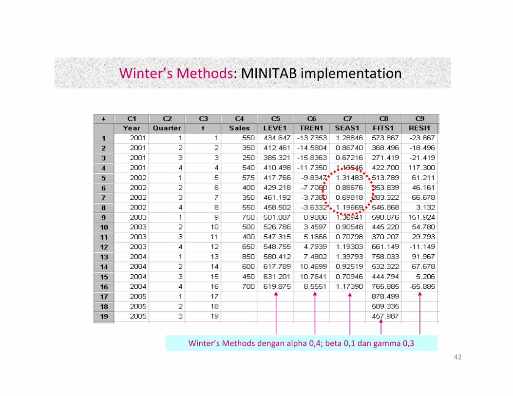
Winter’s Methods: MINITAB implementationWinter s Methods: MINITAB implementation
42
Winter’s Methods dengan alpha 0,4; beta 0,1 dan gamma 0,3
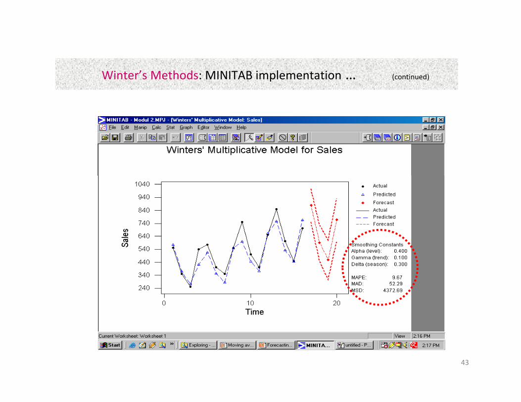
Winter’s Methods: MINITAB implementation ( i d)Winter s Methods: MINITAB implementation … (continued)
43