


Bahasa
Halaman
Hukum

econstorMake Your Publications Visible.
A Service of
zbwLeibniz-InformationszentrumWirtschaftLeibniz Information Centrefor Economics
Hudson, Chris
Working Paper
Witch trials: Discontent in early modern Europe
Graduate Institute of International and Development Studies Working Paper, No. 11-2016
Provided in Cooperation with:International Economics Section, The Graduate Institute of International and DevelopmentStudies
Suggested Citation: Hudson, Chris (2016) : Witch trials: Discontent in early modern Europe,Graduate Institute of International and Development Studies Working Paper, No. 11-2016,Graduate Institute of International and Development Studies, Geneva
This Version is available at:http://hdl.handle.net/10419/156127
Standard-Nutzungsbedingungen:
Die Dokumente auf EconStor dürfen zu eigenen wissenschaftlichenZwecken und zum Privatgebrauch gespeichert und kopiert werden.
Sie dürfen die Dokumente nicht für öffentliche oder kommerzielleZwecke vervielfältigen, öffentlich ausstellen, öffentlich zugänglichmachen, vertreiben oder anderweitig nutzen.
Sofern die Verfasser die Dokumente unter Open-Content-Lizenzen(insbesondere CC-Lizenzen) zur Verfügung gestellt haben sollten,gelten abweichend von diesen Nutzungsbedingungen die in der dortgenannten Lizenz gewährten Nutzungsrechte.
Terms of use:
Documents in EconStor may be saved and copied for yourpersonal and scholarly purposes.
You are not to copy documents for public or commercialpurposes, to exhibit the documents publicly, to make thempublicly available on the internet, or to distribute or otherwiseuse the documents in public.
If the documents have been made available under an OpenContent Licence (especially Creative Commons Licences), youmay exercise further usage rights as specified in the indicatedlicence.
www.econstor.eu
Graduate Institute of International and Development Studies
International Economics Department
Working Paper Series
Working Paper No. HEIDWP11-2016
Witch Trials: Discontent in Early Modern Europe
Chris HudsonThe Graduate Institute, Geneva
Chemin Eugene-Rigot 2P.O. Box 136
CH - 1211 Geneva 21Switzerland
c©The Authors. All rights reserved. Working Papers describe research in progress by the author(s) and are published toelicit comments and to further debate. No part of this paper may be reproduced without the permission of the authors.
1
Witch Trials: Discontent in Early Modern Europe
Chris Hudson
Abstract
This paper examines the relationship between income and witch trials in early modern Europe. We start by using climate data to proxy for income levels. This builds on previous work by exploiting a far richer panel dataset covering 356 regions and 260 years, including both seasonal temperature and rainfall, as well as over 30,036 witch trials newly documented for this study. We find that a one degree temperature shock leads to a near quadrupling in witch trials in any given year. The second part looks at incomes more directly, and we find that different measures of income have different effects on witch trials. Furthermore, the impact may depend on the structure of the economy and how different stakeholder groups are affected. We also present evidence that the stage in the business cycle is important in predicting witch trials, with the bottom of the business cycle coinciding with a doubling of witch trials in England.
Keywords: witchcraft, persecution, plague, conflict, growth, climate change
JEL: I30, J14, J16, N43, N53, O12, Z12
1. Introduction
Witch trials, a series of hearings whereby courts would decide on whether the accused was in fact ‘a
witch’ and should be punished, have had many explanations ascribed to them. From an economics
standpoint, these focus on them being a response to falling incomes. Notably in Oster (2004) and
Miguel (2005), they proxy income shocks through extreme weather behaviour. This implies a two
stage impact, first weather on income and thence income on witch trials. However, we argue that
there are other channels through which climate may effect witch trials. Rather than any implied hit to
economic growth, it may also be that weathers’ linkages with disease or even the negative direct
effects of bad weather were factors in causing the witch trials; a reasonable hypothesis to test given
the historical linkages between witchcraft and weather.
We further postulate that it is not economic output per se which counts, but the real incomes of the
individual villager. By using annual real wage data combined with food inflation, weather, GDP per
capita, plague, war and population data we aim to more precisely identify the channels which affect
the incidence of witch trials. In addition more than previous studies we focus on high resolution data,
annual rather than longer period averages and differentiate between the different seasons in terms
of weather impact. Another aim of this paper is to differentiate between short term cyclical
fluctuations and actual absolute differences in living standards. That is to say, do people adjust their
expectations over time to their present circumstances, or do they value gradual long term
improvements to living standards.
2
While the European witch hunts of the early modern period and before may today seem fantastical
to people in the West they are still practiced in many parts of the world; including Africa, Asia and the
Middle East. The case of Fawza Falih Muhammad Ali in Saudi Arabia bears many striking similarities to
those early European witch hunts. Poor and illiterate she was tortured by the Saudi religious police
into confessing to crimes of witchcraft and sentenced to death in 2006. Even the iconography is
similar, depicting witches flying on broom sticks, causing malady in animals and impotence in men
(Arvin & Arvin, 2010 p.69; Jacobs, 2013).
The European witch trials occurred in a multitude of countries very different with respect to their legal
institutions, cultures, religion, and economic development. They were supported by religious and
state institutions, and were widely viewed as permissible by the society of the day. The impetus for
individual witch trials came from within the general population. Regardless of the willingness of the
state judicial apparatus to hear witchcraft cases, it was down to ordinary villagers to bring these
accusations forward in the first place. So witch trials have two characteristics which make them an
ideal phenomenon through which to measure discontent of the general population. Firstly, they are
instigated at ground level and secondly, they are conducted through the court system and so are
systematically recorded.
The geographical scope of the climate data means that we are able to build a large panel dataset of
30,036 witch trials categorised into 355 regions in Europe over the period 1500-1760. Using this
dataset we analyse the effect climate variability has on witch trials and are able to infer some
interesting conclusions about the underlying causes. Following this we forsake dataset size to directly
examine the effect actual economic variables such as GDP per capita, grain prices, and real wages have
on witch trials. In a section specifically devoted to the English experience we are able to analyse the
incidence of witch trials at different points in the business cycle. We also go into greater depth in
discussing the individual events and conditions affecting English society at the time.
GDP per capita is found to be significant in all specifications in reducing witch trials. In the case where
Holland is excluded, GDP per capita is significant at the 1% level. In the case of Sweden, an increase in
1990 dollar prices from 900 to 1400 leads to an increase in witch trials from 2.12 to 5.79 per year. We
do not find that real wages have a comparable effect, implying that the hourly earning power of labour
was not a deciding factor in fostering discontent. War, defined as the presence of actual fighting in
the region, strongly decreases the incidence of witch trials.
We generally do not find evidence that grain prices influence witch trials. This may at least partly be
because grain prices have disparate effects on different stakeholders in society, and because farmers,
who stand to lose from depressed prices, may be of varying importance across regions. We also find
evidence that grain prices are only partially related to harvest quality. In Sweden, the harvest dummy
variable is significant at the 1% or 5% level depending on how it is defined, while wheat price shocks
are less significant. In the Swedish case we also find that the lowest witch trial years coincided with
‘normal’ harvests, i.e. neither too good nor too bad.
In the section using climate data, temperature seems to play a larger role in determining witch trials
than rainfall. Greater temperature shocks and lower spring-summer temperatures significantly
increase witch trials for up to four years ahead. We see this as consistent with an income based
hypothesis, as the spring and summer months represent the main growing season. Cooler winter and
autumn temperatures tend to decrease witch trials, which suggests temperature could also be linked
3
to other channels than the income one. The results tend to be strongest in the environmental zones
lying mainly in North West Europe – Germany, northern France, the Low Countries, and the UK.
One possible channel that we test for is Plague. The results show tentative evidence that where
temperatures go outside the range which supports the plague virus, witch trials diminish. However,
the evidence for plague is found to be weaker when we test for it explicitly in the GDP per capita and
real wages sections.
Using English GDP data we show that in addition to absolute levels of income, short term income
dynamics also play a role in determining mood. In years in which the economic cycle troughed, witch
trials were significantly higher at the 5% level, while in the first year of recovery witch trials were
significantly lower also at the 5% level.
The paper proceeds as follows. In the next two sections we review the literature on witchcraft and
provide a discussion to the background to the witch hunts. We then discuss theoretical aspects before
presenting the data and then the empirical results. Finally, we conclude the paper.
2. Literature Review
The economics literature pertaining to witch trials is still relatively modest. The literature is mainly
limited to three papers listed in Table 1. Oster(2004) and Miguel(2005) both use weather variation as
a proxy to examine the impact of income shocks on numbers of witch trials.
Oster (2004) focuses her analysis on the 16th-18th Century European witch trials. Using a multicountry
panel dataset she shows a negative correlation between temperature and witch trials. Baten & Woitek
(2003) look at the effect of grain prices on witch trials in Germany, England, and Scotland during the
same early modern period as Oster. Looking at each region on a piecemeal basis they find evidence
that wheat prices are positively correlated with witch trials. Miguel (2005) shifts the context to modern
day Tanzania. Using variation in rainfall between villages he demonstrates there to be positive
correlation between extreme rainfall and witch trials.
The witch trial research fits into the wider literature on persecution and scapegoating. The link
between persecution of blacks and economic downturns in the American South, in the late 19th and
early 20th century, is investigated in papers by Howland & Sears (1940), Hepworth & West (1988), and
Green, Glaser & Rich (1998). Initially, Howland & Sears (1940) find that total lynchings, and lynchings
of just blacks were negatively correlated with the value of land, of cotton, and of economic wellbeing
(the Ayres index). The two later studies re-evaluate the evidence using improved econometric
techniques and lengthening the data sample respectively. In the first instance, the size of the effect is
diminished and in the latter disappears entirely.
Anderson et al. (2013) follow a similar approach to Oster (2004), in using temperature as a proxy for
economic wellbeing. Instead of looking at witch trials however, they investigate the link with Jewish
persecution. Their dependent variable, persecution, measures whether there was an expulsion from
a city or major act of violence of the Jewish population in a given 5 year period. The results are quite
striking; over the sample period 1100-1800 a one standard deviation decrease in temperature leading
4
to an increase in the probability of a city’s Jewish population being persecuted from a baseline of 2%
to between 2.5% and 3%.
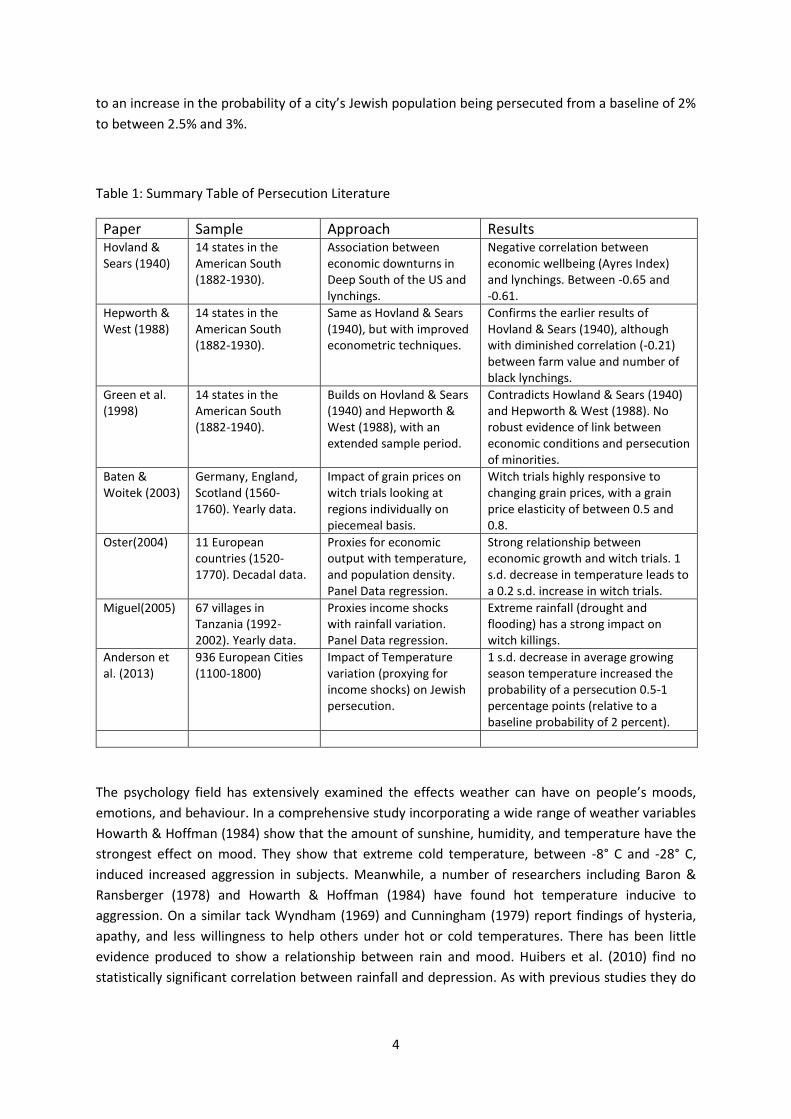
Table 1: Summary Table of Persecution Literature
Paper Sample Approach Results Hovland & Sears (1940)
14 states in the American South (1882-1930).
Association between economic downturns in Deep South of the US and lynchings.
Negative correlation between economic wellbeing (Ayres Index) and lynchings. Between -0.65 and -0.61.
Hepworth & West (1988)
14 states in the American South (1882-1930).
Same as Hovland & Sears (1940), but with improved econometric techniques.
Confirms the earlier results of Hovland & Sears (1940), although with diminished correlation (-0.21) between farm value and number of black lynchings.
Green et al. (1998)
14 states in the American South (1882-1940).
Builds on Hovland & Sears (1940) and Hepworth & West (1988), with an extended sample period.
Contradicts Howland & Sears (1940) and Hepworth & West (1988). No robust evidence of link between economic conditions and persecution of minorities.
Baten & Woitek (2003)
Germany, England, Scotland (1560-1760). Yearly data.
Impact of grain prices on witch trials looking at regions individually on piecemeal basis.
Witch trials highly responsive to changing grain prices, with a grain price elasticity of between 0.5 and 0.8.
Oster(2004) 11 European countries (1520-1770). Decadal data.
Proxies for economic output with temperature, and population density. Panel Data regression.
Strong relationship between economic growth and witch trials. 1 s.d. decrease in temperature leads to a 0.2 s.d. increase in witch trials.
Miguel(2005) 67 villages in Tanzania (1992-2002). Yearly data.
Proxies income shocks with rainfall variation. Panel Data regression.
Extreme rainfall (drought and flooding) has a strong impact on witch killings.
Anderson et al. (2013)
936 European Cities (1100-1800)
Impact of Temperature variation (proxying for income shocks) on Jewish persecution.
1 s.d. decrease in average growing season temperature increased the probability of a persecution 0.5-1 percentage points (relative to a baseline probability of 2 percent).
The psychology field has extensively examined the effects weather can have on people’s moods,
emotions, and behaviour. In a comprehensive study incorporating a wide range of weather variables
Howarth & Hoffman (1984) show that the amount of sunshine, humidity, and temperature have the
strongest effect on mood. They show that extreme cold temperature, between -8° C and -28° C,
induced increased aggression in subjects. Meanwhile, a number of researchers including Baron &
Ransberger (1978) and Howarth & Hoffman (1984) have found hot temperature inducive to
aggression. On a similar tack Wyndham (1969) and Cunningham (1979) report findings of hysteria,
apathy, and less willingness to help others under hot or cold temperatures. There has been little
evidence produced to show a relationship between rain and mood. Huibers et al. (2010) find no
statistically significant correlation between rainfall and depression. As with previous studies they do
5
find a relationship between sunshine and depression however, and so rainfall may be indirectly related
to mood through its correlation with cloud cover.
A number of works have examined the link between weather and witch trials1. Behringer (1995, 1999)
shows that many trials made reference to ‘weather magic’. He documented a number of such cases
such as the remarks made by a contemporary chronicler on the eve of the great 1626-1630 witch hunt
in South Western Germany (Behringer, 1995 p.15) :
“In the year 1626 on the 27th of May, the vineyards of the bishophrics of Bamberg and Wiirzburg in Franconia all froze over, as did the grain fields, which rotted in any case
. . . Everything froze like never before remembered, causing a great inflation . . . There followed great lamentation and pleading among the common rabble, questioning why his princely Grace delayed so long in punishing the sorcerers and witches for
spoiling crops since the beginning of the year.” (Behringer, 1995 p.15)
He also argues that the spikes in witch trials evident in regions such as Scotland, Lorraine, Bar,
Germany, and Switzerland were due to their agrarian dependent economies and high population
densities. In contrast countries like Holland and England were trade centres and not so affected by
weather, while countries in the South of Europe did not suffer the same deterioration in climate.
Pfister (2007) argues that the 1570-1630 cold spell coincided with the wave of witch hunts in
agreement with Oster (2004).
While papers have been done looking at the relationship between weather and witch trials, and
between weather and grain prices the actual channels by which weather effects witch trials have not
been examined in detail. People generally lived closer to nature, whether it be working in the field
during the day or in relatively poorly constructed houses by night. According to (Scott, 2010 p.7) ‘There
were few windows to let in light, and those were small and unglazed. The rooms were unventilated,
unsanitary, cold and damp’. Furthermore ‘Cold weather forced people indoors to spend the long hours
of darkness huddled around whatever sources of heat they could find’. There is little attention given
to these psychological aspects of climate with respect to witch trials however.
In addition to causing considerable damage to property and livestock, the great floods affecting North
Devon and Monmouth in January 1607 also led to considerable loss of life (Jones et al., 1997). Later,
in the storm of 1703 approximately 9,000 people lost their lives in England and Wales (Dukes and
Eden, 1997).
Climate may also impact on the appearance of pests such as locusts (Utterström, 1955), which are
extremely harmful to grain production and as late as 1864 there was an invasion of locusts in England.
The potential impact on the occurrence of disease, in particular the Plague has been slightly less
studied in the literature, but there is some evidence linking it to climate. With the plague there are
two factors to consider. Firstly, the impact on the rats who initially carried the plague and secondly,
the bacteria. The disease results from infection with the plague Bacillus Yersinia pestis and is often
transmitted by fleas. Most mammals can be infected by Yersinia pestis, but rodents are the most
common hosts. The most common vector2 of the plague is Xenopsylla cheopis, the common rat flea
1 A picture depicting witches creating a hailstorm is shown in Appendix 4. 2 In epidemiology, a vector is any agent (person, animal or microorganism) that carries and transmits an infectious pathogen into another living organism.
6
(Raoul et al, 2013; Velimirovic and Velimirovic, 1989) of bubonic plague. There is a clear link between
the plague and temperature. The spread of the disease is checked by temperatures over 26° C, and
cannot exist in epidemic form at temperatures over 27° C. Cold temperatures also limit the plague and
a temperature range of 20-25° C has been judged the most suitable for facilitating the development
of Xenopsylla cheopis (Duncan, 1992). Duncan also observes a link between the spread of the disease
and rainfall, with both excessive and limited humidity being barriers to its spread. Thus the weather
in year t will impact on the bacteria and hence the spread of the plague in the same year.
Oster (2004) uses population density to proxy for economic output, arguing that an economy required
higher economic growth to support a higher population. She finds that higher populations are related
to lower witch trials. Heinshohn & Steiger (2004) put a different interpretation on this relationship
arguing that population stagnation drove accusers and prosecutors to stigmatize birth control3, and
thus to sideline witches.
It seems that there are a number of problems with using population to proxy for prosperity. Population
growth may go together with increased food production and economic output, but it is arguably by
the standard of living of the population which is important not the total output of the economy.
Rather, appealing to Malthusian theory, higher population should lead to declining incomes and that
is broadly what we see over the sample period. Indeed, the rapid population growth of the second
half of the 16th century and beginning of the 17th century, coincided with the worst of the climate
deterioration. Far more influential factors in the evolution of population were war, disease and
migration. The thirty years war in 1618-48 killed as many as 8 million people (Sheikh, 2009). Just
considering England, over half a million people emigrated between 1607-1700 (Foner, 2005).
Population measurement quality may also be an issue. The McEvedy & Jones (1978) data used by
Oster (2004), measured at 50 year intervals may not be optimal to measure the effects of war and
plague on witch trials. It may also be difficult to find population data for the specific region of interest.
This is exemplified in a country like Hungary, where many Hungarians fled the Ottoman invasion to
the Royal Hungary region in the West of the country (Turnbull, 2013). Population growth in the rural
areas, where witch trials were prevalent, may be exaggerated given the increasing urbanization rates.
Additionally, the year by year population changes may be misleading. Disease was a major cause of
these yearly fluctuations in population, and occurring more in cities the effect on rural population may
have been less noticeable. In fact, the effects on rural population may have shown up later as rural
populations moved to the cities to replace the deceased4.
3. Background to the Witch Trials
Notions of witchcraft and witches go back at least as far as Homer’s odyssey in which the character
Circe is called a witch by Odysseus’ companion and later turns his men into pigs (Homer, 1945). The
two books from the old testament, Exodus and Leviticus thought to be written in the 6th century BC
3 Medicine women, often attacked as witches, provided birth control to pregnant women (Ehrenreich, 2010).
4 Large city populations were usually fully repopulated within two years of a major plague outbreak (Yungblut, 2003).
7
(Johnstone, 2003 p.72; Grabbe, 1998 p.92), also make reference to witches: “thou shalt not suffer a
witch to live” (Exodus 22:18, King James Version). The trial of Theoris of Lemmos in Athens circa 338
BC provides an example of an actual documented witch trial in Classical Greece in which the suspect
was tried and burned for necromancy (Collins, 2000).
Witchcraft persecution continued to a greater or lesser extent over the next millennia. By the time of
the early middle ages belief against witches was being actively discouraged. In 789 Charlemagne
proclaimed (Hutton, 1993 p.257):
If anyone, deceived by the Devil, shall believe, as is customary among pagans, that any man or woman is a night-
witch, and eats men, and on that account burn that person to death… he shall be executed.
This policy was not to last, and Charlemagne’s successor Louis the Pious decreed in 829 that anyone
guilty of witchcraft would be executed. Similar laws followed in England and Scotland in the ninth and
10th centuries (Swenson, 2009 p.250).
It was not until the 14th century that witches began to be tried in significant numbers. In the preceding
200 years the Catholic Church had been actively persecuting heretical groups, such as the Cathars and
Waldanesians. At some point though, the state went from persecuting ‘real’ heretics to imaginary
witches (Tremp, 2008). Waldensian regions of central Europe were those to see the first mass trials of
witches. Indeed, in the Savoyard Alps, Waldensian heretics confessed to acts of witchcraft under
interrogation in the early 15th century, and subsequently the Waldensians became synonymous with
sorcery (Herzig, 2010).
Over the next century however, witchcraft came to be seen as a distinct form of heresy. Whereas the
early Swiss witches were predominantly male, as were tried heretics, witchcraft became increasingly
associated with women. While both other heretical groups and witches were in league with the devil
in a plot against Christendom, they remained distinct in that the former were purely doctrinal while
the role of witchcraft was to inflict losses.
“… in the form of daily misfortunes on humans, domestic animals and the fruits of the earth through
the permission of God and with the cooperation of demons.” (Herzig, 2010 p.60)
By the turn of the 16th century the authorities had become more focused on the actual social damage
committed by witches than the aspect of diabolism which had predominated previously (Herzig,
2010).
Although the Church’s stance on witchcraft is mixed, the narrative surrounding witchcraft was
undoubtedly a Christian one. Central to the mythology surrounding witchcraft was the link between
witches and the devil. Christianity’s view of Satan underwent a dramatic change from the times of
the early church to the central middle ages. With the response of the Catholic Church to the Cathars
and Waldesians, and subsequent writings of Thomas Aquinas the devil had gone from mischievous
troublemaker to a deeply sinister figure (Linder, 2005). Martin Luther, a prominent figure in the
reformation, particularly emphasised the dangers of Satan to society (Kors & Peter, 2001 p.261).
Indeed, both protestant and catholic lands persecuted witches with equal fervour.
The church sought to depict the devil similarly to the gods of non christian faiths. So for example, the
goatee beard, the wrinkled skin, the cloven feet and the horns all bear resemblance to the Roman and
8
Greek God Pan and to the Celtic god Cernunnos. Similarly, the female breasts common in English 17th
century depictions of Satan are likely to have derived from the goddess Diana (Levack, 2006 pp.32-
37). It has thus been widely argued that the witches of the middle ages and early modern period were
practicing an ancient fertility religion and in worshipping a horned beastlike god were not worshipping
the devil as depicted in Christianity.
With the approval of Pope Innocent Vlll, the German clergyman Heinrich Kramer published Malleus
Maleficarum (“Hammer of the Witches”) in 1487 detailing the practice of witchcraft, and how best to
catch and prosecute witches. This book was highly influential being reprinted 29 times by 1669 and
translated into many languages. Though officially condemned by the Church in 1490 it was later taken
up by both Protestant and Catholic civil and ecclesiastical judges. It’s sales across Europe were only
rivalled by the bible, until the publication of ‘Pilgrim’s Progress’ in 1678 (Guiley, 2009 p.166).
The invention of the printing press by 1450 allowed Malleus Maleficarum as well as other witchcraft
material to be spread quickly across Europe5. This furnished witches with a vast mythology and
imagery to give pre-existing fears of the population added impetus. Witches were said to fly on
broomsticks (pitchforks for the men) to gather in large congregations. These witch Sabbats would also
usually include the presence of demons or even the devil himself, and the attendees would commit
evil acts such as killing and eating babies and orgies with demons (Bryant, 2004)6. Witches were
believed to have ‘familiars’ which would aid them in their witchcraft. These could be a number of
different types of animals but were usually black dogs or black cats (Wilby, 2005). Another
characteristic associated with witches was that they would have a marking on their body, usually
resembling a wart, which was said to be made by the devil to seal their pact (Guiley, 2009).
The use of torture played a big part in witch trials. Reintroduced into Europe in the mid 13th century,
it’s use became more frequent after Pope Paul ll declared witchcraft crimen excepten7, and allowed
torture to be used without limit (Levack, 2006 p.81, Trevor-Roper, 1969). The frequent use of torture
had the effect of increasing the numbers of victims caught up in the worst panics, as suspects would,
under duress, name others from the region as witches. Under such circumstances suspects also found
themselves confessing to whatever the inquisitor put to them, thus having the effect of confirming to
onlookers the more colourful and lurid activities that witches supposedly got up to. In England where
torture was not used, witch panics were more mild, and the beliefs in the diabolism aspects of witch
trials less apparent (Gijswijt-Hofstra, 1999 p.53). In those cases where torture was routinely used 95%
of defendants were found guilty, compared to less than 50% of cases in England (Levack, 2006 p.87).
The most common form of punishment was execution. On the European continent burning at the
stake was preferred while in England and North America hanging was more common (Bryant, 2004).
Other forms of execution used were breaking on the wheel, drowning, and beheading. Less severe
forms of punishment include exile, imprisonment, and mutilation8 (Pavlac, 2012). Estimates for the
5 Images of the front covers of Malleus Maleficarum and a pamphlet describing a trial in England are shown in Appendix 4. 6 A painting by Francesco Goya depicting the Witches’ sabat is shown in Appendix 4. 7 An exceptional crime of such seriousness that the required level of evidence be lower and normal rights of individuals may be infringed. 8 Removal of an ear or hand.
9
total numbers executed in the 1450-1750 period varies from 35,000 to 100,0009. Given the 30,000
witch accusations collected for this paper and the missing years and regions (See Figure 4 and Table
A1.1 in Appendix 1), as well as taking into account the lost records we would estimate the figure
towards the higher end of this range.
Belief in witchcraft played a big part in people’s everyday lives. Statistics from Macfarlane (1999, p.98),
indicate that the crime of witchcraft was more common than murder, though less common than theft.
During the peak of the witch hunts the impact would have been much greater of course. In Trier, in
present day Germany, a total of 368 individuals were burned alive for witchcraft in 22 villages between
1587 and 1593. In 1585 two villages were left with only one woman remaining in each (Trevor-Roper,
1967 p.139).
The demographic of the accused varied somewhat depending on region. For instance, In Iceland over
90% of witches were men (Burns, 2003 p.140), while for Europe as a whole over 80% were women
(Zika, 2003 p.238). Often unmarried or widowed most were over 50 years of age, and though poor
were not necessarily the poorest of society. The wandering poor do not appear to have been targeted,
other than in the case of the Hapsburg region. (Levack, 2006 pp. 149,156-157). In short the accused
were targeted from among the most vulnerable in society.
Witch trials originated in earnest in the 15th century in the regions of eastern France, Switzerland,
northern Italy, and Southern Germany (Levack, 2006). Over the ensuing years they spread to
encompass almost the entire European continent. In England and the low countries they peaked
around 1580-1610. It is generally the case that the peak of the witch trials came later the further east
one moves. So, in Germany their were still mass witch hunts occurring in 1630 and in Austria, Hungary,
and Russia on towards the end of the 17th and early 18th centuries. In the north in Scandinavia a great
rash of witch trials also took place around the turn of the 18th century. The last witch trial in Europe is
thought to have occurred in Posnan, Poland in 1793 in which two women were executed for
bewitching their neighbours’ cattle (Gijswijt-Hofstra, 1999 p.87)
4. Theory
We approach this from the point of view of the person making the complaint. We will assume a
representative individual who will make a complaint if they believe they will be better off by doing so.
Hence it encompasses the possibility of financial gain and the setting of old scores, but the primary
focus is on the resolution of angst. Against this there are the costs of making a complaint. These
include both the transaction costs, e.g. the time costs and the costs of preparing oneself for an
appearance at the trial. There are also the potential social consequences. Even if the individual is
convicted they may have friends, supporters and family with whom social relationships will
deteriorate. But if the prosecution is not successful, if the individual is found innocent, the social
stigma attached to the complainant may be considerable. Hence the i’th individual will be the subject
of a complaint by the representative individual r over time t if:
9 Monter – 35,000 (Monter, 2002 pp. 6-12); Gaskill – 40,000-50,000 Gaskill (2009, p.76); Levack – 60,000 (Levack, 2006 pp.24-25); Barstow – 100,000 (Barstow, 1995).

10
pitFit + pitArt - (1-pit)Sirt – Trt >0 (1)
where pi is the probability of individual i being found guilty, Fir is the expected financial gain to the
complainant. Ar is the benefit from relieving the angst which we assume is equal to the level of angst.
Sir the expected social stigma following an unsuccessful prosecution, which will be linked to the person
being prosecuted and also includes associated monetary consequences, e.g. the loss of contracts. Tr
is the transaction costs.
Rearranging we can derive a critical level of angst A* above which there will be a witch trial:
A*rt = ((1-pit)/(pit)) Sirt + Trt/pit - Fit (2)
pi is assumed to be a function of the institutional environment of the time (It). At times when witch
trials and guilty verdicts are common people may perceive pit to be relatively high. It will also be a
function of ‘the evidence’ against the target witch. In part this will reflect their individual
characteristics, which in an aggregate time series analysis we will ignore. But in part too they will
depend upon unusual events (Et) such as the Plague, or other epidemics and extreme weather events
such as a violent storm which brings flooding and other damage. In this sense it will be correlated with
angst. But because of the presence of this as part of the critical value which triggers a witch trial, it is
implicit that angst alone is not enough, there has to be a chance of bringing a successful accusation
and hence this is related to the plausibility of linking the underlying cause of the angst to a specific
witch.
The financial gain to individual r, may vary with individual i. The gains may not be limited to the
individual making the accusation, it could impact on much of the local community through, e.g., the
removal of a beggar requiring charity. Its inclusion emphasises that then, as now, some prosecutions
may be bought for reasons linked to financial gain rather than as a direct result of any harm perceived
to have been suffered.
The transaction costs will be different in different locations due, once more, to differences in the
institutional process of bringing a witch prosecution. These differences relate to the number of days
the individual will have to be in the locality of the Court and the part they will play in the proceedings.
In addition the opportunity costs of time are likely to vary. Thus in an emergency such as caused by
war, or the flooding of property, these opportunity costs may be higher and the individual unlikely to
bring a prosecution at this point in time, but at some later date. Hence the impact of extreme events
may be diverse, a long term impact of building up resentment and anger and a short term one related
more to the timing of the prosecution.
We model angst as a function of the extent to which utility, U, falls below expectations:
A= f(U-Ue) if U<Ue (3)
= 0 if U≥Ue
Where Ue is the expected level of utility in the period and place we are studying. In times where we
have consistent economic growth, linking expected utility to the average level of utility might not be
11
a plausible assumption, but for the period we are studying it is. Utility in turn will be a function of living
standards, proxied by GDP per capita (Y), disease (D), and other, non-climatic adverse events (X).
Hence, (3) can be written as:
A= f(Y-Ye, D, X) if U<Ue (4)
where:
Y = Y(|C-Ce|, C, productivity, population, D, War, X)
D = D(C, Y, War) (5)
X = X(C)
Income shocks, Y-Ye, can be viewed as either deviation from a fixed income level or from a moving
average. The latter captures short term shocks such as fluctuations in the business cycle for example,
and assumes that people’s discontent is relative to that of their recent past. A fixed Ye emphasises the
importance of an absolute standard of living which dictates propensity towards persecution. At this
time income shocks in the majority of locations was primarily linked to agricultural shocks. They would
have been functions of both climate shocks (|C-Ce|), and climate, C, per se, but in particular we link
income shocks to climate shocks.
We model shocks as the absolute deviation from the climate norm (Ce). However, there is the potential
for asymmetry in the impact of the climate shock. So for example, a bout of cold weather may cause
a greater increase in witch trials than if it was hotter than normal. In addition, in some cases we have
data on income or agricultural shocks as well as climate shocks. In this case we will be including both
types of shock in the regression.
Thus, combining (4) and (2), the probability of individual i being the subject of a witch trial prosecution
(Pwi) is a function of extreme events and institutional factors:
Pwit = Φ(f(Y-Ye, D,X)- ((1-pit)/pit) Sirt – Trt/pit)) if A>0 (6)
Pwit = Φ(-((1-pit)/pit) Sirt – Trt/pit) if A=0
Where Φ is the cumulative density function of the error terms related to the formulation of both angst
and its critical value. Included in this error term is Fit the financial gain of bringing a witch trial. The
total number of witch trials will then be this probability aggregated across individuals. In a community
the size of N people, the probability of at least one witch trial equals10:
Pwt = 1 − ∏ (1 − 𝑝𝑤𝑖𝑡)𝑁𝑖=1 (7)
and the expected number of witch trials, rather than people being tried, equals:
10 This is the probability of a trial being brought by ‘the representative agent’, but we will equating this to witch trials for the whole population.
12
E(Wt) = ∑ 𝑝𝑤𝑖𝑡𝑁𝑖=1 (8)
and hence also a function of the factors in (6). Witch trials will tend to start with the individual who
maximises 𝑝𝑤𝑖𝑡, then moving to the second most likely and so on. In (8) we order the population in
this way. Thus the expected number of witch trials equals the probability of the most likely witch trial
plus the probability of the second most likely one and so on. Pwit is not independent of the number of
witch trials as it is a function of pit, the probability of a successful witch trial, which because of judicial
capacity constraints will decline with the number of trials occurring at the same time.
We abstract from a number of issues. In particular, a single witch trial may result in multiple
prosecutions because more than one person may be accused. In this case the potential gains and costs
will be more complex and in many cases the type of person bringing the witch trial is different, e.g.
less likely to be a local. We are implicitly assuming, although it makes little difference to the empirical
analysis, that each witch trial involves just one suspect.
We will proxy institutional affects through location and time specific dummy variables. Regardless of
actual institutional factors a high number of recent witch trials will tend to increase perceptions of
their acceptability, the extent of the witch problem and possibly the chances of a successful
prosecution.
Lags are also likely to be important. According to Briggs’ (2007) study on Witchcraft in the Duchy of
Lorraine, the process of persecution of a witch took an average of 10 years, the culmination of which
being the actual trial. It took time for the reputation of an individual to be formed and for critical mass
among the enclosed community to be reached. It was not a costless enterprise for the accuser and
thus they wanted to be sure of community wide support before bringing an official accusation. Lags
could also occur due to time taken for angst to build. One bad harvest, one adverse spell of weather
might not be sufficient for there to be a sufficient degree of angst to trigger a witch trial. But a
sustained series of events might be. The probability of bringing a witch trial would also therefore be a
function of stability of the community. Thus, when the demographic makeup of the community was
affected then the likelihood of a witch trial would diminish. War and plague are both things which
could have an effect, either through death or migration.
13
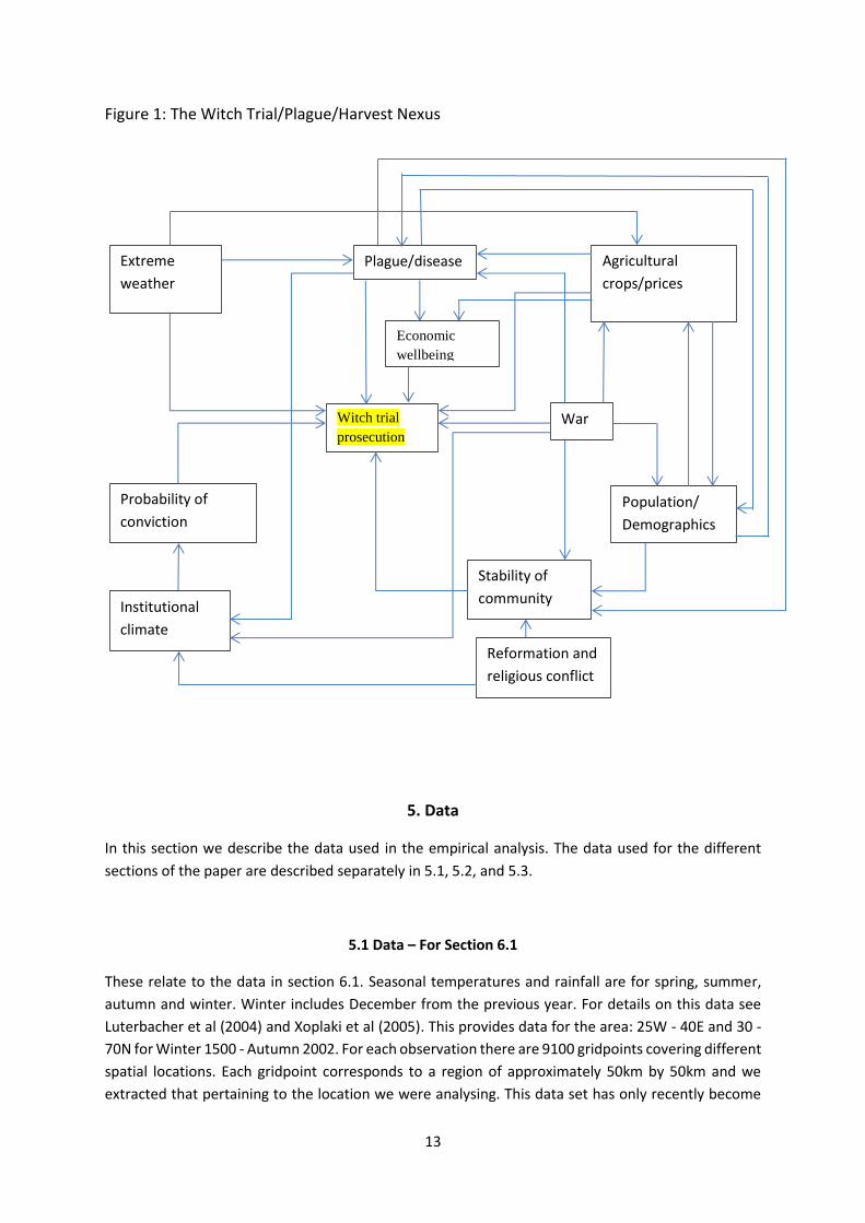
Figure 1: The Witch Trial/Plague/Harvest Nexus
5. Data
In this section we describe the data used in the empirical analysis. The data used for the different
sections of the paper are described separately in 5.1, 5.2, and 5.3.
5.1 Data – For Section 6.1
These relate to the data in section 6.1. Seasonal temperatures and rainfall are for spring, summer,
autumn and winter. Winter includes December from the previous year. For details on this data see
Luterbacher et al (2004) and Xoplaki et al (2005). This provides data for the area: 25W - 40E and 30 -
70N for Winter 1500 - Autumn 2002. For each observation there are 9100 gridpoints covering different
spatial locations. Each gridpoint corresponds to a region of approximately 50km by 50km and we
extracted that pertaining to the location we were analysing. This data set has only recently become
Witch trial
prosecution
Extreme
weather
Agricultural
crops/prices
Plague/disease
War
Population/
Demographics
Institutional
climate
Probability of
conviction
Stability of
community
Reformation and
religious conflict
Economic
wellbeing
14
available and is, as far as we are aware, the first time that seasonal, as well as annual, variations in
climate have been used to analyse witch trials or indeed any historical persecution. We feel this is
important. Annual data can mask substantial seasonal variations, for example a very cold summer and
a very warm winter can cancel each other out. But their impact on the population may not be the
same as that of a normal summer and winter.
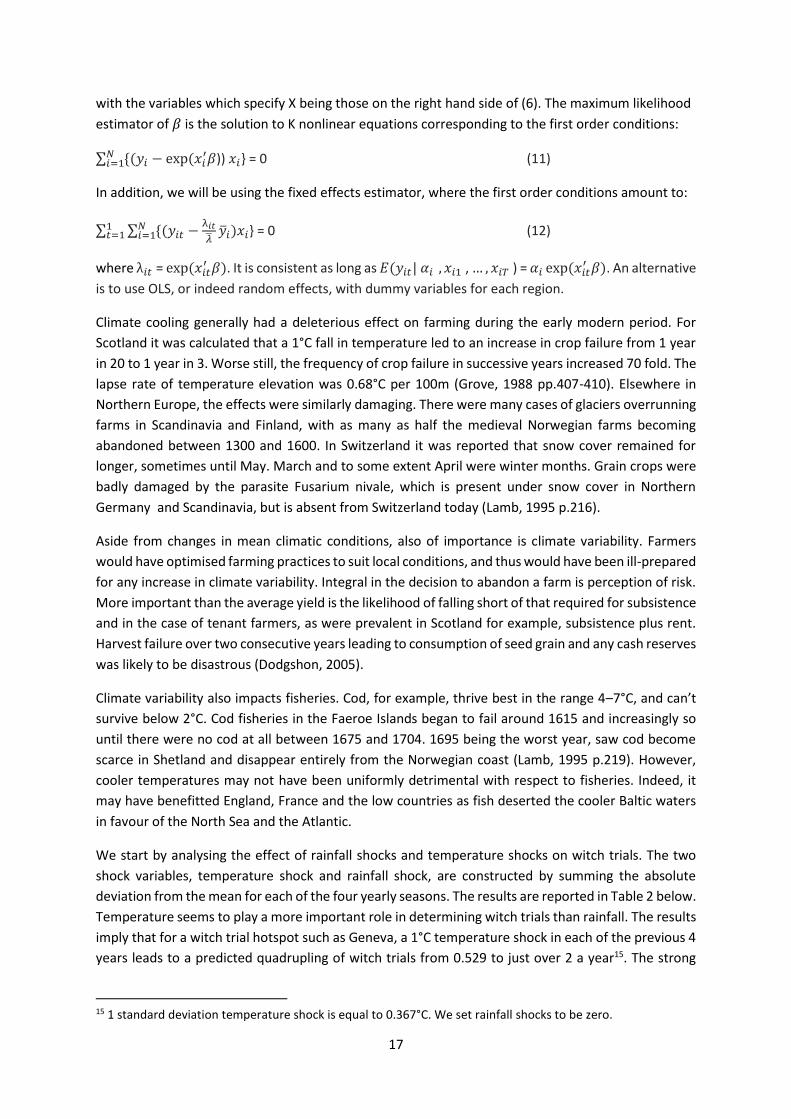
The witch trial data was grouped to correspond with the climate data. In total we have 30,066 witch
trial accusations covering across 355 regions over the period 1500-1760. The location of these regions
for which we have witch trial data is illustrated in Figure 4. The various sources for the witch trial data
are listed in Table A1.1 in Appendix 1. The geographical coverage of the witch trials which took place
in Europe is generally high, with those regions considered to be at the heart of the witch hunt craze,
Germany, Switzerland and North East France (Behringer, 2004 pp.83-164) with very useful tables on
pp 130, 150), particularly well represented.
5.2 Data – For Section 6.2
This relates to the data in the GDP per capita and real wages & grain prices parts of section 6.2. In the
GDP per capita part five regions are considered: Spain, Italy, Holland, England, and Sweden11. For each
country five variables are collated; witch trials, population, GDP per capita, and two binary variables;
Plague epidemics and War. Sources for these variables are provided in Tables A2.1 – A2.5 in Appendix
2. Plague epidemics and war data12 were constructed using the secondary historical sources given.
For the real wages and grain price part, six regions are used: Amsterdam, London, Madrid, Valencia,
Munich and Stockholm. For each region six variables are collated; witch trials, population, real
wages, wheat/rye price shocks, and the two binary variables; Plague epidemics and War. Sources for
these variables are provided in Tables A3.1 – A3.5 in Appendix 3. The harvest quality data for
Sweden comes from Edvinsson (2008).
5.3 Data – For Section 6.3
For this section only England is considered. Much of the data used is the same as for the previous
section. Witch trials, plague, war, population and grain prices are as stated in section 5.2. For real
wages we use two series (Clark, 2007 and Allen, 2001). The business cycle ‘trough’ data comes from
Overton and Van Leeuwen (2012) and the dependency ratio from Wrigley & Schofield (1989, p.447,
Table 10.6).
11 The choice of regions used is dictated by the availability of data. Constructions of yearly GDP per capita data are a recent development with the first, for Holland, published only in 2009. 12 The 80 years war engulfing the Netherlands ran from 1568-1648. It proved difficult to construct our variable for Holland, but we decided to include only the years 1568-1578 since this marked the period from the start of the dutch revolt up until the year 1578 in which the last of the major cities, Amsterdam and Middelburg, declared for the rebels and thus unifying the Holland region (Hart, 2014).
15
6. Empirical Analysis
6.1 Climate and witch trials
We start by using just the weather to explain the incidence of witch trials. This approach follows along
the same lines as Oster (2004), which purports to exploit the relationship between weather and
economic output to predict witch persecution. In addition our study provides a number of innovations.
The high granularity and comprehensiveness of the weather data, both geographically and across
time, allows us to use a much enlarged dataset. In addition for each year we have both rainfall and
temperature observations for spring, summer, autumn and winter.
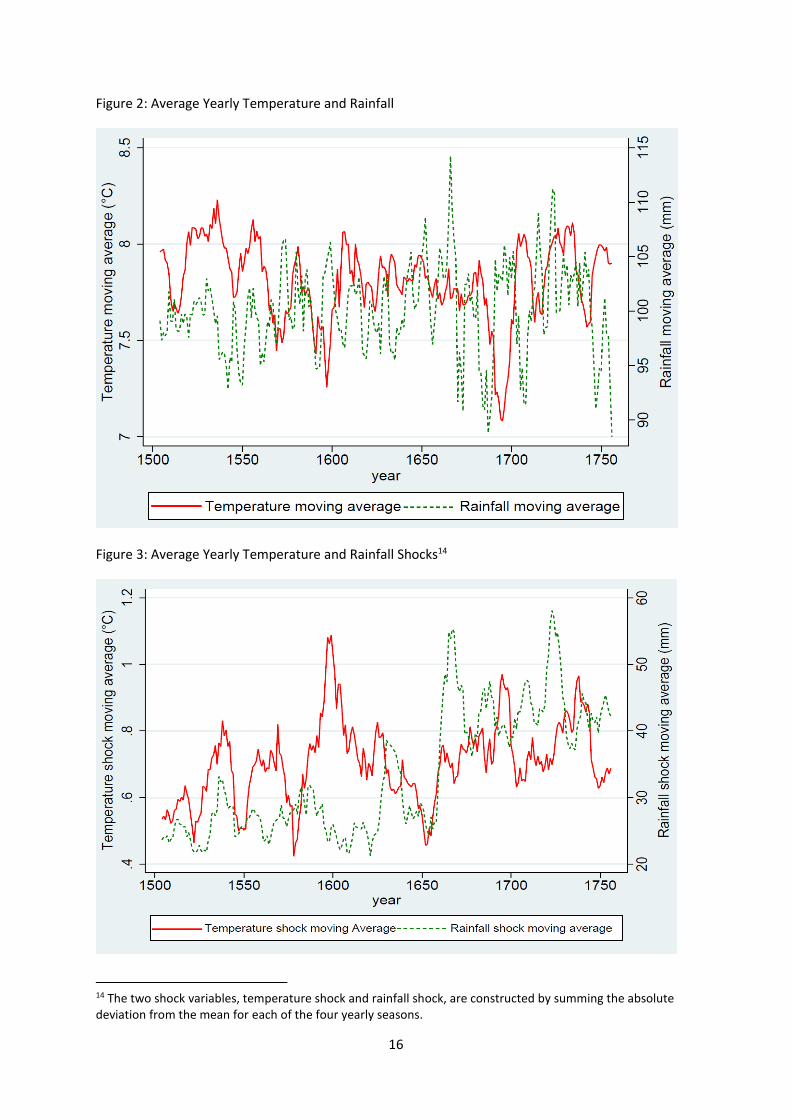
In Figures 2 and 3 we display a summary of the climate variables across our sample. Figure 2 shows
the average temperature and rainfall. We note two troughs in temperature around 1600 and again
around 1700. In Figure 3 we have displayed the average temperature and rainfall shocks. Of note is
the general increase in rainfall variability post 1650 and the peak in temperature around 1600. Also
evident in both charts is the 22 year Hale cycle which has previously been well documented (Newel et
al., 1989).
To model the number of individuals accused of witchcraft a year, we use a Poisson count model for
panel data13. This then gives:
Pr(Y=y) = 𝑒−𝜇𝜇𝑦
𝑦! (9)
Where µ is as defined in (10). In the Poisson regression both the mean and variance of the distribution
equal µ. The Poisson distribution assumes that:
µ = 𝑒𝑋𝑖𝑡′ 𝛽 (10)
13 The poisson fixed effects estimator is consistent and with use of cluster-robust standard errors is likely more robust in our case (Cameron and Trivedi, 2005 pp.667-677). The negative binomial model is designed to address over-dispersion as is present in our dataset. However, the fixed effects model proposed by Hausman et al. (1984), NB1 in Cameron and Traverdi (1986), has been shown to not be a true fixed effects method (Allison and Waterman, 2002). Both NB1 and NB2 give inconsistent results when the distribution is overdispersed but not negative binomial, although the level of bias is much greater in the NB1 case than for NB2. Moreover, Blackburn (2014) discourage the use of either NB1 or NB2 in panel data applications, even when the distribution is negative binomial. The results using the NB2 estimator are presented in appendix 5, and are similar to the poisson case.
16
Figure 2: Average Yearly Temperature and Rainfall
Figure 3: Average Yearly Temperature and Rainfall Shocks14
14 The two shock variables, temperature shock and rainfall shock, are constructed by summing the absolute deviation from the mean for each of the four yearly seasons.
17
with the variables which specify X being those on the right hand side of (6). The maximum likelihood
estimator of 𝛽 is the solution to K nonlinear equations corresponding to the first order conditions:
∑ {(𝑦𝑖 − exp(𝑥𝑖′𝛽𝑁
𝑖=1 ))𝑥𝑖} = 0 (11)
In addition, we will be using the fixed effects estimator, where the first order conditions amount to:
∑ ∑ {(𝑦𝑖𝑡 −λ𝑖𝑡
��𝑁𝑖=1
1𝑡=1 ��𝑖)𝑥𝑖} = 0 (12)
where λ𝑖𝑡 = exp(𝑥𝑖𝑡′ 𝛽). It is consistent as long as 𝐸(𝑦𝑖𝑡|𝛼𝑖, 𝑥𝑖1, … , 𝑥𝑖𝑇) = 𝛼𝑖exp(𝑥𝑖𝑡
′ 𝛽). An alternative
is to use OLS, or indeed random effects, with dummy variables for each region.
Climate cooling generally had a deleterious effect on farming during the early modern period. For
Scotland it was calculated that a 1°C fall in temperature led to an increase in crop failure from 1 year
in 20 to 1 year in 3. Worse still, the frequency of crop failure in successive years increased 70 fold. The
lapse rate of temperature elevation was 0.68°C per 100m (Grove, 1988 pp.407-410). Elsewhere in
Northern Europe, the effects were similarly damaging. There were many cases of glaciers overrunning
farms in Scandinavia and Finland, with as many as half the medieval Norwegian farms becoming
abandoned between 1300 and 1600. In Switzerland it was reported that snow cover remained for
longer, sometimes until May. March and to some extent April were winter months. Grain crops were
badly damaged by the parasite Fusarium nivale, which is present under snow cover in Northern
Germany and Scandinavia, but is absent from Switzerland today (Lamb, 1995 p.216).
Aside from changes in mean climatic conditions, also of importance is climate variability. Farmers
would have optimised farming practices to suit local conditions, and thus would have been ill-prepared
for any increase in climate variability. Integral in the decision to abandon a farm is perception of risk.
More important than the average yield is the likelihood of falling short of that required for subsistence
and in the case of tenant farmers, as were prevalent in Scotland for example, subsistence plus rent.
Harvest failure over two consecutive years leading to consumption of seed grain and any cash reserves
was likely to be disastrous (Dodgshon, 2005).
Climate variability also impacts fisheries. Cod, for example, thrive best in the range 4–7°C, and can’t
survive below 2°C. Cod fisheries in the Faeroe Islands began to fail around 1615 and increasingly so
until there were no cod at all between 1675 and 1704. 1695 being the worst year, saw cod become
scarce in Shetland and disappear entirely from the Norwegian coast (Lamb, 1995 p.219). However,
cooler temperatures may not have been uniformly detrimental with respect to fisheries. Indeed, it
may have benefitted England, France and the low countries as fish deserted the cooler Baltic waters
in favour of the North Sea and the Atlantic.
We start by analysing the effect of rainfall shocks and temperature shocks on witch trials. The two
shock variables, temperature shock and rainfall shock, are constructed by summing the absolute
deviation from the mean for each of the four yearly seasons. The results are reported in Table 2 below.
Temperature seems to play a more important role in determining witch trials than rainfall. The results
imply that for a witch trial hotspot such as Geneva, a 1°C temperature shock in each of the previous 4
years leads to a predicted quadrupling of witch trials from 0.529 to just over 2 a year15. The strong
15 1 standard deviation temperature shock is equal to 0.367°C. We set rainfall shocks to be zero.
18
significance in all specifications of temperature shocks, in particular, for the four proceeding years to
the witch trial casts light on the length of time the witch persecution took, indicating a witch hunt did
not happen overnight, perhaps too the decision to commit an individual to trial was a culmination of
a number of years of angst.
Figure 4. Locations of Witch Trials
The figure shows the locations for which we have witch trial data over the sample period.
Our finding regarding the extended duration of witch persecution is consistent with existing literature
on this subject. Macfarlane (1999, pp.95,103,109), describes how persecutions against a witch lasted
as long as 10 years and that the trial itself was often only the final stage in a process which may have
also included threatening the witch and setting fire to the thatch of the suspect’s house. Briggs (2007,
pp.153-179) discusses the complicated process by which a community passed judgement on who was
and was not a witch. It was a process whereby women, for it was they who concerned themselves
with the business of reputational gossip, felt one another out regarding in which direction community
opinion was moving. Immunity from being suspected often relied on support from others in the
community and it may not always have been clear how much support a given individual could
command. Therefore it paid to be cautious in helping to form public opinion, for fear of reprisals if a
groundswell of support was not forthcoming.
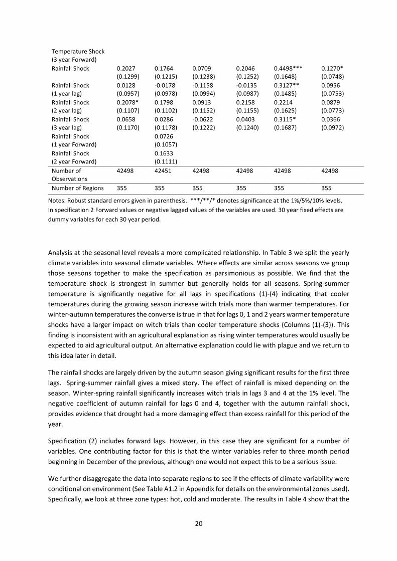
In specification (2) we use the temperature and rainfall occurring in the years after the trials had
concluded as a robustness check to ensure that the significance of the lagged terms is not attributable
to a general correlation of these variables between years. The lack of significance indicates that this is
19
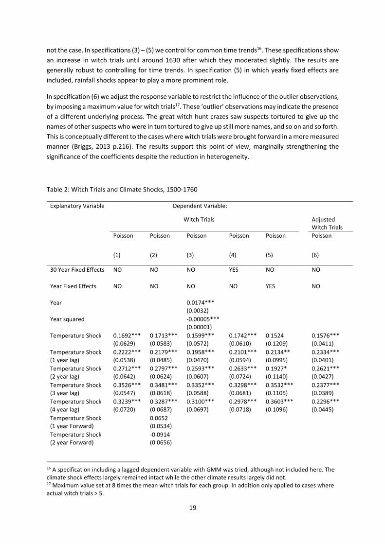
not the case. In specifications (3) – (5) we control for common time trends16. These specifications show
an increase in witch trials until around 1630 after which they moderated slightly. The results are
generally robust to controlling for time trends. In specification (5) in which yearly fixed effects are
included, rainfall shocks appear to play a more prominent role.
In specification (6) we adjust the response variable to restrict the influence of the outlier observations,
by imposing a maximum value for witch trials17. These ‘outlier’ observations may indicate the presence
of a different underlying process. The great witch hunt crazes saw suspects tortured to give up the
names of other suspects who were in turn tortured to give up still more names, and so on and so forth.
This is conceptually different to the cases where witch trials were brought forward in a more measured
manner (Briggs, 2013 p.216). The results support this point of view, marginally strengthening the
significance of the coefficients despite the reduction in heterogeneity.
Table 2: Witch Trials and Climate Shocks, 1500-1760
Explanatory Variable Dependent Variable:
Witch Trials
Adjusted Witch Trials
Poisson Poisson Poisson Poisson Poisson Poisson
(1) (2) (3) (4) (5) (6)
30 Year Fixed Effects NO NO NO YES NO NO
Year Fixed Effects NO NO NO NO YES NO
Year 0.0174*** (0.0032)
Year squared -0.00005*** (0.00001)
Temperature Shock 0.1692*** (0.0629)
0.1713*** (0.0583)
0.1599*** (0.0572)
0.1742*** (0.0610)
0.1524 (0.1209)
0.1576*** (0.0411)
Temperature Shock (1 year lag)
0.2222*** (0.0538)
0.2179*** (0.0485)
0.1958*** (0.0470)
0.2101*** (0.0594)
0.2134** (0.0995)
0.2334*** (0.0401)
Temperature Shock (2 year lag)
0.2712*** (0.0642)
0.2797*** (0.0624)
0.2593*** (0.0607)
0.2633*** (0.0724)
0.1927* (0.1140)
0.2621*** (0.0427)
Temperature Shock (3 year lag)
0.3526*** (0.0547)
0.3481*** (0.0618)
0.3352*** (0.0588)
0.3298*** (0.0681)
0.3532*** (0.1105)
0.2377*** (0.0389)
Temperature Shock (4 year lag)
0.3239*** (0.0720)
0.3287*** (0.0687)
0.3100*** (0.0697)
0.2978*** (0.0718)
0.3603*** (0.1096)
0.2296*** (0.0445)
Temperature Shock (1 year Forward)
0.0652 (0.0534)
Temperature Shock (2 year Forward)
-0.0914 (0.0656)
16 A specification including a lagged dependent variable with GMM was tried, although not included here. The climate shock effects largely remained intact while the other climate results largely did not. 17 Maximum value set at 8 times the mean witch trials for each group. In addition only applied to cases where actual witch trials > 5.
20
Temperature Shock (3 year Forward)
Rainfall Shock 0.2027 (0.1299)
0.1764 (0.1215)
0.0709 (0.1238)
0.2046 (0.1252)
0.4498*** (0.1648)
0.1270* (0.0748)
Rainfall Shock (1 year lag)
0.0128 (0.0957)
-0.0178 (0.0978)
-0.1158 (0.0994)
-0.0135 (0.0987)
0.3127** (0.1485)
0.0956 (0.0753)
Rainfall Shock (2 year lag)
0.2078* (0.1107)
0.1798 (0.1102)
0.0913 (0.1152)
0.2158 (0.1155)
0.2214 (0.1625)
0.0879 (0.0773)
Rainfall Shock (3 year lag)
0.0658 (0.1170)
0.0286 (0.1178)
-0.0622 (0.1222)
0.0403 (0.1240)
0.3115* (0.1687)
0.0366 (0.0972)
Rainfall Shock (1 year Forward)
0.0726 (0.1057)
Rainfall Shock (2 year Forward)
0.1633 (0.1111)
Number of Observations
42498 42451 42498 42498 42498 42498
Number of Regions 355 355 355 355 355 355
0.1713*** (0.0622)
Notes: Robust standard errors given in parenthesis. ***/**/* denotes significance at the 1%/5%/10% levels.
In specification 2 Forward values or negative lagged values of the variables are used. 30 year fixed effects are
dummy variables for each 30 year period.
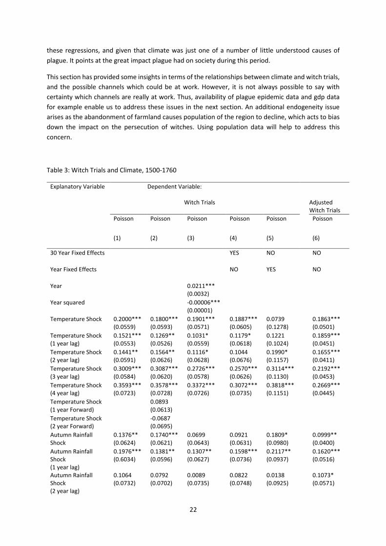
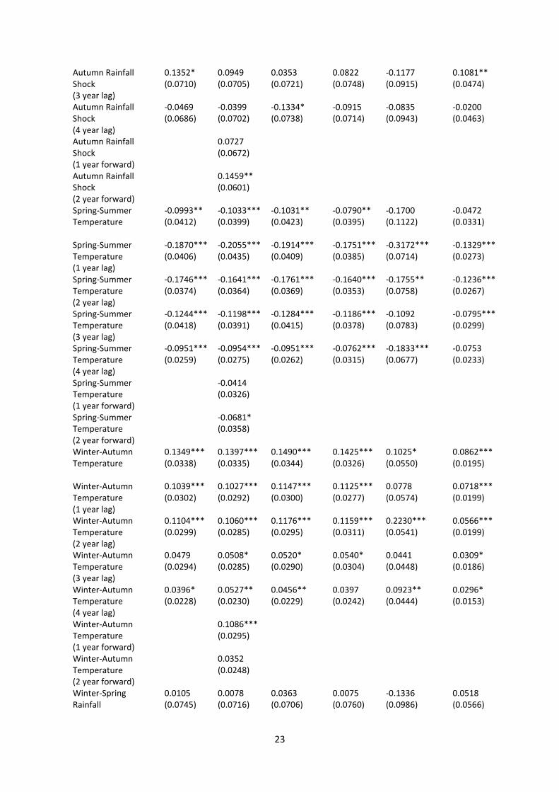
Analysis at the seasonal level reveals a more complicated relationship. In Table 3 we split the yearly
climate variables into seasonal climate variables. Where effects are similar across seasons we group
those seasons together to make the specification as parsimonious as possible. We find that the
temperature shock is strongest in summer but generally holds for all seasons. Spring-summer
temperature is significantly negative for all lags in specifications (1)-(4) indicating that cooler
temperatures during the growing season increase witch trials more than warmer temperatures. For
winter-autumn temperatures the converse is true in that for lags 0, 1 and 2 years warmer temperature
shocks have a larger impact on witch trials than cooler temperature shocks (Columns (1)-(3)). This
finding is inconsistent with an agricultural explanation as rising winter temperatures would usually be
expected to aid agricultural output. An alternative explanation could lie with plague and we return to
this idea later in detail.
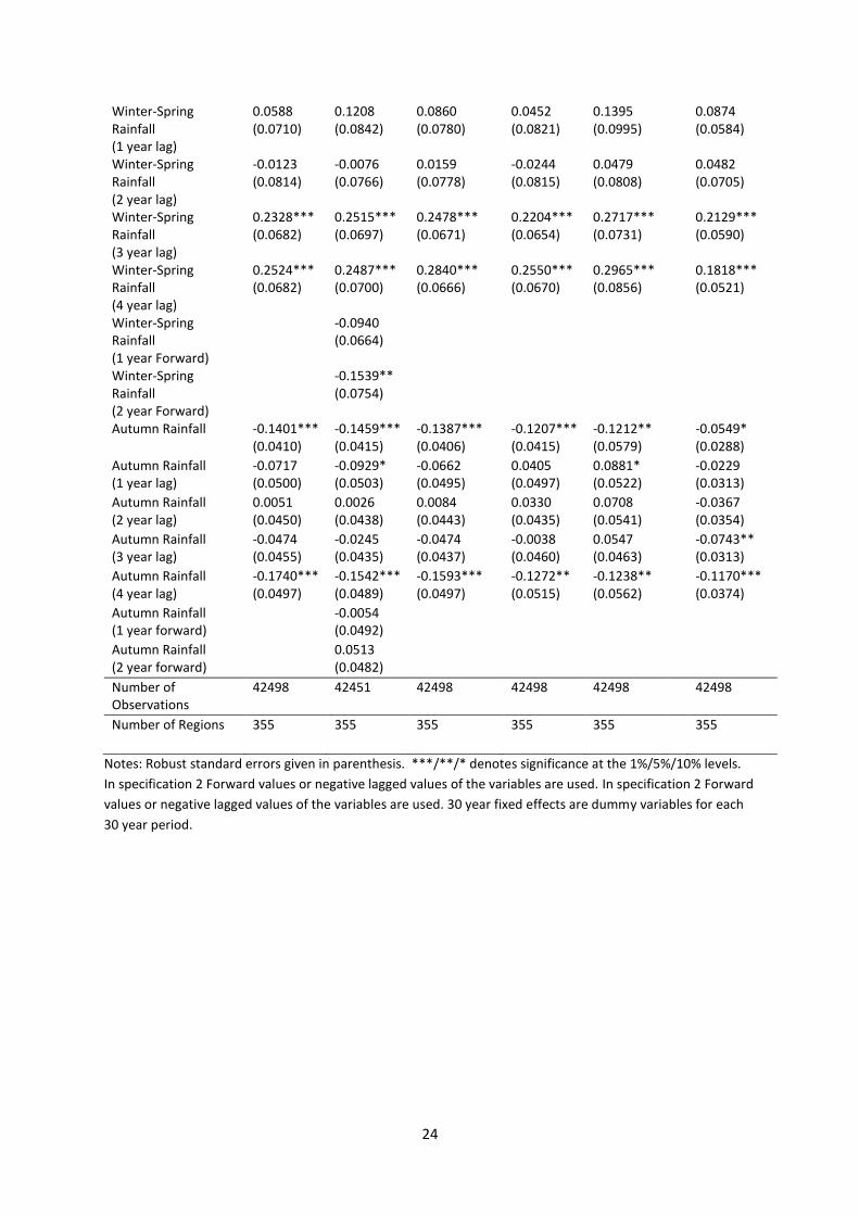
The rainfall shocks are largely driven by the autumn season giving significant results for the first three
lags. Spring-summer rainfall gives a mixed story. The effect of rainfall is mixed depending on the
season. Winter-spring rainfall significantly increases witch trials in lags 3 and 4 at the 1% level. The
negative coefficient of autumn rainfall for lags 0 and 4, together with the autumn rainfall shock,
provides evidence that drought had a more damaging effect than excess rainfall for this period of the
year.
Specification (2) includes forward lags. However, in this case they are significant for a number of
variables. One contributing factor for this is that the winter variables refer to three month period
beginning in December of the previous, although one would not expect this to be a serious issue.
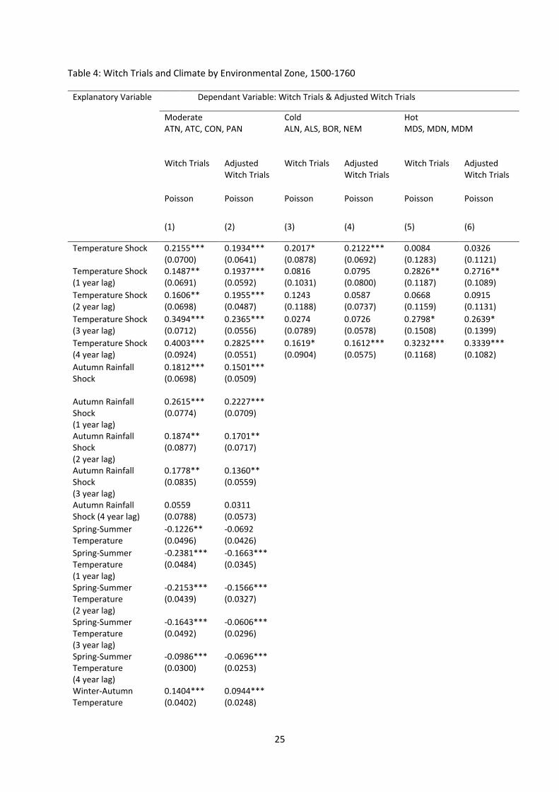
We further disaggregate the data into separate regions to see if the effects of climate variability were
conditional on environment (See Table A1.2 in Appendix for details on the environmental zones used).
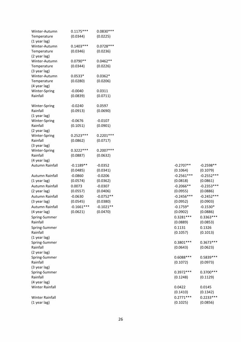
Specifically, we look at three zone types: hot, cold and moderate. The results in Table 4 show that the
21
overall results are largely driven by the moderate region. The significant coefficients for autumn
rainfall shock are stronger than for the overall sample. Additionally, the variables spring-summer
temperature and winter-autumn temperature are only significant in the moderate region. While
strongest in the moderate region there is also evidence for a temperature shock effect in the
remaining regions, with significant coefficients for lags 0 and 4 in the cold region and 1,3 and 4 in the
hot region. The hot region also demonstrates a sensitivity to rainfall, with witch trials increasing with
rainy winter-springs and dry autumns.
While noting the smaller standard errors in the moderate region’s results, possibly owing to the
greater sample size, there are also other reasons why this region may show a greater reliance on
climate. The moderate region would have had both arable and pastoral activity whereas the colder
region was mainly pastoral. Animals are homeostatic which means they can adapt within a range of
temperatures and therefore the region should be less sensitive to climatic variation. The hot region
would have also had arable farming, but cold was not such a limiting factor. It was far less likely that
it would have caused land to be abandoned and may even have been a benefit in some areas. The lack
of any clear effect assigned to increasing temperature in the warmer Mediterranean zones, aside from
a lack of sample size, could be ascribed to the less severe implications of the little ice age. Whereas
northern Europe was often at the margin of usability of the land, this is unlikely to have been the case
further south. Indeed for the hottest parts a cooler climate may have been a benefit to agriculture.
Previously, we noted that plague may have a part to play in explaining the incidence of witch trials.
The effect may move in either direction. On the one hand incidence of plague may disrupt normal life
including the workings of the legal system (Behringer, 2003 p.209) as well as of society. In so much as
people may interact less, this reduces the scope for slanderous gossip and interaction with potential
witches. On the other hand, witches may be branded ‘plague spreaders’ (Monter, 1976 pp. 44-45) or
more indirectly society may be so brutalized by the sudden loss of so many of the population that
people may turn more violent. Indeed, arguments have been put forward that ‘the mass mortality
cheapened life and thus increased warfare, crime, popular revolt, waves of flagellants, and
persecutions against the Jews’ (Cohn, 2002). In Table 3 the positive coefficient of winter-autumn
temperatures are consistent with plague acting to increase witch trials, as colder winters help to
constrain the spread of the rat flea carrier Xenopsylla cheopis (Appleby, 1980).
We would also expect very high temperatures to restrict plague incidence, and indirectly test for this
in Table 5. Xenopsylla cheopis is not sustainable above 25°C and therefore we test the effect of
summer temperature above 22°C18. Summer temperature is significantly negative for lags 1-3 implying
that higher temperatures decrease witch trials in all specifications. Specification (2) includes forward
lags for summer temperature as a robustness check, and both coefficients are insignificant. In
specification (4) we include spring temperatures as a further robustness check to distinguish
agricultural effects from plague effects. Spring and summer both constitute the growing season in
these warmer climes, and tend to have similar effects on farming. Since spring temperatures are too
low, they should not have an effect through the plague channel. The results show spring temperature
is indeed not significant. These results for plague are quite striking given the limited sample size for
18 This is an average temperature so during the daytime temperatures would exceed 25°C.
22
these regressions, and given that climate was just one of a number of little understood causes of
plague. It points at the great impact plague had on society during this period.
This section has provided some insights in terms of the relationships between climate and witch trials,
and the possible channels which could be at work. However, it is not always possible to say with
certainty which channels are really at work. Thus, availability of plague epidemic data and gdp data
for example enable us to address these issues in the next section. An additional endogeneity issue
arises as the abandonment of farmland causes population of the region to decline, which acts to bias
down the impact on the persecution of witches. Using population data will help to address this
concern.
Table 3: Witch Trials and Climate, 1500-1760
Explanatory Variable Dependent Variable: Witch Trials
Adjusted Witch Trials
Poisson Poisson Poisson Poisson Poisson Poisson
(1) (2) (3) (4) (5) (6)
30 Year Fixed Effects YES NO NO
Year Fixed Effects NO YES NO
Year 0.0211*** (0.0032)
Year squared -0.00006*** (0.00001)
Temperature Shock 0.2000*** (0.0559)
0.1800*** (0.0593)
0.1901*** (0.0571)
0.1887*** (0.0605)
0.0739 (0.1278)
0.1863*** (0.0501)
Temperature Shock (1 year lag)
0.1521*** (0.0553)
0.1269** (0.0526)
0.1031* (0.0559)
0.1179* (0.0618)
0.1221 (0.1024)
0.1859*** (0.0451)
Temperature Shock (2 year lag)
0.1441** (0.0591)
0.1564** (0.0626)
0.1116* (0.0628)
0.1044 (0.0676)
0.1990* (0.1157)
0.1655*** (0.0411)
Temperature Shock (3 year lag)
0.3009*** (0.0584)
0.3087*** (0.0620)
0.2726*** (0.0578)
0.2570*** (0.0626)
0.3114*** (0.1130)
0.2192*** (0.0453)
Temperature Shock (4 year lag)
0.3593*** (0.0723)
0.3578*** (0.0728)
0.3372*** (0.0726)
0.3072*** (0.0735)
0.3818*** (0.1151)
0.2669*** (0.0445)
Temperature Shock (1 year Forward)
0.0893 (0.0613)
Temperature Shock (2 year Forward)
-0.0687 (0.0695)
Autumn Rainfall Shock
0.1376** (0.0624)
0.1740*** (0.0621)
0.0699 (0.0643)
0.0921 (0.0631)
0.1809* (0.0980)
0.0999** (0.0400)
Autumn Rainfall Shock (1 year lag)
0.1976*** (0.6034)
0.1381** (0.0596)
0.1307** (0.0627)
0.1598*** (0.0736)
0.2117** (0.0937)
0.1620*** (0.0516)
Autumn Rainfall Shock (2 year lag)
0.1064 (0.0732)
0.0792 (0.0702)
0.0089 (0.0735)
0.0822 (0.0748)
0.0138 (0.0925)
0.1073* (0.0571)
23
Autumn Rainfall Shock (3 year lag)
0.1352* (0.0710)
0.0949 (0.0705)
0.0353 (0.0721)
0.0822 (0.0748)
-0.1177 (0.0915)
0.1081** (0.0474)
Autumn Rainfall Shock (4 year lag)
-0.0469 (0.0686)
-0.0399 (0.0702)
-0.1334* (0.0738)
-0.0915 (0.0714)
-0.0835 (0.0943)
-0.0200 (0.0463)
Autumn Rainfall Shock (1 year forward)
0.0727 (0.0672)
Autumn Rainfall Shock (2 year forward)
0.1459** (0.0601)
Spring-Summer Temperature
-0.0993** (0.0412)
-0.1033*** (0.0399)
-0.1031** (0.0423)
-0.0790** (0.0395)
-0.1700 (0.1122)
-0.0472 (0.0331)
Spring-Summer Temperature (1 year lag)
-0.1870*** (0.0406)
-0.2055*** (0.0435)
-0.1914*** (0.0409)
-0.1751*** (0.0385)
-0.3172*** (0.0714)
-0.1329*** (0.0273)
Spring-Summer Temperature (2 year lag)
-0.1746*** (0.0374)
-0.1641*** (0.0364)
-0.1761*** (0.0369)
-0.1640*** (0.0353)
-0.1755** (0.0758)
-0.1236*** (0.0267)
Spring-Summer Temperature (3 year lag)
-0.1244*** (0.0418)
-0.1198*** (0.0391)
-0.1284*** (0.0415)
-0.1186*** (0.0378)
-0.1092 (0.0783)
-0.0795*** (0.0299)
Spring-Summer Temperature (4 year lag)
-0.0951*** (0.0259)
-0.0954*** (0.0275)
-0.0951*** (0.0262)
-0.0762*** (0.0315)
-0.1833*** (0.0677)
-0.0753 (0.0233)
Spring-Summer Temperature (1 year forward)
-0.0414 (0.0326)
Spring-Summer Temperature (2 year forward)
-0.0681* (0.0358)
Winter-Autumn Temperature
0.1349*** (0.0338)
0.1397*** (0.0335)
0.1490*** (0.0344)
0.1425*** (0.0326)
0.1025* (0.0550)
0.0862*** (0.0195)
Winter-Autumn Temperature (1 year lag)
0.1039*** (0.0302)
0.1027*** (0.0292)
0.1147*** (0.0300)
0.1125*** (0.0277)
0.0778 (0.0574)
0.0718*** (0.0199)
Winter-Autumn Temperature (2 year lag)
0.1104*** (0.0299)
0.1060*** (0.0285)
0.1176*** (0.0295)
0.1159*** (0.0311)
0.2230*** (0.0541)
0.0566*** (0.0199)
Winter-Autumn Temperature (3 year lag)
0.0479 (0.0294)
0.0508* (0.0285)
0.0520* (0.0290)
0.0540* (0.0304)
0.0441 (0.0448)
0.0309* (0.0186)
Winter-Autumn Temperature (4 year lag)
0.0396* (0.0228)
0.0527** (0.0230)
0.0456** (0.0229)
0.0397 (0.0242)
0.0923** (0.0444)
0.0296* (0.0153)
Winter-Autumn Temperature (1 year forward)
0.1086*** (0.0295)
Winter-Autumn Temperature (2 year forward)
0.0352 (0.0248)
Winter-Spring Rainfall
0.0105 (0.0745)
0.0078 (0.0716)
0.0363 (0.0706)
0.0075 (0.0760)
-0.1336 (0.0986)
0.0518 (0.0566)
24
Winter-Spring Rainfall (1 year lag)
0.0588 (0.0710)
0.1208 (0.0842)
0.0860 (0.0780)
0.0452 (0.0821)
0.1395 (0.0995)
0.0874 (0.0584)
Winter-Spring Rainfall (2 year lag)
-0.0123 (0.0814)
-0.0076 (0.0766)
0.0159 (0.0778)
-0.0244 (0.0815)
0.0479 (0.0808)
0.0482 (0.0705)
Winter-Spring Rainfall (3 year lag)
0.2328*** (0.0682)
0.2515*** (0.0697)
0.2478*** (0.0671)
0.2204*** (0.0654)
0.2717*** (0.0731)
0.2129*** (0.0590)
Winter-Spring Rainfall (4 year lag)
0.2524*** (0.0682)
0.2487*** (0.0700)
0.2840*** (0.0666)
0.2550*** (0.0670)
0.2965*** (0.0856)
0.1818*** (0.0521)
Winter-Spring Rainfall (1 year Forward)
-0.0940 (0.0664)
Winter-Spring Rainfall (2 year Forward)
-0.1539** (0.0754)
Autumn Rainfall -0.1401*** (0.0410)
-0.1459*** (0.0415)
-0.1387*** (0.0406)
-0.1207*** (0.0415)
-0.1212** (0.0579)
-0.0549* (0.0288)
Autumn Rainfall (1 year lag)
-0.0717 (0.0500)
-0.0929* (0.0503)
-0.0662 (0.0495)
0.0405 (0.0497)
0.0881* (0.0522)
-0.0229 (0.0313)
Autumn Rainfall (2 year lag)
0.0051 (0.0450)
0.0026 (0.0438)
0.0084 (0.0443)
0.0330 (0.0435)
0.0708 (0.0541)
-0.0367 (0.0354)
Autumn Rainfall (3 year lag)
-0.0474 (0.0455)
-0.0245 (0.0435)
-0.0474 (0.0437)
-0.0038 (0.0460)
0.0547 (0.0463)
-0.0743** (0.0313)
Autumn Rainfall (4 year lag)
-0.1740*** (0.0497)
-0.1542*** (0.0489)
-0.1593*** (0.0497)
-0.1272** (0.0515)
-0.1238** (0.0562)
-0.1170*** (0.0374)
Autumn Rainfall (1 year forward)
-0.0054 (0.0492)
Autumn Rainfall (2 year forward)
0.0513 (0.0482)
Number of Observations
42498 42451 42498 42498 42498 42498
Number of Regions 355 355 355 355 355 355
Notes: Robust standard errors given in parenthesis. ***/**/* denotes significance at the 1%/5%/10% levels.
In specification 2 Forward values or negative lagged values of the variables are used. In specification 2 Forward
values or negative lagged values of the variables are used. 30 year fixed effects are dummy variables for each
30 year period.
25
Table 4: Witch Trials and Climate by Environmental Zone, 1500-1760
Explanatory Variable Dependant Variable: Witch Trials & Adjusted Witch Trials
Moderate ATN, ATC, CON, PAN
Cold ALN, ALS, BOR, NEM
Hot MDS, MDN, MDM
Witch Trials Adjusted Witch Trials
Witch Trials Adjusted Witch Trials
Witch Trials Adjusted Witch Trials
Poisson Poisson Poisson Poisson Poisson Poisson
(1) (2) (3) (4) (5) (6)
Temperature Shock 0.2155*** (0.0700)
0.1934*** (0.0641)
0.2017* (0.0878)
0.2122*** (0.0692)
0.0084 (0.1283)
0.0326 (0.1121)
Temperature Shock (1 year lag)
0.1487** (0.0691)
0.1937*** (0.0592)
0.0816 (0.1031)
0.0795 (0.0800)
0.2826** (0.1187)
0.2716** (0.1089)
Temperature Shock (2 year lag)
0.1606** (0.0698)
0.1955*** (0.0487)
0.1243 (0.1188)
0.0587 (0.0737)
0.0668 (0.1159)
0.0915 (0.1131)
Temperature Shock (3 year lag)
0.3494*** (0.0712)
0.2365*** (0.0556)
0.0274 (0.0789)
0.0726 (0.0578)
0.2798* (0.1508)
0.2639* (0.1399)
Temperature Shock (4 year lag)
0.4003*** (0.0924)
0.2825*** (0.0551)
0.1619* (0.0904)
0.1612*** (0.0575)
0.3232*** (0.1168)
0.3339*** (0.1082)
Autumn Rainfall Shock
0.1812*** (0.0698)
0.1501*** (0.0509)
Autumn Rainfall Shock (1 year lag)
0.2615*** (0.0774)
0.2227*** (0.0709)
Autumn Rainfall Shock (2 year lag)
0.1874** (0.0877)
0.1701** (0.0717)
Autumn Rainfall Shock (3 year lag)
0.1778** (0.0835)
0.1360** (0.0559)
Autumn Rainfall Shock (4 year lag)
0.0559 (0.0788)
0.0311 (0.0573)
Spring-Summer Temperature
-0.1226** (0.0496)
-0.0692 (0.0426)
Spring-Summer Temperature (1 year lag)
-0.2381*** (0.0484)
-0.1663*** (0.0345)
Spring-Summer Temperature (2 year lag)
-0.2153*** (0.0439)
-0.1566*** (0.0327)
Spring-Summer Temperature (3 year lag)
-0.1643*** (0.0492)
-0.0606*** (0.0296)
Spring-Summer Temperature (4 year lag)
-0.0986*** (0.0300)
-0.0696*** (0.0253)
Winter-Autumn Temperature
0.1404*** (0.0402)
0.0944*** (0.0248)
26
Winter-Autumn Temperature (1 year lag)
0.1175*** (0.0344)
0.0830*** (0.0225)
Winter-Autumn Temperature (2 year lag)
0.1403*** (0.0346)
0.0728*** (0.0236)
Winter-Autumn Temperature (3 year lag)
0.0790** (0.0344)
0.0462** (0.0226)
Winter-Autumn Temperature (4 year lag)
0.0533* (0.0280)
0.0362* (0.0206)
Winter-Spring Rainfall
-0.0040 (0.0839)
0.0311 (0.0711)
Winter-Spring Rainfall (1 year lag)
-0.0240 (0.0913)
0.0597 (0.0690)
Winter-Spring Rainfall (2 year lag)
-0.0676 (0.1051)
-0.0107 (0.0901)
Winter-Spring Rainfall (3 year lag)
0.2523*** (0.0862)
0.2201*** (0.0717)
Winter-Spring Rainfall (4 year lag)
0.3222*** (0.0887)
0.2007*** (0.0632)
Autumn Rainfall -0.1189** (0.0485)
-0.0352 (0.0341)
-0.2707** (0.1064)
-0.2598** (0.1079)
Autumn Rainfall (1 year lag)
-0.0860 (0.0574)
-0.0206 (0.0362)
-0.2561*** (0.0818)
-0.2552*** (0.0861)
Autumn Rainfall (2 year lag)
0.0073 (0.0557)
-0.0307 (0.0406)
-0.2066** (0.0955)
-0.2353*** (0.0886)
Autumn Rainfall (3 year lag)
-0.0630 (0.0545)
-0.0752** (0.0380)
-0.2456*** (0.0952)
-0.2452*** (0.0903)
Autumn Rainfall (4 year lag)
-0.1661*** (0.0621)
-0.1021** (0.0470)
-0.1759* (0.0902)
-0.1530* (0.0886)
Spring-Summer Rainfall
0.3281*** (0.0889)
0.3363*** (0.0853)
Spring-Summer Rainfall (1 year lag)
0.1131 (0.1057)
0.1326 (0.1013)
Spring-Summer Rainfall (2 year lag)
0.3801*** (0.0643)
0.3673*** (0.0623)
Spring-Summer Rainfall (3 year lag)
0.6088*** (0.1072)
0.5839*** (0.0973)
Spring-Summer Rainfall (4 year lag)
0.3972*** (0.1248)
0.3700*** (0.1129)
Winter Rainfall 0.0422 (0.1410)
0.0145 (0.1342)
Winter Rainfall (1 year lag)
0.2771*** (0.1025)
0.2233*** (0.0856)
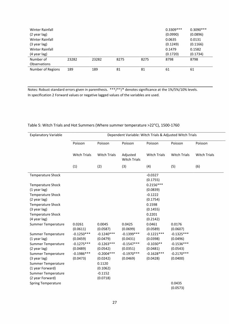
27
Winter Rainfall (2 year lag)
0.3309*** (0.0990)
0.3090*** (0.0896)
Winter Rainfall (3 year lag)
0.0635 (0.1249)
0.0131 (0.1166)
Winter Rainfall (4 year lag)
0.1479 (0.1720)
0.1582 (0.1734)
Number of Observations
23282 23282 8275 8275 8798 8798
Number of Regions 189 189 81 81 61 61
Notes: Robust standard errors given in parenthesis. ***/**/* denotes significance at the 1%/5%/10% levels.
In specification 2 Forward values or negative lagged values of the variables are used.
Table 5: Witch Trials and Hot Summers (Where summer temperature >22°C), 1500-1760
Explanatory Variable Dependent Variable: Witch Trials & Adjusted Witch Trials
Poisson Poisson Poisson Poisson Poisson Poisson
Witch Trials Witch Trials Adjusted Witch Trials
Witch Trials Witch Trials Witch Trials
(1) (2) (3) (4) (5) (6)
Temperature Shock -0.0327 (0.1755)
Temperature Shock (1 year lag)
0.2156*** (0.0839)
Temperature Shock (2 year lag)
-0.1222 (0.1754)
Temperature Shock (3 year lag)
0.1598 (0.1455)
Temperature Shock (4 year lag)
0.2201 (0.2142)
Summer Temperature 0.0261 (0.0611)
0.0045 (0.0587)
0.0425 (0.0699)
0.0461 (0.0589)
0.0176 (0.0607)
Summer Temperature (1 year lag)
-0.1250*** (0.0459)
-0.1240*** (0.0479)
-0.1399*** (0.0431)
-0.1221*** (0.0398)
-0.1325*** (0.0496)
Summer Temperature (2 year lag)
-0.1275*** (0.0489)
-0.1263*** (0.0542)
-0.1547*** (0.0351)
-0.1030** (0.0481)
-0.1536*** (0.0543)
Summer Temperature (3 year lag)
-0.1986*** (0.0473)
-0.2004*** (0.0242)
-0.1970*** (0.0469)
-0.1628*** (0.0428)
-0.2170*** (0.0400)
Summer Temperature (1 year Forward)
0.1120 (0.1062)
Summer Temperature (2 year Forward)
-0.1152 (0.0718)
Spring Temperature
0.0435 (0.0573)
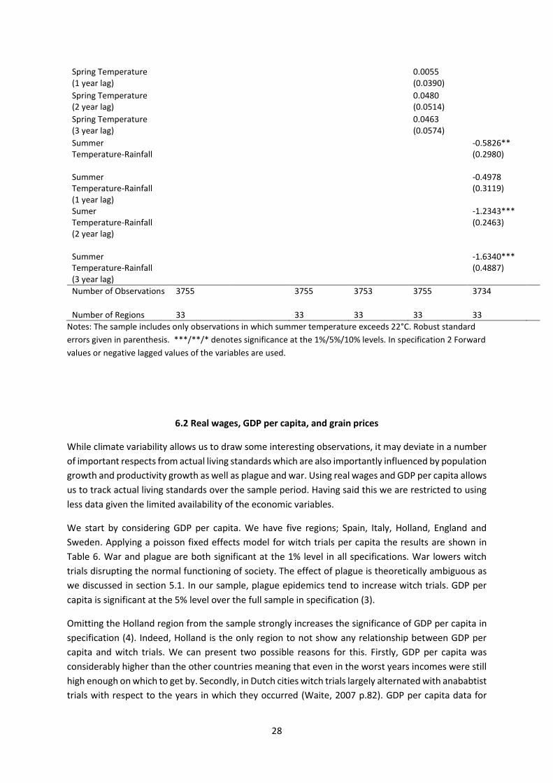
28
Spring Temperature (1 year lag)
0.0055 (0.0390)
Spring Temperature (2 year lag)
0.0480 (0.0514)
Spring Temperature (3 year lag)
0.0463 (0.0574)
Summer Temperature-Rainfall
-0.5826** (0.2980)
Summer Temperature-Rainfall (1 year lag)
-0.4978 (0.3119)
Sumer Temperature-Rainfall (2 year lag)
-1.2343*** (0.2463)
Summer Temperature-Rainfall (3 year lag)
-1.6340*** (0.4887)
Number of Observations 3755 3755 3753 3755 3734
Number of Regions 33 33 33 33 33
Notes: The sample includes only observations in which summer temperature exceeds 22°C. Robust standard
errors given in parenthesis. ***/**/* denotes significance at the 1%/5%/10% levels. In specification 2 Forward
values or negative lagged values of the variables are used.
6.2 Real wages, GDP per capita, and grain prices
While climate variability allows us to draw some interesting observations, it may deviate in a number
of important respects from actual living standards which are also importantly influenced by population
growth and productivity growth as well as plague and war. Using real wages and GDP per capita allows
us to track actual living standards over the sample period. Having said this we are restricted to using
less data given the limited availability of the economic variables.
We start by considering GDP per capita. We have five regions; Spain, Italy, Holland, England and
Sweden. Applying a poisson fixed effects model for witch trials per capita the results are shown in
Table 6. War and plague are both significant at the 1% level in all specifications. War lowers witch
trials disrupting the normal functioning of society. The effect of plague is theoretically ambiguous as
we discussed in section 5.1. In our sample, plague epidemics tend to increase witch trials. GDP per
capita is significant at the 5% level over the full sample in specification (3).
Omitting the Holland region from the sample strongly increases the significance of GDP per capita in
specification (4). Indeed, Holland is the only region to not show any relationship between GDP per
capita and witch trials. We can present two possible reasons for this. Firstly, GDP per capita was
considerably higher than the other countries meaning that even in the worst years incomes were still
high enough on which to get by. Secondly, in Dutch cities witch trials largely alternated with anababtist
trials with respect to the years in which they occurred (Waite, 2007 p.82). GDP per capita data for
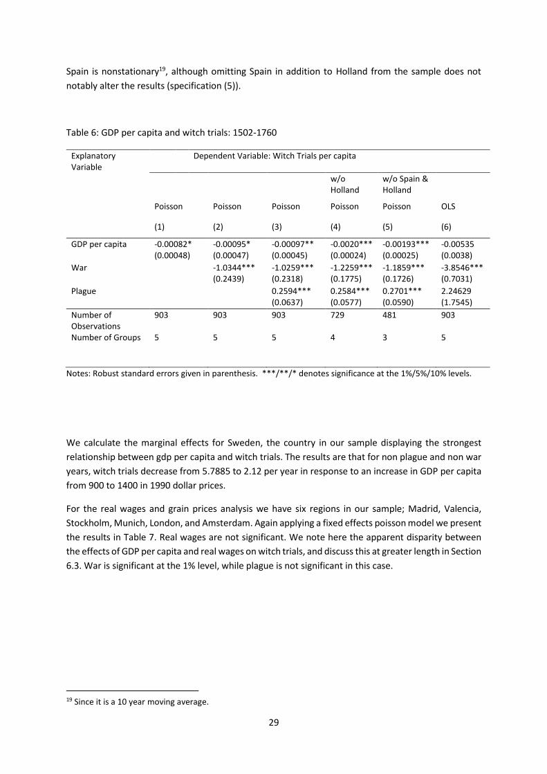
29
Spain is nonstationary19, although omitting Spain in addition to Holland from the sample does not
notably alter the results (specification (5)).
Table 6: GDP per capita and witch trials: 1502-1760
Explanatory Variable
Dependent Variable: Witch Trials per capita
w/o Holland
w/o Spain & Holland
Poisson Poisson Poisson Poisson Poisson OLS
(1) (2) (3) (4) (5) (6)
GDP per capita -0.00082* (0.00048)
-0.00095* (0.00047)
-0.00097** (0.00045)
-0.0020*** (0.00024)
-0.00193*** (0.00025)
-0.00535 (0.0038)
War -1.0344*** (0.2439)
-1.0259*** (0.2318)
-1.2259*** (0.1775)
-1.1859*** (0.1726)
-3.8546*** (0.7031)
Plague 0.2594*** (0.0637)
0.2584*** (0.0577)
0.2701*** (0.0590)
2.24629 (1.7545)
Number of Observations
903 903 903 729 481 903
Number of Groups 5 5 5 4 3 5
Notes: Robust standard errors given in parenthesis. ***/**/* denotes significance at the 1%/5%/10% levels.
We calculate the marginal effects for Sweden, the country in our sample displaying the strongest
relationship between gdp per capita and witch trials. The results are that for non plague and non war
years, witch trials decrease from 5.7885 to 2.12 per year in response to an increase in GDP per capita
from 900 to 1400 in 1990 dollar prices.
For the real wages and grain prices analysis we have six regions in our sample; Madrid, Valencia,
Stockholm, Munich, London, and Amsterdam. Again applying a fixed effects poisson model we present
the results in Table 7. Real wages are not significant. We note here the apparent disparity between
the effects of GDP per capita and real wages on witch trials, and discuss this at greater length in Section
6.3. War is significant at the 1% level, while plague is not significant in this case.
19 Since it is a 10 year moving average.
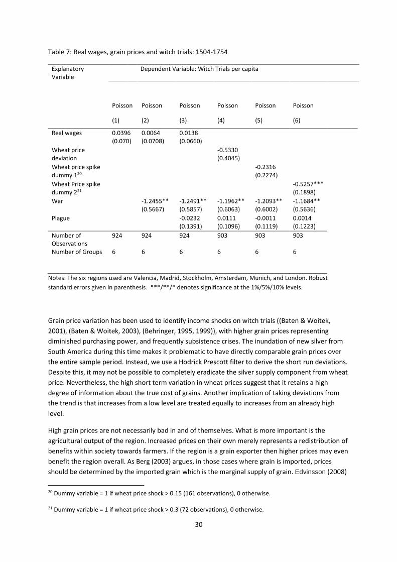
30
Table 7: Real wages, grain prices and witch trials: 1504-1754
Explanatory Variable
Dependent Variable: Witch Trials per capita
Poisson Poisson Poisson Poisson Poisson Poisson
(1) (2) (3) (4) (5) (6)
Real wages 0.0396 (0.070)
0.0064 (0.0708)
0.0138 (0.0660)
Wheat price deviation
-0.5330 (0.4045)
Wheat price spike dummy 120
-0.2316 (0.2274)
Wheat Price spike dummy 221
-0.5257*** (0.1898)
War -1.2455** (0.5667)
-1.2491** (0.5857)
-1.1962** (0.6063)
-1.2093** (0.6002)
-1.1684** (0.5636)
Plague -0.0232 (0.1391)
0.0111 (0.1096)
-0.0011 (0.1119)
0.0014 (0.1223)
Number of Observations
924 924 924 903 903 903
Number of Groups 6 6 6 6 6 6
Notes: The six regions used are Valencia, Madrid, Stockholm, Amsterdam, Munich, and London. Robust
standard errors given in parenthesis. ***/**/* denotes significance at the 1%/5%/10% levels.
Grain price variation has been used to identify income shocks on witch trials ((Baten & Woitek,
2001), (Baten & Woitek, 2003), (Behringer, 1995, 1999)), with higher grain prices representing
diminished purchasing power, and frequently subsistence crises. The inundation of new silver from
South America during this time makes it problematic to have directly comparable grain prices over
the entire sample period. Instead, we use a Hodrick Prescott filter to derive the short run deviations.
Despite this, it may not be possible to completely eradicate the silver supply component from wheat
price. Nevertheless, the high short term variation in wheat prices suggest that it retains a high
degree of information about the true cost of grains. Another implication of taking deviations from
the trend is that increases from a low level are treated equally to increases from an already high
level.
High grain prices are not necessarily bad in and of themselves. What is more important is the
agricultural output of the region. Increased prices on their own merely represents a redistribution of
benefits within society towards farmers. If the region is a grain exporter then higher prices may even
benefit the region overall. As Berg (2003) argues, in those cases where grain is imported, prices
should be determined by the imported grain which is the marginal supply of grain. Edvinsson (2008)
20 Dummy variable = 1 if wheat price shock > 0.15 (161 observations), 0 otherwise. 21 Dummy variable = 1 if wheat price shock > 0.3 (72 observations), 0 otherwise.
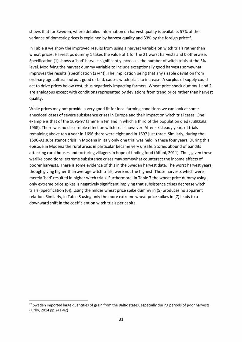
31
shows that for Sweden, where detailed information on harvest quality is available, 57% of the
variance of domestic prices is explained by harvest quality and 33% by the foreign price22.
In Table 8 we show the improved results from using a harvest variable on witch trials rather than
wheat prices. Harvest pc dummy 1 takes the value of 1 for the 21 worst harvests and 0 otherwise.
Specification (1) shows a ‘bad’ harvest significantly increases the number of witch trials at the 5%
level. Modifying the harvest dummy variable to include exceptionally good harvests somewhat
improves the results (specification (2)-(4)). The implication being that any sizable deviation from
ordinary agricultural output, good or bad, causes witch trials to increase. A surplus of supply could
act to drive prices below cost, thus negatively impacting farmers. Wheat price shock dummy 1 and 2
are analogous except with conditions represented by deviations from trend price rather than harvest
quality.
While prices may not provide a very good fit for local farming conditions we can look at some
anecdotal cases of severe subsistence crises in Europe and their impact on witch trial cases. One
example is that of the 1696-97 famine in Finland in which a third of the population died (Jutikkala,
1955). There was no discernible effect on witch trials however. After six steady years of trials
remaining above ten a year in 1696 there were eight and in 1697 just three. Similarly, during the
1590-93 subsistence crisis in Modena in Italy only one trial was held in these four years. During this
episode in Modena the rural areas in particular became very unsafe. Stories abound of bandits
attacking rural houses and torturing villagers in hope of finding food (Alfani, 2011). Thus, given these
warlike conditions, extreme subsistence crises may somewhat counteract the income effects of
poorer harvests. There is some evidence of this in the Sweden harvest data. The worst harvest years,
though giving higher than average witch trials, were not the highest. Those harvests which were
merely ‘bad’ resulted in higher witch trials. Furthermore, in Table 7 the wheat price dummy using
only extreme price spikes is negatively significant implying that subsistence crises decrease witch
trials (Specification (6)). Using the milder wheat price spike dummy in (5) produces no apparent
relation. Similarly, in Table 8 using only the more extreme wheat price spikes in (7) leads to a
downward shift in the coefficient on witch trials per capita.
22 Sweden imported large quantities of grain from the Baltic states, especially during periods of poor harvests (Kirby, 2014 pp.241-42)
32
Table 8: Witch Trials, Harvest Quality and Wheat prices in Sweden, 1665-1754
Explanatory Variable
Dependent Variable: Witch Trials per capita
Poisson Poisson Poisson Poisson Poisson Poisson Poisson
(1) (2) (3) (4) (5) (6) (7)
Harvest pc index Dummy 1
0.4069** (0.1643)
Harvest pc index Dummy 2
0.4483*** (0.1545)
0.4586*** (0.1526)
0.4452*** (0.1509)
Wheat price shock Dummy 1
0.3463** (0.1726)
Wheat price shock Dummy 2
0.2925* (0.1599)
Wheat price shock Dummy 3
0.0699 (0.1822)
War -0.6322* (0.3365)
-0.6497* (0.3367)
-0.6565** (0.3241)
-0.5924* (0.3234)
-0.6374* (0.3604)
Plague -0.5436* (0.3253)
-0.5372 (0.2871)
-0.6519** (0.2836)
-0.6235* (0.3251)
Number of Observations
90 90 90 90 90 90 90
Notes: Robust standard errors given in parenthesis. ***/**/* denotes significance at the 1%/5%/10% levels. ‘Harvest pc index Dummy 1’ takes a value of 1 for the 21
worst harvests, and 0 otherwise. ‘Harvest pc index Dummy 2’ takes the value of 1 for the 17 best harvests, the 21 worst harvests, and 0 otherwise. Analogously, ‘Wheat
price shock Dummy 1’ takes a value of 1 for the 21 biggest positive wheat price deviations from trend, and 0 otherwise. ‘Wheat price shock Dummy 2’ takes the value of 1
for the 17 biggest positive wheat price deviations, the 21 biggest negative wheat price deviations from trend, and 0 otherwise. ‘Wheat price shock Dummy 3’ for the 5
biggest positive wheat price deviations (>0.3).
33
6.3 England
We devote a section looking at the English case in particular owing to the quality of the data. In
addition to the variables considered already we also have the dependency ratio (nonworking age-
working age population ratio), business cycle troughs, real wages for various occupations, and a highly
detailed population series. We also have available GDP data disaggregated by sector.
We present the results in Table 9. GDP per capita significantly affects witch trials per capita in all
specifications. Business cycle troughs represent short term downturns in the economy and its
significance at the 5% level in specification (2) indicates that short run economy dynamics are
important in determining witch trials. Cycle troughs lagged one year are significantly negative
indicating that witch trials are lower in the first year of the upswing phase of the cycle. Combining GDP
per capita and business cycle troughs in the same specification in (4) leads to a weakening in
significance of both variables due to multicolinearity, and lack of sample size. However, evidence
remains that both the long run level of GDP per capita and short run downturns affect persecution.
The results imply that witch trials in trough years were almost double those in non-trough years23.
Plague lagged one year is significantly negatively related to witch trials. This differs to results in the
previous section, suggesting that the belief of whether plague was thought to be caused by witches
may have differed across countries. We have noted previously how witches were accused of ‘plague
spreading’ in Switzerland. In England, on the other hand, witches were not thought to be responsible
for plague which is consistent with our results (Macfarlane, 1999 pp.179-180). Plague may be
indirectly acting to reduce witch trials if it reduces the number of dependents and surplus labour. Real
wages and GDP per capita substantially increased following the Black Death in 1348-1349 (Broadberry
et al., 2010). Localised plague outbreaks in Essex may have impacted regional economic conditions
not picked up in national GDP per capita figures. While ‘War’ is significant it should be noted that there
was only one year, 1648, in which conflict occurred in Essex.
Of interest is the different effect of the variables GDP per capita and real wages on witch trials. While
they are both ostensibly measures of economic wellbeing, GDP per capita seems to display a strong
relationship with witch trials while real wages do not. Figure 5 compares the evolution of different
series of real wages with GDP per capita over 1500-1700. It is clear that GDP per capita grew more
rapidly than any of the measures of real wages. Indeed, for farm workers real wages were by 1675, at
the end of our sample and by which point witch trials were dying out, still below their level of the
1580’s when the witch trials were at their peak.
Angeles (2008) finds that the divergence between real wages and GDP per capita can largely be
explained by an increase in per capita labour hours worked. This reflects not only the increase in days
worked per year by existing workers but is also consistent with the entry into the labour market of
women. Muldrew (2012) documents the importance of advancements in the spinning industry during
the 17th century. Overall, employment from spinning increased from 225,083 in 1580 to 481,564 in
1700. Furthermore, spinning was largely done by single women and women and children of poorer
23 Using the specification in (6) and assuming the year to be without plague, predicted witch trials in non-trough years are 16.5 per million population, increasing to 29.35 in trough years.
34
families. This source of income would have been significant – a 42% increase in the case of married
women- and could well have been the difference keeping these women from having to beg from their
neighbours. The evolution of the spinning industry could be particularly pertinent for our sample given
that many of the towns and villages in which the witch trials occurred were dependent on it
(Macfarlane, 1999 p.149).
The increase in per capita labour supply makes it problematic to use the Williamson Index24 as a
measure of inequality. Nevertheless it does seem that inequality did increase during this period
(Hoffman et al., 2002). One factor which may have ameliorated the effects of low wages was the
development of the poor laws in the 17th century.
The population had grown strongly, as in much of Europe, doubling over the 16th Century. The rapid
expansion was greater than the economy could absorb, and during the latter part of the century in
particular reports of unemployment were frequent. The dissolution of the monasteries, from 1536-
1541, with the reformation, ‘left a huge vacuum’ in aid for the poor according to Slack (1990a). As an
example, at Westminster Abbey the monks distributed £400 per annum, or 10% of the Abbey’s gross
income, to the poor of Westminster and London (Harvey, 1993).
The actions of government to deal with the increasing strain from overpopulation were initially
inclined towards severity. Poor law acts were passed in 1552, 1563, 1572, and 1576 with the 1572 act,
coinciding with the first year of elevated witch trials, calling for offenders to be bored through the ear
for a first offence. The poor law of 1597 was more compassionate in nature, and established overseers
for the poor. Funding for the poor relief after 1597 came from landowners, and thus represents a form
of redistribution of wealth between different strata’s of society and thus effectively supplementing
the incomes of the poor.
Early poor rates and workhouses were less comprehensive than in later years. It was not until 1660
that the coverage of the poor laws really took off with poor rates reaching 1% of national income in
1750 enabling 8% of the population to take relief (Slack, 1990a p.45). Nevertheless, these early efforts
must have helped to some degree in shifting the responsibility of care for the poor from individuals to
the state.
Another factor related to economic hardship is the dependency ratio. Those families close to the
subsistence level could well be pushed beyond their means by increased dependants (Norberg, 1985
pp.104-107). A graphical representation, in Figure 6, would indeed seem to indicate a relationship
between the dependency ratio and witch trials.
24 Proposed by Williamson (1997), the Williamson Index is an inequality index defined as a ratio between the GDP per capita or per worker and the unskilled wage.
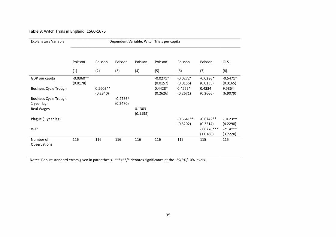
35
Table 9: Witch Trials in England, 1560-1675
Explanatory Variable Dependent Variable: Witch Trials per capita
Poisson Poisson Poisson Poisson Poisson Poisson Poisson OLS
(1) (2) (3) (4) (5) (6) (7) (8)
GDP per capita -0.0360** (0.0178)
-0.0271* (0.0157)
-0.0272* (0.0156)
-0.0286* (0.0155)
-0.5471* (0.3165)
Business Cycle Trough 0.5602** (0.2840)
0.4428* (0.2626)
0.4552* (0.2671)
0.4334 (0.2666)
9.5864 (6.9079)
Business Cycle Trough 1 year lag
-0.4786* (0.2470)
Real Wages 0.1303 (0.1155)
Plague (1 year lag) -0.6641** (0.3202)
-0.6742** (0.3214)
-10.23** (4.2298)
War -22.776*** (1.0188)
-21.4*** (3.7220)
Number of Observations
116 116 116 116 116 115 115 115
Notes: Robust standard errors given in parenthesis. ***/**/* denotes significance at the 1%/5%/10% levels.
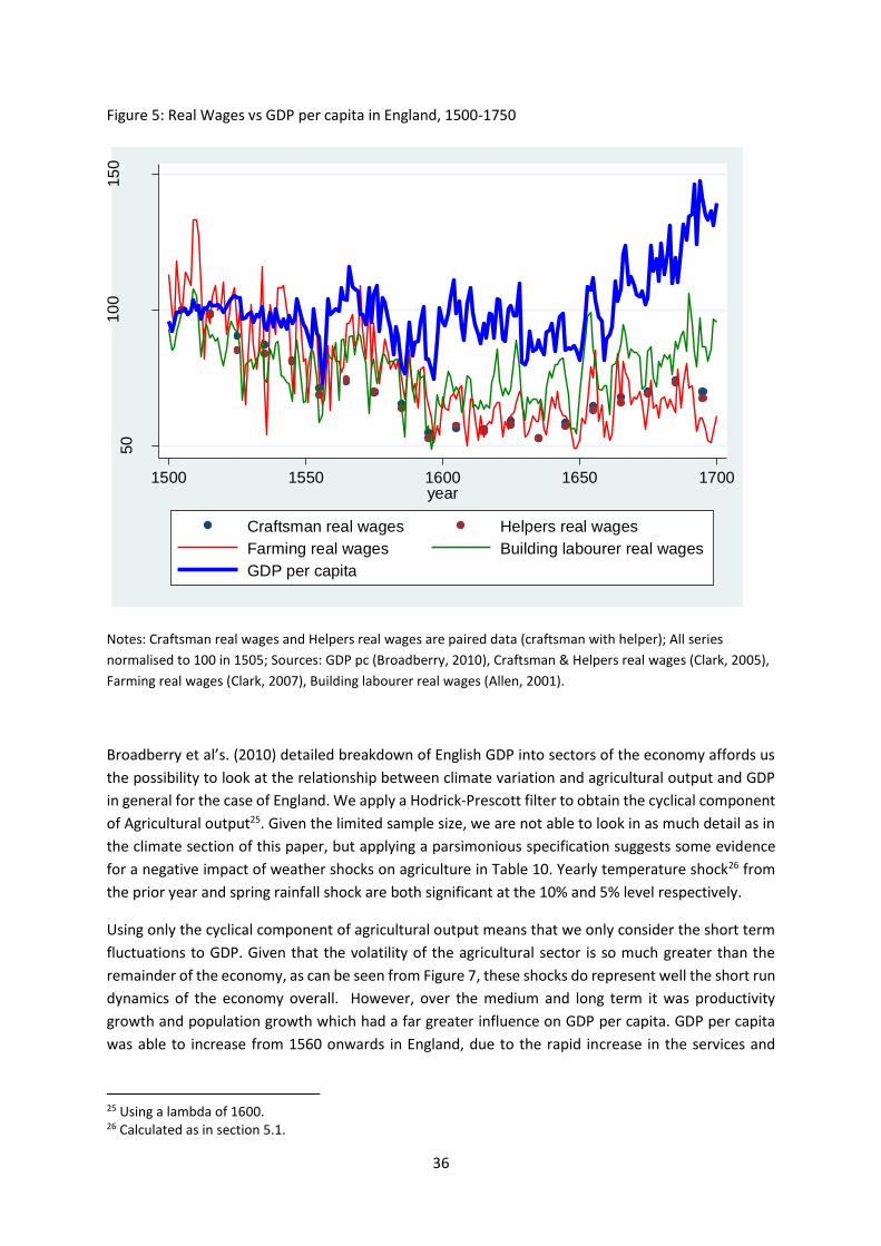
36
Figure 5: Real Wages vs GDP per capita in England, 1500-1750
Notes: Craftsman real wages and Helpers real wages are paired data (craftsman with helper); All series
normalised to 100 in 1505; Sources: GDP pc (Broadberry, 2010), Craftsman & Helpers real wages (Clark, 2005),
Farming real wages (Clark, 2007), Building labourer real wages (Allen, 2001).
Broadberry et al’s. (2010) detailed breakdown of English GDP into sectors of the economy affords us
the possibility to look at the relationship between climate variation and agricultural output and GDP
in general for the case of England. We apply a Hodrick-Prescott filter to obtain the cyclical component
of Agricultural output25. Given the limited sample size, we are not able to look in as much detail as in
the climate section of this paper, but applying a parsimonious specification suggests some evidence
for a negative impact of weather shocks on agriculture in Table 10. Yearly temperature shock26 from
the prior year and spring rainfall shock are both significant at the 10% and 5% level respectively.
Using only the cyclical component of agricultural output means that we only consider the short term
fluctuations to GDP. Given that the volatility of the agricultural sector is so much greater than the
remainder of the economy, as can be seen from Figure 7, these shocks do represent well the short run
dynamics of the economy overall. However, over the medium and long term it was productivity
growth and population growth which had a far greater influence on GDP per capita. GDP per capita
was able to increase from 1560 onwards in England, due to the rapid increase in the services and
25 Using a lambda of 1600. 26 Calculated as in section 5.1.
50
10
015
0
1500 1550 1600 1650 1700year
Craftsman real wages Helpers real wages
Farming real wages Building labourer real wages
GDP per capita
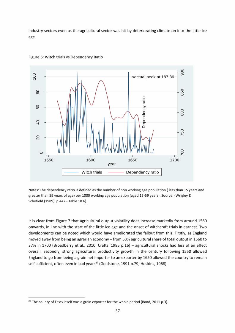
37
industry sectors even as the agricultural sector was hit by deteriorating climate on into the little ice
age.
Figure 6: Witch trials vs Dependency Ratio
Notes: The dependency ratio is defined as the number of non working age population ( less than 15 years and
greater than 59 years of age) per 1000 working age population (aged 15-59 years). Source: (Wrigley &
Schofield (1989), p.447 - Table 10.6)
It is clear from Figure 7 that agricultural output volatility does increase markedly from around 1560
onwards, in line with the start of the little ice age and the onset of witchcraft trials in earnest. Two
developments can be noted which would have ameliorated the fallout from this. Firstly, as England
moved away from being an agrarian economy – from 53% agricultural share of total output in 1560 to
37% in 1700 (Broadberry et al., 2010; Crafts, 1985 p.16) – agricultural shocks had less of an effect
overall. Secondly, strong agricultural productivity growth in the century following 1550 allowed
England to go from being a grain net importer to an exporter by 1650 allowed the country to remain
self sufficient, often even in bad years27 (Goldstone, 1991 p.79; Hoskins, 1968).
27 The county of Essex itself was a grain exporter for the whole period (Band, 2011 p.3).
<actual peak at 187.36
70
075
080
085
090
0
De
pe
nd
en
cy r
atio
020
40
60
80
10
0
Witch
tria
ls (
pe
r m
illio
n p
op
ula
tio
n)
1550 1600 1650 1700year
Witch trials Dependency ratio
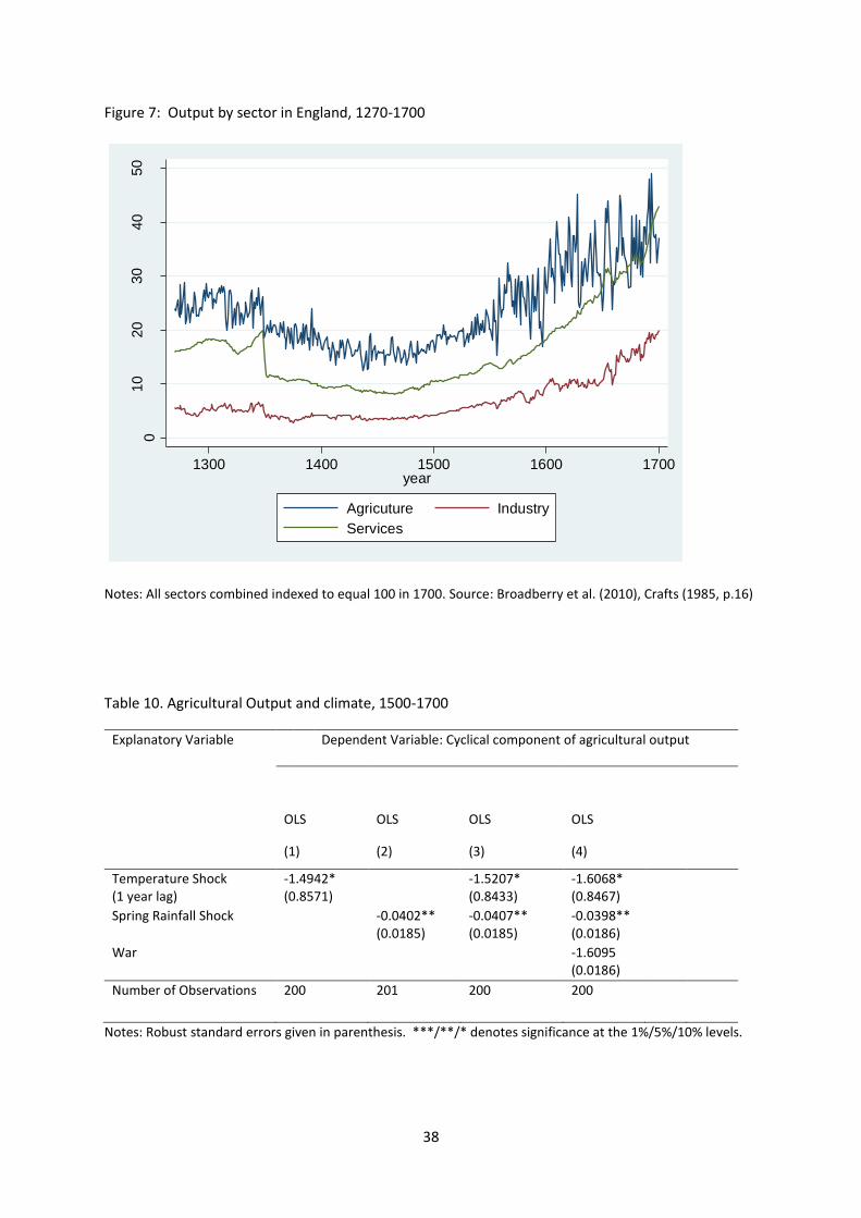
38
Figure 7: Output by sector in England, 1270-1700
Notes: All sectors combined indexed to equal 100 in 1700. Source: Broadberry et al. (2010), Crafts (1985, p.16)
Table 10. Agricultural Output and climate, 1500-1700
Explanatory Variable Dependent Variable: Cyclical component of agricultural output
OLS OLS OLS OLS
(1) (2) (3) (4)
Temperature Shock (1 year lag)
-1.4942* (0.8571)
-1.5207* (0.8433)
-1.6068* (0.8467)
Spring Rainfall Shock -0.0402** (0.0185)
-0.0407** (0.0185)
-0.0398** (0.0186)
War -1.6095 (0.0186)
Number of Observations 200 201 200 200
Notes: Robust standard errors given in parenthesis. ***/**/* denotes significance at the 1%/5%/10% levels.
010
20
30
40
50
Ou
tput
1300 1400 1500 1600 1700year
Agricuture Industry
Services
39
7. Conclusion
While this paper has produced a number of new results it has also brought into focus the difficulty of
identifying specific underlying causes of witch trials when war, plague, population growth, agricultural
output, and economic wellbeing are so interconnected. Furthermore, we have highlighted the
difficulty in using climate variation to proxy for other related phenomena.
The evidence presented indicates that it is climates’ variation with respect to factors such as
agriculture and disease, rather than directly in and of itself that causes witch trials. It is the deviation
around the regional mean, which relates to farming, which is most significant in determining witch
trials. Perhaps the most obvious place to observe any such comfort effect of climate on witch trials is
in winter temperatures. Colder temperatures should increase witch trials through both the comfort
and agricultural channels. However, this is not observed in the data as colder temperatures actually
lead to less witch trials.
Our findings also have relevance for modern day persecution. Particularly in areas heavily dependent
upon agriculture or prone to disease epidemics. This is particularly the case when the disease is new
or unknown and there is evidence that the ebola outbreak in West Africa in 2014 has been linked with
witchcraft (Zaimov, 2014). Given that the weather may become increasingly erratic, and disasters such
as hurricanes and flooding may be more common, there is also the potential for an increase in
witchcraft for this reason.
The results from the GDP per capita analysis again indicate that economic wellbeing is an important
driver of witch trial accusations, and not necessarily directly related to agriculture. The lack of
predictive power of real wages on witch trials indicates that it was total earnings rather than earnings
power which determined the propensity to target witches. Precursory evidence from England points
to both absolute living standards as well as shorter run cyclical economic conditions as factors
dictating persecution.
It is quite clear in the England analysis that the effect of the economic downturn on witch trials is felt
in the lowest point of the cycle, after which the number of trials recedes. This is somewhat at odds
with the results from the climate section and anecdotal evidence which suggest that it often took a
number of years between the perceived infraction and the trial being brought. This incongruity could
be due to the richer dataset in the climate section allowing more complex relationships to be
identified. It is also the case that climate and the business cycle trough may not be directly comparable
variables.
Our analysis shows a strong diminishing effect of war on witch trials. The evidence regarding plague
is mixed. In the climate section and GDP per capita section plague is seen to increase witch trials while
elsewhere it does not. This is consistent with the anecdotal evidence which suggests that witches were
only seen as spreaders of plague in some areas and not in others.
A recurring theme throughout the analysis has been the importance of a certain modicum of stability
for witch trials to flourish. Witch trials represent a state approved outlet for communities’ discontent
whereby the wider community singles out certain individuals for persecution. This relies on a certain
cohesion in society in order for the unfortunate suspects to be weeded out and the effective working
of the courts for them to be tried; both of which can be found lacking in times of war, famine or
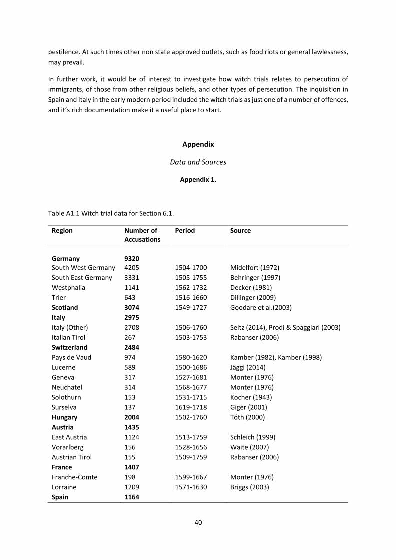
40
pestilence. At such times other non state approved outlets, such as food riots or general lawlessness,
may prevail.
In further work, it would be of interest to investigate how witch trials relates to persecution of
immigrants, of those from other religious beliefs, and other types of persecution. The inquisition in
Spain and Italy in the early modern period included the witch trials as just one of a number of offences,
and it’s rich documentation make it a useful place to start.
Appendix
Data and Sources
Appendix 1.
Table A1.1 Witch trial data for Section 6.1.
Region Number of Accusations
Period Source
Germany
9320
South West Germany 4205 1504-1700 Midelfort (1972)
South East Germany 3331 1505-1755 Behringer (1997)
Westphalia 1141 1562-1732 Decker (1981)
Trier 643 1516-1660 Dillinger (2009)
Scotland 3074 1549-1727 Goodare et al.(2003)
Italy 2975
Italy (Other) 2708 1506-1760 Seitz (2014), Prodi & Spaggiari (2003)
Italian Tirol 267 1503-1753 Rabanser (2006)
Switzerland 2484
Pays de Vaud 974 1580-1620 Kamber (1982), Kamber (1998)
Lucerne 589 1500-1686 Jäggi (2014)
Geneva 317 1527-1681 Monter (1976)
Neuchatel 314 1568-1677 Monter (1976)
Solothurn 153 1531-1715 Kocher (1943)
Surselva 137 1619-1718 Giger (2001)
Hungary 2004 1502-1760 Tóth (2000)
Austria 1435
East Austria 1124 1513-1759 Schleich (1999)
Vorarlberg 156 1528-1656 Waite (2007)
Austrian Tirol 155 1509-1759 Rabanser (2006)
France 1407
Franche-Comte 198 1599-1667 Monter (1976)
Lorraine 1209 1571-1630 Briggs (2003)
Spain 1164
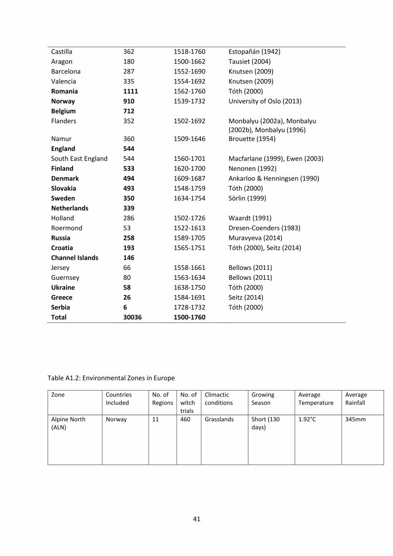
41
Castilla 362 1518-1760 Estopañán (1942)
Aragon 180 1500-1662 Tausiet (2004)
Barcelona 287 1552-1690 Knutsen (2009)
Valencia 335 1554-1692 Knutsen (2009)
Romania 1111 1562-1760 Tóth (2000)
Norway 910 1539-1732 University of Oslo (2013)
Belgium 712
Flanders 352 1502-1692 Monbalyu (2002a), Monbalyu (2002b), Monbalyu (1996)
Namur 360 1509-1646 Brouette (1954)
England 544
South East England 544 1560-1701 Macfarlane (1999), Ewen (2003)
Finland 533 1620-1700 Nenonen (1992)
Denmark 494 1609-1687 Ankarloo & Henningsen (1990)
Slovakia 493 1548-1759 Tóth (2000)
Sweden 350 1634-1754 Sörlin (1999)
Netherlands 339
Holland 286 1502-1726 Waardt (1991)
Roermond 53 1522-1613 Dresen-Coenders (1983)
Russia 258 1589-1705 Muravyeva (2014)
Croatia 193 1565-1751 Tóth (2000), Seitz (2014)
Channel Islands 146
Jersey 66 1558-1661 Bellows (2011)
Guernsey 80 1563-1634 Bellows (2011)
Ukraine 58 1638-1750 Tóth (2000)
Greece 26 1584-1691 Seitz (2014)
Serbia 6 1728-1732 Tóth (2000)
Total 30036 1500-1760
Table A1.2: Environmental Zones in Europe
Zone Countries Included
No. of Regions
No. of witch trials
Climactic conditions
Growing Season
Average Temperature
Average Rainfall
Alpine North (ALN)
Norway 11 460 Grasslands Short (130 days)
1.92°C 345mm
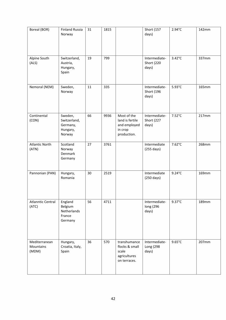
42
Boreal (BOR) Finland Russia Norway
31 1815 Short (157 days)
2.94°C 142mm
Alpine South (ALS)
Switzerland, Austria, Hungary, Spain
19 799 Intermediate-Short (220 days)
3.42°C 337mm
Nemoral (NEM) Sweden, Norway
11 335 Intermediate-Short (196 days)
5.93°C 165mm
Continental (CON)
Sweden, Switzerland, Germany, Hungary, Norway
66 9936 Most of the land is fertile and employed in crop production.
Intermediate-Short (227 days)
7.52°C 217mm
Atlantic North (ATN)
Scotland Norway Denmark Germany
27 3761
Intermediate (255 days)
7.62°C 268mm
Pannonian (PAN) Hungary, Romania
30 2519 Intermediate (250 days)
9.24°C 169mm
Atlanntic Central (ATC)
England Belgium Netherlands France Germany
56 4711 Intermediate-long (296 days)
9.37°C 189mm
Mediterranean Mountains (MDM)
Hungary, Croatia, Italy, Spain
36 570 transhumance flocks & small scale agricultures on terraces.
Intermediate-Long (298 days)
9.65°C 207mm
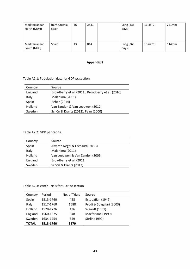
43
Mediterranean North (MDN)
Italy, Croatia, Spain
36 2431 Long (335 days)
11.45°C 221mm
Mediterranean South (MDS)
Spain 13 814
Long (363 days)
13.62°C 114mm
Appendix 2
Table A2.1: Population data for GDP pc section.
Country Source
England Broadberry et al. (2011), Broadberry et al. (2010)
Italy Malanima (2011)
Spain Reher (2014)
Holland Van Zanden & Van Leeuwen (2012)
Sweden Schön & Krantz (2012), Palm (2000)
Table A2.2: GDP per capita.
Country Source
Spain Alvarez-Negal & Escosura (2013)
Italy Malanima (2011)
Holland Van Leeuwen & Van Zanden (2009)
England Broadberry et al. (2011)
Sweden Schön & Krantz (2012)
Table A2.3: Witch Trials for GDP pc section
Country Period No. of Trials Source
Spain 1513-1760 458 Estopañán (1942)
Italy 1517-1760 1588 Prodi & Spaggiari (2003)
Holland 1528-1726 436 Waardt (1991)
England 1560-1675 348 Macfarlane (1999)
Sweden 1634-1754 349 Sörlin (1999)
TOTAL 1513-1760 3179
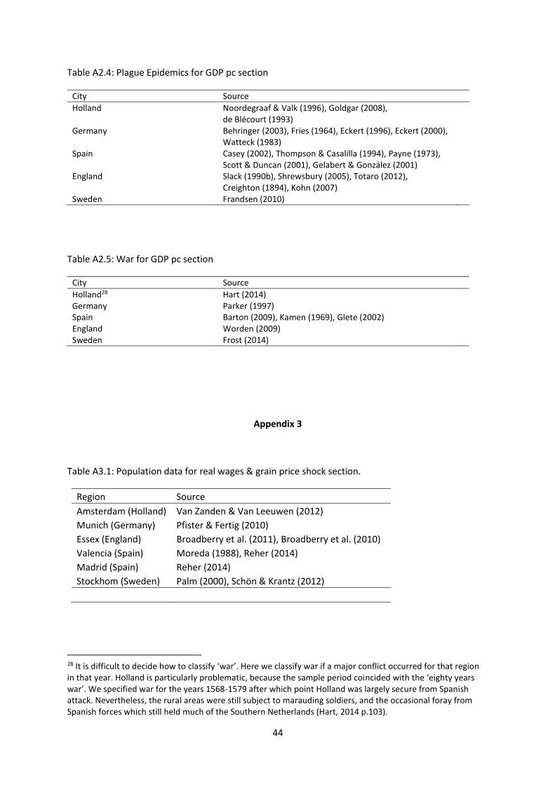
44
Table A2.4: Plague Epidemics for GDP pc section
City Source
Holland Noordegraaf & Valk (1996), Goldgar (2008), de Blécourt (1993)
Germany Behringer (2003), Fries (1964), Eckert (1996), Eckert (2000), Watteck (1983)
Spain Casey (2002), Thompson & Casalilla (1994), Payne (1973), Scott & Duncan (2001), Gelabert & González (2001)
England Slack (1990b), Shrewsbury (2005), Totaro (2012), Creighton (1894), Kohn (2007)
Sweden Frandsen (2010)
Table A2.5: War for GDP pc section
City Source
Holland28 Hart (2014) Germany Parker (1997) Spain Barton (2009), Kamen (1969), Glete (2002) England Worden (2009) Sweden Frost (2014)
Appendix 3
Table A3.1: Population data for real wages & grain price shock section.
Region Source
Amsterdam (Holland) Van Zanden & Van Leeuwen (2012)
Munich (Germany) Pfister & Fertig (2010)
Essex (England) Broadberry et al. (2011), Broadberry et al. (2010)
Valencia (Spain) Moreda (1988), Reher (2014)
Madrid (Spain) Reher (2014)
Stockhom (Sweden) Palm (2000), Schön & Krantz (2012)
28 It is difficult to decide how to classify ‘war’. Here we classify war if a major conflict occurred for that region in that year. Holland is particularly problematic, because the sample period coincided with the ‘eighty years war’. We specified war for the years 1568-1579 after which point Holland was largely secure from Spanish attack. Nevertheless, the rural areas were still subject to marauding soldiers, and the occasional foray from Spanish forces which still held much of the Southern Netherlands (Hart, 2014 p.103).
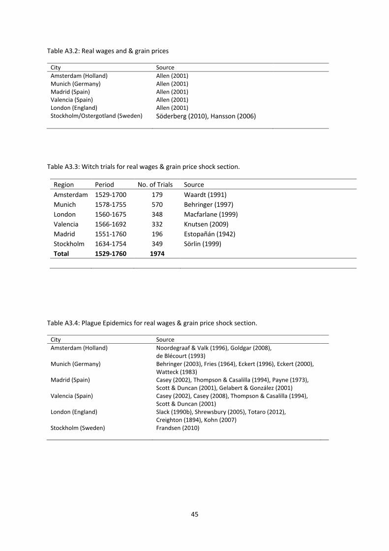
45
Table A3.2: Real wages and & grain prices
City Source
Amsterdam (Holland) Allen (2001) Munich (Germany) Allen (2001) Madrid (Spain) Allen (2001) Valencia (Spain) Allen (2001) London (England) Allen (2001) Stockholm/Ostergotland (Sweden) Söderberg (2010), Hansson (2006)
Table A3.3: Witch trials for real wages & grain price shock section.
Region Period No. of Trials Source
Amsterdam 1529-1700 179 Waardt (1991)
Munich 1578-1755 570 Behringer (1997)
London 1560-1675 348 Macfarlane (1999)
Valencia 1566-1692 332 Knutsen (2009)
Madrid 1551-1760 196 Estopañán (1942)
Stockholm 1634-1754 349 Sörlin (1999)
Total 1529-1760 1974
Table A3.4: Plague Epidemics for real wages & grain price shock section.
City Source
Amsterdam (Holland) Noordegraaf & Valk (1996), Goldgar (2008), de Blécourt (1993)
Munich (Germany) Behringer (2003), Fries (1964), Eckert (1996), Eckert (2000), Watteck (1983)
Madrid (Spain) Casey (2002), Thompson & Casalilla (1994), Payne (1973), Scott & Duncan (2001), Gelabert & González (2001)
Valencia (Spain) Casey (2002), Casey (2008), Thompson & Casalilla (1994), Scott & Duncan (2001)
London (England) Slack (1990b), Shrewsbury (2005), Totaro (2012), Creighton (1894), Kohn (2007)
Stockholm (Sweden) Frandsen (2010)
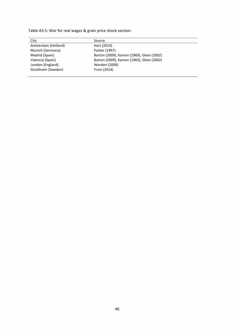
46
Table A3.5: War for real wages & grain price shock section.
City Source
Amsterdam (Holland) Hart (2014) Munich (Germany) Parker (1997) Madrid (Spain) Barton (2009), Kamen (1969), Glete (2002) Valencia (Spain) Barton (2009), Kamen (1969), Glete (2002) London (England) Worden (2009) Stockholm (Sweden) Frost (2014)
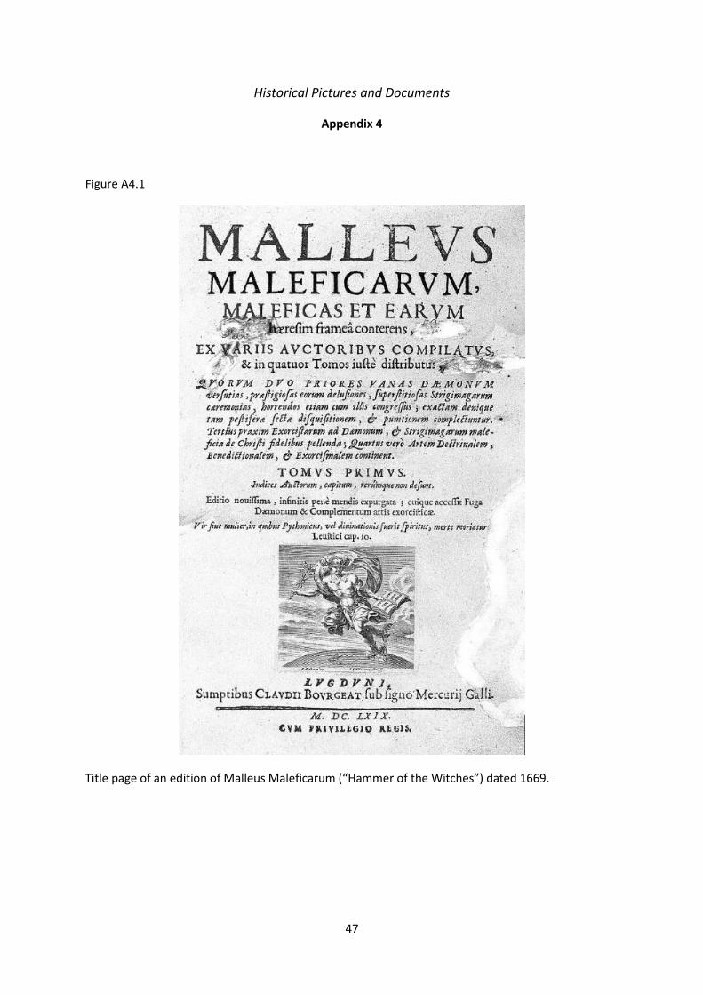
47
Historical Pictures and Documents
Appendix 4
Figure A4.1
Title page of an edition of Malleus Maleficarum (“Hammer of the Witches”) dated 1669.
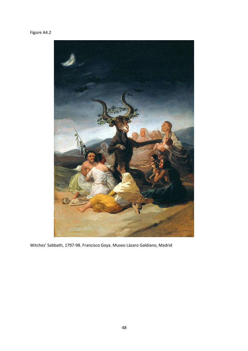
48
Figure A4.2
Witches’ Sabbath, 1797-98. Francisco Goya. Museo Lázaro Galdiano, Madrid
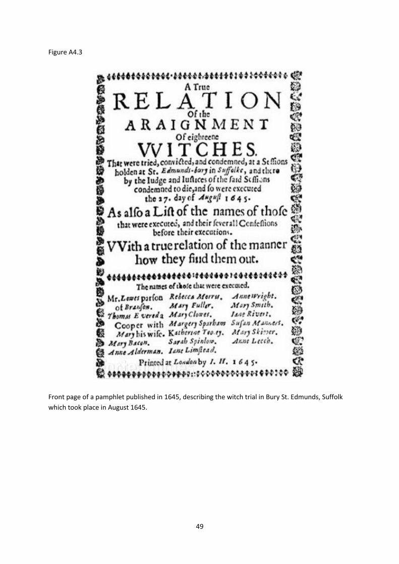
49
Figure A4.3
Front page of a pamphlet published in 1645, describing the witch trial in Bury St. Edmunds, Suffolk
which took place in August 1645.
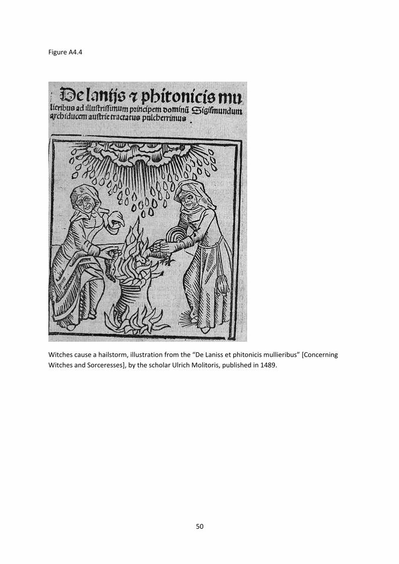
50
Figure A4.4
Witches cause a hailstorm, illustration from the “De Laniss et phitonicis mullieribus” [Concerning
Witches and Sorceresses], by the scholar Ulrich Molitoris, published in 1489.
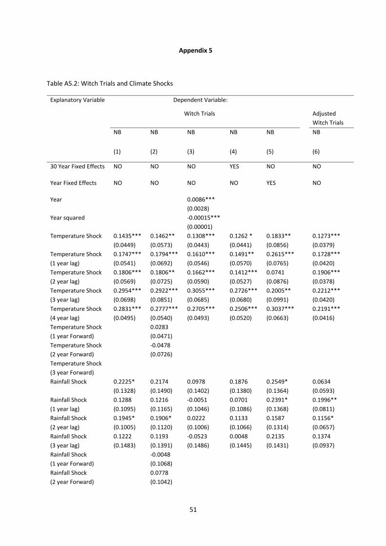
51
Appendix 5
Table A5.2: Witch Trials and Climate Shocks
Explanatory Variable Dependent Variable:
Witch Trials
Adjusted
Witch Trials
NB NB NB NB NB NB
(1) (2) (3) (4) (5) (6)
30 Year Fixed Effects NO NO NO YES NO NO
Year Fixed Effects NO NO NO NO YES NO
Year 0.0086***
(0.0028)
Year squared -0.00015***
(0.00001)
Temperature Shock 0.1435***
(0.0449)
0.1462**
(0.0573)
0.1308***
(0.0443)
0.1262 *
(0.0441)
0.1833**
(0.0856)
0.1273***
(0.0379)
Temperature Shock
(1 year lag)
0.1747***
(0.0541)
0.1794***
(0.0692)
0.1610***
(0.0546)
0.1491**
(0.0570)
0.2615***
(0.0765)
0.1728***
(0.0420)
Temperature Shock
(2 year lag)
0.1806***
(0.0569)
0.1806**
(0.0725)
0.1662***
(0.0590)
0.1412***
(0.0527)
0.0741
(0.0876)
0.1906***
(0.0378)
Temperature Shock
(3 year lag)
0.2954***
(0.0698)
0.2922***
(0.0851)
0.3055***
(0.0685)
0.2726***
(0.0680)
0.2005**
(0.0991)
0.2212***
(0.0420)
Temperature Shock
(4 year lag)
0.2831***
(0.0495)
0.2777***
(0.0540)
0.2705***
(0.0493)
0.2506***
(0.0520)
0.3037***
(0.0663)
0.2191***
(0.0416)
Temperature Shock
(1 year Forward)
0.0283
(0.0471)
Temperature Shock
(2 year Forward)
-0.0478
(0.0726)
Temperature Shock
(3 year Forward)
Rainfall Shock 0.2225*
(0.1328)
0.2174
(0.1490)
0.0978
(0.1402)
0.1876
(0.1380)
0.2549*
(0.1364)
0.0634
(0.0593)
Rainfall Shock
(1 year lag)
0.1288
(0.1095)
0.1216
(0.1165)
-0.0051
(0.1046)
0.0701
(0.1086)
0.2391*
(0.1368)
0.1996**
(0.0811)
Rainfall Shock
(2 year lag)
0.1945*
(0.1005)
0.1906*
(0.1120)
0.0222
(0.1006)
0.1133
(0.1066)
0.1587
(0.1314)
0.1156*
(0.0657)
Rainfall Shock
(3 year lag)
0.1222
(0.1483)
0.1193
(0.1391)
-0.0523
(0.1486)
0.0048
(0.1445)
0.2135
(0.1431)
0.1374
(0.0937)
Rainfall Shock
(1 year Forward)
-0.0048
(0.1068)
Rainfall Shock
(2 year Forward)
0.0778
(0.1042)
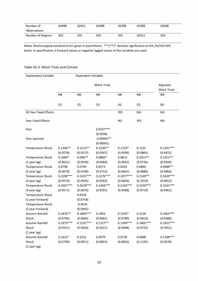
52
Number of
Observations
42498 42451 42498 42498 42498 42498
Number of Regions 355 355 355 355 35551
355
0.1713***
(0.0622)
Notes: Bootstrapped standard errors given in parenthesis. ***/**/* denotes significance at the 1%/5%/10%
levels. In specification 2 Forward values or negative lagged values of the variables are used.
Table A5.3: Witch Trials and Climate
Explanatory Variable Dependent Variable:
Witch Trials
Adjusted
Witch Trials
NB NB NB NB NB NB
(1) (2) (3) (4) (5) (6)
30 Year Fixed Effects YES NO NO
Year Fixed Effects NO YES NO
Year 0.0107***
(0.0036)
Year squared -0.00002**
(0.00001)
Temperature Shock 0.1344**
(0.0578)
0.1214**
(0.0572)
0.1250**
(0.0547)
0.1123*
(0.0599)
0.1222
(0.0805)
0.1241***
(0.0422)
Temperature Shock
(1 year lag)
0.1069*
(0.0631)
0.0967*
(0.0538)
0.0883*
(0.0484)
0.0813
(0.0625)
0.2013**
(0.0736)
0.1251**
(0.0509)
Temperature Shock
(2 year lag)
0.0798
(0.0678)
0.0794
(0.0748)
0.0573
(0.0712)
0.0433
(0.0641)
0.0840
(0.0889)
0.0984**
(0.0466)
Temperature Shock
(3 year lag)
0.2290***
(0.0579)
0.2415***
(0.0595)
0.2276***
(0.0593)
0.2077***
(0.0603)
0.2149**
(0.1019)
0.1820***
(0.0453)
Temperature Shock
(4 year lag)
0.2607***
(0.0571)
0.2678***
(0.0676)
0.2494***
(0.0592)
0.2182***
(0.0588)
0.3239***
(0.0719)
0.2161***
(0.0461)
Temperature Shock
(1 year Forward)
0.0326
(0.0758)
Temperature Shock
(2 year Forward)
-0.0435
(0.0992)
Autumn Rainfall
Shock
0.1876**
(0.0796)
0.1869***
(0.0683)
0.1093
(0.0681)
0.1334*
(0.0789)
0.1516
(0.0813)
0.1063***
(0.0388)
Autumn Rainfall
Shock
(1 year lag)
0.1973***
(0.0551)
0.1531***
(0.0566)
0.1227**
(0.0521)
0.1399***
(0.0498)
0.1802***
(0.0725)
0.1922***
(0.0451)
Autumn Rainfall
Shock
(2 year lag)
0.1431*
(0.0799)
0.1412
(0.0911)
0.0479
(0.0823)
0.0739
(0.0826)
0.0868
(0.1105)
0.1188***
(0.0478)
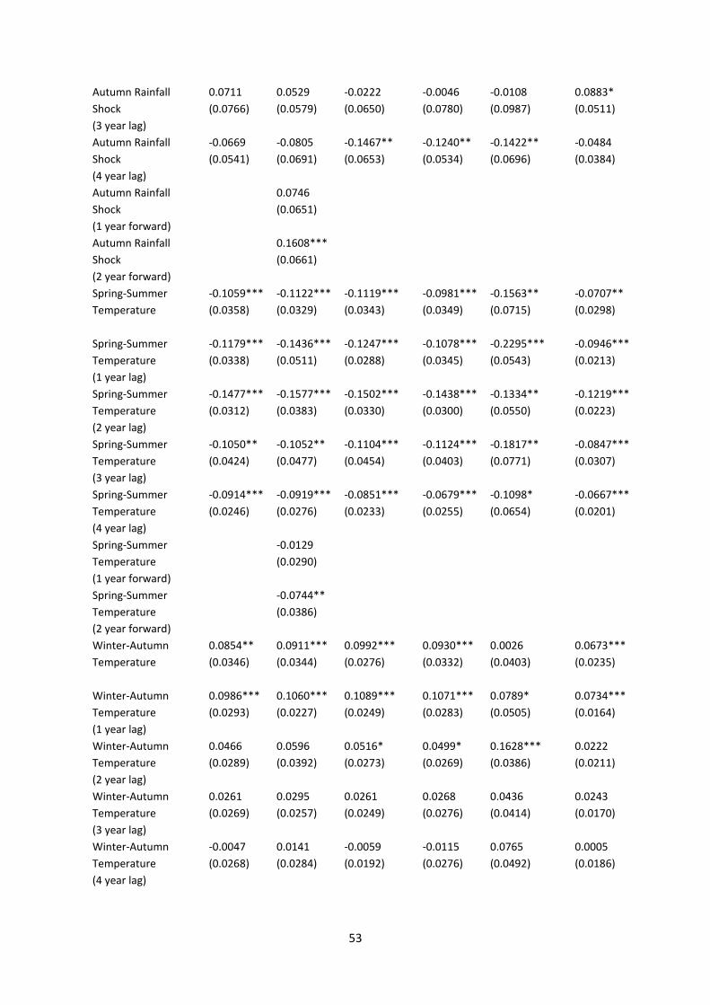
53
Autumn Rainfall
Shock
(3 year lag)
0.0711
(0.0766)
0.0529
(0.0579)
-0.0222
(0.0650)
-0.0046
(0.0780)
-0.0108
(0.0987)
0.0883*
(0.0511)
Autumn Rainfall
Shock
(4 year lag)
-0.0669
(0.0541)
-0.0805
(0.0691)
-0.1467**
(0.0653)
-0.1240**
(0.0534)
-0.1422**
(0.0696)
-0.0484
(0.0384)
Autumn Rainfall
Shock
(1 year forward)
0.0746
(0.0651)
Autumn Rainfall
Shock
(2 year forward)
0.1608***
(0.0661)
Spring-Summer
Temperature
-0.1059***
(0.0358)
-0.1122***
(0.0329)
-0.1119***
(0.0343)
-0.0981***
(0.0349)
-0.1563**
(0.0715)
-0.0707**
(0.0298)
Spring-Summer
Temperature
(1 year lag)
-0.1179***
(0.0338)
-0.1436***
(0.0511)
-0.1247***
(0.0288)
-0.1078***
(0.0345)
-0.2295***
(0.0543)
-0.0946***
(0.0213)
Spring-Summer
Temperature
(2 year lag)
-0.1477***
(0.0312)
-0.1577***
(0.0383)
-0.1502***
(0.0330)
-0.1438***
(0.0300)
-0.1334**
(0.0550)
-0.1219***
(0.0223)
Spring-Summer
Temperature
(3 year lag)
-0.1050**
(0.0424)
-0.1052**
(0.0477)
-0.1104***
(0.0454)
-0.1124***
(0.0403)
-0.1817**
(0.0771)
-0.0847***
(0.0307)
Spring-Summer
Temperature
(4 year lag)
-0.0914***
(0.0246)
-0.0919***
(0.0276)
-0.0851***
(0.0233)
-0.0679***
(0.0255)
-0.1098*
(0.0654)
-0.0667***
(0.0201)
Spring-Summer
Temperature
(1 year forward)
-0.0129
(0.0290)
Spring-Summer
Temperature
(2 year forward)
-0.0744**
(0.0386)
Winter-Autumn
Temperature
0.0854**
(0.0346)
0.0911***
(0.0344)
0.0992***
(0.0276)
0.0930***
(0.0332)
0.0026
(0.0403)
0.0673***
(0.0235)
Winter-Autumn
Temperature
(1 year lag)
0.0986***
(0.0293)
0.1060***
(0.0227)
0.1089***
(0.0249)
0.1071***
(0.0283)
0.0789*
(0.0505)
0.0734***
(0.0164)
Winter-Autumn
Temperature
(2 year lag)
0.0466
(0.0289)
0.0596
(0.0392)
0.0516*
(0.0273)
0.0499*
(0.0269)
0.1628***
(0.0386)
0.0222
(0.0211)
Winter-Autumn
Temperature
(3 year lag)
0.0261
(0.0269)
0.0295
(0.0257)
0.0261
(0.0249)
0.0268
(0.0276)
0.0436
(0.0414)
0.0243
(0.0170)
Winter-Autumn
Temperature
(4 year lag)
-0.0047
(0.0268)
0.0141
(0.0284)
-0.0059
(0.0192)
-0.0115
(0.0276)
0.0765
(0.0492)
0.0005
(0.0186)
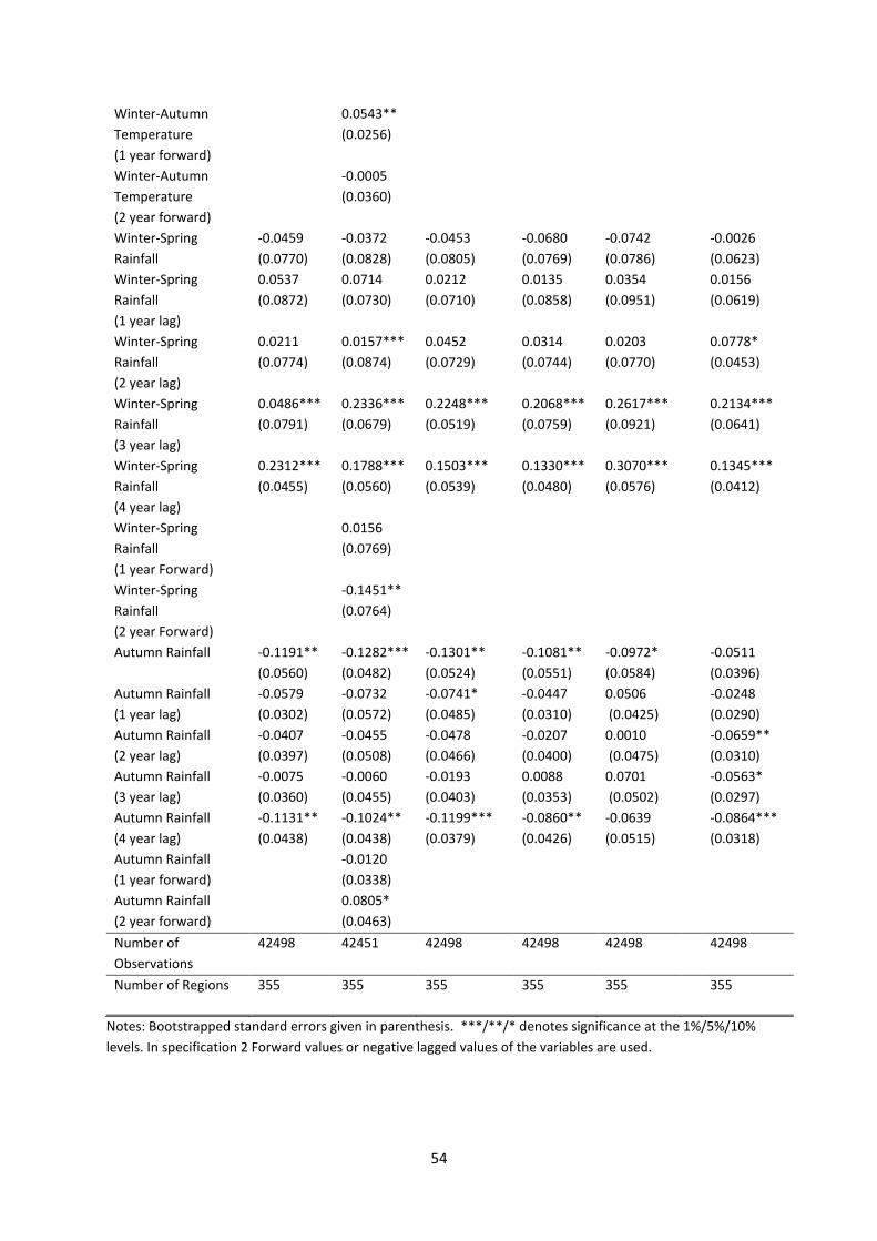
54
Winter-Autumn
Temperature
(1 year forward)
0.0543**
(0.0256)
Winter-Autumn
Temperature
(2 year forward)
-0.0005
(0.0360)
Winter-Spring
Rainfall
-0.0459
(0.0770)
-0.0372
(0.0828)
-0.0453
(0.0805)
-0.0680
(0.0769)
-0.0742
(0.0786)
-0.0026
(0.0623)
Winter-Spring
Rainfall
(1 year lag)
0.0537
(0.0872)
0.0714
(0.0730)
0.0212
(0.0710)
0.0135
(0.0858)
0.0354
(0.0951)
0.0156
(0.0619)
Winter-Spring
Rainfall
(2 year lag)
0.0211
(0.0774)
0.0157***
(0.0874)
0.0452
(0.0729)
0.0314
(0.0744)
0.0203
(0.0770)
0.0778*
(0.0453)
Winter-Spring
Rainfall
(3 year lag)
0.0486***
(0.0791)
0.2336***
(0.0679)
0.2248***
(0.0519)
0.2068***
(0.0759)
0.2617***
(0.0921)
0.2134***
(0.0641)
Winter-Spring
Rainfall
(4 year lag)
0.2312***
(0.0455)
0.1788***
(0.0560)
0.1503***
(0.0539)
0.1330***
(0.0480)
0.3070***
(0.0576)
0.1345***
(0.0412)
Winter-Spring
Rainfall
(1 year Forward)
0.0156
(0.0769)
Winter-Spring
Rainfall
(2 year Forward)
-0.1451**
(0.0764)
Autumn Rainfall -0.1191**
(0.0560)
-0.1282***
(0.0482)
-0.1301**
(0.0524)
-0.1081**
(0.0551)
-0.0972*
(0.0584)
-0.0511
(0.0396)
Autumn Rainfall
(1 year lag)
-0.0579
(0.0302)
-0.0732
(0.0572)
-0.0741*
(0.0485)
-0.0447
(0.0310)
0.0506
(0.0425)
-0.0248
(0.0290)
Autumn Rainfall
(2 year lag)
-0.0407
(0.0397)
-0.0455
(0.0508)
-0.0478
(0.0466)
-0.0207
(0.0400)
0.0010
(0.0475)
-0.0659**
(0.0310)
Autumn Rainfall
(3 year lag)
-0.0075
(0.0360)
-0.0060
(0.0455)
-0.0193
(0.0403)
0.0088
(0.0353)
0.0701
(0.0502)
-0.0563*
(0.0297)
Autumn Rainfall
(4 year lag)
-0.1131**
(0.0438)
-0.1024**
(0.0438)
-0.1199***
(0.0379)
-0.0860**
(0.0426)
-0.0639
(0.0515)
-0.0864***
(0.0318)
Autumn Rainfall
(1 year forward)
-0.0120
(0.0338)
Autumn Rainfall
(2 year forward)
0.0805*
(0.0463)
Number of
Observations
42498 42451 42498 42498 42498 42498
Number of Regions 355 355 355 355 355 355
Notes: Bootstrapped standard errors given in parenthesis. ***/**/* denotes significance at the 1%/5%/10%
levels. In specification 2 Forward values or negative lagged values of the variables are used.
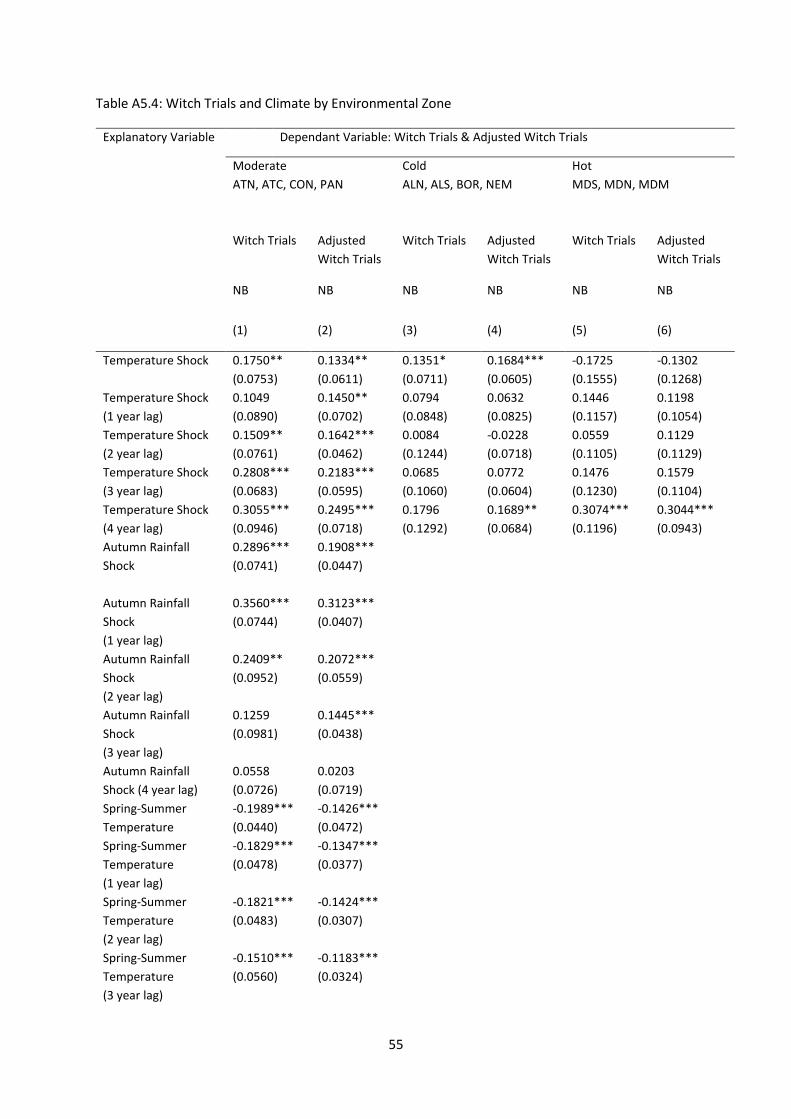
55
Table A5.4: Witch Trials and Climate by Environmental Zone
Explanatory Variable Dependant Variable: Witch Trials & Adjusted Witch Trials
Moderate
ATN, ATC, CON, PAN
Cold
ALN, ALS, BOR, NEM
Hot
MDS, MDN, MDM
Witch Trials Adjusted
Witch Trials
Witch Trials Adjusted
Witch Trials
Witch Trials Adjusted
Witch Trials
NB NB NB NB NB NB
(1) (2) (3) (4) (5) (6)
Temperature Shock 0.1750**
(0.0753)
0.1334**
(0.0611)
0.1351*
(0.0711)
0.1684***
(0.0605)
-0.1725
(0.1555)
-0.1302
(0.1268)
Temperature Shock
(1 year lag)
0.1049
(0.0890)
0.1450**
(0.0702)
0.0794
(0.0848)
0.0632
(0.0825)
0.1446
(0.1157)
0.1198
(0.1054)
Temperature Shock
(2 year lag)
0.1509**
(0.0761)
0.1642***
(0.0462)
0.0084
(0.1244)
-0.0228
(0.0718)
0.0559
(0.1105)
0.1129
(0.1129)
Temperature Shock
(3 year lag)
0.2808***
(0.0683)
0.2183***
(0.0595)
0.0685
(0.1060)
0.0772
(0.0604)
0.1476
(0.1230)
0.1579
(0.1104)
Temperature Shock
(4 year lag)
0.3055***
(0.0946)
0.2495***
(0.0718)
0.1796
(0.1292)
0.1689**
(0.0684)
0.3074***
(0.1196)
0.3044***
(0.0943)
Autumn Rainfall
Shock
0.2896***
(0.0741)
0.1908***
(0.0447)
Autumn Rainfall
Shock
(1 year lag)
0.3560***
(0.0744)
0.3123***
(0.0407)
Autumn Rainfall
Shock
(2 year lag)
0.2409**
(0.0952)
0.2072***
(0.0559)
Autumn Rainfall
Shock
(3 year lag)
0.1259
(0.0981)
0.1445***
(0.0438)
Autumn Rainfall
Shock (4 year lag)
0.0558
(0.0726)
0.0203
(0.0719)
Spring-Summer
Temperature
-0.1989***
(0.0440)
-0.1426***
(0.0472)
Spring-Summer
Temperature
(1 year lag)
-0.1829***
(0.0478)
-0.1347***
(0.0377)
Spring-Summer
Temperature
(2 year lag)
-0.1821***
(0.0483)
-0.1424***
(0.0307)
Spring-Summer
Temperature
(3 year lag)
-0.1510***
(0.0560)
-0.1183***
(0.0324)
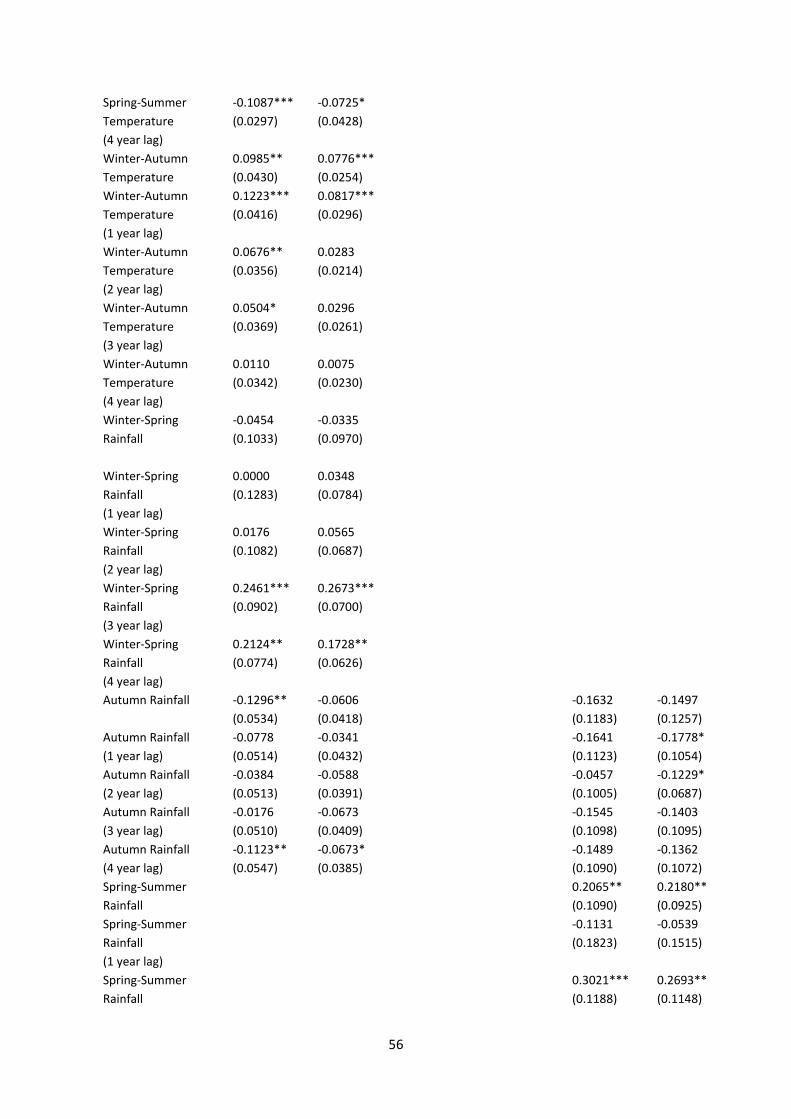
56
Spring-Summer
Temperature
(4 year lag)
-0.1087***
(0.0297)
-0.0725*
(0.0428)
Winter-Autumn
Temperature
0.0985**
(0.0430)
0.0776***
(0.0254)
Winter-Autumn
Temperature
(1 year lag)
0.1223***
(0.0416)
0.0817***
(0.0296)
Winter-Autumn
Temperature
(2 year lag)
0.0676**
(0.0356)
0.0283
(0.0214)
Winter-Autumn
Temperature
(3 year lag)
0.0504*
(0.0369)
0.0296
(0.0261)
Winter-Autumn
Temperature
(4 year lag)
0.0110
(0.0342)
0.0075
(0.0230)
Winter-Spring
Rainfall
-0.0454
(0.1033)
-0.0335
(0.0970)
Winter-Spring
Rainfall
(1 year lag)
0.0000
(0.1283)
0.0348
(0.0784)
Winter-Spring
Rainfall
(2 year lag)
0.0176
(0.1082)
0.0565
(0.0687)
Winter-Spring
Rainfall
(3 year lag)
0.2461***
(0.0902)
0.2673***
(0.0700)
Winter-Spring
Rainfall
(4 year lag)
0.2124**
(0.0774)
0.1728**
(0.0626)
Autumn Rainfall -0.1296**
(0.0534)
-0.0606
(0.0418)
-0.1632
(0.1183)
-0.1497
(0.1257)
Autumn Rainfall
(1 year lag)
-0.0778
(0.0514)
-0.0341
(0.0432)
-0.1641
(0.1123)
-0.1778*
(0.1054)
Autumn Rainfall
(2 year lag)
-0.0384
(0.0513)
-0.0588
(0.0391)
-0.0457
(0.1005)
-0.1229*
(0.0687)
Autumn Rainfall
(3 year lag)
-0.0176
(0.0510)
-0.0673
(0.0409)
-0.1545
(0.1098)
-0.1403
(0.1095)
Autumn Rainfall
(4 year lag)
-0.1123**
(0.0547)
-0.0673*
(0.0385)
-0.1489
(0.1090)
-0.1362
(0.1072)
Spring-Summer
Rainfall
0.2065**
(0.1090)
0.2180**
(0.0925)
Spring-Summer
Rainfall
(1 year lag)
-0.1131
(0.1823)
-0.0539
(0.1515)
Spring-Summer
Rainfall
0.3021***
(0.1188)
0.2693**
(0.1148)
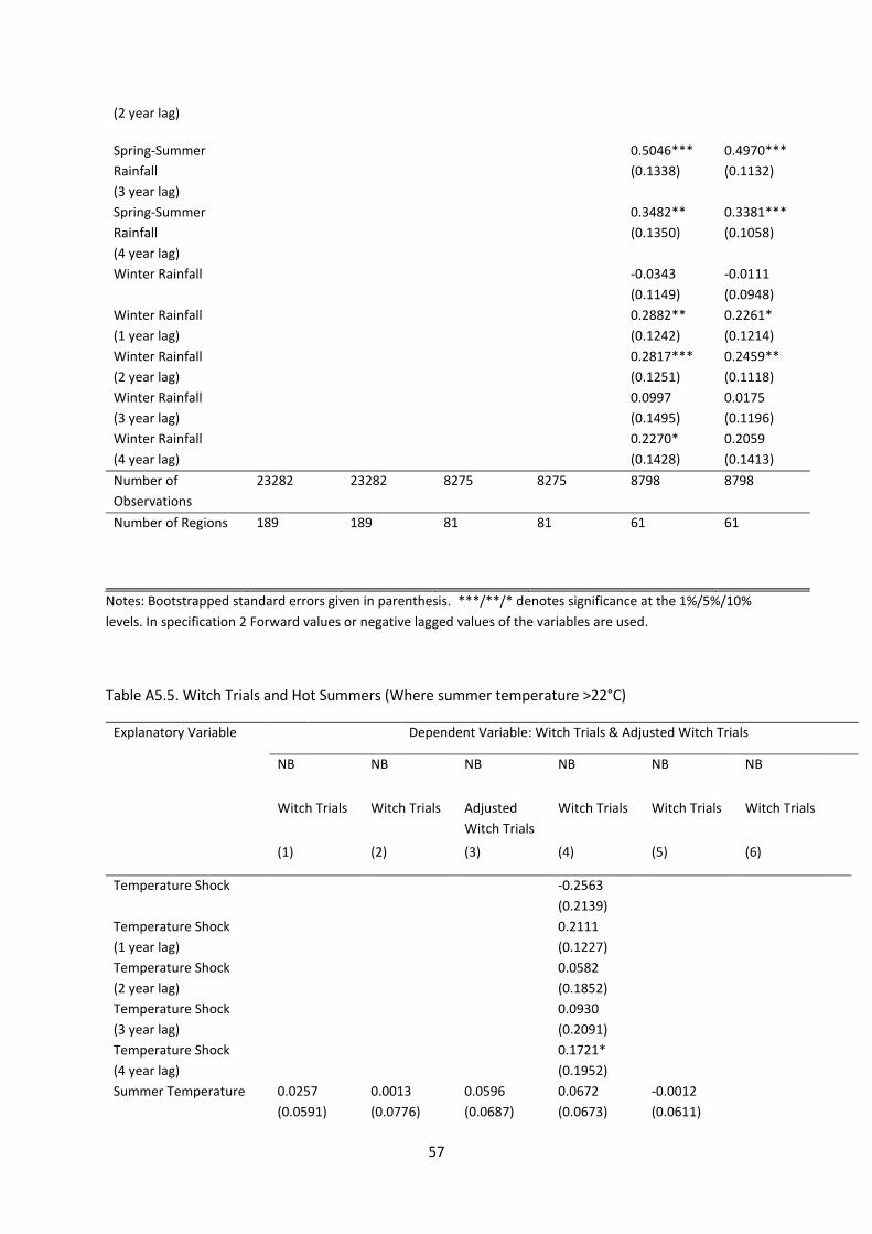
57
(2 year lag)
Spring-Summer
Rainfall
(3 year lag)
0.5046***
(0.1338)
0.4970***
(0.1132)
Spring-Summer
Rainfall
(4 year lag)
0.3482**
(0.1350)
0.3381***
(0.1058)
Winter Rainfall -0.0343
(0.1149)
-0.0111
(0.0948)
Winter Rainfall
(1 year lag)
0.2882**
(0.1242)
0.2261*
(0.1214)
Winter Rainfall
(2 year lag)
0.2817***
(0.1251)
0.2459**
(0.1118)
Winter Rainfall
(3 year lag)
0.0997
(0.1495)
0.0175
(0.1196)
Winter Rainfall
(4 year lag)
0.2270*
(0.1428)
0.2059
(0.1413)
Number of
Observations
23282 23282 8275 8275 8798 8798
Number of Regions 189 189 81 81 61 61
Notes: Bootstrapped standard errors given in parenthesis. ***/**/* denotes significance at the 1%/5%/10%
levels. In specification 2 Forward values or negative lagged values of the variables are used.
Table A5.5. Witch Trials and Hot Summers (Where summer temperature >22°C)
Explanatory Variable Dependent Variable: Witch Trials & Adjusted Witch Trials
NB NB NB NB NB NB
Witch Trials Witch Trials Adjusted
Witch Trials
Witch Trials Witch Trials Witch Trials
(1) (2) (3) (4) (5) (6)
Temperature Shock -0.2563
(0.2139)
Temperature Shock
(1 year lag)
0.2111
(0.1227)
Temperature Shock
(2 year lag)
0.0582
(0.1852)
Temperature Shock
(3 year lag)
0.0930
(0.2091)
Temperature Shock
(4 year lag)
0.1721*
(0.1952)
Summer Temperature 0.0257
(0.0591)
0.0013
(0.0776)
0.0596
(0.0687)
0.0672
(0.0673)
-0.0012
(0.0611)
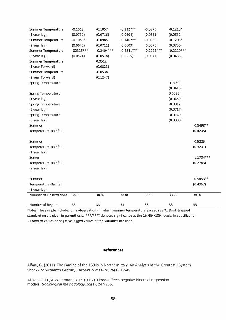
58
Summer Temperature
(1 year lag)
-0.1019
(0.0731)
-0.1057
(0.0716)
-0.1327**
(0.0604)
-0.0975
(0.0661)
-0.1218*
(0.0632)
Summer Temperature
(2 year lag)
-0.1086*
(0.0640)
-0.0985
(0.0711)
-0.1402**
(0.0609)
-0.0830
(0.0670)
-0.1205*
(0.0756)
Summer Temperature
(3 year lag)
-02326***
(0.0524)
-0.2404***
(0.0518)
-0.2241***
(0.0515)
-0.2222***
(0.0577)
-0.2220***
(0.0485)
Summer Temperature
(1 year Forward)
0.0512
(0.0823)
Summer Temperature
(2 year Forward)
-0.0538
(0.1247)
Spring Temperature
0.0489
(0.0415)
Spring Temperature
(1 year lag)
0.0252
(0.0459)
Spring Temperature
(2 year lag)
-0.0012
(0.0717)
Spring Temperature
(3 year lag)
-0.0149
(0.0808)
Summer
Temperature-Rainfall
-0.8498**
(0.4205)
Summer
Temperature-Rainfall
(1 year lag)
-0.5225
(0.3201)
Sumer
Temperature-Rainfall
(2 year lag)
-1.1704***
(0.2743)
Summer
Temperature-Rainfall
(3 year lag)
-0.9453**
(0.4967)
Number of Observations 3838 3824 3838 3836 3836 3814
Number of Regions 33 33 33 33 33 33
Notes: The sample includes only observations in which summer temperature exceeds 22°C. Bootstrapped
standard errors given in parenthesis. ***/**/* denotes significance at the 1%/5%/10% levels. In specification
2 Forward values or negative lagged values of the variables are used.
References
Alfani, G. (2011). The Famine of the 1590s in Northern Italy. An Analysis of the Greatest «System Shock» of Sixteenth Century. Histoire & mesure, 26(1), 17-49 Allison, P. D., & Waterman, R. P. (2002). Fixed–effects negative binomial regression models. Sociological methodology, 32(1), 247-265.
59
Allen, R. C. (2001). The great divergence in European wages and prices from the Middle Ages to the First World War. Explorations in economic history, 38(4), 411-447. Álvarez‐Nogal, C., & De La Escosura, L. P. (2013). The rise and fall of Spain (1270–1850) 1. The
Economic History Review, 66(1), 1-37.
Anderson, R. W., Johnson, N. D., & Koyama, M. (2013). From the Persecuting to the Protective State? Jewish Expulsions and Weather Shocks from 1100 to 1800. University Library of Munich, Germany. Angeles, L. (2008). GDP per capita or real wages? Making sense of conflicting views on pre-industrial Europe. Explorations in Economic History, 45(2), 147-163. Ankarloo, B., & Henningsen, G. (Eds.). (1990). Early modern European witchcraft: Centres and peripheries. Oxford University Press, USA. Appleby, A. B. (1979). Grain prices and subsistence crises in England and France, 1590-1740. Journal of Economic History, 39(4), 865-87. Appleby, A. B. (1980). Epidemics and famine in the little ice age. Journal of Interdisciplinary History, 643-663. Arvin, A. H., & Arvin, H. L. (2010). The Linear Heritage of Women. iUniverse. Band, H. M. K. (2011). Customary law, social memory and collective identity in Essex c. 1540-1700 (Doctoral dissertation, University of East Anglia). Baten, J., & Woitek, U. (2001). Grain price fluctuations and witch hunting in Bavaria. (Unpublished
working paper, University of Munich and University of Glasgow)
Baten, J., & Woitek, U. (2003). Economic Determinants of Witch Hunting, (Unpublished working
paper, University of Munich and University of Tubingen)
Baron, R. A., & Ransberger, V. M. (1978). Ambient temperature and the occurrence of collective violence: the" long, hot summer" revisited. Journal of Personality and Social Psychology, 36(4), 351. Barstow, A. L. (1995). Witchcraze: A new history of the European witch hunts. Pandora Barton, S. (2009). A history of Spain. Palgrave Macmillan. Behringer, W. (1995). Weather, hunger and fear: origins of the European witch-hunts in climate, society and mentality. German History, 13(1), 1-27. Behringer, W. (1997). Hexenverfolgung in Bayern: Volksmagie, Glaubenseifer und Staatsräson in der Frühen Neuzeit. Oldenbourg Verlag. Behringer, W. (1999). Climatic change and witch-hunting: the impact of the Little Ice Age on mentalities. In Climatic variability in sixteenth-century Europe and its social dimension (pp. 335-351). Springer Netherlands. Behringer, W. (2003). Witchcraft Persecutions in Bavaria: Popular Magic, Religious Zealotry and Reason of State in Early Modern Europe. Cambridge University Press.
60
Behringer, W. (2004). Witches and witch-hunts: A global history. Blackwell Publishing.
Bellows, T. (2011). Channel Islands Witchcraft: A critical Survey. : Lulu.com. Berg, B.-Å., 2003, Volatility and integration: Swedish Rye Prices, 1600-1900. Stockholm School of Economics, Department of Economics, Institute for Research in Economic History; Stockholm Biraben, J. N. (1975). Les hommes et la peste en France et dans les pays européens et méditerranéens (Vol. 2). Paris-La Haye: Mouton.
Blackburn, M. L. (2014). The relative performance of Poisson and negative binomial regression estimators. Oxford Bulletin of Economics and Statistics.
Böhm, O., & Wetzel, K. F. (2006). Flood history of the Danube tributaries Lech and Isar in the Alpine foreland of Germany. Hydrological sciences journal, 51(5), 784-798.
Böhm, O. (2011): Hochwassergeschichte des bayerischen Alpenvorlandes: Die Hochwasser der
Sommermonate im Kontext der Klimageschichte Mitteleuropas. Dissertation, Universität Augsburg.
Bressan, D. (2014, November 3). Medieval Witch Hunts Influenced by Climate Change. Retrieved May
6, 2015, from http://blogs.scientificamerican.com/history-of-geology/medieval-witch-hunts-
influenced-by-climate-change/
Briggs, R. (2007). The witches of Lorraine. Oxford University Press.
BRIGGS, R. (2013). WITCHCRAFT AND THE LOCAL COMMUNITIES: THE RHINE—MOSELLE REGION. The Oxford Handbook of Witchcraft in Early Modern Europe and Colonial America, 199. Broadberry, S. N., Campbell, B. M., Klein, A. D., Overton, M., & Leeuwen, B. V. (2010). British economic growth: 1270-1870. Broadberry, S., Campbell, B., Klein, A., Overton, M., & van Leeuwen, B. (2011). BRITISH ECONOMIC GROWTH, 1270-1870: AN OUTPUT-BASED APPROACH. Brouette, E. (1954). La Sorcellerie dans le comté de Namur au début de l'époque moderne, 1509-1646... J. Duculot. Bryant, M. (2004). Witch Trials: Tragic events once led people to accuse neighbors of witchcraft. Retrieved April 24, 2015, from https://www.utexas.edu/features/archive/2004/witches.html. Burns, W. E. (2003). Witch hunts in Europe and America: An encyclopedia. Greenwood Publishing Group. Byrne, J. P. (2012). Encyclopedia of the Black Death (Vol. 1). ABC-CLIO. Cameron, A. C., & Trivedi, P. K. (1986). Econometric models based on count data. Comparisons and applications of some estimators and tests. Journal of applied econometrics, 1(1), 29-53.
61
Cameron, A. C., & Trivedi, P. K. (2005). Microeconometrics: methods and applications. Cambridge university press. Casey, J. (2002). Early modern Spain: a social history. Routledge. Casey, J. (2008). The Kingdom of Valencia in the seventeenth century. Cambridge University Press. Chmielewski, F. M. (1989). Die Wirkung von Klimavariationen in der Landwirtschaft: dargestellt am Beispiel des Winterroggens (Doctoral dissertation). Clark, G. (2001a). Markets and economic growth: The grain market of medieval England. Davis: University of California. Clark, G. (2001b). The Long March of History: Farm Laborers’ Wages in England 1208-1850. Unpublished ms., Department of Economics, University of California, Davis. Clark, G. (2007). The long march of history: Farm wages, population, and economic growth, England 1209–18691. The Economic History Review, 60(1), 97-135. Collins, D. (2000). The Trial of Theoris of Lemnos: A 4th Century Witch or Folk Healer?. Western folklore, 251-278. Cohn, Jr, S. K. (2002). The black death: End of a paradigm. The American Historical Review, 107(3), 703-738. Crafts, N. F. (1985). British economic growth during the industrial revolution (p. 131). Oxford: Clarendon Press. Creighton, C. (1894). A history of epidemics in Britain.. (Vol. 2). The University Press. Creighton, C., Eversley, D. E. C., Underwood, E. A., & Ovenall, L. (1965). A History of Epidemics in Britain: Vol 2: from the Extinction of the Plague to the Present Time. Frank Cass. Cunningham, M. R. (1979). Weather, mood, and helping behavior: Quasi experiments with the sunshine samaritan. Journal of Personality and Social Psychology, 37(11), 1947. de Blécourt, W. (1993). Grenzen van genezing: gezondheid, ziekte en genezen in Nederland, zestiende tot begin twintigste eeuw (Vol. 16). Uitgeverij Verloren. Decker, R. (1981). Die Hexenverfolgungen im Herzogtum Westfalen.Westfälische Zeitschrift, 131(132), 82. De Vries, J. (1976). The economy of Europe in an age of crisis, 1600-1750. Cambridge University Press. Dillinger, J. (2009). " Evil People": A Comparative Study of Witch Hunts in Swabian Austria and the Electorate of Trier. University of Virginia Press. Dodgshon, R. A. (2005). The Little Ice Age in the Scottish Highlands and Islands: documenting its human impact. The Scottish Geographical Magazine, 121(4), 321-337. Dresen-Coenders, L. (1983). Het verbond van heks en duivel. Amboboeken.
62
Dukes, M., & Eden, P. (1997). Phew! What a scorcher: weather records and extremes. Climates of the British Isles, 262-293. Duncan, K. (1992). The possible influence of climate on the bubonic plague in Scotland. The Scottish Geographical Magazine, 108(1), 29-34. Eckert, E. A. (1996). The structure of plagues and pestilences in early modern Europe. Karger. Eckert, E. A. (2000). The retreat of plague from central Europe, 1640-1720: A geomedical approach. Bulletin of the History of Medicine, 74(1), 1-28. Edvinsson, R. (2008). Harvests, prices and population in early modern Sweden(No. 1). Department of
Economic History, Stockholm University.
Ehrenreich, B. (2010). Witches, midwives, and nurses: A history of women healers. ReadHowYouWant.com. Engelman, R. (2010). More: Population, nature, and what women want. Island press. Estopañán, S. C. (1942). Los procesos de hechicerías en la Inquisición de Castilla la Nueva: tribunales de Toledo y Cuenca. " Diana," artes gráficas. Ewen, C. E. (Ed.). (2003). Witch Hunting and Witch Trails [sic], 1929. Kessinger Publishing, LLC. Feliu, G. (1991). Precios y salarios en la Cataluña moderna. Banco de España, Servicio de Estudios. Foner, E. (2005). Give me liberty!: an American history (p. 868). New York: WW Norton. Frandsen, K. E. (2010). The Last Plague in the Baltic Region, 1709-1713. Museum Tusculanum Press. Fries, F. (1964). Die Pest zu Augsburg im Dreißigjährigen Krieg, Diss. München 1887; F. Deininger, Das Collegium Medicum Augustanum, in: Deutsches Ärzteblatt 61 (1964), 1239-1243. Frost, R. I. (2014). The northern wars: war, state and society in northeastern Europe, 1558-1721. Routledge. Gaskill, M. (2010). Witchcraft: A very short introduction. Oxford University Press.
Gelabert, J. E., & González, J. E. G. (2001). Castilla convulsa, 1631-1652. Marcial Pons Historia. Gibson, A. J., & Smout, T. C. (1995). Prices, food and wages in Scotland, 1550-1780. Cambridge University Press. Giger, H. (2001). Hexenwahn und Hexenprozesse in der Surselva. Kommissionsverl. Desertina. Gijswijt-Hofstra, M. (1999). Witchcraft and Magic in Europe, Volume 5: The Eighteenth and Nineteenth Centuries (Vol. 5). A&C Black
Glete, J. (2002). War and the state in early modern Europe: Spain, the Dutch Republic and Sweden as fiscal-military states. Routledge.
63
Goldgar, A. (2008). Tulipmania: money, honor, and knowledge in the Dutch golden age. University of Chicago Press. Goldstone, J. A. (1991). Revolution and rebellion in the early modern world. Univ of California Press. Goodare, J., Martin, L., Miller, J., & Yeoman, L. (2003). The survey of scottish witchcraft [Web]. Retrieved from http://www.shca.ed.ac.uk/witches/ (archived January 2003, accessed 18/11/2013) Grabbe, L. “Leviticus”. in Barton, J., & Muddiman, J. (Eds.). (1998). The Oxford Bible Commentary (Vol. 912). Oxford University Press. Green, D. P., Glaser, J., & Rich, A. (1998). From lynching to gay bashing: the elusive connection between economic conditions and hate crime. Journal of Personality and Social Psychology, 75(1), 82. Grove, J. M. (1988). The Little Ice Age, 498. Methuen, New York. Guiley, R. (2008). The Encyclopedia of Witches, Witchcraft and Wicca. Infobase Publishing.
Guiley, R. (2009). The encyclopedia of Demons and demonology. Infobase Publishing.
Guimaraes, P. (2008). The fixed effects negative binomial model revisited.Economics Letters, 99(1), 63-66.
Hansson, G. (2006). Såld spannmål av kyrkotionden: Priser i Östergötland under Sveriges stormaktstid. Hart, M. T. (2014). The Dutch wars of independence: warfare and commerce in the Netherlands 1570-1680. Routledge. Harvey, B. (1993). Living and Dying in England 1100-1540: The Monastic Experience: The Monastic Experience. Oxford University Press. Heinsohn, G., & Steiger, O. (2004). Witchcraft, Population Catastrophe and Economic Crisis in Renaissance Europe: An Alternative Macroeconomic Explanation-with an Appendix by John M. Riddle. Inst. für Konjunktur-und Strukturforschung. Hepworth, J. T., & West, S. G. (1988). Lynchings and the economy: A time-series reanalysis of Hovland and Sears (1940). Herzig, T. (2010). Flies, Heretics, and the Gendering of Witchcraft. Magic, Ritual, and Witchcraft, 5(1), 51-80. Homer. (1945). The Odyssey. Penguin Books. Hoskins, W. G. (1964). Harvest Fluctuations and English Economic History, 1480—1619. The Agricultural History Review, 12(1), 28-46. Hoskins, W. G. (1968). Harvest fluctuations and english economic history, 1620–1759. The Agricultural History Review, 16(1), 15-31. Houston, R. A., & Houston, R. R. A. (1995). The population history of Britain and Ireland 1500-1750 (Vol. 18). Cambridge University Press.
64
Hovland, C. I., & Sears, R. R. (1940). Minor studies of aggression: VI. Correlation of lynchings with economic indices. The Journal of Psychology,9(2), 301-310. Howarth, E., & Hoffman, M. S. (1984). A multidimensional approach to the relationship between mood and weather. British Journal of Psychology, 75(1), 15-23. Huibers, M. J., de Graaf, L. E., Peeters, F. P., & Arntz, A. (2010). Does the weather make us sad? Meteorological determinants of mood and depression in the general population. Psychiatry research, 180(2), 143-146. Hutton, R. (1993). The pagan religions of the ancient British Isles: their nature and legacy. Wiley-Blackwell. Jacobs, R. (2013, August 19). Saudi Arabia’s War on Witchcraft. The Atlantic. Retrieved from http://www.theatlantic.com Jäggi, S. (2014). [Number of witch trials in Lucerne in the 16th - 18th Centuries]. Unpublished raw data. Jensen, G. (2007). The Path of the Devil: A Study of Early Modern Witch Hunts. Rowman & Littlefield. Johnstone, W D. “Exodus”. In Dunn, J. D., & Rogerson, J. W. (Eds.). (2003). Eerdmans commentary on the Bible. Wm. B. Eerdmans Publishing. Jones, P. D., Conway, D., & Briffa, K. R. (1997). Precipitation variability and drought. Climates of the British Isles: present, past and future. London: Routledge, 197-219. Jutikkala, E. (1955). The great Finnish famine in 1696–97. Scandinavian Economic History
Review, 3(1), 48-63.
Kamber, P. (1982). La chasse aux sorciers et aux sorcières dans le Pays de Vaud: aspects quantitatifs 1581-1620. Kamber, P. (1998). "Croyances et peurs: la sorcellerie dans le pays de vaud (XVIe-XVIIe siécles), in Français Flouck u. a., De l'Ours à la Cocarde, Lausanne. Kamen, H. (1969). The war of succession in Spain, 1700-1715. Indiana University Press. Kirby, D. (2014). Northern Europe in the early modern period: the Baltic world 1492-1772. Routledge. Knutsen, G. W. (2004).Servants of Satan and Masters of Demons: The Spanish Inquisition's Trials for Superstition, Valencia and Barcelona, 1478-1700. Brepols, 2009. Kocher, A. (1943). Regesten zu den solothurnischen Hexenprozessen.Jahrbuch für. Kohn, G. C. (2007). Encyclopedia of plague and pestilence. Infobase Publishing. Kors, A. C., & Peters, E. (Eds.). (2001). Witchcraft in Europe, 400-1700: a documentary history. University of Pennsylvania Press.
65
Kroll, S & Grabinsky, A. "Städtesystem und Urbanisierung im Ostseeraum in der Neuzeit – Historisches Informationssystem und Analyse von Demografie, Wirtschaft und Baukultur im 17. und 18. Jahrhundert. B: Komplexe Historische Informationssysteme. B2: Der letzte Ausbruch der Pest im Ostseeraum zu Beginn des 18. Jahrhunderts. Chronologie des Seuchenzugs und Bestandsaufnahme überlieferter Sterbeziffern. Karte". University of Rostock. Retrieved 2013-08-14. Lamb, H. H. (1995). Climate, History and the Modern World. Laperche-Fournel, M. J. (1985). La population du duché de Lorraine de 1580 à 1720 (Vol. 1). Presses universitaires de Nancy. Levack, B. P. (2006). The witch-hunt in early modern Europe. Pearson Education.
Linder, D. (2005). A Brief History of Witchcraft Persecutions before Salem. Retrieved from http://law2.umkc.edu/faculty/projects/ftrials/salem/witchhistory.html [accessed 19/05/2015] Luterbacher, J., Dietrich, D., Xoplaki, E., Grosjean, M., & Wanner, H. (2004). European seasonal and annual temperature variability, trends, and extremes since 1500. Science, 303(5663), 1499-1503. Malanima, P. (2011). The long decline of a leading economy: GDP in central and northern Italy, 1300–1913. European Review of Economic History, 15(02), 169-219. Macdonald, S. (2010). Creating a Godly Society: Witch-hunts, Discipline and Reformation in Scotland. Historical Papers.
McEvedy, C., & Jones, R. (1978). Atlas of world population history. Penguin Books Ltd, Harmondsworth, Middlesex, England.. MICHAUX, G. (1999). Les épidémies de peste en Lorraine au XVIIe siècle. La lettre du musée : Association des amis du musée de la Faculté de médecine de Nancy, 1999, n°7, p. 2-4 : ill. ; Recueil 1997-2006, p. 32-34 : ill. Midelfort, H. E. (1972). Witch Hunting in Southwestern Germany, 1562-1684: The Social and Intellectual Foundations (p. 521). Stanford: Stanford University Press Miguel, E. (2005). Poverty and witch killing. The Review of Economic Studies, 72(4), 1153-1172. Monballyu, J. (1996). Van hekserij beschuldigd: heksenprocessen in Vlaanderen tijdens de 16de en 17de eeuw. (128 p.). UGA Kortrijk-Heule. Monballyu, J. (2002a). Die Hexenprozesse in der Grafschaft Flandern (1495-1692): Chronologie, Soziographie, Geographie und Verfahren. status: published. Monbalyu, J. (2002b, January 1). Witches burned in the County of Flanders. Retrieved from https://www.kuleuven-kulak.be/facult/rechten/Monballyu/Rechtlagelanden/Heksenvlaanderen/Witches%20burned%20in%20Flanders.htm [accessed 19/05/2015] Monter, E. W. (1976). Witchcraft in France and Switzerland: the Borderlands during the Reformation (p. 24). Ithaca: Cornell University Press.
66
Monter, W. (2002). Witch trials in continental Europe 1560-1660. The Athlone History of Witchcraft and Magic in Europe. Volume 4: The Period of the Witch Trials, 1-52. Monter, E. W. (2007). A Bewitched Dutchy: Lorraine and Its Dukes, 1477-1736 (Vol. 432). Librairie Droz. Moore, F. C., & Lobell, D. B. (2014). Adaptation potential of European agriculture in response to climate change. Nature Climate Change. Muldrew, C. (2012). ‘Th'ancient Distaff’and ‘Whirling Spindle’: measuring the contribution of spinning to household earnings and the national economy in England, 1550–17701. The Economic History Review, 65(2), 498-526. Muravyeva, M. (2014). [Number of witch trials in Russia in the 18th Century]. Unpublished raw data. Munro, J. H. (2003). Wage-stickiness, monetary changes, and real incomes in late-medieval England and the low countries 1300–1500: Did money matter?. Research in Economic History, 21, 185-297. Nadal, J., & i Raventós, E. G. (1960). La population catalane de 1553 à 1717: l'immigration française et les autres facteurs de son développement (Vol. 3). Sevpen. Nenonen, M. (1992). Noituus, taikuus ja noitavainot: Ala-Satakunnan, Pohjois-Pohjanmaan ja Viipurin Karjalan maaseudulla vuosina 1620-1700. SHS. Newell, N. E., Newell, R. E., Hsiung, J., & Zhongxiang, W. (1989). Global marine temperature variation and the solar magnetic cycle. Geophysical research letters, 16(4), 311-314. Noordegraaf, L., & Valk, G. H. (1996). De Gave Gods. De pest in Holland vanaf de late middeleeuwen. Norberg, K. (1985). Rich and poor in Grenoble, 1600-1814. Univ of California Press. Oster, E. (2004). Witchcraft, weather and economic growth in renaissance Europe. The Journal of Economic Perspectives, 18(1), 215-228. Overton, M., & van Leeuwen, B. (2012). BRITISH BUSINESS CYCLES, 1270-1870. Parker, G. (1997). The Thirty Years' War. Routledge. Payne, S. G. (1973). A history of Spain and Portugal (Vol. 2). Madison, WI: University of Wisconsin Press. Persson, K. G. (1996). The seven lean years, elasticity traps, and intervention in grain markets in pre-industrial Europe. Economic History Review, 692-714. Pfister, C. (1994). Bd. 28: Bevölkerungsgeschichte und historische Demographie, 1500-1800. Pfister, C. (2007). Climatic Extremes, Recurrent Crises and Witch Hunts Strategies of European Societies in Coping with Exogenous Shocks in the Late Sixteenth and Early Seventeenth Centuries. The Medieval History Journal, 10(1-2), 33-73. Pfister, U. (2010). Consumer prices and wages in Germany, 1500-1850 (No. 1510). Center for Quantitative Economics (CQE), University of Muenster.
67
Phelps Brown, E. H., & Hopkins, S. V. (1955). Seven centuries of building wages. Economica, 22(87), 195-206. Pilaszek, M. (2008). Procesy o czary w Polsce w wiekach XV-XVIII. Universitas.
Porter, S. (2009). The great plague. Amberley Publishing.
Prodi, P., & Spaggiari, A. (2003). I processi del tribunale dell'inquisizione di Modena: inventario
generale analitico: 1489-1874 [ie 1784 (Vol. 170). Aedes muratoriana.
Rabanser, H. (2006). Hexenwahn: Schicksale und Hintergründe. Die Tiroler Hexenprozesse. Haymon-
Verlag.
Raoult, D., Mouffok, N., Bitam, I., Piarroux, R., & Drancourt, M. (2013). Plague: History and
contemporary analysis. Journal of Infection, vol 66, pp. 18-26
Schleich, J. (1999). Hexen, Zauberer und Teufelskult in Österreich. Steirische Verlagsgesellschaft.
Scott, R. A. (2010). Miracle Cures: Saints, Pilgrimage, and the Healing Powers of Belief. Univ of
California Press.
Scott, S., Duncan, S. R., & Duncan, C. J. (1998). The origins, interactions and causes of the cycles in
grain prices in England, 1450-1812. The Agricultural History Review, 1-14.
Scott, S., & Duncan, C. J. (2001). Biology of plagues: evidence from historical populations. Cambridge
University Press.
Schön, L., & Krantz, O. (2012). The Swedish economy in the early modern period: constructing
historical national accounts. European Review of Economic History, hes015.
Seitz, J. (2014). [Number of witch trials in the Republic of Venice: 1500-1800]. Unpublished raw data.
Sheikh, N. S. (2009). Unpublished manuscript, the royal aal al-bayt institute for islamic thought,
Jordan. Retrieved from rissc.jo/books/en/005-Body-Count-Violence-Civilizations.pdf [accessed
19/05/2015]
Shrewsbury, J. F. D. (2005). A history of bubonic plague in the British Isles. Cambridge University
Press.
Slack, P. (1990a). The English poor law, 1531-1782 (Vol. 9). Cambridge University Press.
Slack, P. (1990b). The impact of plague in Tudor and Stuart England. Oxford University Press
Söderberg, J. (2010). Long-term trends in real wages of labourers.
Sörlin, P. (1999). Wicked Arts: Witchcraft and Magic Trials in Sourthern Sweden: 1635-1754 (Vol. 7).
Brill
Swenson, D. (2009). Society, spirituality, and the sacred: A social scientific introduction. University of
Toronto Press.
68
Tausiet, M. (2004). Ponzoña en los ojos. Brujería y superstición en Aragón en el siglo XVI.
Thompson, I. A. A., & Casalilla, B. Y. (Eds.). (1994). The Castilian crisis of the seventeenth century:
new perspectives on the economic and social history of seventeenth-century Spain. Cambridge
University Press.
Thurston, R. W. (2001). Witch, wicce, mother goose: the rise and fall of the witch hunts in Europe and
North America. Longman.
Totaro, R. (Ed.). (2012). The Plague Epic in Early Modern England: Heroic Measures, 1603-1721. Ashgate Publishing. Tóth, G.P. (2000) magyarországi boszorkányság forrásainak katasztere : 1408-1848 [The catalogue of the sources of Hungarian witchcraft : (1408-1848) /; [Sz. Kristóf Ildikó munkájának felhasználásával] Budapest : MTA Néprajzi Kutató Intézete ; Veszprém : Laczkó Dezso Múzeum. [http://www.Vmmuze um.hu/boszorkanyperek] Tremp, K. U. (2008). Von der Häresie zur Hexerei:" wirkliche" und imaginäre Sekten im
Spätmittelalter (Vol. 59). Hahnsche Buchhandlung.
Trevor-Roper, H. R. (1967). The crisis of the seventeenth century. Harper & Row, Publishers.
Trevor-Roper, H. R. (1968). The European Witch-craze of the Sixteenth and Seventeenth Centuries: And Other Essays (Vol. 1416). Harper & Row. University of Oslo. (2013). [List of Norwegian witch trials]. Retrieved from http://www.edd.uio.no/perl/ikos/prosesslist.cgi accessed [19/05/2015]. Utterström, G. (1955). Climatic fluctuations and population problems in early modern history. Scandinavian Economic History Review, 3(1), 3-47. Van Leeuwen, B., & van Zanden, J. L. (2009). The origins of modern economic growth? Holland
between 1500 and 1800. University of Warwick and Utrecht University.
Van Zanden, J. L. (1999). Wages and the Standard of Living in Europe, 1500–1800. European review of economic history, 3(02), 175-197.
Velimirovic, B., & Velimirovic, H. (1989). Plague in Vienna. Review of Infectious Diseases, 11(5), 808-
826.
Watteck, N. (1983). Die Pest in Salzburg. Mitteilungen der Gesellschaftfiir Salzburger Landeskunde,
CXXIII, 191-206 Wilby, E. (2005). Cunning Folk and Familiar Spirits: Shamanistic Visionary Traditions in Early Modern British Witchcraft and Magic. Brighton: Sussex Academic Press. Voigtländer, N., & Voth, H. J. (2013). The three horsemen of riches: Plague, war, and urbanization in early modern Europe. The Review of Economic Studies, 80(2), 774-811.
69
Xoplaki, E., Luterbacher, J., Paeth, H., Dietrich, D., Steiner, N., Grosjean, M., & Wanner, H. (2005).
European spring and autumn temperature variability and change of extremes over the last half
millennium. Geophysical Research Letters, 32(15).
Yungblut, L. H. (2003). Strangers Settled Here Amongst Us: Policies, Perceptions and the Presence of
Aliens in Elizabethan England. Routledge.
Waardt, H. D. (1991). Toverij en samenleving. Holland 1500-1800. Den Haag: Stichting Hollandse
Historische Reeks.
Waite, G. K. (2007). Eradicating the Devil's Minions: Anabaptists and Witches in Reformation Europe, 1525-1600. university of Toronto Press. Watteck, N. (1983). Die Pest in Salzburg. Mitteilungen der Gesellschaft für Salzburger Landeskunde Salzburg, 123, 191-210. Williamson, J. G. (1997). Globalization and inequality, past and present. The World Bank Research Observer, 12(2), 117-135.
Worden, B. (2009). The English Civil Wars: 1640-1660. Hachette UK.
Wrigley, E. A., Schofield, R. S., & Schofield, R. S. (1989). The population history of England 1541-1871.
Cambridge University Press.
Wyndham, C. H. (1969). Adaptation to heat and cold. Environmental research,2(5), 442-469.
Zaimov, S. (2014, October 10). Ebola Children Survivors Accused of Witchcraft, Black Magic in West
Africa. Retrieved from http://www.christianpost.com/news/ebola-children-survivors-accused-of-
witchcraft-black-magic-in-west-africa-127850 [accessed 06/05/2014]
Zika, C. (2003). Exorcising our demons: magic, witchcraft, and visual culture in early modern
Europe (Vol. 91). Brill.
Top Related
Copyright © 2022 FDOKUMEN

