


Bahasa
Halaman
Hukum

Hindawi Publishing CorporationMathematical Problems in EngineeringVolume 2013 Article ID 736148 16 pageshttpdxdoiorg1011552013736148
Research ArticleVibrations of a Slightly Curved Microbeam Resting on an ElasticFoundation with Nonideal Boundary Conditions
Goumlzde SarJ12 and Mehmet Pakdemirli12
1 Applied Mathematics and Computation Center Celal Bayar University Muradiye 45140 Manisa Turkey2Department of Mechanical Engineering Celal Bayar University Muradiye 45140 Manisa Turkey
Correspondence should be addressed to Gozde Sarı gozdedegercbuedutr
Received 18 January 2013 Accepted 7 May 2013
Academic Editor Mohammad Younis
Copyright copy 2013 G Sarı and M Pakdemirli This is an open access article distributed under the Creative Commons AttributionLicense which permits unrestricted use distribution and reproduction in any medium provided the original work is properlycited
An investigation into the dynamic behavior of a slightly curved resonant microbeam having nonideal boundary conditions ispresented The model accounts for midplane stretching an applied axial load and a small AC harmonic force The ends of thecurved microbeam are on immovable simple supports and the microbeam is resting on a nonlinear elastic foundation The forcedvibration response of curved microbeam due to the small AC load is obtained analytically by means of direct application of themethod of multiple scales (a perturbation method) The effects of the nonlinear elastic foundation as well as the effect of curvatureon the vibrations of the microbeam are examined It is found that the effect of curvature is of softening type For sufficiently highvalues of the coefficients the elastic foundation and the axial load may suppress the softening behavior resulting in hardeningbehavior of the nonlinearity The frequencies and mode shapes obtained are compared with the ideal boundary conditions caseand the differences between them are contrasted on frequency-response curves The frequency response and nonlinear frequencycurves obtained may provide a reference for the choice of reasonable resonant conditions design and industrial applications ofsuch systems Results may be beneficial for future experimental and theoretical works on MEMS
1 Introduction
Electrically actuated microbeams are mostly used in micro-electromechanical systems They have superior features suchas compact size high resolution high sensitivity digitaloutput and low-power consumption These sensors becomean attractive alternative to conventional piezoresistive sensorsdue to these superior features An axial strain is applied toa microbeam to cause variations in its natural frequenciesThese variations of frequency enable the microbeam to beused as a sensor to measure physical quantities such astemperature pressure force and acceleration Vibrations ofelectrically actuated straight microbeams in resonant sensorsare of interest to many researches [1ndash17] Younis and Nayfeh[1] presented response of a resonant microbeam to an electricactuation They used a nonlinear model to account for themidplane stretching a DC electrostatic force and an ACharmonic force The effect of the design parameters onthe dynamic responses is discussed Zhang and Meng [2]
presented a simplified model to study the resonant responsesandnonlinear dynamics of idealized electrostatically actuatedmicrocantilever-based devices in microelectromechanicalsystems (MEMS) They discussed the effects of differentapplied voltages the cubic nonlinear spring and the squeezefilm damping on the nonlinear and chaotic behaviors of thesystem Mestrom et al [3] modeled the dynamics of a MEMSresonator that potentially captures the observed behaviorApart from the model consisting of a mechanical and anelectrical (measurement) part the effect of thermal noisewas also estimated With the proposed model a quantitativematch between the simulation and experimental results wasestablished such that a good starting point is achieved for amore thorough modeling procedure Jia et al [4] presentedan analytical study on the forced vibration of electricallyactuated microswitches near resonance region They usedthe perturbation based method of averaging to solve thegoverning nonlinear partial-differential equation Abu-Salihand Elata [5] analyzed the electromechanical buckling of
2 Mathematical Problems in Engineering
a prestressed layer bonded to an elastic foundation Theeffect of stiffening and softening elastic foundations on thepostbuckling behavior of the system is discussed Rivlinand Elata [6] proposed a method for designing nonlinearelastic springs with increasing stiffness to counteract thenonlinear effects of electrostatic attraction They intended toincrease the dynamic range of the parallel-plates electrostaticactuator and force a linear relation between the appliedvoltage and the displacement in their study They achieved agood agreement between experiments and modal predictionfor concept of nonlinear springs Kong et al [7] solved thedynamic problems of Bernoulli-Euler beams analytically onthe basis of modified couple stress theory The size effecton the microbeamrsquos natural frequencies for two kinds ofboundary conditions that were simply supported microbeamand cantilever microbeam was investigated It was found thatthe natural frequencies of the microbeams predicted by thenew model were larger than that predicted by the classicalbeam model
In recent years curvedmicrobeams have been consideredin the microelectromechanical systems (MEMS) because oftheir superior features than the straight microbeams suchas their bistability nature and performance in large strokesThe curved microbeams can be resting in either of twostates and do not need energy to keep the mechanism ineither of their bistable states They have a practical use inapplications such as micro-valves electrical micro-relaysmicroswitches andmicro-filters thanks to their snap-throughaction This action is static phenomenon due to static forcesThey may exhibit pull-in instability due to an interactionbetween mechanical and electrostatic nonlinearities whenthe curvedmicrobeams are actuated by electro static forces Itis very important that the critical voltage which causes pull-ininstability is defined because of the microbeamsrsquo failure overthe critical voltages [8]
Casals-Terre and Shkel [9] investigated theoretically andexperimentally the use of mechanical resonance to switchbetween states of a bistable nature Qiu et al [10] analyzed abistable mechanism that plays a vital role in the developmentof MEMS mechanisms Modal analysis and finite elementanalysis simulation of the curved beam were used to predictand design its bistable behavior Zhang et al [11] studiedtheoretically and experimentally the snap-through and thepull-in instabilities of themicromachined arch-shaped beamsunder an electrostatic loading Their analysis was static andshowed that the effect of arch configuration was importantfor the snap-through instability
Krylov et al [12] presented results of theoretical andexperimental investigation of initially curved microbeams byelectrostatic force Results of their work provided a betterunderstanding of the physical phenomena of such systemsGood agreement was observed among their theoretical andexperimental results Das and Batra [13] studied transientanalysis of the curved microbeam They emphasized that themicroarches had advantages asMEMS electrodes because thecurved microbeams could have a larger operational rangewithout the pull-in instability than a corresponding straightmicrobeam Younis et al [14] presented an analytic approachand reduced order model to investigate electrically actuated
microbeam Results of their work showed that the pull-involtage corresponds to a saddle-node bifurcation
Ouakad and Younis [8] studied the dynamic behaviorof clamped-clamped micromachined arches They calculatedthe natural frequencies and mode shapes of the arch forvarious values of DC voltages and initial rises Their resultsshowed softening type behavior for the resonance frequencyfor all DC and AC loads as well as the initial rise of the arch
An electrically actuated imperfect microbeam has beeninvestigated very recently [15 16] Ruzziconi et al [15] studiedthe nonlinear response of an electrically actuated microbeamwhich had imperfections due to microfabrications Theirtheoretical and experimental results were in good agreement
Ruzziconi et al [16] also developed a dynamical integrityanalysis to interpret and predict the experimental responseof the microbeam which had imperfections The integritycharts provide invaluable information for engineering designof such structures
The nonlinear vibrations of a slightly curved macroscalebeam have been investigated in the literature [18 19] Ozet al [18] investigated nonlinear vibrations of the slightlycurved beams which were resting on a nonlinear elasticfoundation The amplitude and phase modulation equationswere derived for the case of primary resonances Effectsof the nonlinear elastic foundation and curvature on thevibrations of the microbeam were examined It is found thatthe effect of the curvature is of softening type The elasticfoundation may suppress the softening behavior resulting ina hardening behavior of the nonlinearity Oz and Pakdemirli[19] studied two-to-one internal resonances between any twomodes of vibration of shallow curved beams They discussedthe steady-state solutions and their stability
Nonideal boundary condition concept was proposedrecently [17 20ndash23] Deviations from ideal conditions wereformulated using perturbation theory A nonideal simplesupport may have small deflections or small moments or acombination of both Similarly nonideal built-in supportmayhave small deflections and small slopes
Nonideal boundary conditions of both macroscaleand micro-scale beams have been investigated recentlyPakdemirli and Boyaci [20ndash23] applied the concept ofnonideal boundary conditions to the macroscale beamproblem The boundaries were assumed to allow smalldeflections They showed that the small variations of thedeflections at the ends may affect the frequencies of theresponse Ekici and Boyaci [17] investigated the effect ofnonideal boundary conditions on the vibrations of straightmicrobeams They showed that the nonideal boundaryconditions could cause shifting of the frequencies or thefrequency-response curves to the left or right side or noshifting depending on the mode numbers axial forcesdeflections and moments on the boundaries
In this study the nonlinear model of the microbeamaccounts for the slightly curved beamwith anACelectrostaticforce midplane stretching and an applied axial load Themicrobeam is bonded to an elastic foundation with cubicnonlinearitiesThe equations of motion are made nondimen-sional and solved by the method of multiple scales a pertur-bation technique Approximate response of the microbeam
Mathematical Problems in Engineering 3
VAC
L b
dh
Figure 1 A simply supported slightly curved microbeam resting ona nonlinear elastic foundation
to a primary-resonance excitation is obtained Effects of theelastic foundation the dielectric constants the axial loadthe AC component of the voltage the curvature and thestrength of the midplane stretching on the vibrations of themicrobeam are analyzed The frequencies and mode shapesobtained are compared with the ideal boundary conditionscase and the deviations from the ideal case are shown onthe frequency-response curves This investigation providesan understanding of the nonlinear dynamic characteristicsof slightly curved microbeams having nonideal boundaryconditions
2 Equation of Motion
A schematic view of a slightly curved microbeam bonded toan elastic nonlinear foundation is presented in Figure 1 Thekinetic and potential energies of the system are
119879 =1
2int
1
0
120588119860lowast2119889119909lowast
119881 =1
2
119864119860
1 minus ]2int
1
0
(119906lowast1015840+ 119885lowast1015840
0119908lowast1015840+1
2119908lowast1015840)
2
119889119909lowast
+1
2
119864119868
1 minus ]2int
1
0
119908lowast101584010158402
119889119909lowast+1
2119873lowastint
1
0
119908lowast10158402119889119909lowast
+ int
1
0
(1
21198961119908lowast2+1
41198962119908lowast4)119889119909lowast
(1)
where 119908lowast is the transverse displacement 119906lowast is the longitu-dinal displacement 119885lowast
0is the arbitrary initial rise function
(curvature)119864 is themodulus of elasticity119873lowast is the axial load119860 is the rectangular cross-sectional area (119860 = 119887ℎ) 120592 is thepoissonrsquos ratio and ℎ and 119887 are the microbeam thickness andwidth respectively 119889 is the gap width 119868 is the area momentof inertia with respect to the neutral axis (119868 = (112)119887ℎ
3)
120588 is the volumetric density 1198961is the linear spring constant
for the elastic foundation and 1198962is the nonlinear spring
constant for the elastic foundation 119909lowast and 119905lowast are the spatialand time variables respectively and prime and dot denotedifferentiationwith respect to these variablesThe first term isthe energy due to the stretching of themicrobeam the secondterm is the energy due to the bending of the microbeam thethird term is the energy due to the tensile or compressiveaxial load and the last term is the energy due to the elasticfoundation
The Hamilton Principle can be employed to obtainthe equation of motion for transverse vibrations of themicrobeam The final result is
1205881198601205972119908lowast
120597119905lowast2+
119864119868
1 minus ]21205974119908lowast
120597119909lowast4+ 2120583lowast 120597119908lowast
120597119905lowast+ 1198961119908lowast+ 1198962119908lowast3
= [119864119860
119871 (1 minus ]2)(12059721198850
lowast
120597119909lowast2+1205972119908lowast
120597119909lowast2)]
times [int
1
0
(1
2(120597119908lowast
120597119909lowast)
2
+1205971198850
lowast
120597119909lowast
120597119908lowast
120597119909lowast)119889119909lowast]
+ 119873lowast 1205972119908lowast
120597119909lowast2+1205760119887(119881AC cos (Ω
lowast119905lowast))2
2(119889 + 1198850+ 119908)2
(2)
where 120583lowast is the viscous damping and 1205760is the dielectric
constant of the vacuumThe last term in the right hand side of(2) represents the parallel plate electric forces [24] assuminga complete overlapping area between the microbeam and thestationary electrode Here it is assumed that themicrobeam issimply supported fromboth endsHowever it is assumed thatthe boundary condition at the right hand side is not ideal andsome slight variations occur in the right hand side deflections
119908lowast(0 119905lowast) = 0
1205972119908lowast(0 119905lowast)
120597119909lowast2
= 0
119908lowast(119871 119905lowast) = 120572 (119905
lowast)
1205972119908lowast(119871 119905lowast)
120597119909lowast2
= 0
(3)
where 120576 is a small perturbation parameter denoting that thevariations in deflections are small
Introducing the dimensionless variables for universalityof the results
119908 =119908lowast
119889 119909 =
119909lowast
119871 119905 =
119905lowast
119879 119885
0=1198850
lowast
119889 (4)
the equation of motion and the boundary conditions become
1205974119908
1205971199094+1205972119908
1205971199052+ 2120583
120597119908
120597119905+ 1205721119908 + 120572
21199083
= Γ(11988921198850
1198891199092+1205972119908
1205971199092)[int
1
0
(1
2(120597119908
120597119909)
2
+1198891198850
119889119909
119889119908
119889119909)119889119909]
+ 1198731205972119908
1205971199092+ 1205723119865119890
(5)
119908 (0 119905) = 01205972119908 (0 119905)
1205971199092= 0
119908 (1 119905) = 1205763120572 (119905)
1205972119908 (1 119905
lowast)
1205971199092= 0
(6)
where
119865119890=
1198812
AC cos2Ω119905
(1 + 1198850+ 119908)2 (7)
4 Mathematical Problems in Engineering
Table 1 The nondimensional parameters
Parameter Definition
1205721=11989611198714(1 minus ]2)
1198601198641198892The linear coefficient of the foundation
1205722= 11989621198714(1 minus ]2
119864119860) The nonlinear coefficient of the foundation
1205723=1205760119887(1 minus ]2)1198714
21198893119864119868
The electric force parameter
Γ =121198892
ℎ2Themidplane stretching parameter
120583 =120583lowast1198712
radic120588119860119864119868The damping parameter
119873 =119873lowast1198712(1 minus ]2)
119864119868
The axial force parameter
The model is a nondimensional integropartial-differentialequation with nonlinear terms and 119879 is a time scale whichis chosen as
119879 = ℓ2radic
120588119860(1 minus ]2)
119864119868
(8)
The dimensionless parameters are defined in Table 1
3 Perturbation Analysis
We investigate the nonlinear vibrations of a simply supportedslightly curvedmicrobeam subject to a small AC electric loadWe analyzed its nonlinear response to a primary-resonanceexcitation because it is the case that is mostly encountered inresonator applications
The direct-perturbation method is applied to theintegropartial-differential equation This direct treatmenthas some advantages over the more common method ofdiscretizing the partial-differential system and then applyingperturbations [25ndash28] Solutions are assumed to be of theform
119908 (119909 119905 120576) = 1205761199081(119909 1198790 1198791 1198792) + 12057621199082(119909 1198790 1198791 1198792)
+ 12057631199082(119909 1198790 1198791 1198792)
(9)
where 1198790= 119905 is the usual fast time scale and 119879
1= 120576119905 and
1198792= 1205762119905 are the slow time scales Time derivatives are defined
as
119889
119889119905= 1198630+ 1205761198631+ 12057621198632
1198892
1198891199052= 1198630
2+ 2120576119863
01198631+ 1205762(1198631
2+ 211986301198632)
(10)
where119863119899= 120597120597119879
119899
In order that the nonlinearity balances the effects ofvoltage excitation 120572
3is rescaled as 1205763120572
3 The perturbation
technique is limited to small AC amplitudes Hence theresults of this study are valid under effects of small AC load
and slight curvature The dynamic pull-in [8] phenomenonwas not investigated in this study
If (9) and (10) are substituted into (5) the followingequations are obtained at each order of 120576
Order 120576
119908120484V1+ 1198632
01199081+ 12057211199081minus 119873119908
10158401015840
1minus Γ11988510158401015840
0int
1
0
1198851015840
01199081015840
1119889119909 = 0
1199081(0 1198790 1198791 1198792) = 0 119908
10158401015840
1(0 1198790 1198791 1198792) = 0
1199081(1 1198790 1198791 1198792) = 0 119908
10158401015840
1(1 1198790 1198791 1198792) = 0
(11)
Order 1205762
119908120484V2+ 1198632
01199082+ 12057211199082minus 119873119908
10158401015840
2minus Γ11988510158401015840
0int
1
0
1198851015840
01199081015840
2119889119909
=1
2Γ11988510158401015840
0int
1
0
11990810158402
1119889119909 + Γ119908
10158401015840
1int
1
0
1198851015840
01199081015840
1119889119909 minus 2119863
011986311199081
1199082(0 1198790 1198791 1198792) = 0 119908
10158401015840
2(0 1198790 1198791 1198792) = 0
1199082(1 1198790 1198791 1198792) = 0 119908
10158401015840
2(1 1198790 1198791 1198792) = 0
(12)
Order 1205763
119908120484V3+ 1198632
01199083+ 12057211199083minus Γ11988510158401015840
0int
1
0
1198851015840
01199081015840
3119889119909 minus 119873119908
10158401015840
3
= minus2119863011986311199082minus (1198632
1+ 211986301198632)1199081minus 2120583119863
01199081
minus 12057221199083
1+ Γ11988510158401015840
0int
1
0
1199081015840
11199081015840
2119889119909
+1
2Γ11990810158401015840
1int
1
0
11990810158402
1119889119909 + Γ119908
10158401015840
1int
1
0
1198851015840
01199081015840
2119889119909
+ Γ11990810158401015840
2int
1
0
1198851015840
01199081015840
1119889119909 +
12057231198812
AC cos2Ω119905
(1 + 1198850)2
1199083(0 1198790 1198791 1198792) = 0 119908
10158401015840
3(0 1198790 1198791 1198792) = 0
1199083(1 1198790 1198791 1198792) = 120572 (119879
0 1198791 1198792)
11990810158401015840
3(1 1198790 1198791 1198792) = 0
(13)
At order 120576 the solution may be expressed as
1199081(119909 1198790 1198791 1198793) = (119860 (119879
1 1198792) 1198901198941205961198790 + 119888119888) 119884 (119909) (14)
where 119888119888 stands for the complex conjugates of the precedingterms The mode shapes satisfy the following differentialsystem
119884119868119881minus 1205732119884 minus Γ119885
10158401015840
0int
1
0
1198851015840
01198841015840119889119909 minus 119873119884
10158401015840= 0
119884 (0) = 11988410158401015840(0) = 119884
10158401015840(1) = 0 119884 (1) = 0
(15)
where
1205732= 1205962minus 1205721 (16)
Mathematical Problems in Engineering 5
0 50 100 150 200 250 300 350 400 450 50010
20
30
40
50
60
70
801205961
1205721
N = 0
N = 10
N = 50
N = 100
N = 500
(a)
20
40
60
80
100
120
140
160
1205962
0 50 100 150 200 250 300 350 400 450 5001205721
N = 0
N = 10
N = 50
N = 100
N = 500
(b)
Figure 2 The first two natural frequencies versus linear coefficients of the elastic foundation for various axial force parameters
0 10 20 30 40 50 60 70 800
01
02
03
04
05
06
07
08
09
1
a
120596nl
1205721 = 0
1205721 = 50
1205721 = 100
1205721 = 500
1205721 = 1000
1205721 = 5000
Figure 3 Nonlinear frequency versus amplitude for the first mode120576 = 1 120572
2= 10 119873 = 0 Γ = 15 and 119861
1= 0
Defining
119861 = Γint
1
0
1198851015840
01198841015840119889119909 (17)
one has
119884119868119881minus 1205732119884 minus 119861119885
10158401015840
0minus 119873119884
10158401015840= 0 (18)
By choosing a sinusoidal curvature function
1198850= sin120587119909 (19)
solutions can be obtained for two different cases If 119861 = 0 thesolutions are
119884 = 119862 sin 119899120587119909 120573 = radic11989941205874 + 11989921205872119873 119899 = 2 3 4
(20)
If 119861 = 0 then the solution is
119884 = 119862 sin120587119909 120573 = radic3
21205874 + 1198731205872 119899 = 1 (21)
From the solvability condition at order 1205762 (see details offinding solvability conditions in [29]) one obtains
1198631119860 = 0 119860 = 119860 (119879
2) (22)
A solution can be written at this order of the form
1199082= (119860211989021198941205961198790 + 119888119888) 120601
1(119909) + 2119860119860120601
2(119909) (23)
If one normalizes the eigenfunctions at order 120576 by requiringint1
01198842119889119909 = 1 one has
119884 (119909) = radic2 sin 119899120587119909 (24)
Substituting (23) into (12) yields
120601IV1minus (4120596
2minus 1205721) 1206011minus 11987312060110158401015840
1minus Γ11988510158401015840
0int
1
0
1198851015840
01206011015840
1119889119909
=1
2Γ11988510158401015840
0int
1
0
11988410158402119889119909 + Γ119884
10158401015840int
1
0
1198851015840
01198841015840119889119909
120601IV2minus 11987312060110158401015840
2+ 12057211206012minus Γ11988510158401015840
0int
1
0
1198851015840
01206011015840
2119889119909
6 Mathematical Problems in Engineering
20 22 24 26 28 30 32 34 36 380
01
02
03
04
05
06
07
08
09a
120596nl
1205722 = 0
1205722 = 10
1205722 = 50
1205722 = 100
1205722 = 500
1205722 = 1000
(a)
30 32 34 36 38 40 42120596nl
1205722 = 0
1205722 = 10
1205722 = 50
1205722 = 100
1205722 = 500
1205722 = 1000
0
01
02
03
04
05
06
07
08
09
a(b)
Figure 4 Nonlinear frequency versus amplitude for the first mode (a) 120576 = 1 1205721= 500 119873 = 0 Γ = 15 and 119861
1= 0 (b) 120576 = 1 120572
1=
1000 119873 = 0 Γ = 15 and 1198611= 0
10 20 30 40 50 60 70 800
01
02
03
04
05
06
07
08
09
1
a
120596nl
N = 0
N = 10
N = 20
N = 50
N = 100
N = 500
Figure 5 Nonlinear frequency versus amplitude for the first mode120576 = 1 120572
1= 10 120572
2= 0 Γ = 15 and 119861
1= 0
=1
2Γ11988510158401015840
0int
1
0
11988410158402119889119909 + Γ119884
10158401015840int
1
0
1198851015840
01198841015840119889119909
120601119894(0) = 0 120601
119894(1) = 0 120601
10158401015840
119894(0) = 0
12060110158401015840
119894(1) = 0 119894 = 1 2
(25)
40 50 60 70 80 900
005
01
015
02
025
03
035
04
045
05
a
1205721 = 0
1205721 = 50
1205721 = 100
1205721 = 500
1205721 = 1000
1205721 = 5000
120596nl
Figure 6 Nonlinear frequency versus amplitude for the secondmode 120576 = 1 120572
2= 10 119873 = 0 Γ = 15 and 119861
1= 0
For 119861 = 0 (119899 = 1) case the mode shapes at this order are
1206011=
Γ11989921205874
811989941205874 + 811989921205872119873 + 61205721minus 21198731205872 minus 21205874 minus Γ1205874
times sin120587119909
1206012= minus
Γ11989921205874
21205874 + 21198731205872 + 21205721+ Γ1205874
sin120587119909 119899 = 2 3
(26)
Mathematical Problems in Engineering 7
454 455 456 457 458 459 460
001
002
003
004
005
006
007
008
009
01
a
120596nl
1205722 = 0
1205722 = 1000
1205722 = 5000
Figure 7 Nonlinear frequency versus amplitude for the secondmode 120576 = 1 120572
1= 500 119873 = 0 Γ = 15 and 119861
1= 0
40 60 80 100 120 140 160 1800
01
02
03
04
05
06
07
08
09
1
a
120596nl
N = 0
N = 10
N = 20
N = 50
N = 100
N = 500
Figure 8 Nonlinear frequency versus amplitude for the secondmode 120576 = 1 120572
1= 10 120572
2= 0 Γ = 15 and 119861
1= 0
and for 119861 = 0 (119899 = 1) case
1206011=
3Γ1205874
101205874 + 61198731205872 + 61205721minus Γ1205874
sin120587119909
1206012= minus
3Γ1205874
21205874 + 21198731205872 + 21205721+ Γ1205874
sin120587119909 119899 = 1
(27)
The solution at order 1205763 is written as
1199083(119909 1198790 1198792) = 120593 (119909 119879
2) 1198901198941205961198790 +119882(119909 119879
0 1198792) + 119888119888 (28)
The excitation frequency is taken as
2Ω = 120596 + 1205762120590 (29)
where 120590 is a detuning parameter of 119874(120576) 120593 is the partof solution related to the secular terms and 119882 is thepart of solution related to the nonsecular terms Insertingexpressions (14) (23) (28) and (29) into (13) and consideringonly the terms producing secularities one has
120593119894Vminus (1205962minus 1205721) 120593 minus Γ119885
10158401015840
0int
1
0
1198851015840
01205931015840119889119909 minus 119873120593
10158401015840
= minus2119894120596119884 (1198632119860 + 120583119860)
+ 1198602119860(minus3120572
21198843+ Γ119884101584010158401198874+ 2Γ119884
101584010158401198875
+ Γ1198877(12060110158401015840
1+ 212060110158401015840
2) +
3
2Γ1198992120587211988410158401015840
+ Γ119887211988510158401015840
0+ 2Γ119887311988510158401015840
0) +
120572311988761198812
AC1198901198941205901198792
4
120593 (0) = 0 120593 (1) = 1198611119860 (1198792)
12059310158401015840(0) = 0 120593
10158401015840(1) = 0
(30)
where
1198871= int
1
0
1198844119889119909 119887
2= int
1
0
11988410158401206011015840
1119889119909
1198873= int
1
0
11988410158401206011015840
2119889119909 119887
4= int
1
0
11988501206011015840
1119889119909
1198875= int
1
0
1198851015840
01206011015840
2119889119909 119887
6= int
1
0
119884
(1 + 1198850)2119889119909
1198877= int
1
0
11988410158401198851015840
0119889119909 int
1
0
1198842119889119909 = 1
(31)
Here 1198611is a constant representing the magnitude of the
deflection of the right end of the microbeamThe homogenous problem of (15) possesses a nontrivial
solution For the non-homogenous problem of (30) to pos-sess a solution a solvability condition should be satisfied (see[29] for details of calculating this condition) For the presentproblem the solvability condition requires
119872119860 = minus2119894120596 (1198632119860 + 120583119860) minus 120582119860
2119860 +
1205723
41198812
AC 11988761198901198941205901198792 (32)
where
120582 = minus int
1
0
119884[ minus 312057221198843+ Γ119884101584010158401198874+ 2Γ119887511988410158401015840
+ Γ1198877(12060110158401015840
1+ 212060110158401015840
2) +
3
2Γ1198992120587211988410158401015840
+ Γ119887211988510158401015840
0+ 2Γ119887311988510158401015840
0] 119889119909
119872 = 1198611radic2120587119899 (119899
21205872+ 119873) cos120587119899
(33)
8 Mathematical Problems in Engineering
0
02
04
06
08
1
12
14
16
a
1205721 = 0
0Ω
minus400 minus350 minus300 minus250 minus200 minus150 minus100 minus50
(a)
0
02
04
06
08
1
12
14
16
a
1205721 = 50
0Ω
minus500 minus400minus450 minus350 minus300 minus250 minus200 minus150 minus100 minus50
(b)
0 50 100 150 200 250 300 350 400 450 5000
05
1
15
Ω
a
1205721 = 100
(c)
8 9 10 11 12 13 14 15 16 170
05
1
15
Ω
a
1205721 = 500
(d)
15 155 16 165 17 175 18 1850
05
1
15
Ω
a
1205721 = 1000
15 155 16 165 17 175 18 1850
05
1
15
Ω
a
1205721 = 1000
(e)
34 345 35 355 36 365 37 375 380
05
1
15
Ω
a
1205721 = 5000
(f)
Figure 9 Frequency-response curves for the first mode 120576 = 1 120583 = 04 1205722= 10 120572
3= 1 119881AC = 10 119873 = 0 Γ = 15 and 119861
1= 0 (a) 120572
1= 0
(b) 1205721= 50 (c) 120572
1= 100 (d) 120572
1= 500 (e) 120572
1= 1000 and (f) 120572
1= 5000
Mathematical Problems in Engineering 9
11 12 13 14 15 16 170
01
02
03
04
05
06
07
08
09
Ω
a
1205722 = 0
1205722 = 10
1205722 = 50
1205722 = 100
1205722 = 500
1205722 = 1000
Figure 10 Frequency-response curves for the first mode 120576 = 1 120583 =04 120572
1= 500 120572
3= 1 119881AC = 10 119873 = 0 Γ = 15 and 119861
1= 0
Equation (32) represents the modulations in the complexamplitudes which can be written in the polar form
119860 =1
2119886119890119894120573 (34)
Substituting this form into (32) and separating real andimaginary parts one finally obtains
1205741015840= 120590 minus
119872
2120596119899
minus1198862120582
8120596119899
+1205723
4119886120596119899
11988761198812
AC cos 120574 (35)
1198861015840= minus119886120583 +
1205723
4120596119899
11988761198812
AC sin 120574 (36)
where 120574 is defined to be
120574 = 1205901198792minus 120579 (37)
The response is finally found by substituting (37) (34) (29)(24) (23) and (14) into (9) and is
119908 (119909 119905) = 120576119886 cos (2Ω119905 minus 120574)radic2 sin 119899120587119909
+ 1205762(1198862
2) (cos (4Ω119905 minus 2120574) 120601
1(119909) + 120601
2(119909))
+ 119874 (1205763)
(38)
The amplitude ldquo119886rdquo and the phase ldquo120574rdquo are now governed by(35) and (36)
4 Numerical Results
In this section we determine the nonlinear frequencies 120596the effective nonlinearity parameter 120582 of the system andthe frequency-response curves Numerical results for freevibrations are presented first Then forced vibrations withdamping are considered
41 Free Vibrations Natural frequencies were given in (16)
120596 = radic1205732 + 1205721 (39)
and substituting for 120573 from (20) and (21) yields
120596 = radic3
21205874 + 1198731205872 + 120572
1119899 = 1 119861 = 0
120596 = radic11989941205874 + 11987311989921205872 + 1205721
119899 = 2 3 4 119861 = 0
(40)
Thefirst two frequency valueswith respect to the linear elasticfoundations are given for various axial loads in Figure 2As the axial load increases the natural frequencies increaseSimilarly a gradual small increase of frequencies is observedas the linear elastic coefficient increases
Next the undamped nonlinear frequency correctionsto these linear ones which are amplitude dependent arecalculated Returning to (35) and (36) one takes 120590 = 0 120583 =0 119881AC = 0 and 120574 = minus120579 From (36) one obtains 119886 = 119886
0 119886
constant amplitude Substituting this further into (35) using(37) yields
1205791015840=1198862120582
8120596119899
+119872
2120596119899
(41)
The nonlinear frequency is
120596119899119897= 120596119899+ 1205762(119872
2120596119899
+1198862120582
8120596119899
) (42)
The first correction term is due to the nonideal boundarycondition and the second term is due to the cumulative effectof all nonlinearities
In Tables 2 and 3 120582 values are given for cases 119899 = 1 and119899 = 2 respectively for various linear and nonlinear elasticfoundation coefficients From Table 2 for the first mode (119899 =1) for a fixed lower value of the nonlinear elastic coefficient1205722 a switch from softening to hardening and then hardening
to softening behavior and final to hardening behavior isobserved as linear elastic foundation coefficient 120572
1gradually
increases For sufficiently high values of 1205722 however there is
only one switch from softening to hardening behavior FromTable 3 for the second mode (119899 = 2) the switch betweenhardening and softening behavior cannot be observed Forthis mode only hardening behavior is obtained
In Tables 4 and 5 120582 values are given for cases 119899 = 1
and 119899 = 2 respectively for various linear elastic foundationcoefficients and axial loadings From these tables for the firstmode (119899 = 1) for some values of 120572
1and119873 softening behavior
can be observed (negative 120582) whereas for the second mode(119899 = 2) only hardening behavior is observed
From Table 4 for the first mode (119899 = 1) for sufficientlyhigh values of the axial loads (ie119873 = 500) only hardeningbehavior is observed For lower axial loading switches fromsoftening to hardening and vice versa can be observeddepending on the numerical values of the elastic foundationcoefficients 120572
1and axial loads119873 FromTable 5 for the second
mode (119899 = 2) there is only hardening behavior
10 Mathematical Problems in Engineering
00
02
04
06
08
1
12
14
16
Ω
a
N = 0
minus400 minus350 minus300 minus250 minus200 minus150 minus100 minus50
(a)
0 50 100 150 200 250 3000
02
04
06
08
1
Ω
a
N = 10
(b)
5 10 15 20 25 300
02
04
06
08
1
Ω
a
N = 20
(c)
10 105 11 115 12 125 13 135 14 145 150
02
04
06
08
1
Ω
a
N = 50
(d)
155 16 165 17 175 180
02
04
06
08
1
Ω
a
N = 100
(e)
34 345 35 355 36 365 370
02
04
06
08
1
Ω
a
N = 500
(f)
Figure 11 Frequency-response curves for the first mode 120576 = 1 120583 = 04 1205721= 10 120572
2= 0 120572
3= 1 119881AC = 10 Γ = 15 and 1198611 = 0 (a)119873 = 0
(b)119873 = 10 (c)119873 = 20 (d)119873 = 50 (e)119873 = 100 and (f)119873 = 500
Mathematical Problems in Engineering 11
Table 2 120582 values corresponding to 1205721and 120572
2values for 119899 = 1119873 = 0 and Γ = 15
1205722
1205721
0 50 100 500 1000 50000 minus2913678 minus6011323 7689206 minus121966 minus132126 8687810 minus2909178 minus6006823 7693706 minus117466 minus127625 9137850 minus2891178 minus5988823 7711706 minus99466 minus109626 109378100 minus2868678 minus5966323 7734206 minus76966 minus87126 131878500 minus2688678 minus5786323 7914206 1030335 92874 3118781000 minus2463678 minus5561323 8139206 328034 317874 536878
95 10 105 11 115 12 125 13 135 140
02
04
06
08
1
Ω
a
VAC = 10
VAC = 15
VAC = 20
Figure 12 Frequency-response curves for the first mode 120576 = 1 120583 =04 120572
1= 500 120572
2= 10 120572
3= 01 119873 = 0 Γ = 15 and 119861
1= 0
Table 3 120582 values corresponding to 1205721and 120572
2values for 119899 = 2119873 = 0
and Γ = 15
1205722
1205721
0 50 100 500 1000 50000 1601907 1715116 1815890 2344261 2673984 325551810 1606407 1719616 1820390 2348761 2678484 326001850 1624407 1737616 1838390 2366761 2696484 3278018100 1646907 1760116 1860890 2389261 2718984 3300518500 1826907 1940116 2040890 2569261 2898984 34805181000 2051907 2165116 2265890 2794261 3123984 3705518
In Figures 3ndash5 the nonlinear frequencies versus ampli-tudes are shown for the first mode (119899 = 1) Figure 3 showsthe comparison of nonlinear frequencies for various linearelastic foundation values From this figure since 120572
2= 10
119873 = 0 Γ = 15 from Table 2 the transitions from softeningto hardening are expected between 120572
1= 50 and 120572
1= 100
1205721= 1000 and 120572
1= 5000 Mathematically speaking since
the dependence of 120582 on 1205721is rather complex and 120582 changes
sign depending on the values of 1205721 a frequent change of
sign occurs which causes the transitions However as 1205722
becomes dominant on which 120582 is linearly dependent the signchanges are restricted to only one transition from softening tohardening Physically speaking the hardening behavior dueto nonlinear elastic coefficient suppresses all other softeningbehaviors and becomes dominant for a reasonably largelinear elastic coefficient In Figure 4 linear elastic foundationaxial load and mid plane stretching values are fixed and onlyone transition occurs In Figure 4(a) from Table 2 for 120572
1=
500 Γ = 15 and 119873 = 0 the critical transition value for 1205722
is 27104 As can be verified from the figure for 1205722lt 27104
the behavior is softening type and for 1205722gt 27104 it is of
hardening type In Figure 4(b) from Table 2 for 1205721= 1000
Γ = 15 and 119873 = 0 the critical transition value for 1205722is
29361 As can be verified from the figure for 1205722lt 29361
the behavior is softening type and for 1205722gt 29361 it is of
hardening typeIn Figure 5 linear and nonlinear elastic foundation and
mid plane stretching values are fixed and axial force values areincreased From this figure since 120572
1= 10 120572
2= 0 and Γ =
15 from Table 4 the transitions from softening to hardeningare expected between 119873 = 0 and 119873 = 10 119873 = 100 and119873 = 500 Mathematically speaking since the dependence of120582 on 119873 is rather complex and 120582 changes sign depending onthe values of119873 a frequent change of sign occurs which causesthe transitions Physically speaking the hardening behaviordue to a reasonable large axial force value suppresses all othersoftening behaviors and becomes dominant for a reasonablylarge linear elastic coefficient
In Figures 6 7 and 8 the nonlinear frequency versusamplitudes are shown for the second mode (119899 = 2) For non-negative elastic foundation coefficient values one can observeonly a hardening type of behavior
42 Forced Vibrations with Damping To consider forcedvibrations with damping one returns again to the amplitudeand phase modulation equations given in (35) and (36) Forsteady-state solutions 1198861015840 = 120574
1015840= 0 The frequency response
equation is determined by eliminating 120574 between (35) and(36) finding 120590 and then substituting this value into (29)
2Ω = 120596119899+ 1205762(
1
2120596119899
119872+1
8120596119899
1198862120582 ∓ radic
1205722
31198872
61198814
AC16120596119899
21198862minus 1205832)
(43)
12 Mathematical Problems in Engineering
16 17 18 19 20 21 22 23 240
005
01
015
02
025
03
Ω
a
1205721 = 0
(a)
1205721 = 50
0
005
01
015
02
025
03
a
17 18 19 20 21 22 23 24Ω
(b)
1205721 = 100
0
005
01
015
02
025
03
a
18 19 20 21 22 23 24Ω
(c)
1205721 = 500
0
005
01
015
02
025
03a
21 22 23 24 25 26 27Ω
(d)
1205721 = 1000
22 23 24 25 26 27 28 29 300
005
01
015
02
025
03
Ω
a
(e)
1205721 = 5000
0
005
01
015
02
025
03
a
37 38 39 40 41 42 43 44Ω
(f)
Figure 13 Frequency-response curves for the second mode 120576 = 1 120583 = 04 1205722= 10 120572
3= 05 119881AC = 10 119873 = 0 Γ = 15 and 119861
1= 0 (a)
1205721= 0 (b) 120572
1= 50 (c) 120572
1= 100 (d) 120572
1= 500 (e) 120572
1= 1000 and (f) 120572
1= 5000
Mathematical Problems in Engineering 13
Table 4 120582 values corresponding to 1205721and N values for 119899 = 1 120572
2= 0 and Γ = 15
N 1205721
0 10 50 100 500 1000 50000 minus2913678 minus3176973 minus6011323 7689206 minus121966 minus132126 8687810 8320707 501140 1606878 645878 minus144828 minus122106 8898220 659975 559868 289098 106028 minus150812 minus111722 9102250 minus119490 minus123226 minus134987 minus144149 minus132762 minus81296 96778100 minus133393 minus132423 minus128449 minus123326 minus81936 minus38104 105311500 8545 85671 86547 87627 95678 104465 146158
Table 5 120582 values corresponding to 1205721and N values for 119899 = 2 120572
2= 0 and Γ = 15
N 1205721
0 10 50 100 500 1000 50000 1601907 1625652 1715116 1815890 2344261 2673984 325551810 1788648 1806787 1879360 1961991 2411406 2706634 325756720 1943112 1958835 2018761 2087591 2473588 2738582 325981650 2280936 2290488 2327285 2370336 2628735 2825030 3267256100 2607937 2613031 2632856 2656461 2808272 2936779 3280364500 3221105 3221614 3223634 3226120 3244567 3264538 3357082
21 22 23 24 25 26 27 28 290
005
01
015
02
025
03
Ω
a
1205722 = 0
1205722 = 1000
1205722 = 5000
Figure 14 Frequency-response curves for the second mode 120576 =
1 120583 = 04 1205721= 500 120572
3= 05 119881AC = 10 119873 = 0 Γ = 15 and 119861
1=
0
In this section to describe the dynamic response ofthe microbeam frequency-response curves are analyzedwith respect to the effective physical parameters which arethe linear and nonlinear elastic foundation coefficients thevoltage amplitudes the axial forces and the strength of themidplane stretching In Figures 9ndash11 for the first modethe frequency-response curves are shown with changes ofqualitative behavior from softening to hardening
In Figure 9 frequency-response curves are drawn for thespecific values of linear elastic foundation parameter 120572
1for
1205722= 10119873 = 0 and Γ = 15 As the linear elastic foundation
increases the frequency-response curves shift to the rightwith the changes of qualitative behavior from softening tohardening These changes are observed between 120572
1= 50 and
1205721= 100 120572
1= 1000 and 120572
1= 5000
Effect of nonlinear elastic foundation coefficient on thefrequency-response curves is depicted in Figure 10 Forincreasing nonlinear elastic foundation coefficients transi-tion occurs from softening behavior to hardening behaviorwithout an increase in themaximumamplitudes In Figure 11the frequency-response curves are drawn for specific valuesof the axial force parameter119873 As the axial force increases thefrequency curves shift to the right with a decrease in the peakamplitudes The transitions from softening to hardening areobserved between119873 = 0 and119873 = 10119873 = 100 and119873 = 500
It is observed that the effects of linear elastic foundationcoefficients on frequency-response curves are similar to theeffects of the axial load coefficients when Figures 9 and11 are addressed together Their variations affect maximumamplitudes of the frequency-response curves and shift thesecurves In the frequency-response curves two transitionsfrom softening to hardening are obtained
In Figure 12 frequency-response curves are drawn forspecific values of the voltage amplitude 119881AC for 120572
1= 500
1205722= 10 119873 = 0 and Γ = 15 Note that 120572
3and 119881AC
appear as multiplications in the equations of motion so dueto their similar influences only 119881AC effect is considered Themaximum amplitudes increase for an increase in 119881AC andthe multivalued regions responsible for jump phenomenaincrease considerably
In Figures 13ndash15 the frequency-response curves areshown for the second mode In Figure 13 120572
2and119873 are fixed
and 1205721is increased All curves show hardening behavior In
Figure 14 1205721and119873 are fixed and 120572
2is increased The multi-
valued regions increase without an increase in the maximumamplitude In Figure 15 the frequency-response curves are
14 Mathematical Problems in Engineering
17 18 19 20 21 22 23 240
005
01
015
02
025
03
Ω
a
N = 0
(a)
19 20 21 22 23 24 25 26 270
005
01
015
02
025
03
Ω
a
N = 10
(b)
22 225 23 235 24 245 25 255 26 265 270
005
01
015
02
025
03
Ω
a
N = 20
(c)
28 285 29 295 30 305 31 315 320
005
01
015
02
025
03
Ω
aN = 50
(d)
34 35 36 37 38 39 400
005
01
015
02
025
03
Ω
a
N = 100
(e)
70 705 71 715 72 725 73 735 74 745 750
005
01
015
02
025
03
Ω
a
N = 500
(f)
Figure 15 Frequency-response curves for the second mode 120576 = 1 120583 = 04 1205721= 10 120572
2= 0 120572
3= 05 119881AC = 10 Γ = 15 and 119861
1= 0 (a)
119873 = 0 (b)119873 = 10 (c)119873 = 20 (d)119873 = 50 (e)119873 = 100 and (f)119873 = 500
Mathematical Problems in Engineering 15
11 115 12 125 13 1350
01
02
03
04
05
06
Ω
a
Non-idealIdeal
(a)
20 21 22 23 24 25 26 27 280
005
01
015
02
025
03
Ω
a
Non-idealIdeal
(b)
Figure 16 Frequency-response curves for ideal (solid) and nonideal (dotted) cases (a) first mode (120576 = 1 1205721= 500 120572
2= 10 120572
3= 05119873 = 0
119881AC = 10 120583 = 04 Γ = 15 and 1198611 = 1) (b) second mode (120576 = 1 1205721= 500 120572
2= 10 120572
3= 05119873 = 0 119881AC = 10 120583 = 04 Γ = 15 and 1198611 = 1)
drawn for specific values of the axial force parameter 119873 Asthe axial force increases the frequency curves shift to theright with a decrease in the maximum amplitudes
The designers may use the frequency-response curvesgiven in Figures 9ndash15 to select the optimum values of linear-nonlinear elastic foundation coefficients voltage amplitudesand axial loads for their design
43 Effect of the Nonideal Boundary Condition Responseamplitude versus excitation frequency curves is drawn forideal (solid) and nonideal (dashed) cases for the first modein Figure 16(a) and for the second mode in Figure 16(b) Itcan be seen from these graphs that the nonideal frequency-response curves shift to the left with respect to the ideal casefor the first mode On the contrary for the second mode theshift is to the right Resonance shifting is a very importantphenomenon especially in resonant microbeams It can beachieved by transition from softening to hardening behavioras well as by shifting the curves with nonidealities
It is significant to understand the nonlinear behaviorof resonant microbeams in order to improve their designVarious design parameters such as the curvature of themicrobeam the amplitude of the AC excitation voltages theelastic foundation coefficients and the nonideal boundaryconditions have to be investigated to optimize the resonantMEMS sensors and minimize any undesirable behavior
Using the results of this work frequency responses of themicrobeams can be passively controlled by adjusting designparameters
5 Concluding Remarks
The nonlinear dynamic response of a slightly curvedmicrobeam resting on a nonlinear elastic foundation that
is actuated by an electric load subject to an axial load isanalyzedThe nonlinearities arise due to the nonlinear elasticfoundation and immovable end conditions which cause mid-plane stretching Nonideal boundary conditions are definedand formulated using perturbation theory Approximateanalytical solutions are found using the method of multiplescales a perturbation technique
Effects of the linear elastic foundation the nonlinearelastic foundation the AC harmonic load of amplitude theaxial force and the midplane stretching on the responses areinvestigated Nonlinear frequencies and frequency-responsecurves are drawn for various design parameters Resultsshow that increasing the linear elastic foundation coefficientshifts curves to the right with either hardening or softeningbehavior For an increase in the nonlinear elastic foundationcoefficient the multivalued regions responsible for the jumpphenomena increase considerably without an increase in themaximum amplitudes Maximum amplitudes increase forhigher AC harmonic loads of the amplitude
Softening and hardening behavior can be observed for thefirst mode depending on the physical parameters It is foundthat the effect of curvature is of softening type For sufficientlyhigh values of the coefficients the elastic foundation andaxial load may suppress the softening behavior resulting in ahardening behavior of the nonlinearity For the second modeand for positive values of the elastic foundation coefficientsonly hardening behavior can be observed The curvatureeffects are of hardening type only
The nonideal boundary conditions can cause shifting tothe left or right hand side in the frequency amplitude curvesdepending on the mode numbers This may cause a shift ofthe resonant region which has direct practical implicationsin design of such systems Depending on the goal of thedesign by adjusting nonideal conditions system can be runor avoided from running in the resonant region
16 Mathematical Problems in Engineering
Results provide a reference for the choice of reasonableresonant conditions design and industrial applications ofsuch slightly curved microbeams bonded to an elastic foun-dation
References
[1] M I Younis and A H Nayfeh ldquoA study of the nonlinearresponse of a resonant microbeam to an electric actuationrdquoNonlinear Dynamics vol 31 no 1 pp 91ndash117 2003
[2] W Zhang andGMeng ldquoNonlinear dynamical systemofmicro-cantilever under combined parametric and forcing excitationsin MEMSrdquo Sensors and Actuators A vol 119 no 2 pp 291ndash2992005
[3] RMCMestrom RH B Fey J TM vanBeek K L Phan andH Nijmeijer ldquoModelling the dynamics of a MEMS resonatorsimulations and experimentsrdquo Sensors and Actuators A vol 142no 1 pp 306ndash315 2008
[4] X L Jia J Yang S Kitipornchai and C W Lim ldquoResonancefrequency response of geometrically nonlinear micro-switchesunder electrical actuationrdquo Journal of Sound and Vibration vol331 no 14 pp 3397ndash3411 2012
[5] S Abu-Salih andD Elata ldquoElectromechanical buckling of a pre-stressed layer bonded to an elastic foundationrdquo in Proceedingsof the NSTI Nanotechnology Conference and Trade Show (NSTINanotech rsquo04) pp 223ndash226 March 2004
[6] B Rivlin andD Elata ldquoDesign of nonlinear springs for attaininga linear response in gap-closing electrostatic actuatorsrdquo Interna-tional Journal of Solid and Structures vol 49 no 26 pp 3816ndash3822 2012
[7] S Kong S Zhou ZNie andKWang ldquoThe size-dependent nat-ural frequency of Bernoulli-Euler micro-beamsrdquo InternationalJournal of Engineering Science vol 46 no 5 pp 427ndash437 2008
[8] H M Ouakad and M I Younis ldquoThe dynamic behaviorof MEMS arch resonators actuated electricallyrdquo InternationalJournal of Non-Linear Mechanics vol 45 no 7 pp 704ndash7132010
[9] J Casals-Terre and A Shkel ldquoSnap-action bistable micromech-anism actuated by nonlinear resonancerdquo in Proceedings of the4th IEEEConference on Sensors pp 893ndash896 Irvine Calif USANovember 2005
[10] J Qiu J H Lang and A H Slocum ldquoA curved-beam bistablemechanismrdquo Journal of Microelectromechanical Systems vol 13no 2 pp 137ndash146 2004
[11] Y Zhang Y Wang Z Li Y Huang and D Li ldquoSnap-throughand pull-in instabilities of an arch-shaped beam under an elec-trostatic loadingrdquo Journal of Microelectromechanical Systemsvol 16 no 3 pp 684ndash693 2007
[12] S Krylov B R Ilic D Schreiber S Seretensky and HCraighead ldquoThe pull-in behavior of electrostatically actuatedbistablemicrostructuresrdquo Journal ofMicromechanics andMicro-engineering vol 18 no 5 pp 055026ndash055046 2008
[13] K Das and R C Batra ldquoPull-in and snap-through instabilitiesin transient deformations of microelectromechanical systemsrdquoJournal of Micromechanics and Microengineering vol 19 no 3pp 035008ndash035027 2009
[14] M I Younis E M Abdel-Rahman and A Nayfeh ldquoA reduced-ordermodel for electrically actuatedmicrobeam-basedMEMSrdquoJournal of Microelectromechanical Systems vol 12 no 5 pp672ndash680 2003
[15] L Ruzziconi A M Bataineh M I Younis and S LencildquoTheoretical and experimental investigation of the nonlinearresponse of an electrically actuated imperfect microbeamrdquoin Proceedings of the International Conference on StructuralNonlinear Dynamics and Diagnosis (CSNDD rsquo12) vol 1 2012
[16] L RuzziconiM I Younis and S Lenci ldquoAn electrically actuatedimperfect microbeam dynamical integrity for interpreting andpredicting the device responserdquoMeccanica 2013
[17] H O Ekici and H Boyaci ldquoEffects of non-ideal boundaryconditions on vibrations of microbeamsrdquo Journal of Vibrationand Control vol 13 no 9-10 pp 1369ndash1378 2007
[18] H R Oz M Pakdemirli E Ozkaya and M Yilmaz ldquoNon-linear vibrations of a slightly curved beam resting on anon-linear elastic foundationrdquo Journal of Sound and Vibration vol212 no 2 pp 295ndash309 1998
[19] H R Oz and M Pakdemirli ldquoTwo-to-one internal resonancesin a shallow curved beam resting on an elastic foundationrdquoActaMechanica vol 185 no 3-4 pp 245ndash260 2006
[20] M Pakdemirli and H Boyaci ldquoVibrations of a stretchedbeam with non-ideal boundary conditionsrdquo Mathematical andComputational Applications vol 6 no 3 pp 217ndash220 2001
[21] M Pakdemirli and H Boyaci ldquoEffect of non-ideal boundaryconditions on the vibrations of continuous systemsrdquo Journal ofSound and Vibration vol 249 no 4 pp 815ndash823 2002
[22] M Pakdemirli and H Boyaci ldquoNon-linear vibrations of asimple-simple beam with a non-ideal support in betweenrdquoJournal of Sound andVibration vol 268 no 2 pp 331ndash341 2003
[23] M Pakdemirli andH Boyaci ldquoVibrations of a simply supportedbeam with a non-ideal support at an intermediate pointrdquoMathematical and Computational Applications vol 8 no 1ndash3pp 159ndash164 2003
[24] D J Griffiths Introduction to Electrodynamics Prentice HallEnglewood Cliffs NJ USA 1981
[25] A H Nayfeh J F Nayfeh and D T Mook ldquoOn methods forcontinuous systems with quadratic and cubic nonlinearitiesrdquoNonlinear Dynamics vol 3 no 2 pp 145ndash162 1992
[26] M Pakdemirli S A Nayfeh andAHNayfeh ldquoAnalysis of one-to-one autoparametric resonances in cables-Discretization vsdirect treatmentrdquo Nonlinear Dynamics vol 8 no 1 pp 65ndash831995
[27] M Pakdemirli ldquoA comparison of two perturbationmethods forvibrations of systems with quadratic and cubic nonlinearitiesrdquoMechanics Research Communications vol 21 no 2 pp 203ndash2081994
[28] M Pakdemirli andH Boyaci ldquoThe direct-perturbationmethodversus the discretization-perturbation method linear systemsrdquoJournal of Sound and Vibration vol 199 no 5 pp 825ndash832 1997
[29] A H Nayfeh Introduction to Perturbation Techniques WileyNew York NY USA 1981
Submit your manuscripts athttpwwwhindawicom
OperationsResearch
Advances in
Hindawi Publishing Corporationhttpwwwhindawicom Volume 2013
Hindawi Publishing Corporationhttpwwwhindawicom Volume 2013
Mathematical Problems in Engineering
Hindawi Publishing Corporationhttpwwwhindawicom Volume 2013
Abstract and Applied Analysis
ISRN Applied Mathematics
Hindawi Publishing Corporationhttpwwwhindawicom Volume 2013
Hindawi Publishing Corporationhttpwwwhindawicom
Volume 2013
International Journal of
Combinatorics
Hindawi Publishing Corporationhttpwwwhindawicom Volume 2013
Journal of Function Spaces and Applications
International Journal of Mathematics and Mathematical Sciences
Hindawi Publishing Corporationhttpwwwhindawicom Volume 2013
ISRN Geometry
Hindawi Publishing Corporationhttpwwwhindawicom Volume 2013
Hindawi Publishing Corporationhttpwwwhindawicom Volume 2013
Discrete Dynamicsin Nature and Society
Hindawi Publishing Corporationhttpwwwhindawicom
Volume 2013
Advances in
Mathematical Physics
ISRN Algebra
Hindawi Publishing Corporationhttpwwwhindawicom Volume 2013
ProbabilityandStatistics
Journal of
Hindawi Publishing Corporationhttpwwwhindawicom Volume 2013
ISRN Mathematical Analysis
Hindawi Publishing Corporationhttpwwwhindawicom Volume 2013
Journal ofApplied Mathematics
Hindawi Publishing Corporationhttpwwwhindawicom Volume 2013
Advances in
DecisionSciences
Hindawi Publishing Corporationhttpwwwhindawicom Volume 2013
Hindawi Publishing Corporationhttpwwwhindawicom Volume 2013
Stochastic AnalysisInternational Journal of
Hindawi Publishing Corporation httpwwwhindawicom Volume 2013Hindawi Publishing Corporation httpwwwhindawicom Volume 2013
The Scientific World Journal
Hindawi Publishing Corporationhttpwwwhindawicom Volume 2013
ISRN Discrete Mathematics
Hindawi Publishing Corporationhttpwwwhindawicom
DifferentialEquations
International Journal of
Volume 2013
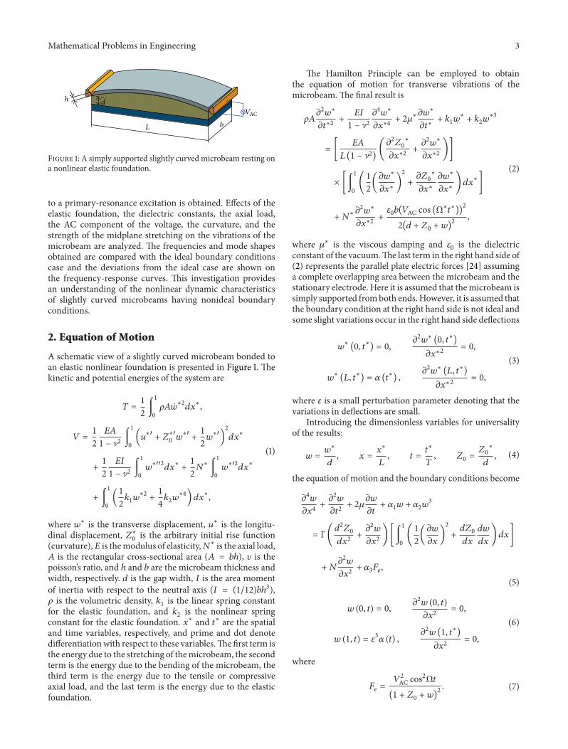
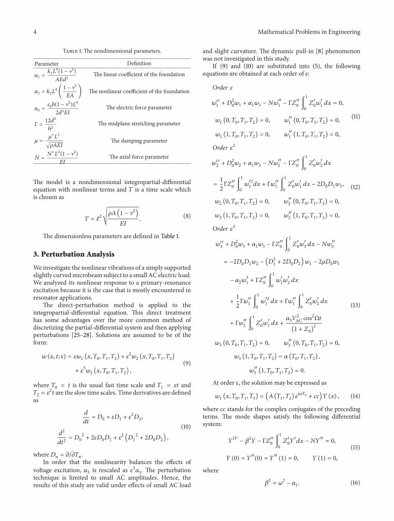
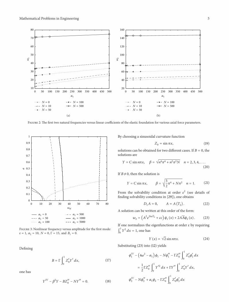
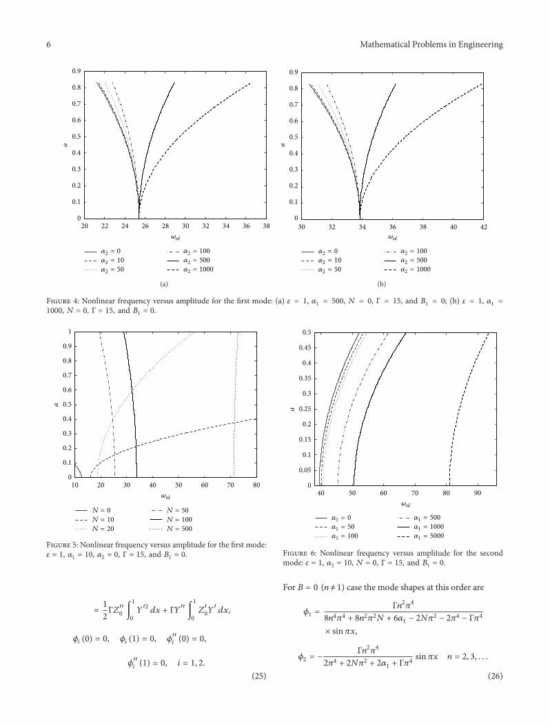
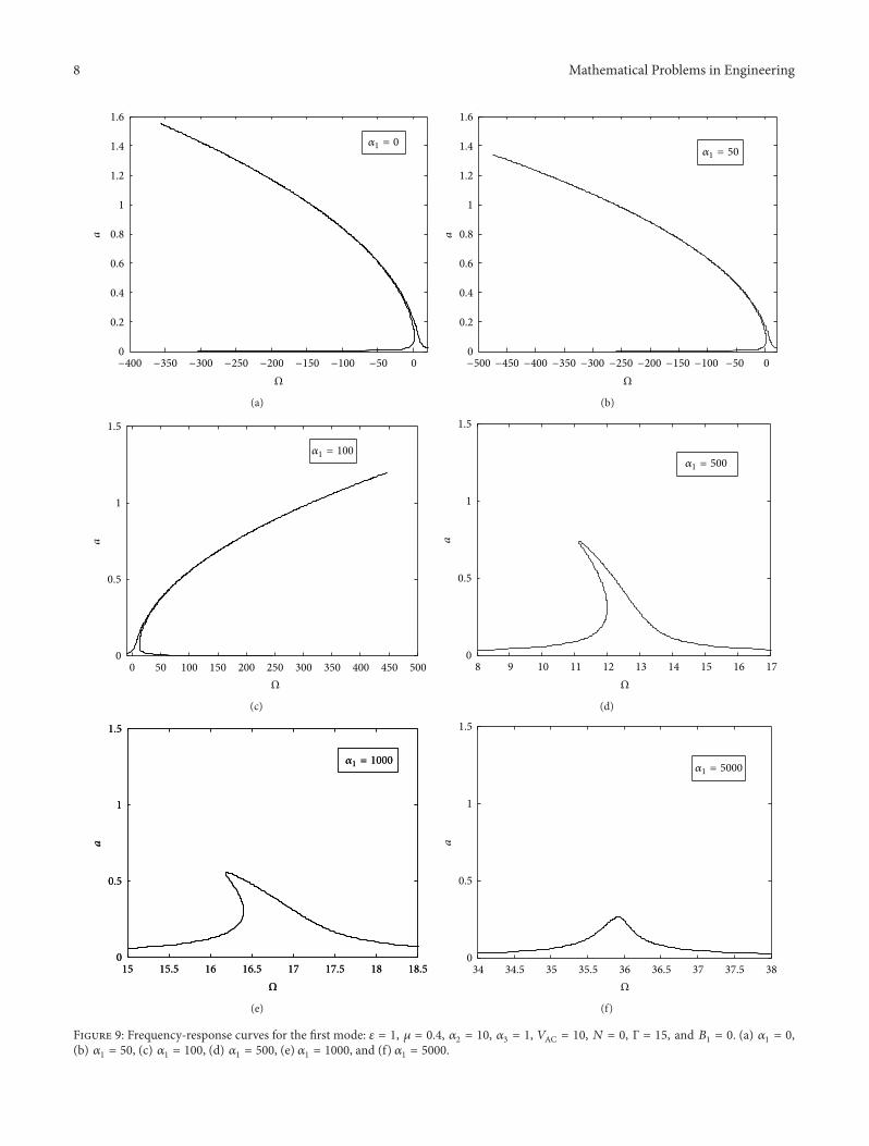
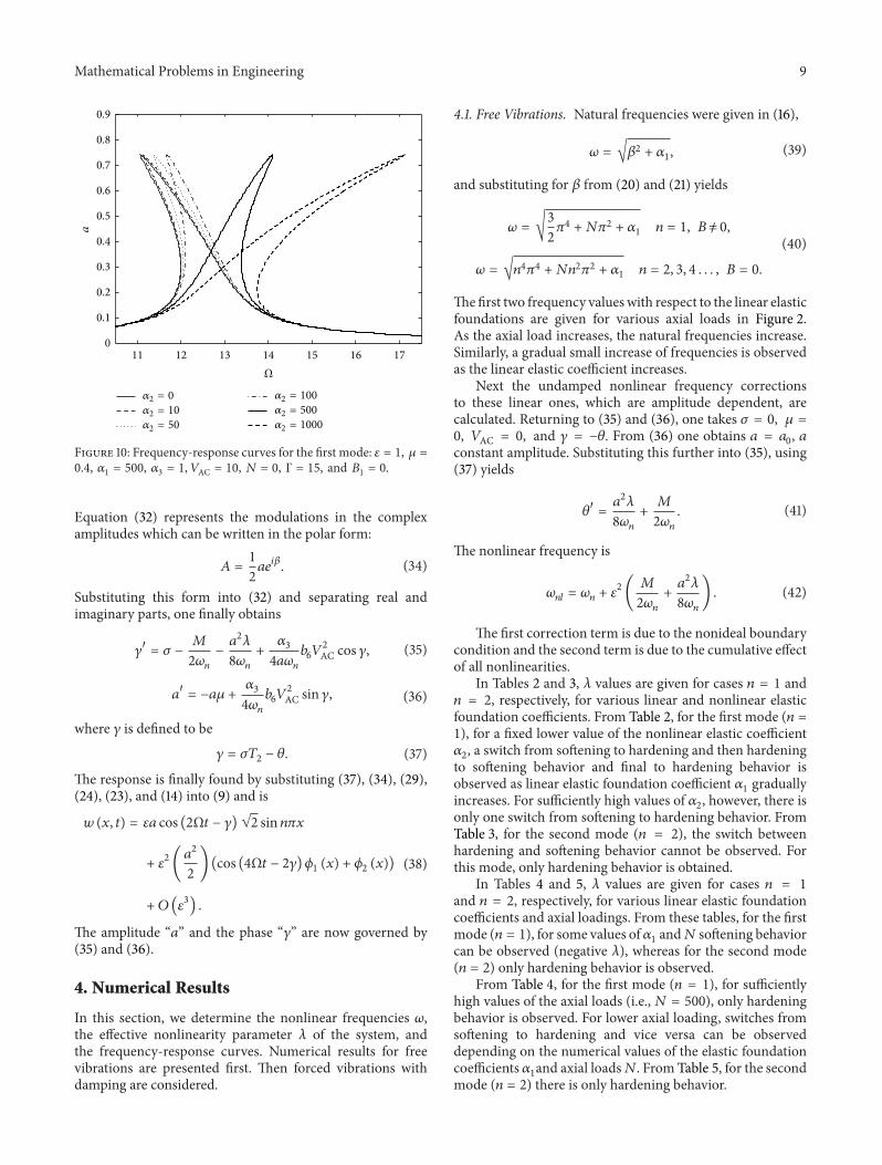
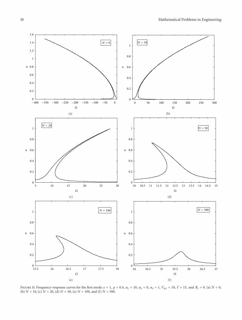
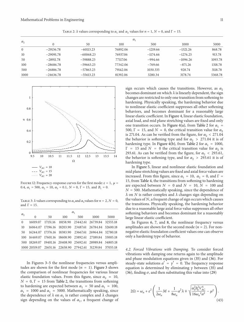
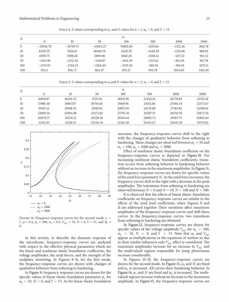
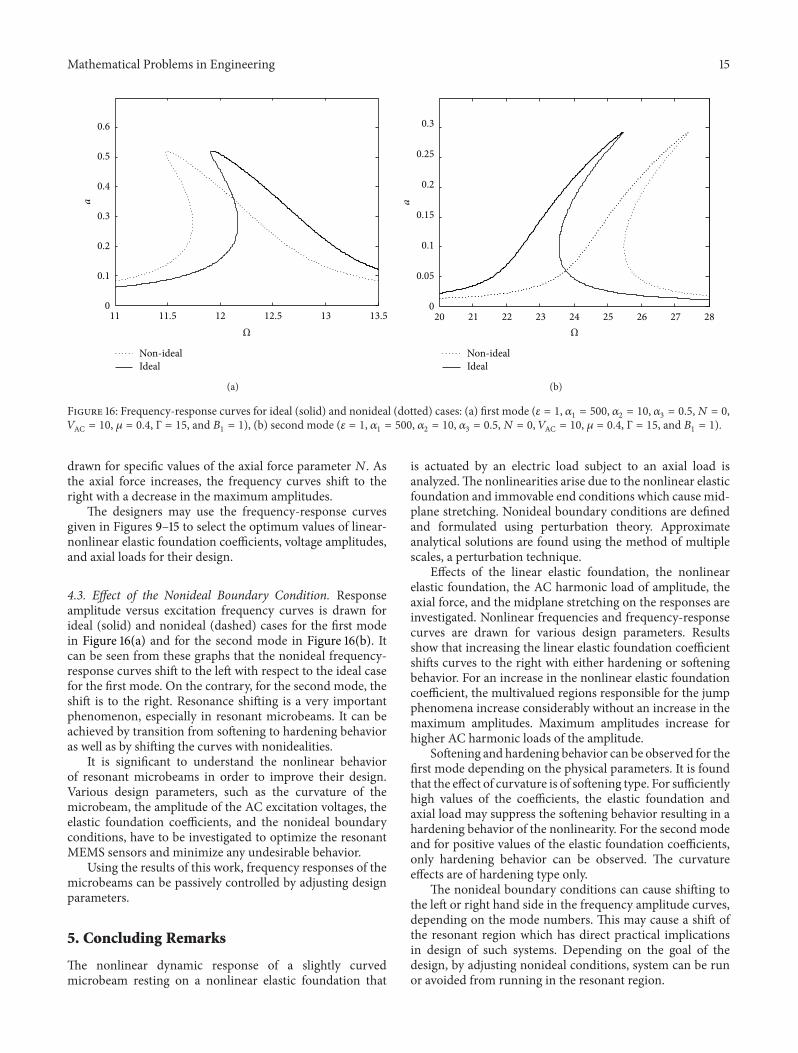
Top Related
Copyright © 2022 FDOKUMEN

