


Bahasa
Halaman
Hukum

www.elsevier.com/locate/petrol
Journal of Petroleum Science and Engineering 44 (2004) 93–114
Valuation of exploration and production assets:
an overview of real options models
Marco Antonio Guimaraes Dias*,1
Petrobras, Brazil
Abstract
This paper presents a set of selected real options models to evaluate investments in petroleum exploration and production
(E&P) under market and technical uncertainties. First are presented some simple examples to develop the intuition about
concepts like option value and optimal option exercise, comparing them with the concepts from the traditional net present value
(NPV) criteria. Next, the classical model of Paddock, Siegel and Smith is presented, including a discussion on the practical
values for the input parameters. The modeling of oil price uncertainty is presented by comparing some alternative stochastic
processes. Other E&P applications discussed here are the selection of mutually exclusive alternatives under uncertainty, the
wildcat drilling decision, the appraisal investment decisions, and the analysis of option to expand the production through
optional wells.
D 2004 Elsevier B.V. All rights reserved.
Keywords: Real options; Investment under uncertainty; E&P investments; Project valuation under uncertainty; Real options in petroleum
1. Introduction and intuitive examples invest in the appraisal phase through delineation wells
This paper focuses on investments in exploration
and production and how oil companies can maximize
value by managing optimally the real options embed-
ded in their portfolio of projects and other real assets.
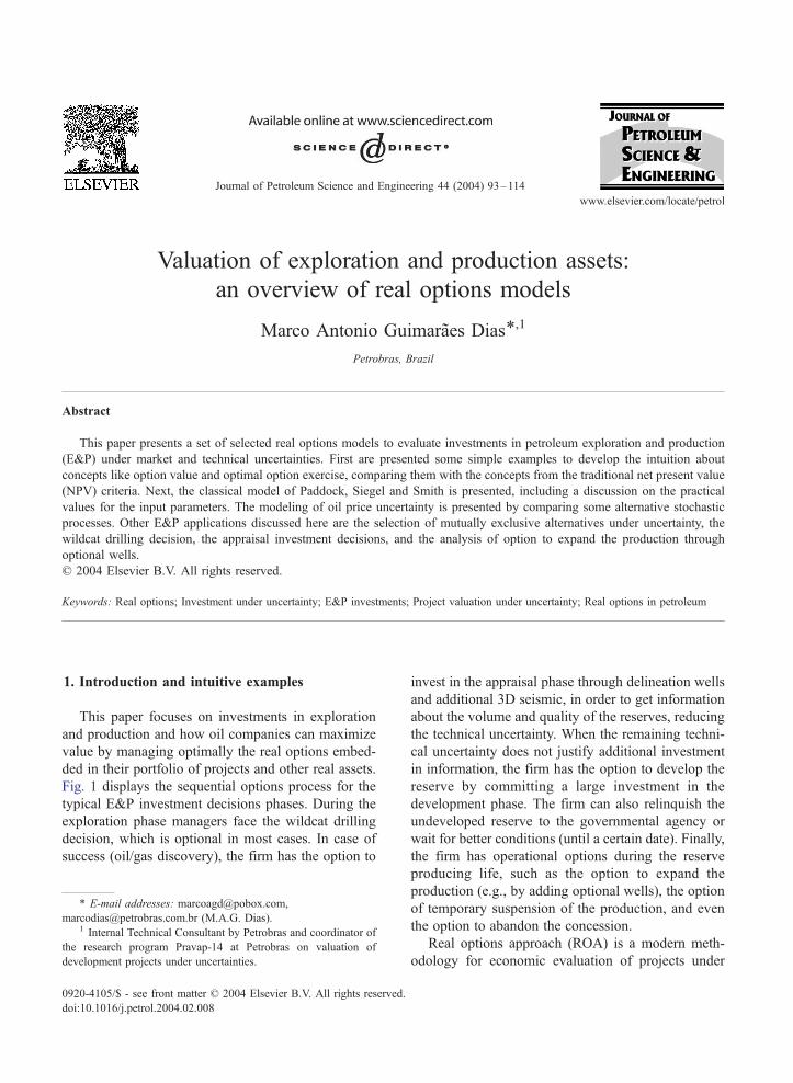
Fig. 1 displays the sequential options process for the
typical E&P investment decisions phases. During the
exploration phase managers face the wildcat drilling
decision, which is optional in most cases. In case of
success (oil/gas discovery), the firm has the option to
0920-4105/$ - see front matter D 2004 Elsevier B.V. All rights reserved.
doi:10.1016/j.petrol.2004.02.008
* E-mail addresses: [email protected],
[email protected] (M.A.G. Dias).1 Internal Technical Consultant by Petrobras and coordinator of
the research program Pravap-14 at Petrobras on valuation of
development projects under uncertainties.
and additional 3D seismic, in order to get information
about the volume and quality of the reserves, reducing
the technical uncertainty. When the remaining techni-
cal uncertainty does not justify additional investment
in information, the firm has the option to develop the
reserve by committing a large investment in the
development phase. The firm can also relinquish the
undeveloped reserve to the governmental agency or
wait for better conditions (until a certain date). Finally,
the firm has operational options during the reserve
producing life, such as the option to expand the
production (e.g., by adding optional wells), the option
of temporary suspension of the production, and even
the option to abandon the concession.
Real options approach (ROA) is a modern meth-
odology for economic evaluation of projects under
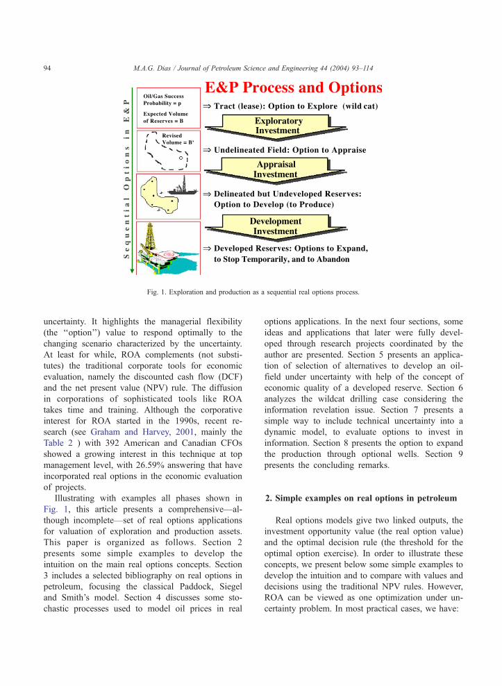
Fig. 1. Exploration and production as a sequential real options process.
M.A.G. Dias / Journal of Petroleum Science and Engineering 44 (2004) 93–11494
uncertainty. It highlights the managerial flexibility
(the ‘‘option’’) value to respond optimally to the
changing scenario characterized by the uncertainty.
At least for while, ROA complements (not substi-
tutes) the traditional corporate tools for economic
evaluation, namely the discounted cash flow (DCF)
and the net present value (NPV) rule. The diffusion
in corporations of sophisticated tools like ROA
takes time and training. Although the corporative
interest for ROA started in the 1990s, recent re-
search (see Graham and Harvey, 2001, mainly the
Table 2 ) with 392 American and Canadian CFOs
showed a growing interest in this technique at top
management level, with 26.59% answering that have
incorporated real options in the economic evaluation
of projects.
Illustrating with examples all phases shown in
Fig. 1, this article presents a comprehensive—al-
though incomplete—set of real options applications
for valuation of exploration and production assets.
This paper is organized as follows. Section 2
presents some simple examples to develop the
intuition on the main real options concepts. Section
3 includes a selected bibliography on real options in
petroleum, focusing the classical Paddock, Siegel
and Smith’s model. Section 4 discusses some sto-
chastic processes used to model oil prices in real
options applications. In the next four sections, some
ideas and applications that later were fully devel-
oped through research projects coordinated by the
author are presented. Section 5 presents an applica-
tion of selection of alternatives to develop an oil-
field under uncertainty with help of the concept of
economic quality of a developed reserve. Section 6
analyzes the wildcat drilling case considering the
information revelation issue. Section 7 presents a
simple way to include technical uncertainty into a
dynamic model, to evaluate options to invest in
information. Section 8 presents the option to expand
the production through optional wells. Section 9
presents the concluding remarks.
2. Simple examples on real options in petroleum
Real options models give two linked outputs, the
investment opportunity value (the real option value)
and the optimal decision rule (the threshold for the
optimal option exercise). In order to illustrate these
concepts, we present below some simple examples to
develop the intuition and to compare with values and
decisions using the traditional NPV rules. However,
ROA can be viewed as one optimization under un-
certainty problem. In most practical cases, we have:
M.A.G. Dias / Journal of Petroleum Science and Engineering 44 (2004) 93–114 95
Maximize the NPV (typical objective function)
subject to:
� Relevant options (managerial flexibilities);� Market uncertainties (oil price, rig rate, etc.); and� Technical uncertainties (petroleum existence, vol-
ume and quality).
Among the relevant options we can mention the
option to defer the investment (timing option), the
option to expand the production, the option to learn
(investment in information), and the option to abandon.
We start with one example from exploration, work-
ing with the uncertainty on the petroleum existence.
Suppose that one oil company has exploratory rights
over a tract with two distinct prospects in the same
geologic play. The chance factor CF (probability of
success) is 30% for both cases. The drilling cost in this
deepwater area is IW=$30 million for each exploratory
well. In case of success, the conditional development
NPV is $95 million in each case (so, economically
equivalent prospects). Both prospects have the same
negative expected monetary value2 (EMV) given by:
EMV ¼ �IW þ ½CF � NPV� ¼ �30þ ½0:3� 95�
¼ �$1:5 million
Are the prospects worthless? In order to answer this
question we need to include at least two features not
considered in the above traditional EMV calculus: the
information revelation and the optional nature of the
drilling. These prospects are dependent so that we need
to consider the sequential drilling case. In case of
success in the first prospect (positive information
revelation), the chance factor for the second prospect
CF2+ increases, whereas in case of a dry hole in the
first drilling, the chance factor for the second pros-
pect CF2� decreases. Imagine that a geologist using a
Bayesian approach found that in the former case the
chance factor increases to CF2+ = 50%. To be consis-
tent, the law of iterated expectations3 tells that we
2 Term largely used in exploratory economics for the value of a
prospect considering the chance factor.3 The expectation (or mean) of a conditional expectation is
equal to the prior expectation. In this case, the new information (first
drilling outcome) will change CF2, but the mean of the possible CF2values, E[CF2j new information], must be equal to the original
chance factor CF2 = 30%. See the proof and other properties for the
information revelation in Dias (2002).
must have CF2� = 21.43%, because 30%=[0.7�CF2
�]+
[0.3� 50%]. Fig. 2 illustrates the information revela-
tion from the first drilling and the conditional chance
factors for the second prospect.
If we drill the first prospect and get a negative
information revelation, the EMV for the second pros-
pect is evenmore negative. However, we do not need to
drill the second prospect because drilling is an option,
not an obligation. So that in case of negative revelation
we stop losses and the second prospect values zero.
However, in case of positive revelation from the first
prospect (with only 30% chances), the revised EMV+2
is positive: EMV+2 =� 30+[0.50� 95]=+$17.5 mil-
lion. So, the value of the tract considering the infor-
mation revelation of the first drilling and the optional
nature of the second drilling is:
EMV½optional well 2 j well 1 outcome�
¼ �1:5þ ½ð0:7� zeroÞ þ ð0:3� 17:5Þ�
¼ þ3:75 million
An apparent worthless tract is much better than a
traditional analysis can indicate. In this simple exam-
ple the optimal decision rule is: ‘‘Drill the first
prospect. Exercise the option to drill the second
prospect only in case of positive information revela-
tion from the first one’’. The real option value of
$3.75 million in this simple example is clearly linked
with this decision rule. The key factors for this
positive value were the optional nature of the prospect
drilling and the information revelation effect of de-
pendent prospects.
There are important business consequences for the
oil company from this example in both farm-in
(buying rights) and farm-out (selling) of tracts. In
addition, the oil company could design some special
Fig. 2. Information revelation for the second prospect.
4 This is a stylized fact known by people working with DCF
models in the fiscal regimes of concession, when performing the
sensitivity analysis NPV�P. However, the same is not true for
production sharing contracts. In addition, in our NPV equations are
not considered the option to abandon and other operational options,
which could introduce non-linearity in the model.5 See Adelman et al. (1989, data in Table 2) for data and
discussion on the market value of a developed reserve.6 The ‘‘one-third’’ rule of the thumb was also used in Paddock
et al. (1988) to perform numerical examples.7 Being V in present value in Eqs. (1) and (2), all discounting
effect is embedded into the quality factor q. Moreover, when using q
estimated from developed reserve market, we need to adjust the
value of q in order to consider the time-to-build the project so that V
and D must be in present values at the same date (the date of the
option exercise, at the investment start-up).
M.A.G. Dias / Journal of Petroleum Science and Engineering 44 (2004) 93–11496
partnership operations. In the example, the oil com-
pany could give 100% of the rights of the first
prospect for free to a Company Y, except that the
Company Y must drill immediately the (first) prospect
and give all the information to original owner of the
tract (Company X). In this case, the expected value for
the Company X tract rises to +$5.25 million because
Company X does not drill the first prospect with
EMV1 =� $1.5 million. This kind of dealing is pos-
sible because firms have different evaluations for the
same prospect.
Now we consider the development investment
decision and the market uncertainty represented by
the oil prices. The NPV rule tells to invest if NPV>0
and reject the investment if NPV< 0. The ROA can
recommend very different actions, as we will illustrate
in the following set of related simple examples. But
before the examples, we need to establish a simple
NPV equation as function of key parameters.
The NPV from the exercise of the development
option is given by the difference between the value of
the developed reserve V and the development cost D.
NPV ¼ V � D ð1Þ
In the oil industry, the value of the developed
reserve V is given by the market transactions on
developed reserves or, most commonly, by the dis-
counted cash flow approach. With the DCF ap-
proach, V is the present value of the revenues net
of operational costs and taxes, whereas the invest-
ment D is the present value of the investment flow
net of tax benefits. In real options nomenclature, V is
the underlying asset and the investment cost D is the
exercise price of the development option. In the next
section we will see that if we have V and D (e.g.,
from the DCF model) and a few more parameters,
we can apply the classical model of Paddock et al. in
order to obtain the real option value. However, for
our intuitive examples here and for some applica-
tions presented later, we will present a parametric
version of V as function of the oil price P and other
few key parameters like the volume and quality of
the reserve.
The two main fiscal regimes in the petroleum
upstream (E&P) industry are the concessions regime
(used in countries like USA, Brazil, UK, etc.) and the
production-sharing regime (used for example in
Africa). See for example Johnston (1995) for a dis-
cussion of fiscal regimes. For concessions, is very
reasonable to assume that the NPV is a linear func-
tion4 of the oil price P, so we will focus in this case for
simplicity.
The simplest linear model is to consider that the
market value of the developed reserve V is propor-
tional to the oil prices. In addition, we can consider
the variable reserve volume in order to price the
reserve in $/bbl. Let B be the number of barrels in
this reserve. The proportional or ‘‘Business Model’’ is
given by:
V ¼ qBP ð2Þ
The motivation for the name ‘‘Business Model’’ is
drawn from the reserves transactions market5, because
the product qP is the value of one barrel of developed
reserve. The called ‘‘one-third’’ rule of the thumb is
well known in USA, where the average value paid for
one barrel of developed reserve is 33% of the well-
head oil price (P), see Gruy et al. (1982).6 The value
of 1/3 is only a particular case of q in our business
model. In general, we can estimate q using the DCF
(see below) or by using data from the reserves market,
if available. This parameter is called economic quality
of the developed reserve because V increases mono-
tonically with q and because q depends on reservoir
rock quality and fluid quality. This value is lower than
1 and it is also function of other issues like discount
rate7 (including country risk), taxes, and operational
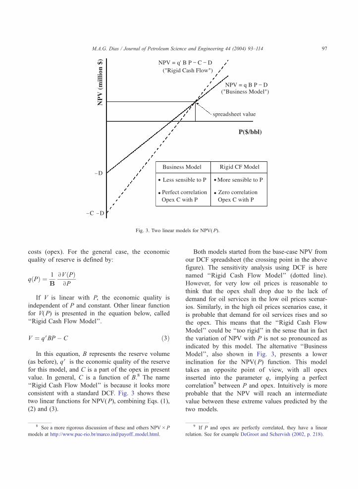
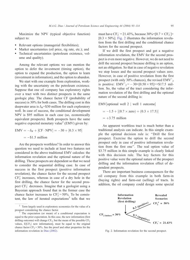
Fig. 3. Two linear models for NPV(P).
M.A.G. Dias / Journal of Petroleum Science and Engineering 44 (2004) 93–114 97
costs (opex). For the general case, the economic
quality of reserve is defined by:
qðPÞ ¼ 1
B
BV ðPÞBP
If V is linear with P, the economic quality is
independent of P and constant. Other linear function
for V(P) is presented in the equation below, called
‘‘Rigid Cash Flow Model’’.
V ¼ qVBP � C ð3Þ
In this equation, B represents the reserve volume
(as before), qV is the economic quality of the reserve
for this model, and C is a part of the opex in present
value. In general, C is a function of B.8 The name
‘‘Rigid Cash Flow Model’’ is because it looks more
consistent with a standard DCF. Fig. 3 shows these
two linear functions for NPV(P), combining Eqs. (1),
(2) and (3).
8 See a more rigorous discussion of these and others NPV�P
models at http://www.puc-rio.br/marco.ind/payoff_model.html.
Both models started from the base-case NPV from
our DCF spreadsheet (the crossing point in the above
figure). The sensitivity analysis using DCF is here
named ‘‘Rigid Cash Flow Model’’ (dotted line).
However, for very low oil prices is reasonable to
think that the opex shall drop due to the lack of
demand for oil services in the low oil prices scenar-
ios. Similarly, in the high oil prices scenarios case, it
is probable that demand for oil services rises and so
the opex. This means that the ‘‘Rigid Cash Flow
Model’’ could be ‘‘too rigid’’ in the sense that in fact
the variation of NPV with P is not so pronounced as
indicated by this model. The alternative ‘‘Business
Model’’, also shown in Fig. 3, presents a lower
inclination for the NPV(P) function. This model
takes an opposite point of view, with all opex
inserted into the parameter q, implying a perfect
correlation9 between P and opex. Intuitively is more
probable that the NPV will reach an intermediate
value between these extreme values predicted by the
two models.
9 If P and opex are perfectly correlated, they have a linear
relation. See for example DeGroot and Schervish (2002, p. 218).

The simpler business model has been used in
numerical examples of real options (Paddock et al.,
1988) and it is recommended by Pickles and Smith
(1993, p. 16): ‘‘in equilibrium the prices of developed
reserves and oil at wellhead must appreciate at the
same rate’’. However, it is not a consensus in the
literature (Bjerksund and Ekern, 1990). Typically, this
business model generates more conservative real
option values (due to the lower sensitivity with P)
than the rigid cash flow model.
Using the business model, let us analyze the first
intuitive example for development decision with mar-
ket (represented by the oil price) uncertainty. Assume
that the current oil price10 P(t = 0)=$18/bbl, the qual-
ity q = 20%, volume B = 500 million barrels, and
development cost D=$1850 million. Hence, the
NPV is negative: qPB�D = 0.2� 18� 500� 1850 =
� $50 million. Imagine we can defer one period the
decision (timing option) and at t= 1 the oil price can
rise or fall only $1/bbl (simple and small market
uncertainty), with 50% chances11 each scenario. See
Fig. 4.
Suppose that other company offer $1 million for
the rights of this oilfield. Do you sell? Assume a
discount rate of 10% per period. Using the traditional
DCF approach, we could accept the offer. However,
with real options in mind we need to check what
happen if we wait one period and exercise the option
only if the future scenario is favorable. In this case, if
we wait one period and the oil price rises to P+=$19/
bbl, the NPV is positive: NPV+ = qP+B�D = 0.2�19�500� 1850=+$50 million. But if the oil price
10 Alternatively, we can think the current long-term expectation
on the oil price, e.g., using a futures market value as proxy.11 For while, we omit the discussion on probability mapping
(stochastic process) and discount rate features for simplicity.
drops to P�=$17/bbl, the NPV is even worse than at
t = 0: NPV�= 0.2� 17� 500� 1850 =� $150 mil-
lion. A rational manager will not exercise the option
with this negative NPV, so that if we wait and see
the scenario P�, the development right values
maximum(NPV�, 0) = 0, because we are not obligate
to invest—it is an option! Hence, recognizing the
option to defer one period, and bringing it in present
value, the value of our real option (F) in this
stylized example is:
F ¼ ½50%�maxðNPVþ; 0Þ þ 50%
�maxðNPV�; 0Þ�=ð1þ discount rateÞ
¼ þ$22:73 million
which is much higher than the offer from the other
company. The very different value obtained here is
because we recognize explicitly both the market un-
certainty and mainly the value to defer the investment
decision (the option/managerial flexibility). Note that
we just used the NPV rule in each scenario at t = 1. The
reader can check that if we increase the variance at t= 1
(e.g., the oil prices can rise or fall by $2/bbl) the value
of real option is even higher. In general, market
volatility increases the real option value.
Let us see a second example using the same Fig. 4.
The only difference here is a lower investment cost:
assume D=$1750 million. In this case the NPV is
positive (0.2� 18� 500� 1750=+$50 million) at the
current market prices (or current market expectations).
Do you exercise immediately or wait and see?
If we use the traditional NPV rule, we could
exercise the option. However, it is necessary to
compare the value of immediate exercise ( + 50 mil-
lion) with the mutually exclusive alternative of defer-
ring one period, exercising the option only in the
favorable scenarios. It is easy to see that in this case
the option value is:
F ¼ ½50%� 150þ 50%� 0�=ð1:1Þ
¼ þ$68:18 million
which is higher than the immediate exercise value,
NPV(t = 0)=$50 million. Hence, in this second exam-
ple the optimal rule is: wait one period, exercising the
option at P+ and not exercising at P�. This example
showed that can be optimal to defer a positive NPV
M.A.G. Dias / Journal of Petroleum Science and Engineering 44 (2004) 93–114 99
project. In this case, the NPV is not high enough to
ignore the option to defer. In addition, this flexibility
to postpone investment increases the value of the
rights on this undeveloped oilfield.
Finally, let us see a third example where the option
to defer is worthless. Consider again Fig. 4 and the
same previous values except that the investment cost
is lower: D=$1700 million. In this case, the NPV from
immediate investment is +$100 million ( = 0.2� 18�500� 1700). The same question: Do you exercise
immediately or wait and see? It is easy to check that
if we defer, the option value is:
F ¼ ½50%� 200þ 50%� 0�=ð1:1Þ
¼ þ$90:91 million
Hence, here the waiting value is lower than the
immediate investment. So, the optimal rule is to
exercise the option immediately (here the traditional
NPV rule holds). We say in this case that the real option
is ‘‘deep-in-the-money’’, because the current NPV is
high enough to justify the immediate investment.
Comparing the two last examples, we could imag-
ine that there exists an intermediate NPV* at t = 0 so
that value of waiting = value of immediate exercise.
This is a threshold NPV* because is optimal the option
exercise the option if NPVzNPV*. The concept of
threshold for the optimal option exercise, for a given
D, could be also the value of developed reserve V* or
even the oil price P*. This threshold also can change
with the time. Note that if we have a ‘‘now-or-never’’
situation to invest (no option), the threshold is
NPV* = 0, or the traditional break-even for P*. These
simple concepts of option value and threshold will be
exploited in more complex applications presented in
the next sections.
12 This simplification for development decisions will be
assumed in the classical model that is presented in this section.
3. Real options in petroleum: literature overview
and the classical model
In a well-known paper of 1977, Stewart Myers
(Myers, 1977) coined the term ‘‘real options’’ observ-
ing that corporate investments opportunities could be
viewed as call options on real assets. Most of the
earlier real options models were developed for natural
resources applications, perhaps due to the availability
of data for commodities prices. See Dias (1999) for a
bibliographical overview on real options. Some im-
portant earlier real options models in natural resources
include Tourinho (1979), first to evaluate oil reserves
using option pricing techniques, Paddock et al. (1988),
a classical model discussed below, Brennan and
Schwartz (1985), analyzing interactions of operation-
al options in a copper mine, and Ekern (1988),
valuing a marginal satellite oilfield.
A sample of other important real options models for
petroleum applications is briefly described in se-
quence, highlighting the main individual contribution.
Bjerksund and Ekern (1990) showed that for initial
oilfield development purposes, in general is possible to
ignore both temporary stopping and abandonment
options in the presence of the option to delay the
investment.12 Kemna (1993) described some case
studies in her long consultant for Shell. Dias (1997)
combined game theory with real options to evaluate
the optimal timing for the exploratory drilling.
Schwartz (1997) compared oil prices models that are
discussed in the next section. Laughton (1998) found
that although oil prospect value increases with both oil
price and reserve size uncertainties, oil price uncer-
tainty delays all options exercise (from exploration to
abandonment), whereas exploration and delineation
occur sooner with reserve size uncertainty. Cortazar
and Schwartz (1998) applied the flexible Monte Carlo
simulation to evaluate the real option to develop an
oilfield. Pindyck (1999) analyzed the long-run behav-
ior of oil prices and the implications for real options.
Galli et al. (1999) discussed real options, decision-tree
and Monte Carlo simulation in petroleum applications.
Chorn and Croft (2000) studied value of reservoir
information. Saito et al. (2001) evaluated development
alternatives by combining reservoir simulation engi-
neering with real options. Kenyon and Tompaidis
(2001) analyzed leasing contracts of offshore rigs.
McCormack and Sick (2001) discussed valuation of
underdeveloped reserves. The real options textbooks
of Dixit and Pindyck (1994, mainly chapter 12),
Trigeorgis (1996, pp. 356–363), and Amram and
Kulatilaka (1999, chapter 12), analyze investment
models for the oil and natural resources industry.
M.A.G. Dias / Journal of Petroleum Science and Engineering 44 (2004) 93–114100
In the beginning of the 1980s, Paddock, Siegel and
Smith started a research in the MIT Energy Labora-
tory using options theory to study the value of an
offshore lease and the development investment tim-
ing. They wrote a series of papers, two of them
published in 1987 and 1988. The Paddock, Siegel
and Smith (PSS) approach is the most popular real
options model for upstream petroleum applications.
This classical model is useful for both learning pur-
poses and as first approximation for investment anal-
ysis of development of oil reserves, even thinking that
in the real life are necessary models that fit better the
real world features. The book of Dixit and Pindyck
(1994, see chapter 12) describes this model in a more
compact and didactic way. This model has practical
advantages (when compared with others options mod-
els) due to its simplicity and few parameters to
estimate. One attractive issue is the simple analogy
between Black–Scholes–Merton financial option and
the real option value of an undeveloped reserve,
which is illustrated in the Table 1.
The analogy above is also useful for other real
options applications. Instead, developed reserve value
is possible to consider any operating project value (V)
as the underlying asset for this option model. For
example, F could be an undeveloped urban land, V the
market value of a hotel, and D the investment to
construct the hotel. In absence of a direct market value
for V, it is possible to compute V as the present value
of the revenue net of operational costs and taxes.
Remember from Eq. (1) that the traditional net present
Table 1
Analogy between financial options and real options
Black–Scholes–Merton’s
financial options
Paddock, Siegel and
Smith’s real options
Financial option value Real option value of an
undeveloped reserve ( F )
Current stock price Current value of developed
reserve (V )
Exercise price of the option Investment cost to develop
the reserve (D)
Stock dividend yield Cash flow net of depletion
as proportion of V (d)Risk-free interest rate Risk-free interest rate (r)
Stock volatility Volatility of developed
reserve value (r)Time to expiration
of the option
Time to expiration of the
investment rights (s)
value is given by NPV=V�D, where D is the present
value of the investment cost to develop the project.
Here, the investment D is analog to the exercise price
of the financial option because it is the commitment
that the oil company faces when exercising the real
option to develop the oilfield.
The time to expiration (s) of this real option is the
deadline when the investment rights expire. There is a
relinquishment requirement and the oil company faces
a ‘‘now-or-never’’ opportunity at this date: or the firm
commits an immediate development investment plan
or returns the concession rights back to the National
Petroleum Agency or similar governmental institu-
tion. This time varies from 3 to 10 years. In other
applications (like development of urban lands), we
have perpetual options (no expiration date).
Volatility (r) is the annual standard deviation of dV/V. In the case that V is proportional to P is possible to
use the same value of the volatility of oil price,13 which
has more available data for estimations. Dixit and
Pindyck (1994, chapter 12) recommend r between
15% and 25% per annum. Some authors (e.g., Baker et
al., 1998, p. 119) use a value higher than 30% p.a. for
r. Another possibility to estimate r of V is the Monte
Carlo simulation of the stochastic processes of key
market components like P, opex elements, and taxes.
With this approach we get a combined variance of V at
t = 1, and with a formula we get the volatility. See
Copeland and Antikarov (2001, chapter 9) for details
on this alternative approach.
In the dividend yield analogy,14 the cash flow yield
d is the (annual) operating net cash flow value as a
percentage of V. For petroleum reserves, there is a
depletion phenomenon due to the finite quantity of
petroleum in the reservoir. This generates a decline rate
(x) in the oilfield output flow-rate along the reserve
14 The project cash flows are like ‘‘dividends’’ earned only if
the option is exercised and the underlying asset start operations. So,
the dividend yield is an opportunity cost of waiting that faces the
investor who has the option but not the underlying asset. In contrast,
the interest rate r rewards the waiting policy (imagine the investor
put the amount D in the bank). So, r and d have opposite effects in
both option value and optimal exercise thresholds, and it is frequent
to see in equations the difference r� d.
13 If both V follows a geometric Brownian motion (GBM) and
V is proportional to P (that is V= kP), then P also follows a GBM
with the same parameters (r, d, a). See Dixit and Pindyck (1994,
p. 178) or the proof with Ito’s Lemma at Dias (2002).
Fig. 5. The
life. The equation to estimate d including the depletion
issue is presented in both Paddock et al. (1988) and in
Dixit and Pindyck (1994),15 but two more practical
ways to estimate d are presented below.
For the model that assume the value of the devel-
oped reserve proportional to the (wellhead) price of
oil is possible to see d as the oil price (net) conve-
nience yield by using data from the futures market.
With the notation U(t) for the oil futures price deliv-
ering at time t, P for the spot oil price (or the earliest
futures contract, at t0), r for the risk-free interest rate,
and Dt = time interval (or t� t0), the equation is:
P ¼ UðtÞexp½�ðr � dÞDt� ð4Þ
The second way is a practical rule using a long-
term perspective that is useful for real options mod-
els. What is a good practical value for the net con-
venience yield d? Pickles and Smith (1993) suggest
the risk-free interest rate. They wrote (pp. 20–21):
‘‘We suggest that option valuations use, initially, the
‘normal’ value of net convenience yield, which seems
to equal approximately the risk-free nominal interest
rate’’.16
One interesting feature of the PSS model is the
resultant partial differential equation for the real
option value (the value of undeveloped reserve) is
identical to the known Black–Scholes–Merton equa-
tion with continuous dividend. Only at the boundary
conditions appear two additional conditions, to take
account of the earlier exercise feature of this Ameri-
can call option (American options can be exercise at
any time up to expiration, whereas European options
can be exercised only at the expiration). See the
equation and the boundary conditions for example in
the book of Dixit and Pindyck (1994, chapter 12). By
solving this partial differential equation numerically
we obtain two linked answers, the real option value of
15 A detailed proof for the Paddock, Siegel and Smith equations
is available at www.puc-rio.br/marco.ind/petmode1.html.16 In the risk-neutral valuation, largely used in options pricing,
the risk-neutral drift is r� d and using the suggestion of Pickles and
Smith (r = d) we get a driftless risk-neutral process, which sounds
reasonable for the long-run equilibrium. Schwartz (1997, p. 969)
uses an interest rate r = 6% p.a. and a convenience yield for the
copper= 12%. However, he suggests (footnote 34) a long-term
convenience yield of 6%, that is equal the interest rate value, as
Pickles and Smith suggested!
real option value of an undeveloped reserve.M.A.G. Dias /
the undeveloped reserve (F) and the decision rule
(invest or wait for better conditions), recall our simple
intuitive examples in the previous section. Here,
thanks to the analogy, any good software that solves
American call options (with continuous dividend-
yield) also solves our PSS real options model.17
The decision rule is given by the critical value (or
threshold) of V, named V*, which the real option is
‘‘deep-in-the-money’’. It is optimal the immediate
exercise of the option to develop the oilfield only
when V(t)zV*(t). For models where V is proportional
to P, it is easier to think with P*, the oil price that
makes a particular undeveloped oilfield to be ‘‘deep-
in-the-money’’. In this case the rule is to invest when
PzP*.
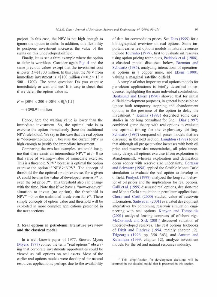
Fig. 5 presents a typical solution for an undevel-
oped oilfield with 100 million barrels (and q = 0.187,
so that V= 18.7�P). The curves represent the real
option values for the cases of 5 years to expiration of
rights (s = 5 years), 1 year (s = 1 year), and at
expiration (s = 0). For the last situation, known as
‘‘now-or-never’’ case, the NPV rule holds and the
real option value is the maximum between the NPV
and zero.
Fig. 5 shows that for P=$15/bbl the NPV is zero.
Hence, $15/bbl is the break-even oil price. It also
shows that at $16/bbl the NPV is positive, but the net
waiting value, also called option premium (the differ-
17 For example, the spreadsheet ‘‘Timing’’, a full functional
shareware available at www.puc-rio.br/marco.ind/.
Journal of Petroleum Science and Engineering 44 (2004) 93–114101

Fig. 6. The real option decision rule: invest above the threshold.
Fig. 7.Fig. 8.102
ence F�NPV), for s = 5 years is not zero—it is even
higher than the NPV. So, at $16/bbl the optimal policy
for this field-example is ‘‘wait and see’’. The option
premium is zero only at the tangency point between
the option curve and the NPV line (continuous line),
which occurs only at the point A, at P*(s = 5)=$24.3/bbl. If Pz 24.3, even with 5 years to expiration the
oilfield is ‘‘deep-in-the-money’’ (the NPV is too high)
in this example and it is optimal the immediate
exercise of the option to invest. Fig. 5 also displays
the real option curve for 1 year to expiration (the
option is less valuable than the case of 5 years), when
the threshold value P* drops to $20.5/bbl (see point
B). Fig. 6 presents the threshold curve for this oilfield,
from 5 years to expiration until the ‘‘now-or-never’’
deadline.
Note in Fig. 6 the correspondence with the points
A and B from Fig. 5. Note also that at the expiration
(now-or-never case), the real option rule collapses to
the NPV rule, that is, invest if the oil price is higher
than the break-even price for the oilfield (in this case
about $15/bbl).
4. Stochastic processes for oil prices
Like Black–Scholes–Merton financial options
model, Paddock, Siegel and Smith model assumes
that the underlying asset (here the developed reserve
value V but could be the oil price P itself) follows a
kind of random-walk model named geometric Brow-
nian motion (GBM). Under this hypothesis, the un-
derlying asset V at a future date t has lognormal
distribution with variance that grows with the fore-
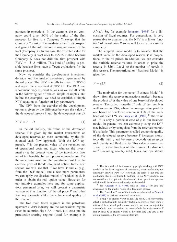
Probability mapping for the geometric Brownian motion.Probability mapping for the mean-reversion model.M.A.G.
casted time-horizon, and a drift that grows (or decays)
exponentially. Fig. 7 illustrates this process.
However, many specialists argue that a realistic
stochastic model for commodities like oil must
consider the mean-reversion feature due to the
microeconomic logic of supply� demand. The idea
is that if the commodity price is too far (above or
below) from a certain long-run equilibrium level P,
market forces (including OPEC) will act to increase
(if P > P) or to reduce (if P < P) the production (for
OPEC) and E&P investment (for non-OPEC oil
companies). This creates a mean-reverting force that
is like a spring force: it is as strong as far is P from
the equilibrium level P. Fig. 8 illustrates the mean-
reversion case.
Dias / Journal of Petroleum Science and Engineering 44 (2004) 93–114
M.A.G. Dias / Journal of Petroleum Science and Engineering 44 (2004) 93–114 103
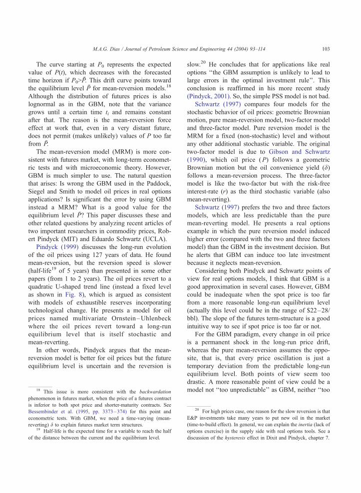
The curve starting at P0 represents the expected
value of P(t), which decreases with the forecasted
time horizon if P0>P. This drift curve points toward
the equilibrium level P for mean-reversion models.18
Although the distribution of futures prices is also
lognormal as in the GBM, note that the variance
grows until a certain time ti and remains constant
after that. The reason is the mean-reversion force
effect at work that, even in a very distant future,
does not permit (makes unlikely) values of P too far
from P.
The mean-reversion model (MRM) is more con-
sistent with futures market, with long-term economet-
ric tests and with microeconomic theory. However,
GBM is much simpler to use. The natural question
that arises: Is wrong the GBM used in the Paddock,
Siegel and Smith to model oil prices in real options
applications? Is significant the error by using GBM
instead a MRM? What is a good value for the
equilibrium level P? This paper discusses these and
other related questions by analyzing recent articles of
two important researchers in commodity prices, Rob-
ert Pindyck (MIT) and Eduardo Schwartz (UCLA).
Pindyck (1999) discusses the long-run evolution
of the oil prices using 127 years of data. He found
mean-reversion, but the reversion speed is slower
(half-life19 of 5 years) than presented in some other
papers (from 1 to 2 years). The oil prices revert to a
quadratic U-shaped trend line (instead a fixed level
as shown in Fig. 8), which is argued as consistent
with models of exhaustible reserves incorporating
technological change. He presents a model for oil
prices named multivariate Ornstein–Uhlenbeck
where the oil prices revert toward a long-run
equilibrium level that is itself stochastic and
mean-reverting.
In other words, Pindyck argues that the mean-
reversion model is better for oil prices but the future
equilibrium level is uncertain and the reversion is
18 This issue is more consistent with the backwardation
phenomenon in futures market, when the price of a futures contract
is inferior to both spot price and shorter-maturity contracts. See
Bessembinder et al. (1995, pp. 3373–374) for this point and
econometric tests. With GBM, we need a time-varying (mean-
reverting) d to explain futures market term structures.19 Half-life is the expected time for a variable to reach the half
of the distance between the current and the equilibrium level.
slow.20 He concludes that for applications like real
options ‘‘the GBM assumption is unlikely to lead to
large errors in the optimal investment rule’’. This
conclusion is reaffirmed in his more recent study
(Pindyck, 2001). So, the simple PSS model is not bad.
Schwartz (1997) compares four models for the
stochastic behavior of oil prices: geometric Brownian
motion, pure mean-reversion model, two-factor model
and three-factor model. Pure reversion model is the
MRM for a fixed (non-stochastic) level and without
any other additional stochastic variable. The original
two-factor model is due to Gibson and Schwartz
(1990), which oil price (P) follows a geometric
Brownian motion but the oil convenience yield (d)follows a mean-reversion process. The three-factor
model is like the two-factor but with the risk-free
interest-rate (r) as the third stochastic variable (also
mean-reverting).
Schwartz (1997) prefers the two and three factors
models, which are less predictable than the pure
mean-reverting model. He presents a real options
example in which the pure reversion model induced
higher error (compared with the two and three factors
model) than the GBM in the investment decision. But
he alerts that GBM can induce too late investment
because it neglects mean-reversion.
Considering both Pindyck and Schwartz points of
view for real options models, I think that GBM is a
good approximation in several cases. However, GBM
could be inadequate when the spot price is too far
from a more reasonable long-run equilibrium level
(actually this level could be in the range of $22–28/
bbl). The slope of the futures term-structure is a good
intuitive way to see if spot price is too far or not.
For the GBM paradigm, every change in oil price
is a permanent shock in the long-run price drift,
whereas the pure mean-reversion assumes the oppo-
site, that is, that every price oscillation is just a
temporary deviation from the predictable long-run
equilibrium level. Both points of view seem too
drastic. A more reasonable point of view could be a
model not ‘‘too unpredictable’’ as GBM, neither ‘‘too
20 For high prices case, one reason for the slow reversion is that
E&P investments take many years to put new oil in the market
(time-to-build effect). In general, we can explain the inertia (lack of
options exercise) in the supply side with real options tools. See a
discussion of the hysteresis effect in Dixit and Pindyck, chapter 7.
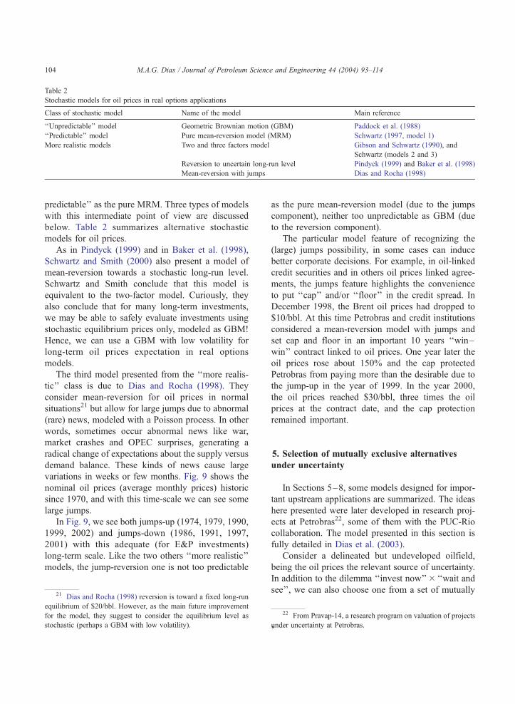
Table 2
Stochastic models for oil prices in real options applications
Class of stochastic model Name of the model Main reference
‘‘Unpredictable’’ model Geometric Brownian motion (GBM) Paddock et al. (1988)
‘‘Predictable’’ model Pure mean-reversion model (MRM) Schwartz (1997, model 1)
More realistic models Two and three factors model Gibson and Schwartz (1990), and
Schwartz (models 2 and 3)
Reversion to uncertain long-run level Pindyck (1999) and Baker et al. (1998)
Mean-reversion with jumps Dias and Rocha (1998)
M.A.G. Dias / Journal of Petroleum Science and Engineering 44 (2004) 93–114104
predictable’’ as the pure MRM. Three types of models
with this intermediate point of view are discussed
below. Table 2 summarizes alternative stochastic
models for oil prices.
As in Pindyck (1999) and in Baker et al. (1998),
Schwartz and Smith (2000) also present a model of
mean-reversion towards a stochastic long-run level.
Schwartz and Smith conclude that this model is
equivalent to the two-factor model. Curiously, they
also conclude that for many long-term investments,
we may be able to safely evaluate investments using
stochastic equilibrium prices only, modeled as GBM!
Hence, we can use a GBM with low volatility for
long-term oil prices expectation in real options
models.
The third model presented from the ‘‘more realis-
tic’’ class is due to Dias and Rocha (1998). They
consider mean-reversion for oil prices in normal
situations21 but allow for large jumps due to abnormal
(rare) news, modeled with a Poisson process. In other
words, sometimes occur abnormal news like war,
market crashes and OPEC surprises, generating a
radical change of expectations about the supply versus
demand balance. These kinds of news cause large
variations in weeks or few months. Fig. 9 shows the
nominal oil prices (average monthly prices) historic
since 1970, and with this time-scale we can see some
large jumps.
In Fig. 9, we see both jumps-up (1974, 1979, 1990,
1999, 2002) and jumps-down (1986, 1991, 1997,
2001) with this adequate (for E&P investments)
long-term scale. Like the two others ‘‘more realistic’’
models, the jump-reversion one is not too predictable
21 Dias and Rocha (1998) reversion is toward a fixed long-run
equilibrium of $20/bbl. However, as the main future improvement
for the model, they suggest to consider the equilibrium level as
stochastic (perhaps a GBM with low volatility).
as the pure mean-reversion model (due to the jumps
component), neither too unpredictable as GBM (due
to the reversion component).
The particular model feature of recognizing the
(large) jumps possibility, in some cases can induce
better corporate decisions. For example, in oil-linked
credit securities and in others oil prices linked agree-
ments, the jumps feature highlights the convenience
to put ‘‘cap’’ and/or ‘‘floor’’ in the credit spread. In
December 1998, the Brent oil prices had dropped to
$10/bbl. At this time Petrobras and credit institutions
considered a mean-reversion model with jumps and
set cap and floor in an important 10 years ‘‘win–
win’’ contract linked to oil prices. One year later the
oil prices rose about 150% and the cap protected
Petrobras from paying more than the desirable due to
the jump-up in the year of 1999. In the year 2000,
the oil prices reached $30/bbl, three times the oil
prices at the contract date, and the cap protection
remained important.
5. Selection of mutually exclusive alternatives
under uncertainty
In Sections 5–8, some models designed for impor-
tant upstream applications are summarized. The ideas
here presented were later developed in research proj-
ects at Petrobras22, some of them with the PUC-Rio
collaboration. The model presented in this section is
fully detailed in Dias et al. (2003).
Consider a delineated but undeveloped oilfield,
being the oil prices the relevant source of uncertainty.
In addition to the dilemma ‘‘invest now’’� ‘‘wait and
see’’, we can also choose one from a set of mutually
22 From Pravap-14, a research program on valuation of projects
under uncertainty at Petrobras.,
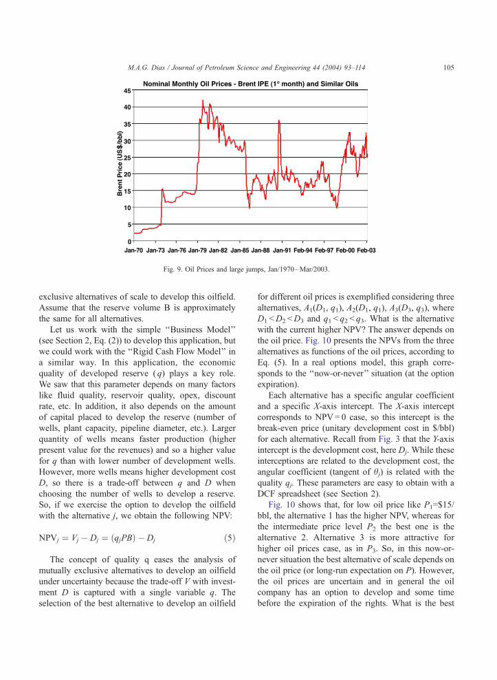
Fig. 9. Oil Prices and large jumps, Jan/1970–Mar/2003.
M.A.G. Dias / Journal of Petroleum Science and Engineering 44 (2004) 93–114 105
exclusive alternatives of scale to develop this oilfield.
Assume that the reserve volume B is approximately
the same for all alternatives.
Let us work with the simple ‘‘Business Model’’
(see Section 2, Eq. (2)) to develop this application, but
we could work with the ‘‘Rigid Cash Flow Model’’ in
a similar way. In this application, the economic
quality of developed reserve ( q) plays a key role.
We saw that this parameter depends on many factors
like fluid quality, reservoir quality, opex, discount
rate, etc. In addition, it also depends on the amount
of capital placed to develop the reserve (number of
wells, plant capacity, pipeline diameter, etc.). Larger
quantity of wells means faster production (higher
present value for the revenues) and so a higher value
for q than with lower number of development wells.
However, more wells means higher development cost
D, so there is a trade-off between q and D when
choosing the number of wells to develop a reserve.
So, if we exercise the option to develop the oilfield
with the alternative j, we obtain the following NPV:
NPVj ¼ Vj � Dj ¼ ðqjPBÞ � Dj ð5Þ
The concept of quality q eases the analysis of
mutually exclusive alternatives to develop an oilfield
under uncertainty because the trade-off V with invest-
ment D is captured with a single variable q. The
selection of the best alternative to develop an oilfield
for different oil prices is exemplified considering three
alternatives, A1(D1, q1), A2(D1, q1), A3(D3, q3), where
D1 <D2 <D3 and q1 < q2 < q3. What is the alternative
with the current higher NPV? The answer depends on
the oil price. Fig. 10 presents the NPVs from the three
alternatives as functions of the oil prices, according to
Eq. (5). In a real options model, this graph corre-
sponds to the ‘‘now-or-never’’ situation (at the option
expiration).
Each alternative has a specific angular coefficient
and a specific X-axis intercept. The X-axis intercept
corresponds to NPV= 0 case, so this intercept is the
break-even price (unitary development cost in $/bbl)
for each alternative. Recall from Fig. 3 that the Y-axis
intercept is the development cost, here Dj. While these
interceptions are related to the development cost, the
angular coefficient (tangent of hj) is related with the
quality qj. These parameters are easy to obtain with a
DCF spreadsheet (see Section 2).
Fig. 10 shows that, for low oil price like P1=$15/
bbl, the alternative 1 has the higher NPV, whereas for
the intermediate price level P2 the best one is the
alternative 2. Alternative 3 is more attractive for
higher oil prices case, as in P3. So, in this now-or-
never situation the best alternative of scale depends on
the oil price (or long-run expectation on P). However,
the oil prices are uncertain and in general the oil
company has an option to develop and some time
before the expiration of the rights. What is the best
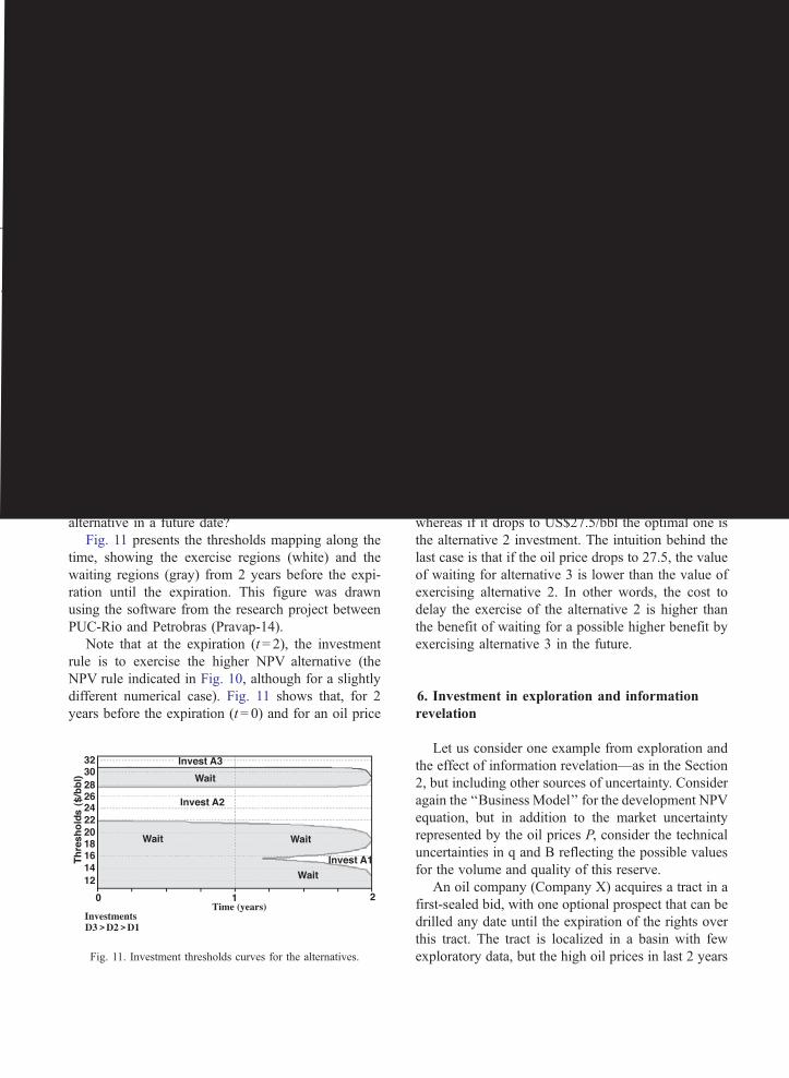
Fig. 10. NPVs from the
M.A.G. Dias / Journal of Petroleum Science and Engineering 44 (2004) 93–114
106
decision in this case? Is better to invest if one
alternative is deep-in-the money or is better to wait
and see for the possibility to invest in a more attractive
alternative in a future date?
Fig. 11 presents the thresholds mapping along the
time, showing the exercise regions (white) and the
waiting regions (gray) from 2 years before the expi-
ration until the expiration. This figure was drawn
using the software from the research project between
PUC-Rio and Petrobras (Pravap-14).
Note that at the expiration (t = 2), the investment
rule is to exercise the higher NPV alternative (the
NPV rule indicated in Fig. 10, although for a slightly
different numerical case). Fig. 11 shows that, for 2
years before the expiration (t= 0) and for an oil price
Fig. 11. Investment thresholds curves for the alternatives.
three alternatives.
of US$28/bbl, the optimal development policy is
‘‘wait and see’’. If the oil price rises to US$31/bbl
the best action is the investment with alternative 3,
whereas if it drops to US$27.5/bbl the optimal one is
the alternative 2 investment. The intuition behind the
last case is that if the oil price drops to 27.5, the value
of waiting for alternative 3 is lower than the value of
exercising alternative 2. In other words, the cost to
delay the exercise of the alternative 2 is higher than
the benefit of waiting for a possible higher benefit by
exercising alternative 3 in the future.
6. Investment in exploration and information
revelation
Let us consider one example from exploration and
the effect of information revelation—as in the Section
2, but including other sources of uncertainty. Consider
again the ‘‘Business Model’’ for the development NPV
equation, but in addition to the market uncertainty
represented by the oil prices P, consider the technical
uncertainties in q and B reflecting the possible values
for the volume and quality of this reserve.
An oil company (Company X) acquires a tract in a
first-sealed bid, with one optional prospect that can be
drilled any date until the expiration of the rights over
this tract. The tract is localized in a basin with few
exploratory data, but the high oil prices in last 2 years
23 The risk-adjusted discount rate of the option is not
necessarily the same of the underlying asset, and could be a
complex problem. Fortunately, we can change (penalize) the
underlying asset probability distribution in order to use the risk-
free discount rate to calculate the present value of options. This is
named risk-neutral approach.
M.A.G. Dias / Journal of Petroleum Science and Engineering 44 (2004) 93–114 107
and acquisitions of tracks in the last 3 years by several
oil companies promise an increasing exploratory ac-
tivity in this basin. Company X has 5 years to explore
and commit a development plan (in case of success).
This prospect today is marginal because a fair EMV
estimate is negative. Another oil company (Company
Y) offers US$3 million for the rights of this prospect.
Shall the Company X accept the Company Y offer?
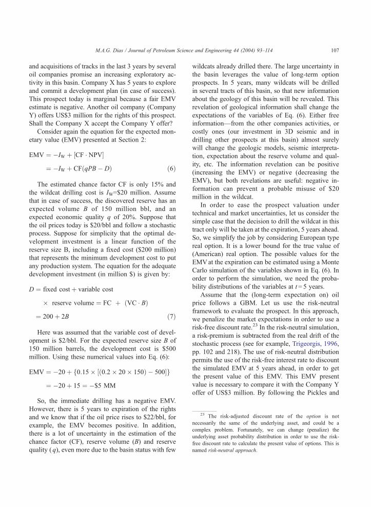
Consider again the equation for the expected mon-
etary value (EMV) presented at Section 2:
EMV ¼ �IW þ ½CF � NPV�
¼ �IW þ CFðqPB� DÞ ð6Þ
The estimated chance factor CF is only 15% and
the wildcat drilling cost is IW=$20 million. Assume
that in case of success, the discovered reserve has an
expected volume B of 150 million bbl, and an
expected economic quality q of 20%. Suppose that
the oil prices today is $20/bbl and follow a stochastic
process. Suppose for simplicity that the optimal de-
velopment investment is a linear function of the
reserve size B, including a fixed cost ($200 million)
that represents the minimum development cost to put
any production system. The equation for the adequate
development investment (in million $) is given by:
D ¼ fixed costþ variable cost
� reserve volume ¼ FC þ ðVC � BÞ
¼ 200þ 2B ð7Þ
Here was assumed that the variable cost of devel-
opment is $2/bbl. For the expected reserve size B of
150 million barrels, the development cost is $500
million. Using these numerical values into Eq. (6):
EMV ¼ �20þ f0:15� ½ð0:2� 20� 150Þ � 500�g
¼ �20þ 15 ¼ �$5 MM
So, the immediate drilling has a negative EMV.
However, there is 5 years to expiration of the rights
and we know that if the oil price rises to $22/bbl, for
example, the EMV becomes positive. In addition,
there is a lot of uncertainty in the estimation of the
chance factor (CF), reserve volume (B) and reserve
quality ( q), even more due to the basin status with few
wildcats already drilled there. The large uncertainty in
the basin leverages the value of long-term option
prospects. In 5 years, many wildcats will be drilled
in several tracts of this basin, so that new information
about the geology of this basin will be revealed. This
revelation of geological information shall change the
expectations of the variables of Eq. (6). Either free
information—from the other companies activities, or
costly ones (our investment in 3D seismic and in
drilling other prospects at this basin) almost surely
will change the geologic models, seismic interpreta-
tion, expectation about the reserve volume and qual-
ity, etc. The information revelation can be positive
(increasing the EMV) or negative (decreasing the
EMV), but both revelations are useful: negative in-
formation can prevent a probable misuse of $20
million in the wildcat.
In order to ease the prospect valuation under
technical and market uncertainties, let us consider the
simple case that the decision to drill the wildcat in this
tract only will be taken at the expiration, 5 years ahead.
So, we simplify the job by considering European type
real option. It is a lower bound for the true value of
(American) real option. The possible values for the
EMVat the expiration can be estimated using a Monte
Carlo simulation of the variables shown in Eq. (6). In
order to perform the simulation, we need the proba-
bility distributions of the variables at t = 5 years.
Assume that the (long-term expectation on) oil
price follows a GBM. Let us use the risk-neutral
framework to evaluate the prospect. In this approach,
we penalize the market expectations in order to use a
risk-free discount rate.23 In the risk-neutral simulation,
a risk-premium is subtracted from the real drift of the
stochastic process (see for example, Trigeorgis, 1996,
pp. 102 and 218). The use of risk-neutral distribution
permits the use of the risk-free interest rate to discount
the simulated EMV at 5 years ahead, in order to get
the present value of this EMV. This EMV present
value is necessary to compare it with the Company Y
offer of US$3 million. By following the Pickles and

Table 3
Distributions for EMV variables at t= 5 years
q
M.A.G. Dias / Journal of Petroleum Science and Engineering 44 (2004) 93–114108
Smith’s advise (r = d, see Section 3), it is possible to
show that this risk-neutralized process has drift a = ze-zero, so that the oil prices risk-neutral distribution at
t= 5 has mean equal to the current value P0. Using a
volatility r = 15% p.a. for the (long-term expectation
on) oil price, the variance of this risk-neutral distri-
bution is (see Dixit and Pindyck, p. 72):
Var½PðtÞ� ¼ P20expð2atÞ½expðr2tÞ � 1�
¼ 202½expð0:152 � 5Þ � 1�
¼ 47:6ð$=bblÞ2 ð8Þ
The technical uncertainties estimation needs a
careful probabilistic analysis of this basin. We need
the prior distributions on the technical variables CF, q,
and B. In 5 years, with the new information from the
exploratory activity, we revise the prior distribution
and many posterior distributions are possible. At the
expiration, we will use again Eqs. (6) and (7) to
calculate the EMV and to decide about the wildcat
drilling. So, at this date we will use the revised
expectation to calculate the EMV, that is, we will
use the mean of the posterior distribution. The possi-
ble means from these posterior distributions at t = 5
years constitute a distribution of conditional expect-
ations (or revelation distribution) at t= 5 years, where
the conditioning is the information revealed by the
exploratory activity in 5 years. The properties of these
revelation distributions are shown in Dias (2002).24 In
short, the mean of the revelation distribution is the
same of the prior distribution (law of iterated expect-
ations, see Section 2), the variance is the expected
reduction of variance induced by the new information,
and the distribution shape is approximately the same
of the prior distribution (it is really true only at the
limit of full revelation). So, in addition to the prior
distributions we need some estimation of the expected
reduction of variance for each variable along the next
5 years. In order to do this, we need some forecast of
the intensity of exploratory activity in the next 5
years, and how much this activity can reveal new
information. Bayesian methods can be used to help us
in this estimation. Assuming this job was performed,
24 Dias (2002) presents four propositions to describe the
revelation distributions, namely the limit, the mean, the variance,
and the martingale property of sequential revelation distributions.
Table 3 shows the revelation distributions for the
technical uncertainties and the risk-neutral distribution
for the oil prices, in all cases at t= 5 years.
Note that we do not penalize the revelation distri-
butions (as in the oil prices case) because these tech-
nical risks have no correlation with market portfolio.
So, corporate finance theory tells us that technical
uncertainty does not require additional risk premium
by diversified shareholders of the oil company.
Using Eqs. (6) and (7) and a Monte Carlo simula-
tion to combine these uncertainties, we get the distri-
bution for the benefit value (CF�NPV) and so the
EMV distribution at t = 5 years. As the expected
values of the distributions at t = 5 years are the same
values used in the today’s EMV estimate (so that we
are not more optimistic in the future), the expected
value of the EMV distribution generated by the Monte
Carlo simulation, must be approximately the current
one (� $5 MM). However, the key insight for valu-
ation of the rights is the optional nature of this wildcat
investment. In this future date (5 years ahead) a
rational manager only will exercise the option to drill
the wildcat if the revised EMV is positive. In other
words, if the information revealed in the basin ex-
ploratory activity combined with the oil prices evolu-
tion set a positive EMV for this prospect, the rational
manager will exercise the drilling option. If the new
information points that the prospect remains with
negative EMV, the drilling option will not be exer-
cised and the prospect value is zero. So, real options’
B
P

Fig. 12. Visual equation for real options value of the prospect.M.A.G. Dias / Journal of Petroleum Science and Engineering 44 (2004) 93–114 1
thinking introduces an asymmetry in the distribution
of the prospect value. Fig. 12, a ‘‘visual equation for
the real option value’’, illustrates this valuation.
Fig. 12 shows that if we ‘‘wait and see’’ until t = 5
years the prospect values US$15 million, contrasting
with the negative current valuation. This value con-
siders both the optional nature of this prospect and
the information revelation along the next five years.
The present value of this option, using a risk-free
discount rate of 10% p.a., is US$9.1 million. So,
Company X shall decline the $3 million offer from
Company Y. In reality, the prospect value is even
higher because was not considered the possibility of
earlier exercise of the option to drilling (American
type option), which could be optimal if the prospect
becomes ‘‘deep-in-the-money’’ with sufficient favor-
able information before 5 years. But this European
option analysis gives an idea about the prospect
minimum value and illustrates the point that real
options is leveraged by the uncertainty if we can
wait and learn from new information.
7. Alternatives to invest in information in a
dynamic framework
After presenting examples and models for devel-
opment investment and primary exploratory invest-
ment (wildcat drilling), let us present one example for
09
the intermediate phase of appraisal investment. Sup-
pose that an oilfield was discovered and some ap-
praisal wells were already drilled, but the residual
technical uncertainty over the parameters q (reserve
quality) and B (reserve size) remains important. Sup-
pose there are 2 years until the exploratory rights
expiration in this concession. Assume that the basin is
mature in the sense that the arrival of external explor-
atory information is not relevant to revise expectations
on q and B. The only way to obtain more information
about the parameters q and B is by investing in
information. The revision in the expectation of B will
revise the development investment D by using Eq. (7),
as in previous section. However, here we will consider
American option type for the development option.
In general, we have some mutually exclusive
alternatives to invest in information. Each alternative
has different costs and different potential for informa-
tion revelation. Exemplifying, Alternative 1 could be
a long-term production test in an already drilled well
(there is a cost to put a rig over the well to perform the
test). Alternative 2 could be the drilling of a new
appraisal well, e.g., a cheaper slim well. Alternative 3
could be the anticipation of part of the development
drilling investment, but in a way that optimizes the
reservoir information gathering instead minimizing
the drilling costs, etc. In the alternatives comparison
we also consider the alternative of not invest in
information, named Alternative 0.
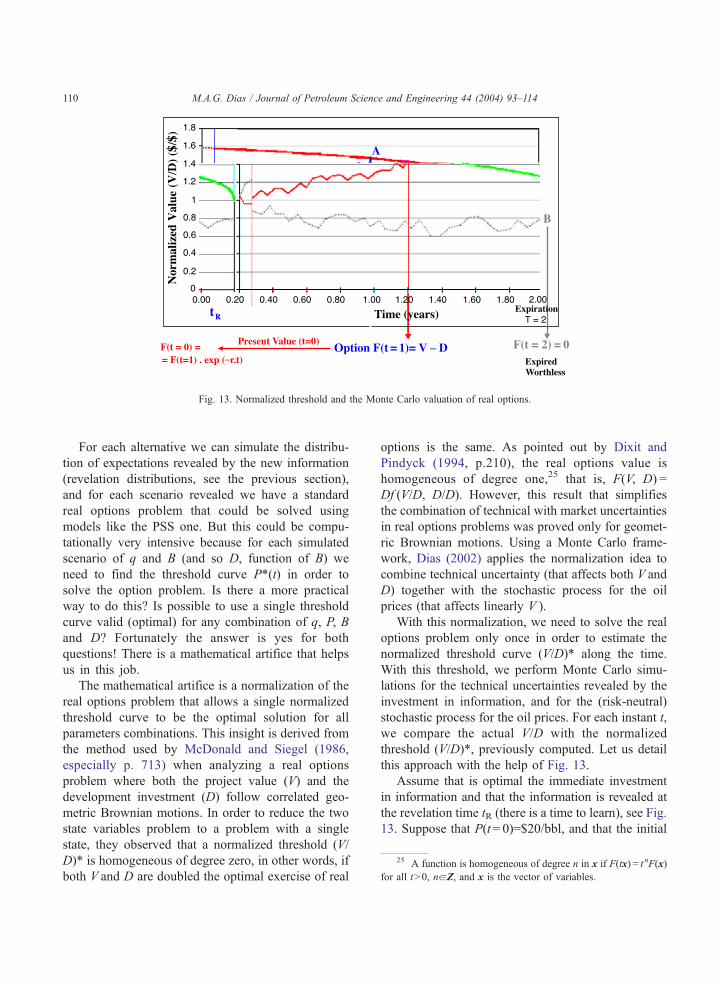
Fig. 13. Normalized threshold and the Monte Carlo valuation of real options.
25 A function is homogeneous of degree n in x if F(tx) = t nF(x)
for all t>0, naZ, and x is the vector of variables.
M.A.G. Dias / Journal of Petroleum Science and Engineering 44 (2004) 93–114110
For each alternative we can simulate the distribu-
tion of expectations revealed by the new information
(revelation distributions, see the previous section),
and for each scenario revealed we have a standard
real options problem that could be solved using
models like the PSS one. But this could be compu-
tationally very intensive because for each simulated
scenario of q and B (and so D, function of B) we
need to find the threshold curve P*(t) in order to
solve the option problem. Is there a more practical
way to do this? Is possible to use a single threshold
curve valid (optimal) for any combination of q, P, B
and D? Fortunately the answer is yes for both
questions! There is a mathematical artifice that helps
us in this job.
The mathematical artifice is a normalization of the
real options problem that allows a single normalized
threshold curve to be the optimal solution for all
parameters combinations. This insight is derived from
the method used by McDonald and Siegel (1986,
especially p. 713) when analyzing a real options
problem where both the project value (V) and the
development investment (D) follow correlated geo-
metric Brownian motions. In order to reduce the two
state variables problem to a problem with a single
state, they observed that a normalized threshold (V/
D)* is homogeneous of degree zero, in other words, if
both V and D are doubled the optimal exercise of real
options is the same. As pointed out by Dixit and
Pindyck (1994, p.210), the real options value is
homogeneous of degree one,25 that is, F(V, D) =
Df (V/D, D/D). However, this result that simplifies
the combination of technical with market uncertainties
in real options problems was proved only for geomet-
ric Brownian motions. Using a Monte Carlo frame-
work, Dias (2002) applies the normalization idea to
combine technical uncertainty (that affects both V and
D) together with the stochastic process for the oil
prices (that affects linearly V ).
With this normalization, we need to solve the real
options problem only once in order to estimate the
normalized threshold curve (V/D)* along the time.
With this threshold, we perform Monte Carlo simu-
lations for the technical uncertainties revealed by the
investment in information, and for the (risk-neutral)
stochastic process for the oil prices. For each instant t,
we compare the actual V/D with the normalized
threshold (V/D)*, previously computed. Let us detail
this approach with the help of Fig. 13.
Assume that is optimal the immediate investment
in information and that the information is revealed at
the revelation time tR (there is a time to learn), see Fig.
13. Suppose that P(t= 0)=$20/bbl, and that the initial
M.A.G. Dias / Journal of Petroleum Science and Engineering 44 (2004) 93–114 111
technical parameters expectations are q = 0.21 and
B = 100 million bbl. By using Eqs. (2) and (7), we
get V= 420 and D = 400 (both in million $), so that V/
D = 1.05 at t = 0. This is the starting point of our
Monte Carlo simulation. While we are investing in
information, until tR the value of V/D for this project
will oscillate only due to the oil prices evolution,
modeled with a risk-neutral GBM. However, at the
revelation time tR we will revise the expectations
about the technical parameters q and B (and D). These
expectations revision will cause a jump-up (in case of
good news on q and/or B) or a jump-down (in case of
negative revelation). The jumps sizes are sampled
from the distributions of conditional expectations of
q and B (or revelation distributions, see the previous
section). Fig. 13 illustrates this method, showing two
simulated sample-paths with jumps at tR, one path
with exercise at t= 1 (the almost continuous line) and
the other (dotted-line) reaching the expiration date
without crossing the normalized threshold curve (V/
D)*.
If V/Dz (V/D)* for the path i at any time t, we
exercise the option (point A in Fig. 13) and calculate
the present value (using the risk-free interest rate) of
this option, denoted by Fi(t= 0). In the opposite case,
we wait and see. The paths that do not cross the
normalized threshold curve (V/D)* along the 2 years
of option are worthless. By summing up all the
simulated real options present values Fi(t = 0) and
dividing it by the total number of simulations, we
get the real options value after the investment in
information. Subtracting the cost of information (the
learning cost), we obtain the real options value net of
the learning cost for the alternative of investment in
information under evaluation.
Remember that for each alternative, there are
different learning costs, different learning time tR,
and different revelation distributions for q and B.
The revelation power (capacity to reduce technical
uncertainty) of one alternative is linked to the variance
of revelation distribution26 (Dias, 2002, proposition
3). So, we repeat this procedure for each alternative of
investment in information and the resultant net real
options values are compared. The higher one is the
best alternative of investment in information. In gen-
26 For the Alternative 0 of not invest in information, we have
single expectations for q and B instead distributions.
eral, large uncertainties in q and B enhance the value
of learning and so the real options value. In order to
see this, think with the ‘‘visual equation for real
options’’. Our simple model captures this idea.
The last point in this section is the equation
necessary to perform the risk-neutral Monte Carlo
simulation of the oil prices. For the geometric Brow-
nian motion, the risk-neutral sample paths are simu-
lated with the equation below, applied to each instant t
using the oil price from the previous instant t� 1:
Pt ¼ Pt�1expfr � d � 0:5r2ÞDt þ rNð0; 1Þffiffiffiffi
Dp
tg ð9Þ
In this equation, Dt represents the time-step in the
simulation, N(0, 1) is the standard Normal distribution
(mean = zero and variance = 1), and the remaining
variables are as before. We use the recursive Eq. (9)
from t = 0 until the option exercise or until the
expiration, several times obtaining several oil prices
paths, and so several V/D paths.
8. The option to expand the production using
optional wells
Sometimes the best way to reduce the remaining
technical uncertainties in the oilfield is by using the
information generated by the cumulated production in
the field and/or measuring the bottom-hole pressure
after months or few years of cumulated production. In
these cases, the investment in information before the
oilfield development is not adequate due to the low
potential to reveal information relative to the cost to
gather the information.
For these cases, the proper way to gather informa-
tion is by embedding options to expand the produc-
tion into the selected alternative of development, so
that depending on the revealed information we exer-
cise or not the option to expand the production. In
case of oilfield development, a good way is to select
some optional wells, which will be drilled only in
favorable scenarios. In addition, the optimal locations
for these wells also depend on the information gener-
ated by the initial oilfield production.
To include this option to expand into the develop-
ment plan, we incur in some costs. For example, at
higher cost the processing plant shall be dimensioned
considering the possible exercise of this option. An-
M.A.G. Dias / Journal of Petroleum Science and Engineering 44 (2004) 93–114112
other way is by leaving free space in the production
unit in order to amply the capacity in case of option
exercise with the drilling of optional wells.27 The third
way is by waiting the main production decline (res-
ervoir depletion) in order to integrate these wells
when the processing capacity permits (see Ekern,
1988, for a real options valuation). But even in this
last case is necessary to consider the possible new
load in the platform from the optional new risers and a
possible additional cost because the subsea layout
must consider the possibility of optional wells flow-
lines going to the production platform. However,
these costs to embed the option to expand are, in
general, only a fraction of the potential benefit of
drilling these wells in the favorable reservoir scenarios
and/or favorable market scenarios for oil prices.
The economic analysis of the option to expand
with optional wells requires an in-depth study of
marginal contribution from each well in the overall
oilfield development. In this study is necessary to
identify the candidate wells that can become optional
wells. Wells with higher reservoir risk are primary
candidates because with new reservoir information
these wells could become unnecessary or its optimal
location could be different. The other class of optional
well candidates is that resultant of the marginal well
contribution for wells that presented negative NPV or
even a small positive NPV28 so that the option to drill
these marginal wells are not ‘‘deep-in-the-money’’.
One feature that sometimes can be important is the
secondary depletion in the optional wells area. The
production of the main wells causes a differential
pressure in the reservoir, inducing some oil migration
from the optional wells area to the producing area. In
most cases the oil migration does not mean that the
main wells will produce this oil (it could be trapped in
the way), or if this oil will be produced, it takes too
long time to reach the distant non-optional wells. In
many cases this oil will never be produced. This
secondary depletion acts as a dividend lost by the
option holder, causing the same effect of the dividend
27 Free area has a relatively high cost for offshore platforms,
mainly in case of floating platforms.28 The direct method to estimate the marginal NPVof a well is
by reservoir simulation with and without each well. With the
production profiles in each case, the two NPVs are calculated and
the marginal NPV is just the difference between these NPVs.
yield in the traditional real options models—higher
incentive to drill earlier the optional well as higher is
the secondary depletion effect.
The general method to analyze the option to
expand production through optional wells is:
� Define the quantity of wells ‘‘deep-in-the-money’’
to start the basic investment in development by the
marginal analysis of each well using several
reservoir simulations;� Define the maximum number of optional wells;� Define the timing (or the accumulated production)
that the reservoir information will be revealed;� Define the of marginal production of each optional
well as function of uncertain parameters and the
possible scenarios (revelation distributions) to be
revealed by the cumulative production;� Consider the secondary depletion in the optional
well area if we wait after learn about reservoir;� Simplify computational effort by limiting the
expiration of the option to drill the optional
wells—remember the declining NPV due to the
secondary depletion and the discount rate effect;� Add market uncertainty, simulating a stochastic
process for oil prices and perhaps for the volatile
daily rate of rigs that could drill the optional wells;� Combine uncertainties using Monte Carlo simula-
tion as shown in the previous section;� Use a threshold curve to consider the optimal
earlier exercise of the option to drill the wells, and
calculate option value; and� Compare this option value with the cost to embed
the option to expand. The option value must be
higher than the cost to embed the option, to justify
this flexibility cost into the development plan.
Fig. 14 presents the timeline of the option to
expand problem that help us understand a practical
modelling of this problem.
The timeline in Fig. 14 considers a time-to-build of
3 years, from the development investment start-up
until the production start-up, at t = 3 years. Between
the years 3 and 4, the initial production of the wells and
eventual production tests give us all relevant technical
information for this example. For the period from year
4 until the year 9, the exercise of the option to drill is
considered mainly for the optional wells that had
reservoir uncertainty before the initial production.
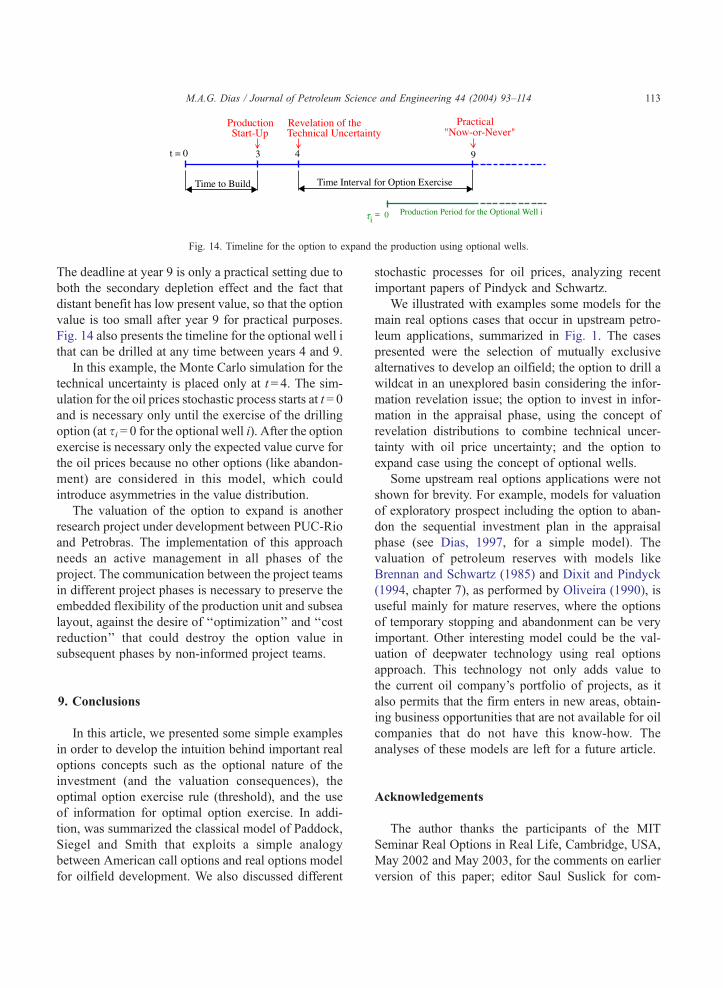
Fig. 14. Timeline for the option to expand the production using optional wells.
M.A.G. Dias / Journal of Petroleum Science and Engineering 44 (2004) 93–114 113
The deadline at year 9 is only a practical setting due to
both the secondary depletion effect and the fact that
distant benefit has low present value, so that the option
value is too small after year 9 for practical purposes.
Fig. 14 also presents the timeline for the optional well i
that can be drilled at any time between years 4 and 9.
In this example, the Monte Carlo simulation for the
technical uncertainty is placed only at t= 4. The sim-
ulation for the oil prices stochastic process starts at t = 0
and is necessary only until the exercise of the drilling
option (at si= 0 for the optional well i). After the optionexercise is necessary only the expected value curve for
the oil prices because no other options (like abandon-
ment) are considered in this model, which could
introduce asymmetries in the value distribution.
The valuation of the option to expand is another
research project under development between PUC-Rio
and Petrobras. The implementation of this approach
needs an active management in all phases of the
project. The communication between the project teams
in different project phases is necessary to preserve the
embedded flexibility of the production unit and subsea
layout, against the desire of ‘‘optimization’’ and ‘‘cost
reduction’’ that could destroy the option value in
subsequent phases by non-informed project teams.
9. Conclusions
In this article, we presented some simple examples
in order to develop the intuition behind important real
options concepts such as the optional nature of the
investment (and the valuation consequences), the
optimal option exercise rule (threshold), and the use
of information for optimal option exercise. In addi-
tion, was summarized the classical model of Paddock,
Siegel and Smith that exploits a simple analogy
between American call options and real options model
for oilfield development. We also discussed different
stochastic processes for oil prices, analyzing recent
important papers of Pindyck and Schwartz.
We illustrated with examples some models for the
main real options cases that occur in upstream petro-
leum applications, summarized in Fig. 1. The cases
presented were the selection of mutually exclusive
alternatives to develop an oilfield; the option to drill a
wildcat in an unexplored basin considering the infor-
mation revelation issue; the option to invest in infor-
mation in the appraisal phase, using the concept of
revelation distributions to combine technical uncer-
tainty with oil price uncertainty; and the option to
expand case using the concept of optional wells.
Some upstream real options applications were not
shown for brevity. For example, models for valuation
of exploratory prospect including the option to aban-
don the sequential investment plan in the appraisal
phase (see Dias, 1997, for a simple model). The
valuation of petroleum reserves with models like
Brennan and Schwartz (1985) and Dixit and Pindyck
(1994, chapter 7), as performed by Oliveira (1990), is
useful mainly for mature reserves, where the options
of temporary stopping and abandonment can be very
important. Other interesting model could be the val-
uation of deepwater technology using real options
approach. This technology not only adds value to
the current oil company’s portfolio of projects, as it
also permits that the firm enters in new areas, obtain-
ing business opportunities that are not available for oil
companies that do not have this know-how. The
analyses of these models are left for a future article.
Acknowledgements
The author thanks the participants of the MIT
Seminar Real Options in Real Life, Cambridge, USA,
May 2002 and May 2003, for the comments on earlier
version of this paper; editor Saul Suslick for com-
M.A.G. Dias / Journal of Petroleum Science and Engineering 44 (2004) 93–114114
ments and suggestions in the final version; and two
anonymous referees’ comments. Any error is mine.
References
Adelman, M.A., Koehn, M.F., de Silva, H., 1989. The valuation of
oil reserves. Society of Petroleum paper no. 18906. Proceedings
of SPE Hydrocarbon Economics and Evaluation Symposium,
Dallas, USA, pp. 45–52.
Amram, M., Kulatilaka, N., 1999. Real Options—Managing Stra-
tegic Investment in an Uncertain World. Harvard Business
School Press, Cambridge, MA.
Baker, M.P., Mayfield, E.S., Parsons, J.E., 1998. Alternative models
of uncertain commodity prices for use with modern asset pri-
cing. Energy Journal 19 (1), 115–148 (January).
Bessembinder, H., Coughenour, J.F., Seguin, P.J., Smoller, M.M.,
1995. Mean reversion in equilibrium asset prices: evidence
from the futures term structure. Journal of Finance 50 (1),
361–375.
Bjerksund, P., Ekern, S., 1990. Managing investment opportunities
under price uncertainty: from last chance to wait and see stra-
tegies. Financial Management 19 (3), 65–83 (Autumn).
Brennan, M.J., Schwartz, E.S., 1985. Evaluating natural resource
investment. Journal of Business 58 (2), 135–157.
Chorn, L.G., Croft, M., 2000. Resolving reservoir uncertainty to
create value. Journal of PetroleumTechnology, 52–59 (August).
Copeland, T., Antikarov, V., 2001. Real Options—A Practitioner’s
Guide. Texere LLC Publishing, New York.
Cortazar, G., Schwartz, E.S., 1998. Monte Carlo evaluation model
of an undeveloped oil field. Journal of Energy Finance and
Development 3 (1), 73–84.
DeGroot, M.H., Schervish, M.J., 2002. Probability and Statistics,
3rd ed. Addison-Wesley, Boston.
Dias, M.A.G., 1997. The timing of investment in E&P: uncer-
tainty, irreversibility, learning, and strategic consideration. So-
ciety of Petroleum paper no. 37949. Proceedings of SPE
Hydrocarbon Economics and Evaluation Symposium, Dallas,
USA., pp. 135–148.
Dias, M.A.G., 1999. A note on bibliographical evolution of real
options. In: Trigeorgis, L. (Ed.), Real Options and Business
Strategy—Applications to Decision Making. Risk Books, Lon-
don, pp. 357–362.
Dias, M.A.G., 2002. Investment in Information in Petroleum: real
options and revelation. Working paper Petrobras and PUC-Rio.
February. Available at www.puc-rio.br/marco.ind/.
Dias, M.A.G., Rocha, K.M.C., 1998. Petroleum concessions with
extendible options using mean reversion with jumps to model
oil prices. Working Paper Petrobras and IPEA. May. Available at
www.puc-rio.br/marco.ind/.
Dias, M.A.G., Rocha, K.M.C., Teixeira, J.P., 2003. The optimal
investment scale and timing: a real option approach to oilfield
development. Pravap-14 Working Paper, Petrobras-PUC-Rio.
November.
Dixit, A.K., Pindyck, R.S., 1994. Investment Under Uncertainty.
Princeton Univ. Press, Princeton, NJ.
Ekern, S., 1988. An option pricing approach to evaluating petro-
leum projects. Energy Economics, 91–99 (April).
Galli, A., Armstrong, M., Jehl, B., 1999. Comparison of three
methods for evaluating oil projects. Journal of Petroleum Tech-
nology, 44–49 (October).
Gibson, R., Schwartz, E., 1990. Stochastic convenience yield and
the pricing of oil contingent claims. Journal of Finance 45 (3),
959–976 (July).
Graham, J.R., Harvey, C.R., 2001. The theory and practice of cor-
porate finance: evidence from the field. Journal of Financial
Economics (60), 187–243.
Gruy, H.J., Grab, F.A., Wood, J.W., 1982. Determining the value of
oil and gas in the ground. World Oil CXCIV, 105–108.
Johnston, D., 1995. Different fiscal systems complicate reserves
values. Oil and Gas Journal 93 (22), 39–42.
Kemna, A.G.Z., 1993. Case studies on real options. Financial
Management (Autumn), 259–270.
Kenyon, C.M., Tompaidis, S., 2001. Real options in leasing: the
effect of idle time. Operations Research 49 (5), 675–689.
Laughton,D.G., 1998. Themanagement of flexibility in the upstream
petroleum industry. Energy Journal 19 (1), 83–114 (January).
McCormack, J., Sick, G., 2001. Valuing PUD reserves: a practical
application of real options techniques. Journal of Applied Cor-
porate Finance 13 (4), 110–115.
McDonald, R., Siegel, D., 1986. The value of waiting to invest.
Quarterly Journal of Economics, 707–727 (November).
Myers, S.C., 1977. Determinants of corporate borrowing. Journal of
Financial Economics, 147–175 (November).
Oliveira, C.A.P., 1990. Avaliacao e Gerencia de Jazidas de Petro-
leo-Uma Abordagem pela Teoria das Opcoes. (Valuation and
Management of Petroleum Deposits—An Options Theory Ap-
proach). Dept. of Industrial Engineering, PUC-RJ, MSc Dis-
sertation (in Portuguese).
Paddock, J.L., Siegel, D.R., Smith, J.L., 1988. Option valuation of
claims on real assets: the case of offshore petroleum leases.
Quarterly Journal of Economics, 479–508 (August).
Pickles, E., Smith, J.L., 1993. Petroleum property evaluation: a
binomial lattice implementation of option pricing theory. Energy
Journal 14 (2), 1–26.
Pindyck, R.S., 1999. The long-run evolution of energy prices.
Energy Journal 20 (2), 1–27.
Pindyck, R.S., 2001. The dynamics of commodity spot and futures
markets: a primer. Energy Journal 22 (3), 1–29.
Saito, R., de Castro, G.N., Mezzomo, C., Schiozer, D.J., 2001.
Value assessment for reservoir recovery optimization. Journal
of Petroleum Science and Engineering 32, 151–158.
Schwartz, E.S., 1997. The Stochastic behavior of commodity pri-
ces: implications for valuation and hedging. Journal of Finance
52 (3), 923–973 (July).
Schwartz, E., Smith, J.E., 2000. Short-term variations and long-
term dynamics in commodity prices. Management Science 46
(7), 893–911 (July).
Tourinho, O.A.F., 1979. The Valuation of Reserves of Natural
Resources: An Option Pricing Approach. University of Califor-
nia, Berkeley, PhD Dissertation.
Trigeorgis, L., 1996. Real Options—Managerial Flexibility and
Strategy in Resource Allocation. MIT Press, Cambridge, MA.
Copyright © 2022 FDOKUMEN

