


Bahasa
Halaman
Hukum


IOSR Journal of Mathematics (IOSR-JM)
e-ISSN: 2278-5728, p-ISSN: 2319-765X. Volume 10, Issue 6 Ver. II (Nov - Dec. 2014), PP 66-75 www.iosrjournals.org
www.iosrjournals.org 66 | Page
Transient State Finite Element Model to Analyse Thermal
Variations in Peripheral Region of Human Limb undergoing
Healing after Surgery
Namrata Gupta1, Madhvi Shakya
2
1,2Department of Mathematics and computer Applications,Maulana Azad National Institute of Technology,
Bhopal-462041 India
Abstract: The temperature distribution in human tissues is significantly affected by the introduction of an
abnormality. The study of temperature distribution in different layers of peripheral tissue is intended to
contribute in the diagnosis of many disorders in various organs. In this paper, an axisymmetric one dimensional
model has been developed to study transient state temperature distribution in different layers of normal and post
surgery peripheral (abnormal) tissues of human limb. Taking into account the variable physiological
parameters in dermal layer of peripheral region, the well known Pennes’ bio heat equation is used to analyse
and compare the time-dependent temperature distribution of normal and abnormal tissues using finite element technique. A computer program in MATLAB has been developed to simulate the results.
Keywords: Crank-Nicolson method, Finite element technique, Healing process, Surgery.
I. Introduction Internal body or core temperature is one of the four clinical vital signs along with pulse rate, blood
pressure and respiratory rates. Any variation in its normal range indicates the presence of an abnormal
metabolism in the body. Also enzymes, essential for metabolism, work properly in between 20-37 oC body
temperature [1, 2]. Thus it becomes important to study thermal variations in order to develop a mechanism for
establishing the limits of thermal regulation in human body during the healing process.
Pennes [3] in 1948 first gave the well known Pennes’ Bio-Heat equation to study heat transfer in perfused tissue. He assumed that all heat transfer between the tissue and the blood occurs in the capillaries and
neglected the local effects of thermally significant blood vessels appearing in the domain under
consideration[4]. He also assumed a constant rate blood perfusion of the form “V.s” where V and s are
respectively the perfusion rate per unit volume of tissues and the density of the blood. Since then it has been
used by many researchers and scientist for analysis in their respective area of research. Perl [5] in 1962 used it to
illustrate heat distribution and tissue blood flow in body tissues by analyzing existing steady state and transient
data obtained by Gibb’s thermo electric probe method. Arya [6] studied temperature distribution in skin and
subcutaneous region under radiation and evaporation conditions. Saxena and Bindra [7] applied finite element
approach to study heat distribution in cutaneous and subcutaneous tissues. Pardasani and Shakya [8, 9] studied
temperature distribution in human dermal regions due to tumours. Adams [10, 11] modelled healing times in
different tissues by considering different factors like size and shape of the wound and the effect of growth factors on wound healing. Gaffney [12] investigated a model of cutaneous wound healing angiogenesis.
Maggelakis [13] developed a mathematical model of tissue replacement during epidermal wound healing by
incorporating the effect of oxygen concentration at the wound site. Gurung [14] dealt with thermo-regulation in
human dermal part in a cold atmosphere with significant air flow. Jain and Shakya [1, 15] studied temperature
variation during wound healing process due to plastic surgery using finite element discretisation of the domain
in Cartesian coordinates. A few scientists have studied thermal variations in surgical wound during healing after
surgery.
In this paper, we have developed an axisymmetric one dimensional finite element model for transient
state temperature distribution in normal and abnormal peripheral tissues of human limb using linear
interpolation function in polar coordinates. Normal tissues are characterised by the normal values of
physiological parameters like blood perfusion rate and metabolic heat generation rate [1]. These parameters
have been assumed to be space dependent in dermis in normal tissues. Abnormal tissues are the tissues with disturbed values of physiological parameters due to incision and removal of tissues and blood vessels. The
physiological parameters in abnormal tissues attain their normal values in due course of time. This is shown by
incorporating an empirical function of time factor in the expressions of parameters in case of abnormal tissues
[16]. A comparison between the temperature profiles of normal and abnormal tissues has been done at different
atmospheric temperature and evaporation rates.

Transient State Finite Element Model to Analyse Thermal Variations in Peripheral Region of Human
www.iosrjournals.org 67 | Page
II. Model Descriptions Nomenclature
c1, c2 Unknown constants used for finding expression for Temperature in an element
E Rate of sweat evaporation in gm/cm2/min
e eth element
G(e) Globalisation matrix for e
th element
h Heat transfer coefficient due to conduction and convection in Cal/cm2/min/
oC
K1, K2, K3 Thermal conductivity of subcutaneous tissues, dermis and epidermis respectively in Cal/cm/min/oC
L Latent heat of vaporisation in Cal/gm
M1, M2, M3 Rate of heat transfer per unit volume per unit difference in temperature in subcutaneous tissues, dermis and
epidermis respectively in Cal/cm3/min/
oC
N Interpolation function
n Normal to skin surface
R Spatial coordinate originating from the centre of the limb in cm
r Thickness of peripheral tissues in cm
r Local spatial coordinate in cm
r1,r12 Spatial coordinate of skin core and skin surface respectively starting from core in cm
S1, S2, S3 Metabolic heat generation rate in subcutaneous tissues, dermis and epidermis respectively in Cal/cm3/min
T Unknown temperature of tissue in oC
Ta, Tb Atmospheric temperature and arterial blood temperature in oC
( )eT
Nodal temperature matrix of eth
element
T Global nodal temperature matrix
t Time in min
Ω(e) Domain of the eth element
α0(1), β0(1), γ0(1) Unknown constants used to find linear expression for K,M and S respectively in dermis
δ(t), ψ(t) Time factor in S and M respectively in abnormal tissues
ρ Density of tissue in gm/cm3
2.1Biological background
Skin is naturally divided into three layers: epidermis, dermis and subcutaneous tissues. Epidermis is the
outer most part of the skin and contains negligible density of blood vessels. In dermis the density of blood
vessels gradually increase from the interface of epidermis and dermis till the interface of dermis and
subcutaneous tissues and becomes almost constant in subcutaneous tissues [1, 6-8, 14, 17-19]. Considering this
anatomy of blood vessels in normal as well as post operated peripheral tissues, the values of physical and
physiological parameters like thermal conductivity (K), volumetric blood mass flow rate (M) and rate of metabolism (S) have been assumed dependent on spatial coordinate in dermis and independent of angular
coordinate (θ).
During surgery a cut is made into the skin tissue which results in vascular injury. Surgery also results in
removal of some tissues and loss of blood. Immediately after incidence of the injury, the process of wound
healing starts with the onset of haemostasis [20]. As a result the normal values of the parameters: blood
perfusion rate, metabolic heat generation rate are disturbed. They resume their normal values in due course of
time. The resumption of normal values by the parameters is achieved by incorporating a temporal factor in the
expression for these parameters [1, 15].
The core temperature of the limb is assumed to be at a constant known temperature. The outer surface
is exposed to the environment and an appropriate boundary condition due to heat loss at the outer surface has
been incorporated.
2.2 Mathematical Formulation
The domain under consideration (shaded region in Fig 1(a)) for the study is the peripheral tissues of
human limb ( 1 12 ,0 2R R R ), where R and θ are polar coordinates. Since the domain, boundary
conditions and tissue properties are identical with respect to angular coordinate (i. e. independent of θ), the two-
dimensional problem is reduced to an analogous one-dimensional axisymmetric problem [21] in spatial
coordinate R. Pennes’ bio-heat equation [3] for one dimensional axisymmetric transient state case takes the
form:
2
2
1( ) (1)b
b b
T T TK M T T S c
R R R t
where M m c

Transient State Finite Element Model to Analyse Thermal Variations in Peripheral Region of Human
www.iosrjournals.org 68 | Page
Fig.1. (a) Annular shaped domain of peripheral tissues (b) Discretised domain for analogous axisymmetric one
dimensional problem with 11elements and 12 nodes (c) eth element with two nodes
Here K, S, mb, cb, ρ, c, T, Tb, and R ( 1 ,R r where R1 and r are the spatial coordinate of core and the
thickness of the peripheral tissues respectively) are thermal conductivity, metabolic heat generation rate, blood
mass flow rate per unit volume, blood specific heat, tissue density, tissue specific heat, unknown tissue
temperature, arterial blood temperature and spatial coordinate respectively. The inner core of the human limb is
at a constant temperature and hence:
The outer surface of skin is exposed to the atmosphere and heat is lost from this surface through convection, radiation and evaporation. This boundary condition is formulated as:
Here h, Ta, L, E and T n are heat transfer coefficient, atmospheric temperature, latent heat of
vaporisation, rate of sweat evaporation and partial derivative of unknown tissue temperature along the normal
direction to the skin surface. It is assumed that the outer surface of the human limb is insulated initially [1, 8]
and is at core body temperature Tb at time t=0. Hence the initial condition is given by
2.3 Variational formulation
The variational formulation [22] of (1-3) is given by :
( ,0) (4)bT R T
1( , ) 0 (2)bT R t T t
( ) 0 (3)a
at surface
TK h T T LE t
n

Transient State Finite Element Model to Analyse Thermal Variations in Peripheral Region of Human
www.iosrjournals.org 69 | Page
2 2 2
1
2
1
1/ 2 2
/ 2 2 (5)
b
a
surfacer r
I K T r M T T ST c T t R r dr
R r h T T LET
where 1R R r ,
12 10 r R R and Ω is the complete domain under consideration.
III. Use of finite element method 3.1 Discretisation of Domain
The region under consideration is discretised into eleven elements and 12 nodes (Fig. 1(b)). Length of
each element is 0.1 cm. The discretised form of (5) is given by:
( )
2 2 2( ) ( ) ( ) ( ) ( ) ( ) ( ) ( )
0
2( ) ( ) ( )
1
1/ 2 2
/ 2 2 (6)
e
e e e e e e e e
b
e e e
j a
j
I K T r M T T S T c T t r r dr
R r h T T LETr r
Here r is the local radial coordinate and ( )e is the domain of eth element (Fig 1 (c)):
( )1, 11
(7)0,
efor e
other elements
In this model, the physical and physiological parameters have been assumed as given below.
3.1.1 for normal tissues
In epidermis and subcutaneous tissues thermal conductivity, blood perfusion rate and metabolic heat
generation rate have been assumed to have constant values. As mentioned above (section 2.1) these parameters
have been considered as space dependent in dermis. They have been approximated by Lagrange’s linear
interpolation formula in dermis: 1 1 1
0 0 0
( ) , ( ) , ( ) (8)e e i e e i e e i
i i i
i i i
K r r M r r S r r
3.1.2 for abnormal tissues In this paper, we have assumed that at time t=0, abnormal tissues have negligible blood perfusion rate
due to the effect of vasoconstriction of blood vessels and platelet plug formation in the traumatised blood
vessels [23]. Also metabolic heat generation rate is assumed to be below normal due to removal of blood and
tissues due to surgery. With progression of time these parameters attain their normal values [1, 15]:
1 1
0 0
( , ) ( ), ( , ) ( ) , ( , ) ( ) (9)e e e e i e e i
i i
i i
K r t K r M r t t r S r t t r
Here ( ) ( ) ( ) ( )
0 1 0 1( ) ( ) ( ) ( ) (10)e e t e e tt e and t e
Where ( ) ( ) ( ) ( )
0 1 0 1, , ,e e e e are unknown constants and are to be found out. The values of and [1, 15] are
assumed for abnormal tissues as:
(0) 0, ( ) 1, (0) 1/ 20, ( ) 1 (11)
There is no blood flow and metabolic heat generation in the epidermis. Thus the values of( ) ( ) ( ) ( ) ( )
0 1 0 1 0, , , ,e e e e e and( )
1
e are taken as given below.
1) Subcutaneous Tissues (e = 1(1)5 ) ( ) ( ) ( ) ( ) ( ) ( )
0 1 1 0 1 1 0 1 1, 0 ; , 0 ; , 0 (12)e e e e e eK M S
Transient State Finite Element Model to Analyse Thermal Variations in Peripheral Region of Human
www.iosrjournals.org 70 | Page
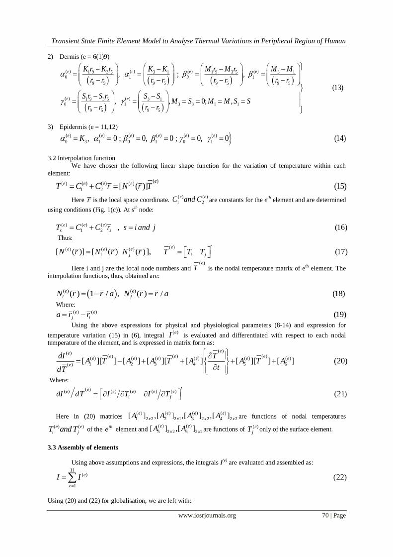
2) Dermis (e = 6(1)9)
( ) ( ) ( ) ( )1 9 3 5 3 1 1 9 3 5 3 10 1 0 1
9 5 9 5 9 5 9 5
( ) ( )1 9 3 5 3 10 1 3 3 1 1
9 5 9 5
, ; ,
(13)
, , 0; ,
e e e e
e e
K r K r K K M r M r M M
r r r r r r r r
S r S r S SM S M M S S
r r r r
3) Epidermis (e = 11,12)
( ) ( ) ( ) ( ) ( ) ( )
0 3 1 0 1 0 1, 0 ; 0, 0 ; 0, 0 (14)e e e e e eK
3.2 Interpolation function
We have chosen the following linear shape function for the variation of temperature within each
element: ( )( ) ( ) ( ) ( )
1 2 [ ( )] (15)ee e e eT C C r N r T
Here r is the local space coordinate. ( ) ( )
1 2
e eC and C are constants for the eth element and are determined
using conditions (Fig. 1(c)). At sth node:
( ) ( ) ( )
1 2 , (16)e e e
s sT C C r s i and j
Thus:
( )( ) ( ) ( )[ ( )] [ ( ) ( ) ], (17)ee e e
i j i jN r N r N r T T T
Here i and j are the local node numbers and ( )e
T is the nodal temperature matrix of eth element. The interpolation functions, thus, obtained are:
( ) ( )( ) 1 / , ( ) / (18)e e
i jN r r a N r r a
Where: ( ) ( ) (19)e e
j ia r r
Using the above expressions for physical and physiological parameters (8-14) and expression for
temperature variation (15) in (6), integral ( )eI is evaluated and differentiated with respect to each nodal
temperature of the element, and is expressed in matrix form as:
( )( )( ) ( ) ( )( ) ( ) ( ) ( ) ( ) ( )
1 2 3 4 5 6( )[ ][ ] [ ] [ ][ [ ] [ ][ ] [ ] (20)
eee e ee e e e e e
e
dI TA T A A T A A T A
tdT
Where:
( )( ) ( ) ( ) ( ) ( ) (21)ee e e e e
i jdI dT I T I T
Here in (20) matrices ( ) ( ) ( ) ( )
1 2 2 2 2 1 3 2 2 4 2 2[ ] ,[ ] ,[ ] ,[ ]e e e e
x x x xA A A A are functions of nodal temperatures
( ) ( )e e
i jT andT of the the element and
( ) ( )
5 2 2 6 2 1[ ] ,[ ]e e
x xA A are functions of ( )e
jT only of the surface element.
3.3 Assembly of elements
Using above assumptions and expressions, the integrals I(e) are evaluated and assembled as: 11
( )
1
(22)e
e
I I
Using (20) and (22) for globalisation, we are left with:

Transient State Finite Element Model to Analyse Thermal Variations in Peripheral Region of Human
www.iosrjournals.org 71 | Page
11( )( ) ( )
1
( ) (23)ee e
e
dI dT G dI dT
Where:
1
1
2( )
2
12 12 1
12 212 12 1
0 0
1 0, (24)
0 1
0 0
th
e
th
x
xx
I
TT
ITi row dI
TG TdTj row
TI
T
On using eqn. (23) to minimise I , we are left with a system of linear simultaneous ordinary differential
equations:
12 12 12 12 12 112 1 12 1
(25)x x xx x
P dT dt Q T U
Where:
( ) ( ) ( ) ( ) ( ) ( ) ( ) ( ) ( ) ( ) ( )
4 1 3 5 2 6, , (26)e e e e e e e e e e eP G A G Q G A A A G U G A A
Crank Nicolson Technique has been employed to solve the system of equations (25) along with initial
condition (4) to obtain the temperature profile at each node for progressive time. A computer program has been
developed in MATLAB to simulate the results.
IV. Numerical results and discussions The numerical calculations have been made for three cases of atmospheric temperatures. The values of
physical and physiological parameters taken [1, 9, 15, 18, 24] to obtain the numerical results are given in
TABLE 1 and 2.
Table 1 Values of physical and physiological parameters Parameter Value Parameter Value Parameter Value
K1 0.060 cal/cm/min/ oC S2 variable h 0.009 cal/cm
2/min/
oC
K2 variable S3 0.0 cal/cm3/min c 0.830 cal/gm/
oC
K3 0.030 cal/cm/min/ oC Tb 37
oC ε 0.01
M2 variable ρ 1.090 gm/cm3 ν 0.01
M3 0.0 cal/cm3/
oC L 579.0 cal/gm
Table 2 Values of M1 and S1 at different Ta and E Parameter Ta
(oC)
M1 = M = (mbcb)
(cal/cm3/min/
oC)
S1 = S
(cal/cm3/min)
E
(gm/cm2/min)
Values
15 0.003 0.0357 0.0
23 0.018 0.018 0.0, 0.00024, 0.00048
33 0.0315 0.018 0.00024, 0.00048, 0.00072
The space coordinate ir of the nodes ( 1(1)12)i have been assigned the values 0.0(0.1)1.1 in cm
respectively.
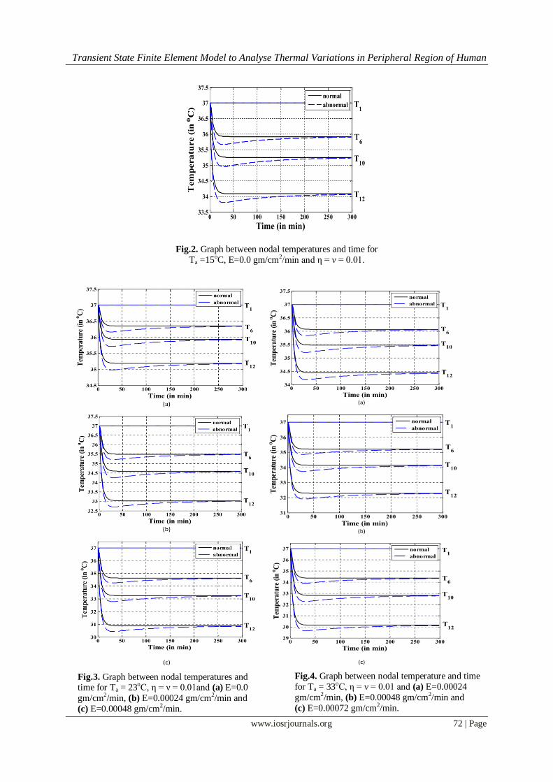
Here in Fig 2 nodal temperature versus time graph has been plotted for Ta = 15oC for both, normal and
abnormal tissues. Fig 3 (a-c) and Fig 4 (a-c) show temperature profiles for Ta = 23oC and 33oC at different rates
of evaporation. For this purpose four nodes chosen are: one at core of the skin (T1), one at the interface of
subcutaneous and dermis (T6), one at the interface of dermis and epidermis (T10) and one at the surface of the skin (T12). Fig 5 (a-c) are the graphs comparing temperature profile of the skin surface against time for different
atmospheric temperatures at fixed rate of sweat evaporation E = 0.0, 0.00024 and 0.00048 gm/cm2/min
respectively.
Transient State Finite Element Model to Analyse Thermal Variations in Peripheral Region of Human
www.iosrjournals.org 72 | Page
Fig.2. Graph between nodal temperatures and time for
Ta =15oC, E=0.0 gm/cm2/min and η = ν = 0.01.
Fig.4. Graph between nodal temperature and time
for Ta = 33oC, η = ν = 0.01 and (a) E=0.00024
gm/cm2/min, (b) E=0.00048 gm/cm2/min and
(c) E=0.00072 gm/cm2/min.
Fig.3. Graph between nodal temperatures and time for Ta = 23oC, η = ν = 0.01and (a) E=0.0
gm/cm2/min, (b) E=0.00024 gm/cm2/min and
(c) E=0.00048 gm/cm2/min.

Transient State Finite Element Model to Analyse Thermal Variations in Peripheral Region of Human
www.iosrjournals.org 73 | Page
Fig 2-4 shows that at the skin core, nodal temperatures are at a constant value of 37 oC as assumed.
With the increase in time the temperature decreases very fast for first 10 minutes and 20 minutes for normal and
abnormal tissues respectively. In normal tissues this is due to the fact that as soon as skin surface comes in contact with the atmosphere which is at lower temperature, heat is lost from the tissues through the physical
phenomenon of conduction and radiation. Also at higher peripheral tissue temperature (as assumed by the initial
condition that the tissues are insulated and thus are at 37oC), the sweat glands become active and sweat is
produced. This sweat is evaporated by utilising the heat of peripheral tissues and thus heat is lost in the form of
latent heat of vaporisation by the tissues through the process of evaporation. It is observed that this fall in
temperature is higher in abnormal tissues than that in the normal ones. This further decrease in temperature in
abnormal tissues can be accounted for by the fact that as soon as incision is made in the tissue, blood perfusion
rate is eventually stopped in the wounded area due to vasoconstriction in the severed blood vessel due to
vascular spasm of the smooth muscle in vessel wall followed by formation of platelet plug to stop bleeding
[23].The blue curves in these graphs give us an idea about the magnitude of the thermal effect of surgical wound
on temperature profiles in the skin layers. Results also show that, abnormal tissue takes more time to attain steady state temperature than that of normal tissue. For normal tissues, the temperature becomes almost steady
after 20 minutes and results match with [1, 17]. In case of abnormal tissues, after attaining the minimum value,
the temperature begins to rise for about 120 - 250 minutes without and with different rates of evaporation (fig.
3-4). This is due to the gradual increase in blood perfusion rate in the surgical wound from surrounding blood
vessels and increase in metabolic generation heat because of the complex process of biochemical reactions
taking place to accomplish wound healing in the operated tissues [23]. The net effect is that the abnormal tissue
temperature falls further for a few minutes and then rise as wound healing progresses with time. The delay in
resumption of steady state temperature profiles by abnormal tissues can be validated on the basis of
experimental findings of Gannon [25].
Fig.5. Graph comparing temperature profile of the node 12 against time for different atmospheric temperatures
at fixed rate of sweat evaporation (a) E = 0.0 gm/cm2/min, (b) E = 0.00024 gm/cm2/min, (c) E = 0.00048
gm/cm2/min and η = ν = 0.01
Transient State Finite Element Model to Analyse Thermal Variations in Peripheral Region of Human
www.iosrjournals.org 74 | Page
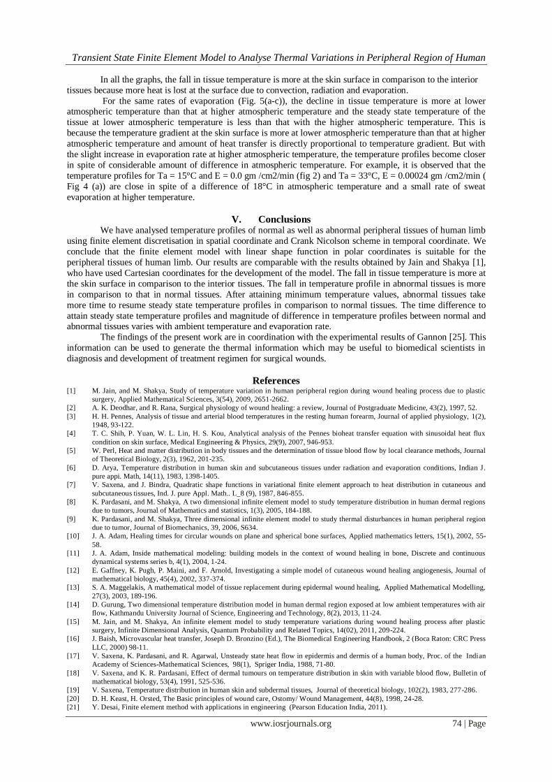
In all the graphs, the fall in tissue temperature is more at the skin surface in comparison to the interior
tissues because more heat is lost at the surface due to convection, radiation and evaporation.
For the same rates of evaporation (Fig. 5(a-c)), the decline in tissue temperature is more at lower atmospheric temperature than that at higher atmospheric temperature and the steady state temperature of the
tissue at lower atmospheric temperature is less than that with the higher atmospheric temperature. This is
because the temperature gradient at the skin surface is more at lower atmospheric temperature than that at higher
atmospheric temperature and amount of heat transfer is directly proportional to temperature gradient. But with
the slight increase in evaporation rate at higher atmospheric temperature, the temperature profiles become closer
in spite of considerable amount of difference in atmospheric temperature. For example, it is observed that the
temperature profiles for Ta = 15°C and E = 0.0 gm /cm2/min (fig 2) and Ta = 33°C, E = 0.00024 gm /cm2/min (
Fig 4 (a)) are close in spite of a difference of 18°C in atmospheric temperature and a small rate of sweat
evaporation at higher temperature.
V. Conclusions We have analysed temperature profiles of normal as well as abnormal peripheral tissues of human limb
using finite element discretisation in spatial coordinate and Crank Nicolson scheme in temporal coordinate. We
conclude that the finite element model with linear shape function in polar coordinates is suitable for the
peripheral tissues of human limb. Our results are comparable with the results obtained by Jain and Shakya [1],
who have used Cartesian coordinates for the development of the model. The fall in tissue temperature is more at
the skin surface in comparison to the interior tissues. The fall in temperature profile in abnormal tissues is more
in comparison to that in normal tissues. After attaining minimum temperature values, abnormal tissues take
more time to resume steady state temperature profiles in comparison to normal tissues. The time difference to
attain steady state temperature profiles and magnitude of difference in temperature profiles between normal and abnormal tissues varies with ambient temperature and evaporation rate.
The findings of the present work are in coordination with the experimental results of Gannon [25]. This
information can be used to generate the thermal information which may be useful to biomedical scientists in
diagnosis and development of treatment regimen for surgical wounds.
References [1] M. Jain, and M. Shakya, Study of temperature variation in human peripheral region during wound healing process due to plastic
surgery, Applied Mathematical Sciences, 3(54), 2009, 2651-2662.
[2] A. K. Deodhar, and R. Rana, Surgical physiology of wound healing: a review, Journal of Postgraduate Medicine, 43(2), 1997, 52.
[3] H. H. Pennes, Analysis of tissue and arterial blood temperatures in the resting human forearm, Journal of applied physiology, 1(2),
1948, 93-122.
[4] T. C. Shih, P. Yuan, W. L. Lin, H. S. Kou, Analytical analysis of the Pennes bioheat transfer equation with sinusoidal heat flux
condition on skin surface, Medical Engineering & Physics, 29(9), 2007, 946-953.
[5] W. Perl, Heat and matter distribution in body tissues and the determination of tissue blood flow by local clearance methods, Journal
of Theoretical Biology, 2(3), 1962, 201-235.
[6] D. Arya, Temperature distribution in human skin and subcutaneous tissues under radiation and evaporation conditions, Indian J.
pure appi. Math, 14(11), 1983, 1398-1405.
[7] V. Saxena, and J. Bindra, Quadratic shape functions in variational finite element approach to heat distribution in cutaneous and
subcutaneous tissues, Ind. J. pure Appl. Math.. L_8 (9), 1987, 846-855.
[8] K. Pardasani, and M. Shakya, A two dimensional infinite element model to study temperature distribution in human dermal regions
due to tumors, Journal of Mathematics and statistics, 1(3), 2005, 184-188.
[9] K. Pardasani, and M. Shakya, Three dimensional infinite element model to study thermal disturbances in human peripheral region
due to tumor, Journal of Biomechanics, 39, 2006, S634.
[10] J. A. Adam, Healing times for circular wounds on plane and spherical bone surfaces, Applied mathematics letters, 15(1), 2002, 55-
58.
[11] J. A. Adam, Inside mathematical modeling: building models in the context of wound healing in bone, Discrete and continuous
dynamical systems series b, 4(1), 2004, 1-24.
[12] E. Gaffney, K. Pugh, P. Maini, and F. Arnold, Investigating a simple model of cutaneous wound healing angiogenesis, Journal of
mathematical biology, 45(4), 2002, 337-374.
[13] S. A. Maggelakis, A mathematical model of tissue replacement during epidermal wound healing, Applied Mathematical Modelling,
27(3), 2003, 189-196.
[14] D. Gurung, Two dimensional temperature distribution model in human dermal region exposed at low ambient temperatures with air
flow, Kathmandu University Journal of Science, Engineering and Technology, 8(2), 2013, 11-24.
[15] M. Jain, and M. Shakya, An infinite element model to study temperature variations during wound healing process after plastic
surgery, Infinite Dimensional Analysis, Quantum Probability and Related Topics, 14(02), 2011, 209-224.
[16] J. Baish, Microvascular heat transfer, Joseph D. Bronzino (Ed.), The Biomedical Engineering Handbook, 2 (Boca Raton: CRC Press
LLC, 2000) 98-11.
[17] V. Saxena, K. Pardasani, and R. Agarwal, Unsteady state heat flow in epidermis and dermis of a human body, Proc. of the Indian
Academy of Sciences-Mathematical Sciences, 98(1), Spriger India, 1988, 71-80.
[18] V. Saxena, and K. R. Pardasani, Effect of dermal tumours on temperature distribution in skin with variable blood flow, Bulletin of
mathematical biology, 53(4), 1991, 525-536.
[19] V. Saxena, Temperature distribution in human skin and subdermal tissues, Journal of theoretical biology, 102(2), 1983, 277-286.
[20] D. H. Keast, H. Orsted, The Basic principles of wound care, Ostomy/ Wound Management, 44(8), 1998, 24-28.
[21] Y. Desai, Finite element method with applications in engineering (Pearson Education India, 2011).

Transient State Finite Element Model to Analyse Thermal Variations in Peripheral Region of Human
www.iosrjournals.org 75 | Page
[22] M. N. O. Sadiku, Numerical techniques in electromagnetics (CRC press , 2000).
[23] J. E. Hall, Guyton and Hall Textbook of Medical Physiology: Enhanced E-book ( Elsevier Health Sciences, 2010).
[24] V. Saxena, and J. Bindra, Pseudo-analytic finite partition approach to temperature distribution problem in human limbs,
International Journal of Mathematics and Mathematical Sciences, 12(2), 1989, 403-408.
[25] R. Gannon, Fact file: Wound cleansing: sterile water or saline?, Nursing Times. net, 103(9), 2007, p44.
Top Related
Copyright © 2022 FDOKUMEN

