


Bahasa
Halaman
Hukum


Subject Code : P16CSE5C IA Marks : 25
No. of Lecture Hrs/Week : 06 Exam Hours : 03
ELECTIVE COURSE V
5.3 DIGITAL IMAGE PROCESSING
Objective: To study the various concepts, methods and algorithms of digital
image processing with image transformation, image enhancement, image
restoration, image compression techniques
Unit I CONTINUOUS AND DISCRETE IMAGES AND SYSTEMS :
Light, Luminance, Brightness and Contrast, Eye, The Monochrome Vision
Model, Image Processing Problems and Applications, Vision Camera, Digital
Processing System, 2-D Sampling Theory, Aliasing, Image Quantization,
Lloyd MaxQuantizer, Dither, Color Images, Linear Systems And Shift
Invariance, Fourier Transform, ZTransform, Matrix Theory Results, Block
Matrices and Kronecker Products.
Unit II IMAGE TRANSFORMS :
2-D orthogonal and Unitary transforms, 1-D and 2-DDFT, Cosine, Sine,
Walsh, Hadamard, Haar, Slant, Karhunen-loeve, Singularvalue
Decomposition transforms.
Unit III IMAGE ENHANCEMENT :
Point operations - contrast stretching, clipping and thresholding density
slicing, Histogram equalization, modification andspecification, spatial
operations - spatial averaging, low pass, high pass, bandpass filtering,
direction smoothing, medium filtering, generalized Spectrum and
homomorphic filtering, edge enhancement using 2-D IIR and FIR filters, color
image enhancement.
Unit IV IMAGE RESTORATION : Image observation models, sources of degradation, inverse and Wiener
filtering, geometric mean filter, non linear filters, smoothingsplines and
interpolation, constrained least squares restoration.
Unit V IMAGE DATA COMPRESSION AND IMAGE RECONSTRUCTION FROM
PROJECTIONS:
Image data rates, pixel coding, predictive techniques transform coding and
vector DPCM, Block truncation coding, wavelet transform coding of images,
color image coding. Random transform, back projection operator, inverse
random transform, back projection algorithm, fan beam and algebraic
restoration techniques.
Book for study :
1. Anil K. Jain, “Fundamentals of Digital Image Processing”, PHI, 1995.
2. Sid Ahmed M.A., “Image Processing”, McGraw Hill Inc, 1995.
3. Gonzalaz R. and Wintz P., “Digital Image Processing”, Addison Wesley,
2nd Ed, 1987.
Unit-1
Introduction
What Is Digital Image Processing?
An image may be defined as a two-dimensional function, f(x, y), where x and y are
spatial (plane) coordinates, and the amplitude of f at any pair of coordinates (x, y) is
called the intensity or gray level of the image at that point. When x, y, and the
amplitude values of f are all finite, discrete quantities, we call the image a digital
image. The field of digital image processing refers to processing digital images by
means of a digital computer. Note that a digital image is composed of a finite number
of elements, each of which has a particular location and value. These elements are
referred to as picture elements, image elements, pels, and pixels. Pixel is the term
most widely used to denote the elements of a digital image.
Fundamental Steps in Digital Image Processing
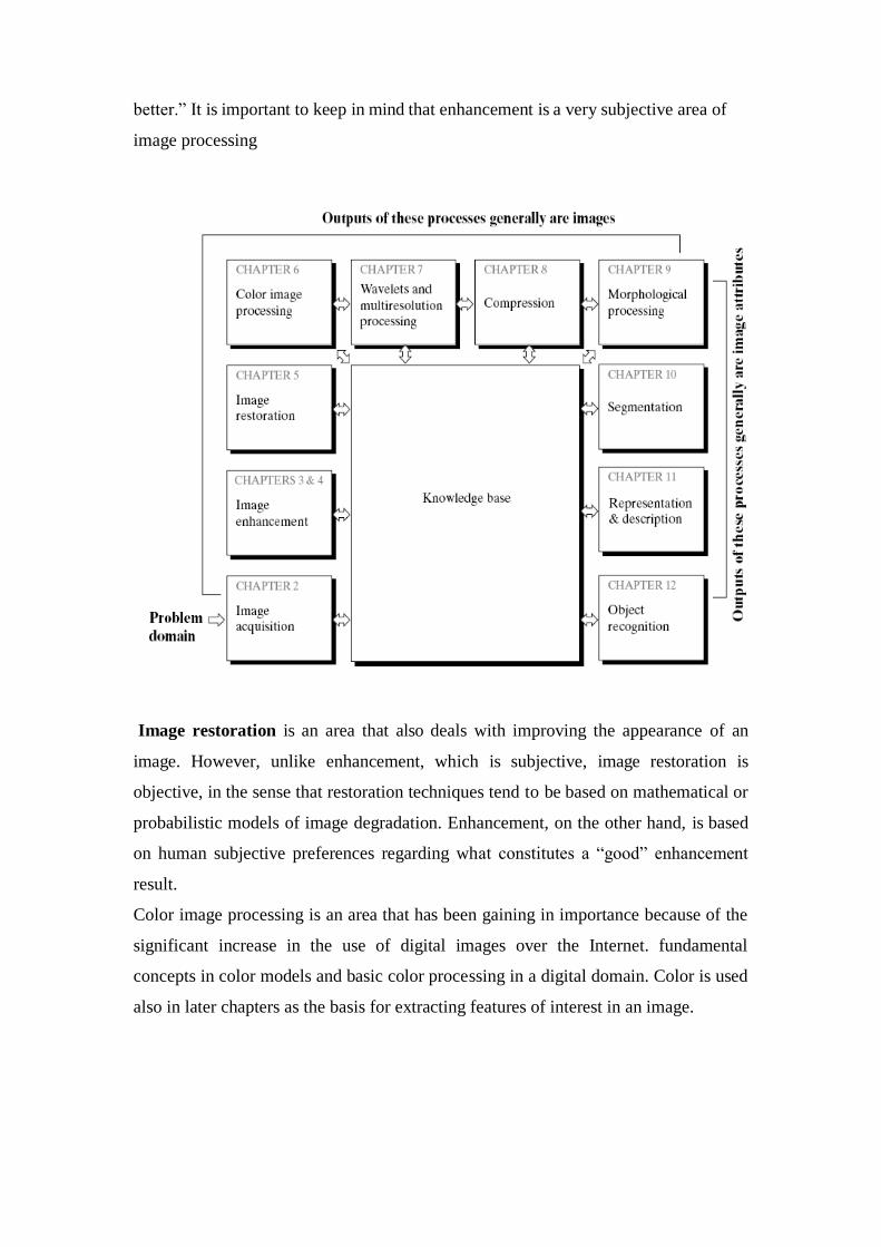
It is helpful to divide the material covered in the following chapters into the two broad
categories defined in Section 1.1: methods whose input and output are images, and
methods whose inputs may be images, but whose outputs are attributes extracted from
those images..The diagram does not imply that every process is applied to an image.
Rather, the intention is to convey an idea of all the methodologies that can be applied
to images for different purposes and possibly with different objectives.
Image acquisition is the first process acquisition could be as simple as being given an
image that is already in digital form. Generally, the image acquisition stage involves
preprocessing, such as scaling.
Image enhancement is among the simplest and most appealing areas of digital image
processing. Basically, the idea behind enhancement techniques is to bring out detail
that is obscured, or simply to highlight certain features of interest in an image. A
familiar example of enhancement is when we increase the contrast of an image
because “it looks
better.” It is important to keep in mind that enhancement is a very subjective area of
image processing
Image restoration is an area that also deals with improving the appearance of an
image. However, unlike enhancement, which is subjective, image restoration is
objective, in the sense that restoration techniques tend to be based on mathematical or
probabilistic models of image degradation. Enhancement, on the other hand, is based
on human subjective preferences regarding what constitutes a “good” enhancement
result.
Color image processing is an area that has been gaining in importance because of the
significant increase in the use of digital images over the Internet. fundamental
concepts in color models and basic color processing in a digital domain. Color is used
also in later chapters as the basis for extracting features of interest in an image.
Wavelets are the foundation for representing images in various degrees of resolution.
In particular, this material is used in this book for image data compression and for
pyramidal representation, in which images are subdivided successively into smaller
regions.
Compression, as the name implies, deals with techniques for reducing the storage
required to save an image, or the bandwidth required to transmit it. Although storage
technology has improved significantly over the past decade, the same cannot be said
for transmission capacity. This is true particularly in uses of the Internet, which are
characterized by significant pictorial content. Image compression is familiar (perhaps
inadvertently) to most users of computers in the form of image file extensions, such as
the jpg file extension used in the JPEG(Joint Photographic Experts Group) image
compression standard.
Morphological processing deals with tools for extracting image components that are
useful in the representation and description of shape. The material in this chapter
begins a transition from processes that output images to processes that output image
attributes, Segmentation procedures partition an image into its constituent parts or
objects. In general, autonomous segmentation is one of the most difficult tasks in
digital image processing. A rugged segmentation procedure brings the process a long
way toward successful solution of imaging problems that require objects to be
identified individually. On the other hand, weak or erratic segmentation algorithms
almost always guarantee eventual failure. In general, the more accurate the
segmentation, the more likely recognition is to succeed.
Representation and description almost always follow the output of a segmentation
stage, which usually is raw pixel data, constituting either the boundary of a region
(i.e., the set of pixels separating one image region from another) or all the points in
the region itself. In either case, converting the data to a form suitable for computer
processing is necessary. The first decision that must be made is whether the data
should be represented as a boundary or as a complete region. Boundary representation
is appropriate when the focus is on external shape characteristics, such as corners and
inflections. Regional representation is appropriate when the focus is on internal
properties, such as texture or skeletal shape. In some applications, these
representations complement each other.
Choosing a representation is only part of the solution for transforming raw data into a
form suitable for subsequent computer processing. A method must also be specified
for describing the data so that features of interest are highlighted. Description, also
called feature selection, deals with extracting attributes that result in some quantitative
information of interest or are basic for differentiating one class of objects from
another.
Recognition is the process that assigns a label (e.g., “vehicle”) to an object based on
its descriptors. As detailed in Section 1.1, we conclude our coverage of digital image
processing with the development of methods for recognition of individual objects. So
far we have said nothing about the need for prior knowledge or about the interaction
between the knowledge base and Knowledge about a problem domain is coded into an
image processing system in the form of a knowledge database. This knowledge may
be as simple as detailing regions of an image where the information of interest is
known to be located, thus limiting the search that has to be conducted in seeking that
information. The knowledge base also can be quite complex, such as an interrelated
list of all major possible defects in a materials inspection problem or an image
database containing high- resolution satellite images of a region in connection with
change-detection applications.
In addition to guiding the operation of each processing module, the knowledge base
also controls the interaction between modules. This distinction is made in Fig. 1.23 by
the use of double headed arrows between the processing modules and the knowledge
base, as opposed to single-headed arrows linking the processing modules. Although
we do not discuss image display explicitly at this point, it is important to keep in mind
that viewing the results of image processing can take place at the output of any stage.
Components of an Image Processing System
Although large-scale image processing systems still are being sold for massive
imaging applications, such as processing of satellite images, the trend continues
toward miniaturizing and blending of general-purpose small computers with
specialized image processing hardware.
The function of each component is discussed in the following paragraphs, starting
with image sensing. With reference to sensing, two elements are required to acquire
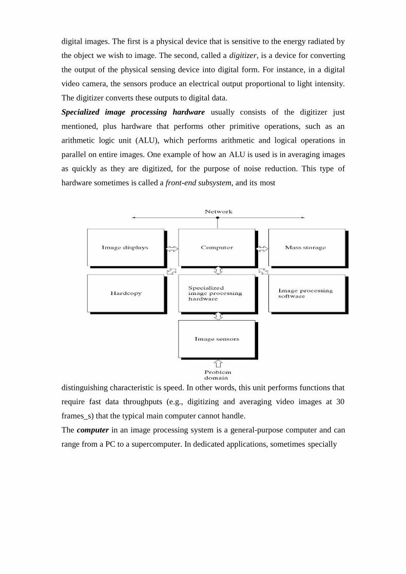
digital images. The first is a physical device that is sensitive to the energy radiated by
the object we wish to image. The second, called a digitizer, is a device for converting
the output of the physical sensing device into digital form. For instance, in a digital
video camera, the sensors produce an electrical output proportional to light intensity.
The digitizer converts these outputs to digital data.
Specialized image processing hardware usually consists of the digitizer just
mentioned, plus hardware that performs other primitive operations, such as an
arithmetic logic unit (ALU), which performs arithmetic and logical operations in
parallel on entire images. One example of how an ALU is used is in averaging images
as quickly as they are digitized, for the purpose of noise reduction. This type of
hardware sometimes is called a front-end subsystem, and its most
distinguishing characteristic is speed. In other words, this unit performs functions that
require fast data throughputs (e.g., digitizing and averaging video images at 30
frames_s) that the typical main computer cannot handle.
The computer in an image processing system is a general-purpose computer and can
range from a PC to a supercomputer. In dedicated applications, sometimes specially
designed computers are used to achieve a required level of performance, but our
interest here is on general-purpose image processing systems. In these systems,
almost any well- equipped PC-type machine is suitable for offline image processing
tasks.
Software for image processing consists of specialized modules that perform specific
tasks. A well-designed package also includes the capability for the user to write code
that, as a minimum, utilizes the specialized modules. More sophisticated software
packages allow the integration of those modules and general- purpose software
commands from at least one computer language.
Mass storage capability is a must in image processing applications.An image of size
1024*1024 pixels, in which the intensity of each pixel is an 8-bit quantity, requires
one megabyte of storage space if the image is not compressed. When dealing with
thousands, or even millions, of images, providing adequate storage in an image
processing system can be a challenge. Digital storage for image processing
applications falls into three principal categories: (1) short term storage for use during
processing, (2) on-line storage for relatively fast recall, and (3) archival storage,
characterized by infrequent access. Storage is measured in bytes (eight bits), Kbytes
(one thousand bytes), Mbytes (one million bytes), Gbytes (meaning giga, or one
billion, bytes), and T bytes (meaning tera, or one trillion, bytes).
One method of providing short-term storage is computer memory.Another is by
specialized boards, called frame buffers, that store one or more images and can be
accessed rapidly, usually at video rates (e.g., at 30 complete images per second).The
latter method allows virtually instantaneous image zoom, as well as scroll (vertical
shifts) and pan (horizontal shifts). Frame buffers usually are housed in the specialized
image processing hardware unit. Online storage generally takes the form of magnetic
disks or optical-media storage. The key factor characterizing on-line storage is
frequent access to the stored data. Finally, archival storage is characterized by massive
storage requirements but infrequent need for access. Magnetic tapes and optical disks
housed in “jukeboxes” are the usual media for archival applications.
Image displays in use today are mainly color (preferably flat screen) TV monitors.
Monitors are driven by the outputs of image and graphics display cards that are an
integral part of the computer system. Seldom are there requirements for image display
applications that cannot be met by display cards available commercially as part of the
computer system. In some cases, it is necessary to have stereo displays, and these are
implemented in the form of headgear containing two small displays embedded in
goggles worn by the user.
Hardcopy devices for recording images include laser printers, film cameras, heat-
sensitive devices, inkjet units, and digital units, such as optical and CD-ROM disks.
Film provides the highest possible resolution, but paper is the obvious medium of
choice for written material. For presentations, images are displayed on film
transparencies or in a digital medium if image projection equipment is used. The latter
approach is gaining acceptance as the standard for image presentations.
Networking is almost a default function in any computer system in use today. Because
of the large amount of data inherent in image processing applications, the key
consideration in image transmission is bandwidth. In dedicated networks, this
typically is not a problem, but communications with remote sites via the Internet are
not always as efficient. Fortunately, this situation is improving quickly as a result of
optical fiber and other broadband technologies.

Recommended Questions
1. What is digital image processing? Explain the fundamental steps in digital image
processing.
2. Briefly explain the components of an image processing system.
3. How is image formed in an eye? Explain with examples the perceived brightness is
not a simple function of intensity.
4. Explain the importance of brightness adaption and discrimination in image
processing.
5. Define spatial and gray level resolution. Briefly discuss the effects resulting from
a reduction in number of pixels and gray levels.
6. What are the elements of visual perception?
Dept. of ECE/SJBIT Page 9
UNIT – 2
Image Sensing and Acquisition
The types of images in which we are interested are generated by the combination of
an “illumination” source and the reflection or absorption of energy from that source
by the elements of the “scene” being imaged. We enclose illumination and scene in
quotes to emphasize the fact that they are considerably more general than the familiar
situation in which a visible light source illuminates a common everyday 3-D (three-
dimensional) scene. For example, the illumination may originate from a source of
electromagnetic energy such as radar, infrared, or X-ray energy. But, as noted earlier,
it could originate from less traditional sources, such as ultrasound or even a
computer-generated illumination pattern. Similarly, the scene elements could be
familiar objects, but they can just as easily be molecules, buried rock formations, or
a human brain. We could even image a source, such as acquiring images of the sun.
Depending on the nature of the source, illumination energy is reflected from, or
transmitted through, objects. An example in the first category is light reflected from a
planar surface. An example in the second category is when X-rays pass through a
patient’s body for thepurpose of generating a diagnostic X-ray film. In some
applications, the reflected or transmitted energy is focused onto a photo converter
(e.g., a phosphor screen), which converts the energy into visible light. Electron
microscopy and some applications of gamma imaging use this approach.
The idea is simple: Incoming energy is transformed into a voltage by the
combination of input electrical power and sensor material that is responsive to the
particular type of energy being detected.
The output voltage waveform is the response of the sensor(s), and a digital quantity
is obtained from each sensor by digitizing its response. In this section, we look at the
principal modalities for image sensing and generation.
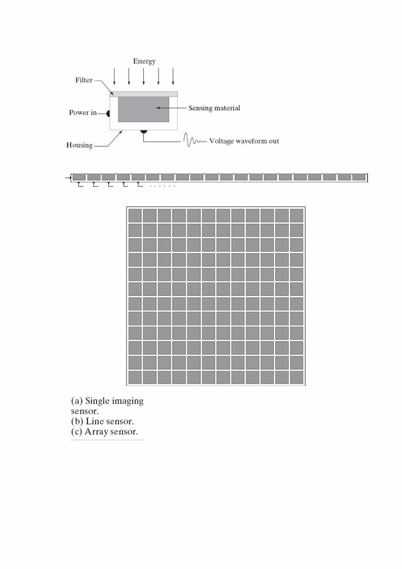
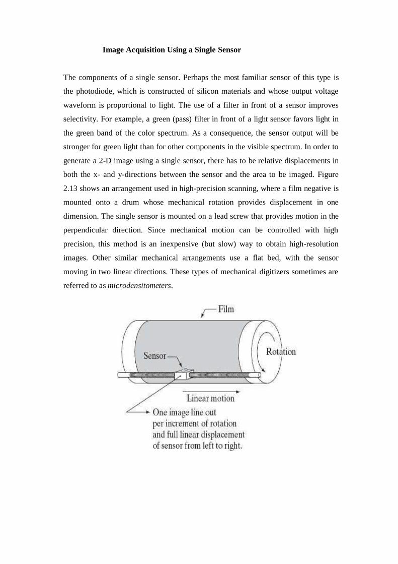
Image Acquisition Using a Single Sensor
The components of a single sensor. Perhaps the most familiar sensor of this type is
the photodiode, which is constructed of silicon materials and whose output voltage
waveform is proportional to light. The use of a filter in front of a sensor improves
selectivity. For example, a green (pass) filter in front of a light sensor favors light in
the green band of the color spectrum. As a consequence, the sensor output will be
stronger for green light than for other components in the visible spectrum. In order to
generate a 2-D image using a single sensor, there has to be relative displacements in
both the x- and y-directions between the sensor and the area to be imaged. Figure
2.13 shows an arrangement used in high-precision scanning, where a film negative is
mounted onto a drum whose mechanical rotation provides displacement in one
dimension. The single sensor is mounted on a lead screw that provides motion in the
perpendicular direction. Since mechanical motion can be controlled with high
precision, this method is an inexpensive (but slow) way to obtain high-resolution
images. Other similar mechanical arrangements use a flat bed, with the sensor
moving in two linear directions. These types of mechanical digitizers sometimes are
referred to as microdensitometers.

Image Acquisition Using Sensor Strips
A geometry that is used much more frequently than single sensors consists of an in-
line arrangement of sensors in the form of a sensor strip, shows. The strip provides
imaging elements in one direction. Motion perpendicular to the strip provides
imaging in the other direction. This is the type of arrangement used in most flat bed
scanners. Sensing devices with 4000 or more in-line sensors are possible. In-line
sensors are used routinely in airborne imaging applications, in which the imaging
system is mounted on an aircraft that flies at a constant altitude and speed over the
geographical area to be imaged. One- dimensional imaging sensor strips that respond
to various bands of the electromagnetic spectrum are mounted perpendicular to the
direction of flight. The imaging strip gives one line of an image at a time, and the
motion of the strip completes the other dimension of a two-dimensional image.
Lenses or other focusing schemes are used to project area to be scanned onto the
sensors.
Sensor strips mounted in a ring configuration are used in medical and industrial
imaging to obtain cross-sectional (“slice”) images of 3-D objects\

Image Acquisition Using Sensor Arrays
The individual sensors arranged in the form of a 2-D array. Numerous
electromagnetic and some ultrasonic sensing devices frequently are arranged in an
array format. This is also the predominant arrangement found in digital cameras. A
typical sensor for these cameras is a CCD array, which can be manufactured with a
broad range of sensing properties and can be packaged in rugged arrays of elements
or more. CCD sensors are used widely in digital cameras and other light sensing
instruments. The response of each sensor is proportional to the integral of the light
energy projected onto the surface of the sensor, a property that is used in
astronomical and other applications requiring low noise images. Noise reduction is
achieved by letting the sensor integrate the input light signal over minutes or even
hours. The two dimensional, its key advantage is that a complete image can be
obtained by focusing the energy pattern onto the surface of the array. Motion
obviously is not necessary, as is the case with the sensor arrangements
This figure shows the energy from an illumination source being reflected from a
scene element, but, as mentioned at the beginning of this section, the energy also
could be transmitted through the scene elements. The first function performed by the
imaging system is to collect the incoming energy and focus it onto an image plane. If
the illumination is light, the front end of the imaging system is a lens, which projects
the viewed scene onto the lens focal plane. The sensor array, which is coincident
with the focal plane, produces outputs proportional to the integral of the light
received at each sensor. Digital and analog circuitry sweep these outputs and convert
them to a video signal, which is then digitized by another section of the imaging
system.
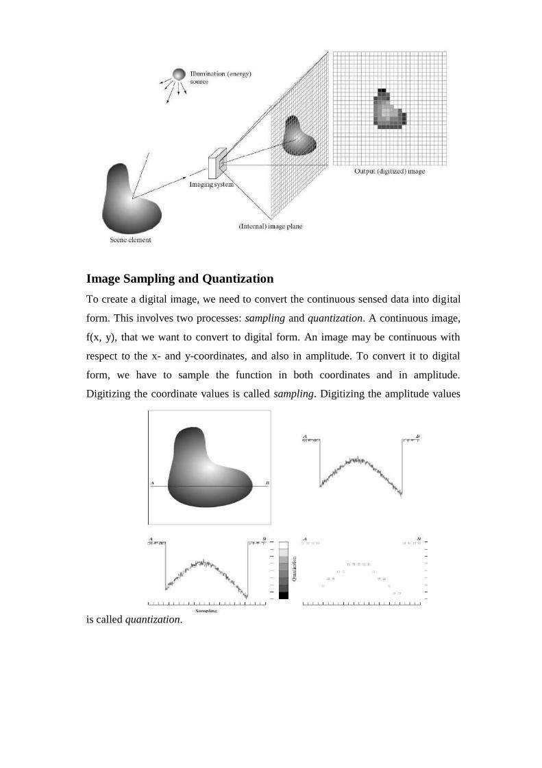
Image Sampling and Quantization
To create a digital image, we need to convert the continuous sensed data into digital
form. This involves two processes: sampling and quantization. A continuous image,
f(x, y), that we want to convert to digital form. An image may be continuous with
respect to the x- and y-coordinates, and also in amplitude. To convert it to digital
form, we have to sample the function in both coordinates and in amplitude.
Digitizing the coordinate values is called sampling. Digitizing the amplitude values
is called quantization.
The one-dimensional function shown in Fig. 2.16(b) is a plot of amplitude (gray
level) values of the continuous image along the line segment AB. The random
variations are due to image noise. To sample this function, we take equally spaced
samples along line AB, The location of each sample is given by a vertical tick mark
in the bottom part of the figure. The samples are shown as small white squares
superimposed on the function. The set of these discrete locations gives the sampled
function. However, the values of the samples still span (vertically) a continuous
range of gray-level values. In order to form a digital function, the gray-level values
also must be converted (quantized) into discrete quantities. The right side gray-level
scale divided into eight discrete levels, ranging from black to white. The vertical tick
marks indicate the specific value assigned to each of the eight gray levels. The
continuous gray levels are quantized simply by assigning one of the eight discrete
gray levels to each sample. The assignment is made depending on the vertical
proximity of a sample to a vertical tick mark. The digital samples resulting from both
sampling and quantization.
Some Basic Relationships Between Pixels
In this section, we consider several important relationships between pixels in a digital
image.As mentioned before, an image is denoted by f(x, y).When referring in this
section to a particular pixel, we use lowercase letters, such as p and q.
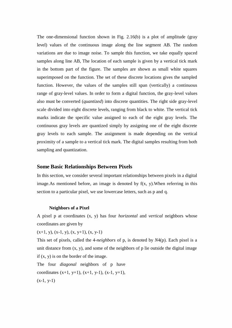
Neighbors of a Pixel
A pixel p at coordinates (x, y) has four horizontal and vertical neighbors whose
coordinates are given by
(x+1, y), (x-1, y), (x, y+1), (x, y-1)
This set of pixels, called the 4-neighbors of p, is denoted by N4(p). Each pixel is a
unit distance from (x, y), and some of the neighbors of p lie outside the digital image
if (x, y) is on the border of the image.
The four diagonal neighbors of p have
coordinates (x+1, y+1), (x+1, y-1), (x-1, y+1),
(x-1, y-1)

and are denoted by ND(p). These points, together with the 4-neighbors, are called the
8- neighbors of p, denoted by N8(p). As before, some of the points in ND(p) and
N8(p) fall outside the image if (x, y) is on the border of the image.
Adjacency, Connectivity, Regions, and Boundaries
Connectivity between pixels is a fundamental concept that simplifies the definition of
numerous digital image concepts, such as regions and boundaries. To establish if two
pixels are connected, it must be determined if they are neighbors and if their gray
levels satisfy a specified criterion of similarity (say, if their gray levels are equal).For
instance, in a binary image with values 0 and 1, two pixels may be 4-neighbors, but
they are said to be connected only if they have the same value.
Let V be the set of gray-level values used to define adjacency. In a binary image,
V={1} if we are referring to adjacency of pixels with value 1. In a grayscale image,
the idea is the same, but set V typically contains more elements. For example, in the
adjacency of pixels with a range of possible gray-level values 0 to 255, set V could
be any subset of these 256 values. We consider three types of adjacency:
(a) 4-adjacency. Two pixels p and q with values from V are 4-adjacent if q is in the set
N4(p).
(b) 8-adjacency. Two pixels p and q with values from V are 8-adjacent if q is in the set
N8(p).
(c) m-adjacency (mixed adjacency).Two pixels p and q with values from V are m-
adjacent if
(i) q is in N4(p), or
(ii) q is in ND(p) and the set has no pixels whose values are from V.
Linear and Nonlinear Operations
Let H be an operator whose input and output are images. H is said to be a linear
operator if, for any two images f and g and any two scalars a and b,
H(af + bg) = aH(f) + bH(g).

In other words, the result of applying a linear operator to the sum of two images
(that have been multiplied by the constants shown) is identical to applying the
operator to the images individually, multiplying the results by the appropriate
constants, and then adding those results. For example, an operator whose function is
to compute the sum of K images is a linear operator. An operator that computes the
absolute value of the difference of two images is not.
Linear operations are exceptionally important in image processing because they are
based on a significant body of well-understood theoretical and practical results.
Although nonlinear operations sometimes offer better performance, they are not
always predictable, and for the most part are not well understood theoretically.
Recommended Questions
1. Explain the concept of sampling and quantization of an image.
2. Explain i) false contouring ii) checkboard pattern
3. How image is acquired using a single sensor? Discuss.
4. Explain zooming and shrinking digital images.
5. Define 4-adjacency, 8 – adjacency and m – adjacency.
6. With a suitable diagram, explain how an image is acquired using a circular
sensor strip.
7. Explain the relationships between pixels . and also the image operations on a
pixel basis.
8. Explain linear and nonlinear operations.
u
Unit-3
Image
Transforms
Two-dimensional orthogonal & unitary transforms
One dimensional signals:
For a one dimensional sequence
{ f (x), 0 x N 1}
represented as a vector
f f (0) f (1) f (N 1)T of size N , a transformation may be written as
N 1
g T f g(u) T (u, x) f (x), 0 u N 1
x 0
where g(u) is the transform (or transformation) of f (x) , and T (u, x) is the so called
Forward transformation kernel. Similarly, the inverse transform is the relation N 1
f (x) I (x,u)g(u), 0 x N 1 u 0
or written in a matrix form f I g T 1
g
where I (x,u) is the so called inverse transformation kernel.
If
I T 1 T
T
the matrix T is called unitary, and the transformation is called unitary as well. It can be
proven (how?) that the columns (or rows) of an N N unitary matrix are orthonormal and therefore, form a complete set of basis vectors in the N dimensional vector
space. In that case f T
T
g f (x) N 1
T u0
(u, x)g(u)
The columns of T T
, that is, the vectors T T (u,0) T (u,1) T (u, N 1)T are called the
basis vectors of T .
Two dimensional signals (images)
As a one dimensional signal can be represented by an orthonormal set of basis
vectors, an image can also be expanded in terms of a discrete set of basis arrays
called basis images through a two dimensional (image) transform.
For an N N image f (x, y) the forward and inverse transforms are given below

1 1
N 1 N 1
g(u, v) T (u, v, x, y) f (x, y) x 0 y 0
N 1 N 1
f (x, y) I (x, y,u, v)g(u, v) u 0 v 0
where, again, T (u, v, x, y) and I (x, y,u, v) are called the forward and inverse
transformation kernels, respectively.
The forward kernel is said to be separable if
T (u,v, x, y) T1(u, x)T2 (v, y)
It is said to be symmetric if T1 is functionally equal to T2
T (u, v, x, y) T1 (u, x)T1 (v, y)
such that
The same comments are valid for the inverse kernel.
If the kernel T (u, v, x, y) of an image transform is separable and symmetric, then the N 1 N 1 N 1 N 1
transform g(u, v) T (u, v, x, y) f (x, y) T1(u, x)T1(v, y) f (x, y) can be written in x 0 y 0
matrix form as follows
x 0 y 0
g T f T T
where f is the original image of size N N , and T 1 is an N N
transformation matrix
with elements tij T1 (i, j) . If, in addition, T 1 is a unitary matrix then the transform is
called separable unitary and the original image is recovered through the relationship
f T
T
g T 1 1
properties of unitary transforms
The property of energy preservation
In the unitary transformation
g T f
it is easily proven (try the proof by using the relation T 1 T
T ) that
Thus, a unitary transformation preserves the signal energy. This property is called energy
preservation property.
This means that every unitary transformation is simply a rotation of the vector f in the
N - dimensional vector space.
g f 2 2

For the 2-D case the energy preservation property is written as N 1 N 1
f (x, y) 2
N 1 N 1
g(u, v) 2
x0 y 0 u0 v 0
The property of energy compaction
Most unitary transforms pack a large fraction of the energy of the image into
relatively few of the transform coefficients. This means that relatively few of the
transform coefficients have significant values and these are the coefficients that are close to
the origin (small index coefficients).
This property is very useful for compression purposes. (Why?)
Two dimensional discrete Fourier transform
Continuous space and continuous frequency
The Fourier transform is extended to a function f (x, y) of two variables. If f (x, y) is
continuous and integrable and F(u, v) is integrable, the following Fourier transform
pair exists:
F (u, v)
f (x, y)e j 2 (uxvy) dxdy
f (x, y) 1
(2 )2
F (u, v)e j 2 (uxvy) dudv
In general F(u, v) is a complex-valued function of two real frequency variables u, v
hence, it can be written as:
and
F(u, v) R(u, v) jI (u, v)
The amplitude spectrum, phase spectrum and power spectrum, respectively, are
defined as follows.
F(u, v)
(u, v) tan1
I (u, v)
R(u, v)
P(u, v) F(u, v) 2 R2
(u, v) I 2(u, v)
Discrete space and continuous frequency
For the case of a discrete sequence f (x, y) of infinite duration we can define the 2-D
discrete space Fourier transform pair as follows
R2(u, v) I 2(u, v)
(2 ) u
F (u, v) f ( x, y)e
j( xuvy )
x y
f ( x, y) 1 F (u, v)e
j(xuvy)dudv
2 v
F(u, v) is again a complex-valued function of two real frequency variables u, v and it is
periodic with a period 2 2 , that is to say
F(u, v) F(u 2, v) F(u, v 2 )
The Fourier transform of f (x, y) is said to converge uniformly when F(u, v) is finite and N1 N2 lim lim f ( x, y)e j(xuvy)
F(u, v) for all u, v .
N1 N2 x N1 y N2
When the Fourier transform of f (x, y) converges uniformly, F(u, v) is an analytic
function and is infinitely differentiable with respect to u and v .
Discrete space and discrete frequency: The two dimensional Discrete
Fourier Transform (2-D DFT)
If f (x, y) is an M N array, such as that obtained by sampling a continuous function of
two dimensions at dimensions M and N on a rectangular grid, then its two dimensional
Discrete Fourier transform (DFT) is the array given by
F (u, v) 1
MN
u 0,, M 1, v 0,, N 1
and the inverse DFT (IDFT) is
M 1 N 1
f (x, y)e j 2 (ux / M vy / N )
x0 y0
f (x, y) M 1 N 1
F(u, v)e j2 (ux / M vy / N )
u0 v0
When images are sampled in a square array, M N and F(u, v) 1 N 1 N 1
f (x, y)e j 2 (ux vy )/ N
N
f (x, y) x 0 y 0
1 N 1 N 1
F(u, v)e j2 (ux vy )/ N
N
It is straightforward to prove that the two dimensional Discrete Fourier Transform is
separable, symmetric and unitary.
Properties of the 2-D DFT
u0 v0
p
m
1
1
Most of them are straightforward extensions of the properties of the 1-D Fourier
Transform. Advise any introductory book on Image Processing.
The importance of the phase in 2-D DFT. Image reconstruction from amplitude or phase only.
The Fourier transform of a sequence is, in general, complex-valued, and the unique
representation of a sequence in the Fourier transform domain requires both the phase
and the magnitude of the Fourier transform. In various contexts it is often
desirable to
reconstruct a signal from only partial domain information. Consider a 2-D sequence
f (x, y) with Fourier transform F(u,v) f (x, y) so that
F(u, v) { f (x, y} F(u, v) e j f (u,v)
It has been observed that a straightforward signal synthesis from the Fourier transform
phase f (u, v) alone, often captures most of the intelligibility of the original image
f (x, y)
F (u, v)
(why?). A straightforward synthesis from the Fourier transform magnitude
alone, however, does not generally capture the original signal’s intelligibility.
The above observation is valid for a large number of signals (or images). To illustrate
this, we can synthesise the phase-only signal f p (x, y) and the magnitude-only signal
fm (x, y) by
f (x, y) 11e
j f (u,v)
f (x, y) 1F(u, v) e j0
and observe the two results (Try this exercise in MATLAB).
An experiment which more dramatically illustrates the observation that phase-only
signal synthesis captures more of the signal intelligibility than magnitude-only
synthesis, can be performed as follows.
Consider two images f (x, y) and g(x, y) . From these two images, we synthesise two
other images f1 (x, y) and g1 (x, y) by mixing the amplitudes and phases of the original
images as follows:
f (x, y) 1G(u, v) e j f
(u,v) g (x, y)
1F(u, v) e j g (u ,v)

In this experiment f1 (x, y) captures the intelligibility of f (x, y) , while g1 (x, y) captures
the intelligibility of g(x, y) (Try this exercise in MATLAB).
THE DISCRETE COSINE TRANSFORM (DCT)
One dimensional signals
This is a transform that is similar to the Fourier transform in the sense that the new
independent variable represents again frequency. The DCT is defined below.
C(u) a(u)N 1
f (x) cos(2x 1)u
, u 0,1,, N 1
x 0
2N
with a(u) a parameter that is defined below.
a(u)
The inverse DCT (IDCT) is defined below.
u 0
u 1,, N 1
f (x) N 1
a(u)C(u) cos(2x 1)u
u 0
2N
Two dimensional signals (images)
For 2-D signals it is defined as C(u, v) a(u)a(v)
N 1 N 1
f (x, y) cos(2x 1)u
cos(2 y 1)v
x 0 y 0
2N
2N
N 1 N 1 f (x, y) (2x 1)u (2 y 1)v a(u)a(v)C(u, v) cos 2N cos 2N
u 0 v 0
a(u) is defined as above and u, v 0,1,, N 1
Properties of the DCT transform
The DCT is a real transform. This property makes it attractive in comparison to
the Fourier transform.
The DCT has excellent energy compaction properties. For that reason it is widely
used in image compression standards (as for example JPEG standards).
There are fast algorithms to compute the DCT, similar to the FFT for computing
the DFT.
1/ N
2 / N

Recommended Questions
1. Define two-dimensional DFT. Explain the following properties of 2-DFT.
i) Translation ii) rotation iii) distributivity and scaling iv) separability
2. What are basis vectors?
3. Derive the expression for 2D circular convolution theorem.
4. Define two – dimensional unitary transform. Check whether the unitary DFT
matrix is unitary or not for N = 4.
5. For the 2 X 2 transform A and the image U
1 1 1 2
A = 1/1 1 -1 and U = 8 4
Calculate the transformed image V and the basis images.
6. Consider the image segment shown in fig
i) Let V = {0, 1}. Compute the lengths of shortest 4 - , 8 – and m – paths
between p and q.
ii) Repeat for V = {1, 2}.
3 1 2 1 (q)
3 2 0 2
( p) 1 2 1 1
UNIT – 4 IMAGE TRANSFORMS
WALSH TRANSFORM (WT)
One dimensional signals
This transform is slightly different from the transforms you have met so far. Suppose we
have a function f (x), x 0,, N 1 where N 2n and its Walsh transform W (u) .
If we use binary representation for the values of the independent variables x and u we
need n bits to represent them. Hence, for the binary representation of x and u we can
write: (x)10 bn1 (x)bn2 (x)b0 (x)2 , (u)10 bn1 (u)bn2 (u)b0 (u)2 with bi (x) 0 or1
for i 0,, n 1.
Example
If f (x), x 0,,7, (8 samples) then n 3 and for x 6 ,
6 = (110)2 b2 (6) 1, b1(6) 1, b0 (6) 0
We define now the 1-D Walsh transform as W (u)
1 N 1
f (x)n1
(1)b (x)b
(u) or
x0
i0
i n 1i
n 1
1 N 1 bi ( x)bn 1i (u )
W (u) f (x)(1) i 0
N x0
The array formed by the Walsh kernels is again a symmetric matrix having
orthogonal rows and columns. Therefore, the Walsh transform is and its elements are
of the form
T (u, x) n1
(1)bi ( x)bn1i (u ) . You can immediately observe that T (u, x) 0
i 0
or 1 depending
on the values of bi (x) and bn1i (u) . If the Walsh transform is written in a matrix form
W T f
for u 0
we see that (u)10 bn1(u)bn2 (u)b0 (u)2 0002 and hence, bn1i (u) 0 , for any i . Thus, T (0, x) 1 and W (0)
1 N 1
f (x) . We see that the first element of the Walsh
N x 0
transform in the mean of the original function
the Fourier transform.
f (x) (the DC value) as it is the case with
The inverse Walsh transform is defined as follows.
N
N 1 f (x) n1
(1)b ( x)b (u) or W (u) i n 1i
u0 i0 n 1
N 1 bi ( x)bn 1i (u)
f (x) W (u)(1) i 0
u0
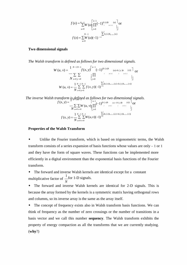
Two dimensional signals
The Walsh transform is defined as follows for two dimensional signals.
W (u, v) 1 N 1 N 1
f (x, y)n1
(1)(b ( x)b
(u)b ( y )b (v)) or
i n1i i n1i
N x0 y 0 i0 n 1
1 N 1 N 1 (bi ( x )bn 1i (u )bi ( y )bn 1 i (v ))
W (u, v) f (x, y)(1) i 0
N x0 y0
The inverse Walsh transform is defined as follows for two dimensional signals. f (x, y)
1 N 1 N 1
n1
(1)(b ( x)b (u) b ( y )b (v)) or
W (u, v) i n1i i n1i
N u0 v0 i0 n1
1 N 1 N 1 (bi ( x )bn1i (u )bi ( y )bn1i (v ))
f (x, y) W (u, v)(1) i0
N u0 v0
Properties of the Walsh Transform
Unlike the Fourier transform, which is based on trigonometric terms, the Walsh
transform consists of a series expansion of basis functions whose values are only 1 or 1
and they have the form of square waves. These functions can be implemented more
efficiently in a digital environment than the exponential basis functions of the Fourier
transform.
The forward and inverse Walsh kernels are identical except for a constant
multiplicative factor of 1
for 1-D signals. N
The forward and inverse Walsh kernels are identical for 2-D signals. This is
because the array formed by the kernels is a symmetric matrix having orthogonal rows
and columns, so its inverse array is the same as the array itself.
The concept of frequency exists also in Walsh transform basis functions. We can
think of frequency as the number of zero crossings or the number of transitions in a
basis vector and we call this number sequency. The Walsh transform exhibits the
property of energy compaction as all the transforms that we are currently studying.
(why?)
For the fast computation of the Walsh transform there exists an algorithm called
Fast Walsh Transform (FWT). This is a straightforward modification of the FFT.
Advise any introductory book for your own interest.
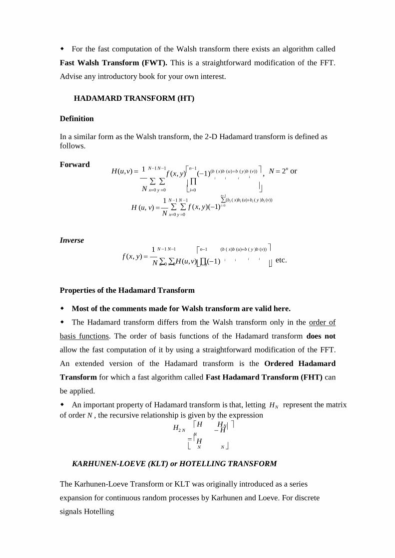
HADAMARD TRANSFORM (HT)
Definition
In a similar form as the Walsh transform, the 2-D Hadamard transform is defined as
follows.
Forward H (u, v)
1 N 1 N 1
f (x, y)n1
(1)(b ( x)b (u)b ( y )b (v)) ,
N 2
n or
i i i
N x0 y 0 i0 n1
1 N 1 N 1 (bi ( x)bi (u)bi ( y )bi (v))
H (u, v) f ( x, y)(1) i0
N x0 y 0
Inverse
f (x, y)
1 N 1 N 1
n1
(b ( x)b (u)b ( y )b (v))
H (u, v)(1) i i
i i etc. N u0 v0 i0
Properties of the Hadamard Transform
Most of the comments made for Walsh transform are valid here.
The Hadamard transform differs from the Walsh transform only in the order of
basis functions. The order of basis functions of the Hadamard transform does not
allow the fast computation of it by using a straightforward modification of the FFT.
An extended version of the Hadamard transform is the Ordered Hadamard
Transform for which a fast algorithm called Fast Hadamard Transform (FHT) can
be applied.
An important property of Hadamard transform is that, letting HN
of order N , the recursive relationship is given by the expression
represent the matrix
H2 N H
N H
HN H
N N
KARHUNEN-LOEVE (KLT) or HOTELLING TRANSFORM
The Karhunen-Loeve Transform or KLT was originally introduced as a series
expansion for continuous random processes by Karhunen and Loeve. For discrete
signals Hotelling
i
x
If C is a matrix of dimension n n , then a scalar is called an eigenvalue of C if there
is a nonzero vector e in Rn such that
Ce e
The vector e is called an eigenvector of the matrix C corresponding to the eigenvalue
.
first studied what was called a method of principal components, which is the discrete
equivalent of the KL series expansion. Consequently, the KL transform is also called
the Hotelling transform or the method of principal components. The term KLT is the
most widely used.
The case of many realisations of a signal or image (Gonzalez/Woods)
The concepts of eigenvalue and eigevector are necessary to understand the KL
transform.
(If you have difficulties with the above concepts consult any elementary linear
algebra book.)
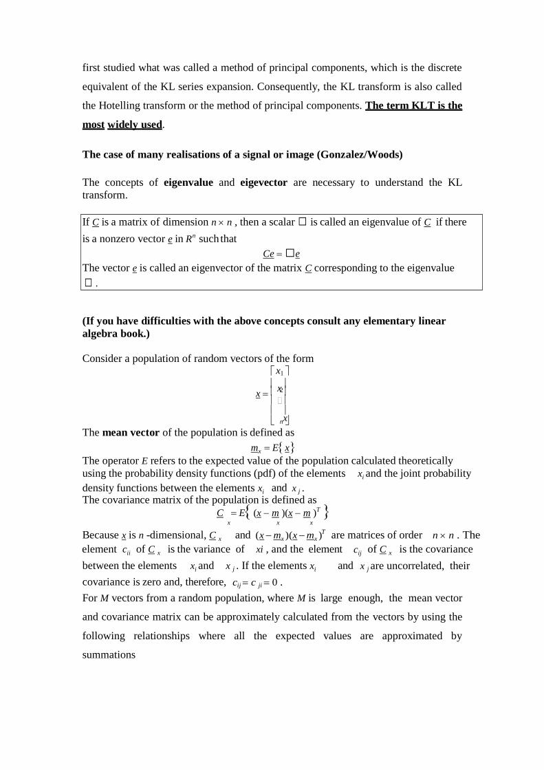
Consider a population of random vectors of the form
x1
x x
2 n
The mean vector of the population is defined as
mx ExThe operator E refers to the expected value of the population calculated theoretically
using the probability density functions (pdf) of the elements xi and the joint probability
density functions between the elements xi and x j . The covariance matrix of the population is defined as
C E(x m )(x m )T x x x
Because x is n -dimensional, C x and (x mx )(x mx )T are matrices of order n n . The
element cii of C x is the variance of xi , and the element cij of C x is the covariance
between the elements xi and x j . If the elements xi and x j are uncorrelated, their
covariance is zero and, therefore, cij c ji 0 .
For M vectors from a random population, where M is large enough, the mean vector
and covariance matrix can be approximately calculated from the vectors by using the
following relationships where all the expected values are approximated by
summations
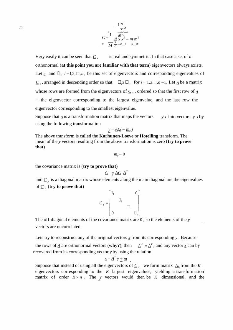
M
y x
0
m 1 M
x
x k k 1
C 1 M x xT m mT
x M k k x x k 1
Very easily it can be seen that C x is real and symmetric. In that case a set of n
orthonormal (at this point you are familiar with that term) eigenvectors always exists.
Let ei and i , i 1,2,,n , be this set of eigenvectors and corresponding eigenvalues of
C x , arranged in descending order so that i i1 for i 1,2,,n 1. Let A be a matrix
whose rows are formed from the eigenvectors of C x , ordered so that the first row of A
is the eigenvector corresponding to the largest eigenvalue, and the last row the
eigenvector corresponding to the smallest eigenvalue.
Suppose that A is a transformation matrix that maps the vectors
using the following transformation
x' s into vectors y' s by
y A(x mx )
The above transform is called the Karhunen-Loeve or Hotelling transform. The
mean of the y vectors resulting from the above transformation is zero (try to prove
that)
my 0
the covariance matrix is (try to prove that)
C AC AT
and C y is a diagonal matrix whose elements along the main diagonal are the eigenvalues
of C x (try to prove that) 1 0
C 2
y n
The off-diagonal elements of the covariance matrix are 0 , so the elements of the y
vectors are uncorrelated.
Lets try to reconstruct any of the original vectors x from its corresponding y . Because
the rows of A are orthonormal vectors (why?), then
A1 AT , and any vector x can by
recovered from its corresponding vector y by using the relation
x AT y m
Suppose that instead of using all the eigenvectors of C x we form matrix AK from the K
eigenvectors corresponding to the K largest eigenvalues, yielding a transformation
matrix of order K n . The y vectors would then be K dimensional, and the
x
K
M
reconstruction of any of the original vectors would be approximated by the following
relationship
xˆ AT y m
The mean square error between the perfect reconstruction x and the approximate
reconstruction xˆ is given by the expression n K n
ems j j j . j 1 j 1 j K 1
By using
data.
AK instead of A for the KL transform we achieve compression of the available
The case of one realisation of a signal or image
The derivation of the KLT for the case of one image realisation assumes that the two
dimensional signal (image) is ergodic. This assumption allows us to calculate the
statistics of the image using only one realisation. Usually we divide the image into
blocks and we apply the KLT in each block. This is reasonable because the 2-D field
is likely to be ergodic within a small block since the nature of the signal changes
within the whole image. Let’s suppose that f is a vector obtained by lexicographic
ordering of the pixels
f (x, y) within a block of size M M (placing the rows of the block sequentially).
The mean vector of the random field inside the block is a scalar that is estimated by
the approximate relationship 1 M 2
mf 2 f (k)
k 1
and the covariance matrix of the 2-D random field inside the block is C f where
1 M 2
cii f (k) f (k) m2
and M 2 k 1
f
cij ci j M 2
f (k) f (k i j) m2
M 2 k 1
After knowing how to calculate the matrix
realisation is the same as described above.
f
C f , the KLT for the case of a single
6.3 Properties of the Karhunen-Loeve transform
Despite its favourable theoretical properties, the KLT is not used in practice for the
following reasons.
x
1

Its basis functions depend on the covariance matrix of the image, and
hence they have to recomputed and transmitted for every image.
Perfect decorrelation is not possible, since images can rarely be modelled
as realisations of ergodic fields.
There are no fast computational algorithms for its implementation.
Recommended Questions
1. Construct Haar transform matrix for N = 2.
2. Explain the importance of discrete cosine transform, with its properties.
3. Define DCT and its inverse transformation .
4. Discuss any three properties of discrete cosine transform.
5. Develop Hadamard transform for n = 3.
6. Discuss the properties of the Hadamard transform .
7. Derive the relation between DCT and DFT.
8. Write H matrix for the Haar transform for N = 8 and explain how it is
constructed.

UNIT – 5
IMAGE ENHANCEMENT
5.1 Image Enhancement in Spatial domain
Suppose we have a digital image which can be represented by a two dimensional
random field f (x, y) .
An image processing operator in the spatial domain may be expressed as a mathematical
function T applied to the image f (x, y)
follows.
to produce a new image g(x, y) T f (x, y) as
g(x, y) T f (x, y)
The operator T applied on f (x, y) may be defined over:
(i) A single pixel (x, y) . In this case T is a grey level transformation (or mapping)
function.
(ii) Some neighbourhood of (x, y) .
(iii) T may operate to a set of input images instead of a single image.
Example 1
The result of the transformation shown in the figure below is to produce an image of
higher contrast than the original, by darkening the levels below m and brightening the
levels above m in the original image. This technique is known as contrast
stretching.
s T (r)
m r
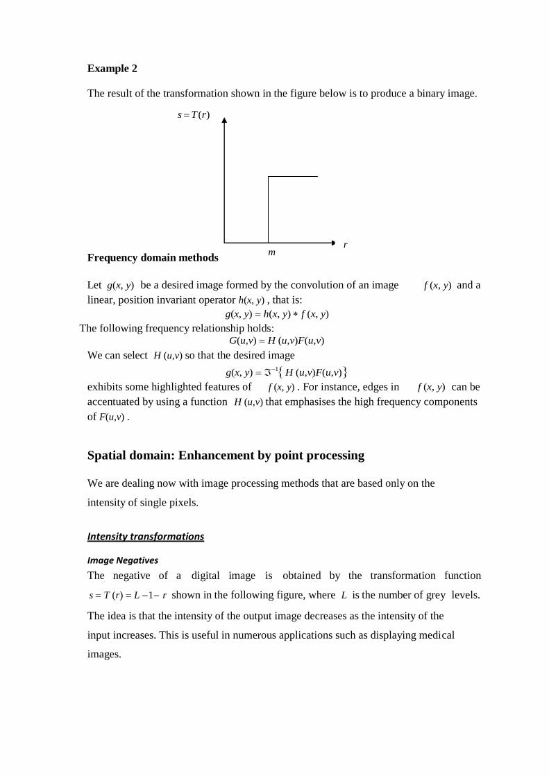
Example 2
The result of the transformation shown in the figure below is to produce a binary image.
s T (r)
Frequency domain methods
Let g(x, y) be a desired image formed by the convolution of an image f (x, y) and a
linear, position invariant operator h(x, y) , that is:
g(x, y) h(x, y) f (x, y)
The following frequency relationship holds: G(u,v) H (u,v)F(u,v)
We can select H (u,v) so that the desired image
g(x, y) 1H (u,v)F(u,v)
exhibits some highlighted features of f (x, y) . For instance, edges in f (x, y) can be
accentuated by using a function
of F(u,v) .
H (u,v) that emphasises the high frequency components
Spatial domain: Enhancement by point processing
We are dealing now with image processing methods that are based only on the
intensity of single pixels.
Intensity transformations
Image Negatives
The negative of a digital image is obtained by the transformation function
s T (r) L 1 r shown in the following figure, where L is the number of grey levels.
The idea is that the intensity of the output image decreases as the intensity of the
input increases. This is useful in numerous applications such as displaying medical
images.
m r

n
s T (r)
L 1
Contrast Stretching
contrast images occur often due to poor or non uniform lighting conditions, or due to
nonlinearity, or small dynamic range of the imaging sensor. In the figure of Example
1 above you have seen a typical contrast stretching transformation.
Histogram processing. Definition of the histogram of an image.
By processing (modifying) the histogram of an image we can create a new image
with specific desired properties.
Suppose we have a digital image of size N N with grey levels in the range [0, L 1] .
The histogram of the image is defined as the following discrete function:
p(rk ) k
N 2
Where
rk is the kth grey level, k 0,1,, L 1
nk is the number of pixels in the image with grey level rk
N 2 is the total number of pixels in the image
The histogram represents the frequency of occurrence of the various grey levels in
the image. A plot of this function for all values of k provides a global description of
the appearance of the image.
Question: Think how the histogram of a dark image, a bright image and an
image of very low contrast would like. Plot its form in each case.
Global histogram equalisation
L 1 r
In this section we will assume that the image to be processed has a continuous
intensity that lies within the interval [0, L 1] . Suppose we divide the image
intensity with its
maximum value L 1. Let the variable r represent the new grey levels (image intensity)
in the image, where now 0 r 1 and let pr (r) denote the probability density function
(pdf) of the variable r . We now apply the following transformation function to the
intensity
r
s T (r) pr (w)dw , 0
0 r 1
(1) By observing the transformation of equation (1) we immediately see that it possesses the following properties:
(i) 0 s 1 .
(ii) r2 r1 T (r2 ) T (r1 ) , i.e., the function T (r) is increase ng with r .
(iii) 0
s T (0) pr (w)dw 0 0
and 1
s T (1) pr (w)dw 1 . Moreover, if the original 0
image has intensities only within a certain range [rmin , rmax ] then
s T (rmin )
rmin
pr (w)dw 0 0
and s T (rmax )
rmax
pr (w)dw 1 0
since
pr (r) 0, r rmin and r rmax . Therefore, the new intensity s takes always all values
within the available range [0 1].
Suppose that Pr (r) , Ps (s) are the probability distribution functions (PDF’s) of the
variables r and s respectively.
Let us assume that the original intensity lies within the values r and r dr with dr a
small quantity. dr can be assumed small enough so as to be able to consider the
function
pr (w) constant within the interval [r, r dr] and equal to pr (r) . Therefore,
Pr [r, r dr] r dr
pr (w)dw pr (r) r
r dr
dw pr (r)dr . r
Now suppose that s T (r) and s1 T (r dr) . The quantity dr can be assumed small
enough so as to be able to consider that s1 s ds with ds small enough so as to be able
to consider the function
Therefore,
ps (w) constant within the interval [s, s ds] and equal to ps (s) .
Ps [s, s ds] s ds
ps (w)dw ps (s) s
s ds
dw ps (s)ds s
Since s T (r) , s ds T (r dr) and the function of equation (1) is increasing with r ,
all and only the values within the interval [r, r dr] will be mapped within the interval
[s, s ds] . Therefore,
Pr [r, r dr] Ps[s, s ds] pr (r)dr r T 1 (s)
ps (s)ds ps (s) pr (r) dr
ds r T 1 (s)
N
From equation (1) we see that ds
p (r)
and hence, dr r
p (s)
p (r)
1
1, 0 s 1 s r
p (r)
r r T 1 (s)
From the above analysis it is obvious that the transformation of equation (1) converts
the original image into a new image with uniform probability density function. This
means that in the new image all intensities are present [look at property (iii) above]
and with equal probabilities. The whole range of intensities from the absolute black
to the absolute white are explored and the new image will definitely have higher
contrast compared to the original image.
Unfortunately, in a real life scenario we must deal with digital images. The discrete
form of histogram equalisation is given by the relation
k s T (r ) n j
k p (r ), 0 r 1, k 0,1,, L 1
k k 2 j 0
r j k j 0
(2) The quantities in equation (2) have been defined in Section 2.2. To see results of
histogram equalisation look at any introductory book on Image Processing.
The improvement over the original image is quite evident after using the technique of
histogram equalisation. The new histogram is not flat because of the discrete
approximation of the probability density function with the histogram function. Note,
however, that the grey levels of an image that has been subjected to histogram
equalisation are spread out and always reach white. This process increases the
dynamic range of grey levels and produces an increase in image contrast.
Local histogram equalisation
Global histogram equalisation is suitable for overall enhancement. It is often
necessary to enhance details over small areas. The number of pixels in these areas
my have negligible influence on the computation of a global transformation, so the
use of this type of transformation does not necessarily guarantee the desired local
enhancement.
The solution is to devise transformation functions based on the grey level distribution
– or other properties – in the neighbourhood of every pixel in the image. The
histogram processing technique previously described is easily adaptable to local
enhancement. The procedure is to define a square or rectangular neighbourhood and
move the centre of this area from pixel to pixel. At each location the histogram of the
points in the neighbourhood is computed and a histogram equalisation transformation
function is obtained. This function is finally used to map the grey level of the pixel
centred in the neighbourhood.
The centre of the neighbourhood region is then moved to an adjacent pixel location
and the procedure is repeated. Since only one new row or column of the
neighbourhood changes during a pixel-to-pixel translation of the region, updating the
histogram obtained in the previous location with the new data introduced at each
motion step is possible quite easily. This approach has obvious advantages over
repeatedly computing the histogram over all pixels in the neighbourhood region each
time the region is moved one pixel location. Another approach often used to reduce
computation is to utilise non overlapping regions, but this methods usually produces
an undesirable checkerboard effect.
Histogram specification
Suppose we want to specify a particular histogram shape (not necessarily uniform)
which is capable of highlighting certain grey levels in the image.
Let us suppose that:
pr (r) is the original probability density function
pz (z) is the desired probability density function
Suppose that histogram equalisation is first applied on the original image r
r
s T (r) pr (w)dw 0
Suppose that the desired image z is available and histogram equalisation is applied as well
ps (s)
and
pv (v)
z
v G(z) pz (w)dw 0
are both uniform densities and they can be considered as identical.
Note that the final result of histogram equalisation is independent of the density inside
the integral. So in equation
z
v G(z) pz (w)dw we can use the symbol s instead of v . 0
The inverse process z G1(s) will have the desired probability density function.
Therefore, the process of histogram specification can be summarised in the
following steps.
(i) We take the original image and equalise its intensity using the relation r
s T (r) pr (w)dw. 0
(ii) From the given probability density function
distribution function G(z) .
pz (z) we specify the probability
(iii) We apply the inverse transformation function z G1(s) G1T (r)
Spatial domain: Enhancement in the case of many realisations of an image of interest
available
Image averaging
Suppose that we have an image f (x, y) of size M N pixels corrupted by noise n(x, y) ,
so we obtain a noisy image as follows.
g(x, y) f (x, y) n(x, y)
For the noise process n(x, y) the following assumptions are made.
(i) The noise process n(x, y) is ergodic.
(ii) It is zero mean, i.e., En(x, y) 1
MN
M 1 N 1
n(x, y) 0 x 0 y 0
(ii) It is white, i.e., the autocorrelation function of the noise process defined as
R[k,l] E{n(x, y)n(x k, y l)} 1
(M k)(N l) M 1k N 1l
n(x, y)n(x k, y l) is zero, apart
for the pair [k,l] [0,0].
x 0 y 0
n ( x, y)
n( x, y)
1
Therefore, Rk,l1 M 1k N 1l
n(x, y)n(x k, y l) 2
(k,l) where 2
(M k)(N l)
n( x, y) n( x, y )
is the variance of noise.
x 0 y 0
Suppose now that we have L different noisy realisations of the same image f (x, y) as
gi (x, y) f (x, y) ni (x, y) , i 0,1,, L . Each noise process ni (x, y) satisfies the
properties (i)-(iii) given above. Moreover, 2 i
2 . We form the image g(x, y) by
averaging these L noisy images as follows: g (x, y)
1
L
g (x, y) 1
L
( f (x, y) n (x, y)) f (x, y) 1
L n (x, y) i i 1
i i 1
i i 1
Therefore, the new image is again a noisy realisation of the original image f (x, y) with noise n(x, y)
1
L n (x, y) . i i 1
The mean value of the noise n(x, y) is found below. E{n(x, y)} E{
1
L
n (x, y)} 1
L E{n (x, y)} 0 i i 1
i i 1
The variance of the noise n(x, y) is now found below. 1 L
2 1 L
2
2 E{n
2 (x, y)} E n (x, y) E n (x, y) n( x, y)
L i 1 L2 i 1
i
L
2
1 L L
1 L 2
1 L L
L2 E{( ni (x, y))}
L2 E{( ( ni (x, y)nj (x, y))}
L2 E{ni (x, y)} L2 E{ni (x, y)nj (x, y)}
i 1
1 L
2 0
1 2
i 1 j 1 i j
i 1 i 1 j 1 i j
i 1 L
Therefore, we have shown that image averaging produces an image g(x, y) , corrupted
by noise with variance less than the variance of the noise of the original noisy images.
Note that if
L we have 2 0 , the resulting noise is negligible.
L L L
L
L L
L
i
2

Recommended Questions
1. What is the importance of image enhancement in image processing? Explain in
brief any two point processing techniques implemented in image processing.
2. Explain histogram equalization technique.
3. What is histogram matching? Explain the development and implementation of
the method.
4. Highlight the importance of histograms in image processing and develop a
procedure to perform histogram equalization.
5. Explain the following image enhancement techniques, highlighting their area
of application.
i) Intensity level slicing
ii) Power – law transformation
6. Explain the following image enhancement techniques, highlighting their area
of application.
i) Bit – plane slicing.
ii) AND and OR operation
UNIT - 6
Basics of Spatial Filtering Image enhancement in the Frequency
Domain
Many image enhancement techniques are based on spatial operations performed on
local neighbourhoods of input pixels. The image is usually convolved with a finite
impulse response filter called spatial mask. The use of spatial masks on a digital
image is called
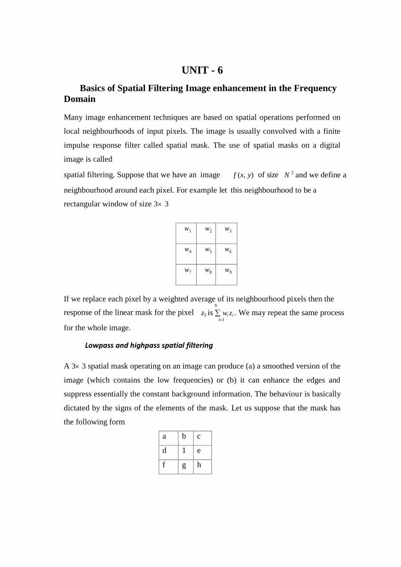
spatial filtering. Suppose that we have an image f (x, y) of size N 2 and we define a
neighbourhood around each pixel. For example let this neighbourhood to be a
rectangular window of size 3 3
w1 w2 w3
w4 w5 w6
w7 w8 w9
If we replace each pixel by a weighted average of its neighbourhood pixels then the 9
response of the linear mask for the pixel
for the whole image.
z5 is wi zi . We may repeat the same process i1
Lowpass and highpass spatial filtering
A 3 3 spatial mask operating on an image can produce (a) a smoothed version of the
image (which contains the low frequencies) or (b) it can enhance the edges and
suppress essentially the constant background information. The behaviour is basically
dictated by the signs of the elements of the mask. Let us suppose that the mask has
the following form
a b c
d 1 e
f g h

To be able to estimate the effects of the above mask with relation to the sign of the
coefficients a,b,c,d,e, f , g,h , we will consider the equivalent one dimensional mask
d 1 e
Let us suppose that the above mask is applied to a signal x(n) . The output of this
operation will be a signal
y(n) dx(n 1) x(n) ex(n 1) Y (z) dz1
X (z) X (z) ezX (z)
Y (z) (dz1
1 ez) X (z) Y (z)
H (z) dz1 1 ez .
X (z)
y(n) as
This is the transfer function of a system that produces the above input-output
relationship. In the frequency domain we have H (e j ) d exp( j) 1 eexp( j) .
The values of this transfer function at frequencies 0 and
H (e j ) d 1 e
0
H (e j ) d 1 e
are:
If a lowpass filtering (smoothing) effect is required then the following condition
must hold
H (e j ) H (e j ) d e 0 0
If a highpass filtering effect is required then
H (e j ) H (e j ) d e 0
0
The most popular masks for lowpass filtering are masks with all their coefficients
positive and for highpass filtering, masks where the central pixel is positive and the
surrounding pixels are negative or the other way round.
Popular techniques for lowpass spatial filtering
Uniform filtering
273
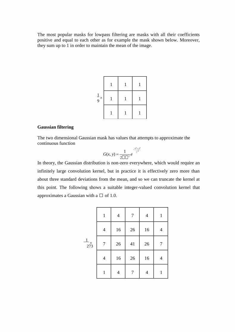
The most popular masks for lowpass filtering are masks with all their coefficients
positive and equal to each other as for example the mask shown below. Moreover,
they sum up to 1 in order to maintain the mean of the image.
1
9
Gaussian filtering
The two dimensional Gaussian mask has values that attempts to approximate the
continuous function
G(x, y) 1
2 2
x2 y2
2
e
In theory, the Gaussian distribution is non-zero everywhere, which would require an
infinitely large convolution kernel, but in practice it is effectively zero more than
about three standard deviations from the mean, and so we can truncate the kernel at
this point. The following shows a suitable integer-valued convolution kernel that
approximates a Gaussian with a of 1.0.
1
1
1
1
1
1
1
1
1
1
1
4
7
4
1
4
16
26
16
4
7
26
41
26
7
4
16
26
16
4
1
4
7
4
1
0 0
0
0 0 0
1 0
0
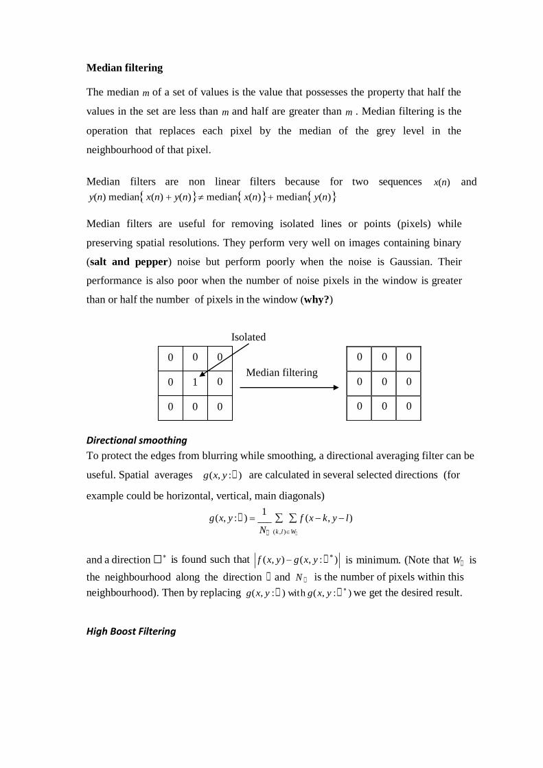
Median filtering
The median m of a set of values is the value that possesses the property that half the
values in the set are less than m and half are greater than m . Median filtering is the
operation that replaces each pixel by the median of the grey level in the
neighbourhood of that pixel.
Median filters are non linear filters because for two sequences
y(n) medianx(n) y(n) medianx(n) mediany(n)x(n) and
Median filters are useful for removing isolated lines or points (pixels) while
preserving spatial resolutions. They perform very well on images containing binary
(salt and pepper) noise but perform poorly when the noise is Gaussian. Their
performance is also poor when the number of noise pixels in the window is greater
than or half the number of pixels in the window (why?)
Isolated
Median filtering
Directional smoothing
To protect the edges from blurring while smoothing, a directional averaging filter can be
useful. Spatial averages g(x, y : ) are calculated in several selected directions (for
example could be horizontal, vertical, main diagonals)
g(x, y : ) 1
f (x k, y l)
and a direction
N (k ,l ) W
is found such that f (x, y) g(x, y : )
is minimum. (Note that W is
the neighbourhood along the direction and N is the number of pixels within this
neighbourhood). Then by replacing g(x, y : ) with g( x, y : ) we get the desired result.
High Boost Filtering
0 0 0
0 0 0
0 0 0
A high pass filtered image may be computed as the difference between the original
image and a lowpass filtered version of that image as follows:
(Highpass part of image) = (Original) - (Lowpass part of image)
Multiplying the original image by an amplification factor denoted by A , yields the so
called high boost filter:
(Highboost image) = ( A) (Original)-(Lowpass) = ( A 1) (Original)+(Original)-(Lowpass)
= ( A 1) (Original) + (Highpass)
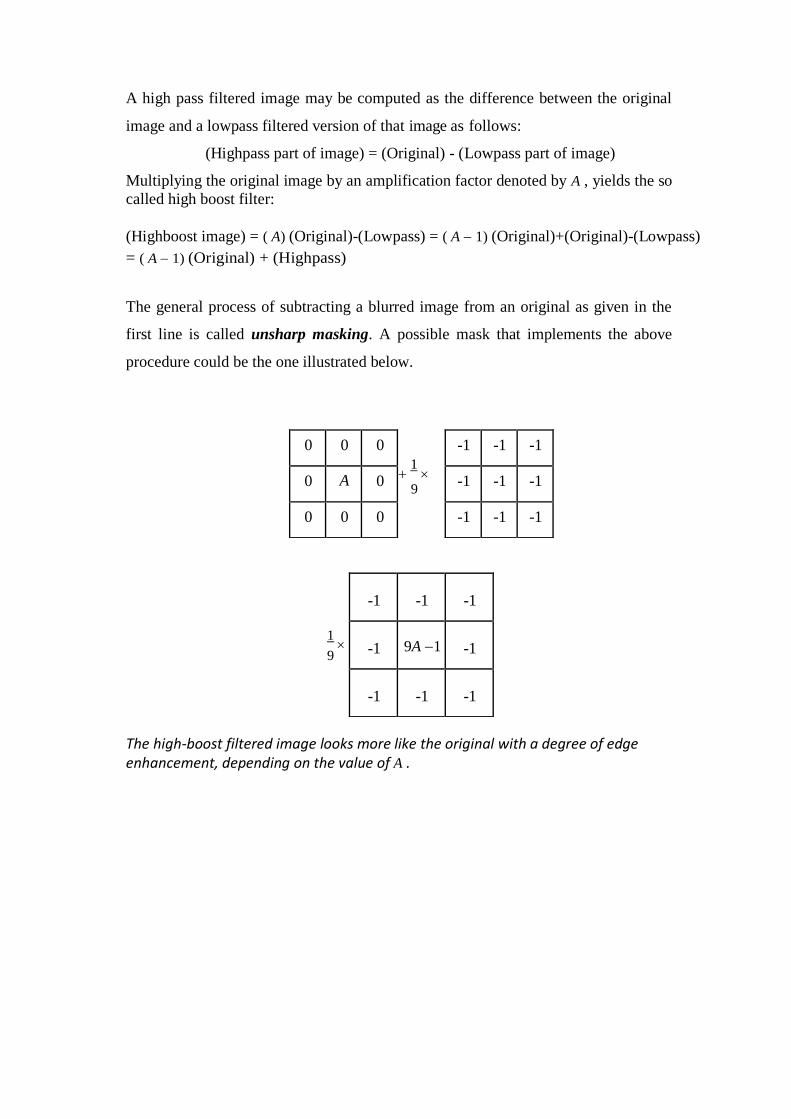
The general process of subtracting a blurred image from an original as given in the
first line is called unsharp masking. A possible mask that implements the above
procedure could be the one illustrated below.
1
9
1
9
The high-boost filtered image looks more like the original with a degree of edge enhancement, depending on the value of A .
0 0 0
0 A 0
0 0 0
-1 -1 -1
-1 -1 -1
-1 -1 -1
-1
-1
-1
-1 9A 1
-1
-1
-1
-1
f (x, y)
x
x
Popular techniques for highpass spatial filtering. Edge detection using derivative filters
About two dimensional high pass spatial filters
An edge is the boundary between two regions with relatively distinct grey level
properties. The idea underlying most edge detection techniques is the computation of
a local derivative operator. The magnitude of the first derivative calculated within a
neighbourhood around the pixel of interest, can be used to detect the presence of an
edge in an image.
The gradient of an image f (x, y) at location (x, y) is a vector that consists of the partial
derivatives of f (x, y) as follows. f (x, y)
f (x, y) x
f (x, y)
y
The magnitude of this vector, generally referred to simply as the gradient f is 1/ 2 f (x.y)
2 f (x, y)
2 f (x, y) mag( f (x, y))
x y
Common practice is to approximate the gradient with absolute values which is
simpler to implement as follows.
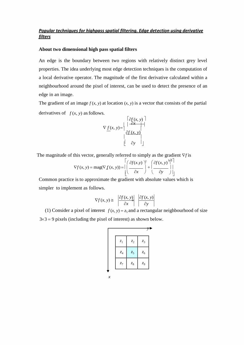
f (x, y)
(1) Consider a pixel of interest f (x, y) z5 and a rectangular neighbourhood of size
33 9 pixels (including the pixel of interest) as shown below.
y
z1 z2 z3
z4 z5 z6
z7 z8 z9
f (x, y)
y
1 0
-1 0
1 -1
0 0
1 0
0 -1
0 1
-1 0
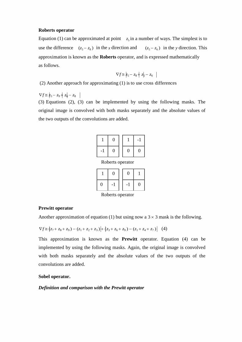
Roberts operator
Equation (1) can be approximated at point
z5 in a number of ways. The simplest is to
use the difference (z5 z8 ) in the x direction and (z5 z6 ) in the y direction. This
approximation is known as the Roberts operator, and is expressed mathematically
as follows.
f z5 z8 z5 z6
(2) Another approach for approximating (1) is to use cross differences
f z5 z9 z6 z8
(3) Equations (2), (3) can be implemented by using the following masks. The
original image is convolved with both masks separately and the absolute values of
the two outputs of the convolutions are added.
Roberts operator
Roberts operator
Prewitt operator
Another approximation of equation (1) but using now a 3 3 mask is the following.
f (z7 z8 z9 ) (z1 z2 z3 ) (z3 z6 z9 ) (z1 z4 z7 ) (4)
This approximation is known as the Prewitt operator. Equation (4) can be
implemented by using the following masks. Again, the original image is convolved
with both masks separately and the absolute values of the two outputs of the
convolutions are added.
Sobel operator.
Definition and comparison with the Prewitt operator
of th
-1 0 1
-1 0 1
-1 0 1
-1 -1 -1
0 0 0
1 1 1
1
1
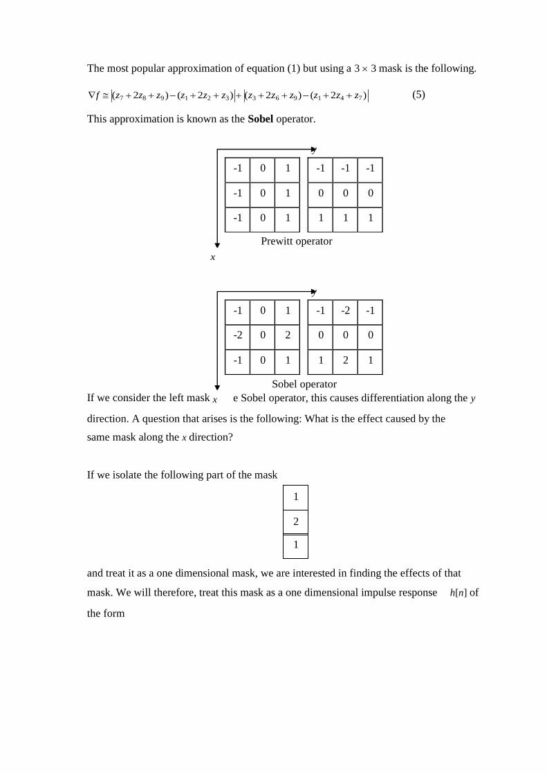
The most popular approximation of equation (1) but using a 3 3 mask is the following.
f (z7 2z8 z9 ) (z1 2z2 z3 ) (z3 2z6 z9 ) (z1 2z4 z7 )
This approximation is known as the Sobel operator.
(5)
y
Prewitt operator
x
y
If we consider the left mask x
Sobel operator
e Sobel operator, this causes differentiation along the y
direction. A question that arises is the following: What is the effect caused by the
same mask along the x direction?
If we isolate the following part of the mask
and treat it as a one dimensional mask, we are interested in finding the effects of that
mask. We will therefore, treat this mask as a one dimensional impulse response
the form
h[n] of
-1 -2 -1
0 0 0
1 2 1
-1 0 1
-2 0 2
-1 0 1
2
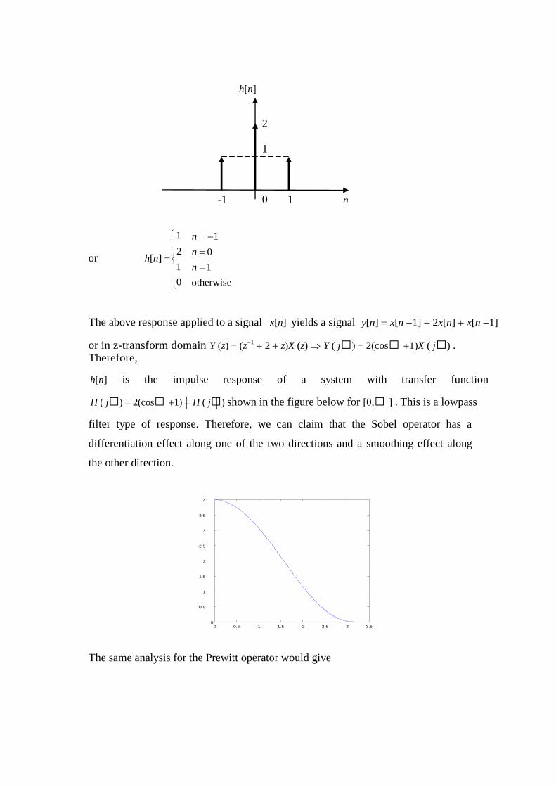
h[n]
2
1
-1 0 1 n
h[n]
1 2
or
1
0
n 1
n 0
n 1
otherwise
The above response applied to a signal x[n] yields a signal y[n] x[n 1] 2x[n] x[n 1]
or in z-transform domain Y (z) (z1
2 z)X (z) Y ( j) 2(cos 1)X ( j) . Therefore,
h[n] is the impulse response of a system with transfer function
H ( j) 2(cos 1) H ( j) shown in the figure below for [0, ] . This is a lowpass
filter type of response. Therefore, we can claim that the Sobel operator has a
differentiation effect along one of the two directions and a smoothing effect along
the other direction.
4
3.5
3
2.5
2
1.5
1
0.5
0 0 0.5 1 1.5 2 2.5 3 3.5
The same analysis for the Prewitt operator would give
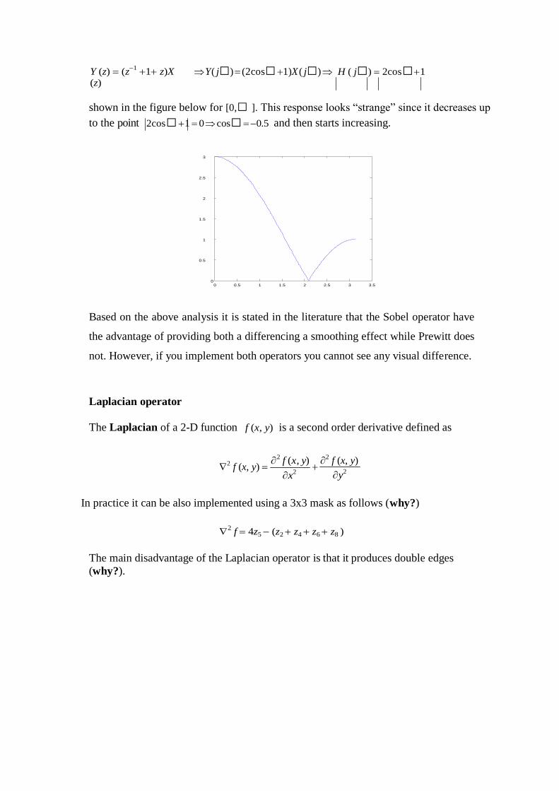
Y (z) (z1
1 z)X (z)
Y ( j) (2cos 1)X ( j) H ( j) 2cos 1
shown in the figure below for [0, ]. This response looks “strange” since it decreases up
to the point 2cos 1 0 cos 0.5 and then starts increasing.
3
2.5
2
1.5
1
0.5
0 0 0.5 1 1.5 2 2.5 3 3.5
Based on the above analysis it is stated in the literature that the Sobel operator have
the advantage of providing both a differencing a smoothing effect while Prewitt does
not. However, if you implement both operators you cannot see any visual difference.
Laplacian operator
The Laplacian of a 2-D function f (x, y) is a second order derivative defined as
2 f (x, y)
2 f (x, y)
x2
2 f (x, y)
y2
In practice it can be also implemented using a 3x3 mask as follows (why?)
2 f 4z5 (z2 z4 z6 z8 )
The main disadvantage of the Laplacian operator is that it produces double edges
(why?).

Recommended Questions
1. Explain the smoothing of images in frequency domain using:
i) Ideal low pass filter
ii) Butterworth lowpass filter
2. With a block diagram and equations, explain the homomorphic filtering. How
dynamic range compression and contrast enhancement is simultaneously achieved?
3. Discuss homomorphic filtering.
4. Explain sharpening filters in the frequency domain
5. Explain the basic concept of spatial filtering in image enhancement and hence
explain the importance of smoothing filters and median filters.

Unit-7
IMAGE RESTORATION
What is image restoration?
Image Restoration refers to a class of methods that aim to remove or reduce the
degradations that have occurred while the digital image was being obtained. All
natural images when displayed have gone through some sort of degradation:
during display mode
during acquisition mode, or
during processing
mode The degradations may
be due to
sensor noise
blur due to camera misfocus
relative object-camera motion
random atmospheric turbulence
others
In most of the existing image restoration methods we assume that the degradation
process can be described using a mathematical model.
How well can we do?
Depends on how much we know about
the original image
the degradations
(how accurate our models are)
Image restoration and image enhancement differences
Image restoration differs from image enhancement in that the latter is
concerned more with accentuation or extraction of image features rather than
restoration of degradations.
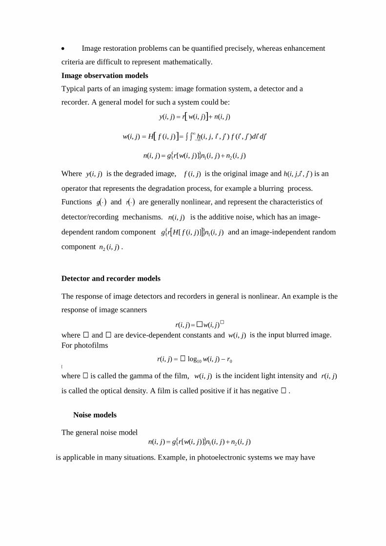
Image restoration problems can be quantified precisely, whereas enhancement
criteria are difficult to represent mathematically.
Image observation models
Typical parts of an imaging system: image formation system, a detector and a
recorder. A general model for such a system could be:
y(i, j) rw(i, j) n(i, j)
w(i, j) H f (i, j)
h(i, j, i, j) f (i, j)didj
n(i, j) gr[w(i, j)]n1(i, j) n2 (i, j)
Where y(i, j) is the degraded image, f (i, j) is the original image and h(i, j,i, j) is an
operator that represents the degradation process, for example a blurring process.
Functions g and r are generally nonlinear, and represent the characteristics of
detector/recording mechanisms. n(i, j) is the additive noise, which has an image-
dependent random component grH[ f (i, j)]n1(i, j) and an image-independent random
component n2 (i, j) .
Detector and recorder models
The response of image detectors and recorders in general is nonlinear. An example is the
response of image scanners
r(i, j) w(i, j)
where and are device-dependent constants and
For photofilms
w(i, j)
is the input blurred image.
r(i, j) log10 w(i, j) r0
[
where is called the gamma of the film, w(i, j) is the incident light intensity and r(i, j)
is called the optical density. A film is called positive if it has negative .
Noise models
The general noise model
n(i, j) gr[w(i, j)]n1(i, j) n2 (i, j)
is applicable in many situations. Example, in photoelectronic systems we may have
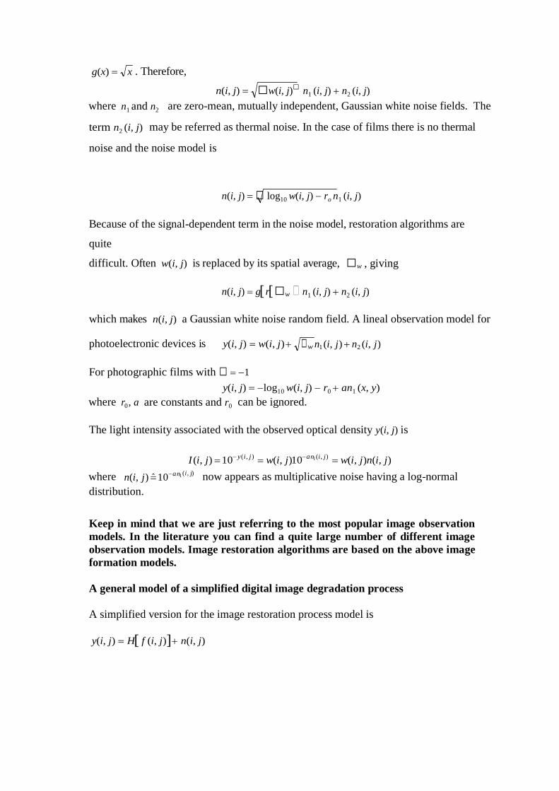
g(x) . Therefore,
n(i, j)
w(i, j) n1 (i, j) n2 (i, j)
where n1 and n2 are zero-mean, mutually independent, Gaussian white noise fields. The
term n2 (i, j) may be referred as thermal noise. In the case of films there is no thermal
noise and the noise model is
n(i, j) log10 w(i, j) ro n1 (i, j)
Because of the signal-dependent term in the noise model, restoration algorithms are
quite
difficult. Often w(i, j) is replaced by its spatial average, w , giving
n(i, j) grw n1 (i, j) n2 (i, j)
which makes n(i, j) a Gaussian white noise random field. A lineal observation model for
photoelectronic devices is y(i, j) w(i, j) w n1 (i, j) n2 (i, j)
For photographic films with 1
y(i, j) log10 w(i, j) r0 an1 (x, y)
where r0 , a are constants and r0 can be ignored.
The light intensity associated with the observed optical density y(i, j) is
I (i, j) 10 y(i ,
j ) w(i, j)10
an1 (i, j) w(i, j)n(i, j)
where n(i, j) ̂ 10an1 (i, j)
now appears as multiplicative noise having a log-normal
distribution.
Keep in mind that we are just referring to the most popular image observation
models. In the literature you can find a quite large number of different image
observation models. Image restoration algorithms are based on the above image
formation models.
A general model of a simplified digital image degradation process
A simplified version for the image restoration process model is
y(i, j) H f (i, j) n(i, j)
x

Where y(i, j) the degraded image
f (i, j) the original image
H an operator that represents the degradation process
independent
n(i, j) the external noise which is assumed to be image-
Possible classification of restoration methods
Restoration methods could be classified as follows:
deterministic: we work with sample by sample processing of the observed
(degraded) image
stochastic : we work with the statistics of the images involved in the process
non-blind : the degradation process H is known
blind : the degradation process H is unknown
semi-blind : the degradation process H could be considered partly
known From the viewpoint of implementation:
direct
iterative
recursive
Linear position invariant degradation models
Definition
We again consider the general degradation model
y(i, j) H f (i, j) n(i, j)
If we ignore the presence of the external noise n(i, j) we get
H is linear if
y(i, j) H f (i, j)
Hk1 f1(i, j) k2 f2 (i, j) k1H f1(i, j) k2 H f2 (i, j)
H is position (or space) invariant if
H f (i a, j b) y(i a, j b)
From now on we will deal with linear, space invariant type of degradations.
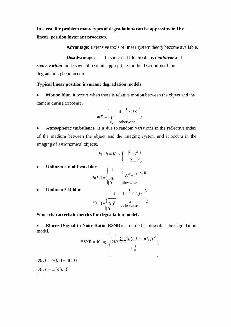
In a real life problem many types of degradations can be approximated by
linear, position invariant processes.
Advantage: Extensive tools of linear system theory become available.
Disadvantage: In some real life problems nonlinear and
space variant models would be more appropriate for the description of the
degradation phenomenon.
Typical linear position invariant degradation models
Motion blur. It occurs when there is relative motion between the object and the
camera during exposure.
1 ,
if L i
L
h(i) L
0, 2 2
otherwise
Atmospheric turbulence. It is due to random variations in the reflective index
of the medium between the object and the imaging system and it occurs in the
imaging of astronomical objects.
h(i, j) K expi2 j2
Uniform out of focus blur
1 , if
2 2
R
Uniform 2-D blur
h(i, j) R
0, otherwise
1 ,
if L i, j
L
h(i, j) (L)2
0,
2 2 otherwise
Some characteristic metrics for degradation models
Blurred Signal-to-Noise Ratio (BSNR): a metric that describes the degradation
model.
BSNR 10log
1 g(i, j) g (i, j)2
MN i j
g(i, j) y(i, j) n(i, j)
g(i, j) E{g(i, j)} [
10 2 n
i2 j2
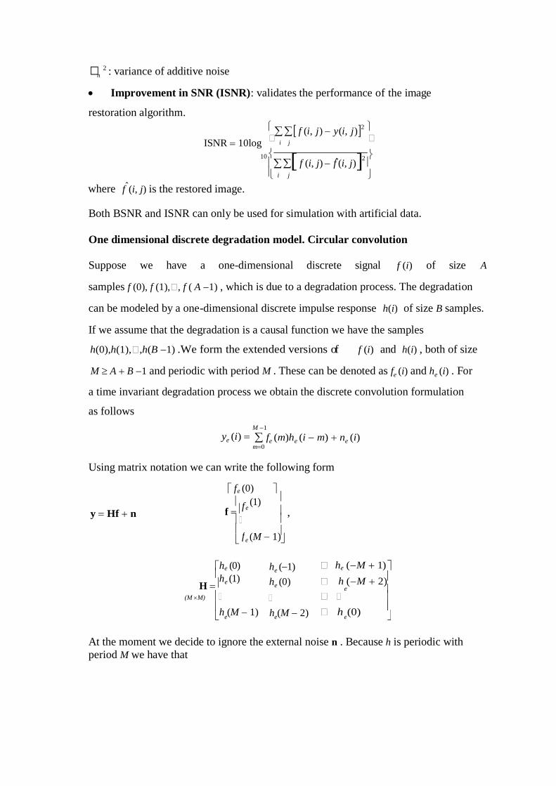
n
e
e e e
2 : variance of additive noise
Improvement in SNR (ISNR): validates the performance of the image
restoration algorithm.
f (i, j) y(i, j)2
ISNR 10log
i j
10 ˆ
2
where
fˆ(i, j) is the restored image.
f (i, j) f (i, j) i j
Both BSNR and ISNR can only be used for simulation with artificial data.
One dimensional discrete degradation model. Circular convolution
Suppose we have a one-dimensional discrete signal f (i) of size A
samples f (0), f (1),, f ( A 1) , which is due to a degradation process. The degradation
can be modeled by a one-dimensional discrete impulse response h(i) of size B samples.
If we assume that the degradation is a causal function we have the samples
h(0),h(1),,h(B 1) .We form the extended versions of f (i) and h(i) , both of size
M A B 1 and periodic with period M . These can be denoted as fe (i) and he (i) . For
a time invariant degradation process we obtain the discrete convolution formulation
as follows
ye (i) M 1
fe (m)he (i m) ne (i) m0
Using matrix notation we can write the following form
fe (0)
y Hf n
f f
e
(1) ,
he (0) h (1)
H e
(M 1)
he (1)
he (0)
he (M 1)
h (M 2)
(M M) h (M 1)
h (M 2)
h (0)
At the moment we decide to ignore the external noise n . Because h is periodic with
period M we have that
f e

e
he (0) h (1)
H e
he (M 1)
he (0)
he (1)
h (2)
(M M) h (M 1) h (M 2) h (0)
e e e
We define (k ) to be
(k) h (0) h (M 1) exp( j 2
k) h (M 2) exp( j 2
2k) e e
M e
M
h (1) exp[ j 2
(M 1)k ], k 0,1,, M 1 e
M
Because exp[ j 2
(M i)k] exp( j 2
ik) we have that M M
(k) MH (k)
H (k) is the discrete Fourier transform of he (i) .
I define w(k) to be 1 exp( j
2 k )
It can be seen that
w(k ) M 2 exp[ j M
(M 1)k ]
Hw(k) (k)w(k)
This implies that (k ) is an eigenvalue of the matrix H and
eigenvector.
w(k)
is its corresponding
We form a matrix w whose columns are the eigenvectors of the matrix H , that is to say
W w(0) w(1) w(M 1)
w(k, i) 2 d w1
(k, i) 1
2
exp j M ki an
M exp j
M ki
We can then diagonalize the matrix H as follows
H WDW-1
D W-1
HW
where
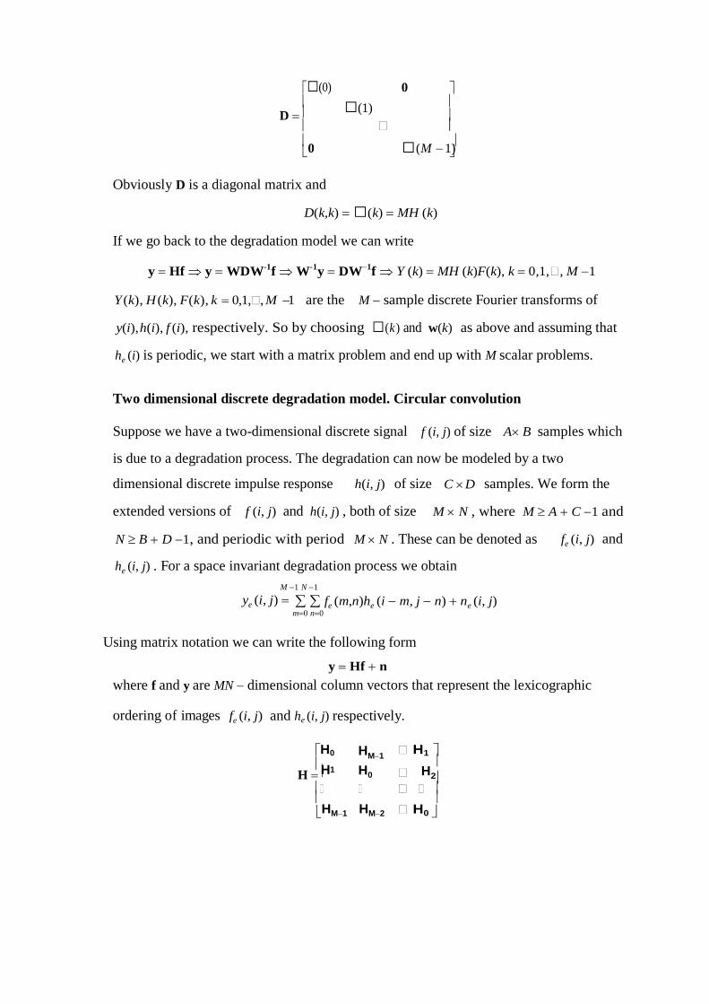
0
H
(0)
D
0
(1)
(M 1)
Obviously D is a diagonal matrix and
D(k,k) (k) MH (k)
If we go back to the degradation model we can write
y Hf y WDW-1
f W-1
y DW1
f Y (k) MH (k)F(k), k 0,1,, M 1
Y (k), H (k), F(k), k 0,1,, M 1 are the M sample discrete Fourier transforms of
y(i), h(i), f (i), respectively. So by choosing (k ) and w(k) as above and assuming that
he (i) is periodic, we start with a matrix problem and end up with M scalar problems.
Two dimensional discrete degradation model. Circular convolution
Suppose we have a two-dimensional discrete signal f (i, j) of size A B samples which
is due to a degradation process. The degradation can now be modeled by a two
dimensional discrete impulse response h(i, j) of size C D samples. We form the
extended versions of f (i, j) and h(i, j) , both of size M N , where M A C 1 and
N B D 1, and periodic with period M N . These can be denoted as fe (i, j) and
he (i, j) . For a space invariant degradation process we obtain
M 1 N 1
ye (i, j) fe (m,n)he (i m, j n) ne (i, j) m0 n0
Using matrix notation we can write the following form
y Hf n
where f and y are MN dimensional column vectors that represent the lexicographic
ordering of images fe (i, j) and he (i, j) respectively.
H0 H
H 1
HM1
H0
H1
2
HM1 HM2 H0
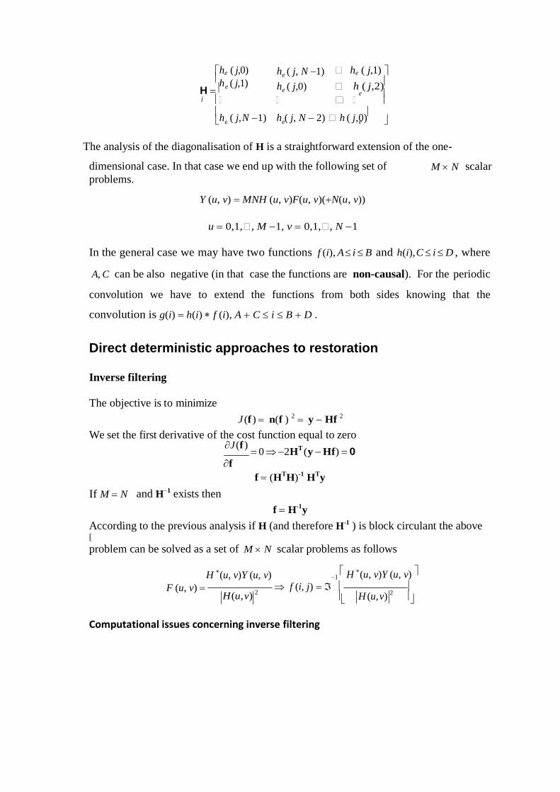
e
e e e
he ( j,0) h ( j,1)
H e
he ( j, N 1)
he ( j,0)
he ( j,1)
h ( j,2)
h ( j, N 1) h ( j, N 2) h ( j,0)
The analysis of the diagonalisation of H is a straightforward extension of the one-
dimensional case. In that case we end up with the following set of
problems. M N scalar
Y (u, v) MNH (u, v)F(u, v)(N(u, v))
u 0,1,, M 1, v 0,1,, N 1
In the general case we may have two functions f (i), A i B and h(i), C i D , where
A, C can be also negative (in that case the functions are non-causal). For the periodic
convolution we have to extend the functions from both sides knowing that the
convolution is g(i) h(i) f (i), A C i B D .
Direct deterministic approaches to restoration
Inverse filtering
The objective is to minimize J (f )
n(f )
2
y Hf
2
We set the first derivative of the cost function equal to zero J (f )
0 2HT (y Hf) 0
f
If M N
and H1
exists then
f (HTH)
-1 H
Ty
f H
-1y
According to the previous analysis if H (and therefore H-1 ) is block circulant the above
[
problem can be solved as a set of M N scalar problems as follows
H (u, v)Y (u, v)
1 H (u, v)Y (u, v)
F (u, v) H (u, v)
2
f (i, j)
H (u, v)
2
Computational issues concerning inverse filtering
j
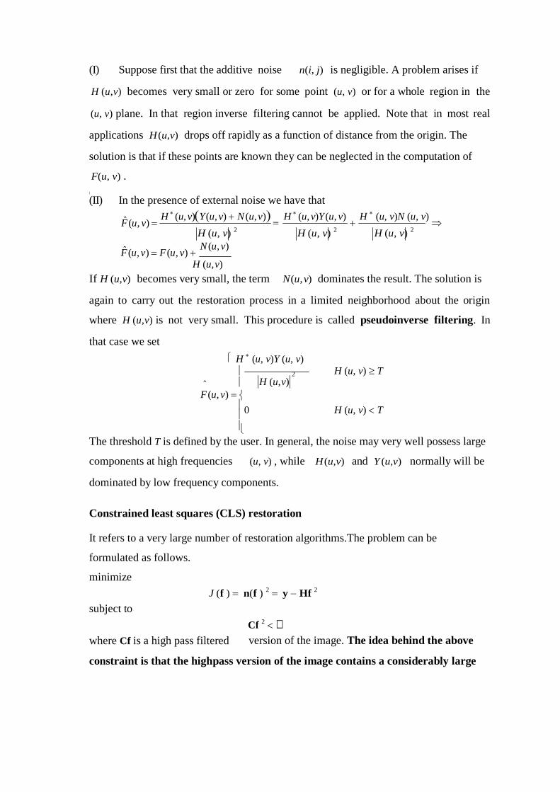
(I) Suppose first that the additive noise n(i, j) is negligible. A problem arises if
H (u,v) becomes very small or zero for some point (u, v) or for a whole region in the
(u, v) plane. In that region inverse filtering cannot be applied. Note that in most real
applications H (u,v) drops off rapidly as a function of distance from the origin. The
solution is that if these points are known they can be neglected in the computation of
F(u, v) .
[
(II) In the presence of external noise we have that
F̂(u, v) H (u, v)Y (u, v) N (u, v)
H (u, v) 2
H (u, v)Y (u, v)
H (u, v) 2
H (u, v)N (u, v)
H (u, v) 2
F̂(u, v) F (u, v) N (u, v)
H (u, v)
If H (u,v) becomes very small, the term N (u, v) dominates the result. The solution is
again to carry out the restoration process in a limited neighborhood about the origin
where H (u,v) is not very small. This procedure is called pseudoinverse filtering. In
that case we set
H (u, v)Y (u, v)
2 H (u, v) ˆ
H (u, v) T
F (u, v)
H (u, v) T
The threshold T is defined by the user. In general, the noise may very well possess large
components at high frequencies (u, v) , while H (u,v) and Y (u,v) normally will be
dominated by low frequency components.
Constrained least squares (CLS) restoration
It refers to a very large number of restoration algorithms.The problem can be
formulated as follows.
minimize
subject to
J (f ) n(f ) 2 y Hf
2
where Cf is a high pass filtered
Cf 2
version of the image. The idea behind the above
constraint is that the highpass version of the image contains a considerably large
0
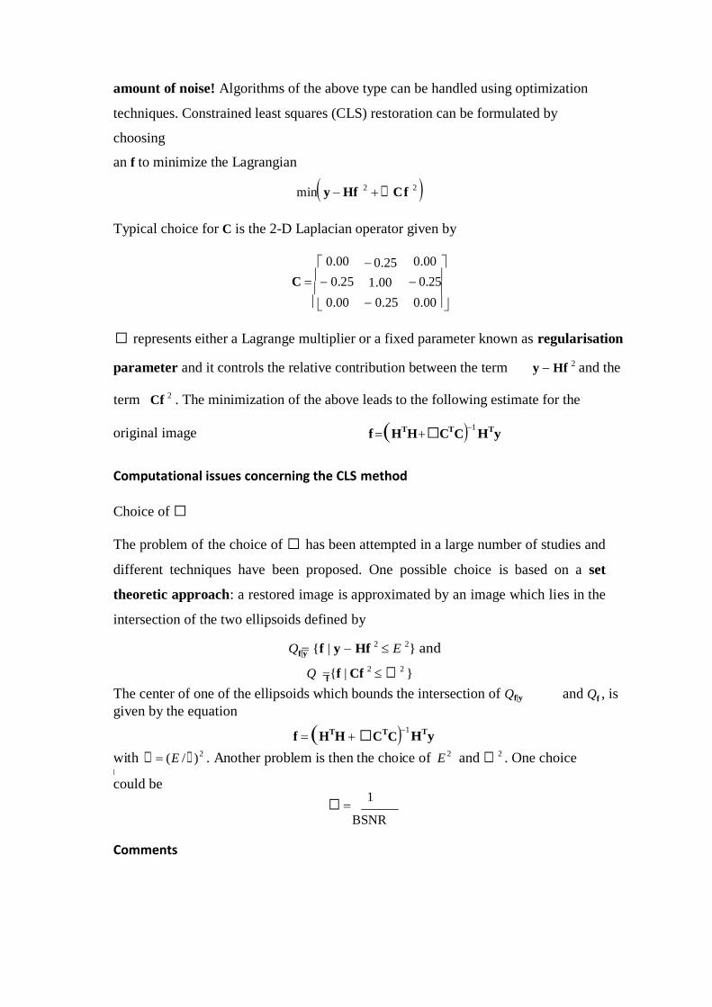
f|y
f
amount of noise! Algorithms of the above type can be handled using optimization
techniques. Constrained least squares (CLS) restoration can be formulated by
choosing
an f to minimize the Lagrangian
min y Hf 2 Cf
2
Typical choice for C is the 2-D Laplacian operator given by
0.00
C 0.25
0.00
0.25
1.00
0.25
0.00
0.25
0.00
represents either a Lagrange multiplier or a fixed parameter known as regularisation
parameter and it controls the relative contribution between the term y Hf 2 and the
term Cf 2 . The minimization of the above leads to the following estimate for the
original image f HTH C
T C1
H
Ty
Computational issues concerning the CLS method
Choice of
The problem of the choice of has been attempted in a large number of studies and
different techniques have been proposed. One possible choice is based on a set
theoretic approach: a restored image is approximated by an image which lies in the
intersection of the two ellipsoids defined by
Q {f | y Hf 2 E 2
} and
Q {f | Cf 2 2
}
The center of one of the ellipsoids which bounds the intersection of Qf|y
given by the equation
and Qf , is
f HTH C
T C1
HTy
with (E / )2 . Another problem is then the choice of E 2
[
could be
and 2 . One choice
1
BSNR
Comments
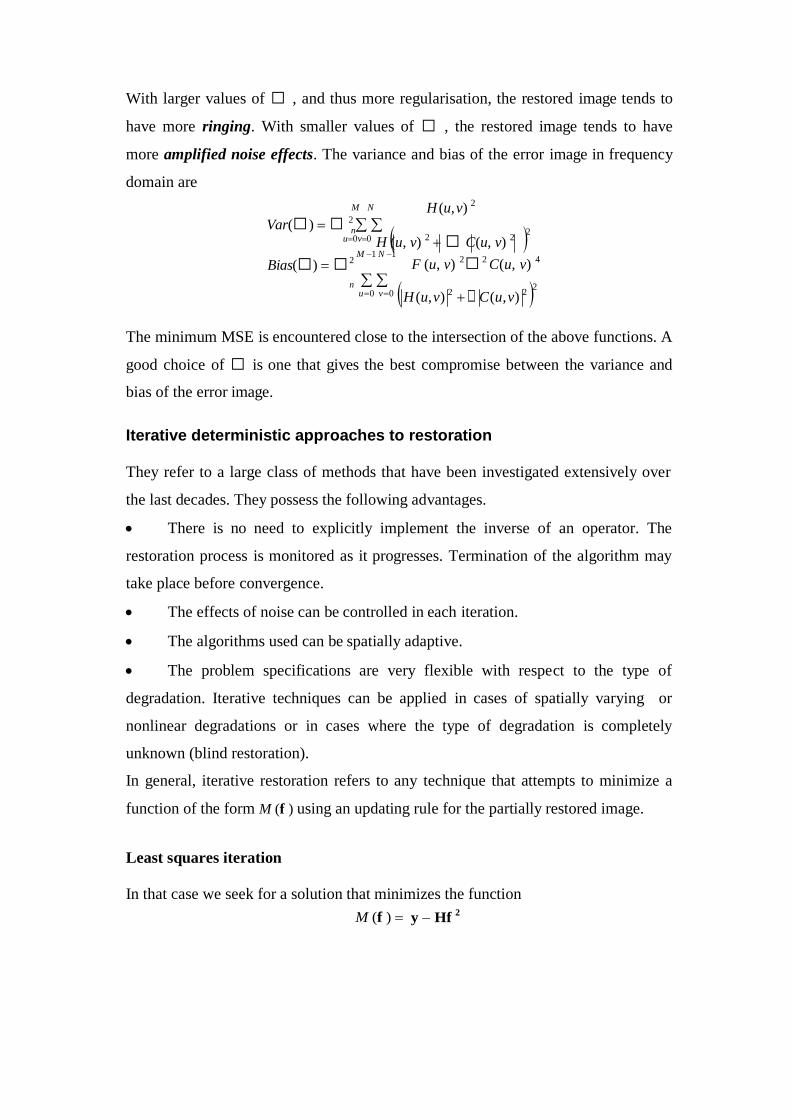
n
2
With larger values of , and thus more regularisation, the restored image tends to
have more ringing. With smaller values of , the restored image tends to have
more amplified noise effects. The variance and bias of the error image in frequency
domain are
M N H (u, v) 2
Var( ) 2
u0v0 H (u, v) 2 C(u, v)
2
Bias( ) 2 M 1 N 1
F (u, v) 2 2 C(u, v)
4
n u0 v0 H (u, v)
2 C(u, v)
2 2
The minimum MSE is encountered close to the intersection of the above functions. A
good choice of is one that gives the best compromise between the variance and
bias of the error image.
Iterative deterministic approaches to restoration
They refer to a large class of methods that have been investigated extensively over
the last decades. They possess the following advantages.
There is no need to explicitly implement the inverse of an operator. The
restoration process is monitored as it progresses. Termination of the algorithm may
take place before convergence.
The effects of noise can be controlled in each iteration.
The algorithms used can be spatially adaptive.
The problem specifications are very flexible with respect to the type of
degradation. Iterative techniques can be applied in cases of spatially varying or
nonlinear degradations or in cases where the type of degradation is completely
unknown (blind restoration).
In general, iterative restoration refers to any technique that attempts to minimize a
function of the form M (f ) using an updating rule for the partially restored image.
Least squares iteration
In that case we seek for a solution that minimizes the function
M (f ) y Hf 2
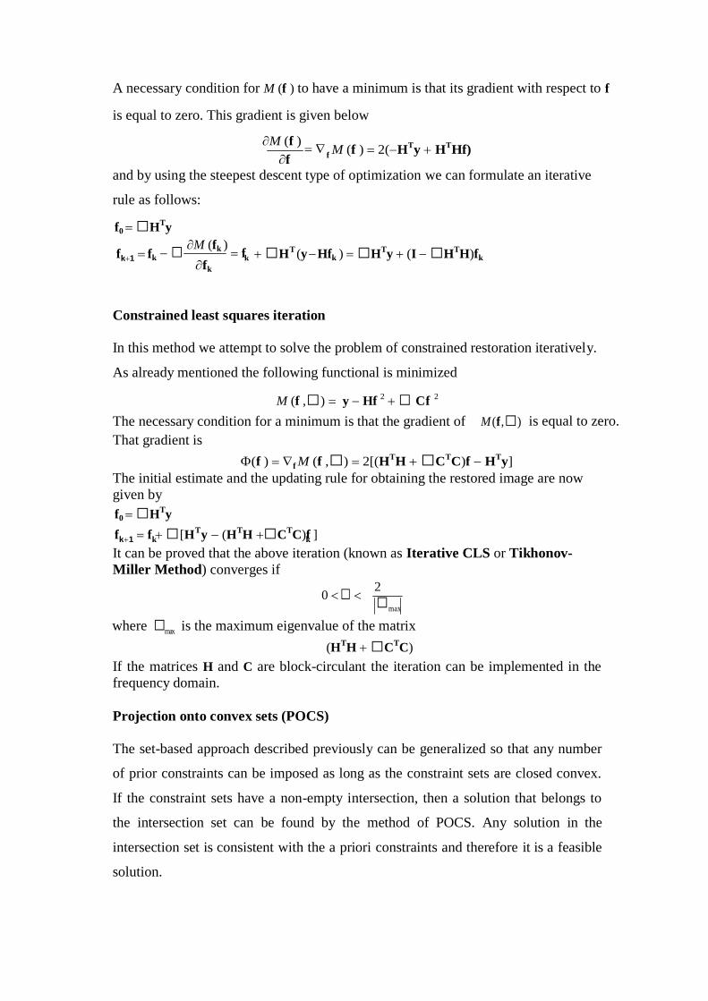
max
k1 k k
A necessary condition for M (f ) to have a minimum is that its gradient with respect to f
is equal to zero. This gradient is given below
M (f )
f f
M (f ) 2(H
Ty H
THf)
and by using the steepest descent type of optimization we can formulate an iterative
rule as follows:
f0 HTy
fk1 fk M (fk )
f
fk
HT (y Hfk ) H
Ty (I H
TH)fk
Constrained least squares iteration
In this method we attempt to solve the problem of constrained restoration iteratively.
As already mentioned the following functional is minimized
M (f ,) y Hf 2 Cf
2
The necessary condition for a minimum is that the gradient of
That gradient is
M (f ,) is equal to zero.
(f ) f M (f ,) 2[(HTH C
TC)f H
Ty]
The initial estimate and the updating rule for obtaining the restored image are now
given by
f0 HTy
f f [HTy (H
TH C
TC)f ]
It can be proved that the above iteration (known as Iterative CLS or Tikhonov-
Miller Method) converges if
0 2
where max is the maximum eigenvalue of the matrix
(HTH C
TC)
If the matrices H and C are block-circulant the iteration can be implemented in the
frequency domain.
Projection onto convex sets (POCS)
The set-based approach described previously can be generalized so that any number
of prior constraints can be imposed as long as the constraint sets are closed convex.
If the constraint sets have a non-empty intersection, then a solution that belongs to
the intersection set can be found by the method of POCS. Any solution in the
intersection set is consistent with the a priori constraints and therefore it is a feasible
solution.
k
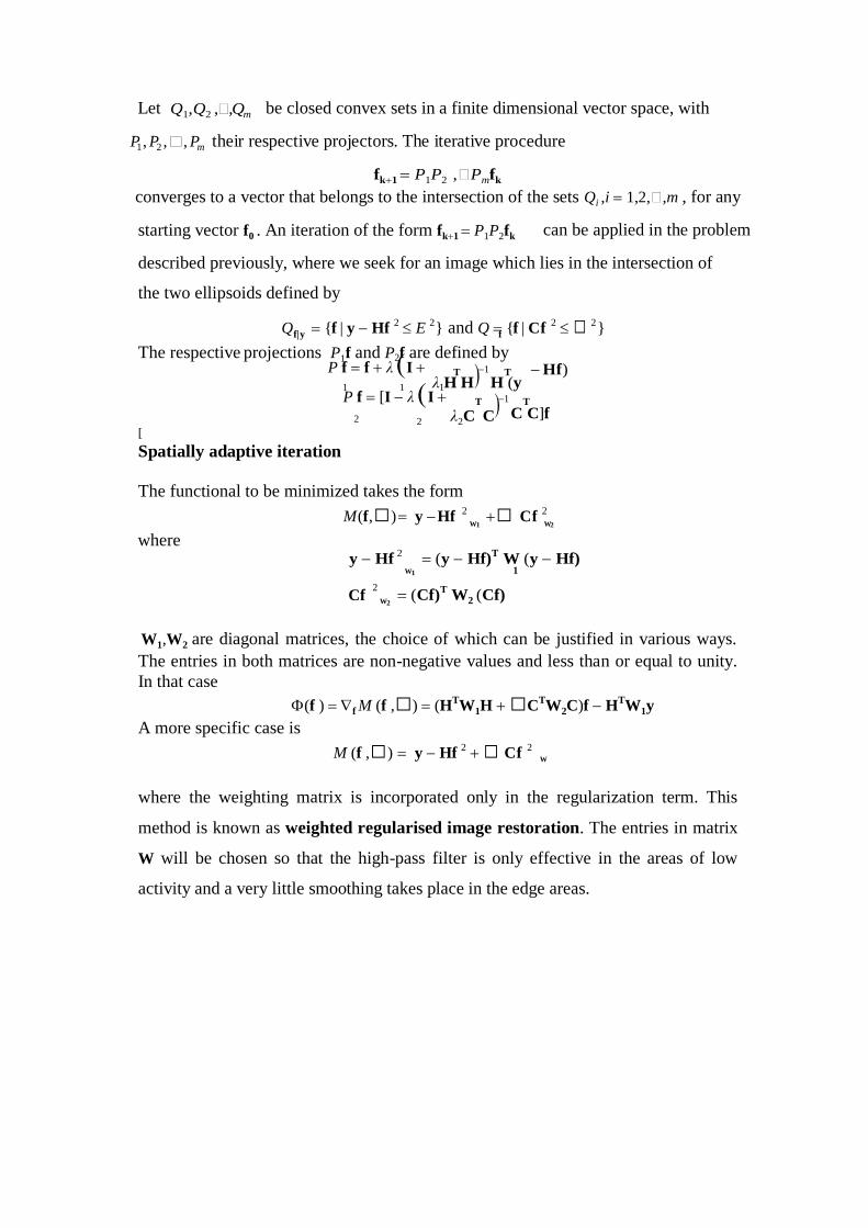
f|y f
W1 W2
Let Q1,Q2 ,,Qm be closed convex sets in a finite dimensional vector space, with
P1, P2 ,, Pm their respective projectors. The iterative procedure
fk1 P1P2 ,Pmfk
converges to a vector that belongs to the intersection of the sets Qi ,i 1,2,,m , for any
starting vector f0 . An iteration of the form fk1 P1P2fk can be applied in the problem
described previously, where we seek for an image which lies in the intersection of
the two ellipsoids defined by
Q {f | y Hf 2 E 2} and Q {f | Cf
2 2
}
The respective projections P1f and P2f are defined by P f f λ I T 1 T Hf)
1 1 λ1H H H (y P f [I λ I T 1 T
2
[
Spatially adaptive iteration
2 λ2C C C C]f
The functional to be minimized takes the form
where
M (f ,)
y Hf
2
y Hf 2 Cf
2
(y Hf)
T W (y Hf)
2
W2
W1 1
(Cf)T W2 (Cf)
W1,W2 are diagonal matrices, the choice of which can be justified in various ways.
The entries in both matrices are non-negative values and less than or equal to unity.
In that case
(f ) f M (f ,) (HTW1H C
TW2C)f H
TW1y
A more specific case is
M (f ,) y Hf 2 Cf
2
where the weighting matrix is incorporated only in the regularization term. This
method is known as weighted regularised image restoration. The entries in matrix
W will be chosen so that the high-pass filter is only effective in the areas of low
activity and a very little smoothing takes place in the edge areas.
W
Cf
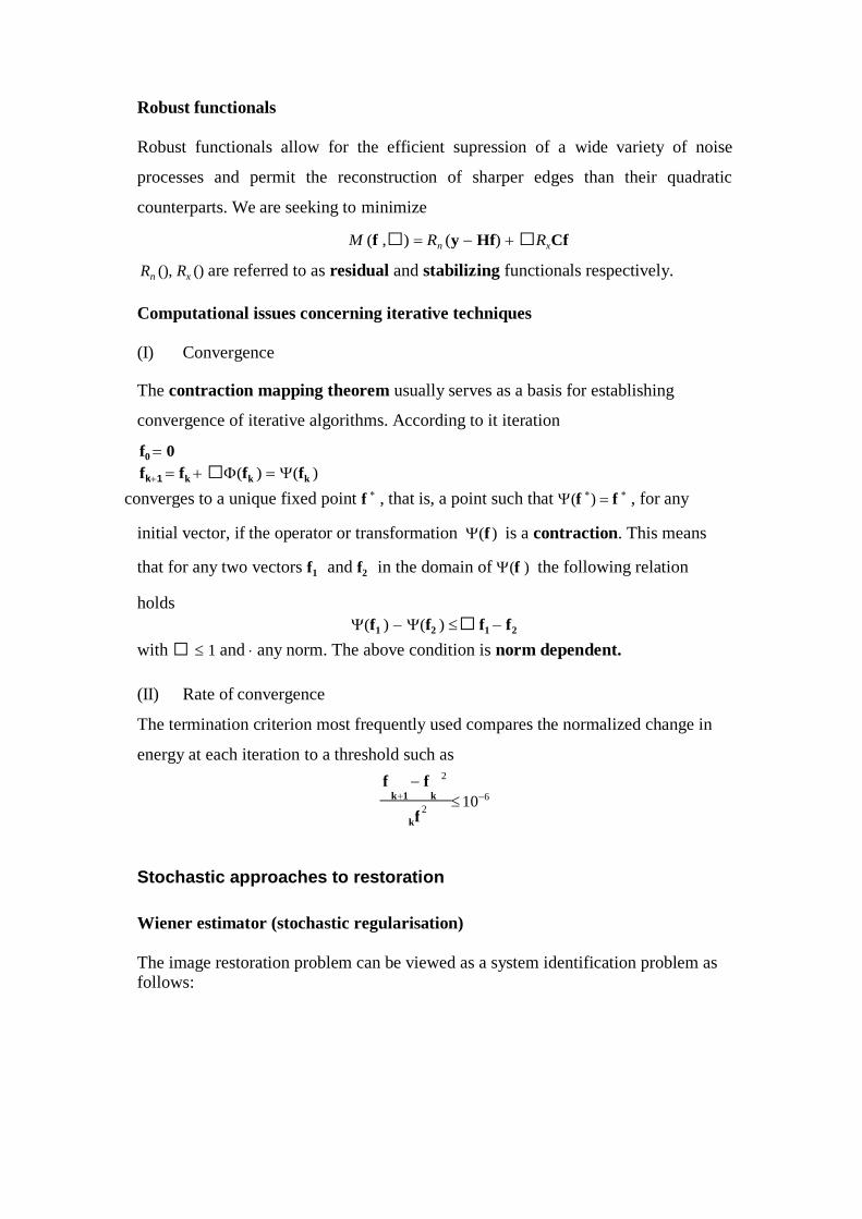
Robust functionals
Robust functionals allow for the efficient supression of a wide variety of noise
processes and permit the reconstruction of sharper edges than their quadratic
counterparts. We are seeking to minimize
M (f ,) Rn (y Hf) RxCf
Rn (), Rx () are referred to as residual and stabilizing functionals respectively.
Computational issues concerning iterative techniques
(I) Convergence
The contraction mapping theorem usually serves as a basis for establishing
convergence of iterative algorithms. According to it iteration
f0 0
fk1 fk (fk ) (fk )
converges to a unique fixed point f , that is, a point such that (f ) f
, for any
initial vector, if the operator or transformation (f ) is a contraction. This means
that for any two vectors f1
holds
and f2 in the domain of (f ) the following relation
(f1 ) (f2 ) f1 f2
with 1 and any norm. The above condition is norm dependent.
(II) Rate of convergence
The termination criterion most frequently used compares the normalized change in
energy at each iteration to a threshold such as
f f 2
k 1 k 106
2
k
Stochastic approaches to restoration
Wiener estimator (stochastic regularisation)
The image restoration problem can be viewed as a system identification problem as follows:
f
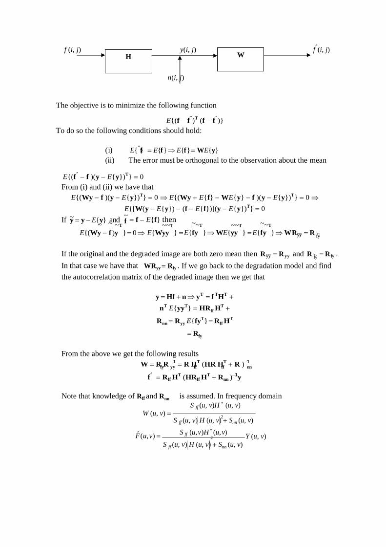
n(i, j)
H W
f
fy
fy
fy yy ff ff nn
2
f (i, j) y(i, j) fˆ(i, j)
The objective is to minimize the following function
E{(f fˆ)T (f fˆ)}
To do so the following conditions should hold:
(i) E{ˆ}f E{f} E{f} WE{y}
(ii) The error must be orthogonal to the observation about the mean
E{(fˆ f )(y E{y})T} 0
From (i) and (ii) we have that
E{(Wy f )(y E{y})T} 0 E{(Wy E{f} WE{y} f )(y E{y})
T} 0
E{[W(y E{y}) (f E{f})](y E{y})T} 0
If ~y y E{y} and ~ f E{f} then
~ ~ ~T ~~T ~~T ~~T ~~T
E{(Wy f )y } 0 E{Wyy } E{fy } WE{yy } E{fy } WR~y~y R~~
If the original and the degraded image are both zero mean then R~y~y R yy and R~~ R fy .
In that case we have that WRyy Rfy . If we go back to the degradation model and find
the autocorrelation matrix of the degraded image then we get that
y Hf n yT f
TH
T
nT E{yy
T} HRff H
T
Rnn Ryy E{fyT} Rff H
T
Rfy
From the above we get the following results
W R R 1 R H
T (HR H
T R )
1
fˆ Rff HT (HRff H
T Rnn )
1y
Note that knowledge of Rff and Rnn is assumed. In frequency domain
S ff (u, v)H (u, v) W (u, v)
S ff (u, v) H (u, v) Snn (u, v)
F̂(u, v) S ff (u, v)H (u, v)
2
Y (u, v)
S ff (u, v) H (u, v) Snn (u, v)
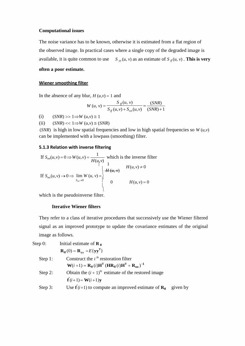
Image Processing 10EC763
Computational issues
The noise variance has to be known, otherwise it is estimated from a flat region of
the observed image. In practical cases where a single copy of the degraded image is
available, it is quite common to use
often a poor estimate.
Wiener smoothing filter
S yy (u, v) as an estimate of S ff (u, v) . This is very
In the absence of any blur, H (u,v) 1 and
(i)
W (u, v)
(SNR) 1W (u,v) 1
S ff (u, v)
S ff (u, v) Snn (u, v)
(SNR)
(SNR) 1
(ii)
(SNR)
(SNR) 1W (u,v) (SNR)
is high in low spatial frequencies and low in high spatial frequencies so W (u,v)
can be implemented with a lowpass (smoothing) filter.
5.1.3 Relation with inverse filtering
If Snn (u, v) 0 W (u, v) 1
H (u, v) which is the inverse filter
1 H (u, v) 0
If Snn (u, v) 0
H (u, v)
lim W (u, v)
Snn0 0 H (u, v) 0
which is the pseudoinverse filter.
Iterative Wiener filters
They refer to a class of iterative procedures that successively use the Wiener filtered
signal as an improved prototype to update the covariance estimates of the original
image as follows.
Step 0: Initial estimate of R ff
Rff (0) Ryy E{yyT}
Step 1: Construct the i th restoration filter
W(i 1) Rff (i)HT (HRff (i)H
T Rnn )
1
Step 2: Obtain the (i 1)th
f̂ (i 1) W(i 1)y
estimate of the restored image
Step 3: Use f̂ (i 1) to compute an improved estimate of Rff given by

R ff (i 1) E{f̂ (i 1)f̂T
(i 1)}
Step 4: Increase i and repeat steps 1,2,3,4.
Recommended Questions
1. Explain the importance process in image restoration process in image
processing. Explain any four important noise probability density functions.
2. Discuss the importance of adaptive filters in image restoration system.
Highlight the working of adaptive median filters.
3. Explain adaptive median filter and its advantages.
4. How do you reduce the periodic noise using frequency domain filters?
5. Derive the expression for observed image when the degradations are linear
position invariant.
6. With a block diagram, briefly explain the image model of degradation-
restoration process.
7. Explain notch reject filters. How can we obtain the notch filter that pass rather
than suppressing the frequency in notch area?
8. Explain the Weiner filtering method of restoring images.

UNIT – 8
Color Fundamentals
The characteristics generally used to distinguish one color from another are
brightness, hue, and saturation
brightness: the achromatic notion of intensity.
hue: dominant wavelength in a mixture of light waves, represents dominant color as
perceived by an observer.
saturation: relative purity or the amount of white light mixed with its hue.
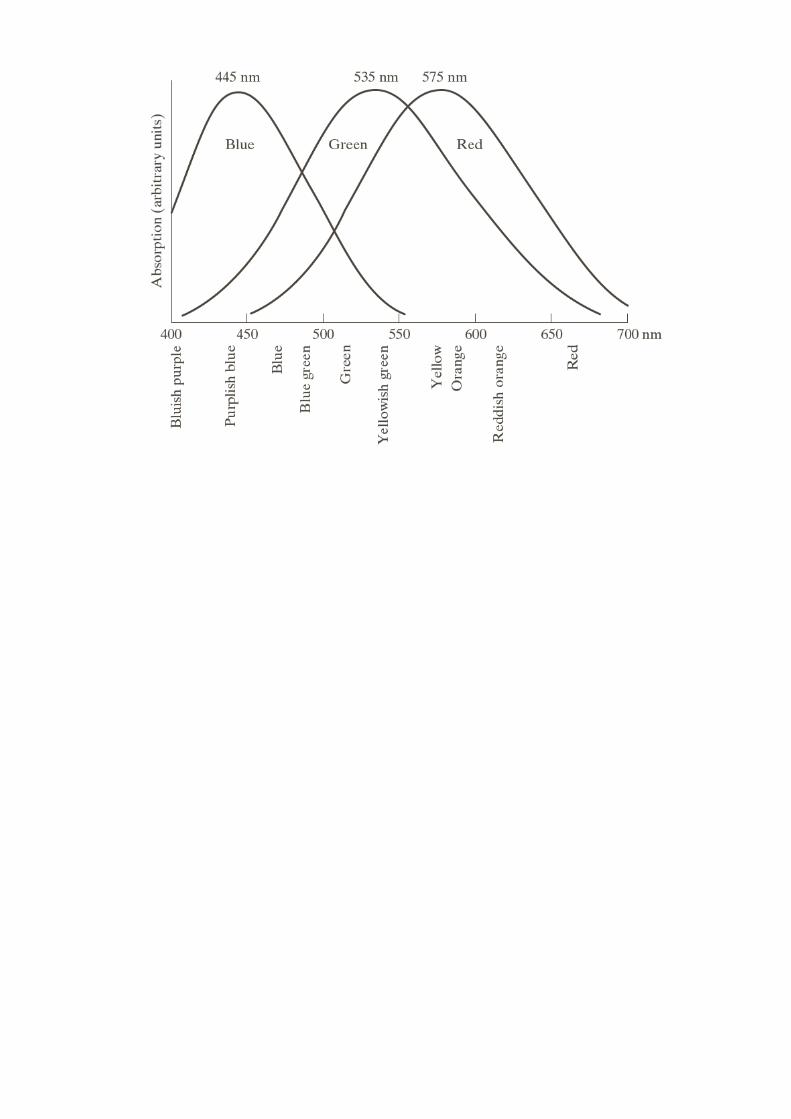

Color Models
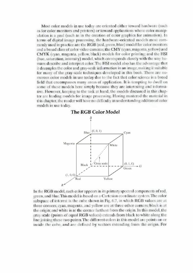

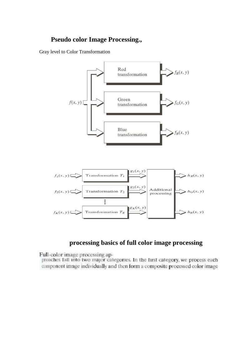
Pseudo color Image Processing.,
Gray level to Color Transformation
processing basics of full color image processing
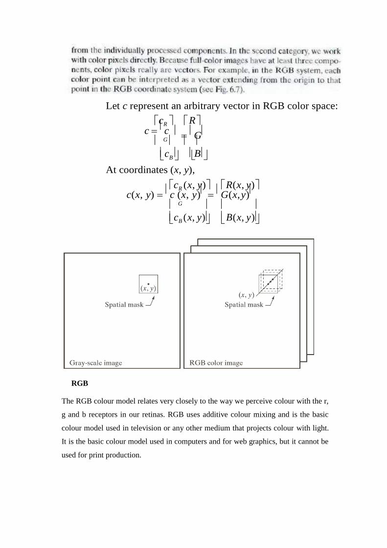
Let c represent an arbitrary vector in RGB color space:
cR R c
c G
G
cB B
At coordinates (x, y),
cR (x, y) R(x, y)c(x, y)
c (x, y)
G(x, y)
G
cB (x, y) B(x, y)
RGB
The RGB colour model relates very closely to the way we perceive colour with the r,
g and b receptors in our retinas. RGB uses additive colour mixing and is the basic
colour model used in television or any other medium that projects colour with light.
It is the basic colour model used in computers and for web graphics, but it cannot be
used for print production.
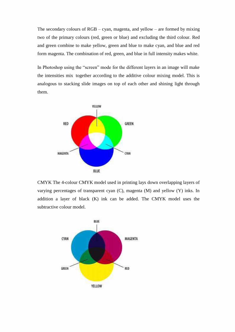
The secondary colours of RGB – cyan, magenta, and yellow – are formed by mixing
two of the primary colours (red, green or blue) and excluding the third colour. Red
and green combine to make yellow, green and blue to make cyan, and blue and red
form magenta. The combination of red, green, and blue in full intensity makes white.
In Photoshop using the “screen” mode for the different layers in an image will make
the intensities mix together according to the additive colour mixing model. This is
analogous to stacking slide images on top of each other and shining light through
them.
CMYK The 4-colour CMYK model used in printing lays down overlapping layers of
varying percentages of transparent cyan (C), magenta (M) and yellow (Y) inks. In
addition a layer of black (K) ink can be added. The CMYK model uses the
subtractive colour model.
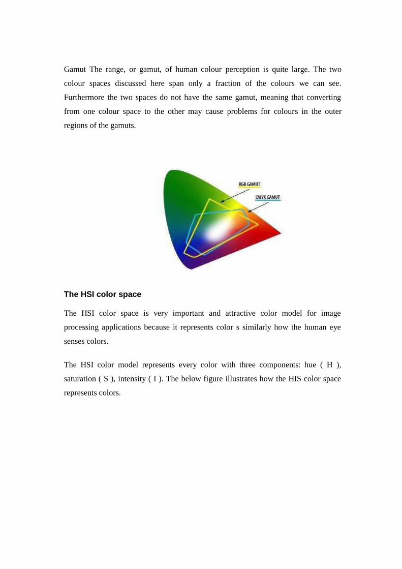
Gamut The range, or gamut, of human colour perception is quite large. The two
colour spaces discussed here span only a fraction of the colours we can see.
Furthermore the two spaces do not have the same gamut, meaning that converting
from one colour space to the other may cause problems for colours in the outer
regions of the gamuts.
The HSI color space
The HSI color space is very important and attractive color model for image
processing applications because it represents color s similarly how the human eye
senses colors.
The HSI color model represents every color with three components: hue ( H ),
saturation ( S ), intensity ( I ). The below figure illustrates how the HIS color space
represents colors.
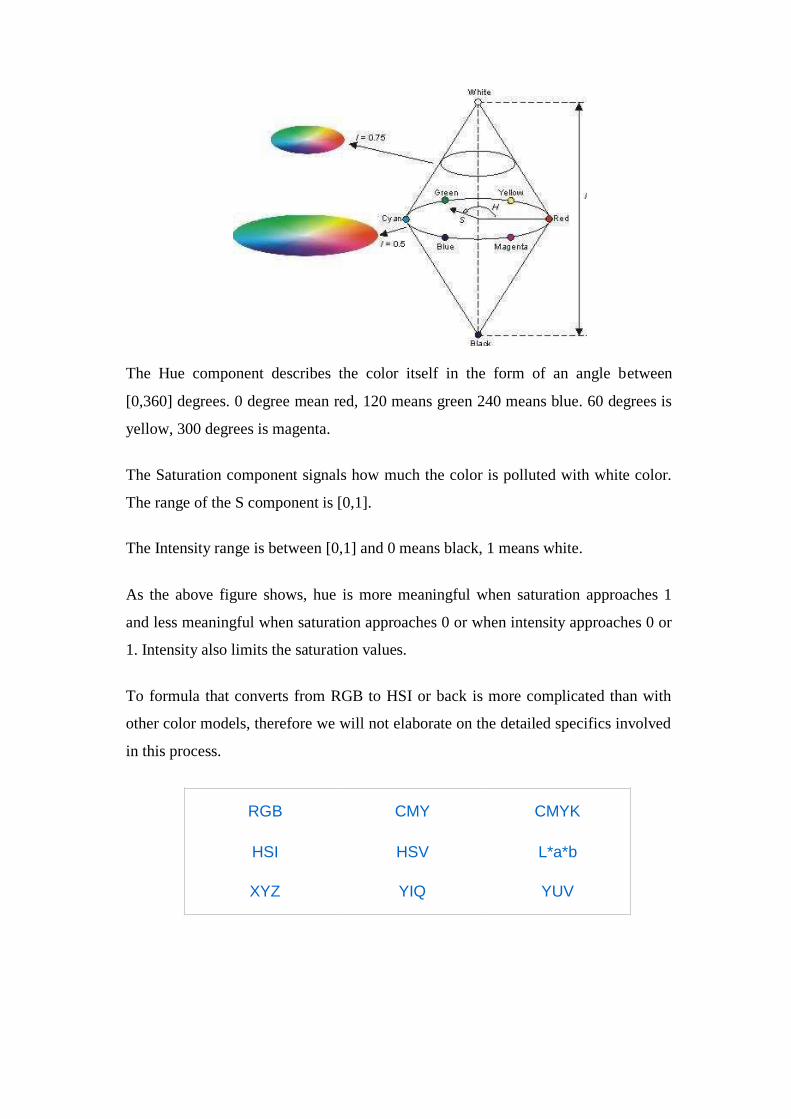
The Hue component describes the color itself in the form of an angle between
[0,360] degrees. 0 degree mean red, 120 means green 240 means blue. 60 degrees is
yellow, 300 degrees is magenta.
The Saturation component signals how much the color is polluted with white color.
The range of the S component is [0,1].
The Intensity range is between [0,1] and 0 means black, 1 means white.
As the above figure shows, hue is more meaningful when saturation approaches 1
and less meaningful when saturation approaches 0 or when intensity approaches 0 or
1. Intensity also limits the saturation values.
To formula that converts from RGB to HSI or back is more complicated than with
other color models, therefore we will not elaborate on the detailed specifics involved
in this process.
RGB CMY CMYK
HSI HSV L*a*b
XYZ YIQ YUV
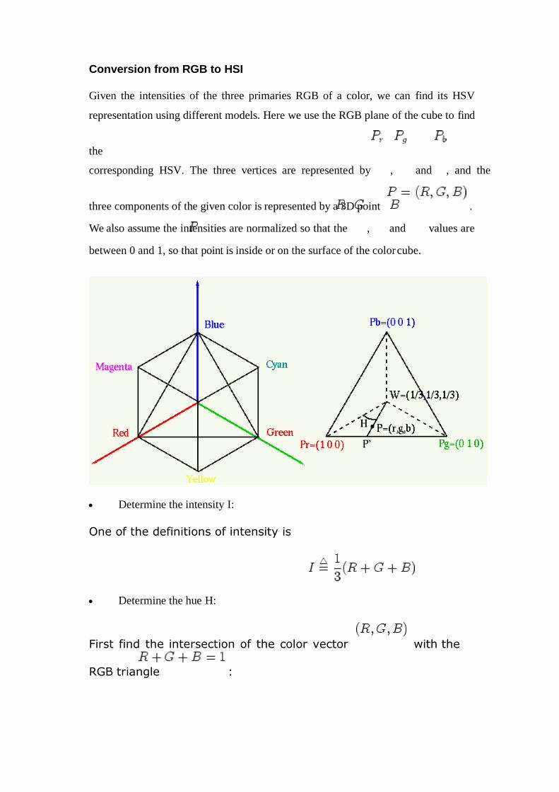
Conversion from RGB to HSI
Given the intensities of the three primaries RGB of a color, we can find its HSV
representation using different models. Here we use the RGB plane of the cube to find
the
corresponding HSV. The three vertices are represented by , and , and the
three components of the given color is represented by a 3D point .
We also assume the intensities are normalized so that the , and values are
between 0 and 1, so that point is inside or on the surface of the color cube.
Determine the intensity I:
One of the definitions of intensity is
Determine the hue H:
First find the intersection of the color vector with the
RGB triangle :
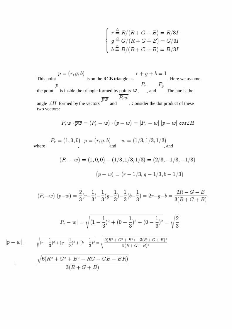
This point is on the RGB triangle as . Here we assume
the point is inside the triangle formed by points , , and . The hue is the
angle formed by the vectors and . Consider the dot product of these
two vectors:
where , and , and
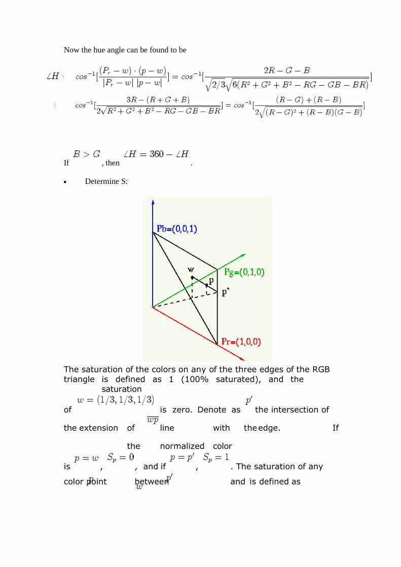
Now the hue angle can be found to be
If , then .
Determine S:
The saturation of the colors on any of the three edges of the RGB
triangle is defined as 1 (100% saturated), and the
saturation
of is zero. Denote as the intersection of
the extension of line with the edge. If
the normalized color
is , , and if , . The saturation of any
color point between and is defined as
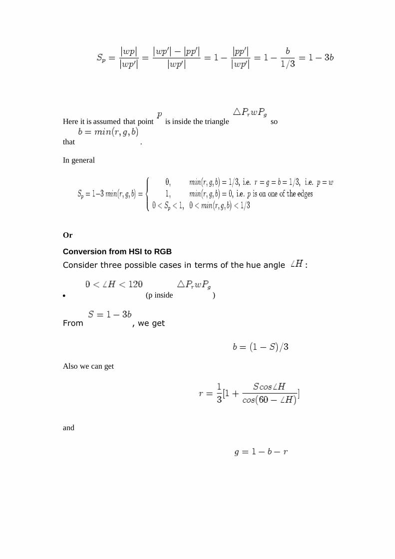
Here it is assumed that point is inside the triangle so
that .
In general
Or
Conversion from HSI to RGB
Consider three possible cases in terms of the hue angle :
(p inside )
From , we get
Also we can get
and
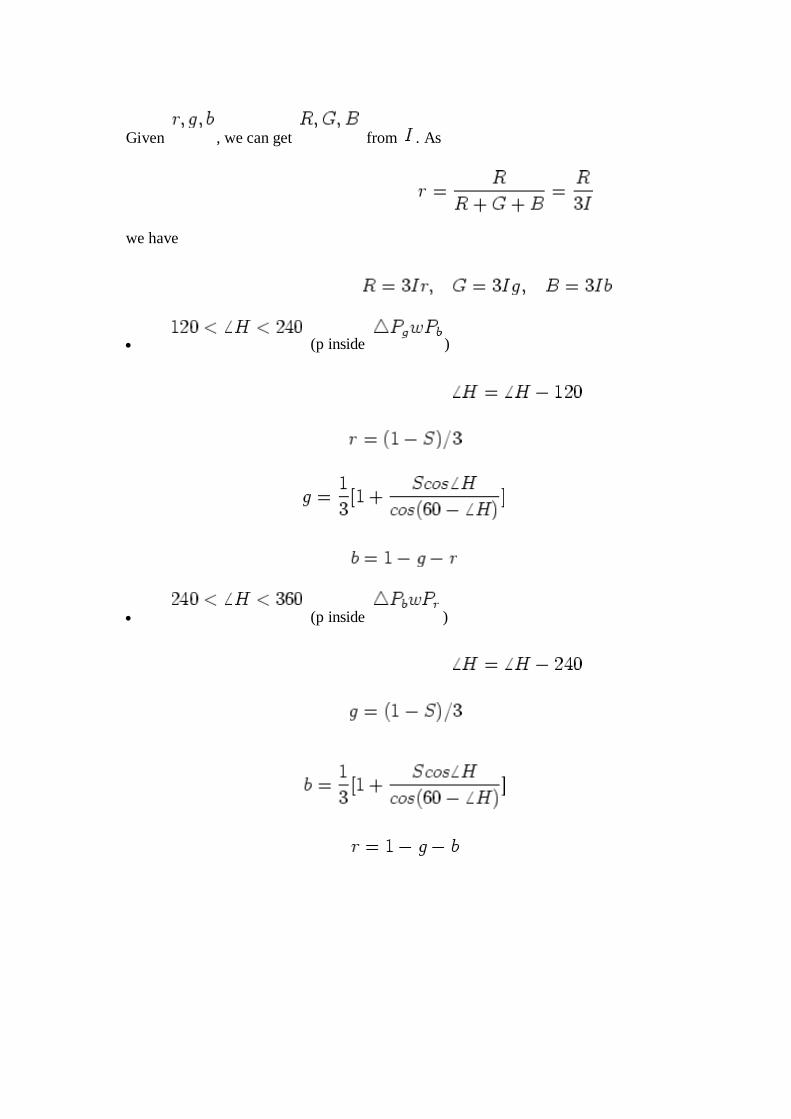
Given , we can get from . As
we have
(p inside )
(p inside )

Note
There is no single method that is used for CMYK/RGB conversion. The method used
by CMYK_CONVERT is the simplest and, depending on printing inks and screen
colors, might not be optimal in all situations.
CMYK_CONVERT
The CMYK_CONVERT procedure converts from the CMYK (cyan-magenta-
yellow- black) color model to RGB (red-green-blue) and vice versa.
The procedure uses the following method to convert from CMYK to
RGB: R = (255 - C) (1 - K/255)
G = (255 - M) (1 - K/255)
B = (255 - Y) (1 - K/255)
To convert from RGB to CMYK, the procedure uses the following
method: K = minimum of (R, G, B)
C = 255 [1 - R/(255 - K)] (if K=255 then
C=0) M = 255 [1 - G/(255 - K)] (if K=255
then M=0) Y = 255 [1 - B/(255 - K)] (if
K=255 then Y=0)
In both cases the CMYK and RGB values are assumed to be in the range 0 to 255.
This routine is written in the IDL language. Its source code can be found in
the file cmyk_convert.pro in the libsubdirectory of the IDL distribution.
Syntax
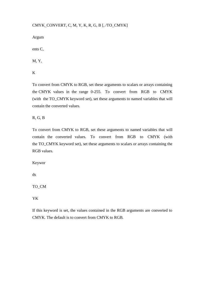
CMYK_CONVERT, C, M, Y, K, R, G, B [, /TO_CMYK]
Argum
ents C,
M, Y,
K
To convert from CMYK to RGB, set these arguments to scalars or arrays containing
the CMYK values in the range 0-255. To convert from RGB to CMYK
(with the TO_CMYK keyword set), set these arguments to named variables that will
contain the converted values.
R, G, B
To convert from CMYK to RGB, set these arguments to named variables that will
contain the converted values. To convert from RGB to CMYK (with
the TO_CMYK keyword set), set these arguments to scalars or arrays containing the
RGB values.
Keywor
ds
TO_CM
YK
If this keyword is set, the values contained in the RGB arguments are converted to
CMYK. The default is to convert from CMYK to RGB.


Recommended Questions
1. Explain the colour models.
2. Explain the following order statistics filters, indicating their uses.
i) Median filter ii) max filter iii) min filter.
3. Explain the RGB colour model.
4. Write a note on the following pseudo image processing techniques.
i) Intensity slicing
ii) Graylevel to colour transformations.
5. Write steps involved in converting colours from RGB to HSI and vice versa.
6. Explain pseudocolour image processing in brief.
7. Write short notes on i) weiner filtering ii) Inverse filtering
Copyright © 2022 FDOKUMEN

