


Bahasa
Halaman
Hukum

JOURNAL OF GEOPHYSICAL RESEARCH, VOL. 97, NO. B13, PAGES 19,537-19,563, DECEMBER 10, 1992
Time-Dependent Mapping of the Magnetic Field
at the Core-Mantle Boundary JEREMY BLOXHAM
Department of Earth and Planetary Sciences, Harvard University, Cambridge, Massachusetts
ANDREW JACKSON
Department of Earth Sciences, Oxford University, Oxford, England
We consider the problem of constructing a time-dependent map of the magnetic field at the core-mantle boundary. We use almost all the available data from the last 300 years to produce two maps, one for the period 1690-1840 and the other for 1840-1990. We represent the spatial dependency of the field using spherical harmonics, the time dependency using a cubic B-spline basis, and seek the smoothest solutions compatible with the observations. Particular attention must be paid to the effects of the crustal field in the data. We argue that for observations from permanent magnetic observatories the most efficient strategy is to use first-differences of annual means; for satellite data the most efficient strategy is simply to limit the number of data used so as to minimize any tendency to map the crustal field into the core field. The resulting model fits the observatory data better than any previous model yet has less power in the secular variation than previous models, demonstrating that very simple models fit the data. The resulting time- dependent field map exhibits much of the same structure in the field and its secular variation identified in earlier studies.
INTRODUCTION
Observations of the Earth's magnetic field provide not only an extremely valuable data set for investigating the dynamo process in the Earth's core responsible for the main- tenance and origin of the field against Ohmic decay, but are also of great use in a host of other geophysical studies rang- ing from studies of decade-period changes in the length of day to studies of thermal core-mantle interactions. In this paper, we pursue one way of making use of these obser- vations by constructing maps of the magnetic field at the core-mantle boundary (CMB).
Is this the best way in which to use these observations? Foremost, field models provide a considerably more com- pact and manageable representation of the field than the original observations, of benefit, for example, in determin- ing fluid flow at the top of the core. Additionally, field models, and in particular maps of the magnetic field at the CMB, are themselves extremely valuable tools for studying the dynamo. Although any inferences must be considered in the light of the rather large uncertainties attending the maps, it may nonetheless prove possible to draw physically reasonable inferences regarding the dynamo and the secular variation.
Perhaps, too much attention is paid to field modeling rather than hypothesis testing. How might we proceed by hypothesis testing? As an example, consider the frozen flux hypothesis [Roberts and Scott, 1965] (the hypothesis that the secular variation of the field over decade time scales arises
primarily from the advection of magnetic field by fluid flow at the surface of the core). One would examine whether sat- isfactory fits to the data can be obtained by a model of. the
Copyright 1992 by the American Geophysical Union.
Paper number 92JB01591.
0148-0227/92JB-01591 $05.00
field consistent with the hypothesis. In such an approach, the details of the particular models are unimportant: all that matters is whether adequate fits to the data can be obtained. This is important since the estimation of the un- certainty in a particular field model is not straightforward. An obvious difficulty, which detracts from the apparent sim- plicity of this approach, is adjudicating what constitutes an adequate fit to the observations, a problem that involves many of the same issues encountered in trying to evaluate uncertainties in field models.
Clearly, both approaches merit consideration. We believe that field modeling is an essential ingredient of any system- atic study of the dynamo. This paper is an extension of Our earlier work in mapping the geomagnetic field at the CMB. In a series of earlier papers [Gubbins and Bloxham, 1985; Bloxham and Gubbins, 1986; Bloxham et al., 1989 (here- inafter paper 0)] we developed a method of constructing spa- tially smooth maps of the main magnetic field at the CMB at particular points in time. More recently, we have extended that work [Bloxham, 1987 (hereinafter paper 1); Bloxham and Jackson, 1989 (hereinafter paper 2)] to the construction of time-dependent maps. However, as discussed in papers i and 2, the extension of the method to time-dependent mapping is not without shortcomings, the most serious of which are problems associated with the choice of basis func- tions for the temporal representation of the field. In this paper, we abandon the use of orthogonal polynomials and use cubic B-splines as basis functions, finding considerable advantages to recommend their use. This is the principal methodological change introduced in this paper.
We apply our modified method to a longer time interval than in the earlier papers. We present two models of the field, one for the interval 1690-1840, the other for 1840-1990. The reason for the split at 1840 is simple: prior to 1840 our data set contains no observations of the absolute intensity of the field, leaving the magnitude of the field undetermined.
19,537
19,538 BLOXHAM AND JACKSON: TIME-DEPENDENT MAGNETIC FIELD MAPPING
METHOD
We must relate measurements of the field at the Earth's
surface to the model of B•, the radial component of the mag- netic field B, at the CMB. The passage of the field through the (in general, conducting) mantle is governed by the elec- tromagnetic diffusion equation; given a model of mantle con- ductivity, the response at the Earth's surface to an input at the CMB is calculable. A lucid description of the process is given by Gubbins and Roberts [1987]. Unfortunately, our knowledge of deep mantle conductivity is at present scanty, though recent high-pressure mineralogical experiments are providing new insight. For example, both Peyronneau and Poirier [1989] and Wood and Nell [1991] find that iron-rich (Mg,Fe)O magnesiowiistite has a conductivity of the order 1 Sm -1 when extrapolated to a depth of 1000km and is thus the dominant conductor in the midmantle; these re- sults are also compatible with the results of Li and Jeanloz [1990] for differing Mg/Fe ratios. Thus there is the prospect that future laboratory studies, combined with perhaps new long-period induction studies, will significantly improve our knowledge of deep mantle conductivity. Some further con- straints on mantle conductivity may be forthcoming from studies of geomagnetic jerks, abrupt changes in the secular variation which place a rather imprecise constraint on the smoothing time of the mantle electromagnetic filter [Backus, 1983], and from studies of nutation which are sensitive to lowermost mantle conductivity [Buffeft, 1992]. Neverthe- less, in the absence of any clear consensus regarding mantle conductivity, we adopt the insulating mantle approximation for this study. The effect of mantle conductivity on the downward continuation of the magnetic field to the CMB has been shown to be small for a broad range of mantle conductivity models which have been proposed [Benton and Whaler, 1983], so that the insulating mantle approximation is an adequate one. However, unusually large conductivities in the middle and deep mantle could negate this conclusion.
As in papers 1 and 2, we begin by representing our model of the radial field Br at the CMB as an expansion spatially in spherical harmonics and temporally in basis functions Mn(t). We write Br as
L 1 N
/=1 ra=0
x (g?"cosm0 + h?" sin m0) PT (cos 0)M. (t) (1)
where (r, 0, ½) are spherical polar coordinates, a is the ra- dius of the Earth's surhce (nominally, 6371.2 km), c is the core radius, the P•(cos 0) are Schmidt quasi-normalized as- sociated Legendre functions, and L and N are the trunca- tion points of the expansions in spherical harmonics and the temporal basis functions respectively. The choice of L and N will be discussed further below. Because of our insu-
lating mantle approximation, the expansion (1) determines the time-dependent geomagnetic field B(t) everywhere as the gradient of a scalar V(t), where B(t) = -VV(t):
L 1 N
/=1 m=0 n=l
x (g?• cos m½+ h? • sin m½) P• (cos O)M• (t) (2)
We take this representation of the field to hold everywhere outside the Earth's core. This introduces several important
approximations. We have discussed that of neglecting man- tle electrical conductivity. Second is the neglect of crustal fields. Third is that by omitting terms in the expansion with dependence (r/a) 1 we neglect fields external to the measure- ment point.
In the crust, additional contributions to the magnetic field will arise from both permanent magnetization of crustal rocks below their Curie temperature and from induced mag- netization. Both result in the field being nonpotential in the crust. We approach this problem by treating the crustal field as an additional source of noise in the data, using the tech- nique described by Jackson [1990], and applied previously in paper 2. An alternative method of treating the crustal field is given by Langel et al. [1989].
We also treat ionospheric fields as an additional source of random noise in the data. Langel et al. [1989] present a formalism to take approximate account of these fields which are partly internal to satellite observations. We do not adopt their method in this paper, in part because of the relatively small number of satellite observations that we use (see be- low).
The expansion (1) involves coefficients {g/•; h? • } which are related to the standard Gauss geomagnetic coefficients (g/•; h?) by
N
gl (t)- m•.. (t) gl iVl n
n=l
(3)
and likewise for {h•}. We represent these coefficients by a model vector m - (gl ©, gl 1ø, h11ø,..., g2øl,...). The observa- tions are related to m by a model equation of the form
-/: f(m) + e (4)
where -/ is a data vector, e is the error vector, and f is, in general, a nonlinear function of m and the independent variables (r, 0, •, t).
We seek the smoothest models for a given fit to the data by seeking as our estimate the model vector m that min- imizes the misfit to the data and two model norms, one measuring roughness in the spatial domain and the other roughness in the temporal domain. For the spatial norm we seek the solution with minimum Ohmic dissipation based on the Ohmic heating bound of Gubbins [1975]; we minimize the integral
• = (re - rs) • (B•) dt - mT$-lm (5) where •r (B•) is the quadratic norm associated with the min- imum Ohmic heating of a field parameterized by {g/•; h•}
•r (B•) • (1 + 1)(2/+ 1)(2/+ 3) (a__) 2/+4 1 C /----1
1
For the temporal model norm we use
where [rs, re] is the time interval over which we solve for the field. This combination of spatial and temporal smoothness
BLOXHAM AND JACKSON: TIME-DEPENDENT MAGNETIC FIELD MAPPING 19,539
is reminiscent of the norm in a Sobolev vector space, where, for example in one dimension, the norm is written
0.7
Then, as before, our model estimate m is that value of m that minimizes the objective function
(3(m) -[7- f(m)] T C• -1 [7- f(m)] + mTC•lm (9) where Ce is the data error covariance matrix, and C•n 1 - /ksS -1 +/kTT -1, with damping parameters/ks and AT. The specification of the data error covariance matrix is described later in the discussion of the data that we used.
The solution is sought iteratively using the scheme
(A:rCZ1A + CZnl) -1 x, [A•C:• (•,- f(mt))- (t0)
mi+l -- miq-
A consequence of these regularization conditions is that the expansion (t) converges so that, with appropriately large values for the truncation points L and N, the solution is insensitive to truncation.
In paper 2 this ideal of convergence and insensitivity to truncation was not fully achieved. In that paper, the tempo- ral basis functions were chosen to be Chebychev polynomi- als, defined over the entire time interval [rs, tel. With such a global representation, the so-called "normal equations" ma- trix, the matrix H - A•CziA is full (although, of course, symmetric), and the number of parameters which must be determined is given by
P - L(L q- 2)(N q- 1) (11)
With L = 14 (an adequately large choice of L) we are severely restricted by computational considerations in our choice of N. In paper 2 we used N = t0, giving a system of dimension 2464, requiring slightly more than 3 megawords of storage. We found some evidence of inadequate temporal convergence suggesting that the temporal basis truncated at degree t0 is incomplete. This is not surprising given that the most oscillatory basis function in our representation has only t0 zeros in the time interval, which in paper 2 was 80 years, or 8 years between zeros. In this paper our choice of basis functions in the temporal domain is motivated by the choice of norm (7). It is well known that in one dimension of all the interpolators re(t) passing through a given set of points in the interval [a, b], the one with minimum roughness R where
(12) •a b is the cubic spline interpolator with R = R.. The same interpolator is optimal when the data are fitted in a least squares sense and R is reduced below R.. This motivates a choice of splines as the expansion in time.
Temporal B-Spline Basis
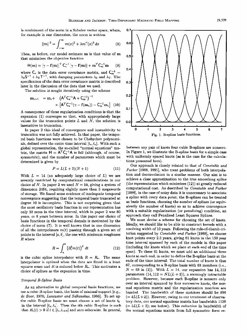
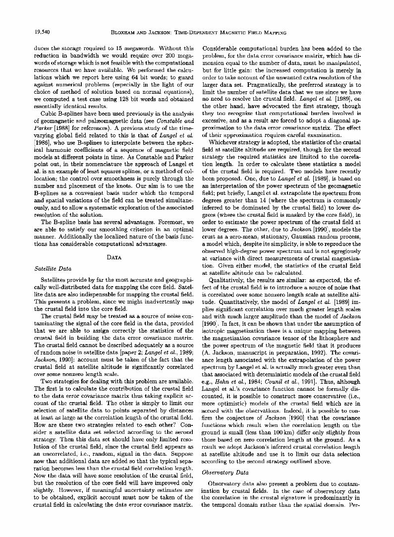
As an alternative to global temporal basis functions, we use a cubic B-spline basis, the basis of minimal support [e.g., de Boor, 1978; Lancaster and Salkauskas, 1986]. To set up the cubic B-spline basis we must choose a set of knots tk in the interval Its,tel. Then the ith cubic B-spline is such that Bi(t) > 0 if t G [ti, ti+4] and zero otherwise. In general,
0.5
0.4
0.5
0.2
0.1
0.0
I I I I I i
2 5 4 5 6 7
Fig. 1. B-spline basis functions.
between any pair of knots four cubic B-splines are nonzero. In Figure t, we illustrate the B-spline basis for a simple case with uniformly spaced knots (as is the case for the calcula- tions presented here).
Our approach is closely related to that of Constable and Parker [1988, 1991], who treat problems of both interpola- tion and deconvolution in a similar manner. Our aim is to
achieve a close approximation to the true smoothing spline (the representation which minimizes (12)) at greatly reduced computational cost. As described by Constable and Parker [1988], in the case of noisy data it is unnecessary to associate a spline with every data point; the B-splines can be treated as basis functions, choosing the number of splines (or equiv- alently the number of knots) so as to achieve convergence with a suitable regularization (or penalizing) condition, an approach they call Penalised Least Squares Splines.
We must devise a scheme for choosing the set of knots. Ideally, we should like to be able to construct kernels with a resolving width of 10 years. Following the rule-of-thumb cri- terion suggested by Constable and Parker [1988], we choose knot points every 2.5 years, giving 61 knots in the 150 year time interval spanned by each of the models in this paper (including the knots which we place at each end of the time span). To these 61 knots, we must add an additional three knots at each end, in order to define the B-spline basis at the ends of the time interval. The total number of knots is thus
67, corresponding to a B-spline basis with 63 members (i.e., N = 63 in (2)). With L - 14, our expansion has 14, 112 parameters (14, 112 = NL(L q- 2)), a seemingly intractable problem. However, because each B-spline is nonzero only over an interval spanned by four successive knots, the nor- mal equations matrix and the regularization matrices are banded. The bandwidth of these matrices should be 896
(= 4L(Lq- 2)). However, owing to our treatment of observa- tory data, our normal equations matrix has bandwidth 1120 (= 5L(L q- 2); see below). This reduction in bandwidth of the normal equations matrix from full symmetric form re-
19,540 BLOXHAM AND JACKSON: TIME-DEPENDENT MAGNETIC FIELD MAPPING
duces the storage required to 15 megawords. Without this reduction in bandwidth we would require over 200 mega- words of storage which is not feasible with the computational resources that we have available. We performed the calcu- lations which we report here using 64 bit words; to guard against numerical problems (especially in the light of our choice of method of solution based on normal equations), we computed a test case using 128 bit words and obtained essentially identical results.
Cubic B-splines have been used previously in the analysis of geomagnetic and palaeomagnetic data (see Constable and Parker [1988] for references). A previous study of the time- varying global field related to this is that of Langet et at. [1986], who use B-splines to interpolate between the spher- ical harmonic coefficients of a sequence of magnetic field models at different points in time. As Constable and Parker point out, in their nomenclature the approach of Langel et al. is an example of least squares splines, or a method of col- location; the control over smoothness is purely through the number and placement of the knots. Our aim is to use the B-splines as a convenient basis under which the temporal and spatial variations of the field can be treated simultane- ously, and to allow a systematic exploration of the associated resolution of the solution.
The B-spline basis has several advantages. Foremost, we are able to satisfy our smoothing criterion in an optimal manner. Additionally the localized nature of the basis func- tions has considerable computational advantages.
DATA
Satellite Data
Satellites provide by far the most accurate and geographi- cally well-distributed data for mapping the core field. Satel- lite data are also indispensable for mapping the crustal field. This presents a problem, since we might inadvertently map the crustal field into the core field.
The crustal field may be treated as a source of noise con- taminating the signal of the core field in the data, provided that we are able to assign correctly the statistics of the crustal field in building the data error covariance matrix. The crustal field cannot be described adequately as a source of random noise in satellite data [paper 2; Langet et at., 1989; Jackson, 1990]: account must be taken of the fact that the crustal field at satellite altitude is significantly correlated over some nonzero length scale.
Two strategies for dealing with this problem are available. The first is to calculate the contribution of the crustal field
to the data error covariance matrix thus taking explicit ac- count of the crustal field. The other is simply to limit our selection of satellite data to points separated by distances at least as large as the correlation length of the crustal field. How are these two strategies related to each other? Con- sider a satellite data set selected according to the second strategy. Then this data set should have only limited reso- lution of the crustal field, since the crustal field appears as an uncorrelated, i.e., random, signal in the data. Suppose now that additional data are added so that the typical sepa- ration becomes less than the crustal field correlation length. Now the data will have some resolution of the crustal field, but the resolution of the core field will have improved only slightly. However, if meaningful uncertainty estimates are to be obtained, explicit account must now be taken of the crustal field in calculating the data error covariance matrix.
Considerable computational burden has been added to the problem, for the data error covariance matrix, which has di- mension equal to the number of data, must be manipulated, but for little gain: the increased computation is merely in order to take account of the unwanted extra resolution of the
larger data set. Pragmatically, the preferred strategy is to limit the number of satellite data that we use since we have
no need to resolve the crustal field. Langet et at. [1989], on the other hand, have advocated the first strategy, though they too recognize that computational burden involved is excessive, and as a result are forced to adopt a diagonal ap- proximation to the data error covariance matrix. The effect of their approximation requires careful examination.
Whichever strategy is adopted, the statistics of the crustal field at satellite altitude are required, though for the second strategy the required statistics are limited to the correla- tion length. In order to calculate these statistics a model of the crustal field is required. Two models have recently been proposed. One, due to Langet et at. [1989], is based on an interpretation of the power spectrum of the geomagnetic field; put briefly, Langel et al. extrapolate the spectrum from degrees greater than 14 (where the spectrum is commonly inferred to be dominated by the crustal field) to lower de- grees (where the crustal field is masked by the core field), in order to estimate the power spectrum of the crustal field at lower degrees. The other, due to Jackson [1990], models the crust as a zero-mean, stationary, Gaussian random process, a model which, despite its simplicity, is able to reproduce the observed high-degree power spectrum and is not egregiously at variance with direct measurements of crustal magnetiza- tion. Given either model, the statistics of the crustal field at satellite altitude can be calculated.
Qualitatively, the results are similar: as expected, the ef- fect of the crustal field is to introduce a source of noise that
is correlated over some nonzero length scale at satellite alti- tude. Quantitatively, the model of Langet et at. [1989] im- plies significant correlation over much greater length scales and with much larger amplitude than the model of Jackson [1990]. In fact, it can be shown that under the assumption of isotropic magnetization there is a unique mapping between the magnetization covariance tensor of the lithosphere and the power spectrum of the magnetic field that it produces (A. Jackson, manuscript in preparation, 1992). The covari- ance length associated with the extrapolation of the power spectrum by Langel et al. is actually much greater even than that associated with deterministic models of the crustal field
e.g., Hahn et at., 1984; Counit et at., 1991]. Thus, although Langel et al.'s covariance function cannot be formally dis- counted, it is possible to construct more conservative (i.e., more optimistic) models of the crustal field which are in accord with the observations. Indeed, it is possible to con- firm the conjecture of Jackson [1990] that the covariance functions which result when the correlation length on the ground is small (less than 100 km) differ only slightly from those based on zero correlation length at the ground. As a result we adopt Jackson's inferred crustal correlation length at satellite altitude and use it to limit our data selection
according to the second strategy outlined above.
Observatory Data
Observatory data also present a problem due to contam- ination by crustal fields. In the case of observatory data the correlation in the crustal signature is predominantly in the temporal domain rather than the spatial domain. Per-
BLOXHAM AND JACKSON: TIME-DEPENDENT MAGNETIC FIELD MAPPING 19,$41
manent observatories are fixed relative to the crust and so
are, to a good approximation, subject to the same crustal signature at all points in time. Spatial correlation is not a problem because the typical separation of observatories is very large compared to any reasonable estimate of the correlation length scale of the crustal field at the Earth's surface.
In paper 2 we presented a formalism for accounting for the covariance of the crustal noise in observatory data and showed how to calculate the data error covariance ma-
trix. We showed that N observations {"/i;i - 1,..., N) of a particular component at a particular observatory with rms crustal field cry and random error ere are best treated
by a linear combination (1/x/-•)•,1 • "/i (or x/-• where is the mean of the observations) with standard deviation v/cr• + Ncr• and (N- 1) linear combinations of the data orthonormal to the first with standard deviation
Ideally, we should like to implement this scheme in the present paper. Unfortunately, to do so would greatly in- crease the bandwidth of the normal equations matrix. The new datum V•i depends on the field at every year which contributes, and so this datum involves many more splines than the usual four. In view of the ratio of the number of
these composite data (•- 3 at each of •- 500 observatories) to the number of survey data, each composite of this type can be omitted with little effect. The other eigenvectors suffer a similar disadvantage. Consider the first few orthog- onal to (1, 1, 1,...): they are, for example, (1,-1, 0, 0, 0...), (1, 1,-2, 0, 0,...), etc. with dependence on increasing num- bers of observations. As a result they increase the band- width in a similar fashion to the datum x/-•i. As a re- sult, we have chosen to use more intuitive combinations of the data. Clearly the first differences of data (such as ("/,• -"/,•-1)) are desensitized to the effect of the constant crustal bias. They do not, however, have the optimal Gaus- sian statistical properties of the combinations presented in paper 2. These first-differences only increase the bandwidth of the normal equations matrix from aL(L+ 2) to 5L(L+ 2). (The increase from 4 to 5 times arises in this case from dif- ferences (%- fin-l) that span a knot point.) Given this, we choose to use only the (N- 1) data corresponding to the differences to take advantage of this very substantial com- putational saving.
In implementing this scheme we require estimates of the random error in each component at each observatory. Initial estimates of cr• were made using independent one- dimensional penalized spline fits [Constable and Parker, 1988] to time series of each component at each observatory, using generalised cross validation [e.g., Craven and Wahba, 1979] to choose an appropriate regularizing parameter. Sub- sequently, the errors were refined using the residuals to the preliminary spline model produced using these initial error estimates. In this way we aim to attain a realistic weighting scheme between observatories whose accuracy varies consid- erably.
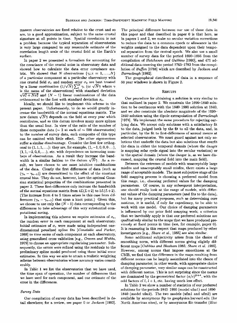
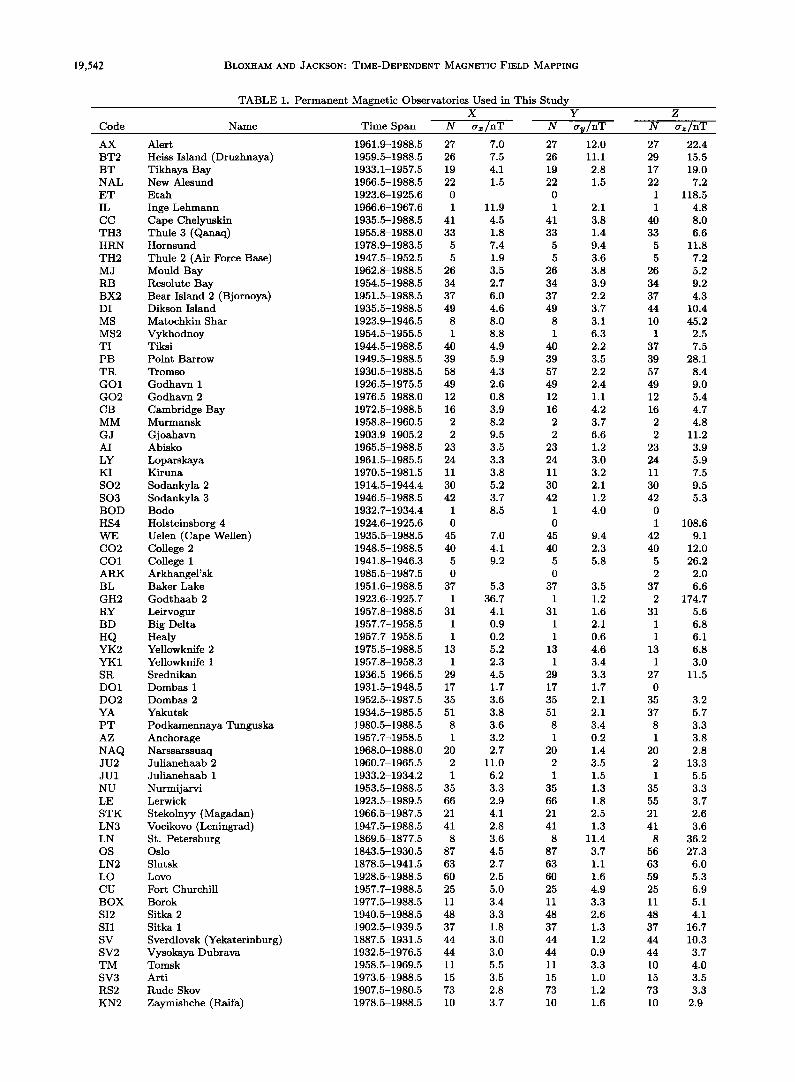
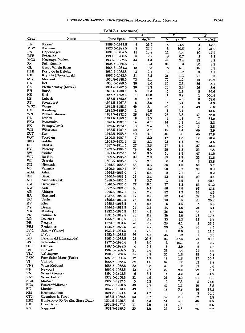
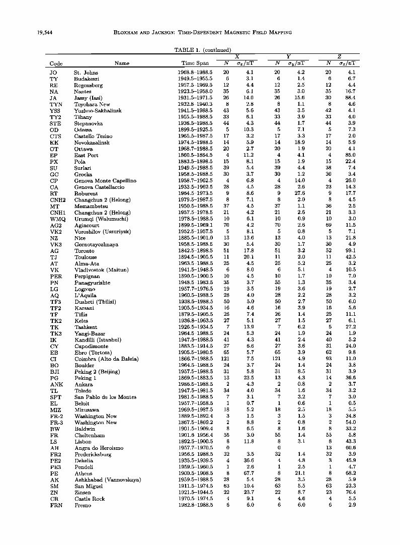
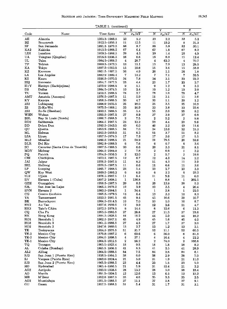
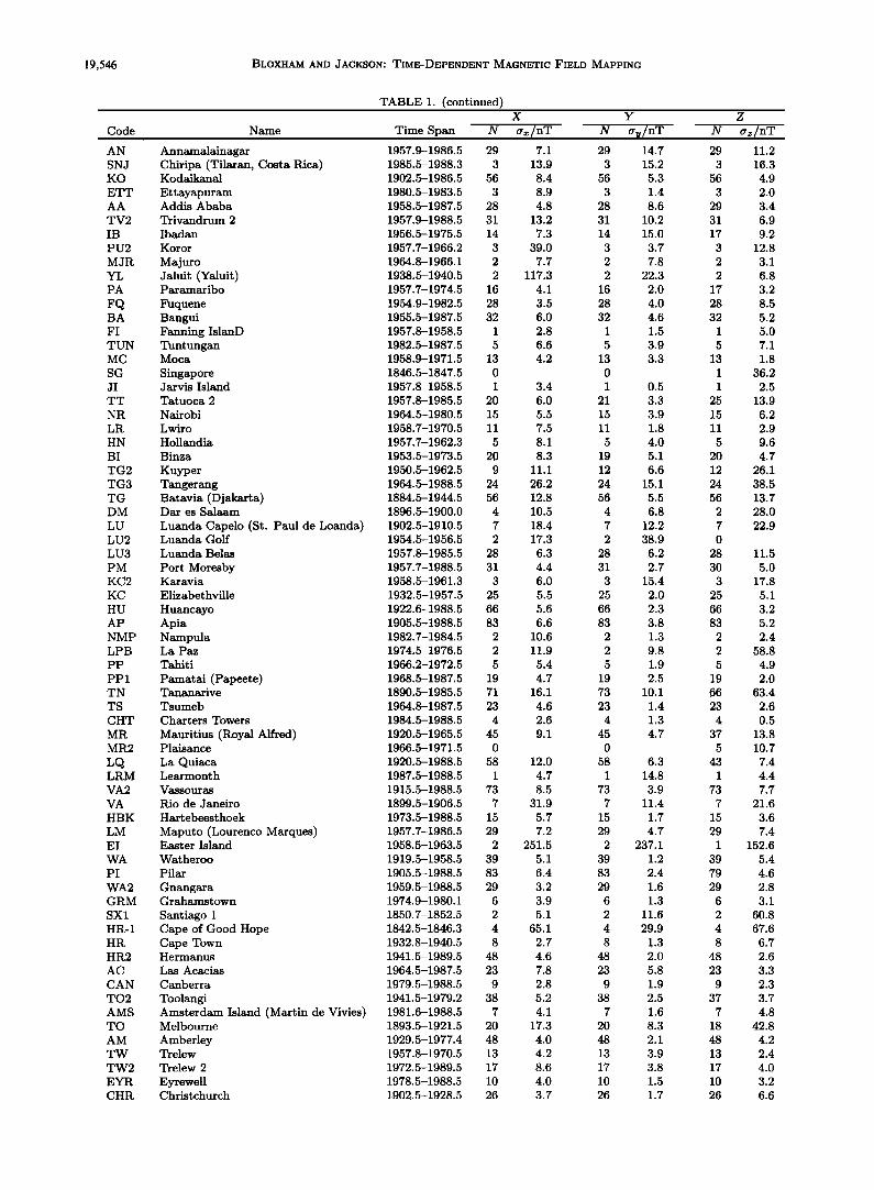
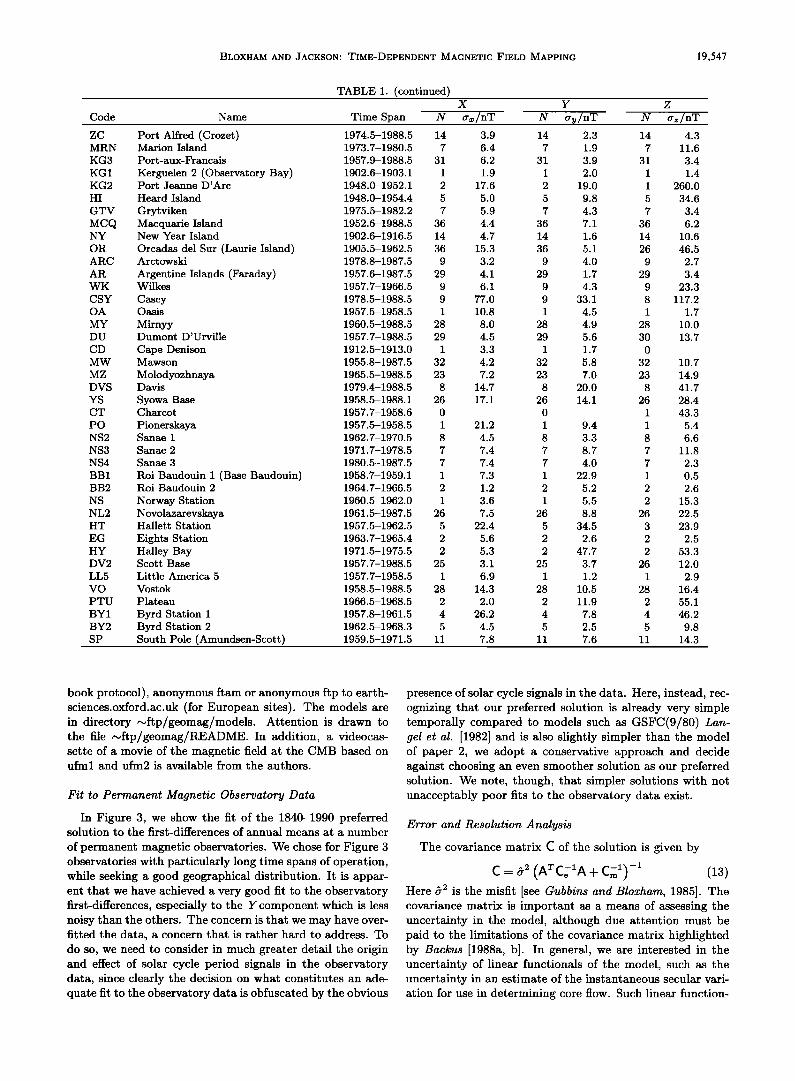
In Table I we list the observatories that we have used, the time span of operation, the number of differences that we have used for each component, and our estimate of the error in the differences.
Survey Data
Our compilation of survey data has been described in de- tail elsewhere; for a review, see paper 0 or Jackson [1992].
The principal difference between our use of these data in this paper and that described in paper 0 is that here, as in papers I and 2, we make no secular variation corrections to reduce the data to a common epoch or allowance in the weights assigned to the data dependent upon their tempo- ral separation from the central epoch. We also use a small number of survey data for the period 1690-1695 from the compilation of Hutcheson and Gubbins [1990], and 471 ad- ditional data covering the period 1763-1782 from the compi- lation of Buffon [1788] which are described by Jackson and Barraclough [1992].
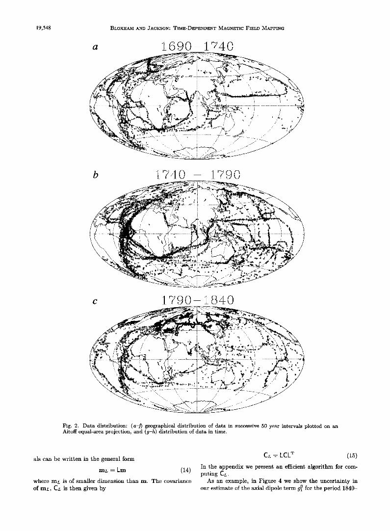
The geographical distribution of data in a sequence of 50 year windows is shown in Figure 2.
RESULTS
Our procedure for obtaining a solution is very similar to that outlined in paper 2. We constrain the 1690-1840 solu- tion to be continuous with the 1840-1990 solution at 1840, and we also constrain the absolute magnitude of the 1690- 1840 solution using the dipole extrapolation of Barraclough [1974]. We implement the same procedure for rejecting out- lying data. We accept only solutions with a satisfactory fit to the data, judged both by the fit to all the data, and, in particular, by the fit to first-differences of annual means at selected observatories. We must guard against not only so- lutions that underfit the data but also solutions that overfit
the data in either the temporal domain (where the danger is mapping solar cycle signal into the secular variation) or in the spatial domain (where the danger is, as we have dis- cussed, mapping the crustal field into the main field).
Between the extremes of models with unacceptably large misfits and unacceptably small misfits, there exists a large range of acceptable models. The most subjective stage of the field mapping process is choosing a preferred model from this range, i.e., choosing preferred values for the damping parameters. Of course, in any subsequent interpretation, one should really look at the range of models, with differ- ent values of the damping parameters (and fits to the data), but for many practical purposes, such as determining core motions, it is useful, if only for expediency, to be able to work with one model. Our choice of damping parameters is influenced by our prior field mapping work; a criterion that we inevitably apply is that our preferred solutions are qualitatively similar to the maps that we have produced pre- viously at fixed points in time (see, for example, paper 0). It is reassuring in this respect that maps produced by other investigators [e.g., Shure et al., 1985] are also similar.
Some additional subjectivity arises from the choice of smoothing norm, with different norms giving slightly dif- ferent maps [ Gubbins and Bloxham 1985; Shure et al. 1985]. However, among norms that impose smoothness at the CMB, we find that the difference in the maps resulting from different norms can be largely assimilated into the choice of damping parameter; in other words, with appropriate choice of damping parameter, very similar maps can be constructed with different norms. This is not surprising since the norms are dominated by the geometrical factor (a/c) 21+4, with the odd factors of l, 1 + 1, etc. having much less effect.
In Table 2 we show a number of statistics of our preferred solutions for the periods 1840-1990 (model ufml) and 1690- 1840 (model ufm2). The two models (ufml and ufm2) are available by anonymous ftp to geophysics.harvard.edu (for North American sites), or by anonymous file transfer (Blue
19,542 BLOXHAM AND JACKSON: TIME-DEPENDENT MAGNETIC FIELD MAPPING
TABLE 1. Permanent Magnetic Observatories Used in This Study
Code
X
Name Time Span N rrx/nT Y
N ery/nT z
N rrz/nT AX
BT2
BT
NAL
ET
IL
CC
TH3
HRN
TH2
MJ
RB
BX2
DI
MS
MS2
TI
PB
TR
GO1
GO2
CB
MM
GJ
AI
LY
KI
SO2
SO3
BOD
HS4
WE
CO2
CO1
ARK
BL
GH2
RY
BD
HQ YK2
YK1
SR
DO1
DO2
YA
PT
AZ
NAQ JU2
JUl
NU
LE
STK
LN3
LN
OS
LN2
LO
CU
BOX
SI2
SI1
SV
SV2
TM
SV3
RS2
KN2
Alert
Heiss Island (Druzhnaya) Tikhaya Bay New Alesund
Etah
Inge Lehmann Cape Chelyuskin Thule 3 (Qanaq) Hornsund
Thule 2 (Air Force Base) Mould Bay Resolute Bay Bear Island 2 (Bjornoya) Dikson Island
Matochkin Shar
Vykhodnoy Tiksi
Point Barrow
Tromso
Godhavn 1
Godhavn 2
Cambridge Bay Murmansk
Gjoahavn Abisko
Loparskaya Kiruna
Sodankyla 2 Sodankyla 3 Bodo
Holsteinsborg 4 Uelen (Cape Wellen) College 2 College 1 Arkhangel'sk Baker Lake
Godthaab 2
Leirvogur Big Delta Healy Yellowknife 2
Yellowknife 1
Srednikan
Dombas 1
Dombas 2
Yakutsk
Podkamennaya Tunguska Anchorage Narssarssuaq Julianehaab 2
Julianehaab 1
Nurmijarvi Lerwick
Stekolnyy (Magadan) Voeikovo (Leningrad) St. Petersburg Oslo
Slutsk
Lovo
Fort Churchill
Borok
Sitka 2
Sitka 1
Sverdlovsk (Yekaterinburg) Vysokaya Dubrava Tomsk
Arti
Rude Skov
Zaymishche (Raifa)
1961.9-1988.5 27 7.0 27 12.0
1959.5-1988.5 26 7.5 26 11.1
1933.1-1957.5 19 4.1 19 2.8
1966.5-1988.5 22 1.5 22 1.5
1923.6-1925.6 0 0
1966.6-1967.6 I 11.9 I 2.1
1935.5-1988.5 41 4.5 41 3.8
1955.8-1988.0 33 1.8 33 1.4
1978.9-1983.5 5 7.4 5 9.4
1947.5-1952.5 5 1.9 5 3.6
1962.8-1988.5 26 3.5 26 3.8
1954.5-1988.5 34 2.7 34 3.9
1951.5-1988.5 37 6.0 37 2.2
1935.5-1988.5 49 4.6 49 3.7
1923.9-1946.5 8 8.0 8 3.1
1954.5-1955.5 I 8.8 I 6.3
1944.5-1988.5 40 4.9 40 2.2
1949.5-1988.5 39 5.9 39 3.5
1930.5-1988.5 58 4.3 57 2.2
1926.5-1975.5 49 2.6 49 2.4
1976.5-1988.0 12 0.8 12 1.1
1972.5-1988.5 16 3.9 16 4.2
1958.8-1960.5 2 8.2 2 3.7
1903.9-1905.2 2 9.5 2 6.6
1965.5-1988.5 23 3.5 23 1.2
1961.5-1985.5 24 3.3 24 3.0
1970.5-1981.5 11 3.8 11 3.2
1914.5-1944.4 30 5.2 30 2.1
1946.5-1988.5 42 3.7 42 1.2
1932.7-1934.4 I 8.5 I 4.0
1924.6-1925.6 0 0
1935.5-1988.5 45 7.0 45 9.4
1948.5-1988.5 40 4.1 40 2.3
1941.8-1946.3 5 9.2 5 5.8
1985.5-1987.5 0 0
1951.6-1988.5 37 5.3 37 3.5
1923.6-1925.7 I 36.7 I 1.2
1957.8-1988.5 31 4.1 31 1.6
1957.7-1958.5 I 0.9 I 2.1
1957.7-1958.5 I 0.2 I 0.6
1975.5-1988.5 13 5.2 13 4.6
1957.8-1958.3 I 2.3 I 3.4
1936.5-1966.5 29 4.5 29 3.3
1931.5-1948.5 17 1.7 17 1.7
1952.5-1987.5 35 3.6 35 2.1
1934.5-1985.5 51 3.8 51 2.1
1980.5-1988.5 8 3.6 8 3.4
1957.7-1958.5 I 3.2 I 0.2
1968.0-1988.0 20 2.7 20 1.4
1960.7-1965.5 2 11.0 2 3.5
1933.2-1934.2 I 6.2 I 1.5
1953.5-1988.5 35 3.3 35 1.3
1923.5-1989.5 66 2.9 66 1.8
1966.5-1987.5 21 4.1 21 2.5
1947.5-1988.5 41 2.8 41 1.3
1869.5-1877.5 8 3.6 8 11.4
1843.5-1930.5 87 4.5 87 3.7
1878.5-1941.5 63 2.7 63 1.1
1928.5-1988.5 60 2.5 60 1.6
1957.7-1988.5 25 5.0 25 4.9
1977.5-1988.5 11 3.4 11 3.3
1940.5-1988.5 48 3.3 48 2.6
1902.5-1939.5 37 1.8 37 1.3
1887.5-1931.5 44 3.0 44 1.2
1932.5-1976.5 44 3.0 44 0.9
1958.5-1969.5 11 5.5 11 3.3
1973.5-1988.5 15 3.5 15 1.0
1907.5-1980.5 73 2.8 73 1.2
1978.5-1988.5 10 3.7 10 1.6
27
29
17
22
1
1
40
33
5
5
26
34
37
44
10
1
37
39
57
49
12
16
2
2
23
24
11
30
42
0
1
42
40
5
2
37
2
31
1
1
13
1
27
0
35
37
8
1
20
2
1
35
55
21
41
8
56
63
59
25
11
48
37
44
44
10
15
73
10
22.4
15.5
19.0
7.2
118.5
4.8
8.0
6.6
11.8
7.2
5.2
9.2
4.3
10.4
45.2
2.5
7.5
28.1
8.4
9.0
5.4
4.7
4.8
11.2
3.9
5.9
7.5
9.5
5.3
108.6
9.1
12.0
26.2
2.0
6.6
174.7
5.6
6.8
6.1
6.8
3.0
11.5
3.2
5.7
3.3
3.8
2.8
13.3
5.5
3.3
3.7
2.6
3.6
36.2
27.3
6.0
5.3
6.9
5.1
4.1
16.7
10.3
3.7
4.0
3.5
3.3
2.9
BLOXHAM AND JACKSON: TIME-DEPENDENT MAGNETIC FIELD MAPPING 19,543
TABLE 1. (continued)
Code X Y Z
Name Time Span N era:/nT N try/nT N rrz/nT KN
MO2
RS
BFE
MO3
ES
GL
PLB
KH
ME
HL
PZ
BH
KE
LB
ST
WN2
HM
WN
DL
PK2
PK
WI3
ZUY
POT
SED
IR
PY
SW
WI2
WI
NI2
VL
ADA
BE
NH
GW
KW
AB
HA
UC
KV
DY
MA
FL
DB
PR
PR2
LV-1
LV
KD
WHS
GLL
BV
VLJ
PSM
VI
VN3
NE
VN
VN2
FU2
FU3
FU
KM
CF3
HB2
UB
NG
Kazan' 1909.5-1913.5 4 26.9 4 24.4 Kuchino 1926.5-1929.5 3 22.0 3 10.5 Copenhagen 1891.5-1908.5 11 13.8 11 1.4 Brorfelde 1980.5-1988.5 8 2.8 8 0.7 Krasnaya Pakhra 1930.5-1987.5 44 4.4 44 2.4 Eskdalemuir 1908.5-1989.5 81 3.4 81 1.9 Great Whale River 1966.5-1984.3 18 9.3 18 6.1 Poste-de-la-Baleine 1985.5-1988.5 3 2.1 3 1.9 Klyuchi (Novosibirsk) 1967.5-1988.5 21 5.3 21 1.3 Meanook 1916.8-1988.5 72 5.1 72 3.2 Hel 1953.5-1989.5 36 3.6 36 3.3 Pleshchenitsy (Minsk) 1961.5-1987.5 26 3.3 26 2.9 Barth 1898.5-1903.5 5 6.4 5 1.1 Kiel 1856.7-1858.0 I 10.8 I 8.9 Lubeck 1885.5-1893.5 8 6.2 8 4.3 Stonyhurst 1961.5-1967.5 6 3.5 6 5.4 Wingst 1939.5-1988.5 49 3.1 49 1.1 Hamburg 1885.5-1886.5 I 5.6 I 3.7 Wilhelmshaven 1884.5-1932.5 28 10.7 28 3.3 Dublin 1841.5-1850.5 9 5.5 9 4.1 Paratunka 1973.5-1987.5 14 4.1 14 2.3 Petropavlovsk 1969.5-1972.5 3 2.4 3 9.5 Witteveen 1938.5-1987.5 49 3.7 49 1.4 Zuy 1915.5-1958.5 40 4.1 40 3.0 Potsdam 1890.5-1907.5 17 3.2 17 1.5 Seddin 1908.5-1931.5 23 3.3 23 1.4 Irkutsk 1887.5-1914.5 27 3.6 27 1.1 Patrony 1959.5-1988.5 29 6.0 29 1.8 Swider 1921.5-1972.5 51 3.5 51 1.9 De Bilt 1899.5-1938.5 39 2.8 39 1.9 Utrecht 1891.5-1898.5 6 2.1 6 5.4 Niemegk 1932.5-1988.5 56 3.3 56 1.0 Valentia 1899.5-1989.5 90 4.2 90 2.7 Adak 1964.8-1966.0 2 6.4 2 2.1 Belsk 1960.5-1989.5 23 3.4 23 1.6 Nizhnedevitsk 1935.5-1936.5 I 3.7 i 6.9 Greenwich 1846.5-1925.5 77 18.2 77 8.3 Kew 1857.6-1924.5 66 5.1 66 4.0 Abinger 1925.5-1957.1 32 2.2 32 1.2 Hartland 1957.5-1989.5 32 2.9 32 1.4 Uccle 1896.5-1919.5 23 9.1 23 3.5 Kiev 1958.5-1963.5 5 8.5 5 4.5 Dymer 1964.5-1988.5 24 3.5 24 1.6 Manhay 1932.5-1985.5 36 4.3 36 4.8 Falmouth 1891.5-1912.5 20 8.8 20 5.0 Dourbes 1955.5-1988.5 33 2.8 33 1.3 Prague 1870.5-1904.5 28 17.9 28 4.1 Pruhonice 1946.5-1972.5 26 4.2 26 1.5 Janow (¾anov) 1933.7-1934.5 I 7.9 I 0.6 L'Vov 1952.5-1988.5 36 4.3 36 1.2 Bereznyaki (Karaganda) 1965.5-1988.5 23 23.6 23 37.4 Whiteshell 1977.5-1980.4 3 6.0 3 10.1 Glenlea 1982.5-1988.5 6 5.8 6 3.9 Budkov 1967.5-1988.5 21 3.6 21 1.4 Val Joyeux 1901.5-1936.5 35 3.3 35 1.6 Parc Saint-Maur (Paris) 1883.5-1900.5 17 4.3 17 1.8 Victoria 1956.6-1988.5 32 4.0 32 1.7 Wien Kobenzl 1955.5-1988.5 33 3.8 33 1.2 Newport 1966.6-1988.5 22 4.7 22 2.2 Wien (Vienna) 1892.5-1898.5 6 5.4 6 3.2 Wien Auhof 1929.5-1950.5 21 4.0 21 2.0 Maisach 1927.5-1932.5 5 5.2 5 7.3 Furstenfeldbruck 1939.5-1988.5 49 3.5 49 1.3 Munich 1842.5-1913.5 49 8.1 49 3.8 Kremsmunster 1901.5-1904.5 3 4.7 3 1.8 Chambon-la-Foret 1936.5-1988.5 52 3.7 52 2.0 Hurbanovo (O Gyalla, Stara Dala) 1894.5-1986.5 61 5.3 61 3.0 Ulan Bator 1966.5-1977.5 11 2.9 11 1.9 Nagycenk 1961.5-1986.5 25 4.0 25 2.8
4
3
10
8
43
80
18
3
21
72
36
26
5
1
8
6
49
1
27
7
14
3
49
40
17
23
27
29
47
35
6
56
9O
2
29
1
63
67
32
32
23
5
24
35
18
33
3
26
1
31
23
3
6
21
35
17
32
33
22
4
21
5
49
46
3
52
46
11
25
52.3
31.0
17.2
3.3
4.3
9.2
6.3
4.1
3.8
19.2
5.1
3.6
56.6
556.4
53.0
4.9
5.6
43.6
58.0
34.9
2.8
2.8
3.9
17.9
20.4
4.5
13.4
4.8
11.9
11.6
23.8
5.2
8.8
8.2
3.4
20.4
21.2
13.6
4.6
2.9
25.2
3.8
3.1
6.6
17.6
3.5
35.6
4.5
11.5
3.6
33.0
9.2
4.8
3.2
9.4
10.7
3.8
3.0
3.1
11.2
6.1
27.9
3.8
17.3
26.1
5.5
8.5
3.5
2.7
19,544 BLOXHAM AND JACKSON' TIME-DEPENDENT MAGNETIC FIELD MAPPING
TABLE 1. (continued)
Code
X Y z
Name Time Span N O'x/nT N o'y/nT N o'z/nT
JO
TY
RE
NA
JA TYN
YSS
TY2
STE
OD
CTS
KK
OT
EP
PX
SU
GC
CP
CA
RT
CNH2
MT
CNH1
WMQ AG2
VK2
NZ
VK3
AG
TJ
AT
VK
PER
PN
LG
AQ TF3
TF2
TF
TK2
TK
TK3
IK
CY
EB
CI
BO
BJI
PG
ANK
TL
SPT
EL
MIZ
FR-2
FR-3
BW
FR
LS
AH
FR2
PE2
PE3
PE
AK
SM
ZN
CR
FRN
St. Johns
Budakeszi
Regensberg Nantes
Jassy (Iasi) Toyohara New Yuzhno-Sakhalinsk
Tihany Stepanovka Odessa
Castello Tesino
Novokazalinsk
Ottawa
East Port
Pola
Surlari
Grocka
Genova Monte Capellino Genova Castellaccio
Roburent
Changchun 2 (Helong) Memambetsu
Changchun 2 (Helong) Urumqi (Wulumuchi) Agincourt Voroshilov (Ussuriysk) Nice
Gornotayozhnaya Toronto
Toulouse
Alma-Ata
Vladivostok (Maitun) Perpignan Panagyurishte Logrono L'Aquila Dusheti (Tbilisi) Karsani
Tiffis
Keles
Tashkent
Yangi-Bazar Kandilli (Istanbul) Capodimonte Ebro (Tortosa) Coimbra (Alto da Baleia) Boulder
Peking 2 (Beijing) Peking 1 Ankara
Toledo
San Pablo de los Montes
Beloit
Mizusawa
Washington New Washington New Baldwin
Cheltenham
Lisbon
Angra do Heroismo Fredericksburg Dekelia
Pendeli
Athens
Ashkhabad (Vannovskaya) San Miguel Zinsen
Castle Rock
Fresno
1968.8-1988.5 20 4.1 20 4.2
1949.5-1955.5 6 3.1 6 1.4
1957.5-1969.5 12 4.4 12 2.5
1923.5-1958.0 35 6.1 35 3.0
1931.5-1971.5 26 14.0 26 15.6
1932.8-1940.3 8 2.8 8 1.1
1941.5-1988.5 43 5.6 43 3.5
1955.5-1988.5 33 6.1 33 3.9
1936.5-1988.5 44 4.3 44 1.7
1899.5-1925.5 5 10.3 5 7.1
1965.5-1987.5 17 3.2 17 3.3
1974.5-1988.5 14 5.9 14 18.9
1968.7-1988.5 20 2.7 20 1.9
1860.5-1864.5 4 11.2 4 4.1
1883.5-1898.5 15 8.1 15 1.9
1949.5-1988.5 39 5.4 39 4.4
1958.5-1988.5 30 3.7 30 1.2
1958.7-1962.5 4 6.8 4 14.0
1933.5-1962.5 28 4.5 28 2.6
1964.5-1973.5 9 8.6 9 27.6
1979.5-1987.5 8 7.1 8 2.0
1950.5-1988.5 37 4.5 37 1.1
1957.5-1978.5 21 4.2 21 2.6
1978.5-1988.5 10 6.1 10 0.9
1899.5-1969.1 70 4.2 70 2.6
1952.5-1957.5 5 8.1 5 0.8
1885.5-1901.0 13 13.6 13 4.0
1958.5-1988.5 30 5.4 30 1.7
1842.5-1898.5 51 17.8 51 3.2
1894.5-1905.5 11 20.1 11 2.0
1963.5-1988.5 25 4.5 25 5.2
1941.5-1948.5 6 8.0 6 5.1
1890.5-1900.5 10 4.5 10 1.7
1948.5-1983.5 35 3.7 35 1.3
1957.7-1976.5 19 3.5 19 3.6
1960.5-1988.5 28 4.0 28 2.2
1938.5-1988.5 50 5.0 50 2.7
1905.5-1934.5 16 4.6 16 3.9
1879.5-1905.5 26 7.4 26 1.4
1936.8-1963.5 27 5.1 27 1.5
1926.5-1934.5 7 13.9 7 6.2
1964.5-1988.5 24 5.3 24 1.9
1947.5-1988.5 41 4.3 41 2.4
1883.5-1914.5 27 6.6 27 3.6
1905.5-1980.5 65 5.7 65 3.9
1866.7-1988.5 121 7.5 121 4.9
1964.5-1988.5 24 3.7 24 1.4
1957.5-1988.5 31 5.8 31 8.5
1869.5-1883.5 13 23.5 13 4.3
1986.5-1988.5 2 4.3 2 0.8
1947.5-1981.5 34 4.0 34 1.6
1981.5-1988.5 7 3.1 7 3.2
1957.7-1958.5 I 0.7 I 0.6
1969.5-1987.5 18 5.2 18 2.5
1889.5-1892.4 3 1.5 3 1.5
1867.5-1869.2 2 8.8 2 0.8
1901.5-1909.4 8 6.5 8 1.6
1901.6-1956.4 55 3.0 55 1.4
1892.5-1900.5 8 11.8 8 3.1
1957.7-1970.5 0 0
1956.5--1988.5 32 3.5 32 1.4
1935.5-1939.5 4 36.6 4 4.8
1959.5-1960.5 I 2.6 I 2.5
1900.5-1908.5 8 67.7 8 21.1
1959.5-1988.5 28 5.4 28 3.5
1911.5-1974.5 63 10.4 63 5.5
1921.5-1944.5 22 23.7 22 8.7
1970.5-1974.5 4 9.1 4 4.6
1982.8-1988.5 6 6.0 6 6.0
20
6
12
35
30
8
42
33
44
5
17
14
20
4
15
38
30
4
23
9
8
36
21
10
69
5
13
30
52
11
25
4
10
35
19
28
50
16
25
27
5
24
40
31
62
93
24
31
14
2
34
7
1
18
3
2
8
55
8
13
32
3
1
8
28
63
23
4
6
4.1
6.7
4.4
16.7
88.4
4.6
4.1
4.0
3.9
7.3
2.0
5.9
4.1
85.0
22.4
7.4
3.4
26.0
14.3
17.7
4.5
2.5
3.3
3.0
11.5
7.1
21.8
4.9
99.1
42.5
3.2
10.5
7.0
3.4
2.7
3.2
6.0
5.6
11.1
6.1
27.2
1.9
5.2
24.0
9.8
11.0
3.8
3.9
36.6
3.7
3.2
3.0
0.5
5.5
34.8
54.0
33.2
5.8
43.3
60.6
3.9
45.9
4.7
68.2
5.9
23.3
76.4
5.5
2.9
BLOXHAM AND JACKSON: TIME-DEPENDENT MAGNETIC FIELD MAPPING 19,545
TABLE 1. (continued)
Code
X Y Z
Name Time Span N o'x/nT N o'y/nT N o'z/nT AE
BZ
SF
KA2
LZH
UA
UL
TP
KA
KZ
LA
KS
SS2
HTY
DS
TU
AMT
KY
ZS2
ZS
ZS3
WHN
BSL
DD2
DD
QU ML
LSA
ML2
DLR
SC
MDY
PQ CBI
JAI
SHL
LP
QW UJJ
HV
GZH
SJL
HVN
CG
TA
BK
HK2
HK3
CQ HK
HO1
HO3
HO2
TE
TE-3
TE-2
TE-1
TQ AL
AL2
S J2
SJ
S J3
HD
AO2
AO
MB
AO3
GU
Almeria 1955.5-1988.5 33 5.2 33 2.2
Bouzareah 1912.5-1950.1 11 12.5 11 19.2
San Fernando 1891.5-1979.5 88 8.7 88 5.9
Kakioka 1913.5-1988.5 67 6.1 67 1.8
Lanzhou 1959.5-1988.5 29 4.3 29 1.4
Tsingtao (Qingdao) 1916.5-1936.5 16 6.6 16 6.0 Tulsa 1984.5-1988.5 4 28.7 4 63.2
Tehran 1960.5-1973.5 13 11.1 13 7.0
Tokyo 1897.5-1912.5 15 19.6 15 3.6 Kanozan 1961.5-1987.5 26 4.9 26 1.1
Los Angeles 1882.9-1889.4 7 13.2 7 7.1 Ksara 1936.5-1970.5 34 7.8 34 3.1
Simosato 1954.7-1977.5 23 4.4 23 1.7
Hatizyo (Hachijojima) 1979.9-1988.5 9 5.1 9 1.2 Dallas 1964.5-1974.5 10 2.4 10 1.2
Tucson 1910.5-1988.5 78 3.7 78 1.0
Amatsia (Amazya) 1976.5-1987.5 11 5.9 11 2.1 Kanoya 1958.5-1988.5 30 4.7 30 1.1 Lukiapang 1908.9-1933.5 25 16.0 25 3.5 Zi-Ka-Wei 1875.5-1908.1 33 16.9 33 3.8
Zo-Se (Sheshan) 1933.5-1988.5 55 5.4 55 3.0 Wuhan 1959.5-1987.5 27 8.9 27 3.9
Bay St Louis (Norda) 1986.7-1988.5 2 7.5 2 5.2 Sabhawala 1964.5-1987.5 23 12.2 23 4.4
Dehra Dun 1903.5-1943.5 40 6.0 40 2.2
(•uetta 1953.9-1988.5 34 7.0 34 13.0 Helwan 1903.5-1959.5 51 8.3 51 3.7
Lhasa 1957.5-1974.5 17 7.3 17 3.0 Misallat 1960.5-1986.5 21 58.9 21 79.5
Del Rio 1982.8-1988.5 6 7.6 6 0.7
Canarias (Santa Cruz de Tenerife) 1967.5-1988.5 20 6.6 20 3.3 Midway 1964.5-1966.0 2 7.6 2 0.9 Patrick 1954.5-1956.5 2 12.0 2 5.7
Chichijima 1973.5-1987.5 12 6.7 12 4.3 Jaipur 1976.5-1987.5 11 8.2 11 4.3 Shillong 1976.5-1987.5 11 6.6 11 6.6 Lunping 1965.7-1988.5 23 5.4 23 2.7 Key West 1860.5-1866.2 6 6.9 6 2.2 Ujjain 1976.5-1987.5 11 6.4 11 9.8 Havana I (Cuba) 1897.2-1898.1 I 136.8 I 8.8 Guangzhou 1958.5-1987.5 29 8.3 29 13.9 San Jose las Lajas 1965.5-1976.2 10 3.9 10 3.5 Havana 2 1983.5-1984.5 1 34.4 1 2.8
Centro Geofisico 1965.5-1979.5 13 6.4 13 3.3
Tamanrasset 1933.5-1981.5 45 9.4 45 10.6
Barrackpore 1904.5-1914.5 10 7.0 10 1.0 Au Tau 1927.6-1939.5 12 9.0 12 2.6
Tate's CAirn 1972.5-1978.5 6 14.4 6 12.6
Cha Pa 1955.5-1983.5 27 28.8 27 11.3
Hong Kong 1884.5-1928.5 44 18.2 44 5.0 Honolulu 1 1902.5-1947.1 45 4.9 45 1.6
Honolulu 3 1961.5-1988.5 27 4.5 27 1.7
Honolulu 2 1947.6-1960.5 13 2.7 13 1.2
Teoloyucan 1914.5-1975.5 51 31.7 52 11.1 Mexico City 1879.8-1887.2 6 60.6 6 56.0 Mexico City 1894.0-1898.5 4 27.1 4 16.4 Mexico City 1904.5-1912.5 2 58.2 2 74.0 Toungoo 1905.5-1923.4 18 9.5 18 1.8 Colaba (Bombay) 1865.5-1906.1 41 8.3 41 2.5 Alibag 1904.5-1988.5 84 7.5 84 2.6 San Juan 1 (Puerto Rico) 1926.5-1964.5 38 6.0 38 2.9 Vieques (Puerto Rico) 1903.6-1924.4 21 5.0 21 1.9 San Juan 2 (Puerto Rico) 1965.5-1988.5 23 4.4 23 1.5 Hyderabad 1965.4-1986.5 21 5.9 21 10.4 Antipolo 1910.5-1938.5 28 13.2 28 5.0 Manila 1891.5-1904.5 13 12.6 13 6.5
M'Bour 1952.6-1987.5 35 4.6 35 3.3
Muntinlupa 1951.5-1988.5 37 11.1 37 5.8 Guam 1957.5-1988.5 31 5.4 31 1.7
33
8
83
67
29
15
4
13
15
26
7
33
23
9
10
78
11
3O
25
33
55
27
2
23
40
32
51
17
20
6
21
1
2
14
11
11
23
6
11
1
29
4
1
10
39
10
11
6
27
44
45
27
13
52
6
4
2
18
41
84
38
21
23
21
28
13
35
37
31
5.2
31.3
30.1
6.2
4.9
12.4
70.7
28.0
58.0
1.8
33.5
23.2
2.7
3.3
2.0
4.7
3.0
1.2
16.9
23.6
8.2
6.9
9.8
9.6
11.6
15.3
8.2
5.5
59.6
3.6
8.1
3.2
19.9
2.2
3.9
3.0
3.3
23.2
6.0
202.5
5.2
20.4
22.0
8.3
10.7
8.7
4.7
11.3
23.6
16.2
4.0
2.0
2.1
60.5
61.3
22.2
106.8
8.2
28.9
6.1
7.0
11.0
5.0
3.2
18.4
15.2
2.5
9.1
3.1
19,$46 BLOXHAM AND JACKSON: TIME-DEPENDENT MAGNETIC FIELD MAPPING
TABLE 1. (continued)
Code
X Y
Name Time Span N •rx/nT N •ry/nT Z
N O'z/nT
AN
SNJ
KO
ETT
AA
TV2
IB
PU2
M JR
YL
PA
FQ BA
FI
TUN
MC
SG
JI
TT
NR
LR
HN
BI
TG2
TG3
TG
DM
LU
LU2
LU3
PM
KC2
KC
HU
AP
NMP
LPB
PP
PP1
TN
TS
CHT
MR
MR2
LQ LRM
VA2
VA
HBK
LM
EI
WA
PI
WA2
GRM
SX1
HR-1
HR
HR2
AC
CAN
TO2
AMS
TO
AM
TW
TW2
EYR
CHR
Annamalainagar 1957.9-1986.5 29 7.1 29 14.7 Chiripa (Tilaran, Costa Rica) 1985.5-1988.3 3 13.9 3 15.2 Kodaikanal 1902.5-1986.5 56 8.4 56 5.3
Ettayapuram 1980.5-1983.5 3 8.9 3 1.4 Addis Ababa 1958.5-1987.5 28 4.8 28 8.6
Trivandrum 2 1957.9-1988.5 31 13.2 31 10.2
Ibadan 1956.5-1975.5 14 7.3 14 15.0
Koror 1957.7-1966.2 3 39.0 3 3.7
Majuro 1964.8-1966.1 2 7.7 2 7.8 Jaluit (¾aluit) 1938.5-1940.5 2 117.3 2 22.3 Paramaribo 1957.7-1974.5 16 4.1 16 2.0
Fuquene 1954.9-1982.5 28 3.5 28 4.0 Bangui 1955.5-1987.5 32 6.0 32 4.6 Fanning Island 1957.8-1958.5 I 2.8 i 1.5 Tuntungan 1982.5-1987.5 5 6.6 5 3.9 Moca 1958.9-1971.5 13 4.2 13 3.3
Singapore 1846.5-1847.5 0 0 Jarvis Island 1957.8-1958.5 i 3.4 i 0.5
Tatuoca 2 1957.8-1985.5 20 6.0 21 3.3
Nairobi 1964.5-1980.5 15 5.5 15 3.9
Lwiro 1958.7-1970.5 11 7.5 11 1.8
Hollandia 1957.7-1962.3 5 8.1 5 4.0
Binza 1953.5-1973.5 20 8.3 19 5.1
Kuyper 1950.5-1962.5 9 11.1 12 6.6 Tangerang 1964.5-1988.5 24 26.2 24 15.1 Batavia (Djakarta) 1884.5-1944.5 56 12.8 56 5.5 Dar es Salaam 1896.5-1900.0 4 10.5 4 6.8
Luanda Capelo (St. Paul de Loanda) 1902.5-1910.5 7 18.4 7 12.2 Luanda Golf 1954.5-1956.5 2 17.3 2 38.9
Luanda Belas 1957.8-1985.5 28 6.3 28 6.2
Port Moresby 1957.7-1988.5 31 4.4 31 2.7 Karavia 1958.5-1961.3 3 6.0 3 15.4
Elizabethville 1932.5-1957.5 25 5.5 25 2.0
Huancayo 1922.6-1988.5 66 5.6 66 2.3 Apia 1905.5-1988.5 83 6.6 83 3.8 Nampula 1982.7-1984.5 2 10.6 2 1.3 La Paz 1974.5-1976.5 2 11.9 2 9.8
Tahiti 1966.2-1972.5 5 5.4 5 1.9
Pamatai (Papeete) 1968.5-1987.5 19 4.7 19 2.5 Tananarive 1890.5-1985.5 71 16.1 73 10.1
Tsumeb 1964.8-1987.5 23 4.6 23 1.4
Charters Towers 1984.5-1988.5 4 2.6 4 1.3
Mauritius (Royal Alfred) 1920.5-1965.5 45 9.1 45 4.7 Plaisance 1966.5-1971.5 0 0
La Quiaca 1920.5-1988.5 58 12.0 58 6.3 Learmonth 1987.5-1988.5 i 4.7 i 14.8
Vassouras 1915.5-1988.5 73 8.5 73 3.9 Rio de Janeiro 1899.5-1906.5 7 31.9 7 11.4
Hartebeesthoek 1973.5-1988.5 15 5.7 15 1.7
Maputo (Lourenco Marques) 1957.7-1986.5 29 7.2 29 4.7 Easter Island 1958.5-1963.5 2 251.5 2 237.1
Watheroo 1919.5-1958.5 39 5.1 39 1.2
Pilar 1905.5-1988.5 83 6.4 83 2.4
Gnangara 1959.5-1988.5 29 3.2 29 1.6 Grahamstown 1974.9-1980.1 6 3.9 6 1.3
Santiago I 1850.7-1852.5 2 5.1 2 11.6 Cape of Good Hope 1842.5-1846.3 4 65.1 4 29.9 Cape Town 1932.8-1940.5 8 2.7 8 1.3 Hermanus 1941.5-1989.5 48 4.6 48 2.0
Las Acacias 1964.5-1987.5 23 7.8 23 5.8 Canberra 1979.5-1988.5 9 2.8 9 1.9
Toolangi 1941.5-1979.2 38 5.2 38 2.5 Amsterdam Island (Martin de Vivies) 1981.6-1988.5 7 4.1 7 1.6 Melbourne 1893.5-1921.5 20 17.3 20 8.3
Amberley 1929.5-1977.4 48 4.0 48 2.1 Trelew 1957.8-1970.5 13 4.2 13 3.9
Trelew 2 1972.5-1989.5 17 8.6 17 3.8
Eyrewell 1978.5-1988.5 10 4.0 10 1.5 Christchurch 1902.5-1928.5 26 3.7 26 1.7
29
3
56
3
29
31
17
3
2
2
17
28
32
1
5
13
1
1
25
15
11
5
2O
12
24
56
2
7
0
28
3O
3
25
66
83
2
2
5
19
66
23
4
37
5
43
1
73
7
15
29
1
39
79
29
6
2
4
8
48
23
9
37
7
18
48
13
17
10
26
11.2
16.3
4.9
2.0
3.4
6.9
9.2
12.8
3.1
6.8
3.2
8.5
5.2
5.0
7.1
1.8
36.2
2.5
13.9
6.2
2.9
9.6
4.7
26.1
38.5
13.7
28.0
22.9
11.5
5.0
17.8
5.1
3.2
5.2
2.4
58.8
4.9
2.0
63.4
2.6
0.5
13.8
10.7
7.4
4.4
7.7
21.6
3.6
7.4
152.6
5.4
4.6
2.8
3.1
60.8
67.6
6.7
2.6
3.3
2.3
3.7
4.8
42.8
4.2
2.4
4.0
3.2
6.6
BLOXHAM AND JACKSON: TIME-DEPENDENT MAGNETIC FIELD MAPPING 19,$47
TABLE 1. (continued) X Y Z
Code Name Time Span N crx/nT N cry/nT N crz/nT
ZC Port Alfred (Crozet) 1974.5-1988.5 14 3.9 14 2.3 14 4.3 MRN Marion Island 1973.7-1980.5 7 6.4 7 1.9 7 11.6 KG3 Port-aux-Francais 1957.9-1988.5 31 6.2 31 3.9 31 3.4
KG1 Kerguelen 2 (Observatory Bay) 1902.6-1903.1 i 1.9 i 2.0 i 1.4 KG2 Port Jeanne D'Arc 1948.0-1952.1 2 17.6 2 19.0 i 260.0 HI Heard Island 1948.0-1954.4 5 5.0 5 9.8 5 34.6
GTV Grytviken 1975.5-1982.2 7 5.9 7 4.3 7 3.4 MCQ Macquarie Island 1952.6-1988.5 36 4.4 36 7.1 36 6.2 NY New Year Island 1902.6-1916.5 14 4.7 14 1.6 14 10.6
OR Orcadas del Sur (Laurie Island) 1905.5-1962.5 36 15.3 36 5.1 26 46.5 ARC Arctowski 1978.8-1987.5 9 3.2 9 4.0 9 2.7
AR Argentine Islands (Faraday) 1957.6-1987.5 29 4.1 29 1.7 29 3.4 WK Wilkes 1957.7-1966.5 9 6.1 9 4.3 9 23.3
CSY Casey 1978.5-1988.5 9 77.0 9 33.1 8 117.2 OA Oasis 1957.5-1958.5 I 10.8 i 4.5 i 1.7
MY Mirnyy 1960.5-1988.5 28 8.0 28 4.9 28 10.0 DU Dumont D'Urville 1957.7-1988.5 29 4.5 29 5.6 30 13.7
CD Cape Denison 1912.5-1913.0 I 3.3 i 1.7 0 MW Mawson 1955.8-1987.5 32 4.2 32 5.8 32 10.7
MZ Molodyozhnaya 1965.5-1988.5 23 7.2 23 7.0 23 14.9 DVS Davis 1979.4-1988.5 8 14.7 8 20.0 8 41.7
YS Syowa Base 1958.5-1988.1 26 17.1 26 14.1 26 28.4 CT Charcot 1957.7-1958.6 0 0 i 43.3
PO Pionerskaya 1957.5-1958.5 i 21.2 i 9.4 i 5.4 NS2 Sanae i 1962.7-1970.5 8 4.5 8 3.3 8 6.6 NS3 Sanae 2 1971.7-1978.5 7 7.4 7 8.7 7 11.8 NS4 Sanae 3 1980.5-1987.5 7 7.4 7 4.0 7 2.3
BB1 Roi Baudouin i (Base Baudouin) 1958.7-1959.1 i 7.3 i 22.9 i 0.5 BB2 Roi Baudouin 2 1964.7-1966.5 2 1.2 2 5.2 2 2.6
NS Norway Station 1960.5-1962.0 i 3.6 i 5.5 2 15.3 NL2 Novolazarevskaya 1961.5-1987.5 26 7.5 26 8.8 26 22.5 HT Hallerr Station 1957.5-1962.5 5 22.4 5 34.5 3 23.9
EG Eights Station 1963.7-1965.4 2 5.6 2 2.6 2 2.5 HY Halley Bay 1971.5-1975.5 2 5.3 2 47.7 2 53.3 DV2 Scott Base 1957.7-1988.5 25 3.1 25 3.7 26 12.0 LL5 Little America 5 1957.7-1958.5 i 6.9 i 1.2 i 2.9 VO Vostok 1958.5-1988.5 28 14.3 28 10.5 28 16.4 PTU Plateau 1966.5-1968.5 2 2.0 2 11.9 2 55.1
BY1 Byrd Station i 1957.8-1961.5 4 26.2 4 7.8 4 46.2 BY2 Byrd Station 2 1962.5-1968.3 5 4.5 5 2.5 5 9.8 SP South Pole (Amundsen-Scott) 1959.5-1971.5 11 7.8 11 7.6 11 14.3
book protocol), anonymous ftam or anonymous ftp to earth- sciences.oxford.ac.uk (for European sites). The models are in directory •ftp/geomag/models. Attention is drawn to the file •-ftp/geomag/README. In addition, a videocas- sette of a movie of the magnetic field at the CMB based on ufml and ufm2 is available from the authors.
Fit to Permanent Magnetic Observatory Data
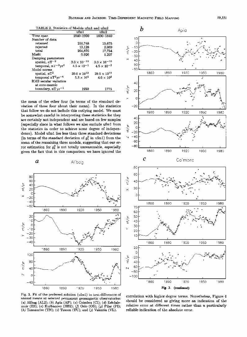
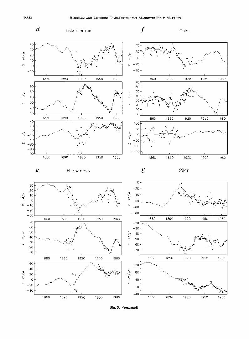
In Figure 3, we show the fit of the 1840-1990 preferred solution to the first-differences of annual means at a number
of permanent magnetic observatories. We chose for Figure 3 observatories with particularly long time spans of operation, while seeking a good geographical distribution. It is appar- ent that we have achieved a very good fit to the observatory first-differences, especially to the Y component which is less noisy than the others. The concern is that we may have over- fitted the data, a concern that is rather hard to address. To do so, we need to consider in much greater detail the origin and effect of solar cycle period signals in the observatory data, since clearly the decision on what constitutes an ade- quate fit to the observatory data is obfuscated by the obvious
presence of solar cycle signals in the data. Here, instead, rec- ognizing that our preferred solution is already very simple temporally compared to models such as GSFC(9/80) Lan- gel et al. [1982] and is also slightly simpler than the model of paper 2, we adopt a conservative approach and decide against choosing an even smoother solution as our preferred solution. We note, though, that simpler solutions with not unacceptably poor fits to the observatory data exist.
Error and Resolution Analysis
The covariance matrix C of the solution is given by
C -- •r2 (ATC;1A -k C•1) -1 (13) Here •r 2 is the misfit [see Gubbins and Bloxham, 1985]. The covariance matrix is important as a means of assessing the uncertainty in the model, although due attention must be paid to the limitations of the covariance matrix highlighted by Backus [1988a, b]. In general, we are interested in the uncertainty of linear functionals of the model, such as the uncertainty in an estimate of the instantaneous secular vari- ation for use in determining core flow. Such linear function-
19,548 BLOXHAM AND JACKSON: TIME-DEPENDENT MAGNETIC FIELD MAPPING
a 1690 1740
740 1790
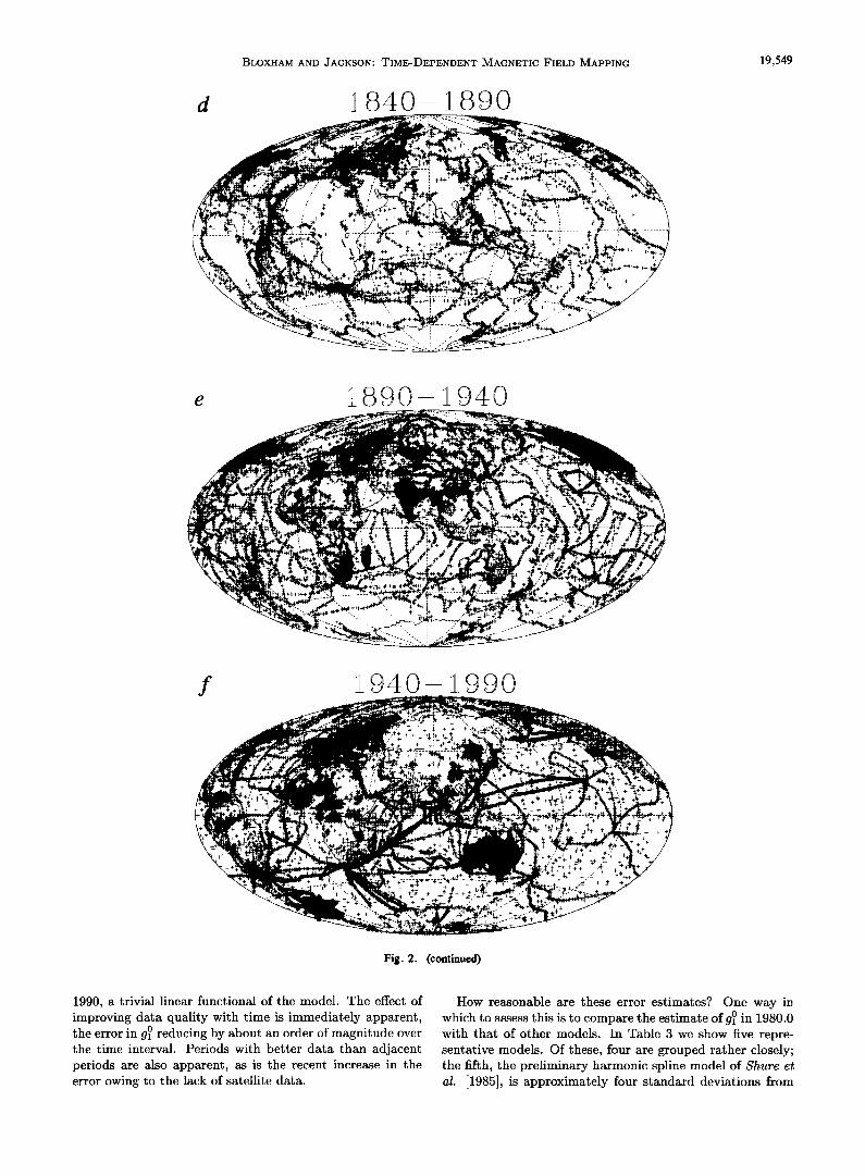
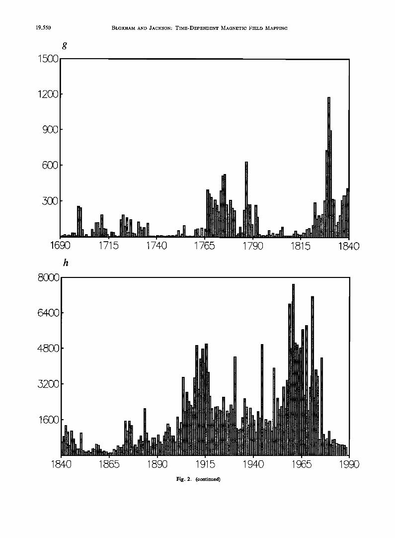
Fig. 2. Data distribution: (a-f) geographical distribution of data in successive 50 year intervals plotted on an Aitoff equal-area projection, and (g-h) distribution of data in time.
als can be written in the general form
m; = km (14)
where na• is of smaller dimension than m. The covariance
of mL, CL is then given by
CL - LCL T (15)
In the appendix we present an efficient algorithm for com- puting CL.
As an example, in Figure 4 we show the uncertainty in our estimate of the axial dipole term gl ø for the period 1840-
BLOXHAM AND JACKSON: TIME-DEPENDENT MAGNETIC FIELD MAPPING 19,549
d 85-0 1890
f
180
Fig. 2. (continued)
1990, a trivial linear functional of the model. The effect of improving data quality with time is immediately apparent, the error in gl ø reducing by about an order of magnitude over the time interval. Periods with better data than adjacent periods are also apparent, as is the recent increase in the error owing to the lack of satellite data.
How reasonable are these error estimates? One way in which to assess this is to compare the estimate of g• in 1980.0 with that of other models. In Table 3 we show five repre- sentative models. Of these, four are grouped rather closely; the fifth, the preliminary harmonic spline model of •qhure et al. [1985], is approximately four standard deviations from
19,550 BLOXHAM AND JACKSON: TIME-DEPENDENT MAGNETIC FIELD MAPPING
$
15o0
12oo
9oo
6OO
300
1690 1715 1740 1765 1790 1815 1840
8OOO
4800
3200
1600
1840 1865 1890 1915 1940 1965 1990
Fig. 2. (continued)
BLOXHAM AND JACKSON: TIME-DEPENDENT MAGNETIC FIELD MAPPING 19,551
TABLE 2. Statistics of Models ufml and ufm2 ufml ufm2
Time span 1840-1990 1690-1840 Number of data
retained 251,748 15,675 rejected 13,128 2,069 total 264,876 17,754
Misfit 0.926 1.207
Damping parameters spatial, nT -2 3.0 x 10 -lø 3.0 x 10 -lø temporal, nT-2yr 4 4.5 x 10 -1 4.5 x 10 -2
Model norms
spatial, nT 2 39.0 x 10¹² 29.5 x 10¹² temporal nT2yr -4 5.3 x 10⁴ 4.0 x 10⁴
RMS secular variation
at core-mantle
boundary, nT yr -1 1950 1775
the mean of the other four (in terms of the standard de- viation of these four about their mean). In the statistics that follow we do not include this outlying model. We must be somewhat careful in interpreting these statistics for they are certainly not independent and are based on few samples (especially since in what follows we also exclude ufml from the statistics in order to achieve some degree of indepen- dence). Model ufml lies less than three standard deviations (in terms of the standard deviation of gl ø in ufml) from the mean of the remaining three models, suggesting that our er- ror estimation for gl ø is not totally unreasonable, especially given the fact that in this comparison we have ignored the
a Alibag
40 . 20 '•-•-•• . •. * 'X * o
-20[ . - 40 -60
1860 18•0 1920 1 •50 1980
2O
-10
-20
-30
-40
_
- V-- ++ I I • i I
1860 1890 1920 1950 1980 +
12o - _ /•+
• 40 •
N 0-
--40 - • • • • + • I 1860 1890 1920 1950 1980
Pig. 3. Pi• of •he preferred solution (ufml) •o nrs•-differences of annual means a• selecCed permanem geomagne½ic observatories: (a) Alibag (AL2); (b) Apia (AP); (c) Coimbra (CI); (d) •skdale- •.i• (•s); (•) •.•b•o•o (•m); (• Oao (os); (a) P•b• (•) ••i• (•); (0 •co• (•u); •d (2 Wb•a• (V•).
b Apio
10
o
-10 -20
-30
-40 -50
-60
-- +
+ _+ n•- - • +
- • •+•+ + ,,••j ' •+' + + + %+ +1
- + • , I - I ! I + I
18•0 1890 1920 1950 1980
4O
2O
.-- 0
-2O
** ***•, _•_. . •.•* ½,*/• \* ** -
I I I I i +++ 1860 1890 1920 1950 1980
4o ** I + +^•+ +-•+ I
20 . ¾ '•• 'x. *1
-20 • *• •* • _ +•+ + +
-40 •' .+
-60 *
-80 1860 1890 1920 1950 1980
C Coimbra
8O + +
60- * * • •* % ++ + A.+
,+ + ++ + •-+ • +. •'.½-•.'
20- * **• +•*• . * * + % +
0- +
I I I • I I 1 860 1890 ]920 1 950 ]980
70-
60
5O
4O
30
2O
10
1860 1890 1920 1950 1980
_ 20
0
•, -20 -•- -40
N --60 --80
-lOO
- + + +k ,+ , z $
_ + +++ ++
_
I I + I I I
1860 1890 1920 1950 1980
Fig. 3. (continued)
correlation with higher degree terms. Nonetheless, Figure 4 should be considered as giving more an indication of the relative error at different times rather than a particularly reliable indication of the absolute error.
19,552 BLOXHAM AND JACKSON: TIME-DEPENDENT MAGNETIC FIELD MAPPING
d Eskdalemuir f Oso
4o
lO
x o
-lO
6o
lo
4o
2o
o -20
-40
-60
-80
-too
++
1860 1890 1920 1950 1980
_ +
_
+ + _
- I I I
1860 1890 1920 1950 ] 980
1860 1890 1920 1950 1980
40
x -20
-40
7O
60
b, 5O • 40
50
•- 20
10
0
IO0
50
o -50
-100
-150
1860 1890 1920 1950 1980
+'¾.' _,_ "'- *,,t--,,• ++,4- + • / - %++
1560 1890 1920 1950 1980
_ +
_ + +++ ++ + + ++ +,++•'• ++
- ++ + ++ +
- +
1860 1890 1920 1950 1980
½ Hurbanovo
5o
0
-10
-20
-50
70
60
50
40
50
20
10
60
o
N -20
-40
_ + +
_ + +
_
- I I +
1860 1890
i i
192_0 1950 1980
_ •-•/_ 1- +••+ _
_ + + +
1860 1890 1920 1950 1980
_ .' ', +++
/ +
_ +
1860 1890 1920 1950 1980
0
-80
-100
-2O
-5O
c -50 -
>- -60
-70
120
.b., 8O
4O
N
o
-4o
1860 1890 t920 1950 1980
'"x\ +
1860 1890 1920 1950 1980
1860 1890 1920 19,.50 1980
Fig. 3. (½ominued)
BLOXHAM AND JACKSON: TIME-DEPENDENT MAGNETIC FIELD MAPPING 19,553
h TGnanarive j Va en tie
40
0
-4o
-12o
80
• 4o
• 0
-40
-80
2OO
150
100
5O
N 0
--50
-lOO
-6o
20
lO
-lO
-20 -3o
-40
-20
-8O
1860 1890 1920 1950 1980
186O
•+ +
+-,-
1890 1920 1950 1980
+
_
-k +
_ + ,•.•.• -t +
- I I -• I 1
1860 1890 1920 1950 1980
i Tuscon
+ + - +. ++aa- + ,•
•/'- •"--k• .+J+ \
• •+ ++
- • + •++ .
_
_
I I + I I t
• 860 1890 ] 920 1950 1980
1860 1890 1920 1950 1980
- • + + +
- I I I + 1
1860 1890 1920 1950 1980
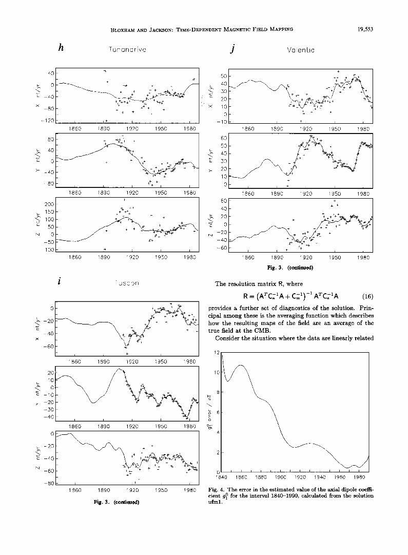
Fig. 3. (continued)
5O
4O
30
20
10
0
-10
+
- ++ + •X +
++ +
x+ *+ + +• 5++
_ • • ,.•" ++. * ++ +
• + +
- I I + i I i
• 860 •90 1920 • 950 1980
60
50
40
30
20
10
0
/•-•-x + + + - / %'5 +
_
1860 1890 1920 1950 1980
6O
4-0
20
0
-20
-40
-60
+
+ 4-
+ +_+ - +.+ * • 7•
- +/+
• + +X•,/, +• ••,' +
1860 1890 1920 1950 1980
Fig. 3. (continued)
The resolution matrix R, where
R- (A':rC:IA + C•-nl) --1 A':rC:IA (16) provides a further set of diagnostics of the solution. Prin- cipal among these is the averaging function which describes how the resulting maps of the field are an average of the true field at the CMB.
Consider the situation where the data are linearly related
12
10
1840 1860 1880 1900 1920 1940 1960 1980
Fig. 4. The error in the estimated value of the axial dipole coeffi- cient g• for the interval 1840-1990, calculated from the solution ufml.
19,554 BLOXHAM AND JACKSON: TIME-DEPENDENT MAGNETIC FIELD MAPPING
TABLE 3. Comparison of the Axial Dipole Component of Selected Geomagnetic Field Models
for 1980
Model g• nT Reference ufml -29990 this paper DGRF 1980 -29992 IAGA Division V [1992] GSFC(9/80) -29988 Langel et al. [1982] D80111 -29993 Gubbins and Bloxham [1985] phs(80) -30001 Shure et al. [1985]
to the model of the CMB field; this is the case for the el- ements X, Y, and Z. Then as discussed in paper 2, the averaging function for an estimate of the field at a particu- lar point in space and time (00, •b0,t0) can be viewed both as a spatial function over other points (0, •b) in space at the same time to (the spatial averaging function), and as a tem- poral function over other points t in time at the same point (•, •b) in space (the temporal averaging function). The av- eraging function shows how the estimate of the model at a particular point is constructed from the data, i.e. how the true model is averaged to produce an estimate of the model at some point. In other words, our estimate of the field at the CMB/•(•0, •b0, to) is given by
• (Oo, •o, to) -
MB
where B•(O,c•,t) is the true field at the CMB, and A(O, •b,t; 00, •b0,t0) is the averaging function. Now we can also write this estimate /• as a linear combination of the data (in the linear situation we are considering)
• (00, •0, to) - •. g(c, 00, •0, to; •, 0•, •, i
(18)
and the data are •elated to the field B• by
7, - O(c, o, 4, t; •,, o,, 4,, t,) •(c, o, 4, t) as at oo MB
(10) where ri, Oi, (•i, ti are the coordinates of the ith datum The Greens function G can be decomposed into temporal and spatial ingredients
G(C, O, •, t; •i, Oi, •i, ti) : Gs(c, O, •; •i, Oi, •i)•(t - ti) (20)
Note that the temporal ingredient of the Greens function is
simply a 5 function owing to our neglect of mantle conductiv- ity. Combining these equations, we can write the averaging function in the form
A(O, 0, t; 0o, 0o, to) • g(c, 0o, ½o, to; r•, 0•, ½•, t•) x i
Gs(c, O, •; •, 0•, •)•(t - t•) (2•)
We may choose to calculate A either in the spatial domain, i.e., by calculating A(O, •b, to; 00, •b0, to), to show how an es- timate of the field is a spatial average of the true field at that same point in time, or in the temporal domain, i.e., by calculating A(00, •b0, t; 00, •b0, to), to show how an estimate of the field is a temporal average of the true field at that point in space.
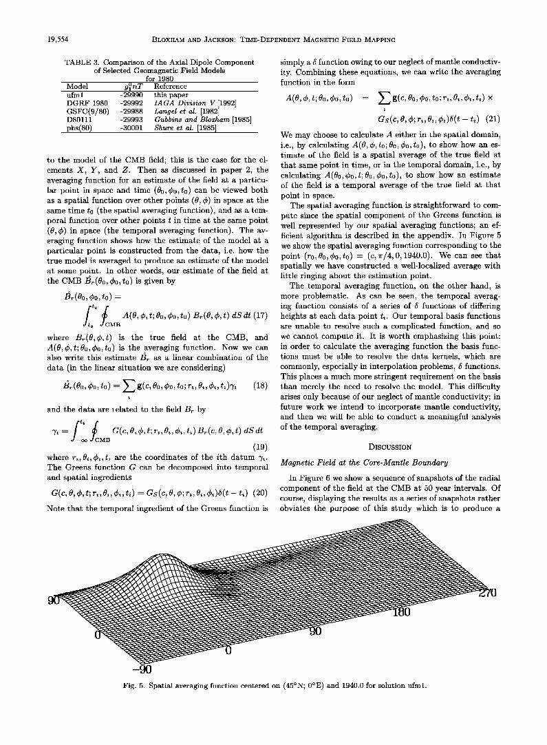
The spatial averaging function is straightforward to com- pute since the spatial component of the Greens function is well represented by our spatial averaging functions; an ef- ficient algorithm is described in the appendix. In Figure 5 we show the spatial averaging function corresponding to the point (r0,00, •b0, to) = (c, •r/4, 0, 1940.0). We can see that spatially we have constructed a well-localized average with little ringing about the estimation point.
The temporal averaging function, on the other hand, is more problematic. As can be seen, the temporal averag- ing function consists of a series of 5 functions of differing heights at each data point ti. Our temporal basis functions are unable to resolve such a complicated function, and so we cannot compute it. It is worth emphasizing this point: in order to calculate the averaging function the basis func- tions must be able to resolve the data kernels, which are commonly, especially in interpolation problems, 5 functions. This places a much more stringent requirement on the basis than merely the need to resolve the model. This difficulty arises only because of our neglect of mantle conductivity; in future work we intend to incorporate mantle conductivity, and then we will be able to conduct a meaningful analysis of the temporal averaging.
DISCUSSION
Magnetic Field at the Core-Mantle Boundary
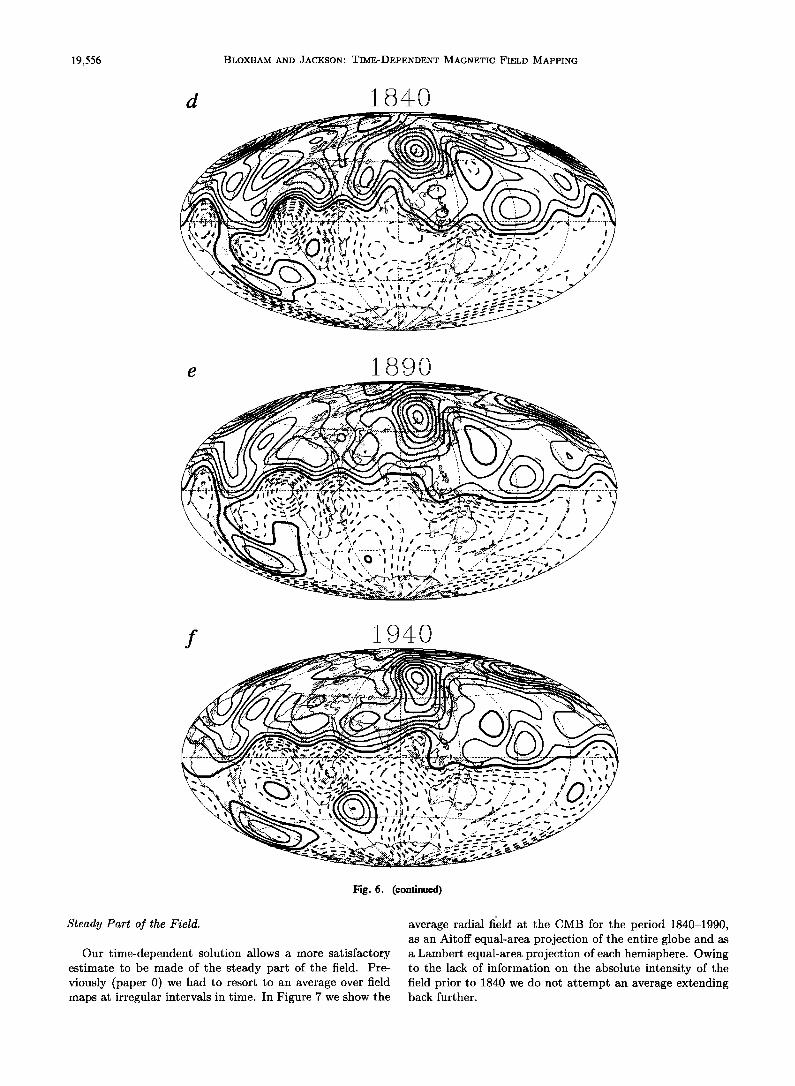
In Figure 6 we show a sequence of snapshots of the radial component of the field at the CMB at 50 year intervals. Of course, displaying the results as a series of snapshots rather obviates the purpose of this study which is to produce a
Fig. 5. Spatial averaging function centered on (45øN; 0øE) and 1940.0 for solution ufml.
BLOXHAM AND JACKSON: TIME-DEPENDENT MAGNETIC FIELD MAPPING 19,555
a 1690
b 1740
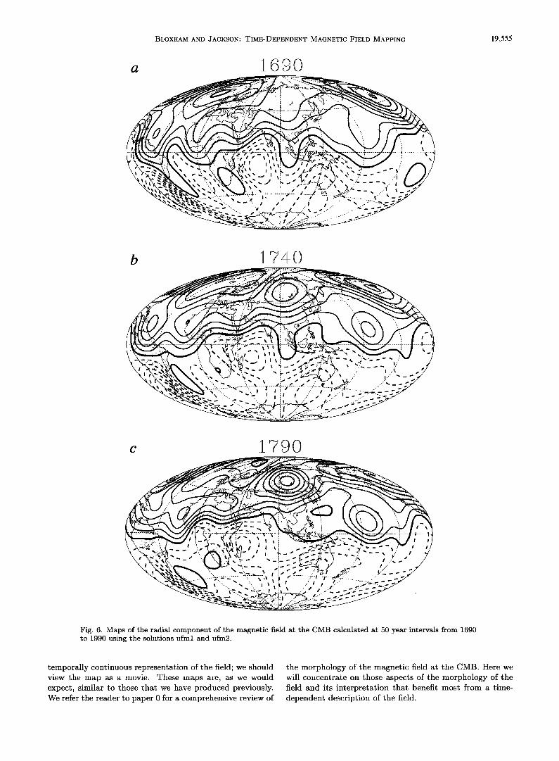
Fig. 6. Maps of the radial component of the magnetic field at the CMB calculated at 50 year intervals from 1690 to 1990 using the solutions ufml and ufm2.
temporally continuous representation of the field; we should view the map as a movie. These maps are, as we would expect, similar to those that we have produced previously. We refer the reader to paper 0 for a comprehensive review of
the morphology of the magnetic field at the CMB. Here we will concentrate on those aspects of the morphology of the field and its interpretation that benefit most from a time- dependent description of the field.
19,556 BLOXHAM AND JACKSON: TIME-DEPENDENT MAGNETIC FIELD MAPPING
Fig. 6. (continued)
Steady Part of the Field.
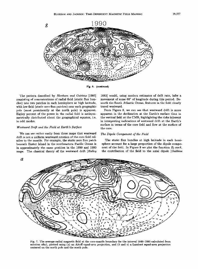
Our time-dependent solution allows a more satisfactory estimate to be made of the steady part of the field. Pre- viously (paper 0) we had to resort to an average over field maps at irregular intervals in time. In Figure 7 we show the
average radial field at the CMB for the period 1840-1990, as an Airoff equal-area projection of the entire globe and as a Lambert equal-area projection of each hemisphere. Owing to the lack of information on the absolute intensity of the field prior to 1840 we do not attempt an average extending back further.
BLOXHAM AND JACKSON: TIME-DEPENDENT MAGNETIC FIELD MAPPING 19,$$7
Fig. 6. (continued)
The pattern described by Bloxham and Gubbins [1985] consisting of concentrations of radial field (static flux bun- dles) into two patches in each hemisphere at high latitude, with low field (static zero flux patches) near each geographic pole (most prominently at the north pole) is apparent. Eighty percent of the power in the radial field is antisym- metrically distributed about the geographical equator, i.e. in odd modes.
Westward Drift and the Field at Earth's Surface
We can see rather easily from these maps that westward drift is not a uniform westward rotation of the core field rel-
ative to the mantle. For example, the static zero flux patch beneath Easter Island in the southeastern Pacific Ocean is
in approximately the same position in the 1690 and 1990 maps. The classical theory of the westward drift [Halley
1683] would, using modern estimates of drift rate, infer a movement of some 60 ø of longitude during this period. Be- neath the South Atlantic Ocean, features in the field clearly travel westward.
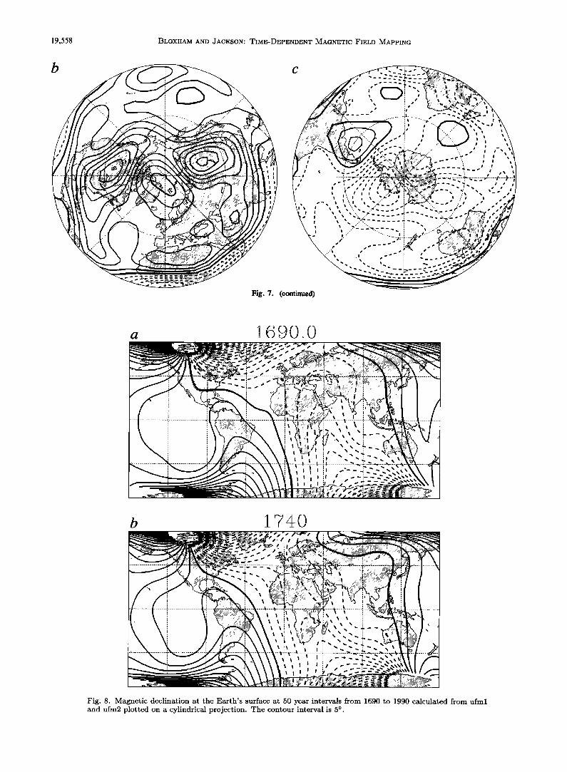
From Figure 8, we can see that westward drift is more apparent in the declination at the Earth's surface than in the vertical field at the CMB, highlighting the risks inherent in interpreting indications of westward drift at the Earth's surface in terms of the core field and flow at the surface of
the core.
The Dipole Component of the Field
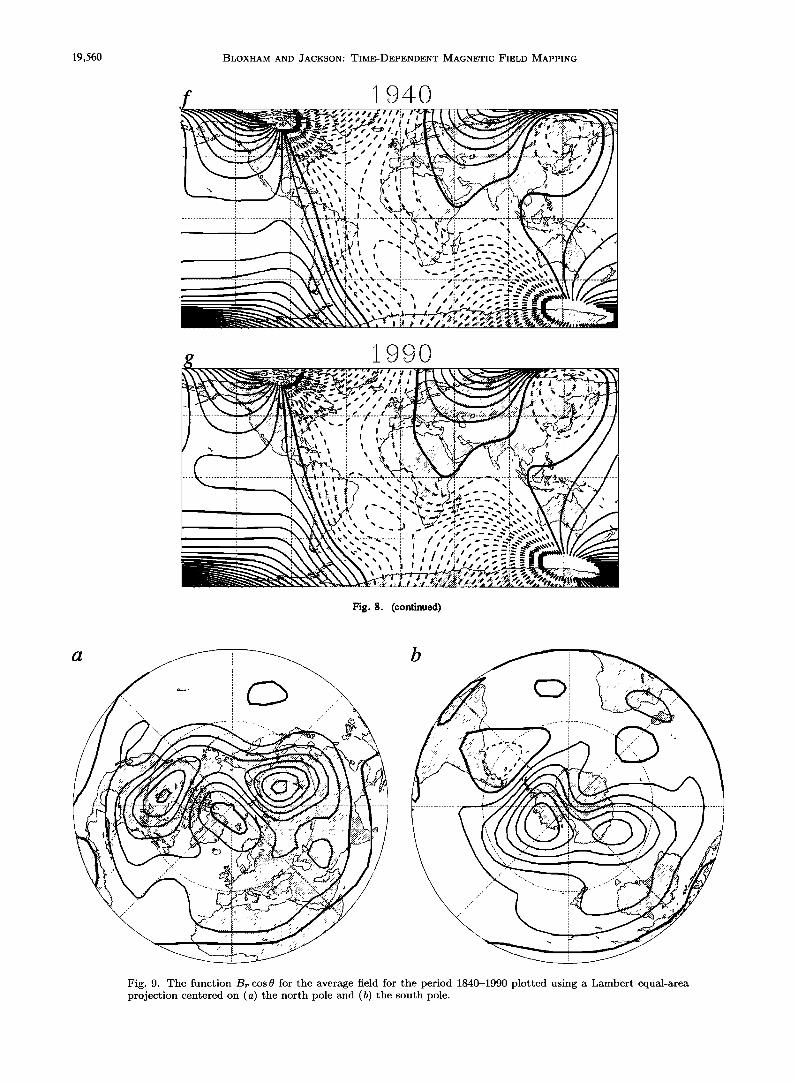
The static flux bundles at high latitude in each hemi- sphere account for a large proportion of the dipole compo- nent of the field. In Figure 9 we plot the function B• cos the contribution of the field to the axial dipole [Gubbins
Fig. 7. The average radial magnetic field at the core-mantle boundary for the interval 1840-1990 calculated from solution ufml, plotted using (a) an Aitoff equal-area projection, and (b and c) a Lambert equal-area projection centered on the north pole and the south pole.
19,558 BLOXHAM AND JACKSON' TIME-DEPENDENT MAGNETIC FIELD MAPPING
b
Fig. 7. (continued)
a ]L690o0
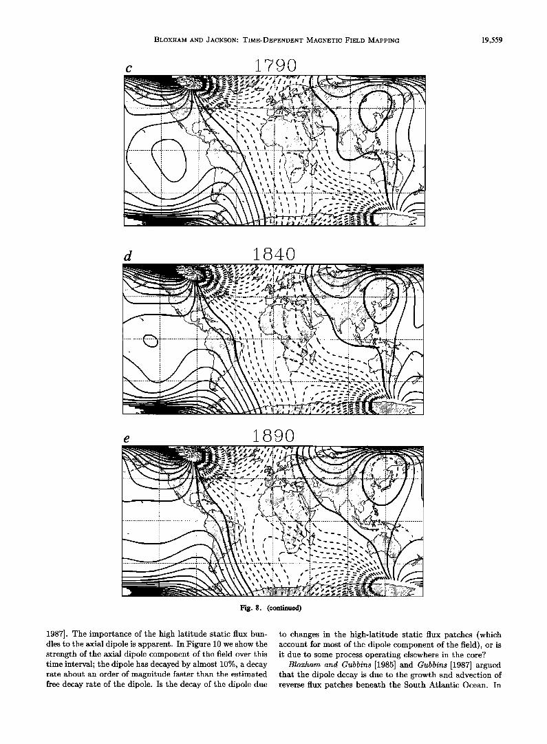
Fig. 8. Magnetic declination at the Earth's surface at 50 year intervals from 1690 to 1990 calculated from ufml and ufm2 plotted on a cylindrical projection. The contour interval is 5 ø.
BLOXHAM AND JACKSON: TIME-DEPENDENT MAGNETIC FIELD MAPPING 19,559
c 1700
Fig. 8. (continued)
1987]. The importance of the high latitude static flux bun- dles to the axial dipole is apparent. In Figure 10 we show the strength of the axial dipole component of the field over this time interval; the dipole has decayed by almost 10%, a decay rate about an order of magnitude faster than the estimated free decay rate of the dipole. Is the decay of the dipole due
to changes in the high-latitude static flux patches (which account for most of the dipole component of the field), or is it due to some process operating elsewhere in the core?
Bloxham and Cubbins [1985] and Cubbins [1987] argued that the dipole decay is due to the growth and advection of reverse flux patches beneath the South Atlantic Ocean. In
19,560 BLOXHAM AND JACKSON: TIME-DEPENDENT MAGNETIC FIELD MAPPING
1940
'?.:::'::-:•*" : / ! • '.',•.• .......
\ • • i •
• ., :,., • .....
:!•.': ':i:¾! ,', • i : •
:• • \'•' -', ' -'"
1990 • • • • ::::::::::::::::::::::::: t '
•__.•_•___t___ • • ........... • • ...... •:•:- .•f•?:•f•?:•:•::.::•:•f• ....
Fig. 8. (continued)
b
Fig. 9. The function Br cos 9 for the average field for the period 1840-1990 plotted using a Lambert equal-area projection centered on (a) the north pole and (b) the south pole.
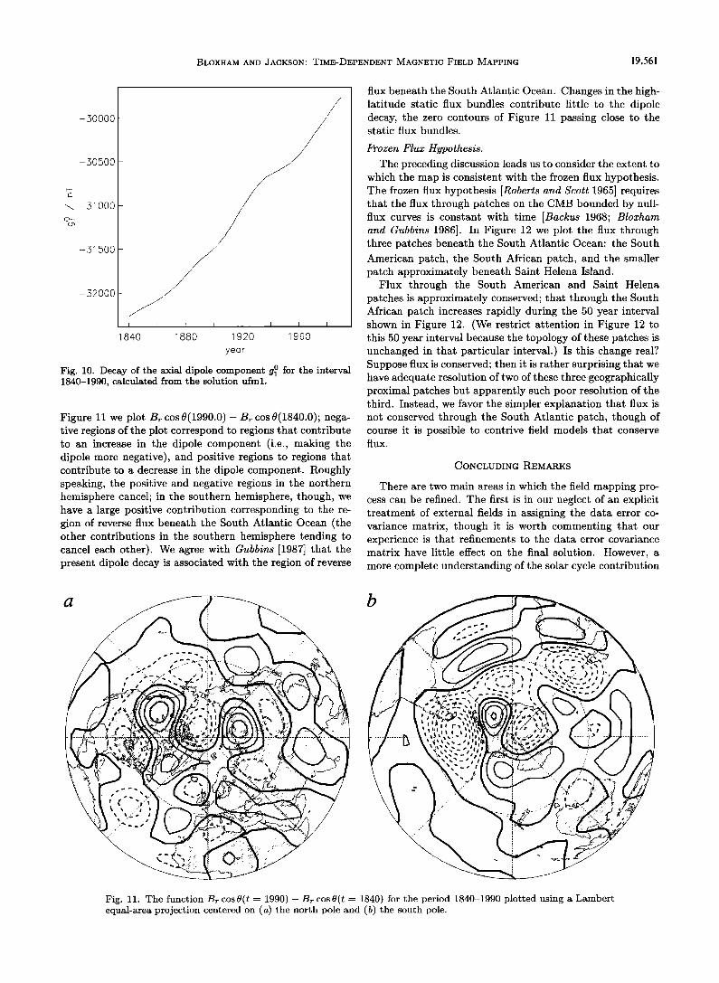
BLOXHAM AND JACKSON: TIME-DEPENDENT MAGNETIC FIELD MAPPING 19,561
-30000
-50500
N -31000
-31500
-32000
84O 1880 1 9170 1960
year
Fig. 10. Decay of the axial dipole component g•0 for the interval 1840-1990, calculated from the solution ufml.
Figure 11 we plot By cos 0(1990.0) - By cos 0(1840.0); nega- tive regions of the plot correspond to regions that contribute to an increase in the dipole component (i.e., making the dipole more negative), and positive regions to regions that contribute to a decrease in the dipole component. Roughly speaking, the positive and negative regions in the northern hemisphere cancel; in the southern hemisphere, though, we have a large positive contribution corresponding to the re- gion of reverse flux beneath the South Atlantic Ocean (the other contributions in the southern hemisphere tending to cancel each other). We agree with Cubbins [1987] that the present dipole decay is associated with the region of reverse
flux beneath the South Atlantic Ocean. Changes in the high- latitude static flux bundles contribute little to the dipole decay, the zero contours of Figure 11 passing close to the static flux bundles.
Frozen Flux Hypothesis.
The preceding discussion leads us to consider the extent to which the map is consistent with the frozen flux hypothesis. The frozen flux hypothesis [Roberts and Scott 1965] requires that the flux through patches on the CMB bounded by null- flux curves is constant with time [Backus 1968; Bloxham and Gubbins 1986]. In Figure 12 we plot the flux through three patches beneath the South Atlantic Ocean: the South American patch, the South African patch, and the smaller patch approximately beneath Saint Helena Island.
Flux through the South American and Saint Helena patches is approximately conserved; that through the South African patch increases rapidly during the 50 year interval shown in Figure 12. (We restrict attention in Figure 12 to this 50 year interval because the topology of these patches is unchanged in that particular interval.) Is this change real? Suppose flux is conserved; then it is rather surprising that we have adequate resolution of two of these three geographically proximal patches but apparently such poor resolution of the third. Instead, we favor the simpler explanation that flux is not conserved through the South Atlantic patch, though of course it is possible to contrive field models that conserve flUX.
CONCLUDING REMARKS
There are two main areas in which the field mapping pro- cess can be refined. The first is in our neglect of an explicit treatment of external fields in assigning the data error co- variance matrix, though it is worth commenting that our experience is that refinements to the data error covariance matrix have little effect on the final solution. However, a more complete understanding of the solar cycle contribution
a b
Fig. 11. The function By cos0(t -- 1990) - By cos0(t = 1840) for the period 1840-1990 plotted using a Lambert equal-area projection centered on (a) the north pole and (b) the south pole.
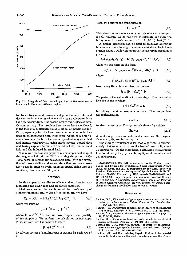
19,562 BLOXHAM AND JACKSON: TIME-DEPENDENT MAGNETIC FIELD MAPPING
800
500
400
300
200
100
0• 1910
• South Americen Petc•
South Africon Porch
I I I I I
1920 1950 1940 1950 1960
yeor
Fig. 12. Integrals of flux through patches on the core-mantle boundary in the south Atlantic region.
to observatory annual means would permit a more informed decision to be made on what constitutes an adequate fit to the observatory data. The second area is our neglect of man- tle conductivity. The problem here, as we have mentioned, is the lack of a sufficiently reliable model of mantle conduc- tivity, especially for the lowermost mantle. One ambitious possibility, addressing both these areas, would be a simulta- neous inversion for both the time-dependent magnetic field and mantle conductivity, using much shorter period data and taking explicit account of the main field, the external field and the induced internal field.
The main result of this paper is a time-dependent map of the magnetic field at the CMB spanning the period 1690- 1990, based on almost all the available data (with the excep- tion of those satellite and survey data that we have chosen not to use in order to avoid mapping crustal fields into the solutions) from the last 300 years.
APPENDIX
In this appendix we discuss efficient algorithms for ma- nipulating the covariance and resolution matrices.
First, we consider the calculation of the covariance CL of a linear functional mL = km of the model m. We have
C• - LCL 2" - a'2L (ATC•-iA -I- C•nl) -1 L • (Ai) which we write as
C• - L (H + C;•-) -•' L • (A2) where H = ArC2XA, and we have dropped the quantity &2 for simplicity. We perform the calculation in two steps. First, we calculate the matrix Y where
(H + CFn') Y- L (A3) by solving the set of simultaneous equations for each row of Y.
Then we perform the multiplication
C• - YL T (A4)
This algorithm represents a substantial savings over comput- ing CL directly. We do not need to calculate and store the full symmetric covariance matrix C - •r 2 (A T C• x A + C•n x ) - X.
A similar algorithm can be used to calculate averaging functions without having to compute and store the full res- olution matrix. Following paper 2, the averaging function is given by
A(O, •b, t; 00, •b0, to) - b T (00, •b0, t0)RS-Xb(0, •b, t) (A5) which we can write in the form
A(O, •b, t; O0, •b0, to) - a T (O0, •b0, t0)b(O, •b, t) (A6) where
T(Oo •b0 to) b T(oo •b0, t0)RS -x (A7) a , , • ,
Now, using the notation introduced above,
R- (H + C•-)-•' H (A8) We perform the calculation in three steps. First, we calcu- late the vector y where
(H + C2') y = b (A9) by solving the simultaneous equations. Then we perform the multiplication
z- Hy (AX0)
to give the vector z. Finally, we calculate a by solving
Sa--z (All)
A similar algorithm can be devised to calculate the diagonal elements of the resolution matrix.
The storage requirements for each algorithm is approxi- mately that required to store the banded matrix H, about 16 megawords. On the other hand, calculating the averaging function directly, i.e., by calculating R, would require about 200 megawords.
Acknowledgments. J.B. is supported by the Packard Foun- dation and by an NSF Presidential Young Investigator Award (EAR-9158298), and A.J. is supported by the Royal Society of London. This work was also supported by NASA awards NAG5- 918 and NAG5-1369, and by NSF awards EAR-8804618 and EAR-9018620. Supercomputer services were provided through NSF at the NASA Numerical Aerodynamic Simulation Program at Ames Research Center.We are very grateful to David Barra- clough for bringing the Buffon data to our attention.
REFERENCES
Backus, G.E., Kinematics of geomagnetic secular variation in a perfectly conducting core, Philos. Trans. R. Soc. London Set. A, 263, 239-266, 1968.
Backus, G.E., Application of mantle filter theory to the magnetic jerk of 1969, Geophys. J. R. Astron. Soc., 7J, 713-746, 1983.
Backus, G.E., Bayesian inference in geomagnetism, Geophys. J., 92, 125-142, 1988a.
Backus, G.E., Comparing hard and soft bounds in geophysical inverse problems, Geophys. J., 9•, 249-261, 1988b.
Barraclough, D.R., Spherical harmonic analyses of the geomag- netic field for eight epochs between 1600 and 1910, Geophys. J. R. Astron. $oc., 36, 497-513, 1974.
Benton, E.R., and K.A. Whaler, Rapid diffusion of the poloidal magnetic field through the weakly conducting mantle: A per-
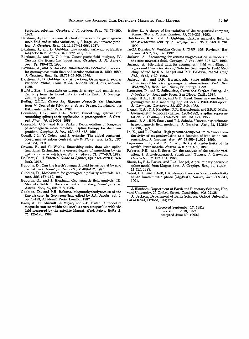
BLOXHAM AND JACKSON: TIME-DEPENDENT MAGNETIC FIELD MAPPING 19,563
turbation solution, Geophys. J. R. Astron. Soc., 75, 77-100, 1983.
Bloxham, J., Simultaneous stochastic inversion for geomagnetic main field and secular variation, 1, A large-scale inverse prob- lem, J. Geophys. Res., 92, 11,597-11,608, 1987.
Bloxham, J., and D. Cubbins, The secular variation of Earth's magnetic field, Nature, 317, 777-781, 1985.
Bloxham, J., and D. Cubbins, Geomagnetic field analysis, IV, Testing the frozen-flux hypothesis, Geophys. J. R. Astron. Soc., 8•, 139-152, 1986.
Bloxham, J., and A. Jackson, Simultaneous stochastic inversion for geomagnetic main field and secular variation 2. 1820-1980, J. Geophys. Res., 9•, 15,753-15,769, 1989.
Bloxham, J., D. Cubbins, and A. Jackson, Geomagnetic secular variation, Philos. Trans. R. Soc. London Set. A, 329, 415-502, 1989.
Buffett, B.A., Constraints on magnetic energy and mantle con- ductivity from the forced nutations of the Earth, J. Geophys. Res., in press, 1992.
Buffon, G.L.L., Comte de, Histoire Naturelie des Min•raux, tome V, Traite• de l'Airnant et de ses Usages, Imprimerie des Batiments du Roi, Paris, 1788.
Constable, C.G., and R.L. Parker, Smoothing, splines and smoothing splines; their application in geomagnetism, J. Corn- put. Phys., 78, 493-508, 1988.
Constable, C.G., and R.L. Parker, Deconvolution of long-core palaeomagnetic measurements -- spline therapy for the linear problem, Geophys. J. Int., 10•, 453-468, 1991.
Counil, J.L., Y. Cohen, and J. Achache, The global continent- ocean magnetization contrast, Earth Planet. Sci. Lett., 103, 354-364, 1991.
Craven, P., and G. Wahba, Smoothing noisy data with spline functions: Estimating the correct degree of smoothing by the method of cross validation, Nurner. Math., 31, 377-403, 1979.
De Boor, C., A Practical Guide to Splines, Springer-Verlag, New York, 1978.
Cubbins, D., Can the Earth's magnetic field be sustained by core oscillations?, Geophys. Res. Lett., 2, 409-412, 1975.
Cubbins, D., Mechanism for geomagnetic polarity reversals, Na- ture, 326, 167-169, 1987.
Cubbins, D., and J. Bloxham, Geomagnetic field analysis, III, Magnetic fields on the core-mantle boundary, Geophys. J. R. Astron. Soc., 80, 695-713, 1985.
Cubbins. D., and P.H. Roberts, Magnetohydrodynamics of the Earth's core, in Geornagnetisrn, edited by J.A. Jacobs, vol. 2, pp. 1-183, Academic Press, London, 1987.
Hahn, A., H. Ahrendt, J. Meyer, and J.H. Hufen, A model of magnetic sources within the earth's crust compatible with the field measured by the satellite Magsat, Geol. Jahrb. Reihe A, 75, 125-126, 1984.
Halley, E., A theory of the variation of the magnetical compass, Philos. Trans. R. Soc. London, 13, 208-221, 1683.
Hutcheson, K.A., and D. Cubbins, Earth's magnetic field in the seventeenth century, J. Geophys. Res., 95, 10,769-10,781, 1990.
IAGA Division V, Working Group 8, IGRF, 1991 Revision, Eos, Trans. A GU, 73, 182, 1992.
Jackson, A., Accounting for crustal magnetization in models of the core magnetic field, Geophys. J. Int., 103, 657-673, 1990.
Jackson, A., Historical data for geomagnetic field modelling, in Types and Characteristics of Data for Geomagnetic Field Mod- eling, edited by R.A. Langel and R.T. Baldwin, NASA Conf. Pub., 3153, 1-30, 1992.
Jackson, A., and D.R. Barraclough, Some additions to the collection of historical geomagnetic observations, Tech. Rep. WM/92•21, Brit. Geol. Surv., Edinburgh, 1992.
Lancaster, P., and K. Salkauskas, Curve and Surface Fitting: An Introduction, Academic Press, San Diego, Calif., 1986.
Langel, R A., R.H. Estes, and G.D. Mead, Some new methods in geomagnetic field modelling applied to the 1960-1980 epoch, J. Geornagn. Geoelectr., 3•, 327-349, 1982.
Langel, R.A., D.J. Kerridge, D.R. Barraclough, and S.R.C. Malin, Geomagnetic temporal change: 1903-1982, a spline represen- tation, J. Geornagn. Geoelectr., 38, 573-597, 1986.
Langel, R A., R.H. Estes, and T.J. Sabaka, Uncertainty estimates in geomagnetic field modeling, J. Geophys. Res., 9J, 12,281- 12,299, 1989.
Li, X., and R. Jeanloz, High pressure-temperature electrical con- ductivity of magnesiowfistite as a function of iron oxide con- centration, J. Geophys. Res., 95, 21,609-21,612, 1990.
Peyronneau, J., and J.P. Poirier, Electrical conductivity of the earth's lower mantle, Nature, 3•2, 537-539, 1989.
Roberts, P.H., and S. Scott, On the analysis of the secular vari- ation, 1, A hydromagnetic constraint: Theory, J. Geornagn. Geoelectr., 17, 137-151, 1965.
Shure, L., R.L. Parker, and R.A. Langel, A preliminary harmonic spline model from Magsat data, J. Geophys. Res., 90, 11,505- 11,512, 1985.
Wood, B.J., and J. Nell, High-temperature electrical conductivity of the lower-mantle phase (Mg,Fe)O, Nature, 351, 309-311, 1991.
J. Bloxham, Department of Earth and Planetary Sciences, Har- vard University, 20 Oxford Street, Cambridge, MA 02138.
A. Jackson, Department of Earth Sciences, Oxford University, Parks Road, Oxford, England.
(Received September 17, 1991; revised June 18, 1992;
accepted June 30, 1992.)
Top Related
Copyright © 2022 FDOKUMEN

