


Bahasa
Halaman
Hukum


Fran De Aquino
T O E
Theory of Everything
November 2012

Fran De Aquino
T O E
Theory of Everything
November
2012

ABSTRACT
This is a set of 25 articles, developed starting from the Relativistic Theory of Quantum Gravity (first article). Together they form the
Theory of Everything.

CONTENTS (421 pages)
1. Mathematical Foundations of the Relativistic Theory of Quantum Gravity
2. Gravity Control by means of Electromagnetic Field through Gas or Plasma at Ultra-Low Pressure
3. Physical Foundations of Quantum Psychology
4. The Gravitational Spacecraft
5. Possibility of controlled nuclear fusion by means of Gravity Control
6. High-power ELF radiation generated by modulated HF heating of the ionosphere can cause
Earthquakes, Cyclones and localized heating
7. The Universal Quantum Fluid
8. The Gravitational Mass of a Charged Supercapacitor
9. Beyond the Material Universe
10. On the Cosmological Variation of the Fine Structure Constant
11. The velocity of neutrinos
12. Proca Equations and the Photon Imaginary Mass
13. Gravity Control by means of Modified Electromagnetic Radiation
14. Transmission of DNA Genetic Information into Water by means of Electromagnetic Fields of Extremely-low Frequencies
15. A Possible Explanation for Anomalous Heat Production in Ni-H Systems
16. Engineering the Ni-H Bomb
17. Gravitational Shockwave Weapons
18. A System to convert Gravitational Energy directly into Electrical Energy
19. Superconducting State generated by Cooper Pairs bound by Intensified Gravitational Interaction
20. Gravitational Separator of Isotopes
21. Gravitational Atomic Synthesis at Room Temperature
22. Ultrafast Conversion of Graphite to Diamond in Gravitational Pressure Apparatus
23. Artificial Gravitational Lenses
24. Gravitational Blueshift and Redshift generated at Laboratory Scale
25. Quantum Reversal of Soul Energy
* * *

Mathematical Foundations of the Relativistic Theory of Quantum Gravity
Fran De Aquino
Maranhao State University, Physics Department, S.Luis/MA, Brazil. Copyright © 2008-2011 by Fran De Aquino. All Rights Reserved
Abstract: Starting from the action function, we have derived a theoretical background that leads to the quantization of gravity and the deduction of a correlation between the gravitational and the inertial masses, which depends on the kinetic momentum of the particle. We show that the strong equivalence principle is reaffirmed and, consequently, Einstein's equations are preserved. In fact, such equations are deduced here directly from this new approach to Gravitation. Moreover, we have obtained a generalized equation for the inertial forces, which incorporates the Mach's principle into Gravitation. Also, we have deduced the equation of Entropy; the Hamiltonian for a particle in an electromagnetic field and the reciprocal fine structure constant directly from this new approach. It was also possible to deduce the expression of the Casimir force and to explain the Inflation Period and the Missing Matter, without assuming existence of vacuum fluctuations. This new approach to Gravitation will allow us to understand some crucial matters in Cosmology. Key words: Quantum Gravity, Quantum Cosmology, Unified Field. PACs: 04.60.-m; 98.80.Qc; 04.50. +h Contents 1. Introduction 3 2. Theory 3 Generalization of Relativistic Time 4 Quantization of Space, Mass and Gravity 6 Quantization of Velocity 7 Quantization of Time 7 Correlation Between Gravitational and Inertial Masses 8 Generalization of Lorentz's Force 12 Gravity Control by means of the Angular Velocity 13 Gravitoelectromagnetic fields and gravitational shielding effect 14 Gravitational Effects produced by ELF radiation upon electric current 26 Magnetic Fields affect gravitational mass and the momentum 27 Gravitational Motor 28 Gravitational mass and Earthquakes 28 The Strong Equivalence Principle 30

2
Incorporation of the Mach's Principle into Gravitation Theory 30 Deduction of the Equations of General Relativity 30 Gravitons: Gravitational Forces are also Gauge forces 31 Deduction of Entropy Equation starting from the Gravity Theory 31 Unification of the Electromagnetic and Gravitational Fields 32 Elementary Quantum of Matter and Continuous Universal Fluid 34 The Casimir Force is a gravitational effect related to the Uncertainty Principle 35 The Shape of the Universe and Maximum speed of Tachyons 36 The expanding Universe is accelerating and not slowing down 38 Gravitational and Inertial Masses of the Photon 39 What causes the fundamental particles to have masses? 40 Electron’s Imaginary Masses 41 Transitions to the Imaginary space-time 44 Explanation for red-shift anomalies 50 Superparticles (hypermassive Higgs bosons) and Big-Bang 51 Deduction of Reciprocal Fine Structure Constant and the Uncertainty Principle 53 Dark Matter, Dark Energy and Inflation Period 53 The Origin of the Universe 59 Solution for the Black Hole Information Paradox 61 A Creator’s need 63 The Origin of Gravity and Genesis of the Gravitational Energy 64 Explanation for the anomalous acceleration of Pioneer 10 66 New type of interaction 68 Appendix A 71 Allais effect explained 71 Appendix B 74 References 75

3
1. INTRODUCTION Quantum Gravity was originally studied, by Dirac and others, as the problem of quantizing General Relativity. This approach presents many difficulties, detailed by Isham [1]. In the 1970's, physicists tried an even more conventional approach: simplifying Einstein's equations by assuming that they are almost linear, and then applying the standard methods of quantum field theory to the thus oversimplified equations. But this method, too, failed. In the 1980's a very different approach, known as string theory, became popular. Thus far, there are many enthusiasts of string theory. But the mathematical difficulties in string theory are formidable, and it is far from clear that they will be resolved any time soon. At the end of 1997, Isham [2] pointed out several "Structural Problems Facing Quantum Gravity Theory". At the beginning of this new century, the problem of quantizing the gravitational field was still open. In this work, we propose a new approach to Quantum Gravity. Starting from the generalization of the action function we have derived a theoretical background that leads to the quantization of gravity. Einstein's General Relativity equations are deduced directly from this theory of Quantum Gravity. Also, this theory leads to a complete description of the Electromagnetic Field, providing a consistent unification of gravity with electromagnetism. 2. THEORY We start with the action for a free-particle that, as we know, is given by
∫−=b
adsS α
where α is a quantity which characterizes the particle. In Relativistic Mechanics, the action can be written in the following form [3]:
dtcVcLdtSt
t
t
t∫ ∫ −−== 2
1
2
1
221α
where 221 cVcL −−= α
is the Lagrange's function. In Classical Mechanics, the Lagrange's function for a free-particle is, as we know, given by: where V is the speed of the particle and is a quantity hypothetically [
2aVL =
a 4] given by:
2ma =where is the mass of the particle. However, there is no distinction about the kind of mass (if gravitational mass, , or inertial mass ) neither about its sign
m
gm im( )± .
The correlation between and aα can be established based on the fact that, on the limit , the relativistic expression for
∞→cL must be
reduced to the classic expression .The result [2aVL = 5] is: cVL 22α= .
Therefore, if mcac =2=α , we obtain . Now, we must decide if 2aVL =
gmm = or imm = . We will see in this work that the definition of includes
. Thus, the right option is , i.e., gm
im gm.ma g 2=
Consequently, cmg=α and the generalized expression for the action of a free-particle will have the following form:
( )1∫−=b
ag dscmS
or

4
( )21 2222
1
dtcVcmSt
t g −−= ∫where the Lagrange's function is
( )31 222 .cVcmL g −−=
The integral dtcVcmSt
t g222 12
1−= ∫ ,
preceded by the plus sign, cannot have a minimum. Thus, the integrand of Eq.(2) must be always positive. Therefore, if , then necessarily
; if , then . The possibility of is based on the well-known equation
0>gm0>t 0<gm 0<t
0<t22
0 1 cVtt −±= of Einstein's Theory. Thus if the gravitational mass of a particle is positive, then t is also positive and, therefore, given by
220 1 cVtt −+= . This leads to the
well-known relativistic prediction that the particle goes to the future, if
. However, if the gravitational mass of the particle is negative, then
is negative and given by
cV →
t22
0 1 cVtt −−= . In this case, the prediction is that the particle goes to the past, if . Consequently,
is the necessary condition for the particle to go to the past. Further on, a correlation between the gravitational and the inertial masses will be derived, which contains the possibility of .
cV →0<gm
0<gm The Lorentz's transforms follow the same rule for and 0>gm 0<gm ,
i.e., the sign before 221 cV− will be when and if ( )+ 0>gm ( )− 0<gm .
The momentum, as we know, is the vector VLp
rr∂∂= .Thus, from
Eq.(3) we obtain
VMcV
Vmp g
g rr
r=
−±=
221The sign in the equation above will be used when and the
( )+0>gm ( )−
sign if 0<gm . Consequently, we will express the momentum in the following form
pr
( )41 22
VMcV
Vmp g
g rr
r=
−=
The derivative dtpdr is the inertial force which acts on the particle. If the force is perpendicular to the speed, we have
iF
( )51 22 dt
Vd
cV
mF g
i
rr
−=
However, if the force and the speed have the same direction, we find that
( )( )6
12
3
22 dtVd
cV
mF g
i
rr
−=
From Mechanics [6], we know that LVp −⋅
rr denotes the energy of the particle. Thus, we can write
( )71
2
22
2
cMcV
cmLVpE g
gg =
−=−⋅=
rr
Note that is not null forgE 0=V , but that it has the finite value
( )8200 cmE gg =
Equation (7) can be rewritten in the following form:
( ) ( )9
1
1
0
2
22
22
2
22
22
ii
gKii
i
g
E
ii
ii
g
gg
gg
Emm
EEmm
cmcV
cmcm
mm
cmcV
cmcmE
Ki
=+=
=
⎥⎥⎥⎥⎥
⎦
⎤
⎢⎢⎢⎢⎢
⎣
⎡
⎟⎟
⎠
⎞
⎜⎜
⎝
⎛−
−+=
=−−
−=
444 3444 21
By analogy to Eq. (8), into the equation above, is the inertial energy at rest. Thus,
200 cmE ii =
Kiii EEE += 0 is the total inertial energy, where is the kinetic KiE

5
inertial energy. From Eqs. (7) and (9) we thus obtain
( )101
2
22
20 .cM
cV
cmE i
ii =
−=
For small velocities , we obtain
( cV << )
( )112212
0 VmcmE iii +≈where we recognize the classical expression for the inertial kinetic energy of the particle. The expression for the gravitational kinetic energy, , is easily deduced by comparing Eq.(7) with Eq.(9). The result is
KgE
( )12.Emm
E Kii
gKg =
In the presented picture, we can say that the gravity, , in a gravitational field produced by a particle of gravitational mass , depends on the particle's gravitational energy, (given by Eq.(7)), because we can write
gr
gM
gE
( )1322
2
22 cr
cMG
cr
EGg gg −=−=
Due to rg ∂Φ∂= , the expression of the relativistic gravitational potential,
, is given by Φ
221 cVr
Gmr
GM gg
−−=−=Φ
Then, it follows that
2222 11 cVcVr
Gmr
GM gg
−=
−−=−=Φ
φ
where rGmg−=φ . Then we get
22222 11 cVr
Gm
cVrrg
−=
−∂
∂=
∂Φ∂ φ
whence we conclude that
222 1 cVr
Gmr
g
−=
∂Φ∂
By definition, the gravitational potential energy per unit of gravitational mass of a particle inside a gravitational field is equal to the gravitational potential of the field. Thus, we can write that
Φ
( )gmrU′
=Φ
Then, it follows that
( )222 1 cVr
mmG
rm
rrUF gg
gg−
′−=
∂Φ∂′−=
∂∂
−=
If and0>gm 0<′gm , or and 0<gm
0>′gm the force will be repulsive; the force will never be null due to the existence of a minimum value for (see Eq. (24)). However, if
gm0<gm
and 0<′gm , or and 0>gm 0>′gm the force will be attractive. Just for ig mm = and we obtain the Newton's attraction law.
ig mm ′=′
On the other hand, as we know, the gravitational force is conservative. Thus, gravitational energy, in agreement with the energy conservation law, can be expressed by the decrease of the inertial energy, i.e.,
( )14ig EE ΔΔ −=This equation expresses the fact that a decrease of gravitational energy corresponds to an increase of the inertial energy. Therefore, a variation iEΔ in
yields a variation iE ig EE ΔΔ −= in . Thus
gE
iii EEE Δ+= 0 ; igggg EEEEE ΔΔ −=+= 00
and ( )1500 igig EEEE +=+
Comparison between (7) and (10) shows that 00 ig EE = , i.e., 00 ig mm = . Consequently, we have

6
( )162 000 iigig EEEEE =+=+
However Kiii EEE += 0 .Thus, (16) becomes ( )170 .EEE Kiig −=
Note the symmetry in the equations of and .Substitution of iE gE Kiii EEE −=0
into (17) yields ( )182 Kigi EEE =−
Squaring the Eqs.(4) and (7) and comparing the result, we find the following correlation between gravitational energy and momentum :
( )192222
2
.cmpcE
gg +=
The energy expressed as a function of the momentum is, as we know, called Hamiltonian or Hamilton's function:
( )20222 .cmpcH gg += Let us now consider the problem of quantization of gravity. Clearly there is something unsatisfactory about the whole notion of quantization. It is important to bear in mind that the quantization process is a series of rules-of-thumb rather than a well-defined algorithm, and contains many ambiguities. In fact, for electromagnetism we find that there are (at least) two different approaches to quantization and that while they appear to give the same theory they may lead us to very different quantum theories of gravity. Here we will follow a new theoretical strategy: It is known that starting from the Schrödinger equation we may obtain the well-known expression for the energy of a particle in periodic motion inside a cubical box of edge length L [ 7 ]. The result now is
( )21,...3,2,18 2
22== n
LmhnEg
n
Note that the term 22 8 Lmh g (energy)
will be minimum for where is the maximum edge length of a cubical box whose maximum diameter
maxLL = maxL
( )223maxmax Ld =is equal to the maximum length scale of the Universe.
The minimum energy of a particle is obviously its inertial energy at rest
. Therefore we can write 22 cmcm ig =
22
22
8cm
Lmhn
gmaxg
=
Then from the equation above it follows that
( )238max
g cLnhm ±=
whence we see that there is a minimum value for given by gm
( ) ( )248max
ming cLhm ±=
The relativistic gravitational mass
( ) 21221 −
−= cVmM gg , defined in the Eqs.(4), shows that
( ) ( ) ( )25minmin gg mM = The box normalization leads to the conclusion that the propagation number
λπ2== kkr
is restricted to the
values Lnk π2= . This is deduced assuming an arbitrarily large but finite cubical box of volume [3L 8]. Thus, we have
λnL =From this equation, we conclude that
min
maxmax
Ln
λ=
and minminminmin nL λλ ==
Since 1=minn . Therefore, we can write that
( )26minmaxmax LnL =From this equation, we thus conclude that
( )27minnLL =or
( )28n
LL max=
Multiplying (27) and (28) by 3 and reminding that 3Ld = , we obtain

7
( )29n
ddorndd max
min ==
Equations above show that the length (and therefore the space) is quantized. By analogy to (23) we can also conclude that
( ) ( )308min
maxmax
cLhn
M g =
since the relativistic gravitational mass,
( ) 21221 −
−= cVmM gg , is just a
multiple of . gm Equation (26) tells us that
maxmaxmin nLL = . Thus, Eq.(30) can be rewritten as follows
( ) ( )318
2
max
maxmax cL
hnM g =
Comparison of (31) with (24) shows that ( ) ( ) ( )32min
2maxmax gg mnM =
which leads to following conclusion that ( ) ( )33min
2gg mnM =
This equation shows that the gravitational mass is quantized. Substitution of (33) into (13) leads to quantization of gravity, i.e.,
( )
( )( )34min
4
2max
min22
gnnr
Gmn
rGM
g gg
=
=⎟⎟⎠
⎞⎜⎜⎝
⎛==
From the Hubble's law, it follows that ( )2maxmaxmax dH~lH~V ==
( )2minminmin dH~lH~V ==whence
min
max
min
max
dd
VV
=
Equations (29) tell us that maxminmax ndd = . Thus the equation
above gives
( )35max
maxmin n
VV =
which leads to following conclusion
( )36n
VV max=
this equation shows that velocity is also quantized.
From this equation one concludes that we can have or maxVV =
2maxVV = , but there is nothing in between. This shows clearly that cannot be equal to c (speed of light in vacuum). Thus, it follows that
maxV
( )
( )( )
...........................................
..........................
max
max
max
max
max
max
max
numberbigaisnwhere
nVVnnTardyonsnVVnn
cnVVnn
nVVnn
TachyonsVVnVVnVVn
x
xx
xx
xx
xx
2211
11
3322
1
+=+=
+=+=
←===−−−−−−−−−−−−−−−−−−−−−−−−
−=−=
==
==
==
Then is the speed upper limit of the Tardyons and also the speed lower limit of the Tachyons. Obviously, this limit is always the same in all inertial frames. Therefore can be used as a reference speed, to which we may compare any speed , as occurs for the relativistic
factor
c
c
V221 cV− . Thus, in this factor,
does not refer to maximum propagation speed of the interactions such as some authors suggest; is just a speed limit which remains the same in any inertial frame.
c
c
The temporal coordinate of space-time is now ( is then obtained when ).
Substitution of into this
equation yields
0xtVx max=0 ctx =0
cVmax →
( lH~nnVVmax == )( )( )lxH~nVxt max
00 1== .
On the other hand, since lH~V = and nVV max= we can write that
nH~Vl max1−= .Thus ( ) ( ) maxtH~ntH~lx ==0 .
Therefore, we can finally write
( )( ) ( )371 0 ntlxH~nt max== which shows the quantization of time.

8
From Eqs. (27) and (37) we can easily conclude that the spacetime is not continuous it is quantized. Now, let us go back to Eq. (20) which will be called the gravitational Hamiltonian to distinguish it from the inertial Hamiltonian : iH
( )38220
2 .cmpcH ii +=Consequently, Eq. (18) can be rewritten in the following form:
( )392 igi HHH Δ=−
where iHΔ is the variation on the inertial Hamiltonian or inertial kinetic energy. A momentum variation pΔ yields a variation iHΔ given by:
( ) ( )40420
22420
22 cmcpcmcppH iii +−+Δ+=Δ By considering that the particle is initially at rest ( . Then, Eqs. (20),
(38) and (39) give respectively: ,
and
)0=p2cmH gg =
20cmH ii =
20
2
0
11 cmcm
pH ii
i ⎥⎥
⎦
⎤
⎢⎢
⎣
⎡−⎟⎟
⎠
⎞⎜⎜⎝
⎛ Δ+=Δ
By substituting , and into Eq.(39), we get
gH iH iHΔ
( )41112 0
2
00 .i
iig m
cmpmm
⎥⎥
⎦
⎤
⎢⎢
⎣
⎡−⎟⎟
⎠
⎞⎜⎜⎝
⎛ Δ+−=
This is the general expression of the correlation between the gravitational and inertial mass. Note that for ( )250cmp i>Δ , the value of becomes negative.
gm
Equation (41) shows that
decreases of for an increase of
. Thus, starting from (4) we obtain
gm
gmΔ
pΔ
( )( )21 cV
Vmmpp gg
−
Δ−=Δ+
By considering that the particle is initially at rest , the equation above gives ( 0=p
( )( )21 cV
Vmmp gg
−
Δ−=Δ
From the Eq.(16) we obtain: ( ) iiiiiiig EEEEEEEE ΔΔ −=+−=−= 0000 22
However, Eq.(14) tells us that gi EE ΔΔ =− ;
what leads to gig EEE Δ+= 0 or gig mmm Δ+= 0 . Thus, in the expression of pΔ we can replace ( )gg mm Δ− for , i.e, 0im
( )20
1 cV
Vmp i
−=Δ
We can therefore write
( )( )42
1 20 cV
cVcm
p
i −=
Δ
By substitution of the expression above into Eq. (41), we thus obtain:
( ) ( )43112 022
021
iig mcVmm ⎥⎦⎤
⎢⎣⎡ −−−=
−
For 0=V we obtain .Then, 0ig mm =
( ) ( )minmin 0ig mm =
Substitution of into the quantized
expression of (Eq. (33)) gives (mingm )
)
gM
( )min02
ig mnM = where is the elementary quantum of inertial mass to be determined.
(min0im
For 0=V , the relativistic
expression 221 cVmM gg −= becomes
00 ggg mMM == . However, Eq. (43) shows
that 00 ig mm = . Thus, the quantized
expression of reduces to gM
( )min02
0 ii mnm =In order to define the inertial quantum number, we will change n in the expression above for . Thus we have in
( ) ( )44min02
0 iii mnm =
)

9
which shows the quantization of inertial mass; is the inertial quantum number.
in
We will change in the quantized expression of for in order to define the gravitational quantum number. Thus, we have
ngM gn
( ) ( )amnM igg 440
2min=
Finally, by substituting given by Eq. (43) into the relativistic expression of , we readily obtain
gm
gM
( ) ( )451121
21
22
22
ii
gg
McVMcV
mM
⎥⎦⎤
⎢⎣⎡ −−−=
=−
=
−
By expanding in power series and neglecting infinitesimals, we arrive at:
( )4612
2
ig McVM ⎟
⎟⎠
⎞⎜⎜⎝
⎛−=
Thus, the well-known expression for the simple pendulum period, ( )( )glMMT giπ2= , can be rewritten in the following form:
cVforc
VglT <<⎟
⎟⎠
⎞⎜⎜⎝
⎛+=
2
2
212π
Now, it is possible to learn why Newton’s experiments using simple penduli do not find any difference between and . The reason is due to the fact that, in the case of penduli, the ratio
gM iM
22 2cV is less than , which is much smaller than the
accuracy of the mentioned experiments.
1710−
Newton’s experiments have been improved upon (one part in 60,000) by Friedrich Wilhelm Bessel (1784–1846). In 1890, Eötvos confirmed Newton’s results with
accuracy of one part in . Posteriorly, Eötvos experiment has been repeated with accuracy of one part in . In 1963, the experiment was repeated with an even greater accuracy, one part in . The result was the same previously obtained.
710
910
1110
In all these experiments, the ratio 22 2cV is less than , which is much smaller than the accuracy of
obtained in the previous more precise experiment.
1710−
1110−
Then, we arrive at the conclusion that all these experiments say nothing in regard to the relativistic behavior of masses in relative motion. Let us now consider a planet in the Sun’s gravitational field to which, in the absence of external forces, we apply Lagrange’s equations. We arrive at the well-known equation:
h=
=−⎟⎠⎞
⎜⎝⎛+⎟
⎠⎞
⎜⎝⎛
dtdr
rGM
dtdr
dtdr i
ϕ
ϕ
2
22
2 2E
where is the inertial mass of the Sun. The term
iMaGM i−=E , as we
know, is called the energy constant; is the semiaxis major of the Kepler-
ellipse described by the planet around the Sun.
a
By replacing into the differential equation above for the expression given by Eq. (46), and expanding in power series, neglecting infinitesimals, we arrive, at:
iM
⎟⎟⎠
⎞⎜⎜⎝
⎛+=−⎟
⎠⎞
⎜⎝⎛+⎟
⎠⎞
⎜⎝⎛
2
222
2 22
cV
rGM
rGM
dtdr
dtdr gg Eϕ
Since ( )dtdrrV ϕω == , we get
2
2
22
2 22⎟⎠⎞
⎜⎝⎛+=−⎟
⎠⎞
⎜⎝⎛+⎟
⎠⎞
⎜⎝⎛
dtd
c
rGMr
GMdtdr
dtdr gg ϕϕ E
which is the Einsteinian equation of the planetary motion.

10
Multiplying this equation by ( )2ϕddt and remembering that
( ) 242 hrddt =ϕ , we obtain
22
3
2
42
2 22
c
rGMrGMrrddr gg ++⎟
⎟⎠
⎞⎜⎜⎝
⎛=+⎟
⎞⎜⎜⎝
⎛
hhE
ϕ ⎟⎠
Making ur 1= and multiplying both members of the equation by u , we get
4
2
3
222
2 22
c
uGMuGMu
ddu gg ++=+⎟⎟
⎞⎜⎜⎛
hhE
ϕ ⎠⎝This leads to the following expression
⎟⎟⎠
⎞⎜⎜⎝
⎛+=+ 2
22
22
2 31cuGM
ud
ud g hhϕ
In the absence of term 2223 cuh , the integration of the equation should be immediate, leading to π2 period. In order to obtain the value of the perturbation we can use any of the well-known methods, which lead to an angleϕ , for two successive perihelions, given by
22
2262
hc
MG g+π
Calculating per century, in the case of Mercury, we arrive at an angle of 43” for the perihelion advance. This result is the best theoretical proof of the accuracy of Eq. (45). Now consider a relativistic particle inside a gravitational field. The condition for it to escape from the gravitational field is that its inertial kinetic energy becomes equal to the absolute value of the gravitational energy of the field, which is given
( )
221 cVr
MGm
rMGM
rU
gg
gg
−
′−=
=′
−=
Since ( ) gMrU ′=Φ and rg ∂Φ∂= then, we get
222 1 cVr
Gmg g
−−=
where is the velocity of the mass
, in respect to the observer. V is also the velocity
V
gmwith which the
observer moves away from gm . If the observer is inside the gravitational
field produced by , then, V is the velocity with which the observer
escapes from (or the escape velocity from the gravitational field of
). Since the gravitational field is created by a particle with non-null gravitational mass, then obviously,
gm
gm
gm
cV < . If cV << the escape velocity is given by
rMm
GVM ggg
′=′ 2
21
whence we obtain
rGm
V g22 =
By substituting this expression into the equation of g , above obtained, the result is
22 21 rcGmr
Gmr
gg
g
−=
∂Φ∂
=
whence we recognize the Schwzarzschilds’ equation. Note in this equation the presence of , whose value, according to Eq. (41) can be reduced or made negative. In
gm

11
this case*, the singularity ∞→g , produced by Schwzarzschilds’ radius
22 cGmr g= , ( )ig mm = , obviously does not occur. Consequently, Black Hole does not exist.
For we get cV << 2222 211 cVcV +≅− .
Since rGmV g22 = , then we can write that
2222 111
crcGm
cV g φ+=+≅−
Substitution of 222 11 ccV φ+=− into the well-known expression below
221 cVtT −=which expresses the relativistic correlation between own time (T) and universal time (t), gives
⎟⎠
⎞⎜⎝
⎛+=
21
ctT φ
It is known from the Optics that the * This can occur, for example, in a stage of gravitational contraction of a neutron star (mass > 2.4M ), when the gravitational masses of the neutrons, in the core of star, are progressively turned negative, as a consequence of the increase of the density of magnetic energy inside the neutrons, 2
021
nn HW μ= , reciprocally produced by the spin magnetic fields of the own neutrons,
( ) ( )3302
1 42 nnnnnnn rmSerMH πγπμrrr
== due to the
decrease of the neutrons radii, , along the very strong compression at which they are subjected. Since , and , then increases much more rapidly – with the decrease of – than
nr
6−∝ nn rW 3−∝ nn rρ nW
nr nρ . Consequently, the ratio
nnW ρ increases progressively with the compression of the neutrons star. According to Eq. (41), the gravitational masses of the neutrons can be turned negative at given stage of the compression. Thus, due to the difference of pressure, the value of nnW ρ in the crust is smaller than the value in the core. This means that, the gravitational mass of the core becomes negative before of the gravitational mass of the crust. This makes the gravitational contraction culminates with an explosion, due to the repulsive gravitational forces between the core and the crust. Therefore, the contraction has a limit and, consequently, the singularity does not occur.
frequency of a wave, measured in units of universal time, remains constant during its propagation, and that it can be expressed by
t∂∂
=ψω0
where dtdψ is the derivative of the eikonal ψ with respect to the time. On the other hand, the frequency of the wave measured in units of own time is given by
T∂∂
=ψω
Thus, we conclude that
Tt
∂∂
=0ω
ω
whence we obtain
⎟⎠
⎞⎜⎝
⎛ +==
20 1
1
cTt
φωω
By expanding in power series, neglecting infinitesimals, we arrive at:
⎟⎠
⎞⎜⎝
⎛−=
20 1cφωω
In this way, if a light ray with a frequency 0ω is emitted from a point where the
gravitational potential is 1φ , it will have a frequency 1ω . Upon reaching a point where the gravitational potential is 2φ its frequency will be 2ω . Then, according to equation above, it follows that
⎟⎠
⎞⎜⎝
⎛−=⎟
⎠
⎞⎜⎝
⎛−=
22
0221
01 11c
andc
φωω
φωω
Thus, from point 1 to point 2 the frequency will be shifted in the interval 21 ωωω −=Δ , given by
⎟⎠
⎞⎜⎝
⎛ −=Δ 2
120
cφφ
ωω
If 0<Δω , ( )21 φφ > , the shift occurs in the direction of the decreasing frequencies (red-shift). If 0>Δω , ( 21 )φφ < the blue-shift occurs. Let us now consider another consequence of the existence of correlation between and . gM iM Lorentz's force is usually written in the following form:

12
BVqEqdtdrrrr
×+=pwhere 22
0 1 cVVmi −=rrp . However,
Eq.(4) tells us that 221 cVVmp g −=r
. Therefore, the expressions above must be corrected by multiplying its members by 0ig mm ,i.e.,
pcV
Vm
cV
Vmmm
mm gi
i
g
i
g rrr
r=
−=
−=
2222
0
00 11p
and
( )00
pi
g
i
g
mm
BVqEqmm
dtd
dtpd rrrrr
×+=⎟⎟⎠
⎞⎜⎜⎝
⎛=
That is now the general expression for Lorentz's force. Note that it depends on
. gm When the force is perpendicular to the speed, Eq. (5) gives
( ) 221 cVdtVdmdtpd g −=rr
.By comparing with Eq.(46), we thus obtain
( )( ) BVqEqdtVdcVmi
rrrr×+=− 22
0 1 Note that this equation is the expression of an inertial force. Starting from this equation, well-known experiments have been carried out in order to verify the relativistic expression: 221 cVmi − . In general, the momentum variation pΔ is expressed by tFp ΔΔ = where is the applied force during a time interval
FtΔ .
Note that there is no restriction concerning the nature of the force , i.e., it can be mechanical, electromagnetic, etc.
F
For example, we can look on the momentum variation pΔ as due to absorption or emission of electromagnetic energy by the particle (by means of radiation and/or by means of Lorentz's force upon the charge of the particle). In the case of radiation (any type), pΔ can be obtained as follows. It is known that the radiation pressure ,
, upon an area of a volume dP dxdydA =
dxdydzd =V of a particle( the incident radiation normal to the
surface )is equal to the energy absorbed per unit volume
dA dU( )VddU .i.e.,
( )47dAdzdU
dxdydzdU
ddUdP ===V
Substitution of vdtdz = ( is the speed of radiation) into the equation above gives
v
( ) ( )48v
dDvdAdtdU
ddUdP ===V
Since dFdPdA = we can write:
( )49v
dUdFdt =
However we know that dtdpdF= , then
( )50v
dUdp =
From Eq. (48), it follows that
( )51vdDddPddU VV ==
Substitution into (50) yields
( )522vdDddp V
=
or
∫ ∫∫ =Dp
dDdv
dp0 020
1 V VΔ
whence
( )532vDp V
=Δ
This expression is general for all types of waves including non-electromagnetic waves such as sound waves. In this case, in Eq.(53), will be the speed of sound in the medium and the intensity of the sound radiation.
vD
In the case of electromagnetic waves, the Electrodynamics tells us that
will be given by v
( ) ⎟⎠⎞⎜
⎝⎛ ++
===
112
2ωεσμεκ
ω
rrr
cdtdzv
where is the real part of the
propagation vector rk
kr
; ir ikkkk +==r
;
ε , μ and σ, are the electromagnetic characteristics of the medium in which the incident (or emitted) radiation is propagating ( 0εεε r= where rε is the relative dielectric permittivity and
;mF /10854.8 120
−×=ε 0μμμ r= where

13
rμ is the relative magnetic permeability and ; m/H7
0 104 −×= πμ σ is the electrical conductivity). For an atom inside a body, the incident (or emitted) radiation on this atom will be propagating inside the body, and consequently, σ=σbody, ε=εbody, μ=μbody. It is then evident that the index of refraction vcnr = will be given by
( ) ( )54112
2 ⎟⎠⎞⎜
⎝⎛ ++== ωεσμε rr
r vcn
On the other hand, from Eq. (50) follows that
rncU
cc
vUp =⎟
⎠⎞
⎜⎝⎛=Δ
Substitution into Eq. (41) yields
( )551121 0
2
20
iri
g mncm
Um⎪⎭
⎪⎬⎫
⎪⎩
⎪⎨⎧
⎥⎥
⎦
⎤
⎢⎢
⎣
⎡−⎟⎟
⎠
⎞⎜⎜⎝
⎛+−=
If the body is also rotating, with an angular speed ω around its central axis, then it acquires an additional energy equal to its rotational energy ( )2
21 ωIEk = . Since this is an increase
in the internal energy of the body, and this energy is basically electromagnetic, we can assume that , such as U , corresponds to an amount of electromagnetic energy absorbed by the body. Thus, we can consider as an increase in the electromagnetic energy absorbed by the body. Consequently, in this case, we must replace in Eq. (55) for ( )
kE
kE
kEU =ΔU
U UU Δ+ . If UU Δ<< , the Eq. (55) reduces to
0
2
20
21
2121 i
i
rg m
cmnI
m⎪⎭
⎪⎬
⎫
⎪⎩
⎪⎨
⎧
⎥⎥⎥
⎦
⎤
⎢⎢⎢
⎣
⎡−⎟
⎟⎠
⎞⎜⎜⎝
⎛+−≅
ω
For ωεσ << , Eq. (54) shows that
rrr vcn με== and fcnr πμσ 42= in the case of ωεσ >> . In this case, if the body is a Mumetal disk ( )17 .101.2;100000,105 −×== mSgaussatr σμ
with radius R , ( )202
1 RmI i= , the equation above shows that the gravitational mass of the disk is
( ) ( )diskidiskg mf
Rm 0
4413 11012.1121
⎪⎭
⎪⎬⎫
⎪⎩
⎪⎨⎧
⎥⎥⎦
⎤
⎢⎢⎣
⎡−×+−≅ − ω
Note that the effect of the electromagnetic radiation applied upon the disk is highly relevant, because in the absence of this radiation the index of refraction, present in equations above, becomes equal to 1. Under these circumstances, the possibility of strongly reducing the gravitational mass of the disk practically disappears. In addition, the equation above shows that, in practice, the frequency of the radiation cannot be high, and that extremely-low frequencies (ELF) are most appropriated. Thus, if the frequency of the electromagnetic radiation applied upon the disk is
f
Hzf 1.0= (See Fig. I (a)) and the radius of the disk is , and its angular speed
mR 15.0=
( )rpmsrad 000,100~/1005.1 4×=ω , the result is
( ) ( )diskidiskg mm 06.2−≅ This shows that the gravitational mass of a body can also be controlled by means of its angular velocity. In order to satisfy the condition
UU Δ<< , we must have dtUddtdU Δ<< , where dtdUPr = is the radiation power. By integrating this expression, we get fPU r 2= . Thus we can conclude that, for UU Δ<< , we must have
2212 ωIfPr << , i.e.,
fIPr2ω<<
By dividing both members of the expression above by the area , we obtain
24 rS π=
2
2
4 rfIDr
πω
<<
Therefore, this is the necessary condition in order to obtain . In the case of the Mumetal disk, we must have
UU Δ<<
( )225 /10 mwattsrDr << From Electrodynamics, we know that a radiation with frequency f propagating within a material with electromagnetic characteristics ε, μ and σ has the amplitudes of its waves

14
attenuated by e−1=0.37 (37%) when it penetrates a distance z, given by †
( ) ⎟⎠⎞⎜
⎝⎛ −+
=11
1
22
1 ωεσεμωz
For ωεσ >> , equation above reduces to
σπμfz 1
=
In the case of the Mumetal subjected to an ELF radiation with frequency
, the value is . Obviously, the thickness of the Mumetal disk must be less than this value.
Hzf 1.0= mmz 07.1=
Equation (55) is general for all types of electromagnetic fields including gravitoelectromagnetic fields (See Fig. I (b)).
Acceleration
Gravitoelectric Field
Gravitomagnetic Field
Fig. I – (a) Experimental set-up in order to measure thegravitational mass decreasing in the rotating Mumetal disk. A sample connected to a dynamometer can measurethe decreasing of gravity above the disk. (b)Gravitoelectromagnetic Field.
(b)
(a)
Transmitter ELF electromagnetic radiation
Mumetal disk
Motor
Balance
The Maxwell-like equations for weak gravitational fields are [9] †Quevedo, C. P. (1978) Eletromagnetismo
McGraw-Hill, p.269-270.
tD
jH
Bt
BE
D
GGG
G
GG
G
∂∂
+−=×∇
=∇∂
∂−=×∇
−=∇
0.
. ρ
where GGrGG ED 04 εε= is the gravitodisplacement field ( rGε is the gravitoelectric relative permittivity of the medium; G0ε is the gravitoelectric permittivity for free space and gEG = is the gravitoelectric field intensity); ρ is the density of local rest mass in the local rest frame of the matter;
GGrGG HB 0μμ= is the gravitomagnetic field ( rGμ is the gravitomagnetic relative permeability, G0μ is the gravitomagnetic permeability for free space and is the gravitomagnetic field intensity;
GH
GGG Ej σ−= is the local rest-mass current density in this frame ( Gσ is the gravitoelectric conductivity of the medium). Then, for free space we can write that
⎟⎠
⎞⎜⎝
⎛===2000 444
rGMgED GGGGG εεε
But from the electrodynamics we know that
24 rqED
πε ==
By analogy we can write that
24 r
MD g
Gπ
=
By comparing this expression with the previous expression of , we get GD
21280 ..1098.2
161 −−×== mNkg
GG πε
which is the expression of the gravitoelectric permittivity for free space. The gravitomagnetic permeability for free space [10,11] is
kgmc
GG
2620 1073316 −×== .πμ
We then convert Maxwell-like equations

15
for weak gravity into a wave equation for free space in the standard way. We conclude that the speed of Gravitational Waves in free space is
cvGG
==00
1με
This means that both electromagnetic and gravitational plane waves propagate at the free space with the same speed. Thus, the impedance for free space is
cGc
HE
Z GGGG
GG
πμεμ 16000 ====
and the Poynting-like vector is GG HESrrr
×=For a plane wave propagating in the vacuum, we have GGG HZE = . Then, it follows that
20
22222
32221
iG
GG
hG
chZ
EZ
Sπωω
===rrr
which is the power per unit area of a harmonic plane wave of angular frequencyω . In classical electrodynamics the density of energy in an electromagnetic field, , has the following expression eW
202
1202
1 HEW rre μμεε +=In analogy with this expression we define the energy density in a gravitoelectromagnetic field, , as follows
GW
202
1202
1GGrGGGrGG HEW μμεε +=
For free space we obtain 1== rGrG εμ
200 1 cGG με =
cHE GGG 0μ=and
GGG HB 0μ=Thus, we can rewrite the equation of as follows
GW
G
G
G
GGG
GG
BBBc
cW
0
22
002
1222
021 1
μμμ
μ=⎟
⎟⎠
⎞⎜⎜⎝
⎛+⎟
⎟⎠
⎞⎜⎜⎝
⎛=
Since VGG WU = , (V is the volume of the particle) and for free space we can write (55) in the following form
1=rn
( )amc
B
mc
Wm
iG
G
iG
g
551121
1121
0
2
20
2
0
2
2
⎪⎭
⎪⎬⎫
⎪⎩
⎪⎨⎧
⎥⎥⎥
⎦
⎤
⎢⎢⎢
⎣
⎡−⎟⎟
⎠
⎞⎜⎜⎝
⎛+−=
⎪⎭
⎪⎬
⎫
⎪⎩
⎪⎨
⎧
⎥⎥⎥
⎦
⎤
⎢⎢⎢
⎣
⎡
−⎟⎟
⎠
⎞
⎜⎜
⎝
⎛+−=
ρμ
ρ
where V0im=ρ . This equation shows how the gravitational mass of a particle is altered by a gravitomagnetic field. A gravitomagnetic field, according to Einstein's theory of general relativity, arises from moving matter (matter current) just as an ordinary magnetic field arises from moving charges. The Earth rotation is the source of a very weak gravitomagnetic field given by
1140 1016
−−≈⎟⎠⎞
⎜⎝⎛−= srad
rMB
Earth
GEarthG .,
ωπ
μ
Perhaps ultra-fast rotating stars can generate very strong gravitomagnetic fields, which can make the gravitational mass of particles inside and near the star negative. According to (55a) this will occur if ρμ GG cB 0061.> . Usually, however, gravitomagnetic fields produced by normal matter are very weak. Recently Tajmar, M. et al., [12] have proposed that in addition to the London moment, ,
(LB
( ) ωω 1110112 −×≅−= .** emBL ; and
are the Cooper-pair mass and charge respectively), a rotating superconductor should exhibit also a large gravitomagnetic field, , to explain an apparent mass increase of Niobium Cooper-pairs discovered by Tate et al[
*m*e
GB
13,14]. According to Tajmar and Matos [15], in the case of coherent matter,
is given by: where GB
202 grGcGB λμωρ−= cρ
is the mass density of coherent matter and grλ is the graviphoton wavelength.
By choosing grλ proportional to the local
density of coherent matter, cρ . i.e.,

16
cGgr
gr
cmρμ
λ 021
=⎟⎟⎠
⎞⎜⎜⎝
⎛=
h
we obtain
ω
ρμμωρλμωρ
2
1220
02
0
−=
=⎟⎟⎠
⎞⎜⎜⎝
⎛−=−=
cGGcgrGcGB
and the graviphoton mass, , is grmcm cGgr hρμ0=
Note that if we take the case of no local sources of coherent matter ( )0=cρ , the graviphoton mass will be zero. However, graviphoton will have non-zero mass inside coherent matter ( )0≠cρ . This can be interpreted as a consequence of the graviphoton gaining mass inside the superconductor via the Higgs mechanism due to the breaking of gauge symmetry. It is important to note that the minus sign in the expression for can be understood as due to the change from the normal to the coherent state of matter, i.e., a switch between real and imaginary values for the particles inside the material when going from the normal to the coherent state of matter. Consequently, in this case the variable U in (55) must be replaced by and not by only. Thus we obtain
GB
GiU GU
( )bmncm
Um ir
i
Gg 551121 0
2
20 ⎪⎭
⎪⎬⎫
⎪⎩
⎪⎨⎧
⎥⎥
⎦
⎤
⎢⎢
⎣
⎡−⎟⎟
⎠
⎞⎜⎜⎝
⎛−−=
Since VGG WU = , we can write (55b) for , in the following form 1=rn
( )cmc
B
mc
Wm
icG
G
ic
Gg
551121
1121
0
2
20
2
0
2
2
⎪⎭
⎪⎬⎫
⎪⎩
⎪⎨⎧
⎥⎥
⎦
⎤
⎢⎢
⎣
⎡−⎟⎟
⎠
⎞⎜⎜⎝
⎛−−=
⎪⎭
⎪⎬⎫
⎪⎩
⎪⎨⎧
⎥⎥
⎦
⎤
⎢⎢
⎣
⎡−⎟⎟
⎠
⎞⎜⎜⎝
⎛−−=
ρμ
ρ
where V0ic m=ρ is the local density of coherent matter. Note the different sign (inside the square root) with respect to (55a).
By means of (55c) it is possible to check the changes in the gravitational mass of the coherent part of a given material (e.g. the Cooper-pair fluid). Thus for the electrons of the Cooper-pairs we have
ieeie
ieeG
ie
ieeG
Giege
mm
mc
m
mc
Bmm
χ
ρμω
ρμ
+=
=⎥⎥⎥
⎦
⎤
⎢⎢⎢
⎣
⎡
⎟⎟⎠
⎞⎜⎜⎝
⎛−−+=
=⎥⎥⎥
⎦
⎤
⎢⎢⎢
⎣
⎡
⎟⎟⎠
⎞⎜⎜⎝
⎛−−+=
2
20
2
2
20
2
4112
112
where eρ is the mass density of the electrons. In order to check the changes in the gravitational mass of neutrons and protons (non-coherent part) inside the superconductor, we must use Eq. (55a) and [Tajmar and
Matos, op.cit.]. Due to ,
that expression of can be rewritten in the following form
202 grGGB λωρμ−=
120 =grcG λρμ
GB
( )cgrGGB ρρωλωρμ 22 20 −=−=
Thus we have
( )
innin
innG
cnin
innG
Gingn
mm
mc
m
mc
Bmm
χ
ρμρρω
ρμ
−=
=⎥⎥⎥
⎦
⎤
⎢⎢⎢
⎣
⎡−⎟
⎟⎠
⎞⎜⎜⎝
⎛+−=
=⎥⎥⎥
⎦
⎤
⎢⎢⎢
⎣
⎡−⎟
⎟⎠
⎞⎜⎜⎝
⎛+−=
14
12
112
2
20
22
2
20
2
( )
ippip
ippG
cpip
ippG
Gipgp
mm
mc
m
mc
Bmm
χ
ρμ
ρρω
ρμ
−=
⎥⎥⎥
⎦
⎤
⎢⎢⎢
⎣
⎡
−⎟⎟
⎠
⎞
⎜⎜
⎝
⎛+−=
=⎥⎥⎥
⎦
⎤
⎢⎢⎢
⎣
⎡−
⎟⎟
⎠
⎞
⎜⎜
⎝
⎛+−=
14
12
112
2
20
22
2
20
2
=

17
where nρ and pρ are the mass density of neutrons and protons respectively. In Tajmar’s experiment, induced accelerations fields outside the superconductor in the order of gμ100 , at
angular velocities of about were observed.
1500 −srad .
Starting from ( ) rGmg initialg= we
can write that ( )( ) rmmGgg ginitialg Δ+=Δ+ .
Then we get rmGg gΔ=Δ . For
( ) rGmgg initialgηη ==Δ it follows that
( ) iinitialgg mmm ηη ==Δ . Therefore a variation of gg η=Δ corresponds to a gravitational mass variation 0ig mm η=Δ .
Thus corresponds to
ggg 4101100 −×=≈Δ μ
04101 ig mm −×≈Δ
On the other hand, the total gravitational mass of a particle can be expressed by
( ) ( )( )
( )( )
( ) 2
2
2
2
2
cENmNmNmNm
cENmNmNmN
cENmNmNmN
cENmmN
mmNmmN
cENmNmNmNm
pieeeipppinnni
pieeeipppinnn
pieeippinn
pieeiee
ippippinninn
pgeegppgnng
Δ+++−=
=Δ+++−
−Δ+++=
=Δ+−+
+−+−
=Δ+++=
χχχ
χχχ
χ
χχ
where EΔ is the interaction energy; , , are the number of neutrons, protons and electrons respectively. Since and
nN pN eN
ipin mm ≅
pn ρρ ≅ it follows that pn χχ ≅ and
consequently the expression of reduces to
gm
( ) ( )dcENmNmNmm pieeeipppig 552 2
0 Δ++−≅ χχ Assuming that ipppieee mNmN χχ 2<< and
ipppp mNcEN χ22 <<Δ Eq. (55d) reduces to
( )emmmNmm ipiipppig 5520 χχ −=−≅ or
00 ipigg mmmm χ−=−=Δ By comparing this expression with
which has been obtained from Tajmar’s experiment, we conclude that at angular velocities
we have
ig mm 4101 −×≈Δ
1500 −≈ srad .ω4101 −×≈pχ
From the expression of we get gpm
( )⎥⎥⎥
⎦
⎤
⎢⎢⎢
⎣
⎡
−⎟⎟
⎠
⎞
⎜⎜
⎝
⎛+=
=⎥⎥⎥
⎦
⎤
⎢⎢⎢
⎣
⎡−
⎟⎟
⎠
⎞
⎜⎜
⎝
⎛+=
14
12
112
2
20
22
2
20
2
c
cB
pG
cp
pG
Gp
ρμ
ρρω
ρμχ
where pVpp m=ρ is the mass density of the protons. In order to calculate pV we need to know the type of space (metric) inside the proton. It is known that there are just 3 types of space: the space of positive curvature, the space of negative curvature and the space of null curvature. The negative type is obviously excluded since the volume of the proton is finite. On the other hand, the space of null curvature is also excluded since the space inside the proton is strongly curved by its enormous mass density. Thus we can conclude that inside the proton the space has positive curvature. Consequently, the volume of the proton, pV , will be expressed by the 3-dimensional space that corresponds to a hypersphere in a 4-dimentional space, i.e., pV will be the space of positive curvature the volume of which is [16]
3222
0 0 0
3 2 pp rdddr πφθχθχππ π
== ∫ ∫ ∫ sinsinpV
In the case of Earth, for example, pEarth ρρ << . Consequently the
curvature of the space inside the Earth is approximately null (space approximately flat). Then
334
EarthEarth rV π≅ .
For we then get mrp151041 −×= .

18
316103 mkgmp
p /×≅=pV
ρ
Starting from the London moment it is easy to see that by precisely measuring the magnetic field and the angular velocity of the superconductor, one can calculate the mass of the Cooper-pairs. This has been done for both classical and high-Tc superconductors [17-20]. In the experiment with the highest precision to date, Tate et al, op.cit., reported a disagreement between the theoretically predicted Cooper-pair mass in Niobium of 99999202 .mm e
* = and its experimental value of ( )210000841. , where is the electron mass. This anomaly was actively discussed in the literature without any apparent solution [
em
21-24]. If we consider that the apparent mass increase from Tate’s measurements results from an increase in the gravitational mass of the
Cooper-pairs due to , then we can write
*gm
GB
( )
***
**
*****
*
**
.
.
.
ii
ii
iginitialggg
i
g
e
g
mm
mm
mmmmm
m
mm
m
χ=×+=
=−=
=−=−=Δ
==
−410840
0000841
00008412
where . 410840 −×= .*χ From (55c) we can write that
***
**
**
ii
iG
ig
mm
mc
mm
χ
ρμω
+=
=⎥⎥⎥
⎦
⎤
⎢⎢⎢
⎣
⎡
⎟⎟⎠
⎞⎜⎜⎝
⎛−−+=
2
20
24112
where is the Cooper-pair mass density.
*ρ
Consequently we can write
42
20
2108404112 −×=
⎥⎥⎥
⎦
⎤
⎢⎢⎢
⎣
⎡
⎟⎟⎠
⎞⎜⎜⎝
⎛−−= .*
*
cG ρμωχ
From this equation we then obtain
316103 mkg /* ×≅ρNote that . *ρρ ≅p
Now we can calculate the graviphoton mass, , inside the Cooper-pairs fluid (coherent part of the superconductor) as
grm
kgcm Ggr
520 104 −×≅= h*ρμ
Outside the coherent matter ( )0=cρ the graviphoton mass will be zero ( )00 == cm cGgr hρμ .
Substitution of pρ , *ρρ =c and
into the expression of
1500 −≈ srad.ω
pχ gives
4101 −×≈pχ
Compare this value with that one obtained from the Tajmar experiment. Therefore, the decrease in the gravitational mass of the superconductor, expressed by (55e), is
SCiSCi
SCipSCiSCg
mm
mmm
,,
,,,
410−−≅
−≅ χ
This corresponds to a decrease of the order of in respect to the initial gravitational mass of the superconductor. However, we must also consider the gravitational shielding effect, produced by this decrease of in the gravitational mass of the particles inside the superconductor (see Fig. II). Therefore, the total weight decrease in the superconductor will be much greater than . According to Podkletnov experiment [
%210−
%210 −≈
%210−
25] it can reach up to 1% of the total weight of the superconductor at 16523 −srad .. ( )rpm5000 . In this experiment a slight decrease (up to
%1≈ ) in the weight of samples hung above the disk (rotating at 5000rpm) was

19
observed. A smaller effect on the order of has been observed when the disk is not rotating. The percentage of weight decrease is the same for samples of different masses and chemical compounds. The effect does not seem to diminish with increases in elevation above the disk. There appears to be a “shielding cylinder” over the disk that extends upwards for at least 3 meters. No weight reduction has been observed under the disk.
%.10
It is easy to see that the decrease in the weight of samples hung above the disk (inside the “shielding cylinder” over the disk) in the Podkletnov experiment, is also a consequence of the Gravitational Shielding Effect showed in Fig. II. In order to explain the Gravitational Shielding Effect, we start with the gravitational field,
μ̂2RGM
g g−=r
, produced by a particle
with gravitational mass, . The
gravitational flux,gM
gφ , through a spherical
surface, with area and radius S R , concentric with the mass , is given by
gM
( ) gg
SSg
GMRR
GM
SgdSgSdg
ππ
φ
44 22 ==
==== ∫∫rr
Note that the flux gφ does not depend on the radius R of the surface , i.e., it is the same through any surface concentric with the mass .
S
gM Now consider a particle with gravitational mass, , placed into the
gravitational field produced by . According to Eq. (41), we can have
gm′
gM
10 −=′′ ig mm , 00 ≅′′ ig mm ‡, 10 =′′ ig mm , etc. In the first case, the gravity ‡ The quantization of the gravitational mass (Eq.(33)) shows that for n = 1 the gravitational mass is not zero but equal to mg(min).Although the gravitational mass of a particle is never null, Eq.(41) shows that it can be turned very close to zero.
acceleration, g ′ , upon the particle gm′ ,
is μ̂2RGM
gg g+=−=′r . This means that
in this case, the gravitational flux, gφ ′ ,
through the particle will be given by gm′
gg gSSg φφ −=−=′=′ , i.e., it will be symmetric in respect to the flux when
0ig mm ′=′ (third case). In the second case
( )0≅′gm , the intensity of the
gravitational force between and will be very close to zero. This is equivalent to say that the gravity acceleration upon the particle with mass
gm′ gM
gm′ will be 0≅′g . Consequently we can
write that 0≅′=′ Sggφ . It is easy to see that there is a correlation between
0ig mm ′′ and gg φφ′ , i.e., _ If 10 −=′′ ig mm ⇒ 1−=′ gg φφ _ If 10 =′′ ig mm ⇒ 1=′ gg φφ _ If 00 ≅′′ ig mm ⇒ 0≅′ gg φφ Just a simple algebraic form contains the requisites mentioned above, the correlation
0i
g
g
g
mm
′
′=
′
φφ
By making χ=′′ 0ig mm we get
gg φχφ =′ This is the expression of the gravitational flux through gm′ . It explains the Gravitational Shielding Effect presented in Fig. II. As gSg =φ and Sgg ′=′φ , we obtain
gg χ=′ This is the gravity acceleration inside gm′ . Figure II (b) shows the gravitational shielding effect produced by two particles at the same direction. In this case, the

20
gravity acceleration inside and above the second particle will be ifg2χ 12 ig mm = . These particles are representative of any material particles or material substance (solid, liquid, gas, plasma, electrons flux, etc.), whose gravitational mass have been reduced by the factor χ . Thus, above the substance, the gravity acceleration is reduced at the same proportion
g ′
0ig mm=χ , and,
consequently, gg χ=′ , where is the gravity acceleration below the substance.
g
Figure III shows an experimental set-up in order to check the factor χ above a high-speed electrons flux. As we have shown (Eq. 43), the gravitational mass of a particle decreases with the increase of the velocity V of the particle. Since the theory says that the factor χ is given by the correlation
0ig mm then, in the case of an electrons
flux, we will have that iege mm=χ where
as function of the velocity V is given by Eq. (43). Thus, we can write that
gem
⎪⎭
⎪⎬⎫
⎪⎩
⎪⎨⎧
⎥⎥⎦
⎤
⎢⎢⎣
⎡−
−−== 1
1
12122 cVm
m
ie
geχ
Therefore, if we know the velocity V of the electrons we can calculate χ . ( is the electron mass at rest).
iem
When an electron penetrates the electric field (see Fig. III) an electric
force,yE
yE EeFrr
−= , will act upon the
electron. The direction of will be
contrary to the direction ofEFr
yEr
. The
magnetic force which acts upon the
electron, due to the magnetic fieldBFr
Br
, is and will be opposite to μ̂eVBFB =
rEFr
because the electron charge is negative. By adjusting conveniently B we can make EB FF
rr= . Under these
circumstances in which the total force is zero, the spot produced by the electrons
flux on the surface α returns from O′ to and is detected by the
galvanometerG . That is, there is no deflection for the cathodic rays. Then it follows that
O
yeEeVB = since EB FFrr
= .
Then, we get
BE
V y=
This gives a measure of the velocity of the electrons. Thus, by means of the experimental set-up, shown in Fig. III, we can easily obtain the velocity V of the electrons below the body β , in order to calculate the theoretical value of χ . The experimental value of χ can be obtained by dividing the weight, gmg ′P =′β β of
the body β for a voltage drop V~ across the anode and cathode, by its weight, gPβ mgβ= , when the voltage
V~ is zero, i.e.,
gg
PP ′
=′
=β
βχ
According to Eq. (4), the gravitational mass, , is defined by gM
221 cV
mM g
g−
=
While Eq. (43) defines by means of the following expression
gm
0221
1
121 ig mcV
m⎪⎭
⎪⎬⎫
⎪⎩
⎪⎨⎧
⎥⎥⎦
⎤
⎢⎢⎣
⎡−
−−=
In order to check the gravitational mass of the electrons it is necessary to know the pressure produced by the electrons flux. Thus, we have put a piezoelectric sensor in the bottom of the glass tube as shown in Fig. III. The electrons flux radiated from the cathode is accelerated by the anode1 and strikes on the piezoelectric sensor yielding a pressure
P
P which is measured by means of the sensor.

21
Fig. I I – The Gravitational Shielding effect.
(a)
mg = mi mg < mi mg < 0
(b)
g′ < g due to the gravitational shielding effect produced by mg 1
Particle 1 mg 1
Particle 2 mg 2
mg 1 = x mi 1 ; x < 1
g′
g
P2 = mg 2 g′ = mg 2 ( x g )
P1 = mg 1 g = x mi 1 g
g g g
g′ < g g g′ < 0

22
Let us now deduce the correlation between P and . geM When the electrons flux strikes the sensor, the electrons transfer to it a momentum . Since
VMnqnQ geeee ==
VFdtFQ 2=Δ= , we conclude that
⎟⎟⎠
⎞⎜⎜⎝
⎛=
ege n
FV
dM 2
2
The amount of electrons, , is given by
enSdne ρ= where ρ is the amount of
electrons per unit of volume (electrons/m
3); is the cross-section
of the electrons flux and the distance between cathode and anode.
Sd
In order to calculate we will start from the Langmuir-Child law and the Ohm vectorial law, respectively given by
en
dVJ
23~
α= and VJ cρ= , ( )ec ρρ =
where is the thermoionic current density;
J23
1610332 −−−×= VmA ...α is the called Child’s constant; V~ is the voltage drop across the anode and cathode electrodes, and V is the velocity of the electrons. By comparing the Langmuir-Child law with the Ohm vectorial law we obtain
VedV
2
23~αρ =
Thus, we can write that
edVSVne
23~α
=
and
PVV
edM ge ⎟⎟⎠
⎞⎜⎜⎝
⎛=
23
22~α
Where SFP = , is the pressure to be measured by the piezoelectric sensor. In the experimental set-up the total force acting on the
piezoelectric sensor is the resultant of all the forces produced by each electrons flux that passes through each hole of area in the grid of the anode 1, and is given by
F
φF
φS
( ) 23
22VVM
ednS
PSnnFF ge~
⎟⎟⎠
⎞⎜⎜⎝
⎛=== φ
φφ
α
where is the number of holes in the grid. By means of the piezoelectric sensor we can measure and consequently obtain .
n
FgeM
We can use the equation above to evaluate the magnitude of the force to be measured by the piezoelectric sensor. First, we will find the expression of V as a function of
F
V~ since the electrons speed V depends on the voltage V~ . We will start from Eq. (46) which is the general expression for Lorentz’s force, i.e.,
( )0i
g
mm
BVqEqdtpd rrrr
×+=
When the force and the speed have the same direction Eq. (6) gives
( ) dtVd
cV
mdtpd g
rr
23
221−=
By comparing these expressions we obtain
( )BVqEq
dtVd
cV
mirrr
r
×+=− 2
322
0
1In the case of electrons accelerated by a sole electric field , the equation above gives
( 0=B )
( )ieie mVecV
mEe
dtVda
~21 22−==rr
r
Therefore, the velocity V of the electrons in the experimental set-up is
( )iemVecVadV~212 4
322−==
From Eq. (43) we conclude that

23
Dynamometer (D)
Fig. III – Experimental set-up in order to check the factor χ above a high-speed electrons flux. The set-up may also check the velocities and the gravitational masses of the electrons.
G
- +
V~
B+ yV~
−
Eyy
O’
⋅
α + γ
↓iG
R
F e V e O
+ −
Anode 1 Filaments Cathode Anode 2 Piezoelectric sensor
β d Collimators g’= χ g ↓g Grid d Collimators

24
0≅gem when . Substitution
of this value of V into equation above givesV
cV 7450.≅
KV1479.~ ≅ . This is the voltage drop necessary to be applied across the anode and cathode electrodes in order to obtain 0≅gem . Since the equation above can be used to evaluate the velocity V of the electrons flux for a givenV~ , then we can use the obtained value of V to evaluate the intensity of B
rin order to
produce yeEeVB = in the experimental set-up. Then by adjusting B we can check when the electrons flux is detected by the galvanometer . In this case, as we have already seen, , and the velocity of the electrons flux is calculated by means of the expression
GyeEeVB =
BEV y= . Substitution of into the expressions of and
, respectively given by V gem
geM
iege mcV
m⎪⎭
⎪⎬⎫
⎪⎩
⎪⎨⎧
⎥⎥⎦
⎤
⎢⎢⎣
⎡−
−−= 1
1
12122
and
221 cV
mM ge
ge−
=
yields the corresponding values of and which can be compared
with the values obtained in the experimental set-up:
gem geM
( )
⎟⎟⎠
⎞⎜⎜⎝
⎛=
′==
φ
ββ
α
χ
nSed
VV
FM
mPPmm
ge
ieiege
22~ 2
3
where and are measured by the dynamometer and is measured by the piezoelectric sensor.
βP′ βPD F
If we have and 2160 mnS .≅φ
md 080.= in the experimental set-up then it follows that
23
1410821 VVMF ge~. ×=
By varying V~ from 10KV up to 500KV we note that the maximum value for
occurs when F KVV 7344.~ ≅ . Under these circumstances, and cV 70.≅
iege mM 280.≅ . Thus the maximum value for is F
gfNF 19091 ≅≅ .max
Consequently, for KVV 500=max~ , the
piezoelectric sensor must satisfy the following characteristics:
− Capacity 200gf − Readability 0.001gf Let us now return to the explanation for the findings of Podkletnov’s experiment. Next, we will explain the decrease of 0.1% in the weight of the superconductor when the disk is only levitating but not rotating. Equation (55) shows how the gravitational mass is altered by electromagnetic fields. The expression of for rn
ωεσ >> can be obtained from (54), in the form
( )564
2
fc
vcnr π
μσ==
Substitution of (56) into (55) leads to
0
2
14
121 ii
g mcm
Uf
m⎪⎭
⎪⎬⎫
⎪⎩
⎪⎨⎧
⎥⎥
⎦
⎤
⎢⎢
⎣
⎡−⎟⎟
⎠
⎞⎜⎜⎝
⎛+−=
πμσ
This equation shows that atoms of ferromagnetic materials with very-high μ can have gravitational masses strongly reduced by means of Extremely Low Frequency (ELF) electromagnetic radiation. It also shows that atoms of superconducting

25
materials (due to very-high σ ) can also have its gravitational masses strongly reduced by means of ELF electromagnetic radiation. Alternatively, we may put Eq.(55) as a function of the power density ( or intensity ), , of the radiation. The integration of (51) gives
D
vDU V= . Thus, we can write (55) in the following form:
( )571121 0
2
3
2
ir
g mcDn
m⎪⎭
⎪⎬⎫
⎪⎩
⎪⎨⎧
⎥⎥
⎦
⎤
⎢⎢
⎣
⎡−⎟⎟
⎠
⎞⎜⎜⎝
⎛+−=
ρ
where V0im=ρ . For ωεσ >> , will be given by (56) and consequently (57) becomes
rn
( )5814
121 0
2
ig mcf
Dm⎪⎭
⎪⎬⎫
⎪⎩
⎪⎨⎧
⎥⎥
⎦
⎤
⎢⎢
⎣
⎡−⎟⎟
⎠
⎞⎜⎜⎝
⎛+−=
ρπμσ
In the case of Thermal radiation, it is common to relate the energy of photons to temperature, T, through the relation,
Thf κ≈
where is the Boltzmann’s constant. On the other hand it is known that
KJ °×= − /. 2310381κ
4TD Bσ=
where 42810675 KmwattsB °×= − /.σis the Stefan-Boltzmann’s constant. Thus we can rewrite (58) in the following form
( )amc
hTm i
Bg 581
4121 0
23
⎪⎭
⎪⎬
⎫
⎪⎩
⎪⎨
⎧
⎥⎥⎥
⎦
⎤
⎢⎢⎢
⎣
⎡−⎟
⎟⎠
⎞⎜⎜⎝
⎛+−=
πκρμσσ
Starting from this equation, we can evaluate the effect of the thermal radiation upon the gravitational mass of the Copper-pair fluid, . Below the transition temperature, ,
CPfluidgm ,
cT( 50.<cTT ) the conductivity of the superconducting materials is usually larger than [mS /2210 26]. On the
other hand the transition temperature, for high critical temperature (HTC) superconducting materials, is in the order of . Thus (58a) gives K210
( )bmm CPfluidiCPfluid
CPfluidg 58110~121 ,2
9
,⎪⎭
⎪⎬⎫
⎪⎩
⎪⎨⎧
⎥⎥⎦
⎤
⎢⎢⎣
⎡−+−=
−
ρ
Assuming that the number of Copper-pairs per unit volume is [
32610 −≈ mN27] we can write that
3410 mkgNmCPfluid /* −≈=ρSubstitution of this value into (58b) yields
CPfluidiCPfluidiCPfluidg mmm ,,, 1.0−=
This means that the gravitational masses of the electrons are decreased of ~10%. This corresponds to a decrease in the gravitational mass of the superconductor given by
( )( )
999976.0
9.02
2
2
2
2
2
,
,
=
=⎟⎟⎠
⎞⎜⎜⎝
⎛
Δ+++
Δ+++=
=⎟⎟⎠
⎞⎜⎜⎝
⎛
Δ+++
Δ+++=
=Δ+++
Δ+++=
cEmmmcEmmm
cEmmmcEmmm
cEmmmNcEmmmN
mm
inipie
inipie
inipie
gngpge
inipie
gngpge
SCi
SCg
Where EΔ is the interaction energy. Therefore, a decrease of ( ) 51099997601 −≈− . , i.e., approximately
in respect to the initial gravitational mass of the superconductor, due to the local thermal radiation only. However, here we must also consider the gravitational shielding effect produced, in this case, by the decrease of in the gravitational mass of the particles inside the superconductor (see Fig. II). Therefore the total weight decrease in the superconductor will
%310−
%310 −≈

26
be much greater than . This can explain the smaller effect on the order of observed in the Podkletnov measurements when the disk is not rotating.
%310 −≈
%.10
Let us now consider an electric current I through a conductor subjected to electromagnetic radiation with power density and frequency .
Df
Under these circumstances the gravitational mass of the electrons of the conductor, according to Eq. (58), is given by
gem
ege mcf
Dm⎪⎭
⎪⎬⎫
⎪⎩
⎪⎨⎧
⎥⎥
⎦
⎤
⎢⎢
⎣
⎡−⎟⎟
⎠
⎞⎜⎜⎝
⎛+−= 1
4121
2
ρπμσ
where . kg.me3110119 −×=
Note that if the radiation upon the conductor has extremely-low frequency (ELF radiation) then can be strongly reduced. For example, if , and the conductor is made of copper (
gem
Hzf 610−≈ 2510 m/WD ≈
0μμ ≅ ; and) then
m/S. 71085 ×=σ38900 m/kg=ρ
14
≈⎟⎟⎠
⎞⎜⎜⎝
⎛cf
Dρπ
μσ
and consequently . ege m.m 10≈ According to Eq. (6) the force upon each free electron is given by
( )Ee
dtVd
cV
mF ge
e
rr
r=
−=
23221
where E is the applied electric field. Therefore, the decrease of produces an increase in the velocity
of the free electrons and consequently the drift velocity is also increased. It is known that the density of electric current through a conductor [
gem
VdV
J28] is given by
deVJrr
Δ=where eΔ is the density of the free electric charges ( For cooper conductors ). Therefore increasing produces an increase in the electric current
3101031 m/C.e ×=Δ
dVI .
Thus if is reduced 10 times gem( )ege m.m 10≈ the drift velocity is increased 10 times as well as the electric current. Thus we conclude that strong fluxes of ELF radiation upon electric/electronic circuits can suddenly increase the electric currents and consequently damage these circuits.
dV
Since the orbital electrons moment of inertia is given by ( ) 2
jjii rmI Σ= , where refers to inertial mass and not to gravitational mass, then the momentum
im
ωiIL = of the conductor orbital electrons are not affected by the ELF radiation. Consequently, this radiation just affects the conductor’s free electrons velocities. Similarly, in the case of superconducting materials, the momentum, ωiIL = , of the orbital electrons are not affected by the gravitomagnetic fields. The vector ( )vUD rr
V= , which we may define from (48), has the same direction of the propagation vector k
r
and evidently corresponds to the Poynting vector. Then can be replaced by
Dr
HErr
× .Thus we can write ( ) ( )[ ] ( ) 2
21
21
21
21 1 EvvEEBEEHD μμμ ==== .
For ωεσ >> Eq. (54) tells us that μσπfv 4= . Consequently, we obtain
μπσf
ED4
221=
This expression refers to the instantaneous values of and D E . The average value for 2E is equal to
22
1mE because E varies sinusoidaly

27
( is the maximum value for mE E ). Substitution of the expression of into (58) gives
D
( )amE
fcm ig 591
44121 02
23
2⎪⎭
⎪⎬⎫
⎪⎩
⎪⎨⎧
⎥⎥
⎦
⎤
⎢⎢
⎣
⎡−⎟⎟
⎠
⎞⎜⎜⎝
⎛+−=
ρπσμ
Since 2mrms EE = and 2212
mEE = we can write the equation above in the following form
( )amE
fcm i
rmsg 591
44121 02
23
2⎪⎭
⎪⎬⎫
⎪⎩
⎪⎨⎧
⎥⎥
⎦
⎤
⎢⎢
⎣
⎡−⎟⎟
⎠
⎞⎜⎜⎝
⎛+−=
ρπσμ
Note that for extremely-low frequencies the value of in this equation becomes highly expressive.
3−f
Since equation (59a) can also be put as a function of
vBE =B ,
i.e.,
( )bmBcf
m ig 5914
121 02
4
2⎪⎭
⎪⎬⎫
⎪⎩
⎪⎨⎧
⎥⎥⎦
⎤
⎢⎢⎣
⎡−⎟⎟
⎠
⎞⎜⎜⎝
⎛+−=
ρμπσ
For conducting materials with ; m/S710≈σ 1=rμ ;
the expression (59b) gives
3310 m/kg≈ρ
04
12
110121 ig mBf
m⎪⎭
⎪⎬⎫
⎪⎩
⎪⎨⎧
⎥⎥⎦
⎤
⎢⎢⎣
⎡−⎟⎟
⎠
⎞⎜⎜⎝
⎛ ≈+−=
−
This equation shows that the decreasing in the gravitational mass of these conductors can become experimentally detectable for example, starting from 100Teslas at 10mHz. One can then conclude that an interesting situation arises when a body penetrates a magnetic field in the direction of its center. The gravitational mass of the body decreases progressively. This is due to the intensity increase of the magnetic field upon the body while it penetrates the field. In order to understand this phenomenon we might, based on (43), think of the inertial mass as being formed by two parts: one positive and another negative. Thus, when the body
penetrates the magnetic field, its negative inertial mass increases, but its total inertial mass decreases, i.e., although there is an increase of inertial mass, the total inertial mass (which is equivalent to gravitational mass) will be reduced. On the other hand, Eq.(4) shows that the velocity of the body must increase as consequence of the gravitational mass decreasing since the momentum is conserved. Consider for example a spacecraft with velocity and gravitational mass . If is reduced to then the velocity becomes
sV
gM gM gm
( ) sggs VmMV =′
In addition, Eqs. 5 and 6 tell us that the inertial forces depend on . Only in the particular case of
gm
0ig mm = the expressions (5) and (6) reduce to the well-known Newtonian expression . Consequently, one can conclude that the inertial effects on the spacecraft will also be reduced due to the decreasing of its gravitational mass. Obviously this leads to a new concept of aerospace flight.
amF i 0=
Now consider an electric current ftsinii π20= through a conductor. Since the current density, Jr
, is expressed by ESddiJrrr
σ== , then we can write that
( ) ftsinSiSiE πσσ 20== . Substitution of this equation into (59a) gives
( )cmftfSc
im ig 591264
121 04
34223
40
⎪⎭
⎪⎬⎫
⎪⎩
⎪⎨⎧
⎥⎥⎦
⎤
⎢⎢⎣
⎡−+−= π
σρπμ sin
If the conductor is a supermalloy rod ( )mm40011 ×× then 000100,r =μ (initial); ; and . Substitution of these values into the equation above yields the following expression for the
38770 m/kg=ρ m/S. 61061 ×=σ26101 mS −×=

28
gravitational mass of the supermalloy rod
( ) ( ) ( )smismg mftfim⎭⎬⎫
⎩⎨⎧
⎥⎦⎤
⎢⎣⎡ −×+−= − 12sin1071.5121 434
012 π
Some oscillators like the HP3325A (Op.002 High Voltage Output) can generate sinusoidal voltages with extremely-low frequencies down to
and amplitude up to 20V (into
Hzf 6101 −×=Ω50 load). The maximum
output current is . ppA.080 Thus, for ( )ppA.A. 08004
Hz.f 610252 −×<
i 00 =
and the equation above shows that the gravitational mass of the rod becomes negative at
22 ππ =ft ; for at Hz.f 61071 −×≅h.s.ft 8401047141 5 ≅×== it shows
that . ( ) ( )smismg mm −≅ This leads to the idea of the Gravitational Motor. See in Fig. IV a type of gravitational motor (Rotational Gravitational Motor) based on the possibility of gravity control on a ferromagnetic wire. It is important to realize that this is not the unique way of decreasing the gravitational mass of a body. It was noted earlier that the expression (53) is general for all types of waves including non-electromagnetic waves like sound waves for example. In this case, the velocity v in (53) will be the speed of sound in the body and the intensity of the sound radiation. Thus from (53) we can write that
D
2cvD
cmD
cmp
ii ρΔ
==V
It can easily be shown that wherevAfD 2222 ρπ= 22 vPA πρλ= ;
320 2 cvcmi ρ
=2PpΔ
Substitution of this expression into (41) gives
( )6012
121 0
2
32
2
ig mcv
Pm⎪⎭
⎪⎬
⎫
⎪⎩
⎪⎨
⎧
⎥⎥⎥
⎦
⎤
⎢⎢⎢
⎣
⎡−⎟
⎟⎠
⎞⎜⎜⎝
⎛+−=
ρ
213 m/N
This expression shows that in the case of sound waves the decreasing of gravitational mass is relevant for very strong pressures only. It is known that in the nucleus of the Earth the pressure can reach values greater than 10 . The equation above tells us that sound waves produced by pressure variations of this magnitude can cause strong decreasing of the gravitational mass at the surroundings of the point where the sound waves were generated. This obviously must cause an abrupt decreasing of the pressure at this place since pressure = weight /area = mgg/area). Consequently a local instability will be produced due to the opposite internal pressure. The conclusion is that this effect may cause Earthquakes. Consider a sphere of radius r around the point where the sound waves were generated (at depth; the Earth's radius is ). If the maximum pressure, at the explosion place ( sphere of radius ), is and the pressure at the distance is
km,0001≈km,3786
0r21310 m/NPmax ≈
kmr 10=( ) 292
0 10 m/NPrrP maxmin ≈= then we can consider that in the sphere
21110 m/NPPP minmax ≈= .Thus assuming
and we can calculate the variation of gravitational mass in the sphere by means of the equation of , i.e.,
s/mv 310≈ 3310 m/kg≈ρA and P are respectively the amplitude and maximum pressure variation of the sound wave. Therefore we readily obtain gm

29
Fig. IV - Rotational Gravitational Motor
One plate of ferromagnetic wireof the Rotor
~
Axis of the Rotor
r
F = mg g = α mi g Ferromagnetic wire
P = mi g
i
Several plates of ferromagnetic wire
Rotor of the Motor
⎪⎭
⎪⎬⎫
⎪⎩
⎪⎨⎧
⎥⎥
⎦
⎤
⎢⎢
⎣
⎡−+−= 1
64121 34223
4
σρπμ
αfSc
i
ELF current source

30
( )
kgVcv
P
mcv
Pm
mmm
ii
ginitialgg
112
32
2
0
2
32
2
0
1012
12
12
121
≈⎥⎥
⎦
⎤
⎢⎢
⎣
⎡−⎟⎟
⎠
⎞⎜⎜⎝
⎛+=
=⎪⎭
⎪⎬⎫
⎪⎩
⎪⎨⎧
⎥⎥
⎦
⎤
⎢⎢
⎣
⎡−⎟⎟
⎠
⎞⎜⎜⎝
⎛+−−=
=−=Δ
ρρ
ρ
The transitory loss of this great amount of gravitational mass may evidently produce a strong pressure variation and consequently a strong Earthquake. Finally, we can evaluate the energy necessary to generate those sound waves. From (48) we can write
. Thus, the released power is
21610 m/WvPD maxmax ≈=
( ) WrDP max212
00 104 ≈= π and the energy EΔ released at the time interval tΔ must be tPE ΔΔ 0= . Assuming we readily obtain st 310−≈Δ
MegatonsjoulestPE 4180 1010 ≈≈= ΔΔ
This is the amount of energy released by an earthquake of magnitude 9
), i.e.,( 9=sM ( ) joules.E sM. 184415 1010741 ≅×= + . The maximum magnitude in the Richter scale is 12. Note that the sole releasing of this energy at 1000km depth (without the effect of gravitational mass decreasing) cannot produce an Earthquake, since the sound waves reach 1km depth with pressures less than 10N/cm2. Let us now return to the Theory. The equivalence between frames of non-inertial reference and gravitational fields assumed ig mm ≡ because the inertial forces were given by amF ii
rr= , while the equivalent
gravitational forces, by gmF ggrr
= . Thus, to satisfy the equivalence ( and ga rr
≡ gi FF ≡r
) it was necessary that . Now, the inertial
force,
ig mm ≡
iFr
, is given by Eq.(6), and from Eq.(13) we can obtain the gravitational force, gF
r. Thus, gi FF
rr≡
leads to
( )
( ) ( )( )61
11
111
23
23
23
22222
2222222
cV
mg
cV
m
r
mG
cV
m
cVr
mGa
cV
m
ggg
ggg
−≡
−⎟⎟⎠
⎞⎜⎜⎝
⎛′
′≡
≡−⎟
⎠⎞⎜
⎝⎛ −′
′≡
−
r
r
whence results ( )62ga rr
≡Consequently, the equivalence is evident, and therefore Einstein's equations from the General Relativity continue obviously valid. The new expression for (Eqs. (5) and (6)) shows that the inertial forces are proportional to the gravitational mass, . This means that these forces result from the gravitational interaction between the particle and the other gravitational masses of the Universe, just as Mach’s principle predicts. Therefore the new expression for the inertial forces incorporates the Mach’s principle into Gravitation Theory, and furthermore reveals that the inertial effects upon a particle can be reduced because, as we have seen, the gravitational mass may be reduced. When the nonrelativistic equation for inertial forces,
iF
gm
0ig mm =
amF girr
= , reduces to
amF iirr
0= . This is the well-known Newton's second law for motion. In Einstein's Special Relativity Theory the motion of a free-particle is described by means of 0=Sδ [29]. Now based on Eq. (1), 0=Sδ will be given by the following expression
( )63.0∫ =−= dscmS g δδ
which also describes the motion of the particle inside the gravitational

31
field. Thus, Einstein's equations from the General Relativity can be derived starting from ( ) 0=+ gm SSδ , where
and refer to the action of the gravitational field and the action of the matter, respectively [
gS mS
30]. gS The variations δ and mSδ can
be written as follows [31]:
( ) ( )6416 2
13
Ω−−= ∫ dggRgRG
cS ikikikg δ
πδ
( )6521
Ω−−= ∫ dggTc
S ikikm δδ
where is the Ricci's tensor; the metric tensor and the matter's energy-momentum tensor:
ikR ikg
ikT
( ) ( )66ikkigik PgPT ++= μμε
where P is the pressure and is now, the density of gravitational energy, , of the particle;
2cgg ρε =
gE gρ is then the density of gravitational mass of the particle, i.e., at the volume unit.
gM
Substitution of (64) and (65) into 0=+ gm SS δδ yields
( ) 016 4
821
3
=−−−∫ Ωδπ
π dggTRgRG
c ikikc
Gikik
whence, ( )6704
821 =⎟
⎠⎞⎜
⎝⎛ −− ikc
Gikik TRgR π
because the ikgδ are arbitrary. Equations (67) in the following form
( )6848
21
ikcG
ikik TRgR π=−
or ( )69.4
821 k
icGk
iki TRgR πδ =−
are the Einstein's equations from the General Relativity. It is known that these equations are only valid if the spacetime is continuous. We have shown at the beginning of this work that the spacetime is not continuous it is quantized. However, the spacetime can be considered approximately “continuous” when the quantum
number is very large (Classical limit). Therefore, just under these circumstances the Einstein's equations from the General Relativity can be used in order to “classicalize” the quantum theory by means of approximated description of the spacetime.
n
Later on we will show that the length of Eq. (29) is given by mind
( ) ( )7010~~ 343min
21
mcGklkd planck−≈== h
(See Eq. (100)). On the other hand, we will find in the Eq. (129) the length scale of the initial Universe, i.e.,
. Thus, from the Eq. (29) we get:
mdinitial1410−≈
203414min 101010 ≈== −−ddn initial
this is the quantum number of the spacetime at initial instant. That quantum number is sufficiently large for the spacetime to be considered approximately “continuous” starting from the beginning of the Universe. Therefore Einstein's equations can be used even at the Initial Universe. Now, it is easy to conclude why the attempt to quantize gravity starting from the General Relativity was a bad theoretical strategy. Since the gravitational interaction can be repulsive, besides attractive, such as the electromagnetic interaction, then the graviton must have spin 1 (called graviphoton) and not 2. Consequently, the gravitational forces are also gauge forces because they are yielded by the exchange of the so-called "virtual" quanta of spin 1, such as the electromagnetic forces and the weak and strong nuclear forces. Let us now deduce the Entropy Differential Equation starting from Eq. (55). Comparison of Eqs. (55) and (41) shows that pcUnr Δ= . For small velocities, i.e., ( )cV << , we have
. Under these 20cmUn ir <<

32
circumstances, the development of Eq. (55) in power of ( )2
0cmUn ir gives
( )710
2
20
0 ii
rig m
cmUn
mm ⎟⎟⎠
⎞⎜⎜⎝
⎛−=
In the particular case of thermal radiation, it is usual to relate the energy of the photons to the temperature, through the relationship
kTh ≈ν where KJ.k 2310381 −×= is the Boltzmann's constant. Thus, in that case, the energy absorbed by the particle will be kThU ηνη ≈= , where η is a particle-dependent absorption/emission coefficient. Therefore, Eq.(71) may be rewritten in the following form:
( )7202
22
20 ir
ig mmT
ckn
mm⎥⎥⎤
⎢⎢⎡
⎟⎠
⎞⎜⎝
⎛−=η
0i ⎦⎣ For electrons at T=300K, we have
172
22
2 10−≈⎟⎞
⎜⎛ r T
ckn η
⎠⎝ emComparing (72) with (18), we obtain
( )7321
0
22
.i
rKi m
Tc
knE ⎟⎠
⎞⎜⎝
⎛=η
The derivative of with respect to temperature T is
KiE
( ) ( ) (7402
irKi mTcknE
η=∂ )
T∂Thus,
( ) ( )752
0
2
cmkTn
TE
Ti
rKi η=
∂∂
Substitution of into (75) gives
0iiKi EEE −=
( ) ( )7620
20
cmkTn
TE
TE
Ti
rii η=⎟
⎠
⎞⎜⎝
⎛∂
∂+
∂∂
By comparing the Eqs.(76) and (73) and considering that 00 =∂∂ TEi because does not depend on
( ) ( )772 Kii ETET =∂∂ However, Eq.(18) shows that
giKi EEE = −2 .Therefore Eq.(77) becomes
0iE T , the Eq.(76) reduces to
( ) ( )78TETE iig ∂∂E −=
Here, we can identify the energy with the free-energy of the system-F and with the internal energy of the system-U. Thus we can write the Eq.(78) in the following form:
iE
gE
( ) ( )79TFU ∂ TF ∂−=This is the well-known equation of Thermodynamics. On the other hand, remembering that UQ ∂+∂=∂ τ (1st
principle of Thermodynamics) and ( )80TSUF −=
(Helmholtz's function), we can easily obtain from (79), the following equation
( )81.STQ ∂+∂τ∂ =0=For isolated systems,∂τ , we have
( )82STQ ∂=∂which is the well-known Entropy Differential Equation. Let us now consider the Eq.(55) in the ultra-relativistic case where the inertial energy of the particle is much larger than its inertial energy at rest . Comparison of (4) and (10) leads to
2cME ii =2
0cmi
2cVEp i=Δ which, in the ultra-relativistic case, gives
cMcEcVEp iii ≅≅= 2Δ . On the other hand, comparison of (55) and (41) shows that Un pcΔr =
20
2 cmcMpcUn iir >>≅Δ=. Thus
. Consequently, Eq.(55) reduces to
( )832 20 cUnmm rig −=
Therefore, the action for such particle, in agreement with the Eq.(2), is

33
( )[ ] ( )841212
1
1
2
22222
222
∫ −+−−=t
t ri
t ri
t
.dtcVUncVcm
12
1
2
1
2222∫
∫=−+−=
=−−=
t
t g
dtcVccUnm
dtcVcmS
The integrant function is the Lagrangean, i.e.,
( )22222 851210 cVUncVcmL ri −+−−=Starting from the Lagrangean we can find the Hamiltonian of the particle, by means of the well-known general formula:
( ) .LVLVH −∂∂=The result is
( ) ( )861
24
1 22
22
22
20 .
⎥⎥⎦
⎤
⎢⎢⎣
⎡
−
−+
−=
cV
cVUncV
cmH r
i
The second term on the right hand side of Eq.(86) results from the particle's interaction with the electromagnetic field. Note the similarity between the obtained Hamiltonian and the well-known Hamiltonian for the particle in an electromagnetic field [32]:
( )871 2220 .ϕQcVcmH i +−=
in which is the electric charge and Qϕ , the field's scalar potential. The quantity ϕQ expresses, as we know, the particle's interaction with the electromagnetic field in the same way as the second term on the right hand side of the Eq. (86). It is therefore evident that it is the same quantity, expressed by different variables. Thus, we can conclude that, in ultra-high energy conditions ( )2
02 cmcMUn iir >≅ , the gravitational
and electromagnetic fields can be described by the same Hamiltonian, i.e., in these circumstances they are unified ! It is known that starting from that Hamiltonian we may obtain a
complete description of the electromagnetic field. This means that from the present theory for gravity we can also derive the equations of the electromagnetic field. Due to the second term on the right hand side of Eq.(86) can be written as follows
2cMpcUn ir ≅= Δ
( )
( )
2200
2
22
22
22
22
144
1
24
1
24
cVr
QQR
QQQ
cMcV
cV
cV
cVpc
i
−
′=
′==
=⎥⎥⎦
⎤
⎢⎢⎣
⎡
−
−=
=⎥⎥⎦
⎤
⎢⎢⎣
⎡
−
−
πεπεϕ
Δ
whence
( )r
QQcMcV i0
222
424
πε′
=−
The factor ( )24 22 −cV becomes equal to 2 in the ultra-relativistic case, then it follows that
( )884
20
2
rQQcM i πε
′=
From (44), we know that there is a minimum value for given by iM
( ) ( )minimini mM = . Eq.(43) shows that
)( ) (minmin 0ig mm = and Eq.(23) gives
( ) maxmaxming cdhcLhm 838 ±=±= . Thus we can write
( ) ( ) ( )89830 maxminmin cdhmM ii ±==
According to (88) the value is correlated to
( )22 cM mini
( ) maxminmin rQrQQ 02
0 44 πεπε =′ , i.e.,
( ) ( )9024
2
0
2
cMr
Qmini
max
min =πε
where is the minimum electric charge in the Universe ( therefore equal to minimum electric charge of the quarks, i.e.,
minQ
e31 ); is the
maximum distance between and maxr
QQ′ , which should be equal to the so-

34
called "diameter", , of the visible
Universe ( where is obtained from the Hubble's law for , i.e.,
). Thus, from (90) we readily obtain
cd
cc ld 2= clcV =
1−= H~clc
( )
( )( )91
96
24
31
120
0
e
dH~hc
ddhcQ
max
maxcmin
=
==
==
−πε
πε
whence we find m.d max
301043 ×=This will be the maximum "diameter" that the Universe will reach. Consequently, Eq.(89) tells us that the elementary quantum of matter is
( ) kgcdhmi73
0 109383 −×±=±= .maxmin
This is, therefore, the smallest indivisible particle of matter. Considering that, the inertial mass of the Observable Universe is
kgGHcMU53
03 102 ≅= and that its volume
is ( ) 379303
4334 10 mHcRV UU ≅== ππ ,
where is the Hubble constant, we can conclude that the number of these particles in the Observable Universe is
1180 1075.1 −−×= sH
( )particles
mM
ni
UU
125
min010≅=
By dividing this number by , we get UV346 /10 mparticles
Vn
U
U ≅
Obviously, the dimensions of the smallest indivisible particle of matter depend on its state of compression. In free space, for example, its volume is
UU nV . Consequently, its “radius” is
mnR UU153 10−≅ .
If particles with diameter N φ fill
all space of then . Thus, if
then the number of particles, with this diameter, necessary to fill all is . Since the number of smallest indivisible particles of
matter in the Universe is
31m 13 =φN
m1510−≅φ
31m particlesN 4510≅
346 /10 mparticlesVn UU ≅ we can conclude that these particles fill all space in the Universe, by forming a Continuous4 Universal Medium or Continuous Universal Fluid (CUF), the density of which is
( ) 327min0 /10 mkgV
mn
U
iUCUF
−≅=ρ
Note that this density is much smaller than the density of the Intergalactic Medium ( )326 /10 mkgIGM
−≅ρ . The extremely-low density of the Continuous Universal Fluid shows that its local gravitational mass can be strongly affected by electromagnetic fields (including gravitoelectromagnetic fields), pressure, etc. (See Eqs. 57, 58, 59a, 59b, 55a, 55c and 60). The density of this fluid is clearly not uniform along the Universe, since it can be strongly compressed in several regions (galaxies, stars, blackholes, planets, etc). At the normal state (free space), the mentioned fluid is invisible. However, at super compressed state it can become visible by giving origin to the known matter since matter, as we have seen, is quantized and consequently, formed by an integer number of elementary quantum of matter with mass . Inside the proton, for example, there are
( )min0im
( )45
min0 10≅= ipp mmn elementary quanta of matter at supercompressed state, with volume pproton nV and “radius”
mnR pp303 10−≅ .
Therefore, the solidification of the matter is just a transitory state of this Universal Fluid, which can back to the primitive state when the cohesion conditions disappear. Let us now study another aspect of the present theory. By combination of gravity and the uncertainty principle we will derive the expression for the Casimir force. An uncertainty imΔ in produces an uncertainty
impΔ in and p
4 At very small scale.

35
therefore an uncertainty gmΔ in , which according to Eq.(41) , is given by
gm
( )921122
ii
ig mcm
pmm ΔΔΔΔΔ
⎥⎥
⎦
⎤
⎢⎢
⎣
⎡−⎟⎟
⎠
⎞⎜⎜⎝
⎛+−=
From the uncertainty principle for position and momentum, we know that the product of the uncertainties of the simultaneously measurable values of the corresponding position and momentum components is at least of the magnitude order of , i.e.,
h
h~rpΔΔSubstitution of r~p ΔΔ h into (92) yields
( )931122
ii
ig mr
cmmm Δ
ΔΔ
ΔΔ⎥⎥
⎦
⎤
⎢⎢
⎣
⎡−⎟
⎠
⎞⎜⎝
⎛+−=h
Therefore if
( )94cm
riΔ
Δ h<<
then the expression (93) reduces to:
( )952rc
mg ΔΔ h
−≅
Note that gmΔ does not depend on . gm
Consequently, the uncertainty FΔ in the gravitational
force 2rmGmF gg ′−= , will be given by
( )
( ) ( )( )962
322
2
⎟⎠⎞
⎜⎝⎛
⎥⎦
⎤⎢⎣
⎡−=
=′
−=
cG
rhc
r
rmm
GF gg
h
ΔΔπ
ΔΔΔ
Δ
The amount ( ) m.cG 353 106112
1 −×=h is called the Planck length, ,( the length scale on which quantum fluctuations of the metric of the space time are expected to be of order unity). Thus, we can write the expression of
planckl
FΔ as follows
( )
( )
( )( )97
480
960480
2
40
224
24
rhcA
lr
hc
lr
hcF
planck
planck
Δπ
πΔπ
ΔπΔ
⎟⎠⎞
⎜⎝⎛−=
=⎥⎦
⎤⎢⎣
⎡⎟⎠⎞
⎜⎝⎛
⎟⎠⎞
⎜⎝⎛−=
=⎟⎠⎞
⎜⎝⎛−=
or
( )98480 4
00 r
hcAF ⎟⎠⎞
⎜⎝⎛−=
π
which is the expression of the Casimir force for ( ) 22
0 960 plancklAA π== . This suggests that is an elementary area related to the existence of a minimum length
0A
planckmin lk~d = what is in accordance with the quantization of space (29) and which points out to the existence of . mind It can be easily shown that the minimum area related to is the area of an equilateral triangle of side length ,i.e.,
mind
mind
( ) ( ) 22432
43
planckminmin lk~dA ==On the other hand, the maximum area related to is the area of a sphere of radius ,i.e.,
mind
mind222planckminmax lk~dA ππ ==
Thus, the elementary area ( )99222
0 planckAminA lk~dA δδ ==
must have a value between and , i.e.,
minA
maxAπδ << A4
3
The previous assumption that ( ) 22
0 960 plancklA π= shows that 22 960 πδ =k~A what means that
91465 .k~. <<Therefore we conclude that
( )10010 34 .mlk~d planckmin−≈=
The esimaln − area after is 0A

36
( ) ( )101022 AnndA minA ==δ
It can also be easily shown that the minimum volume related to is the volume of a regular tetrahedron of edge length , i.e.,
mind
mind
( ) ( ) 3312
2312
2planckminmin lk~d ==Ω
The maximum volume is the volume of a sphere of radius , i.e., mind
( ) ( ) 333
433
4planckminmax lk~d ππΩ ==
Thus, the elementary volume 333
0 planckVminV lk~d δδΩ == must have a value between minΩ and maxΩ , i.e.,
( ) 34
122 πδ << V
On the other hand, the volume after
esimaln −0Ω is
( ) .n,...,,,nnnd maxminV 321033 === ΩδΩ
The existence of given by (26), i.e.,
maxn
( ) 6430 101043 ≈×=
===
planck
minmaxminmaxmax
lk~.
ddLLn
shows that the Universe must have a finite volume whose value at the present stage is
( ) 3330
3pVminVminpUpUp ddddn δδΩΩ ===
where is the present length scale of the Universe. In addition as
pd
( ) 34
122 πδ << V we conclude that the
Universe must have a polyhedral space topology with volume between the volume of a regular tetrahedron of edge length and the volume of the sphere of diameter .
pd
pd A recent analysis of astronomical data suggests not only that the Universe is finite, but also that it has a dodecahedral space topology [33,34], what is in strong accordance with the previous theoretical predictions. From (22) and (26) we have that .dndL minmaxmaxmax 33 == Since (100) gives and
we conclude that . From the Hubble's law and (22) we have that
mdmin3410−≅ 6410≅maxn
mLmax3010≅
( ) ( ) maxmaxmaxmax LH~dH~lH~V 232 ===
where 1181071 −−×= s.H~ . Therefore we obtain
smV /max1210≅ .
This is the speed upper limit imposed by the quantization of velocity (Eq. 36). It is known that the speed upper limit for real particles is equal to c . However, also it is known that imaginary particles can have velocities greater than (Tachyons). Thus, we conclude that
is the speed upper limit for imaginary particles in our ordinary space-time. Later on, we will see that also exists a speed upper limit to the imaginary particles in the imaginary space-time.
c
maxV
Now, multiplying Eq. (98) (the expression of ) by we obtain 0F 2n
( )102480480 44
02
02
rhcA
rhcAnFnF ⎟
⎠⎞
⎜⎝⎛−=⎟⎟
⎠
⎞⎜⎜⎝
⎛−==
ππ
This is the general expression of the Casimir force. Thus, we conclude that the Casimir effect is just a gravitational effect related to the uncertainty principle. Note that Eq. (102) arises only when imΔ and im′Δ satisfy Eq.(94). If only imΔ satisfies Eq.(94), i.e.,
rcmi ΔΔ h<< but rcmi ΔΔ h>>′ then
gmΔ and gm′Δ will be respectively given by
igg mmandrcm ΔΔΔΔ ≅′−≅ h2 Consequently, the expression (96) becomes

37
( ) ( )
( )( )10343
4
2
323
⎟⎠⎞
⎜⎝⎛ ′
=
=⎟⎟⎠
⎞⎜⎜⎝
⎛ ′=⎟
⎠⎞
⎜⎝⎛ ′
=
cEG
rhc
ccmG
rhc
cmG
rhcF ii
πΔ
Δ
πΔ
ΔπΔ
ΔΔ
However, from the uncertainty principle for energy and time we know that
( )104t~E ΔΔ h
Therefore, we can write the expression (103) in the following form:
( )
( )( )1051
1
23
33
⎟⎠⎞
⎜⎝⎛
′=
=⎟⎠⎞
⎜⎝⎛
′⎟⎠⎞
⎜⎝⎛=
ctl
rhc
ctcG
rhcF
planck ΔπΔ
ΔπΔΔ h
From the General Relativity Theory we know that 00gcdtdr −= . If the field is weak then 2
00 21 cg φ−−= and ( ) ( )222 11 crGmcdtccdtdr −=+= φ .
For 122 <<crGm we obtain cdtdr ≅ . Thus, if then rddr ′= tddt ′= . This means that we can change ( )ct ′Δ by ( r)Δ into (105). The result is
( )
( )
( )40
224
24
960
480480
1
021
rhcA
lr
hc
lr
hcF
A
planck
planck
Δπ
πΔπ
πΔΔ
⎟⎠⎞
⎜⎝⎛=
=⎟⎠⎞
⎜⎝⎛
⎟⎠⎞
⎜⎝⎛=
=⎟⎠⎞
⎜⎝⎛=
43421
or
40
0 960 rhcAF ⎟
⎠⎞
⎜⎝⎛=
π
whence
( )106960 4r
hcAF ⎟⎟
⎠
⎞⎜⎜⎝
⎛=
π
Now, the Casimir force is repulsive, and its intensity is half of the intensity previously obtained (102). Consider the case when both imΔ and im′Δ do not satisfy Eq.(94), and
rcmrcm
i
i
ΔΔΔΔ
h
h
>>′>>
In this case, ig mm ΔΔ ≅ and
ig mm ′≅′ ΔΔ . Thus,
( )( )( )
( )( )( ) ( )
( )
( ) ( )402
24
24
22232
2
4
2
22
2
1920960
1920
21
1
rhcAl
rhc
lr
hctcr
hccG
rt
cG
rcEcEG
rmmGF
planck
planck
ii
Δπ
πΔπ
Δπ
ΔΔΔΔ
ΔΔΔ
ΔΔΔΔ
⎟⎠⎞
⎜⎝⎛−=⎟
⎠⎞
⎜⎝⎛
⎟⎠⎞
⎜⎝⎛−=
=⎟⎠⎞
⎜⎝⎛−=
=⎟⎠⎞
⎜⎝⎛
⎟⎠⎞
⎜⎝⎛−=⎟
⎠⎞
⎜⎝⎛−=
=′
−=′
−=
hh
whence
( )1071920 4r
hcAF ⎟⎟
⎠
⎞⎜⎜⎝
⎛−=
π
The force will be attractive and its intensity will be the fourth part of the intensity given by the first expression (102) for the Casimir force. We can also use this theory to explain some relevant cosmological phenomena. For example, the recent discovery that the cosmic expansion of the Universe may be accelerating, and not decelerating as many cosmologists had anticipated [35]. We start from Eq. (6) which shows that the inertial forces, iF
r,
whose action on a particle, in the case of force and speed with same direction, is given by
( )a
cV
mF g
irr
23221 −
=
Substitution of given by (43) into the expression above gives
gm
( ) ( )am
cVcVF ii
rr022222 1
2
1
32
3 ⎟⎟
⎠
⎞
⎜⎜
⎝
⎛
−−
−=
whence we conclude that a particle with rest inertial mass, , subjected
to a force, 0im
iFr
, acquires an acceleration ar given by

38
( ) ( ) 022222 12
1
32
3 i
i
mcVcV
Fa
⎟⎟
⎠
⎞
⎜⎜
⎝
⎛
−−
−
=r
r
By substituting the well-known expression of Hubble’s law for velocity, , ( is the Hubble constant) into the expression of , we get the acceleration for any particle in the expanding Universe, i.e.,
lHV ~= 1181071 −−×= sH .~
ar
( ) ( ) 02222222 ~1
2~1
32
3 i
i
mclHclH
Fa
⎟⎟
⎠
⎞
⎜⎜
⎝
⎛
−−
−
=
rr
Obviously, the distance l increases with the expansion of the Universe. Under these circumstances, it is easy to see that the term
( ) ( ) ⎟⎟
⎠
⎞
⎜⎜
⎝
⎛
−−
−2222222 ~1
2~1
32
3
clHclHdecreases, increasing the acceleration of the expanding Universe. Let us now consider the phenomenon of gravitational deflection of light. A distant star’s light ray, under the Sun’s gravitational force field describes the usual central force hyperbolic orbit. The deflection of the light ray is illustrated in Fig. V, with the bending greatly exaggerated for a better view of the angle of deflection. The distance CS is the distance of closest approach. The angle of deflection of the light ray,
dδ ,
is shown in the Figure V and is .βπδ 2−=
where β is the angle of the asymptote to the hyperbole. Then, it follows that
( ) ββπδ 22 tantantan −=−=From the Figure V we obtain
.tanc
Vy=β
δ Fig. V – Gravitational deflection of light about the Sun.
S C β β
Photons
Since δ and β are very small we can write that
βδ 2= and c
Vy=β
Then
cVy2
=δ
Consider the motion of the photons at some time after it has passed the point of closest approach. We impose Cartesian Co-ordinates with the origin at the point of closest approach, the x axis pointing along its path and the y axis towards the Sun. The gravitational pull of the Sun is
t
2r
MMGP gpgS−=
where is the relativistic gravitational mass of the photon and
the relativistic gravitational mass of the Sun. Thus, the component in a perpendicular direction is
gpM
gSM
222222
2 sin
tcd
dtcd
MMG
r
MMGF
gpgS
gpgSy
++−=
=−= β
According to Eq. (6) the expression of the force is yF
( ) dtdV
cV
mF y
y
gpy ⎟⎟
⎟
⎠
⎞
⎜⎜⎜
⎝
⎛
−=
23
221By substituting Eq. (43) into this expression, we get

39
( ) ( ) dtdV
McVcV
F yip
yyy ⎟⎟
⎟
⎠
⎞
⎜⎜⎜
⎝
⎛
−−
−=
23
22221
21
3
For , we can write this expression in the following form
cVy <<
( )dtdVMF yipy = . This force acts on the photons for a time causing an increase in the transverse velocity
t
dtMF
dVip
yy =
Thus the component of transverse velocity acquired after passing the point of closest approach is
( )( )
⎟⎟⎠
⎞⎜⎜⎝
⎛−=⎟
⎟⎠
⎞⎜⎜⎝
⎛−=
=+
−= ∫
ip
gpgS
ip
gpgS
gS
ip
gpy
mm
dcGM
MM
dcGM
dttcd
GMdMM
V23
222
Since the angle of deflection δ is given by
cVy2
2 == βδ
we readily obtain
⎟⎟⎠
⎞⎜⎜⎝
⎛−==
ip
gpgSy
mm
dc
GMcV
2
22δ
If 2=ipgp mm , the expression above gives
dc
GM gS2
4−=δ
As we know, this is the correct formula indicated by the experimental results. Equation (4) says that
ipip
gp mcm
pm⎪⎭
⎪⎬
⎫
⎪⎩
⎪⎨
⎧
⎥⎥⎥
⎦
⎤
⎢⎢⎢
⎣
⎡−⎟
⎟⎠
⎞⎜⎜⎝
⎛ Δ+−= 1121
2
Since 2=ipgp mm then, by making λhp =Δ into the equation above we
get
ichfmip ⎟
⎠
⎞⎜⎝
⎛+= 232
Due to 2=ipgp mm we get
ichfmgp ⎟
⎠
⎞⎜⎝
⎛+= 234
This means that the gravitational and inertial masses of the photon are imaginaries, and invariants with respect to speed of photon, i.e.
ipip mM = and .On the other hand, we can write that
gpgp mM =
( ) ( ) ichfmmm imaginaryiprealipip ⎟
⎠
⎞⎜⎝
⎛=+= 232
and
( ) ( ) ichfmmm imaginarygprealgpgp ⎟
⎠⎞
⎜⎝⎛=+= 23
4
This means that we must have ( ) ( ) 0== realgprealip mm
The phenomenon of gravitational deflection of light about the Sun shows that the gravitational interaction between the Sun and the photons is attractive. Thus, due to the gravitational force between the Sun and a photon can be expressed by
( ) ( )2rmMGF imaginarygpSung−= , where
) is a quantity positive and imaginary, we conclude that the force
(imaginarygpm
F will only be attractive if the matter ( ) has negative imaginary gravitational mass.
(SungM )
The Eq. (41) shows that if the inertial mass of a particle is null then its gravitational mass is given by
cpmg Δ±= 2 where pΔ is the momentum variation due to the energy absorbed by the particle. If the energy of the particle is invariant, then 0=Δp and, consequently, its gravitational mass will also be null. This is the case of the photons, i.e., they have an invariant energy and a momentum hf
λh . As they cannot absorb additional energy, the variation in the momentum will be null ( )0=Δp and, therefore, their gravitational masses will also be null. However, if the energy of the particle is not invariant (it is able to absorb energy) then the absorbed energy will transfer the amount of motion

40
(momentum) to the particle, and consequently its gravitational mass will be increased. This means that the motion generates gravitational mass. On the other hand, if the gravitational mass of a particle is null then its inertial mass, according to Eq. (41), will be given by
cpmi
Δ±=
52
From Eqs. (4) and (7) we get
VcpV
cE
p g Δ⎟⎠⎞
⎜⎝⎛=Δ⎟⎟
⎠
⎞⎜⎜⎝
⎛=Δ 0
2
Thus we have
Vcp
mg Δ⎟⎠
⎞⎜⎝
⎛±=
202
and Vcp
mi Δ⎟⎟⎠
⎞⎜⎜⎝
⎛±=
20
52
Note that, like the gravitational mass, the inertial mass is also directly related to the motion, i.e., it is also generated by the motion. Thus, we can conclude that is the motion, or rather, the velocity is what makes the two types of mass. In this picture, the fundamental particles can be considered as immaterial vortex of velocity; it is the velocity of these vortexes that causes the fundamental particles to have masses. That is, there exists not matter in the usual sense; but just motion. Thus, the difference between matter and energy just consists of the diversity of the motion direction; rotating, closed in itself, in the matter; ondulatory, with open cycle, in the energy (See Fig. VI). Under this context, the Higgs mechanism† appears as a process, by which the velocity of an immaterial vortex can be increased or decreased by
imaginaryip
)
† The Standard Model is the name given to the current theory of fundamental particles and how they interact. This theory includes: Strong interaction and a combined theory of weak and electromagnetic interaction, known as electroweak theory. One part of the Standard Model is not yet well established. What causes the fundamental particles to have masses? The simplest idea is called the Higgs mechanism. This mechanism involves one additional particle, called the Higgs boson, and one additional force type, mediated by exchanges of this boson.
making the vortex (particle) gain or lose mass. If real motion is what makes real mass then, by analogy, we can say that imaginary mass is made by imaginary motion. This is not only a simple generalization of the process based on the theory of the imaginary functions, but also a fundamental conclusion related to the concept of imaginary mass that, as it will be shown, provides a coherent explanation for the materialization of the fundamental particles, in the beginning of the Universe. It is known that the simultaneous disappearance of a pair (electron/positron) liberates an amount of energy, , under the form of two photons with frequency , in such a way that
( )2
02 cm realei
f
( ) hfcm realei 22 20 =
Since the photon has imaginary masses associated to it, the phenomenon of transformation of the energy into suggests that the imaginary
energy of the photon, m , comes from the transformation of imaginary energy of the electron,
, just as the real energy of the photon, , results from the transformation of real energy of the electron, i.e.,
( )2
02 cm realei
hf2
( )2c
(2
0 cm imaginaryei
hf
( ) ( )
( ) hfcm
cmcm
imaginarypi
realeiimaginaryei
22
222
0
20
20
+=
=+
Then, it follows that
( ) ( )imaginaryipimaginaryei mm −=0 The sign (-) in the equation above, is due to the imaginary mass of the photon to be positive, on the contrary of the imaginary gravitational mass of the matter, which is negative, as we have already seen.
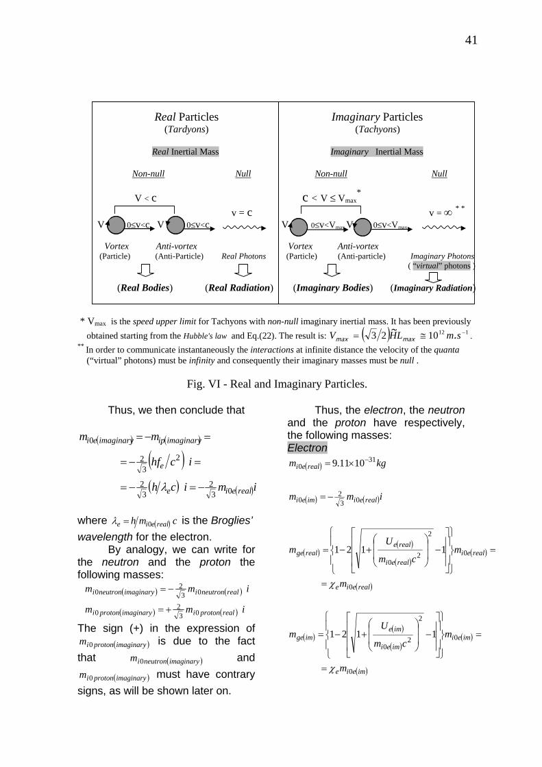
41
Real Particles Imaginary Particles (Tardyons) (Tachyons)
Real Inertial Mass Imaginary Inertial Mass
Non-null Null Non-null Null V < c c < V ≤ Vmax
* v = c v = ∞ * * V 0≤v<c V 0≤v<c V 0≤v<Vmax V 0≤v<Vmax Vortex Anti-vortex Vortex Anti-vortex (Particle) (Anti-Particle) Real Photons (Particle) (Anti-particle) Imaginary Photons ( “virtual” photons )
(Real Bodies) (Real Radiation) (Imaginary Bodies) (Imaginary Radiation) * Vmax is the speed upper limit for Tachyons with non-null imaginary inertial mass. It has been previously obtained starting from the Hubble's law and Eq.(22). The result is: ( ) 1121023 −≅= smLHV .~
maxmax . ** In order to communicate instantaneously the interactions at infinite distance the velocity of the quanta (“virtual” photons) must be infinity and consequently their imaginary masses must be null .
Fig. VI - Real and Imaginary Particles.
Thus, we then conclude that
( ) ( )
( )( ) ( )imich
ichf
mm
realeie
e
imaginaryipimaginaryei
032
32
23
2
0
−=−=
=−=
=−=
λ
where ( ) cmh realeie 0=λ is the Broglies’ wavelength for the electron. By analogy, we can write for the neutron and the proton the following masses:
( ) ( )
( ) ( ) imm
imm
realprotoniimaginaryprotoni
realneutroniimaginaryneutroni
032
0
032
0
+=
−=
The sign (+) in the expression of is due to the fact
that and must have contrary
signs, as will be shown later on.
(imaginaryprotonim 0
Thus, the electron, the neutron and the proton have respectively, the following masses: Electron
( )
( ) ( )
( )( )
( )( )
( )
( )( )
( )( )
( )imeie
imeiimei
imeimge
realeie
realeirealei
realerealge
realeiimei
realei
m
mcm
Um
m
mcm
Um
imm
kgm
0
0
2
20
0
0
2
20
032
0
310
1121
1121
1011.9
χ
χ
=
=⎪⎭
⎪⎬
⎫
⎪⎩
⎪⎨
⎧
⎥⎥⎥
⎦
⎤
⎢⎢⎢
⎣
⎡
−⎟⎟
⎠
⎞
⎜⎜
⎝
⎛+−=
=
=⎪⎭
⎪⎬
⎫
⎪⎩
⎪⎨
⎧
⎥⎥⎥
⎦
⎤
⎢⎢⎢
⎣
⎡
−⎟⎟
⎠
⎞
⎜⎜
⎝
⎛+−=
−=
×= −
)
)
)
(imaginaryneutronim 0
(imaginaryprotonim 0

42
Neutron
( )
( ) ( )
( )( )
( )( )
( )
( )( )
( )( )
( )imnin
imniimni
imnimgn
realnin
realnirealni
realnrealgn
realniimni
realni
m
mcm
Um
m
mcm
Um
imm
kgm
0
0
2
20
0
0
2
20
032
0
270
1121
1121
106747.1
χ
χ
=
=⎪⎭
⎪⎬
⎫
⎪⎩
⎪⎨
⎧
⎥⎥⎥
⎦
⎤
⎢⎢⎢
⎣
⎡
−⎟⎟
⎠
⎞
⎜⎜
⎝
⎛+−=
=
=⎪⎭
⎪⎬
⎫
⎪⎩
⎪⎨
⎧
⎥⎥⎥
⎦
⎤
⎢⎢⎢
⎣
⎡
−⎟⎟
⎠
⎞
⎜⎜
⎝
⎛+−=
−=
×= −
Proton ( )
( ) ( )
( )( )
( )( )
( )
( )( )
( )( )
( )impripr
impriimpri
imprimgpr
realpripr
realprirealpri
realprrealgpr
realpriimpri
realpri
m
mcm
Um
m
mcm
Um
imm
kgm
0
0
2
20
0
0
2
20
032
0
270
1121
1121
106723.1
χ
χ
=
=⎪⎭
⎪⎬
⎫
⎪⎩
⎪⎨
⎧
⎥⎥⎥
⎦
⎤
⎢⎢⎢
⎣
⎡
−⎟⎟
⎠
⎞
⎜⎜
⎝
⎛+−=
=
=⎪⎭
⎪⎬
⎫
⎪⎩
⎪⎨
⎧
⎥⎥⎥
⎦
⎤
⎢⎢⎢
⎣
⎡
−⎟⎟
⎠
⎞
⎜⎜
⎝
⎛+−=
+=
×= −
)
where and are respectively, the real and imaginary energies absorbed by the particles.
(realU ( )imU
When neutrons, protons and electrons were created after the Big-bang, they absorbed quantities of electromagnetic energy, respectively given by
( ) ( )
( ) ( )
( ) ( ) ikTUkTU
ikTUkTU
ikTUkTU
eeimaginaryeeereale
prprimaginaryprprprrealpr
nnimaginarynnnrealn
ηη
ηη
ηη
==
==
==
where nη , prη and eη are the absorption factors respectively, for the neutrons, protons and electrons;
is the Boltzmann constant; , and are the temperatures of the Universe, respectively when neutrons, protons and electrons were created.
KJk /º1038.1 23−×=nT prT eT
In the case of the electrons, it was previously shown that 1.0≅eη . Thus, by considering that
, we get KTe31102.6 ×≅
( ) iikTU eeime7105.8 ×==η
It is known that the protons were created at the same epoch. Thus, we will assume that
( ) iikTU prprimpr7105.8 ×==η
Then, it follows that 21108.1 ×−=eχ17107.9 ×−=prχ
Now, consider the gravitational forces, due to the imaginary masses of two electrons, , two protons, , and one electron and one proton, , all at rest.
eeF prprF
eprF
( ) ( )( )
( ))(
2
28
2
202
2
203
22
2
2
103.234
repulsionrealei
e
realeie
imgeee
rr
mG
r
imG
r
mGF
−×+=+=
=−
−=−=
χ
χ
( ) ( )
( ))(2
28
2
202
2
2
032
22
2
103.234
repulsionrealpri
pr
realpripr
imgprprpr
rr
mG
r
imG
r
mGF
−×+=+=
=⎟⎠⎞⎜
⎝⎛+
−=−=
χ
χ
( ) ( )
( ) ( )
( ) ( )
)(
2
28
200
2
032
032
2
103.234
atraction
realprirealeipre
realprirealeipre
imgprimgeepr
rr
mmG
r
imimG
r
mmGF
−×−=−=
=⎟⎠⎞⎜
⎝⎛+⎟
⎠⎞⎜
⎝⎛−
−=
=−=
χχ
χχ

43
Note that
2
28
20
2 103.24 rr
eFelectric
−×==
πε Therefore, we can conclude that
)(4 2
0
2repulsion
reFFF electricprpree
πε+=≡=
and
)(4 2
0
2atraction
reFF electricep πε
−=≡
These correlations permit to define the electric charge by means of the following relation:
( ) imGq imaginaryg04πε=
For example, in the case of the electron, we have
( )
( )( )( )( )
( )( ) CmG
imG
imG
imGq
realeie
realeie
imaginaryeie
imaginarygee
1903
20
203
20
00
0
106.14
4
4
4
−×−==
=−=
==
==
χπε
χπε
χπε
πε
In the case of the proton, we get
( )
( )( )( )( )( )( ) CmG
imG
imG
imGq
realpripr
realpripr
imaginarypripr
imaginarygprpr
1903
20
203
20
00
0
106.14
4
4
4
−×+=−=
=+=
==
==
χπε
χπε
χπε
πε
For the neutron, it follows that
( )
( )( )( )( )
( )( )realnin
realnin
imaginarynin
imaginarygnn
mG
imG
imG
imGq
032
0
203
20
00
0
4
4
4
4
χπε
χπε
χπε
πε
=
=−=
==
==
However, based on the quantization of the mass (Eq. 44), we can write that
( ) ( ) 0min02
032 ≠= nmnm irealninχ
Since can have only discrete values different of zero (See Appendix B), we conclude that
n
nχ cannot be null. However, it is known that the electric
charge of the neutron is null. Thus, it is necessary to assume that
( )
( )
( )
( )( )( ) ( )[ ] 04
4
4
4
4
203
2203
20
00
00
0
0
=−++=
=+
+⎟⎠⎞⎜
⎝⎛=
=+
+=+=
−
+
−
+−+
imimG
imG
imG
imG
imGqqq
ninnin
imaginarynin
imaginarynin
imaginarygn
imaginarygnnnn
χχπε
χπε
χπε
πε
πε
We then conclude that in the neutron, half of the total amount of elementary quanta of electric charge, , is negative, while the other half is positive.
minq
In order to obtain the value of the elementary quantum of electric charge, , we start with the expression obtained here for the electric charge, where we change by its quantized
expression ,derived from Eq. (44a). Thus, we get
minq
(imaginarygm )
)( ) ( )(min02
imaginaryiimaginaryg mnm =
( )
( )( )
( )( )[ ]( )min0
203
2
min0322
0
min02
0
0
4
4
4
4
i
i
imaginaryi
imaginaryg
mnG
iimnG
imnG
imGq
πε
πε
πε
πε
m=
=±=
==
==
This is the quantized expression of the electric charge. For 1=n we obtain the value of the elementary quantum of electric charge, , i.e., minq
( ) CmGq i83
min0032
min 108.34 −×== mm πε
where is the elementary quantum of matter, whose value previously calculated, is
.
(min0im )
( ) kgmi73
min0 109.3 −×±=
The existence of imaginary mass associated to a real particle suggests the possible existence of imaginary

44
particles with imaginary masses in Nature. In this case, the concept of wave associated to a particle (De Broglie’s waves) would also be applied to the imaginary particles. Then, by analogy, the imaginary wave associated to an imaginary particle with imaginary masses and m would be described by the following expressions
ψi ψgm
ψψ
ψψ
ωh
rh
r
=
=
E
kp
Henceforth, for the sake of simplicity, we will use the Greek letterψ to stand for the word imaginary; is the momentum carried by the
ψpr
ψ wave and
its energy; ψE ψψ λπ2=kr
is the
propagation number and ψλ the
wavelength of the ψ wave; ψψ πω f2= is the cyclical frequency. According to Eq. (4), the momentum is ψpr
VMp g
rrψψ =
Vwhere is the velocity of the ψ particle. By comparing the expressions of
we get ψpr
VMh
gψψλ =
Ψ Ψ
It is known that the variable quantity which characterizes the De Broglie’s waves is called wave function, usually indicated by symbol . The wave function associated with a material particle describes the dynamic state of the particle: its value at a particular point x, y, z, t is related to the probability of finding the particle in that place and instant. Although does not have a physical interpretation, its square (or
Ψ
Ψ
2 *Ψ ) calculated for a particular point x, y, z, t is proportional to the probability of finding the particle in that place and instant. Since is proportional to the probability of finding the particle described by Ψ , the integral of
2ΨP
2Ψ on
the whole space must be finite − inasmuch as the particle is somewhere. On the other hand, if
02 =Ψ∫+∞ Vd∞−
∞−
the interpretation is that the particle will not exist. However, if
( )1082 ∞=Ψ∫+∞ Vd
The particle will be everywhere simultaneously. In Quantum Mechanics, the wave function Ψ corresponds, as we know, to the displacement y of the undulatory motion of a rope. However, Ψ , as opposed to y , is not a measurable quantity and can, hence, be a complex quantity. For this reason, it is assumed that Ψ is described in the
directionx − by ( )( )pxEthie −−Ψ=Ψ π2
0
This is the expression of the wave function for a free particle, with total energy E and momentum , moving in the direction
pr
x+ . As to the imaginary particle, the imaginary particle wave function will be denoted by ψΨ and, by analogy the expression of Ψ , will be expressed by:
( )( )xptEhie ψψπ −−Ψ=Ψ 2ψψ 0
Therefore, the general expression of the wave function for a free particle can be written in the following form
( )( ) ( ) ( )( )
( )( )xptEhi
xptEhireal
e
e realreal
ψψπ
π
−−
−−
Ψ+
+Ψ=Ψ2
20
ψ0
It is known that the uncertainty principle can also be written as a function of EΔ (uncertainty in the energy) and tΔ (uncertainty in the time), i.e.,
≥ΔΔ tE.
h
This expression shows that a variation of energy EΔ , during a

45
time interval , can only be detected if
tΔEt Δ≥ hΔ . Consequently,
a variation of energy EΔ , during a time interval Et Δ<Δ h , cannot be experimentally detected. This is a limitation imposed by Nature and not by our equipments. Thus, a quantum of energy
that varies during a time interval
hfE =ΔEcft Δ<==Δ hλ1 (wave
period) cannot be experimentally detected. This is an imaginary photon or a “virtual” photon. Now, consider a particle with energy . The DeBroglie’s gravitational and inertial wavelengths are respectively
2cM g
cMh gg =λ and cMh ii =λ . In Quantum Mechanics,
particles of matter and quanta of radiation are described by means of wave packet (DeBroglie’s waves) with average wavelength iλ . Therefore, we can say that during a time interval ct iλ=Δ , a quantum of energy varies. According to the uncertainty principle, the particle will be detected if
2cME g=Δ
Et Δ≥Δ h , i.e., if 2cMc gi h≥λ or πλλ 2gi ≥ . This condition is usually satisfied when . In this case, ig MM = ig λλ = and obviously, πλλ 2ii > . However, when decreases gM gλ increases and πλ 2g can become bigger than
iλ , making the particle non-detectable or imaginary. According to Eqs. (7) and (41) we can write in the following form:
gM
iig
g Mmm
M χχ
=−
=−
=2222 cVcV 11
where
( )⎭⎬⎫
⎩⎨⎧
⎥⎦⎤
⎢⎣⎡ −Δ+−= 1121 2
0cmp iχ
Since the condition to make the particle imaginary is
πλ
λ2
gi <
and
πχλ
χπλ
22i
ig
g
cMcM===
hh
Then we get
159.021
=<π
χ
However, χ can be positive or negative ( 159.0+<χ or 159.0−>χ ).This means that when
15901590 .. +<<− χ the particle becomes imaginary. Under these circumstances, we can say that the particle made a transition to the imaginary space-time. Note that, when a particle becomes imaginary, its gravitational and inertial masses also become imaginary. However, the factor
( ) ( )imaginaryiimaginaryg MM=χ remains real because
( )
( )real
MM
iMiM
MM
i
g
i
g
imaginaryi
imaginaryg ====χ

46
χ +0.159 ∞≤≤ V0 Imaginary Body 0 Imaginary Space-time “Virtual” Photons ( ∞=V ) −0.159 Fig. VII – Travel in the imaginary space-time. Similarly to the “virtual” photons, imaginary bodies can have infinite speed in the imaginary space-time.
Ordinary Space-time cV <≤0
Body
Ordinary Space-time
Real Photons ( cV = )

47
Real particle Real particle Δt1 ΔE
Δt2 c (speed upper limit)
Δt3
Imaginary Space-time Ordinary Space-time
Δt3
Δt2 Vmax
(speed upper limit)
ΔE Δt1
Imaginary particle Imaginary particle Fig. VIII – “Virtual” Transitions – (a) “Virtual” Transitions of a real particle to the imaginary space-time. The speed upper limit for real particle in the imaginary space-time is c. (b) - “Virtual” Transitions of an imaginary particle to the ordinary space-time. The speed upper limit for imaginary particle in the ordinary space-time is 11210 −≈ smV .max
Note that to occur a “virtual” transition it is necessary thatΔt=Δt1+ Δt2+ Δt3 <ℏ/ΔE Thus, even at principle, it will be impossible to determine any variation of energy in the particle (uncertainty principle).
(a)
(b)

48
Thus, if the gravitational mass of the particle is reduced by means of the absorption of an amount of electromagnetic energy U , for example, we have
( )⎭⎬⎫
⎩⎨⎧
⎥⎦⎤
⎢⎣⎡ −+−== 1121
220cmU
MM
ii
gχ
This shows that the energyU of the electromagnetic field remains acting on the imaginary particle. In practice, this means that electromagnetic fields act on imaginary particles. The gravity acceleration on a imaginary particle (due to the rest of the imaginary Universe) are given by
.,...,,, njgg jj 321==′ χ where ( ) ( )imaginaryiimaginaryg MM=χ
and ( )2jimaginarygjj rGmg −= . Thus,
the gravitational forces acting on the particle are given by
( )
( ) ( )( )( ) .22
2
jgjgjgjg
jimaginarygjimaginaryg
jimaginaryggj
rmGMriGmiM
rGmM
gMF
χχ
χ
+=−=
=−=
=′=
Note that these forces are real. Remind that, the Mach’s principle says that the inertial effects upon a particle are consequence of the gravitational interaction of the particle with the rest of the Universe. Then we can conclude that the inertial forces upon an imaginary particle are also real. Equation (7) shows that , in the case of imaginary particles, the relativistic mass is
( )( )
11
1
2222
22
−=
−=
=−
=
cV
im
cVi
imcV
mM
gg
imaginarygimaginaryg
This expression shows that imaginary particles can have velocities greater than in our ordinary space-time (Tachyons). The quantization of velocity (Eq. 36) shows that there is a speed upper limit . As we have already calculated previously, , (Eq.102).
V c
cV >max11210 −≈ smV .max
Note that this is the speed upper limit for imaginary particles in our ordinary space-time not in the imaginary space-time (Fig.7) because the infinite speed of the “virtual” quanta of the interactions shows that imaginary particles can have infinite speed in the imaginary space-time. While the speed upper limit for imaginary particles in the ordinary space-time is
, the speed upper limit for real particles in the imaginary space-time is c , because the relativistic expression of the mass shows that the velocity of real particles cannot be larger than c in any space-time. The uncertainty principle permits that particles make “virtual” transitions, during a time interval
11210 −≈ smV .max
tΔ , if Et Δ<Δ h . The “virtual” transition of mesons emitted from nucleons that do not change of mass, during a time interval
2cmt πh<Δ , is a well-known example of “virtual” transition of particles. During a “virtual” transition of a real particle, the speed upper limit in the imaginary space-time is c , while the speed upper limit for an imaginary particle

49
in the our ordinary space-time is . (See Fig. 8). 11210 −≈ smV .max
There is a crucial cosmological problem to be solved: the problem of the hidden mass. Most theories predict that the amount of known matter, detectable and available in the universe, is only about 1/100 to 1/10 of the amount needed to close the universe. That is, to achieve the density sufficient to close-up the universe by maintaining the gravitational curvature (escape velocity equal to the speed of light) at the outer boundary. Eq. (43) may solve this problem. We will start by substituting the expression of Hubble's law for velocity, lH~V = , into Eq.(43). The expression obtained shows that particles which are at distances
( )( ) m.H~cll 260 103135 ×=== have
quasi null gravitational mass ) ; beyond this distance,
the particles have negative gravitational mass. Therefore, there are two well-defined regions in the Universe; the region of the bodies with positive gravitational masses and the region of the bodies with negative gravitational mass. The total gravitational mass of the first region, in accordance with Eq.(45), will be given by
(mingg mm =
1221
111
1i
iig m
cVmMM ≅
−=≅
where is the total inertial mass of the bodies of the mentioned region;
1im
cV <<1 is the average velocity of the bodies at region 1. The total gravitational mass of the second region is
2222
2 11
121 ig McV
M ⎟⎟
⎠
⎞
⎜⎜
⎝
⎛−
−−=
where 2V is the average velocity
of the bodies ; 22
222 1 cVmM ii −= and is the total inertial mass of the bodies of region 2.
2im
Now consider that from Eq.(7), we can write
22
ccME
ggg ρξ ===VV
where ξ is the energy density of matter. Note that the expression of ξ only reduces to the well-known expression , where 2cρ ρ is the sum of the inertial masses per volume unit, when . Therefore, in the derivation of the well-known difference
ig mm =
2
38
HG U ~−
ρπ
which gives the sign of the curvature of the Universe [36], we must use
instead of .The result obviously is
2cgUρξ = 2cUρξ =
( )1093
8 2H~G gU −
ρπ
where
( )11021
U
gg
U
gUgU
MMMVV+
==ρ
gUM and UV are respectively the total gravitational mass and the volume of the Universe. Substitution of and into expression (110) gives
1gM 2gM
U
iiiU
gU
mmcVcV
m
V
⎥⎥
⎦
⎤
⎢⎢
⎣
⎡−
−−
−+
=
22222
222
12
1
3
ρ
where 21 iiiU mmm += is the total inertial mass of the Universe. The volume 1V of the region 1 and the volume 2V of the region 2, are respectively given by

50
132
230
21 22 VVV −== clandl ππ
where m.H~clc
261081 ×== is the so-called "radius" of the visible Universe. Moreover, 111 Vii m=ρ and
222 Vii m=ρ . Due to the hypothesis of the uniform distribution of matter in the space, it follows that
21 ii ρρ = .Thus, we can write
3803
0
2
1
2
1 .ll
mm
ci
i =⎟⎟⎠
⎞⎜⎜⎝
⎛==
VV
Similarly,
1
1
2
2
VVVii
U
iU mmm==
Therefore,
iUiUc
iUU
i m.mll
mm 62013
022 =
⎥⎥⎦
⎤
⎢⎢⎣
⎡⎟⎟⎠
⎞⎜⎜⎝
⎛−==
VV
and . iUi m.m 3801 =Substitution of into the expression of
2im
gUρ yields
U
iUiU
gU
mcVcV
m
V
6201
241
1
86122
222
2
...−
−−
−+
=ρ
Due to cV ≅2 , we conclude that the term between bracket is much larger than . The amount is the mass of matter in the universe (1/10 to 1/100 of the amount needed to close the Universe).
iUm10 iUm
Consequently, the total mass
iUiU mcVcV
m 6201
241
1
86122
222
2
...−
−−
−+
must be sufficient to close the Universe. There is another cosmological problem to be solved: the problem of
the anomalies in the spectral red-shift of certain galaxies and stars. Several observers have noticed red-shift values that cannot be explained by the Doppler-Fizeau effect or by the Einstein effect (the gravitational spectrum shift, supplied by Einstein's theory). This is the case of the so-called Stefan's quintet (a set of five galaxies which were discovered in 1877), whose galaxies are located at approximately the same distance from the Earth, according to very reliable and precise measuring methods. But, when the velocities of the galaxies are measured by its red-shifts, the velocity of one of them is much larger than the velocity of the others. Similar observations have been made on the Virgo constellation and spiral galaxies. Also the Sun presents a red-shift greater than the predicted value by the Einstein effect. It seems that some of these anomalies can be explained if we consider the Eq.(45) in the calculation of the gravitational mass of the point of emission. The expression of the gravitational spectrum shift was previously obtained in this work. It is the same supplied by Einstein's theory [37], and is given by
( )111021122
0212
21
ω
ωφ φωωω
c
rGmrGmc
gg +−=
=−
=−=Δ
where 1ω is the frequency of the light at the point of emission ; 2ω is the frequency at the point of observation; 1φ and 2φ are respectively, the Newtonian gravitational potentials at the point of emission and at the point of observation.

51
In Einstein theory, this expression has been deduced from
00gtT −= [38] which correlates own time (real time), t , with the temporal coordinate x0 of the space-time ( cxt 0= ). When the gravitational field is weak, the temporal component of the metric tensor is given by
2[
00g
21 c/goo φ−−= 39].Thus, we readily obtain
( )11221 2rcGmtT g−=
This is the same equation that we have obtained previously in this work. Curiously, this equation tell us that we can have when ; and for . In addition, if
tT < 0>gmtT > 0<gm
Grcmg 22= , i.e., if 22 cGmr g= (Schwarzschild radius) we obtain
0=T .
Let us now consider the well-known process of stars' gravitational contraction. It is known that the destination of the star is directly correlated to its mass. If the star's mass is less than 1.4M (Schemberg-Chandrasekhar's limit), it becomes a white dwarf. If its mass exceeds that limit, the pressure produced by the degenerate state of the matter no longer counterbalances the gravitational pressure, and the star's contraction continues. Afterwards there occurs the reactions between protons and electrons (capture of electrons), where neutrons and anti-neutrinos are produced.
The contraction continues until the system regains stability (when the pressure produced by the neutrons is sufficient to stop the gravitational collapse). Such systems are called neutron stars.
There is also a critical mass for the stable configuration of neutron stars. This limit has not
been fully defined as yet, but it is known that it is located between 1.8M and 2.4M . Thus, if the mass of the star exceeds 2.4M , the contraction will continue. According to Hawking [40] collapsed objects cannot have mass less than kg.Gc 810114 −×=h . This means that, with the progressing of the compression, the neutrons cluster must become a cluster of superparticles where the minimal inertial mass of the superparticle is
( ) ( )1131011 8 .kg.m spi−×=
Symmetry is a fundamental attribute of the Universe that enables an investigator to study particular aspects of physical systems by themselves. For example, the assumption that space is homogeneous and isotropic is based on Symmetry Principle. Also here, by symmetry, we can assume that there are only superparticles with mass in the cluster of superparticles.
( ) kg.m spi81011 −×=
Based on the mass-energy of the superparticles ( ~1018 GeV ) we can say that they belong to a putative class of particles with mass-energy beyond the supermassive Higgs bosons ( the so-called X bosons). It is known that the GUT's theories predict an entirely new force mediated by a new type of boson, called simply X (or X boson ). The X bosons carry both electromagnetic and color charge, in order to ensure proper conservation of those charges in any interactions. The X bosons must be extremely massive, with mass-energy in the unification range of about 1016 GeV. If we assume the superparticles are not hypermassive Higgs bosons then the possibility of the neutrons cluster become a

52
Higgs bosons cluster before becoming a superparticles cluster must be considered. On the other hand, the fact that superparticles must be so massive also means that it is not possible to create them in any conceivable particle accelerator that could be built. They can exist as free particles only at a very early stage of the Big Bang from which the universe emerged. Let us now imagine the Universe coming back to the past. There will be an instant in which it will be similar to a neutrons cluster, such as the stars at the final state of gravitational contraction. Thus, with the progressing of the compression, the neutrons cluster becomes a superparticles cluster. Obviously, this only can occur before 10-23s (after the Big-Bang). The temperature T of the Universe at the 10-43s< t < 10-23s period can be calculated by means of the well-known expression[41]:
( ) ( )1141010 212322 −−≈ tT
Thus at (at the first spontaneous breaking of symmetry) the temperature was (∼10
st 4310 −≅
KT 3210≈19GeV).Therefore, we can
assume that the absorbed electromagnetic energy by each superparticle, before , was
(see Eqs.(71) and (72)). By comparing with
, we conclude that . Therefore, the
unification condition
st 4310 −≅JkTU 9101×>=η
( ) Jcm spi82 109×≅
( )cmU spi>
( )22 cmcMUn iir >≅ is satisfied. This means that, before
,the gravitational and electromagnetic interactions were unified.
st 4310 −≅
From the unification condition ( )2cMUn ir ≅ , we may conclude that
the superparticles' relativistic inertial mass is ( )spiM
( ) ( )11510 822 kg
ckTn
cUn
M rrspi
−≈=≅η
Comparing with the superparticles' inertial mass at rest (113), we conclude that
( ) ( ) ( )1161011 8kg.mM spispi−×=≈
From Eqs.(83) and (115), we obtain the superparticle's gravitational mass at rest:
( ) ( ) ( )
( ) ( )117
2
2ckTn
M
Mmm
rspi
spispispg
η−≅−≅
≅−=
Consequently, the superparticle's relativistic gravitational mass, is
( )( )
( )1181
1
222
22
cVc
kTncV
mM
r
spgspg
−=
=−
=
η
Thus, the gravitational forces between two superparticles , according to (13), is given by:
( ) ( )
( )
( )( ) ( )119212
25
2
2122112
μκη
μ
ˆrcTn
cG
mM
ˆrMM
GFF
rspi
spi
'spgspg
h
h
rr
⎥⎥
⎦
⎤
⎢⎢
⎣
⎡⎟⎠⎞
⎜⎝⎛
⎟⎟⎠
⎞⎜⎜⎝
⎛=
=−=−=
Due to the unification of the gravitational and electromagnetic interactions at that period, we have
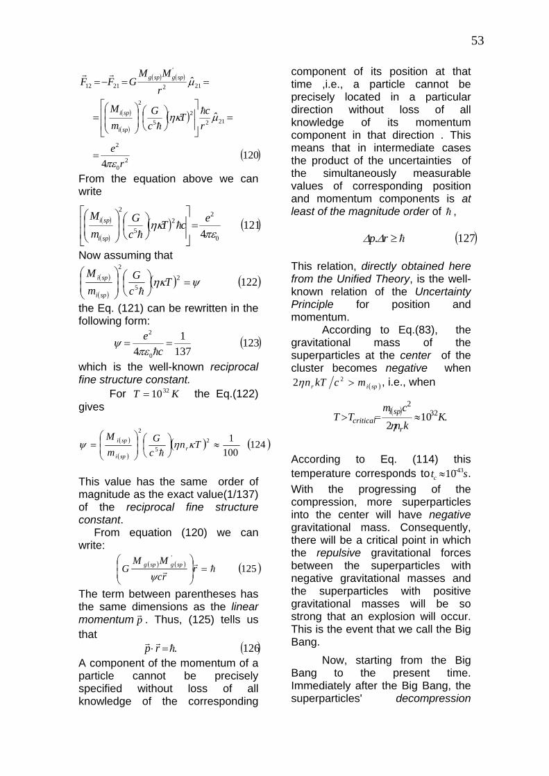
53
( ) ( )
( )
( )( )
( )1204 2
0rπε=
2
2122
5
2
2122112
e
ˆrcT
cG
mM
ˆrMM
GFF
spi
spi
'spgspg
μηκ
μ
=⎥⎥
⎦
⎤
⎢⎢
⎣
⎡⎟⎠⎞
⎜⎝⎛
⎟⎟⎠
⎞⎜⎜⎝
⎛=
==−=
h
h
rr
From the equation above we can write
( )
( )( ) ( )121
4 0
25 πε
ηκ ecTcG
m spi
spi =⎥⎥
⎦⎢⎢
⎣⎟⎠⎞
⎜⎝⎛
⎟⎟⎠
⎜⎜⎝
hh
22
M ⎤⎡ ⎞⎛
( )
( )
Now assuming that
( )25 ηκ⎟
⎠⎞ T
cGh
( )1222
ψ=⎜⎝⎛
⎟⎟⎠
⎞⎜⎜⎝
⎛
mM
spi
spi
the Eq. (121) can be rewritten in the following form:
( )123137
14 0
2
==c
ehπε
ψ
which is the well-known reciprocal fine structure constant. For the Eq.(122) gives
KT 3210=
( )
( )( ) ( )12
2⎞⎛⎞⎛ GM spi
( ) ( )
1241005 ≈⎟
⎠⎜⎝⎟
⎟⎠
⎜⎜⎝
= Tncm r
spi
κηψh
This value has the same order of magnitude as the exact value(1/137) of the reciprocal fine structure constant. From equation (120) we can write:
( )125hr
r =⎟⎟⎠
⎞⎜⎜⎝
⎛r
rcMM
G'
spgspg
ψ
p
The term between parentheses has the same dimensions as the linear momentum r . Thus, (125) tells us that
( )126.rp hrr
=⋅A component of the momentum of a particle cannot be precisely specified without loss of all knowledge of the corresponding
component of its position at that time ,i.e., a particle cannot be precisely located in a particular direction without loss of all knowledge of its momentum component in that direction . This means that in intermediate cases the product of the uncertainties of the simultaneously measurable values of corresponding position and momentum components is at least of the magnitude order of , h
( )127h≥r.pΔ Δ This relation, directly obtained here from the Unified Theory, is the well-known relation of the Uncertainty Principle for position and momentum. According to Eq.(83), the gravitational mass of the superparticles at the center of the cluster becomes negative when
( )spir mckTn >22η
( )
, i.e., when
.102
322
Kkn
cmTT
r
spicritical ≈=>
η
sc4310−≈
According to Eq. (114) this temperature corresponds to t . With the progressing of the compression, more superparticles into the center will have negative gravitational mass. Consequently, there will be a critical point in which the repulsive gravitational forces between the superparticles with negative gravitational masses and the superparticles with positive gravitational masses will be so strong that an explosion will occur. This is the event that we call the Big Bang. Now, starting from the Big Bang to the present time. Immediately after the Big Bang, the superparticles' decompression

54
begins. The gravitational mass of the most central superparticle will only be positive when the temperature becomes smaller than the critical temperature, . At the maximum state of compression (exactly at the Big Bang) the volumes of the superparticles were equal to the elementary volume Ω and the volume of the Universe was
where was the initial length scale of the Universe. At this very moment the average density of the Universe was equal to the average density of the superparticles, thus we can write
KTcritical3210≈
30 mindVδ=
initiald( ) 33initialVminV dnd δδΩ ==
( )
( )( )128
spi
Ui
min
initial
mM
dd
=⎟⎟⎠
⎞⎜⎜⎝
⎛3
( ) kgM Ui5310≈
k
where is the inertial mass of the Universe. It has already been shown that
.ml~dmin3410−≈= planck Then, from
Eq.(128), we obtain:
( )12910 14m−dinitial ≈
d
crd
Kcritical3210≈
initialcr dd −
After the Big Bang the Universe expands itself from up to (when the temperature decrease reaches the critical temperatureT , and the gravity becomes attractive). Thus, it expands by , under effect of the repulsive gravity
initial
( )( ) ( )[ ] ( ) ( )[ ]( ) ( ) ( ) ( )
( ) ( ) ( )
initialcr
Ui
initialcr
Uispi
crUiinitialUg
minmax
ddGM
ddMmG
dMGdMG
ggg
χχ 22
221
212
21
21
==
==
==
∑initialcr
Uispg
initialcr
UiUg
ddMmG
ddMMG 22
=== ∑
during a period of time .Thus,
stc4310−≈
( ) ( ) ( ) ( ) ( )1302221
cinitialcr
Uicinitialcr t
ddGM
tgdd χ==−
( )
( )
The Eq.(83), gives
( ) ( )2
21
21
cmkTn
mUn
m
m
spi
rr
spi
spg ηχ −=−==
2cspi
Calculations by Carr, B.J [41], indicate that it would seem reasonable to suppose that the fraction of initial primordial black hole mass ultimately converted into photons is about . This means that we can take
11.0
11.0=η
Thus, the amount , where is the total inertial mass of the Universe, expresses the total amount of inertial energy converted into photons at the initial instant of the Universe(Primordial Photons).
2cMiUη
iUM
It was previously shown that photons and also the matter have imaginary gravitational masses associated to them. The matter has negative imaginary gravitational mass, while the photons have positive imaginary gravitational mass, given by
( ) ( ) ichfMM imaginaryipimaginarygp ⎟
⎠
⎞⎜⎝
⎛+== 2342
where is the imaginary inertial mass of the photons.
)(imaginaryipM
Then, from the above we can conclude that, at the initial instant of the Universe, an amount of imaginary gravitational mass,
, which was associated to the fraction of the matter transformed into photons, has been converted into imaginary gravitational mass of the primordial
totalimaginarygmM )(

55
photons, , while an amount of real inertial mass of the matter, , has been converted into real energy of the
primordial photons, , i.e.,
totalimaginarygpM )(
2)( cMM iU
totalrealim η=
∑=
=N
jjp hfE
1
43421
2
)()(
)()(
c
E
totalrealip
totalimaginarygp
totalrealim
totalimaginarygm
p
MM
MM
+=
=+
where and total
imaginarygptotal
imaginarygm MM )()( =
iUiU
totalrealim
totalrealipp MMMMcE 11.0)()(
2 ≅==≡ η
It was previously shown that, for the photons equation: , is valid. This means that
ipgp MM 2=
(44444444 21
4444 34444 21
ip
gp
M
realipimagimaryip
M
realgpimagimarygp
MM
MM
)()(
)()(
2 +=
=+
)3
By substituting into the equation above, we get
( ) ( )imaginaryipimaginarygp MM 2=
( ) ( )realiprealgp MM 2=
Therefore we can write that
( ) ( ) iUtotal
realiptotal
realgp MMM 22.02 ==
The phenomenon of gravitational deflection of light about the Sun shows that the gravitational interaction between the Sun and the photons is attractive. This is due to the gravitational force between the Sun and a photon, which is given by
( ) ( )2rmMGF imaginarygpimaginarygSun−= ,
where (the imaginary gravitational mass of the photon) is a quantity positive and imaginary, and (the imaginary gravitational mass associated to the matter of the Sun) is a quantity negative and imaginary.
(imaginarygpm )
)(imaginarygSunM
The fact of the gravitational interaction between the imaginary gravitational masses of the primordial photons and the imaginary gravitational mass of the matter be attractive is highly relevant, because it shows that it is necessary to consider the effect of this gravitational interaction, which is equivalent to the gravitational effect produced by the amount of real gravitational mass, , sprayed by all the Universe.
( ) iUtotal
realgp MM 22.0≅
This means that this amount, which corresponds to 22% of the total inertial mass of the Universe, must be added to the overall computation of the total mass of the matter (stars, galaxies, etc., gas and dust of interstellar and intergalactic media). Therefore, this additional portion corresponds to what has been called Dark Matter (See Fig. IX). On the other hand, the total amount of gravitational mass at the initial instant, , according to Eq.(41), can be expressed by
totalgM
iUtotalg MM χ=
This mass includes the total negative gravitational mass of the matter, , plus the total
gravitational mass, , converted into primordial photons. This tells us that we can put
totalgmM )(−
totalrealgpM )(
iU
totalrealgp
totalgm
totalg MMMM χ=+= − )()(
whence

56
Fig. IX – Conversion of part of the Real Gravitational Mass of the Primordial Universe into Primordial Photons. The gravitational effect caused by the gravitational interaction of imaginarygravitational masses of the primordial photons with the imaginary gravitational mass associated to the matter is equivalent to the effect produced by the amount of real gravitational mass,
( ) iUtotal
realgp MM 22.0≅ , sprayed by all Universe. This additional portion of mass corresponds to what has been called Dark Matter.
∼ 10-14 m
Real spacetime
Imaginary spacetime
( ) ( )totalip
totalgp realimaginary MM + ( ) ( )
totalim
totalgm realimaginary MM +
At the Initial Instant
iUM
Primordial Photons
( ) ( )43421
2c
E
totalip
totalgp
p
realimaginary MM +
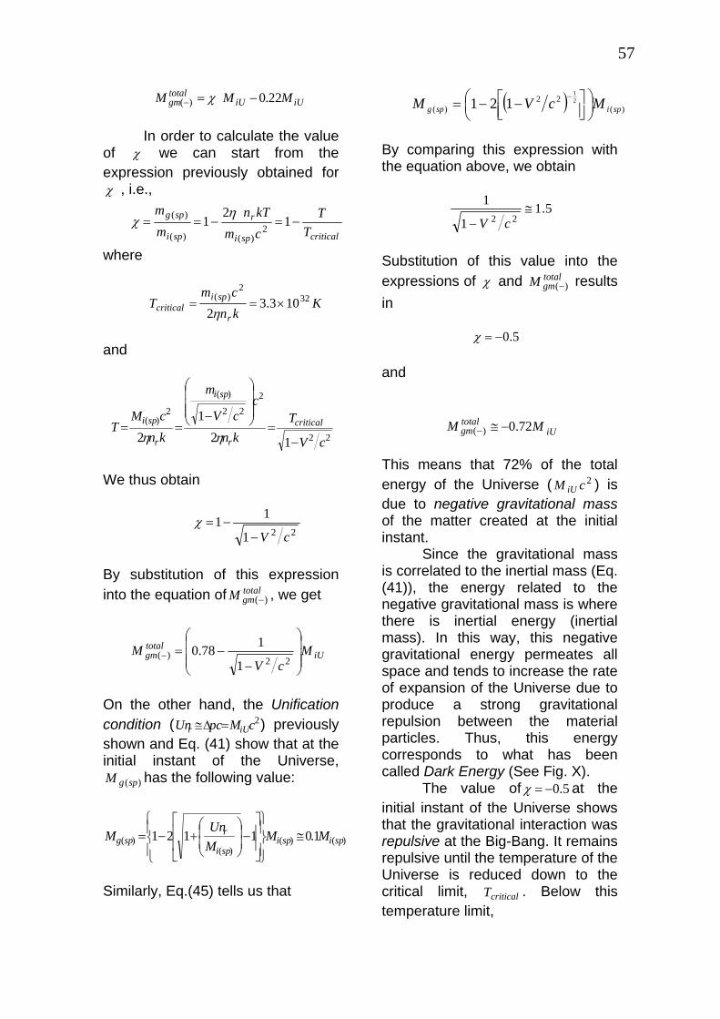
57
iUiUtotalgm MMM 22.0)( −=− χ
In order to calculate the value of χ we can start from the expression previously obtained for χ , i.e.,
criticalspi
r
spi
spg
TT
cmkTn
mm
−=−== 12
1 2)()(
)( ηχ
where
Kkncm
Tr
spicritical
322
)( 103.32
×==η
and
22
222
)(
2)(
121
2 cV
Tkn
ccV
m
kncM
T critical
r
spi
r
spi
−=
⎟⎟⎟
⎠
⎞
⎜⎜⎜
⎝
⎛
−==
ηη
We thus obtain
221
11cV−
−=χ
By substitution of this expression into the equation of , we get total
gmM )(−
iUtotalgm M
cVM
⎟⎟⎟
⎠
⎞
⎜⎜⎜
⎝
⎛
−−=− 22)(
1
178.0
On the other hand, the Unification condition ( ) previously shown and Eq. (41) show that at the initial instant of the Universe,
has the following value:
2cMpcUn iUr =Δ≅
)(spgM
)()()(
)( 1.01121 spispispi
rspg MM
MUn
M ≅⎪⎭
⎪⎬⎫
⎪⎩
⎪⎨⎧
⎥⎥
⎦
⎤
⎢⎢
⎣
⎡−⎟
⎟⎠
⎞⎜⎜⎝
⎛+−=
Similarly, Eq.(45) tells us that
( ) )(22
)(21
121 spispg McVM ⎟⎠⎞⎜
⎝⎛
⎥⎦⎤
⎢⎣⎡ −−=
−
By comparing this expression with the equation above, we obtain
5.11
122
≅− cV
Substitution of this value into the expressions of χ and results in
totalgmM )(−
5.0−=χ
and
iU
totalgm MM 72.0)( −≅−
This means that 72% of the total energy of the Universe ( ) is due to negative gravitational mass of the matter created at the initial instant.
2cM iU
Since the gravitational mass is correlated to the inertial mass (Eq. (41)), the energy related to the negative gravitational mass is where there is inertial energy (inertial mass). In this way, this negative gravitational energy permeates all space and tends to increase the rate of expansion of the Universe due to produce a strong gravitational repulsion between the material particles. Thus, this energy corresponds to what has been called Dark Energy (See Fig. X). The value of 5.0−=χ at the initial instant of the Universe shows that the gravitational interaction was repulsive at the Big-Bang. It remains repulsive until the temperature of the Universe is reduced down to the critical limit, . Below this temperature limit,
criticalT

58
72%
6%
22%
Negative Gravitational Mass of Matter
PositiveGravitational M ass of
M atter
Fig. X - Distribution of Gravitational Masses in the Universe. The total energy related to negative gravitational mass of all the matter in the Universe corresponds to what has been called Dark Energy. While the Dark Matter corresponds to the total gravitational mass carried by the primordial photons, which is manifested in the interaction of the imaginary gravitational masses of the primordial photons with the imaginary mass of matter.
Positive Gravitational Mass carried by the primordial photons

59
the attractive component of the gravitational interaction became greater than the repulsive component, making attractive the resultant gravitational interaction. Therefore, at the beginning of the Universe – before the temperature decreased down to , there occurred an expansion of the Universe that was exponential in time rather than a normal power-law expansion. Thus, there was an evident Inflation Period during the beginning of the expansion of the Universe (See Fig. XI).
criticalT
With the progressing of the decompression the superparticles cluster becomes a neutrons cluster. This means that the neutrons are created without its antiparticle, the antineutron. Thus, this solves the matter/antimatter dilemma that is unresolved in many cosmologies. Now a question: How did the primordial superparticles appear at the beginning of the Universe? It is a proven quantum fact that a wave function may collapse, and that, at this moment, all the possibilities that it describes are suddenly expressed in reality. This means that, through this process, particles can be suddenly materialized. The materialization of the primordial superparticles into a critical volume denotes knowledge of what would happen with the Universe starting from that initial condition, a fact that points towards the existence of a Creator. It was shown previously the possible existence of imaginary particles with imaginary masses in Nature. These particles can be associated with real particles, such as in case of the photons and electrons, as we have shown, or they can be associated with others imaginary particles by constituting the
imaginary bodies. Just as the real particles constitute the real bodies. The idea that we make about a consciousness is basically that of an imaginary body containing psychic energy and intrinsic knowledge. We can relate psychic energy with psychic mass (psychic mass= psychic energy/c2). Thus, by analogy with the real bodies the psychic bodies would be constituted by psychic particles with psychic mass. Consequently, the psychic particles that constitute a consciousness would be equivalent to imaginary particles, and the psychic mass , ,of the psychic particles would be equivalent to the imaginary mass, i.e.,
Ψm
( ) ( )131imaginaryimm =Ψ
Thus, the imaginary masses associated to the photons and electrons would be elementary psyche actually, i.e.,
( )
( )1323
22 i
chf
mm photonimaginaryiphoton
⎟⎠
⎞⎜⎝
⎛=
==Ψ
( )
( ) ( )133032
232
im
ic
hf
mm
electronreali
electron
electronimaginaryielectron
−=
=⎟⎟⎠
⎞⎜⎜⎝
⎛−=
==Ψ
The idea that electrons have elementary psyche associated to themselves is not new. It comes from the pre-Socratic period. By proposing the existence of psyche associated with matter, we are adopting what is called panpsychic posture. Panpsychism dates back to the pre-Socratic period;

60
Fig. XI – Inflation Period. The value of 5.0−≅χ at the Initial Instant of the Universe shows that the gravitational interaction was repulsive at the Big-Bang. It remains repulsive until the temperature of the Universe is reduced down to the critical limit, criticalT . Below this temperature limit, the attractive component of the gravitational interaction became greater than the repulsive component, making attractive the resultant gravitational interaction. Therefore, at beginning of the Universe −before the temperature to be decreased down to criticalT , there occurred an expansion of the Universe that was exponential in time rather than a normal power-law expansion. Thus, there was an evident inflation period during the beginning of the expansion of the Universe.
0=t st 4310−≈
KTT critical32103.3 ×==
Inflation PeriodKT 7.2=
st 4310−≈ st 4310−≈ st 4310−≈ st 4310−≈ st 4310−≈ yearsbilliont 15≈
5.0−≅χ

61
remnants of organized panpsychism may be found in the Uno of Parmenides or in Heracleitus’s Divine Flow. The scholars of Miletus’s school were called hylozoists, that is, “those who believe that matter is alive”. More recently, we will find the panpsychistic thought in Spinoza, Whitehead and Teilhard de Chardin, among others. The latter one admitted the existence of proto-conscious properties at the elementary particles’ level. We can find experimental evidences of the existence of psyche associated to electron in an experiment similar to that commonly used to show the wave duality of light. (Fig. XII). One merely substitutes an electron ray (fine electron beam) for the light ray. Just as in the experiment mentioned above, the ray which goes through the holes is detected as a wave if a wave detector is used (it is then observed that the interference pattern left on the detector screen is analogous with that produced by the light ray), and as a particle if a particle detector is used. Since the electrons are detected on the other side of the metal sheet, it becomes obvious then that they passed through the holes. On the other hand, it is also evident that when they approached the holes, they had to decide which one of them to go through. How can an electron “decide” which hole to go through? Where there is “choice”, isn’t there also psyche, by definition? If the primordial superparticles that have been materialized at the beginning of the Universe came from the collapse of a primordial wave function, then the psychic form described by this wave
function must have been generated in a consciousness with a psychic mass much greater than that needed to materialize the Universe (material and psychic). This giant consciousness, in its turn, would not only be the greatest of all consciences in the Universe but also the substratum of everything that exists and, obviously, everything that exists would be entirely contained within it, including all the spacetime. Thus, if the consciousness we refer to contains all the space, its volume is necessarily infinite, consequently having an infinite psychic mass. This means that it contains all the existing psychic mass and, therefore, any other consciousness that exists will be contained in it. Hence, we may conclude that It is the Supreme Consciousness and that there is no other equal to It: It is unique. Since the Supreme Consciousness also contains all time; past, present and future, then, for It the time does not flow as it flows for us. Within this framework, when we talk about the Creation of the Universe, the use of the verb “to create” means that “something that was not” came into being, thus presupposing the concept of time flow. For the Supreme Consciousness, however, the instant of Creation is mixed up with all other times, consequently there being no “before” or “after” the Creation and, thus, the following question is not justifiable: “What did the Supreme Consciousness do before Creation?” On the other hand, we may also infer, from the above that the

62
Light (a) Dw Light (b) Dp ? Electrons (c) Fig. XII – A light ray, after going through the holes in the metal sheet, will be detected as awave(a) by a wave detector Dw or as a particle if the wave detector is substituted for the wavedetector Dp. Electron ray (c) has similar behavior as that of a light ray. However, before going through the holes, the electrons must “decide” which one to go through.
?

63
existence of the Supreme Consciousness has no defined limit (beginning and end), what confers upon It the unique characteristic of uncreated and eternal. If the Supreme Consciousness is eternal, Its wave function shall never collapse (will never be null). Thus, for having an infinite psychic mass, the value of will be always infinite and, hence, we may write that
SCΨ
2SCΨ
∞=Ψ∫+∞
∞−dVSC
2
By comparing this equation with Eq. (108) derived from Quantum Mechanics, we conclude that the Supreme Consciousness is simultaneously everywhere, i.e., It is omnipresent. Since the Supreme Consciousness contains all consciences, it is expected that It also contain all the knowledge. Therefore, It is also omniscient. Consequently, It knows how to formulate well-defined mental images with psychic masses sufficient for its contents to materialize. In this way, It can materialize everything It wishes (omnipotence). All these characteristics of the Supreme Consciousness (infinite, unique, uncreated, eternal, omnipresent, omniscient and omnipotent) coincide with those traditionally ascribed to God by most religions. It was shown in this work that the “virtual” quanta of the gravitational interaction must have spin 1 and not 2, and that they are “virtual” photons (graviphotons) with zero mass outside the coherent matter. Inside the coherent matter the graviphoton mass is non-zero. Therefore, the gravitational forces are also gauge forces, because they are yielded by the exchange of "virtual" quanta of spin 1,
such as the electromagnetic forces and the weak and strong nuclear forces. Thus, the gravitational forces are produced by the exchange of “virtual” photons. Consequently, this is precisely the origin of the gravity. Newton’s theory of gravity does not explain why objects attract one another; it simply models this observation. Also Einstein’s theory does not explain the origin of gravity. Einstein’s theory of gravity only describes gravity with more precision than Newton’s theory does. Besides, there is nothing in both theories explaining the origin of the energy that produces the gravitational forces. Earth’s gravity attracts all objects on the surface of our planet. This has been going on for well over 4.5 billions years, yet no known energy source is being converted to support this tremendous ongoing energy expenditure. Also is the enormous continuous energy expended by Earth’s gravitational field for maintaining the Moon in its orbit - millennium after millennium. In spite of the ongoing energy expended by Earth’s gravitational field to hold objects down on surface and the Moon in orbit, why the energy of the field never diminishes in strength or drains its energy source? Is this energy expenditure balanced by a conversion of energy from an unknown energy source? The energy necessary to support the effort expended by the gravitational forces is well-known and given by
W
F
rmM
GFdrW ggr−== ∫∞
According to the principle of energy conservation, this energy expenditure must be balanced by a conversion of energy from another energy type.

64 The Uncertainty Principle tells us that, due to the occurrence of exchange of graviphotons in a time interval Et Δ<Δ h (where EΔ is the energy of the graviphoton), the energy variation EΔ cannot be detected in the system . Since the total energy
is the sum of the energy of the n graviphotons, i.e.,
gg mM −W
nEEEW Δ++Δ+Δ= ...21 , then the energy W cannot be detected as well. However, as we know it can be converted into another type of energy, for example, in rotational kinetic energy, as in the hydroelectric plants, or in the Gravitational Motor, as shown in this work. It is known that a quantum of energy which varies during a time interval
hfE =ΔEcft Δ<==Δ hλ1
(wave period) cannot be experimentally detected. This is an imaginary photon or a “virtual” photon. Thus, the graviphotons are imaginary photons, i.e., the energies of the graviphotons are imaginaries energies and therefore the energy
is also an imaginary energy. Consequently, it belongs to the imaginary space-time.
iEΔ
nEEEW Δ++Δ+Δ= ...21
According to Eq. (131), imaginary energy is equal to psychic energy. Consequently, the imaginary space-time is, in fact, the psychic space-time, which contains the Supreme Consciousness. Since the Supreme Consciousness has infinite psychic mass, then the psychic space-time has infinite psychic energy. This is highly relevant, because it confers to the psychic space-time the characteristic of unlimited source of energy. This can be easily confirmed by the fact that, in spite of the enormous amount of energy expended by Earth’s gravitational field to hold objects down on the surface of the planet and maintain the Moon in its orbit, the energy of Earth’s gravitational field
never diminishes in strength or drains its energy source. If an experiment involves a large number of identical particles, all described by the same wave function Ψ , real density of mass ρ of these particles in x, y, z, t is proportional to the corresponding value (2Ψ 2Ψ is known as density of probability. If Ψ is complex then . Thus,
). Similarly, in the case of psychic particles, the density of psychic mass,
*ΨΨ=Ψ 2
*.ΨΨ=Ψ∝ 2ρ
Ψρ , in x, y, z, will be expressed by . It is known that is always real and positive while
*ΨΨΨΨ ΨΨ=Ψ∝ 2ρ
2ΨΨ
VmΨΨ =ρ is an imaginary quantity. Thus, as the modulus of an imaginary number is always real and positive, we can transform the proportion , in equality in the following form:
2ΨΨ Ψ∝ρ
( )1342
ΨΨ =Ψ ρk where is a proportionality constant (real and positive) to be determined.
k
In Quantum Mechanics we have studied the Superpositon Principle, which affirms that, if a particle (or system of particles) is in a dynamic state represented by a wave function
1Ψ and may also be in another dynamic state described by 2Ψ then, the general dynamic state of the particle may be described by Ψ , where Ψ is a linear combination(superposition)of and1Ψ 2Ψ , i.e.,
( )1352211 Ψ+Ψ=Ψ ccComplex constants and respectively indicates the percentage of dynamic state, represented by
1c 2c
1Ψ and 2Ψ in the formation of the general dynamic state described by Ψ . In the case of psychic particles (psychic bodies, consciousness, etc.),

65by analogy, if , ,..., refer to the different dynamic states the psychic particle assume, then its general dynamic state may be described by the wave function
1ΨΨ 2ΨΨ nΨΨ
ΨΨ , given by:
( )1362211 nnccc ΨΨΨΨ Ψ++Ψ+Ψ=Ψ ... The state of superposition of wave functions is, therefore, common for both psychic and material particles. In the case of material particles, it can be verified, for instance, when an electron changes from one orbit to another. Before effecting the transition to another energy level, the electron carries out “virtual transitions” [42]. A kind of relationship with other electrons before performing the real transition. During this relationship period, its wave function remains “scattered” by a wide region of the space [43] thus superposing the wave functions of the other electrons. In this relationship the electrons mutually influence one another, with the possibility of intertwining their wave functions‡‡. When this happens, there occurs the so-called Phase Relationship according to quantum-mechanics concept. In the electrons “virtual” transition mentioned before, the “listing” of all the possibilities of the electrons is described, as we know, by Schrödinger’s wave equation. Otherwise, it is general for material particles. By analogy, in the case of psychic particles, we may say that the “listing” of all the possibilities of the psyches involved in the relationship will be described by Schrödinger’s equation – for psychic case, i.e.,
‡‡ Since the electrons are simultaneously waves and particles, their wave aspects will interfere with each other; besides superposition, there is also the possibility of occurrence of intertwining of their wave functions.
( )13702
22 =Ψ+Ψ∇ Ψ
ΨΨ
h
p
Because the wave functions are capable of intertwining themselves, the quantum systems may “penetrate” each other, thus establishing an internal relationship where all of them are affected by the relationship, no longer being isolated systems but becoming an integrated part of a larger system. This type of internal relationship, which exists only in quantum systems, was called Relational Holism [44]. The equation of quantization of mass (33), in the generalized form, leads us to the following expression:
( ) ( )( )min02
imagynaryiimaginaryi mnm =
Thus, we can also conclude that the psychic mass is also quantized, due to
(imaginaryimm )=Ψ (Eq. 131), i.e.,
( ) ( )1382minΨΨ = mnm
where
( ) ( )( ) ( )139min03
2
2min3
2min
im
ichfm
reali−=
=−=Ψ
It was shown that the minimum quantum of real inertial mass in the Universe, , is given by: ( )min0 realim
( )
( )140109.3
8373
maxmin0
kg
cdhm reali
−×±=
=±=
By analogy to Eqs. (132) and (133), the expressions of the psychic masses associated to the proton and the neutron are respectively given by:
( )
( )( ) ( )14103
2
23
2
im
ichf
mm
protonreali
proton
protonimaginaryiproton
+=
=+=
==Ψ

66( )
( )( ) ( )14203
2
23
2
im
ichf
mm
neutronreali
neutron
neutronimaginaryineutron
−=
=−=
==Ψ
The imaginary gravitational masses of the atoms must be much smaller than their real gravitational masses. On the contrary, the weight of the bodies would be very different of the observed values. This fact shows that and must have contrary signs. In this way, the imaginary gravitational mass of an atom can be expressed by means of the following expression
( )protonimaginaryim ( )neutronimaginaryim
( ) ( ) ic
EmmmNm pneatomimaginaryi ⎟⎠
⎞⎜⎝
⎛ Δ+−±= 2
where, EΔ , is the interaction energy. By comparing this expression with the following expression
( ) ⎟⎠
⎞⎜⎝
⎛ Δ+++=
2cEmmmNm npeatomreali
Thus, ( ) ( )atomrealiatomimaginaryi mm <<
Now consider a monatomic body with real mass and imaginary mass
. Then we have (realiM )
)(imaginaryiM
( )
( )
( )
( )
( )
( )i
cEmmm
cEmmm
cE
cEmmmn
icE
cEmmmn
cE
m
ciE
m
MM
npe
pne
anpe
apne
aatomreali
aatomimaginaryi
reali
imaginaryi
⎟⎟⎟⎟
⎠
⎞
⎜⎜⎜⎜
⎝
⎛
Δ+++
Δ+−±
≅
≅⎟⎠
⎞⎜⎝
⎛ Δ+
Δ+++
⎟⎠
⎞⎜⎝
⎛ Δ+
Δ+−±
=
=⎟⎠
⎞⎜⎝
⎛ Δ+Σ
⎟⎠
⎞⎜⎝
⎛ Δ+Σ
=
2
2
22
22
2
2
Since . EEa Δ<<Δ The intensity of the gravitational forces between and an imaginary particle with mass
, both at rest, is given by
(imaginarygM
( ) ( )
( )( ) ( )
2
2
2
2
r
imiMG
cEmmm
cEmmm
rmMGF
realireali
npe
pne
imaginaryiimaginaryi
⎟⎟⎟⎟
⎠
⎞
⎜⎜⎜⎜
⎝
⎛
Δ+++
Δ+−±
≅
==
Therefore, the total gravity is
( )( )
( )( )2
2
2
2
r
MG
cEmmm
cEmmm
r
MGgg
reali
npe
pne
realiimaginaryreal
⎟⎟⎟⎟
⎠
⎞
⎜⎜⎜⎜
⎝
⎛
Δ+++
Δ+−±
−
−−=Δ+
Thus, the imaginary gravitational mass of a body produces an excess of gravity acceleration, , given by gΔ
( )( )2
2
2
r
MG
cEmmm
cEmmm
g reali
npe
pne
⎟⎟⎟⎟
⎠
⎞
⎜⎜⎜⎜
⎝
⎛
Δ+++
Δ+−±
≅Δ
In the case of soft atoms we can consider . Thus, in this case we obtain
joulesE 13102 −×≅Δ
( )1431062
4
r
MGg i−×≅Δ
In the case of the Sun, for example, there is an excess of gravity acceleration, due to its imaginary gravitational mass, given by
( )2
4106r
MGg iS−×≅Δ
At a distance from the Sun of the value of is mr 13100.1 ×= gΔ
210 .108 −−×≅Δ smg
Experiments in the pioneer 10 spacecraft, at a distance from the Sun of about 67 AU or [mr 13100.1 ×= 45], measured an excess acceleration towards the Sun of
)
)(imaginarygm
210 .1033.174.8 −−×±=Δ smg

67Note that the general expression for the gravity acceleration of the Sun is
( )2
41061r
MGg iS−×≈+=
Therefore, in the case of the gravitational deflection of light about the Sun, the new expression for the deflection of the light is
( ) ( )1444
10612
4
dcGM iS−×≈+=δ
Thus, the increase inδ due to the excess acceleration towards the Sun can be considered negligible. Similarly to the collapse of the real wave function, the collapse of the psychic wave function must suddenly also express in reality all the possibilities described by it. This is, therefore, a point of decision in which there occurs the compelling need of realization of the psychic form. Thus, this is moment in which the content of the psychic form realizes itself in the space-time. For an observer in space-time, something is real when it is in the form of matter or radiation. Therefore, the content of the psychic form may realize itself in space-time exclusively under the form of radiation, that is, it does not materialize. This must occur when the Materialization Condition is not satisfied, i.e., when the content of the psychic form is undefined (impossible to be defined by its own psychic) or it does not contain enough psychic mass to materialize§§ the respective psychic contents. Nevertheless, in both cases, there must always be a production of “virtual” photons to convey the psychic interaction to the other psychic particles, according to the quantum field theory, only through this type of quanta will interaction be conveyed, since it has an infinite reach and may be either attractive or repulsive, just as
§§ By this we mean not only materialization proper but also the movement of matter to realize its psychic content (including radiation).
electromagnetic interaction which, as we know, is conveyed by the exchange of “virtual” photons. If electrons, protons and neutrons have psychic mass, then we can infer that the psychic mass of the atoms are Phase Condensates***. In the case of the molecules the situation is similar. More molecular mass means more atoms and consequently, more psychic mass. In this case the phase condensate also becomes more structured because the great amount of elementary psyches inside the condensate requires, by stability reasons, a better distribution of them. Thus, in the case of molecules with very large molecular masses (macromolecules) it is possible that their psychic masses already constitute the most organized shape of a Phase Condensate, called Bose-Einstein Condensate†††. The fundamental characteristic of a Bose-Einstein condensate is, as we know, that the various parts making up the condensed system not only behave as a whole but also become a whole, i.e., in the psychic case, the various consciousnesses of the system become a single consciousness with psychic mass equal to the sum of the psychic masses of all the consciousness of the condensate. This obviously, increases the available knowledge in the system since it is proportional to the psychic mass of the
*** Ice and NaCl crystals are common examples of imprecisely-structured phase condensates. Lasers, super fluids, superconductors and magnets are examples of phase condensates more structured. ††† Several authors have suggested the possibility of the Bose-Einstein condensate occurring in the brain, and that it might be the physical base of memory, although they have not been able to find a suitable mechanism to underpin such a hypothesis. Evidences of the existence of Bose-Einstein condensates in living tissues abound (Popp, F.A Experientia, Vol. 44, p.576-585; Inaba, H., New Scientist, May89, p.41; Rattermeyer, M and Popp, F. A. Naturwissenschaften, Vol.68, Nº5, p.577.)

68consciousness. This unity confers an individual character to this type of consciousness. For this reason, from now on they will be called Individual Material Consciousness. We can derive from the above that most bodies do not possess individual material consciousness. In an iron rod, for instance, the cluster of elementary psyches in the iron molecules does not constitute Bose-Einstein condensate; therefore, the iron rod does not have an individual consciousness. Its consciousness is consequently, much more simple and constitutes just a phase condensate imprecisely structured made by the consciousness of the iron atoms. The existence of consciousnesses in the atoms is revealed in the molecular formation, where atoms with strong mutual affinity (their consciousnesses) combine to form molecules. It is the case, for instance of the water molecules, in which two Hydrogen atoms join an Oxygen atom. Well, how come the combination between these atoms is always the same: the same grouping and the same invariable proportion? In the case of molecular combinations the phenomenon repeats itself. Thus, the chemical substances either mutually attract or repel themselves, carrying out specific motions for this reason. It is the so-called Chemical Affinity. This phenomenon certainly results from a specific interaction between the consciousnesses. From now on, it will be called Psychic Interaction. Mutual Affinity is a dimensionless psychic quantity with which we are familiar and of which we have perfect understanding as to its meaning. The degree of Mutual Affinity, A , in the case of two consciousnesses, respectively described by and , must be 1ΨΨ 2ΨΨ
correlated to and 21ΨΨ 2
2ΨΨ ‡‡‡. Only a simple algebraic form fills the requirements of interchange of the indices, the product
( )145
..
1,22,1
21
22
22
21
AAA ===
=ΨΨ=ΨΨ ΨΨΨΨ
In the above expression, A is due to
the product will be always positive. From equations (143) and (134) we get
22
21 ΨΨ ΨΨ .
( )146
.
2
2
1
12
2122
22
1
Vm
Vm
k
kA
ΨΨ
ΨΨΨΨ
=
==ΨΨ= ρρ
The psychic interaction can be described starting from the psychic mass because the psychic mass is the source of the psychic field. Basically, the psychic mass is gravitational mass,
(imaginarygmm )≡Ψ . In this way, the equations of the gravitational interaction are also applied to the Psychic Interaction. However, due to the psychic mass, , to be an imaginary quantity, it is necessary to put
Ψm
Ψm into the mentioned equations in order to homogenize them, because as we know, the module of an imaginary number is always real and positive. Thus, based on gravity theory, we can write the equation of the psychic field in nonrelativistic Mechanics.
( )1474 Ψ=ΔΦ ρπG
‡‡‡ Quantum Mechanics tells us that do not have a physical interpretation or a simple meaning and also it cannot be experimentally observed. However such restriction does not apply to , which is known as density of probability and represents the probability of finding the body, described by the wave function
Ψ
2Ψ
Ψ , in the point x, y, z at the moment t. A large value of means a strong possibility to find the body, while a small value of
means a weak possibility to find the body.
2Ψ
2Ψ

69It is similar to the equation of the gravitational field, with the difference that now instead of the density of gravitational mass we have the density of psychic mass. Then, we can write the general solution of Eq. (147), in the following form:
( )1482∫ Ψ−=Φr
dVG
ρ
This equation expresses, with nonrelativistic approximation, the potential of the psychic field of any distribution of psychic mass. Particularly, for the potential of the field of only one particle with psychic mass , we get: 1Ψm
( )1491
rmG Ψ−=Φ
Then the force produced by this field upon another particle with psychic mass is 2Ψm
( )150221
22112
rmm
G
rmFF
ΨΨ
ΨΨΨ
−=
=∂Φ∂
−=−=rr
By comparing equations (150) and (146) we obtain
( )1512221
2112 rkVVAGFF −=−= ΨΨ
rr
In the vectorial form the above equation is written as follows
( )1522221
2112 μ̂rkVVGAFF −=−= ΨΨ
rr
Versor μ̂ has the direction of the line connecting the mass centers (psychic mass) of both particles and oriented from to . 1Ψm 2Ψm In general, we may distinguish and quantify two types of mutual affinity: positive and negative (aversion). The occurrence of the first type is synonym of psychic attraction, (as in the case of the atoms in the water molecule) while the aversion is synonym of repulsion. In fact, Eq. (152) shows that the forces and 12ΨF
r21ΨF
r are
attractive, if A is positive (expressing positive mutual affinity between the two psychic bodies), and repulsive if A is negative (expressing negative mutual affinity between the two psychic bodies). Contrary to the interaction of the matter, where the opposites attract themselves here, the opposites repel themselves. A method and device to obtain images of psychic bodies have been previously proposed [46]. By means of this device, whose operation is based on the gravitational interaction and the piezoelectric effect, it will be possible to observe psychic bodies. Expression (146) can be rewritten in the following form:
( )1532
2
1
12
Vm
Vm
kA = ΨΨ
The psychic masses and are imaginary quantities. However, the product is a real quantity. One can then conclude from the previous expression that the degree of mutual affinity between two consciousnesses depends basically on the densities of their psychic masses, and that:
1Ψm 2Ψm
21 ΨΨ mm .
1) If and then (positive mutual affinity
between them)
01 >Ψm 02 >Ψm0>A
2) If 01 <Ψm and then (positive mutual affinity
between them)
02 <Ψm0>A
3) If and then 01 >Ψm 02 <Ψm0<A (negative mutual affinity
between them) 4) If 01 <Ψm and then 02 >Ψm
0<A (negative mutual affinity between them)
In this relationship, as occurs in the case of material particles (“virtual” transition of the electrons previously mentioned), the consciousnesses interact mutually, intertwining or not their wave functions. When this happens, there occurs the so-called Phase Relationship according to quantum-mechanics concept.

70Otherwise a Trivial Relationship takes place. The psychic forces such as the gravitational forces, must be very weak when we consider the interaction between two particles. However, in spite of the subtleties, those forces stimulate the relationship of the consciousnesses with themselves and with the Universe (Eq.152). From all the preceding, we perceive that Psychic Interaction – unified with matter interactions, constitutes a single Law which links things and beings together and, in a network of continuous relations and exchanges, governs the Universe both in its material and psychic aspects. We can also observe that in the interactions the same principle reappears always identical. This unity of principle is the most evident expression of monism in the Universe.

71
APPENDIX A: Allais effect explained A Foucault-type pendulum slightly increases its period of oscillation at sites experiencing a solar eclipse, as compared with any other time. This effect was first observed by Allais [47] over 40 years ago. Also Saxl and Allen [48], using a torsion pendulum, have observed the phenomenon. Recently, an anomalous eclipse effect on gravimeters has become well-established [49], while some of the pendulum experiments have not. Here, we will show that the Allais gravity and pendulum effects during solar eclipses result from a shielding effect of the Sun’s gravity when the Moon is between the Sun and the Earth. The interplanetary medium includes interplanetary dust, cosmic rays and hot plasma from the solar wind. Its density is inversely proportional to the squared distance from the Sun, decreasing as this distance increases. Near the Earth-Moon system, this density is very low, with values about 3/5 cmprotons ( )321103.8 mkg−× . However, this density is highly variable. It can be increased up to
3/100~ cmprotons ( )319107.1 mgk−× [50]. The atmosphere of the Moon is very tenuous and insignificant in comparison with that of the Earth. The average daytime abundances of the elements known to be present in the lunar atmosphere, in atoms per cubic centimeter, are as follows: H <17, He 2-40x103, Na 70,K 17, Air 4x10⁴, yielding ~8x10⁴ total atoms per cubic centimeter ( )316 .10 −−≅ mkg [51]. According to Öpik [52], near the Moon surface, the density of the lunar atmosphere can reach values up to .The minimum possible
312 .10 −− mkgdensity of the lunar atmosphere is
in the top of the atmosphere and is essentially very close to the value of the interplanetary medium. Since the density of the interplanetary medium is very small it cannot work as gravitational shielding. However, there is a top layer in the lunar atmosphere with density
that can work as a gravitational shielding and explain the Allais and pendulum effects. Below this layer, the density of the lunar atmosphere increases, making the effect of gravitational shielding negligible.
318 .103.1 −−×≅ mkg
During the solar eclipses, when the Moon is between the Sun and the Earth, two gravitational shieldings and , are established in the top layer of the lunar atmosphere (See Fig. 1A). In order to understand how these gravitational shieldings work (the gravitational shielding effect) see Fig. II. Thus, right after (inside the system Moon-Lunar atmosphere), the Sun’s gravity acceleration,
1Sh 2Sh
1Sh
Sgr , becomes Sgrχ where, according to Eq. (57) χ is given by
( )AcDnr 11121
2
3
2
⎪⎭
⎪⎬⎫
⎪⎩
⎪⎨⎧
⎥⎥
⎦
⎤
⎢⎢
⎣
⎡−⎟⎟
⎠
⎞⎜⎜⎝
⎛+−=
ρχ
The total density of solar radiation arriving at the top layer of the lunar atmosphere is given by
D
274 /1032.6 mWTD ×== σSince the temperature of the surface of the Sun is and
. The density of the top layer is then Eq. (1A) gives
KT 310778.5 ×=428 ..1067.5 −−−×= KmWσ
318 .103.1 −−×≅ mkgρ§§§
1.1−=χ
The negative sign of χ shows that
Sgrχ , has opposite direction to Sgr . As previously showed (see Fig. II), after the second gravitational shielding §§§ The text in red in wrong. But the value of
is correct. It is not the solar radiation that produces the phenomenon. The exact description of the phenomenon starting from the same equation (1A) is presented in the end of my paper: “Scattering of Sunlight in Lunar Exosphere Caused by Gravitational Microclusters of Lunar Dust” (2013).
1.1−=χ

72)( 2Sh the gravity acceleration Sgrχ
becomes . This means that Sgr2χ Sgr2χ has the same direction of Sgr . In addition, right after the lunar gravity becomes
( 2Sh )moongrχ . Therefore, the
total gravity acceleration in the Earth will be given by
( )Agggg moonS 22 rrrr χχ −−=′ ⊕
Since and
Eq. (2A), gives
23 /109.5 smg S−×≅
25 /103.3 smgmoon−×≅
( ) ( )
( ) ( )Ag
smg
gggg MoonS
3103.71
.101.7
1.11.1
4
23
2
⊕−
−−⊕
⊕
×−=
=×−≅
=−−−−=′
This decrease in g increases the period glT π2= of a paraconical pendulum (Allais effect) in about
( ) Tg
gTT 00037.1
103.71 4 =×−
=′⊕
−⊕
This corresponds to increase in the period, and is roughly the value (0.0372%) obtained by Saxl and Allen during the total solar eclipse in March 1970 [
%037.0
48]. As we have seen, the density of the interplanetary medium near the Moon is highly variable and can reach values up to 3/100~ cmprotons( )319107.1 mgk−× . When the density of the interplanetary medium increases, the top layer of the lunar atmosphere can also increase its density, by absorbing particles from the interplanetary medium due to the lunar gravitational attraction. In the case of a density increase of roughly 30% ( )318107.1 mgk−× , the value for χ becomes
4.0−=χ Consequently, we get
( ) ( )
( ) ( )Ag
smg
gggg MoonS
4107.91
.106.9
4.04.0
5
24
2
⊕−
−−⊕
⊕
×−=
=×−≅
=−−−−=′
This decrease in increases the pendulum’s period by about
g
( ) Tg
gTT 000048.1
104.91 5 =×−
=′⊕
−⊕
This corresponds to increase in the pendulum’s period. Jun’s abstract [
%0048.0
53] tells us of a relative change less than 0.005% in the pendulum’s period associated with the 1990 solar eclipse. For example, if the density of the top layer of the lunar atmosphere increase up to 318100917.2 mgk−× , the value for χ becomes
3105.1 −×−=χ Thus, we obtain
( ) ( )
( ) ( )Ag
smg
gggg MoonS
5104.61
.103.6
105.1105.1
9
28
323
⊕−
−−⊕
−−⊕
×−=
=×−≅
=×−−×−−=′
So, the total gravity acceleration in the Earth will decrease during the solar eclipses by about
⊕−× g9104.6
The size of the effect, as measured with a gravimeter, during the 1997 eclipse, was roughly [
( ) ⊕−×− g91075
54, 55]. The decrease will be even smaller forρ ≳ ×100917.2 -18kg.m-3. The lower limit now is set by Lageos satellites, which suffer an anomalous acceleration of only about , during “seasons” where the satellite experiences eclipses of the Sun by the Earth [
⊕−× g13103
56].

73
Fig. 1A – Schematic diagram of the Gravitational Shielding around the Moon – The top layer of the Moon’s atmosphere with density of the order of 10-18 kg.m-3 , produces a gravitational shieldingwhen subjected to the radiation from the Sun. Thus, the solar gravity Sgr becomes Sgrχ after the first shielding 1Sh and Sgr2χ after the second shielding 2Sh . The Moon gravity becomes Moongrχafter 2Sh . Therefore the total gravity acceleration in the Earth will be given by
moonS gggg rrrr χχ −−=′ ⊕2 .
Top layer of the Moon’s atmosphere (Gravitational Shielding)
Moon EarthSgr Moongr ⊕gr Sgr2χ Sgr2χSgrχ Moongrχ
Interplanetary medium 31910 mkg−≈
≈10−18 kg.m-3
Moongrχ
≈10−17 kg.m-3 ≈10−12 kg.m-3
Sh1 Sh2
Solar radiation

74 APPENDIX B In this appendix we will show why, in the quantized gravity equation (Eq.34), is excluded from the sequence of possible values of . Obviously, the exclusion of
0=nn0=n ,
means that the gravity can have only discrete values different of zero. Equation (33) shows that the gravitational mass is quantized and given by
( )min2
gg mnM = Since Eq. (43) leads to
( ) ( )minmin iog mm = where
( ) kgcdhmi73
maxmin0 109.383 −×±=±= is the elementary quantum of inertial mass. Then the equation for becomes gM
( ) ( )min2
min2
igg mnmnM == On the other hand, Eq. (44) shows that
( )min02
iii mnM = Thus, we can write that
( )BMMornn
MM
igii
g 122
η=⎟⎟⎠
⎞⎜⎜⎝
⎛=
where inn=η is a quantum number different of n . By multiplying both members of Eq. (1B) by 221 cV− we get
( )Bmm ig 22η= By substituting (2B) into Eq. (21) we get
( )BLm
hnLm
hnEig
n 388 22
22
2
22
η==
From this equation we can easily conclude that η cannot be zero ( )0
0→∞→ nn EorE . On the other hand, the Eq. (2B) shows that the exclusion of 0=η means the exclusion of 0=gm as a possible value for the gravitational mass. Obviously, this also means the exclusion of 0=gM (Relativistic mass). Equation (33) tells us that , thus we can conclude that the exclusion of
(min2
gg mnM = )
0=gM implies in the exclusion of since 0=n
( ) ( ) valuefinitemm ig == min0min (elementary quantum of mass). Therefore Eq. (3B) is only valid for values of and n η different of zero. Finally, from the quantized gravity equation (Eq. 34),
( )
( )min
4
2max
min22
gnnr
Gmn
rGM
g gg
=
=⎟⎟⎠
⎞⎜⎜⎝
⎛−=−=
we conclude that the exclusion of 0=n means that the gravity can have only discrete values different of zero.

75 REFERENCES [1] Isham, C. J. (1975) Quantum gravity, an Oxford Symposium, OUP. [2] Isham, C.J., (1997) "Structural Problems Facing Quantum Gravity Theory'', in M, Francaviglia, G, Longhi, L, Lusanna, and E, Sorace, eds., Proceedings of the 14th International Conference on General Relativity and Gravitation, 167-209, (World Scientific, Singapore, 1997). [3] Landau, L. and Lifchitz, E. (1969) Theorie du Champ, Ed.MIR, Moscow, Portuguese version (1974) Ed. Hemus, S.Paulo, p.35. [4] Landau, L. and Lifchitz, E. (1969) Mecanique, Ed.MIR, Moscow, 15. [5] Landau, L. and Lifchitz, E.[3], p.35. [6] Landau, L. and Lifchitz, E.[3], p.36. [7] Beiser, A. (1967) Concepts of Modern Physics, McGraw-Hill, Portuguese version (1969) Ed. Poligno, S.Paulo, p.151. [8] Schiff, L.I. (1981) Quantum Mechanics, McGraw-Hill, p.54. [9] V.B. Braginsky, C.M. Caves, and K.S.Thorne (1977) Phys. Rev. D15, 2047. [10] L.D. Landau and E.M. Lifshitz,(1951) The Classical Theory of Fields, 1st. Edition (Addison-Wesley), p.328. [11] R.L. Forward,(1961) Proc. IRE 49, 892. [12] Tajmar, M. et at., (2006) Experimental Detection of the Gravitomagnetic London Moment. gr-qc/0603033. [13] Tate, J., Cabrera, B., Felch, S.B., Anderson, J.T., (1989) Precise Determination of the Cooper-Pair Mass. Phys. Rev. Lett. 62(8), 845-848. [14] Tate, J., Cabrera, B., Felch, S.B., Anderson, J.T., (1990) Determination of the Cooper-Pair Mass in Niobium. Phys. Rev. B 42(13), 7885-7893. [15] Tajmar, M. and De Matos, C.J (2006) Local Photon and Graviton Mass and its Consequences, gr-qc / 0603032. [16] Landau, L. and Lifchitz, E.[3], p.426-427. [17] Hildebrandt, A.F.,(1964) Magnetic Field of a Rotating Superconductor. Phys. Rev.Lett. 12(8), 190-191. [18] Verheijen, A.A., van Ruitenbeek, J.M., de Bruyn Ouboter, R., and de Jongh, L.J., (1990) The London Moment for High Temperature Superconductors. Physica B 165-166, 1181-1182.
[19] Verheijen, A.A., van Ruitenbeek, J.M., de Bruyn Ouboter, R., and de Jongh, L.J., (1990) Measurement of the London Moment for Two High Temperature Superconductors. Nature 345, 418-419. [20] Sanzari, M.A., Cui, H.L., and Karwacki, F., (1996) London Moment for Heavy- Fermion Superconductors. Appl. Phys. Lett., 68(26), 3802-3804. [21] Liu, M., (1998) Rotating Superconductors and the Frame-Independent London Equation. Phys. Rev. Lett. 81(15), 3223-3226. [22] Jiang, Y., and Liu, M. Rotating (2001) Superconductors and the London Moment: Thermodynamics versus Microscopics. Phys. Rev. B 63, 184506. [23] Capellmann, H., (2002) Rotating Superconductors: Ginzburg-Landau Equations.Europ. Phys. J. B 25, 25-30. [24] Berger, J., (2004) Nonlinearity of the Field Induced by a Rotating Superconducting Shell. Phys. Rev. B 70, 212502. [25] Podkletnov, E. and Nieminen, R. (1992) Physica C, 203, 441. [26] Ference Jr, M., Lemon, H.B., Stephenson, R.J., Analytical Experimental Physics, Chicago Press, Chicago, Illinois,. Portuguese version (Eletromagnetismo), Ed. Blücher, S.Paulo, Brazil, p.73. [27] Modanese, G. (1996), gr-qc/9612022, p.4 [28] Quevedo, C.P.(1978) Eletromagnetismo, McGraw-Hill, p. 102. [29] Landau, L. and Lifchitz, E.[3], p.324. [30] Landau, L. and Lifchitz, E.[3], p.357. [31] Landau, L.and Lifchitz,E.[3],p.p.358-359. [32] Landau, L. and Lifchitz, E.[3], p.64. [33] Luminet, J. at al.,(2003)Nature 425,593–595. [34] Ellis, G.F.R (2003) Nature 425, 566–567. [35] Hogan, C. et al. (1999) Surveying Space- time with Supernovae, Scientific America, vol.280, January, pp. 46-51. [36] Landau, L. and Lifchitz, E.[3], p.440-441. [37] Landau, L. and Lifchitz, E.[3], p.333. [38] Landau, L. and Lifchitz, E.[3], p.331. [39] Landau, L. and Lifchitz, E.[3], p.327. [40] Hawking, S.W (1971) MNRAS., 152, 75. [41] Carr, B.J.(1976) Astrophys.J., 206,10. [42] Bohm, D. (1951) Quantum Theory, Prentice-Hall, N.Y, p.415.

76 [43] D’Espagnat, B. The Question of Quantum Reality, Scientific American, 241,128. [44] Teller, P. Relational Holism and Quantum Mechanics, British Journal for the Philosophy of Science, 37, 71-81. [45] Anderson, J.D, et al., (2002) Study of the anomalous acceleration of Pioneer 10 and 11, Phys. Rev.D65, 082004. [46] De Aquino, F. (2007) “Gravity Control by means of Electromagnetic Field through Gas at Ultra-Low Pressure”, physics/0701091. [47] Allais, M. (1959) Acad. Sci. URSS 244,2469;245,1875(1959);245,2001 (1959);245,2170(1959);245,2467 (1959). [48] Saxl, E. and Allen, M. (1971) Phys. Rev.D3,823-825. [49] http://science.nasa.gov/newhome/headli nes/ast06aug991.htm [50] Martin, M. and Turyshev, S.G. (2004) Int. J. Mod. Phys.D13, 899-906. [51] Stern, S.A. (1999) Rev. Geophys. 37, 453 [54] Öpik, E,J (1957) The Density of the Lunar Atmosphere, Irish Astr. J., Vol4 (6), p.186. [52] Öpik, E,J (1957) The Density of the Lunar Atmosphere, Irish Astr. J., Vol4(6), p.186. [53] Jun, L., et al. (1991) Phys. Rev. D 44,2611-2613. [54] http://www.spacedaily.com/news/ china-01zi.httml [55] Wang. Q et al., (2000) Phys. Rev. D 62, 041101(R). [56] Rubincam, D. P. (1990) J. Geophys. Res., [Atmos.] 95, 4881.
Gravity Control by means of Electromagnetic Field through Gas or Plasma at Ultra-Low Pressure
Fran De Aquino
Maranhao State University, Physics Department, S.Luis/MA, Brazil. Copyright © 2007-2010 by Fran De Aquino. All Rights Reserved
It is shown that the gravity acceleration just above a chamber filled with gas or plasma at ultra-low pressure can be strongly reduced by applying an Extra Low-Frequency (ELF) electromagnetic field across the gas or the plasma. This Gravitational Shielding Effect is related to recent discovery of quantum correlation between gravitational mass and inertial mass. According to the theory samples hung above the gas or the plasma should exhibit a weight decrease when the frequency of the electromagnetic field is decreased or when the intensity of the electromagnetic field is increased. This Gravitational Shielding Effect is unprecedented in the literature and can not be understood in the framework of the General Relativity. From the technical point of view, there are several applications for this discovery; possibly it will change the paradigms of energy generation, transportation and telecommunications. Key words: Phenomenology of quantum gravity, Experimental Tests of Gravitational Theories, Vacuum Chambers, Plasmas devices. PACs: 04.60.Bc, 04.80.Cc, 07.30.Kf, 52.75.-d.
CONTENTS
I. INTRODUCTION 02
II. THEORY 02 Gravity Control Cells (GCC) 07 III. CONSEQUENCES 09 Gravitational Motor using GCC 11 Gravitational Spacecraft 12 Decreasing of inertial forces on the Gravitational Spacecraft 13 Gravity Control inside the Gravitational Spacecraft 13 Gravitational Thrusters 14 Artificial Atmosphere surrounds the Gravitational Spacecraft. 15 Gravitational Lifter 15 High Power Electromagnetic Bomb (A new type of E-bomb). 16 Gravitational Press of Ultra-High Pressure 16 Generation and Detection of Gravitational Radiation 17 Quantum Gravitational Antennas. Quantum Transceivers 18 Instantaneous Interstellar Communications 18 Wireless Electric Power Transmission, by using Quantum Gravitational Antennas. 18 Method and Device using GCCs for obtaining images of Imaginary Bodies 19 Energy shieldings 19 Possibility of Controlled Nuclear Fusion by means of Gravity Control 20 IV. CONCLUSION 21 APPENDIX A 42 APPENDIX B 70 References 74

2 I. INTRODUCTION It will be shown that the local gravity acceleration can be controlled by means of a device called Gravity Control Cell (GCC) which is basically a recipient filled with gas or plasma where is applied an electromagnetic field. According to the theory samples hung above the gas or plasma should exhibit a weight decrease when the frequency of the electromagnetic field is decreased or when the intensity of the electromagnetic field is increased. The electrical conductivity and the density of the gas or plasma are also highly relevant in this process. With a GCC it is possible to convert the gravitational energy into rotational mechanical energy by means of the Gravitational Motor. In addition, a new concept of spacecraft (the Gravitational Spacecraft) and aerospace flight is presented here based on the possibility of gravity control. We will also see that the gravity control will be very important to Telecommunication. II. THEORY It was shown [1] that the relativistic gravitational mass 221 cVmM gg −= and the relativistic inertial mass
220 1 cVmM ii −= are quantized, and
given by ,
where and are respectively, the gravitational quantum number and the inertial quantum number ;
is the elementary quantum of inertial mass. The masses
and are correlated by means of the following expression:
(min02
igg mnM = ) ( )min02
iii mnM =
gn in
( ) kgmi73
0 1093 −×±= .min
gm 0im
( )1112 0
2
0 .ii
ig mcmpmm
⎥⎥
⎦
⎤
⎢⎢
⎣
⎡−⎟⎟
⎠
⎞⎜⎜⎝
⎛ Δ+−=
Where pΔ is the momentum variation on the particle and is the inertial mass at rest.
0im
In general, the momentum variation
pΔ is expressed by tFp ΔΔ = where is the applied force during a time interval
F
tΔ . Note that there is no restriction concerning the nature of the force , i.e., it can be mechanical, electromagnetic, etc.
F
For example, we can look on the momentum variation pΔ as due to absorption or emission of electromagnetic energy by the particle. In the case of radiation, pΔ can be obtained as follows: It is known that the radiation pressure, , upon an area dP
dxdydA = of a volume dxdydzd =V of a particle ( the incident radiation normal to the surface )is equal to the energy absorbed per unit volume
dAdU
( )VddU .i.e.,
( )2dAdzdU
dxdydzdU
ddUdP ===V
Substitution of vdtdz = ( v is the speed of radiation) into the equation above gives
( ) ( )3v
dDvdAdtdU
ddUdP ===V
Since dFdPdA = we can write:
( )4v
dUdFdt=
However we know that dtdpdF= , then
( )5v
dUdp =
From this equation it follows that
rncU
cc
vUp =⎟
⎠⎞
⎜⎝⎛=Δ
Substitution into Eq. (1) yields
( )61121 0
2
20
iri
g mncm
Um⎪⎭
⎪⎬⎫
⎪⎩
⎪⎨⎧
⎥⎥
⎦
⎤
⎢⎢
⎣
⎡−⎟⎟
⎠
⎞⎜⎜⎝
⎛+−=
WhereU , is the electromagnetic energy absorbed by the particle; is the index of refraction.
rn

3 Equation (6) can be rewritten in the following form
( )71121 0
2
2 irg mnc
Wm⎪⎭
⎪⎬
⎫
⎪⎩
⎪⎨
⎧
⎥⎥⎥
⎦
⎤
⎢⎢⎢
⎣
⎡−⎟
⎟⎠
⎞⎜⎜⎝
⎛+−=
ρ
Where VUW = is the density of electromagnetic energy and V0im=ρ is the density of inertial mass. The Eq. (7) is the expression of the quantum correlation between the gravitational mass and the inertial mass as a function of the density of electromagnetic energy. This is also the expression of correlation between gravitation and electromagnetism. The density of electromagnetic energy in an electromagnetic field can be deduced from Maxwell’s equations [2] and has the following expression
( )82212
21 HEW με +=
It is known that HB μ= , rkBE ω= [3] and
( )( )9
112
2 ⎟⎠⎞⎜
⎝⎛ ++
===
ωεσμεκ
ω
rrr
cdtdzv
Where is the real part of the propagation vector
rkkr
(also called phase constant [4]); ir ikkkk +==
r ; ε , μ and σ,
are the electromagnetic characteristics of the medium in which the incident (or emitted) radiation is propagating ( 0εεε r= where rε is the relative dielectric permittivity and ;
mF/10854.8 120
−×=ε
0μμμ r= where rμ is the relative magnetic permeability and ; m/H7
0 104 −×= πμσ is the electrical conductivity). It is known that for free-space 0=σ and
1== rr με then Eq. (9) gives ( )10cv =
From (9) we see that the index of refraction vcnr = will be given by
( ) ( )11112
2 ⎟⎠⎞⎜
⎝⎛ ++== ωεσ
με rrr v
cn
Equation (9) shows that vr =κω . Thus, vkBE r == ω , i.e., HvvBE μ== .
Then, Eq. (8) can be rewritten in the following form:
( ) ( )1222122
21 HHvW μμμε +=
For ωεσ << , Eq. (9) reduces to
rr
cvμε
=
Then, Eq. (12) gives
( )1322212
2
21 HHHcW
rr
μμμμμε
ε =+⎥⎥⎦
⎤
⎢⎢⎣
⎡⎟⎟⎠
⎞⎜⎜⎝
⎛=
This equation can be rewritten in the following forms:
( )142
μBW =
or ( )152EW ε=
For ωεσ >> , Eq. (9) gives
( )162μσω
=v
Then, from Eq. (12) we get
( )17
2
221
22122
212
21
H
HHHHW
μ
μμσωεμμμ
μσωε
≅
≅+⎟⎠⎞
⎜⎝⎛=+⎥
⎦
⎤⎢⎣
⎡⎟⎟⎠
⎞⎜⎜⎝
⎛=
Since HvvBE μ== , we can rewrite (17) in the following forms:
( )182
2
μBW ≅
or
( )194
2EW ⎟⎠⎞
⎜⎝⎛≅ωσ
By comparing equations (14) (15) (18) and (19) we see that Eq. (19) shows that the better way to obtain a strong value of
in practice is by applying an Extra Low-Frequency (ELF) electric field W
( )Hzfw 12 <<= π through a mean with high electrical conductivity. Substitution of Eq. (19) into Eq. (7), gives
( )20144
121 02
43
2 ig mEfc
m⎪⎭
⎪⎬⎫
⎪⎩
⎪⎨⎧
⎥⎥
⎦
⎤
⎢⎢
⎣
⎡−⎟⎟
⎠
⎞⎜⎜⎝
⎛+−=
ρπσμ
This equation shows clearly that if an

4electrical conductor mean has
and31 −<< mKg.ρ 1>>σ , then it is possible obtain strong changes in its gravitational mass, with a relatively small ELF electric field. An electrical conductor mean with is obviously a plasma.
31 −<< mKg.ρ
There is a very simple way to test Eq. (20). It is known that inside a fluorescent lamp lit there is low-pressure Mercury plasma. Consider a 20W T-12 fluorescent lamp (80044– F20T12/C50/ECO GE, Ecolux® T12), whose characteristics and dimensions are well-known [5]. At around
, an optimum mercury vapor pressure of is obtained, which is required for maintenance of high luminous efficacy throughout life. Under these conditions, the mass density of the Hg plasma can be calculated by means of the well-known Equation of State
KT 015318.≅23 80106 −− =×= mNTorrP ..
( )210
ZRTPM
=ρ
Where is the molecular mass of the Hg;
10 20060 −= molkgM ..
1≅Z is the compressibility factor for the Hg plasma;
is the gases universal constant. Thus we get
1013148 −−= KmoljouleR ...
( )22100676 35 −−×≅ mkgplasmaHg ..ρThe electrical conductivity of the Hg plasma can be deduced from the continuum form of Ohm's Law Ej
rrσ= ,
since the operating current through the lamp and the current density are well-known and respectively given by
[Ai 350.= 5] and 24 intφπiSijlamp == , where
mm136.int =φ is the inner diameter of the lamp. The voltage drop across the electrodes of the lamp is [V57 5] and the distance between them l . Then the electrical field along the lamp is
given by
( )234193 1−== mSEj
lamp
lampplasmaHg ..σ
Substitution of (22) and (23) into (20) yields
( )
( )( )241109091121
3
417
⎪⎭
⎪⎬⎫
⎪⎩
⎪⎨⎧
⎥⎥
⎦
⎤
⎢⎢
⎣
⎡−×+−= −
f
Em
m
plasmaHgi
plasmaHgg .
Thus, if an Extra Low-Frequency electric field with the following characteristics: and
ELFE1100 −≈ mVEELF .
mHZf 1< is applied through the Mercury plasma then a strong decrease in the gravitational mass of the Hg plasma will be produced. It was shown [1] that there is an additional effect of gravitational shielding produced by a substance under these conditions. Above the substance the gravity acceleration is reduced at the same ratio
1g
0ig mm=χ , i.e., , (
gg χ=1
g is the gravity acceleration under the substance). Therefore, due to the gravitational shielding effect produced by the decrease of ) in the region
where the ELF electric field is applied, the gravity acceleration just above this region will be given by
( plasmaHggm
ELFE
( )( )
( )
( )251109091121 3
417
1
gfE
gm
mgg
ELF
ELF
plasmaHgi
plasmaHggplasmaHg
⎪⎭
⎪⎬⎫
⎪⎩
⎪⎨⎧
⎥⎥⎦
⎤
⎢⎢⎣
⎡−×+−=
===
−.
χ
The trajectories of the electrons/ions through the lamp are determined by the electric field along the lamp. If the ELF electric field across the lamp is much greater than , the current through the lamp can be interrupted. However, if
lampE
ELFE lampE
lampELF EE << , these trajectories will be only slightly modified. Since here , then we can
arbitrarily choose . This means that the maximum voltage drop, which can be applied across the metallic
1100 −= mVElamp .133 −≅ mVEELF .max
mm570=lampE
1100570057 −== mVmVElamp .. . Thus, we have

5
= φ
plates, placed at distance d , is equal to the outer diameter (max *) of the bulb of the 20W T-12 Fluorescent lamp, is given by
maxlampφ
VEV lampELF 51.maxmaxmax ≅
Since [mmlamp 340.max =φ 5].
Substitution of into (25) yields
133 −≅ mVEELF .max
( )( )
( )
( )261102642121 3
11
1
gf
gm
mgg
ELF
plasmaHgi
plasmaHggplasmaHg
⎪⎭
⎪⎬⎫
⎪⎩
⎪⎨⎧
⎥⎥⎦
⎤
⎢⎢⎣
⎡−
×+−=
===
−.
χ
Note that, for , the gravity acceleration can be strongly reduced. These conclusions show that the ELF Voltage Source of the set-up shown in Fig.1 should have the following characteristics:
HzmHzf 3101 −=<
- Voltage range: 0 – 1.5 V - Frequency range: 10-4Hz – 10-3Hz In the experimental arrangement shown in Fig.1, an ELF electric field with intensity dVEELF = crosses the fluorescent lamp; V is the voltage drop across the metallic plates of the capacitor and . When the ELF electric field is applied, the gravity acceleration just above the lamp (inside the dotted box) decreases according to (25) and the changes can be measured by means of the system balance/sphere presented on the top of Figure 1.
mmd lamp 340.max == φ
In Fig. 2 is presented an experimental arrangement with two fluorescent lamps in order to test the gravity acceleration above the second lamp. Since gravity acceleration above the first lamp is given by
( gg plasmaHg )rr
11 χ= , where
* After heating.
( )( )
( )
( )
( )( )271109091121
31
4117
1
11
⎪⎭
⎪⎬⎫
⎪⎩
⎪⎨⎧
⎥⎥
⎦
⎤
⎢⎢
⎣
⎡−×+−=
==
−
ELF
ELF
plasmaHgi
plasmaHggplasmaHg
f
E
m
m
.
χ
Then, above the second lamp, the gravity acceleration becomes
( ) ( ) ( ) ( )2812122 ggg plasmaHgplasmaHgplasmaHgrrr χχχ ==
where
( )( )
( )
( )
( )( )291109091121 3
2
4217
2
22
⎪⎭
⎪⎬⎫
⎪⎩
⎪⎨⎧
⎥⎥⎦
⎤
⎢⎢⎣
⎡−×+−=
==
−
ELF
ELF
plasmaHgi
plasmaHggplasmaHg
fE
m
m
.
χ
Then, results
( )
( )
( )
( )( )301109091121
1109091121
32
4217
31
41172
⎪⎭
⎪⎬⎫
⎪⎩
⎪⎨⎧
⎥⎥⎦
⎤
⎢⎢⎣
⎡−×+−×
×⎪⎭
⎪⎬⎫
⎪⎩
⎪⎨⎧
⎥⎥⎦
⎤
⎢⎢⎣
⎡−×+−=
−
−
ELF
ELF
ELF
ELF
fE
fE
gg
.
.
From Eq. (28), we then conclude that if
( ) 01 <plasmaHgχ and also ( ) 02 <plasmaHgχ ,
then will have the same direction of . This way it is possible to intensify several times the gravity in the direction of
2gg
gr . On the other hand, if ( ) 01 <plasmaHgχ
and ( ) 02 >plasmaHgχ the direction of 2gr will be contrary to direction of . In this case will be possible to intensify and become
gr
2gr repulsive in respect to gr . If we put a lamp above the second lamp, the gravity acceleration above the third lamp becomes
( )
( ) ( ) ( ) ( )31123
233
g
gg
plasmaHgplasmaHgplasmaHg
plasmaHgr
rr
χχχ
χ
=
==
or

6
( )
( )
( )
( )
( )
( )( )321109091121
1109091121
1109091121
33
4317
32
4217
31
41173
⎪⎭
⎪⎬⎫
⎪⎩
⎪⎨⎧
⎥⎥
⎦
⎤
⎢⎢
⎣
⎡−×+−×
×⎪⎭
⎪⎬⎫
⎪⎩
⎪⎨⎧
⎥⎥
⎦
⎤
⎢⎢
⎣
⎡−×+−×
×⎪⎭
⎪⎬⎫
⎪⎩
⎪⎨⎧
⎥⎥
⎦
⎤
⎢⎢
⎣
⎡−×+−=
−
−
−
ELF
ELF
ELF
ELF
ELF
ELF
f
E
f
E
f
Egg
.
.
.
If and ( ) ( ) ( ) ffff ELFELFELF === 321
( ) ( ) ( )
.2sin814.243.40sin
0
0
321
ftVmmtV
VEEE ELFELFELF
πω
φ
===
====
Then, for 4Tt = we get ( ) ( ) ( ) 0321 81424 VEEE ELFELFELF .=== .
Thus, Eq. (32) gives
( )331102377121
3
3
40123
⎪⎭
⎪⎬⎫
⎪⎩
⎪⎨⎧
⎥⎥⎦
⎤
⎢⎢⎣
⎡−×+−= −
fV
gg .
For and VV 510 .= mHzf 20.=
( )20.83min12504 === sTt the gravity acceleration above the third lamp will be given by
3gr
gg rr 12653 .−=Above the second lamp, the gravity acceleration given by (30), is
gg rr 2.9722 += . According to (27) the gravity acceleration above the first lamp is
gg rr -1,7241 =Note that, by this process an acceleration can be increased several times in the direction of or in the opposite direction.
gr
gr
In the experiment proposed in Fig. 1, we can start with ELF voltage sinusoidal wave of amplitude VV 010 .= and frequency . Next, the frequency will be progressively decreased down to , , and
. Afterwards, the amplitude of the voltage wave must be increased to
and the frequency decreased in the above mentioned sequence.
mHz1
mHz80. mHz60. mHz40.mHz20.
VV 510 .=
Table1 presents the theoretical values for and , calculated respectively by means of (25) and (30).They are also plotted on Figures 5, 6 and 7 as a function of the frequency .
1g 2g
ELFf Now consider a chamber filled with Air at and 300K as shown in Figure 8 (a). Under these circumstances, the mass density of the air inside the chamber, according to Eq. (21) is .
torr12103 −×
31510944 −−×≅ mkgair ..ρ If the frequency of the magnetic field, B , through the air is then
. Assuming that the electric conductivity of the air inside the chamber,
Hzf 60=
mSf /91032 −×≅= επωε
( )airσ is much less thanωε , i.e., ( ) ωεσ <<air (The atmospheric air conductivity is of the order of
[115101002 −−×− mS . 6, 7]) then we can rewritten the Eq. (11) as follows
( ) ( )341≅≅ rrairrn με
From Eqs. (7), (14) and (34) we thus obtain
( ) ( ) ( )
[ ]{ } ( ) ( )3511023121
1121
46
2
2
2
airi
airiairrairair
airg
mB
mnc
Bm
−×+−=
=⎪⎭
⎪⎬⎫
⎪⎩
⎪⎨⎧
⎥⎥
⎦
⎤
⎢⎢
⎣
⎡−⎟⎟
⎠
⎞⎜⎜⎝
⎛+−=
.
ρμ
Therefore, due to the gravitational shielding effect produced by the decreasing of , the gravity acceleration above the air inside the chamber will be given by
( )airgm
( )
( )
[ ]{ }gB
gmm
ggairi
airgair
11023121 46 −×+−=
===′
.
χ
Note that the gravity acceleration above the air becomes negative for . TB 21052 −×> .

7 For the gravity acceleration above the air becomes
TB 10.=
gg 832.−≅′
Therefore the ultra-low pressure air inside the chamber, such as the Hg plasma inside the fluorescent lamp, works like a Gravitational Shield that in practice, may be used to build Gravity Control Cells (GCC) for several practical applications. Consider for example the GCCs of Plasma presented in Fig.3. The ionization of the plasma can be made of several manners. For example, by means of an electric field between the electrodes (Fig. 3(a)) or by means of a RF signal (Fig. 3(b)). In the first case the ELF electric field and the ionizing electric field can be the same. Figure 3(c) shows a GCC filled with air (at ambient temperature and 1 atm) strongly ionized by means of alpha particles emitted from 36 radioactive ions sources (a very small quantity of Americium 241†). The radioactive element Americium has a half-life of 432 years, and emits alpha particles and low energy gamma rays ( )KeV60≈ . In order to shield the alpha particles and gamma rays emitted from the Americium 241 it is sufficient to encapsulate the GCC with epoxy. The alpha particles generated by the americium ionize the oxygen and † The radioactive element Americium (Am-241) is widely used in ionization smoke detectors. This type of smoke detector is more common because it is inexpensive and better at detecting the smaller amounts of smoke produced by flaming fires. Inside an ionization detector there is a small amount (perhaps 1/5000th of a gram) of americium-241. The Americium is present in oxide form (AmO2) in the detector. The cost of the AmO2 is US$ 1,500 per gram. The amount of radiation in a smoke detector is extremely small. It is also predominantly alpha radiation. Alpha radiation cannot penetrate a sheet of paper, and it is blocked by several centimeters of air. The americium in the smoke detector could only pose a danger if inhaled.
nitrogen atoms of the air in the ionization chamber (See Fig. 3(c)) increasing the electrical conductivity of the air inside the chamber. The high-speed alpha particles hit molecules in the air and knock off electrons to form ions, according to the following expressions
++−+++
++−+++
++→+
++→+
ee
ee
HeNHN
HeOHO
22
22
It is known that the electrical conductivity is proportional to both the concentration and the mobility of the ions and the free electrons, and is expressed by
iiee μρμρσ += Where eρ and iρ express respectively the concentrations ( )3mC of electrons and ions; eμ and iμ are respectively the mobilities of the electrons and the ions. In order to calculate the electrical conductivity of the air inside the ionization chamber, we first need to calculate the concentrations eρ and iρ . We start calculating the disintegration constant,λ , for the Am 241 :
( )111
7 101510153432
6930693021
−−×=×
== ssT
....λ
Where yearsT 43221
= is the half-life of the Am 241. One of an isotope has mass equal to atomic mass of the isotope expressed in kilograms. Therefore, of Am 241 has
kmole
g1
kmoleskmolekgkg 6
3
10154241
10 −−
×= .
One of any isotope contains the Avogadro’s number of atoms. Therefore
of Am 241 has
kmole
g1
atomskmoleatomskmolesN
2126
6
1050210025610154
×=××
××= −
...
Thus, the activity [8] of the sample is

8 disintegrations/s. 111031 ×== .NR λ However, we will use 36 ionization sources each one with 1/5000th of a gram of Am 241. Therefore we will only use of Am 241. Thus, g31027 −×. R reduces to: disintegrations/s 910≅= NR λ This means that at one second, about
hit molecules in the air and knock off electrons to form ions
and inside the ionization chamber. Assuming that each alpha particle yields one ion at each
particlesα910
+2O +
2N
9101 second then the total number of ions produced in one second will be ionsNi
1810≅ . This corresponds to an ions concentration
( )310 mCeN ii V.V ≈=ρ Where V is the volume of the ionization chamber. Obviously, the concentration of electrons will be the same, i.e., ie ρρ = . For and cmd 2= cm20=φ (See Fig.3(c)) we obtain
( ) ( ) 34224 10286102200 m−− ×=×= ..V π The
n we get:
3210 mCie ≈= ρρ This corresponds to the minimum concentration level in the case of conducting materials. For these materials, at temperature of 300K, the mobilities eμ and iμ vary from 10 up to [112100 −− sVm 9]. Then we can assume that . (minimum mobility level for conducting materials). Under these conditions, the electrical conductivity of the air inside the ionization chamber is
11210 −−≈= sVmie μμ
1310 −≈+= mSiieeair .μρμρσ
At temperature of 300K, the air density inside the GCC, is
. Thus, for 314521 −= mkgair ..ρ cmd 2= , and Eq. (20)
gives
1310 −≈ mSair .σ Hzf 60=
( )
( )
[ ]{ }110103121
144
121
416
24
43
2
−×+−=
=⎪⎭
⎪⎬⎫
⎪⎩
⎪⎨⎧
⎥⎥
⎦
⎤
⎢⎢
⎣
⎡−⎟⎟
⎠
⎞⎜⎜⎝
⎛+−=
==
−rms
air
rmsair
airi
airgair
V
dV
fc
mm
.
ρπσμ
χ
Note that, for KVVrms 967.≅ , we obtain:
( ) 0≅airχ . Therefore, if the voltages range of this GCC is: then it is possible to reach
KV100 −1−≅airχ when
KVVrms 10≅ . It is interesting to note that airσ can be strongly increased by increasing the amount of Am 241. For example, by using of Am 241 the value of g10. R increases to: disintegrations/s 1010≅= NR λ This means ionsNi
2010≅ that yield
( )310 mCeN ii VV ≈=ρThen, by reducing, and d φ respectively, to 5mm and to 11.5cm, the volume of the ionization chamber reduces to:
( ) ( ) 35324 101951051150 m−− ×=×= ..V π
Consequently, we get:
3510 mCie ≈= ρρ Assuming that , then the electrical conductivity of the air inside the ionization chamber becomes
11210 −−≈= sVmie μμ
1610 −≈+= mSiieeair .μρμρσ
This reduces for the voltage necessary to yield
VVrms 818.≅
( ) 0≅airχ and reduces

9to the voltage necessary to reach
VVrms 523.≅1−≅airχ .
If the outer surface of a metallic sphere with radius is covered with a radioactive element (for example Am 241), then the electrical conductivity of the air (very close to the sphere) can be strongly increased (for example up to ). By applying a low-frequency electrical potential to the sphere, in order to produce an electric field starting from the outer surface of the sphere, then very close to the sphere the low-frequency electromagnetic field is
a
1610 −≅ msair .σ
rmsV
rmsE
aVE rmsrms = , and according to Eq. (20), the gravitational mass of the air in this region expressed by
( ) ( )airiair
rmsairairg m
aV
fcm 024
43
20 1
44121
⎪⎭
⎪⎬⎫
⎪⎩
⎪⎨⎧
⎥⎥
⎦
⎤
⎢⎢
⎣
⎡−⎟⎟
⎠
⎞⎜⎜⎝
⎛+−=
ρπσμ ,
can be easily reduced, making possible to produce a controlled Gravitational Shielding (similar to a GCC) surround the sphere. This becomes possible to build a spacecraft to work with a gravitational shielding as shown in Fig. 4. The gravity accelerations on the spacecraft (due to the rest of the Universe. See Fig.4) is given by iairi gg χ=′ i = 1, 2, 3 … n Where ( ) ( )airiairgair mm 0=χ . Thus, the gravitational forces acting on the spacecraft are given by
( )iairgigis gMgMF χ=′= By reducing the value of airχ , these forces can be reduced. According to the Mach’s principle; “The local inertial forces are determined by the gravitational interactions of the local system with the distribution of the cosmic masses”.
Thus, the local inertia is just the gravitational influence of the rest of matter existing in the Universe. Consequently, if we reduce the gravitational interactions between a spacecraft and the rest of the Universe, then the inertial properties of the spacecraft will be also reduced. This effect leads to a new concept of spacecraft and space flight. Since airχ is given by
( )
( ) ⎪⎭
⎪⎬⎫
⎪⎩
⎪⎨⎧
⎥⎥
⎦
⎤
⎢⎢
⎣
⎡−⎟⎟
⎠
⎞⎜⎜⎝
⎛+−== 1
44121 24
43
20
0 air
rmsair
airi
airgair a
Vfcm
mρπ
σμχ
Then, for , , 1610 −≅ msair .σ Hzf 6= ma 5= ,
and we get 31 −≅ mKgair .ρ KVVrms 353.=
0≅airχ Under these conditions, the gravitational forces upon the spacecraft become approximately nulls and consequently, the spacecraft practically loses its inertial properties. Out of the terrestrial atmosphere, the gravity acceleration upon the spacecraft is negligible and therefore the gravitational shielding is not necessary. However, if the spacecraft is in the outer space and we want to use the gravitational shielding then, airχ must be replaced by vacχ where
( )
( ) ⎪⎭
⎪⎬⎫
⎪⎩
⎪⎨⎧
⎥⎥
⎦
⎤
⎢⎢
⎣
⎡−⎟⎟
⎠
⎞⎜⎜⎝
⎛+−== 1
44121 24
43
20
0 vac
rmsvac
vaci
vacgvac a
Vfcm
mρπ
σμχ
The electrical conductivity of the ionized outer space (very close to the spacecraft) is small; however, its density is remarkably small ( )31610 −−<< mKg. , in such a manner that the smaller value of the factor 23
vacvac ρσ can be easily compensated by the increase of . rmsV

10 It was shown that, when the gravitational mass of a particle is reduced to ranging between to , it becomes imaginary [
iM1590.+
iM1590.− 1], i.e., the gravitational and the inertial masses of the particle become imaginary. Consequently, the particle disappears from our ordinary space-time. However, the factor
( ) ( )imaginaryiimaginaryg MM=χ remains real because
( )
( )real
MM
iMiM
MM
i
g
i
g
imaginaryi
imaginaryg ====χ
Thus, if the gravitational mass of the particle is reduced by means of absorption of an amount of electromagnetic energy U , for example, we have
( )⎭⎬⎫
⎩⎨⎧
⎥⎦⎤
⎢⎣⎡ −+−== 1121
220cmU
MM
ii
gχ
This shows that the energyU of the electromagnetic field remains acting on the imaginary particle. In practice, this means that electromagnetic fields act on imaginary particles. Therefore, the electromagnetic field of a GCC remains acting on the particles inside the GCC even when their gravitational masses reach the gravitational mass ranging between to − and they become imaginary particles. This is very important because it means that the GCCs of a gravitational spacecraft keep on working when the spacecraft becomes imaginary.
iM1590.+ iM1590.
)
Under these conditions, the gravity accelerations on the imaginary spacecraft particle (due to the rest of the imaginary Universe) are given by
.,...,,, njgg jj 321==′ χ Where ( ) (imaginaryiimaginaryg MM=χ
and ( )2jimaginarygjj rGmg −= . Thus, the
gravitational forces acting on the spacecraft are given by
( )
( ) ( )( )( ) .22
2
jgjgjgjg
jimaginarygjimaginaryg
jimaginaryggj
rmGMriGmiM
rGmM
gMF
χχ
χ
+=−=
=−=
=′=
Note that these forces are real. Remind that, the Mach’s principle says that the inertial effects upon a particle are consequence of the gravitational interaction of the particle with the rest of the Universe. Then we can conclude that the inertial forces upon an imaginary spacecraft are also real. Consequently, it can travel in the imaginary space-time using its thrusters. It was shown that, imaginary particles can have infinite speed in the imaginary space-time [1] . Therefore, this is also the speed upper limit for the spacecraft in the imaginary space-time. Since the gravitational spacecraft can use its thrusters after to becoming an imaginary body, then if the thrusters produce a total thrust and the gravitational mass of the spacecraft is reduced from down
to , the acceleration of the
spacecraft will be,
kNF 1000=
kgMM ig510==
kgM g610−≅
21210 −≅= smMFa g . . With this acceleration the spacecraft crosses the “visible” Universe ( ) in a time interval mddiameter 2610≈=
monthssmadt 5510412 17 ... ≅×≅=Δ − Since the inertial effects upon the spacecraft are reduced by
1110−≅ig MM then, in spite of the effective spacecraft acceleration be
, the effects for the crew and for the spacecraft will be equivalent to an acceleration given by
11210 −= sma .
a′110 −≈=′ sma
MM
ai
g .
This is the order of magnitude of the acceleration upon of a commercial jet aircraft. On the other hand, the travel in the imaginary space-time can be very safe, because there won’t any material body along the trajectory of the spacecraft.

11 Now consider the GCCs presented in Fig. 8 (a). Note that below and above the air are the bottom and the top of the chamber. Therefore the choice of the material of the chamber is highly relevant. If the chamber is made of steel, for example, and the gravity acceleration below the chamber is then at the bottom of the chamber, the gravity becomes
g
gg steelχ=′ ; in the air, the gravity is ggg steelairair χχχ =′=′′ . At the top
of the chamber, . Thus, out of the chamber (close to the top) the gravity acceleration becomes
. (See Fig. 8 (a)). However, for the steel at and , we have
( ) ggg airsteelsteel χχχ 2=′′=′′′
g ′′′
TB 300< Hzf 6101 −×=
( )
( )
( )
( )11
4121
22
4
≅⎪⎭
⎪⎬⎫
⎪⎩
⎪⎨⎧
⎥⎥
⎦
⎤
⎢⎢
⎣
⎡−+−==
cf
Bmm
steel
steel
steeli
steelgsteel μρπ
σχ
Since ,161011 −×= mSsteel ..ρ 300=rμ and
. ( )37800 −= mksteel .ρ
Thus, due to 1≅steelχ it follows that
gggg airair χχ ≅′=′′≅′′′ If instead of one GCC we have three GCC, all with steel box (Fig. 8(b)), then the gravity acceleration above the second GCC, will be given by 2g
ggg airairair χχχ ≅≅ 12
and the gravity acceleration above the third GCC, will be expressed by 3g
ggg airair3
3 χχ ≅′′≅ III. CONSEQUENCES These results point to the possibility to convert gravitational energy into rotational mechanical energy. Consider for example the system presented in Fig. 9. Basically it is a motor with massive iron rotor and a box filled with gas or plasma at ultra-low pressure (Gravity Control Cell-GCC) as shown in Fig. 9. The GCC is placed below the
rotor in order to become negative the acceleration of gravity inside half of the rotor ( )( )ngggg airairsteel −=≅=′ χχχ 2 . Obviously this causes a torque
( )rFFT +′−= and the rotor spins with angular velocityω . The average power, , of the motor is given by P
( )[ ] ( )36ωω rFFTP +′−==Where
gmF g ′=′ 21 gmF g2
1= and ig mm ≅ ( mass of the rotor ). Thus, Eq. (36) gives
( ) ( )372
1rgm
nP i ω+=
On the other hand, we have that ( )382rgg ω=+′−
Therefore the angular speed of the rotor is given by
( ) ( )391r
gn +=ω
By substituting (39) into (37) we obtain the expression of the average power of the gravitational motor, i.e.,
( ) ( )401 3321 rgnmP i +=
Now consider an electric generator coupling to the gravitational motor in order to produce electric energy. Since fπω 2= then for Hzf 60= we have . rpmsrad 3600120 1 == −.πω Therefore for and 1120 −= srad .πω
788=n ( )TB 220.≅ the Eq. (40) tell us that we must have
( ) mgnr 0545012 .=
+=
ωSince 3Rr = and where hRmi
2ρπ= ρ , R and are respectively the mass density, the radius and the height of the
h
rotor then for and (iron) we obtain
mh 50.=37800 −= mKg .ρ
kgmi 05327.=

12 Then Eq. (40) gives
( )4129421910192 5 HPKWwattsP ≅≅×≅ .This shows that the gravitational motor can be used to yield electric energy at large scale. The possibility of gravity control leads to a new concept of spacecraft which is presented in Fig. 10. Due to the Meissner effect, the magnetic field B is expelled from the superconducting shell. The Eq. (35) shows that a magnetic field, B , through the aluminum shell of the spacecraft reduces its gravitational mass according to the following expression:
( )( )
( ) ( ) ( )4211212
2
2
AliAlrAl
Alg mncBm
⎪⎭
⎪⎬
⎫
⎪⎩
⎪⎨
⎧
⎥⎥⎥
⎦
⎤
⎢⎢⎢
⎣
⎡−⎟
⎟⎠
⎞⎜⎜⎝
⎛+−=
ρμ
If the frequency of the magnetic field is then we have that Hzf 410−=
( ) ωεσ >>Al since the electric conductivity of the aluminum is . In this case, the Eq. (11) tell us that
( )1710823 −×= mSAl ..σ
( )( ) ( )43
4
2
fc
n AlAlr π
σμ=
Substitution of (43) into (42) yields
( )( )
( )( ) ( )441
4121 22
4
AliAl
AlAlg m
cfB
m⎪⎭
⎪⎬⎫
⎪⎩
⎪⎨⎧
⎥⎥⎦
⎤
⎢⎢⎣
⎡−+−=
μρπσ
Since the mass density of the Aluminum is then the Eq. (44) can be rewritten in the following form:
( )32700 −= mkgAl .ρ
( )
( )[{ ( )45110683121 48 −×+−== − B
mm
Ali
AlgAl .χ ]}
In practice it is possible to adjust in order to become, for example,
. This occurs to . (Novel superconducting magnets are able to produce up to [
B
910−≅Alχ TB 376.≅
T.714 10, 11]). Then the gravity acceleration in any direction inside the spacecraft, , will be reduced and given by
lg ′
( )
( )nlggg
mm
g llAllAli
Algl ,..,,2110 9 =−≅==′ −χ
Where is the external gravity in the direction . We thus conclude that the gravity acceleration inside the spacecraft becomes negligible if . This means that the aluminum shell, under these conditions, works like a gravity shielding.
lgl
2910 −<< smgl .
Consequently, the gravitational forces between anyone point inside the spacecraft with gravitational mass, , and another external to the spacecraft (gravitational mass ) are given by
gjm
gkm
μ̂2jk
gkgjkj r
mmGFF −=−=
rr
where ikgk mm ≅ and ijAlgj mm χ= . Therefore we can rewrite equation above in the following form
μχ ˆ2jk
ikijAlkj r
mmGFF −=−=
rr
Note that when the initial gravitational forces are
0=B
μ̂2jk
ikijkj r
mmGFF −=−=
rr
Thus, if then the initial gravitational forces are reduced from 10
910−−≅Alχ9
times and become repulsives. According to the new expression for the inertial forces [1], amF g
rr= , we
see that these forces have origin in the gravitational interaction between a particle and the others of the Universe, just as Mach’s principle predicts. Hence mentioned expression incorporates the Mach’s principle into Gravitation Theory, and furthermore reveals that the inertial effects upon a body can be strongly reduced by means of the decreasing of its gravitational mass. Consequently, we conclude that if the gravitational forces upon the spacecraft are reduced from 109 times then also the inertial forces upon the
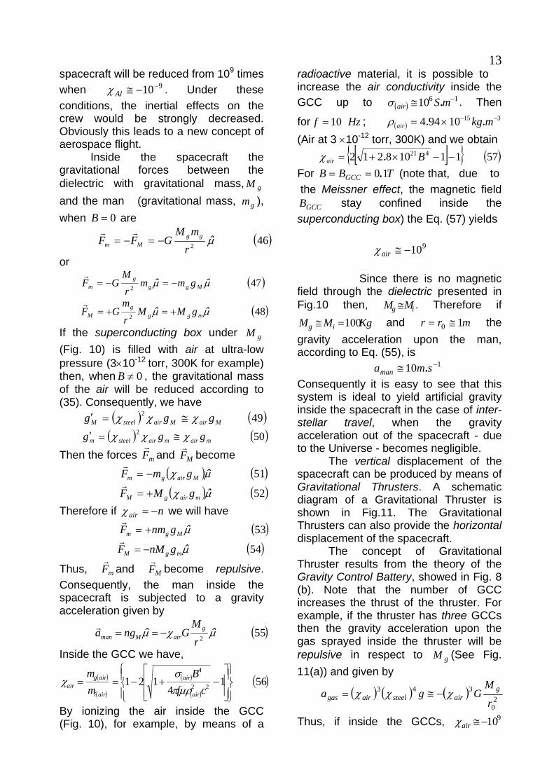
13spacecraft will be reduced from 109 times when . Under these conditions, the inertial effects on the crew would be strongly decreased. Obviously this leads to a new concept of aerospace flight.
910−−≅Alχ
Inside the spacecraft the gravitational forces between the dielectric with gravitational mass, and the man (gravitational mass, ), when are
gM
gm0=B
( )462 μ̂r
mMGFF gg
Mm −=−=rr
or
( )472 μμ ˆˆ Mggg
m gmmr
MGF −=−=
r
( )482
μμ ˆˆ mggg
M gMMrm
GF +=+=r
If the superconducting box under (Fig. 10) is filled with air at ultra-low pressure (3×10
gM
-12 torr, 300K for example) then, when , the gravitational mass of the air will be reduced according to (35). Consequently, we have
0≠B
( ) ( )492MairMairsteelM ggg χχχ ≅=′
( ) ( )502mairmairsteelm ggg χχχ ≅=′
Then the forces mFr
and become MFr
( ) ( )51μχ ˆMairgm gmF −=r
( ) ( )52μχ ˆmairgM gMF +=r
Therefore if nair −=χ we will have ( )53μ̂Mgm gnmF +=
r
( )54μ̂mgM gnMF −=r
Thus, mFr
and become repulsive. Consequently, the man inside the spacecraft is subjected to a gravity acceleration given by
MFr
( )552μχμ ˆˆ
rM
Gnga gairMman −==
r
Inside the GCC we have,
( )
( )
( )
( )( )561
4121 22
4
⎪⎭
⎪⎬⎫
⎪⎩
⎪⎨⎧
⎥⎥⎦
⎤
⎢⎢⎣
⎡−+−==
cfB
mm
air
air
airi
airgair μρπ
σχ
By ionizing the air inside the GCC (Fig. 10), for example, by means of a
radioactive material, it is possible to increase the air conductivity inside the GCC up to . Then
for ; (Air at 3 ×10
( )1610 −≅ mSair .σ
Hzf 10= ( )31510944 −−×= mkgair ..ρ
-12 torr, 300K) and we obtain [ ]{ } ( )5711108212 421 −−×+= Bair .χ
For TBB GCC 10.== (note that, due to the Meissner effect, the magnetic field
stay confined inside the superconducting box) the Eq. (57) yields
GCCB
910−≅airχ
Since there is no magnetic field through the dielectric presented in Fig.10 then, i . Therefore if g MM ≅
KgMM ig 100=≅ and the gravity acceleration upon the man, according to Eq. (55), is
mrr 10 ≅=
110 −≅ smaman .Consequently it is easy to see that this system is ideal to yield artificial gravity inside the spacecraft in the case of inter-stellar travel, when the gravity acceleration out of the spacecraft - due to the Universe - becomes negligible. The vertical displacement of the spacecraft can be produced by means of Gravitational Thrusters. A schematic diagram of a Gravitational Thruster is shown in Fig.11. The Gravitational Thrusters can also provide the horizontal displacement of the spacecraft. The concept of Gravitational Thruster results from the theory of the Gravity Control Battery, showed in Fig. 8 (b). Note that the number of GCC increases the thrust of the thruster. For example, if the thruster has three GCCs then the gravity acceleration upon the gas sprayed inside the thruster will be repulsive in respect to (See Fig. 11(a)) and given by
gM
( ) ( ) ( ) 20
343
r
MGga g
airsteelairgas χχχ −≅=
Thus, if inside the GCCs, 910−≅airχ

14(See Eq. 56 and 57) then the equation above gives
20
2710rM
Ga igas +≅
For , and the thrust is
kgMi 10≅ mr 10 ≅ kgmgas1210−≅
NamF gasgas510≅=
Thus, the Gravitational Thrusters are able to produce strong thrusts. Note that in the case of very strong airχ , for example , the gravity accelerations upon the boxes of the second and third GCCs become very strong (Fig.11 (a)). Obviously, the walls of the mentioned boxes cannot to stand the enormous pressures. However, it is possible to build a similar system with 3 or more GCCs, without material boxes. Consider for example, a surface with several radioactive sources (Am-241, for example). The alpha particles emitted from the Am-241 cannot reach besides 10cm of air. Due to the trajectory of the alpha particles, three or more successive layers of air, with different electrical conductivities
910−≅airχ
1σ , 2σ and 3σ , will be established in the ionized region (See Fig.11 (b)). It is easy to see that the gravitational shielding effect produced by these three layers is similar to the effect produced by the 3 GCCs shown in Fig. 11 (a). It is important to note that if is force produced by a thruster then the spacecraft acquires acceleration
given by [
F
spacecrafta 1]
( ) ( ) ( )AliinsideiAlspacecraftgspacecraft mM
FM
Fa+
==χ
Therefore if ; and (inertial mass of the aluminum shell) then it will be necessary
to produce
910−≅Alχ ( ) KgM insidei410=
( ) Kgm Ali 100=
kNF 10=2100 −= smaspacecraft .
Note that the concept of Gravitational Thrusters leads directly to the Gravitational Turbo Motor concept (See Fig. 12).
Let us now calculate the gravitational forces between two very close thin layers of the air around the spacecraft. (See Fig. 13). The gravitational force that
exerts upon , and the gravitational force that exerts upon are given by
12dF1gdm 2gdm
21dF 2gdm
1gdm
( )582
122112 μ̂
r
dmdmGFdFd gg−==
rr
Thus, the gravitational forces between the air layer 1, gravitational mass , and the air layer 2, gravitational mass
, around the spacecraft are
1gm
2gm
( )592
212
21
0 0 21221121 2
μχχμ
μ
ˆˆ
ˆ
rmm
Gr
mmG
dmdmrGFF
iiairair
gg
m m
ggg g
−=−=
=−=−= ∫ ∫rr
At 100km altitude the air pressure is
torr3106915 −×. and [( )36109985 −−×= mkgair ..ρ 12].
By ionizing the air surround the spacecraft, for example, by means of an oscillating electric field, , starting from the surface of the spacecraft ( See Fig. 13) it is possible to increase the air conductivity near the spacecraft up to
. Since and, in this case
oscE
( )1610 −≅ mSair .σ Hzf 1=
( ) ωεσ >>air , then, according to
Eq. (11), ( ) fcn airr πμσ 42= . From Eq.(56) we thus obtain
( )
( )
( )
( )( )601
4121 22
0
4
⎪⎭
⎪⎬⎫
⎪⎩
⎪⎨⎧
⎥⎥⎦
⎤
⎢⎢⎣
⎡−+−==
cfB
mm
air
air
airi
airgair ρμπ
σχ
Then for TB 763= the Eq. (60) gives
[ ]{ } ( )6110110121 844 −≅−+−= Bair ~χ By substitution of into Eq., (59) we get
810−≅airχ
( )6210 22116
2112 μ̂rmm
GFF ii−=−=rr

15If , and
we obtain
kgmm airairii8
2121 10−≅≅=≅ VV ρρ
mr 310−=( )6310 4
2112 NFF −−≅−=rr
These forces are much more intense than the inter-atomic forces (the forces which maintain joined atoms, and molecules that make the solids and liquids) whose intensities, according to the Coulomb’s law, is of the order of 1-1000×10-8N. Consequently, the air around the spacecraft will be strongly compressed upon their surface, making an “air shell” that will accompany the spacecraft during its displacement and will protect the aluminum shell of the direct attrition with the Earth’s atmosphere. In this way, during the flight, the attrition would occur just between the “air shell” and the atmospheric air around her. Thus, the spacecraft would stay free of the thermal effects that would be produced by the direct attrition of the aluminum shell with the Earth’s atmosphere. Another interesting effect produced by the magnetic field B of the spacecraft is the possibility of to lift a body from the surface of the Earth to the spacecraft as shown in Fig. 14. By ionizing the air surround the spacecraft, by means of an oscillating electric field,
, the air conductivity near the spacecraft can reach, for example,
. Then for
oscE
( )1610 −≅ mSair .σ Hzf 1= ;
and (300K and 1 atm) the Eq. (56) yields
TB 840.= ( )321 −≅ mkgair ..ρ
1011094121 47 .. −≅⎭⎬⎫
⎩⎨⎧
⎥⎦⎤
⎢⎣⎡ −×+−= − Bairχ
Thus, the weight of the body becomes
( ) ( ) ( )gmgmgmP bodyibodyiairbodygbody ′=== χConsequently, the body will be lifted on the direction of the spacecraft with acceleration
1980 −+≅=′ smgg air ..χ Let us now consider an important
aspect of the flight dynamics of a Gravitational Spacecraft. Before starting the flight, the gravitational mass of the spacecraft, , must be strongly reduced, by means of a gravity control system, in order to produce – with a weak thrust , a strong acceleration,
gM
Fr
ar , given by [1]
gMFar
r=
In this way, the spacecraft could be strongly accelerated and quickly to reach very high speeds near speed of light. If the gravity control system of the spacecraft is suddenly turned off, the gravitational mass of the spacecraft becomes immediately equal to its inertial mass, , iM ( )ig MM =′ and the velocity
Vr
becomes equal to V ′r
. According to the Momentum Conservation Principle, we have that
VMVM gg ′′= Supposing that the spacecraft was traveling in space with speed cV ≈ , and that its gravitational mass it was
KgMg 1= and then the velocity of the spacecraft is reduced to
KgM i410=
cVMM
VMM
Vi
g
g
g 410−≈=′
=′
Initially, when the velocity of the spacecraft is V
r, its kinetic energy is
( ) 2cmME ggk −= . Where 221 cVmM gg −= . At the instant in which the gravity control system of the spacecraft is turned off, the kinetic energy becomes
( ) 2cmME ggk ′−′=′ . Where 221 cVmM gg ′−′=′ . We can rewritten the expressions of
and kE kE′ in the following form
( )VcVmVME ggk
2
−=
( )VcVmVME ggk ′
′′−′′=′2
Substitution of pVMVM gg =′′= ,
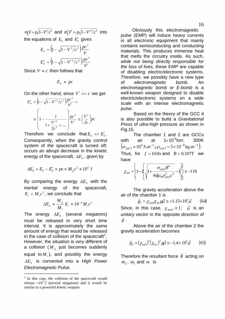
16221 cVpVmg −= and 221 cVpVmg ′−=′′ into
the equations of and gives kE kE′
( )VpccVEk
22211 −−=
( )VpccVEk ′
′−−=′2
2211
Since then follows that cV ≈
pcEk ≈ On the other hand, since we get cV <<′
( )
pcc
VVpc
cV
VpccVEk
⎟⎠⎞
⎜⎝⎛ ′
≅′
⎟⎟⎟⎟
⎠
⎞
⎜⎜⎜⎜
⎝
⎛
+′
+−≅
=′
′−−=′
22
1
11
11
2
2
2
222
...
Therefore we conclude that kk EE ′>> . Consequently, when the gravity control system of the spacecraft is turned off, occurs an abrupt decrease in the kinetic energy of the spacecraft, , given by kEΔ
JcMpcEEE gkkk172 10≈≈≈′−=Δ
By comparing the energy with the inertial energy of the spacecraft,
, we conclude that
kEΔ
2cME ii =
2410 cMEMM
E iii
gk
−≈≈Δ
The energy (several megatons) must be released in very short time interval. It is approximately the same amount of energy that would be released in the case of collision of the spacecraft
kEΔ
‡. However, the situation is very different of a collision ( just becomes suddenly equal to ), and possibly the energy
is converted into a High Power Electromagnetic Pulse.
gM
iM
kEΔ
‡ In this case, the collision of the spacecraft would release ≈1017J (several megatons) and it would be similar to a powerful kinetic weapon.
Obviously this electromagnetic pulse (EMP) will induce heavy currents in all electronic equipment that mainly contains semiconducting and conducting materials. This produces immense heat that melts the circuitry inside. As such, while not being directly responsible for the loss of lives, these EMP are capable of disabling electric/electronic systems. Therefore, we possibly have a new type of electromagnetic bomb. An electromagnetic bomb or E-bomb is a well-known weapon designed to disable electric/electronic systems on a wide scale with an intense electromagnetic pulse. Based on the theory of the GCC it is also possible to build a Gravitational Press of ultra-high pressure as shown in Fig.15. The chamber 1 and 2 are GCCs with air at 1×10⁻⁴torr, 300K
( ) ( )( )3816 10510 −−− ×=≈ mkgmS airair .;. ρσ .Thus, for Hzf 10= and we have
TB 1070.=
( )
( )1181
4121
220
4
−≅⎪⎭
⎪⎬⎫
⎪⎩
⎪⎨⎧
⎥⎥
⎦
⎤
⎢⎢
⎣
⎡−+−=
cf
B
air
airair ρμπ
σχ
The gravity acceleration above the air of the chamber 1 is
( )6410151 31 μμχχ ˆ.ˆ ×+≅= gg airstellr
Since, in this case, 1≅steelχ ; μ̂ is an unitary vector in the opposite direction of gr . Above the air of the chamber 2 the gravity acceleration becomes
( ) ( ) ( )651041 5222 μμχχ ˆ.ˆ ×−≅= gg airstellr
Therefore the resultant force R
r acting on
, and is 2m 1m m

17112212 gmgmgmFFFR =++=++=
r r r r r r r
( )661041
819101511041
25
13
25
μ
μμμ
ˆ.ˆ.ˆ.ˆ.
m
mmm
×−≅
=−×+×−=
where
( )67
−≅steelρ
inn2910 φ≅
42
22 ⎟⎠⎞
⎜⎝⎛== HVm innsteeldisksteel φπρρ
Thus, for we can write that
3410 mkg .
HF2 For the steel consequently we must have
2925 1010 −− =≅ mkgcmkg ..τ
292 10 −< mkgSF .τ HS inn( πφτ = see Fig.15).
This means that 29
2910 −10< mkgHinn .
φHinnπφ
Then we conclude that minn 13.<φ
For minn 2=φ and the Eq. (67) gives mH 1=kgm 4
2 103×≅
2410 mS −=
Therefore from the Eq. (66) we obtain NR 1010≅
Consequently, in the area of the Gravitational Press, the pressure is
The GCCs can also be applied on generation and detection of Gravitational Radiation. Consider a cylindrical GCC (GCC antenna) as shown in Fig.16 (a). The gravitational mass of the air inside the GCC is
( )( )
( )( ) ( )681
4121
22
4
airiair
airairg m
cfB
m⎪⎭
⎪⎬⎫
⎪⎩
⎪⎨⎧
⎥⎥⎦
⎤
⎢⎢⎣
⎡−+−=
μρπ
σ
By varying B one can varies and consequently to vary the gravitational field generated by , producing then gravitational radiation. Then a GCC can work like a Gravitational Antenna.
( )airgm
( )airgm
Apparently, Newton’s theory of gravity had no gravitational waves because, if a gravitational field changed in some way, that change took place instantaneously everywhere in space, and one can think that there is not a wave in this case. However, we have already seen that the gravitational interaction can be repulsive, besides attractive. Thus, as with electromagnetic interaction, the gravitational interaction must be produced by the exchange of "virtual" quanta of spin 1 and mass null, i.e., the gravitational "virtual" quanta (graviphoton) must have spin 1 and not 2. Consequently, the fact of a change in a gravitational field reach instantaneously everywhere in space occurs simply due to the speed of the graviphoton to be infinite. It is known that there is no speed limit for “virtual” photons. On the contrary, the electromagnetic quanta (“virtual” photons) could not communicate the electromagnetic interaction an infinite distance.
2−
211106173 −× mN ..
1410≅= mNSRp .
This enormous pressure is much greater than the pressure in the center of the Earth ( ) [13]. It is near of the gas pressure in the center of the sun ( ). Under the action of such intensities new states of matter are created and astrophysical phenomena may be simulated in the lab for the first time, e.g. supernova explosions. Controlled thermonuclear fusion by inertial confinement, fast nuclear ignition for energy gain, novel collective acceleration schemes of particles and the numerous variants of material processing constitute examples of progressive applications of such Gravitational Press of ultra-high pressure.
216102 −× mN .
Thus, there are two types of gravitational radiation: the real and virtual, which is constituted of graviphotons; the real gravitational waves are ripples in the space-time generated by gravitational field changes. According to Einstein’s theory of gravity the velocity of propagation of these waves is equal to the speed of light (c).

18 Unlike the electromagnetic waves the real gravitational waves have low interaction with matter and consequently low scattering. Therefore real gravitational waves are suitable as a means of transmitting information. However, when the distance between transmitter and receiver is too large, for example of the order of magnitude of several light-years, the transmission of information by means of gravitational waves becomes impracticable due to the long time necessary to receive the information. On the other hand, there is no delay during the transmissions by means of virtual gravitational radiation. In addition the scattering of this radiation is null. Therefore the virtual gravitational radiation is very suitable as a means of transmitting information at any distances including astronomical distances. As concerns detection of the virtual gravitational radiation from GCC antenna, there are many options. Due to Resonance Principle a similar GCC antenna (receiver) tuned at the same frequency can absorb energy from an incident virtual gravitational radiation (See Fig.16 (b)). Consequently, the gravitational mass of the air inside the GCC receiver will vary such as the gravitational mass of the air inside the GCC transmitter. This will induce a magnetic field similar to the magnetic field of the GCC transmitter and therefore the current through the coil inside the GCC receiver will have the same characteristics of the current through the coil inside the GCC transmitter. However, the volume and pressure of the air inside the two GCCs must be exactly the same; also the type and the quantity of atoms in the air inside the two GCCs must be exactly the same. Thus, the GCC antennas are simple but they are not easy to build. Note that a GCC antenna radiates graviphotons and gravitational waves simultaneously (Fig. 16 (a)). Thus, it is not only a gravitational antenna: it is a Quantum Gravitational Antenna because it can also emit and detect gravitational "virtual" quanta (graviphotons), which, in turn, can transmit information instantaneously from any distance in the Universe without scattering. Due to the difficulty to build two similar GCC antennas and, considering that the electric current in the receiver antenna can
be detectable even if the gravitational mass of the nuclei of the antennas are not strongly reduced, then we propose to replace the gas at the nuclei of the antennas by a thin dielectric lamina. The dielectric lamina with exactly 108 atoms (103atoms × 103atoms × 102atoms) is placed between the plates (electrodes) as shown in Fig. 17. When the virtual gravitational radiation strikes upon the dielectric lamina, its gravitational mass varies similarly to the gravitational mass of the dielectric lamina of the transmitter antenna, inducing an electromagnetic field ( ,E B ) similar to the transmitter antenna. Thus, the electric current in the receiver antenna will have the same characteristics of the current in the transmitter antenna. In this way, it is then possible to build two similar antennas whose nuclei have the same volumes and the same types and quantities of atoms. Note that the Quantum Gravitational Antennas can also be used to transmit electric power. It is easy to see that the Transmitter and Receiver (Fig. 17(a)) can work with strong voltages and electric currents. This means that strong electric power can be transmitted among Quantum Gravitational Antennas. This obviously solves the problem of wireless electric power transmission. The existence of imaginary masses has been predicted in a previous work [1]. Here we will propose a method and a device using GCCs for obtaining images of imaginary bodies. It was shown that the inertial imaginary mass associated to an electron is given by
( ) ( ) ( )693
23
22 imi
chfm
realieimaie =⎟⎠⎞
⎜⎝⎛=
Assuming that the correlation between the gravitational mass and the inertial mass (Eq.6) is the same for both imaginary and real masses then follows that the gravitational imaginary mass associated to an electron can be written in the following form:
( ) ( ) ( )7011212
2 imaieri
image mncm
Um⎪⎭
⎪⎬
⎫
⎪⎩
⎪⎨
⎧
⎥⎥⎥
⎦
⎤
⎢⎢⎢
⎣
⎡−⎟⎟
⎠
⎞⎜⎜⎝
⎛+−=
Thus, the gravitational imaginary mass associated to matter can be reduced, made

19negative and increased, just as the gravitational real mass. It was shown that also photons have imaginary mass. Therefore, the imaginary mass can be associated or not to the matter. In a general way, the gravitational forces between two gravitational imaginary masses are then given by
( )( )( )71ˆˆ
22μμ
r
mMG
r
imiMGFF gggg +=−=−=
rr
Note that these forces are real and repulsive. Now consider a gravitational imaginary mass, ( ) gimag imm = , not associated with matter (like the gravitational imaginary mass associated to the photons) and another gravitational imaginary mass
associated to a material body.
( ) gimag iMM =
Any material body has an imaginary mass associated to it, due to the existence of imaginary masses associated to the electrons. We will choose a quartz crystal (for the material body with gravitational imaginary mass ) because quartz crystals are widely used to detect forces (piezoelectric effect).
( ) gimag iMM =
By using GCCs as shown in Fig. 18(b) and Fig.18(c), we can increase the gravitational acceleration, , produced by the imaginary mass upon the crystals. Then it becomes
ar
gim
( )722
3
r
mGa g
airχ−=
As we have seen, the value of airχ can be
increased up to (See Eq.57). Note that in this case, the gravitational forces become attractive. In addition, if is not small, the gravitational forces between the imaginary body of mass and the crystals can become sufficiently intense to be easily detectable.
910−≅airχ
gm
gim
Due to the piezoelectric effect, the gravitational force acting on the crystal will produce a voltage proportional to its intensity. Then consider a board with hundreds micro-crystals behind a set of GCCs, as shown in Fig.18(c). By amplifying the voltages generated in each micro-crystal and sending to an appropriated data acquisition system, it will be thus possible to
obtain an image of the imaginary body of mass placed in front of the board. ( )imagm In order to decrease strongly the gravitational effects produced by bodies placed behind the imaginary body of mass
, one can put five GCCs making a Gravitational Shielding as shown in Fig.18(c). If the GCCs are filled with air at 300Kand
gim
torr12103 −× .Then
and 1. Thus, for and
31510944 −−×= mkgair ..ρ14101 −−×≅ mSair .σ Hzf 60=
TB 70.≅ the Eq. (56) gives ( )
( )( )731015121 24 −−≅
⎭⎬⎫
⎩⎨⎧
⎥⎦⎤
⎢⎣⎡ −+−== B
mm
airi
airgairχ
For the gravitational shielding presented in Fig.18(c) will reduce any value of
210−≅airχ
g to . This will be sufficiently to reduce strongly the gravitational effects proceeding from both sides of the gravitational shielding.
ggair105 10−≅χ
Another important consequence of the correlation between gravitational mass and inertial mass expressed by Eq. (1) is the possibility of building Energy Shieldings around objects in order to protect them from high-energy particles and ultra-intense fluxes of radiation. In order to explain that possibility, we start from the new expression [1] for the momentum of a particle with gravitational mass and velocityV , which is given by
q
gM( )74VMq g=
where 221 cVmM gg −= and [ig mm χ= 1]. Thus, we can write
( )7511 2222 cV
m
cV
m ig
−=
−
χ
Therefore, we get
( )76ig MM χ=It is known from the Relativistic Mechanics that
( )772cUVq =
where is the total energy of the particle. This expression is valid for any velocity V of the particle, including .
U
cV = By comparing Eq. (77) with Eq. (74) we obtain

20( )782cMU g=
It is a well-known experimental fact that ( )792 hfcM i =
Therefore, by substituting Eq. (79) and Eq. (76) into Eq. (74), gives
( )80λ
χ hcVq =
Note that this expression is valid for any velocity of the particle. In the particular case of , it reduces to
VcV =
( )81λ
χ hq =
By comparing Eq. (80) with Eq. (77), we obtain
( )82hfU χ= Note that only for 1=χ the Eq. (81) and Eq. (82) are reduced to the well=known expressions of DeBroglie ( )λhq = and Einstein . ( )hfU = Equations (80) and (82) show for example, that any real particle (material particles, real photons, etc) that penetrates a region (with density ρ and electrical conductivityσ ), where there is an ELF electric field E , will have its momentum and its energy U reduced by the factor
qχ ,
given by
( )83144
121 2
43
2⎪⎭
⎪⎬⎫
⎪⎩
⎪⎨⎧
⎥⎥
⎦
⎤
⎢⎢
⎣
⎡−⎟⎟
⎠
⎞⎜⎜⎝
⎛+−==
ρπσμχ E
fcmm
i
g
The remaining amount of momentum and energy, respectively given by
( )λ
χ hcV⎟⎠⎞
⎜⎝⎛−1 and ( , are
transferred to the imaginary particle associated to the real particle
) hfχ−1
§ (material particles or real photons) that penetrated the mentioned region. It was previously shown that, when the gravitational mass of a particle is reduced to ranging between to , i.e., when
iM1590.+ iM1590.−159.0<χ , it becomes imaginary
[1], i.e., the gravitational and the inertial masses of the particle become imaginary. Consequently, the particle disappears from § As previously shown, there are imaginary particles associated to each real particle [1].
our ordinary space-time. It goes to the Imaginary Universe. On the other hand, when the gravitational mass of the particle becomes greater than , or less than
iM1590.+
iM1590.− , i.e., when 159.0>χ , the particle return to our Universe. Figure 19 (a) clarifies the phenomenon of reduction of the momentum for 159.0>χ , and Figure 19 (b) shows the effect in the case of 159.0<χ . In this case, the particles become imaginary and consequently, they go to the imaginary space-time when they penetrate the electric field E . However, the electric field E stays at the real space-time. Consequently, the particles return immediately to the real space-time in order to return soon after to the imaginary space-time, due to the action of the electric field E . Since the particles are moving at a direction, they appear and disappear while they are crossing the region, up to collide with the plate (See Fig.19) with
a momentum, λ
χ hcVq m ⎟⎠⎞
⎜⎝⎛= , in the case
of the material particle, and λ
χ hqr = in the
case of the photon. Note that by making 0≅χ , it is possible to block high-energy particles and ultra-intense fluxes of radiation. These Energy Shieldings can be built around objects in order to protect them from such particles and radiation. It is also important to note that the gravity control process described here points to the possibility of obtaining Controlled Nuclear Fusion by means of increasing of the intensity of the gravitational interaction between the nuclei. When the gravitational forces 2rmGmF ggG ′= become greater than
the electrical forces 204 rqqFE πε′=
between the nuclei, then nuclear fusion reactions can occur. Note that, according to Eq. (83), the gravitational mass can be strongly increased. Thus, if tEE m ωsin= , then the
average value for 2E is equal to 22
1mE ,
because E varies sinusoidaly ( is the maximum value for
mEE ). On the other hand,
2mrms EE = . Consequently, we can replace

214E for . In addition, as 4
rmsE Ej σ= (Ohm's vectorial Law), then Eq. (83) can be rewritten as follows
( )841121 32
4
0 ⎪⎭
⎪⎬⎫
⎪⎩
⎪⎨⎧
⎥⎥
⎦
⎤
⎢⎢
⎣
⎡−+−==
fj
Kmm rmsr
i
g
σρμ
χ
where and2710758.1 −×=K 2jjrms = . Thus, the gravitational force equation can be expressed by
( )851121 200
2
32
4
200
22
rmGmf
jK
rmGmrmGmF
iirmsr
iiggG
′⎪⎭
⎪⎬⎫
⎪⎩
⎪⎨⎧
⎥⎥⎦
⎤
⎢⎢⎣
⎡−+−=
=′=′=
σρμ
χ
In order to obtain we must have EG FF >
( )864
112100
032
4
ii
rmsr
mGmqq
f
jK
′′
>⎪⎭
⎪⎬⎫
⎪⎩
⎪⎨⎧
⎥⎥
⎦
⎤
⎢⎢
⎣
⎡−+−
πε
σρ
μ
The carbon fusion is a set of nuclear fusion reactions that take place in massive stars (at least at birth). It requires high
temperatures ( ) and densities ( ). The principal reactions are:
sunM8
K8105×>39 .103 −×> mkg
23Na + p + 2.24 MeV 12C + 12C → 20Ne + α + 4.62 MeV 24Mg + γ +13.93 MeV In the case of Carbon nuclei (12C) of a thin carbon wire ( ; ) Eq. (86) becomes
14 .104 −×≅ mSσ 13 .102.2 −×= mSρ
20
2
3
439
1611008.9121
p
rms
Gme
fj
πε>
⎪⎭
⎪⎬⎫
⎪⎩
⎪⎨⎧
⎥⎥⎦
⎤
⎢⎢⎣
⎡−×+− −
whence we conclude that the condition for the 12C + 12C fusion reactions occur is
( )87107.1 43
18 fjrms ×>If the electric current through the carbon wire has Extremely-Low Frequency (ELF), for example, if Hzf μ1= , then the current density, , must have the following value: rmsj
( )88.104.5 213 −×> mAjrms
Since Sij rmsrms = where 42πφ=S is the area of the cross section of the wire, we can conclude that, for an ultra-thin carbon wire
with mμ10 -diameter, it is necessary that the current through the wire, , have the following intensity
rmsi
Akirms 24.4>
Obviously, this current will explode the carbon wire. However, this explosion becomes negligible in comparison with the very strong gravitational implosion, which occurs simultaneously due to the enormous increase in intensities of the gravitational forces among the carbon nuclei produced by means of the ELF current through the carbon wire as predicted by Eq. (85). Since, in this case, the gravitational forces among the carbon nuclei become greater than the repulsive electric forces among them the result is the production of 12C + 12C fusion reactions. Similar reactions can occur by using a lithium wire. In addition, it is important to note that is directly proportional
to
rmsj
43
f (Eq. 87). Thus, for example,
if , the current necessary to produce the nuclear reactions will be
Hzf 810−=
Airms 130= . IV.CONCLUSION The process described here is clearly the better way in order to control the gravity. This is because the Gravity Control Cell in this case is very easy to be built, the cost is low and it works at ambient temperature. The Gravity Control is the starting point for the generation of and detection of Virtual Gravitational Radiation (Quantum Gravitational Transceiver) also for the construction of the Gravitational Motor and the Gravitational Spacecraft which includes the system for generation of artificial gravity presented in Fig.10 and the Gravitational Thruster (Fig.11). While the Gravitational Transceiver leads to a new concept in Telecommunication, the Gravitational Motor changes the paradigm of energy conversion and the Gravitational Spacecraft points to a new concept in aerospace flight.
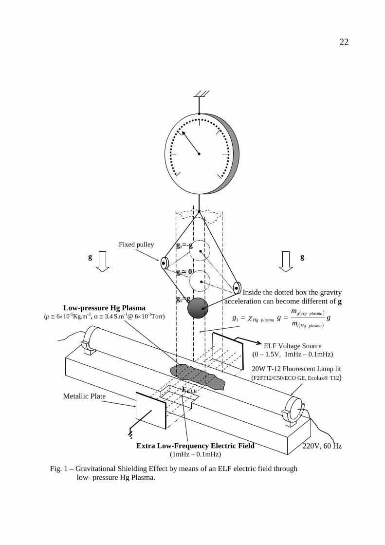
22
g g
ELF Voltage Source (0 – 1.5V, 1mHz – 0.1mHz)
Extra Low-Frequency Electric Field(1mHz – 0.1mHz)
EELF
20W T-12 Fluorescent Lamp lit(F20T12/C50/ECO GE, Ecolux® T12)
Inside the dotted box the gravity acceleration can become different of g
( )
( )g
mm
ggplasmaHgi
plasmaHggplasmaHg == χ1
Low-pressure Hg Plasma (ρ ≅ 6×10⁻⁵Kg.m-3, σ ≅ 3.4 S.m-1@ 6×10⁻³Torr)
Fig. 1 – Gravitational Shielding Effect by means of an ELF electric field through low- pressure Hg Plasma.
Metallic Plate
Fixed pulley g1=-g g1≅ 0 g1=g
220V, 60 Hz

23
g
g
Inside the dotted box the gravity acceleration above the second lamp becomes
( )g
gg
plasmaHgplasmaHg
plasmaHg
12
122
χχ
χ
=
==
Fig. 2 – Gravity acceleration above a second fluorescent lamp.
g1
g2
plasmaHg1χ
plasmaHg2χ
2
1 fELF(2)
fELF(1)

24
(a)
RF Transmitter
ELF Voltage Source
( )
( )g
mm
gplasmaHgi
plasmaHgg=1
Fig. 3 – Schematic diagram of Gravity Control Cells (GCCs). (a) GCC where the ELF electric field and the ionizing electric field can be the same. (b) GCCwhere the plasma is ionized by means of a RF signal. (c) GCC filled with air (at ambient temperature and 1 atm) strongly ionized by means of alpha particles emitted from radioactiveions sources (Am 241, half-life 432 years). Since the electrical conductivity of the ionized air depends on the amount of ions then it can be strongly increased by increasing the amount of Am241 in the GCC. This GCC has 36 radioactive ions sources each one with 1/5000th of gram of Am 241, conveniently positioned around the ionization chamber, in order to obtain 1310 −≅ mSair .σ .
RF SignalLow-density plasma
ElectrodesLow-density plasma
g
g
Electrodes
ELF Voltage Source (b)
~
( )
( )g
mm
gplasmaHgi
plasmaHgg=1
~
~ V , fAir @ 1 atm, 25°C
Radioactive ions sources (Americium 241)
Insulating holder Epoxy Ionization chamber Aluminium, 1mm-thickness
• •d
(c)
φ

25
Fig. 4 – Gravitational Shielding surround a Spherical Spacecraft.
χair
mg
r
Gravitational Shielding
Mg
The gravity accelerations on the spacecraft (due to the rest of the Universe) can be controlled by means of the gravitational shielding, i.e., g’i = χair gi i = 1, 2, 3 … n Thus, Fis= Fsi = Mg g’i = Mg (χair gi) Then the inertial forces acting on the spacecraft (s) can be strongly reduced. According to the Mach’s principle this effect can reduce the inertial properties of the spacecraft and consequently, leads to a new concept of spacecraft and aerospace flight.
Erms (low frequency)
g = G mg / r2
g’ = χair g
Spacecraft
a

26
t = T /4 g1 / g g2 / g V = V0 (Volts) (s) ( min)
EELF (1) (V/m)
fELF (1) (mHz) Exp. Teo.
EELF (2) (V/m)
fELF (2) (mHz) Exp. Teo.
250 4.17 24.81 1 - 0.993 24.81 1 - 0.986 312.5 5.21 24.81 0.8 - 0.986 24.81 0.8 - 0.972 416.6 6.94 24.81 0.6 - 0.967 24.81 0.6 - 0.935 625 10.42 24.81 0.4 - 0.890 24.81 0.4 - 0.792
1.0 V
1250 20.83 24.81 0.2 - 0.240 24.81 0.2 - 0.058 250 4.17 37.22 1 - 0.964 37.22 1 - 0.929
312.5 5.21 37.22 0.8 - 0.930 37.22 0.8 - 0.865 416.6 6.94 37.22 0.6 - 0.837 37.22 0.6 - 0.700 625 10.42 37.22 0.4 - 0,492 37.22 0.4 - 0.242
1.5V
1250 20.83 37.22 0.2 - -1,724 37.22 0.2 - 2.972
Table 1 – Theoretical Results.

27
Fig. 5- Distribution of the correlation g1/ g as a function of f ELF
-2
-1
0
1
2
30,10,20,30,40,50,60,70,80,91,0
f ELF (mHz)
g 1 / g g1/g
1.0V
g1/g
1.5V

28
Fig. 6- Distribution of the correlation g2 / g as a function of f ELF
-2
-1
0
1
2
30,10,20,30,40,50,60,70,80,91,0
f ELF (mHz)
g 2 / g
g2/g 1.0V
g2/g 1.5V

29
Fig. 7- Distribution of the correlations gi / g as a function of f ELF
-2
-1
0
1
2
30,10,20,30,40,50,60,70,80,91,0
f ELF (mHz)
g i / g
g1/g
1.5V
g2/g
1.5V
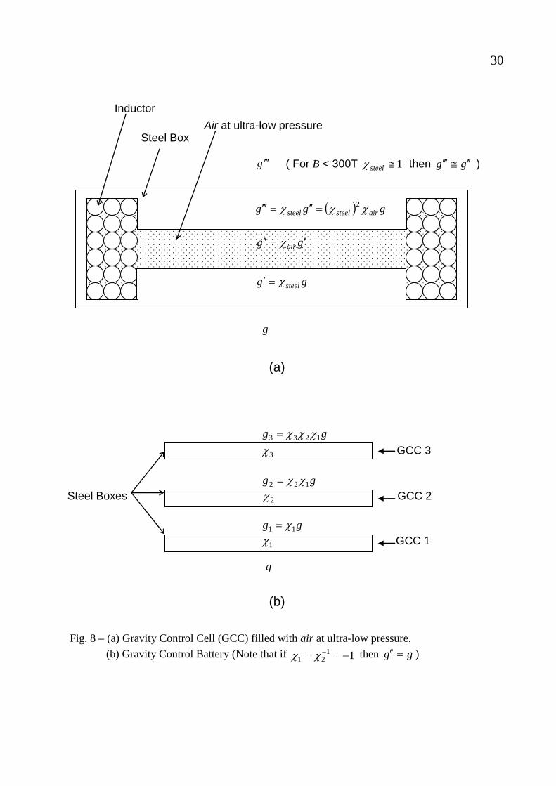
30
Air at ultra-low pressure
Inductor
Steel Box
g ′′′
gg air ′=′′ χ
Fig. 8 – (a) Gravity Control Cell (GCC) filled with air at ultra-low pressure. (b) Gravity Control Battery (Note that if 11
21 −== −χχ then gg =′′ )
(a)
(b)
gg 1233 χχχ= 3χ GCC 3 gg 122 χχ= Steel Boxes 2χ GCC 2 gg 11 χ= 1χ GCC 1 g
g
( ) ggg airsteelsteel χχχ 2=′′=′′′
gg steelχ=′
( For B < 300T 1≅steelχ then gg ′′≅′′′ )

31
g
g’ Massive Rotor
Gravity Control Cell (Steel box)
r r
R
( ) gg airsteel χχ 2=′ ( ) ( ) gg airsteel24 χχ=′′
1≅steelχ ( ) ( ) nairair −== −121 χχ ngg −≅′ gg =′′
g’’= g Gravity Control Cell (Steel box) g Note that and therefore for and we get and
Fig. 9 – The Gravitational Motor

32
Fig. 10 – The Gravitational Spacecraft – Due to the Meissner effect, the magnetic field B is expelled from the superconducting shell. Similarly, the magnetic field BGCC, of the
GCC stay confined inside the superconducting box.
MgFM
mg Fm
μ̂
Gravity Control Cell- GCC
Superconducting Ring
Dielectric Aluminum Shell Superconducting
Shell
Superconducting Box
B

33
Gas
mg μ
Fm
Gas
Fig. 11 – The Gravitational Thruster . (a) Using material boxes. (b) Without material boxes
GCC Mg
FM
GCC GCC agas
Material boxes (a)
(b)
Am - 241
σ3 <σ2 (χair 3) σ2 <σ1 (χair 2)
σ1 (χair 1)
g’’’= χair 3 g’’= χair 3 χair 2 χair 1 g g ’’ = χair 2 g ’ = χair 2 χair 1 g g ’= χair 1 g
α
g

34
GCC GCC GCC
Gas Helix
Gas
HIGH
SPEED Motor axis
GAS
Fig. 12 - The Gravitational Turbo Motor – The gravitationally accelerated gas, by means of the GCCs, propels the helix which movies the motor axis.

35
r
dmg2
dmg1
dF12 dF21 Air Layer 2Air Layer 1
Fig. 13 – Gravitational forces between two layers of the “air shell”. The electric field Eosc provides the ionization of the air.
Spacecraft
Eosc

36
Fig. 14 – The Gravitational Lifter
( )μμχ ˆ..ˆ 2980 −+≅=′ smgg air
r
Eosc
Spacecraft
Eosc
χair
μ̂
B

37
Fig. 15 – Gravitational Press
H
H
0.20
0.20
0.20
B
innφ
τS 262 1041 −×−≅ smg ..
231 103 −×+≅ smg .
2819 −−= smg ..
Chamber 1 Air
Chamber 2 Air
g g
m2
m1
m
S P=R/S

38
i
f
(a) GCC Antenna
i i
f f
Transmitter (b) Receiver
Fig. 16 - Transmitter and Receiver of Virtual Gravitational Radiation.
Real Gravitational Waves v = c
Graviphotons v = ∞
GCC
GCC
Graviphotons v = ∞
GCC
Coil

39
103atoms
Dielectric (108 atoms)
Graviphotons
v = ∞
(a)
Transmitter Receiver
102atoms
Fig. 17 – Quantum Gravitational Microantenna
(b)
Microantenna
Conductor Conductor
103atoms
Dielectric
f f

40
(a)
(b)
(c)
Data
Acquisition System
v
V
( )( )22 rmM
Gr
imiMGF gggg +=−=
F
Imaginary body img
Crystal F
iMg
F
Imaginary body img
Crystal
iMg
Imaginary body img
Mg = Mi
(Mi = inertial mass)
F =Mg a ≅Mi a
a = - (χair )3Gmg / r2
micro-crystals
A M P L Y F I E R
Display
GCC GCC GCC
χair → -109
GCC GCC GCC
χair5g’ χair
5g’ χair4g’ χair
3g’ χair2g’ χair
g’ g’
⏐ Gravitational Shielding ⏐
χair ≅ 10-2
g χair g χair2g χair
3g χair4 g χair
5 g χair5 g
GCC GCC GCC GCC GCC
Fig.18 – Method and device using GCCs for obtaining images of imaginary bodies.

41
(a) * There are a type of neutrino, called "ghost” neutrino, predicted by General Relativity, with zero massand zero momentum. In spite its momentum be zero, it is known that there are wave functions that describe these neutrinos and that prove that really they exist.
(b) ig. 19 – The phenomenon of reduction of the momentum. (a) Shows the reduction o
F f momentum for 159.0>χ . (b) Shows the effect when 159.0<χ . Note that in both cases, the
material particles collide with the cowl with the momentum ( )( )λχ hcVq m = , and the
photons withλ
χ hqr = . Therefore, that by making 0≅χ , it is possible to block high-energy
particles and ultra-intense fluxes of radiation.
material particle imaginary particle associated to the material particle
real photon
imaginary photon associated to the
real photon
σρ ,, fE
159.0>χ
λχ h
cVq m ⎟⎠⎞
⎜⎝⎛=
[ ]λ
χ hqi −= 1
λχ hqr =
[ ]λ
χ hcVqi ⎟⎠⎞
⎜⎝⎛−= 1
λh
cVqm ⎟⎠⎞
⎜⎝⎛≅
*0=iq
λhqr ≅
0=iq
material particle imaginary particle associated to the material particle
real photon
imaginary photon associated to the
real photon
σρ ,, fE
159.0<χ
λχ h
cVq m ⎟⎠⎞
⎜⎝⎛=
[ ]λ
χ hqi −= 1
λχ hqr =
[ ]λ
χ hcVqi ⎟⎠⎞
⎜⎝⎛−= 1
λh
cVqm ⎟⎠⎞
⎜⎝⎛≅
0=iq
λhqr ≅
0=iq

42
APPENDIX A: THE SIMPLEST METHOD TO CONTROL THE GRAVITY In this Appendix we show the simplest method to control the gravity. Consider a body with mass density ρ and
the following electric characteristics: rμ , rε ,σ (relative permeability, relative permittivity and electric conductivity, respectively). Through this body, passes an electric current I , which is the sum of a sinusoidal current tiiosc ωsin0= and
the DC current , i.e., DCI tiII DC ωsin0+=
; fπω 2= . If then . Thus, the
current DCIi <<0 DCII ≅
I varies with the frequency , but the variation of its intensity is quite small in comparison with , i.e.,
f
DCI I will be practically constant (Fig. 1A). This is of fundamental importance for maintaining the value of the gravitational mass of the body, , sufficiently stable during all the time.
gm
The gravitational mass of the body is given by [1]
( )11121 0
2
20
AmcmUnm i
i
rg
⎪⎭
⎪⎬
⎫
⎪⎩
⎪⎨
⎧
⎥⎥⎥
⎦
⎤
⎢⎢⎢
⎣
⎡−⎟
⎟⎠
⎞⎜⎜⎝
⎛+−=
whereU , is the electromagnetic energy absorbed by the body and is the index of refraction of the body.
rn
Equation (A1) can also be rewritten in the following form
( )211212
20
AcWn
mm r
i
g
⎪⎭
⎪⎬
⎫
⎪⎩
⎪⎨
⎧
⎥⎥⎥
⎦
⎤
⎢⎢⎢
⎣
⎡−⎟
⎟⎠
⎞⎜⎜⎝
⎛+−=
ρ
where, VUW = is the density of
electromagnetic energy and V0im=ρ is the density of inertial mass. The instantaneous values of the density of electromagnetic energy in an electromagnetic field can be deduced from Maxwell’s equations and has the following expression
( )32212
21 AHEW με +=
where tEE m ωsin= and tHH ωsin= are the instantaneous values of the electric field and the magnetic field respectively.
Fig. A1 - The electric current I varies withfrequency f . But the variation of
I is quite small
in comparison with DCI due to DCo Ii << . In this way, we can consider DCII ≅ .
t
IDC
I = IDC + iosc
i0
It is known that HB μ= , rkBE ω= [11] and
( )( )4
112
2Ac
dtdzv
rrr ⎟⎠⎞⎜
⎝⎛ ++
===ωεσμεκ
ω
where is the real part of the propagation
vector rkkr
(also called phase constant );
ir ikkkk +==r
; ε , μ and σ, are the
electromagnetic characteristics of the medium in which the incident (or emitted) radiation is propagating( 0εεε r= ;
;
mF /10854.8 120
−×=ε
0μμμ r= where ). It is known that for free-space
m/H70 104 −×= πμ
0=σ and 1== rr με . Then Eq. (A4) gives
cv = From (A4), we see that the index of refraction
vcnr = is given by
( ) ( )5112
2 Avcn rr
r ⎟⎠⎞⎜
⎝⎛ ++== ωεσ
με

43 Equation (A4) shows that vr =κω .
Thus, vkBE r == ω , i.e.,
( )6AHvvBE μ==Then, Eq. (A3) can be rewritten in the following form:
( ) ( )722122
21 AHHvW μμμε +=
For ωεσ << , Eq. (A4) reduces to
rr
cvμε
=
Then, Eq. (A7) gives
22212
2
21 HHHcW
rr
μμμμμε
ε =+⎥⎦
⎤⎢⎣
⎡⎟⎟⎠
⎞⎜⎜⎝
⎛=
This equation can be rewritten in the following forms:
( )82
ABWμ
=
or ( )92 AEW ε=
For ωεσ >> , Eq. (A4) gives
( )102 Avμσω
=
Then, from Eq. (A7) we get
( )11
2
221
22122
212
21
AH
HHHHW
μ
μμσωεμμμ
μσωε
≅
≅+⎟⎠⎞
⎜⎝⎛=+⎥
⎦
⎤⎢⎣
⎡⎟⎟⎠
⎞⎜⎜⎝
⎛=
Since HvvBE μ== , we can rewrite (A11) in the following forms:
( )122
2
ABWμ
≅
or
( )134
2 AEW ⎟⎠⎞
⎜⎝⎛≅
ωσ
By comparing equations (A8) (A9) (A12) and (A13), we can see that Eq. (A13) shows that the best way to obtain a strong value of W in practice is by applying an Extra Low-Frequency (ELF) electric field ( )Hzfw 12 <<= π through a medium with high electrical conductivity. Substitution of Eq. (A13) into Eq. (A2), gives
( )14
110758.1121
1256
121
144
121
04
32
327
04
32
3
230
02
43
2
A
mEf
mEfc
mEfc
m
ir
ir
ig
⎪⎭
⎪⎬⎫
⎪⎩
⎪⎨⎧
⎥⎥⎦
⎤
⎢⎢⎣
⎡−⎟⎟
⎠
⎞⎜⎜⎝
⎛×+−=
=⎪⎭
⎪⎬⎫
⎪⎩
⎪⎨⎧
⎥⎥⎦
⎤
⎢⎢⎣
⎡−⎟⎟
⎠
⎞⎜⎜⎝
⎛⎟⎠
⎞⎜⎝
⎛+−=
=⎪⎭
⎪⎬⎫
⎪⎩
⎪⎨⎧
⎥⎥
⎦
⎤
⎢⎢
⎣
⎡−⎟⎟
⎠
⎞⎜⎜⎝
⎛+−=
−
ρσμ
ρσμ
πμ
ρπσμ
Note that tEE m ωsin= .The average value for 2E is equal to 2
21
mE because E varies
sinusoidaly ( is the maximum value formE E ).
On the other hand, 2mrms EE = . Consequently,
we can change 4E by , and the equation above can be rewritten as follows
4rmsE
04
32
327 110758.1121 irms
rg mE
fm
⎪⎭
⎪⎬⎫
⎪⎩
⎪⎨⎧
⎥⎥⎦
⎤
⎢⎢⎣
⎡−⎟⎟
⎠
⎞⎜⎜⎝
⎛×+−= −
ρσμ
Substitution of the well-known equation of the Ohm's vectorial Law: Ej σ= into (A14), we get
( )15110758.1121 032
427 Am
fj
m irmsr
g⎪⎭
⎪⎬⎫
⎪⎩
⎪⎨⎧
⎥⎥⎦
⎤
⎢⎢⎣
⎡−×+−= −
σρμ
where 2jjrms = . Consider a 15 cm square Aluminum thin foil of 10.5 microns thickness with the following characteristics: 1=rμ ; ;
. Then, (A15) gives
17 .1082.3 −×= mSσ3.2700 −= mKgρ
( )16110313.6121 03
442 Am
fj
m irms
g⎪⎭
⎪⎬⎫
⎪⎩
⎪⎨⎧
⎥⎥⎦
⎤
⎢⎢⎣
⎡−×+−= −
Now, consider that the ELF electric current tiII DC ωsin0+= , ( )DCIi <<0 passes through that Aluminum foil. Then, the current density is
( )17AS
IS
Ij DCrms
rms ≅=
where
( ) 266 1057.1105.1015.0 mmmS −− ×=×= If the ELF electric current has frequency , then, the gravitational mass of the aluminum foil, given by (A16), is expressed by
HzHzf 61022 −×== μ

44
[ ]{ } ( )18113.0121
11089.7121
04
04
425
AmI
mSI
m
iDC
iDC
g
−+−=
=⎪⎭
⎪⎬⎫
⎪⎩
⎪⎨⎧
⎥⎥⎦
⎤
⎢⎢⎣
⎡−×+−= −
Then,
[ ]{ } ( )19113.0121 4
0
AImm
DCi
g −+−≅=χ
For , the equation above gives AI DC 2.2=
( )2010
Amm
i
g −≅⎟⎟⎠
⎞⎜⎜⎝
⎛=χ
This means that the gravitational shielding produced by the aluminum foil can change the gravity acceleration above the foil down to
( )211 Aggg −≅=′ χUnder these conditions, the Aluminum foil works basically as a Gravity Control Cell (GCC). In order to check these theoretical predictions, we suggest an experimental set-up shown in Fig.A2. A 15cm square Aluminum foil of 10.5 microns thickness with the following composition: Al 98.02%; Fe 0.80%; Si 0.70%; Mn 0.10%; Cu 0.10%; Zn 0.10%; Ti 0.08%; Mg 0.05%; Cr 0.05%, and with the following characteristics:
1=rμ ; ; , is fixed on a 17 cm square Foam Board
17 .1082.3 −×= mSσ 3.2700 −= mKgρ** plate of
6mm thickness as shown in Fig.A3. This device (the simplest Gravity Control Cell GCC) is placed on a pan balance shown in Fig.A2. Above the Aluminum foil, a sample (any type of material, any mass) connected to a dynamometer will check the decrease of the local gravity acceleration upon the sample ( )gg χ=′ , due to the gravitational shielding produced by the decreasing of gravitational mass of the Aluminum foil ( )0ig mm=χ . Initially, the sample lies 5 cm above the Aluminum foil. As shown in Fig.A2, the board with the dynamometer can be displaced up to few meters in height. Thus, the initial distance between the Aluminum foil and the sample can be increased in order to check the reach of the gravitational shielding produced by the Aluminum foil. In order to generate the ELF electric current of Hzf μ2= , we can use the widely-
** Foam board is a very strong, lightweight (density: 24.03 kg.m-3) and easily cut material used for the mounting of photographic prints, as backing in picture framing, in 3D design, and in painting. It consists of three layers — an inner layer of polystyrene clad with outer facing of either white clay coated paper or brown Kraft paper.
known Function Generator HP3325A (Op.002 High Voltage Output) that can generate sinusoidal voltages with extremely-low frequencies down to and amplitude up to 20V (40V
Hzf 6101 −×=pp into load). The
maximum output current is ; output
impedance <2Ω at ELF.
Ω500ppA.080
Figure A4 shows the equivalent electric circuit for the experimental set-up. The electromotive forces are: 1ε (HP3325A) and 2ε (12V DC Battery).The values of the resistors are : WR 25001 −Ω= ; ;Ω< 21ir WR 4042 −Ω= ;
Ω< 1.02ir ; ; Rheostat (0≤
R ≤10Ω - 90W). The coupling transformer has the following characteristics: air core with diameter
Ω×= −3105.2pR
mm10=φ ; area 252 108.74 mS −×== πφ ;
wire#12AWG; 2021 === NNN ; mml 42= ;
( ) HlSNLLL 72021 103.9 −×==== μ .Thus, we
get
( ) ( ) Ω≅++= 50122111 LrRZ i ω
and
( ) ( )22222 LRRrRZ pi ω++++=
For 0=R we get ; for Ω≅= 4min22 ZZ
Ω=10R the result is . Thus, Ω≅= 14max22 ZZ
Ω≅⎟⎟⎠
⎞⎜⎜⎝
⎛+=+= 505
2
2
1min21
min,11
min,1 N
NZZZZZ reflectedtotal
Ω≅⎟⎟⎠
⎞⎜⎜⎝
⎛+=+= 515
2
2
1max21
max,11
max,1 N
NZZZZZ reflectedtotal
The maxima rms currents have the following values:
mAZVI totalpp 5640 min,12
1max1 ==
(The maximum output current of the Function Generator HP3325A (Op.002 High Voltage Output) is rmspp mAmA 5.5680 ≅ );
AZ
I 3min2
2max2 ==
ε
and AIII 3max
1max2
max3 ≅+=
The new expression for the inertial forces, (Eq.5) aMF gi
rr= , shows that the inertial forces
are proportional to gravitational mass. Only in the particular case of , the expression above reduces to the well-known Newtonian expression
0ig mm =
amF iirr
0= . The equivalence

45between gravitational and inertial forces ( )gi FF
rr≡
[1] shows then that a balance measures the gravitational mass subjected to acceleration ga = . Here, the decrease in the gravitational mass of the Aluminum foil will be measured by a pan balance with the following characteristics: range 0-200g; readability 0.01g. The mass of the Foam Board plate is:
, the mass of the Aluminum foil is: , the total mass of the ends and the
electric wires of connection is . Thus, initially the balance will show . According to (A18), when the electric current through the Aluminum foil (resistance
g17.4≅g64.0≅
g5≅g81.9≅
Ω×== −3* 105.2Slrp σ ) reaches the
value: , we will get . Under these circumstances, the balance will show:
AI 2.23 ≅ ( ) ( )AliAlg mm 0−≅
gggg 53.864.064.081.9 ≅−− and the gravity acceleration above the
Aluminum foil, becomes .
g ′ggg 1−≅=′ χ
It was shown [1] that, when the gravitational mass of a particle is reduced to the gravitational mass ranging between
to , it becomes imaginary, i.e., the gravitational and the inertial masses of the particle become imaginary. Consequently, the particle disappears from our ordinary space-time. This phenomenon can be observed in the proposed experiment, i.e., the Aluminum foil will disappear when its gravitational mass becomes smaller than . It will become visible again, only when its gravitational mass becomes smaller than , or when it becomes
greater than .
iM1590.+
iM1590.−
iM1590.+
iM1590.−
iM1590.+ Equation (A18) shows that the gravitational mass of the Aluminum foil, , goes close to
zero when . Consequently, the gravity acceleration above the Aluminum foil also goes close to zero since
( )Algm
AI 76.13 ≅
( ) ( )AliAlg mmgg 0==′ χ . Under these circumstances, the Aluminum foil remains invisible. Now consider a rigid Aluminum wire # 14 AWG. The area of its cross section is
( ) 2623 1008.2410628.1 mmS −− ×=×= π If an ELF electric current with frequency passes through this wire, its gravitational mass, given by (A16), will be expressed by
HzHzf 61022 −×== μ
[ ]{ } ( )22113.0121
11089.7121
110313.6121
04
04
425
03
442
AmI
mSI
mfj
m
iDC
iDC
irms
g
−+−=
=⎪⎭
⎪⎬⎫
⎪⎩
⎪⎨⎧
⎥⎥⎦
⎤
⎢⎢⎣
⎡−×+−=
=⎪⎭
⎪⎬⎫
⎪⎩
⎪⎨⎧
⎥⎥⎦
⎤
⎢⎢⎣
⎡−×+−=
−
−
For AI DC 3≅ the equation above gives
08.3 ig mm −≅ Note that we can replace the Aluminum foil for this wire in the experimental set-up shown in Fig.A2. It is important also to note that an ELF electric current that passes through a wire - which makes a spherical form, as shown in Fig A5 - reduces the gravitational mass of the wire (Eq. A22), and the gravity inside sphere at the same proportion, 0ig mm=χ , (Gravitational Shielding Effect). In this case, that effect can be checked by means of the Experimental set-up 2 (Fig.A6). Note that the spherical form can be transformed into an ellipsoidal form or a disc in order to coat, for example, a Gravitational Spacecraft. It is also possible to coat with a wire several forms, such as cylinders, cones, cubes, etc. The circuit shown in Fig.A4 (a) can be modified in order to produce a new type of Gravitational Shielding, as shown in Fig.A4 (b). In this case, the Gravitational Shielding will be produced in the Aluminum plate, with thickness
, of the parallel plate capacitor connected in the point h
P of the circuit (See Fig.A4 (b)). Note that, in this circuit, the Aluminum foil (resistance ) (Fig.A4(a)) has been replaced by a Copper wire # 14 AWG with 1cm length ( ) in order to
produce a resistance . Thus,
the voltage in the point
pR
cml 1=Ω×= −51021.5φR
P of the circuit will have the maximum value when
the resistance of the rheostat is null (VV p
4max 101.1 −×=
)0=R and
the minimum value when VVp5min 1003.4 −×=
Ω=10R . In this way, the voltage (with
frequency pV
Hzf μ2= ) applied on the capacitor will produce an electric field with intensity pE
hVE pp = through the Aluminum plate of
thickness mmh 3= . It is important to note that this plate cannot be connected to ground (earth), in other words, cannot be grounded, because, in

46this case, the electric field through it will be null ††. According to Eq. A14, when
mVhVE pp /036.0maxmax == , Hzf μ2= and
, (Aluminum), we get
mSAl /1082.3 7×=σ 3/2700 mkgAl =ρ
( )
( )9.0−≅=
Ali
Al
mm
χ
Under these conditions, the maximum current density through the plate with thickness will be
given by (It is well-known that the maximum current density supported by the Aluminum is ).
h26maxmax /104.1 mAEj pAl ×==σ
28 /10 mA≈ Since the area of the plate is
, then the maximum current is
. Despite this enormous current, the maximum dissipated power will be
just , because the resistance of the plate is very small, i.e.,
( ) 222 1042.0 mA −×==
kAAji 56maxmax ==
( ) WRiP plate 2.62maxmax ==
Ω×≅= −9102AhR Alplate σ .
Note that the area of the plate (where the Gravitational Shielding takes place) can have several geometrical configurations. For example, it can be the area of the external surface of an ellipsoid, sphere, etc. Thus, it can be the area of the external surface of a Gravitational Spacecraft. In this case, if , for example, the maximum dissipated power will be
, i.e., approximately .
A
2100mA ≅
kWP 4.15max ≅ 2/154 mW All of these systems work with Extra-Low Frequencies ( )Hzf 310−<< . Now, we show that, by simply changing the geometry of the surface of the Aluminum foil, it is possible to increase the working frequency up to more than 1Hz. f Consider the Aluminum foil, now with several semi-spheres stamped on its surface, as shown in Fig. A7 . The semi-spheres have radius , and are joined one to another. The Aluminum foil is now coated by an
mmr 9.00 =
r
†† When the voltage Vp is applied on the capacitor, the charge distribution in the dielectric induces positive and negative charges, respectively on opposite sides of the Aluminum plate with thickness h. If the plate is not connected to the ground (Earth) this charge distribution produces an electric field Ep=Vp/h through the plate. However, if the plate is connected to the ground, the negative charges (electrons) escapes for the ground and the positive charges are redistributed along the entire surface of the Aluminum plate making null the electric field through it.
insulation layer with relative permittivity ε and dielectric strength . A voltage source is connected to the Aluminum foil in order to provide a voltage (rms) with frequency . Thus, the
electric potential V at a distance
k
0V fr , in the
interval from to , is given by 0r a
( )234
1
0
ArqV =
rεπεIn the interval bra ≤< the electric potential is
( )244
1
0
ArqV
πε=
since for the air we have 1≅rε . Thus, on the surface of the metallic spheres ( )0rr = we get
( )254
1
000 A
rqV
rεπε=
Consequently, the electric field is
( )264
12
000 A
rqE
rεπε=
By comparing (A26) with (A25), we obtain
( )270
00 A
rV
E =
The electric potential at is bV br =
( )284
1 00
0
Ab
rVbqV r
bε
πε==
Consequently, the electric field is given by bE
( )294
12
002
0
Ab
rVbqE r
bε
πε==
From 0rr = up to the electric field is approximately constant (See Fig. A7). Along the distance it will be called . For
dabr +==
d airEdar +> , the electric field stops being constant.
Thus, the intensity of the electric field at dabr +== is approximately equal to ,
i.e.,0E
0EEb ≅ . Then, we can write that
( )300
02
00 ArV
brVr ≅
ε
whence we get ( )310 Arb rε≅
Since the intensity of the electric field through the air, , is airE 0EEE bair ≅≅ , then, we can write that
( )324
12
002
0
Ab
rVbqE r
airε
πε==
Note that rε refers to the relative permittivity of

47the insulation layer, which is covering the Aluminum foil. If the intensity of this field is greater than the dielectric strength of the air ( )mV /103 6× there will occur the well-known Corona effect. Here, this effect is necessary in order to increase the electric conductivity of the air at this region (layer with thickness d). Thus, we will assume
mVr
Vb
rVE r
air /103 6min
02
0min
0min ×===ε
0
and
( )33/101 7
0
max0
20
max0max AmV
rV
brV
E rair ×===
ε
The electric field will produce an electrons flux in a direction and an ions flux in an opposite direction. From the viewpoint of electric current, the ions flux can be considered as an “electrons” flux at the same direction of the real electrons flux. Thus, the current density through the air, , will be the double of the current density expressed by the well-known equation of Langmuir-Child
maxminairairair EEE ≤≤
airj
( )341033.2294
26
22023
23
23
AdV
dV
dV
meje
r−×=== αεε
where 1≅rε for the air; is the called Child’s constant.
6−×=α 1033.2
Thus, we have
( )352 2
23
AdVjair α=
where , in this case, is the thickness of the air layer where the electric field is approximately constant and V is the voltage drop given by
d
( )36
41
41
00
00
00
AVab
drab
abrV
bq
aqVVV
rr
ba
⎟⎠
⎞⎜⎝
⎛=⎟⎠⎞
⎜⎝⎛ −
=
=−=−=
εε
πεπε
By substituting (A36) into (A35), we get
( )372
22
23
23
21
23
23
21
23
20000
2
AabE
d
ab
bVr
dabdVr
dj
air
rrair
⎟⎠⎞
⎜⎝⎛=
=⎟⎠⎞
⎜⎝⎛⎟
⎠
⎞⎜⎝
⎛=⎟
⎠
⎞⎜⎝
⎛=
α
εαεα
According to the equation of the Ohm's vectorial Law: Ej σ= , we can write that
( )38AEjair
air=σ
( )39223
21
Aab
dEair
air ⎟⎠⎞
⎜⎝⎛⎟
⎠
⎞⎜⎝
⎛= ασ
If the insulation layer has thickness , mm6.0=Δ 5.3≅rε (1- 60Hz),
mmkVk /17= (Acrylic sheet 1.5mm thickness), and the semi-spheres stamped on the metallic surface have (See Fig.A7) then mmr 9.00 =
mmra 5.10 =Δ+= . Thus, we obtain from Eq. (A33) that
kVV 7.2min0 =
( )409max0 AkVV =
From equation (A31), we obtain the following value for : b
( )411068.1 30 Amrb r
−×== εSince b da += we get
md 4108.1 −×=Substitution of , , and A(32) into (A39) produces
a b d
21
21
024 10375.110117.4 VEairair−− ×=×=σ
Substitution of airσ , and
into (A14) gives
(rmsEair )3.2.1 −= mkgairρ
( )
( )
( )42110923.4121
110758.1121
3
5.5021
32
4327
0
Af
V
fE
mm
air
airair
airi
airg
⎪⎭
⎪⎬⎫
⎪⎩
⎪⎨⎧
⎥⎥⎦
⎤
⎢⎢⎣
⎡−×+−=
=⎪⎭
⎪⎬⎫
⎪⎩
⎪⎨⎧
⎥⎥⎦
⎤
⎢⎢⎣
⎡−×+−=
−
−
ρσ
For V and , the result is kVV 9max00 == Hzf 2=
( )
( )2.1
0
−≅airi
airg
mm
Note that, by increasing , the values of
and 0V
airE airσ are increased. Thus, as show (A42), there are two ways for decrease the value of ) : increasing the value of V or
decreasing the value of . (airgm 0
f Since and
then the dielectric strength of the insulation must be . As mentioned above, the dielectric strength of the acrylic is17 .
mmkVmVE /10/107max0 ==
mm6.0=ΔmmkV /7.16≥
mmkV / It is important to note that, due to the strong value of (Eq. A37) the drift velocity
, airE
dv (air
Substitution of (A37) into (A38) yields )neEnejv airairaird =σ= of the free charges inside the ionized air put them at a

48distance mfvtvx dd 4.02 ≅== , which is much
greater than the distance . Consequently, the number of free charges decreases strongly inside the air layer of thickness
md 4108.1 −×=n
d ‡‡, except, obviously, in a thin layer, very close to the dielectric, where the number of free charges remains sufficiently increased, to maintain the air conductivity with mSair /1.1≅σ (Eq. A39). The thickness of this thin air layer close to the dielectric can be easily evaluated starting from the charge distribution in the neighborhood of the dielectric, and of the repulsion forces established among them. The result is
h
mEeh 90 104406.0 −×≅= πε . This is, therefore,
the thickness of the Air Gravitational Shielding. If the area of this Gravitational Shielding is equal to the area of a format A4 sheet of paper, i.e., , we obtain the following value for the resistance of the
Gravitational Shielding:
20582.0291.020.0 mA =×=airR
Ω×≅= −8106AhR airair σ . Since the maximum electrical current through this air layer is , then the maximum power radiated from the Gravitational
Shielding is . This means that a very strong light will be radiated from this type of Gravitational Shielding. Note that this device can also be used as a lamp, which will be much more efficient than conventional lamps.
kAAji 400maxmax ≅=
( ) kWiRP airairair 102maxmax ≅=
Coating a ceiling with this lighting system enables the entire area of ceiling to produce light. This is a form of lighting very different from those usually known. Note that the value , defines the power of the transformer shown in Fig.A10. Thus, the maximum current in the secondary is
kWPair 10max≅
AkWkVis 9.0109max == . Above the Gravitational Shielding, airσ is reduced to the normal value of conductivity of the atmospheric air ( )mS /10 14−≈ . Thus, the power radiated from this region is
( )( )( ) ( ) WEAhd
AihdP
airair
airairair
42max
2maxmax
10−≅−=
=−=
σ
σ
Now, we will describe a method to coat the Aluminum semi-spheres with acrylic in the necessary dimensions ( 0ra − )=Δ , we propose the following method. First, take an Aluminum plate with (A4 format). By cmcm 1.2921 × ‡‡ Reducing therefore, the conductivity airσ , to the normal value of conductivity of the atmospheric air.
means of a convenient process, several semi-spheres can be stamped on its surface. The semi-spheres have radius , and are joined one to another. Next, take an acrylic sheet (A4 format) with 1.5mm thickness (See Fig.A8 (a)). Put a heater below the Aluminum plate in order to heat the Aluminum (Fig.A8 (b)). When the Aluminum is sufficiently heated up, the acrylic sheet and the Aluminum plate are pressed, one against the other, as shown in Fig. A8 (c). The two D devices shown in this figure are used in order to impede that the press compresses the acrylic and the aluminum to a distance shorter than . After some seconds, remove the press and the heater. The device is ready to be subjected to a voltage with
frequency , as shown in Fig.A9. Note that, in this case, the balance is not necessary, because the substance that produces the gravitational shielding is an air layer with thickness above the acrylic sheet. This is, therefore, more a type of Gravity Control Cell (GCC) with external gravitational shielding.
mmr 9.00 =
ay +
0Vf
d
It is important to note that this GCC can be made very thin and as flexible as a fabric. Thus, it can be used to produce anti- gravity clothes. These clothes can be extremely useful, for example, to walk on the surface of high gravity planets. Figure A11 shows some geometrical forms that can be stamped on a metallic surface in order to produce a Gravitational Shielding effect, similar to the produced by the semi-spherical form. An obvious evolution from the semi-spherical form is the semi-cylindrical form shown in Fig. A11 (b); Fig.A11(c) shows concentric metallic rings stamped on the metallic surface, an evolution from Fig.A11 (b). These geometrical forms produce the same effect as the semi-spherical form, shown in Fig.A11 (a). By using concentric metallic rings, it is possible to build Gravitational Shieldings around bodies or spacecrafts with several formats (spheres, ellipsoids, etc); Fig. A11 (d) shows a Gravitational Shielding around a Spacecraft with ellipsoidal form. The previously mentioned Gravitational Shielding, produced on a thin layer of ionized air, has a behavior different from the Gravitational Shielding produced on a rigid substance. When the gravitational masses of the air molecules, inside the shielding, are reduced to within the range igi mmm 159.0159.0 −<<+ , they go to the imaginary space-time, as previously shown in this article. However, the electric field stays at the real space-time. Consequently, the molecules return immediately to the real space-
airE

49
time in order to return soon after to the imaginary space-time, due to the action of the electric field . airE In the case of the Gravitational Shielding produced on a solid substance, when the molecules of the substance go to the imaginary space-time, the electric field that produces the effect, also goes to the imaginary space-time together with them, since in this case, the substance of the Gravitational Shielding is rigidly connected to the metal that produces the electric field. (See Fig. A12 (b)). This is the fundamental difference between the non-solid and solid Gravitational Shieldings. Now, consider a Gravitational Spacecraft that is able to produce an Air Gravitational Shielding and also a Solid Gravitational Shielding, as shown in Fig. A13 (a) §§. Assuming that the intensity of the electric field, , necessary to reduce the gravitational mass of the air molecules to within the range
, is much smaller
than the intensity of the electric field, , necessary to reduce the gravitational mass of the solid substance to within the range
, then we conclude that the Gravitational Shielding made of ionized air goes to the imaginary space-time before the Gravitational Shielding made of solid substance. When this occurs the spacecraft does not go to the imaginary space-time together with the Gravitational Shielding of air, because the air molecules are not rigidly connected to the spacecraft. Thus, while the air molecules go into the imaginary space-time, the spacecraft stays in the real space-time, and remains subjected to the effects of the Gravitational Shielding around it,
airE
igi mmm 159.0159.0 −<<+
rsE
igi mmm 159.0159.0 −<<+
§§ The solid Gravitational Shielding can also be obtained by means of an ELF electric current through a metallic lamina placed between the semi-spheres and the Gravitational Shielding of Air (See Fig.A13 (a)). The gravitational mass of the solid Gravitational Shielding will be controlled just by means of the intensity of the ELF electric current. Recently, it was discovered that Carbon nanotubes (CNTs) can be added to Alumina (Al2O3) to convert it into a good electrical conductor. It was found that the electrical conductivity increased up to 3375 S/m at 77°C in samples that were 15% nanotubes by volume [12]. It is known that the density of α-Alumina is 3.98kg.m-3 and that it can withstand 10-20 KV/mm. Thus, these values show that the Alumina-CNT can be used to make a solid Gravitational Shielding. In this case, the electric field produced by means of the semi-spheres will be used to control the gravitational mass of the Alumina-CNT.
since the shielding does not stop to work, due to its extremely short permanence at the imaginary space-time. Under these circumstances, the gravitational mass of the Gravitational Shielding can be reduced to
0≅gm . For example, . Thus, if the inertial mass of the Gravitational Shielding is
kgmg410−≅
kgmi 10 ≅ , then 40 10−≅= ig mmχ . As we
have seen, this means that the inertial effects on the spacecraft will be reduced by . Then, in spite of the effective acceleration of the spacecraft be, for example, , the effects on the crew of the spacecraft will be equivalent to an acceleration of only
410−≅χ
25 .10 −= sma
1
0
.10 −≈==′ smaamm
ai
g χ
This is the magnitude of the acceleration upon the passengers in a contemporary commercial jet. Then, it is noticed that Gravitational Spacecrafts can be subjected to enormous accelerations (or decelerations) without imposing any harmful impacts whatsoever on the spacecrafts or its crew. Now, imagine that the intensity of the electric field that produces the Gravitational Shielding around the spacecraft is increased up to reaching the value that reduces the gravitational mass of the solid Gravitational Shielding to within the range
rsE
igi mmm 159.0159.0 −<<+ . Under these circumstances, the solid Gravitational Shielding goes to the imaginary space-time and, since it is rigidly connected to the spacecraft, also the spacecraft goes to the imaginary space-time together with the Gravitational Shielding. Thus, the spacecraft can travel within the imaginary space-time and make use of the Gravitational Shielding around it. As we have already seen, the maximum velocity of propagation of the interactions in the imaginary space-time is infinite (in the real space-time this limit is equal to the light velocity c ). This means that there are no limits for the velocity of the spacecraft in the imaginary space-time. Thus, the acceleration of the spacecraft can reach, for example, , which leads the spacecraft to attain velocities
(about 1 million times the speed of light) after one day of trip. With this velocity, after 1 month of trip the spacecraft would have traveled about . In order to have idea of this distance, it is enough to remind that the diameter of our Universe (visible Universe) is of the order of .
29 .10 −= sma
114 .10 −≈ smV
m2110
m2610

50 Due to the extremely low density of the imaginary bodies, the collision between them cannot have the same consequences of the collision between the real bodies. Thus, for a Gravitational Spacecraft in imaginary state, the problem of the collision in high-speed doesn't exist. Consequently, the Gravitational Spacecraft can transit freely in the imaginary Universe and, in this way, reach easily any point of our real Universe once they can make the transition back to our Universe by only increasing the gravitational mass of the Gravitational Shielding of the spacecraft in such way that it leaves the range of
to . iM1590.+
iM1590.− The return trip would be done in similar way. That is to say, the spacecraft would transit in the imaginary Universe back to the departure place where would reappear in our Universe. Thus, trips through our Universe that would delay millions of years, at speeds close to the speed of light, could be done in just a few months in the imaginary Universe. In order to produce the acceleration of
upon the spacecraft we propose a Gravitational Thruster with 10 GCCs (10 Gravitational Shieldings) of the type with several semi-spheres stamped on the metallic surface, as previously shown, or with the semi-cylindrical form shown in Figs. A11 (b) and (c). The 10 GCCs are filled with air at 1 atm and 300K. If the insulation layer is made with Mica
29 .10 −≈ sma
( )4.5≅rε and
has thickness , and the semi-spheres stamped on the metallic surface have
(See Fig.A7) then
mm1.0=Δ
mmr 4.00 =
mmra 5.00 =Δ+= . Thus, we get
mrb r4
0 10295.9 −×== εand
mabd 410295.4 −×=−=Then, from Eq. A42 we obtain
( )
( )
⎪⎭
⎪⎬⎫
⎪⎩
⎪⎨⎧
⎥⎥⎦
⎤
⎢⎢⎣
⎡−×+−=
=⎪⎭
⎪⎬⎫
⎪⎩
⎪⎨⎧
⎥⎥⎦
⎤
⎢⎢⎣
⎡−×+−==
−
−
1100.1121
110758.1121
3
5.5018
32
4327
0
fV
fE
mm
air
airair
airi
airgair ρ
σχ
For andkVVV 6.15max00 == Hzf 12.0= , the result is
( )
( )
4
0
106.1 ×−≅=airi
airgair m
mχ
Since 0max
0max0 rVE = is now given by
mmkVmmkVE /3.179.06.15max0 == and
then the dielectric strength of the insulation must be . As shown in the table below
mm1.0=Δ
mmkV /173≥***, 0.1mm - thickness of Mica can
withstand 17.6 kV (that is greater than ), in such way that the dielectric strength is 176 kV/mm.
kVV 6.15max0 =
The Gravitational Thrusters are positioned at the spacecraft, as shown in Fig. A13 (b). Then, when the spacecraft is in the intergalactic space, the gravity acceleration upon the gravitational mass of the bottom of the thruster (See Fig.A13 (c)), is given by [
gtm2]
( ) ( ) μχχ ˆ2
1010
rM
Gga gairMair −≅≅
rr
where is the gravitational mass in front of the spacecraft.
gM
For simplicity, let us consider just the effect of a hypothetical volume
of intergalactic matter in front of the spacecraft ( ) . The average density of matter in the intergalactic medium (IGM) is )
3733 10101010 mV =××=mr 30≅
326 .10 −−≈ mkgigρ†††. Thus,
for we get 4106.1 ×−≅airχ
( ) ( )29
2
1911104
.10
30101067.6106.1
−
−−
−=
=⎟⎟⎠
⎞⎜⎜⎝
⎛××−−=
sm
a
In spite of this gigantic acceleration, the inertial effects for the crew of the spacecraft can be strongly reduced if, for example, the gravitational mass of the Gravitational Shielding is reduced *** The dielectric strength of some dielectrics can have different values in lower thicknesses. This is, for example, the case of the Mica. Dielectric Thickness (mm) Dielectric Strength (kV/mm) Mica 0.01 mm 200 Mica 0.1 mm 176 Mica 1 mm 61 ††† Some theories put the average density of the Universe as the equivalent of one hydrogen atom per cubic meter [13,14]. The density of the universe, however, is clearly not uniform. Surrounding and stretching between galaxies, there is a rarefied plasma [15] that is thought to possess a cosmic filamentary structure [16] and that is slightly denser than the average density in the universe. This material is called the intergalactic medium (IGM) and is mostly ionized hydrogen; i.e. a plasma consisting of equal numbers of electrons and protons. The IGM is thought to exist at a density of 10 to 100 times the average density of the Universe (10 to 100 hydrogen atoms per cubic meter, i.e., ). 326 .10 −−≈ mkg

51down to and its inertial mass is
. Then, we get
kgmg610−≅
kgmi 1000 ≅8
0 10−≅= ig mmχ . Therefore, the inertial effects on the spacecraft will be reduced by
, and consequently, the inertial effects on the crew of the spacecraft would be equivalent to an acceleration of only
810−≅χ
a′
( )( ) 298
0
.101010 −− ≈==′ smamm
ai
g
Note that the Gravitational Thrusters in the spacecraft must have a very small diameter (of the order of millimeters) since, obviously, the hole through the Gravitational Shielding cannot be large. Thus, these thrusters are in fact, Micro-Gravitational Thrusters. As shown in Fig. A13 (b), it is possible to place several micro-gravitational thrusters in the spacecraft. This gives to the Gravitational Spacecraft, several degrees of freedom and shows the enormous superiority of this spacecraft in relation to the contemporaries spacecrafts. The density of matter in the intergalactic medium (IGM) is about 10 -26 kg.m-3 , which is very less than the density of matter in the interstellar medium (~10-21 kg.m-3) that is less than the density of matter in the interplanetary medium (~10-20 kg.m-3). The density of matter is enormously increased inside the Earth’s atmosphere (1.2kg.m-3 near to Earth’s surface). Figure A14 shows the gravitational acceleration acquired by a Gravitational Spacecraft, in these media, using Micro-Gravitational thrusters. In relation to the Interstellar and Interplanetary medium, the Intergalactic medium requires the greatest value of airχ ( χ inside the Micro-Gravitational Thrusters), i.e.,
. This value strongly decreases when the spacecraft is within the Earth’s atmosphere. In this case, it is sufficient only
4106.1 ×−≅airχ
‡‡‡ 10−≅airχ in order to obtain:
( )
( ) ( ) ( )( )
242
71110
210
.1020
102.11067.610 −− ≅×−−≅
≅−=
sm
rV
Ga atmair
ρχ
With this acceleration the Gravitational ‡‡‡ This value is within the range of values of χ ( )15..10 3 AEqSee−<χ , which can be produced by means of ELF electric currents through metals as Aluminum, etc. This means that, in this case, if convenient, we can replace air inside the GCCs of the Gravitational Micro-thrusters by metal laminas with ELF electric currents through them.
Spacecraft can reach about 50000 km/h in a few seconds. Obviously, the Gravitational Shielding of the spacecraft will reduce strongly the inertial effects upon the crew of the spacecraft, in such way that the inertial effects of this strong acceleration will not be felt. In addition, the artificial atmosphere, which is possible to build around the spacecraft, by means of gravity control technologies shown in this article (See Fig.6) and [2], will protect it from the heating produced by the friction with the Earth’s atmosphere. Also, the gravity can be controlled inside of the Gravitational Spacecraft in order to maintain a value close to the Earth’s gravity as shown in Fig.3. Finally, it is important to note that a Micro-Gravitational Thruster does not work outside a Gravitational Shielding, because, in this case, the resultant upon the thruster is null due to the symmetry (See Fig. A15 (a)). Figure A15 (b) shows a micro-gravitational thruster inside a Gravitational Shielding. This thruster has 10 Gravitational Shieldings, in such way that the gravitational acceleration upon the bottom of the thruster, due to a gravitational mass in front
of the thruster, is where
gM
010
10 aa airχ=2
0 rMGa g−= is the gravitational acceleration acting on the front of the micro-gravitational thruster. In the opposite direction, the gravitational acceleration upon the bottom of the thruster, produced by a gravitational mass , is
gM
( ) 02
0 ≅′−=′ rGMa gsχ since 0≅sχ due to the Gravitational Shielding around the micro-thruster (See Fig. A15 (b)). Similarly, the acceleration in front of the thruster is
( )[ ] sgairair rGMaa χχχ 2100
1010 ′−=′=′
where ( )[ ] 10
210 arGM gair <′−χ , since rr >′ .
Thus, for and we
conclude that . This means that
. Therefore, we can write that the resultant on the micro-thruster can be expressed by means of the following relation
2910 .10 −≅ sma 810−≈sχ
210 .10 −<′ sma
1010 aa <<′
010
10 FFR airχ=≅ Figure A15 (c) shows a Micro-Gravitational Thruster with 10 Air Gravitational Shieldings (10 GCCs). Thin Metallic laminas are placed after

52each Air Gravitational Shielding in order to retain the electric field xVEb 0= , produced by metallic surface behind the semi-spheres. The laminas with semi-spheres stamped on its surfaces are connected to the ELF voltage source and the thin laminas in front of the Air Gravitational Shieldings are grounded. The air inside this Micro-Gravitational Thruster is at 300K, 1atm.
0V
We have seen that the insulation layer of a GCC can be made up of Acrylic, Mica, etc. Now, we will design a GCC using Water (distilled water, ( ) 80
2=OHrε ) and Aluminum semi-
cylinders with radius . Thus, for , the new value of a is . Then, we get
mmr 3.10 =mm6.0=Δ mma 9.1=
( ) ( )431063.11 30 2
Amrb OHr−×== ε
( )441073.9 3 Amabd −×=−=and
( )
( )( )
( )( )451.1111
41
00
000
200
20
2
AVrVrV
brV
bqE
airr
airrr
airrair
OH
=≅=
==
==
ε
εε
επε
Note that
( )( )OHr
OHrV
E2
200
ε=
and
( )( )acrylicr
acrylicrV
Eε
00=
Therefore, and are much
smaller than . Note that for the intensities of and are not sufficient to produce the ionization effect, which increases the electrical conductivity. Consequently, the conductivities of the water and the acrylic remain . In this way, with
and much smaller than ,
and
( OHE2 ) )
) )
) )
(acrylicE
airE kVV 90 ≤
( OHE2 (acrylicE
1.1 −<< mS( OHE
2 (acrylicE airE
( ) 12 <<OHσ , ( ) 1<<acrylicσ , the decrease in both the gravitational mass of the acrylic and the gravitational mass of water, according to Eq.A14, is negligible. This means that only in the air layer the decrease in the gravitational mass will be relevant. Equation A39 gives the electrical conductivity of the air layer, i.e.,
( )46029.02 212
321
0 AVab
dEair
air =⎟⎠⎞
⎜⎝⎛
⎟⎠⎞
⎜⎝⎛= ασ
Note that ( )OHrrb20 ε= . Therefore, here the
value of b is larger than in the case of the acrylic. Consequently, the electrical conductivity of the air layer will be larger here than in the case of acrylic. Substitution of ( )airσ , (rms) and
into Eq. A14, gives
airE3.2.1 −= mkgairρ
( )
( )( )4711054.4121 3
5.5020
0A
fV
mm
airi
airg
⎪⎭
⎪⎬⎫
⎪⎩
⎪⎨⎧
⎥⎥⎦
⎤
⎢⎢⎣
⎡−×+−= −
For and , the result is
kVVV 9max00 == Hzf 2=
( )
( )4.8
0−≅
airi
airg
mm
This shows that, by using water instead of acrylic, the result is much better. In order to build the GCC based on the calculations above (See Fig. A16), take an Acrylic plate with 885mm X 885m and 2mm thickness, then paste on it an Aluminum sheet with 895.2mm X 885mm and 0.5mm thickness(note that two edges of the Aluminum sheet are bent as shown in Figure A16 (b)). Next, take 342 Aluminum yarns with 884mm length and 2.588mm diameter (wire # 10 AWG) and insert them side by side on the Aluminum sheet. See in Fig. A16 (b) the detail of fixing of the yarns on the Aluminum sheet. Now, paste acrylic strips (with 13.43mm height and 2mm thickness) around the Aluminum/Acrylic, making a box. Put distilled water (approximately 1 litter) inside this box, up to a height of exactly 3.7mm from the edge of the acrylic base. Afterwards, paste an Acrylic lid (889mm X 889mm and 2mm thickness) on the box. Note that above the water there is an air layer with 885mm X 885mm and 7.73mm thickness (See Fig. A16). This thickness plus the acrylic lid thickness (2mm) is equal to
mmabd 73.9=−= where ( ) mmrb OHr 63.1120 == ε
and mmra 99.10 =Δ+= , since mmr 3.10 = ,
( ) 802
=OHrε and mm6.0=Δ . Note that the gravitational action of the electric field , extends itself only up to the distance , which, in this GCC, is given by the sum of the Air layer thickness (7.73mm) plus the thickness of the Acrylic lid (2mm).
airEd
Thus, it is ensured the gravitational effect on the air layer while it is practically nullified in

53the acrylic sheet above the air layer, since
and ( ) airacrylic EE << ( ) 1<<acrylicσ . With this GCC, we can carry out an experiment where the gravitational mass of the air layer is progressively reduced when the voltage applied to the GCC is increased (or when the frequency is decreased). A precision balance is placed below the GCC in order to measure the mentioned mass decrease for comparison with the values predicted by Eq. A(47). In total, this GCC weighs about 6kg; the air layer 7.3grams. The balance has the following characteristics: range 0-6kg; readability 0.1g. Also, in order to prove the Gravitational Shielding Effect, we can put a sample (connected to a dynamometer) above the GCC in order to check the gravity acceleration in this region. In order to prove the exponential effect produced by the superposition of the Gravitational Shieldings, we can take three similar GCCs and put them one above the other, in such way that above the GCC 1 the gravity acceleration will be ; above the GCC2
, and above the GCC3 . Where
gg χ=′
gg 2χ=′′ gg 3χ=′′′χ is given by Eq. (A47).
It is important to note that the intensity of the electric field through the air below the GCC is much smaller than the intensity of the electric field through the air layer inside the GCC. In addition, the electrical conductivity of the air below the GCC is much smaller than the conductivity of the air layer inside the GCC. Consequently, the decrease of the gravitational mass of the air below the GCC, according to Eq.A14, is negligible. This means that the GCC1, GCC2 and GCC3 can be simply overlaid, on the experiment proposed above. However, since it is necessary to put samples among them in order to measure the gravity above each GCC, we suggest a spacing of 30cm or more among them.

54
Figure A2 – Experimental Set-up 1.
50 mm
R
Foam Board Aluminum foil
2R
1R
Rheostat 10Ω - 90W
Battery 12V
Function Generation HP3325A
1ε
2ε
Pan balance
Dynamometer
Flexible Copper wire # 12 AWG
g ggg χ=′
Sample
GCC
4Ω
Coupling Transformer
- 40W
500 - 2W
Flexible Copper wire# 12 AWG
Ω

55
Figure A3 – The Simplest Gravity Control Cell (GCC).
15 cm square Aluminum foil (10.5 microns thickness)
Gum (Loctite Super Bonder)
17 cm square Foam Board plate (6mm thickness)
Foam Board Aluminum foil
Flexible Copper Wire # 12 AWG

56
C
(a)
C
(b)
Fig. A4 – Equivalent Electric Circuits
GC
GC
P
+ −
r
r
1i
2i
pR
1R 2R
R
1
2ε 1I
2I
213 III
ε
+=
( )
( ) ( )
mmlNGenerator FunctionrTransforme Coupling
rmsAIAIrmsmAI
WRReostatRWR
BatteryrDCVWRr
Option
p
ii
42;20N AWG; 12 # wirediameter; mm-10 coreAir Battery thefrom theisolate to
3;3;56
90100;105.2;404
;1.0;12;2500;2
Output) VoltageHigh 002 HP3325A(Generator Function
21
max3
max2
max1
32
2211
1
===•
≅==
−Ω≤≤=Ω×=−Ω=
Ω<=−Ω=Ω<
=
−
ε
ε
Hzf μ2= ~
Wire # 12 AWG
Gravitational Shielding
+ −
1ir
2i
Ω×= −51023.5φR
1R
r
R
1 ε
2ε 1I
2I
213 III +=
Hzf μ2= ~
Wire # 12 AWG
VVR
VVR
p
p
5min
4max
100.410
101.10−
−
×=⇒=
×=⇒=
2R
cml 1= →
0.5 2 h =3mm
200 mm
Gravitational Shielding
Al
# 12 AWG
T
l
d i e l e c t r i c

57
032
427 110758.1121 i
rg m
fjm
⎪⎭
⎪⎬⎫
⎪⎩
⎪⎨⎧
⎥⎥⎦
⎤
⎢⎢⎣
⎡−×+−= −
σρμ
Figure A5 – An ELF electric current through a wire, that makes a spherical form as shown above,reduces the gravitational mass of the wire and the gravity inside sphere at the same proportion
0ig mm=χ (Gravitational Shielding Effect). Note that this spherical form can be transformed into n ellipsoidal form or a disc in order to coat, for example, a Gravitational Spacecraft. It is also a
possible to coat with a wire several forms, such as cylinders, cones, cubes, etc. The characteristics of the wire are expressed by: rμ ,σ , ρ ; j is the electric current density and f is the frequency.
Wire
j
jELF electric current

58
Figure A6 – Experimental set-up 2.
50 mm
Dynamometer
Flexible Copper wire # 12 AWG
R
1R
Rheostat
Battery 12V
Function Generation HP3325A
1ε
2ε
Coupling Transformer
Rigid Aluminum wire # 14 AWG
Length = 28.6 m RS= 0.36 Ω
2R
4 - 40W
Flexible Copper wire# 12 AWG
Ω

59
Figure A7 – Gravitational shielding produced by semi-spheres stamped on the Aluminum foil - By simply changing the geometry of the surface of the Aluminum foil it is possible to ncrease the working frequency f up to more than 1Hz.
i
~
d
b
a
r0
Δ
V0 , f
Eair ,σair
Insulation
Gravitational Shielding
εr
Aluminum Foil
Air

60
(a)
(b)
(c)
(d)
Figure A8 – Method to coat the Aluminum semi-spheres with acrylic ( )mmra 6.00 =−=Δ . (a)Acrylic sheet (A4 format) with 1.5mm thickness and an Aluminum plate (A4) with several semi-spheres (radius mmr 9.00 = ) stamped on its surface. (b)A heater is placed below the Aluminum plate in order to heat the Aluminum. (c)When the Aluminum is sufficiently heated up, the acrylic sheet and the Aluminum plate are pressed, one against the other (The two D devices shown in this figure are used in order to impede that the press compresses the acrylic and the aluminum besides distance ay + ). (d)After some seconds, the press and the heater are removed, and the device is ready to be used.
y
Heater
Aluminum Plate
Acrylic sheet
Press
Δ=0.6 mm a = 1.5 mmr0 =0.9 mm
a =1.5 mm
r0 =0.9 mm
D Dy + a

61
Figure A9 – Experimental Set-up using a GCC subjected to high-voltage 0V with frequency Hzf 1> . Note that in this case, the pan balance is not necessary because the substance of the
Gravitational Shielding is an air layer with thickness d above the acrylic sheet. This is therefore,
more a type of Gravity Control Cell (GCC) with external gravitational shielding.
50 mm
GCC Acrylic/Aluminum
Dynamometer
Flexible Copper wire # 12 AWG
g ggg χ=′
Sample
Rheostat Oscillator f > 1HzTransformer
High-voltage V0

62
(b)
Figure A10 – (a) Equivalent Electric Circuit. (b) Details of the electrical connection with the
Gravitational Shielding
(a)
Aluminum plate. Note that others connection modes (by the top of the device) can produce destructible interference on the electric lines of the airE field.
0V d
R
GCC crylic /Aluminum A
kVV 9max
0 = kVV 7.2min
0 = ~ OscillatorHzf 1>
Acrylic
Aluminum
Pin
Connector (High-voltage)
10kV
wire

63
(a) (b)
(c)
(d)
Figure A11 – Geometrical forms with similar effects as those produced by the semi-spherical form – (a) shows the semi-spherical form stamped on the metallic surface; (b) shows the semi-cylindrical form (an obvious evolution from the semi-spherical form); (c) shows concentric metallic rings stamped on the metallic surface, an evolution from semi-cylindrical form. These geometrical forms produce the same effect as that of the semi-spherical form, shown in Fig.A11 (a). By using concentric metallic rings, it is possible to build Gravitational Shieldings around bodies or spacecrafts with several formats (spheres, ellipsoids, etc); (d) shows a Gravitational Shielding around a Spacecraft with ellipsoidal form.
Dielectric layer
Gravitational Shielding
Metallic Rings
εr
Ellipsoidal metallic base
Oscillator
Transformer
f
V0
Metallic Rings
Metallic base
Eair
Ionized air

64
t
(a) (b)
Figure A12 – Non-solid and Solid Gravitational Shieldings - In the case of the Gravitational Shielding produced on a solid substance (b), when its molecules go to the imaginary space-time, he electric field that produces the effect also goes to the imaginary space-time together with
them, because in this case, the substance of the Gravitational Shielding is rigidly connected (by means of the dielectric) to the metal that produces the electric field. This does not occur in the case of Air Gravitational Shielding.
E
Metal Dielectric
Solid Gravitational Shielding (rigidly connected to the dielectric)
Non-solid Gravitational Shielding
Metal
Spacecraft Spacecraft
Dielectric (rigidly connected to the spacecraft)
E

65
(a)
(b)
210
210
r
VG
r
MGa igmg ρ
χχ ==
(c)
igure A13 – Double Gravitational Shielding and Micro-thrusters – (a) Shows a double ravitational shielding that makes possible to decrease the inertial effects upon the spacecraft
Fgwhen it is traveling both in the imaginary space-time and in the real space-time. The solidGravitational Shielding also can be obtained by means of an ELF electric current through a metallic lamina placed between the semi-spheres and the Gravitational Shielding of Air as shown above. (b) Shows 6 micro-thrusters placed inside a Gravitational Spacecraft, in order to propel the spacecraft in the directions x, y and z. Note that the Gravitational Thrusters in the spacecraft must have a very small diameter (of the order of millimeters) because the hole through the Gravitational Shielding of the spacecraft cannot be large. Thus, these thrusters are in fact Micro-thrusters. (c) Shows a micro-thruster inside a spacecraft, and in front of a volume V of the intergalactic medium (IGM). Under these conditions, the spacecraft acquires an acceleration a in the direction of the volume V.
Eair
Metal Dielectric
Solid Gravitational Shielding
i ELF electric current
Spacecraft Spacecraft Ers
Air Gravitational Shielding
Metal Dielectric Aluminum
Micro-Gravitational Thruster
r
a
Micro-Gravitational Thruster with 10 gravitational shieldings
Gravitational Spacecraft
Volume V of the
Intergallactic medium (IGM)
Mg
ρ igm∼10-26kg.m-3 Gravitational Shielding
gtm

66
210
210
rV
Gr
MGa ismg ρ
χχ ==
(a)
210
210
rV
Gr
MGa ipmg ρ
χχ ==
(b)
210
210
rV
Gr
MGa atmg ρ
χχ ==
(c)
Figure A14 – Gravitational Propulsion using Micro-Gravitational Thruster – (a) Gravitational acceleration produced by a gravitational mass Mg of the Interstellar Medium. The density of the nterstellar Medium is about 105 times greater than the density of the Intergalactic Medium (b) ravitational acceleration produced in the Interplanetary Medium. (c) Gravitational acceleration
IGproduced in the Earth’s atmosphere. Note that, in this case, ρatm (near to the Earth’s surface)is about1026 times greater than the density of the Intergalactic Medium.
r a
Micro-Gravitational Thruster with 10 gravitational shieldings
Gravitational Spacecraft
Volume V of the
Interstellar medium (ISM)
Mg
ρ ism∼10-21kg.m-3
r
aGravitational Spacecraft
Volume V of the
Interplanetary medium (IPM)
Mg
ρ ipm∼10-20kg.m-3
r
aGravitational Spacecraft
Volume V of the
Earth’s atmospheric
Mg
ρ atm∼1.2kg.m-3
Gravitational Shielding
Gravitational Shielding
Gravitational Shielding
Micro-Gravitational Thruster with 10 gravitational shieldings
Micro-Gravitational Thruster with 10 gravitational shieldings

67
(a)
(b)
(c) Figure A15 – Dynamics and Structure of the Micro-Gravitational Thrusters - (a) The Micro-Gravitational Thrusters do not work outside the Gravitational Shielding, because, in this case, the resultant upon the thruster is null due to the symmetry. (b) The Gravitational Shielding ( )810−≅sχ reduces strongly the intensities of the gravitational forces acting on the micro-gravitational thruster, except obviously, through the hole in the gravitational shielding. (c) Micro-Gravitational Thruster with 10 Air Gravitational Shieldings (10GCCs). The grounded metallic laminas are placed so as to retain the electric field produced by metallic surface behind the semi-spheres.
Mica Metal
1 GCC Air Gravitational Shielding
10mm
~ 400 mm
Gravitational Shielding
Micro-Gravitational Thruster with 10 gravitational shieldings
F1 =χairF0
S1
a’0 =χs(-GMg /r’2)
F’0 = F0 => R = (F’0 – F2) + (F1 – F’1 ) + (F’2 – F0) = 0
ELF ~ V0
Hole in the Gravitational Shielding
Grounded Metallic laminas
Mg Mg
r r
S2
F’0 F0
F’1 =χairF’0
F2 =χair2F0
810−−≅sχ
a0 = - GMg/r2
010
10 FFR airχ=≅
Mg
r’ r
Mg
x
F’2=χair2F’0
a10=χair10a0
a’0

68
GCC Cross-section Front view
(a)
GCC Cross-section Side View (b)
Fig. A16 – A GCC using distilled Water. In total this GCC weighs about 6kg; the air layer 7.3 grams. The balance has the following characteristics: Range 0 – 6kg; readability 0.1g. The yarns are inserted side by side on the Aluminum sheet. Note the detail of fixing of the yarns on the Aluminum sheet.
Air layerDistilled Water
0.885 m
Balance
Transformer
g’= χ g
g
Sample Any type of material; any mass
mg (air) = χ mi (air)
~ 2 Hz
V0max = 9 kV
Acrylic Box (2mm thickness)
Aluminum sheet (0.5 mm thickness)
342 Aluminum yarns (# 10 AWG) (2.558 mm diameter; 0.884 mm length)
2 mm
2 mm
7.73 mma = 1.9 mm1.8 mm
d = 9.73 mm
3.2 mm
Balance
0.885 m
0.884 m
Aluminum sheet (0.5 mm thickness)
342 Aluminum yarns (# 10 AWG) (2.558 mm diameter; 0.884 mm length)
1mm 1mm
0.5 mm
3.6mm
1.5mm
0.885 m

69
Fig. A17 – Experimental set-up. In order to prove the exponential effect produced by the superposition of the Gravitational Shieldings, we can take three similar GCCs and put them one above the other, in such way that above the GCC 1 the gravity acceleration will be gg χ=′ ; above the GCC2 gg 2χ=′′ , and above the GCC3 gg 3χ=′′′ . Where χ is given by Eq. (A47). The arrangement above has been designed for values of gmg 13< and χ up to -9 or kgmg 1< and χ up to -2 .
Balance
140 cm
5Kg 70 cm
Balance
5Kg 70 cm
Balance
5Kg 70 cm
mg
mg
mg
Sample Any type of material; any mass
GCC 3
GCC 2
GCC 1
gg χ=′
gg 2χ=′′
gg 3χ=′′′
g

70
APPENDIX B: A DIDACTIC GCC USING A BATTERY OF CAPACITORS Let us now show a new type of GCC - easy to be built with materials and equipments that also can be obtained with easiness. Consider a battery of parallel plate capacitors with capacitances , , ,…, ,
connected in parallel. The voltage applied is V ;
n1C 2C 3C nC
A is the area of each plate of the capacitors and d is the distance between the plates; ( )waterrε is the relative permittivity of the dielectric (water). Then the electric charge on the plates of the capacitors is given by
q
( ) ( )( ) ( )1... 0321 BVdAnVCCCCq waterrn εε=++++=
In Fig. I we show a GCC with two capacitors connected in parallel. It is easy to see that the electric charge density 0σ on each area azA =0 of the edges B of the thin laminas (z is the thickness of the edges B and a is the length of them, see Fig.B2) is given by
( )( ) ( )200
0 BVazd
AnAq
waterr εεσ ==
Thus, the electric field E between the edges B is
( )
( )
( )( )32
2
0
0 BVazdAnE
airr
waterr
airr⎟⎟⎠
⎞⎜⎜⎝
⎛==
εε
εεσ
Since , we can write that yx LLA =
( )
( )( )42 BV
azdLL
nE yx
airr
waterr
⎟⎟⎠
⎞⎜⎜⎝
⎛=
εε
Assuming ( ) 81=waterrε **** (bidistilled
water); ( ) 1≅airrε (vacuum 10-4 Torr; 300K); 2=n ;
; ; and
we obtain
mLL yx 300.== ma 120.= mmz 10.=mmd 10=
VE 810432 ×= .
For , the electric field is VV 220=max ****It is easy to see that by substituting the water for Barium Titanate (BaTiO3) the dimensions of the capacitors can be strongly reduced due to
yx LL ,
( ) 1200BaTiO3 =rε .
mVE /.max101035 ×=
Therefore, if the frequency of the wave voltage is Hzf 60= , ( )fπω 2= , we have that
. It is known that the electric
conductivity of the air,
191033 −−×= mSair ..ωε
airσ , at 10-4 Torr and 300K, is much smaller than this value, i.e.,
airair ωεσ <<
Under this circumstance ( )ωεσ << , we can substitute Eq. 15 and 34 into Eq. 7. Thus, we get
( ) ( )
( ) ( )511068.9121
1121
02
457
02
4
2
3
BmE
mEc
m
airiair
airiair
airairairg
⎪⎭
⎪⎬⎫
⎪⎩
⎪⎨⎧
⎥⎥⎦
⎤
⎢⎢⎣
⎡−×+−=
⎪⎭
⎪⎬⎫
⎪⎩
⎪⎨⎧
⎥⎥⎦
⎤
⎢⎢⎣
⎡−+−=
−
ρ
ρεμ
The density of the air at 10-4 Torr and 300K is
371051 −−×= mkgair ..ρThus, we can write
( )
( )
( )61103.4121 443 BE
mm
airi
airg
⎭⎬⎫
⎩⎨⎧
⎥⎦⎤
⎢⎣⎡ −×+−=
==
−
χ
Substitution of E for into this equation gives
mVE /.max101035 ×=
21.max −≅χ
This means that, in this case, the gravitational shielding produced in the vacuum between the edges B of the thin laminas can reduce the local gravitational acceleration down to g
gg 2.11 −≅
Under these circumstances, the weight, gmP g+= , of any body just above the gravitational shielding becomes
gmgmP gg 211 .−==

71
Vertical Cross Section
Figure B1 – Gravity Control Cell (GCC) using a battery of capacitors. According to Eq. 7 , the electric field, E, through the air at 10-4 Torr; 300K, in the vacuum chamber, produces a gravitational shielding effect. The gravity acceleration above this gravitational shielding is reduced to χg where χ < 1.
V (60Hz) Vmax=220V
Gravitational Shielding εr (air) g1 = χ g
g
Vacuum Chamber (INOX)
(10- 4 Torr, 300K)
χ < 1
E
z
Parallel plate Capacitors
Dielectric: Bidistilled Water εr (water) = 81
Lx
d = 10 mm
q = (C1+C2+...+Cn) V = = n [εr (water) / εr (air)] [A/A0] V / d
εr (water) = 81 ; εr (air) ≅ 1
E = [q/A0] / εr (air) ε0 = n [εr (water) / εr (air)] [A/A0] V / d A is the area of the plates of the capacitors and A0 the cross section area of the edges B of the thin laminas (z is the thickness of the edges).
B B Encapsulating
(EPOXI)
Insulating holder
Edge B of the Thin Lamina
(0.1mm thickness)
Lamina

72
Top view
Figure B2 – The gravitational shielding produced between the thin laminas.
a
a
Lx
Ly E
A0 = a z ; A = Lx Ly
EPOXI Vacuum Chamber
Gravitational Shielding
Lamina Lamina
Thin laminas Thickness = z
Length = a

73
+ P
0
−P
Figure B3 – Experimental arrangement with a GCC using battery of capacitors. By means of this set-up it is possible to check the weight of the sample even when it becomes negative.
Sample Any type of material
Any mass g1 = χ g χ < 1
Elementar Motor
Gravitational Shielding
GCC
GCC
mgg1 = -χ g mg
↓g

74
REFERENCES
1. DeAquino, F. 2010. Mathematical Foundations of the Relativistic Theory of Quantum Gravity. Pacific Journal of Science and Technology. 11(1), pp.173-232. 2. Freire, G. F. O and Diniz, A. B. (1973) Ondas Eletromagnéticas, Ed. USP,p.26. 3. Halliday, D. and Resnick, R. (1968) Physics, J. Willey & Sons, Portuguese Version, Ed. USP, p.1118. 4. Quevedo, C. P. (1977) Eletromagnetismo, McGraw-Hill, p.255 and 269. 5. GE Technical Publications (2007), 80044 – F20T12/C50/ECO, GE Ecolux ®T12. 6. Aplin, K. L. (2000) PhD thesis, The University of Reading, UK 7. Aplin K. L (2005) Rev. Sci. Instrum. 76, 104501. 8. Beiser, A. (1967) Concepts of Modern Physics, McGraw-Hill,Portuguese version (1969) Ed. Polígono, S.Paulo, p.362-363. 9. Hayt, W. H. (1974), Engineering Electromagnetics, McGraw-Hill. Portuguese version (1978) Ed. Livros Técnicos e Científicos Editora S.A, RJ, Brasil. P.146. 10. Benjegerdes, R. et al.,(2001) Proceedings of the 2001Particle Accelerator Conference, Chicago. http://epaper.kek.jp/p01/PAPERS/TOAB009.PDF 11. Gourlay, S. et al., (2000) Fabrication and Test of a 14T, Nb3Sn Superconducting Racetrack Dipole Magnetic, IEE Trans on Applied Superconductivity, p.294. 12. BPE soft, Extreme High Altitude Conditions Calculator. http://bpesoft.com/s/wleizero/xhac/?M=p 13. Handbook of Chemistry and Physics, 77th ed.1996. 14. Halliday, D. and Resnick, R. (1968) Physics, J. Willey & Sons, Portuguese Version, Ed. USP, p.1118.
15. Zhan, G.D et al. (2003) Appl. Phys. Lett. 83, 1228. 16. Davidson, K. & Smoot, G. (2008) Wrinkles in Time. N. Y: Avon, 158-163. 17. Silk, Joseph. (1977) Big Bang. N.Y, Freeman, 299. 18. Jafelice, L.C. and Opher, R. (1992). The origin of intergalactic magnetic fields due to extragalactic jets. RAS. http://adsabs.harvard.edu/cgi-bin/nph- bib query? Bib code = 1992 MNRAS. 257. 135J. Retrieved 2009-06-19. 19. Wadsley, J., et al. (2002). The Universe in Hot Gas. NASA. http://antwrp.gsfc.nasa.gov/apod/ap 020820. html. Retrieved 2009-06-19.

Physical Foundations of Quantum Psychology
Fran De Aquino Maranhao State University, Physics Department, S.Luis/MA, Brazil.
Copyright © 2007 by Fran De Aquino. All Rights Reserved.
Abstract: The existence of imaginary mass associated to the neutrino is already well-known. Although its imaginary mass is not physically observable, its square is. This amount is found experimentally to be negative. Recently, it was shown that quanta of imaginary mass exist associated to the electron and the photon too. These imaginary masses have unusual properties that violate the Parity Conservation Principle. The non-conservation of the parity is also found in the weak interactions, and possibly can be explained by means of the existence of the imaginary masses. Also protons and neutrons would have imaginary masses associated to them and, in this way, atoms and molecules would also have imaginary masses directly proportional to their atomic and molecular masses. The Parity Conservation Principle holds that the material particles are not able to distinguish their right from their left. The non-conservation of the parity would necessarily imply capability of "choice". Thus, as the particles with imaginary mass don't conserve the parity, they would have the elementary capability of “choosing between their right or left”. Where there is “choice” isn’t there also psychism, by definition? This fundamental discovery shows that, in some way, the consciousnesses are related to the imaginary masses. This fact, make it possible to redefine Psychology on a Quantum Physics basis. Key words: Quantum Psychology, Quantized Fields, Unification and Mass Relations, Quantum Mechanics, Bose-Einstein Condensation, Origin of the Universe.
PACs: 03.70.+k; 12.10.Kt; 14.80.Cp; 03.65.-w; 03.75.Nt; 98.80.Bp. 1. INTRODUCTION In the last decades it has become evident that the theoretical foundations of Natural Sciences are based on Physics. Today’s Chemistry is completely based on Quantum Mechanics, Quantum Statistics, Thermodynamics and Kinetic Physics. Also Biology becomes progressively based on Physics, as more and more biological phenomena are being described on the basis of Quantum Physics. Modern Biophysics is now considered a branch of Physics and no longer a secondary part of Biology and Physiology. As regards Psychology, there are recently several authors making use of Quantum Physics in order to explain psychic phenomena [1,2]. The idea of psyche associated with matter dates back to the pre-Socratic period and is usually called panpsychism. Remnants of organized panpsychism may be found in the Uno of Parmenides or in Heracleitus’s Divine Flux. Scholars of Miletus’s school were called hylozoists, that is, “those who believe that matter is alive”. More recently, we will find the panpsychistic thought in Spinoza, Whitehead and Teilhard de Chardin, among others. The latter one admitted the existence of proto-conscious properties at level of elementary particles. Generally, the people believe that there is some type of psyche associated to the animals, and some biologists agree that even very simple animals like the ameba and the sea anemone are endowed with psychism. This led several authors to consider the possibility of the psychic phenomena to be described in a theory based on Physics [3,4,5,6]. This work presents a possible theoretical foundation for Psychology based on Quantum Physics, starting from discoveries published in a recent article [7], where it is shown that there is a quantum of imaginary mass associated to the electron, which would be equivalent to an elementary particle that does not conserves the parity. Thus, besides its inertial mass the electron would have an imaginary mass that would have elementary capacity of “choice”. The theory here presented describes the structures

2
and the interaction between these imaginary particles and also explain their relations with the matter on all levels, from the atom to man. In addition, it gives us a better understanding of life and a more complete cosmological view, which lead us to understand our relationship with ourselves, with others, with the Universe and with God. 2. THEORY It was shown [7] that quanta of imaginary mass exist associated to the electron and the photon and that these imaginary masses would have psychic properties (elementary capacity of “choice”). Thus, we can say that, besides its inertial mass, the electron would have a psychic mass, given by
( ) ( ) ( )013
423
4 imic
hfmm electronreali
electronelectronimaginarygelectron =⎟
⎠
⎞⎜⎝
⎛==Ψ
Where is the real inertial mass of the electron. In the case of the photons, it was shown that the imaginary gravitational mass of the
photon is:
( ) kgm electronreali3110119 −×= .
( ) ichfm photonimaginaryg ⎟
⎠⎞
⎜⎝⎛= 23
4 . Therefore, the psychic mass associated
to a photon with frequency is expressed by the following equation: f
( ) ( )023
42 i
chfmm photonimaginarygphoton ⎟
⎠⎞
⎜⎝⎛==Ψ
The equation of quantization of mass [7], in the generalized form is expressed by: . Thus, we can also conclude that the psychic mass is also quantized, due to
( ) ( )(minimagynarygimaginaryg mnm 2= )
)(imaginarygmm =Ψ , i.e.,
( ) ( )032minΨΨ = mnm
Where
( ) ( ) ( ) ( )043
423
4 imichfm reali minminmin ==Ψ
The minimum quantum of real inertial mass in the Universe, , is given by [7]:
( )minrealim
( ) ( )05109383 73 kgcdhm reali−×±=±= .maxmin
By analogy to Eq. (01), the expressions of the psychic masses associated to the proton and the neutron are respectively given by:
( ) ( ) ( ) ( )063
423
4 imichfmm protonrealiprotonprotonimaginarygproton ===Ψ
( ) ( ) ( ) ( )073
423
4 imichfmm neutronrealineutronneutronimaginarygneutron ===Ψ

3
Where and are respectively the frequencies of the DeBroglie’s waves associated to the proton and the neutron.
protonf neutronf
Thus, from a quantum viewpoint, the psychic particles are similar to the material particles, so that we can use the Quantum Mechanics to describe the psychic particles. In this case, by analogy to the material particles, a particle with psychic mass will be described by the following expressions: Ψm
( )( )09
08
ψψ
ψψ
ωh
rh
r
=
=
E
kp
Where Vmp
rrΨ=ψ is the momentum carried by the wave and its energy; ψE
ψψ λπ2=kr
is the propagation number and Vmh Ψ=ψλ the wavelength and
ψψ πω f2= its cyclic frequency. The variable quantity that characterizes DeBroglie’s waves is called Wave Function, usually indicated byΨ . The wave function associated to a material particle describes the dynamic state of the particle: its value at a particular point x, y, z, t is related to the probability of finding the particle in that place and instant. Although does not have a physical interpretation, its square Ψ 2Ψ or ) calculated for a particular point x, y, z, t is proportional to the probability of experimentally finding the particle in that place and instant. Ψ *Ψ
Since is proportional to the probability 2Ψ P of finding the particle described by , the integral of Ψ 2Ψ on the whole space must be finite – inasmuch as the particle is someplace. Therefore, if
( )100V2 =Ψ∫+∞
∞−d
The interpretation is that the particle does not exist. However, if ( )11V2 ∞=Ψ∫
+∞
∞−d
the particle will be everywhere simultaneously (Omnipresence). The wave function corresponds, as we know, to the displacement of the undulatory motion of a rope. However,
Ψ yΨ as opposed to , is not a
measurable quantity and can, hence, be a complex quantity. For this reason, it is admitted that is described in the
y
Ψ x -direction by ( )( ) ( )122 pxEthiBe −−=Ψ π
This equation is the mathematical description of the wave associated with a free material particle, with total energy E and momentum , moving in the direction p
x+ . As concerns the psychic particle, the variable quantity characterizing psyche waves will also be called wave function, denoted by ΨΨ ( to differentiate it from the material particle wave function), and, by analogy with equation Eq. (12), expressed by:

4
( )( ) ( )1320
xptEhie ΨΨ −−Ψ Ψ=Ψ π
If an experiment involves a large number of identical particles, all described by the same wave function , real density of mass Ψ ρ of these particles in x, y, z, t is proportional to the corresponding value 2Ψ ( 2Ψ is known as density of probability. If Ψ is complex then *ΨΨ=Ψ 2 . Thus, ). Similarly, in the case of psychic particles, the density of psychic mass,
*.ΨΨ=Ψ∝ 2ρ
Ψρ , in x, y, z, will be expressed by . It is known that is always real and positive while
*ΨΨΨΨ ΨΨ=Ψ∝ 2ρ 2
ΨΨVmΨΨ =ρ is an imaginary quantity. Thus, as the modulus of an
imaginary number is always real and positive, we can transform the proportion , in equality in the following form: 2
ΨΨ Ψ∝ρ( )142
ΨΨ =Ψ ρkWhere is a proportionality constant (real and positive) to be determined. k In Quantum Mechanics we have studied the Superpositon Principle, which affirms that, if a particle (or system of particles) is in a dynamic state represented by a wave function 1Ψ and may also be in another dynamic state described by then, the general dynamic state of the particle may be described by , where is a linear combination (superposition) of and
, i.e.,
2ΨΨ Ψ 1Ψ
2Ψ( )152211 Ψ+Ψ=Ψ cc
Complex constants e respectively indicate the percentage of dynamic state, represented by e in the formation of the general dynamic state described by .
1c 2c
1Ψ 2ΨΨ
In the case of psychic particles (psychic bodies, consciousness, etc.), by analogy, if , 1ΨΨ 2ΨΨ ,..., refer to the different dynamic states the psychic particle assume, then its general dynamic state may be described by the wave function , given by:
nΨΨ
ΨΨ( )162211 nnccc ΨΨΨΨ Ψ++Ψ+Ψ=Ψ ...
The state of superposition of wave functions is, therefore, common for both psychic and material particles. In the case of material particles, it can be verified, for instance, when an electron changes from one orbit to another. Before effecting the transition to another energy level, the electron carries out “virtual transitions” [8]. A kind of relationship with other electrons before performing the real transition. During this relationship period, its wave function remains “scattered” by a wide region of the space [9] thus superposing the wave functions of the other electrons. In this relationship the electrons mutually influence each other, with the possibility of intertwining their wave functions1. When this happens, there occurs the so-called Phase Relationship according to quantum-mechanics concept. 1 Since the electrons are simultaneously waves and particles, their wave aspects will interfere with each other; besides superposition, there is also the possibility of occurrence of intertwining of their wave functions.

5
In the electrons “virtual” transition mentioned before, the “listing” of all the possibilities of the electrons is described, as we know, by Schrödinger’s wave equation. Otherwise, it is general for material particles. By analogy, in the case of psychic particles, we may say that the “listing” of all the possibilities of the psyches involved in the relationship will be described by Schrödinger’s equation – for psychic case, i.e.,
02
22 =Ψ+Ψ∇ Ψ
ΨΨ
h
p
Because the wave functions are capable of intertwining themselves, the quantum systems may “penetrate” each other, thus establishing an internal relationship where all of them are affected by the relationship, no longer being isolated systems but becoming an integrated part of a larger system. This type of internal relationship, which exists only in quantum systems, was called Relational Holism [10]. It is a proven quantum fact that a wave function may collapse, and that, at this moment, all the possibilities that it describes are suddenly expressed in reality. This means that, through this process, particles can be suddenly materialized. Similarly, the collapse of the psychic wave function must suddenly also express in reality all the possibilities described by it. This is, therefore, a point of decision in which there occurs the compelling need of realization of the psychic form. Thus, this is moment in which the content of the psychic form realizes itself in the space-time. For an observer in space-time, something is real when it is under a matter or radiation form. Therefore, the content of the psychic form may realize itself in space-time exclusively under the form of radiation, that is, it does not materialize. This must occur when the Materialization Condition is not satisfied, i.e., when the content of the psychic form is undefined (impossible to be defined by its own psychic) or it does not contain enough psychic mass to materialize2 the respective psychic contents. Nevertheless, in both cases, there must always be a production of “virtual” photons to convey the psychic interaction to the other psychic particles, according to the quantum field theory, only through this type of quanta will interaction be conveyed, since it has an infinite reach and may be either attractive or repulsive, just as electromagnetic interaction which, as we know, is conveyed by the exchange of “virtual” photons. If electrons, protons and neutrons have psychic mass, then we can infer that the psychic mass of the atoms are Phase Condensates3. In the case of the molecules the situation is similar. More molecular mass means more atoms and consequently, more psychic mass. In this case the phase condensate also becomes more structured because the great amount of elementary psyches inside the condensate requires, by stability reasons, a better distribution of them. Thus, in the case of molecules with very large molecular masses (macromolecules) it is possible that their psychic masses already constitute the most organized shape of a Phase Condensate, called Bose-Einstein Condensate4.
2 By this we mean not only materialization proper but also the movement of matter to realize its psychic content (including radiation). 3 Ice and NaCl crystals are common examples of imprecisely-structured phase condensates. Lasers, super fluids, superconductors and magnets are examples of phase condensates more structured. 4 Several authors have suggested the possibility of the Bose-Einstein condensate occurring in the brain, and that it might be the physical base of memory, although they have not been able to find a suitable mechanism to underpin such a hypothesis. Evidences of the existence of Bose-Einstein condensates in living tissues abound (Popp, F.A Experientia, Vol. 44, p.576-585; Inaba, H., New Scientist, May89, p.41; Rattermeyer, M and Popp, F. A. Naturwissenschaften, Vol.68, Nº5, p.577.)

6
The fundamental characteristic of a Bose-Einstein condensate is, as we know, that the various parts making up the condensed system not only behave as a whole but also become a whole, i.e., in the psychic case, the various consciousnesses of the system become a single consciousness with psychic mass equal to the sum of the psychic masses of all the consciousness of the condensate. This obviously, increases the available knowledge in the system since it is proportional to the psychic mass of the consciousness. This unity confers an individual character to this type of consciousness. For this reason, from now on they will be called Individual Material Consciousness. It derives from the above that most bodies do not possess individual material consciousness. In an iron rod, for instance, the cluster of elementary psyches in the iron molecules does not constitute Bose-Einstein condensate; therefore, the iron rod does not have an individual consciousness. Its consciousness is consequently, much more simple and constitutes just a phase condensate imprecisely structured made by the consciousness of the iron atoms. The existence of consciousnesses in the atoms is revealed in the molecular formation, where atoms with strong mutual affinity (their consciousnesses) combine to form molecules. It is the case, for instance of the water molecules, in which two Hydrogen atoms join an Oxygen atom. Well, how come the combination between these atoms is always the same: the same grouping and the same invariable proportion? In the case of molecular combinations the phenomenon repeats itself. Thus, the chemical substances either mutually attract or repel themselves, carrying out specific motions for this reason. It is the so-called Chemical Affinity. This phenomenon certainly results from a specific interaction between the consciousnesses. From now on, it will be called Psychic Interaction. Mutual Affinity is a dimensionless psychic quantity with which we are familiar and of which we have perfect understanding as to its meaning. The degree of Mutual Affinity, A , in the case of two consciousnesses, respectively described by e , must be correlated to e 1ΨΨ 2ΨΨ 2
1ΨΨ 22ΨΨ 5. Only a simple
algebraic form fills the requirements of interchange of the indices, the product
( )1712212
12
22
22
1 AAA ===ΨΨ=ΨΨ ΨΨΨΨ ,,.. In the above expression, A is due to the product will be always positive. From equations (17) and (14) we get
22
21 ΨΨ ΨΨ .
(182
2
1
1221
222
21 V
mV
mkkA ΨΨ
ΨΨΨΨ ==ΨΨ= ρρ. )
5 Quantum Mechanics tells us that does not have a physical interpretation nor a simple meaning and also it cannot be experimentally observed. However such restriction does not apply to , which is known as density of probability and represents the probability of finding the body, described by the wave function , in the point x, y, z at the moment t. A large value of means a strong possibility to find
the body, while a small value of means a weak possibility to find the body.
Ψ2Ψ
Ψ 2Ψ2Ψ

7
The psychic interaction can be described starting from the psychic mass because the psychic mass is the source of the psychic field. Basically, the psychic mass is gravitational mass, since )(imaginarygmm =Ψ . In this way, the equations of the gravitational interaction are also applied to the Psychic Interaction. That is, we can use Einstein’s General Relativity equations, given by:
( ) ( )19821
4 TTc
GR ki
ki
ki δπ
−=
in order to describe the Psychic Interaction. In this case, the expression of the energy-momentum tensor, , must have the following form [11]: k
iT( )202 k
ik
i cT μμρΨ=
The psychic mass density, Ψρ , is a imaginary quantity. Thus, in order to homogenize the above equation it is necessary to put Ψρ because, as we know, the module of an imaginary number is always real and positive. Making on the transition to Classical Mechanics [12] one can verify that Eqs. (19) are reduced to:
( )214 Ψ=ΔΦ ρπGThis is, therefore, the equation of the psychic field in nonrelativistic Mechanics. With respect to its form, it is similar to the equation of the gravitational field, with the difference that now, instead of the density of gravitational mass we have the density of psychic mass. Then, we can write the general solution of Eq. (21), in the following form:
( )222∫ Ψ−=Φr
dVG
ρ
This equation expresses, with nonrelativistic approximation, the potential of the psychic field of any distribution of psychic mass. Particularly, for the potential of the field of only one particle with psychic mass , we get: 1Ψm
( )231
rmG Ψ−=Φ
Then the force produced by this field upon another particle with psychic mass is 2Ψm
( )24221
22112 rmm
Gr
mFF ΨΨΨΨΨ −=
∂Φ∂
−=−=rr
By comparing equations (24) and (18) we obtain
(252221
2112 )rkVVAGFF −=−= ΨΨ
rr
In the vectorial form the above equation is written as follows
( )262221
2112 μ̂rkVVGAFF −=−= ΨΨ
rr
Versor μ̂ has the direction of the line connecting the mass centers (psychic mass) of both particles and oriented from to . 1Ψm 2Ψm In general, we may distinguish and quantify two types of mutual affinity: positive and negative (aversion). The occurrence of the first type is synonym of

8
psychic attraction, (as in the case of the atoms in the water molecule) while the aversion is synonym of repulsion. In fact, Eq. (26) shows that the forces
12ΨFr
and 21ΨFr
are attractive, if A is positive (expressing positive mutual affinity between the two psychic bodies), and repulsive if A is negative (expressing negative mutual affinity between the two psychic bodies). Contrary to the interaction of the matter, where the opposites attract themselves here, the opposites repel themselves. A method and device to obtain images of psychic bodies have been previously proposed [13]. By means of this device, whose operation is based on the gravitational interaction and the piezoelectric effect, it will be possible to observe psychic bodies. Expression (18) can be rewritten in the following form:
( )272
2
1
12
Vm
Vm
kA ΨΨ=
The psychic masses and are imaginary quantities. However, the product is a real quantity. One can then conclude from the previous expression
that the degree of mutual affinity between two consciousnesses depends basically on the densities of their psychic masses, and that:
1Ψm 2Ψm
21 ΨΨ mm .
1) If and then (positive mutual affinity between them) 01 >Ψm 02 >Ψm 0>A2) If and then (positive mutual affinity between them) 01 <Ψm 02 <Ψm 0>A3) If and then 01 >Ψm 02 <Ψm 0<A (negative mutual affinity between them) 4) If and then 01 <Ψm 02 >Ψm 0<A (negative mutual affinity between them)
In this relationship, such as occurs in the case of material particles (“virtual” transition of the electrons previously mentioned), the consciousnesses interact mutually, intertwining or not their wave functions. When this happens, there occurs the so-called Phase Relationship according to quantum-mechanics concept. Otherwise a Trivial Relationship takes place. The psychic forces such as the gravitational forces, must be very weak when we consider the interaction between two particles. However, in spite of the subtleties, those forces stimulate the relationship of the consciousnesses with themselves and with the Universe (Eq.26). From all the preceding, we perceive that Psychic Interaction – unified with matter interactions, constitutes a single Law which links things and beings together and, in a network of continuous relations and exchanges, governs the Universe both in its material and psychic aspects. We can also observe that in the interactions the same principle reappears always identical. This unity of principle is the most evident expression of monism in the Universe.
9
3. UNIFIED COSMOLOGY In traditional Cosmology, the Universe arises from a great explosion where everything that exists would be initially concentrated in a minuscule particle with the size of a proton and with a gigantic mass equal to the mass of the Universe. However, the origin this tiny particle is not explained, nor is the reason for its critical volume. This critical volume denotes knowledge of what would happen with the Universe starting from that initial condition, a fact that points towards the existence of a Creator. It was shown that a wave function may collapse and, at this moment, all the possibilities that it describes are suddenly expressed in reality. This means that, through this process, particles can be suddenly materialized. This is a materialization process which can explain the materialization of the Universe. That is, the Primordial Universe would have arisen at the exact moment in which the Primordial Wave Function collapsed (Initial Instant) realizing the content of the psychic form generated at the consciousness of the Creator when He thought to create the Universe. The psychic form described by this primordial wave function must have been generated in a consciousness with a psychic mass much greater than that needed to materialize the Universe (material and psychic). This giant consciousness, in its turn, would not only be the greatest of all consciousnesses in the Universe but also the substratum of everything that exists and, obviously, everything that exists would be entirely contained within it, including all the spacetime. Based on General Theory of Relativity and recent cosmological observations, it is known today that the Universe occupies a space of positive curvature. This space, as we known, is “closed in itself”, its volume is finite but, clearly understood, the space has no frontiers, it is unlimited. Thus, if the consciousness we refer to contains all the space, its volume is necessarily infinite, consequently having an infinite psychic mass. This means that It contains all the existing psychic mass and, therefore, any other consciousness that may exist will contained in It. Hence, we may conclude that It is the Supreme Consciousness and that there no other equal to It: It is unique. The manifestation of the knowledge or auto-accessible knowledge in a consciousness should be related to its quantity of psychic mass. In the Supreme Consciousness, whose psychic mass is infinite, the manifestation of the knowledge is total, and as such, necessarily, It should be omniscient. In the elementary psyche ( )( )minΨm most of the knowledge should be in latent state. Being omniscient, the Supreme Conscience knows evidently, how to formulate well-defined mental images and with sufficiently psychic masses in order to materialize their contents (Materialization Condition). Consequently, It can materialize everything which It wants (Omnipotence). Since the Supreme Consciousness occupies all the space, we can conclude that It cannot be displaced by another consciousness, not even by Itself. Therefore, the Supreme Consciousness is immovable. As Augustine says (Gen. Ad lit viii, 20), "The Creator Spirit moves Himself neither by time, nor by place."

10
Thomas Aquinas also had already considered Creator's immobility as necessary: “From this we infer that it is necessary that the God that moves everything is immovable.” (Summa Theologica). On the other hand, since the Supreme Consciousness contains all the space-time, It should contain obviously, all the time. More explicit, for the Supreme Consciousness, past, present and future are an eternal present, and the time does not flow as it flows for us. Within this framework, when we talk about the Creation of the Universe, the use of the verb “to create” means that something that was not came into being, thus presupposing the concept of time flow. For the Supreme Consciousness, however, the instant of Creation is mixed up with all other times, consequently there being no “before” or “after” the Creation and, thus, the following questions like “What did the Supreme Consciousness do before Creation? We can also infer from the above that the existence of the Supreme Consciousness has no defined limit (beginning and end), which confers upon It the unique characteristic of uncreated and eternal. Being eternal, Its wave function SCΨ shall never collapse. On the other hand, for having an infinite psychic mass, the value of SCΨ will always be infinite and, hence, in agreement with Eq. (11), the Supreme Consciousness is simultaneously everywhere, that is, It is omnipresent. All these characteristics of the Supreme Consciousness (infinite, unique, uncreated, eternal, omnipresent, omniscient and omnipotent) coincide with those traditionally ascribed to God by most religions. The option of the Supreme Consciousness to materialize the primordial Universe into a critical volume denotes the knowledge of what was would happen in the Universe starting from that initial condition. Therefore, It knew how the Universe would behave under already existing laws. Consequently, the laws were not created for the Universe and, hence, are not “Nature’s laws” or “laws placed on Nature by God”, as written by Descartes. They already existed as an intrinsic part of the Supreme Consciousness; Thomas Aquinas had a very clear understanding about this. He talks about the Eternal Law “…which exists in God’s mind and governs the whole Universe”. The Supreme Consciousness had all freedom to choose the initial conditions of the Universe, but opted for the concentration in a critical volume so that the evolution of the Universe would proceed in the most convenient form for the purpose It had in mind and in accordance with the laws inherent in Its own nature. This reasoning then answers Einstein’s famous question: “What level of choice would God have had when building the Universe?” Apparently, Newton was the first one to notice the Divine option. In his book Optiks, he gives us a perfect view of how he imagined the creation of the Universe: “ It seems possible to me that God, in the beginning, gave form to matter in solid, compacted particles[…] in the best manner possible to contribute to the purpose He had in mind…” With what purpose did the Supreme Consciousness create the Universe? This question seems to be difficult to answer. Nevertheless, if we admit the Supreme Consciousness’s primordial desire to procreate, i.e., to generate
11
individual consciousnesses from Itself so that the latter could evolve and manifest Its same creating attributes, then we can infer that, in order for them to evolve, such consciousness would need a Universe, and this might have been the main reason for its creation. Therefore, the origin of the Universe would be related to the generation of said consciousness and, consequently, the materialization of the primordial Universe must have taken place at the same epoch when the Supreme Consciousness decided to individualize the postulated consciousness, hereinafter called Primordial Consciousness. For having been directly individualized from the Supreme Consciousness, the primordial consciousness certainly contained in themselves, although in a latent state, all the possibilities of the Supreme Consciousness, including the germ of independent will, which enables original starting points to be established. However, in spite of the similarity to Supreme Consciousness, the primordial consciousness could not have the understanding of themselves. This self-understanding only arises with the creative mental state that such consciousnesses can only reach by evolution. Thus, in the first evolutionary period, the primordial consciousness must have remained in total unconscious state, this being then the beginning of an evolutionary pilgrimage from unconsciousness to superconsciousness. The evolution of the primordial consciousness in this unconsciousness period takes place basically through psychic relationship among them (superposition of psychic wave functions, having or not intertwining). Thus, the speed at which they evolved was determined by what they obtained in these relationships. After the origin of the first planets, some of them came to develop favorable conditions for the appearance of macromolecules. These macromolecules, as we have shown, may have a special type of consciousness formed by a Bose-Einstein condensate (Individual Material Consciousness). In this case, since the molecular masses of the macromolecules are very large, they will have individual material consciousness of large psychic mass and, therefore, access to a considerable amount of information in its own consciousness. Consequently, macromolecules with individual material consciousness are potentially very capable and some certainly already can carry out autonomous motions, thus being considered as “living” entities. However, if we decompose one of these molecules so as to destroy its individual consciousness, its parts will no longer have access to the information which “instructed” said molecule and, hence, will not be able to carry out the autonomous motions it previously did. Thus, the “life” of the molecule disappears – as we can see, Delbrück’s Paradox is then solved6. The appearance of “living” molecules in a planet marks the beginning of the most important evolutionary stage for the psyche of matter, for it is from the combination of these molecules that there appear living beings with individual material consciousness with even larger psychic masses. Biologists have shown that all living organisms existing on Earth come from two types of molecules – aminoacids and nucleotides – which make up the fundamental building blocks of living beings. That is, the nucleotides and 6 This paradox ascribed to Max Delbrück (Delbrück, Max., (1978) Mind from Matter? American Scholar, 47. pp.339-53.) remained unsolved and was posed as follows: How come the same matter studied by Physics, when incorporated into a living organism, assumes an unexpected behavior, although not contradicting physical laws?

12
aminoacids are identical in all living beings, whether they are bacteria, mollusks or men. There are twenty different species of aminoacids and five of nucleotides. In 1952, Stanley Miller and Harold Urey proved that aminoacids could be produced from inert chemical products present in the atmosphere and oceans in the first years of existence of the Earth. Later, in 1962, nucleotides were created in laboratory under similar conditions. Thus, it was proved that the molecular units making up the living beings could have formed during the Earth’s primitive history. Therefore, we can imagine what happened from the moment said molecules appeared. The concentration of aminoacids and nucleotides in the oceans gradually increased. After a long period of time, when the amount of nucleotides was already large enough, they began to group themselves by mutual psychic attraction, forming the molecules that in the future will become DNA molecules. When the molecular masses of these molecules became large enough, the distribution of elementary psyches in their consciousnesses took the most orderly possible form of phase condensate (Bose-Einstein condensate) and such consciousnesses became the individual material consciousness. Since the psychic mass of the consciousnesses of these molecules is very large (as compared with the psychic mass of the atoms), the amount of self-accessible knowledge became considerable in such consciousnesses and thus, they became apt to instruct the joining of aminoacids in the formation of the first proteins (origin of the Genetic Code). Consequently, the DNA’s capability to serve as guide for the joining of aminoacids in the formation of proteins is fundamentally a result of their psychism. In the psychic of DNA molecules, the formation of proteins certainly had a definite objective: the construction of cells. During the cellular construction, the most important function played by the consciousnesses of the DNA molecules may have been that of organizing the distribution of the new molecules incorporated to the system so that the consciousnesses of these molecules jointly formed with the consciousness of the system a Bose-Einstein condensate. In this manner, more knowledge would be available to the system and, after the cell is completed, the latter would also have an individual material consciousness. Afterwards, under the action of psychic interaction, the cells began to group themselves according to different degrees of positive mutual affinity, in an organized manner so that the distribution of their consciousnesses would also form Bose-Einstein condensates. Hence, collective cell units began to appear with individual consciousnesses of larger psychic masses and, therefore, with access to more knowledge. With greater knowledge available, these groups of cells began to perform specialized functions to obtain food, assimilation, etc. That is when the first multi-celled beings appeared. Upon forming the tissues, the cells gather structurally together in an organized manner. Thus, the tissues and, hence, the organs and the organisms themselves also possess individual material consciousnesses. The existence of the material consciousness of the organisms is proved in a well-known experiment by Karl Lashley, a pioneer in neurophysiology. Lashley initially taught guinea pigs to run through a maze, an ability they remember and keep in their memories in the same way as we acquire new

13
skills. He then systematically removed small portions of the brain tissue of said guinea pigs. He thought that, if the guinea pigs still remembered how to run through the maze, the memory centers would still be intact. Little by little he removed the brain mass; the guinea pigs, curiously enough, kept remembering how to run through the maze. Finally, with more than90% of their cortex removed, the guinea pigs still kept remembering how to run through the maze. Well, as we have seen, the consciousness of an organism is formed by the concretion of all its cellular consciousnesses. Therefore, the removal of a portion of the organism cells does not make it disappear. Their cells, or better saying, the consciousnesses of their cells contribute to the formation of the consciousness of the organism just as the others, and it is exactly due to this that, even when we remove almost all of the guinea pigs’ cortex, they were still able to remember from the memories of their individual material consciousnesses. In this manner, what Lashley’s experiment proved was precisely the existence of individual material consciousnesses in the guinea pigs. Another proof of the existence of the individual material consciousnesses in organisms is given by the regeneration phenomenon, so frequent in animals of simple structure: sponges, isolated coelenterates, worms of various groups, mollusks, echinoderms and tunicates. The arthropods regenerate their pods. Lizards may regenerate only their tail after autoctomy. Some starfish may regenerate so easily that a simple detached arm may, for example, give origin to a wholly new animal. The organization of the psychic parts in the composition of an organism’s individual material consciousness is directly related to the organization of the material parts of the organism, as we have already seen. Thus, due to this interrelationship between body and consciousness, any disturbance of a material (physiological) nature in the body of the being will affect its individual material consciousness, and any psychic disturbance imposed upon its consciousness affects the physiology of its body. When a consciousness is strongly affected to the extent of unmaking the Bose-Einstein’s condensate, which gives it the status of individual consciousness, there also occurs the simultaneous disappearance of the knowledge made accessible by said condensation. Therefore, when a cell’s consciousness no longer constitutes a Bose-Einstein condensate, there is also the simultaneous disappearance of the knowledge that instructs and maintains the cellular metabolism. Consequently, the cell no longer functions thus initiating its decomposition (molecular disaggregation). Similarly, when the consciousness of an animal (or plant) no longer constitutes a Bose-Einstein condensate, the knowledge that instructs and maintains its body functioning also disappears, and it dies. In this process, after the unmaking of the being’s individual consciousness, there follows the unmaking of the individual consciousnesses of the organs; next will be the consciousnesses of their own cells which no longer exit. At the end there will remain the isolated psyches of the molecules and atoms. Death, indeed, destroys nothing, neither what makes up matter nor what makes up psyche. As we have seen, all the information available in the consciousnesses of the beings is also accessible by the consciousnesses of their organs up to their molecules’. Thus, when an individual undergoes a certain experience, the information concerning it not only is recorded somewhere in this consciousness
14
but also pervades all the individual consciousnesses that make up its total consciousness. Consequently, psychic disturbances imposed to a being reflect up to the level of their individual molecular consciousnesses, perhaps even structurally affecting said molecules, due to the interrelationship between body and consciousness already mentioned here. Therefore, one can expect that there may occur modifications in the sequences of nucleotides of DNA molecules when the psychism of the organism to which they are incorporated is sufficiently affected. It is known that such modifications in the structure of DNA molecules may also occur because of the chemical products in the blood stream ( as in the case of the mustard gas used in chemical warface) or by the action of radiation sufficiently energetic. Modifications in the sequences of nucleotides in DNA molecules are called mutations. Mutations as we know, determine hereditary variations which make up the basis of Darwin’s theory of evolution. There may occur “favorable” and unfavorable” mutation to the individuals; the former enhances the individuals’ possibility of survival, whereas the latter decrease such possibility. The theory of evolution is established as a consequence of individuals’ efforts to survive in the environment where they live. This means that their descendants may become different from their ancestors. This is the mechanism that leads to the frequent appearance of new species. Darwin believed that the mutation process was slow and gradual. Nevertheless, it is known today that this is not the general rule, for there are evidences of the appearance of new species in a relatively short period of time [14]. We also know that the characteristics are transmitted from parents to offsprings by means of genes and that the recombination of the parents’ genes, when genetic instructions are transmitted by such genes. However, it was shown that the genetic instructions are basically associated with the psychism of DNA molecules. Consequently, the genes transmit not only physiological but also psychic differences. Thus, as a consequence of genetic transmission, besides the great physiological difference between individuals of the same species, there is also a great psychic dissimilarity. Such psychic dissimilarity associated with the progressive enhancement of the individual’s psychic quantities may have given rise, in immemorial time, to a variety of individuals (most probably among anthropoid primates) which unconsciously established a positive mutual affinity with primordial consciousnesses must have been attracted to the Earth. Thus, the relationship established among them and the consciousnesses of said individuals is enhanced. In the course of evolutionary transformation, there was a time when the fetuses of said variety already presented such a high degree of mutual affinity with the primordial consciousnesses attracted to the Earth that, during pregnancy, the incorporation of primordial consciousnesses may have occurred in said fetuses. In spite of absolute psychic mass of the fetus’s material consciousness being much smaller than that of the mother’s consciousness, the degree of positive mutual affinity between the fetus’s consciousness and the primordial consciousness that is going to be incorporated is much greater than that

15
between the latter and the mother’s, which makes the psychic attraction between the fetus’s consciousness and primordial consciousness much stronger than the attraction between the latter and the mother’s. That is the reason why primordial consciousness incorporates the fetus. Thus, when these new individuals are born, they bring along, besides their individual material consciousness, an individualized consciousness of the Supreme Consciousness. This is how the first hominids were born. Having been directly individualized from Supreme Consciousness, the primordial consciousnesses constitutes as perfect individualities and not as phase condensates as the consciousnesses of matter. In this manner, they do not dissociate upon the death of those that incorporated them. Afterwards, upon the action of psychic attraction, they were again able to incorporate into other fetuses to proceed with their evolution. These consciousnesses (hereinafter called human consciousness) constitutes individualities and, therefore, the larger their psychic mass the more available knowledge they will have and, consequently, greater ability to evolve. Just as the human race evolves biologically, human consciousnesses have also been evolving. When they are incorporated, the difficulties of the material world provide them with more and better opportunities to acquire psychic mass (later on we will see how said consciousnesses may gain or lose psychic mass). That is why they need to perform successive reincorporations. Each reincorporation arises as a new opportunity for said consciousnesses to increase their psychic mass and thus evolve. The belief in the reincarnation is millenary and well known, although it has not yet been scientifically recognized, due to its antecedent probability being very small. In other words, there is small amount of data contributing to its confirmation. This, however, does not mean that the phenomenon is not true, but only that there is the need for a considerable amount of experiments to establish a significant degree of antecedent probability. The rational acceptance of reincarnation entails deep modifications in the general philosophy of the human being. For instance, it frees him from negative feelings, such as nationalistic or racial prejudices and other response patterns based on the naive conception that we are simply what we appear to be. Darwin’s lucid perception upon affirming that not only the individual’s corporeal qualities but also his psychic qualities tend to improve made implicit in his “natural selection” one of the most important rules of evolution: the psychic selection, which basically consists in the survival of the most apt consciousnesses. Psychic aptitude means, in the case of human consciousnesses, mental quality, i.e., quality of thinking. Further on, we will see that the human consciousnesses may gain or lose psychic mass from the Supreme consciousness, respectively due to the mode of resonance (quality) of their thoughts. This means that the consciousnesses that cultivate a greater amount of bad-quality thoughts will have a lesser chance of psychic survival than the others. A human consciousness that permanently cultivates bad-quality thoughts progressively loses psychic mass and may even be extinguished. With the progressive disappearance of psychically less apt consciousnesses, it will be increasingly easy for the more apt consciousnesses to increase their psychic masses during reincorporation periods. There will be a

16
time when psychic selection will have produced consciousnesses of large psychic mass and, therefore, highly evolved. It may happen that such time will precede the critical time from which material life will no longer be possible in the Universe. 4. INTERACTION OF HUMAN CONSCIOUSNESSES The thought originated in a consciousness (static thought) presupposes the individualization of a quantum of psychic mass ΨΔm in the very consciousness where the thought originated. Consequently, the wave function
associated with this psychic body must collapse after a time intervalΨΨ tΔ , expressing in the space-time its psychic content when it contains sufficiently psychic mass for that, or otherwise transforming itself in radiation (psychic radiation). In both cases, there is also production of “virtual” photons (“virtual’ psychic radiation) to convey the psychic interaction. According to the Uncertainty Principle, “virtual” quanta cannot be observed experimentally. However, since they are interaction quanta, their effects may be verified in the very particles or bodies subjected to the interactions. Obviously, only one specific type of interaction occurs between two particles if each one absorbs the quanta of said interaction emitted by the other; otherwise, the interaction will be null. Thus, the null interaction between psychic bodies particularly means that there is no mutual absorption of the “virtual” psychic photons (psychic interaction quanta) emitted by them. That is, the emission spectrum of each one of them does not coincide with the absorption spectrum of the other. By analogy with material bodies, whose emission spectra are, as we know, identical with the absorption ones, also the psychic bodies must absorb within the spectrum they emit. Specifically, in the case of human consciousness, their thoughts cause them to become emitters of psychic radiation in certain frequency spectra and, consequently, receivers in the same spectra. Thus, when a human consciousness, by its thoughts, is receptive coming from a certain thought, said radiation will be absorbed by the consciousness (resonance absorption). Under these circumstances, the radiation absorbed must stimulate – through the Resonance Principle – said consciousness to emit in the same spectrum, just as it happens with matter. Nevertheless, in order for that emission to occur in a human consciousness, it must be preceded by the individualization of thoughts identical with that which originated the radiation absorbed because obviously only identical thoughts will be able to reproduce, when they collapse, the spectrum of “virtual” psychic radiations absorbed. These induced thoughts – such as the thoughts of consciousnesses themselves – must remain individualized for a period of time tΔ (lifetime of the thought) after which its wave function will collapse, thus producing the “virtual” psychic radiation in the same spectrum of frequencies absorbed. The Supreme Consciousness, just as the other consciousnesses, has Its own spectrum of absorption determined by Its thoughts – which make up the standard of a good-quality thought is hereby established. That is, they are resonant thoughts in Supreme Consciousness. Thus, only thoughts of this kind,

17
produced in human consciousnesses, may induce the individualization of similar thoughts in Supreme Consciousness. In this context, a system of judgment is established in which the good and the evil are psychic values, with their origin in free thought. The good is related to the good-quality thoughts, which are thoughts resonant in Supreme Consciousness. The evil, in turn, is related to the bad-quality thoughts, non-resonant in the Supreme Consciousness. Consequently, the moral derived thereof results from the Law itself, inherent in the Supreme Consciousness and, therefore, this psychic moral must be the fundamental moral. Thus, fundamental ethics is neither biological nor located in the aggressive action, as thought by Nietzsche. It is psychic and located in the good-quality thoughts. It has a theological basis and in it the creation of the Universe by a pre-existing God is of an essential nature, opposed, for instance, to Spinoza’s “geometrical ethics”, which eliminated the ideas of the Creation of the Universe by a pre-existing God the main underpinning of Christian theology and philosophy. However, it is very close to Aristotle’s ethics, to the extent that, from it, we understand that we are what we repeatedly do (think) and that excellence is not an act, but a habit (Ethics, II, 4). According to Aristotle: ‘” the goodness of a man is a work of the soul towards excellence in a complete lifetime: … it is not a day or a short period that makes a man fortunate and happy. “ (Ibid, I, 7). The “virtual” psychic radiation coming from a thought may induce several similar thoughts in the consciousness absorbing it, because each photon of radiation absorbed carries in itself the electromagnetic expression of the thought which produced it and, consequently, each one of them stimulates the individualization of a similar thought. However, the amount of thoughts induced is, of course, limited by the amount of psychic mass of the consciousness proper. In the specific case of the Supreme Consciousness, the “virtual” psychic radiation coming from a good-quality thought must induce many similar thoughts. On the other hand, since Supreme Consciousness involves human consciousness the induced thoughts appear in the surroundings of the very consciousness which induced them. These thoughts are then strongly attracted by said consciousness and fuse therewith, for just as the thoughts generated in a consciousness have a high degree of positive mutual affinity with it, they will also have the thoughts induced by it. The fusion of these thoughts in the consciousness obviously determines an increase in its psychic mass. We then conclude that the cultivation of good-quality thoughts is highly beneficial to the individual. On the contrary, the cultivation of bad-quality thoughts makes consciousness lose psychic mass. When bad-quality thoughts are generated in a consciousness, they do not induce identical thoughts in Supreme Consciousness, because the absorption spectrum of Supreme Consciousness excludes psychic radiations coming from bad-quality thoughts. Thus, such radiation directs itself to other consciousnesses; however, it will only induce identical thoughts in those that are receptive in the same frequency spectrum. When this happens and right after the wave functions corresponding to these induced thoughts collapse and materialize said thoughts or changing them into radiation, the receptive consciousness will lose psychic mass, similarly to what happens in the consciousness which first produced the thought. Consequently, both the

18
consciousness which gave rise to the bad-quality thought and those receptive to the psychic radiations coming from this type of thoughts will lose psychic mass. We must observe, however, that our thoughts are not limited only to harming or benefiting ourselves, since they also can, as we have already seen, induce similar thoughts in other consciousnesses, thus affecting them. In this case, it is important to observe that the psychic radiation produced by the induced thoughts may return to the consciousness which initially produced the bad-quality thought, inducing other similar thoughts in it, which evidently cause more loss of psychic mass in said consciousness. The fact of our thoughts not being restricted to influencing ourselves is highly relevant because it leads us to understand we have a great responsibility towards the others as regards what we think. Let us now approach the intensity of thoughts. If two thoughts have the same psychic form and equal psychic masses, they have the same psychic density and, consequently, the same intensity, from the psychic viewpoint. However, if one of them has more psychic mass than the other, it will evidently have a larger psychic density and, thus, will be more intense. The same thought repeated with different intensities in a consciousness – in a time period much shorter than the lifetime of thought – has its psychic mass increased due to the fusion of the psychic masses corresponding to each repetition. The fusion is caused by a strong psychic attraction between them, because the inertial thought and the repeated ones have high degree of positive mutual affinity. It is then possible by this process that the thought may appear with enough psychic mass to materialize when its wave function collapses. If the process is jointly shared with other consciousnesses, the thoughts in these consciousnesses evidently correspond to different dynamics states in the same thought. Thus, if , 1ΨΨ 2ΨΨ ,..., nΨΨ refer to the different dynamic states that the same thought may assume, then its general dynamic state, according to the superposition principle, may be described by a single wave function , given by: ΨΨ
nnccc ΨΨΨΨ Ψ++Ψ+Ψ=Ψ ...2211
Therefore, everything happens as if there were only a single thought described by , with psychic mass determined by the set of psychic masses of all the similar thoughts repeated in the various consciousnesses. In this manner, it is possible that in this process the thought materializes even faster than in the case of a single consciousness.
ΨΨ
It was shown that the consciousnesses may increase their psychic masses by cultivating good-quality thoughts and avoiding the bad-quality thoughts ones. However, both the cultivation of good thoughts and the ability to instantly perceive nature in our thoughts to quickly repel the bad-quality thoughts result in a slow and difficult process. The fact of intense enough mental images being capable of materializing suggests that we must be careful with mental images of fear. Thus more than anything else, it is imperative to avoid their repetition in our consciousnesses, because at each repetition they acquire more psychic mass. Great are the possibilities encompassed in the consciousnesses, just as many are the effects of psychic interaction. At cellular level, the intervention of

19
psychic interaction in the formation of the embryo’s organs is particularly interesting. Despite the recent advances in Embryology, embryologists cannot understand how the cells of the internal cellular mass 7 migrate to defined places in the embryo in order to form the organs of the future child. We will show that this is a typical biological phenomenon which is fundamentally derived from the psychic interaction between the cells’ consciousnesses. Just as the consciousnesses of the children have a high degree of positive mutual affinity with the consciousnesses of their parents, and among themselves (principle of familiar formation), the embryo cells, by having originated from cellular duplication, have a high degree of positive mutual affinity. The embryo cells result, as we know, from the cellular duplication of a single cell containing the paternal and maternal genes and, hence, have a high degree of positive mutual affinity. Thus, under the action of psychic interaction the cells of the internal cellular mass start gathering into small groups, according to the different degrees of mutual affinity. When there is a positive mutual affinity between two consciousnesses there occurs the intertwining between their wave functions, and a Phase Relationship is established among them. Consequently, since the degree of positive mutual affinity among the embryo cells is high, also the relationship among them will be intense, and it is exactly this what enables the construction of the organs of the future child. In other words, when a cell is attracted by certain group in the embryo, it is through the cell-group relationship that determines where the cell is to aggregate to the group. In this manner, each cell finds its correct place in the embryo; that is why observers frequently say that, ”the cells appear to know where to go”, when experimentally observed. The cells of the internal cellular mass are capable of originating any organ, and are hence called totipotents; thus, the organs begin to appear. In the endoderm, there appear the urinary organs, the respiratory system, and part of the digestive system; in the mesoderm are formed the muscles, bones, cartilages, blood, vessels, heart, kidneys; in the ectoderm there appear the skin, the nervous system, etc. Thus, it is the mutual affinity among the consciousnesses of the cells that determines the formation of the body organs and keeps their own physical integrity. For this reason, every body rejects cells from other bodies, unless the latter have positive mutual affinity with their own cells. The higher the degree of cellular positive mutual affinity, the faster the integration of the transplanted cells and, therefore, the less problematic the transplant. In the case of cells from identical twins, this integration takes place practically with no problems, since said degree of mutual affinity is very high.
7 When a spermatozoon penetrates the ovum, an egg is formed. Roughly twelve to fourteen hours later, the egg divides into two identical cells. This is the beginning of the phase where the embryo is called morula. Six days later, in the blastula phase, the external cells fix the embryo to the uterus. The cells inside the blastula remain equal to each other and are known as internal cellular mass.

20
In eight weeks of life, all organs are practically formed in the embryo. From there on, it begins to be called fetus. The embryo’s material individual consciousness is formed by the consciousnesses of its cells united in a Bose-Einstein condensate. As more cells become incorporated into the embryo, its material consciousness acquires more psychic mass. This means that this type of consciousness will be greater in the fetus than in the embryo and even greater in the child. Thus, the psychic mass of the mother-fetus consciousness progressively increases during pregnancy, consequently increasing the psychic attraction between this consciousness and that new one about to incorporate. In normal pregnancies, this psychic attraction also increases due to the habitual increase in the degree of positive mutual affinity between said consciousnesses. Since the embryo's consciousness has greater degree of positive mutual affinity with the consciousness that is going to incorporate, then the embryo's consciousness becomes the center of psychic attraction to where the human consciousness destined to the fetus will go. When the psychic attraction becomes intense enough, human consciousness penetrates the mother-fetus consciousness, forming with it a new Bose–Einstein condensate. From that instant on, the fetus begins to have two consciousnesses: the individual material one and the human consciousness attracted to it. It easy to see that the psychic attraction upon this human consciousness tends to continue, being progressively compressed until effectively incorporating the fetus. When this takes place, it will be ready to be born. It is probably due to this psychic compression process that the incorporated consciousness suffers amnesia of its preceding history. Upon death, after the psychic decompression that arises from the definitive disincorporation of the consciousness, the preceding memory must return. It was shown that particles of matter perform transitions to the imaginary space-time when their gravitational masses reach the gravitational mass ranging between iM1590.+ to iM1590.− [7]. Under these circumstances, the total energy of the particle becomes imaginary and consequently it disappears from our ordinary space-time. Since imaginary mass is equal to psychic mass we can infer that the particle makes a transition to the psychic space-time. The consciousnesses are in the psychic space-time. Therefore, if material bodies can become psychic bodies and to interact with others psychic bodies in this space-time, then they reach a new part of the Universe where the consciousnesses live and from where they come in order to incorporate the human fetus, and to where they should return, after the death of the material bodies. Consequently, the transition to the psychic space-time is a door for us to visit the spiritual Universe.

21
REFERENCES [1] Capra, F. (1988) O Tao da Física, Ed. Cultrix, S.Paulo. [2] Zohar, D. (1990) O Ser Quântico, Ed. Best Seller, S.Paulo. [3] Winger, K. (1967) Symmetries And Reflections, Blooming, Ind., Indiana University Press. [4] Young, A.M. (1976) The Geometry of Meaning, Delacorte Press, N.Y; Young, A.M. The Reflexive Universe: Evolution of Consciousness, Delacorte Press, N.Y. [5] Herbert, N. (1979) Mind Science: A Physics of Consciousness Primer, Boulder Creek, Cal: C -Life Institute. [6] Bohm, D. (1980) A New Theory of Relation of Mind and Matter, The Journal of the American Society of Psychical Research, Vol. 80, Nº 2, p.129. [7] De Aquino, F. (2007) Mathematical Foundations of the Relativistic Theory of Quantum Gravity, preprint, physics/0212033. [8] Bohm, D. (1951) Quantum Theory, Prentice-Hall, N.Y, p.415. [9] D’Espagnat, B. The Question of Quantum Reality, Scientific American, 241,128. [10] Teller, P. Relational Holism and Quantum Mechanics, British Journal for the Philosophy of Science, 37, 71-81. [11] Landau, L. and Lifchitz, E. (1969) Theorie du Champ, Ed.MIR, Moscow, Portuguese version (1974) Ed. Hemus, S.Paulo, pp.116 and 363. [12] Landau, L. and Lifchitz, E. (1969) Theorie du Champ, Ed.MIR, Moscow, Portuguese version (1974) Ed. Hemus, S.Paulo, pp.363-364. [13] De Aquino, F. (2007) “Gravity Control by means of Electromagnetic Field through Gas at Ultra-Low Pressure”, physics/0701091. [14] Grant, P.R., and Grant, B.R. (1995). Predicting microevolutionary responses to directional selection on heritable variation. Evolution 49:241-251.

The Gravitational Spacecraft
Fran De Aquino
Maranhao State University, Physics Department, S.Luis/MA, Brazil. Copyright © 1997-2010 by Fran De Aquino. All Rights Reserved
There is an electromagnetic factor of correlation between gravitational mass and inertial mass, which in specific electromagnetic conditions, can be reduced, made negative and increased in numerical value. This means that gravitational forces can be reduced, inverted and intensified by means of electromagnetic fields. Such control of the gravitational interaction can have a lot of practical applications. For example, a new concept of spacecraft and aerospace flight arises from the possibility of the electromagnetic control of the gravitational mass. The novel spacecraft called Gravitational Spacecraft possibly will change the paradigm of space flight and transportation in general. Here, its operation principles and flight possibilities, it will be described. Also it will be shown that other devices based on gravity control, such as the Gravitational Motor and the Quantum Transceivers, can be used in the spacecraft, respectively, for Energy Generation and Telecommunications. Key words: Gravity, Gravity Control, Quantum Devices.
CONTENTS 1. Introduction 02 2. Gravitational Shielding 02 3. Gravitational Motor: Free Energy 05 4. The Gravitational Spacecraft 06 5. The Imaginary Space-time 13 6. Past and Future 18 7. Instantaneous Interstellar Communications 20 8. Origin of Gravity and Genesis of Gravitational Energy 23 Appendix A 26 Appendix B 58 Appendix C 66 Appendix D 71 References 74

21. Introduction The discovery of the correlation between gravitational mass and inertial mass [1] has shown that the gravity can be reduced, nullified and inverted. Starting from this discovery several ways were proposed in order to obtain experimentally the local gravity control [2]. Consequently, new concepts of spacecraft and aerospace flight have arisen. This novel spacecraft, called Gravitational Spacecraft, can be equipped with other devices also based on gravity control, such as the Gravitational Motor and the Quantum Transceiver that can be used, respectively, for energy generation and telecommunications. Based on the theoretical background which led to the gravity control, the operation principles of the Gravitational Spacecraft and of the devices above mentioned, will be described in this work. 2. Gravitational Shielding The contemporary greatest challenge of the Theoretical Physics was to prove that, Gravity is a quantum phenomenon. Since the General Relativity describes gravity as related to the curvature of the space-time then, the quantization of the gravity implies the quantization of the proper space-time. Until the end of the century XX, several attempts to quantify gravity were accomplished. However, all of them resulted fruitless [3, 4].
In the beginning of this century, it has been clearly noticed that there was something unsatisfactory about the whole notion of quantization and that the quantization process had many ambiguities. Then, a new approach has been proposed starting from the generalization of the action function*. The result has been the derivation of a theoretical background, which finally led to the so-sought quantization of the gravity and of the space-time. Published under the title: “Mathematical Foundations of the Relativistic Theory of Quantum Gravity”†, this theory predicts a consistent unification of Gravity with Electromagnetism. It shows that the strong equivalence principle is reaffirmed and, consequently Einstein’s equations are preserved. In fact, Einstein’s equations can be deduced directly from the Relativistic Theory of Quantum Gravity. This shows, therefore, that the General Relativity is a particularization of this new theory, just as the Newton’s theory is a particular case from the General Relativity. Besides, it was deduced from the new theory an important correlation between the gravitational mass and the inertial mass, which shows that the gravitational mass of a particle can be decreased and even made negative, independently of its inertial mass, i.e., while the gravitational mass is * The formulation of the action in Classical Mechanics extends to the Quantum Mechanics and it has been the basis for the development of the Strings Theory. † http://arxiv.org/abs/physics/0212033

3progressively reduced, the inertial mass does not vary. This is highly relevant because it means that the weight of a body can also be reduced and even inverted in certain circumstances, since Newton’s gravity law defines the weight of a body as the product of its gravitational mass
by the local gravity acceleration , i.e.,
P
gm g
( )1gmP g=
It arises from the mentioned law that the gravity acceleration (or simply the gravity) produced by a body with gravitational mass is given by gM
( )22rGM
g g=
The physical property of mass has two distinct aspects: gravitational mass mg and inertial mass mi. The gravitational mass produces and responds to gravitational fields. It supplies the mass factors in Newton's famous inverse-square law of gravity ( )2rmGMF gg= . The inertial mass is the mass factor in Newton's 2nd Law of Motion . These two masses are not equivalent but correlated by means of the following factor [1]:
( amF i= )
( )311212
00 ⎪⎭
⎪⎬⎫
⎪⎩
⎪⎨⎧
⎥⎥
⎦
⎤
⎢⎢
⎣
⎡−⎟⎟
⎠
⎞⎜⎜⎝
⎛ Δ+−=
cmp
mm
ii
g
Where is the rest inertial mass and
is the variation in the particle’s
kinetic momentum; is the speed of light.
0impΔ
c
This equation shows that only for 0=Δp the gravitational mass is equal to the inertial mass. Instances in which pΔ is produced by electromagnetic radiation, Eq. (3) can be rewritten as follows:
( )411212
3
2
0 ⎪⎭
⎪⎬
⎫
⎪⎩
⎪⎨
⎧
⎥⎥⎥
⎦
⎤
⎢⎢⎢
⎣
⎡−⎟
⎟⎠
⎞⎜⎜⎝
⎛+−=
cDn
mm r
i
g
ρ
Where is the refraction index of the particle; is the power density of the electromagnetic radiation absorbed by the particle; and
rnD
ρ its density of inertial mass. It was shown [1] that there is an additional effect of gravitational shielding produced by a substance whose gravitational mass was reduced or made negative. This effect shows that just above the substance the gravity acceleration will be reduced at the same proportion
1g
0ig mm=χ , i.e., , ( is the gravity acceleration bellow the substance).
gg χ=1 g
Equation (4) shows, for example, that, in the case of a gas at ultra-low pressure (very low density of inertial mass), the gravitational mass of the gas can be strongly reduced or made negative by means of the incidence of electromagnetic radiation with power density relatively low. Thus, it is possible to use this effect in order to produce gravitational shieldings and, thus, to control the local gravity. The Gravity Control Cells (GCC) shown in the article “Gravity Control by means of Electromagnetic

4
Field through Gas or Plasma at Ultra-Low Pressure”‡, are devices designed on the basis, of this effect, and usually are chambers containing gas or plasma at ultra-low pressure. Therefore, when an oscillating electromagnetic field is applied upon the gas its gravitational mass will be reduced and, consequently, the gravity above the mentioned GCC will also be reduced at the same proportion. It was also shown that it is possible to make a gravitational shielding even with the chamber filled with Air at one atmosphere. In this case, the electric conductivity of the air must be strongly increased in order to reduce the intensity of the electromagnetic field or the power density of the applied radiation. This is easily obtained by ionizing the air in the local where we want to build the gravitational shielding. There are several manners of ionizing the air. One of them is by means of ionizing radiation produced by a radioactive source of low intensity, for example, by using the radioactive element Americium (Am-241). The Americium is widely used as air ionizer in smoke detectors. Inside the detectors, there is just a little amount of americium 241 (about of 1/5000 grams) in the form of AmO
2.
Its cost is very low (about of US$ 1500 per gram). The dominant radiation is composed of alpha particles. Alpha particles cannot cross a paper sheet and are also blocked by some centimeters of air. The Americium used in the smoke
‡ http://arxiv.org/abs/physics/0701091
detectors can only be dangerous if inhaled. The Relativistic Theory of Quantum Gravity also shows the existence of a generalized equation for the inertial forces which has the following form
( )5aMF gi =
This expression means a new law for the Inertia. Further on, it will be shown that it incorporates the Mach’s principle to Gravitation theory [5]. Equation (3) tell us that the gravitational mass is only equal to the inertial mass when . Therefore, we can easily conclude that only in this particular situation the new expression of reduces to
0=Δp
iF amF ii = , which is the expression for Newton's 2nd Law of Motion. Consequently, this Newton’s law is just a particular case from the new law expressed by the Eq. (5), which clearly shows how the local inertial forces are correlated to the gravitational interaction of the local system with the distribution of cosmic masses (via ) and thus, incorporates definitively the Mach’s principle to the Gravity theory.
gm
The Mach’s principle postulates that: “The local inertial forces would be produced by the gravitational interaction of the local system with the distribution of cosmic masses”. However, in spite of the several attempts carried out, this principle had not yet been incorporated to the Gravitation theory. Also Einstein had carried out several attempts. The ad hoc introduction of the cosmological

5term in his gravitation equations has been one of these attempts. With the advent of equation (5), the origin of the inertia - that was considered the most obscure point of the particles’ theory and field theory – becomes now evident. In addition, this equation also reveals that, if the gravitational mass of a body is very close to zero or if there is around the body a gravitational shielding which reduces closely down to zero the gravity accelerations due to the rest of the Universe, then the intensities of the inertial forces that act on the body become also very close to zero. This conclusion is highly relevant because it shows that, under these conditions, the spacecraft could describe, with great velocities, unusual trajectories (such as curves in right angles, abrupt inversion of direction, etc.) without inertial impacts on the occupants of the spacecraft. Obviously, out of the above-mentioned condition, the spacecraft and the crew would be destroyed due to the strong presence of the inertia. When we make a sharp curve with our car we are pushed towards a direction contrary to that of the motion of the car. This happens due to existence of the inertial forces. However, if our car is involved by a gravitational shielding, which reduces strongly the gravitational interaction of the car (and everything that is inside the car) with the rest of the Universe, then in accordance with the Mach’s principle, the local inertial forces would also be strongly reduced and, consequently, we would not feel
anything during the maneuvers of the car. 3. Gravitational Motor: Free Energy
It is known that the energy of the gravitational field of the Earth can be converted into rotational kinetic energy and electric energy. In fact, this is exactly what takes place in hydroelectric plants. However, the construction these hydroelectric plants have a high cost of construction and can only be built, obviously, where there are rivers. The gravity control by means of any of the processes mentioned in the article: “Gravity Control by means of Electromagnetic Field through Gas or Plasma at Ultra-Low Pressure” allows the inversion of the weight of any body, practically at any place. Consequently, the conversion of the gravitational energy into rotational mechanical energy can also be carried out at any place. In Fig. (1), we show a schematic diagram of a Gravitational Motor. The first Gravity Control Cell (GCC1) changes the local gravity from to
gngg −=′ , propelling the left side of
the rotor in a direction contrary to the motion of the right side. The second GCC changes the gravity back again to
i.e., from g ngg −=′ to , in such a way that the gravitational change occurs just on the region indicated in Fig.1. Thus, a torque
g
T given by
( ) ( ) ( )[ ]( ) grmn
rgmgmrFFT
g
gg
211
22
+=
=+′−=+′−=

6Is applied on the rotor of gravitational mass , making the rotor spin with angular velocity
gm
ω . The average power, , of the motor is
PωTP = . However,
.Thus, we have rgg 2ω=+′−
( ) ( )61 3321 rgnmP i +=
Consider a cylindrical rotor of iron ( )3.7800 −= mKgρ with height , radius
mh 50.=mRr 0545.03 == and inertial
mass . By adjusting the GCC 1 in order to obtain
kghRmi 05.3272 == ρπ
( ) ( ) ( ) 191 −=−== nmm airiairgairχ and, since , then Eq. (6) gives 2.81.9 −= smg
HPKWwattsP 2942191019.2 5 ≅≅×≅
This shows that this small motor can be used, for example, to substitute the conventional motors used in the cars. It can also be coupled to an electric generator in order to produce electric energy. The conversion of the rotational mechanical energy into electric energy is not a problem since it is a problem technologically resolved several decades ago. Electric generators are usually produced by the industries and they are commercially available, so that it is enough to couple a gravitational motor to an electric generator for we obtaining electric energy. In this case, just a gravitational motor with the power above mentioned it would be enough to supply the need of electric energy of, for example, at least 20 residences. Finally, it can substitute the conventional motors of the same power, with the great advantage of not needing of fuel for its operation. What
means that the gravitational motors can produce energy practically free. It is easy to see that gravitational motors of this kind can be designed for powers needs of just some watts up to millions of kilowatts.
g
g’= -ng
Rotor r
r
R
χar(2)= (χar(1))-1
χar(1)= -n = mg(ar)/mi(ar)
g’’=χair(2)g’ = g
g’=χair(1)g
GCC (2) GCC (1) g Fig. 1 – Gravitational Motor - The first Gravity Control Cell(GCC1) changes the local gravity from g to ngg −=′ , propelling the left side of the rotor in contrary direction to the motion of the right side. The second GCC changes the gravity back again to g i.e., from ngg −=′ to g , in such a way that the gravitational change occurs just on the region shown in figure above.
4. The Gravitational Spacecraft Consider a metallic sphere with radius in the terrestrial atmosphere. If the external surface of the sphere is recovered with a radioactive substance (for example, containing Americium 241) then the air in the space close to the surface of the sphere will be strongly ionized by the radiation emitted from the radioactive element and, consequently, the electric conductivity of the air close to sphere will become strongly increased.
sr

7 By applying to the sphere an electric potential of low frequency , in order to produce an electric field
starting from the surface of the sphere, then very close to the surface, the intensity of the electric field will be
rmsV
rmsE
srmsrms rVE = and, in agreement with Eq. (4), the gravitational mass of the Air in this region will be expressed by
( ) ( ) ( )7144
121 024
43
20
airiairs
rmsairairg m
rV
fcm
⎪⎭
⎪⎬⎫
⎪⎩
⎪⎨⎧
⎥⎥
⎦
⎤
⎢⎢
⎣
⎡−⎟⎟
⎠
⎞⎜⎜⎝
⎛+−=
ρπσμ
Therefore we will have
( )
( )( )81
44121
24
43
20
0 ⎪⎭
⎪⎬⎫
⎪⎩
⎪⎨⎧
⎥⎥
⎦
⎤
⎢⎢
⎣
⎡−⎟⎟
⎠
⎞⎜⎜⎝
⎛+−==
airs
rmsair
airi
airgair r
Vfcm
mρπ
σμχ
The gravity accelerations acting on the sphere, due to the rest of the Universe (See Fig. 2), will be given by
nigg iairi ,...,2,1==′ χ Note that by varying or the frequency , we can easily to reduce and control
rmsVf
airχ . Consequently, we can also control the intensities of the gravity accelerations in order to produce a controllable gravitational shielding around the sphere.
ig ′
Thus, the gravitational forces acting on the sphere, due to the rest of the Universe, will be given by
( )iairgiggi gMgMF χ=′=
where is the gravitational mass of the sphere.
gM
The gravitational shielding around of the sphere reduces both the gravity accelerations acting on the sphere, due to the rest of the Universe, and the gravity acceleration produced by the gravitational mass of the own sphere. That is, if inside the
shielding the gravity produced by the sphere is
gM
2rMGg g−= , then, out of the shielding it becomes gg airχ=′ .Thus,
( ) ( ) 222 rGmrMGrMGg ggairgair −=−=−=′ χχ , where
gairg Mm χ=
Therefore, for the Universe out of the shielding the gravitational mass of the sphere is and not . In these circumstances, the inertial forces acting on the sphere, in agreement with the new law for inertia, expressed by Eq. (5), will be given by
gm gM
( )9igii amF =
Thus, these forces will be almost null when becomes almost null by means of the action of the gravitational shielding. This means that, in these circumstances, the sphere practically loses its inertial properties. This effect leads to a new concept of spacecraft and aerospatial flight. The spherical form of the spacecraft is just one form that the Gravitational Spacecraft can have, since the gravitational shielding can also be obtained with other formats.
gm
An important aspect to be observed is that it is possible to control the gravitational mass of the spacecraft, , simply by controlling the gravitational mass of a body inside the spacecraft. For instance, consider a parallel plate capacitor inside the spacecraft. The gravitational mass of the dielectric between the plates of the capacitor can be controlled by means of the ELF electromagnetic field through it. Under these circumstances, the total gravitational mass of the spacecraft will be given by
(spacecrafgM )

8
( ) ( )
( )1000 idielectrici
gspacecrafgtotal
spacecrafg
mM
mMM
χ+=
=+=
where is the rest inertial mass of the spacecraft(without the dielectric) and is the rest inertial mass of the dielectric;
0iM
0im
0igdielectric mm=χ , where is the gravitational mass of the dielectric. By decreasing the value of
gm
dielectricχ , the gravitational mass of the spacecraft decreases. It was shown, that the value of χ can be negative. Thus, when 00 iidielectric mM−≅χ , the gravitational mass of the spacecraft gets very close to zero. When 00 iidielectric mM−<χ , the gravitational mass of the spacecraft becomes negative. Therefore, for an observer out of the spacecraft, the gravitational mass of the spacecraft is
( ) 00 idielectricispacecrafg mMM χ+= , and not . 00 ii mM +
Another important aspect to be observed is that we can control the gravity inside the spacecraft, in order to produce, for example, a gravity acceleration equal to the Earth’s gravity ( )2.81.9 −= smg . This will be very useful in the case of space flight, and can be easily obtained by putting in the ceiling of the spacecraft the system shown in Fig. 3. This system has three GCC with nuclei of ionized air (or air at low pressure). Above these GCC there is a massive block with mass . gM
χair
M’g
r
Mg Erms
g1 = - G M’g / r2
g1’ = χair g1
S
Gravitational Shielding
Fig.2- The gravitational shielding reduces the gravityaccelerations ( g1’) acting on the sphere (due to the rest of theUniverse) and also reduces the gravity acceleration that the sphereproduces upon all the particles of the Universe (g’). For theUniverse, the gravitational mass of the sphere will be mg = χair Mg.
g’ = - χair g = - χair G Mg / r2 =
= - Gmg / r2
mg = χair Mg
g = - G Mg / r2
As we have shown [2], a gravitational repulsion is established between the mass and any positive gravitational mass below the mentioned system. This means that the particles in this region will stay subjected to a gravity acceleration , given by
gM
ba
( ) ( ) ( )11ˆ20
33 μχχr
MGga g
airMairb −≅≅rr
If the Air inside the GCCs is sufficiently ionized, in such way that
, and if , , and
then the Eq.8 shows that inside the GCCs we will have
13 .10 −≅ mSairσ Hzf 1=3.1 −≅ mkgairρ KVVrms 10≅ cmd 1=
( )
( )
324
43
20
0
10144
121 −≅⎪⎭
⎪⎬⎫
⎪⎩
⎪⎨⎧
⎥⎥
⎦
⎤
⎢⎢
⎣
⎡−⎟⎟
⎠
⎞⎜⎜⎝
⎛+−==
air
rmsair
airi
airgair d
Vfcm
mρπ
σμχ

9 Fig.3 – If the Air inside the GCC is sufficiently ionized, in such way that 13 .10 −≅ mSairσ and
if Hzf 1= ; cmd 1= ; 3.1 −≅ mkgairρ and KVVrms 10≅then Eq. 8 shows that inside the CCGs we will have
310−≅airχ . Therefore, for kgMM ig 100≅≅ and
mro 1≅ the gravity acceleration inside the spacecraftwill be directed from the ceiling to the floor of the spacecraft and its intensity will be 2.10 −≈ smab .
GCC 1
G CC3 GCC 2
Mg
FM
( ) ( ) μχχ ˆ2
0
33
rM
Gga gairMairb −≅≅
rr
ab
airχ
airχ
airχ
μ
Ceiling
Floor
r0
d
Therefore the equation (11) gives
( )1210 20
9
rM
Ga gb +≈
For and (See Fig.3), the gravity inside the spacecraft will be directed from the ceiling to the floor and its intensity will have the following value
kgMM ig 100≅≅ mr 10 ≅
( )13.10 2−≈ smab
Therefore, an interstellar travel in a gravitational spacecraft will be particularly comfortable, since we can travel during all the time subjected to the gravity which we are accustomed to here in the Earth.
We can also use the system shown in Fig. 3 as a thruster in order to propel the spacecraft. Note that the gravitational repulsion that occurs between the block with mass and any particle after the GCCs does not depend on of the place where the system is working. Thus, this Gravitational Thruster can propel the gravitational spacecraft in any direction. Moreover, it can work in the terrestrial atmosphere as well as in the cosmic space. In this case, the energy that produces the propulsion is obviously the gravitational energy, which is always present in any point of the Universe.
gM
The schematic diagram in Fig. 4 shows in details the operation of the Gravitational Thruster. A gas of any type injected into the chamber beyond the GCCs acquires an acceleration
, as shown in Fig.4, the intensity of which, as we have seen, is given by
gasa
( ) ( ) ( )1420
33
rM
Gga ggasMgasgas χχ −≅=
Thus, if inside of the GCCs, then the equation above gives
910−≅gasχ
( )1510 20
27
rM
Ga ggas +≅
For kgMM ig 10≅≅ , we have . With this enormous
acceleration the particles of the gas reach velocities close to the speed of the light in just a few nanoseconds. Thus, if the emission rate of the gas is
mr 10 ≅217 .106.6 −×≅ smagas
hourlitresskgdtdmgas /4000/10 3 ≅≅ − , then the trust produced by the gravitational thruster will be

10( )16105 N
dtdm
cdt
dmvF gasgas
gas ≅≅=
Gas
mg μ
Fm Gas
GCC 1
Mg
FM GCC
3 GCC
2 agas
Fig. 4 – Gravitational Thruster – Schematic diagramshowing the operation of the Gravitational Thruster. Notethat in the case of very strong airχ , for
example 910−≅airχ , the gravity accelerations upon theboxes of the second and third GCCs become very strong.Obviously, the walls of the mentioned boxes cannot to standthe enormous pressures. However, it is possible to build asimilar system [2] with 3 or more GCCs, without materialboxes. Consider for example, a surface with severalradioactive sources (Am-241, for example). The alphaparticles emitted from the Am-241 cannot reach besides10cm of air. Due to the trajectory of the alpha particles, threeor more successive layers of air, with different electricalconductivities 1σ , 2σ and 3σ , will be established in theionized region. It is easy to see that the gravitationalshielding effect produced by these three layers is similar tothe effect produced by the 3 GCCs above.
r0
It is easy to see that the gravitational thrusters are able to produce strong trusts (similarly to the produced by the powerful thrusters of the modern aircrafts) just by consuming the injected gas for its operation. It is important to note that, if
is the thrust produced by the gravitational thruster then, in agreement with Eq. (5), the spacecraft acquires an acceleration , expressed by the following equation
F
spacecrafta
( ) ( )( )17
spacecraftioutspacecraftgspacecraft M
FM
Faχ
==
Where outχ , given by Eq. (8), is the factor of gravitational shielding which depends on the external medium
where the spacecraft is placed. By adjusting the shielding for 01.0=outχ and if then for a thrust
, the acceleration of the spacecraft will be
KgM spacecraft410=
NF 510≅
( )18.1000 2−= smaspacecraft With this acceleration, in just at 1(one) day, the velocity of the spacecraft will be close to the speed of light. However it is easy to see that outχ can still be much more reduced and, consequently, the thrust much more increased so that it is possible to increase up to 1 million times the acceleration of the spacecraft. It is important to note that, the inertial effects upon the spacecraft will be reduced by 01.0≅= igout MMχ . Then, in spite of its effective acceleration to be , the effects for the crew of the spacecraft will be equivalents to an acceleration of only
2.1000 −= sma
1.10 −≈=′ sma
MM
ai
g
This is the magnitude of the acceleration on the passengers in a contemporary commercial jet. Then, it is noticed that the gravitational spacecrafts can be subjected to enormous accelerations (or decelerations) without imposing any harmful impacts whatsoever on the spacecrafts or its crew. We can also use the system shown in Fig. 3, as a lifter, inclusively within the spacecraft, in order to lift peoples or things into the spacecraft as shown in Fig. 5. Just using two GCCs, the gravitational acceleration produced below the GCCs will be
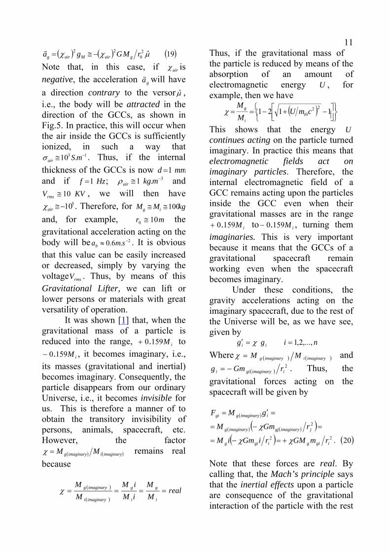
11( ) ( ) ( )19ˆ2
022 μχχ rMGga gairMairg −≅=
r Note that, in this case, if airχ is negative, the acceleration gar will have a direction contrary to the versor μ̂ , i.e., the body will be attracted in the direction of the GCCs, as shown in Fig.5. In practice, this will occur when the air inside the GCCs is sufficiently ionized, in such a way that
. Thus, if the internal thickness of the GCCs is now
13 .10 −≅ mSairσ
mmd 1= and if ; and
, we will then have . Therefore, for
Hzf 1= 3.1 −≅ mkgairρKVVrms 10≅
510−≅airχ kgMM ig 100≅≅ and, for example, the gravitational acceleration acting on the body will be . It is obvious that this value can be easily increased or decreased, simply by varying the voltage . Thus, by means of this Gravitational Lifter, we can lift or lower persons or materials with great versatility of operation.
mr 100 ≅
2.6.0 −≈ smab
rmsV
It was shown [1] that, when the gravitational mass of a particle is reduced into the range, to
, it becomes imaginary, i.e., its masses (gravitational and inertial) becomes imaginary. Consequently, the particle disappears from our ordinary Universe, i.e., it becomes invisible for us. This is therefore a manner of to obtain the transitory invisibility of persons, animals, spacecraft, etc. However, the factor
iM1590.+
iM1590.−
( ) ( )imaginaryiimaginaryg MM=χ remains real because
( )
( )real
MM
iMiM
MM
i
g
i
g
imaginaryi
imaginaryg ====χ
Thus, if the gravitational mass of the particle is reduced by means of the absorption of an amount of electromagnetic energy U , for example, then we have
( )⎭⎬⎫
⎩⎨⎧
⎥⎦⎤
⎢⎣⎡ −+−== 1121 22
0cmUMM
ii
gχ
This shows that the energy U continues acting on the particle turned imaginary. In practice this means that electromagnetic fields act on imaginary particles. Therefore, the internal electromagnetic field of a GCC remains acting upon the particles inside the GCC even when their gravitational masses are in the range
iM1590.+ to iM1590.− , turning them imaginaries. This is very important because it means that the GCCs of a gravitational spacecraft remain working even when the spacecraft becomes imaginary. Under these conditions, the gravity accelerations acting on the imaginary spacecraft, due to the rest of the Universe will be, as we have see, given by
nigg ii ,...,2,1==′ χ
Where ( ) ( )imaginaryiimaginaryg MM=χ and
( )2
iimaginarygii rGmg −= . Thus, the gravitational forces acting on the spacecraft will be given by
( )
( ) ( )( )( ) ( )20.22
2
igigigig
jimaginarygjimaginaryg
iimaginaryggi
rmGMriGmiM
rGmM
gMF
χχ
χ
+=−=
=−=
=′=
Note that these forces are real. By calling that, the Mach’s principle says that the inertial effects upon a particle are consequence of the gravitational interaction of the particle with the rest

12of the Universe. Then we can conclude that the inertial forces acting on the spacecraft in imaginary state are also real. Therefore, it can travel in the imaginary space-time using the gravitational thrusters. Fig.5 – The Gravitational Lifter – If the air inside theGCCs is sufficiently ionized, in such way that
13 .10 −≅ mSairσ and the internal thickness of theGCCs is now mmd 1= then, if Hzf 1= ;
3.1 −≅ mkgairρ and KVVrms 10≅ , we have510−≅airχ . Therefore, for kgMM ig 100≅≅ and
mr 100 ≅ the gravity acceleration acting on thebody will be 2.6.0 −≈ smab .
GCC 1 GCC 2
Mg
( ) ( ) μχχ ˆ2
22
b
gairMairb r
MGga −≅≅
rr
ab
airχ
airχ
μ
rb
It was also shown [1] that imaginary particles can have infinity velocity in the imaginary space-time. Therefore, this is also the upper limit of velocity for the gravitational spacecrafts traveling in the imaginary space-time. On the other hand, the travel in the imaginary space-time can be very safe, because there will not be any material body in the trajectory of the spacecraft.
It is easy to show that the gravitational forces between two thin layers of air (with masses and
) around the spacecraft , are expressed by
1gm
2gm
( ) ( )21ˆ2
2122112 μχ
rmm
GFF iiair−=−=
rr
Note that these forces can be strongly increased by increasing the value of
airχ . In these circumstances, the air around the spacecraft would be strongly compressed upon the external surface of the spacecraft creating an atmosphere around it. This can be particularly useful in order to minimize the friction between the spacecraft and the atmosphere of the planet in the case of very high speed movements of the spacecraft. With the atmosphere around the spacecraft the friction will occur between the atmosphere of the spacecraft and the atmosphere of the planet. In this way, the friction will be minimum and the spacecraft could travel at very high speeds without overheating. However, in order for this to occur, it is necessary to put the gravitational shielding in another position as shown in Fig.2. Thus, the values of airBχ and airAχ will be independent (See Fig.6). Thus, while inside the gravitational shielding, the value of
airBχ is put close to zero, in order to strongly reduce the gravitational mass of the spacecraft (inner part of the shielding), the value of airAχ must be reduced to about in order to strongly increase the gravitational attraction between the air molecules around the spacecraft. Thus, by
810−

13810−≅airAχsubstituting intoEq.21, we
get ( )22ˆ10 2
21162112 μ
rmm
GFF ii−=−=rr
If, and then Eq. 22 gives
kgmm airairii8
2121 10VV −≅≅=≅ ρρ
mr 310−=( )2310 4
2112 NFF −−≅−=rr
These forces are much more intense than the inter-atomic forces (the forces that unite the atoms and molecules) the intensities of which are of the order of
. Consequently, the air around the spacecraft will be strongly compressed upon the surface of the spacecraft and thus will produce a crust of air which will accompany the spacecraft during its displacement and will protect it from the friction with the atmosphere of the planet.
N81010001 −×−
Fig. 6 – Artificial atmosphere around the gravitationalspacecraft - while inside the gravitational shielding the value of airBχ is putted close to zero, in order to strongly reduces the gravitational mass of thespacecraft (inner part of the shielding), the value of
airAχ must be reduced for about 810− in order tostrongly increase the gravitational attraction betweenthe air molecules around the spacecraft.
airBχ
airAχ
rmsE
Atmosphere of the
Spacecraft
Gravitational Shielding (GCC)
Gravitational Spacecraft
5. The Imaginary Space-time The speed of light in free space is, as we know, about of 300.000 km/s. The speeds of the fastest modern airplanes of the present time do not reach 2 km/s and the speed of rockets do not surpass 20 km/s. This shows how much our aircraft and rockets are slow when compared with the speed of light. The star nearest to the Earth (excluding the Sun obviously) is the Alpha of Centaur, which is about of 4 light-years distant from the Earth (Approximately 37.8 trillions of kilometers). Traveling at a speed about 100 times greater than the maximum speed of our faster spacecrafts, we would take about 600 years to reach Alpha of Centaur. Then imagine how many years we would take to leave our own galaxy. In fact, it is not difficult to see that our spacecrafts are very slow, even for travels in our own solar system. One of the fundamental characteristics of the gravitational spacecraft, as we already saw, is its capability to acquire enormous accelerations without submitting the crew to any discomfort. Impelled by gravitational thrusters gravitational spacecrafts can acquire accelerations until or more. This means that these spacecrafts can reach speeds very close to the speed of light in just a few seconds. These gigantic accelerations can be unconceivable for a layman, however they are common in our Universe. For example, when we submit an electron to an electric field
28 .10 −sm

14of just it acquires an acceleration , given by
mVolt /1a
( )( ) 211
31
19
.101011.9
/1106.1 −−
−
≅×
×== smmVC
meEa
e
As we see, this acceleration is about 100 times greater than that acquired by the gravitational spacecraft previously mentioned. By using the gravitational shieldings it is possible to reduce the inertial effects upon the spacecraft. As we have shown, they are reduced by the factor igout MM=χ . Thus, if the inertial mass of the spacecraft is
and, by means of the gravitational shielding effect the gravitational mass of the spacecraft is reduced to then , in spite of the effective acceleration to be gigantic, for example, , the effects for the crew of the spacecraft would be equivalents to an acceleration of only
kgM i 000.10=
ig MM 810−≈
29 .10 −≈ sma
a′
( )( ) 298 .101010 −− ≈==′ smaMM
ai
g
This acceleration is similar to that which the passengers of a contemporary commercial jet are subjected. Therefore the crew of the gravitational spacecraft would be comfortable while the spacecraft would reach speeds close to the speed of light in few seconds. However to travel at such velocities in the Universe may note be practical. Take for example, Alpha of Centaur (4 light-years far from the Earth): a round trip to it would last about eight years. Trips beyond that star could take then several decades, and this obviously is
impracticable. Besides, to travel at such a speed would be very dangerous, because a shock with other celestial bodies would be inevitable. However, as we showed [1] there is a possibility of a spacecraft travel quickly far beyond our galaxy without the risk of being destroyed by a sudden shock with some celestial body. The solution is the gravitational spacecraft travel through the Imaginary or Complex Space-time. It was shown [1] that it is possible to carry out a transition to the Imaginary space-time or Imaginary Universe. It is enough that the body has its gravitational mass reduced to a value in the range of to
iM1590.+
iM1590.− . In these circumstances, the masses of the body (gravitational and inertial) become imaginaries and, so does the body. (Fig.7). Consequently, the body disappears from our ordinary space-time and appears in the imaginary space-time. In other words, it becomes invisible for an observer at the real Universe. Therefore, this is a way to get temporary invisibility of human beings, animals, spacecrafts, etc. Thus, a spacecraft can leave our Universe and appear in the Imaginary Universe, where it can travel at any speed since in the Imaginary Universe there is no speed limit for the gravitational spacecraft, as it occurs in our Universe, where the particles cannot surpass the light speed. In this way, as the gravitational spacecraft is propelled by the gravitational thrusters, it can attain accelerations up to , then after one day of trip with this acceleration, it can
29 .10 −sm

15 transition ( −0.159 > mg > +0.159 ) 1 light-year
dAB = 1 light-year transition ( −0.159 < mg < +0.159 ) mg Gravitational Spacecraft
Fig. 7 – Travel in the Imaginary Space-time.
ΔtAB =1 second
A
B
ΔtAB =1 year
photon
Vmax = ∞ Vmax = c
reach velocities (about 1 million times the speed of light). With this velocity, after 1 month of trip the spacecraft would have traveled about . In order to have idea of this distance, it is enough to remind that the diameter of our Universe (visible Universe) is of the order of .
114 .10 −≈ smV
m2110
m2610 Due to the extremely low density of the imaginary bodies, the collision between them cannot have the same consequences of the collision between the dense real bodies. Thus for a gravitational spacecraft in imaginary state the problem of the collision doesn't exist in high-speed. Consequently, the gravitational spacecraft can transit freely in the imaginary Universe and, in this way reach easily any point of our real Universe once they can make the transition back to our Universe by only increasing the gravitational mass
of the spacecraft in such way that it leaves the range of to
iM1590.+
iM1590.− . Thus the spacecraft can reappear in our Universe near its target. The return trip would be done in similar way. That is to say, the spacecraft would transit in the imaginary Universe back to the departure place where would reappear in our Universe and it would make the approach flight to the wanted point. Thus, trips through our Universe that would delay millions of years, at speeds close to the speed of light, could be done in just a few months in the imaginary Universe. What will an observer see when in the imaginary space-time? It will see light, bodies, planets, stars, etc., everything formed by imaginary photons, imaginary atoms, imaginary protons, imaginary neutrons and imaginary electrons. That is to say, the observer will find an Universe similar to ours, just formed by particles with imaginary masses. The term imaginary adopted from the Mathematics, as we already saw, gives the false impression that these masses do not exist. In order to avoid this misunderstanding we researched the true nature of that new mass type and matter. The existence of imaginary mass associated to the neutrino is well-known. Although its imaginary mass is not physically observable, its square is. This amount is found experimentally to be negative. Recently, it was shown [1] that quanta of imaginary mass exist associated to the photons, electrons, neutrons, and

16protons, and that these imaginary masses would have psychic properties (elementary capability of “choice”). Thus, the true nature of this new kind of mass and matter shall be psychic and, therefore we should not use the term imaginary any longer. Consequently from the above exposed we can conclude that the gravitational spacecraft penetrates in the Psychic Universe and not in an “imaginary” Universe. In this Universe, the matter would be, obviously composed by psychic molecules and psychic atoms formed by psychic neutrons, psychic protons and psychic electrons. i.e., the matter would have psychic mass and consequently it would be subtle, much less dense than the matter of our real Universe. Thus, from a quantum viewpoint, the psychic particles are similar to the material particles, so that we can use the Quantum Mechanics to describe the psychic particles. In this case, by analogy to the material particles, a particle with psychic mass will be described by the following expressions:
Ψm
ψψ
ψψ
ωh
rh
r
=
=
Ekp
Where is the momentum carried by the wave and its energy;
Vmprr
Ψ=ψ
ψE
ψψ λπ2=kr
is the propagation number and Vmh Ψ=ψλ the wavelength and
ψψ πω f2= its cyclic frequency. The variable quantity that characterizes DeBroglie’s waves is called Wave Function, usually
indicated byΨ . The wave function associated to a material particle describes the dynamic state of the particle: its value at a particular point x, y, z, t is related to the probability of finding the particle in that place and instant. Although does not have a physical interpretation, its square
Ψ2Ψ
(orΨ *Ψ ) calculated for a particular point x, y, z, t is proportional to the probability of experimentally finding the particle in that place and instant. Since 2Ψ is proportional to the probability P of finding the particle described byΨ , the integral of 2Ψ on the whole space must be finite – inasmuch as the particle is someplace. Therefore, if
0V2 =Ψ∫+∞
∞−d
The interpretation is that the particle does not exist. Conversely, if
∞=Ψ∫+∞
∞−V2d
the particle will be everywhere simultaneously. The wave function Ψ corresponds, as we know, to the displacement y of the undulatory motion of a rope. However,Ψ as opposed to y , is not a measurable quantity and can, hence, being a complex quantity. For this reason, it is admitted that Ψ is described in the x -direction by
( )( )pxEthiBe −−=Ψ π2
This equation is the mathematical description of the wave associated with a free material particle, with total energy E and momentum , moving in the direction
px+ .
As concerns the psychic particle, the variable quantity characterizing psyche waves will also

17be called wave function, denoted by
( to distinguish it from the material particle wave function), and, by analogy with equation of
ΨΨ
Ψ , expressed by:
( )( )xptEhie ΨΨ −−Ψ Ψ=Ψ π2
0
If an experiment involves a large number of identical particles, all described by the same wave function
, the real density of mass Ψ ρ of these particles in x, y, z, t is proportional to the corresponding value ( is known as density of probability. If is complex then
. Thus, ). Similarly, in the case of psychic particles, the density of psychic mass,
2Ψ 2ΨΨ
*ΨΨ=Ψ 2 *.ΨΨ=Ψ∝ 2ρ
Ψρ , in x, y, z, will be expressed by . It is known that
is always real and positive while
*ΨΨΨΨ ΨΨ=Ψ∝ 2ρ 2
ΨΨ
VmΨΨ =ρ is an imaginary quantity. Thus, as the modulus of an imaginary number is always real and positive, we can transform the proportion , in equality in the following form:
2ΨΨ Ψ∝ρ
ΨΨ =Ψ ρk2
Where is a proportionality constant (real and positive) to be determined.
k
In Quantum Mechanics we have studied the Superposition Principle, which affirms that, if a particle (or system of particles) is in a dynamic state represented by a wave function
and may also be in another dynamic state described by then, the general dynamic state of the particle may be described by
1Ψ
2Ψ
Ψ , where is a linear combination (superposition) of and , i.e.,
Ψ
1Ψ 2Ψ
2211 Ψ+Ψ=Ψ ccThe Complex constants e respectively express the percentage of
dynamic state, represented by
1c 2c
1Ψ e 2Ψ in the formation of the general
dynamic state described by . Ψ In the case of psychic particles (psychic bodies, consciousness, etc.), by analogy, if 1ΨΨ , ,..., refer to the different dynamic states the psychic particle takes, then its general dynamic state may be described by the wave function
2ΨΨ nΨΨ
ΨΨ , given by: nnccc ΨΨΨΨ Ψ++Ψ+Ψ=Ψ ...2211
The state of superposition of wave functions is, therefore, common for both psychic and material particles. In the case of material particles, it can be verified, for instance, when an electron changes from one orbit to another. Before effecting the transition to another energy level, the electron carries out “virtual transitions” [6]. A kind of relationship with other electrons before performing the real transition. During this relationship period, its wave function remains “scattered” by a wide region of the space [7] thus superposing the wave functions of the other electrons. In this relationship the electrons mutually influence each other, with the possibility of intertwining their wave functions§. When this happens, there occurs the so-called Phase Relationship according to quantum-mechanics concept. In the electrons “virtual” transition mentioned before, the “listing” of all the possibilities of the electrons is described, as we know, by Schrödinger’s wave equation. § Since the electrons are simultaneously waves and particles, their wave aspects will interfere with each other; besides superposition, there is also the possibility of occurrence of intertwining of their wave functions.

18Otherwise, it is general for material particles. By analogy, in the case of psychic particles, we may say that the “listing” of all the possibilities of the psyches involved in the relationship will be described by Schrödinger’s equation – for psychic case, i.e.,
02
22 =Ψ+Ψ∇ Ψ
ΨΨ
h
p
Because the wave functions are capable of intertwining themselves, the quantum systems may “penetrate” each other, thus establishing an internal relationship where all of them are affected by the relationship, no longer being isolated systems but becoming an integrated part of a larger system. This type of internal relationship, which exists only in quantum systems, was called Relational Holism [8]. We have used the Quantum Mechanics in order to describe the foundations of the Psychic Universe which the Gravitational Spacecrafts will find, and that influences us daily. These foundations recently discovered – particularly the Psychic Interaction, show us that a rigorous description of the Universe cannot to exclude the psychic energy and the psychic particles. This verification makes evident the need of to redefine the Psychology with basis on the quantum foundations recently discovered. This has been made in the article: “Physical Foundations of Quantum Psychology”**[9], recently published, where it is shown that the Psychic Interaction leads us to understand the Psychic Universe and the extraordinary relationship that the ** http://htpprints.yorku.ca/archive/00000297
human consciousnesses establish among themselves and with the Ordinary Universe. Besides, we have shown that the Psychic Interaction postulates a new model for the evolution theory, in which the evolution is interpreted not only as a biological fact, but mainly as psychic fact. Therefore, is not only the mankind that evolves in the Earth’s planet, but all the ecosystem of the Earth. 6. Past and Future
It was shown [1,9] that the collapse of the psychic wave function must suddenly also express in reality (real space-time) all the possibilities described by it. This is, therefore, a point of decision in which there occurs the compelling need of realization of the psychic form. We have seen that the materialization of the psychic form, in the real space-time, occurs when it contains enough psychic mass for the total materialization†† of the psychic form (Materialization Condition). When this happens, all the psychic energy contained in the psychic form is transformed in real energy in the real space-time. Thus, in the psychic space-time just the holographic register of the psychic form, which gives origin to that fact, survives, since the psychic energy deforms the metric of the psychic space-time‡‡, producing the †† By this we mean not only materialization proper but also the movement of matter to realize its psychic content (including radiation). ‡‡ As shown in General Theory of Relativity the energy modifies the metric of the space-time (deforming the space-time).

19holographic register. Thus, the past survive in the psychic space-time just in the form of holographic register. That is to say, all that have occurred in the past is holographically registered in the psychic space-time. Further ahead, it will be seen that this register can be accessed by an observer in the psychic space-time as well as by an observer in the real space-time. A psychic form is intensified by means of a continuous addition of psychic mass. Thus, when it acquires sufficiently psychic mass, its realization occurs in the real space-time. Thus the future is going being built in the present. By means of our current thoughts we shape the psychic forms that will go (or will not) take place in the future. Consequently, those psychic forms are continually being holographically registered in the psychic space-time and, just as the holographic registrations of the past these future registration can also be accessed by the psychic space-time as well as by the real space-time. The access to the holographic registration of the past doesn't allow, obviously, the modification of the past. This is not possible because there would be a clear violation of the principle of causality that says that the causes should precede the effects. However, the psychic forms that are being shaped now in order to manifest themselves in the future, can be modified before they manifest themselves. Thus, the access to the registration of those psychic forms becomes highly relevant for our present life, since we can avoid the manifestation of many unpleasant facts in the future.
Since both registrations are in the psychic space-time, then the access to their information only occur by means of the interaction with another psychic body, for example, our consciousness or a psychic observer (body totally formed by psychic mass). We have seen that, if the gravitational mass of a body is reduced to within the range iM1590.+ to , its gravitational and inertial masses become imaginaries (psychics) and, therefore, the body becomes a psychic body. Thus, a real observer can also become in a psychic observer. In this way, a gravitational spacecraft can transform all its inertial mass into psychic mass, and thus carry out a transition to the psychic space-time and become a psychic spacecraft. In these circumstances, an observer inside the spacecraft also will have its mass transformed into psychic mass, and, therefore, the observer also will be transformed into a psychic observer. What will this observer see when it penetrates the psychic Universe? According to the Correspondence principle, all that exists in the real Universe must have the correspondent in the psychic Universe and vice-versa. This principle reminds us that we live in more than one world. At the present time, we live in the real Universe, but we can also live in the psychic Universe. Therefore, the psychic observer will see the psychic bodies and their correspondents in the real Universe. Thus, a pilot of a gravitational spacecraft, in travel through the psychic space-time, won't have difficulty to spot the spacecraft in its trips through the Universe.
iM1590.−

20 The fact of the psychic forms manifest themselves in the real space-time exactly at its images and likeness, it indicates that real forms (forms in the real space-time) are prior to all reflective images of psychic forms of the past. Thus, the real space-time is a mirror of the psychic space-time. Consequently, any register in the psychic space-time will have a correspondent image in the real space-time. This means that it is possible that we find in the real space-time the image of the holographic register existing in the psychic space-time, corresponding to our past. Similarly, every psychic form that is being shaped in the psychic space-time will have reflective image in the real space-time. Thus, the image of the holographic register of our future (existing in the psychic space-time) can also be found in the real space-time. Each image of the holographic register of our future will be obviously correlated to a future epoch in the temporal coordinate of the space-time. In the same way, each image of the holographic registration of our past will be correlated to a passed time in the temporal coordinate of the referred space-time. Thus, in order to access the mentioned registrations we should accomplish trips to the past or future in the real space-time. This is possible now, with the advent of the gravitational spacecrafts because they allow us to reach speeds close to the speed of light. Thus, by varying the gravitational mass of the spacecraft for negative or positive we can go respectively to the past or future [1].
If the gravitational mass of a particle is positive, then is always positive and given by
t
22
0 1 cVtt −+=
This leads to the well-known relativistic prediction that the particle goes to the future if . However, if the gravitational mass of the particle is negative, then t is also negative and, therefore, given by
cV →
22
0 1 cVtt −−=
In this case, the prevision is that the particle goes to the past if . In this way, negative gravitational mass is the necessary condition to the particle to go to the past.
cV →
Since the acceleration of a spacecraft with gravitational mass , is given by
gm
gmFa = , where is the thrust of its thrusters, then the more we reduce the value of the bigger the acceleration of the spacecraft will be. However, since the value of cannot be reduced to the range to
F
gm
gm
iM1590.+
iM1590.− because the spacecraft would become a psychic body, and it needs to remain in the real space-time in order to access the past or the future in the real space-time, then, the ideal values for the spacecraft to operate with safety would be . Let us consider a gravitational spacecraft whose inertial mass is . If its gravitational mass was made negative and equal to
im2.0±
kgmi 000.10=
kgmm ig 20002.0 −=−= and, at this instant the thrust produced by the

21thrusters of the spacecraft was
then, the spacecraft would acquire acceleration
NF 510=2.50 −== smmFa g
and, after , the speed of the spacecraft would be
. Therefore, right after that the spacecraft returned to the Earth, its crew would find the Earth in the past (due to the negative gravitational mass of the spacecraft) at a time
sdayst 6105.230 ×==
csmv 4.0.102.1 18 =×= −
220 1 cVtt −−= ; is the time
measured by an observer at rest on the Earth. Thus, if AD, the time interval would be expressed by
0t
20090 =t
0ttt −=Δ
yearst
tcV
tttt
183091.0
116.01
111
1
0
02200
−≅−≅
≅⎟⎠
⎞⎜⎝
⎛ −−
−=⎟⎟
⎠
⎞
⎜⎜
⎝
⎛−
−−=−=Δ
That is, the spacecraft would be in the year 1826 AD. On the other hand, if the gravitational mass of the spacecraft would have become positive
, instead of negative, then the spacecraft would be in the future at
kgmm ig 20002.0 +=+=
yearst 183+=Δ from 2009. That is, it would be in the year 2192 AD. 7. Instantaneous Interestelar Communications Consider a cylindrical GCC (GCC antenna) as shown in Fig.8. The gravitational mass of the air inside the GCC is
( )( )
( )( ) ( )241
4121 22
4
airiair
airairg m
cfB
m⎪⎭
⎪⎬⎫
⎪⎩
⎪⎨⎧
⎥⎥⎦
⎤
⎢⎢⎣
⎡−+−=
μρπσ
Where ( )arσ is the electric conductivity
of the ionized air inside the GCC and ( )arρ is its density; is the frequency of the magnetic field.
f
By varying B one can vary and consequently to vary the
gravitational field generated by , producing then Gravitational Radiation. Then a GCC can work as a Gravitational Antenna.
( )airgm
( )airgm
Apparently, Newton’s theory of gravity had no gravitational waves because, if a gravitational field changed in some way, that change would have taken place instantaneously everywhere in space, and one can think that there is not a wave in this case. However, we have already seen that the gravitational interaction can be repulsive, besides
i f
(a) Antenna GCC i i f f
Transmitter (b) Receiver
Fig. 8 – Transmitter and Receiver of Virtual Gravitational Radiation.
Real gravitational waves v = c
Graviphotons v = ∞
Graviphoton v = ∞
GCC Air
Coil
GCC
GCC

22attractive. Thus, as with electromagnetic interaction, the gravitational interaction must be produced by the exchange of "virtual" quanta of spin 1 and mass null, i.e., the gravitational "virtual" quanta (graviphoton) must have spin 1 and not 2. Consequently, the fact that a change in a gravitational field reaches instantaneously every point in space occurs simply due to the speed of the graviphoton to be infinite. It is known that there is no speed limit for “virtual” photons. On the other hand, the electromagnetic quanta (“virtual” photons) can not communicate the electromagnetic interaction to an infinite distance. Thus, there are two types of gravitational radiation: the real and virtual, which is constituted of graviphotons; the real gravitational waves are ripples in the space-time generated by gravitational field changes. According to Einstein’s theory of gravity the velocity of propagation of these waves is equal to the speed of light [10]. Unlike the electromagnetic waves the real gravitational waves have low interaction with matter and consequently low scattering. Therefore real gravitational waves are suitable as a means of transmitting information. However, when the distance between transmitter and receiver is too large, for example of the order of magnitude of several light-years, the transmission of information by means of gravitational waves becomes impracticable due to the long time necessary to receive the information. On the other hand, there is no delay during the transmissions by means of
virtual gravitational radiation. In addition, the scattering of this radiation is null. Therefore the virtual gravitational radiation is very suitable as a means of transmitting information at any distances, including astronomical distances. As concerns detection of the virtual gravitational radiation from GCC antenna, there are many options. Due to Resonance Principle a similar GCC antenna (receiver) tuned at the same frequency can absorb energy from an incident virtual gravitational radiation (See Fig.8 (b)). Consequently, the gravitational mass of the air inside the GCC receiver will vary such as the gravitational mass of the air inside the GCC transmitter. This will induce a magnetic field similar to the magnetic field of the GCC transmitter and therefore the current through the coil inside the GCC receiver will have the same characteristics of the current through the coil inside the GCC transmitter. However, the volume and pressure of the air inside the two GCCs must be exactly the same; also the type and the quantity of atoms in the air inside the two GCCs must be exactly the same. Thus, the GCC antennas are simple but they are not easy to build. Note that a GCC antenna radiates graviphotons and gravitational waves simultaneously (Fig. 8 (a)). Thus, it is not only a gravitational antenna: it is a Quantum Gravitational Antenna because it can also emit and detect gravitational "virtual" quanta (graviphotons), which, in turn, can transmit information instantaneously from any

23
E
distance in the Universe without scattering. Due to the difficulty to build two similar GCC antennas and, considering that the electric current in the receiver antenna can be detectable even if the gravitational mass of the nuclei of the antennas are not strongly reduced, then we propose to replace the gas at the nuclei of the antennas by a thin dielectric lamina. When the virtual gravitational radiation strikes upon the dielectric lamina, its gravitational mass varies similarly to the gravitational mass of the dielectric lamina of the transmitter antenna, inducing an electromagnetic field ( , B ) similar to the transmitter antenna. Thus, the electric current in the receiver antenna will have the same characteristics of the current in the transmitter antenna. In this way, it is then possible to build two similar antennas whose nuclei have the same volumes and the same types and quantities of atoms. Note that the Quantum Gravitational Antennas can also be used to transmit electric power. It is easy to see that the Transmitter and Receiver can work with strong voltages and electric currents. This means that strong electric power can be transmitted among Quantum Gravitational Antennas. This obviously solves the problem of wireless electric power transmission. Thus, we can conclude that the spacecrafts do not necessarily need to have a system for generation of electric energy inside them. Since the electric energy to be used in the spacecraft can be instantaneously transmitted from any point of the
Universe, by means of the above mentioned systems of transmission and reception of “virtual” gravitational waves. 8. Origin of Gravity and Genesis of the Gravitational Energy It was shown [1] that the “virtual” quanta of the gravitational interaction must have spin 1 and not 2, and that they are “virtual” photons (graviphotons) with zero mass outside the coherent matter. Inside the coherent matter the graviphotons mass is non-zero. Therefore, the gravitational forces are also gauge forces, because they are yielded by the exchange of "virtual" quanta of spin 1, such as the electromagnetic forces and the weak and strong nuclear forces. Thus, the gravitational forces are produced by the exchanging of “virtual” photons (Fig.9). Consequently, this is precisely the origin of the gravity. Newton’s theory of gravity does not explain why objects attract one another; it simply models this observation. Also Einstein’s theory does not explain the origin of gravity. Einstein’s theory of gravity only describes gravity with more precision than Newton’s theory does. Besides, there is nothing in both theories explaining the origin of the energy that produces the gravitational forces. Earth’s gravity attracts all objects on the surface of our planet. This has been going on for over 4.5 billions years, yet no known energy source is being converted to support this tremendous ongoing energy expenditure. Also is the enormous

24continuous energy expended by Earth’s gravitational field for maintaining the Moon in its orbit - millennium after millennium. In spite of the ongoing energy expended by Earth’s gravitational field to hold objects down on surface and the Moon in orbit, why the energy of the field never diminishes in strength or drains its energy source? Is this energy expenditure balanced by a conversion of energy from an unknown energy source? Fig. 9 – Origin of Gravity: The gravitational forces areproduced by the exchanging of “virtual” photons(graviphotons).
Exchanging of “virtual” photons (graviphotons)
g
The energy W necessary to support the effort expended by the gravitational forces is well-known and given by
F
rmM
GFdrW ggr−== ∫∞
According to the Principle of Energy Conservation, the spending of this energy must be compensated by a conversion of another type of energy.
The Uncertainty Principle tells us that, due to the occurrence of exchange of graviphotons in a time interval Et Δ<Δ h (where EΔ is the energy of the graviphoton), the energy variation EΔ cannot be detected in the system gg mM − . Since the total energy
is the sum of the energy of the graviphotons, i.e., W n
nEEEW Δ++Δ+Δ= ...21 , then the energy W cannot be detected as well. However, as we know it can be converted into another type of energy, for example, in rotational kinetic energy, as in the hydroelectric plants, or in the Gravitational Motor, as shown in this work. It is known that a quantum of energy hfE =Δ , which varies during a time interval Ecft Δ<==Δ hλ1 (wave period) cannot be experimentally detected. This is an imaginary photon or a “virtual” photon. Thus, the graviphotons are imaginary photons, i.e., the energies
iEΔ of the graviphotons are imaginaries energies and therefore the energy nEEEW Δ++Δ+Δ= ...21 is also an imaginary energy. Consequently, it belongs to the imaginary space-time. It was shown [1] that, imaginary energy is equal to psychic energy. Consequently, the imaginary space-time is, in fact, the psychic space-time, which contains the Supreme Consciousness. Since the Supreme Consciousness has infinite psychic mass [1], then the psychic space-time contains infinite psychic energy. This is highly relevant, because it confers to the Psychic Universe the characteristic of unlimited source of energy. Thus, as the origin of the gravitational energy it is correlated to the psychic

25energy, then the spending of gravitational energy can be supplied indefinitely by the Psychic Universe. This can be easily confirmed by the fact that, in spite of the enormous amount of energy expended by Earth’s gravitational field to hold objects down on the surface of the planet and maintain the Moon in its orbit, the energy of Earth’s gravitational field never diminishes in strength or drains its energy source. Acknowledgement The author would like to thank Dr. Getúlio Marques Martins (COPPE – UFRJ, Rio de Janeiro-Brasil) for revising the manuscript.

26 APPENDIX A: The Simplest Method to Control the Gravity In this Appendix we show the simplest method to control the gravity. Consider a body with mass density ρ and the following electric characteristics: rμ , rε ,σ (relative permeability, relative permittivity and electric conductivity, respectively). Through this body, passes an electric current I , which is the sum of a sinusoidal current tiiosc ωsin0= and the DC current , i.e., DCI tiII DC ωsin0+= ; fπω 2= . If then DCIi <<0 DCII ≅ . Thus, the current I varies with the frequency , but the variation of its intensity is quite small in comparison with , i.e.,
f
DCI I will be practically constant (Fig. A1). This is of fundamental importance for maintaining the value of the gravitational mass of the body, , sufficiently stable during all the time.
gm
The gravitational mass of the body is given by [1]
( )11121 0
2
20
AmcmUnm i
i
rg
⎪⎭
⎪⎬⎫
⎪⎩
⎪⎨⎧
⎥⎥
⎦
⎤
⎢⎢
⎣
⎡−⎟⎟
⎠
⎞⎜⎜⎝
⎛+−=
whereU , is the electromagnetic energy absorbed by the body and is the index of refraction of the body.
rn
Equation (A1) can also be rewritten in the following form
( )211212
20
AcWn
mm r
i
g
⎪⎭
⎪⎬
⎫
⎪⎩
⎪⎨
⎧
⎥⎥⎥
⎦
⎤
⎢⎢⎢
⎣
⎡−⎟
⎟⎠
⎞⎜⎜⎝
⎛+−=
ρ
Fig. A1 - The electric current I varies withfrequency f . But the variation of
I is quite small
in comparison with DCI due to DCo Ii << . In this way, we can consider DCII ≅ .
t
IDC
I = IDC + iosc
i0
where, VUW = is the density of electromagnetic energy and V0im=ρ is the density of inertial mass. The instantaneous values of the density of electromagnetic energy in an electromagnetic field can be deduced from Maxwell’s equations and has the following expression
( )32212
21 AHEW με +=
where tEE m ωsin= and tHH ωsin= are the instantaneous values of the electric field and the magnetic field respectively. It is known that HB μ= ,
rkBE ω= [11] and

27
( )( )4
112
2Ac
dtdzv
rrr ⎟⎠⎞⎜
⎝⎛ ++
===ωεσμεκ
ω
where is the real part of the propagation vector k
rkr
(also called phase constant ); ir ikkkk +==
r ; ε , μ
and σ, are the electromagnetic characteristics of the medium in which the incident (or emitted) radiation is propagating( 0εεε r= ; ;
mF /10854.8 120
−×=ε
0μμμ r= where ). It is known that for free-space
m/H70 104 −×= πμ
0=σ and 1== rr με . Then Eq. (A4) gives
cv = From (A4), we see that the index of refraction vcnr = is given by
( ) ( )5112
2 Avcn rr
r ⎟⎠⎞⎜
⎝⎛ ++== ωεσ
με
Equation (A4) shows that
vr =κω .Thus, vkBE r == ω , i.e., ( )6AHvvBE μ==
Then, Eq. (A3) can be rewritten in the following form:
( ) ( )722122
21 AHHvW μμμε +=
For ωεσ << , Eq. (A4) reduces to
rr
cvμε
=
Then, Eq. (A7) gives
22212
2
21 HHHcW
rr
μμμμμε
ε =+⎥⎦
⎤⎢⎣
⎡⎟⎟⎠
⎞⎜⎜⎝
⎛=
This equation can be rewritten in the following forms:
( )82
ABWμ
=
or ( )92 AEW ε=
For ωεσ >> , Eq. (A4) gives
( )102 Avμσω
=
Then, from Eq. (A7) we get
( )11
2
221
22122
212
21
AH
HHHHW
μ
μμσωεμμμ
μσωε
≅
≅+⎟⎠⎞
⎜⎝⎛=+⎥
⎦
⎤⎢⎣
⎡⎟⎟⎠
⎞⎜⎜⎝
⎛=
Since HvvBE μ== , we can rewrite (A11) in the following forms:
( )122
2
ABWμ
≅
or ( )13
42 AEW ⎟
⎠⎞
⎜⎝⎛≅
ωσ
By comparing equations (A8) (A9) (A12) and (A13), we can see that Eq. (A13) shows that the best way to obtain a strong value of W in practice is by applying an Extra Low-Frequency (ELF) electric field ( )Hzfw 12 <<= π through a medium with high electrical conductivity. Substitution of Eq. (A13) into Eq. (A2), gives
( )14
110758.1121
1256
121
144
121
04
32
327
04
32
3
230
02
43
2
A
mEf
mEfc
mEfc
m
ir
ir
ig
⎪⎭
⎪⎬⎫
⎪⎩
⎪⎨⎧
⎥⎥⎦
⎤
⎢⎢⎣
⎡−⎟⎟
⎠
⎞⎜⎜⎝
⎛×+−=
=⎪⎭
⎪⎬⎫
⎪⎩
⎪⎨⎧
⎥⎥⎦
⎤
⎢⎢⎣
⎡−⎟⎟
⎠
⎞⎜⎜⎝
⎛⎟⎠
⎞⎜⎝
⎛+−=
=⎪⎭
⎪⎬⎫
⎪⎩
⎪⎨⎧
⎥⎥
⎦
⎤
⎢⎢
⎣
⎡−⎟⎟
⎠
⎞⎜⎜⎝
⎛+−=
−
ρσμ
ρσμ
πμ
ρπσμ
Note that tEE m ωsin= .The average value for 2E is equal to 2
21
mE because

28E varies sinusoidaly ( is the maximum value for
mEE ). On the other
hand, 2mrms EE = . Consequently we can change 4E by , and the equation above can be rewritten as follows
4rmsE
04
32
327 110758.1121 irms
rg mE
fm
⎪⎭
⎪⎬⎫
⎪⎩
⎪⎨⎧
⎥⎥⎦
⎤
⎢⎢⎣
⎡−⎟⎟
⎠
⎞⎜⎜⎝
⎛×+−= −
ρσμ
Substitution of the well-known equation of the Ohm's vectorial Law:
Ej σ= into (A14), we get
( )15110758.1121 032
427 Am
fj
m irmsr
g⎪⎭
⎪⎬⎫
⎪⎩
⎪⎨⎧
⎥⎥⎦
⎤
⎢⎢⎣
⎡−×+−= −
σρμ
where 2jjrms = . Consider a 15 cm square Aluminum thin foil of 10.5 microns thickness with the following characteristics: 1=rμ ; ;
. Then, (A15) gives
17 .1082.3 −×= mSσ3.2700 −= mKgρ
( )16110313.6121 03
442 Am
fj
m irms
g⎪⎭
⎪⎬⎫
⎪⎩
⎪⎨⎧
⎥⎥⎦
⎤
⎢⎢⎣
⎡−×+−= −
Now, consider that the ELF electric current tiII DC ωsin0+= , passes through that Aluminum foil. Then, the current density is
( DCIi <<0 )
( )17AS
IS
Ij DCrms
rms ≅=
where
( ) 266 1057.1105.1015.0 mmmS −− ×=×= If the ELF electric current has frequency , then, the gravitational mass of the aluminum foil, given by (A16), is expressed by
HzHzf 61022 −×== μ
[ ]{ } ( )18113.0121
11089.7121
04
04
425
AmI
mSI
m
iDC
iDC
g
−+−=
=⎪⎭
⎪⎬⎫
⎪⎩
⎪⎨⎧
⎥⎥⎦
⎤
⎢⎢⎣
⎡−×+−= −
Then,
[ ]{ } ( )19113.0121 4
0
AImm
DCi
g −+−≅=χ
For AI DC 2.2= , the equation above gives
( )2010
Amm
i
g −≅⎟⎟⎠
⎞⎜⎜⎝
⎛=χ
This means that the gravitational shielding produced by the aluminum foil can change the gravity acceleration above the foil down to
( )211 Aggg −≅=′ χ Under these conditions, the Aluminum foil works basically as a Gravity Control Cell (GCC). In order to check these theoretical predictions, we suggest an experimental set-up shown in Fig.A2. A 15cm square Aluminum foil of 10.5 microns thickness with the following composition: Al 98.02%; Fe 0.80%; Si 0.70%; Mn 0.10%; Cu 0.10%; Zn 0.10%; Ti 0.08%; Mg 0.05%; Cr 0.05%, and with the following characteristics: 1=rμ ;
; , is fixed on a 17 cm square Foam Board
17 .1082.3 −×= mSσ 3.2700 −= mKgρ§§
plate of 6mm thickness as shown in Fig.A3. This device (the simplest §§ Foam board is a very strong, lightweight (density: 24.03 kg.m-3) and easily cut material used for the mounting of photographic prints, as backing in picture framing, in 3D design, and in painting. It consists of three layers — an inner layer of polystyrene clad with outer facing of either white clay coated paper or brown Kraft paper.

29Gravity Control Cell GCC) is placed on a pan balance shown in Fig.A2. Above the Aluminum foil, a sample (any type of material, any mass) connected to a dynamometer will check the decrease of the local gravity acceleration upon the sample ( )gg χ=′ , due to the gravitational shielding produced by the decreasing of gravitational mass of the Aluminum foil ( )0ig mm=χ . Initially, the sample lies 5 cm above the Aluminum foil. As shown in Fig.A2, the board with the dynamometer can be displaced up to few meters in height. Thus, the initial distance between the Aluminum foil and the sample can be increased in order to check the reach of the gravitational shielding produced by the Aluminum foil. In order to generate the ELF electric current of Hzf μ2= , we can use the widely-known Function Generator HP3325A (Op.002 High Voltage Output) that can generate sinusoidal voltages with extremely-low frequencies down to and amplitude up to 20V (40V
Hzf 6101 −×=
pp into Ω500 load). The maximum output current is ; output impedance <2Ω at ELF .
ppA.080
Figure A4 (a) shows the equivalent electric circuit for the experimental set-up. The electromotive forces are: 1ε (HP3325A) and 2ε (12V DC Battery).The values of the resistors are : ; ;WR 25001 −Ω= Ω< 21ir WR 4042 −Ω=
; ; ; Rheostat (0≤ R ≤10Ω - 90W). The coupling transformer has the following characteristics: air core with diameter
Ω< 1.02ir Ω×= −3105.2pR
mm10=φ ; area 252 108.74 m−×==πφS ; wire#12AWG; 2021 === NNN ; ; mml 42=
( ) HlSNLLL 72021 103.9 −×==== μ .Thus,
we get ( ) ( ) Ω≅++= 50122
111 LrRZ i ω
and ( ) ( )22
222 LRRrRZ pi ω++++=
For 0=R we get ; for Ω≅= 4min
22 ZZΩ=10R the result is .
Thus, Ω≅= 14max
22 ZZ
Ω≅⎟⎟⎠
⎞⎜⎜⎝
⎛+=+= 505
2
2
1min21
min,11
min,1 N
NZZZZZ reflectedtotal
Ω≅⎟⎟⎠
⎞⎜⎜⎝
⎛+=+= 515
2
2
1max21
max,11
max,1 N
NZZZZZ reflectedtotal
The maxima rms currents have the following values:
mAZVI totalpp 5640 min,12
1max1 ==
(The maximum output current of the Function Generator HP3325A (Op.002 High Voltage Output) is
rmspp mAmA 5.5680 ≅ );
AZ
I 3min2
2max2 ==
ε
and AIII 3max
1max2
max3 ≅+=
The new expression for the inertial forces, (Eq.5) , shows that the inertial forces are proportional to gravitational mass. Only in the particular case of , the expression above reduces to the well-known Newtonian expression
aMF girr
=
0ig mm =
amF iirr
0= . The equivalence between gravitational and inertial forces ( )gi FF
rr≡
[1] shows then that a balance measures the gravitational mass subjected to

30acceleration . Here, the decrease in the gravitational mass of the Aluminum foil will be measured by a pan balance with the following characteristics: range 0-200g; readability 0.01g.
ga =
The mass of the Foam Board plate is: , the mass of the Aluminum foil is:
g17.4≅
g64.0≅ , the total mass of the ends and the electric wires of connection is . Thus, initially the balance will show . According to (A18), when the electric current through the Aluminum foil (resistance
g5≅
g81.9≅
Ω×== −3* 105.2Slrp σ ) reaches the value , we will get
. Under these circumstances, the balance will show:
AI 2.23 ≅
( ) ( )AliAlg mm 0−≅
gggg 53.864.064.081.9 ≅−−
and the gravity acceleration above the Aluminum foil, becomes
.
g ′
ggg 1−≅=′ χ It was shown [1] that, when the gravitational mass of a particle is reduced to the gravitational mass ranging between to
, it becomes imaginary, i.e., the gravitational and the inertial masses of the particle become imaginary. Consequently, the particle disappears from our ordinary space-time. This phenomenon can be observed in the proposed experiment, i.e., the Aluminum foil will disappear when its gravitational mass becomes smaller than . It will become visible again, only when its gravitational mass becomes smaller
than
iM1590.+
iM1590.−
iM1590.+
iM1590.− , or when it becomes greater than iM1590.+ . Equation (A18) shows that the gravitational mass of the Aluminum foil, , goes close to zero when
. Consequently, the gravity acceleration above the Aluminum foil also goes close to zero since
( )Algm
AI 76.13 ≅
( ) ( )AliAlg mmgg 0==′ χ . Under these circumstances, the Aluminum foil remains invisible. Now consider a rigid Aluminum wire # 14 AWG. The area of its cross section is ( ) 2623 1008.2410628.1 mmS −− ×=×= π If an ELF electric current with frequency passes through this wire, its gravitational mass, given by (A16), will be expressed by
HzHzf 61022 −×== μ
[ ]{ } ( )22113.0121
11089.7121
110313.6121
04
04
425
03
442
AmI
mSI
mfj
m
iDC
iDC
irms
g
−+−=
=⎪⎭
⎪⎬⎫
⎪⎩
⎪⎨⎧
⎥⎥⎦
⎤
⎢⎢⎣
⎡−×+−=
=⎪⎭
⎪⎬⎫
⎪⎩
⎪⎨⎧
⎥⎥⎦
⎤
⎢⎢⎣
⎡−×+−=
−
−
For AI DC 3≅ the equation above gives
08.3 ig mm −≅
Note that we can replace the Aluminum foil for this wire in the experimental set-up shown in Fig.A2. It is important also to note that an ELF electric current that passes through a wire - which makes a spherical form, as shown in Fig A5 - reduces the gravitational mass of the wire (Eq.

31A22), and the gravity inside sphere at the same proportion, 0ig mm=χ , (Gravitational Shielding Effect). In this case, that effect can be checked by means of the Experimental set-up 2 (Fig.A6). Note that the spherical form can be transformed into an ellipsoidal form or a disc in order to coat, for example, a Gravitational Spacecraft. It is also possible to coat with a wire several forms, such as cylinders, cones, cubes, etc. The circuit shown in Fig.A4 (a) can be modified in order to produce a new type of Gravitational Shielding, as shown in Fig.A4 (b). In this case, the Gravitational Shielding will be produced in the Aluminum plate, with thickness , of the parallel plate capacitor connected in the point
hP of
the circuit (See Fig.A4 (b)). Note that, in this circuit, the Aluminum foil (resistance ) (Fig.A4(a)) has been replaced by a Copper wire # 14 AWG with 1cm length (
pR
cml 1= ) in order to produce a resistance . Thus, the voltage in the point
Ω×= −51021.5φR
P of the circuit will have the maximum value
when the resistance of the rheostat is null and the minimum value when
. In this way, the voltage (with frequency
VV p4max 101.1 −×=
( 0=R )VV p
5min 1003.4 −×=
Ω=10R
pV Hzf μ2= ) applied on the capacitor will produce an electric field with intensity pE
hVE pp = through the Aluminum plate of thickness . It is important to note that this plate cannot be connected to ground (earth), in other words, cannot be grounded, because,
in this case, the electric field through it will be null
mmh 3=
***. According to Eq. A14, when mVhVE pp /036.0maxmax == , Hzf μ2= and
, (Aluminum), we get
mSAl /1082.3 7×=σ 3/2700 mkgAl =ρ
( )
( )9.0−≅=
Ali
Al
mm
χ
Under these conditions, the maximum current density through the plate with thickness will be given by
(It is well-known that the maximum current density supported by the Aluminum is ).
h26maxmax /104.1 mAEj pAl ×==σ
28 /10 mA≈ Since the area of the plate is
( ) 222 1042.0 mA −×== , then the maximum current is . Despite this enormous current, the maximum dissipated power will be just
kAAji 56maxmax ==
( ) WRiP plate 2.62maxmax == , because the
resistance of the plate is very small, i.e., Ω×≅= −9102AhR Alplate σ . Note that the area of the plate (where the Gravitational Shielding takes place) can have several geometrical configurations. For example, it can be the area of the external surface of an ellipsoid, sphere, etc. Thus, it can be the area of the external surface of a Gravitational Spacecraft. In this case, if , for example, the maximum dissipated
A
2100mA ≅
*** When the voltage Vp is applied on the capacitor, the charge distribution in the dielectric induces positive and negative charges, respectively on opposite sides of the Aluminum plate with thickness h. If the plate is not connected to the ground (Earth) this charge distribution produces an electric field Ep=Vp/h through the plate. However, if the plate is connected to the ground, the negative charges (electrons) escapes for the ground and the positive charges are redistributed along the entire surface of the Aluminum plate making null the electric field through it.

32power will be , i.e., approximately .
kWP 4.15max ≅2/154 mW
All of these systems work with Extra-Low Frequencies ( )Hzf 310−<< . Now, we show that, by simply changing the geometry of the surface of the Aluminum foil, it is possible to increase the working frequency up to more than 1Hz.
f
Consider the Aluminum foil, now with several semi-spheres stamped on its surface, as shown in Fig. A7 . The semi-spheres have radius , and are joined one to another. The Aluminum foil is now coated by an insulation layer with relative permittivity
mmr 9.00 =
rε and dielectric strength . A voltage source is connected to the Aluminum foil in order to provide a voltage (rms) with frequency . Thus, the electric potential at a distance
k
0Vf
V r , in the interval from to , is given by 0r a
( )234
1
0
ArqV
rεπε=
In the interval the electric potential is
bra ≤<
( )244
1
0
ArqV
πε=
since for the air we have 1≅rε . Thus, on the surface of the metallic spheres ( we get )0rr =
( )254
1
000 A
rqV
rεπε=
Consequently, the electric field is ( )26
41
200
0 ArqE
rεπε=
By comparing (A26) with (A25), we obtain
( )270
00 A
rV
E =
The electric potential at is bV br =
( )284
1 00
0
Ab
rVbqV r
bε
πε==
Consequently, the electric field is given by
bE
( )294
12
002
0
Ab
rVbqE r
bε
πε==
From 0rr = up to dabr +== the electric field is approximately constant (See Fig. A7). Along the distance it will be called . For
dairE dar +> , the
electric field stops being constant. Thus, the intensity of the electric field at dabr +== is approximately equal to , i.e.,0E 0EEb ≅ . Then, we can write that
( )300
02
00 ArV
brVr ≅
ε
whence we get ( )310 Arb rε≅
Since the intensity of the electric field through the air, , is airE 0EEE bair ≅≅ , then, we can write that
( )324
12
002
0
Ab
rVbqE r
airε
πε==
Note that, rε refers to the relative permittivity of the insulation layer, which is covering the Aluminum foil. If the intensity of this field is greater than the dielectric strength of the air ( )mV /103 6× there will occur the well-known Corona effect. Here, this effect is necessary in order to increase the electric conductivity of the air at this region (layer with thickness d). Thus, we will assume
mVr
Vb
rVE r
air /103 6
0
min0
20
min0min ×===
ε
and
( )33/101 7
0
max0
20
max0max AmV
rV
brV
E rair ×===
ε
The electric field will maxminairairair EEE ≤≤

33produce an electrons flux in a direction and an ions flux in an opposite direction. From the viewpoint of electric current, the ions flux can be considered as an “electrons” flux at the same direction of the real electrons flux. Thus, the current density through the air, , will be the double of the current density expressed by the well-known equation of Langmuir-Child
airj
( )341033.2294
26
22023
23
23
AdV
dV
dV
meje
r−×=== αεε
where 1≅rε for the air; is the called Child’s constant.
61033.2 −×=α
Thus, we have
( )352 2
23
AdVjair α=
where , in this case, is the thickness of the air layer where the electric field is approximately constant and V is the voltage drop given by
d
( )36
41
41
00
00
00
AVdrabrV
bq
aqVVV
rr
ba
⎟⎞
⎜⎛=⎟
⎞⎜⎛ −
=
=−=−=
εε
πεπε
abab ⎠⎝⎠⎝By substituting (A36) into (A35), we get
( )372
22
23
23
21
23
23
21
23
20000
2
AabE
d
ab
bVr
dabdVr
dj
air
rrair
⎟⎠⎞
⎜⎝⎛=
=⎟⎠⎞
⎜⎝⎛⎟
⎠
⎞⎜⎝
⎛=⎟
⎠
⎞⎜⎝
⎛=
α
εαεα
According to the equation of the Ohm's vectorial Law: Ej σ= , we can write that
( )38Ajairair=σ
Eair
Substitution of (A37) into (A38) yields
( )39223
21
Aab
dEair
air ⎟⎠⎞
⎜⎝⎛⎟
⎠
⎞⎜⎝
⎛= ασ
If the insulation layer has
thickness , mm6.0=Δ 5.3≅rε (1- 60Hz), mmkVk /17= (Acrylic sheet 1.5mm thickness), and the semi-spheres stamped on the metallic surface have (See Fig.A7) then
mmr 9.00 =
mmra 5.10 =Δ+= . Thus, we obtain from Eq. (A33) that
kVV 7.2min0 =
( )409max0 AkVV =
From equation (A31), we obtain the following value for b :
( )411068.1 30 Amr
−×=εrb= Since dab += we get
m4−×=
d
d 108.1 Substitution of a , , and A(32) into (A39) produces
b
21
0410117.4 VEairair−×=σ 2
1210375.1 −×=
Substitution of airσ , and
into (A14) gives ( )rmsEair
3.2.1 −= mkgairρ
( )
( )
( )4210923.4121
110758.1121 32
4327
0
A
fE
mm
air
airair
airi
airg
⎭
⎫
⎪⎩
⎪⎨⎧
⎦⎢⎢⎣
⎡×+−=
=⎪⎭
⎪⎬⎫
⎪⎩
⎪⎨⎧
⎥⎥⎦
⎤
⎢⎢⎣
⎡−×+−=
−
−
ρσ
Hzf 2=
( )
13
5.5021
fV
⎪
⎪⎬⎥⎥⎤
−
For and , the result is
kVVV 9max00 ==
( )2.1
0
−≅i
airg
mm
air
air
Note that, by increasing the values of and
0V
airE σ are increased. Thus, as show (A42), there are two ways for decrease the value of )m : increasing the value of V or decreasing the value of .
(airg
0
f

34mmkVmVE /10/107max
0 ==
mm6.0=Δmm
/
airE
dv
Since and then the dielectric strength
of the insulation must be . As mentioned above, the dielectric strength of the acrylic is .
kV /7.16≥
mmkV17 It is important to note that, due to the strong value of (Eq. A37) the drift velocity , ( neEnejv airairaird )σ== of the free charges inside the ionized air put them at a distance mfvtvx dd 4.02 ≅== , which is much greater than the distance
. Consequently, the number of free charges decreases strongly
inside the air layer of thickness
md 4108.1 −×=n
d †††, except, obviously, in a thin layer, very close to the dielectric, where the number of free charges remains sufficiently increased, to maintain the air conductivity with mSair /1.1≅σ (Eq. A39). The thickness of this thin air layer close to the dielectric can be easily evaluated starting from the charge distribution in the neighborhood of the dielectric, and of the repulsion forces established among them. The result is
h
mEeh 90 104406.0 −×≅= πε . This is,
therefore, the thickness of the Air Gravitational Shielding. If the area of this Gravitational Shielding is equal to the area of a format A4 sheet of paper, i.e., , we obtain the following value for the resistance
of the Gravitational Shielding:
20582.0291.020.0 mA =×=
airR
Ω×≅= −8106AhR airair σ . Since the maximum electrical current through this air layer is , then the maximum power radiated from the
kAAji 400maxmax ≅=
††† Reducing therefore the conductivity, airσ , to the normal value of the conductivity of atmospheric air.
Gravitational Shielding is ( ) kWiRP airairair 10
2maxmax ≅= . This means that a very strong light will be radiated from this type of Gravitational Shielding. Note that this device can also be used as a lamp, which will be much more efficient than conventional lamps. Coating a ceiling with this lighting system enables the entire area of ceiling to produce light. This is a form of lighting very different from those usually known. Note that the value , defines the power of the transformer shown in Fig.A10. Thus, the maximum current in the secondary is
kWPair 10max≅
AkWkVis 9.0109max == . Above the Gravitational Shielding, airσ is reduced to the normal value of conductivity of the atmospheric air ( )mS /10 14−≈ . Thus, the power radiated from this region is
( )( )( ) ( ) WEAhd
AihdP
airair
airairair
42max
2maxmax
10−≅−=
=−=
σ
σ
Now, we will describe a method to coat the Aluminum semi-spheres with acrylic in the necessary dimension ( )0ra −=Δ . First, take an Aluminum plate with cmcm 1.2921 × (A4 format). By means of a convenient process, several semi-spheres can be stamped on its surface. The semi-spheres have radius , and are joined one to another. Next, take an acrylic sheet (A4 format) with 1.5mm thickness (See Fig.A8 (a)). Put a heater below the Aluminum plate in order to heat the Aluminum (Fig.A8 (b)). When the Aluminum is
mmr 9.00 =

35sufficiently heated up, the acrylic sheet and the Aluminum plate are pressed, one against the other, as shown in Fig. A8 (c). The two D devices shown in this figure are used in order to impede that the press compresses the acrylic and the aluminum to a distance shorter than . After some seconds, remove the press and the heater. The device is ready to be subjected to a voltage with frequency , as shown in Fig.A9. Note that, in this case, the balance is not necessary, because the substance that produces the gravitational shielding is an air layer with thickness
above the acrylic sheet. This is, therefore, more a type of Gravity Control Cell (GCC) with external gravitational shielding.
ay +
0Vf
d
It is important to note that this GCC can be made very thin and as flexible as a fabric. Thus, it can be used to produce anti- gravity clothes. These clothes can be extremely useful, for example, to walk on the surface of high gravity planets. Figure A11 shows some geometrical forms that can be stamped on a metallic surface in order to produce a Gravitational Shielding effect, similar to the produced by the semi-spherical form. An obvious evolution from the semi-spherical form is the semi-cylindrical form shown in Fig. A11 (b); Fig.A11(c) shows concentric metallic rings stamped on the metallic surface, an evolution from Fig.A11 (b). These geometrical forms produce the same effect as the semi-spherical form, shown in Fig.A11 (a). By using concentric metallic rings, it is possible to build Gravitational Shieldings
around bodies or spacecrafts with several formats (spheres, ellipsoids, etc); Fig. A11 (d) shows a Gravitational Shielding around a Spacecraft with ellipsoidal form. The previously mentioned Gravitational Shielding, produced on a thin layer of ionized air, has a behavior different from the Gravitational Shielding produced on a rigid substance. When the gravitational masses of the air molecules, inside the shielding, are reduced to within the range
igi mmm 159.0159.0 −<<+ , they go to the imaginary space-time, as previously shown in this article. However, the electric field stays at the real space-time. Consequently, the molecules return immediately to the real space-time in order to return soon after to the imaginary space-time, due to the action of the electric field .
airE
airE In the case of the Gravitational Shielding produced on a solid substance, when the molecules of the substance go to the imaginary space-time, the electric field that produces the effect, also goes to the imaginary space-time together with them, since in this case, the substance of the Gravitational Shielding is rigidly connected to the metal that produces the electric field. (See Fig. A12 (b)). This is the fundamental difference between the non-solid and solid Gravitational Shieldings. Now, consider a Gravitational Spacecraft that is able to produce an Air Gravitational Shielding and also a Solid Gravitational Shielding, as

36
igi mmm 159.0159.0 −<<+
shown in Fig. A13 (a) ‡‡‡. Assuming that the intensity of the electric field,
, necessary to reduce the gravitational mass of the air molecules to within the range
, is much smaller than the intensity of the electric field, , necessary to reduce the gravitational mass of the solid substance to within the range
, then we conclude that the Gravitational Shielding made of ionized air goes to the imaginary space-time before the Gravitational Shielding made of solid substance. When this occurs the spacecraft does not go to the imaginary space-time together with the Gravitational Shielding of air, because the air molecules are not rigidly connected to the spacecraft. Thus, while the air molecules go into the imaginary space-time, the spacecraft stays in the real space-time, and remains subjected to the effects of the Gravitational Shielding around it, since the shielding does not stop to work, due to its extremely short permanence at the imaginary space-
airE
igi mmm 159.0159.0 −<<+
rsE
‡‡‡ The solid Gravitational Shielding can also be obtained by means of an ELF electric current through a metallic lamina placed between the semi-spheres and the Gravitational Shielding of Air (See Fig.A13 (a)). The gravitational mass of the solid Gravitational Shielding will be controlled just by means of the intensity of the ELF electric current. Recently, it was discovered that Carbon nanotubes (CNTs) can be added to Alumina (Al2O3) to convert it into a good electrical conductor. It was found that the electrical conductivity increased up to 3375 S/m at 77°C in samples that were 15% nanotubes by volume [12]. It is known that the density of α-Alumina is 3.98×10³kg.m-3 and that it can withstand 10-20 KV/mm. Thus, these values show that the Alumina-CNT can be used to make a solid Gravitational Shielding.
time. Under these circumstances, the gravitational mass of the Gravitational Shielding can be reduced to 0≅gm mg
kgmi 10
. For example, . Thus, if the inertial mass of the Gravitational Shielding is
kg410−≅
≅ , then 4
0 10−≅i= g mmχ
25 .10 −= sma
. As we have seen, this means that the inertial effects on the spacecraft will be reduced by . Then, in spite of the effective acceleration of the spacecraft be, for example, , the effects on the crew of the spacecraft will be equivalent to an acceleration of only
410−≅χ
1
0
.10 −≈==′ smaamm
ai
g χ
This is the magnitude of the acceleration upon the passengers in a contemporary commercial jet. Then, it is noticed that Gravitational Spacecrafts can be subjected to enormous accelerations (or decelerations) without imposing any harmful impacts whatsoever on the spacecrafts or its crew. Now, imagine that the intensity of the electric field that produces the Gravitational Shielding around the spacecraft is increased up to reaching the value that reduces the gravitational mass of the solid Gravitational Shielding to within the range
rsE
igi mmm 159.0159.0 −<<+ . Under these circumstances, the solid Gravitational Shielding goes to the imaginary space-time and, since it is rigidly connected to the spacecraft, also the spacecraft goes to the imaginary space-time together with the Gravitational Shielding. Thus, the spacecraft can travel within the

37
)
imaginary space-time and make use of the Gravitational Shielding around it. As we have already seen, the maximum velocity of propagation of the interactions in the imaginary space-time is infinite (in the real space-time this limit is equal to the light velocity ). This means that there are no limits for the velocity of the spacecraft in the imaginary space-time. Thus, the acceleration of the spacecraft can reach, for example,
, which leads the spacecraft to attain velocities (about 1 million times the speed of light) after one day of trip. With this velocity, after 1 month of trip the spacecraft would have traveled about . In order to have idea of this distance, it is enough to remind that the diameter of our Universe (visible Universe) is of the order of .
c
29 .10 −= sma114 .10 −≈ smV
m2110
m2610 Due to the extremely low density of the imaginary bodies, the collision between them cannot have the same consequences of the collision between the real bodies. Thus, for a Gravitational Spacecraft in imaginary state, the problem of the collision in high-speed doesn't exist. Consequently, the Gravitational Spacecraft can transit freely in the imaginary Universe and, in this way, reach easily any point of our real Universe once they can make the transition back to our Universe by only increasing the gravitational mass of the Gravitational Shielding of the spacecraft in such way that it leaves the range of to . iM1590.+ iM1590.−
The return trip would be done in similar way. That is to say, the spacecraft would transit in the imaginary Universe back to the
departure place where would reappear in our Universe. Thus, trips through our Universe that would delay millions of years, at speeds close to the speed of light, could be done in just a few months in the imaginary Universe. In order to produce the acceleration of upon the spacecraft we propose a Gravitational Thruster with 10 GCCs (10 Gravitational Shieldings) of the type with several semi-spheres stamped on the metallic surface, as previously shown, or with the semi-cylindrical form shown in Figs. A11 (b) and (c). The 10 GCCs are filled with air at 1 atm and 300K. If the insulation layer is made with Mica
29 .10 −≈ sma
( 4.5≅rε and has thickness , and the semi-spheres stamped on the metallic surface have (See Fig.A7) then
mm1.0=Δ
mmr 4.00 =
mmra 5.00 =Δ+= . Thus, we get mrb r
40 10295.9 −×== ε
and mabd 410295.4 −×=−=
Then, from Eq. A42 we obtain ( )
( )
⎪⎭
⎪⎬⎫
⎪⎩
⎪⎨⎧
⎥⎥⎦
⎤
⎢⎢⎣
⎡−×+−=
=⎪⎭
⎪⎬⎫
⎪⎩
⎪⎨⎧
⎥⎥⎦
⎤
⎢⎢⎣
⎡−×+−==
−
−
1100.1121
110758.1121
3
5.5018
32
4327
0
fV
fE
mm
air
airair
airi
airgair ρ
σχ
For andkVVV 6.15max00 == Hzf 12.0= , the
result is
( )
( )
4
0106.1 ×−≅=
airi
airgair m
mχ
Since 0
max0
max0 rVE = is now given by
mmkVmmkVE /3.179.06.15max0 == and
then the dielectric strength of the insulation must be . As
mm1.0=Δ
mmkV /173≥

38shown in the table below§§§, 0.1mm - thickness of Mica can withstand 17.6 kV (that is greater than ), in such way that the dielectric strength is 176 kV/mm.
kVV 6.15max0 =
The Gravitational Thrusters are positioned at the spacecraft, as shown in Fig. A13 (b). Then, when the spacecraft is in the intergalactic space, the gravity acceleration upon the gravitational mass of the bottom of the thruster (See Fig.A13 (c)), is given by [
gtm
2]
( ) ( ) μχχ ˆ2
1010
rM
Gga gairMair −≅≅
rr
)
where is the gravitational mass in front of the spacecraft.
gM
For simplicity, let us consider just the effect of a hypothetical volume
of intergalactic matter in front of the spacecraft
. The average density of matter in the intergalactic medium (IGM) is )
3733 10101010 mV =××=
( mr 30≅
326 .10 −−≈ mkgigρ****. Thus,
for we get 4106.1 ×−≅airχ
§§§ The dielectric strength of some dielectrics can have different values in lower thicknesses. This is, for example, the case of the Mica. Dielectric Thickness (mm) Dielectric Strength (kV/mm) Mica 0.01 mm 200 Mica 0.1 mm 176 Mica 1 mm 61 **** Some theories put the average density of the Universe as the equivalent of one hydrogen atom per cubic meter [13,14]. The density of the universe, however, is clearly not uniform. Surrounding and stretching between galaxies, there is rarefied plasma [15] that is thought to possess a cosmic filamentary structure [16] and that is slightly denser than the average density in the universe. This material is called the intergalactic medium (IGM) and is mostly ionized hydrogen; i.e. a plasma consisting of equal numbers of electrons and protons. The IGM is thought to exist at a density of 10 to 100 times the average density of the Universe (10 to 100 hydrogen atoms per cubic meter, i.e., ). 326 .10 −−≈ mkg
( ) ( )29
2
1911104
.10
30101067.6106.1
−
−−
−=
=⎟⎟⎠
⎞⎜⎜⎝
⎛××−−=
sm
a
In spite of this gigantic acceleration, the inertial effects for the crew of the spacecraft can be strongly reduced if, for example, the gravitational mass of the Gravitational Shielding is reduced down to and its inertial mass is
kgmg610−≅
kgmi 1000 ≅ . Then, we get 8
0 10−≅= ig mmχ . Therefore, the inertial effects on the spacecraft will be reduced by , and consequently, the inertial effects on the crew of the spacecraft would be equivalent to an acceleration a of only
810−≅χ
′
( )( ) 298
0
.101010 −− ≈==′ smamm
ai
g
Note that the Gravitational Thrusters in the spacecraft must have a very small diameter (of the order of millimeters) since, obviously, the hole through the Gravitational Shielding cannot be large. Thus, these thrusters are in fact, Micro-Gravitational Thrusters. As shown in Fig. A13 (b), it is possible to place several micro-gravitational thrusters in the spacecraft. This gives to the Gravitational Spacecraft, several degrees of freedom and shows the enormous superiority of this spacecraft in relation to the contemporaries spacecrafts. The density of matter in the intergalactic medium (IGM) is about 10 -26 kg.m-3 , which is very less than the density of matter in the interstellar medium (~10-21 kg.m-3) that is less than the density of matter in the interplanetary medium (~10-20 kg.m-3). The density of matter is enormously

39increased inside the Earth’s atmosphere (1.2kg.m-3 near to Earth’s surface). Figure A14 shows the gravitational acceleration acquired by a Gravitational Spacecraft, in these media, using Micro-Gravitational thrusters. In relation to the Interstellar and Interplanetary medium, the Intergalactic medium requires the greatest value of airχ ( χ inside the Micro-Gravitational Thrusters), i.e.,
. This value strongly decreases when the spacecraft is within the Earth’s atmosphere. In this case, it is sufficient only
4106.1 ×−≅airχ
†††† 10−≅airχ in order to obtain:
( )
( ) ( ) ( )( )
242
71110
210
.1020
102.11067.610 −− ≅×−−≅
≅−=
sm
rV
Ga atmair
ρχ
With this acceleration the Gravitational Spacecraft can reach about 50000 km/h in a few seconds. Obviously, the Gravitational Shielding of the spacecraft will reduce strongly the inertial effects upon the crew of the spacecraft, in such way that the inertial effects of this strong acceleration will not be felt. In addition, the artificial atmosphere, which is possible to build around the spacecraft, by means of gravity control technologies shown in this article (See Fig.6) and [2], will protect it from the heating produced by the friction with the Earth’s †††† This value is within the range of values of χ ( )15..10 3 AEqSee−<χ , which can be produced by means of ELF electric currents through metals as Aluminum, etc. This means that, in this case, if convenient, we can replace air inside the GCCs of the Gravitational Micro-thrusters by metal laminas with ELF electric currents through them.
atmosphere. Also, the gravity can be controlled inside of the Gravitational Spacecraft in order to maintain a value close to the Earth’s gravity as shown in Fig.3. Finally, it is important to note that a Micro-Gravitational Thruster does not work outside a Gravitational Shielding, because, in this case, the resultant upon the thruster is null due to the symmetry (See Fig. A15 (a)). Figure A15 (b) shows a micro-gravitational thruster inside a Gravitational Shielding. This thruster has 10 Gravitational Shieldings, in such way that the gravitational acceleration upon the bottom of the thruster, due to a gravitational mass
in front of the thruster, is where
gM
010
10 aa airχ= 20 rMGa g−= is the
gravitational acceleration acting on the front of the micro-gravitational thruster. In the opposite direction, the gravitational acceleration upon the bottom of the thruster, produced by a gravitational mass , is gM
( ) 020 ≅′−=′ rGMa gsχ
since 0≅sχ due to the Gravitational Shielding around the micro-thruster (See Fig. A15 (b)). Similarly, the acceleration in front of the thruster is
( )[ ] sgairair rGMaa χχχ 2100
1010 ′−=′=′
where ( )[ ] 10210 arGM gair <′−χ , since rr >′ .
Thus, for and we conclude that . This means that . Therefore, we can write that the resultant on the micro-thruster can be expressed by means of the following relation
2910 .10 −≅ sma 810−≈sχ
210 .10 −<′ sma
1010 aa <<′
0
1010 FFR airχ=≅

40 Figure A15 (c) shows a Micro-Gravitational Thruster with 10 Air Gravitational Shieldings (10 GCCs). Thin Metallic laminas are placed after each Air Gravitational Shielding in order to retain the electric field xVEb 0= , produced by metallic surface behind the semi-spheres. The laminas with semi-spheres stamped on its surfaces are connected to the ELF voltage source and the thin laminas in front of the Air Gravitational Shieldings are grounded. The air inside this Micro-Gravitational Thruster is at 300K, 1atm.
0V
We have seen that the insulation layer of a GCC can be made up of Acrylic, Mica, etc. Now, we will design a GCC using Water (distilled water, ( ) 80
2=OHrε ) and Aluminum semi-
cylinders with radius . Thus, for , the new value of is . Then, we get
mmr 3.10 =
mm6.0=Δ amma 9.1=
( ) ( )431063.11 30 2
Amrb OHr−×== ε
( )441073.9 3 Amabd −×=−=
and
( )
( )( )
( )( )451.1111
41
00
000
200
20
2
AVrVrV
brV
bqE
airr
airrr
airrair
OH
=≅=
==
==
ε
εε
επε
Note that
( )( )OHr
OHrV
E2
200
ε=
and
( )( )acrylicr
acrylicrV
Eε
00=
Therefore, and are much smaller than . Note that for
the intensities of and
are not sufficient to produce the ionization effect, which increases the electrical conductivity. Consequently, the conductivities of the water and the acrylic remain . In this way, with and much smaller than , and
( OHE2 ) )
)
)
)
(acrylicE
airE
kVV 90 ≤ ( OHE2
(acrylicE
1.1 −<< mS
( OHE2 ( )acrylicE
airE ( ) 12 <<OHσ , ( ) 1<<acrylicσ , the decrease in both the
gravitational mass of the acrylic and the gravitational mass of water, according to Eq.A14, is negligible. This means that only in the air layer the decrease in the gravitational mass will be relevant. Equation A39 gives the electrical conductivity of the air layer, i.e.,
( )46029.02 212
321
0 AVab
dEair
air =⎟⎠⎞
⎜⎝⎛
⎟⎠⎞
⎜⎝⎛= ασ
Note that ( )OHrrb20 ε= . Therefore, here
the value of b is larger than in the case of the acrylic. Consequently, the electrical conductivity of the air layer will be larger here than in the case of acrylic. Substitution of ( )airσ , (rms) and into Eq. A14, gives
airE3.2.1 −= mkgairρ
( )
( )( )4711054.4121 3
5.5020
0A
fV
mm
airi
airg
⎪⎭
⎪⎬⎫
⎪⎩
⎪⎨⎧
⎥⎥⎦
⎤
⎢⎢⎣
⎡−×+−= −
For and , the result is
kVVV 9max00 == Hzf 2=
( )
( )4.8
0−≅
airi
airg
mm
This shows that, by using water instead of acrylic, the result is much better. In order to build the GCC based on the calculations above (See Fig. A16), take an Acrylic plate with 885mm X 885m and 2mm thickness, then paste on it an Aluminum sheet

41with 895.2mm X 885mm and 0.5mm thickness(note that two edges of the Aluminum sheet are bent as shown in Figure A16 (b)). Next, take 342 Aluminum yarns with 884mm length and 2.588mm diameter (wire # 10 AWG) and insert them side by side on the Aluminum sheet. See in Fig. A16 (b) the detail of fixing of the yarns on the Aluminum sheet. Now, paste acrylic strips (with 13.43mm height and 2mm thickness) around the Aluminum/Acrylic, making a box. Put distilled water (approximately 1 litter) inside this box, up to a height of exactly 3.7mm from the edge of the acrylic base. Afterwards, paste an Acrylic lid (889mm X 889mm and 2mm thickness) on the box. Note that above the water there is an air layer with 885mm X 885mm and 7.73mm thickness (See Fig. A16). This thickness plus the acrylic lid thickness (2mm) is equal to where
mmabd 73.9=−=
( ) mmrb OHr 63.1120 == ε and
, since , mmra 99.10 =Δ+= mmr 3.10 =
( ) 802
=OHrε and . mm6.0=Δ
Note that the gravitational action of the electric field , extends itself only up to the distance , which, in this GCC, is given by the sum of the Air layer thickness (7.73mm) plus the thickness of the Acrylic lid (2mm).
airE
d
Thus, it is ensured the gravitational effect on the air layer while it is practically nullified in the acrylic sheet above the air layer, since
and ( ) airacrylic EE << ( ) 1<<acrylicσ . With this GCC, we can carry out an experiment where the gravitational mass of the air layer is progressively reduced when the voltage applied to the GCC is increased (or when the
frequency is decreased). A precision balance is placed below the GCC in order to measure the mentioned mass decrease for comparison with the values predicted by Eq. A(47). In total, this GCC weighs about 6kg; the air layer 7.3grams. The balance has the following characteristics: range 0-6kg; readability 0.1g. Also, in order to prove the Gravitational Shielding Effect, we can put a sample (connected to a dynamometer) above the GCC in order to check the gravity acceleration in this region. In order to prove the exponential effect produced by the superposition of the Gravitational Shieldings, we can take three similar GCCs and put them one above the other, in such way that above the GCC 1 the gravity acceleration will be ; above the GCC2 , and above the GCC3
. Where
gg χ=′
gg 2χ=′′
gg 3χ=′′′ χ is given by Eq. (A47). It is important to note that the intensity of the electric field through the air below the GCC is much smaller than the intensity of the electric field through the air layer inside the GCC. In addition, the electrical conductivity of the air below the GCC is much smaller than the conductivity of the air layer inside the GCC. Consequently, the decrease of the gravitational mass of the air below the GCC, according to Eq.A14, is negligible. This means that the GCC1, GCC2 and GCC3 can be simply overlaid, on the experiment proposed above. However, since it is necessary to put samples among them in order to measure the gravity above each GCC, we suggest a spacing of 30cm or more among them.

42
Fig. A2 – Experimental Set-up 1.
50 mm
R
Foam Board Aluminum foil
2R
1R
Rheostat 10Ω - 90W
Battery 12V
Function Generation HP3325A
1ε
2ε
Pan balance
Dynamometer
Flexible Copper wire # 12 AWG
g ggg χ=′
Sample
GCC
4Ω
Coupling Transformer
- 40W
500 - 2W
Flexible Copper wire# 12 AWG
Ω
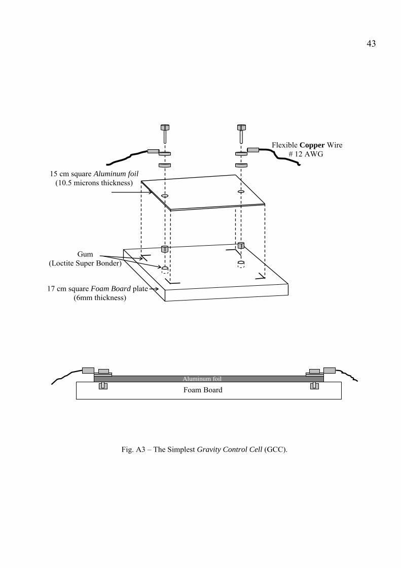
43
Fig. A3 – The Simplest Gravity Control Cell (GCC).
15 cm square Aluminum foil (10.5 microns thickness)
Gum (Loctite Super Bonder)
17 cm square Foam Board plate (6mm thickness)
Foam Board Aluminum foil
Flexible Copper Wire # 12 AWG
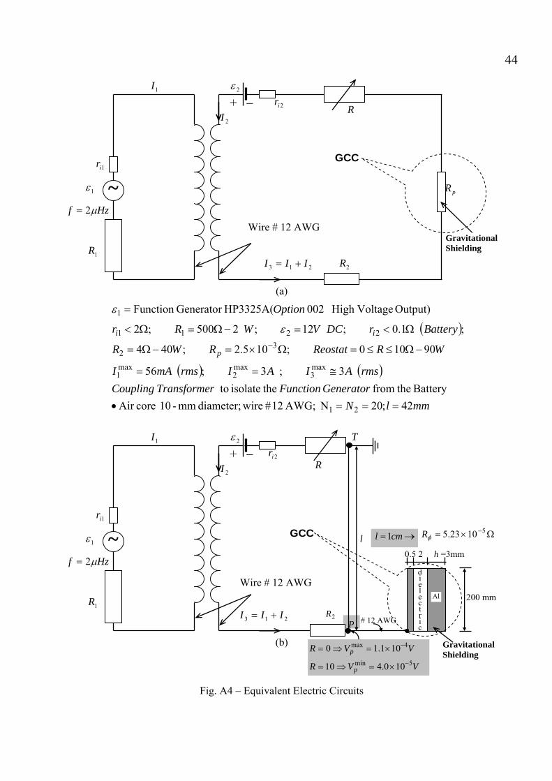
44
C
(a)
C
(b)
Fig. A4 – Equivalent Electric Circuits
GC
GC
P
+ −
r
r
1i
2i
pR
1R 2R
R
1
2ε 1I
2I
213 III
ε
+=
( )
( ) ( )
mmlNGenerator FunctionrTransforme Coupling
rmsAIAIrmsmAI
WRReostatRWR
BatteryrDCVWRr
Option
p
ii
42;20N AWG; 12 # wirediameter; mm-10 coreAir Battery thefrom theisolate to
3;3;56
90100;105.2;404
;1.0;12;2500;2
Output) VoltageHigh 002 HP3325A(Generator Function
21
max3
max2
max1
32
2211
1
===•
≅==
−Ω≤≤=Ω×=−Ω=
Ω<=−Ω=Ω<
=
−
ε
ε
Hzf μ2= ~
Wire # 12 AWG
Gravitational Shielding
+ −
1ir
2i
Ω×= −51023.5φR
1R
r
R
1 ε
2ε 1I
2I
213 III +=
Hzf μ2= ~
Wire # 12 AWG
VVR
VVR
p
p
5min
4max
100.410
101.10−
−
×=⇒=
×=⇒=
2R
cml 1= →
0.5 2 h =3mm
200 mm
Gravitational Shielding
Al
# 12 AWG
T
l
d i e l e c t r i c

45
032
427 110758.1121 i
rg m
fjm
⎪⎭
⎪⎬⎫
⎪⎩
⎪⎨⎧
⎥⎥⎦
⎤
⎢⎢⎣
⎡−×+−= −
σρμ
Fig. A5 – An ELF electric current through a wire, that makes a spherical form as shown above,reduces the gravitational mass of the wire and the gravity inside sphere at the same proportio
n0ig mm=χ (Gravitational Shielding Effect). Note that this spherical form can be transformed into
n ellipsoidal form or a disc in order to coat, for example, a Gravitational Spacecraft. It is alsoossible to coat with a wire several forms, such as cylinders, cones, cubes, etc. The characteristics
of the wire are expressed by: rμ ,
ap
σ , ρ ; j is the electric current density and f is the frequency.
Wire
j
jELF electric current

46
Fig. A6 – Experimental set-up 2.
50 mm
Dynamometer
Flexible Copper wire # 12 AWG
R
1R
Rheostat
Battery 12V
Function Generation HP3325A
1ε
2ε
Coupling Transformer
Rigid Aluminum wire # 14 AWG
Length = 28.6 m RS= 0.36 Ω
2R
4 - 40W
Flexible Copper wire# 12 AWG
Ω

47
i
Fig A7 – Gravitational shielding produced by semi-spheres stamped on the Aluminum foil- By simply changing the geometry of the surface of the Aluminum foil it is possible to ncrease the working frequency f up to more than 1Hz.
~
d
b
a
r0
Δ
V0 , f
Eair ,σair
Insulation
Gravitational Shielding
εr
Aluminum Foil
Air

48
(a)
(b)
(c)
(d) Fig A8 – Method to coat the Aluminum semi-spheres with acrylic ( )mmra 6.00 =−=Δ . (a)Acrylic sheet (A4 format) with 1.5mm thickness and an Aluminum plate (A4) with several semi-spheres (radius mmr 9.00 = ) stamped on its surface. (b)A heater is placed below the Aluminum plate in order to heat the Aluminum. (c)When the Aluminum is sufficiently heated up, the acrylic sheet and the Aluminum plate are pressed, one against the other (The two D devices shown in this figure are used in order to impede that the press compresses the acrylic and the aluminum besides distance ay + ). (d)After some seconds, the press and the heater are removed, and the device is ready to be used.
y
Heater
Aluminum Plate
Acrylic sheet
Press
Δ=0.6 mm a = 1.5 mmr0 =0.9 mm
a =1.5 mm
r0 =0.9 mm
D Dy + a

49
Fig. A9 – Experimental Set-up using a GCC subjected to high-voltage 0V with frequency Hzf 1> .
Note that in this case, the pan balance is not necessary because the substance of the Gravitational Shielding is an air layer with thickness d above the acrylic sheet. This is therefore, more a type of Gravity Control Cell (GCC) with external gravitational shielding.
50 mm
GCC Acrylic/Aluminum
Dynamometer
Flexible Copper wire # 12 AWG
g ggg χ=′
Sample
Rheostat Oscillator f > 1HzTransformer
High-voltage V0

50
(b)
Fig. A10 – (a) Equivalent Electric Circuit. (b) Details of the electrical connection with the
Gravitational Shielding
(a)
Aluminum plate. Note that others connection modes (by the top of the device) can produce destructible interference on the electric lines of the airE field.
0V d
R
GCC crylic /Aluminum A
kVV 9max
0 = kVV 7.2min
0 = ~ OscillatorHzf 1>
Acrylic
Aluminum
Pin
Connector (High-voltage)
10kV
wire

51
(a) (b)
(c)
(d)
Fig. A11 – Geometrical forms with similar effects as those produced by the semi-spherical form – (a) shows the semi-spherical form stamped on the metallic surface; (b) shows the semi-cylindrical form (an obvious evolution from the semi-spherical form); (c) shows concentric metallic rings stamped on the metallic surface, an evolution from semi-cylindrical form. These geometrical forms produce the same effect as that of the semi-spherical form, shown in Fig.A11 (a). By using concentric metallic rings, it is possible to build Gravitational Shieldings around bodies or spacecrafts with several formats (spheres, ellipsoids, etc); (d) shows a Gravitational Shielding around a Spacecraft with ellipsoidal form.
Dielectric layer
Gravitational Shielding
Metallic Rings
εr
Ellipsoidal metallic base
Oscillator
Transformer
f
V0
Metallic Rings
Metallic base
Eair
Ionized air

52
F
(a) (b)
ig. A12 – Non-solid and Solid Gravitational Shieldings - In the case of the Gravitational Shielding produced on a solid substance (b), when its molecules go to the imaginary space-time, the electric field that produces the effect also goes to the imaginary space-time together with them, because in this case, the substance of the Gravitational Shielding is rigidly connected (by means of the dielectric) to the metal that produces the electric field. This does not occur in the case of Air Gravitational Shielding.
E
Metal Dielectric
Solid Gravitational Shielding (rigidly connected to the dielectric)
Non-solid Gravitational Shielding
Metal
Spacecraft Spacecraft
Dielectric (rigidly connected to the spacecraft)
E

53
(a)
(b)
2
102
10
r
VG
r
MGa igmg ρ
χχ ==
(c)
Fig. A13 – Double Gravitational Shielding and Micro-thrusters – (a) Shows a doublegravitational shielding that makes possible to decrease the inertial effects upon the spacecraf
twhen it is traveling both in the imaginary space-time and in the real space-time. The solidGravitational Shielding also can be obtained by means of an ELF electric current through a metalliclamina placed between the semi-spheres and the Gravitational Shielding of Air as shown above. (b)Shows 6 micro-thrusters placed inside a Gravitational Spacecraft, in order to propel thespacecraft in the directions x, y and z. Note that the Gravitational Thrusters in the spacecraftmust have a very small diameter (of the order of millimeters) because the hole through theGravitational Shielding of the spacecraft cannot be large. Thus, these thrusters are in fact Micro-thrusters. (c) Shows a micro-thruster inside a spacecraft, and in front of a volume V of theintergalactic medium (IGM). Under these conditions, the spacecraft acquires an acceleration a inthe direction of the volume V.
Eair
Metal Dielectric
Solid Gravitational Shielding
i ELF electric current
Spacecraft Spacecraft Ers
Air Gravitational Shielding
Metal Dielectric Aluminum
Micro-Gravitational Thruster
r
a
Micro-Gravitational Thruster with 10 gravitational shieldings
Gravitational Spacecraft
Volume V of the
Intergallactic medium (IGM)
Mg
ρ igm∼10-26kg.m-3 Gravitational Shielding
gtm

54
210
210
rV
Gr
MGa ismg ρ
χχ ==
(a)
210
210
rV
Gr
MGa ipmg ρ
χχ ==
(b)
210
210
rV
Gr
MGa atmg ρ
χχ ==
(c)
Fig. A14 – Gravitational Propulsion using Micro-Gravitational Thruster – (a) Gravitational acceleration produced by a gravitational mass Mg of the Interstellar Medium. The density of the nterstellar Medium is about 105 times greater than the density of the Intergalactic Medium (b)
Gravitational acceleration produced in the Interplanetary Medium. (c) Gravitational acceleration I
produced in the Earth’s atmosphere. Note that, in this case, ρatm (near to the Earth’s surface)is about1026 times greater than the density of the Intergalactic Medium.
r a
Micro-Gravitational Thruster with 10 gravitational shieldings
Gravitational Spacecraft
Volume V of the
Interstellar medium (ISM)
Mg
ρ ism∼10-21kg.m-3
r
aGravitational Spacecraft
Volume V of the
Interplanetary medium (IPM)
Mg
ρ ipm∼10-20kg.m-3
r
aGravitational Spacecraft
Volume V of the
Earth’s atmospheric
Mg
ρ atm∼1.2kg.m-3
Gravitational Shielding
Gravitational Shielding
Gravitational Shielding
Micro-Gravitational Thruster with 10 gravitational shieldings
Micro-Gravitational Thruster with 10 gravitational shieldings

55
(a)
(b)
(c) Fig. A15 – Dynamics and Structure of the Micro-Gravitational Thrusters - (a) The Micro-Gravitational Thrusters do not work outside the Gravitational Shielding, because, in this case, the resultant upon the thruster is null due to the symmetry. (b) The Gravitational Shielding ( )810−≅sχ reduces strongly the intensities of the gravitational forces acting on the micro-gravitational thruster, except obviously, through the hole in the gravitational shielding. (c) Micro-Gravitational Thruster with 10 Air Gravitational Shieldings (10GCCs). The grounded metallic laminas are placed so as to retain the electric field produced by metallic surface behind the semi-spheres.
Mica Metal
1 GCC Air Gravitational Shielding
10mm
~ 400 mm
Gravitational Shielding
Micro-Gravitational Thruster with 10 gravitational shieldings
F1 =χairF0
S1
a’0 =χs(-GMg /r’2)
F’0 = F0 => R = (F’0 – F2) + (F1 – F’1 ) + (F’2 – F0) = 0
ELF ~ V0
Hole in the Gravitational Shielding
Grounded Metallic laminas
Mg Mg
r r
S2
F’0 F0
F’1 =χairF’0
F2 =χair2F0
810−−≅sχ
a0 = - GMg/r2
010
10 FFR airχ=≅
Mg
r’ r
Mg
x
F’2=χair2F’0
a10=χair10a0
a’0

56
GCC Cross-section Front view
(a)
GCC Cross-section Side View (b)
Fig. A16 – A GCC using distilled Water. In total this GCC weighs about 6kg; the air layer 7.3 grams. The balance has the following characteristics: Range 0 – 6kg; readability 0.1g. The yarns are inserted side by side on the Aluminum sheet. Note the detail of fixing of the yarns on the Aluminum sheet.
Air layerDistilled Water
0.885 m
Balance
Transformer
g’= χ g
g
Sample Any type of material; any mass
mg (air) = χ mi (air)
~ 2 Hz
V0max = 9 kV
Acrylic Box (2mm thickness)
Aluminum sheet (0.5 mm thickness)
342 Aluminum yarns (# 10 AWG) (2.558 mm diameter; 0.884 mm length)
2 mm
2 mm
7.73 mma = 1.9 mm1.8 mm
d = 9.73 mm
3.2 mm
Balance
0.885 m
0.884 m
Aluminum sheet (0.5 mm thickness)
342 Aluminum yarns (# 10 AWG) (2.558 mm diameter; 0.884 mm length)
1mm 1mm
0.5 mm
3.6mm
1.5mm
0.885 m

57
Fig. A17 – Experimental set-up. In order to prove the exponential effect produced by the superposition of the Gravitational Shieldings, we can take three similar GCCs and put them one above the other, in such way that above the GCC 1 the gravity acceleration will be gg χ=′ ; above the GCC2 gg 2χ=′′ , and above the GCC3 gg 3χ=′′′ . Where χ is given by Eq. (A47). The arrangement above has been designed for values of gmg 13< and χ up to -9 or kgmg 1< and χ up to -2 .
Balance
140 cm
5Kg 70 cm
Balance
5Kg 70 cm
Balance
5Kg 70 cm
mg
mg
mg
Sample Any type of material; any mass
GCC 3
GCC 2
GCC 1
gg χ=′
gg 2χ=′′
gg 3χ=′′′
g

58APPENDIX B: Gravity Control Cells (GCCs) made from Semiconductor Compounds. There are some semiconductors compounds with electrical conductivity between 104S/m to 1 S/m, which can have their gravitational mass strongly decreased when subjected to ELF electromagnetic fields. For instance, the polyvinyl chloride (PVC) compound, called DuracapTM 86103. It has the following characteristics: 1=rμ ; 3=rε mS /3.3333=σ 31400 −= m.kgρ mmKVstrengthdieletric /98=
Then, according to the following equation below (derived from Eq.A14)
( )1110758.1121 04
32
327 BmE
fm irms
rg
⎪⎭
⎪⎬⎫
⎪⎩
⎪⎨⎧
⎥⎥
⎦
⎤
⎢⎢
⎣
⎡−⎟
⎟⎠
⎞⎜⎜⎝
⎛×+−= −
ρσμ
the gravitational mass, , of the Duracap
gmTM 86103, when subjected to an
electromagnetic field of frequency , is given by
f
( )21103.3121 03
423 Bm
f
Em i
rmsg
⎪⎭
⎪⎬⎫
⎪⎩
⎪⎨⎧
⎥⎥
⎦
⎤
⎢⎢
⎣
⎡−×+−= −
Note that, if the electromagnetic field through the Duracap has extremely-low frequency, for example, if , and Hzf 2=
( )mmkVmVErms /94.0/104.9 5×=
Then, its gravitational mass will be reduced down to , reducing in this way, the initial weight
01.1 ig mm −≅
( )gmgmP ig 00 == of the Duracap down to . 01.1 P−
BACKGROUND FOR EXPERIMENTAL The DuracapTM 86103 is sold under the form of small cubes. Its melting temperature varies from 177ºC to 188ºC. Thus, a 15cm square Duracap plate with 1 mm thickness can be shaped by using a suitable mold, as the shown in Fig.B1. Figure B2(a) shows the Duracap plate between the Aluminum plates of a parallel plate capacitor. The plates have the following dimensions: 19cm X 15cm X 1mm. They are painted with an insulating varnish spray of high dielectric strength (ISOFILM). They are connected to the secondary of a transformer, which is connected to a Function Generator. The distance between the Aluminum plates is mmd 1= . Thus, the electric field through the Duracap is given by
( )322
0 BdVE
Er
mrms
ε==
where rε is the relative permittivity of the dielectric (Duracap), and is the amplitude of the wave voltage applied on the capacitor.
0V
In order to generate ELF wave voltage of Hzf 2= , we can use the widely-known Function Generator HP3325A (Op.002 High Voltage Output) that can generate sinusoidal voltages with extremely-low frequencies and amplitude up to 20V (40Vpp into
Ω500 load). The maximum output current is ; output impedance <2Ω at ELF.
ppA.080
The turns ratio of the transformer (Bosch red coil) is . Thus, since the 1:200

59maximum value of the amplitude of the voltage produced by the Function Generator is , then the maximum secondary voltage will be .Consequently, Eq. (B3) gives
VV p 20max =
kVVVs 4max0
max ==
mVErms /108.2 6max ×=
Thus, for , Eq. (B2) gives Hzf 2=
05.29 ig mm −= The variations on the gravitational mass of the Duracap plate can be measured by a pan balance with the following characteristics: range 0 − 1.5kg ; readability 0.01g, using the set-up shown in Fig. B2(a). Figure B2(b) shows the set-up to measure the gravity acceleration variations above the Duracap plate (Gravitational Shielding effect). The samples used in this case, can be of several types of material. Since voltage waves with frequencies very below 1Hz have a very long period, we cannot consider, in practice, their rms values. However, we can add a sinusoidal voltage
tVVosc ωsin0= with a DC voltage , by means of the circuit shown in Fig.B3. Thus, we obtain
DCV
tVVV DC ωsin0+= ; fπω 2= . If then . Thus, the voltage varies with the frequency , but its intensity is approximately equal to , i.e., V will be practically constant. This is of fundamental importance for maintaining the value of the gravitational mass of the body, , sufficiently stable during all the time, in the case of .
DCVV <<0 DCVV ≅
V f
DCV
gm
Hzf << We have shown in this paper that it is possible to control the gravitational mass of a spacecraft, simply by controlling the gravitational mass of a
body inside the spacecraft (Eq.(10)). This body can be, for example, the dielectric between the plates of a capacitor, whose gravitational mass can be easily controlled by means of an ELF electromagnetic field produced between the plates of the capacitor. We will call this type of capacitor of Capacitor of Gravitational Mass Control (CGMC). Figure B 4(a) shows a CGMC placed in the center of the spacecraft. Thus, the gravitational mass of the spacecraft can be controlled simply by varying the gravitational mass of the dielectric of the capacitor by means of an ELF electromagnetic field produced between the plates of the capacitor. Note that the Capacitor of Gravitational Mass Control can have the spacecraft's own form as shown in Fig. B 4(b). The dielectric can be, for example, a Duracap plate, as shown in this appendix. In this case, the gravitational mass of the dielectric is expressed by Eq. (B2). Under these circumstances, the total gravitational mass of the spacecraft will be given by Eq.(10):
( ) 00 idielectricispacecrafg mMM χ+=
where is the rest inertial mass of the spacecraft(without the dielectric) and
is the rest inertial mass of the dielectric;
0iM
0im
0igdielectric mm=χ , where is the gravitational mass of the dielectric. By decreasing the value of
gm
dielectricχ , the gravitational mass of the spacecraft decreases. It was shown, that the value of χ can be negative. Thus, for example, when 00 iidielectric mM−≅χ , the gravitational mass of the spacecraft gets very close to zero. When 00 iidielectric mM−<χ , the

60gravitational mass of the spacecraft becomes negative. Therefore, for an observer out of the spacecraft the gravitational mass of the spacecraft is ( ) 00 idielectricispacecrafg mMM χ+= , and not . 00 ii mM +
Since the dielectric strength of the Duracap is , a Duracap plate with 1mm thickness can withstand up to
. In this case, the value of
mmkV /98
kV98 dielectricχ for , according to Eq. (B2), is Hzf 2=
40 10−≅= igdielectric mmχ
Thus, for example, if the inertial mass of the spacecraft is and, the inertial mass of the dielectric of the Capacitor of Gravitational Mass Control is
, then the gravitational mass of the spacecraft becomes
kgM i 0014.100210 ≅
kgmi 0021.10 ≅
( ) kgmMM idielectricispacecrafg3
00 10−≅+= χ
This value is much smaller than . 0159.0 iM+
It was shown [1] that, when the gravitational mass of a particle is reduced to values between and , it becomes imaginary, i.e., the gravitational and the inertial masses of the particle become imaginary. Consequently, the particle disappears from our ordinary space-time.
iM1590.+
iM1590.−
This means that we cannot reduce the gravitational mass of the spacecraft below , unless we want to make it imaginary.
iM1590.+
Obviously this limits the minimum value of dielectricχ , i.e.
. Consequently, if the gravity acceleration out of the spacecraft (in a given direction) is
159.0min =dielctricχ
g , then, according to the Gravitational Shielding Principle, the corresponding gravity acceleration upon the crew of the
spacecraft can be reduced just down to . In addition, since the Mach’s principle says that the local inertial forces are produced by the gravitational interaction of the local system with the distribution of cosmic masses then the inertial effects upon the crew would be reduced just by
g159.0
159.0=dielectricχ . However, there is a way to strongly reduce the inertial effects upon the crew of the spacecraft without making it imaginary. As shown in Fig. B4 (c), we can build an inertial shielding, with superimposed CGMCs. In this case, according to the Gravitational Shielding Principle, the gravity upon the crew will be given by
, where
n
gg ndielectricn χ= g is the gravity
acceleration out of the spacecraft (in a given direction) and 0igdielectric mm=χ ; and are, respectively, the gravitational mass and the inertial mass of the dielectric. Under these conditions the inertial effects upon the crew will be reduced by .
gm
0im
ndielectricχ
Thus, for (ten superimposed CGMCs), and
10=n2.0≅dielectricχ , the inertial
effects upon the crew will be reduced by . Therefore, if the maximum thrust produced by the thrusters of the spacecraft is , then the intensities of the inertial forces upon the crew will not exceed , i.e. they will be practically negligible.
710 101 −×≅dielectricχ
NF 510=
N01.0
Under these circumstances, the gravitational mass of the spacecraft, for an observer out of the spacecraft, will be just approximately equal to the gravitational mass of the inertial shielding, i.e. . ( ) ( shieldinertialgspacecraftg MM .≅ )
If , and the thrusters of the spacecraft are able to
( ) kgM shieldinertialg3
. 10≅

61produces up to , the spacecraft will acquires an acceleration given by
NF 5103×=
( )
22 .103 −×≅= smM
Faspacecraftg
spacecraft
With this acceleration it can reach velocities close to Mach 10 in some seconds. The velocity that the spacecraft can reach in the imaginary spacetime is much greater than this value, since
, as we have seen, can be reduced down to or less.
(spacecraftgM )
kg310−≅
Thus, if the thrusters of the spacecraft are able to produces up to , and , the spacecraft will acquires an acceleration given by
NF 5103×= ( ) kgM spacecraftg310−≅
( )
28 .103 −×≅= smM
Faspacecraftg
spacecraft
With this acceleration it can reach velocities close to the light speed in less than 1 second. After 1 month, the velocity of the spacecraft would be about (remember that in the imaginary spacetime the maximum velocity of propagation of the interactions is infinity [
sm /1015
1]). OTHER SEMICONDUCTOR COMPOUNDS A semiconductor compound, which can have its gravitational mass strongly decreased when subjected to ELF electromagnetic fields is the CoorsTek Pure SiCTM LR CVD Silicon Carbide, 99.9995% ‡‡‡‡. This Low-resistivity (LR) pure Silicon Carbide has electrical conductivity of 5000S/m at room temperature; 8.10=rε ;
; dielectric strength >10 3.3210 −= mkgρ
‡‡‡‡ www.coorstek.com
KV/mm; maximum working temperature of 1600°C. Another material is the Alumina-CNT, recently discovered §§§§. It has electrical conductivity of 3375 S/m at 77°C in samples that were 15% nanotubes by volume [17]; 8.9=rε ;
; dielectric strength 10-20KV/mm; maximum working temperature of 1750°C.
3.3980 −= mkgρ
The novel Carbon Nanotubes Aerogels*****, called CNT Aerogels are also suitable to produce Gravitational Shieldings, mainly due to their very small densities. The electrical conductivity of the CNT Aerogels is 70.4S/m for a density of [3.5.7 −= mkgρ 18];
10≈rε . Recently (2010), it was announced the discovered of Graphene Aerogel with and [mS /101~ 2×=σ 3.10 −= mkgρ 19] (Aerogels exhibit higher dielectric strength than expected for porous materials). §§§§ Recently, it was discovered that Carbon nanotubes (CNTs) can be added to Alumina (Al2O3) to convert it into a good electrical conductor. ***** In 2007, Mateusz Brying et al. working with Prof. Arjun Yodh at the University of Pennsylvania produced the first aerogels made entirely of carbon nanotubes (CNT Aerogels) [20] that, depending on the processing conditions, can have their electrical conductivity ranging as high as 100 S/m.

62
Fig.B1 – Mold design
5mm
150mm
150mm
150mm
150mm
2mm
3mm
3mm
Aluminum
Aluminum
200mm
200mm

63
(a)
(b)
Fig.B2 – Schematic diagram of the experimental set-up
Duracap 150mmX150mmX1mm
Acrylic 150mmX40mmX1mm
Wood
Balance
Aluminum 190mmX150mmX1mm
1kg
20 mm 20 mm 20 mm
Balance
1kg
Sample
ELF Wave Voltage Generator
Bosch red coil
Bosch red coil
ELF Wave Voltage Generator

64
Fig. B3 – Equivalent Electric Circuit
− +
R
oscV
DCV
Coupling Transformer
f
oscDC VV +ELF voltage waves Generato
~ tVVosc ωsin0= 200:1 oscV
0VDC >>
Bosch red coil
Vr

65
(a)
(b)
(c) Fig.B4 – Gravitational Propulsion System and Inertial Shielding of the Gravitational Spacecraft– (a) eight gravitational thrusters are placed inside a Gravitational Spacecraft, in order to propel thespacecraft along the directions x, y and z. Two gravitational thrusters are inside the columns 1 and 2, inorder to rotate the spacecraft around the y-axis. The functioning of the Gravitational Thrusters is shownin Fig.A14. The gravitational mass of the spacecraft is controlled by the Capacitor of GravitationalMass Control (CGMC). Note that the CGMC can have the spacecraft's own form, as shown in (b). Inorder to strongly reduce the inertial effects upon the crew of the spacecraft, we can build an inertialshielding, with several CGMCs, as shown above (c). In this case, the gravity upon the crew will begiven by gg n
dielectricn χ= , where g is the gravity acceleration out of the spacecraft (in a given direction)and 0igdielectric mm=χ ; gm and 0im are, respectively, the gravitational mass and the inertial mass of
the dielectric. Under these conditions the inertial effects upon the crew will be reduced by ndielectricχ .
Thus, for example, if 10=n and 2.0≅dielectricχ , the inertial effects will be reduced
by 710 101 −×≅dielectricχ . If the maximum thrust produced by the thrusters is NF 510= , then the intensitiesof the inertial forces upon the crew will not exceed N01.0 .
Gravitational Thrusters
Capacitor of Gravitational Mass Control
col 1 col 2
x y z
n 3 2 1 n dielectrics
Capacitor of Gravitational Mass Control(CGMC) dielectric
Inertial Shielding
g gg ndielectricn χ=

66APPENDIX C: Longer-Duration Microgravity Environment Produced by Gravity Control Cells (GCCs). The acceleration experienced by an object in a microgravity environment, by definition, is one-millionth (10-6) of that experienced at Earth’s surface (1g). Consequently, a microgravity environment is one where the acceleration induced by gravity has little or no measurable effect. The term zero-gravity is, obviously inappropriate since the quantization of gravity [1] shows that the gravity can have only discrete values different of zero [1, Appendix B]. Only three methods of creating a microgravity environment are currently known: to travel far enough into deep space so as to reduce the effect of gravity by attenuation, by falling, and by orbiting a planet. The first method is the simplest in conception, but requires traveling an enormous distance, rendering it most impractical with the conventional spacecrafts. The second method, falling, is very common but approaches microgravity only when the fall is in a vacuum, as air resistance will provide some resistance to free fall acceleration. Also it is difficult to fall for long enough periods of time. There are also problems which involve avoiding too sudden of a stop at the end. The NASA Lewis Research Center has several drop facilities. One provides a 132 meter drop into a hole in the ground similar to a mine shaft. This drop creates a reduced gravity environment for 5.2 seconds. The longest drop time currently available (about 10 seconds) is at a 490 meter
deep vertical mine shaft in Japan that has been converted to a drop facility. Drop towers are used for experiments that only need a short duration of microgravity, or for an initial validation for experiments that will be carried out in longer duration of microgravity.
Aircraft can fly in parabolic arcs to achieve period of microgravity of 20 to 25 seconds with g-level of approximately 0.02 g. The airplane climbs rapidly until its nose is about 45-degree angle to the horizon then the engines are cut back. The airplane slows; the plane remains in free fall over the top of the parabola, then it nose-dives to complete the parabola, creating microgravity conditions. Aircraft parabolic flights give the opportunity to perform medical experiments on human subjects in real microgravity environment. They also offer the possibility of direct intervention by investigators on board the aircraft during and between parabolas. In the mid-1980s, NASA KC-135, a modified Boeing 707,

67provided access to microgravity environment. A parabolic flight provided 15 to 20 seconds of 0.01 g or less, followed by a 2-g pull out. On a typical flight, up to 40 parabolic trajectories can be performed. The KC-135 can accommodate up to 21 passengers performing 12 different experiments. In 1993, the Falcon-20 performed its first parabolic flight with microgravity experiment on board. This jet can carry two experimenters and perform up to 3 experiments. Each flight can make up to 4 parabolic trajectories, with each parabola lasting 75 seconds, with 15 to 20 seconds of microgravity at 0.01g or less.
The third method of creating a microgravity environment is orbiting a planet. This is the environment commonly experienced in the space shuttle, International Space Station, Mir (no longer in orbit), etc. While this scenario is the most suitable for scientific experimentation and commercial exploitation, it is still quite expensive to operate in, mostly due to launch costs. A space shuttle provides an ideal laboratory environment to conduct microgravity research. A large panoply of experiments can be carried out in microgravity conditions for up to 17 days, and scientists can make adjustment to avoid experiment failure
and potential loss of data. Unmanned capsules, platforms or satellites, such as the European retrievable carrier Eureka, DLR's retrievable carrier SPAS, or the Russian Photon capsules, the US Space Shuttle (in connection with the European Spacelab laboratory or the US Spacelab module), provide weeks or months of microgravity. A space station, maintaining a low earth orbit for several decades, greatly improves access to microgravity environment for up to several months. Thus, microgravity environment can be obtained via different means, providing different duration of microgravity. While short-duration microgravity environments can be achieved on Earth with relative easiness, longer-duration microgravity environments are too expensive to be obtained. Here, we propose to use the Gravity Control Cells (GCCs), shown in this work, in order to create longer-duration microgravity environments. As we have seen, just above a GCC the gravity can be strongly reduced (down to 1μg or less). In this way, the gravity above a GCC can remain at the
~1 μ g
1 g
GCC
longer-duration microgravity environment
up to 3m
>>1m
>>1m

68
microgravity ranging during a very long time (several years). Thus, GCCs can be used in order to create longer-duration microgravity environments on Earth. In addition, due to the cost of the GCCs to be relatively low, also the longer-duration microgravity environments will be produced with low costs. This possibility appears to be absolutely new and unprecedented in the literature since longer-duration microgravity environments are usually obtained via airplanes, sounding rockets, spacecraft and space station. It is easy to see that the GCCs can be built with width and length of until some meters. On the other hand, as the effect of gravity reduction above the GCC can reach up to 3m, we can then conclude that the longer-duration microgravity environments produced above the GCCs can have sufficiently large volumes to perform any microgravity experiment on Earth. The longer-duration microgravity environment produced by a GCC will be a special tool for microgravity research. It will allow to improve and to optimize physical, chemical and biological processes on Earth that are important in science, engineering and also medicine. The reduction of gravitational effects in a microgravity environment shows, for example, that temperature differences in a fluid do not produce convection, buoyancy or sedimentation. The changes in fluid behavior in microgravity lie at the heart of the studies in materials science, combustion and many aspects of space biology and life sciences. Microgravity research holds the
promise to develop new materials which can not be made on Earth due to gravity. These new materials shall have properties that are superior to those made on Earth and may be used to: -increase the speed of future computers, -improve fiber optics, -make feasible Room Temperature Superconductors, -enable medical breakthroughs to cure several diseases (e.g., diabetes). In a microgravity environment protein crystals can be grown larger and with a purity that is impossible to obtain under gravity of 1g. By analyzing the space-grown crystals it is possible to determine the structure and function of the thousands of proteins used in the human body and in valuable plants and animals. The determination of protein structure represents a huge opportunity for pharmaceutical companies to develop new drugs to fight diseases. Crystal of HIV protease inhibitor grown in microgravity are significantly larger and of higher quality than any specimens grown under gravity of 1g. This will help in defining the structure of the protein crucial in fighting the AIDS virus. Protein Crystal Isocitrate Lysase is an enzyme for fungicides. The isocitrate lysase crystals grown in microgravity environments are of larger sizes and fewer structural defects than crystals grown under gravity of 1g. They will lead to more powerful fungicides to treat serious crop diseases such as rice blast, and increase crop output.

69 Improved crystals of human insulin will help improve treatment for diabetes and potentially create a cure. Anchorage dependent cells attached to a polymer and grown in a bioreactor in microgravity will lead to the production of a protein that is closer in structure and function to the three-dimensional protein living in the body.
This should help reduce or eliminate transplant rejection and is therefore critical for organ transplant and for the replacement of damaged bone and tissues. Cells grown on Earth are far from being three-dimensional due to the effect of 1g gravity. The ZBLAN is a new substance with the potential to revolutionize fiber optics communications. A member of the heavy metal fluoride family of glasses, ZBLAN has promising applications in fiber optics. It can be used in a large array of industries, including manufacture of ultra high
purity fiber optics, optical switches for computing, telecommunications, medical surgery and cauterization, temperature monitoring, infrared imaging, fiber-optic lasers, and optical power transmission. A ZBLAN fiber optic cable manufactured in a microgravity environment has the potential to carry 100 times the amount of data conveyed by conventional silica-based fibers. In microgravity environment where complications of gravity-driven convection flows are eliminated, we can explore the fundamental processes in fluids of several types more easily and test fundamental theories of three-dimensional laminar, oscillatory and turbulent flow generated by various other forces. By improving the basics for predicting and controlling the behavior of fluids, we open up possibilities for improving a whole range of industrial processes: -aCivil engineers can design safe buildings in earthquake-prone areas thanks to a better understanding of the fluid-like behavior of soils under stress. - Materials engineers can benefit from a deeper knowledge of the determination of the structure and properties of a solid metal during its formation and can improve product quality and yield, and, in some cases, lead to the introduction of new products. - Architects and engineers can design more stable and performing power

70plants with the knowledge of the flow characteristics of vapor-liquid mixture. - Combustion scientists can improve fire safety and fuel efficiency with the knowledge of fluid flow in microgravity. In microgravity environment, medical researchers can observe the functional changes in cells when the effect of gravity is practically removed. It becomes possible to study fundamental life processes down to the cellular level. Access to microgravity will provide better opportunities for research, offer repeated testing procedures, and enormously improve the test facilities available for life sciences investigations. This will provide valuable information for medical research and lead to improvements in the health and welfare of the six billion people, which live under the influence of 1g gravity on the Earth's surface. The utilization of microgravity to develop new and innovative materials, pharmaceuticals and other products is waiting to be explored. Access to microgravity environments currently is limited. Better access, as the produced by GCCs, will help researchers accelerate the experimentation into these new products. Terrafoam is a rigid, silicate based inorganic foam. It is nonflammable and does not five off noxious fumes when in the presence of fire. It does not conduct heat to any measurable degree and thus is an outstanding and possible unsurpassed thermal insulator. In addition, it
appears to have unique radiation shielding capabilities, including an ability to block alpha, beta, gamma rays). Terrafoam can be constructed to be extremely lightweight. Altering the manufacturing process and the inclusion of other materials can vary the properties of Terrafoam. Properties such as cell structure, tensile strength, bulk density and temperature resistance can be varied to suit specific applications. It self-welds to concrete, aluminum and other metals. The useful variations on the base product are potentially in the thousands. Perhaps the most exciting potential applications for Terrafoam stem from its extraordinary capability as an ultra-lightweight thermal and radioactive shield. Also, the formation of nanoscale carbon structures by electrical arc discharge plasma synthesis has already been investigated in microgravity experiments by NASA. Furthermore, complex plasmas are relevant for processes in which a particle formation is to be prevented, if possible, as, for example, within plasma etching processes for microchip production.
People will benefit from numerous microgravity experiments that can be conducted in Longer-Duration Microgravity Environment Produced by Gravity Control Cells (GCCs) on Earth.

71 APPENDIX D: Antenna with Gravitational Transducer for Instantaneous Communications at any distance
It was previously shown in this article that Quantum Gravitational Antennas (GCC antennas, Fig.8) can emit and detect virtual gravitational radiation. The velocity of this radiation is infinite, as we have seen. This means that these quantum antennas can transmit and receive communications instantaneously to and from anywhere in the Universe. Here, it is shown how to transmit and receive communications instantaneously from any distance in the Universe by utilizing virtual electromagnetic (EM) radiation instead of virtual gravitational radiation. Starting from the principle that the antennas of usual transceivers (real antennas) radiate real EM radiation, then we can expect that imaginary antennas radiate imaginary EM radiation or virtual EM radiation. The velocity of this radiation is also infinite, in such a way that it can transmit communications instantaneously from any distance in the Universe.
It was shown [1] that when the gravitational mass of a body is decreased down to the range of
to ( is its inertial mass), the body becomes imaginary and goes to an imaginary Universe which contains our real Universe. Thus, we have the method to convert real antennas to imaginary antennas.
im159.0+ im159.0− im
Now, consider a Gravitational Shielding , whose gravitational mass S
is decreased down to the range of iSm159.0+ to iSm159.0− . By analogy, it
becomes imaginary and goes to the imaginary Universe. It is easy to show that, in these circumstances, also a body inside the shielding becomes imaginary and goes to the imaginary Universe together with the gravitational shielding . In order to prove it, consider, for example, Fig.D1 where we clearly see that the Gravitational Shielding Effect is equivalent to a decrease of
S
S
iSgS mm=χ in the gravitational masses of the bodies A and B , since the initial gravitational masses: iAgA mm ≅ and become respectively
iBgB mm ≅
iAgA mm χ= and iBgB mm χ= , when the gravitational shielding is activated. Thus, when χ becomes less than 159.0+ , both the gravitational masses of and S A become respectively:
iSgS mm 159.0+< and
iAgA mm 159.0+< This proves, therefore, that when a Gravitational Shielding becomes imaginary, any particle (including photons
S
‡‡‡‡‡) inside , also becomes imaginary and goes to the imaginary
S
‡‡‡‡‡ As shown in the article “Mathematical Foundations of the Relativistic Theory of Quantum Gravity”, real photons become imaginary photons or virtual photons.

72 A B
(a) S (b) S A
(c) Fig.D1 – (a) (b) The Gravitational ShieldingEffect is equivalent to a decrease of iSgS mm=χin the gravitational masses of the bodies Aand B . (c) When a Gravitational Shielding Sbecomes imaginary, any particle (includingphotons) inside S , also becomes imaginary.
22 rmG
rm
Gg iBgBBA −≅−=
r
22 rm
Gr
mGg iAgA
AB −≅−=
1, <= χχ iSgS mm
22 rm
Gr
mGg iBgB
BAχ
−=−=
22 rm
Grm
Gg iAgAAB
χ−=−=
iSgS mm 159.0+<
Virtual photon iAgA mm 159.0+<
Universe together with the Gravitational Shielding §§§§§S . Now, consider a transceiver antenna inside a Gravitational Shielding . When the gravitational mass of , , is reduced down to the range of to , the
SS gSm
iSm159.0+ iSm159.0− §§§§§ Similarly, the bodies inside a Gravitational Spacecraft become also imaginaries when the Gravitational Spacecraft becomes imaginary.
antenna becomes imaginary, and, together with , it goes to the imaginary Universe. In these circumstances, the real photons radiated from the antenna also become imaginary photons or virtual photons. Since the velocity of these photons is infinite, they can reach instantaneously the receiving antenna, if it is also an imaginary antenna in the imaginary Universe.
S
Therefore, we can say that the Gravitational Shielding around the antenna works as a Gravitational Transducer ****** converting real EM energy into virtual EM energy. In practice, we can encapsulate antennas of transceivers with Aluminum cylinders, as shown in Fig.D2(a). By applying an appropriate ELF electric current through the Al cylinders, in order to put the gravitational masses of the cylinders within the range of to
iCylm159.0+
iCylm159.0− , we can transform real antennas into imaginary antennas, making possible instantaneously communications at any distance, including astronomical distances. Figure D2 (b) shows usual transceivers operating with imaginary antennas, i.e., real antennas turned into imaginary antennas. It is important to note that the communications between them occur through the imaginary space-time. At the end of transmissions, when the Gravitational Transducers are turned off, the antennas reappear in the real space-time, i.e., they become real antennas again. ****** A Transducer is substance or device that converts input energy of one form into output energy of another.
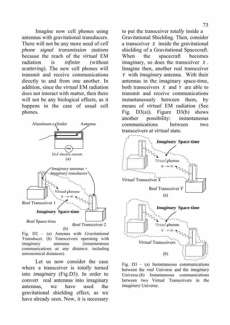
73 Imagine now cell phones using antennas with gravitational transducers. There will not be any more need of cell phone signal transmission stations because the reach of the virtual EM radiation is infinite (without scattering). The new cell phones will transmit and receive communications directly to and from one another. In addition, since the virtual EM radiation does not interact with matter, then there will not be any biological effects, as it happens in the case of usual cell phones.
(a)
(b) Fig. D2 – (a) Antenna with GravitationalTransducer. (b) Transceivers operating withimaginary antennas (instantaneouscommunications at any distance, includingastronomical distances).
Virtual photons v → ∞
Imaginary Space-time
Real Space-time Real Transceiver 2
Real Transceiver 1
Imaginary antennas + Imaginary transducers
~ELF electric current
Aluminum cylinder Antenna
Let us now consider the case where a transceiver is totally turned into imaginary (Fig.D3). In order to convert real antennas into imaginary antennas, we have used the gravitational shielding effect, as we have already seen. Now, it is necessary
to put the transceiver totally inside a Gravitational Shielding. Then, consider a transceiver X inside the gravitational shielding of a Gravitational Spacecraft. When the spacecraft becomes imaginary, so does the transceiver X . Imagine then, another real transceiver
with imaginary antenna. With their antennas in the imaginary space-time, both transceivers
Y
X and Y are able to transmit and receive communications instantaneously between them, by means of virtual EM radiation (See Fig. D3(a)). Figure D3(b) shows another possibility: instantaneous communications between two transceivers at virtual state.
(a)
(b) Fig. D3 – (a) Instantaneous communicationsbetween the real Universe and the imaginaryUniverse.(b) Instantaneous communicationsbetween two Virtual Transceivers in theimaginary Universe.
Virtual photons v → ∞
Imaginary Space-time
Real Transceiver
Virtual Transceiver X
Y
Virtual photov → ∞
Imaginary Space-time
Virtual Transceivers
ns

74References [1] De Aquino, F.(2010) Mathematical Foundations of the Relativistic Theory of Quantum Gravity, Pacific Journal of Science and Technology, 11(1), June 2010, pp.173-232. Physics/0212033. [2] De Aquino, F. (2010) Gravity Control by means of Electromagnetic Field through Gas at Ultra- Low Pressure, Pacific Journal of Science and Technology, 11(2) November 2010, pp.178- 247, Physics/0701091. . [3] Isham, C. J. (1975) Quantum Gravity, in Oxford Symposium, OUP. [4] Isham, C.J., (1997) “Structural Problems Facing Quantum Gravity Theory’’, in M, Francaviglia, G, Longhi, L, Lusanna, and E, Sorace, eds., Proceedings of the 14 International Conference on th
General Relativity and Gravitation, 167-209,(World Scientific, Singapore, 1997). [5] Mach, E., (1893) The Science of Mechanics, London, p.229-38. [6] Bohm, D. (1951) Quantum Theory, Prentice-Hall, N.Y, p.415. [7] D’Espagnat, B. The Question of Quantum Reality, Scientific American, 241,128. [8] Teller, P. Relational Holism and Quantum Mechanics, British Journal for the Philosophy of Science, 37, 71-81. [9] De Aquino, F. (2008) “Physical Foundations of Quantum Psychology”, http://htpprints.yorku.ca/archive/00000297 [10] Landau, L. and Lifchitz, E. (1969) Theorie du Champ, Ed.MIR, Moscow, Portuguese version (1974) Ed. Hemus, S.Paulo, pp.396-397. [11] Halliday, D. and Resnick, R. (1968) Physics, J. Willey & Sons, Portuguese Version, Ed. USP, p.1118. [12] Zhan, G.D et al. (2003) Appl. Phys. Lett. 83, 1228. [13] Davidson, K. & Smoot, G. (2008) Wrinkles in Time. N. Y: Avon, 158-163. [14] Silk, Joseph.(1977) Big Bang. N.Y, Freeman,299. [15] Jafelice, L.C. and Opher, R. (1992). The origin of intergalactic magnetic fields due to extragalactic jets. RAS. http://adsabs.harvard.edu/cgi-bin/nph- bib query? Bib code = 1992 MNRAS. 257. 135J. Retrieved 2009-06-19.
[16] Wadsley, J., et al. (2002). The Universe in Hot Gas. NASA. http://antwrp.gsfc.nasa.gov/apod/ap 020820.html. Retrieved 2009-06-19. [17] Zhan, G.D et al. (2003) Appl Phys. Lett. 83, 1228. [18] Xianping Lu, Ove Nilsson, Jochen. Fricke, Richard W. Pekala,” Thermal and electrical conductivity of monolithic carbon aerogels”, Journal of Applied Physics, 73, 2, 581-584 (Jan 1993). [19] Worsley, M.A et al., (2010) Synthesis of Graphene Aerogel with High Electrical Conductivity , J. Am. Chem. Soc., 132 (40), pp 14067–14069. [20] Bryning, M., Milkie, D., Islam, M., Hough, L., Kikkawa, J. and Yodh, A. (2007), Carbon Nanotube Aerogels. AdvancedMaterials,19: 661–664. doi: 10.1002/adma.200601748.

1
Possibility of controlled nuclear fusion by means of Gravity Control
Fran De Aquino
Maranhao State University, Physics Department, S.Luis/MA, Brazil. Copyright © 2011 by Fran De Aquino
All Rights Reserved The gravity control process described in the articles Mathematical Foundations of the Relativistic Theory of Quantum Gravity [1] and Gravity Control by means of Electromagnetic Field through Gas at Ultra-Low Pressure, [2] points to the possibility of obtaining Controlled Nuclear Fusion by means of increasing of the intensity of the gravitational interaction between the nuclei. When the gravitational forces
2rmGmF ggG ′= become greater than the
electrical forces 204 rqqFE πε′=
between the nuclei, then nuclear fusion reactions can occur. The equation of correlation between gravitational mass and inertial mass [1]
( )1144
121 2
43
2⎪⎭
⎪⎬
⎫
⎪⎩
⎪⎨
⎧
⎥⎥⎥
⎦
⎤
⎢⎢⎢
⎣
⎡−⎟⎟
⎠
⎞⎜⎜⎝
⎛+−==
ρπσμ
χE
fcmm
i
g
tells us that the gravitational mass can be strongly increased. Thus, if
tEE m ωsin= , then the average value for 2E is equal to 2
21
mE , because E varies sinusoidaly ( is the maximum value
formE
E ). On the other hand, 2mrms EE = . Consequently, we can replace 4E for
. In addition, as 4rmsE Ej σ= (Ohm's
vectorial Law), then Eq. (1) can be rewritten as follows
( )21121 32
4
0 ⎪⎭
⎪⎬⎫
⎪⎩
⎪⎨⎧
⎥⎥
⎦
⎤
⎢⎢
⎣
⎡−+−==
fj
Kmm rmsr
i
g
σρμ
χ
where and2710758.1 −×=K 2jjrms = . Thus, the gravitational force equation can be expressed by
( )31121 200
2
32
4
200
22
rmGmf
jK
rmGmrmGmF
iirmsr
iiggG
′⎪⎭
⎪⎬⎫
⎪⎩
⎪⎨⎧
⎥⎥⎦
⎤
⎢⎢⎣
⎡−+−=
=′=′=
σρμ
χ
In order to obtain we must have EG FF >
( )44112100
032
4
ii
rmsrmGm
qqf
jK′
′>
⎪⎭
⎪⎬⎫
⎪⎩
⎪⎨⎧
⎥⎥⎦
⎤
⎢⎢⎣
⎡−+−
πεσρμ
The carbon fusion is a set of nuclear fusion reactions that take place in massive stars (at least at birth). It requires high temperatures ( ) and densities ( ). The principal reactions are:
sunM8
K8105×>39 .103 −×> mkg
23Na + p + 2.24 MeV
12C + 12C → 20Ne + α + 4.62 MeV 24Mg + γ +13.93 MeV In the case of Carbon nuclei (12C) of a thin carbon wire (carbon fiber) ( ; ) Eq. (4) becomes
14 .104 −×≅ mSσ 13 .102.2 −×= mSρ
20
2
3
439
1611008.9121
p
rms
Gme
fj
πε>
⎪⎭
⎪⎬⎫
⎪⎩
⎪⎨⎧
⎥⎥⎦
⎤
⎢⎢⎣
⎡−×+− −
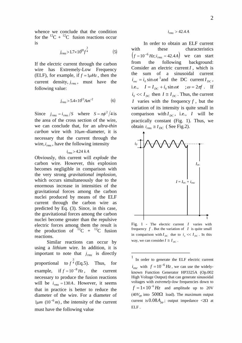
2
whence we conclude that the condition for the 12C + 12C fusion reactions occur is
( )5107.1 43
18 fjrms ×> If the electric current through the carbon wire has Extremely-Low Frequency (ELF), for example, if Hzf μ1= , then the current density, , must have the following value:
rmsj
( )6.104.5 213 −×> mAjrms
Since Sij rmsrms = where 42πφ=S is the area of the cross section of the wire, we can conclude that, for an ultra-thin carbon wire with mμ10 -diameter, it is necessary that the current through the wire, , have the following intensity rmsi
Akirms 24.4>Obviously, this current will explode the carbon wire. However, this explosion becomes negligible in comparison with the very strong gravitational implosion, which occurs simultaneously due to the enormous increase in intensities of the gravitational forces among the carbon nuclei produced by means of the ELF current through the carbon wire as predicted by Eq. (3). Since, in this case, the gravitational forces among the carbon nuclei become greater than the repulsive electric forces among them the result is the production of 12C + 12C fusion reactions. Similar reactions can occur by using a lithium wire. In addition, it is important to note that is directly
proportional to
rmsj
43
f (Eq.5). Thus, for example, if , the current necessary to produce the fusion reactions will be . However, it seems that in practice is better to reduce the diameter of the wire. For a diameter of
, the intensity of the current must have the following value
Hzf 810−=
Airms 130=
)10(1 6 mm −μ
Airms 4.42> In order to obtain an ELF current with these characteristics ( )AiHzf rms 4.42;10 6 == − we can start from the following background: Consider an electric current I , which is the sum of a sinusoidal current
tiiosc ωsin0= 1and the DC current , i.e.,
DCItiII DC ωsin0+= ; fπω 2= . If
DCIi <<0 then DCII ≅ . Thus, the current I varies with the frequency , but the variation of its intensity is quite small in comparison with , i.e.,
f
DCI I will be practically constant (Fig. 1). Thus, we obtain DCrms Ii ≅ ( See Fig.2). Fig. 1 - The electric current I varies withfrequency f . But the variation of I is quite small in comparison with DCI due to DCo Ii << . In this way, we can consider DCII ≅ .
t
IDC
I = IDC + iosc
i0
1 In order to generate the ELF electric current
with , we can use the widely-known Function Generator HP3325A (Op.002 High Voltage Output) that can generate sinusoidal voltages with extremely-low frequencies down to
and amplitude up to 20V (40V
osci Hzf 610−=
Hzf 6101 −×=pp into Ω500 load). The maximum output
current is ; output impedance <2Ω at ELF .
ppA.080

3
Fig. 2 – Electrical Circuit
+ −
Ultra thin wire
DCrms Ii ≅
R
2ε osci
DCI
oscDC iII +=
Hzf μ1= ~
REFERENCES [1] DeAquino, F. (2002). Mathematical Foundations of the Relativistic Theory of Quantum Gravity. Physics/0212033. [2] De Aquino, F. (2007) Gravity Control by means of Electromagnetic Field through Gas at Ultra-Low Pressure. Physics/0701091.

High-power ELF radiation generated by modulated HF heating of the ionosphere can cause Earthquakes, Cyclones and localized heating
Fran De Aquino
Maranhao State University, Physics Department, S.Luis/MA, Brazil. Copyright © 2011 by Fran De Aquino. All Rights Reserved
The High Frequency Active Auroral Research Program (HAARP) is currently the most important facility used to generate extremely low frequency (ELF) electromagnetic radiation in the ionosphere. In order to produce this ELF radiation the HAARP transmitter radiates a strong beam of high-frequency (HF) waves modulated at ELF. This HF heating modulates the electrons’ temperature in the D region ionosphere and leads to modulated conductivity and a time-varying current which then radiates at the modulation frequency. Recently, the HAARP HF transmitter operated with 3.6GW of effective radiated power modulated at frequency of 2.5Hz. It is shown that high-power ELF radiation generated by HF ionospheric heaters, such as the current HAARP heater, can cause Earthquakes, Cyclones and strong localized heating. . Key words: Physics of the ionosphere, radiation processes, Earthquakes, Tsunamis, Storms. PACS: 94.20.-y ; 94.05.Dd ; 91.30.Px ; 91.30.Nw; 92.60.Qx
1. Introduction Generating electromagnetic radiation at extremely-low frequencies is difficult because the long wavelengths require long antennas, extending for hundreds of kilometers. Natural ionospheric currents provide such an antenna if they can be modulated at the desired frequency [1-6]. The generation of ELF electromagnetic radiation by modulated heating of the ionosphere has been the subject matter of numerous papers [7-13]. In 1974, it was shown that ionospheric heater can generate ELF waves by heating the ionosphere with high-frequency (HF) radiation in the megahertz range [7]. This heating modulates the electron’s temperature in the D region ionosphere, leading to modulated conductivity and a time-varying current, which then radiates at the modulation frequency. Several HF ionospheric heaters have been built in the course of the latest decades in order to study the ELF waves produced by the heating of the ionosphere with HF radiation. Currently, the HAARP heater is the most powerful ionospheric heater, with 3.6GW of effective power using HF heating beam, modulated at ELF (2.5Hz) [14, 15]. This paper shows that high-power ELF
radiation generated by modulated HF heating of the lower ionosphere, such as that produced by the current HAARP heater, can cause Earthquakes, Cyclones and strong localized heating. 2. Gravitational Shielding The contemporary greatest challenge of the Theoretical Physics was to prove that, Gravity is a quantum phenomenon. Since General Relativity describes gravity as related to the curvature of space-time then, the quantization of the gravity implies the quantization of the proper space-time. Until the end of the century XX, several attempts to quantize gravity were made. However, all of them resulted fruitless [16, 17]. In the beginning of this century, it was clearly noticed that there was something unsatisfactory about the whole notion of quantization and that the quantization process had many ambiguities. Then, a new approach has been proposed starting from the generalization of the action function*. The result has been the derivation of a theoretical background, which finally led to the so-sought quantization of the gravity and of the * The formulation of the action in Classical Mechanics extends to Quantum Mechanics and has been the basis for the development of the Strings Theory.

2space-time. Published with the title “Mathematical Foundations of the Relativistic Theory of Quantum Gravity”[18], this theory predicts a consistent unification of Gravity with Electromagnetism. It shows that the strong equivalence principle is reaffirmed and, consequently, Einstein’s equations are preserved. In fact, Einstein’s equations can be deduced directly from the mentioned theory. This shows, therefore, that the General Relativity is a particularization of this new theory, just as Newton’s theory is a particular case of the General Relativity. Besides, it was deduced from the new theory an important correlation between the gravitational mass and the inertial mass, which shows that the gravitational mass of a particle can be decreased and even made negative, independently of its inertial mass, i.e., while the gravitational mass is progressively reduced, the inertial mass does not vary. This is highly relevant because it means that the weight of a body can also be reduced and even inverted in certain circumstances, since Newton’s gravity law defines the weight P of a body as the product of its gravitational mass by the local gravity acceleration , i.e.,
gmg
( )1gmP g=
It arises from the mentioned law that the gravity acceleration (or simply the gravity) produced by a body with gravitational mass
is given by gM
( )22rGM
g g=
The physical property of mass has two distinct aspects: gravitational mass mg and inertial mass mi. The gravitational mass produces and responds to gravitational fields; it supplies the mass factor in Newton's famous inverse-square law of gravity ( )2rmGMF gg= . The inertial mass is the mass factor in Newton's 2nd Law of Motion . These two masses are not
equivalent but correlated by means of the following factor [
( amF i= )
18]:
( )311212
00 ⎪⎭
⎪⎬⎫
⎪⎩
⎪⎨⎧
⎥⎥
⎦
⎤
⎢⎢
⎣
⎡−⎟⎟
⎠
⎞⎜⎜⎝
⎛ Δ+−=
cmp
mm
ii
g
Where is the rest inertial mass and 0im pΔ is the variation in the particle’s kinetic momentum; c is the speed of light. This equation shows that only for
0=Δp the gravitational mass is equal to the inertial mass. Instances in which pΔ is produced by electromagnetic radiation, Eq. (3) can be rewritten as follows [18]:
( )411212
3
2
0 ⎪⎭
⎪⎬
⎫
⎪⎩
⎪⎨
⎧
⎥⎥⎥
⎦
⎤
⎢⎢⎢
⎣
⎡−⎟
⎟⎠
⎞⎜⎜⎝
⎛+−=
cDn
mm r
i
g
ρ
Where is the refraction index of the particle; is the power density of the electromagnetic radiation absorbed by the particle; and
rnD
ρ , its density of inertial mass. From electrodynamics we know that
( )( )5
112
2⎟⎠⎞⎜
⎝⎛ ++
===
ωεσμεκ
ω
rrr
cdtdzv
where is the real part of the propagation vector
rkkr
(also called phase constant ); ir ikkkk +==
r ; ε , μ and σ, are
the electromagnetic characteristics of the medium in which the incident radiation is propagating ( 0εεε r= ; ; mF /10854.8 12
0−×=ε
0μμμ r= , where ). m/H70 104 −×= πμ
From (5), we see that the index of refraction vcnr = , for ωεσ >> , is given by
( )64 0επ
σμf
n rr =
Substitution of Eq. (6) into Eq. (4) yields

3
( )714
1212
0 ⎪⎭
⎪⎬
⎫
⎪⎩
⎪⎨
⎧
⎥⎥⎥
⎦
⎤
⎢⎢⎢
⎣
⎡−⎟
⎟⎠
⎞⎜⎜⎝
⎛+−==
cfD
m
m
i
g
πρμσχ
It was shown that there is an additional effect - Gravitational Shielding effect - produced by a substance whose gravitational mass was reduced or made negative [18]. This effect shows that just beyond the substance the gravity acceleration will be reduced at the same proportion
1g01 ig mm=χ ,
i.e., gg11 χ= , ( is the gravity acceleration
before the substance). Consequently, after a second gravitational shielding, the gravity will be given by
g
ggg21122 χχχ == , where
2χ is the value of the ratio 0ig mm for the second gravitational shielding. In a generalized way, we can write that after the nth gravitational shielding the gravity, , will be given by
ng
gg
nn χχχχ ...321
=
The dependence of the shielding effect on the height, at which the samples are placed above a superconducting disk with radius , has been recently measured up to a height of about 3m [
mrD 1375.0=19].
This means that the gravitational shielding effect extends, beyond the disk, for approximately 20 times the disk radius. 3. Gravitational Shieldings in the Van Allen belts The Van Allen belts are torus of plasma around Earth, which are held in place by Earth's magnetic field (See Fig.1). The existence of the belts was confirmed by the Explorer 1 and Explorer 3 missions in early 1958, under Dr James Van Allen at the University of Iowa. The term Van Allen belts refers specifically to the radiation belts surrounding Earth; however, similar radiation belts have been discovered around other planets. Now consider the ionospheric heating with HF beam, modulated at ELF (See Fig. 2). The amplitude-modulated HF heating
Fig.1 – Van Allen belts
Inner belt
Outer belt
Magnetic axis
Earth
Van Allen belts
0 3600km 6600km
wave is absorbed by the ionospheric plasma, modulating the local conductivityσ . The current density 0Ej σ= radiates ELF electromagnetic waves that pass through the Van Allen belts producing two Gravitational Shieldings where the densities are minima, i.e., where they are approximately equal to density of the interplanetary medium near Earth. The quasi-vacuum of the interplanetary space might be thought of as beginning at an altitude of about 1000km above the Earth’s surface [20]. Thus, we can assume that the densities iρ and oρ respectively, at the first gravitational shielding Si (at the inner Van Allen belt) and at So (at the outer Van Allen belt) are
(density of the interplanetary medium near the Earth [
320 .108.0 −−×≅≅ mkgio ρρ21]).
The parallel conductivities,† i0σ and o0σ , respectively at Si and So, present values which lie between those for metallic conductors and those for semiconductors [20], i.e., mSoi /1~00 σσ ≅ . Thus, in these two Gravitational Shielding, according to Eq. (7), we have, respectively:
( )81101.41212
4
⎪⎭
⎪⎬
⎫
⎪⎩
⎪⎨
⎧
⎥⎥⎥
⎦
⎤
⎢⎢⎢
⎣
⎡−⎟
⎟⎠
⎞⎜⎜⎝
⎛×+−=
fDi
iχ
† Conductivity in presence of the Earth’s magnetic field

4 Fig. 2 – Ionospheric Gravitational Shieldings - The amplitude-modulated HF heating wave is absorbed by the ionospheric plasma, modulating the local conductivity 0σ . The current density 00 Ej σ= (E0 is the Electrojet Electric Field), radiates ELF electromagnetic waves (d is the length of the ELF dipole). Two gravitational shieldings(So and Si) are formed at the Van Allen belts. Then, the gravity due to the Sun, after the shielding Si, becomes g’sun
=χoχi gsun. The effect of the gravitational shielding reaches kmdrD 000,110~20~ ≅×=× .
100km
60km
D
E
So
ELF – modulated HF heating radiation
d ~ 100km
mair g’sun
~10× d ~1,000km
σ
6,600 km
Outer Van Allen belt
Inner Van Allen belt 3,600 km Si
ELF radiation
g
30km3.7.0~ −mkgairρ
3.01.0 −< mkgairρ
Electrojet Electric Field, E0

5 and
( )91101.41212
4
⎪⎭
⎪⎬
⎫
⎪⎩
⎪⎨
⎧
⎥⎥⎥
⎦
⎤
⎢⎢⎢
⎣
⎡−⎟
⎟⎠
⎞⎜⎜⎝
⎛×+−=
fDo
oχ
where
( )10a
ELFoi S
PDD ≅≅
ELFP is the ELF radiation power, radiated from the ELF ionospheric antenna; is the area of the antenna.
aS
Substitution of (10) into (8) and (9) leads to
( )111101.4121
22
4
⎪⎭
⎪⎬
⎫
⎪⎩
⎪⎨
⎧
⎥⎥⎥
⎦
⎤
⎢⎢⎢
⎣
⎡−⎟
⎟⎠
⎞⎜⎜⎝
⎛×+−=
fSP
a
ELFioχχ
4. Effect of the gravitational shieldings Si and So on the Earth and its environment. Based on the Podkletnov experiment, previously mentioned, in which the effect of the Gravitational Shielding extends for approximately 20 times the disk radius ( )Dr , we can assume that the effect of the gravitational shielding Si extends for approximately 10 times the dipole length ( ). For a dipole length of about 100km, we can conclude that the effect of the gravitational shielding reaches about 1,000Km below S
d
i (See Fig.2), affecting therefore an air mass, , given by airm ‡
( )( ) ( )( )1210~
000,30000,100.7.0~14
23
kg
mmmkg
Vm airairair
==
==−
ρ
The gravitational potential energy related to , with respect to the Sun’s center, without the effects produced by the gravitational shieldings S
airm
o and Si is ( ) ( )130 sunseairp ggrmE −=
where, (distance from the mrse111049.1 ×=
‡ The mass of the air column above 30km height is negligible in comparison with the mass of the air column below 30km height, whose average density is ~0.7kg./m3.
Sun to Earth, 1 AU), and 2/8.9 smg =232 /1092.5 smrGMg sesunsun
−×=−= , is the gravity due to the Sun at the Earth. The gravitational potential energy related to , with respect to the Sun’s center, considering the effects produced by the gravitational shieldings S
airm
o and Si, is
( ) ( )14sunioseairp ggrmE χχ−=
Thus, the decrease in the gravitational potential energy is
( ) ( )1510 sunseairppp grmEEEioχχ−=−=Δ
Substitution of (11) into (15) gives
( )161101.41211
22
4sunseair
a
ELFp grm
fSPE
⎪⎪⎭
⎪⎪⎬
⎫
⎪⎪⎩
⎪⎪⎨
⎧
⎪⎭
⎪⎬
⎫
⎪⎩
⎪⎨
⎧
⎥⎥⎥
⎦
⎤
⎢⎢⎢
⎣
⎡−⎟
⎟⎠
⎞⎜⎜⎝
⎛×+−−=Δ
The HF power produced by the HAARP transmitter is GWPHF 6.3= modulated at Hzf 5.2= . The ELF conversion efficiency at HAARP is estimated to be
for wave generated using sinusoidal amplitude modulation. This means that
%10~ 4−
kWPELF 4~Substitution of , and kWPELF 4~ Hzf 5.2=
( ) 2102 101000,100 mSa ×== into (16) yields ( )1710~10~ 194 joulesgrmE sunseairp
−Δ
This decrease in the gravitational potential energy of the air column, , produces a
decrease pEΔ
pΔ in the local pressure p ( Bernoulli principle). Then the pressure equilibrium between the Earth’s mantle and the Earth’s atmosphere, in the region corresponding to the air column, is broken. This is equivalent to an increase of pressure pΔ in the region of the mantle corresponding to the air column. This phenomenon is similar to an Earthquake, which liberates an energy equal to (see Fig.3). pEΔ

6 Fig. 3 - The decrease in the gravitational potential energyof the air column, pEΔ , produces a decrease pΔ in the local pressure p (Principle of Bernoulli). Then the pressure equilibrium between the Earth’s mantle and theEarth’s atmosphere, in the region corresponding to the aircolumn, is broken. This is equivalent to an increase ofpressure pΔ in the region of the mantle corresponding tothe air column. This phenomenon is similar to anEarthquake, which liberates an amount of energy equal to
pEΔ .
Sun
Earth
Earth’s atmosphere
Air column
Core
Mantle
p pp Δ−
Curst
The magnitude in the Richter scales, corresponding to liberation of an amount of energy,
sM
joulesEp1910~Δ , is obtained
by means of the well-known equation: ( ) ( )181010 44.1519 sM+=
which gives . That is, an Earthquake with magnitude of about 9.1 in the Richter scales.
1.9=sM
The decrease in the gravitational potential energy in the air column whose mass is gives to the air column an initial
kinetic energy airm
pairairk EVmE Δ== 202
1 , where is given by (15). pEΔ
In the previously mentioned HAARP conditions, Eq.(11) gives . Thus, from (15), we obtain
( ) 410~1 −− ioχχ
( )1910~ 4sunseairp grmE −Δ
Thus, the initial air speed is airV0
( )20/400~/10~10 240 hkmsmrgV sesunair
−≅This velocity will strongly reduce the pressure in the air column (Bernoulli principle) and it is sufficient to produce a powerful Cyclone around the air column (Coriolis Effect).
Note that, by reducing the diameter of the HF beam radiation, it is possible to reduce dipole length (d) and consequently to reduce the reach of the Gravitational Shielding, since the effect of the gravitational shielding reaches approximately18 times the dipole length. By reducing d, we also reduce the area , increasing consequently the value of
aS
ioχχ (See Eq. (18)). This can cause an increase in the velocity (See Eq. (22)). airV0
On the other hand, if the dipole length (d) is increased, the reach of the Gravitational Shielding will also be increased. For example, by increasing the value of for d kmd 101= , the effect of the Gravitational Shielding reaches approximately , and can surpass the surface of the Earth or the Oceans (See Fig.2). In this case, the decrease in the gravitational potential energy at the local, by analogy to Eq.(15), is
km1010
( ) ( )211 sunsep grmEioχχ−=Δ
where is the mass of the soil, or the mass of the ocean water, according to the case.
m
The decrease, pEΔ , in the gravitational potential energy increases the kinetic energy of the local at the same ratio, in such way that the mass acquires a kinetic energy
mpk EE Δ= . If this energy is not enough
to pluck the mass from the soil or the ocean, and launch it into space, then is converted into heat, raising the local temperature by
mkE
TΔ , the value of which can be obtained from the following expression:
( )22TkNEk Δ≅
where is the number of atoms in the volume of the substance considered;
is the Boltzmann constant. Thus, we get
NV
KJk /1038.1 23−×=
( )( )
( )( )23
1
1
nk
gr
knV
grm
NkE
T
sunse
sunsek
io
io
ρχχ
χχ
−=
=−
=≅Δ
where is the number of atoms/mn 3 in the substance considered.

7 In the previously mentioned HAARP conditions, Eq. (11) gives ( ) 410~1 −− ioχχ . Thus, from (23), we obtain
( )24104.6 27ρ
nT ×≅Δ
For most liquid and solid substances the value of is about , and
. Therefore, in this case, Eq. (24) gives
n 328 /10 matoms33 /10~ mkgρ
CKT °≅≅Δ 400640This means that, the region in the soil or in the ocean will have its temperature increased by approximately 400°C. By increasing or decreasing the frequency, , of the ELF radiation, it is possible to increase
ELFPf
TΔ (See Eq.(16)). In this way, it is possible to produce strong localized heating on Land or on the Oceans. This process suggests that, by means of two small Gravitational Shieldings built with Gas or Plasma at ultra-low pressure, as shown in the processes of gravity control [22], it is possible to produce the same heating effects. Thus, for example, the water inside a container can be strongly heated when the container is placed below the mentioned Gravitational Shieldings. Let us now consider another source of ELF radiation, which can activate the Gravitational Shieldings So and Si. It is known that the Schumann resonances [23] are global electromagnetic resonances (a set of spectrum peaks in the extremely low frequency ELF), excited by lightning discharges in the spherical resonant cavity formed by the Earth’s surface and the inner edge of the ionosphere (60km from the Earth’s surface). The Earth–ionosphere waveguide behaves like a resonator at ELF frequencies and amplifies the spectral signals from lightning at the resonance frequencies. In the normal mode descriptions of Schumann resonances, the fundamental mode ( is a standing wave in the Earth–ionosphere cavity with a wavelength equal to the circumference of the Earth. This lowest-frequency (and highest-intensity) mode of the Schumann resonance occurs at a frequency
It was experimentally observed that ELF radiation escapes from the Earth–ionosphere waveguide and reaches the Van Allen belts [25-28]. In the ionospheric spherical cavity, the ELF radiation power density, D , is related to the energy density inside the cavity,W , by means of the well-known expression:
( )254
WcD =
where is the speed of light, and c2
021 EW ε= . The electric field E , is given by
204 ⊕
=r
qEπε
where Cq 000,500= [24] and . Therefore, we get
mr 610371.6 ×=⊕
( )26/1.4
,/104.5
,/7.110
2
38
mWD
mJW
mVE
≅
×=
=−
The area, , of the cross-section of the cavity is . Thus, the ELF radiation power is . The total power escaping from the Earth-ionosphere waveguide, , is only a fraction of this value and need to be determined.
S212
104.22 mdrS ×== ⊕π
WDSP 12108.9 ×≅=
escP
When this ELF radiation crosses the Van Allen belts the Gravitational Shieldings So and Si can be produced (See Fig.4). Fig.4 – ELF radiation escaping from the Earth–ionosphere waveguide can produce the Gravitational Shieldings So and Si in the Van Allen belts.
kmd 000,12610~ =× ⊕ Innercore
Outercore
Crust
Mantle
Earth
So
Si
⊕d
ELF radiation
Reach of the Gravitational Shielding
)1=n
Hzf 83.71 = [24]. The ELF radiation power densities and
, respectively in SiD
oD i and So, are given by

8( )27
4 2i
esci r
PDπ
=
and
( )284 2
o
esco r
PDπ
=
where and are respectively, the distances from the Earth’s center up to the Gravitational Shieldings S
ir or
i and So . Under these circumstances, the kinetic energy related to the mass, , of the Earth’s outer core
ocm§, with respect to the Sun’s
center, considering the effects produced by the Gravitational Shieldings So and Si ** is
( ) ( )291 221
ococsunseock VmgrmEio
=−= χχ
Thus, we get ( ) ( )301 sunseoc grV
ioχχ−=
The average radius of the outer core is mroc
6103.2 ×= . Then, assuming that the average angular speed of the outer core, ocϖ , has the same order of magnitude of the average angular speed of the Earth’s crust, ⊕ϖ , i.e., , then we get
sradoc /1029.7~ 5−⊕ ×=ϖϖ
smrV ocococ /10~ 2ϖ= . Thus, Eq. (30) gives
( ) ( )3110~1 5−−io
χχ
This relationship shows that, if the power of the ELF radiation escaping from the Earth-ionosphere waveguide is progressively increasing (for example, by the increasing of the dimensions of the holes in the Earth-ionosphere waveguide††), then as soon as the value of ioχχ equals 1, and the § The Earth is an oblate spheroid. It is composed of a number of different layers. An outer silicate solid crust, a highly viscous mantle, a liquid outer core that is much less viscous than the mantle, and a solid inner core. The outer core is made of liquid iron and nickel. ** Note that the reach of the Gravitational Shielding is . kmd 000,12610~ =× ⊕†† The amount of ELF radiation that escapes from the Earth-ionosphere waveguide is directly proportional to the number of holes in inner edge of the ionosphere and the dimensions of these holes. Thus, if the amount of holes or its dimensions are increasing, then the power of the ELF radiation escaping from the Earth-ionosphere waveguide will also be increased.
speed ocV will be null. After a time interval, the progressive increasing of the power density of the ELF radiation makes
ioχχ greater than 1. Equation (29) shows that, at this moment, the velocity resurges, but now in the opposite direction.
ocV
The Earth's magnetic field is generated by the outer core motion, i.e., the molten iron in the outer core is spinning with angular speed, ocϖ , and it's spinning inside the Sun’s magnetic field, so a magnetic field is generated in the molten core. This process is called dynamo effect. Since Eq. (31) tells us that the factor ( )
ioχχ−1 is currently very close to zero,
we can conclude that the moment of the reversion of the Earth’s magnetic field is very close. 5. Device for moving very heavy loads. Based on the phenomenon of reduction of local gravity related to the Gravitational Shieldings So and Si, it is possible to create a device for moving very heavy loads such as large monoliths, for example. Imagine a large monolith on the Earth’s surface. At noon the gravity acceleration upon the monolith is basically given by
sunR ggg −=
where 232 /1092.5 smrGMg sesunsun−×=−= is the
gravity due to the Sun at the monolith and . 2/8.9 smg=
If we place upon the monolith a mantle with a set of Gravitational Shieldings inside, the value of becomes
nRg
sunn
R ggg χ−=This shows that, it is possible to reduce down to values very close to zero, and thus to transport very heavy loads (See Fig.5). We will call the mentioned mantle of Gravitational Shielding Mantle. Figure 5 shows one of these mantles with a set of 8 Gravitational Shieldings. Since the mantle thickness must be thin, the option is to use Gravitational Shieldings produced by layers of high-dielectric strength semiconductor [
Rg
22]. When the Gravitational Shieldings are active the

9 (a) (b) Cross-section of the Mantle (c) Fig. 5 – Device for transporting very heavy loads. It is possible to transport very heavy loads by using a Gravitational Shielding Mantle - A Mantle with a set of 8 semiconductor layers or more (each layer with 10μm thickness, sandwiched by two metallic foils with 10μm thickness). The total thickness of the mantle (including the insulation layers) is ~1mm. The metallic foils are connected to the ends of an ELFvoltage source in order to generate ELF electromagnetic fields through the semiconductor layers. Theobjective is to create 8 Gravitational Shieldings as shown in (c). When the Gravitational Shieldings are activethe gravity due to the Sun is multiplied by the factor 8χ , in such way that the gravity resultant upon the
monoliths (a) and (b) becomes SunR ggg 8χ−= . Thus, for example, if 525.2−=χ results 2/028.0 smg R = .
Under these circumstances, the weight of the monolith becomes 3109.2 −× of the initial weight.
~
~ 1 mm
g
Sung8χ g
Sung8χ
Set of 8 Gravitational Shieldings inside the Mantle
ELFf
V
mμ10 mμ100dielectric metallic
foils
High-dielectric strength semiconductor
Mantle

10 gravity due to the Sun is multiplied by the factor , in such way that the gravity resultant
upon the monolith becomes . Thus, for example, if
8χ
SunR ggg 8χ−=525.2−=χ the result is
. Under these circumstances,
the weight of the monolith becomes of the initial weight.
2/028.0 smg R =3109.2 −×
6. Gates to the imaginary spacetime in the Earth-ionosphere waveguide. It is known that strong densities of electric charges can occur in some regions of the upper boundary of the Earth-ionosphere waveguide, for example, as a result of the lightning discharges [29]. These anomalies increase strongly the electric field in the mentioned regions, and possibly can produce a tunneling effect to the imaginary spacetime.
wE
The electric field will produce an electrons flux in a direction and an ions flux in an opposite direction. From the viewpoint of electric current, the ions flux can be considered as an “electrons” flux at the same direction of the real electrons flux. Thus, the current density through the air, , will be the double of the current density expressed by the well-known equation of Langmuir-Child
wE
wj
( )321033.2294
26
22023
23
23
rV
rV
rV
meje
r−×=== αεε
where 1≅rε for the air; is the called Child’s constant;
61033.2 −×=αr , in this case, is
the distance between the center of the charges and the Gravitational Shieldings and
(see Fig.6) (1wS 2wS
( ) mmr 161521 107104.1 −− ×=×= ); V is the
voltage drop given by
( )3322 00 AQrrrEV Q
w εεσ
===
where is the anomalous amount of charge in the region with area , i.e.,
QA
qAQQ ησσ == , η is the ratio of
proportionality, and 2102 /108.94 mCRqq−×≅= πσ
is the normal charge density ; is
the total charge[
Cq 000,500=
24], then nq qAQ ηση == ( qn Aq σ= is the normal amount of charge in the area ). A By substituting (33) into (32), we get
( )342
22222
23
23
23
02
02 ⎟⎟
⎠
⎞⎜⎜⎝
⎛=
⎟⎟⎠
⎞⎜⎜⎝
⎛
===A
Qrr
AQr
rVjjw ε
αεαα
Since 02εσQwE = and www Ej σ= , we can write that
( )
( )351014.2
18.018.018.0
222
5.516
5.50
5.1
5.53
5.50
5.1
5.53
5.55.50
5.1
5.53
0
3
0
34323
η
ε
ησα
ε
σα
ε
α
εεασ
×=
====
=⎥⎥⎥
⎦
⎤
⎢⎢⎢
⎣
⎡
⎟⎟⎠
⎞⎜⎜⎝
⎛==
rrAr
Q
AQ
AQ
rEjE
wwww
The electric field has an oscillating component, , with frequency, , equal to the lowest Schumann resonance frequency
wE
1wE f
Hzf 83.71 = . Then, by using Eq. (7), that can be rewritten in the following form [18]:
( )36110758.1121 32
4327
⎪⎭
⎪⎬⎫
⎪⎩
⎪⎨⎧
⎥⎥
⎦
⎤
⎢⎢
⎣
⎡−×+−== −
f
Em
m r
i
g
ρ
σμχ
we can write that
( )37110758.1121 31
2
41
327
⎪⎭
⎪⎬⎫
⎪⎩
⎪⎨⎧
⎥⎥⎦
⎤
⎢⎢⎣
⎡−×+−== −
fE
m
m
w
wwrw
i
gw ρ
σμχ
By substitution of Eq. (35), 1=rwμ , and into the
expression above, we obtain
32 /101 mkgw−×=ρ Hzf 83.71 =
( )3811084.7121 5.510
⎭⎬⎫
⎩⎨⎧
⎥⎦⎤
⎢⎣⎡ −×+−= − ηχw
The gravity below will be decreased by the effect of the Gravitational Shieldings and , according to the following expression
2wS
1wS 2wS
( )sunww gg 21χχ−
where www χχχ == 21 . Thus, we get
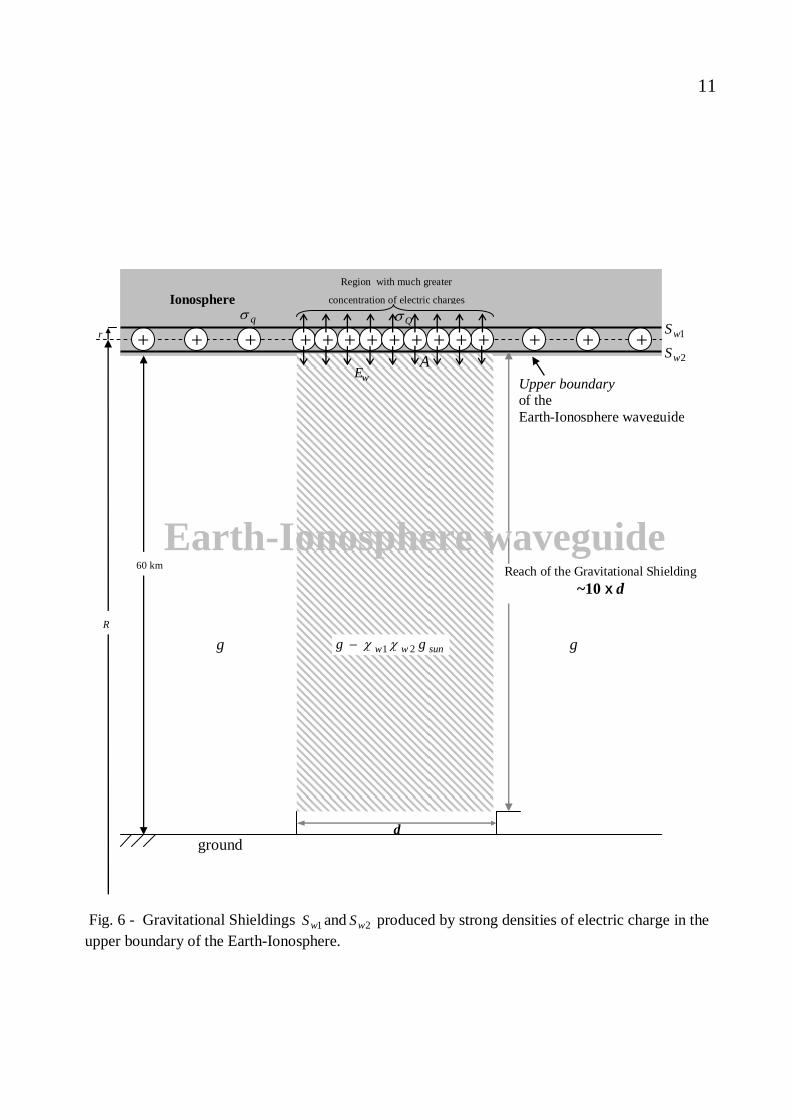
11 Fig. 6 - Gravitational Shieldings 1wS and 2wS produced by strong densities of electric charge in the upper boundary of the Earth-Ionosphere.
ground
+ + + + + + + + + + + + + + +
R
Region with much greater
concentration of electric chargesIonosphere
Upper boundary of the Earth-Ionosphere waveguide
r 1wS
2wS
d
Reach of the Gravitational Shielding~10 X d
60 km
Earth-Ionosphere waveguide
sunww gg 21χχ−g g
wE
Qσ
A
qσ

12
ggg
gsun χη =⎪⎭
⎪⎬⎫
⎪⎩
⎪⎨⎧
⎭⎬⎫
⎩⎨⎧
⎥⎦⎤
⎢⎣⎡ −×+−− −
25.510 11084.71211
where
( )3911084.712112
5.510
⎪⎭
⎪⎬⎫
⎪⎩
⎪⎨⎧
⎭⎬⎫
⎩⎨⎧
⎥⎦⎤
⎢⎣⎡ −×+−−= −
gg sunηχ
In a previous article [18], it was shown that, when the gravitational mass of a body is reduced to a value in the range of to or the local gravity
im159.0+
im159.0− ( )g is reduced to a value in the range of to , the body performs a transition to the imaginary spacetime. This means that, if the value of
g159.0+g159.0−
χ given by Eq.(39) is in the range 159.0159.0 −<< χ , then any body (aircrafts, ships, etc) that enters the region - defined by the volume ( )dA 10~× below the Gravitational Shielding , will perform a transition to the imaginary spacetime. Consequently, it will disappear from our Real Universe and will appear in the Imaginary Universe. However, the electric field , which reduces the gravitational mass of the body (or the gravitational shieldings, which reduce the local gravity) does not
2wS
1wE
accompany the body; they stay at the Real Universe. Consequently, the body returns immediately from the Imaginary Universe. Meanwhile, it is important to note that, in the case of collapse of the wavefunction of the body, it will never more come back to the Real Universe.
Ψ
Equation (39) shows that, in order to obtain χ in the range of 159.0159.0 −<<χ the value of η must be in the following range:
4.1351.127 << η Since the normal charge density is
then it must be increased by about 130 times in order to transform the region , below the Gravitational Shielding , in a gate to the imaginary spacetime.
210 /108.9 mCq−×≅σ
( dA 10~× )2wS
It is known that in the Earth's atmosphere occur transitorily large densities of electromagnetic energy across extensive areas. We have already seen how the density of electromagnetic energy affects the
gravitational mass (Eq. (4)). Now, it will be shown that it also affects the length of an object. Length contraction or Lorentz contraction is the physical phenomenon of a decrease in length detected by an observer of objects that travel at any non-zero velocity relative to that observer. If is the length of the object in its rest frame, then the length
, observed by an observer in relative motion with respect to the object, is given by
0L
L
( ) ( )401 220
0 cVLV
LL −==
γwhere is the relative velocity between the observer and the moving object and the speed of light. The function
Vc
( )Vγ is known as the Lorentz factor. It was shown that Eq. (3) can be written in the following form [18]:
⎪⎭
⎪⎬⎫
⎪⎩
⎪⎨⎧
⎥⎥
⎦
⎤
⎢⎢
⎣
⎡−
−−=
⎪⎭
⎪⎬
⎫
⎪⎩
⎪⎨
⎧
⎥⎥⎥
⎦
⎤
⎢⎢⎢
⎣
⎡−⎟⎟
⎠
⎞⎜⎜⎝
⎛ Δ+−= 1
1
121112122
2
00 cVcmp
mm
ii
g
This expression shows that
( ) ( )411
1122
2
0V
cVcmp
iγ=
−=⎟⎟
⎠
⎞⎜⎜⎝
⎛ Δ+
By substitution of Eq. (41) into Eq.(40) we get
( ) ( )42
12
0
00
⎟⎟⎠
⎞⎜⎜⎝
⎛ Δ+
==
cmp
LV
LL
i
γ
It was shown that, the term, cmp i0Δ , in the equation above is equal to 2cWn r ρ , where
is the density of electromagnetic energy absorbed by the body and the index of refraction, given by
Wrn
( ) ⎟⎠⎞⎜
⎝⎛ ++== 11
22ωεσ
με rrr v
cn
In the case of επσ f2>> , ( ) 28 EfW πσ= and
fcvcnr πμσ 42== [30]. Thus, in this case, Eq. (42) can be written as follows
( )43
10758.11 432
327
0
Ef
LLr
⎟⎟⎠
⎞⎜⎜⎝
⎛×+
=−
ρσμ

13Note that tEE m ωsin= .The average value for 2E is equal to 2
21
mE because E varies sinusoidaly ( is the maximum value
formE
E ). On the other hand, 2mrms EE = . Consequently we can change 4E by , and the equation above can be rewritten as follows
4rmsE
( )44
10758.11 432
327
0
rmsr E
f
LL
⎟⎟⎠
⎞⎜⎜⎝
⎛×+
=−
ρσμ
Now, consider an airplane traveling in a region of the atmosphere. Suddenly, along a distance of the trajectory of the airplane arises an ELF electric field with intensity
and frequency . The Aluminum density is and its conductivity is . According to Eq. (44), for the airplane the distance is shortened by . Under these conditions, a distance of about 3000km will become just 0.08km.
0L
15 .10~ −mVErms Hzf 1~33 .107.2 −×= mkgρ
17 .1082.3 −×= mSσ
0L 5107.2 −×
0L
Time dilation is an observed difference of elapsed time between two observers which are moving relative to each other, or being differently situated from nearby gravitational masses. This effect arises from the nature of space-time described by the theory of relativity. The expression for determining time dilation in special relativity is:
( )22
00
1 cV
TVTT−
== γ
where is the interval time measured at the object in its rest frame (known as the proper time);
0T
T is the time interval observed by an observer in relative motion with respect to the object. Based on Eq. (41), we can write the expression of T in the following form:
2
0022
0 11
⎟⎟⎠
⎞⎜⎜⎝
⎛ Δ+=
−=
cmpT
cV
TTi
For , we can write that and cV << Vmp i0=Δ
ϕϕ 2200
202
1 =⇒== VmgrmVm iii
where ϕ is the gravitational potential. Then, it follows that
22
22
0
22
0
22cc
Vcm
pandVm
p
ii
ϕϕ ==⎟⎟⎠
⎞⎜⎜⎝
⎛ Δ==⎟⎟
⎠
⎞⎜⎜⎝
⎛ Δ
Consequently, the expression of T becomes
20220 21
1 cT
cV
TT ϕ+=
−=
which is the well-known expression obtained in the General Relativity. Based on Eq. (41) we can also write the expression of T in the following form:
( )4510758.111 432
327
0
2
00 rms
r
iE
fT
cmpTT ⎟
⎟⎠
⎞⎜⎜⎝
⎛×+=⎟⎟
⎠
⎞⎜⎜⎝
⎛ Δ+= −
ρσμ
Now, consider a ship in the ocean. It is made of steel ( 300=rμ ; ;
). When subjected to a uniform ELF electromagnetic field, with intensity and frequency
16 .101.1 −×= mSσ33 .108.7 −×= mkgρ
13 .1036.1 −×= mVErms
Hzf 1= , the ship will perform a transition in time to a time T given by
( ) 460195574.1
10758.11
0
432
327
0
T
Ef
TT rmsr
=
=⎟⎟⎠
⎞⎜⎜⎝
⎛×+= −
ρσμ
( ) If shJanuaryT 0min00,19431,0 = then the ship performs a transition in time to shJanuaryT 0min00,19811,= . Note that the use of ELF ( )Hzf 1= is fundamental. It is important to note that the electromagnetic field , besides being uniform, must remain with the ship during the transition to the time
rmsE
T . If it is not uniform, each part of the ship will perform transitions for different times in the future. On the other hand, the field must remain with the ship, because, if it stays at the time , the transition is interrupted. In order to the electromagnetic field remains at the ship, it is necessary that all the parts, which are involved with the generation of the field, stay
0T

14inside the ship. If persons are inside the ship they will perform transitions for different times in the future because their conductivities and densities are different. Since the conductivity and density of the ship and of the persons are different, they will perform transitions to different times. This means that the ship and the persons must have the same characteristics, in order to perform transitions to the same time. Thus, in this way is unsuitable and highly dangerous to make transitions to the future with persons. However, there is a way to solve this problem. If we can control the gravitational mass of a body, in such way that 0ig mm χ= , and we put this body inside a ship with gravitational mass 0ig MM ≅ , then the total gravitational mass of the ship will be given by‡‡
( ) 00 iiggtotalg mMmMM χ+=+=
or ( ) ( )471
0
0
0 i
i
i
totalgship M
m
MM χ
χ +==
Since
⎪⎭
⎪⎬
⎫
⎪⎩
⎪⎨
⎧
⎥⎥⎥
⎦
⎤
⎢⎢⎢
⎣
⎡−⎟⎟
⎠
⎞⎜⎜⎝
⎛ Δ+−== 1121
2
00 cMp
MM
ii
gshipχ
we can write that
( )482
31
2
0
ship
i cMp χ−
=⎟⎟⎠
⎞⎜⎜⎝
⎛ Δ+
Then it follows that
( )492
31 0
2
00 ⎟⎟
⎠
⎞⎜⎜⎝
⎛ −=⎟⎟
⎠
⎞⎜⎜⎝
⎛ Δ+= ship
iT
cMpTT
χ
Substitution of Eq. (47) into Eq. (49) gives
( )502
10
00 ⎟⎟
⎠
⎞⎜⎜⎝
⎛−=
i
i
Mm
TTχ
Note that, if ( )000391148.0 ii mM−=χ , Eq. (50) gives
( )0195574.10TT =which is the same value given by Eq.(46). ‡‡ This idea was originally presented by the author in the paper: The Gravitational Spacecraft [30].
Other safe way to make transitions in the time is by means of flights with relativistic speeds, according to predicted by the equation:
( )511 22
0
cV
TT−±
=
With the advent of the Gravitational Spacecrafts [30], which could reach velocities close to the light speed, this possibility will become very promising. It was shown in a previous paper [18] that by varying the gravitational mass of the spacecraft for negative or positive we can go respectively to the past or future. If the gravitational mass of a particle is positive, then t is always positive and given by
( )521 220 cVtt −+=
This leads to the well-known relativistic prediction that the particle goes to the future if . However, if the gravitational mass of the particle is negative, then t is also negative and, therefore, given by
cV →
( )531 220 cVtt −−=
In this case, the prevision is that the particle goes to the past if . In this way, negative gravitational mass is the necessary condition to the particle to go to the past.
cV →
Now, consider a parallel plate capacitor, which has a high-dielectric strength semiconductor between its plates, with the following characteristics 1=rμ ; ;
. According to Eq.(45), when the semiconductor is subjected to a uniform ELF electromagnetic field, with intensity
14 .10 −= mSσ33 .10 −= mkgρ
( )mmKVmVErms /1.0.10 15 −= and frequency Hzf 1= , it should perform a transition in
time to a time T given by
( ) (5408434.1
10758.11
0
432
327
0
T
Ef
TT rmsr
=
=⎟⎟⎠
⎞⎜⎜⎝
⎛×+= −
ρ
σμ
)However, the transition is not performed, because the electromagnetic field is external to the semiconductor, and obviously would not accompany the semiconductor during the transition. In other words, the field stays at

15the time , and the transition is not performed.
0T
7. Detection of Earthquakes at the Very Early Stage When an earthquake occurs, energy radiates outwards in all directions. The energy travels through and around the earth as three types of seismic waves called primary, secondary, and surface waves (P-wave, S-wave and Surface-waves). All various types of earthquakes follow this pattern. At a given distance from the epicenter, first the P-waves arrive, then the S-waves, both of which have such small energies that they are mostly not threatening. Finally, the surface waves arrive with all of their damaging energies. It is predominantly the surface waves that we would notice as the earthquake. This knowledge, that, preceding any destructive earthquake, there are telltales P-waves, are used by the earthquake warning systems to reliably initiate an alarm before the arrival of the destructive waves. Unfortunately, the warning time of these earthquake warning systems is less than 60 seconds. Earthquakes are caused by the movement of tectonic plates. There are three types of motion: plates moving away from each other (at divergent boundaries); moving towards each other (at convergent boundaries) or sliding past one another (at transform boundaries). When these movements are interrupted by an obstacle (rocks, for example), an Earthquake occurs when the obstacle breaks (due to the sudden release of stored energy). The pressure P acting on the obstacle and the corresponding reaction modifies the gravitational mass of the matter along the pressing surfaces, according to the following expression [18]:
( )5512
121 0
2
32
2
ig mcv
Pm⎪⎭
⎪⎬
⎫
⎪⎩
⎪⎨
⎧
⎥⎥⎥
⎦
⎤
⎢⎢⎢
⎣
⎡−⎟
⎟⎠
⎞⎜⎜⎝
⎛+−=
ρ
where ρ and are respectively, the density of matter and the speed of the pressure waves in the mentioned region.
v
Hooke’s law tells us that , thus Eq. (55) can be rewritten as follows
2vP ρ=
( )5614
121 02 ig mcPm
⎪⎭
⎪⎬⎫
⎪⎩
⎪⎨⎧
⎥⎥⎦
⎤
⎢⎢⎣
⎡−+−=
ρ
or
( )5714
1212
0 ⎪⎭
⎪⎬⎫
⎪⎩
⎪⎨⎧
⎥⎥⎦
⎤
⎢⎢⎣
⎡−+−==
ρχ
cP
m
m
i
g
Thus, the matter subjected to the pressure P works as a Gravitational Shielding. Consequently, if the gravity below it is , then the gravity above it is
⊕g
⊕gχ , in
such way that a gravimeter on the Earth surface (See Fig.7) shall detect a gravity anomaly gΔ given by
( ) ( )581⊕⊕⊕
−=−=Δ gggg χχ
Substitution of Eq. (57) into this Eq. (58) yields
( )5914
122 ⊕
⎥⎥⎦
⎤
⎢⎢⎣
⎡−+=Δ g
cPgρ
Thus, when a gravity anomaly is detected, we can evaluate, by means of Eq. (59), the magnitude of the ratio ρP in the compressing region. On the other hand, several experimental observations of the time interval between the appearing of gravity anomaly gΔ and the breaking of the obstacle (beginning of the Earthquake) will give us a statistical value for the mentioned time interval, which will warn us (earthquake warning system) when to initiate an alarm. Obviously, the earthquake warning time, in this case becomes much greater than 60 seconds.

16
(a)
(b)
(c) Fig. 7 – Three main types of movements: (a) Divergent (tectonic plates diverge). (b) Convergent (plates converge). (c) Transform (plates slide past each other). Earthquakes occur when the obstaclebreaks (due to the sudden release of stored energy).
⊕g
( )⊕
−=Δ gg χ1
( )⊕
−=Δ gg χ1
⊕g
⊕g
⊕gχ
⊕gχ
( )⊕
−=Δ gg χ1
⊕gχ

17References [1] Rietveld, M. T. , Stubbe, P. and Kopka, H., (1987), On the frequency dependence of ELF/VLF waves produced by modulated ionospheric heating, Radio, Sci., J., 24, 270. [2] Papadopoulos, K., Sharma, A., and Chang, C. L.,(1989), On the efficient operation of the plasma antenna driven by modulation of ionospheric currents, Comments Plasma Phys. Control Fusion, 13, 1. [3] Ferraro et al., (1989) Measurements of extremely low frequency signals from modulation of the polar electrojet above Fairbanks, Alaska, IEEE Trans. Antennas Propag., 37, 802. [4] Papadopoulos, K., at al., (1990), On the efficiency of ionospheric ELF generation, Radio Sci., 25, 1311. [5] Mc Carrick, M. D. et al., (1990) Excitation of ELF waves in the Schuman resonance range by modulated HF heating of the polar electrojet, Radio Sci., 25, 1291. [6] Stubbe, P., and Kopka, H., (1977) Modulation of the polar electrojet by powerful HF waves, J. Geophys. Res., 82, 2319-2325. [7] Getmantsev, G.G., et al. (1974), Combination frequencies in the interaction between high-power short-wave radiation and ionospheric plasma, Sov. Phys. JETP, Engl. Trans., 20 , 229-232. [8] Tripathi, V. K., Chang. C. L., and Papadopoulos, K., (1982), Excitation of the Earth ionosphere waveguide by an ELF source in the ionosphere, Radio Sci, 17, 1321. [9] Barr, R., and Stubbe, P. (1984), ELF and VLF radiation from the “polar electrojet antenna”, Radio Sci.,19,1111. [10] Rietveld, M. T. , Koptka, H., and Stubbe, P. (1986), D- Region characteristics deduced from pulsed ionospheric heating under auroral electrojet conditions, J. Atmos. Terr. Phys., 48, 311. [11] Barr, R., and Stubbe, P. (1991), ELF radiation from the Tromso “super heater” facility, Geophys. Res. Lett., 18,1035. [12] Milikh, G.M., et al., (1999), ELF emission generated by the HAAARP HF heater using varying frequency and polarization, Radiophys. Quantum Electr., 42, 728-735. [13] Moore, R. C., et al., (2007) ELF waves generated by modulated HF heating of the auroral electrojet and observed at a ground distance of ~4400km, J. Geophys. Research, 112, A05309. [14] Jin, G., Spasojevic, and Inan, U. S., (2009), Relationship between electrojet current strength and ELF signal intensity in modulated heating experiments, J. Geophys, Res., 114, A08301, doi: 10.1029/2009JA014122. [15] Cohen, M. B., M. Golkowski, and U. S. Inan (2008), Orientation of the HAARP ELF ionospheric dipole and the auroral electrojet, Geophys. Res. Lett., 35, L02806, doi.10.1029/2007GL032424. [16] Isham, C. J. (1975) Quantum Gravity, in Oxford Symposium, OUP.
[17] Isham, C.J., (1997) “Structural Problems Facing Quantum Gravity Theory’’, in M, Francaviglia, G, Longhi, L, Lusanna, and E, Sorace, eds., Proceedings of the 14 International Conference on General th
Relativity and Gravitation, 167-209,(World Scientific, Singapore, 1997). [18] De Aquino, F.(2010) Mathematical Foundations of the Relativistic Theory of Quantum Gravity, Pacific Journal of Science and Technology, 11(1), June 2010, pp.173-232. [19] Modanese, G., (1996), Updating the Theoretical Analysis of the Weak Gravitational Shielding Experiment, supr-con/9601001v2. [20] Van Allen, J. A., (1961), The Earth and Near Space, Bulletin of Atomic Scientists, Vol. 17, Nº5, p.218. [21] Martin, M., and Turychev, S.G., (2004), Measuring the Interplanetary Medium with a Solar Sail, Int. J. Mod. Phys.D13, 899-906. astro-ph/0308108v2. [22] De Aquino, F. (2010) Gravity Control by means of Electromagnetic Field through Gas at Ultra-Low Pressure, Pacific Journal of Science and Technology, 11(2) November 2010, pp.178-247, Physics/0701091. [23] Schumann W. O. (1952). "Über die strahlungslosen Eigenschwingungen einer leitenden Kugel, die von einer Luftschicht und einer Ionosphärenhülle umgeben ist". Zeitschrift und Naturfirschung 7a: 149–154 [24] Volland, H. (1995), Handbook of Atmospheric Electrodynamics, CRC Press, vol.I, Chapter11. [25] Carpenter, D. L., and T. R. Miller (1976), Ducted magnetospheric propagation of signals from the Siple, Antarctica, VLF transmitter, J. Geophys. Res., 81(16), 2692– 2700. [26] Helliwell, R. A., D. L. Carpenter, and T. R. Miller (1980), Power threshold for growth of coherent VLF signals in the magnetosphere, J. Geophys. Res., 85(A7), 3360– 3366. [27] Cohen, M. B., (2009), ELF/VLF Phased array generation via frequency-matched steering of a continuous HF ionospheric heating beam, PHD thesis, p.13. [28] Golkowski, M. et al., (2008), Magnetospheric amplification and emission triggering by ELF/VLF waves injected by the 3.6 MW HAARP ionospheric heater, J. Geophys. Res., 113 (A10201), doi:10.1029/2008JA013, 157.
[29] Cummer, S.A., (2000) Modeling Electromagnetic Propagation in the Earth-ionosphere Waveguide, IEEE Trans. Antennas Propag., Vol. 48, 9, p.1427. [30] De Aquino, F. (1998),The Gravitational Spacecraft, E. Spacecraft Journal, 27,pp.6-13. http://arxiv.org/abs/physics/9904018.

The Universal Quantum Fluid
Fran De Aquino Maranhao State University, Physics Department, S.Luis/MA, Brazil.
Copyright © 2011 by Fran De Aquino. All Rights Reserved The quantization of gravity showed that the matter is also quantized, and that there is an elementary quantum of matter, indivisible, whose mass is kg73109.3 −×± . This means that any body is formed by a whole number of these particles (quantization). It is shown here that these elementary quanta of matter should fill all the space in the Universe forming a Quantum Fluid continuous and stationary. In addition, it is also explained why the Michelson-Morley experiment was not able to detect this Universal Quantum Fluid. Key words: Quantum Fluids, Quantum Gravity, Quantum Cosmology PACS: 67.10.-j; 04.60.-m; 98.80.Qc
1. Introduction Until the end of the century XX, several attempts to quantize gravity were made. However, all of them resulted fruitless [1, 2]. In the beginning of this century, it was clearly noticed that there was something unsatisfactory about the whole notion of quantization and that the quantization process had many ambiguities. Then, a new approach has been proposed starting from the generalization of the action function*. The result has been the derivation of a theoretical background, which finally led to the so-sought quantization of gravity and of matter [3]. The quantization of matter shows that there is an elementary quantum of matter whose mass is kg73109.3 −×± . This means that there are no particles in the Universe with masses smaller than this, and that any body is formed by a whole number of these particles. Here, it will be shown that these elementary quanta of matter should fill all the space in the Universe, forming a quantum fluid continuous and stationary. In addition, it is also explained why the Michelson-Morley experiment found no evidence of the existence of the universal fluid [4]. A modified Michelson-Morley experiment is proposed in order to observe the displacement of the interference bands. 2. The Universal Quantum Fluid The quantization of gravity showed that the matter is also quantized, and that * The formulation of the action in Classical Mechanics extends to Quantum Mechanics and has been the basis for the development of the Strings Theory.
there is an elementary quantum of matter, indivisible, whose mass is kg73109.3 −×± [3]. Considering that the inertial mass of the Observable Universe is kgGHcMU
530
3 102 ≅= , and that its volume is
( ) 379303
4334 10 mHcRV UU ≅== ππ , where
is the Hubble constant, we can conclude that the number of these particles in the Observable Universe is
1180 1075.1 −−×= sH
( )( )110125
min0particles
mM
ni
UU ≅=
By dividing this number by , we get UV
( )2/10 346 mparticlesVn
U
U ≅
Obviously, the dimensions of the elementary quantum of matter depend on its state of compression. In free space, for example, its volume is UU nV . Consequently, its “radius” is mnR UU
153 10−≅ . If particles with diameter N φ fill all space of then . Thus, if
then the number of particles, with this diameter, necessary to fill all is
. Since the number of
31m 13 =φN
m1510−≅φ31m
particlesN 4510≅elementary quantum of matter in the Universe is 346 /10 mparticlesVn UU ≅ we can conclude that these particles fill all space in the Universe, forming a Quantum Fluid continuous and stationary, the density of which is
( ) ( )3/10 327min0 mkgV
mn
U
iUCUF
−≅=ρ
Note that this density is smaller than the

2density of the Intergalactic Medium ( )326 /10 mkgIGM
−≅ρ . The density of the Universal Quantum Fluid is clearly not uniform along the Universe, since it can be strongly compressed in several regions (galaxies, stars, blackholes, planets, etc). At the normal state (free space), the mentioned fluid is invisible. However, at supercompressed state, it can become visible by giving origin to the known matter, since matter, as we have seen, is quantized and consequently, formed by an integer number of elementary quantum of matter with mass . Inside the proton, for example, there are
(min0im )
( )45
min0 10≅= ipp mmn elementary quanta of matter at supercompressed state, with volume
pproton nV and “radius” mnR pp303 10−≅ .
Therefore, the solidification of the matter is just a transitory state of this Universal Quantum Fluid, which can turn back into the primitive state when the cohesion conditions disappear. Due to the cohesion state of the elementary quanta of matter in the Universal Quantum Fluid, any amount of linear momentum transferred to any elementary quantum of matter propagates totally to the neighboring and so on, in such way that, during the propagation of the momentum, the elementary quanta of matter do not move, in the same way as the intermediate spheres in Newton’s pendulum (the well-known device that demonstrates conservation of momentum and energy) [5, 6]. Thus, whether it is a photon that transfers its momentum to the elementary quanta of matter, then the momentum variation due to the incident photon is λhp =Δ , where λ is its wavelength. As we have seen, the diameter of the elementary quantum of matter is
. According to the Uncertainty Principle the variation can only be detected if . In order to satisfy this condition we must have . This means that momentum variations, in the elementary quanta of matter, caused by photons with wavelength cannot
be detected. That is to say that the propagation of these photons through the Universal Quantum Fluid is equivalent to its propagation in the free space. In practice, it works as if there was not the Universal Quantum Fluid. This conclusion is highly important, because it can easily explain why in the historical Michelson-Morley experiment there was no displacement of the interference bands namely because the wavelength of the light used in the Michelson-Morley experiment was fact that led Michelson to conclude that the hypothesis of a stationary ether was incorrect. Posteriorly, several experiments [
mx 1510−≈ΔpΔ
h≥ΔΔ xp
mx 14102 −≈Δ≤ πλ
m1410−>λ
m7105 −×=λ
7-13] have been carried out in order to check the Michelson-Morley experiment, but the results basically were the same obtained by Michelson. Thus, actually there was no displacement of the interference bands in the Michelson-Morley experiment because the wavelength used in the experiment was , which is a value clearly much greater than , and therefore, does not satisfy the condition
derived from the Uncertainty Principle. The substitution of light used in the Michelson-Morley experiment by radiation with is clearly impracticable. However, the Michelson-Morley experiment can be partially modified so as to yield the displacement of the interference bands. The idea is based on the generalized expression for the momentum obtained recently[
m7105 −×=λm1410−
mx 14102 −≈Δ≤ πλ
m1410−≤λ
3], which is given by ( )4VMp g=
where 221 cVmM gg −= is the relativistic
gravitational mass of the particle and V its velocity; the general expression of the correlation between the gravitational and inertial mass;
0ig mm χ=
χ is the correlation factor[3].Thus, we can write
( )511 22
022 cV
m
cV
m ig
−=
−
χ
Therefore, we get

3( )6ig MM χ=
The Relativistic Mechanics tells us that
( )72cUVp =
where is the total energy of the particle. This expression is valid for any velocity V of the particle, including
U
cV = . By comparing Eq. (7) with Eq. (4) we obtain
( )82cMU g=
It is a well-known experimental fact that ( )92 hfcM i =
Therefore, by substituting Eq. (9) and Eq. (6) into Eq. (4), gives
( )10λ
χ hcVp =
Note that this expression is valid for any velocity of the particle. In the particular case of , it reduces to
VcV =
( )11λ
χ hp =
By comparing Eq. (10) with Eq. (7), we obtain
( )12hfU χ=
Note that only for 1=χ Eq. (11) and Eq. (12) are reduced to the well=known expressions of DeBroglie ( )λhq = and Einstein ( ) . hfU = Equations (10) and (12) show, for example, that any real particle (material particles, real photons, etc) that penetrates a region (with density ρ , conductivityσ and relative permeability rμ ), where there is an electromagnetic field ( , will have its momentum
)BE,p and its energy U reduced by
the factor χ , where χ is given by[3]:
( )13110758.1121
1121
4432
327
2
00
⎪⎭
⎪⎬⎫
⎪⎩
⎪⎨⎧
⎥⎥
⎦
⎤
⎢⎢
⎣
⎡−⎟
⎟⎠
⎞⎜⎜⎝
⎛×+−=
=⎪⎭
⎪⎬
⎫
⎪⎩
⎪⎨
⎧
⎥⎥⎥
⎦
⎤
⎢⎢⎢
⎣
⎡−⎟⎟
⎠
⎞⎜⎜⎝
⎛ Δ+−==
−rms
r
ii
g
Bcf
cmp
mm
ρσμ
χ
where is the rms value of the magnetic field
rmsBB .
The remaining amount of momentum and energy, respectively given by
( )λ
χ hcV⎟⎠⎞
⎜⎝⎛−1 and ( ) hfχ−1 , are
transferred to the imaginary particle associated to the real particle† (material particles or real photons) that penetrated the mentioned region. It was previously shown that, when the gravitational mass of a particle is reduced to a range between iM1590.+ to , i.e., when
iM1590.−159.0<χ , it becomes
imaginary[3], i.e., the gravitational and the inertial masses of the particle becomes imaginary. Consequently, the particle disappears from our ordinary space-time. It goes to the Imaginary Universe. On the other hand, when the gravitational mass of the particle becomes greater than iM1590.+ , or less than , i.e., when
iM1590.−159.0>χ , the particle return to our
Universe. Figure 1 (a) clarifies the phenomenon of reduction of the momentum for 159.0>χ , and Figure 1 (b) shows the effect in the case of
159.0<χ . In this case, the particles become imaginary and, consequently, they go to the imaginary space-time when they penetrate the electric field E . However, the electric field E stays in the real space-time. Consequently, the particles return immediately to the real space-time in order to return soon after to the imaginary space-time, due to the action of the electric field E . Since the particles are moving at a direction, they appear and disappear while they are crossing the region, up to collide with the plate (See Fig.1) with a momentum,
λχ h
cVp m ⎟
⎠⎞
⎜⎝⎛= , in the case of a material
particle, and λ
χ hpr = in the case of a photon.
If this photon transfers its momentum to elementary quanta of matter ( )mx 1510−≈Δ , then the momentum variation due to the incident photon is λχ hp =Δ . According to the Uncertainty Principle the variation pΔ can only be detected if , i.e., if h≥ΔΔ xp
( )142 xΔ≤ χπλWe conclude, then, that the interaction between the light used in the Michelson- † As previously shown, there are imaginary particles associated to each real particle[3].

4Morley experiment ( )m7105 −×=λ and the Universal Quantum Fluid just can be detected, and to produce of the displacement of the interference bands, if
( )15108 7×≥χ In order to satisfy this condition in the Michelson-Morley experiment, we must modify the medium where the experiment is performed (for example substituting the air by low-pressure Mercury plasma), and apply through it an electromagnetic field with frequency . Under these conditions, according to Eq. (13), the value of
f
χ will be given by
( )16110758.1121 4432
327
⎪⎭
⎪⎬⎫
⎪⎩
⎪⎨⎧
⎥⎥
⎦
⎤
⎢⎢
⎣
⎡−⎟
⎟⎠
⎞⎜⎜⎝
⎛×+−= −
rmsr Bc
fρ
σμχ
If the low-pressure Mercury plasma is at and [
23 80106 −− =×= mNTorrP .. KT 15.318≅14], then the mass density, according to the
well-known Equation of State, is
( )17.10067.6 350 −−×≅= mkgZRTPM
ρ
where is the molecular mass of the Hg;
10 20060 −= molkgM ..
1≅Z is the compressibility factor for the Hg plasma;
is the gases universal constant.
1013148 −−= KmoljouleR ...
The electrical conductivity of the Hg plasma, under the mentioned conditions, has already been calculated [15], and is given by
( )18.419.3 1−≅ mSσBy substitution of the values of ρ and σ into Eq. (16) yields
( )191105471.11213
417
⎪⎭
⎪⎬⎫
⎪⎩
⎪⎨⎧
⎥⎥
⎦
⎤
⎢⎢
⎣
⎡−×+−=
f
Brmsχ
By comparing with (15), we get
( )2001037.03
4≥
fBrms
Thus, for , the ELF magnetic field must have the following intensity:
Hzf 1=
( )2132.0 TBrms ≥
This means that, if in the Michelson-Morley experiment the air is substituted by Hg
plasma at and , and an ELF magnetic field with frequency
Torr3106 −× K15.318Hzf 1=
and intensity is applied through this plasma (Fig. 2), then the displacement of the interference bands should appear.
TBrms 32.0≥
It is important to note that due to the Gravitational Shielding effect [3], the gravity above the magnetic field is given by
. This value, extends above the vacuum chamber for approximately 10 times its length. In order to eliminate this problem we can replace the ELF magnetic field,
28 .108.7 −×≥ smgχ
B , shown in Fig. 2, by two ELF magnetic fields, and , sharing the same frequency, . The field, , is placed vertically through the region of the experimental set-up. The field, , is also placed vertically, just above (See Fig. 3). Thus, the gravity above is given by
1B 2BHzf 1= 1B
2B
1B
2Bg21χχ where 111 ig mm=χ and
222 ig mm=χ are respectively, the correlation factors in the Gravitational Shieldings 1 and 2, produced by the ELF magnetic fields and , respectively. In order to become
1B 2Bgg =21χχ we must make
712 10811 ×−== χχ . According to Eq.
(19), this value can be obtained if and .
Note that the value of is less than the value of the Earth’s magnetic field ( ). However, this is not a problem because the steel of the vacuum chamber works as a magnetic shielding, isolating the magnetic fields inside the vacuum chamber.
( ) TBrms5
2 10331481522.5 −×= ( ) TBrms 32.01 =
( )2rmsB
TB 5106 −×≅⊕

5
(a) * There are a type of neutrino, called "ghost” neutrino, predicted by General Relativity, with zero massand zero momentum. In spite its momentum be zero, it is known that there are wave functions that describe these neutrinos and that prove that really they exist. (b) Fig. 1 –The correlation factor in the expression of the Momentum. (a) Shows themomentum for 159.0>χ . (b) Shows the effect when 159.0<χ . Note that in both cases, the material particles collide with the cowl with the momentum ( ) λχ h
m cVp = , and
the photons withλ
χ hpr = .
material particleimaginary particleassociated to the material particle
real photon
imaginary photonassociated to the
real photon
σρ ,, fE
159.0>χ
λχ h
cVp m ⎟
⎠⎞
⎜⎝⎛=
[ ]λ
χ hpi −= 1
λχ hpr =
[ ]λ
χ hcVpi ⎟⎠⎞
⎜⎝⎛−= 1
λh
cVpm ⎟⎠⎞
⎜⎝⎛≅
*0=ip
λhpr ≅
0=ip
material particleimaginary particleassociated to the material particle
real photon
imaginary photonassociated to the
real photon
σρ ,, fE
159.0<χ
λχ h
cVp m ⎟⎠⎞
⎜⎝⎛=
[ ]λ
χ hpi −= 1
λχ hpr =
[ ]λ
χ hcVpi ⎟⎠⎞
⎜⎝⎛−= 1
0=ip
0=ip
λhpr ≅
0=ip

6 Fig. 2 - The modified Michelson-Morley experiment. The air is substituted by Hg plasma at
Torr3106 −× and K15.318 , and an ELF magnetic field with frequency Hzf 1= and intensity TBrms 32.0≥ is applied through this plasma, then the displacement of the interference bands should
appear.
Hg Plasma ( Torr3106 −× , K15.318 )
Vacuum Pump
MovableMirror
FixedMirror
Beam splitter Compensator
Detector
Coherent Light source
Hg Plasma
Manometer
ELF magnetic Field
VacuumChamber
Hzf 1=TBrms 32.0≥
B

7
Fig. 3 – Cross-section of the vacuum chamber showing the magnetic fields 1B and 2B .
11
101 i
LN
B ⎟⎟⎠
⎞⎜⎜⎝
⎛= μ ; 2
2
202 i
LN
B ⎟⎟⎠
⎞⎜⎜⎝
⎛= μ
Steel
Vacuum Chamber
χ1
χ2
gg =21χχ
g
Wire
Region of the experimental set-up
B2
B1
N2
N1
L2
L1

8 References [1] Isham, C. J. (1975) Quantum Gravity, in Oxford Symposium, OUP. [2] Isham, C.J., (1997) “Structural Problems Facing Quantum Gravity Theory’’, in M, Francaviglia, G, Longhi, L, Lusanna, and E, Sorace, eds., Proceedings of the 14 International Conference on General th
Relativity and Gravitation, 167-209,(World Scientific, Singapore, 1997). [3] De Aquino, F. (2010) Mathematical Foundations of the Relativistic Theory of Quantum Gravity, Pacific Journal of Science and Technology, 11(1), pp.173-232. [4] Michelson, A. A., (1881) Am. J. Sci, 122, 120. [5] Hermann, F. and Schmälzle, P. (1981), Am. J. Phys.,49,761. [6] Lovett, D. R. et al (1988) Eur. J. Phys., 9, 323-328. [7] Morley. E. W. and Miller, D.C. (1905), Proceedings of the American Academy of Arts and Sciences XLI (12):321–8. [8] Tomaschek, R. (1924). "Über das Verhalten des Lichtes außerirdischer Lichtquellen". Annalen der Physik 378 (1): 105–126. doi:10.1002/and p.19243780107. http://gallica.bnf.fr/ark:/12148/bpt6k153753/f115. [9] Miller, Dayton C. (1925). "Ether-Drift Experiments at Mount Wilson". Proceedings of the National Academy of Sciences 11 (6): 306–314. doi:10.1073/pnas.11.6.306. http://www.pnas.org/content/11/6/306.full.pdf+html. [10] Kennedy, Roy J. (1926). "A Refinement of the Michelson-Morley Experiment". Proceedings of the National Academy of Sciences 12 (11): 621–629. [11] Illingworth, K. K. (1927). "A Repetition of the Michelson-Morley Experiment Using Kennedy's Refinement". Physical Review 30 (5): 692–696. doi:10.1103/PhysRev.30.692. [12] Joos, G. (1930). "Die Jenaer Wiederholung des Michelsonversuchs". Annalen der Physik 399 (4): 385– 407. doi:10.1002/andp.19303990402. [13] Miller, Dayton C. (1933). "The Ether-Drift Experiment and the Determination of the Absolute Motion of the Earth". Reviews of Modern Physics 5 (3): 203–242. [14] GE Technical Publications (2007), 80044 – F20T12/ C50/ECO, GE Ecolux ®T12. [15] De Aquino, F. (2010) Gravity Control by means of Electromagnetic Field through Gas at Ultra- Low Pressure, Pacific Journal of Science and Technology, 11(2) November 2010, pp.178-247, Physics/0701091.

The Gravitational Mass of a Charged Supercapacitor
Fran De Aquino Maranhao State University, Physics Department, S.Luis/MA, Brazil.
Copyright © 2011 by Fran De Aquino. All Rights Reserved Electric double-layer capacitors (EDLCs), also known as supercapacitors, electrochemical double layer capacitors, or ultracapacitors, are electrochemical capacitors that have an unusually high energy density when compared to common capacitors, typically on the order of thousands of times greater than a high capacity electrolytic capacitor. It is shown here that when an EDLC is fully charged its gravitational mass is considerably
eater than when it is discharged. gr Key words: Supercapacitors, Energy storage systems, Experimental tests of gravitational theories PACS: 88.80.fh; 84.60.Ve , 04.80.Cc
1. Introduction The electric double-layer capacitor effect was first noticed in 1957 by General Electric engineers experimenting with devices using porous carbon electrode [1]. It was believed that the energy was stored in the carbon pores and it exhibited "exceptionally high capacitance", although the mechanism was unknown at that time. General Electric did not immediately follow up on this work, and the modern version of the devices were eventually developed by researchers at Standard Oil of Ohio in 1966, after they accidentally re-discovered the effect while working on experimental fuel cell designs [2]. Their cell design used two layers of activated carbon separated by a thin porous insulator, and this basic mechanical design remains the basis of most electric double-layer capacitors to this day. An electric double-layer capacitor (EDLC), is known as supercapacitor, or ultracapacitor. Their energy density is typically hundreds of times greater than conventional electrolytic capacitors. They also have a much higher power density than batteries or fuel cells. As of 2011 EDLCs had a maximum working voltage of 5 volts and capacities of up to 5,000 farads [3]. Currently, the EDLCs are used for energy storage rather than as general-purpose circuit components. The EDLCs also have two metal plates, but they are coated with activated carbon immersed in an electrolyte, and separated by an intervening insulator, forming in this manner, the double-layer of
activated carbon inside the capacitor. During the charging process, ions from the electrolyte accumulate on the surface of each carbon-coated plate. Here it is shown that when an EDLC is fully charged its gravitational mass is considerably greater than when it is discharged. 2. Theory Consider the cross-section of an EDLC as shown in Fig. 1. The double-layer in the EDLCs is generally made of activated carbon immersed in an electrolyte whose conductivity is much less than carbon conductivity [4]. The result is that the conductivity of the double-layer becomes much less than the conductivity of the activated carbon and, in this way, the double-layer can withstand a low voltage, and no significant current flows through the activated carbon layers of an ELDC [3]. This means that they are similar to dielectrics with very low dielectric strength. Thus, due to the electrical charge stored in the activated carbon layers, each layer can be considered as a non-conducting plane of charge, with density of charge, Sq=σ , where is the area of the plates of the capacitor, and
S
CVq = is the amount of electrical charge stored in the activated carbon layers; is the capacity of the EDLC. Thus, according to the well-known expression of the electric field produced by a non-conducting plane of charge [
C
5], we can conclude that the electric field through the layers of activated carbon (See Fig.1) is given by
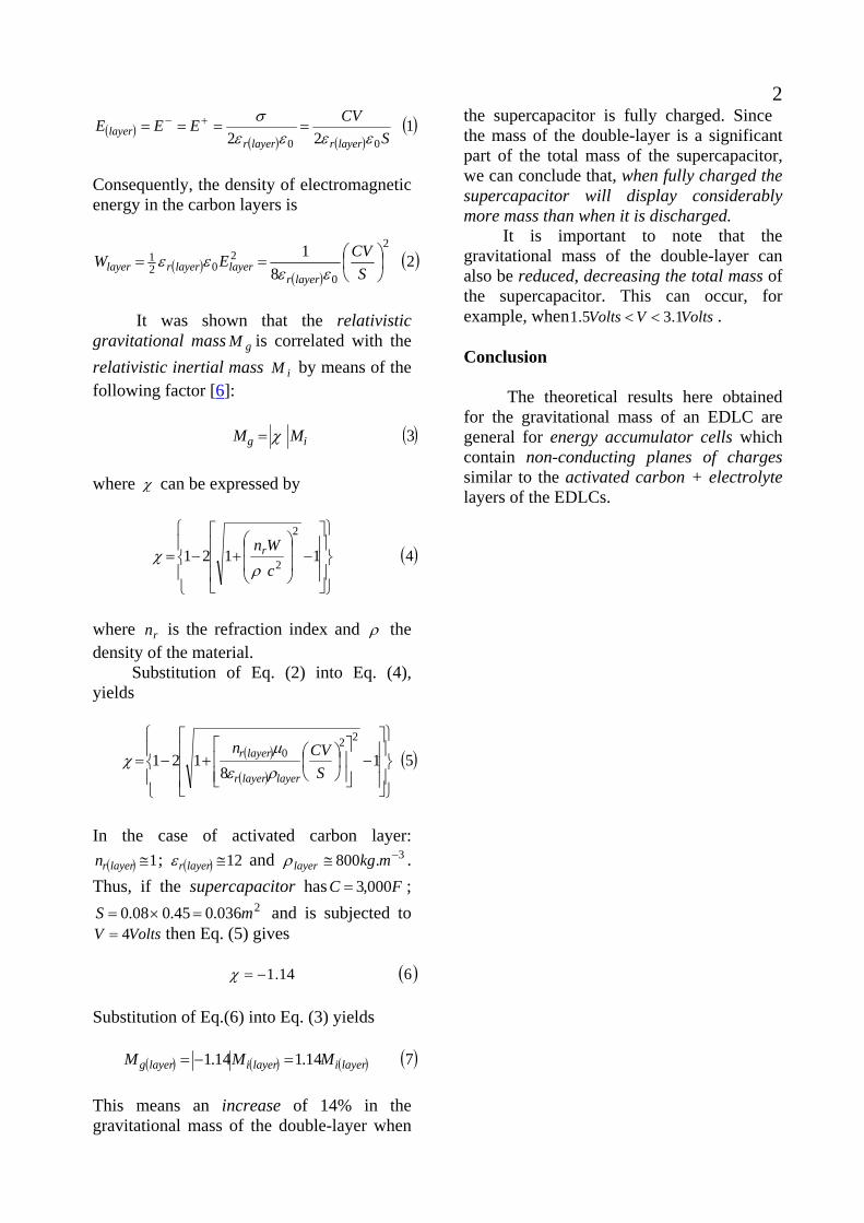
2
( )( ) ( )
( )122 00 S
CVEEElayerrlayerr
layer εεεεσ
==== +−
Consequently, the density of electromagnetic energy in the carbon layers is
( )( )
( )28
1 2
0
202
1 ⎟⎠⎞
⎜⎝⎛==
SCVEW
layerrlayerlayerrlayer εε
εε
It was shown that the relativistic gravitational mass is correlated with the relativistic inertial mass by means of the following factor [
gM
iM6]:
( )3ig MM χ=
where χ can be expressed by
( )41121
2
2⎪⎭
⎪⎬
⎫
⎪⎩
⎪⎨
⎧
⎥⎥⎥
⎦
⎤
⎢⎢⎢
⎣
⎡
−⎟⎟
⎠
⎞
⎜⎜
⎝
⎛+−=
cWnr
ρχ
where is the refraction index and rn ρ the density of the material. Substitution of Eq. (2) into Eq. (4), yields
( )
( )( )51
8121
220
⎪⎭
⎪⎬
⎫
⎪⎩
⎪⎨
⎧
⎥⎥⎥
⎦
⎤
⎢⎢⎢
⎣
⎡−
⎥⎥⎦
⎤
⎢⎢⎣
⎡⎟⎠⎞
⎜⎝⎛+−=
SCVn
layerlayerr
layerr
ρεμ
χ
In the case of activated carbon layer:
; ( ) 1≅layerrn ( ) 12≅layerrε and . Thus, if the supercapacitor has ;
and is subjected to then Eq. (5) gives
3.800 −≅ mkglayerρ
FC 000,3=2036.045.008.0 mS =×=
VoltsV 4=
( )614.1−=χ Substitution of Eq.(6) into Eq. (3) yields
( ) ( ) ( ) ( )714.114.1 layerilayerilayerg MMM =−=
This means an increase of 14% in the gravitational mass of the double-layer when
the supercapacitor is fully charged. Since the mass of the double-layer is a significant part of the total mass of the supercapacitor, we can conclude that, when fully charged the supercapacitor will display considerably more mass than when it is discharged. It is important to note that the gravitational mass of the double-layer can also be reduced, decreasing the total mass of the supercapacitor. This can occur, for example, when . VoltsVVolts 1.35.1 << Conclusion The theoretical results here obtained for the gravitational mass of an EDLC are general for energy accumulator cells which contain non-conducting planes of charges similar to the activated carbon + electrolyte layers of the EDLCs.

3
Fig. 1 – Cross-section of an Electric Double-Layer Capacitor (Supercapacitor) - Each activated carbon + electrolyte layer works as a non-conducting plane of charge, with density of charge
Sq−− =σ and Sq++ =σ respectively. The electric fields through the layers, due to these densities of charges ( )+− EE , , are shown in the figure above.
Electrode
+ −
d
−
−
− −
+
−
− −
−
−−
−
− −
−
−
−
−
−
−
−−
−
+
++
+
+
+
+
+
+
++
+ +
+
+ +
+ +
+
+
+ +
+E−E +E−E
Activated Carbon layer+
Electrolyte Insulator

4
References [1] Becker, H.I., (1957) Low voltage electrolytic capacitor, US Patent 2800616 (A), 1957-07-23. [2] Schindall, J. (2007) The Charge of the Ultra-Capacitors, IEEE Spectrum, November 2007. [3] Electric Double-Layer Capacitor http://en.wikipedia.org/ wiki / Electric_double-layer_capacitor [4] Miller, J. and Simon, P. (2008) Fundamentals of Electrochemical Capacitor Design and Operation, The Electrochemical Society Interface, Spring 2008. [5] Halliday, D. and Resnick, R. (1966) Physics, vol.2, John Wiley & Sons, NY. Portuguese version (1968) Física, Vol. 2, Ao Livro Técnico SA, Rio de Janeiro, Brasil, pp. 768-769. [6] De Aquino, F. (2010) Mathematical Foundations of the Relativistic Theory of Quantum Gravity, Pacific Journal of Science and Technology, 11(1), pp. 173-232.

Beyond the Material Universe
Fran De Aquino Maranhao State University, Physics Department, S.Luis/MA, Brazil.
Copyright © 2011 by Fran De Aquino. All Rights Reserved Science and Religion have always observed the events from their exclusive viewpoint. It was necessary the arising of a bond that would make possible the unification of them. This bond was revealed in the last decades by Quantum Physics, which has shown us that some physical laws extend beyond the material world, pointing to the existence of the spiritual world. Thus, the spiritual world exists now no longer as supernatural one, but as world as real as our material world. This discovery marked the beginning of the understanding of the spiritual world nature and its relationship with the material world. Starting from this knowledge, here widely detailed, it is now possible to understand the eternal puzzles: where have we come from, because here we are, and where do we go. Key words: Science, Religion, Spiritual World, Quantum Gravity, Quantum Cosmology, Quantum Consciousness. 1. Introduction The Spiritual World has always been considered something supernatural. Only recently, with the advent of Quantum Physics, the first evidences of its existence arose. However, it was the theoretical background derived from Quantum Gravity [1] that has shown that our Real Universe is contained in an Imaginary Universe. Here, the terms real and imaginary are borrowed from mathematics (real and imaginary numbers). In addition, it has been possible to show that the Imaginary Energy has the same characteristics of the Psychic Energy, that is, both are equivalent. This means that the Imaginary Universe is in fact the Psychic Universe. This discovery was the starting point for understanding the nature of the Spiritual World and beings it contains. It also made possible the acquisition of a strong knowledge about the relationship of the beings of the Spiritual World with us, and with our Material World. This knowledge, which leads us beyond the Material Universe, is widely detailed in this work. 2. The Psychic Energy It is known that the De Broglie waves are characterized by a variable quantity called the wave function, denoted by the symbolψ. While the frequencies of the De Broglie waves are determined by a simple form, the value of ψ is usually very complicated. The value of 2Ψ (or
*ΨΨ ) calculated for a particular point x, y, z, t is proportional to the probability of finding the particle experimentally in that place and time1. Thus, each particle has a particular wave function, which describes the particle fully. Roughly, it is similar to the "identity card" of the particle, containing all information about the particle or the body. Since is proportional to the probability of finding the particle described byΨ , the integral of on the whole space must be finite – inasmuch as the particle is someplace. Therefore, if
2Ψ P2Ψ
( )010V2 =Ψ∫+∞
∞−d
The interpretation is that the particle does not exist. However, if
1 Interpretation by Max Born in 1926.

2
( )02V2 ∞=Ψ∫+∞
∞−d
the particle will be everywhere simultaneously. Despite the fact that the De Broglie waves are normally associated to material particles and, in general associated to material bodies, it is known that they are also associated to exotic particles that cannot even be detected, such as a type of neutrinos called "ghost” neutrinos, predicted by General Relativity. These are called "ghost” neutrinos, because they have zero mass and zero momentum, and cannot be detected. But even so, it is known that there are wave functions that describe them, which means that they exist and can be present in any place. As a rough analogy, it is like a person who, despite of existing and possessing an identity card, is never seen by anyone. The existence of a wave function associated with the "ghost” neutrino is very important, because, in this context, we can conclude that even a thought may have a wave function associated with it. It is a proven quantum fact that the wave function Ψ may "collapse" and, in that instant, the possibilities that it describes, suddenly express themselves in reality. The moment of the "collapse" of the wave function is then a decision point where the pressing need of realization of the possibilities described by the wave function occurs. For an observer in our universe something is real when it is in the form of matter or radiation. Therefore, it can occur that the possibilities described by the wave function realize themselves in the form of radiation, i.e., they did not materialize. This obviously must occur when the energy that forms the content described by the wave function is not equal to the amount of energy needed for its materialization. Then consider any thought. A thought is a psychic body, with a well-defined psychic energy, and, as such, with a wave function of its own as any other psychic body. When its wave function collapses, two possibilities may occur: (a) the psychic energy contained in the thought is not sufficient to materialize its content - in this case, the collapse of the wave function is realized in the form of radiation: (b) the psychic energy is sufficient for its materialization - in this case, the collapse of the wave function content will be fully materialized. However, in both cases, there must always be production of "virtual" photons to communicate the psychic interaction to other bodies of the universe, because, according to the quantum theory, only through this type of quanta, can the interaction be communicated, since it has infinite range just in the same way as the electromagnetic interaction has, which we know is communicated by exchanging "virtual" photons. The term "virtual" derives from the principle of uncertainty due to the impossibility to detect these photons. This is a limitation imposed by Nature proper. It can be easily seen that this materialization process, although theoretically possible, requires enormous amounts of psychic energy, because, according to Einstein's famous equation E = mc , even a tiny object contains an enormous amount of energy. Moreover, one can 2
conclude that materializations of this type could only be produced by great consciousness with large psychic energy. In addition, it is evident, in this context, that the larger the amount of psychic energy of a consciousness the greater its chances of realization. This is a materialization process that can explain the materialization of the Primordial Universe. In addition, it becomes evident that the Psychic Energy is a type of mother-energy or Universal Fluid, which can produce anything. Since it is in the continuum 4-dimensional (space-time) that the realization of the wave functions which describe the psychic bodies occurs, then we can assume that they are generated in a continuum that, despite of containing all psychic forms, also interpenetrates the space-time continuum. Let us call it, hereafter, Psychic Continuum. By definition this continuum should also contain the Supreme Consciousness. Therefore, it should be infinite.

3
Then, from the above we can see that an accurate description of the universe cannot exclude the psychic energy, psychic particles and psychic bodies. That is, the situation calls for a cosmology that includes the psyche in the description of the Universe, thus complementing the traditional cosmology that is only a matter of cosmology. This idea is not new; it has existed for some time and seems to have arisen mainly in Princeton and Pasadena in the USA in the 70s [2] as a result of the joint effort of eminent physicists, biologists, psychologists and theologians as well. [3]. In traditional cosmology, the universe comes from a big bang where everything that exists would be concentrated in a tiny particle with the size of a proton and an enormous mass equal to the mass of the Universe at the instant before the Big Bang,. But its origin is not explained, nor the why of its critical volume. The critical volume, in our opinion denotes knowledge of what would happen from these initial conditions, a fact which points to the existence of a Creator. In this case, the materialization process described above would explain the materialization of the Primordial Universe. That is, the Primordial Universe arose at the exact moment that the primordial wave function collapsed (initial instant) realizating the contents of the psychic form generated in the consciousness of the Creator when He thought of creating the universe. The psychic form described by this primordial wave function must then have been generated in a consciousness with psychic energy much larger than that needed to materialize the Universe. This enormous consciousness in turn, not only would be the biggest of all consciences, but also would be the substratum of everything that exists, and obviously everything that exists would be wholly contained therein, including all space-time. Based on the General Theory of Relativity and the recent cosmological observations, it is known that the Universe occupies a space of positive curvature. This space, as we know, is "closed in itself", its volume is finite, but rest well understood, the space has no boundaries, it is unlimited. Thus, if the consciousness which we refer to contains all the space, its volume is necessarily infinite, and therefore contains an infinite psychic energy. This means that it contains all the psychic energy that exists and therefore, any other consciousness will be contained in it. Thus, we can conclude that it is the Supreme Consciousness, and there is no other like it: it is unique. In addition, since it contains all the psychic energy, it can accomplish everything that it wants, and therefore is omnipotent. Previously, we showed in the article "Physical Foundations of Quantum Psychology" the manifestation of knowledge, or auto-accessible knowledge in a consciousness, should be related to its quantity of psychic energy. In the Supreme Consciousness, whose psychic energy is infinite, the manifestation of the knowledge is total, thus, necessarily, it must be omniscient. Being omniscient, we cannot doubt its justice or goodness. Thus, God is supremely just and good. Moreover, as it also contains all the time, with past, present and future merging into it in an eternal present, so that the time will not flow as it does for us, in the four-dimensional continuum called space-time, as "we see" the future changing continuously into present and the present into past. Similarly, an observer in five-dimensional continuum would not have access to all time as the Supreme Consciousness, but his dimensional "vision" of the time would certainly be wider than that of the observer positioned in the four-dimensional continuum [3]. In this context, only the Supreme Consciousness would have a perfect "vision" of all dimensional levels. When we speak of creation of the universe, the use of the verb to create means that anything that was not came to be; assuming therefore, the concept of time flow. For the Supreme Consciousness however, the instant of the creation coincides with all the other times, not existing neither before nor after the creation, and in this way, questions like "What did the Supreme Consciousness do before creation?” are not justified.

4
We can also infer from the above that the existence of the Supreme Consciousness has no defined limit (beginning and end), which gives It the peculiar qualities of uncreated and eternal. Being eternal, its wave function ψ never collapses. Moreover, as it has infinite psychic energy, the value of ψ will also be infinite. In this way, according to Quantum Mechanics, it means that the Supreme Consciousness is simultaneously everywhere, or omnipresent. All conclusions presented here about the Supreme Consciousness were mathematically demonstrated in the article "Mathematical Foundations of the Relativistic Theory of Quantum Gravity" [1], and represent nothing more than a formal finding of what was already accepted by most religions. It is then justified the intuitive feeling that people have about the existence of God, and reveals that God is the Supreme Consciousness, the first cause of all things. Although we can understand this and, thus, learn that God is psychic energy, we can say nothing about the nature of psychic energy. Likewise, we do not know the nature of electric charge, etc. This is a limitation imposed by the Creator Himself. The option of the Supreme Consciousness in materializing the Primordial Universe into a critical volume, as we have seen, means that It knew what would happen from that initial condition. Therefore It also knew how the universe would behave under existing laws. Thus, the laws were not created for the Universe, and therefore are not "laws of Nature" or "laws that have been placed in Nature" as Descartes wrote. They already existed as an intrinsic part of the Supreme Consciousness; Thomas Aquinas had a very clear understanding about this. He speaks of the Eternal Law, "... those exist in the mind of God and rules the entire Universe." The Supreme Consciousness had then complete freedom to choose the initial conditions of the Universe. But opted for the concentration of the early Universe in the critical volume in order that its development should be performed in the most convenient way for the purposes It had in mind, according to laws inherent in its very nature. This responds to Einstein's famous question: "What level of choice would God have had to build the universe?" It seems that Newton was the first to realize the divine option. In his book Opticks, he gives us a perfect view of how he imagined the creation of the Universe: "It seems to me that God, at the beginning, first gave way to matter in solid particles, compacted [...] in such way that best contribute to the purpose He had in mind ..." For what purpose the Supreme Consciousness created the universe? This is a question that seems difficult to answer. However, if we assume the natural desire of the Supreme Consciousness of procreating, that is, of generating individual consciousness from itself so that they could evolve and express themselves creating attributes to Her, then, we can infer that in order to evolve, such consciousness would need a Universe, and this may have been the main reason for its creation. Thus, the origin of the Universe would be related to the generation of said consciousness and, consequently, the materialization of the Primordial Universe must have occurred at the same time at which the Supreme Consciousness decided to individualize the Primordial Consciousnesses. As the Supreme Consciousness occupies all the space, it follows that it cannot be displaced by another consciousness, and not for himself. Therefore, the Supreme Consciousness is immovable. As Augustine says (Gen. Ad lit vii, 20), "The Creator does not move either in time or space." The immobility of God had been deemed necessary also by Thomas Aquinas, "we can infer be necessary that the God who puts into motion all the objects, it is immovable." (Summa Theologica).

5
Due to fact that they were individualized directly from the Supreme Consciousness, the primordial consciousnesses certainly contained in themselves - albeit in a latent state, all the possibilities of the Supreme Consciousness, including the germ of independent will that allows the establishment of original points of departure. However, although similar to the Supreme Consciousness, the primordial consciousnesses could have no understanding of themselves. This understanding comes only with the creative mental state that the consciousnesses can only achieve by evolution. Thus, in the first evolutionary period, the primordial consciousnesses must have remained in complete unconsciousness. It was then, the beginning of a pilgrimage from unconsciousness to the superconsciousness. 3. The Good and the Evil Basically, in the Universe there are two types of radiation: the real radiation constituted by of real photon, and the “virtual” radiation constituted by "virtual" photons. Previously, we talked about the "virtual" quanta, which are responsible for the interaction among the psychic particles. According to the Uncertainty Principle, “virtual” quanta cannot be observed experimentally. However, since they are interaction quanta, their effects may be verified in the very particles or bodies subjected to the interactions. Obviously, only one specific type of interaction occurs between two particles if each one absorbs the quanta of said interaction emitted by the other; otherwise, the interaction will be null. Thus, the null interaction between psychic bodies particularly means that there is no mutual absorption of the “virtual” psychic photons (psychic interaction quanta) emitted by them. That is, the emission spectrum of each one of them does not coincide with the absorption spectrum of the other. It was shown that, in all interactions (gravitational, electromagnetic, strong nuclear and weak nuclear), the "virtual" quanta are "virtual" photons [1]. It is obvious, then, that an interaction between two particles only occurs if each of them absorbs the "virtual" photons emitted by the other, otherwise the interaction will be zero. Thus, the null interaction means specifically that the emission spectrum of each particle does not coincide with the absorption spectrum of the other. By analogy with material bodies, the emission spectra of which are, as we know, identical to the absorption spectra, also the psychic bodies must absorb radiation within the spectrum they emit. Specifically, in the case of human consciousness, their thoughts cause them to become emitters of psychic radiation in certain frequency spectra and, consequently, receivers in the same spectra. Thus, when a human consciousness, by its thoughts, is receptive to a radiation coming from a certain thought, said radiation will be absorbed by the consciousness (resonance absorption). Under these circumstances, the radiation absorbed must stimulate – through the Resonance Principle – said consciousness to emit in the same spectrum, just as it happens with matter. Nevertheless, in order for that emission to occur in a human consciousness, it must be preceded by the individualization of thoughts identical with that which originated the radiation absorbed, because obviously only identical thoughts will be able to reproduce - when they collapse - the spectrum of “virtual” psychic radiations absorbed. These induced thoughts – such as the thoughts of consciousnesses themselves – must remain individualized for a period of time tΔ (lifetime of the thought) after which its wave functions collapse, thus producing the “virtual” psychic radiation in the same spectrum of frequencies absorbed. The Supreme Consciousness, just as other consciousnesses, has Its own spectrum of absorption determined by Its thoughts – which make up the standard of a good-quality thought.

6
Thus, the concept of good-quality thoughts is immediately established. That is, they are resonant thoughts in the Supreme Consciousness. Thus, only thoughts of this kind, produced in human consciousnesses, may induce the individualization of similar thoughts in the Supreme Consciousness. In this context, a system of judgment is established in which the good and the evil are psychic values, with their origin in free thought. The good is related to the good-quality thoughts, which are thoughts resonant in the Supreme Consciousness. The evil, in turn, is related to the bad-quality thoughts, non-resonant in the Supreme Consciousness. Consequently, the moral derived thereof results from the Law itself, inherent in the Supreme Consciousness and, therefore, this psychic moral must be the fundamental moral. Thus, fundamental ethics is neither biological nor located in the aggressive action, as thought by Nietzsche. It is psychic and located in the good-quality thoughts. It has a theological basis and, in it, the creation of the Universe by a pre-existing God is of an essential nature, opposed, for instance, to Spinoza’s “geometrical ethics”, which eliminated the ideas of Creation of the Universe by a pre-existing God, the main underpinning of Christian theology and philosophy. However, it is very close to Aristotle’s ethics, to the extent that, from it, we understand that we are what we repeatedly do (think) and that excellence is not an act, but a habit (Ethics, II, 4). According to Aristotle: ‘” the goodness of a man is a work of the soul towards excellence in a complete lifetime: … it is not a day or a short period that makes a man fortunate and happy. “ (Ibid, I, 7). The “virtual” psychic radiation coming from a thought may induce several similar thoughts in the consciousness absorbing it, because each photon of radiation absorbed carries in itself the electromagnetic expression of the thought which produced it and, consequently, each one of them stimulates the individualization of a similar thought. However, the amount of thoughts induced is, of course, limited by the amount of psychic mass of the consciousness proper. In the specific case of the Supreme Consciousness, the “virtual” psychic radiation coming from a good-quality thought must induce many similar thoughts. On the other hand, since Supreme Consciousness involves human consciousness, the induced thoughts appear in the surroundings of the very consciousness which induced them. These thoughts are then strongly attracted by said consciousness and fuse therewith, for, just as the thoughts generated in a consciousness have a high degree of positive mutual affinity [4] with it, they will also have the thoughts induced by it. The fusion of these thoughts in the consciousness obviously determines an increase in its psychic mass. We then conclude that the cultivation of good-quality thoughts is highly beneficial to the individual. Reversally, the cultivation of bad-quality thoughts makes consciousness lose psychic mass. When bad-quality thoughts are generated in a consciousness, they do not induce identical thoughts in Supreme Consciousness, because the absorption spectrum of Supreme Consciousness excludes psychic radiations coming from bad-quality thoughts. Thus, such radiation directs itself to other consciousnesses; however, it will only induce identical thoughts in those that are receptive in the same frequency spectrum. When this happens and right after the wave functions corresponding to these induced thoughts collapse and materialize said thoughts or change them into radiation, the receptive consciousness will lose psychic mass, similarly to what happens in the consciousness which first produced the thought. Consequently, both the consciousness which gave rise to the bad-quality thought and those receptive to the psychic radiations coming from this type of thoughts will lose psychic mass. We must observe, however, that our thoughts are not limited only to harming or benefiting ourselves, since they also can, as we have already seen, induce similar thoughts in other consciousnesses, thus affecting them. In this case, it is important to observe that the

7
psychic radiation produced by the induced thoughts may return to the consciousness which initially produced the bad-quality thought, inducing other similar thoughts in it, which evidently cause more loss of psychic mass in said consciousness. The fact that our thoughts are not restricted to influencing ourselves is highly relevant, because it leads us to understand we have a great responsibility towards other persons as regards what we think. 4. The Psychic Universe When we studied elementary Mathematics, we learned the called Imaginary Numbers. Just as there are the real numbers and imaginary numbers, there are also the real space-time and imaginary time. In the article "Mathematical Foundations of the Relativistic Theory of Quantum Gravity", we showed that the former contains our Real Universe, and the latter contains the Imaginary Universe. We also saw how a material body can make a transition to the Imaginary Universe. Simply reducing its gravitational mass to the range iM1590.+ to . Under these circumstances, its gravitational and inertial masses become imaginaries, and therefore, the body becomes imaginary. Consequently, the body disappears from our ordinary space-time and resurges in the imaginary space-time like an imaginary body. In other words, it becomes invisible for persons in the Real Universe.
iM1590.−
What will an observer see when in the imaginary space-time? It will see light, bodies, planets, stars, etc., everything formed by imaginary photons, imaginary atoms, imaginary protons, imaginary neutrons and imaginary electrons. That is to say, the observer will find an Universe similar to ours, just formed by particles with imaginary masses. The term imaginary adopted from the Mathematics, as we already saw, gives the false impression that these masses do not exist. In order to avoid this misunderstanding we researched the true nature of that new mass type and matter. The existence of imaginary mass associated to the neutrino is well-known. Although its imaginary mass is not physically observable, its square is. This amount is found experimentally to be negative. Recently, it was shown [1] that quanta of imaginary mass exist associated to the photons, electrons, neutrons, and protons, and that these imaginary masses would have psychic properties (elementary capability of “choice”). Thus, the true nature of this new kind of mass and matter shall be psychic and, therefore we should not use the term imaginary any longer. Consequently, from the previously described, we can conclude that the gravitational spacecraft penetrates in the Psychic Universe and not in an “imaginary” Universe. In this Universe, the matter would be, obviously composed by psychic molecules and psychic atoms formed by psychic neutrons, psychic protons and psychic electrons. i.e., the matter would have psychic mass and consequently it would be subtle, much less dense than the matter of our real Universe. From the quantum viewpoint, the psychic particles are similar to the material particles, so that we can use the Quantum Mechanics to describe the psychic particles. In this case, by analogy to the material particles, a particle with psychic mass will be described by the following expressions:
Ψm
( )( )03
02
ψψ
ψψ
ωh
rh
r
=
=
E
kp
where is the momentum carried by the wave and its energy; Vmprr
Ψ=ψ ψE ψψ λπ2=kr
is
the propagation number and Vmh Ψ=ψλ the wavelength and ψψ πω f2= its cyclic
frequency. As we already have seen, the variable quantity that characterizes DeBroglie’s waves is called Wave Function, usually indicated byΨ .

8
The wave function Ψ corresponds, as we know, to the displacement of the undulatory motion of a rope. However, as opposed to , is not a measurable quantity and can, hence, be a complex quantity. For this reason, it is admitted that
yΨ y
Ψ is described in the x -direction by ( )( ) ( )042 pxEthiBe −−
=Ψπ
This equation is the mathematical description of the wave associated with a free material particle, with total energy E and momentum p , moving in the direction x+ . As concerns the psychic particle, the variable quantity characterizing psyche waves will also be called wave function, denoted by ΨΨ ( to differentiate it from the material particle wave function), and, by analogy with equation Eq. (04), expressed by:
( )( ) ( )0520
xptEhie ΨΨ −−Ψ Ψ=Ψ
π
If an experiment involves a large number of identical particles, all described by the same wave function , real density of mass Ψ ρ of these particles in x, y, z, t is proportional to the
corresponding value ( is known as density of probability. If 2Ψ 2Ψ Ψ is complex then . Thus, ). Similarly, in the case of psychic particles, the density
of psychic mass,
*ΨΨ=Ψ 2 *.ΨΨ=Ψ∝ 2ρ
Ψρ , in x, y, z, will be expressed by . It is known that is always real and positive while
*ΨΨΨΨ ΨΨ=Ψ∝ 2ρ
2ΨΨ VmΨΨ =ρ is an imaginary quantity. Thus, as the
modulus of an imaginary number is always real and positive, we can transform the proportion , in equality in the following form: 2
ΨΨ Ψ∝ρ( )062
ΨΨ =Ψ ρkWhere k is a proportionality constant (real and positive) to be determined. In Quantum Mechanics we have studied the Superposition Principle, which affirms that, if a particle (or system of particles) is in a dynamic state represented by a wave function and may also be in another dynamic state described by
1Ψ
2Ψ then, the general dynamic state of the particle may be described by Ψ , where Ψ is a linear combination (superposition) of and
, i.e., 1Ψ
2Ψ( )072211 Ψ+Ψ=Ψ cc
Complex constants e respectively indicate the percentage of dynamic state, represented by e in the formation of the general dynamic state described by
1c 2c
1Ψ 2Ψ Ψ . In the case of psychic particles (psychic bodies, consciousness, etc.), by analogy, if ,
,..., refer to the different dynamic states the psychic particle assume, then its general
dynamic state may be described by the wave function
1ΨΨ
2ΨΨ nΨΨ
ΨΨ , given by: ( )08...2211 nnccc ΨΨΨΨ Ψ++Ψ+Ψ=Ψ
The state of superposition of wave functions is, therefore, common for both psychic and material particles. In the case of material particles, it can be verified, for instance, when an electron changes from one orbit to another. Before effecting the transition to another energy level, the electron carries out “virtual transitions” [5]. A kind of relationship with other electrons before performing the real transition. During this relationship period, its wave function remains “scattered” by a wide region of the space [6] thus superposing the wave functions of the other electrons. In this relationship the electrons mutually influence each other, with the

9
possibility of intertwining their wave functions2. When this happens, there occurs the so-called Phase Relationship according to quantum-mechanics concept. In the electrons “virtual” transition mentioned before, the “listing” of all the possibilities of the electrons is described, as we know, by Schrödinger’s wave equation. Otherwise, it is general for material particles. By analogy, in the case of psychic particles, we may say that the “listing” of all the possibilities of the psyches involved in the relationship will be described by Schrödinger’s equation – for psychic case, i.e.,
( )0902
22 =Ψ+Ψ∇ Ψ
ΨΨ
h
p
Because the wave functions are capable of intertwining themselves, the quantum systems may “penetrate” each other, thus establishing an internal relationship where all of them are affected by the relationship, no longer being isolated systems but becoming an integrated part of a larger system. This type of internal relationship, which exists only in quantum systems, was called Relational Holism [7]. The idea of psyche associated with matter dates back to the pre-Socratic period and is usually called panpsychism. Remnants of organized panpsychism may be found in the Uno of Parmenides or in Heracleitus’s Divine Flux. Scholars of Miletus’s school were called hylozoists, that is, “those who believe that matter is alive”. More recently, we will find the panpsychistic thought in Spinoza, Whitehead and Teilhard de Chardin, among others. The latter one admitted the existence of proto-conscious properties at level of elementary particles. Generally, the people believe that there is some type of psyche associated to the animals, and some biologists agree that even very simple animals like the ameba and the sea anemone are endowed with psychism. This led several authors to consider the possibility of the psychic phenomena to be described in a theory based on Physics [8-11]. The fact that an electron carries out “virtual” transitions to several energetic levels before performing the real transition [5] clearly shows a “choice” made by the electron. Where there is “choice” isn’t there also psyche, by definition? An elementary psyche associated to the electron would be an entity very similar to the elementary electric charge associated to the electron, whose existence was necessary to postulate for the establishment of electromagnetic theory. However, the elementary psyche has unique characteristics. Being a discrete quantity (quantum) of the Supreme Consciousness, which is omniscient, it must also contain within it all knowledge. In the Supreme Consciousness, whose psychic energy is infinite, the manifestation of this knowledge is total. In the case of the elementary psyche, would be minimal by definition, remaining the rest of the knowledge in a latent state. But still this knowledge would be sufficient, for example, for electrons to define their orbital position (energy level) around the nuclei when they were electromagnetically attracted by the such nuclei. How else could they have the knowledge of the exact orbit to stay? The electrosphere of atoms is a complex and accurate structure, and in no way could have been created randomly. Its construction undoubtedly involves knowledge. Due to the fact that the formation of the electrosphere of the atoms is an organized process, the psyches of the electrons is also grouped in an organized manner, specifically in phase condensates, forming, what we can define as the Individual Consciousnesses of the atoms. Ice and NaCl crystals are common examples of imprecisely-structured phase condensates. Lasers, superfluids, superconductors, and magnets are examples of better-structured phase condensates. 2 Since the electrons are simultaneously waves and particles, their wave aspects will interfere with each other. Besides superposition, there is also the possibility of occurrence of intertwining of their wave functions.

10
If electrons, protons and neutrons have psychic mass, then we can infer that the psychic mass of the atoms are Phase Condensates. In the case of the molecules the situation is similar. More molecular mass means more atoms and consequently, more psychic mass. In this case the phase condensate also becomes more structured because the great amount of elementary psyches inside the condensate requires, by stability reasons, a better distribution of them. Thus, in the case of molecules with very large molecular masses (macromolecules) it is possible that their psychic masses already constitute the most organized shape of a Phase Condensate, called Bose-Einstein Condensate3. The fundamental characteristic of a Bose-Einstein condensate is, as we know, that the various parts making up the condensed system not only behave as a whole but also become a whole, i.e., in the psychic case, the various consciousnesses of the system become a single consciousness with psychic mass equal to the sum of the psychic masses of all the consciousness of the condensate. This obviously, increases the available knowledge in the system since it is proportional to the psychic mass of the consciousness. This unity confers an individual character to this type of consciousness. For this reason, from now on they will be called Individual Material Consciousness. It derives from the above that most bodies do not possess individual material consciousness. In an iron rod, for instance, the cluster of elementary psyches in the iron molecules does not constitute Bose-Einstein condensate; therefore, the iron rod does not have an individual consciousness. Its consciousness is consequently, much more simple and constitutes just a phase condensate imprecisely structured made by the consciousness of the iron atoms. The existence of consciousnesses in the atoms is revealed in the molecular formation, where atoms with strong mutual affinity (their consciousnesses) combine to form molecules. It is the case, for instance of the water molecules, in which two Hydrogen atoms join an Oxygen atom. Well, how come the combination between these atoms is always the same: the same grouping and the same invariable proportion? In the case of molecular combinations the phenomenon repeats itself. Thus, the chemical substances either mutually attract or repel themselves, carrying out specific motions for this reason. It is the so-called Chemical Affinity. This phenomenon certainly results from a specific interaction between the consciousnesses. From now on, it will be called Psychic Interaction. After the formation of the first planets, some of them came to develop favorable conditions for the appearance of macromolecules. These macromolecules, as we have shown, may have a special type of consciousness formed by a Bose-Einstein condensate (Individual Material Consciousness). In this case, since the molecular masses of the macromolecules are very large, they will have individual material consciousness of large psychic mass and, therefore, have access to a considerable amount of information in its own consciousness. Consequently, macromolecules with individual material consciousness are potentially very capable of, and some certainly already can carry out, autonomous motions, thus being considered as “living” entities. However, if we decompose one of these molecules so as to destroy its individual consciousness, its parts will no longer have access to the information which “instructed” said molecule and, hence, will not be able to carry out the autonomous motions it previously did. Thus, the “life” of the molecule disappears – as we can see, Delbrück’s Paradox is then solved4.
3 Several authors have suggested the possibility of the Bose-Einstein condensate occur in the brain, and that it might be the physical base of memory, although they have not been able to find a suitable mechanism to underpin such a hypothesis. Evidences of the existence of Bose-Einstein condensates in living tissues abound (Popp, F.A Experientia, Vol. 44, p.576-585; Inaba, H., New Scientist, May89, p.41; Rattermeyer, M and Popp, F. A. Naturwissenschaften, Vol.68, Nº5, p.577.) 4 This paradox ascribed to Max Delbrück (Delbrück, Max., (1978) Mind from Matter? American Scholar, 47. pp.339-53.) remained unsolved and was posed as follows: How come the same matter studied by Physics, when incorporated into a living organism, assumes an unexpected behavior, although not contradicting physical laws?
11
The appearance of “living” molecules in a planet marks the beginning of the most important evolutionary stage for the psyche of matter, for it is from the combination of these molecules that there appear living beings with individual material consciousness with even larger psychic masses. Biologists have shown that all living organisms existing on Earth come from two types of molecules – aminoacids and nucleotides – which make up the fundamental building blocks of living beings. That is, the nucleotides and aminoacids are identical in all living beings, whether they are bacteria, mollusks or men. There are twenty different species of aminoacids and five of nucleotides. In 1952, Stanley Miller and Harold Urey proved that aminoacids could be produced from inert chemical products present in the atmosphere and oceans in the first years of existence of the Earth. Later, in 1962, nucleotides were created in laboratory under similar conditions. Thus, it was proved that the molecular units making up the living beings could have formed during the Earth’s primitive history. Therefore, we can imagine what happened from the moment said molecules appeared. The concentration of aminoacids and nucleotides in the oceans gradually increased. After a long period of time, when the amount of nucleotides was already large enough, they began to group themselves by mutual psychic attraction, forming the molecules that in the future will become DNA molecules. When the molecular masses of these molecules became large enough, the distribution of elementary psyches in their consciousnesses took the most orderly possible form of phase condensate (Bose-Einstein condensate) and such consciousnesses became the individual material consciousness. Since the psychic mass of the consciousnesses of these molecules is very large (as compared with the psychic mass of the atoms), the amount of self-accessible knowledge in such consciousnesses became considerable and, thus, they became apt to instruct the joining of aminoacids in the formation of the first proteins (origin of the Genetic Code). Consequently, the DNA’s capability to serve as guide for the joining of aminoacids in the formation of proteins is fundamentally a result of their psychism. In the psychic of DNA molecules, the formation of proteins certainly had a definite objective: the construction of cells. During the cellular construction, the most important function played by the consciousnesses of the DNA molecules may have been that of organizing the distribution of the new molecules incorporated to the system so that the consciousnesses of these molecules jointly formed with the consciousness of the system a Bose-Einstein condensate. In this manner, more knowledge would be available to the system and, after the cell is completed, the latter would also have an individual material consciousness. Afterwards, under the action of psychic interaction, the cells began to group themselves according to different degrees of positive mutual affinity, in an organized manner so that the distribution of their consciousnesses would also form Bose-Einstein condensates. Hence, collective cell units began to appear with individual consciousnesses of larger psychic masses and, therefore, with access to more knowledge. With greater knowledge available, these groups of cells began to perform specialized functions to obtain food, assimilation, etc. That is when the first multi-celled beings appeared. Upon forming the tissues, the cells gather structurally together in an organized manner. Thus, the tissues and, hence, the organs and the organisms themselves also possess individual material consciousnesses. The existence of the material consciousness of the organisms is proved in a well-known experiment by Karl Lashley, a pioneer in neurophysiology.

12
Lashley initially taught guinea pigs to run through a maze, an ability they remember and keep in their memories in the same way as we acquire new skills. He then systematically removed small portions of the brain tissue of said guinea pigs. He thought that, if the guinea pigs still remembered how to run through the maze, the memory centers would still be intact. Little by little he removed the brain mass; the guinea pigs, curiously enough, kept remembering how to run through the maze. Finally, with more than90% of their cortex removed, the guinea pigs still kept remembering how to run through the maze. Well, as we have seen, the consciousness of an organism is formed by the concretion of all its cellular consciousnesses. Therefore, the removal of a portion of the organism cells does not make it disappear. Their cells, or better saying, the consciousnesses of their cells contribute to the formation of the consciousness of the organism just as the others, and it is exactly due to this fact that, even when we remove almost all of the guinea pigs’ cortex, they were still able to remember from the memories of their individual material consciousnesses. In this manner, what Lashley’s experiment proved was precisely the existence of individual material consciousnesses in the guinea pigs. Another proof of the existence of the individual material consciousnesses in organisms is given by the regeneration phenomenon, so frequent in animals of simple structure: sponges, isolated coelenterates, worms of various groups, mollusks, echinoderms and tunicates. The arthropods regenerate their pods. Lizards may regenerate only their tail after autotomy. Some starfish may regenerate so easily that a simple detached arm may, for example, give origin to a wholly new animal. The organization of the psychic parts in the composition of an organism’s individual material consciousness is directly related to the organization of the material parts of the organism, as we have already seen. Thus, due to this interrelationship between body and consciousness, any disturbance of a material (physiological) nature in the body of the being will affect its individual material consciousness, and any psychic disturbance imposed upon its consciousness affects the physiology of its body. When a consciousness is strongly affected to the extent of unmaking the Bose-Einstein’s condensate, which gives it the status of individual consciousness, there also occurs the simultaneous disappearance of the knowledge made accessible by said condensation. Therefore, when a cell’s consciousness no longer constitutes a Bose-Einstein condensate, there is also the simultaneous disappearance of the knowledge that instructs and maintains the cellular metabolism. Consequently, the cell no longer functions thus initiating its decomposition (molecular desegregation). Similarly, when the consciousness of an animal (or vegetables) no longer constitutes a Bose-Einstein condensate, the knowledge that instructs and maintains its body functioning also disappears, and it dies. In this process, after the unmaking of the being’s individual consciousness, there follows the unmaking of the individual consciousnesses of the organs; next will be the consciousnesses of their own cells which no longer exist. At the end there will remain the isolated psyches of the molecules and atoms. Death, indeed, destroys nothing, neither what makes up matter nor what makes up psyche. As we have seen, all the information available in the consciousnesses of the beings is also accessible by the consciousnesses of their organs up to their molecules’. Thus, when an individual undergoes a certain experience, the information concerning it not only is recorded somewhere in this consciousness but also pervades all the individual consciousnesses that make up its total consciousness. Consequently, psychic disturbances imposed to a being reflect up to the level of their individual molecular consciousnesses, perhaps even structurally affecting said molecules, due to the interrelationship between body and consciousness already mentioned here.
13
Therefore, some modifications in the sequences of nucleotides of the DNA molecules can occur when the psychism of the organism in which the molecules are incorporated is sufficiently affected. It is known that such modifications in the structure of DNA molecules may also occur as consequence of chemical products in the blood stream (as in the case of the mustard gas used in chemical warfare) or exposition to high-energy radiation. Modifications in the sequences of nucleotides in DNA molecules are called mutations. Mutations, as we know, determine hereditary variations, which are the basis of Darwin’s theory of evolution. It is known that mutations of two types, “favorable” or “unfavorable”, can occur. The former type enhances the individuals’ possibility of survival, whereas the second reduces such possibility. The theory of evolution is established as a consequence of individuals’ efforts to survive in the environment where they live. This means that their descendants may become different from their ancestors. This is the mechanism that leads to frequent appearance of new species. Darwin believed that the mutation process was slow and gradual. Nevertheless, it is known today that this is not the general rule, for there are evidences of the appearance of new species in a relatively short period of time [12]. We also know that individual’s characteristics are transmitted from parents to offsprings by means of genes and that the recombination of the parents’ genes, when genetic instructions are transmitted, by such genes. However, it was shown that the genetic instructions are basically associated with the psychism of DNA molecules. Consequently, the genes transmit not only physiological but also psychic differences. Thus, as a consequence of genetic transmission, besides the great physiological difference between individuals of the same species, there is also a great psychic dissimilarity. Such psychic dissimilarity associated with the progressive enhancement of the individual’s psychic quantities may have given rise, in immemorial time, to a variety of individuals (most probably among anthropoid primates) which unconsciously established a positive mutual affinity with primordial consciousnesses that must have been attracted to Earth. Thus, the relationship established among them and the consciousnesses of said individuals is enhanced. In the course of evolutionary transformation, there must have been a time when the fetuses of said variety already presented such a high degree of mutual affinity with the primordial consciousnesses attracted to Earth that, during pregnancy, the incorporation of primordial consciousnesses may have occurred in said fetuses. In spite of absolute psychic mass of the fetus’s material consciousness be much smaller than that of the mother’s consciousness, the degree of positive mutual affinity between the fetus’s consciousness and the primordial consciousness that is going to be incorporated is much greater than that between the latter and the mother’s, which makes the psychic attraction between the fetus’s consciousness and primordial consciousness much stronger than the attraction between the latter and the mother’s. That is the reason why primordial consciousness incorporates the fetus. Thus, when these new individuals are born, they bring with them their individual material consciousness, an individualized consciousness of the Supreme Consciousness. In this way were the first hominids born. Having been directly individualized from Supreme Consciousness, the primordial consciousnesses are perfect individualities and not phase condensates as the consciousnesses of the matter. In this manner, they do not dissociate after the death of those that incorporated them. Afterwards, upon the action of psychic attraction, they are again able to incorporate into other fetuses to proceed on their evolution.

14
These consciousnesses (hereinafter called human consciousness) constitutes individualities and, therefore, the larger their psychic mass the more available knowledge they will have and, consequently, greater ability to evolve. Just as the human race evolves biologically, human consciousnesses have also been evolving. When they are incorporated, the difficulties of the material world provide them with more and better opportunities to acquire psychic mass (later on we will see how said consciousnesses may gain or lose psychic mass). That is why they need to perform successive reincorporations. Each reincorporation arises as a new opportunity for said consciousnesses to increase their psychic mass and thus evolve. The belief in the reincarnation is millenary and well known, although it has not yet been scientifically recognized, due to its antecedent probability being very small. In other words, there is small amount of data contributing to its confirmation. This, however, does not mean that the phenomenon is not true, but only that there is the need for a considerable amount of experiments to establish a significant degree of antecedent probability. The rational acceptance of reincarnation entails deep modifications in the general philosophy of the human being. For instance, it frees him from negative feelings, such as nationalistic or racial prejudices and other response patterns based on the naive conception that we are simply what we appear to be. Darwin’s lucid perception upon affirming that not only the individual’s corporeal qualities but also his psychic qualities tend to improve made implicit in his “natural selection” one of the most important rules of evolution: the psychic selection, which basically consists in the survival of the most apt consciousnesses. Psychic aptitude means, in the case of human consciousnesses, mental quality, i.e., quality of thinking. In this context, the human consciousnesses are equivalent to the called Spirits, mentioned in the Kardecist literature [13], where the reincarnation was strongly considered. 5. The Spirits Origin and Nature of the Spirits As we have already seen, the origin of the spirits is related to the natural desire of the Supreme Consciousness to procreate, that is, of generating individual consciousnesses in itself so that they could evolve and express the same creative attributes pertinent to Her. In this way, the nature of Spirits is the same of the Supreme Consciousness. Form and Ubiquity of the Spirits By definition the consciousnesses, the thought, etc., are psychic bodies, i.e., psychic energy locally concentrated. In the material world, we can not distinguish the form of thoughts probably because the density of concentrated psychic energy is so low that would be equivalent to a fluid with a density much lower than the densities of gases. We know that we can only see a body if the light emitted by it can be detected by our eyes. The solids and liquids generally reflect light well and this makes them visible. The gases, on the contrary, are only visible in a state of high density, as in the case of the clouds. In a state of low density, like the wind, become invisible, because, practically, do not reflect the rays of light. In the case of thoughts, whose density would be much lower than the density of the gases, we also cannot distinguish its shape. The same is true in the case of Spirits. Thus, it becomes very difficult for us to see the Spirits. However, as the concentration of energy in spirits is greater than the thoughts it is possible that we can see traces of its forms in certain circumstances. This would then

15
correspond to the vision of figures, flashes, etc. Thus, the perfect vision of the forms of the spirits will probably only be possible for an observer in the Spiritual World. As concerns the ubiquity of the Spirits, it is necessary to use the Quantum Physics in order to understand it. We start from the Uncertainty Principle, under the form obtained in 1927 by Werner Heisenberg, i.e.,
( )10hpx ≥ΔΔThis expression shows that the product of the uncertainty xΔ in the position of a particle in a certain instant by the uncertainty pΔ in its momentum is equal or greater than the Planck’s constant h. We cannot measure simultaneously both, position and momentum, with perfect accuracy. If we reduce pΔ , then xΔ will be increased and vice-versa. Such uncertainties are not in our appliances, but in Nature. A mathematical approach more accurate than the one proposed by Heisenberg presents to the uncertainty principle the following relationship:
( )112πhpx ≥ΔΔ
When we want to correlate the uncertainty EΔ in the energy with the uncertainty tΔ in the time interval it is customary to write the Uncertainty Principle in the following form:
( )12h≈ΔΔ tEwhere π2h=h . According to this expression, an event in which an amount of energy EΔ is not conserved is not prohibited, provided that the duration of the event does not exceed tΔ . This means that it can occur variations of energy in a system, that even in principle are impossible to determine them. The emission of a meson by a nucleus that does not change its mass - clear violation of the principle of conservation of energy - can occur if the nucleon reabsorb the meson (or similar) in a time interval less than 2cmE πΔ hh = , ( is the mass of the meson). πm Therefore, it can also occur that a material particle moves temporarily to a certain position without actually leaving your starting position. In this case, it is said that the particle made a Virtual Transition to a certain position. The designation virtual must not lead the reader to imagine that the transition was not made. It is effectively carried out: it is real. But, according to the uncertainty principle, it is impossible to be observed. This is a limitation imposed by Nature. However, although we cannot observe the virtual transitions, their occurrence can often be detected by the produced effects. The psychic particles can also perform virtual transitions, since the uncertainty principle also applies to them. This means, therefore, that quanta of human consciousnesses (from the minds’ conscious, subconscious and unconscious) can perform "temporary exits" but without leaving them effectively. These transitions correspond to virtual transitions of the own minds where the quanta are originated, since these, when individualized, form Bose-Einstein condensates with the mind where they are originated, and therefore, share all the knowledge and attributes relevant to it. During pseudo-medical deaths, projections, etc., people report later that they "saw" themselves out of the body, a clear indication of virtual transitions originating from the conscious and subconscious. In dreams, besides such transitions, there are also indications of transitions from the unconscious. According to Feynman’s Quantum Theory of Electromagnetic Interaction [14], no energy is spent in virtual transitions, which can occur around at any distance. Moreover, as is easily concluded from the uncertainty principle, one single quantum can perform several virtual

16
transitions simultaneously. It all depends on how quickly it makes the transitions. Therefore, through this process, the quanta of human consciousnesses or it all may go to several places simultaneously. We conclude, therefore, that a spirit can be in several places at a time. But of course this is not a division of Spirit, but himself present simultaneously in several places. Incarnation of Spirits The great dissimilarity associated with the progressive enhancement of the individual’s psychic quantities may have given rise, in immemorial time, to a variety of individuals (most probably among anthropoid primates) which unconsciously established a positive mutual affinity with Primordial Spirits, previously mentioned. As this affinity was developed with the psychic enhancement, it is expected that natural selection has made it much higher in the offspring of this variety. Thus, due to the psychic interaction, several Primordial Spirits must have been attracted to the Earth. With this, the relationship established among them and the material consciousnesses of said individuals was intensified. In the course of evolutionary transformation, there was a time when the fetuses of said variety already presented such a high degree of mutual affinity with the primordial consciousnesses attracted to the Earth that, during pregnancy, the incorporation of Primordial Spirits may have occurred in said fetuses5. This phenomenon should not have occurred only on Earth, may also have occurred in the same way on other planets with evolutionary conditions similar to Earth's. The belief that this phenomenon occurred only in the incarnation of Spirits on Earth would question the wisdom of God, favoring only the Earth and excluding thousands of other worlds. As we have already seen, these Spirits constitute perfect individualities and, therefore, as greater their psychic energy greater auto-knowledge accessible and, consequently, they will have greater opportunities to evolve. Thus, also the Spirits evolve as the human race evolved biologically. Return to Corporal Life Just as the consciousnesses of the children have a high degree of positive mutual affinity with the consciousnesses of their parents, and among themselves (principle of familiar formation), the embryo cells, by having originated from cellular duplication, have a high degree of positive mutual affinity. The embryo cells result, as we know, from the cellular duplication of a single cell containing the paternal and maternal genes and, hence, have a high degree of positive mutual affinity. Thus, under the action of psychic interaction the cells of the internal cellular mass start gathering into small groups, according to the different degrees of mutual affinity. When there is a positive mutual affinity between two consciousnesses there occurs the intertwining between their wave functions, and a Phase Relationship is established among them. Consequently, since the degree of positive mutual affinity among the embryo cells is high, also the relationship among them will be intense, and it is exactly this what enables the construction of the organs of the future child. In other words, when a cell is attracted by certain group in the embryo, it is through the cell-group relationship that determines where the cell is to aggregate to
5 When incarnated, the Spirit is commonly called of Soul. However, considering that while incarnated the Spirit form a Bose-Einstein condensate with the material consciousness of the body, we can define the Soul as the individual consciousness of being, i.e., a Bose-Einstein condensate containing the incarnated Spirit and material consciousness of the body.

17
the group. In this manner, each cell finds its correct place in the embryo; that is why observers frequently say that, ”the cells appear to know where to go”, when experimentally observed. The cells of the internal cellular mass are capable of originating any organ, and are hence called totipotents; thus, the organs begin to appear. In the endoderm, there appear the urinary organs, the respiratory system, and part of the digestive system; in the mesoderm are formed the muscles, bones, cartilages, blood, vessels, heart, kidneys; in the ectoderm there appear the skin, the nervous system, etc. Thus, it is the mutual affinity among the consciousnesses of the cells that determines the formation of the body organs and keeps their own physical integrity. For this reason, every body rejects cells from other bodies, unless the latter have positive mutual affinity with their own cells. The higher the degree of cellular positive mutual affinity, the faster the integration of the transplanted cells and, therefore, the less problematic the transplant. In the case of cells from identical twins, this integration takes place practically with no problems, since said degree of mutual affinity is very high. In eight weeks of life, all organs are practically formed in the embryo. From there on, it begins to be called fetus. The embryo’s material individual consciousness is formed by the consciousnesses of its cells united in a Bose-Einstein condensate. As more cells become incorporated into the embryo, its material consciousness acquires more psychic mass. This means that this type of consciousness will be greater in the fetus than in the embryo and even greater in the child. Thus, the psychic mass of the mother-fetus consciousness progressively increases during pregnancy, consequently increasing the psychic attraction between this consciousness and that new one about to incorporate. In normal pregnancies, this psychic attraction also increases due to the habitual increase in the degree of positive mutual affinity between said consciousnesses. Since the embryo's consciousness has greater degree of positive mutual affinity with the consciousness that is going to incorporate, then the embryo's consciousness becomes the center of psychic attraction to where the human consciousness (Spirit) destined to the fetus will go. When the psychic attraction becomes intense enough, human consciousness penetrates the mother consciousness, forming with it a new Bose–Einstein condensate. From that instant on, the fetus begins to have two consciousnesses: the individual material one and the human consciousness attracted to it. However, this should only occur after eight weeks, when all organs are practically formed in the embryo, and it is called fetus. This is a critical period in which the imperfections of matter can cause fetal death. Thus, the Spirit waits to complete formation of the fetus. If the fetus can not be structured conveniently, it will naturally be aborted and the Spirit will look for another body to reincarnate. We conclude, therefore, that the initial eight weeks are a period imposed by Nature herself to finish the building of the fetus and test whether it will be able to be used by the Spirit that want to incarnate. Thus, in this period of "construction" of the fetus, both the Spirit and the mother, based on free will, also have the freedom to give up the process. In this case, breaks easily the Bose-Einstein condensate, and the Spirit and both the mother can restart on other basis, making sure they have fully exercised their rights and have not harmed or caused harm to either party involved in the process. However, if the fetus is able, the process to continue the psychic attraction between material consciousness of the fetus and the Spirit that want to incarnate, accepted by the mother and by said Spirit, will progressively increase. In this way, with the psychic attraction, this human consciousness tends to continue, being progressively compressed until effectively incorporating the fetus. When this takes place, it will be ready to be born.

18
It is probably due to this psychic compression process that the incorporated consciousness suffers amnesia of its preceding history. Upon death, after the psychic decompression that arises from the definitive disincorporation of the consciousness, the preceding memory must return. Evolutionary Degree and Fate of the Spirit We have already seen that, when the gravitational mass, Mg, of a body is smaller than −0.159Mi or larger than +0.159 Mi it is in the Material World. However, if its gravitational mass is reduced to the range between −0.159Mi < Mg < +0.159 Mi, it performs a transition to the Psychic World or Spiritual World. [1] When this occurs, its real gravitational mass, ) , is
totally converted into imaginary gravitational mass, , due to the Principle of Conservation of Energy.
(realgm
)(imaginariagm
On the other hand, it was shown that the psychic mass, , is equal to the imaginary gravitational mass[
Ψm1] , i.e.,
(( ) )13imaginariagmm =Ψ
realgmThus, when a body perform a transition to the Psychic World, its real gravitational mass
) , is totally converted into psychic mass. (
( ) ( )realgimaginariag mmm ≡=Ψ Since the mass is quantized, the body performs a transition to a quantum level correspondent to its psychic mass (See Fig.1). Thus, the body goes to a region corresponding to the gravitational mass that it acquired in the Material World. According to the new concepts of spacecraft and aerospatial flight shown in the book Física dos UFOs6, the called Gravitational Spacecrafts must use the Psychic Universe in order to viabilize trips that would require much time in the Material Universe. As the mentioned spacecrafts just perform transition to the Psychic Universe if and only if its gravitational masses are reduced to the range −0.159Mi < Mg < +0.159 Mi, then, with negative gravitational mass in the range −0.159Mi < Mg, they perform the transition, and their gravitational masses would be transformed into negative gravitational mass. Thus, they will enter the Psychic Universe by the zone energetically located in the range −∞ < MΨ < 0 (See Fig. 1). In the case of the gravitational mass of the spacecraft be reduced to the positive range, i.e., 0< Mg < +0.159 Mi, the spacecraft will enter the Psychic Universe by zone of positive energy of the psychic spectrum. Only after the discovery of the correlation between the gravitational mass and the inertial mass could the finding of negative gravitational mass be achieved, making it possible to find ways to obtain it. It is clear, then, that the common material in the Material Universe is the existence of bodies with positive gravitational mass. Similarly, in the Psychic Universe, the common is to find psychic bodies with positive psychic mass. Thus, to find the World of Spirits, a Gravitational Spacecraft must enter the Psychic Universe with positive psychic mass. When a spirit disincarnates, he does not makes a transition to the Spiritual Universe because, due to its own nature, the Spirit is already in the Spiritual Universe. Thus, the Spirit just turn off the material body which they lived. As it leaves the Material World with a given positive psychic mass7, − Ψm acquired during its evolution, and during its recent reincarnation in the Material World − it should proceed to the region of the World of Spirits corresponding to its psychic mass. Thus, as the evolutionary degree of each Spirit is defined by the amount of
6 See at www.frandeaquino.org 7 It is fact that the presence of negative psychic energy in the Spirits would cause a decrease in its total psychic energy, which would imply involution (since the addition of positive psychic energy implies in evolution) and, as we have seen, the Spirits do not involute.

19
psychic mass contained in the Spirit8, then the Spirits proceed precisely to the regions that correspond to their evolutionary degrees, and there, brought together by mutual affinity, they continue the evolutionary process and wait for the time of new reincarnation. Driven by the need for progress, this is therefore the destiny of Spirits. Thus, in the World of Spirit there is a natural selection that brings together Spirits with the same level of evolution, and that does not allow the less evolved access to more evolved regions. The most evolved Spirits, however, can transit through the lower regions, making the already mentioned "virtual" transitions. In this way, they may intervene with less evolved regions.
Fig. 1 – When the gravitational mass, Mg, of a body is in the range −0.159Mi > Mg > +0.159 Mi it is in the Material Universe. However, If Mg is reduced to the range −0.159Mi< Mg < +0.159 Mi, then it makes a transition to the Psychic Universe (or Spiritual) with its gravitational mass converted to in psychic mass. Since the mass is quantized, the bodyperforms a transition to a quantum level correspondent to its psychic mass. Thus, it follows to a region correspondent to the gravitational mass, which it acquired in the MaterialUniverse.
UNIVERSO
MATERIAL
∞−
UNIVERSO
ESPÍRITUAL
gM ΨM
00
∞+
∞−
∞+
Transição
Life in the World of Spirits By doing the good, spirits acquire more psychic mass, and thus, more latent powers are awaken, which facilitates their achievements, and makes them happier9. But they should not occupy themselves only with their personal improvement, since life in the Spirit World, such as life in the Material World, is a continuous occupation. We can also conclude from the above
8 As already seen, the Spirits were individualized in the Supreme Consciousness, and therefore brought with them, in a latent state, the same attributes pertinent to Her. With the progressive evolution of the Spirit, these attributes are being awakened, so that the degree of evolution of a Spirit is directly related to the quantity of attributes it aroused. On the other hand, the number of attributes in a Spirit is directly correlated to the amount of mass psychic of the Spirit. Thus, more psychic mass the Spirit has greater the amount of attributes awakened and, therefore, more evoluted is the Spirit. 9The happiness of the good Spirits certainly consists in knowing more and more; not having hate, jealousy, envy, or any of the passions that make the misery of men. They don't experience needs or suffering, or the anxieties of material life, and this in itself is synonymous of great happiness.

20
that even the spirits of the highest order, in having nothing more to improve, do not cease their activities, once the eternal idleness would also be an eternal punishment. We have seen that the realization of what we want requires an expenditure of psychic energy proportional to the nature of desire. In other words, in order to have what we want realized through the collapse of its wave function, it is necessary an expenditure of psychic energy sufficient for its accomplishment. As the density of material bodies is much greater than the density of psychic bodies, the realization of our desires in the Material Universe usually requires much more the psychic energy than in the Psychic Universe. Thus, life in the World of Spirit becomes much easier and more enjoyable than in the Material World. But the difficulties of the Material World are what allow the Spirits to progress in their evolution, and that might have been the main reason for the creation of the Material Universe. The possibility of transition to the Psychic Universe increased the likelihood of close encounters with beings from other planets in our ordinary Universe, and also with the people who live in planets of the Psychic Universe, since Gravitational Spacecraft trips can also be carried over in this Universe, as already shown. The characteristics associated to the subtle psychic mass indicate that the life of these beings should not be finite as the lives of the humans. This makes us think that maybe life in the Psychic Universe be the real life while our brief life in this Universe has only specific goals such as, for example, a learning period. The Psychic Universe, by its very nature, it is constituted of photons, atoms and molecules psychics. This means that all types of photons, atoms and molecules that exist here may have its corresponding counterparts in the Psychic Universe. Therefore, all we have here can exist there with a similar form. However, considering the characteristics associated to the subtle psychic mass, we can conclude that life here may be an imperfect copy of the life there. Time in the World of Spirits We have already seen that the Real Universe, where we live, is contained in the Psychic Universe (Imaginary Universe), so the real space-time that corresponds to the Real Universe is within the Imaginary space-time, which forms the Psychic Universe, where the Spirits live. By definition, in the imaginary space-time both the space coordinates and the time coordinate are, obviously, imaginary. This means that the time in the Universe of the Spirits (imaginary time) is different from the real time of our Universe. Only recently the concept of imaginary time was considered by physicists. Difficult to understand, but deemed essential to connect the Statistical Mechanics to Quantum Mechanics, the concept of imaginary time also became instrumental in Quantum Cosmology, where it was introduced in order to eliminate singularities (points where the curvature of space-time becomes infinite), which occur in the real time (See Hartle-Hawking state [15]). Twenty-two years ago, Hawking popularized the concept of imaginary time in his book: A Brief History of Time [16]. The imaginary time is not imaginary in the sense that it does not exist. Nor is it a mathematical artifice. No, it really exists, however, it has different characteristics of the time which we are used to. The existence of the imaginary time is mathematically sustained by a mechanism called Wick Rotation10, which transform the metrics of the Minkowski space-time
( ) ( )1422222 dzdydxdtds +++−=into the metrics of the Euclidean space-time
( )1522222 dzdydxdds +++= τ
where it=τ ; 1−=i is called imaginary unit, which defines the imaginary numbers in the form , where and b are real numbers, called respectively, the real part of “z” and the imaginary part of “z”.
biaz += a
10 It is the called rotation because when we multiply an imaginary number by i the result, on the Cartesian plane, is equivalent to a rotation of 900 of the vector that represents the number. Assim, − dt2 = − dt. dt = i2 dt. dt = i(i dt). dt = dτ2.

21
From the definition of complex numbers follows that they can interpreted as points in the Cartesian plane (where conventionally we mark on the x-axis the real part and on the y-axis the imaginary part of a imaginary number “z”) or, as vectors whose origin “O” is at the origin of the Cartesian grid, and the point “Z” with the coordinates (a, b). (See Fig. 2).
→OZ
Thus, imaginary numbers can be conceived as a new type of number perpendicular to the real numbers. This leads to the possibility of expressing mathematically imaginary time in a direction perpendicular to the common real time. In this model, the imaginary time is a function of real time and vice versa (See Fig.3). Thus, the imaginary time appears as a new dimension that makes a right angles to real time, and thereby, as Hawking showed [17], it has much more possibilities than the real time, which always flows from past to future, and only may have a beginning and an end.
Im b Z 0 a Re
(a) Im b Z Z’ a - b 0 a Re
(b) Fig. 2 – (a) The Imaginary Plane (or Argand-Gauss Plane) is a way to visualize the space of imaginary numbers. Can be understood as amodified Cartesian plane, where the real part is represented on the x-axis and the imaginary parton the y-axis. The x-axis is called real axis while the y-axis is called imaginary axis. (b) When we multiply a imaginary number z = a+bi by i (iz= ai - b = z’) the result on the Cartesian plane is equivalent to a rotation of 90° of the vector OZthat represents the number.

22
Fig.3 – Mathematically, it is possible to express theimaginary time in a direction perpendicular to thecommon real time. In this model, the imaginary time is a function of real time and vice versa.
-5 -4 -3 -2 -1 0 1 2 3 4 5-1 -2 -3 -4
-5
1 2 3 4 5
t Im
t Re
Fig. 4 – The Model of the Imaginary Universe (or Psychic Universe) containing the Real Universe. In the Imaginary Universe the space-time is flat (Euclideanmetric), whereas in the Real Universe space-time iscurved due to the presence of matter. In this model, the boundaries of the Real Universe confuse itself with theImaginary Universe that is unlimited.
Universo Real espaço-tempo curvo
Universo Imaginárioespaço-tempo plano

23
Imaginary time is measured in imaginary units (e.g., 2i seconds instead of 2 seconds). This imaginary unit of time may seem strange to us, such as our unit of real time measurement seems to the spirits, accustomed in their world measuring time in imaginary units. It all depends, of course, on the Universe where we are. Based on the very definition of imaginary time, it is easy to see that we can interpret it as a
vector →
OZ . Thus, being a vector, the imaginary time need not necessarily be always oriented in the same direction as the real time. It can freely change direction and intensity. This means that an observer in imaginary time can move in any direction for the future or past, such as we can move in any direction in space. This unique feature creates for us − accustomed to the flow of time always in the same direction − a horizon of events full of possibilities, hard to imagine because of the limitations imposed upon our consciousnesses by the Material Universe. The existence of imaginary time derives from the very existence of the imaginary space-time contained in the Psychic Universe. As already shown, the speed of propagation of interactions in the Psychic Universe is infinite, which means that the metrics of space-imaginary time is Euclidean (or flat), while the metrics of the real universe is non-Euclidean (or curve). Since the Psychic Universe contains the Real Universe, we can conclude that the limits of the Real Universe mix itself up with the Psychic Universe that is unlimited (See Fig. 4). The fact that the Psychic Universe have no limits implies that it has no singularities or boundaries in the imaginary time direction. With this condition, there is no beginning or end of the imaginary time. Conclusion Both the traditional physicists and most people recognize that there are phenomena where matter does not act alone, i.e., which involves also what we call psychism (consciousness, thought). These phenomena had hitherto been relegated to the professional affair of experts other than the traditional physicists. However, in recent decades, Quantum Physics has shown us that some physical laws are stretched beyond the Material World, revealing the existence of the Spiritual World. Thus, the Spiritual World arises not as a supernatural world11, but as something as real as our Material World. On the other hand, this knowledge paved the way for Physics to study psychic phenomena using the same criteria adopted for the study of physical phenomena. In other words, it was evident that psychic phenomena could also be described by the laws of Physics. This unification is the basis for the Grand Unification of Science and Religion. Thereafter, both could no longer follow on separately. It was clear that Science could more accurately describe the truth postulated by Religion. In this context, the Religion - absorbed by Science, must leave the scene just as the purely philosophical Cosmology gave way, in the past century, to Quantum Cosmology, when Quantum Physics discovered the laws that accurately describe the structures of the Universe. The unification of Science and Religion is highly relevant because it will eliminate the spread of religious beliefs that have caused so much harm to Humanity in recent millennia. Now, the truth postulated by Religion will be transmitted by Science in schools and universities, and the human beings will understand it and use it, such as they use and understand, for example, the electric current, knowing that it can cause harm and also benefits for its users. It would be too much presumptuous to believe that, due to the simple revelation of this new knowledge, the human nature could change suddenly. It will certainly take several decades for a complete assimilation of such truth. It will then be taught to people from early stages of learning, the fundamental importance of the quality of our thoughts, since it is from them that the psychic interaction is defined and, 11 In the eyes of the general public, all phenomena of unknown cause become readily supernatural, wonderful and miraculous: the cause, once known, shows that the phenomenon, for more extraordinary it may seems, is nothing but a consequence of one or more natural laws. It is in this way that the set of supernatural facts is reduced with the Science progress.

24
consequently, the extraordinary relationship that is established among the human consciousnesses, the Universe and God. Mankind then will begin to develop its psychic possibilities starting from the regular training at school. There will come a time when, on Earth, the good will prevail over evil. The good spirits incarnated on Earth will become more numerous and, by the law of Psychic Interaction and Mutual Affinity, they will attract more and more the good spirits to Earth, warding off evil Spirits. The great transformation of Humanity then will be made by the progressive incarnation of better Spirits, which will give origin, on Earth, to a generation much more evolved than the current one.

25
References [1] DeAquino, F. (2010) Mathematical Foundations of the Relativistic Theory of Quantum Gravity, Pacific Journal of Science and Technology, 11(1), pp.173-232. [2] Ruyer, R. (1976) La Gnose de Princeton, Fayard. [3] Dunne, J. W (1934) An Experiment with Time, 3ª Ed. Faber, London [4] De Aquino, F. (2010) Physical Foundations of Quantum Psychology, Bulletin of Pure and Applied Science, Vol.29D, Number 2, Section D, pp.105-130. [5] Bohm, D. (1951) Quantum Theory, Prentice-Hall, N.Y, p.415. [6] D’Espagnat, B. The Question of Quantum Reality, Scientific American, 241,128. [7] Teller, P. Relational Holism and Quantum Mechanics, British Journal for the Philosophy of Science, 37, 71-81. [8] Winger, K. (1967) Symmetries And Reflections, Blooming, Ind., Indiana University Press. [9] Young, A.M. (1976) The Geometry of Meaning, Delacorte Press, N.Y; Young, A.M. The Reflexive Universe: Evolution of Consciousness, Delacorte Press, N.Y. [10] Herbert, N. (1979) Mind Science: A Physics of Consciousness Primer, Boulder Creek, Cal: C -Life Institute. [11] Bohm, D. (1980) A New Theory of Relation of Mind and Matter, The Journal of the American Society of Psychical Research, Vol. 80, Nº 2, p.129. [12] Grant, P.R., and Grant, B.R. (1995). Predicting microevolutionary responses to directional selection on heritable variation. Evolution 49:241-251. [13] Kardec, A. (1954) Le Livre des Esprits, Èdition de L’U.S.K.B, Paris. [14] Feynman, R. (1950) Mathematical Formulation of the Quantum Theory of Electromagnetic Interaction, Phys. Rev. 80, 440. [15] Hartle, J. and Hawking, S. (1983). "Wave function of the Universe". Physical Review D 28: 2960 [16] Hawking, S. (1988) A Brief History of Time, Bantam Books, ISBN 0-553-380016.8. [17] Hawking, S. (2001) The Universe in a Nutshell, United States & Canada: Bantam Books. pp. 58–61, 63, 82–85, 90–94, 99, 196. ISBN 055380202X.

On the Cosmological Variation of the Fine Structure Constant
Fran De Aquino Maranhao State University, Physics Department, S.Luis/MA, Brazil.
Copyright © 2011 by Fran De Aquino. All Rights Reserved
Recently, evidence indicating cosmological variations of the fine structure constant, α, has been reported. This result led to the conclusion that possibly the physical constants and the laws of physics vary throughout the universe. However, it will be shown here that variations in the value of the elementary electric charge, e, can occur under specific conditions, consequently producing variations in the value of α.
Key words: Fine Structure Constant, Elementary Electric Charge, Cosmology, Physics of Black-Holes. PACS: 06.20. Jr, 98.80.-k, 98.80.Jk, 04.70.-s.
The well-known Fine Structure Constant determines the strength of the electromagnetic field and is expressed by the following equation (in SI units) [1]:
( )158(52)137.035999
14 0
2==
cehπε
α
However, recently, Webb, J.K et al., [2] using data of the Very Large Telescope (VLT) and of the ESO Science archive, noticed small variation in the value ofα in several distant galaxies. This led to the conclusion that α is not a constant [2- 4]. It will be shown here, that variations in the value of the elementary electric charge, e, can occur under specific conditions, consequently producing variations in the value of α. This effect may be explained starting from the expression recently obtained for the electric charge [5], i.e.,
( ) ( )24 0 imGq imgπε=
where are the imaginary gravitational mass of the elementary particle;
is the permittivity of the free space and is the universal constant of gravitation.
( )imgm
mF /10854.8 120
−×=ε1211 ..1067.6 −−×= kgmNG
For example, in the case of the electron, it was shown [5] that
( )( )
( )( )
( ) ( )3
1121
0
0
2
20
imeie
imeiimei
imeimge
m
mcm
Um
χ=
=⎪⎭
⎪⎬
⎫
⎪⎩
⎪⎨
⎧
⎥⎥⎥
⎦
⎤
⎢⎢⎢
⎣
⎡
−⎟⎟
⎠
⎞
⎜⎜
⎝
⎛+−=
where ( ) ( ) imm realeiimei 032
0 −= , ( ) kgm realei31
0 1011.9 −×=
and ( ) ikTU eeime η= . In this expression 1.0≅eη is the absorption factor for the
electron and is its internal temperature (temperature of the Universe when the electron was created);
is the Boltzmann constant.
KTe31102.6 ×≅
KJk /º1038.1 23−×= Thus, according to Eq. (3), the value of
eχ is given by . Then, according to Eq. (2), the electric charge of the electron is
21108.1 ×−=eχ
( )
( )( )( )( )
( )( ) CmG
imG
imG
imGq
realeie
realeie
imeie
imgee
1903
20
203
20
00
0
106.14
4
4
4
−×−==
=−=
==
==
χπε
χπε
χπε
πε
As we know, the absolute value of this charge is called the elementary electric charge, . e Since the internal temperature of the particle can vary, we then conclude that χ is not a constant, and consequently the value of
also cannot be a constant in the Universe. Its value will depend on the local conditions that can vary the internal temperature of the particle. The gravitational compression, for example, can reduce the volume V of the particles, diminishing their internal temperature
e
T to a temperature T ′ according to the well-known equation:
( )TVVT ′=′ [6]. This decreases the value of , decreasing consequently the value of ( )imU

2χ . Equation (2) shows that e is proportional to χ , i.e.,
( )
( )( )( )( )
( ) )real
=
=
( reali
i
imi
img
mG
imG
imG
imGe
032
0
203
20
00
0
4
4
4
4
χπε
χπε
χπε
πε
=
=−=
=
=
Therefore, when the volume of the particle decreases, the value of e will be less than . Similarly, if the volume
is increased, the temperature C19106.1 −×
V T will be increased at the same ratio, increasing the value of χ , and also the value of . The gravitational traction, for example, can increase the volume V of the particles, increasing their internal temperature
e
T , and consequently increasing their electric charges (See Fig.1). Conclusions – Our theoretical results show that variations in the value of the elementary electric charge, e, can occur under specific conditions, consequently producing variations of the fine structure constant, α, as shown in Fig.1. This excludes totally the erroneous hypothesis that the laws of physics vary throughout the universe.

3
Fig. 1 – A spatial dipole that can explain the dipole variation of α reported by Webb. J.K. et al.
Extremely large Black-hole (QUASAR)
α
Extremely largeWhite-hole
The strong traction upon the particles increasestheir volumes, increasing the value of α .
The strong gravitational compression in this region decreases the volumes of the particles, decreasing the values of α .

4 References [1] P. J. Mohr, and B. N. Taylor, (2000) Rev. Mod. Phys., 72, 351 [2] Webb, J.K. et al., (2011) Phys. Rev. Lett., 107, 191101. [3] King, J.A. et al., “Spatial variation in the fine structure constant- new results from VLT/UVES” to be published. [4] Koch, F. E. et al., “Spatial variation in the fine structure constant- a search for systematic effects” to be published. [5] De Aquino, F. (2010) Mathematical Foundations of the Relativistic Theory of Quantum Gravity, Pacific Journal of Science and Technology, 11(1), pp. 173-232. [6] M.J. Moran and H.N. Shapiro (2000), Fundamentals of Engineering Thermodynamics, Wiley, 4th Ed.

The velocity of neutrinos
Fran De Aquino Maranhao State University, Physics Department, S.Luis/MA, Brazil.
Copyright © 2011 by Fran De Aquino. All Rights Reserved
Recently, the OPERA neutrino experiment at the underground Gran Sasso Laboratory has measured the velocity of neutrinos from the CERN CNGS beam over a baseline of about 730 km. The experiment shows that neutrinos can have superluminal velocities. This result could, in principle, be taken as a clear violation of the Special Relativity. However, it will be show here that neutrinos can actually travel at velocities faster than light speed, without violating Special Relativity.
Key words: Neutrino mass, Neutrino interactions, Special relativity. PACS: 14.60.Pq, 13.15.+g, 03.30.+p.
The mass of the electron neutrino ( )eν is usually measured using the beta decay. The continuous spectrum of beta decay electrons terminates at a maximal energy, which depends on the neutrino mass and on the emitting nucleus type. Because of the way that the neutrino mass affects the electron energy spectrum, the measured quantity is the square of the neutrino mass. All recent measurements show that the neutrino mass squared is negative [1]. However, the square root of a negative number is an imaginary number. Thus, the measurements suggest that the electron neutrino has an imaginary mass. Assuming that the neutrino has no real mass, and considering that the imaginary momentum has a real value, i.e., ( ) ( ) ( ) ( )realimimim SIL ≡= ω and , we can infer that the neutrino is an imaginary particle with a measurable property; the square of its imaginary mass.
( ) ( ) ( ) ( )realimimgim pVMp ≡=
The OPERA neutrino experiment [2] at the underground Gran Sasso Laboratory (LNGS) was designed to perform the first detection of neutrino oscillations. Recently, it was reported that the OPERA neutrino experiment had discovered neutrinos with velocities greater than the light speed [3]. The neutrinos in question appear to be reaching the detector 60 nanoseconds faster than light would take to cover the same distance. That translates to a speed 0.002% higher than (the speed upper limit for real particles in the real spacetime).
-1m.s8299,792,45=c
The quantization of velocity shows that there is a speed upper limit, , for imaginary particles in the real spacetime (real Universe)
cci >
*. This means that Einstein's speed limit ( )c not applies to imaginary particles propagating in the real spacetime. Theoretical predictions show that
[112 .10 −≈ smci 4]. Consequently, the imaginary particles, such as the neutrinos, can reaches velocities faster than light speed. Therefore, in the case of imaginary particles, we must replace c in the Lorentz transformation by in order to generalize the equations of Special relativity. Thus, the imaginary kinetic energy of imaginary particles, for example, is written in the following form:
( ) icC iim =
( ) ( ) ( )( ) ( )( )
( )
( ) ( )
( ) ( )2
0
2
2
20
2
22
0
1
1
1
1
1
1
imimi
i
imimi
im
imimimiimiim
Cm
c
V
Cm
C
VCmmK
⎟⎟⎟⎟⎟⎟
⎠
⎞
⎜⎜⎜⎜⎜⎜
⎝
⎛
−
−
=
=
⎟⎟⎟⎟⎟⎟
⎠
⎞
⎜⎜⎜⎜⎜⎜
⎝
⎛
−
−
=−=
where is the imaginary mass of the particle at rest. The expression above shows
( )imim 0
* The speed upper limit for real particles in the imaginary spacetime is , because the relativistic expression of the mass shows that the velocity of real particles cannot be larger than c in any space-time.
c
2that the imaginary particle has a real velocity
. This means that imaginary particles propagating in the real spacetime can be detected. This is the case, for example, of the neutrinos with observed in the OPERA neutrino experiment.
V
cV >
Note that the imaginary kinetic energy of the particle is what gives to the neutrino its real velocity ( )( )VK im → . This solves therefore, the problem of how the neutrino propagates in the space. In addition, we can conclude that in the neutrino-electron reactions, mediated by the Z particle, the neutrino does not enter as a real mass but as a real angular momentum (spin ½). The real mass of the neutrino is null, but the real angular momentum and the imaginary angular momentum of the neutrino are not null. The real angular momentum of the neutrino, , derives from its imaginary (realS )angular momentum, according to the following relation: ( ) ( ) ( ) ( ) ( )h1+=≡= ssSIL realimimim ω .

3 References [1] Eidelman, S. et al. (Particle Data Group), Phys. Lett. B 592, 1 (2004) and (2005) partial update for edition 2006 (URL: http://pdg.lbl.gov). [2] OPERA Collaboration, R. Acquafredda et al., JINST 4 (2009) P04018. [3] Measurement of the neutrino velocity with the OPERA detector in the CNGS beam (2011) [arXiv:1109.4897v1] [4] De Aquino, F. (2010) Mathematical Foundations of the Relativistic Theory of Quantum Gravity, Pacific Journal of Science and Technology, 11 (1), pp. 173-232.

Proca Equations and the Photon Imaginary Mass
Fran De Aquino Maranhao State University, Physics Department, S.Luis/MA, Brazil.
Copyright © 2011 by Fran De Aquino. All Rights Reserved
It has been recently proposed that the photon has imaginary mass and null real mass. Proca equations are the unique simplest relativistic generalization of Maxwell equations. They are the theoretical expressions of possible nonzero photon rest mass. The fact that the photon has imaginary mass introduces relevant modifications in Proca equations which point to a deviation from the Coulomb’s inverse square law.
Key words: Quantum electrodynamics, Specific calculations, Photons PACS: 12.20.-m, 12.20.Ds, 14.70.Bh. For quite a long time it has been known that the effects of a nonzero photon rest mass can be incorporated into electromagnetism through the Proca equations [1-2]. It is also known that particles with imaginary mass can be described by a real Proca field with a negative mass square [3-5]. They could be generated in storage rings, jovian magnetosphere, and supernova remnants. The existence of imaginary mass associated to the neutrino is already well-known. It has been reported by different groups of experimentalists that the mass square of the neutrino is negative [6]. Although the imaginary mass is not a measurable amount, its square is [7]. Recently, it was shown that an imaginary mass exist associated to the electron and the photon too [8]. The photon imaginary mass is given by
( ) ( )123
2 ichfm =γ
This means that the photon has null real mass and an imaginary mass, , expressed by the previous equation.
γm
Proca equations may be found in many textbooks [9-11]. They provide a complete and self-consistent description of electromagnetic phenomena [12]. In the presence of sources ρ and j
r, these
equations may be written as (in SI units)
( )
( )
( )
( )5
4
30
2
2000
2
0
AtEjB
tBE
B
E
rr
rr
rr
r
r
γ
γ
μεμμ
φμερ
−∂∂
+=×∇
∂∂
−=×∇
=⋅∇
−=⋅∇
where hcmγγμ = , with the real variables
γμ and . However, according to Eq. (1) is an imaginary mass. Then,
γm
γm γμ must be
also an imaginary variable. Thus, is a
negative real number similarly to . Consequently, we can write that
2γμ
2γm
( )6342
34 2
2
2
222
rkcm
=⎟⎠⎞
⎜⎝⎛==λπμ γ
γh
whence we recognize λπ2=rk as the real part of the propagation vector k
r;
( )722irir kkikkkk +=+==
r
Substitution of Eq. (6) into Proca equations, gives
( )
( )
( )
( )1134
10
90
834
2000
2
0
AktEjB
tBE
B
kE
r
r
rr
rr
rr
r
r
−∂∂
+=×∇
∂∂
−=×∇
=⋅∇
−=⋅∇
εμμ
φερ
In four-dimensional space these equations can be rewritten as
( )12341
02
2
2
22
μμ μ jAktc r
r−=⎟⎟
⎠
⎞⎜⎜⎝
⎛−
∂∂
−∇
where and μA μjr
are the 4-vector of potential ( )ciA φ, and the current density ( )ρicj ,r
, respectively. In free space the above equation reduces to
( )130341 2
2
2
22 =⎟⎟
⎠
⎞⎜⎜⎝
⎛−
∂∂
−∇ μAktc r

2which is essentially the Klein-Gordon equation for the photon. Therefore, the presence of a photon in a static electric field modifies the wave equation for all potentials (including the Coulomb potential) in the form
( )14341
0
22
2
22
ερφ −=⎟⎟
⎠
⎞⎜⎜⎝
⎛−
∂∂
−∇ rktc
For a point charge, we obtain
( )( )
( )154
1 32
0
rke
rqr
r−=
πεφ
and the electric field
( ) ( )( )
( )163
214
32
20
rkerk
rqrE
rr
−⎥⎦
⎤⎢⎣
⎡+=
πε Note that only in the absence of the photon
the expression of reduces to the well-known expression: ( 0=rk ) ( )rE
( ) 204 rqrE πε= .
Thus, these results point to an exponential deviation from Coulomb’s inverse square law, which, as we know, is expressed by the following equation (in SI units):
( )174
13
12
1221
02112
r
rqqFF r
rrr
πε=−=
As seen in Eq. (16), the term
( )rkr32
only becomes significant if ( )1810~ 4λ−>r
This means that the Coulomb’s law is a good approximation when . However, if
, the expression of the force departs from the prediction of Maxwell’s equations.
λ410~ −<r
λ410~ −>r
The lowest-frequency photons of the primordial radiation of 2.7K is about
[Hz810 13]. Therefore, the wavelength of these photons is m1≈λ . Consider the presence of these photons in a terrestrial experiment designed to measure the force between two electric charges separated by a distance r . According to Eq. (18), the deviation from the Coulomb’s law only
becomes relevant if . Then, if we take
mr 410−>mr 1.0= , the result is
( ) 73.03
43
2=⎟
⎠⎞
⎜⎝⎛=λ
π rrkr
and
( )( )
83.03
21 32
=−
⎥⎦
⎤⎢⎣
⎡+
rkerk
rr
Therefore, a deviation of 17% in respect to the value predicted by the Coulomb’s law. Then, why the above deviation is not experimentally observed? Theoretically because of the presence of Schumann radiation ( )mHzf 7
11 108.3,83.7 ×== λ [14-15]. According to Eq. (18), for , the deviation only becomes significant if
m71 108.3 ×=λ
Kmr 8.310~ 14 => − λ
Since the values of r in usual experiments are much smaller than the result is that the deviation is negligible. In fact, this is easy to verify. For example, if , we get
Km8.3
mr 1.0=
( ) 87
1109.1
108.31.0
34
34
32 −×=⎟
⎠⎞
⎜⎝⎛
×=⎟⎟
⎠
⎞⎜⎜⎝
⎛=
πλ
π rrkr
and
( )( )
999999999.03
21 32
=−
⎥⎦
⎤⎢⎣
⎡+
rkerk
rr
Now, if we put the experiment inside an aluminum box whose thickness of the walls are equal to 21cm * the experiment will be shielded for the Schumann radiation. By putting inside the box a photons source of
m1≈λ , and making , then it will be possible to observe the deviation previously computed of 17% in respect to the value predicted by the Coulomb’s law.
mr 1.0=
* The thickness δ necessary to shield the experiment for Schumann radiation can be calculated by means of the well-known expression [16]: fz πμσδ 2105 == where μ and σ are, respectively, the permeability and the electric conductivity of the material; is the frequency of the radiation to be shielded.
f

3 References [1] Proca A 1936 J. Phys. Radium Ser. VII 7 347–53 [2] Proca A 1937 J. Phys. Radium Ser. VII 8 23–8 [3] Tomaschitz, R. (2001) Physica A 293, 247. [4] Tomaschitz, R. (2004) Physica A 335, 577. [5] Tomaschitz, R. (2005) Eur. Phys. J. D. 32, 241. [6] S. Eidelman et al. (Particle Data Group), Phys. Lett. B 592, 1 (2004) and 2005 partial update for edition 2006 (URL: http://pdg.lbl.gov). [7] Pecina-Cruz, J. N., (2006) arXiv: physics/0604003v2 [8] De Aquino, F. (2010) Mathematical Foundations of the Relativistic Theory of Quantum Gravity, Pacific Journal of Science and Technology, 11 (1), pp. 173-232. [9] Greiner, W. (2000) Relativistic Quantum Mechanics, Springer, Berlin, 3rd edition. [10] Itzykson, C., and Zuber, J.B., (1980) Quantum Field Theory, McGraw-Hill, N.Y.). [11] Morse. P.M., Feshbach, H., (1953) Methods of Theoretical Physics (McGraw-Hill, N.Y.). [12] Byrne J C 1977 Astrophys. Space Sci. 46 115–32
[13] Audouze, J. (1980) An introduction to Nuclear Astrophysics, D. Reidel Publishing Company-Holland, p. 22. [14] Schumann W. O. (1952). "Über die strahlungslosen Eigenschwingungen einer leitenden Kugel, die von einer Luftschicht und einer Ionosphärenhülle umgeben ist". Zeitschrift und Naturfirschung 7a: 149–154 [15] Volland, H. (1995), Handbook of Atmospheric Electrodynamics, CRC Press, vol.I, Chapter11. [16] Quevedo, C. P. (1977) Eletromagnetismo, McGraw- Hill, p.270.

Gravity Control by means of Modified Electromagnetic Radiation
Fran De Aquino Maranhao State University, Physics Department, S.Luis/MA, Brazil.
Copyright © 2011 by Fran De Aquino. All Rights Reserved.
Here a new way for gravity control is proposed that uses electromagnetic radiation modified to have a smaller wavelength. It is known that when the velocity of a radiation is reduced its wavelength is also reduced. There are several ways to strongly reduce the velocity of an electromagnetic radiation. Here, it is shown that such a reduction can be done simply by making the radiation cross a conductive foil. Key words: Modified theories of gravity, Experimental studies of gravity, Electromagnetic wave propagation.
PACS: 04.50.Kd , 04.80.-y, 41.20.Jb, 75.70.-i. It was shown that the gravitational mass mg and inertial mass mi are correlated by means of the following factor [1]:
( )111212
00 ⎪⎭
⎪⎬⎫
⎪⎩
⎪⎨⎧
⎥⎥
⎦
⎤
⎢⎢
⎣
⎡−⎟⎟
⎠
⎞⎜⎜⎝
⎛ Δ+−=
cmp
mm
ii
g
where is the rest inertial mass of the particle and is the variation in the particle’s kinetic momentum; is the speed of light.
0impΔ
c
When is produced by the absorption of a photon with wavelength
pΔλ , it
is expressed by λhp =Δ . In this case, Eq. (1) becomes
( )21121
1121
20
20
0
⎪⎭
⎪⎬⎫
⎪⎩
⎪⎨⎧
⎥⎥
⎦
⎤
⎢⎢
⎣
⎡−⎟
⎠
⎞⎜⎝
⎛+−=
⎪⎭
⎪⎬⎫
⎪⎩
⎪⎨⎧
⎥⎥
⎦
⎤
⎢⎢
⎣
⎡−⎟
⎠
⎞⎜⎝
⎛+−=
λλ
λcmh
mm i
i
g
where cmh i00 =λ is the De Broglie wavelength for the particle with rest inertial mass . 0im It is easily seen that cannot be strongly reduced simply by using electromagnetic waves with wavelength
gm
λ because 0λ is very smaller than . However, it is known that the wavelength of a radiation can be strongly reduced simply by strongly reducing its velocity.
m1010−
There are several ways to reduce the velocity of an electromagnetic radiation. For example, by making light cross an ultra cold atomic gas, it is possible to reduce its velocity down to 17m/s [2-7]. Here, it is shown that the velocity of an electromagnetic radiation can
be strongly reduced simply by making the radiation cross a conductive foil. From Electrodynamics we know that when an electromagnetic wave with frequency and velocity incides on a material with relative permittivity
f c
rε , relative magnetic permeability rμ and electrical conductivity σ , its velocity is reduced to rncv = where is the index of refraction of the material, given by [
rn8]
( ) ( )3112
2 ⎟⎠⎞⎜
⎝⎛ ++== ωεσ
με rrr v
cn
If ωεσ >> f, π2ω = , the Eq. (3) reduces to
( )44 0 f
n rr πε
σμ=
Thus, the wavelength of the incident radiation becomes
( )54mod σμ
πλλfnn
fcfv
rr====
Fig. 1 – Modified Electromagnetic Wave. The wavelength of the electromagnetic wave can bestrongly reduced, but its frequency remains the same.
v = c v = c/nr
λ = c/f λmod = v/f = c/nr f
nr
Now consider a (GHz1 m3.0≅λ ) radiation incident on Aluminum foil with
and thicknessmS /1082.3 7×=σ mμξ 5.10= . According to Eq. (5), the modified wavelength is

2
( )6106.14 5mod m
f−×==
σμπλ
Consequently, the wavelength of the radiation inside the foil will be
and not
GHz1
m5mod 106.1 −×=λ m3.0≅λ .
It is known that a radiation with frequency f, propagating through a material with electromagnetic characteristics ε, μ and σ , has the amplitudes of its waves decreased in e−1=0.37 (37%), when it passes through a distance z, given by
( ))7(
11
12
21 ⎟
⎠⎞⎜
⎝⎛ −+
=ωεσεμω
z
The radiation is totally absorbed at a distance δ≅5z [8]. In the case of the radiation propagating through the Aluminum foil Eq. (7), gives
GHz1
)8(57.21057.21 6 mf
z μπμσ
=×== −
Since the thickness of the Aluminum foil is mμξ 5.10= then, we can conclude that,
practically all the incident radiation is absorbed by the foil.
GHz1
If the foil contains atoms/mn 3, then the number of atoms per area unit is ξn . Thus, if the electromagnetic radiation with frequency incides on an area of the foil it reaches
f SξnS atoms. If it incides on the total
area of the foil, , then the total number of atoms reached by the radiation is
fSξfnSN = .
The number of atoms per unit of volume, , is given by
n
( )90
AN
nρ
=
where is the Avogadro’s number ;
kmoleatomsN /1002.6 260 ×=
ρ is the matter density of the foil (in kg/m3) and A is the atomic mass. In the case of the Aluminum ( )kmoleAmkg 98.26,/2700 3 ==ρ the result is
( )10/1002.6 328 matomsnAl ×=The total number of photons inciding on the foil is 2hfPn photonstotal = , where is the
power of the radiation flux incident on the foil.
P
When an electromagnetic wave incides on the Aluminum foil, it strikes on front atoms, where
fN( ) atomff nSN φ≅ . Thus, the
wave incides effectively on an area
af SNS = , where 241
atomaS πφ= is the cross
section area of one Aluminum atom. After these collisions, it carries out with the other atoms of the foil (See Fig.2).
collisionsn
Fig. 2 – Collisions inside the foil.
foil
atom Sa
Wave
Thus, the total number of collisions in the volume ξS is
( )( )11ξ
φξφ
nS
nSnSnSnNN atomatomcollisionsfcollisions
=
=−+=+=
The power density, , of the radiation on the foil can be expressed by
D
( )12af SN
PSPD ==
The same power density as a function of the power radiated from the antenna, is given by 0P
( )134 2
0
rP
Dπ
=
where r is the distance between the antenna and the foil. Comparing equations (12) and (13), we get
( )144 02 P
rSN
P af⎟⎟⎠
⎞⎜⎜⎝
⎛=
π We can express the total mean number of collisions in each atom, , by means of the following equation
1n
( )151 NNn
n collisionsphotonstotal=
Since in each collision is transferred a momentum λh to the atom, then the total momentum transferred to the foil will be
( ) λhNnp 1=Δ . Therefore, in accordance with Eq. (1), we can write that

3
( )
( )161121
1121
20
20
10
⎪⎭
⎪⎬⎫
⎪⎩
⎪⎨⎧
⎥⎥
⎦
⎤
⎢⎢
⎣
⎡−⎥
⎦
⎤⎢⎣
⎡+−=
=⎪⎭
⎪⎬⎫
⎪⎩
⎪⎨⎧
⎥⎥
⎦
⎤
⎢⎢
⎣
⎡−⎥
⎦
⎤⎢⎣
⎡+−=
λλ
λλ
collisionsphotonstotal
i
g
Nn
Nnmm
Since Eq. (11) gives ξnSNcollisions = , we get
( ) (172 ξnShfPNn collisionsphotonstotal ⎟⎟
⎠
⎞⎜⎜⎝
⎛= )
Substitution of Eq. (17) into Eq. (16) yields
( ) ( )1811212
02
0 ⎪⎭
⎪⎬
⎫
⎪⎩
⎪⎨
⎧
⎥⎥⎥
⎦
⎤
⎢⎢⎢
⎣
⎡−
⎥⎥⎦
⎤
⎢⎢⎣
⎡⎟⎟⎠
⎞⎜⎜⎝
⎛+−=
λλ
ξnShfP
mm
i
g
Substitution of Eq. (14) into Eq. (18) gives
( )19114
1212
0220
0 ⎪⎭
⎪⎬
⎫
⎪⎩
⎪⎨
⎧
⎥⎥⎥
⎦
⎤
⎢⎢⎢
⎣
⎡−
⎥⎥⎦
⎤
⎢⎢⎣
⎡⎟⎟⎠
⎞⎜⎜⎝
⎛⎟⎟⎠
⎞⎜⎜⎝
⎛+−=
λξ
π cmnS
fr
PSNmm
i
af
i
g
Substitution of ( ) atomff nSN φ≅ and af SNS = into Eq. (19) it reduces to
( )20114
121
2
20
20
2223
0 ⎪⎭
⎪⎬
⎫
⎪⎩
⎪⎨
⎧
⎥⎥⎥
⎦
⎤
⎢⎢⎢
⎣
⎡
−⎥⎥⎦
⎤
⎢⎢⎣
⎡
⎟⎟
⎠
⎞
⎜⎜
⎝
⎛+−=
λπ
ξφ
cfmr
PSSnmm
i
atomaf
i
g
In the case of a 20cm square Aluminum foil, with thickness mμξ 5.10= , we get
kgmi3
0 101.1 −×= , ,
, ,
22104 mSf−×= 21010 matom
−≅φ22010 mSa
−≅ 328 /1002.6 matomsnn Al ×==Substitution of these values into Eq. (20), gives
( )
( )( )21111084.8121
2
22011
0 ⎪⎭
⎪⎬
⎫
⎪⎩
⎪⎨
⎧
⎥⎥⎥
⎦
⎤
⎢⎢⎢
⎣
⎡−
⎥⎥⎦
⎤
⎢⎢⎣
⎡⎟⎟⎠
⎞⎜⎜⎝
⎛×+−=
λfrP
mm
Ali
Alg
Thus, if the Aluminum foil is at a distance mr 1= from the antenna, and the power
radiated from the antenna is WP 320 = , and the frequency of the radiation is GHzf 1= then Eq.(21) gives
( )
( )( )221108.2121
25
0 ⎪⎭
⎪⎬
⎫
⎪⎩
⎪⎨
⎧
⎥⎥⎥
⎦
⎤
⎢⎢⎢
⎣
⎡−⎥
⎦
⎤⎢⎣
⎡ ×+−=
−
λAli
Alg
mm
In the case of the Aluminum foil and Ghz1 radiation, Eq. (6) shows that
m5mod 106.1 −×=λ . Thus, by substitution of λ by modλ into Eq. (22), we get the following expression
( )
( )( )231
0−≅
Ali
Alg
mm
Since gmP grr
= then the result is
( ) ( ) ( ) ( )240 gmgmP AliAlgAlrrr
−≅=This means that, in the mentioned conditions, the weight force of the Aluminum foil is inverted. It was shown [1] that there is an additional effect of Gravitational Shielding produced by a substance whose gravitational mass was reduced or made negative. This effect shows that just above the substance the gravity acceleration will be reduced at the same ratio
1g
01 ig mm=χ , i.e., gg 11 χ= , ( g is the gravity acceleration bellow the substance). This means that above the Aluminum foil the gravity acceleration will be modified according to the following expression
( )
( )( )25
011 g
mm
ggAli
Alg
⎟⎟⎠
⎞⎜⎜⎝
⎛== χ
where the factor ( ) ( )AliAlg mm 01 =χ will be given Eq. (21). In order to check the theory presented here, we propose the experimental set-up shown in Fig. 3. The distance between the Aluminum foil and the antenna is mr 1= . The maximum output power of the transmitter is 32W CW. A 10g body is placed above Aluminum foil , in order to check the Gravitational Shielding Effect. The distance between the Aluminum foil and the 10g body is approximately 10 cm. The alternative device to measure the weight variations of the foil and the body (including the negative values) uses two balances (200g / 0.01g) as shown in Fig .3.
GHz1
In order to check the effect of a second Gravitational Shielding above the first one(Aluminum foil), we can remove the 10g body, putting in its place a second Aluminum foil, with the same characteristics of the first one. The 10g body can be then placed at a

4distance of 10cm above of the second Aluminum foil. Obviously, it must be connected to a third balance. As shown in a previous paper [9] the gravity above the second Gravitational Shielding, in the case of 12 χχ = , is given by
( )2621122 ggg χχ ==
If a third Aluminum foil is placed above the second one, then the gravity above this foil is
, and so on. gggg 31123233 χχχχχ ===
In practice, Multiple Gravitational Shieldings can be constructed by inserting N several parallel Aluminum foils inside the dielectric of a parallel plate capacitor (See Fig. 4). In this case, the resultant capacity of the capacitor becomes NdSNCC frr 0εε== , where is the area of the Aluminum foils and the distance between them;
fSd rε is the
relative permeability of the dielectric. By applying a voltage on the plates of the capacitor a current is produced through the Aluminum foils. It is expressed by
rmsV
rmsi
rmsrCrmsrms VfCXVi π2== . Since rmsrms Ej σ= and frmsrms Sij = we get σfrmsrms SiE = , which is the oscillating electric field through the Aluminum foils. By substituting this expression into Eq. (20), and considering that ( )2
1
4mod σμπλλ f== (Eq.6) and cEnrPD rrmsr 0
220 24 μμπ == , where
( )21
04 fn rr πεσμ= (Eq. 4), we obtain:
( )27164
121 422222
4446
⎪⎭
⎪⎬⎫
⎪⎩
⎪⎨⎧
⎥⎥⎦
⎤
⎢⎢⎣
⎡−+−=
fSciSn
AlfAl
rmsatomaAl
σρπφ
χ
Since ( ) rmsfrrmsrCrmsrms VNdSfVfCXVi 022 εεππ ===
Then
( ) ( )282 0 rmsfrrms VNdSf
iεεπ=
Substitution of this equation into Eq. (27) gives
( )2914
121 44222
4240
44462
⎪⎭
⎪⎬⎫
⎪⎩
⎪⎨⎧
⎥⎥⎦
⎤
⎢⎢⎣
⎡−+−=
dNcVSSn
AlAl
rmsfratomaAl
σρεεφπ
χ
Substitution of the known value of , , 328 /1002.6 matomsnAl ×= matom
10101 −×≅φ
( )[ ] 22022
122
1 10124 mS atomatoma−×≅== πφφπ ,
1.2=rε (Teflon mmKV/24 , Short Time, 1.6 mm [10]), , we get 3.2700 −= mkgAlρ
( )301104.11214
4
229
⎪⎭
⎪⎬⎫
⎪⎩
⎪⎨⎧
⎥⎥
⎦
⎤
⎢⎢
⎣
⎡−⎟
⎠
⎞⎜⎝
⎛×+−= −
dV
NS rmsfχ
Note that, based on the equation above, it is possible to create a device for moving very heavy loads such as large monoliths, for example. Imagine a large monolith on the Earth’s surface. If we place below the monolith some sets with Multiple Gravitational Shieldings (See Fig.4), the value of the gravity acceleration above each set of Gravitational Shieldings becomes
( )31ggRηχ=
where η is the number of Gravitational Shieldings in each set. Since we must have mmKVdVrms /24< (dielectric strength of Teflon) [10] then, for
KVVmmd rms 4.386.1 <→= . For KVrms 37V = , mmd 6.1= , , and 27.2 mS f = 2=N 3=η Eq.
(30) gives 36.0−=χ and Eq. (31) shows that . The sign (-) shows that the gravity acceleration above the six sets of Gravitational Shieldings becomes repulsive in respect to the Earth. Thus, by controlling the value of
23 /46.0 smgg R −≅= χ
χ it is possible to make the total mass of the monolith slightly negative in order to the monolith can float and, in this way, it can be displaced and carried to anywhere with ease. Considering the dielectric strength of known dielectrics, we can write that ( ) mmKVdVrms /200max < . Thus, for a single capacitor ( )1=N Eq. (30) gives
( )[ ]{ } ( )311102.2121 24 −×<<+−= fSχ
The Gravitational Shielding effect becomes negligible for 01.0<χ (variation smaller than 1% in the gravitational mass). Thus, considering Eq. (31), we can conclude that the Gravitational Shielding effect becomes significant only for 2210 mS f
−>> . Possibly this is why it was not yet detected.

5
Fig. 3 – Experimental Set-up
Coaxial 50 Ω
10g
Balances 200g / 0.01g
Aluminum foilNylon thread
100g 100g
Transmitter 1GHz
32W CW
1 m
1 m Antenna
10 cm
1.0 m 2.0 m 1.0 m
PVC tube

6
(a)
(b) Fig. 4 – System with six sets of Gravitational Shieldings for moving very heavy loads. For KVVrms 37= , mmd 6.1= , 27.2 mS f = , 2=N and 3=η Eq. (30) gives 36.0−=χ and Eq. (31)
shows that 23 /46.0 smggR −≅= χ . The sign (-) shows that the gravity acceleration above the six sets of Gravitational Shieldings becomes repulsive in respect to the Earth. Thus, by controlling the value of χ it is possible to make the total mass of the monolith slightly negative in order to the monolith can float and, in this way, it can be displaced and carried to anywhere with ease.
Monolith
Six sets of Gravitational Shieldings Each one with three (N = 3) Gravitational Shieldings
g
fS
Aluminum foil
Capacitor Plates (Aluminum)
Dielectric 1
2
3
χ3g χ3g χ3gχ3gχ3gχ3g
Monolith
χ3g χ3g χ3gχ3gχ3gχ3g
gggg g g g

7 References [1] De Aquino, F. (2010) Mathematical Foundations of the Relativistic Theory of Quantum Gravity, Pacific Journal of Science and Technology, 11 (1), pp. 173-232. [2] Hau, L.V., et al., (1999) Nature, 397, 594-598. [3] Kash, M. M. et al., (1999) Phys. Rev. Lett. 82, 5229. [4] Budiker, D. et al., (1999) Phys. Rev. Lett. 83, 1767. [5] Liu, Ch. et al., (2001) Nature 409, 490. [6] Dutton, Z., et al., (2001) Science 293, 663. [7] Turukhin, A. V., et al., (2002) Phys. Rev. Lett. 88, 023602 [8] Quevedo, C. P. (1977) Eletromagnetismo, McGraw- Hill, p. 270. [9] De Aquino, F. (2010) Gravity Control by means of Electromagnetic Field through Gas at Ultra- Low Pressure, Pacific Journal of Science and Technology, 11(2) November 2010, pp.178- 247. [10] Teflon® PTFE, Properties Handbook, Du Pont, (7/96) 220313D, USA.
Transmission of DNA Genetic Information into Water by means of Electromagnetic Fields of Extremely-low Frequencies
Fran De Aquino
Maranhao State University, Physics Department, S.Luis/MA, Brazil. Copyright © 2012 by Fran De Aquino. All Rights Reserved.
Recently it was experimentally shown that the DNA genetic information can be transmitted into water when the DNA and the water are subjected jointly to an electromagnetic field with 7Hz frequency. As announced, the reported phenomenon could allow developing highly sensitive detection systems for chronic bacterial and viral infections. Here, it is shown a possible explanation for the phenomenon based on the recent framework of Quantum Gravity. It is shown that, if volume of water with a DNA molecule is placed near another volume of pure water, and the gravitational masses of the two water volumes are simultaneously reduced to values in the range + 0.159mi0 to − 0.159mi0, by means of electromagnetic fields of extremely-low frequency (ELF), then the DNA genetic information are transmitted to pure water, imprinting onto it the structure of the DNA molecule. After several hours, as final result, a replication of the DNA can arise in the pure water. Key words: DNA, Modified theories of gravity, Experimental studies of gravity, Memory of Water.
PACS: 87.14.gk , 04.50.Kd , 04.80.-y, 41.20.Jb.
1. Introduction A recent experiment showed that the DNA genetic information can be transmitted into water when the DNA and the water are subjected jointly to an electromagnetic field with 7Hz frequency. The main researcher behind the new DNA experiment is a recent Nobel prizewinner, Luc Montagnier. He and his research partners have made a summary of his findings [1]. Montagnier’s experiment basically consists in two test tubes, one of which contained a tiny piece of bacterial DNA, the other pure water. The tubes were then placed close to one another inside a horizontally oriented solenoid. Both tubes were jointly subjected to a weak electromagnetic field with 7Hz frequency. Eighteen hours later, after DNA amplification using a polymerase chain reaction, as if by magic, the DNA was detectable in the test tube containing pure water, showing that, under certain conditions, DNA can project copies of itself in another place. As mentioned in a recently published article in the New Scientist [2], ‘physicists in Montagnier's team suggest that DNA emits low-frequency electromagnetic waves which imprint the structure of the molecule onto the water. This structure, they claim, is preserved and amplified through quantum coherence effects, and because it mimics the shape of the original DNA, the enzymes in the PCR process mistake it for DNA itself, and somehow use it as a template to make DNA match that which "sent" the signal’.
Here, based on the framework of a recently proposed theory of Quantum Gravity [3], is presented a consistent explanation showing how an exact copy of the structure of the DNA molecule is imprinted onto the pure water. 2. Theory The quantization of gravity showed that the gravitational mass mg and inertial mass mi are correlated by means of the following factor [3]:
( )111212
00 ⎪⎭
⎪⎬⎫
⎪⎩
⎪⎨⎧
⎥⎥
⎦
⎤
⎢⎢
⎣
⎡−⎟⎟
⎠
⎞⎜⎜⎝
⎛ Δ+−=
cmp
mm
ii
g
where is the rest inertial mass of the particle and
0impΔ is the variation in the
particle’s kinetic momentum; is the speed of light.
c
When pΔ is produced by the absorption of a photon with wavelengthλ , it is expressed by λhp =Δ . In this case, Eq. (1) becomes
( )21121
1121
20
20
0
⎪⎭
⎪⎬⎫
⎪⎩
⎪⎨⎧
⎥⎥
⎦
⎤
⎢⎢
⎣
⎡−⎟
⎠
⎞⎜⎝
⎛+−=
⎪⎭
⎪⎬⎫
⎪⎩
⎪⎨⎧
⎥⎥
⎦
⎤
⎢⎢
⎣
⎡−⎟
⎠
⎞⎜⎝
⎛+−=
λλ
λcmh
mm i
i
g
where cmh i00 =λ is the De Broglie wavelength for the particle with rest inertial mass . 0im
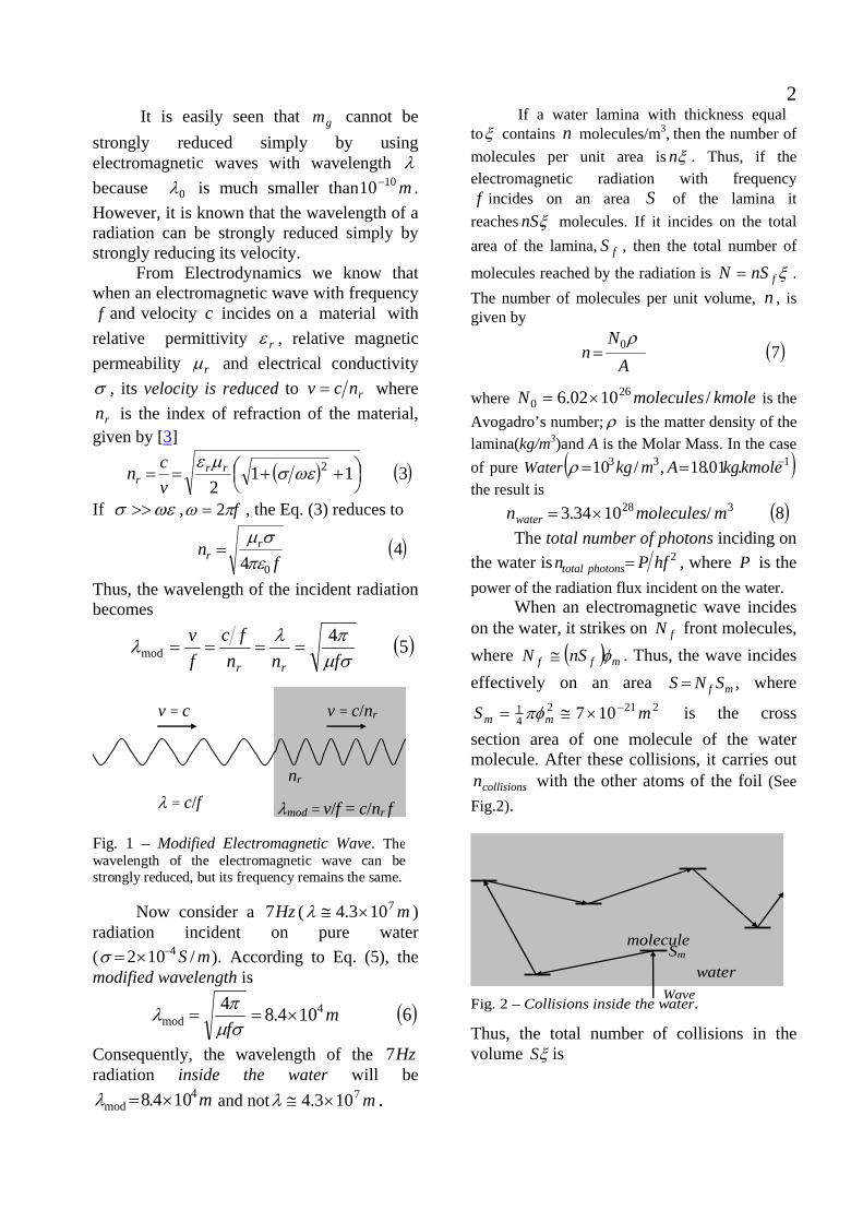
2 It is easily seen that cannot be strongly reduced simply by using electromagnetic waves with wavelength
gm
λ because 0λ is much smaller than . However, it is known that the wavelength of a radiation can be strongly reduced simply by strongly reducing its velocity.
m1010−
From Electrodynamics we know that when an electromagnetic wave with frequency
and velocity incides on a material with relative permittivity f c
rε , relative magnetic permeability rμ and electrical conductivity σ , its velocity is reduced to rncv = where
is the index of refraction of the material, given by [
rn3]
( ) ( )3112
2 ⎟⎠⎞⎜
⎝⎛ ++== ωεσ
με rrr v
cn
If ωεσ >> , fπω 2= , the Eq. (3) reduces to
( )44 0 f
n rr πε
σμ=
Thus, the wavelength of the incident radiation becomes
( )54mod σμ
πλλfnn
fcfv
rr====
Fig. 1 – Modified Electromagnetic Wave. The wavelength of the electromagnetic wave can bestrongly reduced, but its frequency remains the same.
v = c v = c/nr
λ = c/f λmod = v/f = c/nr f
nr
Now consider a ( ) radiation incident on pure water ( ). According to Eq. (5), the modified wavelength is
Hz7 m7103.4 ×≅λ
mS /102 4−×=σ
( )6104.84 4mod m
f×==
σμπλ
Consequently, the wavelength of the radiation inside the water will be
and not .
Hz7
m4mod 104.8 ×=λ m7103.4 ×≅λ
If a water lamina with thickness equal toξ contains n molecules/m3, then the number of molecules per unit area is ξn . Thus, if the electromagnetic radiation with frequency
incides on an area of the lamina it reachesf S
ξnS molecules. If it incides on the total area of the lamina, , then the total number of
molecules reached by the radiation is fS
ξfnSN = . The number of molecules per unit volume, n , is given by
( )70
AN
nρ
=
where is the Avogadro’s number;
kmolemoleculesN /1002.6 260 ×=
ρ is the matter density of the lamina(kg/m3)and A is the Molar Mass. In the case of pure Water ( )133 .01.18,/10 −== kmolekgAmkgρ the result is
( )8/1034.3 328 mmoleculesnwater ×= The total number of photons inciding on the water is 2hfPn photonstotal = , where P is the power of the radiation flux incident on the water. When an electromagnetic wave incides on the water, it strikes on front molecules, where
fN( ) mff nSN φ≅ . Thus, the wave incides
effectively on an area , where mf SNS =2212
41 107 mS mm
−×≅= πφ is the cross section area of one molecule of the water molecule. After these collisions, it carries out
with the other atoms of the foil (See Fig.2).
collisionsn
Fig. 2 – Collisions inside the water.
water
molecule Sm
Wave
Thus, the total number of collisions in the volume ξS is

3( )
( )9ξ
δξδ
nS
nSnSnSnNN ffcollisionsfcollisions
=
=−+=+=
The power density, , of the radiation on the water can be expressed by
D
( )10mf SN
PSPD ==
We can express the total mean number of collisions in each molecule, , by means of the following equation
1n
( )111 NNn
n collisionsphotonstotal=
Since in each collision a momentum λh is transferred to the molecule, then the total momentum transferred to the water will be
( ) λhNnp 1=Δ . Therefore, in accordance with Eq. (1), we can write that
( )
( )121121
1121
20
20
10
⎪⎭
⎪⎬⎫
⎪⎩
⎪⎨⎧
⎥⎥
⎦
⎤
⎢⎢
⎣
⎡−⎥
⎦
⎤⎢⎣
⎡+−=
=⎪⎭
⎪⎬⎫
⎪⎩
⎪⎨⎧
⎥⎥
⎦
⎤
⎢⎢
⎣
⎡−⎥
⎦
⎤⎢⎣
⎡+−=
λλ
λλ
collisionsphotonstotal
i
g
Nn
Nnmm
Since Eq. (9) gives ξnSNcollisions = , we get
( ) (132 ξnShfPNn collisionsphotonstotal ⎟⎟
⎠
⎞⎜⎜⎝
⎛= )
Substitution of Eq. (13) into Eq. (12) yields
( ) ( )1411212
02
0 ⎪⎭
⎪⎬
⎫
⎪⎩
⎪⎨
⎧
⎥⎥⎥
⎦
⎤
⎢⎢⎢
⎣
⎡−
⎥⎥⎦
⎤
⎢⎢⎣
⎡⎟⎟⎠
⎞⎜⎜⎝
⎛+−=
λλ
ξnShfP
mm
i
g
Substitution of P given by Eq. (10) into Eq. (14) gives
( )15111212
02
0 ⎪⎭
⎪⎬
⎫
⎪⎩
⎪⎨
⎧
⎥⎥⎥
⎦
⎤
⎢⎢⎢
⎣
⎡−
⎥⎥⎦
⎤
⎢⎢⎣
⎡⎟⎟⎠
⎞⎜⎜⎝
⎛⎟⎟⎠
⎞⎜⎜⎝
⎛+−=
λξcm
nSf
DSNmm
i
mf
i
g
Substitution of ( ) mff nSN φ≅ and mf SNS = into Eq. (15) the result is
( )1611121
11121
2
2
223
2
20
2223
0
⎪⎭
⎪⎬
⎫
⎪⎩
⎪⎨
⎧
⎥⎥⎥
⎦
⎤
⎢⎢⎢
⎣
⎡
−⎥⎥
⎦
⎤
⎢⎢
⎣
⎡
⎟⎟
⎠
⎞
⎜⎜
⎝
⎛+−=
⎪⎭
⎪⎬
⎫
⎪⎩
⎪⎨
⎧
⎥⎥⎥
⎦
⎤
⎢⎢⎢
⎣
⎡
−⎥⎥⎦
⎤
⎢⎢⎣
⎡
⎟⎟
⎠
⎞
⎜⎜
⎝
⎛+−=
λρ
φ
λξφ
cf
DSSn
cfm
DSSnmm
fmm
i
mmf
i
g
In the case of the water, we can take the following values: ;
( fS is the area of the horizontal cross-section of the test tube);
; ;
328 /1034.3 mmoleculesn ×=25109.1 mS f
−×≅
221107 mSm−×≅ mm 1≅ 1010−×φ ξ (height of
water inside the test tube). Substitution of these values into Eq. (16), gives
( )
( )( )1711101.1121
2
29
0 ⎪⎭
⎪⎬
⎫
⎪⎩
⎪⎨
⎧
⎥⎥⎥
⎦
⎤
⎢⎢⎢
⎣
⎡−
⎥⎥⎦
⎤
⎢⎢⎣
⎡⎟⎟⎠
⎞⎜⎜⎝
⎛×+−=
λfD
mm
wateri
waterg
In the case of a 7Hz radiation, Eq. (6) shows that . Thus, by substitution of
m4mod 104.8 ×=λλ by modλ into Eqs. (17) , we
get the following expression ( )
( )[ ]{ } ( )181101.7121 24
0−×+−≅ D
mm
wateri
waterg
Now, considering that the water is inside a solenoid, which produces a weak ELF electromagnetic field with and , then we can write that [
mE mB4]
( )( )19
222 0
2
0
22
0
2
water
m
water
mwater
water
m
ncB
vBv
vE
Dμμμ
===
Equation (4) shows that for Hzf 7= ,
( ) 7.506=waterrn .Substitution of this value into Eq.(19) gives
211103.2 mBD ×=Substitution of this value into Eq. (19) gives
( )
( )[ ]{ } ( )201107.3121 427
0−×+−≅ m
wateri
waterg Bmm

4 Fig. 3 – The vector of Pointing BES
rrr×= at
the test tube. The electromagnetic radiationpropagates in the direction of the vector ofPointing
Er
Br
ξ
Sr
fS
Coil
Test tube
In Montagnier’s experiment, the set-up was placed in a container shielded by 1 mm thick layer of mumetal in order to avoid interference from the earth's natural magnetic field, whose intensity is . This is because the intensity of magnetic field in Montagnier’s experiment was much smaller than . Note that, if the intensity of the magnetic field is in the range
, then, according to Eq. (20), the gravitational masses of the water with DNA and the water inside the other test tube are reduced to values in the range
to . It was shown in a previous paper [
TB 5106 −⊕ ×≅
⊕B
TBT m77 104.1102.1 −− ×<<×
0159.0 im+ 0159.0 im−3] that, when this occurs the
gravitational masses becomes imaginaries and the bodies leave our Real Universe, i.e., they perform transitions to the Imaginary Universe, which contains our Real Universe. The terms real and imaginary are borrowed from mathematics (real and imaginary numbers). It was also shown that in the Imaginary Universe the imaginary bodies are subjected to the Imaginary Interaction that is similar to the Gravitational Interaction. If the masses of the bodies have the same sign, then the interaction among them will be attractive. The masses of the water with DNA and the pure water are decreased at the same ratio,
(a)
(b)
(c)
(d) Fig. 4 – (a) Transition to the Imaginary Universe and attraction. (b) Fusion of the two waters. (c) Return to Real Universe. (d) After several comings and goings to the Imaginary Universe a real copy of the DNA can be detected in the tube with pure water.
F
Imaginary UniverseReal Universe
Imaginary UniverseReal Universe
Imaginary UniverseReal Universe
1
F
Imaginary UniverseReal Universe
DNA
First impression of DNA into water. It is a
tenuous copy that cannot yet be detected.
waterWater with DNA
Test tube with water
Test tube with waterand DNA
Fusion of the two waters. The DNA prints a tenuous copy of itself in the water of the second tube.
2
After several hours the copy of the
DNA is sufficiently intensified in order
to be detected

5in such way that they remain with the same sign. Thus, when they arrive the Imaginary Universe the attractive imaginary interaction approaches each other. Due to the small distance between them*, they are subjected to a significative attraction. Consequently, they entered one another (fusion). This imprints in the pure water an exactly copy of the DNA molecule. However, the water with DNA and the pure water return immediately to the real universe because the ELF electromagnetic field does not accompany them during the transition. When they get back to the real universe, the effect previously produced by the ELF electromagnetic field sends again the water with DNA and pure water to Imaginary Universe, and again a new imprint of the DNA is produced at the same place of the first one, strengthening the copy of DNA onto the water. Thus, during the time interval in what the ELF electromagnetic field remains on, the process continue. After some hours (16 to 18 hours in the case of Montagnier’s experiment) the copy of the DNA can become sufficiently strong to be detected. Thus, when the ELF electromagnetic field is turned off, the water can contain a real DNA molecule, which is an exactly equal to that one that exists in the other tube. The physicists in Montagnier's team suggest that the imprints of the DNA are preserved through quantum coherence effects [1]. This conclusion is based on the framework of a recently proposed theory of liquid water based on Quantum Field Theory (QFT) [5-10]. Jacques Benveniste [11] has been the first to propose (1988) that water has memory. The fact that the water contains electric dipoles, which can give to it a significant memory capacity, has been also considered by Brian Josephson [12] and, more recently by J. Dunning-Davies [13]. * Due to the small distance between the two test tubes. The tubes were then placed near to one another inside a horizontally oriented solenoid.
6 References [1] L. Montagnier, J. Aissa, E. Del Giudice, C. Lavalee, A. Tedeschi, and G. Vitiello, “DNA Waves and Water,” (2010) http://arxiv.org/pdf/1012.5166 [2] Coghlan, A. (2011) Scorn over claim of teleported DNA, New Scientist, 12 January. [3] De Aquino, F. (2010) Mathematical Foundations of the Relativistic Theory of Quantum Gravity, Pacific Journal of Science and Technology, 11 (1), pp. 173-232. [4] Halliday, D. and Resnick, R. (1968) Physics, J. Willey & Sons, Portuguese Version, Ed. USP, p.1124. [5] Preparata G 1995 QED Coherence in matter (Singapore: World Scientific) [6] Arani R, Bono I, Del Giudice E, Preparata G 1995 Int. J. Mod. Phys. B 9 1813–1841 [7] Del Giudice E, Preparata G and Vitiello G 1988 Phys. Rev. Lett. 61 1085–1088 [8] Del Giudice E and Vitiello G 2006 Phys. Rev. A 74 022105 [9] Del Giudice E and Tedeschi A 2009 Electr. Biol. Med. 26 48–54 [10] Del Giudice E, Spinetti P R and Tedeschi A 2010 Water 2 566–586 (online Journal). [11] Benveniste, Jacques (2005) Ma vérité sur la 'mémoire de l'eau', Albin Michel. ISBN 2-226-15877-4. [12] Brian Josephson (1997) Molecule Memories, New Scientist letters, 1 November. [13] J. Dunning-Davies (2011) Structure and Memory in Water, General Science and Philosophy, vixra.org/abs/1101.0081

A Possible Explanation for Anomalous Heat Production in Ni-H Systems
Fran De Aquino
Maranhao State University, Physics Department, S.Luis/MA, Brazil. Copyright © 2012 by Fran De Aquino. All Rights Reserved.
Anomalous heat production has been detected in Ni-H Systems. Several evidences point to the occurrence of nuclear fusion reactions. A possible explanation for this phenomenon is shown here based on the recent discovery that electromagnetic fields of extremely-low frequencies (ELF) can increase the intensities of gravitational forces. Under certain circumstances, the intensities of gravitational forces can even overcome the intensity of the electrostatic repulsion forces, and, in this way, produce nuclear fusion reactions, without need high temperatures for these reactions occur.
Key words: Modified theories of gravity, Nuclear Fusion, Fusion Reactors. PACS: 04.50.Kd , 89.30.Jj , 28.52.-s.
1. Introduction Since the experiment of Fleischmann, Hawkins and Pons [1] the anomalous production of heat has been searched for in various systems. Recently, a large anomalous production of heat has been reported by Focardi et al., [2] in a nickel rod filled with hydrogen. This phenomenon was posteriorly confirmed by Cerron-Zeballos et al., [3]. The called “cold fusion” was a process of nuclear fusion that was first conceived of by Fleischmann, Hawkins and Pons during their experiment that involved heavy water electrolysis through hydrogen on a palladium electrode surface [1]. They made claims originally that there was heat and energy being created from the reaction taking place at room temperature. This is why it is referred to as cold fusion, because it occurred in an environment that was previously considered too cool for nuclear fusion to occur. Here it is shown that nuclear fusion can be produced at room temperature by increasing the gravitational forces in order to overcome the electrostatic repulsion forces between the nuclei. This process became feasible after the Quantization of Gravity [4], with the discovery that the gravitational mass mg can be made negative and strongly intensified by means of electromagnetic fields of extremely-low frequencies. This effect can provide a consistent and coherent explanation for anomalous heat production detected in Ni-H Systems.
2. Theory The quantization of gravity shown that the gravitational mass mg and inertial mass mi are correlated by means of the following factor [4]:
( )111212
00 ⎪⎭
⎪⎬⎫
⎪⎩
⎪⎨⎧
⎥⎥
⎦
⎤
⎢⎢
⎣
⎡−⎟⎟
⎠
⎞⎜⎜⎝
⎛ Δ+−=
cmp
mm
ii
g
where is the rest inertial mass of the particle and
0impΔ is the variation in the
particle’s kinetic momentum; is the speed of light.
c
When pΔ is produced by the absorption of a photon with wavelengthλ , it is expressed by λhp =Δ . In this case, Eq. (1) becomes
( )21121
1121
20
20
0
⎪⎭
⎪⎬⎫
⎪⎩
⎪⎨⎧
⎥⎥
⎦
⎤
⎢⎢
⎣
⎡−⎟
⎠
⎞⎜⎝
⎛+−=
⎪⎭
⎪⎬⎫
⎪⎩
⎪⎨⎧
⎥⎥
⎦
⎤
⎢⎢
⎣
⎡−⎟
⎠
⎞⎜⎝
⎛+−=
λλ
λcmh
mm i
i
g
where cmh i00 =λ is the De Broglie wavelength for the particle with rest inertial mass 0im . From Electrodynamics we know that when an electromagnetic wave with frequency and velocity incides on a material with relative permittivity
f c
rε , relative magnetic permeability rμ and electrical conductivity σ , its velocity is

2reduced to rncv = where is the index of refraction of the material, given by [
rn5]
( ) ( )3112
2 ⎟⎠⎞⎜
⎝⎛ ++== ωεσ
με rrr v
cn
If ωεσ >> , fπω 2= , Eq. (3) reduces to
( )44 0 f
n rr πε
σμ=
Thus, the wavelength of the incident radiation (See Fig . 1) becomes
( )54mod σμ
πλλfnn
fcfv
rr====
Fig. 1 – Modified Electromagnetic Wave. The wavelength of the electromagnetic wave can bestrongly reduced, but its frequency remains the same.
v = c v = c/nr
λ = c/f λmod = v/f = c/nr f
nr
It is known that the Schumann resonances [6] are global electromagnetic resonances (a set of spectrum peaks in the extremely low frequency ELF), excited by lightning discharges in the spherical resonant cavity formed by the Earth’s surface and the inner edge of the ionosphere (60km from the Earth’s surface). The Earth–ionosphere waveguide behaves like a resonator at ELF frequencies and amplifies the spectral signals from lightning at the resonance frequencies. In the normal mode descriptions of Schumann resonances, the fundamental mode ( is a standing wave in the Earth–ionosphere cavity with a wavelength equal to the circumference of the Earth. This lowest-frequency (and highest-
intensity) mode of the Schumann resonance occurs at a frequency [
)1=n
Hzf 83.71 = 7]. Now consider a ( ) radiation passing through a Nickel powder cylinder ( ;
Hz83.7m7108.3 ×≅λ
mS /106.1 7×=σ17.2=rμ [8,9]) as shown in Fig.2.
According to Eq. (5), the modified wavelength is
( )619.04mod m
f==
σμπλ
Consequently, the wavelength of the radiation inside the Nickel powder will be
Hz83.7
m19.0mod =λ and not . m7108.3 ×≅λ If a Nickel powder* lamina with thickness equal toξ contains molecules/m
n3, then the number of molecules
per area unit is ξn . Thus, if the electromagnetic radiation with frequency
incides on an area of the lamina it reachesf S
ξnS molecules. If it incides on the total area of the lamina, , then the total number of molecules reached by the radiation is
fS
ξfnSN = . The number of molecules per unit of volume, , is given by n
( )70
AN
nρ
=
where is the Avogadro’s number;
kmolemoleculesN /1002.6 260 ×=
ρ is the matter density of the lamina (in kg/m3) and A is the molar mass. In the case of Nickel powder ( )13 .71.58,/8800 −== kmolekgAmkgρ the result is
( ) ( )8/1002.9 328 mmoleculesn Ni ×= The total number of photons inciding on the Nickel powder is 2hfPn photonstotal = , where P is the power of the radiation flux incident on the Nickel powder. * Ultra fine nickel powder (e.g. Inco type 210) with particle size of 0.5-1.0μm.

3 Fig.2 – Experimental set-up. The electromagnetic radiation propagates in the direction ofthe vector of Pointing BES
rrr×= . The set-up is
placed in a container shielded by 1 mm thick layer ofmumetal in order to avoid interference from external electromagnetic fields. In practice, the solenoid is not necessary, since the 7.83 Hz electromagnetic fieldnaturally exists inside the spherical resonant cavityformed by the Earth’s surface and the inner edge of the ionosphere. (Schumann resonance).
7.83 Hz current
Nickel powder
α
ξ
Metal tube
Mumetal
Solenoid
S=EmXBm
When an electromagnetic wave incides on a solid lamina of Nickel, it strikes on front molecules, where
fN
( )( ) ( )NifNif SnN φ≅ . Thus, the electromagnetic wave incides effectively on an area , where ( )Nif SNS =
( ) ( )2202
41 102.1 mS NiNi
−×≅= πφ is the cross
section area of one Ni atom. After these collisions, it carries out with the other atoms of the Nickel powder (See Fig.3).
collisionsn
Fig. 3 – Collisions inside the Nickel powder.
Nickel powder
molecule S(Ni)
Wave
Thus, the total number of collisions in the volume ξS is
( ) ( ) ( ) ( ) ( )( )( ) ( )9ξ
φξφ
Sn
SnSnSnnNN
Ni
NiNiNiNiNicollisionsfcollisions
=
=−+=+=
The power density, , of the radiation on the Nickel powder can be expressed by
D
( )( )10
Nif SNP
SPD ==
We can express the total mean number of collisions in each Ni molecule, , by means of the following equation
1n
( )111 NNn
n collisionsphotonstotal=
Since in each collision a momentum λh is transferred to the molecule, then the total momentum transferred to the Nickel will be
( ) λhNnp 1=Δ . Therefore, in accordance with Eq. (1), we can write that
( )
( )( )
( )121121
1121
20
20
10
⎪⎭
⎪⎬⎫
⎪⎩
⎪⎨⎧
⎥⎥
⎦
⎤
⎢⎢
⎣
⎡−⎥
⎦
⎤⎢⎣
⎡+−=
=⎪⎭
⎪⎬⎫
⎪⎩
⎪⎨⎧
⎥⎥
⎦
⎤
⎢⎢
⎣
⎡−⎥
⎦
⎤⎢⎣
⎡+−=
λλ
λλ
collisionsphotonstotal
wi
wg
Nn
Nnmm
Since Eq. (9) gives ( ) ξSnN Nicollisions = , we get
( )( ) ( )132 ξSnhfPNn Nicollisionsphotonstotal ⎟⎟
⎠
⎞⎜⎜⎝
⎛=
Substitution of Eq. (13) into Eq. (12) yields
( )
( )( )( ) ( )141121
20
20 ⎪
⎭
⎪⎬
⎫
⎪⎩
⎪⎨
⎧
⎥⎥⎥
⎦
⎤
⎢⎢⎢
⎣
⎡−
⎥⎥⎦
⎤
⎢⎢⎣
⎡⎟⎟⎠
⎞⎜⎜⎝
⎛+−=
λλξSn
hfP
mm
NiNii
Nig
Substitution of P given by Eq. (10) into Eq. (14) gives
( )
( )
( ) ( )
( )( )1511121
2
02
0 ⎪⎭
⎪⎬
⎫
⎪⎩
⎪⎨
⎧
⎥⎥⎥
⎦
⎤
⎢⎢⎢
⎣
⎡−
⎥⎥⎦
⎤
⎢⎢⎣
⎡⎟⎟⎠
⎞⎜⎜⎝
⎛⎟⎟⎠
⎞⎜⎜⎝
⎛+−=
λξcm
Snf
DSNmm
Nii
NiNif
Nii
Nig
Substitution of ( )( ) ( )NifNif SnN φ≅ and ( )Nif SNS = into Eq. (15) results

4
( )
( )
( ) ( ) ( )
( )( )1611121
2
20
2223
0 ⎪⎭
⎪⎬
⎫
⎪⎩
⎪⎨
⎧
⎥⎥⎥
⎦
⎤
⎢⎢⎢
⎣
⎡−
⎥⎥⎦
⎤
⎢⎢⎣
⎡
⎟⎟⎠
⎞⎜⎜⎝
⎛+−=
λξφ
cfmDSSn
mm
Nii
NiNifNi
Nii
Nig
where ( ) ( ) ( )( )ξπαρρ 420 NicylNiNii Vm == .
Thus, Eq. (16) reduces to
( )
( )
( ) ( ) ( )
( )( ) ( )17114
1212
22
2223
0 ⎪⎭
⎪⎬
⎫
⎪⎩
⎪⎨
⎧
⎥⎥⎥
⎦
⎤
⎢⎢⎢
⎣
⎡−
⎥⎥⎦
⎤
⎢⎢⎣
⎡
⎟⎟⎠
⎞⎜⎜⎝
⎛+−=
λπαρφ
cfDSSn
mm
Ni
NiNifNi
Nii
Nig
For cm5=φ we get 232 109.14 mS −×==παα . Note that is not equal to because the area is not continuous, but expressed by
, where is the area of the cross-section of one Ni particle, and is the number of particles in the front area, which is expressed by
fS αS
pf nSS = pSn
( )αφ Snxn pp= , 1<<x , where αφ Sn pp is the number of particles inside area ; is the number of Ni particles/m
αS pn3, given by ξαSNn pp = where
vpp VVSN += ξα ; is the mean volume of one Ni particle and is the void volume, corresponding to that particle. This volume can be calculated considering one sphere with
pV
VV
pφ - diameter inside a cube whose edge
is pφ . The result is . The mean size of the particles is
348.0 pVV φ≅
mp μφ 75.0= . Thus,
and .
Consequently, . Then,
we get . Now, we can calculate the value of :
319102.2 mVp−×≅ 213104.4 mS p
−×≅219102.4 mVV Vp
−×≅+318 /104.2 mparticlesnp ×=
fS
( ) ( ) 23105.1 mxSSnxS pppf−×≅= αφ
Substitution of this value jointly with
; ; ( )328 /1002.9 mmolecn Ni ×= ( ) mNi
101024.1 −×=φ232 109.14 mS −×==παα ; ;
; (Note that, this is lowest-frequency mode of the Schumann resonance. Therefore, in practice, is not necessary to provide the 7.83 Hz
electromagnetic field) and
( )220102.1 mS Ni
−×≅
( )3.8800 −= mkgNiρ Hzf 83.7=
m19.0mod == λλ into Eq.(17), gives
( )
( )[ ]{ } ( )181109.3121 2421
0−×+−= Dx
mm
Nii
Nig
Now, considering that the Nickel powder is inside a solenoid, which produces a weak ELF electromagnetic field with
and , then we can write that [mE mB 10]
( )( )19
222 0
2
0
22
0
2
Nir
m
Ni
mNi
Ni
m
ncB
vBv
vE
Dμμμ
===
Equation (4) shows that, for , .Substitution of this value into
Eq.(19) gives
Hzf 83.7=
( )8102×=Nirn
( )21109.5 25mBD ×=
Substitution of this value into Eq. (18) gives ( )
( )[ ]{ } ( )221103.1121 4433
0−×+−≅= m
Nii
Nig Bxmm
χ
The value of is limited by the ionization energy of the atoms, which is, as we known, the energy required to remove electrons from atoms. Since the minimum energy required for the electron to leave the atom is:
mB
jouleseU 19max0
2min 107.74 −×=−= φπε
then, for the ionization does not occur, the energy of the wave ( )hf must be smaller than
. Thus, it follows that minUfSfUDSfUShf aaa ≅<⇒< minmin
2
According to Eq. (19), 02maxmax 2μcBD = .
Then, the result is fB 8
max 109 −×<In the case of Hzf 83.7= , we conclude that
( )23102 7max TB −×<
Assuming that then Eq. (22) yields
TB 7max 102 −×≅
( )
( )[ ]{ } ( )241101.2121 46
0−×+−≅= x
mm
Nii
Nigχ
Since 1<<x , we can conclude that there is no significant variation in the gravitational mass of the Nickel powder. However, if the air inside the Nickel powder is evacuated by means of a vacuum pump, and after Hydrogen (or Deuterium,

5Tritium, Helium, etc) is injected into the Nickel powder (See Fig.4) then, the area to be considered, in order to calculate the gravitational mass of the Hydrogen, is the surface area of the Nickel powder, which can be obtained by multiplying the specific surface area of the Nickel powder
fS
† ( ) by the total mass of the Nickel powder (
Kgm /104~ 23×
( ) ( ) ( )ξπαρ 420 NiNiim = ).
Thus, we get . ( ) ξρ αSS Nif3104 ×≅
The characteristics of the Nickel prevail on those of the Hydrogen, in the Ni-H systems, because the Nickel amount is much larger than the Hydrogen amount. Thus, we must take the values of ρ , rμ , and σ equal to ( )Niρ , ( )Nirμ and ( )Niσ respectively, in order to calculate , in Ni-H systems. In addition, since
( )HgmANn ρ0= and
σμπλ f4mod= we can conclude that also and ( )Ninn ≡ ( ) mNi 19.0modmod == λλ .
Therefore, in order to obtain the expression ( ) ( )HiHg mm 0 we can take Eq. (17) only
substituting for the expression above
obtained fS
( )( )ξρ αSS Nif3104 ×≅ . Thus we
get ( )
( )
( ) ( ) ( ) ( ) ( )25117.18
121
2
2
2223
0
⎪⎭
⎪⎬
⎫
⎪⎩
⎪⎨
⎧
⎥⎥⎥
⎦
⎤
⎢⎢⎢
⎣
⎡
−⎥⎥⎦
⎤
⎢⎢⎣
⎡
⎟⎟
⎠
⎞
⎜⎜
⎝
⎛+−
=
λφξρ α
f
DSSn
mm
NiNiNiNi
Hi
Hg
For m1.0=ξ (length of the Ni-H cylinder in Focardi experiment) Eq.(25) gives
( )
( )[ ]{ } ( )261105.1121 248
0−×+−== D
mm
Hi
Hgχ
Based on Eq. (19), we can write that † Ultra fine nickel powder (e.g. Inco type 210) with particle size of 0.5-1.0μm has specific surface areas range from 1.5 to 6m2/g [11]. Hydrogen production with nickel powder cathode points to a value of 4.31m2 /g in the case of new cathodes, and 3.84 m2 /g in the case of used cathodes [12].
( )Hrm ncBD 02 2μ= , where . Thus,
we get . Substitution of this expression into Eq. (26) yields
( ) 1≅Hrn214102.1 mBD ×=
( )
( )[ ]{ } ( )271101.2121 476
0−×+−== m
Hi
Hg Bmm
χ
It is known that, at any time in the spherical resonant cavity formed by the Earth’s surface and the inner edge of the ionosphere (60km from the Earth’s surface) there is a drop voltage of 200KV. This, produces an electric field with intensity
mVEm /3≅ , which gives . Substitution of this value into Eq. (27), yields
TBm8101 −×≅
( )28102 22×−≅χThus, the gravitational forces between two protons (hydrogen nuclei) becomes
22022222 107 rrGmrGmF ipgp−×−≅−=−= χ
Comparing with the electrostatic repulsion forces between the nuclei, which is given by
22820
2 103.24 rreFe−×== πε
We conclude that the intensities of the gravitational forces overcome the intensities of the electrostatic repulsion forces between the nuclei. This is sufficient to produce their fusion. Fig.4 – Cold Fusion Reactor on Earth. Note that here the 7.83 Hz electromagnetic field is what naturally exists inside the spherical resonant cavityformed by the Earth’s surface and the inner edge of the ionosphere. (Schumann resonance).
H2
Nickel powder +
Hydrogen
α
ξ
Metal tube
S=EmXBm

6 The enormous value of χ (Eq. 28) strongly increases the gravitational masses of the Hydrogen nuclei ( pigp mm 0χ= ) and their
respective electrons ( eige mm 0χ= ). Thus, the gravitational force between a nucleus (proton) and the corresponding electron is given by
200
2 rmGmF eipipe χ−= and the gravitational force between two Hydrogen nuclei is
200
2 rmGmF pipipp χ−= . Therefore, two well-known types of fusions can occur, i.e.,
( )29enep ν+→+ −
( )3042.0 MeVedpp e +++→+ +ν Due to the strong gravitational attraction, the following fusions occur instantaneously:
ee pnd νν ++→+and
epen ν+→+ +
These reactions are widely known because they have been studied extensively due to their importance in astrophysics and neutrino physics [13–16]. Thus, the term in Eq. (30) reduces instantaneously to
+++ ep eν
eepp νν +++ . In these fusion reactions, neutrons (Eq. (29)), neutrinos and antineutrinos, and energy (0.42MeV at each fusion of two Hydrogen nuclei) are produced. Note that there is no gamma ray emission during the process. The evidence of neutron emission during energy production in Ni-H systems has been reported by Battaglia, A. et al., [17]. In order to calculate the number of Hydrogen atoms/m3 inside the Nickel powder we will calculate the density of the Hydrogen. According to Focardi’s experiments, the pressure of the Hydrogen is
at temperature . Thus, according to the well-kwon
Equation of State
23 /10166.5051.0 mNatmP ×==KT 400=
ZRTPM 0=ρ , we get
( )( )( )( )( )
33
11
1323
/101.3
400..314.81~.102/10166.5
mkg
KKmoljoulemolkgmN
H
−
−−
−−
×=
=××
=ρ
Thus, the number of Hydrogen atoms/m3 inside the Nickel powder is
32620 /1001.3 matomsANn HHHH ρρ ×==
Then, the number of H atoms inside the Nickel powder is given by
ξαρδ 224103.8 HHfHHH SnVn ×≅= where nmNiNiH 1≅−Δ= φδ ; Niφ is the diameter of Ni atom; is the average molecular separation in the Ni. Then, we get
. Thus, the total energy realized in the p-p fusions is
NiΔ
atomsSnVn HfHHH18104.6 ×≅= δ
( )
( )
KwhJ
eVMeV
MeVVn
E HH
05.0101.2
103.142.02104.6
42.02
5
2418
≅×≅
≅×=×
=
==
This energy correspond to a power of
WhKwh 5005.0 = , which is the same value detected in the Focardi’s experiments. This explains the anomalous heat production in Ni-H Systems detected in the Focardi’s experiments. Since the 7.83 Hz electromagnetic field (Schumann resonances) does not disappear when the device is switched off, the energy conversion can remain running for long period after it is switched off because, when the device is switched off, the value of the electrical conductivity of the Ni-H system, which was approximately equal to
Niσ , slowly decreases, tending to Hσ , which is much smaller than 1. When the electrical conductivity becomes smaller than ωε the value of becomes approximately equal to 1. Consequently,
rn
modλ becomes equal to
mfc 7108.3 ×= and, according to Eq.(17), the result is 1≅χ . This explain why in the Focardi’s experiment the device remained running for twenty four days after being switched off. It is evident that the discovery of this energy conversion device is highly relevant. However, this system is not an efficient energy source if compared to the Gravitational Motor [18], which can provide

7219KW/m3 while the Ni-H system only 20Kw/m3 (by increasing α from 5cm up to 100cm). Furthermore, the Gravitational Motor converts gravitational energy into rotational mechanical energy directly from the gravitational field, while the Ni-H system needs to produce vapor in order to convert the energy into rotational mechanical energy. 3. Transforming a Ni-H system into a Hydrogen Bomb. It is easy to see that a Ni-H System can be transformed into a Hydrogen bomb, simply increasing the volume of the Ni-H cylinder and substituting the Hydrogen by a liquid deuterium LD (12.5 MeV of energy is produced at each fusion of two deuterium nuclei ‡ ). For example, if α = 0.27m, ξ = 2 m, and, if a liquid deuterium ( [3.8.67 −= mkgHρ 19]) is injected into the Ni powder, then the total energy realized in the fusions becomes
( )
( )
kilotonsJeV
MeV
MeVVn
E
H
H
HH
20102.8102.5
25.122
104.8
5.122
13231
224
≅×≅×≅
≅×
=
==
ξαρ
ξαρ ( )
The Hiroshima’s atomic bomb had 20 kilotons. It is important to note that this bomb type is much easier to build than the conventional nuclear bombs. Basically, these bombs are made of Nickel powder (99%), liquid deuterium-tritium mixture and Mumetal. These materials can be easily obtained. Due to the simplicity of its construction these bombs can be built at the
‡ The d + d fusion reaction has two branches that occur with nearly equal probability: (T + p + 4.03MeV and 3He + n + 3.27MeV ). Then, a deuteron d is produced by the fusion of the proton p (produced in the first branch) with the neutron (produced in the second branch). Next, occurs the fusion of this deuteron with the tritium T produced in the first branch, i.e., (d + T → + n + 17.6 MeV). Thus, we count He3
2 the d + d fusion energy as Efus = (4.03+17.6+3.27)/2 = 12.5 MeV.
very place of the target (For example, inside a house or apartment at the target city.). This means that, in the most of cases missiles are not necessary to launch them. In addition, they cannot be easily detected during their building because the necessary materials are trivial, and there is no radioactive material.
8References [1] Fleischmann M., Hawkins, M. and Pons S., (1989) J. Electroanal. Chem., 261, 301. [2] Focardi, S., Habel, R. and Piantelli, F., (1994) Nuovo Cimento A, 107, 163. [3] Cerron-Zeballos et al., (1996) Nuovo Cimento A, 109, 1645. [4] De Aquino, F. (2010) Mathematical Foundations of the Relativistic Theory of Quantum Gravity, Pacific Journal of Science and Technology, 11 (1), pp. 173-232. [5] Quevedo, C. P. (1977) Eletromagnetismo, McGraw- Hill, p. 270. [6] Schumann W. O. (1952). "Über die strahlungslosen Eigenschwingungen einer leitenden Kugel, die von einer Luftschicht und einer Ionosphärenhülle umgebenist". Zeitschrift und Naturfirschung 7a: 149–154 [7] Volland, H. (1995), Handbook of Atmospheric Electrodynamics, CRC Press, vol.I, Chapter11. [8] Lin Li and Chung D.,(1991) Composites, 22, 3, p.212. [9] Göktürk, H., et al., (1993) J. App. Polymer Science, 50, p.1900. [10] Halliday, D. and Resnick, R. (1968) Physics, J. Willey & Sons, Portuguese Version, Ed. USP, p.1124. [11] Neikov, O.D, et al., (2009) Handbook of Non-Ferrous Metal Powders: Technologies and Applications, Elsevier Ltd., p.374. [12]Selembo, P. A, et al., (2010) Hydrogen production with nickel powder cathode catalysts in microbial electrolysis cells, International Journal of Hydrogen Energy, 35, p. 431, p.433. [13] Park T. S. et al., (1998) Astrophys. J. 507 443. [14] Kong X and Ravndal, F. (1999) Nucl. Phys. A 656 421; Kong X and Ravndal, F. (1999) Phys. Lett. B 470, 1; Kong X and Ravndal (2001) F. Phys. Rev. C 64 , 044002. [15] Butler. M. and Chen, J. W., (2001) Phys. Lett. B 520 , 87. [16] Park T. S. et al., (2003) Phys. Rev. C 67 055206 (nucl-th/0208055); Park T. S. et al., nucl-th/0106025 and nucl-th/0107012. [17] Battaglia, A. et al., (1999) NuovoCimento A, 112, 921. [18] De Aquino, F. (2010) Gravity Control by means of Electromagnetic Field through Gas at Ultra-Low Pressure, Pacific Journal of Science and Technology, 11(2) November 2010, pp. 178-247, Physics /0701091. [19] Rossini, F.D. (1968) IPTS-1968, Butterworths, London.

Engineering the Ni-H Bomb
Fran De Aquino Maranhao State University, Physics Department, S.Luis/MA, Brazil.
Copyright © 2012 by Fran De Aquino. All Rights Reserved.
The anomalous heat production detected in Ni-H systems was recently explained based on the fact that electromagnetic fields of extremely-low frequencies (ELF) can increase the intensities of gravitational forces and overcome the intensity of the electrostatic repulsion forces, producing nuclear fusion reactions. This effect can provide a consistent and coherent explanation for anomalous heat production detected in Ni-H Systems, and shows that a Ni-H System can be easily transformed into a Hydrogen bomb. Here, a Ni-H bomb of 20 kilotons is engineered.
Key words: Modified theories of gravity, Nuclear Fusion, Fusion Reactors. PACS: 04.50.Kd , 89.30.Jj , 28.52.-s.
1. Introduction Recently, a large anomalous production of heat in a nickel rod filled with hydrogen has been reported by Focardi et al., [1]. This phenomenon was posteriorly confirmed by Cerron-Zeballos et al., [2]. Nuclear fusion can be produced by increasing the gravitational forces in order to overcome the electrostatic repulsion forces between the nuclei. This process became feasible after the Quantization of Gravity [3], with the discovery that the gravitational mass mg can be made negative and strongly intensified by means of electromagnetic fields of extremely-low frequencies. This effect can provide a consistent and coherent explanation for anomalous heat production detected in Ni-H Systems, and shows that a Ni-H System can be easily transformed into a Hydrogen bomb [4]. Here, a Ni-H bomb of 20 kilotons is engineered. 2. Theory Consider the Ni-H system showed in Fig. 1. In a previous paper [4] it was showed that, if the air inside the Nickel powder is evacuated by means of a vacuum pump (down to at temperature ) and after Hydrogen is injected into the Nickel powder, then, the number of Hydrogen atoms/m
23 /10166.5051.0 mNatmP ×==KT 400=
3 inside the Nickel powder is
32920 /1094.1 matomsANn HHHH ρρ ×==
where Hρ is the Hydrogen density;
is the Avogadro’s number and A is the molar mass.
kmolemoleculesN /1002.6 260 ×=
Then, the number of atoms inside the Nickel powder is given by
ξαρδ 224103.8 HHfHHH SnVn ×≅= where ; ; ( ) ξρ αSS Nif
3104×≅ ( )3.8800 −= mkgNiρ
42παα =S and nmNiNiH 1≅−Δ= φδ ; Niφ is the diameter of Ni atom; is the average molecular separation in the Ni.
NiΔ
Fig.1 – Ni-H system. Note that, on Earth, the system is subjected to a 7.83 Hz electromagnetic field. This field is what naturally exists inside the spherical resonant cavity formed by the Earth’s surface and the inner edge of the ionosphere. (Schumann resonance).
Nickel powder +
Hydrogen
α
ξ
Metal tube

2 Thus, the total energy realized in the protons fusions is*
( )
JouleseV
MeVVn
E
HH
HHH
ξαρξαρ
ξαρ
211230
224
107.2107.1
142.02
103.82
×≅×≅
≅×
== ( )
It is easy to see that a Ni-H System can be transformed into a Hydrogen bomb, simply increasing the volume of the Ni-H cylinder and substituting the Hydrogen by a liquid deuterium LD (12.5 MeV of energy is produced at each fusion of two deuterium nuclei † ). For example, if α = 0.27m, ξ = 2 m (See Fig.2), and, if a liquid deuterium ( [3.8.67 −= mkgHρ 5]) is injected into the Ni powder, then the total energy realized in the fusions becomes
( )
kilotonsJeV
MeVE
H
H
20103.8102.5
25.122
104.8
13231
224
≅×≅×≅
≅×
=
ξαρ
ξαρ ( )
The Hiroshima’s atomic bomb had 20 kilotons. Fig.2 – The core of the Ni-H bomb of 20 kilotons.
Nickel powder +
LD
α =0.27 m
Metal tube
ξ= 2 m
It is important to note that this bomb type is much easier to build than the * 0.42MeV are realized at each fusion of two Hydrogen nuclei. † The d + d fusion reaction has two branches that occur with nearly equal probability: (T + p + 4.03MeV and 3He + n + 3.27MeV ). Then, a deuteron d is produced by the fusion of the proton p (produced in the first branch) with the neutron (produced in the second branch). Next, occurs the fusion of this deuteron with the tritium T produced in the first branch, i.e., (d + T → + n + 17.6 MeV). Thus, we count He3
2 the d + d fusion energy as Efus = (4.03+17.6+3.27)/2 = 12.5 MeV.
conventional nuclear bombs. Basically, these bombs are made of Nickel powder (99%), liquid deuterium and Mumetal. These materials can be easily obtained. Due to the simplicity of its construction, these bombs can be built at the very location of the target (For example, inside a house or apartment at the target city.). This means that, in most of cases missiles are not necessary to deliver them, except for launching the Ni-H bomb at the height of explosion (<1Km ‡ ) when necessary. Thus, the Ni-H bomb so far seems to be the simplest atomic bomb ever to be built. It can be made by every nation, in such a way that, peace in the World will be reached in the future due to the equilibrium of forces among nations. Figure 3 shows the Ni-H bomb. It is enveloped by a Mumetal box in order to avoid the action of the 7.83Hz electromagnetic field that naturally exists inside the spherical resonant cavity formed by the Earth’s surface and the inner edge of the ionosphere. (Schumann resonance [6, 7]). When the mumetal shielding is exploded the 7.83Hz electromagnetic field acts on the core of the Ni-H bomb and it explodes. Fig.3 – The Ni-H bomb of 20 kilotons.
MumetalShielding
LD
Nickel powder
Explosivesin order to explode the Mumetal shielding
Mumetal boxes
Antenna
Detonator
Control
‡ Hiroshima 600m above. Nagasaki 500m above.

3 References [1] Focardi, S., Habel, R. and Piantelli, F., (1994) Nuovo Cimento A, 107, 163. [2] Cerron-Zeballos et al., (1996) Nuovo Cimento A, 109, 1645. [3] De Aquino, F. (2010) Mathematical Foundations of the Relativistic Theory of Quantum Gravity, Pacific Journal of Science and Technology, 11 (1), pp. 173-232. [4] De Aquino, F. (2012), A Possible Explanation for Anomalous Heat Production in Ni-H Systems, http://vixra.org/pdf/1202.0039v3.pdf [5] Rossini, F.D. (1968) IPTS-1968, Butterworths, London. [6] Schumann W. O. (1952). "Über die strahlungslosen Eigenschwingungen einer leitenden Kugel, die von einer Luftschicht und einer Ionosphärenhülle umgebenist". Zeitschrift und Naturfirschung 7a: 149–154 [7] Volland, H. (1995), Handbook of Atmospheric Electrodynamics, CRC Press, vol.I, Chapter11.

Gravitational Shockwave Weapons Fran De Aquino
Maranhao State University, Physics Department, S.Luis/MA, Brazil. Copyright © 2012 by Fran De Aquino. All Rights Reserved.
Detonation velocities, greater than that generated by high explosives (~104m/s), can be achieved by using the gravitational technology recently discovered. This possibility leads to the conception of powerful shockwave weapons. Here, we show the design of a portable gravitational shockwave weapon, which can produce detonation velocities greater than 105m/s, and detonation pressures greater than 1010N/m2 .
Key words: Modified theories of gravity, Detonation waves, Shockwaves, Nozzle flow. PACS: 04.50.Kd, 47.40.Rs, 47.40.-x, 47.60.Kz. 1. Introduction The most important single property of an explosive is the detonation velocity. It is the speed at which the detonation wave travels through the explosive. Typical detonation velocities in solid explosives often range beyond 3,000 m/s to 10,300 m/s [1]. At the front of the detonation zone, an energy pulse or “shockwave” is generated and transmitted to the adjacent region. The shockwave travels outward as a compression wave, moving at or near detonation velocity. When the intensity of the shockwave exceeds the compression strength of the materials they are destroyed. If the mass of the body is too large the wave energy is simply absorbed by the body [2]. The pressure produced in the explosion zone is called Detonation Pressure. It expresses the intensity of the generated shockwave. A high detonation pressure is necessary when blasting hard, dense bodies. Detonation pressures of high explosives are in the range from 106N/m2 to over 107 N/m2 [3]. Here, we show the design of a portable shockwave weapon, which uses the Gravitational Shielding Effect (BR Patent Number: PI0805046-5, July 31, 2008) in order to produce detonations velocities greater than 100,000m/s, and detonation pressures greater than 1010N/m2. It is important to remember that an aluminum-nitrate truck bomb has a relatively low detonation velocity of 3,500 m/s (sound speed is 343.2m/s)*. High explosives such as * When a shockwave is created by high explosives it will always travel at high supersonic velocity from its point of origin.
TNT has a detonation velocity of 6,900m/s; Military explosives used to destroy strong concrete and steel structures have a detonation velocity of 7,000 to 8,000 m/s [3]. 2. Theory The contemporary greatest challenge of the Theoretical Physics was to prove that, Gravity is a quantum phenomenon. The quantization of gravity showed that the gravitational mass mg and inertial mass mi are correlated by means of the following factor [4]:
( )111212
00 ⎪⎭
⎪⎬⎫
⎪⎩
⎪⎨⎧
⎥⎥
⎦
⎤
⎢⎢
⎣
⎡−⎟⎟
⎠
⎞⎜⎜⎝
⎛ Δ+−==
cmp
mm
ii
gχ
where is the rest inertial mass of the particle and
0impΔ is the variation in the
particle’s kinetic momentum; is the speed of light.
c
When pΔ is produced by the absorption of a photon with wavelengthλ , it is expressed by λhp =Δ . In this case, Eq. (1) becomes
( )21121
1121
20
20
0
⎪⎭
⎪⎬⎫
⎪⎩
⎪⎨⎧
⎥⎥
⎦
⎤
⎢⎢
⎣
⎡−⎟
⎠
⎞⎜⎝
⎛+−=
⎪⎭
⎪⎬⎫
⎪⎩
⎪⎨⎧
⎥⎥
⎦
⎤
⎢⎢
⎣
⎡−⎟
⎠
⎞⎜⎝
⎛+−=
λλ
λcmh
mm i
i
g

2where cmh i00 =λ is the De Broglie wavelength for the particle with rest inertial mass . 0im It was shown that there is an additional effect - Gravitational Shielding effect - produced by a substance whose gravitational mass was reduced or made negative [5]. The effect extends beyond substance (gravitational shielding) , up to a certain distance from it (along the central axis of gravitational shielding). This effect shows that in this region the gravity acceleration, , is reduced at the same proportion, i.e.,
1ggg
11 χ= where
01 ig mm=χ and is the gravity acceleration before the gravitational shielding). Consequently, after a second gravitational shielding, the gravity will be given by
g
ggg21122 χχχ == , where
2χ is
the value of the ratio 0ig mm for the second gravitational shielding. In a generalized way, we can write that after the nth gravitational shielding the gravity, , will be given by ng
( )3...
321gg
nn χχχχ=
This possibility shows that, by means of a battery of gravitational shieldings, we can make particles acquire enormous accelerations. In practice, this can lead to the conception of powerful particles accelerators, kinetic weapons or weapons of shockwaves. From Electrodynamics we know that when an electromagnetic wave with frequency and velocity incides on a material with relative permittivity
f c
rε , relative magnetic permeability rμ and electrical conductivity σ , its velocity is reduced to rncv = where is the index of refraction of the material, given by [
rn6]
( ) ( )4112
2 ⎟⎠⎞⎜
⎝⎛ ++== ωεσ
με rrr v
cn
If ωεσ >> , fπω 2= , Eq. (4) reduces to
( )54 0 f
n rr πε
σμ=
Thus, the wavelength of the incident radiation (See Fig. 1) becomes
( )64mod σμ
πλλfnn
fcfv
rr====
Fig. 1 – Modified Electromagnetic Wave. The wavelength of the electromagnetic wave can bestrongly reduced, but its frequency remains the same.
v = c v = c/nr
λ = c/f λmod = v/f = c/nr f
nr
If a lamina with thickness equal toξ contains molecules/mn 3, then the number of molecules per area unit is ξn . Thus, if the electromagnetic radiation with frequency
incides on an area of the lamina it reachesf S
ξnS molecules. If it incides on the total area of the lamina, , then the total number of molecules reached by the radiation is
fS
ξfnSN = . The number of molecules per unit of volume, , is given by n
( )70
AN
nρ
=
where is the Avogadro’s number;
kmolemoleculesN /1002.6 260 ×=
ρ is the matter density of the lamina (in kg/m3) and A is the molar mass. When an electromagnetic wave incides on the lamina, it strikes on front molecules, where
fN( ) mff SnN φ≅ , mφ is the
“diameter” of the molecule. Thus, the electromagnetic wave incides effectively on an area mf SNS= , where 2
41
mmS πφ= is the cross
section area of one molecule. After these collisions, it carries out with the other molecules (See Fig.2).
collisionsn
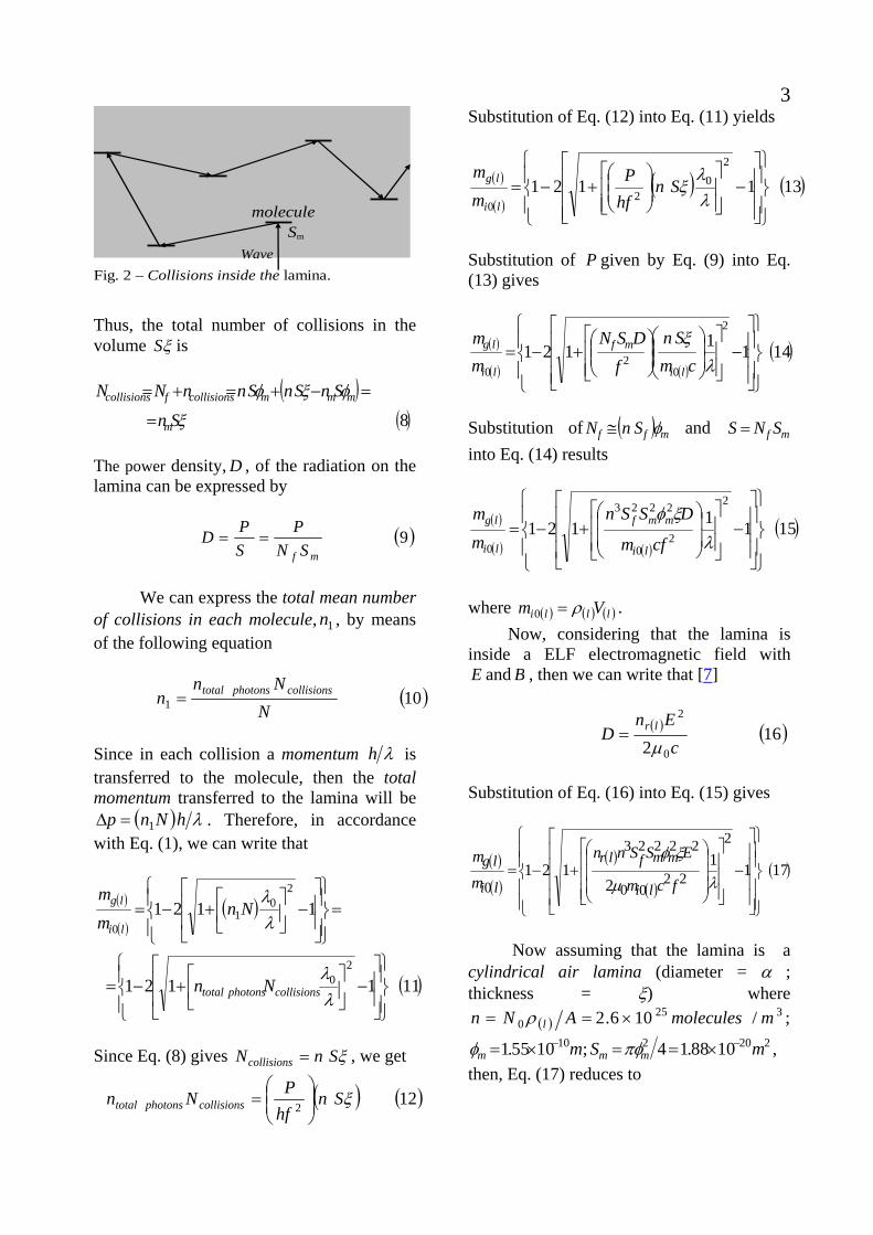
3 Fig. 2 – Collisions inside the lamina.
molecule Sm
Wave
Thus, the total number of collisions in the volume ξS is
( )( )8ξ
φξφ
Sn
SnSnSnnNN
m
mmmcollisionsfcollisions
=
=−+=+=
The power density, , of the radiation on the lamina can be expressed by
D
( )9mf SN
PSPD ==
We can express the total mean number of collisions in each molecule, , by means of the following equation
1n
( )101 NNn
n collisionsphotonstotal=
Since in each collision a momentum λh is transferred to the molecule, then the total momentum transferred to the lamina will be
( ) λhNnp 1=Δ . Therefore, in accordance with Eq. (1), we can write that
( )
( )( )
( )111121
1121
20
20
10
⎪⎭
⎪⎬⎫
⎪⎩
⎪⎨⎧
⎥⎥
⎦
⎤
⎢⎢
⎣
⎡−⎥
⎦
⎤⎢⎣
⎡+−=
=⎪⎭
⎪⎬⎫
⎪⎩
⎪⎨⎧
⎥⎥
⎦
⎤
⎢⎢
⎣
⎡−⎥
⎦
⎤⎢⎣
⎡+−=
λλ
λλ
collisionsphotonstotal
li
lg
Nn
Nnmm
Since Eq. (8) gives ξSnNcollisions = , we get
( ) ( )122 ξSnhfPNn collisionsphotonstotal ⎟⎟
⎠
⎞⎜⎜⎝
⎛=
Substitution of Eq. (12) into Eq. (11) yields
( )
( )( ) ( )131121
20
20 ⎪
⎭
⎪⎬
⎫
⎪⎩
⎪⎨
⎧
⎥⎥⎥
⎦
⎤
⎢⎢⎢
⎣
⎡−
⎥⎥⎦
⎤
⎢⎢⎣
⎡⎟⎟⎠
⎞⎜⎜⎝
⎛+−=
λλ
ξSnhfP
mm
li
lg
Substitution of given by Eq. (9) into Eq. (13) gives
P
( )
( ) ( )( )1411121
2
02
0 ⎪⎭
⎪⎬
⎫
⎪⎩
⎪⎨
⎧
⎥⎥⎥
⎦
⎤
⎢⎢⎢
⎣
⎡−
⎥⎥⎦
⎤
⎢⎢⎣
⎡⎟⎟⎠
⎞⎜⎜⎝
⎛⎟⎟⎠
⎞⎜⎜⎝
⎛+−=
λξcm
Snf
DSNmm
li
mf
li
lg
Substitution of ( ) mff SnN φ≅ and mf SNS = into Eq. (14) results
( )
( ) ( )( )1511121
2
20
2223
0 ⎪⎭
⎪⎬
⎫
⎪⎩
⎪⎨
⎧
⎥⎥⎥
⎦
⎤
⎢⎢⎢
⎣
⎡
−⎥⎥⎦
⎤
⎢⎢⎣
⎡
⎟⎟
⎠
⎞
⎜⎜
⎝
⎛+−=
λ
ξφ
cfm
DSSnmm
li
mmf
li
lg
where ( ) ( ) ( )llli Vm ρ=0 . Now, considering that the lamina is inside a ELF electromagnetic field with E and B , then we can write that [7]
( ) ( )162 0
2
cEn
D lr
μ=
Substitution of Eq. (16) into Eq. (15) gives
( )( )
( )
( )( )1711
2121
2
2200
22223
0⎪⎪⎭
⎪⎪⎬
⎫
⎪⎪⎩
⎪⎪⎨
⎧
⎥⎥⎥⎥
⎦
⎤
⎢⎢⎢⎢
⎣
⎡
−⎥⎥⎥
⎦
⎤
⎢⎢⎢
⎣
⎡
⎟⎟⎟
⎠
⎞
⎜⎜⎜
⎝
⎛+−=
λμ
ξφ
fcm
ESSnn
mm
li
mmflr
li
lg
Now assuming that the lamina is a cylindrical air lamina (diameter = α ; thickness = ξ) where
( )325
0 /106.2 mmoleculesANn l ×== ρ ;
mm101055.1 −×=φ ; 2202 1088.14 mS mm
−×==πφ , then, Eq. (17) reduces to

4
( )( )
( )
( )( )1811066121
22
20
25
0⎪⎪⎭
⎪⎪⎬
⎫
⎪⎪⎩
⎪⎪⎨
⎧
⎥⎥⎥⎥
⎦
⎤
⎢⎢⎢⎢
⎣
⎡
−⎥⎥⎥
⎦
⎤
⎢⎢⎢
⎣
⎡
⎟⎟⎟
⎠
⎞
⎜⎜⎜
⎝
⎛×+−=
λ
ξ E
fm
Sn
mm
li
flr
li
lg .
An atomized water spray is created by forcing the water through an orifice. The energy required to overcome the pressure drop is supplied by the spraying pressure at each detonation. Spraying pressure depends on feed characteristics and desired particle size. If atomizing water is injected into the air lamina, then the area to be considered is the surface area of the atomizing water, which can be obtained by multiplying the specific surface area(SSA) of the atomizing water (which is given by
fS
dww rVASSA ρρ 3== ) by the total mass of the atomizing water ( ( ) ddropletswaterwwi NVm ρ=0 ).
Assuming that the atomizing water is composed of monodisperse particles with
mμ10 radius ( )mrd5101 −×= , and that the
atomizing water has [38 /10 mdropletsN p ≈ 8]
then we obtain kgmrSSA dw23003 == ρ and
. Thus, we
get ( ) kgNVm ddropletswaterwwi
50 10−≈= ρ
( ) ( ) ( )1810 23
0 mmSSAS wif−≈=
Substitution of and 2310 mS f
−≈
( ) ξξρ αα SSm airli 2.10 == into Eq. (18) gives
( )
( )
( ) ( )191121 242
42
0 ⎪⎭
⎪⎬
⎫
⎪⎩
⎪⎨
⎧
⎥⎥⎥
⎦
⎤
⎢⎢⎢
⎣
⎡
−+−=λα fS
En
m
m lr
li
lg~
The injection of atomized water increases the electrical conductivity of the mean, making it greater than the conductivity of water ( mS /005.0>>
( )204
0mod σμ
πλλf
==
where is the frequency of the ELF electromagnetic field.
f
Substitution of Eq. (20) into Eq. (19) yields
( )( )
( ) ( )21110121 32
427
0 ⎪⎭
⎪⎬
⎫
⎪⎩
⎪⎨
⎧
⎥⎥⎥
⎦
⎤
⎢⎢⎢
⎣
⎡
−+−== −
fS
En
mm lr
li
lg
α
σχ ~
where ( ) fn rlr 02 4πεσμ=
Note that tEE m ωsin= .The average value for 2E is equal to 2
21
mE because E varies sinusoidaly ( is the maximum value
formE
E ). On the other hand, 2mrms EE = . Consequently we can change 4E by , and the equation above can be rewritten as follows
4rmsE
( )( )
( ) ( )22110121 32
47
0 ⎪⎭
⎪⎬
⎫
⎪⎩
⎪⎨
⎧
⎥⎥⎥
⎦
⎤
⎢⎢⎢
⎣
⎡−+−== −
fS
Enmm rmslr
li
lg
α
σχ ~
Now consider the weapon showed in Fig. 3 ( )mm7.12=α . When an ELF electromagnetic field with frequency
Hzf 10= is activated, an electric field passes through the 7 cylindrical air laminas. Then, according to Eq. (22) the value of
rmsE
χ (for mS /005.0>>σ ) at each lamina is
( )23110121 43⎭⎬⎫
⎩⎨⎧
⎥⎦⎤
⎢⎣⎡ −+−>> −
rmsE~χ
For example, if we get
mVErms /.93125≅
)σ . Under these conditions, the value of λ , given by Eq. (6), becomes ( )24103−>>χ
Therefore, according to Eq. (3) the gravitational acceleration produced by the gravitational mass , just after kgM g 23.4=

5the 7th cylindrical air lamina ( ) , will be given by
mmr 1507 =
( )25/10 2132
7
777 sm
r
GMgg g +>>−== χχ
This is the acceleration acquired by the air molecules that are just after the 7th cylindrical air lamina. Obviously, this produces enormous pressure in the air after the 7th cylindrical air lamina, in a similar way that pressure produced by a detonation. The detonation velocity after the 7th cylindrical air lamina is
( ) ( )26/102 57 smrgvd >>Δ=
Consequently, the detonation pressure is
( )27/102 2102 mNvp dair >>= ρ These values show how powerful can be the gravitational shockwaves weapons. The maxima resistance of the most resistant steels is of the order of 1011N/m2 (Graphene ~1012N/m2). Since the gravitational shockwave weapons can be designed to produce detonation pressures of these magnitudes, we can conclude that it can destroy anything.

6
Fig. 3 – Portable Weapon of Gravitational Shockwaves. Note that there are two sets of Gravitational Shieldings (GS): the set A (accelerator) with 7 GS and the set D (decelerator) with 12 GS. The objective of the set D, with 12 GCC, is to reduce strongly the value of the external gravity along the axis of the tube (in the opposite direction of the acceleration 7g ). In this case, the value
of the external gravity, extg , is reduced by the factor extd g12χ , where 210−=dχ . For example, if the
opening of the tube ( )α of the weapon is positioned on the Earth surface then 2/81.9 smgext = is
reduced to extd g12χ and, after in the set A, it is increased by 7χ . Without the set D, the back of the weapon can explode.
1 2 127
Battery
ELF
Oscillator
Water
Filter
NozzleRuby-orifice
(0.38 mm diameter)
Tungsten CarbideρWC = 15,800 kg.m-3
Mg = 4.23 kg 40 mm radius
Mg
E
Capacitor plates
α
ξ
r7 = 150 mm
HV Transformer
Spherical detonation
2 1 D Ag7
7 References [1] Cooper, P. W.(1996) Explosives Engineering, New York: Wiley-VCH. [2] Lee, J.H.(1984)"Dynamic parameters of gaseous detonations" ,Ann. Rev. Fluid Mech., 16 [3] Fickett, W. and Davis, W.C. (1979)"Detonation", University of California Press, Berkeley. [4] De Aquino, F. (2010) Mathematical Foundations of the Relativistic Theory of Quantum Gravity, Pacific Journal of Science and Technology, 11 (1), pp. 173-232. [5] De Aquino, F. (2010) Gravity Control by means of Electromagnetic Field through Gas at Ultra-Low Pressure, Pacific Journal of Science and Technology, 11(2) November 2010, pp.178-247, Physics/0701091. [6] Quevedo, C. P. (1977) Eletromagnetismo, McGraw- Hill, p. 270. [7] Halliday, D. and Resnick, R. (1968) Physics, J. Willey & Sons, Portuguese Version, Ed. USP, p.1124. [8] Yashiro, H., et al., (2010) Measurement of Number Density of Water Droplets in Aerosol by Laser-Induced Breakdown, Applied Physics Express 3, 036601.

A System to convert Gravitational Energy directly into Electrical Energy
Fran De Aquino
Maranhao State University, Physics Department, S.Luis/MA, Brazil. Copyright © 2012 by Fran De Aquino. All Rights Reserved.
We show that it is possible to produce strong gravitational accelerations on the free electrons of a conductor in order to obtain electrical current. This allows the conversion of gravitational energy directly into electrical energy. Here, we propose a system that can produce several tens of kilowatts of electrical energy converted from the gravitational energy.
Key words: Modified theories of gravity, Electric fields effects on material flows, Electron tubes, Electrical instruments. PACS: 04.50.Kd, 83.60.Np , 84.47.+w, 07.50.-e. 1. Introduction In a previous paper [1], we have proposed a system to convert gravitational energy into rotational kinetic energy (Gravitational Motor), which can be converted into electrical energy by means of a conventional electrical generator. Now, we propose a novel system to convert gravitational energy directly into electrical energy. It is known that, in some materials, called conductors, the free electrons are so loosely held by the atom and so close to the neighboring atoms that they tend to drift randomly from one atom to its neighboring atoms. This means that the electrons move in all directions by the same amount. However, if some outside force acts upon the free electrons their movement becomes not random, and they move from atom to atom at the same direction of the applied force. This flow of electrons (their electric charge) through the conductor produces the electrical current, which is defined as a flow of electric charge through a medium [2]. This charge is typically carried by moving electrons in a conductor, but it can also be carried by ions in an electrolyte, or by both ions and electrons in a plasma [3]. Thus, the electrical current arises in a conductor when an outside force acts upon the free electrons. This force is called, in a generic way, of electromotive force (EMF). Usually, it is of electrical nature ( ) . eEF =
Here, it is shown that the electrical flow can also be achieved by means of gravitational forces ( )gmF e= . The Gravitational Shielding Effect (BR Patent Number: PI0805046-5, July 31, 2008 [4]), shows that a battery of Gravitational Shieldings can strongly intensify the gravitational acceleration in any direction and, in this way, it is possible to produce strong gravitational accelerations on the free electrons of a conductor in order to obtain electrical current. 2. Theory From the quantization of gravity it follows that the gravitational mass mg and the inertial mass mi are correlated by means of the following factor [1]:
( )111212
00 ⎪⎭
⎪⎬⎫
⎪⎩
⎪⎨⎧
⎥⎥
⎦
⎤
⎢⎢
⎣
⎡−⎟⎟
⎠
⎞⎜⎜⎝
⎛ Δ+−==
cmp
mm
ii
gχ
where is the rest inertial mass of the particle and
0impΔ is the variation in the
particle’s kinetic momentum; is the speed of light.
c
When pΔ is produced by the absorption of a photon with wavelengthλ , it is expressed by λhp =Δ . In this case, Eq. (1) becomes

2
( )21121
1121
20
20
0
⎪⎭
⎪⎬⎫
⎪⎩
⎪⎨⎧
⎥⎥
⎦
⎤
⎢⎢
⎣
⎡−⎟
⎠
⎞⎜⎝
⎛+−=
⎪⎭
⎪⎬⎫
⎪⎩
⎪⎨⎧
⎥⎥
⎦
⎤
⎢⎢
⎣
⎡−⎟
⎠
⎞⎜⎝
⎛+−=
λλ
λcmh
mm i
i
g
where cmh i00 =λ is the De Broglie wavelength for the particle with rest inertial mass . 0im It has been shown that there is an additional effect - Gravitational Shielding effect - produced by a substance whose gravitational mass was reduced or made negative [5]. The effect extends beyond substance (gravitational shielding) , up to a certain distance from it (along the central axis of gravitational shielding). This effect shows that in this region the gravity acceleration, , is reduced at the same proportion, i.e.,
1ggg
11 χ= where
01 ig mm=χ and is the gravity acceleration before the gravitational shielding). Consequently, after a second gravitational shielding, the gravity will be given by
g
ggg21122 χχχ == , where
2χ is
the value of the ratio 0ig mm for the second gravitational shielding. In a generalized way, we can write that after the nth gravitational shielding the gravity, , will be given by ng
( )3...
321gg
nn χχχχ=
This possibility shows that, by means of a battery of gravitational shieldings, we can make particles acquire enormous accelerations. In practice, this can lead to the conception of powerful particles accelerators, kinetic weapons or weapons of shockwaves. From Electrodynamics we know that when an electromagnetic wave with frequency and velocity incides on a material with relative permittivity
f c
rε , relative magnetic permeability rμ and electrical conductivity σ , its velocity is reduced to rncv = where is the index of refraction of the material, given by [
rn6]
( ) ( )4112
2 ⎟⎠⎞⎜
⎝⎛ ++== ωεσ
με rrr v
cn
If ωεσ >> , fπω 2= , Eq. (4) reduces to
( )54 0 f
n rr πε
σμ=
Thus, the wavelength of the incident radiation (See Fig. 1) becomes
( )64mod σμ
πλλfnn
fcfv
rr====
Fig. 1 – Modified Electromagnetic Wave. The wavelength of the electromagnetic wave can bestrongly reduced, but its frequency remains the same.
v = c v = c/nr
λ = c/f λmod = v/f = c/nr f
nr
If a lamina with thickness equal toξ contains atoms/mn 3, then the number of atoms per area unit is ξn . Thus, if the electromagnetic radiation with frequency
incides on an area of the lamina it reachesf S
ξnS atoms. If it incides on the total area of the lamina, , then the total number of atoms reached by the radiation is
fS
ξfnSN = . The number of atoms per unit of volume, , is given by n
( )70
AN
nρ
=
where is the Avogadro’s number;
kmoleatomsN /1002.6 260 ×=
ρ is the matter density of the lamina (in kg/m3) and A is the molar mass(kg/kmole). When an electromagnetic wave incides on the lamina, it strikes front atoms, where
fN( ) mff SnN φ≅ , mφ is the “diameter” of
the atom. Thus, the electromagnetic wave incides effectively on an area , where mf SNS=
241
mmS πφ= is the cross section area of one atom.

3After these collisions, it carries out with the other atoms (See Fig.2).
collisionsn
Fig. 2 – Collisions inside the lamina.
atom Sm
Wave
Thus, the total number of collisions in the volume ξS is
( )( )8ξ
φξφ
SnSnSnSnnNN
l
mmlmlcollisionsfcollisions
=
=−+=+=
The power density, , of the radiation on the lamina can be expressed by
D
( )9mf SN
PSPD ==
We can express the total mean number of collisions in each atom, , by means of the following equation
1n
( )101 NNn
n collisionsphotonstotal=
Since in each collision a momentum λh is transferred to the atom, then the total momentum transferred to the lamina will be
( ) λhNnp 1=Δ . Therefore, in accordance with Eq. (1), we can write that
( )
( )( )
( )111121
1121
20
20
10
⎪⎭
⎪⎬⎫
⎪⎩
⎪⎨⎧
⎥⎥
⎦
⎤
⎢⎢
⎣
⎡−⎥
⎦
⎤⎢⎣
⎡+−=
=⎪⎭
⎪⎬⎫
⎪⎩
⎪⎨⎧
⎥⎥
⎦
⎤
⎢⎢
⎣
⎡−⎥
⎦
⎤⎢⎣
⎡+−=
λλ
λλ
collisionsphotonstotal
li
lg
Nn
Nnmm
Since Eq. (8) gives ξSnN lcollisions = , we get
( ) (122 ξSnhfPNn lcollisionsphotonstotal ⎟⎟
⎠
⎞⎜⎜⎝
⎛= )
Substitution of Eq. (12) into Eq. (11) yields
( )
( )( ) ( )131121
20
20 ⎪
⎭
⎪⎬
⎫
⎪⎩
⎪⎨
⎧
⎥⎥⎥
⎦
⎤
⎢⎢⎢
⎣
⎡−
⎥⎥⎦
⎤
⎢⎢⎣
⎡⎟⎟⎠
⎞⎜⎜⎝
⎛+−=
λλξSn
hfP
mm
lli
lg
Substitution of P given by Eq. (9) into Eq. (13) gives
( )
( ) ( )( )1411121
2
02
0 ⎪⎭
⎪⎬
⎫
⎪⎩
⎪⎨
⎧
⎥⎥⎥
⎦
⎤
⎢⎢⎢
⎣
⎡−
⎥⎥⎦
⎤
⎢⎢⎣
⎡⎟⎟⎠
⎞⎜⎜⎝
⎛⎟⎟⎠
⎞⎜⎜⎝
⎛+−=
λξcm
Snf
DSNmm
li
lmf
li
lg
Substitution of ( ) mflf SnN φ≅ and mf SNS = into Eq. (14) results
( )
( ) ( )( )1511121
2
20
2223
0 ⎪⎭
⎪⎬
⎫
⎪⎩
⎪⎨
⎧
⎥⎥⎥
⎦
⎤
⎢⎢⎢
⎣
⎡−
⎥⎥⎦
⎤
⎢⎢⎣
⎡
⎟⎟⎠
⎞⎜⎜⎝
⎛+−=
λξφ
cfmDSSn
mm
li
mmfl
li
lg
where ( ) ( ) ( )llli Vm ρ=0 . Now, considering that the lamina is inside an ELF electromagnetic field with E and B , then we can write that [7]
( ) ( )162 0
2
cEn
D lr
μ=
Substitution of Eq. (16) into Eq. (15) gives
( )
( )
( )
( )( )1711
2121
2
2200
22223
0 ⎪⎭
⎪⎬
⎫
⎪⎩
⎪⎨
⎧
⎥⎥⎥
⎦
⎤
⎢⎢⎢
⎣
⎡−
⎥⎥⎦
⎤
⎢⎢⎣
⎡
⎟⎟⎠
⎞⎜⎜⎝
⎛+−=
λμ
ξφ
fcmESSnn
mm
li
mmfllr
li
lg
In the case in which the area is just the area of the cross-section of the lamina
fS( )αS ,
we obtain from Eq. (17), considering that ( ) ( ) ξρ αSm lli =0 , the following expression

4
( )
( )
( )
( )( )1811
2121
2
220
2223
0 ⎪⎭
⎪⎬
⎫
⎪⎩
⎪⎨
⎧
⎥⎥⎥
⎦
⎤
⎢⎢⎢
⎣
⎡−
⎥⎥⎦
⎤
⎢⎢⎣
⎡
⎟⎟⎠
⎞⎜⎜⎝
⎛+−=
λρμ
φα
fcESSnn
mm
l
mmllr
li
lg
According to Eq. (6) we have
( )( )19
fnc
fv
lr=== modλλ
Substitution of Eq. (19) into Eq. (18) gives
( )( )
( )
( )( )201
4121 2622
0
444264
0 ⎪⎭
⎪⎬
⎫
⎪⎩
⎪⎨
⎧
⎥⎥⎥
⎦
⎤
⎢⎢⎢
⎣
⎡
−+−=fc
ESSnn
mm
l
mmllr
li
lg
ρμ
φα
Note that tEE m ωsin= .The average value for 2E is equal to 2
21
mE because E varies sinusoidaly ( is the maximum value
formE
E ). On the other hand, 2mrms EE = . Consequently we can change 4E by , and the equation above can be rewritten as follows
4rmsE
( )
( )
( )
( )( )211
4121 2622
0
4442640
⎪⎭
⎪⎬
⎫
⎪⎩
⎪⎨
⎧
⎥⎥⎥
⎦
⎤
⎢⎢⎢
⎣
⎡
−+−=
==
fc
ESSnn
m
m
l
rmsmmllr
li
lg
ρμ
φ
χ
α
Now consider the system shown in Fig.3. It was designed to convert Gravitational Energy directly into Electrical Energy. Thus, we can say that it is a Gravitational EMF Source. Inside the system there is a dielectric tube ( 1≅rε ) with the following characteristics:
mm8=α (diameter), 252 1003.54 mS −×==παα . Inside the tube there is a Lead sphere ( ) with 4mm radius and mass
3/11340 mKgs =ρkgM gs
31004.3 −×= . The tube is filled with air at ambient temperature and 1atm. Thus, inside the tube, the air density is
( )22.2.1 3−= mkgairρThe number of atoms of air (Nitrogen) per unit of volume, , according to Eq.(7), is given by
airn
( )23/1016.5 3250 matomsA
Nn
N
airair ×==
ρ
The parallel metallic plates (p), shown in Fig.3 are subjected to different drop voltages. The two sets of plates (D), placed on the extremes of the tube, are subjected to ( ) VV rmsD 72134 .= at Hzf 60= , while the
central set of plates (A) is subjected to ( ) VV rmsA 98273 .= at Hzf 60= . Since
mmd 14= , then the intensity of the electric field, which passes through the 36 cylindrical air laminas (each one with 5mm thickness) of the two sets (D), is
( ) ( ) mVdVE rmsDrmsD /. 3106239 ×==
and the intensity of the electric field, which passes through the 19 cylindrical air laminas of the central set (A), is given by
( ) ( ) mVdVE rmsArmsA /. 4109571 ×==
Note that the metallic rings (5mm thickness) are positioned in such way to block the electric field out of the cylindrical air laminas. The objective is to turn each one of these laminas into a Gravity Control Cells (GCC) [5]. Thus, the system shown in Fig. 3 has 3 sets of GCC. Two with 18 GCC each, and one with 19 GCC. The two sets with 18 GCC each are positioned at the extremes of the tube (D). They work as gravitational decelerator while the other set with 19 GCC (A) works as a gravitational accelerator, intensifying the gravity acceleration produced by the mass of the Lead sphere. According to Eq. (3), this gravity, after the GCC becomes
gsM
th19 20
1919 rGMg gsχ= ,
where ( ) ( )lilg mm=χ given by Eq. (21) and mmr 90 = is the distance between the center
of the Lead sphere and the surface of the first GCC of the set (A). The objective of the sets (D), with 18 GCC each, is to reduce strongly the value of the external gravity along the axis of the tube. In this case, the value of the external gravity, , is reduced by the factor ,
where extg extd g18χ
210−=dχ . For example, if the base BS of the system is positioned on the Earth

5
Fig. 3 – A Gravitational EMF Source (Developed from a process patented in July, 31 2008, PI0805046-5)
E
ξ = 5 mm
Parallel plate capacitor (p)
1
2
17
18
1
2
18
19
1
2
1718
α=8mm d = 14 mm
Mg
Metallic ring (5 mm thickness)
Electric field of capacitor
Lead sphere (8 mm diameter)
Iron rod (8 mm diameter, 100 mm height)
Fe +Fp+Fn = 0 Σ F = 0
Dielectric tube εr ≅ 1
BS
A
D
D
ED(rms)
EA(rms)
Air
Air
Air
AirAir 1 atm 300K
Air
r0=9mm
Air
Air
Air
134.72V60Hz
273.98V 60Hz
Transformer
B 2.5m T
220V 60Hz128.9 kW
Converter 60Hz / 1μHz
20V 1μHz
xB = 100 mm
5Ω 80W
Inductor 1 turn (inner radius: r =5mm)
100 mm + r
Aluminum
is = 58.6A, # 1 AWG Cable 500AWG
2.2kV60Hz
T
Np =100 turns Ns =10 turns
Nucleus μ r = 60
(iron cast)
Relay
Initializationsource ~
i = 4 A # 14 AWG

6surface, then is reduced
to and, after the set A, it is increased by . Since the system is designed for
2/81.9 smgext =
extd g18χ19χ
4138.6−=χ , then the gravity acceleration on the sphere becomes
, this value is much smaller than
2201819 /101.2 smgextd−×=χχ
282 /1027.1 smrGMg sgssphere−×== .
The values of χ and dχ , according to Eq. (21) are given by
( ) ( )
( ) ( )24110441121
14
121
416
26220
444264
⎭⎬⎫
⎩⎨⎧
⎥⎦⎤
⎢⎣⎡ −×+−=
=⎪⎭
⎪⎬
⎫
⎪⎩
⎪⎨
⎧
⎥⎥⎥
⎦
⎤
⎢⎢⎢
⎣
⎡
−+−=
−rmsA
air
rmsAmmairairr
E
fc
ESSnn
.
ρμ
φχ
α
( ) ( )
( ) ( )25110441121
14
121
416
26220
444264
⎭⎬⎫
⎩⎨⎧
⎥⎦⎤
⎢⎣⎡ −×+−=
=⎪⎭
⎪⎬
⎫
⎪⎩
⎪⎨
⎧
⎥⎥⎥
⎦
⎤
⎢⎢⎢
⎣
⎡
−+−=
−rmsD
air
rmsDmmairairrd
E
fc
ESSnn
.
ρμ
φχ
α
where ( ) 1≅= rrairrn με , since ( )ωεσ << *;
, , 325 /1016.5 matomsnair ×= mm101055.1 −×=φ
2202 1088.14 mS mm−×==πφ and Hzf 60= .
Since and
, we get ( ) mVE rmsA /. 4109571 ×=
( ) mVE rmsD /. 3106239 ×=
( )264138.6−=χ and
( )2710 2−≅dχ Note that there is a uniform magnetic field, B , through the Iron rod. Then, the gravitational forces due to the gravitational mass of the sphere ( )gsM acting on electrons
* The electrical conductivity of air, inside the dielectric tube, is equal to the electrical conductivity of Earth’s atmosphere near the land, whose average value is mSair /101 14−×≅σ [8].
( )eF , protons ( )pF and neutrons ( )pF of the Iron rod, are respectively expressed by the following relations
( )2820
7⎟⎟⎠
⎞⎜⎜⎝
⎛==
rM
GmamF gseBeegee χχ
( )2920
7⎟⎟⎠
⎞⎜⎜⎝
⎛==
rM
GmamF gspBppgpp χχ
( )3020
7⎟⎟⎠
⎞⎜⎜⎝
⎛==
rM
GmamF gsnBnngnn χχ
The factors Bχ are due to the electrons, protons and neutrons are inside the magnetic field B. In order to make null the resultant of these forces in the Iron (and also in the sphere) we must have , i.e., npe FFF +=
( )31BnnBppBee mmm χχχ += It is important to note that the set with 19 GCC (A) cannot be turned on before the magnetic field B is on. Because the gravitational accelerations on the Iron rod and Lead sphere will be enormous ( )262
019 /104.5 smrGM gs ×≅χ , and will
explode the device. The force is the electromotive force (EMF), which produces the electrical current. Here, this force has gravitational nature. The corresponding force of electrical nature is
eF
eEFe = . Thus, we can write that ( )32eEam ege =
The electrons inside the Iron rod (See Fig. 3) are subjected to the gravity acceleration produced by the sphere, and increased by the 19 GCC in the region (A). The result is
( )3320
1919
rM
Gga gsse χχ ==
Comparing Eq. (32) with Eq.(33), we obtain
( )3420
19
rM
Ge
mE gsge χ⎟⎟
⎠
⎞⎜⎜⎝
⎛=
The electron mobility, eμ , considering various scattering mechanisms can be obtained by solving the Boltzmann equation

7in the relaxation time approximation. The result is [9]
( )35ge
e me τ
μ =
where τ is the average relaxation time over the electron energies and is the gravitational mass of electron, which is the effective mass of electron.
gem
Since τ can be expressed by 2nemgeστ = [10], then Eq. (35) can be
written as follows
( )36neeσμ =
Thus, the drift velocity will be expressed by
( )3720
19
rM
Ge
mne
Ev gsgeed χσμ ⎟⎟
⎠
⎞⎜⎜⎝
⎛==
and the electrical current density expressed by
( )3820
19
rM
Ge
mvj gsge
irondqee χσρ ⎟⎟⎠
⎞⎜⎜⎝
⎛==
where neqe =ρ , and eBege mm χ= . Therefore, Eq. (38) reduces to
( )3920
19
rM
Ge
mj gs
Bee
irone χχσ ⎟⎠
⎞⎜⎝
⎛=
In order to calculate the expressions of Beχ , Bpχ and Bnχ we start from Eq. (17), for
the particular case of single electron in the region subjected to the magnetic field B (Iron rod). In this case, we must substitute by ( )lrn
( )( )21
04 fn ironironrriron πεσμ= ln; by 3
3411 ee rV π= ( is the electrons radius),
by er fS
( ) eee VSSA ρ ( is the specific surface area for electrons in this case:
eSSA
eeeeeeeee VrVAmASSA ρπρ 221
21 2=== ),
by , mS 2ee rS π= ξ by em r2=φ and
by . The result is ( )lim 0
em
( )40156.45
121 244220
4242
⎪⎭
⎪⎬⎫
⎪⎩
⎪⎨⎧
⎥⎥⎦
⎤
⎢⎢⎣
⎡−+−=
λμπ
χfcm
Enr
e
rironeBe
Electrodynamics tells us that ( )( ) rmsironrrmsrms BncvBE == , and Eq. (19)
gives ( )fironironσμπλλ 4mod == . Substitution of these expressions into Eq. (40) yields
( )41156.45121 22220
442
⎪⎭
⎪⎬⎫
⎪⎩
⎪⎨⎧
⎥⎥⎦
⎤
⎢⎢⎣
⎡−+−=
fcmBr
e
rmseBe μ
πχ
Similarly, in the case of proton and neutron we can write that
( )42156.45
1212222
0
442
⎪⎭
⎪⎬⎫
⎪⎩
⎪⎨⎧
⎥⎥
⎦
⎤
⎢⎢
⎣
⎡−+−=
fcm
Br
p
rmspBp μ
πχ
( )43156.45
1212222
0
442
⎪⎭
⎪⎬⎫
⎪⎩
⎪⎨⎧
⎥⎥⎦
⎤
⎢⎢⎣
⎡−+−=
fcmBr
n
rmsnBn
μπ
χ
The radius of free electron is mre141087.6 −×=
(See Appendix A) and the radius of protons inside the atoms (nuclei) is mrp
15102.1 −×= ,
pn rr ≅ , then we obtain from Eqs. (41) (42) and (43) the following expressions:
( )4411049.81212
44
⎪⎭
⎪⎬⎫
⎪⎩
⎪⎨⎧
⎥⎥⎦
⎤
⎢⎢⎣
⎡−×+−=
fBrms
Beχ
( )4511035.21212
49
⎪⎭
⎪⎬⎫
⎪⎩
⎪⎨⎧
⎥⎥⎦
⎤
⎢⎢⎣
⎡−×+−=≅ −
fBrms
BpBn χχ
Then, from Eq. (31) it follows that ( )462 BppBee mm χχ ≅
Substitution of Eqs. (44) and (45) into Eq. (46) gives
( )473.3666
11035.2121
11049.8121
2
49
2
44
=
⎪⎭
⎪⎬⎫
⎪⎩
⎪⎨⎧
⎥⎥⎦
⎤
⎢⎢⎣
⎡−×+−
⎪⎭
⎪⎬⎫
⎪⎩
⎪⎨⎧
⎥⎥⎦
⎤
⎢⎢⎣
⎡−×+−
−
fB
fB
rms
rms
For Hzf μ1= , we get
[ ]{ }[ ]{ } ( )483.3666
11035.2121
11049.812147
46
=−×+−
−×+−−
rms
rms
B
B
whence we obtain ( )495.2 TmBrms =
Consequently, Eq. (44) and (45) yields ( )503.3666−=Beχ
and

8( )51999.0≅≅ BpBn χχ
In order to the forces and have contrary direction (such as occurs in the case, in which the nature of the electromotive force is electrical) we must have
eF pF
0<Beχ and 0>≅ BpBn χχ (See equations (28) (29) and (30)), i.e.,
( )52011049.8121 2
44 <
⎪⎭
⎪⎬⎫
⎪⎩
⎪⎨⎧
⎥⎥⎦
⎤
⎢⎢⎣
⎡−×+−
fBrms
and
( )53011035.2121 2
49 >
⎪⎭
⎪⎬⎫
⎪⎩
⎪⎨⎧
⎥⎥⎦
⎤
⎢⎢⎣
⎡−×+− −
fBrms
This means that we must have ( )5486.15106.0 fBf rms <<
In the case of HzHzf 6101 −== μ the result is ( )55151.0105.6 5 TBT rms <<× −
Note the cylindrical format (1turn, ) of the inductor (Figs. 3 and 6). By
using only 1 turn it is possible to eliminate the capacitive effect between the turns. This is highly relevant in this case because the extremely-low frequency
mmr 5=
Hzf μ1= would strongly increase the capacitive reactance ( ) associated to the inductor. When a current passes through this inductor, the value of
CXi
B inside the Iron rod is given by Br xiB 0μμ= where is
inductor’s length and mmxB 100=
4000=rμ (very pure Iron). However, the effective permeability is defined as ( ) ( ) mrreffr N11 −+= μμμ , where is the average demagnetizing factor [
mN11]. Since
the iron rod has 5mm diameter and 100mm height, then we obtain the factor
205/100 == mmmmγ which gives 02.0=mN (See table V[12]). Therefore, we obtain
( ) 4.49=effrμ . Thus, for mTBrms 5.2= (See Eq. (49)) ,i.e., ( ) mTxiB Beffr 5.20 == μμ , the value of must be i Ai 4= . Then, the resistor in Fig.3. must have Ω= 5420 AV . The dissipated power is 80W. Let us now calculate the current density through the Iron rod (Fig. 3). According to Eq. (39) we have
20
19
rM
Ge
mj gs
Bee
irone χχσ ⎟⎠
⎞⎜⎝
⎛=
Since , mSiron /1003.1 7×=σ 4138.6−=χ ,
3.3666−=Beχ , kgM gs31004.3 −×= and
mmr 90 = , we obtain 26 /10164.1 mAje ×=
Given that 252 1003.54 mS −×==παα we get
ASji esource 6.58≅= α
The resistance of the Iron rod is
Ω×=⎟⎟⎠
⎞⎜⎜⎝
⎛= −41093.1
ασ SxR
iron
Bsource
Thus, the dissipated power by the Iron rod is ( )5666.02 WiRP sourcesourced ≅=
Note that this Gravitational EMF source is a Current Source. As we known, a Current Source is a device that keeps invariable the electric current between its terminals. So, if the source is connected to an external load, and the resistance of the load varies, then the own source will increase or decrease its output voltage in order to maintain invariable the value of the current in the circuit.
Fig. 4 – Current Source
Vsource ~ isource
Rsource
R Load
V
Based on Kirchhoff’s laws we can express the electric voltage between the terminals of the Current Source, , by means of the following relation (See Fig.4):
sV
ViRV sourcesourcesource +=where is the voltage applied on the charge.
V
The transformer connected to Gravitational EMF Source (See Fig. 3) is
T

9designed† to make the voltage
. Since , then we can write that . Thus, in the primary circuit, the voltage is
and the current is ; the winding turns ratio
is
HzkVV [email protected]= ViR sourcesource <<VVsource ≅
kVVVV sourcep 2.2=≅=
Aii sourcep 6.58==
10=sp NN ; thus, in the secondary circuit the output voltage is HzVVs 60@220= and the current is Ais 586= . Consequently, the source output power is
kWiVP ss 9.128== Note that, in order to initializing the Gravitational EMF Source, is used an external source, which is removed after the initialization of the Gravitational EMF Source. Now it will be shown that this Gravitational EMF source can be miniaturized. We start making and mmxB 10=
mm5.0=ξ ; mm2=α , , mmdA 8= mmdD 16= and mmr 5.10 = (See Fig. 5). The sphere with 2mm diameter is now of Tungsten carbide (W+Cobalt) with density.
Then
3/630,15 mkgkgMgs
51054.6 −×= and 261014.3 mS −×=α . Thus, for Hzf μ1= Eq.(21) gives
( ) ( )57110032121 43⎭⎬⎫
⎩⎨⎧
⎥⎦⎤
⎢⎣⎡ −×+−= −
rmsAE.χ
For ( ) mVV rmsA 593.= and mmdA 8= we get , and Eq. (57) yields ( ) mVE rmsA /.68811=
236.6−=χFor ( ) mVV rmsD 593.= and mmdD 16= we get
and ( ) mVE rmsD /.8445= 010.−≅dχ .
† The impedances are respectively,
( ) Ω==≅ 36.1422 20 ppprpp lANffLZ μμππ
( ) Ω×==≅ −420 10154.622 sssrss lANffLZ μμππ
( ) ( ) Ω=+=+= 56.37ssppreflectedptotalp ZNNZZZZ where 60=rμ (iron cast), 100=pN , 10=sN ,
,mll sp 18.0== mmp 6.107=φ , mms 8.136=φ ,
, . 20091.0 mA p = 20147.0 mAs =
Since and mSiron /1003.1 7×=σ3.3666−=Beχ , then the value of is ej
25
20
19
/1029.5 mA
rM
Ge
mj gs
Bee
irone
×=
=⎟⎠⎞
⎜⎝⎛= χχσ
and ASji esource 66.1≅= α
The resistance of the iron rod is given by
Ω×=⎟⎟⎠
⎞⎜⎜⎝
⎛= −4101.3
ασ SxR
iron
Bsource
Thus, the dissipated power by the Iron rod is mWiRP sourcesourced 9.02 ≅=
In the case of the miniaturized source, the iron rod has 2mm diameter and 10mm height, then we obtain the factor
52/10 == mmmmγ which gives 06.0=mN (See table V[12]). Therefore, we
obtain ( ) 6.16=effrμ . Since mVVVV rmsDrmsAs 593.)()( === and the resistance of the resistor 1R is
mWm 31/6.21 Ω (See Fig.5), then the current from the first source is Ai 2.1= . Thus, we get
( ) mTxiB Beffr 5.20 == μμ . Since the current through the second source is Aisource 66.1= , and, if the voltage required by the charge, is VV 7.3= (usual lithium batteries’ voltage), then the source voltage is given by
VViRV sourcesourcesource 7.3≅+=Consequently, the miniaturized source can provide the power:
( ) WAViVP sorcesource 1.666.17.3 ≅==This is the magnitude of the power of lithium batteries used in mobiles. Note that the miniaturized source of Gravitational EMF does not need to be recharged and it occupies a volume (8mm x 70mm x 80mm. See Fig.6) similar to the volume of the mobile batteries. In addition, note that the dimensions of this miniaturized source can be further reduced (possibly down to a few millimeters or less).

10 R1
Fig. 5 – A Miniaturized Source of Gravitational EMF
E
ξ = 0.5 mm 1
2
17
18
1
2
18
19
1
2
1718
α=2mm dD = 16 mm
Mg
Metallic ring (0.5 mm thickness)
Lead sphere (2 mm diameter)
Iron rod (2 mm diameter, 10 mm height)
Dielectric tube εr ≅ 1 D
D
ED(rms)
EA(rms)
Air
Air
AirAir 1 atm 300K
r0=1.5mm
Air
Air
Air
70 mm
93.5mV1μHz
93.5mV 1μHz
93.5mV 1μHz
2.5m T
Printed circuit board B
Cylindrical Inductor 1 turn (inner radius: r = 2mm)
A
dA = 8 mm
R1
B2.5m T
xB = 10 mm
Full wave
rectifier
D
A
D
Mg
3.7V DC6.1W
1
2
17
18
Air
Air
19
18
2
1Air
α=2mm dD = 16 mm dA = 8 mm
1Air
2
17
18
V=3.7V
is=1.66A
Tungsten carbide sphere (2 mm diameter)
Vs=V=3.7V Vs=93.5mVi=1.2 A
Initialization source
~ 93.5mV
1μHz
80mm
mWm 31/6.21 Ω

11
High-power Source
Low-power Source
Fig. 6 – Schematic Diagram in 3D of the Gravitational EMF Sources
134,72V/60Hz
273.98V/60Hz
2.2kV/60Hz
Transformers and Converter (60Hz/1μHz)
(inside)
Full wave rectifier
93.5mV 1μHz
Cross-section
Cross-section
8 3 3 18mm
18mm
2 12mm
1
1
12
6
1
1
80mm
70mm 8mm thickness
Aluminum
Iron rod (8 mm diameter, 100mm height)
Inductor 1 turn (inner radius: R=5mm)
20V 1μHz
B
93.5mV 1μHz
4.495;4
5.22
0
≅==
==
r
r
mmrAi
mTr
iB
μ
μμ
6.162;2.1
5.22
0
≅==
==
r
r
mmrAi
mTr
iB
μ
μμ
5Ω 80W
220V 60Hz 128.9 kW
Initializationsource
R1
3.7V DC 6.1W
•• •
Initialization source

12 Appendix A: The “Geometrical Radii” of Electron and Proton It is known that the frequency of oscillation of a simple spring oscillator is
( )121 A
mKf
π=
where is the inertial mass attached to the spring and
mK is the spring constant (in
N·m−1). In this case, the restoring force exerted by the spring is linear and given by
( )2AKxF −= where x is the displacement from the equilibrium position. Now, consider the gravitational force: For example, above the surface of the Earth, the force follows the familiar Newtonian function, i.e., 2rmGMF gg⊕−= , where
the mass of Earth is, is the gravitational mass of a particle and
⊕gM gmr is the
distance between the centers. Below Earth’s surface the force is linear and given by
( )33
ArR
mGMF gg
⊕
⊕−=
where is the radius of Earth. ⊕R By comparing (A3) with (A2) we obtain
( )43
Axr
R
GM
mK
mK g
g⎟⎠⎞
⎜⎝⎛==
⊕
⊕
χ
Making , and substituting (A4) into (A1) gives
⊕== Rrx
( )521
3 AR
GMf g
⊕
⊕=χ
π In the case of an electron and a positron, we substitute by , ⊕gM gem χ by eχ and by
, where is the radius of electron (or positron). Thus, Eq. (A5) becomes
⊕R
eR eR
( )621
3A
R
Gmf
e
egeχπ
=
The value of eχ varies with the density of energy [1]. When the electron and the positron are distant from each other and the local density of energy is small, the value of
eχ becomes very close to 1. However, when the electron and the positron are penetrating one another, the energy densities in each particle become very strong due to the proximity of their electrical charges e and, consequently, the value of eχ strongly increases. In order to calculate the value of
eχ under these conditions ( ), we start from the expression of correlation between electric charge and gravitational mass, obtained in a previous work [
eRrx ==
q1]:
( ) ( )74 0 AimGq imaginarygπε=
where is the imaginary
gravitational mass, and (imaginarygm )
1−=i . In the case of electron, Eq. (A7) gives
( )
( )( )( )( )
( )( ) ( )8106.14
4
4
4
1903
20
203
20
00
0
ACmG
imG
imG
imGq
realeie
realeie
imaginaryeie
imaginarygee
−×−==
=−=
==
==
χπε
χπε
χπε
πε
where we obtain
( )9108.1 21 Ae ×−=χ This is therefore, the value of eχ increased by the strong density of energy produced by the electrical charges of the two particles, under previously mentioned conditions.
e
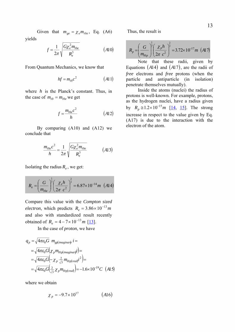
13 Given that eiege mm 0χ= , Eq. (A6) yields
( )1021
30
2
AR
mGf
e
eieχπ
=
From Quantum Mechanics, we know that
( )1120 Acmhf i=
where is the Planck’s constant. Thus, in the case of we get
heii mm 00 =
( )122
0 Ah
cmf ei=
By comparing (A10) and (A12) we conclude that
( )1321
30
220 A
RmG
hcm
e
eieei χπ
=
Isolating the radius , we get: eR
( )141087.62
142
0
32
31
Amch
mGR e
eie
−×=⎟⎠
⎞⎜⎝
⎛⎟⎟⎠
⎞⎜⎜⎝
⎛=
πχ
Compare this value with the Compton sized electron, which predicts and also with standardized result recently obtained of [
mRe131086.3 −×=
mRe131074 −×−= 13].
In the case of proton, we have
( )
( )( )( )( )
( )( ) ( )15106.14
4
4
4
1903
20
203
20
00
0
ACmG
imG
imG
imGq
realpip
realpip
imaginarypip
imaginarygpp
−×−==
=−=
==
==
χπε
χπε
χπε
πε
where we obtain
( )16107.9 17 Ap ×−=χ
Thus, the result is
( )171072.32
172
0
32
31
Amc
hmGR p
pip
−×=⎟⎟⎠
⎞⎜⎜⎝
⎛⎟⎟⎠
⎞⎜⎜⎝
⎛=
π
χ
Note that these radii, given by Equations ( )14A and ( , are the radii of free electrons and free protons (when the particle and antiparticle (in isolation) penetrate themselves mutually).
)17A
Inside the atoms (nuclei) the radius of protons is well-known. For example, protons, as the hydrogen nuclei, have a radius given by [mRp
15102.1 −×≅ 14, 15]. The strong increase in respect to the value given by Eq. (A17) is due to the interaction with the electron of the atom.

14
Appendix B: An Experimental Setup for Testing a GCC with Air Nucleus
~
5 mm
d = 14 mm
Metallic rings
Dielectric tube (Acrylic)
φ = 8 mm
5 mm
10 mm
Rectangular plate
χ
g
g
gg χ=′
Digital Force Gauge ( )NN 01.0;2±
Dielectric tube
Metallic ring d = 14 mm
8 mm
Metallic plate 20 mm
888888
Acrylic plates
GCC

15
DETAILS OF PARTS
5 mm
Metal
5 mm
5 mm
30 mm
20 mm
8 mm
10 mm
12 mm
5 mm
Metal
Acrylic
Metal

16DETAIS OF THE BOX
2 mm
20 mm
26 mm
5 mm
2 mm
20 mm
20mm
26 mm
26 mm
20 mm
20 mm
2 mm
20 mm
5 mm
5 mm
10 mm
Acrylic 3 plates 20mm x 26 mm x 2mm 2 plates 20mm x 20mm x 2mm 2 plates 20mm x 20mm x 1mm (inner plates) 4 plates 20mm x 5mm x 2mm Aluminum 2 plates 20mm x 10mm
1 mm 1 mm

17 References [1] De Aquino, F. (2010) Mathematical Foundations of the Relativistic Theory of Quantum Gravity, Pacific Journal of Science and Technology, 11 (1), pp. 173- 232. [2] Valkengurg, V., (1992) Basic Electricity, Prompt Publications, 1-38. [3] Fischer-Cripps, A., (2004) The electronics companion. CRC Press, p. 13, ISBN 9780750310123. [4] De Aquino, F. (2008) Process and Device for Controlling the Locally the Gravitational Mass and the Gravity Acceleration, BR Patent Number: PI0805046-5, July 31, 2008. [5] De Aquino, F. (2010) Gravity Control by means of Electromagnetic Field through Gas at Ultra-Low Pressure, Pacific Journal of Science and Technology, 11(2) November 2010, pp.178-247, Physics/0701091. [6] Quevedo, C. P. (1977) Eletromagnetismo, McGraw- Hill, p. 270. [7] Halliday, D. and Resnick, R. (1968) Physics, J. Willey & Sons, Portuguese Version, Ed. USP, p.1124. [8] Chalmers, J.A., (1967) Atmospheric Electricity, Pergamon press, Oxford, London; Kamsali, N. et al., (2011) Advanced Air Pollution, chapter 20, DOI: 10.5772/17163, edited by Farhad Nejadkoorki, Publisher: InTech, ISBN 978-953-307-511-2, under CC BY-NC- SA 3.0 license. [9] Kundu, J. et al., (2007) Semiconductor Physics, Quantum Electronics& Optoelectronics, 10, 1, pp.1-3. [10] Alonso, M. and Finn, E. (1967) Fundamental University Physics, Addison-Wesley Co., Portuguese version Ed Edgard Blücher (1972), p. 153. [11] Marshall, S. V. and Skitec, G.G. (1980 ) Electromagnetic Concepts and Applications, Prentice-Hall, NJ, Second Edition, p.287 [12] Chen, D. et al., (1991) Demagnetizing Factors for Cylinders, IEE Transactions on Magnetics, Vol. 27, Number,4, p. 3601. Table V, p. 3610. [13] Mac Gregor. M. H., (1992) The Enigmatic Electron. Boston: Klurer Academic, 1992, pp. 4-5. [14] N.D. Cook (2010). Models of the Atomic Nucleus (2nd ed.). Springer. p. 57 ff.. ISBN 978-3-642-14736-4. [15] K.S. Krane (1987). Introductory Nuclear Physics. Wiley-VCH. ISBN 0-471-80553-X.

Superconducting State generated by Cooper Pairs bound by
Intensified Gravitational Interaction Fran De Aquino
Maranhao State University, Physics Department, S.Luis/MA, Brazil. Copyright © 2012 by Fran De Aquino. All Rights Reserved.
We show that by intensifying the gravitational interaction between electron pairs it is possible to produce pair binding energies on the order of 10−1eV, enough to keep electron’s pairs (Cooper Pairs) at ambient temperatures. By means of this method, metals can be transformed into superconductors at ambient temperature.
Key words: Modified theories of gravity, Theories and models of superconducting state, superconducting materials,
Nonconventional mechanisms. PACS: 04.50.Kd, 74.20.-z, 74.70.-b, 74.20.Mn. 1. Introduction A pair of weakly bound electrons in a superconductor is called Cooper pair; it was first described in 1956 by Leon Cooper [1]. As showed by Cooper, an attraction between electrons in a metal can cause a paired state of electrons to have a lower energy than the Fermi energy, which implies that the pair is bound. In conventional superconductors, this attraction is due to the electron–phonon interaction. The Cooper pair state is responsible for superconductivity, as described in the BCS theory developed by John Bardeen, John Schrieffer and Leon Cooper for which they shared the 1972 Nobel Prize [2]. In spite of Cooper pairing to be a quantum effect the reason for the pairing can be seen from a simplified classical explanation [3]. In order to understand how an attraction between two electrons can occur, it is necessary to consider the interaction with the positive ions lattice of the metal. Usually an electron in a metal behaves as a free particle. Its negative charge causes attraction between the positive ions that make up the rigid lattice of the metal. This attraction distorts the ion lattice, moving the ions slightly toward the electron, increasing the positive charge density of the lattice in the local (See gray glow in Fig.1 (a)). Then, another electron is attracted to the positive charge density (gray glow) created by the first electron distorting the lattice around itself. This attraction can overcome the electrons' repulsion due to their negative charge and create a binding between the two
+ + + + + + + + - + + + + + + + +
(a) + + + + + + + + - + + + + + + + +
(b) + + + + + + + + - - + + + + + + + +
(c) Fig. 1 – Cooper Pair Formation
-

2electrons (See Fig.1 (b)). The electrons can then travel through the lattice as a single entity, known as a Cooper Pair (See Fig.1 (c)). While conventional conduction is resisted by thermal vibrations within the lattice, Cooper Pairs carry the supercurrent relatively unresisted by thermal vibrations. The energy of the pairing interaction is quite weak, of the order of 10−3eV, and thermal energy can easily break the pairs. So only at low temperatures, are a significant number of the electrons in a metal in Cooper pairs. Here is showed that, by intensifying the gravitational interaction * [4] between electrons pairs, it is possible to produce pair binding energies on the order of 10−1eV, enough to keep them paired at ambient temperatures. Thus, by this way, metals at ambient temperature can have a significant number of the electrons in Cooper pairs, transforming such metals in superconductors at ambient temperature. 2. Theory The quantization of gravity showed that the gravitational mass mg and the inertial mass mi are correlated by means of the following factor [4]:
( )111212
00 ⎪⎭
⎪⎬⎫
⎪⎩
⎪⎨⎧
⎥⎥
⎦
⎤
⎢⎢
⎣
⎡−⎟⎟
⎠
⎞⎜⎜⎝
⎛ Δ+−==
cmp
mm
ii
gχ
where is the rest inertial mass of the particle and is the variation in the particle’s kinetic momentum; is the speed of light.
0impΔ
c
When is produced by the absorption of a photon with wavelength
pΔλ , it
is expressed by λhp =Δ . In this case, Eq. (1) becomes * De Aquino, F. (2008) Process and Device for Controlling the Locally the Gravitational Mass and the Gravity Acceleration, BR Patent Number: PI0805046-5, July 31, 2008.
( )21121
1121
20
20
0
⎪⎭
⎪⎬⎫
⎪⎩
⎪⎨⎧
⎥⎥
⎦
⎤
⎢⎢
⎣
⎡−⎟
⎠
⎞⎜⎝
⎛+−=
⎪⎭
⎪⎬⎫
⎪⎩
⎪⎨⎧
⎥⎥
⎦
⎤
⎢⎢
⎣
⎡−⎟
⎠
⎞⎜⎝
⎛+−=
λλ
λcmh
mm i
i
g
where cmh i00 =λ is the DeBroglie wavelength for the particle with rest inertial mass . 0im In general, the momentum variation
pΔ is expressed by tFp Δ=Δ where is the applied force during a time interval
FtΔ . Note
that there is no restriction concerning the nature of the force, i.e., it can be mechanical, electromagnetic, etc. For example, we can look on the momentum variation as due to absorption or emission of electromagnetic energy by the particle.
pΔ
This means that, by means of electromagnetic fields, the gravitational mass can be decreased down to become negative and increased (independently of the inertial mass ). In this way, the gravitational forces can be intensified. Consequently, we can use, for example, oscillating magnetic fields in order to intensify the gravitational interaction between electrons pairs, in order to produce pair binding energies enough to keep them paired at ambient temperatures. We will show that the magnetic field used in this case must have extremely-low frequency (ELF).
im
From Electrodynamics we know that when an electromagnetic wave with frequency and velocity incides on a material with relative permittivity
f c
rε , relative magnetic permeability rμ and electrical conductivity σ , its velocity is reduced to rncv = where is the index of refraction of the material, given by [
rn5]
( ) ( )3112
2 ⎟⎠⎞⎜
⎝⎛ ++== ωεσ
με rrr v
cn

3If ωεσ >> , fπω 2= , Eq. (3) reduces to
( )44 0 f
n rr πε
σμ=
Thus, the wavelength of the incident radiation (See Fig. 2) becomes
( )54mod σμ
πλλfnn
fcfv
rr
====
Fig. 2 – Modified Electromagnetic Wave. The wavelength of the electromagnetic wave can bestrongly reduced, but its frequency remains the same.
v = c v = c/nr
λ = c/f λmod = v/f = c/nr f
nr
If a lamina with thickness equal toξ contains atoms/mn 3, then the number of atoms per area unit is ξn . Thus, if the electromagnetic radiation with frequency
incides on an area of the lamina it reachesf S
ξnS atoms. If it incides on the total area of the lamina, , then the total number of atoms reached by the radiation is
fS
ξfnSN = . The number of atoms per unit of volume, , is given by n
( )60
AN
nρ
=
where is the Avogadro’s number;
kmoleatomsN /1002.6 260 ×=
ρ is the matter density of the lamina (in kg/m3) and A is the molar mass(kg/kmole). When an electromagnetic wave incides on the lamina, it strikes front atoms, where
fN( ) mff SnN φ≅ , mφ is the “diameter” of
the atom. Thus, the electromagnetic wave incides effectively on an area , where mf SNS=
241
mmS πφ= is the cross section area of one atom. After these collisions, it carries out with the other atoms (See Fig.3).
collisionsn
Fig. 3 – Collisions inside the lamina.
atom Sm
Wave
Thus, the total number of collisions in the volume ξS is
( )( )7ξ
φξφ
Sn
SnSnSnnNN
m
mmlmlcollisionsfcollisions
=
=−+=+=
The power density, , of the radiation on the lamina can be expressed by
D
( )8mf SN
PSPD ==
We can express the total mean number of collisions in each atom, , by means of the following equation
1n
( )91 NNn
n collisionsphotonstotal=
Since in each collision a momentum λh is transferred to the atom, then the total momentum transferred to the lamina will be
( ) λhNnp 1=Δ . Therefore, in accordance with Eq. (1), we can write that
( )
( )( )
( )101121
1121
20
20
10
⎪⎭
⎪⎬⎫
⎪⎩
⎪⎨⎧
⎥⎥
⎦
⎤
⎢⎢
⎣
⎡−⎥
⎦
⎤⎢⎣
⎡+−=
=⎪⎭
⎪⎬⎫
⎪⎩
⎪⎨⎧
⎥⎥
⎦
⎤
⎢⎢
⎣
⎡−⎥
⎦
⎤⎢⎣
⎡+−=
λλ
λλ
collisionsphotonstotal
li
lg
Nn
Nnmm

4Since Eq. (7) gives ξSnN lcollisions = , we get
( ) (112 ξSnhfPNn lcollisionsphotonstotal ⎟⎟
⎠
⎞⎜⎜⎝
⎛= )
Substitution of Eq. (11) into Eq. (10) yields
( )
( )( ) ( )121121
2
02
0 ⎪⎭
⎪⎬⎫
⎪⎩
⎪⎨⎧
⎥⎥⎥
⎦
⎤
⎢⎢⎢
⎣
⎡−⎥
⎦
⎤⎢⎣
⎡⎟⎟⎠
⎞⎜⎜⎝
⎛+−=
λλ
ξSnhfP
mm
lli
lg
Substitution of P given by Eq. (8) into Eq. (12) gives
( )
( ) ( )( )1311121
2
02
0 ⎪⎭
⎪⎬
⎫
⎪⎩
⎪⎨
⎧
⎥⎥⎥
⎦
⎤
⎢⎢⎢
⎣
⎡−
⎥⎥⎦
⎤
⎢⎢⎣
⎡⎟⎟⎠
⎞⎜⎜⎝
⎛⎟⎟⎠
⎞⎜⎜⎝
⎛+−=
λξcm
Snf
DSNmm
li
lmf
li
lg
Substitution of ( ) mflf SnN φ≅ and mf SNS = into Eq. (13) results
( )
( ) ( )( )1411121
2
20
2223
0 ⎪⎭
⎪⎬
⎫
⎪⎩
⎪⎨
⎧
⎥⎥⎥
⎦
⎤
⎢⎢⎢
⎣
⎡−
⎥⎥⎦
⎤
⎢⎢⎣
⎡⎟⎟⎠
⎞⎜⎜⎝
⎛+−=
λξφ
cfmDSSn
mm
li
mmfl
li
lg
where ( ) ( ) ( )llli Vm ρ=0 . Now, considering that the lamina is inside an ELF electromagnetic field with E and B , then we can write that [6]
( ) ( )152 0
2
cEn
D lr
μ=
Substitution of Eq. (15) into Eq. (14) gives
( )
( )
( )
( )( )1611
2121
2
2200
22223
0 ⎪⎭
⎪⎬
⎫
⎪⎩
⎪⎨
⎧
⎥⎥⎥
⎦
⎤
⎢⎢⎢
⎣
⎡−
⎥⎥⎦
⎤
⎢⎢⎣
⎡⎟⎟⎠
⎞⎜⎜⎝
⎛+−=
λμξφfcmESSnn
mm
li
mmfllr
li
lg
Note that tEE m ωsin= .The average value for 2E is equal to 2
21
mE because E varies sinusoidaly ( is the maximum value
formE
E ). On the other hand, 2mrms EE = . Consequently we can replace 4E for .
Thus, for
4rmsE
modλλ = , the equation above can be rewritten as follows
( )
( )
( )
( )( )1711
2121
2
mod22
00
22223
0 ⎪⎭
⎪⎬
⎫
⎪⎩
⎪⎨
⎧
⎥⎥⎥
⎦
⎤
⎢⎢⎢
⎣
⎡−
⎥⎥⎦
⎤
⎢⎢⎣
⎡⎟⎟⎠
⎞⎜⎜⎝
⎛+−=
λμξφfcmESSnn
mm
li
rmsmmfllr
li
lg
Electrodynamics tells us that
( )( ) rmslrrmsrms BncvBE == . Substitution of this expression into Eq. (17) gives
( )
( ) ( ) ( )( )181
4121 22
mod42
020
424446
0 ⎪⎭
⎪⎬⎫
⎪⎩
⎪⎨⎧
⎥⎥⎦
⎤
⎢⎢⎣
⎡−+−==
lrli
rmsmmfl
li
lg
nfmBSSn
mm
λμξφ
χ
Since ( )lrnλλ =mod then Eq. (18) can be rewritten in the following form
( )
( ) ( )( )191
4121 222
020
424446
0 ⎪⎭
⎪⎬⎫
⎪⎩
⎪⎨⎧
⎥⎥⎦
⎤
⎢⎢⎣
⎡−+−==
fcmBSSn
mm
li
rmsmmfl
li
lg
μξφ
χ
In order to calculate the expressions of
Beχ for the particular case of a free electron inside a conductor, subjected to an external magnetic field with frequency , we must consider the interaction with the positive ions that make up the rigid lattice of the metal.
rmsB f
The negative charge of the free electron causes attraction between the positive ions lattice of the metal. This attraction distorts the ion lattice, moving the ions slightly toward the electron, increasing the positive charge density of the lattice in the local (See gray glow in Fig.1 (a)). Then, another electron is attracted to the positive charge density (gray glow) created by the first electron distorting the lattice around itself, which produces a strong attraction upon the electron deforming its surface as showed in Fig. 4. Under these circumstances, the volume of the electron does not vary, but its external surface is strongly increased, becomes equivalent to the external area of a sphere with radius ( is the radius of the free electron out of the ions “gage”
exe rr >> er
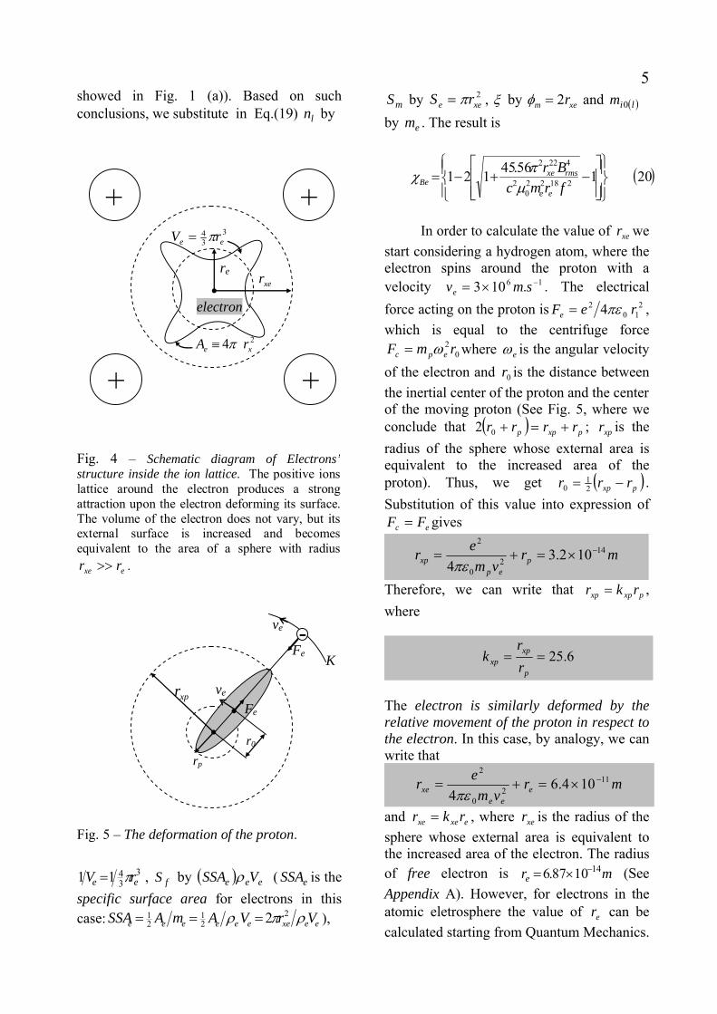
5showed in Fig. 1 (a)). Based on such conclusions, we substitute in Eq.(19) by ln Fig. 4 – Schematic diagram of Electrons’structure inside the ion lattice. The positive ionslattice around the electron produces a strongattraction upon the electron deforming its surface.The volume of the electron does not vary, but itsexternal surface is increased and becomesequivalent to the area of a sphere with radius
exe rr >> .
re
24 xe rA π≡
334
ee rV π=
electron
++
++
xer
Fig. 5 – The deformation of the proton.
xpr
-
Fe
Fe
ve
K
ve
rp
r0
33411 ee rV π= , by ( )fS eee VSSA ρ ( is the
specific surface area for electrons in this case:
eSSA
eexeeeeeeeSSA = VrVAmA ρπρ 221
21 2== ),
by , mS 2xee rS π= ξ by xem r2=φ and
by . The result is ( )lim 0
em
( )20156.45121 218220
2
4222
⎪⎭
⎪⎬⎫
⎪⎩
⎪⎨⎧
⎥⎥⎦
⎤
⎢⎢⎣
⎡−+−=
frmcBr
ee
rmsxeBe μ
πχ
In order to calculate the value of we start considering a hydrogen atom, where the electron spins around the proton with a velocity . The electrical force acting on the proton is
xer
16 .103 −×= smve2
102 4 reFe πε= ,
which is equal to the centrifuge force where 0
2rmF epc ω= eω is the angular velocity of the electron and is the distance between the inertial center of the proton and the center
0r
of the moving proton (See Fig. 5, where we conclude that ( ) pxpp rrrr +=+02 ; is the radius of the sphere whose external area is equivalent to the increased area of the proton). Thus, we get
xpr
( )pxp rrr −= 21
0 . Substitution of this value into expression of
ec FF = gives
mrvm
er pep
xp14
20
2
102.34
−×=+=πε
Therefore, we can write that pxpxp rkr = , where
6.25==p
xpxp r
rk
The electron is similarly deformed by the relative movement of the proton in respect to the electron. In this case, by analogy, we can write that
mrvm
er eee
xe11
20
2
104.64
−×=+=πε
and exexe rkr = , where is the radius of the sphere whose external area is equivalent to the increased area of the electron. The radius of free electron is
xer
mre141087.6 −×= (See
Appendix A). However, for electrons in the atomic eletrosphere the value of can be calculated starting from Quantum Mechanics.
er

6The wave packet that describes the electron satisfies an uncertainty principle ( )h2
1≥ΔΔ xp , where and kp Δ=Δ h kΔ is the approximate extension of the wave packet. Thus, we can write that ( 2
1≥ΔΔ xk ). For the ``square'' packet the full width in is k
02 λπ=Δk ( cmh e=0λ is the average wavelength). The width in x is a little harder to define, but, lets use the first node in the probability found at ( ) πλπ =22 0 x or
0λ=x . So, the width of the wave packet is twice this or 02λ=Δx . Obviously, cannot be greater than
er2 xΔ , i.e., must be
smaller and close to er
mcmh e12
0 1043.2 −×==λ . Then, assuming that , we get
mre12104.2 −×≅
6.26==e
xexe r
rk
Note that . In the case of electrons inside the ion lattice (See Fig. 4), we can note that, in spite of the electron speed be null, the deformations are similar, in such way that, in this case, we can take the values above.
xpxe kk ≅
ev
Substitution of these values into Eq. (20) gives
( )211108.2121
1108.3121
2
442
2
442257
⎪⎭
⎪⎬⎫
⎪⎩
⎪⎨⎧
⎥⎥⎦
⎤
⎢⎢⎣
⎡−×+−=
=⎪⎭
⎪⎬⎫
⎪⎩
⎪⎨⎧
⎥⎥⎦
⎤
⎢⎢⎣
⎡−×+−=
fB
fBrk
rms
rmsexeBeχ
Similarly, in the case of proton and neutron we can write that
( )22156.45
121 2220
2
44222
⎪⎭
⎪⎬⎫
⎪⎩
⎪⎨⎧
⎥⎥⎦
⎤
⎢⎢⎣
⎡−+−=
fmcBrk
p
rmspxpBp μ
πχ
( )23156.45
1212222
0
442
⎪⎭
⎪⎬⎫
⎪⎩
⎪⎨⎧
⎥⎥⎦
⎤
⎢⎢⎣
⎡−+−=
fcmBr
n
rmsnBn μ
πχ
In the case of the neutron, due to its electric charge be null. The radius of protons inside the atoms (nuclei) is
1=xnk
mrp15102.1 −×=
[7,8], pn rr ≅ , then we obtain from Eqs. (22) and (23) following expressions:
( )241102.2121 2
422
⎪⎭
⎪⎬⎫
⎪⎩
⎪⎨⎧
⎥⎥⎦
⎤
⎢⎢⎣
⎡−×+−=
fBrms
Bpχ
( )af
BrmsBn 2411035.2121 2
49
⎪⎭
⎪⎬⎫
⎪⎩
⎪⎨⎧
⎥⎥⎦
⎤
⎢⎢⎣
⎡−×+−= −χ
Since eBege mm χ= , pBpgp mm χ= and
nBngn mm χ= , it easy to see, by means of Eqs. (21), (24) and (24a), that is much greater than and . This means that, in the calculation of the gravitational force
(between the positive ions + electron and the external electron), we can
gem
gpm gpm
gFdisregard the
effects of the gravitational masses of the ions. Thus, the expression of reduces to the expression of the gravitational forces between the two electrons, i.e.,
gF
( )252
22
2
2
rm
Grm
GF eBe
geg χ−=−=
For the creation of the Cooper Pairs must overcome the electrons' repulsion due to their negative charge
gF
( )20
2 4 re πε . Thus, we must have 0
222 4πεχ eGmeBe > or
( ) ( )261024
21
0
×−=>G
me eBe
πεχ
For the Cooper Pairs not be destructed by the thermal vibrations due to the temperature T , we must have kTrGmeBe >22χ whence we conclude that rGmT eBe
22χ< . Consequently, the transition temperature, , can be expressed by the following expression
cT

7
( )2722
ξχ
kGm
T eBec =
where ξ is the size of the Cooper pair, which is given by the coherence length of the Cooper-pair wavefunction. It is known that the coherence length is typically 1000 Å (though it can be as small as 30Å in the copper oxides). The coherence length of the Cooper-pair in Aluminum superconductor is quite large ( [micron1≅ξ 9]). Substitution of this value into Eq. (27) gives
( )28104 242BecT χ−×=
For we obtain ( CKTc °= 127~400 )
( )29101 22×−=Beχ By comparing (29) with (26), we can conclude that this value of eχ is sufficient for the creation of the Cooper Pairs, and also in order that they do not be destructed by the thermal vibrations due to the temperature up to . ( )CKTc °= 127~400 In order to calculate the intensity of the magnetic field with frequency , necessary to produce the value given by Eq.(29), it is necessary the substitution of Eq. (29) into Eq. (21). Thus, we get
mB f
( )301011108.2121 222
442 ×−≅
⎪⎭
⎪⎬⎫
⎪⎩
⎪⎨⎧
⎥⎥⎦
⎤
⎢⎢⎣
⎡−×+−
fBrms
For Hzf 2= the value of is rmsB
TBrms 3> Therefore, if a magnetic field with frequency
Hzf 2= and intensity TBrms 3> † is applied upon an Aluminum wire it becomes superconductor at ambient temperature ( ( CKTc °= 127~400 )
). Note that the
† Modern magnetic resonance imaging systems work with magnetic fields up to 8T [10, 11].
magnetic field is used only during a time interval sufficient to transform the Aluminum into a superconductor. This means that the process is a some sort of “magnetization” that transforms a conductor into a “permanent” superconductor. After the “magnetization” the magnetic field can be turned off, similarly to the case of “magnetization” that transforms an iron rod into a “permanent” magnet.

8
Appendix A: The “Geometrical Radii” of Electron and Proton It is known that the frequency of oscillation of a simple spring oscillator is
( )121 A
mKf
π=
where is the inertial mass attached to the spring and
mK is the spring constant (in
N·m−1). In this case, the restoring force exerted by the spring is linear and given by
( )2AKxF −= where x is the displacement from the equilibrium position. Now, consider the gravitational force: For example, above the surface of the Earth, the force follows the familiar Newtonian function, i.e., 2rmGMF gg⊕−= , where
is the mass of Earth, is the gravitational mass of a particle and
⊕gM gmr is the
distance between the centers. Below Earth’s surface the force is linear and given by
( )33
ArR
mGMF gg
⊕
⊕−=
where is the radius of Earth. ⊕R By comparing (A3) with (A2) we obtain
( )43
Axr
R
GM
mK
mK g
g⎟⎠⎞
⎜⎝⎛==
⊕
⊕
χ
Making , and substituting (A4) into (A1) gives
⊕== Rrx
( )521
3 AR
GMf g
⊕
⊕=χ
π In the case of an electron and a positron, we substitute by , ⊕gM gem χ by eχ and by
, where is the radius of electron (or positron). Thus, Eq. (A5) becomes
⊕R
eR eR
( )621
3A
R
Gmf
e
egeχπ
=
The value of eχ varies with the density of energy [4]. When the electron and the positron are distant from each other and the local density of energy is small, the value of
eχ becomes very close to 1. However, when the electron and the positron are penetrating one another, the energy densities in each particle become very strong due to the proximity of their electrical charges e and, consequently, the value of eχ strongly increases. In order to calculate the value of
eχ under these conditions ( ), we start from the expression of correlation between electric charge and gravitational mass, obtained in a previous work [
eRrx ==
q4]:
( ) ( )74 0 AimGq imaginarygπε=
where is the imaginary
gravitational mass, and (imaginarygm )
1−=i . In the case of electron, Eq. (A7) gives
( )
( )( )( )( )
( )( ) ( )8106.14
4
4
4
1903
20
203
20
00
0
ACmG
imG
imG
imGq
realeie
realeie
imaginaryeie
imaginarygee
−×−==
=−=
==
==
χπε
χπε
χπε
πε
where we obtain
( )9108.1 21 Ae ×−=χ This is therefore, the value of eχ increased by the strong density of energy produced by the electrical charges of the two particles, under previously mentioned conditions.
e
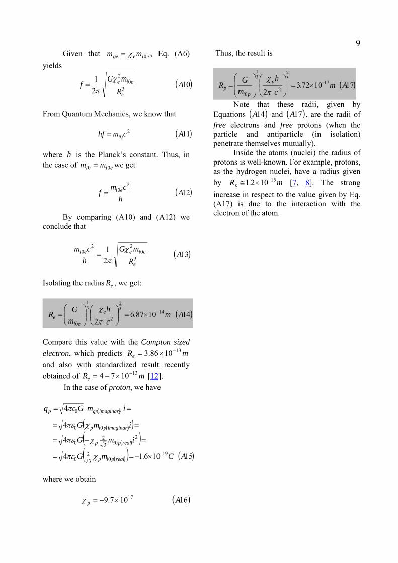
9 Given that eiege mm 0χ= , Eq. (A6) yields
( )1021
30
2
AR
mGf
e
eieχπ
=
From Quantum Mechanics, we know that
( )1120 Acmhf i=
where is the Planck’s constant. Thus, in the case of we get
heii mm 00 =
( )122
0 Ah
cmf ei=
By comparing (A10) and (A12) we conclude that
( )1321
30
220 A
RmG
hcm
e
eieei χπ
=
Isolating the radius , we get: eR
( )141087.62
142
0
32
31
Amch
mGR e
eie
−×=⎟⎠
⎞⎜⎝
⎛⎟⎟⎠
⎞⎜⎜⎝
⎛=
πχ
Compare this value with the Compton sized electron, which predicts and also with standardized result recently obtained of [
mRe131086.3 −×=
mRe131074 −×−= 12].
In the case of proton, we have
( )
( )( )( )( )
( )( ) ( )15106.14
4
4
4
1903
20
203
20
00
0
ACmG
imG
imG
imGq
realpip
realpip
imaginarypip
imaginarygpp
−×−==
=−=
==
==
χπε
χπε
χπε
πε
where we obtain
( )16107.9 17 Ap ×−=χ
Thus, the result is
( )171072.32
172
0
32
31
Amc
hmGR p
pip
−×=⎟⎟⎠
⎞⎜⎜⎝
⎛⎟⎟⎠
⎞⎜⎜⎝
⎛=
π
χ
Note that these radii, given by Equations ( )14A and ( , are the radii of free electrons and free protons (when the particle and antiparticle (in isolation) penetrate themselves mutually).
)17A
Inside the atoms (nuclei) the radius of protons is well-known. For example, protons, as the hydrogen nuclei, have a radius given by [mRp
15102.1 −×≅ 7, 8]. The strong increase in respect to the value given by Eq. (A17) is due to the interaction with the electron of the atom.

10References [1] Cooper, Leon N. (1956). "Bound electron pairs in a degenerate Fermi gas". Physical Review 104 (4): 1189– 1190. [2] Bardeen, J.; Cooper, L. N., Schrieffer, J. R. (April 1957). "Microscopic Theory of Superconductivity". Physical Review 106 (1): 162–164. Bardeen, J.; Cooper, L. N.; Schrieffer, J. R. (December 1957). "Theory of Superconductivity". Physical Review 108 (5): 1175– 1204. [3] Nave, Carl R. (2006). "Cooper Pairs". Hyperphysics. Dept. of Physics and Astronomy, Georgia State Univ.. Retrieved 2008-07-24; Kadin, Alan M. (2005). "Spatial Structure of the Cooper Pair". Journal of Superconductivity and Novel Magnetism 20 (4): 285. [4] De Aquino, F. (2010) Mathematical Foundations of the Relativistic Theory of Quantum Gravity, Pacific Journal of Science and Technology, 11 (1), pp. 173- 232. [5] Quevedo, C. P. (1977) Eletromagnetismo, McGraw- Hill, p. 270. [6] Halliday, D. and Resnick, R. (1968) Physics, J. Willey & Sons, Portuguese Version, Ed. USP, p.1124. [7] N.D. Cook (2010). Models of the Atomic Nucleus (2nd ed.). Springer. p. 57 ff.. ISBN 978-3-642-14736-4. [8] K.S. Krane (1987). Introductory Nuclear Physics. Wiley-VCH. ISBN 0-471-80553-X. [9] Fujiki, H. et al. Nonlinear resistivity in the mixed state of superconducting aluminum films. Physica C 297, 309 (1998). [10] Smith, Hans-Jørgen. "Magnetic resonance imaging". Medcyclopaedia Textbook of Radiology. GE Healthcare. Retrieved 2007-03-26.
[11]Orenstein, Beth W. (2006-02-16). "Ultra High-Field MRI — The Pull of Big Magnets". Radiology Today 7 (3): pp. 10. Archived from the original on March 15, 2008. Retrieved 2008-07-10 [12] Mac Gregor. M. H., (1992) The Enigmatic Electron. Boston: Klurer Academic, 1992, pp. 4-5.

Gravitational Separator of Isotopes
Fran De Aquino Maranhao State University, Physics Department, S.Luis/MA, Brazil.
Copyright © 2012 by Fran De Aquino. All Rights Reserved. In this work we show a gravitational separator of isotopes which can be much more effective than those used in the conventional processes of isotopes separation. It is based on intensification of the gravitational acceleration, and can generate accelerations tens of times more intense than those generated in the most powerful centrifuges used for Uranium enrichment.
Key words: Modified theories of gravity, Isotope separation and enrichment, Nonconventional mechanisms. PACS: 04.50.Kd, 28.60.+ s, 74.20.Mn. 1. Introduction A conventional gas centrifuge is basically a cylinder that spins around its central axis with ultra-high angular speed while a gas is injected inside it. Under these conditions, the heavier molecules of the gas move towards the cylinder wall and the lighter ones remain close to the center. In addition, if one creates a thermal gradient in a perpendicular direction by keeping the top of the rotating column cool and the bottom hot, the resulting convection current carries the lighter molecules to the top while the heavier ones settle at the bottom, from which they can be continuously withdrawn. An important use of gas centrifuges is for the separation of uranium-235 from uranium-238. As a first step, the uranium metal is turned into a gas (uranium hexafluoride, UF6). Next, the UF6 is injected inside a gas centrifuge, which spins at about 100.000 rpm in order to produce a strong centrifugal force upon the UF6 molecules. Thus, the UF6 is separated by the difference in molecular weight between 235UF6 and 238UF6 [1]. The heavier molecules of the gas (238UF6) move towards the cylinder wall and the lighter ones (235UF6) remain close to the center. The convection current carries the lighter molecules (235UF6) to the top while the heavier ones (238UF6) settle at the bottom. However, the gas at the top is not composed totally by 235UF6 it contains also 238UF6, in such way that we can say that the gas at the top is only a gas rich in 235U. In practice, several of such centrifuges are connected in
series. A cascade of identical stages produces successively higher concentrations of 235U. This process is called Uranium enrichment. Uranium occurs naturally as two isotopes: 99.3% is Uranium-238 and 0.7% is Uranium-235. Their atoms are identical except for the number of neutrons in the nucleus: Uranium-238 has three more and this makes it less able to fission. Uranium enrichment is used to increase the percentage of the fissile U-235. Nuclear reactors typically require uranium fuel enriched to about 3% to 5% U-235. Nuclear bombs typically use ‘Highly Enriched Uranium’, enriched to 90% U-235 [2]. In order to extract the 235U from the 235UF6 it is necessary to add Calcium. The Calcium reacts with the gas producing a salt and pure 235U. The conventional gas centrifuges used in the Uranium enrichment are very expensive, and they consume much energy during the process. Here, it is proposed a new type of separator of isotopes based on the intensification the gravitational acceleration * [3]. It can generate accelerations tens times more intense than those generated in the most powerful centrifuges used for Uranium enrichment. * De Aquino, F. (2008) Process and Device for Controlling the Locally the Gravitational Mass and the Gravity Acceleration, BR Patent Number: PI0805046-5, July 31, 2008.

22. Theory From the quantization of gravity it follows that the gravitational mass mg and the inertial mass mi are correlated by means of the following factor [3]:
( )111212
00 ⎪⎭
⎪⎬⎫
⎪⎩
⎪⎨⎧
⎥⎥
⎦
⎤
⎢⎢
⎣
⎡−⎟⎟
⎠
⎞⎜⎜⎝
⎛ Δ+−==
cmp
mm
ii
gχ
where is the rest inertial mass of the particle and is the variation in the particle’s kinetic momentum; is the speed of light.
0impΔ
c
When is produced by the absorption of a photon with wavelength
pΔλ , it
is expressed by λhp =Δ . In this case, Eq. (1) becomes
( )21121
1121
20
20
0
⎪⎭
⎪⎬⎫
⎪⎩
⎪⎨⎧
⎥⎥
⎦
⎤
⎢⎢
⎣
⎡−⎟
⎠
⎞⎜⎝
⎛+−=
⎪⎭
⎪⎬⎫
⎪⎩
⎪⎨⎧
⎥⎥
⎦
⎤
⎢⎢
⎣
⎡−⎟
⎠
⎞⎜⎝
⎛+−=
λλ
λcmh
mm i
i
g
where cmh i00 =λ is the De Broglie wavelength for the particle with rest inertial mass . 0im It has been shown that there is an additional effect - Gravitational Shielding effect - produced by a substance whose gravitational mass was reduced or made negative [4]. The effect extends beyond substance (gravitational shielding) , up to a certain distance from it (along the central axis of gravitational shielding). This effect shows that in this region the gravity acceleration, , is reduced at the same proportion, i.e.,
1ggg
11 χ= where
01 ig mm=χ and g is the gravity acceleration before the gravitational shielding). Consequently, after a second gravitational shielding, the gravity will be given by ggg
21122 χχχ == , where 2
χ is the value of the ratio 0ig mm for the second gravitational shielding. In a generalized way, we can write that after the nth gravitational shielding the gravity, , will be given by ng
( )3...
321gg
nn χχχχ=
This possibility shows that, by means of a battery of gravitational shieldings, we can make particles acquire enormous accelerations. From Electrodynamics we know that when an electromagnetic wave with frequency and velocity incides on a material with relative permittivity
f c
rε , relative magnetic permeability rμ and electrical conductivity σ , its velocity is reduced to rncv = where is the index of refraction of the material, given by [
rn5]
( ) ( )4112
2 ⎟⎠⎞⎜
⎝⎛ ++== ωεσ
με rrr v
cn
If ωεσ >> f, π2ω = , Eq. (4) reduces to
( )54 0 f
n rr πε
σμ=
Thus, the wavelength of the incident radiation (See Fig. 1) becomes
( )64mod σμ
πλλfnn
fcfv
rr====
Fig. 1 – Modified Electromagnetic Wave. The wavelength of the electromagnetic wave can bestrongly reduced, but its frequency remains the same.
v = c v = c/nr
λ = c/f λmod = v/f = c/nr f
nr
If a lamina with thickness equal toξ contains atoms/mn 3, then the number of atoms per area unit is ξn . Thus, if the electromagnetic radiation with frequency
incides on an area of the lamina it reachesf S
ξnS atoms. If it incides on the total area of the lamina, , then the total number of atoms reached by the radiation is
fS
ξfnSN = . The number of atoms per unit of volume, , is given by n

3
( )70
AN
nρ
=
where is the Avogadro’s number;
kmoleatomsN /1002.6 260 ×=
ρ is the matter density of the lamina (in kg/m3) and A is the molar mass(kg/kmole). When an electromagnetic wave incides on the lamina, it strikes front atoms, where
fN( ) mff SnN φ≅ , mφ is the “diameter” of
the atom. Thus, the electromagnetic wave incides effectively on an area , where mf SNS=
241
mmS πφ= is the cross section area of one atom. After these collisions, it carries out with the other atoms (See Fig.2).
collisionsn
Fig. 2 – Collisions inside the lamina.
atom Sm
Wave
Thus, the total number of collisions in the volume ξS is
( )( )8ξ
φξφ
Sn
SnSnSnnNN
m
mmlmlcollisionsfcollisions
=
=−+=+=
The power density, , of the radiation on the lamina can be expressed by
D
( )9mf SN
PSPD ==
We can express the total mean number of collisions in each atom, , by means of the following equation
1n
( )101 NNn
n collisionsphotonstotal=
Since in each collision a momentum λh is transferred to the atom, then the total momentum transferred to the lamina will be
( ) λhNnp 1=Δ . Therefore, in accordance with Eq. (1), we can write that
( )
( )( )
( )111121
1121
20
20
10
⎪⎭
⎪⎬⎫
⎪⎩
⎪⎨⎧
⎥⎥
⎦
⎤
⎢⎢
⎣
⎡−⎥
⎦
⎤⎢⎣
⎡+−=
=⎪⎭
⎪⎬⎫
⎪⎩
⎪⎨⎧
⎥⎥
⎦
⎤
⎢⎢
⎣
⎡−⎥
⎦
⎤⎢⎣
⎡+−=
λλ
λλ
collisionsphotonstotal
li
lg
Nn
Nnmm
Since Eq. (8) gives ξSnN lcollisions = , we get
( ) (122 ξSnhfPNn lcollisionsphotonstotal ⎟⎟
⎠
⎞⎜⎜⎝
⎛= )
Substitution of Eq. (12) into Eq. (11) yields
( )
( )( ) ( )131121
20
20 ⎪
⎭
⎪⎬
⎫
⎪⎩
⎪⎨
⎧
⎥⎥⎥
⎦
⎤
⎢⎢⎢
⎣
⎡−
⎥⎥⎦
⎤
⎢⎢⎣
⎡⎟⎟⎠
⎞⎜⎜⎝
⎛+−=
λλξSn
hfP
mm
lli
lg
Substitution of P given by Eq. (9) into Eq. (13) gives
( )
( ) ( )( )1411121
2
02
0 ⎪⎭
⎪⎬
⎫
⎪⎩
⎪⎨
⎧
⎥⎥⎥
⎦
⎤
⎢⎢⎢
⎣
⎡−
⎥⎥⎦
⎤
⎢⎢⎣
⎡⎟⎟⎠
⎞⎜⎜⎝
⎛⎟⎟⎠
⎞⎜⎜⎝
⎛+−=
λξcm
Snf
DSNmm
li
lmf
li
lg
Substitution of ( ) mflf SnN φ≅ and mf SNS = into Eq. (14) results
( )
( ) ( )( )1511121
2
20
2223
0 ⎪⎭
⎪⎬
⎫
⎪⎩
⎪⎨
⎧
⎥⎥⎥
⎦
⎤
⎢⎢⎢
⎣
⎡−
⎥⎥⎦
⎤
⎢⎢⎣
⎡
⎟⎟⎠
⎞⎜⎜⎝
⎛+−=
λξφ
cfmDSSn
mm
li
mmfl
li
lg
where ( ) ( ) ( )llli Vm ρ=0 . Now, considering that the lamina is inside an ELF electromagnetic field with E and B , then we can write that [6]
( ) ( )162 0
2
cEn
D lr
μ=

4Substitution of Eq. (16) into Eq. (15) gives
( )
( )
( )
( )( )1711
2121
2
2200
22223
0 ⎪⎭
⎪⎬
⎫
⎪⎩
⎪⎨
⎧
⎥⎥⎥
⎦
⎤
⎢⎢⎢
⎣
⎡−
⎥⎥⎦
⎤
⎢⎢⎣
⎡
⎟⎟⎠
⎞⎜⎜⎝
⎛+−=
λμ
ξφ
fcmESSnn
mm
li
mmfllr
li
lg
In the case in which the area is just the area of the cross-section of the lamina
fS( )αS ,
we obtain from Eq. (17), considering that ( ) ( ) ξρ αSm lli =0 , the following expression
( )
( )
( )
( )( )1811
2121
2
220
2223
0 ⎪⎭
⎪⎬
⎫
⎪⎩
⎪⎨
⎧
⎥⎥⎥
⎦
⎤
⎢⎢⎢
⎣
⎡−
⎥⎥⎦
⎤
⎢⎢⎣
⎡
⎟⎟⎠
⎞⎜⎜⎝
⎛+−=
λρμ
φα
fcESSnn
mm
l
mmllr
li
lg
According to Eq. (6) we have
( )( )19
fnc
fv
lr=== modλλ
Substitution of Eq. (19) into Eq. (18) gives
( )( )
( )
( )( )201
4121 2622
0
444264
0 ⎪⎭
⎪⎬
⎫
⎪⎩
⎪⎨
⎧
⎥⎥⎥
⎦
⎤
⎢⎢⎢
⎣
⎡
−+−=fc
ESSnn
mm
l
mmllr
li
lg
ρμ
φα
Note that tEE m ωsin= .The average value for 2E is equal to 2
21
mE because E varies sinusoidaly ( is the maximum value
formE
E ). On the other hand, 2mrms EE = . Consequently we can replace 4E for , and the equation above can be rewritten as follows
4rmsE
( )
( )
( )
( )( )211
4121 2622
0
4442640
⎪⎭
⎪⎬
⎫
⎪⎩
⎪⎨
⎧
⎥⎥⎥
⎦
⎤
⎢⎢⎢
⎣
⎡
−+−=
==
fc
ESSnn
m
m
l
rmsmmllr
li
lg
ρμ
φ
χ
α
Now consider the system shown in Fig.3. It was originally designed to convert Gravitational Energy directly into Electrical Energy [7]. Here, it works as Separator of Isotopes. These systems are basically similar, except in the core. The core of the original
system has been replaced by the one shown in Fig.3 and Fig.4 (detailed). Inside the Gravitational Separator of Isotopes there is a dielectric tube ( 1≅rε ) with the following characteristics: mm60=α ,
232 1083.24 mS −×== παα . Inside the tube there is an Aluminum sphere with 30mm radius and mass kgM gs 30536.0= . The tube is filled with air at ambient temperature and 1atm. Thus, inside the tube, the air density is
( )22.2.1 3−= mkgairρ The number of atoms of air (Nitrogen) per unit of volume, , according to Eq.(7), is given by
airn
( )23/1016.5 3250 matomsA
Nn
N
airair ×==
ρ
The parallel metallic plates (p), shown in Fig.3 are subjected to different drop voltages. The two sets of plates (D), placed on the extremes of the tube, are subjected to ( ) VV rmsD 2216.= at Hzf 1= , while the central
set of plates (A) is subjected to ( ) VV rmsA 98191.= at Hzf 1= . Since mmd 98= ,
then the intensity of the electric field, which passes through the 36 cylindrical air laminas (each one with 5mm thickness) of the two sets (D), is
( ) ( ) mVdVE rmsDrmsD /.53165==
and the intensity of the electric field, which passes through the 7 cylindrical air laminas of the central set (A), is given by
( ) ( ) mVdVE rmsArmsA /. 3109591 ×==
Note that the metallic rings (5mm thickness) are positioned in such way to block the electric field out of the cylindrical air laminas. The objective is to turn each one of these laminas into a Gravity Control Cells (GCC) [4]. Thus, the system shown in Fig. 3 has 3 sets of GCC. Two with 18 GCC each, and one with 7 GCC. The two sets with 18
5GCC each are positioned at the extremes of the tube (D). They work as gravitational decelerator while the other set with 7 GCC (A) works as a gravitational accelerator, intensifying the gravity acceleration produced by the mass of the Aluminum sphere. According to Eq. (3), this gravity, after the GCC becomes
gsM
th7 20
77 rGMg gsχ= ,
where ( ) ( )lilg mm=χ given by Eq. (21) and mmr 350 = is the distance between the
center of the Aluminum sphere and the surface of the first GCC of the set (A). The objective of the sets (D), with 18 GCC each, is to reduce strongly the value of the external gravity along the axis of the tube. In this case, the value of the external gravity, , is reduced by the factor ,
where extg extd g18χ
210−=dχ . For example, if the base BS of the system is positioned on the Earth surface, then is reduced
to and, after the set A, it is increased
by . Since the system is designed for
2/81.9 smgext =
extd g18χ7χ
5.308−=χ (See Eq. (26)), then the gravity acceleration on the sphere becomes
. This value is much
smaller than
218187 /106.2 smgextd−×=χχ
282 /1026.2 smrGMg sgssphere−×== .
Note that there is a uniform magnetic field, B , through the core of the Gravitational Separator of Isotopes (a cylindrical Dielectric Chamber with 60mm external diameter; 50mm internal diameter and 100mm height). The values of χ and dχ , according to Eq. (21) are given by
( ) ( )
( )
( ) ( )241106451121
14
121
49
26220
444264
⎭⎬⎫
⎩⎨⎧
⎥⎦⎤
⎢⎣⎡ −×+−=
=⎪⎭
⎪⎬
⎫
⎪⎩
⎪⎨
⎧
⎥⎥⎥
⎦
⎤
⎢⎢⎢
⎣
⎡
−+−=
−rmsA
l
rmsAmmllr
E
fc
ESSnn
.
ρμ
φχ
α
( ) ( )
( )
( ) ( )251106451121
14
121
49
26220
444264
⎭⎬⎫
⎩⎨⎧
⎥⎦⎤
⎢⎣⎡ −×+−=
=⎪⎭
⎪⎬
⎫
⎪⎩
⎪⎨
⎧
⎥⎥⎥
⎦
⎤
⎢⎢⎢
⎣
⎡
−+−=
−rmsD
l
rmsDmmllrd
E
fc
ESSnn
.
ρμ
φχ
α
where ( ) 1≅= rrairrn με , since ( )ωεσ << †;
, , 325 /1016.5 matomsnair ×= mm101055.1 −×=φ
2202 1088.14 mS mm−×==πφ and Hzf 1= . Since
and, we get ( ) mVE rmsA /. 3109591 ×= ( ) mVE rmsD /.53165=
( )265.308−=χ
and
( )2710 2−≅dχ It is important to note that the set with 7 GCC (A) cannot be turned on before the magnetic field B is on. Because the gravitational accelerations on the dielectric chamber and Al sphere will be enormous ( )292
07 /104.4 smrGM gs ×≅χ , and will
explode the device. The isotopes inside the Dielectric Chamber are subjected to the gravity acceleration produced by the sphere, and increased by the 7 GCC in the region (A). Its value is
( )28/100.6 292
77 smr
MGga
s
gssi ×≅== χχ
Comparing this value with the produced in the most powerful centrifuges (at 100,000 rpm), which is of the order of 107m/s2, we conclude that the accelerations in the Gravitational Separator of Isotopes is about 600 times greater than the values of the centrifuges. † The electrical conductivity of air, inside the dielectric tube, is equal to the electrical conductivity of Earth’s atmosphere near the land, whose average value is mSair /101 14−×≅σ [8].

6 In the case of Uranium enrichment, the gas UF6 is injected inside this core where it is strongly accelerated. Thus, the UF6 is separated by the difference in molecular weight between 235UF6 and 238UF6 (See Fig.4). The heavier molecules of the gas (238UF6) move towards the cylinder bottom and the lighter ones (235UF6) remain close to the center. The convection current, produced by a thermal gradient of about 300°C between the bottom and the top of the cylinder, carries the lighter molecules (235UF6) to the top while the heavier ones (238UF6) settle at the bottom, from which they can be continuously withdrawn. The gas withdrawn at the top of the cylinder is a gas rich in 235U. The gravitational forces due to the gravitational mass of the sphere ( )gsM acting on electrons ( , protons )eF ( )pF and neutrons ( )pF of the dielectric of the Dielectric Chamber, are respectively expressed by the following relations
( )2920
7⎟⎟⎠
⎞⎜⎜⎝
⎛==
rM
GmamF gseBeegee χχ
( )3020
7⎟⎟⎠
⎞⎜⎜⎝
⎛==
rM
GmamF gspBppgpp χχ
( )3120
7⎟⎟⎠
⎞⎜⎜⎝
⎛==
rM
GmamF gsnBnngnn χχ
In order to make null the resultant of these forces in the Dielectric Chamber (and also in the sphere) we must have , i.e., npe FFF +=
( )32BnnBppBee mmm χχχ += In order to calculate the expressions of
Beχ , Bpχ and Bnχ we start from Eq. (17), for the particular case of single electron in the region subjected to the magnetic field B. In this case, we must substitute by ( )lrn
( )21
04 fn rr πεσμ= ; by ln 33411 ee rV π= ( is
the electrons radius), by
er
fS ( ) eee VSSA ρ ( is the specific surface area for electrons in this case:
eSSA
eeeeeeeee VrVAmASSA ρπρ 221
21 2=== ),
by , mS 2ee rS π= ξ by em r2=φ and
by . The result is ( )lim 0
em
( )33156.45
121 244220
4242
⎪⎭
⎪⎬⎫
⎪⎩
⎪⎨⎧
⎥⎥⎦
⎤
⎢⎢⎣
⎡−+−=
λμπ
χfcm
Enr
e
reBe
Electrodynamics tells us that ( ) rmsrrmsrms BncvBE == , and Eq. (19) gives
( )frσμπλλ 4mod == . Substitution of these expressions into Eq. (33) yields
( )34156.45
121 22220
442
⎪⎭
⎪⎬⎫
⎪⎩
⎪⎨⎧
⎥⎥⎦
⎤
⎢⎢⎣
⎡−+−=
fcmBr
e
rmseBe μ
πχ
Similarly, in the case of proton and neutron we can write that
( )35156.45
1212222
0
442
⎪⎭
⎪⎬⎫
⎪⎩
⎪⎨⎧
⎥⎥
⎦
⎤
⎢⎢
⎣
⎡−+−=
fcm
Br
p
rmspBp μ
πχ
( )36156.45
121 22220
442
⎪⎭
⎪⎬⎫
⎪⎩
⎪⎨⎧
⎥⎥⎦
⎤
⎢⎢⎣
⎡−+−=
fcmBr
n
rmsnBn μ
πχ
The radius of free electron is mre
141087.6 −×= (See Appendix A) and the radius of protons inside the atoms (nuclei) is mrp
15102.1 −×= ,
pn rr ≅ [9, 10], then we obtain from Eqs. (34) (35) and (36) the following expressions:
( )3711049.8121 2
44
⎪⎭
⎪⎬⎫
⎪⎩
⎪⎨⎧
⎥⎥⎦
⎤
⎢⎢⎣
⎡−×+−=
fBrms
Beχ
( )3811035.21212
49
⎪⎭
⎪⎬⎫
⎪⎩
⎪⎨⎧
⎥⎥⎦
⎤
⎢⎢⎣
⎡−×+−=≅ −
fBrms
BpBn χχ
Then, from Eq. (32) it follows that

7( )392 BppBee mm χχ ≅
Substitution of Eqs. (37) and (38) into Eq. (39) gives
( )403.3666
11035.2121
11049.8121
2
49
2
44
=
⎪⎭
⎪⎬⎫
⎪⎩
⎪⎨⎧
⎥⎥⎦
⎤
⎢⎢⎣
⎡−×+−
⎪⎭
⎪⎬⎫
⎪⎩
⎪⎨⎧
⎥⎥⎦
⎤
⎢⎢⎣
⎡−×+−
−
fB
fB
rms
rms
For Hzf 1.0= , we get
[ ]{ }[ ]{ } ( )413.3666
11035.2121
11049.812147
46
=−×+−
−×+−−
rms
rms
B
B
whence we obtain
( )42793.0 TBrms = Consequently, Eq. (37) and (38) yields
( )433.3666−=Beχand
( )44999.0≅≅ BpBn χχ In order for the forces and have contrary direction (such as it occurs in the case, in which the nature of the electromotive force is electrical) we must have
eF pF
0<Beχ and 0>≅ BpBn χχ (See equations (29) (30) and (31)), i.e.,
( )45011049.8121 2
44 <
⎪⎭
⎪⎬⎫
⎪⎩
⎪⎨⎧
⎥⎥⎦
⎤
⎢⎢⎣
⎡−×+−
fBrms
and
( )46011035.2121 2
49 >
⎪⎭
⎪⎬⎫
⎪⎩
⎪⎨⎧
⎥⎥⎦
⎤
⎢⎢⎣
⎡−×+− −
fBrms
This means that we must have
( )4786.15106.0 fBf rms <<
In the case of Hzf 1.0= the result is
( )4802.4801.0 TBT rms <<

8
Fig. 3 – Schematic Diagram of a Gravitational Separator of Isotopes (Based on a process of gravity control patented in July, 31 2008, PI0805046-5). In the case of Uranium enrichment, the gas UF6 is injected inside the core of the Gravitational Separator of Isotopes where it is strongly accelerated. Thus, the UF6 is separated by the difference in molecular weight between 235UF6 and 238UF6. The heavier molecules of the gas (238UF6) move towards the cylinder bottom and the lighter ones (235UF6) remain close to the center. The convection current, produced by a thermal gradient of about 300°C between the bottom and the top of the cylinder, carries the lighter molecules (235UF6) to the topwhile the heavier ones (238UF6) settle at the bottom, from which they can be continuously withdrawn. The gaswithdrawn at the top of the cylinder is a gas rich in 235U.
E
ξ = 5 mm
Parallel plate capacitor (p)
FeFe
1
2
17
18
1
2
6
7
1
2
1718
α=60mm
d = 98 mm
Mg
Metallic ring (5 mm thickness)
Electric field of capacitor
Aluminum sphere (60 mm diameter)
Coil (f = 0.1Hz)
Dielectric tube εr ≅ 1
BS
A
D
D
ED(rms)
EA(rms)
Air
Air
Air
AirAir 1 atm 300K
Air
r0=35mm
Air
Air
Air
UF6
238UF6
Core of the Gravitational Separator of Isotopes(Dielectric Chamber)
235UF6 235UF6
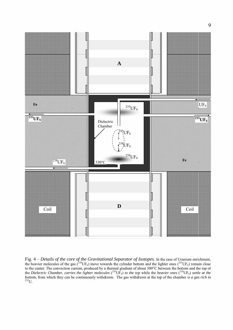
9 235UF6
Fig. 4 – Details of the core of the Gravitational Separator of Isotopes. In the case of Uranium enrichment,the heavier molecules of the gas (238UF6) move towards the cylinder bottom and the lighter ones (235UF6) remain close to the center. The convection current, produced by a thermal gradient of about 300°C between the bottom and the top of the Dielectric Chamber, carries the lighter molecules (235UF6) to the top while the heavier ones (238UF6) settle at the bottom, from which they can be continuously withdrawn. The gas withdrawn at the top of the chamber is a gas rich in235U.
Fe
Fe
Coil
A
D
UF6
235UF6235UF6
238UF6
Coil
330°C
235UF6
235UF6
238UF6
238UF6
Dielectric Chamber
10 Appendix A: The “Geometrical Radii” of Electron and Proton It is known that the frequency of oscillation of a simple spring oscillator is
( )121 A
mKf
π=
where is the inertial mass attached to the spring and
mK is the spring constant (in
N·m−1). In this case, the restoring force exerted by the spring is linear and given by
( )2AKxF −= where x is the displacement from the equilibrium position. Now, consider the gravitational force: For example, above the surface of the Earth, the force follows the familiar Newtonian function, i.e., 2rmGMF gg⊕−= , where
is the mass of Earth, is the gravitational mass of a particle and
⊕gM gmr is the
distance between the centers. Below Earth’s surface the force is linear and given by
( )33
ArR
mGMF gg
⊕
⊕−=
where is the radius of Earth. ⊕R By comparing (A3) with (A2) we obtain
( )43
Axr
R
GM
mK
mK g
g⎟⎠⎞
⎜⎝⎛==
⊕
⊕
χ
Making , and substituting (A4) into (A1) gives
⊕== Rrx
( )521
3A
R
GMf g
⊕
⊕=χ
π In the case of an electron and a positron, we substitute by , ⊕gM gem χ by eχ and by
, where is the radius of electron (or positron). Thus, Eq. (A5) becomes
⊕R
eR eR
( )621
3A
R
Gmf
e
egeχπ
=
The value of eχ varies with the density of energy [3]. When the electron and the positron are distant from each other and the local density of energy is small, the value of
eχ becomes very close to 1. However, when the electron and the positron are penetrating one another, the energy densities in each particle become very strong due to the proximity of their electrical charges e and, consequently, the value of eχ strongly increases. In order to calculate the value of
eχ under these conditions ( ), we start from the expression of correlation between electric charge and gravitational mass, obtained in a previous work [
eRrx ==
q3]:
( ) ( )74 0 AimGq imaginarygπε=
where is the imaginary
gravitational mass, and (imaginarygm )
1−=i . In the case of electron, Eq. (A7) gives
( )
( )( )( )( )
( )( ) ( )8106.14
4
4
4
1903
20
203
20
00
0
ACmG
imG
imG
imGq
realeie
realeie
imaginaryeie
imaginarygee
−×−==
=−=
==
==
χπε
χπε
χπε
πε
where we obtain
( )9108.1 21 Ae ×−=χ

11This is therefore, the value of eχ increased by the strong density of energy produced by the electrical charges of the two particles, under previously mentioned conditions.
e
Given that eiege mm 0χ= , Eq. (A6) yields
( )1021
30
2
AR
mGf
e
eieχπ
=
From Quantum Mechanics, we know that
( )1120 Acmhf i=
where is the Planck’s constant. Thus, in the case of we get
heii mm 00 =
( )122
0 Ah
cmf ei=
By comparing (A10) and (A12) we conclude that
( )1321
30
220 A
RmG
hcm
e
eieei χπ
=
Isolating the radius , we get: eR
( )141087.62
142
0
32
31
Amch
mGR e
eie
−×=⎟⎠
⎞⎜⎝
⎛⎟⎟⎠
⎞⎜⎜⎝
⎛=
πχ
Compare this value with the Compton sized electron, which predicts and also with standardized result recently obtained of [
mRe131086.3 −×=
mRe131074 −×−= 11].
In the case of proton, we have
( )
( )( )( )( )
( )( ) ( )15106.14
4
4
4
1903
20
203
20
00
0
ACmG
imG
imG
imGq
realpip
realpip
imaginarypip
imaginarygpp
−×−==
=−=
==
==
χπε
χπε
χπε
πε
where we obtain
( )16107.9 17 Ap ×−=χ
Thus, the result is
( )171072.32
172
0
32
31
Amc
hmGR p
pip
−×=⎟⎟⎠
⎞⎜⎜⎝
⎛⎟⎟⎠
⎞⎜⎜⎝
⎛=
π
χ
Note that these radii, given by Equations ( )14A and ( , are the radii of free electrons and free protons (when the particle and antiparticle (in isolation) penetrate themselves mutually).
)17A
Inside the atoms (nuclei) the radius of protons is well-known. For example, protons, as the hydrogen nuclei, have a radius given by [mRp
15102.1 −×≅ 9, 10]. The strong increase in respect to the value given by Eq. (A17) is due to the interaction with the electron of the atom.

12 References [1] Emsley, John (2001). "Uranium". Nature's Building Blocks: An A to Z Guide to the Elements. Oxford: Oxford University Press. p. 478. [2] "Uranium Enrichment". Argonne National Laboratory. Retrieved 2007-02-11. [3] De Aquino, F. (2010) Mathematical Foundations of the Relativistic Theory of Quantum Gravity, Pacific Journal of Science and Technology, 11 (1), pp. 173- 232. [4] De Aquino, F. (2010) Gravity Control by means of Electromagnetic Field through Gas at Ultra-Low Pressure, Pacific Journal of Science and Technology, 11(2) November 2010, pp.178-247, Physics/0701091. [5] Quevedo, C. P. (1977) Eletromagnetismo, McGraw- Hill, p. 270. [6] Halliday, D. and Resnick, R. (1968) Physics, J. Willey & Sons, Portuguese Version, Ed. USP, p.1124. [7] De Aquino, F. (2012) A System to convert Gravitational Energy directly into Electrical Energy, http://viXra.org/abs/1205.0119 [8] Chalmers, J.A., (1967) Atmospheric Electricity, Pergamon press, Oxford, London; Kamsali, N. et al., (2011) Advanced Air Pollution, chapter 20, DOI: 10.5772/17163, edited by Farhad Nejadkoorki, Publisher: InTech, ISBN 978-953-307-511-2, under CC BY-NC- SA 3.0 license. [9] N.D. Cook (2010). Models of the Atomic Nucleus (2nd ed.). Springer. p. 57 ff.. ISBN 978-3-642-14736-4. [10] K.S. Krane (1987). Introductory Nuclear Physics. Wiley-VCH. ISBN 0-471-80553-X. [11] Mac Gregor. M. H., (1992) The Enigmatic Electron. Boston: Klurer Academic, 1992, pp. 4-5.

Gravitational Atomic Synthesis at Room Temperature
Fran De Aquino Maranhao State University, Physics Department, S.Luis/MA, Brazil.
Copyright © 2012 by Fran De Aquino. All Rights Reserved. It is described a process for creating new atoms starting from pre-existing atoms. We show that all the elements of the periodic table can be synthesized, at room temperature, by a gravitational process based on the intensification of the gravitational interaction by means of electromagnetic fields.
Key words: Modified theories of gravity, Atom manipulation, Atomic forces. PACS: 04.50.Kd, 37.90.+j, 34.20.-b. 1. Introduction Rutherford [1] was the first to observe the transmutation of the atoms, and also the first to perform transmutation of the atoms. That gave him a double justification for being labeled an alchemist. It is currently believed that the synthesis of precious metals, a symbolic goal long sought by alchemists, is only possible with methods involving either nuclear reactors or particle accelerators. However, it will be shown here that all the elements of the periodic table can be synthesized, at room temperature, by a gravitational process based on the intensification of the gravitational interaction by means of electromagnetic fields. The process is very simple, but it requires extremely-low frequency (ELF) magnetic field with very strong intensity (BBrms > 2,500T). The strongest continuous magnetic field yet produced in a laboratory had 45 T (Florida State University's National High Magnetic Field Laboratory in Tallahassee, USA) [2]. The strongest (pulsed) magnetic field yet obtained non-destructively in a laboratory had about 100T. (National High Magnetic Field Laboratory, Los Alamos National Laboratory, USA) [3]. The strongest pulsed magnetic field yet obtained in a laboratory, destroying the used equipment, but not the laboratory itself (Institute for Solid State Physics, Tokyo) reached 730 T . The strongest (pulsed) magnetic field ever obtained (with explosives) in a laboratory (VNIIEF in Sarov, Russia, 1998) reached 2,800T [4].
2. Theory The quantization of gravity showed that the gravitational mass mg and the inertial mass mi are correlated by means of the following factor [5]:
( )111212
00 ⎪⎭
⎪⎬⎫
⎪⎩
⎪⎨⎧
⎥⎥
⎦
⎤
⎢⎢
⎣
⎡−⎟⎟
⎠
⎞⎜⎜⎝
⎛ Δ+−==
cmp
mm
ii
gχ
where is the rest inertial mass of the particle and
0impΔ is the variation in the
particle’s kinetic momentum; is the speed of light.
c
When pΔ is produced by the absorption of a photon with wavelengthλ , it is expressed by λhp =Δ . In this case, Eq. (1) becomes
( )21121
1121
20
20
0
⎪⎭
⎪⎬⎫
⎪⎩
⎪⎨⎧
⎥⎥
⎦
⎤
⎢⎢
⎣
⎡−⎟
⎠
⎞⎜⎝
⎛+−=
⎪⎭
⎪⎬⎫
⎪⎩
⎪⎨⎧
⎥⎥
⎦
⎤
⎢⎢
⎣
⎡−⎟
⎠
⎞⎜⎝
⎛+−=
λλ
λcmh
mm i
i
g
where cmh i00 =λ is the DeBroglie wavelength for the particle with rest inertial mass . 0im In general, the momentum variation
pΔ is expressed by tFp Δ=Δ where is the applied force during a time interval
FtΔ . Note
that there is no restriction concerning the nature of the force, i.e., it can be mechanical, electromagnetic, etc. For example, we can

2look on the momentum variation as due to absorption or emission of electromagnetic energy by the particle.
pΔ
This means that, by means of electromagnetic fields, the gravitational mass can be decreased down to become negative and increased (independently of the inertial mass ). In this way, the gravitational forces can be intensified. Consequently, we can use, for example, oscillating magnetic fields in order to intensify the gravitational interaction between electrons and protons.
im
From Electrodynamics we know that when an electromagnetic wave with frequency and velocity incides on a material with relative permittivity
f c
rε , relative magnetic permeability rμ and electrical conductivity σ , its velocity is reduced to rncv = where is the index of refraction of the material, given by [
rn6]
( ) ( )3112
2 ⎟⎠⎞⎜
⎝⎛ ++== ωεσ
με rrr v
cn
If ωεσ >> , fπω 2= , Eq. (3) reduces to
( )44 0 f
n rr πε
σμ=
Thus, the wavelength of the incident radiation (See Fig. 2) becomes
( )54mod σμ
πλλfnn
fcfv
rr
====
Fig. 2 – Modified Electromagnetic Wave. The wavelength of the electromagnetic wave can bestrongly reduced, but its frequency remains the same.
v = c v = c/nr
λ = c/f λmod = v/f = c/nr f
nr
If a lamina with thickness equal toξ contains atoms/mn 3, then the number of atoms per area unit is ξn . Thus, if the electromagnetic radiation with frequency
incides on an area of the lamina it reachesf S
ξnS atoms. If it incides on the total area of the lamina, , then the total number of atoms reached by the radiation is
fS
ξfnSN = . The number of atoms per unit of volume, , is given by n
( )60
AN
nρ
=
where is the Avogadro’s number;
kmoleatomsN /1002.6 260 ×=
ρ is the matter density of the lamina (in kg/m3) and A is the molar mass(kg/kmole). When an electromagnetic wave incides on the lamina, it strikes front atoms, where
fN( ) mff SnN φ≅ , mφ is the “diameter” of
the atom. Thus, the electromagnetic wave incides effectively on an area , where mf SNS=
241
mmS πφ= is the cross section area of one atom. After these collisions, it carries out with the other atoms (See Fig.3).
collisionsn
Fig. 3 – Collisions inside the lamina.
atom Sm
Wave
Thus, the total number of collisions in the volume ξS is
( )( )7ξ
φξφ
Sn
SnSnSnnNN
m
mmlmlcollisionsfcollisions
=
=−+=+=
The power density, , of the radiation on the lamina can be expressed by
D
( )8mf SN
PSPD ==

3 We can express the total mean number of collisions in each atom, , by means of the following equation
1n
( )91 NNn
n collisionsphotonstotal=
Since in each collision a momentum λh is transferred to the atom, then the total momentum transferred to the lamina will be
( ) λhNnp 1=Δ . Therefore, in accordance with Eq. (1), we can write that
( )
( )( )
( )101121
1121
20
20
10
⎪⎭
⎪⎬⎫
⎪⎩
⎪⎨⎧
⎥⎥
⎦
⎤
⎢⎢
⎣
⎡−⎥
⎦
⎤⎢⎣
⎡+−=
=⎪⎭
⎪⎬⎫
⎪⎩
⎪⎨⎧
⎥⎥
⎦
⎤
⎢⎢
⎣
⎡−⎥
⎦
⎤⎢⎣
⎡+−=
λλ
λλ
collisionsphotonstotal
li
lg
Nn
Nnmm
Since Eq. (7) gives ξSnN lcollisions = , we get
( ) (112 ξSnhfPNn lcollisionsphotonstotal ⎟⎟
⎠
⎞⎜⎜⎝
⎛= )
Substitution of Eq. (11) into Eq. (10) yields
( )
( )( ) ( )121121
2
02
0 ⎪⎭
⎪⎬⎫
⎪⎩
⎪⎨⎧
⎥⎥⎥
⎦
⎤
⎢⎢⎢
⎣
⎡−⎥
⎦
⎤⎢⎣
⎡⎟⎟⎠
⎞⎜⎜⎝
⎛+−=
λλ
ξSnhfP
mm
lli
lg
Substitution of given by Eq. (8) into Eq. (12) gives
P
( )
( ) ( )( )1311121
2
02
0 ⎪⎭
⎪⎬
⎫
⎪⎩
⎪⎨
⎧
⎥⎥⎥
⎦
⎤
⎢⎢⎢
⎣
⎡−
⎥⎥⎦
⎤
⎢⎢⎣
⎡⎟⎟⎠
⎞⎜⎜⎝
⎛⎟⎟⎠
⎞⎜⎜⎝
⎛+−=
λξcm
Snf
DSNmm
li
lmf
li
lg
Substitution of ( ) mflf SnN φ≅ and mf SNS = into Eq. (13) results
( )
( ) ( )( )1411121
2
20
2223
0 ⎪⎭
⎪⎬
⎫
⎪⎩
⎪⎨
⎧
⎥⎥⎥
⎦
⎤
⎢⎢⎢
⎣
⎡−
⎥⎥⎦
⎤
⎢⎢⎣
⎡⎟⎟⎠
⎞⎜⎜⎝
⎛+−=
λξφ
cfmDSSn
mm
li
mmfl
li
lg
where ( ) ( ) ( )llli Vm ρ=0 . Now, considering that the lamina is inside an ELF electromagnetic field with E and B , then we can write that [7]
( ) ( )152 0
2
cEn
D lr
μ=
Substitution of Eq. (15) into Eq. (14) gives
( )
( )
( )
( )( )1611
2121
2
2200
22223
0 ⎪⎭
⎪⎬
⎫
⎪⎩
⎪⎨
⎧
⎥⎥⎥
⎦
⎤
⎢⎢⎢
⎣
⎡−
⎥⎥⎦
⎤
⎢⎢⎣
⎡⎟⎟⎠
⎞⎜⎜⎝
⎛+−=
λμξφfcmESSnn
mm
li
mmfllr
li
lg
Note that tEE m ωsin= .The average value for 2E is equal to 2
21
mE because E varies sinusoidaly ( is the maximum value
formE
E ). On the other hand, 2mrms EE = . Consequently we can replace 4E for . Thus, for
4rmsE
modλλ = , the equation above can be rewritten as follows
( )
( )
( )
( )( )1711
2121
2
mod22
00
22223
0 ⎪⎭
⎪⎬
⎫
⎪⎩
⎪⎨
⎧
⎥⎥⎥
⎦
⎤
⎢⎢⎢
⎣
⎡−
⎥⎥⎦
⎤
⎢⎢⎣
⎡⎟⎟⎠
⎞⎜⎜⎝
⎛+−=
λμξφfcmESSnn
mm
li
rmsmmfllr
li
lg
Electrodynamics tells us that
( )( ) rmslrrmsrms BncvBE == . Substitution of this expression into Eq. (17) gives
( )
( ) ( ) ( )( )181
4121 22
mod42
020
424446
0 ⎪⎭
⎪⎬⎫
⎪⎩
⎪⎨⎧
⎥⎥⎦
⎤
⎢⎢⎣
⎡−+−==
lrli
rmsmmfl
li
lg
nfmBSSn
mm
λμξφ
χ
Since ( )lrnλλ =mod then Eq. (18) can be rewritten in the following form
( )
( ) ( )( )191
4121 222
020
424446
0 ⎪⎭
⎪⎬⎫
⎪⎩
⎪⎨⎧
⎥⎥⎦
⎤
⎢⎢⎣
⎡−+−==
fcmBSSn
mm
li
rmsmmfl
li
lg
μξφ
χ
In order to calculate the expressions of
Beχ for the particular case of a electron of the electrophere of a atom, subjected to an external magnetic field with frequency rmsB

4f , we must substitute in Eq. (19)
forln
33411 ee rV π= , for fS ( ) eee VSSA ρ ( is
the specific surface area for electrons in this case:
eSSA
eexeeeeeee VrVAmASSA ρπρ 221
21 2=== ),
by , mS 2xee rS π= ξ by xem r2=φ and
by . The result is ( )lim 0
em
( )20156.45121 218220
2
4222
⎪⎭
⎪⎬⎫
⎪⎩
⎪⎨⎧
⎥⎥⎦
⎤
⎢⎢⎣
⎡−+−=
frmcBr
ee
rmsxeBe μ
πχ
In order to calculate the value of we start considering a hydrogen atom, where the electron spins around the proton with a velocity . The electrical force acting on the proton is
xer
16 .103 −×= smve2
102 4 reFe πε= ,
which is equal to the centrifuge force where 0
2rmF epc ω= eω is the angular velocity of the electron and is the distance between the inertial center of the proton and the center of the moving proton (See Fig. 5, where we conclude that
0r
( ) pxpp rrrr +=+02 , where is the radius of the sphere whose external
area is equivalent to the increased area of the proton). Thus, we get
xpr
( )pxp rrr −= 21
0 . Fig. 5 – The deformation of the proton.
xpr
-
Fe
Fe
ve
K
ve
rp
r0
Substitution of this value into expression of gives ec FF =
mrvm
er pep
xp14
20
2
102.34
−×=+=πε
Therefore, we can write that pxpxp rkr = , where
6.25==p
xpxp r
rk
The electron is similarly deformed by the relative movement of the proton in respect to it. In this case, by analogy, we can write that
mrvm
er eee
xe11
20
2
104.64
−×=+=πε
and exexe rkr = , where is the radius of the sphere whose external area is equivalent to the increased area of the electron. The radius of free electron is
xer
mre141087.6 −×= (See
Appendix A). However, for electrons in the atomic eletrosphere of atoms the value of must be calculated starting from Quantum Mechanics. The wave packet that describes the electron satisfies an uncertainty principle
er
( )h21≥ΔΔ xp , where and kp Δ=Δ h kΔ is
the approximate extension of the wave packet. Thus, we can write that ( )2
1≥ΔΔ xk . For the ``square'' packet the full width in is k
02 λπ=Δk ( cmh e=0λ is the average wavelength). The width in x is a little harder to define, but, lets use the first node in the probability found at ( ) πλπ =22 0 x or
0λ=x . So, the width of the wave packet is twice this or 02λ=Δx . Obviously, cannot be greater than , i.e., must be smaller and close to
er2 xΔ er
mcmh e12
0 1043.2 −×==λ . Then, assuming that , we get
mre12104.2 −×≅
6.26==e
xexe r
rk
Note that xpxe kk ≅ . Substitution of these values into Eq. (20) gives

5
( )211108.2121
1108.3121
2
442
2
442257
⎪⎭
⎪⎬⎫
⎪⎩
⎪⎨⎧
⎥⎥⎦
⎤
⎢⎢⎣
⎡−×+−=
=⎪⎭
⎪⎬⎫
⎪⎩
⎪⎨⎧
⎥⎥⎦
⎤
⎢⎢⎣
⎡−×+−=
fB
fBrk
rms
rmsexeBeχ
Similarly, in the case of proton and neutron we can write that
( )22156.45
121 2220
2
44222
⎪⎭
⎪⎬⎫
⎪⎩
⎪⎨⎧
⎥⎥⎦
⎤
⎢⎢⎣
⎡−+−=
fmcBrk
p
rmspxpBp μ
πχ
( )23156.45
1212222
0
442
⎪⎭
⎪⎬⎫
⎪⎩
⎪⎨⎧
⎥⎥⎦
⎤
⎢⎢⎣
⎡−+−=
fcmBr
n
rmsnBn μ
πχ
In the case of the neutron, due to its electric charge be null. The radius of protons inside the atoms (nuclei) is
1=xnk
mrp15102.1 −×=
[8,9], , then we obtain from Eqs. (22) and (23) the following expressions:
pn rr ≅
( )241102.2121 2
422
⎪⎭
⎪⎬⎫
⎪⎩
⎪⎨⎧
⎥⎥⎦
⎤
⎢⎢⎣
⎡−×+−=
fBrms
Bpχ
( )2511035.2121 2
49
⎪⎭
⎪⎬⎫
⎪⎩
⎪⎨⎧
⎥⎥⎦
⎤
⎢⎢⎣
⎡−×+−= −
fBrms
Bnχ
When a strong magnetic field is applied on the atom, the enormous value of
rmsB
Beχ (See Eq. 21) makes the gravitational force between the electrons greater than the electric force due to its charges, and consequently, the electrons are joined in pairs (Cooper pairs)[10]. However, due to the vales of Beχ and Bpχ , the gravitational attraction between the electrons of the K shell and the protons of the nucleus becomes greater than the nuclear force, i.e.,
( )2621
21
Nep
BeBpgegp F
rmm
Grmm
G >= χχ
Then, the proton more weakly bound to the nucleus is ejected towards the nearest electron. When they collide, there occurs the formation of one neutron and one neutrino, according the well-known reaction
enep ν+→+ . Since the neutron is beyond the reach of the nuclear force, it is not
attracted to the nucleus and leaves the atom. The final result is that the atom loses a proton and an electron and is transformed in a new atom. But the transmutation is not completed until the magnetic field is turned off. When this occurs the Cooper pairs are broken, and the new atom leaves the transitory state, and passes to the normal state. In order to satisfy the condition expressed by Eq. (26), we must have
( )27103 482
1 ×≈>ep
NBeBp mGm
rFχχ
By substitution of Eq. (21) and (22) into Eq. (27), we obtain
72
106×>f
Brms
Thus, for Hzf 1.0= we conclude that the required value of is rmsB
TBrms 500,2> This means that, if we subject, for example, an amount of 198Hg (80 electrons, 80 protons, 118 neutrons) to a magnetic field with BBrms>2,500 T and frequency 0.1Hz the
Hg loses 1 proton and 1 electron and consequently will be transmuted to Au (79 electrons, 79 protons, 118 neutrons) when the magnetic field is turned off. Besides the transformation of mercury into gold, we can make several transmutations. For example, if the Au is after subjected to the same magnetic field it will be transmuted to Pt (78 electrons, 78 protons, 118 neutrons). Similarly, if Cd (48 electrons, 48 protons, 62 neutrons) is subjected to the mentioned field it will be transmuted to Ag (47 electrons, 47 protons, 62 neutrons). Also U can be easily obtained by this process, i.e., if we subject an amount of Np (93 electrons, 93 protons, 143 neutrons) to the magnetic field with >2,500 T and frequency 0.1Hz, the Np loses 1 proton and 1 electron and consequently will be transmuted to U (92 electrons, 92 protons, 143 neutrons).
198
197
197
196
110
109
235
236
236
235

6
Appendix A: The “Geometrical Radii” of Electron and Proton It is known that the frequency of oscillation of a simple spring oscillator is
( )121 A
mKf
π=
where is the inertial mass attached to the spring and
mK is the spring constant (in
N·m−1). In this case, the restoring force exerted by the spring is linear and given by
( )2AKxF −= where x is the displacement from the equilibrium position. Now, consider the gravitational force: For example, above the surface of the Earth, the force follows the familiar Newtonian function, i.e., 2rmGMF gg⊕−= , where
is the mass of Earth, is the gravitational mass of a particle and
⊕gM gmr is the
distance between the centers. Below Earth’s surface the force is linear and given by
( )33
ArR
mGMF gg
⊕
⊕−=
where is the radius of Earth. ⊕R By comparing (A3) with (A2) we obtain
( )43
Axr
R
GM
mK
mK g
g⎟⎠⎞
⎜⎝⎛==
⊕
⊕
χ
Making , and substituting (A4) into (A1) gives
⊕== Rrx
( )521
3 AR
GMf g
⊕
⊕=χ
π In the case of an electron and a positron, we substitute by , ⊕gM gem χ by eχ and by
, where is the radius of electron (or positron). Thus, Eq. (A5) becomes
⊕R
eR eR
( )621
3A
R
Gmf
e
egeχπ
=
The value of eχ varies with the density of energy [5]. When the electron and the positron are distant from each other and the local density of energy is small, the value of
eχ becomes very close to 1. However, when the electron and the positron are penetrating one another, the energy densities in each particle become very strong due to the proximity of their electrical charges e and, consequently, the value of eχ strongly increases. In order to calculate the value of
eχ under these conditions ( ), we start from the expression of correlation between electric charge and gravitational mass, obtained in a previous work [
eRrx ==
q5]:
( ) ( )74 0 AimGq imaginarygπε=
where is the imaginary
gravitational mass, and (imaginarygm )
1−=i . In the case of electron, Eq. (A7) gives
( )
( )( )( )( )
( )( ) ( )8106.14
4
4
4
1903
20
203
20
00
0
ACmG
imG
imG
imGq
realeie
realeie
imaginaryeie
imaginarygee
−×−==
=−=
==
==
χπε
χπε
χπε
πε
where we obtain
( )9108.1 21 Ae ×−=χ This is therefore, the value of eχ increased by the strong density of energy produced by the electrical charges of the two particles, under previously mentioned conditions.
e

7 Given that eiege mm 0χ= , Eq. (A6) yields
( )1021
30
2
AR
mGf
e
eieχπ
=
From Quantum Mechanics, we know that
( )1120 Acmhf i=
where is the Planck’s constant. Thus, in the case of we get
heii mm 00 =
( )122
0 Ah
cmf ei=
By comparing (A10) and (A12) we conclude that
( )1321
30
220 A
RmG
hcm
e
eieei χπ
=
Isolating the radius , we get: eR
( )141087.62
142
0
32
31
Amch
mGR e
eie
−×=⎟⎠
⎞⎜⎝
⎛⎟⎟⎠
⎞⎜⎜⎝
⎛=
πχ
Compare this value with the Compton sized electron, which predicts and also with standardized result recently obtained of [
mRe131086.3 −×=
mRe131074 −×−= 11].
In the case of proton, we have
( )
( )( )( )( )
( )( ) ( )15106.14
4
4
4
1903
20
203
20
00
0
ACmG
imG
imG
imGq
realpip
realpip
imaginarypip
imaginarygpp
−×−==
=−=
==
==
χπε
χπε
χπε
πε
where we obtain
( )16107.9 17 Ap ×−=χ
Thus, the result is
( )171072.32
172
0
32
31
Amc
hm
GR p
pip
−×=⎟⎟⎠
⎞⎜⎜⎝
⎛⎟⎟⎠
⎞⎜⎜⎝
⎛=
π
χ
Note that these radii, given by Equations ( )14A and ( , are the radii of free electrons and free protons (when the particle and antiparticle (in isolation) penetrate themselves mutually).
)17A
Inside the atoms (nuclei) the radius of protons is well-known. For example, protons, as the hydrogen nuclei, have a radius given by [mRp
15102.1 −×≅ 8,9]. The strong increase in respect to the value given by Eq. (A17) is due to the interaction with the electron of the atom.

8 References [1] Rutherford, E. (1933) The Artificial Transmutation of the Elements; Rutherford, E. (1937)The Newer Alchemy. [2] "World's Most Powerful Magnet Tested Ushers in New Era for Steady High Field Research". National High Magnetic Field Laboratory. http://www.magnet.fsu.edu/mediacenter/news/ pressreleases/1999december17.html [3] http://gizmodo.com/5896092/the-worlds-most- powerful-non+destructive-magnet-screams-like-a- banshee. [4] Bykov, A.I et al., Pulsed Power Conference, 1999. Digest of Technical Papers. 12th IEEE International, 2, pp. 746 – 749. [5] De Aquino, F. (2010) Mathematical Foundations of the Relativistic Theory of Quantum Gravity, Pacific Journal of Science and Technology, 11 (1), pp. 173- 232. [6] Quevedo, C. P. (1977) Eletromagnetismo, McGraw- Hill, p. 270. [7] Halliday, D. and Resnick, R. (1968) Physics, J. Willey & Sons, Portuguese Version, Ed. USP, p.1124. [8] N.D. Cook (2010). Models of the Atomic Nucleus (2nd ed.). Springer. p. 57 ff.. ISBN 978-3-642-14736-4. [9] K.S. Krane (1987). Introductory Nuclear Physics. Wiley-VCH. ISBN 0-471-80553-X. [10] De Aquino, F. (2012) Superconducting State generated by Cooper Pairs bound by Intensified Gravitational Interaction, http://vixra.org/abs/1207.0008. [11] Mac Gregor. M. H., (1992) The Enigmatic Electron. Boston: Klurer Academic, 1992, pp. 4-5.

Ultrafast Conversion of Graphite to Diamond in Gravitational Pressure Apparatus
Fran De Aquino
Maranhao State University, Physics Department, S.Luis/MA, Brazil. Copyright © 2012 by Fran De Aquino. All Rights Reserved.
Currently the artificial production of diamond is very expensive because it consumes large amounts of energy in order to produce a single diamond. Here, we propose a new type of press based on the intensification of the gravitational acceleration. This Gravitational Press can generate pressures several times more intense than the 80GPa required for ultrafast transformation of graphite into diamond. In addition, due to the enormous pressure that the Gravitational Press can produce, the "synthesis capsule" may be very large (up to about 1000 cm3 in size). This is sufficient to produce diamonds with up to 100 carats (20g) or more. On the other hand, besides the ultrafast conversion, the energy required for the Gravitational Presses is very low, in such a way that the production cost of the diamonds becomes very low, what means that they could be produced on a large scale.
Key words: Modified theories of gravity, High-pressure apparatus, Graphite, Diamond. PACS: 04.50.Kd, 07.35.+k, 81.05.uf , 81.05.ug 1. Introduction After the discovery that diamond was pure carbon, many attempts were made to convert various carbon forms into diamond. Converting graphite into diamond has been a long held dream of alchemists. The artificial production of diamond was first achieved by H.T Hall in 1955. He used a press capable of producing pressures above 10 GPa and temperatures above 2,000 °C [1]. Today, there are several methods to produce synthetic diamond. The more widely utilized method uses high pressure and high temperature (HPHT) of the order of 10 GPa and 2500°C during many hours in order to produce a single diamond. The fact that this process requires high pressure and high temperatures during a long time means that it consumes large amounts of energy, and this is the reason why the production cost of artificial diamond is so expensive. The second method, using chemical vapor deposition (CVD), creates a carbon plasma over a substrate onto which the carbon atoms deposit to form diamond. Other methods include explosive formation and sonication of graphite solutions [2,3,4]. In the HPHT method, there are three main press designs used to supply the pressure and temperature necessary to produce synthetic diamond: the Belt press,
the Cubic press and the split-sphere (BARS) press. Typical pressures and temperatures achievable are of the order of 10 GPa and 2500°C [5]. Diamonds may be formed in the Earth’s mantle mainly by direct transition, graphite to diamond or by systems involving carbon dissolved in molten metals. The classic high-pressure, high-temperature synthesis of diamond utilizes molten transition metals as solvent/catalysts. Converting diamond from graphite in the absence of a catalyst requires pressures that are significantly higher than those at equilibrium coexistence [6-12]. At lower temperatures, the formation of the metastable hexagonal polymorph of diamond is favored instead of the more stable cubic diamond [7, 10-12]. These phenomena cannot be explained by the concerted mechanism suggested in previous theoretical studies [13-17]. However, recently Michele Parrinello, Professor of Computational Science at ETH Zurich, and his team have developed a method by which they have successfully simulated this phase transition accurately and adequately using computer models [18]. Instead of happening concerted, all at once, the conversion evidently takes place in a step by step process involving the formation of a

2diamond seed in the graphite, which is then transformed completely at high pressure. In quantitative agreement with the ab initio calculations of Tateyama at al. [19], the stability of diamond relative to graphite increases with pressure whereas the barrier separating two phases decreases. Parrinello’s work shows that at a pressure of 80 GPa and temperature between 0 and 1,000K graphite reaches a lattice instability point and undergoes an ultrafast transformation to diamond as was previously observed in ab initio simulations by Scandolo et al [20]. Here, we propose a new type of press based on the intensification of the gravitational acceleration*. This press can generate pressures several times more intense† than the 80GPa required for the ultrafast transformation of graphite to diamond. In addition, due to the enormous pressure that the Gravitational Press can produce (>>80GPa), the ceramic cube ("synthesis capsule") can be very large (up to about 1000 cm3 in size). This is sufficient to produce diamonds up to 100 carats (20g) or more. On the other hand, besides the ultrafast conversion, the energy required for the Gravitational Presses is very low, in such a way that the production cost of the diamonds becomes very low, what means that they could be produced on a large scale. 2. Theory From the quantization of gravity it follows that the gravitational mass mg and the inertial mass mi are correlated by means of the following factor [21]:
( )111212
00 ⎪⎭
⎪⎬⎫
⎪⎩
⎪⎨⎧
⎥⎥
⎦
⎤
⎢⎢
⎣
⎡−⎟⎟
⎠
⎞⎜⎜⎝
⎛ Δ+−==
cmp
mm
ii
gχ
* De Aquino, F. (2008) Process and Device for Controlling the Locally the Gravitational Mass and the Gravity Acceleration, BR Patent Number: PI0805046-5, July 31, 2008. † The limit is basically determined by the compression resistance of the material of the piston and anvils of the Gravitational Press since it can produce pressures far beyond 1000 GPa.
where is the rest inertial mass of the particle and
0impΔ is the variation in the
particle’s kinetic momentum; is the speed of light.
c
When pΔ is produced by the absorption of a photon with wavelengthλ , it is expressed by λhp =Δ . In this case, Eq. (1) becomes
( )21121
1121
20
20
0
⎪⎭
⎪⎬⎫
⎪⎩
⎪⎨⎧
⎥⎥
⎦
⎤
⎢⎢
⎣
⎡−⎟
⎠
⎞⎜⎝
⎛+−=
⎪⎭
⎪⎬⎫
⎪⎩
⎪⎨⎧
⎥⎥
⎦
⎤
⎢⎢
⎣
⎡−⎟
⎠
⎞⎜⎝
⎛+−=
λλ
λcmh
mm i
i
g
where cmh i00 =λ is the De Broglie wavelength for the particle with rest inertial mass . 0im It has been shown that there is an additional effect - Gravitational Shielding effect - produced by a substance whose gravitational mass was reduced or made negative [22]. The effect extends beyond substance (gravitational shielding) , up to a certain distance from it (along the central axis of gravitational shielding). This effect shows that in this region the gravity acceleration, , is reduced at the same proportion, i.e.,
1ggg
11 χ= where
01 ig mm=χ and g is the gravity acceleration before the gravitational shielding). Consequently, after a second gravitational shielding, the gravity will be given by ggg
21122 χχχ == , where 2
χ is the value of the ratio 0ig mm for the second gravitational shielding. In a generalized way, we can write that after the nth gravitational shielding the gravity, , will be given by ng
( )3...
321gg
nn χχχχ=
This possibility shows that, by means of a battery of gravitational shieldings, we can make particles acquire enormous accelerations. In practice, this is the basis to the conception of the Gravitational Press.

3 From Electrodynamics we know that when an electromagnetic wave with frequency and velocity incides on a material with relative permittivity
f c
rε , relative magnetic permeability rμ and electrical conductivity σ , its velocity is reduced to rncv = where is the index of refraction of the material, given by [
rn23]
( ) ( )4112
2 ⎟⎠⎞⎜
⎝⎛ ++== ωεσ
με rrr v
cn
If ωεσ >> f, πω 2= , Eq. (4) reduces to
( )54 0 f
n rr πε
σμ=
Thus, the wavelength of the incident radiation (See Fig. 1) becomes
( )64mod σμ
πλλfnn
fcfv
rr====
Fig. 1 – Modified Electromagnetic Wave. The wavelength of the electromagnetic wave can bestrongly reduced, but its frequency remains the same.
v = c v = c/nr
λ = c/f λmod = v/f = c/nr f
nr
If a lamina with thickness equal toξ contains atoms/mn 3, then the number of atoms per area unit is ξn . Thus, if the electromagnetic radiation with frequency
incides on an area of the lamina it reachesf S
ξnS atoms. If it incides on the total area of the lamina, , then the total number of atoms reached by the radiation is
fS
ξfnSN = . The number of atoms per unit of volume, , is given by n
( )70
AN
nρ
=
where is the Avogadro’s number;
kmoleatomsN /1002.6 260 ×=
ρ is the matter density of the lamina (in kg/m3) and A is the molar mass(kg/kmole). When an electromagnetic wave incides on the lamina, it strikes front atoms, where
fN( ) mff SnN φ≅ , mφ is the “diameter” of
the atom. Thus, the electromagnetic wave incides effectively on an area , where mf SNS=
241
mmS πφ= is the cross section area of one atom. After these collisions, it carries out with the other atoms (See Fig.2).
collisionsn
Fig. 2 – Collisions inside the lamina.
atom Sm
Wave
Thus, the total number of collisions in the volume ξS is
( )( )8ξ
φξφ
Sn
SnSnSnnNN
m
mmlmlcollisionsfcollisions
=
=−+=+=
The power density, , of the radiation on the lamina can be expressed by
D
( )9mf SN
PSPD ==
We can express the total mean number of collisions in each atom, , by means of the following equation
1n
( )101 NNn
n collisionsphotonstotal=
Since in each collision a momentum λh is transferred to the atom, then the total momentum transferred to the lamina will be

4( ) λhNnp 1=Δ . Therefore, in accordance
with Eq. (1), we can write that
( )
( )( )
( )111121
1121
20
20
10
⎪⎭
⎪⎬⎫
⎪⎩
⎪⎨⎧
⎥⎥
⎦
⎤
⎢⎢
⎣
⎡−⎥
⎦
⎤⎢⎣
⎡+−=
=⎪⎭
⎪⎬⎫
⎪⎩
⎪⎨⎧
⎥⎥
⎦
⎤
⎢⎢
⎣
⎡−⎥
⎦
⎤⎢⎣
⎡+−=
λλ
λλ
collisionsphotonstotal
li
lg
Nn
Nnmm
Since Eq. (8) gives ξSnN lcollisions = , we get
( ) (122 ξSnhfPNn lcollisionsphotonstotal ⎟⎟
⎠
⎞⎜⎜⎝
⎛= )
Substitution of Eq. (12) into Eq. (11) yields
( )
( )( ) ( )131121
20
20 ⎪
⎭
⎪⎬
⎫
⎪⎩
⎪⎨
⎧
⎥⎥⎥
⎦
⎤
⎢⎢⎢
⎣
⎡−
⎥⎥⎦
⎤
⎢⎢⎣
⎡⎟⎟⎠
⎞⎜⎜⎝
⎛+−=
λλξSn
hfP
mm
lli
lg
Substitution of given by Eq. (9) into Eq. (13) gives
P
( )
( ) ( )( )1411121
2
02
0 ⎪⎭
⎪⎬
⎫
⎪⎩
⎪⎨
⎧
⎥⎥⎥
⎦
⎤
⎢⎢⎢
⎣
⎡−
⎥⎥⎦
⎤
⎢⎢⎣
⎡⎟⎟⎠
⎞⎜⎜⎝
⎛⎟⎟⎠
⎞⎜⎜⎝
⎛+−=
λξcm
Snf
DSNmm
li
lmf
li
lg
Substitution of ( ) mflf SnN φ≅ and mf SNS = into Eq. (14) results
( )
( ) ( )( )1511121
2
20
2223
0 ⎪⎭
⎪⎬
⎫
⎪⎩
⎪⎨
⎧
⎥⎥⎥
⎦
⎤
⎢⎢⎢
⎣
⎡−
⎥⎥⎦
⎤
⎢⎢⎣
⎡
⎟⎟⎠
⎞⎜⎜⎝
⎛+−=
λξφ
cfmDSSn
mm
li
mmfl
li
lg
where ( ) ( ) ( )llli Vm ρ=0 . Now, considering that the lamina is inside an ELF electromagnetic field with E and B , then we can write that [24]
( ) ( )162 0
2
cEn
D lr
μ=
Substitution of Eq. (16) into Eq. (15) gives
( )
( )
( )
( )( )1711
2121
2
2200
22223
0 ⎪⎭
⎪⎬
⎫
⎪⎩
⎪⎨
⎧
⎥⎥⎥
⎦
⎤
⎢⎢⎢
⎣
⎡−
⎥⎥⎦
⎤
⎢⎢⎣
⎡
⎟⎟⎠
⎞⎜⎜⎝
⎛+−=
λμ
ξφ
fcmESSnn
mm
li
mmfllr
li
lg
In the case in which the area is just the area of the cross-section of the lamina
fS( )αS ,
we obtain from Eq. (17), considering that ( ) ( ) ξρ αSm lli =0 , the following expression
( )
( )
( )
( )( )1811
2121
2
220
2223
0 ⎪⎭
⎪⎬
⎫
⎪⎩
⎪⎨
⎧
⎥⎥⎥
⎦
⎤
⎢⎢⎢
⎣
⎡−
⎥⎥⎦
⎤
⎢⎢⎣
⎡
⎟⎟⎠
⎞⎜⎜⎝
⎛+−=
λρμ
φα
fcESSnn
mm
l
mmllr
li
lg
According to Eq. (6) we have
( )( )19
fnc
fv
lr=== modλλ
Substitution of Eq. (19) into Eq. (18) gives
( )( )
( )
( )( )201
4121 2622
0
444264
0 ⎪⎭
⎪⎬
⎫
⎪⎩
⎪⎨
⎧
⎥⎥⎥
⎦
⎤
⎢⎢⎢
⎣
⎡
−+−=fc
ESSnn
mm
l
mmllr
li
lg
ρμ
φα
Note that tEE m ωsin= .The average value for 2E is equal to 2
21
mE because E varies sinusoidaly ( is the maximum value
formE
E ). On the other hand, 2mrms EE = . Consequently we can change 4E by , and the equation above can be rewritten as follows
4rmsE
( )
( )
( )
( )( )211
4121 2622
0
4442640
⎪⎭
⎪⎬
⎫
⎪⎩
⎪⎨
⎧
⎥⎥⎥
⎦
⎤
⎢⎢⎢
⎣
⎡
−+−=
==
fc
ESSnn
m
m
l
rmsmmllr
li
lg
ρμ
φ
χ
α
Now consider the system (Gravitational Press) shown in Fig.3. Inside the system there is a dielectric tube ( 1≅rε ) with the following characteristics:
mm60=α , 232 1083.24 mS −×== παα . Inside the tube there is an Aluminum sphere

5with 30mm radius and mass
kgM gs 30536.0= . The tube is filled with air at ambient temperature and 1atm. Thus, inside the tube, the air density is
( )22.2.1 3−= mkgairρ The number of atoms of air (Nitrogen) per unit of volume, , according to Eq.(7), is given by
airn
( )23/1016.5 3250 matomsA
Nn
N
airair ×==
ρ
The parallel metallic plates (p), shown in Fig.3 are subjected to different drop voltages. The two sets of plates (D), placed on the extremes of the tube, are subjected to ( ) VV rmsD 89614.= at Hzf 1= , while the
central set of plates (A) is subjected to ( ) VV rmsA 55183.= at Hzf 1= . Since ,
then the intensity of the electric field, which passes through the 36 cylindrical air laminas (each one with 5mm thickness) of the two sets (D), is
mmd 98=
( ) ( ) mVdVE rmsDrmsD /. 2105821 ×==
and the intensity of the electric field, which passes through the 7 cylindrical air laminas of the central set (A), is given by
( ) ( ) mVdVE rmsArmsA /. 3108731 ×==
Note that the metallic rings (5mm thickness) are positioned in such way to block the electric field out of the cylindrical air laminas. The objective is to turn each one of these laminas into a Gravity Control Cell (GCC) [22]. Thus, the system shown in Fig. 3 has 3 sets of GCC. Two with 18 GCC each and one with 7 GCC. The two sets with 18 GCC each are positioned at the extremes of the tube (D). They work as gravitational decelerator while the other set with 7 GCC (A) works as a gravitational accelerator, intensifying the gravity acceleration
produced by the mass of the Aluminum sphere. According to Eq. (3), this gravity, after the GCC becomes
gsM
th72
07
7 rGMg gsχ= , where ( ) ( )lilg mm=χ given by Eq. (21) and mmr0 35= is the distance between the center of the Aluminum sphere and the surface of the first GCC of the set (A). The objective of the sets (D), with 18 GCC each, is to reduce strongly the value of the external gravity along the axis of the tube. In this case, the value of the external gravity, , is reduced by the factor ,
where extg extd g18χ
210−=dχ . For example, if the base BS of the system is positioned on the Earth surface, then is reduced
to and, after the set A, it is increased
by . Since the system is designed for
2/81.9 smgext =
extd g18χ7χ
5.308−=χ , then the gravity acceleration on the sphere becomes , this value is much smaller than
218187 /106.2 smgextd−×=χχ
282 /1026.2 smrGMg sgssphere−×== .
This values of χ and dχ , according to Eq. (21) are given by
( ) ( )
( ) ( )24110971121
14
121
49
26220
444264
⎭⎬⎫
⎩⎨⎧
⎥⎦⎤
⎢⎣⎡ −×+−=
=⎪⎭
⎪⎬
⎫
⎪⎩
⎪⎨
⎧
⎥⎥⎥
⎦
⎤
⎢⎢⎢
⎣
⎡
−+−=
−rmsA
air
rmsAmmairairr
E
fc
ESSnn
.
ρμ
φχ
α
( ) ( )
( ) ( )25110971121
14
121
49
26220
444264
⎭⎬⎫
⎩⎨⎧
⎥⎦⎤
⎢⎣⎡ −×+−=
=⎪⎭
⎪⎬
⎫
⎪⎩
⎪⎨
⎧
⎥⎥⎥
⎦
⎤
⎢⎢⎢
⎣
⎡
−+−=
−rmsD
air
rmsDmmairairrd
E
fc
ESSnn
.
ρμ
φχ
α

6where , since ( ) 1≅airrn ( )ωεσ << ‡;
, , 325 /1016.5 matomsnair ×= mm101055.1 −×=φ
2202 1088.14 mS mm−×== πφ and Hzf 1= .
Since and
, Eq. (24) and (25) , given the following values
( ) mVE rmsA /. 3108731 ×=
( ) mVE rmsD /. 2105821 ×= ( )265.308−=χ
and
( )2710 2−≅dχ Then, the gravitational acceleration
upon the piston of the Gravitational Press shown in Fig. 3 is equal to the value of the gravitational acceleration after the 7th gravitational shielding, i.e.,
( )28/104.4 292
0
777 sm
rGM
gg gs ×≅−== χχ
If the mass of the piston is kgm piston 15= with 20cm diameter then the pressure upon the cubic-anvil apparatus (Fig. 4) is
( )GPamN
gmSFp piston 2000/102
1.0212
27 =×===
π
It is important to note that the pressure can be easily increased by increasing the value of χ . However, the pressure limit is basically determined by the compression resistance of the material of the piston and anvils of the Gravitational Press since it can produce pressures far beyond 2000 GPa.
‡ The electrical conductivity of air, inside the
dielectric tube, is equal to the electrical conductivity of Earth’s atmosphere near the land, whose average value is mSair /101 14−×≅σ [25].

7
To Cubic-Anvil Apparatus (Fig.4)
Fig. 3 – Gravitational Press (Developed from a process patented in July, 31 2008, PI0805046-5)
E
ξ = 5 mm
Parallel plate capacitor (p)
1
2
17
18
1
2
6
7
1
2
1718
α=60mm
d = 98 mm
Mg
Metallic ring (5 mm thickness)
Electric field of capacitor
Aluminum sphere (60 mm diameter)
Dielectric tube εr ≅ 1
A
D
D
ED(rms)
Air
Air
Air
AirAir 1 atm 300K
Air
r0=35mm
Air
Air
Air
Piston of
Gravitational Press(Tungsten Carbide)
g7 20
777 r
GMgg gsχχ −==

8
Fig.4 - Diagram of Cubic-Anvil Apparatus for the Gravitational Press. – In the center of the apparatus, is placed a ceramic cube("synthesis capsule") of pyrophyllite ceramics, which containsgraphite and is pressed by the anvils made from cemented carbide(e.g., tungsten carbide or VK10 hard alloy). Note that, due to the enormous pressure that the Gravitational Press can produce(>>80GPa), the "synthesis capsule" can be very large (up to about 1000 cm3 in size). This is sufficient to produce diamonds with up to 100 carats (20g) or more.
Gravitational Press Piston (Tungsten Carbide)
Anvils (Tungsten Carbide or
VK10 hard alloy)

9 References [1] Hall, H. T. (1960). "Ultra-high pressure apparatus". Rev. Sci. Instr. 31 (2): 125.[2] Werner, M; Locher, R (1998). "Growth and application of undoped and doped diamond films". Rep. Prog. Phys. 61 (12): 1665. [3] Osawa, E (2007). "Recent progress and perspectives in single-digit nanodiamond". Diamond and Related Materials 16 (12): 2018.[4] Galimov, É. M.; Kudin, A. M.; Skorobogatskii, V. N.; Plotnichenko, V. G.; Bondarev, O. L.; Zarubin, B. G.; Strazdovskii, V. V.; Aronin, A. S. et al. (2004). "Experimental Corroboration of the Synthesis of Diamond in the Cavitation Process". Doklady Physics 49 (3): 150. [5] N. Pal'yanov et al. (2002). "Fluid-bearing alkaline carbonate melts as the medium for the formation of diamonds in the Earth's mantle: an experimental study". Lithos 60: 145. [6] F. P. Bundy(1963) J. Chem. Phys. 38, 631. [7] F. P. Bundy and J. S. Kasper(1967) J. Chem. Phys. 46, 3437. [8] F. P. Bundy,W. A. Bassett, M. S.Weathers, R. J. Hemley, H. K. Mao, and A. F. Goncharov (1996) Carbon, 34, 141. [9] T. Irifune, A. Kurio, S. Sakamoto, T. Inoue, and H. Sumiya(2003) Nature 421, 806. [10] V. F. Britun, A. V. Kurdyumov, and I. A. Petrusha (2004) Powder Metall. Met. Ceram. 43, 87. [11] H. Sumiya, H. Yusa, T. Inoue, H. Ofuji, and T. Irifune (2006) High Pressure Res. 26, 63. [12] H. Ohfuji and K. Kuroki(2009) J. Mineral. Petrol. Sci. 104, 307. [13] S. Fahy, S. G. Louie, and M. L. Cohen (1986) Phys. Rev. B 34, 1191. [14] S. Fahy, S. G. Louie, and M. L. Cohen (1987) Phys. Rev. B 35, 7623. [15]Y. Tateyama, T. Ogitsu, K. Kusakabe, and S. Tsuneyuki (1996) Phys. Rev. B 54, 14994. [16] S. Scandolo, M. Bernasconi, G. L. Chiarotti, P. Focher, and E. Tosatti (1995) Phys. Rev. Lett. 74, 4015. [17] F. Zipoli, M. Bernasconi, and R. Martonak (2004) Eur. Phys. J. B 39, 41. [18] Khaliullin, RZ, Eshet, H, Kühne, TD, Jörg Behler, J & Parrinello, M. (2011) Nucleation mechanism for the direct graphite-to-diamond phase transition, Nature Materials, 10, 693–697. [19] Y. Tateyama, T. Ogitsu, K. Kusakabe, and S. Tsuneyuki (1996) Phys. Rev. B 54, 14994. [20] S. Scandolo, M. Bernasconi, G. L. Chiarotti, P. Focher and E. Tosatti (1995) Phys. Rev. Lett. 74, 4015. [21] De Aquino, F. (2010) Mathematical Foundations of the Relativistic Theory of Quantum Gravity, Pacific Journal of Science and Technology, 11 (1), pp. 173-232. [22] De Aquino, F. (2010) Gravity Control by means of Electromagnetic Field through Gas at Ultra-Low Pressure, Pacific Journal of Science and Technology, 11(2) November 2010, pp.178-247, Physics/0701091. [23] Quevedo, C. P. (1977) Eletromagnetismo, McGraw- Hill, p. 270. [24] Halliday, D. and Resnick, R. (1968) Physics, J. Willey & Sons, Portuguese Version, Ed. USP, p.1124. [25] Chalmers, J.A., (1967) Atmospheric Electricity, Pergamon press, Oxford, London; Kamsali, N. et al., (2011) Advanced Air Pollution, chapter 20, DOI: 10.5772/17163, edited by Farhad Nejadkoorki, Publisher: InTech, ISBN 978-953-307-511-2, under CC BY-NC- SA 3.0 license.

Artificial Gravitational Lenses
Fran De Aquino Maranhao State University, Physics Department, S.Luis/MA, Brazil.
Copyright © 2012 by Fran De Aquino. All Rights Reserved. We show that it is possible to produce gravitational lenses at laboratory scale by means of a toroidal device which strongly intensifies the radial gravitational acceleration at its nucleus, and can make the acceleration repulsive besides attractive. This means that a light flux through the toroid can become convergent or divergent from its central axis. These lenses are similar to optical lenses and can be very useful for telescopes, microscopes, and for the concentration of solar light in order to convert solar energy into thermal energy.
Key words: Modified theories of gravity, Gravitational lenses, Solar instruments. PACS: 04.50.Kd, 98.62.Sb, 95.55.Ev. 1. Introduction It is known that Gravitational fields can bend light. This effect was confirmed in 1919 during a solar eclipse, when Arthur Eddington observed the light from stars passing close to the sun was slightly bent, so that stars appeared slightly out of position [1]. Einstein realized that a massive astronomical object can bend light making what is called a gravitational lens. The gravitational lensing is one of the predictions of Einstein's general theory of relativity. Although this phenomenon was first mentioned in 1924 by Orest Chwolson [2], the effect is more commonly associated with Einstein, who published a more famous article on the subject in 1936 [3, 4]. Here we show that it is possible to produce gravitational lenses at laboratory scale, by means of a toroidal device which strongly intensifies the radial gravitational acceleration at its nucleus, and can make the acceleration repulsive besides attractive * [5]. This means that a light flux through the toroid can becomes convergent or divergent from its central axis. These lenses are similar to optical lenses and can be very useful for telescopes, microscopes, and for the concentration of solar light in order to convert solar energy into thermal energy. * De Aquino, F. (2008) Process and Device for Controlling the Locally the Gravitational Mass and the Gravity Acceleration, BR Patent Number: PI0805046-5, July 31, 2008.
2. Theory From the quantization of gravity it follows that the gravitational mass mg and the inertial mass mi are correlated by means of the following factor [5]:
( )111212
00 ⎪⎭
⎪⎬⎫
⎪⎩
⎪⎨⎧
⎥⎥
⎦
⎤
⎢⎢
⎣
⎡−⎟⎟
⎠
⎞⎜⎜⎝
⎛ Δ+−==
cmp
mm
ii
gχ
where is the rest inertial mass of the particle and
0impΔ is the variation in the
particle’s kinetic momentum; is the speed of light.
c
When pΔ is produced by the absorption of a photon with wavelengthλ , it is expressed by λhp =Δ . In this case, Eq. (1) becomes
( )21121
1121
20
20
0
⎪⎭
⎪⎬⎫
⎪⎩
⎪⎨⎧
⎥⎥
⎦
⎤
⎢⎢
⎣
⎡−⎟
⎠
⎞⎜⎝
⎛+−=
⎪⎭
⎪⎬⎫
⎪⎩
⎪⎨⎧
⎥⎥
⎦
⎤
⎢⎢
⎣
⎡−⎟
⎠
⎞⎜⎝
⎛+−=
λλ
λcmh
mm i
i
g
where cmh i00 =λ is the De Broglie wavelength for the particle with rest inertial mass . 0im It has been shown that there is an additional effect - Gravitational Shielding effect - produced by a substance whose gravitational mass was reduced or made negative [6]. The effect extends beyond

2substance (gravitational shielding) , up to a certain distance from it (along the central axis of gravitational shielding). This effect shows that in this region the gravity acceleration, , is reduced at the same proportion, i.e.,
1ggg
11 χ= where
01 ig mm=χ and is the gravity acceleration before the gravitational shielding). Consequently, after a second gravitational shielding, the gravity will be given by
g
ggg21122 χχχ == , where
2χ is
the value of the ratio 0ig mm for the second gravitational shielding. In a generalized way, we can write that after the nth gravitational shielding the gravity, , will be given by ng
( )3...321
ggnn χχχχ=
This possibility shows that, by means of a battery of gravitational shieldings, we can strongly intensify the gravitational acceleration. From Electrodynamics we know that when an electromagnetic wave with frequency and velocity incides on a material with relative permittivity
f c
rε , relative magnetic permeability rμ and electrical conductivity σ , its velocity is reduced to rncv = where is the index of refraction of the material, given by [
rn7]
( ) ( )4112
2 ⎟⎠⎞⎜
⎝⎛ ++== ωεσ
με rrr v
cn
If ωεσ >> , fπω 2= , Eq. (4) reduces to
( )54 0 f
n rr πε
σμ=
Thus, the wavelength of the incident radiation (See Fig. 1) becomes
( )64mod σμ
πλλfnn
fcfv
rr====
Fig. 1 – Modified Electromagnetic Wave. The wavelength of the electromagnetic wave can bestrongly reduced, but its frequency remains the same.
v = c v = c/nr
λ = c/f λmod = v/f = c/nr f
nr
If a lamina with thickness equal toξ contains atoms/mn 3, then the number of atoms per area unit is ξn . Thus, if the electromagnetic radiation with frequency
incides on an area of the lamina it reachesf S
ξnS atoms. If it incides on the total area of the lamina, , then the total number of atoms reached by the radiation is
fS
ξfnSN = . The number of atoms per unit of volume, , is given by n
( )70
AN
nρ
=
where is the Avogadro’s number;
kmoleatomsN /1002.6 260 ×=
ρ is the matter density of the lamina (in kg/m3) and A is the molar mass(kg/kmole). When an electromagnetic wave incides on the lamina, it strikes front atoms, where
fN( ) mff SnN φ≅ , mφ is the “diameter” of
the atom. Thus, the electromagnetic wave incides effectively on an area mf SNS= ,
where 241
mmS πφ= is the cross section area of one atom. After these collisions, it carries out
with the other atoms (See Fig.2). collisionsn
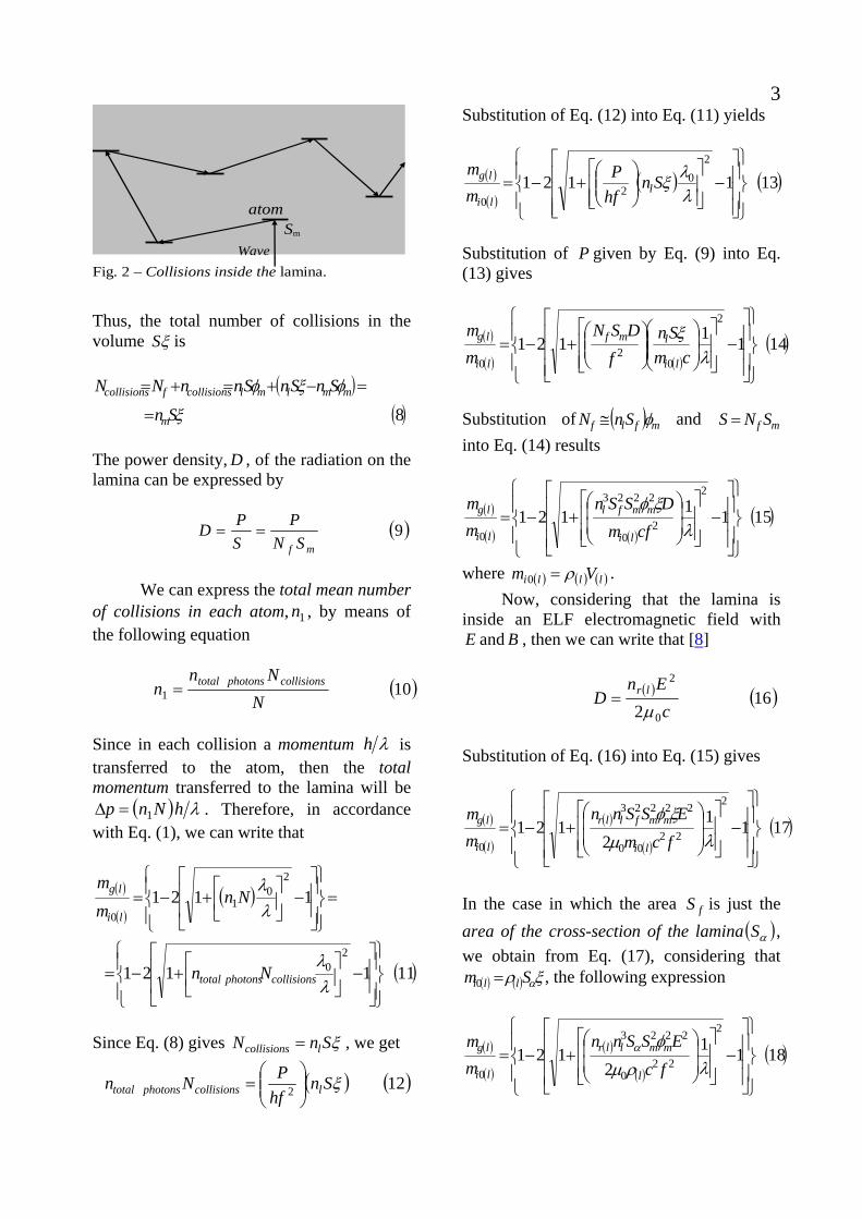
3 Fig. 2 – Collisions inside the lamina.
atom Sm
Wave
Thus, the total number of collisions in the volume ξS is
( )( )8ξ
φξφ
Sn
SnSnSnnNN
m
mmlmlcollisionsfcollisions
=
=−+=+=
The power density, , of the radiation on the lamina can be expressed by
D
( )9mf SN
PSPD ==
We can express the total mean number of collisions in each atom, , by means of the following equation
1n
( )101 NNn
n collisionsphotonstotal=
Since in each collision a momentum λh is transferred to the atom, then the total momentum transferred to the lamina will be
( ) λhNnp 1=Δ . Therefore, in accordance with Eq. (1), we can write that
( )
( )( )
( )111121
1121
20
20
10
⎪⎭
⎪⎬⎫
⎪⎩
⎪⎨⎧
⎥⎥
⎦
⎤
⎢⎢
⎣
⎡−⎥
⎦
⎤⎢⎣
⎡+−=
=⎪⎭
⎪⎬⎫
⎪⎩
⎪⎨⎧
⎥⎥
⎦
⎤
⎢⎢
⎣
⎡−⎥
⎦
⎤⎢⎣
⎡+−=
λλ
λλ
collisionsphotonstotal
li
lg
Nn
Nnmm
Since Eq. (8) gives ξSnN lcollisions = , we get
( ) (122 ξSnhfPNn lcollisionsphotonstotal ⎟⎟
⎠
⎞⎜⎜⎝
⎛=
Substitution of Eq. (12) into Eq. (11) yields
( )
( )( ) ( )131121
20
20 ⎪
⎭
⎪⎬
⎫
⎪⎩
⎪⎨
⎧
⎥⎥⎥
⎦
⎤
⎢⎢⎢
⎣
⎡−
⎥⎥⎦
⎤
⎢⎢⎣
⎡⎟⎟⎠
⎞⎜⎜⎝
⎛+−=
λλξSn
hfP
mm
lli
lg
Substitution of P given by Eq. (9) into Eq. (13) gives
( )
( ) ( )( )1411121
2
02
0 ⎪⎭
⎪⎬
⎫
⎪⎩
⎪⎨
⎧
⎥⎥⎥
⎦
⎤
⎢⎢⎢
⎣
⎡−
⎥⎥⎦
⎤
⎢⎢⎣
⎡⎟⎟⎠
⎞⎜⎜⎝
⎛⎟⎟⎠
⎞⎜⎜⎝
⎛+−=
λξcm
Snf
DSNmm
li
lmf
li
lg
Substitution of ( ) mflf SnN φ≅ and mf SNS = into Eq. (14) results
( )
( ) ( )( )1511121
2
20
2223
0 ⎪⎭
⎪⎬
⎫
⎪⎩
⎪⎨
⎧
⎥⎥⎥
⎦
⎤
⎢⎢⎢
⎣
⎡−
⎥⎥⎦
⎤
⎢⎢⎣
⎡
⎟⎟⎠
⎞⎜⎜⎝
⎛+−=
λξφ
cfmDSSn
mm
li
mmfl
li
lg
where ( ) ( ) ( )llli Vm ρ=0 . Now, considering that the lamina is inside an ELF electromagnetic field with E and B , then we can write that [8]
( ) ( )162 0
2
cEn
D lr
μ=
Substitution of Eq. (16) into Eq. (15) gives
( )
( )
( )
( )( )1711
2121
2
2200
22223
0 ⎪⎭
⎪⎬
⎫
⎪⎩
⎪⎨
⎧
⎥⎥⎥
⎦
⎤
⎢⎢⎢
⎣
⎡−
⎥⎥⎦
⎤
⎢⎢⎣
⎡
⎟⎟⎠
⎞⎜⎜⎝
⎛+−=
λμ
ξφ
fcmESSnn
mm
li
mmfllr
li
lg
In the case in which the area is just the area of the cross-section of the lamina
fS( )αS ,
we obtain from Eq. (17), considering that ( ) ( ) ξρ αSm lli =0 , the following expression
( )
( )
( )
( )( )1811
2121
2
220
2223
0 ⎪⎭
⎪⎬
⎫
⎪⎩
⎪⎨
⎧
⎥⎥⎥
⎦
⎤
⎢⎢⎢
⎣
⎡−
⎥⎥⎦
⎤
⎢⎢⎣
⎡
⎟⎟⎠
⎞⎜⎜⎝
⎛+−=
λρμ
φα
fcESSnn
mm
l
mmllr
li
lg
)
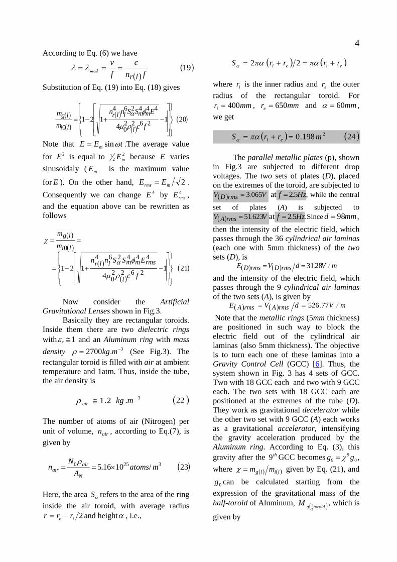
4According to Eq. (6) we have
( )( )19
fnc
fv
lr=== modλλ
Substitution of Eq. (19) into Eq. (18) gives
( )( )
( )
( )( )201
4121 2622
0
444264
0 ⎪⎭
⎪⎬
⎫
⎪⎩
⎪⎨
⎧
⎥⎥⎥
⎦
⎤
⎢⎢⎢
⎣
⎡
−+−=fc
ESSnn
mm
l
mmllr
li
lg
ρμ
φα
Note that tEE m ωsin= .The average value for 2E is equal to 2
21
mE because E varies sinusoidaly ( is the maximum value
formE
E ). On the other hand, 2mrms EE = . Consequently we can change 4E by , and the equation above can be rewritten as follows
4rmsE
( )
( )
( )
( )( )211
4121 2622
0
4442640
⎪⎭
⎪⎬
⎫
⎪⎩
⎪⎨
⎧
⎥⎥⎥
⎦
⎤
⎢⎢⎢
⎣
⎡
−+−=
==
fc
ESSnn
m
m
l
rmsmmllr
li
lg
ρμ
φ
χ
α
Now consider the Artificial Gravitational Lenses shown in Fig.3. Basically they are rectangular toroids. Inside them there are two dielectric rings with 1≅rε and an Aluminum ring with mass density (See Fig.3). The rectangular toroid is filled with air at ambient temperature and 1atm. Thus, inside the tube, the air density is
3.2700 −= mkgρ
( )22.2.1 3−≅ mkgairρ
The number of atoms of air (Nitrogen) per unit of volume, , according to Eq.(7), is given by
airn
( )23/1016.5 3250 matomsA
Nn
N
airair ×==
ρ
Here, the area refers to the area of the ring inside the air toroid, with average radius
αS
2ie rrr += and heightα , i.e.,
( ) ( )eiei rrrrS +=+= παπαα 22
where is the inner radius and the outer radius of the rectangular toroid. For
ir er
mmri 400= , mmre 650= and mm60=α , we get
( ) ( )24198.0 2mrrS ei =+= παα
The parallel metallic plates (p), shown in Fig.3 are subjected to different drop voltages. The two sets of plates (D), placed on the extremes of the toroid, are subjected to ( ) VV rmsD 0653.= at Hzf 5.2= , while the central
set of plates (A) is subjected to ( ) VV rmsA 62351.= at Hzf 5.2= .Since mmd 98= ,
then the intensity of the electric field, which passes through the 36 cylindrical air laminas (each one with 5mm thickness) of the two sets (D), is
( ) ( ) mVdVE rmsDrmsD /.2831==
and the intensity of the electric field, which passes through the 9 cylindrical air laminas of the two sets (A), is given by
( ) ( ) mVdVE rmsArmsA /.77526==
Note that the metallic rings (5mm thickness) are positioned in such way to block the electric field out of the cylindrical air laminas (also 5mm thickness). The objective is to turn each one of these laminas into a Gravity Control Cell (GCC) [6]. Thus, the system shown in Fig. 3 has 4 sets of GCC. Two with 18 GCC each and two with 9 GCC each. The two sets with 18 GCC each are positioned at the extremes of the tube (D). They work as gravitational decelerator while the other two set with 9 GCC (A) each works as a gravitational accelerator, intensifying the gravity acceleration produced by the Aluminum ring. According to Eq. (3), this gravity after the GCC becomes , where
th9 09
9 gg χ=
( ) ( )lilg mm=χ given by Eq. (21), and can be calculated starting from the
expression of the gravitational mass of the half-toroid of Aluminum,
0g
( toroidgM21 ) , which is
given by

5
( ) ( )
( ) ( ) (2521
21
00
iietoroidg
r
ie
M
toroidg
rrrMwhence
dzrrdM ig
−=
−= ∫∫
πρα
ραπ
) On the other hand, we have that
( )∫∫∫
−−=−= ig r
ieM
g
gdz
rrrGdM
rGdg
παρ0200 2
whence we get
( ) ( )262rrrrG
g iie −−=παρ
which gives the value of produced by the half-toroid at a point inside the nucleus of the toroid, distant
g
r from the center of the cross-section of the rectangular toroid. Thus, the value of , due to the first half-toroid is
0g ′ ( )0rr =
iie r
rrr
Gg ⎟⎟⎠
⎞⎜⎜⎝
⎛ −−≅′ 2
00 πρα
The value of , due to the opposite half-toroid is
0g ′′
( )
⎪⎪
⎭
⎪⎪
⎬
⎫
⎪⎪
⎩
⎪⎪
⎨
⎧
⎥⎦
⎤⎢⎣
⎡⎟⎠
⎞⎜⎝
⎛ −−⎟
⎠
⎞⎜⎝
⎛ +−
−
−−≅′′ 2
0
0
222 ieie
e
iie
rrr
rrr
rrrGg πρα
Consequently, the resultant is
( )
( )( ) ⎥
⎥⎦
⎤
⎢⎢⎣
⎡
+
−−
=
⎪⎪
⎭
⎪⎪
⎬
⎫
⎪⎪
⎩
⎪⎪
⎨
⎧
⎥⎦
⎤⎢⎣
⎡⎟⎠
⎞⎜⎝
⎛ −−⎟
⎠
⎞⎜⎝
⎛ +−
−
−−
−⎟⎟⎠
⎞⎜⎜⎝
⎛ −−≅
20
2
0
20
0
222
rrrrr
G
rrr
rrr
rrrG
rr
rrGg
i
iie
ieiee
iie
iie
πρα
πρα
πρα
In the case of , the equation above reduces to
0rri >>
( )2720
0 iie r
rrr
Gg ⎟⎟⎠
⎞⎜⎜⎝
⎛ −−≅ πρα
where is the inner radius of the toroid; is the distance between the center of the cross-section of the Aluminum ring and the surface of the first GCC of the set (A);
ir 0r
α is the thickness of the Aluminum ring. Here,
mmr 350 = and mm60=α (See Fig. 3 (a)). The objective of the sets (D), with 18 GCC each, is to reduce strongly the value of the external gravity along the rectangular toroid of air in D region. In this case, the value of the external gravity, , is reduced
by the factor , where extg
extd g18χ 210−=dχ . For
example, if then this value is
reduced to and, after the set A, it is increased by . Since the system is designed for
2/81.9 smgext =
extd g18χ9χ
1.627−=χ , then the gravity acceleration on the Aluminum ring becomes , this value is smaller than
210189 /1047.1 smg extd−×=χχ
( )[ ] 28200 .109.9 −−×=−−≅ smrrrrGg iieπρα .
The values of χ and dχ , according to Eq. (21) are given by

6
( ) ( )
( ) ( )241102891121
14
121
46
26220
444264
⎭⎬⎫
⎩⎨⎧
⎥⎦⎤
⎢⎣⎡ −×+−=
=⎪⎭
⎪⎬
⎫
⎪⎩
⎪⎨
⎧
⎥⎥⎥
⎦
⎤
⎢⎢⎢
⎣
⎡
−+−=
−rmsA
air
rmsAmmairairr
E
fc
ESSnn
.
ρμ
φχ
α
( ) ( )
( ) ( )251102891121
14
121
46
26220
444264
⎭⎬⎫
⎩⎨⎧
⎥⎦⎤
⎢⎣⎡ −×+−=
=⎪⎭
⎪⎬
⎫
⎪⎩
⎪⎨
⎧
⎥⎥⎥
⎦
⎤
⎢⎢⎢
⎣
⎡
−+−=
−rmsD
air
rmsDmmairairrd
E
fc
ESSnn
.
ρμ
φχ
α
where ( ) 1≅= rrairrn με , since ( )ωεσ << †;
, , 325 /1016.5 matomsnair ×= mm101055.1 −×=φ
2202 1088.14 mS mm−×==πφ and Hzf 5.2= .
Since , , we get
( ) mVE rmsA /.77526= ( ) mVE rmsD /.2831=
( )301.627−=χ
and
( )3110 2−≅dχ Then the gravitational acceleration after the 9th gravitational shielding is
( ) ( )3220
90
99 ⎥
⎦
⎤⎢⎣
⎡ −−==
rrrr
Ggg iieπραχχ
It is known that gravitational fields can bend light, and that due to this effect, a light ray that passes very close to a body with gravitational mass is deviated of an angle
gMδ (deflection angle) given by [3]
† The electrical conductivity of air, inside the dielectric tube, is equal to the electrical conductivity of Earth’s atmosphere near the land, whose average value is mSair /101 14−×≅σ [9].
( )334
2dcGM g−=δ
where is the distance of closest approach. d Here, we can obtain the expression of δ as follows: by comparing Eq. (26) with Eq. (25) we obtain . Substitution of this expression into Eq. (33) leads to the following equation
2grGM g =
( )344
2
2
dcgr
=δ
For 0rr = we have and equation above can be rewritten as follows
0gg =
( )354
2
200
dcrg
=δ
However, considering the symmetry of the gravitational lenses shown in Fig.3, it is easy to see that Eq. (35) must be rewritten as follows
( )3644
2
200
2
200
dcrg
dcrg
′′−
′=δ
where d ′ and d ′′ are respectively, the distances of closest approach of the light ray with respect to the two sides of the Aluminum ring (See Fig 3 (b)). When the gravitational lenses are activated the value of is amplified to
, then Eq. (36) becomes 0g
09 gχ
( )3744
2
200
9
2
200
9
dcrg
dcrg
′′−
′=
χχδ
Note that, for dd ′′=′ (light ray at the center of the Gravitational lens) Eq. (37) gives
0=δ ( null deflection). On the other hand, if dd ′′<′ we have 0>δ (the light ray is
gravitationally attracted to the inner edge of rectangular toroid). Under these conditions, when a light flux crosses the gravitational lens (nucleus of the rectangular toroid), it becomes divergent in respect to the central axis of the toroid (See Fig. 3(c)). If

7dd ′′>′ then Eq. (37) shows that 0<δ (the
light ray is gravitationally repelled from the inner edge of rectangular toroid). In this case, when a light flux crosses the gravitational lens, it becomes convergent in respect to the central axis of the toroid (See Fig. 3(b)). Substitution of the known values into Eq. (37) yields
( )38111.0 ⎟⎠⎞
⎜⎝⎛
′′−′
≅dd
δ
Note that the values of δ can be easily controlled simply by controlling of the value of χ . Also note that the curvatures of the light rays are proportional to the distances
and , similarly to the curvature of the light rays in the optical lenses. Then it is easy to see that these gravitational lenses can be very useful in building of telescopes, microscopes, and in concentrating solar light in order to convert solar energy into thermal energy.
d ′ d ′′
I would like to thank Physicist André Luis Martins (RJ, Brazil) who came up with the original idea to build Artificial Gravitational Lens using sets of Gravitational Shieldings, as shown in my previous papers.

8
(a)
(b)
(c)
Fig. 3 – Artificial Gravitational Lens. (a) Cross-section of the Artificial Gravitational Lens. (b)Cross-section of a Convergent Gravitational Lens. The light rays are gravitationally repelled from the inner edge of toroid (c) Cross-section of a Divergent Gravitational Lens. The light rays aregravitationally attracted to the inner edge of toroid.
ξ = 5 mm Parallel plate capacitor (p)
(Metallic ring)
1 2 17 1888
Dielectric rings εr ≅ 1
D
Mg 1 2 6 9
A
Air Aird = 98 mm
α=60mm
Rectangular ToroidMetallic ring (5 mm thickness)
r0=35mm ED(rms)
EA(rms) Air
1 atm 300K
Gravitational Lens
Rectangular Toroid
Rectangular Toroid
Mg D A DA Mg
D and A Sets of
Gravitational Shieldings
D DA A Mg Mg Gravitational Lens
Gravitational Lens
Light
Light
g’ g’
g’ g’
Aluminum ring
re ri
d ′′d ′

9 References [1] Dyson, F.W., Eddington, A.S., and Davidson, C.R. (1920). A Determination of the Deflection of Light by the Sun's Gravitational Field, from Observations Made at the Solar eclipse of May 29, 1919. Phil. Trans. Roy. Soc. A 220 (571-581): 291–333. [2] Chwolson, O (1924). Über eine mögliche Form fiktiver Doppelsterne. Astronomische Nachrichten 221 (20): 329. [3] Einstein, A. (1936). Lens-like Action of a Star by the Deviation of Light in the Gravitational Field. Science 84 (2188): 506–7. [4] Renn, J., Tilman S., and Stachel, J., (1997). The Origin of Gravitational Lensing: A Postscript to Einstein's 1936 Science paper. Science 275 (5297): 184–6. [5] De Aquino, F. (2010) Mathematical Foundations of the Relativistic Theory of Quantum Gravity, Pacific Journal of Science and Technology, 11 (1), pp. 173- 232. [6] De Aquino, F. (2010) Gravity Control by means of Electromagnetic Field through Gas at Ultra-Low Pressure, Pacific Journal of Science and Technology, 11(2) November 2010, pp.178-247, Physics/0701091. [7] Quevedo, C. P. (1977) Eletromagnetismo, McGraw- Hill, p. 270. [8] Halliday, D. and Resnick, R. (1968) Physics, J. Willey & Sons, Portuguese Version, Ed. USP, p.1124. [9] Chalmers, J.A., (1967) Atmospheric Electricity, Pergamon press, Oxford, London; Kamsali, N. et al., (2011) Advanced Air Pollution, chapter 20, DOI: 10.5772/17163, edited by Farhad Nejadkoorki, Publisher: InTech, ISBN 978-953-307-511-2, under CC BY-NC- SA 3.0 license.

Gravitational Blueshift and Redshift
generated at Laboratory Scale
Fran De Aquino Maranhao State University, Physics Department, S.Luis/MA, Brazil.
Copyright © 2012 by Fran De Aquino. All Rights Reserved. In this paper we show that it is possible to produce gravitational blueshift and redshift at laboratory scale by means of a device that can strongly intensify the local gravitational potential. Thus, by using this device, it is possible to generate electromagnetic radiation of any frequency, from ELF radiation (f < 10Hz) up to high energy gamma-rays. In this case, several uses, such as medical imaging, radiotherapy and radioisotope production for PET (positron emission tomography) scanning, could be realized. The device is smaller and less costly than conventional sources of gamma rays.
Key words: Modified theories of gravity, Relativity and Gravitation, Gravitational Redshift and Blueshift. PACS: 04.50.Kd, 95.30.Sf, 98.62.Py. 1. Introduction It is known that electromagnetic radiation is blueshifted when propagating from a region of weaker gravitational field to a region of stronger gravitational field. In this case the radiation is blueshifted because it gains energy during propagation. In the contrary case, the radiation is redshifted. This effect was predicted by Einstein’s Relativity Theory [1, 2] and was widely confirmed by several experiments [3, 4]. It was first confirmed in 1959 in the Pound and Rebka experiment [3]. Here we show that it is possible to produce gravitational blueshift and redshift at laboratory scale by means of a device that can strongly intensify the local gravitational potential* [5]. Thus, by using this device, it is possible to generate electromagnetic radiation of any frequency, from ELF radiation (f < 10Hz) up to high energy gamma-rays. In this case, several uses, such as in medical imaging, radiotherapy and radioisotope production for PET (positron emission tomography) scanning and others, could be devised. The device is smaller and less costly than conventional sources of gamma rays. * De Aquino, F. (2008) Process and Device for Controlling the Locally the Gravitational Mass and the Gravity Acceleration, BR Patent Number: PI0805046-5, July 31, 2008.
2. Theory From the quantization of gravity it follows that the gravitational mass mg and the inertial mass mi are correlated by means of the following factor [5]:
( )111212
00 ⎪⎭
⎪⎬⎫
⎪⎩
⎪⎨⎧
⎥⎥
⎦
⎤
⎢⎢
⎣
⎡−⎟⎟
⎠
⎞⎜⎜⎝
⎛ Δ+−==
cmp
mm
ii
gχ
where is the rest inertial mass of the particle and
0impΔ is the variation in the
particle’s kinetic momentum; is the speed of light.
c
When pΔ is produced by the absorption of a photon with wavelengthλ , it is expressed by λhp =Δ . In this case, Eq. (1) becomes
( )21121
1121
20
20
0
⎪⎭
⎪⎬⎫
⎪⎩
⎪⎨⎧
⎥⎥
⎦
⎤
⎢⎢
⎣
⎡−⎟
⎠
⎞⎜⎝
⎛+−=
⎪⎭
⎪⎬⎫
⎪⎩
⎪⎨⎧
⎥⎥
⎦
⎤
⎢⎢
⎣
⎡−⎟
⎠
⎞⎜⎝
⎛+−=
λλ
λcmh
mm i
i
g
where cmh i00 =λ is the De Broglie wavelength for the particle with rest inertial mass . 0im It has been shown that there is an additional effect - Gravitational Shielding

2effect - produced by a substance whose gravitational mass was reduced or made negative [6]. The effect extends beyond substance (gravitational shielding) , up to a certain distance from it (along the central axis of gravitational shielding). This effect shows that in this region the gravity acceleration, , is reduced at the same proportion, i.e.,
1ggg
11 χ= where
01 ig mm=χ and is the gravity acceleration before the gravitational shielding). Consequently, after a second gravitational shielding, the gravity will be given by
g
ggg21122 χχχ == , where
2χ is
the value of the ratio 0ig mm for the second gravitational shielding. In a generalized way, we can write that after the nth gravitational shielding the gravity, , will be given by ng
( )3...321
ggnn χχχχ=
This possibility shows that, by means of a battery of gravitational shieldings, we can strongly intensify the gravitational acceleration. In order to measure the extension of the shielding effect, samples were placed above a superconducting disk with radius
, which was producing a gravitational shielding. The effect has been detected up to a distance of about 3m from the disk (along the central axis of disk) [
mrD 1375.0=
7]. This means that the gravitational shielding effect extends, beyond the disk by approximately 20 times the disk radius. From Electrodynamics we know that when an electromagnetic wave with frequency and velocity incides on a material with relative permittivity
f c
rε , relative magnetic permeability rμ and electrical conductivity σ , its velocity is reduced to rncv = where is the index of refraction of the material, given by [
rn8]
( ) ( )4112
2 ⎟⎠⎞⎜
⎝⎛ ++== ωεσ
με rrr v
cn
If ωεσ >> , fπω 2= , Eq. (4) reduces to
( )54 0 f
n rr πε
σμ=
Thus, the wavelength of the incident radiation (See Fig. 1) becomes
( )64mod σμ
πλλfnn
fcfv
rr====
Fig. 1 – Modified Electromagnetic Wave. The wavelength of the electromagnetic wave can bestrongly reduced, but its frequency remains the same.
v = c v = c/nr
λ = c/f λmod = v/f = c/nr f
nr
If a lamina with thickness equal toξ contains atoms/mn 3, then the number of atoms per area unit is ξn . Thus, if the electromagnetic radiation with frequency
incides on an area of the lamina it reachesf S
ξnS atoms. If it incides on the total area of the lamina, , then the total number of atoms reached by the radiation is
fS
ξfnSN = . The number of atoms per unit of volume, , is given by n
( )70
AN
nρ
=
where is the Avogadro’s number;
kmoleatomsN /1002.6 260 ×=
ρ is the matter density of the lamina (in kg/m3) and A is the molar mass(kg/kmole). When an electromagnetic wave incides on the lamina, it strikes front atoms, where
fN( ) mff SnN φ≅ , mφ is the “diameter” of
the atom. Thus, the electromagnetic wave incides effectively on an area mf SNS= ,
where 241
mmS πφ= is the cross section area of

3one atom. After these collisions, it carries out
with the other atoms (See Fig.2). collisionsn Fig. 2 – Collisions inside the lamina.
atom Sm
Wave
Thus, the total number of collisions in the volume ξS is
( )( )8ξ
φξφ
Sn
SnSnSnnNN
m
mmlmlcollisionsfcollisions
=
=−+=+=
The power density, , of the radiation on the lamina can be expressed by
D
( )9mf SN
PSPD ==
We can express the total mean number of collisions in each atom, , by means of the following equation
1n
( )101 NNn
n collisionsphotonstotal=
Since in each collision a momentum λh is transferred to the atom, then the total momentum transferred to the lamina will be
( ) λhNnp 1=Δ . Therefore, in accordance with Eq. (1), we can write that
( )
( )( )
( )111121
1121
20
20
10
⎪⎭
⎪⎬⎫
⎪⎩
⎪⎨⎧
⎥⎥
⎦
⎤
⎢⎢
⎣
⎡−⎥
⎦
⎤⎢⎣
⎡+−=
=⎪⎭
⎪⎬⎫
⎪⎩
⎪⎨⎧
⎥⎥
⎦
⎤
⎢⎢
⎣
⎡−⎥
⎦
⎤⎢⎣
⎡+−=
λλ
λλ
collisionsphotonstotal
li
lg
Nn
Nnmm
Since Eq. (8) gives ξSnN lcollisions = , we get
( ) (122 ξSnhfPNn lcollisionsphotonstotal ⎟⎟
⎠
⎞⎜⎜⎝
⎛= )
Substitution of Eq. (12) into Eq. (11) yields
( )
( )( ) ( )131121
20
20 ⎪
⎭
⎪⎬
⎫
⎪⎩
⎪⎨
⎧
⎥⎥⎥
⎦
⎤
⎢⎢⎢
⎣
⎡−
⎥⎥⎦
⎤
⎢⎢⎣
⎡⎟⎟⎠
⎞⎜⎜⎝
⎛+−=
λλξSn
hfP
mm
lli
lg
Substitution of P given by Eq. (9) into Eq. (13) gives
( )
( ) ( )( )1411121
2
02
0 ⎪⎭
⎪⎬
⎫
⎪⎩
⎪⎨
⎧
⎥⎥⎥
⎦
⎤
⎢⎢⎢
⎣
⎡−
⎥⎥⎦
⎤
⎢⎢⎣
⎡⎟⎟⎠
⎞⎜⎜⎝
⎛⎟⎟⎠
⎞⎜⎜⎝
⎛+−=
λξcm
Snf
DSNmm
li
lmf
li
lg
Substitution of ( ) mflf SnN φ≅ and mf SNS = into Eq. (14) results
( )
( ) ( )( )1511121
2
20
2223
0 ⎪⎭
⎪⎬
⎫
⎪⎩
⎪⎨
⎧
⎥⎥⎥
⎦
⎤
⎢⎢⎢
⎣
⎡−
⎥⎥⎦
⎤
⎢⎢⎣
⎡
⎟⎟⎠
⎞⎜⎜⎝
⎛+−=
λξφ
cfmDSSn
mm
li
mmfl
li
lg
where ( ) ( ) ( )llli Vm ρ=0 . Now, considering that the lamina is inside an ELF electromagnetic field with E and B , then we can write that [9]
( ) ( )162 0
2
cEn
D lr
μ=
Substitution of Eq. (16) into Eq. (15) gives
( )
( )
( )
( )( )1711
2121
2
2200
22223
0 ⎪⎭
⎪⎬
⎫
⎪⎩
⎪⎨
⎧
⎥⎥⎥
⎦
⎤
⎢⎢⎢
⎣
⎡−
⎥⎥⎦
⎤
⎢⎢⎣
⎡
⎟⎟⎠
⎞⎜⎜⎝
⎛+−=
λμ
ξφ
fcmESSnn
mm
li
mmfllr
li
lg
In the case in which the area is just the area of the cross-section of the lamina
fS( )αS ,
we obtain from Eq. (17), considering that ( ) ( ) ξρ αSm lli =0 , the following expression

4
( )
( )
( )
( )( )1811
2121
2
220
2223
0 ⎪⎭
⎪⎬
⎫
⎪⎩
⎪⎨
⎧
⎥⎥⎥
⎦
⎤
⎢⎢⎢
⎣
⎡−
⎥⎥⎦
⎤
⎢⎢⎣
⎡
⎟⎟⎠
⎞⎜⎜⎝
⎛+−=
λρμ
φα
fcESSnn
mm
l
mmllr
li
lg
According to Eq. (6) we have
( )( )19
fnc
fv
lr=== modλλ
Substitution of Eq. (19) into Eq. (18) gives
( )( )
( )
( )( )201
4121 2622
0
444264
0 ⎪⎭
⎪⎬
⎫
⎪⎩
⎪⎨
⎧
⎥⎥⎥
⎦
⎤
⎢⎢⎢
⎣
⎡
−+−=fc
ESSnn
mm
l
mmllr
li
lg
ρμ
φα
Note that tEE m ωsin= .The average value for 2E is equal to 2
21
mE because E varies sinusoidaly ( is the maximum value
formE
E ). On the other hand, 2mrms EE = . Consequently we can change 4E by , and the equation above can be rewritten as follows
4rmsE
( )
( )
( )
( )( )211
4121 2622
0
4442640
⎪⎭
⎪⎬
⎫
⎪⎩
⎪⎨
⎧
⎥⎥⎥
⎦
⎤
⎢⎢⎢
⎣
⎡
−+−=
==
fc
ESSnn
m
m
l
rmsmmllr
li
lg
ρμ
φ
χ
α
Now consider the Gravitational Shift Device shown in Fig.3. Inside the device there is a dielectric tube ( 1≅rε ) with the following characteristics:
mm60=α , 232 1083.24 mS −×== παα . Inside the tube there is an Aluminum sphere with 30mm radius and mass
kgM gs 30536.0= . The tube is filled with air at ambient temperature and 1atm. Thus, inside the tube, the air density is
( )22.2.1 3−= mkgairρThe number of atoms of air (Nitrogen) per unit of volume, , according to Eq.(7), is given by
airn
( )23/1016.5 3250 matomsA
Nn
N
airair ×==
ρ
The parallel metallic plates (p), shown in Fig.3 are subjected to different drop voltages. The two sets of plates (D), placed on the extremes of the tube, are subjected to ( ) VV rmsD 2216.= at Hzf 1= , while the central
set of plates (A) is subjected to ( ) VV rmsA 98191.= at Hzf 1= . Since mmd 98= ,
then the intensity of the electric field, which passes through the 36 cylindrical air laminas (each one with 5mm thickness) of the two sets (D), is
( ) ( ) mVdVE rmsDrmsD /.53165==
and the intensity of the electric field, which passes through the 7 cylindrical air laminas of the central set (A), is given by
( ) ( ) mVdVE rmsArmsA /. 3109591 ×==
Note that the metallic rings (5mm thickness) are positioned in such way to block the electric field out of the cylindrical air laminas. The objective is to turn each one of these laminas into a Gravity Control Cells (GCC) [10]. Thus, the system shown in Fig. 3 has 3 sets of GCC. Two with 18 GCC each, and one with 19 GCC. The two sets with 18 GCC each are positioned at the extremes of the tube (D). They work as gravitational decelerator while the other set with 19 GCC (A) works as a gravitational accelerator, intensifying the gravity acceleration and the gravitational potential produced by the mass
of the Aluminum sphere. According to
Eq. (3) the gravity, after the GCC becomes
gsMth19
21
1919 rGMg gsχ= , and the
gravitational potential 119 rGM gsχϕ =
where ( ) ( )lilg mm=χ is given by Eq. (21) and mmr 351 = is the distance between the center of the Aluminum sphere and the surface of the first GCC of the set (A). The objective of the sets (D), with 18 GCC each, is to reduce strongly the value of the external gravity along the axis of the tube. In this case, the value of the external gravity, , is reduced by the factor , extg extd g18χ

5where 210−=dχ . For example, if the base BS of the system is positioned on the Earth surface, then is reduced
to and, after the set A, it is increased by . Since the system is designed for
2/81.9 smgext =
extd g18χ19χ
5.308−=χ , then the gravity acceleration on the sphere becomes , this value is much smaller than
2121819 /104.2 smgextd−×=χχ
282 /1026.2 smrGMg sgssphere−×== .
The values of χ and dχ , according to Eq. (21) are given by
( ) ( )
( )
( ) ( )241106451121
14
121
49
26220
444264
⎭⎬⎫
⎩⎨⎧
⎥⎦⎤
⎢⎣⎡ −×+−=
=⎪⎭
⎪⎬
⎫
⎪⎩
⎪⎨
⎧
⎥⎥⎥
⎦
⎤
⎢⎢⎢
⎣
⎡
−+−=
−rmsA
l
rmsAmmllr
E
fc
ESSnn
.
ρμ
φχ
α
( ) ( )
( )
( ) ( )251106451121
14
121
49
26220
444264
⎭⎬⎫
⎩⎨⎧
⎥⎦⎤
⎢⎣⎡ −×+−=
=⎪⎭
⎪⎬
⎫
⎪⎩
⎪⎨
⎧
⎥⎥⎥
⎦
⎤
⎢⎢⎢
⎣
⎡
−+−=
−rmsD
l
rmsDmmllrd
E
fc
ESSnn
.
ρμ
φχ
α
where ( ) 1≅= rrairrn με , since ( )ωεσ << †;
, , 325 /1016.5 matomsnair ×= mm101055.1 −×=φ
2202 1088.14 mS mm−×== πφ and Hzf 1= .
Since and , we get
( ) mVE rmsA /. 3109591 ×=
( ) mVE rmsD /.53165=
( )265.308−=χ
and
( )2710 2−≅dχ † The electrical conductivity of air, inside the dielectric tube, is equal to the electrical conductivity of Earth’s atmosphere near the land, whose average value is mSair /101 14−×≅σ [11].
Then the gravitational acceleration after the 19th gravitational shielding of the set A (See Fig.3) ‡ is
( )2821
191
1919 rGMgg gsχχ ==
and the gravitational potential is
( )29119
119 rGM gsχϕχϕ ==
Thus, if photons with frequency are emitted from a point 0 near the Earth’s surface, where the gravitational potential is
0f
⊕⊕−≅ rGM0ϕ (See photons source in Fig.3), and these photons pass through the region in front of the 19th gravitational shielding, where the gravitational potential is increased to the value expressed by Eq. (29) then the frequency of the photons in this region, according to Einstein’s relativity theory, becomes , wherefff Δ+= 0 fΔ is given by
( )3021
19
020
crGMrGM
fc
f gs ⊕⊕+−=
−=Δ
χϕϕ
If 0<χ , then and 019 <χ
0>Δf (blueshift). Note that, if the number of Gravitational Shieldings in the set A is
odd (n
,...7,5,3,1=n ) then the result is 0>Δf (blueshift). But, if is even
(n
,...8,6,4,2=n ) and ⊕⊕> rMrMgsn
1χ then the result is 0<Δf (redshift). Note that to reduce down to it is necessary that . This precision is not easy to be obtained in practice. On the other hand, if for example,
Hzf 140 10= Hzf 1110≅
Hzf 1410999.0 ×−=Δ
‡ The gravitational shielding effect extends beyond the gravitational shielding by approximately 20 times its radius (along the central axis of the gravitational shielding). [7] Here, this means that, in absence of the set D (bottom of the device), the gravitational shielding effect extends, beyond the 19thgravitational shielding, by approximately 20 (α/2) ≈ 600mm.

6 Hzf 14
0 10= and then i.e., the redshift is
negligible. However, the device can be useful to generate ELF radiation by redshift. For example, if
Hzf 1010−=Δ
Hzfff 140 10≅Δ+=
GHzf 10 = , and 18=n15278521.95=χ , then we obtain ELF
radiation with frequency . Radiation of any frequency can be generated by gravitational blueshift. For example, if
and then . What means that a
light beam with frequency was converted into a gamma-ray beam with frequency . Similarly, if and
Hzf 1≅
Hzf 140 10= Hzf 1810+=Δ
Hzfff 180 10≅Δ+=
Hz1410
Hz1810 MHzf 10 =MHzf 9+=Δ , then ,
and so on. MHzfff 100 ≅Δ+=
Now, consider the device shown in Fig. 3, where 5.308−=χ , kgM gs 30536.0= ,
mmr 351 = . According to Eq. (30), it can produce a given by fΔ
( )31106.3 222
119
Hzc
rGMf gs ×≅
−≅Δ
χ
Thus, we get
( )32106.3 220 Hzfff ×≅Δ+=
What means that the device is able to convert any type of electromagnetic radiation (frequency ) into a gamma-ray beam with frequency . Thus, by controlling the value of
0f
Hz22106.3 ×χ and , it is possible to
generate radiation of any frequency. 0f

7
Fig. 3 – Schematic diagram of the Gravitational Shift Device (Blueshift and Redshift) – The device can generate electromagnetic radiation of any frequency, since ELF radiation (f < 10Hz) up to high energy gamma-rays.
E
ξ = 5 mm
Parallel plate capacitor (p)
1
2
17
18
1
2
18
19
1
2
1718
α=60mm
d = 98 mm
Mg
Metallic ring (5 mm thickness)
Electric field of capacitor
Aluminum sphere (60 mm diameter)
Dielectric tube εr ≅ 1
A
D
D
ED(rms)
EA(rms)
Air
Air
Air
AirAir 1 atm 300K
r1=35mm
Air
Air
Air
Photons Source (frequency f0 )
Photons Beam (frequency f ) 0f
019 <χ ⊕⊕−= rGM0ϕ
11,ϕg
ssg ϕ,rs
0ϕ
f
Region with potential ϕ
119ϕχϕ =
21
19
020
crGMrGM
fc
f gs ⊕⊕+−=
−=Δ
χϕϕ

8 References [1] Misner, Charles W.; Thorne, Kip S.; Wheeler, John Archibald (1973-09-15 1973). Gravitation. San Francisco: W. H. Freeman. [2] Bonometto, Silvio; Gorini, Vittorio; Moschella, Ugo (2002). Modern Cosmology. CRC Press. [3] R.V. Pound and G.A. Rebka, Jr. (1959) Gravitational Red-Shift in Nuclear Resonance, Phys. Rev. Lett. 3 439– 441. [4] Vessot, R. F. C., et al., (1980) Test of Relativistic Gravitation with a Space-Borne Hydrogen Maser. Physical Review Letters 45 (26): 2081–2084. [5] De Aquino, F. (2010) Mathematical Foundations of the Relativistic Theory of Quantum Gravity, Pacific Journal of Science and Technology, 11 (1), pp. 173- 232. [6] De Aquino, F. (2010) Gravity Control by means of Electromagnetic Field through Gas at Ultra-Low Pressure, Pacific Journal of Science and Technology, 11(2) November 2010, pp.178-247, Physics/0701091. [7] Modanese, G., (1996), Updating the Theoretical Analysis of the Weak Gravitational Shielding Experiment, supr-con/9601001v2. [8] Quevedo, C. P. (1977) Eletromagnetismo, McGraw- Hill, p. 270. [9] Halliday, D. and Resnick, R. (1968) Physics, J. Willey & Sons, Portuguese Version, Ed. USP, p.1124. [10] De Aquino, F. (2010) Gravity Control by means of Electromagnetic Field through Gas at Ultra-Low Pressure, Pacific Journal of Science and Technology, 11(2) November 2010, pp.178-247, Physics/0701091. [11] Chalmers, J.A., (1967) Atmospheric Electricity, Pergamon press, Oxford, London; Kamsali, N. et al., (2011) Advanced Air Pollution, chapter 20, DOI: 10.5772/17163, edited by Farhad Nejadkoorki, Publisher: InTech, ISBN 978-953-307-511-2, under CC BY-NC- SA 3.0 license.

Quantum Reversal of Soul Energy
Fran De Aquino Maranhao State University, Physics Department, S.Luis/MA, Brazil.
Copyright © 2012 by Fran De Aquino. All Rights Reserved. In the last decades, the existence of the Soul has been seriously considered by Quantum Physics. It has been frequently described as a body of unknown energy coupled to human body by means of a mutual interaction. The Quantum Physics shows that energy is quantized, i.e., it has discrete values that are defined as energy levels. Thus, along the life of a person, the energy of its soul is characterized by several quantum levels of energy. Here, we show by means of application of specific electromagnetic radiations on the human body, that it is possible to revert the energy of the soul to previous energy levels. This process can have several therapeutic applications.
Key words: Modified theories of gravity, Microwave fields effects, Therapeutic applications, Quantum information. PACS: 04.50.Kd, 87.50.S-,87.50.st, 03.67.-a. 1. Introduction Since long the Soul has remained an element of strongly consideration by Religion. Some authors claim that Religion is the science of the Soul [1]. Others claim that Soul and Religion are related to evolution. Sir Julian Huxley, a leading evolutionary biologist, the first Director-General of UNESCO and signatory to the Humanist Manifesto II, wrote: “Human Soul and Religion are just the product of evolution” [2]. This show how important the Soul is for the Religion. Philosophy also realizes the importance of the Soul. Plato, drawing on the words of his teacher Socrates, considered the Soul the essence of a person, being that which decides how we behave. As bodies die, the Soul is continually reborn in subsequent bodies. Nowadays, Quantum Physics and other branches of Science are seriously considering the existence of the Soul. It has been frequently described as a body of unknown energy coupled to human body by means of a mutual interaction. This type of energy from the viewpoint of Physics has been considered as Imaginary Energy. The term imaginary are borrowed from Mathematics (real and imaginary numbers) [3]. Quantum Physics shows that energy is quantized, i.e., that it has discrete values that are defined as discrete energy levels that correspond to all positive integer values of
the quantum number , [n ( ),...3,2,1=n 4]. Thus, along the life of a person, the energy of its Soul is characterized by several quantum levels of energy. Here, we show that, by means of application of specific electromagnetic radiations on the human body (its Soul), it is possible to revert the energy of the Soul to previous energy levels. This process can have several therapeutic applications.
2. Theory
From the quantization of gravity it follows that the imaginary gravitational mass mg (im) and the imaginary inertial mass mi0 (im) are correlated by means of the following factor [5]:
( )
( )
( )
( )( )11121
2
00 ⎪⎭
⎪⎬
⎫
⎪⎩
⎪⎨
⎧
⎥⎥⎥
⎦
⎤
⎢⎢⎢
⎣
⎡−⎟
⎟⎠
⎞⎜⎜⎝
⎛ Δ+−==
cmp
mm
imi
im
imi
imgχ
where ( ) imm iimi 03
20 −= is the imaginary
inertial mass at rest of the particle and ( ) ( ) ( ) cnUicnUp rrimim ==Δ is the variation
in the particle’s imaginary kinetic momentum; is the speed of light. Thus, Eq. (1) can be rewritten as follows
c

2
( )
( )( )21
43121
2
200 ⎪⎭
⎪⎬⎫
⎪⎩
⎪⎨⎧
⎥⎥
⎦
⎤
⎢⎢
⎣
⎡−⎟⎟
⎠
⎞⎜⎜⎝
⎛+−==
cmUn
mm
i
r
imi
imgχ
When is produced by the absorption of a photon with wavelength
pΔλ ,
i.e., , Eq. (2) becomes hfU =
( )
( )( )31
43121
2
mod
0
0 ⎪⎭
⎪⎬⎫
⎪⎩
⎪⎨⎧
⎥⎥
⎦
⎤
⎢⎢
⎣
⎡−⎟⎟
⎠
⎞⎜⎜⎝
⎛+−==
λλ
χimi
img
mm
where cmh i00 =λ is the De Broglie wavelength for the particle with rest inertial mass (real) and 0im rnλλ =mod . From Electrodynamics we know that when an electromagnetic wave with frequency and velocity incides on a material with relative permittivity
f c
rε , relative magnetic permeability rμ and electrical conductivity σ , its velocity is reduced to rncv = where is the index of refraction of the material, given by [
rn6]
( ) ( )4112
2 ⎟⎠⎞⎜
⎝⎛ ++== ωεσ
με rrr v
cn
If ωεσ >> , fπω 2= , Eq. (4) reduces to
( )54 0 f
n rr πε
σμ=
Thus, the wavelength of the incident radiation (See Fig. 1) becomes
( )64mod σμ
πλλfnn
fcfv
rr====
Fig. 1 – Modified Electromagnetic Wave. The wavelength of the electromagnetic wave can bestrongly reduced, but its frequency remains the same.
v = c v = c/nr
λ = c/f λmod = v/f = c/nr f
nr
If an imaginary lamina with thickness equal toξ contains imaginary molecules/m
n3, then the number of molecules
per unit area is ξn . Thus, if the electromagnetic radiation with frequency
incides on an area of the lamina it reachesf S
ξnS molecules. If it incides on the total area of the lamina, , then the total number of molecules reached by the radiation is
fS
ξfnSN = . The number of molecules per unit volume, , is given by n
( )70
AN
nρ
=
where is the Avogadro’s number;
kmolemoleculessN /1002.6 260 ×=
ρ is the matter density of the lamina (in kg/m3) and A is the molar mass(kg/kmole). When an electromagnetic wave incides on the lamina, it strikes front molecules, where
fN( ) mff SnN φ≅ , mφ is the “diameter” of
the molecule. Thus, the electromagnetic wave incides effectively on an area mf SNS= ,
where 241
mmS πφ= is the cross section area of one molecule. After these collisions, it carries out with the other molecules (See Fig.2).
collisionsn
Fig. 2 – Collisions inside the imaginary lamina.
Imaginary molecule Sm
Wave
Thus, the total number of collisions in the volume ξS is
( )( )8ξ
φξφ
Sn
SnSnSnnNN
m
mmlmlcollisionsfcollisions
=
=−+=+=
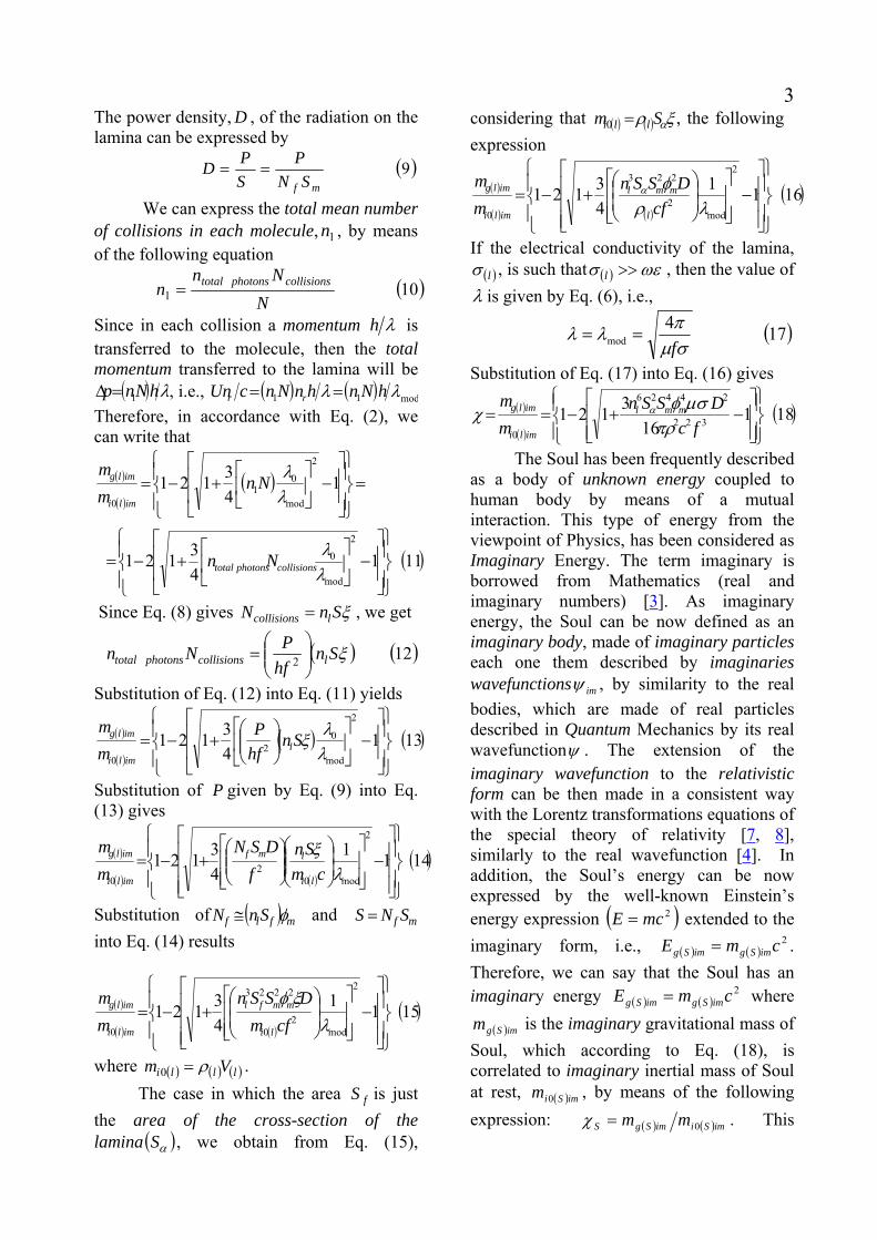
3The power density, , of the radiation on the lamina can be expressed by
D
( )9mf SN
PSPD ==
We can express the total mean number of collisions in each molecule, , by means of the following equation
1n
( )101 NNn
n collisionsphotonstotal=
Since in each collision a momentum λh is transferred to the molecule, then the total momentum transferred to the lamina will be
( ) λhNnp 1=Δ , i.e., ( ) ( ) mod11 λλ hNnhnNncUn rr == Therefore, in accordance with Eq. (2), we can write that
( )
( )( )
( )11143121
143121
2
mod
0
2
mod
01
0
⎪⎭
⎪⎬⎫
⎪⎩
⎪⎨⎧
⎥⎥
⎦
⎤
⎢⎢
⎣
⎡−⎥
⎦
⎤⎢⎣
⎡+−=
=⎪⎭
⎪⎬⎫
⎪⎩
⎪⎨⎧
⎥⎥
⎦
⎤
⎢⎢
⎣
⎡−⎥
⎦
⎤⎢⎣
⎡+−=
λλ
λλ
collisionsphotonstotal
imli
imlg
Nn
Nnmm
Since Eq. (8) gives ξSnN lcollisions = , we get
( ) (122 ξSnhfPNn lcollisionsphotonstotal ⎟⎟
⎠
⎞⎜⎜⎝
⎛= )
Substitution of Eq. (12) into Eq. (11) yields
( )
( )( ) ( )131
43121
2
mod
02
0 ⎪⎭
⎪⎬⎫
⎪⎩
⎪⎨⎧
⎥⎥
⎦
⎤
⎢⎢
⎣
⎡−⎥
⎦
⎤⎢⎣
⎡⎟⎟⎠
⎞⎜⎜⎝
⎛+−=
λλξSn
hfP
mm
limli
imlg
Substitution of given by Eq. (9) into Eq. (13) gives
P
( )
( ) ( )( )1411
43121
2
mod02
0 ⎪⎭
⎪⎬
⎫
⎪⎩
⎪⎨
⎧
⎥⎥⎥
⎦
⎤
⎢⎢⎢
⎣
⎡−
⎥⎥⎦
⎤
⎢⎢⎣
⎡⎟⎟⎠
⎞⎜⎜⎝
⎛⎟⎟⎠
⎞⎜⎜⎝
⎛+−=
λξcm
Snf
DSNmm
li
lmf
imli
imlg
Substitution of ( ) mflf SnN φ≅ and mf SNS = into Eq. (14) results
( )
( ) ( )( )1511
43121
2
mod2
0
2223
0 ⎪⎭
⎪⎬
⎫
⎪⎩
⎪⎨
⎧
⎥⎥⎥
⎦
⎤
⎢⎢⎢
⎣
⎡−
⎥⎥⎦
⎤
⎢⎢⎣
⎡⎟⎟⎠
⎞⎜⎜⎝
⎛+−=
λξφ
cfmDSSn
mm
li
mmfl
imli
imlg
where ( ) ( ) ( )llli Vm ρ=0 . The case in which the area is just the area of the cross-section of the lamina ( , we obtain from Eq. (15),
considering that
fS
)αS
( ) ( ) ξρ αSm lli =0 , the following expression
( )
( ) ( )( )1611
43121
2
mod2
223
0 ⎪⎭
⎪⎬
⎫
⎪⎩
⎪⎨
⎧
⎥⎥⎥
⎦
⎤
⎢⎢⎢
⎣
⎡−
⎥⎥⎦
⎤
⎢⎢⎣
⎡⎟⎟⎠
⎞⎜⎜⎝
⎛+−=
λρφα
cfDSSn
mm
l
mml
imli
imlg
If the electrical conductivity of the lamina, ( )lσ , is such that ( ) ωεσ >>l , then the value of
λ is given by Eq. (6), i.e.,
( )174mod σμ
πλλf
==
Substitution of Eq. (17) into Eq. (16) gives
( )
( )( )181
163121 322
24426
0 ⎪⎭
⎪⎬⎫
⎪⎩
⎪⎨⎧
⎥⎥⎦
⎤
⎢⎢⎣
⎡−+−==
fcDSSn
mm mml
imli
imlg
πρμσφχ α
The Soul has been frequently described as a body of unknown energy coupled to human body by means of a mutual interaction. This type of energy from the viewpoint of Physics, has been considered as Imaginary Energy. The term imaginary is borrowed from Mathematics (real and imaginary numbers) [3]. As imaginary energy, the Soul can be now defined as an imaginary body, made of imaginary particles each one them described by imaginaries wavefunctions imψ , by similarity to the real bodies, which are made of real particles described in Quantum Mechanics by its real wavefunctionψ . The extension of the imaginary wavefunction to the relativistic form can be then made in a consistent way with the Lorentz transformations equations of the special theory of relativity [7, 8], similarly to the real wavefunction [4]. In addition, the Soul’s energy can be now expressed by the well-known Einstein’s energy expression ( )2mcE = extended to the imaginary form, i.e., . Therefore, we can say that the Soul has an imaginary energy where
is the imaginary gravitational mass of Soul, which according to Eq. (18), is correlated to imaginary inertial mass of Soul at rest, , by means of the following expression:
( ) ( )2cmE imSgimSg =
( ) ( )2cmE imSgimSg =
( )imSgm
( )imSim 0
( ) ( )imSiimSgS mm 0=χ . This

4means that the value of can be decreased and also made negative by means of absorption of energy of radiation incident upon the Soul (See Eq.18).
( )imSgE
As widely mentioned in the literature of Spiritualistic Philosophy, the Soul has 2 parts: Perispirit and Spirit (See Fig.1). The Spirit is inside the human body (HB); the Perispirit is an involucre of the spirit, its boundaries coincide with the boundaries of the human body. The perispirit density
( ) ( )( )realVm impeimpeipe == 0ρ is equal to the density of the mean where the Soul is [9]. This occurs by the imaginary mass decrease or by the imaginary mass increase, resultant, respectively, from the emission or absorption of imaginary energy from the Universe. Thus, in the human body the perispirit density is
3.1000 −≅= mkgHBpe ρρTherefore, according to Eq. (7), we can write that the density of molecules in the perispirit is given by
( ) 3280 .103.3 −×≅= mmoleculesANn pepe ρ
where . Out of the Earth’s atmosphere (outer space) the density of the perispirit is equal to the density of the spirit
kg/kmole182 == OHAA
( ) ( )( )realVm imsimsis == 0ρ . In the outer space, the Earth's atmospheric pressure drops to about 3.2 × 10⁻⁷ atm [10]. Thus using the well-known Equation of State ( ZTPM 0= )ρ , we can write the following correlation expression:
( )
( ) atmatm
spaceouterair
atmair7
1
102.31
−×=
ρρ
This means that the density of spirit is given by
( ) ( )37 .108.3 −−×=
===
mkgspaceouterairspaceouterpes ρρρ
Thus, inside the human body the perispirit density is and the spirit density is . Since the Perispirit is just an involucre of the spirit, we can assume that
3.1000 −≅= mkgHBpe ρρ37 .108.3 −−×= mkgsρ
sS ρρ ≅ .
The gravitational mass of the Soul, , is given by the sum of the spirit’s gravitational mass with the perispirit’s gravitational mass, i.e.,
( )imSgm
( ) ( ) ( )impegimsgimSg mmm += As the perispirit is the unique part of the Soul with sufficient density to absorb measurable amounts of electromagnetic energy, we can neglect the contribution of the energy absorbed by the spirit in the calculation of the total energy absorbed by the Soul making . Under these conditions, we can write that the gravitational mass of the Soul, , is given by
( ) 0=imsgm
( )imSgm
( ) ( ) ( ) ( ) ( )190
impegimpegimsgimSg mmmm =+=321
By analogy, the expression of the inertial mass of the Soul, can be written as follows
( )imsim 0
( ) ( ) ( ) ( ) ( )2000
0
00 impeiimpeiimsiimSi mmmm ≅+=321
Based on Eq. (19) we can write that ( ) ( )impepeimSS VV ρρ = , where ( ) ( ) peimimpe xSV Δ= α ;
pexΔ is the thickness of perispirit. Since
sS ρρ ≅ and ( ) ( )imsimS VV ≅ , we can write that
( ) ( ) ( )impepeimssimSS VVV ρρρ =≅ . In addition, we have
( ) ( ) ( ) ( ) mmmSVSVSV HBHBimimsimimS 4.01.14.0 23 ≅≅=≅ αα . Thus, we can conclude that
( )
( )( )21102 10m
SV
xim
ims
pe
spe
−×≅⎟⎟⎠
⎞⎜⎜⎝
⎛⎟⎟⎠
⎞⎜⎜⎝
⎛=Δ
αρρ
Fig. 3 – Perispirit and Spirit. The Spirit is inside the human body; the Perispirit is an involucre of the spirit, its boundaries coincide with the boundaries of the human body.
Spirit
Perispirit
Human body
~2x10⁻¹⁰m

5 The power density of radiation, , absorbed by the perispirit can be expressed by
peD
( )DxD pepepe δΔ= where peδ is length scale for total absorption of the radiation with frequency fπω 2= . As we know, if the electrical conductivity of the mean,σ , is such that ωεσ >> , where ε is the permittivity of the mean, then δ is given by [11]:
( )22105.2 3 σδ f×=
Therefore, we can write that ( ) ( )23108 14 DfDxD pepepepe σδ −×≅Δ=
where is the total power density of the incident radiation on the perispirit.
D
By dividing Eq. (19) by Eq. (20) we obtain
( )
( )
( )
( )pe
impei
impeg
imSi
imSgS m
mmm
χχ ===00
Thus, based on Eq. (18), we can write that
( )
( )
( )24116
3121 322
20
4426
0
⎪⎭
⎪⎬⎫
⎪⎩
⎪⎨⎧
⎥⎥
⎦
⎤
⎢⎢
⎣
⎡−+−=
===
fcDSSn
mm
pe
pepemmpe
impei
impegpeS
πρ
σμφ
χχ
α
Further on, we will show that the electrical conductivity of perispirit is enormous (10 trillion times greater than that of the metals), what shows that it contains a plasma. For the population of excited states for the elements in the plasma to be predominately caused by collisions with electrons and not by radioactive processes, it requires a minimal electron density to ensure these collisions. This minimal electron density is known as the McWhirter criterion and is defined as [12]:
( ) (25106.1 318 21
ETNe Δ×≥ ) where EΔ (in eV) is the largest gap between 2 adjacent energy levels; T (in K) is the plasma temperature, and is in electrons/m
eN3.
This condition is deduced for hydrogen and hydrogen-like atoms in an optically thin,
stationary and homogenous plasma [13]. The largest gap for hydrogen is indeed between the ground state and the first excited energy state and corresponds to 4 eV. This is not always the case for other elements. The largest energy gap for oxygen does not include the ground state and is 10 eV. In order to calculate the value of for the perispirit at the human body, we must take these values:
en
eVE 10=Δ , . The result is
KT 300≅
( )26.103 322 −×≥ melectronsN e
As we have already shown
. Thus, we can assume that
328 .103.3 −×≅ mmoleculesnpe
328 .10 −≈ mionsN pe
It is known that the electrical conductivity is proportional to both the concentration and the mobility of the ions and the free electrons, and is expressed by
iiee nn μμσ +=where and express respectively the concentrations
en in( )3mC of electrons and
atom-ions; eμ and iμ are respectively the mobilities of the electrons and the ions. In order to calculate the electrical conductivity of the perispirit, we first need to calculate the concentrations and . We start by calculating the value of , which is given by
en in
in
39 /10 mCeNnn peei ≈==
This corresponds to the concentration level in the case of conducting materials. For these materials, at temperature of 300K, the mobilities eμ and iμ are of the order of
[112110 −−− sVm 14]. Very high mobility has been found in several low-dimensional systems, such as two-dimensional electron gases (2DEG) ( ), [112300 −− sVm 15] carbon nanotubes ( ) [11210 −− sVm 16] and more

6recently, graphene ( )[11220 −− sVm 17]. It is known that the mobility dμ is related to the drift velocity by means of the following equation:
dv
Ev dd μ=
where E is the electric field. Thus, based on this equation, we can relate the mobility of free electrons of the Soul, eμ , with the typical mobility of conductors,
, by means of the following expression:
112110 −−−≈ sVmcondμ
( )
( )( )27cond
condd
pede v
vμμ =
where the typical drift velocity in conductors is [( ) smv condd /10 4−≈ 18], and the drift velocity in perispirit is (since there are no collisions among the imaginary electrons). Thus, we get
( ) cv ped ≈
1121210 −−≈ sVmeμConsequently, we can write that the electrical conductivity of perispirit is given by
( )28.10 121 −≈+= mSnn iieepe μμσ By substitution of this value into Eq. (22), we get
( )2910 7 fpe−≅δ
By substitution of mSHB /1.0≈σ (conductivity of human body) into Eq. (22), we obtain
( )30104 fHB ≅δ Substitution of the values of ,pen peσ ,
peρ , , ,(average “diameter”
of the molecules),peD mm
101055.1 −×=φ2202 1088.14 mS mm
−×==πφ and into Eq. (24), gives 21.1 mS ≅α
( )31110~
121 2
239
⎪⎭
⎪⎬⎫
⎪⎩
⎪⎨⎧
⎥⎥⎦
⎤
⎢⎢⎣
⎡−+−=
fD
Sχ
In this expression, the minimum value of is limited by the uncertainty principle, i.e., by the amount of energy
D
EΔ that can be detectable by our instruments. According to the uncertainty principle, . Thus, h≥ΔΔ tE
tE Δ≥Δ h → maxmin tE Δ=Δ h . Since we can write that 2tStSED Δ≥ΔΔ= αα h → 2
maxmin tSD Δ= αh , we obtain αSED h2
minmin Δ= . Here, kTE =Δ min , because if , then the action
of the incident radiation will be hidden by the action of the thermal radiation
kT<
( )kT . Consequently, we can write that
αSTkD h22min = . Therefore, for KT 300=
and , we get 21.1 mS ≅α
27
min /105.1 mWD −×≅. Based on Eq.(31), we can write that the Soul imaginary energy can be expressed by
( ) ( )2cmE imSgimSg =
( ) ( ) ( )
( ) ( )32110
121 202
239
20
2
cmf
D
cmcmE
imSi
imSiSimSgimSg
⎪⎭
⎪⎬⎫
⎪⎩
⎪⎨⎧
⎥⎥⎦
⎤
⎢⎢⎣
⎡−+−≅
≅== χ
This energy varies along the time, having a minimum value at the beginning of life and a maximum value, , in a specific instant of the life of the person. After this maximum value, the energy decreases progressively down to the instant of the death of the person. This means that the average variation of this energy along the time can be expressed by the well-known bell curve (probability curve [
( )2max cm imSg
19]), in the following form
( ) ( ) ( )3322242max2 tb
imSgimSg ecmcm π−=

7where is a time-constant to be defined. Since
b( ) ( )imSiimSg mm 0χ= and
Eq. (33) can be rewritten as follows ( ) ( )
max0
maximSiSg mm χ=
( ) ( ) ( )34
2224max00
tbSiSi emm π−=
Fig.4 - The variation of the gravitational mass ofthe Soul (Soul energy mg(S)c2) along the life of a person, and Quantum Reversal from the currentenergy level to a previous energy level.
( )max
Sgm
( )a
Sgm
ttR ta
( )0
Sgm
( )R
Sgm
( )Sgm
Making (current time in the life of the person), and after (reversal time
att =
Rtt = *, see Fig.4) into Eq. (34), we obtain the following expressions
( ) ( ) ( )352224max
00atb
Sia
Si emm π−=and
( ) ( ) ( )362224max
00Rtb
SiR
Si emm π−= By dividing Eq.(35) by Eq. (36), we get
( ) ( )( ) ( )37
2222400
Ra ttbRSi
aSi emm −−= π
Positive values of the Soul energy express the progress of the energy levels and obviously, a given positive value cannot to cause reversion. Thus, in order to occur the reversion it is necessary that 0<Sχ , When * This is not a return in time. It is only return to energy level that the Soul had at a specific time of its life.
this occurs, the energy of the Soul ( ) becomes positive and returns to the corresponding value (
( ) ( )2
02 cmcm a
imSiSa
imSg χ=
( ) ( )2
02
0 cmcm aimSiS
RimSi χ= ). Thus, we can write
that ( ) ( )a
SiSR
Si mm 00 χ= . Substitution of this expression into Eq. (37) gives
( ) ( )( ) ( )38
2222400
Ra ttbaSiS
aSi emm −−= πχ
or ( ) ( )39
22224 Ra ttbS e −= πχ
Note that the time-constant must be a very big number, because the values of
2−b( )22
Ra tte − are enormous in the case of 0<< ta < 3.1 x 10⁹s (100years). Thus, if the value of is not very big then the values of
2−bSχ lose their
meaning. A very big number related to the time is, certainly, the age of the Universe. Thus, we will define the time-constant as follows
2−b
Universeofagecurrentsb =×=− 172 1026.4
For example, if a person is exactly 62 years old ( ), and wants to revert its Soul energy to the energy that it had at 5 years ago (57 years old, ), then the value of
sta910928.1 ×=
stR910774.1 ×=
Sχ , according Eq.(39), must be given by
( ) ( )40109.1 2232.514 2222
×≅≅= − ee Ra ttbS
πχ Equation (31) shows that, in order to obtain , is necessary to apply on the Soul (body) an electromagnetic radiation with frequency f and power density D, given by
22109.1 ×−=Sχ
( )41300 fD ≅Maximum Permissible Exposure (MPE) levels have been established by ANSI Z136.1 [20] for various laser wavelengths and exposure durations. The MPE is the level of laser radiation to which a person may be exposed without hazardous effect or adverse biological changes in the eye or skin. This limit is ~1000 W/m2. Here, considering this limit, we can conclude that, according to Eq.

8(41), the maximum value for the frequency is about 3.3Hz. Now, we can verify the effect of the ELF radiation upon the gravitational mass of the human body. By substitution of
, peHB nn = peHB ρρ = , mSHB /1.0~σ ,
, mm101055.1 −×=φ 2202 1088.14 mS mm
−×==πφ and into Eq. (18) we obtain 21.1 mS ≅α
( )42110~121 3
223
⎪⎭
⎪⎬⎫
⎪⎩
⎪⎨⎧
⎥⎥⎦
⎤
⎢⎢⎣
⎡−+−=
fDHBHB
HBσχ
The expression of can be obtained from the following relation
HBD
( )43HB
pe
pe
HB
DD
δδ
=
where DfD pepe σ14108 −×≅ (Eq. 23). Thus, Eq. (43) can be rewritten as follows
( )4410 14 DfD HB−≅
Substitution of this equation into Eq. (42), gives
( )45110~
121 2
26
⎪⎭
⎪⎬⎫
⎪⎩
⎪⎨⎧
⎥⎥⎦
⎤
⎢⎢⎣
⎡−+−=
−
fD
HBχ
Substitution of Eq. (41) into (45) yields 9.0>HBχ . This corresponds to a weight
decrease of less than 10%, which shows that, here, in the case of fD 300≅ , the effect of the ELF radiation upon the gravitational mass of the human body is negligible. Quantum Physics shows that the energy is quantized, i.e., it has discrete values that are defined as discrete energy levels that correspond to all positive integer values of the quantum number n , . Thus, along the life of a person, the energy of its Soul is characterized by several quantum levels of energy. Then, we can say that, when occurs a reversal of soul energy, it carries out a quantum reversal to a previous level of energy.
( ),...3,2,1=n
Any action once performed leaves an impression on the Soul (its energy). Thus, each energy level of a Soul expresses, at the corresponding moment, the human being in its totality. This means, for example, that our current human shape results from the current energy level (spectrum) of our Soul. Imagine
that a person break a leg when it is 50 years old. If he is subjected to an electromagnetic radiation flux with HzatmWD 1/300 2≈ , then its Soul carries out a quantum reversal to the energy level that he had 5 years ago. At this energy level the leg was not broken in the human body. Consequently, we can expect that the broken part disappears, and the leg returns to the form that it had in this energy level. By means of this process it seems possible the immediate cure of any wound, any kind of disease, and also the resuscitation of persons who have died some seconds ago (before the spirit leaves the human body). It is known that the brain is able to generate electromagnetic waves with frequencies smaller than 100HZ. The brainwaves of lowest frequencies are the Delta waves. Delta waves are defined as having a frequency between 0.5 and 2 hertz. They are the highest amplitude brainwaves. In adults they are radiated from their forehead [21]. Also, it is known that the total electromagnetic power (all the frequencies) generated by the brain can reach up to 25Wor more [22]. This means that at a distance of 1m from the brain a maximum power density is about 2W/m2. Substitution of this value and Hzf 1= into Eq. (31) gives
( )4610265.1 20×−=SχComparing with Eq. (40), yields
( ) ( )4710265.1 20286.464 2222
×≅≅= − ee Ra ttbS
πχ whence we obtain
( )4810994.4 172 ×−= aR ttFor , we obtain yearssta 6210928.1 9 =×=
( )495810794.1 9 yearsstR ≅×≅This means a return of approximately 4 years in the Soul energy level. Note that, while it is necessary 2W/m2 at 1Hz to return 4 years, it is necessary 300W/m2 at 1Hz to return 5 years. However, only a small part of the 25W is due to the delta waves. This means that the return is yet smaller. It obvious that the power densities of the delta waves radiated from the brains vary of persons for persons. Possibly, for most the persons the power

9densities of delta waves radiated from its brains are negligible (smaller than the critical value ). Since we can relate the radiation density, , with the intensity of the electric field,
27min /105.1 mWD −×≅
DE , by
means of the following expression cEnD r 0
2 2μ= [23], then, considering that the value of electric field in the forehead of a person (when emitting delta waves) is
rVE = , where V is the local electric potential (for ordinary persons VV μ150≈ [24]), and r is the radius of the sphere with the same volume of the brain , then we can write that
( )mr 1.0≈
min29
20
2
0
2
/1022
DmWcr
Vc
ED <<≈== −
μμThis shows why the ordinary persons cannot to produce immediate cures. Equation above shows that to produce is necessary that (approximately 10 times greater than that of ordinary persons).
minDD >mVV 1>
Note that, if , and we want to return 1 year, then for 1Hz the necessary value of
yearssta 610866.1 8 =×=
Sχ , according to Eq. (39) is 986.0eS =χ → 68.2−=Sχ . Thus, according to Eq. (31) the value of is
. However, as we have already seen, the value of is limited to
D220 /104.8 mW−×
D27
min /105.1 mWD −×≅ . This means that the return of 1 year, in the case what
, is impossible. Also, note that for
yearssta 610866.1 8 =×=
minDD ≥ the values of become imaginaries. What means that it is impossible to return the soul energy of a child with 6 years old. In general, it is impossible to return the soul energy of any person with
Rt
224ln bt Sa πχ< .
Since and 23max /10 mWD ≅ Hzf 1.0min≅ ,
we obtain from Eqs. (31) and (39) the following expression:
( )5010914.5 172max ×−= aR tt
For , we get yearssta 6210928.1 9 =×=
yearsstR 8.5610768.1 9max ≅×= . This means a maximum return of ~ 5.2 years in the soul
energy level. For , Eq. (50) gives yearssta 3010330.9 8 =×=
yearsstR 1710282.5 8max ≅×= . Therefore, a return of approximately 13 years, in the soul energy level. Note that, the maximum return possible,
, occurs for . years8.13~ yearsta 29≅
Fig. 5 – The immediate Cure or Resuscitation. Delta waves are defined as having a frequency between 0.5 and 2 hertz. They are the highest amplitude brainwaves. In adults they are radiated from their forehead.
Delta waves
The building of ELF transmitters is very difficult because the length of the antenna is enormous. In the case of 1Hz the antenna length must be of the order of 100.000km. However, by using the process of gravitational redshift at laboratory scale, shown in a previous paper [25] it is possible for example, to reduce frequencies
GHzf 1≅ down to ~1Hz. In order to produce a power density at ~1Hz, by the mentioned redshift process, it is necessary an initial flux with at ~1GHz, what corresponds to the minimum frequency band of MASERS. These devices were invented before the laser, but have languished in obscurity because they required high magnetic fields and difficult cooling schemes. Hydrogen masers oscillate at a frequency at around 1.42GHZ and have a typical power of ~ 10
26 /10 mWD −≅
23 /10 mWD ≅
-13W [26]. They are very complex and expensive devices. Recently, it was discovered a room-temperature solid-state maser, which oscillates at frequency of 1.45GHZ. Basically, it is a simple crystal called p-terphenyl. This new device is very simple to
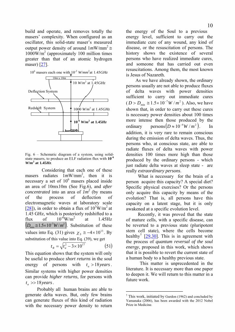
10build and operate, and removes totally the masers’ complexity. When configured as an oscillator, this solid-state maser’s measured output power density of around 1mW/mm2 ≅ 1000W/m2 (approximately 100 million times greater than that of an atomic hydrogen maser) [27]. Fig. 6 – Schematic diagram of a system, using solid-state masers, to produce an ELF radiation flux with 10-6
W/m2 at 1.45Hz.
106 masers each one with 10-3 W/mm2at 1.45GHz 10m x 10m
10 W/m2 at 1.45GHz
1000 W/m2 at 1.45GHz
10-6 W/m2 at 1.45Hz
Deflection System
Redshift System
Considering that each one of these masers radiates 1mW/mm2, then it is necessary a set of 106 masers placed inside an area of 10mx10m (See Fig.6), and after concentrated into an area of 1m2 (by means of the process of deflection of electromagnetic waves at laboratory scale [28]), in order to obtain a flux of 103W/m2 at 1.45 GHz, which is posteriorly redshifted to a flux of 10-6W/m2 at 1.45Hz ( )27
min /105.1 mWD −×≅ . Substitution of these values into Eq. (31) gives . By substitution of this value into Eq. (39), we get
13104×−≅Sχ
( )51103 172 ×−= aR ttThis equation shows that the system will only be useful to produce short returns in the soul energy of persons with . Similar systems with higher power densities can provide higher returns, for persons with
.
yearsta 18>
yearsta 18>> Probably all human brains are able to generate delta waves. But, only few brains can generate fluxes of this kind of radiation with the necessary power density to return
the energy of the Soul to a previous energy level, sufficient to carry out the immediate cure of any wound, any kind of disease, or the resuscitation of persons. The history shows the existence of several persons who have realized immediate cures, and someone that has carried out even resuscitations. Among them, the most known is Jesus of Nazareth. As we have already shown, the ordinary persons usually are not able to produce fluxes of delta waves with power densities sufficient to carry out immediate cures ( ). Also, we have shown that, in order to carry out these cures is necessary power densities about 100 times more intense then those produced by the ordinary persons
27min /105.1 mWDD −×≅>
( )29 /10 mWD −≈ . In addition, it is very rare to remain conscious during the emission of delta waves. Thus, the persons who, at conscious state, are able to radiate fluxes of delta waves with power densities 100 times more high than those produced by the ordinary persons - which just radiate delta waves at sleep state - are really extraordinary persons. What is necessary for the brain of a person acquire this capacity? A special diet? Specific physical exercises? Or the persons only acquire this capacity by means of the evolution? That is, all persons have this capacity on a latent stage, but it is only awakened at a specific evolution level. Recently, it was proved that the state of mature cells, with a specific disease, can be reverted to a previous state (pluripotent stem cell state), where the cells become healthy† [29,30]. This is in agreement with the process of quantum reversal of the soul energy, proposed in this work, which shows that it is possible to revert the current state of a human body to a healthy previous state. This matter is unprecedented in the literature. It is necessary more than one paper to deepen it. We will return to this matter in a future work. † This work, initiated by Gurdon (1962) and concluded by Yamanaka (2006), has been awarded with the 2012 Nobel Prize in Medicine.
11 References [1] Falk, G. D., (2004) The Science of the Soul, Blue Dolphin Publishing, Inc. , USA. [2] Huxley, J. (1969) Essays of a Humanist, Penguin Books, UK, pp. 82–83. [3] De Aquino, F., (2012) Beyond the Material Universe, Journal for Interdisciplinary Research on Religion and Science, No. 10, pp.83-128. [4] Schiff, L. I., (1981) Quantum Mechanics, McGraw-Hill, third edition, pp.39-41. [5] De Aquino, F. (2010) Mathematical Foundations of the Relativistic Theory of Quantum Gravity, Pacific Journal of Science and Technology, 11 (1), pp. 173-232. [6] Quevedo, C. P. (1977) Eletromagnetismo, McGraw- Hill, p. 270. [7] Schwartz, H. M. (1968) Introduction to Special Relativity, chaps. 3, 4, 8, McGraw-Hill, NY. [8] Bergmann, P. G. (1946) Introduction to the Theory of Relativity, pt I, Prentice-Hall, N.J. [9] Kardec, A., (1954) Le Livre des Espirits, Éditions de L’U.S.K.B., q.187. [10] Squire, Tom (2000), "U.S. Standard Atmosphere, 1976", Thermal Protection Systems Expert and Material Properties Database (NASA), retrieved 2011-10-23. [11] Quevedo, C. P. (1977) Eletromagnetismo, McGraw-Hill, p. 270. [12] G. Cristoforetti, A. De Giacomo, M. Dell'Aglio, S. Legnaioli, E. Tognoni, V.Palleschi and N. Omenetto (2010) Local Thermodynamic Equilibrium in Laser-Induced Breakdown Spectroscopy: Beyond the McWhirter criterion, Spectrochimica Acta Part B: 65, 86-95. [13] N. Omenetto, EMSLIBS TALK, Rome 2009 [14] E. O. Knutson and K. T. Whitby (1975). "Aerosol classification by electric mobility: Apparatus, theory, and applications". J. Aerosol Sci. 6 (6): 443–451. [15] Harris, J. J.; Foxon, C. T.; Barnham, K. W. J.; Lacklison, D. E.; Hewett, J.; White, C. (1987). "Two- dimensional electron gas structures with mobilities in excess of 3×106 cm2 V−1 s−1". Journal of Applied Physics 61: 1219. [16] Dürkop, T., Getty, S. A., Cobas, E., Fuhrer, M. S. (2004). "Extraordinary Mobility in Semiconducting Carbon Nanotubes". Nano Letters 4: 35.
[17] Bolotin, K., Sikes, K., Jiang, Z., Klima, M.,Fudenberg, G., Hone, J., Kim, P., Stormer, H., (2008). "Ultrahigh electron mobility in suspended graphene". Solid State Communications 146: 351. [18] Knutson, E. O. and Whitby, K. T. (1975). "Aerosol classification by electric mobility: Apparatus, theory, and applications". J. Aerosol Sci. 6 (6): 443–451. [19] Casella, G., Berger, R. L. (2001) Statistical inference (2nd ed.). Duxbury; Patel, J. K.; Read, C. B., (1996) Handbook of the normal distribution(2nded.) CRC Press. [20] Laser Institute of America - Secretariat and Publisher of the ANSI Z136 Series of Laser Safety Standards. http://www.lia.org/publications/ansi/Z136-1 [21] H. Aurlien, I.O. Gjerde, J. H. Aarseth, B. Karlsen, H. Skeidsvoll, N. E. Gilhus (March 2004). "EEG background activity described by a large computerized database" Clinical Neurophysiology 115 (3): 665–673. [22] Kandel, E. R., and Schwartz, J, H., (1985) Principles of Neural Science, 2nd edition, Elsevier. [23] Halliday, D. and Resnick, R. (1968) Physics, J. Willey & Sons, Portuguese Version, Ed. USP, p.1124. [24] Pilon M; Zadra A; Joncas S et al. Hypersynchronous delta waves and somnambulism: brain topography and effect of sleep deprivation. SLEEP 2006;29(1): 77-84. [25] De Aquino, F., (2012) Gravitational Blueshift and Redshift generated at Laboratory Scale, http://vixra.org/abs/1208.0239 [26] Klepper, D., Goldenberg, H.M., Ramsey, N.F., (1962) Properties of the hydrogen maser, Appl. Opt., 1,55-60. [27] Oxborrow, M. et al., (16 August 2012) Room- temperature solid-state maser, Nature 488,353–356.
[28] De Aquino, F., (2012) Artificial Gravitational Lenses, http://vixra.org/abs/1208.0221 [29] Takahashi K., Yamanaka, S. (2006).Induction of pluripotent stem cells from mouse embryonic and adult fibroblast cultures by defined factors.Cell126:663-676. [30] Gurdon JB (1962). Developmental Capacity of Nuclei Taken from Intestinal Epithelium Cells of Feeding Tadpoles. J Embryol Exp Morph 10: 622-640.
Top Related
Copyright © 2022 FDOKUMEN

