1

The importance of energy quality in energy intensive manufacturing: Evidence from panel cointegration and panel FMOLS

Brantley Liddle Centre for Strategic Economic Studies Victoria University Level 13, 300 Flinders Street Melbourne, VIC 8001 Australia +61 3 9919 1094 (phone) +61 3 9919 1350 (fax) btliddle@alum.mit.edu

Published in Energy Economics, Vol.34, pp. 1819-1825.

2

The importance of energy quality in energy intensive manufacturing: Evidence from panel

cointegration and panel FMOLS

ABSTRACT

This paper expands on the panel GDP-energy cointegration modeling literature; it does so by using data disaggregated along sectoral lines and adjusting energy consumption for the quality of the energy source (e.g., electricity is of higher quality than oil, which is of higher quality than coal) in order to examine the role of energy quality in the five most energy intensive manufacturing sectors (iron and steel, non-ferrous metals, non-metallic minerals, chemicals, and pulp and paper). The database was constructed by combining energy consumption (and energy price data to construct the energy quality index) from the IEA with economic data (value added, labor employed, and physical capital services) from the OECD’s Structural Analysis Database. In addition to finding the variables analyzed are panel I(1) and cointegrated for each sector-based panel, the long-run elasticity estimates (from panel FMOLS) indicate the importance of energy quality—primarily the shift toward the use of high quality electricity—in these energy-intensive manufacturing sectors. In each case, the elasticity for energy quality is greater than that for conventionally measured energy consumption—sometimes orders of magnitude greater. Indeed, the elasticity of conventionally measured energy consumption is insignificant to very small for three of the five sectors. Also, when using the energy quality measure, the importance of energy consumption relative to the other production factors stands out. Such results are useful for both energy-GDP cointegration/causality modelers and CGE modelers, who may need to estimate elasticities.

Keywords: Energy intensive manufacturing; Panel cointegration and Panel FMOLS; energy

quality index; disaggregated energy consumption; elasticity estimation

3

1. Introduction and literature review

There is a substantial and growing literature employing cointegration modeling to

examine the energy-GDP relationship at a national scale (see reviews by Payne 2010a and

2010b and Ozturk 2010); among the most popular models is one based on an aggregate

neoclassical production function. Among the consensuses emerging from this vast literature

are: (i) models should be multivariate to avoid the missing variable bias; (ii) analyses should

employ panel data to improve the power of unit root and cointegration tests that otherwise

can be impaired by the short time spans typically available for single countries; and (iii)

investigators should determine the magnitude, sign, and significance of elasticities, rather

than just performing Granger-type causality tests (see the concluding sections of the two

Payne reviews).

This paper borrows those three consensus ideas along with two seldom used ones: (i)

to use data disaggregated along sectoral lines, and (ii) to adjust energy consumption for the

quality of the energy source (e.g., electricity is of higher quality than oil, which is of higher

quality than coal); those five ideas are used to examine with OECD panel data the role of

energy quality in the five most energy intensive manufacturing sectors. The finding that

accounting for energy quality does indeed impact the production function elasticity estimates

should be of interest for both energy-GDP cointegration/causality modelers and CGE

modelers (who may need to estimate elasticities too).

Perhaps the first to use the aggregate production function model (GDP as a log-linear

function of energy, labor, and capital) was Stern (2000); he focused on the US, found

cointegration among the four variables, and tested for Granger-causality (but did not estimate

elasticities). Recently, several papers have used panel data for such an aggregate model and

have estimated elasticities via methods like panel Fully Modified OLS (FMOLS) and panel

Dynamic OLS (DOLS). For example, Narayan and Smyth (2008) focused on G7 countries;

4

Lee et al. (2008) focused on OECD countries; Lee and Chang (2008) on Asian countries; and

three papers from Apergis and Payne (2009a, 2009b, and 2010) considered Central

American, former Soviet, and South American countries, respectively. All six studies found

the production variables to be cointegrated, and the long-run energy elasticity estimations (all

statistically significant) ranged from 0.12 to 0.42.

Very few energy-GDP cointegration studies, however, have used disaggregated data

and the production function model (perhaps, only this one and Soytas and Sari 2007).

Furthermore, to my knowledge, no studies using disaggregated data and the production

function model have (i) used data disaggregated at a greater level than manufacturing (i.e.,

ISIC two-digit or higher resolution) or (ii) estimated elasticities. Soytas and Sari (2007)

considered manufacturing in Turkey, and determined that electricity consumption, capital,

labor, and value added are integrated order one and cointegrated. (They performed Granger-

causality tests but did not estimate elasticities.)

Neither Sari et al. (2008), who focused on industrial output in the US, nor Ziramba

(2009), who focused on manufacturing in South Africa, considered capital, but both did

estimate elasticities via the autoregressive distributed lag approach. Sari et al. (2008), in

addition to focusing on industrial production, appeared to use aggregate employment and

coal consumption (as opposed to industrial employment and consumption). They found those

three variables to be cointegrated, but their estimated long-run coefficients for employment

and coal to be negative, significant, and large, and their estimated short-run coefficients for

both to be insignificant. Ziramba (2009) analyzed manufacturing production and

manufacturing employment, and separately, both electricity and oil consumption (again, it is

not clear whether that consumption was economy-wide or industrial consumption). Ziramba

found both sets of variables to be cointegrated (production, employment, and electricity; and

production, employment, and oil); but for both models, employment’s elasticity is highly

5

insignificant (p-value 0.7 or higher), as is oil’s elasticity. Electricity’s elasticity is significant

and equal to 0.70.1

The Stern (2000) paper used a quality weighted index of energy, an inclusion

apparently motivated by the results of a still earlier paper, Stern (1993). Stern (1993)

considered both a conventional measure of energy consumption and a quality weighted index

of energy (that paper, also based on the US, used an aggregate production function model, but

did not test for cointegration). Consideration of a quality weighted index is important because

some forms of energy can produce more work than others: a unit of electricity is of higher

quality than a unit of oil, which itself is of higher quality than a unit of coal. Also, arguably

reflecting these differences in productivity, electricity tends to be the most expensive energy

source, followed by oil, and coal tends to be among the least expensive energy sources.

Berndt (1978) describes this situation as follows: “the different prices of energy forms per

Btu illustrate the fact that end-users of energy are concerned not only with the Btu heat

content of the various energy types, but also with other attributes.” Or according to Stern

(1993), “quality weighted final energy use … is likely to be a superior measure of the energy

input to economic activity as it will reflect better the productivity of the uses to which energy

is put.” Indeed, Stern (1993) found energy consumption to be endogenous when measured

conventionally, but found that energy quality weighted consumption Granger-caused GDP.

Despite the results of Stern (1993 and 2000) and the well known energy ladder

phenomenon (i.e., the shift away from biomass and coal and toward oil and electricity as

countries develop), very few energy-GDP cointegration/causality studies have considered

1 Bowden and Payne (2009), employing US data, used the Toda-Yamamoto causality tests, and thus, did not test for cointegration (they did not estimate elasticities either). In addition, they appeared to analyze aggregate real GDP, gross fixed capital formation, and civilian employment with industrial primary energy consumption. Thus, as with Sari et al. (2008) and Ziramba (2009), they were not technically using a sectoral-level production function model.

6

quality adjusted energy consumption since then.2 Oh and Lee (2004) applied Stern’s methods

to Korea and arrived at similar conclusions. Similarly, Warr and Ayres (2010) replicated

Stern’s model for the US using their own measure of exergy (i.e., the amount of energy

available for useful work) in place of Stern’s energy quality index, and found both short- and

long-run causality running from either of their energy quality measures to GDP but not vice

versa.

2. Data, models, and methods

The database used in this paper was constructed by combining energy consumption

data (and energy price data to construct the energy quality index) from the IEA’s Energy

Balances with economic data (value added, labor employed, and physical capital formation)

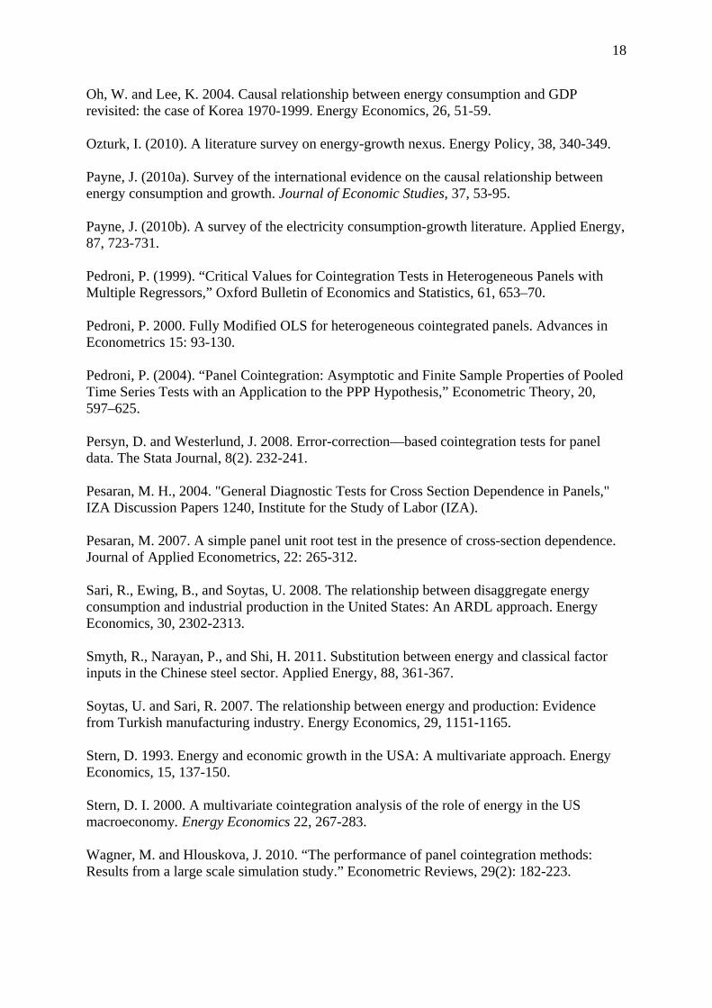
from the Structural Analysis Database (STAN) published by the OECD. Table 1 shows, for

each manufacturing sector, the sector designation used for the remainder of the paper, the

sector classification (based on the ISIC Rev. 3) used to assemble the database, and the

average energy intensity (in thousand tons of oil equivalent, ktoe, per million yr-2005 US$)

for OECD countries in 2005 for that sector. This analysis focuses on the five most energy

intensive manufacturing sectors: iron and steel, non-ferrous metals, non-metallic minerals,

chemicals, and pulp and paper.

Table 1

Despite the increased importance of the service sector, seen both in an increasing

share of GDP and share of trade flows and in the phenomenon of deindustrialization, energy

intensive manufacturing is not unimportant in OECD countries. Table 2 shows the share of

manufacturing value added attributable to each of the five most energy intensive sectors for

individual OECD countries in 2005. On average, these five sectors account for nearly one-

quarter of OECD manufacturing value added. The non-ferrous metal sector (e.g., aluminium

2 There is a separate strand of the literature that focuses on electricity consumption; again, see the survey by Payne (2010b).

7

smelting) tends to be concentrated in areas with inexpensive energy. Australia, Canada,

Norway, and the US produced 70% of the OECD’s primary aluminium in 2006. Although

more evenly distributed across the OECD than smelting activity, iron and steel is a sector in

which several OECD countries are substantial net importers (e.g., Belgium, Finland, and

Japan); whereas, other countries are substantial net exporters (e.g., Canada, Poland, US). By

contrast, chemicals, non-metallic minerals (e.g., ceramics, cement, and glass), and pulp and

paper are sectors in which value-added has increased more or less steadily and uniformly in

all OECD countries.

Table 2

2.1 Models

3I take a constant return to scale Cobb-Douglas production function used elsewhere in

the energy-GDP literature (e.g., Lee et al. 2008); depending on whether conventionally

measured energy consumption or the energy quality index is used, there are two equations for

each sector:

( )γαβtitititi LEKVA ,,,, = (1)

( )γαβtitititi LEQKVA ,,,, = (2)

Where VAi,t is value added for country i in time period t, Ki,t is capital formation/services, Ei,t

is conventional energy consumption, Li,t is labor employed, and EQi,t is energy quality

(defined in Equation 5 below). Taking natural logs forms the following two models, which

are estimated for each of five energy intensive manufacturing sectors:

3 The translog production function is a highly flexible form (e.g., unlike the Cobb-Douglas function, it does not assume an elasticity of substitution among inputs to be equal to unity) that is often used in empirical analyses (e.g., Smyth et al. 2011). However, because the variables analyzed here will be shown to be I(1) and nonlinear transformations of such variables introduce statistical problems, a translog estimation would require the first-differencing of the variables. When a first-difference, translog model was estimated, the hypothesis of the Cobb-Douglas form could be rejected only for pulp and paper; and even for that panel, all of the cross-product terms were insignificant.

8

titititititi LEKbaVA ,,,,, lnlnlnln εγαβ +++++= (3)

titititititi LEQKbaVA ,,,,, lnlnlnln εγαβ +++++= (4)

Where the constants a and b are the country and time fixed effects, respectively, and ε is the

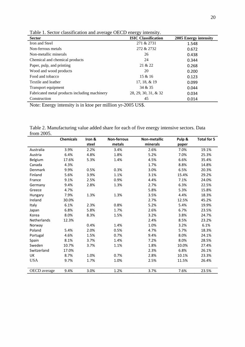
error term. The time span of the data4 and the countries included depend on data availability

and are described for each sector in Table 3 below. Value added and gross fixed capital

formation5 are in real yr-2000 US$, and labor is the number of persons engaged (from

STAN). Conventional energy consumption is in thousand tons of oil equivalent (ktoe), and

the energy quality index is described below. All variables are in natural log form, and all

variables are flows.

Table 3

Berndt (1978) proposed a Divisia index in which the consumption of the individual

fuel types is weighted by their expenditure shares, i.e., the differences in prices reflect the

differences in energy quality or productivity. Stern (1993 and 2000) used this approach in his

analysis of energy and economic growth in the US. Borrowing from Berndt and Stern, I use

the following formula to calculate quality weighted final energy use, EQi,t:

ln , ln . ∑∑ ∑ ln ln (5)

Where P are the prices of the fuels i, and E are the quantities consumed (in ktoe) for

each fuel in final energy use. The (n = 5) fuel types are electricity, oil, natural gas, coal, and

combustible renewables and waste. Like Stern (1993), I assume the price of combustible

renewables and waste is equal to 60% of the coal price.

4 The IEA price series begins in 1978. 5 It is the well-used convention in the literature (perhaps beginning with Soytas and Sari 2007) to use real gross fixed capital formation—a flow, akin to capital services—rather than capital stock. In addition to capital stock data not being readily available, Soytas and Sari (2007) argued that if one assumes a constant depreciation rate, then changes in fixed investment closely follow changes in the capital stock.

9

The energy mix for industry as a whole in the OECD changed dramatically over

1974-2007. The share of oil and coal consumption fell from 32% to 15% and from 19% to

13%, respectively, while the share of electricity rose from 17% to 31% to become the main

source of energy in industry.

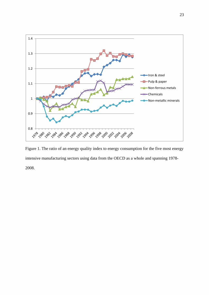
As an initial indication of the importance of energy quality, the quality index was

calculated for each of the five energy intensive manufacturing sectors using data from the

OECD as a whole. Figure 1 displays the ratio of energy quality to conventionally measured

energy consumption for each of those five sectors; thus, a value greater than unity means that

energy quality is larger than energy consumption (as was the case in Stern’s analysis of the

US—see Figure 2 in Stern 1993). Figure 1 shows that energy quality was greater than energy

consumption (at least from the 1990s onward) for all sectors but non-metallic minerals, and

energy quality was mostly increasing faster than energy consumption for all five sectors from

the mid-1980s onward.

Figure 1

2.2 Methods

The first step is to determine whether all the variables are integrated of the same

order. A number of panel unit root tests have been developed to determine the order of

integration of panel variables. These tests typically extend to a panel model the Augmented

Dickey-Fuller (ADF) unit root framework, where the first difference of a series is regressed

on the one-period lag of that series and on a selected number of additional lagged first

difference terms to control for autocorrelation.

Im, Pesaran and Shin (2003) developed a test (IPS) that allows for a heterogeneous

autoregressive unit root process across cross-sections by testing a statistic that is the average

of the individual (i.e., for each cross-sectional unit) ADF statistics. Maddala and Wu (1999)

proposed a panel unit root test based on Fisher (1932) that, like Im et al., allows for

10

individual unit roots, but improves upon Im et al. by being more general and more

appropriate for unbalanced panels. Maddala and Wu’s test (ADF-Fisher) is based on

combining the p-values of the test statistic for a unit root in each cross-sectional unit, is non-

parametric, and has a chi-square distribution.

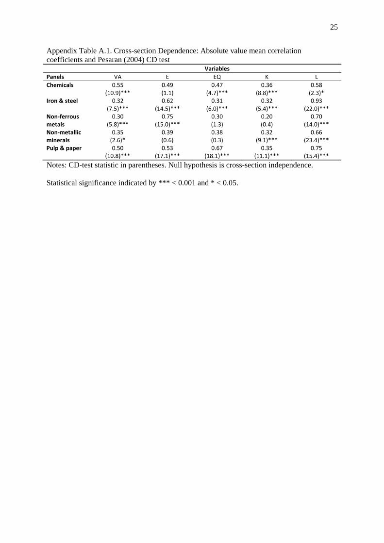
Both of the above tests assume that the cross-sections are independent; yet, for

variables like GPD per capita, cross-sectional dependence is possible to likely for panels of

similar countries because of, for example, regional and macroeconomic linkages. Indeed,

using the Pesaran (2004) test for cross-sectional dependence (CD test), cross-sectional

independence can be rejected for several variables (results shown in Appendix Table A.1).

Pesaran (2007) determined that when cross-sectional dependence is high, the first-

generation tests tend to over-reject the null. More recently, panel unit root tests—so-called

second-generation tests—have been developed that relax this independence assumption.

Among the most commonly used so far is that of Pesaran (2007), which is based on the IPS

test, allows for cross-sectional dependence to be caused by a single (unobserved) common

factor, and is valid for both unbalanced panels and panels in which the cross-section and time

dimensions are of the same order of magnitude. All three tests assume the null hypothesis of

nonstationarity.

If all the variables are integrated of the same order, the next step is to test for

cointegration. Engle and Granger (1987) pointed out that a linear combination of two or more

nonstationary series may be stationary. If such a stationary linear combination exists, the

nonstationary series are said to be cointegrated. The stationary linear combination is called

the cointegrating equation and may be interpreted as a long-run equilibrium relationship

among the variables.

The Pedroni (1999, 2004) heterogeneous panel cointegration test is an extension to

panel data of the Engle-Granger framework. The test involves regressing the variables along

11

with cross-section specific intercepts, and examining whether the residuals are integrated

order one (i.e., not cointegrated). Pedroni proposes two sets of test statistics: (i) a panel test

based on the within dimension approach (panel cointegration statistics), of which four

statistics are calculated: the panel v-, rho-, PP-, and ADF-statistic; and (ii) a group test based

on the between dimension approach (group mean panel cointegration statistics), of which

three statistics are calculated: the group rho-, PP-, and ADF-statistic. Pedroni (1999) further

showed that the panel ADF and group ADF statistics have the best small-sample properties of

the seven test statistics, and thus, provide the strongest single evidence of cointegration.

If the variables are shown to be cointegrated, then the FMOLS estimator from Pedroni

(2000) produces asymptotically unbiased estimates of the long-run elasticities and efficient,

normally distributed standard errors. In addition, the FMOLS uses a semi-parametric

correction for endogeneity and residual autocorrelation, and the FMOLS estimator is a group

mean or between-group estimator that allows for a high degree of heterogeneity in the panel.6

3. Pre-testing results

Table 4 shows the results of the panel unit root tests. For no variable is a panel unit

root in levels rejected by both tests; in addition, for all the variables, panel unit roots in first

differences are rejected by both tests. (Several additional first-generation unit root tests were

applied as well. None of those results conflict with the ones displayed.) Thus, there is no

evidence that any variable is I(2); at the same time I(1) integration cannot be ruled out for any

variable.

Table 4

6 DOLS is another method for estimating cointegrated relationships. FMOLS requires fewer assumptions and tends to be more robust (Pedroni 2000). However, for the case of a single regressor, Kao and Chiang (2000) concluded that DOLS had a smaller bias than FMOLS. But because DOLS involves adding lead and lagged difference terms of the independent variables, in cases in which there are several independent variables and limited time observations—as is the case here—DOLS can result in severe loss in degrees of freedom; and thus, FMOLS is our preferred estimation method.

12

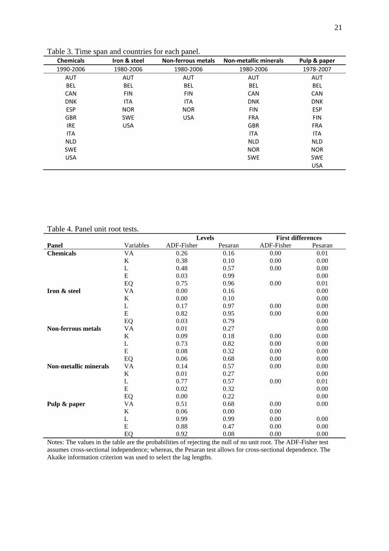
Table 5 displays the panel cointegration test results for both models (using energy and

energy quality) for each of the five sectors. For all variants the two ADF-test statistics reject

the no cointegration null. Thus, given the several previous findings of cointegration of the

production variables discussed above (using both aggregate and more disaggregated data), the

results in Table 5 provide no plausible reason to reject cointegration for the panels used here.

Table 5

3.1 Additional cointegration tests

Pedroni (1999, 2004) recommended subtracting out common time effects (in both

cointegration tests and estimations) to capture a limited form of cross-sectional dependency.

Pedroni (2000) further argued that “… in many cases cross sectional dependence does not

play as large a role as one might anticipate once common time dummies have been

included… .” In addition, Pedroni (2000) claimed that to deal with dynamic cross sectional

dependence in cases in which time dummies are not sufficient requires that the time series

dimension be considerably larger than the cross sectional dimension. Furthermore, a

consensus in the theoretical or applied literature has yet to emerge on how best to deal with

cross sectional dependence in both cointegration testing and estimation (Wagner and

Hlouskova 2010).

Yet, the second-generation Westerlund (2007) cointegration test was applied as well.

The Westerlund test’s results are particularly sensitive to the setting of lag and lead lengths

when the time dimension is short (Persyn and Westerlund 2008)—as is the case with this

data. Thus, the failure of that test to reject the null of no cointegration for some of the panels

(i.e., non-metallic minerals, pulp and paper) seems likely to be the result of the small panel

size (and thus, limited lag and lead length possibilities) rather than the presence of cross-

sectional dependence (results not shown). Indeed, the motivation for developing the test was

13

to avoid an incorrect failure to reject, rather than to avoid an incorrect rejection (Westerlund

2007).

Lastly, the Pedroni (1999, 2004) cointegration test assumes a single cointegrating

vector—a reasonable assumption since the models used here are based on the single equation

Cobb-Douglas production function. However, there are so-called systems cointegration

methods that allow for the possibility of more than one cointegrating vector. Yet, it is well-

known that systems methods perform poorly when the number of cross-sections is relatively

large compared to the time dimension (Banerjee et al. 2003 and Wagner and Hlouskova

2010); thus, such methods seem particularly inappropriate for the chemicals panel. A systems

cointegration test proposed by Maddala and Wu (1999)—a panel version of Johansen (1988)

cointegration test7—confirmed a single cointegrating vector for the other four panels (results

not shown).

4. Estimation results and discussion

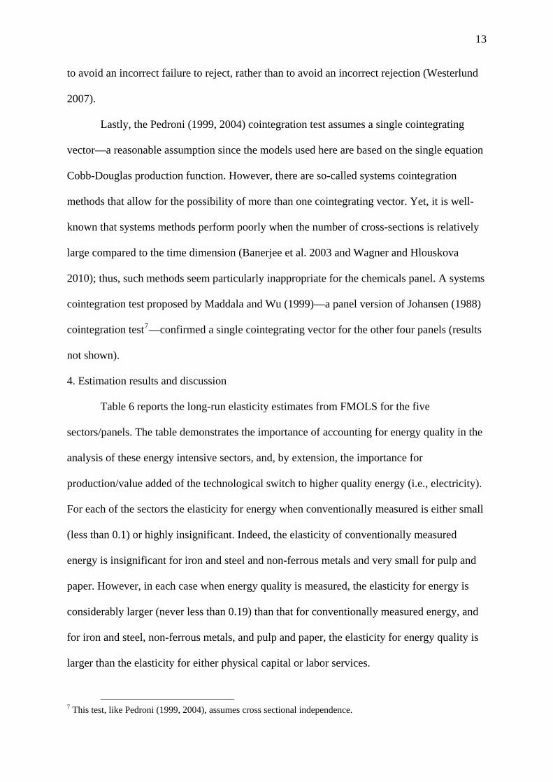
Table 6 reports the long-run elasticity estimates from FMOLS for the five

sectors/panels. The table demonstrates the importance of accounting for energy quality in the

analysis of these energy intensive sectors, and, by extension, the importance for

production/value added of the technological switch to higher quality energy (i.e., electricity).

For each of the sectors the elasticity for energy when conventionally measured is either small

(less than 0.1) or highly insignificant. Indeed, the elasticity of conventionally measured

energy is insignificant for iron and steel and non-ferrous metals and very small for pulp and

paper. However, in each case when energy quality is measured, the elasticity for energy is

considerably larger (never less than 0.19) than that for conventionally measured energy, and

for iron and steel, non-ferrous metals, and pulp and paper, the elasticity for energy quality is

larger than the elasticity for either physical capital or labor services.

7 This test, like Pedroni (1999, 2004), assumes cross sectional independence.

14

Table 6

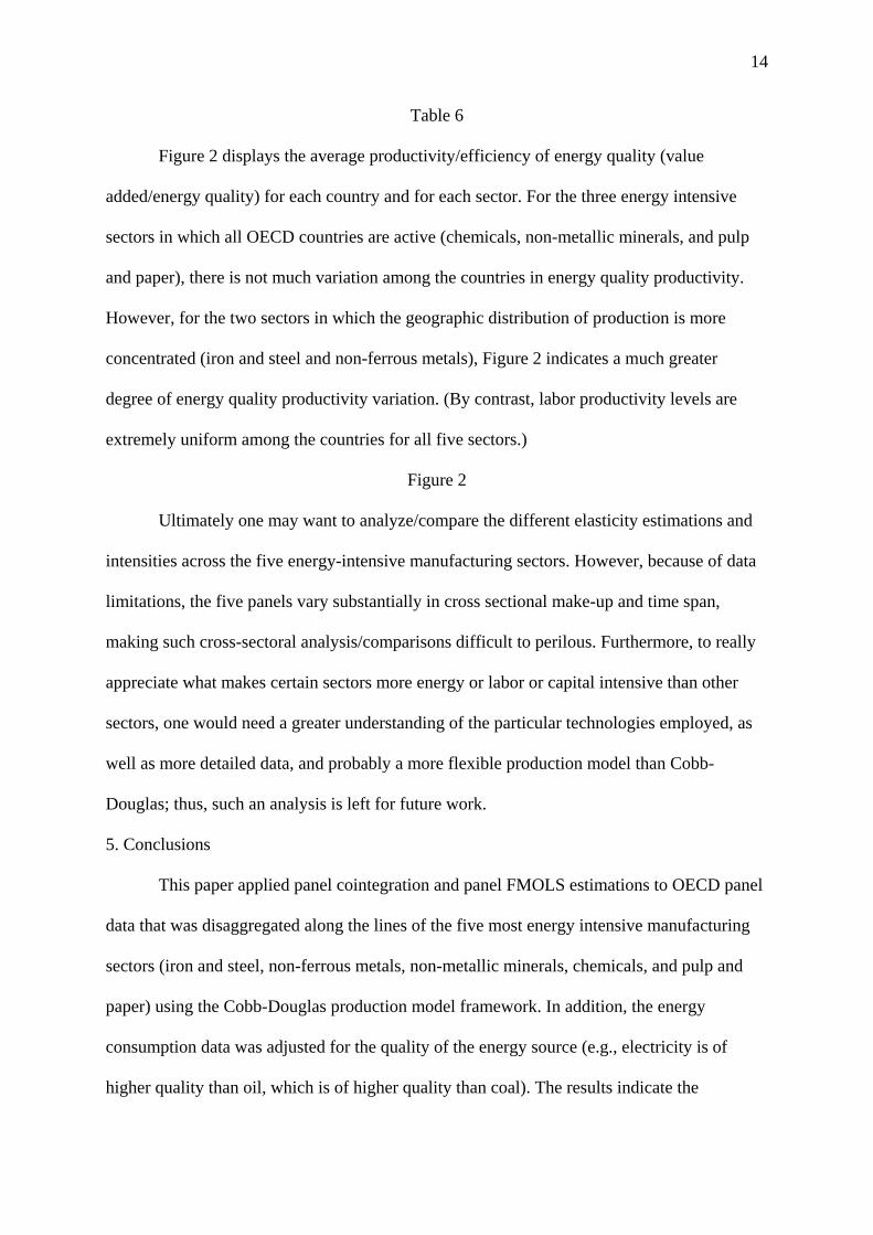
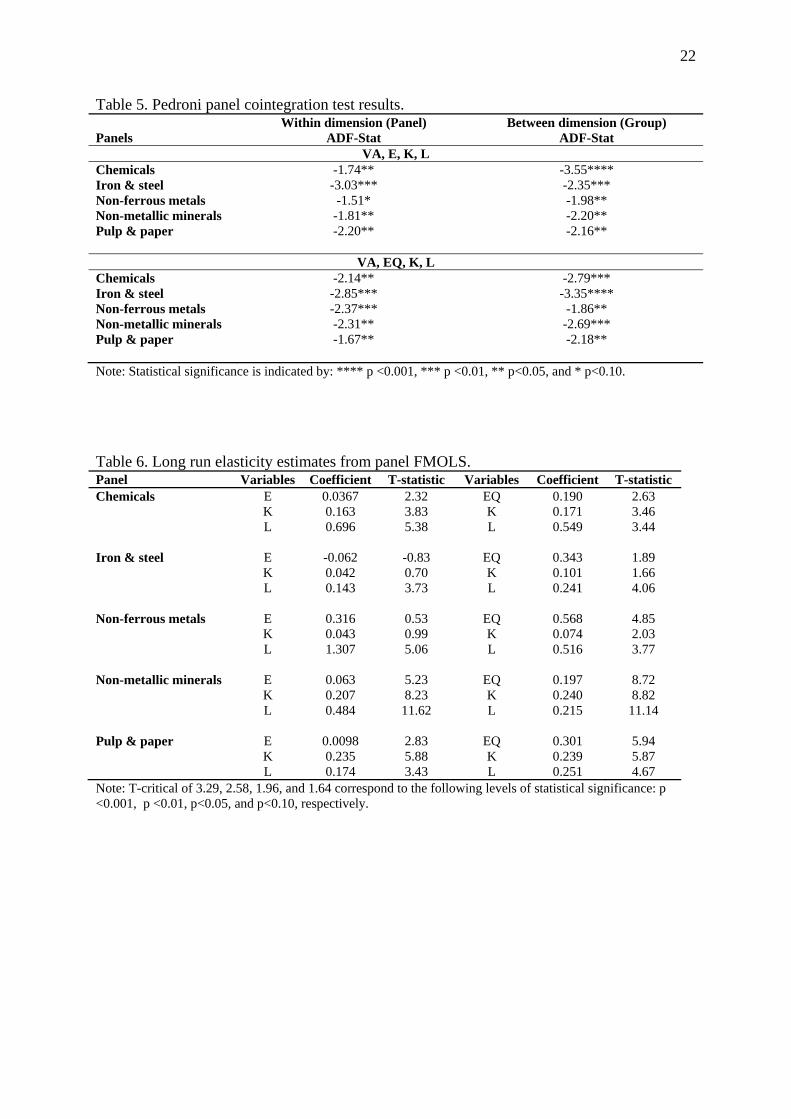
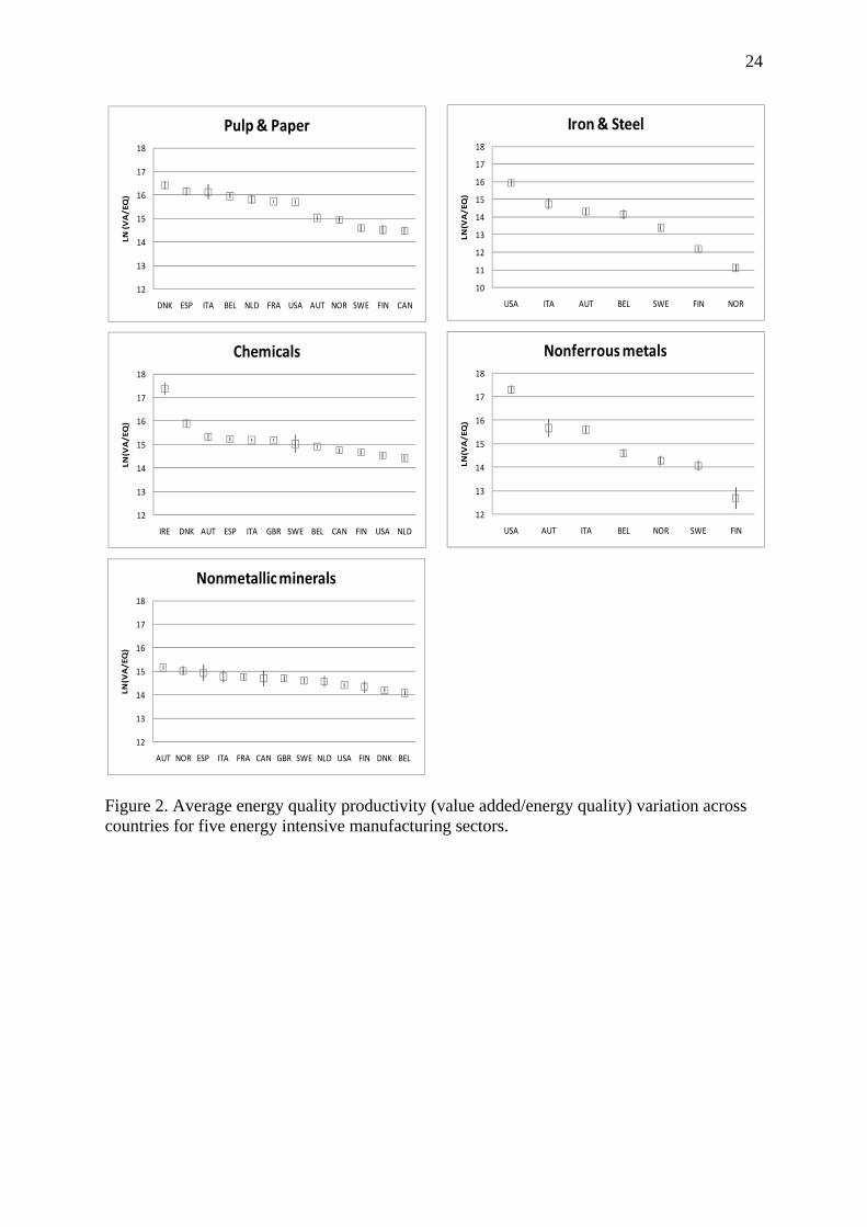
Figure 2 displays the average productivity/efficiency of energy quality (value

added/energy quality) for each country and for each sector. For the three energy intensive

sectors in which all OECD countries are active (chemicals, non-metallic minerals, and pulp

and paper), there is not much variation among the countries in energy quality productivity.

However, for the two sectors in which the geographic distribution of production is more

concentrated (iron and steel and non-ferrous metals), Figure 2 indicates a much greater

degree of energy quality productivity variation. (By contrast, labor productivity levels are

extremely uniform among the countries for all five sectors.)

Figure 2

Ultimately one may want to analyze/compare the different elasticity estimations and

intensities across the five energy-intensive manufacturing sectors. However, because of data

limitations, the five panels vary substantially in cross sectional make-up and time span,

making such cross-sectoral analysis/comparisons difficult to perilous. Furthermore, to really

appreciate what makes certain sectors more energy or labor or capital intensive than other

sectors, one would need a greater understanding of the particular technologies employed, as

well as more detailed data, and probably a more flexible production model than Cobb-

Douglas; thus, such an analysis is left for future work.

5. Conclusions

This paper applied panel cointegration and panel FMOLS estimations to OECD panel

data that was disaggregated along the lines of the five most energy intensive manufacturing

sectors (iron and steel, non-ferrous metals, non-metallic minerals, chemicals, and pulp and

paper) using the Cobb-Douglas production model framework. In addition, the energy

consumption data was adjusted for the quality of the energy source (e.g., electricity is of

higher quality than oil, which is of higher quality than coal). The results indicate the

15

importance of energy quality—primarily the shift toward the use of high quality electricity—

in these energy intensive manufacturing sectors. In each case the elasticity for energy quality

is greater than that for conventionally measured energy consumption—sometimes orders of

magnitude greater. Also, when using the energy quality measure, the importance of energy

consumption relative to the other production factors (capital and labor) stands out. Such

results are useful for both energy-GDP cointegration/causality modelers and CGE modelers,

who may need to estimate elasticities.

The importance of electricity to productivity in these energy intensive sectors has

implications for the impacts of carbon policy on the geographic locations of those sectors.

For countries in which electricity generation is not carbon intensive (i.e., countries that rely

on renewable sources), a carbon tax would not necessarily be damaging to even the most

energy intensive industries. However, a carbon tax could lead to the loss of energy intensive

manufacturing in countries with carbon intensive electricity generation.

An obvious next step in the analysis would be to use a more flexible production

model like the translog one. However, such a model’s estimations would need to be in first

differences since the variables are panel I(1), and most likely additional time observations

would be needed to estimate statistically significant second order and cross-product terms,

and thus, to demonstrate the inadequacy of the Cobb-Douglas framework.

16

Acknowledgement

Comments from two anonymous referees helped to improve the final version.

17

References

Apergis, N. and Payne, J. 2009a. Energy consumption and economic growth in Central America: Evidence from a panel cointegration and error correction model. Energy Economics 31, 211-216.

Apergis, N. and Payne, J. 2009b. Energy consumption and economic growth: evidence from the Commonwealth of Independent States, Energy Economics 31, pp. 641–647.

Apergis, N. and Payne J. 2010. Energy consumption and growth in South America: Evidence from a panel error correction model. Energy Economics 32, 1421-1426. Banerjee, A., Marcellino, M., and Osbat, C. 2004. Some cautions on the use of panel methods for integrated series of macroeconomic data. Econometrics Journal, 7, 322-340. Berndt, E. 1978. Aggregate energy, efficiency, and productivity measurement. Annual Review of Energy, 3, 225-273. Bowden, N. and Payne, J. 2009. The causal relationship between US energy consumption and real output: A disaggregated analysis. Journal of Policy Modeling, 31, 180-188. Engle, R. and Granger, C. 1987. Co-integration and error correction: representation, estimation, and testing. Econometrica 55(2), 251-276. Fisher, R. A. (1932). Statistical Methods for Research Workers, 4th Edition, Edinburgh: Oliver & Boyd. Im, K. S., M. H. Pesaran, and Y. Shin (2003). “Testing for Unit Roots in Heterogeneous Panels,” Journal of Econometrics, 115, 53–74. Johansen, S., 1988. Statistical Analysis of Cointegration Vectors. Journal of Economic Dynamics and Control 12, 231-254. Kao, C. and Chaing, M. (2000). On the estimation and inference of a cointegrated regression in panel data. Advances in Econometrics 15, 179-222. Lee, C. and Chang, C. 2008. “Energy consumption and economic growth in Asian economies: A more comprehensive analysis using panel data,” Resource and Energy Economics, 30, 50-65. Lee, C., Chang, C., and Chen, P. 2008. “Energy-income causality in OECD countries revisited: The key role of capital stock. Energy Economics, 30, 2359-2373. Maddala, G. S. and S. Wu (1999). “A Comparative Study of Unit Root Tests with Panel Data and A New Simple Test,” Oxford Bulletin of Economics and Statistics, 61, 631–52. Narayan, P. and Smyth, R. 2008. “Energy consumption and real GDP in G7 countries: New evidence from panel cointegration with structural breaks.” Energy Economics, 30, 2331-2341.

18

Oh, W. and Lee, K. 2004. Causal relationship between energy consumption and GDP revisited: the case of Korea 1970-1999. Energy Economics, 26, 51-59. Ozturk, I. (2010). A literature survey on energy-growth nexus. Energy Policy, 38, 340-349. Payne, J. (2010a). Survey of the international evidence on the causal relationship between energy consumption and growth. Journal of Economic Studies, 37, 53-95. Payne, J. (2010b). A survey of the electricity consumption-growth literature. Applied Energy, 87, 723-731. Pedroni, P. (1999). “Critical Values for Cointegration Tests in Heterogeneous Panels with Multiple Regressors,” Oxford Bulletin of Economics and Statistics, 61, 653–70.

Pedroni, P. 2000. Fully Modified OLS for heterogeneous cointegrated panels. Advances in Econometrics 15: 93-130.

Pedroni, P. (2004). “Panel Cointegration: Asymptotic and Finite Sample Properties of Pooled Time Series Tests with an Application to the PPP Hypothesis,” Econometric Theory, 20, 597–625.

Persyn, D. and Westerlund, J. 2008. Error-correction—based cointegration tests for panel data. The Stata Journal, 8(2). 232-241. Pesaran, M. H., 2004. "General Diagnostic Tests for Cross Section Dependence in Panels," IZA Discussion Papers 1240, Institute for the Study of Labor (IZA). Pesaran, M. 2007. A simple panel unit root test in the presence of cross-section dependence. Journal of Applied Econometrics, 22: 265-312. Sari, R., Ewing, B., and Soytas, U. 2008. The relationship between disaggregate energy consumption and industrial production in the United States: An ARDL approach. Energy Economics, 30, 2302-2313. Smyth, R., Narayan, P., and Shi, H. 2011. Substitution between energy and classical factor inputs in the Chinese steel sector. Applied Energy, 88, 361-367. Soytas, U. and Sari, R. 2007. The relationship between energy and production: Evidence from Turkish manufacturing industry. Energy Economics, 29, 1151-1165. Stern, D. 1993. Energy and economic growth in the USA: A multivariate approach. Energy Economics, 15, 137-150. Stern, D. I. 2000. A multivariate cointegration analysis of the role of energy in the US macroeconomy. Energy Economics 22, 267-283. Wagner, M. and Hlouskova, J. 2010. “The performance of panel cointegration methods: Results from a large scale simulation study.” Econometric Reviews, 29(2): 182-223.

19

Warr, B. and Ayres, R. 2010. Evidence of causality between the quantity and quality of energy consumption and economic growth. Energy, 35, 1688-1693. Westerlund, J. 2007. Testing for Error Correction in Panel Data. Oxford Bulletin of Economics and Statistics 69(6): 709-748. Ziramba, E. 2009. Disaggregate energy consumption and industrial production in South Africa. Energy Policy, 37, 2214-2220.

20

Table 1. Sector classification and average OECD energy intensity. Sector ISIC Classification 2005 Energy intensity Iron and Steel 271 & 2731 1.548 Non-ferrous metals 272 & 2732 0.672 Non-metallic minerals 26 0.438 Chemical and chemical products 24 0.344 Paper, pulp, and printing 21 & 22 0.268 Wood and wood products 20 0.200 Food and tobacco 15 & 16 0.123 Textile and leather 17, 18, & 19 0.099 Transport equipment 34 & 35 0.044 Fabricated metal products including machinery 28, 29, 30, 31, & 32 0.034 Construction 45 0.014 Note: Energy intensity is in ktoe per million yr-2005 US$.

Table 2. Manufacturing value added share for each of five energy intensive sectors. Data from 2005. Chemicals  Iron & 

steel Non‐ferrous 

metals Non‐metallic minerals 

Pulp & paper 

Total for 5

Australia  3.9% 2.2%  3.4% 2.6% 7.0%  19.1%Austria  6.4% 4.8%  1.8% 5.2% 7.0%  25.3%Belgium  17.6% 5.3%  1.4% 4.5% 6.6%  35.4%Canada  4.3%   1.7% 8.8%  14.8%Denmark  9.9% 0.5%  0.3% 3.0% 6.5%  20.3%Finland  5.6% 3.9%  1.1% 3.1% 15.4%  29.2%France  9.1% 2.5%  0.9% 4.4% 7.1%  24.0%Germany  9.4% 2.8%  1.3% 2.7% 6.3%  22.5%Greece  4.7%   5.8% 5.3%  15.8%Hungary  7.9% 1.3%  1.3% 3.5% 4.4%  18.3%Ireland  30.0%   2.7% 12.5%  45.2%Italy  6.1% 2.3%  0.8% 5.2% 5.4%  19.9%Japan  6.8% 5.8%  1.7% 2.6% 6.7%  23.5%Korea  8.0% 8.3%  1.5% 3.2% 3.8%  24.7%Netherlands  12.3%   2.4% 8.5%  23.2%Norway    0.4%  1.4% 1.0% 3.2%  6.1%Poland  5.4% 2.0%  0.5% 4.7% 5.7%  18.3%Portugal  4.6% 1.5%  0.7% 9.4% 8.0%  24.1%Spain  8.1% 3.7%  1.4% 7.2% 8.0%  28.5%Sweden  10.7% 3.7%  1.1% 1.8% 10.0%  27.4%Switzerland  17.0%   2.3% 6.8%  26.1%UK  8.7% 1.0%  0.7% 2.8% 10.1%  23.3%USA 9.7% 1.7%  1.0% 2.5% 11.5%  26.4%      OECD average 9.4% 3.0%  1.2% 3.7% 7.6%  23.5%

21

Table 3. Time span and countries for each panel. Chemicals  Iron & steel  Non‐ferrous metals Non‐metallic minerals  Pulp & paper1990‐2006  1980‐2006  1980‐2006 1980‐2006 1978‐2007

AUT  AUT  AUT AUT AUTBEL  BEL  BEL BEL BELCAN  FIN  FIN CAN CANDNK  ITA  ITA DNK DNKESP  NOR  NOR FIN ESPGBR  SWE  USA FRA FINIRE  USA  GBR FRAITA    ITA ITA NLD    NLD NLDSWE    NOR NORUSA    SWE SWE

    USA

Table 4. Panel unit root tests. Levels First differences Panel Variables ADF-Fisher Pesaran ADF-Fisher Pesaran Chemicals VA 0.26 0.16 0.00 0.01 K 0.38 0.10 0.00 0.00 L 0.48 0.57 0.00 0.00 E 0.03 0.99 0.00 EQ 0.75 0.96 0.00 0.01 Iron & steel VA 0.00 0.16 0.00 K 0.00 0.10 0.00 L 0.17 0.97 0.00 0.00 E 0.82 0.95 0.00 0.00 EQ 0.03 0.79 0.00 Non-ferrous metals VA 0.01 0.27 0.00 K 0.09 0.18 0.00 0.00 L 0.73 0.82 0.00 0.00 E 0.08 0.32 0.00 0.00 EQ 0.06 0.68 0.00 0.00 Non-metallic minerals VA 0.14 0.57 0.00 0.00 K 0.01 0.27 0.00 L 0.77 0.57 0.00 0.01 E 0.02 0.32 0.00 EQ 0.00 0.22 0.00 Pulp & paper VA 0.51 0.68 0.00 0.00 K 0.06 0.00 0.00 L 0.99 0.99 0.00 0.00 E 0.88 0.47 0.00 0.00 EQ 0.92 0.08 0.00 0.00 Notes: The values in the table are the probabilities of rejecting the null of no unit root. The ADF-Fisher test assumes cross-sectional independence; whereas, the Pesaran test allows for cross-sectional dependence. The Akaike information criterion was used to select the lag lengths.

22

Table 5. Pedroni panel cointegration test results. Panels

Within dimension (Panel) ADF-Stat

Between dimension (Group) ADF-Stat

VA, E, K, L Chemicals -1.74** -3.55**** Iron & steel -3.03*** -2.35*** Non-ferrous metals -1.51* -1.98** Non-metallic minerals -1.81** -2.20** Pulp & paper -2.20** -2.16**

VA, EQ, K, L Chemicals -2.14** -2.79*** Iron & steel -2.85*** -3.35**** Non-ferrous metals -2.37*** -1.86** Non-metallic minerals -2.31** -2.69*** Pulp & paper -1.67** -2.18** Note: Statistical significance is indicated by: **** p <0.001, *** p <0.01, ** p<0.05, and * p<0.10.

Table 6. Long run elasticity estimates from panel FMOLS. Panel Variables Coefficient T-statistic Variables Coefficient T-statistic Chemicals E 0.0367 2.32 EQ 0.190 2.63 K 0.163 3.83 K 0.171 3.46 L 0.696 5.38 L 0.549 3.44 Iron & steel E -0.062 -0.83 EQ 0.343 1.89 K 0.042 0.70 K 0.101 1.66 L 0.143 3.73 L 0.241 4.06 Non-ferrous metals E 0.316 0.53 EQ 0.568 4.85 K 0.043 0.99 K 0.074 2.03 L 1.307 5.06 L 0.516 3.77 Non-metallic minerals E 0.063 5.23 EQ 0.197 8.72 K 0.207 8.23 K 0.240 8.82 L 0.484 11.62 L 0.215 11.14 Pulp & paper E 0.0098 2.83 EQ 0.301 5.94 K 0.235 5.88 K 0.239 5.87 L 0.174 3.43 L 0.251 4.67 Note: T-critical of 3.29, 2.58, 1.96, and 1.64 correspond to the following levels of statistical significance: p <0.001, p <0.01, p<0.05, and p<0.10, respectively.

23

0.8

0.9

1

1.1

1.2

1.3

1.4

Iron & steel

Pulp & paper

Non‐ferrous metals

Chemicals

Non‐metallic minerals

Figure 1. The ratio of an energy quality index to energy consumption for the five most energy

intensive manufacturing sectors using data from the OECD as a whole and spanning 1978-

2008.

24

12

13

14

15

16

17

18

DNK ESP ITA BEL NLD FRA USA AUT NOR SWE FIN CAN

LN (V

A/EQ)

Pulp & Paper

12

13

14

15

16

17

18

IRE DNK AUT ESP ITA GBR SWE BEL CAN FIN USA NLD

LN(VA/EQ)

Chemicals

10

11

12

13

14

15

16

17

18

USA ITA AUT BEL SWE FIN NOR

LN(VA/EQ)

Iron & Steel

12

13

14

15

16

17

18

USA AUT ITA BEL NOR SWE FIN

LN(VA/EQ)

Nonferrous metals

12

13

14

15

16

17

18

AUT NOR ESP ITA FRA CAN GBR SWE NLD USA FIN DNK BEL

LN(VA/EQ)

Nonmetallic minerals

Figure 2. Average energy quality productivity (value added/energy quality) variation across countries for five energy intensive manufacturing sectors.

25

Appendix Table A.1. Cross-section Dependence: Absolute value mean correlation coefficients and Pesaran (2004) CD test   VariablesPanels  VA  E EQ K LChemicals  0.55 

(10.9)*** 0.49(1.1) 

0.47(4.7)*** 

0.36 (8.8)*** 

0.58(2.3)* 

Iron & steel  0.32 (7.5)*** 

0.62(14.5)*** 

0.31(6.0)*** 

0.32 (5.4)*** 

0.93(22.0)*** 

Non‐ferrous metals 

0.30 (5.8)*** 

0.75(15.0)*** 

0.30(1.3) 

0.20 (0.4) 

0.70(14.0)*** 

Non‐metallic minerals 

0.35 (2.6)* 

0.39(0.6) 

0.38(0.3) 

0.32 (9.1)*** 

0.66(23.4)*** 

Pulp & paper  0.50 (10.8)*** 

0.53(17.1)*** 

0.67(18.1)*** 

0.35 (11.1)*** 

0.75(15.4)*** 

Notes: CD-test statistic in parentheses. Null hypothesis is cross-section independence.

Statistical significance indicated by *** < 0.001 and * < 0.05.