©20

15N

atu

re A

mer

ica,

Inc.

All

rig

hts

res

erve

d.

protocol

nature protocols | VOL.10 NO.5 | 2015 | 733

IntroDuctIonThe interactions of macromolecules (proteins, DNA and RNA) with other macromolecules and small ligands are at the core of many biological fields. The nature of these interactions is impor-tant for understanding fundamental biological processes, as well as for applications in drug discovery. It has been established that the binding sites of macromolecules include smaller regions called hot spots that are major contributors to binding free energy, and hence they are crucial to binding any ligand at that particular site1–3. This concept was originally introduced in the context of mutating interface residues to alanine in protein-protein or protein-peptide interfaces4–7. On the basis of this method, a residue is considered a hot spot if its mutation to alanine gives rise to a substantial drop in binding affinity. An alternative experimental method for determining binding hot spots, more directly related to the binding of small ligands, is based on screening libraries of fragment-sized organic molecules for binding to the target protein8. A fundamental property of hot spots is their ability to bind a variety of small organic probe molecules3,8–10. Because the binding of the small compounds is very weak, the interac-tions are most frequently detected by X-ray crystallography11–13 or nuclear magnetic resonance (NMR) imaging8. In the multiple solvent crystal structures (MSCS) method, X-ray crystallography is used to determine the structure of the target protein soaked in aqueous solutions of 6–8 organic solvents used as probes. By superimposing the structures, regions that bind multiple differ-ent probes can be detected11,12. Although individual probes may bind at a number of locations, their clusters indicate binding hot spots. Similarly, in the structure-activity relationship by the NMR method, proteins are immersed in a series of organic solvents, and perturbations in residue chemical shifts are used to identify residues that participate in small-molecule binding8. It was shown that the small ‘probe’ ligands cluster at hot spots and that the hit

rate (HR) predicts the importance of the site8,11. The NMR-based screening correctly identified known drug-like molecule-binding sites in 94% of cases within a set of 23 target proteins, and the method has been extended to a much larger test set8. Although the existence of binding hot spots has been experimentally veri-fied beyond doubt, there is no generally accepted explanation for their origin. On the basis of simulations, our hypothesis is that hot spots are distinguishable from other regions of the protein owing to their concave topology combined with a mosaic-like pattern of hydrophobic and polar functionality9,14,15.

The main advantage of studying hot spots is that they are less sensitive to conformational changes than binding sites are, and they can be identified in almost any structure of a protein, includ-ing those without a bound ligand14–17. The knowledge of hot spots is very valuable for a variety of applications. First, hot spots identify the most important regions of binding sites that should be considered when exploring macromolecule-ligand interac-tions. Second, the strength of hot spots determines druggabil-ity of a site, defined as the ability of a site to bind drug-sized compounds with at least low-micromolar affinity9,18–21. Third, an important application is the identification of binding sites22. Fourth, as hot spots are the energetically important regions of binding sites, the ligand moieties interacting with hot spots are the ones that are essential for binding23. Fifth, the determination of hot spots provides information on the importance of residues in protein-protein interfaces. In particular, it was shown that over 90% of side chains at such interfaces that are identified as hot spots by alanine scanning protrude into hot spots of the partner protein24. Finally, probably the most important use of hot spot determination is as an input for fragment-based ligand discovery. Fragment-based ligand discovery is a combinatorial approach in which individual fragments binding to regions of the target site

The FTMap family of web servers for determining and characterizing ligand-binding hot spots of proteinsDima Kozakov1, Laurie E Grove2, David R Hall3, Tanggis Bohnuud1, Scott E Mottarella4, Lingqi Luo4, Bing Xia1, Dmitri Beglov1 & Sandor Vajda1

1Department of Biomedical Engineering, Boston University, Boston, Massachusetts, USA. 2Department of Sciences, Wentworth Institute of Technology, Boston, Massachusetts, USA. 3Acpharis Inc., Holliston, Massachusetts, USA. 4Program in Bioinformatics, Boston University, Boston, Massachusetts, USA. Correspondence should be addressed to S.V. (vajda@bu.edu) or D.K. (midas@bu.edu).

Published online 9 April 2015; doi:10.1038/nprot.2015.043

FtMap is a computational mapping server that identifies binding hot spots of macromolecules—i.e., regions of the surface with major contributions to the ligand-binding free energy. to use FtMap, users submit a protein, Dna or rna structure in pDB (protein Data Bank) format. FtMap samples billions of positions of small organic molecules used as probes, and it scores the probe poses using a detailed energy expression. regions that bind clusters of multiple probe types identify the binding hot spots in good agreement with experimental data. FtMap serves as the basis for other servers, namely Ftsite, which is used to predict ligand-binding sites, FtFlex, which is used to account for side chain flexibility, FtMap/param, used to parameterize additional probes and FtDyn, for mapping ensembles of protein structures. applications include determining the druggability of proteins, identifying ligand moieties that are most important for binding, finding the most bound-like conformation in ensembles of unliganded protein structures and providing input for fragment-based drug design. FtMap is more accurate than classical mapping methods such as GrID and Mcss, and it is much faster than the more-recent approaches to protein mapping based on mixed molecular dynamics. By using 16 probe molecules, the FtMap server finds the hot spots of an average-size protein in <1 h. as FtFlex performs mapping for all low-energy conformers of side chains in the binding site, its completion time is proportionately longer.

©20

15N

atu

re A

mer

ica,

Inc.

All

rig

hts

res

erve

d.

protocol

734 | VOL.10 NO.5 | 2015 | nature protocols

are selected from a fragment library and then combined to form potential lead compounds25–27. Hot spots help investigators iden-tify the important subsites, determine their druggability18,19,28 and select an appropriate fragment library; once fragment hits are identified they can be used in optimally extending such fragment hits into higher-affinity ligands29.

Experimental techniques for determining binding hot spots are time-consuming, and they can be limited by the physical constraints of the protein-solvent system. Here we describe a protocol using the FTMap family of web servers for determin-ing and characterizing binding hot spots using computational approaches that can replace these experimental methods and that provide the benefit of ease of use (Table 1). Each algorithm has been developed for a specific application and implemented as a separate server. The basic algorithm and server is FTMap, a close computational analog of the X-ray crystallography or NMR-based screening experiments14. FTMap provides direct information on binding hot spots and their druggability and can be used for extending fragment hits into larger ligands. The second server is FTSite, aimed at the identification of ligand-binding sites on the basis of the structure of ligand-free proteins22. The third server is FTFlex, which performs repeated mapping calculations while exploring low-energy conformers of side chains in the vicinity of hot spots30, primarily for opening pockets in protein-protein interfaces that have the potential to bind small ligands28. The fourth server is FTMap/param31, which can be used to determine whether small molecules selected by the user bind in the hot spot regions predicted by FTMap. Finally, the FTDyn server has been developed to map ensembles of conformationally diverse struc-tures obtained by NMR experiments32 or by MD simulations21,33. Although FTSite, FTFlex, FTmap/param and FTDyn are all built on the FTMap algorithm, there are slight differences in the details of their implementation, and the methods serve very different applications (Table 1). In addition, FTMap already had a sizeable

user base by the time the other servers were developed. In view of these factors and in order to retain the simplicity of use, we decided to implement each algorithm as a separate server rather than creating a single server with a complex interface and poten-tially confusing presentation of results.

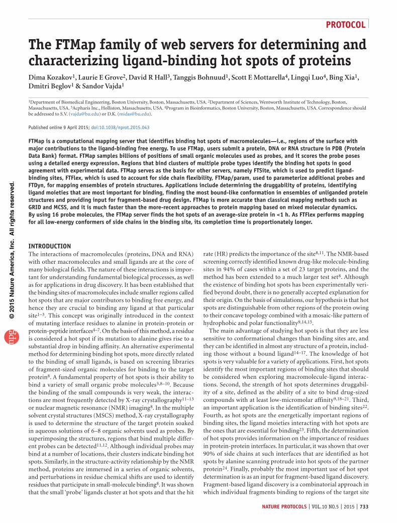
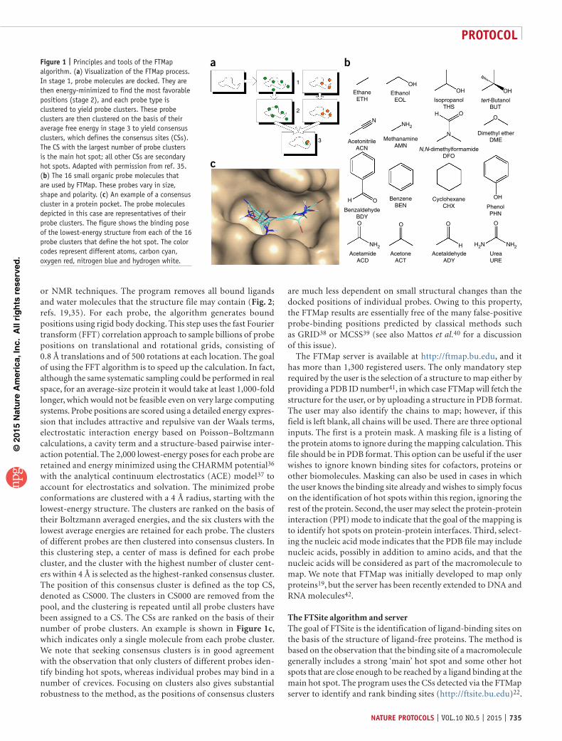
The FTMap algorithm and serverFTMap has been developed as a close computational analog of the X-ray crystallography or NMR-based screening experiments14. The method distributes small organic probe molecules of varying size, shape and polarity on a macromolecule surface; it finds the most favorable positions for each probe type and then clusters the probes and ranks the clusters on the basis of their average energy (Fig. 1a). FTMap19 uses 16 organic molecules as probes (ethanol, isopropanol, isobutanol, acetone, acetaldehyde, dimethyl ether, cyclohexane, ethane, acetonitrile, urea, methylamine, phenol, benzaldehyde, benzene, acetamide and N,N-dimethylformamide; see Fig. 1b). Regions that bind several different probe clusters are called consensus sites (CSs), and the site that contains the largest number of probe clusters is considered the main hot spot; all other CSs are secondary hot spots. As the hot spots are identified by CSs, and in turn the CSs are defined by consensus clusters, we use these terms interchangeably when computational mapping is discussed. For each CS, each probe cluster contained is shown as a single structure that represents the cluster center (Fig. 1c). Because the existence of hot spots is a fundamental property of a protein structure, unbound structures can be used as the input, and thus no information related to ligand binding is required. Even in cases in which there exist conformational differences between unbound and bound structures, the struc-tural features of the hot spot are robust enough to be identified in the unbound structure28,34.

The only input required for FTMap is a protein, DNA or RNA structure, which can be typically obtained by X-ray crystallography

taBle 1 | The FTMap family of servers.

server (url) Function required input

http://ftmap.bu.edu Identifying binding hot spots; determining druggability; providing information for fragment-based drug discovery

PDB ID of a protein, DNA or RNA structure, or structure file in PDB format

http://ftsite.bu.edu Identifying likely ligand-binding sites; ranking of sites in terms of probe-protein interactions; listing of binding site residues

PDB ID of a protein structure, protein structure file in PDB format, or a zip file containing up to 15 protein PDB files

http://ftflex.bu.edu Identifying binding hot spots of proteins and determining druggability, while accounting for side-chain flexibility around selected hot spots; opening pockets in protein-protein interfaces

Stage 1: PDB ID of a protein structure, or protein structure file in PDB formatStage 2: selection of hot spots for side-chain adjustment and remapping

http://ftmap.bu.edu/param/ Same as FTMap, plus determining the low-energy binding poses of up to 15 user-selected probe molecules in hot spot regions

PDB ID of a protein, DNA or RNA structure, or a structure file in PDB format; plus formal charges and SMILES strings to define additional probes

http://ftdyn.bu.edu Mapping potentially large ensembles of protein structures; determining probe-protein interactions for each structure, and averages over the ensemble; identifying the structure most similar to a ligand-bound conformation

Ensemble of protein structures specified in PDB model record format

©20

15N

atu

re A

mer

ica,

Inc.

All

rig

hts

res

erve

d.

protocol

nature protocols | VOL.10 NO.5 | 2015 | 735

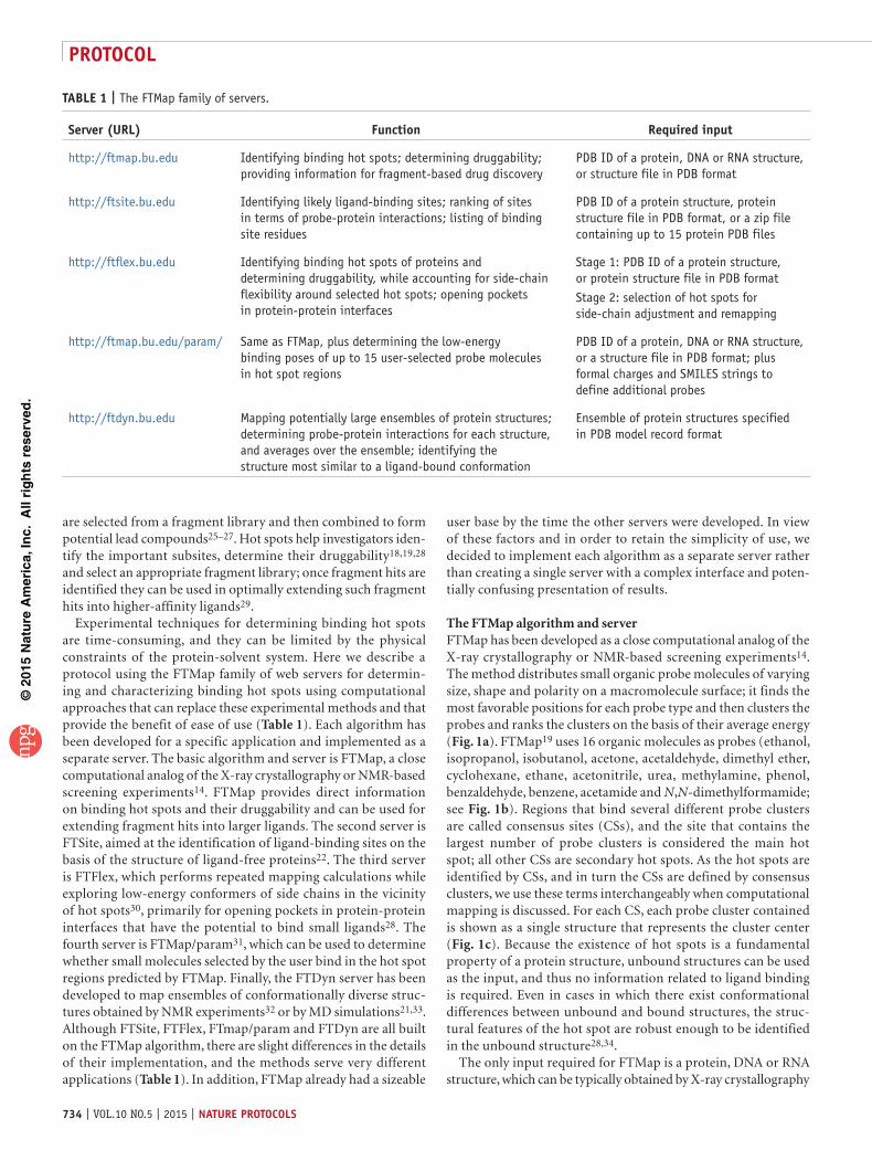
or NMR techniques. The program removes all bound ligands and water molecules that the structure file may contain (Fig. 2; refs. 19,35). For each probe, the algorithm generates bound positions using rigid body docking. This step uses the fast Fourier transform (FFT) correlation approach to sample billions of probe positions on translational and rotational grids, consisting of 0.8 Å translations and of 500 rotations at each location. The goal of using the FFT algorithm is to speed up the calculation. In fact, although the same systematic sampling could be performed in real space, for an average-size protein it would take at least 1,000-fold longer, which would not be feasible even on very large computing systems. Probe positions are scored using a detailed energy expres-sion that includes attractive and repulsive van der Waals terms, electrostatic interaction energy based on Poisson–Boltzmann calculations, a cavity term and a structure-based pairwise inter-action potential. The 2,000 lowest-energy poses for each probe are retained and energy minimized using the CHARMM potential36 with the analytical continuum electrostatics (ACE) model37 to account for electrostatics and solvation. The minimized probe conformations are clustered with a 4 Å radius, starting with the lowest-energy structure. The clusters are ranked on the basis of their Boltzmann averaged energies, and the six clusters with the lowest average energies are retained for each probe. The clusters of different probes are then clustered into consensus clusters. In this clustering step, a center of mass is defined for each probe cluster, and the cluster with the highest number of cluster cent-ers within 4 Å is selected as the highest-ranked consensus cluster. The position of this consensus cluster is defined as the top CS, denoted as CS000. The clusters in CS000 are removed from the pool, and the clustering is repeated until all probe clusters have been assigned to a CS. The CSs are ranked on the basis of their number of probe clusters. An example is shown in Figure 1c, which indicates only a single molecule from each probe cluster. We note that seeking consensus clusters is in good agreement with the observation that only clusters of different probes iden-tify binding hot spots, whereas individual probes may bind in a number of crevices. Focusing on clusters also gives substantial robustness to the method, as the positions of consensus clusters

are much less dependent on small structural changes than the docked positions of individual probes. Owing to this property, the FTMap results are essentially free of the many false-positive probe-binding positions predicted by classical methods such as GRID38 or MCSS39 (see also Mattos et al.40 for a discussion of this issue).

The FTMap server is available at http://ftmap.bu.edu, and it has more than 1,300 registered users. The only mandatory step required by the user is the selection of a structure to map either by providing a PDB ID number41, in which case FTMap will fetch the structure for the user, or by uploading a structure in PDB format. The user may also identify the chains to map; however, if this field is left blank, all chains will be used. There are three optional inputs. The first is a protein mask. A masking file is a listing of the protein atoms to ignore during the mapping calculation. This file should be in PDB format. This option can be useful if the user wishes to ignore known binding sites for cofactors, proteins or other biomolecules. Masking can also be used in cases in which the user knows the binding site already and wishes to simply focus on the identification of hot spots within this region, ignoring the rest of the protein. Second, the user may select the protein-protein interaction (PPI) mode to indicate that the goal of the mapping is to identify hot spots on protein-protein interfaces. Third, select-ing the nucleic acid mode indicates that the PDB file may include nucleic acids, possibly in addition to amino acids, and that the nucleic acids will be considered as part of the macromolecule to map. We note that FTMap was initially developed to map only proteins19, but the server has been recently extended to DNA and RNA molecules42.

The FTSite algorithm and server The goal of FTSite is the identification of ligand-binding sites on the basis of the structure of ligand-free proteins. The method is based on the observation that the binding site of a macromolecule generally includes a strong ‘main’ hot spot and some other hot spots that are close enough to be reached by a ligand binding at the main hot spot. The program uses the CSs detected via the FTMap server to identify and rank binding sites (http://ftsite.bu.edu)22.

1

2

3

EthaneETH

AcetonitrileACN

MethanamineAMN

BenzeneBEN

CyclohexaneCHX Phenol

PHN

UreaURE

AcetaldehydeADY

AcetoneACT

AcetamideACD

BenzaldehydeBDY

Dimethyl etherDME

N,N-dimethylformamideDFO

EthanolEOL Isopropanol

THStert-Butanol

BUT

OH

H

NH2 NH2H H2N

O

O O O O

OH

OH OH

OOH

NH2N

N

a

c

bFigure 1 | Principles and tools of the FTMap algorithm. (a) Visualization of the FTMap process. In stage 1, probe molecules are docked. They are then energy-minimized to find the most favorable positions (stage 2), and each probe type is clustered to yield probe clusters. These probe clusters are then clustered on the basis of their average free energy in stage 3 to yield consensus clusters, which defines the consensus sites (CSs). The CS with the largest number of probe clusters is the main hot spot; all other CSs are secondary hot spots. Adapted with permission from ref. 35. (b) The 16 small organic probe molecules that are used by FTMap. These probes vary in size, shape and polarity. (c) An example of a consensus cluster in a protein pocket. The probe molecules depicted in this case are representatives of their probe clusters. The figure shows the binding pose of the lowest-energy structure from each of the 16 probe clusters that define the hot spot. The color codes represent different atoms, carbon cyan, oxygen red, nitrogen blue and hydrogen white.

©20

15N

atu

re A

mer

ica,

Inc.

All

rig

hts

res

erve

d.

protocol

736 | VOL.10 NO.5 | 2015 | nature protocols

One difference from the FTMap algorithm is that FTSite ranks the consensus clusters by the number of nonbonded contacts between the protein and all probes in the consensus cluster, rather than by the number of probe clusters, as the former approach provides slightly better binding site predictions22. A residue of the protein and a probe are considered to be in contact if any atom of the residue is <4 Å from any atom of the probe. To identify the ligand-binding sites of a protein, FTSite selects CS000 and expands it by adding any neighboring CS if the center of any of its probe is closer than 3.5 Å to the center of any probe in CS000. The protein residues that are within 4 Å of the expanded CS constitute the top prediction of the binding site, defined as Site 1, whereas other CSs identify lower ranked predictions. As the goal of FTSite is to rank all binding sites, no part of the protein can be masked. The server facilitates application to multiple protein structures by allowing the upload of a zip file that contains up to 15 PDB files. The user may provide an e-mail address, in which case upon completion of the job an e-mail will be sent with a link to the results. There are no additional input parameters.

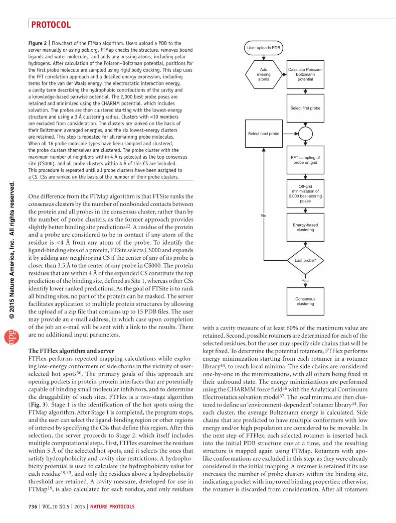
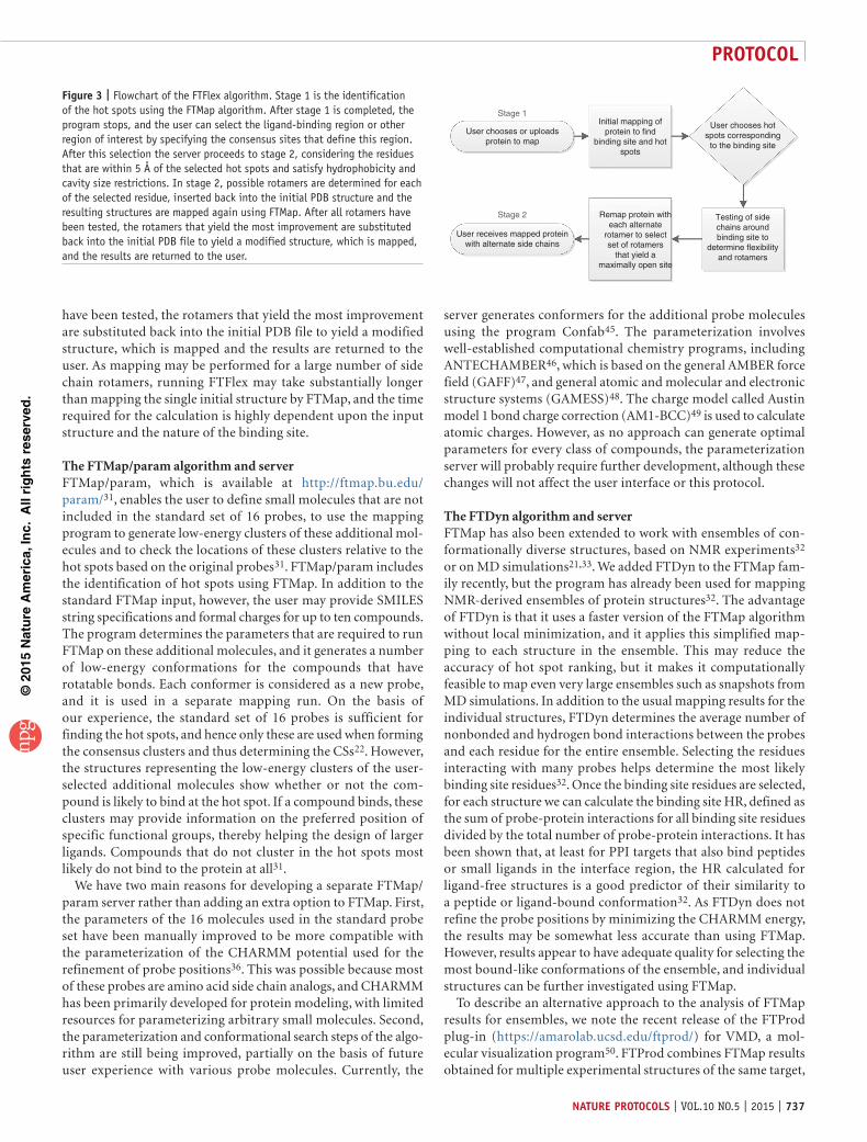
The FTFlex algorithm and server FTFlex performs repeated mapping calculations while explor-ing low-energy conformers of side chains in the vicinity of user-selected hot spots30. The primary goals of this approach are opening pockets in protein-protein interfaces that are potentially capable of binding small molecular inhibitors, and to determine the druggability of such sites. FTFlex is a two-stage algorithm (Fig. 3). Stage 1 is the identification of the hot spots using the FTMap algorithm. After Stage 1 is completed, the program stops, and the user can select the ligand-binding region or other regions of interest by specifying the CSs that define this region. After this selection, the server proceeds to Stage 2, which itself includes multiple computational steps. First, FTFlex examines the residues within 5 Å of the selected hot spots, and it selects the ones that satisfy hydrophobicity and cavity size restrictions. A hydropho-bicity potential is used to calculate the hydrophobicity value for each residue19,43, and only the residues above a hydrophobicity threshold are retained. A cavity measure, developed for use in FTMap19, is also calculated for each residue, and only residues

with a cavity measure of at least 60% of the maximum value are retained. Second, possible rotamers are determined for each of the selected residues, but the user may specify side chains that will be kept fixed. To determine the potential rotamers, FTFlex performs energy minimization starting from each rotamer in a rotamer library44, to reach local minima. The side chains are considered one-by-one in the minimizations, with all others being fixed in their unbound state. The energy minimizations are performed using the CHARMM force field36 with the Analytical Continuum Electrostatics solvation model37. The local minima are then clus-tered to define an ‘environment-dependent’ rotamer library44. For each cluster, the average Boltzmann energy is calculated. Side chains that are predicted to have multiple conformers with low energy and/or high population are considered to be movable. In the next step of FTFlex, each selected rotamer is inserted back into the initial PDB structure one at a time, and the resulting structure is mapped again using FTMap. Rotamers with apo-like conformations are excluded in this step, as they were already considered in the initial mapping. A rotamer is retained if its use increases the number of probe clusters within the binding site, indicating a pocket with improved binding properties; otherwise, the rotamer is discarded from consideration. After all rotamers

Addmissingatoms

User uploads PDB

Calculate Poisson–Boltzmannpotential

FFT sampling ofprobe on grid

Off-gridminimization of

2,000 best-scoringposes

Energy-basedclustering

Last probe?

Select next probe

No

Select first probe

Consensusclustering

Yes

Figure 2 | Flowchart of the FTMap algorithm. Users upload a PDB to the server manually or using pdb.org. FTMap checks the structure, removes bound ligands and water molecules, and adds any missing atoms, including polar hydrogens. After calculation of the Poisson–Boltzman potential, positions for the first probe molecule are sampled using rigid body docking. This step uses the FFT correlation approach and a detailed energy expression, including terms for the van der Waals energy, the electrostatic interaction energy, a cavity term describing the hydrophobic contributions of the cavity and a knowledge-based pairwise potential. The 2,000 best probe poses are retained and minimized using the CHARMM potential, which includes solvation. The probes are then clustered starting with the lowest-energy structure and using a 3 Å clustering radius. Clusters with <10 members are excluded from consideration. The clusters are ranked on the basis of their Boltzmann averaged energies, and the six lowest-energy clusters are retained. This step is repeated for all remaining probe molecules. When all 16 probe molecule types have been sampled and clustered, the probe clusters themselves are clustered. The probe cluster with the maximum number of neighbors within 4 Å is selected as the top consensus site (CS000), and all probe clusters within 4 Å of this CS are included. This procedure is repeated until all probe clusters have been assigned to a CS. CSs are ranked on the basis of the number of their probe clusters.

©20

15N

atu

re A

mer

ica,

Inc.

All

rig

hts

res

erve

d.

protocol

nature protocols | VOL.10 NO.5 | 2015 | 737

have been tested, the rotamers that yield the most improvement are substituted back into the initial PDB file to yield a modified structure, which is mapped and the results are returned to the user. As mapping may be performed for a large number of side chain rotamers, running FTFlex may take substantially longer than mapping the single initial structure by FTMap, and the time required for the calculation is highly dependent upon the input structure and the nature of the binding site.

The FTMap/param algorithm and server FTMap/param, which is available at http://ftmap.bu.edu/param/31, enables the user to define small molecules that are not included in the standard set of 16 probes, to use the mapping program to generate low-energy clusters of these additional mol-ecules and to check the locations of these clusters relative to the hot spots based on the original probes31. FTMap/param includes the identification of hot spots using FTMap. In addition to the standard FTMap input, however, the user may provide SMILES string specifications and formal charges for up to ten compounds. The program determines the parameters that are required to run FTMap on these additional molecules, and it generates a number of low-energy conformations for the compounds that have rotatable bonds. Each conformer is considered as a new probe, and it is used in a separate mapping run. On the basis of our experience, the standard set of 16 probes is sufficient for finding the hot spots, and hence only these are used when forming the consensus clusters and thus determining the CSs22. However, the structures representing the low-energy clusters of the user-selected additional molecules show whether or not the com-pound is likely to bind at the hot spot. If a compound binds, these clusters may provide information on the preferred position of specific functional groups, thereby helping the design of larger ligands. Compounds that do not cluster in the hot spots most likely do not bind to the protein at all31.

We have two main reasons for developing a separate FTMap/param server rather than adding an extra option to FTMap. First, the parameters of the 16 molecules used in the standard probe set have been manually improved to be more compatible with the parameterization of the CHARMM potential used for the refinement of probe positions36. This was possible because most of these probes are amino acid side chain analogs, and CHARMM has been primarily developed for protein modeling, with limited resources for parameterizing arbitrary small molecules. Second, the parameterization and conformational search steps of the algo-rithm are still being improved, partially on the basis of future user experience with various probe molecules. Currently, the

server generates conformers for the additional probe molecules using the program Confab45. The parameterization involves well-established computational chemistry programs, including ANTECHAMBER46, which is based on the general AMBER force field (GAFF)47, and general atomic and molecular and electronic structure systems (GAMESS)48. The charge model called Austin model 1 bond charge correction (AM1-BCC)49 is used to calculate atomic charges. However, as no approach can generate optimal parameters for every class of compounds, the parameterization server will probably require further development, although these changes will not affect the user interface or this protocol.

The FTDyn algorithm and server FTMap has also been extended to work with ensembles of con-formationally diverse structures, based on NMR experiments32 or on MD simulations21,33. We added FTDyn to the FTMap fam-ily recently, but the program has already been used for mapping NMR-derived ensembles of protein structures32. The advantage of FTDyn is that it uses a faster version of the FTMap algorithm without local minimization, and it applies this simplified map-ping to each structure in the ensemble. This may reduce the accuracy of hot spot ranking, but it makes it computationally feasible to map even very large ensembles such as snapshots from MD simulations. In addition to the usual mapping results for the individual structures, FTDyn determines the average number of nonbonded and hydrogen bond interactions between the probes and each residue for the entire ensemble. Selecting the residues interacting with many probes helps determine the most likely binding site residues32. Once the binding site residues are selected, for each structure we can calculate the binding site HR, defined as the sum of probe-protein interactions for all binding site residues divided by the total number of probe-protein interactions. It has been shown that, at least for PPI targets that also bind peptides or small ligands in the interface region, the HR calculated for ligand-free structures is a good predictor of their similarity to a peptide or ligand-bound conformation32. As FTDyn does not refine the probe positions by minimizing the CHARMM energy, the results may be somewhat less accurate than using FTMap. However, results appear to have adequate quality for selecting the most bound-like conformations of the ensemble, and individual structures can be further investigated using FTMap.

To describe an alternative approach to the analysis of FTMap results for ensembles, we note the recent release of the FTProd plug-in (https://amarolab.ucsd.edu/ftprod/) for VMD, a mol-ecular visualization program50. FTProd combines FTMap results obtained for multiple experimental structures of the same target,

Stage 1

Stage 2

User chooses or uploadsprotein to map

Initial mapping ofprotein to find

binding site and hotspots

User chooses hotspots corresponding

to the binding site

User receives mapped proteinwith alternate side chains

Remap protein witheach alternate

rotamer to selectset of rotamers

that yield amaximally open site

Testing of sidechains aroundbinding site to

determine flexibilityand rotamers

Figure 3 | Flowchart of the FTFlex algorithm. Stage 1 is the identification of the hot spots using the FTMap algorithm. After stage 1 is completed, the program stops, and the user can select the ligand-binding region or other region of interest by specifying the consensus sites that define this region. After this selection the server proceeds to stage 2, considering the residues that are within 5 Å of the selected hot spots and satisfy hydrophobicity and cavity size restrictions. In stage 2, possible rotamers are determined for each of the selected residue, inserted back into the initial PDB structure and the resulting structures are mapped again using FTMap. After all rotamers have been tested, the rotamers that yield the most improvement are substituted back into the initial PDB file to yield a modified structure, which is mapped, and the results are returned to the user.

©20

15N

atu

re A

mer

ica,

Inc.

All

rig

hts

res

erve

d.

protocol

738 | VOL.10 NO.5 | 2015 | nature protocols

clusters the results and displays them for analysis within VMD. In contrast to our servers, FTProd is a plug-in that should be down-loaded and installed. Although FTProd is a useful tool extending the capabilities of FTMap, it is not part of the FTMap family, and hence we refer potential users to the instructions for download-ing, installing and using the program via the FTProd online tuto-rial at https://amarolab.ucsd.edu/ftprod/tutorial/01.

Comparison with existing methodsA variety of computational methods have been developed for the prediction of hot spot residues7,51–54, originally defined as those in the protein-protein interface that give rise to a substantial drop in binding affinity when mutated to alanine. However, in this work, we focus on hot spots that bind small molecules, and hence do not review methods of hot-spot residue prediction. Because FTFlex simply accounts for receptor flexibility and FTMap/param defines new probes for FTMap, we consider the basic functions of the programs—i.e., the identification of binding sites and the determination and ranking of binding hot spots. A number of methods exist for binding site detection. These methods largely fall into one of three categories: (i) geometry-based methods, (ii) knowledge-based methods and (iii) energy-based methods55. In geometry-based methods, cavity size is measured and the ligand-binding site is identified as the largest pocket. This category includes methods such as POCKET56, LIGSITE57,58, PASS59 and CASTp60. However, these methods sometimes fail to detect shallow cavities or pockets that may be partially closed, and the results generally do not correlate with ligand-binding energet-ics. That is, it is impossible to assess which sites contribute most to the ligand-binding free energy. Knowledge-based methods can be used to identify binding sites in proteins by comparison with structures with high sequence similarity. These methods include 3DLigandSite61 and FINDSITE62. For targets with highly conserved binding sites, this type of method can be quite suc-cessful63; however, for other targets, this method has success rates closer to 70%. In the energy-based method, the propensity of the site to interact favorably with probe molecules is meas-ured, thus making this method favored in drug design applica-tions. FTMap falls under this category, as does Q-SiteFinder64, SiteMap65 and SITEHOUND66. Q-SiteFinder and SITEHOUND both use a methyl probe, whereas SiteMap uses a water molecule as the probe. Both GRID38 and MCSS39 use multiple functional group types to probe the surface and identify regions that are capable of binding multiple probe types, in a similar manner as the experimental MSCS method11.

Both GRID38 and MCSS39 also rank the regions where probes bind, they provide some information that is similar to the results of FTMap and they have been used for structure-based drug discovery. Both programs have strengths and shortcomings. GRID performs efficient global sampling, finds the potential binding pockets and discriminates between polar and nonpolar regions38. The main shortcoming of the method is that the very small probes bind in many different pockets, which results in a large number of false-positive local minima11,67. The original implementation had no solvation term in the scoring function, which may have contributed to the false positives. MCSS uses CHARMM36, which is a detailed and well-established potential function. MCSS performs simultaneous Monte Carlo minimi-zation of multiple probes distributed on the protein surface.

The probes do not interact with each other, but they interact with the protein. As all probes and the protein are fully flex-ible in the simulation, the conformation of the protein can be influenced by the entire ensemble of probes, which is a potential advantage39. However, it has been reported that MCSS also yields a large number of false-positive energy minima11,68, possibly owing to the lack of solvation, which was added later69. Another problem is that both GRID and MCSS generally predict different locations for different types of probes, contradicting the results of experiments such as the X-ray crystallography–based MSCS, showing that the different small organic molecules overlap at a few locations. More recently, mixed MD has emerged as an alternative approach to protein mapping. The method performs MD simulations of the target in an aqueous solution of probe molecules70–73. Although the use of explicit water molecules potentially improves the accuracy of simulations, they also reduce the diffusivity of the probes, and hence it is frequently questionable whether equilibrium distribution can be achieved on reasonable time scales34. In addition, owing to the need for long simulations, current mixed MD methods rely only on a few probe types, which is likely to limit the reliability of hot spot prediction.

Relative to the above methods, FTMap has several advantages. First, it uses 16 probe molecules with a variety of sizes, shapes and functional groups; this variety of probes is known to pro-vide the robustness required to accurately identify binding sites and eliminate false positives, such as sites in narrow cavities19,34. Second, FTMap is able to provide adequate accuracy with maxi-mum efficiency19. A key to FTMap’s high accuracy is the use of a detailed energy expression to sample probe positions on the protein surface. To achieve maximum efficiency using this energy expression, the FFT correlation approach is used19. FTMap also accounts for solvation using a continuum electrostatic model within the CHARMM implementation37. Finally, FTMap is avail-able as a free, easy-to-use server, for which the only required input is a protein, DNA or RNA structure in PDB format. This enables exploring binding properties of macromolecules and answering biological questions with limited efforts.

LimitationsCurrently, FTMap maps structures that include only naturally occurring amino acid residues and nucleotides. Most HETATM records are removed before mapping. Although a few cofactors can be explicitly added by the user using the chains field, this list is limited (Supplementary Table 1). FTMap itself does not include protein flexibility; however, the FTFlex server (http://ftflex.bu.edu) accounts for side chain flexibility30. Another limitation is that, owing to memory limits on our computational resources, the analysis of proteins over 1,100 residues frequently fails.

AvailabilityAll servers are available to any user, but their jobs will be publicly accessible. Users with education or government e-mail addresses can also set up FTMap accounts. The advantage of such accounts is that the results are available only to the user, and the job does not show up on the website. Although results can be viewed online, most analyses require the use of protein visualization software; PyMOL is the recommended software, and it is used within this protocol to demonstrate data analysis.

©20

15N

atu

re A

mer

ica,

Inc.

All

rig

hts

res

erve

d.

protocol

nature protocols | VOL.10 NO.5 | 2015 | 739

MaterIalsEQUIPMENT

A computer with internet access and a web browserAtomic resolution structures of biomolecules under investigation, in PDB format. The PDB ID can be used to directly fetch in structure, or the structure may be uploaded from the computer

••

Access to PyMOL or similar structure viewing software is recommended but not required. PyMOL can be downloaded at http://www.PyMOLwiki.org/index.php/Category:Installation

•

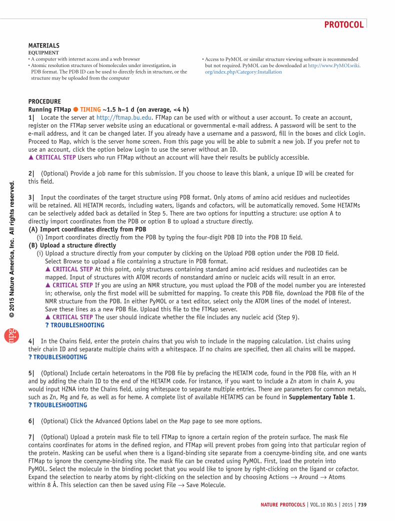
proceDurerunning FtMap ● tIMInG ~1.5 h–1 d (on average, <4 h)1| Locate the server at http://ftmap.bu.edu. FTMap can be used with or without a user account. To create an account, register on the FTMap server website using an educational or governmental e-mail address. A password will be sent to the e-mail address, and it can be changed later. If you already have a username and a password, fill in the boxes and click Login. Proceed to Map, which is the server home screen. From this page you will be able to submit a new job. If you prefer not to use an account, click the option below Login to use the server without an ID. crItIcal step Users who run FTMap without an account will have their results be publicly accessible.

2| (Optional) Provide a job name for this submission. If you choose to leave this blank, a unique ID will be created for this field.

3| Input the coordinates of the target structure using PDB format. Only atoms of amino acid residues and nucleotides will be retained. All HETATM records, including waters, ligands and cofactors, will be automatically removed. Some HETATMs can be selectively added back as detailed in Step 5. There are two options for inputting a structure: use option A to directly import coordinates from the PDB or option B to upload a structure directly.(a) Import coordinates directly from pDB (i) Import coordinates directly from the PDB by typing the four-digit PDB ID into the PDB ID field.(B) upload a structure directly (i) Upload a structure directly from your computer by clicking on the Upload PDB option under the PDB ID field.

Select Browse to upload a file containing a structure in PDB format. crItIcal step At this point, only structures containing standard amino acid residues and nucleotides can be mapped. Input of structures with ATOM records of nonstandard amino or nucleic acids will result in an error. crItIcal step If you are using an NMR structure, you must upload the PDB of the model number you are interested in; otherwise, only the first model will be submitted for mapping. To create this PDB file, download the PDB file of the NMR structure from the PDB. In either PyMOL or a text editor, select only the ATOM lines of the model of interest. Save these lines as a new PDB file. Upload this file to the FTMap server. crItIcal step The user should indicate whether the file includes any nucleic acid (Step 9). ? trouBlesHootInG

4| In the Chains field, enter the protein chains that you wish to include in the mapping calculation. List chains using their chain ID and separate multiple chains with a whitespace. If no chains are specified, then all chains will be mapped.? trouBlesHootInG

5| (Optional) Include certain heteroatoms in the PDB file by prefacing the HETATM code, found in the PDB file, with an H and by adding the chain ID to the end of the HETATM code. For instance, if you want to include a Zn atom in chain A, you would input HZNA into the Chains field, using whitespace to separate multiple entries. There are parameters for common metals, such as Zn, Mg and Fe, as well as for heme. A complete list of available HETATMS can be found in supplementary table 1.? trouBlesHootInG

6| (Optional) Click the Advanced Options label on the Map page to see more options.

7| (Optional) Upload a protein mask file to tell FTMap to ignore a certain region of the protein surface. The mask file contains coordinates for atoms in the defined region, and FTMap will prevent probes from going into that particular region of the protein. Masking can be useful when there is a ligand-binding site separate from a coenzyme-binding site, and one wants FTMap to ignore the coenzyme-binding site. The mask file can be created using PyMOL. First, load the protein into PyMOL. Select the molecule in the binding pocket that you would like to ignore by right-clicking on the ligand or cofactor. Expand the selection to nearby atoms by right-clicking on the selection and by choosing Actions → Around → Atoms within 8 Å. This selection can then be saved using File → Save Molecule.

©20

15N

atu

re A

mer

ica,

Inc.

All

rig

hts

res

erve

d.

protocol

740 | VOL.10 NO.5 | 2015 | nature protocols

8| (Optional) If you are looking for binding hot spots in a protein-protein interface, select the PPI mode option.

9| (Optional) Select the Nucleic Acids option if the PDB file includes nucleic acids. This option uses a specific set of parameters.

10| Click on the Map button to begin the calculation. You can immediately check the status of the job on the Queue page. Jobs are run in order of their submission. Your calculation will be listed with ID number, job name, user name and a status update. Click on the ID of your job to see a detailed Status Page. The Status Page shows the job ID number, job name, job status, submission time stamp and PDB ID. The page also shows pictorial representations of the uploaded and processed inputs, and Probe Status—i.e., status for each small-molecule probe. See Box 1 for information pertaining to status abbreviations.

11| An e-mail will be sent when the job has been completed or if an error has occurred (see Box 2 for a listing of possible errors and their meanings). The e-mail will contain a link to the mapping results. Click the link; alternatively, locate the results under the Results tab on the server. All user results will be listed in order of ID number. If there was an error, an error message will be provided in an e-mail to the user, as well as in the Results tab. crItIcal step The mapping result files will only be stored on the server for 2 months. After this time, the results will be deleted.? trouBlesHootInG

12| View results by clicking on the ID number of the job under the Results tab. The Result page (Fig. 4) starts with the job name. The page also offers direct visualization that shows the protein and all CSs. Click on the image to interact with the resulting structure using JSmol. crItIcal step Allow several seconds for JSmol to load for interactive visualization.

13| To manipulate the structure in JSmol, use the left mouse button and drag to rotate your structure. Use your mouse wheel to zoom in and out. Use the checkboxes along the bottom to select/deselect any specific consensus cluster. Use the color options to change the structure coloring. Execute JSmol scripts from the text field. Information on using JSmol is provided on several websites—e.g., http://wiki.jmol.org/index.php/Jmol_JavaScript_ObjectJSmol.

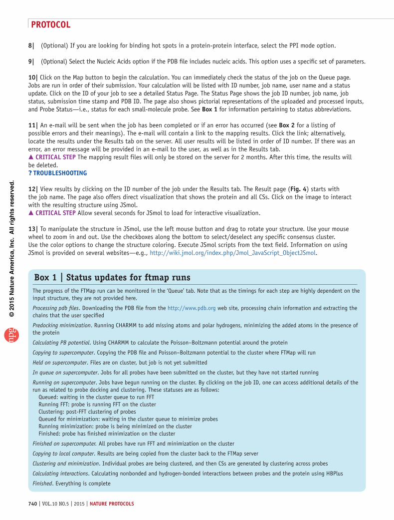
Box 1 | Status updates for ftmap runs The progress of the FTMap run can be monitored in the ‘Queue’ tab. Note that as the timings for each step are highly dependent on the input structure, they are not provided here.

Processing pdb files. Downloading the PDB file from the http://www.pdb.org web site, processing chain information and extracting the chains that the user specified

Predocking minimization. Running CHARMM to add missing atoms and polar hydrogens, minimizing the added atoms in the presence of the protein

Calculating PB potential. Using CHARMM to calculate the Poisson–Boltzmann potential around the protein

Copying to supercomputer. Copying the PDB file and Poisson–Boltzmann potential to the cluster where FTMap will run

Held on supercomputer. Files are on cluster, but job is not yet submitted

In queue on supercomputer. Jobs for all probes have been submitted on the cluster, but they have not started running

Running on supercomputer. Jobs have begun running on the cluster. By clicking on the job ID, one can access additional details of the run as related to probe docking and clustering. These statuses are as follows: Queued: waiting in the cluster queue to run FFT Running FFT: probe is running FFT on the cluster Clustering: post-FFT clustering of probes Queued for minimization: waiting in the cluster queue to minimize probes Running minimization: probe is being minimized on the cluster Finished: probe has finished minimization on the cluster

Finished on supercomputer. All probes have run FFT and minimization on the cluster

Copying to local computer. Results are being copied from the cluster back to the FTMap server

Clustering and minimization. Individual probes are being clustered, and then CSs are generated by clustering across probes

Calculating interactions. Calculating nonbonded and hydrogen-bonded interactions between probes and the protein using HBPlus

Finished. Everything is complete

©20

15N

atu

re A

mer

ica,

Inc.

All

rig

hts

res

erve

d.

protocol

nature protocols | VOL.10 NO.5 | 2015 | 741

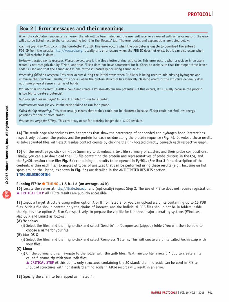
14| The result page also includes two bar graphs that show the percentage of nonbonded and hydrogen bond interactions, respectively, between the probes and the protein for each residue along the protein sequence (Fig. 4). Download these results as tab-separated files with exact residue contact counts by clicking the link located directly beneath each respective graph.

15| On the result page, click on Probe Summary to download a text file summary of clusters and their probe compositions. Finally, you can also download the PDB file containing the protein and representatives of probe clusters in the CSs, and the PyMOL session (.pse file; Fig. 5a) containing all results to be opened in PyMOL. (See Box 3 for a description of the contents within each file.) Examples of types of analyses that can be performed using these results (e.g., focusing on hot spots around the ligand, as shown in Fig. 5b) are detailed in the ANTICIPATED RESULTS section.? trouBlesHootInG

running Ftsite ● tIMInG ~1.5 h–1 d (on average, <4 h)16| Locate the server at http://ftsite.bu.edu, and (optionally) repeat Step 2. The use of FTSite does not require registration. crItIcal step All FTSite results are publicly accessible.

17| Input a target structure using either option A or B from Step 3, or you can upload a zip file containing up to 15 PDB files. Such a file should contain only the chains of interest, and the individual PDB files should not be in folders inside the zip file. Use option A, B or C, respectively, to prepare the zip file for the three major operating systems (Windows, Mac OS X and Linux) as follows:(a) Windows (i) Select the files, and then right-click and select ‘Send to’ → ‘Compressed (zipped) folder’. You will then be able to

choose a name for your file.(B) Mac os X (i) Select the files, and then right-click and select ‘Compress N Items’. This will create a zip file called Archive.zip with

your files.(c) linux (i) On the command line, navigate to the folder with the .pdb files. Next, run zip filename.zip *.pdb to create a file

called filename.zip with your .pdb files. crItIcal step At this point, only structures containing the 20 standard amino acids can be used in FTSite. Input of structures with nonstandard amino acids in ATOM records will result in an error.

18| Specify the chain to be mapped as in Step 4.

Box 2 | Error messages and their meanings When the calculation encounters an error, the job will be terminated and the user will receive an e-mail with an error reason. The error will also be listed next to the corresponding job id in the ‘Results’ tab. The error codes and explanations are listed below:

xxxx not found in PDB. xxxx is the four-letter PDB ID. This error occurs when the computer is unable to download the entered PDB ID from the website http://www.pdb.org. Usually this error occurs when the PDB ID does not exist, but it can also occur when the PDB website is down.

Unknown residue xxx in receptor. Please remove. xxx is the three-letter amino acid code. This error occurs when a residue in an atom record is not recognizable by FTMap, and thus FTMap does not have parameters for it. Check to make sure that the proper three-letter code is used and that the amino acid is one of the 20 naturally occurring amino acids.

Processing failed on receptor. This error occurs during the initial steps when CHARMM is being used to add missing hydrogens and minimize the structure. Usually, this occurs when the protein structure has sterically clashing atoms or the structure generally does not make physical sense in terms of bonds.

PB Potential not created. CHARMM could not create a Poisson-Boltzmann potential. If this occurs, it is usually because the protein is too big to create a potential.

Not enough lines in output for xxx. FFT failed to run for a probe.

Minimization error for xxx. Minimization failed to run for a probe.

Failed during clustering. This error usually means that probes could not be clustered because FTMap could not find low-energy positions for one or more probes.

Protein too large for FTMap. This error may occur for proteins longer than 1,100 residues.

©20

15N

atu

re A

mer

ica,

Inc.

All

rig

hts

res

erve

d.

protocol

742 | VOL.10 NO.5 | 2015 | nature protocols

19| (Optional) You may provide an e-mail address. If this option is used, an e-mail will be sent to the address with a link to the results when the FTSite run is completed, or if an error occurred (see Step 11 for details).

20| Click on the ‘Find My Binding Site’ button to begin the calculation. Unless there is an error, you will immediately see the message ‘Success, job submit-ted’, and you can check the status of the job on the Queue page. Your calculation will be listed with the job name and a status update. See Box 1 for a listing of status updates.? trouBlesHootInG

21| After the FTSite run is completed, view the results (Fig. 6) using option A via a web interface or select option B to use PyMOL:(a) Web interface (i) View the results via a web

interface. The interface contains a Java Applet. Mesh representations of the top three sites and sticks of the residues around the sites can be turned on and off along with various representations of the protein. Residues near each site are also listed. An example of results is shown in the ANTICIPATED RESULTS section.

(B) pyMol (i) Click on the ‘Download PyMOL Session’ label to download a file containing the PyMOL session, which shows the

protein, the detected sites and the residues that surround the site.

20non bonded %

Hbond %

SequenceNonbonded interactions

SequenceHbond interactionsProbes summary

15

10

5

0

20

15

10

5

0A17

A18A20

A38A40

A41A42

A43A45

A82A83

A84A85

A86A118

A121A135

A162A165

A189A226

A227A228

A229A230

A231A233

A302A303

A306A309

A17 A20 A37 A40 A43 A81 A84 A87A11

9A12

4A13

5A16

2A18

9A20

0A22

7A23

0A23

3A30

3A30

6A30

9A31

4

Figure 4 | Screenshot of FTMap results for PDB ID 2ren (apo structure of renin). Five different output files are available for download; descriptions can be found in Box 3. The user can view the mapping results by using the PyMOL plug-in, or by downloading either the PDB file containing the protein and probe coordinate or a PyMOL session. The target protein is shown as a green cartoon, and the probes representing each cluster at the consensus sites are shown in various colors as sticks. Clicking on the image will activate JSmol, and the image can be manipulated (e.g., rotated and translated) using the JSmol tools. JSmol also provides checkboxes along the bottom of the picture of the protein to select/deselect any of the consensus clusters. The two bar graphs at the bottom of the page show the percentage of nonbonded and hydrogen bond (Hbond) interactions, respectively, between the probes and the protein for each residue along the protein sequence. You can download these results as tab-separated files with exact residue contact counts by clicking the link located directly beneath each respective graph.

©20

15N

atu

re A

mer

ica,

Inc.

All

rig

hts

res

erve

d.

protocol

nature protocols | VOL.10 NO.5 | 2015 | 743

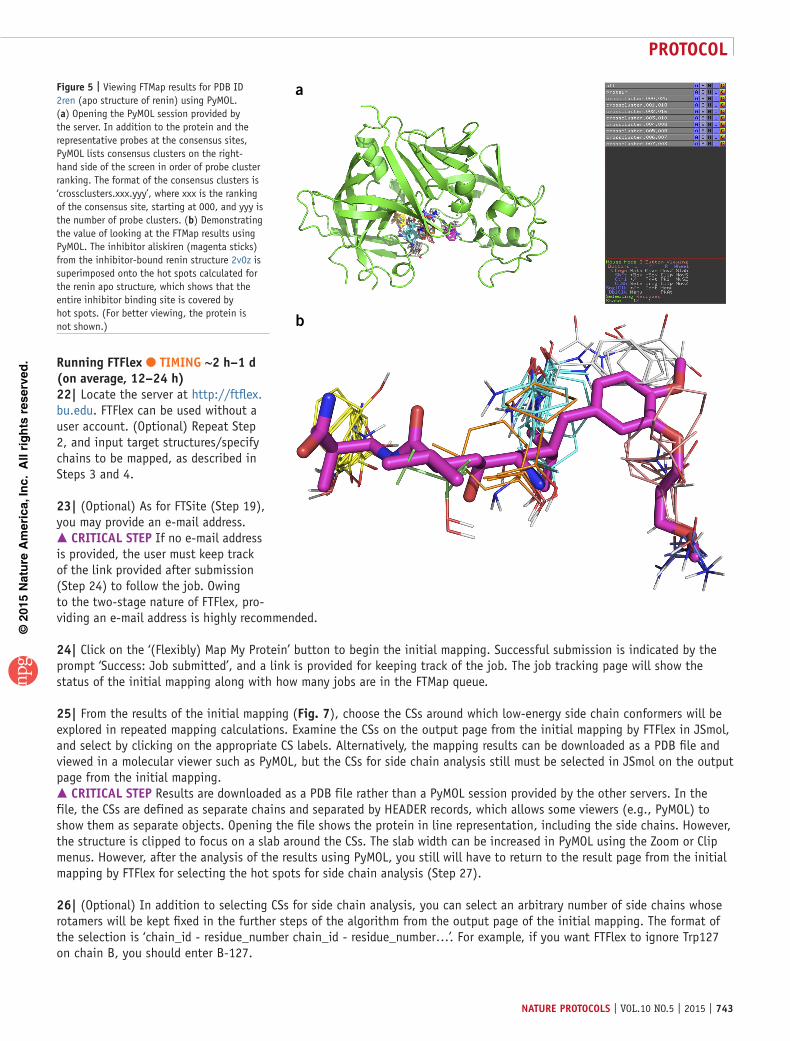
running FtFlex ● tIMInG ~2 h–1 d (on average, 12–24 h)22| Locate the server at http://ftflex.bu.edu. FTFlex can be used without a user account. (Optional) Repeat Step 2, and input target structures/specify chains to be mapped, as described in Steps 3 and 4.

23| (Optional) As for FTSite (Step 19), you may provide an e-mail address. crItIcal step If no e-mail address is provided, the user must keep track of the link provided after submission (Step 24) to follow the job. Owing to the two-stage nature of FTFlex, pro-viding an e-mail address is highly recommended.

24| Click on the ‘(Flexibly) Map My Protein’ button to begin the initial mapping. Successful submission is indicated by the prompt ‘Success: Job submitted’, and a link is provided for keeping track of the job. The job tracking page will show the status of the initial mapping along with how many jobs are in the FTMap queue.

25| From the results of the initial mapping (Fig. 7), choose the CSs around which low-energy side chain conformers will be explored in repeated mapping calculations. Examine the CSs on the output page from the initial mapping by FTFlex in JSmol, and select by clicking on the appropriate CS labels. Alternatively, the mapping results can be downloaded as a PDB file and viewed in a molecular viewer such as PyMOL, but the CSs for side chain analysis still must be selected in JSmol on the output page from the initial mapping. crItIcal step Results are downloaded as a PDB file rather than a PyMOL session provided by the other servers. In the file, the CSs are defined as separate chains and separated by HEADER records, which allows some viewers (e.g., PyMOL) to show them as separate objects. Opening the file shows the protein in line representation, including the side chains. However, the structure is clipped to focus on a slab around the CSs. The slab width can be increased in PyMOL using the Zoom or Clip menus. However, after the analysis of the results using PyMOL, you still will have to return to the result page from the initial mapping by FTFlex for selecting the hot spots for side chain analysis (Step 27).

26| (Optional) In addition to selecting CSs for side chain analysis, you can select an arbitrary number of side chains whose rotamers will be kept fixed in the further steps of the algorithm from the output page of the initial mapping. The format of the selection is ‘chain_id - residue_number chain_id - residue_number…’. For example, if you want FTFlex to ignore Trp127 on chain B, you should enter B-127.

a

b

Figure 5 | Viewing FTMap results for PDB ID 2ren (apo structure of renin) using PyMOL. (a) Opening the PyMOL session provided by the server. In addition to the protein and the representative probes at the consensus sites, PyMOL lists consensus clusters on the right-hand side of the screen in order of probe cluster ranking. The format of the consensus clusters is ‘crossclusters.xxx.yyy’, where xxx is the ranking of the consensus site, starting at 000, and yyy is the number of probe clusters. (b) Demonstrating the value of looking at the FTMap results using PyMOL. The inhibitor aliskiren (magenta sticks) from the inhibitor-bound renin structure 2v0z is superimposed onto the hot spots calculated for the renin apo structure, which shows that the entire inhibitor binding site is covered by hot spots. (For better viewing, the protein is not shown.)

©20

15N

atu

re A

mer

ica,

Inc.

All

rig

hts

res

erve

d.

protocol

744 | VOL.10 NO.5 | 2015 | nature protocols

27| After choosing the CSs, initiate the analysis of side chain rotamers by clicking on the ‘Submit’ button. FTFlex will individually generate and test rotamers for all side chains within the 5 Å radius of the selected CSs, and it will map all resulting structures. The status page will show all side chains and their rotamers being tested along with their status and position in the mapping queue. After mapping with all the rotamers individually, FTFlex determines whether a change in a side chain rotamer would increase the number of probe clusters. If the answer is positive, a new protein structure is generated with all selected side chains changed to their appropriate rotamers simultaneously, and the resulting structure is considered in a final mapping. In this structure, the number of probe clusters is maximized within the binding site defined by the selected CSs, indicating a maximally opened binding pocket. The status page will show that FTFlex is performing the final mapping, the actual steps performed by the algorithm and the position of the job in the mapping queue.

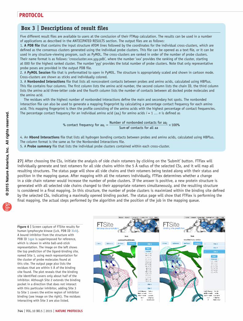
Box 3 | Descriptions of result files Five different result files are available to users at the conclusion of their FTMap calculation. The results can be used in a number of applications as described in the ANTICIPATED RESULTS section. The output files are as follows:1. a pDB file that contains the input structure ATOM lines followed by the coordinates for the individual cross-clusters, which are defined as the consensus clusters generated using the individual probe clusters. This file can be opened as a text file, or it can be used in any structure-viewing program, such as PyMOL. The cross-clusters are ranked in order of the number of probe clusters. Their name format is as follows: ‘crosscluster.xxx.yyy.pdb’, where the number ‘xxx’ provides the ranking of the cluster, starting at 000 for the highest ranked cluster. The number ‘yyy’ provides the total number of probe clusters. Note that only representative probe poses are provided in the output PDB file.2. A pyMol session file that is preformatted to open in PyMOL. The structure is appropriately scaled and shown in cartoon mode. Cross-clusters are shown as sticks and individually colored.3. A nonbonded Interactions file that lists all noncovalent contacts between probes and amino acids, calculated using HBPlus. This file contains four columns. The first column lists the amino acid number, the second column lists the chain ID, the third column lists the amino acid three-letter code and the fourth column lists the number of contacts between all docked probe molecules and the amino acid. The residues with the highest number of nonbonded interactions define the main and secondary hot spots. The nonbonded interaction file can also be used to generate a mapping fingerprint by calculating a percentage contact frequency for each amino acid. This mapping fingerprint is then the profile consisting of the amino acids with the highest percentage of contact frequencies. The percentage contact frequency for an individual amino acid (aai) for amino acids i = 1 … n is defined as

% contact frequency forNumber of nonbonded contacts for aa

Sumaai

i=oof contacts for all aa

× 100%

4. An Hbond Interactions file that lists all hydrogen bonding contacts between probes and amino acids, calculated using HBPlus. The column format is the same as for the Nonbonded Interactions file.5. A probe summary file that lists the individual probe clusters contained within each cross-cluster.

Figure 6 | Screen capture of FTSite results for human lymphocyte kinase (Lck, PDB ID 3lck). A bound inhibitor from the structure with PDB ID 1qpe is superimposed for reference, which is shown in white ball-and-stick representation. The image on the left shows the top prediction of the ligand-binding site, named Site 1, using mesh representation for the cluster of probe molecules found at this site. The output page also lists the residues that are within 5 Å of the binding site found. The plot reveals that the binding site identified covers only about half of the inhibitor. Although Site 2 extends the binding pocket in a direction that does not interact with this particular inhibitor, adding Site 3 to Site 1 covers the entire region of inhibitor binding (see image on the right). The residues interacting with Site 3 are also listed.

©20

15N

atu

re A

mer

ica,

Inc.

All

rig

hts

res

erve

d.

protocol

nature protocols | VOL.10 NO.5 | 2015 | 745

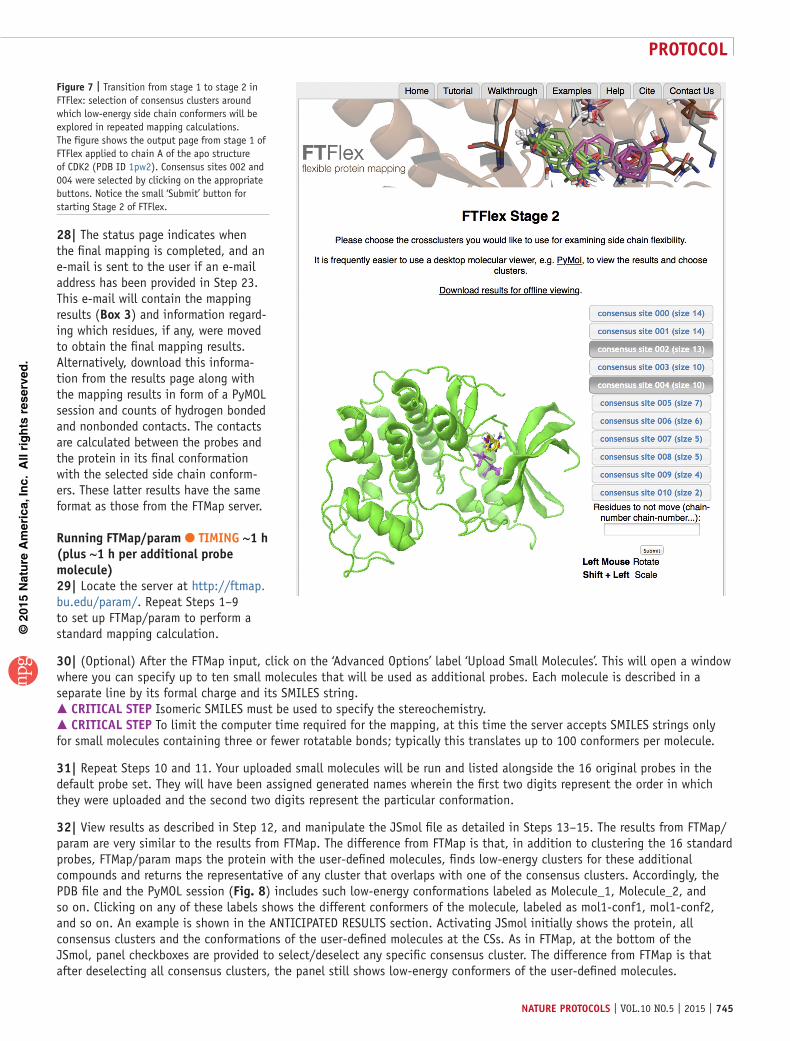
28| The status page indicates when the final mapping is completed, and an e-mail is sent to the user if an e-mail address has been provided in Step 23. This e-mail will contain the mapping results (Box 3) and information regard-ing which residues, if any, were moved to obtain the final mapping results. Alternatively, download this informa-tion from the results page along with the mapping results in form of a PyMOL session and counts of hydrogen bonded and nonbonded contacts. The contacts are calculated between the probes and the protein in its final conformation with the selected side chain conform-ers. These latter results have the same format as those from the FTMap server.

running FtMap/param ● tIMInG ~1 h (plus ~1 h per additional probe molecule)29| Locate the server at http://ftmap.bu.edu/param/. Repeat Steps 1–9 to set up FTMap/param to perform a standard mapping calculation.

30| (Optional) After the FTMap input, click on the ‘Advanced Options’ label ‘Upload Small Molecules’. This will open a window where you can specify up to ten small molecules that will be used as additional probes. Each molecule is described in a separate line by its formal charge and its SMILES string. crItIcal step Isomeric SMILES must be used to specify the stereochemistry. crItIcal step To limit the computer time required for the mapping, at this time the server accepts SMILES strings only for small molecules containing three or fewer rotatable bonds; typically this translates up to 100 conformers per molecule.

31| Repeat Steps 10 and 11. Your uploaded small molecules will be run and listed alongside the 16 original probes in the default probe set. They will have been assigned generated names wherein the first two digits represent the order in which they were uploaded and the second two digits represent the particular conformation.

32| View results as described in Step 12, and manipulate the JSmol file as detailed in Steps 13–15. The results from FTMap/param are very similar to the results from FTMap. The difference from FTMap is that, in addition to clustering the 16 standard probes, FTMap/param maps the protein with the user-defined molecules, finds low-energy clusters for these additional compounds and returns the representative of any cluster that overlaps with one of the consensus clusters. Accordingly, the PDB file and the PyMOL session (Fig. 8) includes such low-energy conformations labeled as Molecule_1, Molecule_2, and so on. Clicking on any of these labels shows the different conformers of the molecule, labeled as mol1-conf1, mol1-conf2, and so on. An example is shown in the ANTICIPATED RESULTS section. Activating JSmol initially shows the protein, all consensus clusters and the conformations of the user-defined molecules at the CSs. As in FTMap, at the bottom of the JSmol, panel checkboxes are provided to select/deselect any specific consensus cluster. The difference from FTMap is that after deselecting all consensus clusters, the panel still shows low-energy conformers of the user-defined molecules.

Figure 7 | Transition from stage 1 to stage 2 in FTFlex: selection of consensus clusters around which low-energy side chain conformers will be explored in repeated mapping calculations. The figure shows the output page from stage 1 of FTFlex applied to chain A of the apo structure of CDK2 (PDB ID 1pw2). Consensus sites 002 and 004 were selected by clicking on the appropriate buttons. Notice the small ‘Submit’ button for starting Stage 2 of FTFlex.

©20

15N

atu

re A

mer

ica,

Inc.

All

rig

hts

res

erve

d.

protocol

746 | VOL.10 NO.5 | 2015 | nature protocols

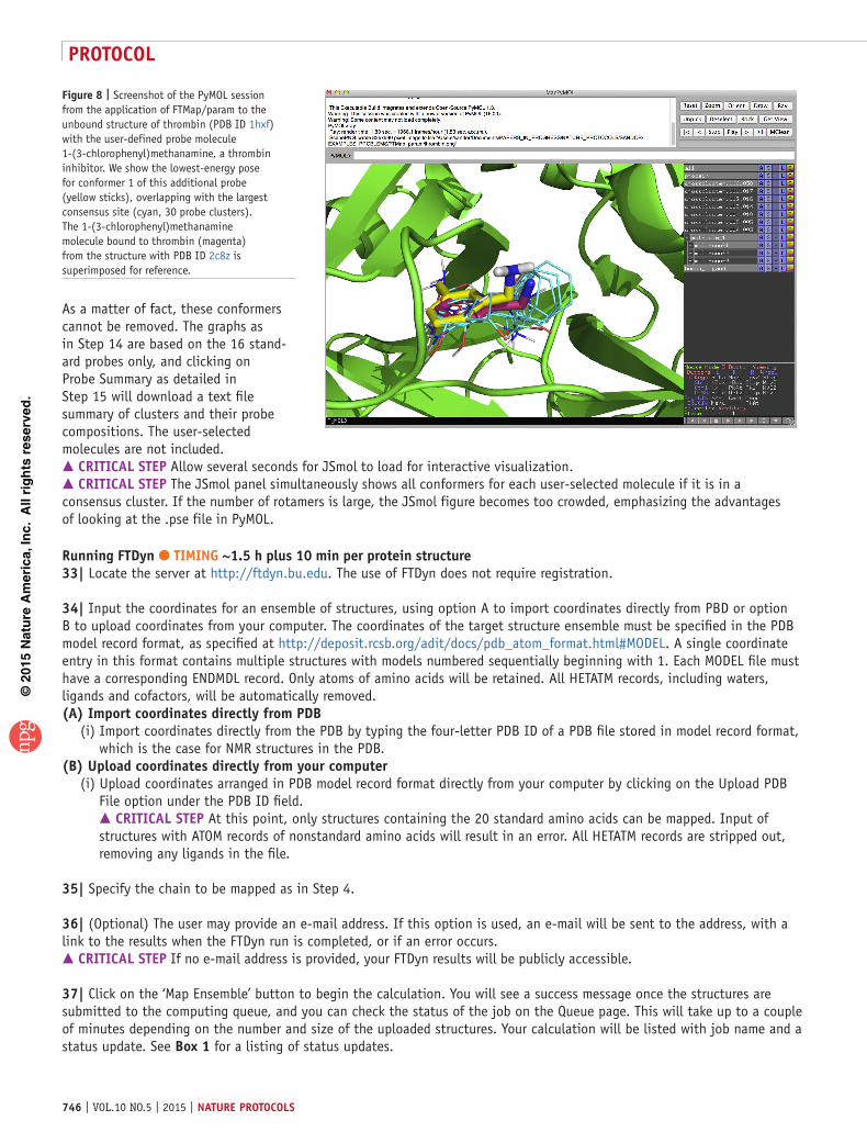
As a matter of fact, these conformers cannot be removed. The graphs as in Step 14 are based on the 16 stand-ard probes only, and clicking on Probe Summary as detailed in Step 15 will download a text file summary of clusters and their probe compositions. The user-selected molecules are not included. crItIcal step Allow several seconds for JSmol to load for interactive visualization. crItIcal step The JSmol panel simultaneously shows all conformers for each user-selected molecule if it is in a consensus cluster. If the number of rotamers is large, the JSmol figure becomes too crowded, emphasizing the advantages of looking at the .pse file in PyMOL.

running FtDyn ● tIMInG ~1.5 h plus 10 min per protein structure33| Locate the server at http://ftdyn.bu.edu. The use of FTDyn does not require registration.

34| Input the coordinates for an ensemble of structures, using option A to import coordinates directly from PBD or option B to upload coordinates from your computer. The coordinates of the target structure ensemble must be specified in the PDB model record format, as specified at http://deposit.rcsb.org/adit/docs/pdb_atom_format.html#MODEL. A single coordinate entry in this format contains multiple structures with models numbered sequentially beginning with 1. Each MODEL file must have a corresponding ENDMDL record. Only atoms of amino acids will be retained. All HETATM records, including waters, ligands and cofactors, will be automatically removed.(a) Import coordinates directly from pDB (i) Import coordinates directly from the PDB by typing the four-letter PDB ID of a PDB file stored in model record format,

which is the case for NMR structures in the PDB.(B) upload coordinates directly from your computer (i) Upload coordinates arranged in PDB model record format directly from your computer by clicking on the Upload PDB

File option under the PDB ID field. crItIcal step At this point, only structures containing the 20 standard amino acids can be mapped. Input of structures with ATOM records of nonstandard amino acids will result in an error. All HETATM records are stripped out, removing any ligands in the file.

35| Specify the chain to be mapped as in Step 4.

36| (Optional) The user may provide an e-mail address. If this option is used, an e-mail will be sent to the address, with a link to the results when the FTDyn run is completed, or if an error occurs. crItIcal step If no e-mail address is provided, your FTDyn results will be publicly accessible.

37| Click on the ‘Map Ensemble’ button to begin the calculation. You will see a success message once the structures are submitted to the computing queue, and you can check the status of the job on the Queue page. This will take up to a couple of minutes depending on the number and size of the uploaded structures. Your calculation will be listed with job name and a status update. See Box 1 for a listing of status updates.

Figure 8 | Screenshot of the PyMOL session from the application of FTMap/param to the unbound structure of thrombin (PDB ID 1hxf) with the user-defined probe molecule 1-(3-chlorophenyl)methanamine, a thrombin inhibitor. We show the lowest-energy pose for conformer 1 of this additional probe (yellow sticks), overlapping with the largest consensus site (cyan, 30 probe clusters). The 1-(3-chlorophenyl)methanamine molecule bound to thrombin (magenta) from the structure with PDB ID 2c8z is superimposed for reference.

©20

15N

atu

re A

mer

ica,

Inc.

All

rig

hts

res

erve

d.

protocol

nature protocols | VOL.10 NO.5 | 2015 | 747

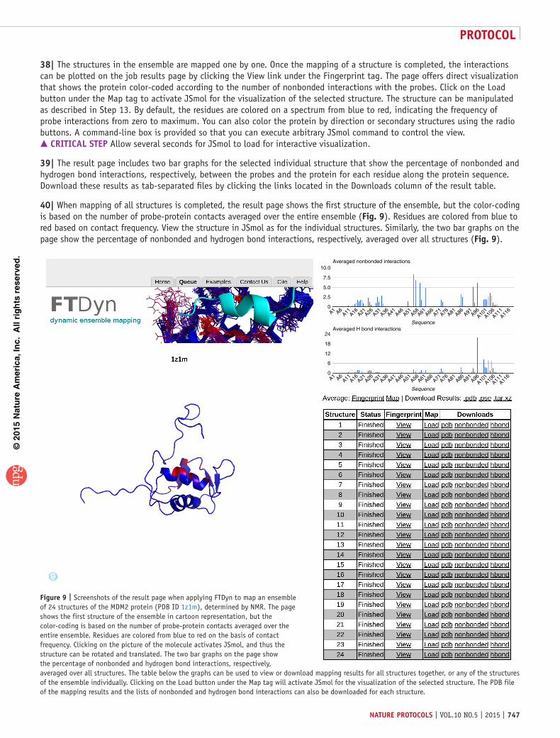
38| The structures in the ensemble are mapped one by one. Once the mapping of a structure is completed, the interactions can be plotted on the job results page by clicking the View link under the Fingerprint tag. The page offers direct visualization that shows the protein color-coded according to the number of nonbonded interactions with the probes. Click on the Load button under the Map tag to activate JSmol for the visualization of the selected structure. The structure can be manipulated as described in Step 13. By default, the residues are colored on a spectrum from blue to red, indicating the frequency of probe interactions from zero to maximum. You can also color the protein by direction or secondary structures using the radio buttons. A command-line box is provided so that you can execute arbitrary JSmol command to control the view. crItIcal step Allow several seconds for JSmol to load for interactive visualization.

39| The result page includes two bar graphs for the selected individual structure that show the percentage of nonbonded and hydrogen bond interactions, respectively, between the probes and the protein for each residue along the protein sequence. Download these results as tab-separated files by clicking the links located in the Downloads column of the result table.

40| When mapping of all structures is completed, the result page shows the first structure of the ensemble, but the color-coding is based on the number of probe-protein contacts averaged over the entire ensemble (Fig. 9). Residues are colored from blue to red based on contact frequency. View the structure in JSmol as for the individual structures. Similarly, the two bar graphs on the page show the percentage of nonbonded and hydrogen bond interactions, respectively, averaged over all structures (Fig. 9).

10.0

24

18

12

6

0

Averaged nonbonded interactions

Averaged H bond interactionsSequence

Sequence

7.5

5.0

2.5

0A1 A6

A11 A16 A21A26 A31 A36A41 A46 A51 A56A61 A66 A71A76 A81 A86 A91 A96A10

1A10

6A11

1A11

6

A1 A6A11 A16 A21 A26 A31 A36 A41 A46 A51 A56A61A66 A71A76 A81 A86 A91 A96

A101A10

6A11

1A11

6

Figure 9 | Screenshots of the result page when applying FTDyn to map an ensemble of 24 structures of the MDM2 protein (PDB ID 1z1m), determined by NMR. The page shows the first structure of the ensemble in cartoon representation, but the color-coding is based on the number of probe-protein contacts averaged over the entire ensemble. Residues are colored from blue to red on the basis of contact frequency. Clicking on the picture of the molecule activates JSmol, and thus the structure can be rotated and translated. The two bar graphs on the page show the percentage of nonbonded and hydrogen bond interactions, respectively, averaged over all structures. The table below the graphs can be used to view or download mapping results for all structures together, or any of the structures of the ensemble individually. Clicking on the Load button under the Map tag will activate JSmol for the visualization of the selected structure. The PDB file of the mapping results and the lists of nonbonded and hydrogen bond interactions can also be downloaded for each structure.

©20

15N

atu

re A

mer

ica,

Inc.

All

rig

hts

res

erve

d.

protocol

748 | VOL.10 NO.5 | 2015 | nature protocols

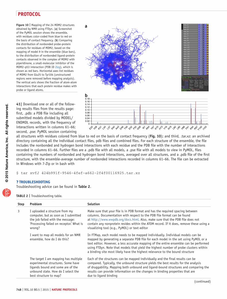
41| Download one or all of the follow-ing results files from the results page: first, .pdb: a PDB file including all submitted models divided by MODEL/ENDMDL records, with the frequency of interactions written in columns 61–66; second, .pse: PyMOL session containing all structures with residues colored from blue to red on the basis of contact frequency (Fig. 10); and third, .tar.xz: an archived directory containing all the individual contact files, pdb files and combined files. For each structure of the ensemble, the file includes the nonbonded and hydrogen bond interactions with each residue and the PDB file with the number of interactions recorded in columns 61–66. Further files are a .pdb file with all models, a .pse file with all models to view in PyMOL, files containing the numbers of nonbonded and hydrogen bond interactions, averaged over all structures, and a .pdb file of the first structure, with the ensemble-average number of nonbonded interactions recorded in columns 61–66. The file can be extracted in Windows with 7-Zip or in bash with

$ tar xvfJ 424b991f-9546-4fef-a662-2f4f00116925.tar.xz

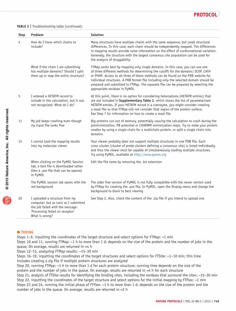
? trouBlesHootInGTroubleshooting advice can be found in table 2.

0.180.160.140.120.100.080.060.040.02

0

E25 S40 A43 D46 T49 E52 F55 G58 I61

K64 Y67 K70 H73 Y76 N79 L82

L85

V88 F91 K94 R97Y10

0I1

03L37

L34

K31V28

a

b

Figure 10 | Mapping of the 24 MDM2 structures obtained by NMR using FTDyn. (a) Screenshot of the PyMOL session shows the ensemble, with residues color-coded from blue to red on the basis of contact frequency. (b) Comparing the distribution of nonbonded probe-protein contacts for residues of MDM2, based on the mapping of model 9 in the ensemble (blue bars), to the distribution of nonbonded ligand-protein contacts observed in the complex of MDM2 with piperidinone, a small-molecular inhibitor of the MDM2–p53 interaction (PDB ID 2lzg), which is shown as red bars. Horizontal axes list residues of MDM2 from Glu25 to Tyr104 (unstructured regions were removed before mapping analysis). The vertical axis shows the fraction of atom-atom interactions that each protein residue makes with probe or ligand atoms.

taBle 2 | Troubleshooting table.

step problem solution

3 I uploaded a structure from my computer, but as soon as I submitted the job failed with the message: ‘Processing failed on receptor.’ What is wrong?

Make sure that your file is in PDB format and has the required spacing between columns. Documentation with respect to the PDB file format can be found at http://www.wwpdb.org/docs.html. Also, make sure that the PDB file does not contain any nonprotein resides within the ATOM record. If it does, remove these using a visualizing tool (e.g., PyMOL) or text editor

I want to map all models for an NMR ensemble, how do I do this?

In FTMap, each model needs to be mapped individually. Individual models can be mapped by generating a separate PDB file for each model in the set using PyMOL or a text editor. However, a less accurate mapping of the entire ensemble can be performed using FTDyn. Note that models that yield the highest number of probe clusters within a binding site most likely have the highest relevance to the bound structure

The target I am mapping has multiple experimental structures. Some have ligands bound and some are of the unbound state. How do I select the best structure to map?

Each of the structures can be mapped individually and the final results can be compared. Typically, the unbound structure yields the best results for the analysis of druggability. Mapping both unbound and ligand-bound structures and comparing the results can provide information on the changes in binding properties that are due to ligand binding

(continued)

©20

15N

atu

re A

mer

ica,

Inc.

All

rig

hts

res

erve

d.

protocol

nature protocols | VOL.10 NO.5 | 2015 | 749

● tIMInGSteps 1–9, inputting the coordinates of the target structure and select options for FTMap: ~1 minSteps 10 and 11, running FTMap: ~1 h to more than 1 d; depends on the size of the protein and the number of jobs in the queue. On average, results are returned in <4 hSteps 12–15, analyzing FTMap results: ~15–30 minSteps 16–19, inputting the coordinates of the target structures and select options for FTSite: ~1–10 min; this time includes creating a zip file if multiple protein structures are analyzedStep 20, running FTMap: ~1 h to more than 1 d for each protein structure; running time depends on the size of the protein and the number of jobs in the queue. On average, results are returned in <4 h for each structureStep 21, analysis of FTSite results for identifying the binding sites, including the residues that surround the sites: ~15–30 minStep 22, inputting the coordinates of the target structure and select options for the initial mapping by FTFlex: ~1 minSteps 23 and 24, running the initial phase of FTFlex: ~1 h to more than 1 d; depends on the size of the protein and the number of jobs in the queue. On average, results are returned in <2 h

taBle 2 | Troubleshooting table (continued).

step problem solution

4 How do I know which chains to include?

Many structures have multiple chains with the same sequence, but small structural differences. In this case, each chain should be independently mapped. The differences in mapping results provide some information on the effect of conformational variation. Generally, the structure with the largest consensus site population can be used for the analysis of druggability

What if the chain I am submitting has multiple domains? Should I split them up or map the entire structure?

FTMap works best by mapping only single domains. In this case, you can use one of three different methods for determining the cutoffs for the domains: SCOP, CATH or PFAM. Access to all three of these methods can be found on the PDB website for individual structures. A PDB format file including only the selected domain should be prepared and submitted to FTMap. The separate file can be prepared by selecting the appropriate residues in PyMOL

5 I entered a HETATM record to include in the calculation, but it was not recognized. What do I do?

At this point, there is no option for considering heteroatoms (HETATM entries) that are not included in supplementary table 1, which shows the list of parameterized HETATM entries. If your HETATM record is a coenzyme, you might consider creating a mask file so that FTMap will not consider that region of the protein surface. See Step 7 for information on how to create a mask file

11 My job keeps crashing even though my input file looks fine

Big proteins run out of memory, potentially causing the calculation to crash during the preminimization, PB potential or CHARMM minimization steps. Try to make your protein smaller by using a single chain for a multichain protein, or split a single chain into domains

15 I cannot load the mapping results into my molecular viewer

Your viewer probably does not support multiple structures in one PDB file. Each cross-cluster (cluster of probe clusters defining a consensus site) is listed individually, and thus the viewer must be capable of simultaneously loading multiple structures. Try using PyMOL, available at http://www.pymol.org

When clicking on the PyMOL Session tab, a text file is downloaded rather then a .pse file that can be opened in PyMOL

Edit the file name by removing the .txt extension

The PyMOL session tab opens with the red background

The older free version of PyMOL is not fully compatible with the newer version used by FTMap for creating the .pse file. In PyMOL, open the Display menu and change the background to black to best viewing

20 I uploaded a structure from my computer, but as soon as I submitted the job failed with the message: ‘Processing failed on receptor.’ What is wrong?

See Step 2. Also, check the content of the .zip file if you intend to upload one

©20

15N

atu

re A

mer

ica,

Inc.

All

rig

hts

res

erve

d.

protocol

750 | VOL.10 NO.5 | 2015 | nature protocols

Steps 25 and 26, choosing the CSs around which low-energy side chain conformers will be explored: ~5 minStep 27, mapping structures with the low-energy conformers of the side chains in the selected hot spots: because mapping may take 1 h or more or each low-energy rotamer, the length of this step will depend on the number of the low-energy side chain rotamers around the selected hot spots, and hence the time that this step takes is highly variable. The timing also depends on the number of jobs in the mapping queue. On average, using FTFlex requires 12–24 hStep 28, analyzing FTFlex results, including the list of residues that were moved to obtain the final hot spots: ~15–30 minStep 29, inputting the coordinates of the target structure and select options for FTMap/param: ~1 minStep 30, inputting formal charges and isomeric SMILES strings to specify up to ten small molecules to be used as additional probes: ~5 minStep 31, running FTMap/param: mapping with the standard set of 16 probes takes ~1 h or more, depending on the size of the protein and the number of jobs in the queue. However, the total run time may be substantially longer if you submit several additional molecules, some having many conformersStep 32, analyzing FTMap/param results for the determination of the binding hot spots and the most likely binding modes of additional probes: ~15–30 minSteps 33–36, inputting the coordinates of the target structure and select options for FTDyn: ~10 minSteps 37 and 38, running FTDyn: ~10 min for each protein structure; the total run time is proportional to the number and size of structures in the ensemble. The running time also depends on the size of the protein and the number of jobs in the queueSteps 39–41, analyzing FTDyn results: ~1 h

antIcIpateD resultsIdentification of hot spots using FtMapFigure 4 shows an example of the results page at the successful completion of a FTMap run. In this case, results are shown for the mapping of renin using a structure of the apo protein (PDB ID 2ren; ref. 74). The target protein is shown as a green cartoon, and the small molecules representing each probe cluster at the CSs are shown in various colors as sticks. Clicking on the image will activate JSmol, and the image can be manipulated using the JSmol tools. The CSs are defined by the positions of the consensus clusters, which are shown as sticks, with each consensus cluster represented by a different color. The protein can be rotated by pressing the left mouse button and moving the mouse, and its size can be increased or decreased by rotating the mouse wheel. The CSs, each with the number of probe clusters they contain, are listed below the JSmol panel, and they can be individually turned on and off. The consensus clusters are colored in the following order, with the highest ranking color first: cyan, magenta, yellow, salmon, white, periwinkle, orange, pale green, teal, fuchsia and so on. Each CS is shown as the collection of probes representing the centers of the probe clusters in the consensus cluster. The two graphs below the JSmol panel show the percentage of nonbonded and hydrogen bond interactions, respectively, between the probes and the protein for each residue along the protein sequence.

In addition to viewing the results in JSmol, you can download the PDB file containing the protein and representatives of probe clusters in the CSs, as well as a PyMOL session (.pse file) containing all results to be opened in PyMOL (Fig. 5a). In the session, the naming of consensus clusters indicates the number of probe clusters at each CS. The CSs are labeled in the format crosscluster.xxx.yyy, where xxx refers to the ranking of the CS, starting at 000, and yyy denotes the number of probe clusters in the CS. The ranking indicates the importance of the CS, with the highest ranking sites having the highest number of probe clusters.

Mapping the apo structure of renin (PDB ID 2ren; ref. 74) yields the CSs CS000 (cyan, 25 probe clusters), CS001 (magenta, 18 probe clusters), C002 (yellow, 16 probe clusters) and CS003 (salmon, 10 probe clusters), CS004 (white, 8 probe clusters), CS005 (blue, 8 probe clusters), CS006 (orange, 7 probe clusters) and CS007 (green, 3 probe clusters). Downloading and working with the .pse file is very useful, because you can add further structures, e.g., ones with bound ligands, align the proteins, select particular side chains, and generally use the versatility of PyMOL. For example, Figure 5b shows aliskiren, a novel nonpeptidic renin inhibitor from the inhibitor-bound renin structure 2v0z superimposed on the hot spots of the apo renin75. This result demonstrates that the hot spots, based on ligand-free protein structures, can very well trace out the shape of high-affinity ligands. Indeed, aliskiren overlaps with all CSs apart from CS001 (not shown). We note that CS001 overlaps with the transition state inhibitor CGP 38′560 (PDB ID 1rne; ref. 76), which is not shown here. Of course, such a high level of agreement assumes that the conformational changes of the protein upon ligand binding are moderate, which is the case for renin18. However, we have demonstrated that the hot spots are relatively robust, and in most cases they can be determined by mapping unbound structures28.

agreement between computational and experimental mapping results when using FtMapThe hot spots identified by FTMap generally are in good agreement with those obtained using experimental mapping tech-niques such as MSCS based on X-ray crystallography19. Figure 11a shows MCSS results for RNase A77. The method identified

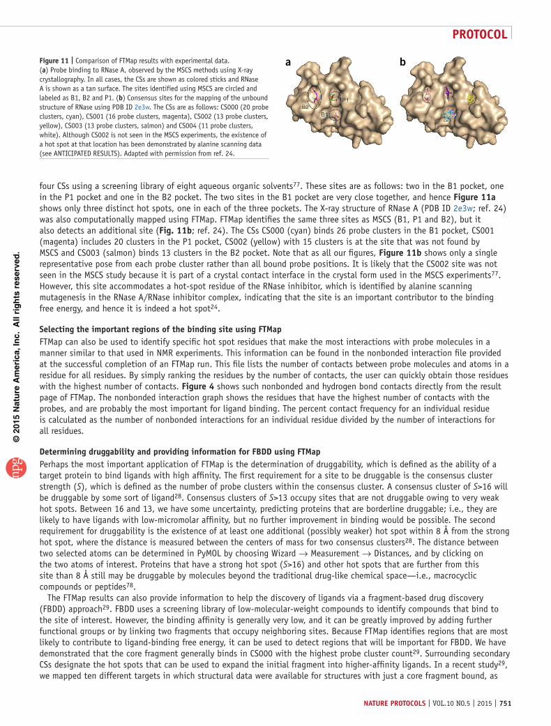
©20

15N

atu

re A

mer

ica,

Inc.

All

rig

hts

res

erve

d.

protocol

nature protocols | VOL.10 NO.5 | 2015 | 751

four CSs using a screening library of eight aqueous organic solvents77. These sites are as follows: two in the B1 pocket, one in the P1 pocket and one in the B2 pocket. The two sites in the B1 pocket are very close together, and hence Figure 11a shows only three distinct hot spots, one in each of the three pockets. The X-ray structure of RNase A (PDB ID 2e3w; ref. 24) was also computationally mapped using FTMap. FTMap identifies the same three sites as MSCS (B1, P1 and B2), but it also detects an additional site (Fig. 11b; ref. 24). The CSs CS000 (cyan) binds 26 probe clusters in the B1 pocket, CS001 (magenta) includes 20 clusters in the P1 pocket, CS002 (yellow) with 15 clusters is at the site that was not found by MSCS and CS003 (salmon) binds 13 clusters in the B2 pocket. Note that as all our figures, Figure 11b shows only a single representative pose from each probe cluster rather than all bound probe positions. It is likely that the CS002 site was not seen in the MSCS study because it is part of a crystal contact interface in the crystal form used in the MSCS experiments77. However, this site accommodates a hot-spot residue of the RNase inhibitor, which is identified by alanine scanning mutagenesis in the RNase A/RNase inhibitor complex, indicating that the site is an important contributor to the binding free energy, and hence it is indeed a hot spot24.

selecting the important regions of the binding site using FtMapFTMap can also be used to identify specific hot spot residues that make the most interactions with probe molecules in a manner similar to that used in NMR experiments. This information can be found in the nonbonded interaction file provided at the successful completion of an FTMap run. This file lists the number of contacts between probe molecules and atoms in a residue for all residues. By simply ranking the residues by the number of contacts, the user can quickly obtain those residues with the highest number of contacts. Figure 4 shows such nonbonded and hydrogen bond contacts directly from the result page of FTMap. The nonbonded interaction graph shows the residues that have the highest number of contacts with the probes, and are probably the most important for ligand binding. The percent contact frequency for an individual residue is calculated as the number of nonbonded interactions for an individual residue divided by the number of interactions for all residues.

Determining druggability and providing information for FBDD using FtMapPerhaps the most important application of FTMap is the determination of druggability, which is defined as the ability of a target protein to bind ligands with high affinity. The first requirement for a site to be druggable is the consensus cluster strength (S), which is defined as the number of probe clusters within the consensus cluster. A consensus cluster of S>16 will be druggable by some sort of ligand28. Consensus clusters of S>13 occupy sites that are not druggable owing to very weak hot spots. Between 16 and 13, we have some uncertainty, predicting proteins that are borderline druggable; i.e., they are likely to have ligands with low-micromolar affinity, but no further improvement in binding would be possible. The second requirement for druggability is the existence of at least one additional (possibly weaker) hot spot within 8 Å from the strong hot spot, where the distance is measured between the centers of mass for two consensus clusters28. The distance between two selected atoms can be determined in PyMOL by choosing Wizard → Measurement → Distances, and by clicking on the two atoms of interest. Proteins that have a strong hot spot (S>16) and other hot spots that are further from this site than 8 Å still may be druggable by molecules beyond the traditional drug-like chemical space—i.e., macrocyclic compounds or peptides78.

The FTMap results can also provide information to help the discovery of ligands via a fragment-based drug discovery (FBDD) approach29. FBDD uses a screening library of low-molecular-weight compounds to identify compounds that bind to the site of interest. However, the binding affinity is generally very low, and it can be greatly improved by adding further functional groups or by linking two fragments that occupy neighboring sites. Because FTMap identifies regions that are most likely to contribute to ligand-binding free energy, it can be used to detect regions that will be important for FBDD. We have demonstrated that the core fragment generally binds in CS000 with the highest probe cluster count29. Surrounding secondary CSs designate the hot spots that can be used to expand the initial fragment into higher-affinity ligands. In a recent study29, we mapped ten different targets in which structural data were available for structures with just a core fragment bound, as

B2B1

P1

a bFigure 11 | Comparison of FTMap results with experimental data. (a) Probe binding to RNase A, observed by the MSCS methods using X-ray crystallography. In all cases, the CSs are shown as colored sticks and RNase A is shown as a tan surface. The sites identified using MSCS are circled and labeled as B1, B2 and P1. (b) Consensus sites for the mapping of the unbound structure of RNase using PDB ID 2e3w. The CSs are as follows: CS000 (20 probe clusters, cyan), CS001 (16 probe clusters, magenta), CS002 (13 probe clusters, yellow), CS003 (13 probe clusters, salmon) and CS004 (11 probe clusters, white). Although CS002 is not seen in the MSCS experiments, the existence of a hot spot at that location has been demonstrated by alanine scanning data (see ANTICIPATED RESULTS). Adapted with permission from ref. 24.

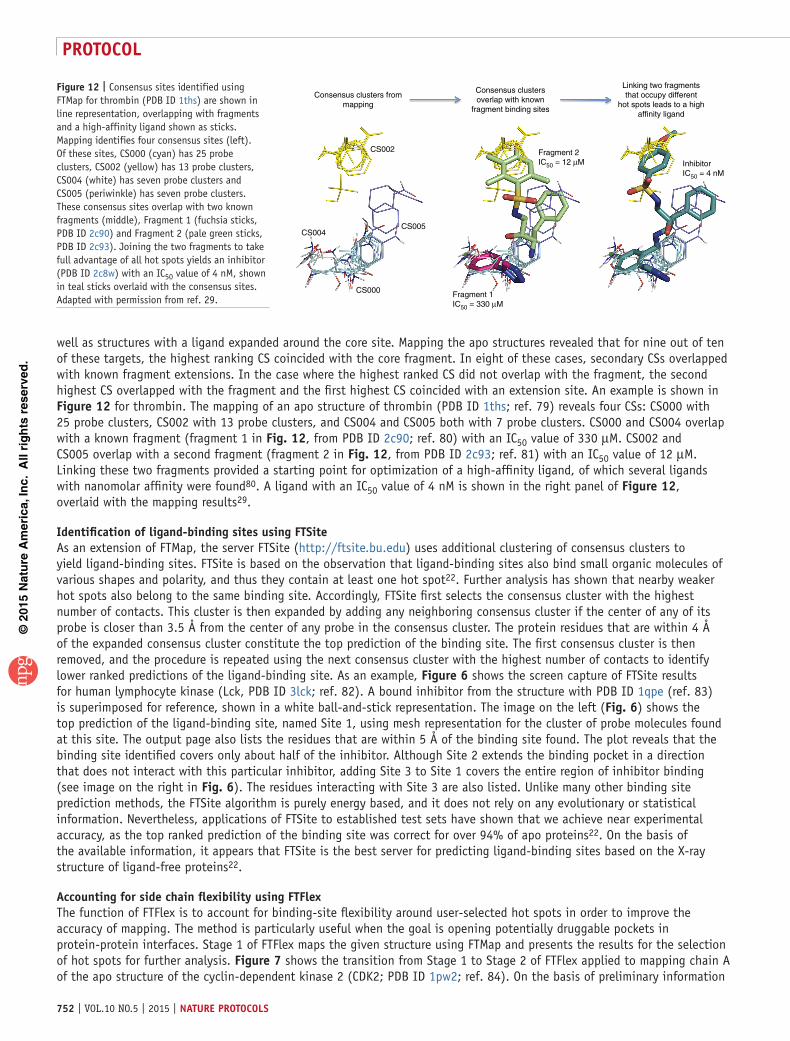
©20

15N

atu

re A

mer

ica,

Inc.

All

rig

hts

res

erve

d.

protocol

752 | VOL.10 NO.5 | 2015 | nature protocols

well as structures with a ligand expanded around the core site. Mapping the apo structures revealed that for nine out of ten of these targets, the highest ranking CS coincided with the core fragment. In eight of these cases, secondary CSs overlapped with known fragment extensions. In the case where the highest ranked CS did not overlap with the fragment, the second highest CS overlapped with the fragment and the first highest CS coincided with an extension site. An example is shown in Figure 12 for thrombin. The mapping of an apo structure of thrombin (PDB ID 1ths; ref. 79) reveals four CSs: CS000 with 25 probe clusters, CS002 with 13 probe clusters, and CS004 and CS005 both with 7 probe clusters. CS000 and CS004 overlap with a known fragment (fragment 1 in Fig. 12, from PDB ID 2c90; ref. 80) with an IC50 value of 330 µM. CS002 and CS005 overlap with a second fragment (fragment 2 in Fig. 12, from PDB ID 2c93; ref. 81) with an IC50 value of 12 µM. Linking these two fragments provided a starting point for optimization of a high-affinity ligand, of which several ligands with nanomolar affinity were found80. A ligand with an IC50 value of 4 nM is shown in the right panel of Figure 12, overlaid with the mapping results29.

Identification of ligand-binding sites using FtsiteAs an extension of FTMap, the server FTSite (http://ftsite.bu.edu) uses additional clustering of consensus clusters to yield ligand-binding sites. FTSite is based on the observation that ligand-binding sites also bind small organic molecules of various shapes and polarity, and thus they contain at least one hot spot22. Further analysis has shown that nearby weaker hot spots also belong to the same binding site. Accordingly, FTSite first selects the consensus cluster with the highest number of contacts. This cluster is then expanded by adding any neighboring consensus cluster if the center of any of its probe is closer than 3.5 Å from the center of any probe in the consensus cluster. The protein residues that are within 4 Å of the expanded consensus cluster constitute the top prediction of the binding site. The first consensus cluster is then removed, and the procedure is repeated using the next consensus cluster with the highest number of contacts to identify lower ranked predictions of the ligand-binding site. As an example, Figure 6 shows the screen capture of FTSite results for human lymphocyte kinase (Lck, PDB ID 3lck; ref. 82). A bound inhibitor from the structure with PDB ID 1qpe (ref. 83) is superimposed for reference, shown in a white ball-and-stick representation. The image on the left (Fig. 6) shows the top prediction of the ligand-binding site, named Site 1, using mesh representation for the cluster of probe molecules found at this site. The output page also lists the residues that are within 5 Å of the binding site found. The plot reveals that the binding site identified covers only about half of the inhibitor. Although Site 2 extends the binding pocket in a direction that does not interact with this particular inhibitor, adding Site 3 to Site 1 covers the entire region of inhibitor binding (see image on the right in Fig. 6). The residues interacting with Site 3 are also listed. Unlike many other binding site prediction methods, the FTSite algorithm is purely energy based, and it does not rely on any evolutionary or statistical information. Nevertheless, applications of FTSite to established test sets have shown that we achieve near experimental accuracy, as the top ranked prediction of the binding site was correct for over 94% of apo proteins22. On the basis of the available information, it appears that FTSite is the best server for predicting ligand-binding sites based on the X-ray structure of ligand-free proteins22.

accounting for side chain flexibility using FtFlexThe function of FTFlex is to account for binding-site flexibility around user-selected hot spots in order to improve the accuracy of mapping. The method is particularly useful when the goal is opening potentially druggable pockets in protein-protein interfaces. Stage 1 of FTFlex maps the given structure using FTMap and presents the results for the selection of hot spots for further analysis. Figure 7 shows the transition from Stage 1 to Stage 2 of FTFlex applied to mapping chain A of the apo structure of the cyclin-dependent kinase 2 (CDK2; PDB ID 1pw2; ref. 84). On the basis of preliminary information

Consensus clusters frommapping

CS002

CS004CS005

CS000

Fragment 2IC50 = 12 µM

Fragment 1IC50 = 330 µM

InhibitorIC50 = 4 nM

Consensus clustersoverlap with known

fragment binding sites

Linking two fragmentsthat occupy different

hot spots leads to a highaffinity ligand

Figure 12 | Consensus sites identified using FTMap for thrombin (PDB ID 1ths) are shown in line representation, overlapping with fragments and a high-affinity ligand shown as sticks. Mapping identifies four consensus sites (left). Of these sites, CS000 (cyan) has 25 probe clusters, CS002 (yellow) has 13 probe clusters, CS004 (white) has seven probe clusters and CS005 (periwinkle) has seven probe clusters. These consensus sites overlap with two known fragments (middle), Fragment 1 (fuchsia sticks, PDB ID 2c90) and Fragment 2 (pale green sticks, PDB ID 2c93). Joining the two fragments to take full advantage of all hot spots yields an inhibitor (PDB ID 2c8w) with an IC50 value of 4 nM, shown in teal sticks overlaid with the consensus sites. Adapted with permission from ref. 29.

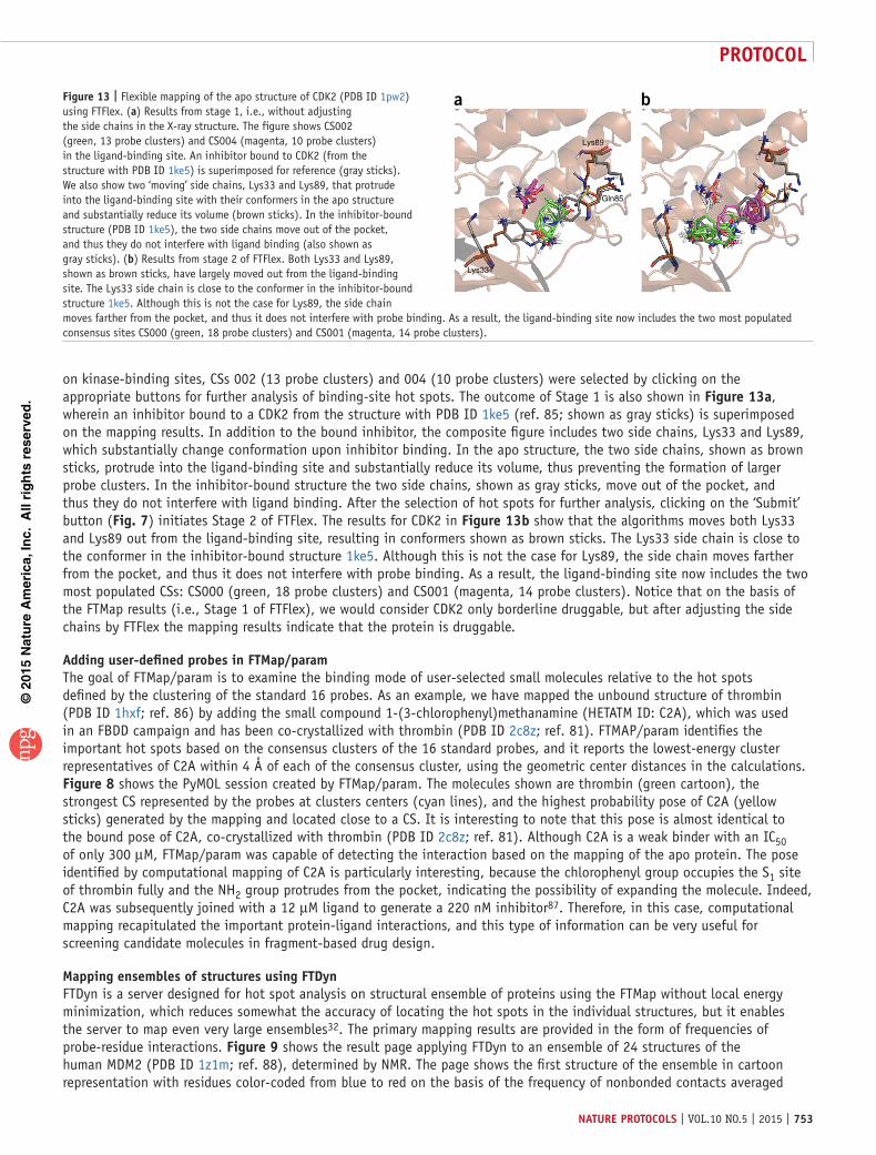
©20

15N

atu

re A

mer

ica,

Inc.

All

rig

hts

res

erve

d.

protocol

nature protocols | VOL.10 NO.5 | 2015 | 753

on kinase-binding sites, CSs 002 (13 probe clusters) and 004 (10 probe clusters) were selected by clicking on the appropriate buttons for further analysis of binding-site hot spots. The outcome of Stage 1 is also shown in Figure 13a, wherein an inhibitor bound to a CDK2 from the structure with PDB ID 1ke5 (ref. 85; shown as gray sticks) is superimposed on the mapping results. In addition to the bound inhibitor, the composite figure includes two side chains, Lys33 and Lys89, which substantially change conformation upon inhibitor binding. In the apo structure, the two side chains, shown as brown sticks, protrude into the ligand-binding site and substantially reduce its volume, thus preventing the formation of larger probe clusters. In the inhibitor-bound structure the two side chains, shown as gray sticks, move out of the pocket, and thus they do not interfere with ligand binding. After the selection of hot spots for further analysis, clicking on the ‘Submit’ button (Fig. 7) initiates Stage 2 of FTFlex. The results for CDK2 in Figure 13b show that the algorithms moves both Lys33 and Lys89 out from the ligand-binding site, resulting in conformers shown as brown sticks. The Lys33 side chain is close to the conformer in the inhibitor-bound structure 1ke5. Although this is not the case for Lys89, the side chain moves farther from the pocket, and thus it does not interfere with probe binding. As a result, the ligand-binding site now includes the two most populated CSs: CS000 (green, 18 probe clusters) and CS001 (magenta, 14 probe clusters). Notice that on the basis of the FTMap results (i.e., Stage 1 of FTFlex), we would consider CDK2 only borderline druggable, but after adjusting the side chains by FTFlex the mapping results indicate that the protein is druggable.

adding user-defined probes in FtMap/paramThe goal of FTMap/param is to examine the binding mode of user-selected small molecules relative to the hot spots defined by the clustering of the standard 16 probes. As an example, we have mapped the unbound structure of thrombin (PDB ID 1hxf; ref. 86) by adding the small compound 1-(3-chlorophenyl)methanamine (HETATM ID: C2A), which was used in an FBDD campaign and has been co-crystallized with thrombin (PDB ID 2c8z; ref. 81). FTMAP/param identifies the important hot spots based on the consensus clusters of the 16 standard probes, and it reports the lowest-energy cluster representatives of C2A within 4 Å of each of the consensus cluster, using the geometric center distances in the calculations. Figure 8 shows the PyMOL session created by FTMap/param. The molecules shown are thrombin (green cartoon), the strongest CS represented by the probes at clusters centers (cyan lines), and the highest probability pose of C2A (yellow sticks) generated by the mapping and located close to a CS. It is interesting to note that this pose is almost identical to the bound pose of C2A, co-crystallized with thrombin (PDB ID 2c8z; ref. 81). Although C2A is a weak binder with an IC50 of only 300 µM, FTMap/param was capable of detecting the interaction based on the mapping of the apo protein. The pose identified by computational mapping of C2A is particularly interesting, because the chlorophenyl group occupies the S1 site of thrombin fully and the NH2 group protrudes from the pocket, indicating the possibility of expanding the molecule. Indeed, C2A was subsequently joined with a 12 µM ligand to generate a 220 nM inhibitor87. Therefore, in this case, computational mapping recapitulated the important protein-ligand interactions, and this type of information can be very useful for screening candidate molecules in fragment-based drug design.

Mapping ensembles of structures using FtDynFTDyn is a server designed for hot spot analysis on structural ensemble of proteins using the FTMap without local energy minimization, which reduces somewhat the accuracy of locating the hot spots in the individual structures, but it enables the server to map even very large ensembles32. The primary mapping results are provided in the form of frequencies of probe-residue interactions. Figure 9 shows the result page applying FTDyn to an ensemble of 24 structures of the human MDM2 (PDB ID 1z1m; ref. 88), determined by NMR. The page shows the first structure of the ensemble in cartoon representation with residues color-coded from blue to red on the basis of the frequency of nonbonded contacts averaged

Lys89

Gln85

Lys33

a bFigure 13 | Flexible mapping of the apo structure of CDK2 (PDB ID 1pw2) using FTFlex. (a) Results from stage 1, i.e., without adjusting the side chains in the X-ray structure. The figure shows CS002 (green, 13 probe clusters) and CS004 (magenta, 10 probe clusters) in the ligand-binding site. An inhibitor bound to CDK2 (from the structure with PDB ID 1ke5) is superimposed for reference (gray sticks). We also show two ‘moving’ side chains, Lys33 and Lys89, that protrude into the ligand-binding site with their conformers in the apo structure and substantially reduce its volume (brown sticks). In the inhibitor-bound structure (PDB ID 1ke5), the two side chains move out of the pocket, and thus they do not interfere with ligand binding (also shown as gray sticks). (b) Results from stage 2 of FTFlex. Both Lys33 and Lys89, shown as brown sticks, have largely moved out from the ligand-binding site. The Lys33 side chain is close to the conformer in the inhibitor-bound structure 1ke5. Although this is not the case for Lys89, the side chain moves farther from the pocket, and thus it does not interfere with probe binding. As a result, the ligand-binding site now includes the two most populated consensus sites CS000 (green, 18 probe clusters) and CS001 (magenta, 14 probe clusters).

©20

15N

atu

re A

mer

ica,

Inc.

All

rig

hts

res

erve

d.

protocol

754 | VOL.10 NO.5 | 2015 | nature protocols

over the entire ensemble (Fig. 9a). Clicking on the picture of the molecule activates JSmol. The result page also presents the ensemble-averaged frequency of nonbonded and hydrogen bond interactions in the form of bar graphs (Fig. 9b). Below the graphs, the table can be used to view or download mapping results for all structures, or for any of the structures of the ensemble individually. The screenshot of the PyMOL session, which is downloaded from the result page (Fig. 10a), shows substantial variation among the structures within the NMR-derived MDM2 ensemble. However, the color-coding from blue to red based on contact frequency reveals that largely the same residues interact with the probes in all structures. The bar graph in Figure 10b compares the distribution of nonbonded probe-protein contacts for residues of MDM2, based on the mapping of model 9 in the ensemble (blue bars), with the distribution of nonbonded ligand-protein contacts observed in the complex of MDM2 with piperidinone, a small molecular inhibitor of the MDM2-p53 interaction (PDB ID 2lzg; ref. 89), shown as red bars. Model 9 was selected because it had the maximum HR, which is defined as the total number of probe-protein interactions in the binding site among all models. The comparison demonstrates that the averaging of probe-protein interactions identifies and ranks by importance the binding site residues fairly well, in spite of the substantial structural variation.

Note: Any Supplementary Information and Source Data files are available in the online version of the paper.

acknoWleDGMents This investigation was supported by grants GM064700 from the National Institute of General Medical Sciences.

autHor contrIButIons D.K., D.R.H., T.B., B.X. and S.E.M. developed the servers; D.K., L.E.G., D.R.H., T.B., D.B., L.L. and B.X. performed experiments; L.E.G., D.R.H. and S.V. prepared the manuscript with editing by T.B., S.V. and L.E.G.

coMpetInG FInancIal Interests The authors declare competing financial interests: details are available in the online version of the paper.

Reprints and permissions information is available online at http://www.nature.com/reprints/index.html.

1. DeLano, W.L., Ultsch, M.H., de Vos, A.M. & Wells, J.A. Convergent solutions to binding at a protein-protein interface. Science 287, 1279–1283 (2000).

2. Thanos, C.D., DeLano, W.L. & Wells, J.A. Hot-spot mimicry of a cytokine receptor by a small molecule. Proc. Natl. Acad. Sci. USA 103, 15422–15427 (2006).

3. DeLano, W.L. Unraveling hot spots in binding interfaces: progress and challenges. Curr. Opin. Struct. Biol. 12, 14–20 (2002).

4. Clackson, T. & Wells, J.A. A hot spot of binding energy in a hormone-receptor interface. Science 267, 383–386 (1995).

5. Keskin, O., Ma, B.Y. & Nussinov, R. Hot regions in protein-protein interactions: the organization and contribution of structurally conserved hot spot residues. J. Mol. Biol. 345, 1281–1294 (2005).

6. Bogan, A.A. & Thorn, K.S. Anatomy of hot spots in protein interfaces. J. Mol. Biol. 280, 1–9 (1998).

7. Kortemme, T. & Baker, D. A simple physical model for binding energy hot spots in protein-protein complexes. Proc. Natl. Acad. Sci. USA 99, 14116–14121 (2002).

8. Hajduk, P.J., Huth, J.R. & Fesik, S.W. Druggability indices for protein targets derived from NMR-based screening data. J. Med. Chem. 48, 2518–2525 (2005).

9. Vajda, S. & Guarnieri, F. Characterization of protein-ligand interaction sites using experimental and computational methods. Curr. Opin. Drug Discov. Devel. 9, 354–362 (2006).

10. Seco, J., Luque, F.J. & Barril, X. Binding site detection and druggability index from first principles. J. Med. Chem. 52, 2363–2371 (2009).

11. Mattos, C. & Ringe, D. Locating and characterizing binding sites on proteins. Nat. Biotechnol. 14, 595–599 (1996).

12. Allen, K.N. et al. An experimental approach to mapping the binding surfaces of crystalline proteins. J. Phys. Chem. 100, 2605–2611 (1996).

13. Ciulli, A., Williams, G., Smith, A.G., Blundell, T.L. & Abell, C. Probing hot spots at protein-ligand binding sites: a fragment-based approach using biophysical methods. J. Med. Chem. 49, 4992–5000 (2006).

14. Dennis, S., Kortvelyesi, T. & Vajda, S. Computational mapping identifies the binding sites of organic solvents on proteins. Proc. Natl. Acad. Sci. USA 99, 4290–4295 (2002).

15. Silberstein, M. et al. Identification of substrate binding sites in enzymes by computational solvent mapping. J. Mol. Biol. 332, 1095–1113 (2003).

16. Landon, M.R. et al. Detection of ligand binding hot spots on protein surfaces via fragment-based methods: application to DJ-1 and glucocerebrosidase. J. Comput. Aided Mol. Des. 23, 491–500 (2009).

17. Kuttner, Y.Y. & Engel, S. Protein hot spots: the islands of stability. J. Mol. Biol. 415, 419–428 (2012).

18. Landon, M.R., Lancia, D.R. Jr., Yu, J., Thiel, S.C. & Vajda, S. Identification of hot spots within druggable binding regions by computational solvent mapping of proteins. J. Med. Chem. 50, 1231–1240 (2007).

19. Brenke, R. et al. Fragment-based identification of druggable ′hot spots′ of proteins using Fourier domain correlation techniques. Bioinformatics 25, 621–627 (2009).

20. Chuang, G.Y. et al. Binding hot spots and amantadine orientation in the influenza a virus M2 proton channel. Biophys. J. 97, 2846–2853 (2009).

21. Landon, M.R. et al. Novel druggable hot spots in avian influenza neuraminidase H5N1 revealed by computational solvent mapping of a reduced and representative receptor ensemble. Chem. Biol. Drug Des. 71, 106–116 (2008).

22. Ngan, C.H. et al. FTSite: high accuracy detection of ligand binding sites on unbound protein structures. Bioinformatics 28, 286–287 (2012).

23. Villar, E.A. et al. How proteins bind macrocycles. Nat. Chem. Biol. 10, 723–731 (2014).

24. Zerbe, B.S., Hall, D.R., Vajda, S., Whitty, A. & Kozakov, D. Relationship between hot spot residues and ligand binding hot spots in protein-protein interfaces. J. Chem. Inf. Model. 52, 2236–2244 (2012).

25. Rees, D.C., Congreve, M., Murray, C.W. & Carr, R. Fragment-based lead discovery. Nat. Rev. Drug Discov. 3, 660–672 (2004).

26. Erlanson, D.A., McDowell, R.S. & O’Brien, T. Fragment-based drug discovery. J. Med. Chem. 47, 3463–3482 (2004).

27. Hartshorn, M.J. et al. Fragment-based lead discovery using X-ray crystallography. J. Med. Chem. 48, 403–413 (2005).

28. Kozakov, D. et al. Structural conservation of druggable hot spots in protein-protein interfaces. Proc. Natl. Acad. Sci. USA 108, 13528–13533 (2011).

29. Hall, D.R., Ngan, C.H., Zerbe, B.S., Kozakov, D. & Vajda, S. Hot spot analysis for driving the development of hits into leads in fragment-based drug discovery. J. Chem. Inf. Model. 52, 199–209 (2012).

30. Grove, L.E., Hall, D.R., Beglov, D., Vajda, S. & Kozakov, D. FTFlex: accounting for binding site flexibility to improve fragment-based identification of druggable hot spots. Bioinformatics 29, 1218–1219 (2013).

31. Ngan, C.H. et al. FTMAP: extended protein mapping with user-selected probe molecules. Nucleic Acids Res. 40, W271–275 (2012).

32. Bohnuud, T., Kozakov, D. & Vajda, S. Evidence of conformational selection driving the formation of ligand binding sites in protein-protein interfaces. PLoS Comput. Biol. 10, e1003872 (2014).

33. Ivetac, A. & McCammon, J.A. Mapping the druggable allosteric space of G protein–coupled receptors: a fragment-based molecular dynamics approach. Chem. Biol. Drug Des. 76, 201–217 (2010).

34. Hall, D.H. et al. Robust identification of binding hot spots using continuum electrostatics: application to hen egg-white lysozyme. J. Am. Chem. Soc. 133, 20668–20671 (2011).

©20

15N

atu

re A

mer

ica,

Inc.

All

rig

hts

res

erve

d.

protocol

nature protocols | VOL.10 NO.5 | 2015 | 755

35. Hall, D.R., Kozakov, D. & Vajda, S. Analysis of protein binding sites by computational solvent mapping. Methods Mol. Biol. 819, 13–27 (2012).

36. Brooks, B.R. et al. Charmm - a program for macromolecular energy, minimization, and dynamics calculations. J. Comput. Chem. 4, 187–217 (1983).

37. Schaefer, M. & Karplus, M. A comprehensive analytical treatment of continuum electrostatics. J. Phys. Chem. 100, 1578–1599 (1996).

38. Goodford, P.J. A computational procedure for determining energetically favorable binding sites on biologically important macromolecules. J. Med. Chem. 28, 849–857 (1985).

39. Miranker, A. & Karplus, M. Functionality maps of binding-sites - a multiple copy simultaneous search method. Proteins 11, 29–34 (1991).

40. Mattos, C. et al. Multiple solvent crystal structures: probing binding sites, plasticity and hydration. J. Mol. Biol. 357, 1471–1482 (2006).

41. Berman, H.M. et al. The Protein Data Bank. Nucleic Acids Res. 28, 235–242 (2000).

42. Bohnuud, T. et al. Computational mapping reveals dramatic effect of Hoogsteen breathing on duplex DNA reactivity with formaldehyde. Nucleic Acids Res. 40, 7644–7652 (2012).

43. Chuang, G.Y., Kozakov, D., Brenke, R., Comeau, S.R. & Vajda, S. DARS (Decoys As the Reference State) potentials for protein-protein docking. Biophys. J. 95, 4217–4227 (2008).

44. Beglov, D. et al. Minimal ensembles of side chain conformers for modeling protein-protein interactions. Proteins 80, 591–601 (2012).

45. O′Boyle, N.M., Vandermeersch, T., Flynn, C.J., Maguire, A.R. & Hutchison, G.R. Confab: systematic generation of diverse low-energy conformers. J. Cheminform. 3, 8 (2011).

46. Wang, J., Wang, W., Kollman, P.A. & Case, D.A. Automatic atom type and bond type perception in molecular mechanical calculations. J. Mol. Graph. Model. 25, 247–260 (2006).

47. Wang, J., Wolf, R.M., Caldwell, J.W., Kollman, P.A. & Case, D.A. Development and testing of a general amber force field. J. Comput. Chem. 25, 1157–1174 (2004).

48. Alexeev, Y., Mazanetz, M.P., Ichihara, O. & Fedorov, D.G. GAMESS as a free quantum-mechanical platform for drug research. Curr. Top. Med. Chem. 12, 2013–2033 (2012).

49. Jakalian, A., Jack, D.B. & Bayly, C.I. Fast, efficient generation of high-quality atomic charges. AM1-BCC model: II. Parameterization and validation. J. Comput. Chem. 23, 1623–1641 (2002).

50. Votapka, L. & Amaro, R.E. Multistructural hot spot characterization with FTProd. Bioinformatics 29, 393–394 (2013).

51. Guerois, R., Nielsen, J.E. & Serrano, L. Predicting changes in the stability of proteins and protein complexes: a study of more than 1,000 mutations. J. Mol. Biol. 320, 369–387 (2002).

52. Zhu, X. & Mitchell, J.C. KFC2: a knowledge-based hot spot prediction method based on interface solvation, atomic density, and plasticity features. Proteins 79, 2671–2683 (2011).

53. Tuncbag, N., Gursoy, A. & Keskin, O. Identification of computational hot spots in protein interfaces: combining solvent accessibility and inter-residue potentials improves the accuracy. Bioinformatics 25, 1513–1520 (2009).

54. Deng, L. et al. PredHS: a web server for predicting protein-protein interaction hot spots by using structural neighborhood properties. Nucleic Acids Res. 42, W290–W295 (2014).

55. Laurie, A.T. & Jackson, R.M. Methods for the prediction of protein-ligand binding sites for structure-based drug design and virtual ligand screening. Curr. Protein Pept. Sci. 7, 395–406 (2006).

56. Levitt, D.G. & Banaszak, L.J. Pocket: a computer-graphics method for identifying and displaying protein cavities and their surrounding amino acids. J. Mol. Graph. 10, 229–234 (1992).

57. Huang, B. & Schroeder, M. LIGSITEcsc: predicting ligand binding sites using the Connolly surface and degree of conservation. BMC Struct. Biol. 6, 19 (2006).

58. Hendlich, M., Rippmann, F. & Barnickel, G. LIGSITE: automatic and efficient detection of potential small molecule-binding sites in proteins. J. Mol. Graph. Model 15, 359–363, 389 (1997).

59. Brady, G.P. Jr. & Stouten, P.F. Fast prediction and visualization of protein binding pockets with PASS. J. Comput. Aided Mol. Des. 14, 383–401 (2000).

60. Binkowski, T.A., Naghibzadeh, S. & Liang, J. CASTp: Computed atlas of surface topography of proteins. Nucleic Acids Res. 31, 3352–3355 (2003).

61. Wass, M.N., Kelley, L.A. & Sternberg, M.J. 3DLigandSite: predicting ligand-binding sites using similar structures. Nucleic Acids Res. 38, W469–W473 (2010).

62. Brylinski, M. & Skolnick, J. A threading-based method (FINDSITE) for ligand-binding site prediction and functional annotation. Proc. Natl. Acad. Sci. USA 105, 129–134 (2008).

63. Chou, K.C. & Cai, Y.D. A novel approach to predict active sites of enzyme molecules. Proteins 55, 77–82 (2004).

64. Laurie, A.T.R. & Jackson, R.M. Q-SiteFinder: an energy-based method for the prediction of protein-ligand binding sites. Bioinformatics 21, 1908–1916 (2005).

65. Halgren, T.A. Identifying and characterizing binding sites and assessing druggability. J. Chem. Inf. Model. 49, 377–389 (2009).

66. Hernandez, M., Ghersi, D. & Sanchez, R. SITEHOUND-web: a server for ligand binding site identification in protein structures. Nucleic Acids Res. 37, W413–W416 (2009).

67. English, A.C., Done, S.H., Caves, L.S., Groom, C.R. & Hubbard, R.E. Locating interaction sites on proteins: the crystal structure of thermolysin soaked in 2% to 100% isopropanol. Proteins 37, 628–640 (1999).

68. English, A.C., Groom, C.R. & Hubbard, R.E. Experimental and computational mapping of the binding surface of a crystalline protein. Protein Eng. 14, 47–59 (2001).

69. Haider, M.K., Bertrand, H.O. & Hubbard, R.E. Predicting fragment binding poses using a combined MCSS MM-GBSA approach. J. Chem. Inf. Model. 51, 1092–1105 (2011).

70. Lexa, K.W. & Carlson, H.A. Improving protocols for protein mapping through proper comparison to crystallography data. J. Chem. Inf. Model. 53, 391–402 (2013).

71. Bakan, A., Nevins, N., Lakdawala, A.S. & Bahar, I. Druggability assessment of allosteric proteins by dynamics simulations in the presence of probe molecules. J. Chem. Theory Comput. 8, 2435–2447 (2012).

72. Raman, E.P., Yu, W., Lakkaraju, S.K. & MacKerell, A.D. Jr. Inclusion of multiple fragment types in the site identification by ligand competitive saturation (SILCS) approach. J. Chem. Inf. Model. 53, 3384–3398 (2013).

73. Yu, W., Lakkaraju, S.K., Raman, E.P. & Mackerell, A.D. Jr. Site identification by ligand competitive saturation (SILCS) assisted pharmacophore modeling. J. Comput. Aided Mol. Des. 8, 491–507 (2014).

74. Sielecki, A.R. et al. Structure of recombinant human renin, a target for cardiovascular-active drugs, at 2.5 Å resolution. Science 243, 1346–1351 (1989).

75. Rahuel, J. et al. Structure-based drug design: the discovery of novel nonpeptide orally active inhibitors of human renin. Chem. Biol. 7, 493–504 (2000).

76. Rahuel, J., Priestle, J.P. & Grutter, M.G. The crystal structures of recombinant glycosylated human renin alone and in complex with a transition state analog inhibitor. J. Struct. Biol. 107, 227–236 (1991).

77. Dechene, M., Wink, G., Smith, M., Swartz, P. & Mattos, C. Multiple solvent crystal structures of ribonuclease A: an assessment of the method. Proteins 76, 861–881 (2009).

78. Villar, E.A. et al. How proteins bind macrocycles. Nat. Chem. Biol. 10, 723–731 (2014).

79. Qiu, X.Y., Yin, M.L., Padmanabhan, K.P., Krstenansky, J.L. & Tulinsky, A. Structures of thrombin complexes with a designed and a natural exosite peptide inhibitor. J. Biol. Chem. 268, 20318–20326 (1993).

80. Howard, N. et al. Application of fragment screening and fragment linking to the discovery of novel thrombin inhibitors. J. Med. Chem. 49, 1346–1355 (2006).

81. Howard, N. et al. Application of fragment screening and fragment linking to the discovery of novel thrombin inhibitors. J. Med. Chem. 49, 1346–1355 (2006).

82. Yamaguchi, H. & Hendrickson, W.A. Structural basis for activation of human lymphocyte kinase Lck upon tyrosine phosphorylation. Nature 384, 484–489 (1996).

83. Zhu, X.T. et al. Structural analysis of the lymphocyte-specific kinase Lck in complex with non-selective and Src family selective kinase inhibitors. Structure 7, 651–661 (1999).

84. Wu, S.Y. et al. Discovery of a novel family of CDK inhibitors with the program LIDAEUS: structural basis for ligand-induced disordering of the activation loop. Structure 11, 399–410 (2003).

85. Bramson, H.N. et al. Oxindole-based inhibitors of cyclin-dependent kinase 2 (CDK2): design, synthesis, enzymatic activities, and X-ray crystallographic analysis. J. Med. Chem. 44, 4339–4358 (2001).

86. Zhang, E. & Tulinsky, A. The molecular environment of the Na+ binding site of thrombin. Biophys. Chem. 63, 185–200 (1997).

87. Howard, N. et al. Application of fragment screening and fragment linking to the discovery of novel thrombin inhibitors. J. Med. Chem. 49, 1346–1355 (2006).

88. Uhrinova, S. et al. Structure of free MDM2 N-terminal domain reveals conformational adjustments that accompany p53-binding. J. Mol. Biol. 350, 587–598 (2005).

89. Michelsen, K. et al. Ordering of the N-terminus of human MDM2 by small-molecule inhibitors. J. Am. Chem. Soc. 134, 17059–17067 (2012).