Download - The annual cycle of heavy precipitation across the United Kingdom: a model based on extreme value statistics

INTERNATIONAL JOURNAL OF CLIMATOLOGYInt. J. Climatol. 29: 1731–1744 (2009)Published online 17 December 2008 in Wiley InterScience(www.interscience.wiley.com) DOI: 10.1002/joc.1811

The annual cycle of heavy precipitation across the UnitedKingdom: a model based on extreme value statistics

D. Maraun,a* H. W. Rustb and T. J. Osborna

a Climatic Research Unit, School of Environmental Sciences, University of East Anglia, Norwich NR4 7TJ, UKb Physics Institute, University of Potsdam, Am Neuen Palais 10, 14469 Potsdam, Germany

ABSTRACT: The annual cycle of extreme 1-day precipitation events across the UK is investigated by developing astatistical model and fitting it to data from 689 rain gauges. A generalized extreme-value distribution (GEV) is fit to thetime series of monthly maxima, across all months of the year simultaneously, by approximating the annual cycles of thelocation and scale parameters by harmonic functions, while keeping the shape parameter constant throughout the year. Weaverage the shape parameter of neighbouring rain gauges to decrease parameter uncertainties, and also interpolate valuesof all model parameters to give complete coverage of the UK. The model reveals distinct spatial patterns for the estimatedparameters. The annual mean of the location and scale parameter is highly correlated with orography. The annual cycle ofthe location parameter is strong in the northwest UK (peaking in late autumn or winter) and in East Anglia (where it peaksin late summer), and low in the Midlands. The annual cycle of the scale parameter exhibits a similar pattern with strongestamplitudes in East Anglia. The spatial patterns of the annual cycle phase suggest that they are linked to the dominance offrontal precipitation for generating extreme precipitation in the west and convective precipitation in the southeast of theUK. The shape parameter shows a gradient from positive values in the east to negative values in some areas of the west.We also estimate 10-year and 100-year return levels at each rain gauge, and interpolated across the UK. Copyright 2008Royal Meteorological Society

KEY WORDS observed climate; daily precipitation; extreme value statistics; UK climate; annual cycle

Received 17 March 2008; Revised 23 June 2008; Accepted 23 September 2008

1. Introduction

The strongest weather impact on agriculture, economyand society results from rare extreme events, as, forinstance, heat waves, heavy storms and flooding due tointense rainfall. The occurrence of precipitation extremesalready shows persistent trends in many regions of theworld (Trenberth et al., 2007) and is projected to furtherincrease under anthropogenic global warming (Meehl etal., 2007).

For the UK, Osborn et al. (2000); Osborn and Hulme(2002) and Maraun et al. (2008 hereafter M2008), studiedthe decadal variability of the daily precipitation intensitydistribution, and found trends towards heavy precipitationduring winter, and to a lesser extent also during springand autumn. Fowler and Kilsby (2003), however, foundno overall trend in the annual 1-day precipitation maxi-mum during recent decades.

Regional climate model simulations according to theIS92a and IPCC SRES scenarios project an increase inextreme precipitation across the UK (Jones and Reid,2001; Ekstrom et al., 2005).

One method for analysing the occurrence rate ofextreme weather events is extreme-value statistics (EVS)

* Correspondence to: D. Maraun, Climatic Research Unit, School ofEnvironmental Sciences, University of East Anglia, Norwich NR4 7TJUK. E-mail: [email protected]

(Embrechts et al., 1997; Coles, 2001). This branch ofstatistics has been widely applied in hydrology and cli-matology (Brown and Katz, 1995; Coles and Tawn, 1996;Coles and Casson, 1998; Katz, 1999; Katz et al., 2002;Naveau et al., 2005). For the popular block maximaapproach, one divides the observed time series into blocksand aims to model the distribution of the maxima of theseblocks. Most analyses of heavy precipitation considereither annual or seasonal maxima. As many applicationsrequire knowledge about return levels corresponding toreturn periods of the order of decades or even centuries,disregarding month-to-month variations is a seeminglyjustified simplification. Using this approach, one further-more avoids the difficulties of explicitly modelling theannual cycle.

Precipitation in the UK, however, does show a pro-nounced annual cycle, and for the assessment of agricul-tural and hydrological impacts it is important to knowwhen during the year precipitation extremes are expectedto occur. While an increase in mean precipitation aloneduring the growing season tends to increase the agricul-tural yield, heavy precipitation might damage crops, espe-cially in their juvenile stage. Furthermore, grain crops arehighly vulnerable to flooding, and the intensity and tim-ing of rainfall influence the persistence and efficiency ofpesticides (Rosenzweig et al., 2001). The annual cycleof extremes is also important for flooding and erosion:

Copyright 2008 Royal Meteorological Society

1732 D. MARAUN ET AL.

droughts reduce the capability of soil to absorb water;heavy rains following a period of drought – a situationmore likely during summer than in winter – thus resultin increased runoff and a higher potential for flooding(Rosenzweig et al., 2001). Likewise, the erosion of soilby heavy rainfall may depend on the time of year thatthe event occurs: erosion may be more likely if the soil isinitially dry (Yu et al., 2006), or if there is little vegeta-tion, such as on agricultural fields during winter (Favis-Mortlock, 2006). The latter effect is likely to increase,because more winter precipitation is expected to fall asrain, rather than snow, due to global warming (Nearingaet al., 2005).

Additionally, changes in extreme precipitation havenot been homogeneous throughout the year. As statedabove, M2008 found sustained trends towards heavierprecipitation in winter, but during summer no clear trendsmanifested themselves. This observation is consistentwith model projections of future climate (Jones and Reid,2001; Ekstrom et al., 2005). Consequently, knowledgeabout the present-day occurrence of extreme precipitationduring the year is essential to assess the impact offuture changes. Also, the above-mentioned discrepancybetween the results of M2008 and Fowler and Kilsby(2003) might become clearer by studying the changingoccurrence of heavy rainfall during the year: if theannual maxima considered in the latter study occurpredominantly during summer time (where no trendsoccur), the overall trend might be vanishing althoughprecipitation extremes during other seasons become morelikely.

Finally, there are valid reasons to investigate theannual cycle of extreme precipitation even if the focusis actually on annual maxima. For example, the blockmaxima approach requires identically distributed randomvariables within a block. If the occurrence rate ofhigh magnitudes is changing from season to season,this condition is in general not fulfilled. By explicitlymodelling the annual cycle we may reduce the violationof this condition.

Therefore, we develop a model for the annual cycleof precipitation extremes, based on EVS. Consideringmonthly maxima instead of annual maxima, we makebetter use of the rather limited data. We include the annualcycle in the form of a harmonic function that modulatesthe distribution of monthly maxima in the course ofa year. The parametric (harmonic) form of the modelreduces the uncertainty of the parameter estimates. Thisapproach is based on a more general method described inColes (2001) and Katz et al. (2003), who include externalinfluences as covariates in their extreme-value analysis.We analyse a set of 689 rain gauge records acrossthe UK, revealing coherent spatial patterns of extremeprecipitation characteristics and their annual cycle.

In Section 2, we present the data used in this study,and in Section 3 we briefly introduce the concepts ofextreme-value statistics, maximum likelihood estimationand covariates. The actual statistical model of the annual

cycle is developed in Section 4. Results are presented inSection 5 and discussed in Section 6.

2. Data

The selection of daily precipitation data we use in thisstudy is based on the (Met Office Integrated Data ArchiveSystem) MIDAS land surface observation data, pro-vided by the British Atmospheric Data Centre (BADC,www.badc.ac.uk).

We choose a subset identical to the one in M2008,which is itself an update of earlier work first presentedin Osborn et al. (2000). Our selection comprises 689stations covering the whole UK, selected according totheir overall length of record and a low number ofmissing values. The spatial coverage is dense in England,with fewer stations elsewhere, especially in the north ofScotland.

We use all data in the range of 1 January 1900–31 December 2006; most gauges, however, commencedrecording in January 1961, and for some stations norecent values (e.g. for the last decade) are available.For a detailed discussion of the selected rain gauges,including a list of stations, please refer to M2008 andthe corresponding supplementary material. Dry days ofzero precipitation are not removed in our analysis.

3. Methods

To analyse the annual cycle of extreme precipitation, weemploy EVS. This branch of statistics aims to describethe occurrence rate of extreme values in a sequence ofrandom numbers, that is, the tail of a probability distri-bution. The central theorem of EVS (Fisher-Tippett, orThree-Types Theorem) states that for increasingly largevalues, the tails of most probability distributions canbe approximated using the general extreme-value dis-tribution (GEV) (Embrechts et al., 1997; Coles, 2001).A standard approach of EVS describes the probabilitydistribution of the most extreme values within a blockof consecutive data points, the so-called block maximaapproach, which we pursue here. We estimate the param-eters of the GEV from a series of maxima with themaximum likelihood approach (Coles, 2001).

3.1. The generalized extreme-value distribution

Assume a physical process (here, precipitation) is rep-resented by a sequence of n random variables, Xt (t =1..n), which are independent and identically distributed(iid), with unknown distribution. Denote the maximumof this sequence as

Mn = max{X1, . . . , Xn} (1)

The Fisher-Tippett theorem states the following: if theprobability distribution of the properly rescaled maximumconverges for increasing block length (n → ∞) to a

Copyright 2008 Royal Meteorological Society Int. J. Climatol. 29: 1731–1744 (2009)DOI: 10.1002/joc

THE ANNUAL CYCLE OF HEAVY PRECIPITATION ACROSS THE UNITED KINGDOM 1733

limiting distribution G(z), then G(z) belongs to thefamily of GEV distributions:

G(z; µ, σ, ξ) = exp

{−

[1 + ξ

(z − µ

σ

)]−1/ξ}

(2)

defined on {z : 1 + ξ(z − µ)/σ > 0}, where −∞ < µ <

∞, σ > 0 and −∞ < ξ < ∞. The parameter µ is calledthe location parameter and determines the position of thedistribution, the scale parameter σ determines the width,and ξ , the shape parameter, determines the decay of thedistribution for large values of z: for ξ < 0, the tail hasa finite upper value (Weibull distribution); for ξ > 0, thetail is long with a power law decay (Frechet distribution).In the limit ξ → 0 one obtains a Gumbel distribution withan exponential decay, i.e. a short tail (Embrechts et al.,1997; Coles, 2001). Leadbetter et al. (1983) have shownthat the iid condition can be relaxed such that the Fisher-Tippet theorem holds also for a wide class of stationary,but not necessarily independent, stochastic processes.

For a set of empirical data, an infinite sequence is ofcourse not possible. However, in many cases a reasonableapproximation by the GEV can be reached already forfinite values of n, depending on the auto-correlation anddistribution of Xt . Furthermore, for the estimation of theGEV parameters, a sufficiently large number of observedmaxima is needed. Therefore, one divides the time seriesinto blocks and considers the maxima in these blocks.Here, one has to trade-off block length and number ofmaxima, that is, bias and variance (uncertainty). Formany purposes in climatology, annual maxima are apreferred choice, not only because of the block length butalso to avoid an explicit modelling of the seasonal cycle.In some cases, such as precipitation, monthly maximacan already be approximated sufficiently well with theGEV (see Section 5.1).

For risk assessment, one is interested in the proba-bility of the observed variable (here, daily precipitation)exceeding a certain level. These levels are expressed asreturn levels rT for a certain return period T ; rT is definedas the level which is exceeded with probability

P(z > rT ) = 1 − G(rT ;µ, σ, ξ) = 1

T(3)

i.e. on average, once every T blocks. For further detailson extreme-value statistics we refer the reader to theexcellent introduction by Coles (2001) and the compre-hensive book by Embrechts et al. (1997).

3.2. Maximum likelihood estimation

From an observed series, xt , t = 1..n · m, divided intom blocks of length n, one can extract a block maximaseries zi , i = 1..m, according to Equation 1. From this,one can estimate the parameters of a GEV distributiondescribing this series. One possible approach is maximumlikelihood estimation (Edwards, 1992; Embrechts et al.,1997; Coles, 2001).

The likelihood for the parameters given a maximaseries zi is

L(µ, σ, ξ | zi) =m∏

i=1

g(zi;µ, σ, ξ) (4)

where g(z; µ, σ, ξ) is the density function of the distri-bution G(z; µ, σ, ξ). The likelihood is a function of theparameters µ, σ and ξ , for a given set of maxima zi ; assuch, it is not a probability density function. It is, how-ever, proportional to the probability that data zi wouldoccur given the parameters µ, σ and ξ . For a discussionof the difference between a probability and a likelihoodrefer to, for instance, Edwards (1992).

The idea of maximum likelihood estimation is now toadjust the parameters such that L(µ, σ, ξ | zi) attains amaximum. The resulting vector

θ = (µ, σ , ξ ) = arg maxµ,σ,ξ

{L(µ, σ, ξ)} (5)

is the maximum likelihood estimator (MLE) for theparameters. We solve Equation 5 by numerical opti-mization. The covariance matrix measuring the uncer-tainty of the estimates is calculated from the estimatedFisher information matrix. The latter is the secondderivative of the log-likelihood function �(µ, σ, ξ | zi) =log L(µ, σ, ξ | zi) and is a measure for the curvature ofthe likelihood at the maximum (Coles, 2001).

Maximum likelihood estimation assumes that the dataare a typical realization from the distribution with param-eters µ, σ , ξ . Therefore, it works very well for largedatasets; for very limited data, one might prefer otherstrategies, e.g. probability-weighted moments (Hoskinget al., 1985; Embrechts et al., 1997).

However, the MLE has an advantage which we will usein the following: GEV parameters that depend on timeor external variables can straightforwardly be included inthe model.

In climatology, the characteristics of extremes areoften non-stationary and depend on changes in large-scaleprocesses, seasonality or long-term trends. Consequently,the GEV parameters are no longer constants but functionsof a driving process or time. For instance, the constant µ

(or σ or ξ ) can be replaced by the function

µ = µ(t) = µ0 + aµ · c(t) (6)

The c(t) can either be a function in time, for instance, aparametric trend or a harmonic function, or it can be theobservation of a process that influences the extremes, forinstance, a large-scale weather index. In the latter case,c(t) is called a covariate (Coles, 2001; Katz et al., 2003).

These new parameters, µ0 and aµ (or the correspond-ing parameters for σ and ξ ), can be estimated in the sameway as µ, σ and ξ using Equation 5.



4. Developing the statistical model of the annualcycle

4.1. Exploratory fit

To investigate how the distribution of extreme precipita-tion events in the UK changes during the year, we firstcarried out an exploratory study. We separated each sta-tion’s time series into 12 sub-series, 1 for each month.Within these sub-series, we chose the length of the monthas the block length, n. The difference in lenghts of themonths of 1, or maximally 3 days, is disregarded. InSection 5.1, we will demonstrate that this block length isalready sufficient to yield an adequate approximation ofthe maxima distribution with the GEV. We also repeatedthe analysis with a block length of 2 months (combiningthe months of 2 consecutive years) and found no signifi-cant change in the results. A potential reason is that thedistribution of daily precipitation (commonly modelledas gamma, e.g. Osborn and Hulme (2002)) is already

close to a GEV distribution. Furthermore, the low auto-correlation of the precipitation process does not slowdown the convergence of the maxima distribution towardsthe GEV.

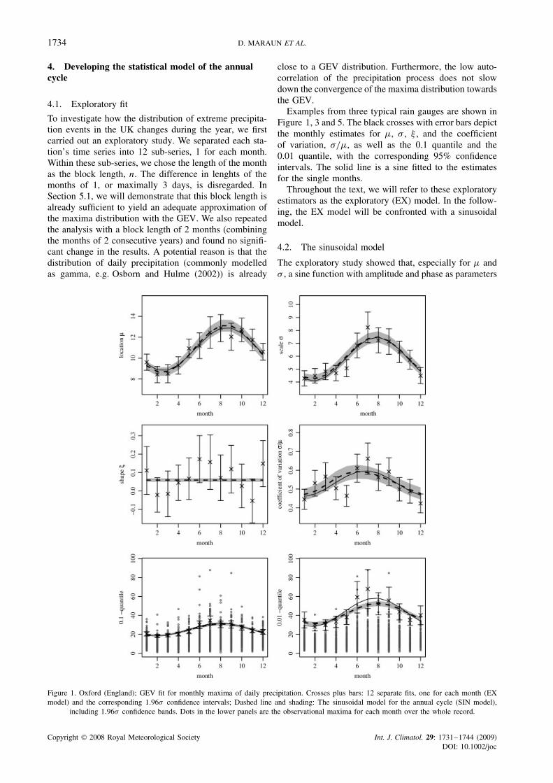
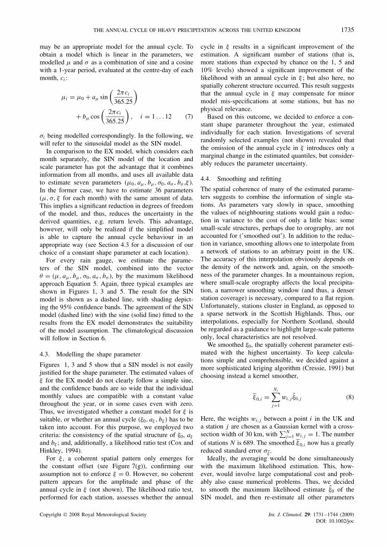
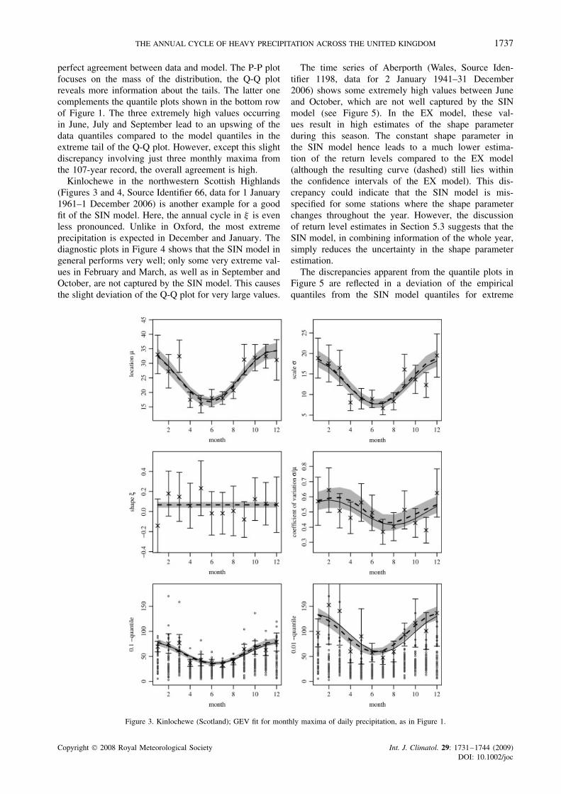
Examples from three typical rain gauges are shown inFigure 1, 3 and 5. The black crosses with error bars depictthe monthly estimates for µ, σ , ξ , and the coefficientof variation, σ/µ, as well as the 0.1 quantile and the0.01 quantile, with the corresponding 95% confidenceintervals. The solid line is a sine fitted to the estimatesfor the single months.

Throughout the text, we will refer to these exploratoryestimators as the exploratory (EX) model. In the follow-ing, the EX model will be confronted with a sinusoidalmodel.

4.2. The sinusoidal model

The exploratory study showed that, especially for µ andσ , a sine function with amplitude and phase as parameters

Figure 1. Oxford (England); GEV fit for monthly maxima of daily precipitation. Crosses plus bars: 12 separate fits, one for each month (EXmodel) and the corresponding 1.96σ confidence intervals; Dashed line and shading: The sinusoidal model for the annual cycle (SIN model),

including 1.96σ confidence bands. Dots in the lower panels are the observational maxima for each month over the whole record.



may be an appropriate model for the annual cycle. Toobtain a model which is linear in the parameters, wemodelled µ and σ as a combination of sine and a cosinewith a 1-year period, evaluated at the centre-day of eachmonth, ci :

µi = µ0 + aµ sin(

2πci

365.25

)

+ bµ cos(

2πci

365.25

), i = 1 . . . 12 (7)

σi being modelled correspondingly. In the following, wewill refer to the sinusoidal model as the SIN model.

In comparison to the EX model, which considers eachmonth separately, the SIN model of the location andscale parameter has got the advantage that it combinesinformation from all months, and uses all available datato estimate seven parameters (µ0, aµ, bµ, σ0, aσ , bσ ,ξ ).In the former case, we have to estimate 36 parameters(µ, σ, ξ for each month) with the same amount of data.This implies a significant reduction in degrees of freedomof the model, and thus, reduces the uncertainty in thederived quantities, e.g. return levels. This advantage,however, will only be realized if the simplified modelis able to capture the annual cycle behaviour in anappropriate way (see Section 4.3 for a discussion of ourchoice of a constant shape parameter at each location).

For every rain gauge, we estimate the parame-ters of the SIN model, combined into the vectorθ = (µ, aµ, bµ, σ0, aσ , bσ ), by the maximum likelihoodapproach Equation 5. Again, three typical examples areshown in Figures 1, 3 and 5. The result for the SINmodel is shown as a dashed line, with shading depict-ing the 95% confidence bands. The agreement of the SINmodel (dashed line) with the sine (solid line) fitted to theresults from the EX model demonstrates the suitabilityof the model assumption. The climatological discussionwill follow in Section 6.

4.3. Modelling the shape parameter

Figures 1, 3 and 5 show that a SIN model is not easilyjustified for the shape parameter. The estimated values ofξ for the EX model do not clearly follow a simple sine,and the confidence bands are so wide that the individualmonthly values are compatible with a constant valuethroughout the year, or in some cases even with zero.Thus, we investigated whether a constant model for ξ issuitable, or whether an annual cycle (ξ0, aξ , bξ ) has to betaken into account. For this purpose, we employed twocriteria: the consistency of the spatial structure of ξ0, aξ

and bξ ; and, additionally, a likelihood ratio test (Cox andHinkley, 1994).

For ξ , a coherent spatial pattern only emerges forthe constant offset (see Figure 7(g)), confirming ourassumption not to enforce ξ = 0. However, no coherentpattern appears for the amplitude and phase of theannual cycle in ξ (not shown). The likelihood ratio test,performed for each station, assesses whether the annual

cycle in ξ results in a significant improvement of theestimation. A significant number of stations (that is,more stations than expected by chance on the 1, 5 and10% levels) showed a significant improvement of thelikelihood with an annual cycle in ξ ; but also here, nospatially coherent structure occurred. This result suggeststhat the annual cycle in ξ may compensate for minormodel mis-specifications at some stations, but has nophysical relevance.

Based on this outcome, we decided to enforce a con-stant shape parameter throughout the year, estimatedindividually for each station. Investigations of severalrandomly selected examples (not shown) revealed thatthe omission of the annual cycle in ξ introduces only amarginal change in the estimated quantiles, but consider-ably reduces the parameter uncertainty.

4.4. Smoothing and refitting

The spatial coherence of many of the estimated parame-ters suggests to combine the information of single sta-tions. As parameters vary slowly in space, smoothingthe values of neighbouring stations would gain a reduc-tion in variance to the cost of only a little bias: somesmall-scale structures, perhaps due to orography, are notaccounted for (’smoothed out’). In addition to the reduc-tion in variance, smoothing allows one to interpolate froma network of stations to an arbitrary point in the UK.The accuracy of this interpolation obviously depends onthe density of the network and, again, on the smooth-ness of the parameter changes. In a mountainous region,where small-scale orography affects the local precipita-tion, a narrower smoothing window (and thus, a denserstation coverage) is necessary, compared to a flat region.Unfortunately, stations cluster in England, as opposed toa sparse network in the Scottish Highlands. Thus, ourinterpolations, especially for Northern Scotland, shouldbe regarded as a guidance to highlight large-scale patternsonly, local characteristics are not resolved.

We smoothed ξ0, the spatially coherent parameter esti-mated with the highest uncertainty. To keep calcula-tions simple and comprehensible, we decided against amore sophisticated kriging algorithm (Cressie, 1991) butchoosing instead a kernel smoother,

ξ 0,i =Ns∑

j=1

wi,j ξ0,j (8)

Here, the weights wi,j between a point i in the UK anda station j are chosen as a Gaussian kernel with a cross-section width of 30 km, with

∑Nj=1 wi,j = 1. The number

of stations N is 689. The smoothed ξ 0,i now has a greatlyreduced standard error σ

ξ.

Ideally, the averaging would be done simultaneouslywith the maximum likelihood estimation. This, how-ever, would involve large computational cost and prob-ably also cause numerical problems. Thus, we decidedto smooth the maximum likelihood estimate ξ0 of theSIN model, and then re-estimate all other parameters



with a fixed ξ0 = ξ 0 for every station (i.e. each station’smaximum likelihood estimate of ξ0 is replaced by thevalue from the smoothed field for that location). Thereduced parameter vector of this model is then θ−ξ0 =(µ0, aµ, bµ, σ0, aσ , bσ ), leading to a new maximum like-lihood estimate. A Monte Carlo study (not shown) indi-cated that the standard error of ξ , σ

ξ, was small enough

not to affect the (reduced) covariance matrix of the re-estimated parameters.

The increase in bias of these estimates compared tothe fit including a (variable) parameter ξ0 is low, but thevariance is considerably reduced. Smoothing the quiteaccurately estimated scale and location parameter wouldnot gain much reduction of variance; hence, we forbearfrom any further spatial smoothing.

5. Results

In the following, all results from the SIN model areobtained with a spatially smoothed and fixed value ofthe shape parameter ξ 0 (without an annual cycle), andre-estimated location and scale parameters, each with asinusoidal annual cycle.

5.1. Example stations

A typical example of an observation where daily precipi-tation extremes are well modelled by a sinusoidal annualcycle (i.e. where the SIN model fits well) is the recordfrom Oxford (Met Office Source Identifier 606). We useddata from 1 January 1900 to 31 December 2006. One canclearly see the strong annual cycle in the location andscale parameter µ and σ (upper row in Figure 1).

The suitability of the SIN model becomes evident fromthe good agreement between the results for the individualmonths (the EX model, crosses), and the dashed curvedepicting the SIN model. One also sees the reduction ofthe error bars by about 50%, when using the SIN modelinstead of the EX model. The middle row shows the fitof the shape parameter ξ and the coefficient of variationσ/µ. The shape parameter apparently exhibits a bi-annualcycle (crosses), but all values for the single months are

compatible with the constant value we included in theSIN model. In some studies, the coefficient of variationis modelled as a constant to further simplify the statisticalmodel. Our results indicate that here this assumption isnot justified: the annual cycle for µ and σ are slightly outof phase, which results in an asymmetric sine-like shapeof the coefficient of variation (though its amplitude isreduced relative to the annual cycle of µ and σ ).

The bottom row of Figure 1 shows the 0.1 and0.01 quantiles, that is, the magnitude exceeded with aprobability of 10 and 1% in a certain month, respectively.Good agreement between the EX and the SIN model isevident again. However, for the 0.01 quantile, a deviationbecomes apparent: for the EX model, some extremelyhigh values in June, July and September lead to highestimates of the shape parameter for these months, andthus, also to high quantiles (crosses). In the SIN model,the time-independent shape parameter ξ is estimated fromvalues of the whole year. In this representation, therecord maximum precipitation values in June, July andSeptember are seen as quite improbable ’outliers’; hencethe estimates of the corresponding quantiles in the SINmodel are considerably lower (dashed line) than thosefrom the EX model. Nevertheless, in both models thehighest extreme precipitation events for Oxford are to beexpected in August.

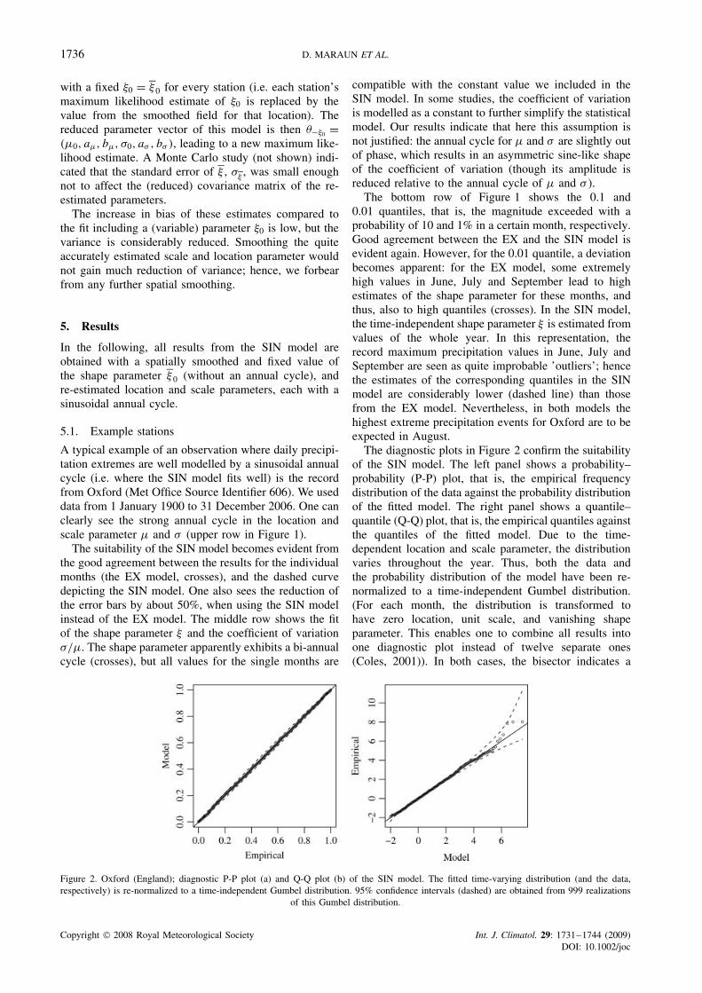
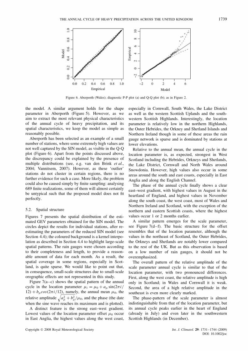
The diagnostic plots in Figure 2 confirm the suitabilityof the SIN model. The left panel shows a probability–probability (P-P) plot, that is, the empirical frequencydistribution of the data against the probability distributionof the fitted model. The right panel shows a quantile–quantile (Q-Q) plot, that is, the empirical quantiles againstthe quantiles of the fitted model. Due to the time-dependent location and scale parameter, the distributionvaries throughout the year. Thus, both the data andthe probability distribution of the model have been re-normalized to a time-independent Gumbel distribution.(For each month, the distribution is transformed tohave zero location, unit scale, and vanishing shapeparameter. This enables one to combine all results intoone diagnostic plot instead of twelve separate ones(Coles, 2001)). In both cases, the bisector indicates a

Figure 2. Oxford (England); diagnostic P-P plot (a) and Q-Q plot (b) of the SIN model. The fitted time-varying distribution (and the data,respectively) is re-normalized to a time-independent Gumbel distribution. 95% confidence intervals (dashed) are obtained from 999 realizations

of this Gumbel distribution.



perfect agreement between data and model. The P-P plotfocuses on the mass of the distribution, the Q-Q plotreveals more information about the tails. The latter onecomplements the quantile plots shown in the bottom rowof Figure 1. The three extremely high values occurringin June, July and September lead to an upswing of thedata quantiles compared to the model quantiles in theextreme tail of the Q-Q plot. However, except this slightdiscrepancy involving just three monthly maxima fromthe 107-year record, the overall agreement is high.

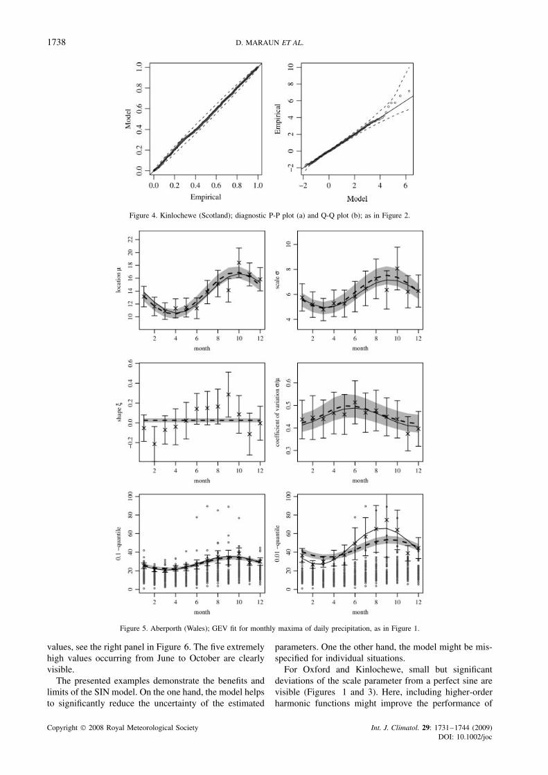
Kinlochewe in the northwestern Scottish Highlands(Figures 3 and 4, Source Identifier 66, data for 1 January1961–1 December 2006) is another example for a goodfit of the SIN model. Here, the annual cycle in ξ is evenless pronounced. Unlike in Oxford, the most extremeprecipitation is expected in December and January. Thediagnostic plots in Figure 4 shows that the SIN model ingeneral performs very well; only some very extreme val-ues in February and March, as well as in September andOctober, are not captured by the SIN model. This causesthe slight deviation of the Q-Q plot for very large values.

The time series of Aberporth (Wales, Source Iden-tifier 1198, data for 2 January 1941–31 December2006) shows some extremely high values between Juneand October, which are not well captured by the SINmodel (see Figure 5). In the EX model, these val-ues result in high estimates of the shape parameterduring this season. The constant shape parameter inthe SIN model hence leads to a much lower estima-tion of the return levels compared to the EX model(although the resulting curve (dashed) still lies withinthe confidence intervals of the EX model). This dis-crepancy could indicate that the SIN model is mis-specified for some stations where the shape parameterchanges throughout the year. However, the discussionof return level estimates in Section 5.3 suggests that theSIN model, in combining information of the whole year,simply reduces the uncertainty in the shape parameterestimation.

The discrepancies apparent from the quantile plots inFigure 5 are reflected in a deviation of the empiricalquantiles from the SIN model quantiles for extreme

Figure 3. Kinlochewe (Scotland); GEV fit for monthly maxima of daily precipitation, as in Figure 1.



Figure 4. Kinlochewe (Scotland); diagnostic P-P plot (a) and Q-Q plot (b); as in Figure 2.

Figure 5. Aberporth (Wales); GEV fit for monthly maxima of daily precipitation, as in Figure 1.

values, see the right panel in Figure 6. The five extremelyhigh values occurring from June to October are clearlyvisible.

The presented examples demonstrate the benefits andlimits of the SIN model. On the one hand, the model helpsto significantly reduce the uncertainty of the estimated

parameters. One the other hand, the model might be mis-specified for individual situations.

For Oxford and Kinlochewe, small but significantdeviations of the scale parameter from a perfect sine arevisible (Figures 1 and 3). Here, including higher-orderharmonic functions might improve the performance of



Figure 6. Aberporth (Wales); diagnostic P-P plot (a) and Q-Q plot (b); as in Figure 2.

the model. A similar argument holds for the shapeparameter in Aberporth (Figure 5). However, as weaim to extract the most relevant physical characteristicsof the annual cycle of heavy precipitation, and itsspatial characteristics, we keep the model as simple asreasonably possible.

Aberporth has been selected as an example of a smallnumber of stations, where some extremely high values arenot well captured by the SIN model, as visible in the Q-Qplot (Figure 6). Apart from the points discussed above,the discrepancy could be explained by the presence ofmultiple distributions (see, e.g. van den Brink et al.,2004; Vannitsem, 2007). However, as these ‘outlier’stations do not cluster in certain regions, there is nofurther evidence for such a case. More likely, the problemcould also be caused simply by finite sampling: analysing689 finite realizations, some of them will almost certainlybe untypical such that the proposed model does not fitperfectly.

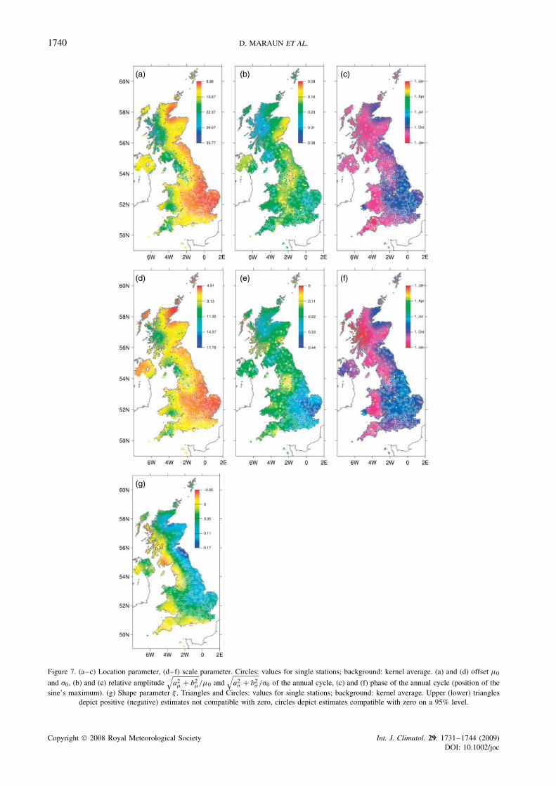
5.2. Spatial structure

Figures 7 presents the spatial distribution of the esti-mated GEV parameters obtained for the SIN model. Thecircles depict the results for individual stations, after re-estimating the parameters of the reduced SIN model (seeSection 4.4); the coloured background is a kernel interpo-lation as described in Section 4.4 to highlight large-scalespatial patterns. The rain gauges were chosen accordingto their completeness and length, to provide a reason-able amount of data for each month. As a result, thespatial coverage in some regions, especially in Scot-land, is quite sparse. We would like to point out that,in consequence, small-scale structures due to small-scaleorographic effects are not represented in this study.

Figure 7(a–c) shows the spatial pattern of the annualcycle in the location parameter µi = µ0 + aµ sin(2πi/

12) + bµcos(2πi/12), namely, the annual mean µ0, the

relative amplitude√

a2µ + b2

µ/µ0, and the phase (the datewhen the sine wave reaches its maximum and is plotted).

A distinct feature is the strong east–west gradient.Lowest values of the location parameter offset µ0 occurin East Anglia, the highest values along the west coast,

especially in Cornwall, South Wales, the Lake Districtas well as the western Scottish Uplands and the south-western Scottish Highlands. Interestingly, the locationparameter is relatively low in the northern Highlands,the Outer Hebrides, the Orkney and Shetland Islands andNorthern Ireland though in some of these areas the raingauge network is sparse and is dominated by stations atlower elevations.

Relative to the annual mean, the annual cycle in thelocation parameter is, as expected, strongest in WestScotland including the Hebrides, Orkneys and Shetlands,the Lake District, Cornwall and North Wales aroundSnowdonia. However, high values also occur in someareas around the south and east coasts, especially in EastAnglia and along the English Channel.

The phase of the annual cycle finally shows a cleareast–west gradient, with highest values in August in theheartland of England, and highest values in Novemberalong the south coast, the west coast, most of Wales andNorthern Ireland and Scotland, with the exception of thenorthern and eastern Scottish coasts, where the highestvalues occur 1 or 2 months earlier.

A similar pattern emerges for the scale parameter,see Figure 7(d–f). The basic structure for the offsetresembles that of the location parameter, although thevalues in the northeast of Scotland, the Outer Hebrides,the Orkneys and Shetlands are notably lower comparedto the rest of the UK. But as this observation is basedon a low number of rain gauges, it should not beoveremphasized.

The overall pattern of the relative amplitude of thescale parameter annual cycle is similar to that of thelocation parameter, with two pronounced differences.First, along the west coast, the relative amplitude is highonly in Scotland; in Wales and Cornwall it is weak.Second, the area of a high relative amplitude in thesoutheast is even more clearly marked.

The phase-pattern of the scale parameter is almostindistinguishable from that of the location parameter, butits annual cycle peaks earlier in the heart of England(already in July) and even later in the southwesternScottish Highlands (in December).



(a) (b) (c)

(d) (e) (f)

(g)

Figure 7. (a–c) Location parameter, (d–f) scale parameter. Circles: values for single stations; background: kernel average. (a) and (d) offset µ0

and σ0, (b) and (e) relative amplitude√

a2µ + b2

µ/µ0 and√

a2σ + b2

σ /σ0 of the annual cycle, (c) and (f) phase of the annual cycle (position of thesine’s maximum). (g) Shape parameter ξ . Triangles and Circles: values for single stations; background: kernel average. Upper (lower) triangles

depict positive (negative) estimates not compatible with zero, circles depict estimates compatible with zero on a 95% level.



(a) (b) (c)

(d) (e) (f)

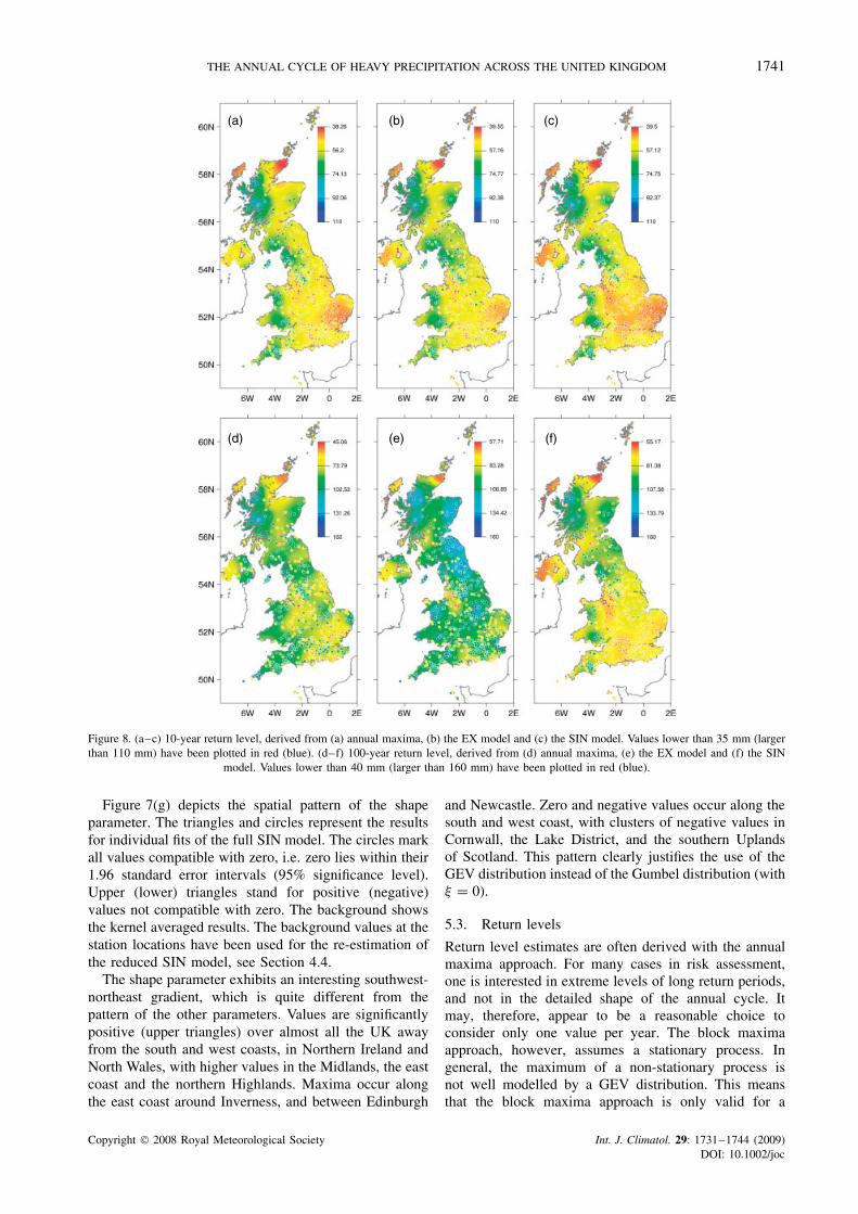
Figure 8. (a–c) 10-year return level, derived from (a) annual maxima, (b) the EX model and (c) the SIN model. Values lower than 35 mm (largerthan 110 mm) have been plotted in red (blue). (d–f) 100-year return level, derived from (d) annual maxima, (e) the EX model and (f) the SIN

model. Values lower than 40 mm (larger than 160 mm) have been plotted in red (blue).

Figure 7(g) depicts the spatial pattern of the shapeparameter. The triangles and circles represent the resultsfor individual fits of the full SIN model. The circles markall values compatible with zero, i.e. zero lies within their1.96 standard error intervals (95% significance level).Upper (lower) triangles stand for positive (negative)values not compatible with zero. The background showsthe kernel averaged results. The background values at thestation locations have been used for the re-estimation ofthe reduced SIN model, see Section 4.4.

The shape parameter exhibits an interesting southwest-northeast gradient, which is quite different from thepattern of the other parameters. Values are significantlypositive (upper triangles) over almost all the UK awayfrom the south and west coasts, in Northern Ireland andNorth Wales, with higher values in the Midlands, the eastcoast and the northern Highlands. Maxima occur alongthe east coast around Inverness, and between Edinburgh

and Newcastle. Zero and negative values occur along thesouth and west coast, with clusters of negative values inCornwall, the Lake District, and the southern Uplandsof Scotland. This pattern clearly justifies the use of theGEV distribution instead of the Gumbel distribution (withξ = 0).

5.3. Return levels

Return level estimates are often derived with the annualmaxima approach. For many cases in risk assessment,one is interested in extreme levels of long return periods,and not in the detailed shape of the annual cycle. Itmay, therefore, appear to be a reasonable choice toconsider only one value per year. The block maximaapproach, however, assumes a stationary process. Ingeneral, the maximum of a non-stationary process isnot well modelled by a GEV distribution. This meansthat the block maxima approach is only valid for a



process without, for instance, an annual cycle. A casewhere the GEV might be a reasonable approximation isa situation, where the extreme precipitation occurs onlyin a particular pronounced season. As demonstrated inthe previous sections, UK precipitation extremes showa distinct, though spatially varying, annual cycle and, apriori, it is not clear whether the annual maxima approachprovides reasonable results.

In the following, we compare return levels derivedfrom the annual maxima approach with those from the EXmodel and the SIN model. The estimation of return levelsfrom annual maxima is straightforward according toEquation 3. Return levels from the EX model and the SINmodel have to be calculated numerically. When Gi(z)

(i = 1, . . . , 12) denotes the probability of the occurrenceof a value smaller than z in the month i, then the T -yearreturn level rT can be calculated by solving the equation

12∏i=1

Gi(rT ) = 1 − 1

T(9)

Corresponding confidence intervals for the SIN and theEX model can be derived by propagating the parameteruncertainties through Equation 9. These intervals willdepend on the actual length of the observation and thedesired return level. For a guideline of the expected range,we refer the reader to the 0.9 and 0.99 quantile plots forOxford and Kinlochewe (Figures 1 and 3), representingthe monthly 10-year and 100-year return levels for a longand a rather short observation, respectively.

We estimate return levels for all stations. By spatialinterpolation, we highlight large-scale structures of returnlevels, disregarding small-scale orographic effects.

The return levels derived from annual maxima shouldsuffer from the non-stationarity given by the annual cycle.The EX model explicitly, and without any constraints,models the annual cycle based on monthly maxima.It relies on the suitability of approximating monthlymaxima with the GEV, and on the stationarity assumptionwithin every month. As this model has the most degreesof freedom, it is afflicted with the widest confidenceintervals. The shape parameter, estimated for every monthseparately, might be particularly sensitive to extreme’outliers’. The SIN model provides return level estimateswith considerably narrower error intervals, yet it relies onthe suitability of the sine shape to model the annual cycleof the location and scale parameters, and the assumptionthat the shape parameter is invariant during the year.Figure 8(a–c) shows the 10-year return levels estimatedfrom (a) annual maxima, (b) the EX model and (c) theSIN model. At first glance, the three panels are virtuallyindistinguishable.

The most notable exceptions are that estimates fromthe EX model are higher than those from the otherapproaches in two regions: southern East Anglia andsoutheast Scotland/northeast England. One can see theexpected east–west gradient, with higher return levelsalong the west coast and lower values especially in the

southeast. Particularly high return levels prevail in thewestern Highlands and the Lake District.

Figure 8(d–f) shows the 100-year return levels esti-mated from (d) annual maxima, (e) the EX model and(f) the SIN model. A marked discrepancy stands out:values estimated from the EX model are larger thanthose derived from the SIN model or the annual max-ima approach in most parts of the UK. This discrepancyis especially strong in the coastal stretch from Edinburghto Newcastle where the shape parameter is positive andrelatively large; a rather small discrepancy is found inthe Lake District and the western Highlands where theshape parameter is compatible with zero or even negative(Figure 7(g)). Large positive shape parameter estimatescan be a consequence of a few extremely high rainfallevents. In the EX model, shape parameters are estimatedseparately for every month of the year which results inlarge positive shape parameter estimates for months witha few large events (see Figure 5). These months con-tribute strongly to the calculation of extreme return levels,while months with small shape parameters do not. Thisflexibility in the shape parameter to vary during the yearis neither present in the SIN model nor in the annualmaxima approach; shape parameter estimates are con-fined to a smaller value, closer to an annual average thanto the extreme estimates in the EX model. As a conse-quence, the SIN model and the annual maxima approachyield smaller 100-year return levels. Without any fur-ther a priori knowledge about the model structure (e.g.physical reasons for a time-constant shape parameter), it

is not clear which of the return level estimates are morerealistic.

The differences between the 100-year return levelestimates from the SIN model and the annual maximaapproach are less pronounced. In general, the latterresults show a higher spatial variability, a fact notsurprising, since the former approach combines theshape parameters of neighbouring rain gauges. Therelatively good agreement between the two approachessuggests that annual maxima mostly provide reasonablereturn level estimates, despite the previously discussedtheoretical limitations. Equally, the agreement supportsthe specification of our SIN model.

The overall spatial pattern of the 100-year return levelresembles that of the 10-year return levels: highest valuesare observed in the western Highlands and the LakeDistrict, lowest values in the southeast.

6. Discussion and conclusions

We studied the annual cycle of heavy daily precipitationacross the UK by means of EVS, and approximated thedistribution of monthly maxima by the GEV distribution.To combine the information from individual months, wedeveloped a parametric model which described the annualvariations in the location and scale parameter of the GEVdistribution as a phase-shifted sine function, and assumeda time-independent shape parameter.



This model proved to be suitable: the approximationof the monthly maxima distribution by the GEV andthe annual cycle by a sine wave both appeared to bereasonable. The parametrization in form of a sine wavehelped to considerably reduce the parameter uncertaintiescompared with a model that was fit to each monthindependently. The combination of the estimated shapeparameter values from neighbouring rain gauges furtherreduced parameter uncertainties.

Our statistical results demonstrate that the scaleparameter, in general, is not in phase with the loca-tion parameter (Figures 7(c) and 7(f)), although the spa-tial patterns of their annual means are highly corre-lated (Figures 7(a) and 7(d)). Thus, modelling the shapeparameter as a constant multiple of the location param-eter is not valid when looking at the seasonal variationsof extreme precipitation. For a study of annual maxima,the phase shift is irrelevant and a combination of locationand scale parameter might be useful, although their ratiomight be spatially varying.

We compared return levels derived from annual max-ima, an exploratory model of separately consideredmonthly maxima and the parametric sinusoidal model(see Figure 8). We found that, although the annual max-ima approach relies on a stationarity assumption of dailyprecipitation, it provides, in general, reasonable results.The exploratory model is afflicted with the highest param-eter uncertainties and, perhaps, systematically overesti-mates the shape parameter, and hence, the return levels ofrare events (e.g. 100-year events). The sinusoidal modelproved to be a good compromise between a bias due to astationarity assumption and the uncertainty owing to toomany parameters.

Our study provides detailed insight into the seasonalvariations of extreme precipitation in the UK. Alongthe middle north-south axis, the amplitude of the annualcycle in the location parameter is less than 15% of thecorresponding annual mean (Figure 7 (b)), in the scaleparameter even just around 10% (Figure 7(e)). However,along the west coast and in the southeast, seasonal varia-tions are strong, with up to 30% in the location parameterand 40% in the scale parameter.

The season when precipitation extremes are most likelyto occur depends strongly on the region as well: along thewest coast, the heaviest precipitation is expected duringlate autumn and winter, whereas along the east coast andthe Midlands, the maximum location and scale parame-ters occur during late summer (Figures 7 (c) and (f)).

The estimated return levels agree well with the resultspublished in the Flood Estimation Handbook (Faulkner,1999). Those results additionally account for small-scalevariations by additional empirical knowledge. In thatstudy, however, the accuracy of very high return levelsmight be limited because of the restriction to a Gumbeldistribution, that is, a vanishing shape parameter. In ouranalysis, a coherent spatial pattern of the shape parameteremerged, indicating that different geographical situationsmight influence the shape parameter (see Figure 7(g)).

Our results are related to different processes of precipi-tation and driving mechanisms. The offset of the locationparameter is correlated (Pearson) at 0.65 with the max-imum elevation in the 10-km vicinity of a rain gauge(topography data from the USGS ETOPO30 dataset),clearly showing the effect of mountain ranges on oro-graphic precipitation.

Regions of predominantly convective rainfall extremescan be identified by extremes occurring in summer.In the UK, these are, especially, the Midlands andthe east of England. Here the location parameter islow without a strong annual cycle. The scale param-eter in this region also has a low offset, but showsa pronounced annual cycle. In other words: in Cen-tral and East England, precipitation is generally low,but from time to time very heavy summer thunder-storms occur. These findings agree notably well withthe thunderstorm climatology for the UK, developed byPerry and Hollis (2005, thunderstorm climatology, avail-able at http://www.metoffice.gov.uk/climate/uk/averages/19712000/mapped.html). Convective precipitation andthunderstorms also accompany frontal precipitation dur-ing winter, especially along the remotest parts of theBritish west coast. These areas, dominated by frontal pre-cipitation, are characterized by low values of the shapeparameter, and high values of the location and scaleparameter, peaking in winter.

Between the frontal dominated climate along the westcoast with extremes occurring during winter, and thesomewhat more continental climate with extremes arisingpredominantly from summer convection, a transition zoneexists. Here, the overall annual cycle is weak, withconvective rain contributing during summer, and frontalprecipitation contributing during winter.

Our results help to assess the future impact of climatechange. Climate models predict an increase in UKheavy precipitation throughout the year, though moreconsistently during winter than summer (Christensen etal., 2007). On the one hand, our study identifies regionsand seasons, where extremes are already strong and mightget even stronger (e.g. early winter in western UK).On the other hand, we showed regions and seasons,where extreme precipitation is weaker at present butmight become significant in the future (e.g. winter inEast Anglia). These results might prove important foragriculture and hydro engineering.

Future work could further investigate the different pre-cipitation processes discussed above and try to incor-porate, for instance, the elevation into the statisticalmodel. Furthermore, it could be interesting to add ahigher harmonic to the model to decrease possible mis-specifications, and to study whether the shape of theannual cycle might be region dependent. A recentlydeveloped approach by Heffernan and Tawn (2004) canbe used to assess the interdependencies between precip-itation events at different stations, and provide estimatesfor the total volume of rainfall in a single event. Finally,our results might be used to evaluate the performance of



regional climate models at simulating the annual cycle ofextreme precipitation.

Acknowledgements

This study was supported by the NERC Flood Risk fromExtreme Events programme (NE/E002412/1), the Collab-orative Research Centre SFB 555 by the DFG, and theEC Project ’Extreme Events: Causes and Consequences(E2-C2)’, Contract No. 12975 (NEST). We thank theBritish Council (ARC 1291) and the German AcademicExchange Service (DAAD, D/07/09988) for providingtravel grants within the ARC program, and our colleaguesat the BADC and the Met Office for assistance withobtaining data. Special thanks go to Dr Jonathan Tawnfor valuable discussions on EVS. The analysis was car-ried out with software written in R (R Development CoreTeam, 2007), based on the ISMEV package (Coles andStephenson, 2006).

References

Brown BG, Katz RW. 1995. Regional analysis of temperatureextremes: spatial analog for climate change? Journal of Climate 8(1):108–119.

Christensen JH, Hewitson B, Busuioc A, Chen A, Gao X, Held I,Jones R, Kolli RK, Kwon WT, Laprise R, Rueda VM, Mearns L,Menendez CG, Raisanen J, Rinke A, Sarr A, Whetton P. 2007.Climate change 2007: the physical science basis. Contributionof Working Group I to the Fourth Assessment Report of theIntergovernmental Panel on Climate Change, Chapter RegionalClimate Projections. Cambridge University Press: Cambridge.

Coles S. 2001. An Introduction to Statistical Modeling of ExtremeValues, Springer Series in Statistics . Springer: London.

Coles S, Casson E. 1998. Extreme value modelling of hurricane windspeeds. Structural Safety 20(3): 283–296.

Coles S, Stephenson A. 2006. Ismev: An Introduction to StatisticalModeling of Extreme Values, R package version 1. 2.

Coles SG, Tawn JA. 1996. A bayesian analysis of extreme rainfall data.Journal of the Royal Statistical Society. Series C, (Applied Statistics)45(4): 463–478.

Cox DR, Hinkley DV. 1994. Theoretical Statistics. Chapman & Hall:London.

Cressie NAC. 1991. Statistics for spatial data. Wiley Series inProbability and Mathematical Statistics. Wiley: London.

Edwards AWF. 1992. Likelihood. Johns Hopkins University Press:Baltimore.

Ekstrom M, Fowler HJ, Kilsby CG, Jones PD. 2005. New estimatesof future changes in extreme rainfall across the UK using regionalclimate model integrations. 2. Future estimates and use in impactstudies. Journal of Hydrology 300: 234–251.

Embrechts P, Kluppelberg C, Mikosch T. 1997. Modelling extremalevents for insurance and finance. Applications in Mathematics.Springer: Berlin.

Faulkner D. 1999. Flood estimation handbook. Rainfall FrequencyEstimation, Vol. 2. Institute of Hydrology: Wallingford.

Favis-Mortlock D. 2006. Encyclopedia of Soil Science, chapter Erosionby Water. CRC Press: Boca Raton; 568–573.

Fowler HJ, Kilsby CG. 2003. A regional frequency analysis of UnitedKingdom extreme rainfall from 1961–2000. International Journalof Climatology 23: 1313–1334.

Heffernan JE, Tawn JA. 2004. A conditional approach for multivariateextreme values. Journal of the Royal Statistical Society, Series B66(3): 497–530.

Hosking JRM, Wallis JR, Wood EF. 1985. Estimation of thegeneralized extreme-value distribution by the method of probability-weighted moments. Technometrics 27(3): 251–261.

Jones PD, Reid PA. 2001. Assessing future changes in extremeprecipitation over Britain using regional climate model integrations.International Journal of Climatology 21: 1337–1356.

Katz RW. 1999. Extreme value theory for precipitation: Sensitivityanalysis for climate change. Advances in Water Resources 23(2):133–139.

Katz RW, Parlange MB, Naveau P. 2002. Statistics of extremes inhydrology. Advances in Water Resources 25(8–12): 1287–1304.

Katz RW, Parlange MB, Tebaldi C. 2003. Stochastic modeling of theeffects of large-scale circulation on daily weather in the southeasternu. s. Climatic Change 60(1–2): 189–216.

Leadbetter MR, Lindgren G, Rootzen H. 1983. Extremes and RelatedProperties of Random Sequences and Processes, Springer Series inStatistics . Springer: New York.

Maraun D, Osborn TJ, Gillett NP. 2008. United Kingdom dailyprecipitation intensity: Improved early data, error estimates and anupdate from 2000 to 2006. International Journal of Climatology28(6): 833–842, DOI 10. 1002/joc. 1672.

Meehl GA, Stocker TF, Collins WD, Friedlingstein P, Gaye AT,Gregory JM, Kitoh A, Knutti R, Murphy JM, Noda A, Raper SCB,Watterson IG, Weaver AJ, Zhao ZC. 2007. Climate change 2007:The physical science basis. Contribution of Working Group I to theFourth Assessment Report of the Intergovernmental Panel on ClimateChange, Chapter Global Climate Projections. Cambridge UniversityPress: Cambridge, New York.

Naveau P, Nogaj M, Ammann C, Yiou P, Cooley D, Jomelli V. 2005.Statistical methods for the analysis of climate extremes. ComptesRendus Geoscience 337(10–11): 1013–1022.

Nearinga MA, Jettenb V, Baffautc C, Cerdand O, Couturierd A, Her-nandeza M, Bissonnaise YL, Nicholsa MH, Nunesf JP, Rensch-lerg CS, Souchereh V, van Oos K. 2005. Modeling response of soilerosion and runoff to changes in precipitation and cover. Catena61(2–3): 131–154.

Osborn TJ, Hulme M. 2002. Evidence for trends in heavy rainfallevents over the UK. Philosophical Transactions of the Royal Societyof London Series A-Mathematical Physical and Engineering Sciences360: 1313–1325.

Osborn TJ, Hulme M, Jones PD, Basnett TA. 2000. Observed trendsin the daily intensity of United Kingdom precipitation. InternationalJournal of Climatology 20: 347–364.

Perry M, Hollis D. 2005. The development of a new set of long termclimate averages for the UK. International Journal of Climatology25(8): 1023–1039.

R Development Core Team. 2007. R: A Language and Environmentfor Statistical Computing. R Foundation for Statistical Computing:Vienna, ISBN 3-900051-07-0.

Rosenzweig C, Iglesias A, Yang XB, Epstein PR, Chivian E. 2001.Climate change and extreme weather events: Implications for foodproduction, plant diseases, and pests. Global Change and HumanHealth 2(2): 90–104.

Trenberth KE, Jones PD, Ambenje P, Bojariu R, Easterling D,Tank AK, Parker D, Rahimzadeh F, Renwick JA, Rusticucci M,Soden B, Zhai P. 2007. Climate change 2007: the physical sciencebasis. Contribution of Working Group I to the Fourth AssessmentReport of the Intergovernmental Panel on Climate Change, ChapterObservations: Surface and Atmospheric Climate Change. CambridgeUniversity Press: Cambridge, New York.

van den Brink HW, Konnen GP, Opsteegh JD. 2004. Statistics ofextreme synoptic-scale wind speeds in ensemble simulations ofcurrent and future climate. Journal of Climate 17(23): 4564–4574.

Vannitsem S. 2007. Statistical properties of the temperature maximain an intermediate order quasi-geostrophic model. Tellus A 59(1):80–95.

Yu J, Shainberg I, Mamedov AI, Levy GJ. 2006. Effects of wettingby spray on concentrated flow erosion and intake rate. Soil Science171(12): 929–936.
