Download - Subsurface Stratification and Aquifer Characterization of Federal College of Education (Technical), Gusauusing Geoelectric Method

IOSR Journal of Applied Geology and Geophysics (IOSR-JAGG)

e-ISSN: 2321–0990, p-ISSN: 2321–0982.Volume 2, Issue 6 Ver. II (Nov-Dec. 2014), PP 11-23 www.iosrjournals.org

www.iosrjournals.org 11 | Page

Subsurface Stratification and Aquifer Characterization of

Federal College of Education (Technical), Gusauusing Geoelectric

Method

1Murana, K.A.,

2Sule, P.,

2Ahmed, A.L,

3Girigisu, S And

4Abraham, E. M

1SLT Department, Abdu Gusau Polytechnic, TalataMafara. ZamfaraState. 2Department of Physics,AhmaduBello University, Zaria.

3 Department of Physics, Federal College of Education(Technical), Gusau. 4 Department of Geophysics, Federal UniversityNdufu Alike, Ikwo. Abakaliki.

Abstract: The determination of subsurface stratification and aquifer characterization were carried out at

Federal College of Education (Technical), Gusau using the Schlumberger electrical resistivity array with

maximum current electrode separation of 200m. Twenty four Vertical electrical soundings (VES) were

conducted along six profiles.WinGlink software has been used in interpreting the results. Two and three

subsurface layers exist in the study area. The topmost geoelectric layer has resistivity mostly within the range of

1-522 .The lithology of the topsoil is mainly clay to sandy clay. The topsoil thickness ranges from 0.40 to

4.0 m while the overburden thickness of the surveyed area ranges from 0.40 to 18.0 m. The aquifer thickness of

the study area ranges from 1.00 to 19.32m. The interpreted results suggest that the main aquifer in the area

appears to be the weathered and fractured basements. Productive boreholes can be located around VES 3, 10,

16 and 17. The stratification of the survey revealed mainly clay, sandy clay, weathered and fractured sand

which show the formation characterization obtained through interpretation of VES curves and this corroborate with the borehole log of the area.

Keywords: Vertical electrical sounding, Stratification, Aquifers, Overburden, geoelectric section and geologic

section.

I. Introduction

This paper describes geoelectric investigations undertaken at Federal College of

Education(Technical),Gusau to investigate: the basement structure, geologic characteristics of the overburden of

the area and groundwater potential of the area. On the basis of increasing economic activities and booming

construction works coupled with the incidence of collapsed building and structures in the country, this investigation is expected to provide detailed information on the characteristic of the subsurface and ground

condition prior to the commencement of the construction work. Since every civil engineering structure, bridge,

tunnel, tower and dam must be founded on the surface of the earth,it is appropriate to provide detailed

information on the strength and fitness of the host earth materialsthrough investigation of the subsurface at the

proposed site (Muranaet al., 2011).

Generally, numbers of geophysical techniques are available which enable an insight to obtain the

nature of water bearing layers. These include geoelectric, electromagnetic, seismic and geophysical borehole

logging. The choice of a particular method is governed by the nature of the area and cost consideration.

The success of any geophysical technique in groundwater exploration depends largely on the

relationship between the physical parameters such as conductivity/resistivity, magnetic permeability and

density, and the properties of the geologic formations such as porosity.

Geoelectric methods are based upon the correlation of subsurface electrical properties with the occurrence of geophysical targets such as groundwater (quality) zone, fracture (discontinuity) zone, and

mineralized zone e.t.c. (Telfordet al., 1976, Dobrin, 1976,Mussett and Khan, 2000, andSharma 2002). In

locating suitable electrical conditions, this method makes use of resistivity contrast, which exists between fresh

unproductive rock and saturated zones.Groundwater is water located beneath the ground surface in the soil pore

spaces and in the fractures of lithologic formations. Groundwater is of major importance to civilization because

it is the largest reserve of drinkable water in the regions where humans live.

Although, water from seas and oceans: the surface bodies of virtually inexhaustible water sources are

available for exploitation. None of these surface sources can be as naturally suitable and economically

exploitable as groundwater (Garg, 2003 and Singh, 2004). Groundwater is relatively safe from hazards of

chemical, radiogenic and biological pollution for which surface water bodies are badly exposed. Groundwater is

also free from turbidity, objectionable colours and pathogenic organisms and hence requiring not much treatment.

m

Subsurface Stratification and Aquifer Characterization of Federal College of Education …..


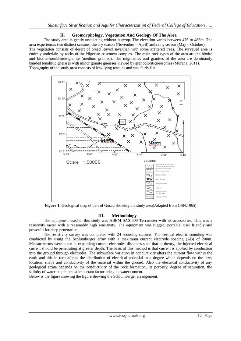
II. Geomorphology, Vegetation And Geology Of The Area The study area is gently undulating without outcrop. The elevation varies between 476 to 486m. The

area experiences two distinct seasons: the dry season (November – April) and rainy season (May – October).

The vegetation consists of desert of bread leaved savannah with some scattered trees. The surveyed area is

entirely underlain by rocks of the Nigerian-basement complex. The main rock types of the area are the biotite

and biotite-hornblende-granite (medium grained). The migmatites and granites of the area are dominantly

banded tonallitic gneisses with minor granite gneisses viewed by granodioriticneosomes (Murana, 2011).

Topography of the study area consists of low-lying terrains and was fairly flat.

Figure 1. Geological map of part of Gusau showing the study area(Adapted from GSN,1965)

III. Methodology

The equipment used in this study was ABEM SAS 300 Terrameter with its accessories. This was a

resistivity meter with a reasonably high sensitivity. The equipment was rugged, portable, user friendly and

powerful for deep penetration.

The resistivity survey was completed with 24 sounding stations. The vertical electric sounding was conducted by using the Schlumberger array with a maximum current electrode spacing (AB) of 200m.

Measurements were taken at expanding current electrodes distances such that in theory, the injected electrical

current should be penetrating at greater depth. The basis of this method is that current is applied by conduction

into the ground through electrodes. The subsurface variation in conductivity alters the current flow within the

earth and this in turn affects the distribution of electrical potential to a degree which depends on the size,

location, shape and conductivity of the material within the ground. Also the electrical conductivity of any

geological strata depends on the conductivity of the rock formation, its porosity, degree of saturation, the

salinity of water etc; the most important factor being its water content.

Below is the figure showing the figure showing the Schlumberger arrangement.

Mareri Damba



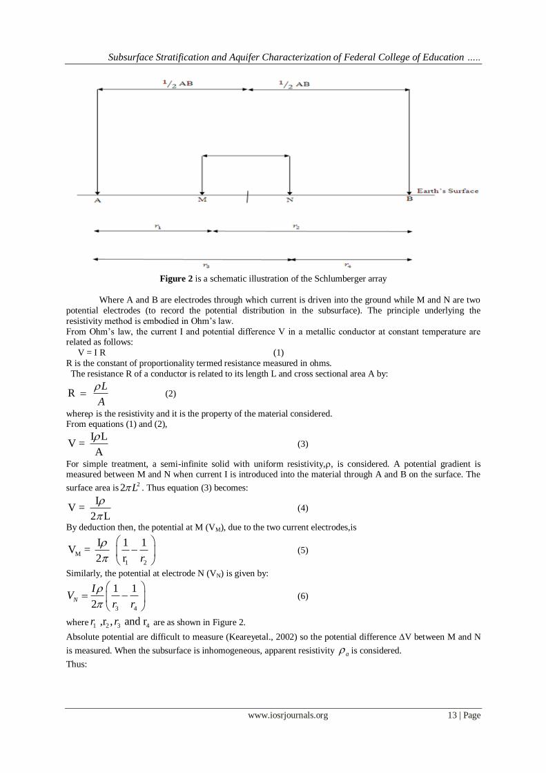
Figure 2 is a schematic illustration of the Schlumberger array

Where A and B are electrodes through which current is driven into the ground while M and N are two

potential electrodes (to record the potential distribution in the subsurface). The principle underlying the

resistivity method is embodied in Ohm’s law.

From Ohm’s law, the current I and potential difference V in a metallic conductor at constant temperature are related as follows:

V = I R (1)

R is the constant of proportionality termed resistance measured in ohms.

The resistance R of a conductor is related to its length L and cross sectional area A by:

R L

A

(2)

where is the resistivity and it is the property of the material considered. From equations (1) and (2),

I LV =

A

(3)

For simple treatment, a semi-infinite solid with uniform resistivity,, is considered. A potential gradient is measured between M and N when current I is introduced into the material through A and B on the surface. The

surface area is22 L . Thus equation (3) becomes:

IV =

2 L

(4)

By deduction then, the potential at M (VM), due to the two current electrodes,is

M

1 2

I 1 1V =

2 r r

(5)

Similarly, the potential at electrode N (VN) is given by:

3 4

1 1

2N

IV

r r

(6)

where 1 2 3 4 ,r , and rr r are as shown in Figure 2.

Absolute potential are difficult to measure (Keareyetal., 2002) so the potential difference V between M and N

is measured. When the subsurface is inhomogeneous, apparent resistivity a is considered.

Thus:



1 2 3 4

1 1 1 1

2

aM N

IV V V

r r r r

(7)

Then,

1 2 3 4

2

1 1 1 1a

V

Ir r r r

(8)

where a is apparent resistivity in ohm-metre. From equation (8),

a

VK

I

(9)

i.e.

1

1 2 3 4

1 1 1 12K

r r r r

where K is the geometric factor in metres which depends on the electrode array used.

For Schlumberger array, if MN= b and ½ AB = a then,

2

4

a bK

b

(10)

Data Processing And Presentation To minimize erroneous interpretation due to human error, the WinGlink software was utilized for

processing the acquired data. The processed data were presented in the form of 1-D models resistivity curves

and 2-D geoelectric sections.

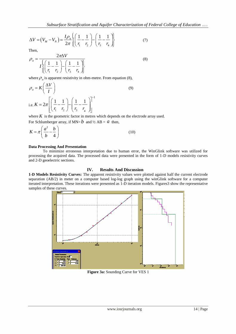
IV. Results And Discussion 1-D Models Resistivity Curves: The apparent resistivity values were plotted against half the current electrode

separation (AB/2) in meter on a computer based log-log graph using the winGlink software for a computer

iterated interpretation. These iterations were presented as 1-D iteration models. Figures3 show the representative

samples of these curves.

Figure 3a: Sounding Curve for VES 1



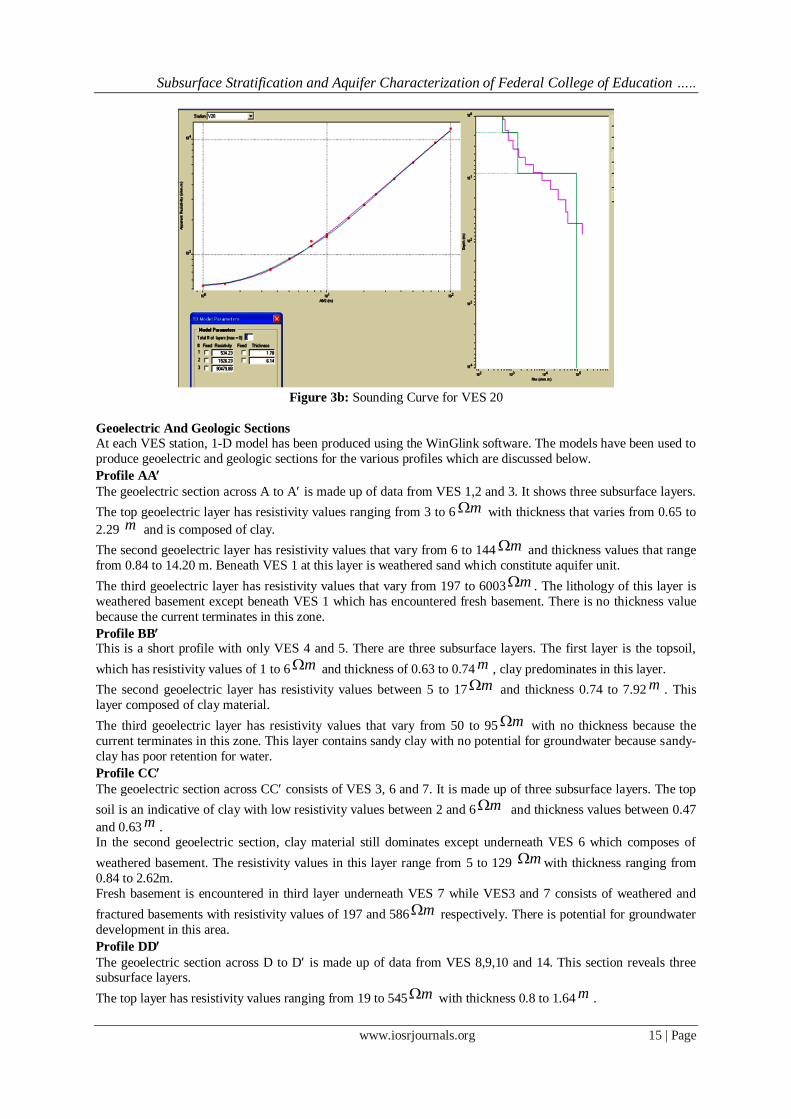
Figure 3b: Sounding Curve for VES 20

Geoelectric And Geologic Sections

At each VES station, 1-D model has been produced using the WinGlink software. The models have been used to

produce geoelectric and geologic sections for the various profiles which are discussed below.

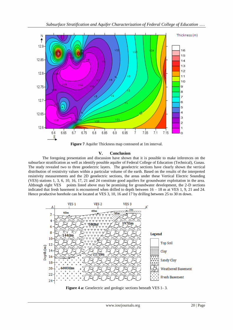
Profile AA

The geoelectric section across A to A is made up of data from VES 1,2 and 3. It shows three subsurface layers.

The top geoelectric layer has resistivity values ranging from 3 to 6 m with thickness that varies from 0.65 to

2.29 m and is composed of clay.

The second geoelectric layer has resistivity values that vary from 6 to 144 m and thickness values that range

from 0.84 to 14.20 m. Beneath VES 1 at this layer is weathered sand which constitute aquifer unit.

The third geoelectric layer has resistivity values that vary from 197 to 6003 m . The lithology of this layer is

weathered basement except beneath VES 1 which has encountered fresh basement. There is no thickness value

because the current terminates in this zone.

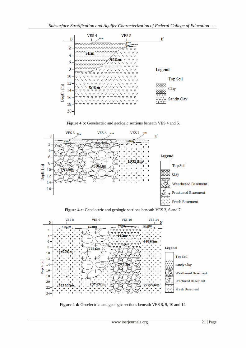
Profile BB This is a short profile with only VES 4 and 5. There are three subsurface layers. The first layer is the topsoil,

which has resistivity values of 1 to 6 m and thickness of 0.63 to 0.74 m , clay predominates in this layer.

The second geoelectric layer has resistivity values between 5 to 17 m and thickness 0.74 to 7.92 m . This

layer composed of clay material.

The third geoelectric layer has resistivity values that vary from 50 to 95 m with no thickness because the

current terminates in this zone. This layer contains sandy clay with no potential for groundwater because sandy-

clay has poor retention for water.

Profile CC

The geoelectric section across CC consists of VES 3, 6 and 7. It is made up of three subsurface layers. The top

soil is an indicative of clay with low resistivity values between 2 and 6 m and thickness values between 0.47

and 0.63 m . In the second geoelectric section, clay material still dominates except underneath VES 6 which composes of

weathered basement. The resistivity values in this layer range from 5 to 129 m with thickness ranging from

0.84 to 2.62m.

Fresh basement is encountered in third layer underneath VES 7 while VES3 and 7 consists of weathered and

fractured basements with resistivity values of 197 and 586 m respectively. There is potential for groundwater

development in this area.

Profile DD

The geoelectric section across D to D is made up of data from VES 8,9,10 and 14. This section reveals three subsurface layers.

The top layer has resistivity values ranging from 19 to 545 m with thickness 0.8 to 1.64 m .



The fresh basement is encountered right from the second layer underneath VES 8 and 14. Beneath station 9, the

fractured basement with resistivity of 733 m forms the aquifer unit with thickness 16.47 m while clayey sand

with resistivity 44 m and thickness 6.14m is underneath VES 10.

The third layer is composed of fresh bedrock except underneath VES 10 which contains weathered bedrock with

resistivity of 292 m , this constitute an aquifer unit and can be drilled for productive borehole.

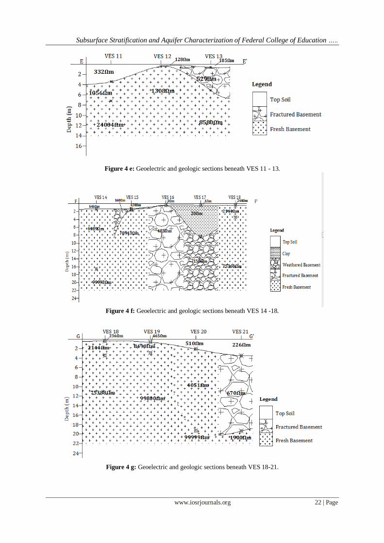
Profile EE The VES 11,12 and 13 constitute this profile. The geoelectric section reveals two to three subsurface layers.

The lithology of the topsoil contain weathered and fractured basement with resistivity values between 128 to

332 m and thickness values of 0.4 to 3.39 m.

Fresh basement has been encountered in the second layer in this section with the exception of VES 13 which

consists of fractured basement with resistivity value of 529 m and thickness 1.33 m . Although, fractured

basement constitute aquifer unit, it is not so thick to retain enough water.

The third layer composed of fresh basement with resistivity values between 8580 and 24004 m with no thickness because current terminate in this zone.

Profile FF This is the longest profile consisting of VES points 14,15,16,17 and18. The geoelectric section revealed two to

three subsurface layers.

The topsoil lithology ranges from clay to fractured bedrock with resistivity values ranging from 1 to 545 m

and thickness between 0.45 and 1.33m.

In the second geoelectric layer, fresh basement is being encountered beneath VES 14 and 18. Fractured bedrock

with resistivity value 485 m is encountered beneath VES 16 with no thickness because the current terminates

in the zone. Beneath VES 15 is the weathered basement having resistivity value of 160 m and thickness 0.37

m while clay predominates underneath VES 17 with resistivity value of 20 m and thickness 7.71 m .

The third layer has resistivity which ranges from 150 to 99993.1 m .

Profile GG

The geoelectric section across G to G consists of data from VES 18, 19, 20 and 21. Three subsurface layers are

revealed across this profile.

The first layer reveal weathered and fractured basement with resistivity values ranging from 226 to 510 m and

thickness between 0.47 and 3.5 m .

In the second layer high values of resistivity is an indication of fresh basement especially beneath VES 18, 19

and 20. Beneath station 21, the fractured bedrock with resistivity of 670 m forms the aquifer unit with

thickness 15.88 m and constitutes a favourable location for groundwater development.

The third layer is fresh basement having resistivity values between 1900 and 99999 m .

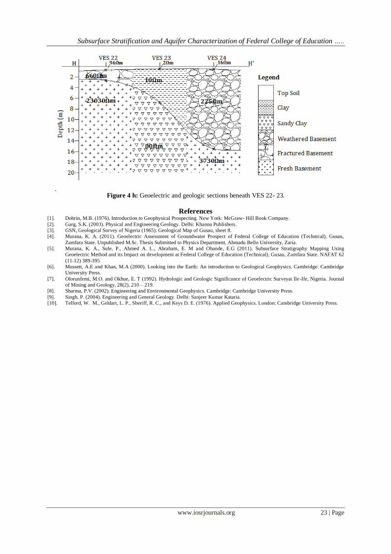
Profile HH

The geoelectric section across H to H is made up of data from VES 22, 23 and 24. It reveals three subsurface

layers. The topsoil lithology ranges from clay to sandy clay with resistivity values ranging from 2 to 96 m and

thickness values 0.44 to 0.66 m .

Beneath VES 23 in the second layer, low resistivity value of 9 m is an indication of clay. It has thickness of

6.37 m. The layer is composed of weathered / fractured basement beneath VES 22 and 24 with resistivity value

in the range of 225 to 660 m and thickness ranging between 2.58 and 14.99 m. These constitute good aquifer

for groundwater exploitation along this traverse.

The lithology of the third layer ranges from sandy clay to fresh basement with resistivity variation from 80 to

23030 m .

Maps Produced From The Interpreted Data

Contour maps were produced from the interpreted layer parameters for all VES stations established.

This was done in order to study specific aspects such as the degree of weathering and fracturing of the

subsurface rocks, as well as other structures within the study area. These maps include: isoresistivity maps at

various pre-selected depths, topsoil map, overburden thickness map and aquifer thickness map of the study area.

Isoresistivity Maps

The maps were produced by contouring the interpreted resistivity values for any particular depth taken.

The isoresistivity maps were at the following depths (1m, 5m, 10m,) were drawn with the aid of the WinGlink



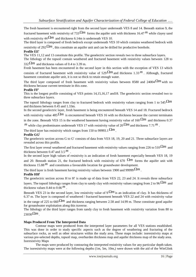
software. The isoresistivity at 1m depth (Figure 4.1) was meant to see if there is possibility of water saturation at

this depth. The regions around VES (1, 2, 3, 4, 5, 7, 17) are saturated at this depth (based on the low resistivity

values) while regions around VES (16, 17, 18, 19) have high resistivity values. However, the highly resistive areas may indicate high content of sand and silt mixed together with topsoil at this depth.

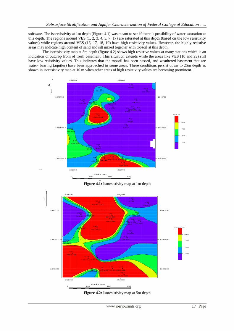
The isoresistivity map at 5m depth (figure 4.2) shows high resistive values at many stations which is an

indication of outcrop from of fresh basement. This situation extends while the areas like VES (10 and 23) still

have low resistivity values. This indicates that the topsoil has been passed, and weathered basement that are

water- bearing (aquifer) have been approached in some areas. These conditions persist down to 25m depth as

shown in isoresistivity map at 10 m when other areas of high resistivity values are becoming prominent.

Figure 4.1: Isoresistivity map at 1m depth


250

250

500

500

500

500

500

500

750

750

750

750

750

1000

1000

V1

6.726

V2

6.353

V3

5.878

V4

22.383

V5

7.714

V6

129.121

V7

7.960

V8

412.775

V9

522.468

V10

50.205

V11

332.472

V12

23324.299

V13

528.609

V14

545.425

V15

418.103

V16

484.566

V17

8.247

V18

2144.049

V19

8486.575

V20

509.339

V21

4067.968

V22

361.077

V23

8.783V24

202.281

251750 252000

251750 252000

1343750

1343500

1343250

1343750

1343500

1343250

Zamfara

Gusau

Resistivity (Layered Model) at 1 m Depth

Legend

VES Points

1000

750

500

250

ohm.m

Scale 1:3842

m

0 100 200 300

N

250

250

250

250

250

500

500

500

500

500

750

750

750 750

750

1000

1000

1000

1000

1000

V1

156.888

V2

50.501

V3

197.982

V4

22.383

V5

95.585

V6

586.219

V7

1687.950

V8

6623.593

V9

733.073

V10

44.280

V11

1055.797

V12

1307.830

V13

528.609

V14

4488.728

V15

78943.172

V16

484.566

V17

84.000

V18

2720.150

V19

99768.016

V20

405.190

V21

4067.968

V22

34047.120

V23

8.783V24

209.530

251750 252000

251750 252000

1343750

1343500

1343250

1343750

1343500

1343250

Zamfara

FCE(T)GUSAU

Legend

VES Points

isoresistivity at5m

1000

750

500

250

ohm-meter

Scale 1:3842

m

0 100 200 300

N

--




Topsoil Thickness Map

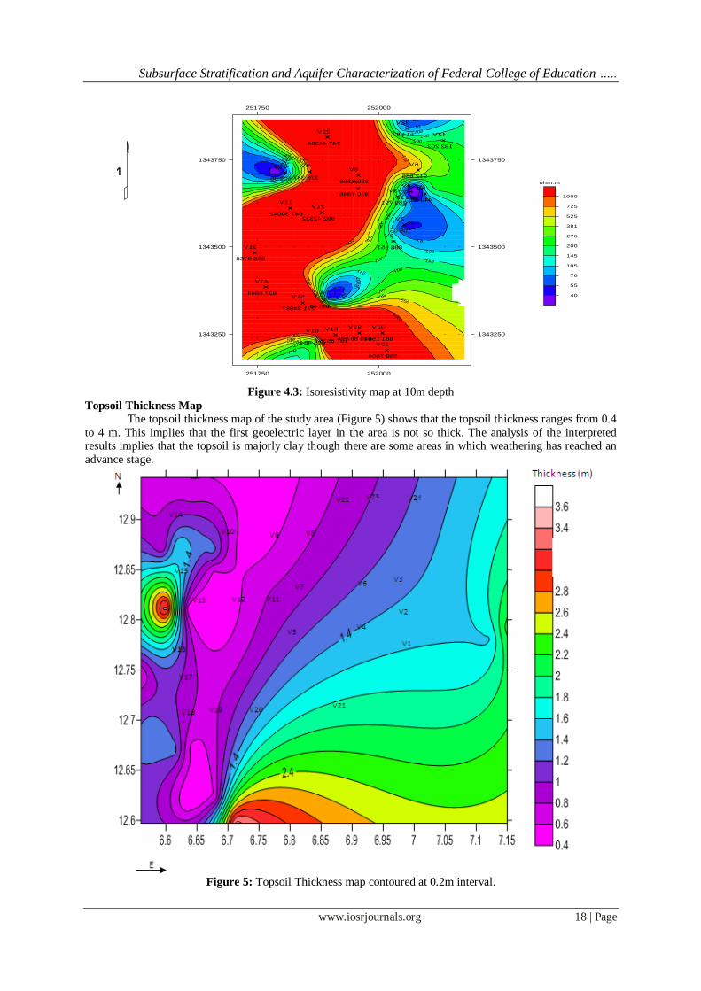
The topsoil thickness map of the study area (Figure 5) shows that the topsoil thickness ranges from 0.4

to 4 m. This implies that the first geoelectric layer in the area is not so thick. The analysis of the interpreted results implies that the topsoil is majorly clay though there are some areas in which weathering has reached an

advance stage.

Figure 5: Topsoil Thickness map contoured at 0.2m interval.

55

55

55

55

76

76

76

76

76

105

105

105

105

105

145

145

145

145

145

200

200

200

200

200

276

276

276

276

381

381

381

381

525

525

525

525

725

725

725

725

1000

1000

1000

1000

V1

156.888

V2

50.501

V3

197.982

V4

22.383

V5

89.244

V6

586.219

V7

6487.019

V8

6623.593

V9

733.073

V10

50.205

V11

24003.746

V12

23324.299

V13

8579.598

V14

4488.728V15

78943.172

V16

484.566

V17

84.004

V18

75358.781

V19

99768.016

V20

4051.188V21

4067.968

V22

46344.742

V23

78.415 V24

202.281

251750 252000

251750 252000

1343750

1343500

1343250

1343750

1343500

1343250

Zamfara

Gusau

Isores at depth 1om edd

Info Box

DC Sounding

1000

725

525

381

276

200

145

105

76

55

40

ohm.m

Scale 1:4858

m

0 100 200 300

N



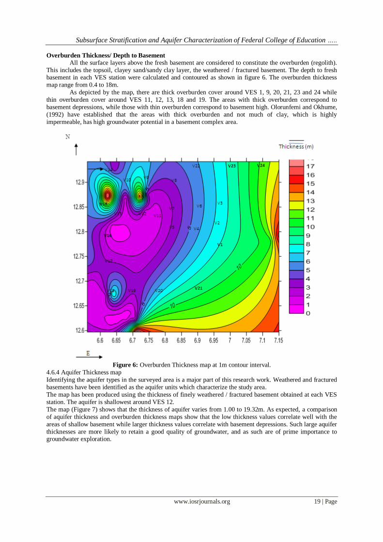
Overburden Thickness/ Depth to Basement

All the surface layers above the fresh basement are considered to constitute the overburden (regolith).

This includes the topsoil, clayey sand/sandy clay layer, the weathered / fractured basement. The depth to fresh basement in each VES station were calculated and contoured as shown in figure 6. The overburden thickness

map range from 0.4 to 18m.

As depicted by the map, there are thick overburden cover around VES 1, 9, 20, 21, 23 and 24 while

thin overburden cover around VES 11, 12, 13, 18 and 19. The areas with thick overburden correspond to

basement depressions, while those with thin overburden correspond to basement high. Olorunfemi and Okhume,

(1992) have established that the areas with thick overburden and not much of clay, which is highly

impermeable, has high groundwater potential in a basement complex area.

Figure 6: Overburden Thickness map at 1m contour interval.

4.6.4 Aquifer Thickness map

Identifying the aquifer types in the surveyed area is a major part of this research work. Weathered and fractured

basements have been identified as the aquifer units which characterize the study area.

The map has been produced using the thickness of finely weathered / fractured basement obtained at each VES

station. The aquifer is shallowest around VES 12.

The map (Figure 7) shows that the thickness of aquifer varies from 1.00 to 19.32m. As expected, a comparison

of aquifer thickness and overburden thickness maps show that the low thickness values correlate well with the

areas of shallow basement while larger thickness values correlate with basement depressions. Such large aquifer

thicknesses are more likely to retain a good quality of groundwater, and as such are of prime importance to groundwater exploration.



Figure 7 Aquifer Thickness map contoured at 1m interval.

V. Conclusion The foregoing presentation and discussion have shown that it is possible to make inferences on the

subsurface stratification as well as identify possible aquifer of Federal College of Education (Technical), Gusau.

The study revealed two to three geoelectric layers. The geoelectric sections have clearly shown the vertical

distribution of resistivity values within a particular volume of the earth. Based on the results of the interpreted

resistivity measurements and the 2D geoelectric sections, the areas under these Vertical Electric Sounding

(VES) stations 1, 3, 6, 10, 16, 17, 21 and 24 constitute good aquifers for groundwater exploitation in the area.

Although eight VES points listed above may be promising for groundwater development, the 2-D sections indicated that fresh basement is encountered when drilled to depth between 16 – 18 m at VES 1, 9, 21 and 24.

Hence productive borehole can be located at VES 3, 10, 16 and 17 by drilling between 25 to 30 m down.

Figure 4 a: Geoelectric and geologic sections beneath VES 1- 3.



Figure 4 b: Geoelectric and geologic sections beneath VES 4 and 5.

Figure 4 c: Geoelectric and geologic sections beneath VES 3, 6 and 7.

Figure 4 d: Geoelectric and geologic sections beneath VES 8, 9, 10 and 14.



Figure 4 e: Geoelectric and geologic sections beneath VES 11 - 13.

Figure 4 f: Geoelectric and geologic sections beneath VES 14 -18.

Figure 4 g: Geoelectric and geologic sections beneath VES 18-21.



Figure 4 h: Geoelectric and geologic sections beneath VES 22- 23.

References [1]. Dobrin, M.B. (1976). Introduction to Geophysical Prospecting. New York: McGraw- Hill Book Company.

[2]. Garg, S.K. (2003). Physical and Engineering Geology. Delhi: Khanna Publishers.

[3]. GSN, Geological Survey of Nigeria (1965). Geological Map of Gusau, sheet 8.

[4]. Murana, K. A. (2011). Geoelectric Assessment of Groundwater Prospect of Federal College of Education (Technical), Gusau,

Zamfara State. Unpublished M.Sc. Thesis Submitted to Physics Department, Ahmadu Bello University, Zaria.

[5]. Murana, K. A., Sule, P., Ahmed A. L., Abraham, E. M and Obande, E.G (2011). Subsurface Stratigraphy Mapping Using

Geoelectric Method and its Impact on development at Federal College of Education (Technical), Gusau, Zamfara State. NAFAT 62

(11-12) 389-395

[6]. Mussett, A.E and Khan, M.A (2000). Looking into the Earth: An introduction to Geological Geophysics. Cambridge: Cambridge

University Press.

[7]. Olorunfemi, M.O. and Okhue, E. T (1992). Hydrologic and Geologic Significance of Geoelectric Surveyat Ile-Ife, Nigeria. Journal

of Mining and Geology, 28(2), 210 – 219.

[8]. Sharma, P.V. (2002). Engineering and Environmental Geophysics. Cambridge: Cambridge University Press.

[9]. Singh, P. (2004). Engineering and General Geology. Delhi: Sanjeer Kumar Kataria.

[10]. Telford, W. M., Geldart, L. P., Sheriff, R. C., and Keys D. E. (1976). Applied Geophysics. London: Cambridge University Press.