


Bahasa
Halaman
Hukum

Strong Stability in an (R, s, S) Inventory Model
Boualem RABTA∗ and Djamil AISSANIL.A.M.O.S.
Laboratory of Modelization and Optimization of SystemsUniversity of Bejaia, 06000 (Algeria)E-mail : lamos [email protected]
Abstract
In this paper, we prove the applicability of the strong stability method to inven-tory models. Real life inventory problems are often very complicated and they areresolved only through approximations. Therefore, it is very important to justify theseapproximations and to estimate the resultant error. We study the strong stabilityin a periodic review inventory model with an (R, s, S) policy. After showing thestrong v−stability of the underlying Markov chain with respect to the perturbationof the demand distribution, we obtain quantitative stability estimates with an exactcomputation of constants.
Keywords : Inventory control, (R, s, S) policy, Markov chain, Perturbation,Strong Stability, Quantitative Estimates.
Introduction
When modelling practical problems, one may often replace a real system by another one
which is close to it in some sense but simpler in structure and/or components. This
approximation is necessary because real systems are generally very complicated, so their
analysis can not lead to analytical results or it leads to complicated results which are not
∗Corresponding author : Boualem RABTA, L.A.M.O.S., Laboratory of Modelization and Optimizationof Systems, University of Bejaia, 06000 (Algeria). Tel : (213) 34 21 08 00. Fax : (213) 34 21 51 88. E-mail: [email protected].
1

useful in practice. Also, all model parameters are imprecisely known because they are
obtained by means of statistical methods. Such circumstances suggest to seek qualitative
properties of the real system, i.e., the manner in which the system is affected by the
changes in its parameters. These qualitative properties include invariance, monotonicity
and stability (robustness). It’s by means of qualitative properties that bounds can be
obtained mathematically and approximations can be made rigorously [18]. On the other
hand, in case of instability, a small perturbation may lead to at least a finite deviation [11].
The paper by F.W. Harris [8] was the first contribution to inventory research. Since,
thousands of papers were written about inventory problems and this field still a wide area
for research. for a recent contribution see for exemple [15]. Inventory models are the first
stochastic models for which monotonicity properties were proved (see [12, 20]). In 1969,
Boylan has proved a robustness theorem for inventory problems by showing that the solu-
tion of the optimal inventory equation depends continuously on its parameters including
the demand distribution [5]. Recently, Chen and Zheng (1997) in [6] have shown that the
inventory cost in an (R, s, S) model is relatively insensitive to the changes in D = S − s.
Also, Tee and Rossetti in [19] examine the robustness of a standard model of multi-echelon
inventory systems by developing a simulation model to explore the model’s ability to pre-
dict system performance for a two-echelon one-warehouse, multiple retailer system using
(R,Q) inventory policies under conditions that violate the model’s fundamental modeling
assumptions.
As many other stochastic systems, inventory systems can be entirely described by a
Markov chain. We will say that the inventory system (or model) is stable if the underly-
2

ing Markov chain is stable. For the investigation of the stability of Markov chains many
methods have been elaborated. Kalashnikov and Tsitsishvili [11] have proposed a method
inspired from Liapunov’s direct method for differential equations. Also, we can find in
the literature the weak convergence method (Stoyan [18]), metric method (Zolotarev [22]),
renewal method (Borovkov [3]), strong stability method (Aıssani and Kartashov [1]), uni-
form stability method (Ipsen and Meyer [10]),... Some of these methods allow us to obtain
quantitative estimates in addition to the qualitative affirmation of the continuity.
The strong stability method elaborated in the beginning of the 80’s is applicable to
all operations research models which can be represented by a Markov chain. It has been
applied to queueing systems (see for example [2]). According to this approach, we suppose
that the perturbation is small with respect to a certain norm. Such a strict condition
allow us to obtain better estimations on the characteristics of the perturbed chain. For
definitions and results on this method we suggest [14].
In this paper, we apply the strong stability method to the investigation of the stability in
an (R, s, S) periodic review inventory model and to the obtention of quantitative estimates.
In section 1, we present the model, define the underlying Markov chain and study its
transient and permanent regime. Notations are introduced in section 2. The main results
of this paper are given in sections 3, 4 and 5. After perturbing the demand probabilities,
we first prove the strong v−stability of the considered Markov chain (section 3), estimate
the deviation of its transition matrix (section 4) and then, we give an upper bound to the
approximation error (section 5). A numerical example is given in section 6 to illustrate the
use of the method. Definition and basic theorems of the strong stability method are given
3
in appendix.
1 The model
Consider the following single-item, single-echelon, inventory problem. Inventory level is
inspected every R time units. At the beginning of each period, the manager decides
whether he should order and if yes, how much to order. Suppose that the outside supplier
is perfectly reliable and that orders arrive immediately. During period n, n ≥ 1, total
demand is a random variable ξn. Assume that ξn, n ≥ 1, are independent and identically
distributed (i.i.d.) random variables with common probabilities given by
ak = P (ξ1 = k), k = 0, 1, 2, ...
So, ak is the probability to have a demand of k items during the period.
For such inventory problems, (R, s, S) policy is proved to be optimal (see [17, 9, 21]).
According to this control rule, if at review moment (tn = nR, n ≥ 1), the inventory level
Xn is below or equal to s (Order-Point) we order so much items to raise the inventory level
to S (Order-Up-To level). Thus, at the beginning of n + 1 period, the size of the order
is equal to Zn = S − Xn. Figure (1) illustrates the mechanism of this model. Note that
for this model, R, s and S are decision variables which values should be optimally chosen
through a suitable algorithm (see for example [21]).
Assume that the initial inventory level s < X0 ≤ S (if not, we raise it to S by ordering
sufficient quantity). The inventory level Xn+1 at the end of period n + 1 is given by :
Xn+1 =
{
(S − ξn+1)+ if Xn ≤ s,
(Xn − ξn+1)+ if Xn > s,
4

Figure 1: The inventory level in the (R, s, S) inventory system with zero lead time.
where (A)+ = max(A, 0).
The random variable Xn+1 depends only on Xn and ξn+1, where ξn+1 is independent
of n and the state of the system. Thus, X = {Xn, n ≥ 0} is a homogeneous Markov chain
with values in E = {0, 1, ..., S}.
1.1 Transition probabilities
Suppose that at date tn = nR, Xn = i.
1. If 0 ≤ i ≤ s, then Xn+1 = (S − ξn+1)+, and we have two cases :
for j = 0,
P (Xn+1 = 0|Xn = i) = P (S − ξn+1 ≤ 0) = P (ξn+1 ≥ S) =∞
∑
k=S
ak,
for 0 < j ≤ S,
P (Xn+1 = j|Xn = i) = P (S − ξn+1 = j) = P (ξn+1 = S − j) = aS−j.
5
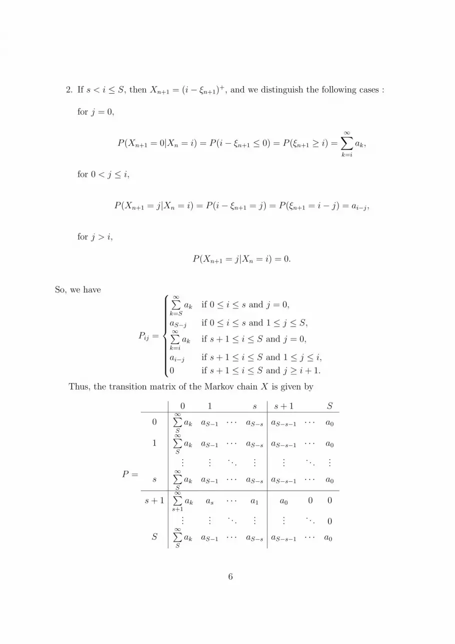
2. If s < i ≤ S, then Xn+1 = (i − ξn+1)+, and we distinguish the following cases :
for j = 0,
P (Xn+1 = 0|Xn = i) = P (i − ξn+1 ≤ 0) = P (ξn+1 ≥ i) =∞
∑
k=i
ak,
for 0 < j ≤ i,
P (Xn+1 = j|Xn = i) = P (i − ξn+1 = j) = P (ξn+1 = i − j) = ai−j,
for j > i,
P (Xn+1 = j|Xn = i) = 0.
So, we have
Pij =
∞∑
k=S
ak if 0 ≤ i ≤ s and j = 0,
aS−j if 0 ≤ i ≤ s and 1 ≤ j ≤ S,∞∑
k=i
ak if s + 1 ≤ i ≤ S and j = 0,
ai−j if s + 1 ≤ i ≤ S and 1 ≤ j ≤ i,
0 if s + 1 ≤ i ≤ S and j ≥ i + 1.
Thus, the transition matrix of the Markov chain X is given by
P =
0 1 s s + 1 S
0∞∑
S
ak aS−1 · · · aS−s aS−s−1 · · · a0
1∞∑
S
ak aS−1 · · · aS−s aS−s−1 · · · a0
......
. . ....
.... . .
...
s∞∑
S
ak aS−1 · · · aS−s aS−s−1 · · · a0
s + 1∞∑
s+1
ak as · · · a1 a0 0 0
......
. . ....
.... . . 0
S∞∑
S
ak aS−1 · · · aS−s aS−s−1 · · · a0
6
The Markov chain X is irreducible and aperiodic. It has a unique stationary distribution
π = (π0, π1, ..., πS) given by the solution of
π.P = πS∑
i=0
πi = 1 .
Furthermore, this stationary distribution is independent from the initial inventory level
X0.
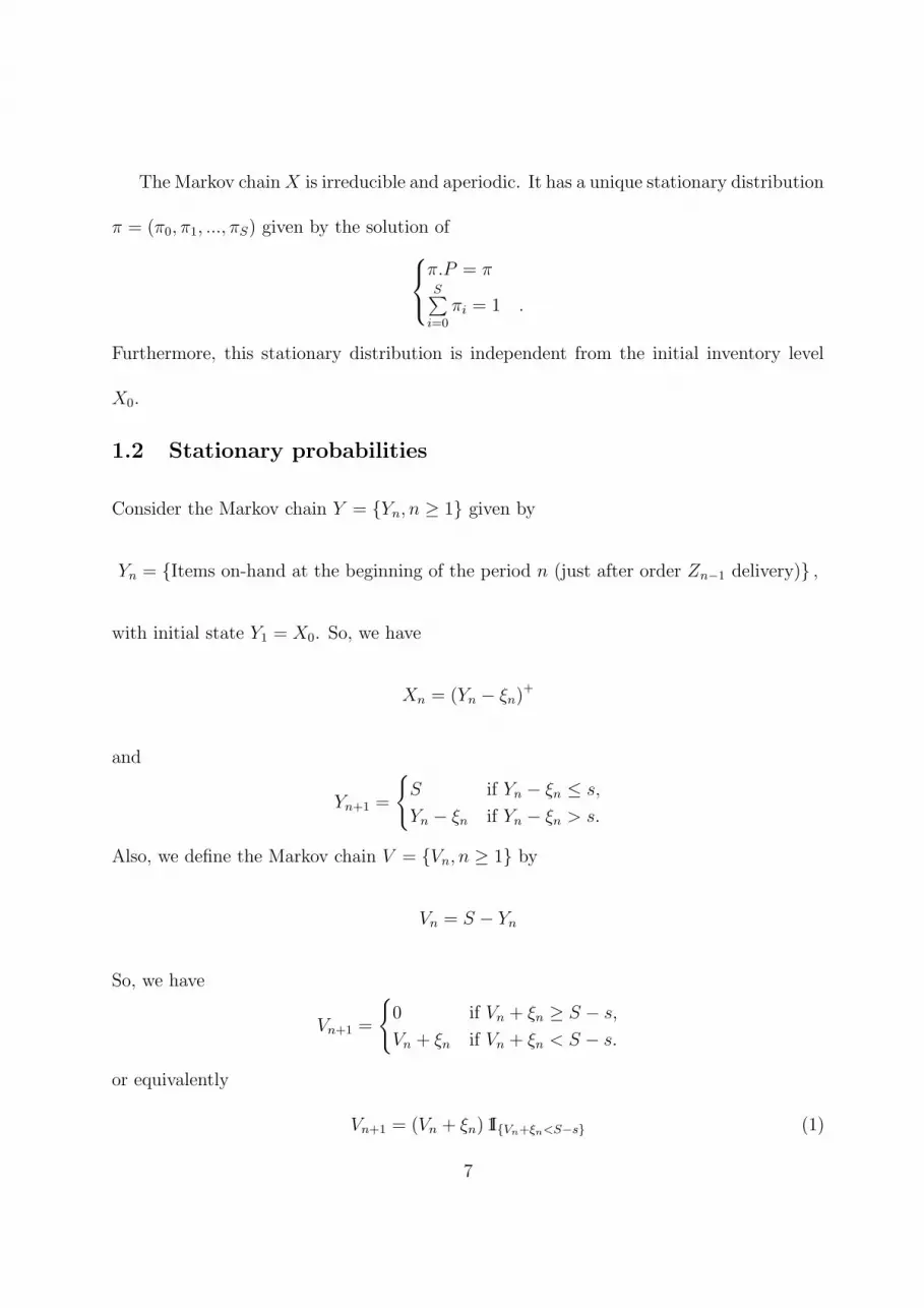
1.2 Stationary probabilities
Consider the Markov chain Y = {Yn, n ≥ 1} given by
Yn = {Items on-hand at the beginning of the period n (just after order Zn−1 delivery)} ,
with initial state Y1 = X0. So, we have
Xn = (Yn − ξn)+
and
Yn+1 =
{
S if Yn − ξn ≤ s,
Yn − ξn if Yn − ξn > s.
Also, we define the Markov chain V = {Vn, n ≥ 1} by
Vn = S − Yn
So, we have
Vn+1 =
{
0 if Vn + ξn ≥ S − s,
Vn + ξn if Vn + ξn < S − s.
or equivalently
Vn+1 = (Vn + ξn) 1I{Vn+ξn<S−s} (1)
7

V is a Markov chain with states in {0, 1, ..., S − s − 1}. If we denote by V∞ the random
variable having the stationary distribution of the Markov chain V then
V∞ = (V∞ + ξ1) 1I{V∞+ξ1<S−s} (2)
This relation implies that for every 0 ≤ v ≤ S − s − 1
FV (v) = P (V∞ ≤ v) = C + (FV ∗ Fξ)(v), (3)
where C = 1 − (FV ∗ Fξ)(S − s − 1) is a normalisation constant and Fξ(x) = P (ξ1 ≤ x) is
the cumulative function common to all ξn, n ≥ 1. Since (3) is a renewal type equation, it
follows (cf. [16]) that its uniquely determined solution is given by
FV (v) = C(1 + H(v)),
where H =∞∑
n=1
F n∗ξ is the renewal function associated to Fξ. The constant C can be
easily determined by the condition FV (S − s− 1) = 1, therefore we obtain that the unique
invariant distribution of the Markov chain V is given by
FV (v) =1 + H(v)
1 + H(S − s − 1), 0 ≤ v ≤ S − s − 1.
Now, we can deduce the stationary distribution of the Markov chain X from relation
X∞ = (S − (V∞ + ξ1))+
where X∞ is the random variable having the stationary distribution of the Markov chain
X.
8

2 Preliminary and notations
In this section, we introduce necessary notations adapted to our case, i.e., the case of
a finite discrete Markov chain. For a general framework see [14] and comments in the
appendix.
Let X = {Xn, n ≥ 0} be a homogeneous discrete Markov chain with values in a finite
space E = {0, 1, ..N}, given by a transition matrix P . Assume that X admits a unique
stationary vector π.
For a transition matrix P and a function f : E → R, we define
Pf(i) =∑
j∈E
Pijf(j), ∀i ∈ E,
and for a vector µ ∈ RN+1 we define
µf =∑
i∈E
µif(i).
Also, f ◦ µ is the matrix having the form
f(i)µi,∀i, j ∈ E.
We introduce in RN+1 the special family of norms
‖µ‖v =∑
i∈E
v(i)|µi|,∀µ ∈ RN+1, (4)
where v : E → R+ is a function bounded from bellow by a positive constant (not necessary
finite). So, the induced norms on space of matrices of size (N + 1)× (N + 1) will have the
following form
‖Q‖v = maxi∈E
(v(i))−1∑
j∈E
|Qij|v(j), (5)
9
Also, for a function f : E → R,
‖f‖v = maxi∈E
(v(i))−1 |f(i)|.
3 Strong v−stability of the (R, s, S) inventory model
Denote by Σ the considered inventory model. Let X = {Xn, n ≥ 0} be the Markov chain
where Xn is the on-hand inventory level at date tn = nR, n ≥ 1 and X0 is the initial
inventory level. Let Σ′ be another inventory model with the same structure but with
demands ξ′n having common probabilities
a′k = P (ξ′1 = k), k = 0, 1, ...
Let X ′ = {X ′n, n ≥ 0} be the Markov chain where X ′
n is the on-hand inventory level at
date tn = nR, n ≥ 1 in Σ′ and X ′0 = X0 is the initial inventory level. Denote by P and Q
the transition operators of the Markov chains X and X ′ respectively.
Definition 3.1. (cf. [1]) We say that the Markov chain X verifying ‖P‖v < ∞ is strongly
v−stable, if every stochastic matrix Q in the neighborhood {Q : ‖Q − P‖v < ε} admits a
unique stationary vector ν and :
‖ν − π‖v −→ 0 when ‖Q − P‖v −→ 0.
Theorem 3.1. In the (R, s, S) inventory model with instant replenishments, the Markov
chain X = {Xn, n ≥ 0} is strongly v−stable for a function v(k) = βk for all β > 1.
Proof. To prove the strong v−stability of the Markov chain X for a function v(k) = βk,
β > 1, we check the conditions of Theorem A.1.
10

So, we choose the measurable function
h(i) =
{
1 if 0 ≤ i ≤ s,
0 if s < i ≤ S,
and the measure α = (α0, α1, ..., αS), where
αj = P0j.
Thus, we can easily verify that
• πh =S∑
i=0
πih(i) =s
∑
i=0
πi > 0,
• α1I =S∑
j=0
P0j = 1,
• αh =S∑
j=0
P0jh(j) =s
∑
j=0
P0j =∞∑
i=S−s
ai > 0.
It is obvious that
Tij = Pij − h(i)αj =
{
0 if 0 ≤ i ≤ s,
Pij otherwise,
is a nonnegative matrix.
Now, we aim to show that there exists some constant ρ < 1 such that Tv(k) ≤ ρv(k) for
all k ∈ E.
Compute Tv(k) =S∑
j=0
Tkjv(j). If 0 ≤ k ≤ s, then
Tv(k) = 0.
If s < k ≤ S, then we have
Tv(k) =k
∑
j=0
Pkjβj =
∞∑
i=k
ai +k
∑
j=1
ak−jβj =
∞∑
i=k
ai +k−1∑
i=0
aiβk−i
11

=∞
∑
i=k
ai + βk
k−1∑
i=0
aiβ−i =
∞∑
i=k
ai
βk+
k−1∑
i=s+1
aiβ−i +
s∑
i=0
aiβ−i
βk
≤
∞∑
i=k
ai
βs+1+
k−1∑
i=s+1
ai
βs+1+
s∑
i=0
aiβ−i
βk =
∞∑
i=s+1
ai
βs+1+
s∑
i=0
aiβ−i
βk.
It suffices to take
ρ =
∞∑
i=s+1
ai
βs+1+
s∑
i=0
aiβ−i (6)
which is smaller then 1 for all β > 1.
Now, we verify that ‖P‖v < ∞
‖P‖v = maxk∈{0,1,..,S}
1
βk
S∑
j=0
Pkjβj = max(A,B)
where
A = maxk∈{0,1,..,s}
1
βk
S∑
j=0
Pkjβj = max
k∈{0,1,..,s}
1
βk
[
∞∑
i=S
ai +S
∑
j=1
aS−jβj
]
=∞
∑
i=S
ai +S
∑
j=1
aS−jβj
= 1 −
S−1∑
i=0
ai +S−1∑
i=0
aiβS−i = 1 +
S−1∑
i=0
ai
(
βS−i − 1)
and
B = maxk∈{s+1,..,S}
1
βk
S∑
j=0
Pkjβj = max
k∈{s+1,..,S}
1
βk
[
∞∑
i=k
ai +k
∑
j=1
ak−jβj
]
= maxk∈{s+1,..,S}
1
βk
[
1 +k−1∑
i=0
ai
(
βk−i − 1)
]
≤ maxk∈{s+1,..,S}
1
βs+1
[
1 +k−1∑
i=0
ai
(
βk−i − 1)
]
≤1
βs+1
[
1 +S−1∑
i=0
ai
(
βS−i − 1)
]
≤ 1 +S−1∑
i=0
ai
(
βS−i − 1)
= A.
So, we have
‖P‖v = 1 +S−1∑
i=0
ai
(
βS−i − 1)
< ∞.
12

�
4 Deviation of the transition matrix
The considered inventory system is strongly v−stable. This means that its characteristics
can approximate those of a similar inventory model having different demand distribution
under the condition that this distribution is close (in some sense) to the ideal system
demand distribution. To characterize this proximity we define the quantity
W =∞
∑
i=S
|ai − a′i| +
S−1∑
i=0
|ai − a′i| β
S−i. (7)
Before estimating numerically the deviation between stationary distributions of the chains
X and X ′, we estimate the deviation of the transition matrix P of the chain X. So, we
have
Lemma 4.1. Let P (resp. Q) be the transition matrix of the Markov chain X (resp. X ′).
Then,
‖P − Q‖v ≤ W
Proof.
‖P − Q‖v = maxk∈{0,1,..,S}
1
βk
S∑
j=0
|Pkj − Qkj| βj = max(C,D)
where
C = maxk∈{0,1,..,s}
1
βk
S∑
j=0
|Pkj − Qkj| βj ≤ max
k∈{0,1,..,s}
1
βk
[
∞∑
i=S
|ai − a′i| +
S∑
j=1
∣
∣aS−j − a′S−j
∣
∣ βj
]
=∞
∑
i=S
|ai − a′i| +
S−1∑
i=0
|ai − a′i| β
S−i
13

and
D = maxk∈{s+1,..,S}
1
βk
S∑
j=0
|Pkj − Qkj| βj ≤ max
k∈{s+1,..,S}
1
βk
[
∞∑
i=k
|ai − a′i| +
k∑
j=1
∣
∣ak−j − a′k−j
∣
∣ βj
]
= maxk∈{s+1,..,S}
∞∑
i=k
|ai − a′i|
βk+
k−1∑
i=0
|ai − a′i| β
−i
= maxk∈{s+1,..,S}
∞∑
i=k
|ai − a′i|
βk+
k−1∑
i=s+1
|ai − a′i| β
−i +s
∑
i=0
|ai − a′i| β
−i
≤
∞∑
i=s+1
|ai − a′i|
βs+1+
s∑
i=0
|ai − a′i| β
−i
≤ W.
So, we obtain
‖P − Q‖v ≤∞
∑
i=S
|ai − a′i| +
S−1∑
i=0
|ai − a′i| β
S−i = W.
�
5 Stability inequalities
The purpose of this section is to obtain a numerical estimation of the deviation between
stationary distributions of the Markov chains X and X ′. This can be done using Theorem
A.2.
First, estimate ‖π‖v.
Lemma 5.1. Let γ be the constant given by
γ =
(
∞∑
i=S
ai +S−1∑
i=0
aiβS−i
)
(1 − ρ)(1 + H(S − s − 1))(8)
14

where ρ is given by (6) and H =∞∑
n=1
F n∗ξ is the renewal function associated to the cumulative
distribution function Fξ of the random variable ξ1. Then,
‖π‖v ≤ γ
Proof. According to Theorem A.2,
‖π‖v ≤ (αv)(1 − ρ)−1(πh).
Since
αv =S
∑
j=0
α(j)v(j) =S
∑
j=0
P0jβj =
∞∑
i=S
ai +S
∑
j=1
aS−jβj =
∞∑
i=S
ai +S−1∑
i=0
aiβS−i
and
πh =S
∑
i=0
πih(i) =s
∑
i=0
πi = 1 −
S∑
i=s+1
πi = 1 − P (X∞ > s) = 1 − P (S − (V∞ + ξ1) > s)
= 1−P (V∞+ξ1 ≤ S−s−1) = 1−(FV ∗Fξ)(S−s−1) = 1−H(S − s − 1)
1 + H(S − s − 1)=
1
1 + H(S − s − 1),
it follows that
‖π‖v ≤
(
∞∑
i=S
ai +S−1∑
i=0
aiβS−i
)
(1 − ρ)(1 + H(S − s − 1))= γ.
�
Now, we can prove the following result
Theorem 5.1. Let π and ν be the stationary distributions of the Markov chains X and
X ′ respectively. Then, under the condition
W <1 − ρ
1 + γ(9)
15
we have
‖π − ν‖v ≤Wγ (1 + γ)
1 − ρ − (1 + γ) W(10)
where ρ is given by (6) and γ by (8).
Proof. We have ‖π‖v ≤ γ and
‖1I‖v = maxk∈E
1
βk= 1.
Imposing the condition
W <1 − ρ
1 + γ
and replacing constants in (12) by their values, we obtain
‖π − ν‖v ≤Wγ (1 + γ)
1 − ρ − (1 + γ) W.
�
Remark 1. The quantitative estimates obtained by means of the strong stability method
and given by the last result gives an upper bound of the deviation of the stationary distri-
bution of the Markov chain X with respect to the perturbation of the transition matrix
‖π − ν‖ ≤ C(P )‖P − Q‖ (11)
Some other stability methods can also be used to obtain such a bound. For the ”Absolutely
stable chain” defined in [10], the survey of Cho and Mayer [7] collects and compares several
bounds of the form (11). Note that this method study the sensitivity of the individual
stationary probabilities of a finite Markov chain.
16

6 Numerical example
Consider the (R, s, S) inventory model with Poisson distributed demand. This can cor-
respond to the case where clients arrive following a Poisson distribution and request all
exactly one item. Now, we apply the above results to test the sensitivity of the model
when perturbing the arriving rate λ to λ′ = λ + ε (for example, ε can be the error when
estimating λ from real data). For model parameters we take R = 1, S = 6, s = 3, λ = 5.
The transition matrix P of the Markov chain X is constructed and computations are made
by means a computer program. In a first step, we vary β to see the impact of the choice
of the norm. The perturbed parameter we take is λ′ = 5, 1 so ε = 0, 1. For each value of
β, the program compute the deviation W of the transition matrix and check whether the
condition (9) of Theorem 5.1 is satisfied. If yes, the program compute the upper bound of
the approximation error from relation (10).
The transition matrix of the chain X is given by
P =
0, 384039 0, 175467 0, 175467 0, 140374 0, 084224 0, 033690 0, 0067380, 384039 0, 175467 0, 175467 0, 140374 0, 084224 0, 033690 0, 0067380, 384039 0, 175467 0, 175467 0, 140374 0, 084224 0, 033690 0, 0067380, 384039 0, 175467 0, 175467 0, 140374 0, 084224 0, 033690 0, 0067380, 734974 0, 140374 0, 084224 0, 033690 0, 006738 0, 000000 0, 0000000, 559507 0, 175467 0, 140374 0, 084224 0, 033690 0, 006738 0, 0000000, 384039 0, 175467 0, 175467 0, 140374 0, 084224 0, 033690 0, 006738
The stationary distribution of the chain X is given by
π = (0, 416287, 0, 172774, 0, 167402, 0, 130486, 0, 076747, 0, 030288, 0, 006017)
Table 1 gives the results of the computations and the error e = ‖π − ν‖v = f(β) is
graphically represented in Figure 2. Observe that the condition (9) is satisfied only for
17

β W ‖π − ν‖v β W ‖π − ν‖v β W ‖π − ν‖v
1,11 0,042886 0,108725 1,21 0,052256 0,053748 1,31 0,064310 0,0492351,41 0,079634 0,057096 1,51 0,098904 0,075016 1,61 0,122900 0,1067491,71 0,152513 0,161400 1,81 0,188755 0,258115 1,91 0,232772 0,4406082,01 0,285853 0,828827 2,11 0,349444 1,894640 2,21 0,425156 9,022420
Table 1: The deviation of the transition matrix and the error e = ‖π − ν‖v = f(β) fordifferent values of β.
Figure 2: The error e = ‖π − ν‖v = f(β).
1, 03 ≤ β ≤ 2, 24. So, the choice of the norm (β) is relevant. The minimum estimation of
the error e = 0, 0489 is taken for β = 1, 29.
Now, let us vary the perturbation ε for a fixed value of β. The error e = ‖π−ν‖v = g(ε)
ε 0,01 0,02 0,03 0,04 0,1 0,2 0,3 0,4 0,5e 0,0043 0,0087 0,0133 0,0179 0,0489 0,1150 0,2091 0,3537 0,6041
Table 2: The error e = ‖π − ν‖v = g(ε).
is given in Table 2 for β = 1, 29. Naturally, the error is proportional to the perturbation
18
and the two quantities grow in the same time. Observe that the model have resisted to an
important perturbation (0, 5 represents 10% of the value of λ).
7 Conclusion
The Markov chain X denoting the on-hand inventory level at the end of periods in the
(R, s, S) inventory system with instant replenishments, is strongly v−stable with respect
to the perturbation of the demand distribution, for a function v(k) = βk, ∀β > 1. This
means that its characteristics are close to those of another inventory model with the same
structure but with demand distribution close to the ideal model demand distribution. The
last result gives us a numerical estimation of the error due to the approximation.
References
[1] Aıssani, D. and N.V. Kartashov, 1983, Ergodicity and stability of Markov chains with
respect to operator topology in the space of transition kernels, Dokl. Akad. Nauk.
Ukr. SSR, ser. A 11, 3–5.
[2] Aıssani, D. and N.V. Kartashov, 1984, Strong stability of the imbedded markov chain
in an M/G/1 system, International Journal Theor. Probability and Math. Statist. 29,
(American Mathematical Society), 1–5.
[3] Borovkov, A.A., 1972, Processus probabilistes de la theorie des files d’attente (Edition
Navka, Moskou).
19
[4] Boualouche, L. and D. Aıssani, 2002, Performance evaluation of an SW Communica-
tion Protocol (Send and Wait), Proceedings of the MCQT’02 (First Madrid Interna-
tional Conference on Queueing Theory), Madrid (Spain), 18.
[5] Boylan, E.S., 1969, Stability theorems for solutions to the optimal inventory equation,
Journal of Applied Probability 6, 211–217.
[6] Chen, F. and Y.S. Zheng, 1997, Sensitivity analysis of an (s, S) inventory model,
Operations Research Letters 21(1), 19–23.
[7] Cho, G. and C. Mayer, 2001, Comparaison of perturbation bounds for the stationary
probabilities of a finite Markov chain, Linear Algebra and its Applications, 335, 137–
150.
[8] Harris, F.W., 1913, How many parts to make at once, Factory (The magazine of
Management), 10(2), 135–136.
[9] Iglehart, D., 1963, Dynamic programming and stationary analysis of inventory prob-
lems, multistage inventory models and techniques, in : H. Scarf, D. Gilford, and
M. Shelly, editors, Multistage Inventory Models and Techniques, (Stanford University
Press) 1–31.
[10] Ipsen, I. and C. Meyer, 1994, Uniform stability of Markov chains, SIAM Journal on
Matrix Analysis and Applications, 15(4), 1061–1074.
20

[11] Kalashnikov, V.V. and G.Sh. Tsitsishvili, 1971, On the stability of queueing systems
with respect to disturbances of their distribution functions, Queueing theory and
reliability, 211–217.
[12] Karlin, S., 1960, Dynamic inventory policy with varing stochastic demands, Manage-
ment Sciences 6, 231–258.
[13] Kartashov, N.V., 1981, Strong Stability of Markov Chains, VNISSI, Vsesayouzni Sem-
inar on Stability Problems for stochastic Models, Moscow, 54-59 (See also : 1986, J.
Soviet Mat. 34, 1493–1498).
[14] Kartashov, N.V., 1996, Strong Stable Markov Chains (VSP, Utrecht, TbiMC Scientific
Publishers).
[15] Mohebbi, E., 2004, A replenishment model for the supply-uncertainty problem, Inter-
national Journal of Production Economics, 87(1), 25–37.
[16] Ross, S.M., 1970, Applied probability with optimization applications (Holden-Day,
San Francisco).
[17] Scarf, H., 1960, The optimality of (S, s) policies in the dynamic inventory problem, in
: K.J. Arrow, S. Karlin, and P. Suppes, editors, Mathematical methods in the social
sciences, (Stanford University Press, Stanford, Calif.) 196–202.
[18] Stoyan, D., 1983, Comparaison Methods for Queues and Other Stochastic Models,
English translation, D.J. Daley, Editor ( J. Wiley and Sons, New York).
21

[19] Y.S. Tee and M.D. Rossetti, 2002, A robustness study of a multi-echelon inventory
model via simulation, International Journal of Production Economics, 80(3), 265–277.
[20] Veinott, A., 1965, Optimal policy in a dynamic, single product, non-stationary inven-
tory model with several demand classes, Operations Research 13, 761–778.
[21] Veinott, A., and H. Wagner, 1965, Computing optimal (s, S) policies, Management
Sciences 11, 525–552.
[22] Zolotarev, V.M., 1975, On the continuity of stochastic sequenses generated by recurent
processes, Theory of Probability and Its Applications, XX(4), 819–832.
A Strong stability criterion
Conserve notations of section 2. The following theorem (cf. [1]) gives sufficient conditions
for the strong stability of a Harris recurrent Markov chain.
Theorem A.1. The Harris recurrent Markov chain X verifying ‖P‖v < ∞ is strongly
v-stable, if the following conditions are satisfied
1. ∃α ∈ RN+1+ ,∃h : E → R+ such that : πh > 0, α1I = 1, αh > 0,
2. T = P − h ◦ α is a nonnegative matrix,
3. ∃ ρ < 1 such that, Tv(x) ≤ ρ v(x),∀x ∈ E.
where 1I is the function identically equal to 1.
22
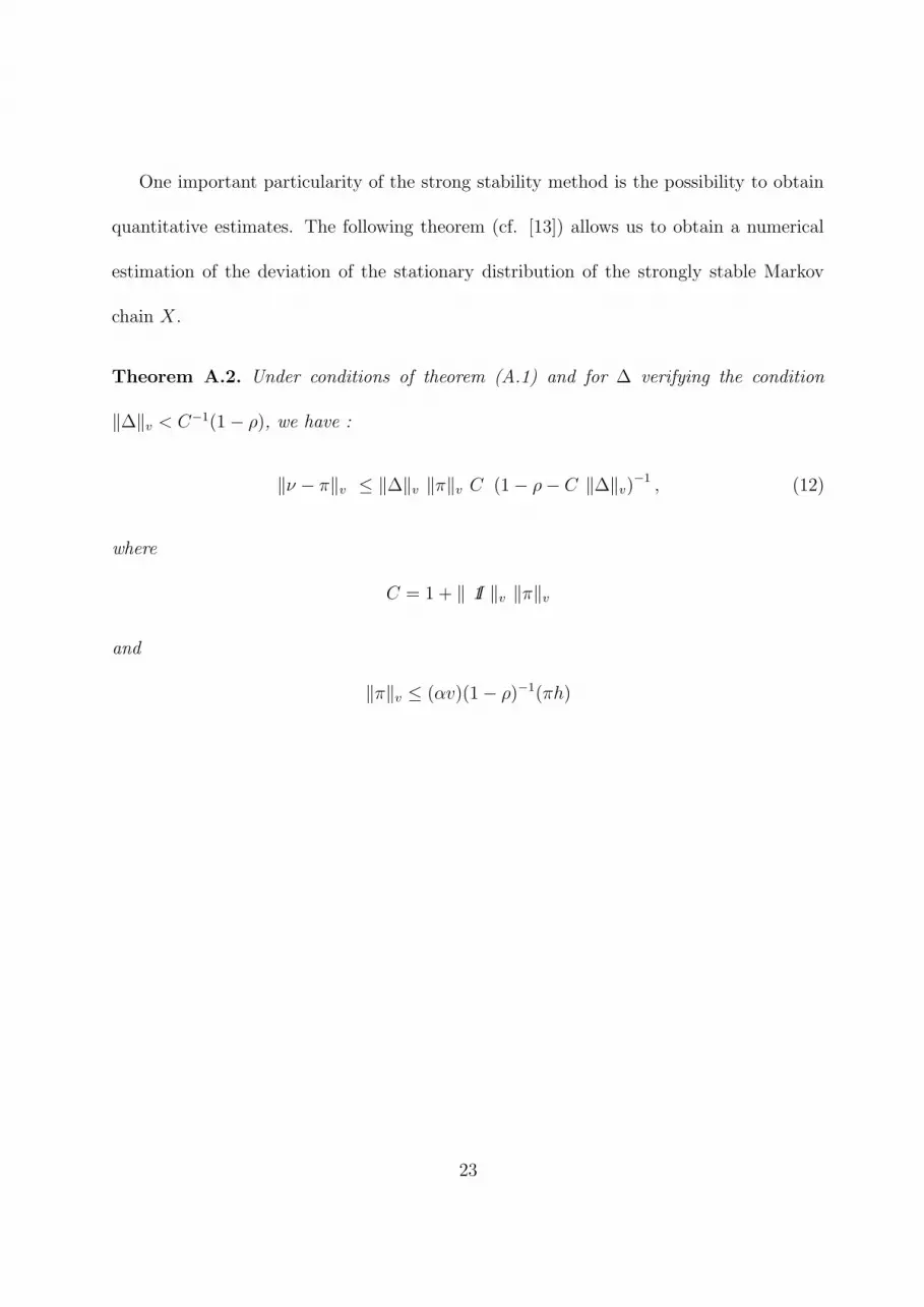
One important particularity of the strong stability method is the possibility to obtain
quantitative estimates. The following theorem (cf. [13]) allows us to obtain a numerical
estimation of the deviation of the stationary distribution of the strongly stable Markov
chain X.
Theorem A.2. Under conditions of theorem (A.1) and for ∆ verifying the condition
‖∆‖v < C−1(1 − ρ), we have :
‖ν − π‖v ≤ ‖∆‖v ‖π‖v C (1 − ρ − C ‖∆‖v)−1
, (12)
where
C = 1 + ‖ 1I ‖v ‖π‖v
and
‖π‖v ≤ (αv)(1 − ρ)−1(πh)
23
Top Related
Copyright © 2022 FDOKUMEN

