Download - Software Design Description For Subsurface Transport Over Multiple Phases (STOMP) Software

PNNL-SA-54078

Software Design Description For

Subsurface Transport Over Multiple Phases (STOMP) Software

Authors: William E. Nichols & Mark D. White

This document describes the STOMP software design in sufficient detail to adequately describe how the system implements the requirements. The information also includes the analysis or rationale for the design chosen. Assumptions in the design analysis are documented.

This document describes how the software will satisfy the requirements; how the software functions internally; and how the operating system, structure, interfaces, design inputs and sources, design constraints, timing between components, and data structures are considered and integrated into the code. The control flow, control logic, data flow model (structure, rules), and relationship between data and process are detailed. Methods to mitigate the consequences of software failure are an integral part of the software design.

Numerical methods, mathematical models, and physical models are described separately in the STOMP Theory Guides (White & Oostrom 2000, PNNL-11217, Ward et al. 2005, PNNL-15465) and unpublished addendums.

Table of Contents 1.0 Software Context ................................................................................................................................... 4 2.0 Architecture Requirements .................................................................................................................. 4

2.1. Overview of Key Objectives ............................................................................................................ 4 2.2. Architecture Use Cases .................................................................................................................... 5 2.3. Stakeholder Architectural Requirements.......................................................................................... 5 2.4. Constraints ....................................................................................................................................... 5 2.5. Non-functional Requirements .......................................................................................................... 5

3.0 Solution................................................................................................................................................... 6 3.1. Relevant Architectural Patterns........................................................................................................ 6 3.2. Architecture – Structural View......................................................................................................... 6 3.3. Architecture – Dynamic View........................................................................................................ 22 3.4. Implementation Strategy ................................................................................................................ 22 3.5. Architecture Analysis..................................................................................................................... 22 3.6. Risks............................................................................................................................................... 23 3.7. References...................................................................................................................................... 23

SDD Revision History

Revision #

Comments Authors Revision Date

Effective Date

0 Initial Software Design Description Release

W. Nichols, M. White

21 Dec 2006 1 Jan 2007

1.0 Editorial revisions V. Freedman 18 Jan 2007 18 Jan 2007 1.1 Editorial revisions/QE

Review V. FreedmanC. Carlson

25 Feb 2007 26 Feb 2007

Software Design Description

1.0 Software Context This Software Design Description (SDD) describes the architecture of the Subsurface Transport Over Multiple Phases (STOMP) Software. If significant changes to the design occur as a result of further development efforts during the life cycle of this software, this SDD will be revised. The purpose and intended use of the STOMP software is to produce numerical predictions of thermal and hydrogeologic flow and transport phenomena in variably saturated subsurface environments, which are contaminated with volatile or nonvolatile organic compounds or radionuclides including radioactive chain decay processes. The software is a variable-source Fortran code that requires compilation using an ANSI-standard Fortran compiler for the host platform and selection of a specific solution mode and solver. The use and purpose of this software is more fully described in the following documents:

• White, M.D., and M. Oostrom. 1996. STOMP Subsurface Transport Over Multiple Phases: Theory Guide, PNNL-11217, Pacific Northwest National Laboratory, Richland, Washington.

• Nichols, W.E., N.J. Aimo, M. Oostrom, and M.D. White. 1997. STOMP Subsurface Transport Over Multiple Phases: Application Guide, PNNL-11216, Pacific Northwest National Laboratory, Richland, Washington.

• White, M. D., and M. Oostrom. 2006. STOMP Subsurface Transport Over Multiple Phases: User’s Guide, PNNL-15782, Pacific Northwest National Laboratory, Richland, Washington.

• Ward A.L., M.D. White, E.J. Freeman, and Z.F. Zhang. 2005. STOMP Subsurface Transport Over Multiple Phase Addendum: Sparse Vegetation Evapotranspiration Model for the Water-Air-Energy Operational Mode. PNNL-15465, Pacific Northwest National Laboratory, Richland, Washington.

2.0 Architecture Requirements

2.1. Overview of Key Objectives The STOMP software must read input for a problem from a structured ASCII file that conforms to the format specified in the STOMP User’s Guide, numerically solve the partial differential equations that describe subsurface environment transport phenomena, and write results to an output file, plot files, surface flux integration report files, and

standard output. If errors are encountered in the input file, the nature of the problem must be reported to the output file. If the solution fails to converge (a strong possibility when solving highly nonlinear partial differential equations), the software must end execution and report the status to the output file.

2.2. Architecture Use Cases Architecture use cases are provided in the numerous application examples provided in the STOMP Application Guide (Nichols et al. 1997).

2.3. Stakeholder Architectural Requirements The architecture uses a variable source code configuration where source code configurations are called operational modes. Operational modes are classified according to the solved governing flow equations and transport equations, constitutive relation equations, and implementation type. This architectural constraint will provide for flexibility to meet the needs of multiple stakeholders by permitting efficient coupling of needed equations to solve for a variety of subsurface flow and transport problems without the substantial computational overhead that would burden the simulator if all possible equations and implementation types were included in a single source code configuration. The variable source code configuration also provides for inclusion of proprietary modules that may be restricted in scope to only certain clients or use scenario.

2.4. Constraints The ANSI Standard Fortran 77 will be used (without extensions) for all source code to ensure maximum portability to different operating systems, computer platforms, and Fortran compilers.

Constraints on the STOMP input, controlled through a text file, are stipulated in Section 2.0 of the following software requirements specification:

Zhang, Z. F. 2006. Requirements for STOMP – Subsurface Transport Over Multiple Phases. Pacific Northwest National Laboratory, Richland, WA.

The input file requirements differ with each Operational Mode, consistent with the variable source code architecture of STOMP.

2.5. Non-functional Requirements Performance: It is recognized that the performance of a numerical simulator for nonlinear processes cannot be stipulated a priori. Therefore, no requirements are placed on the STOMP software in this regard but it is noted that every effort to employ efficient numerical solvers and techniques is expected in code design and development.

Reliability: The STOMP simulator will degrade gracefully when code operation is halted for reasons of:

• Numerical non-convergence

• Detection of input file format errors

• Exceedance of user-specified runtime or simulation steps

• Exceedance of parameter limits for array sizing

Degrade gracefully here is used to mean that the code will record the reason for termination in an appropriate output file, write a restart file if solution is in progress, and close all open files.

Simplicity: The STOMP simulator will use an input file format structure that promotes human readability. The input file will be an ASCII text file and input will be organized into groupings of related parameters.

Scalability: The design of the STOMP simulator will utilize code scaling parameters that will permit the software to be efficiently sized to the features, events, and processes the problem includes. This is achieved by use of an includable ‘parameters’ file that includes all scalable code parameters that determine the size of each dimension of variable arrays. For example: parameters LX, LY, and LZ specify the maximum number of nodes in the x-, y-, and z- dimensions respectively. These parameters are set in the ‘parameters’ file once, included in all code modules that require these parameters, and thereby allow efficient scaling of the software to the problem under consideration.

3.0 Solution

3.1. Relevant Architectural Patterns Monolithic system architecture is specified (single user, single invocation; processing, data, and user interface all reside in the same system).

3.2. Architecture – Structural View STOMP uses a single program module to control execution of the code, and a number of dependent, single-purpose subroutines to carry out specific calculations or operations. However, in STOMP is in fact a multiple-source code, customizable to a large number of operational modes (e.g., water, water-air, water-air-oil, etc.). Each operational mode is essentially a different software program, using a different program module to control execution of the code and a different combination of available subroutines depending on the needs of the operational mode. STOMP currently has available 17 different operational modes that are identified in Table 2.1 of the STOMP Version 4.0 User’s Guide (White and Oostrom 2006). Other modes may be under development at any given time (but not yet qualified).

The Unix “make” utility is used to assist in building a STOMP executable for a given operational mode and selected solver package. The STOMP source includes embedded

tags that direct inclusion or exclusion of code segments depending on the operational mode, solver, and other options chosen.

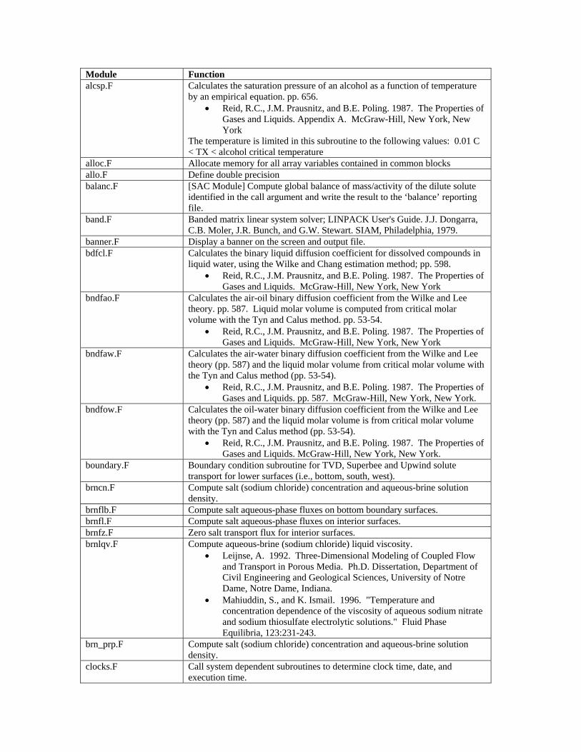
Each operational mode of the STOMP simulator comprises global and mode dependent subroutines. Global subroutines are those subroutines that are generally included in more than one operational mode. Mode dependent subroutines, however, are associated with a single operational mode. Subroutine names are generally descriptive abbreviations. These abbreviations frequently contain the letters G, L, or N, which respectively correspond to the gas, aqueous, or NAPL phases. Other common letters are A, C, O, and W, which represent air, carbon dioxide, aqueous, and water compositions, respectively. The letter T refers to solute transport, the letter E to energy equations (thermal transport). Mode dependent subroutines include a numerical suffix, which corresponds to the operational mode. The full set of subroutines available for STOMP is listed in Table 1, along with a brief description of the function or purpose of each module.

Table 1 STOMP Code Modules Module Function adsorp.F Compute the solid-liquid adsorption factor advbb.F Computes the average Darcy velocity on a boundary bottom surface advb.F Computes the average Darcy velocity on the bottom surface airdfl.F Calculates binary liquid diffusion coefficient for air in liquid water, using the

Wilke and Chang estimation method; pp. 598 • Reid, R.C., J.M. Prausnitz, and B.E. Poling. 1987. The Properties of

Gases and Liquids. McGraw-Hill, New York, New York airgsd.F Calculates component density of air with the ideal gas equation of state airgsh.F Calculate the specific enthalpy and internal energy of air as a function of

temperature and air partial pressure with a reference state of enthalpy at 0 C. Calculate the isobaric specific heat as a function of temperature from an empirical relation. pp. 580. (Sandler). Calculate the specific enthalpy by integrating the isobaric specific heat using a two-point Gaussian quadrature method. pp. 101-105. (Carnahan et al.)

• Carnahan, B., H.A. Luther, and J.O. Wilkes. 1969. Applied Numerical Methods. John Wiley and Sons Inc., New York.

• Sandler, S.I. 1989. Chemical and Engineering Thermodynamics. John Wiley and Sons, Inc., New York.

airgsv.F Calculate the air viscosity from the kinetic theory. pp. 528-530. • Hirschfelder, J.O., C.F. Curtiss, and R.B. Bird. 1954. Molecular

Theory of Gases and Liquids. John Wiley & Sons. alclqd.F Calculate the saturated volatile organic compound liquid density as a function

of temperature with a modified Rackett technique. Calculate the compressed volatile organic compound liquid density as a function of temperature and pressure following the Hankinson-Brobst-Thomson technique. pp 66-67.

• Reid, R.C., J.M. Prausnitz, and B.E. Poling. 1987. The Properties of Gases and Liquids. McGraw-Hill, New York, New York

The temperature is limited in this subroutine to the following values: 0.01 C < TX < alcohol critical temperature

Module Function alcsp.F Calculates the saturation pressure of an alcohol as a function of temperature

by an empirical equation. pp. 656. • Reid, R.C., J.M. Prausnitz, and B.E. Poling. 1987. The Properties of

Gases and Liquids. Appendix A. McGraw-Hill, New York, New York

The temperature is limited in this subroutine to the following values: 0.01 C < TX < alcohol critical temperature

alloc.F Allocate memory for all array variables contained in common blocks allo.F Define double precision balanc.F [SAC Module] Compute global balance of mass/activity of the dilute solute

identified in the call argument and write the result to the ‘balance’ reporting file.

band.F Banded matrix linear system solver; LINPACK User's Guide. J.J. Dongarra, C.B. Moler, J.R. Bunch, and G.W. Stewart. SIAM, Philadelphia, 1979.

banner.F Display a banner on the screen and output file. bdfcl.F Calculates the binary liquid diffusion coefficient for dissolved compounds in

liquid water, using the Wilke and Chang estimation method; pp. 598. • Reid, R.C., J.M. Prausnitz, and B.E. Poling. 1987. The Properties of

Gases and Liquids. McGraw-Hill, New York, New York bndfao.F Calculates the air-oil binary diffusion coefficient from the Wilke and Lee

theory. pp. 587. Liquid molar volume is computed from critical molar volume with the Tyn and Calus method. pp. 53-54.


bndfaw.F Calculates the air-water binary diffusion coefficient from the Wilke and Lee theory (pp. 587) and the liquid molar volume from critical molar volume with the Tyn and Calus method (pp. 53-54).

• Reid, R.C., J.M. Prausnitz, and B.E. Poling. 1987. The Properties of Gases and Liquids. pp. 587. McGraw-Hill, New York, New York.

bndfow.F Calculates the oil-water binary diffusion coefficient from the Wilke and Lee theory (pp. 587) and the liquid molar volume is from critical molar volume with the Tyn and Calus method (pp. 53-54).

• Reid, R.C., J.M. Prausnitz, and B.E. Poling. 1987. The Properties of Gases and Liquids. McGraw-Hill, New York, New York.

boundary.F Boundary condition subroutine for TVD, Superbee and Upwind solute transport for lower surfaces (i.e., bottom, south, west).

brncn.F Compute salt (sodium chloride) concentration and aqueous-brine solution density.

brnflb.F Compute salt aqueous-phase fluxes on bottom boundary surfaces. brnfl.F Compute salt aqueous-phase fluxes on interior surfaces. brnfz.F Zero salt transport flux for interior surfaces. brnlqv.F Compute aqueous-brine (sodium chloride) liquid viscosity.

• Leijnse, A. 1992. Three-Dimensional Modeling of Coupled Flow and Transport in Porous Media. Ph.D. Dissertation, Department of Civil Engineering and Geological Sciences, University of Notre Dame, Notre Dame, Indiana.

• Mahiuddin, S., and K. Ismail. 1996. "Temperature and concentration dependence of the viscosity of aqueous sodium nitrate and sodium thiosulfate electrolytic solutions." Fluid Phase Equilibria, 123:231-243.

brn_prp.F Compute salt (sodium chloride) concentration and aqueous-brine solution density.

clocks.F Call system dependent subroutines to determine clock time, date, and execution time.

Module Function crntnb.F Compute the local maximum Courant numbers. dbgbfa.F Double precision, gaussian elimination, banded matrix factorization.

• LINPACK User's Guide. J.J. Dongarra, C.B. Moler, J.R. Bunch, and G.W. Stewart. SIAM, Philadelphia, 1979.

dbgbsl.F Double precision, gaussian elimination, banded matrix solver. • LINPACK User's Guide. J.J. Dongarra, C.B. Moler, J.R. Bunch, and

G.W. Stewart. SIAM, Philadelphia, 1979. ddfgob.F Compute advective, diffusive-dispersive oil gas fluxes on bottom boundary

surfaces. ddfgo.F Compute advective, diffusive-dispersive oil gas fluxes on interior surfaces. ddflob.F Compute dissolved VOC fluxes on bottom boundary surfaces. ddflo.F Compute dissolved oil fluxes on interior surfaces. dff_36.F Compute diffusive CO2 gas fluxes on interior surfaces. dffgab.F Compute CO2 mole diffusion rates on a bottom boundary. dffga.F Compute diffusive air or CO2 gas fluxes on interior surfaces. dffgob.F Compute VOC vapor mole diffusion rates on a bottom boundary. dffgo.F Compute diffusive oil gas fluxes on interior surfaces. dffgwb.F Compute water vapor mole diffusion rates on a bottom boundary. dffgw.F Compute water vapor mole diffusion rates. dfflab.F Compute dissolved air mole diffusion rates on a bottom boundary. dffla.F Compute dissolved air molar diffusion rates through the aqueous phase. dfflob.F Compute VOC vapor mole diffusion rates on a bottom boundary. dfflo.F Compute dissolved oil fluxes on interior surfaces. dfflsb.F Compute salt aqueous-phase fluxes on bottom boundary surfaces. dffls.F Compute salt aqueous-phase fluxes on interior surfaces. dffnab.F Compute water-NAPL mole diffusion rates on a bottom boundary. dffna.F Compute dissolved water molar diffusion rates through the NAPL. dffnwb.F Compute water-NAPL mole diffusion rates on a bottom boundary. dffnw.F Compute dissolved water molar diffusion rates through the NAPL. difmn.F Computes interfacial averages. drcv_36.F Compute the gas-phase Darcy flux from pressure gradients and gravitational

body forces. drcvgb.F Compute the gas-phase Darcy flux from pressure gradients and gravitational

body forces on a bottom boundary. drcvg.F Compute the gas-phase Darcy flux from pressure gradients and gravitational

body forces. drcvlb.F Compute the aqueous-phase Darcy flux from pressure gradients and

gravitational body forces on a bottom boundary. drcvl.F Compute the aqueous-phase Darcy flux from pressure gradients and

gravitational body forces. drcvnb.F Compute the NAPL Darcy flux from pressure gradients and gravitational

body forces on a bottom boundary. drcvn.F Compute the NAPL Darcy flux from pressure gradients and gravitational

body forces. eckechem.F Back step.

Module Function eos_33.F H2O-NaCl-CO2 Equation of state. This subroutine calculates the bubbling

pressure of CO2 dissolved in an aqueous solution of CO2 and NaCl, as a function of temperature, dissolved CO2 mole fraction and dissolved NaCl mole fraction. Newton iteration is used to resolve the equation nonlinearities. The temperature and salt concentration dependence on Henry's coefficient is computed external to this routine.

• Reid, R.C., J.M. Prausnitz, and B.E. Poling. 1987. The Properties of Gases and Liquids. McGraw-Hill, New York, New York. pp: 332-337.

• Anderson, G.M., and D.A. Crerar. 1992. Thermodynamics in Geochemistry: The Equilibrium Model, Oxford University Press.

eos_35.F H2O-NaCl-CO2 Equation of state. This subroutine calculates the bubbling pressure of CO2 dissolved in an aqueous solution of CO2 and NaCl, as a function of temperature, dissolved CO2 mole fraction and dissolved NaCl mole fraction. Newton iteration is used to resolve the equation nonlinearities. The temperature and salt concentration dependence on Henry's coefficient is computed external to this routine.

• Reid, R.C., J.M. Prausnitz, and B.E. Poling. 1987. The Properties of Gases and Liquids. McGraw-Hill, New York, New York. pp: 332-337.

• Anderson, G.M., and D.A. Crerar. 1992. Thermodynamics in Geochemistry: The Equilibrium Model, Oxford University Press.

eos_36.F Activity coefficient of water in aqueous phase. • Vanderbeken, I., S. Ye, B. Bouyssiere, H. Carrier, and P. Xans.

1999. "Ability of the MHV2 mixing rule to describe the effect of salt on gas solubility in brines at high temperature and high pressure. High Temperatures - High Pressures, 31:653-663.

flsh_35.F Total-liquid unsaturated w/ CO2 vapor pressure and salt aqueous concentration specified. Flash from gas pressure, aqueous pressure, temperature, CO2 vapor pressure and salt aqueous concentration.

flsh_36.F Compute dissolved-salt, -CO2, and -CH4 aqueous mass fractions and CO2 and CH4 hydrate mass fractions (for hydrate conditions) from dissolved-salt aqueous concentration, hydrate saturation, and total-CH4 mass fraction of hydrate formers.

fnhgbg.F Gas hydraulic gradient boundary condition function. fnhgbl.F Aqueous hydraulic gradient boundary condition function. fnhgbls.F Brine hydraulic gradient boundary condition function. fnhgbn.F NAPL hydraulic gradient boundary condition function. fnitp.F Linear interpolation function. fntblx.F Linearly interpolate from a table of values. fntbly.F Linearly interpolate from a table of values. frac.F Converts between mole and mass fractions. fsplnx.F Given arrays TBLY and TBLX containing a tabulated function (i.e., x(n) =

f(y(n))), with y(1) < y(2) < ... < y(n), and given the array TBLDDX, which is output from subroutine SPLINE, and given a value of FY this function returns a cubic spline interpolated value.

fsplny.F Given arrays TBLX and TBLY containing a tabulated function (i.e., y(n) = f(x(n))), with x(1) < x(2) < ... < x(n), and given the array TBLDDY, which is output from subroutine SPLINE, and given a value of FX this function returns a cubic spline interpolated value.

gasvis.F Calculate the gas viscosity using an extension of the Chapman-Enskog theory for multicomponent gas mixtures at low density (pp. 528-530).

• Hirschfelder, J.O., C.F. Curtiss, and R.B. Bird. 1954. Molecular Theory of Gases and Liquids. John Wiley & Sons.

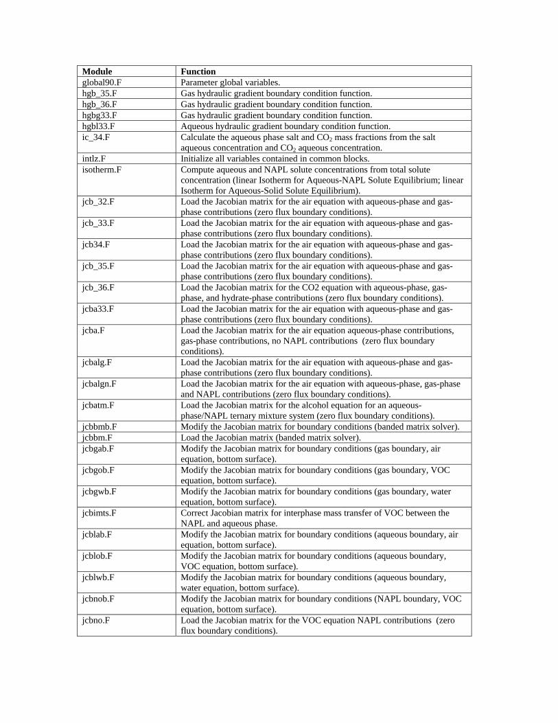
Module Function global90.F Parameter global variables. hgb_35.F Gas hydraulic gradient boundary condition function. hgb_36.F Gas hydraulic gradient boundary condition function. hgbg33.F Gas hydraulic gradient boundary condition function. hgbl33.F Aqueous hydraulic gradient boundary condition function. ic_34.F Calculate the aqueous phase salt and CO2 mass fractions from the salt

aqueous concentration and CO2 aqueous concentration. intlz.F Initialize all variables contained in common blocks. isotherm.F Compute aqueous and NAPL solute concentrations from total solute

concentration (linear Isotherm for Aqueous-NAPL Solute Equilibrium; linear Isotherm for Aqueous-Solid Solute Equilibrium).

jcb_32.F Load the Jacobian matrix for the air equation with aqueous-phase and gas-phase contributions (zero flux boundary conditions).


jcb34.F Load the Jacobian matrix for the air equation with aqueous-phase and gas-phase contributions (zero flux boundary conditions).


jcb_36.F Load the Jacobian matrix for the CO2 equation with aqueous-phase, gas-phase, and hydrate-phase contributions (zero flux boundary conditions).

jcba33.F Load the Jacobian matrix for the air equation with aqueous-phase and gas-phase contributions (zero flux boundary conditions).

jcba.F Load the Jacobian matrix for the air equation aqueous-phase contributions, gas-phase contributions, no NAPL contributions (zero flux boundary conditions).

jcbalg.F Load the Jacobian matrix for the air equation with aqueous-phase and gas-phase contributions (zero flux boundary conditions).

jcbalgn.F Load the Jacobian matrix for the air equation with aqueous-phase, gas-phase and NAPL contributions (zero flux boundary conditions).

jcbatm.F Load the Jacobian matrix for the alcohol equation for an aqueous-phase/NAPL ternary mixture system (zero flux boundary conditions).

jcbbmb.F Modify the Jacobian matrix for boundary conditions (banded matrix solver). jcbbm.F Load the Jacobian matrix (banded matrix solver). jcbgab.F Modify the Jacobian matrix for boundary conditions (gas boundary, air

equation, bottom surface). jcbgob.F Modify the Jacobian matrix for boundary conditions (gas boundary, VOC

equation, bottom surface). jcbgwb.F Modify the Jacobian matrix for boundary conditions (gas boundary, water

equation, bottom surface). jcbimts.F Correct Jacobian matrix for interphase mass transfer of VOC between the

NAPL and aqueous phase. jcblab.F Modify the Jacobian matrix for boundary conditions (aqueous boundary, air

equation, bottom surface). jcblob.F Modify the Jacobian matrix for boundary conditions (aqueous boundary,

VOC equation, bottom surface). jcblwb.F Modify the Jacobian matrix for boundary conditions (aqueous boundary,

water equation, bottom surface). jcbnob.F Modify the Jacobian matrix for boundary conditions (NAPL boundary, VOC

equation, bottom surface). jcbno.F Load the Jacobian matrix for the VOC equation NAPL contributions (zero

flux boundary conditions).

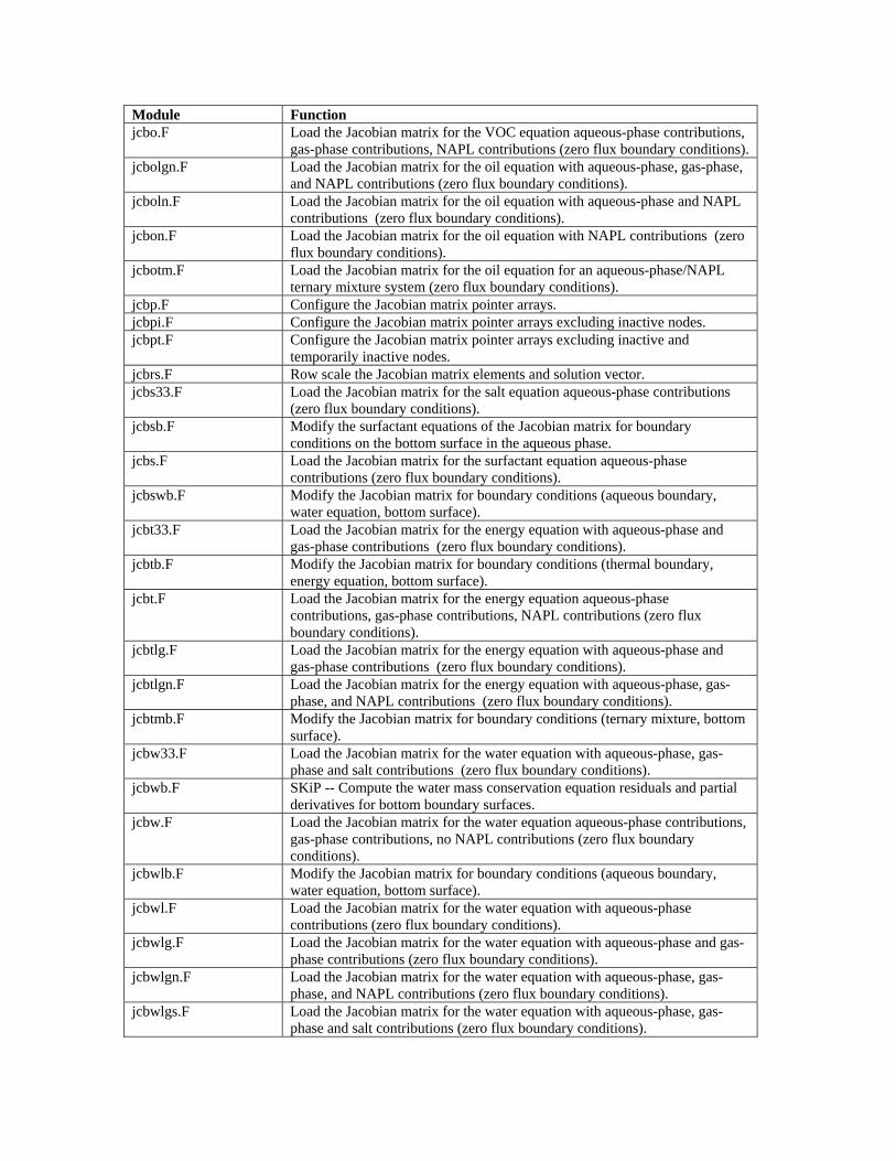
Module Function jcbo.F Load the Jacobian matrix for the VOC equation aqueous-phase contributions,

gas-phase contributions, NAPL contributions (zero flux boundary conditions). jcbolgn.F Load the Jacobian matrix for the oil equation with aqueous-phase, gas-phase,

and NAPL contributions (zero flux boundary conditions). jcboln.F Load the Jacobian matrix for the oil equation with aqueous-phase and NAPL

contributions (zero flux boundary conditions). jcbon.F Load the Jacobian matrix for the oil equation with NAPL contributions (zero

flux boundary conditions). jcbotm.F Load the Jacobian matrix for the oil equation for an aqueous-phase/NAPL

ternary mixture system (zero flux boundary conditions). jcbp.F Configure the Jacobian matrix pointer arrays. jcbpi.F Configure the Jacobian matrix pointer arrays excluding inactive nodes. jcbpt.F Configure the Jacobian matrix pointer arrays excluding inactive and

temporarily inactive nodes. jcbrs.F Row scale the Jacobian matrix elements and solution vector. jcbs33.F Load the Jacobian matrix for the salt equation aqueous-phase contributions

(zero flux boundary conditions). jcbsb.F Modify the surfactant equations of the Jacobian matrix for boundary

conditions on the bottom surface in the aqueous phase. jcbs.F Load the Jacobian matrix for the surfactant equation aqueous-phase

contributions (zero flux boundary conditions). jcbswb.F Modify the Jacobian matrix for boundary conditions (aqueous boundary,

water equation, bottom surface). jcbt33.F Load the Jacobian matrix for the energy equation with aqueous-phase and

gas-phase contributions (zero flux boundary conditions). jcbtb.F Modify the Jacobian matrix for boundary conditions (thermal boundary,

energy equation, bottom surface). jcbt.F Load the Jacobian matrix for the energy equation aqueous-phase

contributions, gas-phase contributions, NAPL contributions (zero flux boundary conditions).

jcbtlg.F Load the Jacobian matrix for the energy equation with aqueous-phase and gas-phase contributions (zero flux boundary conditions).

jcbtlgn.F Load the Jacobian matrix for the energy equation with aqueous-phase, gas-phase, and NAPL contributions (zero flux boundary conditions).

jcbtmb.F Modify the Jacobian matrix for boundary conditions (ternary mixture, bottom surface).

jcbw33.F Load the Jacobian matrix for the water equation with aqueous-phase, gas-phase and salt contributions (zero flux boundary conditions).

jcbwb.F SKiP -- Compute the water mass conservation equation residuals and partial derivatives for bottom boundary surfaces.

jcbw.F Load the Jacobian matrix for the water equation aqueous-phase contributions, gas-phase contributions, no NAPL contributions (zero flux boundary conditions).

jcbwlb.F Modify the Jacobian matrix for boundary conditions (aqueous boundary, water equation, bottom surface).

jcbwl.F Load the Jacobian matrix for the water equation with aqueous-phase contributions (zero flux boundary conditions).

jcbwlg.F Load the Jacobian matrix for the water equation with aqueous-phase and gas-phase contributions (zero flux boundary conditions).

jcbwlgn.F Load the Jacobian matrix for the water equation with aqueous-phase, gas-phase, and NAPL contributions (zero flux boundary conditions).

jcbwlgs.F Load the Jacobian matrix for the water equation with aqueous-phase, gas-phase and salt contributions (zero flux boundary conditions).

Module Function jcbwln.F Load the Jacobian matrix for the water equation with aqueous-phase, gas-

phase, and NAPL contributions (zero flux boundary conditions). jcbwlns.F Load the Jacobian matrix for the water equation with aqueous-phase, NAPL,

and salt contributions (zero flux boundary conditions). jcbwls.F Load the Jacobian matrix for the water equation with aqueous-phase and salt

contributions (zero flux boundary conditions). jcbwtm.F Load the Jacobian matrix for the water equation for an aqueous-phase/NAPL

ternary mixture system (zero flux boundary conditions). jcbz.F Zero the Jacobian matrix elements and solution vector. jctlgb.F (Water-Air-Energy-VOC Transport Mode) Modify the VOC transport

Jacobian matrix for boundary conditions. jctlg.F Load the Jacobian matrix for the VOC transport equation aqueous-phase

contributions, gas-phase contributions, no NAPL contributions (zero flux boundary conditions).

lcase.F Convert all upper-case characters in a variable-length string variable to lower case. This subroutine does not disturb non-alphabetic characters; only capital letters (ASCII 65 through 90) are modified.

masfrc.F Calculates mass fractions from mole fractions. molfrc.F Calculates mole fractions from mass fractions. mx_lqd.F Calculate the liquid density of a liquid mixture based on mass fraction

weighting. mx_lqv.F Calculate the liquid viscosity of a liquid mixture following the method of

corresponding states formulated by Teja and Rice (pp. 479-481). Reference:


pnspcg.F Calling routine for the NSPCG (Nonsymmetric Preconditioned Conjugate Gradient) solver for large sparse linear systems by various iterative methods. Reference:

• NSPCG User's Guide, Version 1.0. T. C. Oppe, W. D. Joubert, D. R. Kincaid. Center for Numerical Analysis, The University of Texas at Austin. April, 1988.

porsty.F Compute diffusive and total porosities. psplib.F Calling routine for the SPLIB: A Library of Iterative Methods for Sparse

Linear Systems. Reference:

• Randall Bramley and Xiaoge Wang, Department of Computer Science, Indiana University – Bloomington, December 18, 1995

pumfpk.F Calling routine for the UMFPACK Version 2.0, Unsymmetric-pattern Multifrontal Package for solving systems of sparse linear systems, Ax=b; where A is sparse and can be unsymmetric. Reference:

• Timothy A. Davis and Iain S. Duff, Copyright (C) 1995. September 13, 1995.

rdalchl.F Read input file for alcohol compound information. rdatmos.F Read input file for atmospheric conditions. rdbala.F [SAC Module] Read input file for global balance check times information. rdchr.F Fill character string ADUM with characters between commas. Return 'null'

for null entries. rddpr.F Fill double precision variable VAR with data between commas. Return

default value or zero for null entries. rdgrid.F Read input file for grid geometry information. Compute geometric length,

area, and volume parameters. rdgrp.F Read input file for rock/soil gas relative permeability function information.

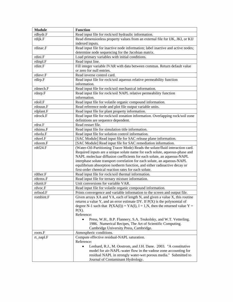
Module Function rdhydr.F Read input file for rock/soil hydraulic information. rdijk.F Read dimensionless property values from an external file for IJK, JKI, or KIJ

indexed inputs. rdinac.F Read input file for inactive node information; label inactive and active nodes;

determine node sequencing for the Jacobian matrix. rdini.F Load primary variables with initial conditions. rdinpl.F Read input line. rdint.F Fill integer variable IVAR with data between commas. Return default value

or zero for null entries. rdinvr.F Read inverse control card. rdlrp.F Read input file for rock/soil aqueous relative permeability function

information. rdmech.F Read input file for rock/soil mechanical information. rdnrp.F Read input file for rock/soil NAPL relative permeability function

information. rdoil.F Read input file for volatile organic compound information. rdouun.F Read reference node and plot file output variable units. rdplant.F Read input file for plant property information. rdrock.F Read input file for rock/soil zonation information. Overlapping rock/soil zone

definitions are sequence dependent. rdrst.F Read restart file. rdsimu.F Read input file for simulation title information. rdsolu.F Read input file for solution control information. rdsrel.F [SAC Module] Read input file for SAC release plane information. rdsrem.F [SAC Module] Read input file for SAC remediation information. rdtf24.F (Water-Oil-Partitioning Tracer Mode) Reads the solute/fluid interaction card.

Required inputs are a unique solute name for each solute, aqueous-phase and NAPL molecluar diffusion coefficients for each solute, an aqueous-NAPL interphase solute transport correlation for each solute, an aqueous-NAPL equilibrium absorption isotherm function, and either radioactive decay or first-order chemical reaction rates for each solute.

rdther.F Read input file for rock/soil thermal information. rdtrmx.F Read input file for ternary mixture information. rdunit.F Unit conversions for variable VAR. rdvoc.F Read input file for volatile organic compound information. refnod.F Prints convergence and variable information to the screen and output file. rombint.F Given arrays XA and YA, each of length N, and given a value X, this routine

returns a value Y, and an error estimate DY. If P(X) is the polynomial of degree N-1 such that P(XA(I)) = YA(I), I = 1,N, then the returned value Y = P(X). Reference:

• Press, W.H., B.P. Flannery, S.A. Teukolsky, and W.T. Vetterling. 1986. Numerical Recipes, The Art of Scientific Computing. Cambridge University Press, Cambridge.

roots.F Atmospheric conditions. rt_napl.F Compute effective residual-NAPL saturation.

Reference: • Lenhard, R.J., M. Oostrom, and J.H. Dane. 2003. "A constitutive

model for air-NAPL-water flow in the vadose zone accounting for residual NAPL in strongly water-wet porous media." Submitted to Journal of Contaminant Hydrology.

Module Function sacout.F [SAC Module] This subroutine is used whenever STOMP ends a simulation

before the simulation time is over; i.e., when a time step maximum is exceeded, a run time maximum is exceeded, or a time step reduction limit (non-convergence) is exceeded. This subroutine finishes writing the 'balance', 'release', and 'remediate' files.

sacrem.F [SAC Module] Computes mass or activity remediated in a SAC remediation event and call another subroutine to report this quantity to a remediation transfer file. Concentration of the dilute solute is reduced in nodes subject to remediation in accordance with the remediation description.

saczip.F [SAC Module] check if there is effectively zero analyte source for the simulation, and if so, writes a single zero-release to the 'release' file and then terminates the program without full transport simulation to improve overall SAC execution efficiency.

sfcflb.F Compute surfactant aqueous-phase fluxes on bottom boundary surfaces. sfcfl.F Compute surfactant aqueous-phase fluxes on interior surfaces. sfcfz.F Zero surfactant transport flux for interior surfaces. sfcscf.F Interfacial tension scaling factors for surfactant solutions. sfcsol.F Dissolved VOC solubility in surfactant solution. sfin.F Surface flux and source term integrator. sft_mix.F (Water-Oil-Alcohol Mode) Compute the gas-aqueous, gas-NAPL and NAPL-

aqueous interfacial surface tensions. This subroutine assumes equilibrium conditions between the aqueous, NAPL and gas phase component concentrations and follows the formulation by Reitsma and Kueper. Reference:

• Reitsma, S. and B.H. Kueper. "Non-equilibrium alcohol flooding model for immiscible phase remediation: 1. Equation development." Advances in Water Resources, Vol. 21, No. 8, pp. 649-662, 1998.

sfxb32.F Compute solute aqueous-phase fluxes on boundary surfaces. sfxgb.F Compute solute gas-phase fluxes on boundary surfaces. sfxg.F Compute solute transport flux gas-phase, excluding boundaries. sfxglb.F Compute solute gas-phase fluxes on boundary surfaces. sfxlb.F Compute solute aqueous-phase fluxes on boundary surfaces. sfxl.F Compute solute transport flux aqueous-phase, excluding boundaries, using

either a Patankar scheme or a TVD scheme with third-order Leonard limiting for the advective transport component.

sfxnb.F Compute solute NAPL fluxes on boundary surfaces. sfxn.F Compute solute transport flux NAPL-phase, excluding boundaries. sfxz.F Zero solute transport flux. shdp.F Subroutine computes hydrodynamic dispersion coefficients for the aqueous

and gas phases from phase velocities and user- specified dispersivities. shdpg.F Calculates hydrodynamic dispersion coefficients for the gas phase from phase

velocities and user-specified dispersivities. shdpl.F Calculates hydrodynamic dispersion coefficients for the aqueous phase from

phase velocities and user-specified dispersivities. shdpn.F Calculates hydrodynamic dispersion coefficients for the NAPL phase from

phase velocities and user-specified dispersivities. sjcbg.F Loads the matrix elements and solution vector for the gas-phase convective-

dispersive mass transport equation. The Jacobian matrix is initially configured assuming zero-flux boundary conditions. The matrix is then updated for other user-specified boundary conditions.

sjcbl.F Loads the matrix elements and solution vector for the aqueous-phase convective-dispersive mass transport equation. The Jacobian matrix is initially configured assuming zero-flux boundary conditions. The matrix is then updated for other user-specified boundary conditions.

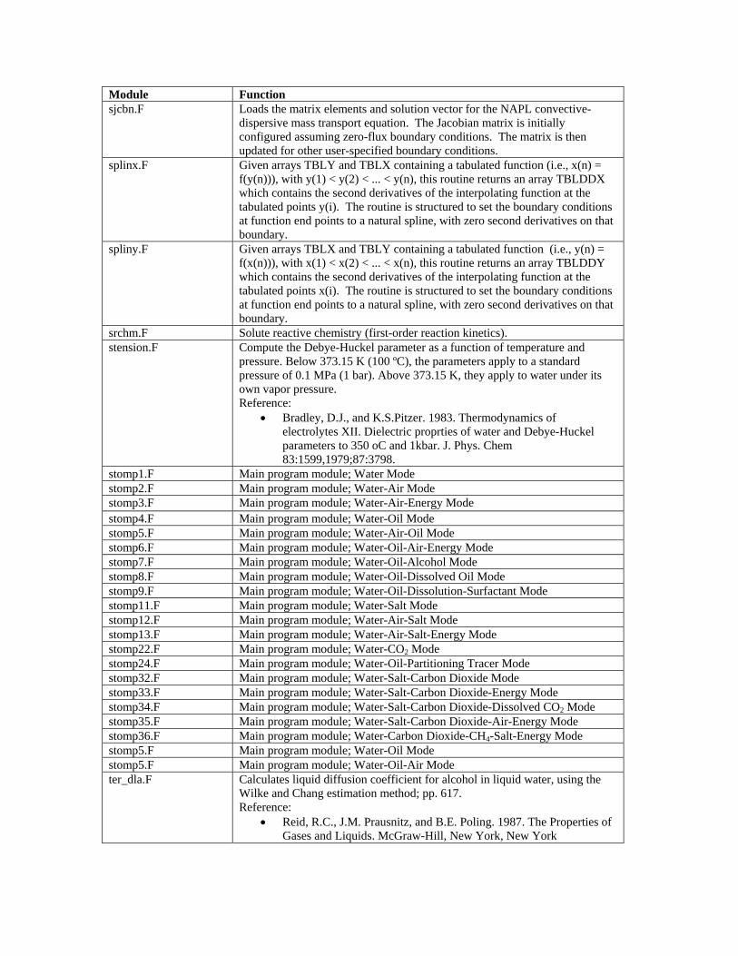
Module Function sjcbn.F Loads the matrix elements and solution vector for the NAPL convective-

dispersive mass transport equation. The Jacobian matrix is initially configured assuming zero-flux boundary conditions. The matrix is then updated for other user-specified boundary conditions.

splinx.F Given arrays TBLY and TBLX containing a tabulated function (i.e., x(n) = f(y(n))), with y(1) < y(2) < ... < y(n), this routine returns an array TBLDDX which contains the second derivatives of the interpolating function at the tabulated points y(i). The routine is structured to set the boundary conditions at function end points to a natural spline, with zero second derivatives on that boundary.

spliny.F Given arrays TBLX and TBLY containing a tabulated function (i.e., y(n) = f(x(n))), with x(1) < x(2) < ... < x(n), this routine returns an array TBLDDY which contains the second derivatives of the interpolating function at the tabulated points x(i). The routine is structured to set the boundary conditions at function end points to a natural spline, with zero second derivatives on that boundary.

srchm.F Solute reactive chemistry (first-order reaction kinetics). stension.F Compute the Debye-Huckel parameter as a function of temperature and

pressure. Below 373.15 K (100 ºC), the parameters apply to a standard pressure of 0.1 MPa (1 bar). Above 373.15 K, they apply to water under its own vapor pressure. Reference:

• Bradley, D.J., and K.S.Pitzer. 1983. Thermodynamics of electrolytes XII. Dielectric proprties of water and Debye-Huckel parameters to 350 oC and 1kbar. J. Phys. Chem 83:1599,1979;87:3798.

stomp1.F Main program module; Water Mode stomp2.F Main program module; Water-Air Mode stomp3.F Main program module; Water-Air-Energy Mode stomp4.F Main program module; Water-Oil Mode stomp5.F Main program module; Water-Air-Oil Mode stomp6.F Main program module; Water-Oil-Air-Energy Mode stomp7.F Main program module; Water-Oil-Alcohol Mode stomp8.F Main program module; Water-Oil-Dissolved Oil Mode stomp9.F Main program module; Water-Oil-Dissolution-Surfactant Mode stomp11.F Main program module; Water-Salt Mode stomp12.F Main program module; Water-Air-Salt Mode stomp13.F Main program module; Water-Air-Salt-Energy Mode stomp22.F Main program module; Water-CO2 Mode stomp24.F Main program module; Water-Oil-Partitioning Tracer Mode stomp32.F Main program module; Water-Salt-Carbon Dioxide Mode stomp33.F Main program module; Water-Salt-Carbon Dioxide-Energy Mode stomp34.F Main program module; Water-Salt-Carbon Dioxide-Dissolved CO2 Mode stomp35.F Main program module; Water-Salt-Carbon Dioxide-Air-Energy Mode stomp36.F Main program module; Water-Carbon Dioxide-CH4-Salt-Energy Mode stomp5.F Main program module; Water-Oil Mode stomp5.F Main program module; Water-Oil-Air Mode ter_dla.F Calculates liquid diffusion coefficient for alcohol in liquid water, using the

Wilke and Chang estimation method; pp. 617. Reference:


Module Function ter_dlo.F Calculates liquid diffusion coefficient for oil in liquid water, using the Wilke

and Chang estimation method; pp. 617. Reference:


ter_dna.F Calculates liquid diffusion coefficient for alcohol in NAPL, using a modification to the Wilke and Chang estimation method, Reddy-Doraiswamy correlation. Reference:


ter_dnw.F Calculates liquid diffusion coefficient for water in NAPL, using a modification to the Wilke and Chang estimation method, Reddy-Doraiswamy correlation. Reference:


ter_mix.F Compute the component distributions for a ternary mixture. thd_33.F Compute the contribution to the energy flux by thermal conduction for non-

boundary node faces. thd_35.F Compute the contribution to the energy flux by thermal conduction for non-

boundary node faces. thd_36.F Compute the contribution to the energy flux by thermal conduction for non-

boundary node faces. thdgb.F Compute the contribution to the energy flux by water vapor, VOC vapor, and

air molecular diffusion on a bottom boundary thdg.F Compute the contribution to the energy flux by water vapor, VOC vapor, and

air molecular diffusion for non-boundary node faces. Donor cell interfacial averaging.

thdgwb.F Compute the contribution to the energy flux by water vapor, and air molecular diffusion on a bottom boundary

thdgw.F Compute the contribution to the energy flux by water vapor, and air molecular diffusion for non-boundary node faces. Donor cell interfacial averaging.

thke.F Calculate equivalent thermal conductivity. thmagb.F Compute the contribution to the energy flux by gas advection on a bottom

boundary thmag.F Compute the contribution to the energy flux by gas advection for non-

boundary node faces. Donor cell interfacial averaging. thmalb.F Compute the contribution to the energy flux by aqueous advection on a

bottom boundary thmal.F Compute the contribution to the energy flux by aqueous advection for non-

boundary node faces. Donor cell interfacial averaging. thmanb.F Compute the contribution to the energy flux by NAPL advection on a bottom

boundary thman.F Compute the contribution to the energy flux by NAPL advection for non-

boundary node faces. Donor cell interfacial averaging. thmdb.F Compute the contribution to the energy flux by thermal conduction on a

bottom boundary. thmd.F Compute the contribution to the energy flux by thermal conduction for non-

boundary node faces. tmstep.F Compute the time step based on the previous time step, the acceleration

factor, the maximum time step, the time until the next print, and the time until the next start of a boundary condition.

Module Function tortu.F Compute phase tortuosity. updtc.F Updates concentrations. vflgb.F Water-Air-Energy-VOC Transport mode; compute VOC transport fluxes on

boundary surfaces. vflg.F Compute VOC transport fluxes, gas-phase diffusion, aqueous-phase

advection, gas-phase advection, (zero flux boundary conditions). vocdfg.F Calculates VOC diffusion coefficient by the Wilke method (pp. 34).

Reference: • Falta, R.W., K. Pruess, I. Javandel, and P.A. Witherspoon. 1990.

Numerical Modeling of Steam Injection for the Removal of Nonaqueous Phase Liquids from the Subsurface: 1 Numerical Formulation. LBL-29615, Lawrence Berkeley Laboratory.

vocdfl.F Calculate binary liquid diffusion coefficient for VOC in liquid water, using the Wilke and Chang estimation method (pp. 598). Reference:


vocgsd.F Calculates either: • vapor component density of an volatile organic compound with the

ideal gas law equation of state, -OR- • calculates component density of an volatile organic compound with

van der Waals equation of state using an iterative solution (pp. 43) Reference:


vocgsh.F Calculate: • the enthalpy and internal energy of VOC vapor as a function of

temperature and pressure with a reference state of liquid VOC at 0 C • the enthalpy as the sum of the liquid enthalpy and heat of

vaporization • the heat of vaporization at the normal boiling point with a method by

Chen (pp. 226) • the heat of vaporization as a function of temperature with the

Watson relation and the Viswanath and Kuloor extention (pp. 228) Reference:


vocgsv.F Calculate component viscosity of a volatile organic compound vapor with the corresponding states method (pp 397, Reid et al. 1987). Reference:


voclqd.F Calculate: • the saturated volatile organic compound liquid density as a function

of temperature with a modified Rackett technique. • the compressed volatile organic compound liquid density as a

function of temperature and pressure following the Hankinson-Brobst-Thomson technique (pp 66-67).

Reference: • Reid, R.C., J.M. Prausnitz, and B.E. Poling. 1987. The Properties of

Gases and Liquids. McGraw-Hill, New York, New York

Module Function voclqh.F Calculate:

• the liquid VOC enthalpy as a function of temperature with a reference state of liquid VOC at 0 C;

• the ideal gas isobaric specific heat from empirical coefficients (pp. 657, Reid et al.)

• the specific heat for liquid VOC from the ideal gas molar specific heat using the corresponding states method (pp. 140, Reid et al.)

• the liquid VOC enthalpy by integrating the specific heat for liquid VOC from a reference temperature of 0 C, with a two-point Gauss-Legendre quadrature method (pp. 101-105, Carnahan et al.).

References: • Carnahan, B., H.A. Luther, and J.O. Wilkes. 1969. Applied

Numerical Methods. John Wiley and Sons Inc., New York. • Reid, R.C., J.M. Prausnitz, and B.E. Poling. 1987. The Properties of

Gases and Liquids. McGraw-Hill, New York. voclqk.F Calculate the liquid VOC thermal conductivity by the method of Sato and

Riedel. • Reid, R.C., J.M. Prausnitz, and B.E. Poling. 1987. The Properties of

Gases and Liquids. pp 550. McGraw-Hill, New York, New York voclqv.F Calculate the saturated volatile organic compound liquid viscosity as a

function of temperature, with the Lewis and Squires liquid viscosity-temperature correlation or with empirical equations. pp 441- 445.


vocsp.F Calculates the saturation pressure of an organic vapor as a function of temperature by an empirical equation (pp. 656).

• Reid, R.C., J.M. Prausnitz, and B.E. Poling. 1987. The Properties of Gases and Liquids. Appendix A. McGraw-Hill, New York, New York

vplwr.F Compute vapor pressuring lowering. watdfg.F Calculate water diffusion coefficient by the Wilke method. pp. 34.

• Falta, R.W., K. Pruess, I. Javandel, and P.A. Witherspoon. 1990. Numerical Modeling of Steam Injection for the Removal of Nonaqueous Phase Liquids from the Subsurface: 1 Numerical Formulation. LBL-29615, Lawrence Berkeley Laboratory.

watgsd.F Calculate the water vapor component density with the ideal gas law equation of state –OR- calculate the water vapor component density, as a function of temperature and pressure per the steam table equations as given by the 1967 International Formulation Committee: Formulation for Industrial Use.

• Thermodynamic and Transport Properties of Steam. 1967. ASME Steam Tables. The American Society of Mechanical Engineers. United Engineering Center, 345 East 47th Street, New York, N.Y.

watgsh.F Calculate the water vapor enthalpy and internal energy, as a function of temperature and pressure per the steam table equations as given by the 1967 International Formulation Committee: Formulation for Industrial Use.


watgsv.F Calculates component viscosity of water vapor with the corresponding states method (pp 397).


Module Function waticd.F Calculate the density of ice as a function of temperature using a using

polynomial fit of data from ASHRAE (1977) • ASHRAE, 1977; Psychrometric Tables given by ASHRAE

Handbook 1977 Fundamentals, American Society of Heating, Refrigerating and Air-Conditioning Engineering, Inc., 345 East 47th Street, New York, N.Y.

watich.F Calculate the enthalpy of ice as a function of temperature using a using polynomial fit of data from ASHRAE (1977).

• ASHRAE, 1977; Psychrometric Tables given by ASHRAE Handbook 1977 Fundamentals, American Society of Heating, Refrigerating and Air-Conditioning Engineering, Inc., 345 East 47th Street, New York, N.Y.

watick.F Calculate the thermal conductivity of ice as a function of temperature using polynomial fit of data from Dickerson (1969).

• Dickerson, R. W., Jr., Thermal properties of food, in The Freezing Preservation of Foods, 4th ed., Vol. 2, D. K. Tressler, W. B. Van Arnsdel, and M. J. Copley (Editors), AVI Publishing Co., Westport, Conn.

watlqd.F Calculate the subcooled or saturated density, as a function of temperature and pressure per the steam table equations as given by the 1967 International Formulation Committee: Formulation for Industrial Use.


watlqh.F Calculate the subcooled or saturated enthalpy, as a function of temperature and pressure per the steam table equations as given by the 1967 International Formulation Committee: Formulation for Industrial Use.


watlqk.F Calculate the subcooled or saturated thermal conductivity, as a function of temperature per the steam table equations as given by the 1967 International Formulation Committee: Formulation for Industrial Use.


watlqv.F Calculate the subcooled or saturated viscosity, as a function of temperature and pressure per the steam table equations as given by the 1967 International Formulation Committee: Formulation for Industrial Use.


watsp.F Calculate the saturation pressure of water as a function of temperature per the 1967 International Formulation Committee Formulation for Industrial Use.


well2.F Water-Air mode well boundary condition fluxes. well4.F Water-Oil mode well boundary condition fluxes. wrmsg.F Write warnings and error messages to the screen and output file. wrplot.F Write plot files. wrrst.F Write restart files.

Module Function xyz.F Contains functions XGR, YGR, and ZGR, which respectively compute the x,

coordinates at the centroid of the west surface, the y coordinate at the centroid of the south surface, and the z coordinate at the centroid of the bottom surface.

The STOMP simulator variable structure is designed around large arrays held in common blocks, which are included in nearly every subroutine. Globally shared data variables are therefore another means of communication between various modules of the STOMP code. Hence, subroutines generally have very few arguments. Table 3.2 in the STOMP User’s Guide (White & Oostrom, 2006) identifies the global variables in STOMP and their descriptions and dimensionality. The structure of the architecture is hierarchical, with the main program module in control of the execution of the software. When executed, the main program module carries out activities in three major areas:

1. Initialization 2. Solution (of governing partial differential equations for flow and transport) 3. Closure

From there, subroutines and functions are invoked as necessary in the code to complete activities and solve the governing partial differential equations. Depiction of the control flow is shown in Figures 3.1 and 3.2 of the STOMP Version 4.0 User’ Guide (White and Oostrom 2006), and is summarized here. Initialization includes:

1. Start clocks 2. Initialize variables 3. Print file banners 4. Read input data 5. Check physical states 6. Set matrix pointers 7. Set initial primary increments 8. Set initial saturation properties 9. Set initial physical properties 10. Set initial concentration

Solution of the coupled partial governing equations, which differ depending on the operational mode of STOMP used, involve iterative solution to meet convergence criteria for each equation. Flow equations are solved first, and transport equations secondly. Solution of the flow proceeds from time step to time step, beginning with an initial step and ending when the simulation limit is reached (either the simulated time duration or any user-defined limit on the number of time steps or execution time). The software itself controls time step length; if convergence criteria are not met, the time step is reduced automatically and solution attempted again for the shorter time step. Conversely, if the convergence criteria are met, the length of the subsequent time step is allowed to grow according to user instructions provided in the input file. Once flow is solved for a

time step, the transport solution is undertaken for the same time step. Closure consists of writing plot files, restart files, and closing open unit files. Closure activities are undertaken at user-defined times and when the simulation limit is reached. The code design is described in further detail in Section 3.0, “Code Design” of the STOMP Version 4.0 User’s Guide (White and Oostrom, 2006).

3.3. Architecture – Dynamic View Components of STOMP interact with each other using:

Shared data: all code components in STOMP directly share data that are identified in the ‘commons’ block.

Peer-to-peer: all code components in STOMP can communicate directly with any other through the use of shared data or through passed arguments.

In keeping with Fortran standards, all code execution is sequential; only one line of code may be active at one time. Control begins in the program module and is passed to subroutines and functions as the logic of the code directs.

3.4. Implementation Strategy STOMP is developed exclusively using ANSI Standard Fortran 77. The ANSI Standard will is strictly adhered to so that this software can be compiled, linked, and run on a variety of hardware platforms and operating systems.

All of STOMP is custom built except for some solver packages used to solve the matrix equations. The banded matrix solver is custom built, but the open-source SPLIB solver set will also be used to provide a more efficient solver for larger problems.

External solvers are obtained from universities and other research agencies that generate computer code suites that provide for efficient iterative solution of nonlinear matrix equations. The source of all numerical solver code packages incorporated into the STOMP simulator will be documented in the software configuration management system and appropriately referenced. Checks against Internet information sources on the current software status of incorporated numerical solvers will be checked annually or more often to capture code corrections, if any, into the error tracking system for STOMP software.

3.5. Architecture Analysis STOMP has evolved since the software’s inception, and is expected to continue to evolve as the need for additional operational modes, additional constitutive equations, and other needs emerge. The open architecture described in this SDD supports these changes.

Because the software is used to simulate systems (not as operational software), post-deployment to the software will be accommodated by offering newer versions of the

software to replace older versions (i.e., there is no need to consider deployed applications while these are in use).

3.6. Risks Risks for this software are identified in the STOMP code Project Management Plan (PMP) as follows:

There are specific risks and hazards that pertain to the maintenance and development of the STOMP software that are identified here, along with the planned means to manage and mitigate these risks and hazards. The primary risk posed by use of this software is that a mistake in the software design or implementation could result in the calculation of an erroneous result, resulting in one or more of the following undesirable outcomes:

1. For projects in progress, adverse impacts to project budget and schedule as corrections are made and calculations repeated to correct the mistake.

2. For completed projects, invalidation of regulatory products (e.g., Environmental Impact Statements, License Applications, or Composite Analysis) that rely on the calculations performed with the software.

3. Damage to the reputation of the Laboratory.

STOMP software is widely adopted and applied both in and out of the Laboratory, at Hanford and at other sites worldwide. Therefore the quality of the software is expected to be above reproach. Every effort must and will be undertaken to minimize the adverse outcomes identified above.

The primary means to minimize the risk of a software error of consequence are:

• Strict adherence to a STOMP Software Configuration Management Plan,

• Strict adherence to the STOMP Software Test Plan, and

Timely identification, response, and communication regarding software errors and anomalies discovered by PNNL staff involved in use, maintenance, and development of the STOMP software.

3.7. References Nichols, W.E., N.J. Aimo, M. Oostrom, and M.D. White. 1997. STOMP Subsurface Transport Over Multiple Phases: Application Guide, PNNL-11216, Pacific Northwest National Laboratory, Richland, Washington.

White, M.D., and M. Oostrom. 2006. STOMP Subsurface Transport Over Multiple Phases Theory Guide. PNNL-11217, Pacific Northwest National Laboratory, Richland, WA.

White, M. D., and M. Oostrom. 2006. STOMP Subsurface Transport Over Multiple Phases Version 4.0 User’s Guide. PNNL-15782, Pacific Northwest National Laboratory, Richland, WA.

Ward A.L., M.D. White, E.J. Freeman, and Z.F. Zhang. 2005. STOMP Subsurface Transport Over Multiple Phase Addendum: Sparse Vegetation Evapotranspiration Model

for the Water-Air-Energy Operational Mode. PNNL-15465, Pacific Northwest National Laboratory, Richland, Washington.