


Bahasa
Halaman
Hukum


Socio-economic and Engineering Assessments of Renewable Energy
Cost Reduction Potential
By
Joachim Seel
A dissertation submitted in partial satisfaction of the
Requirements for the degree of
Doctor of Philosophy
in
Energy and Resources
in the
Graduate Division
of the
University of California, Berkeley
Committee in charge:
Professor Severin Borenstein, Chair
Senior Scientist Ryan H. Wiser
Professor Duncan S. Callaway
Professor Meredith L. Fowlie
Summer 2017


1
Abstract
Socio-economic and Engineering Assessments of Renewable Energy Cost Reduction Potential
by
Joachim Seel
Doctor of Philosophy in Energy and Resources
University of California, Berkeley
Professor Severin Borenstein, Chair
This dissertation combines three perspectives on the potential of cost reductions of renewable
energy – a relevant topic, as high energy costs have traditionally been cited as major reason to
vindicate developments of fossil fuel and nuclear power plants, and to justify financial support
mechanisms and special incentives for renewable energy generators.
First, I highlight the role of market and policy drivers in an international comparison of upfront
capital expenses of residential photovoltaic systems in Germany and the United States that result
in price differences of a factor of two and suggest cost reduction opportunities. In a second article
I examine engineering approaches and siting considerations of large-scale photovoltaic projects
in the United States that enable substantial system performance increases and allow thus for
lower energy costs on a levelized basis. Finally, I investigate future cost reduction options of wind
energy, ranging from capital expenses, operating expenses, and performance over a project’s
lifetime to financing costs. The assessment shows both substantial further cost decline potential
for mature technologies like land-based turbines, nascent technologies like fixed-bottom
offshore turbines, and experimental technologies like floating offshore turbines. The following
paragraphs summarize each analysis:
International upfront capital cost comparison of residential solar systems
Residential photovoltaic (PV) systems were twice as expensive in the United States as in Germany
(median of $5.29/W vs. $2.59/W) in 2012. This price discrepancy stems primarily from differences
in non-hardware or “soft” costs between the two countries, of which only 35% be explained by
differences in cumulative market size and associated learning. A survey of German PV installers
was deployed to collect granular data on PV soft costs in Germany, and the results are compared
to those of a similar survey of U.S. PV installers. Non-module hardware costs and all analyzed soft
costs are lower in Germany, especially for customer acquisition, installation labor, and
profit/overhead costs, but also for expenses related to permitting, interconnection, and
inspection procedures. Additional costs occur in the United States due to state and local sales
taxes, smaller average system sizes, and longer project-development times. To reduce the

2
identified additional costs of residential PV systems, the United States could introduce policies
that enable a robust and lasting market while minimizing market fragmentation. Regularly
declining incentives offering a transparent and certain value proposition—combined with simple
interconnection, permitting, and inspection requirements—might help accelerate PV cost
reductions in the United States.
Performance analysis of large-scale solar installations in the United States
This paper presents the first known use of multi-variate regression techniques to statistically
explore empirical variation in utility-scale PV project performance across the United States.
Among a sample of 128 utility-scale PV projects totaling 3,201 MWAC, net capacity factors in 2014
varied by more than a factor of two. Regression models developed for this analysis find that just
three highly significant independent variables – the level of global horizontal irradiance (GHI), the
use of single-axis tracking, and the inverter loading ratio (ILR) – can explain 92% of this project-
level variation (with GHI alone able to explain 71.6%). Adding the commercial operation year as
a fourth independent variable and three interactive variables (tracking x GHI, tracking x ILR, GHI
x ILR) improves the model further and reveals interesting relationships (e.g., the performance
benefit of tracking increases with a higher GHI but diminishes with a higher ILR). Taken together,
the empirical data and statistical modeling results presented in this paper can provide a useful
indication of the level of performance that solar project developers and investors can expect
from various project configurations in different regions of the United States. Moreover, the tight
relationship between fitted and actual capacity factors should instill confidence among investors
that the utility-scale projects in this sample have largely performed as predicted by our models,
with no significant outliers to date.
Holistic assessment of future cost reduction opportunities of wind energy applications
Wind energy supply has grown rapidly over the last decade. However, the long-term contribution
of wind to future energy supply, and the degree to which policy support is necessary to motivate
higher levels of deployment, depends—in part—on the future costs of both onshore and offshore
wind. Here, I summarize the results of an expert elicitation survey of 163 of the world’s foremost
wind experts, aimed at better understanding future costs and technology advancement
possibilities. Results suggest significant opportunities for cost reductions, but also underlying
uncertainties. Under the median scenario, experts anticipate 24–30% reductions by 2030 and
35–41% reductions by 2050 across the three wind applications studied. Costs could be even
lower: experts predict a 10% chance that reductions will be more than 40% by 2030 and more
than 50% by 2050. The main identified drivers for near term cost reductions are rotor-related
advancements and taller towers for onshore installations, fixed-bottom offshore turbines can
benefit from an upscaling in generator capacity, streamlined foundation design and reduced
financing costs, while floating offshore turbines require further progress in buoyant support
structure design and installation process efficiencies. Insights gained through this expert
elicitation complement other tools for evaluating cost-reduction potential, and help inform
policy, planning, R&D, and industry strategy.

i
This dissertation is dedicated to my wife, Alison Michelle Seel.
While she has always been a loving and giving partner for the past seven years, she outdid
herself with profound support over the course of the last year. This dissertation would have
been impossible without her continuous and relentless aid.
I thank her for all her aid, her fantastic dinner cooking while I wrote this paper, her critical
feedback, and her continued encouragement over the last years to finish this dissertation.

ii
Table of Contents Abstract ......................................................................................................................................................... 1
List of Figures ............................................................................................................................................... iv
List of Tables ................................................................................................................................................. v
Acknowledgements ...................................................................................................................................... vi
Curriculum Vitae: Joachim Seel.................................................................................................................... ix
Introduction to the Dissertation ................................................................................................................... 1
An Analysis of Residential PV System Price Differences Between the United States and Germany ............ 4
1. Introduction ......................................................................................................................................... 4
2. Overview of the U.S. and German PV Markets .................................................................................... 5
3. Historical Residential PV System Pricing............................................................................................... 7
3.1 Data Sources and Methodology ..................................................................................................... 7
3.2 Results ............................................................................................................................................ 8
4. Non-module Costs as primary Driver of Price Differences ................................................................. 11
4.1 Introduction to Soft-Cost Survey and Methodology .................................................................... 12
4.2. Survey Findings ............................................................................................................................ 13
5. Discussion of Findings ......................................................................................................................... 19
6. Conclusion .......................................................................................................................................... 22
Maximizing MWh: A Statistical Analysis of the Performance of Utility-Scale Photovoltaic Projects in the
United States ............................................................................................................................................... 23
1. Introduction ....................................................................................................................................... 23
2. Characterization of Dependent and Independent Variables .............................................................. 25
2.1 The Dependent Variable: Project-Level Capacity Factors in 2014 ............................................... 25
2.2 Possible Drivers of Project-Level Capacity Factors in 2014 .......................................................... 27
2.3 Selection of Independent Variables for the Regression Analysis ................................................. 32
3. Model Specification and Results ......................................................................................................... 34
4. Conclusion .......................................................................................................................................... 42
Forecasting Wind Energy Costs and Cost Drivers: The Views of the World’s Leading Experts .................. 45
1. Introduction ....................................................................................................................................... 45
2. The Expert Elicitation Survey ............................................................................................................. 46
2.1 Review of Expert Elicitation and other Methods to Assess Future Costs .................................... 46
2.2 Scope of Expert Assessment: What Were We Asking? ................................................................ 49
2.3 Application of Expert Elicitation Principles .................................................................................. 52

iii
2.4 Survey Design, Testing, and Implementation .............................................................................. 54
2. 5 Selection and Response of Experts ............................................................................................. 54
3. Summary of Elicitation Results ........................................................................................................... 56
3.1 Forecasts for LCOE Reduction ...................................................................................................... 57
3.2 Baseline Values for 2014 .............................................................................................................. 63
3.3 Sources of LCOE Reduction: CapEx, OpEx, Capacity Factor, Lifetime, WACC .............................. 65
3.4 Expectations for Wind Turbine Size ............................................................................................. 69
3.5 Future Wind Technology, Market, and Other Changes Affecting Costs ...................................... 72
3.6 Broad Market, Policy, and R&D Conditions Enabling Low LCOE .................................................. 77
3.7 Comparison of Expert-Specified LCOE Reduction to Broader Literature ..................................... 79
4. Conclusion .......................................................................................................................................... 84
Conclusion of the Dissertation .................................................................................................................... 87
References / Bibliography ........................................................................................................................... 89
Appendices .................................................................................................................................................. 99
Appendix A. Survey Respondents ........................................................................................................... 99
Appendix B. Additional Survey Results ................................................................................................. 103
Appendix C. Documents Included in Forecast Comparison ................................................................. 126

iv
List of Figures Figure 1: German and U.S. annual and cumulative PV capacity additions across all sectors ....................... 5
Figure 2: Residential annual and cumulative PV capacity additions: United States, Germany, California... 6
Figure 3: Median installed price of non-appraised PV systems <= 10 kW, 2001-2012 ................................ 8
Figure 4: Median installed price of non-appraised PV systems <= 10 kW, 2010-2012 ................................ 9
Figure 5: Price distribution of non-appraised PV systems <= 10 kW installed in the United States and
Germany in 2011 and 2012 ......................................................................................................................... 10
Figure 6: Levelized cost of electricity estimates for residential PV systems at varying global horizontal
annual insolation rates in Q4 2012 ............................................................................................................. 11
Figure 7: Average customer acquisition costs in the United States and Germany ..................................... 14
Figure 8: Installation labor hours and costs in the United States and Germany ........................................ 16
Figure 9: Permitting, interconnection, inspection, and incentive application hours and costs in the United
States and Germany .................................................................................................................................... 17
Figure 10: Cost difference between German and the U.S. residential PV systems in 2011 ....................... 18
Figure 11: German residential PV system prices and the value of FiT payments in high (southern) and low
(northern) irradiation regions in Germany ................................................................................................. 21
Figure 12: Histogram of 2014 Net AC Capacity Factors within the Sample ................................................ 30
Figure 13: 2014 Net AC Capacity Factor by Resource Strength, Fixed-Tilt vs. Tracking, and Inverter Loading
Ratio ............................................................................................................................................................ 33
Figure 14: Scatter Plot of Model 5 Fitted versus Actual 2014 NCF ............................................................. 37
Figure 15: Impact of COD Year at Average 2014 GHI and ILR ..................................................................... 38
Figure 16: Impact of 2014 GHI for 2013 COD Year and Average ILR .......................................................... 39
Figure 17: Impact of ILR for 2013 COD Year and Average 2014 GHI .......................................................... 39
Figure 18: Individual and Combined Effects of Model 5 Regression Terms ............................................... 42
Figure 19: Steps in a Formal Expert Elicitation ........................................................................................... 47
Figure 20: Definition of “Typical” LCOE in Expert Elicitation ...................................................................... 51
Figure 21: Characteristics of the 163 Expert Survey Respondents ............................................................. 56
Figure 22: Estimated Change in LCOE over Time for (a) Onshore, (b) Fixed-Bottom Offshore, and (c)
Floating Offshore Wind Projects ................................................................................................................. 58
Figure 23: Expert Estimates of Median-Scenario LCOE for All Three Wind Applications ........................... 60
Figure 24: Impact of Leading-Expert vs. Larger Group on Median-Scenario LCOE of All Three Applications
(left) and Organization Type on Median-Scenario LCOE of Fixed-Bottom Wind (right) ............................ 62
Figure 25: Relative Change in LCOE and LCOE Components from 2014 to 2030 for (a) Onshore, (b) Fixed-
Bottom Offshore, and (c) Floating Offshore Wind Projects ........................................................................ 66
Figure 26: Sources of LCOE Reduction of Leading-Expert Group vs. Larger Group .................................... 67
Figure 27: Relative Impact of Changes in Each Component on LCOE in 2030 ............................................ 68
Figure 28: Wind Turbine Characteristics in 2030 for (a) Onshore, (b) Fixed-Bottom Offshore, and (c)
Floating Offshore Wind Projects ................................................................................................................. 70
Figure 29: Wind Turbine Specific Power in 2030 ........................................................................................ 72
Figure 30: Top Advancement Opportunities .............................................................................................. 73
Figure 31: Historical and Forecasted Onshore Wind LCOE and Learning Rates ......................................... 80
Figure 32: Estimated Change in LCOE over Time for (a) Onshore and (b) Fixed-Bottom Offshore Wind
Projects: Expert Survey Results vs. Other Forecasts ................................................................................... 83
Figure 33: Summary of Expert Survey Findings .......................................................................................... 85

v
List of Tables Table 1: Fully burdened wages at PV installation companies [$/h] ............................................................ 13
Table 2: Project Sample by Commercial Operation Year ............................................................................ 25
Table 3: Sample Descriptive Statistics ........................................................................................................ 28
Table 4: Sample Description by State (sorted in descending order by mean capacity factor) ................... 28
Table 5: Model Buildup and Robust Results ............................................................................................... 35
Table 6: Primary and Interactive Effects of GHI, ILR, and Tracking on Fitted 2014 NCF ............................. 41
Table 7: 2014 Baseline LCOE and Associated Components for Onshore Wind .......................................... 64
Table 8: 2014 Baseline LCOE and Associated Component for Fixed-Bottom Offshore Wind .................... 64
Table 9: Expected Impact of Wind Technology, Market, and Other Changes on Reducing LCOE by 2030 for
All Three Wind Applications ........................................................................................................................ 75
Table 10: Ranking of Broad Drivers for Lower Onshore and Fixed-Bottom Offshore LCOE in 2030 .......... 78

vi
Acknowledgements This dissertation would not have been possible without the manifold support from many funders,
professors, colleagues and friends.
I am grateful to the U.S. Department of Energy Office of Energy Efficiency and Renewable Energy
for funding this dissertation through multiple contracts. Additional gratitude goes to the
Studienstiftung des deutschen Volkes, the Deutsche Akademischer Austauschdienst and UC
Berkeley for enabling me to pursue this dissertation with several scholarships.
I thank Dr. Ryan Wiser at the Electricity Markets and Policy Group at the Lawrence Berkeley
National Laboratory for employing, advising, and mentoring me as a Graduate Student
Researcher, Senior Research Associate and Scientific Engineering Associate throughout the
duration of this dissertation. Gratitude goes as well to my other colleagues at LBNL, specifically
Dr. Naim Darghouth, Dr. Andrew Mills, Galen Barbose, Mark Bolinger, Ben Hoen and Joe Rand.
I thank my Dissertation Committee for their advice and guidance throughout this dissertation,
specifically Prof. Dr. Severin Borenstein, Dr. Ryan Wiser, Prof. Dr. Duncan Callaway, and Prof. Dr.
Meredith Fowlie. I further thank Prof. Dr. Lee Friedman for advising me during the period of my
qualifying exam and Prof. Dr. Dan Kammen for advising me for my master thesis.
I thank my friends at the Energy and Resources Group for supporting me during this dissertation
and providing very valuable feedback – gratitude goes as well to the fantastic Kay Burns.
I thank my family, both in the United States and in Germany, for encouraging me to pursue my
education and their never-ending love and support in all the many steps that have led up to this
dissertation.
Specific acknowledgements for individual projects that make up this dissertation follow:
An Analysis of Residential PV System Price Differences Between the United States and Germany
I thank my coauthors Galen L. Barbose and Ryan H. Wiser at the Lawrence Berkeley National
Laboratory, Berkeley, CA, 94720 USA
This work described in this paper was supported by the Solar Energy Technologies Program,
Office of Energy Efficiency and Renewable Energy of the U.S. Department of Energy under
Lawrence Berkeley National Laboratory Contract No. DE-AC02-05CH11231.
This work would not have been possible without the assistance of many residential PV installers
in the United States and Germany, data support by the firm EuPD, and collaboration and guidance
by our colleagues at NREL, especially the work of surveying U.S. installers by Kristen Ardani, Ted
James, and Al Goodrich. I thank the sponsors of this work at the U.S. Department of Energy’s
Solar Energy Technologies Office, in particular Minh Le, Christina Nichols, and Elaine Ulrich. In
addition I am indebted to the helpful comments of our anonymous reviewers. Of course, any
remaining errors or omissions are my own.

vii
Maximizing MWh: A Statistical Analysis of the Performance of Utility-Scale Photovoltaic
Projects in the United States
I thank my coauthors Mark Bolinger (Lawrence Berkeley National Laboratory, Berkeley, CA, 94720
USA) and Manfei Wu (Goldman School of Public Policy, University of California at Berkeley,
Berkeley, CA, 94720 USA)
The work described in this paper was funded by the U.S. Department of Energy’s Solar Energy
Technologies Office, within the Office of Energy Efficiency and Renewable Energy, under Contract
No. DE-AC02-05CH11231.
For supporting this work, I thank Elaine Ulrich, Odette Mucha, Joshua Honeycutt and the entire
DOE Solar Energy Technologies Office. I also thank Gwendalyn Bender of Vaisala for providing
average 2014 irradiance data for each of the projects in our sample, and the following individuals
for providing comments on earlier drafts: Ben Hoen and Ryan Wiser (Lawrence Berkeley National
Laboratory), David Feldman (National Renewable Energy Laboratory), Daniel Boff (U.S.
Department of Energy), Greg Wagoner (Black & Veatch), Sophie Pelland (Vaisala), and Greg
Nemet (University of Wisconsin). Of course, any remaining errors or omissions are the sole
responsibility of the author.
Forecasting Wind Energy Costs and Cost Drivers: The Views of the World’s Leading Experts
I thank my coauthors
Ryan H. Wiser (Lawrence Berkeley National Laboratory, Berkeley, CA, 94720 USA)
Karen Jenni (U.S. Geological Survey, Reston, VA, 20192 USA) Prof. Erin Baker (University of Massachusetts—Amherst, MA, 01003 USA)
Maureen Hand, Eric Lantz, Aaron Smith (National Renewable Energy Laboratory, Golden, CO, 80401 USA)
and contributors: Volker Berkhout, Aidan Duffy, Brendan Cleary, Roberto Lacal-Arántegui, Leif
Husabø, Jørgen Lemming, Silke Lüers, Arjan Mast, Walt Musial, Bob Prinsen, Klaus Skytte, Gavin
Smart, Brian Smith, Iver Bakken Sperstad, Paul Veers, Aisma Vitina, David Weir.
This global elicitation survey of wind energy experts would not have been possible without the
assistance and support of many individuals and organizations.
Funders: This report was sponsored by the International Energy Agency (IEA) Wind Implementing
Agreement for Cooperation in the Research, Development, and Deployment of Wind Energy
Systems (IEA Wind), and it was funded by the respective entities in the participating countries of
Task 26, The Cost of Wind Energy, including Denmark, Germany, Ireland, Netherlands, Norway,
Sweden, United Kingdom, the European Commission, and the United States. I thank the IEA Wind
Executive Committee for supporting this work, particularly those members who sponsor the

viii
corresponding research in each of the participating countries. Specifically, this effort would not
have been possible without the funding of the Wind and Water Power Technologies Office of the
U.S. Department of Energy (DOE) under Lawrence Berkeley National Laboratory (LBNL) Contract
No. DE-AC02-05CH11231, and National Renewable Energy Laboratory (NREL) Contract No. DE-
AC36-09GO28308. Thanks especially to Jose Zayas, Patrick Gilman, Mark Higgins, Richard Tusing,
and Daniel Beals of the U.S. DOE.
Survey Respondents: This work would not have been possible without the gracious contributions
of the experts who chose to participate in the survey—I list those individuals, and their affiliated
organizations, in Appendix A. For assistance in identifying possible survey respondents, I thank
the members of IEA Wind Task 26 and a wide variety of others: American Wind Energy
Association (Michael Goggin, Hannah Hunt), BVG Associates (Bruce Valpy), Danish Wind Industry
Association (Martin Risum Bøndergaard), IEA Wind Executive Committee, Denmark Technical
University (Peter Hauge Madsen, Peter Hjuler Jensen), Energy Centre of Netherlands (Bernard
Bulder), European Wind Energy Association (Andrew Ho, Giorgio Corbetta), Global Wind Energy
Council (Steve Sawyer), and International Renewable Energy Agency (Michael Taylor).
Project Execution: Earlier versions of the survey were reviewed by members of IEA Wind Task 26
on several occasions, as well as a select group of other wind energy experts. Additionally, for
participating in an expert workshop and early pilot of the survey, and providing comments
therein, I thank: Aaron Barr (MAKE), Daniel Beals (DOE), Michael Finger (EDP Renewables), Mark
Higgins (DOE), Ben Quinn (Vestas), Walt Musial (NREL), Bruce Valpy (BVG), Paul Veers (NREL),
Emily Williams (Altenex), and Adam Wilson (formerly NREL). Ultimately, the survey was
implemented online via a platform designed by Near Zero, and I greatly appreciate Near Zero’s
many efforts to creatively implement aspects of our complex design: thanks especially to Steve
Davis, Seth Nickell, and Karen Fries. I also thank Claudine Custodio (formerly of LBNL) for
assistance with survey design and Naim Darghouth (LBNL) for assistance with the literature
review of future cost reduction estimates.
Review Comments and Editing: For reviewing earlier versions of this manuscript, I thank: Volker
Berkhout (Fraunhofer IWES), Robert Brückmann (Eclareon), Bernard Chabot (consultant), Steve
Sawyer (GWEC), Iver Bakken Sperstad (SINTEF Energy Research), Bruce Valpy (BVG Associates),
Aisma Vitina (EA Energy Analyses), and Carolin Wiegand (Fraunhofer IWES). I appreciate Jarett
Zuboy’s assistance in improving the text of this report, and Ben Paulos (PaulosAnalysis) for
communications support.

ix
Curriculum Vitae: Joachim Seel Lawrence Berkeley National Laboratory, 1 Cyclotron Road, MS 90-4000, Berkeley, CA 94720
(510) 486-5087, [email protected] and https://www.linkedin.com/in/joachimseel
EDUCATION
University of California at Berkeley. Ph.D. in Energy and Resources. August 2017. M.S. in Energy and Resources and Master in Public Policy, May 2012.
Jacobs University Bremen, Germany. B.A. in International Politics and History with an Environmental Policy and European Integration emphasis. Graduated at the top 5% of the class, May 2009.
SELECTED PROFESSIONAL EXPERIENCE
LAWRENCE BERKELEY NATIONAL LABORATORY, Berkeley, CA, USA Scientific Engineering Associate, Electricity Market and Policy Group, 2017.01 - present Senior Research Associate, Electricity Market and Policy Group, 2015.05 -2016.12 Graduate Student Research Assistant, Electricity Markets and Policy Group, 2011- 2015.05
Member of a diverse, nationally recognized research program on the planning, design, and evaluation of renewable energy policies; on the costs, benefits, and market potential of renewable electricity sources; on electric grid operations and infrastructure impacts; and on public acceptance.
Analyzing the impacts of high renewable energy penetrations on wholesale power markets, electric industry participants and load-based energy programs
Contributing to cost, performance and pricing analyses of utility-scale solar projects in the US.
Contributed to a study under the International Energy Agency on wind cost reduction opportunities
Contributed to an analysis of utility flexibility needs under higher renewable energy penetrations.
Led comparative research on soft cost components of distributed solar installations between the U.S. and Germany and contributed to a comparative study between the U.S. and Japan.
FEDERAL GERMAN MINISTRY FOR ECONOMICS AND ENERGY, Berlin, Germany Research Fellow at Referat IIIB1 Electricity Market Design 06/2011 – 08/2011
Conducted research on electricity market design proposals for Germany that allow for high renewable penetration levels and German utility business models and infrastructure finance models
SINO-DANISH RENEWABLE ENERGY DEVELOPMENT PROGRAMME, Beijing, China Fellow at “Center for Renewable Energy Development” (CRED) of the “China National Energy Administration” 06/2011 – 08/2011
Consulted and published on German policies guiding the expansion of distributed photovoltaics.
PG&E, RENEWABLE ENERGY DIVISION, San Francisco, CA, USA Consultant, 01/2011 – 05/2011
Assessed the cost-effectiveness of tracking systems for 250MW of utility-scale photovoltaic projects.
SECOND STREET CONSULTING, INC., Walnut Creek, CA, USA Policy Analyst and Consultant for Panasonic, 05/2010 – 08/2010
Advised on necessary conditions for new market entrants to thrive in the U.S. solar market.
Analyzed the federal government’s role in the energy sector: Regulation, Policy and Funding.

x
AMERICAN WIND ENERGY ASSOCIATION, Washington D.C., USA Policy and Data Analyst, 05/2010 – 08/2010
Analyzed and compared renewable energy policies debated in the U.S. Senate and in 40+ countries.
EUROPEAN PARLIAMENT, Brussels, Belgium Assistant to MEP Dr. Schmidt, Vice President of the Development Committee, 06/2008-08/2008
Evaluated EU policies on illegal logging and fishing in West Africa, wrote policy memos and conference presentations.
Coordinated press relations and took minutes at several committees and high-level conferences.
BREMEN PARLIAMENT, Bremen, Germany Assistant to MBP Dr. Maike Schäfer, Speaker for development politics, 09/2007-05/2008
Investigated options of public procurement reform respecting social and ecological sustainability criteria leading to legal reform in procurement practices of the state of Bremen.
SELECTED HONORS AND AWARDS
SPOT Recognition Award, Lawrence Berkeley National Laboratory, 2016
Best Student Presentation Award, 39th IEEE Photovoltaics Specialist Conference, 2013
Graduate Studies Fellowship, German Academic Exchange Service (DAAD) 2012
UC Regents Fellowship, University of California, Berkeley, 2011
Goldman School of Public Policy Fellowship, University of California, Berkeley, 2010.
Fulbright Scholarship, The Fulbright Program, 2009
Hamburg Scholarship, German National Academic Foundation, 2009
Scholarships for Bachelor and Master Studies, German National Academic Foundation, 2006-2012
SELECTED PRESENTATIONS AND PUBLICATIONS
5 refereed conference papers, 2 journal articles, about 10 webinars, about 25 invited presentations and industry and academic conferences, the California Public Utility Commission, the California Energy Commission, and California Governor Brown.
Recent invited presentations include:
Seel. 2017. “Impacts of High Penetrations of Variable Renewable Energy on Wholesale Electricity Prices” Energy Policy Research Conference 2017, Park City, UT
Seel. 2017. “Utility-Scale Solar 2016: An Empirical Analysis of Project Cost, Performance, and Pricing Trends in the United States” Solar Power International 2017, Law Vegas, NV
Seel. 2016. “Trends in Utility-Scale Solar in the US and Expert Views on Future Wind Energy Costs”, Presentation to Indonesian Energy Policy Makers Delegation, Berkeley, CA
Seel. 2016. “Utility-Scale Solar 2015: An Empirical Analysis of Project Cost, Performance, and Pricing Trends in the United States” Solar Power International 2016, Las Vegas, NV
Seel. 2016. “Utility-Scale Solar 2015: An Empirical Analysis of Project Cost, Performance, and Pricing Trends in the United States” InterSolar North America 2016, San Francisco, CA
Seel. 2016. “Maximizing MWh: A Statistical Analysis of the Performance of Utility-Scale Photovoltatic Projects in the United States” 43rd IEEE PVSC 2016, Portland, OR
Seel. 2016. “Utility-Scale Solar 2014: An Empirical Analysis of Project Cost, Performance, and Pricing Trends in the United States” EUEC 2016, San Diego, CA
Seel. 2016. “Utility-Scale Solar 2014: An Empirical Analysis of Project Cost, Performance, and Pricing Trends in the United States” Presentation to World Bank delegation and to Chinese Energy Research Institute, Berkeley, CA

xi
Relevant publications include:
R. Wiser, A. Mills, J. Seel, T. Levin, A. Botterud, “Impacts of Variable Renewable Energy on Bulk Power System Assets, Pricing and Costs” - Memo to Secretary of Energy Rick Perry, Department of Energy. Lawrence Berkeley National Laboratory (LBNL), 2017.
A. Mills, R. Wiser, J. Seel, “Power Plant Retirements: Trends and Possible Drivers” - Memo to Secretary of Energy Rick Perry, Department of Energy. Lawrence Berkeley National Laboratory (LBNL), 2017.
A. Mills, J. Seel, G. Gallo. B. Paulos, R. Wiser, “Evaluating Impacts of High VRE Penetrations on Demand and Supply Side Resources” - Memo to the Energy Efficiency and Renewable Energy Office, Department of Energy. Lawrence Berkeley National Laboratory (LBNL), 2017.
A. Mills, G. Barbose, J. Seel, C. Dong, T. Mai, B. Sigrin, J. Zuboy. “Planning for a Distributed Disruption: Innovative Practices for Incorporating Distributed Solar into Utility Planning. Lawrence Berkeley National Laboratory (LBNL), 2016.
R. Wiser, K. Jenni, J. Seel, E. Baker, M. Hand, E. Lantz, A. Smith. 2016.” Expert Elicitation Survey on Future Wind Energy Costs”. Nature Energy, 1(10): 16135-16143. doi:10.1038/nenergy.2016.135
R. Wiser, K. Jenni, J. Seel, E. Baker, M. Hand, E. Lantz, A. Smith.” Forecasting Wind Energy Costs and Cost Drivers: The Views of the World’s Leading Experts”. Lawrence Berkeley National Laboratory (LBNL), 2016.
G. Barbose, J. Miller, B. Sigrin, E. Reiter, K. Cory, J. McLaren, J. Seel, A. Mills, N. Darghouth, A. Satchwell. “Utility Regulatory and Business Model Reforms for Addressing the Financial Impacts of Distributed Solar on Utilities”. Lawrence Berkeley National Laboratory (LBNL), 2016.
M. Bolinger, J. Seel. “Utility-Scale Solar 2015: An Empirical Analysis of Project Cost, Performance, and Pricing Trends in the United States”. Lawrence Berkeley National Laboratory (LBNL), 2016.
M. Bolinger, J. Seel, M. Wu. “Maximizing MWh: A Statistical Analysis of the Performance of Utility-Scale Photovoltatic Projects in the United States”. Lawrence Berkeley National Laboratory (LBNL), 2016.
A. Mills and J. Seel. “Flexibility Inventory for Western Resource Planners”. Lawrence Berkeley National Laboratory (LBNL), 2015.
M. Bolinger and J. Seel. “Utility-Scale Solar 2014: An Empirical Analysis of Project Cost, Performance, and Pricing Trends in the United States”. Lawrence Berkeley National Laboratory (LBNL), 2015.
D. Feldman, G. Barbose, R. Margolis, M. Bolinger, D. Chung, R. Fu, J. Seel, C. Davidson, and R. Wiser. “Photovoltaic System Pricing Trends: Historical, Recent and Near-Term Projections.” National Renewable Energy Laboratory (NREL), 2015.
J. Seel., G. Barbose, and R. Wiser. 2014. “An Analysis of Residential PV System Price Differences Between the United States and Germany.” Energy Policy, 69(2014): 216-226.
B. Friedman, B. Margolis, and J. Seel. “Comparing Photovoltaic (PV) Costs and Deployment Drivers in the Japanese and U.S. Residential and Commercial Markets”. National Renewable Energy Laboratory (NREL), 2014.
B. Hoen, G. Klise, J. Graff-Zivin, M. Thayer, J. Seel, and R. Wiser. “Exploring California PV Home Premiums”. Lawrence Berkeley National Laboratory (LBNL), 2013.
G. Barbose, N. Darghouth, R. Wiser, and J. Seel. “Tracking the Sun IV An Historical Summary of the Installed Cost of Photovoltaics in the United States from 1998 to 2010”. Lawrence Berkeley National Laboratory (LBNL), 2011.
Contributed to: R. Wiser, and M. Bolinger.”Wind Technologies Market Report 2010”. Department of Energy, 2011.

1
Introduction to the Dissertation
Growing levels of greenhouse gases in the Earth’s atmosphere threaten the stability of global
social, biological, and geophysical systems (Schneider et al., 2007) and require massive mitigation
efforts (Betz, Davidson, Bosch, Dave, & Meyers, 2007). Both wind and photovoltaic (PV)
technologies offer significant opportunities for decarbonizing the electricity industry, due to their
abundant energy potential in many parts of the world that often exceeds local electricity demand
by far (IPCC, 2014).
Although the threat of human-induced climate change has been known for several decades,
initial growth of wind and solar generation capacity started only at a slow pace in the early 1990s.
Aside from the lack of well-rehearsed interconnection procedures and concerns about the ability
to integrate these variable renewable energy resources, a chief obstacle to large-scale
construction efforts was the high upfront capital cost requirements relative to the amount of
generated electricity. The resulting levelized cost of electricity (LCOE) was expensive, especially
in comparison to the established fossil-fueled generation alternatives in the industrialized
countries (IPCC, 1996). High costs thus limited the appetite of established large-scale power
producers to pivot quickly to wind and solar resources, and cautioned policy-makers to initiate
large-scale investment programs or limitless incentive regimes due to the associated high public
expenses.
Continued maturation of the generation technology and the underlying manufacturing
infrastructure has thus been a core focus of the wind and solar industry since their early days,
with the objective of reducing costs to competitive levels. Several methods have been available
in the academic literature to assess both past progress and further cost reduction potentials.
Learning curve analyses have a long history within both the wind and solar sector (Lindman &
Söderholm, 2012; Maycock & Wakefield, 1975; Neij, 1997; Nemet, 2006; Rubin, Azevedo,
Jaramillo, & Yeh, 2015; van der Zwaan & Rabl, 2003; R. Wiser et al., 2011), but they have been
criticized for simplifying the many causal mechanisms that lead to cost reduction (Ek &
Söderholm, 2010; Ferioli, Schoots, & van der Zwaan, 2009; Junginger, Sark, & Faaji, 2010; Mukora,
Winksel, Jeffrey, & Mueller, 2009; Witajewski-Baltvilks, Verdolini, & Tavoni, 2015; Yeh & Rubin,
2012). In addition, using historical data to generate learning rates that are then extrapolated into
the future implicitly assumes that future trends will replicate past ones (Arrow, 1962; Ferioli et
al., 2009; Nordhaus, 2014). Engineering assessments provide a bottom-up, technology-rich
alternative to learning curve analyses (Mukora et al., 2009) and involve detailed modeling of
specific possible technology advancements. They require a robust understanding of possible
technology advancements. Opportunities captured by engineering studies are hence often
incremental and generally realizable in the near to medium term (less than 15 years). Expert
knowledge can be obtained through informal interviews, workshops, formalized expert
elicitations (Baker, Bosetti, Anadon, Henrion, & Aleluia Reis, 2015; Gillenwater, 2013; Nemet,
2
Anadon, & Verdolini, 2017; Verdolini, Adadon, Baker, Bosetti, & Reis, 2016), and other
approaches, and has become a mainstay of many attempts to forecast future wind and solar
technology advancement and cost reduction. It can be paired with engineering assessment and
learning curve tools to bolster the reliability of the overall estimates, garner a more detailed
understanding of how cost reductions may be realized, and clarify the uncertainty in these
estimates.
A criticism of many studies in this field is that they focus often on only one determinant of
renewable energy costs, namely the upfront capital costs (Rubin et al., 2015). While the relative
ease of access to such capital expense data facilitates investigatory probing, exclusive attention
to this component disregards potential gains in energy capture. Larger wind rotors relative to the
generator rating, oversized module arrays relative to the inverter capacity, single-axis tracking
mechanisms, and higher quality components associated with lower energy losses or system
downtime may well offset increases in upfront costs. Similarly, an extension in the project design
life yields more hours over which capital costs can be depreciated and a reduction of perceived
investment risks may lower financing costs. To assess progress in renewable energy cost
reductions adequately one should thus analyze fully levelized energy cost.
Just as onshore wind and solar energy technologies have progressively lowered their energy costs
over the last decades and reached (or even surpassed) cost parity with fossil-fueled and nuclear
generators on a levelized basis (Lazard, 2016), increasing attention has been drawn to electricity
system value considerations of non-dispatchable wind and solar assets (Joskow, 2011). At low
penetration levels, solar and wind generators barely affected the price formation of wholesale
electricity markets and – especially in the case of solar - often generated electricity at times of
high demand and associated high prices. With increasing capacity deployment of wind and solar
projects, however, their role has started to change, and concerns about value erosion at times of
oversupply are beginning to arise (either due to limited technological flexibility of other
generators to decrease their output, inefficient market signals or simply low demand hours)
(Denholm & Margolis, 2007; Hirth, 2013; A. D. Mills & Wiser, 2013). To soften inherent system
limits of economic carrying capacity for non-dispatchable but output-correlated generation
technologies (Denholm, Novacheck, Jorgenson, & O’Connell, 2016), further investments in
flexibility capabilities or co-located storage resources may become essential for renewable
energy project developers. As consequence the pressure to reduce underlying renewable energy
costs and thus to enable further economic headroom for additional flexibility means is likely to
continue as renewable generators gain prominence in electricity systems.
In the context of this larger discussion, my dissertation combines three perspectives on the
potential of cost reductions of renewable energy.
First, I highlight the role of market and policy drivers in an international comparison of upfront
capital expenses of residential photovoltaic systems in Germany and the United States that result
in price differences of a factor of two and suggest cost reduction opportunities.

3
In a second article I examine engineering approaches and siting considerations of large-scale
photovoltaic projects in the United States that enable substantial system performance increases
and thus allow for lower energy costs on a levelized basis.
Finally, I investigate future cost reduction options of wind energy, ranging from capital expenses,
operating expenses, and performance over a project’s lifetime to financing costs. The assessment
shows both substantial further cost decline potential for mature technologies like land-based
turbines, nascent technologies like fixed-bottom offshore turbines, and experimental
technologies like floating offshore turbines.
A conclusion summarizes the dissertation and provides some brief updates on market
developments since the writing of each preceding paper.

4
An Analysis of Residential PV System Price Differences Between
the United States and Germany
A peer-reviewed article version of this research project has been published in the Energy Policy
Journal in June 2014 (Vol 69, pp216-226) and is available online at:
http://www.sciencedirect.com/science/article/pii/S0301421514001116
http://dx.doi.org/10.1016/j.enpol.2014.02.022
A webinar briefing and further material is available at https://emp.lbl.gov/publications/why-
are-residential-pv-prices-germany
1. Introduction Growing levels of greenhouse gases in Earth’s atmosphere threaten the stability of global social,
biological, and geophysical systems (Schneider et al., 2007) and require massive mitigation
efforts (Betz et al., 2007). Photovoltaic (PV) technologies offer significant potential for
decarbonizing the electricity industry, because direct solar energy is the most abundant of all
energy resources (Arvizu et al., 2011). Although PV historically has contributed little to the
electricity mix owing to its high cost relative to established generation technologies,
technological improvements and robust industry growth have reduced global PV prices
substantially over the past decade. Numerous sources document these price reductions,
including the national survey reports under Task 1 of the International Energy Agency’s “Co-
operative program on PV systems” and subscription-based trade publications such as those
produced by Bloomberg New Energy Finance, Greentech Media (GTM), Photon Consulting,
Navigant, and EuPD Research.
In the academic literature, pricing analyses of PV modules and whole systems have been
discussed primarily in the learning or experience curve literature (Maycock & Wakefield, 1975;
Neij, 1997; Nemet, 2006; van der Zwaan & Rabl, 2003; Watanabe, Wakabayashi, & Miyazawa,
2000). (Haas, 2004; Schaeffer et al., 2004) expanded the field by comparing pricing trends
between countries and by distinguishing among prices for complete systems and costs of
modules as well as hardware and “soft” (non-hardware) balance of system (BoS,) costs. Although
PV system soft BoS costs were already examined 35 years ago (Rosenblum, 1978), they have
received increased attention from the private and public sectors recently as their share of total
system prices rose in conjunction with a decline in hardware component prices. Today, soft costs
seem to be a major attribute for PV system price differences among various international mature
markets.
The price difference is particularly stark for residential PV systems in Germany and the United
States, averaging $14,000 for a 5-kW system in 2012. This article aims to explain the large
residential system price differences between Germany and the United States to illuminate cost-

5
reduction opportunities for U.S. PV systems. This research was conducted in the context of the
U.S. Department of Energy’s SunShot Initiative, which aims to make unsubsidized PV competitive
with conventional generating technologies by 2020 (enabling PV system prices of $1/W for utility-
scale applications and $1.50/W for residential applications) (U.S. Department of Energy, 2012).
2. Overview of the U.S. and German PV Markets While the United States was a global leader in PV deployment in the 1980s, the German PV
market was significantly larger than the U.S. market from 2000 until 2012. Annual capacity
additions (including residential, commercial, and utility-scale projects) accelerated in Germany
since a reform of the German Renewable Energy Sources Act (EEG) in 2004, after which annual
German PV installations were three to nine times higher than U.S. installations in terms of
capacity. During 2010–2012, Germany added more than 7.4 GW per year, producing a cumulative
installed capacity across all customer segments about four times greater (33.2 GW vs. 8.5 GW)
than in the United States by the first quarter of 2013 (Figure 1) (Bundesnetzagentur, 2013; GTM
Research & SEIA, 2011, 2012, 2013, Wissing, 2006, 2011) .
Figure 1: German and U.S. annual and cumulative PV capacity additions across all sectors
However, after the German Feed-in Tariff (FiT) was cut nearly 40% in 2012 and FiT degressions
transitioned to a monthly schedule, German capacity additions slowed nearly to U.S. levels: 776
MW in Germany vs. 723 MW in the United States across all customer segments in the first quarter
of 2013. Extrapolating from the first 6 months of 2013, German PV capacity additions would total
about 3.6 GW in 2013, significantly lower than in previous years and close to the government
target of 2.5–3.5 GW established in the 2010 EEG amendment.

6
A similar trend exists in the residential PV sector (defined here as any systems of 10 kW or
smaller). Cumulative residential capacity in Germany was about 2.5 times greater (4,230 MW vs.
1,631 MW) than in the United States by the first quarter of 2013 (Figure 2) (Bundesnetzagentur,
2013; GTM Research & SEIA, 2011, 2012, 2013). However, German residential additions have
slowed since the record year of 2011 and were for the first time smaller than U.S. residential
additions in the first quarter of 2013 (136 MW vs. 164 MW). The recent residential growth in the
United States has been spurred by new third-party-ownership business models, where either the
system is leased to the site-host or the generation output is sold to the site-host under a power
purchase agreement (quarterly market shares of third-party ownership range from 43% in
Massachusetts to 91% in Arizona in Q4 2012) (GTM Research & SEIA, 2013). In contrast, third-
party-ownership is uncommon in Germany.
Figure 2: Residential annual and cumulative PV capacity additions: United States, Germany, California
Despite this recent trend, residential PV systems remain much more ubiquitous in Germany than
in the United States, especially in relation to each country’s population; cumulative per capita
residential PV capacity is 5 W in the United States, 20 W in California (the largest PV market in
the United States), and 53 W in Germany in Q1 2013. This sizeable difference indicates that the
German residential PV market is more mature than the growing U.S. residential PV market.

7
3. Historical Residential PV System Pricing
3.1 Data Sources and Methodology For this article, information for complete U.S. PV systems (but not individual soft-cost categories)
and information on the country of origin of modules are derived from the database underlying
the recent Lawrence Berkeley National Laboratory “Tracking the Sun VI” report, which reflects
70% of the U.S. PV capacity installed between 1998 and 2012 (G. Barbose & Darghouth, 2015).
Systems larger than 10 kW and data entries with explicit information about non-residential use
were excluded. It is important to note that the US data sample includes many third-party-owned
projects. For systems installed by integrated companies (that both perform the installation and
customer financing) the installed price data represents an appraised value, which was often
significantly higher than prices of non-integrated installers between the years 2008 through
2011. The “appraised value prices” of many such systems stem from incentive applications that
often utilize a “fair market value” methodology, which is based on a discounted cash flow from
the project. This assessment can yield substantially higher values than the prices that would be
paid under a cash-sale transaction of non-integrated installers. In order to avoid any bias that
such data would otherwise introduce, projects for which reported installed prices were deemed
likely to represent an appraised value – roughly 20,000 systems or 8% of the U.S. dataset – were
removed from the sample to enable price comparisons with customer-owned residential systems
in Germany. Unless otherwise noted, U.S. prices are reported as the statistical median from the
Tracking the Sun dataset.
German system prices for 2001–2006 are arithmetic averages of data from the International
Energy Agency’s national PV survey reports (Wissing, 2006, 2011), the PV loan program of the
German state bank Kreditanstalt für Wiederaufbau (KfW) (Oppermann, 2002, 2004), and a report
comparing system prices between several European countries (Schaeffer et al., 2004). For 2007–
2013, installed price averages for systems of 10 kW or smaller were obtained from quarterly
surveys of 100 installers by the market research company EuPD for the German Solar Industry
Association (BSW) (Tepper, 2013). In addition, 6,542 German price quotes for systems of 10 kW
or smaller were analyzed for price distributions and module brand market shares (EuPD, 2013).
Annual module prices reflect average sales prices for a blend of monocrystalline and
polycrystalline silicon modules at the factory gate in a mix of representative geographic locations,
based on data from Navigant (Mints, 2012, 2013). Quarterly module prices from 2010 to 2012
are a blend of UBS spot market prices for Chinese and non-Chinese modules (Meymandi, Chin,
Sanghavi, & Prasad, 2013), while quarterly residential inverter prices are based on the U.S. Solar
Market Insights report series by Greentech Media (GTM Research & SEIA, 2011, 2012, 2013).
Throughout the analysis all prices are reported in average 2011 U.S. dollars (US$2011). German
historical data were adjusted with German inflation data to average 2011 euros (€2011) and then
translated to US$2011 by using the mean dollar-euro exchange rate for 2011 ($1.39/€).

8
Focusing only on the upfront installed price of a PV system (with the metric $/W) has inherent
limitations. A range of important quality characteristics are not captured, such as longevity and
degradation rates of the hardware components, module capabilities (e.g., efficiency under
diffuse light in cloudy Germany), inverter power-quality-management capabilities (e.g. reactive
power supply), and the ability to analyze generated and self-consumed electricity data remotely.
In addition, the levelized cost of solar electricity (which matters most to consumers) depends not
only on installed price, but also on factors such as system uptime and, more importantly, annual
insolation. Nevertheless, capacity pricing in $/W (including sales tax if applicable) is a useful
metric because it enables a direct comparison of residential PV system prices between the two
countries at a granular level. It is used for the remainder of the analysis, with the exception of a
brief comparison of PV electricity generation costs in the results section. Operation,
maintenance, and financing costs are outside the scope of this research.
3.2 Results Average residential PV system prices have fallen significantly over the past 11 years in both
countries: about 75% in Germany (starting from $11.44/W in 2001) and about 50% in the United
States (starting from $10.61/W). After initial fluctuation, prices became similar in each country
by 2005 (around $8.6/W). In the following years, prices increasingly diverged; during a time of
nearly constant module prices from 2005 to 2008, U.S. system prices decreased only to $8.03/W
in 2009, while German non-module cost reductions yielded a system price of $4.82/W in 2009
(Figure 3).
Figure 3: Median installed price of non-appraised PV systems <= 10 kW, 2001-2012

9
Median system prices decreased largely in parallel from 2010 through 2012, maintaining a price
gap of about $2.8/W between residential systems installed in Germany and the United States. As
shown in Figure 4, the price reductions in both countries were aided by a decline in module and
inverter costs.
Figure 4: Median installed price of non-appraised PV systems <= 10 kW, 2010-2012
System-level prices are also much more heterogeneous in the United States than in Germany
(Figure 5). For example, in 2012 the U.S. standard deviation was $1.54/W, compared with
$0.45/W in Germany. Because of this wider spread of prices in the United States relative to
Germany, the cheapest 15% of U.S. systems were installed at prices found among the more
expensive systems in Germany.
The wider distribution can be explained in part by significant system price differences among
individual U.S. states and the absence of clear price signals on the national level. For example,
New Jersey (one of the lower-priced markets) had a median residential price of $4.38/W in the
fourth quarter of 2012, compared with $5.16/W in California (one of the higher-priced markets
and the largest U.S. PV market). This difference is partly due to varying business process costs
(such as labor costs), but it also suggests the presence of value-based pricing and relatively
fragmented markets across states and local jurisdictions. For example, the electricity costs
avoided by net-metering agreements vary based on electricity rates and structures in different
utility service territories and states, as do additional incentives.

10
Figure 5: Price distribution of non-appraised PV systems <= 10 kW installed in the United States and Germany in 2011 and 2012
The system price differences between Germany and the United States affect the associated
electricity generation costs, although they are partly offset by the different insolation resources.
Germany’s average insolation ranges between Alaska’s and the State of Washington’s, the least
sunny areas of the United States (900–1,200 kWh/m2 annual global horizontal irradiation
averages). A levelized cost of electricity (LCoE) analysis based on the National Renewable Energy
Laboratory’s (NREL’s) System Advisor Model showed that residential PV electricity generation
costs at PV system prices from the fourth quarter of 2012 ($2.26/W in Germany and $4.92/W in
the United States) in the cloudier parts of Germany were comparable to costs in sunny regions
of the United States such as California.1 If residential PV system prices in the United States
decreased to German levels, electricity could be generated at very low costs in sunny areas in the
United States. Figure 6 suggests that, with the 30% U.S. federal investment tax credit (ITC),
achieving German PV system prices could reduce PV electricity generation cost to $0.06/kWh for
residential installations in Los Angeles.
1 LCoE assumptions: 25-year life span, nominal discount rate of 4.5%, O&M $100/year, one inverter
replacement over the system lifetime for $1,200, derate factor of 0.77, degradation rates of 0.5%/year.

11
Figure 6: Levelized cost of electricity estimates for residential PV systems at varying global horizontal annual insolation rates in Q4 2012
4. Non-module Costs as primary Driver of Price Differences With the significant growth and internationalization of PV module manufacturing, modules
increasingly have become a global commodity that can be purchased at very similar prices in the
large and mature PV markets around the world. Previous analyses have shown very little recent
pricing discrepancy for PV modules between Germany and the United States (Goodrich, James,
& Woodhouse, 2012). Further, lower-cost Chinese and Taiwanese module brands penetrated the
residential markets of both countries similarly in 2012 (increasing from 23% to 39% in Germany
and from 32% to 40% in the United States from 2010 to 2012), even though German brands were
more popular in Germany (56% of all systems in 2010 declining to 46% in 2012 (EuPD, 2013))
than were American brands in the United States (relatively stable around 20% (G. Barbose &
Darghouth, 2015))2. This leaves non-module costs as the primary driver of system price
differences.
Non-module costs can be divided into two general categories: inverter and other BoS hardware
costs and non-hardware costs, which are also called “business process costs” or “soft (BoS)
costs.” Since the strong decline in module prices starting in 2008, increasing attention has been
devoted to BoS costs and soft costs for further price reductions. The U.S. Department of Energy
has dedicated significant consideration to these costs in the context of the SunShot Initiative
(Ardani et al., 2012; U.S. Department of Energy, 2010, 2012). Other public entities on both sides
2 Information is based on the country of the headquarter of the 25 most ubiquitous module brands in the U.S., derived from 106,472 systems installed in 20 different U.S. states between 2010 and 2012.

12
of the Atlantic (e.g. Bony et al., 2010; Melanie Persem et al., 2011; Sonvilla et al., 2013), private
industry (e.g. GTM Research, 2011), and academic researchers have taken on this subject
increasingly as well (Ringbeck & Sutterlueti, 2013; Schaeffer et al., 2004; Shrimali & Jenner, 2012).
Our analysis complements that literature by providing an in-depth comparison of soft-BoS cost
components in Germany and the United States, that was derived from one consistent survey
instrument distributed to a larger number of respondents and resulting in more granular soft-
BoS cost categories than previously available. These survey results, which are more recent then
what has previously been available in the literature, are then aggregated in complete bottom-up
cost models for both countries. The survey data is also contextualized with additional statistical
analyses of the largest U.S. PV system database (G. Barbose & Darghouth, 2015), and a complete
database of interconnected German PV systems (Bundesnetzagentur, 2013) to discern influences
of system sizes and system development times on soft costs. At last we highlight best practices
and associated BoS cost-reduction opportunities for both the United States and Germany.
4.1 Introduction to Soft-Cost Survey and Methodology More detailed information on the composition of soft costs was needed to identify the sources
of the significant residential PV system price gap between the United States and Germany.
Building on a bottom-up benchmarking analysis of the U.S. residential PV market in 2010 (Ardani
et al., 2012), we adapted a survey developed by NREL to collect granular data on soft costs for
residential PV systems in Germany and to enable direct comparisons between the two countries.
The survey instrument inquired about German residential systems installed in 2011. It was
distributed in early 2012 to more than 300 German residential PV installers in Microsoft Excel
format and as an online survey on the platform www.photovoltaikstudie.de. The survey asked
either for total annual expenditures for a given business process, translated into $/W based on
each installer’s annual installation volume, or for labor-hour requirements per installation for
individual business process tasks, which were multiplied by a survey-derived, task-specific, fully
burdened wage rate to estimate $/W costs.
The German survey respondent sample consisted of 24 installers that completed 2,056
residential systems in 2011, yielding a residential capacity of 17.9 MW. This is roughly half the
sample size of the corresponding U.S. survey.
Due to surprisingly low reported installation labor hours in the German survey (likely because of
a misunderstanding of the term “man-hours”), a follow-up survey was fielded in October 2012
focusing solely on installation labor requirements during the preceding 12 months. Forty-one
German installers participated in this second survey, collectively representing 1,842 residential
systems installed over the previous year, with a capacity of 11.9 MW.
The median reported residential system size was 8 kW, which is close to the median system size
of all grid-connected PV systems of 10 kW or smaller in Germany in 2011 (6.8 kW)
(Bundesnetzagentur, 2013). In both German surveys, most respondents were relatively small-
volume installers, completing fewer than 50 residential systems per year (median: 25 in 2011, 26

13
in 2012). These German firm sizes are generally comparable to the installer firm sizes of the U.S.
survey (median of 30 residential installations per year), although two U.S. firms installed more
than 1000 systems per year, a threshold not reached by a single German company in the survey.
Survey responses were weighted by the installed residential capacity of each installer, giving a
stronger emphasis to larger companies.
In contrast to the earlier reporting of median prices, capacity-weighted means are more
meaningful in a bottom-up cost analysis and thus are used for the survey results. The capacity-
weighted mean price for U.S. residential systems was slightly higher than the median price in
2011 ($6.19/W vs. $6.04/W).
4.2. Survey Findings The capacity-weighted mean price for German residential systems reported in the survey for
2011 was $3.00/W, slightly lower than the BSW estimate for 2011 of $3.38/W (Tepper, 2013).
Total non-hardware costs (including margin) were much lower in Germany, accounting in 2011
for only $0.62/W (21% of system price) versus $3.34/W in the United States (54%).
A comparison of fully burdened wages between the two countries reveals that installation labor
was cheaper in Germany but that wages of system design engineers, sales representatives, and
administrative workers were higher in Germany (Table 1).
Electrician Installation
Non-electrician Installation
System Design Engineer
Sales Representative
Administrative Labor
United States 62 42 35 32 20
Germany 48 38 47 53 42 Table 1: Fully burdened wages at PV installation companies [$/h]
The wage data includes taxes and welfare contributions but excludes employment-related
overhead costs incurred by human resources departments. Data for Germany was derived from
the fielded survey, while U.S. wage data was utilized that had been previously used in U.S. soft
cost analyses by the U.S. National Renewable Energy Laboratory (RSMeans, 2010). Some of the
German wage data derived from the survey are higher than estimates by the German federal
statistical agency (Destatis), especially for sales labor. This discrepancy can be explained by the
fact that many German residential installers are small businesses and local craftsmen—where
the business owner is often involved in the sales process—while the Destatis numbers are not
specific to the PV industry and represent sales labor wages in larger companies.
Of the three specific soft cost categories examined, the largest difference between the United
States and Germany was associated with customer acquisition costs (a difference of $0.62/W).

14
Figure 7: Average customer acquisition costs in the United States and Germany
In Figure 7, “Non-project-specific Marketing & Advertising” includes expenses such as online and
magazine ad campaigns, while “Other project-specific Customer Acquisition” includes categories
such as sales calls, site visits, travel time, bid preparation, and contract negotiation (averaging
about $400 for a German installation). Previous analyses confirmed a similar degree of expense
differences between the two countries for 2010 and similar levels of U.S. customer acquisition
costs in 2012 (Woodlawn Associates, 2012). “Non-project-specific Marketing and Advertising”
costs average about $200 for a residential installation in Germany, although one third of the
respondents reported no expenses for such broad advertising activities for their businesses.
“Other project-specific Customer Acquisition” expenses are in comparison both more substantial
(averaging about $400 per installation) and more ubiquitous (only two respondents reporting no
costs for this category).
Customer acquisition costs may be lower in Germany because of partnerships between installers
and both equipment manufacturers and lead-aggregation websites, where potential customers
are quickly linked to three to five installers in their zip code areas. German residential PV installers
also have a higher bid success rate, which lowers per-customer acquisition costs: 40% of leads
translate into final contracts in Germany compared to 30% in the United States.
In addition, the large German market has transformed residential PV systems from an early-
adopter product into a more mainstream product, and new customers are recruited primarily by
word of mouth. Peer effects in the diffusion of PV (Bollinger & Gillingham, 2012), therefore,
further explain the relatively low customer acquisition costs in the more mature German market;
about 1 of 32 German households owned PV systems in the first quarter of 2013 compared with
1 of 83 California households and 1 of 323 U.S. households. As explained later, the relatively

15
straightforward value proposition of PV systems under the FiT in Germany may further facilitate
the sales process and contribute to lower customer acquisition costs compared to the United
States.
The second-largest soft cost difference ($0.36/W) stems from the physical installation process
(Figure 8). According to the follow-up survey, German companies installed residential PV systems
in 39 man-hours, on average, while U.S. installers required about twice as many labor hours (75
man-hours per residential system). One possible contributor to the difference in installation labor
hour requirements is the prevalence of roof penetrations. Most surveyed German installers
either never or only rarely install residential systems requiring rooftop penetration; this share is
likely higher in the United States due to differences in roofing materials and climatic
requirements.3 Other studies have reported even shorter installation times for Germany
(Bromley, 2012; PV Grid, 2012).
A recent field study by the Rocky Mountain Institute—using a time and motion methodology for
residential PV installations in both countries—confirmed our findings and provided further
details on differences in installation practices that highlight remaining optimization opportunities
for U.S. installers (Morris, Calhoun, Goodman, & Seif, 2013). The required installation labor hours
for German installations are not strongly positively correlated with the installed system size,
suggesting further economies of scale for the slightly larger German residential PV systems in
comparison to U.S. residential systems. The standard deviation in reported total installation labor
hours is only 12h for German systems, and even the 90th percentile of German labor hours (55h)
is significantly less than what their American counterparts reported for the year 2010.
In Germany, the bulk of installation labor consisted of cheaper non-electrician labor (77% of total
man-hours), whereas non-electrician labor represented only 65% of total installation labor hours
for U.S. residential systems. Fully burdened wages were also slightly lower in Germany than in
the United States. As a result of this combination of factors (fewer total installation labor hours,
greater reliance on non-electrician labor, and lower overall wage rates), installation labor costs
averaged $0.23/W in Germany compared to $0.59/W in the United States (Figure 8).
3 Additional hypotheses about faster German installations due to a lower prevalence of an extra conduit for wiring or much faster grounding practices could not be confirmed.

16
Figure 8: Installation labor hours and costs in the United States and Germany
Costs associated with permitting, interconnection, inspection (PII) have been discussed widely
in the United States. As shown in Figure 9, our survey indicated PII costs (including incentive
application processes) were $0.21/W lower in Germany than in the United States. This difference
is mostly due to lower PII labor hour requirements in Germany (5.2 h vs. 22.6 h). In Germany,
local permits (structural, electrical, aesthetic) and inspection by county officials are not required
for the construction of residential PV systems. Incentive applications are done quickly online on
one unified national platform - all respondents of the German survey reported zero labor hours
for this activity, suggesting that this is done by the owner of the PV system and no facilitation of
the installer is required. In addition, no permit fee is required in Germany, while residential
permitting fees in the United States average $0.09/W. As result, the only sizable PII activity in
Germany is the actual interconnection process to the distribution grid (the respondents are very
consistent in their reports of 2h -3.5h) and an associated notification to the local utility (20% of
the respondents stating that 0h are required for this activity, while 12% report time budgets of
3.5h-4h).
These survey results are very similar to other estimates of permit time requirements and total PII
costs (Tong, 2012; PV Grid, 2012; Sprague, 2011; Dong & Wiser, 2013). Since the assessment of
U.S. permitting time requirements in 2010 (Ardani et al., 2012), substantial efforts have been
made across many U.S. jurisdictions to streamline processes and make reporting requirements
more transparent. Among the initiatives are online databases such as www.solarpermit.org, the
U.S. Department of Energy’s “Rooftop Solar Challenge” with best practices shared in an online
resource center, and state legislation limiting permit fees in Vermont, Colorado, and California.

17
Figure 9: Permitting, interconnection, inspection, and incentive application hours and costs in the United States and Germany
In addition to the soft cost categories explored through the survey, sales taxes are another reason
for the divergence between residential PV system prices in the United States and Germany.
German PV systems are effectively exempt from sales and value-added taxes (usually 19%) either
due to the “Kleinunternehmer” or “Vorsteuererstattungs” clause (Bundesverband
Solarwirtschaft (BSW-Solar), 2012). In the United States, 23 states assess sales taxes on
residential PV systems, usually ranging between 4% and 8% of the hardware costs. In addition,
local sales taxes are often levied (The Tax Foundation, 2013). Given the spatial distribution of PV
systems in the United States (G. Barbose & Darghouth, 2015), and accounting for PV sales tax
exemptions in some states (DSIRE, 2012), state and local sales taxes added according to our
analysis approximately $0.21/W to the median price of U.S. residential PV systems in 2011.
We devised a bottom-up cost model for U.S. systems using hardware cost estimates for 2011
(GTM Research & SEIA, 2012; Goodrich et al., 2012) and soft cost benchmarks for 2010 (Ardani
et al., 2012). Figure 10 summarizes the identified sources for the price difference of $3.19/W
between U.S. and German residential systems installed in 2011. Besides the residual costs, the
largest difference in soft costs stems from customer acquisition costs, followed by installation
labor costs, sales taxes, and PII costs.
To our knowledge, no detailed national data are available on additional overhead costs (e.g.,
property-related expenses, inventory-related costs, insurance, fees, and general administrative
costs) and net profit margins of U.S. residential installers. The additional category “overhead,
profit, and other residual costs” in Figure 10, therefore, accounts for the difference between the
system prices (G. Barbose, Wiser, & Darghouth, 2012) and the bottom-up cost estimates. German

18
installers reported $0.29/W for overhead costs and profits, while the U.S. residual was $1.61/W
(a difference of $1.32/W). Additional research is needed to understand the source of this large
difference.
Figure 10: Cost difference between German and the U.S. residential PV systems in 2011
Two additional hypotheses may explain in part why residential PV prices are higher in the United
States, even though they do not add directly to the numbers already represented in the bottom-
up cost model: implications of longer development times and the effect of differences in system
sizes on final system prices.
According to the survey, German residential PV installers require on average 35 days between
first contact with a potential customer and the completion of the PV system installation and
interconnection. System development times are substantially longer in the United States, where
the average time between the first application date for a future specific PV installation and the
reported system completion is 126 days. This substantially longer period of nearly 3 months
impacts an installer’s financing costs for purchased materials, the volume of annual installations,
and the associated relative burden of general business overhead costs per installation. It also
influences the installer’s ability to pass down material price reductions to the final customer in a
timely manner. For example, prices for systems completed in the fourth quarter of 2012 may
have been negotiated in that quarter in Germany but in the third quarter of 2012 in the United
States. The effects of these temporal misalignments vary with pricing dynamics in both countries
over time. In the fourth quarter of 2012, they may explain $0.18/W of the system price difference
(the price difference between the third and fourth quarters of 2012 in Germany).

19
An analysis of German PV interconnection data (Bundesnetzagentur, 2013) for systems of 10 kW
or smaller shows that systems in Germany are also slightly larger than those in the United States,
with respective medians of 6.80 kW and 4.95 kW in 2011. Although the mode is in the 5–6 kW
bin in both countries, the German distribution of system sizes is positively skewed, while the U.S.
distribution is negatively skewed. This difference can be explained by the fact that German
residential system sizes historically have been constrained only by available roof area and the
customers’ willingness to pay for larger system sizes, because the FiT payments are not system-
size dependent within each FiT bin (0–30 kW until April 2012, 0–10 kW since then). Because PV
systems exhibit economies of scale, larger systems result in a higher rate of return, providing an
incentive for larger systems. In the United States, by contrast, PV customers size their systems
predominantly according to their own electricity consumption, because excess generation is not
compensated favorably under most net-metering agreements (Darghouth, Barbose, & Wiser,
2011). Thus, owing to economies of scale, the larger German systems have lower average system
prices than the smaller U.S. systems. Applying the German system size distribution to the U.S.
system price distribution quantifies this price advantage at $0.15/W for systems installed in 2011.
5. Discussion of Findings Our preceding empirical analysis shows that the primary sources of price differences between
U.S. and German residential PV systems are non-module costs, primarily soft costs such as
business process costs and “overhead costs and profit.” The following discussion section
contextualizes our quantitative results with a few general hypotheses that are not exclusively
linked to individual business process cost categories, but that may explain differences in the
broader market characteristics between the two countries. As the observed price disparities are
likely of multi-causal origin, we first turn to structural market differences including market size
and the degree of market fragmentation. In a second step we examine differences in the
economic valuation of the generated electricity of PV systems to illuminate possible
consequences on system pricing by installers and the customers’ willingness to pay. We recognize
however that the postulated hypotheses are by no means exhaustive and that a further analysis
of market differences between both countries provides an excellent field for future research.
At first, some of the price discrepancy between the United States and Germany may be in part
attributable to the smaller size of both the annual residential PV market in the United States
compared with Germany as well as a significantly lower amount of cumulative installations. In
general one would suppose that a larger market gives installers more experience, enabling them,
for example, to streamline workflows during the physical installation process.
The transferability of the German experience to the Unites States may be limited due to a number
of structural differences between the two markets that are unlikely to change: Germany has a
higher population density, leading to lower transportation costs and travel times, while climatic
differences such as higher wind loads and roofs not designed to withstand large snow masses
may require a higher degree of scrutiny during the structural design process for PV systems in
the United States.
20
Some of the market fragmentation in the United States—particularly fragmented permitting
processes among states, utility service territories, and cities—is politically induced and originates
in the substantial regulatory role that state and local governments assume. In contrast, the
national Renewable Energy Sources Act and the German Energy Act primarily govern Germany’s
renewable energy policy, which provides the country with a national incentive structure and one
unified PV market with few PII requirements. One may postulate the hypothesis that four aspects
of the German PV market seem to work more effectively than in the U.S. and enable thus a
quicker project flow and lower customer acquisition costs: the relative simplicity of the German
regulatory framework, a large potential customer base that holds strong environmental values,
bandwagon and diffusion effects among customers, and a very competitive PV market.
German PV market growth and rapidly falling prices also may have been facilitated by the
regularly adjusted FiT, which has provided a simpler, more certain, and more lasting value
proposition to the final customer (Haas et al., 2011; Klessmann et al., 2013; Mendonca, 2009)
compared to U.S. policies consisting of a combination of tax credits, local incentives, and net-
metering policies.
It is relatively easy to calculate the value of the FiT-payments revenue stream in Germany; its
decline for new systems is shown in Figure 11 (blue line in $/kWh, right axis), along with its
corresponding net present value (NPV) in $/W. The modeled NPV accounts for module
degradation and inflation but excludes additional operation and maintenance costs—the FiT NPV
should thus be higher than corresponding system prices to allow for cost recuperation and the
earning of a return on the investment. Because the NPV for a given FiT level is determined
primarily by local insolation, a representative system for the sunny regions in the German south
(generating roughly 860 kWh/kW each year, light green dotted line, left axis) and one for the less
sunny northern regions (generating roughly 730 kWh/kW each year, dark green dotted line, left
axis) are modeled in Figure 11.

21
Figure 11: German residential PV system prices and the value of FiT payments in high (southern) and low (northern) irradiation regions in Germany
This policy mechanism of regular incentive reductions has forced residential installers to lower
system prices (even in times of stable module prices before 2008) to offer their customers
attractive rates of return. In 2012, however, the FiT for German residential PV systems reached
“grid parity” as the remuneration amount was less than average residential electricity prices for
the first time. Since then, the FiT has continued to decline while retail electricity prices have risen
(orange dashed line, right axis in Figure 11) (Haller, Hermann, Loreck, & Matthes, 2013), leading
to a difference of $0.17/kWh in July 2013. This spread has motivated new German PV customers
increasingly to displace electricity purchased from the utility with self-generated electricity from
the PV system. In contrast to most U.S. net-metering policies, this displacement must occur on
an instantaneous basis and not on a net basis over a longer period (typically a year), which
historically has limited the attractiveness of this option for German customers. However, a new
federal subsidy program for batteries (30% of the battery price up to a cap of 2€ per Watt PV
capacity for new residential installations) and the growing value discrepancy between the
purchase price of retail electricity and the set sales price of the FiT may overcome these hurdles.
The overall price-decreasing pressure of the degressing FiT could thus become less effective over
the coming years should German residential PV customers rely increasingly on the higher value
of the self-consumption option. That and a stagnation of module prices may explain the increase
in German system prices in the second quarter of 2013, the first rise compared to the previous
quarter since the second quarter of 2010. German customers have not yet responded, however,
to these new value propositions by optimizing PV systems for self-consumption; size distributions
between the first quarter of 2010 (pre-FiT-grid parity) and the first quarter of 2013 (post-FiT-grid
parity) show no change in either shape or average values (Bundesnetzagentur, 2013).

22
Similar pressures to reduce system prices may not exist to the same degree in the United States.
Even though state-level incentives (such as upfront rebates and performance-based incentives)
have declined over time, they have done so with less consistency than the German FiT, while the
largest national incentive (the federal Investment Tax Credit) has remained stable at 30% of the
total system price, at least until 2016. Furthermore, significant variation in PV customer bill
savings can occur in the United States due to complicated rate structures, such as changing
marginal electricity prices for different consumption tiers in California (Darghouth et al., 2011; A.
Mills, Wiser, Barbose, & Golove, 2008), which make the true value proposition of the PV system
less transparent to the average consumer. In addition, the NPV associated with electricity cost
savings from net-metering agreements does not fall regularly and may even increase with rising
electricity prices over time (similar to the new reality in Germany after 2012). These facts may
explain higher customer acquisition costs and the potentially more prevalent above-cost, value-
based pricing of PV systems. Only a very competitive installer market and the motivation to
capture a higher market share may drive installers to price their systems more aggressively.
One subject still insufficiently understood is the composition of overhead costs and margins
among U.S. residential PV installers. Studies analyzing pricing decisions—such as the degree of
value-based-pricing—and competition between installers would fill an important gap in the
current literature and help determine whether structural differences in incentive policies can
explain the sizable price gap between German and U.S. residential PV systems.
6. Conclusion Residential PV systems in the United States were nearly twice as expensive as those in Germany
in 2011 - recent price differences of about $2.8/W continued through 2012 and then declined
slightly over the first half of 2013. Most of these differences originated in high business process
and overhead costs in the United States and cannot be explained by mere differences in national
market size. To reduce these costs, actors in the United States could consider policy reforms that
enable a larger residential PV market with a stable growth trajectory while minimizing market
fragmentation. Simpler PII requirements and regularly decreasing incentives, which drive and
follow price reductions and offer a transparent and certain value proposition, might help
accelerate residential PV price reductions in the United States.

23
Maximizing MWh: A Statistical Analysis of the Performance of
Utility-Scale Photovoltaic Projects in the United States
A report version of this research, a presentation, and a webinar recording is available at
https://emp.lbl.gov/publications/maximizing-mwh-statistical-analysis.
1. Introduction The installed cost of photovoltaic (“PV”) projects in the United States has declined significantly
in recent years, both at the distributed (Barbose et al., 2015; Barbose & Darghouth, 2015; GTM
Research & SEIA, 2015) and utility-scale levels (Bolinger & Seel, 2015; Bolinger, Weaver, & Zuboy,
2015; GTM Research & SEIA, 2015). Reflecting in part this decline in costs, the prices at which
utility-scale PV projects have been selling their output through long-term power purchase
agreements (“PPAs”) have also fallen to all-time lows, below $50/MWh on a levelized basis in
some cases (Bolinger & Seel, 2015; Bolinger et al., 2015).4
As a result, utility-scale PV deployment has been booming (Bolinger & Seel, 2015; GTM Research
& SEIA, 2015). Just five years after the first truly “utility-scale” project – defined here as any
ground-mounted project with a capacity that is larger than 5 MWAC – was built in the United
States in 2007, the utility-scale sector became the largest segment of the overall PV market
(ahead of both residential and commercial/industrial capacity) in 2012, and has held that
distinction ever since. There were 9,744 MWDC of utility-scale PV operating in the United States
at the end of 2014, nearly double the 5,087 MWDC of commercial/industrial and nearly triple the
3,486 MWDC of residential PV capacity (GTM Research & SEIA, 2015). In addition, each MW of
utility-scale PV tends to generate more MWh per year than each MW of commercial/industrial
or residential PV (Lee & Moses, 2015; Tsuchida et al., 2015), as the latter must often contend
with sub-optimal roof orientation and/or partial shading, and seldom make use of tracking
devices. As a result, utility-scale PV’s market-leading position is even greater in energy terms than
in capacity terms (Lee & Moses, 2015). This holds true even after accounting for losses incurred
by transmitting often-remote utility-scale solar generation over long distances to load. Estimates
of transmission losses vary, but are generally less than 10%, and are often in the low-to-mid single
digits (Energy Information Administration, 2015; Wong, 2011). For example, a recent review of
utility-scale PV projects serving California load estimates transmission losses in the range of 0%-
3.9%, with the upper end of the range representing projects that are located out of state
(California Public Utilities Commission, 2015).
But the market is still young – e.g., 40% of the 9,744 MWDC of utility-scale PV operating in the
United States at the end of 2014 came online that same year (GTM Research & SEIA, 2015) – and
4 These levelized prices reflect the receipt of federal tax benefits, including the 30% federal investment tax credit and accelerated tax depreciation, as well as any state-level incentives that are available, and would be higher absent these incentives.

24
whether or not these utility-scale projects ultimately turn out to be profitable, particularly at such
low PPA prices, depends in large part on how well they perform over time. Given that
substantially all costs born by utility-scale PV projects are fixed in nature (the vast majority of
which are tied to initial construction of the project), the number of MWh over which those fixed
costs can be amortized is a key determinant of utility-scale PV’s levelized cost of energy.
Understanding how existing projects have performed and what has driven variations in
performance is, therefore, paramount to understanding the likely profitability of the utility-scale
PV sector. This in turn directly impacts the sector’s ability to attract the large amounts of
investment capital needed to fund continued deployment at levels required to progress towards
national policy goals like those of the Clean Power Plan. Moreover, the importance of project
performance will only increase as the federal investment tax credit (ITC) is gradually phased down
from its current 30% to 26%, 22%, and ultimately 10% in future years, leaving a greater
proportion of each project’s overall post-tax profit dependent on revenue tied to the number of
MWh generated.
Against this backdrop, this paper presents selected results from a multi-variable regression
analysis of the drivers of utility-scale PV project performance, as measured empirically by net AC
capacity factor in 2014 (“NCF”). The analysis is based on a sample of 128 utility-scale PV projects
totaling 3,201 MWAC that achieved commercial operation in 18 different states over the seven-
year period from 2007-2013, and that were operating throughout the entirety of 2014.5 This
sample represents essentially the entire universe of utility-scale projects that were operating in
the United States at the end of 2013 (note that the definition of “utility-scale” used in this paper
– i.e., any ground-mounted project larger than 5 MWAC – varies somewhat from how others (GTM
Research & SEIA, 2015; Lee & Moses, 2015) define it). Previous related work calculated empirical
project-level NCFs from this same sample and found that they varied by more than a factor of
two (Bolinger & Seel, 2015), but did not statistically evaluate the drivers of this significant
variability. Other earlier work analyzed some of the predictors of PV project capacity factors in
the United States, but through simulation rather than examination of empirical data (Drury,
Lopez, Denholm, & Margolis, 2013). In contrast, this paper presents the first known use of multi-
variate regression techniques to statistically explore empirical variation in utility-scale PV project
performance across the United States.
This article proceeds as follows. Section 2 defines and characterizes the dependent variable – i.e.,
net AC capacity factor in 2014 (i.e., NCF) – as well as a number of independent variables that
potentially influence the dependent variable, within the context of the project sample. Unless
otherwise noted, the project-level data behind these dependent and independent variables
come from (Bolinger & Seel, 2015). Section 3 specifies the regression model and then presents
and discusses results. Section 4 concludes.
5 None of these 128 projects includes any type of storage capacity; rather, all generation net of the project’s own consumption is delivered to the grid in real time.

25
2. Characterization of Dependent and Independent Variables
2.1 The Dependent Variable: Project-Level Capacity Factors in 2014 The purpose of our regression analysis is to examine potential drivers of the observed variation
in the performance of utility-scale PV projects. In order to normalize and compare performance
across all 128 projects in our sample, we rely on each project’s capacity factor as the dependent
variable in our regression model. The capacity factor is a measure of the actual generation from
a project over the course of one or more years expressed as a percentage of the maximum
possible generation from that project if it were operating at full capacity at all hours (including at
night) during that same single- or multi-year period. 6 Although many projects in our sample have
been operational for multiple years, thereby potentially enabling us to analyze cumulative
capacity factors that are calculated over as many full operational years as are available for each
project, we instead chose to focus exclusively on capacity factors in a single year, 2014, for three
reasons:
1) The bulk of our project sample is very young. Although there are two projects in the sample that date back to 2007 (and hence have been operational for seven full years, from 2008-2014, over the period of study), only 10% of the total projects in the sample and 7% of the total capacity were built in the four years from 2007-2010. Conversely, 90% of all projects in the sample, and 93% of all capacity, were built in the three years from 2011-2013, with 2013 alone accounting for 37% of all projects and 52% of all capacity in the sample (Table 2). With the bulk of our sample having been built in either 2013 or 2012, it seemed more appropriate to focus on performance in one or more recent years than to include performance from as far back as 2008 in some cases, as would be the case if working with cumulative capacity factors.
COD Year Projects in Sample Capacity in Sample (MWAC)
2007 2 19
2008 1 10
2009 3 54
2010 7 144
2011 32 464
2012 36 834
2013 47 1,676
Total 128 3,201 Table 2: Project Sample by Commercial Operation Year
6 The formula is: Net Generation (MWhAC) over Single- or Multi-Year Period / [Project Capacity (MWAC) * Number of Hours in that Same Single- or Multi-Year Period]. For variable, weather-dependent generation technologies like solar and wind that can exhibit strong seasonal generation profiles, capacity factors should only be measured over full-year increments.

26
2) Data availability favors a focus on 2014. We have access to high-quality, site-specific insolation data for 2014,7 but not for earlier years. Even under normal atmospheric conditions, the strength of the solar resource can vary by up to 10% or more from year to year, and these inter-year variations are not necessarily consistent across sites – i.e., insolation may increase in some regions but decrease in others (Bender, 2015; Vaisala, 2015). Without knowing how insolation has varied from year-to-year at each project site, these annual deviations from the long-term norm could confound an analysis of cumulative capacity factors. For example, even ignoring any site-specific differences, if 2014 was generally a strong insolation year compared to 2013, then projects built in 2013 (which were operational for a full year only in 2014) would likely have higher cumulative capacity factors than projects built in 2012 (which were operational for all of 2013 and 2014) for this reason alone. Focusing instead on capacity factors in a single year – 2014 in this case – enables us to somewhat control for these inter-year variations in the strength of the solar resource. That said, focusing exclusively on 2014 also means that the absolute capacity factors discussed in this paper may not be representative over longer terms if 2014 was not a representative year in terms of the strength of the solar resource.
3) Focusing on 2014 allows us to isolate the potential impact of time. Focusing on performance in a single year – and specifically the most recent year possible – enables us to better isolate the potential impact of time (manifested here in the year in which commercial operation is achieved) within the regression model. For example, assuming we have adequately controlled for all other influences, comparing how older and newer projects performed in 2014 might help to shed light on empirical module degradation rates over time. This time variable becomes less-intuitive and less-meaningful if analyzing cumulative capacity factors measured over multiple years.
We thus focus in this paper on net capacity factors (NCF) in calendar year 2014, using the
following formula:
𝑁𝐶𝐹 𝑖𝑛 2014 =𝑁𝑒𝑡 𝐺𝑒𝑛𝑒𝑟𝑎𝑡𝑖𝑜𝑛 (𝑀𝑊ℎ𝐴𝐶) 𝑖𝑛 2014
𝑃𝑟𝑜𝑗𝑒𝑐𝑡 𝐶𝑎𝑝𝑎𝑐𝑖𝑡𝑦 (𝑀𝑊𝐴𝐶) × 8,760 𝐻𝑜𝑢𝑟𝑠 𝑖𝑛 2014
7 Vaisala – a prominent solar and wind resource consultancy (www.vaisala.com) – graciously furnished us with site-specific 2014 insolation estimates for each project in our sample. These estimates are based on project coordinates that we provided, in conjunction with Vaisala’s publication of resource deviations from long-term norms in 2014 (Vaisala, 2015). Without Vaisala’s data, we may have instead had to rely on publicly available government data on long-term average annual insolation over the period from 1998-2009 – a period that does not match the 2008-2014 performance period of the oldest projects in our sample, and does not overlap at all with the 2012-2014 performance period of 90% of our sample. This mismatch in measurement periods could have potentially biased the analysis due to the inter-year variation in the solar resource noted above.

27
Note that we express capacity factors in net, rather than gross, terms (i.e., they represent the
output of each project to the grid, net of its own consumption). We use AC terms, which results
in higher capacity factors than if we expressed them in DC terms (e.g. a project with a 30%
capacity factor in AC terms would have a 25% capacity factor in DC terms if the array DC capacity
were 20% greater than the inverter AC capacity). However, this allows for direct comparison with
the capacity factors of other generation sources (e.g., wind energy or conventional energy),
which are also calculated and expressed in AC terms.
2.2 Possible Drivers of Project-Level Capacity Factors in 2014 A utility-scale PV project’s capacity factor can be influenced by a number of independent
variables, as described below.
Strength of the solar resource: The amount of solar generation is, of course, directly correlated
with the amount of solar energy, or insolation, reaching the PV array.8 For PV projects, global
horizontal irradiance (“GHI”), which measures both the direct and diffuse sunlight reaching the
array, is the most appropriate measure of insolation.9 Vaisala provided us with average annual
GHI estimates in 2014 for each site in our sample, which range from 3.73-6.02 kWh/m2/day with
a median of 5.39 kWh/m2/day (Table 3) and a mean of 5.08 kWh/m2/day (Table 3). Not
surprisingly, the majority of the projects in our sample are located in the southwestern United
States, where the solar resource is the strongest (Table 4). For example, 83% of the capacity and
66% of the projects in our sample reside within the five states (AZ, CA, NV, CO, and NM) that have
the highest mean capacity factors and 2014 GHI in Table 4. California alone accounts for 49% of
the capacity and 32% of the projects in the sample.
8 Irradiance (W/m2) measures the power of the sun reaching a square meter of the earth’s surface at any given time, while insolation (kWh/m2/day) measures the amount of solar energy reaching that same surface over the course of a day. One can derive average insolation – the variable used in this analysis – from average irradiance by multiplying the latter by 0.024. 9 Another measure of insolation, direct normal irradiance (“DNI”), measures only the direct radiation reaching the array. DNI is more suitable for concentrating solar projects, including concentrating photovoltaics (none of which are in our sample) and concentrating solar thermal (which is outside the scope of this PV-focused analysis), as well as perhaps PV projects that employ dual-axis tracking (none of which are in our sample).

28
Project Capacity (MWAC)
2014 Net Capacity Factor
2014 GHI (kWh/m2/day)
ILR (MWDC/MWAC)
Minimum 5.2 14.8% 3.73 1.05
10th percentile 7.6 18.4% 3.84 1.11
25th percentile 10.0 20.7% 4.65 1.17
Median 15.0 25.7% 5.39 1.24
75th percentile 20.0 29.9% 5.61 1.28
90th percentile 38.5 31.8% 5.81 1.35
Maximum 250.0 34.9% 6.02 1.50 Table 3: Sample Descriptive Statistics
State # of Projects
Capacity (MWAC)
Mean 2014 NCF
Mean 2014 GHI (kWh/m2/day)
Mean ILR (MWDC/MWAC)
% Tracking
AZ 19 594 30.4% 5.62 1.27 89.5%
CA 41 1,561 28.1% 5.52 1.26 46.3%
NV 8 284 27.9% 5.41 1.23 50.0%
CO 4 62 27.3% 5.30 1.14 100.0%
NM 13 154 26.9% 5.63 1.17 61.5%
TX 6 84 23.0% 4.85 1.18 83.3%
GA 3 54 22.5% 4.65 1.27 0.0%
TN 1 8 21.0% 4.36 1.26 0.0%
NC 3 54 20.9% 4.26 1.21 66.7%
FL 4 53 20.0% 4.88 1.12 50.0%
DE 2 22 19.9% 3.94 1.19 50.0%
IN 4 39 19.4% 3.88 1.35 0.0%
MD 3 39 19.2% 3.90 1.27 0.0%
IL 2 28 19.0% 3.77 1.18 50.0%
NY 1 32 18.5% 3.93 1.20 0.0%
OH 2 18 18.4% 3.75 1.20 50.0%
NJ 11 107 17.5% 3.85 1.20 9.1%
PA 1 10 15.9% 3.76 1.15 0.0%
Total US 128 3,201 25.5% 5.08 1.23 50.8% Table 4: Sample Description by State (sorted in descending order by mean capacity factor)
Tracking: Single- or dual-axis tracking devices that keep the plane of the array as perpendicular
as possible to the sun’s rays throughout the day and/or year boost performance relative to a
fixed-tilt project. Previous simulation work found that single-axis tracking can boost performance
relative to a fixed-tilt array by 12-25% (i.e., in percentage, rather than absolute, terms) depending
on location, while the corresponding increase for dual-axis tracking is 30-45% (Drury et al., 2013).
Roughly half (50.8%) of the projects in our sample use single-axis tracking (Table 4, Figure 12),
while the remaining projects have modules that are mounted at a fixed tilt and azimuth (i.e.,

29
there are no dual-axis tracking projects in our sample).10 Single-axis tracking is more common in
southwestern states with a strong solar resource (Table 4), for several reasons:
the greater up-front cost and ongoing maintenance expense of tracking is more easily justified when tracking a stronger resource (the mean 2014 GHI among the tracking projects in our sample is 5.33 kWh/m2/day, compared to 4.83 kWh/m2/day among the fixed-tilt projects);
most single-axis trackers are installed horizontally (i.e., not tilted southward), which incurs less of a production penalty in lower latitudes where, in the United States, the sun is higher in the sky and the resource is also typically stronger;
the Southwest still has expansive and relatively inexpensive tracts of land that can accommodate the greater land-area-per-MW requirements of tracking (to avoid shading).
Figure 12 shows the distribution of capacity factors within our sample, broken out by fixed-tilt
(dark/red bars) versus tracking projects (light/yellow bars), as well as in aggregate
(shaded/orange bars). The distribution is somewhat bi-modal, due to the influence of tracking on
capacity factor. The 63 fixed-tilt projects in our sample range in capacity factor from 14.8-30.6%,
with 19% being the most common bin, while the 65 tracking projects range in capacity factor
from 18.5-34.9%, with 29% being the most common bin. The project-level capacity factor data
presented in Figure 12 and used in our regression analysis was originally compiled for (Bolinger
& Seel, 2015) and originates from a combination of sources, including the Federal Energy
Regulatory Commission’s (FERC’s) Electronic Quarterly Report filings, FERC Form 1 filings, the
Energy Information Administration’s (EIA’s) Form EIA-923, and various state regulatory filings.
10 Despite the potential incremental increase in output relative to single-axis trackers, dual-axis trackers have not yet been deployed to any great extent in the utility-scale sector in the United States. This is due to a combination of cost and performance concerns (given a greater number of moving parts) plus the fact that the largest performance boost from dual-axis tracking occurs in more-northerly latitudes (Drury, Lopez, Denholm, & Margolis, 2013), which to date have seen only limited utility-scale PV deployment in the United States. That said, several Texas projects that achieved commercial operation in 2014 do use dual-axis tracking, and it will be interesting to track their performance in the future.

30
Figure 12: Histogram of 2014 Net AC Capacity Factors within the Sample
Inverter loading ratio (“ILR”): Also sometimes referred to as the DC/AC ratio, array-to-inverter
ratio, oversizing ratio, overloading ratio, or DC load ratio, the ILR is simply the ratio of a project’s
DC capacity rating (determined by the number and rated capacity of PV modules) to its AC
capacity rating (determined by the maximum AC power output of the inverters). With the cost of
PV modules having dropped precipitously in recent years, and more rapidly than the cost of
inverters, many developers have found it economically advantageous to increase the DC capacity
rating of the array relative to the AC capacity rating of the inverters. As this happens, the inverters
operate closer to (or at) full capacity for a greater percentage of the day, which – like tracking –
boosts the capacity factor,11 at least in AC terms. This practice will actually decrease the capacity
factor in DC terms, as some amount of power “clipping” may occur during peak production
periods in high-insolation summer months. This practice, also known as power limiting, is
comparable to spilling excess water over a dam (rather than running it through the hydropower
turbines) or feathering a wind turbine blade to allow excess wind to slip by. In the case of solar,
however, clipping occurs electronically rather than physically: as the DC input to the inverter
approaches maximum capacity, the inverter moves away from the maximum power point so that
the array operates less efficiently, resulting in lower DC power output (Fiorelli & Zuercher-
Martinson, 2013). That said, it is important to recognize that PV module capacity ratings are
based on standard test conditions (“STC”) of 1,000 W/m2 of irradiance at 25° C and an air mass
of 1.5. Actual operating conditions in the field are often less-advantageous (e.g., cell
temperatures are often greater than 25° C), which limits the actual DC output to something less
than STC-rated output. This limitation, in turn, reduces the amount of power clipping that occurs.
11 This is analogous to the boost in capacity factor achieved by a wind turbine when the size of the rotor increases relative to it’s nameplate capacity rating. This decline in “specific power” (W/m2 of rotor swept area) causes the generator to operate closer to its peak rating more often, thereby increasing capacity factor.

31
The ILRs in our project sample range from 1.05 to 1.50 with a median of 1.24 (Table 3) and a
mean of 1.23 (Table 4). Though not shown in Table 3 and Table 4, the fixed-tilt projects in our
sample have a slightly higher mean ILR (1.25) than the tracking projects (1.21), which makes sense
given that tracking and a high ILR are, at least to some extent, substitutes for one another in the
sense that they both flatten the diurnal generation profile by boosting production during the
morning and evening “shoulder” periods.
Project vintage: Project vintage might be expected to play a role, with newer projects having
higher capacity factors because the efficiency of PV modules has increased over time. As module
efficiency increases, however, developers simply either use fewer modules to reach a desired
amount of capacity (thereby saving on balance-of-system and land costs in addition to module
costs), or they use the same number of modules to boost the amount of capacity installed on a
fixed amount of land (which directly reduces at least $/WDC costs, if not also $/WAC costs). In
other words, PV module efficiency improvements over time show up primarily as cost savings
rather than as higher capacity factors. Project vintage is, nevertheless, important to our purpose
given that PV module performance tends to degrade over time, on the order of 0.2% to 1%/year
(Campeau et al., 2013; Jordan & Kurtz, 2013). For this reason, we would expect older projects to
have lower capacity factors than newer projects, all else equal. Conversely, one might expect
newer projects – and in particular those completed in late 2013 – to possibly exhibit lower 2014
capacity factors if they spent a portion of 2014 ironing out potential “teething issues” that can
sometimes hamper initial production at new projects. Such teething issues have been particularly
notable among several recent concentrating solar thermal power projects (Bolinger & Seel,
2015), and are also somewhat common in the wind power industry, though PV projects are
perhaps less susceptible to such problems, due to having fewer moving parts. Though not
presented in this paper, we did test for potential teething issues within our sample by including
a dummy variable to represent projects that achieved commercial operation in 2013; the
coefficient was extremely small and highly insignificant, leading us to ignore this possible driver.
Tilt and azimuth: Especially for fixed-tilt projects, which make up 49.2% of our sample, PV module
orientation will impact capacity factor. Unfortunately, we lack good data on the tilt and azimuth
of the fixed-tilt projects in our sample. However, for the types of projects analyzed in this paper
– i.e., ground-mounted utility-scale PV projects that can cost tens or hundreds of millions of
dollars to build – we assume that these two fundamental parameters will always be optimized
across projects to maximize revenue, and therefore would not add any incremental explanatory
power to our models even if known and included (i.e., under this assumption of optimal
orientation, the omission of tilt and azimuth should not detract from the models). This is one
important reason why utility-scale projects are more amenable to this type of empirical capacity
factor analysis than are residential and commercial systems, which must often contend with sub-
optimal roof orientation and/or partial shading – factors that that are difficult to ascertain
remotely. Another reason that we focus on the utility-scale sector is that performance data are
much more readily available for utility-scale projects than for residential and commercial
projects. To date, given that most PPAs either do not vary pricing based on the time of delivery

32
or else employ time-of-delivery pricing that favors mid-day generation (Bolinger & Seel, 2015;
Bolinger et al., 2015), maximizing revenue has almost universally been achieved by maximizing
annual energy production (i.e., capacity factor).
Operating temperature and module power temperature coefficient: PV modules are less
efficient at higher operating temperatures, though certain types or brands of modules are better
able to handle the heat than others. For example, First Solar, which makes cadmium-telluride
modules, claims that its modules (with a power temperature coefficient of -0.25%/°C)
outperform typical crystalline silicon modules (with power temperature coefficients ranging from
-0.3%/°C to -0.5%/°C) at operating temperatures in excess of 25°C (First Solar, 2015).
Unfortunately, we do not have universally good information on module make and model, and
hence temperature coefficient, within our project sample. Nor do we have reliable data on site-
specific daytime operating temperatures. We did attempt to include a rather crude proxy for
operating temperature – i.e., the long-term annual mean of maximum monthly temperatures at
the approximate project location – within our regression model, but the coefficient was highly
insignificant and its sign was the opposite of expectations (perhaps due to the likely correlation
between temperature and GHI), prompting us to abandon this variable. Similarly, we attempted
to approximate the effect of the power temperature coefficient by comparing the performance
of projects using cadmium-telluride and silicon modules (given cadmium-telluride’s lower power
temperature coefficient), but the results were inconclusive. This may be because we are unable
to account for potentially just-as-large differences in power temperature coefficient among
different types or brands of silicon modules (which are used by 77% of the projects and 62% of
the capacity in our sample).
2.3 Selection of Independent Variables for the Regression Analysis Of the six potential drivers of 2014 capacity factors described above in Section 2.2, we included
the first four – solar resource strength (GHI), tracking, ILR, and commercial operation year – as
independent variables in the regression model and omitted the last two – tilt/azimuth and
temperature – due to lack of sufficient, or sufficiently high-quality, data (and in the case of
tilt/azimuth, also a presumption of little relevant differentiation among this sample).
Figure 13 presents our sample’s 2014 net capacity factors broken out among three of these four
independent variables (commercial operation year is excluded). The columns show the mean
2014 NCF within each bin, while the circle markers show 2014 NCFs for each individual project.
In order to ensure an even distribution of projects among bins, the width of the GHI and ILR bins
are based on the 33rd and 66th percentile values for each. Though several bins include only two
or three projects (and one has no projects at all), in general a positive relationship between net
capacity factor and ILR, tracking, and GHI is evident, particularly among the mean values (there
is, naturally, more variability among the individual projects).

33
Figure 13: 2014 Net AC Capacity Factor by Resource Strength, Fixed-Tilt vs. Tracking, and Inverter Loading Ratio
We also included three “interactive” variables in the regression analysis to try to capture the
nuances in how GHI, tracking, and ILR influence capacity factor in relation to one another. For
example, we would expect single-axis tracking to provide a greater boost to capacity factor at
sites with a stronger solar resource, and so interacted tracking with GHI to try and isolate that
relationship.12 Similarly, given that tracking and a high ILR can, to some extent, be thought of as
substitutes for one another, we would expect the benefit of tracking to diminish at higher ILRs,
and so interacted tracking with ILR to analyze this tradeoff. Finally, as with tracking, we would
also expect higher ILRs to provide a greater NCF boost at sites with a stronger solar resource, and
so interacted ILR with GHI to examine this relationship.
Unlike with GHI, tracking, and ILR, there is relatively little intuition for interacting our fourth
independent variable – commercial operation year – with any of the other three. Nevertheless,
we did try including a variable that interacted commercial operation year with tracking, on the
possibility that tracking technology may have improved sufficiently over the timeframe of our
sample to have a discernible impact on capacity factor among different project vintages. The
12 This interaction between tracking and GHI is somewhat of a simplification and approximation, as the NCF benefit of single-axis tracking is more accurately driven by the amount of direct normal irradiance or DNI (a component of GHI, along with diffuse horizontal irradiance) at any given location, along with latitude (e.g., all else equal, horizontal-mounted single-axis tracking projects will perform better at lower latitudes where the sun is higher in the sky) (Drury et al., 2013). We did try adding both a long-term (as opposed to 2014) measure of DNI and latitude to the regression model and interacting them both with tracking (in lieu of interacting tracking with GHI), but the results were counterintuitive, and adding these variables introduced heteroskedacity and multicollinearity problems (presumably due to the strong correlation between DNI and GHI). To avoid these issues, we chose to stick with the simpler model that interacts 2014 GHI with tracking (i.e., avoiding the addition of DNI and latitude), even if this specification is somewhat imperfect.

34
coefficient, however, was extremely small and highly insignificant, leading us to not include it in
the final models.
The next section quantifies these individual and interactive relationships through multiple
regression analyses.
3. Model Specification and Results The four individual (i.e., non-interactive) independent variables included in the regression model
are solar resource strength (GHI), tracking vs. fixed-tilt (a dummy variable), ILR, and commercial
operation year. An examination of the two continuous independent variables – resource strength
(GHI) and ILR – suggested that the ILR variable should be transformed by taking its natural
logarithm. This transformation makes intuitive sense in that it reflects the diminishing marginal
benefit of increasing the ILR at higher levels, due to the resulting increase in power clipping.
Additionally, to ease interpretation of results and to guard against multicollinearity, we centered
our independent variables (except for the tracking dummy variable) by either subtracting their
means (in the case of the two continuous variables) or by subtracting 2007 (in the case of the
commercial operation year variable). Because the independent variables are centered, the
constant terms in Table 5 can be easily interpreted as the 2014 NCF of a fixed-tilt project (for
Models 2-5 that include the Tracking dummy variable) built in 2007 (for Models 4 and 5 that
include the COD Year variable) at the mean values of all other independent variables. Although
our data do not appear to have heteroscedasticity problems, we nevertheless took the
precaution of running “robust” regressions that correct the standard errors using Huber-White
sandwich estimators.
Table 5 presents a buildup of the regression model, starting with just a single independent
variable – 2014 GHI – in Model 1, and then adding each additional independent variable (as well
as the three interactive variables) to progress to our preferred model specification in Model 5.
The R2 of Model 1 shows that 2014 GHI alone predicts 71.6% of the variance in the 2014 net
capacity factor.13 The constant value of 0.2546 means that at the average 2014 GHI value among
our sample (from Table 4, 5.08 kWh/m2/day), the projected capacity factor is 25.46%. The
coefficient of the 2014 GHI variable means that for each 1 kWh/m2/day increase in GHI, the
model would expect capacity factor to increase by 6.04% (in absolute rather than percentage
terms, so from 25.46% at the mean to 31.50% for a GHI of 6.08 kWh/m2/day – which is slightly
above the maximum 2014 GHI among our sample). Both the 2014 GHI variable and the constant
term are highly statistically significant (p<0.01).
13 Though not shown in Table 5, we also regressed each of the other three non-interactive independent variables individually against 2014 net capacity factor, to get a sense for their relative individual explanatory power. The resulting R2 for each individual variable is as follows: 0.716 for 2014 GHI, 0.345 for Tracking, 0.098 for ln(ILR), and 0.065 for COD Year. When building up to Models 4 and 5 in Table 5, we added each of these variables in the descending order of their individual R2.

35
Model 2 adds the Tracking dummy variable, which increases the R2 to 0.811. The constant term
finds that at the average value for 2014 GHI, the projected capacity factor for a fixed-tilt project
is 23.75%. Adding single-axis tracking would increase capacity factor by 3.37% (to 27.12%), and a
1 kWh/m2/day increase in 2014 GHI would increase capacity factor by 5.21% (to 28.96% and
32.33% for a fixed-tilt and tracking project, respectively). Both independent variables and the
constant term are highly significant (p<0.01).
Model 1 Model 2 Model 3 Model 4 Model 5
2014 GHI 0.0604*** (0.00280)
0.0521*** (0.00265)
0.0478*** (0.00199)
0.0479*** (0.00202)
0.0423*** (0.00245)
Tracking
0.0337*** (0.00443)
0.0429*** (0.00296)
0.0421*** (0.00303)
0.0405*** (0.00285)
ln(ILR)
0.2391*** (0.01911)
0.2146*** (0.02206)
0.2158*** (0.03393)
COD Year
0.0033** (0.00138)
0.0023* (0.00132)
Tracking x 2014 GHI
0.0186*** (0.00501)
Tracking x ln(ILR)
-0.0015 (0.04686)
2014 GHI x ln(ILR)
0.0575* (0.02952)
Constant 0.2546*** (0.00243)
0.2375*** (0.00268)
0.2328*** (0.00198)
0.2172*** (0.00640)
0.2202*** (0.00598)
Observations 128 128 128 128 128
R2 0.716 0.811 0.920 0.926 0.938
Root MSE 0.02746 0.02248 0.01467 0.01423 0.01316
In all five models, the dependent variable is the net AC capacity factor in 2014. Robust standard errors are in parentheses, below the coefficients. All continuous variables are centered around their means. The COD Year variable is based in the earliest possible year, 2007. ***p<0.01, **p<0.05, *p<0.1
Table 5: Model Buildup and Robust Results
Interpretation of Models 3 and 4 becomes more involved due to the presence of multiple
continuous variables, and so will be bypassed in favor of spending more time on the similar, but
more-complete, Model 5. Suffice it to say that adding the natural logarithm of ILR (“ln(ILR)”) in
Model 3 boosts the R2 to 0.920, while adding the commercial operation year (“COD Year”) in
Model 4 pushes the R2 only slightly higher to 0.926. With the exception of “COD Year” in Model
4 (for which p<0.05), all other independent variables and constant terms in both Model 3 and
Model 4 are highly significant (p<0.01).

36
Given the strong statistical significance of all variables and constant terms in Models 1-4, along
with the relative stability in the coefficients, robust standard errors, and constant terms across
models as each new independent variable is added, Model 5 introduces the three additional
“interactive” variables that seek to capture the nuances in how GHI, tracking, and ILR influence
capacity factor in relation to one another. Two of these three interactive variables are statistically
significant (Tracking x 2014 GHI at the 1% significance level, 2014 GHI x ln(ILR) at the 10%
significance level), while the third (Tracking x ln(ILR)) is not significant. However, three “partial F”
tests of (1) all three variables (one individual, two interactive) that involve 2014 GHI, (2) all three
variables that involve Tracking, and (3) all three variables that involve ln(ILR) find high statistical
significance in all three cases. The R2 of Model 5 increases only slightly with the addition of these
three interactive variables, to 0.938, while the COD Year variable is now only significant at the
10% level (compared to significance at the 5% level in Model 4).
Figure 14 plots the fitted 2014 NCF estimates resulting from Model 5 against the actual empirical
values (along with a best fit line).14 The relationship appears to be highly linear, and the relatively
small differences between estimated and actual NCFs visually support the high adjusted R2 values
reported in Table 5. In addition to using robust regression techniques and plotting and visually
inspecting the residuals from Figure 14 and Model 5, we also conducted several statistical tests
to ensure that our data and model specification conform to the underlying assumptions of OLS
regression. The Breusch-Pagan and White tests both indicate that there is no heteroscedasticity
problem in the error term, the Shapiro-Wilk test indicates normality in the residuals, the Variance
Inflator Factor test suggests no multicollinearity problems, and the linktest finds good model
specification.
14 The full equation for Model 5 is as follows: 2014 NCF = .0423*(2014 GHI-mean(2014 GHI)) + 0.0405*(1 if Tracking, 0 if Fixed-Tilt) + 0.2158*(ln(ILR)-mean(ln(ILR)) + 0.0023*(COD Year-2007) + 0.0186*(1 if Tracking, 0 if Fixed-Tilt)*(2014 GHI-mean(2014 GHI)) + -0.0015*(1 if Tracking, 0 if Fixed-Tilt)*(ln(ILR)-mean(ln(ILR)) + 0.0575*(2014 GHI-mean(2014 GHI))*(ln(ILR)-mean(ln(ILR)) + 0.2202.
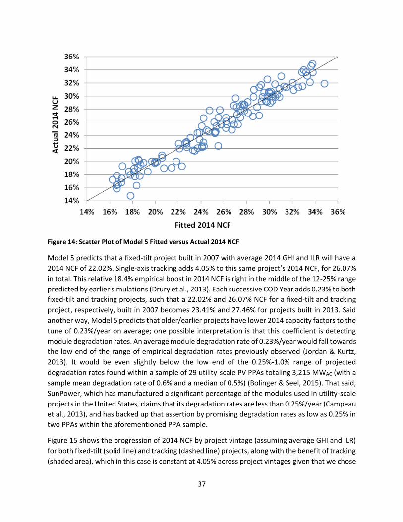
37
Figure 14: Scatter Plot of Model 5 Fitted versus Actual 2014 NCF
Model 5 predicts that a fixed-tilt project built in 2007 with average 2014 GHI and ILR will have a
2014 NCF of 22.02%. Single-axis tracking adds 4.05% to this same project’s 2014 NCF, for 26.07%
in total. This relative 18.4% empirical boost in 2014 NCF is right in the middle of the 12-25% range
predicted by earlier simulations (Drury et al., 2013). Each successive COD Year adds 0.23% to both
fixed-tilt and tracking projects, such that a 22.02% and 26.07% NCF for a fixed-tilt and tracking
project, respectively, built in 2007 becomes 23.41% and 27.46% for projects built in 2013. Said
another way, Model 5 predicts that older/earlier projects have lower 2014 capacity factors to the
tune of 0.23%/year on average; one possible interpretation is that this coefficient is detecting
module degradation rates. An average module degradation rate of 0.23%/year would fall towards
the low end of the range of empirical degradation rates previously observed (Jordan & Kurtz,
2013). It would be even slightly below the low end of the 0.25%-1.0% range of projected
degradation rates found within a sample of 29 utility-scale PV PPAs totaling 3,215 MWAC (with a
sample mean degradation rate of 0.6% and a median of 0.5%) (Bolinger & Seel, 2015). That said,
SunPower, which has manufactured a significant percentage of the modules used in utility-scale
projects in the United States, claims that its degradation rates are less than 0.25%/year (Campeau
et al., 2013), and has backed up that assertion by promising degradation rates as low as 0.25% in
two PPAs within the aforementioned PPA sample.
Figure 15 shows the progression of 2014 NCF by project vintage (assuming average GHI and ILR)
for both fixed-tilt (solid line) and tracking (dashed line) projects, along with the benefit of tracking
(shaded area), which in this case is constant at 4.05% across project vintages given that we chose

38
not to interact Tracking with COD Year. Given our natural interest in newer rather than older
projects, and the need to fix the COD Year in order to more-easily interpret the influence of other
variables, the rest of the Model 5 interpretation focuses on projects that achieved commercial
operation in 2013.
Figure 15: Impact of COD Year at Average 2014 GHI and ILR
Figure 16 shows the impact of 2014 GHI on a 2013 project with an average ILR. For each 1
kWh/m2/day change in 2014 GHI, the model predicts a linear 4.23% absolute change in 2014 NCF
for a fixed-tilt project and a 6.08% absolute change in 2014 NCF for a tracking project.15 This
means that the benefit of tracking increases at sites with a stronger solar resource, which makes
intuitive sense and is consistent with the greater prevalence of tracking at high-GHI sites seen in
Section 2.2. In percentage terms, the benefit of tracking is 10.8% at a 2014 GHI of 4.0 and 22.7%
at a 2014 GHI of 6.0 – similar to the 12%-25% range predicted by earlier simulations (Drury et al.,
2013).
15 The effect of GHI on a fixed-tilt project is simply the 2014 GHI coefficient of 0.0423. For a tracking project, simply add the Tracking x 2014 GHI coefficient of 0.0186 to reach 0.0608 in total.

39
Figure 16: Impact of 2014 GHI for 2013 COD Year and Average ILR
Conversely, Figure 17 shows the impact of ILR (transformed back from the natural logarithm) on
a 2013 project with an average 2014 GHI. As shown by the slight deviation from the linear dashed
lines (included only for visual comparison), due to its logarithmic specification, ILR has a slightly
diminishing marginal effect on 2014 NCF as it increases. For example, for both fixed-tilt and
tracking projects, 2014 NCF increases by 1.00% when moving from an ILR of 1.05 to 1.10, but by
only 0.73% when moving from an ILR of 1.45 to 1.50. This diminishing effect potentially reflects
greater amounts of power clipping at higher ILRs. As shown earlier in Table 3, however, 90% of
the projects in our sample have ILRs of 1.35 or less – levels at which significant power clipping is
unlikely to occur.
Figure 17: Impact of ILR for 2013 COD Year and Average 2014 GHI

40
Similarly, though hard to see in Figure 17, the positive influence of tracking also diminishes ever
so slightly at higher ILRs (again, due to its logarithmic specification) – e.g., from 4.07% at an ILR
of 1.05 to 4.02% at an ILR of 1.50. This deterioration makes intuitive sense (though the small
magnitude is somewhat surprising, and is not statistically significant), given that boosting the ILR
has a similar effect as tracking in terms of flattening the diurnal generation profile by increasing
generation during the morning and evening shoulder periods. In other words, if a project’s diurnal
generation profile is already fairly flat due to a high ILR, then the incremental ability of tracking
to increase generation during the shoulder periods should be reduced.
Lastly, Table 6 demonstrates the changing effect of ILR at different GHI levels and vice versa, for
both fixed-tilt and tracking projects. The two shaded rows labeled “(A)” show the difference in
fitted 2014 NCF between one project with an ILR of 1.45 and another with an ILR of 1.10 at
different levels of GHI. The NCF benefit of a higher ILR increases at higher GHI levels, simply
because there is more available insolation that can be captured by boosting the ILR. Moreover,
for any given GHI, the benefit of a higher ILR is slightly greater for fixed-tilt than for tracking
projects (e.g., 4.24% vs. 4.20% for a GHI of 4.0), which also makes intuitive sense given that
tracking is somewhat redundant with a high ILR.
Similarly, the two shaded columns labeled “(B)” in Table 6 show the difference in fitted 2014 NCF
between one project with an average 2014 GHI of 5.5 kWh/m2/day and another with 4.0
kWh/m2/day at different ILRs. The NCF benefit of a higher GHI increases with higher ILRs, as the
latter is better able to capture the former. Moreover, for any given ILR, the benefit of a higher
GHI is greater for tracking than for fixed-tilt projects (e.g., 8.9% vs. 6.1% for an ILR of 1.20), as
tracking is able to capitalize on the stronger solar resource.
Finally, the bottom third of Table 6 confirms earlier findings from Figure 16 and Figure 17 above:
for a given ILR, the benefit of tracking increases with GHI (given a greater resource to capture
through tracking); conversely, for a given GHI, the benefit of tracking decreases slightly as ILR
increases (again, given that tracking is somewhat redundant with a high ILR).

41
Fitted 2014 NCF of a Fixed-Tilt Project with a 2013 COD (B)
ILR\GHI 3.5 4.0 4.5 5.0 5.5 6.0 5.5-4.0
1.05 14.8% 16.4% 18.1% 19.7% 21.4% 23.1% 5.0%
1.10 15.3% 17.1% 18.9% 20.7% 22.5% 24.3% 5.4%
1.15 15.9% 17.8% 19.7% 21.7% 23.6% 25.5% 5.8%
1.20 16.4% 18.5% 20.5% 22.6% 24.6% 26.7% 6.1%
1.25 16.9% 19.1% 21.3% 23.4% 25.6% 27.8% 6.5%
1.30 17.4% 19.7% 22.0% 24.3% 26.5% 28.8% 6.8%
1.35 17.9% 20.3% 22.7% 25.0% 27.4% 29.8% 7.2%
1.40 18.4% 20.8% 23.3% 25.8% 28.3% 30.8% 7.5%
1.45 18.8% 21.4% 24.0% 26.6% 29.1% 31.7% 7.8%
1.50 19.2% 21.9% 24.6% 27.3% 30.0% 32.6% 8.1%
(A) 1.45-1.10 3.44% 4.24% 5.03% 5.83% 6.62% 7.42%
Fitted 2014 NCF of a Tracking Project with a 2013 COD (B)
ILR\GHI 3.5 4.0 4.5 5.0 5.5 6.0 5.5-4.0
1.05 15.9% 18.5% 21.1% 23.7% 26.3% 28.8% 7.8%
1.10 16.5% 19.2% 21.9% 24.6% 27.4% 30.1% 8.2%
1.15 17.0% 19.9% 22.7% 25.6% 28.4% 31.3% 8.6%
1.20 17.5% 20.5% 23.5% 26.5% 29.4% 32.4% 8.9%
1.25 18.0% 21.1% 24.2% 27.3% 30.4% 33.5% 9.3%
1.30 18.5% 21.7% 24.9% 28.1% 31.3% 34.5% 9.6%
1.35 19.0% 22.3% 25.6% 28.9% 32.2% 35.6% 9.9%
1.40 19.4% 22.9% 26.3% 29.7% 33.1% 36.5% 10.3%
1.45 19.9% 23.4% 26.9% 30.4% 33.9% 37.5% 10.6%
1.50 20.3% 23.9% 27.5% 31.1% 34.8% 38.4% 10.8%
(A) 1.45-1.10 3.40% 4.20% 4.99% 5.79% 6.58% 7.37%
Benefit of Tracking for a Project with a 2013 COD
ILR\GHI 3.5 4.0 4.5 5.0 5.5 6.0
1.05 1.13% 2.06% 2.99% 3.91% 4.84% 5.77%
1.10 1.12% 2.05% 2.98% 3.91% 4.84% 5.77%
1.15 1.11% 2.04% 2.97% 3.90% 4.83% 5.76%
1.20 1.11% 2.04% 2.97% 3.90% 4.82% 5.75%
1.25 1.10% 2.03% 2.96% 3.89% 4.82% 5.75%
1.30 1.10% 2.02% 2.95% 3.88% 4.81% 5.74%
1.35 1.09% 2.02% 2.95% 3.88% 4.81% 5.74%
1.40 1.08% 2.01% 2.94% 3.87% 4.80% 5.73%
1.45 1.08% 2.01% 2.94% 3.87% 4.80% 5.73%
1.50 1.07% 2.00% 2.93% 3.86% 4.79% 5.72% Table 6: Primary and Interactive Effects of GHI, ILR, and Tracking on Fitted 2014 NCF

42
As a way to graphically summarize the interpretation of Model 5, Figure 18 shows the individual
and combined effects of the regressors in waterfall format. It begins at the far left with the
constant term of 22.02%, which represents the predicted 2014 net capacity factor from a 2007
fixed-tilt project with average GHI (5.08 kWh/m2/day) and ILR (1.23). It then adds the impact of
each of the four non-tracking-related regressors until arriving, in the middle of the graph, at a
2013 fixed-tilt project with a GHI of 6.08 kWh/m2/day and an ILR of 1.33, which has a predicted
2014 net capacity factor of 29.78%. The three tracking-related regressors are then added in turn
to reach, on the far right of Figure 18, a predicted 2014 net capacity factor of 35.68% for a 2013
tracking project with the same GHI (6.08) and ILR (1.33) levels.
Figure 18: Individual and Combined Effects of Model 5 Regression Terms
4. Conclusion The rapid ascendency of utility-scale PV in the United States over the last few years has resulted
in a diverse fleet of operating projects that exhibit significant variation in empirical AC capacity
factors, with the highest and lowest capacity factors in our sample differing by more than a factor
of two. The regression models developed for this analysis find that just three highly significant
independent variables – GHI, Tracking, and ILR – can explain 92% of this variation (see Model 3
in Table 5), with GHI alone able to explain 71.6% (see Model 1 in Table 5). That said, adding COD
Year (in Model 4) and three interactive variables (in Model 5) improves the model further and
reveals interesting relationships between these independent variables, without over-specifying
the model.

43
Of the two additional potential drivers that were discussed in Section 2.2 but were omitted from
the model due to insufficient data – i.e., the effect of module orientation (tilt and azimuth) and
temperature (power temperature coefficient and module operating temperature) on
performance – temperature is likely the more significant gap. Module orientation is primarily of
relevance to only about half of the projects in our sample (i.e., the fixed-tilt projects), and it is
highly likely that ground-mounted, fixed-tilt projects of this size and cost are almost universally
oriented to maximize generation (and hence net AC capacity factor) at each site, thereby not
adding much explanatory power to the model. The model would, however, presumably be
improved with good data on power temperature coefficients and module operating
temperatures.16
Taken together, the empirical data and statistical modeling results presented in this paper can
provide a useful indication of the level of performance that solar project developers and investors
can expect from various project configurations in different parts of the country. Moreover,
although this paper has not attempted to compare ex-post to published ex-ante capacity factor
projections, the tight relationship between fitted and actual capacity factors (for example, see
Figure 14) should nevertheless instill confidence among investors that the projects in this sample,
at least, have largely performed as expected.
Looking ahead, the analysis presented in this paper suggests that there is still room for utility-
scale PV project capacity factors to progress further. For example, even within the confines of
our sample and Model 5’s specification, Table 6 suggest that the NCF of tracking projects at the
highest limits of the GHI and ILR ranges could potentially move a little higher (e.g., as high as
38.4%) than the maximum empirical 2014 NCF in our sample of 34.9%. Moving beyond our
sample and Model 5, progress towards even higher net capacity factors could come from several
different directions:
First, ILRs could possibly move higher than the 1.50 maximum seen in our sample, as some
inverters are designed to handle ILRs as high as 1.75 (Advanced Energy, 2013). The extent to
which ILRs will continue to move higher in the future depends in large part on the relative pricing
of modules and inverters (and perhaps even trackers) going forward, which – in combination with
PPA terms – determines the optimal ILR from an economic perspective. Even so, our analysis
finds diminishing marginal returns to higher ILRs.
Second, dual-axis tracking would boost net capacity factor beyond the levels achieved by the
single-axis trackers in our sample. Although no utility-scale (i.e., >5 MWAC) PV projects using dual-
axis tracking had been built in the United States through 2013, several such projects came online
16 Module operating temperature may, however, be correlated with GHI to some extent, in which case perhaps power temperature coefficient may be the more important of these two variables. We did attempt to approximate the effect of power temperature coefficient by comparing the performance of projects using cadmium-telluride and silicon modules (given cadmium-telluride’s claimed advantage in this area), but the results were inconclusive.

44
during 2014, with 2015 being their first full year of operation. Adding these projects to the sample
would be one way to refresh this analysis and perhaps improve the model.
Third, although insolation is dictated by weather patterns and natural events and cannot be
directly influenced with ease, it is, of course, possible to concentrate the strength of the sun’s
energy to boost generation. To date, most commercial concentrating photovoltaic (“CPV”)
projects have focused on minimizing the size of the solar cell in order to save on materials costs,
thereby tempering the benefit of concentration on capacity factor.17 But this need not be the
case going forward, particularly if the price of solar-grade silicon remains low.
Though each of the three approaches described above could boost capacity factors in the future,
the extent to which any of these are implemented will depend in large part on whether it is
economically advantageous to do so. At present, for example, the economics of utility-scale PV
in the United States generally do not favor any of these three approaches, though this could
change in the future. In fact, depending on how module and inverter prices, as well as PPA terms,
play out going forward, one could even envision a future that economically favors a lower ILR
than we see today, in which case capacity factors would presumably move lower as a result.
Analyzing how these economic considerations interact with the empirical technical parameters
reviewed herein is beyond the scope of this paper, but is fertile ground for future work.
Finally, the advent of project-level energy storage – still rare in the utility-scale PV market within
the United States (and not reflected at all within our project sample) – will likely change how
utility-scale PV project developers think about capacity factor and its relative importance.
Maximizing generation (e.g., through tracking and/or array oversizing) to take better advantage
of available transmission capacity over more of the day, or alternatively merely shifting
generation from lower- to higher-priced periods, are just two possible responses. Whatever the
optimal strategy (which could differ depending on a variety of factors, including PPA terms), this
paradigm shift will, no doubt, complicate future analyses of comparative PV project performance.
17 In fact, to date, the two largest CPV projects in the United States have performed at capacity factors well below what one would have expected from a similarly sited PV project using single-axis (as opposed to CPV’s dual-axis) tracking (Bolinger & Seel, 2015). SunPower’s new C7 technology (which concentrates the sun’s energy just seven times, compared to the hundreds of times achieved by other CPV technologies) is just now starting to be deployed, and time will tell whether this low-concentration approach yields better results than earlier high-concentration technology.

45
Forecasting Wind Energy Costs and Cost Drivers: The Views of the
World’s Leading Experts
A report version of this research, fact sheets, summary briefings, a webinar recording and further
supplemental material is available at https://emp.lbl.gov/iea-wind-expert-survey
A peer-reviewed article version of this research project has been published in the Journal Nature
Energy on September 12th 2016 (Article number 16135) and is available online at:
http://rdcu.be/khRk
http://dx.doi.org/10.1038/nenergy.2016.135
1. Introduction Wind energy supply has grown rapidly over the last decade, supported by a myriad of national
and sub-national energy policies and facilitated by technology advancements and related cost
reductions (GWEC, 2015; IEA, 2013; IRENA, 2015; REN21, 2015). Though the vast majority of this
expansion has occurred onshore (>97%), offshore wind power deployment has also recently
increased, especially in Europe. The rising maturity of wind power technology suggests that wind
energy might play a significant future role in global electricity supply, perhaps especially in the
context of efforts to reduce greenhouse gas emissions (GWEC, 2014; IEA, 2015; IPCC, 2014;
Luderer et al., 2014; R. Wiser et al., 2011).
The long-term contribution that wind energy makes to global energy supply, and the degree to
which policy support is necessary to motivate higher levels of deployment, depends—in part—
on the future costs of both onshore and offshore wind. Those costs will be affected by technology
advancements, as impacted by private and public research and development (R&D), among other
factors. Yet there remains sizable uncertainty about both the degree to which costs will continue
to decline and the conditions that might drive greater cost reduction (DOE, 2015; Lantz, Wiser, &
Hand, 2012; R. Wiser et al., 2011).
This report summarizes the results of an expert elicitation survey on future wind energy costs
and technology advancement possibilities. The research relies on expert knowledge to gain
insight into the possible magnitude of future wind energy cost reductions, and to identify the
sources of future cost reduction and the enabling conditions needed to realize continued
innovation and lower costs. An understanding of the potential for wind power costs to fall and
the means by which future cost reductions could be delivered can inform policy and planning
decisions affecting wind power deployment, R&D in the private and public sectors, and industry
investment and strategy development. Enhanced insight into future cost-reduction opportunities

46
also supports improved representation of wind energy technology in energy-sector modeling
efforts.
Lawrence Berkeley National Laboratory and the National Renewable Energy Laboratory led the
gathering of data and insights through an online elicitation survey of a large sample of the world’s
foremost wind energy experts, under the auspices of the International Energy Agency (IEA) Wind
Implementing Agreement. The survey is global in scope—though with a focus on North America
and Europe—and covers onshore (land-based), fixed-bottom offshore, and floating offshore wind
technology. It emphasizes costs and associated drivers of cost changes in 2030, but with
additional markers in 2020 and 2050. This report summarizes the 163 survey responses received,
in what may be the largest single expert elicitation ever performed on an energy technology.
Insights gained through this survey can complement other tools for evaluating cost-reduction
potential, including the use of learning curves, engineering assessments, and less-formal means
of synthesizing expert knowledge.
The remainder of this report is organized as follows. Chapter 2 introduces expert elicitation and
discusses the scope, design, and implementation of our assessment. Chapter 3 summarizes our
core results. Finally, Chapter 4 offers conclusions and discusses anticipated future work.
2. The Expert Elicitation Survey
2.1 Review of Expert Elicitation and other Methods to Assess Future Costs
Though multiple approaches have been used to assess the past and future cost of wind energy
(discussed below), ours is one of the first publically available formal expert elicitation surveys
with an explicit focus on future wind energy costs and related technology advancements.
Expert elicitation is a tool used to develop estimates of unknown or uncertain quantities based
on careful assessment of the knowledge and beliefs of experts about those quantities (Morgan,
2014). Several options are available to a researcher who wishes to make such estimates: make
projections based on past data and trends, review existing literature and adopt projections made
by others, develop detailed models based on experience in related fields and apply them to
create forecasts, and so on. The expert elicitation approach is to carefully assess projections of
the quantities of interest from relevant subject-matter experts. It is often considered the best—
or perhaps the only—way to develop credible estimates when data are sparse or lacking, or when
projections are sought for future conditions that are very different from past conditions (Kotra,
Lee, Eisenberg, & DeWispelare, 1996; Meyer & Booker, 2001). Several formal protocols for
organizing and conducting expert elicitations have been developed; all follow a very similar set
of steps to those described by (Knol, Slottje, van der Sluijs, & Lebret, 2010) and summarized in
Figure 19.

47
Source: Knol et al., 2010
Figure 19: Steps in a Formal Expert Elicitation
Within this general protocol, a rich literature provides guidance on elicitation question design,
the importance of clarity in what is being asked, how to avoid or minimize the effects of expert
motivational and cognitive biases, and the importance of providing feedback to experts and
providing opportunities for them to review and update their assessments (Coppersmith, Jenni,
Perman, & Youngs, 2009; Hora, 2007; Morgan, 2014). Section 2.3 below describes how we
applied these principles in our expert elicitation.
Expert elicitations have been widely used to support decision making in the private sector
(Sharpe & Keelin, 1998) and in policy decisions (Hora & Von Winterfeldt, 1997). Their use is
explicitly called for in a review of the Intergovernmental Panel on Climate Change (InterAcademy
Council, 2010) and implicitly called for in a National Academies review of the U.S. Department of
Energy’s Applied Energy R&D programs (NRC, 2007). Within the energy community, expert
elicitation is increasingly common as a tool for making estimates of the future costs of energy
technologies under different possible future scenarios. (Baker et al., 2015), for example, review
nearly 20 such elicitations conducted over the past decade, including studies focused on carbon
capture and storage, solar, nuclear, biomass, and storage technologies. Gillenwater (2013) uses
expert elicitation to explore wind investment decisions, and Kempton, McClellan, & Ozkan (2016)
use elicitation to understand future offshore wind costs in one region of the United States, but
formal elicitation procedures have not yet been widely applied to wind energy costs and related

48
technology advancements. (Verdolini et al., 2016) provide a comprehensive review of energy
technology expert elicitation studies.
Expert elicitation is not without weaknesses—in general and when applied to wind energy. Expert
responses may be affected by the design of the data-collection instrument, by the individuals
selected to submit their views, by the behavior of the interviewers (for in-person elicitation), and
by features of the questionnaire or web-based instrument. Notably, it is impossible to entirely
eliminate—or even to fully test for—the possibility of motivational or cognitive biases. Those
individuals who are considered subject-matter experts on wind energy, for example, might have
a tendency to be optimistic about the future of the sector. On the other hand, experts sometimes
underestimate the possibility of technological change, as has been the case with solar energy
(Verdolini et al., 2016). Regardless of the possible limitations, though, when implemented well,
expert elicitation can provide valuable insights on the views of subject-matter experts,
complementing other tools to assess cost-reduction potential, including learning curves,
engineering assessments, and less-formal means of synthesizing expert knowledge (Lantz et al.,
2012). These other methods have been used regularly—both individually and in combination—
to assess potential future wind energy cost reductions:
Learning curves have a long history within the wind sector (Lindman & Söderholm, 2012; Rubin
et al., 2015; R. Wiser et al., 2011), but they have been criticized for simplifying the many causal
mechanisms that lead to cost reduction (Ek & Söderholm, 2010; Ferioli et al., 2009; Junginger et
al., 2010; Mukora et al., 2009; Witajewski-Baltvilks et al., 2015; Yeh & Rubin, 2012). Further, few
published studies focus on the most important metric of wind energy costs, the levelized cost of
energy (LCOE) (BNEF, 2015b; Rubin et al., 2015; R. Wiser et al., 2011), with most research directed
towards one component of LCOE: upfront capital costs (Dinica, 2011; Ferioli et al., 2009; Rubin
et al., 2015). In addition, using historical data to generate learning rates that are then
extrapolated into the future implicitly assumes that future trends will replicate past ones (Arrow,
1962; Ferioli et al., 2009; Nordhaus, 2014). For technologies with limited historical data, such as
floating offshore wind, it is not even possible to compute technology-specific learning rates.
Engineering assessments provide a bottom-up, technology-rich alternative or complement to
learning curve analyses (Mukora et al., 2009). They involve detailed modeling of specific possible
technology advancements (BVG Associates, 2015; Bywaters et al., 2005; Crown Estate, 2012;
Fingersh, Hand, & Laxson, 2006; Fitchner-Prognos, 2013; Malcolm & Hansen, 2002; Sieros,
Chaviaropoulos, Sørensen, Bulder, & Jamieson, 2012; Valpy & English, 2014b, 2014a). Because
this approach often models both cost and performance, it inherently emphasizes expected
reductions in LCOE. It requires a robust understanding of possible technology advancements,
thus the opportunities captured by engineering studies are often incremental and generally
realizable in the near to medium term (less than 15 years). This approach also generally requires
sophisticated design and cost models to capture the full array of component- and system-level
interactions, and rarely provides insight into the probability of different outcomes.

49
Expert knowledge can be obtained through many means, not only through formal elicitation
procedures. Through interviews, workshops, and other approaches, expert insight is a mainstay
of many recent attempts to forecast future wind technology advancement and cost reduction. It
can be paired with engineering assessment and learning curve tools to bolster the reliability of
the overall estimates, garner a more detailed understanding of how cost reductions may be
realized, and clarify the uncertainty in these estimates. The use of expert knowledge has proven
especially valuable for emergent offshore wind technologies, for which historical data are often
lacking (Crown Estate, 2012; Fitchner-Prognos, 2013; Junginger, Faaij, & Turkenburg, 2004;
Navigant, 2013; TKI Wind op Zee, 2015), but expert insight has also been used to assess onshore
wind (Cohen et al., 2008; Neij, 2008) and to compare onshore and offshore (Wüstemeyer,
Madlener, & Bunn, 2015). As with more-formal elicitation procedures, care is needed to avoid
bias and overconfidence in expert responses.
2.2 Scope of Expert Assessment: What Were We Asking? The scope of our assessment comprises three wind power applications: utility-scale onshore
wind, fixed-bottom offshore wind, and floating offshore wind. Onshore (i.e., land-based) wind is
relatively mature, and it already makes a significant contribution to energy supply in many
countries. Fixed-bottom offshore wind can use multiple foundation types (e.g., monopile, jacket,
gravity base). It is less mature than onshore wind, but it is being deployed at scale in Europe and,
to a lesser degree, outside of Europe. Floating offshore wind (e.g., spar buoy, semi-submersible
platform, tension-leg platform) is not yet fully commercialized, but it has been deployed in full
scale demonstration projects.
Our analysis centers on potential changes in the LCOE of projects that use each of the three wind
applications, in dollars or euros per megawatt-hour ($/MWh or €/MWh). The LCOE is the
levelized cost per unit of generated electricity from a specific source over its project design life
that allows recovery of all project expenses and meets investor return expectations.18 Though
LCOE should not be the only metric used when comparing electric generation assets, the LCOE is
regularly and appropriately used to assess the unit costs of electric-generation technologies, and
minimizing LCOE is a primary goal of the wind industry and of wind energy R&D.19
18 We calculate LCOE in real 2014$ or 2014€ per MWh. This LCOE estimate equates to the minimum power price a project must obtain to cover all project costs, service debt, pay expected returns to equity shareholders, and cover income tax. LCOE is calculated at the plant boundary and excludes the valuation of public benefits (e.g., Renewable Energy Credits, carbon credits, Green Certificates) as well as ratepayer, taxpayer, or other forms of project-level government support (e.g., investment and production tax credits, feed-in-tariff premiums). The formula used to calculate LCOE and more details on its use in this survey can be found at: http://rincon.lbl.gov/lcoe_v2/background.html. 19 Though LCOE is useful for showing generation cost trends, simply comparing LCOEs among different electric-generation technologies is not sufficient to judge the relative value of those technologies. This is because electric system planners and modelers must consider not only levelized generation costs, but also system costs that include consideration of system peaking needs, transmission expenditure, and variable generation

50
In surveying the experts, we sought insight on the LCOE of the three wind applications at four
time points: a recent-cost baseline in 2014 (for which respondents could accept a predefined
baseline or create their own) and then in 2020, 2030, and 2050.20 Note that these dates are based
on the year in which a new wind project is commissioned. We did not seek a baseline estimate
for floating offshore wind, given the nascent present state of that technology and lack of current
commercial applications.
For the baseline year, and for our focus year of 2030, we further requested details on five core
input components of LCOE: (1) total upfront capital costs to build the project (CapEx, $ or €/kW);
(2) levelized total annual operating expenditures over the project design life, including
maintenance and all other ongoing costs, e.g., insurance and land payments (OpEx, $ or €/kW-
yr); (3) average annual net project-level energy output (capacity factor, %); (4) project design life
considered by investors (years); and (5) costs of financing, in terms of the after-tax, nominal
weighted-average cost of capital (WACC, %).21,22 For the other two time points (2020, 2050), we
solicited only estimates of the LCOE.
For the 2014 and 2030 CapEx estimates, respondents were asked to include only costs within the
plant boundary, which include costs for electrical cabling within the plant but exclude costs for
any needed substations, transmission lines, or grid interconnection costs. As applied to offshore
wind, this means that CapEx includes costs for within-plant array cabling but excludes the costs
for offshore substations, any high-voltage direct-current collector stations and associated cables,
and grid connection to land (e.g., subsea export cables, onshore substations, and onshore
transmission cables). As defined in the survey, OpEx excludes any costs associated with grid
interconnection, substations, or transmission use; for offshore wind, transmission system use
charges are also excluded.
integration (Edenhofer et al., 2013; Hirth, 2013; Joskow, 2011; A. D. Mills & Wiser, 2013; R. Wiser et al., 2011). Differences in taxation, incentives, and societal benefits and costs are also often considered. 20 Inclusion of a 2014 baseline allows for any changes over time to be characterized in absolute ($ or €) and relative terms (% increase or decrease). 21 This represents the average return required by the combination of equity and debt investors to make a project an attractive investment opportunity, where each category of capital is proportionately weighted. The WACC may be defined in after-tax or pre-tax terms. Owing to highly variable tax rules as well as the use of the tax code to incentivize wind energy in some countries, this survey relies exclusively on an after-tax WACC. Under these conditions, respective equity returns should reflect the annual average rate of return for equity positions after expenses and taxes, independent of how the rate of equity return is impacted by the applicable tax code. Similarly, debt interest rates should account for their status as a business tax deduction where applicable. In practice, after-tax WACCs may be considered either in real or nominal terms. Assuming an inflation rate of 2%, the following conversions between nominal and real apply: 4% nominal WACC = 2% real WACC; 8% nominal WACC = 5.9% real WACC; 12% nominal WACC = 9.8% real WACC. 22 In calculating the LCOE, we use standardized taxation and inflation assumptions: standardized income tax rate (25%), depreciation schedule (20-year straight-line), and long-term inflation rate (2%); 100% of capital costs are assumed depreciable.

51
Our survey emphasized the “typical” LCOE of wind projects in each respondent’s primary region
of expertise. We defined “typical” as the median project in terms of costs (Figure 20).
Figure 20: Definition of “Typical” LCOE in Expert Elicitation
Future wind LCOEs are uncertain. They can be affected by project-specific factors, such as the
quality of the wind resource at a particular site, as well as by factors that affect the entire wind
sector, such as changes in wind turbine technologies, markets, and policies. Technological
changes may be induced by direct R&D or other advances. Market changes comprise, for
example, systemic changes in the average wind speed of sites that remain for development as
well as the amount of competition in the wind supply chain. Policy changes may directly or
indirectly support or impede wind energy development and deployment.
In exploring future LCOE trends, we asked respondents to provide probabilistic estimates for
three future scenarios: a low LCOE scenario (10th percentile), a high LCOE scenario (90th
percentile), and a median LCOE scenario (50th percentile), considering only the broader, non-
project-specific factors. We asked experts specifically to focus on changes in the typical LCOE
(i.e., to ignore project-to-project variation) that might result from changes in factors that affect
the industry as a whole (i.e., changes in wind energy technologies, markets, and policies). We
also asked respondents to assume no changes in macroeconomic conditions (such as interest
rates, inflation, and currency fluctuations), materials and commodity prices, and other factors
not directly related to the wind energy business.23
In addition to asking about LCOE and the five core LCOE inputs, we asked about the market and
technology characteristics and drivers most likely to impact LCOE trends in 2030. Specifically, we
sought information on: (1) expected typical turbine characteristics for projects installed in 2030—
nameplate capacity, hub height, and rotor diameter for all three wind applications; (2) the
expected impact of each of a list of specific changes in wind development, technology, design,
manufacturing, construction, operations, and markets on achieving reduced LCOE by 2030 for all
three wind applications; and (3) broad drivers most likely to facilitate achieving “low” estimates
23 For more detail, see: http://rincon.lbl.gov/lcoe_v2/typical_costs.html

52
of LCOE in 2030 as opposed to “median” estimates in that year, separately for onshore and fixed-
bottom offshore wind.
2.3 Application of Expert Elicitation Principles We applied many of the basic concepts, tools, and guidelines of a well-designed expert elicitation
in order to minimize biases. Best elicitation practices include clearly defining the quantities that
are being assessed, minimizing extra cognitive burden on the expert by asking questions using
familiar terminology and units, and minimizing the need for “side” calculations. In addition, we
sought to minimize the effects of anchoring and overconfidence biases (Kahneman, Slovic, &
Tversky, 1982) by asking for low- and high-scenario estimates before asking for a mid-point
estimate, and providing experts with feedback and the opportunity to review and modify their
responses (Coppersmith et al., 2009). Our online survey format created challenges (e.g., we had
a limited ability to tailor questions to respondent preferences) but also provided benefits over
traditional interview-based elicitations in terms of easily accessible calculation and graphical
display tools that gave experts immediate feedback and context for their assessments.
We carefully and clearly defined each of the cost-related factors for which we elicited input, and
we reinforced those definitions throughout the survey. In part we took extra care here because
of differences across the industry in how each factor is defined—for example, whether a project’s
CapEx includes or excludes transmission and grid interconnection costs, or whether nominal or
real WACC is used in calculating LCOE. Because we could not ask each expert how he or she
defined each term, and because we wanted to compare answers across the experts, we needed
to provide detailed definitions of each quantity.
Although the experts could not challenge the definitions of the quantities being assessed, we
provided some flexibility in how they provided responses, and we reduced the need for
extraneous calculations. Respondents could answer cost questions in real U.S. dollars or real
euros (we used the average 2014 exchange rate of €1 = US $1.33). They were also asked to
indicate which of the three wind applications they were comfortable discussing, and then they
were asked questions only about those applications. They were provided with an in-survey, easy-
to-use LCOE calculator to translate component estimates into an LCOE estimate.24 Additionally,
respondents had the opportunity to qualify their answers with additional written comments and
could skip questions they did not feel comfortable answering.
A particular challenge in online elicitations is how to provide experts with feedback and context
for their responses so they can consider their own internal consistency and modify their
assessments as desired. Without personal interaction, the elicitation team cannot direct an
expert’s attention to particular questions and responses. We addressed this issue by including
graphical elements in the survey instrument and by building useful feedback into the instrument
24 For an example, see http://rincon.lbl.gov/lcoe_v2/lcoe_calculator.html.

53
based on the results of pretesting that identified feedback needs. Most critical was the use of a
time-trend graphical interface that (1) displayed the experts’ previous assessments of a 2014
baseline LCOE and their low, median, and high scenario LCOE values for 2030, and (2) asked for
low, median, and high scenario LCOE estimates for 2020 and 2050 on the same graph. This
interface explicitly showed the experts all of their LCOE responses, encouraging them to think
about the internal consistency of those estimates.
Though we followed expert elicitation principles and design guidelines in our assessment, three
unique aspects of the present assessment deserve mention:
Casting a Wide Net with an Online Survey: Many expert elicitations feature detailed and sometimes lengthy in-person interviews with fewer than 20 experts. In contrast, we distributed our survey online to a wide group of possible respondents. This necessitated a shorter, more focused survey than would be common in an in-person setting, with less follow-up and in-depth exploration of responses.25 In part, this choice reflected the need for a greater number of overall respondents to address one goal of our effort: to compare responses by wind application, organizational type, location, expertise, and other respondent characteristics.26
No Comprehensive Elicitation of Probability Distributions or Technical Parameters: Our assessment combined aspects of expert elicitation and an opinion survey. We focused the expert elicitation on LCOE and the five key inputs to LCOE under low, median, and high scenarios, and we limited consideration of the five key inputs to only two specific points in time. Our assessment of technical and market drivers mirrored an opinion survey—we did not seek detailed quantitative assessment of the LCOE effect of specific technical advancement possibilities. Instead we asked experts to identify which advancements they believe would be larger contributors to cost reductions.
No Elicitation of Opinions Conditional on Specific R&D, Policy, Deployment, or Other Factors: We asked respondents to make low, high, and median scenario estimates of future LCOE, and we left it to them to define for themselves the future scenarios that might drive those cost changes. In contrast, many expert elicitations condition responses based on defined R&D expenditures and on specific market and policy scenarios, in order
25 Some research shows that elicitations relying on self-administered, web-based surveys yield results different from those relying on in-person interviews (Nemet, Anadon, & Verdolini, 2017; Verdolini, Anadon, Lu, & Nemet, 2015), whereas other research shows less evidence of such differences (Anadón, Nemet, & Verdolini, 2013; Baker, Bosetti, Anadon, Henrion, & Aleluia Reis, 2015); where differences exist, the relative accuracy of the two methods remains unclear, though it is generally believed that in-person interviews represent the “gold standard.” On the other hand, (Baker et al., 2015; Nemet et al., 2017) also suggest there is value in including diverse and relatively large groups of experts when conducting elicitations, suggesting—all else being equal, and due to the resource intensity of in-person elicitation—that there is value to online elicitations. 26 Our interest in assessing the effect of respondent type on elicitation results follows related work conducted by Anadón et al. (2013) on nuclear energy cost expectations, Verdolini et al. (2015) on solar photovoltaics, and Nemet et al. (2017) on a range of energy technologies.

54
to more directly inform R&D and policy decisions. Our survey was designed to map the universe of possible future LCOEs but provides only limited information about specific contributions to lower or higher costs.
2.4 Survey Design, Testing, and Implementation We gathered data and insights through an online elicitation survey (via the Near Zero platform27)
of a large sample of the world’s foremost wind energy experts under the auspices of IEA Wind
Task 26 on the “Cost of Wind Energy.”
The survey was carefully designed over a number of months, including numerous rounds of
review, testing, and revision. Reviewers included the core survey design team, IEA Wind Task 26
members, and a select group of external wind energy experts. An expert workshop was held early
in the process to discuss the goals of the survey and to pilot test an early draft of the survey. A
PDF version of the final survey can be found online at: https://emp.lbl.gov/iea-wind-expert-
survey.
The survey was launched in October 2015 and closed in December 2015. During the intervening
period, various steps were taken to maximize response rate and ensure respondent
comprehension of the survey. In particular, we first “pre-announced” the survey to possible
respondents, and we invited participation in a webinar during which we discussed the purpose,
structure, and details of the elicitation: 33 people attended the webinar, the recording was
viewed 19 times, and the slides were made available for download. The online survey was
distributed with personalized web links, and six separate waves of reminders were sent before
the survey finally closed—including personalized and less-personalized email reminders as well
as some phone and in-person exhortations. Because of the depth and length of the online survey,
respondents were allowed to complete it in multiple sittings as necessary. In some cases, several
individuals within an organization collaborated on a single, collective survey response.
2. 5 Selection and Response of Experts The success of an expert elicitation depends on the expertise and commitment of the
contributing experts. Given the focus of our elicitation on project-level LCOE, our ideal
respondents included strategic, system-level thought leaders with wind technology, cost, and/or
market expertise. Such individuals might come from the various strands of the private wind
industry, public R&D institutes, academia, or a range of other organizations. We sought a
relatively large number of respondents in part to ensure an adequate number of possible experts
versed in each of the three wind applications. Though the survey was global in scope, we focused
on experts from North America and Europe given the constitution of the members of IEA Wind
Task 26.
27 See: http://www.nearzero.org/.

55
We received considerable assistance in identifying possible respondents from IEA Wind Task 26
members and their affiliated institutions, and we reached out to many other wind energy experts
and organizations to ensure broad coverage. We allowed our initial set of potential respondents
to suggest additional names, which yielded a small number of additional respondents.
In addition to the full survey sample, we identified a smaller group of “leading experts.” These
individuals were selected through an iterative, deliberative process by a core group of IEA Wind
Task 26 members and several leading external wind energy experts. The survey team believed
this small group was uniquely qualified to complete the survey, and the group was created in part
to enable comparison of survey results between the smaller leading-expert sub-sample
(paralleling a more traditional elicitation) and the larger group (excluding the leading-expert sub-
sample).
We successfully distributed surveys to 482 experts, including 42 in the leading-expert group. The
total number of returned surveys was 163, of which 22 came from the leading-expert group and
the remaining 141 fall within the larger group. This reflects a response rate of 34% across the full
set and 52% among the smaller group.28 Appendix A lists the individuals who submitted
responses.
Responses came from a broad cross-section of the wind sector. Figure 21 summarizes the
characteristics of the 163 respondents by wind application area addressed, region of the world
with which experts are most familiar, organizational type, and type of expertise. Note that
respondents were able to identify multiple wind applications, geographies, and types of
expertise. The median respondent dedicated 49 minutes to completing the survey, with the 25th-
to-75th percentile range from 29 to 99 minutes.
28 In practice, there were some instances in which multiple individuals collaborated on a single survey response. Where we know of these instances, they are marked in Appendix A, and they result in a total response rate of 36% (by experts).

56
Figure 21: Characteristics of the 163 Expert Survey Respondents
3. Summary of Elicitation Results The analysis presented in this report summarizes the full set of 163 survey responses received.
Additionally, in a number of text boxes, we highlight—on a cursory basis—notable differences in
responses: (1) between the smaller leading-expert group vs. the full set of responses less that
group; (2) by organizational type29; (3) between respondents who provided opinions on only
onshore or offshore wind vs. those who provided responses to both onshore and offshore wind;
(4) by type of expertise; and (5) by familiarity with different geographic regions.30 Such
29 We consolidated the nine organizational type categories presented in Figure 21 into five larger categories: (1) public R&D and academic (consolidating two of the original categories, and called the “research” group for the remainder of the report); (2) wind developer/owner/financier/operator and construction/installation contractor (consolidating two of the original categories, and called the “wind deployment” group); (3) wind turbine and/or component manufacturer (called the “equipment manufacturing” group); (4) other private-sector wind industry; and (5) other (consolidating three of the original categories—government agency not associated with research, other not-for-profit, and other). 30 Note that in many instances a single respondent may have identified multiple geographies (e.g., North America and Europe) or types of expertise (e.g., expertise on wind energy costs and on wind energy technologies). Such respondents may, therefore, fall within multiple categories when the survey responses are

57
comparisons are insightful in their own right, but might also help reveal underlying biases in the
survey sample. Future work is planned to assess more thoroughly any systematic differences in
survey responses by respondent characteristics.
3.1 Forecasts for LCOE Reduction For each of the wind applications, experts provided a single estimate of LCOE for 2014 (the
“baseline” value) and then provided low-, median-, and high-scenario estimates for the typical
LCOE of wind projects in 2020, 2030, and 2050. In estimating the low-, median-, and high-scenario
estimates, experts were asked to ignore project-to-project variation and instead to focus on
factors that affect the industry as a whole, e.g., changes in wind energy technologies, markets,
and policies. All dates are based on the year in which a new wind project is commissioned.
Figure 22 shows the resulting changes in LCOE from 2014 through 2050 in percentage terms for
(a) onshore, (b) fixed-bottom offshore, and (c) floating offshore wind. Expert-specific changes in
LCOE are calculated using each expert’s baseline and later values. Because a 2014 baseline was
not established for floating offshore, the change is shown relative to the expert-specific baseline
for fixed-bottom offshore wind. The figure shows the change from the baseline values for each
of the three scenarios the experts were asked to provide: low, median, and high scenarios of
typical LCOE. Expert opinions on these changes vary, and the figure also shows the range of those
opinions. Lines and markers show the median value of expert responses, and the shaded regions
around each line show the range (25th to 75th percentile) of expert responses.
While the figure summarizes the full set of survey responses, Text Box 1 highlights key differences
in LCOE estimates among various respondent groups. Though the differences identified in the
text box are notable, it is also important that the results from most respondent groups—by
organization, by region, and by expertise type—vary only to a relatively small degree. This
suggests that any biases in the results that derive from our survey sample are either limited or
apply similarly to many of the wind expert respondent groupings.
split by geography or expertise type. In these instances, careful interpretation is required. This issue is not present when culling results by organizational type; leading experts vs. larger group; or onshore, offshore, vs. both onshore and offshore—in each of the latter cases, the groupings are mutually exclusive.

58
Note: All dates are based on the year in which a new wind project is commissioned.
Figure 22: Estimated Change in LCOE over Time for (a) Onshore, (b) Fixed-Bottom Offshore, and (c) Floating Offshore Wind Projects

59
Focusing first on the median (50th percentile) scenario for typical LCOE, experts clearly predict
significant continued reductions in the cost of wind energy. Though onshore wind technology is
already relatively mature, experts anticipate further advancements, with the median value of
expert responses (also referred to as the median-expert response) showing LCOE reductions from
baseline values of 10% in 2020, 24% in 2030, and 35% in 2050. Expert views on the long-term
opportunities for fixed-bottom offshore wind are even more aggressive—perhaps not
surprisingly, given the earlier state of the technology—with median LCOE reductions of 10% in
2020, 30% in 2030, and 41% in 2050. Floating offshore wind comes in at a 6% LCOE premium in
2020 relative to the 2014 fixed-bottom offshore baseline (reflective of the emerging state of the
technology), but then it steeply declines to 25% below and then 38% below baseline values by
2030 and 2050, respectively.
There is also clearly a sizable range of uncertainty in future LCOEs, reflected both in the median-
expert response for the low-scenario and high-scenario LCOE estimates as well as the range of
expert views for all three scenarios shown by the shaded regions. For onshore wind, under the
high scenario, the median-expert response shows effectively no change in LCOE from 2014 to
2050. Under the low scenario, however, the LCOE declines by 44% in 2030 and 53% in 2050. For
fixed-bottom offshore wind, high-scenario LCOEs similarly remain at 2014 values, but only to
2030—in contrast with the onshore wind results, the high-scenario LCOE declines for fixed-
bottom offshore after 2030, with a 17% reduction by 2050 for the median-expert response. High-
scenario estimates for floating offshore wind show a somewhat different pattern: 25% higher
than baseline values in 2020, 5% higher in 2030, and then 6% lower in 2050. Low-scenario
estimates, at least in the long term, show a similar pattern for fixed-bottom and floating offshore
wind (also bearing a strong similarity to onshore wind): a 43%–45% reduction in 2030 and a 53%
reduction in 2050. Overall, the range in results among the high, median, and low scenarios
demonstrates a sizable “opportunity space” for R&D- and deployment-related advancements.
Though percentage changes from the baseline are the most broadly applicable approach to
presenting survey findings, depicting the relative absolute value for expert-specified LCOE (in $
or €/MWh) is also relevant. Figure 23 shows the estimated LCOE values for all three wind energy
applications, over time, on a single plot, focusing only on the median scenario and depicting the
median value of all expert responses as well as the range of expert responses. In reviewing this
chart, emphasis should be placed on the relative positioning of and changes in LCOE, not on
absolute magnitudes. This is because experts could accept a given 2014 baseline, or could create
their own baseline. The median baseline shown in the figure therefore does not intend to
represent any specific region of the world; for any specific region, the 2014 baseline figure and
therefore expected absolute future LCOEs relative to that figure would vary. Additionally,
because roughly 80% of experts chose to use the default 2014 baseline values for onshore and
fixed-bottom offshore, the 1st and 3rd quartile as well and the median expert response for 2014
are all equivalent to those default baseline values. Appendix B includes two similar figures
focused on the low-scenario (Figure A-1) and the high-scenario (Figure A-2) LCOE estimates.

60
Not surprisingly, experts clearly believe that onshore wind energy will remain lower cost than
offshore, at least for typical projects. That being said, offshore wind energy is anticipated to see
more-significant absolute reductions in LCOE over time, and so a narrowing occurs between the
LCOEs of onshore and offshore wind applications. A similar trend is apparent for fixed-bottom
and floating offshore wind: while the typical floating offshore wind project is expected to remain
more costly than fixed-bottom wind over the entire period, the gap narrows over time, especially
because of the sizable expected LCOE reductions for floating offshore wind between 2020 and
2030. Under the median scenario, of those experts who provided both fixed-bottom and floating
LCOE figures, 23% see floating as less expensive than fixed-bottom by 2030, and 40% see it as
less expensive by 2050.31 These LCOE results—and comparisons—exclude costs of transmission
interconnection to shore; differential interconnection costs between fixed-bottom and floating
projects could therefore shift these relative LCOE results. Finally, there is clearly much higher
uncertainty for the future LCOE of offshore wind energy than for onshore wind energy, depicted
by the much larger 25th-to-75th percentile range for expert responses.
Figure 23: Expert Estimates of Median-Scenario LCOE for All Three Wind Applications
31 In the median scenario , the median-respondent LCOE of floating offshore wind is anticipated to remain slightly higher than that of fixed-bottom offshore wind through 2050, but the gap narrows and is very small by 2050 (Figure 23). In the low scenario, the median respondent expects an earlier LCOE convergence (see Appendix B). A deeper review shows that the leading-expert group is somewhat more optimistic for this convergence than the larger group of respondents (less the leading group). In the median LCOE scenario in 2050, for example, the small number of leading experts predicts a median LCOE reduction of 51% for fixed-bottom and 50% for floating offshore wind, whereas the larger respondent group predicts a 40% reduction for fixed-bottom and 31% for floating (see Figure 24, in Text Box 1). In the low-LCOE scenario, meanwhile, the leading experts predict median LCOE reductions of 62% for fixed-bottom and 64% for floating offshore wind (lower costs for floating offshore wind than fixed-bottom), whereas the larger respondent group expects a 53% reduction for fixed-bottom and 50% for floating (Appendix B).

61
Respondents were given the option of providing a textual discussion of the conditions that might
produce low-, median-, or high-scenario LCOE estimates; these qualitative observations
complement other survey results discussed later in this report that cover similar themes. For
onshore wind, the experts identify a wide variety of factors as important to achieving low-
scenario LCOE and, to a lesser extent, median-scenario LCOE estimates, including technical
advancements (e.g., larger rotor and taller towers as well as improved and lighter materials,
component reliability, turbine life, controls, and understanding of wind flow) and other market
factors (e.g., learning through deployment volume and policy stability, transmission to access
high-quality sites, lower-cost financing with industry maturation, and supply-chain efficiencies).
Expert comments also reveal the tradeoff between CapEx and capacity factor, with some experts
anticipating continued capacity factor improvements but only with stagnating CapEx value in
order to pay for those performance increases. Conditions that might lead to high-scenario LCOE
estimates often include weak demand for new wind power additions and/or a depletion of
higher-quality wind resource sites (and/or lack of investment in new transmission to access those
sites).
Expert-provided conditions for achieving low-, median-, or high-scenario LCOE for offshore wind
energy—whether fixed-bottom or floating—are easier to summarize. The dominant themes
relate to deployment volumes and market stability. Simply put, many experts believe that
significant deployment is an essential precondition to the technical advancements,
standardization, and supply-chain efficiencies in manufacturing, installation, and operations that
would be required to achieve the low-scenario or even median-scenario LCOE estimate. Larger
machine ratings are also especially important, according to the experts.

62
Text Box 1. LCOE-Reduction Expectations: Comparing Respondent Groups
We explored whether differences in LCOE expectations existed among respondent groups, namely between the
leading-expert group vs. the full set of responses less that group; by organizational type (see Footnote 299 for
definitions of the categories used); between respondents who provided opinions on only onshore or offshore wind vs.
those who provided responses to both onshore and offshore; by type of expertise; and by familiarity with different
geographic regions. Many respondents indicate familiarity with multiple geographies or have several types of
expertise—such respondents may fall within multiple categories when responses are split by geography or expertise
type, requiring careful interpretation. Expectations for LCOE reduction do not appear to differ substantially across
many of the respondent groupings, including most regions. Though full results are presented in Appendix B (Tables A-
9 through A-11), some of the more notable differences include:
Leading vs. Larger Group: The leading-expert group expects greater LCOE reduction for onshore (27% in the median
scenario in 2030 for the leading group vs. 24% for the larger group), fixed-bottom (35% vs. 29%), and floating offshore
(38% vs. 15%, albeit with only six experts in the leading group). These differences persist or grow through 2050, as
shown in Figure 24. Similar differences exist in the low- and high-LCOE scenarios as well.
Organization Type: For fixed-bottom offshore, respondents in the “wind deployment” group anticipate larger LCOE
reductions (e.g., median response of 36% reduction in the median scenario in 2030), whereas those in the “equipment
manufacturer” group anticipate much smaller LCOE reductions in the median scenario in 2030 (9%). As shown in Figure
24, these differences narrow by 2050; similar patterns exist for the low and high LCOE scenarios. For onshore wind,
expected LCOE reduction is largely consistent across all organizational types and, though sample size is limited, the
same appears largely true for floating offshore wind (note, however, that no equipment manufacturers responded to
questions on floating offshore LCOE).
Applications Considered: Respondents who only expressed knowledge of offshore wind (i.e., did not answer the
onshore questions) tend to be more aggressive about the LCOE reduction of offshore wind than those who expressed
expertise in both onshore and offshore. For fixed-bottom, the median offshore-only respondent anticipates a 36%
reduction in LCOE in 2030 in the median scenario, while those who also have expertise with onshore anticipate a 28%
reduction. For floating offshore wind, the LCOE reductions are 25% and 20%, respectively. These differences persist
to 2050 and also exist within the low and high LCOE scenarios.
Expertise Type: Those who claimed expertise on “wind energy markets and/or cost analysis” are generally more
aggressive about LCOE reduction than those with “systems-level” or “subsystems-level” technology expertise; those
with “subsystems-level” expertise (i.e., those focused on specific turbine or plant subsystems or components) tend to
be the most cautious. These trends exist for all three applications, but the differences are small except for floating
offshore wind (for floating, median 2030 LCOE reductions are 31% for “wind energy markets and/or cost analysis,”
25% for “systems-level technology,” and 17% for “subsystems-level technology”).
Figure 24: Impact of Leading-Expert vs. Larger Group on Median-Scenario LCOE of All Three Applications (left) and Organization Type on Median-Scenario LCOE of Fixed-Bottom Wind (right)

63
3.2 Baseline Values for 2014 To unpack the LCOE results presented earlier, it is first important to better understand the 2014
baseline values used by experts—not only for LCOE but also for the five key components that
drive LCOE: CapEx, OpEx, capacity factor, project design life, and cost of financing. Rather than
assume that all experts have the same internal “baseline” for the typical LCOE of recent projects,
we offered a default option but allowed experts to provide their own estimates for onshore and
fixed-bottom offshore wind; we did not provide or seek a baseline estimate for floating offshore
wind, given the nascent state of that technology and lack of current commercial applications. The
default baseline values offered for onshore wind were intended to reflect an average 2014
project installed in the United States or Europe, while the offshore baseline was intended to
reflect European experience. Table 7 and Table 8 summarize both the default values and the
range of other values provided by those experts who opted to provide their own.
The majority of experts accepted the default baseline values. For experts providing input on
onshore wind projects, 103 of 134 respondents used the default baseline values shown in the
tables. For experts providing input on offshore wind projects, 88 of 110 respondents used the
baseline values.
Among experts modifying the 2014 baseline values for onshore wind projects, most estimated a
lower LCOE, through lower CapEx and OpEx and through a longer project design life and higher
capacity factor. Based on a review of open-ended responses to a question asking experts to
describe their revised baseline, these revisions towards a lower LCOE came primarily from
respondents who were seeking to reflect lower-cost projects in the United States, often through
higher capacity factors, lower CapEx, or both. Those who revised the baseline figures to better
reflect European costs did so less consistently in one direction or the other, given very different
market and resource contexts from one European country to the next; a number of participants
reduced the default capacity factor to better match European—and especially German—
conditions, for example, while others left capacity factor at the default value but altered CapEx
to better match conditions in certain windier European countries.32
In contrast to the onshore wind results, among those modifying the baseline values for offshore
wind projects, most estimated a higher LCOE, in part through higher operating expenses. These
upward revisions came from respondents seeking to better reflect European projects and, to a
much lesser degree, hypothetical North American projects. In both cases, the revisions tended to
result in higher 2014 baseline LCOEs; the upward revisions were particularly sizable in the few
32 As is apparent in some of the figures in Appendix B, some experts altered the default baseline values very significantly. In some cases, these revisions were made to reflect conditions that might be considered reasonably widespread, e.g., very high capacity factors in parts of the United States. In a few cases, however, respondents developed these “outlier” values considering relatively narrow project parameters, e.g., a small project in the Northeastern United States or in a difficult site in Switzerland.

64
cases reflecting projects in the United States, perhaps due to the lack commercial offshore
experience in that country.
LCOE Capital costs
Operating expenses
Capacity factor
Project design
life
Cost of financing
Default baseline values (also the median response of all experts)
$79/MWh $1,800/kW $60/kW-yr 35% 20 years 8%
€59/MWh €1,353/kW €45/kW-yr
Mean baseline value across all experts
$77/MWh $1,784/kW $59/kW-yr 35% 20.7 years 7.9%
€58/MWh €1,341/kW €44/kW-yr
% of responding experts who defined their own baseline values (of 134 total respondents)
23% 21% 20% 19% 13% 14%
Median for respondents changing the baseline LCOE
$64/MWh $1,650/kW $55/kW-yr 36% 25 years 8%
€48/MWh €1,241/kW €41/kW-yr
% of self-defined values indicative of a lower LCOE than the default values
71% 71% 74% 52% 52% 45%
Table 7: 2014 Baseline LCOE and Associated Components for Onshore Wind
LCOE Capital costs
Operating expenses
Capacity factor
Project design
life
Cost of financing
Default baseline values (also the median response of all experts)
$169/MWh $4,600/kW $110/kW-yr 45% 20 years 10%
€127/MWh €3,459/kW €83/kW-yr
Mean baseline values across all experts
$171/MWh $4,646/kW $115/kW-yr 45% 20.3 years 10%
€129/MWh €3,493/kW €86/kW-yr
% of responding experts who defined their own baseline values (of 110 total respondents)
20% 19% 18% 12% 7% 5%
Median for respondents changing the baseline LCOE
$189/MWh $4,600/kW $123/kW-yr 45% 20 years 10%
€142/MWh €3,459/kW €93/kW-yr
% of self-defined values indicative of a lower LCOE than the default values
23% 32% 14% 14% 36% 14%
Table 8: 2014 Baseline LCOE and Associated Component for Fixed-Bottom Offshore Wind

65
3.3 Sources of LCOE Reduction: CapEx, OpEx, Capacity Factor, Lifetime, WACC With the baseline values now presented, the earlier LCOE results can be unpacked into five key
components that impact LCOE. Due in part to the complexity of the relationships between the
various LCOE components,33 the elicitation focused on the distribution of LCOE, asking for a 10th
(low scenario), 50th (median scenario), and 90th (high scenario) percentile estimate for the typical
LCOE of wind projects, as presented earlier. Associated with each of these LCOE values, for 2030,
the experts provided a set of LCOE component estimates that they felt would represent a project
with that LCOE. With this focus, the component values themselves should not be directly
interpreted as defining a specific probability range for each factor, but they do provide insight
into which components experts believe are more likely to change, and by how much, as LCOE
changes over time.
Appendix B provides detailed box-and-whisker charts showing the full range of expert opinions for LCOE
and the five components for the 2014 baseline and for the low-, median-, and high-scenario 2030
estimates (Figures A-3 to A-5). To complement these results,
Figure 25 focuses on relative changes in LCOE and LCOE components. For this analysis, each
expert’s responses for low-, median-, and high-scenario values in 2030 are compared to their
2014 baseline values, and the median result across all experts is shown in the figure. The change
between the 2014 baseline and the estimates associated with the 2030 median scenario are
shown with blue bars; markers also show the relative change associated with the low- and high-
LCOE scenarios for 2030. Mean baseline values for each factor are shown in the x-axis labels for
reference. Though the figure uses the full set of survey responses, Text Box 2 highlights key
differences among various respondent groups.
Starting with the median scenario for onshore wind (LCOE reduction of 24%), experts anticipate
that CapEx (-12%) and OpEx (-9%) will decline by 2030, while capacity factor (+10%) and project
life (+10%) will increase; the median respondent anticipates no change in the cost of financing.34
Under the low LCOE scenario, these directional trends become even stronger, while cost of
financing declines.
33 For example, there is a non-linear relationship between the components and LCOE, and a logical dependency among the components: e.g., a higher CapEx may lead to higher capacity factors (and possibly, lower LCOE). 34 That the cost of financing does not change in the median scenario is—initially—somewhat surprising. Most respondents are most-familiar with the established markets in North America and Europe, however, where advancements in the cost of financing are less-likely than in less-developed wind regions. Results based on mean survey responses (Figure A – 3) do show a reduction in the cost of finance even in the median scenario.

66
Figure 25: Relative Change in LCOE and LCOE Components from 2014 to 2030 for (a) Onshore, (b) Fixed-Bottom Offshore, and (c) Floating Offshore Wind Projects

67
Text Box 2. Sources of LCOE Reduction: Comparing Respondent Groups
Text Box 1 highlighted differences in LCOE reduction expectations by different respondent groups. Here we
summarize some of the underlying drivers of those differences in terms of the five components that impact LCOE.
See Appendix B (Tables A-12 to A-14) for data tables that underlie the text that follows.
Leading vs. Larger Group: As noted earlier, the leading-experts group is more aggressive than the larger group in
terms of LCOE reduction. As shown in Figure 26, for the
median LCOE scenario for onshore wind in 2030 (relative
to the 2014 baseline), the key contributors to these
differences are CapEx (-17% for leading experts vs. -11%
for the larger group) and OpEx (-17% for leading experts
vs. -9% for larger group).
For fixed-bottom offshore, major contributors are CapEx
(-18% vs. -14%), capacity factor (+11% vs. +4%), and
project design life (+25% vs. +15%).
For floating offshore wind, primary contributions come
from CapEx (-10% vs. -5%), capacity factor (+20% vs.
+8%), and finance cost (-15% vs. no change).
Organization Type: As noted earlier, organization type has an impact on the LCOE of fixed-bottom offshore wind but
less-obvious impacts on the other two wind applications. In reviewing the five components of median-scenario
LCOEs in 2030 (relative to the 2014 baseline), however, we observe a number of notable differences across all three
applications. Starting with onshore wind and again focusing on the median value for each respondent group, the
larger variations include: (a) lower CapEx and OpEx reductions, as well as lower capacity factor and project life
improvements, for the “equipment manufacturing” group relative to all respondents (CapEx: -3% vs. -12% for all
respondents; OpEx: -4% vs. -9%; capacity factor: +8% vs. +10%; project life: +5% vs. +10%); and (b) higher OpEx
reductions, capacity factor improvements, and project life for the “research” group (OpEx: -14% vs. -9% for all
respondents; capacity factor: +14% vs. +10%; project life: +25% vs. +10%). For fixed-bottom offshore wind, some of
the same trends are apparent for the “equipment manufacturing” group: lower CapEx improvement (-4% vs. -14%),
lower OpEx reduction (-2% vs. -9%), no capacity factor improvement (0% vs. +4%), no reduction in cost of finance
(0% vs. -10%), and no change in project life (0% vs. +15%). Reflecting the lower LCOEs from the “wind deployment”
group, this group is more aggressive on CapEx (-18% vs. -14% for all respondents), capacity factor (+9% vs. +4%),
project life (+23% vs. +15%), and cost of finance (-20% vs. -10%). For both onshore and offshore, equipment
manufacturers expect lower levels of improvement across many factors. Given the small sample for floating offshore,
findings are less robust and so are not reported here.
Wind Application Coverage: As noted earlier, respondents who only expressed knowledge of offshore wind tend to
be more aggressive about the LCOE reduction potential of offshore wind than those who expressed expertise in both
onshore and offshore applications. A review of these responses reveals that, for the median-LCOE scenario for fixed-
bottom offshore in 2030 (relative to the 2014 baseline), the key contributors to LCOE differences are OpEx (-13% for
offshore-only group vs. -9% for both), capacity factor (+7% vs. +4%), project design life (+20% vs. +13%), and
especially cost of finance (-17% vs. -1%); CapEx reductions are actually lower for the offshore-only group (-11% vs. -
16%). For floating offshore wind, key contributors are capacity factor (+11% vs. +7%) and, again, cost of finance (-
15% vs. 0%). Particularly notable here is that the offshore-only group is actually less optimistic about CapEx reduction
(0% vs. -8%), but offsets this with their greater optimism for other contributors to LCOE, and especially a reduced
cost of finance.
Figure 26: Sources of LCOE Reduction of Leading-Expert Group vs. Larger Group

68
Expectations for fixed-bottom offshore component trends from 2014 to 2030 differ from
onshore. Under the median scenario (LCOE reduction of 30%), experts anticipate a slightly larger
reduction in CapEx (-14%) than onshore, a smaller increase in capacity factors (+4%), and a sizable
decline in the cost of financing (-10%). Results for OpEx (-9%) are consistent with onshore, in
percentage terms, while experts are somewhat more optimistic on extended project lifetimes
offshore (+15%). For floating offshore wind (LCOE reduction of 25%, relative to 2014 fixed-
bottom baseline), experts anticipate a tradeoff between smaller CapEx improvements (-5%) and
stronger capacity factor growth (+9%), relative to fixed-bottom wind; financing cost reductions (-
5%), project life extensions (+25%), and OpEx reductions (-8%) also play a role in achieving the
median-scenario LCOE estimated for 2030. Under the low LCOE scenario, these directional trends
become stronger, for both fixed-bottom and floating offshore wind.
A review of the percentage change in each component, as presented above, is an imperfect proxy
for the relative importance of those changes in driving LCOE—because some components (e.g.,
CapEx) play a larger absolute role in LCOE than others (e.g., OpEx). To gain insight into the relative
importance of changes in each component, we use a sensitivity analysis. In particular, we use
each expert’s baseline and 2030 component estimates to calculate what the change in LCOE
would be for that expert if only one of the five components changed, relative to that expert’s
overall estimated change in LCOE. We do this for each of the five components for each expert
and then normalize these “one-off” effects to sum to the overall LCOE percentage reduction. The
resulting median values of expert responses are shown in Figure 27 for both the median scenario
and the low scenario, for all three wind applications.35
Figure 27: Relative Impact of Changes in Each Component on LCOE in 2030
35 The high LCOE estimates for 2030 are close to the 2014 baselines, so the contribution of each component is of less interest.

69
For onshore wind energy, CapEx and capacity factor improvements are expected to constitute
the largest drivers of LCOE reductions. Under the median scenario, 75% of the total LCOE
reduction comes from these two components, with a slightly larger contribution of the capacity
factor (39%) than CapEx (36%); under the low scenario, 61% of the total LCOE reduction comes
from the two, with a somewhat greater impact from CapEx (34%) than capacity factor (27%).
Under both the median and low scenarios, lower OpEx (~11% in both cases) and longer project
life (~15% in both cases) play significant but far-smaller roles in driving LCOE changes. Lower-cost
financing is not expected by experts to play a significant role for the median scenario, but it does
have an impact (12%) in the low scenario.
The relative impact of the five factors differs for offshore wind. Focusing first on fixed-bottom
offshore, CapEx reductions play the largest role, constituting 40% and 37% of total LCOE
reduction under the median and low scenarios, respectively. Reductions in the cost of financing
are also especially significant, at 23% in the median scenario and 25% in the low scenario, perhaps
due to the still-early current state of commercial deployment and expectations of reduced risks
over time. Capacity factor is the third most-impactful factor, at 15% and 19% for the low and
median scenarios, respectively—lower in terms of contribution to LCOE reduction than for
onshore wind. Closely following capacity factor improvements is project design life at 15%
(median scenario) and 13% (low scenario). Improvements in OpEx are the least important driver
for both the median (6%) and low (7%) scenarios.
The trends are different still for floating offshore wind, relative to the 2014 fixed-bottom
baseline, with a notably more significant role for capacity factor improvements. This may reflect
a belief that floating technology will tend to be deployed in windier sites as enabled by the ability
to access deeper water locations. To achieve median-scenario 2030 LCOE estimates, the
component rankings are: capacity factor (34%), project design life (29%), CapEx (18%), cost of
financing (13%), and OpEx (6%). For low-scenario 2030 LCOE estimates, the component rankings
are: capacity factor (28%), CapEx (26%), cost of financing (23%), project design life (16%), and
OpEx (7%).
3.4 Expectations for Wind Turbine Size Experts were asked to provide their estimates of wind turbine characteristics in 2030 for typical
projects: turbine capacity, hub height, and rotor diameter. Because these characteristics may
vary by region, experts identified the specific region of the world in which their estimates applied.
Figure 28 summarizes the results by presenting the median of the responses,36 split into three
regional groupings: Europe, North America, and other. To provide a recent-year benchmark, the
figure also includes 2014 onshore averages for the United States and Germany as well as 2014
offshore averages for Europe as a whole. Appendix B (Tables A-15 and A-16) summarizes North
American and European turbine characteristic expectations among various respondent groups,
36 Experts did not provide specific numeric estimates, but chose a range from a list (e.g., 2.5 to 3.0 MW for capacity). For simplicity of presentation, the figures and data included in this section show the median response as the mid-point of the range of the median category selected (e.g., 3.75).

70
which—as shown there—are reasonably consistent with the full set of responses summarized
below.
Figure 28: Wind Turbine Characteristics in 2030 for (a) Onshore, (b) Fixed-Bottom Offshore, and (c) Floating Offshore Wind Projects

71
It is clear that survey respondents anticipate pronounced upward scaling in wind turbine size,
with some regional variations. Starting with nameplate capacity, experts believe that onshore
turbines will continue to scale, with a typical size in 2030 of 3.75 MW in Europe and 3.25 MW in
North America and elsewhere for the median expert response. Turbines deployed offshore are
expected to grow even more dramatically, to 9 or 11 MW, depending on the region and
technology. Growth in offshore wind represents another turbine design evolution beyond
current commercial product development, which is generally focusing on turbines 8 MW and
below.
This growth in nameplate capacity is matched by continued scaling in hub heights and rotor
diameters. Hub heights onshore are expected—globally, in Europe, and in North America—to be
roughly 115 m for typical wind projects, substantially higher than the 2014 benchmark average
in the United States but equivalent to the 2014 average in Germany; typical hub heights are
anticipated to be lower outside of Europe and North America. Increased hub heights offshore are
also expected, to roughly 125 m, though with some modest regional variation. Turning to rotor
diameters, onshore averages are expected to reach roughly 135 m for typical projects, with some
regional variations, while median offshore estimates equal 190 m, though again with some
regional differences.
Overall, for offshore wind, expectations are for somewhat smaller turbines—capacity, hub
height, and rotor diameters—in North America than in Europe. While the reasons for this modest
divergence are unclear, it might be hypothesized that, as the leading offshore market globally,
European projects may be expected to remain on the leading edge of technology deployment.
Experts may simply believe that offshore development in North America, a lagging market, will
emphasize somewhat smaller turbines for which greater commercial experience exists.
All of these results reflect expectations for typical wind projects deployed in 2030; in reality,
turbines used in 2030 will—of course—span a wide range, depending on site characteristics.
Moreover, the results presented here represent median expert responses, but experts have
divergent views on the degree of future scaling; accordingly, Appendix B shows the distribution
of expert responses in histogram form (Figure A-6), and it presents median responses based on
different respondent groupings (Tables A-15 and A-16).
Finally, we calculated the implied 2030 turbine specific power37 for each expert, with
Figure 29 summarizing median responses for that metric. As shown, the median specific power
estimate for onshore wind is roughly 260 W/m2, with lower estimates for North America (250
W/m2) and somewhat higher estimates in Europe and especially outside of Europe and North
America. These specific power estimates are similar to 2014 averages from the United States,
and they demonstrate that specific power is expected to decline globally by 2030, but only to the
37 Specific power was calculated by dividing the turbine capacity by the rotor swept area, a function of rotor diameter; because turbine characteristics were presented as ranges (e.g., 4–5 MW), we used midpoints of each range for turbine capacity and for turbine rotor diameter to estimate the specific power for each expert.

72
current averages already seen in the United States. In North America, continued reductions in
average specific power are not anticipated, through 2030.
Turning to offshore wind, estimates of typical specific power in 2030 vary regionally, but with a
rough average of 375 W/m2 for fixed-bottom offshore and 390 W/m2 for floating offshore
installations, slightly higher than the 2014 European averages of 325 W/m2 and considerably
higher than the 2030 estimates for onshore wind. The higher specific power for offshore wind—
whether fixed-bottom or floating—in concert with other survey findings suggests that experts
are prioritizing turbine capacity scaling (with proportional rotor scaling) and associated CapEx
reductions in reducing offshore LCOE, whereas, for onshore wind, the declining global specific
power reflects a more significant role for capacity factor improvements in driving LCOE trends.
Appendix B offers a closer look at the distribution of the experts’ implicit estimates of specific
power (Figure A-7).
Figure 29: Wind Turbine Specific Power in 2030
3.5 Future Wind Technology, Market, and Other Changes Affecting Costs A variety of wind development, technology, design, manufacturing, construction, operational,
and market changes might contribute to reducing the LCOE for wind projects. To gauge the
relative importance of the many possible drivers, we asked respondents to rate 28 different
changes on a four-point scale based on their expected impact on reducing LCOE by 2030, for each
of the three wind applications.38 The 28 possible drivers were listed under seven broader
categories: scaling in wind turbines; wind plant design; turbine and component design;
foundation, support structure, and installation; supply-chain manufacturing; operating
expenditures and performance; and competition, risk, development, and other opportunities.
Respondents were allowed to add and rate “write-in” factors not otherwise specified in our list.
The full set of results for all 28 listed items—across all three wind applications—is included in
38 Respondents were also allowed to mark “no opinion,” though few did so.

73
Appendix B (Table A-1 to A-3), while a listing of the write-in responses is also included in the
appendix (Table A-4 to A-6).39
Figure 30 summarizes the findings at a superficial level, while Table 9 highlights the top-12 rated
items for onshore, fixed-bottom offshore, and floating offshore wind. Specifically, the table
summarizes the percentage of experts who said each item would have a “large expected impact”
on LCOE in 2030, an “average” rating for each item based on converting the overall four-point
scale to numerical scores, and the distribution of ratings (from left to right, the % of experts rating
the item as having a large, medium, low, or no expected impact on LCOE). The table lists only the
12 highest-rated advancements—based on the percentage of experts who identified an item as
having a “large expected impact”—for each of the three wind applications (see Appendix B for
the results across all 28 items). Text Box 3 lists key differences in how the possible advancements
were rated among various respondent groups.
Figure 30: Top Advancement Opportunities
That the two leading drivers of LCOE reduction for onshore wind are related to rotors—increased
rotor diameters and rotor design advancements—is consistent with the survey results presented
earlier indicating capacity factor improvements as a major contributor to expected LCOE
reduction, and with the anticipated global increase in rotor diameters (and declining specific
power). Increased hub heights, coming in at number three on the ranked list, are also consistent
with this theme and with previously presented results showing significant expected increases in
hub height. After those three top-ranked items, a wide variety of technical and market
advancements follows, from reduced financing costs and new transmission, to improved
component durability and extended design lifetimes.
39 A review of these write-in responses reveals that, in the majority of cases, experts listed: (a) detailed examples of advancements that were already captured in the 28 provided options; (b) items that might motivate an advancement but are not actually a direct advancement itself; or, in some cases, (c) options that do not obviously have a proximate impact on LCOE. Based on our review of these responses, we conclude that the 28 items originally listed do not obviously miss major advancement options.
Major LCOE-
Reduction Drivers
Onshore: rotor-related advancements viewed as especially important
Fixed-bottom offshore: upscaling, foundations, lower financing costs
Floating offshore: support structures, more efficient installation processes

74
The relative ranking of the various drivers differs for offshore wind, and many more items were
given higher ratings for offshore than for onshore. Starting with fixed-bottom offshore wind, the
most highly rated advancements include increased turbine capacity ratings, design
advancements for foundations and support structures, and reduced financing costs and project
contingencies. Each of these is fully consistent with the findings noted earlier in terms of industry
expectations for growth in turbine nameplate capacity ratings, and the relatively high importance
of CapEx improvements and reducing financing costs, along with the relatively lower stated
importance of capacity factor and OpEx improvements. Other highly rated items are also
consistent with these themes, including larger project size and installation equipment and
process advancements. Finally, turning to floating offshore wind, many of the themes here are
similar to those for fixed-bottom technology, except with an even greater emphasis on
foundations and support structures as well as turbine installation.
Five drivers show up in the top-12 for each of the three wind applications, though with different
levels of prioritization within those lists: reduced financing costs and project contingencies;
improved component durability and reliability; increased turbine capacity ratings; turbine and
component manufacturing standardization, efficiencies, and volume; and integrated turbine-
level system design optimization. Two other drivers are found within the top-12 for onshore and
one of the top-12 offshore lists: rotor design advancements and extended turbine design
lifetimes. The remaining items are more exclusive to either onshore or offshore wind, but not
both. For example, increased rotor diameters and tower heights, new transmission, operating
efficiencies, and improved plant layout are included in the top-12 list for onshore wind, but not
for offshore. Similarly, a wide variety of foundation, support structure, installation, and
transportation advancements as well as increased competition and project size are embedded in
the top-12 lists for offshore wind, but not for onshore wind.
Experts identify some items as having no or negligible effect on reducing LCOE by 2030. As shown
in Appendix B, for onshore wind, these include: lower decommissioning costs, reduced fixed
operation and maintenance costs, installation process efficiencies, altered siting and permitting
procedures, foundation design and manufacturing advancements, maintenance equipment
advancements, and non-conventional turbine designs. For offshore wind, some of the same
themes are evident, but added to those are site-specific turbine designs, non-conventional plant
layouts, and increased tower height and tower design advancements.

75
Table 9: Expected Impact of Wind Technology, Market, and Other Changes on Reducing LCOE by 2030 for All Three Wind Applications
Wind technology, market, or other change
Percentage of
experts rating item
"Large expected
impact"
Mean rating
Distribution of
expected impact
ratings
Increased rotor diameter such that specific power declines 58% 2.5
Rotor design advancements 45% 2.3
Increased tower height 33% 2.2
Reduced financing costs and project contingencies 32% 2.1
Improved component durability and reliability 31% 2.1
Increased energy production due to new transmission to higher wind speed sites 31% 2.0
Extended turbine design lifetime 29% 2.0
Operating efficiencies to increase plant performance 28% 2.0
Increased turbine capacity and rotor diameter (thereby maintaining specific power) 28% 1.9
Turbine and component manufacturing standardization, efficiencies, and volume 27% 2.0
Improved plant layout via understanding of complex flow and high-resolution micro-siting 27% 2.0
Integrated turbine-level system design optimization 23% 2.0
Increased turbine capacity and rotor diameter (thereby maintaining specific power) 55% 2.4
Foundation and support structure design advancements 53% 2.4
Reduced financing costs and project contingencies 49% 2.4
Economies of scale through increased project size 48% 2.3
Improved component durability and reliability 48% 2.3
Installation process efficiencies 46% 2.4
Installation and transportation equipment advancements 44% 2.3
Foundation/support structure manufacturing standardization, efficiencies, and volume 43% 2.2
Extended turbine design lifetime 36% 2.2
Turbine and component manufacturing standardization, efficiencies, and volume 36% 2.1
Increased competition among suppliers 35% 2.1
Integrated turbine-level system design optimization 33% 2.1
Foundation and support structure design advancements 80% 2.8
Installation process efficiencies 78% 2.7
Foundation/support structure manufacturing standardization, efficiencies, and volume 68% 2.6
Economies of scale through increased project size 65% 2.6
Installation and transportation equipment advancements 63% 2.5
Increased turbine capacity and rotor diameter (thereby maintaining specific power) 59% 2.4
Improved component durability and reliability 58% 2.5
Reduced financing costs and project contingencies 46% 2.3
Increased competition among suppliers 46% 2.2
Rotor design advancements 45% 2.1
Integrated turbine-level system design optimization 44% 2.3
Turbine and component manufacturing standardization, efficiencies, and volume 40% 2.3
On
sho
re W
ind
Fixe
d-B
ott
om
Off
sho
re W
ind
Flo
atin
g O
ffsh
ore
Win
dMean Rating , Rating Distribution
3- large impact
2- median impact
1- small impact
0- no impact

76
Text Box 3. Technology, Market, and Other Changes Affecting LCOE: Comparing Respondent Groups
As presented in tabular form in Appendix B (Table A-17 to A-19), there is a substantial consistency across respondent
groups in how the technology, market, and other changes are ranked based on expected impact on LCOE. There are,
however some interesting differences, some of which are summarized below. Note that we focus on the leading-
expert vs. larger-group distinction and on different organization types; we emphasize only items prioritized within
the top-12 of at least one of the two groups being compared, and we only highlight those items that are at least five
ranks different between the two comparison groups.
Onshore Wind: All respondent categories agree about the importance of increased rotor diameters and related rotor
design advancements, and the various respondent categories agree—in broad terms—to the full ranking of items.
The leading-expert group, however, places a number of items higher on its rank-ordered list in comparison to the
larger group, notable examples of which include: improved plant-level layout; increased competition among
suppliers; and installation and transportation equipment advancements. The leading-expert group places lower on
its list—comparatively—items such as: turbine and component manufacturing standardization, efficiencies, and
volume; increased turbine capacity; and reduced financing costs and contingencies.
Fixed-Bottom Offshore Wind: Again, the various respondent types agree—in broad terms—to the full ranking of
items. The leading-expert group, however, places a number of items higher on its list in comparison to the larger
group, including: improved component durability and reliability, extended turbine design lifetime, rotor design
advancements, maintenance process efficiencies, operating efficiencies to increase plant performance, and
increased energy production due to new transmission. The leading-expert group places lower on its list items such
as: integrated turbine-level system design optimization; turbine and component manufacturing standardization,
efficiencies, and volume; foundation and support structure manufacturing standardization, efficiencies, and volume;
installation process efficiencies; and reduced financing costs and contingencies.
Floating Offshore Wind: Notwithstanding the smaller respondent sample for floating offshore wind, many of the
respondent categories again generally agree to the full ranking of items. The leading-expert group places a number
of items higher on its list, including: increased turbine capacity, integrated turbine-level system design optimization,
innovative non-conventional turbine designs, tower design advancements, nacelle components design
advancements, operating efficiencies to increase plant performance, and improved plant-level layout. The leading-
expert group places lower on its list items such as: extended turbine design lifetime; turbine and component
manufacturing standardization, efficiencies, and volume; and increased competition among suppliers.
Differences by organization type match expectations. The research group, for example, tends to rank emerging areas
of research as more important. For onshore wind, this means comparatively higher rankings for: improved plant-
level layout, integrated turbine-level system design optimization, and innovative non-conventional plant-level
layouts. For floating offshore wind, integrated turbine-level system design optimization, innovative non-
conventional turbine designs, and tower design advancements all rank comparatively higher. Equipment
manufacturers, on the other hand, tend to focus on issues related to component and equipment design,
manufacturing, and installation. As one example, for onshore wind, this means higher rankings for: turbine and
component manufacturing standardization, efficiencies, and volume; large variety of alternative turbine designs to
suit site-specific conditions; and innovative non-conventional turbine designs. Finally, the wind deployment group
tends to place additional emphasis on matters related to development and operations. For fixed-bottom offshore
wind, as one example, this means comparatively higher rankings for: extended turbine design lifetime; increased
competition among suppliers; and reduced fixed operating costs, excluding maintenance.

77
3.6 Broad Market, Policy, and R&D Conditions Enabling Low LCOE Whether future LCOE trends generally follow the low-, median-, or high-scenario estimates is—
in part—under the control of public and private decision makers. As such, in a final question, we
asked experts to rank four broad drivers that might enable achieving low-scenario LCOE (as
opposed to median-scenario LCOE) in 2030 for onshore and fixed-bottom offshore wind
separately (we did not ask a similar question for floating offshore wind). The four drivers were
defined as:
Research and Development: Breakthrough discoveries and technological innovation resulting from public- and private-sector research and development
Learning with Market Growth: Incremental technical, manufacturing, process, and/or workforce-efficiency improvements resulting from learning with market growth
Increased Competition and Decreased Risk: Lower contingencies and greater competition within the supply chain resulting from market maturity and reduced technology and construction risk
Eased Wind Project and Transmission Siting: Reduced development costs and/or increased access to higher wind resources resulting from conditions that ease wind project and transmission siting
Table 10 shows the overall expert rankings of these four drivers. In particular, the table shows
the percentage of experts who ranked each item as the most important, an “average” rank for
each item, and the distribution of rankings (from left to right, the % of experts ranking each driver
as 1, 2, 3, 4, or lower than 4). Respondents were allowed to add and rank additional “write-in”
items—a listing of those write-in responses is included in Appendix B (Table A-7 and A-8).40 Text
Box 4 highlights key differences in how these broad drivers were rated among various respondent
groups.
Overall, respondents ranked “learning with market growth,” followed closely by “research and
development,” as the two leading drivers for achieving low LCOE estimates, and they did so for
both onshore and offshore wind. Experts clearly view these two items as the highest priority
items for achieving low-scenario LCOE estimates. For onshore wind, “increased competition and
decreased risk” and then “eased wind project and transmission siting” followed. For offshore
wind, these last two items were switched in order. Somewhat surprising is the low ranking of
“increased competition and decreased risk” for offshore wind energy, given the current state of
the offshore wind sector.41
40 A review of write-in responses reveals that most are consistent in tone and detail with the question and results discussed in Section 3.6: no obvious major “broad driver” was missed in our question formulation. 41 Note that the question asked respondents to rank these drivers based on their expected impact in achieving the low-scenario LCOE estimates in 2030 as opposed to median-scenario estimates in 2030. Presuming that this careful wording was understood by respondents, experts might believe that “increased competition and decreased risk” is important in driving LCOE towards median-scenario values in 2030, but that there is relatively limited incremental opportunity for that driver to motivate even-lower LCOE.

78
Table 10: Ranking of Broad Drivers for Lower Onshore and Fixed-Bottom Offshore LCOE in 2030
Text Box 4. Broad Market, Policy, and R&D Enablers to Low LCOE: Comparing Respondent Groups
As presented in tabular form in Appendix B (Tables A-20 and A-21), there are various differences among respondent
groups in how the four broad drivers are ranked based on their ability to enable the low-scenario 2030 LCOE
estimates:
For onshore wind, the leading-experts group places “learning with market growth” squarely at the top of the list,
followed—at some distance—by “research and development.” By organization type, the most notable difference is
that equipment manufacturers identify “learning with market growth” as the least important driver, listing “research
and development” as the leading driver. The other group, on the other hand, rates “research and development”
considerably below “learning with market growth” and on par with the other two options. Interpretations for
geography and expertise type are complicated by the large number of experts that fall within multiple respondent
groups. Nonetheless, experts who expressed familiarity with North America—at least in comparison to those with
familiarity with Europe—tend to emphasize to a greater degree “research and development” and “eased wind
project siting,” while respondents with familiarity with Europe place greater focus on “learning with market growth”
and “increased competition and decreased risk.” Respondents with expertise outside of Europe and North America
tend to place a great deal of emphasis on “learning with market growth.” Finally, those with systems- and
subsystems-level wind technologies expertise tend to rank “research and development” above “learning with
market growth,” while the opposite is true for those with wind markets and/or cost analysis expertise.
For fixed-bottom offshore wind, the leading-experts group ranks “research and development,” “eased wind project
and transmission siting,” and “learning with market growth” largely equivalently. By organization type, notable
differences include a comparatively higher rating for “research and development” by the research group and a higher
rating for “learning with market growth” by the other private-sector wind group. The other organizational group
rates “eased wind project and transmission siting” comparatively higher. Respondents who expressed familiarity
with Europe rate “eased wind project and transmission siting” somewhat higher than other respondents, while
respondents with knowledge of markets outside of Europe and North America again tend to emphasize “learning
with market growth” and, in some cases, “eased wind project and transmission siting.”
Wind technology, market, or other change
Percentage of
experts ranking
item "most
important"
Mean rating
Distribution of
expected impact
ratings
Learning with market growth33% 2.2
Research & development32% 2.4
Increased competition & decreased risk 16% 2.5
Eased wind project & transmission siting 14% 3.2
Learning with market growth33% 2.2
Research & development32% 2.3
Eased wind project & transmission siting25% 2.3
Increased competition & decreased risk 5% 3.4
On
sho
re W
ind
Off
sho
re W
ind
Mean Rating , Rating Distribution
Ranking from 1- most important
to 5- least important

79
3.7 Comparison of Expert-Specified LCOE Reduction to Broader Literature As indicated earlier, a considerable amount of literature has sought to track and understand
historical wind energy cost trends and/or estimate future costs—using learning curves,
engineering analysis, and/or various forms of expert knowledge. Here we compare expert survey
results on LCOE expectations with: (1) past LCOE trends, and (2) other forecasts of future LCOE.
Notwithstanding the sizable range in LCOE estimates reflected in the expert survey results, those
results are found to be broadly consistent with historical LCOE trends—at least for onshore wind.
Results are also broadly consistent with many other wind energy cost forecasts, though with
some notable caveats.
3.7.1 Historical LCOE and Learning Estimates
A substantial literature has sought to estimate historical learning rates for onshore wind energy.
Summaries of that literature are available in (Lindman & Söderholm, 2012; Rubin et al., 2015; R.
Wiser et al., 2011). Estimated learning rates (LRs) span an enormous range, from a 33% cost
decline with each doubling of cumulative production (LR = 33%) to a cost increase of 11% for
each doubling (LR = -11%). The wide variation can be partly explained by differences in learning
model specification (e.g., whether cumulative production is the only driver considered), assumed
geographic scope of learning (e.g., whether global or country-level cumulative installations are
used), and the period of the analysis (R. Wiser et al., 2011). Additionally, Rubin et al. (2015) shows
that, with few exceptions, learning rates have been estimated based on turbine- or project-level
CapEx, and have rarely focused on the more decision-relevant metric of LCOE. Recent CapEx
learning rates have been estimated at 6-9% (BNEF, 2015b; Criqui, Mima, Menanteau, & Kitous,
2015; Ryan Wiser & Bolinger, 2015), but the use of learning rates solely based on individual
factors that influence LCOE can be misleading.
To compare properly expert survey results with historical LCOE and LCOE learning rates, Figure
31 depicts four published estimates of historical onshore wind energy LCOE. Each of those
estimates is derived differently, and each covers distinct geographies. Also included in the graphic
are the implicit single-factor learning rates associated with the four historical LCOE trajectories,
each based on historical growth in cumulative global wind capacity. The absolute values of the
LCOE estimates span a considerable range—reflecting the different methods, periods,
assumptions, and geographies involved—with effective onshore wind LCOE learning rates
ranging from 10.5% to 18.6%.
Our expert survey did not ask respondents for their estimates of cumulative wind deployment in
the low-, median-, or high-LCOE scenarios. However, a reasonable range of projections for
cumulative wind capacity from (BNEF, 2015a; GWEC, 2014; IEA, 2015) can be applied to estimate
an implicit onshore LCOE learning rate from the expert survey results of about 14%–18% when

80
focused on median-scenario LCOE in 203042; 2050 learning rate estimates are broadly consistent
with this range. As indicated earlier, learning rates are an imperfect tool for understanding the
drivers of past cost reduction or forecasting future costs. Moreover, elicitation results show that
both deployment growth and R&D are expected to exert downward pressure on LCOE, implying
that a two-factor learning curve would be a more appropriate specification. Nonetheless, the
implicit single-factor learning rate embedded in the median-scenario LCOE forecast from our
experts is highly consistent with past learning trends for onshore LCOE.
Note: For the expert survey results, emphasis should be placed on the relative positioning of and changes in LCOE, not on absolute magnitudes. Because the 2014 baselines shown in the figure are the median of expert responses, they do not represent any specific region of the world. For any specific region, the 2014 baselines and future absolute LCOE values would vary. For similar reasons, it is not appropriate to compare expert-survey results in terms of absolute LCOE magnitudes with the historical LCOE estimates shown on the chart for specific regions. Finally, learning rates are calculated based on a log-log relationship between LCOE and cumulative wind installations; as such, while historical learning rates closely match expected future learning predicted by the expert elicitation, visual inspection of the figure does not immediately convey that result.
Figure 31: Historical and Forecasted Onshore Wind LCOE and Learning Rates
42 To best reflect median-scenario LCOE estimates from wind energy experts, we apply a range of projections for cumulative global wind capacity that includes the IEA (2015) “New Policies” scenario (1,046 GW in 2030), the BNEF (2015b) base scenario (1,300 GW in 2030), and the GWEC (2014) “moderate” scenario (1,480 GW). Forecasts that are higher or lower than this range would result in lower or higher learning rate estimates, respectively. Note also that we use total wind installations here, including both onshore and offshore, which implicitly presumes that onshore LCOE benefits from experience with both onshore and offshore wind deployment.
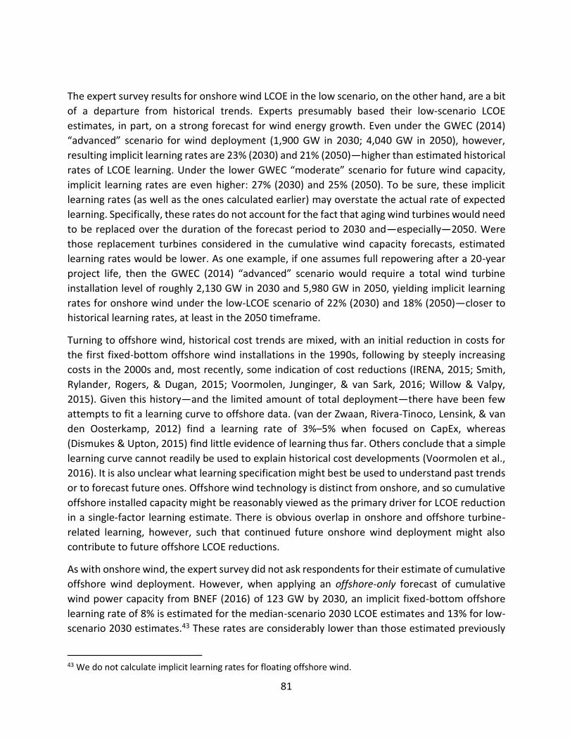
81
The expert survey results for onshore wind LCOE in the low scenario, on the other hand, are a bit
of a departure from historical trends. Experts presumably based their low-scenario LCOE
estimates, in part, on a strong forecast for wind energy growth. Even under the GWEC (2014)
“advanced” scenario for wind deployment (1,900 GW in 2030; 4,040 GW in 2050), however,
resulting implicit learning rates are 23% (2030) and 21% (2050)—higher than estimated historical
rates of LCOE learning. Under the lower GWEC “moderate” scenario for future wind capacity,
implicit learning rates are even higher: 27% (2030) and 25% (2050). To be sure, these implicit
learning rates (as well as the ones calculated earlier) may overstate the actual rate of expected
learning. Specifically, these rates do not account for the fact that aging wind turbines would need
to be replaced over the duration of the forecast period to 2030 and—especially—2050. Were
those replacement turbines considered in the cumulative wind capacity forecasts, estimated
learning rates would be lower. As one example, if one assumes full repowering after a 20-year
project life, then the GWEC (2014) “advanced” scenario would require a total wind turbine
installation level of roughly 2,130 GW in 2030 and 5,980 GW in 2050, yielding implicit learning
rates for onshore wind under the low-LCOE scenario of 22% (2030) and 18% (2050)—closer to
historical learning rates, at least in the 2050 timeframe.
Turning to offshore wind, historical cost trends are mixed, with an initial reduction in costs for
the first fixed-bottom offshore wind installations in the 1990s, following by steeply increasing
costs in the 2000s and, most recently, some indication of cost reductions (IRENA, 2015; Smith,
Rylander, Rogers, & Dugan, 2015; Voormolen, Junginger, & van Sark, 2016; Willow & Valpy,
2015). Given this history—and the limited amount of total deployment—there have been few
attempts to fit a learning curve to offshore data. (van der Zwaan, Rivera-Tinoco, Lensink, & van
den Oosterkamp, 2012) find a learning rate of 3%–5% when focused on CapEx, whereas
(Dismukes & Upton, 2015) find little evidence of learning thus far. Others conclude that a simple
learning curve cannot readily be used to explain historical cost developments (Voormolen et al.,
2016). It is also unclear what learning specification might best be used to understand past trends
or to forecast future ones. Offshore wind technology is distinct from onshore, and so cumulative
offshore installed capacity might be reasonably viewed as the primary driver for LCOE reduction
in a single-factor learning estimate. There is obvious overlap in onshore and offshore turbine-
related learning, however, such that continued future onshore wind deployment might also
contribute to future offshore LCOE reductions.
As with onshore wind, the expert survey did not ask respondents for their estimate of cumulative
offshore wind deployment. However, when applying an offshore-only forecast of cumulative
wind power capacity from BNEF (2016) of 123 GW by 2030, an implicit fixed-bottom offshore
learning rate of 8% is estimated for the median-scenario 2030 LCOE estimates and 13% for low-
scenario 2030 estimates.43 These rates are considerably lower than those estimated previously
43 We do not calculate implicit learning rates for floating offshore wind.

82
for onshore wind. In contrast, if one applies a range of projections for cumulative total (onshore
and offshore) wind capacity from (BNEF, 2015a; GWEC, 2014; IEA, 2015) (which, while much
greater in total capacity terms, leads to fewer total “doublings” of capacity given the higher
starting point in 2014), then implicit LCOE learning rates from the expert survey range from about
16%–20% when focused on median LCOE in 2030. This learning rate range is somewhat higher
than but closer to the range for onshore wind. Overall, these results for offshore wind suggest
that experts either anticipate lower offshore-only learning (relative to learning for onshore wind)
or expect learning spillovers from onshore to offshore.
3.7.2 Forecasts for Future LCOE Reduction
It is also relevant to compare the expert elicitation results to other forecasts of LCOE change over
time. Figure 32 does just that, for onshore wind and for fixed-bottom offshore wind (see
Appendix C for a listing of the references from which the other forecasts were obtained).44
The expert survey results for onshore wind are generally within the range of other forecasts, but
elicitation results tend to show greater expectations for LCOE reductions for onshore wind in the
median scenario than the majority of other forecasts. The reasons for this somewhat-more
aggressive set of onshore LCOE estimates from wind energy experts in the median scenario is not
known. However, other forecasts are sometimes informed by published learning rates that, as
noted earlier, have been primarily based on CapEx (Criqui et al., 2015). Learning rates based on
CapEx alone, however, will understate LCOE-based learning given concomitant advances in
capacity factor, OpEx, and other factors impacting LCOE (BNEF, 2015b). Recent estimates of
CapEx-based learning (LR = 6-9%) cited earlier, for example, are well below the historical LCOE-
based learning rates shown in Figure 31. As such, at least some of the broader literature might
be biased low in terms of onshore wind energy LCOE forecasts due to inappropriate use of CapEx-
based learning estimates (Criqui et al., 2015). Alternatively, our expert survey results could be
biased in some way, or other forecasters might have tended to err on the side of conservatism
for other reasons, such as a presumed decline in the learning rate over time.
The expert survey results for fixed-bottom offshore wind, meanwhile, tend to be more
conservative than the broader literature, both for the median and low scenarios. Specifically, a
sizable number of other forecasts anticipate steeper LCOE reductions than even the low-scenario
expert survey results. As indicated earlier, offshore wind energy costs have not experienced the
sizable historical reductions witnessed onshore. Those historical data points may be encouraging
some conservatism among the experts, at least relative to the broader literature.
44 We do not include a similar chart for floating offshore wind because of the limited number of unique estimates for the future cost of this technology, relative to a 2014 fixed-bottom baseline.

83
Note: See Appendix C for a listing of the references from which the literature-derived estimates were sourced.
Figure 32: Estimated Change in LCOE over Time for (a) Onshore and (b) Fixed-Bottom Offshore Wind Projects: Expert Survey Results vs. Other Forecasts

84
4. Conclusion The wind energy industry has matured substantially since its beginnings in the 1970s, as has wind
power technology. Sizable reductions in the cost of onshore wind energy have accompanied that
maturation, with some experts anticipating that those reductions will also be witnessed offshore.
But how much additional cost reduction is possible, both onshore and offshore? What
technological and market factors are the most likely contributors to those reductions? And what
broad trends might drive even greater technological advancements and cost reductions?
This study has sought to help answer these questions, leveraging the unique insights of 163 of
the world’s foremost wind energy experts. Specifically, we have summarized the core results of
an expert elicitation survey on future wind energy costs and technology advancement
possibilities, in what may be the largest single elicitation ever performed on an energy technology
in terms of expert participation. Insights gained through this survey can complement other tools
for evaluating cost-reduction potential, including the use of learning curves, engineering
assessments, and less-formal means of synthesizing expert knowledge. Ultimately, we hope this
work informs policy and planning decisions, R&D decisions, and industry investment and strategy
development while improving the representation of wind energy in energy-sector planning
models.
Notwithstanding the growing maturity of onshore wind and the limited evidence of historical cost
reductions for offshore wind, we find that experts anticipate significant additional reductions in
the levelized cost of wind energy across all three applications. As summarized in Figure 33, under
the median scenario, experts anticipate 24%–30% reductions by 2030 and 35%–41% reductions
by 2050. Costs could be even lower: experts predict a 10% chance that reductions will be more
than 40% by 2030 and more than 50% by 2050. Though onshore wind is anticipated to remain
less expensive than offshore—and fixed-bottom less expensive than floating—there are greater
absolute reductions (and more uncertainty) in the long-term LCOE of offshore wind compared
with onshore wind.
For onshore wind, CapEx and capacity factor improvements are expected to constitute the largest
drivers of LCOE reduction. The importance of higher capacity factors is consistent with expert
views on turbine characteristics, with scaling expected not only in turbine capacity ratings but
also rotor diameters and hub heights. For fixed-bottom offshore wind, on the other hand, CapEx
reductions and improvements in financing costs are the largest expected contributors to LCOE
reduction. The relatively higher importance of CapEx and lower importance of capacity factor is
consistent with expert opinions on future offshore turbine size: expected turbine capacity ratings
(and hub heights) grow significantly in order to minimize CapEx, but specific power is expected
to remain roughly at recent levels. Capacity factor improvements play a larger role for floating
offshore wind (relative to the 2014 baseline for fixed-bottom), perhaps reflecting a belief that
floating technology will tend to be deployed in windier sites as enabled by the ability to access
deeper water locations. Some of the specific technology, market, and other changes expected to
drive down LCOE are listed in Figure 33 and detailed earlier.

85
Figure 33: Summary of Expert Survey Findings
Elicitation results for onshore wind are consistent with historical LCOE learning, suggesting that
properly constructed learning rates may be reasonably used to forecast future costs in more
mature applications. However, the majority of the literature assessing historical learning rates
for wind have emphasized only upfront capital costs, and some energy-sector and integrated-
assessment models rely on those learning estimates when forecasting future costs (Criqui et al.,
2015). Expert elicitation findings demonstrate that capital-cost improvements are only one
means of achieving LCOE reductions, and not always the dominant one. Extrapolation of past
capital-cost-based learning models therefore likely understates the opportunities for future LCOE
reduction by ignoring major drivers for that reduction. This is illustrated by the fact that the
elicitation-based forward-looking LCOE learning rates are twice as high as recently estimated
CapEx-based learning rates for onshore wind of 6-9%, and may explain why onshore cost
reduction estimates from wind experts are more aggressive than many past forecasts.
Expert survey results further illustrate the considerable uncertainty that exists across all of these
variables and factors. This uncertainty is, in part, reflected in the range among expert-specified
low-, median-, and high-scenario LCOE estimates. And, to some degree, managing this
uncertainty is within the control of public and private decision makers: learning with market
growth along with R&D, for example, are the two most significant factors in enabling the low-

86
LCOE scenario. Differences are also found when reviewing the range in expert-specific responses
(rather than median responses). Some of the variation in expert-specific responses, meanwhile,
can be explained by segmenting respondents into various categories. As presented in various text
boxes earlier, for example, we find that the smaller “leading-expert” group generally expects
greater wind energy cost reductions than the larger set of other respondents, whereas
equipment manufacturers are sometimes more cautious about nearer-term advancement
possibilities. Future work is planned to assess more thoroughly these differences in survey
responses by respondent characteristics.

87
Conclusion of the Dissertation Working on renewable energy cost developments has been a rewarding field for me and the
continued progress in the wind and especially solar industry over the past years has been exciting
to follow. The downside of working on market developments is that individual values are often
already outdated as soon they are published and the next quarter commences with new
statistics.
Since 2013 the German and U.S. solar sector have developed with differing dynamics: In the
United States installed solar capacity has soared thanks to continued project price declines (G.
Barbose & Darghouth, 2017; Bolinger & Seel, 2017), an extension of the investment tax credit
until 2023, and overall very favorable solar resource conditions, to nearly 15GWDC of new annual
installations at the end of 2016. In Germany the pace of new solar installations has slowed in
contrast since the heights of 2009-2012, largely due to strongly reduced remuneration levels and
the introduction of annual capacity limits, to a mere tenth of U.S. annual installations. As a result,
both markets are now on par with about 40GWDC of cumulative solar capacity at the end of 2016.
Even though significant progress has been made towards achieving the ambitious cost reduction
targets of U.S. SunShot initiative for 2020 (leading to a second set of targets for 2030 that aim at
further energy cost reductions of 50%), a cursory look seems to indicate that upfront capital costs
of U.S. residential systems in 2016 continue to be nearly twice as high as their German
counterparts.
It is instead utility-scale solar systems that have led the capacity explosion in the United States
over the last years, and project cost declines enabled many new state markets outside of the
traditional Southwest in less sunny regions. At the same time, falling prices for single-axis trackers
have since promoted the increasing ubiquity of tracking capabilities, even among the northern-
most installations in Minnesota. As result of these opposing trends, national average net capacity
factors have stabilized around 28% over the past three years. While some U.S. developers have
started to incorporate electric storage solutions into their utility-scale PV system designs, I have
not yet seen a widespread deployment outside of Hawaii. Increasingly the focus among project
developers seems to shift from maximizing overall net generation (and thus reducing the average
LCOE) to increasing the project’s value proposition (for example via a more western orientation
to deliver electricity in high-demand evening hours).
Since polling our experts on future wind energy cost reductions in late 2015, there have been
frequent media reports on record-low PPA announcements for fixed-bottom offshore wind
projects in Europe. While it is difficult to place these new low-cost projects exactly within our
methodological framework of “typical projects” (several of them are built on the continental shelf
in favorable low-depths and it is unclear whether all costs that we included in our “plant-
boundary” definition are captured in the reported estimates, or whether additional incentives
may have lowered the strike prices), it seems that fixed-bottom offshore LCOE are tumbling far
faster in Europe than what our survey respondents predicted.

88
While individual statistics are prone to become quickly stale and outdated in the very dynamic
environment of renewable energy costs, I have demonstrated repeatable methods in this
dissertation that are hopefully of lasting value and that can be re-applied as desired.
Whereas system components for wind and solar projects have increasingly been standardized
globally (although some pricing and technical differences may persist due to import tariffs or local
content requirements), project design choices continue to be potentially quite distinct to capture
the highest value based on local electricity demand and supply patterns, different regulatory
approaches and policy incentive design. Cross-market analyses in particular can discover
innovative project design approaches and business practices that may have not yet fully
permeated to other markets, but that could offer significant benefits. This will hold especially
true as system design becomes increasingly differentiated to capture a larger variety of value
streams (e.g. ancillary service and capacity value in addition to energy value alone) and to
arbitrage across high and low value hours (either via demand response or energy storage in
increasingly sophisticated energy management systems).
This dissertation focused on examples of renewable energy cost reduction potentials, but equally
important are complementary analyses that investigate opportunities to increase the value that
can be captured by variable renewable energy projects that harness wind and solar energy. While
continued cost reductions are essential given the staggering task of broad renewable energy
capacity deployment to slow destructive climate change, an exclusive focus on such measures
may be misleading. In an extreme scenario, non-dispatchable solar and wind resources would be
caught in a vicious spiral of self-inflicted value destruction and further forced excessive cost-
cutting measures in a race to the bottom as they gain larger shares in an electricity system –
potentially negating benefits such as widespread employment opportunities with livable wages
across a range of worker skills and vitalized communities.
Utilizing the aforementioned cross-market analyses to identify and learn from promising
engineering approaches, successful business strategies, insightful market designs, or broader
policy and community-based initiatives will thus become increasingly important to facilitate a
continued cost- and value-effective build-out of low-carbon, renewable energy systems – even
at higher penetration levels.

89
References / Bibliography
Advanced Energy. (2013). DC Loading of AE TX Inverters. San Jose, CA: Advanced Energy. Retrieved from http://solarenergy.advanced-energy.com/upload/File/Application%20Notes/ENG-DCLoadingTX-260-02_Web.pdf
Anadón, L. D., Nemet, G., & Verdolini, E. (2013). The future costs of nuclear power using multiple expert elicitations: effects of RD&D and elicitation design. Environmental Research Letters, 8(3), 034020. https://doi.org/10.1088/1748-9326/8/3/034020
Ardani, K., Barbose, G., Margolis, R., Wiser, R., Feldman, D., & Ong, S. (2012). Benchmarking non-hardware BoS costs for US PV systems using a data-driven analysis from PV installer surveys (No. DOE/GO-10212-3834). US Department of Energy (DoE).
Arrow, K. J. (1962). The economic implications of learning by doing. The Review of Economic Studies, 29, 155–173.
Arvizu, D., Balaya, P., Cabeza, L., Hollands, T., Jaeger-Waldau, A., Kondo, M., … Zilles, R. (2011). Direct Solar Energy. In Special Report on Renewable Energy Sources and Climate Change Mitigation. Intergovernmental Panel on Climate Change (IPCC).
Baker, E., Bosetti, V., Anadon, L. D., Henrion, M., & Aleluia Reis, L. (2015). Future costs of key low-carbon energy technologies: Harmonization and aggregation of energy technology expert elicitation data. Energy Policy, 80, 219–232. https://doi.org/10.1016/j.enpol.2014.10.008
Barbose, G., & Darghouth, N. (2015). Tracking the Sun VI- A Historical Summary of Installed Cost of Photovoltaics in the United States from 1998 to 2012 (LBNL-188238). Berkeley, CA: Lawrence Berkeley National Laboratory (LBNL). Retrieved from http://emp.lbl.gov/publications/tracking-sun-vi-historical-summary-installed-price-photovoltaics-united-states-1998-201
Barbose, G., & Darghouth, N. (2017). Tracking the Sun X: The Installed Price of Residential and Non-Residential Photovoltaic Systems in the United States. Berkeley, CA: Lawrence Berkeley National Laboratory (LBNL). Retrieved from trackingthesun.lbl.gov
Barbose, G., Darghouth, N., Weaver, S., Feldman, D., Margolis, R., & Wiser, R. (2015). Tracking U.S. Photovoltaic System Prices 1998-2012: A Rapidly Changing Market. Progress in Photovoltaics: Research and Applications, 23(6), 692–704.
Barbose, G. L., & Darghouth, N. R. (2015). Tracking the Sun VIII: The Installed Price of Residential and Non-Residential Photovoltaic Systems in the United States. Retrieved from https://emp.lbl.gov/publications/tracking-sun-viii-installed-price
Barbose, G., Wiser, R., & Darghouth, N. (2012). Tracking the Sun V- A Historical Summary of Installed Cost of Photovoltaics in the United States from 1998 to 2012 (LBNL-5919E). Berkeley, CA: Lawrence Berkeley National Laboratory (LBNL). Retrieved from http://emp.lbl.gov/publications/tracking-sun-v-historical-summary-installed-price-photovoltaics-united-states-1998-2011
Bender, G. (2015). Subpar Solar Irradiance Undermines East Coast Project Performance. Vaisala. Retrieved from http://www.vaisala.com/en/press/news/2015/Pages/Page_1907711.aspx

90
Betz, M., Davidson, O., Bosch, P., Dave, R., & Meyers, L. (Eds.). (2007). Climate Change 2007: Mitigation of Climate Change. Contribution of Working Group III to AR4. In Fourth Assessment Report of the Intergovernmental Panel on Climate Change. Cambridge, UK: Cambridge University Press.
BNEF. (2015a). New Energy Outlook 2015 (Wind Insight). Bloomberg New Energy Finance. BNEF. (2015b). The Future Cost of Onshore Wind – An Accelerating Rate of Progress (Wind
Insight). Bloomberg New Energy Finance. BNEF. (2016). H1 2016 Offshore Wind Market Outlook (Wind Insight). Bloomberg New Energy
Finance. Bolinger, M., & Seel, J. (2015). Utility-Scale Solar 2014: An Empirical Analysis of Project Cost,
Performance, and Pricing Trends in the United States (No. LBNL-1000917). Berkeley, CA: Lawrence Berkeley National Laboratory. Retrieved from https://emp.lbl.gov/publications/utility-scale-solar-2014-empirical
Bolinger, M., & Seel, J. (2017). Utility-Scale Solar 2016: An Empirical Analysis of Project Cost, Performance, and Pricing Trends in the United States. Berkeley, CA: Lawrence Berkeley National Laboratory. Retrieved from http://utilityscalesolar.lbl.gov
Bolinger, M., Weaver, S., & Zuboy, J. (2015). Is $50/MWh solar for real? Falling project prices and rising capacity factors drive utility-scale PV toward economic competitiveness: Technical and economic improvements drive utility-scale PV to $50/MWh. Progress in Photovoltaics: Research and Applications, 23(12), 1847–1856. https://doi.org/10.1002/pip.2630
Bollinger, B., & Gillingham, K. (2012). Peer Effects in the Diffusion of Solar Photovoltaic Panels. Marketing Science, 31(6), 900–912. https://doi.org/10.1287/mksc.1120.0727
Bony, L., Doig, S., Hart, C., Maurer, E., & Newman, S. (2010). Achieving Low-Cost Solar PV. Snowmass, CO: Rocky Mountain Institute (RMI).
Bromley, H. (2012). California versus German solar prices: same dope, twice as high (Research Note). Bloomberg New Energy Finance.
Bundesnetzagentur. (2013). Monthly PV System Interconnection Announcements 2009-2013. Retrieved from http://www.bundesnetzagentur.de/cln_1911/DE/Sachgebiete/ElektrizitaetundGas/Unternehmen_Institutionen/ErneuerbareEnergien/Photovoltaik/DatenMeldgn_EEG-VergSaetze/DatenMeldgn_EEG-VergSaetze_node.html
Bundesverband Solarwirtschaft (BSW-Solar). (2012). Photovoltaik - Steuerrecht, Gewerberecht, Verguetungsrecht (No. 6. Auflage). Berlin.
BVG Associates. (2015). Offshore Wind: Delivering More for Less. prepared for Statkraft UK. Retrieved from https://www.statkraft.com/globalassets/4-statkraft-uk/offshore_wind_more_for_less_pages.pdf
Bywaters, G., John, V., Lynch, J., Mattila, P., Norton, G., Stowell, J., … Hablanian, D. (2005). Northern Power Systems WindPACT Drive Train Alternative Design Study Report (No. NREL/SR-500-35524). Golden, CO: National Renewable Energy Laboratory (NREL). Retrieved from http://www.nrel.gov/docs/fy05osti/35524.pdf
California Public Utilities Commission. (2015). RPS Calculator V6.1. Retrieved from http://www.cpuc.ca.gov/RPS_Calculator/

91
Campeau, Z., Anderson, M., Hasselbrink, E., Kavulak, D., Yu-Chen, S., Lacerda, R., … Budiman, A. (2013). SunPower Module Degradation Rate. Richmond, CA: SunPower Corporation. Retrieved from https://us.sunpower.com/sites/sunpower/files/media-library/white-papers/wp-sunpower-module-degradation-rate.pdf
Cohen, J., Schweizer, T., Laxson, A., Butterfield, S., Schreck, S., Fingersh, L., … Ashwill, T. (2008). Technology Improvement Opportunities for Low Wind Speed Turbines and Implications for Cost of Energy Reduction (No. NREL/TP-500-41036). Golden, CO: National Renewable Energy Laboratory (NREL). Retrieved from http://www.nrel.gov/docs/fy08osti/41036.pdf
Coppersmith, K. J., Jenni, K. E., Perman, R. C., & Youngs, R. R. (2009). Formal expert assessment in probabilistic seismic and volcanic hazard analysis. In C. B. Connor, N. A. Chapman, & L. J. Connor (Eds.), Volcanic and Tectonic Hazard Assessment for Nuclear Facilities. Cambridge, UK: Cambridge University Press.
Criqui, P., Mima, S., Menanteau, P., & Kitous, A. (2015). Mitigation strategies and energy technology learning: An assessment with the POLES model. Technological Forecasting and Social Change, 90, 119–136. https://doi.org/10.1016/j.techfore.2014.05.005
Crown Estate. (2012). Offshore Wind Cost Reduction Pathways Study. London, UK: The Crown Estate. Retrieved from https://www.thecrownestate.co.uk/media/5493/ei-offshore-wind-cost-reduction-pathways-study.pdf
Darghouth, N. R., Barbose, G., & Wiser, R. (2011). The impact of rate design and net metering on the bill savings from distributed PV for residential customers in California. Energy Policy, 39(9), 5243–5253. https://doi.org/10.1016/j.enpol.2011.05.040
Denholm, P., & Margolis, R. M. (2007). Evaluating the limits of solar photovoltaics (PV) in electric power systems utilizing energy storage and other enabling technologies. Energy Policy, 35(9), 4424–4433. https://doi.org/10.1016/j.enpol.2007.03.004
Denholm, P., Novacheck, J., Jorgenson, J., & O’Connell, M. (2016). Impact of Flexibility Options on Grid Economic Carrying Capacity of Solar and Wind: Three Case Studies | Department of Energy. Golden, CO: National Renewable Energy Laboratory.
Dinica, V. (2011). Renewable electricity production costs—A framework to assist policy-makers’ decisions on price support. Energy Policy, 39(7), 4153–4167. https://doi.org/10.1016/j.enpol.2011.04.021
Dismukes, D. E., & Upton, G. B. (2015). Economies of scale, learning effects and offshore wind development costs. Renewable Energy, 83, 61–66. https://doi.org/10.1016/j.renene.2015.04.002
DOE. (2015). Wind Vision: A New Era for Wind Power in the United States. Washington D.C.: U.S. Department of Energy. Retrieved from https://www.energy.gov/sites/prod/files/WindVision_Report_final.pdf
Dong, C., & Wiser, R. (2013). The impact of local permitting processes on residential PV installation prices and development times (No. LBNL 6140-E). Berkeley, CA: Lawrence Berkeley National Laboratory (LBNL).
Drury, E., Lopez, A., Denholm, P., & Margolis, R. (2013). Relative performance of tracking versus fixed tilt photovoltaic systems in the USA: Relative performance of tracking versus fixed tilt photovoltaic systems. Progress in Photovoltaics: Research and Applications. https://doi.org/10.1002/pip.2373

92
DSIRE. (2012). Solar Sales Tax Incentives. Database of State Incentives for Renewables and Efficiency. Retrieved from http://www.dsireusa.org/solar/solarpolicyguide/?id=12
Edenhofer, O., Hirth, L., Knopf, B., Pahle, M., Schlömer, S., Schmid, E., & Ueckerdt, F. (2013). On the economics of renewable energy sources. Energy Economics, 40, S12–S23. https://doi.org/10.1016/j.eneco.2013.09.015
Ek, K., & Söderholm, P. (2010). Technology learning in the presence of public R&D: The case of European wind power. Ecological Economics, 69(12), 2356–2362. https://doi.org/10.1016/j.ecolecon.2010.07.002
Energy Information Administration. (2015). How much electricity is lost in transmission and distribution in the United States? (Frequently Asked Questions). Retrieved from https://www.eia.gov/tools/faqs/faq.cfm?id=105&t=3
EuPD. (2013). Database of Installer Offer Prices for German Residential PV Systems 2006-2012. Ferioli, F., Schoots, K., & van der Zwaan, B. C. C. (2009). Use and limitations of learning curves for
energy technology policy: A component-learning hypothesis. Energy Policy, 37(7), 2525–2535. https://doi.org/10.1016/j.enpol.2008.10.043
Fingersh, L., Hand, M., & Laxson, A. (2006). Wind Turbine Design Cost and Scaling Model (No. NREL/SR-500-40566). Golden, CO: National Renewable Energy Laboratory (NREL). Retrieved from https://www.scribd.com/document/3862797/NREL-Wind-Turbine-Design-Costs-and-Scale-Model
Fiorelli, J., & Zuercher-Martinson, M. (2013). Array Oversizing. Solectria Renewables. Retrieved from https://www.solectria.com//site/assets/files/1480/solectria_array_oversizing_white_paper.pdf
First Solar. (2015). First Solar Advanced Thin-Film Module Features (First Solar PV Modules). Tempe, AZ: First Solar. Retrieved from http://www.firstsolar.com/Home/Technologies-and-Capabilities/PV-Modules/First-Solar-Series-3-Black-Module
Fitchner-Prognos. (2013). Cost Reduction Potentials of Offshore Wind Power in Germany. Berlin, Germany: Prepared for the German Offshore Wind Energy Foundation. Retrieved from https://www.prognos.com/uploads/tx_atwpubdb/130822_Prognos_Fichtner_Studie_Offshore-Wind_Kurz_EN_05.pdf
Gillenwater, M. (2013). Probabilistic decision model of wind power investment and influence of green power market. Energy Policy, 63, 1111–1125. https://doi.org/10.1016/j.enpol.2013.09.049
Goodrich, A., James, T., & Woodhouse, M. (2012). Residential, Commercial and Utility-Scale PV System Prices in the US: Current Drivers and Cost-Reduction Opportunities. National Renewable Energy Laboratory (NREL).
GTM Research. (2011). Solar PV Balance of system (BOS): Technologies and Markets. GTM Research, & SEIA. (2011). U.S. Solar Market Insight Report 2010. GTM Research, & SEIA. (2012). U.S. Solar Market Insight Report 2011. GTM Research, & SEIA. (2013). U.S. Solar Market Insight Report 2012. GTM Research, & SEIA. (2015). U.S. Solar Market Insight Report: 2014 Year in Review. Washington
D.C.: Solar Energy Industry Association.

93
GWEC. (2014). Global Wind Energy Outlook 2014. Brussels, Belgium: Global Wind Energy Council. Retrieved from http://www.gwec.net/publications/global-wind-energy-outlook/global-wind-energy-outlook-2014/
GWEC. (2015). Global Wind Report: Annual Market Update 2014. Brussels, Belgium: Global Wind Energy Council. Retrieved from http://www.gwec.net/publications/global-wind-report-2/global-wind-report-2014-annual-market-update/
Haas, R. (2004). Progress in markets for grid-connected PV systems in the built environment. Progress in Photovoltaics: Research and Applications, 12(6), 427–440. https://doi.org/10.1002/pip.560
Haas, R., Resch, G., Panzer, C., Busch, S., Ragwitz, M., & Held, A. (2011). Efficiency and effectiveness of promotion systems for electricity generation from renewable energy sources – Lessons from EU countries. Energy, 36(4), 2186–2193. https://doi.org/10.1016/j.energy.2010.06.028
Haller, M., Hermann, H., Loreck, C., & Matthes, F. (2013). EEG-Umlage und die Kosten der Stroversorgung fuer 2013, Eine Analyse von Trends, Ursachen und Wechselwirkungen. Berlin: Oeko-Institut e.V.
Hirth, L. (2013). The market value of variable renewables: The effect of solar wind power variability on their relative price. Energy Economics, 38, 218–236. https://doi.org/10.1016/j.eneco.2013.02.004
Hora, S. C. (2007). Assessing Probabilities from Experts. In W. Edwards, R. F. Miles, & D. Von Winterfeldt (Eds.), Advances in Decision Analysis: From Foundations to Applications. Cambridge, UK: Cambridge University Press.
Hora, S. C., & Von Winterfeldt, D. (1997). Nuclear waste and future societies: A look into the deep future. Technological Forecasting and Social Change, 56(2), 155–170. https://doi.org/10.1016/S0040-1625(97)00075-9
IEA. (2013). Technology Roadmap: Wind energy. Paris, France: International Energy Agency (IEA). Retrieved from https://www.iea.org/publications/freepublications/publication/Wind_2013_Roadmap.pdf
IEA. (2015). World Energy Outlook 2015. Paris, France: International Energy Agency (IEA). Retrieved from http://www.worldenergyoutlook.org/weo2015/
InterAcademy Council. (2010). Climate Change Assessments: Review of the Processes and Procedures of the IPCC. Alkmaar, The Netherlands: InterAcademy Council. Retrieved from http://www.interacademycouncil.net/24026/26050.aspx
IPCC. (1996). Impacts, Adaptations and Mitigation of Climate Change: Scientific Technical Analyses. Contributions of the Working Group II to the Second Assessment Report of the Intergovernmental Panel on Climate Change. Cambridge, UK and New York, NY, US: Intergovernmental Panel on Climate Change. Retrieved from https://www.ipcc.ch/ipccreports/sar/wg_II/ipcc_sar_wg_II_full_report.pdf
IPCC. (2014). Climate Change 2014: Mitigation of Climate Change: Working Group III Contribution to the Fifth Assessment Report of the IPCC. Cambridge, UK: Cambridge University Press.
IRENA. (2015). Renewable Power Generation Costs in 2014. Bonn, Germany: International Renewable Energy Agency (IRENA). Retrieved from

94
https://www.irena.org/DocumentDownloads/Publications/IRENA_RE_Power_Costs_2014_report.pdf
Jordan, D. C., & Kurtz, S. R. (2013). Photovoltaic Degradation Rates-an Analytical Review: Photovoltaic degradation rates. Progress in Photovoltaics: Research and Applications, 21(1), 12–29. https://doi.org/10.1002/pip.1182
Joskow, P. L. (2011). Comparing the Costs of Intermittent and Dispatchable Electricity Generating Technologies. American Economic Review, 101(3), 238–241. https://doi.org/10.1257/aer.101.3.238
Junginger, M., Faaij, A., & Turkenburg, W. (2004). Cost Reduction Prospects for Offshore Wind Farms. Wind Engineering, 28(1), 97–118. https://doi.org/10.1260/0309524041210847
Junginger, M., Sark, W. van, & Faaji, A. (2010). Technological Learning in the Energy Sector. Northampton, Massachusetts, USA: Edward Elgar Publishing, Inc.
Kahneman, D., Slovic, P., & Tversky, A. (1982). Judgment under Uncertainty: Heuristics and Biases. Cambridge, UK: Cambridge University Press.
Kempton, W., McClellan, S., & Ozkan, D. (2016). Massachusetts Offshore Wind Future Cost Study. University of Delaware Special Initiative on Offshore Wind. Retrieved from https://www.ceoe.udel.edu/File%20Library/About/SIOW/MA-Offshore-Wind-Future-Cost-Study-FINAL-14-Mar-16.pdf
Klessmann, C., Rathmann, M., de Jager, D., Gazzo, A., Resch, G., Busch, S., & Ragwitz, M. (2013). Policy options for reducing the costs of reaching the European renewables target. Renewable Energy, 57, 390–403. https://doi.org/10.1016/j.renene.2013.01.041
Knol, A. B., Slottje, P., van der Sluijs, J. P., & Lebret, E. (2010). The use of expert elicitation in environmental health impact assessment: a seven step procedure. Environmental Health, 9(1). https://doi.org/10.1186/1476-069X-9-19
Kotra, J. P., Lee, M. P., Eisenberg, N. A., & DeWispelare, A. R. (1996). Branch Technical Position on the Use of Expert Elicitation in the High-Level Radioactive Waste Program. Washington, DC: Nuclear Regulatory Commission. Retrieved from https://www.nrc.gov/reading-rm/doc-collections/nuregs/staff/sr1563/
Lantz, E. R., Wiser, R. H., & Hand, M. (2012). The Past and Future Cost of Wind Energy (International Energy Agency Wind Task 26). Golden, CO: National Renewable Energy Laboratory (NREL). Retrieved from https://www.ieawind.org/index_page_postings/WP2_task26.pdf
Lazard. (2016). Levelized Cost of Energy Analysis 10. Retrieved from https://www.lazard.com/media/438038/levelized-cost-of-energy-v100.pdf
Lee, A., & Moses, C. (2015). EIA electricity data now include estimated small-scale solar PV capacity and generation (Today in Energy). Energy Information Administration. Retrieved from http://www.eia.gov/todayinenergy/detail.cfm?id=23972
Lindman, Å., & Söderholm, P. (2012). Wind power learning rates: A conceptual review and meta-analysis. Energy Economics, 34(3), 754–761. https://doi.org/10.1016/j.eneco.2011.05.007
Luderer, G., Krey, V., Calvin, K., Merrick, J., Mima, S., Pietzcker, R., … Wada, K. (2014). The role of renewable energy in climate stabilization: results from the EMF27 scenarios. Climatic Change, 123(3–4), 427–441. https://doi.org/10.1007/s10584-013-0924-z

95
Malcolm, D., & Hansen, A. (2002). WindPACT Turbine Rotor Design Study (No. NREL/SR-500-32495). Golden, CO: National Renewable Energy Laboratory (NREL). Retrieved from http://www.nrel.gov/docs/fy06osti/32495.pdf
Maycock, P., & Wakefield, G. (1975). Business analysis of solar photovoltaic conversion. Presented at the 11th IEEE PV Specialist Conference, Scottsdale, AZ, USA.
Mendonca, M. (2009). Powering the green economy: the feed-in tariff handbook. Sterling, VA: Earthscan.
Meyer, M. A., & Booker, J. M. (2001). Eliciting and Analyzing Expert Judgment: A Practical Guide. Philadelphia, Pennsylvania: Society for Industrial and Applied Mathematics (SIAM).
Meymandi, J.-F., Chin, S., Sanghavi, M., & Prasad, S. (2013). UBS Global Solar Industry Update. UBS Investment Research. Retrieved from www.ubs.com/investmentresearch
Mills, A. D., & Wiser, R. H. (2013). Changes in the Economic Value of Photovoltaic Generation at High Penetration Levels: A Pilot Case Study of California. IEEE Journal of Photovoltaics, 3(4), 1394–1402. https://doi.org/10.1109/JPHOTOV.2013.2263984
Mills, A., Wiser, R., Barbose, G., & Golove, W. (2008). The impact of retail rate structures on the economics of commercial photovoltaic systems in California. Energy Policy, 36(9), 3266–3277. https://doi.org/10.1016/j.enpol.2008.05.008
Mints, P. (2012, April). Photovoltaic Manufacturer Shipments, Capacity & Competitive Analysis 2011/2012. Navigant Consulting.
Mints, P. (2013). The Global Market for PV Technologies. Presented at the PVSAT-9, Swansea University: Paula Mints Solar PV Market Research.
Morgan, M. G. (2014). Use (and abuse) of expert elicitation in support of decision making for public policy. Proceedings of the National Academy of Sciences, 111(20), 7176–7184. https://doi.org/10.1073/pnas.1319946111
Morris, J., Calhoun, K., Goodman, J., & Seif, D. (2013). Reducing Solar PV Soft Costs. Snowmass, CO: Rocky Mountain Institute (RMI). Retrieved from http://www.rmi.org/simple
Mukora, A., Winksel, M., Jeffrey, H. F., & Mueller, M. (2009). Learning curves for emerging energy technologies. Proceedings of the Institution of Civil Engineers - Energy, 162(4), 151–159. https://doi.org/10.1680/ener.2009.162.4.151
Navigant. (2013). U.S. Offshore Wind Manufacturing and Supply Chain Development. Burlington, Massachusetts: Navigant Consulting. Retrieved from https://www1.eere.energy.gov/wind/pdfs/us_offshore_wind_supply_chain_and_manufacturing_development.pdf
Neij, L. (1997). Use of experience curves to analyse the prospects for diffusion and adoption of renewable energy technology. Energy Policy, 25(13), 1099–1107. https://doi.org/10.1016/S0301-4215(97)00135-3
Neij, L. (2008). Cost development of future technologies for power generation—A study based on experience curves and complementary bottom-up assessments. Energy Policy, 36(6), 2200–2211. https://doi.org/10.1016/j.enpol.2008.02.029
Nemet, G. F. (2006). Beyond the learning curve: factors influencing cost reductions in photovoltaics. Energy Policy, 34(17), 3218–3232. https://doi.org/10.1016/j.enpol.2005.06.020

96
Nemet, G. F., Anadon, L. D., & Verdolini, E. (2017). Quantifying the Effects of Expert Selection and Elicitation Design on Experts’ Confidence in Their Judgments About Future Energy Technologies. Risk Analysis, 37(2), 315–330. https://doi.org/10.1111/risa.12604
Nordhaus, W. D. (2014). The Perils of the Learning Model for Modeling Endogenous Technological Change. The Energy Journal, 35(1). https://doi.org/10.5547/01956574.35.1.1
NRC. (2007). Prospective Evaluation of Applied Energy Research and Development at DOE (Phase Two). Washington D.C.: National Research Council.
Oppermann, K. (2002). Perspektiven Erneuerbarer Energien Teil 4: Fördergebnisse des 100.000 Dächer-Solarstrom-Programms- eine Zwischenbilanz (KfW Beiträge zur Mittelstands- und Strukturpolitik 28). Frankfurt am Main: Kreditanstalt für Wiederaufbau (KfW).
Oppermann, K. (2004). Perspektiven Erneuerbarer Energien: Das 100.000 Dächer-Solarstrom-Programm: Eine Schlussbilanz (KfW Beiträge zur Mittelstands- und Strukturpolitik 31). Frankfurt am Main: Kreditanstalt für Wiederaufbau (KfW).
Persem, M., Chrometzka, T., Brennig, C., Brohm, R., Moch, F., & Hielscher, T. (2011). Reduction of administrative barriers for PV systems in Germany at the national level (PV Legal). Bundesverband der Solarwirtschaft (BSW).
PV Grid. (2012). Time estimates for residential PV systems in Germany. Bundesverband der Solarwirtschaft (BSW).
REN21. (2015). Renewables 2015: Global Status Report. Paris, France: Renewable Energy Policy Network for the 21st Century. Retrieved from http://www.ren21.net/wp-content/uploads/2015/07/REN12-GSR2015_Onlinebook_low1.pdf
Ringbeck, S., & Sutterlueti, J. (2013). BoS costs: status and optimization to reach industrial grid parity. Progress in Photovoltaics: Research and Applications. https://doi.org/10.1002/pip.2383
Rosenblum, L. (1978). Cost of Photovoltaic Energy Systems as Determined by Balance-Of-System Costs (NASA Technical Memorandum No. NASA-TM-78957). Cleveland, OH: Lewis Research Center.
RSMeans. (2010). Building Construction Cost Data. Norwell, Massachusetts: Reed Construction Data.
Rubin, E. S., Azevedo, I. M. L., Jaramillo, P., & Yeh, S. (2015). A review of learning rates for electricity supply technologies. Energy Policy, 86, 198–218. https://doi.org/10.1016/j.enpol.2015.06.011
Schaeffer, G. J., Alsema, E., Seebregts, A., Beurskens, L., Moor, H. de, Sark, W. van, … Zuccaro, C. (2004). Learning from the Sun. Energy Research Centre of the Netherlands (ECN).
Schneider, S., Semenov, S., Patwardhan, A., Burton, I., Magadza, C., Oppenheimer, M., … Yamin, F. (2007). Climate Change 2007: Impacts, Adaptation and Vulnerability. Contribution of Working Group II to AR4. In Fourth Assessment Report of the Intergovernmental Panel on Climate Change (pp. 779–810). Cambridge, UK: Cambridge University Press.
Sharpe, P., & Keelin, T. (1998). How SmithKline Beecham Makes Better Resource-Allocation Decisions. Harvard Business Review, 76, 45–57.
Shrimali, G., & Jenner, S. (2012). The Impact of State Policy on Deployment and Cost of Solar PV: A Sector-Specific Empirical Analysis. SSRN Electronic Journal. https://doi.org/10.2139/ssrn.2180498

97
Sieros, G., Chaviaropoulos, P., Sørensen, J. D., Bulder, B. H., & Jamieson, P. (2012). Upscaling wind turbines: theoretical and practical aspects and their impact on the cost of energy. Wind Energy, 15(1), 3–17. https://doi.org/10.1002/we.527
Smith, J., Rylander, M., Rogers, L., & Dugan, R. (2015). It’s All in the Plans: Maximizing the Benefits and Minimizing the Impacts of DERs in an Integrated Grid. IEEE Power and Energy Magazine, 13(2), 20–29. https://doi.org/10.1109/MPE.2014.2379855
Sonvilla, P., Zane, E., Poblocka, A., & Brueckmann, R. (2013). PV Grid - Initial Project Report (p. Brussels, Belgium). PV Grid, Intelligent Energy Europe.
Sprague, E. (2011). The Impact of Local Permitting on the Cost of Solar Power. SunRun. Tepper, M. (2013). Serie der statistischen Zahlen der deutschen Solarstrombranche
(Photovoltaik). Bundesverband der Solarwirtschaft (BSW). Retrieved from http://www.solarwirtschaft.de/presse-mediathek/marktdaten.html
The Tax Foundation. (2013). States and Local Sales Tax Rates 2011-2013. The Tax Foundation. Retrieved from http://taxfoundation.org/article/state-and-local-sales-tax-rates-2011-2013
TKI Wind op Zee. (2015). Cost reduction options for offshore wind in the Netherlands FID 2010-2020. Amsterdam, The Netherlands: PwC, DNV GL, Ecofys. Retrieved from http://www.tki-windopzee.nl/files/2015-10/151028-tki-offshore-wind-cost-reduction-final-stc.pdf
Tong, J. (2012). Nationwide analysis of solar permitting and the implications for soft costs. Clean Power Finance (CPF).
Tsuchida, B., Sergici, S., Mudge, B., Gorman, W., Fox-Penner, P., & Schoene, J. (2015). Comparative Generation Costs of Utility-Scale and Residential-Scale PV in Xcel Energy Colorado’s Service Area. The Brattle Group. Retrieved from http://brattle.com/system/publications/pdfs/000/005/188/original/Comparative_Generation_Costs_of_Utility-Scale_and_Residential-Scale_PV_in_Xcel_Energy_Colorado’s_Service_Area.pdf
U.S. Department of Energy. (2010). $1/W Photovoltaic Systems. White Paper to explore a grand challenge for electricity from solar. U.S. Department of Energy.
U.S. Department of Energy. (2012). SunShot Vision Study. Washington D.C. Vaisala. (2015). 2014 US Solar Performance Maps. Retrieved from
http://www.vaisala.com/Vaisala%20Documents/Vaisala%20News%20Articles/Misc/2014_US_Solar_Performance_report.pdf
Valpy, B., & English, P. (2014a). Future Renewable Energy Costs: Offshore Wind. Cricklade, UK: BVG Associates and KIC InnoEnergy. Retrieved from http://www.innoenergy.com/wp-content/uploads/2014/09/KIC_IE_OffshoreWind_anticipated_innovations_impact1.pdf
Valpy, B., & English, P. (2014b). Future Renewable Energy Costs: Onshore Wind. Cricklade, UK: BVG Associates and KIC InnoEnergy. Retrieved from http://www.innoenergy.com/wp-content/uploads/2014/09/KIC_IE_OnshoreWind_anticipated_innovations_impact.pdf
van der Zwaan, B., & Rabl, A. (2003). Prospects for PV: a learning curve analysis. Solar Energy, 74(1), 19–31. https://doi.org/10.1016/S0038-092X(03)00112-9
van der Zwaan, B., Rivera-Tinoco, R., Lensink, S., & van den Oosterkamp, P. (2012). Cost reductions for offshore wind power: Exploring the balance between scaling, learning and R&D. Renewable Energy, 41, 389–393. https://doi.org/10.1016/j.renene.2011.11.014

98
Verdolini, E., Adadon, L. D., Baker, E., Bosetti, V., & Reis, L. A. (2016). The future of energy technologies: an overview of expert elicitations. Green Growth Knowledge Platform. Retrieved from http://www.greengrowthknowledge.org/sites/default/files/downloads/resource/The_Future_of_Energy_Technologies_An_Overview_of_Expert_Elicitations_0.pdf
Verdolini, E., Anadon, L. D., Lu, J., & Nemet, G. F. (2015). The effects of expert selection, elicitation design, and R&D assumptions on experts’ estimates of the future costs of photovoltaics. Energy Policy, 80, 233–243. https://doi.org/10.1016/j.enpol.2015.01.006
Voormolen, J. A., Junginger, H. M., & van Sark, W. G. J. H. M. (2016). Unravelling historical cost developments of offshore wind energy in Europe. Energy Policy, 88, 435–444. https://doi.org/10.1016/j.enpol.2015.10.047
Watanabe, C., Wakabayashi, K., & Miyazawa, T. (2000). Industrial dynamism and the creation of a “virtuous cycle” between R&D, market growth and price reduction. Technovation, 20(6), 299–312. https://doi.org/10.1016/S0166-4972(99)00146-7
Willow, C., & Valpy, B. (2015). Approaches to Cost-Reduction in Offshore Wind. A report to the Committee on Climate Change. Cricklade, UK: BVG Associates. Retrieved from https://www.theccc.org.uk/wp-content/uploads/2015/06/BVG-Associates-2015-Approaches-to-cost-reduction-in-offshore-wind.pdf
Wiser, R., Yang, Z., Hand, M., Hohmeyer, O., Infield, D., Jensen, P. H., … Zervos, A. (2011). Wind Energy. In O. Edenhofer, R. Pichs-Madruga, Y. Sokona, K. Seyboth, P. Matschoss, S. Kadner, … C. von Stechow (Eds.), IPCC Special Report on Renewable Energy Sources and Climate Change Mitigation (p. 108 pp). Cambridge, UK and New York, NY, USA: Cambridge University Press.
Wiser, Ryan, & Bolinger, M. (2015). 2014 Wind Technologies Market Report (No. LBNL-188167). Washington D.C.: U.S. Department of Energy. Retrieved from http://emp.lbl.gov/publications/2014-wind-technologies-ma
Wissing, L. (2006). National Survey Report of PV Power Applications in Germany 2006 (Exchange and Dissemination of PV Power Systems). International Energy Agency (IEA).
Wissing, L. (2011). National Survey Report of PV Power Applications in Germany 2010 (Exchange and Dissemination of PV Power Systems). International Energy Agency (IEA).
Witajewski-Baltvilks, J., Verdolini, E., & Tavoni, M. (2015). Bending the learning curve. Energy Economics, 52, S86–S99. https://doi.org/10.1016/j.eneco.2015.09.007
Wong, L. (2011). A Review of Transmission Losses in Planning Studies (No. CEC-200-2011-009). California Energy Commission. Retrieved from http://www.energy.ca.gov/2011publications/CEC-200-2011-009/CEC-200-2011-009.pdf
Woodlawn Associates. (2012). The economics of residential solar installations. Presented at the US Department of Energy (DoE), Sunshot Initiative.
Wüstemeyer, C., Madlener, R., & Bunn, D. W. (2015). A stakeholder analysis of divergent supply-chain trends for the European onshore and offshore wind installations. Energy Policy, 80, 36–44. https://doi.org/10.1016/j.enpol.2015.01.017
Yeh, S., & Rubin, E. S. (2012). A review of uncertainties in technology experience curves. Energy Economics, 34(3), 762–771. https://doi.org/10.1016/j.eneco.2011.11.006
99
Appendices
Appendix A. Survey Respondents Respondents to the survey are listed below. If it is known that multiple individuals within an
organization collaborated on a single survey response, that is noted by listing multiple names in
one row of the table. Prior to survey release, a select group of “top experts” were identified.
Survey participants among that group are identified with an asterisk (*) after their name.
Name(s) Organization John Dalsgaard Sørensen Aalborg University
Scott Baron Acciona
Thomas Donoghue Acciona
Michaela O'Donohoe Adwen
Alberto Ceña AEE
Wallace Ebner AIG
David Blittersdorf All Earth Renewables
Michael Goggin American Wind Energy Association
Bruce Bailey AWS Truepower
Ryan Pletka Black and Veatch
John Reilly Bord na Mona
Sandy Butterfield Boulder Wind Consulting
Mike Blanch, Charlie Nordstrom, Alun Roberts, Bruce Valpy*
BVG Associates
Nancy Rader California Wind Energy Association
Denja Lekou Center for Renewable Energy Sources
Rashid Abdul CG Holdings
Ignacio Cruz CIEMAT
Michael Skelly Clean Line Energy Partners
Matt McCabe Clear Wind
Andy Paliszewski Consultant
Bernard Chabot Consultant
David Milborrow Consultant
Eize de Vries Consultant
John Brereton Consultant
Paul Gipe Consultant
Edgar DeMeo Consultant
Per Vøland COWI
Flemming Rasmussen Denmark Technical University
Kenneth Thomsen Denmark Technical University
Klaus Skytte Denmark Technical University
Lena Kitzing Denmark Technical University
Peter Hjuler Jensen Denmark Technical University
Poul Erik Morthorst* Denmark Technical University
Thomas Buhl* Denmark Technical University
Carl Sixtensson DNV GL
Carlos Albero Fuyola DNV GL
Clint Johnson DNV GL

100
Name(s) Organization Johan Sandberg DNV GL
Karen Conover DNV GL
Peter Frohbose DNV GL
Robert Poore* DNV GL
Mats Vikholm* DONG energy
Sune Strom DONG energy
Aidan Duffy Dublin Institute of Technology
Aisma Vitina EA Energy Analyses
Robert Brueckmann Eclareon
Sander Lensink ECN
Bob Prinsen Ecofys
David de Jager Ecofys
James Walker* EDF
Jeffery Ghilardi EDF
Francisco Galván González EDPR
Mike Finger EDPR
Christopher Namovicz Energy Information Agency
Andrew Scott Energy Technologies Institute
Jasper Voormolen Energyprofs
Kevin Standish Envision Energy
Roberto Lacal Arantegui European Commission Joint Research Centre
Andrew Ho European Wind Energy Association
Joe Phillips Everoze Partners
Mark Jonkhof EWT
Randall Swisher formerly American Wind Energy Association
Jorgen Lemming formerly Denmark Technical University
Birger Madsen formerly Navigant
Per Krogsgaard formerly Navigant
Henrik Stiesdal* formerly Siemens
Volker Berkhout Fraunhofer IWES
Jochen Giebhardt Fraunhofer IWES
Aris Karcanis FTI
Feng Zhao FTI
Juan Diego Diaz Vega Gamesa
Henk-Jan Kooijman General Electric
Seth Dunn General Electric
Thomas Fischetti* General Electric
Steve Sawyer Global Wind Energy Council
Weiping Pan Goldwind
Fort Felker Google
Jérôme Guillet* Green Giraffe Energy Bankers
Carlos Casco Iberdrola
Richard Glick, Scott Haynes, Wayne Mays, Kevin Walker, Scott Winneguth
Iberdrola
Thomas Choisnet Ideol
Matt Daprato IHS
Maxwell Cohen IHS

101
Name(s) Organization Philip Heptonstall* Imperial College
Heymi Bahar, Cedric Philibert International Energy Agency
Christian Kjaer International Renewable Energy Agency
Michael Taylor International Renewable Energy Agency
Gadi Hareli Israeli Wind Energy Association
Carsten Ploug Jensen K2 Management
Albert Jochems Laidlaw Capital Management
Mark Bolinger Lawrence Berkeley National Lab
Lorry Wagner LEEDCo
Lena Neij Lund University
Jeffrey Kehne Magellanwind
Jim Lanard Magellanwind
Aaron Barr MAKE
Dan Shreve* MAKE
Aaron Zubaty MAP
Sam Enfield* MAP
Jorg Kubitza MHI Vestas
Brian Smith National Renewable Energy Lab
Christopher Mone National Renewable Energy Lab
Daniel Laird National Renewable Energy Lab
Paul Veers National Renewable Energy Lab
Rick Damiani National Renewable Energy Lab
Robert Thresher* National Renewable Energy Lab
Senu Sirnivas National Renewable Energy Lab
Walt Musial National Renewable Energy Lab
Bruce Hamilton Navigant
Dan Brake NextEra
Mike O'Sullivan* NextEra
Leif Husabo Norwegian Water Resources and Energy Directorate
Jim Lyons NOVUS Energy Partners
Gavin Smart Offshore Renewable Energy Catapult
Ignacio Marti Perez Offshore Renewable Energy Catapult
Andreas Wagner Offshore Wind Energy Foundation
John Calaway Pattern
Joshua Weinstein Principal Power Inc
Brian Healer RES
Rob Morgan RES
Brian Naughton Sandia National Lab
Steve Dayney Senvion
Henning Kruse Siemens
Jason Folsom Siemens
John Amos* Siemens
Lanny Kirkpatrick Siemens
Liz Salerno Siemens
Morten Rasmussen Siemens
Peder Nickelsen Siemens

102
Name(s) Organization Iver Bakken Sperstad SINTEF Energy Research
Jan Schelling Statkraft
Eirik Byklum Statoil
Finn Gunnar Nielsen Statoil
Jan-Fredrik Stadaas* Statoil
Duncan Koerbel* Suzlon
Reto Rigassi Swiss Wind Energy Association
Jim O'sullivan Technip
Andy Swift Texas Tech University
Jurgen Weiss The Brattle Group
Alastair Dutton* The Crown Estate
Craig Christenson Turbine Technology Partners
Doug Pfeister TUV-SUD PMSS
Daniel Beals U.S. Department of Energy
Greg Matzat U.S. Department of Energy
Jim Ahlgrimm U.S. Department of Energy
Mike Derby U.S. Department of Energy
Mike Robinson* U.S. Department of Energy
Nick Johnson U.S. Department of Energy
Patrick Gilman U.S. Department of Energy
Rich Tusing U.S. Department of Energy
Case Van Dam UC Davis
Steve Clemmer Union of Concerned Scientists
Jimmy Murphy University College Cork
Stephanie McClellan University of Delaware
Barry Butler University of Iowa
Robert de Bruin, Dolf Elsevier van Griethuysen Van Oord
Johannes Kammer* Vattenfall
Anurag Gupta Vestas
Chris Brown Vestas
Jorge Magalhaes Vestas
Margaret Montanez* Vestas
Mark Ahlstrom* WindLogics
Bob Gates Windstream Properties

103
Appendix B. Additional Survey Results This appendix includes a number of additional figures and tables based on the survey results:
Absolute LCOE, 2014-2050: The main report includes a figure (Figure 23) depicting estimated
absolute LCOE values for all three wind energy applications, over time, on a single plot, focusing
only on median-scenario LCOE estimates, and showing the median and range of expert responses.
This appendix includes two similar figures, one focused on the low-scenario LCOE and the other
one on the high-scenario LCOE.
LCOE and LCOE Components, 2014 and 2030: This appendix includes three detailed figures for
LCOE and the five components of LCOE for the baseline year of 2014 and 2030, one for each of
the wind applications. These figures show the mean, median, and range of expert estimates in
box-and-whiskers plots. In these plots, shaded grey boxes show the 1st to 3rd quartile values, and
the “whiskers” generally show the minimum to maximum assessed values, except where there
are outlier values, which appears as small circles. Outliers are defined as values that are less than
the 1st quartile or greater than the 3rd quartile by more than 1.5 times the inter-quartile difference.
Most experts endorsed the default 2014 baseline values—as a result, the median values for 2014
as well as the 25th and 75th percentiles are all equal to the default baseline values, and all cases
where experts defined baseline values different from the default values appear as outliers.
Turbine Characteristics, 2030: This appendix includes histograms of respondent assessments of
turbine nameplate capacity, hub height, and rotor diameter, for all three wind energy
applications. Implied specific power is also presented, in the form of a box-and-whiskers plot;
unlike in (2), above, however, outlier values are not presented in this chart, and so the whiskers
do not necessarily represent absolute maximum or minimum respondent values.
Wind Technology, Market, and Other Changes: This appendix provides survey results for all 28
wind technology, market, and other changes that might impact LCOE by 2030, for each of the
three wind applications. It also lists the expert-provided “write-in” responses to the question,
separately for onshore, fixed-bottom offshore, and floating offshore wind.
Broad Drivers for Lower LCOE: This appendix lists the expert-provided “write-in” responses to the
question about broad drivers for achieving low LCOE estimates in 2030, for onshore and fixed-
bottom offshore wind projects.
Differences among Respondent Groups: This appendix includes a series of color coded tables that
provide additional detail on the results found in text boxes and elsewhere throughout the main
body of the report, summarizing key differences in expert responses based on various respondent
groupings.

104
Figure A –1. Expert Estimates of Low-Scenario LCOE for All Three Wind Applications
Figure A – 2. Expert Estimates of High-Scenario LCOE for All Three Wind Applications

105
Figure A – 3. Expert Estimates of LCOE and LCOE Components for Onshore Wind in 2014 and 2030

106
Figure A – 4. Expert Estimates of LCOE and LCOE Components for Fixed-Bottom Offshore Wind in 2014 and 2030

107
Figure A – 5. Expert Estimates of LCOE and LCOE Components for Floating Offshore Wind in 2030, Compared to Fixed-Bottom 2014 Baseline
108
Figure A – 6. Wind Turbine Characteristics in 2030 for Onshore, Fixed-Bottom Offshore, and Floating Offshore Wind Projects

109
Figure A – 7. Wind Turbine Specific Power in 2030 for Onshore, Fixed-Bottom Offshore, and Floating Offshore Wind Projects

110
Table A – 1. Expected Impact of Wind Technology, Market, and Other Changes on Reducing LCOE of Onshore Wind Projects by 2030

111
Table A – 2. Expected Impact of Wind Technology, Market, and Other Changes on Reducing LCOE of Fixed-Bottom Offshore Wind Projects by 2030

112
Table A – 3. Expected Impact of Wind Technology, Market, and Other Changes on Reducing LCOE of Floating Offshore Wind Projects by 2030

113
Table A – 4. Expert-Added Wind Technology, Market, and Other Changes that Are Expected to Reduce LCOE of Onshore Wind Projects by 2030
Access to high wind class due to taller towers and larger rotors
Hybrid projects, mainly PV, better use of electrical infrastructure
Advanced controls with smart rotors Improved control strategy
Advanced feed-in tariffs adapted to the quality of sites and giving incentives to use wind turbines with high specific area Su (m2/kW) values
Improved operational forecasts
Advanced storage systems Increased lifetime of wind turbine generators
Advanced wind plant control Lighter structures, less material
Better wind feedback from i.e. lidar measuring in front of the turbine
Lower financing costs
Carbon blades Modularity in electric generators and power electronics
Carbon tax Modularization
Continuing increase in specific area Su ratio (m2/kW) New climate change agreement
Cross border infrastructure New electricity demand
Cross-country alignment of regulations Optimization of blade design
Dispersed energy solutions and comprehensive wind farm controls balancing annual energy productions, grid quality, loads, and noise
Plant control systems
Disruptive new airborne wind energy systems Reduced energy storage costs
Electrical system efficiency improvements Reduced tax credits , lower cost of capital
Energy storage technologies combined with wind power to provide more stability to the grid
Regulation
Enhanced power-system flexibility that reduces curtailment
Regulatory stability
Farm control strategies Segmented blades to reduce transportation cost
Full transparency, public access, and good data based on actual projects' performances and costs
Smarter modularized tower designs to ease transport logistics
Global energy market reform Tailored gearbox designs for wind turbines
Hardware reliability improvements High altitude kite turbine technology
Wind plant control to enable new plant layout options and efficiencies
Wind plant control to optimize production and minimize losses

114
Table A – 5. Expert-Added Wind Technology, Market, and Other Changes that Are Expected to Reduce LCOE of Fixed-Bottom Offshore Wind Projects by 2030
Advanced wind plant control Improvements in electrical collection systems
Carbon rotors at low cost Inland Sea developments
Coastal State energy policies Integrated Logistics
Cross-border alignment of regulation for greater
development flexibility
Large vessel strategy
Departure from onshore technology with emphasis on
reducing offshore installation and maintenance
Less complex sites
Design of turbines for offshore installation Market introduction of floating systems
Development of foundations for rocky seabeds Nearshore, shallow, good wind, good geology sites
Development of interest rates New business models
Disruptive new airborne wind energy systems New custom design procedures for wind turbine
gearboxes
Electricity demand Smarter foundation design i.e. jackets with suction-
buckets
Far-shore site development Stable energy policy framework in support of offshore
wind
Higher transmission voltage Tailored installation vessels
Table A – 6. Expert-Added Wind Technology, Market, and Other Changes that Are Expected to Reduce LCOE of Floating Offshore Wind Projects by 2030
Advanced wind plant control with dynamic turbine
positioning
Float out installation
Aggressive GHG reduction policies Integration with fishing industry
Aggressive GHG reduction policies in Pacific Rim
jurisdictions opening new markets for large-scale
development
Integration with Oil & Gas industry (e.g. the WIn WIn
project)
Carbon rotors at low cost Large scale energy storage technology providing grid
stability
Coastal State energy policies Mooring components qualification
Creating public support through information campaigns
and demonstrating that floating wind can be built
beyond the horizon
Nearshore, good wind sites
Departure from onshore and fixed offshore technologies
to take advantage of unique system opportunities
available to pre-fabricated floating units
New customized design procedures for wind turbine
gearboxes
Dry dock fabrication Rational federal tax policy
Electricity demand
115
Table A – 7. Expert-Added Broad Drivers to Move from Median to Low LCOE Scenario for Onshore Wind in 2030
A carbon fiber cost reduction breakthrough will enable
lighter weight and very large rotor turbines
Larger rotors compared to generator
Availability of IEC3 and IEC2 wind turbines with
increasing high and very high specific area ratios Su
(m2/kW), delivering high and very high capacity factors
on IEC3 and IEC2 sites (or from 55 to 85 m/s average at
hub height)
Low natural gas prices and possible withdrawal of
subsidies force turbine vendors and purchasers to lower
installed costs
Cheaper financing: stable regulatory frameworks and
increasing familiarity with risks allow for cheaper types
of capital, with longer term horizon
Lower cost of financing as offshore wind becomes more
like other utility projects
Common components and systems and modules R&D incremental improvements leading to efficiency in
O&M
Cost reduction of longer blades and taller towers Reduced hurdle rates
Increased economic life of projects Robust, stable policy driving markets for wind
Increased net capacity factor through technology and
manufacturing innovation
Standardization and modularization
Integrated design of wind farms with holistic approach
and system optimization, and continuous improvement
of wind detection and capture as well as improved
reliability of wind farm plants
Table A – 8. Expert-Added Broad Drivers to Move from Median to Low LCOE Scenario for Fixed-Bottom Offshore Wind in 2030
A carbon fiber cost reduction breakthrough will enable
lighter weight and very large rotor turbines
Increased turbine rating (yield)
Cheaper financing: stable regulatory frameworks and
increasing familiarity with risks allow for cheaper types
of capital, with longer term horizon
Lower costs of capital as per previous
Gigawatts of development Realistic project pipeline with appropriate support at the
state and federal level
Increase of project design life over 30 years Site selection: nearshore, shallow, good wind, good
geology

116
Table A – 9. Estimated Change in LCOE over Time for Onshore Wind Projects, by Respondent Group
Note: Colors refer to whether and the degree to which the LCOE estimate is lower (green) or higher (red) than for “all” respondents
Table A – 10. Estimated Change in LCOE over Time for Fixed-Bottom Offshore Wind Projects, by Respondent Group
Note: Colors refer to whether and the degree to which the LCOE estimate is lower (green) or higher (red) than for “all” respondents
2020 2030 2050 2020 2030 2050 2020 2030 2050
134 -10% -24% -35% -20% -44% -53% 3% 1% -2%
Leading 17 -13% -27% -48% -26% -57% -66% 0% 0% -7%
Larger 117 -10% -24% -35% -19% -44% -52% 3% 2% -1%
Research 38 -9% -25% -31% -21% -44% -50% 7% 10% 1%
Wind deployment 22 -10% -22% -34% -21% -43% -50% 0% 1% -1%
Equipment manufacturer 22 -12% -23% -36% -21% -40% -53% -3% 0% -10%
Other private sector 39 -10% -26% -37% -18% -48% -54% 5% 7% 0%
Other 13 -10% -24% -34% -20% -42% -47% 0% 0% -2%
Onshore only 52 -9% -24% -36% -19% -43% -52% 4% 2% 3%
Both onshore and offshore 82 -11% -24% -35% -21% -44% -54% 3% 1% -5%
Wind energy markets 94 -10% -27% -38% -21% -46% -54% 1% 0% -2%
Systems level 74 -11% -26% -38% -21% -44% -53% 1% 0% -6%
Subsystem level 36 -8% -24% -34% -21% -44% -53% 5% 0% -4%
North American 93 -10% -25% -38% -22% -46% -55% 2% 0% -2%
Europe 77 -10% -23% -32% -21% -44% -53% 5% 5% -2%
Asia 22 -12% -27% -40% -27% -49% -55% 33% 4% 9%
Latin America 24 -8% -19% -34% -22% -37% -54% 1% 0% 0%
Middle East and Africa 6 -11% -24% -30% -24% -54% -50% 17% -5% -6%
Onshore wind (LCOE relative to expert-specific 2014 baseline)
Respondent GroupNumber of
respondents
All
Median scenario for typical LCOE
(median expert response)
Low scenario for typical LCOE
(median expert response)
High scenario for typical LCOE
(median expert response)
By familiarity
with region
By type of
expertise
By applications
evaluated
By type of
organization
By Lead /
Larger group
2020 2030 2050 2020 2030 2050 2020 2030 2050
110 -10% -30% -41% -20% -43% -53% 0% 0% -17%
Leading 15 -15% -35% -51% -29% -53% -62% 8% -3% -21%
Larger 95 -10% -29% -40% -19% -42% -53% 0% 0% -15%
Research 38 -10% -26% -39% -20% -43% -51% 6% 0% -12%
Wind deployment 16 -11% -36% -45% -23% -53% -58% -4% -12% -25%
Equipment manufacturer 12 -4% -9% -41% -7% -32% -51% 3% 0% -11%
Other private sector 32 -12% -29% -40% -20% -43% -55% 0% 0% -16%
Other 12 -10% -32% -41% -17% -43% -54% -3% -4% -22%
Offshore only 28 -11% -36% -44% -24% -49% -56% -2% -12% -22%
Both onshore and offshore 82 -10% -28% -39% -18% -42% -53% 2% 0% -14%
Wind energy markets 77 -12% -31% -41% -21% -45% -55% -1% 0% -19%
Systems level 59 -10% -31% -41% -19% -43% -54% 0% 0% -17%
Subsystem level 30 -10% -29% -39% -18% -43% -53% 2% 1% -13%
North American 65 -8% -27% -39% -18% -42% -53% 0% 0% -15%
Europe 79 -11% -32% -42% -20% -43% -53% 1% 0% -16%
Asia 21 -14% -29% -44% -26% -47% -56% -1% -4% -23%
Latin America 11 -11% -28% -39% -15% -42% -52% -1% 0% -28%
Middle East and Africa 6 -6% -25% -38% -10% -37% -53% -1% -3% -17%
Median scenario for typical LCOE
(median expert response)
Low scenario for typical LCOE
(median expert response)
High scenario for typical LCOE
(median expert response)
Fixed-Bottom Offshore wind (LCOE relative to expert-specific 2014 baseline)
All
Respondent Group
By Lead /
Larger group
By type of
organization
By applications
evaluated
By type of
expertise
By familiarity
with region
Number of
respondents

117
Table A – 11. Estimated Change in LCOE over Time for Floating Offshore Wind Projects, by Respondent Group
Note: Colors refer to whether and the degree to which the LCOE estimate is lower (green) or higher (red) than for “all” respondents
2020 2030 2050 2020 2030 2050 2020 2030 2050
44 6% -25% -38% -11% -45% -53% 25% 5% -6%
Leading 6 -5% -38% -50% -23% -54% -64% 28% 2% -13%
Larger 38 7% -15% -31% -11% -40% -50% 23% 5% -5%
Research 17 7% -26% -31% -11% -45% -48% 18% 8% -4%
Wind deployment 7 5% -25% -38% -13% -47% -55% 28% 5% -9%
Equipment manufacturer 0 NA NA NA NA NA NA NA NA NA
Other private sector 15 5% -20% -39% -14% -44% -53% 19% 0% -5%
Other 5 13% -15% -44% -9% -39% -55% 29% 9% -6%
Offshore only 13 8% -25% -39% -11% -45% -56% 25% 5% -9%
Both onshore and offshore 31 5% -20% -31% -11% -44% -52% 24% 4% -5%
Wind energy markets 29 5% -31% -42% -20% -45% -53% 19% 0% -12%
Systems level 31 6% -25% -38% -10% -45% -53% 26% 5% -6%
Subsystem level 16 0% -17% -31% -11% -43% -48% 13% 4% -4%
North American 27 5% -20% -31% -11% -45% -53% 22% 4% -5%
Europe 31 8% -15% -38% -11% -40% -53% 28% 13% -5%
Asia 9 7% -15% -31% -12% -34% -44% 27% 13% -1%
Latin America 4 13% -4% -23% -8% -4% -36% 26% 13% 2%
Middle East and Africa 2 -4% -22% -31% -23% -34% -42% 13% -3% -9%
Floating Offshore wind (LCOE relative to expert-specific 2014 baseline)
Respondent Group
All
By type of
organization
By applications
evaluated
High scenario for typical LCOE
(median expert response)
By type of
expertise
By familiarity
with region
Number of
respondents
Median scenario for typical LCOE
(median expert response)
Low scenario for typical LCOE
(median expert response)
By Lead /
Larger group

118
Table A – 12. Relative Change in LCOE and LCOE Components from 2014 to 2030 for Onshore Wind Projects, by Respondent Group
Note: Colors refer to whether and the degree to which the factor change will result in LCOE estimates that are lower (green) or higher (red) than for “all” respondents
LCOE CapEx OpExCapacity
Factor
Project
LifeWACC
134 -24% -12% -9% 10% 10% 0%
Leading 17 -27% -17% -17% 10% 10% 0%
Larger 117 -24% -11% -9% 10% 10% 0%
Research 38 -25% -11% -14% 14% 25% 0%
Wind deployment 22 -22% -11% -8% 11% 0% -1%
Equipment manufacturer 22 -23% -3% -4% 8% 5% 0%
Other private sector 39 -26% -15% -11% 11% 10% 0%
Other 13 -24% -15% -8% 10% 0% 0%
Onshore only 52 -24% -11% -8% 10% 0% 0%
Both onshore and offshore 82 -24% -14% -12% 11% 15% 0%
Wind energy markets 94 -27% -14% -11% 11% 10% 0%
Systems level 74 -26% -15% -11% 9% 10% 0%
Subsystem level 36 -24% -15% -8% 11% 13% 0%
North American 93 -25% -11% -8% 14% 10% 0%
Europe 77 -23% -15% -10% 9% 15% 0%
Asia 22 -27% -17% -12% 4% 13% 0%
Latin America 24 -19% -9% 0% 8% 0% 0%
Middle East and Africa 6 -24% -11% -13% 9% 13% 0%
By Lead /
Larger group
Onshore wind (LCOE component values in 2030 relative to expert-specific 2014 baseline)
Respondent Group
All
By type of
organization
By applications
evaluated
By type of
expertise
By familiarity
with region
Median scenario for typical LCOENumber of
respondents

119
Table A – 13. Relative Change in LCOE and LCOE Components from 2014 to 2030 for Fixed-Bottom Offshore Wind Projects, by Respondent Group
Note: Colors refer to whether and the degree to which the factor change will result in LCOE estimates that are lower (green) or higher (red) than for “all” respondents
LCOE CapEx OpExCapacity
Factor
Project
LifeWACC
110 -30% -14% -9% 4% 15% -10%
Leading 15 -35% -18% -7% 11% 25% -8%
Larger 95 -29% -14% -9% 4% 15% -10%
Research 38 -26% -17% -9% 7% 0% -5%
Wind deployment 16 -36% -18% -8% 9% 23% -20%
Equipment manufacturer 12 -9% -4% -2% 0% 0% 0%
Other private sector 32 -29% -15% -13% 4% 20% -10%
Other 12 -32% -10% -4% 4% 13% -20%
Offshore only 28 -36% -11% -13% 7% 20% -17%
Both onshore and offshore 82 -28% -16% -9% 4% 13% -1%
Wind energy markets 77 -31% -14% -9% 7% 20% -10%
Systems level 59 -31% -17% -9% 7% 15% -9%
Subsystem level 30 -29% -17% -13% 3% 25% 0%
North American 65 -27% -13% -9% 4% 10% -5%
Europe 79 -32% -17% -12% 7% 20% -10%
Asia 21 -29% -18% -13% 4% 20% -10%
Latin America 11 -28% -11% -9% 4% 20% 0%
Middle East and Africa 6 -25% -10% 0% 4% 23% -13%
All
Fixed-Bottom Offshore wind (LCOE component values in 2030 relative to expert-specific 2014 baseline)
By type of
expertise
By familiarity
with region
Number of
respondents
Median scenario for typical LCOE
By Lead /
Larger group
By type of
organization
By applications
evaluated
Respondent Group

120
Table A – 14. Relative Change in LCOE and LCOE Components from 2014 to 2030 for Floating Offshore Wind Projects, by Respondent Group
Note: Colors refer to whether and the degree to which the factor change will result in LCOE estimates that are lower (green) or higher (red) than for “all” respondents
LCOE CapEx OpExCapacity
Factor
Project
LifeWACC
44 -25% -5% -8% 9% 25% -5%
Leading 6 -38% -10% -9% 20% 25% -15%
Larger 38 -15% -5% -7% 8% 23% 0%
Research 17 -26% -7% -9% 9% 25% 0%
Wind deployment 7 -25% -3% 5% 2% 25% -20%
Equipment manufacturer 0 NA NA NA NA NA NA
Other private sector 15 -20% -8% -7% 7% 16% -3%
Other 5 -15% 0% -7% 11% 0% -5%
Offshore only 13 -25% 0% -9% 11% 25% -15%
Both onshore and offshore 31 -20% -8% -7% 7% 25% 0%
Wind energy markets 29 -31% -12% -9% 9% 25% -5%
Systems level 31 -25% -3% -7% 11% 25% -4%
Subsystem level 16 -17% -4% -8% 4% 25% 0%
North American 27 -20% -2% -9% 7% 25% -7%
Europe 31 -15% 0% -5% 9% 25% -3%
Asia 9 -15% -7% 0% 10% 25% 0%
Latin America 4 -4% -6% 0% 3% 0% 10%
Middle East and Africa 2 -22% -10% -6% 22% 8% 8%
All
Floating Offshore wind (LCOE component values in 2030 relative to expert-specific 2014 baseline)
By type of
expertise
By familiarity
with region
Number of
respondents
Median scenario for typical LCOE
By Lead /
Larger group
By type of
organization
By applications
evaluated
Respondent Group

121
Table A – 15. Wind Turbine Characteristics in 2030 for North American Wind Projects, by Respondent Group
Note: Colors refer to whether turbine size is larger (green) or smaller (red) than for “all” respondents
Table A – 16. Wind Turbine Characteristics in 2030 for European Wind Projects, by Respondent Group
Note: Colors refer to whether turbine size is larger (green) or smaller (red) than for “all” respondents
n
Turbine
capacity
(MW)
Hub
height
(m)
Rotor
diameter
(m)
n
Turbine
capacity
(MW)
Hub
height
(m)
Rotor
diameter
(m)
n
Turbine
capacity
(MW)
Hub
height
(m)
Rotor
diameter
(m)
77 71 3.25 115 135 37 9 115 170 18 9 120 190
69 Larger 63 3.25 115 135 31 9 125 170 16 9 115 180
8 Leading 8 3.5 115 125 6 8 115 190 2 10 125 210
52 Wind energy markets 47 3.25 115 125 24 9 125 190 11 11 125 190
46 Systems level 44 3.25 115 135 22 9 115 170 4 9 120 180
23 Subsystem level 23 3.25 115 135 12 9 120 190 8 9 120 190
35 Onshore only 34 3.25 115 135 NA NA NA NA NA NA
5 Offshore only NA NA NA 4 11 125 200 3 11 125 210
37 Both onshore and offshore 37 3.25 115 125 33 9 115 170 15 9 115 170
22 Research 20 3.25 115 125 17 9 115 190 11 9 125 190
16 Wind deployment 14 3.5 130 140 2 12 130 210 2 12 130 210
14 Equipment manufacturer 14 3.25 125 145 4 12 155 200 0 NA NA NA
21 Other private sector 19 2.75 105 125 13 7 100 170 4 9 95 170
4 Other 4 3 115 115 1 7 155 150 1 9 170 170
North America
Number of all
respondentsRespondent Group
All North America
By Lead / Larger
group
By type of
expertise
By applications
evaluated
By type of
organization
Onshore Fixed-Bottom Offshore Floating Offshore
n
Turbine
capacity
(MW)
Hub
height
(m)
Rotor
diameter
(m)
n
Turbine
capacity
(MW)
Hub
height
(m)
Rotor
diameter
(m)
n
Turbine
capacity
(MW)
Hub
height
(m)
Rotor
diameter
(m)
73 49 3.75 115 130 58 11 125 190 20 11 125 190
61 Larger 41 3.75 120 135 50 11 125 190 18 10 125 190
12 Leading 8 3.25 115 110 8 10 130 150 2 11 125 200
53 Wind energy markets 34 3.5 115 125 42 11 125 190 14 10 125 190
34 Systems level 23 4.25 115 135 9 11 125 190 13 11 125 190
13 Subsystem level 9 3.25 125 130 13 11 125 190 5 9 115 170
12 Onshore only 10 3.75 115 115 NA NA NA NA NA NA
22 Offshore only NA NA NA 20 11 125 190 8 11 125 190
39 Both onshore and offshore 39 3.75 125 135 38 11 135 190 12 9 125 180
20 Research 17 3.75 115 135 17 11 125 170 4 10 125 190
14 Wind deployment 7 4.75 125 135 12 11 125 210 5 9 115 190
9 Equipment manufacturer 6 3.75 130 145 7 11 135 190 0 NA NA NA
20 Other private sector 12 3.5 115 125 15 11 125 190 8 11 125 190
10 Other 7 3.25 115 125 7 11 135 190 3 11 135 190
Respondent Group
By Lead / Larger
group
All Europe
By type of
expertise
By type of
organization
By applications
evaluated
Europe
Number of all
respondents
Onshore Fixed-Bottom Offshore Floating Offshore

122
Table A – 17. Expected Impact of Wind Technology, Market, and Other Changes on Reducing LCOE for Onshore Wind Projects by 2030, by Respondent Group
Note: Colors refer to the relative rating of each advancement possibility within each respondent category (i.e., colors are coded based on each column, with green designating a higher-rated advancement and red a lower-rated advancement)
Wind technology, market, or other changeAll
RespondentsLarge Leading Research
Wind
deployment
Equipment
manufacturer
Other
private
sector
OtherNorth
AmericaEurope Asia
Latin
America
Middle
East &
Africa
Wind
energy
markets
Systems
level
Subsystems
level
Number of respondents 129 112 17 37 22 22 36 12 89 75 21 24 6 90 74 35
Increased rotor diameter such that specific power declines 58% 62% 39% 68% 68% 60% 51% 33% 60% 56% 50% 52% 50% 58% 61% 62%
Rotor design advancements 45% 46% 38% 47% 45% 64% 35% 33% 43% 49% 48% 54% 60% 40% 52% 46%
Increased tower height 33% 33% 33% 31% 32% 45% 30% 33% 36% 28% 33% 54% 17% 36% 28% 36%
Reduced financing costs and project contingencies due to lower risk
profile, greater accuracy in energy production estimates, improved risk
management, and increased industry experience and standardization
32% 35% 17% 47% 24% 27% 21% 46% 29% 39% 36% 21% 33% 31% 32% 35%
Improved component durability and reliability 31% 31% 31% 39% 19% 23% 31% 42% 26% 39% 48% 29% 60% 31% 32% 28%
Increased energy production due to new transmission to higher wind
speed sites31% 32% 22% 22% 38% 33% 31% 38% 36% 25% 32% 35% 33% 35% 31% 35%
Extended turbine design lifetime 29% 29% 25% 31% 27% 32% 24% 33% 24% 40% 38% 25% 20% 28% 29% 31%
Operating efficiencies to increase plant performance 28% 29% 24% 31% 14% 27% 32% 33% 24% 32% 43% 21% 67% 30% 26% 25%
Increased turbine capacity and rotor diameter (thereby maintaining
specific power)28% 30% 12% 19% 45% 36% 28% 8% 31% 24% 24% 46% 0% 31% 34% 26%
Turbine and component manufacturing standardization, efficiencies, and
volume27% 30% 12% 21% 14% 48% 32% 17% 20% 36% 43% 29% 60% 24% 34% 29%
Improved plant-level layout through understanding of complex flow and
high-resolution micro-siting27% 27% 29% 32% 18% 32% 24% 27% 29% 28% 33% 38% 17% 26% 34% 31%
Integrated turbine-level system design optimization 23% 23% 21% 36% 10% 32% 15% 10% 20% 28% 20% 17% 0% 20% 30% 26%
Increased competition among suppliers of components, turbines, Balance
of Plant services, installation, and operations and maintenance21% 20% 24% 17% 14% 14% 26% 38% 16% 32% 32% 29% 50% 23% 20% 23%
Large variety of alternative turbine designs to suit site-specific conditions 17% 18% 12% 19% 10% 33% 8% 25% 16% 15% 24% 13% 17% 18% 15% 20%
Innovative non-conventional plant-level layouts that could involve mixed
turbine ratings, hub heights and rotor diameters17% 19% 0% 22% 14% 27% 8% 11% 16% 17% 24% 25% 0% 16% 19% 17%
Maintenance process efficiencies 17% 16% 18% 22% 10% 9% 14% 36% 10% 22% 14% 8% 0% 18% 12% 11%
Tower design advancements 14% 16% 6% 12% 19% 14% 14% 17% 15% 13% 5% 22% 20% 14% 17% 18%
Economies of scale through increased project size 12% 12% 17% 5% 14% 14% 19% 8% 8% 15% 15% 13% 0% 13% 18% 17%
Nacelle components design advancements 12% 12% 14% 12% 14% 9% 15% 8% 10% 12% 15% 13% 0% 11% 17% 15%
Installation and transportation equipment advancements 12% 11% 19% 18% 5% 14% 11% 8% 14% 9% 10% 21% 20% 13% 16% 26%
Innovative non-conventional turbine designs 12% 13% 0% 12% 14% 22% 8% 0% 14% 13% 21% 10% 0% 11% 16% 20%
Maintenance equipment advancements 10% 10% 12% 9% 10% 5% 11% 30% 8% 13% 14% 8% 0% 12% 8% 9%
Foundation and support structure manufacturing standardization,
efficiencies, and volume10% 11% 0% 18% 5% 15% 6% 0% 6% 14% 10% 13% 0% 6% 15% 12%
Foundation and support structure design advancements 10% 11% 0% 18% 10% 0% 8% 9% 6% 11% 5% 4% 0% 8% 11% 11%
Reduced total development costs and risks from greater transparency and
certainty around siting and permitting approval timelines and procedures9% 9% 11% 14% 5% 5% 5% 23% 7% 14% 9% 8% 17% 10% 13% 12%
Installation process efficiencies 9% 9% 6% 15% 10% 0% 11% 0% 6% 11% 10% 13% 20% 8% 14% 11%
Reduced fixed operating costs, excluding maintenance 5% 4% 12% 3% 0% 5% 5% 17% 1% 6% 5% 0% 0% 3% 1% 3%
Lower decommissioning costs 1% 1% 0% 0% 5% 0% 0% 0% 1% 1% 0% 4% 0% 1% 0% 0%
Onshore
Percent of experts rating item "Large expected impact"By Lead / Larger
groupBy type of organization By familiarity with region By type of expertise

123
Table A – 18. Expected Impact of Wind Technology, Market, and Other Changes on Reducing LCOE for Fixed-Bottom Offshore Wind Projects by 2030, by Respondent Group
Note: Colors refer to the relative rating of each advancement possibility within each respondent category (i.e., colors are coded based on each column, with green designating a higher-rated advancement and red a lower-rated advancement)
Wind technology, market, or other changeAll
RespondentsLarge Leading Research
Wind
deployment
Equipment
manufacturer
Other
private
sector
OtherNorth
AmericaEurope Asia
Latin
America
Middle
East &
Africa
Wind
energy
markets
Systems
level
Subsystems
level
Number of respondents 98 83 15 33 15 9 30 11 56 74 20 11 6 70 6 29
Increased turbine capacity and rotor diameter (thereby maintaining
specific power)55% 57% 47% 55% 67% 44% 50% 64% 50% 58% 45% 73% 50% 61% 54% 52%
Foundation and support structure design advancements 53% 55% 36% 44% 60% 67% 47% 73% 53% 51% 50% 73% 80% 53% 51% 45%
Reduced financing costs and project contingencies due to lower risk
profile, greater accuracy in energy production estimates, improved risk
management, and increased industry experience and standardization
49% 51% 33% 46% 56% 44% 42% 67% 44% 49% 45% 55% 33% 53% 47% 38%
Economies of scale through increased project size 48% 49% 40% 46% 50% 44% 57% 30% 46% 47% 40% 64% 60% 51% 44% 38%
Improved component durability and reliability 48% 48% 50% 56% 53% 33% 41% 45% 46% 49% 50% 73% 40% 45% 56% 52%
Installation process efficiencies 46% 49% 29% 41% 56% 22% 47% 70% 47% 45% 50% 73% 50% 46% 46% 55%
Installation and transportation equipment advancements 44% 46% 36% 39% 44% 44% 50% 45% 46% 45% 55% 64% 20% 43% 43% 48%
Foundation and support structure manufacturing standardization,
efficiencies, and volume43% 48% 8% 42% 38% 44% 45% 45% 39% 45% 42% 55% 20% 46% 42% 43%
Extended turbine design lifetime 36% 35% 43% 24% 56% 33% 33% 55% 26% 42% 45% 55% 40% 41% 37% 34%
Turbine and component manufacturing standardization, efficiencies, and
volume36% 40% 8% 30% 50% 22% 38% 40% 30% 37% 26% 45% 20% 36% 35% 32%
Increased competition among suppliers of components, turbines, Balance
of Plant services, installation, and operations and maintenance35% 38% 20% 31% 56% 22% 32% 33% 31% 38% 25% 36% 17% 39% 30% 24%
Integrated turbine-level system design optimization 33% 37% 7% 39% 23% 38% 33% 20% 30% 40% 33% 40% 25% 32% 38% 36%
Rotor design advancements 32% 32% 36% 33% 27% 33% 36% 27% 33% 35% 42% 55% 20% 26% 38% 39%
Maintenance process efficiencies 32% 32% 33% 28% 27% 33% 33% 45% 25% 34% 30% 36% 17% 32% 32% 34%
Maintenance equipment advancements 30% 30% 27% 31% 40% 11% 27% 36% 19% 32% 25% 36% 17% 31% 26% 34%
Operating efficiencies to increase plant performance 29% 28% 33% 31% 27% 33% 24% 36% 23% 32% 25% 45% 17% 26% 25% 24%
Increased rotor diameter such that specific power declines 27% 29% 14% 28% 27% 33% 28% 13% 26% 30% 35% 45% 0% 26% 33% 32%
Reduced total development costs and risks from greater transparency and
certainty around siting and permitting approval timelines and procedures25% 28% 7% 20% 20% 44% 29% 17% 24% 30% 37% 45% 17% 22% 23% 34%
Increased energy production due to new transmission to higher wind
speed sites21% 20% 27% 21% 20% 33% 19% 20% 21% 22% 20% 36% 40% 22% 20% 11%
Improved plant-level layout through understanding of complex flow and
high-resolution micro-siting21% 23% 7% 24% 15% 33% 17% 18% 27% 21% 26% 45% 20% 14% 24% 24%
Nacelle components design advancements 19% 20% 14% 16% 21% 13% 28% 9% 26% 16% 26% 40% 20% 19% 20% 31%
Innovative non-conventional turbine designs 17% 20% 0% 16% 14% 33% 17% 10% 20% 17% 26% 10% 25% 15% 21% 24%
Tower design advancements 12% 11% 14% 16% 7% 11% 10% 9% 9% 13% 10% 9% 20% 9% 13% 10%
Reduced fixed operating costs, excluding maintenance 10% 10% 7% 3% 29% 11% 7% 10% 7% 12% 11% 18% 0% 10% 9% 17%
Increased tower height 6% 6% 7% 6% 0% 11% 7% 9% 11% 5% 10% 18% 0% 8% 9% 14%
Innovative non-conventional plant-level layouts that could involve mixed
turbine ratings, hub heights and rotor diameters5% 6% 0% 9% 0% 0% 7% 0% 5% 6% 5% 0% 25% 1% 9% 10%
Large variety of alternative turbine designs to suit site-specific conditions 5% 6% 0% 3% 6% 0% 0% 30% 7% 5% 10% 18% 50% 6% 4% 3%
Lower decommissioning costs 2% 3% 0% 0% 14% 0% 0% 0% 2% 1% 0% 0% 0% 3% 2% 4%
By type of expertise
Fixed-Bottom Offshore
Percent of experts rating item "Large expected impact"By Lead / Larger
groupBy type of organization By familiarity with region

124
Table A – 19. Expected Impact of Wind Technology, Market, and Other Changes on Reducing LCOE for Floating Offshore Wind Projects by 2030, by Respondent Group
Win
d te
chno
logy
, mar
ket,
or o
ther
chan
geAl
l
Resp
onde
nts
Larg
eLe
adin
gRe
sear
chW
ind
depl
oym
ent
Equi
pmen
t
man
ufac
ture
r
Oth
er
priv
ate
sect
or
Oth
erN
orth
Amer
ica
Euro
peAs
iaLa
tin
Amer
ica
Mid
dle
East
&
Afric
a
Win
d
ener
gy
mar
kets
Syst
ems
leve
l
Subs
yste
ms
leve
l
Num
ber o
f res
pond
ents
4137
415
70
145
2629
83
228
2914
Foun
datio
n an
d su
ppor
t str
uctu
re d
esig
n ad
vanc
emen
ts80
%78
%10
0%80
%86
%N
A79
%80
%77
%76
%63
%33
%0%
79%
83%
79%
Inst
alla
tion
proc
ess e
ffic
ienc
ies
78%
76%
100%
80%
57%
NA
86%
80%
88%
69%
75%
100%
50%
79%
72%
79%
Foun
datio
n an
d su
ppor
t str
uctu
re m
anuf
actu
ring
stan
dard
izat
ion,
effic
ienc
ies,
and
vol
ume
68%
69%
50%
43%
86%
NA
79%
80%
54%
75%
75%
67%
0%70
%57
%43
%
Econ
omie
s of s
cale
thro
ugh
incr
ease
d pr
ojec
t siz
e65
%64
%75
%71
%71
%N
A64
%40
%72
%61
%75
%10
0%50
%61
%64
%69
%
Inst
alla
tion
and
tran
spor
tatio
n eq
uipm
ent a
dvan
cem
ents
63%
65%
50%
60%
43%
NA
79%
60%
77%
59%
75%
100%
50%
64%
62%
71%
Incr
ease
d tu
rbin
e ca
paci
ty a
nd ro
tor d
iam
eter
(the
reby
mai
ntai
ning
spec
ific p
ower
)59
%54
%10
0%47
%71
%N
A57
%80
%62
%55
%63
%10
0%50
%61
%59
%57
%
Impr
oved
com
pone
nt d
urab
ility
and
relia
bilit
y58
%56
%75
%50
%86
%N
A50
%60
%54
%57
%75
%67
%10
0%67
%64
%71
%
Incr
ease
d co
mpe
titio
n am
ong
supp
liers
of c
ompo
nent
s, tu
rbin
es, B
alan
ce
of P
lant
serv
ices
, ins
talla
tion,
and
ope
ratio
ns a
nd m
aint
enan
ce46
%49
%25
%33
%57
%N
A43
%80
%42
%48
%50
%10
0%50
%57
%41
%21
%
Redu
ced
finan
cing
cost
s and
pro
ject
cont
inge
ncie
s due
to lo
wer
risk
prof
ile, g
reat
er a
ccur
acy
in e
nerg
y pr
oduc
tion
estim
ates
, im
prov
ed ri
sk
man
agem
ent,
and
incr
ease
d in
dust
ry e
xper
ienc
e an
d st
anda
rdiz
atio
n
46%
46%
50%
40%
43%
NA
50%
60%
42%
45%
50%
67%
50%
46%
38%
36%
Roto
r des
ign
adva
ncem
ents
45%
44%
50%
53%
57%
NA
31%
40%
52%
43%
63%
67%
50%
39%
50%
64%
Inte
grat
ed tu
rbin
e-le
vel s
yste
m d
esig
n op
timiz
atio
n44
%41
%75
%60
%14
%N
A43
%40
%42
%48
%50
%67
%50
%43
%45
%57
%
Turb
ine
and
com
pone
nt m
anuf
actu
ring
stan
dard
izat
ion,
eff
icie
ncie
s, a
nd
volu
me
40%
44%
0%21
%57
%N
A43
%60
%38
%43
%38
%10
0%50
%44
%36
%21
%
Exte
nded
turb
ine
desi
gn li
fetim
e39
%41
%25
%33
%57
%N
A36
%40
%38
%38
%50
%67
%50
%43
%41
%50
%
Mai
nten
ance
pro
cess
eff
icie
ncie
s35
%36
%25
%29
%14
%N
A50
%40
%38
%36
%63
%67
%10
0%41
%32
%50
%
Inno
vativ
e no
n-co
nven
tiona
l tur
bine
des
igns
34%
32%
50%
47%
0%N
A43
%20
%38
%31
%50
%33
%10
0%32
%41
%57
%
Incr
ease
d ro
tor d
iam
eter
such
that
spec
ific p
ower
dec
lines
32%
31%
33%
36%
14%
NA
38%
25%
29%
38%
38%
33%
0%27
%41
%46
%
Incr
ease
d en
ergy
pro
duct
ion
due
to n
ew tr
ansm
issi
on to
hig
her w
ind
spee
d si
tes
29%
30%
25%
27%
57%
NA
14%
40%
35%
24%
38%
67%
50%
32%
28%
21%
Tow
er d
esig
n ad
vanc
emen
ts28
%25
%50
%40
%14
%N
A31
%0%
28%
29%
50%
33%
0%18
%32
%50
%
Nac
elle
com
pone
nts d
esig
n ad
vanc
emen
ts28
%25
%50
%27
%29
%N
A31
%20
%40
%18
%38
%33
%0%
29%
29%
50%
Mai
nten
ance
equ
ipm
ent a
dvan
cem
ents
25%
25%
25%
7%14
%N
A36
%60
%23
%29
%38
%67
%10
0%30
%21
%14
%
Redu
ced
tota
l dev
elop
men
t cos
ts a
nd ri
sks f
rom
gre
ater
tran
spar
ency
and
cert
aint
y ar
ound
sitin
g an
d pe
rmitt
ing
appr
oval
tim
elin
es a
nd p
roce
dure
s20
%22
%0%
20%
0%N
A29
%20
%23
%25
%57
%67
%50
%21
%14
%29
%
Ope
ratin
g ef
ficie
ncie
s to
incr
ease
pla
nt p
erfo
rman
ce18
%14
%50
%7%
0%N
A23
%60
%16
%22
%38
%67
%50
%22
%15
%21
%
Impr
oved
pla
nt-le
vel l
ayou
t thr
ough
und
erst
andi
ng o
f com
plex
flow
and
high
-res
olut
ion
mic
ro-s
iting
15%
11%
50%
20%
0%N
A8%
40%
12%
11%
0%0%
0%18
%15
%14
%
Incr
ease
d to
wer
hei
ght
15%
14%
25%
13%
0%N
A15
%40
%16
%14
%13
%33
%0%
21%
18%
21%
Larg
e va
riety
of a
ltern
ativ
e tu
rbin
e de
sign
s to
suit
site
-spe
cific
cond
ition
s12
%14
%0%
13%
0%N
A7%
40%
8%14
%13
%33
%50
%11
%7%
0%
Inno
vativ
e no
n-co
nven
tiona
l pla
nt-le
vel l
ayou
ts th
at co
uld
invo
lve
mix
ed
turb
ine
ratin
gs, h
ub h
eigh
ts a
nd ro
tor d
iam
eter
s12
%14
%0%
20%
0%N
A7%
20%
8%17
%13
%33
%50
%7%
10%
7%
Redu
ced
fixed
ope
ratin
g co
sts,
exc
ludi
ng m
aint
enan
ce8%
9%0%
0%0%
NA
15%
20%
4%12
%14
%0%
0%7%
8%7%
Low
er d
ecom
mis
sion
ing
cost
s3%
3%0%
0%0%
NA
7%0%
0%4%
14%
0%50
%4%
4%8%
By Le
ad /
Larg
er
grou
pPe
rcen
t of e
xper
ts ra
ting
item
"Lar
ge e
xpec
ted
impa
ct"
Floa
ting
Off
shor
e
By ty
pe o
f org
aniz
atio
nBy
fam
iliar
ity w
ith re
gion
By ty
pe o
f exp
ertis
e

125
Note for Table A-19: Colors refer to the relative rating of each advancement possibility within each respondent category (i.e., colors are coded based on each column, with green designating a higher-rated advancement and red a lower-rated advancement)
Table A – 20. Ranking of Broad Drivers for Lower Onshore LCOE in 2030, by Respondent Group
Note: Colors refer to the relative rating of each broad driver within each respondent category (i.e., colors are coded based on each column, with green designating a higher-rated driver and red a lower-rated driver)
Table A – 21. Ranking of Broad Drivers for Lower Fixed-Bottom Offshore LCOE in 2030, by Respondent Group
Note: Colors refer to the relative rating of each broad driver within each respondent category (i.e., colors are coded based on each column, with green designating a higher-rated driver and red a lower-rated driver)
DriverAll
RespondentsLarge Leading Research
Wind
deployment
Equipment
manufacturer
Other
private
sector
OtherNorth
AmericaEurope Asia
Latin
America
Middle
East &
Africa
Wind
energy
markets
Systems
level
Subsystems
level
Learning with market growth 33% 30% 47% 39% 30% 10% 32% 54% 31% 35% 48% 32% 67% 34% 24% 25%
Research and development 32% 32% 25% 32% 33% 48% 26% 17% 38% 24% 19% 26% 0% 28% 36% 42%
Increased competion and decreased risk 16% 16% 19% 16% 15% 14% 19% 17% 9% 24% 14% 22% 17% 16% 21% 17%
Eased wind project and transmisison siting 14% 15% 7% 11% 14% 14% 16% 17% 15% 11% 10% 13% 17% 15% 14% 17%
Ranking of Broad Drivers for Lower Onshore LCOE in 2030
By type of organization By familiarity with region By type of expertisePercent of experts rating item "Large expected impact"By Lead / Larger
group
DriverAll
RespondentsLarge Leading Research
Wind
deployment
Equipment
manufacturer
Other
private
sector
OtherNorth
AmericaEurope Asia
Latin
America
Middle
East &
Africa
Wind
energy
markets
Systems
level
Subsystems
level
Learning with market growth 33% 34% 27% 27% 31% 33% 42% 33% 32% 35% 52% 36% 50% 30% 33% 27%
Research and development 32% 33% 29% 41% 31% 36% 23% 27% 31% 26% 15% 18% 33% 32% 31% 37%
Eased wind project and transmisison siting 25% 25% 29% 19% 25% 27% 29% 36% 24% 29% 33% 45% 0% 30% 25% 30%
Increased competion and decreased risk 5% 3% 14% 8% 6% 0% 3% 0% 7% 4% 0% 0% 17% 4% 7% 7%
By type of organization By familiarity with region By type of expertisePercent of experts rating item "Large expected impact"By Lead / Larger
group
Ranking of Broad Drivers for Lower Offshore LCOE in 2030

126
Appendix C. Documents Included in Forecast Comparison ARUP. 2011. Review of the Generation Costs and Deployment Potential of Renewable Electricity
Technologies in the UK. London, UK: Ove Arup & Partners Ltd.
BNEF. 2015a. The Future Cost of Onshore Wind – An Accelerating Rate of Progress. Wind Insight. Bloomberg New Energy Finance.
BNEF. 2015b. Route to Offshore Wind 2020 LCOE Target: From Riches to Rags. Wind – Research Note. Bloomberg New Energy Finance.
BNEF. 2016. H1 2016 Wind LCOE Outlook. Bloomberg New Energy Finance.
BP. 2016. BP Energy Outlook, 2016 Edition. London, UK: BP p.l.c.
BVG. 2011. Offshore Wind: Forecasts of Future Costs and Benefits. Prepared for renewableUK.
BVG. 2015. Offshore Wind: Delivering More for Less. Prepared for Statkraft UK.
Crown Estate. 2012. Offshore Wind Cost Reduction Pathways Study. London, UK: The Crown Estate.
DLR. 2012. Langfristszenarien und Strategien für den Ausbau der erneuerbaren Energien in Deutschland bei Berücksichtigung der Entwicklung in Europa und global. BMU - FKZ 03MAP146.
E3. 2014. 2014 WECC Capital Cost Model. San Francisco, California: Energy+Environmental Economics.
EIA. 2015. Levelized Cost and Levelized Avoided Cost of New Generation Resources in the Annual Energy Outlook 2015. Washington, D.C.: Energy Information Administration.
EPA. 2015. Incremental Documentation for EPA Base Case v.5.15 using Incremental Planning
Model (IPM). Washington, D.C.: Environmental Protection Agency.
EPRI. 2011. Wind Power: Issues and Opportunities for Advancing Technology, Expanding
Renewable Generation and Reducing Emissions. Palo Alto, California: Electric Power
Research Institute.
EWEA. 2011. Pure Power: Wind Energy Targets for 2020 and 2030. Brussels, Belgium: European Wind Energy Association.
Fitchner-Prognos. 2013. Cost Reduction Potentials of Offshore Wind Power in Germany. Prepared for the German Offshore Wind Energy Foundation.
Gernaat, D., D. Van Vuuren, J. Van Vliet, P. Sullivan and D. Arent. 2014. “Global Long-term Cost Dynamics of Offshore Wind Electricity Generation.” Energy 76: 663-672.
Greenpeace. 2015. The Energy [R]evolution 2015. Prepared by Global Wind Energy Council, SolarPower Europe, and Greenpeace International.
GWEC. 2014. Global Wind Energy Outlook 2014. Brussels, Belgium: Global Wind Energy Council.
IEA. 2015. Energy Technology Perspectives 2015. Paris, France: International Energy Agency.

127
IEA and NEA. 2015. Projected Costs of Generating Electricity. France: International Energy Agency and Nuclear Energy Agency.
IRENA. 2016. The Power to Change: Cost Reduction Potential of Solar and Wind Technologies. Bonn, Germany: International Renewable Energy Agency.
Kempton, W., S. McClellan and D. Ozkan. 2016. Massachusetts Offshore Wind Future Cost Study. University of Delaware Special Initiative on Offshore Wind.
MAKE. 2015. Global Wind Turbine Trends 2015. Chicago, Illinois: MAKE Consulting.
Navigant. 2013. U.S. Offshore Wind Manufacturing and Supply Chain Development. Burlington, Massachusetts: Navigant Consulting.
NREL. 2012. Renewable Electricity Futures Study. Golden, Colorado: National Renewable Energy Laboratory.
NREL. 2016. 2016 Annual Technology Baseline – Discussion Draft. Golden, Colorado: National Renewable Energy Laboratory.
TKI Wind op Zee. 2015. Cost Reduction Options for Offshore Wind in the Netherlands FID 2010-2020. Prepared for TKI Wind op Zee.
Valpy, B. and P. English. 2014a. Future Renewable Energy Costs: Offshore Wind. BVG Associates and KIC InnoEnergy.
Valpy, B. and P. English. 2014b. Future Renewable Energy Costs: Onshore Wind. BVG Associates and KIC InnoEnergy.
Weiss, J., M. Sarro and M. Berkman. 2013. A Learning Investment-based Analysis of the Economic Potential for Offshore Wind: The Case of the United States. Prepared by The Brattle Group.
Willow, C. and B. Valpy. 2015. Approaches to Cost-Reduction in Offshore Wind. A report to the Committee on Climate Change.
Top Related
Copyright © 2022 FDOKUMEN

