Download - Simulation of Regression Analysis by an Automated System utilizing Artificial Neural Networks

Int. J Latest Trends Computing Vol-2 No 3 September, 2011

378

Simulation of Regression Analysis by an

Automated System Utilizing Artificial Neural

Networks T.M.D.K. Bandara

1, R.D. Yapa

2 and S. R. Kodituwakku

3

1,2,3 Department of Statistics and Computer Science,

Faculty of Science, University of Peradeniya, Sri Lanka [email protected],

[email protected],

[email protected]

Abstract: Artificial Neural Networks have been gaining

popularity as statistical tools since it resolves some

disadvantages of conventional regression analysis

techniques. This paper describes the implementation issues

on designing dynamically changing artificial neural

networks which are to be applied for the situations where

the Regression Analysis is to be used. Furthermore, in

order to resolve some of the problems of existing statistical

packages like MINITAB, R and SAS, a computer based

analysis system is proposed in order to simulate the

complete process of building up a regression model and to

make future predictions. When implementing the

automated system, we used JAVA which supports Object

Oriented Programming and MATLAB for easy calculation

of mathematical functions. Finally we present a

comparative study on the results obtained by the proposed

system and the conventional statistical methods. This

system provides better output in identifying relationships

between independent and dependent variables compared

to conventional regression techniques.

Keywords: Regression Analysis, Artificial Neural Network

(ANN), Error Sums of Squares (SSE), Principal Component

Analysis (PCA).

1. Introduction

Regression analysis is one of the statistical concepts of

fitting models to data from practical problems,

validation of the predicted models and finally extracting

useful information from them. The main advantage of

artificial neural networks over the conventional

regression analysis is that they are capable of processing

vast amounts of data and making predictions without

having to know statistical background. Although many

of the previous studies have used artificial neural

networks in identifying relationships between

independent and dependent variables, most of them are

focused on single application. For instance, the structure

of the neural network proposed by Hashem et. al. [1]

contains 7 input nodes, 2 hidden layers consisting of 15

nodes and only one output node. Although the system

proposed by Hashem was applied to similar situations

later, none of them represent any functional relationship

between the independent and dependant variables.

Although it uses a fixed learning rate of 0.1 and a

momentum term of 0.5, these values are not suitable for

the analysis of any kind of dataset because the value

range of the dataset varies one to another. According to

the study done by Sousa et. al. [2] a relationship has

been developed using an artificial neural network which

consists of a hidden layer of neurons in addition to the

input and output layers. Although the predictions done

by the neural network is more accurate than the

conventional regression models, since there is a hidden

layer of neurons, the proposed system cannot be used

for the general situations where a mathematical function

is actually needed to represent the multiple linear

regression models.

Furthermore, the available statistical packages like

MINITAB, R and SAS, require a better statistical

knowledge in case of selecting the best regression

technique for a particular situation, validating the built

models and also when applying proper transformations.

Hence, those who are not familiar with statistical data

analysis may have to seek help of statisticians to solve

problems arising when accessing above mentioned

statistical packages.

Therefore, the aim of our research is to develop an

automated system in order to identify relationships

between the variables and make predictions by means of

artificial neural network approach [6]. The proposed

system could be used with any kind of dataset with

which the regression analysis are required to be applied.

It can design the artificial neural network which is

suitable for the given dataset, train the network by

choosing the proper parameters (Weight values,

moment terms, learning rate), represent the model by

means of mathematical functions, validate the model

and apply the transformations without imposing any

burden on the user.

2. Methodology

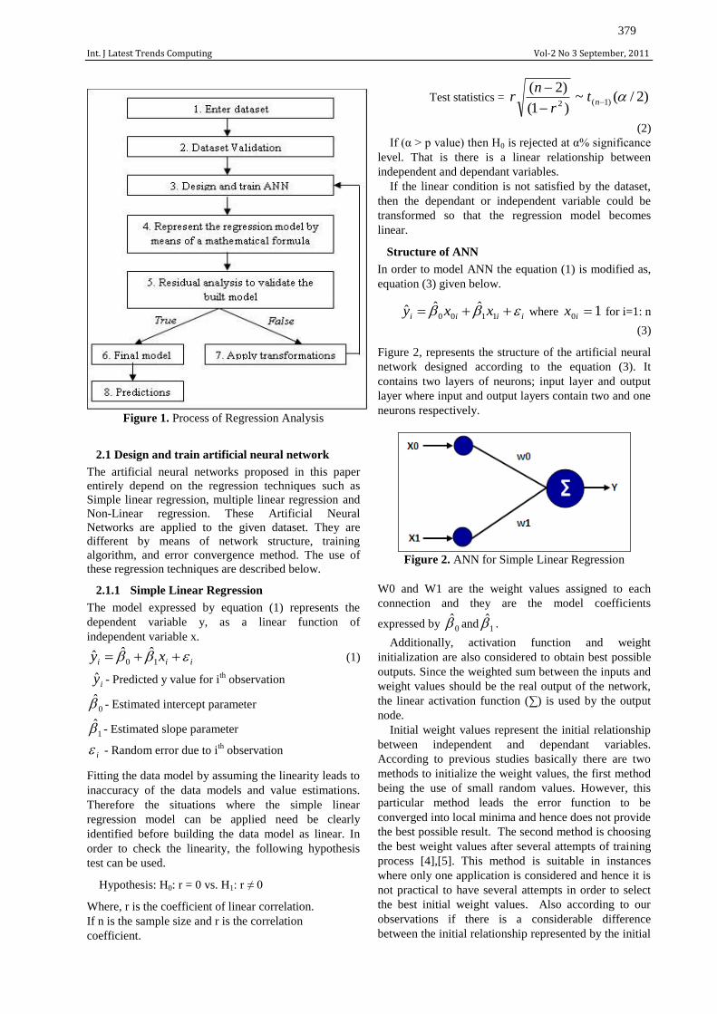
The overall process is designed as a collection of

activities. The flow diagram of the continuous process

of regression analysis with the aid of Artificial Neural

Network is shown in figure 1.

As the first step of the process a dataset which contains

the values for independent and dependent variables are

entered through an interface. Secondly entered dataset is

validated before training. Validation stage checks

whether the dataset contains missing values or outliers.

In the proposed system there is no necessacity for

manual handling of outliers using statistical concepts,

because the artificial neural networks themselves have

the capability of dealing with outliers automatically.

______________________________________________________________ International Journal of Latest Trends in Computing IJLTC, E-ISSN: 2045-5364

Copyright © ExcelingTech, Pub, UK (http://excelingtech.co.uk/)

mailto:[email protected]

http://excelingtech.co.uk/


379

Figure 1. Process of Regression Analysis

2.1 Design and train artificial neural network

The artificial neural networks proposed in this paper

entirely depend on the regression techniques such as

Simple linear regression, multiple linear regression and

Non-Linear regression. These Artificial Neural

Networks are applied to the given dataset. They are

different by means of network structure, training

algorithm, and error convergence method. The use of

these regression techniques are described below.

2.1.1 Simple Linear Regression

The model expressed by equation (1) represents the

dependent variable y, as a linear function of

independent variable x.

iii xy 10ˆˆˆ (1)

iy - Predicted y value for ith

observation

0 - Estimated intercept parameter

1 - Estimated slope parameter

i - Random error due to ith

observation

Fitting the data model by assuming the linearity leads to

inaccuracy of the data models and value estimations.

Therefore the situations where the simple linear

regression model can be applied need be clearly

identified before building the data model as linear. In

order to check the linearity, the following hypothesis

test can be used.

Hypothesis: H0: r = 0 vs. H1: r ≠ 0

Where, r is the coefficient of linear correlation.

If n is the sample size and r is the correlation

coefficient.

Test statistics = )2/(~)1(

)2()1(2

nt

r

nr

(2)

If (α > p value) then H0 is rejected at α% significance

level. That is there is a linear relationship between

independent and dependant variables.

If the linear condition is not satisfied by the dataset,

then the dependant or independent variable could be

transformed so that the regression model becomes

linear.

Structure of ANN

In order to model ANN the equation (1) is modified as,

equation (3) given below.

iiii xxy 1100ˆˆˆ where 10 ix for i=1: n

(3)

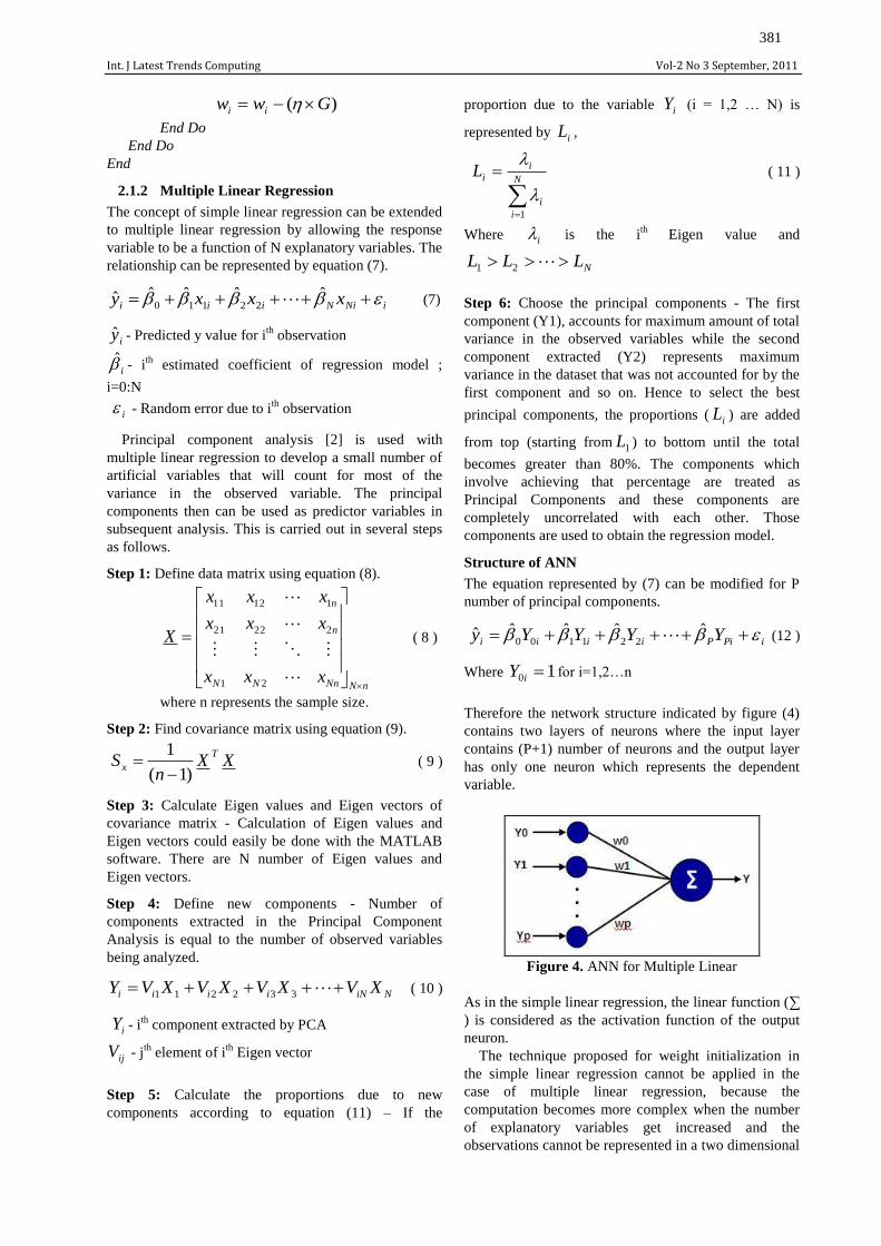
Figure 2, represents the structure of the artificial neural

network designed according to the equation (3). It

contains two layers of neurons; input layer and output

layer where input and output layers contain two and one

neurons respectively.

Figure 2. ANN for Simple Linear Regression

W0 and W1 are the weight values assigned to each

connection and they are the model coefficients

expressed by 0 and 1 .

Additionally, activation function and weight

initialization are also considered to obtain best possible

outputs. Since the weighted sum between the inputs and

weight values should be the real output of the network,

the linear activation function (∑) is used by the output

node.

Initial weight values represent the initial relationship

between independent and dependant variables.

According to previous studies basically there are two

methods to initialize the weight values, the first method

being the use of small random values. However, this

particular method leads the error function to be

converged into local minima and hence does not provide

the best possible result. The second method is choosing

the best weight values after several attempts of training

process [4],[5]. This method is suitable in instances

where only one application is considered and hence it is

not practical to have several attempts in order to select

the best initial weight values. Also according to our

observations if there is a considerable difference

between the initial relationship represented by the initial


380

weight values and the optimal relationship which is to

be obtained at the end of the training process, either

there is a higher possibility of occurring inaccurate

results or time taken to complete the training process

gets increased. In view of the above reasons, the method

proposed uses the following steps to initialize the

weight values of the artificial neural network designed

for simple linear regression.

Figure 3. Weight Initialization for Simple Linear

Regression

As shown in the figure 3, the slope and intercept

parameters of the line obtained by first and last

observations can be computed using the equations (4)

and (5). They are the initial weight values of the neural

network.

Slope parameter =

12

12

xx

yy

(4 )

Intercept parameter = 2

12

122

)(

)(x

xx

yyy

( 5 )

The final objective of the training algorithm is to adapt

weight values (W0, W1) by minimizing the error

function which is considered as error sum of squares

(SSE). In order to map the real output given by the

artificial neural network with the target outputs given in

the dataset the supervised, back propagation training

algorithm is used. Two training algorithms, the Online

and the Batch mode have been tested out. According to

our observations, the online training algorithm requires

less time for training process, but there is a higher

possibility of converging into local minima and also the

outliers significantly influence the training cycle. Hence

we used Batch mode algorithm during the training

process. The following Gradient descent algorithm [4] is

used and the weight values are updated per epoch

according to equation (6).

)( Gww ii

(6)

Where

n

d

ddddd xoootG1

)1()(

dt - Target output of the dth

observation

do - Real output of ANN for the dth

observation

dx - dth

observation of the independent variable

- Learning \ Gain term

iw - ith

weight value; i=0,1

The training algorithm is carried out as follows.

input [0][d]=< 1; d=0,2,3….(n-1)>

input [1][d]=< x1d ; d=0,2,3….(n-1)>

target_output[d]=<yd ; d=0,2,3….(n-1)>

integer: y1,y2,x1,x2;

Function find_Min_Max()

Begin

x1=input[1][0];

x2=input[1][0];

For observations (<x1d ; d=1,2,…(n-1)>), Do

If x1>input[1][d]

x1= input[1][d];

y1= target_output[d];

End if

If x2<input[1][d]

x2= input[1][d];

y2= target_output[d];

End if

End for

End

Function GradientDescent_BatchMode

Begin

//Initialize weights

find_Min_Max();

W0=

12

12

xx

yy

W1= 2

12

122

)(

)(x

xx

yyy

Do (termination condition is false)

For each independent variable (<Xi; i=0,1>)

Do

G=0;

For each observation (<xid ;

d=1,2,…n>), Do

//Compute output od

od= w0 + (w1*xid)

//compute G

n

d

ddddd xoootG1

)1()(

End Do

//Update weight


381

)( Gww ii

End Do

End Do

End

2.1.2 Multiple Linear Regression

The concept of simple linear regression can be extended

to multiple linear regression by allowing the response

variable to be a function of N explanatory variables. The

relationship can be represented by equation (7).

iNiNiii xxxy ˆˆˆˆˆ22110 (7)

iy - Predicted y value for ith

observation

i - ith

estimated coefficient of regression model ;

i=0:N

i - Random error due to ith

observation

Principal component analysis [2] is used with

multiple linear regression to develop a small number of

artificial variables that will count for most of the

variance in the observed variable. The principal

components then can be used as predictor variables in

subsequent analysis. This is carried out in several steps

as follows.

Step 1: Define data matrix using equation (8).

nNNnNN

n

n

xxx

xxx

xxx

X

21

22221

11211

( 8 )

where n represents the sample size.

Step 2: Find covariance matrix using equation (9).

XXn

ST

x)1(

1

( 9 )

Step 3: Calculate Eigen values and Eigen vectors of

covariance matrix - Calculation of Eigen values and

Eigen vectors could easily be done with the MATLAB

software. There are N number of Eigen values and

Eigen vectors.

Step 4: Define new components - Number of

components extracted in the Principal Component

Analysis is equal to the number of observed variables

being analyzed.

NiNiiii XVXVXVXVY 332211 ( 10 )

iY - ith

component extracted by PCA

ijV - jth

element of ith

Eigen vector

Step 5: Calculate the proportions due to new

components according to equation (11) – If the

proportion due to the variable iY (i = 1,2 … N) is

represented by iL ,

N

i

i

i

iL

1

( 11 )

Where i is the ith

Eigen value and

NLLL 21

Step 6: Choose the principal components - The first

component (Y1), accounts for maximum amount of total

variance in the observed variables while the second

component extracted (Y2) represents maximum

variance in the dataset that was not accounted for by the

first component and so on. Hence to select the best

principal components, the proportions ( iL ) are added

from top (starting from 1L ) to bottom until the total

becomes greater than 80%. The components which

involve achieving that percentage are treated as

Principal Components and these components are

completely uncorrelated with each other. Those

components are used to obtain the regression model.

Structure of ANN

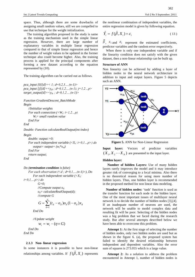
The equation represented by (7) can be modified for P

number of principal components.

iPiPiiii YYYYy ˆˆˆˆˆ221100 (12 )

Where 10 iY for i=1,2…n

Therefore the network structure indicated by figure (4)

contains two layers of neurons where the input layer

contains (P+1) number of neurons and the output layer

has only one neuron which represents the dependent

variable.

Figure 4. ANN for Multiple Linear

As in the simple linear regression, the linear function (∑

) is considered as the activation function of the output

neuron.

The technique proposed for weight initialization in

the simple linear regression cannot be applied in the

case of multiple linear regression, because the

computation becomes more complex when the number

of explanatory variables get increased and the

observations cannot be represented in a two dimensional


382

space. Thus, although there are some drawbacks of

assigning small random values, still we are compelled to

use that technique for the weight initialization.

The training algorithm proposed in the study is same

as the training mechanism used in the simple linear

regression. However, there are large number of

explanatory variables in multiple linear regression

compared to that of simple linear regression and hence

the number of weight values to be updated in the former

technique also could become higher. Also, the training

process is applied for the principal components after

forming a new dataset according to the equation

represented by (10).

The training algorithm can be carried out as follows.

pca_input [0][d]=< 1; d=0,2,3….(n-1)>

pca_input [j][d]=<yjd ; d=0,1,2….(n-1); j=1,2…p>

target_output[d]=<yd, ; d=0,1,2….(n-1)>

Function GradientDescent_BatchMode

Begin

//Initialize weights

For each connection (<Wi; i=1,2…p)

Wi= small random value

End For

End

Double: Function calculateRealOutput(int:index)

Begin double: output:=0;

For each independent variable (<Xi; i=0,1…p>) do

output= output+ (wi*xid)

End For

return output;

End


For each observation (<d ; d=0,1,…(n-1)>), Do

For each independent variable (<Xi;

i=0,1,…p>) do

G=0;

//Compute output od

od= calculateRealOutput(d);

//compute G

n

d

ddddd xoootG1

)1()(

End Do

//Update weight

)( Gww ii

End Do

End Do

2.1.3 Non- linear regression

In some instances it is possible to have non-linear

relationships among variables. If ),ˆ( iXf represents

the nonlinear combination of independent variables, the

entire regression model is given by following equation.

iii XfY ),ˆ(ˆ ( 13 )

, and represent the estimated coefficients,

predictor variables and the random error respectively.

When there is only one independent variable and if

the linearity condition does not satisfy with the given

dataset, then a non-linear relationship can be built up.

Structure of ANN

Non linearity can be achieved by adding a layer of

hidden nodes to the neural network architecture in

addition to input and output layers. Figure 5 depicts

such an ANN.

Figure 5. ANN for Non-Linear Regression

Input layer: Vectors of predictor variables

),( 21 NXXX are presented to the input layer.

Hidden layer:

Number of hidden Layers: Use of many hidden

layers rarely improves the model and it may introduce

greater risk of converging to a local minima. Also there

is no theoretical reason for using more number of

hidden layers. Thus, one hidden layer is recommended

in the proposed method for non linear data modeling.

Number of hidden nodes: ‘tanh’ function is used as

the transfer function for each node in the hidden layer.

One of the most important issues of multilayer neural

network is to decide the number of hidden nodes [3],[4].

If an inadequate number of neurons are used, the

network will be unable to model complex data and

resulting fit will be poor. Selecting of the hidden nodes

was a big problem that we faced during the research

study. But after several attempts described below we

have been able to overcome this problem.

Attempt 1: At the first stage of selecting the number

of hidden nodes, only two hidden nodes are used but as

shown in the figure 6. (a), the proposed system has

failed to identify the desired relationship between

independent and dependent variables. Also the error

sum of squares is 273.055 which is a large value.

Attempt 2: As a solution to address the problem

encountered in Attempt 1, number of hidden nodes is


383

gradually increased. With the increase of hidden nodes

up to 10, we have been able to observe considerable

improvement of the system with increased capabilities

for identification of relationships. However, in our study

another attempt has been made by us using still more

hidden nodes so as to ascertain whether the proposed

system could further be improved.

Attempt 3: With the increase of hidden nodes up to

14, we have been able to obtain the best relationship,

with which the errors are found to be minimal. Also no

further improvement of the system in identifying

relationship among variables has been observed with the

increase of hidden nodes beyond 14. It is also essential

to take in to consideration computer memory wastage

with the increase of hidden nodes unnecessarily. In view

of the above reasons we assumed that when the number

of hidden nodes is equal to the sample size the proposed

system could yield best results in data analysis. In order

to verify the above assumptions several datasets with

varied number of observations are analyzed and finally

we have been able to conclude that the method tested

out by us could provide the best result in data analysis.

Although this technique could provide optimal

results in the analysis of any kind of dataset, more often

it also may create problems when the sample size is too

large because, as the sample size increases, the number

of connections between neurons becomes too large and

consequently this could increase the computational

complexity of the system. As a result, training process

requires more computer memory and the time required

for the completion of training cycle becomes

excessively long.

Usually, the problems described above can arise as

the sample size increases beyond 20. Therefore it is

suggested that if the sample size exceeds 20, the number

of hidden nodes then should be limited to 20.

Output layer: Output layer contains only one neuron

which uses the linear activation function. The outputs

from the hidden nodes are distributed to the output

layer. It obtains the real output of the entire network.

Figure 6. Number of hidden nodes

As in the multiple linear regression, small random

values are assigned as weights for the connections

between neurons.

The value from each input neuron ( idx ) is multiplied by

a weight assigned to the connections between input and

hidden layer and the resulting weighted values are

added together producing a combined value jdU .

N

i

idijjd xwU1

(

14 )

ijw - Weight of the connection between ith

input node

and jth

hidden node

idx - dth

observation from ith

input node

jdU can be fed into a activation function ‘tanh’, which

outputs a value jd . Let jdU =S then,

SS

SS

jdjdee

eeU

)tanh( ( 15)

Arriving at the output neuron, the results given by each

hidden layer neuron is multiplied by the weights

assigned for the connections between hidden and output

layers and then the resulting weighted values are added

together producing combined output where d

represents the dth

observation of the dataset.


384

h

j

jdjd wo1

(

16 )

Where jw represents the weight value assigned for the

connection between the jth

hidden node and the output

node.

One of the main limitations in resorting to batch

mode training algorithm is that when the number of

calculations increases the proposed system too requires

more computer memory during the execution. This may

lead to slower convergence and sometimes the training

process can lead to incomplete termination due to

limited space available in the computer memory. This

may result in poor performance of the system. Hence

rather than using the batch mode, gradient descent

online training algorithm for non linear neural network

training was used.The training algorithm is carried out

as follows.

input [0][d]= <1; d=0,1,2….(n-1)>

input[j][d] = <xjd; d=0,1,2….(n-1); j=1,2,….N>


d=Select a random point from dataset

Uj=0;

For each hidden_node (<j; j=1,2,…,h>), Do

For each input_node (<i; i=1,2…N>) Do

Ujd=Ujd+(wij*xid)

End Do

SS

SS

jdee

ee

End For


od=od+(wj* jd )

End For


G=(td-od)od(1-od)δjd

W ←W – η* G;

End for


For each input_node (<i; i=1,2…N>) Do

G=(td-od)δjd(1- δjd) xid

W ← W –η*G;

End for

End for

End Do

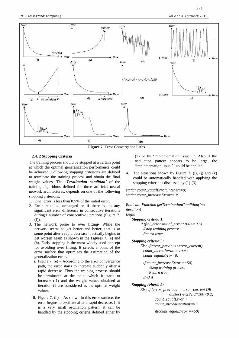
2.4 Error convergence path

The theoretical approach describes that the error surface

is expected to reach zero error at the end of the training

process as shown in Figure 7: (a). However, it is

impossible to always expect such smoothness from the

real situations. The graphs depicted in Figure 7

represent other error convergence paths that can occur at

the training cycle. According to our observations, the

performance of the error convergence process depends

on initial weight values and the learning rate.

2.4.1 Learning rate / Gain term

Once the weight values are initialized using the methods

described in the previous sections, the learning process

could be improved further by defining a proper learning

rate. Choosing the best learning rate is a tedious task to

achieve since a learning rate chosen for one particular

dataset is not suitable for another dataset. This was a

common problem for all three regression models.

According to our observations, using a large gain

term for training process may cause several problems

like increasing the error term rapidly and reaching

infinity (Figure 7: (b)) and occurring large oscillating

patterns (Figure 7: (c),(d)). In order to address this

problem it is suggested that the gain term should be

reduced. However, it is also very important to remember

that the selection of very small gain term may result in

very slow convergence to a solution which may

consequently become very time consuming.

When considering above facts, defining a fixed gain

term for all the datasets cannot be considered as an

efficient solution. Thus, in the implementation of our

research study, we propose the following three

implementation strategies in order to extract the optimal

gain term by the system itself for a particular dataset.

1. The learning process starts with a large learning

rate (0.1) and keeps reducing it until the best gain

term is found. This is a better solution once the

error function reaches infinity. The system

automatically identifies the infinite error and

retrains the network with the reduced gain term.

2. In case of the occurrence of large number of

oscillation patterns, there can still be some

problems associated in identifying all of them

distinctly from one another. These situations can

only be identified by visual observations. Therefore

the user should examine the error convergence path

and if it appears to be large oscillation, then the best

solution is to retrain the neural network with a

reduced learning rate.

3. On the other hand, if there is a small oscillation,

then leave the training process to proceed

uninterrupted as small oscillation patterns usually

occur when the solution is oscillating around the

global minima in a small range (Figure 7: (g),(h)).


385

Figure 7. Error Convergence Paths

2.4. 2 Stopping Criteria

The training process should be stopped at a certain point

at which the optimal generalization performance could

be achieved. Following stopping criterions are defined

to terminate the training process and obtain the final

weight values. The ‘Termination condition’ of the

training algorithms defined for three artificial neural

network architectures, depends on one of the following

stopping criterions.

1. Final error is less than 0.5% of the initial error.

2. Error remains unchanged or if there is no any

significant error difference in consecutive iterations

during t number of consecutive iterations (Figure 7.

(f)).

3. The network prone to over fitting- While the

network seems to get better and better, that is at

some point after a rapid decrease it actually begins to

get worsen again as shown in the Figures 7. (e) and

(h). Early stopping is the most widely used concept

for avoiding over fitting. It selects a point of the

error surface that optimizes the estimation of the

generalization error.

i. Figure 7. (e) – According to the error convergence

path, the error starts to increase suddenly after a

rapid decrease. Thus the training process should

be terminated at the point which it starts to

increase (t1) and the weight values obtained at

iteration t1 are considered as the optimal weight

values.

ii. Figure 7. (h) – As shown in this error surface, the

error begins to oscillate after a rapid decrease. If it

is a very small oscillation pattern, it can be

handled by the stopping criteria defined either by

(2) or by ‘implementation issue 3’. Also if the

oscillation pattern appears to be large, the

‘implementation issue 2’ could be applied.

4. The situations shown by Figure 7. (i), (j) and (k)

could be automatically handled with applying the

stopping criterions discussed by (1)-(3).

static: count_equalError:Integer:=0;

static: count_increaseError:=0;

Boolean: Function getTerminationCondition(Int:

iteration)

Begin

Stopping criteria 1:

If (finl_error/initial_error*100<=0.5)

//stop training process

Return true;


Else if(error_previous<error_current)

count_increaIterations ++;

count_equalError=0;

if(count_increaseError ==50)


Return true;

End if


Else if (error_previous==error_current OR

abs(er1-er2)/er1*100<0.2)

count_equalError ++;

count_increaIterations=0;

if(count_equalError ==50)


386


Return true;

End if

Else

Return false;

End if

End

* In above algorithm er1 and er2 represent the SSE of

previous and current iterations of the training process.

2.5 Model Validation

Once the regression data model is constructed, the

residuals ( ) could be found by calculating the vertical

distances between the predicted values )ˆ( iy and the

observed values ).( iy

iii yy ˆ

(17)

Residual analysis is used to assess the quality of the

regression model. In order to be an optimal regression

model, the residuals should hold the following four

properties [7].

1. Mean of the residuals is equal to zero.

2. Residuals have a constant variance

(homoscedasticity).

3. Residuals are uncorrelated.

4. The residuals should follow a normal distribution.

The proposed system uses a database to store the critical

values of F test and Durbin Watson test which are

needed to check 2nd

and 3rd

conditions respectively. In

addition to test the normality of the residuals (4th

condition) Kolmogorov Smirnov test has been

performed with the MATLAB tool.

2.6 Transformations

If the residual analysis proves that the model is not

adequate, then the solution involves either transforming

response variable or predictor variables into another

form [5][7].

2.6.1 Transforming predictor variable

In simple linear regression, if the linearity condition is

violated the independent variable could be transformed

to achieve linearity. This is performed based on the

shape of the scatter plot.

2.6.2 Transforming response variable

If the residual analysis suggests that the variance of the

residuals is not constant, residuals are correlated or the

residuals are non-normal, then the response variable is

usually transformed to achieve constant variance,

independence and normality. The transformation

method is chosen based on the trend represented by the

residual plot.

Figure 8. Shapes of the residual and scatter plots

Table 1 indicates the transformation techniques which

are suitable for the shapes given by figure 8.

Usually the best transformation technique out of the list

given in table 1 is selected by visual observation of the

shape of the scatter plot and residual plot for which a

better knowledge on statistical transformation is

prerequisite. Hence as a further development we wish to

apply the image processing in pattern recognition to

automate the entire transformation process.

3. Results

The results given below represent how the proposed

automated system could be applied for modeling

relationships associated with three regression techniques

described above.

Table 1. Transformation Techniques

Pattern Transformation method

Tra

nsf

orm

ing

pre

dic

tor

va

ria

ble

(a)

0);log( xxx

0);1log( xxx

xx

(b) 2xx

(c)

0;/1 xxx

0);1/(1 xxx xex

(d)

2xx xex

Tra

nsf

orm

ing

resp

on

se v

ari

ab

le

(e)

0;/1 xyy

0);1/(1 xyy 2yy

(f)

0;log yyy

0);1log( yyy

0; yyy

(g) 2yy

(h) 0;log yyy

0);1log( yyy

(i) 0; yyy


387

3.1 Simple linear regression modeling

Step 1: Check the linearity (Figure 9)

In this case, P value < α

Therefore there is enough evidence to say that there is a

linear relationship between X and Y variables at 5%

significance level.

Step 2: Design the artificial neural network (Figure 10)

Since the linearity condition is satisfied, the system

itself designs an artificial neural network associated

with simple linear regression and initialize the weight

values based on the method proposed.

In Figure 10, Line 1 represents the initial regression

model which is indicated by the initial weight values 8.0

and -0.78.

Step 3: Train the artificial neural network in order to

obtain the optimal regression model (Figure 11)

According to the figure 11, the system has found that

the best gain term is 0.0001 and the error convergence

path is similar to the one which is represented by Figure

7. (k). The mathematical formula given by the

developed system to indicate the best regression model

is,

Y = 8.269 – 0.828X

Hence 8.269 and 0.828 are the estimated intercept and

slope parameters respectively.

Step 4: Residual Analysis

Figure 12 represents that all four conditions are satisfied

by the regression model. Hence it could be used for

further predictions as shown in Figure 13.

3.2 Multiple linear regression modeling

Step 1: Enter the dataset and perform principal

component analysis (Figure 14)

According to the output given by the system, there

were two principal components.

Y1 =0.5X1 + 0.69X2 + 0.52X3

Y1 =0.26X1 + 0.45X2 - 0.85X3

Then a new dataset is formed with the independent

variables Y1 and Y2 and original Y variable still

remains as the dependant variable.

Step 2: Design the artificial neural network and train it

to obtain the regression model (Figure 15).

The final regression model obtained by the training

process of the Artificial Neural Network is represented by

equation,

Y =7.793 + 7.088Y1 +3.575Y2

Step 3: Model validation - As in previous model, once the

residual analysis was performed on this regression model, it

proved that the obtained model is sufficient enough to make

future predictions.

3.3 Non-Linear regression modeling

A result given by the proposed system for non-linear

regression is represented by the figure 6. (c).

Figure 9. Check linearity condition


388

Figure 10.Weight Initialization

Figure 11. Train ANN-Simple Linear Regression

Line 1


389

Figure 12. Residual Analysis

Figure 13. Predictions-Simple Linear Regression


390

Figure 14.Principal Component Analysis

Figure 15.Train ANN-Multiple Linear Regression

4. Conclusion

Table 2 represents the comparison between the results

obtained by the proposed system and the models

developed with R statistical package for two datasets

used for simple linear regression modeling and multiple

linear regression modeling described in the sections 4.1

and 4.2.

According to the observations it can be concluded

that the proposed system has a higher capability of

identifying relationships between independent and

dependant variables with 100% accuracy. Also when the

SSE values of conventional regression methods and the

artificial neural network approach are compared, it is

clear that the performance of the proposed system is

much superior compared to that of the conventional

regression techniques.

In conventional regression modeling better

knowledge on statistical concepts is required for non

linear data modeling whereas the proposed system itself

can build the non linear regression model without

requiring any statistical knowledge of the user.

The proposed system also has some limitations. The

model building phase in artificial neural network is

somewhat time- consuming and, due to the hidden layer

of nodes it is difficult to indicate the relationship by a

simple mathematical formula.

However, the overall results of this study indicate that

the system that has been developed could be used

successfully for interpretation of relationships which

exist between independent and dependant variables.

Having identified these relationships, future trends of a

given application could be determined. Also, the

developed user interface could be used as a teaching

Line 1

Line (1)


391

tool to illustrate how the artificial neural networks work

for the situations where regression analysis to be

applied.

Table 2. Comparison between ANN approach and

Conventional Regression technique.

Conventional Regression

Analysis

Proposed System

Simple Linear Regression

Y = 8.2991 – 0.8434X

SSE = 26.35707

Y = 8.269 – 0.828X

SSE=26.418

Multiple Linear Regression

Y =7.432 + 6.66Y1 +3.245Y2 SSE= 398.0539

Y =7.793 + 7.088Y1

+3.575Y2

SSE=377.17

References

[1] M. Hashem, H. Karkory, “Artificial Neural

Networks as alternative approach for predicting

Trihalomethane formation in Chlorinated waters”,

Eleventh International Water Technology Conference,

2007.

[2] S.I.V. Sousa, F.G. Martins, M.C.M. Alvim-Ferraz,

M.C. Pereira, “Multiple linear regression and artificial

neural networks based on principal components to

predict ozone concentrations”, August 2005.

[3] K. B. DeTienne, S. A. Joshi, “Neural Networks as

Statistical tools for management science researchers”,

Conference Procedings from the 28th

annual meeting of

the western decision sciences institute,April 1999.

[4]Stringer, Jeffrey W.; Loftis, David L., eds. 1999.

Proceedings, 12th central hardwood forest conference;

1999 February.

[5]H. Motulsky, A. Christopoulos, “Fitting models to

biological data using linear and non-linear regression”,

A practical guide to curve fitting. 2003, GraphPad

software Inc., San Diego CA, www.graphpad.com.

[6] W. S. Sarle, “Neural Networks and Statistical

Models”, Proceedings of the Nineteenth Annual SAS

Users Group International Conference, April 1994.

[7] G. E. P. Box , D. R. Cox, "Journal of the Royal

Statistical Society. Series B (Methodological)", Vol. 26,

No. 2. (1964), pp. 211-252.

http://www.graphpad.com/