1 23

Journal of Coastal ConservationPlanning and Management ISSN 1400-0350 J Coast ConservDOI 10.1007/s11852-013-0297-5

Shoreline changes in response to sea levelrise along Digha Coast, Eastern India: ananalytical approach of remote sensing, GISand statistical techniques

Adarsa Jana, Arkoprovo Biswas,Sabyasachi Maiti & AmitK. Bhattacharya

1 23

Your article is protected by copyright and all

rights are held exclusively by Springer Science

+Business Media Dordrecht. This e-offprint

is for personal use only and shall not be self-

archived in electronic repositories. If you wish

to self-archive your article, please use the

accepted manuscript version for posting on

your own website. You may further deposit

the accepted manuscript version in any

repository, provided it is only made publicly

available 12 months after official publication

or later and provided acknowledgement is

given to the original source of publication

and a link is inserted to the published article

on Springer's website. The link must be

accompanied by the following text: "The final

publication is available at link.springer.com”.

Shoreline changes in response to sea level rise along DighaCoast, Eastern India: an analytical approach of remotesensing, GIS and statistical techniques

Adarsa Jana & Arkoprovo Biswas & Sabyasachi Maiti &Amit K. Bhattacharya

Received: 24 July 2013 /Revised: 15 November 2013 /Accepted: 18 November 2013# Springer Science+Business Media Dordrecht 2013

Abstract Shoreline is one of the rapidly changing linearfeatures of the coastal zone which is dynamic in nature. Theissue of shoreline changes due to sea level rise over the nextcentury has increasingly become a major social, economic andenvironmental concern to a large number of countries alongthe coast, where it poses a serious problem to the environmentand human settlements. As a consequence, some coastal sci-entists have advocated analyzing and predicting coastalchanges on a more local scale. The present study demonstratesthe potential of remote sensing, geospatial and statistical tech-niques for monitoring the shoreline changes and sea level risealong Digha coast, the eastern India. In the present study,multi-resolution and multi temporal satellite images ofLandsat have been utilized to demarcate shoreline positionsduring 1972, 1980, 1990, 2000, and 2010. The statisticaltechniques, linear regression, end-point rate and regressioncoefficient (R2) have been used to find out the shorelinechange rates and sea level change during the periods of1972–2010. Monthly and annual mean sea level data for threenearby station viz., Haldia, Paradip and Gangra from 1972 to2006 have been used to this study. Finally, an attempt has beenmade to find out interactive relationship between the sea levelrise and shoreline change of the study area. The results of thepresent study show that combined use of satellite imagery, sea

level data and statistical methods can be a reliable method incorrelating shoreline changes with sea level rise.

Keywords Shoreline change rate . Sea level rise (SLR) .

Landsat . Linear regression . End-point rate . Regressionco-efficient (R2)

Introduction

Shoreline occurring between land and sea, is highly dynamic,and changes temporally and spatially in response to variationsin influencing factors such as wind, wave tide, storm surge,sea level rise and land subsidence (Orford et al. 2002; Forbeset al. 2004; Cooper et al. 2004). It undergoes frequent chang-es, short term and long term, caused by hydrodynamic chang-es (e.g., river cycles, sea level rise), geomorphological chang-es (e.g., barrier island formation, spit development) and otherfactors (e.g., sudden and rapid seismic and storm events)(Scott 2005). Accurate demarcation and monitoring of shore-line changes are necessary for understanding and decipheringthe coastal processes, coastal zone management planning,hazard zoning, erosion-accretion studies, regional sedimentbudgets, analysis and modeling the coastal morphodynamics.The conventional techniques for determining the rate ofchange of shoreline position include: field measurement ofpresent mean high water level, shoreline tracing from aerialphotographs and topographic sheets; comparison with thehistorical data using one of the several methods, (viz., endpoint rate (EPR) (Fenster et al. 1993), average of rates (AOR),linear regression (LR), and jackknife (JK) (Dolan et al. 1991).Recent advancements in remote sensing and geographicalinformation system (GIS) techniques have led to improve-ments in coastal geomorphological studies, such as: semi-automatic determination of shorelines (Ryu et al. 2002;

A. Jana (*) :A. Biswas : S. Maiti :A. K. BhattacharyaDepartment of Geology and Geophysics, Indian Institute ofTechnology, Kharagpur 721302, West Bengal, Indiae-mail: adarsa.rsiitkgp@gmail.com

A. Biswase-mail: arkoprovo@gmail.com

S. Maitie-mail: maiti.sabyasachi@gmail.com

A. K. Bhattacharyae-mail: amkb@gg.iitkgp.ernet.in

J Coast ConservDOI 10.1007/s11852-013-0297-5

Author's personal copy

Yamano et al. 2006); identification of relative changes amongcoastal units (Jantunen and Raitala 1984; Siddiqui and Maajid2004); extraction of topographic and bathymetric information(Lafon et al. 2002) and their integrated GIS analysis (Whiteand El Asmar 1999). These techniques are attractive, due totheir cost-effectiveness, reduction in manual error and absenceof the subjective approach of conventional field techniques.

Sea level rise is a major consequence of global warming,which threatens many low-lying, highly populated coastal re-gions of the world (Becker et al. 2012). Today the issue ofshoreline changes due to sea level rise which caused by globalwarming/climate change has increasingly become a major is-sues in terms of impact on the population along the coastal area.Changes in mean sea level as measured by coastal tide gaugesare called relative sea-level changes (Church et al. 2001). Sea-level has been rising at the rate of 1.7–1.8 mm/year over the lastcentury and the rate has increased to 3 mm/year in the lastdecade (Church et al. 2004; Holgate and Woodworth 2004;Church et al. 2006). The tide gauge records at five coastallocations in India; Mumbai, Kolkata, Cochin, Kandla and SagarIslands have reported an increase in sea level. The change in sealevel appears to be higher on eastern coast compared to westerncoast. The average sea level rise for India has been reported as2.5 mm/year since 1950’s (Das and Radhakrishna 1993; KumarDanish 2001; Chand and Acharya 2010).

In the present study, multi-temporal Landsat imageries(from 1972 to 2010) have been utilized to demarcate differentshorelines. In comparison to previous works (Maiti andBhattacharya 2009; Jana and Bhattacharya 2012), here weused transects with closed interval (250 m) with additionalstatistical techniques viz., end point rate, linear regression andregression coefficient (R2). Although relative sea-level fre-quently is influenced by local factors like sedimentation andtectonism, but studied temporal span and sedimentation rate isalmost constant within chosen space. Therefore, choices ofthree nearby gauge stations were sufficient to represent theinfluence of sea level. Finally, an attempt has been made tofind out the interactive relationship between the sea level riseand shoreline change in the present area.

Study area

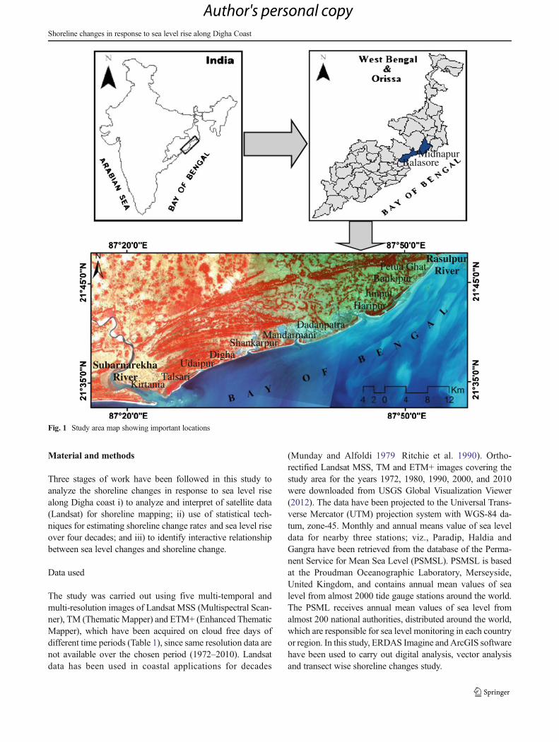
The study area chosen in the present work is a 60 km longcoastal stretch on the east coast of India, covering parts ofBalasore and Midnapur littoral tracts occurring in Orissa andWest Bengal states respectively, adjoining Bay of Bengal(Fig. 1). The western end of the study area is bounded bySubarnarekha River (Orissa), while Rasulpur River (WestBengal) forms the eastern boundary. It lies between 21° 30′0″ N to 21°48′ 0″ N latitudes and 87°24′ 0″ E to 57°54′ 0″ Elongitude.

The geological history of the coast is relatively short andthe coast is still in its formative state. Geologically, this is the

coastal stretch of the Indo-Gangetic plain and situated be-tween tectonically active Ganga Delta and wave dominatedSubarnarekha estuary. The area had formed due to out- build-ing of the Subarnarekha delta through recession of the seabetween 6,000 years B.P. and present day (Niyogi 1970; Deyet al. 2002). The area comprises of recent alluvial depositsbelonging to Balasore-Contai coastal plain. Geomorphologi-cal studies of the area shows that this coastal region was madeup of alternate lines of beach ridges or chennier plains andbarriers islands, situated on silty or clayey marine terraces.The study area has overall uniform geomorphology withnorthern boundary (landward) comprising of older dune com-plex, followed by series of chenniers, beach ridges and inter-mediate mudflats; while the southern boundary (seaward)made up of recent remobilized sand and clay at various places(Chakrabarti 1991; Maiti and Bhattacharya 2009). Almostshore parallel formations of six ancient shoreline positionshave been found over the 30 km wide coastal region whichindicates the landward shifting of shoreline positions duringdifferent time periods.

The studied zone experiences strong long shore currentfrom SW to NE direction during the monsoon season and aless powerful long shore current from NE to SW directionduring the winter season, due to seasonal variation in winddirection. The long shore current velocity recorded atSubarnarekha mouth and Digha are 1.2164 m/sec and1.2620 m/sec respectively (Paul 2002). The present coastlineis dominated by high energy macro-tidal environment (tidalrange 4.5 m to 5 m) with predominantly southwesterly mon-soon derived wave and bay-head cyclone prone areas (Paul2002). The coast experiences semi-diurnal tidal fluctuationswith a tidal range of 5 m to 5.8 m in the spring tide and 1.5 mor less in the nip tide (Paul 2006). The area falls withinsubtropical humid climate with three distinct seasons viz.pre-monsoon (March- June), monsoon (July - Oct), andpost-monsoon (Nov- Feb). The maximum daily temperatureranges between 26.9 °C and 36.8 °C while the minimumtemperature lies in between 5.7 °C and 24.7 °C. The rangeof average annual rainfall is 1,192 mm to 1,956 mm withrelative humidity varying between 60 % and 90 % (GSI1995). Seasonal changes in sea level have been known tooccur for a long time in the coast. In March, sea level is lowerthan the mean in Northern Hemisphere. At this time the largestdeviation occur in the Bay of Bengal, where values of −40 cmoccur. In the month of June, the largest positive value of +30 cm occurs in the Bay of Bengal and negative value of−26 cm occurs in the month of December in the same region(Paul 2002). The local mean sea level at Sagar Island is +2.82 m above the Datum level. So far as tidal records areconcerned the local meanwater level gradually increased from1956 to 1978 at the Hugli river tidal stations. The lowestrecorded low water in 1940 was −0.21 m below the Datumlevel at Sagar Island tidal station.

A. Jana et al.

Author's personal copy

Material and methods

Three stages of work have been followed in this study toanalyze the shoreline changes in response to sea level risealong Digha coast i) to analyze and interpret of satellite data(Landsat) for shoreline mapping; ii) use of statistical tech-niques for estimating shoreline change rates and sea level riseover four decades; and iii) to identify interactive relationshipbetween sea level changes and shoreline change.

Data used

The study was carried out using five multi-temporal andmulti-resolution images of Landsat MSS (Multispectral Scan-ner), TM (Thematic Mapper) and ETM+ (Enhanced ThematicMapper), which have been acquired on cloud free days ofdifferent time periods (Table 1), since same resolution data arenot available over the chosen period (1972–2010). Landsatdata has been used in coastal applications for decades

(Munday and Alfoldi 1979 Ritchie et al. 1990). Ortho-rectified Landsat MSS, TM and ETM+ images covering thestudy area for the years 1972, 1980, 1990, 2000, and 2010were downloaded from USGS Global Visualization Viewer(2012). The data have been projected to the Universal Trans-verse Mercator (UTM) projection system with WGS-84 da-tum, zone-45. Monthly and annual means value of sea leveldata for nearby three stations; viz., Paradip, Haldia andGangra have been retrieved from the database of the Perma-nent Service for Mean Sea Level (PSMSL). PSMSL is basedat the Proudman Oceanographic Laboratory, Merseyside,United Kingdom, and contains annual mean values of sealevel from almost 2000 tide gauge stations around the world.The PSML receives annual mean values of sea level fromalmost 200 national authorities, distributed around the world,which are responsible for sea level monitoring in each countryor region. In this study, ERDAS Imagine and ArcGIS softwarehave been used to carry out digital analysis, vector analysisand transect wise shoreline changes study.

SubarnarekhaRiver

RasulpurRiver

MidnapurBalasore

Kirtania

UdaipurDigha

ShankarpurMandarmani

Dadanpatra

HaripurJunput

Petua Ghat

Talsari

Bankipur

Fig. 1 Study area map showing important locations

Shoreline changes in response to sea level rise along Digha Coast

Author's personal copy

Shoreline mapping and change rate calculation

In order to estimate and represent best shoreline positionsconsidering the grid resolutions and effect of tides, we followadopted methods by Maiti and Bhattacharya (2009). Bandrationing method, involving ratio between bands 4 and 2 andother between bands 5 and 2 have been used in this study todemarcate shorelines of different years. Generally, the ratiob5/b2 is greater than one (1) for water, and less than one (1) forland in large areas of coastal zone. These results obtained fromabove rationing method are correct in coastal zones which arecovered by soil, but not for land with vegetation cover, since iterroneously assigns some of the vegetation land to water dueto aggregate background reflectance. To solve this problem,the two ratios are combined in this study. It gives the finalbinary image which represents the shoreline. At last to refinethe overall results from above method the visual inter-pretation has been carried out to edit visually evidenterrors near the outlet of the river. For this purpose acolor composite can be used and the best suited falsecolor composite (FCC) band 432 in MSS and 543 inTM and ETM+ nicely depicts land-water interface. Fi-nally, the shoreline along the study area was digitized

using ArcMap 9.1 and ERDAS Imagine software usingthe on-screen digitization technique.

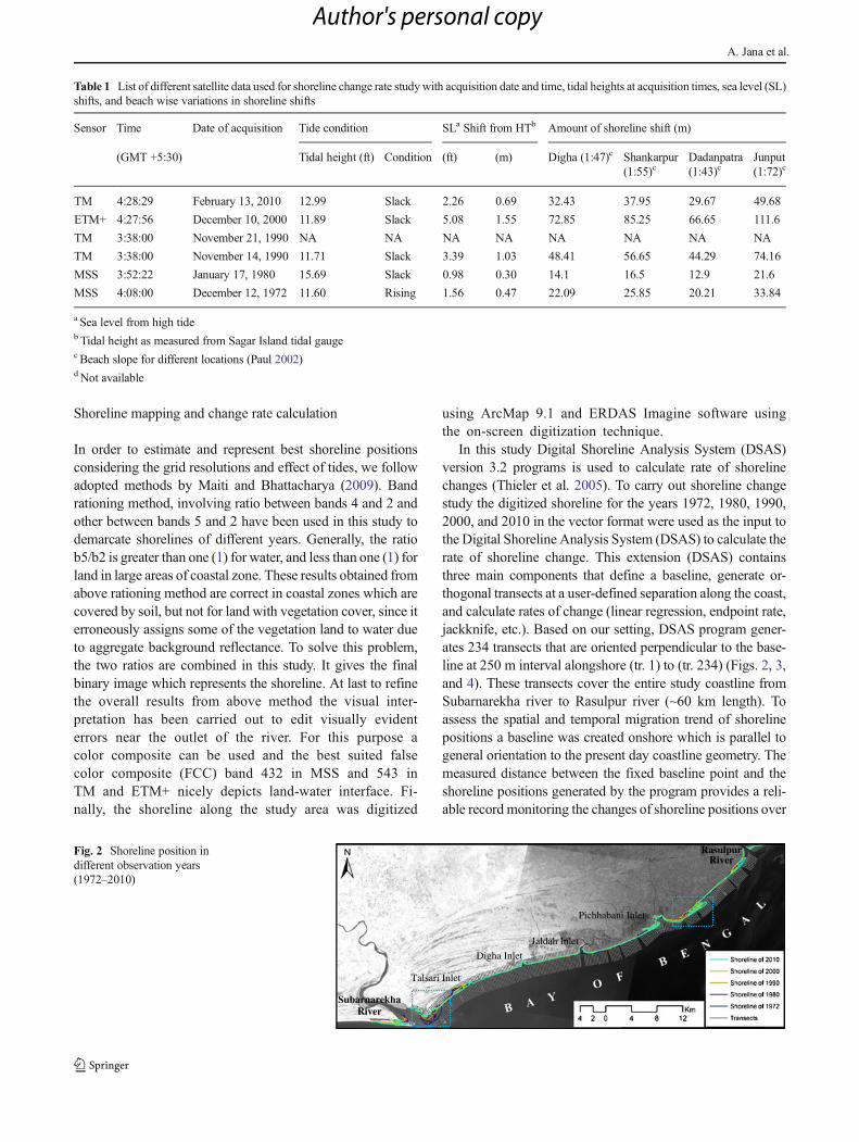
In this study Digital Shoreline Analysis System (DSAS)version 3.2 programs is used to calculate rate of shorelinechanges (Thieler et al. 2005). To carry out shoreline changestudy the digitized shoreline for the years 1972, 1980, 1990,2000, and 2010 in the vector format were used as the input tothe Digital Shoreline Analysis System (DSAS) to calculate therate of shoreline change. This extension (DSAS) containsthree main components that define a baseline, generate or-thogonal transects at a user-defined separation along the coast,and calculate rates of change (linear regression, endpoint rate,jackknife, etc.). Based on our setting, DSAS program gener-ates 234 transects that are oriented perpendicular to the base-line at 250 m interval alongshore (tr. 1) to (tr. 234) (Figs. 2, 3,and 4). These transects cover the entire study coastline fromSubarnarekha river to Rasulpur river (~60 km length). Toassess the spatial and temporal migration trend of shorelinepositions a baseline was created onshore which is parallel togeneral orientation to the present day coastline geometry. Themeasured distance between the fixed baseline point and theshoreline positions generated by the program provides a reli-able record monitoring the changes of shoreline positions over

Table 1 List of different satellite data used for shoreline change rate studywith acquisition date and time, tidal heights at acquisition times, sea level (SL)shifts, and beach wise variations in shoreline shifts

Sensor Time Date of acquisition Tide condition SLa Shift from HTb Amount of shoreline shift (m)

(GMT +5:30) Tidal height (ft) Condition (ft) (m) Digha (1:47)c Shankarpur(1:55)c

Dadanpatra(1:43)c

Junput(1:72)c

TM 4:28:29 February 13, 2010 12.99 Slack 2.26 0.69 32.43 37.95 29.67 49.68

ETM+ 4:27:56 December 10, 2000 11.89 Slack 5.08 1.55 72.85 85.25 66.65 111.6

TM 3:38:00 November 21, 1990 NA NA NA NA NA NA NA NA

TM 3:38:00 November 14, 1990 11.71 Slack 3.39 1.03 48.41 56.65 44.29 74.16

MSS 3:52:22 January 17, 1980 15.69 Slack 0.98 0.30 14.1 16.5 12.9 21.6

MSS 4:08:00 December 12, 1972 11.60 Rising 1.56 0.47 22.09 25.85 20.21 33.84

a Sea level from high tideb Tidal height as measured from Sagar Island tidal gaugec Beach slope for different locations (Paul 2002)d Not available

SubarnarekhaRiver

RasulpurRiver

Talsari Inlet

Digha Inlet

Jaldah Inlet

Pichhabani Inlet

Fig. 2 Shoreline position indifferent observation years(1972–2010)

A. Jana et al.

Author's personal copy

the 38 years time frame of the generated vectors. The gener-ated cross-shore transects together with the extracted 5 shore-line vectors are graphically depicted in Fig. 2. The data mea-sured from each profile are then used to estimate the meanannual rate of shoreline change (m/yr) employing end pointrate, linear regression and net shoreline change techniques.The end point rate is calculated by dividing the distance ofshoreline movement by the time elapsed between the earliestand latest measurements (i.e., the oldest and the most recentshoreline). The net shoreline movement calculates a distance,not a rate. The NSM is associated with the dates of only twoshorelines. It calculates the distance between the oldest andyoungest shorelines for each transect. This represents the totaldistance between the oldest and youngest shorelines. If thisdistance is divided by the number of years elapsed betweenthe two shoreline positions, the result is the EPR. NSM andEPR are essentially the same thing; however NSM gives usinformation on the absolute distance of shift as opposed to arate. Linear regression method have been used since it is mostcommonly applied statistical technique for expressing shore-line movement and estimating rates of change (Crowell et al.1997). The linear regression method is susceptible to outlier

effects, and also tends to underestimate the rate of changerelative to other statistics, such as EPR (Dolan et al. 1991). InLinear regression, rate of change statistic can be determinedby fitting a least-squares regression line to all shoreline pointsfor a particular transects. The rate is the slope of the regres-sion’s line (Thieler et al. 2003).

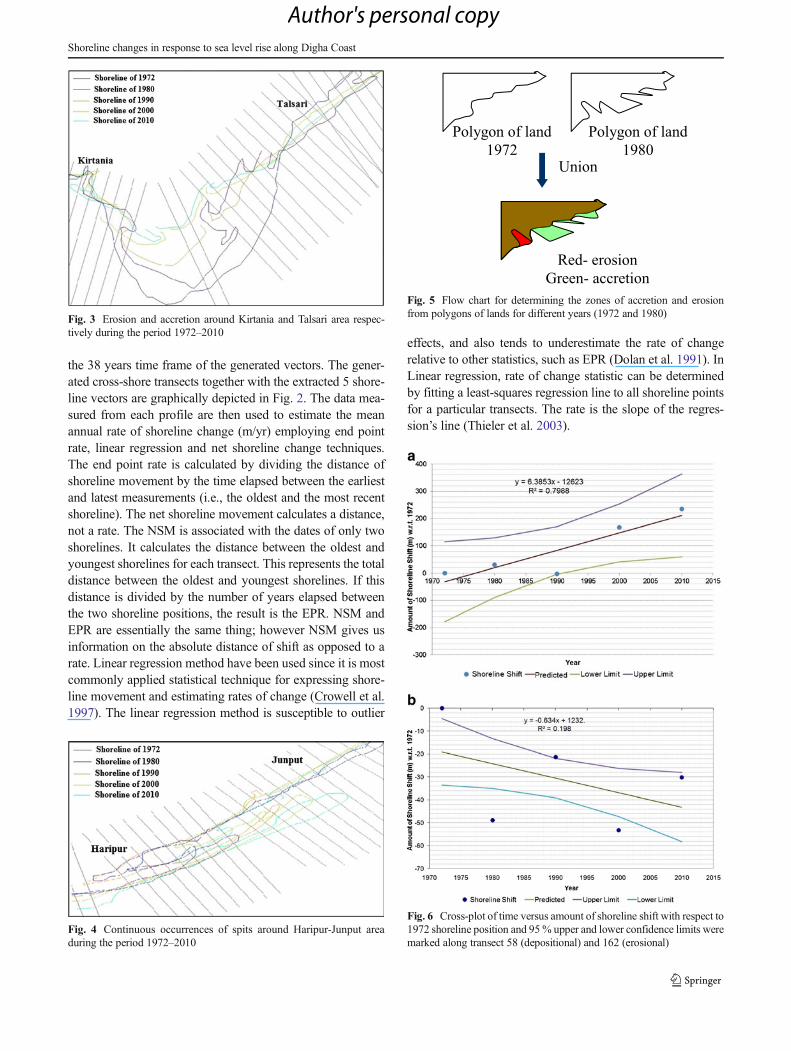
Fig. 3 Erosion and accretion around Kirtania and Talsari area respec-tively during the period 1972–2010

Fig. 4 Continuous occurrences of spits around Haripur-Junput areaduring the period 1972–2010

Union

Red- erosion

Green- accretion

Polygon of land

1972

Polygon of land

1980

Fig. 5 Flow chart for determining the zones of accretion and erosionfrom polygons of lands for different years (1972 and 1980)

Fig. 6 Cross-plot of time versus amount of shoreline shift with respect to1972 shoreline position and 95% upper and lower confidence limits weremarked along transect 58 (depositional) and 162 (erosional)

Shoreline changes in response to sea level rise along Digha Coast

Author's personal copy

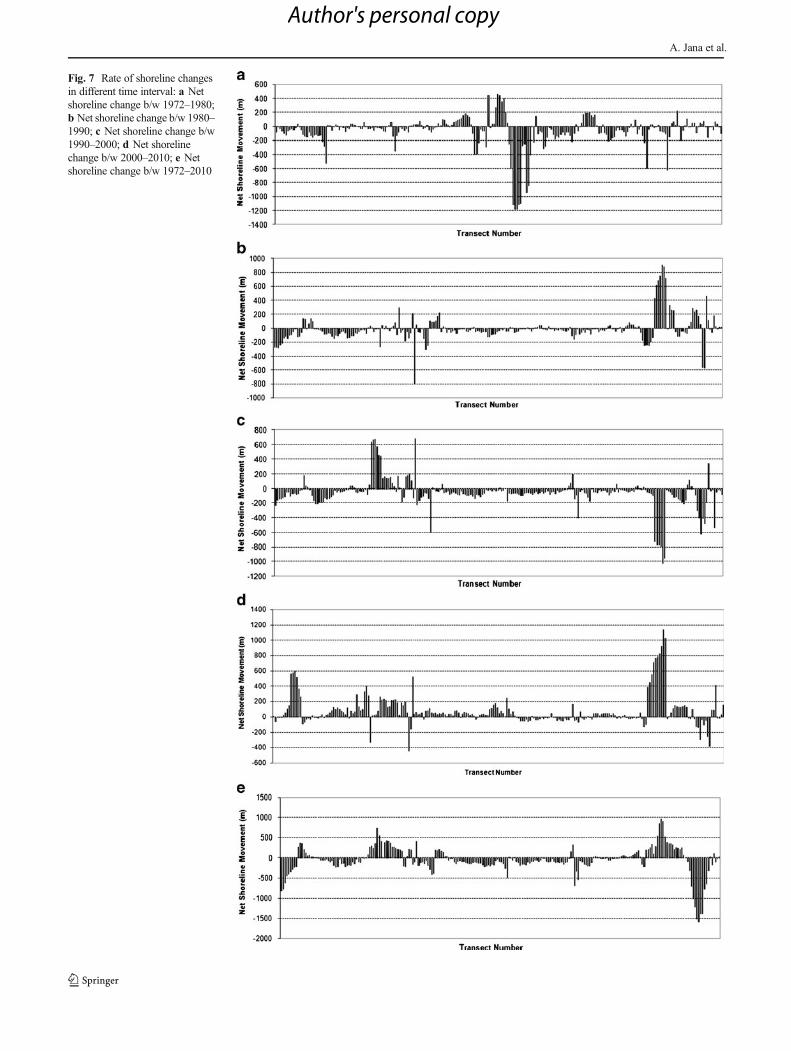
Fig. 7 Rate of shoreline changesin different time interval: a Netshoreline change b/w 1972–1980;b Net shoreline change b/w 1980–1990; c Net shoreline change b/w1990–2000; d Net shorelinechange b/w 2000–2010; e Netshoreline change b/w 1972–2010

A. Jana et al.

Author's personal copy

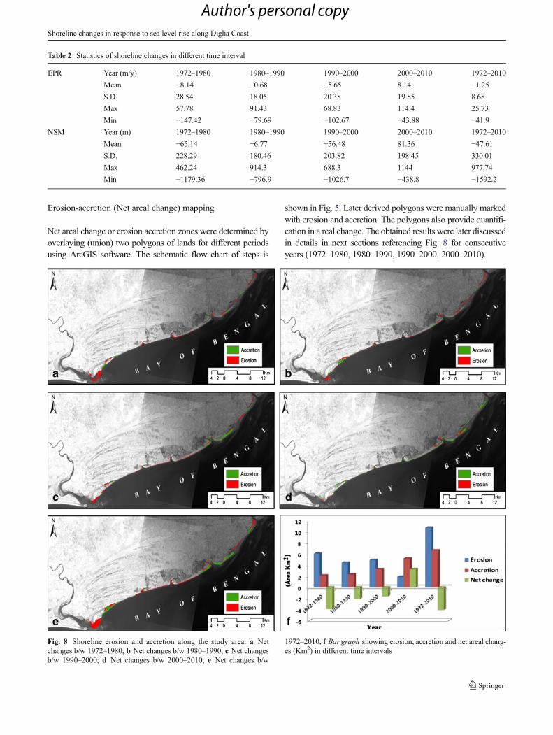
Erosion-accretion (Net areal change) mapping

Net areal change or erosion accretion zones were determined byoverlaying (union) two polygons of lands for different periodsusing ArcGIS software. The schematic flow chart of steps is

shown in Fig. 5. Later derived polygons were manually markedwith erosion and accretion. The polygons also provide quantifi-cation in a real change. The obtained results were later discussedin details in next sections referencing Fig. 8 for consecutiveyears (1972–1980, 1980–1990, 1990–2000, 2000–2010).

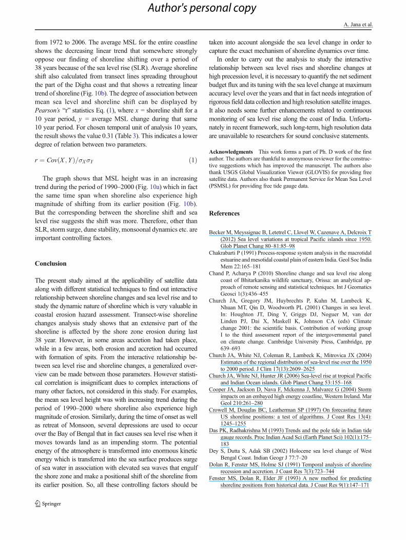
Table 2 Statistics of shoreline changes in different time interval

EPR Year (m/y) 1972–1980 1980–1990 1990–2000 2000–2010 1972–2010

Mean −8.14 −0.68 −5.65 8.14 −1.25S.D. 28.54 18.05 20.38 19.85 8.68

Max 57.78 91.43 68.83 114.4 25.73

Min −147.42 −79.69 −102.67 −43.88 −41.9NSM Year (m) 1972–1980 1980–1990 1990–2000 2000–2010 1972–2010

Mean −65.14 −6.77 −56.48 81.36 −47.61S.D. 228.29 180.46 203.82 198.45 330.01

Max 462.24 914.3 688.3 1144 977.74

Min −1179.36 −796.9 −1026.7 −438.8 −1592.2

Fig. 8 Shoreline erosion and accretion along the study area: a Netchanges b/w 1972–1980; b Net changes b/w 1980–1990; c Net changesb/w 1990–2000; d Net changes b/w 2000–2010; e Net changes b/w

1972–2010; f Bar graph showing erosion, accretion and net areal chang-es (Km2) in different time intervals

Shoreline changes in response to sea level rise along Digha Coast

Author's personal copy

Sea level changes

Sea-level rise is an important consequence of climate change,both for societies and for the environment (Kumar et al. 2010).Sea-level rise can be a product of global warming through twomain processes: thermal expansion of seawater and widespreadmelting of land ice. Global warming is predicted to causesignificant rises in sea level over the course of the twenty-first

century. Thus it becomes necessary to study the effect of sea-level rise on the coastal areas. In the present world due to thebuildup of global warming mainly there is a general tendencycomes that shoreline fluctuate in response to sea level fluctua-tion. But this sometimes may not be the exact reason of shore-line shifting. Beach erosion through wave action, long shoredrift and rip current that moves the beach sediment perpendic-ular to the shoreline is some other ways of altering the shoreline

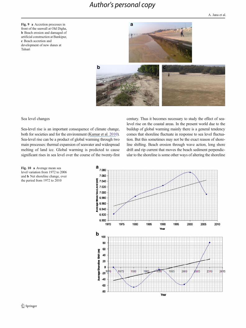
Fig. 9 a Accretion processes infront of the seawall at Old Digha,b Beach erosion and damaged ofartificial construction at Bankipur,c Beach accretion anddevelopment of new dunes atTalsari

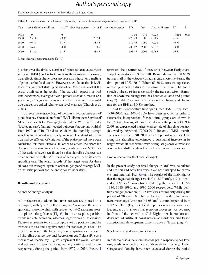
Fig. 10 a Average mean sealevel variation from 1972 to 2006and b Net shoreline change, overthe period from 1972 to 2010

A. Jana et al.

Author's personal copy

position over the time. A number of processes can cause meansea level (MSL) to fluctuate such as thermostatic expansion,tidal effect, atmospheric pressure, isostatic adjustment, meltingof polar ice shelf and sea ice. However, such fluctuation inMSLleads to significant shifting of shoreline. Mean sea level at thecoast is defined as the height of the sea with respect to a localland benchmark, averaged over a period, such as a month or ayear-long. Changes in mean sea level as measured by coastaltide gauges are called relative sea-level changes (Church et al.2001).

To assess the averageMSL of the coastal region three sets ofpoint data have been taken from PSMSL (Permanent Service ofMean Sea Level) for Paradip (located at the West) and Haldia(located at East), Gangra (located between Paradip and Haldia)from 1972 to 2010. The data set shows the monthly averagewhich is transformed into yearly average. The standard devia-tion and co-efficient of variation of the entire period have beencalculated for these stations. In order to assess the shorelinechanges in response to sea level rise, yearly average MSL dataof the stations have been filtered so that shoreline changes canbe compared with the MSL data of same year or to its corre-sponding one. The MSL records of the target years for thesestations are averaged again in order to get grand average MSLof the same periods for the entire coast under study.

Results and discussion

Shoreline change analysis

All measurements along the same transect are plotted in across-plot, with ‘year’ plotted along the X-axis and the corre-sponding shoreline shift with respect to 1972 shoreline posi-tion plotted along Y-axis (Fig. 6). In the cross-plots, positivetrends indicate accretion, whereas negative trends as erosion.Figure 6 represents typical cross-plots with a positive trend fortransect (tr. 58) and negative trend for transect (tr. 162). Theplot also represents the linear regression equation as a measureof shoreline change rate and Regression coefficient (R2) as ameasure of uncertainty. Figure 3 represent the overall erosionand accretion in specific areas, namely Kirtania and Talsarirespectively during the period from 1972 to 2010. Figure 4

represent the occurrences of three spits between Haripur andJunput areas during 1972–2010. Result shows that 30.63 %transect fall in the category of advancing shoreline during thetime span of 1972–2010. Where 69.36 % transect experienceretreating shoreline during the same time span. The entirestretch of the coastline under study, the transect-wise informa-tion of shoreline change rate has been calculated and plotted(Fig. 7). Table 2 summarizes the shoreline change and changerate for the EPR and NSM method.

Total four consecutive time span (1972–1980; 1980–1990;1990–2000; and 2000–2010) have been grouped in order tosummarize interpretation. Various time groups are shown inFig. 7a to e. Among all four time intervals, the period of 1990–2000 has experienced highest change rate of shoreline positionfollowed by the period of 2000-2010. Records ofMSL over theyears reveals that 1990–2000 was the period when sea levelalong this shoreline experienced a substantial increase in itsheight which in association with strong long shore current andwave action shift the shoreline back at a greater magnitude.

Erosion-accretion (Net areal change)

In the present study net areal change in km2 was calculatedand erosion and accretion zone have been mapped for differ-ent time interval (Fig. 8a–e). The results of the study showsthat the negative change (erosion) (−3.93 km2), (−2.11 km2),and (−1.63 km2) was observed during the period of 1972–1980, 1980–1990, and 1990–2000 respectively. While posi-tive change (accretion) (3.32 km2) was found only during theperiod of 2000–2010. The results also revealed the overallnegative change (erosion) (−4.08 km2) during the period from1972 to 2010 (Fig. 8f). Field reports during the month ofDecember 2011, shows that accretion processes was occurredin front of the seawall at Old Digha, beach erosion anddamaged of artificial construction at Bankipur and beachaccretion and development of new dunes at Talsari (Fig. 9).

Sea level rise and shoreline changes

In order to assess the shoreline changes in response to sea levelrise, yearly average MSL data of three stations namely, Haldia,Gangra and Paradip have been calculated during the period

Table 3 Statistics show the interactive relationship between shoreline changes and sea level rise (SLR)

Year Avg. shoreline shift (m) % of Tr. showing erosion % of Tr. showing accretion SD Year Avg. MSL (m) SD R2

1972 0 0 0 0.00 1972 6.923 5.000 0.311980 −65.14 29.06 70.94 228.29 1980 6.987 21.67

1990 −6.77 61.54 38.46 180.46 1990 7.026 40.50

2000 −56.48 80.34 19.66 203.82 2000 7.072 33.00

2010 81.36 61.54 38.46 198.45 2006 6.993 16.51

R-statistics was measured using Eq. (1)

Shoreline changes in response to sea level rise along Digha Coast

Author's personal copy

from 1972 to 2006. The average MSL for the entire coastlineshows the decreasing linear trend that somewhere stronglyoppose our finding of shoreline shifting over a period of38 years because of the sea level rise (SLR). Average shorelineshift also calculated from transect lines spreading throughoutthe part of the Digha coast and that shows a retreating lineartrend of shoreline (Fig. 10b). The degree of association betweenmean sea level and shoreline shift can be displayed byPearson’s “r” statistics Eq. (1), where x = shoreline shift for a10 year period, y = average MSL change during that same10 year period. For chosen temporal unit of analysis 10 years,the result shows the value 0.31 (Table 3). This indicates a lowerdegree of relation between two parameters.

r ¼ Cov X ; Yð Þ=σXσY ð1Þ

The graph shows that MSL height was in an increasingtrend during the period of 1990–2000 (Fig. 10a) which in factthe same time span when shoreline also experience highmagnitude of shifting from its earlier position (Fig. 10b).But the corresponding between the shoreline shift and sealevel rise suggests the shift was more. Therefore, other thanSLR, storm surge, dune stability, monsoonal dynamics etc. areimportant controlling factors.

Conclusion

The present study aimed at the applicability of satellite dataalong with different statistical techniques to find out interactiverelationship between shoreline changes and sea level rise and tostudy the dynamic nature of shoreline which is very valuable incoastal erosion hazard assessment. Transect-wise shorelinechanges analysis study shows that an extensive part of theshoreline is affected by the shore zone erosion during last38 year. However, in some areas accretion had taken place,while in a few areas, both erosion and accretion had occurredwith formation of spits. From the interactive relationship be-tween sea level rise and shoreline changes, a generalized over-view can be made between those parameters. However statisti-cal correlation is insignificant dues to complex interactions ofmany other factors, not considered in this study. For examples,the mean sea level height was with increasing trend during theperiod of 1990–2000 where shoreline also experience highmagnitude of erosion. Similarly, during the time of onset as wellas retreat of Monsoon, several depressions are used to occurover the Bay of Bengal that in fact causes sea level rise when itmoves towards land as an impending storm. The potentialenergy of the atmosphere is transformed into enormous kineticenergy which is transferred into the sea surface produces surgeof sea water in association with elevated sea waves that engulfthe shore zone and make a positional shift of the shoreline fromits earlier position. So, all these controlling factors should be

taken into account alongside the sea level change in order tocapture the exact mechanism of shoreline dynamics over time.

In order to carry out the analysis to study the interactiverelationship between sea level rises and shoreline changes athigh precession level, it is necessary to quantify the net sedimentbudget flux and its tuning with the sea level change at maximumaccuracy level over the years and that in fact needs integration ofrigorous field data collection and high resolution satellite images.It also needs some further enhancements related to continuousmonitoring of sea level rise along the coast of India. Unfortu-nately in recent framework, such long-term, high resolution dataare unavailable to researchers for sound conclusive statements.

Acknowledgments This work forms a part of Ph. D work of the firstauthor. The authors are thankful to anonymous reviewer for the construc-tive suggestions which has improved the manuscript. The authors alsothank USGS Global Visualization Viewer (GLOVIS) for providing freesatellite data. Authors also thank Permanent Service for Mean Sea Level(PSMSL) for providing free tide gauge data.

References

Becker M, Meyssignac B, Letetrel C, Llovel W, Cazenave A, Delcroix T(2012) Sea level variations at tropical Pacific islands since 1950.Glob Planet Chang 80–81:85–98

Chakrabarti P (1991) Process-response system analysis in the macrotidalestuarine andmesotidal coastal plain of eastern India. Geol Soc IndiaMem 22:165–181

Chand P, Acharya P (2010) Shoreline change and sea level rise alongcoast of Bhitarkanika wildlife sanctuary, Orissa: an analytical ap-proach of remote sensing and statistical techniques. Int J GeomaticsGeosci 1(3):436–455

Church JA, Gregory JM, Huybrechts P, Kuhn M, Lambeck K,Nhuan MT, Qin D, Woodworth PL (2001) Changes in sea level.In: Houghton JT, Ding Y, Griggs DJ, Noguer M, van derLinden PJ, Dai X, Maskell K, Johnson CA (eds) Climatechange 2001: the scientific basis. Contribution of working groupI to the third assessment report of the intergovernmental panelon climate change. Cambridge University Press, Cambridge, pp639–693

Church JA, White NJ, Coleman R, Lambeck K, Mitrovica JX (2004)Estimates of the regional distribution of sea-level rise over the 1950to 2000 period. J Clim 17(13):2609–2625

Church JA, White NJ, Hunter JR (2006) Sea-level rise at tropical Pacificand Indian Ocean islands. Glob Planet Chang 53:155–168

Cooper JA, Jackson D, Nava F, Mckenna J, Malvarez G (2004) Stormimpacts on an embayed high energy coastline, Western Ireland. MarGeol 210:261–280

Crowell M, Douglas BC, Leatherman SP (1997) On forecasting futureUS shoreline positions: a test of algorithms. J Coast Res 13(4):1245–1255

Das PK, Radhakrishna M (1993) Trends and the pole tide in Indian tidegauge records. Proc Indian Acad Sci (Earth Planet Sci) 102(1):175–183

Dey S, Dutta S, Adak SB (2002) Holocene sea level change of WestBengal Coast. Indian Geogr J 77:7–20

Dolan R, Fenster MS, Holme SJ (1991) Temporal analysis of shorelinerecession and accretion. J Coast Res 7(3):723–744

Fenster MS, Dolan R, Elder JF (1993) A new method for predictingshoreline positions from historical data. J Coast Res 9(1):147–171

A. Jana et al.

Author's personal copy

Forbes D, Parkers G, Manson G, Ketch K (2004) Storms and shorelineretreat in the southern Gulf of St. Lawrence. Mar Geol 210(1–4):169–204

USGS Global Visualization Viewer (2012) USGS science for a changingworld. http://glovis.usgs.gov/. Accessed 2012

GSI (1995) Unpublished report on the coastal zone management plan ofDigha Planning area, Medinipur District, West Bengal. GSI opera-tion: WB-SIK-AN, Eastern Region Environmental GeologyDivisions- II

Holgate SJ, Woodworth PL (2004) Evidence for enhanced coastal sea-level rise during the 1990s. Geophys Res Lett 31, L07305. doi:10.1029/2004GL01 9626

Jana A, Bhattacharya AK (2012) Assessment of coastal erosion vulner-ability around Midnapur-Balasore Coast, Eastern India using inte-grated remote sensing and GIS techniques. J Indian Soc Rem Sens41(3):675–686. doi:10.1007/s12524-012-0251-2

Jantunen H, Raitala J (1984) Locating shoreline changes in thePorttipahta (Finland) water reservoir by using multitemporal landsatdata. Photogrammetria 39:1–12

Kumar Danish PK (2001) Monthly mean sea level variation at Cochin,Southwest Coast of India. Int J Ecol Environ Sci 27:209–214

Kumar TS, Mahendra RS, Nayak S, Radhakrishnan K, Sahu KC (2010)Coastal vulnerability assessment for Orissa State, East Coast ofIndia. J Coast Res 26(3):523–534

Lafon V, Froidefonda JM, Lahetb F, Castaing P (2002) SPOT shallowwater bathymetry of a moderately turbid tidal inlet based on fieldmeasurements. Remote Sens Environ 81:136–138

Maiti S, Bhattacharya AK (2009) Shoreline change analysis and itsapplication to prediction: a remote sensing and statistics basedapproach. Mar Geol 257:11–23

Munday JC, Alfoldi TT (1979) LANDSAT test of diffuse reflectancemodels for aquatic suspended solids measurement. Remote SensEnviron 8:169–183

Niyogi D (1970) Geological background of beach Erosional Digha, WestBengal. Bull Geol Min Metall Soc India 43:1–36

Orford JD, Forbes DL, Jennings SC (2002) Organizational controls,typologies and time scales of paraglacial gravel-dominated coastalsystems. Geomorphology 48:51–85

Paul AK (2002) Coastal geomorphology and environment: SunadrbanCoastal Plain, Kanthi Coastal Plain, Subarnarekha Delta Plain. ACBPublication, Kolkata

Paul SK (2006) Issues in coastal zone management of Digha-Shankarpurcoastal area. ISRO-RSAM project report. RRSSC, Kharagpur

Ritchie JC, Cooper CM, Schiebe FR (1990) The relationship of MSS andTM digital data with suspended sediments, chlorophyll, and temper-ature in Moon lake, Mississippi. Remote Sens Environ 33:137–148

Ryu JH, Won JS, Min KD (2002) Waterline extraction from Landsat TMdata in a tidal flat: a case study in Gosmo Bay, Korea. Remote SensEnviron 83:442–456

Scott DB (2005) Coastal changes, rapid. In: Schwartz ML (ed)Encyclopedia of coastal sciences. Springer, The Netherlands, pp253–255

Siddiqui MN, Maajid S (2004) Monitoring of geomorphological changesfor planning reclamation work in coastal area of Karachi, Pakistan.Adv Space Res 33:1200–1205

Thieler ER, Martin D, Ergul A (2003) The digital shoreline analysissystem, version 2.0: shoreline change measurement software exten-sion for Arcview. USGS U.S. Geological Survey Open-File Report03-076

Thieler ER, Himmelstoss EA, Zichichi JL, Miller TL (2005) DigitalShoreline Analysis System (DSAS) version 3.0: an ArcGIS exten-sion for calculating shoreline change. US Geological Survey Open-File Rep 2005-1304

White K, El Asmar HM (1999) Monitoring changing position of coast-lines using thematic mapper imagery, an example from the NileDelta. Geomorphology 29:93–105

Yamano H, Shimazaki H, Matsunaga T, Ishoda A, McClennen C, YokokiH, Fujita K, Osawa Y, Kayanne H (2006) Evaluation of varioussatellite sensors for waterline extraction in a coral reef environment:Majuro Atoll, Marshall Islands. Geomorphology 82:398–411

Shoreline changes in response to sea level rise along Digha Coast

Author's personal copy