


Bahasa
Halaman
Hukum

Prepared for SHIP SAFETY NORTHERN TRANSPORT CANADA by: Claude Daley and Richard Hayward Memorial University Of Newfoundland and Kaj Riska Helsinki University of Technology November 1996 Memorial University of Newfoundland
Ocean Engineering Research Centre
Ship-Ice Interaction
Determination of Bow Forces and Hull Resopnse Due to Head-on and Glancing Impact between
a Ship and an Ice Floe
i
1. Transport Canada Publication No.
2. Project No. 3. Recipients Catalogue No.
4. Title and Subtitle
5. Publication Date
6. Performing Organization Document No.
7. Author(s)
8. Transport Canada File No.
9. Performing Organization Name and Address
10. DSS File No.
11. DSS Contract No.
12. Sponsoring Agency and Address 13. Type of Publication and Period Covered
14. Sponsoring Agency Code
15. Supplementary Notes
16. Project Officer
17. Abstract
18. Key Words
19. Distribution Statement
20. Security Classification (of this publication)
21 Security Classification (of this page)
22. Declassification (date) 23. No. of Pages 24. Price
02-0149 (09-88)
PUBLICATION DATA FORMTransport Canada
Transports Canada
SHIP-ICE INTERACTION Determination of Bow Forces and Hull Response Due to Head-on and Glancing Impact between a Ship and an Ice Floe
Claude Daley, Richard Hayward, Kaj Riska
Helsinki University of Technology Espoo, Finland
Memorial University Faculty of Engineering, St. John’s, Newfoundland, Canada, A1B 3X5
Ship Safety Northern 344 Slater Street, 5th Floor Ottawa, Ontario K1A 0N7
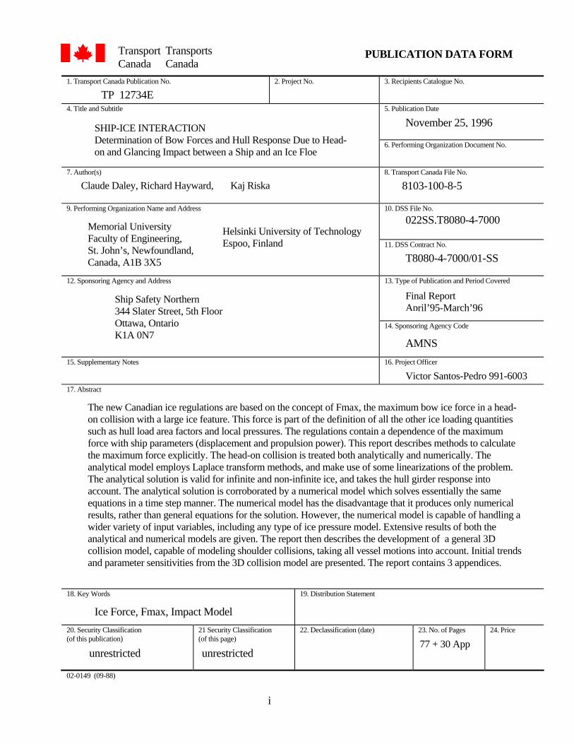
The new Canadian ice regulations are based on the concept of Fmax, the maximum bow ice force in a head-on collision with a large ice feature. This force is part of the definition of all the other ice loading quantities such as hull load area factors and local pressures. The regulations contain a dependence of the maximum force with ship parameters (displacement and propulsion power). This report describes methods to calculate the maximum force explicitly. The head-on collision is treated both analytically and numerically. The analytical model employs Laplace transform methods, and make use of some linearizations of the problem. The analytical solution is valid for infinite and non-infinite ice, and takes the hull girder response into account. The analytical solution is corroborated by a numerical model which solves essentially the same equations in a time step manner. The numerical model has the disadvantage that it produces only numerical results, rather than general equations for the solution. However, the numerical model is capable of handling a wider variety of input variables, including any type of ice pressure model. Extensive results of both the analytical and numerical models are given. The report then describes the development of a general 3D collision model, capable of modeling shoulder collisions, taking all vessel motions into account. Initial trends and parameter sensitivities from the 3D collision model are presented. The report contains 3 appendices.
Ice Force, Fmax, Impact Model
unrestrictedunrestricted 77 + 30 App
AMNS
Victor Santos-Pedro 991-6003
T8080-4-7000/01-SS
8103-100-8-5
022SS.T8080-4-7000
November 25, 1996
Final Report April’95-March’96
TP 12734E

ii
1. No de la publication de Transports Canada
2. No de l’étude. 3. No de catalogue du destinaire.
4. Titre et sous-titre
5. Date de la publication
6. No du document de l’organizme
7. Auteur(s)
8. No du dossier de Transports Canada
9. Nom et addresse de l’organizme exécutant
10. No du dossier - ASC.
11. No de contrat - ASC.
12. Nom et addresse de l’organizme parrain 13. Genre de publication et périod visée
14. de l’organizme parrain
15. Remarques additionnelles
16. Agent de projet
17. Résumé
18. Mots-clés
19. Diffusion
20. Classification de sécurité (de cette publication)
21 Classification de sécurité (de cette page)
22. Déclassification (date) 23. Nombre de pages 24. Prix
02-0149 (09-88)
FORMULE DE DONNÉES POUR PUBLICATION Transports Canada
Transport Canada
INTERACTION NAVIRE-GLACE Détermination des forces exercées sur l’avant d’un navire suite au choc frontal d’un bloc de glace.
Claude Daley, Richard Hayward, Kaj Riska
Helsinki University of TechnologyEspoo, Finland
Memorial University Faculty of Engineering, St. John’s, Newfoundland, Canada, A1B 3X5
Sécurité des navires, Nord 344, rue Slater Street, 5e ètage Ottawa (ON) K1A 0N7
Le nouveau règlement canadien des glace est basé sur la notion de Fmax, la force maximale exercée par la glace sur l’avant en cas d’abordage frontal d’une masse de glace importante. Cette force fait partie de la définition de toutes les autres charges de glace comme les facteurs de surface de charge de la coque et les pressions locales. Le règlement fait référence à la dépendence de la force maximale en fonction des paramètres du navire (jauge et puissance de propulsion). Le rapport décrit les méthodes de calcul de la force maximale de façon explicite. L'abordage frontal est traité analytiquement et numériquement. Le modèle analytique utilise des méthodes avec transformée de Laplace et fait appel à certaines linéarisations. La solution analytique est valide pour de la glace infinie et non infinie et tient compte de la réponse de la poutre coque. La solution analytique est corroborée par un modèle numérique qui résout essentiellement les mêmes équations dans des intervalles de temps. Le modèle numérique a l'inconvénient de ne produire que des résultats numériques et non des équations générales de la solution. Toutefois, le modèle numerique permet de traiter une plus grande variété de variables d'entrées, y compris n’importe quel type de modèle de pressions de glace. Le rapport donne les résultats extensifs du modèle analytique et du modèle numérique et décrit ensuite le developpement d'un modèle des abordages en 3D capable de modéliser des abordages d'épaulement, en tenant compte de tous les mouvements du navire. Il présente les tendances initiales et les sensibilités paramètriques du modèle d'abordage en 3D. Le rapport contient trois annexes.
Force des glace, Fmax, modèle d’impact - Phase II
sans restriction sans restriction 77 + 30 Ann
Victor Santos-Pedro 991-6003
T8080-4-7000/01-SS
022SS.T8080-4-7000
10 août 1996
Rapport final avril 95-mars 96
TP 12734 E
iii
Abstract
The new Canadian ice regulations are based on the concept of Fmax, the maximum bow ice force in a head-on collision with a large ice feature. This force is part of the definition of all the other ice loading quantities such as hull load area factors and local pressures. The regulations contain a dependence of the maximum force with ship parameters (displacement and propulsion power). This report describes methods to calculate the maximum force explicitly. The head-on collision is treated both analytically and numerically. The analytical model employs Laplace transform methods, and make use of some linearizations of the problem. The analytical solution is valid for infinite and non-infinite ice, and takes the hull girder response into account. The analytical solution is corroborated by a numerical model which solves essentially the same equations in a time step manner. The numerical model has the disadvantage that it produces only numerical results, rather than general equations for the solution. However, the numerical model is capable of handling a wider variety of input variables, including any type of ice pressure model. Extensive results of both the analytical and numerical models are given. The report then describes the development of a general 3D collision model, capable of modeling shoulder collisions, taking all vessel motions into account. Initial trends and parameter sensitivities from the 3D collision model are presented. The report contains 3 appendices. Acknowledgment
The authors wish to acknowledge the support and patience that Mr. Victor Santos-Pedro showed throughout the project.
iv
TABLE OF CONTENTS
Abstract iii
Acknowledgement iii
Table of Figures vi
Table of Tables viii
Nomenclature ix
1. INTRODUCTION 1-1
2. DEFINITION OF INTERACTION SCENARIOS 2-1
3. ANALYSIS OF HEAD-ON COLLISION WITH MULTI-YEAR ICE 3-1
3.1 Definition of the problem 3-1
3.2 Analytical solution for the ramming problem 3-3
3.2.1 The displacement into ice 3-5
3.2.2 Ship bow displacement 3-7
3.2.3 Ice displacement 3-11
3.2.4 Solution of the ramming equations 3-12
3.3 The ram on an ice feature of infinite mass 3-18
3.4 Case study of head-on ramming 3-21
3.5 Head-on ram on a finite ice floe 3-36
3.6 Analysis of the Influence of Contact Pressure on Force 3-41
3.7 Numerical simulation of head-on ramming 3-44
3.8 Discussion 3-52
4. ANALYSIS OF OBLIQUE RAMS 4-1
4.1 Physical Description of Ship-Ice Interaction 4-1
4.2 Definition of the problem 4-2
v
4.3 Numerical Simulation of Oblique Ship-Ice Interaction 4-4
4.3.1 Specification of Ship/Ice Constants 4-5
4.3.2 Specification of Ship/Ice Initial Values 4-6
4.3.2 Response Characteristics of Ship to Impact 4-7
4.3.4 Responses Characteristics of the Ice Floe to Impact 4-9
4.3.5 Calculation of Ship Penetration into Ice Floe 4-10
4.3.6 Calculation of Contact Area 4-11
4.3.7 Calculation of Forces and Moments 4-13
4.3.8 Calculation of Accelerations, Velocities and Displacements 4-14
4.3.9 Time Step 4-14
4.4 Results 4-15
4.4.1 Force-Time Simulation Results 4-16
4.4.2 Parametric results 4-16
4.5 Discussion 4-19
5. CONCLUSION 5-1
5.1 Summary 5-1
5.2 Recommendations 5-5
6. REFERENCES 6-1
Appendix A - Listing of 2D Collision Model
Appendix B - Listing of 3D Collision Model
Appendix C - Force-Time Plots for 3D Collision Model
vi
Table of Figures
Figure 1. Ship and ice motion coordinates........................................................................................... 3-1
Figure 2. Bow ice penetration coordinates .......................................................................................... 3-3
Figure 3. Relationship of Shear and Bending in the Hull.................................................................. 3-14
Figure 4. Non-Dimensional Shear Distributions .............................................................................. 3-22
Figure 5. Non-Dimensional Bending Moment Distribution ............................................................. 3-23
Figure 6. Characteristic frequencies vs. dimensionless ice strength................................................. 3-24
Figure 7. Non-dimensional force vs. dimensionless ice strength...................................................... 3-25
Figure 8 Non-dimensional shear vs. dimensionless ice strength. ..................................................... 3-25
Figure 9 Non-dimensional moment vs. dimensionless ice strength. ................................................ 3-26
Figure 10. Influence of K on force time history. ...............................................................................3-27
Figure 11. Influence of K on shear time history. ...............................................................................3-27
Figure 12. Influence of K on moment time history. .......................................................................... 3-28
Figure 13. Influence of β on force time history. ................................................................................ 3-29
Figure 14. Influence of β on shear time history................................................................................. 3-29
Figure 15. Influence of β on moment time history. ........................................................................... 3-30
Figure 16. Influence of μ on force time history................................................................................. 3-31
Figure 17. Influence of μ on shear time history................................................................................. 3-31
Figure 18. Influence of λ on force time history. ................................................................................ 3-32
Figure 19. Influence of λ on shear time history................................................................................. 3-32
Figure 20. Influence of λ on moment time history. ........................................................................... 3-33
Figure 21. Influence of length on force time history. ........................................................................ 3-34
Figure 22. Influence of length on shear time history......................................................................... 3-34
Figure 23. Influence of length on moment time history. ................................................................... 3-35
Figure 24. Influence of floe diameter / ship length ratio on characteristic frequencies. .................. 3-38
Figure 25. Influence of floe diameter / ship length ratio on dimensionless force amplitudes. ........ 3-39
Figure 26. Influence of floe diameter on ice force, for a 4 knot ram with M.V. ARCTIC.............. 3-39
Figure 27. Influence of floe edge radius on ice force. ....................................................................... 3-40
Figure 28. Influence of pressure/area exponemt on ice force. .......................................................... 3-43
Figure 29. Vessel ramming thick ice head-on. .................................................................................. 3-44
Figure 30. Equivalent spring-mass system for head-on ramming. ................................................... 3-45
vii
Table of Figures (cont.)
Figure 31. Comparison of Analytical and Numerical Results. (The numerical results are shown with dashed lines and labled “Mcad”)............................................................................ 3-46
Figure 32. Force time-history for a head-on at 10 kts, for the case of p=500 kPa. .......................... 3-47
Figure 33. Force time-history for a head-on at 10 kts, for the case of p=3000 kPa. ........................ 3-48
Figure 34. Force time-history for a head-on at 10 kts, for the case of p=3000 A-.5 kPa. ................. 3-48
Figure 35. Influence of vessel displacement on ice force, for various ice pressure-area models.......................................................................................................................................... 3-49
Figure 36. Influence of vessel displacement on ice force, for various (constant) ice pressure levels............................................................................................................................................ 3-49
Figure 37. Influence of C2 on ice force, for various ship lengths...................................................... 3-50
Figure 38. Influence of C2 on ice force, for various ship speeds (for LBP=195 m, C1 = 3 MPa). ........................................................................................................................................... 3-50
Figure 39. Influence of C2 on normalized ice force, for various ship speeds (for LBP=195 m)....... 3-51
Figure 40. Superposition of Figures 28 and 38. The curves labeled (n) are those from the numerical model.......................................................................................................................... 3-51
Figure 41. General collision geometry................................................................................................. 4-1
Figure 42. Flow Chart for Sii Oblique Ramming Model Mathcad.................................................... 4-4
Figure 43. 3D Ship Shoulder Geometry Description ........................................................................ 4-10
Figure 44. Contact geometry with a round floe edge ........................................................................ 4-12
Figure 45. Contact geometry with angular floe edge. ....................................................................... 4-12
Figure 46 Geometry of ice block during the interaction ................................................................... 4-14
Figure 47. Force vs time for Case 1 using the 3D collision model................................................... 4-16
Figure 48. Relationship between force acting on the ship and the length of the ship between perpendiculars. Variables held constant include: L/B=7.5m, α=40o, β=75o, Rice=50m and hice=3m, and vo= 5 m/s. ........................................................................................................ 4-17
Figure 49. Relationship between force acting on the ship and the radius of the ice floe. Variables held constant include Lbp=100m, B=13.3m, α=40o, β=65o and hice=3m................. 4-17
Figure 50. Relationship between force acting on the ship and the thickness of the ice floe. Variables held constant include: Lbp=100m, B=13.3m, α=40o, β=65o and Rice=50m. ............ 4-18
Figure 51. Relationship between force acting on the ship and the waterline entrance angle. Variables held constant include: Lbp=100m, B=13.3m, Rice=50m, hice=3m and β=65o........... 4-18
Figure 52. Relationship between force acting on the ship and the normal frame angle. Variables held constant include: Lbp=100m, B=13.3m, Rice=50m, hice=3m and α=40o. ......... 4-19
Figure 53. General 3D ship-ice collision scenario............................................................................... 5-3
viii
Table of Tables
Table 1 Particulars of the M.V.Arctic................................................................................................ 3-21
Table 2 Dimensionless coefficients for M.V. ARCTIC.................................................................... 3-21
Table 3. Definition of ship constants ................................................................................................... 4-5
Table 4. Definition of ice constants...................................................................................................... 4-5
Table 5. Dynamic variables of ship-ice interaction. ............................................................................ 4-6
Table 6 Simulation parameters for 3D numerical model runs. ......................................................... 4-15

ix
NOMENCLATURE Chapter 2 Fmax - total maximum contact force VP - height of ice load PAV - average ice pressure over VP pice(x,y) - ice pressure x - coordinate along waterline y - coordinate along shell normal to
waterline Chapter 3, sections 1-6 α - angle between waterline and fwd. β - angle between stem and fwd. βi - modal constants ξ - x location for shear or bending κ - dimensionless ice strength λ - dimensionless hull stiffness Ω - principal heave frequency ρ - density of water ρi - density of ice θ - pitch angle &&θ - pitch acceleration δx - added mass for vessel in x direction δz - added mass for vessel in z direction δix - added mass for ice in x direction δiθ - added mass for ice in θ direction δiz - added mass for ice in z direction ηi(t) - generalized coordinated of bending
modes μ - coefficient of friction τ2,τ1 - time integration variables ωθ - natural frequency in pitch ωz - natural frequency in heave ωi - natural frequencies in bending ωi - ice motion constant A - loaded area, contact area Awp - waterplane area A2 - 2nd moment of waterplane area Aj - dimensionless amplitudes of
ramming interaction force Aside - nominal contact area on one side of
stem B(x) - breadth of vessel
i, j, k - unit vectors on the x, y, z axes C - ice elastic parameter C - a ship modal constant Cx - a ship modal constant Cz - a ship modal constant Cb - a ship modal constant Cθ - a ship modal constant Cix - an ice modal constant Ciz - an ice modal constant CΔ - ice mass constant Cwp - ice mass constant CB - ice mass constant C1 - ice pressure constant C2 - ice pressure exponent Ci - ith mode constant for nat. freq. CG - center of gravity of the ship D - ice floe diameter E - Young’s modulus F(s) - Laplace transform of f(t) f(t) - any function of time Fn(t) - normal ice force Fn,max - maximum normal ice force Fmax - maximum normal ice force Fn(s) - Laplace transform of normal ice
force Fx(t) - longitudinal ice force Fz(t) - vertical ice force g - gravity G1(α,β) - ice load constant Gμ1 - ice friction constant Gμ2 - ice friction constant H - ice floe thickness Iθ - pitch moment of inertia kice - ice elastic constant keq - equivalent ice stiffness L - length of ship m - meters mi - ice floe mass mz(x) - added mass in vertical direction M - mass of the vessel Mx - total mass of the vessel in x Mi - dimensionless amplitudes of
bending moment N - number of vertical bending modes
x
Ni(t) - generalized modal force n1,2 - unit normal vectors on each side of
the stem p(A) - pressure on area A P(s) - polynomial in s Q(s) - polynomial in s Qi - dimensionless amplitudes of shear
force q(x) - ice load intensity q - dimensionless frequencies R - radius of loaded area RA2 - long. radius of gyration of vessel Rθ - pitch radius of gyration of vessel s - Laplace variable si - roots of the Q polynomial t - time T - Kinetic energy in ramming uav - average deflection of loaded area ubow - bow movement normal to stem ucr - ice crushing displacement umax - maximum ice crushing
displacement ue - ice elastic displacement ui - ice edge displacement ux - bow position forward (surge) &&ux - bow acceleration forward (surge) &&uix - ice acceleration forward &ux - bow velocity forward (surge)
uix - ice edge position forward (surge) uz - bow position up (heave of bow) uiz - ice edge position down (heave of
ice edge) v - vessel velocity vn - vessel velocity normal to ice vt - vessel velocity tangential to ice W - energy consumed in crushing wi(x’) - ith vert. bending mode of the vessel wic - deflection of ith mode at ice contact X,x - fore-aft coordinate, from the CG x’ - fore-aft coordinate, from aft perp. xc - x coord. of the center of contact Z,z - vertical coord. from the CG zb(t) - vertical movement of the contact
point due to elastic bending of the ship
zc - z coordinate of the center of contact
Chapter 3, section 7 x - fore-aft coordinate, measured from
the ice edge (bow surge) y - vertical coordinate, measured from
the ice edge (bow heave) cx - damping in surge cy - damping in bow heave Mx - vessel surge mass My - bow heave mass Kx - vessel surge stiffness (0) Ky - bow heave stiffness kel - ice elastic spring stiffness kcr - ice crushing spring pen - total ice penetration (el +cru) LBP - ship length vship - ship speed C1 - ice pressure constant C2 - ice pressure exponent p(A) - ice pressure (= C1 AC2) Chapter 4 α - waterline entrance angle βn - normal frame angle Φ - ice pitch coordinate φ - ship roll coordinate κ - ice geometry (tan κ =h/2R) ψ - ship yaw coordinate ϕ - ice edge angle (angular edge) θ - ship pitch coordinate ρi - density of ice [kg/m3] ρw - density of sea water [kg/m3] σ - ice pressure Ω - ice yaw coordinate Φ - ice pitch coordinate ∇ - vessel displacement volume Δ - vessel displacement mass A - contact area B - beam [m] BML - center of buoyancy to longitudinal
metacentre
xi
BMT - center of buoyancy to transverse metacentre
Cb - block coefficient CG - center of gravity Ci - added mass coefficient (i = x,y,z) CIi - added inertia coefficient (i = φ,ψ,θ) Cm - added mass coefficient Cwp - waterplane coefficient Di - drag terms (i = y, ψ, y) elast - thickness of the elastic ice layer [m] F - ice force Fmax - maximum contact force Fi - force on ship (i = x,y,z) Fi - force on ice floe (i = u, w, Ω) GMT - transverse metacentric height GML - longitudinal metacentric height hice, h - thickness of ice floe [m] hl - ice edge penetration imax - number of simulation steps Ii - mass moments of inertia (i =
φ,ψ,θ, Ω) IT - transverse moment of inertia of the
waterplane IL - longitudinal moment of inertia of
the waterplane KB - keel to center of buoyancy KG - keel to CG Ki - stiffness terms (i = z, φ,θ, ω, Ω) Lbp - length between perpendiculars [m] L - length between perpendiculars [m] mice - mass of ice Mφ - roll moment Mψ - yaw moment Mθ - pitch moment pcr - average contact pressure Rice - radius of circular ice floe [m] T - draught [m] t - time [s] time - total simulation time u - ice horizontal movement normal to
waterline at contact v - ship velocity velpen - ice penetration velocity vo - initial ship velocity w - ice vertical movement x - fore-aft coordinate, from the CG
xg - fore-aft coordinate, (earth fixed) xi - x coordinate for ice y - lateral coordinate, from the CG y0 - ship displacement in the x-direction y1 - ship velocity in the x-direction y10 - ship displacement in the ψ-
direction y11 - ship velocity in the ψ-direction y12 - ice displacement in the u-direction y13 - ice velocity in the u-direction y14 - ice displacement in the w-direction y15 - ice velocity in the w-direction y16 - ice displacement in the Ω-direction y17 - ice velocity in the Ω-direction y18 - maximum penetration into ice y19 - penetration velocity into ice y2 - ship displacement in the y-direction y3 - ship velocity in the y-direction y4 - ship displacement in the z-direction y5 - ship velocity in the z-direction y6 - ship displacement in the φ-direction y7 - ship velocity in the φ-direction y8 - ship displacement in the θ-direction y9 - ship velocity in the θ-direction yg - lateral coordinate, (earth fixed) yi - y coordinate for ice z - vertical coordinate, from the CG zg - vertical coordinate, (earth fixed) zi - z coordinate for ice x’’ - surge acceleration y’’ - sway acceleration z’’ - heave acceleration
Ship-Ice Interaction 1-1
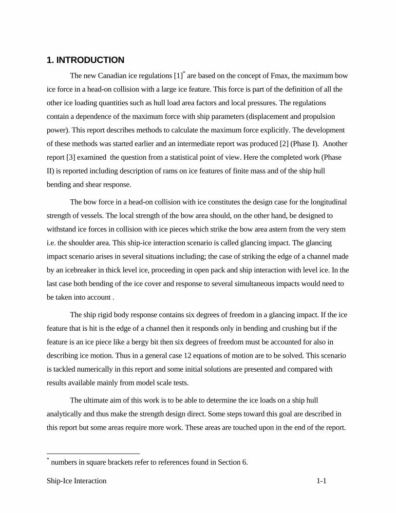
1. INTRODUCTION The new Canadian ice regulations [1]* are based on the concept of Fmax, the maximum bow
ice force in a head-on collision with a large ice feature. This force is part of the definition of all the
other ice loading quantities such as hull load area factors and local pressures. The regulations
contain a dependence of the maximum force with ship parameters (displacement and propulsion
power). This report describes methods to calculate the maximum force explicitly. The development
of these methods was started earlier and an intermediate report was produced [2] (Phase I). Another
report [3] examined the question from a statistical point of view. Here the completed work (Phase
II) is reported including description of rams on ice features of finite mass and of the ship hull
bending and shear response.
The bow force in a head-on collision with ice constitutes the design case for the longitudinal
strength of vessels. The local strength of the bow area should, on the other hand, be designed to
withstand ice forces in collision with ice pieces which strike the bow area astern from the very stem
i.e. the shoulder area. This ship-ice interaction scenario is called glancing impact. The glancing
impact scenario arises in several situations including; the case of striking the edge of a channel made
by an icebreaker in thick level ice, proceeding in open pack and ship interaction with level ice. In the
last case both bending of the ice cover and response to several simultaneous impacts would need to
be taken into account .
The ship rigid body response contains six degrees of freedom in a glancing impact. If the ice
feature that is hit is the edge of a channel then it responds only in bending and crushing but if the
feature is an ice piece like a bergy bit then six degrees of freedom must be accounted for also in
describing ice motion. Thus in a general case 12 equations of motion are to be solved. This scenario
is tackled numerically in this report and some initial solutions are presented and compared with
results available mainly from model scale tests.
The ultimate aim of this work is to be able to determine the ice loads on a ship hull
analytically and thus make the strength design direct. Some steps toward this goal are described in
this report but some areas require more work. These areas are touched upon in the end of the report.
* numbers in square brackets refer to references found in Section 6.
Ship-Ice Interaction 2-1
2. DEFINITION OF INTERACTION SCENARIOS
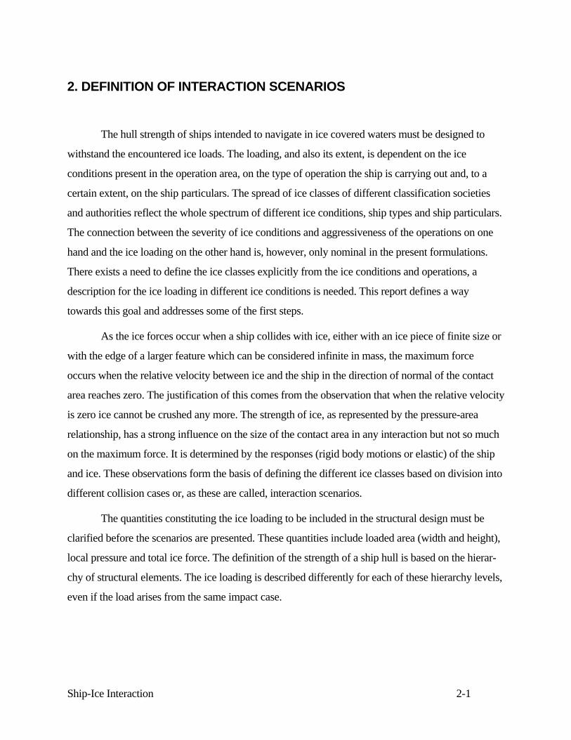
The hull strength of ships intended to navigate in ice covered waters must be designed to
withstand the encountered ice loads. The loading, and also its extent, is dependent on the ice
conditions present in the operation area, on the type of operation the ship is carrying out and, to a
certain extent, on the ship particulars. The spread of ice classes of different classification societies
and authorities reflect the whole spectrum of different ice conditions, ship types and ship particulars.
The connection between the severity of ice conditions and aggressiveness of the operations on one
hand and the ice loading on the other hand is, however, only nominal in the present formulations.
There exists a need to define the ice classes explicitly from the ice conditions and operations, a
description for the ice loading in different ice conditions is needed. This report defines a way
towards this goal and addresses some of the first steps.
As the ice forces occur when a ship collides with ice, either with an ice piece of finite size or
with the edge of a larger feature which can be considered infinite in mass, the maximum force
occurs when the relative velocity between ice and the ship in the direction of normal of the contact
area reaches zero. The justification of this comes from the observation that when the relative velocity
is zero ice cannot be crushed any more. The strength of ice, as represented by the pressure-area
relationship, has a strong influence on the size of the contact area in any interaction but not so much
on the maximum force. It is determined by the responses (rigid body motions or elastic) of the ship
and ice. These observations form the basis of defining the different ice classes based on division into
different collision cases or, as these are called, interaction scenarios.
The quantities constituting the ice loading to be included in the structural design must be
clarified before the scenarios are presented. These quantities include loaded area (width and height),
local pressure and total ice force. The definition of the strength of a ship hull is based on the hierar-
chy of structural elements. The ice loading is described differently for each of these hierarchy levels,
even if the load arises from the same impact case.
Ship-Ice Interaction 2-2
The shell plating is sensitive mainly to the local ice pressure distribution pice(x,y) and, to a
lesser degree, to the load height along the supporting transverse frames, hc. The strength of
transverse framing is defined by the horizontal line load intensity q(x)=PAV VP , where PAV is the
average pressure in the vertical direction. The coordinates x and y are attached to the shell plating so
that x is along the waterline and y along the shell tangent at the contact point normal to x. The larger
shell elements like stringers, web frames, bulkheads and decks are designed based on the total
contact force Fmax and the contact area, if this area is larger than the area from where these structures
draw their loading. The hull beam strength is solely sensitive to the total contact force Fmax and
naturally its point of application.
The ship-ice interaction scenarios depend on the ice environment considered. Also the hull
area considered has an influence on which scenarios are relevant. Here the scenarios are described
taking only the bow loads into account. In a Polar (Arctic and Antarctic) ice environment the ship-
ice interaction scenarios may be divided into six basic cases:
1. Collision head-on with multi-year ice
2. Glancing collision with multi-year ice
3. Navigation in heavily ridged first-year ice
4. Navigation in level ice
5. Ship proceeding in an old navigation channel
6. Ship caught in compressing ice.
Each of these cases is different from the point of view of ship-ice interaction. The two first
scenarios are tackled in this report. The third scenario has been tackled based on statistical analysis
of full scale ice load measurements in the Baltic. The concept of equivalent ice thickness has been
presented [4] to calculate these loads. In this method the loading scenario is not explicitly defined
because it is based on measured statistics of ice loads. The use of the equivalent ice thickness
concept in the Arctic ice conditions means an extrapolation to larger ice thickness, from those used
to develop the concept.
Ship-Ice Interaction 2-3
The loads from level ice have been analyzed in detail and thus the physical background is
well known [5]. The statistics related to loads in level ice are, however, less well known. The origin
of statistical variation in level ice lies in the variation of the breaking pattern of the vessel.
The ice loads in the case of a ship proceeding in an old navigation channel arise from the
ship hitting the channel edges or large ice pieces grown from the brash ice in the channel. These
loads resemble those in glancing impact but also differences exist, the main one being the resistance
to motion from brash ice which surrounds the ice pieces. Not much research has been done to clarify
this case.
When a ship is stuck in compressing ice, large loads are applied to the parallel midbody.
Most of the ice damage occurring in the Baltic comes from this kind of situations. The analysis of
loads in the compressive situation is very similar to the analysis of loads on offshore structures. One
main difference exists, however. It is that for ships it is necessary to analyze the origin of the
compressive situation i.e. the way ships are getting stuck in converging ice fields. This analysis
reveals immediately that the operational mode of the vessel is important. The mechanics of the
situation is very different if the vessel is assisted by an icebreaker or not.
All the six interaction scenarios are dependent on the operational profile of the vessel. It
makes a difference if the vessel is supposed to navigate unassisted in ice or if the vessel is supposed
to ram all the ice to be encountered in the operation area. These considerations are very important in
determining the design loads of a vessel but are not the topic of this report. Here the mechanics of
the two first cases is investigated. It is shown that the first two cases are explicitly solvable. These
solutions are described in this report.
Ship-Ice Interaction 3-1
3. ANALYSIS OF HEAD-ON COLLISION WITH MULTI-YEAR ICE
3.1 Definition of the problem
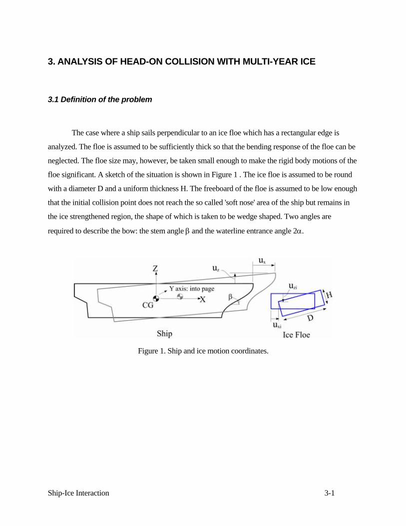
The case where a ship sails perpendicular to an ice floe which has a rectangular edge is
analyzed. The floe is assumed to be sufficiently thick so that the bending response of the floe can be
neglected. The floe size may, however, be taken small enough to make the rigid body motions of the
floe significant. A sketch of the situation is shown in Figure 1 . The ice floe is assumed to be round
with a diameter D and a uniform thickness H. The freeboard of the floe is assumed to be low enough
that the initial collision point does not reach the so called 'soft nose' area of the ship but remains in
the ice strengthened region, the shape of which is taken to be wedge shaped. Two angles are
required to describe the bow: the stem angle β and the waterline entrance angle 2α.
Figure 1. Ship and ice motion coordinates.
Ship-Ice Interaction 3-2
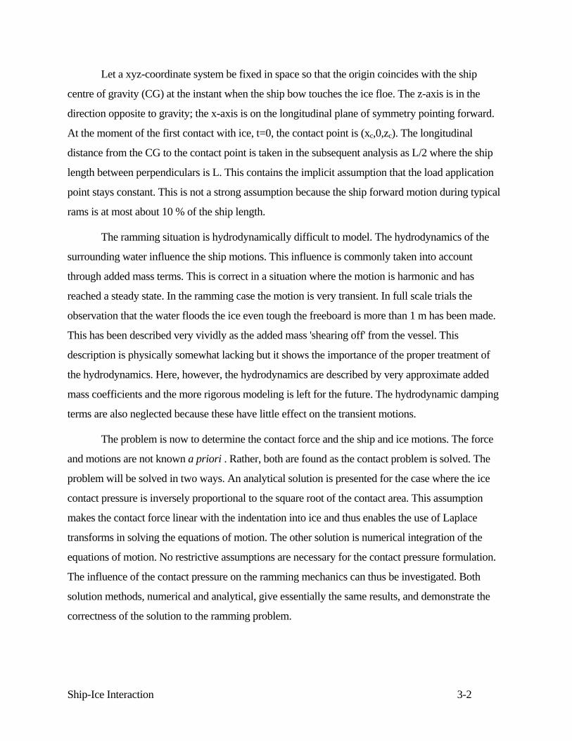
Let a xyz-coordinate system be fixed in space so that the origin coincides with the ship
centre of gravity (CG) at the instant when the ship bow touches the ice floe. The z-axis is in the
direction opposite to gravity; the x-axis is on the longitudinal plane of symmetry pointing forward.
At the moment of the first contact with ice, t=0, the contact point is (xc,0,zc). The longitudinal
distance from the CG to the contact point is taken in the subsequent analysis as L/2 where the ship
length between perpendiculars is L. This contains the implicit assumption that the load application
point stays constant. This is not a strong assumption because the ship forward motion during typical
rams is at most about 10 % of the ship length.
The ramming situation is hydrodynamically difficult to model. The hydrodynamics of the
surrounding water influence the ship motions. This influence is commonly taken into account
through added mass terms. This is correct in a situation where the motion is harmonic and has
reached a steady state. In the ramming case the motion is very transient. In full scale trials the
observation that the water floods the ice even tough the freeboard is more than 1 m has been made.
This has been described very vividly as the added mass 'shearing off' from the vessel. This
description is physically somewhat lacking but it shows the importance of the proper treatment of
the hydrodynamics. Here, however, the hydrodynamics are described by very approximate added
mass coefficients and the more rigorous modeling is left for the future. The hydrodynamic damping
terms are also neglected because these have little effect on the transient motions.
The problem is now to determine the contact force and the ship and ice motions. The force
and motions are not known a priori . Rather, both are found as the contact problem is solved. The
problem will be solved in two ways. An analytical solution is presented for the case where the ice
contact pressure is inversely proportional to the square root of the contact area. This assumption
makes the contact force linear with the indentation into ice and thus enables the use of Laplace
transforms in solving the equations of motion. The other solution is numerical integration of the
equations of motion. No restrictive assumptions are necessary for the contact pressure formulation.
The influence of the contact pressure on the ramming mechanics can thus be investigated. Both
solution methods, numerical and analytical, give essentially the same results, and demonstrate the
correctness of the solution to the ramming problem.
Ship-Ice Interaction 3-3
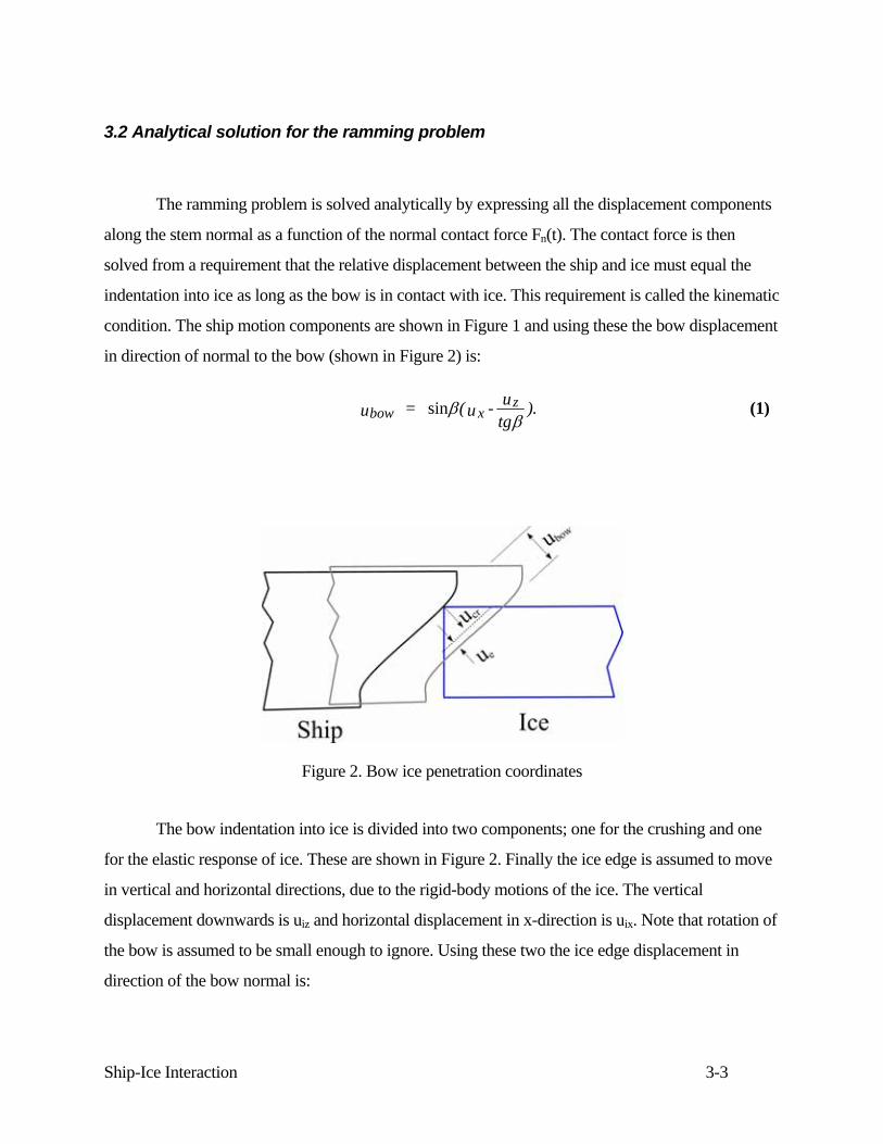
3.2 Analytical solution for the ramming problem
The ramming problem is solved analytically by expressing all the displacement components
along the stem normal as a function of the normal contact force Fn(t). The contact force is then
solved from a requirement that the relative displacement between the ship and ice must equal the
indentation into ice as long as the bow is in contact with ice. This requirement is called the kinematic
condition. The ship motion components are shown in Figure 1 and using these the bow displacement
in direction of normal to the bow (shown in Figure 2) is:
bow xzu = (u - u
tg).sinβ
β (1)
Figure 2. Bow ice penetration coordinates
The bow indentation into ice is divided into two components; one for the crushing and one
for the elastic response of ice. These are shown in Figure 2. Finally the ice edge is assumed to move
in vertical and horizontal directions, due to the rigid-body motions of the ice. The vertical
displacement downwards is uiz and horizontal displacement in x-direction is uix. Note that rotation of
the bow is assumed to be small enough to ignore. Using these two the ice edge displacement in
direction of the bow normal is:
Ship-Ice Interaction 3-4
iu = ixu + izu .sin cosβ β⋅ ⋅ (2)
The kinematic condition is now:
Indentation into ice = Bow displacement - Ice displacement
which can be expanded using the displacement components as:
cr e xz
ixizu + u = (u -
utg
- u -u
tg).sinβ
β β (3)
The problem is now shifted in expressing the displacement components as a function of the
bow force, inserting these into eq. (3) and taking the Laplace transform. After this the bow force may
be solved and the final problem is to find the inverse Laplace Transform of the expression. For
future reference the Laplace transform F(s) of a function f(t) is given by:
F s = e f t dtst( ) ( )−∞
∫0
(4)
where f(t) must fulfill some conditions usually met in a physical problem.
The solution for the displacement components amounts to constructing the equations of
motion for the ship and ice and solving them using the Duhamel integral. This is done in the
following sections.
Ship-Ice Interaction 3-5
3.2.1 The displacement into ice
The elastic displacement into ice can be treated as static because the time rate of change of
the bow force is slow and the related frequency components are very small compared to the elastic
natural frequencies of ice deformation. The damping due to radiation of stress waves is ignored as
well. Further, the visco-elastic deformation of ice is ignored as the ramming incidents last only some
seconds making the visco-elastic deformation negligible. Further the wedge shaped bow is assumed
to be rigid so that one coordinate is needed to describe indentation into ice. Based on these
assumptions the elastic displacement of ice normal to the bow is:
en
iceu (t) = F (t)
k (5)
The spring constant kice must be determined numerically for each bow geometry. Its
magnitude, within realistic bounds, does not have a strong influence on the resulting bow force. An
estimate of kice may be obtained from the analogy with the Boussinesq solution for the deflection of
an elastic half space. The average deflection of the loaded area, uav, is, if the load is a circular
uniform pressure PAV, of the form (see e.g. [6]):
avu = CPAV A
ERC
FER
⋅= (6)
where R is radius of the loaded area A and E is the Young's modulus. C is a constant being about
0.5. The case of ship bow indenting the ice edge requires a numerical solution for the spring
constant. A rough estimate is given in [7] where kice≈20 GN/m.
The crushing penetration into ice is obtained by considering the pressure on the contact area
to be composed of the two sides, port and starboard sides of the bow. As a prerequisite, the contact
area of one side is evaluated as a function of bow angles and the penetration into ice:
sidecr2 2 2
2A = u2
tg +.
α ββ β
sinsin cos
(7)
Ship-Ice Interaction 3-6
Also the unit normal to each side of the bow imprint is needed. These are, expressed using the unit
vectors i, j and k along the coordinate axes x, y and z, the following:
n = 1
tg +(tg i j - tg k).
2 21 2,sin
sin sin cosα β
α β β α β⋅ ± ⋅ ⋅ (8)
The contact force during the penetration into ice is commonly given as Fn=p(Aside) Aside where the
pressure is dependent on the contact area. The total bow force is now:
n side side 1 2
side side 2 2
F (t) = p( A ) A (n + n )
= p( A ) A2tg
tg +( i - k)α
α ββ β
sinsin cos
(9)
The analytical solution is made possible if the ice pressure is assumed to depend on the contact area
as follows:
p(A) = C A1-0.5 (10)
where the constant C1 is empirical, and the exponent of -0.5 is typical of observed values, see e.g.[8].
The magnitude of the bow force is in this case is:
n 12 2
cr
1 1 cr
F (t) = C2tg
tg +u (t)
= C G ( , )u (t),
α
β β α β
α β
sin cos sin (11)
where the definition of the constant G1(Ι,ϑ) is evident from the equation. The expressions of the
relationship between the bow force and the crushing and elastic displacements (eqs. (5) and (11)) are
straightforward to Laplace transform.
Ship-Ice Interaction 3-7
One comment about the description of the displacement in ice is perhaps needed here.
During a head-on ram the ice edge is first crushed and at the same time there is elastic displacement
in the ice. Ramming tests have shown that after the initial phase of ramming the crushing ceases and
the bow just slides up onto the ice edge. During this phase of ramming, the only ice displacement
quantity is the elastic component. Thus the kinematic condition (3) should be treated in phases. This,
however, complicates the solution much and here both the elastic and the crushing components are
taken to be active throughout the ram. This assumption entails actually that the crushing is taken to
be a two way spring.
3.2.2 Ship bow displacement
The longitudinal motion of the ship is considered independently from the other motion
components. The equation of motion in the longitudinal direction is:
x x xF (t) = M(1+ )u ,δ && (12)
where Λx is the added mass coefficient for surge motion, M displacement of the vessel and Fx
longitudinal component of the bow force. The components in x- and z-directions of the normal bow
force are, if the friction is taken into account (Τ is the coefficient of friction):
x n 2 n
z n 1 n
F (t) = - F (t)( + ) = - G F (t)
F (t) = F (t)( - ) = G F (t).
sin cos
cos sin
β μ β
β μ β
μ
μ
(13)
Integration of eq. (12) yields:
x x x0
t
10
2
xn 2 2u (t) - u (0) = u (0)t - d
GM(1+ ) F ( )d .
1
& ∫ ∫τδ
τ ττ
μ (14)
This equation can be Laplace transformed to give:
Ship-Ice Interaction 3-8
xx
22
xn 2u (s) =
u (0)s
+u 0)s
-G
M(1+ ) F (s)1s
.&( μ
δ (15)
The vertical bow motion is composed of two components; one due to the rigid body motions
of the vessel and the other due to the elastic deflection of the hull. These two cases are solved here
separately even if they could be treated simultaneously using the modal superposition technique. The
rigid body motions are composed of the heave and pitch motions. If the heave motion is denoted as z
and pitch angle as Π and the coupling between heave and pitch motions ignored as well as the
damping terms, the equations of motion for these are:
M(1+ )z + gA z = G F (t)
I + g A = G x F (t),
z wp 1 n
2 1 c n
δ ρ
θ ρ θ
μ
θ μ
&&
&&
(16)
where Ψ is the density of water, g acceleration of gravity, Awp water plane area and Λz is the heave
added mass coefficient. The other quantities are defined as:
θ θδI = M(1+ ) R
A = x B(x)dx
z2
2L
2 ,∫ (17)
where B(x) is the ship breadth and RΠ is the radius of gyration for the pitch motion. The assumption
that heave and pitch motions are uncoupled means a strong fore-and-aft symmetry requirement.
Explicitly it means that the ship centre of gravity is also the centre of gravity for the added mass and
that the centre of the water plane area is above the centre of mass i.e. that:
L
zL
x m (x)dx = x B(x)dx = 0.∫ ∫ (18)
The heave and pitch equations of motion can be solved using the Duhamel integral as:
Ship-Ice Interaction 3-9
z = 1(1+ )M
G F ( ) (t - )d
= 1I
G x F ( ) (t - )d
z z 0
t
1 n z
0
t
1 c n
ω δτ ω τ τ
θω
τ ω τ τ
μ
θ θμ θ
∫
∫
sin
sin
(19)
where the heave and pitch frequencies are:
zwp
z
2 = gA
(1+ )M ; =
gAI
ωρ
δω
ρθ
θ (20)
The Laplace transforms of eqs. (19) are:
z(s) = G
(1+ )MF (s)
s +
(s) = x G
IF (s)
s +
1
z
n2
z2
c 1 n2 2
μ
μ
θ θ
δ ω
θω
(21)
The elastic deflection of the hull beam under the vertical point load at the bow may be solved
using modal superposition technique. The vertical orthonormalized bending modes are denoted by
wi(x'), and the natural frequencies ωi, i=1,.... The coordinate x' coincides with the x-axis but its origin
is at the aft perpendicular. This is done because the future equations are shorter this way. If the mode
value at the location of the force (assumed to be constant) is denoted as wi(L)=wic then the bow
vertical displacement due to elastic deformation is:
bi=1
Nic iz (t) = w (t)Σ η (22)
where N is the number of modes included into the calculation and Οi(t) are the generalized
coordinates. These can be solved from the Duhamel integral:

Ship-Ice Interaction 3-10
ii 0
t
(t) = 1
iN ( ) i (t - )dηω
τ ω τ τ∫ sin (23)
once the initial conditions are for displacements and speeds are set to zero. The generalized force is:
i ic 1 nN (t) = w G F (t).μ (24)
Now the vertical bow displacement may be expressed as:
bi=1
N
ic
i 0
t
z (t) = w iN ( ) i (t - )d1 Σω
τ ω τ τ∫ sin (25)
and its Laplace transform as:
bi=1
N ic2
1 n2
i2z (s) =
w G F (s)
s +Σ μ
ω (26)
The values for the natural modes and frequencies could be solved case by case for any ship.
This does not, however, provide the generality to the solution what is required. In order to examine
the parameter dependencies and to derive a general solution for the ramming problem the hull beam
is assumed to be a uniform beam, the moment of inertia being the main frame moment of inertia I.
The natural frequencies for this beam are:
i iz
3 = CEI
M(1+ ) Lω
δ (27)
where the constants are C1=22.38 and C2=61.69 for the first two modes [9], E is the Young's
modulus. The mass-normalized natural modes are:
iz
i i
i ii i i iw (x ) =
1M(1+ )
L - LL - L
( x + x ) - x - x′ ′ ′ ′ ′⎡
⎣⎢
⎤
⎦⎥δ
β ββ β
β β β βcos coshsin sinh
sin sinh cos cosh (28)
where the constants are:
i4 i
2z =
M(1+ )EIL
β ω δ (29)
Ship-Ice Interaction 3-11
The final bow vertical displacement is:
z c bu (t) = z(t)+ x (t)+ z (t)θ (30)
which can be directly Laplace transformed and the transforms of the components inserted.
3.2.3 Ice displacement
The rigid body displacement of the ice edge is divided into two components: vertical and
horizontal. The equation of motion for the horizontal surge motion is (the x-coordinate and uix
coincide):
i ix ix x n 2m (1+ )u = F = F (t)Gδ μ&& (31)
where mi is the ice mass. This equation can be solved in a manner similar to the ship surge motion.
The solution for the vertical displacement uiz requires the solution of the heave and pitch
equations of motion which are:
z z
2 x z
m z + gAz = F (t)
I + g A = - F (t) H2
+ F (t) D2
&&
&&
ρ
θ ρ θθ
(32)
Once the floe is assumed to be round then the constants in the equations of motion can be
determined as (assuming D H):
θ θδπ ρ δ
π ρ
π π
I = (1+ )64
H D , m = (1+ )4 HD
A = 64 D , A =
4 D .
i i4
i iz i2
24 2
(33)
If it is assumed that the added mass coefficients for pitch and heave, ΛiΠ and Λiz, are equal, then the
equation of the ice edge vertical displacement downwards is:
Ship-Ice Interaction 3-12
π ρ δπ ρ
4HD (1+ )u +
4gD u = 5 F + 4 H
DF .i
2iz iz i
2iz z x&& (34)
The ice force is in the subsequent derivation denoted as:
5 F + 4 HD
F = (5G + 4 HD
G ) F (t) = G F (t).z x 1 2 n i nμ μ (35)
The solution of the vertical displacement is analogous to the similar ship equation.
3.2.4 Solution of the ramming equations
The solution of the Laplace transformed ramming force is obtained now by inserting the
displacement components into the Laplace transformed kinematic condition (3). The following basic
equation is obtained (the initial conditions are all zero):
n
eq 22
x2 n
2
ix i2 2
n
1
z
n2
z2
c2
1 n2 2
j=1
N
jc2
1n
2j2
i
i2
n2
i2
F (s)k
= vs
- G
(1+ ) MsF (s) -
G
(1+ )4 HD s
F (s)
- G
(1+ )MF (s)
s -
x GI
F (s)
s +
- w G F (s)
s + - G
4 HD
F (s)
s +
sin sin sin
cos cos
cos cos
β β
δ
β
δπ ρ
β
δ ω
β
ω
βω
βπ ρ ω
μ μ
μ μ
θ θ
μ∑
(36)
from where the bow normal force can be solved by the inverse Laplace Transform. Some notational
simplifications are introduced; the frequency related to ice floe heaving is denoted as:
i2 i
iz iz =
gAm
= g(1+ )H
.ωρ
δ (37)
Ship-Ice Interaction 3-13
Further, the indentation stiffness of ice is described by one constant keq which is composed of the
elastic and crushing displacements as:
1k
= 1C G
+ 1keq 1 1 ice
(38)
The Laplace transformed solution for the bow force is now:
n eqF (s) = k v P(s)Q(s)
sin β (39)
where the polynomial P(s) is:
P(s) = ( s + )( s + )( s + ) ( s + )2z2 2 2 2
i2
j=1
N2
j2ω ω ω ωθ ∏ (40)
The form of polynomial Q(s) is far more complicated and instead of writing it out, it is evaluated for
several special cases in the following.
Finally, the solution of the bow force is obtained by inverting the Laplace transform in eq.
(39). The inversion is made based on a theorem for Laplace transforms, valid for polynomials. It is
based on the zero points si of the denominator Q(s). The form of eq. (39) is such that the variable in
the denominator is actually s2 and thus the roots always appear pair-wise, one negative and one
positive. The inverse is now (see e.g. [9]):
n eqi
i
is tF (t) = k v P( s )
Q ( s ) e .isin β ∑ ′ (41)
The roots si are complex and thus this equation can be modified slightly. The complexity of
all roots follows from the fact that all constants in Q(s) are positive so that any roots s2 must be
negative. This is done because the derivative Q'(s) can be expressed as Q'(s)=sR(s) where the
polynomial R(s) is two degrees lower than Q(s). This is because the variable appears everywhere as
s2. Now the final solution can be written as:
n eqi
i
i
i
iF (t) = k v 2 P( s )
R( s )s t
ssin sinβ ∑ (42)
Ship-Ice Interaction 3-14
where the sum is over the root pairs si2 and the notation s = s ii i
2 is used. The question is now
shifted to solving the roots of the denominator Q(s). The degree of Q(s) is 8+2N. The solution is
obtained explicitly if the degree is at most 8. Thus two special cases are considered next. The case
where the ice size is infinite, the ice displacement may be ignored and the degree is 6+2N. If the hull
bending is described only by the first bending mode, then the degree of the denominator becomes 8
and is thus explicitly solvable. The other case considered is that where the hull bending displacement
is ignored but ice is allowed to be of finite size.
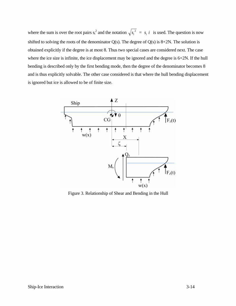
Figure 3. Relationship of Shear and Bending in the Hull
Ship-Ice Interaction 3-15
Before the solution of these special cases is considered, the ship hull response is also
described. The hull response is composed of two quantities: shear force and bending moment. These
may, in principle, be solved by a modal superposition technique once the bow force is known. As
this requires the inclusion of many natural modes here a different approach is taken. The forces
which act on the vessel are caused by inertial forces, ice forces or hydrostatic forces. A balance of
these forces, see Figure 3, yields the shear force and bending moment. If the ship sectional mass is
denoted as m(x)=M/L, the average breadth as B(x)=A/L (A is the waterplane area) and further, if the
centre of ship gravity is assumed to be amidships i.e. xc=L/2 then the shear force at the location x=ς
is:
Q(t, ) = m( )[(1+ )z + z +(1+ ) ]d + z gB( )d + g B( )d - F (t)c c cx
z b
x x
zξ η δ δ ηθ η ρ η η θ ρ η η ηξ
θξ ξ
∫ ∫ ∫&& && &&
(43)
and the bending moment at the same location is:
M(t, ) = ( - )m( )[(1+ )z + z + (1+ ) ]d
+ ( - ) g(B( )z + B( ) )d - ( x - ) F (t).
c
c
x
z b
x
c z
ξ η ξ η δ δ ηθ η
η ξ ρ η η η θ η ξ
ξθ
ξ
∫
∫
&& && &&
(44)
where only the first bending mode has been taken into account. These equations may be Laplace
transformed and then the solutions of the rigid body motions and the hull bending displacement zb
inserted. This yields equations which include the bow force. If the bow force given in eq. (39) is
used, then the final form of these equations is reached as:
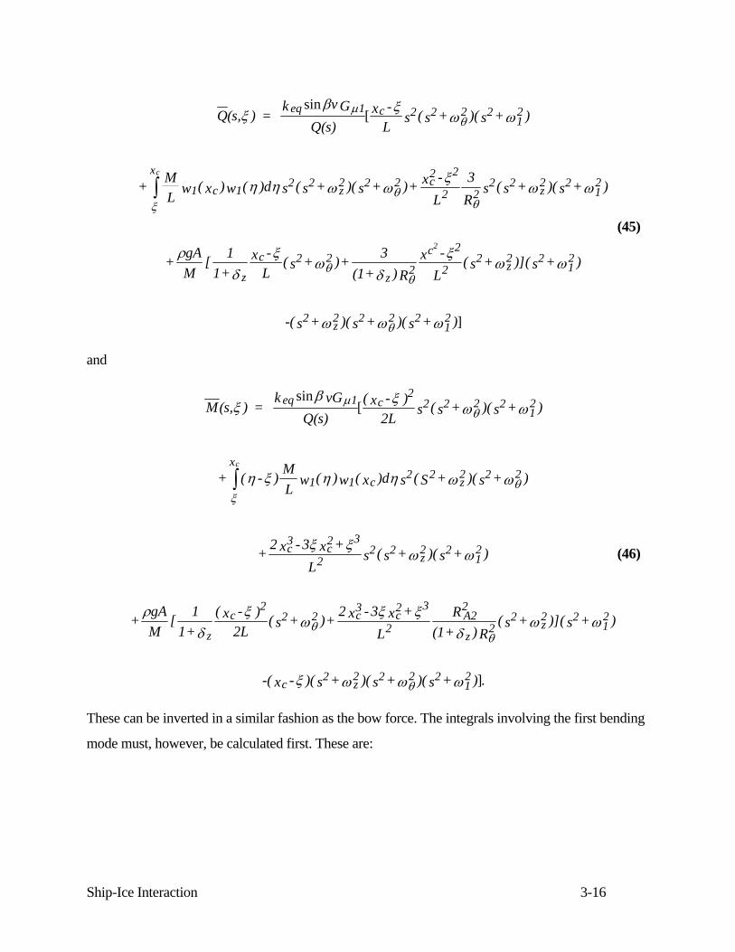
Ship-Ice Interaction 3-16
Q(s, ) = k v G
Q(s)x -
Ls ( s + )( s + )
+ ML w ( x )w ( )d s ( s + )( s + )+ x -
L3
Rs ( s + )( s + )
+ gAM
[ 11+
x -L
( s + )+ 3(1+ ) R
x -L
( s + )]( s + )
-( s + )( s + )( s
eq 1 c 2 2 2 212
x
1 c 12 2
z2 2 2 c
2 2
2 22 2
z2 2
12
z
c 2 2
z2
c 2
22
z2 2
12
2z2 2 2 2
c
2
ξβ ξ
ω ω
η η ω ωξ
ω ω
ρδ
ξω
δξ
ω ω
ω ω
μθ
ξθ
θ
θθ
θ
sin[
∫
+ )12ω ]
(45)
and
M(s, ) = k vG
Q(s)( x - )
2L s ( s + )( s + )
+ ( - ) ML w ( )w ( x )d s ( S + )( s + )
+ 2 x - 3 x +L
s ( s + )( s + )
+ gAM
[ 11+
( x - )2L
( s + )+ 2 x - 3 x +L
R(1+ ) R
( s + )](
eq 1 c2
2 2 2 212
x
1 1 c2 2
z2 2 2
c3
c2 3
22 2
z2 2
12
z
c2
2 2 c3
c2 3
2A22
z2
2z2 2
c
ξβ ξ
ω ω
η ξ η η ω ω
ξ ξω ω
ρδ
ξω
ξ ξδ
ω
μθ
ξθ
θθ
sin[
∫
s + )
-( x - )( s + )( s + )( s + ) .
12
c2
z2 2 2 2
12
ω
ξ ω ω ωθ ]
(46)
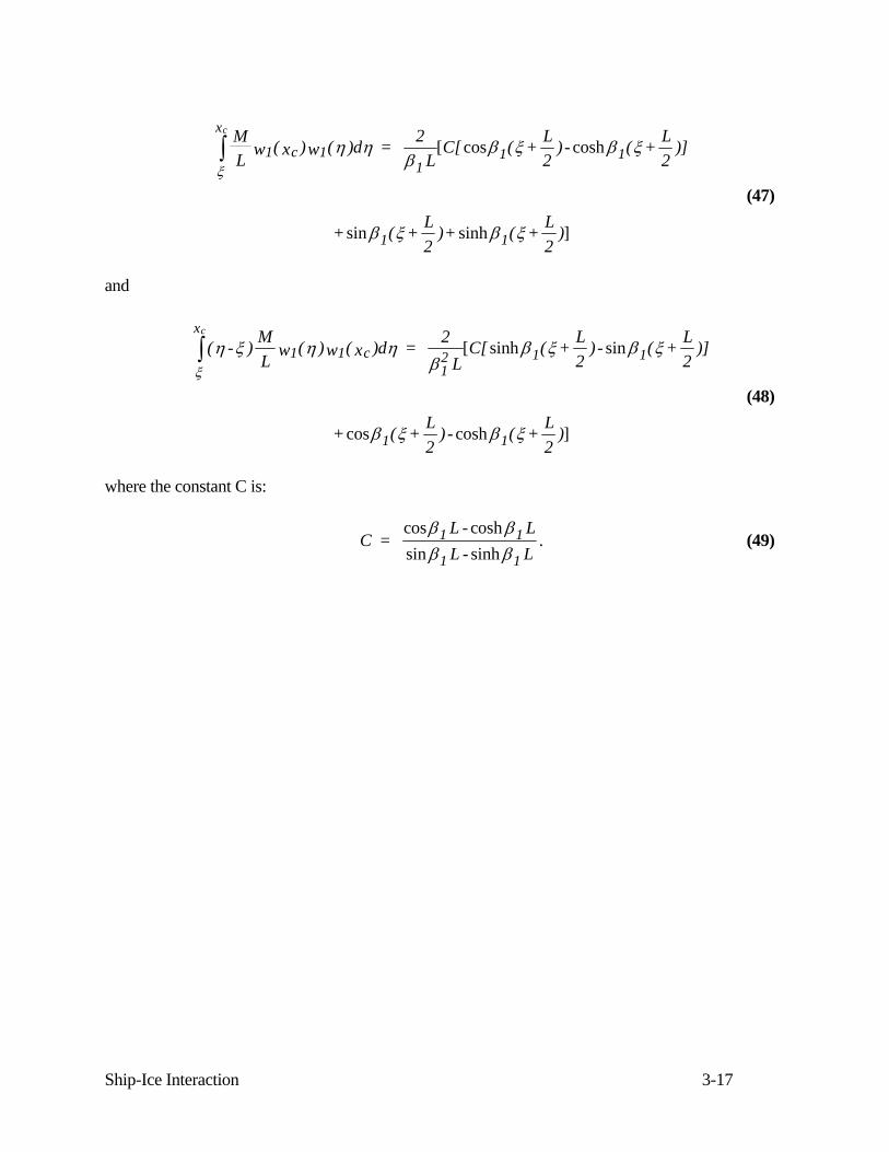
These can be inverted in a similar fashion as the bow force. The integrals involving the first bending
mode must, however, be calculated first. These are:
Ship-Ice Interaction 3-17
ξ
η ηβ
β ξ β ξ
β ξ β ξ
cx
1 c 11
1 1
1 1
ML w ( x )w ( )d = 2
LC[ ( + L
2)- ( + L
2)]
+ ( + L2
)+ ( + L2
)
∫ [
]
cos cosh
sin sinh
(47)
and
ξ
η ξ η ηβ
β ξ β ξ
β ξ β ξ
cx
1 1 c12 1 1
1 1
( - ) ML w ( )w ( x )d = 2
LC[ ( + L
2)- ( + L
2)]
+ ( + L2
)- ( + L2
)
∫ [
]
sinh sin
cos cosh
(48)
where the constant C is:
C = L - LL - L
.1 1
1 1
cos coshsin sinh
β ββ β
(49)

Ship-Ice Interaction 3-18
3.3 The ram on an ice feature of infinite mass
When the ship rams on an ice feature of very large mass, the ice rigid body motions may be
ignored. If further the ship hull bending is described only by the first bending mode, then the
denominator in eq. (39) becomes:
Q(s) = s + ( + + + C + C + C + C )s +
+ [ + + + C ( + + )+ C ( + )+ C ( + )+ C ( + )] s
( + C ( + + )+ C
8z2 2
12
x z b6
2z2 2
12
z2
12
x z2 2
12
z2
12
z2
12
b z2 2 4
z2 2
12
x2
z2 2
12
z2
12
z2
ω ω ω
ω ω ω ω ω ω ω ω ω ω ω ω ω ω ω
ω ω ω ω ω ω ω ω ω
θ θ
θ θ θ θ θ θ
θ θ θ θω ω ω ω ω ω ω ω ωθ θ θ12
z2
12
b2
z2 2
x z2 2
12+ C + C )s + C .
(50)
where the constants are:
x2 2
xz
2 1
z
2 1
z2 b
2 1
z
C = G
1+ , C =
G1+
C = 3 G(1+ ) R
, C = 4 G
1+
Ω Ω
Ω Ω
κ β
δ
κ β
δ
κ β
δ
κ β
δ
μ μ
θμ
θ
μ
sin cos
cos cos (51)
the dimensionless ice strength number is:
κρ
= kgAeq (52)
and the principal frequency is:
Ω = gAM
.ρ (53)
In determining the constant Cb, the value of the first bending mode at the end of the hull
beam w1(L/2)=2/√M has been taken into account. Once the frequencies ω are expressed with the aid
of Α and Ρ, the aim of the analysis becomes clearer. The frequencies are:

Ship-Ice Interaction 3-19
z2 2
z
2 2
z
A2 2
12 2
= 1
1+ , =
11+
(RR
)
=
ωδ
ωδ
ω λ
θθ
Ω Ω
Ω
(54)
where the second moment of the waterplane area has been estimated to be:
2 A22A = 1
3( R
L2
) A. (55)
and the non-dimensional hull stiffness λ is defined as:
λβ
ρ δ =
( L ) EIg(1+ ) AL
14
z3
For the first natural bending mode ϑ1L=1.506Ξ. The definition of RA2 is justified when it is
compared with the value of the second moment for a rectangular waterplane area, A2=☺ (L/2)2A.
Thus when RA2<1 the waterplane area coefficient is less than one.
All the terms in the polynomial, eq. (50), contain the principal frequency as a factor. Further, the
inspection of the constants in the polynomial (50) shows that all its zero points si2, i=1,...,4, must be
negative. Thus a non-dimensional frequency q may be defined as:
2 2 2s = - qΩ (56)
The eight roots of the polynomial (50) are thus:
2j-1,2j js = q i , j = 1,...,4± Ω (57)
Inserting these roots into the solution of the bow force yields the solution:
n eqj=1
4 j
j jjF (t) = k v 2 p(q i)
q r(q i)q tsin sinβ ∑ Ω
Ω (58)
where the polynomials p and r are defined as:
Ship-Ice Interaction 3-20
P( qi) = p(qi)
Q ( qi) = qi r(qi).
6
6
Ω Ω
Ω Ω Ω′
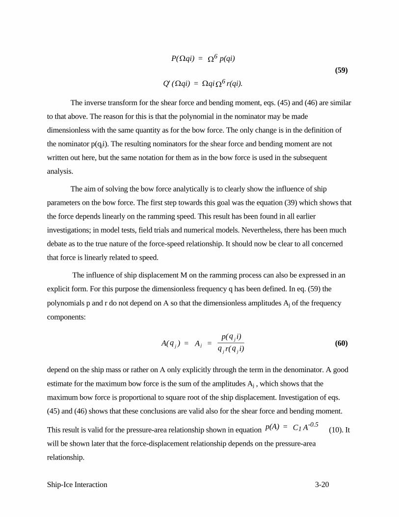
(59)
The inverse transform for the shear force and bending moment, eqs. (45) and (46) are similar
to that above. The reason for this is that the polynomial in the nominator may be made
dimensionless with the same quantity as for the bow force. The only change is in the definition of
the nominator p(qji). The resulting nominators for the shear force and bending moment are not
written out here, but the same notation for them as in the bow force is used in the subsequent
analysis.
The aim of solving the bow force analytically is to clearly show the influence of ship
parameters on the bow force. The first step towards this goal was the equation (39) which shows that
the force depends linearly on the ramming speed. This result has been found in all earlier
investigations; in model tests, field trials and numerical models. Nevertheless, there has been much
debate as to the true nature of the force-speed relationship. It should now be clear to all concerned
that force is linearly related to speed.
The influence of ship displacement M on the ramming process can also be expressed in an
explicit form. For this purpose the dimensionless frequency q has been defined. In eq. (59) the
polynomials p and r do not depend on Α so that the dimensionless amplitudes Aj of the frequency
components:
A(q ) = A = p(q i)
q r(q i)j jj
j j (60)
depend on the ship mass or rather on Α only explicitly through the term in the denominator. A good
estimate for the maximum bow force is the sum of the amplitudes Aj , which shows that the
maximum bow force is proportional to square root of the ship displacement. Investigation of eqs.
(45) and (46) shows that these conclusions are valid also for the shear force and bending moment.
This result is valid for the pressure-area relationship shown in equation p(A) = C A1-0.5
(10). It
will be shown later that the force-displacement relationship depends on the pressure-area
relationship.
Ship-Ice Interaction 3-21
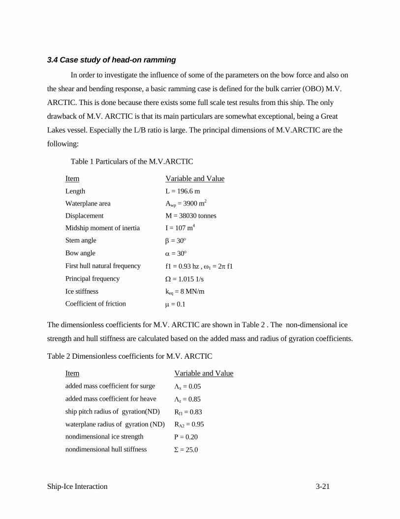
3.4 Case study of head-on ramming
In order to investigate the influence of some of the parameters on the bow force and also on
the shear and bending response, a basic ramming case is defined for the bulk carrier (OBO) M.V.
ARCTIC. This is done because there exists some full scale test results from this ship. The only
drawback of M.V. ARCTIC is that its main particulars are somewhat exceptional, being a Great
Lakes vessel. Especially the L/B ratio is large. The principal dimensions of M.V.ARCTIC are the
following:
Table 1 Particulars of the M.V.ARCTIC
Item Variable and Value Length L = 196.6 m
Waterplane area Awp = 3900 m2
Displacement M = 38030 tonnes
Midship moment of inertia I = 107 m4
Stem angle β = 30°
Bow angle α = 30°
First hull natural frequency f1 = 0.93 hz , ω1 = 2π f1
Principal frequency Ω = 1.015 1/s
Ice stiffness keq = 8 MN/m
Coefficient of friction μ = 0.1
The dimensionless coefficients for M.V. ARCTIC are shown in Table 2 . The non-dimensional ice
strength and hull stiffness are calculated based on the added mass and radius of gyration coefficients.
Table 2 Dimensionless coefficients for M.V. ARCTIC
Item Variable and Value added mass coefficient for surge Λx = 0.05
added mass coefficient for heave Λz = 0.85
ship pitch radius of gyration(ND) RΠ = 0.83
waterplane radius of gyration (ND) RA2 = 0.95
nondimensional ice strength Ρ = 0.20
nondimensional hull stiffness Σ = 25.0
Ship-Ice Interaction 3-22
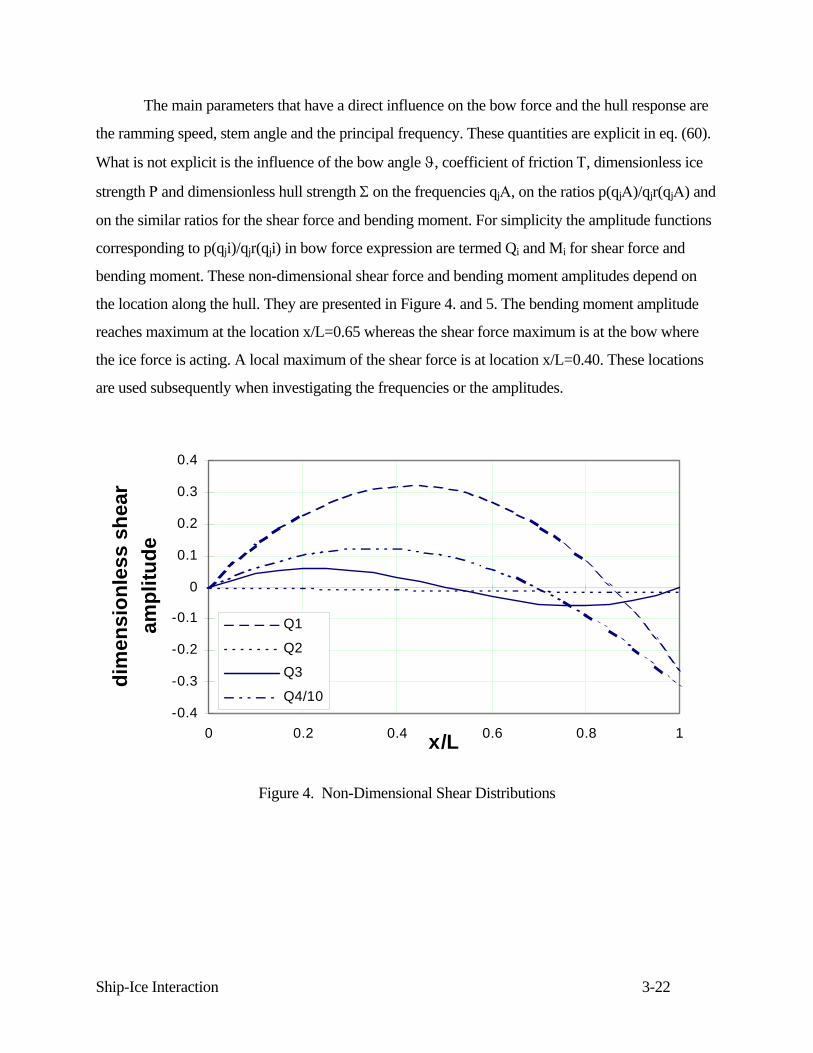
The main parameters that have a direct influence on the bow force and the hull response are
the ramming speed, stem angle and the principal frequency. These quantities are explicit in eq. (60).
What is not explicit is the influence of the bow angle ϑ, coefficient of friction Τ, dimensionless ice
strength Ρ and dimensionless hull strength Σ on the frequencies qjΑ, on the ratios p(qjΑ)/qjr(qjΑ) and
on the similar ratios for the shear force and bending moment. For simplicity the amplitude functions
corresponding to p(qji)/qjr(qji) in bow force expression are termed Qi and Mi for shear force and
bending moment. These non-dimensional shear force and bending moment amplitudes depend on
the location along the hull. They are presented in Figure 4. and 5. The bending moment amplitude
reaches maximum at the location x/L=0.65 whereas the shear force maximum is at the bow where
the ice force is acting. A local maximum of the shear force is at location x/L=0.40. These locations
are used subsequently when investigating the frequencies or the amplitudes.
-0.4
-0.3
-0.2
-0.1
0
0.1
0.2
0.3
0.4
0 0.2 0.4 0.6 0.8 1x/L
dim
ensi
onle
ss s
hear
am
plitu
de
Q1
Q2
Q3
Q4/10
Figure 4. Non-Dimensional Shear Distributions

Ship-Ice Interaction 3-23
-10
-9
-8
-7
-6
-5
-4
-3
-2
-1
00 0.2 0.4 0.6 0.8 1x/L
dim
ensi
onle
ss b
endi
ng
mom
ent a
mpl
itude
M1
M2
M3
M4/10
Figure 5. Non-Dimensional Bending Moment Distribution
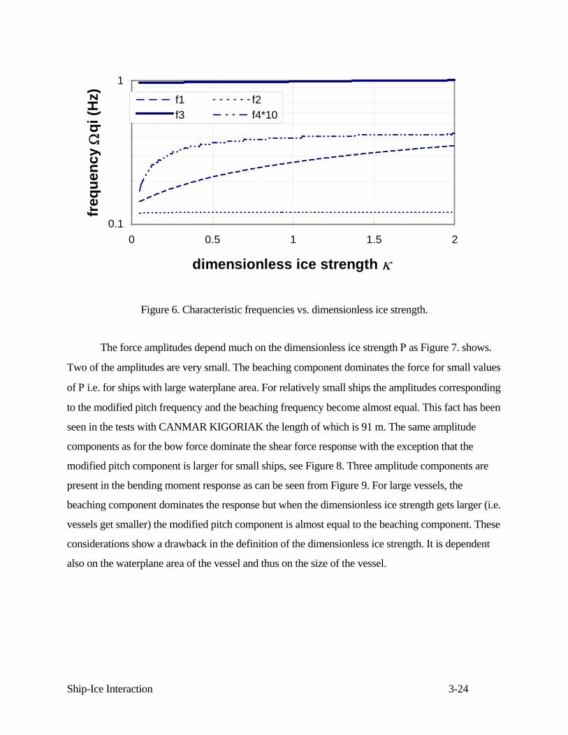
The roots of the equation Q(s)=0 may be solved explicitly as it is of 4th degree in s2. Using
the substitution (56) this equation may be made non-dimensional and then it may be denoted as
q(q)=0. The four roots qj depend only on dimensionless parameters (ϑ,Τ,Ρ,Σ,Λx,Λz,RΠ,RA2). The
M.V.ARCTIC is used as a basic case and thus it is easier to gain insight on the frequency
components if the qj's are multiplied with Α to make them dimensional. The frequencies are plotted
versus the dimensionless ice strength Ρ in Figure 6. Three of the frequencies are close to heave, pitch
and first elastic bending frequency. The fourth frequency may be termed the beaching frequency as
its period corresponds to the time for the ship to reach the maximum penetration (multiplied by
four). These frequencies do not change much with the ice strength or rather with the ship waterplane
area as the ice strength may be considered as constant.
Ship-Ice Interaction 3-24
0.1
1
0 0.5 1 1.5 2
dimensionless ice strength κ
freq
uenc
y Ω
qi (H
z) f1 f2f3 f4*10
Figure 6. Characteristic frequencies vs. dimensionless ice strength.
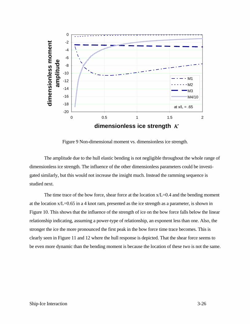
The force amplitudes depend much on the dimensionless ice strength Ρ as Figure 7. shows.
Two of the amplitudes are very small. The beaching component dominates the force for small values
of Ρ i.e. for ships with large waterplane area. For relatively small ships the amplitudes corresponding
to the modified pitch frequency and the beaching frequency become almost equal. This fact has been
seen in the tests with CANMAR KIGORIAK the length of which is 91 m. The same amplitude
components as for the bow force dominate the shear force response with the exception that the
modified pitch component is larger for small ships, see Figure 8. Three amplitude components are
present in the bending moment response as can be seen from Figure 9. For large vessels, the
beaching component dominates the response but when the dimensionless ice strength gets larger (i.e.
vessels get smaller) the modified pitch component is almost equal to the beaching component. These
considerations show a drawback in the definition of the dimensionless ice strength. It is dependent
also on the waterplane area of the vessel and thus on the size of the vessel.

Ship-Ice Interaction 3-25
0.001
0.01
0.1
1
10
0 0.5 1 1.5 2dimensionless ice strength κ
dim
ensi
onle
ss F
orce
A
mpl
itude
Ai
A1 A2A3 A4
Figure 7. Non-dimensional force vs. dimensionless ice strength.
-0.2
0
0.2
0.4
0.6
0.8
1
0 0.5 1 1.5 2dimensionless ice strength κ
dim
ensi
onle
ss s
hear
am
plitu
de
Q1Q2Q3Q4
at x/L = .4
Figure 8 Non-dimensional shear vs. dimensionless ice strength.
Ship-Ice Interaction 3-26
-20
-18
-16
-14
-12
-10
-8
-6
-4
-2
0
0 0.5 1 1.5 2
dimensionless ice strength κ
dim
ensi
onle
ss m
omen
t am
plitu
de
M1M2M3M4/10
at x/L = .65
Figure 9 Non-dimensional moment vs. dimensionless ice strength.
The amplitude due to the hull elastic bending is not negligible throughout the whole range of
dimensionless ice strength. The influence of the other dimensionless parameters could be investi-
gated similarly, but this would not increase the insight much. Instead the ramming sequence is
studied next.
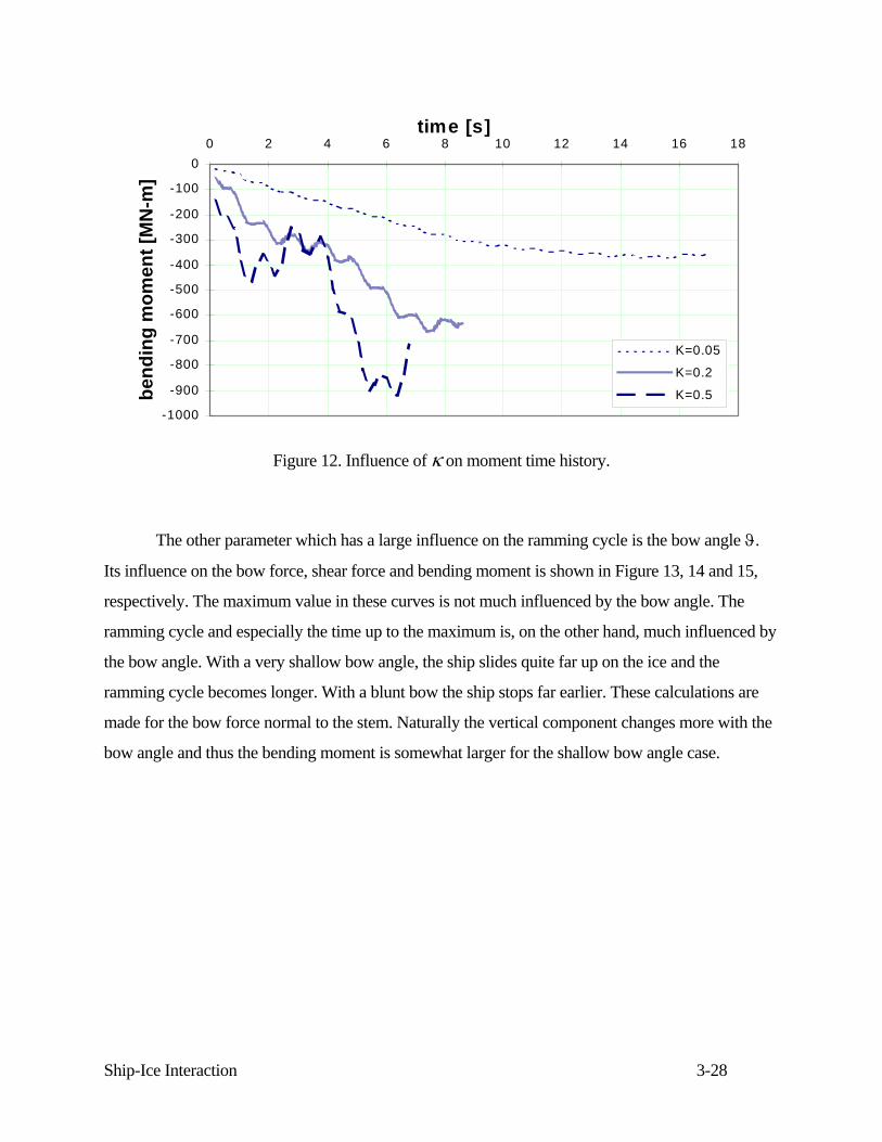
The time trace of the bow force, shear force at the location x/L=0.4 and the bending moment
at the location x/L=0.65 in a 4 knot ram, presented as the ice strength as a parameter, is shown in
Figure 10. This shows that the influence of the strength of ice on the bow force falls below the linear
relationship indicating, assuming a power-type of relationship, an exponent less than one. Also, the
stronger the ice the more pronounced the first peak in the bow force time trace becomes. This is
clearly seen in Figure 11 and 12 where the hull response is depicted. That the shear force seems to
be even more dynamic than the bending moment is because the location of these two is not the same.

Ship-Ice Interaction 3-27
0
5
10
15
20
25
30
35
0 2 4 6 8 10 12 14 16
time [s]
vert
ical
ice
forc
e [M
N]
Κ=0.05Κ=0.2Κ=0.5
Figure 10. Influence of κ on force time history.
0
2
4
6
8
10
12
14
16
0 2 4 6 8 10 12 14 16time [s]
shea
r [M
N]
Κ=0.05Κ=0.2Κ=0.5
Figure 11. Influence of κ on shear time history.
Ship-Ice Interaction 3-28
-1000
-900
-800
-700
-600
-500
-400
-300
-200
-100
00 2 4 6 8 10 12 14 16 18
time [s]be
ndin
g m
omen
t [M
N-m
]
K=0.05
K=0.2
K=0.5
Figure 12. Influence of κ on moment time history.
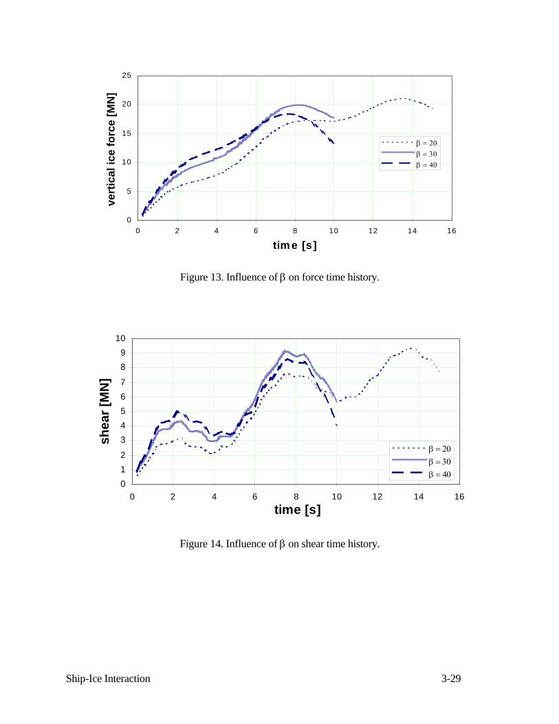
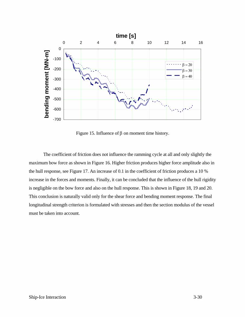
The other parameter which has a large influence on the ramming cycle is the bow angle ϑ.
Its influence on the bow force, shear force and bending moment is shown in Figure 13, 14 and 15,
respectively. The maximum value in these curves is not much influenced by the bow angle. The
ramming cycle and especially the time up to the maximum is, on the other hand, much influenced by
the bow angle. With a very shallow bow angle, the ship slides quite far up on the ice and the
ramming cycle becomes longer. With a blunt bow the ship stops far earlier. These calculations are
made for the bow force normal to the stem. Naturally the vertical component changes more with the
bow angle and thus the bending moment is somewhat larger for the shallow bow angle case.
Ship-Ice Interaction 3-29
0
5
10
15
20
25
0 2 4 6 8 10 12 14 16
tim e [s]
vert
ical
ice
forc
e [M
N]
β = 20β = 30β = 40
Figure 13. Influence of β on force time history.
012
34567
89
10
0 2 4 6 8 10 12 14 16time [s]
shea
r [M
N]
β = 20β = 30β = 40
Figure 14. Influence of β on shear time history.
Ship-Ice Interaction 3-30
-700
-600
-500
-400
-300
-200
-100
00 2 4 6 8 10 12 14 16
time [s]
bend
ing
mom
ent [
MN
-m]
β = 20β = 30β = 40
Figure 15. Influence of β on moment time history.
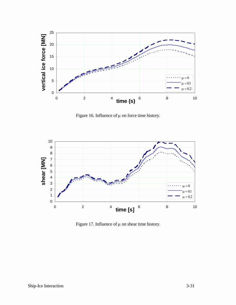
The coefficient of friction does not influence the ramming cycle at all and only slightly the
maximum bow force as shown in Figure 16. Higher friction produces higher force amplitude also in
the hull response, see Figure 17. An increase of 0.1 in the coefficient of friction produces a 10 %
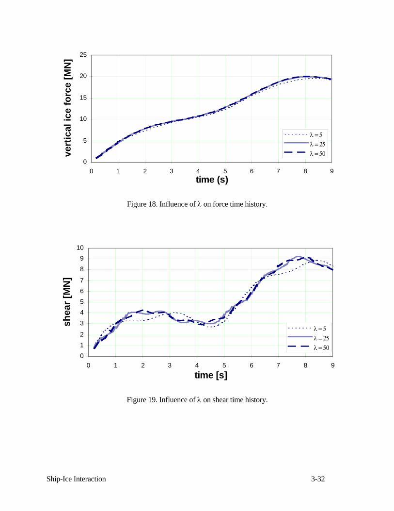
increase in the forces and moments. Finally, it can be concluded that the influence of the hull rigidity
is negligible on the bow force and also on the hull response. This is shown in Figure 18, 19 and 20.
This conclusion is naturally valid only for the shear force and bending moment response. The final
longitudinal strength criterion is formulated with stresses and then the section modulus of the vessel
must be taken into account.
Ship-Ice Interaction 3-31
0
5
10
15
20
25
0 2 4 6 8 10time (s)
vert
ical
ice
forc
e [M
N]
μ = 0μ = 0.1μ = 0.2
Figure 16. Influence of μ on force time history.
0123456789
10
0 2 4 6 8 10time [s]
shea
r [M
N]
μ = 0μ = 0.1μ = 0.2
Figure 17. Influence of μ on shear time history.
Ship-Ice Interaction 3-32
0
5
10
15
20
25
0 1 2 3 4 5 6 7 8 9time (s)
vert
ical
ice
forc
e [M
N]
λ = 5λ = 25λ = 50
Figure 18. Influence of λ on force time history.
012
34567
89
10
0 1 2 3 4 5 6 7 8 9time [s]
shea
r [M
N]
λ = 5λ = 25λ = 50
Figure 19. Influence of λ on shear time history.
Ship-Ice Interaction 3-33
-700
-600
-500
-400
-300
-200
-100
00 1 2 3 4 5 6 7 8 9
time [s]be
ndin
g m
omen
t [M
N-m
]
λ = 5λ = 25λ = 50
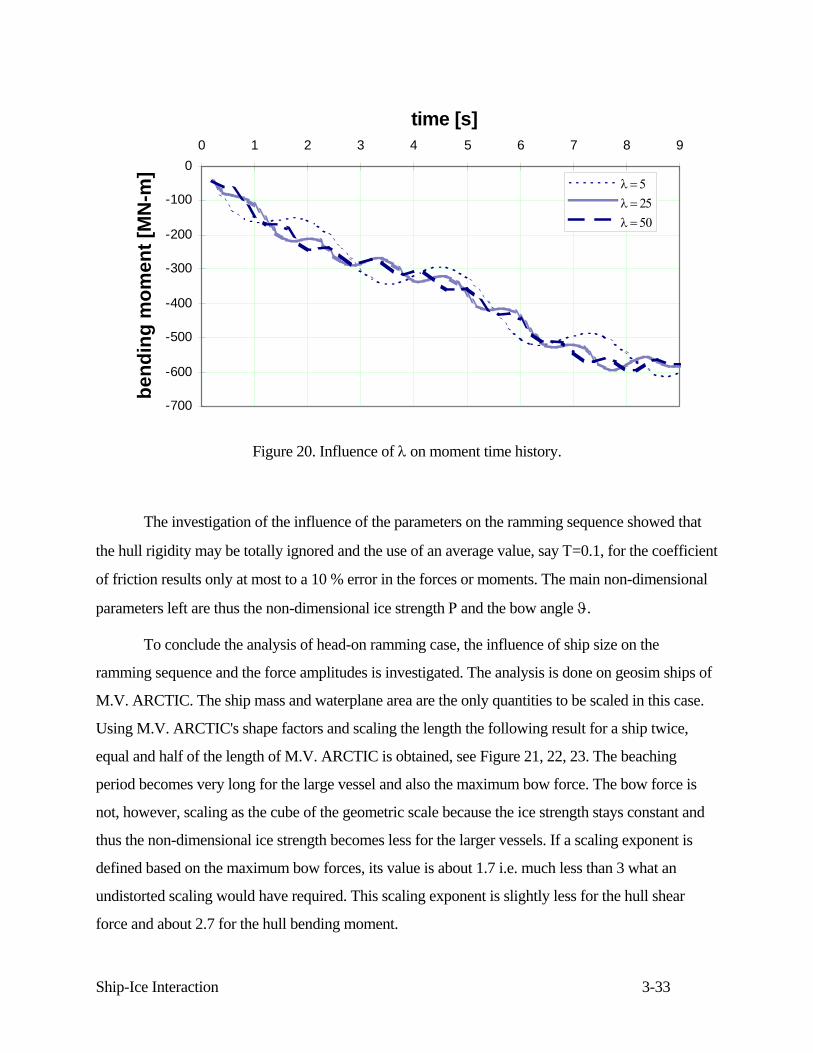
Figure 20. Influence of λ on moment time history.
The investigation of the influence of the parameters on the ramming sequence showed that
the hull rigidity may be totally ignored and the use of an average value, say Τ=0.1, for the coefficient
of friction results only at most to a 10 % error in the forces or moments. The main non-dimensional
parameters left are thus the non-dimensional ice strength Ρ and the bow angle ϑ.
To conclude the analysis of head-on ramming case, the influence of ship size on the
ramming sequence and the force amplitudes is investigated. The analysis is done on geosim ships of
M.V. ARCTIC. The ship mass and waterplane area are the only quantities to be scaled in this case.
Using M.V. ARCTIC's shape factors and scaling the length the following result for a ship twice,
equal and half of the length of M.V. ARCTIC is obtained, see Figure 21, 22, 23. The beaching
period becomes very long for the large vessel and also the maximum bow force. The bow force is
not, however, scaling as the cube of the geometric scale because the ice strength stays constant and
thus the non-dimensional ice strength becomes less for the larger vessels. If a scaling exponent is
defined based on the maximum bow forces, its value is about 1.7 i.e. much less than 3 what an
undistorted scaling would have required. This scaling exponent is slightly less for the hull shear
force and about 2.7 for the hull bending moment.
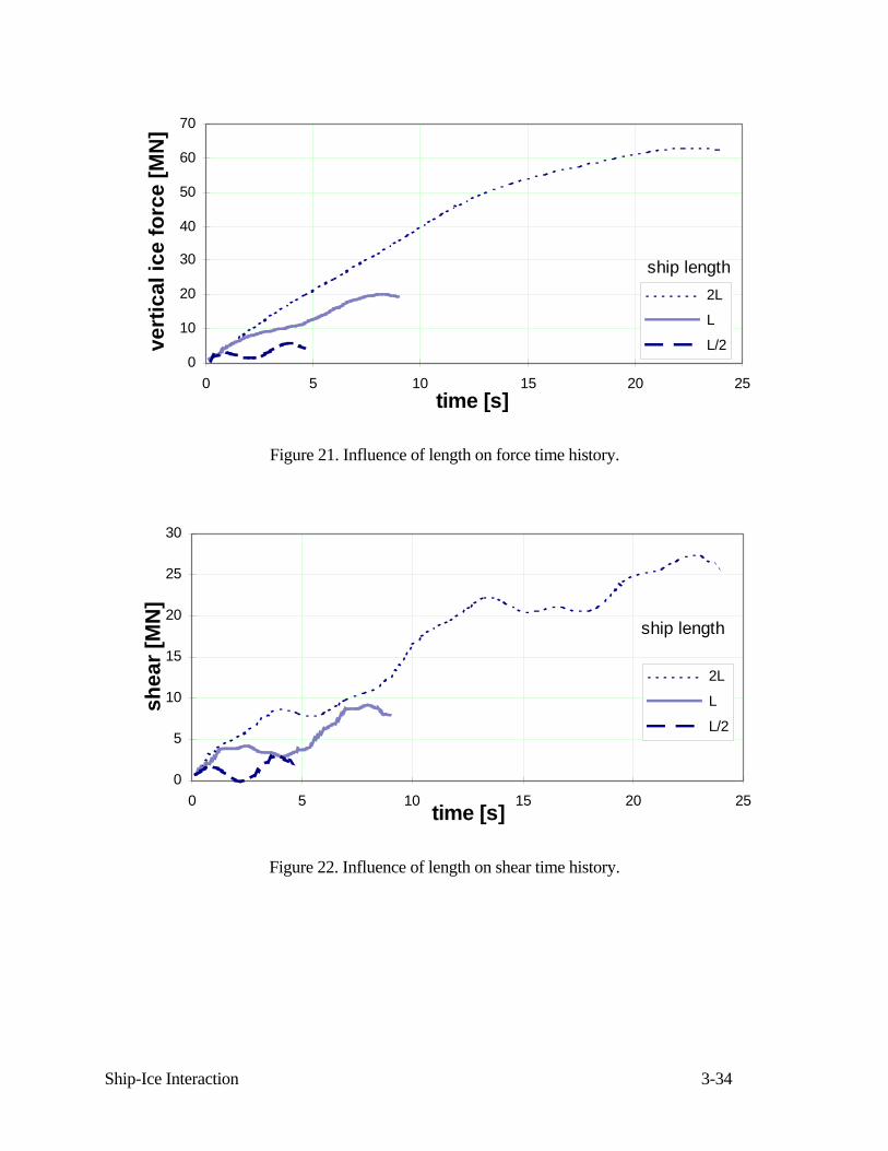
Ship-Ice Interaction 3-34
0
10
20
30
40
50
60
70
0 5 10 15 20 25time [s]
vert
ical
ice
forc
e [M
N]
2L
L
L/2
ship length
Figure 21. Influence of length on force time history.
0
5
10
15
20
25
30
0 5 10 15 20 25time [s]
shea
r [M
N]
2L
L
L/2
ship length
Figure 22. Influence of length on shear time history.
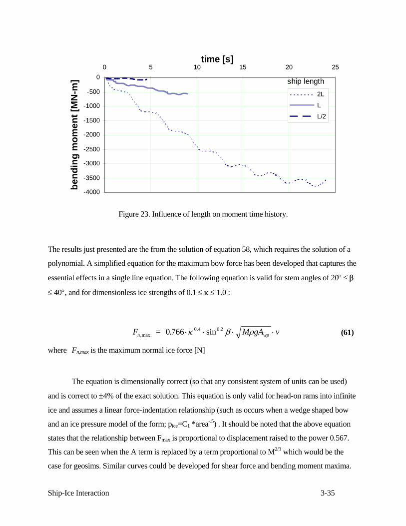
Ship-Ice Interaction 3-35
-4000
-3500
-3000
-2500
-2000
-1500
-1000
-500
00 5 10 15 20 25
time [s]be
ndin
g m
omen
t [M
N-m
]
2L
L
L/2
ship length
Figure 23. Influence of length on moment time history.
The results just presented are the from the solution of equation 58, which requires the solution of a
polynomial. A simplified equation for the maximum bow force has been developed that captures the
essential effects in a single line equation. The following equation is valid for stem angles of 20° ≤ β
≤ 40°, and for dimensionless ice strengths of 0.1 ≤ κ ≤ 1.0 :
F = M gA vn wp,max. .. sin0 766 0 4 0 2⋅ ⋅ ⋅ ⋅κ β ρ (61)
where Fn,max is the maximum normal ice force [N]
The equation is dimensionally correct (so that any consistent system of units can be used)
and is correct to ±4% of the exact solution. This equation is only valid for head-on rams into infinite
ice and assumes a linear force-indentation relationship (such as occurs when a wedge shaped bow
and an ice pressure model of the form; pice=C1 *area-.5) . It should be noted that the above equation
states that the relationship between Fmax is proportional to displacement raised to the power 0.567.
This can be seen when the A term is replaced by a term proportional to M2/3 which would be the
case for geosims. Similar curves could be developed for shear force and bending moment maxima.
Ship-Ice Interaction 3-36
3.5 Head-on ram on a finite ice floe
The ice features in nature are never infinite in mass or size, they just can be considered
infinite because the rigid body motions of ice may be ignored when the ice features are large
compared to the ship. What is the limiting ice mass after which the ice floe may be considered
infinite is thus of interest. The floe size is important also from another perspective. The design ice
force and design hull bending moment should take into account the size of the ice floe encountered.
Only if the ship is designed to withstand a collision with the largest floes, the design case may be
taken to be the collision with an infinite floe. This should not be the case for merchant vessels. The
design case for them could be a collision with certain size of a floe representing for example the
average of the biggest 1/3 of the floes present in a sea area. The case is made more difficult by the
observation that the larger floes may be detected from a longer distance and thus ships can avoid
these easier than the smaller floes which may be hidden in deformed first year ice. Anyway, the
design case should take into account the distribution of the floe sizes encountered.
Several assumptions must be made in tackling the finite floe case. Some of these were
mentioned when the equations of motion for the ice edge displacement, eqs. (31) and (34), were
developed. The main assumption is that the bending of the ice floe is ignored. This assumption is
justified because big floes usually are thick, the thickness of 5 m is typical in the Arctic, and the
smaller floes again tilt more readily and thus make the bending displacement small in comparison.
The other assumption is to treat the ice floe as round. Floes are usually not round but the irregularity
of floe shape makes the round shape as good as any other shape.
If the hull elastic bending component is ignored and the other displacement components are
inserted in the Laplace transformed kinematic condition (3) then the basic equation for the normal
bow force in ramming ice floe of finite size is obtained as eq. (39). Now the polynomials P(s) and
Q(s) differ from those in the previous case. They are now:
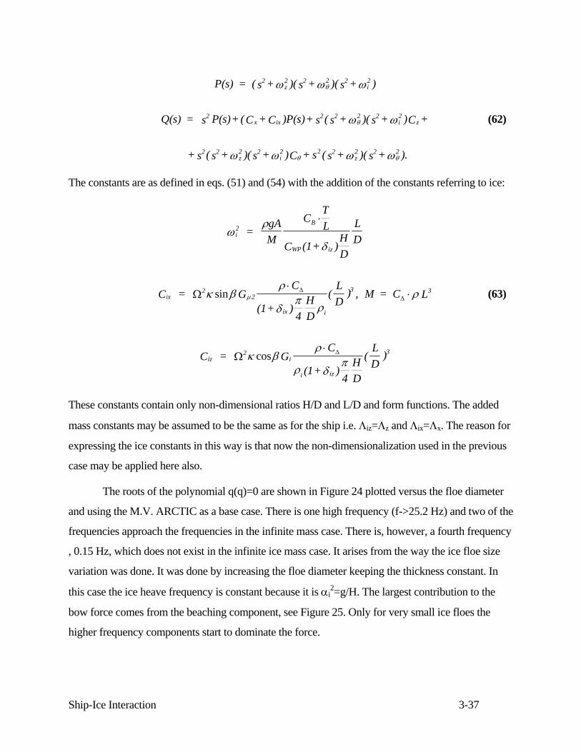
Ship-Ice Interaction 3-37
P(s) = ( s + )( s + )( s + )
Q(s) = s P(s)+ (C + C )P(s)+ s ( s + )( s + )C +
+ s ( s + )( s + )C + s ( s + )( s + ).
2z2 2 2 2
i2
2x ix
2 2 2 2i2
z
2 2z2 2
i2 2
z2 2 2
ω ω ω
ω ω
ω ω ω ω
θ
θ
θ θ2
(62)
The constants are as defined in eqs. (51) and (54) with the addition of the constants referring to ice:
i2
B
WP iz
ix2
2
ix i
3 3
iz2
i
i iz
3
= gAM
CTL
C (1+ )HD
LD
C = GC
(1+ )4
HD
(LD
) , M = C L
C = GC
(1+ )4
HD
(LD
)
ωρ
δ
κ βρ
δπ ρ
ρ
κ βρ
ρ δπ
μ
⋅
⋅⋅
⋅
Ω
Ω
ΔΔ
Δ
sin
cos
(63)
These constants contain only non-dimensional ratios H/D and L/D and form functions. The added
mass constants may be assumed to be the same as for the ship i.e. Λiz=Λz and Λix=Λx. The reason for
expressing the ice constants in this way is that now the non-dimensionalization used in the previous
case may be applied here also.
The roots of the polynomial q(q)=0 are shown in Figure 24 plotted versus the floe diameter
and using the M.V. ARCTIC as a base case. There is one high frequency (f->25.2 Hz) and two of the
frequencies approach the frequencies in the infinite mass case. There is, however, a fourth frequency
, 0.15 Hz, which does not exist in the infinite ice mass case. It arises from the way the ice floe size
variation was done. It was done by increasing the floe diameter keeping the thickness constant. In
this case the ice heave frequency is constant because it is αi2=g/H. The largest contribution to the
bow force comes from the beaching component, see Figure 25. Only for very small ice floes the
higher frequency components start to dominate the force.
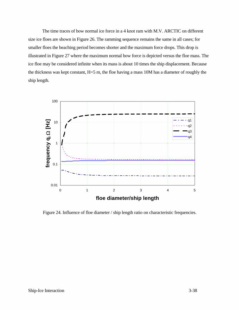
Ship-Ice Interaction 3-38
The time traces of bow normal ice force in a 4 knot ram with M.V. ARCTIC on different
size ice floes are shown in Figure 26. The ramming sequence remains the same in all cases; for
smaller floes the beaching period becomes shorter and the maximum force drops. This drop is
illustrated in Figure 27 where the maximum normal bow force is depicted versus the floe mass. The
ice floe may be considered infinite when its mass is about 10 times the ship displacement. Because
the thickness was kept constant, H=5 m, the floe having a mass 10M has a diameter of roughly the
ship length.
0.01
0.1
1
10
100
0 1 2 3 4 5
floe diameter/ship length
freq
uenc
y q i
Ω [H
z] q1q2q3q4
Figure 24. Influence of floe diameter / ship length ratio on characteristic frequencies.
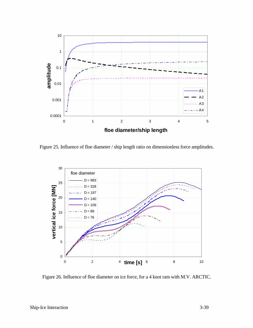
Ship-Ice Interaction 3-39
0.0001
0.001
0.01
0.1
1
10
0 1 2 3 4 5
floe diameter/ship length
ampl
itude
A1
A2
A3
A4
Figure 25. Influence of floe diameter / ship length ratio on dimensionless force amplitudes.
0
5
10
15
20
25
30
0 2 4 6 8 10time [s]
vert
ical
ice
forc
e [M
N]
D = 983
D = 328
D = 197
D = 140
D = 109
D = 89
D = 76
floe diameter
Figure 26. Influence of floe diameter on ice force, for a 4 knot ram with M.V. ARCTIC.

Ship-Ice Interaction 3-40
0
5
10
15
20
25
30
0 100 200 300 400 500 600
ice floe radius [m]
max
nor
mal
ice
forc
e [M
N]
for MV Arctic ram at 4 kts.h = 5m
Figure 27. Influence of floe edge radius on ice force.
Ship-Ice Interaction 3-41
3.6 Analysis of the Influence of Contact Pressure on Force
One of the main assumptions in deriving the analytical solution of the ramming equations
was that the crushing force is linear with the penetration into ice. This linearity results from the
assumption that the bow is wedge shaped and the ice pressure is inversely proportional to the square
root of the contact area. How much this assumption influences the solution for the bow force is
investigated by numerical solution of the ramming case. In the numerical solution the contact force
may take any form. However, before the numerical solution is considered, it may be of use to
investigate very roughly the influence of the exponent of the contact area on the maximum normal
force.
A more general form for the contact pressure is:
p(A) = C A1-C2 (64)
The case C2=0 corresponds to the constant pressure case, and C2=1 corresponds to the constant force
case (i.o.w. all contact areas give the same force, a rather strange situation). The normal bow force is
now obtained using equations. (7) and (9) as:
n 1 2 2
2 2
21-C cr
2(1-C )
cr2(1-C )
F = C2tg
tg +(
tg +2
) u
= a u
2 2
2
α
α β
α ββ βsin
sinsin cos
(65)
where a constant a has been defined for simplicity. The initial kinetic energy may be split in two
parts; one corresponding to the speed along the stem and the other to the speed normal to the stem.
Thus:
T = 12 M v =
12 M (v + v )x
2x t
2n2 (66)
where vn=sinϑ v and vt=cosϑ v. Now the assumption is made that the normal kinetic energy is
consumed totally in crushing the ice. Thus the crushing energy:
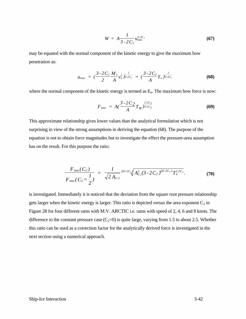
Ship-Ice Interaction 3-42
W = A1
3 - 2 Cu
2
3-2C2max (67)
may be equated with the normal component of the kinetic energy to give the maximum bow
penetration as:
maxu = (3 - 2C
2MA v ) = (
3 - 2CA T )2 x
n2
13-2C
2n
13-2C2 2 (68)
where the normal component of the kinetic energy is termed as En. The maximum bow force is now:
maxF = A(3 - 2 2C
A nT )2-2 2C3-2 2C (69)
This approximate relationship gives lower values than the analytical formulation which is not
surprising in view of the strong assumptions in deriving the equation (68). The purpose of the
equation is not to obtain force magnitudes but to investigate the effect the pressure-area assumption
has on the result. For this purpose the ratio:
max
max
F (C )
F (C =12
) =
12 A
A (3 - 2C ) T .2
21/ 2
C2
22(2-2C )
n1-2C2(3-2C )
22 22 (70)
is investigated. Immediately it is noticed that the deviation from the square root pressure relationship
gets larger when the kinetic energy is larger. This ratio is depicted versus the area exponent C2 in
Figure 28 for four different rams with M.V. ARCTIC i.e. rams with speed of 2, 4, 6 and 8 knots. The
difference to the constant pressure case (C2=0) is quite large, varying from 1.5 to about 2.5. Whether
this ratio can be used as a correction factor for the analytically derived force is investigated in the
next section using a numerical approach.
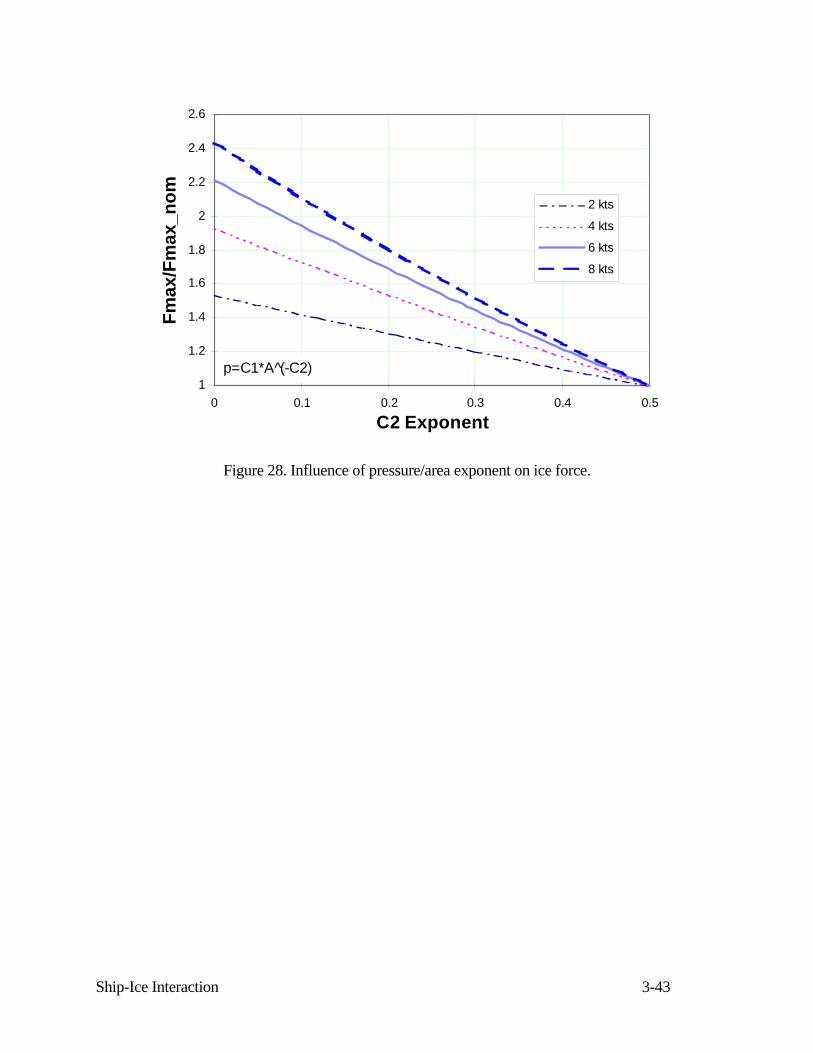
Ship-Ice Interaction 3-43
1
1.2
1.4
1.6
1.8
2
2.2
2.4
2.6
0 0.1 0.2 0.3 0.4 0.5
C2 Exponent
Fmax
/Fm
ax_n
om 2 kts
4 kts
6 kts
8 kts
p=C1*A (̂-C2)
Figure 28. Influence of pressure/area exponent on ice force.
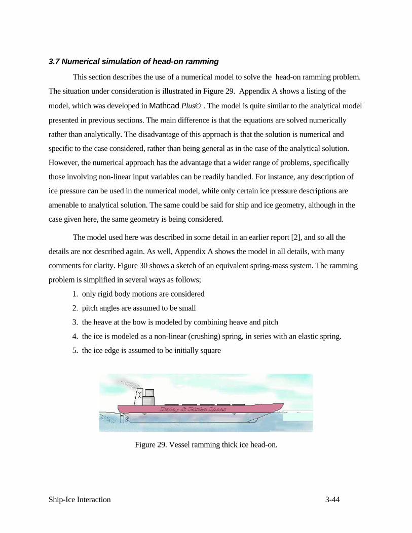
Ship-Ice Interaction 3-44
3.7 Numerical simulation of head-on ramming
This section describes the use of a numerical model to solve the head-on ramming problem.
The situation under consideration is illustrated in Figure 29. Appendix A shows a listing of the
model, which was developed in Mathcad Plus© . The model is quite similar to the analytical model
presented in previous sections. The main difference is that the equations are solved numerically
rather than analytically. The disadvantage of this approach is that the solution is numerical and
specific to the case considered, rather than being general as in the case of the analytical solution.
However, the numerical approach has the advantage that a wider range of problems, specifically
those involving non-linear input variables can be readily handled. For instance, any description of
ice pressure can be used in the numerical model, while only certain ice pressure descriptions are
amenable to analytical solution. The same could be said for ship and ice geometry, although in the
case given here, the same geometry is being considered.
The model used here was described in some detail in an earlier report [2], and so all the
details are not described again. As well, Appendix A shows the model in all details, with many
comments for clarity. Figure 30 shows a sketch of an equivalent spring-mass system. The ramming
problem is simplified in several ways as follows;
1. only rigid body motions are considered
2. pitch angles are assumed to be small
3. the heave at the bow is modeled by combining heave and pitch
4. the ice is modeled as a non-linear (crushing) spring, in series with an elastic spring.
5. the ice edge is assumed to be initially square
Figure 29. Vessel ramming thick ice head-on.

Ship-Ice Interaction 3-45
Figure 30. Equivalent spring-mass system for head-on ramming.
It was shown earlier [2], that when the parameters are the same, this numerical model produces
results which are almost identical to the analytical solution. This is not surprising, as both
approaches are solving the same sets of equations. The similarity is illustrated further in Figure 31,
which compares the analytical results from Figure 10, with Mathcad simulations for the same cases.
The main aim of this section is to investigate an issue that is difficult to handle with
analytical methods. The issue is the influence of the pressure-area effect in the ice crushing model.
The pressure area effect can be modeled using equation 64:
p(A) = C A1-C2 (64)
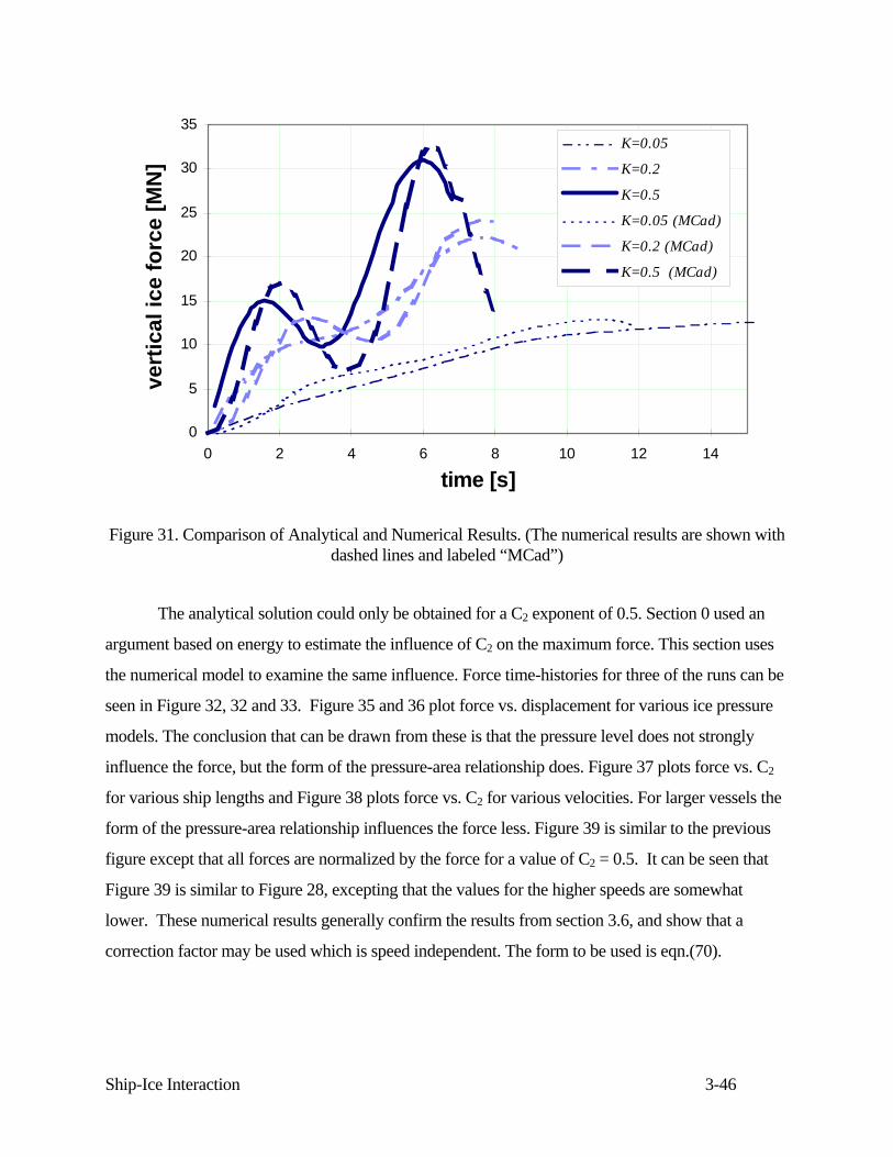
Ship-Ice Interaction 3-46
0
5
10
15
20
25
30
35
0 2 4 6 8 10 12 14
time [s]
vert
ical
ice
forc
e [M
N]
K=0.05
K=0.2
K=0.5
K=0.05 (MCad)
K=0.2 (MCad)
K=0.5 (MCad)
Figure 31. Comparison of Analytical and Numerical Results. (The numerical results are shown with dashed lines and labeled “MCad”)
The analytical solution could only be obtained for a C2 exponent of 0.5. Section 0 used an
argument based on energy to estimate the influence of C2 on the maximum force. This section uses
the numerical model to examine the same influence. Force time-histories for three of the runs can be
seen in Figure 32, 32 and 33. Figure 35 and 36 plot force vs. displacement for various ice pressure
models. The conclusion that can be drawn from these is that the pressure level does not strongly
influence the force, but the form of the pressure-area relationship does. Figure 37 plots force vs. C2
for various ship lengths and Figure 38 plots force vs. C2 for various velocities. For larger vessels the
form of the pressure-area relationship influences the force less. Figure 39 is similar to the previous
figure except that all forces are normalized by the force for a value of C2 = 0.5. It can be seen that
Figure 39 is similar to Figure 28, excepting that the values for the higher speeds are somewhat
lower. These numerical results generally confirm the results from section 3.6, and show that a
correction factor may be used which is speed independent. The form to be used is eqn.(70).
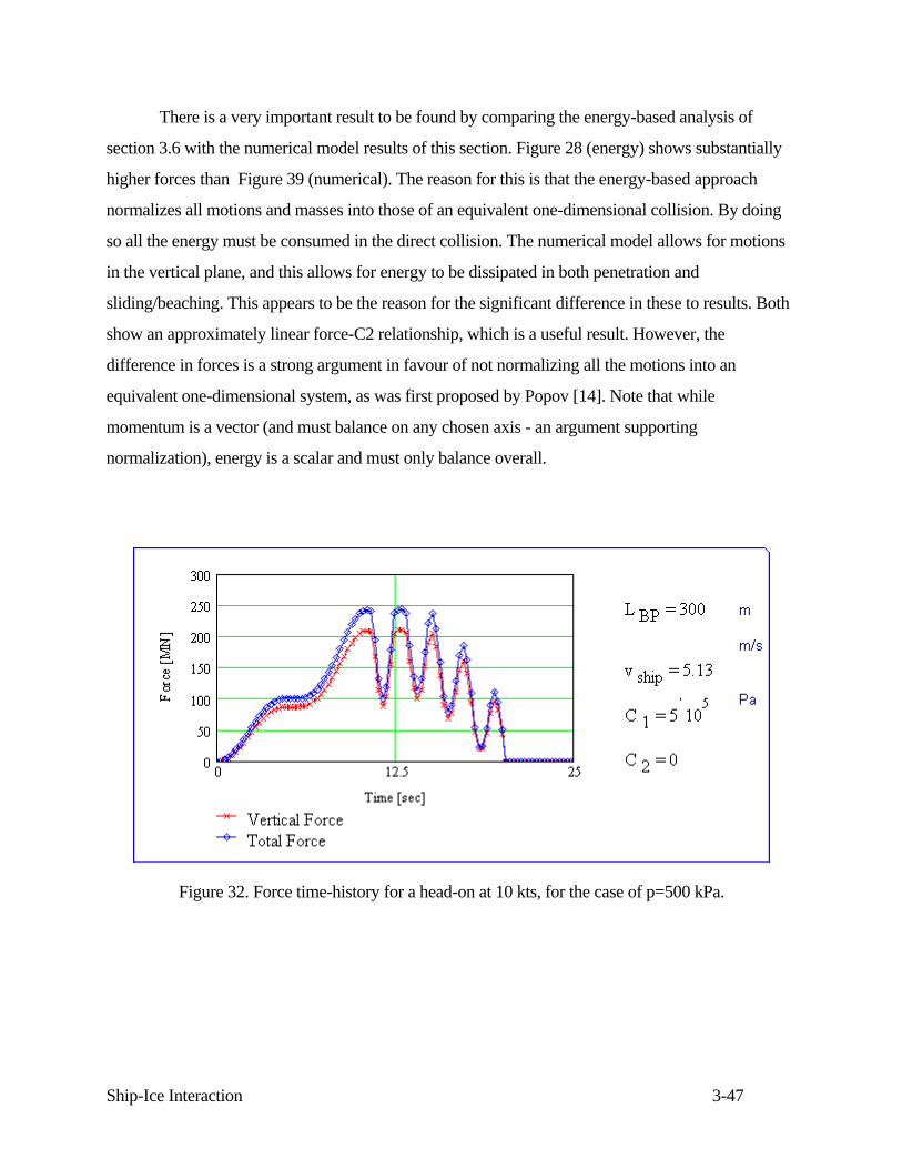
Ship-Ice Interaction 3-47
There is a very important result to be found by comparing the energy-based analysis of
section 3.6 with the numerical model results of this section. Figure 28 (energy) shows substantially
higher forces than Figure 39 (numerical). The reason for this is that the energy-based approach
normalizes all motions and masses into those of an equivalent one-dimensional collision. By doing
so all the energy must be consumed in the direct collision. The numerical model allows for motions
in the vertical plane, and this allows for energy to be dissipated in both penetration and
sliding/beaching. This appears to be the reason for the significant difference in these to results. Both
show an approximately linear force-C2 relationship, which is a useful result. However, the
difference in forces is a strong argument in favour of not normalizing all the motions into an
equivalent one-dimensional system, as was first proposed by Popov [14]. Note that while
momentum is a vector (and must balance on any chosen axis - an argument supporting
normalization), energy is a scalar and must only balance overall.
Figure 32. Force time-history for a head-on at 10 kts, for the case of p=500 kPa.
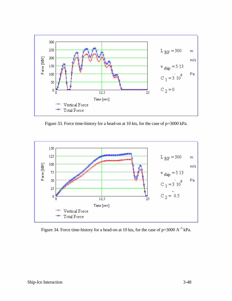
Ship-Ice Interaction 3-48
Figure 33. Force time-history for a head-on at 10 kts, for the case of p=3000 kPa.
Figure 34. Force time-history for a head-on at 10 kts, for the case of p=3000 A-.5 kPa.
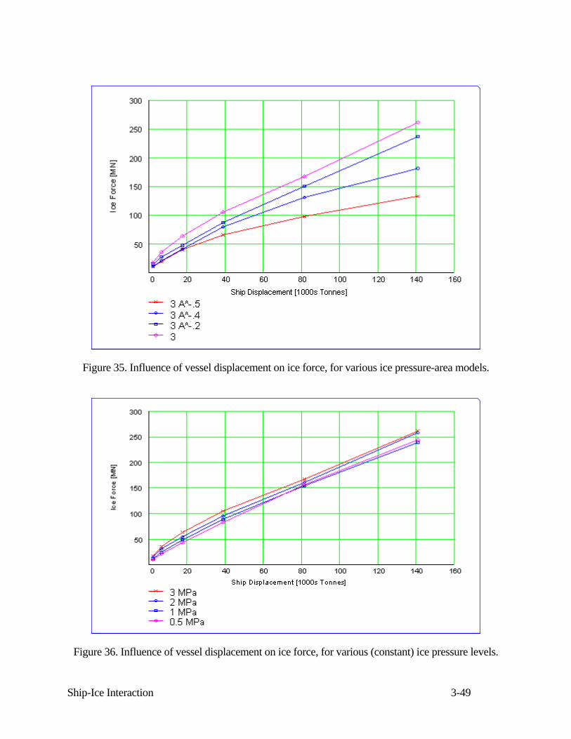
Ship-Ice Interaction 3-49
Figure 35. Influence of vessel displacement on ice force, for various ice pressure-area models.
Figure 36. Influence of vessel displacement on ice force, for various (constant) ice pressure levels.
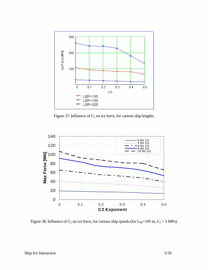
Ship-Ice Interaction 3-50
Figure 37. Influence of C2 on ice force, for various ship lengths.
0
20
40
60
80
100
120
140
0 0.1 0.2 0.3 0.4 0.5C2 Exponent
Max
For
ce [M
N]
2 kts (n)4 kts (n)6 kts (n)8 kts (n)10 kts (n)
Figure 38. Influence of C2 on ice force, for various ship speeds (for LBP=195 m, C1 = 3 MPa).
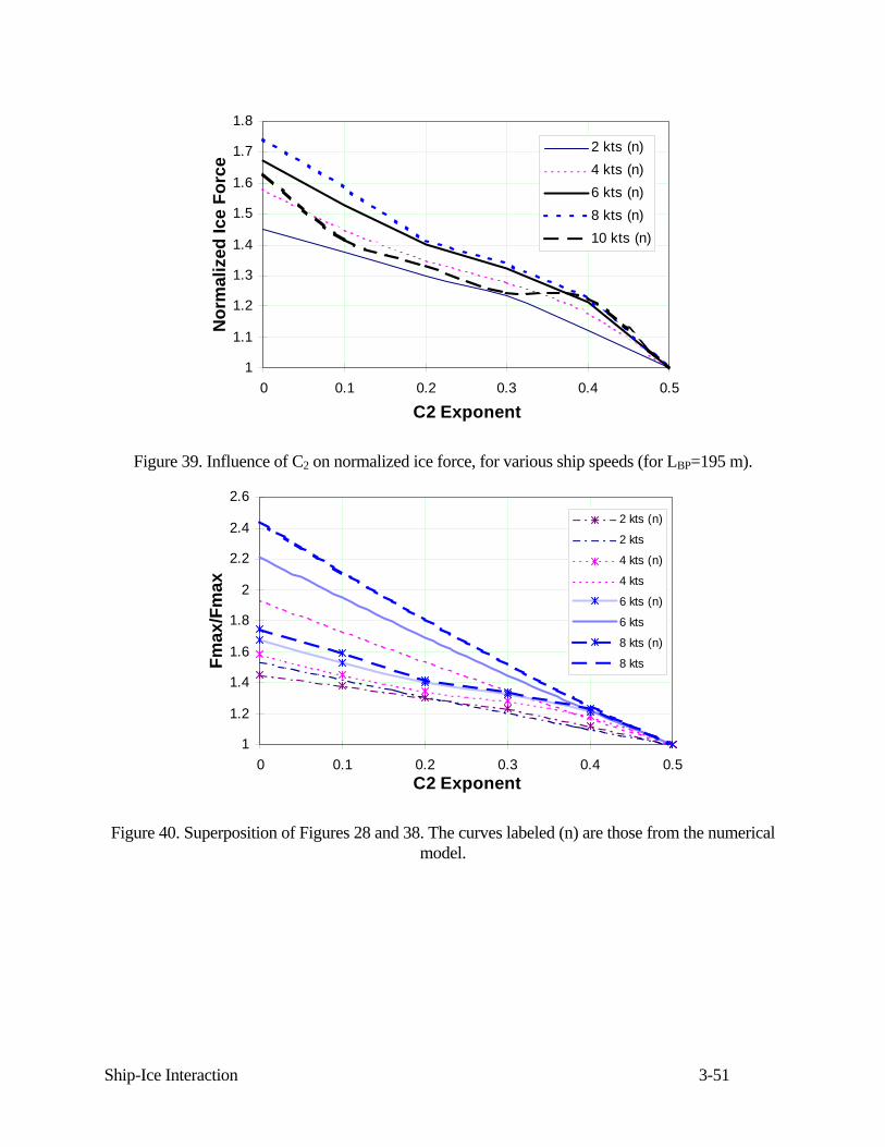
Ship-Ice Interaction 3-51
1
1.1
1.2
1.3
1.4
1.5
1.6
1.7
1.8
0 0.1 0.2 0.3 0.4 0.5
C2 Exponent
Nor
mal
ized
Ice
Forc
e
2 kts (n)4 kts (n)6 kts (n)8 kts (n)10 kts (n)
Figure 39. Influence of C2 on normalized ice force, for various ship speeds (for LBP=195 m).
1
1.2
1.4
1.6
1.8
2
2.2
2.4
2.6
0 0.1 0.2 0.3 0.4 0.5C2 Exponent
Fmax
/Fm
ax
2 kts (n)
2 kts
4 kts (n)
4 kts
6 kts (n)
6 kts
8 kts (n)
8 kts
Figure 40. Superposition of Figures 28 and 38. The curves labeled (n) are those from the numerical model.
Ship-Ice Interaction 3-52
3.8 Discussion
Head-on rams can be effectively modeled using by either analytical or numerical models. In
either case the equations to be solved are two-dimensional, meaning that all motions are in the
longitudinal vertical plane. Results have been presented above for the cases of infinite and non-
infinite ice. The analytical and numerical results corroborate each other. The analytical results show
directly the influence of various parameters, while the numerical model can be applied to a variety of
relatively difficult situations. The influence of various ship and ice parameters has been described
and plotted.
These results provide a firm basis, founded in mechanics, for calculation of loads and
response of ships. These results can be used to directly specify hull girder shear area and section
modulus criteria, with ship and ice parameters as input. The following section will extend this 2D
model, by considering shoulder impacts.
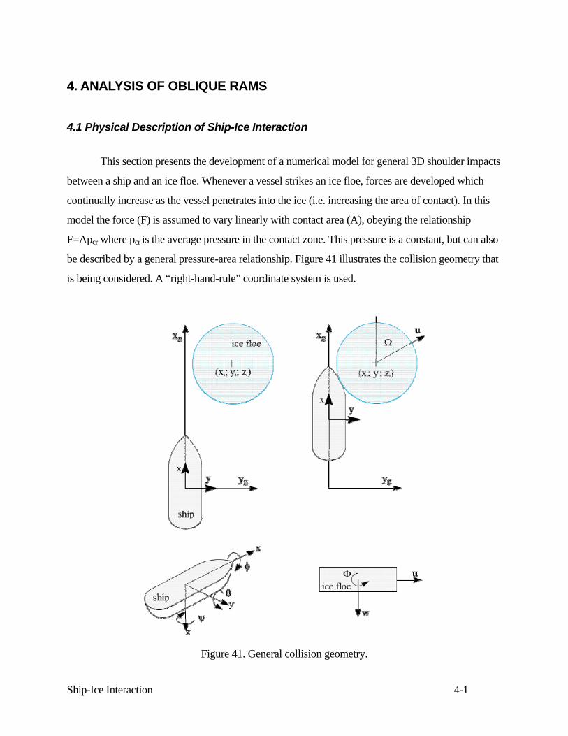
Ship-Ice Interaction 4-1
4. ANALYSIS OF OBLIQUE RAMS
4.1 Physical Description of Ship-Ice Interaction This section presents the development of a numerical model for general 3D shoulder impacts
between a ship and an ice floe. Whenever a vessel strikes an ice floe, forces are developed which
continually increase as the vessel penetrates into the ice (i.e. increasing the area of contact). In this
model the force (F) is assumed to vary linearly with contact area (A), obeying the relationship
F=Apcr where pcr is the average pressure in the contact zone. This pressure is a constant, but can also
be described by a general pressure-area relationship. Figure 41 illustrates the collision geometry that
is being considered. A “right-hand-rule” coordinate system is used.
Figure 41. General collision geometry.
Ship-Ice Interaction 4-2
The contact mechanics considered here are very general. The contact force is not generally
aligned with the centers of gravity of either the ship or ice floe. Further, the types of response being
considered include rigid-body translation and rotation for both ship and ice, elastic response in both
the ship and ice and inelastic response in the ice, in the form of crushing and flexural failure. The
contact mechanics are truly interactive. Once contact is made, forces (and moments) are developed
which accelerate both ship and ice. The resulting motion determines the relative position of the two
bodies and thereby the contact area. Since the force is a function of the contact area, a true physical
interaction is established which can only be modeled by a set of coupled equations. These equations
will be solved here using numerical methods.
4.2 Definition of the problem
When a ship collides with an ice floe with the bow between the very stem and the shoulder
area, all the ship rigid body degrees of freedom respond. That is, the ship moves in sway, roll and
yaw as well as in surge, heave and pitch. A sketch of the situation is presented in Figure 41 where
the assumption about the floe shape is also shown.
The contact geometry is, however, more complicated than in the head-on case. During the
collision both the ship and, in the case of finite mass ice floe, the ice floe move. This changes the
contact geometry. Usually here the assumption that the bow angles stay constant is made. The other
complication is presented by the movement of the contact point along the ship hull. If the bow is
assumed to be of wedge shape where the port and starboard sides of the bow are planes, this contact
point movement may be ignored. The direction of the frictional force opposes the motion but in the
oblique ram case the direction of the relative motion is not clear. One way to treat this problem is
given in [10].
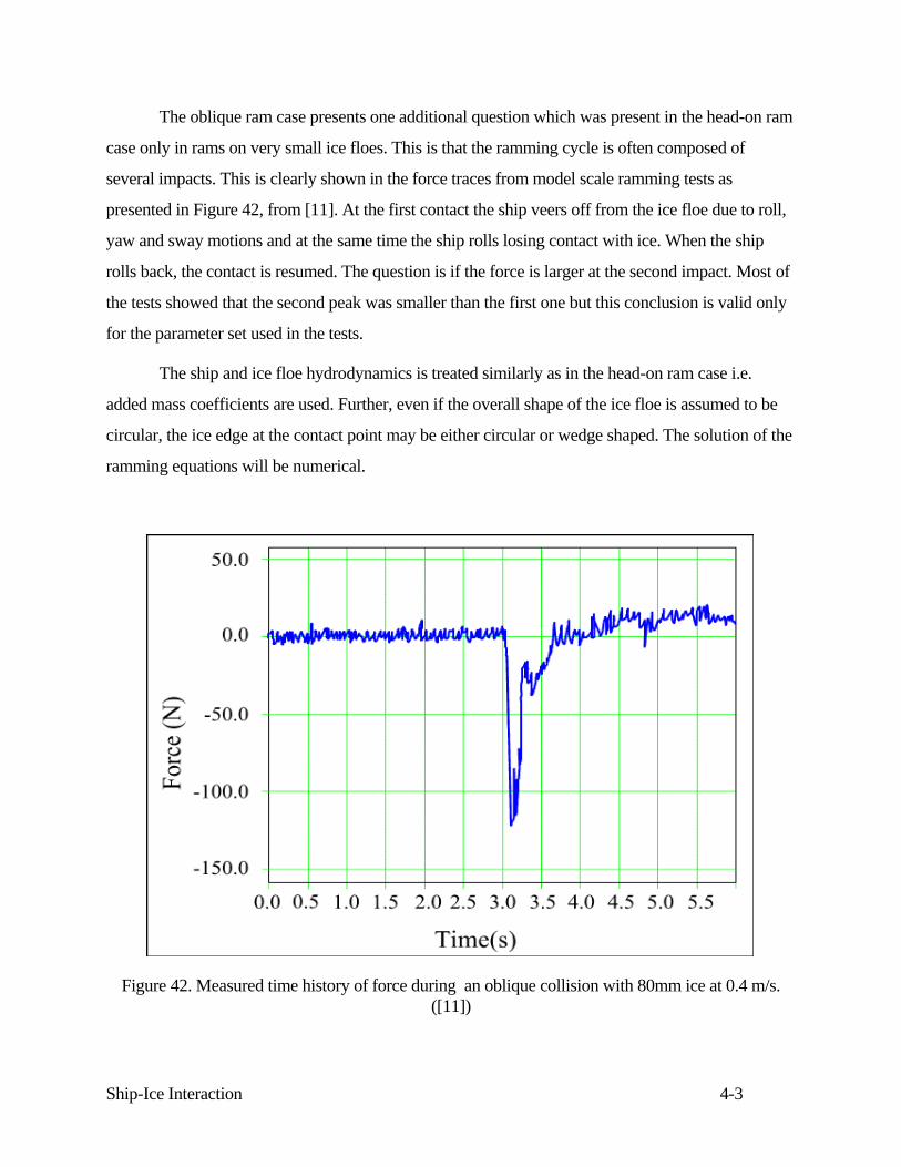
Ship-Ice Interaction 4-3
The oblique ram case presents one additional question which was present in the head-on ram
case only in rams on very small ice floes. This is that the ramming cycle is often composed of
several impacts. This is clearly shown in the force traces from model scale ramming tests as
presented in Figure 42, from [11]. At the first contact the ship veers off from the ice floe due to roll,
yaw and sway motions and at the same time the ship rolls losing contact with ice. When the ship
rolls back, the contact is resumed. The question is if the force is larger at the second impact. Most of
the tests showed that the second peak was smaller than the first one but this conclusion is valid only
for the parameter set used in the tests.
The ship and ice floe hydrodynamics is treated similarly as in the head-on ram case i.e.
added mass coefficients are used. Further, even if the overall shape of the ice floe is assumed to be
circular, the ice edge at the contact point may be either circular or wedge shaped. The solution of the
ramming equations will be numerical.
Figure 42. Measured time history of force during an oblique collision with 80mm ice at 0.4 m/s. ([11])
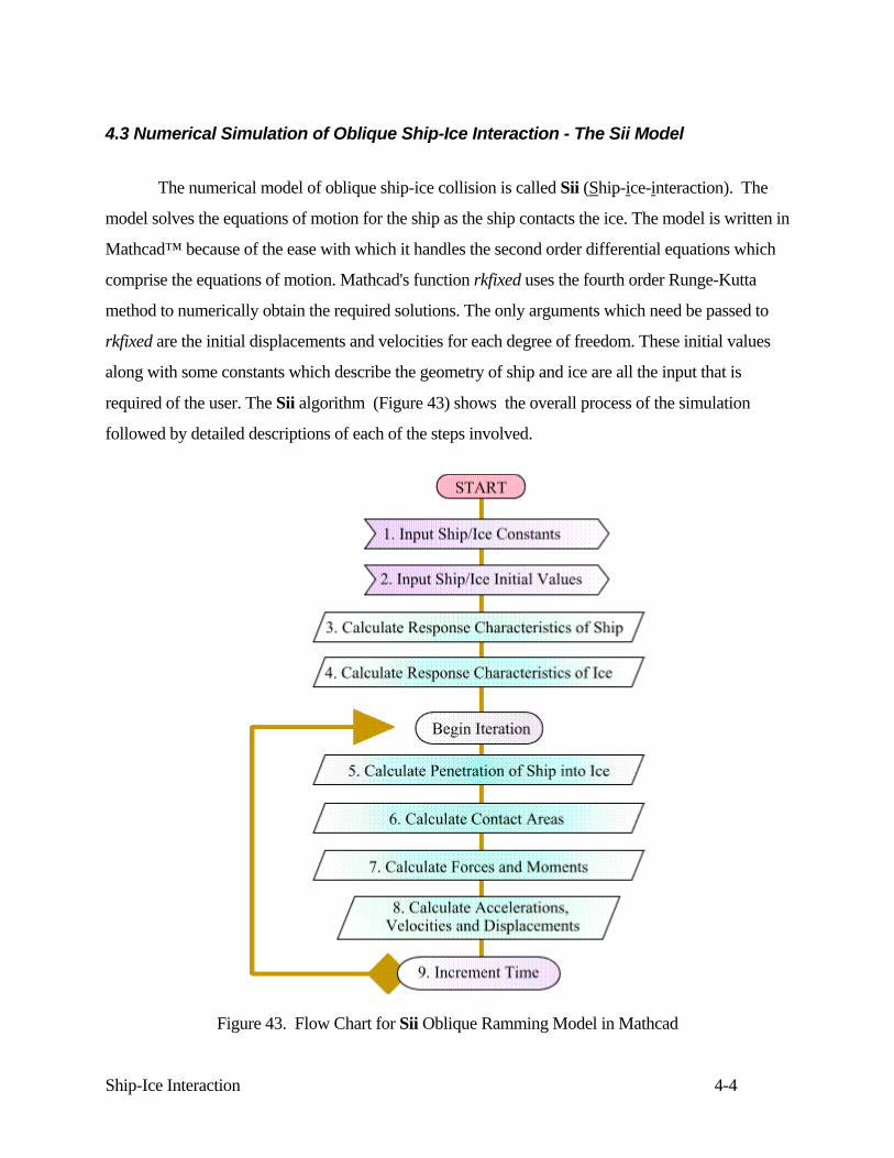
Ship-Ice Interaction 4-4
4.3 Numerical Simulation of Oblique Ship-Ice Interaction - The Sii Model
The numerical model of oblique ship-ice collision is called Sii (Ship-ice-interaction). The
model solves the equations of motion for the ship as the ship contacts the ice. The model is written in
Mathcad™ because of the ease with which it handles the second order differential equations which
comprise the equations of motion. Mathcad's function rkfixed uses the fourth order Runge-Kutta
method to numerically obtain the required solutions. The only arguments which need be passed to
rkfixed are the initial displacements and velocities for each degree of freedom. These initial values
along with some constants which describe the geometry of ship and ice are all the input that is
required of the user. The Sii algorithm (Figure 43) shows the overall process of the simulation
followed by detailed descriptions of each of the steps involved.
Figure 43. Flow Chart for Sii Oblique Ramming Model in Mathcad
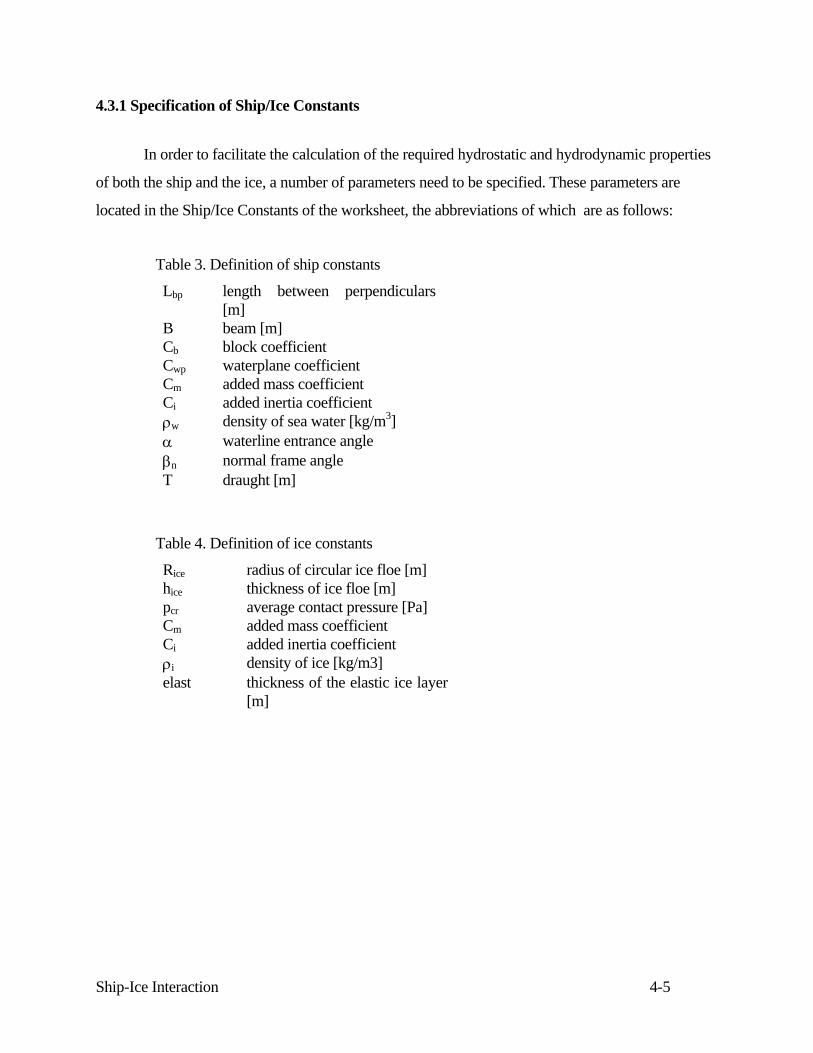
Ship-Ice Interaction 4-5
4.3.1 Specification of Ship/Ice Constants In order to facilitate the calculation of the required hydrostatic and hydrodynamic properties
of both the ship and the ice, a number of parameters need to be specified. These parameters are
located in the Ship/Ice Constants of the worksheet, the abbreviations of which are as follows:
Table 3. Definition of ship constants
Lbp length between perpendiculars [m]
B beam [m] Cb block coefficient Cwp waterplane coefficient Cm added mass coefficient Ci added inertia coefficient ρw density of sea water [kg/m3] α waterline entrance angle βn normal frame angle T draught [m]
Table 4. Definition of ice constants
Rice radius of circular ice floe [m] hice thickness of ice floe [m] pcr average contact pressure [Pa] Cm added mass coefficient Ci added inertia coefficient ρi density of ice [kg/m3] elast thickness of the elastic ice layer
[m]
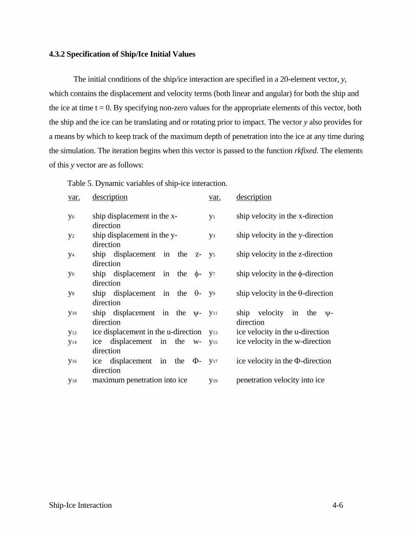
Ship-Ice Interaction 4-6
4.3.2 Specification of Ship/Ice Initial Values
The initial conditions of the ship/ice interaction are specified in a 20-element vector, y,
which contains the displacement and velocity terms (both linear and angular) for both the ship and
the ice at time t = 0. By specifying non-zero values for the appropriate elements of this vector, both
the ship and the ice can be translating and or rotating prior to impact. The vector y also provides for
a means by which to keep track of the maximum depth of penetration into the ice at any time during
the simulation. The iteration begins when this vector is passed to the function rkfixed. The elements
of this y vector are as follows:
Table 5. Dynamic variables of ship-ice interaction.
var. description var. description
y0 ship displacement in the x-direction
y1 ship velocity in the x-direction
y2 ship displacement in the y-direction
y3 ship velocity in the y-direction
y4 ship displacement in the z-direction
y5 ship velocity in the z-direction
y6 ship displacement in the φ-direction
y7 ship velocity in the φ-direction
y8 ship displacement in the θ-direction
y9 ship velocity in the θ-direction
y10 ship displacement in the ψ-direction
y11 ship velocity in the ψ-direction
y12 ice displacement in the u-direction y13 ice velocity in the u-direction y14 ice displacement in the w-
direction y15 ice velocity in the w-direction
y16 ice displacement in the Φ-direction
y17 ice velocity in the Φ-direction
y18 maximum penetration into ice y19 penetration velocity into ice
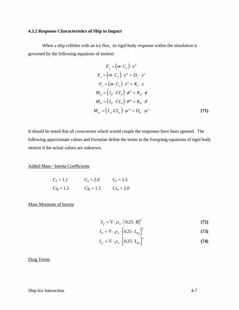
Ship-Ice Interaction 4-7
4.3.2 Response Characteristics of Ship to Impact
When a ship collides with an ice floe, its rigid body response within the simulation is
governed by the following equations of motion:
( )F m C xx x= ⋅ ⋅ ′′
( )F m C y D yy y y= ⋅ ⋅ ′′ + ⋅ ′
( )F m C z K zz z z= ⋅ ⋅ ′′ + ⋅
( )M I CI Kφ φ φ φφ φ= ⋅ ⋅ ′′ + ⋅
( )M I CI Kθ θ θ θθ θ= ⋅ ⋅ ′′ + ⋅
( )M I CI Dψ ψ ψ ψψ ψ= ⋅ ⋅ ′′ + ⋅ ′ (71)
It should be noted that all cross-terms which would couple the responses have been ignored. The
following approximate values and formulae define the terms in the foregoing equations of rigid body
motion if the actual values are unknown.
Added Mass / Inertia Coefficients
Cx = 1.1 Cy = 2.0 Cz = 1.5
CIφ = 1.2 CIθ = 1.5 CIψ = 2.0
Mass Moments of Inertia
[ ]I Bwφ ρ= ∇ ⋅ ⋅ ⋅0 25 2. (72)
[ ]I Lw bpθ ρ= ∇ ⋅ ⋅ ⋅0 252
. (73)
[ ]I Lw bpψ ρ= ∇ ⋅ ⋅ ⋅0 252
. (74)
Drag Terms
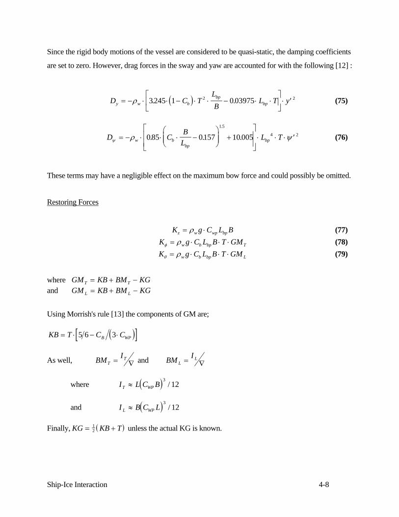
Ship-Ice Interaction 4-8
Since the rigid body motions of the vessel are considered to be quasi-static, the damping coefficients
are set to zero. However, drag forces in the sway and yaw are accounted for with the following [12] :
( )D C TLB
L T yy w bbp
bp= − ⋅ ⋅ − ⋅ ⋅ − ⋅ ⋅⎡
⎣⎢
⎤
⎦⎥ ⋅ ′ρ 3 245 1 0 039752 2. . (75)
D CB
LL Tw b
bpbpψ ρ ψ= − ⋅ ⋅ ⋅ −
⎛
⎝⎜⎜
⎞
⎠⎟⎟ +
⎡
⎣⎢⎢
⎤
⎦⎥⎥
⋅ ⋅ ⋅ ′0 85 0157 10 0051 5
4 2. . ..
(76)
These terms may have a negligible effect on the maximum bow force and could possibly be omitted.
Restoring Forces
K g C L Bz w wp bp= ⋅ρ (77) K g C L B T GMw b bp Tφ ρ= ⋅ ⋅ ⋅ (78) K g C L B T GMw b bp Lθ ρ= ⋅ ⋅ ⋅ (79)
where GM KB BM KGT T= + − and GM KB BM KGL L= + − Using Morrish's rule [13] the components of GM are;
( )[ ]KB T C CB WP= ⋅ − ⋅5 6 3
As well, BM IT
T= ∇ and BM IL
L= ∇
where ( )I L C BT WP≈3
12/
and ( )I B C LL WP≈3
12/
Finally, ( )KG KB T= +12 unless the actual KG is known.

Ship-Ice Interaction 4-9
4.3.4 Responses Characteristics of the Ice Floe to Impact When a ship collides with an ice floe, the rigid body response of the ice within the simulation is
governed by the following equations of motion.
( )F m Cm u D uu ice u u= ⋅ ⋅ ′′ + ⋅ ′ (80)
( )F m Cm w K ww ice w w= ⋅ ⋅ ′′ + ⋅ (81)
( )M I KΦ Φ ΦΦ Φ= ⋅ ′′ + ⋅ (82)
The following approximate values and formulae define the terms in the foregoing equations of rigid
body motion if the actual values are unknown.
Added Mass / Inertia Coefficients
Cmu = 1.5 Cmw = 2.0 CiΦ = 1.5
Mass Moments of Inertia
m R hice ice ice i= ⋅ ⋅ ⋅π ρ2 (83)
( )I R m Ciice iceΦ Φ= ⋅ ⋅ ⋅14
2 (84)
Drag Terms
Since the rigid body motions of the ice floe are transient, the damping coefficients are set to
zero. However, drag forces in surge are accounted for with the following formula for an immersed
circular disk parallel to flow:
D R uy w ice= ⋅ ⋅ ⋅ ′2 2 2ρ (85)
Restoring Forces
K g Rw w ice= ⋅ ⋅ρ π 2 (86) K g R h GMw iceΦ = ⋅ ⋅ ⋅ρ π 2 (87)
where GM KB BM KG= + −
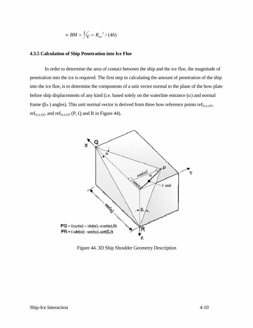
Ship-Ice Interaction 4-10
≈ = ∇ =BM I R hice2 4/ ( )
4.3.5 Calculation of Ship Penetration into Ice Floe
In order to determine the area of contact between the ship and the ice floe, the magnitude of
penetration into the ice is required. The first step in calculating the amount of penetration of the ship
into the ice floe, is to determine the components of a unit vector normal to the plane of the bow plate
before ship displacements of any kind (i.e. based solely on the waterline entrance (α) and normal
frame (βn ) angles). This unit normal vector is derived from three bow reference points ref(x,y,z)1,
ref(x,y,z)2, and ref(x,y,z)3 (P, Q and R in Figure 44).
Figure 44. 3D Ship Shoulder Geometry Description
Ship-Ice Interaction 4-11
By the use of transformation formulae, e.g. transformation due to roll (φ)
x* = x {i} (88) y* = [y cos(φ)-z sin(φ)] {j} (89) z* = [y sin(φ)+z cos(φ)] {k} (90)
where {i} {j} and {k} are the unit vectors in the x, y and z directions respectively, the change in vector
components for the bow plate due to roll, pitch and yaw can be determined for each time step in the
iteration. By tracking the position of a reference point anywhere on the bow plate, ref1(x,y,z),as well as
the position of the ice floe's centre of gravity (CGice), the perpendicular distance between the bow
plate and CGice can be determined at any point in the simulation. By comparing this quantity (v(y))
with the minimum distance required between the bow plate and CGice before penetration into the ice
floe occurs (minpen), the amount of penetration (ζ(y)) can be determined.
4.3.6 Calculation of Contact Area
In reviewing the literature of ship-ice interaction two shapes of ice floes have been
considered,
1. circular
2. protruding angle
Although the model is based presently on the circular form, it is a relatively simple matter to provide
for both.
Contact Area with Circular Ice Edge
The contact area with a circular ice floe was first defined by [14] using the following
approximation
A =
43
h 2 R h - hl ice l l
n
2
sin β (91)
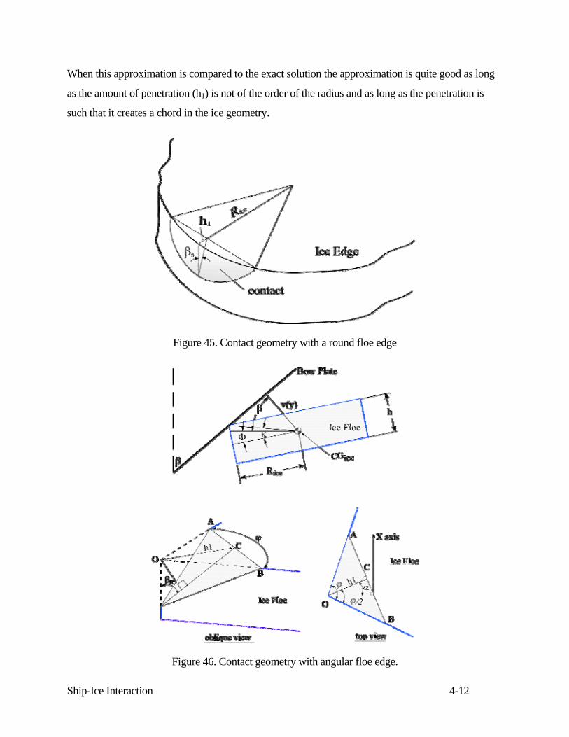
Ship-Ice Interaction 4-12
When this approximation is compared to the exact solution the approximation is quite good as long
as the amount of penetration (h1) is not of the order of the radius and as long as the penetration is
such that it creates a chord in the ice geometry.
Figure 45. Contact geometry with a round floe edge
Figure 46. Contact geometry with angular floe edge.
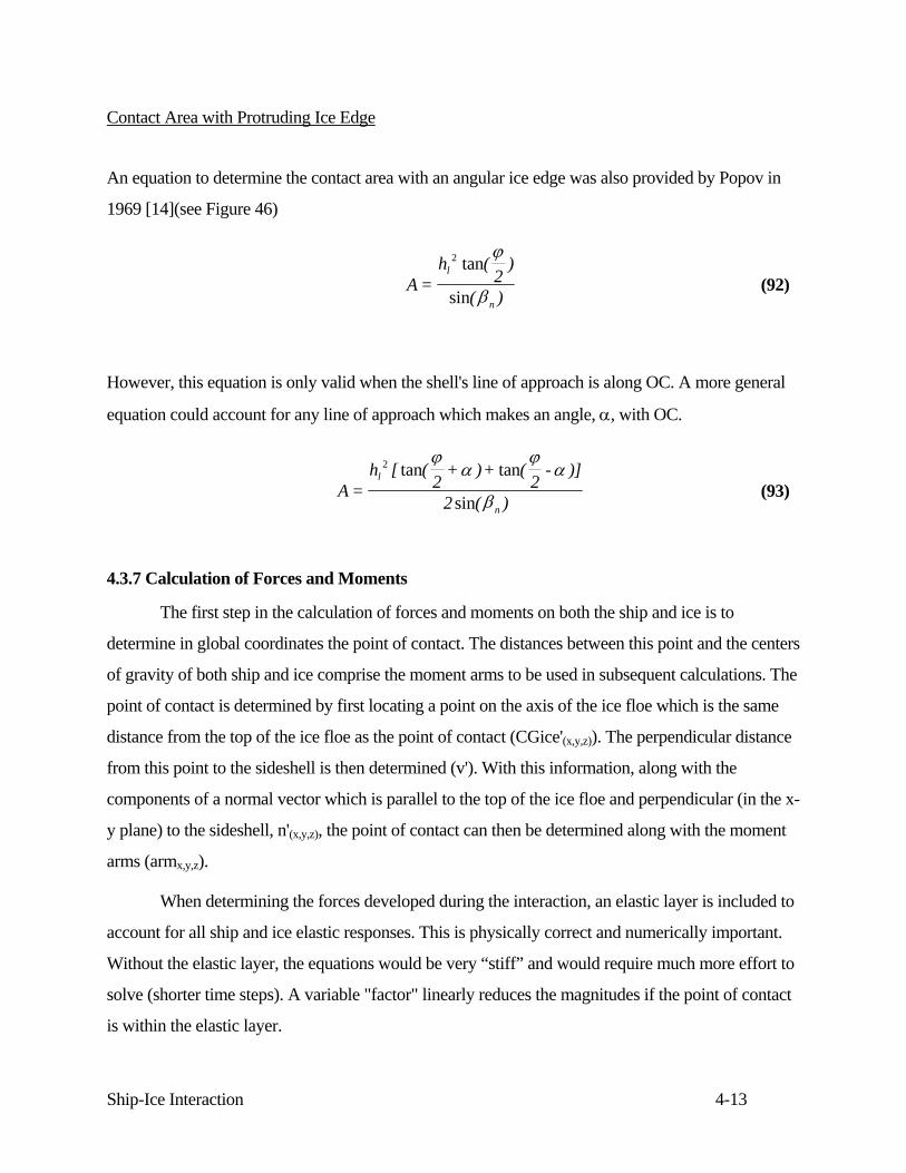
Ship-Ice Interaction 4-13
Contact Area with Protruding Ice Edge
An equation to determine the contact area with an angular ice edge was also provided by Popov in
1969 [14](see Figure 46)
A =h (
2)
( )
l
n
2 tan
sin
ϕ
β (92)
However, this equation is only valid when the shell's line of approach is along OC. A more general
equation could account for any line of approach which makes an angle, α, with OC.
A =h [ (
2+ )+ (
2- )]
2 ( )l
n
2 tan tan
sin
ϕα
ϕα
β (93)
4.3.7 Calculation of Forces and Moments
The first step in the calculation of forces and moments on both the ship and ice is to
determine in global coordinates the point of contact. The distances between this point and the centers
of gravity of both ship and ice comprise the moment arms to be used in subsequent calculations. The
point of contact is determined by first locating a point on the axis of the ice floe which is the same
distance from the top of the ice floe as the point of contact (CGice'(x,y,z)). The perpendicular distance
from this point to the sideshell is then determined (v'). With this information, along with the
components of a normal vector which is parallel to the top of the ice floe and perpendicular (in the x-
y plane) to the sideshell, n'(x,y,z), the point of contact can then be determined along with the moment
arms (armx,y,z).
When determining the forces developed during the interaction, an elastic layer is included to
account for all ship and ice elastic responses. This is physically correct and numerically important.
Without the elastic layer, the equations would be very “stiff” and would require much more effort to
solve (shorter time steps). A variable "factor" linearly reduces the magnitudes if the point of contact
is within the elastic layer.
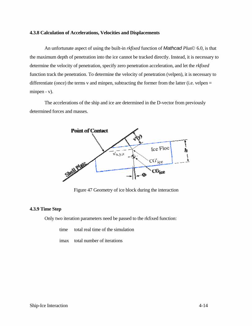
Ship-Ice Interaction 4-14
4.3.8 Calculation of Accelerations, Velocities and Displacements
An unfortunate aspect of using the built-in rkfixed function of Mathcad Plus© 6.0, is that
the maximum depth of penetration into the ice cannot be tracked directly. Instead, it is necessary to
determine the velocity of penetration, specify zero penetration acceleration, and let the rkfixed
function track the penetration. To determine the velocity of penetration (velpen), it is necessary to
differentiate (once) the terms v and minpen, subtracting the former from the latter (i.e. velpen =
minpen - v).
The accelerations of the ship and ice are determined in the D-vector from previously
determined forces and masses.
Figure 47 Geometry of ice block during the interaction
4.3.9 Time Step
Only two iteration parameters need be passed to the rkfixed function:
time total real time of the simulation
imax total number of iterations
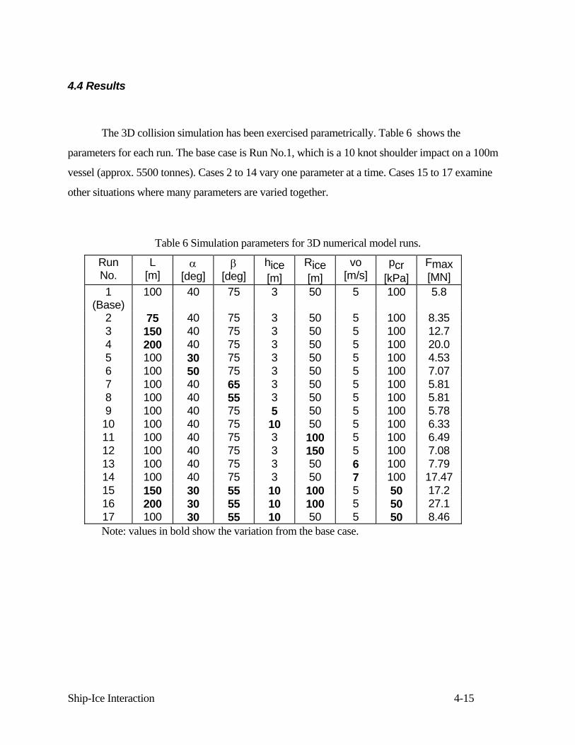
Ship-Ice Interaction 4-15
4.4 Results
The 3D collision simulation has been exercised parametrically. Table 6 shows the
parameters for each run. The base case is Run No.1, which is a 10 knot shoulder impact on a 100m
vessel (approx. 5500 tonnes). Cases 2 to 14 vary one parameter at a time. Cases 15 to 17 examine
other situations where many parameters are varied together.
Table 6 Simulation parameters for 3D numerical model runs.
Run No.
L [m]
α [deg]
β [deg]
hice [m]
Rice [m]
vo [m/s]
pcr [kPa]
Fmax [MN]
1 (Base)
100 40 75 3 50 5 100 5.8
2 75 40 75 3 50 5 100 8.35 3 150 40 75 3 50 5 100 12.7 4 200 40 75 3 50 5 100 20.0 5 100 30 75 3 50 5 100 4.53 6 100 50 75 3 50 5 100 7.07 7 100 40 65 3 50 5 100 5.81 8 100 40 55 3 50 5 100 5.81 9 100 40 75 5 50 5 100 5.78 10 100 40 75 10 50 5 100 6.33 11 100 40 75 3 100 5 100 6.49 12 100 40 75 3 150 5 100 7.08 13 100 40 75 3 50 6 100 7.79 14 100 40 75 3 50 7 100 17.47 15 150 30 55 10 100 5 50 17.2 16 200 30 55 10 100 5 50 27.1 17 100 30 55 10 50 5 50 8.46 Note: values in bold show the variation from the base case.
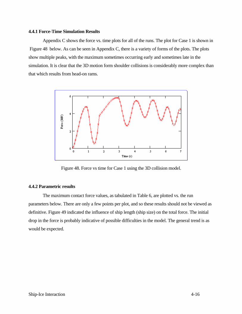
Ship-Ice Interaction 4-16
4.4.1 Force-Time Simulation Results
Appendix C shows the force vs. time plots for all of the runs. The plot for Case 1 is shown in
Figure 48 below. As can be seen in Appendix C, there is a variety of forms of the plots. The plots
show multiple peaks, with the maximum sometimes occurring early and sometimes late in the
simulation. It is clear that the 3D motion form shoulder collisions is considerably more complex than
that which results from head-on rams.
Figure 48. Force vs time for Case 1 using the 3D collision model.
4.4.2 Parametric results
The maximum contact force values, as tabulated in Table 6, are plotted vs. the run
parameters below. There are only a few points per plot, and so these results should not be viewed as
definitive. Figure 49 indicated the influence of ship length (ship size) on the total force. The initial
drop in the force is probably indicative of possible difficulties in the model. The general trend is as
would be expected.

Ship-Ice Interaction 4-17
0
24
6
810
12
14
1618
20
0 50 100 150 200
ship length [m]
Fmax
[MN
]
Figure 49. Relationship between force acting on the ship and the length of the ship between perpendiculars. Variables held constant include: L/B=7.5, α=40o, β=75o, Rice=50m and hice=3m, and
vo= 5 m/s.
Figure 50 shows the influence of floe radius, which is not strong for the range of sizes
considered. Figure 51 shows the influence of floe thickness, which is almost zero for the range of
thickness considered. Figure 52 shows the influence of the waterline entrance angle. Figure 53
shows the influence of the frame angle. The frame angle has no influence, while the waterline angle
has an important influence. The significance of this deserves further attention.
0
1
2
3
4
5
6
7
8
0 50 100 150
floe radius [m]
Fmax
[MN
]
Figure 50. Relationship between force acting on the ship and the radius of the ice floe. Variables held constant include Lbp=100m, B=13.3m, α=40o, β=65o and hice=3m.
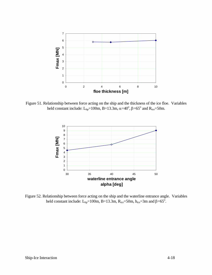
Ship-Ice Interaction 4-18
0
1
2
3
4
5
6
7
0 2 4 6 8 10
floe thickness [m]
Fmax
[MN
]
Figure 51. Relationship between force acting on the ship and the thickness of the ice floe. Variables held constant include: Lbp=100m, B=13.3m, α=40o, β=65o and Rice=50m.
0123456789
10
30 35 40 45 50
waterline entrance anglealpha [deg]
Fmax
[MN
]
Figure 52. Relationship between force acting on the ship and the waterline entrance angle. Variables held constant include: Lbp=100m, B=13.3m, Rice=50m, hice=3m and β=65o.
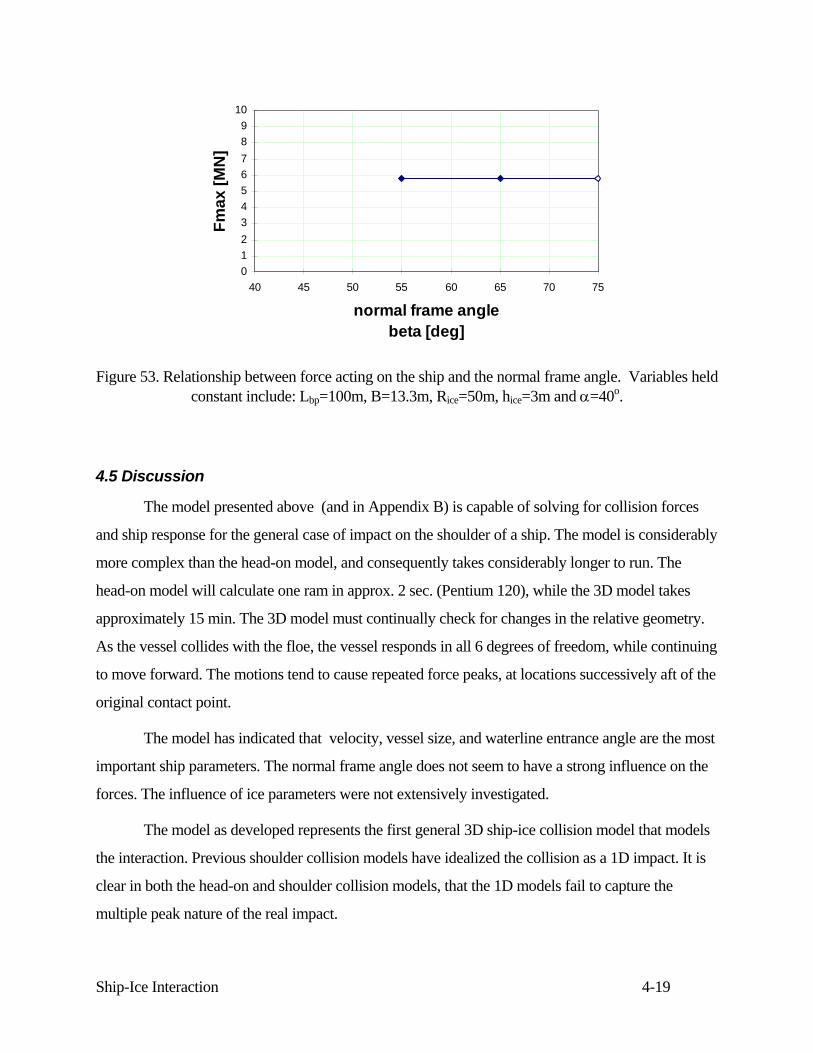
Ship-Ice Interaction 4-19
0123456789
10
40 45 50 55 60 65 70 75
normal frame anglebeta [deg]
Fmax
[MN
]
Figure 53. Relationship between force acting on the ship and the normal frame angle. Variables held constant include: Lbp=100m, B=13.3m, Rice=50m, hice=3m and α=40o.
4.5 Discussion
The model presented above (and in Appendix B) is capable of solving for collision forces
and ship response for the general case of impact on the shoulder of a ship. The model is considerably
more complex than the head-on model, and consequently takes considerably longer to run. The
head-on model will calculate one ram in approx. 2 sec. (Pentium 120), while the 3D model takes
approximately 15 min. The 3D model must continually check for changes in the relative geometry.
As the vessel collides with the floe, the vessel responds in all 6 degrees of freedom, while continuing
to move forward. The motions tend to cause repeated force peaks, at locations successively aft of the
original contact point.
The model has indicated that velocity, vessel size, and waterline entrance angle are the most
important ship parameters. The normal frame angle does not seem to have a strong influence on the
forces. The influence of ice parameters were not extensively investigated.
The model as developed represents the first general 3D ship-ice collision model that models
the interaction. Previous shoulder collision models have idealized the collision as a 1D impact. It is
clear in both the head-on and shoulder collision models, that the 1D models fail to capture the
multiple peak nature of the real impact.
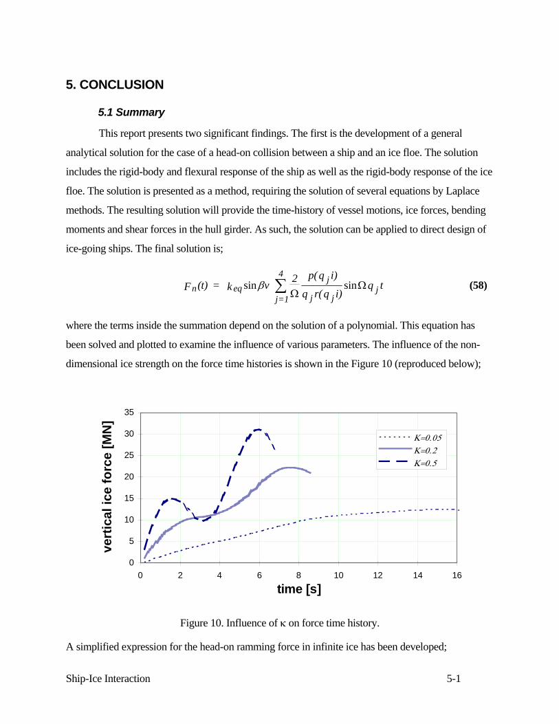
Ship-Ice Interaction 5-1
5. CONCLUSION
5.1 Summary
This report presents two significant findings. The first is the development of a general
analytical solution for the case of a head-on collision between a ship and an ice floe. The solution
includes the rigid-body and flexural response of the ship as well as the rigid-body response of the ice
floe. The solution is presented as a method, requiring the solution of several equations by Laplace
methods. The resulting solution will provide the time-history of vessel motions, ice forces, bending
moments and shear forces in the hull girder. As such, the solution can be applied to direct design of
ice-going ships. The final solution is;
n eqj=1
4 j
j jjF (t) = k v 2 p(q i)
q r(q i)q tsin sinβ ∑ Ω
Ω (58)
where the terms inside the summation depend on the solution of a polynomial. This equation has
been solved and plotted to examine the influence of various parameters. The influence of the non-
dimensional ice strength on the force time histories is shown in the Figure 10 (reproduced below);
0
5
10
15
20
25
30
35
0 2 4 6 8 10 12 14 16
time [s]
vert
ical
ice
forc
e [M
N]
Κ=0.05Κ=0.2Κ=0.5
Figure 10. Influence of κ on force time history.
A simplified expression for the head-on ramming force in infinite ice has been developed;
Ship-Ice Interaction 5-2
F = M gA vn wp,max. .. sin0 766 0 4 0 2⋅ ⋅ ⋅ ⋅κ β ρ (61)
where Fn,max is the maximum normal ice force [N]
κ is the non-dimensional ice strength (equation 52) β is the angle of the stem (to the horizontal) Awp is the water plane area of the vessel [m^2] v is the vessel speed [m/s] M is the vessel mass in surge [kg]
Equation 61 assumes a square-root pressure-area relationship and infinite ice floes. When the
terms are expanded to show the influence of ship size, the equation implies a relationship between
Fmax and displacement of the form:
Fmax.≈ Δ567 (94)
Equation 58 can also be applied to the case of ramming finite floes, with the use of equation
62, in place of equations 40 and 50. The influence of floe size on the force time history is shown in
Figure 26 (reproduced below). If finite floe collisions were included as part of the basis for Fmax, it
would be expected that the exponent on displacement would be lower than the value 0.567 shown in
Equation (94) , and possibly much lower. This is because it is very difficult for very large vessels to
find floes large enough to be considered “effectively infinite”.
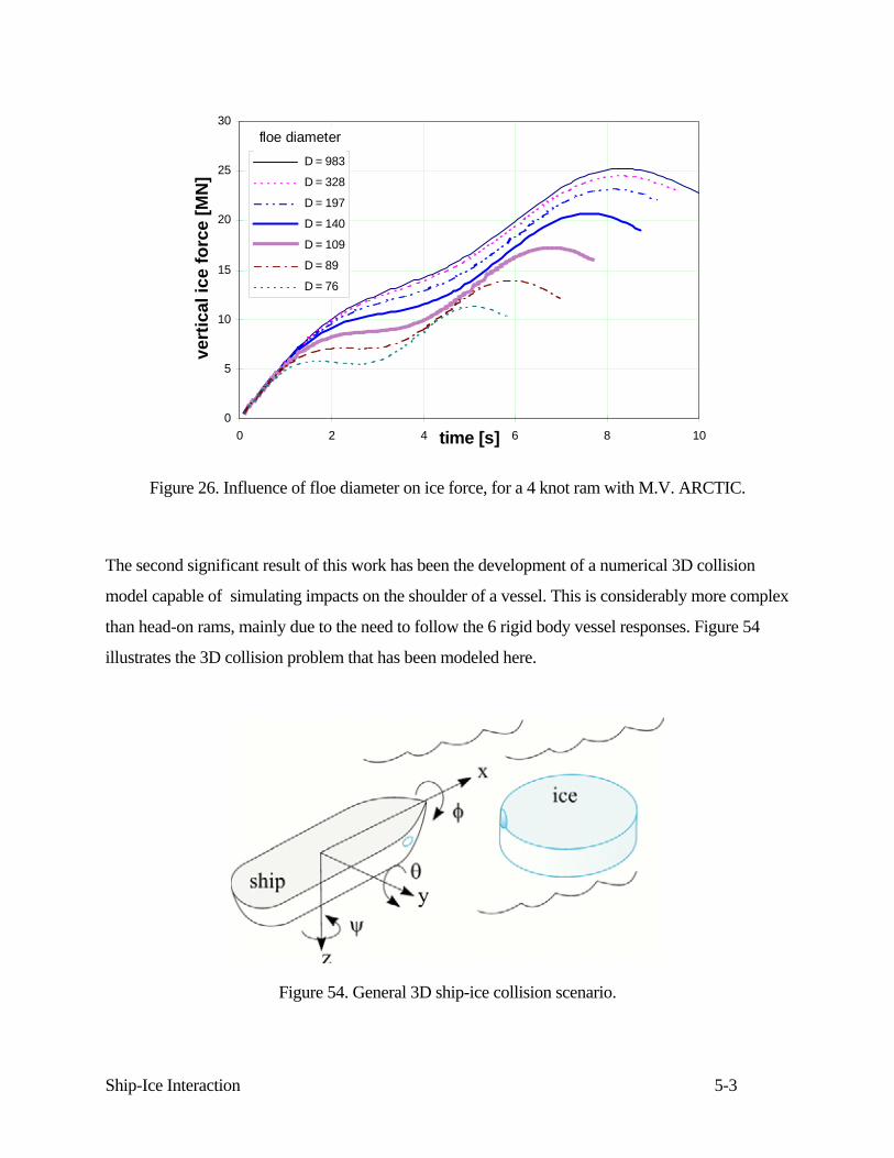
Ship-Ice Interaction 5-3
0
5
10
15
20
25
30
0 2 4 6 8 10time [s]
vert
ical
ice
forc
e [M
N]
D = 983
D = 328
D = 197
D = 140
D = 109
D = 89
D = 76
floe diameter
Figure 26. Influence of floe diameter on ice force, for a 4 knot ram with M.V. ARCTIC.
The second significant result of this work has been the development of a numerical 3D collision
model capable of simulating impacts on the shoulder of a vessel. This is considerably more complex
than head-on rams, mainly due to the need to follow the 6 rigid body vessel responses. Figure 54
illustrates the 3D collision problem that has been modeled here.
Figure 54. General 3D ship-ice collision scenario.
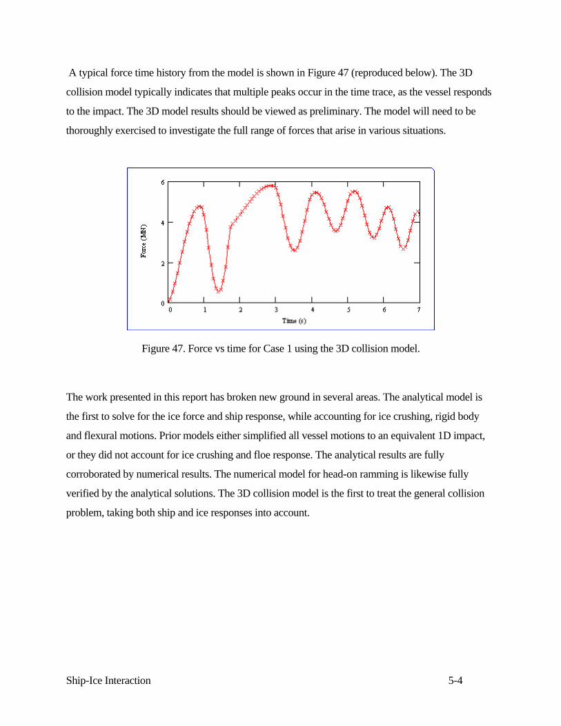
Ship-Ice Interaction 5-4
A typical force time history from the model is shown in Figure 47 (reproduced below). The 3D
collision model typically indicates that multiple peaks occur in the time trace, as the vessel responds
to the impact. The 3D model results should be viewed as preliminary. The model will need to be
thoroughly exercised to investigate the full range of forces that arise in various situations.
Figure 47. Force vs time for Case 1 using the 3D collision model.
The work presented in this report has broken new ground in several areas. The analytical model is
the first to solve for the ice force and ship response, while accounting for ice crushing, rigid body
and flexural motions. Prior models either simplified all vessel motions to an equivalent 1D impact,
or they did not account for ice crushing and floe response. The analytical results are fully
corroborated by numerical results. The numerical model for head-on ramming is likewise fully
verified by the analytical solutions. The 3D collision model is the first to treat the general collision
problem, taking both ship and ice responses into account.
Ship-Ice Interaction 5-5
5.2 Recommendations
There are several new avenues that this work has opened up. The recommendations for further work
are as follows;
• The analytical results should be synthesized into a general rule formula, taking finite
floe size into account. The difficulty here will be in the selection of a suitable floe
size (or size/speed combinations) for design purposes.
• There should be comparison of both analytical and numerical results with available
full scale data, for the purposes of further verifying the results.
• The 3D model requires several improvements, in terms of its efficiency (time to run)
and in presentation of results. Visualization of vessel motions in 3D would also be
very useful. A simplified 3D model, still accounting for full rigid body motions, but
not accounting for movement of the contact location could be developed, and would
likely run almost as fast as the 2D model. Alternatively, the present formulation
would run better if it were programmed in C or FORTRAN.
• The 3D model needs to be verified by comparison with full scale and model scale
data. There are various sources for this data.
• The 3D model will need to be further exercised to full explore the influence of
various parameters, which can lead to the development of a ice load design rule.
Specifically the model should be compared with the Russian rules and models, which
are likewise intended to treat shoulder collisions. (Note: it is believed that the
Russian models are essentially 1D equivalent models. This will need to be checked.)
• The 3D case should be tackled analytically, at least for certain cases, so that the
numerical results can be placed on a solid foundation. Analytical models give a clear
presentation of which parameters and non-dimensional groups govern the results.
Ship-Ice Interaction 6-1
6. REFERENCES
1. Equivalent Standards for the Construction of Arctic Class Ships - Arctic Shipping Pollution
Prevention Regulations, by Transport Canada, Ship Safety, Ottawa, Report No. TP 12260,
©Minister of Supply and Services, Canada, 1995
2. Daley, C., Riska, K., “Formulation of Fmax for Regulatory Purposes, Volume 1 -
Development of Design Ramming Force for Arctic Vessels, Volume 2 - The Determination of
Bow Force of a Ship Ramming a Massive Ice Floe ”, Report by Daley R&E and Helsinki
University of Technology for Canadian Coast Guard Northern, Transport Canada Report No.
TP 12150E, March 1994.
3. Carter, J., et.al. “Maximum Bow Force for Arctic Shipping Pollution Prevention regulations -
Phase II” Report by Memorial University for Transport Canada, Ship Safety Northern,
Transport Canada Report No. TP 12652, January 1996.
4. Kujala “On the statistics of ice load on a ship hull in the Baltic”, Acta Polytechnica
Scandinavica, Mechanics Engineering Series No. 116, helsinki, Finland, 1994.
5. Varsta,P., “On the mechanics of ice load ships in level ice in the Baltic Sea”, Thesis for the
degree of Doctor of Technology, Technical Research Centre of Finland, Publications 11,
Espoo, Finland, 1983.
6. Selvadurai, A., Elastic Analysis of Soil-foundation Interaction, Pub. by Elsevier, Amsterdam,
1979
7. Riska, K., “On the Mechanics of the Ramming Interaction between a Ship and a Massive Ice
Floe”, Thesis for the degree of Doctor of Technology, Technical Research Centre of Finland,
Publications 43, Espoo, Finland, 1987.
8. Sanderson, T.J.O., Ice Mechanics, Riska to Offshore Structures, Grahan and Trotman, London
, 1988.
Ship-Ice Interaction 6-2
9. Meirovitch, L., Analytical Methods in Vibrations, Pub. by MacMillan Co., London, 1967
10. Lindstrom, C., “Ship Interaction with a Single Ice Floe - A Simulation Model” - report from
the Finnish-Canadian Joint Research Project No.5, Helsinki University of Technology, Ship
Laboratory, M169, 1993
11. Riska, et.al., “Ice Impact Model Tests for Three Bow forms of a Vessel”, Vol 1 and 2 ,
Helsinki University of Technology, Ship Laboratory, 1990.
12. Wilson, P.A., "The prediction of manoeuvring characteristics of surface ships in the design
spiral". Advances in Underwater Technology, Ocean Science and Offshore Engineering,
Volume 15: Technology Common to Aero and Marine Engineering. p 237.
13. Rawson, K.J., and Tupper, E.C., Basic Ship Theory, pub. by Longman, Harlow, 3rd Ed. 1983.
14. Popov, Yu. Et.al. “Strength of Ships Sailing in Ice (English Translation) Washington D.C.,
1969 Army Foreign Science and Technology Center, FSTC-HT-23-96-68. 228p.
A1
Appendix A - Listing of 2D Collision Model file: sii_geo2a.mcd

B1
Appendix B - Listing of 3D Collision Model file: sii_rev2a.mcd
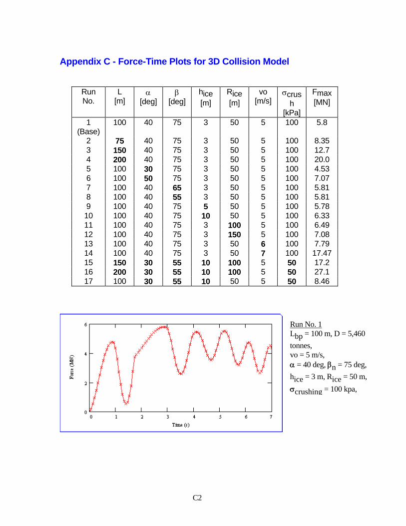
C2
Appendix C - Force-Time Plots for 3D Collision Model
Run No.
L [m]
α [deg]
β [deg]
hice [m]
Rice [m]
vo [m/s]
σcrush
[kPa]
Fmax [MN]
1 (Base)
100 40 75 3 50 5 100 5.8
2 75 40 75 3 50 5 100 8.35 3 150 40 75 3 50 5 100 12.7 4 200 40 75 3 50 5 100 20.0 5 100 30 75 3 50 5 100 4.53 6 100 50 75 3 50 5 100 7.07 7 100 40 65 3 50 5 100 5.81 8 100 40 55 3 50 5 100 5.81 9 100 40 75 5 50 5 100 5.78 10 100 40 75 10 50 5 100 6.33 11 100 40 75 3 100 5 100 6.49 12 100 40 75 3 150 5 100 7.08 13 100 40 75 3 50 6 100 7.79 14 100 40 75 3 50 7 100 17.47 15 150 30 55 10 100 5 50 17.2 16 200 30 55 10 100 5 50 27.1 17 100 30 55 10 50 5 50 8.46
Run No. 1 Lbp = 100 m, D = 5,460 tonnes, vo = 5 m/s, α = 40 deg, βn = 75 deg, hice = 3 m, Rice = 50 m, σcrushing = 100 kpa,
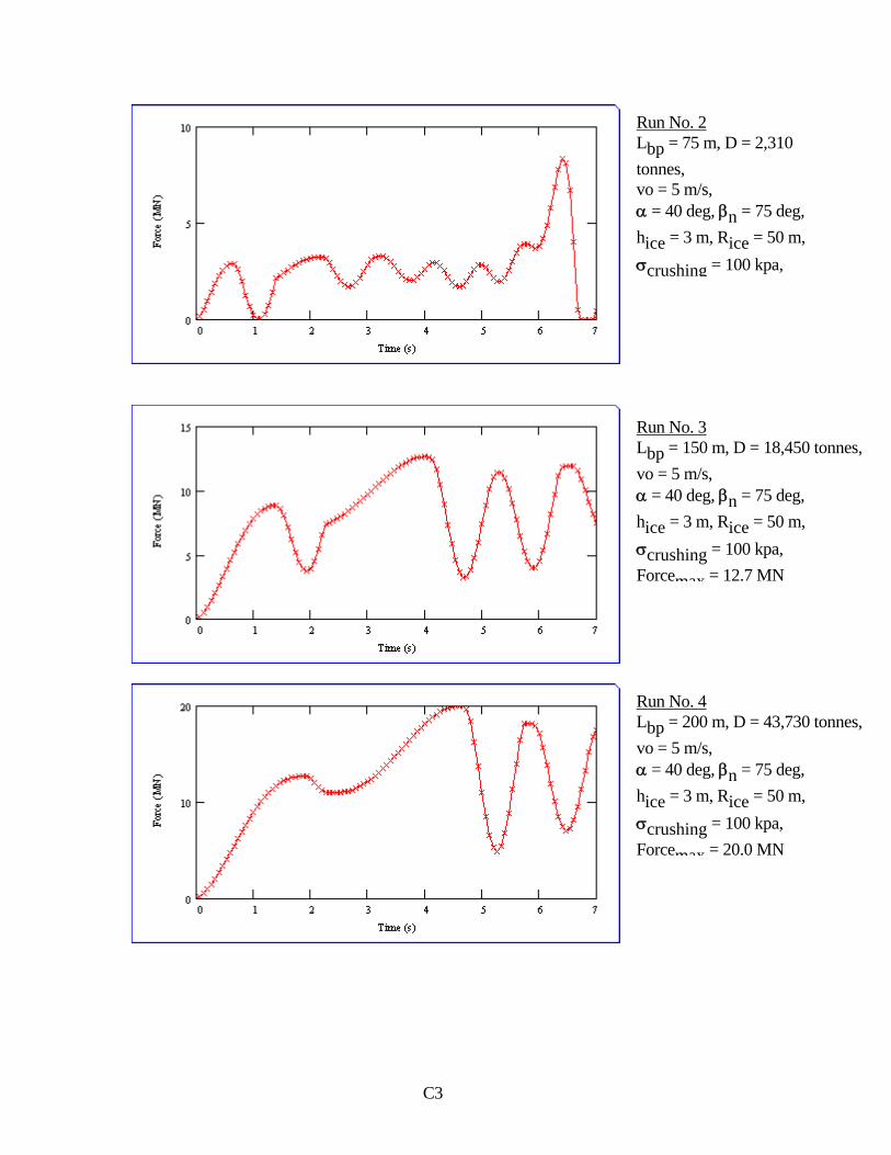
C3
Run No. 2 Lbp = 75 m, D = 2,310 tonnes, vo = 5 m/s, α = 40 deg, βn = 75 deg, hice = 3 m, Rice = 50 m, σcrushing = 100 kpa,
Run No. 3 Lbp = 150 m, D = 18,450 tonnes,vo = 5 m/s, α = 40 deg, βn = 75 deg, hice = 3 m, Rice = 50 m, σcrushing = 100 kpa, Forcemax = 12.7 MN
Run No. 4 Lbp = 200 m, D = 43,730 tonnes,vo = 5 m/s, α = 40 deg, βn = 75 deg, hice = 3 m, Rice = 50 m, σcrushing = 100 kpa, Forcemax = 20.0 MN
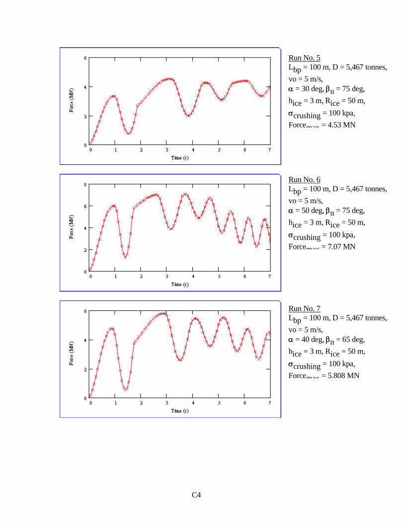
C4
Run No. 5 Lbp = 100 m, D = 5,467 tonnes, vo = 5 m/s, α = 30 deg, βn = 75 deg, hice = 3 m, Rice = 50 m, σcrushing = 100 kpa, Forcemax = 4.53 MN
Run No. 6 Lbp = 100 m, D = 5,467 tonnes, vo = 5 m/s, α = 50 deg, βn = 75 deg, hice = 3 m, Rice = 50 m, σcrushing = 100 kpa, Forcemax = 7.07 MN
Run No. 7 Lbp = 100 m, D = 5,467 tonnes, vo = 5 m/s, α = 40 deg, βn = 65 deg, hice = 3 m, Rice = 50 m, σcrushing = 100 kpa, Forcemax = 5.808 MN
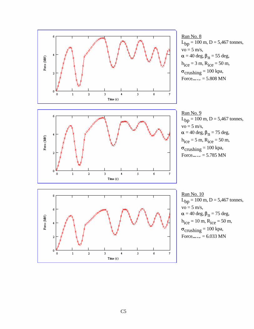
C5
Run No. 8 Lbp = 100 m, D = 5,467 tonnes, vo = 5 m/s, α = 40 deg, βn = 55 deg, hice = 3 m, Rice = 50 m, σcrushing = 100 kpa, Forcemax = 5.808 MN
Run No. 9 Lbp = 100 m, D = 5,467 tonnes, vo = 5 m/s, α = 40 deg, βn = 75 deg, hice = 5 m, Rice = 50 m, σcrushing = 100 kpa, Forcemax = 5.785 MN
Run No. 10 Lbp = 100 m, D = 5,467 tonnes, vo = 5 m/s, α = 40 deg, βn = 75 deg, hice = 10 m, Rice = 50 m, σcrushing = 100 kpa, Forcemax = 6.033 MN
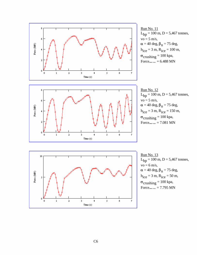
C6
Run No. 11 Lbp = 100 m, D = 5,467 tonnes, vo = 5 m/s, α = 40 deg, βn = 75 deg, hice = 3 m, Rice = 100 m, σcrushing = 100 kpa, Forcemax = 6.488 MN
Run No. 12 Lbp = 100 m, D = 5,467 tonnes, vo = 5 m/s, α = 40 deg, βn = 75 deg, hice = 3 m, Rice = 150 m, σcrushing = 100 kpa, Forcemax = 7.081 MN
Run No. 13 Lbp = 100 m, D = 5,467 tonnes, vo = 6 m/s, α = 40 deg, βn = 75 deg, hice = 3 m, Rice = 50 m, σcrushing = 100 kpa, Forcemax = 7.795 MN
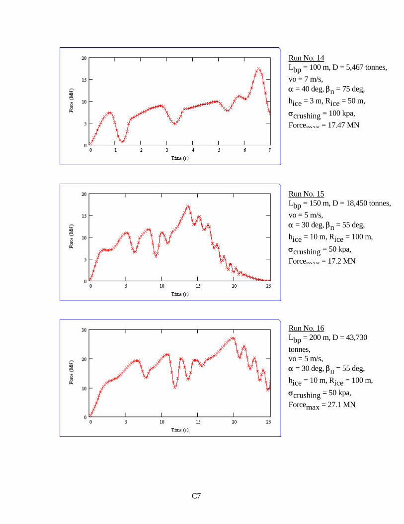
C7
Run No. 14 Lbp = 100 m, D = 5,467 tonnes, vo = 7 m/s, α = 40 deg, βn = 75 deg, hice = 3 m, Rice = 50 m, σcrushing = 100 kpa, Forcemax = 17.47 MN
Run No. 15 Lbp = 150 m, D = 18,450 tonnes,vo = 5 m/s, α = 30 deg, βn = 55 deg, hice = 10 m, Rice = 100 m, σcrushing = 50 kpa, Forcemax = 17.2 MN
Run No. 16 Lbp = 200 m, D = 43,730 tonnes, vo = 5 m/s, α = 30 deg, βn = 55 deg, hice = 10 m, Rice = 100 m, σcrushing = 50 kpa, Forcemax = 27.1 MN

C8
Run No. 17 Lbp = 100 m, D = 5,460 tonnes, vo = 5 m/s, α = 30 deg, βn = 55 deg, hice = 10 m, Rice = 50 m, σcrushing = 50 kpa, Forcemax = 8.46 MN
C9
1 ASPPR Rules 2 Daley &Riska 94 3 Carter et al 96 4 Kujala 94 5 Varsta 83 6 Selvadurai 79 7 Riska 87 8 Sanderson (1988). 9 (Meirovitch 1967) 10 Lindström (1993). 11 Riska, et. al.(1990 12 Wilson 13 Rawson &Tupper 14 Popov (1969
Top Related
Copyright © 2022 FDOKUMEN

