


Bahasa
Halaman
Hukum

SCHOOLING ATTAINMENT, SCHOOLING EXPENDITURES, AND TEST SCORES
WHAT CAUSES ECONOMIC GROWTH?
Theodore R. Breton
No. 13-16
2013
Schooling Attainment, Schooling Expenditures, and Test Scores
What Causes Economic Growth?
Theodore R. Breton
Universidad EAFIT
May 9, 2013
Abstract
Using a dynamic augmented Solow model, I estimate the effect of students’ schooling
attainment, schooling expenditures, and students’ test scores on growth rates over the period
1985-2005. I also estimate the effect of related measures for human capital stocks on national
income in a static model in 2005. Individually all of the measures cause growth, and when
included in the same model, more than one is statistically significant. Relative measurement
error appears to determine which measure provides the best results. The results support the
importance of increases in human capital for growth and the validity of the augmented Solow
model.
Key Words: Schooling Attainment; Schooling Expenditures, Test Scores, Economic Growth
JEL Codes: O41; I25
Hanushek and Woessmann [2008, 2012a, and 2012b] (hereafter HW) averaged available
student scores on international tests of science and mathematics between 1964 and 2006 to create
a measure of students’ cognitive skills for a large set of countries. They show that this measure
explains three times as much of the variation in national growth rates during 1960-2000 as
adults’ average schooling attainment in 1960 and that when both measures are included in their
growth model, average schooling attainment in 1960 has no effect on growth.
HW [2008 and 2012a] interpret their empirical results to mean that students’ cognitive
skills at ages 9 to 15 determine economic growth and that schooling only affects growth to the
degree that it raises students’ cognitive skills. They document the low level of students’
cognitive skills in developing countries and argue that increases in schooling attainment have a
limited effect on growth because schools in developing countries do not reliably raise students’
skills.
Breton [2011] disputes HW’s [2008] finding that students’ average test scores explain
income differences much better than adults’ average schooling attainment. He argues that their
analysis is flawed because their average test scores are a proxy for workers’ human capital in
2010, ten years after their growth period and fifty years after their measure of adult schooling
attainment. He shows that when their average scores and adults’ average schooling attainment in
2000 are compared, either measure can explain differences in national income in 2000, but
adults’ schooling attainment explains more of the variation than average test scores.1
HW [2012a and 2012b] present additional estimates of essentially the same growth model
used in HW [2008]. They use a slightly larger data set with test scores obtained during 1964-
2006 and several instruments for test scores, and again they show that average test scores explain
economic growth much better than adults’ schooling attainment in 1960. In HW [2012a] they
claim that adults’ average schooling in Latin America in 1960 did not produce the expected
economic growth during 1960-2000 because students (mostly tested in 1997 and in 2006) did not
acquire adequate cognitive skills while in school.
HW [2008 and 2012b] argue that their findings provide direction for a nation’s
educational strategy, because they show that better schools, as measured by students’ test scores,
1 A number of other recent studies show that increases in average schooling attainment cause growth, including
Cohen and Soto [2007], Breton [2013a], and Gennaioli, La Porta, Lopez-de-Silanes, and Shleifer [2013].
can raise a nation’s future level of income. Using their estimated coefficients on average test
scores, they estimate how much growth rates could increase if students’ test scores were raised.
Breton’s [2011] results suggest that HW have misinterpreted their findings. If their
comparison of adults’ average schooling attainment and students’ average test scores is invalid
and either can explain growth, then implicitly both measures are a proxy for a nation’s human
capital, and HW’s estimated coefficient on average test scores measures the effect of increasing a
nation’s human capital on growth, not solely the effect of raising students’ skills at ages 9 to 15.
If children’s test scores are an incomplete measure of a nation’s human capital, then other
aspects of their human capital are omitted variables in HW’s growth model, and their results do
not provide clear guidance for educational policy. Increasing other components of a nation’s
human capital, such as the share of the population completing secondary school, might be more
feasible or more cost-effective than increasing children’s test scores as a means to increase
economic growth.2
In this paper I investigate whether students’ average test scores are the key determinant of
a nation’s future growth rate, or just a proxy for a nation’s level of human capital. I begin this
investigation by specifying a theoretically-consistent growth model and selecting estimation
periods that are appropriate for the vintage of the test scores. I then compare the estimated effect
of average test scores and two other measures of human capital, being careful to use measures
that are appropriate for the specified models and that represent the correct time period. I
estimate the growth models with each measure separately and with combinations of these
measures to determine whether the effect of average test scores is robust to the inclusion of the
other measures in the model.
For reasons explained in detail below, I use a dynamic version of the augmented Solow
model as the primary model for this analysis. This model includes the statistically-significant
variables in HW’s model, but in a different mathematical form, and it also has other differences
that are important for proper model specification. This model estimates the effect of flows of
human capital on growth rates, so I compare three measures of these flows during the estimation
period: students’ average test scores, average schooling expenditures, and students’ (not adults’)
average schooling attainment.
2 HW [2008, P. 658] observe that “student achievement has been relatively impervious to a number of interventions
that have been tried by countries around the world.”
I also examine the effect of three measures of human capital in a static version of the
augmented Solow model. The static model examines the effect of changes in capital stocks
rather than capital flows. My stock measures are students’ (earlier) average test scores, the
cumulative earlier investment in workers’ schooling, and adults’ average schooling attainment.
Since the measurement error differs in the stock and flow data, the empirical results from the
dynamic and static models provide information on whether differences in the estimated
coefficients for the different measures are due to the aspect of human capital measured or to
differences in the accuracy of the data.
For the dynamic model the estimation period is 1985-2005 and for the static model it is
2005. I estimate all of the models using both OLS and 2SLS, with instruments for the human
capital measures.
Overall my empirical results differ substantially from HW’s results. I first examine the
data and show that across countries adults’ average schooling attainment (in years) is highly
correlated with (the log of) the financial stock of human capital. These results contradict HW’s
[2008, 2012a, and 2012b] repeated claim that average schooling attainment is not a good
measure of human capital across countries.
I then show that in the dynamic models average test scores, average schooling
expenditures, and students’ average schooling attainment all provide similar, statistically-
significant estimates of the effect of human capital on growth. All of the models have estimated
coefficients on physical capital and initial income that correspond to the expected results for a
dynamic augmented Solow model. Subsequently, I show that in the static models average test
scores, the financial stock of human capital, and adults’ average schooling attainment provide
similar, statistically-significant estimates of the effect of human capital on national income.
Since each measure of schooling quantifies a different aspect of a nation’s human capital,
the effects of the measures are not mutually exclusive. When two or more measures are included
in the same model, generally at least two are statistically significant. These results indicate that
children’s cognitive skills are not the only component of human capital that contributes to
economic growth.
The average test score measure provides good estimates of the effect of human capital in
the growth model, and it explains more of the variation in growth rates than the other two
measures. But the opposite is the case in the static model where the average test score measure
explains less of the variation in national income than the other two measures. In each set of
models, the human capital measure with the data that appear to be most accurate, provides the
best statistical estimates of the effect of human capital on growth or income.
HW [2012a] show that students’ scores on international tests in Latin America are low
compared to other regions with similar adult levels of schooling attainment. In my results either
average schooling expenditures or average test scores explain growth. One possible
interpretation is that average schooling expenditures/year of schooling are relatively low in Latin
America. This interpretation is consistent with the relatively high pupil-teacher ratios in primary
school in Latin America.
Overall the results presented in this paper support the validity of the augmented Solow
growth model and provide considerable evidence that increases in human capital cause economic
growth. The results support HW’s contention that increases in students’ cognitive skills, as
measured by average test scores, raise the rate of economic growth, but they reject their
contention that cognitive skills measured at ages 9 to 15 are the only aspect of human capital that
causes growth.
The rest of the paper is organized as follows: Section II presents the conceptual
framework and specifies the econometric models. Section III describes the data. Section IV
presents the empirical results. Section V presents additional analysis of the effect of schooling
expenditures on student achievement. Section VI concludes.
II. Methodological Considerations
HW [2008, 2012a, and 2012b] use the following model to estimate the effect of average
test scores on growth rates:
1) d(Y/cap)/dt = α0 + α1 Sch-1960i + α2 AvgTSi + α3 Y/cap-1960i + α4 Xi + ɛi
In this model d(Y/cap)/dt is the annual average growth rate in real GDP/capita during 1960-
2000, Sch-1960 is adults’ average schooling attainment in 1960, AvgTS is average student test
scores during 1964-2006, Y/cap-1960 is GDP/capita in 1960, and X are other conditioning
variables that differ in each of their articles. This model does not correspond to any particular
growth theory, and HW do not explain why these particular variables are included in their model.
HW include the initial level of GDP/capita in all of their models, which is included in
neoclassical models to control for the state of convergence on the steady-state growth rate. But
HW’s growth model is not a neoclassical model. Neoclassical models do not include a variable

for the initial human capital stock, since in this model the change in this stock, and not its initial
level, determines the rate of growth [Acemoglu, 2009]. In a dynamic neoclassical model, the
effect of the initial capital stocks is captured in the initial level of GDP/capita, which unlike their
model, is included in log form. Since the initial level of GDP/capita and the initial level of
schooling/capita are measuring the same thing, it is not surprising that in all of HW’s empirical
results, the estimated coefficient on the initial level of schooling is insignificant.3
The most unusual aspect of their model is that it includes the average schooling
attainment of the adult population in 1960 and the average test scores of students obtained during
1964-2006 (or for most developing countries during 1990-2006). These two variables do not
measure the characteristics of the same population at the same time, so it is impossible to
conclude anything about whether students’ level of schooling or their test scores is more
important for growth.
Conceptual Framework for the Analysis
I begin my analysis by selecting a conceptual framework for specifying all of the
econometric models. Given the choices of either an endogenous or a neoclassical growth model,
I adopt the neoclassical, augmented Solow model for six reasons.
First, the structure of the neoclassical model is consistent with the widely-accepted
Mincerian relationship between workers’ salaries and their level of schooling, while the structure
of the endogenous model is not [Krueger and Lindahl, 2001]. The Mincerian model and the
neoclassical model assume that increases in human capital rather than the level of human capital
raise income, and both models exhibit diminishing returns [Breton, 2013b].
Second, the empirical evidence rejects the endogenous growth model [Jones, 1995 and
Lau, 2008]. The endogenous growth model predicts that increases in physical capital and/or
R&D will lead to permanent increases in the rate of economic growth, and the empirical
evidence indicates that this is not the case.
Third, Mankiw, Romer, and Weil [1992], Breton [2004], Cohen and Soto [2007], Ding
and Knight [2009], and Breton [2013a] present evidence that over long periods the augmented
Solow model explains economic growth across countries quite well.
3 In HW [2012a and 2012b] the initial levels of income, physical capital, and average schooling attainment are all
included in the model. Neither coefficient on the two initial stocks of capital is significant.
Fourth, Barro and Sala-i-Martin [2004] show that growth patterns across countries exhibit
the conditional convergence predicted by the neoclassical model.
Fifth, Breton [2013b] shows that after accounting for schooling’s external effects on
physical capital in the augmented Solow model, the model’s estimate of the effect of schooling
on national income in is consistent with micro estimates of the direct and external effects of
schooling on workers’ salaries. He also presents evidence that no important variables are
omitted in the augmented Solow model.
Sixth, in the particular case of the HW analyses, their regression results consistently
reject the importance of initial human capital and support conditional convergence. So if there is
a valid existing conceptual model that is consistent with HW’s statistical correlations, it is a
dynamic version of the neoclassical model.
Mankiw, Romer, and Weil’s [1992] Dynamic Neoclassical Model
Mankiw, Romer, and Weil’s (hereafter MRW) augmented Solow model is well-known,
but it is useful to review its formal specification:
2) Yt = Kt α
Ht β (A0 e
gt Lt)
1-α-β
In this model, GDP or national income (Y) changes over time (t) in response to changes in
physical capital (K), human capital (H), labor (L), and total factor productivity (A), which is
assumed to grow at a constant rate g. In this model α + β < 1, so increases in physical capital or
human capital, or the two together, raise income, but at a diminishing rate. As a consequence,
when investment rates are a stable fraction of GDP, a country’s rate of economic growth
converges on the steady state rate g.
MRW derive the mathematical structure for a dynamic version of this model, in which
growth is modeled as convergence to the steady state. As a consequence, the growth rate
includes a permanent, steady-state component (gt) and a temporary, transitional component. The
transitional component varies in size depending on the difference between the magnitude of the
capital stock/worker entering the economy (implicit in y*) and the capital stock/worker already
in the economy (implicit in y0). The variation in this difference across countries creates the
difference in growth rates during convergence. Mathematically, the equation is:
3) ∆ ln(Y/L)t = gt + (1-e–λt
) ln(y*) – (1-e–λt
) ln(y0)
Where y = Y/(egt
L), which is constant (y*) in the steady state. MRW show that in equilibrium
y* is a function of the shares of GDP invested in human and physical capital (sh and sk), the rate
of growth in the labor force (n), and the rates of depreciation of the stocks of physical and human
capital (δk and δh):
4) y* = α/(1-α-β) [log (sk)/(n + g + δk)] + β/(1-α-β) [log (sh)/(n + g + δh)]
Substitution of equation (4) into equation (3) creates the dynamic version of the model:
5) ∆ ln(Y/L)t = gt + (1-e–λt
) (α/(1-α-β) [ln (sk)/(n+g+δk)] + (1-e–λt
) β/(1-α-β) [ln (sh)/(n+g+δh)] –
(1-e–λt
) log(Y/L)0 + (1-e–λt
) log(A0)
Importantly, in this model the shares of investment measure the flow of physical and human
capital resources into the economy. Alternative measures of human capital, such as average test
scores, must be used in this model with this conceptual requirement in mind.4
The average test score for a cohort of students is a measure of the human capital of a
cohort of future workers. Students’ average test scores over time can be considered a measure of
the changing flow of human capital into the economy. Given the nature of the schooling process,
these scores represent this flow with a lag of 5-10 years. So the average score for a cohort of
students is a proxy for the amount of human capital flowing into the economy 5-10 years later.
Although sk and sh are constant in equation (4), the model remains conceptually valid if sk
and sh are the average shares of GDP invested during the convergence period. If these shares are
not constant, then implicitly yt is converging on a moving target y*t. Although variation in y*t
introduces measurement error into an estimate of the convergence rate λ, the bias is likely to be
small, as long as the variation in ln(average y*t) during the period of estimation is small relative
to the difference between ln(average y*t) and ln(y0).
Student’s average scores on international tests are an innovative cross-country measure of
human capital, but conceptually the measure only represents the human capital of the school-age
population that is in school. Its practical limitation is that for most developing countries average
test scores are only available since 1990.
HW [2008] use these scores to represent workers’ skills at an earlier time by assuming
that workers in developing countries during 1960-2000 had the same cognitive skills as the
students tested during 1990-2006. Cohen and Soto’s [2007] data on the schooling of the work 4 Since HW do not specify a conceptual growth model for their analyses, it is not clear whether they use average
tests scores during 1964-2006 to represent a flow of human capital during 1960-2000 or the stock of human capital
in some year. Since they compare these scores to average schooling attainment in 1960, it appears that they are
assuming that students’ average test scores during 1964-2006 represent the human capital of workers in 1960, which
clearly they do not. They obtain good results for average test scores and not for adults’ schooling attainment in 1960
because the dynamic neoclassical model requires a measure of the average flow of human capital into the economy,
and students average test scores over the 1964-2003 period are a measure of this average flow.
force during 1960-2010 clearly show that HW’s assumption is not plausible. A very large share
of workers in developing countries during their growth period had little or no schooling.
In developed countries students’ average scores on the same international test increase by
about 1/3 of a standard deviation (33 points compared to an OECD mean score of 500) for each
additional year that they remain in school [Fuchs and Woessmann, 2006, Juerges and Schneider,
2004, and Woessmann, 2003]. Since prior to 1990 a large share of the population of school age
in developing countries was not in school, if they had been tested, clearly their scores would
have been substantially lower than the scores of the students tested in the 1990s.
The model in equation (4) is estimated in log form, so trends in average scores over the
growth period do not bias the estimated coefficients, as long as the trends are similar across
countries. Cohen and Soto’s [2007] data clearly show, however, that the trends in primary and
secondary school attendance were quite different in developed and developing countries over the
1960-2000 period. So the trends in the cognitive skills of the school age population are also
likely to have been very different.
One solution to this problem is to estimate the growth model over a later period when a
much higher share of the school age population in developing countries attended school until the
age that the tests were given. The estimates of the growth model in equation (5) using average
test scores are likely to be more accurate if the estimation period begins much later than 1960.
Econometric Model Specification and Period of Estimation
Although a period beginning after 1995 would provide the best match for the test scores
obtained in developing countries, estimation of growth models over very short periods increases
the measurement error in the other data. National growth rates are unstable over short periods
due to economic cycles, and the differencing of data over short periods reduces the signal-to-
noise ratio [Krueger and Lindahl, 2001].
Based on these considerations, I estimate the growth model over the 1985-2005 period.
This period corresponds relatively well to the period the tests were given, it is long enough to
provide good results in the convergence model, and economic data are available to estimate
models through 2005.
I estimate the static model in 2005. By this time most of the students tested in developed
countries over the 1964-2003 period were in the work force, so the average of their scores is
representative of the human capital of the work force in 2005. Since the test scores in the
developing countries are mostly from the 1990-2006 period, the average of their scores are not as
representative of human capital in 2005, so a priori I expect average test scores to be a less
accurate measure of human capital in the static model than in the growth model.
As explained below, the relative accuracy of the data for the flows and the stocks of
schooling attainment has the opposite pattern. The data for adults’ average schooling attainment
in 2005 are likely to be more accurate than the data for students’ average schooling attainment
during 1985-2005.
The conceptual specification for human capital in the augmented Solow model is
financial, so the form required for these data in the dynamic and static models is clear. In the
growth model these data are the share of GDP invested in schooling, while in the static model
they are the net financial stock of human capital [OECD, 2001].
Since there is a lag between investment in schooling and the entry of students into the
work force, I use the average investment in schooling during 1980-2000 to represent the flow of
human capital into the economy during 1985-2005. Although on average, the lag can be longer
than five years, higher levels of schooling cost more and the lag between expenditures and
students’ entry into the work force is shorter for higher levels. Five years is a good average lag
from a financial standpoint. For 2005 I use the net stock of human capital calculated from
cumulative investment in schooling less depreciation during the prior 40-year period, again
lagged five years. This investment includes public and private expenditures, the cost of capital
during schooling and students’ foregone earnings. The detailed methodology for this calculation
is presented in Breton [2013b].
Average schooling attainment of the population 15 to 64 is a measure of the stock of
human capital, so I use this measure for 2005 in the static model. The corresponding flow of
schooling attainment is the average years of schooling for students (not adults) of primary,
secondary, and tertiary school age. Again I use average attainment during 1980-2000 to
represent the flow of resources into the economy during 1985-2005.
Mathematical Relationships Between the Measures of Human Capital
Utilization of the average test score data and the schooling attainment data as proxies for
the financial data requires some care because the data for these measures do not have a linear
relationship to the financial data. If an inappropriate form of these data is used to estimate the
models, the resulting model is mis-specified and the estimated coefficients will be biased.
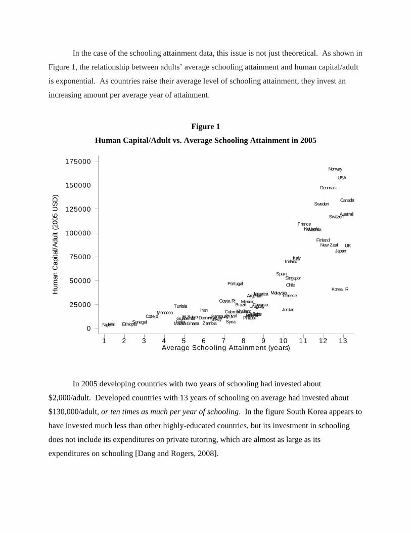
In the case of the schooling attainment data, this issue is not just theoretical. As shown in
Figure 1, the relationship between adults’ average schooling attainment and human capital/adult
is exponential. As countries raise their average level of schooling attainment, they invest an
increasing amount per average year of attainment.
Figure 1
Human Capital/Adult vs. Average Schooling Attainment in 2005
In 2005 developing countries with two years of schooling had invested about
$2,000/adult. Developed countries with 13 years of schooling on average had invested about
$130,000/adult, or ten times as much per year of schooling. In the figure South Korea appears to
have invested much less than other highly-educated countries, but its investment in schooling
does not include its expenditures on private tutoring, which are almost as large as its
expenditures on schooling [Dang and Rogers, 2008].
Hum
an C
apital/A
dult (
2005 U
SD
)
Average School ing Attainment (years)1 2 3 4 5 6 7 8 9 10 11 12 13
0
25000
50000
75000
100000
125000
150000
175000
Argentin
Australi
Austria
Bolivia
Brazil
Canada
Chile
Colombia
Costa Ri
Cote d`I
Denmark
DominicaEcuadorEgyptEl Salva
Ethiopia
Finland
France
Ghana
Greece
GuatemalIndia
Iran
IrelandItaly
Jamaica
Japan
Jordan
Korea, R
Malawi
Malaysia
Mali
Mexico
Morocco
Netherla
New Zeal
Niger
Norway
Panama
ParaguayPeru
Philippi
Portugal
Senegal
SingaporSpain
Sweden
Switzerl
Syria
ThailandTunisia
Turkey
UK
Uruguay
USA
Zambia
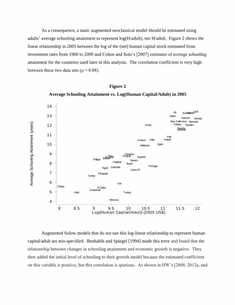
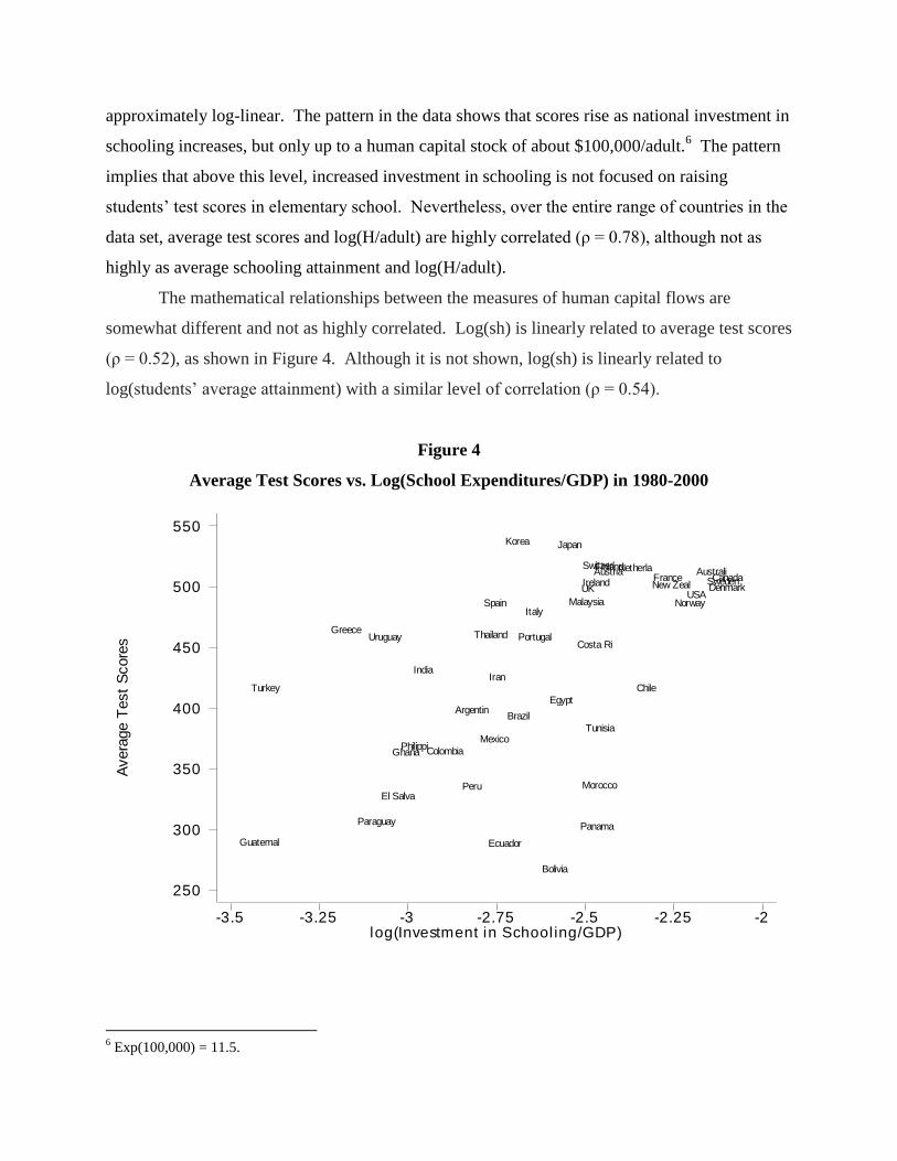
As a consequence, a static augmented neoclassical model should be estimated using
adults’ average schooling attainment to represent log(H/adult), not H/adult. Figure 2 shows the
linear relationship in 2005 between the log of the (net) human capital stock estimated from
investment rates from 1960 to 2000 and Cohen and Soto’s [2007] estimates of average schooling
attainment for the countries used later in this analysis. The correlation coefficient is very high
between these two data sets (ρ = 0.88).
Figure 2
Average Schooling Attainment vs. Log(Human Capital/Adult) in 2005
Augmented Solow models that do not use this log-linear relationship to represent human
capital/adult are mis-specified. Benhabib and Spiegel [1994] made this error and found that the
relationship between changes in schooling attainment and economic growth is negative. They
then added the initial level of schooling to their growth model because the estimated coefficient
on this variable is positive, but this correlation is spurious. As shown in HW’s [2008, 2012a, and
Avera
ge S
choolin
g A
ttain
ment
(years
)
Log(Human Capital/Adul t) (2005 US$)8 8.5 9 9.5 10 10.5 11 11.5 12
4
5
6
7
8
9
10
11
12
13
14
Argentin
Australi
Austria
Bolivia
Brazil
Canada
Chile
ColombiaCosta Ri
Denmark
Ecuador
Egypt
El Salva
FinlandFrance
Ghana
Greece
GuatemalIndia
Iran
IrelandItaly
Japan
Korea
Malaysia
Mexico
Morocco
Netherla
New ZealNorway
Panama
Paraguay
Peru
Philippi
Portugal
Spain
Sweden
Switzerl
Thailand
Tunisia
Turkey
UK
Uruguay
USA
2012b] results, the positive estimated coefficient on the initial level of schooling is not robust to
the inclusion of correctly-specified human capital variables in a growth model.
As part of their comprehensive review of the growth literature, Krueger and Lindahl
[2001] discuss the inconsistency between Benhabib and Spiegel’s linear income-schooling
specification and the standard assumption in the Mincerian model. They show that the log-linear
relationship provides better empirical results. Cohen and Soto [2007] and Breton [2011, 2013a,
and 2013b] also discuss the necessity of using the log-linear relationship in the augmented Solow
model.
HW [2008, 2012a, and 2012b] mischaracterize the relationship between average
schooling attainment and human capital, which has led them to claim repeatedly and incorrectly
that average schooling attainment is a very inaccurate proxy for human capital across countries.
As an example, in HW [2012b] they state:
“…all analyses using average years of schooling as the human capital measure
implicitly assume that a year of schooling delivers the same increase in
knowledge and skills regardless of the education system. For example, a year of
schooling in Peru is assumed to create the same increase in productive human
capital as a year of schooling in Japan.”5
This statement is incorrect. The log-linear relationship between human capital and
schooling implies that two countries with the same level of average attainment have the same
level of human capital (e.g., Japan and the U.S). But each additional year of schooling does not
increase human capital by the same amount, even within the same country. Each additional year
of average attainment has an exponential effect on a country’s human capital/adult and on its
GDP/adult. Since average schooling attainment is much greater in Japan than in Peru, an
additional year of schooling in Japan raises human capital by much more than an additional year
in Peru.
There is no reason to expect that countries with similar levels of average schooling
attainment would have similar levels of human capital. Countries that have provided their adults
with the same average years of schooling could have provided very different amounts of
education to these adults. But in practice this seems not to be the case.
5 HW, 2012b, p. 269.

Curriculums are very similar across the globe, even in the same year of schooling.
International tests of student achievement are only possible because students of the same age
study the same subjects. As a consequence, all of the countries that participate in international
testing programs educate their students using relatively similar curriculums. And as shown in
Figure 1, the net financial stock of human capital rises quite consistently across countries as they
raise their adult population’s average schooling attainment.
While the log-linear mathematical relationship between human capital/adult and average
schooling attainment is well-known, the appropriate relationships for other measures of the flow
or stock of human capital, such as average test scores, have not been rigorously analyzed in the
literature. Figure 3 shows the relationship between average test scores and log(human
capital/adult) in 2005. As with average schooling attainment, this relationship appears to be
Figure 3
Average Test Scores vs. Log(Human Capital/Adult) in 2005
Avera
ge T
est
Score
s
Log(Human Capital/Adul t) (2005 US$)8 8.5 9 9.5 10 10.5 11 11.5 12
250
300
350
400
450
500
550
Argentin
AustraliAustria
Bolivia
Brazil
Canada
Chile
Colombia
Costa Ri
Denmark
Ecuador
Egypt
El Salva
FinlandFrance
Ghana
Greece
Guatemal
IndiaIran
Ireland
Italy
JapanKorea
Malaysia
Mexico
Morocco
Netherla
New Zeal
Norway
PanamaParaguay
Peru
Philippi
Portugal
Spain
Sweden
Switzerl
Thailand
Tunisia
Turkey
UK
Uruguay
USA
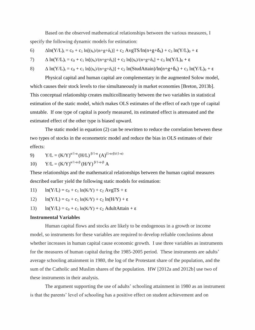
approximately log-linear. The pattern in the data shows that scores rise as national investment in
schooling increases, but only up to a human capital stock of about $100,000/adult.6 The pattern
implies that above this level, increased investment in schooling is not focused on raising
students’ test scores in elementary school. Nevertheless, over the entire range of countries in the
data set, average test scores and log(H/adult) are highly correlated (ρ = 0.78), although not as
highly as average schooling attainment and log(H/adult).
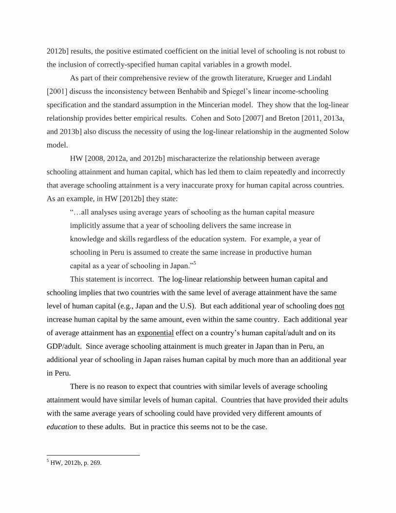
The mathematical relationships between the measures of human capital flows are
somewhat different and not as highly correlated. Log(sh) is linearly related to average test scores
(ρ = 0.52), as shown in Figure 4. Although it is not shown, log(sh) is linearly related to
log(students’ average attainment) with a similar level of correlation (ρ = 0.54).
Figure 4
Average Test Scores vs. Log(School Expenditures/GDP) in 1980-2000
6 Exp(100,000) = 11.5.
Avera
ge T
est
Score
s
l og(Investment in School ing/GDP)-3.5 -3.25 -3 -2.75 -2.5 -2.25 -2
250
300
350
400
450
500
550
Argentin
AustraliAustria
Bolivia
Brazil
Canada
Chile
Colombia
Costa Ri
Denmark
Ecuador
Egypt
El Salva
FinlandFrance
Ghana
Greece
Guatemal
IndiaIran
Ireland
Italy
JapanKorea
Malaysia
Mexico
Morocco
Netherla
New Zeal
Norway
PanamaParaguay
Peru
Philippi
Portugal
Spain
Sweden
Switzerl
Thailand
Tunisia
Turkey
UK
Uruguay
USA
Based on the observed mathematical relationships between the various measures, I
specify the following dynamic models for estimation:
6) ∆ln(Y/L)t = c0 + c1 ln[(sk)/(n+g+δk)] + c2 AvgTS/ln(n+g+δh) + c3 ln(Y/L)0 + ɛ
7) ∆ ln(Y/L)t = c0 + c1 ln[(sk)/(n+g+δk)] + c2 ln[(sh)/(n+g+δh] + c3 ln(Y/L)0 + ɛ
8) ∆ ln(Y/L)t = c0 + c1 ln[(sk)/(n+g+δk)] + c2 ln(StudAttain)/ln(n+g+δh) + c3 ln(Y/L)0 + ɛ
Physical capital and human capital are complementary in the augmented Solow model,
which causes their stock levels to rise simultaneously in market economies [Breton, 2013b].
This conceptual relationship creates multicollinearity between the two variables in statistical
estimation of the static model, which makes OLS estimates of the effect of each type of capital
unstable. If one type of capital is poorly measured, its estimated effect is attenuated and the
estimated effect of the other type is biased upward.
The static model in equation (2) can be rewritten to reduce the correlation between these
two types of stocks in the econometric model and reduce the bias in OLS estimates of their
effects:
9) Y/L = (K/Y)α/1-α
(H/L) β/1-α
(A)(1-α-β)/(1-α)
10) Y/L = (K/Y)α/1-α-β
(H/Y) β/1-α-β
A
These relationships and the mathematical relationships between the human capital measures
described earlier yield the following static models for estimation:
11) ln(Y/L) = c0 + c1 ln(K/Y) + c2 AvgTS + ɛ
12) ln(Y/L) = c0 + c1 ln(K/Y) + c2 ln(H/Y) + ɛ
13) ln(Y/L) = c0 + c1 ln(K/Y) + c2 AdultAttain + ɛ
Instrumental Variables
Human capital flows and stocks are likely to be endogenous in a growth or income
model, so instruments for these variables are required to develop reliable conclusions about
whether increases in human capital cause economic growth. I use three variables as instruments
for the measures of human capital during the 1985-2005 period. These instruments are adults’
average schooling attainment in 1980, the log of the Protestant share of the population, and the
sum of the Catholic and Muslim shares of the population. HW [2012a and 2012b] use two of
these instruments in their analysis.
The argument supporting the use of adults’ schooling attainment in 1980 as an instrument
is that the parents’ level of schooling has a positive effect on student achievement and on
political support for providing financial resources to schools. Juerges and Schneider [2004] and
Parcel and Dufur [2009] document the positive effect of parental education on students’ test
scores in mathematics achievement. Rubinfeld and Shapiro [1989] show that voter support for
public school expenditures in the U.S. is positively related to income and education levels.
Adults’ average attainment in 1980 would be an invalid instrument if it caused growth
directly, as hypothesized in endogenous growth theory, but as mentioned earlier, the evidence
rejects endogenous growth theory. In the dynamic version of the neoclassical model, growth
rates are affected by the change in the level of schooling, not by the initial level. The initial level
of GDP in 1985 is affected by the initial level of schooling attainment in 1985, which is highly
correlated with the level in 1980, but since the initial level of income in 1985 is already in the
growth model, conceptually the level of schooling attainment in 1980 is not likely to have any
additional direct effect.
The shares of the population affiliated with different religions are attractive instruments
because these measures are not endogenous in the economic growth process and they are
correlated with measures of human capital. Catholic/Muslim affiliation and the log of Protestant
affiliation are inversely correlated (ρ = -0.53), but they have different patterns across countries,
so both instruments can be used in the same model.
Most countries have some level of Protestant affiliation, and the Protestant share of the
population has been positively correlated with schooling levels and with expenditures on
schooling for centuries [Means, 1966, Cipolla, 1969, Johansson, 1981, Soysal and Strang, 1989,
and Goldin and Katz, 1998]. The correlations apparently exist because Protestant doctrine
emphasizes the responsibility of members to read the Bible and the responsibility of the
community to ensure that each member develops this capability. The log of the Protestant share
in 1980 is highly correlated with average schooling attainment in 2005 (ρ = 0.55) and with
log(H/Y) in 2005 (ρ = 0.58).
The validity of the Protestant share of the population as an instrument for schooling is
somewhat controversial because there are hypotheses that Protestant affiliation creates a
“Protestant Ethic” that affects the economy in ways other than just through schooling. Despite
their popularity, these hypotheses have been tested and consistently rejected [Iannocconne,
1998]. Recently, Becker and Woessmann [2009 and 2010] show that Protestant counties in the
19th
century had higher incomes than Catholic counties, but they also show that differences in
educational levels explain the income differences. Arruñada [2010] presents evidence rejecting
the hypothesis that Protestants have a greater work ethic today than Catholics. Breton [2004]
shows that Protestant affiliation is not correlated with indices for institutional characteristics that
include measures of corruption.
Protestant affiliation has a positive correlation with average test scores, but the
correlation is too weak for it to serve as an instrument (ρ = 0.23). However, Catholic/Muslim
affiliation can serve as an instrument because it has a strong negative correlation with average
test scores (ρ = -0.48). Two possible explanations for this relationship are the higher emphasis in
Catholic/Muslim societies on family relationships for employment and the relatively low
tolerance in the Catholic and Muslim religions for scientific or other ideas that may be perceived
to contradict religious dogma. Arruñada [2010] presents evidence from 32 countries that
Catholics prefer personal exchange and family-related occupations more than Protestants.
Mansouri [2007] argues that Muslim theologians have opposed science because they perceive
scientific ideas as a challenge to Islamic religious beliefs.
III. Data for Estimation of the Models
Two sets of data are required to estimate the models, one for the period 1985-2005 and
one for 2005. Both sets include data for 49 countries which have been market economies and
that are not based heavily on natural resource extraction. These restrictions increase the
likelihood that the countries have production functions with similar parameters.
Since the primary focus of this study was on comparing HW’s test score results to other
measures of human capital, the availability of test scores was the initial determinant of the
countries in the data set. HW [2012a] provide average test scores for 59 countries, so I began
with these countries and excluded ten for various reasons. I excluded China and Romania
because they were not market economies. I excluded Venezuela because its economy is
dependent on oil exports. I excluded Israel, Hong Kong, Taiwan, and Iceland because Cohen
and Soto [2007] do not have schooling attainment data for them. I excluded Singapore because
schooling enrollment data are unavailable. Finally, I excluded Jordan and Zimbabwe because
they are consistent outliers in the analytic results.
The financial measures for schooling are only available for 44 of these 49 countries due
to the limited UNESCO data for historic public expenditures on schooling. In the estimations
using the financial measures, the data set is limited to 44 countries.
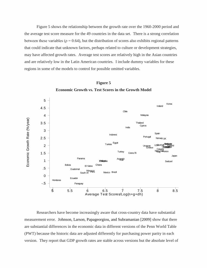
Figure 5 shows the relationship between the growth rate over the 1960-2000 period and
the average test score measure for the 49 countries in the data set. There is a strong correlation
between these variables (ρ = 0.64), but the distribution of scores also exhibits regional patterns
that could indicate that unknown factors, perhaps related to culture or development strategies,
may have affected growth rates. Average test scores are relatively high in the Asian countries
and are relatively low in the Latin American countries. I include dummy variables for these
regions in some of the models to control for possible omitted variables.
Figure 5
Economic Growth vs. Test Scores in the Growth Model
Researchers have become increasingly aware that cross-country data have substantial
measurement error. Johnson, Larson, Papageorgiou, and Subramanian [2009] show that there
are substantial differences in the economic data in different versions of the Penn World Table
(PWT) because the historic data are adjusted differently for purchasing power parity in each
version. They report that GDP growth rates are stable across versions but the absolute level of
Econom
ic G
row
th R
ate
(%
/year)
Average Test Scores/Log(n+g+dh)55 5.5 6 6.5 7 7.5 8 8.5
-.5
0
.5
1
1.5
2
2.5
3
3.5
4
4.5
5
Argentin
AustraliAustria
Belgium
Bolivia
Brazil
Canada
Chile
Colombia
Costa Ri
Cyprus
Denmark
Ecuador
Egypt
El Salva
Finland
France
Ghana
Greece
Guatemal
Honduras
India
Indonesi
Iran
Ireland
Italy
Japan
Korea
Malaysia
MexicoMorocco
Netherla
New Zeal
Norway
Panama
Paraguay
Peru
Philippi
Portugal
South Af
Spain
Sweden
Switzerl
Thailand
Tunisia
Turkey
UK
Uruguay USA
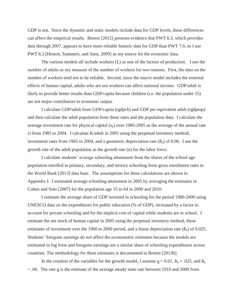
GDP is not. Since the dynamic and static models include data for GDP levels, these differences
can affect the empirical results. Breton [2012] presents evidence that PWT 6.3, which provides
data through 2007, appears to have more reliable historic data for GDP than PWT 7.0, so I use
PWT 6.3 [Heston, Summers, and Aten, 2009] as my source for the economic data.
The various models all include workers (L) as one of the factors of production. I use the
number of adults as my measure of the number of workers for two reasons. First, the data on the
number of workers tend not to be reliable. Second, since the macro model includes the external
effects of human capital, adults who are not workers can affect national income. GDP/adult is
likely to provide better results than GDP/capita because children (i.e. the population under 15)
are not major contributors to economic output.
I calculate GDP/adult from GDP/capita (rgdpch) and GDP per equivalent adult (rgdpeqa)
and then calculate the adult population from these rates and the population data. I calculate the
average investment rate for physical capital (sk) over 1985-2005 as the average of the annual rate
ci from 1985 to 2004. I calculate K/adult in 2005 using the perpetual inventory method,
investment rates from 1965 to 2004, and a geometric depreciation rate (δk) of 0.06. I use the
growth rate of the adult population as the growth rate (n) for the labor force.
I calculate students’ average schooling attainment from the shares of the school age
population enrolled in primary, secondary, and tertiary schooling from gross enrollment rates in
the World Bank [2013] data base. The assumptions for these calculations are shown in
Appendix I. I estimated average schooling attainment in 2005 by averaging the estimates in
Cohen and Soto [2007] for the population age 15 to 64 in 2000 and 2010.
I estimate the average share of GDP invested in schooling for the period 1980-2000 using
UNESCO data on the expenditures for public education (% of GDP), increased by a factor to
account for private schooling and for the implicit cost of capital while students are in school. I
estimate the net stock of human capital in 2005 using the perpetual inventory method, these
estimates of investment over the 1960 to 2000 period, and a linear depreciation rate (δh) of 0.025.
Students’ foregone earnings do not affect the econometric estimates because the models are
estimated in log form and foregone earnings are a similar share of schooling expenditures across
countries. The methodology for these estimates is documented in Breton [2013b].
In the creation of the variables for the growth model, I assume g = 0.01, δh = .025, and δk
= .06. The rate g is the estimate of the average steady state rate between 1910 and 2000 from
Breton [2013a]. The depreciation rate for human capital is from Breton [2013b]. The
depreciation rate for physical capital is from Caselli [2004].
The data on average test scores are from HW [2012a and 2012b]. The data for Protestant
affiliation are from Barrett [1982] and the data for Catholic and Muslim affiliation are from La
Porta, Lopez-de-Silanes, Shleifer, and Vishny [1999].
The schooling measures have varying amounts of measurement error. Cohen and Soto’s
[2007] data on adults’ average schooling attainment appear to be relatively accurate. In contrast,
the data on students’ average schooling attainment are not very accurate, since gross enrollment
and net attendance can be very different and the magnitude of the discrepancy varies across
countries.
The data on rates of investment in schooling and human capital/adult have similar levels
of measurement error, since they are calculated from the same underlying data and the human
capital data is used as the ratio H/Y in the estimation. These data are likely to be less accurate
than the data on adults’ average schooling attainment, but more accurate than the data on
students’ average schooling attainment.
IV. Empirical Results for the Econometric Models
Table 1 presents the results for the growth models specified in equations (6), (7), and (8).
The first six columns show the OLS estimates of the model with the three measures of human
capital flows, with and without dummy variables for Asia and Latin America. The results for all
of these models are consistent with expectations for an augmented Solow model. In this model α
is the share of income that accrues to physical capital, which Bernanke and Guykarnak [2001]
estimate to be about 0.35 across countries. The implied values of α for the three models range
from 0.28 to 0.41, which are acceptable. The implied values of β are acceptable and are
statistically significant at the one percent level. The speed of convergence on the steady-state
ranges from 0.016 to 0.021, which is consistent with expectations.
Columns 7 presents the results with all three measures in the same model. In this model
the estimated coefficients on schooling expenditures and average test scores are both statistically
significant at the one percent level. Column 8 shows the model with only these two measures
and the estimated coefficients on both continue to be statistically significant. The estimated
coefficients for these two measures are very similar, which indicates that students’ test scores in
elementary school and overall national expenditures on schooling are equally important
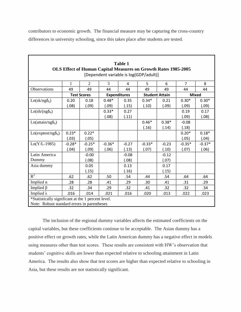
contributors to economic growth. The financial measure may be capturing the cross-country
differences in university schooling, since this takes place after students are tested.
Table 1
OLS Effect of Human Capital Measures on Growth Rates 1985-2005
[Dependent variable is log(GDP/adult)]
1 2 3 4 5 6 7 8 Observations 49 49 44 44 49 49 44 44 Test Scores Expenditures Student Attain Mixed
Ln(sk/ngδk) 0.20 (.08)
0.18 (.09)
0.48* (.09)
0.35 (.15)
0.34* (.10)
0.21 (.09)
0.30* (.09)
0.30* (.09)
Ln(sh/(ngδh) 0.33* (.08)
0.27 (.11)
0.19 (.09)
0.17 (.08)
Ln(attain/ngδh)
0.46* (.16)
0.38* (.14)
-0.08 (.18)
Ln(exptest/ngδh) 0.23* (.03)
0.22* (.05)
0.20* (.05)
0.18* (.04)
Ln(Y/L-1985) -0.28* (.04)
-0.25* (.09)
-0.36* (.06)
-0.27 (.13)
-0.33* (.07)
-0.23 (.10)
-0.35* (.07)
-0.37* (.06)
Latin America
Dummy -0.00
(.08) -0.08
(.08) -0.12
(.07)
Asia dummy 0.05 (.15)
0.13 (.16)
0.17 (.15)
R2 .62 .62 .50 .54 .44 .54 .64 .64
Implied α .28 .28 .41 .29 .30 .41 .31 .29
Implied β .32 .34 .29 .32 .41 .32 .32 .34 Implied λ .016 .014 .021 .016 .020 .013 .022 .023 *Statistically significant at the 1 percent level.
Note: Robust standard errors in parentheses
The inclusion of the regional dummy variables affects the estimated coefficients on the
capital variables, but these coefficients continue to be acceptable. The Asian dummy has a
positive effect on growth rates, while the Latin American dummy has a negative effect in models
using measures other than test scores. These results are consistent with HW’s observation that
students’ cognitive skills are lower than expected relative to schooling attainment in Latin
America. The results also show that test scores are higher than expected relative to schooling in
Asia, but these results are not statistically significant.
Students’ average schooling attainment can explain growth rates across countries, but not
as well as the other two measures. This result is not surprising, since the estimates of student
attainment are clearly less accurate than the data for the other two measures. The important
thing about these results is that all of the measures provide reasonable, similar estimates of the
effect of human capital on economic growth, even measures that are known to be relatively
inaccurate.
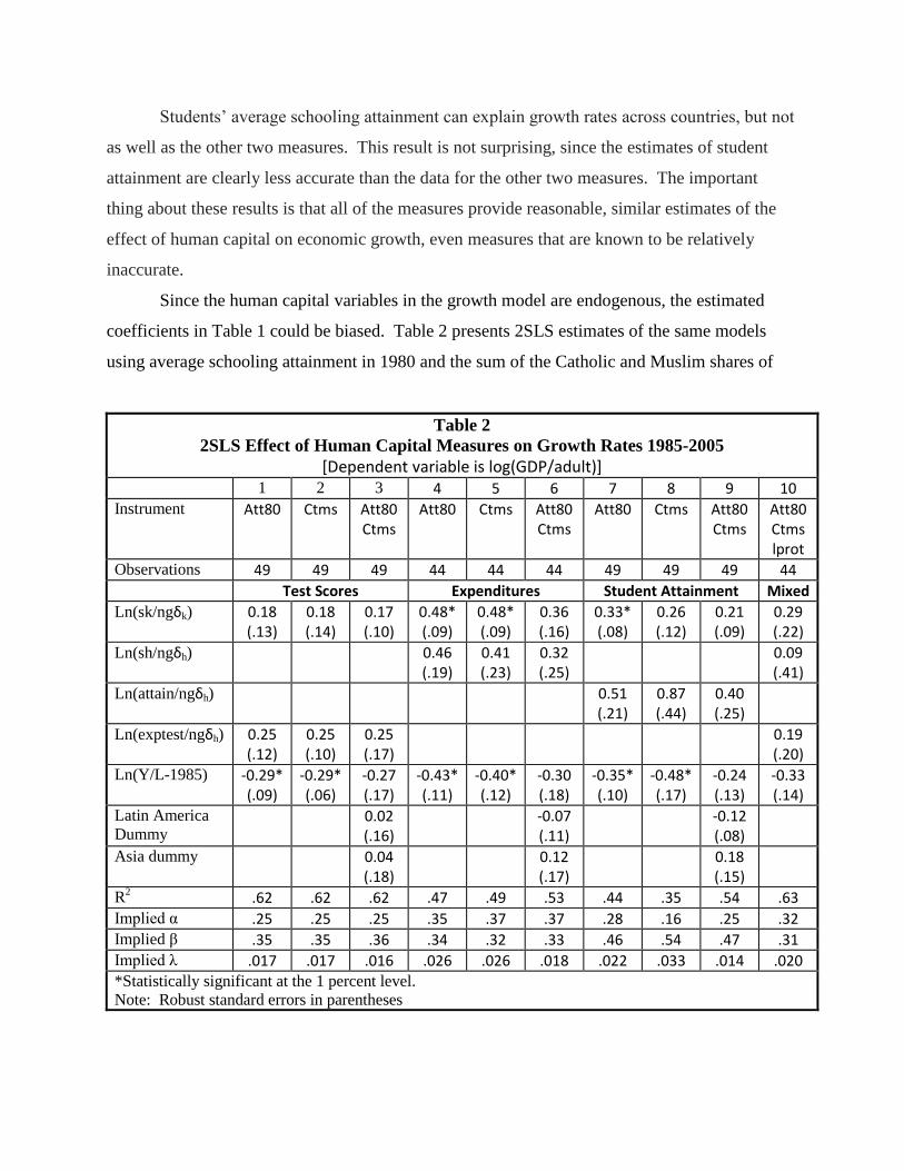
Since the human capital variables in the growth model are endogenous, the estimated
coefficients in Table 1 could be biased. Table 2 presents 2SLS estimates of the same models
using average schooling attainment in 1980 and the sum of the Catholic and Muslim shares of
Table 2
2SLS Effect of Human Capital Measures on Growth Rates 1985-2005
[Dependent variable is log(GDP/adult)] 1 2 3 4 5 6 7 8 9 10 Instrument Att80 Ctms Att80
Ctms Att80 Ctms Att80
Ctms Att80 Ctms Att80
Ctms Att80 Ctms lprot
Observations 49 49 49 44 44 44 49 49 49 44
Test Scores Expenditures Student Attainment Mixed
Ln(sk/ngδk) 0.18 (.13)
0.18 (.14)
0.17 (.10)
0.48* (.09)
0.48* (.09)
0.36 (.16)
0.33* (.08)
0.26 (.12)
0.21 (.09)
0.29 (.22)
Ln(sh/ngδh) 0.46 (.19)
0.41 (.23)
0.32 (.25)
0.09 (.41)
Ln(attain/ngδh)
0.51 (.21)
0.87 (.44)
0.40 (.25)
Ln(exptest/ngδh) 0.25 (.12)
0.25 (.10)
0.25 (.17)
0.19 (.20)
Ln(Y/L-1985) -0.29* (.09)
-0.29* (.06)
-0.27 (.17)
-0.43* (.11)
-0.40* (.12)
-0.30 (.18)
-0.35* (.10)
-0.48* (.17)
-0.24 (.13)
-0.33 (.14)
Latin America
Dummy 0.02
(.16) -0.07
(.11) -0.12
(.08)
Asia dummy 0.04 (.18)
0.12 (.17)
0.18 (.15)
R2 .62 .62 .62 .47 .49 .53 .44 .35 .54 .63
Implied α .25 .25 .25 .35 .37 .37 .28 .16 .25 .32 Implied β .35 .35 .36 .34 .32 .33 .46 .54 .47 .31
Implied λ .017 .017 .016 .026 .026 .018 .022 .033 .014 .020 *Statistically significant at the 1 percent level.
Note: Robust standard errors in parentheses
the population as instruments. I estimate each model with each instrument alone and then with
both instruments and the dummy variables for Asia and Latin America.
As shown in columns 1 to 9, the estimates of the effects of the measures with each
instrument are very consistent and similar to the OLS estimates. The consistency of the 2SLS
estimates with different instruments provides reassurance that the instruments are valid, even
though from a conceptual standpoint it is possible that either one could affect growth directly.
The model with average test scores explains the most variation in growth rates, but the
model with schooling expenditures provides the most accurate estimates of α. The model with
student attainment provides the worst results. The estimated coefficients are similar for all the
measures when the regional dummies are included in the models, but they all lose statistical
significance. These results again confirm the importance of accurate data to obtain robust
estimates of the effect of human capital on growth.
Column 10 presents the 2SLS results using three instruments, with both average test
scores and schooling expenditures in the model. The estimated coefficients are all positive, but
none of them are statistically significant.
Table 3 presents the results for the first stage regressions for the 2SLS estimates in Table
2. The results show that the estimated coefficients on the individual instruments are statistically
significant in the absence of the regional dummies. When the dummies are included these
coefficients lose their significance, most likely because the religious affiliation measures are
correlated with the regional dummies.
Overall the results for the dynamic growth model provide strong support for the validity
of the augmented Solow model and the validity of average test scores at ages 9 to 15 as a
measure of a nation’s human capital. This measure consistently explains more of the variation in
growth than the other measures.
But the positive empirical results for all the measures also indicate that average test
scores are a proxy for human capital, so the estimated coefficient on average test scores when it
is the only measure in a model cannot be interpreted to be the effect of cognitive skills in
elementary school alone. The actual effect of changes in test scores on growth appears to be
about half of the estimated coefficient on test scores in these models, with expenditures on
schooling accounting for the rest of the effect.
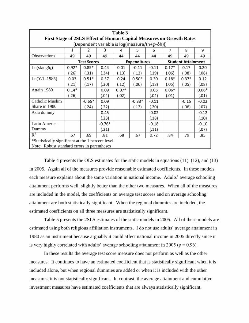
Table 3
First Stage of 2SLS Effect of Human Capital Measures on Growth Rates
[Dependent variable is log(measure/(n+g+δh))] 1 2 3 4 5 6 7 8 9 Observations 49 49 49 44 44 44 49 49 49 Test Scores Expenditures Student Attainment
Ln(sk/ngδk) 0.92* (.26)
0.85* (.31)
0.44 (.34)
0.01 (.13)
-0.11 (.12)
-0.11 (.19)
0.17* (.06)
0.17 (.08)
0.20 (.08)
Ln(Y/L-1985) 0.03 (.21)
0.51* (.17)
0.37 (.30)
0.24 (.12)
0.50* (.06)
0.30 (.18)
0.18* (.05)
0.37* (.05)
0.12 (.08)
Attain 1980 0.14* (.26)
0.09 (.04)
0.07* (.02)
0.05 (.04)
0.06* (.01)
0.06* (.01)
Catholic Muslim
Share in 1980 -0.65*
(.24) 0.09 (.22)
-0.33* (.12)
-0.11 (.20)
-0.15 (.06)
-0.02 (.07)
Asia dummy 0.45 (.23)
-0.02 (.18)
-0.12 (.10)
Latin America
Dummy -0.76*
(.21) -0.18
(.11) -0.10
(.07)
R2 .67 .69 .81 .68 .67 0.72 .84 .79 .85
*Statistically significant at the 1 percent level.
Note: Robust standard errors in parentheses
Table 4 presents the OLS estimates for the static models in equations (11), (12), and (13)
in 2005. Again all of the measures provide reasonable estimated coefficients. In these models
each measure explains about the same variation in national income. Adults’ average schooling
attainment performs well, slightly better than the other two measures. When all of the measures
are included in the model, the coefficients on average test scores and on average schooling
attainment are both statistically significant. When the regional dummies are included, the
estimated coefficients on all three measures are statistically significant.
Table 5 presents the 2SLS estimates of the static models in 2005. All of these models are
estimated using both religious affiliation instruments. I do not use adults’ average attainment in
1980 as an instrument because arguably it could affect national income in 2005 directly since it
is very highly correlated with adults’ average schooling attainment in 2005 (ρ = 0.96).
In these results the average test score measure does not perform as well as the other
measures. It continues to have an estimated coefficient that is statistically significant when it is
included alone, but when regional dummies are added or when it is included with the other
measures, it is not statistically significant. In contrast, the average attainment and cumulative
investment measures have estimated coefficients that are always statistically significant.
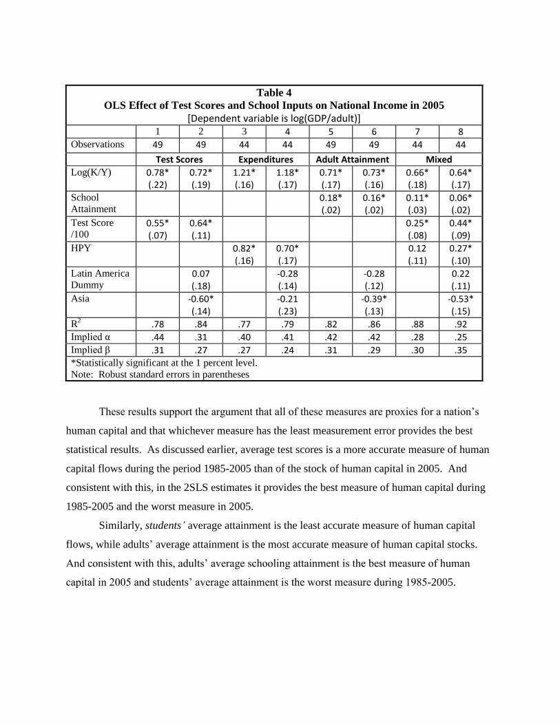
Table 4
OLS Effect of Test Scores and School Inputs on National Income in 2005
[Dependent variable is log(GDP/adult)] 1 2 3 4 5 6 7 8 Observations 49 49 44 44 49 49 44 44
Test Scores Expenditures Adult Attainment Mixed
Log(K/Y) 0.78* (.22)
0.72* (.19)
1.21* (.16)
1.18* (.17)
0.71* (.17)
0.73* (.16)
0.66* (.18)
0.64* (.17)
School
Attainment 0.18*
(.02) 0.16* (.02)
0.11* (.03)
0.06* (.02)
Test Score
/100 0.55* (.07)
0.64* (.11)
0.25* (.08)
0.44* (.09)
HPY 0.82* (.16)
0.70* (.17)
0.12 (.11)
0.27* (.10)
Latin America
Dummy 0.07
(.18) -0.28
(.14) -0.28
(.12) 0.22
(.11) Asia -0.60*
(.14) -0.21
(.23) -0.39*
(.13) -0.53*
(.15)
R2 .78 .84 .77 .79 .82 .86 .88 .92
Implied α .44 .31 .40 .41 .42 .42 .28 .25
Implied β .31 .27 .27 .24 .31 .29 .30 .35
*Statistically significant at the 1 percent level.
Note: Robust standard errors in parentheses
These results support the argument that all of these measures are proxies for a nation’s
human capital and that whichever measure has the least measurement error provides the best
statistical results. As discussed earlier, average test scores is a more accurate measure of human
capital flows during the period 1985-2005 than of the stock of human capital in 2005. And
consistent with this, in the 2SLS estimates it provides the best measure of human capital during
1985-2005 and the worst measure in 2005.
Similarly, students’ average attainment is the least accurate measure of human capital
flows, while adults’ average attainment is the most accurate measure of human capital stocks.
And consistent with this, adults’ average schooling attainment is the best measure of human
capital in 2005 and students’ average attainment is the worst measure during 1985-2005.
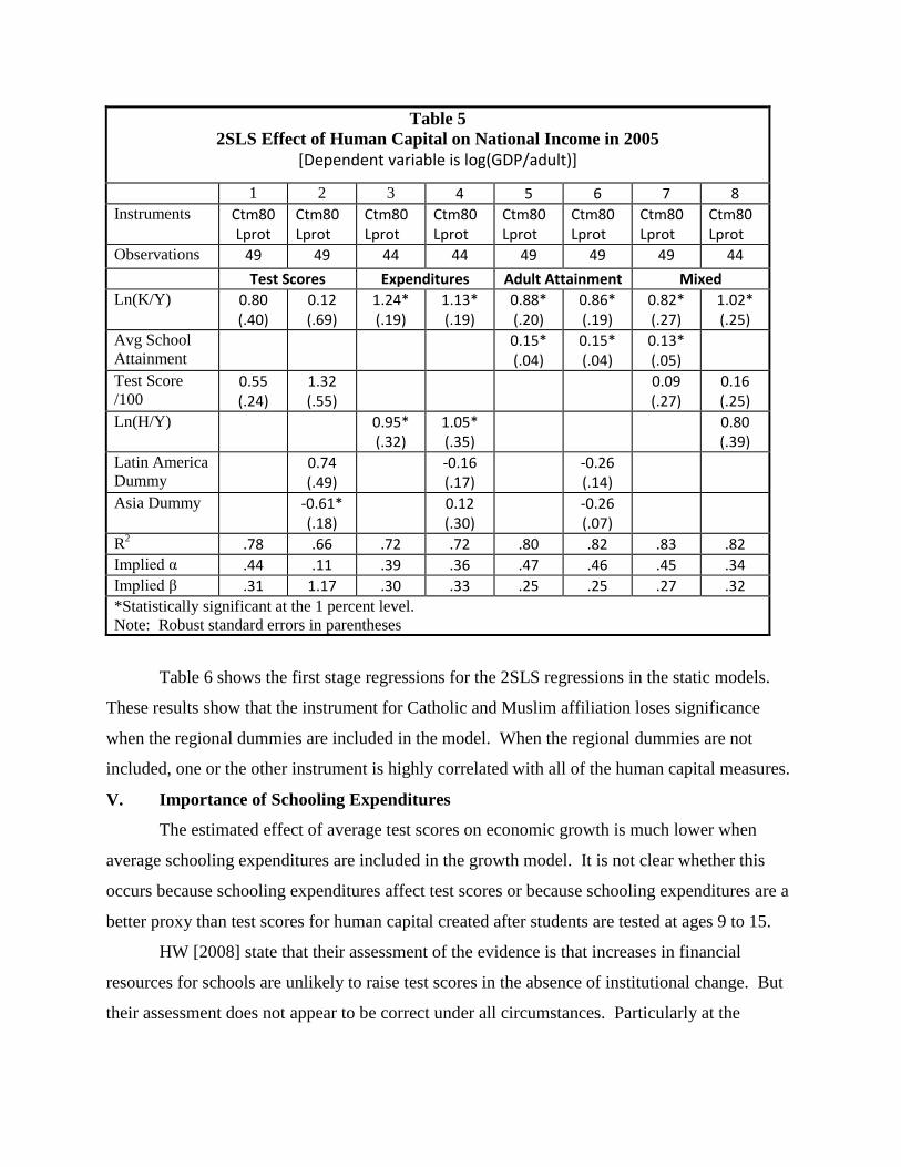
Table 5
2SLS Effect of Human Capital on National Income in 2005
[Dependent variable is log(GDP/adult)]
1 2 3 4 5 6 7 8 Instruments Ctm80
Lprot Ctm80 Lprot
Ctm80 Lprot
Ctm80 Lprot
Ctm80 Lprot
Ctm80 Lprot
Ctm80 Lprot
Ctm80 Lprot
Observations 49 49 44 44 49 49 49 44
Test Scores Expenditures Adult Attainment Mixed
Ln(K/Y) 0.80 (.40)
0.12 (.69)
1.24* (.19)
1.13* (.19)
0.88* (.20)
0.86* (.19)
0.82* (.27)
1.02* (.25)
Avg School
Attainment 0.15*
(.04) 0.15* (.04)
0.13* (.05)
Test Score
/100 0.55 (.24)
1.32 (.55)
0.09 (.27)
0.16 (.25)
Ln(H/Y) 0.95* (.32)
1.05* (.35)
0.80 (.39)
Latin America
Dummy 0.74
(.49) -0.16
(.17) -0.26
(.14)
Asia Dummy -0.61* (.18)
0.12 (.30)
-0.26 (.07)
R2 .78 .66 .72 .72 .80 .82 .83 .82
Implied α .44 .11 .39 .36 .47 .46 .45 .34
Implied β .31 1.17 .30 .33 .25 .25 .27 .32
*Statistically significant at the 1 percent level.
Note: Robust standard errors in parentheses
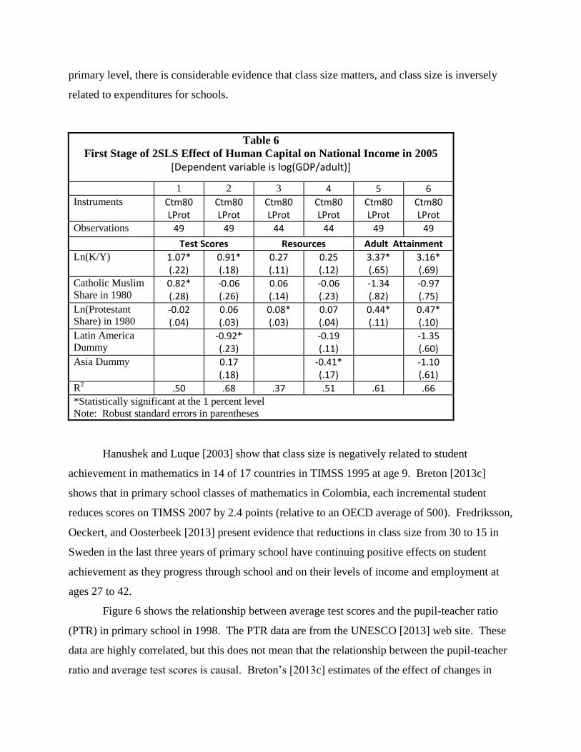
Table 6 shows the first stage regressions for the 2SLS regressions in the static models.
These results show that the instrument for Catholic and Muslim affiliation loses significance
when the regional dummies are included in the model. When the regional dummies are not
included, one or the other instrument is highly correlated with all of the human capital measures.
V. Importance of Schooling Expenditures
The estimated effect of average test scores on economic growth is much lower when
average schooling expenditures are included in the growth model. It is not clear whether this
occurs because schooling expenditures affect test scores or because schooling expenditures are a
better proxy than test scores for human capital created after students are tested at ages 9 to 15.
HW [2008] state that their assessment of the evidence is that increases in financial
resources for schools are unlikely to raise test scores in the absence of institutional change. But
their assessment does not appear to be correct under all circumstances. Particularly at the
primary level, there is considerable evidence that class size matters, and class size is inversely
related to expenditures for schools.
Table 6
First Stage of 2SLS Effect of Human Capital on National Income in 2005
[Dependent variable is log(GDP/adult)]
1 2 3 4 5 6 Instruments Ctm80
LProt Ctm80 LProt
Ctm80 LProt
Ctm80 LProt
Ctm80 LProt
Ctm80 LProt
Observations 49 49 44 44 49 49
Test Scores Resources Adult Attainment Ln(K/Y) 1.07*
(.22) 0.91* (.18)
0.27 (.11)
0.25 (.12)
3.37* (.65)
3.16* (.69)
Catholic Muslim
Share in 1980 0.82* (.28)
-0.06 (.26)
0.06 (.14)
-0.06 (.23)
-1.34 (.82)
-0.97 (.75)
Ln(Protestant
Share) in 1980 -0.02 (.04)
0.06 (.03)
0.08* (.03)
0.07 (.04)
0.44* (.11)
0.47* (.10)
Latin America
Dummy -0.92*
(.23) -0.19
(.11) -1.35
(.60) Asia Dummy 0.17
(.18) -0.41*
(.17) -1.10
(.61)
R2 .50 .68 .37 .51 .61 .66
*Statistically significant at the 1 percent level
Note: Robust standard errors in parentheses
Hanushek and Luque [2003] show that class size is negatively related to student
achievement in mathematics in 14 of 17 countries in TIMSS 1995 at age 9. Breton [2013c]
shows that in primary school classes of mathematics in Colombia, each incremental student
reduces scores on TIMSS 2007 by 2.4 points (relative to an OECD average of 500). Fredriksson,
Oeckert, and Oosterbeek [2013] present evidence that reductions in class size from 30 to 15 in
Sweden in the last three years of primary school have continuing positive effects on student
achievement as they progress through school and on their levels of income and employment at
ages 27 to 42.
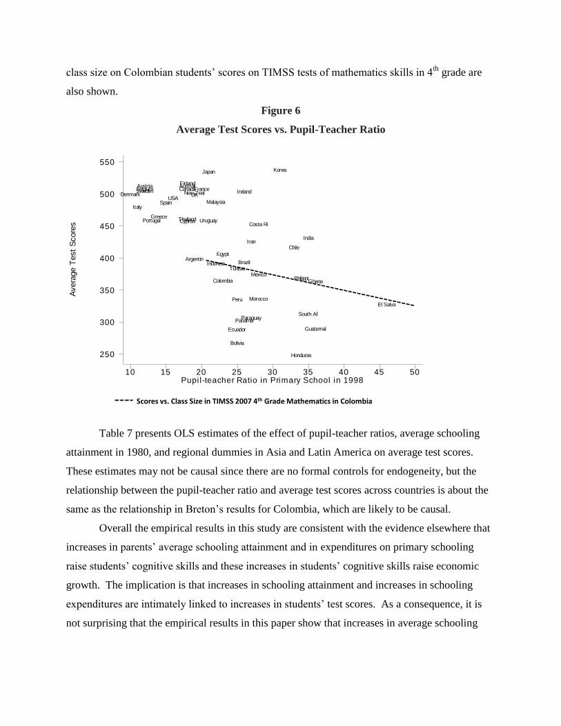
Figure 6 shows the relationship between average test scores and the pupil-teacher ratio
(PTR) in primary school in 1998. The PTR data are from the UNESCO [2013] web site. These
data are highly correlated, but this does not mean that the relationship between the pupil-teacher
ratio and average test scores is causal. Breton’s [2013c] estimates of the effect of changes in
class size on Colombian students’ scores on TIMSS tests of mathematics skills in 4th
grade are
also shown.
Figure 6
Average Test Scores vs. Pupil-Teacher Ratio
Avera
ge T
est
Score
s
Pupi l-teacher Ratio in Primary School in 199810 15 20 25 30 35 40 45 50
250
300
350
400
450
500
550
Argentin
AustraliAustriaBelgium
Bolivia
Brazil
Canada
Chile
Colombia
Costa RiCyprus
Denmark
Ecuador
Egypt
El Salva
FinlandFrance
Ghana
Greece
Guatemal
Honduras
India
Indonesi
Iran
Ireland
Italy
Japan Korea
Malaysia
Mexico
Morocco
New Zeal
PanamaParaguay
Peru
Philippi
Portugal
South Af
Spain
Sweden
Thailand
Tunisia
UK
Uruguay
USA
Scores vs. Class Size in TIMSS 2007 4th Grade Mathematics in Colombia
Table 7 presents OLS estimates of the effect of pupil-teacher ratios, average schooling
attainment in 1980, and regional dummies in Asia and Latin America on average test scores.
These estimates may not be causal since there are no formal controls for endogeneity, but the
relationship between the pupil-teacher ratio and average test scores across countries is about the
same as the relationship in Breton’s results for Colombia, which are likely to be causal.
Overall the empirical results in this study are consistent with the evidence elsewhere that
increases in parents’ average schooling attainment and in expenditures on primary schooling
raise students’ cognitive skills and these increases in students’ cognitive skills raise economic
growth. The implication is that increases in schooling attainment and increases in schooling
expenditures are intimately linked to increases in students’ test scores. As a consequence, it is
not surprising that the empirical results in this paper show that increases in average schooling
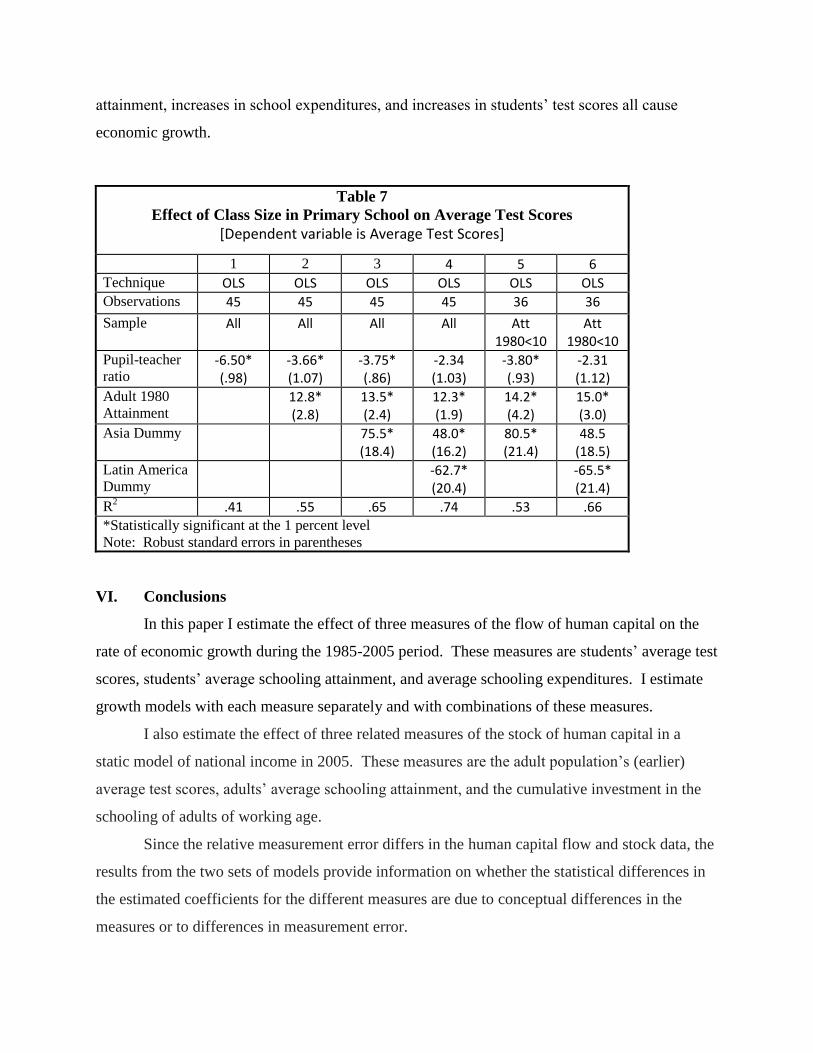
attainment, increases in school expenditures, and increases in students’ test scores all cause
economic growth.
Table 7
Effect of Class Size in Primary School on Average Test Scores
[Dependent variable is Average Test Scores]
1 2 3 4 5 6 Technique OLS OLS OLS OLS OLS OLS Observations 45 45 45 45 36 36
Sample All All All All Att 1980<10
Att 1980<10
Pupil-teacher
ratio -6.50* (.98)
-3.66* (1.07)
-3.75* (.86)
-2.34 (1.03)
-3.80* (.93)
-2.31 (1.12)
Adult 1980
Attainment 12.8*
(2.8) 13.5* (2.4)
12.3* (1.9)
14.2* (4.2)
15.0* (3.0)
Asia Dummy 75.5* (18.4)
48.0* (16.2)
80.5* (21.4)
48.5 (18.5)
Latin America
Dummy -62.7*
(20.4) -65.5*
(21.4) R
2 .41 .55 .65 .74 .53 .66
*Statistically significant at the 1 percent level
Note: Robust standard errors in parentheses
VI. Conclusions
In this paper I estimate the effect of three measures of the flow of human capital on the
rate of economic growth during the 1985-2005 period. These measures are students’ average test
scores, students’ average schooling attainment, and average schooling expenditures. I estimate
growth models with each measure separately and with combinations of these measures.
I also estimate the effect of three related measures of the stock of human capital in a
static model of national income in 2005. These measures are the adult population’s (earlier)
average test scores, adults’ average schooling attainment, and the cumulative investment in the
schooling of adults of working age.
Since the relative measurement error differs in the human capital flow and stock data, the
results from the two sets of models provide information on whether the statistical differences in
the estimated coefficients for the different measures are due to conceptual differences in the
measures or to differences in measurement error.
Overall my empirical results differ substantially from HW’s results. I confirm their
findings that increases in students’ cognitive skills, as measured on standardized tests, cause
economic growth, but I also find that the other two measures of human capital also cause growth.
The estimated effects are similar with all three measures.
The results for the two sets of models indicate that whichever measure of human capital
has the least measurement error provides the best results. The average test score measure
provides the best results for the dynamic growth model and the worst results for the static model.
I also show that adults’ average years of schooling attainment is a valid and surprisingly
accurate measure of the financial stock of human capital across countries. It provides the best
results for the static model in 2005. These results contradict HW’s claim that adults’ average
schooling attainment is not a good measure of human capital across countries.
Since the different measures of human capital quantify different aspects of a nation’s
human capital, the effects of the measures are not mutually exclusive. I show that when two or
more measures are included in the same model, generally at least two are statistically significant.
These results indicate that the various components of human capital created through schooling
all contribute to economic growth. These results provide very strong support for the validity of
the augmented Solow growth model and for the causal relationship between increases in human
capital and economic growth.
The empirical results in this study also suggest that it may not be possible to raise
students’ cognitive skills without raising average schooling attainment and schooling
expenditures. More schooling, more expenditures, and higher test scores appear to go together.
These measures of human capital are highly correlated, and clearly it has been principally
through many generations of schooling, with slowly rising total investment/pupil and increasing
average schooling attainment, that nations have slowly raised their average level of cognitive
skills.
.
References
Acemoglu, Daron, 2009, Introduction to Modern Economic Growth, Princeton University Press,
Princeton
Arruñada, Benito, 2010, “Protestants and Catholics: Similar Work Ethic, Different Social Ethic,”
The Economic Journal, v120, n547, 890-918]
Barrett, David B., 1982, The World Christian Encyclopedia, New York: Oxford University
Press.
Barro, Robert J., and Sala-i-Martin, Xavier, 2004, Economic Growth, The MIT Press, Cambridge
Becker, Sascha O., Wössmann, Ludger, 2009, “Was Weber wrong? A human capital theory of
protestant economic history,” Quarterly Journal of Economics, v124, i2, 531-596.
Becker, Sascha O., and Wössmann, Ludger, 2010, “The Effect of Protestantism on Education
Before the Industrialization: Evidence from 1816 Prussia,” Economics Letters, v107, 224-228
Benhabib, Jess, and Spiegel, Mark M., 1994, “The Role of Human Capital in Economic
Development: Evidence from Aggregate Cross-Country Data,” Journal of Monetary Economics,
34, 143-173
Bernanke, Ben S. and Refet S. Gurkaynak, 2001, “Taking Mankiw, Romer, and Weil seriously,”
NBER Macroeconomics Annual, v16, 11-57.
Breton, Theodore R., 2004, “Can Institutions or Education Explain World Poverty? An
Augmented Solow Model Provides Some Insights,” Journal of Socio-Economics 33, 45-69
Breton, Theodore R., 2011, “The Quality vs. the Quantity of Schooling: What Drives Economic
Growth?,” Economics of Education Review, v30, 765-773
Breton, Theodore R., 2012, “Penn World Table 7.0: Are the Data flawed?,” Economics Letters,
v117, n1, 208-210
Breton, Theodore R., 2013a, “World Total Productivity Growth and the Steady State Rate in the
20th Century,”Economics Letters, v119, n3, 340-343
Breton, Theodore R., 2013b, “Were Mankiw, Romer, and Weil Right? A Reconcilation of the
Macro and Micro Returns on Investment in Schooling” Macroeconomic Dynamics, v17, n5,
forthcoming, published online March, 2012
Breton, Theodore R., 2013c, “Evidence that Class Size Matters in 4th
Grade Mathematics: An
Analysis of TIMSS 2007 Data for Colombia,” International Journal of Educational
Development, forthcoming
Caselli, Francesco, 2004, “Accounting for Cross-Country Income Differences,” National Bureau
of Economic Research, WP 10828’
Cipolla, Carlo M, 1969, Literacy and Development in the West, Baltimore: Pelican Books.
Cohen, Daniel and Marcelo Soto, 2007, “Growth and human capital: good data, good results,”
Journal of Economic Growth, v12, n1, 51-76.
Dang, Hai-Anh, and Rogers, F. Halsey, 2008, “The Growing Phenomenon of Private Tutoring:
Does It Deepen Human Capital, Widen Inequalities, or Waste Resources?,” The World Bank
Research Observer, v23, n2, 161-200
Ding, Sai, and Knight, John, 2009, “Can the Augmented Solow Model Explain China’s
Remarkable Economic Growth? A Cross-Country Panel Data Analysis,” Journal of
Comparative Economics, v37, 432-452
Fredriksson, Peter, Ӧeckert, Björn, Oosterbeek, Hessel, 2013, “Long-Term Effects of Class
Size,” Quarterly Journal of Economics, v128, n1, 249-285
Fuchs, Thomas, and Woessmann, Ludger, 2007, “What accounts for international differences in
student performance? A re-examination using PISA data,” Empirical Economics, 32, 433-464
Gennaioli, Nicola, La Porta, Rafael, Lopez-de-Silanes, Florencio, and Shleifer, Andrei, 2013,
“Human Capital and Regional Development,” Quarterly Journal of Economics, v128, n1, 105-
164
Goldin, Claudia and Lawrence F. Katz, 1998, “Human capital and social capital: the rise of
secondary schooling in America, 1910 to 1940,” National Bureau of Economic Research,
Working paper 6439. .
Hanushek, Eric A., and Luque, J.A., 2003, “Efficiency and equity in schools around the world,”
Economics of Education Review, v22, n4, 481-502
Hanushek, Eric A. and Woessmann, Ludger, 2008, “The Role of Cognitive Skills in Economic
Development,” Journal of Economic Literature, 46.3, 607-668
Hanushek, Eric A. and Woessmann, Ludger, 2012a, “Schooling, educational achievement, and
the Latin American growth puzzle,” Journal of Development Economics, 99, 497-512
Hanushek, Eric A. and Woessmann, Ludger, 2012b, “Do Better Schools Lead to More Growth?
Cognitive Skills, Economic Outcomes, and Causation,” Journal of Economic Growth, 17, 267-
321
Heston, Alan, Summers, Robert, and Aten, Bettina, 2009, Penn World Table Version 6.3, Center
for International Comparisons of Production, Income and Prices at the University of
Pennsylvania (CICUP)
Iannaccone, Laurence R., 1998, “Introduction to the economics of religion,” Journal of
Economic Literature 36, 1465-1496.
Johansson, Egil, 1981, “The history of literacy in Sweden,” in Harvey J. Graff, Literacy and
Social Development in the West: A Reader, pp. 151-182, New York: Cambridge University
Press.
Johnson, Simon, Larson, William, Papageorgiou, Chris, and Subramanian, Arvind, 2009, “Is
Newer Better? Penn World Table Revisions and Their Impact on Growth Estimates,” NBER,
Working Paper 15455
Jones, Charles, 1995, “Time Series Tests of Endogenous Growth Models, Quarterly Journal of
Economics, v110, n2, 495-525
Juergis, Hendrik, and Schneider, Kerstin, 2004, “International Differences in Student
Achievement: An Economic Perspective,” German Economic Review 5, 3, 357-380
Krueger, Alan B., and Lindahl, Mikael, 2001, “Education for Growth: Why and For Whom?,”
Journal of Economic Literature, v39, 1101-1136
La Porta, Rafael, Lopez-de –Silanes, Florencio, Shleifer, Andrei, and Vishny, Robert, 1999,
“The Quality of Government,” Journal of Law, Economics, and Organization, v15, n1, 222-282
Lau, Sau-Him Paul, 2008, “Using an error-correction model to test whether endogenous long-run
growth exists,” Journal of Economic Dynamics & Control 32, 648-676
Mankiw, N. Gregory, David Romer, and David Weil, 1992, “A contribution to the empirics of
economic growth,” Quarterly Journal of Economics, v107, Issue 2, 407-437
Mansouri, Reza, 2007, “A Way Forward for Islamic Science,” Physics World, v20, n8, 12-13
Means, Richard L., 1966, “Protestantism and economic institutions: auxiliary theories to
Weber’s protestant ethic,” Social Forces, v44, n3, 372-381.
OECD, 2001, Measuring Capital; OECD Manual: Measurement of Capital Stocks, Consumption
of Fixed Capital, and Capital Services. OECD Publication Services, www.SourceOECD.org.
Parcel, Toby L., and Dufur, Mikaela, 2009, “Family and School Capital Explaining Regional
Variation in Math and Reading Achievement,” Research in Social Stratification and Mobility,
v27, 157-176
Rubinfeld, Daniel L., and Shapiro, Perry, 1989, “Micro-Estimation of the Demand for
Schooling,” Regional Science and Urban Economics, 19, 381-398
Soysal, Yasemin Nuhoglu and David Strang (1989) Construction of the first mass education
systems in nineteenth-century Europe. Sociology of Education, v62, n4, 277-288.
UNESCO, 2013, UNESCO Institute for Statistics, Table 11, Indicators on Teaching Staff at
ISED levels at ISCED Levels 0 to 3, Pupil-Teacher Ratio Primary 1998,
http://stats.uis.unesco.org
Woessmann, Ludger, 2003, “Schooling Resources, Educational Institutions and Student
Performance: the International Evidence,” Oxford Bulletin of Economics and Statistics, 65, 2,
117-170.
World Bank, 2013, World Bank Data, School Enrollment, Primary (% gross), Secondary (%
gross), and Tertiary (% gross)
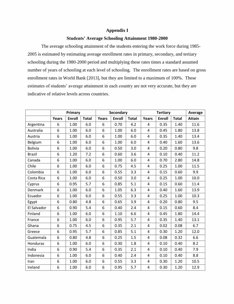
Appendix I
Students’ Average Schooling Attainment 1980-2000
The average schooling attainment of the students entering the work force during 1985-
2005 is estimated by estimating average enrollment rates in primary, secondary, and tertiary
schooling during the 1980-2000 period and multiplying these rates times a standard assumed
number of years of schooling at each level of schooling. The enrollment rates are based on gross
enrollment rates in World Bank [2013], but they are limited to a maximum of 100%. These
estimates of students’ average attainment in each country are not very accurate, but they are
indicative of relative levels across countries.
Primary Secondary Tertiary Average
Years Enroll Total Years Enroll Total Years Enroll Total Attain
Argentina 6 1.00 6.0 6 0.70 4.2 4 0.35 1.40 11.6
Australia 6 1.00 6.0 6 1.00 6.0 4 0.45 1.80 13.8
Austria 6 1.00 6.0 6 1.00 6.0 4 0.35 1.40 13.4
Belgium 6 1.00 6.0 6 1.00 6.0 4 0.40 1.60 13.6
Bolivia 6 1.00 6.0 6 0.50 3.0 4 0.20 0.80 9.8
Brazil 6 1.20 7.2 6 0.60 3.6 4 0.10 0.40 11.2
Canada 6 1.00 6.0 6 1.00 6.0 4 0.70 2.80 14.8
Chile 6 1.00 6.0 6 0.75 4.5 4 0.25 1.00 11.5
Colombia 6 1.00 6.0 6 0.55 3.3 4 0.15 0.60 9.9
Costa Rica 6 1.00 6.0 6 0.50 3.0 4 0.25 1.00 10.0
Cyprus 6 0.95 5.7 6 0.85 5.1 4 0.15 0.60 11.4
Denmark 6 1.00 6.0 6 1.05 6.3 4 0.40 1.60 13.9
Ecuador 6 1.00 6.0 6 0.55 3.3 4 0.25 1.00 10.3
Egypt 6 0.80 4.8 6 0.65 3.9 4 0.20 0.80 9.5
El Salvador 6 0.90 5.4 6 0.40 2.4 4 0.15 0.60 8.4
Finland 6 1.00 6.0 6 1.10 6.6 4 0.45 1.80 14.4
France 6 1.00 6.0 6 0.95 5.7 4 0.35 1.40 13.1
Ghana 6 0.75 4.5 6 0.35 2.1 4 0.02 0.08 6.7
Greece 6 0.95 5.7 6 0.85 5.1 4 0.30 1.20 12.0
Guatemala 6 0.80 4.8 6 0.25 1.5 4 0.08 0.32 6.6
Honduras 6 1.00 6.0 6 0.30 1.8 4 0.10 0.40 8.2
India 6 0.90 5.4 6 0.35 2.1 4 0.10 0.40 7.9
Indonesia 6 1.00 6.0 6 0.40 2.4 4 0.10 0.40 8.8
Iran 6 1.00 6.0 6 0.55 3.3 4 0.30 1.20 10.5
Ireland 6 1.00 6.0 6 0.95 5.7 4 0.30 1.20 12.9
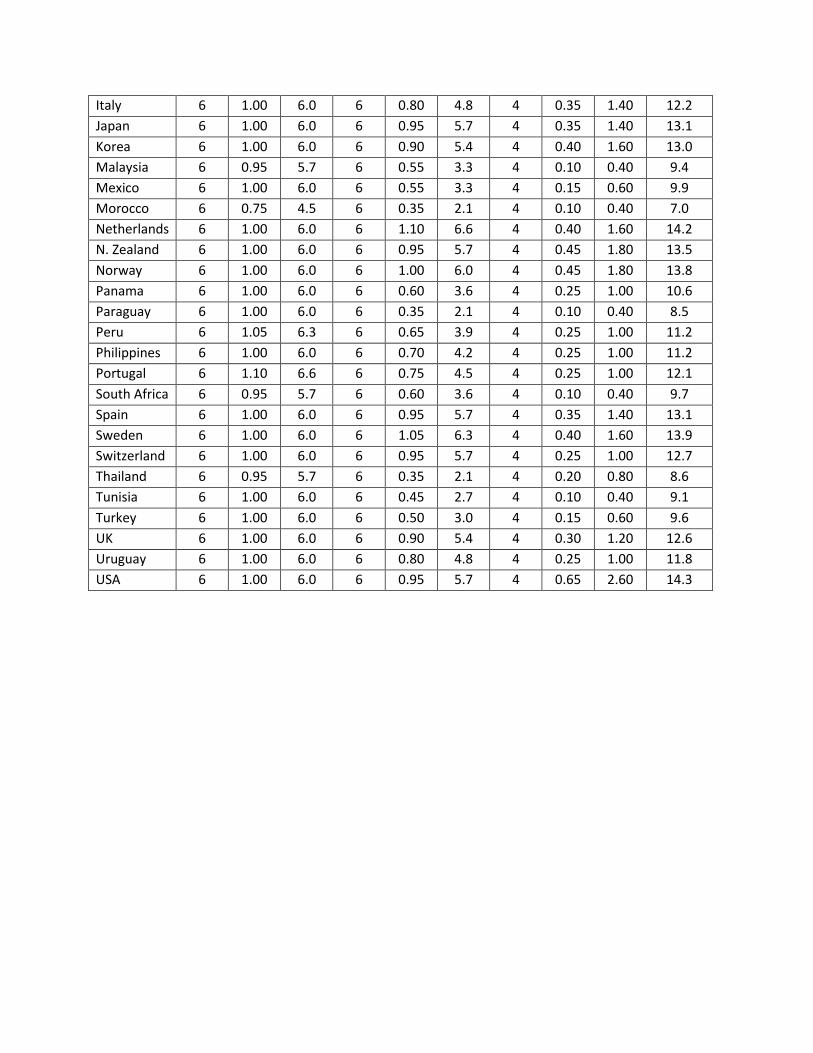
Italy 6 1.00 6.0 6 0.80 4.8 4 0.35 1.40 12.2
Japan 6 1.00 6.0 6 0.95 5.7 4 0.35 1.40 13.1
Korea 6 1.00 6.0 6 0.90 5.4 4 0.40 1.60 13.0
Malaysia 6 0.95 5.7 6 0.55 3.3 4 0.10 0.40 9.4
Mexico 6 1.00 6.0 6 0.55 3.3 4 0.15 0.60 9.9
Morocco 6 0.75 4.5 6 0.35 2.1 4 0.10 0.40 7.0
Netherlands 6 1.00 6.0 6 1.10 6.6 4 0.40 1.60 14.2
N. Zealand 6 1.00 6.0 6 0.95 5.7 4 0.45 1.80 13.5
Norway 6 1.00 6.0 6 1.00 6.0 4 0.45 1.80 13.8
Panama 6 1.00 6.0 6 0.60 3.6 4 0.25 1.00 10.6
Paraguay 6 1.00 6.0 6 0.35 2.1 4 0.10 0.40 8.5
Peru 6 1.05 6.3 6 0.65 3.9 4 0.25 1.00 11.2
Philippines 6 1.00 6.0 6 0.70 4.2 4 0.25 1.00 11.2
Portugal 6 1.10 6.6 6 0.75 4.5 4 0.25 1.00 12.1
South Africa 6 0.95 5.7 6 0.60 3.6 4 0.10 0.40 9.7
Spain 6 1.00 6.0 6 0.95 5.7 4 0.35 1.40 13.1
Sweden 6 1.00 6.0 6 1.05 6.3 4 0.40 1.60 13.9
Switzerland 6 1.00 6.0 6 0.95 5.7 4 0.25 1.00 12.7
Thailand 6 0.95 5.7 6 0.35 2.1 4 0.20 0.80 8.6
Tunisia 6 1.00 6.0 6 0.45 2.7 4 0.10 0.40 9.1
Turkey 6 1.00 6.0 6 0.50 3.0 4 0.15 0.60 9.6
UK 6 1.00 6.0 6 0.90 5.4 4 0.30 1.20 12.6
Uruguay 6 1.00 6.0 6 0.80 4.8 4 0.25 1.00 11.8
USA 6 1.00 6.0 6 0.95 5.7 4 0.65 2.60 14.3
Top Related
Copyright © 2022 FDOKUMEN

